This page gives a beginner\u2019s introduction to the ABINIT resources, the package, and the main ABINIT applications.
"},{"location":"#foreword","title":"Foreword","text":"The ABINIT project is a group effort of dozens of people worldwide, who develop the main ABINIT application which is delivered with many other files (post-processors, tests, documentation, \u2026) in the ABINIT package. The ABINIT project includes also resources provided on the ABINIT Web site and the github organization.
Before reading the present page, and get some grasp about the main ABINIT application, you should get some theoretical background. In case you have already used another electronic structure code, or a quantum chemistry code, it might be sufficient to read the introduction of [Payne1992]. If you have never used another electronic structure code or a Quantum Chemistry package, you should complete such reading by going (at your own pace) through the Chaps. 1 to 13 , and appendices L and M of R.M. Martin\u2019s book [Martin2004].
After having gone through the present New User\u2019s Guide, you should follow the ABINIT tutorials.
"},{"location":"#introduction","title":"Introduction","text":"ABINIT is a package whose main program allows to find the total energy, charge density and electronic structure of systems made of electrons and nuclei (molecules and periodic solids) within Density Functional Theory, using pseudopotentials and a planewave basis, or augmented plane waves, or even wavelets.
Some possibilities of ABINIT go beyond Density Functional Theory, i.e. the many-body perturbation theory (GW approximation the Bethe-Salpeter equation), Time-Dependent Density Functional Theory, Dynamical Mean-Field Theory, the Allen-Heine-Cardona theory to find temperature-dependent electronic structure.
ABINIT also includes options to optimize the geometry according to the DFT forces and stresses, or to perform molecular dynamics simulation using these forces, or to generate dynamical (vibrations - phonons) properties, dielectric properties, mechanical properties, thermodynamical properties, etc. In addition to the main ABINIT code, different utility programs are provided.
We suppose that you have downloaded the ABINIT package from the Web site, unpacked it and installed it. If not, you might nevertheless continue reading the present Web page, just to get an overview, but it might prove more fruitful to have first downloaded the ABINIT package and at least unpacked it, see the installation notes.
Note
We will use the name \u201c~abinit\u201d to refer to the directory that contains the ABINIT package after download. In practice, a version number is appended to this name, to give for example: abinit-10.6.3. The ABINIT package versioning scheme is explained later in this file.
~abinit contains different subdirectories. For example, the present file, as well as other descriptive files, should be found in ~abinit/doc/. Other subdirectories will be described later.
"},{"location":"#the-main-executable-abinit","title":"The main executable: abinit","text":"After compilation, the main code will be present in the package as ~abinit/src/98_main/abinit (or perhaps at another place, depending on your installation).
To run abinit you need three things:
With these items a job can be run.
The full list of input variables, all of which are provided in the single input file, is given in the ABINIT list of all variable. The detailed description of input variables is given in many \u201cVariable Set\u201d files, including:
A set of examples aimed at guiding the beginner is available in the tutorials.
Other test cases (more than 1000 input files) can be found in the ~abinit/test subdirectories, e.g. \u201cfast\u201d, the \u201cvX\u201d series (v1, v2, \u2026 v67mbpt, v7, .., v9, v10), \u201clibxc\u201d, \u201cparal\u201d, the \u201ctutoX\u201d series \u2026
Many different sorts of pseudopotentials can be used with ABINIT. Most of them can be found on the atomic data files page of the ABINIT web site. There are official recommended pseudopotentials tables (the PAW JTH table, and the norm-conserving table from ONCVPSP), and also some older sets of pseudopotentials. Information on pseudopotential files can be found in the ABINIT help file, the Pseudopotential theory document, the Description of the format for the norm-conserving pseudopotential header, and in the PseudosPAW topics.
Warning
A subset of existing pseudopotentials are used for test cases, and are located in the ~abinit/tests/Pspdir directory but they are not recommended for production.
"},{"location":"#other-programs-in-the-package","title":"Other programs in the package","text":"In addition to abinit, there are utility programs provided in the package. Some utility programs are written in Fortran (like the main abinit program), and their sources is also in ~abinit/src/98_main. These include:
mrgddb and anaddb They allow one to post-process responses to atomic displacements and/or to homogeneous electric field, and/or to strain perturbation, as generated by abinit, to produce full phonon band structures, thermodynamical functions, piezoelectric properties, superconducting properties, to name a few.mrgddb is for \u201cMerge of Derivative DataBases\u201d, while anaddb is for \u201cAnalysis of Derivative DataBases\u201d. abitk This simple tool is used to parse and supply descriptive output concerning a completed run, and is designed primarily to examine output files in netcdf format. The name stands for \u201cAbinit Tool Kit\u201d. Running abitk -h gives the various options. cut3d It can be used to post-process the three-dimensional density (or potential) files generated by abinit. It allows one to deduce charge density in selected planes (for isodensity plots), along selected lines, or at selected points. It allows one also to make the Hirshfeld decomposition of the charge density in \u201catomic\u201d contributions. fold2Bloch It is used for unfolding first-principle electronic band structures aim It is also a post-processor of the three-dimensional density files generated by abinit. It performs the Bader Atom-In-Molecule decomposition of the charge density in \u201catomic\u201d contributions. conducti It allows one to compute the frequency-dependent optical conductivity. Some utility programs are not written in Fortran, but in Python. They are contained in ~abinit/scripts, where post-processing (numerous tools) and pre- processing scripts are distinguished. Some allows one to visualize ABINIT outputs, like abinit_eignc_to_bandstructure.py.
"},{"location":"#other-resources-outside-the-abinit-package","title":"Other resources outside the ABINIT package","text":"In addition to the ABINIT package, other resources can be obtained from the ABINIT github site. The sources of the latest version of the ABINIT package are actually mirrored on this site, but for other resources (not in the package) this is the only download point.
AbiPy is an open-source library for analyzing the results produced by ABINIT (including visualisation), and for preparing input files and workflows to automate calculations (so-called high-throughput calculations). It provides interface with pymatgen, developed by the Materials Project. Abinit tutorials based on AbiPy are available in the abitutorials repository. PseudoDojo is a Python framework for generating and validating pseudopotentials (or PAW atomic data files). Normal ABINIT users benefit a lot from this project, since the ABINIT recommended table of norm-conserving pseudopotentials has been generated thanks to it. The recommended PAW table is also provided via the pseudo-dojo interface. abiconfig is a holding area for configuration files used to configure/compile Abinit on clusters. You might benefit from it if you are installing Abinit on a cluster. abiflows provides flows for high-throughput calculations with ABINIT. abiconda contains conda recipes to build Abinit-related packages (like AbiPy). You might benefit from it if you install Abipy on your machine.In addition to the resources that the ABINIT developer provide to the community through the ABINIT packages, portal and Github, many ABINIT-independent commercial or free applications can be used to visualize ABINIT outputs or interact with ABINIT. We provide a (not very well maintained) list of links in the last section of http://www.abinit.org/sponsors. Of course, you might get more by browsing the Web.
"},{"location":"#input-variables-to-abinit","title":"Input variables to abinit","text":"As an overview, the most important input variables, to be provided in the input file, are listed below:
Specification of the geometry of the problem, and types of atoms:
natomtotal number of atoms in unit cell
ntypat number of types of atoms typat(natom): sequence of integers, specifying the type of each atom. NOTE: the atomic coordinates (xcart or xred) must be specified in the same order rprim(3,3) unscaled primitive translations of periodic cell; each COLUMN of this array is one primitive translation xcart(3,natom) cartesian coordinates (Bohr) of atoms in unit cell; NOTE: only used when xred is absent xred(3,natom) fractional coordinates for atomic locations; NOTE: leave out if xcart is used znucl(ntypat) Nuclear charge of each type of element; must agree with nuclear charge found in psp file.Specification of the planewave basis set, Brillouin zone wavevector sampling, and occupation of the bands:
ecutplanewave kinetic energy cutoff in Hartree
kptoptoption for specifying the k-point grid; if kptopt=1, automatic generation, using ngkpt and shiftk.
ngkpt(3)dimensions of the three-dimensional grid of k-points
occoptset the occupation of electronic levels: =1 for semiconductors; =3 \u2026 7 for metals
Specification of the type of calculation to be done:
moldynwhen moldyn is \u201cnone\u201d: the ions and cell shape are fixed ; when moldyn is \u201cnve_verlet\u201d: molecular dynamics (NVE)
geooptwhen geoopt is \u201cnone\u201d: the ions and cell shape are fixed ; when moldyn is \u201cbfgs\u201d: search for the equilibrium geometry
iscfeither a positive number for defining self-consistent algorithm (usual), or -2 for band structure in fixed potential
optdriverwhen == 3 and 4: will do GW calculations (many-body perturbation theory)
rfelfdwhen /= 0: will do response calculation to electric field
rfphonwhen = 1: will do response calculation to atomic displacements
Specification of the numerical convergence of the calculation:
nstep maximal number of self-consistent cycles (on the order of 20) tolvrs tolerance on self-consistent convergence ntimenumber of molecular dynamics or relaxation steps
tolmxfforce tolerance for structural relaxation in Hartree/Bohr
"},{"location":"#output-files","title":"Output files","text":"Output from an abinit run shows up in several files and in the standard output. Usually one runs the command with a pipe of standard output to a log file, which can be inspected for warnings or error messages if anything goes wrong or otherwise can be discarded at the end of a run. The more easily readable formatted output goes to the standard output file, generated by abinit with default extension .abo . No error message is reported in the latter file. On the other hand, this is the file that is usually kept for archival purposes.
In addition, wavefunctions can be input (starting point) or output (result of the calculation), and possibly, charge density and/or electrostatic potential, if they have been asked for. These three sets of data are stored in unformatted binary files (native Fortran), or in NetCDF format.
The Density Of States (DOS) can also be an output as a formatted (readable) file. An analysis of geometry can also be provided (GEO file). The name of these files is constructed from a \u201croot\u201d name, that might be different for input files and output files, and that is either provided by ABINIT or provided by the user, to which the code will append a descriptor, like WFK for wavefunctions, DEN for the density, POT for the potential, DOS for the density of states\u2026
There are also different temporary files, also constructed from a \u201croot\u201d name. Amongst these files, there is a \u201cstatus\u201d file, summarizing the current status of advancement of the code, in long jobs. The ABINIT help file contains more details.
"},{"location":"#what-the-code-does","title":"What the code does","text":"The simplest sort of job computes an electronic structure for a fixed set of atomic positions within a periodic unit cell. By electronic structure, we mean a set of eigenvalues and wavefunctions which achieve the lowest DFT energy possible for that basis set (that number of planewaves).
The code takes the description of the unit cell and atomic positions and assembles a crystal potential from the input atomic pseudopotentials, then uses either an input wavefunction or simple gaussians to generate the initial charge density and screening potential, then uses a self-consistent algorithm to iteratively adjust the planewave coefficients until a sufficient convergence is reached in the energy.
Analytic derivatives of the energy with respect to atomic positions and unit cell primitive translations yield atomic forces and the stress tensor. The code can optionally adjust atomic positions to move the forces toward zero and adjust unit cell parameters to move toward zero stress. It can performs molecular dynamics. It can also be used to find responses to atomic displacements and homogeneous electric field, so that the full phonon band structure can be constructed.
"},{"location":"#versioning-logic","title":"Versioning logic","text":"We finish this \u201chelp for new user\u201d with a brief explanation of the logic of ABINIT version releases.
The full name of a version has three digits (for example, 10.6.3). The first digit is the slowly varying one (in average, it is changed after two or three years). It indicates the major efforts and trends in that version. At the level of 1.x.y ABINIT (before 2000 !), the major effort was placed on the \u201cground-state\u201d properties (total energy, forces, geometry optimisation, molecular dynamics \u2026). With version 2.x.y , response-function features (phonons, dielectric response, effective charges, interatomic force constants \u2026) were included. The main additional characteristics of version 3.x.y were the distribution under the GNU General Public Licence, the set-up of the documentation and help to the user through the Web site in html format, and the availability of GW capabilities. The version 4.x.y put a lot of effort in the speed of ABINIT (e.g. PAW), and its parallelisation. These historical developments explain why the tests are gathered in directories \u201cv1\u201d, \u201cv2\u201d, \u201cv3\u201d, etc. Every 4 to 8 months, we release a \u201cproduction version\u201d of ABINIT in which the second digit, an even number, is incremented, which usually goes with additional features. A release notes document is issued, with the list of additional capabilities, and other information with respect to modifications with the previous release. The odd second digits are used for internal management only, so-called \u201cdevelopment versions\u201d of ABINIT (for example 10.7.0). Two versions differing by the last (third) digit have the same capabilities, but the one with the largest last digit is more debugged than the other: version 10.6.5 is more debugged than 10.6.3, but no new features has been added (so likely, no additional bug!).
In order to start using ABINIT, please follow the tutorials. The tutorials also include information about how to compile the code from source.
"},{"location":"AGENTS/","title":"Documentation Guidelines for AI Agents","text":"This document provides instructions for automated agents, AI assistants, and bots that contribute to or modify the Abinit documentation. Please adhere to these guidelines when generating, formatting, or updating content.
"},{"location":"AGENTS/#general-approach","title":"General Approach","text":"The Abinit documentation is built using MkDocs with the Material for MkDocs theme. All documentation is written in Markdown and must be compatible with the extensions configured in mkdocs.yml.in.
doc/ directory (e.g., doc/tutorial, doc/topics, doc/theory, etc.). All new pages must be registered in the nav section of mkdocs.yml.in../mksite.py serve starts a local server at http://127.0.0.1:8000/..md files (e.g., title, authors).# (H1) heading for the title, followed by ## (H2) and ### (H3) as needed...//abimkdocs/variables_abinit.py) as lists of dictionaries.r\"\"\"...\"\"\") to prevent escape sequence errors when using LaTeX (e.g., \\alpha).[MBPT document](../theory/mbt.md)) instead of root-relative paths, as this is the recommended practice to avoid link breakage.[[ecut]] for Abinit variables or [[dipdip@anaddb]] if dipdip is an anaddb variable[[cite:Amadon2008]][[topic:BSE]][[test:libxc_41]][[tutorial:gw1]][[src:94_scfcv/m_scfcv.F90]]abimkdocs/website.py (specifically the get_wikilink function). It dynamically parses tokens and generates compliant HTML links.index.md (e.g., ../tutorial/index.md), and links pointing to specific files must include the .md extension (e.g., ../theory/mbt.md). Failure to include .md will cause MkDocs to reject the link as unrecognized.python3 ./mksite.py build (or ./mksite.py build) to trigger MkDocs\u2019 strict link validator. Scan the output for INFO or WARNING messages (e.g., \u201ccontains an unrecognized relative link\u201d). MkDocs often provides the correct resolution string (\u201cDid you mean \u2018\u2026\u2019?\u201d), which should be used to fix the target links directly in the Python macros or static Markdown files.doc/topics/ that start with an underscore (e.g., _AbiPy.md) are template files. They are automatically processed by ../mksite.py to fill in {{ related_variables }} and {{ selected_input_files }}. Agents must modify the template file with the underscore, not the auto-generated one.$...$ for inline equations and $$...$$ or \\begin{equation}...\\end{equation} for block equations.\\rr, \\GG, \\kk, \\qq, \\kq). See ../abinit_theme/main.html for details.!!! note, !!! warning, !!! tip, !!! danger).??? note \"Title\" or ???+ note \"Title\" for an initially open block).assets directory named after the markdown file (e.g., doc/tutorial/bse_assets/ for doc/tutorial/bse.md).[[pdf:filename]] to link to internal PDFs.abimkdocs_tests/ directory at the project root.pytest after modifying any code in abimkdocs/ to ensure no regressions are introduced: bash pytest abimkdocs_testsRules: 1. Follow existing conventions: - Match naming, formatting, typing, and structure already present. - Do not introduce new patterns unless explicitly requested.
Avoid large refactoring: - Keep changes minimal and localized. - Do not rename functions, move files, or restructure code unless instructed.
When in doubt: - Stop and ask for clarification before making changes. - Do not guess intent.
Preserve behavior: - Do not change logic unless explicitly required. - If behavior must change, explain why.
Comments for Agents: Instructions or context directed specifically to the AI assistant should be prefixed with # AGENT: (e.g., # AGENT: refactor this loop).
By adhering to these rules, you will ensure that the documentation remains consistent, correctly processed by the custom Abinit MkDocs pipeline, and seamlessly integrated with the rest of the project.
"},{"location":"INSTALL_CentOS/","title":"How to install ABINIT on CentOS","text":"This step-by-step recipe describes how to build ABINIT on Fedora/RHEL/CentOS *nix distributions. Tested with CentOS 8.2
Quick Guide for the Impatient
Quick Guide for the Impatient (MKL version)
"},{"location":"INSTALL_CentOS/#prerequisites","title":"Prerequisites","text":"Fortran compiler. Possible options:
Python interpreter
MPI library (if you want to benefit from parallelism; recommended). Possible options:
All mandatory libraries are installed through the DNF package manager. For other optional libraries, compilation from source is needed.
The steps required to install MPICH, fftw3 and OpenBLAS with dnf and compile a relatively simple parallel version of ABINIT are summarized below:
Install the compiler
sudo dnf install gcc-gfortran
Install the MPI library (MPICH)
sudo dnf install mpich mpich-devel
Install the linear algebra library (OpenBLAS)
sudo dnf install openblas
Install other mandatory libraries (use hdf5 with support for parallel MPI-IO)
sudo dnf install hdf5-mpich hdf5-mpich-devel
sudo dnf install netcdf-mpich-devel netcdf-fortran-mpich-devel
sudo dnf install libxc libxc-devel
Install fftw3
sudo dnf install fftw fftw-devel
Install the python interpreter
sudo dnf install python3
Important
Before continuing, it is important to test whether your development environment is properly configured. To check whether the MPICH package is installed, execute the following command:
sh mpif90 --version
If the output is:
sh bash: mpif90: command not found...
then, you need to find out where the MPI wrappers are installed.
If you installed the MPICH package via dnf, the installation directories can be obtained by using e.g.
sh rpm -ql mpich-devel | grep mpif90
that should print
sh /usr/lib64/mpich/bin/mpif90
The $PATH variable needs to be updated:
```sh export PATH=/usr/lib64/mpich/bin:$PATH
mpif90 \u2013version
GNU Fortran (GCC) 8.3.1 20191121 (Red Hat 8.3.1-5) /usr/lib64/mpich/bin/mpif90 ```
"},{"location":"INSTALL_CentOS/#compiling-testing-and-installing-abinit","title":"Compiling, testing and installing ABINIT","text":"Download ABINIT.
For normal users, it is advised to get the latest stable version from our website (replace 9.0.4 by the latest version available).
sh wget https://www.abinit.org/sites/default/files/packages/abinit-9.0.4.tar.gz tar xzf abinit-9.0.4.tar.gz cd abinit-9.0.4
Create a working directory:
sh mkdir build && cd build
Configure with:
sh ../configure --with-config-file='my_config_file.ac'
where my_config_file.ac is an external file providing all the configuration flags and options. More on the configure options is presented in next section.
Compile with:
make -j 4
where -j 4 means that 4 cores are used to compile. Adjust this value according to number of physical cores available on your machine.
To run the test suite, issue:
sh cd tests ./runtests.py fast -j 4
Important
At the end of the test, one should get something like:
``` Suite failed passed succeeded skipped disabled run_etime tot_etime fast 0 0 11 0 0 27.72 27.98
Completed in 9.95 [s]. Average time for test=2.52 [s], stdev=2.94 [s] Summary: failed=0, succeeded=11, passed=0, skipped=0, disabled=0 ```
otherwise there is a problem with the compilation.
Install (optional):
make install\nThe configure command takes in input variables and flags. For example:
sh ../configure --with-mpi=\"yes\"
tells ABINIT to enable MPI support. All the variables and flags supported by the script can be found by typing:
sh ../configure --help
Some options are detected automatically by the script. For example, with the option --with-mpi=\"yes\", ABINIT will try to use the parallel fortran compiler found in $PATH (e.g. mpifort) and will try to detect the directories containing the libraries and the associated header files required by MPI.
When a lot of options are needed, it is advised to use a config file.
The .ac file for our simple parallel ABINIT build based on OpenBLAS is:
```sh
"},{"location":"INSTALL_CentOS/#installation-location","title":"installation location","text":"prefix=$HOME/local
"},{"location":"INSTALL_CentOS/#mpi-settings","title":"MPI settings","text":"with_mpi=\u201dyes\u201d enable_mpi_io=\u201dyes\u201d
"},{"location":"INSTALL_CentOS/#linear-algebra-settings","title":"linear algebra settings","text":"with_linalg_flavor=\u201dopenblas\u201d LINALG_LIBS=\u201d-L/usr/lib64 -lopenblas\u201d
"},{"location":"INSTALL_CentOS/#mandatory-libraries","title":"mandatory libraries","text":"with_hdf5=\u201dyes\u201d with_netcdf=\u201dyes\u201d with_netcdf_fortran=\u201dyes\u201d with_libxc=\u201dyes\u201d
"},{"location":"INSTALL_CentOS/#fft-flavor","title":"FFT flavor","text":"with_fft_flavor=\u201dfftw3\u201d FFTW3_LIBS=\u201d-L/usr/lib64 -lfftw3 -lfftw3f\u201d
"},{"location":"INSTALL_CentOS/#enable-netcdf-mode-in-abinit-use-netcdf-as-default-io-library","title":"Enable Netcdf mode in Abinit (use netcdf as default I/O library)","text":"enable_netcdf_default=\u201dyes\u201d ```
Important
The name of the options in the .ac files is in normalized form that is the initial -- is removed from the option name and all the other - characters in the string are replaced by an underscore _. Following these simple rules, the configure option --with-mpi becomes with_mpi in the ac file.
We will build ABINIT with the following components:
sh sudo dnf install gcc-gfortran sudo dnf install mpich mpich-devel sudo dnf install openblas sudo dnf install hdf5-mpich hdf5-mpich-devel sudo dnf install netcdf-mpich-devel netcdf-fortran-mpich-devel sudo dnf install libxc libxc-devel sudo dnf install fftw fftw-devel sudo dnf install python3
sh wget https://www.abinit.org/sites/default/files/packages/abinit-9.0.4.tar.gz tar xzf abinit-9.0.4.tar.gz cd abinit-9.0.4 mkdir build && cd build export PATH=/usr/lib64/mpich/bin:$PATH
Edit a config.ac file:
```sh
"},{"location":"INSTALL_CentOS/#installation-location_1","title":"installation location","text":"prefix=$HOME/local
"},{"location":"INSTALL_CentOS/#mpi-settings_1","title":"MPI settings","text":"with_mpi=\u201dyes\u201d enable_mpi_io=\u201dyes\u201d
"},{"location":"INSTALL_CentOS/#linear-algebra-settings_1","title":"linear algebra settings","text":"with_linalg_flavor=\u201dopenblas\u201d LINALG_LIBS=\u201d-L/usr/lib64 -lopenblas\u201d
"},{"location":"INSTALL_CentOS/#mandatory-libraries_1","title":"mandatory libraries","text":"with_hdf5=\u201dyes\u201d with_netcdf=\u201dyes\u201d with_netcdf_fortran=\u201dyes\u201d with_libxc=\u201dyes\u201d
"},{"location":"INSTALL_CentOS/#fft-flavor_1","title":"FFT flavor","text":"with_fft_flavor=\u201dfftw3\u201d FFTW3_LIBS=\u201d-L/usr/lib64 -lfftw3 -lfftw3f\u201d
"},{"location":"INSTALL_CentOS/#enable-netcdf-mode-in-abinit-use-netcdf-as-default-io-library_1","title":"Enable Netcdf mode in Abinit (use netcdf as default I/O library)","text":"enable_netcdf_default=\u201dyes\u201d ```
"},{"location":"INSTALL_CentOS/#compiling-abinit","title":"Compiling ABINIT","text":"sh ../configure -q --with-config-file='config.ac' make -j 8
sh cd tests export OPENBLAS_NUM_THREADS=1 ./runtest.py fast -j 8 --no-logo
sh make install
We will build ABINIT with the following components:
sh sudo dnf install gcc-gfortran sudo dnf install mpich mpich-devel sudo dnf install hdf5-mpich hdf5-mpich-devel sudo dnf install netcdf-mpich-devel netcdf-fortran-mpich-devel sudo dnf install libxc libxc-devel sudo dnf install python3
sh wget https://www.abinit.org/sites/default/files/packages/abinit-9.0.4.tar.gz tar xzf abinit-9.0.4.tar.gz cd abinit-9.0.4 mkdir build && cd build export PATH=/usr/lib64/mpich/bin:$PATH
Edit a config.ac file:
```sh
"},{"location":"INSTALL_CentOS/#installation-location_2","title":"installation location","text":"prefix=$HOME/local
"},{"location":"INSTALL_CentOS/#mpi-settings_2","title":"MPI settings","text":"with_mpi=\u201dyes\u201d enable_mpi_io=\u201dyes\u201d
"},{"location":"INSTALL_CentOS/#linear-algebra-settings_2","title":"linear algebra settings","text":"with_linalg_flavor=\u201dmkl\u201d LINALG_CPPFLAGS=\u201d-I\\({MKLROOT}/include\" LINALG_FCFLAGS=\"-I\\)/include\u201d LINALG_LIBS=\u201d-L${MKLROOT}/lib/intel64 -Wl,\u2013start-group -lmkl_gf_lp64 -lmkl_sequential -lmkl_core -Wl,\u2013end-group\u201d
"},{"location":"INSTALL_CentOS/#mandatory-libraries_2","title":"mandatory libraries","text":"with_hdf5=\u201dyes\u201d with_netcdf=\u201dyes\u201d with_netcdf_fortran=\u201dyes\u201d with_libxc=\u201dyes\u201d
"},{"location":"INSTALL_CentOS/#fft-flavor_2","title":"FFT flavor","text":"with_fft_flavor=\u201ddfti\u201d FFT_FCFLAGS=\u201d-I${MKLROOT}/include\u201d
"},{"location":"INSTALL_CentOS/#enable-netcdf-mode-in-abinit-use-netcdf-as-default-io-library_2","title":"Enable Netcdf mode in Abinit (use netcdf as default I/O library)","text":"enable_netcdf_default=\u201dyes\u201d ```
"},{"location":"INSTALL_CentOS/#compiling-abinit_1","title":"Compiling ABINIT","text":"sh ../configure --with-config-file='config.ac' make -j 8
sh cd tests export MKL_NUM_THREADS=1 ./runtest.py fast -j 8 --no-logo
sh make install
This page describes how to compile and install ABINIT with EasyBuild, a python framework for managing scientific software on clusters that allows one to build an entire software stack and the associated modules with a single command.
For further information about EasyBuild, please consult the official documentation. We also recommended to read this tutorial in which the different steps required to build and install software are discussed in more detail. For an introduction to Lmod and Environment Modules, see the Lmod user guide.
Note also that EasyBuild configuration files (easyconfigs) for different ABINIT versions and different toolchains are available on github. If you are not interested in learning how to use EasyBuild, feel free to ask your sysadmin to build an ABINIT module using one of the easyconfigs already available. If, on the other hand, you love learning how to use new tools to facilitate your work and you like to organize your own software stack in a clean way with automatically-generated modules, continue reading.
"},{"location":"INSTALL_EasyBuild/#getting-started-with-easybuild","title":"Getting started with EasyBuild","text":"First of all, let\u2019s use the module spider command to check whether an ABINIT module is already installed:
```sh $ module spider abinit
"},{"location":"INSTALL_EasyBuild/#abinit","title":"ABINIT:","text":"Description:\n ABINIT is a package whose main program allows one to find the total energy, charge density and electronic\n structure of systems made of electrons and nuclei (molecules and periodic solids) within Density Functional\n Theory (DFT), using pseudopotentials and a planewave or wavelet basis.\n\n Versions:\n ABINIT/8.2.2-foss-2016b\n ABINIT/8.4.4-intel-2017b\n ABINIT/8.6.3-intel-2018a\n ABINIT/8.10.2-intel-2017b\n ABINIT/8.10.3-intel-2018b\nFor detailed information about a specific \u201cABINIT\u201d package (including how to load the modules) use the module\u2019s full name. Note that names that have a trailing (E) are extensions provided by other modules. For example:
$ module spider ABINIT/8.10.3-intel-2018b\n```
The output shows that there are five ABINIT versions already installed. The good news is that we can directly load one of these modules with
sh $ module load ABINIT/8.10.3-intel-2018b
to activate the 8.10.3 executable compiled with the intel toolchain 2018b. The bad news is that all the available versions are rather old so we have to use the EasyBuild command line interface to build a more recent version.
To build software with EasyBuild, we need the eb python script. If eb is not already in $PATH, you will get the following error message:
sh $ which eb bash: eb: command not found...
In this case, issue module spider EasyBuild and follow the instructions printed to the terminal to load the EasyBuild module, e.g.:
```sh $ module load EasyBuild/4.2.2
$ which eb /opt/sw/arch/easybuild/software/EasyBuild/4.2.2/bin/eb ```
Now execute eb with the -S option to search for ABINIT easyconfigs:
```sh $ eb -S abinit
== found valid index for /usr/easybuild/easyconfigs, so using it\u2026 == found valid index for /usr/easybuild/easyconfigs, so using it\u2026 CFGS1=/usr/easybuild/easyconfigs CFGS2=/usr/easybuild/easyconfigs * $CFGS1/a/ABINIT/ABINIT-8.0.8-intel-2016a.eb * $CFGS1/a/ABINIT/ABINIT-8.0.8b-foss-2016b.eb * $CFGS1/a/ABINIT/ABINIT-8.0.8b-intel-2016b.eb * $CFGS1/a/ABINIT/ABINIT-8.10.2-intel-2018b.eb * $CFGS1/a/ABINIT/ABINIT-8.10.3-intel-2018b.eb * $CFGS1/a/ABINIT/ABINIT-8.2.2-foss-2016b.eb * $CFGS1/a/ABINIT/ABINIT-8.2.2-intel-2016b.eb * $CFGS1/a/ABINIT/ABINIT-8.4.4-intel-2017b.eb * $CFGS1/a/ABINIT/ABINIT-8.6.3-intel-2018a.eb * $CFGS2/a/ABINIT/ABINIT-8.0.8-intel-2016a.eb * $CFGS2/a/ABINIT/ABINIT-8.0.8b-foss-2016b.eb * $CFGS2/a/ABINIT/ABINIT-8.0.8b-intel-2016b.eb * $CFGS2/a/ABINIT/ABINIT-8.10.2-intel-2018b.eb * $CFGS2/a/ABINIT/ABINIT-8.10.3-intel-2018b.eb * $CFGS2/a/ABINIT/ABINIT-8.2.2-foss-2016b.eb * $CFGS2/a/ABINIT/ABINIT-8.2.2-intel-2016b.eb * $CFGS2/a/ABINIT/ABINIT-8.4.4-intel-2017b.eb * $CFGS2/a/ABINIT/ABINIT-8.6.3-intel-2018a.eb * $CFGS2/a/ABINIT/ABINIT-9.0.4-foss-2019b.eb * $CFGS2/a/ABINIT/ABINIT-9.0.4-intel-2019b.eb ```
Various easyconfig files are found for different ABINIT versions and different toolchains: foss 2016b, intel 2018a, etc. Note that the output may change depending on the version of EasyBuild installed on your machine as these eb files are shipped with the EasyBuild installation. More recent easyconfigs files can be found in the github repository.
Important
eb files typically follow the naming scheme <name>-<version>[-<toolchain>][<versionsuffix>].eb. The name reflects the fact each easyconfig file is associated to a particular version of the library/application and a particular toolchain. For example, foss stands for Free and Open Source Software toolchain based on GCC, OpenMPI, OpenBLAS/LAPACK, ScaLAPACK, and FFTW3 whereas the intel toolchain is based on the intel compilers, MKL and intel MPI.
Applications based on foss are relatively easy to build since all the basic building blocks (including the GCC compiler suite) can be compiled from source if needed. On the contrary, the intel toolchain requires licensed software and valid licenses must be available to install and use it.
It is worth to mention that applications compiled with the intel toolchain are usually more performant than the foss version especially on intel hardware. Unfortunately, compiling and linking with the intel toolchain requires a pre-existent licensed installation that is usually done by the sysadmin. As a consequence, building software with an intel easyconfig is not that easy if the sysadmin hasn\u2019t already installed the intel toolchain.
We are lucky as our installation kindly provides two configuration files for ABINIT 9.0.4:
sh * $CFGS2/a/ABINIT/ABINIT/9.0.4-foss-2019b.eb * $CFGS2/a/ABINIT/ABINIT/9.0.4-intel-2019b.eb
but before discussing the build process, let\u2019s have a look at the Meta Modules section that lists the releases available on our machine:
```sh $ module avail
------------------ Meta Modules ------------------ releases/elic-2017b releases/2016b (S,L) releases/2016a (S) releases/2017b (S) releases/2018a (S) releases/2019b (S,D) use.own releases/2018b (S) tis/2018.01 (S,L)
```
The (D) after the name of the module stands for Default. It means that EasyBuild uses this release by default.
Since we want to build 9.0.4-foss-2019b.eb and 2019b is the default release, we can proceed directly with the next steps. If you want to build a recipe associated to a different release e.g. 2016a, you need to load the associated module before building the code using e.g.:
sh module load releases/2016a`
Now invoke eb with the name of the easyconfig file and the two options --dry-run and --robot (or just -Dr if you prefer the short version):
sh eb ABINIT-9.1.0-foss-2019b.eb --robot --dry-run
--dry-run tells eb to print all the required dependencies without actually building software. We strongly suggest to use this option to understand what\u2019s going on before performing a full installation. The --robot option tells eb to automatically build and install all dependencies while searching for easyconfigs files in a set of pre-defined directories. To prepend additional directories to search for eb files (like the current directory $PWD), use the syntax --robot-paths=$PWD. Multiple directories can be specified using: --robot-paths=PATH1:PATH2
On my machine, I get the following results:
```sh eb ABINIT-9.1.0-foss-2019b.eb \u2013robot \u2013dry-run
== temporary log file in case of crash /tmp/eb-ttdRNl/easybuild-hVtLoS.log == found valid index for /usr/easybuild/easyconfigs, so using it\u2026 Dry run: printing build status of easyconfigs and dependencies * [x] /usr/easybuild/easyconfigs/m/M4/M4-1.4.18.eb (module: M4/1.4.18) * [x] /usr/easybuild/easyconfigs/b/Bison/Bison-3.3.2.eb (module: Bison/3.3.2) * [x] /usr/easybuild/easyconfigs/z/zlib/zlib-1.2.11.eb (module: zlib/1.2.11) * [x] /usr/easybuild/easyconfigs/h/help2man/help2man-1.47.4.eb (module: help2man/1.47.4) * [x] /usr/easybuild/easyconfigs/f/flex/flex-2.6.4.eb (module: flex/2.6.4) * [x] /usr/easybuild/easyconfigs/b/binutils/binutils-2.32.eb (module: binutils/2.32) * [x] /usr/easybuild/easyconfigs/g/GCCcore/GCCcore-8.3.0.eb (module: GCCcore/8.3.0) * [x] /usr/easybuild/easyconfigs/h/help2man/help2man-1.47.8-GCCcore-8.3.0.eb (module: help2man/1.47.8-GCCcore-8.3.0) * [x] /usr/easybuild/easyconfigs/m/M4/M4-1.4.18-GCCcore-8.3.0.eb (module: M4/1.4.18-GCCcore-8.3.0) * [x] /usr/easybuild/easyconfigs/z/zlib/zlib-1.2.11-GCCcore-8.3.0.eb (module: zlib/1.2.11-GCCcore-8.3.0) * [x] /usr/easybuild/easyconfigs/b/Bison/Bison-3.3.2-GCCcore-8.3.0.eb (module: Bison/3.3.2-GCCcore-8.3.0) * [x] /usr/easybuild/easyconfigs/f/flex/flex-2.6.4-GCCcore-8.3.0.eb (module: flex/2.6.4-GCCcore-8.3.0) * [x] /usr/easybuild/easyconfigs/b/binutils/binutils-2.32-GCCcore-8.3.0.eb (module: binutils/2.32-GCCcore-8.3.0) * [x] /usr/easybuild/easyconfigs/g/GCC/GCC-8.3.0.eb (module: GCC/8.3.0) * [x] /usr/easybuild/easyconfigs/s/Szip/Szip-2.1.1-GCCcore-8.3.0.eb (module: Szip/2.1.1-GCCcore-8.3.0) * [x] /usr/easybuild/easyconfigs/n/ncurses/ncurses-6.1-GCCcore-8.3.0.eb (module: ncurses/6.1-GCCcore-8.3.0) * [x] /usr/easybuild/easyconfigs/e/expat/expat-2.2.7-GCCcore-8.3.0.eb (module: expat/2.2.7-GCCcore-8.3.0) * [x] /usr/easybuild/easyconfigs/b/bzip2/bzip2-1.0.8-GCCcore-8.3.0.eb (module: bzip2/1.0.8-GCCcore-8.3.0) * [x] /usr/easybuild/easyconfigs/l/libreadline/libreadline-8.0-GCCcore-8.3.0.eb (module: libreadline/8.0-GCCcore-8.3.0) * [x] /usr/easybuild/easyconfigs/c/cURL/cURL-7.66.0-GCCcore-8.3.0.eb (module: cURL/7.66.0-GCCcore-8.3.0) * [x] /usr/easybuild/easyconfigs/p/pkg-config/pkg-config-0.29.2-GCCcore-8.3.0.eb (module: pkg-config/0.29.2-GCCcore-8.3.0) * [x] /usr/easybuild/easyconfigs/l/libtool/libtool-2.4.6-GCCcore-8.3.0.eb (module: libtool/2.4.6-GCCcore-8.3.0) * [x] /usr/easybuild/easyconfigs/o/OpenBLAS/OpenBLAS-0.3.7-GCC-8.3.0.eb (module: OpenBLAS/0.3.7-GCC-8.3.0) * [x] /usr/easybuild/easyconfigs/c/CMake/CMake-3.15.3-GCCcore-8.3.0.eb (module: CMake/3.15.3-GCCcore-8.3.0) * [x] /usr/easybuild/easyconfigs/p/Perl/Perl-5.30.0-GCCcore-8.3.0.eb (module: Perl/5.30.0-GCCcore-8.3.0) * [x] /usr/easybuild/easyconfigs/d/Doxygen/Doxygen-1.8.16-GCCcore-8.3.0.eb (module: Doxygen/1.8.16-GCCcore-8.3.0) * [x] /usr/easybuild/easyconfigs/a/Autoconf/Autoconf-2.69-GCCcore-8.3.0.eb (module: Autoconf/2.69-GCCcore-8.3.0) * [x] /usr/easybuild/easyconfigs/a/Automake/Automake-1.16.1-GCCcore-8.3.0.eb (module: Automake/1.16.1-GCCcore-8.3.0) * [ ] /usr/easybuild/easyconfigs/l/libxc/libxc-4.3.4-GCC-8.3.0.eb (module: libxc/4.3.4-GCC-8.3.0) * [x] /usr/easybuild/easyconfigs/a/Autotools/Autotools-20180311-GCCcore-8.3.0.eb (module: Autotools/20180311-GCCcore-8.3.0) * [x] /usr/easybuild/easyconfigs/n/numactl/numactl-2.0.12-GCCcore-8.3.0.eb (module: numactl/2.0.12-GCCcore-8.3.0) * [x] /usr/easybuild/easyconfigs/x/xorg-macros/xorg-macros-1.19.2-GCCcore-8.3.0.eb (module: xorg-macros/1.19.2-GCCcore-8.3.0) * [x] /usr/easybuild/easyconfigs/l/libpciaccess/libpciaccess-0.14-GCCcore-8.3.0.eb (module: libpciaccess/0.14-GCCcore-8.3.0) * [x] /usr/easybuild/easyconfigs/n/ncurses/ncurses-6.0.eb (module: ncurses/6.0) * [x] /usr/easybuild/easyconfigs/g/gettext/gettext-0.19.8.1.eb (module: gettext/0.19.8.1) * [x] /usr/easybuild/easyconfigs/x/XZ/XZ-5.2.4-GCCcore-8.3.0.eb (module: XZ/5.2.4-GCCcore-8.3.0) * [x] /usr/easybuild/easyconfigs/l/libxml2/libxml2-2.9.9-GCCcore-8.3.0.eb (module: libxml2/2.9.9-GCCcore-8.3.0) * [x] /usr/easybuild/easyconfigs/h/hwloc/hwloc-1.11.12-GCCcore-8.3.0.eb (module: hwloc/1.11.12-GCCcore-8.3.0) * [x] /usr/easybuild/easyconfigs/o/OpenMPI/OpenMPI-3.1.4-GCC-8.3.0.eb (module: OpenMPI/3.1.4-GCC-8.3.0) * [x] /usr/easybuild/easyconfigs/g/gompi/gompi-2019b.eb (module: gompi/2019b) * [x] /usr/easybuild/easyconfigs/f/FFTW/FFTW-3.3.8-gompi-2019b.eb (module: FFTW/3.3.8-gompi-2019b) * [x] /usr/easybuild/easyconfigs/s/ScaLAPACK/ScaLAPACK-2.0.2-gompi-2019b.eb (module: ScaLAPACK/2.0.2-gompi-2019b) * [x] /usr/easybuild/easyconfigs/h/HDF5/HDF5-1.10.5-gompi-2019b.eb (module: HDF5/1.10.5-gompi-2019b) * [x] /usr/easybuild/easyconfigs/n/netCDF/netCDF-4.7.1-gompi-2019b.eb (module: netCDF/4.7.1-gompi-2019b) * [x] /usr/easybuild/easyconfigs/n/netCDF-Fortran/netCDF-Fortran-4.5.2-gompi-2019b.eb (module: netCDF-Fortran/4.5.2-gompi-2019b) * [x] /usr/easybuild/easyconfigs/f/foss/foss-2019b.eb (module: foss/2019b) * [ ] /home/users/g/m/gmatteo/try_eb/ABINIT-9.1.0-foss-2019b.eb (module: ABINIT/9.0.4-foss-2019b) == Temporary log file(s) /tmp/eb-ttdRNl/easybuild-hVtLoS.log* have been removed. == Temporary directory /tmp/eb-ttdRNl has been removed. ```
The output indicates that most of the dependencies are already installed (checked boxes). Only libxc/4.3.4-GCC-8.3.0 and ABINIT-9.1.0-foss-2019b.eb must be built from source (unchecked boxes).
Now we can finally build and install ABINIT v9.1.0 with foss-2019b by executing the same command without --dry-run:
```sh eb ABINIT-9.1.0-foss-2019b.eb \u2013robot
== temporary log file in case of crash /tmp/eb-4IOAjW/easybuild-vBwXik.log == found valid index for /usr/easybuild/easyconfigs, so using it\u2026 == resolving dependencies \u2026 == processing EasyBuild easyconfig /usr/easybuild/easyconfigs/l/libxc/libxc-4.3.4-GCC-8.3.0.eb == building and installing libxc/4.3.4-GCC-8.3.0\u2026 == fetching files\u2026 == creating build dir, resetting environment\u2026 == starting iteration #0 \u2026 == unpacking\u2026 == patching\u2026 == preparing\u2026 == configuring\u2026 == building\u2026 == testing\u2026 == installing\u2026 == taking care of extensions\u2026 == creating build dir, resetting environment\u2026 == starting iteration #1 \u2026 == unpacking\u2026 == patching\u2026 == preparing\u2026 == configuring\u2026 == building\u2026 == testing\u2026 == installing\u2026 == taking care of extensions\u2026 == restore after iterating\u2026 == postprocessing\u2026 == sanity checking\u2026 == cleaning up\u2026 == creating module\u2026 == permissions\u2026 == packaging\u2026 == COMPLETED: Installation ended successfully (took 18 min 29 sec) == Results of the build can be found in the log file(s) /home/ucl/modl/gmatteo/.local/easybuild/software/libxc/4.3.4-GCC-8.3.0/easybuild/easybuild-libxc-4.3.4-20200904.010629.log == processing EasyBuild easyconfig /home/users/g/m/gmatteo/try_eb/ABINIT-9.1.0-foss-2019b.eb == building and installing ABINIT/9.0.4-foss-2019b\u2026 == fetching files\u2026 == creating build dir, resetting environment\u2026 == unpacking\u2026 == patching\u2026 == preparing\u2026 == configuring\u2026 == building\u2026 == testing\u2026 == installing\u2026 == taking care of extensions\u2026 == restore after iterating\u2026 == postprocessing\u2026 == sanity checking\u2026 == cleaning up\u2026 == creating module\u2026 == permissions\u2026 == packaging\u2026 == COMPLETED: Installation ended successfully (took 7 min 4 sec) == Results of the build can be found in the log file(s) /home/ucl/modl/gmatteo/.local/easybuild/software/ABINIT/9.0.4-foss-2019b/easybuild/easybuild-ABINIT-9.0.4-20200904.011333.log == Build succeeded for 2 out of 2 == Temporary log file(s) /tmp/eb-4IOAjW/easybuild-vBwXik.log* have been removed. == Temporary directory /tmp/eb-4IOAjW has been removed. ```
As you can see from the log messages, eb has compiled libxc and finally abinit. Executables, libraries and modules are now installed in our ~/.local/easybuild/ directory.
```sh $ ls ~/.local/easybuild/ build ebfiles_repo modules software sources
$ tree ~/.local/easybuild/modules/ /home/ucl/modl/gmatteo/.local/easybuild/modules/ |\u2013 all | |\u2013 ABINIT | | -- 9.0.4-foss-2019b.lua |\u2013 libxc | -- 4.3.4-GCC-8.3.0.lua\u2013 chem |\u2013 ABINIT | -- 9.0.4-foss-2019b.lua -> /home/ucl/modl/gmatteo/.local/easybuild/modules/all/ABINIT/9.0.4-foss-2019b.lua\u2013 libxc `\u2013 4.3.4-GCC-8.3.0.lua -> /home/ucl/modl/gmatteo/.local/easybuild/modules/all/libxc/4.3.4-GCC-8.3.0.lua ```
Since we need to load modules installed in ~/.local/easybuild/modules/all, we must add this directory to $MODULEPATH. With a recent version of EasyBuild, issue:
sh module use use.own
If the use.own module is not available, execute the command:
sh module use ~/.local/easybuild/modules/all
At this point, we should have our version of ABINIT and the dependencies available as User Modules
```sh $ module avail
------------- User Modules ------------- ABINIT/9.0.4-foss-2019b libxc/4.3.4-GCC-8.3.0 ```
We can finally load our brand-new ABINIT module with:
sh module load ABINIT/9.0.4-foss-2019b
and check that the abinit executable is in $PATH
sh $ which abinit ~/.local/easybuild/software/ABINIT/9.0.4-foss-2019b/bin/abinit
and that we have the correct version:
sh $ abinit -v 9.0.4
The output of ldd shows that the executable is dynamically linked to our version of libxc whereas openblas, fftw3, netcdf, hdf5 and MPI are provided by the 2019b release of foss as expected:
``sh $ lddwhich abinit`
libxc.so.5 => /home/ucl/modl/gmatteo/.local/easybuild/software/libxc/4.3.4-GCC-8.3.0/lib64/libxc.so.5 (0x00002aaaaaccf000) libfftw3f.so.3 => /opt/sw/arch/easybuild/2019b/software/FFTW/3.3.8-gompi-2019b/lib/libfftw3f.so.3 (0x00002aaaab2d9000) libfftw3.so.3 => /opt/sw/arch/easybuild/2019b/software/FFTW/3.3.8-gompi-2019b/lib/libfftw3.so.3 (0x00002aaaab5c0000) libopenblas.so.0 => /opt/sw/arch/easybuild/2019b/software/OpenBLAS/0.3.7-GCC-8.3.0/lib/libopenblas.so.0 (0x00002aaaab856000) libnetcdff.so.7 => /opt/sw/arch/easybuild/2019b/software/netCDF-Fortran/4.5.2-gompi-2019b/lib/libnetcdff.so.7 (0x00002aaaaaad3000) libnetcdf.so.15 => /opt/sw/arch/easybuild/2019b/software/netCDF/4.7.1-gompi-2019b/lib64/libnetcdf.so.15 (0x00002aaaaab59000) libhdf5_hl.so.100 => /opt/sw/arch/easybuild/2019b/software/HDF5/1.10.5-gompi-2019b/lib/libhdf5_hl.so.100 (0x00002aaaaac95000) libhdf5.so.103 => /opt/sw/arch/easybuild/2019b/software/HDF5/1.10.5-gompi-2019b/lib/libhdf5.so.103 (0x00002aaaac607000) libmpi.so.40 => /opt/sw/arch/easybuild/2019b/software/OpenMPI/3.1.4-GCC-8.3.0/lib/libmpi.so.40 (0x00002aaaad432000) ```
The binary works out of the box because the ABINIT module is automatically loading all the dependencies we need and our local installation is prepended to LD_LIBRARY_PATH and PATH. To see this, use module show:
```sh module show ABINIT/9.0.4-foss-2019b
whatis(\u201cDescription: ABINIT is a package whose main program allows one to find the total energy, charge density and electronic structure of systems made of electrons and nuclei (molecules and periodic solids) within Density Functional Theory (DFT), using pseudopotentials and a planewave or wavelet basis.\u201d) whatis(\u201cHomepage: https://www.abinit.org/\u201d) whatis(\u201cURL: https://www.abinit.org/\u201d) conflict(\u201cABINIT\u201d) load(\u201cfoss/2019b\u201d) load(\u201clibxc/4.3.4-GCC-8.3.0\u201d) load(\u201cHDF5/1.10.5-gompi-2019b\u201d) load(\u201cnetCDF/4.7.1-gompi-2019b\u201d) load(\u201cnetCDF-Fortran/4.5.2-gompi-2019b\u201d) prepend_path(\u201cCMAKE_PREFIX_PATH\u201d,\u201d/home/ucl/modl/gmatteo/.local/easybuild/software/ABINIT/9.0.4-foss-2019b\u201d) prepend_path(\u201cLD_LIBRARY_PATH\u201d,\u201d/home/ucl/modl/gmatteo/.local/easybuild/software/ABINIT/9.0.4-foss-2019b/lib\u201d) prepend_path(\u201cLIBRARY_PATH\u201d,\u201d/home/ucl/modl/gmatteo/.local/easybuild/software/ABINIT/9.0.4-foss-2019b/lib\u201d) prepend_path(\u201cPATH\u201d,\u201d/home/ucl/modl/gmatteo/.local/easybuild/software/ABINIT/9.0.4-foss-2019b/bin\u201d) prepend_path(\u201cPKG_CONFIG_PATH\u201d,\u201d/home/ucl/modl/gmatteo/.local/easybuild/software/ABINIT/9.0.4-foss-2019b/lib/pkgconfig\u201d) setenv(\u201cEBROOTABINIT\u201d,\u201d/home/ucl/modl/gmatteo/.local/easybuild/software/ABINIT/9.0.4-foss-2019b\u201d) setenv(\u201cEBVERSIONABINIT\u201d,\u201d9.0.4\u201d) setenv(\u201cEBDEVELABINIT\u201d,\u201d/home/ucl/modl/gmatteo/.local/easybuild/software/ABINIT/9.0.4-foss-2019b/easybuild/ABINIT-9.0.4-foss -2019b-easybuild-devel\u201d) ```
Q: What happens if you run
sh module load releases/2016a eb ABINIT-9.1.0-foss-2019b.eb -Dr
In the previous example we used one of the official easyconfig files shipped with the EasyBuild package. There are cases, however, in which we need to perform a customized build. For example, we may want to compile the latest stable version of ABINIT recently released, or use a different version, or maybe we just need to activate configuration options that are not present in the official file. In this case, we can simply copy the original easyconfig file, change it according to our needs and finally pass this customized file to the eb script.
First of all, let\u2019s have a look at ABINIT-9.0.4-foss-2019b.eb:
```python easyblock = \u2018ConfigureMake\u2019
name = \u2018ABINIT\u2019 version = \u20189.0.4\u2019
homepage = \u2018https://www.abinit.org/\u2019 description = \u201c\u201d\u201cABINIT is a package whose main program allows one to find the total energy, charge density and electronic structure of systems made of electrons and nuclei (molecules and periodic solids) within Density Functional Theory (DFT), using pseudopotentials and a planewave or wavelet basis.\u201d\u201c\u201d
toolchain = {\u2018name\u2019: \u2018foss\u2019, \u2018version\u2019: \u20182019b\u2019} toolchainopts = {\u2018usempi\u2019: True, \u2018pic\u2019: True}
source_urls = [\u2018https://www.abinit.org/sites/default/files/packages/\u2019] sources = [SOURCELOWER_TAR_GZ]
"},{"location":"INSTALL_EasyBuild/#checksums-82e8d071088ab8dc1b3a24380e30b68c544685678314df1213180b449c84ca65","title":"checksums = [\u201882e8d071088ab8dc1b3a24380e30b68c544685678314df1213180b449c84ca65\u2019]","text":"dependencies = [ (\u2018libxc\u2019, \u20184.3.4\u2019), (\u2018netCDF-Fortran\u2019, \u20184.5.2\u2019), ]
"},{"location":"INSTALL_EasyBuild/#ensure-mpi","title":"Ensure MPI.","text":"configopts = \u2018\u2013with-mpi=\u201dyes\u201d \u2013enable-openmp=\u201dno\u201d \u2018
"},{"location":"INSTALL_EasyBuild/#blaslapack","title":"BLAS/Lapack","text":"configopts += \u2018\u2013with-linalg-flavor=\u201dopenblas\u201d LINALG_LIBS=\u201d-L${EBROOTOPENBLAS}/lib -lopenblas\u201d \u2018
"},{"location":"INSTALL_EasyBuild/#fftw3-support","title":"FFTW3 support","text":"configopts += \u2018\u2013with-fft-flavor=fftw3 FFTW3_LIBS=\u201d-L${EBROOTFFTW} -lfftw3f -lfftw3\u201d \u2018
"},{"location":"INSTALL_EasyBuild/#libxc-support","title":"libxc support","text":"configopts += \u2018\u2013with-libxc=${EBROOTLIBXC} \u2018
"},{"location":"INSTALL_EasyBuild/#hdf5netcdf4","title":"hdf5/netcdf4.","text":"configopts += \u2018with_netcdf=\u201d\\({EBROOTNETCDF}\" ' configopts += 'with_netcdf_fortran=\"\\)\u201d \u2019 configopts += \u2018with_hdf5=\u201d${EBROOTHDF5}\u201d \u2018
"},{"location":"INSTALL_EasyBuild/#make-sure-free-line-length-none-is-added-to-fcflags","title":"make sure \u2013free-line-length-none is added to FCFLAGS","text":"configopts += \u2018FCFLAGS=\u201d${FCFLAGS} \u2013free-line-length-none\u201d \u2018
runtest = \u2018check\u2019
sanity_check_paths = { \u2018files\u2019: [\u2018bin/%s\u2019 % x for x in [\u2018abinit\u2019, \u2018aim\u2019, \u2018cut3d\u2019, \u2018conducti\u2019, \u2018mrgddb\u2019, \u2018mrgscr\u2019, \u2018optic\u2019]], \u2018dirs\u2019: [\u2018lib/pkgconfig\u2019], }
moduleclass = \u2018chem\u2019 ```
The meaning of the different easyconfig parameters is explained here.
In most of the cases, a customized build requires changing one of the following entries:
version: string with the version number. Used to download the tarball from source_urlsconfigopts: string with the options passed to the ABINIT configure scriptChanging version and/or toolchain version is straightforward. To use a different version of ABINIT (e.g. 9.2.0), simply change the value of version.
diff - version = '9.0.4' + version = '9.2.0'
save the new file as ABINIT-9.2.0-foss-2019b.eb and execute:
eb ./ABINIT-9.2.0-foss-2019b.eb --robot
to install a new module for version 9.2.0. Everything should work out of the box provided version 9.2.0 is still supporting the version of the libraries listed in dependencies. By the same token, one can compile with version 2020a of the foss toolchain by just changing
diff - toolchain = {'name': 'foss', 'version': '2019b'} + toolchain = {'name': 'foss', 'version': '2020a'}
provided releases/2020a is available on our cluster.
Changing dependencies and configopts requires some basic understanding of the ABINIT build system and of the logic used by EasyBuild to automate the compilation. If you need a specialized eb file, feel free to contact the ABINIT developers on the forum or the EasyBuild developers to ask for support.
This file describes how to install ABINIT on macOS using one of the following approaches:
Tested with:
A Homebrew official formula for ABINIT is available in this github repository.
"},{"location":"INSTALL_MacOS/#prerequisites","title":"Prerequisites","text":"Before the first installation, type:
brew tap abinit/tap\nTo install ABINIT just type
brew install abinit\nand ABINIT should install smoothly with all its dependencies.
Note that:
the LibXC and netCDF fallbacks are enabled by default. Wannier90 and BigDFT are not available in Homebrew. AtomPAW can be installed as a separate formula.
the following extra options are available for the ABINIT formula:
ABINIT is available on the MacPorts project, but it is not necessarily the latest version. The procedure has been tested with Mac OS X v10.8 (Mountain Lion) and v10.15 (Catalina)
"},{"location":"INSTALL_MacOS/#prerequisites_1","title":"Prerequisites:","text":"MacPorts installed (see https://www.macports.org/install.php)
Some basic ports already installed:
Before starting, it is preferable to update the MacPorts system:
sudo port selfupdate\nsudo port upgrade outdated\nTo install ABINIT, just type:
sudo port install abinit\nBy default, ABINIT is installed with libXC and Wannier90
To activate support for the FFTW3 library:
sudo port install abinit @X.Y.Z +fftw3\nwhere X.Y.X is to be replaced by the version of ABINIT that has been installed (you might skip X.Y.Z if there is only one version installed).
To link ABINIT with the parallel Linear Algebra ScaLapack:
sudo port install abinit @X.Y.Z +scalapack\nTo install a multi-threaded (openMP) version of ABINIT:
sudo port install abinit @X.Y.Z +threads\nIt is possible to mix all previous variants:
sudo port install abinit @X.Y.Z +fftw3+threads+scalapack\nOther options available, see:
port info abinit\nmacOS
Xcode installed with \u201cXcode command line tools\u201d; just type:
xcode-select --install\nA Fortran compiler installed. Possible options:
Mandatory libraries.
HDF5 (High-performance data management and storage suite)
NetCDF (Network Common Data Form)
A MPI library installed (if you want to benefit from parallelism; recommended). Possible options:
A Linear Algebra library installed. By default the accelerate Framework is installed on macOS and the ABINIT build system should find it. But you might want to install a parallel library: scalapack, atlas, mkl, etc. If ABINIT is linked with the accelerate library, make sure the code is configured with --enable-zdot-bugfix=\"yes\". Use otool -L abinit to print the shared libraries required by the program.
For normal users it is advised to get the newest version from our website (replace 9.4.2 by the newest version available).
wget https://www.abinit.org/sites/default/files/packages/abinit-9.4.2.tar.gz\ntar xzf abinit-9.4.2.tar.gz\ncd abinit-9.4.2\nCreate a working directory:
mkdir build && cd build\nTo configure the sequential version, use:
../configure FC=gfortran CC=clang FCFLAGS_EXTRA=\"-ffree-line-length-none\"\nFor the parallel version (only if MPI installed):
../configure FC=mpif90 CC=mpicc FCFLAGS_EXTRA=\"-ffree-line-length-none\" \\\n --enable-mpi --enable-mpi-io\nFor the GNU compiler version 10 or beyond, \u201c-ffree-line-length-none\u201d needs to be replaced by \u201c-ffree-line-length-none -fallow-argument-mismatch\u201d.
Compile with:
make -j4\nInstall (optional):
make install\nRemember that on MacOs, the environment variant LD_LIBRARY_PATH should be replaced by DYLD_LIBRARY_PATH.
"},{"location":"INSTALL_MacOS/#example-macports-abinit-source","title":"Example : macports + ABINIT source","text":"We give an example of using ABINIT sources (to get the latest ABINIT version) combined with the ease of installation of Macports. Indeed, the libraries (mandatory or optional) used by ABINIT are available from the MacPorts project. The procedure has been tested with Mac OS X v11.5 (Big Sur)
Start with the prerequisite of the macports approach, as explained in the section using macports. Then, install the libraries needed by ABINIT. There are different choices for the linear algebra and mpi, as mentioned in the section Compiling from source. Focusing on the choice of OpenBLAS and openmpi, and supposing that GNU compiler version 11 is to be used, one might issue
sudo port install gcc11\n sudo port install OpenBLAS +gcc11+fortran\n sudo port install openmpi-gcc11 +gfortran\n sudo port install fftw-3 +gfortran\n sudo port install fftw-3-single +gfortran\n sudo port install fftw-3-long +gfortran\n sudo port install hdf5 +cxx+gcc11+hl+openmpi\n sudo port install netcdf +cdf5+dap+x+gcc11+netcdf4+openmpi\n sudo port install netcdf-fortran +gcc11+openmpi\n sudo port install libxc4 +gcc11\nand optionally
sudo port install wannier90 +accelerate+gcc11\n sudo port install atompaw +accelerate+gcc11+libxc\nAfter this step, one can follow the steps described in the subsection \u201cInstalling ABINIT from source\u201d of Compiling from source.
"},{"location":"INSTALL_MacOS/#troubleshooting","title":"Troubleshooting","text":"When switching from GNU compiler version 10 to GNU compiler version 11 on the same machine, with MacOs Big Sur v11.5, it has been seen that Xcode needs to be reinstalled. Indeed, at the level of the abinit compilation, the system library (-lSystem) was not found, which was quite hard to debug. Actually, the reinstallation of Xcode might be good practice to solve other problems. To do this, use
sudo rm -rf /Library/Developer/CommandLineTools\nsudo xcode-select --install\nYou might have to accept the licence on the screen. Also, possibly first using
sudo xcodebuild -license\nTo benefit from the optional \u201cfallbacks\u201d (Wannier90, libPSML, \u2026), consult the abinit-fallbacks Project
This file describes how to install ABINIT on Ubuntu. The procedure for other Linux-based systems is similar, but the package manager and the location of the libraries may differ. Explicit testing was done with Ubuntu 19.10.
This page discusses how to install ABINIT with two different approaches:
Other possibilities (such as installation using the binary files provided by conda) are not discussed.
"},{"location":"INSTALL_Ubuntu/#using-apt","title":"Using apt","text":"To install a precompiled version of ABINIT, just type:
sudo apt install abinit\nthen enter your user password and ABINIT should install smoothly with all its dependencies.
Warning
This version of ABINIT is most likely an old one. Use abinit -v to print the version number.
The source code of the latest stable release is available at https://www.abinit.org/packages. Compiling from source enables one to optimize the build, activate MPI parallelism, customize linear algebra libraries etc. All the required packages are available via apt and can be installed with the syntax:
sudo apt install [package]\nUse the commands apt search and apt show to search for a package or to get info about a particular package.
Ubuntu packages install their executables in the bin folder (e.g. /usr/bin). The location of the executable can be found via the unix which command. For example
which gfortran\nwill show the location of the gfortran executable provided the binary is in $PATH.
Other packages of interest when compiling code from source are the so-called develop packages (denoted by the -dev suffix) that contain among others:
.h) providing the declaration of prototypes and named constants. These files are usually installed in an include folder (e.g. /usr/include)..so). that are usually installed in a lib folder (e.g. /usr/lib).To obtain the location of such files, use the command
dpkg -L [package]\nfrom the dpkg package
"},{"location":"INSTALL_Ubuntu/#prerequisites","title":"Prerequisites","text":"The prerequisites are first discussed qualitatively, because the installation may depend on the linux distribution. Then we discuss how to compile the source code.
A possible list of prerequisites (tested for Ubuntu 19.10) is:
Ubuntu or similar Ubuntu-based distributions
A Fortran compiler. Possible options:
A MPI library installed (If you want to benefit from parallelism; recommended). Possible options:
libopenmpi-dev package) or http://www.open-mpi.orglibmpich-dev package) or http://www.mpich.orgDepending on your distribution, you might need to manually add the mpi-default-dev package, a metapackage for both MPI libraries.
A Linear Algebra library installed. A fallback (see next point) is available inside ABINIT (basic version of lapack), but you might want to install a math library yourself, especially for parallel computations: You can choose among:
blas (libblas-dev)lapack (liblapack-dev)scalapack (libscalapack-\u2026-dev)atlas (libatlas-base-dev),mkl from Intel (or you might try the libmkl-full-dev package).Some mandatory libraries:
HDF5, NetCDF and NetCDF-Fortran, libraries to write/read binary files in netcdf4 format. These libraries are available via the libhdf5-dev, libnetcdf-dev and libnetcdff-dev packages from apt. For parallel IO, the libpnetcdf-dev is required.
LIBXC, a library containing exchange-correlation potentials, from the libxc-dev package.
Note that it is also possible to generate these libraries via the ABINIT fallbacks:
sh cd fallbacks ./build-abinit-fallbacks.sh
In the latter case, the ABINIT configuration file (see later) should contain with_fallbacks=\"yes\".
These are the commands required to install the required packages from apt assuming a relatively simple ABINIT build with MPI support. The list of commands may change depending on your linux distribution, the exact ABINIT version you want to compile and the libraries you want to use.
```sh
"},{"location":"INSTALL_Ubuntu/#1-compiler","title":"1 # compiler","text":"sudo apt install gfortran
"},{"location":"INSTALL_Ubuntu/#2-mpi-libraries-choice-for-open-mpi","title":"2 # MPI libraries - choice for Open MPI","text":"sudo apt install mpi-default-dev libopenmpi-dev
"},{"location":"INSTALL_Ubuntu/#3-math-libraries-choice-for-lapack-and-blas","title":"3 # math libraries - choice for lapack and blas","text":"sudo apt install liblapack-dev libblas-dev
"},{"location":"INSTALL_Ubuntu/#4-mandatory-libraries","title":"4 # mandatory libraries","text":"sudo apt install libhdf5-dev libnetcdf-dev libnetcdff-dev libpnetcdf-dev libxc-dev ```
Note that if you prefer to compile hdf5 and netcdf4 from source, you will need the zlib library that can be installed with:
sudo apt-get install -y libz-dev\nFor normal users it is advised to download the latest stable version from our website (replace 9.0.4 by the newest version available).
sh wget https://www.abinit.org/sites/default/files/packages/abinit-9.0.4.tar.gz tar xzf abinit-9.0.4.tar.gz cd abinit-9.0.4
Create a working directory:
sh mkdir build && cd build
To configure, use:
sh ../configure --with-config-file='my_config_file.ac9'
where my_config_file.ac9 is a configuration file that is discussed in more details in the next section.
Compile with:
sh make -j4
Install (optional):
sh make install
The configure script accepts variables and flags to customize the configuration. For example
sh ../configure FC=mpifort --with-mpi=\"yes\"
tells ABINIT to configure for a MPI build with the mpifort MPI wrapper. To obtain the documentation for the different variables and flags, use:
sh ../configure --help
Most configuration options are detected automatically by configure. For example, if with_mpi is set to \u2018yes\u2019, configure will try to use the parallel fortran compiler (mpifort) and automatically detect the MPI installation with libraries (.so) and header (.h) files. When you install the Open MPI package via apt, these directories can be printed to terminal by using dpkg -L 'libopenmpi-dev'.
When a lot of options must be passed to configure, it is advised to use an external configuration file with the syntax:
sh ../configure --with-config-file='my_config_file.ac9'
An example of configuration file to build abinit with MPI, lapack and blas and automatic detection for libxc, hdf5, and netcdf:
```sh
"},{"location":"INSTALL_Ubuntu/#mpi-settings","title":"MPI settings","text":"with_mpi=\u201dyes\u201d enable_mpi_io=\u201dyes\u201d
"},{"location":"INSTALL_Ubuntu/#linear-algebra-settings","title":"linear algebra settings","text":"with_linalg_flavor=\u201dnetlib\u201d LINALG_LIBS=\u201d-L/usr/lib/x86_64-linux-gnu -llapack -lblas\u201d
"},{"location":"INSTALL_Ubuntu/#mandatory-libraries","title":"mandatory libraries","text":"with_libxc=\u201dyes\u201d with_hdf5=\u201dyes\u201d with_netcdf=\u201dyes\u201d with_netcdf_fortran=\u201dyes\u201d ```
Note that:
--with-mpi=\"yes\" becomes with_mpi=\"yes\".LINALG_LIBS variable was explicitly set for this linux distribution. The directory was extracted via dpkg -L liblapack-dev and dpkg -L libblas-dev.~abinit/doc/build/config-template.ac9. For example, the setting of LINALG_LIBS in this template file is given by the line #LINALG_LIBS=\"-L/usr/local/lib -llapack -lblas\".More specialized libraries might be harder to detect. For example, the following section was added to the config file to detect customized FFT and XML libraries. These libraries are available via apt (libfftw3-dev and libxml2-dev). The directories for the corresponding library and header files can be found by using dpkg -L [package] and other flags can be extracted from the ~abinit/doc/build/config-template.ac9 template
```sh
"},{"location":"INSTALL_Ubuntu/#fast-fourier-settings","title":"fast fourier settings","text":"with_fft_flavor=\u201dfftw3\u201d FFTW3_CPPFLAGS=\u201d-I/usr/include\u201d FFTW3_FCFLAGS=\u201d-I/usr/include\u201d FFTW3_LIBS=\u201d-L/usr/lib/x86_64-linux-gnu -lfftw3 -lfftw3f\u201d
"},{"location":"INSTALL_Ubuntu/#xml2-library-used-by-multibinit","title":"XML2 library (used by multibinit)","text":"with_libxml2=\u201dyes\u201d LIBXML2_FCFLAGS=\u201d-I/usr/lib/x86_64-linux-gnu/\u201d LIBXML2_LIBS=\u201d-L/usr/include/libxml2/libxml/ -lxmlf90\u201d ```
"},{"location":"INSTALL_gpu/","title":"GPU support in ABINIT","text":""},{"location":"INSTALL_gpu/#introduction","title":"Introduction","text":"This page explains how to compile ABINIT with GPU support enabled and provides a brief overview of the current state of GPU support in ABINIT.
Current GPU support primarily relies on OpenMP GPU offloading and is actively developed to support more features of ABINIT. Legacy GPU implementations also remain in the code and can still be enabled, but their scope is limited to ground-state calculations on NVIDIA GPUs.
"},{"location":"INSTALL_gpu/#state-of-gpu-support","title":"State of GPU support","text":"Since ABINIT v10.0 (April 2024), a new GPU implementation of ABINIT has been made available. It is based on the OpenMP GPU offload paradigm and supports both NVIDIA and AMD GPUs.
GPU vendor libraries are also used:
As of version 10.8, the only FULLY validated compilers for enabling GPU support in ABINIT through OpenMP GPU offload are:
Support for other compilers such as GCC or LLVM is currently being explored but isn\u2019t production-ready yet.
"},{"location":"INSTALL_gpu/#how-to-enable-gpu-during-compilation","title":"How to enable GPU during compilation","text":"ABINIT can be built using two build systems, Autotools and CMake, the latter being under developement.
The three following settings are required to enable GPU support:
80 for NVIDIA A100, gfx90a for AMD MI250)The following flags are REQUIRED for enabling GPU support:
--enable-openmp-offload--with-cuda=<path> or --with-rocm=<path> for CUDA/ROCm root installation pathGPU_ARCH variable must be set to the architecture identifier of the targeted GPUThe following flags may be used for additional tuning:
--enable-mpi-gpu-aware enables passing GPU buffers directly to selected MPI calls, to leverage GPU-Direct capabilities--enable-gpu-nvidia-unified-memory is specific to NVHPC compiler and enables unified-memory optimizationsFinally, the flag --with-gpu-markers=yes may be passed to enable NVTX/rocTX markers calls in ABINIT code for profiling purposes (using tools such as NVIDIA NSight Systems or AMD ROCprofiler).
The traditional way to use Autotools with ABINIT is usually by storing flags inside a .ac9 configuration file.
Three example configuration files are provided below, covering both NVIDIA and AMD GPUs. Adapt them as needed for your hardware and software environment.
Architecture 1 CPU: AMD Milan EPYC 7763 GPU: Nvidia A100 SXM4 80 GB Compilers: Nvidia HPC compilers Libraries: MKL, CUDA
Architecture 2 CPU: NVIDIA Grace ARM Neoverse-V2 GPU: Nvidia H200 90 GB Compilers: Nvidia HPC compilers Libraries: NVPL, CUDA
Architecture 3 CPU: AMD Trento EPYC 7A53 GPU: AMD Instinct MI250X 2*64 GB Compilers: Cray Compiler Environment (CCE) Libraries: FFTW3, libSCI, HIP+ROCm
The following flags are REQUIRED for enabling GPU support:
GPU vendor NVIDIA AMD Enable GPU-DABINIT_ENABLE_GPU_CUDA=ON -DABINIT_ENABLE_GPU_HIP=ON GPU architecture code -DCMAKE_CUDA_ARCHITECTURES=XYZ -DCMAKE_HIP_ARCHITECTURES=gfxXYZ OpenMP offload support should be detected and enabled automatically.
The following flags may be used for additional tuning:
-DABINIT_ENABLE_GPU_AWARE_MPI=ON enables passing GPU buffers directly to selected MPI calls, to leverage GPU-Direct capabilities-DABINIT_ENABLE_NVIDIA_UNIFIED_MEM=ON is specific to NVHPC compiler and tells to enable unified memory tuningFinally, the flag -DABINIT_ENABLE_GPU_MARKERS=ON may be passed for enabling NVTX/rocTX markers calls in ABINIT code for profiling purposes (using tools such as NVIDIA NSight Systems or AMD ROCprofiler).
In order to effectively use GPU at runtime, a specific parameter must be set in the ABINIT input file, gpu_option.
Simply add the following line in your file : gpu_option \"GPU_OPENMP\" or the less verbose: gpu_option 2
For Ground-State calculations, it is best to use GPU with Chebyshev Filtering as the wavefunction optimisation algorithm : ``` wfoptalg 111
"},{"location":"INSTALL_gpu/#second-choice-less-efficient-and-requires-tuning-with-nblock_lobpcg","title":"second choice, less efficient, and requires tuning with nblock_lobpcg","text":""},{"location":"INSTALL_gpu/#wfoptalg-114","title":"wfoptalg 114","text":"```
In addition to ground-state calculations, GPU acceleration is also available for:
Other values for gpu_option serve to access previous GPU implementations and are restricted to GS calculation.
"},{"location":"INSTALL_gpu/#legacy-gpu-implementations","title":"Legacy GPU implementations","text":"Previous GPU implementations have been deprecated but kept in the code. They can still be used for testing purposes but are no longer supported.
The first implementation from 2013 was based on CUDA and MAGMA and is now fully obsolete. It is restricted to NVIDIA GPUs and only requires flags related to CUDA support. However, it remains available for testing purposes only, provided that wfoptalg is set to 14.
A subsequent GPU implementation using Kokkos and YAKL and partially leveraging previous CUDA implementation was also developed.
This Kokkos implementation supports the same Chebyshev filtering algorithm (wfoptalg set to 111) as current OpenMP implementation and should offer similar performance on ground-state calculations. However, its development was discontinued, so it does not support additional use cases.
To enable Kokkos support in the Autotools build system, one must provide the following flags:
--with-kokkos=<path> for Kokkos installation directory--with-yakl=<path> for YAKL installation directory--with-cuda=<path> for CUDA installation directoryCMake requires similar flags but should auto-detect installation directories:
-DABINIT_KOKKOS_WANTED=ON to enable Kokkos-DABINIT_YAKL_WANTED=ON to enable YAKL-DABINIT_ENABLE_GPU_CUDA to enable CUDABoth Kokkos and YAKL can be built on the fly if not available:
-DABINIT_KOKKOS_BUILD=ON to build Kokkos (must be installed otherwise)-DABINIT_YAKL_BUILD=ON to build YAKL (must be installed otherwise)The first version of this TODO was written by Yann. Several points have been adressed in the mkdocs version but there are still points worth discussing
General remarks:
aim_help.html:
aimhelp.tex,aimhelp.ps:
anaddb_help.html:
band2eps_help:
check_list:
conducti_manual.tex:
contributors:
cut3d_help:
cut3d_help.html:
ddbs.upgrade:
elphon_manual.ps:
format_KSS:
gwmanual.txt:
known_problems.x.y.z:
make_help, make_dev_help, make_targz_help, makefile_macros_help:
mrgddb_help.html:
new_user_guide.html:
other_codes:
paral_use:
piezoelectric.txt:
planning:
problem_report:
respfn_help.html:
spacegrouphelpfile.html, spgrdefinition.html, spgrdescription.html, spgrhead.html, spgrcopyright.html:
tuning:
welcome.html:
Features/features*:
Images/*:
Installation_notes/install*.htm*:
Macroave_Docs/README:
Macroave_Docs/macroave.(tex,ps,pdf):
Macroave_Docs/macroave.toc:
Miscellaneous/*:
Notes_for_coding/*:
Presentation/*.tex:
Presentation/presentation.pdf.gz:
Psp_Infos/*.info:
Release_notes/release_notes*
Theory/*:
Tutorial/*.html:
README_conda with ${CONDA_ENV}
This page provides an introduction to the installation of the ABINIT package and the compilation of the executables. It also discusses how to test whether the compilation was successful by running the internal test suite. Finally, it gives related complements for the developers.
Any comment or suggestion to improve the procedure or this page is welcome! Simply contact the ABINIT group on the discourse forum.
"},{"location":"installation/#overview","title":"Overview","text":"For the vast majority of people willing to use ABINIT (simple users -not developers-, with Unix/Linux or MacOS working in the terminal), the installation/compilation steps are:
./configure (or, even better, first create a tmp directory for the build then cd tmp and finally run ../configure within the build directory). For further details, consult the ABINIT_build tutorial.make (or make -jN for compiling with N processors, e.g. make -j4 to use four processors). This step might take dozen of minutes depending on the compilation options. More information are available here.make install to install the package (root privileges are needed if the installation direction is not specified via --prefix).Note that the details of step 1 and 3 might vary significantly depending on the operating system. Further details are provided by the ABINIT_build tutorial that covers the scenario in which you want to build everything from source and install libraries in your $HOME directory. There are also other pages focusing on macOS, CentOS and Ubuntu that discuss how to bypass the compilation of the external libraries using homebrew or MacPorts (for macOS), dnf (for CentOS) or apt (for Ubuntu).
Examples of configuration files to compile Abinit on clusters are available in the abiconfig package on github (specifically the directory for ABINITv9), while the configuration files used for our buildbot testfarm are available in the autoconf_examples section. The current documentation for the fallback procedure is available here.
If you succeed to build the executables, and would like to check whether the executables work properly, please consult the two sections on Internal tests and Automatic tests.
If you want to have a much better handling on the ABINIT source code than normal users, or if you downloaded ABINIT from Gitlab or GitHub anyhow, then consult the section For developers.
From abinit version 10, there is an experimental support for the CMake build system; see below.
"},{"location":"installation/#how-to-get-a-version-of-abinit","title":"How to get a version of ABINIT?","text":"We assume that you have a F90 compiler under UNIX/Linux or macOS X and that you want to compile the source files, and, perhaps, modify and/or add new files. This is the typical scenario for most users and system administrators. In what follows, x.y.z represents the ABINIT version.
In order to get the ABINIT package, you have first to download the file abinit-x.y.z.tar.gz from the packages webpage of the ABINIT Web site, then issue:
sh gunzip abinit-x.y.z.tar.gz | tar -xvf -
Alternatively, you may use
sh wget https://www.abinit.org/sites/default/files/packages/abinit-x.y.z.tar.gz tar xzf abinit-x.y.z.tar.gz
If correctly done, a main directory, denoted ~abinit in the present document (usually, its real name will be abinit-x.y.z) and a whole set of subdirectories should have been created, including:
Obviously, the package does not contain object files and binary executables that will be built by make. Note also that pseudopotentials for production runs are not shipped with the package. The tarball contains several dozen pseudopotentials for testing purposes in ~abinit/tests/Psps_for_tests. The largest set of pseudopotentials and PAW atomic datafiles for production runs can be found on the ABINIT Atomic data pseudopotentials and PAW datasets Web page. Other pseudopotentials have been generated by many different users, and might be shared but you might have to contact them.
The web site https://www.abinit.org contains many other resources including links to the forum, the mailing list, the ABINIT events etc and, last but not least, tutorials and documentation pages.
"},{"location":"installation/#how-to-compile-the-executables","title":"How to compile the executables?","text":"We now suppose that you have a F90 compiler and that you want to compile the source files.
In most cases, you will have to provide to the configure utility some information: the location of the F90 compiler (and sometimes even the C compiler), the adequate compiler options, and, if you want to produce the parallel binaries, the location of the MPI library.
Although the present building tools should be powerful enough to succeed to build the binaries without you giving such information, on a significant number of platforms it has been observed that it is still better to specify options explicitly in order to avoid suboptimal executables or downgraded capabilities.
Supposing that you are in the lucky case in which the build system is able detects all the requirements, then building ABINIT is rather simple. Issue:
./configure (or first create a tmp directory, then cd tmp, then ../configure).make (or make -jN for compiling with N processors on a SMP machine, e.g. make -j4 for four processors). Might take two minutes.make installWell, it might also be that only one additional information is needed, in which case something like:
sh configure FC=gfortran make
might work. In both cases, let\u2019s explain a bit what is done, and the further possibilities.
The configure step produces the set of Makefile files (among other things), taking into account information about your machine and the \u201chostname\u201d.ac9 file. It takes three minute or less. The make step compiles everything, according to the Makefile files produced in the previous step. The executables will be located in the subdirectory ~abinit/src/98_main, if you have chosen to issue ./configure in the ~abinit directory. If you have issued ./configure in another directory, it will be placed accordingly.
Important
The time required to build everything is highly dependent on the compiler and platform. On a 2.8 GHz quad-proc machine (using make -j4), the whole compilation is about 10 minutes. On other platforms, with only one processor, it might be more than one hour.
The make command accepts the name of the target(s) as optional argument. To compile only one of the executable after the configure step, issue
sh make name_of_the_binary
where name_of_the_binary can be abinit, cut3d, anaddb, etc.
Also,
sh make install
will install the package in the /usr/local directory.
"},{"location":"installation/#how-to-write-the-hostnameac9-file","title":"How to write the \u201chostname\u201d.ac9 file?","text":"Let\u2019s come back to the case where the build system needs some more information. This information should be stored in a file named \u201chostname\u201d.ac9, where \u201chostname\u201d is the result of executing the command hostname -s.
Tip
Note that the command hostname by default returns the fully qualified domain name (FQDN), e.g. abiref.pcpm.ucl.ac.be, while only the first word of the returned chain of character is needed, e.g. abiref. This is the reasone why we had to use hostname -s.
There is a template for such \u201chostname\u201d.ac9 file, located in ~abinit/doc/config. Its name is config-template.ac9. Examples of such files, that are used for testing the package on our testfarm, can be found in ~abinit/doc/build/config-examples, or equivalently in the autoconf_examples section. Additional examples of configuration files for clusters are provided by the abiconfig project and are available here.
Most of the examples provided in the ~abinit/doc/build/config-examples directory contain five important variables: location of the F90/C compilers, F90 and C compilation options, location of MPI library (if enabled). On the other hand, there are many other additional control flags (\u201cwith_XYZ\u201d), needed for advanced use.
Your hostname.ac9 file might be placed in your home directory inside a new directory named ~/.abinit/build. If you opt for this solution, every time you install a new version of ABINIT, the configuration file will be automatically used by the configure script so you do not have to care anymore about this file after the first installation.
On the other hand, if you want to play with several configurations, you can place the hostname.ac9 file in the ~abinit directory, where such a hostname.ac9 file will be also seen by the build system (and preferred over the one located in ~/.abinit/build) or inside your build directory (like ~abinit/tmp). As mentioned above, you might even input the options contained in the hostname.ac9 file directly on the command line.
Note the order of precedence for the location of the hostname.ac9 file (or command-line interface), in case more than one possibility is used (decreasing order of precedence):
When the hostname.ac9 file is ready, you can come back to the configure/make sequence.
"},{"location":"installation/#how-to-build-abinit-with-cmake","title":"How to build ABINIT with CMake ?","text":"As an alternative to the autotools, you can use CMake to build ABINIT. You just need to follow step 1 and 2 from the overview above. No need to write an ac9 file_, CMake should be able to figure out where all required software dependencies are installed on your build host.
Here are the steps for building abinit, where all options take default values:
```bash
"},{"location":"installation/#step-0-create-build-directory","title":"step 0: create build directory","text":"cd $(ABINIT_TOPLEVEL_SOURCE) mkdir _build_cmake && cd _build_cmake
"},{"location":"installation/#step-1-cmake-configure","title":"step 1: cmake configure","text":"cmake -S ..
"},{"location":"installation/#step-2-build-using-8-threads","title":"step 2: build using 8 threads","text":"make -j 8 ```
Then ABINIT executable will be available in folder _build_cmake/src/98_main/. You can use it as if you had built ABINIT with the autotools build system.
Important note: Assisting CMake build system is highly recommended The external depndencies detection system is still under development; only pkg-config detection is fully operational (see note below). It is strongly recommended to guide the build system by specifying the path to the libraries as follows (steps 1 and 2 above): bash PKG_CONFIG_PATH=\"path/to/netcdf/lib/pkgconfig:path/to/netcdf_fortran/lib/pkgconfig:path/to/libxc/lib/pkgconfig:$PKG_CONFIG_PATH\" CC=\"my_C_compiler\" CXX=\"my_C++_compiler\" FC=\"my_Fortran_compiler\" CPP=\"my_C_preprocessor\" cmake -S .. make -j 8
If you want to change CMake build parameters, you can either add optional flags on the cmake configure command line, i.e. modify step 1. For example, let\u2019s assume you want ABINIT to use MKL instead of FFTW library for computing Fast Fourier transforms, use the following modified step 1:
bash cmake -S .. -DABINIT_FFT_FLAVOR=MKL_DFTI
If you want to explore all available CMake configuration parameters and build options, simply use ccmake for the configuration step:
bash ccmake -S ..
You will enter a terminal user interface where you can navigate using the up and down arrow keys to select a CMake parameter, view the available options, and choose a new value. If you modify a parameter within the ccmake interface, you must press \u2018c\u2019 to prompt CMake to acknowledge the change and then \u2018g\u2019 to regenerate all Makefiles. Typically, you can simply follow the instructions displayed at the bottom of the ccmake interface.
Most of the configuration parameters available in the autotools build system are also supported in the CMake build process.
Additionally, you can configure ABINIT to leverage GPU hardware, if supported by your system. To do so, you should consider enabling the option ABINIT_ENABLE_GPU_CUDA (NVIDIA) or ABINIT_ENABLE_GPU_HIP (AMD) (e.g.: cmake -S .. -DABINIT_ENABLE_GPU_CUDA=ON). Documentation for this feature will be provided soon.
How CMake detects external dependencies?
Most of the external dependencies are detected by CMake using either macro find_package or macro pkg_check_modules. In case CMake isn\u2019t able to detect the location of some required dependencies, e.g. when you installed a library in a non standard directory, most of the time you just need to export an environment variable to tell CMake where to look for. As an example, if you installed library fftw in a custom location, as fftw is detected by pkg_check_modules you just need to prepend variable PKG_CONFIG_PATH with the name of the folder containing file fftw3.pc. Alternatively, if the library is detected using find_package, you may need to adjust environment variable CMAKE_PREFIX_PATH with the full path location where the library is installed (usually a subfolder named cmake).
After compiling ABINIT, it is highly recommended to run some tests to validate the installation.
Obviously, it is recommended to run the full test suite, but this can take a lot of time. However, it is possible to run a smaller set of tests that cover most of the main features. For these tests, only a comparison of the main physical results in the output is performed (and not a line-by-line comparison of the output files), making it a very useful feature for quickly verifying an installation on a new architecture.
To do this, simply run: bash make check
Note: make check is strictly equivalent to executing: cd tests && ~abinit_src_dir/tests/runtests.py --keywords MINIMAL --yaml-simplified-diff
The abinit code has several small internal tests (three basic ones, called fast, v1 and v5, and then one for each of the libraries bigdft, etsf_io, libxc, wannier90), that can be issued automatically, and that check automatically whether the results are correct. These tests are available whether you have got the package from the Web or from the ABINIT archive. Of course, you need to have compiled abinit in order to run the internal tests. Moreover, the simple implementation procedure assumes that the executable is located in ~abinit/src/98_main (the standard location after issuing make).
Note: The difference between the internal tests and running make check lies in the fact that these internal tests only include testing a fixed set of very simple features, and in this case, the output files are compared line by line.
You can begin with the fast suite. Simply issue the command:
sh make test_fast
It will run for a few seconds. It should print:
```text Status file, reporting on built-in test fast
==> The run finished cleanly. Moreover, comparison of the total energy, and other (few) relevant quantities with reference values has been successful. This does not mean that no problem is present, however. Please run the complete set of ABINIT tests to gain a better confidence in your installation. ```
This means that the internal fast suite ran successfully. If you do not get this message, then the executables were not properly generated, or there is a problem with the makefile that drives the internal test. In this case, after having tried to solve the problem by yourself, you should contact somebody in the ABINIT group.
In addition to this small message, you can have access to all generated files, that are located inside the tests/built-in/Input subdirectory.
Supposing the fast tests are OK, then you might issue the command:
sh make tests_in
The fast tests will be executed once more, followed by the other internal tests. Again, we hope that you will get the positive diagnostics for the other tests. Of course, the bigdft, etsf_io, libxc, and wannier90 needs the appropriate library to be installed in order to work properly.
For further information on these internal tests, see the ~abinit/tests/built-in/README file.
You might now read the new user\u2019s guide, in order to learn how to use the code, and then follow the four basic tutorials, see the entry page for the tutorials. This is useful if you consider that the installation has been successful. Or you might continue to read the present Web page, and try to perform the speed tests, as well as the other tests.
"},{"location":"installation/#how-to-execute-the-automatic-tests","title":"How to execute the automatic tests","text":"The workhorse script to run the test suite is called runtests.py. It is very flexible. A reasonable set of tests (those contained in the fast and v\u201dx\u201d directories), can be executed automatically by issuing inside the ~abinit/tests directory the command:
sh ./runtests.py
or e.g.
sh ./runtests.py -j4
to run the test suite in parallel with 4 cores.
This is the recommended procedure for developers. In order to execute these tests, you will need a larger disk space than for the simple installation of the code (the total additional disk space required is on the order of 1GB).
The command line options of runtests.py are numerous. Please issue
sh ./runtests.py --help
in order to access the documentation with the examples or consult the video below.
Let us now examine the different subdirectories of the ~abinit/tests directory.
~ABINIT/tests/fast is the simplest, and its content will be described in some detail below. For tests of the parallel version see the directory tests/paral. For tests of the response function features of abinit, and for tests of mrgddb and anaddb, see the subdirectories tests/v2. The other directories tests/v3, tests/v4, etc present further tests of recently implemented features of ABINIT.
1) tests/fast (for the sequential version only)
This subdirectory contains a basic set of tests of the code, aimed at testing whether the code is coherent in time (successive versions), and exercising several parts of the code. However, they do not examine its accuracy on physical problems, mainly because the number of plane waves is too small, and some tests are not run to self-consistent convergence. 32 MB of memory should be enough for these tests.
The input files for each of the tests can be found in the ~abinit/tests/fast/Input directory. At the bottom of each input file, there is a section with metadata and parameters defining the test. Such metadata mentions the executable to be used, the output files to be analyzed, the admitted tolerances with respect to reference output files, the author of the test and a brief description of the test.
To run only the tests in this directory, simply issue
sh ./runtests.py fast in the ~abinit/tests/ directory.
The script will create a directory named Test_suite. All the results will be stored in that directory. The output files are be automatically compared to a set of reference files (in ~abinit/tests/fast/Refs) thanks to the GNU \u2018diff\u2019 utility. The corresponding difference files are prefixed by \u2018diff.\u2019.
In addition to \u2018diff\u2019, there are two other levels of automatic analysis: one based on a python diff tool called \u2018fldiff\u2019, producing \u2018fldiff.report\u2019 files, and another where the output of \u2018fldiff\u2019 is further analyzed to produce a brief report called \u2018report\u2019. The latter step is only performed in case all the tests cases of one directory are performed (including the case where tests of different directories are performed).
The one-line summaries produced by fldiff (see later) are compared with the tolerances indicated in the input file (metadata added at the end of the input file). This procedure produces a file called \u201creport\u201d, in which there is a one line assessment of the behaviour of each test: succeeded (everything is OK), passed (the test is OK for users in production), passed marginally (the test is within 1.5 of the usually accepted deviation, which is likely OK for most applications - still to be improved by the development team, though), failed (there is a problem, the deviation is usually not accepted). This is by far the most convenient tool to analyze the automatic tests of abinit.
The vast majority of tests cases succeed or pass on all platforms that are used by the developer team in Louvain-la-neuve. Some problems are mentioned in the file ~abinit/KNOWN_PROBLEMS. Additionally, there might be specific problems for some test case for some platforms, also mentioned in ~abinit/KNOWN_PROBLEMS. So, apart from the known problems, mentioned in this file, the \u201creport\u201d file should mention, for each test case, only \u201csucceeded\u201d or \u201cpassed\u201d.
The comparing tool \u2018fldiff\u2019 -for \u2018floating diff\u2019- performs in a more detailed way the comparison of floating numbers between the output files and the reference files than in the case of a \u2018diff\u2019 command. As used presently, for each run inside one directory, one single file, called \u2018fldiff.report\u2019, will be produced, and gather the analysis for all tests in that directory.
If for one test case, the two files differ by the number of lines, the \u2018fldiff.report\u2019 file will report that it cannot compare the two files. Usually this problem will be seen at the level of \u2018command signs\u2019 appearing sometimes in the first column of the output files, so a typical error message (announcing something went wrong) will be:
Case_1\n22\nThe diff analysis cannot be pursued: the command sign differ.\nBy contrast, it will identify the floating numbers and ignore their differences if they are within some prescribed tolerance, or if the difference is not relevant. For example, it is able to ignore the differences in timings. If everything goes fine for a test, fldiff should identify only the differences in:
So, a successful execution of one test case may be announced as follows in the fldiff.report file:
Case_1\n2\n< Version 8.0.6 of ABINIT\n> Version 8.0.3 of ABINIT\n5\n< Starting date: Mon 23 May 2016.\n> Starting date: Mon 4 Apr 2016\n202\n< +overall time at end (sec): cpu= 7.1 wall= 8.0\n> +Overall time at end (sec): cpu= 7.3 wall= 8.0\nSummary Case_1: no significant difference has been found\nThe fldiff.report file will have one such section for each test_case that was run. It begins with the number of the test case, then includes a few blocks of three lines: the number of the line where something is happening, followed by the content of the two lines. Finally, there is a one-line summary for each test case.
More information on the fldiff script can be found in the ~abinit/tests/Scripts/fldiff.pl file.
2) tests/v1
This directory contains tests built in the same spirit as those in the test/fast directory, but that exercise other basic features, like the treatment of metals, the GGA, the new pseudopotentials, the multi-dataset mode, the cell parameters optimization, and the spatial symmetry groups database. These were developed during the development time of the version 1 of ABINIT. Of course, the automatic difference procedure only compares to recent runs of the ABINIT code. As for the \u2018fast\u2019 test cases, the fldiff.report and report files are also available. 64 MB of memory should be enough for these tests.
3) tests/v2
This directory contains tests built in the same spirit as those in the tests/fast/ or tests/v1 directory, but that exercise features not present in version 1 of the ABINIT package, mainly the response function features, and the use of the mrgddb and anaddb codes. Again, the automatic difference procedure only compares to recent runs of the ABINIT code. As for the \u2018fast\u2019 test cases, the fldiff.report and report files are also available. 64 MB of memory should be enough for these tests.
4) tests/v3, tests/v4, tests/v5, tests/v6, tests/v67mbpt, tests/v7, tests/v8, tests/v9, tests/bigdft, tests/etsf_io, tests/libxc, tests/wannier90
These directories contain tests built in the same spirit as those in the tests/fast/, tests/v1, tests/v2 directory, but that exercise features not present in the version 1 or 2 of the ABINIT package, noticeably the use of the GW code, the utilities Cut3d, AIM, .., the PAW \u2026 . Or the interfacing with fallbacks. Again, the automatic difference procedure only compares to recent runs of the ABINIT code. Like for the \u2018fast\u2019 test cases, the fldiff.report and report files are also available. 64 MB of memory should be enough for these tests.
5) tests/paral/ and tests/mpiio/ (need MPI support)
This directory contains tests built in the same spirit as those in the test/fast/ directory, but that exercise the parallel version of the ABINIT code.
The script runtests.py considers one of the different input files, and for this file, it will use the parallel code with one processing node, then perform different parallel runs with an increasing number of processing nodes, as specified in the metadata contained in the input file. As for the other series of test, the diff and the fldiff utilities are used automatically, and fldiff.report and report files are produced automatically.
"},{"location":"installation/#for-developers","title":"For developers","text":"Note the documentation available in the pages labelled Developers, as well as the developer\u2019s corner of the ABINIT web site. The following sections are complements for the installation from gitlab, and the generation of the ABINIT distribution.
"},{"location":"installation/#git-autotools-and-makemake","title":"Git, autotools and makemake","text":"If you want to have a full handle on the package (compilation, modification of files, writing of scripts, you need additional prerequisites, the (free) software applications git, automake, autoconf, libtools.
More explicitly, you need minimally (version numbers can be upgraded)
If you do not have these tools, please consult your local computer guru, and/or the page an overview of ABINIT development.
If you want to develop on a regular basis, please have a Git(lab) access created for you by contacting Jean-Michel Beuken, as described in these pages. If it is only very occasional, you might as well rely on the ABINIT Github Web site.
It is strongly advised to subscribe to the ABINIT discourse forum to receive the latest information concerning new developments.
After having installed git, and obtained a gitlab branch on the ABINIT internal server, create an autonomous copy of the source code, on top of which you have to make your development. This is explained in the page about git(lab) ABINIT specificities.
For your gitlab branches on the internal server, you will have the permission not only to clone/fetch/pull, but also to commit/push your modifications. You might alternatively download other branches of the archives, but you will not be able to commit to these branches. So, do not start to modify these, you will not be able to include them afterwards in the archive.
Working with git clone creates a local archive for your daily work, this archive being linked to the main ABINIT archive. This very efficient technique is recommended as it makes you more independent for the management of your work (you will be able to create new branches). One big advantage of this approach is that people working with a laptop can develop and commit safely without a network connection.
Then, make sure you have the ABINIT prerequisite (compilers, libraries etc), and that you have set up an ac9 file.
At this stage, before being able to compile, cd to the newly created abinit directory, and issue:
sh ./config/scripts/makemake
This command initializes a whole set of files and scripts, needed for the autotools, as well as for the global work on ABINIT sources. This initialization might take up to two minutes. After this initialisation, you can proceed with the configure/make procedure as described in section 2.
"},{"location":"installation/#how-to-generate-the-source-package","title":"How to generate the source package","text":"If you want to produce the source package abinit-x.y.z.tar.gz, after having compiled and tested ABINIT, issue:
sh make dist
inside ~abinit/.
"},{"location":"about/history/","title":"ABINIT package: context of development","text":"The Corning code for electronic structure calculations began to be developed in the late eighties by D.C. Allan, Corning Inc. The fundamental algorithm of this code, the band-by-band conjugate gradient algorithm, was proposed by M.P. Teter, M. Payne and D.C.Allan, and described thoroughly in the review paper [Payne1992] where other references can be found. It was written in Fortran 77. Some technical features were: a plane-wave representation of wavefunctions, use of pseudopotentials, local-density approximation (LDA) within the Density-Functional Theory (DFT).
In July 1990, X. Gonze joined Cornell University, where M.P.Teter was professor. Building upon the Corning code, the Respfn (Response Function code) was written. See [Gonze1997a] for a complete description of the algorithms. While the Corning and Respfn code were consistent at the end of X. Gonze stay in Cornell University (in september 1992), they began to diverge afterwards. Corning Inc. had agreed to allow further development based on the version 920813 in Louvain-la-Neuve. Some features of Respfn were developed by J.-C. Charlier and C. Lee both before the separation of codes as well as after it.
In 1993 Corning Inc. agreed with Biosym Inc. that the Corning code, renamed Plane_Wave, would be commercialized by Biosym Inc. In 1995, Biosym Inc. merged with MSI (Molecular Simulation Inc.), and shortly afterwards, the decision was taken by MSI not to continue the development of the Plane_Wave code.
In 1996, D.C. Allan and X. Gonze explored the possibility to write a new code, that should not be commercialized, but rendered available to the scientific community as a freeware. It would be written in Fortran 90, would include parallel features, would be based on a SCF (Self-Consistency Field) algorithm. Its writing would be facilitated by the availability of the Respfn codes and Corning 920813 codes, as well as later developments of the Corning code (then renamed Plane_Wave), excluding the features developed by Biosym computer scientists, or tightly bound with Biosym proprietary features.
The project was first named DFT2000, but the name ABINIT was definitely adopted in September 1998. Version 1.9 of ABINIT was made available in March 1999 to beta testers (for some it was done a bit earlier), outside Louvain-la-Neuve or Corning. It had only \u201cground-state\u201d features.
Version 2.0 was released in July 1999. The possibility to compute response-functions (phonons, Born effective charges, dielectric constant) was available.
Version 3.0, the first version to be proposed on the Web under GNU GPL licence, has features that considerably improve upon the existing Respfn and the 920813 version of Corning (or even the latest available version of Plane_Wave), i.e. much faster, better parallelisation \u2026 ABINIT v3.0 was made available in December 2000.
An advisory commitee was set up in June 2000, and served for the whole lifetime of the version 3.
Version 4.0 was delivered after the first international ABINIT developer workshop, in January 2003, with a renewed advisory committee, and the aim to bridge the speed gap with respect to other plane-wave based first-principles codes: PAW, parallel FFT, better geometry optimization, better molecular dynamics.
The second international ABINIT workshop, in May 2005 was held in Paris.
Version 5.0 was delivered in Autumn 2005, with a completely renewed build system.
"},{"location":"about/license/","title":"License","text":" \n GNU GENERAL PUBLIC LICENSE\n Version 3, 29 June 2007\n\n Copyright (C) 2007 Free Software Foundation, Inc. \n Everyone is permitted to copy and distribute verbatim copies\n of this license document, but changing it is not allowed.\n\n Preamble\n\n The GNU General Public License is a free, copyleft license for\nsoftware and other kinds of works.\n\n The licenses for most software and other practical works are designed\nto take away your freedom to share and change the works. By contrast,\nthe GNU General Public License is intended to guarantee your freedom to\nshare and change all versions of a program--to make sure it remains free\nsoftware for all its users. We, the Free Software Foundation, use the\nGNU General Public License for most of our software; it applies also to\nany other work released this way by its authors. You can apply it to\nyour programs, too.\n\n When we speak of free software, we are referring to freedom, not\nprice. Our General Public Licenses are designed to make sure that you\nhave the freedom to distribute copies of free software (and charge for\nthem if you wish), that you receive source code or can get it if you\nwant it, that you can change the software or use pieces of it in new\nfree programs, and that you know you can do these things.\n\n To protect your rights, we need to prevent others from denying you\nthese rights or asking you to surrender the rights. Therefore, you have\ncertain responsibilities if you distribute copies of the software, or if\nyou modify it: responsibilities to respect the freedom of others.\n\n For example, if you distribute copies of such a program, whether\ngratis or for a fee, you must pass on to the recipients the same\nfreedoms that you received. You must make sure that they, too, receive\nor can get the source code. And you must show them these terms so they\nknow their rights.\n\n Developers that use the GNU GPL protect your rights with two steps:\n(1) assert copyright on the software, and (2) offer you this License\ngiving you legal permission to copy, distribute and/or modify it.\n\n For the developers' and authors' protection, the GPL clearly explains\nthat there is no warranty for this free software. For both users' and\nauthors' sake, the GPL requires that modified versions be marked as\nchanged, so that their problems will not be attributed erroneously to\nauthors of previous versions.\n\n Some devices are designed to deny users access to install or run\nmodified versions of the software inside them, although the manufacturer\ncan do so. This is fundamentally incompatible with the aim of\nprotecting users' freedom to change the software. The systematic\npattern of such abuse occurs in the area of products for individuals to\nuse, which is precisely where it is most unacceptable. Therefore, we\nhave designed this version of the GPL to prohibit the practice for those\nproducts. If such problems arise substantially in other domains, we\nstand ready to extend this provision to those domains in future versions\nof the GPL, as needed to protect the freedom of users.\n\n Finally, every program is threatened constantly by software patents.\nStates should not allow patents to restrict development and use of\nsoftware on general-purpose computers, but in those that do, we wish to\navoid the special danger that patents applied to a free program could\nmake it effectively proprietary. To prevent this, the GPL assures that\npatents cannot be used to render the program non-free.\n\n The precise terms and conditions for copying, distribution and\nmodification follow.\n\n TERMS AND CONDITIONS\n\n 0. Definitions.\n\n \"This License\" refers to version 3 of the GNU General Public License.\n\n \"Copyright\" also means copyright-like laws that apply to other kinds of\nworks, such as semiconductor masks.\n\n \"The Program\" refers to any copyrightable work licensed under this\nLicense. Each licensee is addressed as \"you\". \"Licensees\" and\n\"recipients\" may be individuals or organizations.\n\n To \"modify\" a work means to copy from or adapt all or part of the work\nin a fashion requiring copyright permission, other than the making of an\nexact copy. The resulting work is called a \"modified version\" of the\nearlier work or a work \"based on\" the earlier work.\n\n A \"covered work\" means either the unmodified Program or a work based\non the Program.\n\n To \"propagate\" a work means to do anything with it that, without\npermission, would make you directly or secondarily liable for\ninfringement under applicable copyright law, except executing it on a\ncomputer or modifying a private copy. Propagation includes copying,\ndistribution (with or without modification), making available to the\npublic, and in some countries other activities as well.\n\n To \"convey\" a work means any kind of propagation that enables other\nparties to make or receive copies. Mere interaction with a user through\na computer network, with no transfer of a copy, is not conveying.\n\n An interactive user interface displays \"Appropriate Legal Notices\"\nto the extent that it includes a convenient and prominently visible\nfeature that (1) displays an appropriate copyright notice, and (2)\ntells the user that there is no warranty for the work (except to the\nextent that warranties are provided), that licensees may convey the\nwork under this License, and how to view a copy of this License. If\nthe interface presents a list of user commands or options, such as a\nmenu, a prominent item in the list meets this criterion.\n\n 1. Source Code.\n\n The \"source code\" for a work means the preferred form of the work\nfor making modifications to it. \"Object code\" means any non-source\nform of a work.\n\n A \"Standard Interface\" means an interface that either is an official\nstandard defined by a recognized standards body, or, in the case of\ninterfaces specified for a particular programming language, one that\nis widely used among developers working in that language.\n\n The \"System Libraries\" of an executable work include anything, other\nthan the work as a whole, that (a) is included in the normal form of\npackaging a Major Component, but which is not part of that Major\nComponent, and (b) serves only to enable use of the work with that\nMajor Component, or to implement a Standard Interface for which an\nimplementation is available to the public in source code form. A\n\"Major Component\", in this context, means a major essential component\n(kernel, window system, and so on) of the specific operating system\n(if any) on which the executable work runs, or a compiler used to\nproduce the work, or an object code interpreter used to run it.\n\n The \"Corresponding Source\" for a work in object code form means all\nthe source code needed to generate, install, and (for an executable\nwork) run the object code and to modify the work, including scripts to\ncontrol those activities. However, it does not include the work's\nSystem Libraries, or general-purpose tools or generally available free\nprograms which are used unmodified in performing those activities but\nwhich are not part of the work. For example, Corresponding Source\nincludes interface definition files associated with source files for\nthe work, and the source code for shared libraries and dynamically\nlinked subprograms that the work is specifically designed to require,\nsuch as by intimate data communication or control flow between those\nsubprograms and other parts of the work.\n\n The Corresponding Source need not include anything that users\ncan regenerate automatically from other parts of the Corresponding\nSource.\n\n The Corresponding Source for a work in source code form is that\nsame work.\n\n 2. Basic Permissions.\n\n All rights granted under this License are granted for the term of\ncopyright on the Program, and are irrevocable provided the stated\nconditions are met. This License explicitly affirms your unlimited\npermission to run the unmodified Program. The output from running a\ncovered work is covered by this License only if the output, given its\ncontent, constitutes a covered work. This License acknowledges your\nrights of fair use or other equivalent, as provided by copyright law.\n\n You may make, run and propagate covered works that you do not\nconvey, without conditions so long as your license otherwise remains\nin force. You may convey covered works to others for the sole purpose\nof having them make modifications exclusively for you, or provide you\nwith facilities for running those works, provided that you comply with\nthe terms of this License in conveying all material for which you do\nnot control copyright. Those thus making or running the covered works\nfor you must do so exclusively on your behalf, under your direction\nand control, on terms that prohibit them from making any copies of\nyour copyrighted material outside their relationship with you.\n\n Conveying under any other circumstances is permitted solely under\nthe conditions stated below. Sublicensing is not allowed; section 10\nmakes it unnecessary.\n\n 3. Protecting Users' Legal Rights From Anti-Circumvention Law.\n\n No covered work shall be deemed part of an effective technological\nmeasure under any applicable law fulfilling obligations under article\n11 of the WIPO copyright treaty adopted on 20 December 1996, or\nsimilar laws prohibiting or restricting circumvention of such\nmeasures.\n\n When you convey a covered work, you waive any legal power to forbid\ncircumvention of technological measures to the extent such circumvention\nis effected by exercising rights under this License with respect to\nthe covered work, and you disclaim any intention to limit operation or\nmodification of the work as a means of enforcing, against the work's\nusers, your or third parties' legal rights to forbid circumvention of\ntechnological measures.\n\n 4. Conveying Verbatim Copies.\n\n You may convey verbatim copies of the Program's source code as you\nreceive it, in any medium, provided that you conspicuously and\nappropriately publish on each copy an appropriate copyright notice;\nkeep intact all notices stating that this License and any\nnon-permissive terms added in accord with section 7 apply to the code;\nkeep intact all notices of the absence of any warranty; and give all\nrecipients a copy of this License along with the Program.\n\n You may charge any price or no price for each copy that you convey,\nand you may offer support or warranty protection for a fee.\n\n 5. Conveying Modified Source Versions.\n\n You may convey a work based on the Program, or the modifications to\nproduce it from the Program, in the form of source code under the\nterms of section 4, provided that you also meet all of these conditions:\n\n a) The work must carry prominent notices stating that you modified\n it, and giving a relevant date.\n\n b) The work must carry prominent notices stating that it is\n released under this License and any conditions added under section\n 7. This requirement modifies the requirement in section 4 to\n \"keep intact all notices\".\n\n c) You must license the entire work, as a whole, under this\n License to anyone who comes into possession of a copy. This\n License will therefore apply, along with any applicable section 7\n additional terms, to the whole of the work, and all its parts,\n regardless of how they are packaged. This License gives no\n permission to license the work in any other way, but it does not\n invalidate such permission if you have separately received it.\n\n d) If the work has interactive user interfaces, each must display\n Appropriate Legal Notices; however, if the Program has interactive\n interfaces that do not display Appropriate Legal Notices, your\n work need not make them do so.\n\n A compilation of a covered work with other separate and independent\nworks, which are not by their nature extensions of the covered work,\nand which are not combined with it such as to form a larger program,\nin or on a volume of a storage or distribution medium, is called an\n\"aggregate\" if the compilation and its resulting copyright are not\nused to limit the access or legal rights of the compilation's users\nbeyond what the individual works permit. Inclusion of a covered work\nin an aggregate does not cause this License to apply to the other\nparts of the aggregate.\n\n 6. Conveying Non-Source Forms.\n\n You may convey a covered work in object code form under the terms\nof sections 4 and 5, provided that you also convey the\nmachine-readable Corresponding Source under the terms of this License,\nin one of these ways:\n\n a) Convey the object code in, or embodied in, a physical product\n (including a physical distribution medium), accompanied by the\n Corresponding Source fixed on a durable physical medium\n customarily used for software interchange.\n\n b) Convey the object code in, or embodied in, a physical product\n (including a physical distribution medium), accompanied by a\n written offer, valid for at least three years and valid for as\n long as you offer spare parts or customer support for that product\n model, to give anyone who possesses the object code either (1) a\n copy of the Corresponding Source for all the software in the\n product that is covered by this License, on a durable physical\n medium customarily used for software interchange, for a price no\n more than your reasonable cost of physically performing this\n conveying of source, or (2) access to copy the\n Corresponding Source from a network server at no charge.\n\n c) Convey individual copies of the object code with a copy of the\n written offer to provide the Corresponding Source. This\n alternative is allowed only occasionally and noncommercially, and\n only if you received the object code with such an offer, in accord\n with subsection 6b.\n\n d) Convey the object code by offering access from a designated\n place (gratis or for a charge), and offer equivalent access to the\n Corresponding Source in the same way through the same place at no\n further charge. You need not require recipients to copy the\n Corresponding Source along with the object code. If the place to\n copy the object code is a network server, the Corresponding Source\n may be on a different server (operated by you or a third party)\n that supports equivalent copying facilities, provided you maintain\n clear directions next to the object code saying where to find the\n Corresponding Source. Regardless of what server hosts the\n Corresponding Source, you remain obligated to ensure that it is\n available for as long as needed to satisfy these requirements.\n\n e) Convey the object code using peer-to-peer transmission, provided\n you inform other peers where the object code and Corresponding\n Source of the work are being offered to the general public at no\n charge under subsection 6d.\n\n A separable portion of the object code, whose source code is excluded\nfrom the Corresponding Source as a System Library, need not be\nincluded in conveying the object code work.\n\n A \"User Product\" is either (1) a \"consumer product\", which means any\ntangible personal property which is normally used for personal, family,\nor household purposes, or (2) anything designed or sold for incorporation\ninto a dwelling. In determining whether a product is a consumer product,\ndoubtful cases shall be resolved in favor of coverage. For a particular\nproduct received by a particular user, \"normally used\" refers to a\ntypical or common use of that class of product, regardless of the status\nof the particular user or of the way in which the particular user\nactually uses, or expects or is expected to use, the product. A product\nis a consumer product regardless of whether the product has substantial\ncommercial, industrial or non-consumer uses, unless such uses represent\nthe only significant mode of use of the product.\n\n \"Installation Information\" for a User Product means any methods,\nprocedures, authorization keys, or other information required to install\nand execute modified versions of a covered work in that User Product from\na modified version of its Corresponding Source. The information must\nsuffice to ensure that the continued functioning of the modified object\ncode is in no case prevented or interfered with solely because\nmodification has been made.\n\n If you convey an object code work under this section in, or with, or\nspecifically for use in, a User Product, and the conveying occurs as\npart of a transaction in which the right of possession and use of the\nUser Product is transferred to the recipient in perpetuity or for a\nfixed term (regardless of how the transaction is characterized), the\nCorresponding Source conveyed under this section must be accompanied\nby the Installation Information. But this requirement does not apply\nif neither you nor any third party retains the ability to install\nmodified object code on the User Product (for example, the work has\nbeen installed in ROM).\n\n The requirement to provide Installation Information does not include a\nrequirement to continue to provide support service, warranty, or updates\nfor a work that has been modified or installed by the recipient, or for\nthe User Product in which it has been modified or installed. Access to a\nnetwork may be denied when the modification itself materially and\nadversely affects the operation of the network or violates the rules and\nprotocols for communication across the network.\n\n Corresponding Source conveyed, and Installation Information provided,\nin accord with this section must be in a format that is publicly\ndocumented (and with an implementation available to the public in\nsource code form), and must require no special password or key for\nunpacking, reading or copying.\n\n 7. Additional Terms.\n\n \"Additional permissions\" are terms that supplement the terms of this\nLicense by making exceptions from one or more of its conditions.\nAdditional permissions that are applicable to the entire Program shall\nbe treated as though they were included in this License, to the extent\nthat they are valid under applicable law. If additional permissions\napply only to part of the Program, that part may be used separately\nunder those permissions, but the entire Program remains governed by\nthis License without regard to the additional permissions.\n\n When you convey a copy of a covered work, you may at your option\nremove any additional permissions from that copy, or from any part of\nit. (Additional permissions may be written to require their own\nremoval in certain cases when you modify the work.) You may place\nadditional permissions on material, added by you to a covered work,\nfor which you have or can give appropriate copyright permission.\n\n Notwithstanding any other provision of this License, for material you\nadd to a covered work, you may (if authorized by the copyright holders of\nthat material) supplement the terms of this License with terms:\n\n a) Disclaiming warranty or limiting liability differently from the\n terms of sections 15 and 16 of this License; or\n\n b) Requiring preservation of specified reasonable legal notices or\n author attributions in that material or in the Appropriate Legal\n Notices displayed by works containing it; or\n\n c) Prohibiting misrepresentation of the origin of that material, or\n requiring that modified versions of such material be marked in\n reasonable ways as different from the original version; or\n\n d) Limiting the use for publicity purposes of names of licensors or\n authors of the material; or\n\n e) Declining to grant rights under trademark law for use of some\n trade names, trademarks, or service marks; or\n\n f) Requiring indemnification of licensors and authors of that\n material by anyone who conveys the material (or modified versions of\n it) with contractual assumptions of liability to the recipient, for\n any liability that these contractual assumptions directly impose on\n those licensors and authors.\n\n All other non-permissive additional terms are considered \"further\nrestrictions\" within the meaning of section 10. If the Program as you\nreceived it, or any part of it, contains a notice stating that it is\ngoverned by this License along with a term that is a further\nrestriction, you may remove that term. If a license document contains\na further restriction but permits relicensing or conveying under this\nLicense, you may add to a covered work material governed by the terms\nof that license document, provided that the further restriction does\nnot survive such relicensing or conveying.\n\n If you add terms to a covered work in accord with this section, you\nmust place, in the relevant source files, a statement of the\nadditional terms that apply to those files, or a notice indicating\nwhere to find the applicable terms.\n\n Additional terms, permissive or non-permissive, may be stated in the\nform of a separately written license, or stated as exceptions;\nthe above requirements apply either way.\n\n 8. Termination.\n\n You may not propagate or modify a covered work except as expressly\nprovided under this License. Any attempt otherwise to propagate or\nmodify it is void, and will automatically terminate your rights under\nthis License (including any patent licenses granted under the third\nparagraph of section 11).\n\n However, if you cease all violation of this License, then your\nlicense from a particular copyright holder is reinstated (a)\nprovisionally, unless and until the copyright holder explicitly and\nfinally terminates your license, and (b) permanently, if the copyright\nholder fails to notify you of the violation by some reasonable means\nprior to 60 days after the cessation.\n\n Moreover, your license from a particular copyright holder is\nreinstated permanently if the copyright holder notifies you of the\nviolation by some reasonable means, this is the first time you have\nreceived notice of violation of this License (for any work) from that\ncopyright holder, and you cure the violation prior to 30 days after\nyour receipt of the notice.\n\n Termination of your rights under this section does not terminate the\nlicenses of parties who have received copies or rights from you under\nthis License. If your rights have been terminated and not permanently\nreinstated, you do not qualify to receive new licenses for the same\nmaterial under section 10.\n\n 9. Acceptance Not Required for Having Copies.\n\n You are not required to accept this License in order to receive or\nrun a copy of the Program. Ancillary propagation of a covered work\noccurring solely as a consequence of using peer-to-peer transmission\nto receive a copy likewise does not require acceptance. However,\nnothing other than this License grants you permission to propagate or\nmodify any covered work. These actions infringe copyright if you do\nnot accept this License. Therefore, by modifying or propagating a\ncovered work, you indicate your acceptance of this License to do so.\n\n 10. Automatic Licensing of Downstream Recipients.\n\n Each time you convey a covered work, the recipient automatically\nreceives a license from the original licensors, to run, modify and\npropagate that work, subject to this License. You are not responsible\nfor enforcing compliance by third parties with this License.\n\n An \"entity transaction\" is a transaction transferring control of an\norganization, or substantially all assets of one, or subdividing an\norganization, or merging organizations. If propagation of a covered\nwork results from an entity transaction, each party to that\ntransaction who receives a copy of the work also receives whatever\nlicenses to the work the party's predecessor in interest had or could\ngive under the previous paragraph, plus a right to possession of the\nCorresponding Source of the work from the predecessor in interest, if\nthe predecessor has it or can get it with reasonable efforts.\n\n You may not impose any further restrictions on the exercise of the\nrights granted or affirmed under this License. For example, you may\nnot impose a license fee, royalty, or other charge for exercise of\nrights granted under this License, and you may not initiate litigation\n(including a cross-claim or counterclaim in a lawsuit) alleging that\nany patent claim is infringed by making, using, selling, offering for\nsale, or importing the Program or any portion of it.\n\n 11. Patents.\n\n A \"contributor\" is a copyright holder who authorizes use under this\nLicense of the Program or a work on which the Program is based. The\nwork thus licensed is called the contributor's \"contributor version\".\n\n A contributor's \"essential patent claims\" are all patent claims\nowned or controlled by the contributor, whether already acquired or\nhereafter acquired, that would be infringed by some manner, permitted\nby this License, of making, using, or selling its contributor version,\nbut do not include claims that would be infringed only as a\nconsequence of further modification of the contributor version. For\npurposes of this definition, \"control\" includes the right to grant\npatent sublicenses in a manner consistent with the requirements of\nthis License.\n\n Each contributor grants you a non-exclusive, worldwide, royalty-free\npatent license under the contributor's essential patent claims, to\nmake, use, sell, offer for sale, import and otherwise run, modify and\npropagate the contents of its contributor version.\n\n In the following three paragraphs, a \"patent license\" is any express\nagreement or commitment, however denominated, not to enforce a patent\n(such as an express permission to practice a patent or covenant not to\nsue for patent infringement). To \"grant\" such a patent license to a\nparty means to make such an agreement or commitment not to enforce a\npatent against the party.\n\n If you convey a covered work, knowingly relying on a patent license,\nand the Corresponding Source of the work is not available for anyone\nto copy, free of charge and under the terms of this License, through a\npublicly available network server or other readily accessible means,\nthen you must either (1) cause the Corresponding Source to be so\navailable, or (2) arrange to deprive yourself of the benefit of the\npatent license for this particular work, or (3) arrange, in a manner\nconsistent with the requirements of this License, to extend the patent\nlicense to downstream recipients. \"Knowingly relying\" means you have\nactual knowledge that, but for the patent license, your conveying the\ncovered work in a country, or your recipient's use of the covered work\nin a country, would infringe one or more identifiable patents in that\ncountry that you have reason to believe are valid.\n\n If, pursuant to or in connection with a single transaction or\narrangement, you convey, or propagate by procuring conveyance of, a\ncovered work, and grant a patent license to some of the parties\nreceiving the covered work authorizing them to use, propagate, modify\nor convey a specific copy of the covered work, then the patent license\nyou grant is automatically extended to all recipients of the covered\nwork and works based on it.\n\n A patent license is \"discriminatory\" if it does not include within\nthe scope of its coverage, prohibits the exercise of, or is\nconditioned on the non-exercise of one or more of the rights that are\nspecifically granted under this License. You may not convey a covered\nwork if you are a party to an arrangement with a third party that is\nin the business of distributing software, under which you make payment\nto the third party based on the extent of your activity of conveying\nthe work, and under which the third party grants, to any of the\nparties who would receive the covered work from you, a discriminatory\npatent license (a) in connection with copies of the covered work\nconveyed by you (or copies made from those copies), or (b) primarily\nfor and in connection with specific products or compilations that\ncontain the covered work, unless you entered into that arrangement,\nor that patent license was granted, prior to 28 March 2007.\n\n Nothing in this License shall be construed as excluding or limiting\nany implied license or other defenses to infringement that may\notherwise be available to you under applicable patent law.\n\n 12. No Surrender of Others' Freedom.\n\n If conditions are imposed on you (whether by court order, agreement or\notherwise) that contradict the conditions of this License, they do not\nexcuse you from the conditions of this License. If you cannot convey a\ncovered work so as to satisfy simultaneously your obligations under this\nLicense and any other pertinent obligations, then as a consequence you may\nnot convey it at all. For example, if you agree to terms that obligate you\nto collect a royalty for further conveying from those to whom you convey\nthe Program, the only way you could satisfy both those terms and this\nLicense would be to refrain entirely from conveying the Program.\n\n 13. Use with the GNU Affero General Public License.\n\n Notwithstanding any other provision of this License, you have\npermission to link or combine any covered work with a work licensed\nunder version 3 of the GNU Affero General Public License into a single\ncombined work, and to convey the resulting work. The terms of this\nLicense will continue to apply to the part which is the covered work,\nbut the special requirements of the GNU Affero General Public License,\nsection 13, concerning interaction through a network will apply to the\ncombination as such.\n\n 14. Revised Versions of this License.\n\n The Free Software Foundation may publish revised and/or new versions of\nthe GNU General Public License from time to time. Such new versions will\nbe similar in spirit to the present version, but may differ in detail to\naddress new problems or concerns.\n\n Each version is given a distinguishing version number. If the\nProgram specifies that a certain numbered version of the GNU General\nPublic License \"or any later version\" applies to it, you have the\noption of following the terms and conditions either of that numbered\nversion or of any later version published by the Free Software\nFoundation. If the Program does not specify a version number of the\nGNU General Public License, you may choose any version ever published\nby the Free Software Foundation.\n\n If the Program specifies that a proxy can decide which future\nversions of the GNU General Public License can be used, that proxy's\npublic statement of acceptance of a version permanently authorizes you\nto choose that version for the Program.\n\n Later license versions may give you additional or different\npermissions. However, no additional obligations are imposed on any\nauthor or copyright holder as a result of your choosing to follow a\nlater version.\n\n 15. Disclaimer of Warranty.\n\n THERE IS NO WARRANTY FOR THE PROGRAM, TO THE EXTENT PERMITTED BY\nAPPLICABLE LAW. EXCEPT WHEN OTHERWISE STATED IN WRITING THE COPYRIGHT\nHOLDERS AND/OR OTHER PARTIES PROVIDE THE PROGRAM \"AS IS\" WITHOUT WARRANTY\nOF ANY KIND, EITHER EXPRESSED OR IMPLIED, INCLUDING, BUT NOT LIMITED TO,\nTHE IMPLIED WARRANTIES OF MERCHANTABILITY AND FITNESS FOR A PARTICULAR\nPURPOSE. THE ENTIRE RISK AS TO THE QUALITY AND PERFORMANCE OF THE PROGRAM\nIS WITH YOU. SHOULD THE PROGRAM PROVE DEFECTIVE, YOU ASSUME THE COST OF\nALL NECESSARY SERVICING, REPAIR OR CORRECTION.\n\n 16. Limitation of Liability.\n\n IN NO EVENT UNLESS REQUIRED BY APPLICABLE LAW OR AGREED TO IN WRITING\nWILL ANY COPYRIGHT HOLDER, OR ANY OTHER PARTY WHO MODIFIES AND/OR CONVEYS\nTHE PROGRAM AS PERMITTED ABOVE, BE LIABLE TO YOU FOR DAMAGES, INCLUDING ANY\nGENERAL, SPECIAL, INCIDENTAL OR CONSEQUENTIAL DAMAGES ARISING OUT OF THE\nUSE OR INABILITY TO USE THE PROGRAM (INCLUDING BUT NOT LIMITED TO LOSS OF\nDATA OR DATA BEING RENDERED INACCURATE OR LOSSES SUSTAINED BY YOU OR THIRD\nPARTIES OR A FAILURE OF THE PROGRAM TO OPERATE WITH ANY OTHER PROGRAMS),\nEVEN IF SUCH HOLDER OR OTHER PARTY HAS BEEN ADVISED OF THE POSSIBILITY OF\nSUCH DAMAGES.\n\n 17. Interpretation of Sections 15 and 16.\n\n If the disclaimer of warranty and limitation of liability provided\nabove cannot be given local legal effect according to their terms,\nreviewing courts shall apply local law that most closely approximates\nan absolute waiver of all civil liability in connection with the\nProgram, unless a warranty or assumption of liability accompanies a\ncopy of the Program in return for a fee.\n\n END OF TERMS AND CONDITIONS\n\n How to Apply These Terms to Your New Programs\n\n If you develop a new program, and you want it to be of the greatest\npossible use to the public, the best way to achieve this is to make it\nfree software which everyone can redistribute and change under these terms.\n\n To do so, attach the following notices to the program. It is safest\nto attach them to the start of each source file to most effectively\nstate the exclusion of warranty; and each file should have at least\nthe \"copyright\" line and a pointer to where the full notice is found.\n\n \n Copyright (C) \n\n This program is free software: you can redistribute it and/or modify\n it under the terms of the GNU General Public License as published by\n the Free Software Foundation, either version 3 of the License, or\n (at your option) any later version.\n\n This program is distributed in the hope that it will be useful,\n but WITHOUT ANY WARRANTY; without even the implied warranty of\n MERCHANTABILITY or FITNESS FOR A PARTICULAR PURPOSE. See the\n GNU General Public License for more details.\n\n You should have received a copy of the GNU General Public License\n along with this program. If not, see .\n\nAlso add information on how to contact you by electronic and paper mail.\n\n If the program does terminal interaction, make it output a short\nnotice like this when it starts in an interactive mode:\n\n Copyright (C) \n This program comes with ABSOLUTELY NO WARRANTY; for details type `show w'.\n This is free software, and you are welcome to redistribute it\n under certain conditions; type `show c' for details.\n\nThe hypothetical commands `show w' and `show c' should show the appropriate\nparts of the General Public License. Of course, your program's commands\nmight be different; for a GUI interface, you would use an \"about box\".\n\n You should also get your employer (if you work as a programmer) or school,\nif any, to sign a \"copyright disclaimer\" for the program, if necessary.\nFor more information on this, and how to apply and follow the GNU GPL, see\n.\n\n The GNU General Public License does not permit incorporating your program\ninto proprietary programs. If your program is a subroutine library, you\nmay consider it more useful to permit linking proprietary applications with\nthe library. If this is what you want to do, use the GNU Lesser General\nPublic License instead of this License. But first, please read\n.\n\n\n"},{"location":"about/release-notes/","title":"Release Notes","text":""},{"location":"about/release-notes/#v108","title":"v10.8","text":"Version 10.8, released on August 7, 2026.
These release notes are relative to modifications/improvements of ABINIT v10.8 with respect to v10.6.
Many thanks to the contributors to the ABINIT project between January 2026 and August 2026 ! The list of contributors includes:
J. Abreu, G. Antonius, L. Baguet, C. Barat, J. Boust, T. Cavignac, S. Chen, F. Gendron, M. Giantomassi, X. Gonze, R. Gupta, P. Kestener, J.-M. Lihm, I.-M. Lygatsika, O. Mattelaer, S. Ponc\u00e9, S. Rostami, M. Royo, M. Sarraute, M. Stengel, Le Shu, M. Torrent, Hsiaoyi Tsai, M. Verstraete, Xu He, A. Zabalo
It is worthwhile to read carefully all the modifications that are mentioned in the present file, and examine the links to help files or test cases. This might take some time \u2026
Xavier
"},{"location":"about/release-notes/#a-remarks-and-warnings","title":"A. Remarks and warnings.","text":"A.1 The ABINIT2026 developer workshop has taken place at Sant Feliu de Guixols, 8-11 June 2026. The slides of the scientific presentations are available and might be a useful complement to the present release notes.
A.2 The script band2eps is not supported anymore. Please use AbiPy. As a consequence, the rf2 tutorial has been modified, with the section on band2eps suppressed.
"},{"location":"about/release-notes/#b-most-noticeable-developments","title":"B. Most noticeable developments","text":"B.1 Constrained Density Functional Perturbation Theory
Constrained Density Functional Perturbation Theory, as described in [Royo2026], is available. Also, (linear-response) time-dependent Density Functional Perturbation Theory is available, by the same token.
It is a general methodological framework to achieve parametric control over the local spin moments at the linear-response level. The strategy builds on the concept of Legendre transform to switch between various flavors of magnetic functionals and to relate their second derivatives via simple linear-algebra operations. Thereby, one can address an arbitrary response function at the time-dependent density-functional level of theory with optimal accuracy and minimal computational effort.
See tests cdfpt[1] to cdfpt[11].
New input variables :
By M. Royo, M. Stengel, with S. Rostami for integration in the trunk. (MR 1319)
B.2 GW Perturbation Theory
In the GWPT method [Li2019], the electron-phonon matrix elements are computed by replacing the first-order change of the KS Hamiltonian induced by a phonon with the variation of the \\(GW\\) self-energy. It is much heavier than usual Kohn-Sham DFT (DFPT), but allows one e.g. to get much better temperature-dependence of the electronic band gap, see [Gong2026].
Please note that ZPR computations at the GWPT level are still a field of active research, especially in polar materials where additional long-range (LR) terms of many-body nature appear in the e-ph matrix elements. Also note that as GWPT is still under active development, results should be interpreted with care. Some functionalities may change without notice. Use the code at your own risk.
The GSTORE infrastructure has been updated to support the simultaneous storage of KS and GWPT-based electron-phonon matrix elements.
A tutorial is available, eph4zpr_gwpt tutorial. See the corresponding tests eph4zpr_gwpt[1] to eph4zpr_gwpt[8]. See also the new tests gwpt_suite[06] to gwpt_suite[12]. An auxiliary gstore tutorial is also available, to describe the GSTORE file format.
New input variables (see also previous releases of ABINIT): gwpt_wmode, gwpt_g2mode, symsigma_de.
By M. Giantomassi helped by S. Chen (testing and debugging), with involvement of S. Ponc\u00e9 , J.-M. Lihm, G. Antonius and X. Gonze (MR1277, 1331, 1335, 1342)
B.3 New SCF preconditioners
Two new SCF preconditioners based on model non-interacting susceptibility have been implemented: the LDOS preconditioner and the Hybrid preconditioner. In many cases, they allow to improve significantly the SCF rate of convergence for metals (or systems that have no gap), or make the SCF loop converge.
See tests v10[161] and v10[162]. Related input variable: iprcel with values 200 or 202.
By C. Barat and M. Torrent (MR1356)
B.4 GPU: a paper, a tutorial and miscellaneous developments and bug fixes
There have been many developments related to GPU in ABINIT over more than one decade, culminating with the recent implementations using the MPI-OpenMP GPU offloading programming model and new low-level libraries provided by GPU vendors for executing mathematical operations. The GPU implementation for the ground state in ABINIT, as well as associated tests, are described in [Lygatsika2026].
The documentation of GPU usage has been considerably extended A tutorial for the usage of GPU for the ground state with ABINIT is now available, see paral_gpu tutorial. See also the associated tests paral_gpu[01] to paral_gpu[05]. A new topic_GPU has been set-up. Existing content of files such as INSTALL_gpu.md for compilation guidelines and gpu_option and other related input parameters has been updated..
The GPU coverage has been extended (chebfi, k-point generation, accuracy, interpolation, metaGGA \u2026), with the associated testing, see the new gpu_omp[53] to gpu_omp[63]. In particular, allow istwfk > 2 when using GPU: it seem to work now, this may have been fixed inadvertently earlier. Fix bug when attempting to run a system with many K-points having both istwfk 1 and istwfk 2, when using ChebFI with GPU enabled.
New input variable: gpu_nfft_blocks, present in tests gpu_omp[53] and gpu_omp[54].
Add gpu_xdot implementation in HIP (fix compilation on AMD GPUs, LUMI/Adastra)
Add a HIP implementation that mirrors the CUDA implementation, like other GPU wrappers, and checked it compiles with ROCm 6.x and 7.x on Adastra cluster so develop branch is fine again on Adastra.
GPU - Optimize fourwf and forstrnps memory for big usecases
A key breakthrough is that Ga2O3 case with 8640 bands that required to run on 12 A100-80GB GPU nodes can run on 4 nodes of the same GPU.
Optimize GPU transfers of wavefunction, by reducing the amount of transfers between CPU and GPU of wavefunctions. Those were needlessly transfered at the beginning and the end of CHEBFI/LOBPCG/SLICE and again when computing densities (mkrho). To do so, a routine has been partially batched, meanvalue_g, only for its basic usecase (no GBT nor DMFT).
Add AMD GPU detection in runtests.py, using amd-smi.
Add a fallback for counting GPU when nvidia-smi/amd-smi is buggy.
Decrease memory consumption (13 GB -> 6 GB) paral_gpu[02].
Add an AMD version of profiling start/stop calls (only NVIDIA ones were supported)
Several fixes :
By M. Sarraute, I.-M. Lygatsika, L. Baguet, P. Kestener and M. Torrent. (MR1305, 1313, 1334, 1343, 1350, 1354 and miscellaneous MRs of the previous versions of ABINIT).
B.5 DFPT with 2D Coulomb cutoff and other DFPT developments
DFPT with a 2D Coulomb cut-off and short-range 2D Coulomb kernel, as described in Royo and Stengel PRX 11, 041027 (2021) is available. See v10[52] and v10[53].
DFPT with a finite q monochromatic scalar potential perturbation is also available (activated via rfmagn=3). See v10[54] for the scalar potential response combined with the PCM 3D short-circuit electrical boundary conditions, as described in Royo and Stengel PRX 11, 041027 (2021).
By M. Royo, M. Stengel, with S. Rostami for integration in the trunk. (MR 1319)
"},{"location":"about/release-notes/#c-changes-for-the-developers-or-for-the-installation-of-abinit-including-information-about-compilers","title":"C. Changes for the developers or for the installation of ABINIT (including information about compilers)","text":"C.1 Fallbacks bygroup
Going to three steps for compilation with fallbacks (instead of two). Enforce to compile together for the netcdf/netcdf-fortran/libxc fallbacks
By O. Mattelaer (MR1280)
C.2 Upgrade abinit fallbacks
Replace abinit-fallbacks-10.2 with abinit-fallbacks-10.6
By G. Antonius (MR1296)
C.3 Makemake improvements, test suite modernization, relative path migration, abimkdocs refactoring
Fix a couple of issues encountered during the work to migrate to the new abibuildbot package.
Abisrc.py is now much faster thanks to the use of a cache. File and directory permissions are no longer set by makemake by default because this step is very slow on HPC clusters.
Used AI to update some of the documentation for the Python scripts and applied automatic changes with Ruff.
Relative Path Migration: Fully migrated documentation to relative URLs to improve portability and fix broken links in the generated website.
Abimkdocs Refactoring: Significant overhaul of the Python-based documentation machinery (abimkdocs/) to support robust link generation and modern Markdown extensions. New Guidelines: Introduced doc/AGENTS.md to define standard operating procedures for automated coding assistants.
Test Suite Modernization (tests/pymods), Python 3 Overhaul: Re-implemented the core testing engine with native Python 3 type hints, removing legacy logic and improving maintainability.
Work on buildbot:
By M. Giantomassi. (MR1314, 1327)
C.4 Pre-commit configurations
Add local pre-commit Git rule checks for common repository hygiene issues. This MR introduces git_rules_scripts/ and registers the scripts in .pre-commit-config.yaml.
The new local pre-commit hooks check for:
Some simple issues are fixed automatically:
Usage:
By He Xu. (MR1336)
C.5 Improve autotools build system, other fixes
Move final summary back to the end of configure, so user can see it again.
Add two new warnings related to GPU.
Enable back tests depending on libXC 7 on EOE and EOI bots.
Fix for compiling using CRAY 25.9 on GENOA (pure CPU), in plowannier.
Fix old LOBPCG on CRAY 25.09.
By M. Sarraute. (MR1337, 1346, 1354)
C.6 Several small fixes to the build system
Add missing files to distribution. The \u201cmake dist\u201d command was missing some important files in the resulting tarball: the \u201cfallbacks/Makefile.am\u201d as well as the \u201cfkiss\u201d package. Those are now explicitly listed.
Fix fallback versions. Some versions of the fallbacks had not been updated in the configuration files. The version of certain fallbacks used to be hard-coded in the various m4 files, while the file fbversion.conf was not really used. Add a script to update the m4 files with the last version number. From now on, when the fallbacks tarball is updated, a developer only needs to add a new section at the top of fbversion.conf with the new versions, then re-run autogen.sh.
Fix naming scheme inconsistency. When configure detects a missing mandatory library and needs to build fallbacks, it constructs the fallback path using abiccvendor/{abi_cc_vendor}/abic\u200bcv\u200bendor/{abi_cc_version} (the C compiler identity) but build-abinit-fallbacks.sh installs the fallbacks under abifcvendor/{abi_fc_vendor}/abif\u200bcv\u200bendor/{abi_fc_version} (the Fortran compiler identity). We fix this by replacing every abiccvendor/{abi_cc_vendor}/abic\u200bcv\u200bendor/{abi_cc_version} in the fb_path construction by abifcvendor/{abi_fc_vendor}/abif\u200bcv\u200bendor/{abi_fc_version}.
Add install_fallbacks.sh script The configure script instructs the user to run install_fallbacks.sh and tries to copy this script in the build directory, but it does not exist. It was probably removed at some point. Now it has been recreated. It is only a small wrapper script.
Most of these problems were diagnosed and fixed with AI assistance.
By G. Antonius. (MR1349)
C.7 Improve detection of Intel one API compiler (autotools). By M. Torrent. (MR1352)
C.8 Adapt abinit-fallback script to new bigDFT version (removal of a comment that prievent compilation with nvhpc). By M. Torrent. (MR1362)
"},{"location":"about/release-notes/#d-other-developments-possibly-not-yet-finalized-other-new-tests-new-input-variables-new-tutorials-optimizations","title":"D. Other developments (possibly not yet finalized), other new tests, new input variables, new tutorials, optimizations.","text":"D.1 Libpsml metaGGA features added
Import features from libPSML v2 for reading of metaGGA quantities, exported in particular by oncvpsp successor metapsp.
By M. Verstraete (MR1288)
D.2 Spin quantization axis
The spin quantization axis is not restricted anymore to be the z axis in cartesian coordinates. It can be any arbitrary direction in space. This is governed by the input variable spinaxis, with the usual spinat and hspinfield input variables refering to that spin quantization axis. It is possible to define similar quantities independent of the spin quantization axis (in cartesian coordinates) thanks to the newly introduced input variables spinat_cart and hspinfield_cart.
This is available for both Norm-conserving and PAW cases, although there is a remaining issue for PAW + spinaxis + hspinfield.
See v10[51].
By Le Shu (with X. Gonze). (MR1293, 1322)
D.3 Further developments for spin spirals.
The Generalized Bloch Theorem had been implemented in v10.6. New developments are:
See v10[50].
By Le Shu (with X. Gonze). (MR1293)
D.4 PAW DFT l>3
PAW DFT can now go to quantum number l larger than 3 within spheres. This is relevant for relaxed core PAW. See v10[132].
Also, there has been a small relaxed core PAW bug fix.
See paral[122].
By J. Boust. (MR1295, 1298)
D.5 New spectrum slicing algorithm for computing the wave function
Added a highly experimental Spectrum Slicing algorithm for computing the wave function.
Spectrum slicing is expected to reduce the execution time spent on the Rayleigh-Ritz step when compared to LOBPCG and Chebyshev filtering, as it solves the generalized eigenvalue problem for fewer bands per process. The logic of spectrum slicing is a variation of the Chebyshev polynomial filtering with the Rayleigh-Ritz step applied independently to smaller parts of the wanted spectrum, called slices. Eigenvector extraction per slice allows to achieve scalability in the number of slices, contrary to a single big Rayleigh-Ritz step applied to the entire wanted spectrum that does not allow parallelism over bands. In theory, spectrum slicing presents an interest for systems where the Rayleigh-Ritz step dominates execution time in other algorithms. Current status
Present code implements a first working version of spectrum slicing including the following features:
This code introduces non-breaking changes to existing modules xgTools, xgTransposer and chebfi.
Spectrum slicing is enabled with wfoptalg=112. Internal parameters are tuned using input variables nslice that currently supports only 2 slices, paral_slice supports 0 (sequential) and 1 (parallel), nstep_mixed activates a hybrid algorithm where the first steps are Chebyshev filtering and remaining ones, greater than nstep_mixed, are spectrum slicing.
See v10[150], paral[150] and paral[151].
By I.-M. Lygatsika and M. Torrent . (MR1302)
D.6 Developments related to DMFT
Add a new tag dmft_solv=10 that allows to take into account the imaginary part of the hybridization function in the CTQMC solver. Add a test paral[119] for the abinit QMC solver when dmft_solv=10. See also the input variable dmft_hybri_limit.
Also restored the dmft_full_chipsi input variable TO BE TESTED to generate or not the wannier functions in the DMFT loop.
Add the input variable dmftcheck, see e.g. v6[07].
By F. Gendron. (MR1304, 1311)
D.7 GPU for GWR
A preliminary CUDA+OpenMP implementation is available for the GWR approach, see tests gwr_suite[13] and gwr_suite[14], although further development is needed to achieve good performance.
By M. Giantomassi (MR1277).
D.8 Refactor atdep
(This is still a work in progress. Needs more testing, and more symmetrization options might be added.)
Organize the main atdep routine with three objects:
New functionalities with Born effective charges (BEC)
By G. Antonius (MR1316)
D.9 EPH subdrivers are now compatible with useylm= 1. By M. Giantomassi. (MR1331)
D.10 RMMS-DIIS is now compatible with GPU. By M. Giantomassi. (MR1331)
D.11 Forbid use of fftalg=1xx when threads and bands>1. By M. Torrent. (MR1358)
"},{"location":"about/release-notes/#e-bug-fixes-not-yet-mentioned-in-the-previous-sections-of-these-release-notes","title":"E. Bug fixes, not yet mentioned in the previous sections of these release notes.","text":"E.1 Fix xred shifting in atdep.
Sove a bug in atdep that would place the atoms in the wrong supercell, compared to the ideal coordinates, which resulted in an incorrect computation of the displacements and ultimately, the IFC. Now, when the averaged values of xred are compared to the ideal equilibrium values, the supercell shift is correctly applied to xred_average and to xred.
By G. Antonius (MR1276).
E.2 DFPT memory duplication avoided
Removes copies of large / medium DFPT arrays used in xmpi_sum. They were first in buffer1 in dfpt_scfcv and dfpt_vtorho, then copied again!! inside xmpi_sum, as mpi_in_place was not activated.
Also mpi_in_place now set to true by default. Might change your life.
Also, small patch for cumulant EPC calculations where the transport output was accumulated incorrectly.
By M. Verstraete with Joao Abreu and Raveena Gupta (MR1278).
E.3 DFPT: fix segmentation fault in dfpt_nsteltwf during band parallelization (elastic response)
In file 72_response/m_dfpt_scfcv.F90, in the subroutine dfpt_nsteltwf, inside the loop over bands, the global band index iband was incorrectly used together with the local MPI band index iband_me when extracting wavefunctions cwave0 and cwavef from cg and cg1. This mismatch between global and local band indexing could lead to a segmentation fault when band parallelization is active.
By A. Zabalo (MR1318)
E.4 Fix time-reversal in GW Analytical Continuation
In GW+AC, there is a complex denominator in the correlation self-energy, so the denominator should be excluded when using the time-reversal symmetry. Note that this fix has not yet been propagated to GW+CD.
By Hsiao-yi Tsai. (MR1325)
E.6 Miscellaneous bug fixes and cleaning
Version 10.6, released on Feb 6, 2026.
These release notes are relative to modifications/improvements of ABINIT v10.6 with respect to v10.4.
Many thanks to the contributors to the ABINIT project between April 2025 and May 2026 ! The list of contributors includes:
B. Amadon, G. Antonius, L. Baguet, J.-M. Beuken, A. Blanchet, J. Boust, F. Brieuc, F. Bruneval, E. Castiel, F. Gendron, G. Geneste, M. Giantomassi, O. Gingras, X. Gonze, H. Lebrun, O. Mattelaer, G. Petretto, S. Ponc\u00e9, S. Rostami, M. Royo, M. Sarraute, Le Shu, M. Torrent, Hsiaoyi Tsai, M. Verstraete, Xu He, A. Zabalo, J. Zwanziger.
It is worthwhile to read carefully all the modifications that are mentioned in the present file, and examine the links to help files or test cases. This might take some time \u2026
Xavier
"},{"location":"about/release-notes/#a-remarks-and-warnings_1","title":"A. Remarks and warnings.","text":"A.1 Remark: ABINIT paper
The ABINIT project developments since 2020 have been the subject of a recently published paper, see [Verstraete2025].
A.2 Update of ABINIT to CODATA2022 version of the fundamental constants
Update ABINIT to the 2022 version of the fundamental constants, see https://www.nist.gov/publications/codata-internationally-recommended-2022-values-fundamental-physical-constants . In 2019, four of the seven SI based unit were defined as exact to avoid to depend on the standard kilogram. In SI, the Planck constant (h), the elementary electric charge (e), the Boltzmann constant (kB), and the Avogadro constant (NA) are now exact. In previous versions of ABINIT, CODATA2006 had been used (with some exceptions, from CODATA 2014 or 2017). The difference is not very large, usually at most at the fourth digit. All references of tests have been updated. However, the values quoted in most tutorials have not yet been updated (again this is a very small effect).
By S. Ponc\u00e9 and X. Gonze (MR1233).
A.3 Renaming of input variable zeemanfield to hspinfield
The Zeeman effect is the global response of a system to a magnetic field, acting on both the spin and orbital magnetic moment. So, the previously defined input variable zeemanfield, where only the spin was considered, was wrongly named.
New input variable : hspinfield. See v10[30], v6[17].
By Le Shu (MR1211)
A.4 Suppress rfuser (free natom+6 and natom+7). Not used anymore. Also suppress rfddk=2 (free natom+6). By X.Gonze (MR1229)
B.1 Progresses in Dynamical Mean Field Theory (DMFT) including interfacing with TRIQS
There have been many improvements in the DMFT part of ABINIT, already started with ABINITv10.4 but now, with v10.6, ready for production, with adequate documentation and testing.
Two precompiler variables are now available: HAVE_TRIQS_INTERNAL when linking ABINIT with my internal version of TRIQS that I provide in my (ECastiel) Github repository, and HAVE_TRIQS_v3_2 when linking with the official version of TRIQS from v.3.2.x and upwards.
Currently, the only parts of the code that are not tested are the interface with the complex version of TRIQS/CT-HYB (HAVE_TRIQS_COMPLEX) and with the additional features provided with my version of TRIQS, as the TRIQS bot in the test farm is only compiled with the real, official version of TRIQS. Testing these parts of the code would thus require configuring some new bots.
See numerous new tests, paral[102] to paral[118], paral[121], as well as the new dmft_triqs tutorial.
New input variables :
See numerous tests, paral[102] to paral[118], paral[121], as well as the new dmft_triqs tutorial.
By F. Castiel, F. Gendron, O. Gingras, B. Amadon, M. Sarraute (MR1063, 1077, 1084, 1107, 1148 for v10.4, then MR1165, 1168, 1170, 1172, 1273, 1183, 1191, 1200, 1208, 1214, 1265, 1266, 1274 for v10.6)
B.2 Generalized Bloch theorem to study spin spirals
The generalized Bloch theorem (GBT) can be used to study spin spirals, still keeping the usual small primitive cell instead of using a supercell. Full spin-orbit coupling (SOC) is not compatible with GBT. However, the periodic part of SOC (along the spin rotation axis) can be treated. See the following references, among others : [Sandratskii1986], [Kurz2004], [Heide2009], and [Sandratskii2017].
In the present ABINIT implementation, the atomic magnetic moment rotates in the x-y plane (Cartesian coords.) while the z-component remains lattice-periodic. For this reason, one should set spinat so to have non-zero components in the x-y plane. Soon, this restriction should be waived, by defining an arbitrary spin projection axis. Forces, stresses and electric polarization are compatible with the GBT. Tests for forces and stresses are provided. The treatment of the periodic part of SOC (along the z direction) has been implemented as well. For the time being, only NC pseudos with useylm = 0 are supported. Also, paral_kgb must be set to 0 and GPUs cannot be used (gpu_option=0).
New input variables: use_gbt, qgbt, qgbt_cart.
New tests : v10[27], v10[28], v10[29]
By Le Shu, M. Giantomassi and X. Gonze (MR1223, 1226, 1237, 1239)
B.3 New convergence criterion, suited for non-collinear magnetism studies
A new tolerance parameter toldmag has been added to monitor and control the magnetization convergence in SCF cycles. The output file now reports the maximum value of the magnetization in the atomic spheres and the difference between the values between two SCF steps.
Since toldfe, toldff, tolrff, toldmag and tolvrs are aimed at the same goal (causing the SCF cycle to stop), they are seen as a unique input variable at reading. Hence, it is forbidden that two of these input variables have non-zero values for the same dataset, or generically (for all datasets).
New v10[110], and the output of many tests has been updated, due to the above-mentioned writings.
By S. Rostami (MR1243)
B.4 Born contribution (\u201celectron-phonon\u201d) to the total energy (beyond the usual Born-Oppenheimer energy)
Calculation of the Born contribution (\u201celectron-phonon\u201d) to the total energy. More information: https://arxiv.org/abs/2512.04897. New tests: v10[61] to v10[65]. This energy contribution is printed with optdriver=7, eph_task=4.
By S. Ponc\u00e9 with help by X. Gonze for the theory (MR1270)
B.5 Nuclear spin dipole coupling, indirect J coupling, control of ZORA Hamiltonian
New input variables: atndlist, iatnd, natnd, zora.
New tests: v10[44], v10[84], v9[141] and tutorial nuc[5]. Enlarged: v10[42].
By J. Zwanziger (MR1212, 1222, 1253, 1259, 1275)
B.6 ANADDB overhaul
There has been a reorganization and beautification of Anaddb.
Moreover, internally,
By G. Antonius (MR1228)
"},{"location":"about/release-notes/#c-changes-for-the-developers-or-for-the-installation-of-abinit-including-information-about-compilers_1","title":"C. Changes for the developers or for the installation of ABINIT (including information about compilers)","text":"C.1 ARM-based systems
Support for ARM architectures in ABINIT has been significantly extended and improved. The code has been thoroughly tested on multiple ARM-based systems, including Amazon Graviton3 and Kunpeng 920, ensuring robust performance and compatibility across diverse hardware platforms. These developments further enhance ABINIT\u2019s portability and efficiency on modern energy-efficient architectures.
By G. Petretto (MR1240)
C.2 Improvements of the ABINIT build system: pkg_config and simplified usage of fallbacks.
It is now possible to better discover how to configure FFTW3, libxc, netcdf, ELPA and hdf5 using pkg_config (if present). This follows the same strategy as for netcdf_fortran. One change of behavior is that ./configure will try to detect/configure FFTW3 (and fallback to Goedecker\u2019s version if FFTW3 is not installed/working). Therefore, some buildbot might be running now with FFTW3 instead of Goedecker. If that\u2019s problematic, one can add \u2013without-fftw3 to forbid such detection. This is for example the case for alps_nag_7.2_serial which is now using FFTW3. This also allows having NAG compiler working with FFTW3 which was not working before (at least in general and in particular within buildbot).
Simplified usage of fallbacks (\u201cone-step fallbacks\u201d). The idea is that even if some of the mandatory fallbacks code are not present then the code will configure itself as if the fallback were present. If the user then chooses to proceed by doing \u201cmake\u201d then the fallbacks script is run (compiling only the needed one) and then abinit compile against those fallbacks. Note that currently the fallback always compile hdf5, a PR on the fallback repo has been created to fix that small issue. But technically this PR can be seen as independent.
Fix detection of intel on manneback.
Fix a typo in a config file: a copy-paste issue when hdf5 installation path was wrongly having reference to libxc.
By O. Mattelaer, with some help from M. Giantomassi and S. Ponc\u00e9 (MR1194, 1227, 1246, 1255, 1262)
C.3 Improvement of configure
Configure now displays Python version and is OK with python version > 3.12 There is a new version of the fallbacks (10.6). EOI and EOE builders have been fixed for new fallbacks
By J.-M. Beuken (MR1213, 1267)
C.4
By M. Sarraute (MR1196, 1204, 1234, 1244, 1248, 1254, 1264, 1292, )
C.5 Replace complex(dpc) with complex(dp). Remove gwpc and spc; use gwp and sp instead. By M. Giantomassi (MR1235)
"},{"location":"about/release-notes/#d-other-developments-possibly-not-yet-finalized-other-new-tests-new-input-variables-new-tutorials-optimizations_1","title":"D. Other developments (possibly not yet finalized), other new tests, new input variables, new tutorials, optimizations.","text":"D.1 Miscellaneous optimizations or testing for GPU
Add GPU optimization for use cases with multiple K-points.
This brings GPU acceleration to sections that bottlenecks GPU performance when using multiple K-points:
I slipped in a slight optimization of getgh1c, using CUDA/HIP math libs instead of OpenMP kernels when possible.
Run gpu_omp[31], a DFPT test, on a single direction to avoid timeout. Added gpu_omp[51] for Chebyshev, and gpu_omp[52] for non-collinear magnetism.
By M. Sarraute (MR1196, 1210)
D.2 New GSTORE format. New input variables related to GSTORE.
The GSTORE.nc file now always stores complex electron\u2013phonon matrix elements in the atomic representation. The format also supports different numbers of bands for incoming and outgoing electrons. Backward compatibility with older GSTORE files is not preserved (too difficult to maintain). This is not a major issue since GSTORE is currently only used in varpeq, and V. Vasilchenko has agreed to adopt the new format.
Introduced new variables gstore_use_lgk, gstore_use_lgq to use symmetries by restricting the computation to the little group (of k or q).
Introduced new variable gstore_gname. This input variable specifies the name of the netcdf variable from which the e-ph matrix elements will be read from the GSTORE.nc file.
See test:gwpt_suite_04 and test:gwpt_suite_05to be activated later.
By M. Giantomassi (MR1235 and 1238)
D.3 New developments in GW and GWR
See v67mbpt[54] to v67mbpt[60], also gwr_suite[12].
By M. Giantomassi and Hsiao-Yi Tsai (MR1187, 1201)
D.4 It is now possible to separately define the rcut for GW and for Fock, thanks to the new input variables fock_rcut and gw_rcut.
For fock_rcut, see gwr_suite[10], gwr_suite[11], and v10[121] For gw_rcut, see gwr_suite[10], gwr_suite[11], paral[75], paral[77], v67mbpt[03], v67mbpt[09], v67mbpt[15], v67mbpt[19], v7[68], v9[31].
By F. Bruneval (commit 54d0c199f18 among others)
D.5 Relaxed-core PAW (Still in development, alsi extended FMPD.)
Implemented the relaxed-core PAW method, see v10[108].
New input variables : use_rcpaw, rcpaw_frocc, rcpaw_elin, rcpaw_tpaw, rcpaw_vhtnzc, rcpaw_rctypat, rcpaw_sc, rcpaw_tolnc, rcpaw_updaepw, rcpaw_updatetnc . To be documented.
Print now core contribution when running PAW; with this contribution the total energy can be compared when using different pseudopotentials, even when they have different cores. Also, the total energy of the isolated atom is now identical to the one out put by atompaw.
New paw_add_core (not activated by default) to include the core contribution in the total energy printed during iterations. By default, this is the behavior when running relaxed-core paw. See v10[109].
Other new input variables, to be tested, to be documented : extfpmd_prterr, extfpmd_pawsph, cwfs_wouth.
D.6 Remove the output in the log of PAW related quantities (Dij and Rhoij) at each SCF cycle when pawprtvol is 0
By F. Brieuc (MR1207)
D.7 Allow dilatmx > 1 only for ground state.
As discussed in the coredev meeting, now dilatmx > 1 is allowed only for ground state. Some tests were using dilatmx > 1 for DFPT, so they are changed. Also, a warning is printed if dilatmx > 1 and optcell==0.
By L. Baguet (MR1216)
D.8 No more bandpp in testsuite.
Remove bandpp in input files of the testsuite, except in paral[33] and v9[205], and replace it by nblock_lobpcg. For now the paral_bandpw tutorial is not changed, but has to be reworked.
By L. Baguet (MR1217)
D.9 Fix unit cell matching in atdep, with three new input variables.
Three new input variables in atdep (to replace tolmotifinboxmatch):
Cell matching fix: tolinbox@atdep is used when searching for reference unit cell in supercell.
See atdep[07], atdep[08], atdep[12] and atdep[15]
By G. Antonius (MR1218)
D.10 New test related to cprj, paral[120] for metaGGA, PAW, cprj. F. Brieuc.
D.11 New test related to cprj, paral[18] for chebfi2, test atoms not ordered by types, also v10[26]. L. Baguet.
D.12 Some beautifications and cleaning in xg-tools
By L. Baguet (MR1224)
D.13 Variables irddkdk, irddkde, and irddelfd added, to complement the existing getdkdk, getdkde, and getdelfd.
Their use is similar to the corresponding get* input variables, no test is provided.
By J. Zwanziger (MR1230)
D.14 Significantly improved the error message output to ABI_MPIABORTFILE. Use POSIX API to create a file lock.
"},{"location":"about/release-notes/#e-bug-fixes-not-yet-mentioned-in-the-previous-sections-of-these-release-notes_1","title":"E. Bug fixes, not yet mentioned in the previous sections of these release notes.","text":"E.1 Axial vectors and symmetries
An input axial vector, like hspinfield was wrongly treated as a normal vector for the determination of symmetries. For example, a non-zero hspinfield was wrongly preventing the inversion symmetry to occur. Same thing for spinat. The recognition of symmetry groups was also incorrect. This has been fixed.
See v10[30].
By Le Shu and X. Gonze (MR1205).
E.2 Various fixes for the extended dft model
Fixes the estimation of the extended dft energy shift when using a fine grid (ecut \u2260 pawecutdg). Before this fix, using a fine grid led to a misestimation of the shift factor and subsequently of all the contributions. Also fixes the evaluation of the hybrid Kohn-Sham + Thomas-Fermi contribution to the electron density (work in progress).
By A. Blanchet (MR1252).
E.3 Re-enable SOC/spinor treatment with wannier90, which was broken some time ago. Catch PAW + W90 which is not functional for the moment (afaik). Start changes to enable PAW as well.
By M. Verstraete (MR1215)
E.4 Bugfix: the Born effective charge was not printed in output when there was electric/displacement term at Gamma, but no displacement/displacement term. No autotest needed to be added as tutorespfn/telast_3 is in this case. The reference has been updated.
By He Xu (MR1241)
E.5 Fix nhat overlap threads
Fix a bug occuring with threads when a PAW sphere overlaps with itself (possible if the sphere is larger than the unit cell). In that particular case, the compensating charge density could be wrong (depending on the system and the number of threads\u2026). This case is now covered by the v10[39].
By L. Baguet (MR1269)
E.6 Miscellaneous bug fixes and cleaning
Version 10.4, released on May 15, 2025.
These release notes are relative to modifications/improvements of ABINIT v10.4 with respect to v10.2.
Many thanks to the contributors to the ABINIT project between October 2024 and August 2025 ! The list of contributors includes:
G. Allemand, B. Amadon, G. Antonius, M. Azizi, L. Baguet, S. Bandyopadhyay, L. Bastogne, R. B\u00e9jaud, J.-M. Beuken, A. Blanchet, F. Bottin, J. Boust, J. Bouquiaux, F. Brieuc, E. Castiel, Q. Delacroix, F. Gendron, G. Geneste, M. Giantomassi, O. Gingras, F. Gomez-Ortiz, X. Gonze, R. Gupta, V. Karasiev, I.-M. Lygatsika, O. Mattelaer, M. Mignolet, G. Petretto, S. Ponc\u00e9, S. Rostami, M. Royo, M. Sarraute, A. Sasani, Le Shu, M. Torrent, V. Trinquet, Hsiaoyi Tsai, V. Vasilchenko, M. Verstraete, Xu He, Huazhang Zhang, J. Zwanziger.
It is worthwhile to read carefully all the modifications that are mentioned in the present file, and examine the links to help files or test cases. This might take some time \u2026
Xavier
"},{"location":"about/release-notes/#a-remarks-and-warnings_2","title":"A. Remarks and warnings.","text":"A.1 Remark: forthcoming ABINIT paper
ABINIT will be the subject of a forthcoming paper, that will contain the brief description of the new features of ABINIT since the 2020 previous papers [Gonze2020] and [Romero2020]. This will provide complementary information to the present release notes. So, when it will be available, the user is strongly suggested to rely on both the present release notes and this paper.
A.2 Downgrading of ionmov, in favor of geoopt and moldyn
The variable ionmov (used to define geometry optimization and molecular dynamics) is now considered to be a developer variable. Two new input variables should be preferred to drive these calculatioins: geoopt and moldyn. For example, ionmov 2 corresponds now to geoopt \u201cbfgs\u201d .
All documentation and tutorials include these changes (there are many input files now using these). For backward compatibility reasons, ionmov can still be used. Multibinit has not been modified.
See topic_MolecularDynamics and topic_GeoOpt for more informations.
By Augustin Blanchet, Romuald B\u00e9jaud, Fabien Brieuc, Gr\u00e9gory Geneste (MR1085). See also point B.5 .
A.3 Renaming of test suites
This is to avoid confusion with the tutorial bearing the same name. Accordingly, the new suite of tests for real-time time-dependent DFT has been named tests/rttddft_suite .
By M. Giantomassi and X. Gonze.
"},{"location":"about/release-notes/#b-most-noticeable-developments_2","title":"B. Most noticeable developments","text":"B.1 Variational Polaron Equations
The variational polaron equation implementation in ABINIT is ready for production. It allows one to compute polaron formation energies and associated quantities, in the strong-coupling approximation. See [Vasilchenko2025] and [Vasilchenko2022]. Activate it using optdriver=7 and eph_task=13 (see also eph_task=-13). The corresponding eph4vpq tutorial is available. In this tutorial, there are 10 tests, eph4vpq[1] to eph4vpq[10].
Related input variables: getvpq, getvpq_filepath,vpq_aseed, vpq_avg_g, vpq_gpr_energy, vpq_gpr_length, vpq_interp, vpq_mix_fact, vpq_mesh_fact, vpq_nstates, vpq_nstep, vpq_nstep_ort, vpq_select, vpq_pkind, vpq_tolgrs, vpq_translate, vpq_trvec. The previously introduced input variables varpeq_<\u2026> (or containing the string varpeq) have been renamed with the prefix vpq_ (or the string vpq).
By V. Vasilchenko, with help from M. Giantomassi, X. Gonze and S. Ponc\u00e9 (MR1126, 1161, 1164, 1166)
B.2 Real-time Time-Dependent Density-Functional-Theory
The real-time time-dependent density-functional theory implementation in ABINIT is ready for production. It includes the calculation of the current density response to an impulse electric field and associated response functions (conductivity, dielectric function). Different time-propagators are coded, see td_propagator. Activate it using optdriver=9. Control the number of time steps using ntime, and the time step value using dtele. The corresponding rttddft tutorial is available.
Related input variables: prtcurrent, td_propagator, dtele, td_ef_type, td_ef_induced_vecpot, td_ef_tzero, td_ef_pol The new input units \u201cfs\u201d and \u201cas\u201d have been introduced (for \u201cfemtoseconds\u201d and \u201cattoseconds\u201d). Related tests: rttddft_suite[01] to rttddft_suite[06] as well as the tests of the tutorial, rttddft[1] to rttddft[4].
By F. Brieuc (MR1137)
B.3 Electron-phonon interaction: thermal transport, cumulant and miscellaneous improvements.
Thanks to the treatment of thermal gradients in addition to electric fields, the calculation of Seebeck, electronic thermal conductivity and Peltier coefficients is available both in the Relexation-Time Approximation (RTA - eph_task=7) and in the Iterative Boltzmann Transport Equation (IBTE - eph_task=8). The implementation of chemical potential varying with temperature in the transport coefficient calculations has been fixed (in the RTA). Related tests for RTA: v9[60], v9[61], eph4mob[5], eph4mob[6], eph4mob[7]. Related tests for RTA and IBTE: v9[65].
The calculation of mobility using Dyson-Migdal spectral functions (that can be generated by different means, including the cumulant approach - eph_task=9) has also been implemented. Related v10[104] to v10[107]
Support for useylm=1 has been implemented in EPH routines.
There is a new eph_task=18 to compute e-ph matrix elements along a k- or q-path. See eph4zpr[9] as well as the new input variables eph_path_brange, eph_fix_korq, and eph_fix_wavevec.
By G. Allemand, R. Gupta, M. Giantomassi, M. Verstraete (MR1156, 1162, 1102)
B.4 Multibinit
Multibinit has been improved in many different aspects.
There have been also several bug Fixes:
The input variables fit_ncoeff_per_cycle and fit_drop_rate have been disabled.
See v9[210] to v9[215] for the inhomogeneous spatiotemporal electric fields, v9[216] for Weighting of training set, v8[104] for the maximum number of bodies.
By Xu He, Louis Bastogne, Alireza Sasani, Fernando Gomez-Ortiz, Huazhang Zhang, Philippe Ghosez, with inspiration from Subhadeep Bandyopadhyay (MR1146 gives more details on each contribution, including the author or inspirator)
B.5 New molecular dynamics algorithms, new features in the _HIST file, PIMD changes.
New molecular dynamics algorithms
These algorithms are tested in v10[20] and v10[21].
New features in the _HIST.nc file
PIMD changes
By Augustin Blanchet, Romuald B\u00e9jaud, Fabien Brieuc, Gr\u00e9gory Geneste (MR1085) - See also point A.2 .
B.6 Support for entropy for thermal exchange-correlation functionals.
At finite temperature, the exchange-correlation free energy is defined as: \\(F_\\mathrm{xc} = E_\\mathrm{xc} - TS_\\mathrm{xc}\\).
ABINIT was initially designed for zero-temperature exchange-correlation (xc) functionals, where \\(S_\\mathrm{xc} \\equiv 0\\) and \\(F_\\mathrm{xc} \\equiv E_\\mathrm{xc}\\). However, this is not the case for finite-temperature xc functionals. To obtain the correct total internal energy and total entropy, both needed for accurate equation-of-state data, \\(S_\\mathrm{xc}\\) must be accessible when summing energies after the SCF cycle. Otherwise, only properties derived from the free energy, such as stresses, pressure, and forces, will be correctly computed. This implementation ensures that \\(S_\\mathrm{xc}\\) is properly accounted for.
In a previous release, ABINIT was adapted to communicate the electronic temperature to LibXC. However, the issue is that while LibXC provides the exchange-correlation free energy, it does not yet return the entropy contribution. We have implemented native exchange-correlation free energy functionals to ensure accurate equation-of-state data. We have introduced two new native thermal xc functionals:
These functionals are not compatible with spin-polarized calculations yet. The documentation includes them, as well as a warning while using LibXC thermal functionals. The already implemented Ichimaru thermal LDA functional (ixc=50) now sets xc entropy the same way as KSDT and KDT16 functionals.
See v10[22] and v10[23].
By A. Blanchet, V. V. Karasiev and M. Torrent (MR1121, MR1135).
B.7 Computation of stress in mGGA
mGGA exchange-correlation functionals for the energy (e.g. R2SCAN01 and the other mGGA functionals available in libxc) are now available with the stresses, allowing to use these for cell optimization.
See v9[95].
By M. Torrent (MR1099)
B.8 Orbital magnetization, chemical shielding, and electric field gradient: mGGA, abipy integration, GPU.
By J. Zwanziger with help from M. Giantomassi (MR1101, 1111, 1119, 1128)
B.9 GPU porting of DMFT, mGGA and spin-orbit and miscellaneous GPU improvements.
The global GPU porting of ABINIT using recent libraries/compilers, started three years ago, has been continued. In the previous releases 10.0 and 10.2, ground-state calculations optdriver=0 including Fock operator, and Density-Functional Perturbation Theory optdriver=1 had been made available.
In the present release 10.4, DMFT and mGGA have been ported to GPU, also using OpenMP. Also, the previous implementations have been generalized to the spin-orbit case. Bugs have been fixed in the previous implementations, slowdowns have been eliminated, and some documentation has been added. The implementation is working with compiler NVHPC 24.9 openmpi (in addition to NVHPC 23.9).
The new input variable gpu_thread_limit has been introduced, allowing to avoid to use a high number of threads in some OpenMP regions of the code (NOT TESTED).
Numerous new tests are available, gpu_omp[30] to gpu_omp[46], including checks for PAW and norm-conserving formalism and nspden 4. Also, gpu[06] has been added for GPU+PAW+non-collinear magnetism.
See the description of the GPU possibilities of ABINIT in the documentation, input variable gpu_option=2 for the OpenMP capabilities.
By M. Sarraute, with help from L. Baguet and M. Torrent (MR 1120, 1123, 1125, 1129, 1134, 1136, 1142, 1144, 1163)
B.10 aTDEP: Command-Line Interface, file format, and compatibility with Abipy.
The aTDEP utility has been upgraded to match the standard of most executables in the ABINIT package.
Moreover, aTDEP has been debugged and made more portable (no exclusion for selected workers of the ABINIT test farm). There are more tests of aTEDP features, e.g for initial atoms translation to the same unit cell and for rotation of the crystal to the conventional orientation. The variable bzpath@atdep is no longer of mixed type (int + str), thanks to special_qpt@atdep. The optional variable znucl@atdep has been added so that it is included in the output DDB.
See atdep[05], atdep[05], atdep[38]-atdep[40].
By G. Antonius with some contribution by F. Bottin (MR 1105, 1112, 1113, 1117, 1145, 1155)
B.11 Variable cell NEB
Generalized solid-state NEB algorithm has been implemented. New input variable: neb_cell_algo. See v10[83].
By Q. Delacroix and M. Torrent (MR1149)
B.12 Dynamical quadrupoles for standard pseudopotentials (with non-linear XC core correction).
Previously, dynamical quadrupoles could be computed only using norm-conserving pseudopotentials WITHOUT non-linear XC core correction. However, the state-of-the-art pseudopotentials include this feature (e.g. pseudo-dojo). This implementation has been done.
See v10[43].
By M. Royo (MR1154).
B.13 GWR (real-space imaginary-time GW) algorithm: tutorial and miscellaneous improvements.
For the GWR, use optdriver=6, and specify gwr_task.
See gwr[1] to gwr[5].
By M. Giantomassi (MR1147, MR1154)
B.14 Degree of filtering and its oracle in Chebyshev algorithm
The mdeg_filter input variable for spectrum filtering algorithms has been defined. Moreover, it can be automatically computed: chebfi_oracle, oracle_factor and oracle_min_occ can be used to activate and control the computation of mdeg_filter parameter from the residuals.
See v10[07] to v10[09] and paral[34].
Also, the residuals in chebfi and lobpcg (wfoptalg==114 and 111) have been corrected, which solves the issue #168 (closed). The timing in chebfi has been corrected.
By L. Baguet (MR1103) and M. Torrent (MR1098)
B.15 Abipy: Automated computation of luminescence spectra
A set of Python modules integrated into the AbiPy framework now facilitates the automated computation of phonon-resolved luminescence spectra for defects in inorganic solids. The workflow automates key steps in a classical computational process, from the initial \u2206SCF DFT calculations with constrained occupations to simulate the excited state, to the generation of defect phonon modes in large supercells, and finally the calculation of luminescence spectra based on Huang-Rhys theory, using the generating function formalism.
The workflow is available in the GitHub abipy repo. See for example https://abinit.github.io/abipy/flow_gallery/run_lumi_Eu_doped_SLA.html, and https://abinit.github.io/abipy/flow_gallery/run_lumi_NV_center.html.
By J. Bouquiaux, with help from M. Giantomassi (see the forthcoming ABINIT2025 paper and a forthcoming JOSS paper).
B.16 Abipy: Automated computation of thermal expansion (volumetric as well as anisotropic)
Abipy workflows for thermal expansion calculations are available, within the Quasi-Harmonic Approximation (QHA) for materials with diverse crystallographic symmetries, with efficient Zero Static Internal Stress Approximation (ZSISA) and its volume-constrained variant, v-ZSISA.
The v-ZSISA workflow is available in the Github abipy repo, https://abinit.github.io/abipy/flow_gallery/run_qha_vzsisa.html . The ZSISA workflow will soon be available.
By S. Rostami, with help from M. Giantomassi and X. Gonze (see forthcoming ABINIT2025 paper).
"},{"location":"about/release-notes/#c-changes-for-the-developers-or-for-the-installation-of-abinit-including-information-about-compilers_2","title":"C. Changes for the developers or for the installation of ABINIT (including information about compilers)","text":"C.1 Remote servers for the test farm.
The possibility to include remote servers in the ABINIT test farm has been developed. This needed some modifications to the testbot.py script to handle a few more options.
By G. Petretto, with tests by JM Beuken (MR1169)
C.2 Resource-aware version of runtests.py
Now, runtests.py and testbot.py are aware of the maximum number of available CPUs/GPUs. The Python processes share two counters tracking the number of CPUs/GPUs in use and wait for sufficient resources to become available before launching the test.
By M. Giantomassi and M. Sarraute (MR1116)
C.2 Improve autotools & CMake build systems
By M. Mignolet (MR1081), M. Torrent (MR1089, 1151), M. Sarraute (MR1096), M. Verstraete (MR1110)
C.3 Add documentation on how to debug and profile MPI jobs
In the developer HowTo, added:
By I. Lygatsika (MR1158)
C.4 Change HDF5 detection when using \u201cwith_hdf5=path/to/hdf5\u201d. Same for netcdf and netcdf-fortran
The situation was the following:
When giving a path in the ac9 file (\u201cwith_hdf5=path/to/hdf5\u201d), the build system kind of ignores the command line if some environment variables are found (HDF5_CPPFLAGS,HDF5_CFLAGS,HDF5_FFLAGS,HDF5_FCFLAGS,HDF5_LDFLAGS,HDF5_LIBS). In that case the build system uses only the environment variables, whatever the path given in the ac9 file. This feature leads to confusing situations, especially when environment variables are set by the system, not the developer himself.
The new policy is the following:
The build system follows the command line \u201cwith_hdf5=path/to/hdf5\u201d, whatever the context. If some environment variables are found, a warning is printed and the developer is advised to set \u201cwith_hdf5=yes\u201d if he or she wants to use environment variables.
The same change is done for netcdf and netcdf-fortran. In addition, for netcdf (netcdf-fortran), fcflags and libs are filled with the information given by nc-config (nf-config), which is a binary found in \u201cpath/to/netcdf/bin/\u201d. This merge improves hdf5 and netcdf detection on our supercomputers, and works on the testfarm.
By L. Baguet (MR1079).
C.5 Add netcdf_fortran as dependency for 42_parser and 68_dmft
The fortran file in 42_parser and 68_dmft both have \u201cuse netcdf\u201d but netcdf_fortran is not marked as dependency which does not seem consistent. This has been fixed.
By O. Mattelaer (MR1140)
C.6 Intel debug
Corrections to improve the use of debug options from the intel compiler (still 2020 version):
At first there were crashes at compiling time: the compiler does not like operations on arrays inside a matmul call. Then many of warnings of temporary arrays have been removed, sometimes allocating explicitly an array (when the subarray is not contiguous, or very small), sometimes using a pointer (when it is contiguous). There are still many warnings, but for GS computations with lobpcg or chebfi and PAW pseudos the amount of warnings is limited, so one can run big computations without generating gigabytes of output every minute.
The debug options used are: -traceback -check all -check uninit -ftrapuv -debug all -warn declarations All these changes do not affect the performances at all.
By L. Baguet (MR1139)
C.7 OneAPI Adding mpiifx and mpiicx before mpiifort and mpiicc in order to better support the new versions of oneAPI.
By Hsiaoyi Tsai (MR1114)
"},{"location":"about/release-notes/#d-other-developments-possibly-not-yet-finalized-other-new-tests-new-input-variables-new-tutorials","title":"D. Other developments (possibly not yet finalized), other new tests, new input variables, new tutorials.","text":"D.1 Progresses in Dynamical Mean Field Theory (DMFT)
There have been many improvements in the DMFT part of ABINIT, not yet though to be considered in production yet, because of lack of tests and/or documentation. This will be for ABINITv10.6 \u2026
There has also been miscellaneous DMFT fixes and improvements
By F. Castiel, F. Gendron, O. Gingras, B. Amadon (MR1063, 1077, 1084, 1107, 1148 give more details)
D.2 Improvements and bug fixes in the implementation of cprj_in_memory
As a consequence of the first point, xg_tools now uses OpenMP \u201ccollapse\u201d directive when appropriate (as discussed with @torrent).
Other minor corrections:
See paral[19], paral[20], v10[19], v10[24], v10[25].
By L. Baguet (MR1067, 1108, 1133)
D.3 Test cases for dilatmx with chebfi or lobpcg
See paral[33] and paral[34].
By L. Baguet (MR1122)
D.4 Change nbdbuf for all testcases with chebfi2 to clearly show that band residuals of occupied bands are as good as with lobpcg.
By L. Baguet (MR1122)
D.5 Math operation beautification (from Abidev24 Hackathon).
The goal was mainly to improve the readability of the code through the use of Fortran intrinsic math functions and vectorization capabilities.
By M. Mignolet, F. Gomez-Ortiz and I. Lygatsika (MR1083)
D.6 Developments and bug fixes in extended First-Principles Molecular Dynamics (high temperature).
The extended First-Principles Molecular Dynamics model now allows values of occopt different from 3 by setting the electronic temperature during the initialization (metallic occupations are still required).
By A. Blanchet (MR1135).
D.7 MRGDDB polishing.
Allow for single DDB file in command line interface for DDB conversion. Remove unwanted output file fort.7.
By G. Antonius (MR1132).
D.8 Spinat check
Reestablish the test on spinat and update input and ref files v5[16]
By Le Shu (MR 1093)
D.9. Dynamical allocation of the input string.
Now, INPUT_STRING is allocated dynamically instead of using strlen=2000000. This reduces the size of the NetCDF files by ~2 MB and also decreases the memory footprint per node when all cores on the node are used as MPI processes.
By M. Giantomassi (MR1109)
D.10. Optic utility: antiresonant terms and band decomposition
Anti-resonant contributions were missing in the Optic calculations of second-harmonic generation. Now they can be included. Use do_antiresonant = .FALSE. parameter in the input file of optics (meaning that the antiresonant approximation is NOT done - this is confusing and should be changed).
Add option to print the contribution of each bands-triplet to the SHG at a given frequency.
By V. Trinquet (MR1143)
D.11 Various improvements to Conducti in PAW.
Among others, the code can now handle different atomic types in the unit cell and compute the reflectivity at any angle. A complete userguide is now available, and some bugs were fixed.
By J. Boust (MR1152)
"},{"location":"about/release-notes/#e-bug-fixes-not-yet-mentioned-in-the-previous-sections-of-these-release-notes_2","title":"E. Bug fixes, not yet mentioned in the previous sections of these release notes.","text":"E.1 The prtevk variable was not read from input file. Now fixed.
By M. Torrent (MR1141)
E.2 Add netcdf_fortran as dependency for 42_parser and 68_dmft The fortran file in 42_parser and 68_dmft both have \u201cuse netcdf\u201d but netcdf_fortran is not marked as dependency which does not seem consistent.
By O. Mattelaer (MR1140)
E.3 The syntax for $(<.current_version) might not work properly in some older versions of sh, making $(cat .current_version) a more stable alternative. By Hsiaoyi Tsai (MR1114)
E.3 Using libyaml.a instead -lyaml if bigdft using internal yaml
In fallbacks, bigdft will install its internal yaml library if the system does not have the yaml library. However, this is not shown in the dynamic linking during the execution of abinit; using static linking can avoid the issue of missing libraries.
By Hsiaoyi Tsai (MR1138)
E.4 Fixing langevin_pimd moldyn algorithm
The recently implemented Langevin PIMD was encountering NaN values when Abinit was compiled with specific optimization options. This issue was fixed by initializing arrays.
By A. Blanchet (MR1094)
E.5. Tolerances have been cleaned in tests/Input/*.abi files.
By M. Azizi (MR1086)
E.6 Miscellaneous bug fixes and cleaning
By L. Baguet (MR1127), M. Mignolet (MR1118), F. Brieuc (MR1219), M. Sarraute (MR1225).
"},{"location":"about/release-notes/#v102","title":"v10.2","text":"Version 10.2, released on October 10, 2024. List of changes with respect to version 10.0.
Many thanks to the contributors to the ABINIT project between March 2024 and October 2024.
These release notes are relative to modifications/improvements of ABINIT v10.2 with respect to v10.0, with also some late fixes to v10.0, after March 2024, that had not yet been documented.
The list of contributors includes: G. Antonius, M. Azizi, L. Baguet, J.-M. Beuken, O. Bistoni, A. Blanchet, F. Bottin, F. Bruneval, Siyu Chen, F. Gendron, M. Giantomassi, X. Gonze, P. Kestener, L. MacEnulty, M. Mignolet, C. Paillard, S. Ponc\u00e9, M. Royo, M. Sarraute, M. Torrent, V. Vasilchenko, M. Verstraete, Xu He, J. Zwanziger
It is worthwhile to read carefully all the modifications that are mentioned in the present file, and examine the links to help files or test cases. This might take some time \u2026
Xavier
"},{"location":"about/release-notes/#a-remarks-and-warnings_3","title":"A. Remarks and warnings.","text":"A.1 Change nline default to 6 for ChebFi algorithm .
By M. Torrent (MR1069)
A.2 Renaming tests/Psps_for_tests to tests/Pspdir
By X. Gonze (fc5345534a and subsequent commits)
"},{"location":"about/release-notes/#b-most-noticeable-developments_3","title":"B. Most noticeable developments","text":"B.1 GPU porting of the DFPT driver of ABINIT
The global GPU porting of ABINIT using recent libraries/compilers, started three years ago, has been continued. In the previous release 10.0, two implementations (OpenMP or KOKKOS+CUDA) for ground-state calculations optdriver=0 had been made available.
In the present release 10.2, the Density-Functional Perturbation Theory optdriver=1 has been ported, using OpenMP, along with the following perturbations: - phonons (rfphon) - electric field (rfelfd) - strains (rfstrs) Numerous tests are available, gpu_omp[11] to gpu_omp[25]
See the description of the GPU possibilities of ABINIT in the documentation, input variable gpu_option=2 for the OpenMP capabilities. For the description of the modifications of ABINIT, see the Merge Requests (MR) below.
By M. Sarraute and M. Torrent (MR 1027, MR1055, MR1059, MR1071)
B.2 GPU porting of Fock calculations
Similarly, the Fock calculation has been ported to GPU, using OpenMP. Tests are available, gpu_omp[26] to gpu_omp[29]. See the description of the GPU possibilities of ABINIT in the documentation, input variable gpu_option=2.
For the description of the modifications of ABINIT, see the MR below.
By M. Sarraute and M. Torrent (MR 1062)
B.3 Interface to coupled-cluster CC4S calculations
The file needed as input for computations with the CC4S package, https://manuals.cc4s.org/user-manual, allowing to perform coupled-cluster calculations (e.g. CCSD), perturbative triples (and more), can be produced using optdriver=6 and gwr_task=\u201dCC4S\u201d. This functionality was available in v10.0. Now it can be considered in production, as it has been tested reasonably and debugged. Moreover, there is a new option gwr_task = \u201cCC4S_FROM_WFK\u201d to read orbitals from file instead of using direct diagonalization. The support for istwfk=2 has been added. See tests: gwr_suite[07], gwr_suite[08], gwr_suite[09], gwr_suite[10] and gwr_suite[11].
By M. Giantomassi (MR 1006) and F. Bruneval (MR1024).
B.4 Speed-up of the calculation (PAW as well as norm-conserving), thanks to cprj_in_memory.
The coefficients of the wavefunctions giving the in-sphere contribution, denoted \u201ccprj\u201d, can now be stored in memory, thanks to the input variable cprj_in_memory. LOBPCG (wfoptalg=114) and Chebyshev filtering (wfoptalg=111) can be accelerated using this option. There are many tests of this functionality, v10[10] to v10[19], paral[35] to paral[40], paral[48] and paral[49], and v9[71] to v9[74]. However, as usual, the users are advised to check for themselves the results from turning on this new implementation (still mentioned as being \u201cin development\u201d).
Many parts are now computed with matrix-matrix multiplications, done with BLAS routines (\u201cgemm\u201d). As a consequence, the efficiency of the implementation strongly depends on the BLAS library, which has to be multi-threaded if used with OpenMP.
Available only for the ground state. See the other limitations in the documentation of cprj_in_memory.
It is available for both PAW and norm-conserving (NC) pseudopotentials, but with some constraints for the latter. Indeed, NC can be used only with useylm=1 (set automatically if cprj_in_memory=1). Also nspinor=2 does not work properly (but works well for PAW). This case is forbidden at the moment (test paral_50 is not activated).
At last: ABINIT also contains a small fix of tolwfr_diago, which was not used in lobpcg (tolwfr was used instead).
In the case of Chebyshev filtering, two implementations are available, controlled by xg_nonlop_option (see paral[35], paral[38]). In practice, only the default option has good performance.
By L. Baguet (MR 1058, MR1067, MR1070, MR1072)
B.5 Wannier90 with spinors, and other Wannier90 improvements.
There has been several improvements of the Wannier90 usage together with ABINIT: enable w90 output with spinor wave functions, improvements to parallel calls, general cleaning of mlwf routines. See wannier90[05] and wannier90[14].
By M. Verstraete and He Xu (MR1005).
B.6 New developments and bug fixes in extended First-Principles Molecular Dynamics (high temperature).
Now ABINIT can compute extFPMD high energy contributions with a discrete sum on the orbitals. This is activated with useextfpmd=5, and controlled with the new input variable extfpmd_nband. This allows ABINIT to compute smooth DOS between Kohn-Sham eingenstates and extended ideal electronic states. See v9[92].
Also, useextfpmd=4 has been fixed, by computing the band shift. Now useextfpmd=1 and useextfpmd=4 show very similar results (not exactly equal though).
The value of extfpmd_eshift has been added in the header of wave function files (made optional in order not to break post processing tools): this allows for a faster restart of a calculation from the wavefunctions.
By A. Blanchet (MR1013).
"},{"location":"about/release-notes/#c-changes-for-the-developers-or-for-the-installation-of-abinit-including-information-about-compilers_3","title":"C. Changes for the developers or for the installation of ABINIT (including information about compilers)","text":"C.1 The \u201cMINIMAL\u201d tag has been added to a selected set of automatic tests (about 20 abi files). They cover the basic functionalities of ABINIT, and the detection of failures is modified and made more robust. There should not be false failures due to tight tolerances. So, this should be the ideal set of tests to be executed after a new installation. Use \u201cruntests.py -k MINIMAL\u201d. Also, \u201cmake check-local\u201d and \u201cmake check-am\u201d trigger this suite.
By M. Verstrate, M. Torrent and X. Gonze (MR1035, MR1041)
C.2 Fix support for new compilers: ifort / ifx oneAPI 2024 ( replace some implicit loop by an explicit one ) and improve detection of cray compilers. In addition, oneapi and newer intel compilers refuse the old syntax -mkl=cluster, moved to -qmkl. One can presume that all future compilations will be done with this. So, this has been modified in config/m4/sd_math_linalg_core.m4 .
By J.-M. Beuken (MR995) and M. Verstraete (MR1007)
C.3 The build system has been modified in order to include cmake files in \u2018make dist\u2019. Some modifications needed to compile with cmake have been made.
By M. Torrent (MR986, MR1032)
C.4 There is an embryo documentation for cmake build. Also, the need to modify CMakeLists.txt is not mentioned in developers_howto.
By P. Kestener (MR994), and a comment from Maxime Mignolet.
C.5 Manage GPU markers with compilation flag rather than input parameters.
By M. Sarraute (MR989)
C.6 Improve NVPL lib support in build system
By M. Torrent (MR1069)
C.7 Upgrade of mksite.py (abimkdocs).
Make mksite.py compatible with mkdocs-material==9.5.43, mkdocs==1.6.1 and python3.12
By M. Giantomassi (MR1078), with checking by M. Azizi of possible glitches in the web pages.
"},{"location":"about/release-notes/#d-other-developments-possibly-not-yet-finalized-other-new-tests-new-input-variables-new-tutorial","title":"D. Other developments (possibly not yet finalized), other new tests, new input variables, new tutorial.","text":"D.1 The work on the ground-state GPU porting of ABINIT is continuing.
Concerning eigensolvers on AMD GPU: By eigensolver routines, one refers to LAPACK DSYGVD/ZHEGVD and DSYEVD/ZHEEVD, which are provided on GPU by AMD HipSOLVER and NVIDIA CuSOLVER under specific names. As of today, DSYGVD and DSYEVD are significantly slower on AMD GPU, and usually account for most of execution time in Adastra GPU partition. But somehow, the complex variants ZHEGVD and ZHEEVD are incredibly slow, which lead to introduce a workaround, use ZHEGVJ instead of ZHEGVD: J stands for Jacobi and it takes two extra parameter for tolerance and max step. The maximum step number was raised from 1 to 100, as numerical issues would sometime occur otherwise. Performance impact seems light. At varianes, ZHEEVD is used on CPU: AMD HIP provides a ZHEEVJ it was not possible to make it work. Running ZHEEVD on CPU is slow\u2026 but faster than AMD HIP ZHEEVD
Concerning GPU-aware MPI: This concept consists of providing GPU buffers addresses to MPI routines. If GPU-direct is enabled, data will transmit between GPU interconnect, aka NVlink (NVIDIA) or InfinityFabric (AMD), UAlink (next-gen AMD/Intel). In ABINIT, it can be enabled using enable_mpi_gpu_aware=yes in Autotools buildsys (CMake buildsys uses autodetect). This usually bring performance improvements, if GPU-direct is enabled, works fine on NVIDIA A100\u2026 but works erratically on AMD MI250. It is only used to perform a MPI_SUM in xg_RayleighRitz, which is a performance bottleneck on GPU. Anyway, this section was broken for some usecases (istwfk==2, AMD GPU) in xg submod so it has been fixed.
In addition, there were the following fixes: fix unprotected OpenMP TARGET directives; fix compilation with NVHPC 23.11-24.7 by switching mkrho optionals positions.
By M. Sarraute (MR1056, MR1060, MR1061)
D.2 Tests of the GPU (KOKKOS+CUDA) porting of ABINIT are available, gpu_kokkos_01 (disabled for sporadic failure in v10.4) and gpu_kokkos[02], nonlop with BLAS, chebycheff. See input variable gpu_option=3.
By M. Sarraute and M. Torrent (b3b2ce14ca1)
D.3 New tests of the GPU (OpenMP) porting of ABINIT are available, gpu_omp[04] to gpu_omp[09]. See input variable gpu_option=2. Bug fix: istwfk==2 when using CHEBFI as diago algorithm. Small fixes around ELPA+GPU, Cray and GPU-aware MPI have been done.
By M. Sarraute and M. Torrent (MR1002, MR1004)
D.4 New developments and tests related to the chemical shielding, orbital magnetization, nuclear dipole moment.
PEAD wavefunctions have been added to orbital magnetism capabilities: Can call orbmag and berryopt=-2 together, to compute orbital magnetic moment using PEAD derivative wavefunctions (instead of DFPT-based DDK wavefunctions).
Spatial symmetries (kptopt=4) have been added to nuclear dipole moment in ground state. kptopt 4 now allows for systems with nuclear dipole moments (nucdipmom). Usually not much symmetry is left once a single nuclear dipole moment has been added, but there may be some. See v10[40].
The requirement for m_orbmag routine to have pawxcdev 0 has been lifted. The default 1 works fine also, and the flexibility in pawxcdev makes the m_orbmag routine compatible with more features (mgga related, hybrid functional related, etc)
The fock_getghc code has been corrected to allow for cplex_dij = 2 case; necessary for use with nucdipmom. Now for example pbe0 calculations run together with nuclear dipole moments, allowing NMR shieldings to be calculated in the hybrid functional case.
By J.Zwanziger (MR993, MR1016, MR1051, MR1052)
D.5 Miscellaneous developments for ground state.
This includes the rework of istwfk=2 with xg_tools (both CPU and GPU) and the extension of istwfk>2 to lobpcg2 and chebfi2 (but works only with DFTI - the FFT from MKL). Tested in v10[03], v10[04], paral[44] and paral[45] for DFTI. Same inputs are tested without DFTI in v10[05], v10[06], paral[46] and paral[47], but they use only istwfk=1 and 2. The Chebicheff filtering algorithm has been generalized to PAW with Spin-Orbit Coupling. See paral[44] to paral[47], as well as v10[03] to v10[06].
By L. Baguet (MR 1014,1021,1022)
D.6 Authorize Hartree-Fock with time-reversal symmetry when a single k-point is used.
By F. Bruneval (MR1038)
D.7 Migration of a set of files previously present in the Dokuwiki of ABINIT, to the inner documentation of ABINIT. The dokuwiki has been suppressed, as all its content is migrated either to the main ABINIT package, or to the Web site.
By M. Azizi (MR1046)
D.8 Write magmoms to GSR.nc file in order to re-train chgnet.
By M. Giantomassi (MR1047)
D.9 Add documentation for eph_task=14, and small correction to release notes.
By M. Mignolet (MR990)
D.10 Add new input variables getabiwan and getabiwan_filepath. Define the name and path of the ABIWAN.nc file with the Wannier rotation matrices produced by ABINIT when wannier90 in invoked in library mode. This is documented, but there is no test available yet as this feature is still under development.
By M. Giantomassi (ac10911a)
D.11 Add new input variables getgwan and getgwan_filepath. Define the name and path of the GWAN.nc file with the e-ph matrix elements in the Wannier representation when wannier90 in invoked in library mode. This is documented, but there is no test available yet as this feature is still under development.
By M. Giantomassi (5c6ff934)
D.12 Add new input variables getdrhodb, getdrhodb_filepath, irddrhodb. to read the database with the first-order densities for GWPT calculations. There is no test available yet (except the fake one test:gwpt_04), as this feature is still under development.
By Siyu Chen (867b11f9) and documentation of input variable by M. Giantomassi (MR1066)
D.13 The post-process mode of Wannier90 with wfk_task \u201cwannier\u201d is now tested. Upgraded w90[7] for that purpose.
By M. Giantomassi (5c5ff934b4c) on top of HeXu initial w90[7] (63fb2a6be73).
D.14 Very preliminary work to support wannier-based interpolation of e-ph matrix elements.
By M. Giantomassi (MR1047)
D.15 Acceleration of the \u2018atdep\u2019 test series and normalization of eigenvectors.
By F. Bottin (MR1048)
D.16 GWPT implementation is on-going. See eph_task=17. Testing has been initialized, see test:gwpt_01 to test:gwpt_04 New input variable gwpt_np_wpqbks. Note that for the time being, gwpt is commented in tests/__init__.py
By M. Giantomassi (5b9bb0e88ab, 306ccc446a2, c03fa967bde)
D.17 New test for mGGA Norm conserving, v9[95]. Copper atom isolated in a box. Tests the reading of the upf2 potential, and inputs related to the model core kinetic energy density, then their usage. nc_xccc_gspace 0 calculates model core contribution in real space, and is much cleaner (0 kinE and density outside NLCC radius). Density (+kinE) mixing works much better than potential mixing: in the vacuum the mGGA potential is very sensitive.
By M. Vertraete (43214101824)
D.18 DMFT improvements. Fixing size name of susceptibility files in DMFT. Include local charge susceptibility in 62_ctqmc and results for tau = beta.
By F. Gendron (MR987 and MR1030)
D.19 Add documentation for eph_task=14, and small correction to release notes.
By M. Mignolet (MR990)
D.20 The variational polaron equation methodology Ongoing implementation of the methodology described in [Vasilchenko2022], activated with optdriver=7 and eph_task=13. Current commit containts intermediate developments & variables, which are used for testing purposes only and are to be modified or removed later on. Final release of the framework is expected in the next version of the code. Related input variables: varpeq_aseed, varpeq_erange, varpeq_gau_params, varpeq_interpolate, varpeq_orth, varpeq_nstep, varpeq_pkind, varpeq_tolgrs, varpeq_pc_nupdate, varpeq_pc_factor, getvarpeq, getvarpeq_filepath.
By V. Vasilchenko, with help from M. Giantomassi (MR 1047, MR1065).
D.21 A new tutorial, on the computation of dynamical quadrupoles, has been created. Also, the elph legacy tutorial has been updated.
By S. Ponc\u00e9, with contribution from M. Royo (MR1034).
D.22
Clickable version of the tutorial flowchart
By M. Azizi (MR1076, backported to ABINITv10.2)
"},{"location":"about/release-notes/#e-bug-fixes-not-yet-mentioned-in-the-previous-sections-of-these-release-notes_3","title":"E. Bug fixes, not yet mentioned in the previous sections of these release notes.","text":"E.1 Fix bugs in the recognition of symmetries (trigonal and hexagonal groups).
Work based on a user\u2019s report of a Wyckoff position error in space groups 151 and 153. Update symsghexa and update relevant tests. Provide a new v10[02] that tests all Wyckoff positions in groups 143-167, the trigonal groups. See also v10[40] and v3[98]. By J.Zwanziger and M. Verstraete (MR1019, MR1025)
E.2 Fix an error when using ABI_GPU_LEGACY with xg_tools (wfoptalg=114 or 111).
By L. Baguet (MR988)
E.3 Fix: velocity was not read from hist file with restartxf.
By He Xu (MR991)
E.4 Multibinit fixes: multibinit spin monte carlo did not run; multibinit did not read more than one single-ion anisotropy from xml file.
By He Xu (MR992)
E.5 Correct some small defects in the GPU version (test residue).
By M. Torrent (MR996)
E.6 Pawrhoij fixing: Correct indexing in write/read of pawrhoij datastructures to POT and DEN files when qphase=2; Correct indexing in storing of pawrhoij datastructures after rotation in the symmetrization subroutine when qphase=2 .
By Oliviero Bistoni (MR998)
E.7 Fix race condition in inwffil (cg_envlop kernel) occurring when ABINIT is compiled with -O0 with OpenMP parallelism enabled. -O0 might be used for debugging and it is always handy when code numerically behaves the same regardless of optimization flags.
By M. Sarraute (MR1023)
E.8 Fix wrong start and count in eph_task=-2 when nsppol = 2. Create indata/tmpdata directories if dirs do not exist. Set OMP_NUM_THREADS to 1 if env var is undefined
By M. Giantomassi (MR124)
E.9 Fixed a nasty bug in m_fftcore.F90 . The remainder != 1 check must be performed outside the loop. Otherwise, for a valid number of nproc_fft the code throws an error and stops.
By V. Vasilchenko (MR1028)
E.10 Fix:Virtual Crystal Approximation and useylm=1. In 64_psp/m_pspini.F90, filling the ffspl array when useylm=1 lead in certain cases to segmentation fault due iln set to ilmn, thus running beyond ffspl dimension psps%lnmax. The filling of ffspl has been revised, as well as the indexation in psps%indlmn (see lines 514 - 554, where most of the changes were made). Similar index problems in 66_nonlocal/m_mkffnl.F90, that has thus been modified. Now, one should be able to run non-linear response DFPT calculations with VCA, such as the electro-optic response.
By C. Paillard (MR1033)
E.11 A bug had been introduced in Abinit v9.8 when updating the format of _EIG2D file to make them real DDB files that can be merged. In the case of ieig2rf > 2, only the Sternheimer part of the EIG2D should be written to file. This was achieved using the outbsd routine by copying the eig2nkq array into eig2nkq_tmp in the eig2tot subroutine. When the outbsd routine was replaced by ddb%set_d2eig_reshape(), the eig2nkq was passed instead of the correct eig2nkq_tmp one, resulting in a bug \u2192 the fully EIG2D was printed to file instead of the partial Sternheimer only one. See documentation of ieig2rf for explanation. This bug is corrected here. In addition, the coding was not optimal. The content of the former array eig2nkq_tmp could be printed directly in m_eig2d/eig2stern, instead of inside m_dfpt_looppert, avoiding the allocation of this large array, and mirroring the same printing done in eig2tot.
Fix EIGR2D files for the case ieig2rf=5. Move writing of EIGR2D files in eig2stern. Add a test comparing an EIGR2D file against reference ([[test:eph_tdep_legacy_5).
The electron-phonon legacy scripts have been put back in the package, and have been updated to work with Python 3.6 and to support the new EIGR2D.nc DDB file format.
By S. Ponce (MR1036, MR1045) and G. Antonius (MR1043), with help from X. Gonze.
E.12 AbiDev 2024 hackathon tutorial fixes, specifically to the lruj tutorial, the eph_legacy and the DFPT2 modifications. LRUJ tutorial fixes and acknowledgements changes.
By L. MacEnulty (MR1044)
E.13 Fix regression in eph_driver when DDB file contains dynamical quadrupoles.
By M. Giantomassi (MR1047)
E.14 Fix portability issues in GWR code. Fix SIGSEGV when calling PZLATRA, likely due to ABI mismatch between gcc and intel scalapack in functions returning complex results. Replace PZLATRA calls with home-made implementation. Fix wrong index in slk_get_trace. Allocate dummy_vec scalapack matrix before calling heevm and here the compiler is too picky because dummy_vec is never referenced when computing eigenvalues only!
By M. Giantomassi (MR1049, MR1050)
E.15 Fix internal mapping of k-points when kptopt = 2 or 3.
m_kpts:kpts_map was always assuming spatial symmetries for mapping one set of k-points on another. This was causing gstore_compute to crash when trying to use a _WFK file generated with kptopt=3, and with gstore_kzone=\u201dbz\u201d.
By M. Mignolet (MR1057)
E.16 New NVHPC version 24.9 dropped recently and was failing to compile (again). Switching loop order simply fixes the thing.
By M. Sarraute (MR1064)
E.17 Minor fixes: fix compilation with gcc8.5 regarding contiguous pointers; Fix gpu[1], by fixing condition restricting GPU to DFPT, only with OpenMP; Reduce implicit copies when nspinor==1 in GEMM nonlop.
By M. Sarraute (MR1074)
E.18 Several fixes
Bug 1: random errors on bob (only bot with threads) for some test cases (in fact: cases with bandpp>1). It was due to calls of goedecker fft (non thread-safe) by multiple threads in the routine multithreaded_getghc. Bug 2: error on eos for paral[45] It was due to uninitialized variables in m_slk module. Bug 3: random compiler errors with cray. Modifications done to compile and run with fortran cray compiler.
By L. Baguet (MR1087)
E.19 Miscellaneous bug fixes and cleaning
By He Xu (MR1009), by M. Verstraete (MR1025)
"},{"location":"about/release-notes/#v100","title":"v10.0","text":"Version 10.0, released on March 18, 2024. List of changes with respect to version 9.10.
Many thanks to the contributors to the ABINIT project between May 2023 and March 2024.
These release notes are relative to modifications/improvements of ABINIT v10.0 with respect to v9.10, with also some late fixes to v10.0, after March 2024, that had not yet been documented.
The list of contributors includes: G. Antonius, L. Baguet, J.-M. Beuken, F. Bottin, J. Bouchet, J. Bouquiaux, F. Brieuc, A. Donkov, F. Gendron, M. Giantomassi, X. Gonze, F. Goudreault, B. Guster, P. Kestener, M. Mignolet, S. Ponce, M. Sarraute, M. Torrent, V. Vasilchenko, M. Verstraete, J. Zwanziger
It is worthwhile to read carefully all the modifications that are mentioned in the present file, and examine the links to help files or test cases. This might take some time \u2026
Xavier
"},{"location":"about/release-notes/#a-important-remarks-and-warnings","title":"A. Important remarks and warnings.","text":"A.1 The input variable rfasr, used in DFPT, in case of phonon perturbations and electric field perturbations has been replaced by asr and chneut. The latter variables have been used already for some time for a more detailed imposition of the acoustic sum rule and the charge neutrality sum rule in the electron-phonon part of ABINIT, and even for a longer time in the ANADDB utility. Actually, rfasr was used to initialize asr and chneut internally. The default values for asr and chneut, namely 1, are however not the same as the previous default value of rfasr, namely 0. Thus a large fraction of the reference files of the test have been upgraded to the new default. However, in a sizeable number of reference files the old default value has been specified explicitly.
A.2 The input variables rf1atpol, rf1dir, rf1elfd and rf1phon (and similar input variables for perturbations 2 and 3) have been suppressed. They were used in the case of Raman calculations (one derivative with respect to an atomic displacement, and two displacements with respect to an electric field), but have been superceded by rf2_XXX input variables a long time ago.
"},{"location":"about/release-notes/#b-most-noticeable-achievements","title":"B. Most noticeable achievements","text":"B.1 Low-scaling GW and RPA implementations
A cubic scaling real-space imaginary-time algorithm for GW and RPA has been implemented. See the theory in [Liu2016] and related references. It relies on the minimax time-frequency grids available in the GreenX library [Azizi2023]. At present, only norm-conserving pseudopotentials can be used. The implementation is restricted to non-magnetic materials, and without spin-orbit coupling. Still, different types of flows and algorithms (including self-consistency) are available, see gwr_task.
Activate it using optdriver=6, and specify gwr_task.
New input variables: gwr_task, gwr_chi_algo, gwr_sigma_algo, gwr_np_kgts, gwr_ucsc_batch, gwr_ntau, gwr_boxcutmin, gwr_max_hwtene, gwr_rpa_ncut, gwr_nstep. Also, gwr_tolqpe replaces the obsolete gw_toldfeig input variable.
A introductory tutorial (work in progress) is available, see gwr_intro tutorial. Tests are provided in the newly created subdirectory tests/gwr_suite, see test:gwr_suite__01 to test:gwr_suite_08 See also test:paral_78 and test:paral_79
By M. Giantomassi (MR875, MR907, MR964)
B.2 GPU porting of ABINIT
While there was already an old CUDA-based port of ABINIT on GPU, two new implementations are provided in ABINITv10 . One implementation is based on OpenMP, the other one is based on KOKKOS+CUDA. At present, this is only available for ground-state calculations optdriver=0. See the description of the GPU possibilities of ABINIT in the documentation, input variable gpu_option.
The OpenMP implementation works on NVidia accelerators, if ABINIT has been compiled with a CUDA compatible compiler and linked with NVidia FFT/linear algebra libraries (cuFFT, cuBLAS and cuSOLVER). It also works on AMD accelerators (EXPERIMENTAL), if ABINIT has been compiled with a AMD compatible compiler and linked with NVidia FFT/linear algebra libraries (ROCm or HIP).
The KOKKOS+CUDA implementation \u2013 at present \u2013 is only compatible with NVidia accelerators. It requires that ABINIT has been linked to the Kokkos and YAKL performance libraries. It also uses NVidia FFT/linear algebra libraries (cuFFT, cuBLAS). The KOKKOS GPU implementation can be used in conjuction with openMP threads on CPU (see gpu_kokkos_nthrd).
For an expert user of ABINIT on GPU, some additional keywords can be used. See gpu_nl_distrib, gpu_nl_splitsize.
Note: the input variable use_gpu_nvtx has been suppressed and replaced by an option to be set at configure step: \u2013enable-gpu-nvtx.
Several GPU devices can be detected and used on a node.
GPU regression tests are present in new directories, gpu_omp[01], gpu_omp[02], gpu_omp[03], hpc_gpu_omp[01] to hpc_gpu_omp[13], as well as in the previously existing directory gpu.
The ABINIT test farm has been upgraded to support those tests. The NVHPC compiler is supported. Also, ABINIT works on Adastra cluster with newest Cray version (23.12).
FOR THE TIME BEING (APRIL 2024), THE DOCUMENTATION TO BUILD THE GPU VERSION OF ABINIT REMAINS TO BE WRITTEN. Still, there are three examples *ac9 files in the directory doc/build of the package, that are also available from https://github.com/abinit/abinit/tree/master/doc/build . Moreover, if you want to be a beta tester and collaborate on this topic, please contact Marc Torrent.
By P. Kesterner, M. Sarraute, J.-M. Beuken, L. Baguet and M. Torrent (MR942, 943, 951, 954, 955, 961, 965, 966, 967, 968, 969, 974, 978)
B.3 CMake build of ABINIT
ABINIT can now be build using CMake instead of the standard configure+make. This is needed to build the GPU version of ABINIT relying on KOKKOS. Try:
mkdir build; cd build; cmake ..
More information is available in the ABINIT installation guide. Still, the usual build procedure, using autotools is to be preferred by non-experts. CMake is to be considered experimental.
Also, the version number of ABINIT is now generated automatically from the git tag information.
By P. Kestener with M. Torrent (MR944, 979)
B.4 Computation of phonon angular momentum
It is now possible to compute the angular momentum of phonons in anaddb, following the formula provided in [Zhang2014]. A new type of file (*_PHANGMOM) has been defined. The phonon angular momentum is also written to *_PHBST.nc. See rf2[5].
By M. Mignolet (MR921)
B.5 New input \u201csupra\u201dvariable write_files
It is now possible to govern the printing of files thanks to the \u201csupra\u201dvariable write_files, instead of using the numerous prt* input variables.
This supravariable is introduced while maintaining the underlying logic of the prt file options inside abinit. (Experienced) Users can now trigger the presence or absence of a file in a calculation via a string using
write_files ``<list_of_file_suffixes_with_options>\u201c
When rationalizing the set of prt* variables and their behavior, new ones were introduced: prtevk, prthist and prtddb.
See v9[150].
By B. Guster (MR920)
B.6 New capabilities of mrgddb, and netcdf reading/writing for pseudopotential and crystal types.
A new DDB IO interface has been coded. The netcdf format can be activated with iomode. The postprocessor mrgddb can convert a single DDB file between text format and netcdf format Also the IO capabilities have been extended for pseudopotential_type and crystal_t See v9[160] and v9[161]
By G. Antonius (MR 927)
B.7 Improvements for metaGGA.
There are several new input variables related to metaGGA. The new variable xc_taupos allows one to control positivity of kinetic energy density, regardless the one for the density. The new variables irdkden and getkden allow one not to read KDEN when reading DEN (and other possible applications). There are several other improvements for automatic settings (forces, stresses, self-consistent cycle). The computation of c parameter of TB09 functional, compatible with NCPP and PAW, is now implemented in a specific routine.
By the way, mBJ/TB09 is not adapted to forces/stresses computation because it does not solve a variational problem for the energy. This means that it is probably not suitable for DFPT.
See the new tests libxc[23], libxc[24]
By M. Torrent (MR 938)
B.8 Spin-orbit for orbital magnetism.
The spin-orbit coupling has been added to the computation of orbital magnetism. See v9[141].
By J. Zwanziger (MR980)
B.9 Interface to coupled-cluster CC4S calculations.
The writing of the file needed as input for computations with the CC4S package, https://manuals.cc4s.org/user-manual, allowing to perform coupled-cluster calculations (e.g. CCSD), perturbative triples (and more), can be activated using optdriver=6 and gwr_task=\u201dCC4S\u201d. See test test:gwr_07
By M. Giantomassi (MR 875, 907)
"},{"location":"about/release-notes/#c-changes-for-the-developers-including-information-about-compilers","title":"C. Changes for the developers (including information about compilers)","text":"C.1 A new bot called EOS has been included in the test farm, in order to test ABINIT on GPUs. Several flavors of the NVHPC compiler are available.
By J.-M. Beuken, M. Torrent, M. Sarraute, P. Kesterner (MR949)
C.2 New bots have been introduced to replace obsolete ones: bob_gnu_13.2_openmp, higgs_gnu_12.3_cov, scope_gnu_13.2_dep.
By J.-M. Beuken (MR960)
C.3 Support for Py3.12 has been added to ./runtest.py . Use importlib if py>3.12, this fixes SyntaxWarning due to invalid escape sequence.
By M. Giantomassi (MR958)
C.4 Fixes to make Abinit compile when fft_flavor=fftw3-threads and openMP.
By M. Torrent (MR970)
"},{"location":"about/release-notes/#d-other-changes-or-on-going-developments-not-yet-finalized-as-well-as-miscellaneous-bug-fixes","title":"D. Other changes (or on-going developments, not yet finalized, as well as miscellaneous bug fixes)","text":"D.1 There are several improvements related to tolwfr.
Now one can couple tolwfr with other tolerances. In that case, the SCF loop stops if both criteria are satisfied. The documentation has been upgraded accordingly. See v9[200].
The input variable tolwfr_diago has been added, to distinguish the criterion used for SCF loop and the one used inside diagonalization algorithms to skip lines. tolwfr_diago is set to tolwfr by default. Note that one can define tolwfr_diago while tolwfr is not defined.
There is a new use of nbdbuf (=-101), which is kind of an automatic buffering. In that case, the maximum of residuals is computed as max(res*occ) instead of max(res). Used for both tolwfr and tolwfr_diago. This is experimental, so not documented yet.
Apart from LOBPCG (wfoptalg==114), these developments are new features without altering the previous code behavior, as shown in the testsuite. See mpiio[26], mpiio[27], mpiio[51], paral[31],paral[63], paral[66],paral[86] psic[03], v9[202].
By L. Baguet (MR947, MR1070))
D.2 Introduced the new nblock_lobpcg variable (default=1), and set bandpp accordingly (taking into account npband). If bandpp is used, set nblock_lobpcg accordingly (taking into account npband). bandpp and nblock_lobpcg cannot be used simultaneously. bandpp should be considered as an internal variable in the future. autoparal behavior is not changed, so it sets nblock_lobpcg according to npband and bandpp.
A preferable behavior would be to look for the best values of npband with a fixed value of nblock_lobpcg, and set bandpp accordingly. But this would be a big modification of autoparal and would require more tests. Ground state parallelization tutorial should be updated too.
See v9[201], v9[202], v9[205]. From L. Baguet (MR957)
D.3 Miscellaneous developments for ground state CPU calculations, including refactoring (e.g. create independent Rayleigh-Ritz and Ortho routines, originally linked to lobpcg or chebfi modules, and merge of the two RR routines). Timing is improved thanks to these modifications, also related to GPU development.
From L. Baguet (MR973 and MR981)
D.4 Add post comparison of initial spgroup with final spgroup, with related bug fixes and improvements. Also, information about non-primitive cells.
After echoing all the variables as usual, ABINIT performs a post-analysis of the symmetries and associated spgroup (and spgroupma), with comparison with the initial assessment. In case the post analysis and the initial one give differences, a comment is issued in the output file, and a more detailed analysis is produced in the log file. While implementing this feature, several bug fixes and improvements have been done. Several errors in the (magnetic) space group generator were uncovered. The documentation of spgroupma has been fixed. Unneeded redundant write of spgroup in the log file is avoided.
The information about the primitive cell when the input contains a non-primitive cell is now echoed in the log file. See v9[189].
By X. Gonze (MR932, MR976)
D.5 ANADDB can now read and write DDB files with more than 1000 atoms.
By J. Bouquiaux (MR956)
D.6 The new input variable eph_ahc_type has been introduced to allow computing of adiabatic AHC ZPR (previously, only the non-adiabatic one). See the new test case v8[44], where the new dataset 7 has been added for that purpose.
By S. Ponce (MR962)
D.7 DMFT susceptibility.
Add local charge and magnetic susceptibility for DMFT in CTQMC Add two tests, paral[100] and paral[101] for testing local susceptibility in DMFT.
By F. Gendron (MR963, MR983)
D.8 Check on consistency of parallelism input variables autoparal and paral_kgb with optdriver. Introduce chkparal. Can be disabled by non-zero expert_user input variable (already existed, from 9.2). See v67mbpt[36].
By X. Gonze (MR982)
D.9 New input variable vloc_rcut. This variable defines the cutoff for the radial mesh used to compute epsatm (the alpha term in the total energy due to the pseudos) and the Bessel transform for the local part in the case of NC pseudos given in UPF2 format.
This parameter can be used to cut off the numerical noise arising from the large-r tail when integrating V_loc(r) - Z_v/r. In Quantum Espresso, vloc_rcut is harcoded to 10 Bohr. However, numerical experiments showed that such value leads to oscillations in the second order derivatives of the vloc form factors. For this reason, the default value in Abinit is set to 6.0.
By M. Giantomassi (6 April 2023)
D.10 New input variable eph_frohl_ntheta. Only relevant for optdriver = 7 and eph_task = 4, i.e. computation of the electron-phonon self-energy. This variable defines the angular mesh for the spherical integration of the Frohlich divergence in the microzone around the Gamma point to accelerate the convergence with the number of q-points.
Numerous tests: v8[57], v8[60], v9[60], v9[66] and several tests in the eph4zpr tutorial
By M. Giantomassi
D.11 Progress in the implementation of the strong coupling variational polaron equations.
Introduced a new frohlich_t datatype (replaces the src/78_eph/m_frohlichmodel.f90 module). The src/78_eph/m_frohlichmodel.f90 module is replaced by the src/78_eph/m_frohlich.f90, containing the frohlich_t datatype. The previous module provided routines that did not store any data and only produced output to the main output file. The new datatype is more modular and allows for reusing the Fr\u00f6hlich model data for multiple calculations.
By V. Vasilchenko (MR971)
D.12 Developments in the aTDEP post-processing application. See e.g. atdep[38].
By F. Bottin and J. Bouchet (MR496)
D.13 There are significant documentation updates to EFG and NMR topics, as well as for the rf2 tutorial.
By J. Zwanziger (MR980)
D.14 Introduced a warning in m_respfn_driver.f90 regarding non-colinear dfpt in metals for norm-conserving psps. I compared results obtained by dfpt to results obtained via finite differences on Fe bcc. Everything seems alright. There is no paw implementation yet for nspden=4.
By M. Mignolet (MR922)
D.15 Fixed a parser issue: the input file was not be parsed correctly when more than one environment variable was present in the input file.
By M. Mignolet (MR928)
D.16 Fixed d2eig parallel writing. Reactivated the tests v6[37] to v6[37], v6[50] to v6[53], v7[50] to v6[54]. Now the communicator is properly passed to the ddb when writing d2eig.
By G. Antonius (MR931)
D.17 Fixed a typo in \u2018bs_nstates\u2019 docs where direct diago was mapped to \u2018bs_algorithm=2\u2019 while it is 1.
By F. Goudreault (MR945)
D.18 Fix DFT+U + SOC + nspden=1 case. Now local magnetic moment is correctly forced to be zero.
By M Torrent (MR948)
D.19 Fix in posdoppler routine.
From A. Donkov, through M. Torrent (MR950)
D.20 There was a Bug when doing AHC computations with dipoles+quadrupoles activated. In that case the DDB block dimension is bigger, from \\((3*mpert)^2\\) to \\((3*mpert)^3\\) and a reshaping is needed in ddb_get_dielt_zeff. This has been fixed. There was also a bug for phonons in supercells, for the reconstruction of the dynamical matrices using crystal symmetries. The dimensionless real-space and reciprocal-space primitive translations were used instead of their dimensional counterpart.
From S. Ponce (MR952 and MR985)
D.21 Get rid of all cp added/cp modified lines.
From M. Torrent (MR959)
D.22 Introduced new input variable invovl_blksliced.
From M. Torrent
D.23 Handle the Debye-Waller when only VB in the active space. There was a bug in the case where highest energy state was degenerate and when the interpolation of the potential was used. In that case the Sternheimer contribution was omitted. Other bug fix: missing i eta in the denominator of the Debye-Waller term on the active space. Such factor is important to exactly cancel the Fan term on the active space. This missing factor was only present when us- ing the Fourier interpolation of the perturbed potential. From S. Ponce (MR972 and commit a84206b4)
D.24 Bug fixes for the LRUJ utility, documentation, and subroutines. Polynomial regression subroutine written from scratch to replace that subroutine. LRUJ tutorial documentation updated. LRUJ post-processor now calculates HP error correctly. Reference files redone and updated.
From L. MacEnulty (MR975)
D.25 Molecular Berry curvature
DDB support has been added for the molecular Berry curvature. A new block type has been introduced inside anaddb (number 85). It represents the molecular Berry curvature and is of kind d2E.
When computing the molecular Berry curvature (eph_task=14), it is now written to a ddb file (*_BERRY_DBB).
From M. Mignolet (MR984)
D.26 Bug fixes for Gstore, Molecular Berry curvature and VdW DFT-D3
Gstore module: incorrect parallelization over spins would make abinit crash when computing the GSTORE.nc with nsppol=2. Molecular Berry curvature module: incorrect initialization of the DDB would result in a crash when using kptopt!=3. VdW DFT-D3 module: the max/min values of the C6 coefficient would not be displayed correctly if larger than 100. Partially fix issue #160, removed tests libxc/t34,35 . Multidataset parsing ignoring ? wildcard when the first index is above 10.
From M. Mignolet (MR999, MR1011, MR1015)
D.27
Add new DFT-D3 compatible XC functionals + slight changes in doc. Typo in CPU name corrected. Suppress -mtune when -march is specified (march=>mtune); this is problematic with clang v<15. Several improvements of the build system (including better openMP detection). Autodetect ZDOT bugfix (autotools & cmake) + autodetect some important MPI features (cmake).
From M. Torrent (MR1000, MR1001, MR1008, MR1031, MR1037)
D.28
Fix usecase of istwfk==2 when using CHEBFI as diago algorithm . Add tests checking Kokkos code path. Fixes for OpenMP GPU (LOBPCG multi-GPU and istwfk==2). Fix race condition in inwffil (cg_envlop kernel). Various fixes related to OpenMP GPU code.
From M. Sarraute (MR1002, MR1003, MR1018, MR1020, MR1023, MR1053)
D.29
Chebfi2 norm-conserving. Fix istwfk2. Fix openblas.
From L. Baguet (MR1021, MR1039, MR1040)
D.30
Fix restartxf -1 in Molecular Dynamics. See tests v10 81 & 82.
From F. Brieuc (MR1054)
"},{"location":"about/release-notes/#v910","title":"v9.10","text":"Version 9.10, released on June 24, 2023. List of changes with respect to version 9.8.
Many thanks to the contributors to the ABINIT project between September 2022 and April 2023 (with some late contributions until June 2023). These release notes are relative to modifications/improvements of ABINIT v9.10 with respect to v9.8.
The list of contributors includes: J. Abreu, F. Akhmetov (Radioteddy on github), J.-M. Beuken, A. Blanchet, F. Bruneval, M. Cote, M. Giantomassi, X. Gonze, B. Guster, P. Kesterner, L. MacEnulty, M. Mignolet, D.D. O\u2019Regan, S. Rostami, M. Royo, A. Sasani, M. Stengel, M. Torrent, M. Verstraete, A. Zabalo, J. Zwanziger.
It is worthwhile to read carefully all the modifications that are mentioned in the present file, and examine the links to help files or test cases. This might take some time \u2026
Xavier
"},{"location":"about/release-notes/#a-important-remarks-and-warnings_1","title":"A. Important remarks and warnings.","text":"A.1 The names of several tutorial files have been changed to make them easier to understand. \u201cgspw\u201d is now \u201cparal_bandpw\u201d, \u201cucrpa\u201d is now \u201cucalc_crpa\u201d, \u201cdepes\u201d is now \u201ceph_tdep_legacy\u201d, \u201ceph\u201d is now \u201ceph_legacy\u201d, \u201cffield\u201d is now \u201cpolarization\u201d. The tutorial \u201cudet\u201d relying on an old utility is now superceded by the tutorial \u201clruj\u201d, see section B.3. The name of the topic CRPA has been changed to topic_CalcUJ.
A.2 The default value for dosdeltae@anaddb has been changed from 1 cm-1 to 0.2 cm-1, and the default value for dossmear@anaddb has been changed from 5 cm-1 to 1 cm-1. Also, the default values for dosdeltae@atdep has been changed from 4.5d-6 to 0.2 cm-1. This is to allow default calculations of thermal expansion using abipy to be more stable numerically.
By S. Rostami and X. Gonze (commit 8b7697502c)
"},{"location":"about/release-notes/#b-most-noticeable-achievements_1","title":"B. Most noticeable achievements","text":"B.1 Orbital magnetization
The computation of the orbital magnetization and chemical shielding (in the converse method, that is, with a nuclear dipole moment added) has been implemented, as described and tested in [Zwanziger2023]. This implementation works for insulators and metals, with nspinor=1 and 2. However it works with PAW only, not with NC pseudopotentials. Lamb shielding is treated. The PAW atomic dataset generator \u201cAtompaw\u201d has been updated accordingly to compute and output the Lamb shielding in xml files.
See v9[44], v9[140], v9[141], v9[142], v9[143], and nuc[4], with input variables orbmag, nucdipmom, lambsig.
The tutorial on properties at nuclei has been modified to present such computations.
By J. Zwanziger, M. Torrent and X. Gonze (MR895, 904, 917).
B.2 Natural optical activity tensor, linear response to a vector potential (orbital magnetic field linear response) and other modifications of the longwave driver.
Computation of the natural optical activity tensor can be performed via the input variable lw_natopt. This is demonstrated with the test lw[8]. The topic topic_longwave has been upgraded.
In addition, the computation of the linear response to a vector potential in the long-wavelength limit has been implemented via minimal modifications of the routines that calculate second derivatives of wavefunctions with respect to wavevector as explained in [Zabalo2022]. See test v9[146], and input variable rf2_dkdk with value 2. Related test v9[147].
These are by-products of large modifications of the longwave driver, mimicking the structure of the nonlinear one. Other improvements related to the large modifications: i) the number of source code lines has been reduced. ii) the number of I/O operations has been reduced. iii) symmetries are now used in order to calculate only linearly independent components of the tensors. This also reduces the number of linear-response functions to precalculate. iv) the whole structure is now more general, thus facilitating the implementation of future spatial dispersion quantities.
Also, the new input variable ffnl_lw has been introduced. It allows to reduce memory footprint at the expense of CPU time.
Finally, a bug has been removed (when all KB energies are negative), and a test introduced v9[145].
By Miquel Royo, Asier Zabalo and Massimiliano Stengel (MR913).
B.3 Linear response computation of the U and J parameters
The old utility \u201cujdet\u201d to compute the U and J parameters in DFT+U with the linear response method [Cococcioni2005] has been replaced by the new \u201clruj\u201d utility. The workflow is different. The lruj tutorial has been written, with three corresponding tests, lruj[1], lruj[2], lruj[3]. See also the input variables pawujv. The tutorial and corresponding tests \u201cujdet\u201d have been suppressed. The tests v5_38, v5_39, v5_40, v6_41 have been suppressed, and replaced by v9[105], v9[106], v9[107], v9[108], v9[109]. This is also documented in topic_CalcUJ.
By L\u00f3rien MacEnulty with help from David D. O\u2019Regan (MR905, 912).
B.4 Cumulant method for spectral function
The computation of the electronic spectral function with electron-phonon coupling included is now enabled using the cumulant method. See [Nery2018] and [Abreu2022] and other related publications.
Activate it using eph_task=9 when optdriver == 7. New input variable: tolcum. See the v9[60].
By J. Abreu with help from M. Giantomassi (MR 907)
B.5 Support for norm-conserving pseudopotentials in UPF2 format
Abinit can now read NC pseudos in UPF2 format (both scalar and relativistic version) thanks to the UPF parser imported from quantum espresso and an additional routine used to convert FR pseudos from (j,kappa) to scalar + SOC term taken from oncvpsp.
The total energy computed with UPF pseudos does not perfectly agree with the one obtained with the corresponding psp8 pseudos. Most of the difference originates from the value of epsatm $$ \\int r^2 (V(r)+\\frac{Zv}{r}) dr$$ as the local part in the UPF file is tabulated on a much larger radial mesh. This should not represent a serious issue as long as total energy calculations are performed with the same pseudopotentials. Forces, stress tensor and KS eigenvalues are in much better agreement in the systems investigated so far.
See the v9[130] and v9[131]
By M. Giantomassi (MR896)
B.6 Initialization of the wavefunctions using atomic pseudo-orbitals
For pseudopotentials that contain the information about atomic local pseudo-orbitals, like the UPF2 format, the wavefunctions inside ABINIT can be initialized from the Hilbert space spanned by such set of functions, using the input variable wfinit=2.
See test v9[130].
By M. Giantomassi (MR896)
B.7 Temperature-dependent XC functionals (free energy), using libXC
The following temperature-dependent XC functionals from libXC are now available: LDA T-dependent functionals from [Karasiev2014], with ixc=-269, from [Karasiev2018], with ixc=-318, and from [Groth2017], with ixc=-577. Previously, the IIT temperature-dependent Free Energy functional of [Ichimaru1987], with ixc=50 had been coded, but not documented. Documentation is delivered in the present release.
See libxc[22].
By M. Torrent (MR901)
B.8 Atomic orbital magnetic moment inside PAW spheres
Implementation of atom-by-atom orbital magnetization integration inside the PAW spheres. x, y and z components are printed. Decomposition on p, d and f orbitals is also done. Works only for PAW+U+SOC (and nspden=4). Works also for orbitals where no U is specified. New input flag prt_lorbmag. See test v9[112]. Mentioned in topic_AtomCentered.
By A. Sasani & E. Bousquet (MR915).
B.9 High-temperature DFT: Improvements of the Extended First-Principles Molecular Dynamic (ExtFPMD) calculations.
useextfpmd=1 now computes contributions using Fermi gas DOS (which was found to be more stable for pure and mixtures). Old useextfpmd=1 is now useextfpmd=4 (tests were changed accordingly)
useextfpmd=10 controls the Hybrid Thomas-Fermi / Kohn-Sham scheme see [Hollebon2022]. This model aims at reducing further the needed number of bands at high temperature compared to Extended FPMD. No documentation is available since it is work in progress.
Added a new input variable extfpmd_nbdbuf which specifies the number of bands to use for the buffer if useextfpmd /= 0. Among the total number of bands, last extfpmd_nbdbuf bands occupation will be set to 0, and ExtFPMD model will take charge of computing electronic contributions starting from nband - extfpmd_nbdbuf. In some cases, setting this input variable to a positive number can solve convergency problems due to high variations of electron density within the SCF cycle. Moreover, setting extfpmd_nbdbuf = nband should theoretically give access to Fermi gas orbital free calculations (not tested yet). This fix has been proposed on the forum by Thomas Gawne (University of Oxford, UK)
By A. Blanchet (MR883 and MR916)
"},{"location":"about/release-notes/#c-changes-for-the-developers-including-information-about-compilers_1","title":"C. Changes for the developers (including information about compilers)","text":"C.1 Improvement of gfortran handling.
Previously Abinit did not add the specific flags for gfortran 12, similar to gfortran 11, because this new version was not anticipated in config/hints/ . The logic has been changed in config/hints, the default being the newest version. The old gfortran versions 7, 8 and 9 are treated as specific cases. So, ABINIT is working with gfortran 12 & 13.
By F Bruneval, with adaptation to gfortran 12 by JM Beuken and to gfortran 13 by M Torrent (MR914, MR919),
C.2 A new bot for memory profiling has been added to the test farm, named scope_gnu_12.2_mpich .
By JM Beuken (MR888)
"},{"location":"about/release-notes/#d-other-changes-or-on-going-developments-not-yet-finalized","title":"D. Other changes (or on-going developments, not yet finalized)","text":"D.1 Low-scaling GW and RPA implementations The implementation of a cubic scaling real space imaginary time algorithm for GW and RPA is on-going. By M. Giantomassi (MR875, MR907)
D.2 Interface to coupled-cluster CC4S calculations.
The implementation of writing a file needed as input for computations with the CC4S package, https://manuals.cc4s.org/user-manual, is working, but not yet in production. By M. Giantomassi (MR 875, 907)
D.2 Coulomb interaction with 2D cut-off is now working for the total energy and forces. This has been tested agains Quantum Espresso implementation. However, stresses are still incorrect. New test v9[132]. By B. Guster, with help from X. Gonze (MR908).
D.3 Implemented forces and stresses using \u201cgemm\u201d programming model. This will later allow computing forces/stresses on GPU. By M. Torrent (MR886 and 887).
D.4 Added prteig=2, in order to print EIG.nc file at each timestep (using already used for other variables TIMx suffix). (No test - should be added). By A. Blanchet (MR916).
D.5 Allow for band-by-band decomposition of the STM density, using negative values of prtstm. See test v4[46]. By X. Gonze (MR880).
D.6 Several improvements for recognition of parallel netcdf for macbookpro and the Zenobe Belgian supercomputer. By M. Verstraete (MR876).
D.7 Improve the initialization of paral_kgb/wfoptalg/istwfk. By M. Torrent (MR918).
D.8 New units are recognized by the input file parser: \u201cmeV\u201d (for millielectron-volt); \u201cS\u201d, \u201cSec\u201d or \u201cSecond\u201d; \u201cKelvin\u201d. By M. Giantomassi (commit 692a4ee0c6) and X. Gonze (commit 39801af30).
D.9 New tests of the band parallelism in DFPT: paral[65] and paral[66]. By M. Giantomassi (commit 31e8aa66d8).
D.10 Improved developer documentation, section . How to add a new test. By X. Gonze (commit dabc1b905).
D.11 Fixed typo in CITATION.cff. By P. Kestener (MR910).
D.12 New topic topic_AtomCentered created. By X. Gonze (commit 425e8c)
D.13 Improvements of tutorials base3.md and gw1.md in order to better avoid students to commit mistakes. By X. Gonze (commits 1d56e983f and dfd207458)
D.14 In m_phgamma.F90, spin-resolved calculations for the case prteliash==3 did not work correctly since phonon linewidths were calculated for spin=1 only. spin>=2 values are filled by NaNs. This small addition fixes the issue. Also, a minor format fix. By F. Akhmetov (Radioteddy on Github). commit bd76768 on abinit github, but directly ported to the trunk/release-9.10 branch.
D.15 Fix parser problem. The input would not be parsed correctly when more than one environment variable is present in the input file. By M. Mignolet (MR 928 backported to ABINITv9.10)
D.16 Improvements of documentation for spinmagntarget and occopt, in the case of ferromagnetic insulators. Improvements of documentation for rfasr, asr and chneut. Fix timing issues for Fock. Update doc about the change from npkpt to np_spkpt. Cross refer between U(J) tutorials By X. Gonze (several commits)
"},{"location":"about/release-notes/#v98","title":"v9.8","text":"Version 9.8, released on December 23, 2022. List of changes with respect to version 9.6.
Many thanks to the contributors to the ABINIT project between October 2021 and August 2022, and some late contributions up to April 2023 ! These release notes are relative to modifications/improvements of ABINIT v9.8 with respect to v9.6.
The list of contributors includes: B. Amadon, G. Antonius, L. Baguet, S. Bandyopadhyay, L. Bastogne, J.-M. Beuken, J. Bieder, A. Blanchet, F. Bottin, J. Bouchet, E. Bousquet, F. Brieuc, V. Brousseau-Couture, N. Brouwer, F. Bruneval, M. Cote, C. Espejo, Ph. Ghosez, M. Giantomassi, O. Gingras, X. Gonze, B. Guster, P. Kesterner, R. Outerovich, Ch. Paillard, M. Royo, A. Sasani, B. Sataric, M. Schmitt, F. Soubiran, M. Torrent, M. Verstraete, He Xu, J. Zwanziger.
It is worth to read carefully all the modifications that are mentioned in the present file, and examine the links to help files or test cases. This might take some time \u2026
Xavier
"},{"location":"about/release-notes/#a-important-remarks-and-warnings-also-hotfixes-for-v983-a4-to-a10","title":"A. Important remarks and warnings. Also, hotfixes for v9.8.3 (A.4 to A.10).","text":"A.1 Warning: the input variables prtefg and prtfc have been renamed nucefg and nucfc.
By J. Zwanziger (MR850)
A.2 Within PAW in ABINIT, the ZORA relativistic factor for all PAW+spin-orbit coupling has been corrected: A ^2 was missing for the 1/(1-(v/c)^2) factor. This changes slightly all the PAW+SOC results (because the factor is very small), without any influence on physical results. However, previous results cannot be anymore obtained.
By M. Torrent (MR849)
A.3 The default value for rfdir is now (1 1 1), instead of (0 0 0). The one of rfatpol is now (1 natom), instead of (1 1).
By X. Gonze (MR852)
A.4 The default values of dossmear (@anaddb) and dosdeltae (@anaddb and @atdep) have changed, to smaller values, to improve default accuracy.
By X. Gonze
A.5 Correction and cleaning of DFT+U with magnetism (nspden=4), following the merge 881. Introduce optdcmagpawu input to control different choices of DC term (for tests and code comparisons, not useful for production). Versions before 9.8 is equivalent to optdcmagpawu=1 (no magnetism in the DC term). Now the default is 3 (magnetism in the DC term). Some refs are changed accordingly. Change of the tests v9/76,77 and 78 for better precision. Add the tests v9/88 and 89 to tests the combination of PAW+U with different pawxcdev.
By L. Baguet (MR898)
A.6 Some users have reported that with the new optcell=4,5 or 6 option, the calculation continues when the criterion should be already reached. For example, with optcell=5 (relaxing b only), the xx component of the stress could still be large but shouldn\u2019t be checked. This has been fixed.
By Xu He (MR897)
A.7 More fix on the generation of symmetry-adapted terms in Multibinit. A more complete set of terms are now generated, with improved time and memory performance.
By Xu He and A. Sasani (MR899)
A.8 m4 detection netcdf(-f) //: AC_RUN_IFELSE hangs with some compilers then switch to AC_LINK_IFELSE
By JM Beuken (MR900)
A.9 Several improvements for external libs: FFTW3 thread safety, openBLAS multithreading, netCDF Fortran parallel
By M. Torrent, with patch from P. Kestener (MR902)
A.10 Several fixes, including documentation for icutcoul and related input variables
By. X. Gonze (MR903)
"},{"location":"about/release-notes/#b-most-noticeable-achievements_2","title":"B. Most noticeable achievements","text":"B.1 Lattice Wannier functions can be computed, using the SCDM-k algorithm, or the projected Wannier function algorithm.
The lattice_wannier tutorial has been written to teach how to construct such lattice Wannier functions. They are used in localized bases for atomic distortions. One typical use case is to build an effective Hamiltonian of collective, localized, atomic displacements (see the next achievement).
A script (compare_phbands.py) to compare phonon/LWF band structures is added to the scripts/post_processing directory.
Related input variables: lwfflag@anaddb, lwf_anchor_ibands@anaddb, lwf_anchor_proj@anaddb, lwf_anchor_qpt@anaddb, lwf_disentangle@anaddb, lwf_mu@anaddb, lwf_ngqpt@anaddb, lwf_nwann@anaddb, lwf_projector@anaddb, lwf_sigma@anaddb.
Related topic topic_LWFModel. See tests lwf[1], v9[110], and v9[111].
This feature is still under heavy development. The current version should be regarded as a \u201ctechnology preview\u201d.
By He Xu (MR844)
B.2 Lattice Wannier function dynamics is available inside the second-principle engine MULTIBINIT.
Once Lattice Wannier functions are available, they can be used with different dynamical algorithm to deduce heat capacity, susceptibility, structural phase transition, critical temperature, instead of doing standard molecular dynamics with all atoms. Related input variables: lwf_constraint@multibinit, lwf_dt@multibinit, lwf_dynamics@multibinit, lwf_init_state@multibinit, lwf_init_hist_fname@multibinit, lwf_mc_avg_amp@multibinit, lwf_nctime@multibinit, lwf_ntime@multibinit, lwf_pot_fname@multibinit, lwf_taut@multibinit, lwf_temperature@multibinit, lwf_temperature_end@multibinit, lwf_temperature_nstep@multibinit, lwf_temperature_start@multibinit, lwf_var_temperature@multibinit.
See the tutorial lwf_model tutorial and related tests.
This feature is still under heavy development. The current version should be regarded as a \u201ctechnology preview\u201d.
By He Xu (MR851)
B.3 Numerous miscellaneous improvements of the second-principle engine MULTIBINIT.
Hybrid Monte-Carlo Mover with NPT ensemble (ionmov=25).
MULTIBINIT can now be used without \u2018files\u2019 file, as the main ABINIT or ANADDB. Related input variables latt_pot_fname@multibinit, latt_harm_pot_fname@multibinit, latt_anharm_pot_fname@multibinit, latt_training_set_fname@multibinit, latt_test_set_fname@multibinit, spin_pot_fname@multibinit, spin_init_hist_fname@multibinit, slc_pot_fname@multibinit, outdata_prefix@multibinit.
The MULTIBINIT tutorial has been improved. In particular, it is now starting with a global introduction (multibinit tutorial).
The following MULTIBINIT features and input variables have been introduced: define oblique supercells (ncellmat@multibinit), print Goal-Function values in CSV format (prt_GF_csv@multibinit), impose the seed for MULTIBINIT spin/LWF dynamics to obtain reproducible results (randomseed@multibinit), specify three weights for Energy, Forces and Stresses in the calculation of the Goal Function (bound_factors@multibinit), specify three weights for Energy, Forces and Stresses in the calculation of the Goal Function during the fit process (fit_factors@multibinit), specify three weights for Energy, Forces and Stresses in the calculation of the Goal Function during the optimization process (opt_factors@multibinit), specify the relative penalty for the determination of bounding coefficient values (bound_penalty@multibinit), activate the generation of pure displacement coefficients (fit_dispterms@multibinit), specify the number of anharmonic coefficients per symmetric irreducible atom to add during fit process (fit_ncoeff_per_iatom@multibinit), specify the number of coefficients imposed with fixed value as in the input xml during the fit process for the mode (fit_nimposecoeff@multibinit), specify the indices of the imposed coefficients with fixed coefficient value during the fit process for the model (fit_imposecoeff@multibinit),
See the tests in which these input variables are used.
By He Xu, M. Schmitt, A. Sasani, L. Bastogne, S. Bandyopadhyay, and P. Ghosez (MR812, 851, 868, 894)
B.4 The TDEP formalism implemented in ABINIT (aTDEP), allowing to compute temperature-dependent phonon band structures, has been made more robust, and tested extensively. One tutorial (atdep1 tutorial) is now available. See the thirty-seven tests from atdep[01] to atdep[37] and the tests mentioned in the tutorial atdep1 tutorial. Related publication, see [Bottin2020].
By F. Bottin, J. Bieder and J. Bouchet (MR 836).
B.5 The conducti utility can treat Spin-Orbit Coupling for transport properties (within PAW): conductivity, XANES, transport coefficients, \u2026 See [Brouwer2021]. The writing of documentation and tutorial is in progress.
By M. Torrent and N. Brouwer (MR849).
"},{"location":"about/release-notes/#c-changes-for-the-developers-including-information-about-compilers_2","title":"C. Changes for the developers (including information about compilers)","text":"C.1 Added support for NAG 7.1
From J.-M. Beuken (MR830).
C.2 Update build system to allow the use of NVTX library, providing profiling annotations (only when gpu is enabled). This makes more readable profiling and tracing information when viewed with nsys-ui. If abinit is built without gpu, annotations completely vanish at compile time.
From P. Kestener (MR843)
C.3 Improve detection of inlined macros. The developers should now use
ABI_SFREE(allocatable_array)\ninstead of
if(allocated(allocatable_array)) ABI_FREE(allocatable_array)\nFrom M. Giantomassi (MR859)
C.4 The DDB IO routines have been refactored throughout the different main codes (respfn, gstate, anaddb, nonlineal, longwave, ddb_interpolate, gruns_new, thmeig). The ddb merging routines have been refactored (merge_ddb replaces mblktyp1 and mblktyp5). New MPI treatment of ddb reading (no more free-for-all reading). Removed several arguments of ddb_from_file: natom, natifc and atifc. Moved routine dfptnl_doutput from m_ddb to m_nonlinear. Remove dfpt_lw_doutput .
From G. Antonius (MR872)
C.5 Suppressed CHILDREN and PARENTS sections in ROBODOC header. They were not maintained automatically anymore, so many had become misleading.
From X. Gonze (MR874)
C.6 A new type of file \u2018GSTORE\u2019 has been introduced, for the electron-phonon matrix element storage, where it is taken advantage of filters (on energy or band or wavevectors) to reduce the size compared to the more usual EIG1 file type. It contains also the related metadata. Related input variables: getgstore_filepath, gstore_with_vk, gstore_kzone, gstore_qzone, gstore_kfilter, gstore_brange, gstore_erange.
By M. Giantomassi (MR870)
"},{"location":"about/release-notes/#d-other-changes-or-on-going-developments-not-yet-finalized_1","title":"D. Other changes (or on-going developments, not yet finalized)","text":"D.1 New tutorial on the use of the Z2pack postprocessor (z2pack tutorial). In this tutorial, the topological transition from Z2 trivial to Z2 non-trivial under pressure is reproduced. A test has been added but one needs to install z2pack to test it. See doc/tests/tutoplugs/z2.py, and z2pack tutorial.
From O. Gingras, V. Brousseau-Couture and M. Cote (MR 871)
D.2 Improved the Wannier90 tutorial (wannier90 tutorial). There is a new part, that describes projecting the band structure of La\\(_2\\)CuO\\(_4\\) to a single orbital (\\(d_{x^2-y^2}\\)) Hamiltonian. This is the first step in order the study the Mott transition in La\\(_2\\)CuO\\(_4\\) using DFT+DMFT. From this step, one can use TRIQS to study the Mott transition.
From O. Gingras (MR 871)
D.3 Make abinit compile and run with libxc v6
From M. Torrent (MR885)
D.4 Modified optcell=4,5,6 to allow for relaxation of a vectors length and angle without constraining it to be orthogonal to the three others
From C. Paillard (MR858)
D.5 New input variable for Optic, nband_sum@optic, allowing to select the maximal number of bands included. This is convenient for convergence studies.
From M. Giantomassi (MR817)
D.6 Implementation of Chebyshev filtering algorithm, version 2.
From B. Sataric, J. Bieder, and M. Torrent (MR 826)
D.7 Miscellaneous improvements of the iterative Boltzmann transport equation coding. Input variable ibte_alpha_mix.
From M. Giantomassi (MR821)
D.8 Improvements related to electron-phonon interaction.
Miscellaneous improvement of the electron-phonon part of ABINIT (documentation, bug fixes, improved parallelism)
Work in progress: a new tutorial eph4isotc tutorial to demonstrate the computation of superconducting properties within the isotropic Eliashberg formalism. See tests in the eph4isotc tutorial.
By M. Giantomassi (MR870)
D.9 Improvements of the cRPA determination of the U and J parameters (default keywords, tests and tutos).
From R. Outerovich (MR835)
D.10 Work on Real-time Time-Dependent Density Functional Theory implementation within ABINIT.
From F. Brieuc (MR853)
D.11 Test of the Zero-point renormalization for hexagonal systems (Frohlich generalized model). See v8[60].
From B. Guster (MR815)
D.12 Implement chksymtnons=3: FFT grid and spatial symmetry operations are coherent.
From X. Gonze (MR828)
D.13 Improvement of VdW-DF. Corrections to the implementation of vdW-DF non-local functional found in files 56_xc_/m_xc_vdw.F90 and 98_main/vdw_kernelgen have been done, also several debugging lines have been included. From a careful comparison of the computed quantities from a pre-calculated density and gradient obtained with Siesta, it has been observed that Abinit is getting the correct numbers up to the final 3D FFTs which still present differences that lead to incorrect values for the vdW-DF correlation energy.
From C. Espejo (MR829)
D.14 Make use of gvnlxc optional in getghc, which allows memory savings in lobpcg2 and chebfi2. Could be useful in other parts of the code.
From L. Baguet (MR831)
D.15 Miscellaneous changes in DMFT: keyword for Wannier orthonormalisation, implementation of calculation of the weight of configuration in CTMQC, double counting for charge only DFT+DMFT (dmft_dc=6), work in progress concerning alternate calculation of electronic entropy in DMFT.
From B. Amadon and R. Outerovich (MR833)
D.16 Move DDK reading outside of loop for non var matrix element calculations. Should be much more efficient IO.
From M. Verstraete (MR840)
D.17 Use wfdgw_t subclass in GW/BSE code. This is needed so that the wfd in EPH does not allocate bks_tab whose size scales badly with nprocs and nkibz.
From M. Giantomassi (MR841)
D.18 Add spinat to GSR.nc
From M. Giantomassi (MR842)
D.19 Orbital magnetism progress
From J. Zwanziger (MR847)
D.20 Fix prtwf and prtpot in DFPT
From M. Giantomassi (MR848).
D.21 Improved ABINIT+TRIQS python invocation interface.
From O. Gingras (MR851)
D.22 Bug fixes for PAW+Hybrid
From F. Bruneval and F. Soubiran (MR854)
D.23 Improvements of the Frohlich model implementation (e.g. dielectric average decomposition).
From B. Guster (MR860)
D.24 Bug fix of DFT+U in the non-collinear case
From E. Bousquet (MR881)
D.25 GPU coding: inverse overlap matrix, and non-local operator
From P. Kestener (MR843 and 869)
D.26 Restructuring of the tutorial index page, doci/tutorial/index.md ..
From X. Gonze
D.27 A CITATION.cff file has been created. Also, a LICENCE file (pointing toward COPYING).
From X. Gonze
D.28 Updated the tarball for the fallbacks
From JM Beuken (MR911)
D.29 Improve the procedure to examine the convergence with respect to ecut and pawecutdg in tutorial PAW1.
From X. Gonze (20230424)
D.30 Miscellaneous additional bug fixes, typos fixes, or upgrade of build system.
By F. Goudreault (MR816), M. Giantomassi (MR821 and 845), P. Kestener (MR827 and 843), A. Blanchet (MR832), C. Paillard (MR834), M. Verstraete (MR837), M. Torrent (MR838 and 873), B. Seddon and X. Gonze (MR839 and 855), L. Baguet (MR857), J.-M. Beuken (MR882).
"},{"location":"about/release-notes/#v96","title":"v9.6","text":"Version 9.6, released on October 4, 2021. List of changes with respect to version 9.4.
Many thanks to the contributors to the ABINIT project between February 2021 and September 2021. These release notes are relative to modifications/improvements of ABINIT v9.6 with respect to v9.4.
The list of contributors includes: L. Baguet, J.-M. Beuken, J. Bieder, A. Blanchet, J. Clerouin, C. Espejo, M. Giantomassi, O. Gingras, X. Gonze, F. Goudreault, B. Guster, Ch. Paillard, Y. Pouillon, M. Rodriguez-Mayorga, M. Royo, F. Soubiran, M. Torrent, M. Verstraete, J. Zwanziger.
It is worth to read carefully all the modifications that are mentioned in the present file, and examine the links to help files or test cases. This might take some time \u2026
Xavier
"},{"location":"about/release-notes/#a-important-remarks-and-warnings_2","title":"A. Important remarks and warnings.","text":"(nothing to mention for this v9.6)
"},{"location":"about/release-notes/#b-most-noticeable-achievements_3","title":"B. Most noticeable achievements","text":"B.1 Band-parallel implementation of DFPT: the memory footprint is now distributed over different processors. Previously, the memory was distributed only for k-point parallelism. This is automatically managed, no user action is to be taken to activate this memory saving.
See test dfpt[04].
By M. Verstraete (MR784, 803)
B.2 The Iterative Boltzmann Transport Equation (IBTE) to compute the electric conductivity has been implemented. To activate the IBTE, use ibte_prep = 1 with eph_task -4. The IBTE solver can also be invoked in standalone mode by providing a SIGEPH file with eph_task = 8. Related input variables: ibte_niter, ibte_abs_tol and ibte_alpha_mix. See test v9[65].
By M. Giantomassi (MR794)
B.3 The computation of dynamical quadrupoles and flexoelectricity is now available within the GGA. Test for GGA + longwaves v9[46].
Also, the usage of the quadrupoles has been rationalized (and made easier) in anaddb as the default value of dipquad@anaddb and quadquad@anaddb has been changed to 1. This means that dipole-quadrupole and quadrupole-quadrupole contributions are always included in the Fourier interpolation of the dynamical matrix provided the DDB provides these terms.
This \u201cdefault behaviour\u201d is similar to the one used for the dipole-dipole treatment. Indeed, the default value of dipdip@anaddb is 1 hence the dipolar term is automatically included if the DDB contains the Born effective charges and the electronic dielectric tensor. Still, the user can deactivate the inclusion of the different terms by setting the corresponding variable to zero for testing purposes. See the ANADDB input variables and test lw[6]
By M. Royo with contribution by M. Giantomassi for the change of default (MR795)
B.4 Stresses are available within cDFT (constrained DFT). See tests v9[01], v9[02] and v9[03].
By X. Gonze (MR802)
B.5 The computation of effective mass renormalization due to electron-phonon coupling, treated in the generalized Frohlich model, is now available, for cubic materials. An article has been submitted, see . Activate it using eph_task=10.
See test v9[66].
By B. Guster (MR800)
B.6 Important speed-up of the PAW calculations is allowed thanks to the storage of \u201ccprj\u201d coefficients. See the input variable cprj_update_lvl. However, at present this is only possible for ground-state calculations, with several restrictions, spelled in cprj_update_lvl. So, this is not activated by default. There is also an internal variable cprj_in_memory exposed in the documentation. Other input variables have been introduced in the development process: fft_count and nonlop_ylm_count. They allow one to monitor better the number of FFTs and non-local operator applications.
See tests v9[71], v9[72], v9[73] and v9[74].
By L. Baguet (MR793).
B.7 The Extended First-Principles Molecular Dynamics has been implemented. This method allows one to drastically reduce the needed number of bands for high temperature simulations, using pure single plane waves description based on the Fermi gas model beyond explicitly computed bands. The implementation and usage are described in https://doi.org/10.1016/j.cpc.2021.108215 (Authors: A. Blanchet, J. Cl\u00e9rouin, M. Torrent, F. Soubiran).
See topic_ExtFPMD, as well as the input variables useextfpmd and extfpmd_nbcut, and test v9[92].
By A. Blanchet, J. Cl\u00e9rouin, M. Torrent, F. Soubiran. (MR788).
"},{"location":"about/release-notes/#c-changes-for-the-developers-including-information-about-compilers_3","title":"C. Changes for the developers (including information about compilers)","text":"C.1 Supported compilers
By JM Beuken
"},{"location":"about/release-notes/#d-other-changes-or-on-going-developments-not-yet-finalized_2","title":"D. Other changes (or on-going developments, not yet finalized)","text":"D.1 New input variable for \u201coptic\u201d: prtlincompmatrixelements@optic.
Added this flag in order to make it possible to print the different elements that are used to build the susceptibility of the linear component of the dielectric tensor. These elements are namely: the matrix elements, the renormalized electronic eigenvalues, the occupations and the kpt weights. Everything is dumped into the _OPTIC.nc file by the main process. Thus optimization could be done memory-wise and speed wise if MPI-IO is implemented for this nc file.
v9[49] was created which is the same as v9[48] except with the aforementioned flag set to 1. This test checks that everything works well even though we print the matrix elements. It does not test that matrix elements are well printed because that would require testing of the OPTIC.nc file. Although it is possible to check that it works well using a simple python script (see the figure in the merge request on Gitlab). (Note that the tests v9_13 and v9_14 have been moved to v9_47 and v9_48 in this change).
By F. Goudreault (MR776)
D.2 New radial sine transform for the vdW-DF kernel.
By C. Espejo (MR 797)
D.3 New test of orbital magnetism, v9[37]. Also, on-going work on orbital magnetism, including use with DDK wavefunctions.
By J. Zwanziger (MR767, MR775, MR779 and MR787)
D.4 Migration to mkdocs==1.1.2 and mkdocs-material==7.0.6. mksite.py now requires python >= 3.6 . Activated search capabilities, available in the new mkdocs version.
By M. Giantomassi (MR774)
D.5 Fixed bug in make_efg_onsite for nspden=2 case.
By J. Zwanziger (MR783)
D.6 Correction of tutorials Rf1 and Rf2 for version 9
By O. Gingras (MR785)
D.7 Fixed errors and bugs detected by using -ftrapuv intel option
By M. Giantomassi (MR789)
D.8 Bug fix in nspden=4 DFPT for Fe
By M. Verstraete (MR790)
D.9 Fixed a spurious test line 711 of m_occ.F90 that caused abinit to abort in the case of occopt=9, if the number of conduction bands was enough to accommodate nqFD but not enough to accommodate nelect.
By Ch. Paillard (MR791)
D.10 GW methodology with Kohn-Sham density matrix. Solving a bug producing a segmentation fault when using bdgw and gw1rdm. New test v9[37].
By M. Rodriguez-Mayorga (MR792)
D.11 Introduced new input variable use_oldchi. This input variable is temporary, for testing purposes. It is documented, but not tested.
By Wei Chen (modified line 743 in src/95_drive/screening.F90 on 23 April 2021).
D.12 The input variable rfstrs_ref has been introduced, but not yet documented and tested, as this is on-going work.
By M. Royo
D.13 Miscellaneous additional bug fixes, or upgrade of build system. in the upgrade of tutorials). By J. Bieder, M. Giantomassi, Y. Pouillon, M. Torrent, J. Zwanziger.
"},{"location":"about/release-notes/#v94","title":"v9.4","text":"Version 9.4, released on February 25, 2021. List of changes with respect to version 9.2.
Many thanks to the contributors to the ABINIT project between November 2020 and April 2021. These release notes are relative to modifications/improvements of ABINIT v9.4 with respect to v9.2.
The list of contributors includes: B. Amadon, L. Baguet, J.-M. Beuken, J. Bieder, E. Bousquet, V. Brousseau, F. Bruneval, W. Chen, M. Cote, M. Giantomassi, O. Gingras, X. Gonze, F. Goudreault, B. Guster, T. Karatsu, A. H. Larsen, O. Nadeau, R. Outerovich, Ch. Paillard, G. Petretto, S. Ponce, Y. Pouillon, G.-M. Rignanese, M. Rodriguez-Mayorga, M. Schmitt, M. Torrent, M. Verstraete, He Xu, J. Zwanziger.
It is worth to read carefully all the modifications that are mentioned in the present file, and examine the links to help files or test cases. This might take some time \u2026
Xavier
"},{"location":"about/release-notes/#a-important-remarks-and-warnings_3","title":"A. Important remarks and warnings.","text":"A.1 The charge variable is obsolete, and has been replaced by cellcharge. Indeed, charge was quite ambiguous, and the string charge present in some other input variables. For the time being, ABINIT still recognizes charge in the input file, but this might not last longer than in ABINITv9.
A.2 There is a new check, governed by the input variable chksymtnons, to examine whether the tnons of all symmetry operations is zero or a rational number with small denominator, which is required for GW calculations as implemented in ABINIT. It is always possible to choose the origin of coordinate with such properties, and ABINIT can gives suggestions. If you do not want to change your coordinate origin (e.g. you have no intention to perform a GW calculation), set chksymtnons to zero, or (but this is more dangerous) set the meta-variable expert_user to one to disable several checks of input variables at once.
By X. Gonze (MR712)
A.3 The input variable npkpt has been changed to np_spkpt . Indeed the parallelism governed by npkpt was about spin and k points, not only k points. For the time being npkpt is still admitted, but will become obsolete at the next major version change.
By X. Gonze
A.4 When nimage>1, the default value of prtgsr is now 0, like for several prt* variables.
By X. Gonze
A.5 The code does not stop anymore at the first occurence of overlap between PAW spheres being larger than pawovlp in case of ionmov/=0 or imgmov/=0, but only at the second occurrence per dataset. Indeed, such trespassing might only be transient. See the description of pawovlp.
By X. Gonze
"},{"location":"about/release-notes/#b-most-noticeable-achievements_4","title":"B. Most noticeable achievements","text":"B.1 The RMM-DIIS algorithm has been implemented. This SCF (ground-state) algorithm is faster, but potentially more unstable, than the CG or LOBPCG algorithms, for medium to large size systems, as it has less cubic scaling steps (e.g. orthogonalisation). Typically used for molecular dynamics or structural relaxations as the restart from the previous time step gives RMM-DIIS less opportunities to fail. See input variables rmm_diis and rmm_diis_savemem. Several tests exist (paral[32], paral[63], paral[64], v9[29], v9[30]) covering many cases, including NC/PAW and spin-orbit. Note that the PAW version of RMM-DIIS is more unstable than the NC one and extra operations are needed to make it convergence. So the speedup for PAW calculations is not as good as the one observed for NC.
By M. Giantomassi (MR757, MR719, MR718)
B.2 The treatment of quasi-Fermi energies in the valence and conduction band, with populations of electrons (in the conduction bands) and holes (in the valence bands) has been implemented (gapped materials only, of course). This has been used e.g. in [Paillard2019]. See the variables occopt=9, and nqfd. See also the related input variable: ivalence. Internal variables ne_qFD and nh_qFD are presently initialized to nqfd, which is NOT INTERNAL. See test v9[91].
By Ch. Paillard (MR755).
B.3 All the tutorials have been carefully reexamined and improved, when appropriate. In particular:
abinit input_file instead of abinit < files_file) and the pseudopotentials are mentioned in the input file;.in to .abiand the output file suffix has been changed from .outto .abo;Also, nlo tutorial and eph4zpr tutorial have been enlarged to new developments (see eph4zpr[8] and nlo[6]).
By B. Amadon, L. Baguet, J. Bieder, E. Bousquet, F. Bruneval, W. Chen, M. Cote, O. Gingras, M. Giantomassi, X. Gonze, F. Goudreault, B. Guster, O. Nadeau, R. Outerovich, S. Ponce, M. Schmitt, M. Torrent, M. Verstraete, He Xu, J. Zwanziger (numerous MRs)
B.4 The GW 1-body reduced density matrix (1RDM) from the linearized Dyson equation has been implemented. Its effect on the Hartree-Fock expectation values and therefore on the GW quasiparticle energies can be evaluated. The resulting total energy parts, kinetic energy (including correlation), electron-nucleus, Hartree, Exchange, can be calculated. Together with the Galitskii-Migdal correlation, it gives a new approximation the self-consistent GW total energy. See input variables gw1rdm, x1rdm, also irdchkprdm, prtchkprdm and gwgmcorr. See tests v9[33] to v9[36].
Also, some missing tests have been added: - GW calculations based on Hartree-Fock wavefunctions can use mini Brillouin Zone integration technique, see v9[31]. - A new test v9[40] has been provided for the computation of the susceptibility matrix \\(\\chi_0\\) with inclvkb.
By Mauricio Rodriguez-Mayorga and F. Bruneval (MR722).
B.5 The pSIC (polaron self-interaction corrected) methodology has been implemented. See [Sadigh2015] and [Sadigh2015a]. This is based on the images capability of ABINIT, that has been extended to different values of the input variable cellcharge for different images, and also parallelized. To activate pSIC, use imgmov=6 with the proper occupation numbers. See the test examples v9[22], psic[01], psic[02] and psic[03].
By X. Gonze (initial test from C. Tantardini) (MR770).
B.6 The computation of the electric conductivity has been implemented for metals in the relaxation-time approximation with transport lifetimes computed from the imaginary part of the Fan-Migdal self-energy. See tests v9[62] to v9[65].
By O. Nadeau (MR756, MR716)
B.7 Implementation of the i-pi client-server protocol as described in [Kapil2019]. This option requires ionmov 28 and the specification of the socket via command line options. For UNIX socket, use: \u2013ipi {unixsocket}:UNIX . For INET socket, use \u2013ipi {host}:{port} . Usage example:
abinit run.abi --ipi {unixsocket}:UNIX > run.log\nNote that, at present, this feature is mainly used to interface ABINIT with the ASE optimization routines. Moreover the user is responsible for creating an input file with tuned tolerances to prevent Abinit from exiting when internal convergence is reached. See examples available in the ASE documentation
By M. Giantomassi and A. H. Larsen.
"},{"location":"about/release-notes/#c-changes-for-the-developers-including-information-about-compilers_4","title":"C. Changes for the developers (including information about compilers)","text":"C.2 Test farm: new and obsolete bots
Bigdft tests have been activated on ALPS.
By JM Beuken
C.3 Supported compilers
Support for AOCC has been added in the build system.
By JM Beuken
"},{"location":"about/release-notes/#d-other-changes-or-on-going-developments-not-yet-finalized_3","title":"D. Other changes (or on-going developments, not yet finalized)","text":"D.1 Calculation of Luttinger parameters (in the Frohlich model) and echo (see v8[57]). By V. Brousseau (MR736)
D.2 New test v9[90] of the treatment of the Coulomb interaction for low dimensional materials (0D and 2D). By B. Guster.
D.3 DFPT (including ddk perturbation) can now be done in the presence of nucdipmom. By J. Zwanziger (MR749)
D.4 Bug fix and new test v9[43] for the use of ANADDB in the presence of a large tolsym value. By G. Petretto
D.5 Several bug fixes related to the treatment of inaccurate atomic positions (and large tolsym). Several test have been created test:v9_17 to test:v9_20 (NOTE: all these tests are now v9_180 to v9_199).
D.6 AiiDA+ABINIT developments
By S. Ponce, also with G.-M. Rignanese, G. Petretto, M. Giantomassi.
D.7 The new input variable dmft_wanorthnorm has been introduced, see v6[07] and v6[46]. However, it should still be documented. By B. Amadon.
D.8 Increase stack size limit inside xmpi_init using POSIX C-API By M. Giantomassi. MR 770.
D.9 Document i-pi interface with links to ASE docs. By M. Giantomassi. MR 770.
D.10 Correction (from a message on the forum) related to the forces in electron-positron mode. By M. Torrent. MR 780
D.11 Miscellaneous additional bug fixes, improvements of documentation including for the build system (many other were made in the upgrade of tutorials).. By B. Amadon, L. Baguet, F. Bruneval, T. Karatsu, G. Petretto, Y. Pouillon, M. Torrent, J. Zwanziger.
"},{"location":"about/release-notes/#v92","title":"v9.2","text":"Version 9.2, released on September 30, 2020. List of changes with respect to version 8.10. Release notes updated on November 10, 2020.
Many thanks to the contributors to the ABINIT project between October 2018 and November 2020. These release notes are relative to modifications/improvements of ABINIT v9.2 with respect to v8.10. Merge requests up to and including MR692 are taken into account, also MR 697-702, 705, 707-710, 712, 715.
The list of contributors includes: B. Amadon, G. Antonius, L. Baguet, J.-M. Beuken, J. Bieder, J. Bouchet, E. Bousquet, F. Bruneval, G. Brunin, Wei Chen, J.-B. Charraud, Ph. Ghosez, M. Giantomassi, O. Gingras, X. Gonze, F. Goudreault, B. Guster, G. Hautier, Xu He, N. Helbig, F. Jollet, H. Miranda, F. Naccarato, R. Outerovitch, G. Petretto, N. Pike, Y. Pouillon, F. Ricci, M. Royo, M. Schmitt, M. Stengel, M. Torrent, J. Van Bever, M. Verstraete, J. Zwanziger.
It is worth to read carefully all the modifications that are mentioned in the present file, and examine the links to help files or test cases. This might take some time \u2026
Xavier
"},{"location":"about/release-notes/#a-important-remarks-and-warnings_4","title":"A. Important remarks and warnings.","text":"A.1 At the occasion of the switch from ABINITv8 to ABINITv9, many improvements of the formats and content of files written by ABINIT have been made, so the backward compatibility of ABINITv9 may be broken.
In particular:
.ac9 files (see B.6), superceeding the v8 .ac files. A bash script (upgrade-build-config-file.sh) located in the top level directory of the package can be used to convert from the old .acformat to .ac9.A.2 A new account of the ABINIT effort has been published in Computer Phys. Comm. [Gonze2020]. It provides description of several new features. A version of this paper that is not formatted for Computer Phys. Comm. is also available. The licence allows the authors to put it on the Web.
A second new account of the ABINIT effort has been published in J. Chem. Phys. [Romero2020]. The scope of this second paper is different from the first one. It is more a survey of ABINIT, focusing on its specific capabilities. Still, it contains also some description of some new features. A version of this paper that is not formatted for J. Chem. Phys. is also available. The licence allows the authors to put it on the Web.
Other specific publications are mentioned in the Suggested acknowledgment page.
A.3 The default values of the following ABINIT input variables have been changed: ixcrot, chneut, ntime, prtkden, symsigma and tolsym. In particular the new default value of tolsym, 1e-5, is more in line with the tolerances of other codes, so that for users of such codes, one barrier to the use of ABINIT is removed. By the same token, some bug in the recognition of symmetries has been fixed, when tolsym is close to the default, see the new tests v9[190] and v9[191]. The new input variable chksymtnons has been introduced, to govern the possible automatic alignment of the tnons with the FFT grid (actually needed for GW calculations). By X. Gonze (MR 689 and others)
A.4 The initialization of the wavefunctions when paral_kgb=1 and nspinor=2 has been changed, since the previous one could prevent the code to converge. By M Torrent (MR 562).
A.5 The input variable xangst has been disabled. Use xcart instead, and specify the unit, namely Angstrom.
A.6 Work is on-going concerning the Coulomb singularity treatment, see D.32. The usage of the input variable icutcoul is changing. For the time being, use gw_icutcoul instead.
A.7 The name of the t-DEP main executable has been changed from tdep to atdep, in line with [Romero2020]. By J. Bieder (MR 642, 641).
B.1 Electron-phonon interaction (mobilities in the self-energy relaxation time approximation, temperature-dependent electronic band structures including the zero-point renormalization, etc.)
The new capabilities of ABINITv9 related to electron-phonon calculations are described fully in the Sec. 3.3.2 of [Gonze2020], as follows.
In abinit v9, it is possible to compute the EPH self-energy in the Kohn\u2013Sham representation using the EPH matrix elements. The code employs optimized algorithms to compute either the full self-energy (needed for QP corrections and spectral functions) or just the imaginary part that is then used to evaluate mobilities within the self-energy relaxation time approximation (SERTA). The computation of the mobility is fully integrated inside abinit, and is an automatic output of the computation of the imaginary part of the self-energy, bypassing the need to post-process results. When computing the full self-energy, it is possible to reduce the number of empty states required for convergence by using the first-order wavefunctions obtained by solving the relevant Sternheimer equation.
In the case of lifetime computations, the code takes advantage of the tetrahedron method to filter contributing q-points, a double-grid integration technique to accelerate the convergence at marginal additional computational cost, and samples the relevant regions in the Brillouin zone contributing to transport properties thus leading to a significant reduction of the computational effort. Crystalline symmetries are used throughout the code in order to reduce the number of k- and q-points that must be explicitly included in the integrals. To achieve good parallel efficiently, the most CPU demanding parts are parallelized with MPI employing a distribution schemes over k/q-points, perturbations and bands (the band level is available only when computing the full self-energy).
Moreover, the interpolation of the DFPT potential, described in Sec. 3.3.1 of [Gonze2020] is fully operational, with many tests, and three tutorials provided.
List of tests: v8[44], v9[50], v9[53], v9[56], v9[60], v9[61], eph4mob[1], eph4mob[2], eph4mob[3], eph4mob[4], eph4mob[5], eph4mob[6], eph4mob[7], eph4zpr[1], eph4zpr[2], eph4zpr[3], eph4zpr[4], eph4zpr[5], eph4zpr[6], eph4zpr[7].
New input variables: brav, dvdb_add_lr, dvdb_qdamp, dvdb_rspace_cell, eph_doping, eph_phrange, eph_tols_idelta, eph_ecutosc, eph_restart, eph_stern, eph_use_ftinterp, eph_phwinfact, getdvdb, getdvdb_filepath, getkerange_filepath, getsigeph_filepath, irddvdb, prteliash, rifcsph, sigma_bsum_range, sigma_erange, sigma_ngkpt, sigma_nshiftk, sigma_shiftk, symv1scf.
Note that the new EPH processing unit of ABINIT optdriver=7 has a different implementation than the one implemented in anaddb. Three new tutorials are availables, eph_intro tutorial, eph4mob tutorial and eph4zpr tutorial, and supercede the legacy tutorials eph_legacy tutorial and eph_tdep_legacy tutorial. For further details about the implementation and usage, please consult [Brunin2020b].
By G. Brunin, H. Miranda, M. Giantomassi, G.-M. Rignanese, G. Hautier.
B.2 Flexoelectricity and dynamical quadrupoles
A new driver has been included in abinit that allows one to compute 4 spatial dispersion tensorial quantities: the clamped-ion flexoelectric tensor, the dynamical quadrupoles, the first moment of IFC matrix and the first moment of the piezoelectric force response tensor. Precalculation of ground state, first and second (d2_dkdk) order response functions is required. After execution, the driver creates a 3rd order energy derivative database file that is used by anaddb to compute the mixed and lattice-mediated flexoelectric tensors or to include the dipole-quadrupole and quadrupole-quadrupole electrostatic interactions in the calculation of the dynamical matrix.
See the complementary description in the Sec. V. D of [Romero2020], with underlying theory and test calculations presented in [Royo2019]. At the practical level, see [Romero2020]:
In this way, both perturbations are generalized to finite q, as is already the case for atomic displacements. This enables us to carry out an analytical third order derivative of the energy with respect to two of the standard perturbations, and to the momentum q, which directly provides the sought-after spatial dispersion tensors. Remarkably, by virtue of the 2n+1 theorem, the third-order energies are computed in one shot using precalculated first-order response functions to the standard perturbations, without the necessity of self-consistently computing any response function to a perturbation gradient. After execution, the long-wave DFPT routines generate a derivative database that is subsequently used by post-processing tools implemented in ANADDB to compute and print the different contributions to the FxE tensor.
The dynamical quadrupoles are the spatial dispersion counterparts of the Born effective charges, and can be used in lattice dynamics calculations to improve the prevalent dipole-dipole treatment of the long-range interactions. The ANADDB routines that carry out the process of interpolating the dynamical matrix following Ref. 34 have been adapted to incorporate the dipole-quadrupole and quadrupole-quadrupole electrostatic interactions derived in Ref. 102. This new functionality results in a faster convergence of the phonon bands calculation with respect to the density of q points and, in some materials, represents the only route to obtain the correct sound velocities.
Currently, the implementation is restricted to the use of norm-conserving pseudopotentials without non-linear core corrections, and the LDA functional.
A tutorial is in preparation, with tests lw[1] to lw[7].
See the topic_longwave. The relevant input variable is optdriver==10. New input variables have been defined: lw_flexo, lw_qdrpl, prepalw, flexoflag@anaddb, dipquad@anaddb, quadquad@anaddb.
This capability is still under development and not completely stable. Interested users are strongly recommended to contact Miquel Royo (mroyo@icmab.es) or Massimiliano Stengel (mstengel@icmab.es) before start using it.
By M. Royo, M. Stengel
B.3 DFT+DMFT
The new capabilities of ABINITv9 related to DFT+DMFT calculations are described fully in the Sec. 3.7 of [Gonze2020], as follows.
The DFT+DMFT parallelism was improved for large systems. In particular, it is now possible to parallelize the calculation on both k-points and bands/g-vectors by using the input variable paral_kgb = 1 and related input variables.
Two new approaches to CT-QMC have been added to solve the AIM. In the first one, the density\u2013density CT-QMC code available in abinit [Gonze2016], [Bieder2014] was generalized in order to take into account off-diagonal elements of the hybridization function. This implementation is activated with the input variable dmft_solv = 8. Spin\u2013orbit coupling calculations are possible, but using a real valued imaginary time hybridization function. This solver was used in Refs. [Amadon2015], [Amadon2016].
In the second approach, we use the Toolbox for Research on Interacting Quantum System (TRIQS)library [Parcollet2015], which is an open-source project that provides a framework for many-body quantum physics and more specifically for strongly-correlated electronic systems. TRIQS provides an open source implementation of the continuous-time hybridization expansion quantum impurity solver (CT-HYB) [Seth2016], considered a state-of-the art solver for multi-orbital AIM. An interface between abinit and the impurity solver TRIQS/CT-HYB is now available and will make use of the independent progress made by the TRIQS library. <\u2026>
Also, the DMFT k-resolved spectral function is available (MR 529, 490).
List of tests: paral[84], paral[86], paral[99], v8[01]. New input variables: dmft_charge_prec and dmft_kspectralfunc (test to be provided for the latter). Also dmft_occnd_imag, but only for keeping backward compatibility for tests.
By T. Cavignac, B. Amadon and O. Gingras.
B.4 Spin model within Multibinit
The new capabilities of Multibinit within ABINITv9 are described fully in the Sec. 4.1 of [Gonze2020]. See also Sec. D.1. In particular, a spin model, described specifically in Sec. 4.1.2 of [Gonze2020], is available, as follows.
Multibinit implements the most commonly used model for spin systems, via the Heisenberg Hamiltonian including magnetic exchange and Dzyaloshinskii Moriya interactions. Single ion anisotropy and dipole\u2013dipole interactions are also included, and all terms bear a very strong similarity to the quadratic part of the lattice model Hamiltonian. A number of open source spin dynamics codes already exist, such as UPPASD, VAMPIR, OOMF; the distinguishing features of multibinit are the integration with abinit, to fit parameters, and the simultaneous dynamics with other degrees of freedom (in particular using the inter-atomic force constants).
A tutorial for the multibinit spin model has been written, spin_model tutorial.
Many new input variables are present, tested and documented: slc_coupling, spin_calc_thermo_obs, spin_damping, spin_init_orientation, spin_init_qpoint, spin_init_rotate_axis, spin_init_state, spin_ntime_pre, spin_projection_qpoint, spin_sia_add, spin_sia_k1amp, spin_sia_k1dir, spin_temperature_start, spin_temperature_end, spin_temperature_nstep, spin_var_temperature, spin_write_traj.
List of tests in addition to those of the tutorial: v8[16], v8[23], v9[81], v9[82], v9[86], v9[87].
By Xu He, N. Helbig, J. Bieder, E. Bousquet, Ph. Ghosez, M. Verstraete
B.5 Constrained DFT
Constrained Density-Functional Theory (see topic_ConstrainedDFT) is available, with a new algorithm allowing to impose the constraints to arbitrary precision, whether it relates to the charge, magnetization, magnetization direction, or magnetisation size, or a combination thereof for different atoms. The constraints are smeared spherical integrals with ajustable sphere radius, centered on atoms. The algorithms has been demonstrated for norm-conserving pseudopotentials as well as PAW. Forces and derivatives with respect to the constraints are available (i.e. magnetic torque for the non-collinear spin case). Stresses are still to be coded, will be available in ABINITv9.4 or ABINITv9.6.
New tests: v8#24-29, v8#95-97 and v9#1-3. New input variables: chrgat, constraint_kind, ratsm.
By X. Gonze.
B.6 Large modifications of the build system
The build system relies on new .ac9 files, superceeding the v8 .ac files. Fully documented example files can be found in doc/build/config-examples. A bash script (upgrade-build-config-file.sh) located in the top level directory of the package can be used to convert from the old .acformat to .ac9.
The build system of ABINITv9 does not build anymore the (hard and soft) dependencies (Linalg, NetCDF4, HDF, LibXC, Wannier90, \u2026), as this was not sustainable. Three libraries are now mandatory: linalg, NetCDF4/HDF5 and LibXC. Failing to link to them will prevent building ABINIT. The other libraries are optional, there will only be a warning if they are not available. If the user does not provide the path to these libraries, the build system will try to find them in the \u201cusual\u201d directories, and inform the user that it has done so. The build system also can make suggestions to the user, to complete its *.ac9 file.
Specialized INSTALL notes are available to help the user for CentOS, EasyBuild, MacOS, and Ubuntu.
By Y. Pouillon and JM Beuken
B.7 New command line interface
There is a new (recommended) command line interface to run ABINIT, without the \u201cfiles\u201d file. The new syntax is:
abinit run.abi\nor
abinit run.abi > run.log 2> run.err &\nwhere run.abi is the Abinit input file that now provides all the information related to pseudos and the prefixes that were previously passed via the \u201cfiles\u201d file. For comparison, the old syntax is
abinit < run.files > run.log 2> run.err & ! This is the old syntax\nA file extension for the input file is highly recommended (in this example we use .abi) as by default the parser will use the string before the file extension as root to build the prefixes for the input/output/temporary files.
The user can specify the name of the main output file thanks to the output_file input variable, the list of pseudopotentials thanks to the pseudos input variable and the directory where all pseudos are located with pp_dirpath. The prefix for other input, output or temporary files can be specified with indata_prefix, outdata_prefix and tmpdata_prefix, respectively. A default set of prefixes computed from the basename of the input file is used if these variables are not specified in the input.
For some examples, see tests v8[90], v7[45], and v5[54]. See also topic_Control.
A similar command line interface can also be used for the anaddb code. In this case, the relevant variables are: output_file@anaddb, ddb_filepath@anaddb, ddk_filepath@anaddb, gkk_filepath@anaddb, eph_prefix@anaddb.
The new syntax is:
anaddb run.in > run.log 2> run.err &\nSee tests v8[52] for a standard analysis of the DDB file and test v7_94 for the (old implementation) of electron-phonon calculations in anaddb.
Important
The old \u201cfiles file\u201d interface is still operational although deprecated and will be REMOVED in Abinit v10.
By M. Giantomassi (MR 586).
B.8 Reading strings from the input file
A new mechanism to read strings enclosed between double quotation marks from the input file has been activated. So, many new input keywords are reading strings as data, and, often, can be used alternatively to similar input keywords that were expecting numerical values such as the get* and ird* variables. The goal is to encourage a new approach for performing ABINIT calculations in which multiple datasets and get* variables are replaced by independent input files that are connected together via file paths.
List of new input variables that rely on this feature:
By M. Giantomassi
B.9 YAML sections in the output file
YAML sections are now generated in the output file, sometimes replacing text sections, sometime providing new information. At present there is a YAML section for the components of the total energy, the GS results including forces and stresses as well as a YAML section for GW calculations, and some YAML sections giving information about the iteration status.
At the occasion of the development of this capability, and its adaptation to the test farm, the perl script fldiff.pl has been replaced by a Python version. See related information in Sec. 5.5 of [Gonze2020].
By T. Cavignac, M. Giantomassi, GM Rignanese, X Gonze.
B.10 New approach to define crystalline structures in the Abinit input
The new variable structure can be used to initialize the lattice vectors and the atomic positions from an external file. Variables such as natom, ntypat, typat and znucl are automatically initialized and need not to be specified in the ABINIT input. At present, the code can read netcdf files produced by ABINIT (GSR.nc, WFK.nc, DEN.nc, HIST.nc) and POSCAR files in VASP-5 format. See the documentation for the syntax and limitations.
By M. Giantomassi.
B.11 New capabilities of abipy and abiflows
The abipy and abiflows projects have been significantly extended. See Sec. 6 of [Gonze2020], as well as the gallery of plotting scripts \u00a0 and the gallery of abipy workflows \u00a0.
By M. Giantomassi, G. Petretto, F. Naccarato.
"},{"location":"about/release-notes/#c-changes-for-the-developers-including-information-about-compilers_5","title":"C. Changes for the developers (including information about compilers)","text":"C.1 A python script to help ABINIT developers and development.
The new python script abisrc.py located in the top directory of the ABINIT package has been developed. It has superceded abilint.py in the makemake procedure.
Try
./abisrc.py --help\nthen follow the suggestions, to get info about files, directories, interfaces, to visualize dependencies of the ABINIT subroutines, etc.
Note that there are dependencies of abisrc.py, to be installed prior being able to use some of its capabilities. Use:
pip install -r requirements.txt --user\nto install the dependencies in user mode.
By M. Giantomassi.
C.2 New characteristics of input variables
In the description of input variables (e.g. files abimkdocs/variables_abinit.py), a new field added_in_version has been introduced, for example,
added_in_version=\"9.2.0\"\nor, for variables introduced prior to v9,
added_in_version=\"before_v9\"\nC.2 Test farm: new and obsolete bots
By JM Beuken
C.3 Supported compilers
By JM Beuken
C.4 Unitary ttransposer#1 . Test of the transposer for linear algebra to KGB parallelisation.
By J. Bieder.
C.5 Linkchecker has been reenabled, only for internal link checking.
By JM Beuken (MR 513).
C.6 Enable the generation of a HTML side-by-side diff on the test farm when fldiff fails with a line count error and it was not caused by a crash of Abinit. The diff algorithms uses a specialized heuristic to improve line synchronization and prevent weird matching.
By Th. Cavignac (MR 526)
C.7 Split of the source tree (ongoing).
In order to improve modularity, the source tree must be split in two parts, one for low-level routines, largely independent of ABINIT, and one for more specific routines to ABINIT. The low-level routines should become a separate library, with its own build system and make. At present the low-level library have been moved out of src, inside the shared/common/src directory. See related information in Sec. 5.4 of [Gonze2020].
C.8 New FFT specifications for the build system See https://gitlab.abinit.org/pouillon/abinit/-/issues/33 .
By Y. Pouillon (MR 619)
C.9 Reorganisation of the tests/Psps_for_tests directory, in preparation of the beautification. Clarification on which pseudopotentials are of recent format, and which are legacy pseudopotentials. Preparation of beautification.
By X. Gonze (MR 683)
"},{"location":"about/release-notes/#d-other-changes-or-on-going-developments-not-yet-finalized_4","title":"D. Other changes (or on-going developments, not yet finalized)","text":"D.1 Miscellaneous improvements of Multibinit (lattice part)
Miscellaneous improvements have been made to the lattice part of Multibinit. See the new input variables below, also see the Sec. 4.1.1 of [Gonze2020].
New tests: v8[38], v8[94], v8[98], v8[99], v8[101], v8[102], v8[103], v9[83], v9[84], v9[85]. New input variables are listed below. Not all these new input variables are present in automatic tests, though.
Finally, several input variables of the main ABINIT application are also reused for Multibinit, without modification of meaning, like iatfix, natfix (and related similar input variables), and also tolmxf.
By M. Schmitt, Xu He, F. Ricci, M. Verstraete, Ph. Ghosez
D.2 Miscellaneous improvements in the Chern number and orbital magnetization calculations, including parallelization over k points of the Chern number calculation.
By J. Zwanziger (MR 469, 500, 545, 588)
D.3 Calculation of Debye-Waller tensor. New test v8[58].
By M. Giantomassi
D.4 Speed-up of susceptibility matrix calculations and GW analytic continuation calculations. See the new input variable gwaclowrank and new test v9[32].
By F. Bruneval (MR 687).
D.5 NCPP Wavefunction mixing with Variational Energy and minor improvements to prepare PAW+Hybrid variational energy. New test v7[73], simple system for testing Hartree-Fock and the SCF algorithms.
By X. Gonze (MR 434, 444, 445).
D.6 New weight distribution of the Fourier components of the force constants. Test tolerance in the new integration weights, tests v8[52], v8[53], v8[54].
By H. Miranda and M. Giantomassi
D.7 Test calculation of velocity matrix elements (DDK) with optdriver 8 and wfk_task \u201cwfk_ddk\u201d, see v8[59]. By the way, the other capabilities linked to wfk_task (\u201cwfk_fullbz\u201d, \u201cwfk_einterp\u201d, \u201cwfk_optics_fullbz\u201d, \u201cwfk_kpts_erange\u201d) seem not to have been properly advertised.
By M. Giantomassi
D.8 Upgraded paral_bandpw tutorial, new version of auto paral (with threads)
By M. Torrent (MR502).
D.9 Test wannier90 interface with nsppol=2 and nspden=2, wannier90[04].
By Xu He
D.10 Mixed precision for FFT transforms. New input variable mixprec see v8[44], v9[57], v9[60], and v9[61].
From M. Giantomassi (MR491).
D.11 Multibinit has been interfaced with scale-up.
By Marcus Schmitt, Jordan Bieder, Matthieu Verstraete and Philippe Ghosez
D.12 The following units are now also allowed in input files:
D.13 aTDEP utility: added aTDEP guide, aTDEP topic, and corresponding input variable documentation. References: aTDEP paper. Also, see Sec. 4.2 of [Gonze2020].
By F. Bottin, J. Bouchet, J. Bieder (MR491,422).
D.14 Improvements of NLO calculations. Optimize memory allocation. In particular for usepead = 1. Write Raman susceptibilities to netcdf in anaddb.
By G. Petretto (MR 599).
D.15 MetaGGA + PAW in progress. All internal and unit tests are OK. The implementation seems close to the end. Still need to perform physical tests.
By M. Torrent and J.-B. Charraud (MR 587, 558, 625).
D.16 Implementation of an alternate version of MPI reductions valid when the number of data exceeds 2^32.
By M. Torrent (MR 587)
D.17 Build system and src support for llvm (clang/flang) and ARM (armflang/armclang/armpl).
By M Torrent (MR 571)
D.18 Improvement of core WF reading (optics + electron-positron)
By M Torrent (MR 557)
D.19 Fix bootstrap kernel convergence issues
By Wei Chen (MR 546)
D.20 Upgrade versions of libraries used with ABINIT. Upgrade atompaw to 4.1.0.6. Upgrade Libxc to 4+. Prepare the interface to LibXC 5 and a bit of LibXC 6.
By M. Torrent, JM Beuken (MR 649, 532, 470, 465, 441)
D.21 Write yaml file for fatbands (phonopy format) with aTDEP
By J. Bieder (MR510)
D.22 Write polarization vectors in GSR.nc.
By H. Miranda (MR 462).
D.23 Updated user interface of Raman_spec.py . Added one section to tutorial NLO to describe use of Raman_spec.py.
By N. Pike (MR 460, MR 581)
D.24 XML format for core wavefunctions
By F. Jollet (MR 423)
D.25 Wavefunction prediction for molecular dynamics.
By F. Jollet (MR 412)
D.26 Added a preview for the toptic_4.abi file in the optic tutorial.
By F. Goudreault (MR 408)
D.27 Improve ELPA detection; make abinit compatible with ELPA2019
By M. Torrent (MR 626)
D.28 Upgrade of base3 tutorial and basepar tutorial.
By X. Gonze (MR628)
D.29 New input variable prtprocar, see test v9[108].
By M. Verstraete (MR630)
D.30 The ABINIT input variable supercell_latt is documented. See also v8[94].
By X. Gonze
D.31 New implementation of the cRPA (to compute U and J in DFT+U or DFT+DMFT) that can consider any subset of orbitals in the system. Compilation was a bit long on certain compilers, so new keywords have been added to the build system: enable_crpa_optim and enable_crpa_no_optim
By R. Outerov and B. Amadon (MR622).
D.32 On-going work on refactoring the Coulomb interaction part of ABINIT.
New input variables fock_icutcoul, and gw_icutcoul, that should superceed icutcoul. New test added for the mini-Brillouin Zone integration, gw_icutcoul=14, 15, 16, see v9[181].
By B. Guster, M. Giantomassi, F. Bruneval and X. Gonze (MR 627, 633, 673, 679, 686).
D.33 New TB2J python script to compute the superexchange (J) and the Dzyaloshinskii-Moriya (DMI) interactions. The script can be found in http://gitlab.abinit.org/xuhe/TB2J with doc and tutorials. The script is interfaced with wannier90 and use the w90 output files. The J calculation works in production, the DMI is much more sensitive to disentanglement noise and have to be use with care. An article is under construction to describe the method and its implementation. The script can deliver input data file for the spin model of Multibinit.
By He Xu, M. Verstraete and E. Bousquet (MR 639).
D.34 Test linear electro-optical coefficient, tutorespfn optic[5].
By N. Pike (MR 575).
D.35 Optic: print spin-decomposition when applicable. Fixed reflectivity screwed results. Test more thoroughly optics (incl. interfacing using NetCDF), see new tests v9[05] to v9[12], also v9[47] and v9[48]
By X. Gonze (MR 654, 674).
D.36 Fixed DFPT+PAW+GGA+usexcnhat=1+q<> bug, and also add new related tests v9[41] and v9[42].
By M. Torrent and X. Gonze (MR 657).
D.37 Update PAW tutorial
By F. Jollet (MR 643, 645, 652, 653).
D.38 Nonlinear xc preliminary
Preliminary work for some changes in the exchange correlation terms in nonlinear (3rd order DFPT). One term was implemented in both pead and dfptnl routines. Now it is merged in one routine (dfptnl_exc3). Due to a subtle reordering of nonlinear core correction terms, some pead refs are changed, but the final result (\u201cFirst order change in electronic dielectric susceptibility tensor\u201d) remain the same.
By L. Baguet (MR 650).
D.39 Anaddb output data prefix
The former writing of anaddb.nc (fixed path and fixed name) has been made more flexible, by introducing a prefix
By J. Bieder and He Xu (MR702)
D.40 New \u201cmacro\u201d input variable expert_user
When non-zero expert_user automatically switch off all checks done by chkprim, chkdilatmx, chksymbreak and chksymtnons.
By X. Gonze (MR715)
D.41 Miscellaneous additional bug fixes, improvements of documentation including for the build system. G. Antonius, L. Baguet, JM Beuken, J. Bieder, E. Bousquet, F. Bruneval, T. Cavignac, M. Giantomassi, X. Gonze, F. Jollet, R. Outerovitch, N. Pike, Y Pouillon, M. Royo, M. Torrent, J. Van Bever, M. Verstraete, Xu He.
"},{"location":"about/release-notes/#v90","title":"v9.0","text":"Version 9.0, released on March 29, 2020. List of changes with respect to version 8.10.
Many thanks to the contributors to the ABINIT project between October 2018 and March 2020. These release notes are relative to modifications/improvements of ABINIT v9.0 with respect to v8.10 (merge requests up to, and including, MR636 are taken into account)
The list of contributors includes: B. Amadon, L. Baguet, J.-M. Beuken, J. Bieder, J. Bouchet, E. Bousquet, F. Bruneval, G. Brunin, Wei Chen, J.-B. Charraud, Ph. Ghosez, M. Giantomassi, O. Gingras, X. Gonze, F. Goudreault, B. Guster, G. Hautier, Xu He, N. Helbig, F. Jollet, H. Miranda, F. Naccarato, R. Outerov, G. Petretto, N. Pike, Y. Pouillon, F. Ricci, M. Royo, M. Schmitt, M. Stengel, M. Torrent, J. Van Bever, M. Verstraete, J. Zwanziger.
It is worth to read carefully all the modifications that are mentioned in the present file, and examine the links to help files or test cases. This might take some time \u2026
Xavier
"},{"location":"about/release-notes/#a-important-remarks-and-warnings_5","title":"A. Important remarks and warnings.","text":"A.1 At the occasion of the switch from ABINITv8 to ABINITv9, many improvements of the formats and content of files written by ABINIT have been made, so the backward compatibility of ABINITv9 may be broken. The present ABINITv9.0 is NOT to be considered a production version. It is a beta release, allowing developers to get feedback from the users. Many features will work correctly, of course. Still, beginners are advised to stick to ABINITv8.10.3 except if ABINITv8.10.3 is not appropriate (or not working) for them.
In particular:
.ac9 files (see B.6), superceeding the v8 .ac files. A bash script (upgrade-build-config-file.sh) located in the top level directory of the package can be used to convert from the old .acformat to .ac9.A.2 A new account of the ABINIT effort has been published in Computer Phys. Comm. [Gonze2020] It provides description of several new features. A version of this paper that is not formatted for Computer Phys. Comm. is also available. The licence allows the authors to put it on the Web.
A second new account of the ABINIT effort has been published in J. Chem. Phys. [Romero2020]. The scope of this second paper is different from the first one. It is more a survey of ABINIT, focusing on its specific capabilities. Still, it contains also some description of some new features. A version of this paper that is not formatted for J. Chem. Phys. is also available. The licence allows the authors to put it on the Web.
Other specific publications are mentioned in the Suggested acknowledgment page.
A.3 The default values of the following ABINIT input variables have been changed: ixcrot, chneut, ntime, symsigma, prtkden.
A.4 The initialization of the wavefunctions when paral_kgb=1 and nspinor=2 has been changed, since the previous one could prevent the code to converge. By M Torrent (MR 562).
A.5 The input variable xangst has been disabled. Use xcart instead, and specify the unit, namely Angstrom.
A.6 The name of the t-DEP main executable has been changed from tdep\" toatdep`, in line with [Romero2020].
B.1 Electron-phonon interaction (mobilities in the self-energy relaxation time approximation, temperature-dependent electronic band structures including the zero-point renormalization, etc.)
The new capabilities of ABINITv9 related to electron-phonon calculations are described fully in the Sec. 3.3.2 of [Gonze2020], as follows.
In abinit v9, it is possible to compute the EPH self-energy in the Kohn\u2013Sham representation using the EPH matrix elements. The code employs optimized algorithms to compute either the full self-energy (needed for QP corrections and spectral functions) or just the imaginary part that is then used to evaluate mobilities within the self-energy relaxation time approximation (SERTA). The computation of the mobility is fully integrated inside abinit, and is an automatic output of the computation of the imaginary part of the self-energy, bypassing the need to post-process results. When computing the full self-energy, it is possible to reduce the number of empty states required for convergence by using the first-order wavefunctions obtained by solving the relevant Sternheimer equation.
In the case of lifetime computations, the code takes advantage of the tetrahedron method to filter contributing q-points, a double-grid integration technique to accelerate the convergence at marginal additional computational cost, and samples the relevant regions in the Brillouin zone contributing to transport properties thus leading to a significant reduction of the computational effort. Crystalline symmetries are used throughout the code in order to reduce the number of k- and q-points that must be explicitly included in the integrals. To achieve good parallel efficiently, the most CPU demanding parts are parallelized with MPI employing a distribution schemes over k/q-points, perturbations and bands (the band level is available only when computing the full self-energy).
Moreover, the interpolation of the DFPT potential, described in Sec. 3.3.1 of [Gonze2020] is fully operational, with many tests provided.
List of tests: v9[50], v9[61] and v8[44].
New input variables: eph_phrange, eph_tols_idelta, eph_ecutosc, eph_restart, eph_stern, eph_use_ftinterp, getdvdb, getdvdb_filepath, getkerange_filepath, irddvdb, prteliash, sigma_bsum_range, sigma_erange, sigma_ngkpt, sigma_nshiftk, sigma_shiftk, symv1scf.
Note that the new EPH processing unit of ABINIT optdriver=7 has a different implementation than the one implemented in anaddb. A new set of tutorials are in preparation and they will be made available in the forthcoming versions. For further details about the implementation, please consult this preprint.
By G. Brunin, H. Miranda, M. Giantomassi, G.-M. Rignanese, G. Hautier.
B.2 Flexoelectricity and dynamical quadrupoles
A new driver has been included in abinit that allows one to compute 4 spatial dispersion tensorial quantities: the clamped-ion flexoelectric tensor, the dynamical quadrupoles, the first moment of IFC matrix and the first moment of the piezoelectric force response tensor. Precalculation of ground state, first and second (d2_dkdk) order response functions is required. After execution, the driver creates a 3rd order energy derivative database file that is used by anaddb to compute the mixed and lattice-mediated flexoelectric tensors or to include the dipole-quadrupole and quadrupole-quadrupole electrostatic interactions in the calculation of the dynamical matrix.
See the complementary description in the Sec. V. D of [Romero2020], with underlying theory and test calculations presented in [Royo2019].
At the practical level, see [Romero2020]:
In this way, both perturbations are generalized to finite q, as is already the case for atomic displacements. This enables us to carry out an analytical third order derivative of the energy with respect to two of the standard perturbations, and to the momentum q, which directly provides the sought-after spatial dispersion tensors. Remarkably, by virtue of the 2n+1 theorem, the third-order energies are computed in one shot using precalculated first-order response functions to the standard perturbations, without the necessity of self-consistently computing any response function to a perturbation gradient. After execution, the long-wave DFPT routines generate a derivative database that is subsequently used by post-processing tools implemented in ANADDB to compute and print the different contributions to the FxE tensor.
The dynamical quadrupoles are the spatial dispersion counterparts of the Born effective charges, and can be used in lattice dynamics calculations to improve the prevalent dipole-dipole treatment of the long-range interactions. The ANADDB routines that carry out the process of interpolating the dynamical matrix following Ref. 34 have been adapted to incorporate the dipole-quadrupole and quadrupole-quadrupole electrostatic interactions derived in Ref. 102. This new functionality results in a faster convergence of the phonon bands calculation with respect to the density of q points and, in some materials, represents the only route to obtain the correct sound velocities.
Currently, the implementation is restricted to the use of norm-conserving pseudopotentials without non-linear core corrections, and the LDA functional.
A tutorial is in preparation, with tests lw[1] to lw[7], as well as a specific topic.
New input variables have been defined: lw_flexo, lw_qdrpl, prepalw, flexoflag@anaddb, dipquad@anaddb, quadquad@anaddb.
This capability is still under development and not completely stable. Interested users are strongly recommended to contact Miquel Royo (mroyo@icmab.es) or Massimiliano Stengel (mstengel@icmab.es) before start using it.
By M. Royo, M. Stengel, M. Giantomassi.
B.3 DFT+DMFT
The new capabilities of ABINITv9 related to DFT+DMFT calculations are described fully in the Sec. 3.7 of [Gonze2020], as follows.
The DFT+DMFT parallelism was improved for large systems. In particular, it is now possible to parallelize the calculation on both k-points and bands/g-vectors by using the input variable paral_kgb = 1 and related input variables.
Two new approaches to CT-QMC have been added to solve the AIM. In the first one, the density\u2013density CT-QMC code available in abinit [Gonze2016], [Bieder2014] was generalized in order to take into account off-diagonal elements of the hybridization function. This implementation is activated with the input variable dmft_solv = 8. Spin\u2013orbit coupling calculations are possible, but using a real valued imaginary time hybridization function. This solver was used in Refs. [Amadon2015], [Amadon2016].
In the second approach, we use the Toolbox for Research on Interacting Quantum System (TRIQS)library [Parcollet2015], which is an open-source project that provides a framework for many-body quantum physics and more specifically for strongly-correlated electronic systems. TRIQS provides an open source implementation of the continuous-time hybridization expansion quantum impurity solver (CT-HYB) [Seth2016], considered a state-of-the art solver for multi-orbital AIM. An interface between abinit and the impurity solver TRIQS/CT-HYB is now available and will make use of the independent progress made by the TRIQS library. <\u2026>
Also, the DMFT k-resolved spectral function is available (MR 529, 490).
List of tests: paral[84], paral[86], paral[99], v8[01]. New input variables: dmft_charge_prec and dmft_kspectralfunc (test to be provided for the latter). Also dmft_occnd_imag, but only for keeping backward compatibility for tests.
By T. Cavignac, B. Amadon and O. Gingras.
B.4 Spin model within Multibinit
The new capabilities of Multibinit within ABINITv9 are described fully in the Sec. 4.1 of [Gonze2020]. See also Sec. D.1. In particular, a spin model, described specifically in Sec. 4.1.2 of [Gonze2020], is available, as follows.
Multibinit implements the most commonly used model for spin systems, via the Heisenberg Hamiltonian including magnetic exchange and Dzyaloshinskii Moriya interactions. Single ion anisotropy and dipole\u2013dipole interactions are also included, and all terms bear a very strong similarity to the quadratic part of the lattice model Hamiltonian. A number of open source spin dynamics codes already exist, such as UPPASD, VAMPIR, OOMF; the distinguishing features of multibinit are the integration with abinit, to fit parameters, and the simultaneous dynamics with other degrees of freedom (in particular using the inter-atomic force constants).
A tutorial for the multibinit spin model has been written, spin_model tutorial.
Many new input variables are present. Not all these new input variables are present in automatic tests, though, in this beta-release. These \u201cnon-tested\u201d input variables are indicated below with \u2018NT\u2019. This will be completed for the production version v9.2 . List of tests in addition to those of the tutorial: v8[16], v8[23], v9[81], and v9[82].
New input variables tested and documented: spin_calc_thermo_obs, spin_damping, spin_init_orientation, spin_init_qpoint, spin_init_rotate_axis, spin_init_state, spin_ntime_pre, spin_projection_qpoint, spin_sia_add, spin_sia_k1amp, spin_sia_k1dir, spin_temperature_start, spin_temperature_end, spin_temperature_nstep, spin_var_temperature, spin_write_traj. Additionnal new input variables: slc_coupling (NT), spin_calc_correlation_obs (NT and not documented), spin_calc_traj_obs (NT and not documented), spin_projection_qpoint (NT).
By Xu He, N. Helbig, J. Bieder, E. Bousquet, Ph. Ghosez, M. Verstraete
B.5 Constrained DFT
Constrained Density-Functional Theory (see topic_ConstrainedDFT) is available, with a new algorithm allowing to impose the constraints to arbitrary precision, whether it relates to the charge, magnetization, magnetization direction, or magnetisation size, or a combination thereof for different atoms. The constraints are smeared spherical integrals with ajustable sphere radius, centered on atoms. The algorithms has been demonstrated for norm-conserving pseudopotentials as well as PAW. Forces and derivatives with respect to the constraints are available (i.e. magnetic torque for the non-collinear spin case). Stresses are still to be coded, will be available in ABINITv9.2.
New tests: v8#24-29, v8#95-97 and v9#1-3. New input variables: chrgat, constraint_kind, ratsm.
By X. Gonze.
B.6 Large modifications of the build system
The build system relies on new .ac9 files, superceeding the v8 .ac files. Fully documented example files can be found in doc/build/config-examples. A bash script (upgrade-build-config-file.sh) located in the top level directory of the package can be used to convert from the old .acformat to .ac9.
The build system of ABINITv9 does not build anymore the (hard and soft) dependencies (Linalg, NetCDF4, HDF, LibXC, Wannier90, \u2026), as this was not sustainable. Three libraries are now mandatory: linalg, NetCDF4/HDF5 and LibXC. Failing to link to them will prevent building ABINIT. The other libraries are optional, there will only be a warning if they are not available. If the user does not provide the path to these libraries, the build system will try to find them in the \u201cusual\u201d directories, and inform the user that it has done so. The build system also can make suggestions to the user, to complete its *.ac9 file.
By Y. Pouillon and JM Beuken
B.7 New command line interface
There is a new (recommended) command line interface to run ABINIT, without the \u201cfiles\u201d file. The new syntax is:
abinit run.abi\nor
abinit run.abi > run.log 2> run.err &\nwhere run.abi is the Abinit input file that now provides all the information related to pseudos and the prefixes that were previously passed via the \u201cfiles\u201d file. For comparison, the old syntax is
abinit < run.files > run.log 2> run.err & ! This is the old syntax\nA file extension for the input file is highly recommended (in this example we use .abi) as by default the parser will use the string before the file extension as root to build the prefixes for the input/output/temporary files.
The user can specify the name of the main output file thanks to the output_file input variable, the list of pseudopotentials thanks to the pseudos input variable and the directory where all pseudos are located with pp_dirpath. The prefix for other input, output or temporary files can be specified with indata_prefix, outdata_prefix and tmpdata_prefix, respectively. A default set of prefixes computed from the basename of the input file is used if these variables are not specified in the input.
For some examples, see tests v8[90], v7[45], and v5[54]. See also topic_Control.
A similar command line interface can also be used for the anaddb code. In this case, the relevant variables are: output_file@anaddb, ddb_filepath@anaddb, ddk_filepath@anaddb, gkk_filepath@anaddb, eph_prefix@anaddb.
The new syntax is:
anaddb run.in > run.log 2> run.err &\nSee tests v8[52] for a standard analysis of the DDB file and test v7_94 for the (old implementation) of electron-phonon calculations in anaddb.
Important
The old \u201cfiles file\u201d interface is still operational although deprecated and will be REMOVED in Abinit v10.
By M. Giantomassi (MR 586).
B.8 Reading strings from the input file
A new mechanism to read strings enclosed between double quotation marks from the input file has been activated. So, many new input keywords are reading strings as data, and, often, can be used alternatively to similar input keywords that were expecting numerical values such as the get* and ird* variables. The goal is to encourange a new approach for performing ABINIT calculations in which multiple datasets and get* variables are replaced by indipendent input files that are connected together via file paths.
List of new input variables that rely on this feature:
By M. Giantomassi
B.9 YAML sections in the output file
YAML sections are now generated in the output file, sometimes replacing text sections, sometime providing new information. At present there is a YAML section for the components of the total energy, the GS results including forces and stresses as well as a YAML section for GW calculations, and some YAML sections giving information about the iteration status.
At the occasion of the development of this capability, and its adaptation to the test farm, the perl script fldiff.pl has been replaced by a Python version. See related information in Sec. 5.5 of [Gonze2020].
By T. Cavignac, M. Giantomassi, GM Rignanese, X Gonze.
B.10 New approach to define crystalline structures in the Abinit input
The new variable structure can be used to initialize the lattice vectors and the atomic positions from an external file. Variables such as natom, ntypat, typat and znucl are automatically initialized and need not to be specified in the ABINIT input. At present, the code can read netcdf files produced by ABINIT (GSR.nc, WFK.nc, DEN.nc, HIST.nc) and POSCAR files in VASP-5 format. See the documentation for the syntax and limitations.
By M. Giantomassi.
B.11 New capabilities of abipy and abiflows
The abipy and abiflows projects have been significantly extended. See Sec. 6 of [Gonze2020], as well as the gallery of plotting scripts \u00a0 and the gallery of abipy workflows \u00a0.
By M. Giantomassi, G. Petretto, F. Naccarato.
"},{"location":"about/release-notes/#c-changes-for-the-developers-including-information-about-compilers_6","title":"C. Changes for the developers (including information about compilers)","text":"C.1 A python script to help ABINIT developers and development.
The new python script abisrc.py located in the top directory of the ABINIT package has been developed. It has superceded abilint.py in the makemake procedure.
Try
./abisrc.py --help\nthen follow the suggestions, to get info about files, directories, interfaces, to visualize dependencies of the ABINIT subroutines, etc.
Note that there are dependencies of abisrc.py, to be installed prior being able to use some of its capabilities. Use:
pip install -r requirements.txt --user\nto install the dependencies in user mode.
By M. Giantomassi.
C.2 New characteristics of input variables
In the description of input variables (e.g. files abimkdocs/variables_abinit.py), a new field added_in_version has been introduced, for example,
added_in_version=\"9.0.0\"\nor, for variables introduced prior to v9,
added_in_version=\"before_v9\"\nC.2 Test farm: new and obsolete bots
By JM Beuken
C.3 Supported compilers
By JM Beuken
C.4 Unitary ttransposer#1 . Test of the transposer for linear algebra to KGB parallelisation.
By J. Bieder.
C.5 Linkchecker has been reenabled, only for internal link checking.
By JM Beuken (MR 513).
C.6 Enable the generation of a HTML side-by-side diff on the test farm when fldiff fails with a line count error and it was not caused by a crash of Abinit. The diff algorithms uses a specialized heuristic to improve line synchronization and prevent weird matching.
By Th. Cavignac (MR 526)
C.7 Split of the source tree (ongoing).
In order to improve modularity, the source tree must be split in two parts, one for low-level routines, largely independent of ABINIT, and one for more specific routines to ABINIT. The low-level routines should become a separate library, with its own build system and make. At present the low-level library have been moved out of src, inside the shared/common/src directory. See related information in Sec. 5.4 of [Gonze2020].
C.8 New FFT specifications for the build system See https://gitlab.abinit.org/pouillon/abinit/-/issues/33 .
By Y. Pouillon (MR 619)
"},{"location":"about/release-notes/#d-other-changes-or-on-going-developments-not-yet-finalized_5","title":"D. Other changes (or on-going developments, not yet finalized)","text":"D.1 Miscellaneous improvements of Multibinit (lattice part)
Miscellaneous improvements have been made to the lattice part of Multibinit. See the new input variables below, also see the Sec. 4.1.1 of [Gonze2020].
New tests: v8[38], v8[94], v8[98], v8[99], v9[83], v9[84], and v9[85]. New input variables are listed below. Not all these new input variables are present in automatic tests, though, in this beta-release. These \u201cnon-tested\u201d input variables are indicated below with \u2018NT\u2019. Also, not all of these are documented, or only partly documented (e.g. variable type, acronym, default, but no more). This will be completed for the production version v9.2 .
By M. Schmitt, Xu He, F. Ricci, M. Verstraete, Ph. Ghosez
D.2 Miscellaneous improvements in the Chern number and orbital magnetization calculations, including parallelization over k points of the Chern number calculation.
By J. Zwanziger (MR 469, 500, 545, 588)
D.3 Calculation of Debye-Waller tensor. New test v8[58].
By M. Giantomassi
D.4 Test linear electro-optical coefficient, tutorespfn optic[5].
By N. Pike (MR 575).
D.5 NCPP Wavefunction mixing with Variational Energy and minor improvements to prepare PAW+Hybrid variational energy. New test v7[73], simple system for testing Hartree-Fock and the SCF algorithms.
By X. Gonze (MR 434, 444, 445).
D.6 New weight distribution of the Fourier components of the force constants. Test tolerance in the new integration weights, tests v8[52], v8[53], v8[54].
By H. Miranda and M. Giantomassi
D.7 Test calculation of velocity matrix elements (DDK) with optdriver 8 and wfk_task \u201cwfk_ddk\u201d, see v8[59].
By M. Giantomassi
D.8 Upgraded paral_bandpw tutorial, new version of auto paral (with threads)
By M. Torrent (MR502).
D.9 Test wannier90 interface with nsppol=2 and nspden=2, wannier90[04].
By Xu He
D.10 Mixed precision for FFT transforms. New input variable mixprec see v8[44], v9[57], v9[60], and v9[61].
From M. Giantomassi (MR491).
D.11 Multibinit has been interfaced with scale-up, https://www.secondprinciples.unican.es
By Marcus Schmitt, Jordan Bieder, Matthieu Verstraete and Philippe Ghosez
D.12 The following units are now also allowed in input files:
D.13 aTDEP utility: added aTDEP guide, aTDEP topic, and corresponding input variable documentation. References: aTDEP paper. Also, see Sec. 4.2 of [Gonze2020].
By F. Bottin, J. Bouchet, J. Bieder (MR491,422).
D.14 Improvements of NLO calculations. Optimize memory allocation. In particular for usepead = 1. Write Raman susceptibilities to netcdf in anaddb.
By G. Petretto (MR 599).
D.15 MetaGGA + PAW in progress. All internal and unit tests are OK. The implementation seems close to the end. Still need to perform physical tests.
By M. Torrent and J.-B. Charraud (MR 587, 558, 625).
D.16 Implementation of an alternate version of MPI reductions valid when the number of data exceeds 2^32.
By M. Torrent (MR 587)
D.17 Build system and src support for llvm (clang/flang) and ARM (armflang/armclang/armpl).
By M Torrent (MR 571)
D.18 Improvement of core WF reading (optics + electron-positron)
By M Torrent (MR 557)
D.19 Fix bootstrap kernel convergence issues
By Wei Chen (MR 546)
D.20 Upgrade versions of libraries used with ABINIT. Upgrade atompaw to 4.1.0.6. Upgrade Libxc to 4+.
By M. Torrent, JM Beuken (MR 532, 470, 465, 441)
D.21 Write yaml file for fatbands (phonopy format) with aTDEP
By J. Bieder (MR510)
D.22 Write polarization vectors in GSR.nc.
By H. Miranda (MR 462).
D.23 Updated user interface of Raman_spec.py . Added one section to tutorial NLO to describe use of Raman_spec.py.
By N. Pike (MR 460, MR 581)
D.24 XML format for core wavefunctions
By F. Jollet (MR 423)
D.25 Wavefunction prediction for molecular dynamics.
By F. Jollet (MR 412)
D.26 Added a preview for the toptic_4.abi file in the optic tutorial.
By F. Goudreault (MR 408)
D.27 Improve ELPA detection; make abinit compatible with ELPA2019
By M. Torrent (MR 626)
D.28 Upgrade of base3 tutorial and basepar tutorial.
By X. Gonze (MR628)
D.29 New input variable prtprocar, see test v9[108].
By M. Verstraete (MR630)
D.30 The ABINIT input variable supercell_latt is documented. See also v8[94].
By X. Gonze
D.31 New implementation of the cRPA (to compute U and J in DFT+U or DFT+DMFT) that can consider any subset of orbitals in the system. Compilation was a bit long on certain compilers, so new keywords have been added to the build system: enable_crpa_optim and enable_crpa_no_optim
By R. Outerov and B. Amadon (MR622).
D.32 Work on refactoring the Coulomb interaction part of ABINIT.
By B. Guster, M. Giantomassi and X. Gonze (MR 627&633).
D.33 New TB2J python script to compute the superexchange (J) and the Dzyaloshinskii-Moriya (DMI) interactions. The script can be found in http://gitlab.abinit.org/xuhe/TB2J with doc and tutorials. The script is interfaced with wannier90 and use the w90 output files. The J calculation works in production, the DMI is much more sensitive to disentanglement noise and have to be use with care. An article is under construction to describe the method and its implementation. The script can deliver input data file for the spin model of Multibinit.
By He Xu, M. Verstraete and E. Bousquet
D.34 Miscellaneous additional bug fixes and improvements of documentation. L. Baguet, JM Beuken, J. Bieder, E. Bousquet, F. Bruneval, T. Cavignac, M. Giantomassi, X. Gonze, F. Jollet, N. Pike, Y Pouillon, M. Torrent, J. Van Bever, M. Verstraete, Xu He.
"},{"location":"about/release-notes/#v810","title":"v8.10","text":"Version 8.10, released on October 15, 2018. List of changes with respect to version 8.8.
Many thanks to the contributors to the ABINIT project between April 2018 and October 2018. These release notes are relative to modifications/improvements of ABINIT v8.10 with respect to v8.8. The merge request #408 is the first MR not reported in these release notes. Then, #410-411, #413-416 have also been included.
The list of contributors includes: B. Amadon, G. Antonius, L. Baguet, J.-M. Beuken, J. Bieder, E. Bousquet, F. Bruneval, Wei Chen, M. Cote, J. Denier, G. Geneste, Ph. Ghosez, M. Giantomassi, O. Gingras, X. Gonze, F. Goudreault, B. Guster, Xu He, Y. Jia, F. Jollet, A. Lherbier, A. Martin, H. Miranda, F. Naccarato, G. Petretto, N. Pike, S. Ponce, Y. Pouillon, S. Prokhorenko, F. Ricci, M. Torrent, M. van Setten, B. Van Troeye, M. Verstraete, J. Zwanziger.
It is worth to read carefully all the modifications that are mentioned in the present file, and examine the links to help files or test cases. This might take some time \u2026
Xavier
"},{"location":"about/release-notes/#a-warnings-and-important-remarks","title":"A. Warnings and important remarks","text":"A.1 The correct definition of the temperature has been implemented in the isokinetic algorithm ionmov=12.
A.2 The multibinit input variable \u201csupercell\u201d has been renamed \u201csupercell_latt\u201d.
A.3 Tests v8#100-107 have been moved to v8#81-88. Tests paral#100-103 have been moved to paral#80-83
"},{"location":"about/release-notes/#b-most-noticeable-achievements_7","title":"B. Most noticeable achievements","text":"B.1 The computation of the Raman intensity in DFPT with PAW is now possible (it was only available with norm conserving psps previously). This is based on the second-order Sternheimer equation for the derivative with respect to an electric field. See tests v8[81] to v8[89]. By L. Baguet and M. Torrent.
B.2 There has been a large effort to clean the documentation, that was needed and made possible thanks to the recent move to the mkdocs system. In particular, many new hyperlinks have been created in dozens of markdown files, references have been centralized in the bibliography. By B. Amadon, G. Antonius, L. Baguet, J. Bieder, E. Bousquet, F. Bruneval, Wei Chen, M. Cote, G. Geneste, M. Giantomassi, X. Gonze, Xu He, F. Jollet, A. Lherbier, H. Miranda, F. Naccarato, G. Petretto, N. Pike, S. Ponce, Y. Pouillon, M. Torrent, M. van Setten, B. Van Troeye, M. Verstraete, J. Zwanziger.
B.3 The multibinit application (for second-principles calculations) has considerably progressed. Documentation has thus been set up: \u201ctopics\u201d have been written, as well as a tutorial, in addition to the already existing input variable documentation and test cases. See topic_LatticeModel, topic_BoundingProcess, topic_FitProcess and topic_DynamicsMultibinit, that are hub to the relevant tutorial, input variables and test cases (e.g. lattice_model lesson,v8[15], v8[16]\u2026). By A. Martin, in collaboration with Fabio Ricci and Ph. Ghosez
B.4 Several new options are available for the ionmov input variable governing ionic dynamic or geometry optimization:
Also, the documentation for the hybrid Monte Carlo algorithm has been improved, see v8[34], and the new input variables hmcsst and hmctt.
By Xu He, S. Prokhorenko and X. Gonze.
B.5 The linear combination of images is now allowed, with the new value for input variable imgmov=6, and mixing factor given by mixesimgf. In this case, the total energy and forces are also assembled as a linear combination, and the geometry is optimized using algorithms selected with the usual ionmov input variable. See test v8[20]. The wavefunctions from the previous itimimage value (see ntimimage input variables) can be stored, using the new input variable imgwfstor. This allows saving CPU time at the expense of memory, in all the image based algorithms. By X. Gonze, testing by Y. Jia.
B.6 Tutorial nuc tutorial has now a section for the computation of the isomer shift (Mossbauer spectroscopy) based on Fermi contact interaction. By J. Zwanziger.
B.7 The Frohlich model is now implemented in the electron-phonon part of ABINIT, optdriver=7. The Frohlich average of effective masses is computed with the DFPT computation of effective masses, see v8[56]. Also, the zero-point renormalization of the band extrema is computed using a general formula valid for isotropic and anisotropic solids, as well as for non-degenerate or degenerate extrema, see eph_frohlichm and v8[57]. By X. Gonze.
"},{"location":"about/release-notes/#c-changes-for-the-developers-also-compilers","title":"C. Changes for the developers (also compilers)","text":"C.1 All F90 ABINIT sources are now inside modules. Makemake now aborts if F90 procedures outside modules. By M. Giantomassi, with some help by J. Zwanziger, M. Torrent and B. Amadon.
C.2 Prepared the removal of the bindings subsystem. By Y. Pouillon and M. Torrent.
C.2 New Howto for developers (variables, mkparents, robodoc, test_suite). By M. Giantomassi.
C.3 New Howto for the test suite. By M. Giantomassi.
"},{"location":"about/release-notes/#d-other-changes-or-on-going-developments-not-yet-finalized_6","title":"D. Other changes (or on-going developments, not yet finalized)","text":"D.1 New input variable prtkbff. This input variable activates the output of the Kleynman-Bylander form factors in the netcdf WFK file produced at the end of the ground-state calculation. The form factors are needed to compute the matrix elements of the commutator [Vnl, r] of the non-local part of the (NC) pseudopotentials. This WFK file can therefore be used to perform optical and/or many-body calculations with external codes such as DP/EXC and Yambo. The option is ignored if PAW. By H. Miranda and M. Giantomassi.
D.2. A new routine to calculate and write the DDK matrix elements in a EVK.nc files for norm-conserving pseudo-potentials (and nspinor == 1), from a WFK file using the commutator [H, r] used to calculate the matrix elements for chi. These files are in the same format and contain the same information as the EVK.nc files (former DDK.nc) produced by the DFPT part of the code. This routine is parallelized over k-points and bands and requires a much smaller memory footprint than the DFPT code. By H. Miranda and M. Giantomassi.
D.3 New input variable slk_rankpp. This variable controls how the number of processes to be used in Scalapack diagonalization algorithm: np_slk will be calculated according to this value. By J. Bieder.
D.4 New input variables prtefmas, irdefmas and getefmas, to deal with the effective masses, e.g. to allow feeding computed effective masses from one dataset to another one. By X. Gonze.
D.5 The spin dynamics has been implemented in multibinit. By He Xu.
D.6 New value for input variable usepawu=4. The FLL double counting is used. However, and in comparison to usepaw=1, the calculation is done without polarization in the exchange correlation functional. By B. Amadon.
D.7 New extensive testing of the DFPT+PAW+GGA, see v8[51]. However, pawxcdev=0 is still needed. By M. Torrent.
D.8 New input variable prtfull1wf to print the full perturbed wavefunctions. By G. Antonius.
D.9 Allows one to suppress completion of the 2DTE for vanishing elements using symmetries only, negative values of rfmeth. By X. Gonze.
D.10 Interface with TRIQS_2.0. By O. Gingras.
D.11 Allows to define different occupations for different spins, when occopt=0 and nsppol=2. By X. Gonze.
D.12 NEB is now tested (at last), v6[29]. By X. Gonze.
D.13 Many abitutorials have been improved. By X. Gonze.
D.14 Work on orbital magnetization. By J. Zwanziger.
D.15 Elastic and piezoelectric tensors in netcdf format. By M. Giantomassi
D.16 Allow boxcutmin for DFPT case, after check by H. Miranda.
D.17 ABIWAN.nc files with Wannier output that can be analyzed wit AbiPy. See the AbiwanFile notebook for futher information. By M. Giantomassi.
D.18 The topic_Macroave has been created. By X. Gonze.
D.19. Include CTQMC Code using non diagonal hybridization function. See paral[83]. By B. Amadon, J. Denier and J. Bieder.
D.20. Finalize scalapack/elpa integration in lobpcg. Use ONLY if no openmp. Warning: scalapack is not thread-safe in general. By J. Bieder.
D.21 Automatic test v8[37] for TDep application. By J. Bieder.
D.22 Python scripts to calculate physical properties that can be derived from the elastic tensor (which is the result of an anaddb calculation). By N. Pike.
D.23 Miscellaneous additional bug fixes and improvements of documentation. By B. Amadon, G. Antonius, L Baguet, J.-M. Beuken, J. Bieder, F. Goudreault, F. Jollet, H. Miranda, F. Nacaratto, N. Pike, M. Torrent, M. Verstraete.
"},{"location":"about/release-notes/#v88","title":"v8.8","text":"Version 8.8, released on April 28, 2018. List of changes with respect to version 8.6.
Many thanks to the contributors to the ABINIT project between November 2017 and April 2018. These release notes are relative to modifications/improvements of ABINIT v8.8 with respect to v8.6. The merge request #285 is the first MR not reported in these release notes.
The list of contributors includes: B. Amadon, G. Antonius, L. Baguet, J.-M. Beuken, J. Bieder, F. Bottin, Y. Bouchet, E. Bousquet, W. Chen, C. Espejo, Ph. Ghosez, M. Giantomassi, X. Gonze, F. Jollet, A. Martin, H. Miranda, G. Petretto, N. Pike, Y. Pouillon, S. Prokhorenko, F. Ricci, G.-M. Rignanese, M. Torrent, M. Verstraete, J. Zwanziger
It is worth to read carefully all the modifications that are mentioned in the present file, and examine the links to help files or test cases \u2026 This might take some time \u2026
Xavier
"},{"location":"about/release-notes/#a-warnings-and-important-remarks_1","title":"A. Warnings and important remarks","text":"A.1 Due to the availability of new input variables, some obsolete input variables have been suppressed:
A.2 The algorithm used for computing the weights for the phonon band structure interpolation in ANADDB in the case brav@anaddb = 1 has changed. See B.5.
A.3 Tests v7#71-72 have been moved to v7#76-77.
A.4 Replaced tribes by relevance in doc/topics.
A.5 Replace EELF file extension by ELF. See prtelf. By Guido Petretto.
A.6 Definition of a maximal value for dilatmx, at 1.15, than can be bypassed by setting chkdilatmx=0. This is to prevent users slowing down ABINIT too much inadvertantly.
"},{"location":"about/release-notes/#b-most-noticeable-achievements_8","title":"B. Most noticeable achievements","text":"B.1 The whole ABINIT documentation has been placed under the control of mkdocs, and most files have been translated to markdown (well, there are still a few remaining files not placed in this system, but these are quite few). The capabilities developed for v8.6 (Topics -B.1-, central bibliography -B.2-, restructured and searcheable list of input variables -B.3-, frequency statistics -B.4-) have been maintained and consolidated. More documentation is available for developers than before. The whole system is better integrated and easier to maintain. The appearance is also new. The work on documentation is nearly complete, still not all bibliographical references of the doc have been entered in this central bibliographic database. Entry point: see the new header of any ABINIT documentation file e.g. the new user\u2019s guide. By M. Giantomassi, with some help from X. Gonze.
B.2 The DFPT has been extended to non-collinear systems (nspden = 4), with or without spin-orbit coupling, for the ddk, electric field and atomic displacement perturbations, as well as for the Zeeman magnetic field perturbation (see B.3). See tests from v8[66] to v8[80]. For experts, see the new input variable ixcrot. By F. Ricci, S. Prokhorenko, M. Verstraete, M. Torrent and E. Bousquet.
B.3 DFPT can now treat the magnetic field perturbation (Zeeman interaction - magnetic field couple to the spin). See the input variable rfmagn, as well as tests v8[66] to v8[70]. The new input variable tim1rev has been introduced, to allow treating perturbations with non-zero q wavevectors. By S. Prokhorenko and E. Bousquet.
B.4 The python library AbiPy, for launching ABINIT (also in high-throughput mode) and the jupyter notebook based tutorials, nicknamed abitutorials are now sufficiently mature to be advertised. They have been used at the ICTP electron-phonon doctoral school in March 2018. Feedback on AbiPy and abitutorials is welcome. By M. Giantomassi.
B.5 A new algorithm (Wigner-Seitz cell based) for computing the weights for the phonon band structure interpolation in ANADDB has been implemented. It has replaced the old algorithm in case brav@anaddb = 1. The old algorithm is still available for back-compatibility purposes, now corresponding to brav@anaddb = -1, see test:v7_93, although there is no real reason for using it. The new algorithm is very general, respect better the symmetries, and should even supercede the use of other values of brav@anaddb. By G. Petretto following discussions with GM Rignanese and XGonze, and tests by Henrique Pereira Miranda.
B.6 The Chern number can be computed, in the norm-conserving case as well as in the PAW case. See the theory in [Ceresoli2006]. Associated input variable: orbmag. Nuclear magnetic dipole moment code has been improved for efficiency. In particular, this improvement is due to converted nucdipmom_k to complex type and explicit BLAS call. Tutorial nuc is nightly tested. By J. Zwanziger (nuc testing by X. Gonze).
"},{"location":"about/release-notes/#c-changes-for-the-developers-also-compilers_1","title":"C. Changes for the developers (also compilers)","text":"C.1 Add support for NAG 6.2, use netcdf4 and hdf5 with NAG 6.2. New builders: abiref_nag_6.2_openmpi and atlas_gnu_7.2_fb
C.2 New version of ELPA module (2011 -> 2017 compatible) By M. Torrent
C.3 Replaced http://www.abinit.org by https://www.abinit.org everywhere in the doc. By JM Beuken
C.4 Added fake -n/\u2013no-split option to makemake. This little change will let the test farm keep on working with all branches while the source tree is split into common + core. By Y. Pouillon
C.5 Upgrade Abinit to PSML API 1.1. By Y. Pouillon
C.6 Allowed for free-form link flags statements in configure options By Y. Pouillon
C.7 Intel 18.0 is now officially supported (one bot using it is present in the test farm). The situation is not perfect though, as in mrgscr and mrgdv, the ADVANCE=\u2019NO\u2019 specification for the write instruction does not work, but it works in simple programs. Thus all tests (and their chain of tests) that rely on mrgscr and mrgdv have been disabled for this compiler. Namely, v3#87-91, vv67mbpt#37-39, v7#86-88, v8#41-44, v8#63 Also, the reading of WFK files using MPIIO is not correct, for tests mpiio#26 and 62.
"},{"location":"about/release-notes/#d-other-changes-or-on-going-developments-not-yet-finalized_7","title":"D. Other changes (or on-going developments, not yet finalized)","text":"D.1 Implementation of the LDA-\u00bd methodology (see the announcement B.10 of v8.6): v8[32] has been provided. By F. Jollet.
D.2 Numerous progresses have been made related to the hybrid functionals (although hybrid functionals are not yet in production).
Stresses are now computed correctly.
The downsampling of the Brillouin Zone to build the Fock operator has been implemented and tested. See the input variable fockdownsampling as well as tests libxc[72] and paral[09].
The B3LYP functional has been implemented, ixc = -402.
The new input variables hyb_mixing, hyb_mixing_sr, hyb_range_dft, and hyb_range_fock give sufficient flexibility in the PBE0 and HSE family of functionals.
GW calculations can now start on top of hybrid functional calculations.
At variance, there is also now more flexibility to run hybrid calculations using the GW infrastructure (gwcalctyp = 5, 15, 25) by the definition of the ixc_sigma input variable.
There has been also important work concerning the self-consistency, although this work is not finalized yet (one reason why hybrid functionals are not yet in production). The self-consistency at fixed ACE operator can take advantage of an auxiliary XC functional to decrease the number of inner iterations, see fockoptmix, auxc_ixc and auxc_scal, while for the outer loop, in which the ACE operator is upgraded, the wavefunction mixing has been implemented (fockoptmix and wfmix).
See the new tests v7#67-72 libxc#44, 45, 72, 73, 74, and also the updated tests v4#86, 87, v67mbpt#09, v7#65, libxc#41, 42, 43, paral#09. By X. Gonze and F. Jollet, with help by M. Torrent.
D.3 The tutorial on temperature-dependence of the electronic structure has been upgraded, and carefully tested. See all tests in tutorespfn/teph_tdep_legacy*. By X. Gonze and M. Giantomassi
D.4 Output of interpolated density in the MPI-IO case is now tested, mpiio[26] and mpiio[27].
D.5 Ongoing work on the multibinit project. New input variables fit_nfixcoeff, fit_fixcoeff, fix_generateTerm, see v8[13] and v8[14]. New input variable dipdip_prt, see v8[06], as well as tests paral[96] to paral[102]. New generator for the polynomial coefficients, debug strain for the fit process, add tolerance in the fit process, add the plot of the comparison between model and DFT. By A. Martin, M. Verstraete and Ph. Ghosez.
D.6 Adjustment of tutorial tutoparal ucrpa, see test tutoparal#tucrpa_4. By B. Amadon
D.7 The ddk file is now available in netCDF format (lightweight version without first-order wavefunctions), and test with the optic post-processor has been set up. See the new v7[49]. By M. Giantomassi
D.8 Continued development of the electron-phonon optdriver = 7 module of ABINIT. New input variable tmesh, defining a linear mesh of temperatures, see tests v8[44] and v8[45]. Also, debugging and improvement of doc. By M. Giantomassi
D.9 Added netcdf output of phonons for full grid, not just band structure. Only in tetrahedron prtdos 2 case. By M. Verstraete
D.10 On-going development: main executable atdep, for the TDEP algorithm, by Hellman and coworkers. See 98_main/tdep.F90, as well as directory 80_tdep. No automatic tests provided yet, no documentation as well \u2026 By F. Bottin, J. Bouchet, J. Bieder.
D.11 Capability to print perturbed vxc potential in response function calculations. By G. Antonius
D.12 On-going modularization of all source F90 files, to get rid off abilint. By M. Giantomassi
D.13 On-going improvements in the doc, to benefit from the new processing capabilities, like central bibliography, matjax, etc \u2026 By M. Giantomassi, X. Gonze
D.14 Post-processing script for Raman calculations (script/post-processing/Raman_spec.py). Reads the anaddb output file and extracts the Raman tensor and then calculates the Raman spectra as a function of frequency at a user-defined temperature. Additionally, the script will automatically extract the dielectric tensor as a function of frequency if it is available. By N. Pike
D.15 Refactoring for DFPT+NON_COLL: first version for PAW By M. Torrent
D.16 Fix of several bugs in constrained magnetization calculations magconon. By E. Bousquet
D.17 Wrong sign of the derivative of spherical harmonics for f orbitals. Can lead to problems in BSE and GW calculations if pseudos with explicit f-projectors are used. Detected and corrected by Henrique Pereira Miranda. See 87617d2 for the corrected expressions.
D.18 Add possibility to do DFT+U calculations without spin polarization in the exchange and correlation functional: the spin polarization thus only comes from the U and J terms. Can be used with usepawu = 4, but still under tests. By B. Amadon
D.19 GW is now available with nspinor = 2 with or without spin-orbit coupling, and with nspden = 1 or 4 (collinear or non-collinear spin-magnetisation). Implemented only in the norm-conserving case. Still under testing. See tests from v8[90] to v8[93]. By M. Giantomassi.
D.20 Miscellaneous additional bug fixes and improvements of documentation by: L. Baguet, W. Chen, C. Espejo, M. Giantomassi, Y. Pouillon, M. Torrent, J. Zwanziger.
"},{"location":"about/release-notes/#v86","title":"v8.6","text":"Many thanks to the contributors to the ABINIT project between May 2017 and October 2017. These release notes are relative to modifications/improvements of ABINITv8.6 with respect to v8.4.
The list of contributors includes: B. Amadon, G. Antonius, L. Baguet, J.-M. Beuken, J. Bieder, F. Bottin, Y. Bouchet, E. Bousquet, M. Giantomassi, O. Gingras, Ph. Ghosez, M. Giantomassi, X. Gonze, F. Jollet, J. Junquera, A. Martin, F. Naccarato, G. Petretto, N. Pike, Y. Pouillon, S. Prokhorenko, M. Torrent, M. Verstraete, J. Wiktor, J. Zwanziger
It is worth to read carefully all the modifications that are mentioned in the present file, and examine the links to help files or test cases. This might take some time \u2026
Xavier
Version 8.6, released on November 3, 2017.
List of changes with respect to version 8.4 .
"},{"location":"about/release-notes/#a-warnings-and-important-remarks_2","title":"A. Warnings and important remarks","text":"A.1 The interface between ABINIT and TRIQS has been changed, such that TRIQS 1.4 is used now instead of TRIQS 1.3. No backward compatibility with TRIQS 1.3 has been coded, sorry. See D.4.
A.2 Some changes of names:
tutorial tlda has become tdftu;
Also, the input variable gwls_second_model_parameter, not used, has been suppressed.
A.3 The definition of Hund\u2019s coupling J as computed within cRPA has changed: it now uses the same convention as the convention used (for the variable jpawu) in DFT+U and DFT+DMFT in ABINIT (automatic tests, and tutorial are accordingly changed). By B. Amadon
"},{"location":"about/release-notes/#b-most-noticeable-achievements_9","title":"B. Most noticeable achievements","text":"B.1 The whole ABINIT documentation has been significantly improved by the introduction of Topics, replacing the previous \u201clists of ABINIT features\u201d. All the capabilities of ABINIT are now presented in about 70 short topic Web pages. Those topic web pages usually have: - a brief introduction; - the list of related tutorials -if any-; - the list of related input variables (ordered according to their importance for the topics -compulsory, basic, useful or expert-); - possibly example input files; - list of references. Entry point: see the new header of any ABINIT documentation file e.g. the new user\u2019s guide By F. Jollet and X. Gonze (also tests/fixes by B. Amadon, M. Torrent).
B.2 A central bibliography database abiref.bib has been created, and linked to the above-mentioned topics (B.1) but also to other parts of the ABINIT documentation (e.g. input variable list, the tutorials, the theory documents, the acknowledgments). More than 200 bibliographical references are present. Not all bibliographical references of the doc have been entered in this central bibliographic database, though. By X. Gonze and F. Jollet.
B.3 The list of input variables has been restructured, and is now searchable. The input variables for anaddb, aim and optic have been included in the database. By J. Bieder, X. Gonze and F. Jollet.
B.4 The frequency of usage of each input variable (in the set of automatic tests) is now automatically computed, and mentioned in the documentation for this input variable. Examples input files are also now mentioned in the documentation. The input files for the automatic tests can now be directly accessed on the Web, as well as the reference files for the tutorials. By. X. Gonze and F. Jollet.
B.5 Several important developments related to electron-phonon matrix element computation have been made. The Frohlich interpolation procedure for electron-phonon matrix elements, as explained in PRL 115, 176401 (2015), has been implemented. The long-range part of the phonon coupling potential is modeled with the Born effective charges and the dielectric tensor. This long-range part is substracted from the potential before the Fourier interpolation then added after the interpolation. The resulting potential is in much better agreement with the full calculation, as can be verified from the el-ph matrix elements. Also, a functionality has been added in the eph driver (eph_task=5) to only interpolate the phonon potential onto a fine q-point grid. The interpolation is performed one perturbation at a time, and is thus more memory efficient than the previous procedures. There is additional testing of the new \u201cdriver\u201d optdrive=7 specifically dealing with electron-phonon related computations (including zero-point renormalisation), especially the interpolation. The symmetries have been fixed. See new tests v8[61]-v8[65]. By G. Antonius and M. Giantomassi.
B.6 ABINIT can now read pseudopotentials in the PSML 1.1 format, as described in https://arxiv.org/abs/1707.08938. This XML-based format is produced by ONCVPSP 3.2 and 3.3, as well as SIESTA\u2019s ATOM 4.2, and allows to perform calculations with the exact same pseudopotential files in both ABINIT and SIESTA. See the new directory ~abinit/tests/psml, tests psml[01] to psml[14]. Note: patches are provided at https://launchpad.net/pspgenpatch to enable PSML output in ONCVPSP. By Y. Pouillon, M. Verstraete, J. Junquera and A. Garcia.
B.7 ABINIT is now interfaced with Libxc 3.0. The interface with Libxc 4.0 is in preparation. Tests libxc[06], libxc[07], libxc[17], libxc[18], libxc[20], libxc[21] have been modified, because some functionals of libxc v2.0 have changed category in v3.0. By M. Torrent.
B.8 A new tutorial, called Electron-positron annihilation has been created. By J. Wiktor and M. Torrent.
B.9 The new input variable chkdilatmx has been introduced, to allow expert users to make ABINIT bypass the stopping criterion related to dilatmx. In practice, if the condition related to dilatmx is not met, ABINIT continues, and delivers an (approximate) optimized geometry and energy, that might be used by external drivers like e.g. USPEX to continue the search for global optimized structures. See input variable chkdilatmx, and test v3[42]. By X. Gonze.
B.10 Implementation of the LDA-\u00bd methodology. Tests to be provided. By F. Jollet.
"},{"location":"about/release-notes/#c-changes-for-the-developers-also-compilers_2","title":"C. Changes for the developers (also compilers)","text":"C.1 There are large changes of the procedure to document ABINIT, for most of the documentation files. The HTML files are now produced from YAML files, under the control of the script ~abinit/doc/generate_doc.py . This is directly linked to the modifications in the doc presented in B1-B4. By F. Jollet and X. Gonze.
"},{"location":"about/release-notes/#d-other-changes-or-on-going-developments-not-yet-finalized_8","title":"D. Other changes (or on-going developments, not yet finalized)","text":"D.1 The \u201cAdaptively Compressed Operator\u201d approach for the fast application of the Fock operator has been implemented, and replaces the traditional way to apply the Fock operator in hybrid functionals (e.g. HSE06, PBE0, \u2026). Hybrid functionals are not yet to be considered in production, though (see D.6), but likely for ABINITv8.8. See tests libxc 51, 52, 53, 67, 68, 69, 70, 71, and also v7#65, 66, 70. By F. Jollet and X. Gonze.
D.2 A set of 6 input files and accompanying references (from 32 to 2048 procs), for benchmarking high-performance computing is available in the new directory ~abinit/tests/hpc . Not yet tested automatically, but this future capability is prepared. By M. Torrent.
D.3 The tutorial on the temperature-dependent electronic structure has been imported from the ABINIT wiki to the usual location ~abinit/doc/tutorial and suppressed from the Wiki. However, it is not yet operational. Work is also going on on tutorial fold2bloch. By X. Gonze.
D.4 Interfacing with TRIQS 1.4 (instead of 1.3). By O. Gingras, B. Amadon and J.-M. Beuken.
D.5 Anaddb can now interpolate and print out the DDB onto an arbitrary set of q-point. The same procedure was used to produce the phonon band structure. Now, with the input variable prtddb, anaddb will produce both the _DDB file and the _DDB.nc files, the latter being separated for each q-point. By G. Antonius.
D.6 On-going work on hybrid functionals: speed-up of the SCF loop, computation of stresses, joint computation of forces and stresses, downsampling the wavevectors. By X. Gonze and F. Jollet.
D.7 On-going work on the implementation of the TDEP algorithm (temperature dependent sampling). By J. Bieder, F. Bottin and Y. Bouchet.
D.8 Replacements of http:// by https:// in many documentation files. By J.M. Beuken.
D.9 Test of non-magnetic DFT+U and DFT+U+SO. See the new test v5#16 By M. Torrent.
D.10 Make DFT+U and local EX-exchange compatible with nspden=1/nspinor=2 By M. Torrent.
D.11 Test of the Velocity Verlet algorithm ionmov=24 See the new test v8#13 By S. Prokhorenko.
D.12 Make thermally occupied supercell of a given size, with input variable thermal_supercell. See test v8#46 By M. Giantomassi
D.13 Write dielectric tensor to anaddb.nc when only perturbations w.r.t. electric field are present; Test for nlflag=2,3 Test the computation of the nonlinear coefficients and first change of dielectric tensor. See test v8#47-50 By F. Naccarato.
D.14 Ongoing work: Raman intensities, in the PAW case, using DFPT. By L. Baguet and M. Torrent.
D.15 Ongoing work on the multibinit project. New hist storage. New tests paral#101-102, to test the anharmonic part. Rationalization of supercell treatment with multibinit By A. Martin, M. Verstraete and Ph. Ghosez.
D.16 On-going work on the extension of DFPT within non-collinear magnetism. By F. Ricci, S. Prokhorenko, M. Verstraete, M. Torrent and E. Bousquet.
D.17 On-going work on DFPT with magnetic field perturbation (Zeeman field). By S. Prokhorenko and E. Bousquet.
D.18 Begin transport epc calculations within the eph part of the code. By M. Verstraete.
D.19 Improvements for the reading and initialization of density (esp. nspden=4). By M. Torrent.
D.20 New interface to the build system and new ac8 config file format. By Y. Pouillon.
D.21 Store fold2bloch results in NetCDF format. Add new option to cut3d to convert DEN/POT from Fortran to netcdf By M. Giantomassi.
D.22 Add mdtemp in the _HIST file. This can be useful (mandatory) for post processing MD/PIMD Add imgmov in the _HIST file. Convenient to know if it is PIMD or NEB/string for postprocessing By J. Bieder.
D.23 Use inversion symmetry if nspden == 4 and NC By M. Giantomassi.
D.24 Update elastic tutorial By J. Zwanziger.
D.25 Add LO-TO terms to netcdf files By M. Giantomassi.
D.26 Numerous miscellaneous additional bug fixes and improvements of documentation by: G. Antonius, J. Bieder, M. Giantomassi, F. Jollet, G. Petretto, N. Pike, Y. Pouillon, M. Verstraete, M. Torrent.
"},{"location":"about/release-notes/#v84","title":"v8.4","text":"Many thanks to the contributors to the ABINIT project between January 2017 and May 2017. These release notes are relative to modifications/improvements of ABINITv8.4 with respect to v8.2.
The list of contributors includes: F. Altvater, G. Antonius, L. Baguet, J.-M. Beuken, J. Bieder, E. Bousquet, W. Chen, G. Geneste, M. Giantomassi, Y. Gillet, X. Gonze, F. Jollet, A. Martin, F. Naccarato, G. Petretto, S. Prokhorenko, F. Ricci, M. Torrent, M. Verstraete, J. Zwanziger
It is worth to read carefully all the modifications that are mentioned in the present file, and examine the links to help files or test cases \u2026 This might take some time \u2026
Xavier
Version 8.4, released on June 2, 2017.
List of changes with respect to version 8.2 .
A. Warnings and important remarks
A.1 The Github ABINIT Web page, at https://github.com/abinit, allows one to access the mirror of the repository of ABINIT, as well as some other projects related to ABINIT, like AbiPy or the pseudo-dojo.
A.2 The content of the ABINIT Web portal, specifically for the pages related to the presentation of ABINIT (http://www.abinit.org/about/what-is-abinit), has been upgraded.
B. Most noticeable achievements
B.1 Implementation of algorithms to interpolate the electronic band structure, based either on \u201cstar functions\u201d of on \u201cB-splines\u201d (as alternatives to Wannier function interpolation). See the input variables einterp, nkpath, and prtebands, and tests old syntax: Tlibxc#42, Tv8#04 replaced by tests/libxc/Input/t41.abi, v8[04]. Work by M. Giantomassi
B.2 The Fock mixing factor for the HSE hybrid functional can be tuned thanks to the input variable gwfockmix. (Warning: this is for the GW-type approach to electronic structure only, not for total energies) See test Tlibxc#43 . Work by W. Chen.
B.3 Implementation of spatially-varying chemical potential, for each atomic species. See the input variables chempot and nzchempot, and tests Tv8#30 and 31. Work by X. Gonze
B.4 Linear geometrical constraints can now be imposed on PIMD runs. This allows ABINIT to use the blue moon sampling technique. See the input variable pimd_contraint, and test Tv8#05 The use of history (HIST) files is now possible with images. Work by G. Geneste and M. Torrent.
B.5 Computation of linear reponse (optics executable as well as BSE part of ABINIT) in the case of temperature-dependent electronic structure. See tests Tv67mbpt#50-53. WARNING: This capability of ABINIT has not been fully tested. However, the basic tests for non-spin-polarized simple semiconductors are OK. As usual, use at your own risk. Work by Y. Gillet and M. Giantomassi.
B.6 Computation of Gruneisen parameters by finite differences, within ANADDB. See test v8#45 Work by M. Giantomassi
B.7 New LOBPCG implementation wfoptalg = 114. This is the default when paral_kgb == 1. Performances are equivalent in standard use (MPI alone) and much better with openmp+multithreaded linalg. It also allows to have only one block for large system and to reduce memory copies. This version has been developed keeping in mind the next generation of HPC. Work by J. Bieder
B.8 New algorithms for the displacement of nuclei (ionmov): - Hybrid Monte Carlo (HMC) predictor (ionmov=25) - Velocity Verlet (VV) NVE molecular dynamics predictor (ionmov=24) See Tv8#12 for ionmov=24. Work by S. Prokhorenko
B.9 Refactoring of ANADDB for the production of DOS and other thermodynamic quantities, also the mean square displacement and mean square velocity. The DOS is obtained using usual DOS methods, instead of the histogram method, and converges much faster with ng2qpt. Activated with prtdos 1 or 2 in anaddb. Work by M. Verstraete.
C. Changes for the developers (also compilers)
C.1 Management of the test farm: the new bot ubu_intel_17_openmpi has been activated, so that Intel 17 is now supported. Also, replacement of shiva_gnu_6.3_py3k by inca_gnu_6.3_py3k, update of graphene (MacPorts) to gcc6.3 + scalapack. By J.M. Beuken.
D. Other changes (or on-going developments, not yet finalized).
D.1 The printing of potentials (e.g. prtvxc \u2026) works now for DFPT. By M. Verstraete.
D.2 New input variable prtphbands. See tests v7#88 and v8#46. By M. Giantomassi
D.3 In case the ANADDB interpolation of phonon frequencies produces erroneously a negative slope around gamma, the new nsphere = -1 possibility allows ANADDB to select a set of IFCs that does not lead to such non-physical behaviour. See test v8#46. Work by M. Giantomassi.
D.4 Added new value for nlflag = 3 that computes only the non-linear susceptibility. By F. Naccarato.
D.5 Computation of forces is now possible in the Wavelets + PAW case. By M. Torrent.
D.6 Ongoing work concerning the new \u201cdriver\u201d optdriver = 7 specifically dealing with electron-phonon related computations (including zero-point renormalisation). See new tests v8#41 to 44. Work by M. Giantomassi.
D.7 Ongoing work: Raman intensities, in the PAW case, using DFPT. By L. Baguet and M. Torrent
D.8 Ongoing work related to non-collinear DFPT. Definition of the new input variable rfmagn, as well as Tv8#20 . DFPT with static B-field (Zeeman term only) works for q=(0 0 0). Adjustmanet of dfpt corrections for metals to non-collinear case. Bug fix for GS calculations with finite magnetic field (case of collinear spins). By S. Prokhorenko, F. Ricci, and E. Bousquet
D.9 Ongoing work on the multibinit project. NPT simulations are possible. New tests v8#06 and paral#100, to check the correct IO of XML files. Note that tests Tv7#120-124 have been renumbered Tv8#07-11. Work by A. Martin
D.10 New test paral#62, to make sure paral_kgb = 0 works when there are some idle procs. By M. Giantomassi
D.11 Ongoing work on forces and stresses for hybrid functionals. By F. Jollet
D.12 Ongoing work on the electron-phonon postprocessor ElectronPhononCoupling. Fix bug affecting MPI runs. By G. Antonius.
D.13 Improvement of zheevd using MAGMA (from a msg on the forum) By M. Torrent
D.14 Implemented KSS.nc output with netcdf primitives By M. Giantomassi
D.15 Concerning the Fourier interpolation of the phonon band structure, inside ANADDB, work by G Petretto: - Updates in the calculation of sound velocity, - Small modifications for nlflag == 3 and added some quantities to the anaddb netcdf file, - Fix a bug in the implementation of the new weights
D.16 Concerning Path Integral Molecular Dynamics with Quantum Thermal Bath: allow restart from history file. By M. Torrent
D.17 Refactored the computation of the electric dipole moment. By M. Torrent
D.18 The energy width for the bands in the Boltztrap intrans file is now automatically set. Previously a constant 0.4 Ryd, and the user should have checked by hand if the value was sufficient. Should be considered a bug fix. By M Verstraete
D.19 Numerous miscellaneous additional bug fixes and improvements of documentation by: F. Altvater, G. Antonius, J. Bieder, M. Giantomassi, F. Jollet, G. Petretto, M. Verstraete, M. Torrent, J. Zwanziger.
"},{"location":"about/release-notes/#v82","title":"v8.2","text":"Many thanks to the contributors to the ABINIT project between June 2016 and January 2017. These release notes are relative to modifications/improvements of ABINITv8.2 with respect to v8.0.
Moreover, most of them are also described in the Computer Physics Communications 2016 ABINIT paper, doi:10.1016/j.cpc.2016.04.003
The list of contributors includes: B. Amadon, G. Antonius, L. Baguet, J.-M. Beuken, J. Bieder, E. Bousquet, F. Bruneval, W. Chen, M. Giantomassi, Y. Gillet, X. Gonze, G. Petretto, F. Jollet, A. Martin, V. Planes, Y. Pouillon, T. Rangel, F. Ricci, M. Torrent, M. Verstraete
It is worth to read carefully all the modifications that are mentioned in the present file, and examine the links to help files or test cases \u2026 This might take some time \u2026
Xavier
Version 8.2, released on February 16, 2017.
List of changes with respect to version 8.0 .
A. WARNINGS AND IMPORTANT REMARKS
A.0 The 2016 article by the ABINIT group is now mentioned in the acknowledgments: \u201cRecent developments in the ABINIT software package. Computer. Phys. Communications 205, 106 (2016)\u201d. See http://www.abinit.org/doc/helpfiles/for-v8.2/users/acknowledgments.html, as well as the notice at the end of ABINIT runs.
A.1 inclvkb 1 has been removed. Now the possible values are either 0 or 2
A.2 The default strategy of so_psp has been changed (see the description of the input variable so_psp).
B. Most noticeable achievements
B.1 Implementation of the Limited-memory Broyden-Fletcher-Goldfarb-Shanno (LBFGS) minimization algorithm. Activate this algorithm using ionmov = 22. From the tests that have been run, this algorithm can be much better than the native implementation of BFGS in ABINIT when one approaches convergence, perhaps because of better treatment of numerical details. This algorithm might become the default in ABINIT, if the better behaviour is confirmed. Test case: v8#02 . The working routines were based on the original implementation of J. Nocedal available on netlib.org. They have been reshaped and translated into modern fortran, then interfaced to ABINIT by F. Bruneval (sources in 45_geomoptim/m_lbfgs.F90).
B.2 A new tutorial is available, on the calculation of the effective interactions U and J using constrained Random Phase Approximation (cRPA) for DFT+DMFT (or DFT+U) calculations. See doc/tutorial/_ucalc_crpa.md as well as the automatic tests tutorial/tucrpa#1-5 . This tutorial was prepared by B. Amadon.
B.3 Implementation of temperature-dependent spectral functions (electronic spectral function, with electron-phonon interactions), as well as real part of phonon self-energy (Pi) for gapped systems. Also, automatic test for spectral function, v7#89, and improved documentation. Work by G. Antonius.
B.4 The RPA one-shot bootstrap fxc kernel has been implemented for GW calculations (gwgamma=-8). See Rigamonti et al PRL 114, 146402 (2014) and Berger PRL 115, 137402 (2015). The test v67mbpt#36 has been updated. Work by W. Chen.
C. Changes for the developers (also compilers)
C.1 The version control system that is used for the development of ABINIT has been changed: the whole ABINIT project has been ported from bzr to git. Work by J.-M. Beuken, Y. Pouillon, M. Giantomassi, X. Gonze, with discussions with many developers.
C.2 New versions of Fortran compilers have been integrated in the test farm: - intel 16.0 - gnu 6.1 and 6.2 - IBM xlf compiler 14.1 - NAG 5.3 Corresponding examples are available in doc/build/config-examples. On the contrary, g95 is not tested anymore. Work by J.-M. Beuken
C.3 The v8 directory for tests has been initialized. By Matteo Giantomassi.
C.4 Python 3 >= 3.4 is now supported in build system scripts (compatibility with py2_ version >= is maintained). By Matteo Giantomassi.
D. Other changes (or on-going developments, not yet finalized).
D.1 The main executable \u201cmultibinit\u201d has been created. Its goal is to perform \u201csecond-principles calculations\u201d, building model Hamiltonians using the data provided by the DDB (or other info from ABINIT). Tests v7#120-124 (should be renamed) as well as paral#95-98. Work by A. Martin.
D.2 A new \u201cdriver\u201d within ABINIT has been defined, specifically dealing with electron-phonon related computations (including zero-point renormalisation). Set optdriver=7 . New input variables: ddb_shiftq, eph_task, eph_transport, prtphdos, prtphsurf. See tests v7#88 and 89. Work by M. Giantomassi and G. Antonius.
D.3 The generation of k-point meshes with kptrlatt and shiftk is now tested. See test v8#03 . Work by M. Giantomassi
D.4 As a follow-up of the Achievement B3 in the release notes of ABINITv8.0 (DMFT + TRIQS), new input variables have been defined for DMFT: dmft_tolfreq and dmftctqmc_triqs_nleg. Automatic tests have been set-up, tests v8#01 and paral#99. Work by B. Amadon and V. Planes
D.5 More systematic tests of the IO in parallel (different files) have been set up, in the norm-conserving, PAW and PAW + spin-orbit cases. See tests mpiio#26, 27 and 28. Also, the case paral_kgb = 0 is now tested with idle processors. See test paral#62. Work by M. Giantomassi
D.6 The load balancing for the repartition of the plane waves among procs is now monitored, and a dynamical equilibration is made possible thanks to the new input variable pw_unbal_thresh. See test mpiio#26. Work by M. Torrent
D.7 The capability to output spin-resolved DOS in case of spin-orbit NC pseudopotential calculations has been checked, and a test has been set-up (test v7#17). Work by M. Giantomassi
D.8 Files generated by ABINIT, and used by BOLTZTRAP are now tested. See v6#11. Work by M. Giantomassi
D.9 Unit tests (fftprof) have been set up for the use of the MKL-DFTI routines: unitary#tfftmkl_03 and 04. Work by M. Giantomassi
D.10 Ongoing work: Raman intensities, in the PAW case, using DFPT. By L. Baguet and M. Torrent
D.11 prtvcbm working with all parallelizations. Tests mpiio 26:28 have been reactivated on 4 processors. By M. Torrent
D.12 On going work related to non-collinear DFPT. By F. Ricci, S. Prokhorenko, and E. Bousquet
D.13 MBPT: support for the commutator [Vnl r] in the case of NC pseudos with more than one projector per l-channel has been added. Tests in v67mbpt[40] (GW run with psp8 files). SOC is not yet available, though. The KSS file continues to use the old implementation to maintain backward compatibility hence outkss won\u2019t produce the file if multiple-projectors are detected inclvkb 1 has been removed. Now the possible values are either 0 or 2 By M Giantomassi
D.14 For Hirshfeld and Bader: doc and warning. For Hirshfeld charges the output was unclear: the density integral (electrons only) was called the hirshfeld charge, as opposed to the net one. For Bader there was no check that the core charge file corresponded to the pseudopotential used. Now checks at least that it integrates to znucl-zion, which is a first step. Important as the default fc files on the web do not have semicore electrons, whereas many of the psp8 will. Contribution by M. Verstraete.
D.15 Updated acknowledgments, including the 2016 paper. By X. Gonze
D.16 Ongoing work on forces and stresses for hybrid functionals. By F. Jollet
D.17 Ongoing work concerning weights for the Fourier interpolation inside ANADDB. By G. Petretto
D.18 Numerous miscellaneous additional bug fixes (to the sources, as well as to the build system, including patches for the fallbacks), and improvements of documentation by: G. Antonius, L. Baguet, J. Bieder, F. Bruneval, M. Giantomassi, Y. Gillet, G. Petretto, Y. Pouillon, M. Verstraete, M. Torrent (in particular, for DFPT+PAW).
"},{"location":"build/GPU_AMD_InstinctMI250X%2BEPYC7453.ac9/","title":"GPU AMD InstinctMI250X+EPYC7453.ac9","text":"```
"},{"location":"build/GPU_AMD_InstinctMI250X%2BEPYC7453.ac9/#_1","title":"================================================================","text":""},{"location":"build/GPU_AMD_InstinctMI250X%2BEPYC7453.ac9/#configuration-file-for-abinit-105-compilation","title":"Configuration file for ABINIT 10.5 compilation","text":""},{"location":"build/GPU_AMD_InstinctMI250X%2BEPYC7453.ac9/#_2","title":"GPU AMD InstinctMI250X+EPYC7453.ac9","text":""},{"location":"build/GPU_AMD_InstinctMI250X%2BEPYC7453.ac9/#cpu-amd-trento-epyc-7453","title":"CPU: AMD Trento EPYC 7453","text":""},{"location":"build/GPU_AMD_InstinctMI250X%2BEPYC7453.ac9/#gpu-amd-instinct-mi250x-64-gb","title":"GPU: AMD Instinct MI250X 64 GB","text":""},{"location":"build/GPU_AMD_InstinctMI250X%2BEPYC7453.ac9/#compilers-cray-compiling-environment-2509","title":"Compilers: Cray Compiling Environment 25.09","text":""},{"location":"build/GPU_AMD_InstinctMI250X%2BEPYC7453.ac9/#libraries-fttw3-libsci-hiprocm","title":"Libraries: FTTW3, libSCI, HIP+ROCm","text":""},{"location":"build/GPU_AMD_InstinctMI250X%2BEPYC7453.ac9/#_3","title":"================================================================","text":""},{"location":"build/GPU_AMD_InstinctMI250X%2BEPYC7453.ac9/#prefixrootinstallabinit-gpu","title":"prefix=\\({ROOT}/install/\\)/abinit-gpu","text":"ROCM_PREFIX=${ROCM_PATH}
"},{"location":"build/GPU_AMD_InstinctMI250X%2BEPYC7453.ac9/#compilers-flags","title":"Compilers + flags","text":""},{"location":"build/GPU_AMD_InstinctMI250X%2BEPYC7453.ac9/#_4","title":"========================================","text":"with_optim_flavor=\u201dstandard\u201d
"},{"location":"build/GPU_AMD_InstinctMI250X%2BEPYC7453.ac9/#parallel-compilation","title":"Parallel compilation","text":""},{"location":"build/GPU_AMD_InstinctMI250X%2BEPYC7453.ac9/#_5","title":"========================================","text":"with_mpi=\u201dyes\u201d with_debug_flavor=\u201dnone\u201d enable_mpi_io=\u201dyes\u201d enable_openmp=\u201dyes\u201d
"},{"location":"build/GPU_AMD_InstinctMI250X%2BEPYC7453.ac9/#amd-gpu","title":"AMD GPU","text":""},{"location":"build/GPU_AMD_InstinctMI250X%2BEPYC7453.ac9/#_6","title":"========================================","text":"with_rocm=\u201d${ROCM_PREFIX}\u201d enable_openmp_offload=\u201dyes\u201d enable_mpi_inplace=\u201dyes\u201d GPU_ARCH=gfx90a
"},{"location":"build/GPU_AMD_InstinctMI250X%2BEPYC7453.ac9/#linear-algebra-library","title":"Linear Algebra library","text":""},{"location":"build/GPU_AMD_InstinctMI250X%2BEPYC7453.ac9/#_7","title":"========================================","text":"BLAS_PREFIX=\u201d\\(CRAY_LIBSCI_PREFIX_DIR\" with_linalg=\"\\)BLAS_PREFIX\u201d LINALG_FCFLAGS=\u201d-I\\({BLAS_PREFIX}/include\" LINALG_LIBS=\"-L\\)/lib -lsci_cray\u201d
"},{"location":"build/GPU_AMD_InstinctMI250X%2BEPYC7453.ac9/#fftw3","title":"FFTW3","text":""},{"location":"build/GPU_AMD_InstinctMI250X%2BEPYC7453.ac9/#_8","title":"================================","text":"with_fft_flavor=\u201dfftw3\u201d with_fftw3=\u201d\\({FFTW_ROOT}\" FFTW3_CFLAGS=\"-I\\)/include\u201d FFTW3_FCFLAGS=\u201d-I\\({FFTW_ROOT}/include\" FFTW3_CPPFLAGS=\"-I\\)/include\u201d FFTW3_LIBS=\u201d-L${FFTW_ROOT}/lib -lfftw3 -lfftw3f -lfftw3_threads \u201c
"},{"location":"build/GPU_AMD_InstinctMI250X%2BEPYC7453.ac9/#netcdf-library","title":"NetCDF library","text":""},{"location":"build/GPU_AMD_InstinctMI250X%2BEPYC7453.ac9/#_9","title":"========================================","text":"with_hdf5=\u201d\\({HDF5_DIR}\" with_netcdf=\"\\)\u201d with_netcdf_fortran=\u201d${NETCDF_DIR}\u201d
"},{"location":"build/GPU_AMD_InstinctMI250X%2BEPYC7453.ac9/#additional-plugins-libs","title":"Additional plugins & libs","text":""},{"location":"build/GPU_AMD_InstinctMI250X%2BEPYC7453.ac9/#_10","title":"========================================","text":"with_libxc=\u201d${LIBXC_ROOT}\u201d
"},{"location":"build/GPU_AMD_InstinctMI250X%2BEPYC7453.ac9/#miscellaneous-options","title":"Miscellaneous options","text":""},{"location":"build/GPU_AMD_InstinctMI250X%2BEPYC7453.ac9/#_11","title":"========================================","text":"enable_zdot_bugfix=\u201dno\u201d enable_gw_dpc=\u201dyes\u201d ```
"},{"location":"build/GPU_Nvidia_A100%2BEPYC7763.ac9/","title":"GPU Nvidia A100+EPYC7763.ac9","text":"```
"},{"location":"build/GPU_Nvidia_A100%2BEPYC7763.ac9/#_1","title":"================================================================","text":""},{"location":"build/GPU_Nvidia_A100%2BEPYC7763.ac9/#configuration-file-for-abinit-105-compilation","title":"Configuration file for ABINIT 10.5 compilation","text":""},{"location":"build/GPU_Nvidia_A100%2BEPYC7763.ac9/#_2","title":"GPU Nvidia A100+EPYC7763.ac9","text":""},{"location":"build/GPU_Nvidia_A100%2BEPYC7763.ac9/#cpu-amd-milan-epyc-7763","title":"CPU: AMD Milan EPYC 7763","text":""},{"location":"build/GPU_Nvidia_A100%2BEPYC7763.ac9/#gpu-nvidia-a100-sxm4-80-go","title":"GPU: Nvidia A100 SXM4 80 Go","text":""},{"location":"build/GPU_Nvidia_A100%2BEPYC7763.ac9/#compilers-nvidia-hpc-compilers-239","title":"Compilers: Nvidia HPC compilers 23.9","text":""},{"location":"build/GPU_Nvidia_A100%2BEPYC7763.ac9/#libraries-mkl-cuda","title":"Libraries: MKL, Cuda","text":""},{"location":"build/GPU_Nvidia_A100%2BEPYC7763.ac9/#_3","title":"================================================================","text":""},{"location":"build/GPU_Nvidia_A100%2BEPYC7763.ac9/#prefixrootinstallabinit-gpu","title":"prefix=\\({ROOT}/install/\\)/abinit-gpu","text":"CUDA_PREFIX=${CUDA_HOME}
"},{"location":"build/GPU_Nvidia_A100%2BEPYC7763.ac9/#compilers-and-flags","title":"Compilers and flags","text":""},{"location":"build/GPU_Nvidia_A100%2BEPYC7763.ac9/#_4","title":"========================================","text":"FC=\\(FC_MPI CC=\\)CC_MPI CXX=$CXX_MPI with_optim_flavor=\u201dstandard\u201d fcflags_opt_80_tdep=\u201d-O1 -g\u201d
"},{"location":"build/GPU_Nvidia_A100%2BEPYC7763.ac9/#parallel-compilation","title":"Parallel compilation","text":""},{"location":"build/GPU_Nvidia_A100%2BEPYC7763.ac9/#_5","title":"========================================","text":"with_mpi=\u201dyes\u201d enable_mpi_io=\u201dyes\u201d enable_mpi_inplace=\u201dyes\u201d enable_openmp=\u201dyes\u201d
"},{"location":"build/GPU_Nvidia_A100%2BEPYC7763.ac9/#cuda-gpu","title":"CUDA GPU","text":""},{"location":"build/GPU_Nvidia_A100%2BEPYC7763.ac9/#_6","title":"========================================","text":"with_cuda=\u201d${CUDA_PREFIX}\u201d enable_mpi_gpu_aware=\u201dyes\u201d enable_openmp_offload=\u201dyes\u201d GPU_ARCH=80
"},{"location":"build/GPU_Nvidia_A100%2BEPYC7763.ac9/#debug","title":"Debug","text":""},{"location":"build/GPU_Nvidia_A100%2BEPYC7763.ac9/#with_gpu_markersyes","title":"with_gpu_markers=\u201dyes\u201d","text":""},{"location":"build/GPU_Nvidia_A100%2BEPYC7763.ac9/#linear-algebra-library","title":"Linear Algebra library","text":""},{"location":"build/GPU_Nvidia_A100%2BEPYC7763.ac9/#_7","title":"========================================","text":"with_linalg_flavor=\u201dmkl\u201d LINALG_FCFLAGS=\u201d\\({MKL_FFLAGS}\" LINALG_LIBS=\"-L\\)/lib/intel64 -lmkl_intel_lp64 -lmkl_scalapack_lp64 -lmkl_blacs_openmpi_lp64 -lmkl_core -lmkl_pgi_thread -lpthread -lm\u201d LINALG_LDFLAGS=\u201d${LINALG_LIBS}\u201d
"},{"location":"build/GPU_Nvidia_A100%2BEPYC7763.ac9/#fft","title":"FFT","text":""},{"location":"build/GPU_Nvidia_A100%2BEPYC7763.ac9/#_8","title":"========================================","text":"with_fft_flavor=\u201ddfti\u201d
"},{"location":"build/GPU_Nvidia_A100%2BEPYC7763.ac9/#netcdf-library","title":"NetCDF library","text":""},{"location":"build/GPU_Nvidia_A100%2BEPYC7763.ac9/#_9","title":"========================================","text":"with_hdf5=\u201d\\({HDF5_ROOT}\" with_netcdf=\"\\)\u201d with_netcdf_fortran=\u201d${NETCDFFORTRAN_ROOT}\u201d
"},{"location":"build/GPU_Nvidia_A100%2BEPYC7763.ac9/#additional-plugins-libs","title":"Additional plugins & libs","text":""},{"location":"build/GPU_Nvidia_A100%2BEPYC7763.ac9/#_10","title":"========================================","text":"with_libxc=\u201d\\({BENCH_ROOT}/install/\\)/libxc\u201d
"},{"location":"build/GPU_Nvidia_A100%2BEPYC7763.ac9/#miscellaneous-options","title":"Miscellaneous options","text":""},{"location":"build/GPU_Nvidia_A100%2BEPYC7763.ac9/#_11","title":"========================================","text":"enable_zdot_bugfix=\u201dno\u201d enable_gw_dpc=\u201dyes\u201d ```
"},{"location":"build/GPU_Nvidia_GH200.ac9/","title":"GPU Nvidia GH200.ac9","text":"```
"},{"location":"build/GPU_Nvidia_GH200.ac9/#_1","title":"================================================================","text":""},{"location":"build/GPU_Nvidia_GH200.ac9/#configuration-file-for-abinit-105-compilation","title":"Configuration file for ABINIT 10.5 compilation","text":""},{"location":"build/GPU_Nvidia_GH200.ac9/#_2","title":"GPU Nvidia GH200.ac9","text":""},{"location":"build/GPU_Nvidia_GH200.ac9/#cpu-nvidia-grace-arm-neoverse-2","title":"CPU: Nvidia Grace ARM Neoverse-2","text":""},{"location":"build/GPU_Nvidia_GH200.ac9/#gpu-nvidia-gh100-120-gb","title":"GPU: Nvidia GH100 120 GB","text":""},{"location":"build/GPU_Nvidia_GH200.ac9/#compilers-nvidia-hpc-compilers-245","title":"Compilers: Nvidia HPC compilers 24.5","text":""},{"location":"build/GPU_Nvidia_GH200.ac9/#libraries-nvpl-fftw-cuda","title":"Libraries: NVPL, FFTW, CUDA","text":""},{"location":"build/GPU_Nvidia_GH200.ac9/#_3","title":"================================================================","text":""},{"location":"build/GPU_Nvidia_GH200.ac9/#prefixrootinstallabinit-gpu","title":"prefix=\\({ROOT}/install/\\)/abinit-gpu","text":""},{"location":"build/GPU_Nvidia_GH200.ac9/#compilers-and-flags","title":"Compilers and flags","text":""},{"location":"build/GPU_Nvidia_GH200.ac9/#_4","title":"========================================","text":"FC=\\(FC_MPI CC=\\)CC_MPI CXX=$CXX_MPI with_optim_flavor=\u201dstandard\u201d fcflags_opt_80_tdep=\u201d-O1 -g -fPIC\u201d # NVFORTRAN has difficulties to compile 80_tdep directory
"},{"location":"build/GPU_Nvidia_GH200.ac9/#parallel-compilation","title":"Parallel compilation","text":""},{"location":"build/GPU_Nvidia_GH200.ac9/#_5","title":"========================================","text":"with_mpi=\u201dyes\u201d enable_mpi_io=\u201dyes\u201d enable_openmp=\u201dyes\u201d
"},{"location":"build/GPU_Nvidia_GH200.ac9/#cuda-gpu","title":"CUDA GPU","text":""},{"location":"build/GPU_Nvidia_GH200.ac9/#_6","title":"========================================","text":"with_gpu=\u201d${CUDA_PREFIX}\u201d enable_gpu_nvidia_unified_memory=\u201dyes\u201d enable_openmp_offload=\u201dyes\u201d enable_mpi_gpu_aware=\u201dyes\u201d GPU_ARCH=90
"},{"location":"build/GPU_Nvidia_GH200.ac9/#debug","title":"Debug","text":""},{"location":"build/GPU_Nvidia_GH200.ac9/#with_gpu_markersyes","title":"with_gpu_markers=\u201dyes\u201d","text":""},{"location":"build/GPU_Nvidia_GH200.ac9/#linear-algebra-library","title":"Linear Algebra library","text":""},{"location":"build/GPU_Nvidia_GH200.ac9/#_7","title":"========================================","text":"with_linalg_flavor=\u201dnetlib\u201d LINALG_LDFLAGS=\u201d-L${NVHPC_ROOT}/compilers/lib -lblas -llapack\u201d
"},{"location":"build/GPU_Nvidia_GH200.ac9/#fft","title":"FFT","text":""},{"location":"build/GPU_Nvidia_GH200.ac9/#_8","title":"========================================","text":"with_fft_flavor=\u201dfftw3\u201d with_fftw3=\u201d\\({FFTW3_ROOT}\" FFTW3_CFLAGS=\"-I\\)/include\u201d FFTW3_FCFLAGS=\u201d-I\\({FFTW3_ROOT}/include\" FFTW3_CPPFLAGS=\"-I\\)/include\u201d FFTW3_LIBS=\u201d-L${FFTW3_ROOT}/lib -lfftw3 -lfftw3f -lfftw3_threads \u201c
"},{"location":"build/GPU_Nvidia_GH200.ac9/#netcdf-library","title":"NetCDF library","text":""},{"location":"build/GPU_Nvidia_GH200.ac9/#_9","title":"========================================","text":"with_hdf5=\u201d\\({HDF5_ROOT}\" with_netcdf=\"\\)\u201d with_netcdf_fortran=\u201d${NETCDF_FORTRAN_ROOT}\u201d
"},{"location":"build/GPU_Nvidia_GH200.ac9/#additional-plugins-libs","title":"Additional plugins & libs","text":""},{"location":"build/GPU_Nvidia_GH200.ac9/#_10","title":"========================================","text":"with_libxc=\u201d\\({ROOT}/install/\\)/libxc\u201d
"},{"location":"build/GPU_Nvidia_GH200.ac9/#miscellaneous-options","title":"Miscellaneous options","text":""},{"location":"build/GPU_Nvidia_GH200.ac9/#_11","title":"========================================","text":"enable_zdot_bugfix=\u201dno\u201d enable_gw_dpc=\u201dyes\u201d ```
"},{"location":"build/Obsolete/build-howto/","title":"How to build ABINIT","text":""},{"location":"build/Obsolete/build-howto/#introduction","title":"Introduction","text":"This document describes how to build ABINIT using the autotools-based build framework.
If you find something out-of-date or incorrect, please send a message to Yann Pouillon.
"},{"location":"build/Obsolete/build-howto/#build-requirements","title":"Build requirements","text":"Before you try to build ABINIT, please make sure that you have installed the correct tools, and they are correctly setup too.
"},{"location":"build/Obsolete/build-howto/#unixlinux","title":"Unix/Linux","text":""},{"location":"build/Obsolete/build-howto/#hardware","title":"Hardware","text":"The following software are used only by developers. If you have no idea what their purposes are, then don\u2019t worry. You don\u2019t need them to build ABINIT.
ABINIT builds for Mac OS X are Mach-O builds, built with gcc and Makefiles. Doing builds on Mac OS X is therefore very similar to doing Unix builds. You should be comfortable with the Terminal app (in /Applications/Utilities). To install the software requirements, you will need to have admin privileges on the machine.
"},{"location":"build/Obsolete/build-howto/#hardware_1","title":"Hardware","text":"The latest Developer Tools from Apple, if you don\u2019t have them already. You\u2019ll need a (free) ADC membership to download the tools. The December 2002 tools or later are required to build ABINIT.
The current version of Fink (0.7.0 at time of writing). Note that there is conflict between Fink and Virex (both use /sw), so if you have Virex installed, you need to update to the latest version of Virex (7.2.1) and resolve the conflict as described in the Fink news (2003-04-16).
Earlier versions of Mac OS are not supported.
"},{"location":"build/Obsolete/build-howto/#get-the-source","title":"Get the source","text":"The source package of ABINIT is usually available through the ABINIT website, https://www.abinit.org/. Developers are strongly advised to use Bazaar instead, as it will accelerate a lot the integration of their contributions. For more details on Bazaar, please consult the ABINIT website (https://www.abinit.org/bzr/) and Bazaar\u2019s website (http://bazaar-vcs.org/).
"},{"location":"build/Obsolete/build-howto/#configure-build-options","title":"Configure build options","text":"Running configure and make with the default options will not give you a fully optimized build. In order to take full benefit from your machine, you should use a config file. Please read these directions carefully before building ABINIT.
"},{"location":"build/Obsolete/build-howto/#using-a-per-user-config-file","title":"Using a per-user config file","text":"Though it is possible to manually call \u201cconfigure\u201d with command-line options, there is a better and more permanent way to tune the build parameters. This is typically done by placing a config file in your home directory: ~/.abinit/build/.ac .
This file is actually a Bourne shell-script which will be executed by configure to set-up or override its default values. Since it is named after the host it is stored on, you will be able to build ABINIT on several machines sharing the same home directory.
You will find a self-documented tunable configuration for ABINIT in ~abinit/doc/build/config-template.ac9.
"},{"location":"build/Obsolete/build-howto/#building-with-an-objdir","title":"Building with an OBJDIR","text":"It is highly recommended that you use a separate object directory (OBJDIR) when building ABINIT. This means that the source code and object files are not intermingled, and that you can build ABINIT for multiple architectures from the same source tree.
To build ABINIT using an OBJDIR, just create it, go inside and run configure from there, e.g.:
\nmkdir tmp-builddir ; cd tmp-builddir ; ../configure ; make\n"},{"location":"build/Obsolete/build-howto/#other-options","title":"Other options","text":"
There are many other options recognized by the configure script. Some of them are special-purpose options intended for embedders or other users, and should not be used to build the full suite. The full list can be obtained by running ./configure \u2013help.
Advice: if you can\u2019t figure out what a configure option does, don\u2019t use it!
"},{"location":"build/Obsolete/build-howto/#build-install","title":"Build & install","text":"Building ABINIT is done by following the now traditional configure - make - make install trilogy. To be more precise:
A make check may be performed after make, at your option.
"},{"location":"developers/XgType/","title":"Documentation ofXg_t and XgBlock_t for abinit","text":"Written on: 2018/09/07 Updated on:
"},{"location":"developers/XgType/#introduction-and-motivation","title":"Introduction and motivation","text":"For the last decade, computers and more precisely processors have evolved a lot. To answer the issue of renewal, a new set of functions has been written to ease and adapt abinit to new architectures. This abstract layer is still a prototype and proof of concept. The true library should be written in an Oriented Object way to allow to switch during runtime between different libraries, or accelerators.
This current state of the code is stable. It is designed for 2D arrays of complex or real It is Fortran2003 compliant and without any OOP. Here is a list of what you can do
Memory management
Fortran90 array from an objectFortran90 arrayBLAS operations
LAPACK operations
ScaLAPACK
Custom extensions
Tools
Each function is explained in detail below.
"},{"location":"developers/XgType/#memory-management","title":"Memory management","text":"In this section, two types are explained. The first one, xg_t, is for allocating memory whereas the second one, xgBlock_t works on an already allocated object or pointer. I did not find an other way of doing thing in Fortran. Of course, in C, both types would be the same.
To create a new xg_t, one has to declare a xg_t and allocate its memory through the xg_init function:
fortran type(xg_t) :: xg1 call xg_init(xg1,space,rows,cols,comm)
space can either be SPACE_C, SPACE_R or SPACE_CR. SPACE_C is for true complex numbers, SPACE_R is for real numbers taken from only the real part of complex numbers whereas SPACE_CR is consider both the real and imaginary parts of complex numbers as independent real numbers. The difference between SPACE_R and SPACE_CR is only visible for getting and setting the values. See the Get/Set values section for more details.
rows would be the number of rows to consider and cols the number of columns. comm is optional and is use if reductions are needed for algebra operations, and even ScaLAPACK if available.
Once you do not need an array anymore, or you do not need the memory anymore, you can free it with xg_free:
fortran call xg_free(xg1)
It may happen that you do not want to work on the full array but only a part of the array. This is the main motivation to introduce the block notion. A block is a part of an array on which you can work. The main thing to remember is that a block work on an already allocated memory. Therefore there is no check allocation nor freeing of block. The Fortran90 type for this object is xgBlock_t and you can create it with
fortran type(xgBlock_t) :: xgblockA
Basically, this is the main object you will use. Even if you created a xg_t object to allocate memory, you cannot work on xg_t but rather on its own block that you can access with xg%self. xg%self is of type xgBlock_t and represents the full array you allocated.
To work on a subarray, you will need a xgBlock_t object, and build it with the xg_setBlock function
fortran type(xg_t)::xg1 type(xgBlock_t)::xgblockA call xg_init(xg1,SPACE_C,maxRows,maxCols) call xg_setBlock(xg1,xgblockA,firstColumn,rows,cols)
xgblockA represents a subarray of xg1 starting from the first column firstColumn (the very first one is 1) of xg1 and has rows rows and cols columns.
Usually, you will have a Fortran90 array that you may want to plug in an xgBlock_t or vice versa you have a xgBlock_t object and want to get a Fortran90 array variable. You can achieve this operation with what is called mapping and reverse mapping. From Fortran90 array to xgBlock_t it is mapping On a regular cpu, this should be free, no allocations, no memory transfer, nothing. But keep in mind that if you xgBlock_t represent an array on a GPU or other coprocessor unit, this will allocate memory and transfer it!
fortran double precision :: array(2,10) type(xgBlock_t) :: xgblockA ! if array represents complex numbers, it has 10 complex numbers call xgBlock_map(xgblockA,array,SPACE_C,rows,cols,comm) ! if array represents real numbers, it has 20 real numbers (SPACE_CR) call xgBlock_map(xgblockA,array,SPACE_CR,rows,cols,comm) rows and cols are the number of rows and columns for the representation inside the xgBlock_t. It takes into account the space: regardless the space you chose, row*cols is the size of elements. Example: array if Fortran90
fortran call xgBlock_map(xgblockA,array,SPACE_C,5,2,comm)
gives
1 2 (a,b) (k,l) (c,d) (m,n) (e,f) (o,p) (g,h) (q,r) (i,j) (s,t)(a,b) is the complex number at position (1,1)
fortran call xgBlock_map(xgblockA,array,SPACE_CR,5,2,comm)
gives
1 2 a f b g c h d i e ja is the real number at position (1,1)
Fortran90 array from an object","text":"From xgBlock_t to Fortran90 array is a reverse mapping. This is exactly the opposite operation as the mapping.
fortran double precision :: array(2,10) type(xgBlock_t) :: xgblockA ! if array represents complex numbers, we take only the 10 first complex numbers call xgBlock_reverseMap(xgblockA,array,rows,cols) ! if array represents real numbers, it has 20 real numbers (SPACE_CR) to put in a (2,10) array. call xgBlock_reverseMap(xgblockA,array,rows,cols)
Be careful! If you work with complex, the array(2,10) has 10 complex numbers, only one row of complex numbers, not 2!!! Example: xgBlock_t is (complex)
fortran call xgBlock_reverseMap(xgblockA,array,1,10)
gives
1 2 3 4 5 6 7 8 9 10 a c e g i k m o q s b d f h j l n p r tand xgBlock_t is (real)
fortran call xgBlock_reverseMap(xgblockA,array,2,5)
gives
1 2 3 4 5 a c e g i b d f h jfortran call xgBlock_reverseMap(xgblockA,array,1,10)
gives
1 2 3 4 5 6 7 8 9 10 a b c d e f g h i jYou can access the space of an xgBlock_t and the dimensions with
fortran ! depending on the version it can be space(xgblockA) space = getSpace(xgblockA) ! depending on the version it can be cols(xgblockA) cols = getCols(xgBlock1) ! In a next version there will be a getRows(xgblockA) function too call xgBlock_getSize(xgBlock1,rows,cols)
Fortran90 array","text":"Those are old functions that should not be used that much. Before the mapping and reverse mapping processes, on had to copy values from Fortran90 array to xgBlock_t and vice versa Here it is very import to take care of the declared space for the xgBlock_t. Furthermore, for abinit compliance, a Fortran90 array is here always a 2D array with the first dimension equals to 2 double precision :: array(2,:). Each setter/getter exist for xg_t and xgBlock_t. Only the xgBlock_t version follows.
fortran double precision :: array(2,10) type(xgBlock_t) :: xgblockA ... Manage memory call xgBlock_set(xgblockA,array,shiftCol,rows)
Let\u2019s say array is
1 2 3 4 5 6 7 8 9 10 a c e g i k m o q s b d f h j l n p r tshiftCol = 1 and rows = 5. The result array in xgblockA will be * if SPACE_C
SPACE_CR Here we set 5 rows of complex numbers so there are 5*2=10 rows of realsJust to be clear, the first half columns are the real parts and the second half parts are the imaginary parts. This is absolutely not important since both are decoupled.
SPACE_RHere we only take the reals parts of the number so there is actually 5 rows.
1 2 3 xxxxx a k xxxxx c m xxxxx e o xxxxx g q xxxxx i sThe getter works to reverse the set operation.
If you want to copy a xgBlock_t into an other one, then you can use this functions. As in the BLAS copy function, you can specify the incrementation for each object
fortran call xgBlock_copy(xgblockA,xgblockB,inc1,inc2)
This will copy xgblockA by incrementation of inc1 into xgblockB by incrementation of inc2
Packing is only usefull if you intent to use LAPACK functions that need packing. Both upper and lower triangular packing are implemented.
fortran call xgBlock_pack(xgblockA,xgblockB,uplo)
xgblockA will be packed into xgblockB according to the value of uplo: l or L for lower packing and u or U for upper packing (See BLAS documentation for more explanations).
This tool is only here if the shape of the block should be changed.
fortran call xgBlock_reshape(xgblockA,newShape)
newShape is a 2 values array, the first one for the number of rows and the second one for the number of columns.
Here were presented the tools to allocate, free and manage memory blocks. The next part will focus on BLAS functions and ease of use compare to bare BLAS functions.
"},{"location":"developers/XgType/#blas-operations","title":"BLAS operations","text":"All Blas functions have input variable names identical to real BLAS calls. Missing arguments are not needed with this library. Please refer to blas documentation at Netlib documentation
"},{"location":"developers/XgType/#potrf","title":"POTRF","text":""},{"location":"developers/XgType/#trsm","title":"TRSM","text":""},{"location":"developers/XgType/#gemm","title":"GEMM","text":""},{"location":"developers/XgType/#add","title":"ADD","text":""},{"location":"developers/XgType/#scale","title":"Scale","text":""},{"location":"developers/XgType/#lapack-operations","title":"LAPACK operations","text":"All Lapack functions have input variable names identical to real Lapack calls. Missing arguments are not needed with this library. Please refer to blas documentation at Netlib documentation
"},{"location":"developers/XgType/#heev","title":"HEEV","text":""},{"location":"developers/XgType/#heevd","title":"HEEVD","text":""},{"location":"developers/XgType/#hpev","title":"HPEV","text":""},{"location":"developers/XgType/#hpevd","title":"HPEVD","text":""},{"location":"developers/XgType/#hegv","title":"HEGV","text":""},{"location":"developers/XgType/#hegvx","title":"HEGVX","text":""},{"location":"developers/XgType/#hpgvx","title":"HPGVX","text":""},{"location":"developers/XgType/#hpgvd","title":"HPGVD","text":""},{"location":"developers/XgType/#scalapack","title":"ScaLAPACK","text":"Warning
At the present time (2018/10), none of scalapack implementation is thread safe. ELPA should work but requires MPI_THREAD_MULTIPLE to work which is not yet available on our architectures! So it is not tested and for security, scalapack/elpa is disabled at runtime with threads.
Before using a ScaLAPACK function, one has to check if it is possible or not (or event efficient). The xgScalapack_init function is design for this purpose and is very similar to what was already done in the old implementation but in a more flexible way.
```fortran use m_xgScalapack type(xgScalapack_t) :: xgScalapack integer :: comm integer :: maxDim integer :: verbosity logical :: usable
call xgScalapack_init(xgScalapack,comm,maxDim,verbosity,usable) ```
comm is the MPI communicator to use. Note that not all of the processes available will be used. maxDim is the maximum dimension of a matrix that will be used with this xgScalapack object. verbosity is 0 or positive value. If 0 then nothing is printed. If positive, then the number of processes inside the communicator comm is displayed.
To configure the number of processus that will be selected, you must invoke the function xgScalapack_config before calling xgScalapack_init.
fortran call xgScalapack_config(config,rankpp)
where config is one of {SLK_AUTO,SLK_DISABLED} or any positive value. A positive value will force scalapack to use exactly config processes. In SLK_AUTO mode, maxDim will drive the number of processes to use on the fly. Basically it is the maximum size of a matrix that a processes can hold. For instance, if the full matrix is 2000x2000 and maxDim=500, then scalapack will use at most 4 processes. When config=SLK_DISABLED, scalapack will not be used and usable will be set to false. In addition, if the matrix is too small with respect to the configuration of the moddule, usable is set to false. usable is set to true only if scalapack can be used. In this case, subcommincators are created in the xgScalapack object. Do not forget to call xgScalapack_free(xgScalapack) to free memory and destroy communicators.
With threads, usable is always set to false
Calling the following functions when usable=false is not tested and will crash (I think) or give trash results !
This is equivalent to HEEV to solve matrixA*X=eigenvalues*X
fortran call xgScalapack_heev(xgScalapack,matrixA,eigenvalues)
xgScalapack is a previously initialized xgScalapac_t object, matrixA is the matrix to diagonalize and eigenvalues the eigenvalues. Eigenvectors are placed in matrixA at the end.
This is equivalent to HEGV to solve matrixA*X=eigenvalues*matrixB*X
fortran call xgScalapack_hegv(xgScalapack,matrixA,matrixB,eigenvalues)
Eigenvectors are placed in matrixA at the end.
This function is the same as the standard fortran cshift function. It is just an interface.
fortran integer :: nshift integer :: shiftdim call xgBlock_cshift(xgBlock,nshift,shiftdim)
nshift is the shift to perform along the shiftdim dimension. See fortran documentation for more information.
This function is usefull to compute the square L2 norm \u2013 meaning dot product \u2013 of each column. The function also provide information on min and max if there are present.
fortran call xgBlock_colwiseNorm2(xgBlock,dot,max_val,max_elt,min_val,min_elt)
dot is the resulting dot product (BLAS call) for each column of xgBlock. Therefore dot is a SPACE_R column vector with xgBlock%cols rows. max_val, min_val are the maximal and minimal values of the dot vector and max_elt, min_elt are the indices of maximal and minimal values. All those 4 variables are optional.
The colwise operation done here is done column by columns. It is a useful function to compute residuals for eigen problems. Let suppose you solve HX=eX or HX=eBX, then calling this function will compute HX-eX or HX-eBX for each eigenvector of the matrix X.
fortran call xgBlock_colwiseCymax(xgBlockA, da, xgBlockB,xgBlockW)
Here the operation is xgBlockA(:,i) = xgBlockW(:,i)-da(i)*xgBlockB(:,i). da is a xgBlock_t colum vector of xgBlockA%cols rows. In our example, xgBlockA is HX and xgBlockW is X or BX and da is the eigenvalues vector. Note: this function is very similar to the BLAS saxpy function by the last one is not used because the minus operation would require an array copy that I want to avoid.
Nullify \u2013set to 0\u2013 all coefficient of the block.
fortran call xgBlock_zero(xgBlock)
This function just set the diagonal to ones. The off-diagonal coefficients are not modified. If you want to build the identity matrix, first call the xgBlock_zero function.
fortran call xgBlock_one(xgBlock)
Impose the diagonal of a matrix.
fortran call xgBlock_diagonal(xgBlock,diag)
diag is of type xgBlock_t is is a column vector. It is the diagonal to impose to xgBlock object.
Only keep the diagonal termes and set the off-diagonal terms to 0.
fortran call xgBlock_diagonalOnly(xgBlock)
Compute the average of the full block
fortran call xgBlock_average(xgBlock,average)
average is the resulting real number.
Compute the deviation of the full block.
fortran call xgBlock_deviation(xgBlock,deviation)
deviation is the resulting real number.
As obvious as it seems, this function just print in a convenient way the data inside the block.
fortran call xgBlock_print(xgBlock,outunit)
xgBlock is the block to print and outunit is the unit number in which the data will be written.
This page describes the details of the documentation system of Abinit and how to contribute to it.
Most of the documentation is written in Markdown a lightweight markup language with plain text formatting syntax. The documentation includes the User Guide, the Abinit tutorial, the topics, the release notes as well as the pages with the input variables and the bibliographic references that are generated automatically in python from the information reported in ~abinit/mkdocs/variables_abinit.py (and similar files in the same directory for other main executables) and the bibtex entries given in the ~abinit/doc/abiref.bib file.
The website is automatically generated with MkDocs a static site generator geared towards project documentation. MkDocs employs Python-Markdown to parse the Markdown documentation and use a single YAML configuration file (mkdocs.yml) defining the organization of the pages on the website. Navigation bars, header and footer are generated automatically by the framework using the jinja template engine.
MkDocs includes a couple built-in themes as well as various third party themes, all of which can easily be customized with extra CSS or JavaScript or overridden from the theme directory. The Abinit website uses Mkdocs-Material, a theme built using Google\u2019s Material Design guidelines.
Note that the majority of the Abinit developers do not need to know how to use these technologies since they will mainly interact with markdown files (plain text files that can be easily modified in the editor) while Mkdocs and mkdocs-material will handle the HTML/CSS/Javascript part.
In addition to the basic markdown syntax, the Abinit documentation supports extensions and shortcuts to ease the writing of hyperlinks and the inclusion of bibliographic citations. A detailed description of our markdown dialect is given in our markdown page. Also MathJax for equations in LaTeX is activated, and the (few) specificities of its usage in the Abinit docs are explained in this section.
As a net result, Abinit developers can write nice-looking documentation and release notes without having to use HTML explicitly while working in an environment that is well-integrated with the Abinit ecosystem (the yaml database of input variables, the test suite, bibtex citations). Adding new content is straightforward: write a new page in Markdown, add the new entry to mkdocs.yml and finally regenerate the website with MkDocs.
Make sure you are in the top-level ABINIT directory. We strongly suggest using a virtual environment to install all the dependencies and python > 3.9.
With conda, one can easily create an environment (let\u2019s call it mkdocs-3.12`) with:
conda create -n mkdocs-3.12 python=3.12 --yes\nThen activate the new environment, and install the python packages required to build the website using:
sh pip install -r requirements.txt
if the packages are not already installed.
If you already have a pre-existent installation and you need to upgrade to more recent versions add the -upgrade option (-U for short):
sh pip install -r requirements.txt -U
This step may be needed if the version of mkdocs and MkDocs are updated upstream in trunk/develop (check the version listed in requirements.txt).
Note
The entire documentation supports Unicode so feel free to use unicode symbols in the docs.
MkDocs comes with a built-in dev-server that lets you preview your documentation as you work on it. First issue */*/makemake (actually config/scripts/makemake) in the top ABINIT directory. Then start our customized server by running the ./mksite.py serve command:
```sh ./mksite.py serve
Regenerating database\u2026 Saving database to /Users/gmatteo/git_repos/abidocs/doc/tests/test_suite.cpkl Initial website generation completed in 9.17 [s] Generating markdown files with input variables of code: abinit\u2026 \u2026 \u2026 INFO - Building documentation\u2026 INFO - Cleaning site directory [I 170826 03:37:05 server:283] Serving on http://127.0.0.1:8000 [I 170826 03:37:05 handlers:60] Start watching changes [I 170826 03:37:05 handlers:62] Start detecting changes ```
Open up http://127.0.0.1:8000/ in your browser, and you will ll see the default home page being displayed. Note that the generation of the website takes 1-2 minutes but this is a price that must be paid only once. The web server, indeed, reloads automatically the source files that are modified by the user so that one can easily change the documentation and inspect the changes in the corresponding HTML files.
Tip
Use ./mksite.py serve --dirtyreload to enable the live reloading in the development server, but only re-build files that have changed. This option is designed for site development purposes and is much faster than the default live reloading.
Warning
The server re-builds automatically the pages generated from changed .md files, but not the ones from changed ~abinit/doc/abiref.bib neither from changed ~abinit/abimkdocs/\\*.py . This means that the upgrade of the description of an input variable or a bibtex reference is done by closing the server and reissuing the ./mksite.py command. Also, the case of the .md files in the ~abinit/doc/topics directory is similar, as the .md source files, prepended with an underscore, must be preprocessed by ./mksite.py to deliver the .md files, without underscore, that are live reloaded.
./mksite serve builds the website in a temporary directory. If you need to inspect the HTML files produced by the script, use:
./mksite.py build\nThe HTML pages will be available in the site directory.
Note that the HTML files are produced in a temporary directory, thus they are not under revision control. The real source is represented by the .md files and the other .yml files. These are the files that can be changed by the developers and are therefore known to git. The Markdown pages generated by ./mksite.py are automatically listed in ~abinit/doc/.gitignore and are thus ignored by git.
The ~abinit/doc/mksite.py script generates the website by converting markdown files into HTML. The script:
~abinit/doc/abiref.bib for the list of Bibliographic references,~abinit/tests/*/Input.mkdocs to parse the markdown files declared in mkdocs.ymlThe expansion of special strings is documented in the links section. It can be used in all the YAML files mentioned below. For equations/formulas, Mathjax is activated, and allows to process and visualize LaTeX formulas, see also this section for further details.
"},{"location":"developers/abimkdocs/#writing-docs","title":"Writing docs","text":"The markdown files are stored inside the doc directory according to the following structure:
console \u251c\u2500\u2500 doc \u2502\u00a0\u00a0 \u251c\u2500\u2500 about \u2502\u00a0\u00a0 \u251c\u2500\u2500 css \u2502\u00a0\u00a0 \u251c\u2500\u2500 developers \u2502\u00a0\u00a0 \u251c\u2500\u2500 extra_javascript \u2502\u00a0\u00a0 \u251c\u2500\u2500 images \u2502\u00a0\u00a0 \u251c\u2500\u2500 variables \u2502\u00a0\u00a0 \u251c\u2500\u2500 tests \u2502\u00a0\u00a0 \u251c\u2500\u2500 theory \u2502\u00a0\u00a0 \u251c\u2500\u2500 topics \u2502\u00a0\u00a0 \u251c\u2500\u2500 tutorial \u2502\u00a0\u00a0 \u2514\u2500\u2500 guide
~abinit/tests directory.The directory in italic are mainly used to build the website and are not visible outside. The other directories contain markdown files, each directory is associated to an entry in the website menu (see pages in mkdocs.yml). The pages configuration in mkdocs.yml defines which pages are built by MkDocs and how they appear in the documentation navigation.
Each directory contains an index.md file that is supposed to be a \u201cgeneral\u201d page with an overview of the topics treated in that directory. Some of these index.md files are automatically generated by python (e.g. variables/index.md) but others such as tutorial/index.md are not. So make sure that new documentation pages are properly mentioned and linked in the corresponding index.md file when a new page is added.
Images and additional material (e.g. scripts) associated to a markdown page are stored in the corresponding \u201cassets\u201d directory whose name is constructed from the base name of the markdown page. For instance the figures used in tutorial/bse.md are stored in tutorial/bse_assets
Front matter is the first section of the markdown file and must take the form of valid YAML document enclosed between triple-dashed lines. Here is a basic example:
"},{"location":"developers/abimkdocs/#yaml","title":"```yaml","text":"title: Documenting Code Like a Hacker authors: MG
```
Between these triple-dashed lines, you can set predefined variables (see below for a reference) or even create custom ones of your own. These variables will then be made available to the framework. For instance, the list of authors is reported in the HTML page footer while title is added to to the HTML meta section.
Each paragraph name should be short enough to fit nicely in the menu, but also long enough to stand on its own to a reasonable extent. The titles set here are used in the navigation menu and the page title that displays in the browser tab.
Each page should start with a paragraph that explains what will be covered. The first heading in a page should be Heading1 (# in Markdown). All others should be in H2 (##) and H3 (###), only where necessary. If you find yourself wanting to use H4, consider if it\u2019s truly necessary.
Don\u2019t use terms like \u201cprevious page\u201d, etc. because we may add or re-arrange pages in the future. Instead, use a hyperlink to the chapter. Also avoid sentences like If you follow the tutorial, you should go back to the tutorial window now.
Number the paragraphs only if really needed: the links in the navigation bar are not readable and besides the number will appear in the permalink. This means that you may need to change several links if you decide to add a new section to the page later on. Users may want to share or bookmarks links to the Abinit documentation so broken links should be avoided as much as possible.
The fact the wikilink syntax facilitates the inclusion of hyperlinks does not mean that we have to add links everywhere. This is especially true in the documentation of the input variables in which it does not make sense to put links to the same variable we are describing or the same link over and over again in the same paragraph.
Text in all uppercase is significantly more difficult to read than lower and mixed case text. Writing in all caps is like shouting so use all caps sparingly.
The variables for a given executable are declared in ~abinit/abimkdocs/variables_CODENAME.py. This file consists of a list of python dictionaries, each dictionary contains the declaration of a single variable and the associated documentation in markdown format. Wikilinks, latex and markdown extensions can be used inside text. Adding a new variable is easy. Edit the python module and add a new item at the end of the list. A template is provided.
Remember that \\ is an escaping character in python so the interpreter may raise an Exception if you start to add Latex equations in the documentation e.g.
python Error: '\\alpha' is an unrecognized escape in character string starting \"\"^\\alpha\"
The solution is simple. Declare the string as raw string by prepending r e.g.:
python text=r\"\"\" The [[spmeth]] input variable defines the method used to calculate the irreducible polarizability $\\chi^{(0)}_{KS}$. \"\"\"
Note that input variables for the executables other than the main abinit (e.g. anaddb, aim, optic) are denoted input_variable_name@executable, e.g. dipdip@anaddb (this allows to waive the ambiguity with the e.g. dipdip input variable used in the main abinit).
After having edited the python modules you must rerun ./mksite serve to see the changes.
Important
Use pytest abimkdocs_tests/test_variables.py to validate your changes before rebuilding the documentation.
Well, at present (v8.7.7) this script detect too many problems for this procedure to be useful. So this is (not yet operational).
"},{"location":"developers/abimkdocs/#how-to-add-a-bibliographic-reference","title":"How to add a bibliographic reference","text":"Bibliographic references must be in bibtex format and should provide enough information so that the python code can generate appropriate links in the website. The central bibliography database is presently located in ~abinit/doc/abiref.bib.
For published work with a DOI, we strongly recommend avoiding a cut&paste from your own bibtex file to the central bibliography database. Indeed, there are units tests to enforce the presence of particular entries in the bibtex document and your bibtex may not fulfill these requirements.
Providing bibtex data from the publisher site is a better method. If you know the DOI of the article, it is also possible to use BetterBib to fetch data from Crossref and produce the bibtex entry. BetterBib is available from the Python Package Index, so simply type:
pip install betterbib\nand then use doi2bibtex from the command line:
```text betterbib-doi2bibtex 10.1103/PhysRevLett.96.066402
@article{bibtex, author = {Amadon, B. and Biermann, S. and Georges, A. and Aryasetiawan, F.}, doi = {10.1103/physrevlett.96.066402}, issn = {0031-9007, 1079-7114}, journal = {Physical Review Letters}, month = feb, number = {6}, publisher = {American Physical Society (APS)}, source = {Crossref}, title = {{The \u03b1\u2212\u03b3 Transition} of Cerium Is Entropy Driven}, url = {http://dx.doi.org/10.1103/physrevlett.96.066402}, volume = {96}, year = {2006} } ```
Add the entry to the bibtex file and use the FirstAuthorYear convention for the key (make sure it\u2019s not a duplicated entry). Note that the bibtex ID must be of the form \u201cFirstauthornameYEAR\u201d, e.g. \u201cAmadon2008\u201d (start with an uppercase letter, then lower case, then four-digit year). Possibly, a letter might be added in case of ambiguity: e.g. there exists also Amadon2008a Then, build the HTML pages using ./mksite.py serve.
Run the tests with:
pytest abimkdocs_tests/test_bibtex.py\nwith pytest to validate your changes.
In order to refer to a bibliography entry, use the Wikilink syntax with the \u201ccite\u201d namespace.
"},{"location":"developers/abimkdocs/#topics","title":"Topics","text":"The topic files are written in Markdown and can be found in ~abinit/doc/topics. The source files start with an underscore e.g. _AbiPy.md. These are template files containing the text and two variables:
```
"},{"location":"developers/abimkdocs/#related-input-variables","title":"Related Input Variables","text":"{{ related_variables }}
"},{"location":"developers/abimkdocs/#selected-input-files","title":"Selected Input Files","text":"{{ selected_input_files }} ```
that will be filled by ./mksite.py by inspecting the database of variables and the tests of the test suite.. A new Markdown file without underscore will be generated and included in mkdocs.yml.
Important
Developers are supposed to edit the version with the underscore and provide enough information in the declaration of the variable and in the TEST_INFO section so that ./mksite.py can fill the template. Remember to restart ./mksite.py to see the changes.
In order to add a new tutorial, create a new Markdown file in doc/tutorial and register it in mkdocs.yml Then, build the HTML using ./mksite.py serve and start to enjoy the Markdown syntax. The organization of help files and theory documents is very similar to the one for the other tutorials.
Since the beginning of the ABINIT HTML documentation, every input variable has been required to belong to a varset (set of variables, e.g. varbas, varfil). However, starting in Summer 2017, we require every input variable to be also mentioned in at least one of the documentation topics and, for such topic, to be characterized by a relevance.
The allowed list of relevancies (a generic list, irrespective of the topic) is declared in ~abinit/abimkdocs/variables.py. Standard names are:
Other relevance names have been allowed for specific topics, in which such a classification (compulsory/basic/useful/expert) is not a relevant one.
In order to specify the (possibly several) combinations of topic+relevance to which an input variable is attached, the field \u201ctopics\u201d is used inside the ~abinit/abimkdocs/variables_abinit.py file (and similar files in the same directory for the other executables).
Some examples:
The latter is a case where one input variable is associated to two topics, with a different relevance for topic \u201cparallelism\u201d and topic \u201cGW\u201d.
"},{"location":"developers/abimkdocs/#release-notes","title":"Release Notes","text":"Release notes are written in Markdown so it is possible to use the wikilink syntax to insert links to new tests, new autoconf files and even links to pull-requests and issues that will redirect the reader to the Abinit repository on github. For example, the following markdown text
```md B.1 Implementation of algorithms to interpolate the electronic band structure. See the new input variables einterp, nkpath, and prtebands, and the new tests v8[04], libxc[41]. Added in f74dba1
B.2 Added subsuite syntax paral_bandpw[01]
C.2 New versions of Fortran compilers have been integrated in the test farm:
Corresponding examples are available in ```
produces a nice report with links to the features available in the new version:
B.1 Implementation of algorithms to interpolate the electronic band structure. See the new input variables einterp, nkpath, and prtebands, and the new tests v8[04], libxc[41]. Added in f74dba1.
B.2 Added subsuite syntax paral_bandpw[01]
C.2 New versions of Fortran compilers have been integrated in the test farm:
Corresponding examples are available in .
Important
We are already using Markdown on gitlab to document our merge requests. This means that we can easily integrate all this gitlab documentation with the release notes published on the website.
"},{"location":"developers/abimkdocs/#variable-object","title":"Variable object","text":"It is the type that contains the other fields.
abivarname The name of the variable. Note that the name for input variables of the executables anaddb, aim and optic is always finished with @anaddb, @aim or @optic. characteristics Possibly, a specific characteristics of the input variable. To be chosen among the names in~abinit/doc/input_variables/origin_files/characteristics.yml. commentdefault Possibly, some comment about a default value. commentdims Possibly, some comment about the dimension of an array. defaultval Must be an integer or real value, possibly specified using the types presented below (e.g. !multiplevalue) dimensions Either scalar or a list of dimensions, using YML syntax. excludes Possible excluded values mnemonics A longer description of the variable role, in a few words requires The input variable is relevant only if this condition is fulfilled text Free text describing the input variable topics A string, specified in topics_and_relevances varset a unique \u201cset of variables\u201d to which the variable belong. To be chosen among the names in ~abinit/doc/input_variables/origin_files/varsets.yml. vartype to be chosen among integer, real or string If there is no information of a type for a specific variable, its value must be \u201cnull\u201d."},{"location":"developers/abimkdocs/#multiplevalue-object","title":"MultipleValue object","text":"This is the equivalent to the X * Y syntax in the Abinit parser.
X * Y
will become
yaml !multiplevalue number : X value : Y
If X is null, it means that you want to do *Y (all Y)
"},{"location":"developers/abimkdocs/#range-object","title":"Range object","text":"yaml !range start: 1 stop: N
As a default value, it means that the default value is 1, 2, \u2026 N
"},{"location":"developers/abimkdocs/#valuewithconditions-object","title":"ValueWithConditions object","text":"This type allows to specify conditions on values:
yaml !valuewithconditions defaultval: -[[diemix]] '70 < [[iprcel]] and [[iprcel]] < 80': '[[diemix]]' '[[iscf]]<10': '[[diemix]]' '[[iprcel]]==0': '[[diemix]]'
defaultval is the default value if no condition is fulfilled. As condition, please use strings with the most basic expressions, containing <, < =, >, >=, ==, !=, +, -, *, /, etc to allow for further simple parsing !
As a convention, we use \u201cpythonic\u201d way for expressions, so you can use \u201cor\u201d, \u201cand\u201d and \u201cin\u201d also as [ [varname] ] in [1,2,5] for example \u2026
"},{"location":"developers/abimkdocs/#valuewithunit-object","title":"ValueWithUnit object","text":"This type allows to specify values with units:
yaml !valuewithunit units: eV value: 100.0
means \u201c100 eV\u201d.
"},{"location":"developers/abimkdocs/#constraints-between-variables","title":"Constraints between variables","text":"In the YML file (and via the GUI), there are some constraints between variables that have been introduced. You can specify \u201crequires: CONDITION\u201d and \u201cexcludes: CONDITION\u201d in the YML file (or fill the fields requires and excludes in the GUI).
If a varname has \u201crequires: CONDITION\u201d, it means that the variable is only relevant when CONDITION is fulfilled. If a varname has as \u201cexcludes: CONDITION\u201d, it means that the specification of the variable in the input file forbids the CONDITION to be fulfilled.
Pay attention to strings. If it is recognized as string directly, you don\u2019t need ticks (\u2019 \u2018). Otherwise, you need to put ticks. For example, if you want to use a link as a value, use a link shortcut like [ [abivarname] ] . See the doc about link shortcuts at links shortcuts.
"},{"location":"developers/autoconf_examples/","title":"Autoconf_examples","text":""},{"location":"developers/autoconf_examples/#autoconf-examples","title":"Autoconf examples","text":"This page gathers the autoconf files used by the buildbot testfarm. The different bots are described in Abinit web site server matrix and builder matrix.
"},{"location":"developers/autoconf_examples/#eos_gnu_132_mpichac9","title":"eos_gnu_13.2_mpich.ac9","text":"```shell
"},{"location":"developers/autoconf_examples/#c-preprocessor-additional-custom-flags","title":"C preprocessor additional custom flags","text":""},{"location":"developers/autoconf_examples/#_1","title":"Autoconf_examples","text":"CPPFLAGS_EXTRA=\u201d-DHAVE_TEST_TIME_PARTITIONING\u201d
"},{"location":"developers/autoconf_examples/#fortran-compiler-additional-custom-flags","title":"Fortran compiler additional custom flags","text":""},{"location":"developers/autoconf_examples/#_2","title":"Autoconf_examples","text":"FCFLAGS_EXTRA=\u201d-O2 -g -Wall -Wno-maybe-uninitialized -ffpe-trap=invalid,zero,overflow -fbacktrace -fcheck=all,no-pointer -fallow-argument-mismatch -lcurl\u201d
"},{"location":"developers/autoconf_examples/#determine-whether-to-build-parallel-code-default-is-auto","title":"Determine whether to build parallel code (default is auto)","text":""},{"location":"developers/autoconf_examples/#_3","title":"Autoconf_examples","text":""},{"location":"developers/autoconf_examples/#permitted-values","title":"Permitted values:","text":""},{"location":"developers/autoconf_examples/#_4","title":"Autoconf_examples","text":""},{"location":"developers/autoconf_examples/#no-disable-mpi-support","title":"* no : disable MPI support","text":""},{"location":"developers/autoconf_examples/#yes-enable-mpi-support-assuming-the-compiler-is-mpi-aware","title":"* yes : enable MPI support, assuming the compiler is MPI-aware","text":""},{"location":"developers/autoconf_examples/#look-for-mpi-in-the-directory","title":"* : look for MPI in the directory","text":""},{"location":"developers/autoconf_examples/#_5","title":"","text":""},{"location":"developers/autoconf_examples/#if-left-unset-the-build-system-will-take-all-appropriate-decisions-by","title":"If left unset, the build system will take all appropriate decisions by","text":""},{"location":"developers/autoconf_examples/#itself-and-mpi-will-be-enabled-only-if-the-build-environment-supports","title":"itself, and MPI will be enabled only if the build environment supports","text":""},{"location":"developers/autoconf_examples/#it-if-set-to-yes-the-configure-script-will-stop-if-it-does-not-find","title":"it. If set to \u201cyes\u201d, the configure script will stop if it does not find","text":""},{"location":"developers/autoconf_examples/#a-working-mpi-environment","title":"a working MPI environment.","text":""},{"location":"developers/autoconf_examples/#_6","title":"","text":""},{"location":"developers/autoconf_examples/#note","title":"Note:","text":""},{"location":"developers/autoconf_examples/#_7","title":"","text":""},{"location":"developers/autoconf_examples/#the-build-system-expects-to-find-subdirectories-named-bin-lib","title":"* the build system expects to find subdirectories named bin/, lib/,","text":""},{"location":"developers/autoconf_examples/#include-under-the-prefix","title":"include/ under the prefix.","text":""},{"location":"developers/autoconf_examples/#_8","title":"with_mpi=\u201d${MPI_HOME}\u201d
","text":""},{"location":"developers/autoconf_examples/#activate-parallel-io-default-is-auto","title":"Activate parallel I/O (default is auto)","text":""},{"location":"developers/autoconf_examples/#_9","title":"","text":""},{"location":"developers/autoconf_examples/#permitted-values_1","title":"Permitted values:","text":""},{"location":"developers/autoconf_examples/#_10","title":"","text":""},{"location":"developers/autoconf_examples/#auto-let-the-configure-script-auto-detect-mpi-io-support","title":"* auto : let the configure script auto-detect MPI I/O support","text":""},{"location":"developers/autoconf_examples/#no-disable-mpi-io-support","title":"* no : disable MPI I/O support","text":""},{"location":"developers/autoconf_examples/#yes-enable-mpi-io-support","title":"* yes : enable MPI I/O support","text":""},{"location":"developers/autoconf_examples/#_11","title":"","text":""},{"location":"developers/autoconf_examples/#if-left-unset-the-build-system-will-take-all-appropriate-decisions-by_1","title":"If left unset, the build system will take all appropriate decisions by","text":""},{"location":"developers/autoconf_examples/#itself-and-mpi-io-will-be-enabled-only-if-the-build-environment-supports","title":"itself, and MPI I/O will be enabled only if the build environment supports","text":""},{"location":"developers/autoconf_examples/#it-if-set-to-yes-the-configure-script-will-stop-if-it-does-not-find_1","title":"it. If set to \u201cyes\u201d, the configure script will stop if it does not find","text":""},{"location":"developers/autoconf_examples/#a-working-mpi-io-environment","title":"a working MPI I/O environment.","text":""},{"location":"developers/autoconf_examples/#_12","title":"enable_mpi_io=\u201dyes\u201d
","text":""},{"location":"developers/autoconf_examples/#flavor-of-linear-algebra-libraries-to-use-default-is-netlib","title":"Flavor of linear algebra libraries to use (default is netlib)","text":""},{"location":"developers/autoconf_examples/#_13","title":"with_linalg_flavor=\u201dmkl\u201d
","text":""},{"location":"developers/autoconf_examples/#c-preprocessing-flags-for-linear-algebra-default-is-unset","title":"C preprocessing flags for linear algebra (default is unset)","text":""},{"location":"developers/autoconf_examples/#_14","title":"LINALG_CPPFLAGS=\u201d-I${MKLROOT}/include\u201d
","text":""},{"location":"developers/autoconf_examples/#fortran-flags-for-linear-algebra-default-is-unset","title":"Fortran flags for linear algebra (default is unset)","text":""},{"location":"developers/autoconf_examples/#_15","title":"LINALG_FCFLAGS=\u201d-m64 -I${MKLROOT}/include\u201d
","text":""},{"location":"developers/autoconf_examples/#library-flags-for-linear-algebra-default-is-unset","title":"Library flags for linear algebra (default is unset)","text":""},{"location":"developers/autoconf_examples/#_16","title":"LINALG_LIBS=\u201d-m64 -L${MKLROOT}/lib/intel64 -lmkl_scalapack_lp64 -Wl,\u2013no-as-needed -lmkl_gf_lp64 -lmkl_sequential -lmkl_core -lmkl_blacs_intelmpi_lp64 -lpthread -lm -ldl -lcurl\u201d
","text":""},{"location":"developers/autoconf_examples/#flavor-of-fft-framework-to-support-default-is-auto","title":"Flavor of FFT framework to support (default is auto)","text":""},{"location":"developers/autoconf_examples/#_17","title":"with_fft_flavor=\u201ddfti\u201d
","text":""},{"location":"developers/autoconf_examples/#fortran-flags-for-the-fft-framework-default-is-unset","title":"Fortran flags for the FFT framework (default is unset)","text":""},{"location":"developers/autoconf_examples/#_18","title":"FFT_FCFLAGS=\u201d-I${MKLROOT}/include\u201d
","text":""},{"location":"developers/autoconf_examples/#trigger-and-install-prefix-for-libxc-default-is-unset","title":"Trigger and install prefix for LibXC (default is unset)","text":""},{"location":"developers/autoconf_examples/#_19","title":"with_libxc=\u201d\\({FALLBACKS_HOME}/\\)/libxc/7.0.0\u201d
","text":""},{"location":"developers/autoconf_examples/#trigger-and-install-prefix-for-hdf5-default-is-unset","title":"Trigger and install prefix for HDF5 (default is unset)","text":""},{"location":"developers/autoconf_examples/#_20","title":"with_hdf5=\u201d\\({FALLBACKS_HOME}/\\)/hdf5/1.14.6\u201d
","text":""},{"location":"developers/autoconf_examples/#trigger-and-install-prefix-for-netcdf-default-is-unset","title":"Trigger and install prefix for NetCDF (default is unset)","text":""},{"location":"developers/autoconf_examples/#_21","title":"with_netcdf=\u201d\\({FALLBACKS_HOME}/\\)/netcdf4/4.9.3\u201d
","text":""},{"location":"developers/autoconf_examples/#enable-netcdf-mode-in-abinit-use-netcdf-as-default-io-library","title":"Enable Netcdf mode in Abinit (use netcdf as default I/O library,","text":""},{"location":"developers/autoconf_examples/#change-the-default-values-of-accesswff","title":"change the default values of accesswff)","text":""},{"location":"developers/autoconf_examples/#_22","title":"enable_netcdf_default=\u201dno\u201d
","text":""},{"location":"developers/autoconf_examples/#trigger-and-install-prefix-for-netcdf-fortran-default-is-unset","title":"Trigger and install prefix for NetCDF-Fortran (default is unset)","text":""},{"location":"developers/autoconf_examples/#_23","title":"with_netcdf_fortran=\u201d\\({FALLBACKS_HOME}/\\)/netcdf4_fortran/4.6.2\u201d
","text":""},{"location":"developers/autoconf_examples/#enable-libpsml-support-default-is-no","title":"Enable LibPSML support (default is no)","text":""},{"location":"developers/autoconf_examples/#_24","title":"with_libpsml=\u201d\\({FALLBACKS_HOME}/\\)/libpsml/2.1.0\u201d
","text":""},{"location":"developers/autoconf_examples/#enable-wannier90-support-default-is-no","title":"Enable Wannier90 support (default is no)","text":""},{"location":"developers/autoconf_examples/#_25","title":"with_wannier90=\u201d\\({FALLBACKS_HOME}/\\)/wannier90/2.0.1.1\u201d
","text":""},{"location":"developers/autoconf_examples/#enable-xmlf90-support-default-is-no","title":"Enable XMLF90 support (default is no)","text":""},{"location":"developers/autoconf_examples/#_26","title":"with_xmlf90=\u201d\\({FALLBACKS_HOME}/\\)/xmlf90/1.6.3\u201d
","text":""},{"location":"developers/autoconf_examples/#enable-double-precision-for-gw-calculations-gmatteo","title":"Enable double precision for GW calculations (gmatteo)","text":""},{"location":"developers/autoconf_examples/#_27","title":"enable_gw_dpc=\u201dyes\u201d
```
","text":""},{"location":"developers/autoconf_examples/#eos_gnu_132_mpichtac9","title":"eos_gnu_13.2_mpichT.ac9","text":"```shell
"},{"location":"developers/autoconf_examples/#c-preprocessor-additional-custom-flags_1","title":"C preprocessor additional custom flags","text":""},{"location":"developers/autoconf_examples/#_28","title":"CPPFLAGS_EXTRA=\u201d-DHAVE_TEST_TIME_PARTITIONING\u201d
","text":""},{"location":"developers/autoconf_examples/#fortran-compiler-additional-custom-flags_1","title":"Fortran compiler additional custom flags","text":""},{"location":"developers/autoconf_examples/#_29","title":"FCFLAGS_EXTRA=\u201d-O2 -g -Wall -Wno-maybe-uninitialized -ffpe-trap=invalid,zero,overflow -fbacktrace -fcheck=all,no-pointer -fallow-argument-mismatch -lcurl\u201d
","text":""},{"location":"developers/autoconf_examples/#determine-whether-to-build-parallel-code-default-is-auto_1","title":"Determine whether to build parallel code (default is auto)","text":""},{"location":"developers/autoconf_examples/#_30","title":"","text":""},{"location":"developers/autoconf_examples/#permitted-values_2","title":"Permitted values:","text":""},{"location":"developers/autoconf_examples/#_31","title":"","text":""},{"location":"developers/autoconf_examples/#no-disable-mpi-support_1","title":"* no : disable MPI support","text":""},{"location":"developers/autoconf_examples/#yes-enable-mpi-support-assuming-the-compiler-is-mpi-aware_1","title":"* yes : enable MPI support, assuming the compiler is MPI-aware","text":""},{"location":"developers/autoconf_examples/#look-for-mpi-in-the-directory_1","title":"* : look for MPI in the directory","text":""},{"location":"developers/autoconf_examples/#_32","title":"","text":""},{"location":"developers/autoconf_examples/#if-left-unset-the-build-system-will-take-all-appropriate-decisions-by_2","title":"If left unset, the build system will take all appropriate decisions by","text":""},{"location":"developers/autoconf_examples/#itself-and-mpi-will-be-enabled-only-if-the-build-environment-supports_1","title":"itself, and MPI will be enabled only if the build environment supports","text":""},{"location":"developers/autoconf_examples/#it-if-set-to-yes-the-configure-script-will-stop-if-it-does-not-find_2","title":"it. If set to \u201cyes\u201d, the configure script will stop if it does not find","text":""},{"location":"developers/autoconf_examples/#a-working-mpi-environment_1","title":"a working MPI environment.","text":""},{"location":"developers/autoconf_examples/#_33","title":"","text":""},{"location":"developers/autoconf_examples/#note_1","title":"Note:","text":""},{"location":"developers/autoconf_examples/#_34","title":"","text":""},{"location":"developers/autoconf_examples/#the-build-system-expects-to-find-subdirectories-named-bin-lib_1","title":"* the build system expects to find subdirectories named bin/, lib/,","text":""},{"location":"developers/autoconf_examples/#include-under-the-prefix_1","title":"include/ under the prefix.","text":""},{"location":"developers/autoconf_examples/#_35","title":"with_mpi=\u201d${MPI_HOME}\u201d
","text":""},{"location":"developers/autoconf_examples/#activate-parallel-io-default-is-auto_1","title":"Activate parallel I/O (default is auto)","text":""},{"location":"developers/autoconf_examples/#_36","title":"","text":""},{"location":"developers/autoconf_examples/#permitted-values_3","title":"Permitted values:","text":""},{"location":"developers/autoconf_examples/#_37","title":"","text":""},{"location":"developers/autoconf_examples/#auto-let-the-configure-script-auto-detect-mpi-io-support_1","title":"* auto : let the configure script auto-detect MPI I/O support","text":""},{"location":"developers/autoconf_examples/#no-disable-mpi-io-support_1","title":"* no : disable MPI I/O support","text":""},{"location":"developers/autoconf_examples/#yes-enable-mpi-io-support_1","title":"* yes : enable MPI I/O support","text":""},{"location":"developers/autoconf_examples/#_38","title":"","text":""},{"location":"developers/autoconf_examples/#if-left-unset-the-build-system-will-take-all-appropriate-decisions-by_3","title":"If left unset, the build system will take all appropriate decisions by","text":""},{"location":"developers/autoconf_examples/#itself-and-mpi-io-will-be-enabled-only-if-the-build-environment-supports_1","title":"itself, and MPI I/O will be enabled only if the build environment supports","text":""},{"location":"developers/autoconf_examples/#it-if-set-to-yes-the-configure-script-will-stop-if-it-does-not-find_3","title":"it. If set to \u201cyes\u201d, the configure script will stop if it does not find","text":""},{"location":"developers/autoconf_examples/#a-working-mpi-io-environment_1","title":"a working MPI I/O environment.","text":""},{"location":"developers/autoconf_examples/#_39","title":"enable_mpi_io=\u201dyes\u201d
","text":""},{"location":"developers/autoconf_examples/#flavor-of-linear-algebra-libraries-to-use-default-is-netlib_1","title":"Flavor of linear algebra libraries to use (default is netlib)","text":""},{"location":"developers/autoconf_examples/#_40","title":"with_linalg_flavor=\u201dmkl\u201d
","text":""},{"location":"developers/autoconf_examples/#c-preprocessing-flags-for-linear-algebra-default-is-unset_1","title":"C preprocessing flags for linear algebra (default is unset)","text":""},{"location":"developers/autoconf_examples/#_41","title":"LINALG_CPPFLAGS=\u201d-I${MKLROOT}/include\u201d
","text":""},{"location":"developers/autoconf_examples/#fortran-flags-for-linear-algebra-default-is-unset_1","title":"Fortran flags for linear algebra (default is unset)","text":""},{"location":"developers/autoconf_examples/#_42","title":"LINALG_FCFLAGS=\u201d-m64 -I${MKLROOT}/include\u201d
","text":""},{"location":"developers/autoconf_examples/#library-flags-for-linear-algebra-default-is-unset_1","title":"Library flags for linear algebra (default is unset)","text":""},{"location":"developers/autoconf_examples/#_43","title":"LINALG_LIBS=\u201d-m64 -L${MKLROOT}/lib/intel64 -lmkl_scalapack_lp64 -Wl,\u2013no-as-needed -lmkl_gf_lp64 -lmkl_sequential -lmkl_core -lmkl_blacs_intelmpi_lp64 -lpthread -lm -ldl -lcurl\u201d
","text":""},{"location":"developers/autoconf_examples/#flavor-of-fft-framework-to-support-default-is-auto_1","title":"Flavor of FFT framework to support (default is auto)","text":""},{"location":"developers/autoconf_examples/#_44","title":"with_fft_flavor=\u201ddfti\u201d
","text":""},{"location":"developers/autoconf_examples/#fortran-flags-for-the-fft-framework-default-is-unset_1","title":"Fortran flags for the FFT framework (default is unset)","text":""},{"location":"developers/autoconf_examples/#_45","title":"FFT_FCFLAGS=\u201d-I${MKLROOT}/include\u201d
","text":""},{"location":"developers/autoconf_examples/#trigger-and-install-prefix-for-libxc-default-is-unset_1","title":"Trigger and install prefix for LibXC (default is unset)","text":""},{"location":"developers/autoconf_examples/#_46","title":"with_libxc=\u201d\\({FALLBACKS_HOME}/\\)/libxc/7.0.0\u201d
","text":""},{"location":"developers/autoconf_examples/#trigger-and-install-prefix-for-hdf5-default-is-unset_1","title":"Trigger and install prefix for HDF5 (default is unset)","text":""},{"location":"developers/autoconf_examples/#_47","title":"with_hdf5=\u201d\\({FALLBACKS_HOME}/\\)/hdf5/1.14.6\u201d
","text":""},{"location":"developers/autoconf_examples/#trigger-and-install-prefix-for-netcdf-default-is-unset_1","title":"Trigger and install prefix for NetCDF (default is unset)","text":""},{"location":"developers/autoconf_examples/#_48","title":"with_netcdf=\u201d\\({FALLBACKS_HOME}/\\)/netcdf4/4.9.3\u201d
","text":""},{"location":"developers/autoconf_examples/#enable-netcdf-mode-in-abinit-use-netcdf-as-default-io-library_1","title":"Enable Netcdf mode in Abinit (use netcdf as default I/O library,","text":""},{"location":"developers/autoconf_examples/#change-the-default-values-of-accesswff_1","title":"change the default values of accesswff)","text":""},{"location":"developers/autoconf_examples/#_49","title":"enable_netcdf_default=\u201dno\u201d
","text":""},{"location":"developers/autoconf_examples/#trigger-and-install-prefix-for-netcdf-fortran-default-is-unset_1","title":"Trigger and install prefix for NetCDF-Fortran (default is unset)","text":""},{"location":"developers/autoconf_examples/#_50","title":"with_netcdf_fortran=\u201d\\({FALLBACKS_HOME}/\\)/netcdf4_fortran/4.6.2\u201d
","text":""},{"location":"developers/autoconf_examples/#enable-libpsml-support-default-is-no_1","title":"Enable LibPSML support (default is no)","text":""},{"location":"developers/autoconf_examples/#_51","title":"with_libpsml=\u201d\\({FALLBACKS_HOME}/\\)/libpsml/2.1.0\u201d
","text":""},{"location":"developers/autoconf_examples/#enable-wannier90-support-default-is-no_1","title":"Enable Wannier90 support (default is no)","text":""},{"location":"developers/autoconf_examples/#_52","title":"with_wannier90=\u201d\\({FALLBACKS_HOME}/\\)/wannier90/2.0.1.1\u201d
","text":""},{"location":"developers/autoconf_examples/#enable-xmlf90-support-default-is-no_1","title":"Enable XMLF90 support (default is no)","text":""},{"location":"developers/autoconf_examples/#_53","title":"with_xmlf90=\u201d\\({FALLBACKS_HOME}/\\)/xmlf90/1.6.3\u201d
","text":""},{"location":"developers/autoconf_examples/#enable-double-precision-for-gw-calculations-gmatteo_1","title":"Enable double precision for GW calculations (gmatteo)","text":""},{"location":"developers/autoconf_examples/#_54","title":"enable_gw_dpc=\u201dyes\u201d
```
","text":""},{"location":"developers/autoconf_examples/#eos_gnu_132_nanac9","title":"eos_gnu_13.2_nan.ac9","text":"```shell
"},{"location":"developers/autoconf_examples/#c-preprocessor-additional-custom-flags_2","title":"C preprocessor additional custom flags","text":""},{"location":"developers/autoconf_examples/#_55","title":"CPPFLAGS_EXTRA=\u201d-DHAVE_TEST_TIME_PARTITIONING\u201d
","text":""},{"location":"developers/autoconf_examples/#fortran-compiler-additional-custom-flags_2","title":"Fortran compiler additional custom flags","text":""},{"location":"developers/autoconf_examples/#_56","title":"FCFLAGS_EXTRA=\u201d-O2 -g -Wall -Wno-maybe-uninitialized -ffpe-trap=invalid,zero,overflow -fbacktrace -fcheck=all,no-pointer -fallow-argument-mismatch -lcurl -finit-real=nan\u201d
","text":""},{"location":"developers/autoconf_examples/#determine-whether-to-build-parallel-code-default-is-auto_2","title":"Determine whether to build parallel code (default is auto)","text":""},{"location":"developers/autoconf_examples/#_57","title":"","text":""},{"location":"developers/autoconf_examples/#permitted-values_4","title":"Permitted values:","text":""},{"location":"developers/autoconf_examples/#_58","title":"","text":""},{"location":"developers/autoconf_examples/#no-disable-mpi-support_2","title":"* no : disable MPI support","text":""},{"location":"developers/autoconf_examples/#yes-enable-mpi-support-assuming-the-compiler-is-mpi-aware_2","title":"* yes : enable MPI support, assuming the compiler is MPI-aware","text":""},{"location":"developers/autoconf_examples/#look-for-mpi-in-the-directory_2","title":"* : look for MPI in the directory","text":""},{"location":"developers/autoconf_examples/#_59","title":"","text":""},{"location":"developers/autoconf_examples/#if-left-unset-the-build-system-will-take-all-appropriate-decisions-by_4","title":"If left unset, the build system will take all appropriate decisions by","text":""},{"location":"developers/autoconf_examples/#itself-and-mpi-will-be-enabled-only-if-the-build-environment-supports_2","title":"itself, and MPI will be enabled only if the build environment supports","text":""},{"location":"developers/autoconf_examples/#it-if-set-to-yes-the-configure-script-will-stop-if-it-does-not-find_4","title":"it. If set to \u201cyes\u201d, the configure script will stop if it does not find","text":""},{"location":"developers/autoconf_examples/#a-working-mpi-environment_2","title":"a working MPI environment.","text":""},{"location":"developers/autoconf_examples/#_60","title":"","text":""},{"location":"developers/autoconf_examples/#note_2","title":"Note:","text":""},{"location":"developers/autoconf_examples/#_61","title":"","text":""},{"location":"developers/autoconf_examples/#the-build-system-expects-to-find-subdirectories-named-bin-lib_2","title":"* the build system expects to find subdirectories named bin/, lib/,","text":""},{"location":"developers/autoconf_examples/#include-under-the-prefix_2","title":"include/ under the prefix.","text":""},{"location":"developers/autoconf_examples/#_62","title":"with_mpi=\u201d${MPI_HOME}\u201d
","text":""},{"location":"developers/autoconf_examples/#activate-parallel-io-default-is-auto_2","title":"Activate parallel I/O (default is auto)","text":""},{"location":"developers/autoconf_examples/#_63","title":"","text":""},{"location":"developers/autoconf_examples/#permitted-values_5","title":"Permitted values:","text":""},{"location":"developers/autoconf_examples/#_64","title":"","text":""},{"location":"developers/autoconf_examples/#auto-let-the-configure-script-auto-detect-mpi-io-support_2","title":"* auto : let the configure script auto-detect MPI I/O support","text":""},{"location":"developers/autoconf_examples/#no-disable-mpi-io-support_2","title":"* no : disable MPI I/O support","text":""},{"location":"developers/autoconf_examples/#yes-enable-mpi-io-support_2","title":"* yes : enable MPI I/O support","text":""},{"location":"developers/autoconf_examples/#_65","title":"","text":""},{"location":"developers/autoconf_examples/#if-left-unset-the-build-system-will-take-all-appropriate-decisions-by_5","title":"If left unset, the build system will take all appropriate decisions by","text":""},{"location":"developers/autoconf_examples/#itself-and-mpi-io-will-be-enabled-only-if-the-build-environment-supports_2","title":"itself, and MPI I/O will be enabled only if the build environment supports","text":""},{"location":"developers/autoconf_examples/#it-if-set-to-yes-the-configure-script-will-stop-if-it-does-not-find_5","title":"it. If set to \u201cyes\u201d, the configure script will stop if it does not find","text":""},{"location":"developers/autoconf_examples/#a-working-mpi-io-environment_2","title":"a working MPI I/O environment.","text":""},{"location":"developers/autoconf_examples/#_66","title":"enable_mpi_io=\u201dyes\u201d
","text":""},{"location":"developers/autoconf_examples/#flavor-of-linear-algebra-libraries-to-use-default-is-netlib_2","title":"Flavor of linear algebra libraries to use (default is netlib)","text":""},{"location":"developers/autoconf_examples/#_67","title":"with_linalg_flavor=\u201dmkl\u201d
","text":""},{"location":"developers/autoconf_examples/#c-preprocessing-flags-for-linear-algebra-default-is-unset_2","title":"C preprocessing flags for linear algebra (default is unset)","text":""},{"location":"developers/autoconf_examples/#_68","title":"LINALG_CPPFLAGS=\u201d-I${MKLROOT}/include\u201d
","text":""},{"location":"developers/autoconf_examples/#fortran-flags-for-linear-algebra-default-is-unset_2","title":"Fortran flags for linear algebra (default is unset)","text":""},{"location":"developers/autoconf_examples/#_69","title":"LINALG_FCFLAGS=\u201d-m64 -I${MKLROOT}/include\u201d
","text":""},{"location":"developers/autoconf_examples/#library-flags-for-linear-algebra-default-is-unset_2","title":"Library flags for linear algebra (default is unset)","text":""},{"location":"developers/autoconf_examples/#_70","title":"LINALG_LIBS=\u201d-m64 -L${MKLROOT}/lib/intel64 -lmkl_scalapack_lp64 -Wl,\u2013no-as-needed -lmkl_gf_lp64 -lmkl_sequential -lmkl_core -lmkl_blacs_intelmpi_lp64 -lpthread -lm -ldl -lcurl\u201d
","text":""},{"location":"developers/autoconf_examples/#flavor-of-fft-framework-to-support-default-is-auto_2","title":"Flavor of FFT framework to support (default is auto)","text":""},{"location":"developers/autoconf_examples/#_71","title":"with_fft_flavor=\u201ddfti\u201d
","text":""},{"location":"developers/autoconf_examples/#fortran-flags-for-the-fft-framework-default-is-unset_2","title":"Fortran flags for the FFT framework (default is unset)","text":""},{"location":"developers/autoconf_examples/#_72","title":"FFT_FCFLAGS=\u201d-I${MKLROOT}/include\u201d
","text":""},{"location":"developers/autoconf_examples/#trigger-and-install-prefix-for-libxc-default-is-unset_2","title":"Trigger and install prefix for LibXC (default is unset)","text":""},{"location":"developers/autoconf_examples/#_73","title":"with_libxc=\u201d\\({FALLBACKS_HOME}/\\)/libxc/7.0.0\u201d
","text":""},{"location":"developers/autoconf_examples/#trigger-and-install-prefix-for-hdf5-default-is-unset_2","title":"Trigger and install prefix for HDF5 (default is unset)","text":""},{"location":"developers/autoconf_examples/#_74","title":"with_hdf5=\u201d\\({FALLBACKS_HOME}/\\)/hdf5/1.14.6\u201d
","text":""},{"location":"developers/autoconf_examples/#trigger-and-install-prefix-for-netcdf-default-is-unset_2","title":"Trigger and install prefix for NetCDF (default is unset)","text":""},{"location":"developers/autoconf_examples/#_75","title":"with_netcdf=\u201d\\({FALLBACKS_HOME}/\\)/netcdf4/4.9.3\u201d
","text":""},{"location":"developers/autoconf_examples/#enable-netcdf-mode-in-abinit-use-netcdf-as-default-io-library_2","title":"Enable Netcdf mode in Abinit (use netcdf as default I/O library,","text":""},{"location":"developers/autoconf_examples/#change-the-default-values-of-accesswff_2","title":"change the default values of accesswff)","text":""},{"location":"developers/autoconf_examples/#_76","title":"enable_netcdf_default=\u201dno\u201d
","text":""},{"location":"developers/autoconf_examples/#trigger-and-install-prefix-for-netcdf-fortran-default-is-unset_2","title":"Trigger and install prefix for NetCDF-Fortran (default is unset)","text":""},{"location":"developers/autoconf_examples/#_77","title":"with_netcdf_fortran=\u201d\\({FALLBACKS_HOME}/\\)/netcdf4_fortran/4.6.2\u201d
","text":""},{"location":"developers/autoconf_examples/#enable-libpsml-support-default-is-no_2","title":"Enable LibPSML support (default is no)","text":""},{"location":"developers/autoconf_examples/#_78","title":"with_libpsml=\u201d\\({FALLBACKS_HOME}/\\)/libpsml/2.1.0\u201d
","text":""},{"location":"developers/autoconf_examples/#enable-wannier90-support-default-is-no_2","title":"Enable Wannier90 support (default is no)","text":""},{"location":"developers/autoconf_examples/#_79","title":"with_wannier90=\u201d\\({FALLBACKS_HOME}/\\)/wannier90/2.0.1.1\u201d
","text":""},{"location":"developers/autoconf_examples/#enable-xmlf90-support-default-is-no_2","title":"Enable XMLF90 support (default is no)","text":""},{"location":"developers/autoconf_examples/#_80","title":"with_xmlf90=\u201d\\({FALLBACKS_HOME}/\\)/xmlf90/1.6.3\u201d
","text":""},{"location":"developers/autoconf_examples/#enable-double-precision-for-gw-calculations-gmatteo_2","title":"Enable double precision for GW calculations (gmatteo)","text":""},{"location":"developers/autoconf_examples/#_81","title":"enable_gw_dpc=\u201dyes\u201d
```
","text":""},{"location":"developers/autoconf_examples/#scope_gnu_132_depac9","title":"scope_gnu_13.2_dep.ac9","text":"```shell
"},{"location":"developers/autoconf_examples/#forced-fortran-compiler-flags","title":"Forced Fortran compiler flags","text":""},{"location":"developers/autoconf_examples/#note-will-override-build-system-configuration-use-at-your-own-risks","title":"Note: will override build-system configuration - USE AT YOUR OWN RISKS!","text":""},{"location":"developers/autoconf_examples/#_82","title":"FCFLAGS=\u201d-O0 -g -ffree-line-length-none -ffree-form -fbacktrace\u201d
","text":""},{"location":"developers/autoconf_examples/#forced-fortran-linker-libraries","title":"Forced Fortran linker libraries","text":""},{"location":"developers/autoconf_examples/#note-will-override-build-system-configuration-use-at-your-own-risks_1","title":"Note: will override build-system configuration - USE AT YOUR OWN RISKS!","text":""},{"location":"developers/autoconf_examples/#_83","title":"FC_LIBS=\u201d-lstdc++ -ldl\u201d
","text":""},{"location":"developers/autoconf_examples/#determine-whether-to-build-parallel-code-default-is-auto_3","title":"Determine whether to build parallel code (default is auto)","text":""},{"location":"developers/autoconf_examples/#_84","title":"","text":""},{"location":"developers/autoconf_examples/#permitted-values_6","title":"Permitted values:","text":""},{"location":"developers/autoconf_examples/#_85","title":"","text":""},{"location":"developers/autoconf_examples/#no-disable-mpi-support_3","title":"* no : disable MPI support","text":""},{"location":"developers/autoconf_examples/#yes-enable-mpi-support-assuming-the-compiler-is-mpi-aware_3","title":"* yes : enable MPI support, assuming the compiler is MPI-aware","text":""},{"location":"developers/autoconf_examples/#look-for-mpi-in-the-directory_3","title":"* : look for MPI in the directory","text":""},{"location":"developers/autoconf_examples/#_86","title":"","text":""},{"location":"developers/autoconf_examples/#if-left-unset-the-build-system-will-take-all-appropriate-decisions-by_6","title":"If left unset, the build system will take all appropriate decisions by","text":""},{"location":"developers/autoconf_examples/#itself-and-mpi-will-be-enabled-only-if-the-build-environment-supports_3","title":"itself, and MPI will be enabled only if the build environment supports","text":""},{"location":"developers/autoconf_examples/#it-if-set-to-yes-the-configure-script-will-stop-if-it-does-not-find_6","title":"it. If set to \u201cyes\u201d, the configure script will stop if it does not find","text":""},{"location":"developers/autoconf_examples/#a-working-mpi-environment_3","title":"a working MPI environment.","text":""},{"location":"developers/autoconf_examples/#_87","title":"","text":""},{"location":"developers/autoconf_examples/#note_3","title":"Note:","text":""},{"location":"developers/autoconf_examples/#_88","title":"","text":""},{"location":"developers/autoconf_examples/#the-build-system-expects-to-find-subdirectories-named-bin-lib_3","title":"* the build system expects to find subdirectories named bin/, lib/,","text":""},{"location":"developers/autoconf_examples/#include-under-the-prefix_3","title":"include/ under the prefix.","text":""},{"location":"developers/autoconf_examples/#_89","title":"with_mpi=\u201d${MPI_HOME}\u201d
","text":""},{"location":"developers/autoconf_examples/#activate-parallel-io-default-is-auto_3","title":"Activate parallel I/O (default is auto)","text":""},{"location":"developers/autoconf_examples/#_90","title":"","text":""},{"location":"developers/autoconf_examples/#permitted-values_7","title":"Permitted values:","text":""},{"location":"developers/autoconf_examples/#_91","title":"","text":""},{"location":"developers/autoconf_examples/#auto-let-the-configure-script-auto-detect-mpi-io-support_3","title":"* auto : let the configure script auto-detect MPI I/O support","text":""},{"location":"developers/autoconf_examples/#no-disable-mpi-io-support_3","title":"* no : disable MPI I/O support","text":""},{"location":"developers/autoconf_examples/#yes-enable-mpi-io-support_3","title":"* yes : enable MPI I/O support","text":""},{"location":"developers/autoconf_examples/#_92","title":"","text":""},{"location":"developers/autoconf_examples/#if-left-unset-the-build-system-will-take-all-appropriate-decisions-by_7","title":"If left unset, the build system will take all appropriate decisions by","text":""},{"location":"developers/autoconf_examples/#itself-and-mpi-io-will-be-enabled-only-if-the-build-environment-supports_3","title":"itself, and MPI I/O will be enabled only if the build environment supports","text":""},{"location":"developers/autoconf_examples/#it-if-set-to-yes-the-configure-script-will-stop-if-it-does-not-find_7","title":"it. If set to \u201cyes\u201d, the configure script will stop if it does not find","text":""},{"location":"developers/autoconf_examples/#a-working-mpi-io-environment_3","title":"a working MPI I/O environment.","text":""},{"location":"developers/autoconf_examples/#_93","title":"enable_mpi_io=\u201dyes\u201d
","text":""},{"location":"developers/autoconf_examples/#flavor-of-linear-algebra-libraries-to-use-default-is-netlib_3","title":"Flavor of linear algebra libraries to use (default is netlib)","text":""},{"location":"developers/autoconf_examples/#_94","title":"with_linalg_flavor=\u201dopenblas\u201d
","text":""},{"location":"developers/autoconf_examples/#library-flags-for-linear-algebra-default-is-unset_3","title":"Library flags for linear algebra (default is unset)","text":""},{"location":"developers/autoconf_examples/#_95","title":"LINALG_LIBS=\u201d-L/usr/local/OpenBLAS-0.3.25_gcc13.2/lib -lopenblas -lpthread\u201d
","text":""},{"location":"developers/autoconf_examples/#trigger-and-install-prefix-for-libxc-default-is-unset_3","title":"Trigger and install prefix for LibXC (default is unset)","text":""},{"location":"developers/autoconf_examples/#_96","title":"with_libxc=\u201d\\({FALLBACKS_HOME}_10.6/\\)/libxc/7.0.0\u201d
","text":""},{"location":"developers/autoconf_examples/#trigger-and-install-prefix-for-hdf5-default-is-unset_3","title":"Trigger and install prefix for HDF5 (default is unset)","text":""},{"location":"developers/autoconf_examples/#_97","title":"with_hdf5=\u201d\\({FALLBACKS_HOME}_10.6/\\)/hdf5/1.14.6\u201d
","text":""},{"location":"developers/autoconf_examples/#trigger-and-install-prefix-for-netcdf-default-is-unset_3","title":"Trigger and install prefix for NetCDF (default is unset)","text":""},{"location":"developers/autoconf_examples/#_98","title":"with_netcdf=\u201d\\({FALLBACKS_HOME}_10.6/\\)/netcdf4/4.9.3\u201d
","text":""},{"location":"developers/autoconf_examples/#enable-netcdf-mode-in-abinit-use-netcdf-as-default-io-library_3","title":"Enable Netcdf mode in Abinit (use netcdf as default I/O library,","text":""},{"location":"developers/autoconf_examples/#change-the-default-values-of-accesswff_3","title":"change the default values of accesswff)","text":""},{"location":"developers/autoconf_examples/#_99","title":"enable_netcdf_default=\u201dyes\u201d
","text":""},{"location":"developers/autoconf_examples/#trigger-and-install-prefix-for-netcdf-fortran-default-is-unset_3","title":"Trigger and install prefix for NetCDF-Fortran (default is unset)","text":""},{"location":"developers/autoconf_examples/#_100","title":"with_netcdf_fortran=\u201d\\({FALLBACKS_HOME}_10.6/\\)/netcdf4_fortran/4.6.2\u201d
","text":""},{"location":"developers/autoconf_examples/#enable-libpsml-support-default-is-no_3","title":"Enable LibPSML support (default is no)","text":""},{"location":"developers/autoconf_examples/#_101","title":"with_libpsml=\u201d\\({FALLBACKS_HOME}_10.6/\\)/libpsml/2.1.0\u201d
","text":""},{"location":"developers/autoconf_examples/#allow-fortran-programs-to-call-python","title":"Allow Fortran programs to call Python","text":""},{"location":"developers/autoconf_examples/#_102","title":"enable_python_invocation=\u201dyes\u201d
","text":""},{"location":"developers/autoconf_examples/#enable-wannier90-support-default-is-no_3","title":"Enable Wannier90 support (default is no)","text":""},{"location":"developers/autoconf_examples/#_103","title":"with_wannier90=\u201d\\({FALLBACKS_HOME}_10.6/\\)/wannier90/2.0.1.1\u201d
","text":""},{"location":"developers/autoconf_examples/#enable-xmlf90-support-default-is-no_3","title":"Enable XMLF90 support (default is no)","text":""},{"location":"developers/autoconf_examples/#_104","title":"with_xmlf90=\u201d\\({FALLBACKS_HOME}_10.6/\\)/xmlf90/1.6.3\u201d
","text":""},{"location":"developers/autoconf_examples/#enable-double-precision-for-gw-calculations-gmatteo_3","title":"Enable double precision for GW calculations (gmatteo)","text":""},{"location":"developers/autoconf_examples/#_105","title":"enable_gw_dpc=\u201dyes\u201d
```
","text":""},{"location":"developers/autoconf_examples/#scope_gnu_122_abipyac9","title":"scope_gnu_12.2_abipy.ac9","text":"```shell
"},{"location":"developers/autoconf_examples/#fortran-compiler-additional-custom-flags_3","title":"Fortran compiler additional custom flags","text":""},{"location":"developers/autoconf_examples/#_106","title":"FCFLAGS_EXTRA=\u201d-fbacktrace\u201d
","text":""},{"location":"developers/autoconf_examples/#determine-whether-to-build-parallel-code-default-is-auto_4","title":"Determine whether to build parallel code (default is auto)","text":""},{"location":"developers/autoconf_examples/#_107","title":"","text":""},{"location":"developers/autoconf_examples/#permitted-values_8","title":"Permitted values:","text":""},{"location":"developers/autoconf_examples/#_108","title":"","text":""},{"location":"developers/autoconf_examples/#no-disable-mpi-support_4","title":"* no : disable MPI support","text":""},{"location":"developers/autoconf_examples/#yes-enable-mpi-support-assuming-the-compiler-is-mpi-aware_4","title":"* yes : enable MPI support, assuming the compiler is MPI-aware","text":""},{"location":"developers/autoconf_examples/#look-for-mpi-in-the-directory_4","title":"* : look for MPI in the directory","text":""},{"location":"developers/autoconf_examples/#_109","title":"","text":""},{"location":"developers/autoconf_examples/#if-left-unset-the-build-system-will-take-all-appropriate-decisions-by_8","title":"If left unset, the build system will take all appropriate decisions by","text":""},{"location":"developers/autoconf_examples/#itself-and-mpi-will-be-enabled-only-if-the-build-environment-supports_4","title":"itself, and MPI will be enabled only if the build environment supports","text":""},{"location":"developers/autoconf_examples/#it-if-set-to-yes-the-configure-script-will-stop-if-it-does-not-find_8","title":"it. If set to \u201cyes\u201d, the configure script will stop if it does not find","text":""},{"location":"developers/autoconf_examples/#a-working-mpi-environment_4","title":"a working MPI environment.","text":""},{"location":"developers/autoconf_examples/#_110","title":"","text":""},{"location":"developers/autoconf_examples/#note_4","title":"Note:","text":""},{"location":"developers/autoconf_examples/#_111","title":"","text":""},{"location":"developers/autoconf_examples/#the-build-system-expects-to-find-subdirectories-named-bin-lib_4","title":"* the build system expects to find subdirectories named bin/, lib/,","text":""},{"location":"developers/autoconf_examples/#include-under-the-prefix_4","title":"include/ under the prefix.","text":""},{"location":"developers/autoconf_examples/#_112","title":"with_mpi=\u201d${MPI_HOME}\u201d
","text":""},{"location":"developers/autoconf_examples/#activate-parallel-io-default-is-auto_4","title":"Activate parallel I/O (default is auto)","text":""},{"location":"developers/autoconf_examples/#_113","title":"","text":""},{"location":"developers/autoconf_examples/#permitted-values_9","title":"Permitted values:","text":""},{"location":"developers/autoconf_examples/#_114","title":"","text":""},{"location":"developers/autoconf_examples/#auto-let-the-configure-script-auto-detect-mpi-io-support_4","title":"* auto : let the configure script auto-detect MPI I/O support","text":""},{"location":"developers/autoconf_examples/#no-disable-mpi-io-support_4","title":"* no : disable MPI I/O support","text":""},{"location":"developers/autoconf_examples/#yes-enable-mpi-io-support_4","title":"* yes : enable MPI I/O support","text":""},{"location":"developers/autoconf_examples/#_115","title":"","text":""},{"location":"developers/autoconf_examples/#if-left-unset-the-build-system-will-take-all-appropriate-decisions-by_9","title":"If left unset, the build system will take all appropriate decisions by","text":""},{"location":"developers/autoconf_examples/#itself-and-mpi-io-will-be-enabled-only-if-the-build-environment-supports_4","title":"itself, and MPI I/O will be enabled only if the build environment supports","text":""},{"location":"developers/autoconf_examples/#it-if-set-to-yes-the-configure-script-will-stop-if-it-does-not-find_9","title":"it. If set to \u201cyes\u201d, the configure script will stop if it does not find","text":""},{"location":"developers/autoconf_examples/#a-working-mpi-io-environment_4","title":"a working MPI I/O environment.","text":""},{"location":"developers/autoconf_examples/#_116","title":"enable_mpi_io=\u201dyes\u201d
","text":""},{"location":"developers/autoconf_examples/#flavor-of-linear-algebra-libraries-to-use-default-is-netlib_4","title":"Flavor of linear algebra libraries to use (default is netlib)","text":""},{"location":"developers/autoconf_examples/#_117","title":"with_linalg_flavor=\u201dopenblas\u201d
","text":""},{"location":"developers/autoconf_examples/#library-flags-for-linear-algebra-default-is-unset_4","title":"Library flags for linear algebra (default is unset)","text":""},{"location":"developers/autoconf_examples/#_118","title":"LINALG_LIBS=\u201d-L/usr/local/OpenBLAS-0.3.21_gcc12.2/lib -lopenblas -lpthread\u201d
","text":""},{"location":"developers/autoconf_examples/#trigger-and-install-prefix-for-libxc-default-is-unset_4","title":"Trigger and install prefix for LibXC (default is unset)","text":""},{"location":"developers/autoconf_examples/#_119","title":"with_libxc=\u201d\\({FALLBACKS_HOME}_10.6/\\)/libxc/7.0.0\u201d
","text":""},{"location":"developers/autoconf_examples/#trigger-and-install-prefix-for-hdf5-default-is-unset_4","title":"Trigger and install prefix for HDF5 (default is unset)","text":""},{"location":"developers/autoconf_examples/#_120","title":"with_hdf5=\u201d\\({FALLBACKS_HOME}_10.6/\\)/hdf5/1.14.6\u201d
","text":""},{"location":"developers/autoconf_examples/#trigger-and-install-prefix-for-netcdf-default-is-unset_4","title":"Trigger and install prefix for NetCDF (default is unset)","text":""},{"location":"developers/autoconf_examples/#_121","title":"with_netcdf=\u201d\\({FALLBACKS_HOME}_10.6/\\)/netcdf4/4.9.3\u201d
","text":""},{"location":"developers/autoconf_examples/#enable-netcdf-mode-in-abinit-use-netcdf-as-default-io-library_4","title":"Enable Netcdf mode in Abinit (use netcdf as default I/O library,","text":""},{"location":"developers/autoconf_examples/#change-the-default-values-of-accesswff_4","title":"change the default values of accesswff)","text":""},{"location":"developers/autoconf_examples/#_122","title":"enable_netcdf_default=\u201dno\u201d
","text":""},{"location":"developers/autoconf_examples/#trigger-and-install-prefix-for-netcdf-fortran-default-is-unset_4","title":"Trigger and install prefix for NetCDF-Fortran (default is unset)","text":""},{"location":"developers/autoconf_examples/#_123","title":"with_netcdf_fortran=\u201d\\({FALLBACKS_HOME}_10.6/\\)/netcdf4_fortran/4.6.2\u201d
","text":""},{"location":"developers/autoconf_examples/#enable-libpsml-support-default-is-no_4","title":"Enable LibPSML support (default is no)","text":""},{"location":"developers/autoconf_examples/#_124","title":"with_libpsml=\u201d\\({FALLBACKS_HOME}_10.6/\\)/libpsml/2.1.0\u201d
","text":""},{"location":"developers/autoconf_examples/#enable-wannier90-support-default-is-no_4","title":"Enable Wannier90 support (default is no)","text":""},{"location":"developers/autoconf_examples/#_125","title":"with_wannier90=\u201d\\({FALLBACKS_HOME}_10.6/\\)/wannier90/2.0.1.1\u201d
","text":""},{"location":"developers/autoconf_examples/#enable-xmlf90-support-default-is-no_4","title":"Enable XMLF90 support (default is no)","text":""},{"location":"developers/autoconf_examples/#_126","title":"with_xmlf90=\u201d\\({FALLBACKS_HOME}_10.6/\\)/xmlf90/1.6.3\u201d
","text":""},{"location":"developers/autoconf_examples/#enable-double-precision-for-gw-calculations-gmatteo_4","title":"Enable double precision for GW calculations (gmatteo)","text":""},{"location":"developers/autoconf_examples/#_127","title":"enable_gw_dpc=\u201dyes\u201d
","text":""},{"location":"developers/autoconf_examples/#enable-memory-profiling-waroquiers","title":"Enable memory profiling (waroquiers)","text":""},{"location":"developers/autoconf_examples/#_128","title":"enable_memory_profiling=\u201dno\u201d
```
","text":""},{"location":"developers/autoconf_examples/#eos_nvhpc_239_elpaac9","title":"eos_nvhpc_23.9_elpa.ac9","text":"```shell
"},{"location":"developers/autoconf_examples/#reduce-avx-optimizations-in-sensitive-subprograms-default-is-no","title":"Reduce AVX optimizations in sensitive subprograms (default is no)","text":""},{"location":"developers/autoconf_examples/#_129","title":"enable_avx_safe_mode=\u201dno\u201d
","text":""},{"location":"developers/autoconf_examples/#c-compiler","title":"C compiler","text":""},{"location":"developers/autoconf_examples/#_130","title":"CC=\u201dmpicc\u201d
","text":""},{"location":"developers/autoconf_examples/#c-compiler_1","title":"C++ compiler","text":""},{"location":"developers/autoconf_examples/#_131","title":"CXX=\u201dmpicxx\u201d
","text":""},{"location":"developers/autoconf_examples/#fortran-compiler","title":"Fortran compiler","text":""},{"location":"developers/autoconf_examples/#_132","title":"FC=\u201dmpifort\u201d
","text":""},{"location":"developers/autoconf_examples/#fortran-compiler-additional-custom-flags_4","title":"Fortran compiler additional custom flags","text":""},{"location":"developers/autoconf_examples/#_133","title":"FCFLAGS_EXTRA=\u201d-I${ELPA_FC_INC}\u201d
","text":""},{"location":"developers/autoconf_examples/#forced-fortran-linker-libraries_1","title":"Forced Fortran linker libraries","text":""},{"location":"developers/autoconf_examples/#note-will-override-build-system-configuration-use-at-your-own-risks_2","title":"Note: will override build-system configuration - USE AT YOUR OWN RISKS!","text":""},{"location":"developers/autoconf_examples/#_134","title":"FC_LIBS=\u201d-lstdc++ -ldl -lhwloc\u201d
","text":""},{"location":"developers/autoconf_examples/#determine-whether-to-build-parallel-code-default-is-auto_5","title":"Determine whether to build parallel code (default is auto)","text":""},{"location":"developers/autoconf_examples/#_135","title":"","text":""},{"location":"developers/autoconf_examples/#permitted-values_10","title":"Permitted values:","text":""},{"location":"developers/autoconf_examples/#_136","title":"","text":""},{"location":"developers/autoconf_examples/#no-disable-mpi-support_5","title":"* no : disable MPI support","text":""},{"location":"developers/autoconf_examples/#yes-enable-mpi-support-assuming-the-compiler-is-mpi-aware_5","title":"* yes : enable MPI support, assuming the compiler is MPI-aware","text":""},{"location":"developers/autoconf_examples/#look-for-mpi-in-the-directory_5","title":"* : look for MPI in the directory","text":""},{"location":"developers/autoconf_examples/#_137","title":"","text":""},{"location":"developers/autoconf_examples/#if-left-unset-the-build-system-will-take-all-appropriate-decisions-by_10","title":"If left unset, the build system will take all appropriate decisions by","text":""},{"location":"developers/autoconf_examples/#itself-and-mpi-will-be-enabled-only-if-the-build-environment-supports_5","title":"itself, and MPI will be enabled only if the build environment supports","text":""},{"location":"developers/autoconf_examples/#it-if-set-to-yes-the-configure-script-will-stop-if-it-does-not-find_10","title":"it. If set to \u201cyes\u201d, the configure script will stop if it does not find","text":""},{"location":"developers/autoconf_examples/#a-working-mpi-environment_5","title":"a working MPI environment.","text":""},{"location":"developers/autoconf_examples/#_138","title":"","text":""},{"location":"developers/autoconf_examples/#note_5","title":"Note:","text":""},{"location":"developers/autoconf_examples/#_139","title":"","text":""},{"location":"developers/autoconf_examples/#the-build-system-expects-to-find-subdirectories-named-bin-lib_5","title":"* the build system expects to find subdirectories named bin/, lib/,","text":""},{"location":"developers/autoconf_examples/#include-under-the-prefix_5","title":"include/ under the prefix.","text":""},{"location":"developers/autoconf_examples/#_140","title":"with_mpi=\u201dyes\u201d
","text":""},{"location":"developers/autoconf_examples/#activate-parallel-io-default-is-auto_5","title":"Activate parallel I/O (default is auto)","text":""},{"location":"developers/autoconf_examples/#_141","title":"","text":""},{"location":"developers/autoconf_examples/#permitted-values_11","title":"Permitted values:","text":""},{"location":"developers/autoconf_examples/#_142","title":"","text":""},{"location":"developers/autoconf_examples/#auto-let-the-configure-script-auto-detect-mpi-io-support_5","title":"* auto : let the configure script auto-detect MPI I/O support","text":""},{"location":"developers/autoconf_examples/#no-disable-mpi-io-support_5","title":"* no : disable MPI I/O support","text":""},{"location":"developers/autoconf_examples/#yes-enable-mpi-io-support_5","title":"* yes : enable MPI I/O support","text":""},{"location":"developers/autoconf_examples/#_143","title":"","text":""},{"location":"developers/autoconf_examples/#if-left-unset-the-build-system-will-take-all-appropriate-decisions-by_11","title":"If left unset, the build system will take all appropriate decisions by","text":""},{"location":"developers/autoconf_examples/#itself-and-mpi-io-will-be-enabled-only-if-the-build-environment-supports_5","title":"itself, and MPI I/O will be enabled only if the build environment supports","text":""},{"location":"developers/autoconf_examples/#it-if-set-to-yes-the-configure-script-will-stop-if-it-does-not-find_11","title":"it. If set to \u201cyes\u201d, the configure script will stop if it does not find","text":""},{"location":"developers/autoconf_examples/#a-working-mpi-io-environment_5","title":"a working MPI I/O environment.","text":""},{"location":"developers/autoconf_examples/#_144","title":"enable_mpi_io=\u201dyes\u201d
","text":""},{"location":"developers/autoconf_examples/#trigger-and-install-prefix-for-nvidia-cuda-libraries-and-compilers","title":"Trigger and install prefix for NVIDIA CUDA libraries and compilers","text":""},{"location":"developers/autoconf_examples/#_145","title":"","text":""},{"location":"developers/autoconf_examples/#permitted-values_12","title":"Permitted values:","text":""},{"location":"developers/autoconf_examples/#_146","title":"","text":""},{"location":"developers/autoconf_examples/#no-disable-cuda-support","title":"* no : disable CUDA support","text":""},{"location":"developers/autoconf_examples/#yes-enable-cuda-support-assuming-the-build-environment","title":"* yes : enable CUDA support, assuming the build environment","text":""},{"location":"developers/autoconf_examples/#is-properly-set","title":"is properly set","text":""},{"location":"developers/autoconf_examples/#look-for-cuda-in-the-directory","title":"* : look for CUDA in the directory","text":""},{"location":"developers/autoconf_examples/#_147","title":"","text":""},{"location":"developers/autoconf_examples/#note-the-build-system-expects-to-find-subdirectories-named-bin-lib","title":"Note: The build system expects to find subdirectories named bin/, lib/,","text":""},{"location":"developers/autoconf_examples/#include-under-the-prefix_6","title":"include/ under the prefix.","text":""},{"location":"developers/autoconf_examples/#_148","title":"with_cuda=\u201d$CUDA_INSTALL_PATH\u201d
","text":""},{"location":"developers/autoconf_examples/#gpu-arch-useful-for-autosetting-openmp-offload-flags-default-is-nvidia-ampere","title":"GPU arch, useful for autosetting OpenMP offload flags (default is NVIDIA Ampere)","text":""},{"location":"developers/autoconf_examples/#example-values-60-nvidia-pascal","title":"Example values : - 60 (NVIDIA Pascal)","text":""},{"location":"developers/autoconf_examples/#-70-nvidia-volta","title":"- 70 (NVIDIA Volta)","text":""},{"location":"developers/autoconf_examples/#-75-nvidia-turing","title":"- 75 (NVIDIA Turing)","text":""},{"location":"developers/autoconf_examples/#-80-nvidia-ampere","title":"- 80 (NVIDIA Ampere)","text":""},{"location":"developers/autoconf_examples/#-90-nvidia-hopper","title":"- 90 (NVIDIA Hopper)","text":""},{"location":"developers/autoconf_examples/#-gfx90a-amd-instinct-mi250","title":"- gfx90a (AMD Instinct MI250)","text":""},{"location":"developers/autoconf_examples/#_149","title":"GPU_ARCH=\u201d80\u201d
","text":""},{"location":"developers/autoconf_examples/#flavor-of-linear-algebra-libraries-to-use-default-is-netlib_5","title":"Flavor of linear algebra libraries to use (default is netlib)","text":""},{"location":"developers/autoconf_examples/#_150","title":"with_linalg_flavor=\u201dmkl+elpa\u201d
","text":""},{"location":"developers/autoconf_examples/#c-preprocessing-flags-for-linear-algebra-default-is-unset_3","title":"C preprocessing flags for linear algebra (default is unset)","text":""},{"location":"developers/autoconf_examples/#_151","title":"LINALG_CPPFLAGS=\u201d-I\\({MKLROOT}/include -I\\)\u201c
","text":""},{"location":"developers/autoconf_examples/#fortran-flags-for-linear-algebra-default-is-unset_3","title":"Fortran flags for linear algebra (default is unset)","text":""},{"location":"developers/autoconf_examples/#_152","title":"LINALG_FCFLAGS=\u201d-I\\({MKLROOT}/include -I\\)\u201d} -I${ELPA_FC_INC
","text":""},{"location":"developers/autoconf_examples/#library-flags-for-linear-algebra-default-is-unset_5","title":"Library flags for linear algebra (default is unset)","text":""},{"location":"developers/autoconf_examples/#_153","title":"LINALG_LIBS=\u201d-L\\({MKLROOT}/lib/intel64 -lmkl_scalapack_lp64 -lmkl_intel_lp64 -lmkl_pgi_thread -lmkl_core -lmkl_blacs_openmpi_lp64 -pgf90libs -mp -lpthread -lm -ldl -L\\) -lelpa\u201d
","text":""},{"location":"developers/autoconf_examples/#flavor-of-fft-framework-to-support-default-is-auto_3","title":"Flavor of FFT framework to support (default is auto)","text":""},{"location":"developers/autoconf_examples/#_154","title":"with_fft_flavor=\u201ddfti\u201d
","text":""},{"location":"developers/autoconf_examples/#fortran-flags-for-the-fft-framework-default-is-unset_3","title":"Fortran flags for the FFT framework (default is unset)","text":""},{"location":"developers/autoconf_examples/#_155","title":"FFT_FCFLAGS=\u201d-I${MKLROOT}/include\u201d
","text":""},{"location":"developers/autoconf_examples/#enable-kokkos-core-support-default-is-no","title":"Enable Kokkos Core support (default is no)","text":""},{"location":"developers/autoconf_examples/#_156","title":"with_kokkos=\u201d/usr/local/kokkos-4.2.0_cuda-12.0_nvhpc-23.1\u201d
","text":""},{"location":"developers/autoconf_examples/#trigger-and-install-prefix-for-libxc-default-is-unset_5","title":"Trigger and install prefix for LibXC (default is unset)","text":""},{"location":"developers/autoconf_examples/#_157","title":"with_libxc=\u201d\\({FALLBACKS_HOME}/\\)/libxc/7.0.0\u201d
","text":""},{"location":"developers/autoconf_examples/#trigger-and-install-prefix-for-hdf5-default-is-unset_5","title":"Trigger and install prefix for HDF5 (default is unset)","text":""},{"location":"developers/autoconf_examples/#_158","title":"with_hdf5=\u201d\\({FALLBACKS_HOME}/\\)/hdf5/1.14.6\u201d
","text":""},{"location":"developers/autoconf_examples/#trigger-and-install-prefix-for-netcdf-default-is-unset_5","title":"Trigger and install prefix for NetCDF (default is unset)","text":""},{"location":"developers/autoconf_examples/#_159","title":"with_netcdf=\u201d\\({FALLBACKS_HOME}/\\)/netcdf4/4.9.3\u201d
","text":""},{"location":"developers/autoconf_examples/#enable-netcdf-mode-in-abinit-use-netcdf-as-default-io-library_5","title":"Enable Netcdf mode in Abinit (use netcdf as default I/O library,","text":""},{"location":"developers/autoconf_examples/#change-the-default-values-of-accesswff_5","title":"change the default values of accesswff)","text":""},{"location":"developers/autoconf_examples/#_160","title":"enable_netcdf_default=\u201dyes\u201d
","text":""},{"location":"developers/autoconf_examples/#trigger-and-install-prefix-for-netcdf-fortran-default-is-unset_5","title":"Trigger and install prefix for NetCDF-Fortran (default is unset)","text":""},{"location":"developers/autoconf_examples/#_161","title":"with_netcdf_fortran=\u201d\\({FALLBACKS_HOME}/\\)/netcdf4_fortran/4.6.2\u201d
","text":""},{"location":"developers/autoconf_examples/#enable-yakl-support-default-is-no","title":"Enable YAKL support (default is no)","text":""},{"location":"developers/autoconf_examples/#_162","title":"with_yakl=\u201d/usr/local/yakl-cuda_12.0-nvhpc_23.1\u201d
","text":""},{"location":"developers/autoconf_examples/#enable-double-precision-for-gw-calculations-gmatteo_5","title":"Enable double precision for GW calculations (gmatteo)","text":""},{"location":"developers/autoconf_examples/#_163","title":"enable_gw_dpc=\u201dyes\u201d
","text":""},{"location":"developers/autoconf_examples/#enable-openmp-gmatteo-torrent","title":"Enable OpenMP (gmatteo, torrent)","text":""},{"location":"developers/autoconf_examples/#_164","title":"enable_openmp=\u201dyes\u201d
","text":""},{"location":"developers/autoconf_examples/#enable-openmp-gpu-offload-sarrautem-torrent","title":"Enable OpenMP GPU offload (sarrautem, torrent)","text":""},{"location":"developers/autoconf_examples/#_165","title":"enable_openmp_offload=\u201dyes\u201d
```
","text":""},{"location":"developers/autoconf_examples/#eos_intel_2023_cmakeac9","title":"eos_intel_2023_cmake.ac9","text":"```shell
"},{"location":"developers/autoconf_examples/#reduce-avx-optimizations-in-sensitive-subprograms-default-is-no_1","title":"Reduce AVX optimizations in sensitive subprograms (default is no)","text":""},{"location":"developers/autoconf_examples/#_166","title":"enable_avx_safe_mode=\u201dno\u201d
","text":""},{"location":"developers/autoconf_examples/#c-preprocessor-should-not-be-set-in-most-cases","title":"C preprocessor (should not be set in most cases)","text":""},{"location":"developers/autoconf_examples/#_167","title":"CPP=\u201dicpx -E\u201d
","text":""},{"location":"developers/autoconf_examples/#c-compiler_2","title":"C compiler","text":""},{"location":"developers/autoconf_examples/#_168","title":"CC=\u201dmpiicx -cc=icx\u201d
","text":""},{"location":"developers/autoconf_examples/#c-compiler_3","title":"C++ compiler","text":""},{"location":"developers/autoconf_examples/#_169","title":"CXX=\u201dmpiicpx\u201d
","text":""},{"location":"developers/autoconf_examples/#fortran-compiler_1","title":"Fortran compiler","text":""},{"location":"developers/autoconf_examples/#_170","title":"FC=\u201dmpiifort\u201d
","text":""},{"location":"developers/autoconf_examples/#fortran-compiler-additional-custom-flags_5","title":"Fortran compiler additional custom flags","text":""},{"location":"developers/autoconf_examples/#_171","title":"FCFLAGS_EXTRA=\u201d-traceback\u201d
","text":""},{"location":"developers/autoconf_examples/#forced-fortran-linker-libraries_2","title":"Forced Fortran linker libraries","text":""},{"location":"developers/autoconf_examples/#note-will-override-build-system-configuration-use-at-your-own-risks_3","title":"Note: will override build-system configuration - USE AT YOUR OWN RISKS!","text":""},{"location":"developers/autoconf_examples/#_172","title":"FC_LIBS=\u201d-lstdc++ -ldl\u201d
","text":""},{"location":"developers/autoconf_examples/#determine-whether-to-build-parallel-code-default-is-auto_6","title":"Determine whether to build parallel code (default is auto)","text":""},{"location":"developers/autoconf_examples/#_173","title":"","text":""},{"location":"developers/autoconf_examples/#permitted-values_13","title":"Permitted values:","text":""},{"location":"developers/autoconf_examples/#_174","title":"","text":""},{"location":"developers/autoconf_examples/#no-disable-mpi-support_6","title":"* no : disable MPI support","text":""},{"location":"developers/autoconf_examples/#yes-enable-mpi-support-assuming-the-compiler-is-mpi-aware_6","title":"* yes : enable MPI support, assuming the compiler is MPI-aware","text":""},{"location":"developers/autoconf_examples/#look-for-mpi-in-the-directory_6","title":"* : look for MPI in the directory","text":""},{"location":"developers/autoconf_examples/#_175","title":"","text":""},{"location":"developers/autoconf_examples/#if-left-unset-the-build-system-will-take-all-appropriate-decisions-by_12","title":"If left unset, the build system will take all appropriate decisions by","text":""},{"location":"developers/autoconf_examples/#itself-and-mpi-will-be-enabled-only-if-the-build-environment-supports_6","title":"itself, and MPI will be enabled only if the build environment supports","text":""},{"location":"developers/autoconf_examples/#it-if-set-to-yes-the-configure-script-will-stop-if-it-does-not-find_12","title":"it. If set to \u201cyes\u201d, the configure script will stop if it does not find","text":""},{"location":"developers/autoconf_examples/#a-working-mpi-environment_6","title":"a working MPI environment.","text":""},{"location":"developers/autoconf_examples/#_176","title":"","text":""},{"location":"developers/autoconf_examples/#note_6","title":"Note:","text":""},{"location":"developers/autoconf_examples/#_177","title":"","text":""},{"location":"developers/autoconf_examples/#the-build-system-expects-to-find-subdirectories-named-bin-lib_6","title":"* the build system expects to find subdirectories named bin/, lib/,","text":""},{"location":"developers/autoconf_examples/#include-under-the-prefix_7","title":"include/ under the prefix.","text":""},{"location":"developers/autoconf_examples/#_178","title":"with_mpi=\u201dyes\u201d
","text":""},{"location":"developers/autoconf_examples/#activate-parallel-io-default-is-auto_6","title":"Activate parallel I/O (default is auto)","text":""},{"location":"developers/autoconf_examples/#_179","title":"","text":""},{"location":"developers/autoconf_examples/#permitted-values_14","title":"Permitted values:","text":""},{"location":"developers/autoconf_examples/#_180","title":"","text":""},{"location":"developers/autoconf_examples/#auto-let-the-configure-script-auto-detect-mpi-io-support_6","title":"* auto : let the configure script auto-detect MPI I/O support","text":""},{"location":"developers/autoconf_examples/#no-disable-mpi-io-support_6","title":"* no : disable MPI I/O support","text":""},{"location":"developers/autoconf_examples/#yes-enable-mpi-io-support_6","title":"* yes : enable MPI I/O support","text":""},{"location":"developers/autoconf_examples/#_181","title":"","text":""},{"location":"developers/autoconf_examples/#if-left-unset-the-build-system-will-take-all-appropriate-decisions-by_13","title":"If left unset, the build system will take all appropriate decisions by","text":""},{"location":"developers/autoconf_examples/#itself-and-mpi-io-will-be-enabled-only-if-the-build-environment-supports_6","title":"itself, and MPI I/O will be enabled only if the build environment supports","text":""},{"location":"developers/autoconf_examples/#it-if-set-to-yes-the-configure-script-will-stop-if-it-does-not-find_13","title":"it. If set to \u201cyes\u201d, the configure script will stop if it does not find","text":""},{"location":"developers/autoconf_examples/#a-working-mpi-io-environment_6","title":"a working MPI I/O environment.","text":""},{"location":"developers/autoconf_examples/#_182","title":"enable_mpi_io=\u201dyes\u201d
","text":""},{"location":"developers/autoconf_examples/#flavor-of-linear-algebra-libraries-to-use-default-is-netlib_6","title":"Flavor of linear algebra libraries to use (default is netlib)","text":""},{"location":"developers/autoconf_examples/#_183","title":"with_linalg_flavor=\u201dmkl+elpa\u201d
","text":""},{"location":"developers/autoconf_examples/#c-preprocessing-flags-for-linear-algebra-default-is-unset_4","title":"C preprocessing flags for linear algebra (default is unset)","text":""},{"location":"developers/autoconf_examples/#_184","title":"LINALG_CPPFLAGS=\u201d-I\\({MKLROOT}/include -I\\)\u201c
","text":""},{"location":"developers/autoconf_examples/#fortran-flags-for-linear-algebra-default-is-unset_4","title":"Fortran flags for linear algebra (default is unset)","text":""},{"location":"developers/autoconf_examples/#_185","title":"LINALG_FCFLAGS=\u201d-I\\({MKLROOT}/include -I\\)\u201d} -I${ELPA_FC_INC
","text":""},{"location":"developers/autoconf_examples/#library-flags-for-linear-algebra-default-is-unset_6","title":"Library flags for linear algebra (default is unset)","text":""},{"location":"developers/autoconf_examples/#_186","title":"LINALG_LIBS=\u201d-L\\({MKLROOT}/lib/intel64 -lmkl_scalapack_lp64 -lmkl_intel_lp64 -lmkl_sequential -lmkl_core -lmkl_blacs_intelmpi_lp64 -lpthread -lm -ldl -L\\) -lelpa\u201d
","text":""},{"location":"developers/autoconf_examples/#flavor-of-fft-framework-to-support-default-is-auto_4","title":"Flavor of FFT framework to support (default is auto)","text":""},{"location":"developers/autoconf_examples/#_187","title":"with_fft_flavor=\u201ddfti\u201d
","text":""},{"location":"developers/autoconf_examples/#fortran-flags-for-the-fft-framework-default-is-unset_4","title":"Fortran flags for the FFT framework (default is unset)","text":""},{"location":"developers/autoconf_examples/#_188","title":"FFT_FCFLAGS=\u201d-I${MKLROOT}/include\u201d
","text":""},{"location":"developers/autoconf_examples/#trigger-and-install-prefix-for-libxc-default-is-unset_6","title":"Trigger and install prefix for LibXC (default is unset)","text":""},{"location":"developers/autoconf_examples/#_189","title":"with_libxc=\u201d\\({FALLBACKS_HOME}_10.6/\\)/libxc/7.0.0\u201d
","text":""},{"location":"developers/autoconf_examples/#trigger-and-install-prefix-for-hdf5-default-is-unset_6","title":"Trigger and install prefix for HDF5 (default is unset)","text":""},{"location":"developers/autoconf_examples/#_190","title":"with_hdf5=\u201d\\({FALLBACKS_HOME}_10.6/\\)/hdf5/1.14.6\u201d
","text":""},{"location":"developers/autoconf_examples/#trigger-and-install-prefix-for-netcdf-default-is-unset_6","title":"Trigger and install prefix for NetCDF (default is unset)","text":""},{"location":"developers/autoconf_examples/#_191","title":"with_netcdf=\u201d\\({FALLBACKS_HOME}_10.6/\\)/netcdf4/4.9.3\u201d
","text":""},{"location":"developers/autoconf_examples/#enable-netcdf-mode-in-abinit-use-netcdf-as-default-io-library_6","title":"Enable Netcdf mode in Abinit (use netcdf as default I/O library,","text":""},{"location":"developers/autoconf_examples/#change-the-default-values-of-accesswff_6","title":"change the default values of accesswff)","text":""},{"location":"developers/autoconf_examples/#_192","title":"enable_netcdf_default=\u201dyes\u201d
","text":""},{"location":"developers/autoconf_examples/#trigger-and-install-prefix-for-netcdf-fortran-default-is-unset_6","title":"Trigger and install prefix for NetCDF-Fortran (default is unset)","text":""},{"location":"developers/autoconf_examples/#_193","title":"with_netcdf_fortran=\u201d\\({FALLBACKS_HOME}_10.6/\\)/netcdf4_fortran/4.6.2\u201d
","text":""},{"location":"developers/autoconf_examples/#allow-fortran-programs-to-call-python_1","title":"Allow Fortran programs to call Python","text":""},{"location":"developers/autoconf_examples/#_194","title":"enable_python_invocation=\u201dyes\u201d
","text":""},{"location":"developers/autoconf_examples/#enable-double-precision-for-gw-calculations-gmatteo_6","title":"Enable double precision for GW calculations (gmatteo)","text":""},{"location":"developers/autoconf_examples/#_195","title":"enable_gw_dpc=\u201dyes\u201d
```
","text":""},{"location":"developers/autoconf_examples/#alps_nag_72_serialac9","title":"alps_nag_7.2_serial.ac9","text":"```shell
"},{"location":"developers/autoconf_examples/#forced-c-compiler-flags","title":"Forced C compiler flags","text":""},{"location":"developers/autoconf_examples/#note-will-override-build-system-configuration-use-at-your-own-risks_4","title":"Note: will override build-system configuration - USE AT YOUR OWN RISKS!","text":""},{"location":"developers/autoconf_examples/#_196","title":"CFLAGS=\u201d-lcurl\u201d
","text":""},{"location":"developers/autoconf_examples/#fortran-compiler-additional-custom-flags_6","title":"Fortran compiler additional custom flags","text":""},{"location":"developers/autoconf_examples/#_197","title":"FCFLAGS_EXTRA=\u201d-lcurl\u201d
","text":""},{"location":"developers/autoconf_examples/#determine-whether-to-build-parallel-code-default-is-auto_7","title":"Determine whether to build parallel code (default is auto)","text":""},{"location":"developers/autoconf_examples/#_198","title":"","text":""},{"location":"developers/autoconf_examples/#permitted-values_15","title":"Permitted values:","text":""},{"location":"developers/autoconf_examples/#_199","title":"","text":""},{"location":"developers/autoconf_examples/#no-disable-mpi-support_7","title":"* no : disable MPI support","text":""},{"location":"developers/autoconf_examples/#yes-enable-mpi-support-assuming-the-compiler-is-mpi-aware_7","title":"* yes : enable MPI support, assuming the compiler is MPI-aware","text":""},{"location":"developers/autoconf_examples/#look-for-mpi-in-the-directory_7","title":"* : look for MPI in the directory","text":""},{"location":"developers/autoconf_examples/#_200","title":"","text":""},{"location":"developers/autoconf_examples/#if-left-unset-the-build-system-will-take-all-appropriate-decisions-by_14","title":"If left unset, the build system will take all appropriate decisions by","text":""},{"location":"developers/autoconf_examples/#itself-and-mpi-will-be-enabled-only-if-the-build-environment-supports_7","title":"itself, and MPI will be enabled only if the build environment supports","text":""},{"location":"developers/autoconf_examples/#it-if-set-to-yes-the-configure-script-will-stop-if-it-does-not-find_14","title":"it. If set to \u201cyes\u201d, the configure script will stop if it does not find","text":""},{"location":"developers/autoconf_examples/#a-working-mpi-environment_7","title":"a working MPI environment.","text":""},{"location":"developers/autoconf_examples/#_201","title":"","text":""},{"location":"developers/autoconf_examples/#note_7","title":"Note:","text":""},{"location":"developers/autoconf_examples/#_202","title":"","text":""},{"location":"developers/autoconf_examples/#the-build-system-expects-to-find-subdirectories-named-bin-lib_7","title":"* the build system expects to find subdirectories named bin/, lib/,","text":""},{"location":"developers/autoconf_examples/#include-under-the-prefix_8","title":"include/ under the prefix.","text":""},{"location":"developers/autoconf_examples/#_203","title":"with_mpi=\u201dno\u201d
","text":""},{"location":"developers/autoconf_examples/#activate-parallel-io-default-is-auto_7","title":"Activate parallel I/O (default is auto)","text":""},{"location":"developers/autoconf_examples/#_204","title":"","text":""},{"location":"developers/autoconf_examples/#permitted-values_16","title":"Permitted values:","text":""},{"location":"developers/autoconf_examples/#_205","title":"","text":""},{"location":"developers/autoconf_examples/#auto-let-the-configure-script-auto-detect-mpi-io-support_7","title":"* auto : let the configure script auto-detect MPI I/O support","text":""},{"location":"developers/autoconf_examples/#no-disable-mpi-io-support_7","title":"* no : disable MPI I/O support","text":""},{"location":"developers/autoconf_examples/#yes-enable-mpi-io-support_7","title":"* yes : enable MPI I/O support","text":""},{"location":"developers/autoconf_examples/#_206","title":"","text":""},{"location":"developers/autoconf_examples/#if-left-unset-the-build-system-will-take-all-appropriate-decisions-by_15","title":"If left unset, the build system will take all appropriate decisions by","text":""},{"location":"developers/autoconf_examples/#itself-and-mpi-io-will-be-enabled-only-if-the-build-environment-supports_7","title":"itself, and MPI I/O will be enabled only if the build environment supports","text":""},{"location":"developers/autoconf_examples/#it-if-set-to-yes-the-configure-script-will-stop-if-it-does-not-find_15","title":"it. If set to \u201cyes\u201d, the configure script will stop if it does not find","text":""},{"location":"developers/autoconf_examples/#a-working-mpi-io-environment_7","title":"a working MPI I/O environment.","text":""},{"location":"developers/autoconf_examples/#_207","title":"enable_mpi_io=\u201dno\u201d
","text":""},{"location":"developers/autoconf_examples/#flavor-of-linear-algebra-libraries-to-use-default-is-netlib_7","title":"Flavor of linear algebra libraries to use (default is netlib)","text":""},{"location":"developers/autoconf_examples/#_208","title":"with_linalg_flavor=\u201dnetlib\u201d
","text":""},{"location":"developers/autoconf_examples/#library-flags-for-linear-algebra-default-is-unset_7","title":"Library flags for linear algebra (default is unset)","text":""},{"location":"developers/autoconf_examples/#_209","title":"LINALG_LIBS=\u201d-L/usr/local/lapack-3.10_nag7.2 -llapack -lrefblas -lpthread -lm\u201d
","text":""},{"location":"developers/autoconf_examples/#trigger-and-install-prefix-for-libxc-default-is-unset_7","title":"Trigger and install prefix for LibXC (default is unset)","text":""},{"location":"developers/autoconf_examples/#_210","title":"with_libxc=\u201d\\({FALLBACKS_HOME}_10.6/\\)/libxc/7.0.0\u201d
","text":""},{"location":"developers/autoconf_examples/#trigger-and-install-prefix-for-hdf5-default-is-unset_7","title":"Trigger and install prefix for HDF5 (default is unset)","text":""},{"location":"developers/autoconf_examples/#_211","title":"with_hdf5=\u201d\\({FALLBACKS_HOME}_10.6/\\)/hdf5/1.14.6\u201d
","text":""},{"location":"developers/autoconf_examples/#trigger-and-install-prefix-for-netcdf-default-is-unset_7","title":"Trigger and install prefix for NetCDF (default is unset)","text":""},{"location":"developers/autoconf_examples/#_212","title":"with_netcdf=\u201d\\({FALLBACKS_HOME}_10.6/\\)/netcdf4/4.9.3\u201d
","text":""},{"location":"developers/autoconf_examples/#enable-netcdf-mode-in-abinit-use-netcdf-as-default-io-library_7","title":"Enable Netcdf mode in Abinit (use netcdf as default I/O library,","text":""},{"location":"developers/autoconf_examples/#change-the-default-values-of-accesswff_7","title":"change the default values of accesswff)","text":""},{"location":"developers/autoconf_examples/#_213","title":"enable_netcdf_default=\u201dno\u201d
","text":""},{"location":"developers/autoconf_examples/#trigger-and-install-prefix-for-netcdf-fortran-default-is-unset_7","title":"Trigger and install prefix for NetCDF-Fortran (default is unset)","text":""},{"location":"developers/autoconf_examples/#_214","title":"with_netcdf_fortran=\u201d\\({FALLBACKS_HOME}_10.6/\\)/netcdf4_fortran/4.6.2\u201d
```
","text":""},{"location":"developers/autoconf_examples/#manneback_gnu_142_hpcac9","title":"manneback_gnu_14.2_hpc.ac9","text":"```shell
"},{"location":"developers/autoconf_examples/#determine-whether-to-build-parallel-code-default-is-auto_8","title":"Determine whether to build parallel code (default is auto)","text":""},{"location":"developers/autoconf_examples/#_215","title":"","text":""},{"location":"developers/autoconf_examples/#permitted-values_17","title":"Permitted values:","text":""},{"location":"developers/autoconf_examples/#_216","title":"","text":""},{"location":"developers/autoconf_examples/#no-disable-mpi-support_8","title":"* no : disable MPI support","text":""},{"location":"developers/autoconf_examples/#yes-enable-mpi-support-assuming-the-compiler-is-mpi-aware_8","title":"* yes : enable MPI support, assuming the compiler is MPI-aware","text":""},{"location":"developers/autoconf_examples/#look-for-mpi-in-the-directory_8","title":"* : look for MPI in the directory","text":""},{"location":"developers/autoconf_examples/#_217","title":"","text":""},{"location":"developers/autoconf_examples/#if-left-unset-the-build-system-will-take-all-appropriate-decisions-by_16","title":"If left unset, the build system will take all appropriate decisions by","text":""},{"location":"developers/autoconf_examples/#itself-and-mpi-will-be-enabled-only-if-the-build-environment-supports_8","title":"itself, and MPI will be enabled only if the build environment supports","text":""},{"location":"developers/autoconf_examples/#it-if-set-to-yes-the-configure-script-will-stop-if-it-does-not-find_16","title":"it. If set to \u201cyes\u201d, the configure script will stop if it does not find","text":""},{"location":"developers/autoconf_examples/#a-working-mpi-environment_8","title":"a working MPI environment.","text":""},{"location":"developers/autoconf_examples/#_218","title":"","text":""},{"location":"developers/autoconf_examples/#note_8","title":"Note:","text":""},{"location":"developers/autoconf_examples/#_219","title":"","text":""},{"location":"developers/autoconf_examples/#the-build-system-expects-to-find-subdirectories-named-bin-lib_8","title":"* the build system expects to find subdirectories named bin/, lib/,","text":""},{"location":"developers/autoconf_examples/#include-under-the-prefix_9","title":"include/ under the prefix.","text":""},{"location":"developers/autoconf_examples/#_220","title":"with_mpi=\u201dyes\u201d
","text":""},{"location":"developers/autoconf_examples/#activate-parallel-io-default-is-auto_8","title":"Activate parallel I/O (default is auto)","text":""},{"location":"developers/autoconf_examples/#_221","title":"","text":""},{"location":"developers/autoconf_examples/#permitted-values_18","title":"Permitted values:","text":""},{"location":"developers/autoconf_examples/#_222","title":"","text":""},{"location":"developers/autoconf_examples/#auto-let-the-configure-script-auto-detect-mpi-io-support_8","title":"* auto : let the configure script auto-detect MPI I/O support","text":""},{"location":"developers/autoconf_examples/#no-disable-mpi-io-support_8","title":"* no : disable MPI I/O support","text":""},{"location":"developers/autoconf_examples/#yes-enable-mpi-io-support_8","title":"* yes : enable MPI I/O support","text":""},{"location":"developers/autoconf_examples/#_223","title":"","text":""},{"location":"developers/autoconf_examples/#if-left-unset-the-build-system-will-take-all-appropriate-decisions-by_17","title":"If left unset, the build system will take all appropriate decisions by","text":""},{"location":"developers/autoconf_examples/#itself-and-mpi-io-will-be-enabled-only-if-the-build-environment-supports_8","title":"itself, and MPI I/O will be enabled only if the build environment supports","text":""},{"location":"developers/autoconf_examples/#it-if-set-to-yes-the-configure-script-will-stop-if-it-does-not-find_17","title":"it. If set to \u201cyes\u201d, the configure script will stop if it does not find","text":""},{"location":"developers/autoconf_examples/#a-working-mpi-io-environment_8","title":"a working MPI I/O environment.","text":""},{"location":"developers/autoconf_examples/#_224","title":"enable_mpi_io=\u201dyes\u201d
","text":""},{"location":"developers/autoconf_examples/#trigger-and-install-prefix-for-libxc-default-is-unset_8","title":"Trigger and install prefix for LibXC (default is unset)","text":""},{"location":"developers/autoconf_examples/#_225","title":"with_libxc=\u201dyes\u201d
","text":""},{"location":"developers/autoconf_examples/#trigger-and-install-prefix-for-hdf5-default-is-unset_8","title":"Trigger and install prefix for HDF5 (default is unset)","text":""},{"location":"developers/autoconf_examples/#_226","title":"with_hdf5=\u201dyes\u201d
","text":""},{"location":"developers/autoconf_examples/#trigger-and-install-prefix-for-netcdf-default-is-unset_8","title":"Trigger and install prefix for NetCDF (default is unset)","text":""},{"location":"developers/autoconf_examples/#_227","title":"with_netcdf=\u201dyes\u201d
","text":""},{"location":"developers/autoconf_examples/#enable-netcdf-mode-in-abinit-use-netcdf-as-default-io-library_8","title":"Enable Netcdf mode in Abinit (use netcdf as default I/O library,","text":""},{"location":"developers/autoconf_examples/#change-the-default-values-of-accesswff_8","title":"change the default values of accesswff)","text":""},{"location":"developers/autoconf_examples/#_228","title":"enable_netcdf_default=\u201dno\u201d
","text":""},{"location":"developers/autoconf_examples/#enable-openmp-gmatteo-torrent_1","title":"Enable OpenMP (gmatteo, torrent)","text":""},{"location":"developers/autoconf_examples/#_229","title":"enable_openmp=\u201dno\u201d
```
","text":""},{"location":"developers/autoconf_examples/#bob_gnu_132_openmpac9","title":"bob_gnu_13.2_openmp.ac9","text":"```shell
"},{"location":"developers/autoconf_examples/#fortran-compiler-additional-custom-flags_7","title":"Fortran compiler additional custom flags","text":""},{"location":"developers/autoconf_examples/#_230","title":"FCFLAGS_EXTRA=\u201d-fopenmp -I/usr/lib64/gfortran/modules\u201d
","text":""},{"location":"developers/autoconf_examples/#fortran-linker-custom-flags","title":"Fortran linker custom flags","text":""},{"location":"developers/autoconf_examples/#_231","title":"FC_LDFLAGS_EXTRA=\u201d-fopenmp\u201d
","text":""},{"location":"developers/autoconf_examples/#determine-whether-to-build-parallel-code-default-is-auto_9","title":"Determine whether to build parallel code (default is auto)","text":""},{"location":"developers/autoconf_examples/#_232","title":"","text":""},{"location":"developers/autoconf_examples/#permitted-values_19","title":"Permitted values:","text":""},{"location":"developers/autoconf_examples/#_233","title":"","text":""},{"location":"developers/autoconf_examples/#no-disable-mpi-support_9","title":"* no : disable MPI support","text":""},{"location":"developers/autoconf_examples/#yes-enable-mpi-support-assuming-the-compiler-is-mpi-aware_9","title":"* yes : enable MPI support, assuming the compiler is MPI-aware","text":""},{"location":"developers/autoconf_examples/#look-for-mpi-in-the-directory_9","title":"* : look for MPI in the directory","text":""},{"location":"developers/autoconf_examples/#_234","title":"","text":""},{"location":"developers/autoconf_examples/#if-left-unset-the-build-system-will-take-all-appropriate-decisions-by_18","title":"If left unset, the build system will take all appropriate decisions by","text":""},{"location":"developers/autoconf_examples/#itself-and-mpi-will-be-enabled-only-if-the-build-environment-supports_9","title":"itself, and MPI will be enabled only if the build environment supports","text":""},{"location":"developers/autoconf_examples/#it-if-set-to-yes-the-configure-script-will-stop-if-it-does-not-find_18","title":"it. If set to \u201cyes\u201d, the configure script will stop if it does not find","text":""},{"location":"developers/autoconf_examples/#a-working-mpi-environment_9","title":"a working MPI environment.","text":""},{"location":"developers/autoconf_examples/#_235","title":"","text":""},{"location":"developers/autoconf_examples/#note_9","title":"Note:","text":""},{"location":"developers/autoconf_examples/#_236","title":"","text":""},{"location":"developers/autoconf_examples/#the-build-system-expects-to-find-subdirectories-named-bin-lib_9","title":"* the build system expects to find subdirectories named bin/, lib/,","text":""},{"location":"developers/autoconf_examples/#include-under-the-prefix_10","title":"include/ under the prefix.","text":""},{"location":"developers/autoconf_examples/#_237","title":"with_mpi=\u201dno\u201d
","text":""},{"location":"developers/autoconf_examples/#activate-parallel-io-default-is-auto_9","title":"Activate parallel I/O (default is auto)","text":""},{"location":"developers/autoconf_examples/#_238","title":"","text":""},{"location":"developers/autoconf_examples/#permitted-values_20","title":"Permitted values:","text":""},{"location":"developers/autoconf_examples/#_239","title":"","text":""},{"location":"developers/autoconf_examples/#auto-let-the-configure-script-auto-detect-mpi-io-support_9","title":"* auto : let the configure script auto-detect MPI I/O support","text":""},{"location":"developers/autoconf_examples/#no-disable-mpi-io-support_9","title":"* no : disable MPI I/O support","text":""},{"location":"developers/autoconf_examples/#yes-enable-mpi-io-support_9","title":"* yes : enable MPI I/O support","text":""},{"location":"developers/autoconf_examples/#_240","title":"","text":""},{"location":"developers/autoconf_examples/#if-left-unset-the-build-system-will-take-all-appropriate-decisions-by_19","title":"If left unset, the build system will take all appropriate decisions by","text":""},{"location":"developers/autoconf_examples/#itself-and-mpi-io-will-be-enabled-only-if-the-build-environment-supports_9","title":"itself, and MPI I/O will be enabled only if the build environment supports","text":""},{"location":"developers/autoconf_examples/#it-if-set-to-yes-the-configure-script-will-stop-if-it-does-not-find_19","title":"it. If set to \u201cyes\u201d, the configure script will stop if it does not find","text":""},{"location":"developers/autoconf_examples/#a-working-mpi-io-environment_9","title":"a working MPI I/O environment.","text":""},{"location":"developers/autoconf_examples/#_241","title":"enable_mpi_io=\u201dno\u201d
","text":""},{"location":"developers/autoconf_examples/#flavor-of-linear-algebra-libraries-to-use-default-is-netlib_8","title":"Flavor of linear algebra libraries to use (default is netlib)","text":""},{"location":"developers/autoconf_examples/#_242","title":"with_linalg_flavor=\u201datlas\u201d
","text":""},{"location":"developers/autoconf_examples/#fortran-flags-for-linear-algebra-default-is-unset_5","title":"Fortran flags for linear algebra (default is unset)","text":""},{"location":"developers/autoconf_examples/#_243","title":"LINALG_FCFLAGS=\u201d-I/usr/include/atlas\u201d
","text":""},{"location":"developers/autoconf_examples/#library-flags-for-linear-algebra-default-is-unset_8","title":"Library flags for linear algebra (default is unset)","text":""},{"location":"developers/autoconf_examples/#_244","title":"LINALG_LIBS=\u201d-L/usr/lib64/atlas -ltatlas -lsatlas\u201d
","text":""},{"location":"developers/autoconf_examples/#trigger-and-install-prefix-for-libxc-default-is-unset_9","title":"Trigger and install prefix for LibXC (default is unset)","text":""},{"location":"developers/autoconf_examples/#_245","title":"with_libxc=\u201dyes\u201d
","text":""},{"location":"developers/autoconf_examples/#trigger-and-install-prefix-for-hdf5-default-is-unset_9","title":"Trigger and install prefix for HDF5 (default is unset)","text":""},{"location":"developers/autoconf_examples/#_246","title":"with_hdf5=\u201dyes\u201d
","text":""},{"location":"developers/autoconf_examples/#trigger-and-install-prefix-for-netcdf-default-is-unset_9","title":"Trigger and install prefix for NetCDF (default is unset)","text":""},{"location":"developers/autoconf_examples/#_247","title":"with_netcdf=\u201dyes\u201d
","text":""},{"location":"developers/autoconf_examples/#enable-netcdf-mode-in-abinit-use-netcdf-as-default-io-library_9","title":"Enable Netcdf mode in Abinit (use netcdf as default I/O library,","text":""},{"location":"developers/autoconf_examples/#change-the-default-values-of-accesswff_9","title":"change the default values of accesswff)","text":""},{"location":"developers/autoconf_examples/#_248","title":"enable_netcdf_default=\u201dno\u201d
","text":""},{"location":"developers/autoconf_examples/#trigger-and-install-prefix-for-netcdf-fortran-default-is-unset_8","title":"Trigger and install prefix for NetCDF-Fortran (default is unset)","text":""},{"location":"developers/autoconf_examples/#_249","title":"with_netcdf_fortran=\u201dyes\u201d
","text":""},{"location":"developers/autoconf_examples/#enable-openmp-gmatteo-torrent_2","title":"Enable OpenMP (gmatteo, torrent)","text":""},{"location":"developers/autoconf_examples/#_250","title":"enable_openmp=\u201dyes\u201d
```
","text":""},{"location":"developers/autoconf_examples/#alps_gnu_95_sdebugac9","title":"alps_gnu_9.5_sdebug.ac9","text":"```shell
"},{"location":"developers/autoconf_examples/#select-debug-level-default-is-basic","title":"Select debug level (default is basic)","text":""},{"location":"developers/autoconf_examples/#_251","title":"","text":""},{"location":"developers/autoconf_examples/#allowed-values","title":"Allowed values:","text":""},{"location":"developers/autoconf_examples/#_252","title":"","text":""},{"location":"developers/autoconf_examples/#none-strip-debugging-symbols","title":"* none : strip debugging symbols","text":""},{"location":"developers/autoconf_examples/#custom-allow-for-user-defined-debug-flags","title":"* custom : allow for user-defined debug flags","text":""},{"location":"developers/autoconf_examples/#basic-add-g-option-when-the-compiler-allows-for-it","title":"* basic : add \u2018-g\u2019 option when the compiler allows for it","text":""},{"location":"developers/autoconf_examples/#verbose-like-basic-definition-of-the-debug_verbose-cpp-option","title":"* verbose : like basic + definition of the DEBUG_VERBOSE CPP option","text":""},{"location":"developers/autoconf_examples/#enhanced-disable-optimizations-and-debug-verbosely","title":"* enhanced : disable optimizations and debug verbosely","text":""},{"location":"developers/autoconf_examples/#paranoid-enhanced-debugging-with-additional-warnings","title":"* paranoid : enhanced debugging with additional warnings","text":""},{"location":"developers/autoconf_examples/#naughty-paranoid-debugging-with-array-bound-checks","title":"* naughty : paranoid debugging with array bound checks","text":""},{"location":"developers/autoconf_examples/#_253","title":"","text":""},{"location":"developers/autoconf_examples/#levels-other-than-no-and-yes-are-profile-mode-levels-in-which","title":"Levels other than no and yes are \u201cprofile mode\u201d levels in which","text":""},{"location":"developers/autoconf_examples/#user-defined-flags-are-overriden-and-optimizations-disabled-see","title":"user-defined flags are overriden and optimizations disabled (see","text":""},{"location":"developers/autoconf_examples/#below","title":"below)","text":""},{"location":"developers/autoconf_examples/#_254","title":"","text":""},{"location":"developers/autoconf_examples/#note-debug-levels-are-incremental-ie-the-flags-of-one-level-are","title":"Note: debug levels are incremental, i.e. the flags of one level are","text":""},{"location":"developers/autoconf_examples/#appended-to-those-of-the-previous-ones","title":"appended to those of the previous ones","text":""},{"location":"developers/autoconf_examples/#_255","title":"with_debug_flavor=\u201denhanced\u201d
","text":""},{"location":"developers/autoconf_examples/#select-optimization-level-whenever-possible-default-is-standard","title":"Select optimization level whenever possible (default is standard,","text":""},{"location":"developers/autoconf_examples/#except-when-debugging-is-in-profile-mode-see-above-in-which-case","title":"except when debugging is in profile mode - see above - in which case","text":""},{"location":"developers/autoconf_examples/#optimizations-are-turned-off","title":"optimizations are turned off)","text":""},{"location":"developers/autoconf_examples/#_256","title":"","text":""},{"location":"developers/autoconf_examples/#supported-levels","title":"Supported levels:","text":""},{"location":"developers/autoconf_examples/#_257","title":"","text":""},{"location":"developers/autoconf_examples/#none-disable-optimizations","title":"* none : disable optimizations","text":""},{"location":"developers/autoconf_examples/#custom-enable-optimizations-with-user-defined-flags","title":"* custom : enable optimizations with user-defined flags","text":""},{"location":"developers/autoconf_examples/#safe-build-slow-and-very-reliable-code","title":"* safe : build slow and very reliable code","text":""},{"location":"developers/autoconf_examples/#standard-build-fast-and-reliable-code","title":"* standard : build fast and reliable code","text":""},{"location":"developers/autoconf_examples/#aggressive-build-very-fast-code-regardless-of-reliability","title":"* aggressive : build very fast code, regardless of reliability","text":""},{"location":"developers/autoconf_examples/#_258","title":"","text":""},{"location":"developers/autoconf_examples/#levels-other-than-no-and-yes-are-profile-mode-levels-in-which_1","title":"Levels other than no and yes are \u201cprofile mode\u201d levels in which","text":""},{"location":"developers/autoconf_examples/#user-defined-flags-are-overriden","title":"user-defined flags are overriden","text":""},{"location":"developers/autoconf_examples/#_259","title":"","text":""},{"location":"developers/autoconf_examples/#note_10","title":"Note:","text":""},{"location":"developers/autoconf_examples/#_260","title":"","text":""},{"location":"developers/autoconf_examples/#this-option-is-ignored-when-the-debug-is-level-is-higher-than-basic","title":"* this option is ignored when the debug is level is higher than basic","text":""},{"location":"developers/autoconf_examples/#_261","title":"with_optim_flavor=\u201dnone\u201d
","text":""},{"location":"developers/autoconf_examples/#c-compiler-additional-custom-flags","title":"C compiler additional custom flags","text":""},{"location":"developers/autoconf_examples/#_262","title":"CFLAGS_EXTRA=\u201d-lcurl\u201d
","text":""},{"location":"developers/autoconf_examples/#fortran-compiler-additional-custom-flags_8","title":"Fortran compiler additional custom flags","text":""},{"location":"developers/autoconf_examples/#_263","title":"FCFLAGS_EXTRA=\u201d-Wall -fbacktrace -lcurl\u201d
","text":""},{"location":"developers/autoconf_examples/#forced-fortran-linker-libraries_3","title":"Forced Fortran linker libraries","text":""},{"location":"developers/autoconf_examples/#note-will-override-build-system-configuration-use-at-your-own-risks_5","title":"Note: will override build-system configuration - USE AT YOUR OWN RISKS!","text":""},{"location":"developers/autoconf_examples/#_264","title":"FC_LIBS=\u201d-lstdc++ -ldl\u201d
","text":""},{"location":"developers/autoconf_examples/#use-c-clock-instead-of-fortran-clock-for-timings-default-is-no","title":"Use C clock instead of Fortran clock for timings (default is no)","text":""},{"location":"developers/autoconf_examples/#_265","title":"enable_cclock=\u201dno\u201d
","text":""},{"location":"developers/autoconf_examples/#wrap-fortran-compiler-calls-default-is-auto-detected","title":"Wrap Fortran compiler calls (default is auto-detected)","text":""},{"location":"developers/autoconf_examples/#combine-this-option-with-with_debug_flavorbasic-or-some-other-debug-flavor-to-keep-preprocessed-source","title":"Combine this option with with_debug_flavor=\u201dbasic\u201d (or some other debug flavor) to keep preprocessed source","text":""},{"location":"developers/autoconf_examples/#files-they-are-removed-by-default-except-if-their-build-fails","title":"files (they are removed by default, except if their build fails)","text":""},{"location":"developers/autoconf_examples/#_266","title":"enable_fc_wrapper=\u201dno\u201d
","text":""},{"location":"developers/autoconf_examples/#determine-whether-to-build-parallel-code-default-is-auto_10","title":"Determine whether to build parallel code (default is auto)","text":""},{"location":"developers/autoconf_examples/#_267","title":"","text":""},{"location":"developers/autoconf_examples/#permitted-values_21","title":"Permitted values:","text":""},{"location":"developers/autoconf_examples/#_268","title":"","text":""},{"location":"developers/autoconf_examples/#no-disable-mpi-support_10","title":"* no : disable MPI support","text":""},{"location":"developers/autoconf_examples/#yes-enable-mpi-support-assuming-the-compiler-is-mpi-aware_10","title":"* yes : enable MPI support, assuming the compiler is MPI-aware","text":""},{"location":"developers/autoconf_examples/#look-for-mpi-in-the-directory_10","title":"* : look for MPI in the directory","text":""},{"location":"developers/autoconf_examples/#_269","title":"","text":""},{"location":"developers/autoconf_examples/#if-left-unset-the-build-system-will-take-all-appropriate-decisions-by_20","title":"If left unset, the build system will take all appropriate decisions by","text":""},{"location":"developers/autoconf_examples/#itself-and-mpi-will-be-enabled-only-if-the-build-environment-supports_10","title":"itself, and MPI will be enabled only if the build environment supports","text":""},{"location":"developers/autoconf_examples/#it-if-set-to-yes-the-configure-script-will-stop-if-it-does-not-find_20","title":"it. If set to \u201cyes\u201d, the configure script will stop if it does not find","text":""},{"location":"developers/autoconf_examples/#a-working-mpi-environment_10","title":"a working MPI environment.","text":""},{"location":"developers/autoconf_examples/#_270","title":"","text":""},{"location":"developers/autoconf_examples/#note_11","title":"Note:","text":""},{"location":"developers/autoconf_examples/#_271","title":"","text":""},{"location":"developers/autoconf_examples/#the-build-system-expects-to-find-subdirectories-named-bin-lib_10","title":"* the build system expects to find subdirectories named bin/, lib/,","text":""},{"location":"developers/autoconf_examples/#include-under-the-prefix_11","title":"include/ under the prefix.","text":""},{"location":"developers/autoconf_examples/#_272","title":"with_mpi=\u201d${MPI_HOME}\u201d
","text":""},{"location":"developers/autoconf_examples/#activate-parallel-io-default-is-auto_10","title":"Activate parallel I/O (default is auto)","text":""},{"location":"developers/autoconf_examples/#_273","title":"","text":""},{"location":"developers/autoconf_examples/#permitted-values_22","title":"Permitted values:","text":""},{"location":"developers/autoconf_examples/#_274","title":"","text":""},{"location":"developers/autoconf_examples/#auto-let-the-configure-script-auto-detect-mpi-io-support_10","title":"* auto : let the configure script auto-detect MPI I/O support","text":""},{"location":"developers/autoconf_examples/#no-disable-mpi-io-support_10","title":"* no : disable MPI I/O support","text":""},{"location":"developers/autoconf_examples/#yes-enable-mpi-io-support_10","title":"* yes : enable MPI I/O support","text":""},{"location":"developers/autoconf_examples/#_275","title":"","text":""},{"location":"developers/autoconf_examples/#if-left-unset-the-build-system-will-take-all-appropriate-decisions-by_21","title":"If left unset, the build system will take all appropriate decisions by","text":""},{"location":"developers/autoconf_examples/#itself-and-mpi-io-will-be-enabled-only-if-the-build-environment-supports_10","title":"itself, and MPI I/O will be enabled only if the build environment supports","text":""},{"location":"developers/autoconf_examples/#it-if-set-to-yes-the-configure-script-will-stop-if-it-does-not-find_21","title":"it. If set to \u201cyes\u201d, the configure script will stop if it does not find","text":""},{"location":"developers/autoconf_examples/#a-working-mpi-io-environment_10","title":"a working MPI I/O environment.","text":""},{"location":"developers/autoconf_examples/#_276","title":"enable_mpi_io=\u201dyes\u201d
","text":""},{"location":"developers/autoconf_examples/#flavor-of-linear-algebra-libraries-to-use-default-is-netlib_9","title":"Flavor of linear algebra libraries to use (default is netlib)","text":""},{"location":"developers/autoconf_examples/#_277","title":"with_linalg_flavor=\u201dopenblas\u201d
","text":""},{"location":"developers/autoconf_examples/#library-flags-for-linear-algebra-default-is-unset_9","title":"Library flags for linear algebra (default is unset)","text":""},{"location":"developers/autoconf_examples/#_278","title":"LINALG_LIBS=\u201d-L/usr/local/scalapack/lib -lscalapack -L/usr/local/OpenBLAS-0.3.28/lib -lopenblas -lpthread\u201d
","text":""},{"location":"developers/autoconf_examples/#flavor-of-fft-framework-to-support-default-is-auto_5","title":"Flavor of FFT framework to support (default is auto)","text":""},{"location":"developers/autoconf_examples/#_279","title":"with_fft_flavor=\u201dfftw3\u201d
","text":""},{"location":"developers/autoconf_examples/#fortran-flags-for-the-fftw3-library-default-is-unset","title":"Fortran flags for the FFTW3 library (default is unset)","text":""},{"location":"developers/autoconf_examples/#_280","title":"FFTW3_FCFLAGS=\u201d-I/usr/include\u201d
","text":""},{"location":"developers/autoconf_examples/#library-flags-for-the-fftw3-library-default-is-unset","title":"Library flags for the FFTW3 library (default is unset)","text":""},{"location":"developers/autoconf_examples/#_281","title":"FFTW3_LIBS=\u201d-L/usr/lib64 -lfftw3 -lfftw3f\u201d
","text":""},{"location":"developers/autoconf_examples/#enable-bigdft-support-default-is-no","title":"Enable BigDFT support (default is no)","text":""},{"location":"developers/autoconf_examples/#_282","title":"with_bigdft=\u201dno\u201d
","text":""},{"location":"developers/autoconf_examples/#trigger-and-install-prefix-for-levmar-default-is-unset","title":"Trigger and install prefix for Levmar (default is unset)","text":""},{"location":"developers/autoconf_examples/#_283","title":"with_levmar=\u201dno\u201d
","text":""},{"location":"developers/autoconf_examples/#trigger-and-install-prefix-for-libxc-default-is-unset_10","title":"Trigger and install prefix for LibXC (default is unset)","text":""},{"location":"developers/autoconf_examples/#_284","title":"with_libxc=\u201d\\({FALLBACKS_HOME}_10.6/\\)/libxc/7.0.0\u201d
","text":""},{"location":"developers/autoconf_examples/#trigger-and-install-prefix-for-libxml2-default-is-unset","title":"Trigger and install prefix for LibXML2 (default is unset)","text":""},{"location":"developers/autoconf_examples/#_285","title":"with_libxml2=\u201dno\u201d
","text":""},{"location":"developers/autoconf_examples/#trigger-and-install-prefix-for-hdf5-default-is-unset_10","title":"Trigger and install prefix for HDF5 (default is unset)","text":""},{"location":"developers/autoconf_examples/#_286","title":"with_hdf5=\u201d\\({FALLBACKS_HOME}_10.6/\\)/hdf5/1.14.6\u201d
","text":""},{"location":"developers/autoconf_examples/#trigger-and-install-prefix-for-netcdf-default-is-unset_10","title":"Trigger and install prefix for NetCDF (default is unset)","text":""},{"location":"developers/autoconf_examples/#_287","title":"with_netcdf=\u201d\\({FALLBACKS_HOME}_10.6/\\)/netcdf4/4.9.3\u201d
","text":""},{"location":"developers/autoconf_examples/#enable-netcdf-mode-in-abinit-use-netcdf-as-default-io-library_10","title":"Enable Netcdf mode in Abinit (use netcdf as default I/O library,","text":""},{"location":"developers/autoconf_examples/#change-the-default-values-of-accesswff_10","title":"change the default values of accesswff)","text":""},{"location":"developers/autoconf_examples/#_288","title":"enable_netcdf_default=\u201dno\u201d
","text":""},{"location":"developers/autoconf_examples/#trigger-and-install-prefix-for-netcdf-fortran-default-is-unset_9","title":"Trigger and install prefix for NetCDF-Fortran (default is unset)","text":""},{"location":"developers/autoconf_examples/#_289","title":"with_netcdf_fortran=\u201d\\({FALLBACKS_HOME}_10.6/\\)/netcdf4_fortran/4.6.2\u201d
","text":""},{"location":"developers/autoconf_examples/#enable-libpsml-support-default-is-no_5","title":"Enable LibPSML support (default is no)","text":""},{"location":"developers/autoconf_examples/#_290","title":"with_libpsml=\u201dno\u201d
","text":""},{"location":"developers/autoconf_examples/#trigger-and-install-prefix-for-triqs-default-is-unset","title":"Trigger and install prefix for TRIQS (default is unset)","text":""},{"location":"developers/autoconf_examples/#_291","title":"with_triqs=\u201dno\u201d
","text":""},{"location":"developers/autoconf_examples/#allow-fortran-programs-to-call-python_2","title":"Allow Fortran programs to call Python","text":""},{"location":"developers/autoconf_examples/#_292","title":"enable_python_invocation=\u201dyes\u201d
","text":""},{"location":"developers/autoconf_examples/#enable-wannier90-support-default-is-no_5","title":"Enable Wannier90 support (default is no)","text":""},{"location":"developers/autoconf_examples/#_293","title":"with_wannier90=\u201dno\u201d
","text":""},{"location":"developers/autoconf_examples/#enable-xmlf90-support-default-is-no_5","title":"Enable XMLF90 support (default is no)","text":""},{"location":"developers/autoconf_examples/#_294","title":"with_xmlf90=\u201dno\u201d
","text":""},{"location":"developers/autoconf_examples/#enable-papi-support-default-is-no","title":"Enable PAPI support (default is no)","text":""},{"location":"developers/autoconf_examples/#_295","title":"with_papi=\u201dno\u201d
","text":""},{"location":"developers/autoconf_examples/#enable-double-precision-for-gw-calculations-gmatteo_7","title":"Enable double precision for GW calculations (gmatteo)","text":""},{"location":"developers/autoconf_examples/#_296","title":"enable_gw_dpc=\u201dno\u201d
","text":""},{"location":"developers/autoconf_examples/#enable-openmp-gmatteo-torrent_3","title":"Enable OpenMP (gmatteo, torrent)","text":""},{"location":"developers/autoconf_examples/#_297","title":"enable_openmp=\u201dno\u201d
```
","text":""},{"location":"developers/autoconf_examples/#minimac_gnu_132_homebrewac9","title":"minimac_gnu_13.2_homebrew.ac9","text":"```shell
"},{"location":"developers/autoconf_examples/#forced-c-compiler-flags_1","title":"Forced C compiler flags","text":""},{"location":"developers/autoconf_examples/#note-will-override-build-system-configuration-use-at-your-own-risks_6","title":"Note: will override build-system configuration - USE AT YOUR OWN RISKS!","text":""},{"location":"developers/autoconf_examples/#_298","title":"CFLAGS=\u201d-O2 -g\u201d
","text":""},{"location":"developers/autoconf_examples/#forced-c-compiler-flags_2","title":"Forced C++ compiler flags","text":""},{"location":"developers/autoconf_examples/#note-will-override-build-system-configuration-use-at-your-own-risks_7","title":"Note: will override build-system configuration - USE AT YOUR OWN RISKS!","text":""},{"location":"developers/autoconf_examples/#_299","title":"CXXFLAGS=\u201d-O2 -g\u201d
","text":""},{"location":"developers/autoconf_examples/#forced-fortran-compiler-flags_1","title":"Forced Fortran compiler flags","text":""},{"location":"developers/autoconf_examples/#note-will-override-build-system-configuration-use-at-your-own-risks_8","title":"Note: will override build-system configuration - USE AT YOUR OWN RISKS!","text":""},{"location":"developers/autoconf_examples/#_300","title":"FCFLAGS=\u201d-O2 -g -ffree-line-length-none -fallow-argument-mismatch\u201d
","text":""},{"location":"developers/autoconf_examples/#determine-whether-to-build-parallel-code-default-is-auto_11","title":"Determine whether to build parallel code (default is auto)","text":""},{"location":"developers/autoconf_examples/#_301","title":"","text":""},{"location":"developers/autoconf_examples/#permitted-values_23","title":"Permitted values:","text":""},{"location":"developers/autoconf_examples/#_302","title":"","text":""},{"location":"developers/autoconf_examples/#no-disable-mpi-support_11","title":"* no : disable MPI support","text":""},{"location":"developers/autoconf_examples/#yes-enable-mpi-support-assuming-the-compiler-is-mpi-aware_11","title":"* yes : enable MPI support, assuming the compiler is MPI-aware","text":""},{"location":"developers/autoconf_examples/#look-for-mpi-in-the-directory_11","title":"* : look for MPI in the directory","text":""},{"location":"developers/autoconf_examples/#_303","title":"","text":""},{"location":"developers/autoconf_examples/#if-left-unset-the-build-system-will-take-all-appropriate-decisions-by_22","title":"If left unset, the build system will take all appropriate decisions by","text":""},{"location":"developers/autoconf_examples/#itself-and-mpi-will-be-enabled-only-if-the-build-environment-supports_11","title":"itself, and MPI will be enabled only if the build environment supports","text":""},{"location":"developers/autoconf_examples/#it-if-set-to-yes-the-configure-script-will-stop-if-it-does-not-find_22","title":"it. If set to \u201cyes\u201d, the configure script will stop if it does not find","text":""},{"location":"developers/autoconf_examples/#a-working-mpi-environment_11","title":"a working MPI environment.","text":""},{"location":"developers/autoconf_examples/#_304","title":"","text":""},{"location":"developers/autoconf_examples/#note_12","title":"Note:","text":""},{"location":"developers/autoconf_examples/#_305","title":"","text":""},{"location":"developers/autoconf_examples/#the-build-system-expects-to-find-subdirectories-named-bin-lib_11","title":"* the build system expects to find subdirectories named bin/, lib/,","text":""},{"location":"developers/autoconf_examples/#include-under-the-prefix_12","title":"include/ under the prefix.","text":""},{"location":"developers/autoconf_examples/#_306","title":"with_mpi=\u201d/opt/homebrew\u201d
","text":""},{"location":"developers/autoconf_examples/#activate-parallel-io-default-is-auto_11","title":"Activate parallel I/O (default is auto)","text":""},{"location":"developers/autoconf_examples/#_307","title":"","text":""},{"location":"developers/autoconf_examples/#permitted-values_24","title":"Permitted values:","text":""},{"location":"developers/autoconf_examples/#_308","title":"","text":""},{"location":"developers/autoconf_examples/#auto-let-the-configure-script-auto-detect-mpi-io-support_11","title":"* auto : let the configure script auto-detect MPI I/O support","text":""},{"location":"developers/autoconf_examples/#no-disable-mpi-io-support_11","title":"* no : disable MPI I/O support","text":""},{"location":"developers/autoconf_examples/#yes-enable-mpi-io-support_11","title":"* yes : enable MPI I/O support","text":""},{"location":"developers/autoconf_examples/#_309","title":"","text":""},{"location":"developers/autoconf_examples/#if-left-unset-the-build-system-will-take-all-appropriate-decisions-by_23","title":"If left unset, the build system will take all appropriate decisions by","text":""},{"location":"developers/autoconf_examples/#itself-and-mpi-io-will-be-enabled-only-if-the-build-environment-supports_11","title":"itself, and MPI I/O will be enabled only if the build environment supports","text":""},{"location":"developers/autoconf_examples/#it-if-set-to-yes-the-configure-script-will-stop-if-it-does-not-find_23","title":"it. If set to \u201cyes\u201d, the configure script will stop if it does not find","text":""},{"location":"developers/autoconf_examples/#a-working-mpi-io-environment_11","title":"a working MPI I/O environment.","text":""},{"location":"developers/autoconf_examples/#_310","title":"enable_mpi_io=\u201dyes\u201d
","text":""},{"location":"developers/autoconf_examples/#flavor-of-linear-algebra-libraries-to-use-default-is-netlib_10","title":"Flavor of linear algebra libraries to use (default is netlib)","text":""},{"location":"developers/autoconf_examples/#_311","title":"with_linalg_flavor=\u201dopenblas\u201d
","text":""},{"location":"developers/autoconf_examples/#fortran-flags-for-linear-algebra-default-is-unset_6","title":"Fortran flags for linear algebra (default is unset)","text":""},{"location":"developers/autoconf_examples/#_312","title":"LINALG_FCFLAGS=\u201d-I/opt/homebrew/opt/openblas/include\u201d
","text":""},{"location":"developers/autoconf_examples/#library-flags-for-linear-algebra-default-is-unset_10","title":"Library flags for linear algebra (default is unset)","text":""},{"location":"developers/autoconf_examples/#_313","title":"LINALG_LIBS=\u201d-L/opt/homebrew/opt/openblas/lib -lopenblas\u201d
","text":""},{"location":"developers/autoconf_examples/#flavor-of-fft-framework-to-support-default-is-auto_6","title":"Flavor of FFT framework to support (default is auto)","text":""},{"location":"developers/autoconf_examples/#_314","title":"with_fft_flavor=\u201dfftw3\u201d
","text":""},{"location":"developers/autoconf_examples/#c-preprocessor-flags-for-the-fftw3-library-default-is-unset","title":"C preprocessor flags for the FFTW3 library (default is unset)","text":""},{"location":"developers/autoconf_examples/#_315","title":"FFTW3_CPPFLAGS=\u201d-I/opt/homebrew/include\u201d
","text":""},{"location":"developers/autoconf_examples/#fortran-flags-for-the-fftw3-library-default-is-unset_1","title":"Fortran flags for the FFTW3 library (default is unset)","text":""},{"location":"developers/autoconf_examples/#_316","title":"FFTW3_FCFLAGS=\u201d-I/opt/homebrew/include\u201d
","text":""},{"location":"developers/autoconf_examples/#library-flags-for-the-fftw3-library-default-is-unset_1","title":"Library flags for the FFTW3 library (default is unset)","text":""},{"location":"developers/autoconf_examples/#_317","title":"FFTW3_LIBS=\u201d-L/opt/homebrew/lib -lfftw3 -lfftw3f\u201d
","text":""},{"location":"developers/autoconf_examples/#trigger-and-install-prefix-for-libxc-default-is-unset_11","title":"Trigger and install prefix for LibXC (default is unset)","text":""},{"location":"developers/autoconf_examples/#_318","title":"with_libxc=\u201d/opt/homebrew\u201d
","text":""},{"location":"developers/autoconf_examples/#trigger-and-install-prefix-for-hdf5-default-is-unset_11","title":"Trigger and install prefix for HDF5 (default is unset)","text":""},{"location":"developers/autoconf_examples/#_319","title":"with_hdf5=\u201d/opt/homebrew\u201d
","text":""},{"location":"developers/autoconf_examples/#trigger-and-install-prefix-for-netcdf-default-is-unset_11","title":"Trigger and install prefix for NetCDF (default is unset)","text":""},{"location":"developers/autoconf_examples/#_320","title":"with_netcdf=\u201d/opt/homebrew\u201d
","text":""},{"location":"developers/autoconf_examples/#enable-netcdf-mode-in-abinit-use-netcdf-as-default-io-library_11","title":"Enable Netcdf mode in Abinit (use netcdf as default I/O library,","text":""},{"location":"developers/autoconf_examples/#change-the-default-values-of-accesswff_11","title":"change the default values of accesswff)","text":""},{"location":"developers/autoconf_examples/#_321","title":"enable_netcdf_default=\u201dno\u201d
","text":""},{"location":"developers/autoconf_examples/#trigger-and-install-prefix-for-netcdf-fortran-default-is-unset_10","title":"Trigger and install prefix for NetCDF-Fortran (default is unset)","text":""},{"location":"developers/autoconf_examples/#_322","title":"with_netcdf_fortran=\u201d/opt/homebrew\u201d
","text":""},{"location":"developers/autoconf_examples/#enable-double-precision-for-gw-calculations-gmatteo_8","title":"Enable double precision for GW calculations (gmatteo)","text":""},{"location":"developers/autoconf_examples/#_323","title":"enable_gw_dpc=\u201dno\u201d
```
","text":""},{"location":"developers/autoconf_examples/#eos_gnu_132_serialac9","title":"eos_gnu_13.2_serial.ac9","text":"```shell
"},{"location":"developers/autoconf_examples/#c-compiler_4","title":"C compiler","text":""},{"location":"developers/autoconf_examples/#_324","title":"CC=\u201dgcc\u201d
","text":""},{"location":"developers/autoconf_examples/#c-compiler_5","title":"C++ compiler","text":""},{"location":"developers/autoconf_examples/#_325","title":"CXX=\u201dg++\u201d
","text":""},{"location":"developers/autoconf_examples/#fortran-compiler_2","title":"Fortran compiler","text":""},{"location":"developers/autoconf_examples/#_326","title":"FC=\u201dgfortran\u201d
","text":""},{"location":"developers/autoconf_examples/#fortran-compiler-additional-custom-flags_9","title":"Fortran compiler additional custom flags","text":""},{"location":"developers/autoconf_examples/#_327","title":"FCFLAGS_EXTRA=\u201d-O2 -g -Wall -Wno-maybe-uninitialized -ffpe-trap=invalid,zero,overflow -fbacktrace -fcheck=all,no-pointer -fallow-argument-mismatch -lcurl\u201d
","text":""},{"location":"developers/autoconf_examples/#determine-whether-to-build-parallel-code-default-is-auto_12","title":"Determine whether to build parallel code (default is auto)","text":""},{"location":"developers/autoconf_examples/#_328","title":"","text":""},{"location":"developers/autoconf_examples/#permitted-values_25","title":"Permitted values:","text":""},{"location":"developers/autoconf_examples/#_329","title":"","text":""},{"location":"developers/autoconf_examples/#no-disable-mpi-support_12","title":"* no : disable MPI support","text":""},{"location":"developers/autoconf_examples/#yes-enable-mpi-support-assuming-the-compiler-is-mpi-aware_12","title":"* yes : enable MPI support, assuming the compiler is MPI-aware","text":""},{"location":"developers/autoconf_examples/#look-for-mpi-in-the-directory_12","title":"* : look for MPI in the directory","text":""},{"location":"developers/autoconf_examples/#_330","title":"","text":""},{"location":"developers/autoconf_examples/#if-left-unset-the-build-system-will-take-all-appropriate-decisions-by_24","title":"If left unset, the build system will take all appropriate decisions by","text":""},{"location":"developers/autoconf_examples/#itself-and-mpi-will-be-enabled-only-if-the-build-environment-supports_12","title":"itself, and MPI will be enabled only if the build environment supports","text":""},{"location":"developers/autoconf_examples/#it-if-set-to-yes-the-configure-script-will-stop-if-it-does-not-find_24","title":"it. If set to \u201cyes\u201d, the configure script will stop if it does not find","text":""},{"location":"developers/autoconf_examples/#a-working-mpi-environment_12","title":"a working MPI environment.","text":""},{"location":"developers/autoconf_examples/#_331","title":"","text":""},{"location":"developers/autoconf_examples/#note_13","title":"Note:","text":""},{"location":"developers/autoconf_examples/#_332","title":"","text":""},{"location":"developers/autoconf_examples/#the-build-system-expects-to-find-subdirectories-named-bin-lib_12","title":"* the build system expects to find subdirectories named bin/, lib/,","text":""},{"location":"developers/autoconf_examples/#include-under-the-prefix_13","title":"include/ under the prefix.","text":""},{"location":"developers/autoconf_examples/#_333","title":"with_mpi=\u201dno\u201d
","text":""},{"location":"developers/autoconf_examples/#activate-parallel-io-default-is-auto_12","title":"Activate parallel I/O (default is auto)","text":""},{"location":"developers/autoconf_examples/#_334","title":"","text":""},{"location":"developers/autoconf_examples/#permitted-values_26","title":"Permitted values:","text":""},{"location":"developers/autoconf_examples/#_335","title":"","text":""},{"location":"developers/autoconf_examples/#auto-let-the-configure-script-auto-detect-mpi-io-support_12","title":"* auto : let the configure script auto-detect MPI I/O support","text":""},{"location":"developers/autoconf_examples/#no-disable-mpi-io-support_12","title":"* no : disable MPI I/O support","text":""},{"location":"developers/autoconf_examples/#yes-enable-mpi-io-support_12","title":"* yes : enable MPI I/O support","text":""},{"location":"developers/autoconf_examples/#_336","title":"","text":""},{"location":"developers/autoconf_examples/#if-left-unset-the-build-system-will-take-all-appropriate-decisions-by_25","title":"If left unset, the build system will take all appropriate decisions by","text":""},{"location":"developers/autoconf_examples/#itself-and-mpi-io-will-be-enabled-only-if-the-build-environment-supports_12","title":"itself, and MPI I/O will be enabled only if the build environment supports","text":""},{"location":"developers/autoconf_examples/#it-if-set-to-yes-the-configure-script-will-stop-if-it-does-not-find_25","title":"it. If set to \u201cyes\u201d, the configure script will stop if it does not find","text":""},{"location":"developers/autoconf_examples/#a-working-mpi-io-environment_12","title":"a working MPI I/O environment.","text":""},{"location":"developers/autoconf_examples/#_337","title":"enable_mpi_io=\u201dno\u201d
","text":""},{"location":"developers/autoconf_examples/#flavor-of-linear-algebra-libraries-to-use-default-is-netlib_11","title":"Flavor of linear algebra libraries to use (default is netlib)","text":""},{"location":"developers/autoconf_examples/#_338","title":"with_linalg_flavor=\u201dmkl\u201d
","text":""},{"location":"developers/autoconf_examples/#c-preprocessing-flags-for-linear-algebra-default-is-unset_5","title":"C preprocessing flags for linear algebra (default is unset)","text":""},{"location":"developers/autoconf_examples/#_339","title":"LINALG_CPPFLAGS=\u201d-I${MKLROOT}/include\u201d
","text":""},{"location":"developers/autoconf_examples/#fortran-flags-for-linear-algebra-default-is-unset_7","title":"Fortran flags for linear algebra (default is unset)","text":""},{"location":"developers/autoconf_examples/#_340","title":"LINALG_FCFLAGS=\u201d-m64 -I${MKLROOT}/include\u201d
","text":""},{"location":"developers/autoconf_examples/#library-flags-for-linear-algebra-default-is-unset_11","title":"Library flags for linear algebra (default is unset)","text":""},{"location":"developers/autoconf_examples/#_341","title":"LINALG_LIBS=\u201d-m64 -L${MKLROOT}/lib/intel64 -Wl,\u2013no-as-needed -lmkl_gf_lp64 -lmkl_sequential -lmkl_core -lpthread -lm -ldl -lcurl\u201d
","text":""},{"location":"developers/autoconf_examples/#flavor-of-fft-framework-to-support-default-is-auto_7","title":"Flavor of FFT framework to support (default is auto)","text":""},{"location":"developers/autoconf_examples/#_342","title":"with_fft_flavor=\u201ddfti\u201d
","text":""},{"location":"developers/autoconf_examples/#fortran-flags-for-the-fft-framework-default-is-unset_5","title":"Fortran flags for the FFT framework (default is unset)","text":""},{"location":"developers/autoconf_examples/#_343","title":"FFT_FCFLAGS=\u201d-I${MKLROOT}/include\u201d
","text":""},{"location":"developers/autoconf_examples/#trigger-and-install-prefix-for-libxc-default-is-unset_12","title":"Trigger and install prefix for LibXC (default is unset)","text":""},{"location":"developers/autoconf_examples/#_344","title":"with_libxc=\u201d\\({FALLBACKS_HOME}/\\)/libxc/7.0.0\u201d
","text":""},{"location":"developers/autoconf_examples/#trigger-and-install-prefix-for-hdf5-default-is-unset_12","title":"Trigger and install prefix for HDF5 (default is unset)","text":""},{"location":"developers/autoconf_examples/#_345","title":"with_hdf5=\u201d\\({FALLBACKS_HOME}/\\)/hdf5/1.14.6\u201d
","text":""},{"location":"developers/autoconf_examples/#trigger-and-install-prefix-for-netcdf-default-is-unset_12","title":"Trigger and install prefix for NetCDF (default is unset)","text":""},{"location":"developers/autoconf_examples/#_346","title":"with_netcdf=\u201d\\({FALLBACKS_HOME}/\\)/netcdf4/4.9.3\u201d
","text":""},{"location":"developers/autoconf_examples/#enable-netcdf-mode-in-abinit-use-netcdf-as-default-io-library_12","title":"Enable Netcdf mode in Abinit (use netcdf as default I/O library,","text":""},{"location":"developers/autoconf_examples/#change-the-default-values-of-accesswff_12","title":"change the default values of accesswff)","text":""},{"location":"developers/autoconf_examples/#_347","title":"enable_netcdf_default=\u201dno\u201d
","text":""},{"location":"developers/autoconf_examples/#trigger-and-install-prefix-for-netcdf-fortran-default-is-unset_11","title":"Trigger and install prefix for NetCDF-Fortran (default is unset)","text":""},{"location":"developers/autoconf_examples/#_348","title":"with_netcdf_fortran=\u201d\\({FALLBACKS_HOME}/\\)/netcdf4_fortran/4.6.2\u201d
","text":""},{"location":"developers/autoconf_examples/#enable-libpsml-support-default-is-no_6","title":"Enable LibPSML support (default is no)","text":""},{"location":"developers/autoconf_examples/#_349","title":"with_libpsml=\u201d\\({FALLBACKS_HOME}/\\)/libpsml/2.1.0\u201d
","text":""},{"location":"developers/autoconf_examples/#enable-wannier90-support-default-is-no_6","title":"Enable Wannier90 support (default is no)","text":""},{"location":"developers/autoconf_examples/#_350","title":"with_wannier90=\u201d\\({FALLBACKS_HOME}/\\)/wannier90/2.0.1.1\u201d
","text":""},{"location":"developers/autoconf_examples/#enable-xmlf90-support-default-is-no_6","title":"Enable XMLF90 support (default is no)","text":""},{"location":"developers/autoconf_examples/#_351","title":"with_xmlf90=\u201d\\({FALLBACKS_HOME}/\\)/xmlf90/1.6.3\u201d
","text":""},{"location":"developers/autoconf_examples/#enable-double-precision-for-gw-calculations-gmatteo_9","title":"Enable double precision for GW calculations (gmatteo)","text":""},{"location":"developers/autoconf_examples/#_352","title":"enable_gw_dpc=\u201dyes\u201d
```
","text":""},{"location":"developers/autoconf_examples/#scope_gnu_102_s64ac9","title":"scope_gnu_10.2_s64.ac9","text":"```shell
"},{"location":"developers/autoconf_examples/#fortran-compiler-additional-custom-flags_10","title":"Fortran compiler additional custom flags","text":""},{"location":"developers/autoconf_examples/#_353","title":"FCFLAGS_EXTRA=\u201d-fbacktrace\u201d
","text":""},{"location":"developers/autoconf_examples/#determine-whether-to-build-parallel-code-default-is-auto_13","title":"Determine whether to build parallel code (default is auto)","text":""},{"location":"developers/autoconf_examples/#_354","title":"","text":""},{"location":"developers/autoconf_examples/#permitted-values_27","title":"Permitted values:","text":""},{"location":"developers/autoconf_examples/#_355","title":"","text":""},{"location":"developers/autoconf_examples/#no-disable-mpi-support_13","title":"* no : disable MPI support","text":""},{"location":"developers/autoconf_examples/#yes-enable-mpi-support-assuming-the-compiler-is-mpi-aware_13","title":"* yes : enable MPI support, assuming the compiler is MPI-aware","text":""},{"location":"developers/autoconf_examples/#look-for-mpi-in-the-directory_13","title":"* : look for MPI in the directory","text":""},{"location":"developers/autoconf_examples/#_356","title":"","text":""},{"location":"developers/autoconf_examples/#if-left-unset-the-build-system-will-take-all-appropriate-decisions-by_26","title":"If left unset, the build system will take all appropriate decisions by","text":""},{"location":"developers/autoconf_examples/#itself-and-mpi-will-be-enabled-only-if-the-build-environment-supports_13","title":"itself, and MPI will be enabled only if the build environment supports","text":""},{"location":"developers/autoconf_examples/#it-if-set-to-yes-the-configure-script-will-stop-if-it-does-not-find_26","title":"it. If set to \u201cyes\u201d, the configure script will stop if it does not find","text":""},{"location":"developers/autoconf_examples/#a-working-mpi-environment_13","title":"a working MPI environment.","text":""},{"location":"developers/autoconf_examples/#_357","title":"","text":""},{"location":"developers/autoconf_examples/#note_14","title":"Note:","text":""},{"location":"developers/autoconf_examples/#_358","title":"","text":""},{"location":"developers/autoconf_examples/#the-build-system-expects-to-find-subdirectories-named-bin-lib_13","title":"* the build system expects to find subdirectories named bin/, lib/,","text":""},{"location":"developers/autoconf_examples/#include-under-the-prefix_14","title":"include/ under the prefix.","text":""},{"location":"developers/autoconf_examples/#_359","title":"with_mpi=\u201d${MPI_HOME}\u201d
","text":""},{"location":"developers/autoconf_examples/#activate-parallel-io-default-is-auto_13","title":"Activate parallel I/O (default is auto)","text":""},{"location":"developers/autoconf_examples/#_360","title":"","text":""},{"location":"developers/autoconf_examples/#permitted-values_28","title":"Permitted values:","text":""},{"location":"developers/autoconf_examples/#_361","title":"","text":""},{"location":"developers/autoconf_examples/#auto-let-the-configure-script-auto-detect-mpi-io-support_13","title":"* auto : let the configure script auto-detect MPI I/O support","text":""},{"location":"developers/autoconf_examples/#no-disable-mpi-io-support_13","title":"* no : disable MPI I/O support","text":""},{"location":"developers/autoconf_examples/#yes-enable-mpi-io-support_13","title":"* yes : enable MPI I/O support","text":""},{"location":"developers/autoconf_examples/#_362","title":"","text":""},{"location":"developers/autoconf_examples/#if-left-unset-the-build-system-will-take-all-appropriate-decisions-by_27","title":"If left unset, the build system will take all appropriate decisions by","text":""},{"location":"developers/autoconf_examples/#itself-and-mpi-io-will-be-enabled-only-if-the-build-environment-supports_13","title":"itself, and MPI I/O will be enabled only if the build environment supports","text":""},{"location":"developers/autoconf_examples/#it-if-set-to-yes-the-configure-script-will-stop-if-it-does-not-find_27","title":"it. If set to \u201cyes\u201d, the configure script will stop if it does not find","text":""},{"location":"developers/autoconf_examples/#a-working-mpi-io-environment_13","title":"a working MPI I/O environment.","text":""},{"location":"developers/autoconf_examples/#_363","title":"enable_mpi_io=\u201dyes\u201d
","text":""},{"location":"developers/autoconf_examples/#flavor-of-linear-algebra-libraries-to-use-default-is-netlib_12","title":"Flavor of linear algebra libraries to use (default is netlib)","text":""},{"location":"developers/autoconf_examples/#_364","title":"with_linalg_flavor=\u201dopenblas\u201d
","text":""},{"location":"developers/autoconf_examples/#library-flags-for-linear-algebra-default-is-unset_12","title":"Library flags for linear algebra (default is unset)","text":""},{"location":"developers/autoconf_examples/#_365","title":"LINALG_LIBS=\u201d-L/usr/local/OpenBLAS-0.3.10_gcc10.2/lib -lopenblas -lpthread\u201d
","text":""},{"location":"developers/autoconf_examples/#flavor-of-fft-framework-to-support-default-is-auto_8","title":"Flavor of FFT framework to support (default is auto)","text":""},{"location":"developers/autoconf_examples/#_366","title":"with_fft_flavor=\u201dfftw3\u201d
","text":""},{"location":"developers/autoconf_examples/#c-preprocessor-flags-for-the-fftw3-library-default-is-unset_1","title":"C preprocessor flags for the FFTW3 library (default is unset)","text":""},{"location":"developers/autoconf_examples/#_367","title":"FFTW3_CPPFLAGS=\u201d-I/usr/include\u201d
","text":""},{"location":"developers/autoconf_examples/#fortran-flags-for-the-fftw3-library-default-is-unset_2","title":"Fortran flags for the FFTW3 library (default is unset)","text":""},{"location":"developers/autoconf_examples/#_368","title":"FFTW3_FCFLAGS=\u201d-I/usr/include\u201d
","text":""},{"location":"developers/autoconf_examples/#library-flags-for-the-fftw3-library-default-is-unset_2","title":"Library flags for the FFTW3 library (default is unset)","text":""},{"location":"developers/autoconf_examples/#_369","title":"FFTW3_LIBS=\u201d-L/usr/lib/x86_64-linux-gnu -lfftw3 -lfftw3f\u201d
","text":""},{"location":"developers/autoconf_examples/#trigger-and-install-prefix-for-libxc-default-is-unset_13","title":"Trigger and install prefix for LibXC (default is unset)","text":""},{"location":"developers/autoconf_examples/#_370","title":"with_libxc=\u201d\\({FALLBACKS_HOME}_10.6/\\)/libxc/7.0.0\u201d
","text":""},{"location":"developers/autoconf_examples/#trigger-and-install-prefix-for-hdf5-default-is-unset_13","title":"Trigger and install prefix for HDF5 (default is unset)","text":""},{"location":"developers/autoconf_examples/#_371","title":"with_hdf5=\u201d\\({FALLBACKS_HOME}_10.6/\\)/hdf5/1.14.6\u201d
","text":""},{"location":"developers/autoconf_examples/#trigger-and-install-prefix-for-netcdf-default-is-unset_13","title":"Trigger and install prefix for NetCDF (default is unset)","text":""},{"location":"developers/autoconf_examples/#_372","title":"with_netcdf=\u201d\\({FALLBACKS_HOME}_10.6/\\)/netcdf4/4.9.3\u201d
","text":""},{"location":"developers/autoconf_examples/#enable-netcdf-mode-in-abinit-use-netcdf-as-default-io-library_13","title":"Enable Netcdf mode in Abinit (use netcdf as default I/O library,","text":""},{"location":"developers/autoconf_examples/#change-the-default-values-of-accesswff_13","title":"change the default values of accesswff)","text":""},{"location":"developers/autoconf_examples/#_373","title":"enable_netcdf_default=\u201dyes\u201d
","text":""},{"location":"developers/autoconf_examples/#trigger-and-install-prefix-for-netcdf-fortran-default-is-unset_12","title":"Trigger and install prefix for NetCDF-Fortran (default is unset)","text":""},{"location":"developers/autoconf_examples/#_374","title":"with_netcdf_fortran=\u201d\\({FALLBACKS_HOME}_10.6/\\)/netcdf4_fortran/4.6.2\u201d
","text":""},{"location":"developers/autoconf_examples/#enable-libpsml-support-default-is-no_7","title":"Enable LibPSML support (default is no)","text":""},{"location":"developers/autoconf_examples/#_375","title":"with_libpsml=\u201d\\({FALLBACKS_HOME}_10.6/\\)/libpsml/2.1.0\u201d
","text":""},{"location":"developers/autoconf_examples/#enable-wannier90-support-default-is-no_7","title":"Enable Wannier90 support (default is no)","text":""},{"location":"developers/autoconf_examples/#_376","title":"with_wannier90=\u201d\\({FALLBACKS_HOME}_10.6/\\)/wannier90/2.0.1.1\u201d
","text":""},{"location":"developers/autoconf_examples/#enable-xmlf90-support-default-is-no_7","title":"Enable XMLF90 support (default is no)","text":""},{"location":"developers/autoconf_examples/#_377","title":"with_xmlf90=\u201d\\({FALLBACKS_HOME}_10.6/\\)/xmlf90/1.6.3\u201d
","text":""},{"location":"developers/autoconf_examples/#enable-double-precision-for-gw-calculations-gmatteo_10","title":"Enable double precision for GW calculations (gmatteo)","text":""},{"location":"developers/autoconf_examples/#_378","title":"enable_gw_dpc=\u201dyes\u201d
```
","text":""},{"location":"developers/autoconf_examples/#haicgu_gnu_141_hpcac9","title":"haicgu_gnu_14.1_hpc.ac9","text":"```shell
"},{"location":"developers/autoconf_examples/#select-optimization-level-whenever-possible-default-is-standard_1","title":"Select optimization level whenever possible (default is standard,","text":""},{"location":"developers/autoconf_examples/#except-when-debugging-is-in-profile-mode-see-above-in-which-case_1","title":"except when debugging is in profile mode - see above - in which case","text":""},{"location":"developers/autoconf_examples/#optimizations-are-turned-off_1","title":"optimizations are turned off)","text":""},{"location":"developers/autoconf_examples/#_379","title":"","text":""},{"location":"developers/autoconf_examples/#supported-levels_1","title":"Supported levels:","text":""},{"location":"developers/autoconf_examples/#_380","title":"","text":""},{"location":"developers/autoconf_examples/#none-disable-optimizations_1","title":"* none : disable optimizations","text":""},{"location":"developers/autoconf_examples/#custom-enable-optimizations-with-user-defined-flags_1","title":"* custom : enable optimizations with user-defined flags","text":""},{"location":"developers/autoconf_examples/#safe-build-slow-and-very-reliable-code_1","title":"* safe : build slow and very reliable code","text":""},{"location":"developers/autoconf_examples/#standard-build-fast-and-reliable-code_1","title":"* standard : build fast and reliable code","text":""},{"location":"developers/autoconf_examples/#aggressive-build-very-fast-code-regardless-of-reliability_1","title":"* aggressive : build very fast code, regardless of reliability","text":""},{"location":"developers/autoconf_examples/#_381","title":"","text":""},{"location":"developers/autoconf_examples/#levels-other-than-no-and-yes-are-profile-mode-levels-in-which_2","title":"Levels other than no and yes are \u201cprofile mode\u201d levels in which","text":""},{"location":"developers/autoconf_examples/#user-defined-flags-are-overriden_1","title":"user-defined flags are overriden","text":""},{"location":"developers/autoconf_examples/#_382","title":"","text":""},{"location":"developers/autoconf_examples/#note_15","title":"Note:","text":""},{"location":"developers/autoconf_examples/#_383","title":"","text":""},{"location":"developers/autoconf_examples/#this-option-is-ignored-when-the-debug-is-level-is-higher-than-basic_1","title":"* this option is ignored when the debug is level is higher than basic","text":""},{"location":"developers/autoconf_examples/#_384","title":"with_optim_flavor=\u201dcustom\u201d
","text":""},{"location":"developers/autoconf_examples/#c-compiler_6","title":"C compiler","text":""},{"location":"developers/autoconf_examples/#_385","title":"CC=\u201d${EBROOTOPENMPI}/bin/mpicc\u201d
","text":""},{"location":"developers/autoconf_examples/#c-compiler_7","title":"C++ compiler","text":""},{"location":"developers/autoconf_examples/#_386","title":"CXX=\u201d${EBROOTOPENMPI}/bin/mpicxx\u201d
","text":""},{"location":"developers/autoconf_examples/#fortran-compiler_3","title":"Fortran compiler","text":""},{"location":"developers/autoconf_examples/#_387","title":"FC=\u201d${EBROOTOPENMPI}/bin/mpif90\u201d
","text":""},{"location":"developers/autoconf_examples/#fortran-compiler-custom-optimization-flags-when-with_optim_flavorcustom","title":"Fortran compiler custom optimization flags (when with_optim_flavor=custom)","text":""},{"location":"developers/autoconf_examples/#_388","title":"FCFLAGS_OPTIM=\u201d-O2 -fallow-argument-mismatch\u201d
","text":""},{"location":"developers/autoconf_examples/#determine-whether-to-build-parallel-code-default-is-auto_14","title":"Determine whether to build parallel code (default is auto)","text":""},{"location":"developers/autoconf_examples/#_389","title":"","text":""},{"location":"developers/autoconf_examples/#permitted-values_29","title":"Permitted values:","text":""},{"location":"developers/autoconf_examples/#_390","title":"","text":""},{"location":"developers/autoconf_examples/#no-disable-mpi-support_14","title":"* no : disable MPI support","text":""},{"location":"developers/autoconf_examples/#yes-enable-mpi-support-assuming-the-compiler-is-mpi-aware_14","title":"* yes : enable MPI support, assuming the compiler is MPI-aware","text":""},{"location":"developers/autoconf_examples/#look-for-mpi-in-the-directory_14","title":"* : look for MPI in the directory","text":""},{"location":"developers/autoconf_examples/#_391","title":"","text":""},{"location":"developers/autoconf_examples/#if-left-unset-the-build-system-will-take-all-appropriate-decisions-by_28","title":"If left unset, the build system will take all appropriate decisions by","text":""},{"location":"developers/autoconf_examples/#itself-and-mpi-will-be-enabled-only-if-the-build-environment-supports_14","title":"itself, and MPI will be enabled only if the build environment supports","text":""},{"location":"developers/autoconf_examples/#it-if-set-to-yes-the-configure-script-will-stop-if-it-does-not-find_28","title":"it. If set to \u201cyes\u201d, the configure script will stop if it does not find","text":""},{"location":"developers/autoconf_examples/#a-working-mpi-environment_14","title":"a working MPI environment.","text":""},{"location":"developers/autoconf_examples/#_392","title":"","text":""},{"location":"developers/autoconf_examples/#note_16","title":"Note:","text":""},{"location":"developers/autoconf_examples/#_393","title":"","text":""},{"location":"developers/autoconf_examples/#the-build-system-expects-to-find-subdirectories-named-bin-lib_14","title":"* the build system expects to find subdirectories named bin/, lib/,","text":""},{"location":"developers/autoconf_examples/#include-under-the-prefix_15","title":"include/ under the prefix.","text":""},{"location":"developers/autoconf_examples/#_394","title":"with_mpi=\u201dyes\u201d
","text":""},{"location":"developers/autoconf_examples/#activate-the-mpi_in_place-option-whenever-possible-default-is-no","title":"Activate the MPI_IN_PLACE option whenever possible (default is no)","text":""},{"location":"developers/autoconf_examples/#warning-this-feature-requires-mpi2-ignored-if-the-mpi-library","title":"WARNING: this feature requires MPI2, ignored if the MPI library","text":""},{"location":"developers/autoconf_examples/#is-not-mpi2-compliant","title":"is not MPI2 compliant.","text":""},{"location":"developers/autoconf_examples/#_395","title":"enable_mpi_inplace=\u201dyes\u201d
","text":""},{"location":"developers/autoconf_examples/#activate-parallel-io-default-is-auto_14","title":"Activate parallel I/O (default is auto)","text":""},{"location":"developers/autoconf_examples/#_396","title":"","text":""},{"location":"developers/autoconf_examples/#permitted-values_30","title":"Permitted values:","text":""},{"location":"developers/autoconf_examples/#_397","title":"","text":""},{"location":"developers/autoconf_examples/#auto-let-the-configure-script-auto-detect-mpi-io-support_14","title":"* auto : let the configure script auto-detect MPI I/O support","text":""},{"location":"developers/autoconf_examples/#no-disable-mpi-io-support_14","title":"* no : disable MPI I/O support","text":""},{"location":"developers/autoconf_examples/#yes-enable-mpi-io-support_14","title":"* yes : enable MPI I/O support","text":""},{"location":"developers/autoconf_examples/#_398","title":"","text":""},{"location":"developers/autoconf_examples/#if-left-unset-the-build-system-will-take-all-appropriate-decisions-by_29","title":"If left unset, the build system will take all appropriate decisions by","text":""},{"location":"developers/autoconf_examples/#itself-and-mpi-io-will-be-enabled-only-if-the-build-environment-supports_14","title":"itself, and MPI I/O will be enabled only if the build environment supports","text":""},{"location":"developers/autoconf_examples/#it-if-set-to-yes-the-configure-script-will-stop-if-it-does-not-find_29","title":"it. If set to \u201cyes\u201d, the configure script will stop if it does not find","text":""},{"location":"developers/autoconf_examples/#a-working-mpi-io-environment_14","title":"a working MPI I/O environment.","text":""},{"location":"developers/autoconf_examples/#_399","title":"enable_mpi_io=\u201dyes\u201d
","text":""},{"location":"developers/autoconf_examples/#flavor-of-linear-algebra-libraries-to-use-default-is-netlib_13","title":"Flavor of linear algebra libraries to use (default is netlib)","text":""},{"location":"developers/autoconf_examples/#_400","title":"with_linalg_flavor=\u201dnetlib+openblas\u201d
","text":""},{"location":"developers/autoconf_examples/#fortran-flags-for-linear-algebra-default-is-unset_8","title":"Fortran flags for linear algebra (default is unset)","text":""},{"location":"developers/autoconf_examples/#_401","title":"LINALG_FCFLAGS=\u201d-I${EBROOTSCALAPACK}/include\u201d
","text":""},{"location":"developers/autoconf_examples/#library-flags-for-linear-algebra-default-is-unset_13","title":"Library flags for linear algebra (default is unset)","text":""},{"location":"developers/autoconf_examples/#_402","title":"LINALG_LIBS=\u201d-L${EBROOTSCALAPACK}/lib -lopenblas -lscalapack\u201d
","text":""},{"location":"developers/autoconf_examples/#flavor-of-fft-framework-to-support-default-is-auto_9","title":"Flavor of FFT framework to support (default is auto)","text":""},{"location":"developers/autoconf_examples/#_403","title":"with_fft_flavor=\u201dfftw3\u201d
","text":""},{"location":"developers/autoconf_examples/#fortran-flags-for-the-fftw3-library-default-is-unset_3","title":"Fortran flags for the FFTW3 library (default is unset)","text":""},{"location":"developers/autoconf_examples/#_404","title":"FFTW3_FCFLAGS=\u201d-I${EBROOTFFTWMPI}/include\u201d
","text":""},{"location":"developers/autoconf_examples/#library-flags-for-the-fftw3-library-default-is-unset_3","title":"Library flags for the FFTW3 library (default is unset)","text":""},{"location":"developers/autoconf_examples/#_405","title":"FFTW3_LIBS=\u201d-L${EBROOTFFTWMPI}/lib -lfftw3 -lfftw3f -lfftw3_mpi -lfftw3f_mpi\u201d
","text":""},{"location":"developers/autoconf_examples/#trigger-and-install-prefix-for-libxc-default-is-unset_14","title":"Trigger and install prefix for LibXC (default is unset)","text":""},{"location":"developers/autoconf_examples/#_406","title":"with_libxc=\u201dyes\u201d
","text":""},{"location":"developers/autoconf_examples/#trigger-and-install-prefix-for-hdf5-default-is-unset_14","title":"Trigger and install prefix for HDF5 (default is unset)","text":""},{"location":"developers/autoconf_examples/#_407","title":"with_hdf5=\u201d${EBROOTHDF5}\u201d
","text":""},{"location":"developers/autoconf_examples/#location-of-the-h5cc-or-h5pcc-compiler-default-is-unset","title":"Location of the h5cc (or h5pcc) compiler (default is unset)","text":""},{"location":"developers/autoconf_examples/#_408","title":"","text":""},{"location":"developers/autoconf_examples/#note-this-parameter-can-greatly-help-the-build-system-of-abinit-in","title":"Note: This parameter can greatly help the build system of ABINIT in","text":""},{"location":"developers/autoconf_examples/#selecting-the-correct-version-of-hdf5","title":"selecting the correct version of HDF5.","text":""},{"location":"developers/autoconf_examples/#_409","title":"H5CC=\u201d${EBROOTHDF5}/bin/h5pcc
with_libxc = ${EBROOTLIBXC}\u201d
","text":""},{"location":"developers/autoconf_examples/#trigger-and-install-prefix-for-netcdf-default-is-unset_14","title":"Trigger and install prefix for NetCDF (default is unset)","text":""},{"location":"developers/autoconf_examples/#_410","title":"with_netcdf=\u201d${EBROOTNETCDF}\u201d
","text":""},{"location":"developers/autoconf_examples/#trigger-and-install-prefix-for-netcdf-fortran-default-is-unset_13","title":"Trigger and install prefix for NetCDF-Fortran (default is unset)","text":""},{"location":"developers/autoconf_examples/#_411","title":"with_netcdf_fortran=\u201d${EBROOTNETCDFMINFORTRAN}\u201d
","text":""},{"location":"developers/autoconf_examples/#enable-openmp-gmatteo-torrent_4","title":"Enable OpenMP (gmatteo, torrent)","text":""},{"location":"developers/autoconf_examples/#_412","title":"enable_openmp=\u201dno\u201d
```
","text":""},{"location":"developers/autoconf_examples/#eos_gnu_132_serialtac9","title":"eos_gnu_13.2_serialT.ac9","text":"```shell
"},{"location":"developers/autoconf_examples/#c-compiler_8","title":"C compiler","text":""},{"location":"developers/autoconf_examples/#_413","title":"CC=\u201dgcc\u201d
","text":""},{"location":"developers/autoconf_examples/#c-compiler_9","title":"C++ compiler","text":""},{"location":"developers/autoconf_examples/#_414","title":"CXX=\u201dg++\u201d
","text":""},{"location":"developers/autoconf_examples/#fortran-compiler_4","title":"Fortran compiler","text":""},{"location":"developers/autoconf_examples/#_415","title":"FC=\u201dgfortran\u201d
","text":""},{"location":"developers/autoconf_examples/#fortran-compiler-additional-custom-flags_11","title":"Fortran compiler additional custom flags","text":""},{"location":"developers/autoconf_examples/#_416","title":"FCFLAGS_EXTRA=\u201d-O2 -g -Wall -Wno-maybe-uninitialized -ffpe-trap=invalid,zero,overflow -fbacktrace -fcheck=all,no-pointer -fallow-argument-mismatch -lcurl\u201d
","text":""},{"location":"developers/autoconf_examples/#determine-whether-to-build-parallel-code-default-is-auto_15","title":"Determine whether to build parallel code (default is auto)","text":""},{"location":"developers/autoconf_examples/#_417","title":"","text":""},{"location":"developers/autoconf_examples/#permitted-values_31","title":"Permitted values:","text":""},{"location":"developers/autoconf_examples/#_418","title":"","text":""},{"location":"developers/autoconf_examples/#no-disable-mpi-support_15","title":"* no : disable MPI support","text":""},{"location":"developers/autoconf_examples/#yes-enable-mpi-support-assuming-the-compiler-is-mpi-aware_15","title":"* yes : enable MPI support, assuming the compiler is MPI-aware","text":""},{"location":"developers/autoconf_examples/#look-for-mpi-in-the-directory_15","title":"* : look for MPI in the directory","text":""},{"location":"developers/autoconf_examples/#_419","title":"","text":""},{"location":"developers/autoconf_examples/#if-left-unset-the-build-system-will-take-all-appropriate-decisions-by_30","title":"If left unset, the build system will take all appropriate decisions by","text":""},{"location":"developers/autoconf_examples/#itself-and-mpi-will-be-enabled-only-if-the-build-environment-supports_15","title":"itself, and MPI will be enabled only if the build environment supports","text":""},{"location":"developers/autoconf_examples/#it-if-set-to-yes-the-configure-script-will-stop-if-it-does-not-find_30","title":"it. If set to \u201cyes\u201d, the configure script will stop if it does not find","text":""},{"location":"developers/autoconf_examples/#a-working-mpi-environment_15","title":"a working MPI environment.","text":""},{"location":"developers/autoconf_examples/#_420","title":"","text":""},{"location":"developers/autoconf_examples/#note_17","title":"Note:","text":""},{"location":"developers/autoconf_examples/#_421","title":"","text":""},{"location":"developers/autoconf_examples/#the-build-system-expects-to-find-subdirectories-named-bin-lib_15","title":"* the build system expects to find subdirectories named bin/, lib/,","text":""},{"location":"developers/autoconf_examples/#include-under-the-prefix_16","title":"include/ under the prefix.","text":""},{"location":"developers/autoconf_examples/#_422","title":"with_mpi=\u201dno\u201d
","text":""},{"location":"developers/autoconf_examples/#activate-parallel-io-default-is-auto_15","title":"Activate parallel I/O (default is auto)","text":""},{"location":"developers/autoconf_examples/#_423","title":"","text":""},{"location":"developers/autoconf_examples/#permitted-values_32","title":"Permitted values:","text":""},{"location":"developers/autoconf_examples/#_424","title":"","text":""},{"location":"developers/autoconf_examples/#auto-let-the-configure-script-auto-detect-mpi-io-support_15","title":"* auto : let the configure script auto-detect MPI I/O support","text":""},{"location":"developers/autoconf_examples/#no-disable-mpi-io-support_15","title":"* no : disable MPI I/O support","text":""},{"location":"developers/autoconf_examples/#yes-enable-mpi-io-support_15","title":"* yes : enable MPI I/O support","text":""},{"location":"developers/autoconf_examples/#_425","title":"","text":""},{"location":"developers/autoconf_examples/#if-left-unset-the-build-system-will-take-all-appropriate-decisions-by_31","title":"If left unset, the build system will take all appropriate decisions by","text":""},{"location":"developers/autoconf_examples/#itself-and-mpi-io-will-be-enabled-only-if-the-build-environment-supports_15","title":"itself, and MPI I/O will be enabled only if the build environment supports","text":""},{"location":"developers/autoconf_examples/#it-if-set-to-yes-the-configure-script-will-stop-if-it-does-not-find_31","title":"it. If set to \u201cyes\u201d, the configure script will stop if it does not find","text":""},{"location":"developers/autoconf_examples/#a-working-mpi-io-environment_15","title":"a working MPI I/O environment.","text":""},{"location":"developers/autoconf_examples/#_426","title":"enable_mpi_io=\u201dno\u201d
","text":""},{"location":"developers/autoconf_examples/#flavor-of-linear-algebra-libraries-to-use-default-is-netlib_14","title":"Flavor of linear algebra libraries to use (default is netlib)","text":""},{"location":"developers/autoconf_examples/#_427","title":"with_linalg_flavor=\u201dmkl\u201d
","text":""},{"location":"developers/autoconf_examples/#c-preprocessing-flags-for-linear-algebra-default-is-unset_6","title":"C preprocessing flags for linear algebra (default is unset)","text":""},{"location":"developers/autoconf_examples/#_428","title":"LINALG_CPPFLAGS=\u201d-I${MKLROOT}/include\u201d
","text":""},{"location":"developers/autoconf_examples/#fortran-flags-for-linear-algebra-default-is-unset_9","title":"Fortran flags for linear algebra (default is unset)","text":""},{"location":"developers/autoconf_examples/#_429","title":"LINALG_FCFLAGS=\u201d-m64 -I${MKLROOT}/include\u201d
","text":""},{"location":"developers/autoconf_examples/#library-flags-for-linear-algebra-default-is-unset_14","title":"Library flags for linear algebra (default is unset)","text":""},{"location":"developers/autoconf_examples/#_430","title":"LINALG_LIBS=\u201d-m64 -L${MKLROOT}/lib/intel64 -Wl,\u2013no-as-needed -lmkl_gf_lp64 -lmkl_sequential -lmkl_core -lpthread -lm -ldl -lcurl\u201d
","text":""},{"location":"developers/autoconf_examples/#flavor-of-fft-framework-to-support-default-is-auto_10","title":"Flavor of FFT framework to support (default is auto)","text":""},{"location":"developers/autoconf_examples/#_431","title":"with_fft_flavor=\u201ddfti\u201d
","text":""},{"location":"developers/autoconf_examples/#fortran-flags-for-the-fft-framework-default-is-unset_6","title":"Fortran flags for the FFT framework (default is unset)","text":""},{"location":"developers/autoconf_examples/#_432","title":"FFT_FCFLAGS=\u201d-I${MKLROOT}/include\u201d
","text":""},{"location":"developers/autoconf_examples/#trigger-and-install-prefix-for-libxc-default-is-unset_15","title":"Trigger and install prefix for LibXC (default is unset)","text":""},{"location":"developers/autoconf_examples/#_433","title":"with_libxc=\u201d\\({FALLBACKS_HOME}/\\)/libxc/7.0.0\u201d
","text":""},{"location":"developers/autoconf_examples/#trigger-and-install-prefix-for-hdf5-default-is-unset_15","title":"Trigger and install prefix for HDF5 (default is unset)","text":""},{"location":"developers/autoconf_examples/#_434","title":"with_hdf5=\u201d\\({FALLBACKS_HOME}/\\)/hdf5/1.14.6\u201d
","text":""},{"location":"developers/autoconf_examples/#trigger-and-install-prefix-for-netcdf-default-is-unset_15","title":"Trigger and install prefix for NetCDF (default is unset)","text":""},{"location":"developers/autoconf_examples/#_435","title":"with_netcdf=\u201d\\({FALLBACKS_HOME}/\\)/netcdf4/4.9.3\u201d
","text":""},{"location":"developers/autoconf_examples/#enable-netcdf-mode-in-abinit-use-netcdf-as-default-io-library_14","title":"Enable Netcdf mode in Abinit (use netcdf as default I/O library,","text":""},{"location":"developers/autoconf_examples/#change-the-default-values-of-accesswff_14","title":"change the default values of accesswff)","text":""},{"location":"developers/autoconf_examples/#_436","title":"enable_netcdf_default=\u201dno\u201d
","text":""},{"location":"developers/autoconf_examples/#trigger-and-install-prefix-for-netcdf-fortran-default-is-unset_14","title":"Trigger and install prefix for NetCDF-Fortran (default is unset)","text":""},{"location":"developers/autoconf_examples/#_437","title":"with_netcdf_fortran=\u201d\\({FALLBACKS_HOME}/\\)/netcdf4_fortran/4.6.2\u201d
","text":""},{"location":"developers/autoconf_examples/#enable-libpsml-support-default-is-no_8","title":"Enable LibPSML support (default is no)","text":""},{"location":"developers/autoconf_examples/#_438","title":"with_libpsml=\u201d\\({FALLBACKS_HOME}/\\)/libpsml/2.1.0\u201d
","text":""},{"location":"developers/autoconf_examples/#enable-wannier90-support-default-is-no_8","title":"Enable Wannier90 support (default is no)","text":""},{"location":"developers/autoconf_examples/#_439","title":"with_wannier90=\u201d\\({FALLBACKS_HOME}/\\)/wannier90/2.0.1.1\u201d
","text":""},{"location":"developers/autoconf_examples/#enable-xmlf90-support-default-is-no_8","title":"Enable XMLF90 support (default is no)","text":""},{"location":"developers/autoconf_examples/#_440","title":"with_xmlf90=\u201d\\({FALLBACKS_HOME}/\\)/xmlf90/1.6.3\u201d
","text":""},{"location":"developers/autoconf_examples/#enable-double-precision-for-gw-calculations-gmatteo_11","title":"Enable double precision for GW calculations (gmatteo)","text":""},{"location":"developers/autoconf_examples/#_441","title":"enable_gw_dpc=\u201dyes\u201d
```
","text":""},{"location":"developers/autoconf_examples/#atlas_gnu_142_openmpac9","title":"atlas_gnu_14.2_openmp.ac9","text":"```shell
"},{"location":"developers/autoconf_examples/#fortran-compiler-additional-custom-flags_12","title":"Fortran compiler additional custom flags","text":""},{"location":"developers/autoconf_examples/#_442","title":"FCFLAGS_EXTRA=\u201d-fopenmp -I/usr/lib64/gfortran/modules\u201d
","text":""},{"location":"developers/autoconf_examples/#fortran-linker-custom-flags_1","title":"Fortran linker custom flags","text":""},{"location":"developers/autoconf_examples/#_443","title":"FC_LDFLAGS_EXTRA=\u201d-fopenmp\u201d
","text":""},{"location":"developers/autoconf_examples/#determine-whether-to-build-parallel-code-default-is-auto_16","title":"Determine whether to build parallel code (default is auto)","text":""},{"location":"developers/autoconf_examples/#_444","title":"","text":""},{"location":"developers/autoconf_examples/#permitted-values_33","title":"Permitted values:","text":""},{"location":"developers/autoconf_examples/#_445","title":"","text":""},{"location":"developers/autoconf_examples/#no-disable-mpi-support_16","title":"* no : disable MPI support","text":""},{"location":"developers/autoconf_examples/#yes-enable-mpi-support-assuming-the-compiler-is-mpi-aware_16","title":"* yes : enable MPI support, assuming the compiler is MPI-aware","text":""},{"location":"developers/autoconf_examples/#look-for-mpi-in-the-directory_16","title":"* : look for MPI in the directory","text":""},{"location":"developers/autoconf_examples/#_446","title":"","text":""},{"location":"developers/autoconf_examples/#if-left-unset-the-build-system-will-take-all-appropriate-decisions-by_32","title":"If left unset, the build system will take all appropriate decisions by","text":""},{"location":"developers/autoconf_examples/#itself-and-mpi-will-be-enabled-only-if-the-build-environment-supports_16","title":"itself, and MPI will be enabled only if the build environment supports","text":""},{"location":"developers/autoconf_examples/#it-if-set-to-yes-the-configure-script-will-stop-if-it-does-not-find_32","title":"it. If set to \u201cyes\u201d, the configure script will stop if it does not find","text":""},{"location":"developers/autoconf_examples/#a-working-mpi-environment_16","title":"a working MPI environment.","text":""},{"location":"developers/autoconf_examples/#_447","title":"","text":""},{"location":"developers/autoconf_examples/#note_18","title":"Note:","text":""},{"location":"developers/autoconf_examples/#_448","title":"","text":""},{"location":"developers/autoconf_examples/#the-build-system-expects-to-find-subdirectories-named-bin-lib_16","title":"* the build system expects to find subdirectories named bin/, lib/,","text":""},{"location":"developers/autoconf_examples/#include-under-the-prefix_17","title":"include/ under the prefix.","text":""},{"location":"developers/autoconf_examples/#_449","title":"with_mpi=\u201dno\u201d
","text":""},{"location":"developers/autoconf_examples/#activate-parallel-io-default-is-auto_16","title":"Activate parallel I/O (default is auto)","text":""},{"location":"developers/autoconf_examples/#_450","title":"","text":""},{"location":"developers/autoconf_examples/#permitted-values_34","title":"Permitted values:","text":""},{"location":"developers/autoconf_examples/#_451","title":"","text":""},{"location":"developers/autoconf_examples/#auto-let-the-configure-script-auto-detect-mpi-io-support_16","title":"* auto : let the configure script auto-detect MPI I/O support","text":""},{"location":"developers/autoconf_examples/#no-disable-mpi-io-support_16","title":"* no : disable MPI I/O support","text":""},{"location":"developers/autoconf_examples/#yes-enable-mpi-io-support_16","title":"* yes : enable MPI I/O support","text":""},{"location":"developers/autoconf_examples/#_452","title":"","text":""},{"location":"developers/autoconf_examples/#if-left-unset-the-build-system-will-take-all-appropriate-decisions-by_33","title":"If left unset, the build system will take all appropriate decisions by","text":""},{"location":"developers/autoconf_examples/#itself-and-mpi-io-will-be-enabled-only-if-the-build-environment-supports_16","title":"itself, and MPI I/O will be enabled only if the build environment supports","text":""},{"location":"developers/autoconf_examples/#it-if-set-to-yes-the-configure-script-will-stop-if-it-does-not-find_33","title":"it. If set to \u201cyes\u201d, the configure script will stop if it does not find","text":""},{"location":"developers/autoconf_examples/#a-working-mpi-io-environment_16","title":"a working MPI I/O environment.","text":""},{"location":"developers/autoconf_examples/#_453","title":"enable_mpi_io=\u201dno\u201d
","text":""},{"location":"developers/autoconf_examples/#flavor-of-linear-algebra-libraries-to-use-default-is-netlib_15","title":"Flavor of linear algebra libraries to use (default is netlib)","text":""},{"location":"developers/autoconf_examples/#_454","title":"with_linalg_flavor=\u201datlas\u201d
","text":""},{"location":"developers/autoconf_examples/#fortran-flags-for-linear-algebra-default-is-unset_10","title":"Fortran flags for linear algebra (default is unset)","text":""},{"location":"developers/autoconf_examples/#_455","title":"LINALG_FCFLAGS=\u201d-I/usr/include/atlas\u201d
","text":""},{"location":"developers/autoconf_examples/#library-flags-for-linear-algebra-default-is-unset_15","title":"Library flags for linear algebra (default is unset)","text":""},{"location":"developers/autoconf_examples/#_456","title":"LINALG_LIBS=\u201d-L/usr/lib64/atlas -ltatlas -lsatlas\u201d
","text":""},{"location":"developers/autoconf_examples/#flavor-of-fft-framework-to-support-default-is-auto_11","title":"Flavor of FFT framework to support (default is auto)","text":""},{"location":"developers/autoconf_examples/#_457","title":"with_fft_flavor=\u201dfftw3\u201d
","text":""},{"location":"developers/autoconf_examples/#fortran-flags-for-the-fftw3-library-default-is-unset_4","title":"Fortran flags for the FFTW3 library (default is unset)","text":""},{"location":"developers/autoconf_examples/#_458","title":"FFTW3_FCFLAGS=\u201d-I/usr/include\u201d
","text":""},{"location":"developers/autoconf_examples/#library-flags-for-the-fftw3-library-default-is-unset_4","title":"Library flags for the FFTW3 library (default is unset)","text":""},{"location":"developers/autoconf_examples/#_459","title":"FFTW3_LIBS=\u201d-L/usr/lib64 -lfftw3 -lfftw3f\u201d
","text":""},{"location":"developers/autoconf_examples/#trigger-and-install-prefix-for-libxc-default-is-unset_16","title":"Trigger and install prefix for LibXC (default is unset)","text":""},{"location":"developers/autoconf_examples/#_460","title":"with_libxc=\u201dyes\u201d
","text":""},{"location":"developers/autoconf_examples/#trigger-and-install-prefix-for-hdf5-default-is-unset_16","title":"Trigger and install prefix for HDF5 (default is unset)","text":""},{"location":"developers/autoconf_examples/#_461","title":"with_hdf5=\u201dyes\u201d
","text":""},{"location":"developers/autoconf_examples/#trigger-and-install-prefix-for-netcdf-default-is-unset_16","title":"Trigger and install prefix for NetCDF (default is unset)","text":""},{"location":"developers/autoconf_examples/#_462","title":"with_netcdf=\u201dyes\u201d
","text":""},{"location":"developers/autoconf_examples/#enable-netcdf-mode-in-abinit-use-netcdf-as-default-io-library_15","title":"Enable Netcdf mode in Abinit (use netcdf as default I/O library,","text":""},{"location":"developers/autoconf_examples/#change-the-default-values-of-accesswff_15","title":"change the default values of accesswff)","text":""},{"location":"developers/autoconf_examples/#_463","title":"enable_netcdf_default=\u201dno\u201d
","text":""},{"location":"developers/autoconf_examples/#trigger-and-install-prefix-for-netcdf-fortran-default-is-unset_15","title":"Trigger and install prefix for NetCDF-Fortran (default is unset)","text":""},{"location":"developers/autoconf_examples/#_464","title":"with_netcdf_fortran=\u201dyes\u201d
","text":""},{"location":"developers/autoconf_examples/#enable-openmp-gmatteo-torrent_5","title":"Enable OpenMP (gmatteo, torrent)","text":""},{"location":"developers/autoconf_examples/#_465","title":"enable_openmp=\u201dyes\u201d
```
","text":""},{"location":"developers/autoconf_examples/#eos_nvhpc_249_openmpiac9","title":"eos_nvhpc_24.9_openmpi.ac9","text":"```shell
"},{"location":"developers/autoconf_examples/#reduce-avx-optimizations-in-sensitive-subprograms-default-is-no_2","title":"Reduce AVX optimizations in sensitive subprograms (default is no)","text":""},{"location":"developers/autoconf_examples/#_466","title":"enable_avx_safe_mode=\u201dno\u201d
","text":""},{"location":"developers/autoconf_examples/#c-compiler_10","title":"C compiler","text":""},{"location":"developers/autoconf_examples/#_467","title":"CC=\u201dmpicc\u201d
","text":""},{"location":"developers/autoconf_examples/#c-compiler-additional-custom-flags_1","title":"C compiler additional custom flags","text":""},{"location":"developers/autoconf_examples/#_468","title":"CFLAGS_EXTRA=\u201d-lcurl\u201d
","text":""},{"location":"developers/autoconf_examples/#c-compiler_11","title":"C++ compiler","text":""},{"location":"developers/autoconf_examples/#_469","title":"CXX=\u201dmpicxx\u201d
","text":""},{"location":"developers/autoconf_examples/#fortran-compiler_5","title":"Fortran compiler","text":""},{"location":"developers/autoconf_examples/#_470","title":"FC=\u201dmpifort\u201d
","text":""},{"location":"developers/autoconf_examples/#fortran-compiler-additional-custom-flags_13","title":"Fortran compiler additional custom flags","text":""},{"location":"developers/autoconf_examples/#_471","title":"FCFLAGS_EXTRA=\u201d-lcurl -traceback\u201d
","text":""},{"location":"developers/autoconf_examples/#forced-fortran-linker-libraries_4","title":"Forced Fortran linker libraries","text":""},{"location":"developers/autoconf_examples/#note-will-override-build-system-configuration-use-at-your-own-risks_9","title":"Note: will override build-system configuration - USE AT YOUR OWN RISKS!","text":""},{"location":"developers/autoconf_examples/#_472","title":"FC_LIBS=\u201d-lstdc++ -ldl -lhwloc\u201d
","text":""},{"location":"developers/autoconf_examples/#set-per-directory-fortran-optimizations-useful-when-a-fortran-compiler","title":"Set per-directory Fortran optimizations (useful when a Fortran compiler","text":""},{"location":"developers/autoconf_examples/#crashes-during-the-build","title":"crashes during the build)","text":""},{"location":"developers/autoconf_examples/#_473","title":"","text":""},{"location":"developers/autoconf_examples/#note-this-option-is-not-available-through-the-command-line","title":"Note: this option is not available through the command line","text":""},{"location":"developers/autoconf_examples/#_474","title":"fcflags_opt_80_tdep=\u201d-O1\u201d
","text":""},{"location":"developers/autoconf_examples/#determine-whether-to-build-parallel-code-default-is-auto_17","title":"Determine whether to build parallel code (default is auto)","text":""},{"location":"developers/autoconf_examples/#_475","title":"","text":""},{"location":"developers/autoconf_examples/#permitted-values_35","title":"Permitted values:","text":""},{"location":"developers/autoconf_examples/#_476","title":"","text":""},{"location":"developers/autoconf_examples/#no-disable-mpi-support_17","title":"* no : disable MPI support","text":""},{"location":"developers/autoconf_examples/#yes-enable-mpi-support-assuming-the-compiler-is-mpi-aware_17","title":"* yes : enable MPI support, assuming the compiler is MPI-aware","text":""},{"location":"developers/autoconf_examples/#look-for-mpi-in-the-directory_17","title":"* : look for MPI in the directory","text":""},{"location":"developers/autoconf_examples/#_477","title":"","text":""},{"location":"developers/autoconf_examples/#if-left-unset-the-build-system-will-take-all-appropriate-decisions-by_34","title":"If left unset, the build system will take all appropriate decisions by","text":""},{"location":"developers/autoconf_examples/#itself-and-mpi-will-be-enabled-only-if-the-build-environment-supports_17","title":"itself, and MPI will be enabled only if the build environment supports","text":""},{"location":"developers/autoconf_examples/#it-if-set-to-yes-the-configure-script-will-stop-if-it-does-not-find_34","title":"it. If set to \u201cyes\u201d, the configure script will stop if it does not find","text":""},{"location":"developers/autoconf_examples/#a-working-mpi-environment_17","title":"a working MPI environment.","text":""},{"location":"developers/autoconf_examples/#_478","title":"","text":""},{"location":"developers/autoconf_examples/#note_19","title":"Note:","text":""},{"location":"developers/autoconf_examples/#_479","title":"","text":""},{"location":"developers/autoconf_examples/#the-build-system-expects-to-find-subdirectories-named-bin-lib_17","title":"* the build system expects to find subdirectories named bin/, lib/,","text":""},{"location":"developers/autoconf_examples/#include-under-the-prefix_18","title":"include/ under the prefix.","text":""},{"location":"developers/autoconf_examples/#_480","title":"with_mpi=\u201dyes\u201d
","text":""},{"location":"developers/autoconf_examples/#activate-parallel-io-default-is-auto_17","title":"Activate parallel I/O (default is auto)","text":""},{"location":"developers/autoconf_examples/#_481","title":"","text":""},{"location":"developers/autoconf_examples/#permitted-values_36","title":"Permitted values:","text":""},{"location":"developers/autoconf_examples/#_482","title":"","text":""},{"location":"developers/autoconf_examples/#auto-let-the-configure-script-auto-detect-mpi-io-support_17","title":"* auto : let the configure script auto-detect MPI I/O support","text":""},{"location":"developers/autoconf_examples/#no-disable-mpi-io-support_17","title":"* no : disable MPI I/O support","text":""},{"location":"developers/autoconf_examples/#yes-enable-mpi-io-support_17","title":"* yes : enable MPI I/O support","text":""},{"location":"developers/autoconf_examples/#_483","title":"","text":""},{"location":"developers/autoconf_examples/#if-left-unset-the-build-system-will-take-all-appropriate-decisions-by_35","title":"If left unset, the build system will take all appropriate decisions by","text":""},{"location":"developers/autoconf_examples/#itself-and-mpi-io-will-be-enabled-only-if-the-build-environment-supports_17","title":"itself, and MPI I/O will be enabled only if the build environment supports","text":""},{"location":"developers/autoconf_examples/#it-if-set-to-yes-the-configure-script-will-stop-if-it-does-not-find_35","title":"it. If set to \u201cyes\u201d, the configure script will stop if it does not find","text":""},{"location":"developers/autoconf_examples/#a-working-mpi-io-environment_17","title":"a working MPI I/O environment.","text":""},{"location":"developers/autoconf_examples/#_484","title":"enable_mpi_io=\u201dyes\u201d
","text":""},{"location":"developers/autoconf_examples/#trigger-and-install-prefix-for-nvidia-cuda-libraries-and-compilers_1","title":"Trigger and install prefix for NVIDIA CUDA libraries and compilers","text":""},{"location":"developers/autoconf_examples/#_485","title":"","text":""},{"location":"developers/autoconf_examples/#permitted-values_37","title":"Permitted values:","text":""},{"location":"developers/autoconf_examples/#_486","title":"","text":""},{"location":"developers/autoconf_examples/#no-disable-cuda-support_1","title":"* no : disable CUDA support","text":""},{"location":"developers/autoconf_examples/#yes-enable-cuda-support-assuming-the-build-environment_1","title":"* yes : enable CUDA support, assuming the build environment","text":""},{"location":"developers/autoconf_examples/#is-properly-set_1","title":"is properly set","text":""},{"location":"developers/autoconf_examples/#look-for-cuda-in-the-directory_1","title":"* : look for CUDA in the directory","text":""},{"location":"developers/autoconf_examples/#_487","title":"","text":""},{"location":"developers/autoconf_examples/#note-the-build-system-expects-to-find-subdirectories-named-bin-lib_1","title":"Note: The build system expects to find subdirectories named bin/, lib/,","text":""},{"location":"developers/autoconf_examples/#include-under-the-prefix_19","title":"include/ under the prefix.","text":""},{"location":"developers/autoconf_examples/#_488","title":"with_cuda=\u201d$CUDA_INSTALL_PATH\u201d
","text":""},{"location":"developers/autoconf_examples/#gpu-arch-useful-for-autosetting-openmp-offload-flags-default-is-nvidia-ampere_1","title":"GPU arch, useful for autosetting OpenMP offload flags (default is NVIDIA Ampere)","text":""},{"location":"developers/autoconf_examples/#example-values-60-nvidia-pascal_1","title":"Example values : - 60 (NVIDIA Pascal)","text":""},{"location":"developers/autoconf_examples/#-70-nvidia-volta_1","title":"- 70 (NVIDIA Volta)","text":""},{"location":"developers/autoconf_examples/#-75-nvidia-turing_1","title":"- 75 (NVIDIA Turing)","text":""},{"location":"developers/autoconf_examples/#-80-nvidia-ampere_1","title":"- 80 (NVIDIA Ampere)","text":""},{"location":"developers/autoconf_examples/#-90-nvidia-hopper_1","title":"- 90 (NVIDIA Hopper)","text":""},{"location":"developers/autoconf_examples/#-gfx90a-amd-instinct-mi250_1","title":"- gfx90a (AMD Instinct MI250)","text":""},{"location":"developers/autoconf_examples/#_489","title":"GPU_ARCH=\u201d80\u201d
","text":""},{"location":"developers/autoconf_examples/#enable-unified-memory-for-nvidia-gpus-exclusive-to-nvhpc","title":"Enable Unified Memory for NVIDIA GPUs (exclusive to NVHPC)","text":""},{"location":"developers/autoconf_examples/#_490","title":"enable_gpu_nvidia_unified_memory=\u201dno\u201d
","text":""},{"location":"developers/autoconf_examples/#flavor-of-linear-algebra-libraries-to-use-default-is-netlib_16","title":"Flavor of linear algebra libraries to use (default is netlib)","text":""},{"location":"developers/autoconf_examples/#_491","title":"with_linalg_flavor=\u201dmkl+elpa\u201d
","text":""},{"location":"developers/autoconf_examples/#c-preprocessing-flags-for-linear-algebra-default-is-unset_7","title":"C preprocessing flags for linear algebra (default is unset)","text":""},{"location":"developers/autoconf_examples/#_492","title":"LINALG_CPPFLAGS=\u201d-I${MKLROOT}/include\u201d
","text":""},{"location":"developers/autoconf_examples/#fortran-flags-for-linear-algebra-default-is-unset_11","title":"Fortran flags for linear algebra (default is unset)","text":""},{"location":"developers/autoconf_examples/#_493","title":"LINALG_FCFLAGS=\u201d-I${MKLROOT}/include\u201d
","text":""},{"location":"developers/autoconf_examples/#library-flags-for-linear-algebra-default-is-unset_16","title":"Library flags for linear algebra (default is unset)","text":""},{"location":"developers/autoconf_examples/#_494","title":"LINALG_LIBS=\u201d-L${MKLROOT}/lib/intel64 -lmkl_scalapack_lp64 -lmkl_intel_lp64 -lmkl_pgi_thread -lmkl_core -lmkl_blacs_openmpi_lp64 -pgf90libs -mp -lpthread -lm -ldl\u201d
","text":""},{"location":"developers/autoconf_examples/#flavor-of-fft-framework-to-support-default-is-auto_12","title":"Flavor of FFT framework to support (default is auto)","text":""},{"location":"developers/autoconf_examples/#_495","title":"with_fft_flavor=\u201ddfti\u201d
","text":""},{"location":"developers/autoconf_examples/#fortran-flags-for-the-fft-framework-default-is-unset_7","title":"Fortran flags for the FFT framework (default is unset)","text":""},{"location":"developers/autoconf_examples/#_496","title":"FFT_FCFLAGS=\u201d-I${MKLROOT}/include\u201d
","text":""},{"location":"developers/autoconf_examples/#trigger-and-install-prefix-for-libxc-default-is-unset_17","title":"Trigger and install prefix for LibXC (default is unset)","text":""},{"location":"developers/autoconf_examples/#_497","title":"with_libxc=\u201d\\({FALLBACKS_HOME}/\\)/libxc/7.0.0\u201d
","text":""},{"location":"developers/autoconf_examples/#trigger-and-install-prefix-for-hdf5-default-is-unset_17","title":"Trigger and install prefix for HDF5 (default is unset)","text":""},{"location":"developers/autoconf_examples/#_498","title":"with_hdf5=\u201d\\({FALLBACKS_HOME}/\\)/hdf5/1.14.6\u201d
","text":""},{"location":"developers/autoconf_examples/#trigger-and-install-prefix-for-netcdf-default-is-unset_17","title":"Trigger and install prefix for NetCDF (default is unset)","text":""},{"location":"developers/autoconf_examples/#_499","title":"with_netcdf=\u201d\\({FALLBACKS_HOME}/\\)/netcdf4/4.9.3\u201d
","text":""},{"location":"developers/autoconf_examples/#enable-netcdf-mode-in-abinit-use-netcdf-as-default-io-library_16","title":"Enable Netcdf mode in Abinit (use netcdf as default I/O library,","text":""},{"location":"developers/autoconf_examples/#change-the-default-values-of-accesswff_16","title":"change the default values of accesswff)","text":""},{"location":"developers/autoconf_examples/#_500","title":"enable_netcdf_default=\u201dyes\u201d
","text":""},{"location":"developers/autoconf_examples/#trigger-and-install-prefix-for-netcdf-fortran-default-is-unset_16","title":"Trigger and install prefix for NetCDF-Fortran (default is unset)","text":""},{"location":"developers/autoconf_examples/#_501","title":"with_netcdf_fortran=\u201d\\({FALLBACKS_HOME}/\\)/netcdf4_fortran/4.6.2\u201d
","text":""},{"location":"developers/autoconf_examples/#enable-double-precision-for-gw-calculations-gmatteo_12","title":"Enable double precision for GW calculations (gmatteo)","text":""},{"location":"developers/autoconf_examples/#_502","title":"enable_gw_dpc=\u201dyes\u201d
","text":""},{"location":"developers/autoconf_examples/#enable-openmp-gmatteo-torrent_6","title":"Enable OpenMP (gmatteo, torrent)","text":""},{"location":"developers/autoconf_examples/#_503","title":"enable_openmp=\u201dyes\u201d
","text":""},{"location":"developers/autoconf_examples/#enable-openmp-gpu-offload-sarrautem-torrent_1","title":"Enable OpenMP GPU offload (sarrautem, torrent)","text":""},{"location":"developers/autoconf_examples/#_504","title":"enable_openmp_offload=\u201dyes\u201d
```
","text":""},{"location":"developers/autoconf_examples/#scope_gnu_102_paralac9","title":"scope_gnu_10.2_paral.ac9","text":"```shell
"},{"location":"developers/autoconf_examples/#fortran-compiler-additional-custom-flags_14","title":"Fortran compiler additional custom flags","text":""},{"location":"developers/autoconf_examples/#_505","title":"FCFLAGS_EXTRA=\u201d-fbacktrace\u201d
","text":""},{"location":"developers/autoconf_examples/#determine-whether-to-build-parallel-code-default-is-auto_18","title":"Determine whether to build parallel code (default is auto)","text":""},{"location":"developers/autoconf_examples/#_506","title":"","text":""},{"location":"developers/autoconf_examples/#permitted-values_38","title":"Permitted values:","text":""},{"location":"developers/autoconf_examples/#_507","title":"","text":""},{"location":"developers/autoconf_examples/#no-disable-mpi-support_18","title":"* no : disable MPI support","text":""},{"location":"developers/autoconf_examples/#yes-enable-mpi-support-assuming-the-compiler-is-mpi-aware_18","title":"* yes : enable MPI support, assuming the compiler is MPI-aware","text":""},{"location":"developers/autoconf_examples/#look-for-mpi-in-the-directory_18","title":"* : look for MPI in the directory","text":""},{"location":"developers/autoconf_examples/#_508","title":"","text":""},{"location":"developers/autoconf_examples/#if-left-unset-the-build-system-will-take-all-appropriate-decisions-by_36","title":"If left unset, the build system will take all appropriate decisions by","text":""},{"location":"developers/autoconf_examples/#itself-and-mpi-will-be-enabled-only-if-the-build-environment-supports_18","title":"itself, and MPI will be enabled only if the build environment supports","text":""},{"location":"developers/autoconf_examples/#it-if-set-to-yes-the-configure-script-will-stop-if-it-does-not-find_36","title":"it. If set to \u201cyes\u201d, the configure script will stop if it does not find","text":""},{"location":"developers/autoconf_examples/#a-working-mpi-environment_18","title":"a working MPI environment.","text":""},{"location":"developers/autoconf_examples/#_509","title":"","text":""},{"location":"developers/autoconf_examples/#note_20","title":"Note:","text":""},{"location":"developers/autoconf_examples/#_510","title":"","text":""},{"location":"developers/autoconf_examples/#the-build-system-expects-to-find-subdirectories-named-bin-lib_18","title":"* the build system expects to find subdirectories named bin/, lib/,","text":""},{"location":"developers/autoconf_examples/#include-under-the-prefix_20","title":"include/ under the prefix.","text":""},{"location":"developers/autoconf_examples/#_511","title":"with_mpi=\u201d${MPI_HOME}\u201d
","text":""},{"location":"developers/autoconf_examples/#activate-parallel-io-default-is-auto_18","title":"Activate parallel I/O (default is auto)","text":""},{"location":"developers/autoconf_examples/#_512","title":"","text":""},{"location":"developers/autoconf_examples/#permitted-values_39","title":"Permitted values:","text":""},{"location":"developers/autoconf_examples/#_513","title":"","text":""},{"location":"developers/autoconf_examples/#auto-let-the-configure-script-auto-detect-mpi-io-support_18","title":"* auto : let the configure script auto-detect MPI I/O support","text":""},{"location":"developers/autoconf_examples/#no-disable-mpi-io-support_18","title":"* no : disable MPI I/O support","text":""},{"location":"developers/autoconf_examples/#yes-enable-mpi-io-support_18","title":"* yes : enable MPI I/O support","text":""},{"location":"developers/autoconf_examples/#_514","title":"","text":""},{"location":"developers/autoconf_examples/#if-left-unset-the-build-system-will-take-all-appropriate-decisions-by_37","title":"If left unset, the build system will take all appropriate decisions by","text":""},{"location":"developers/autoconf_examples/#itself-and-mpi-io-will-be-enabled-only-if-the-build-environment-supports_18","title":"itself, and MPI I/O will be enabled only if the build environment supports","text":""},{"location":"developers/autoconf_examples/#it-if-set-to-yes-the-configure-script-will-stop-if-it-does-not-find_37","title":"it. If set to \u201cyes\u201d, the configure script will stop if it does not find","text":""},{"location":"developers/autoconf_examples/#a-working-mpi-io-environment_18","title":"a working MPI I/O environment.","text":""},{"location":"developers/autoconf_examples/#_515","title":"enable_mpi_io=\u201dyes\u201d
","text":""},{"location":"developers/autoconf_examples/#flavor-of-linear-algebra-libraries-to-use-default-is-netlib_17","title":"Flavor of linear algebra libraries to use (default is netlib)","text":""},{"location":"developers/autoconf_examples/#_516","title":"with_linalg_flavor=\u201dopenblas\u201d
","text":""},{"location":"developers/autoconf_examples/#library-flags-for-linear-algebra-default-is-unset_17","title":"Library flags for linear algebra (default is unset)","text":""},{"location":"developers/autoconf_examples/#_517","title":"LINALG_LIBS=\u201d-L/usr/local/OpenBLAS-0.3.10_gcc10.2/lib -lopenblas -lpthread\u201d
","text":""},{"location":"developers/autoconf_examples/#flavor-of-fft-framework-to-support-default-is-auto_13","title":"Flavor of FFT framework to support (default is auto)","text":""},{"location":"developers/autoconf_examples/#_518","title":"with_fft_flavor=\u201dfftw3\u201d
","text":""},{"location":"developers/autoconf_examples/#c-preprocessor-flags-for-the-fftw3-library-default-is-unset_2","title":"C preprocessor flags for the FFTW3 library (default is unset)","text":""},{"location":"developers/autoconf_examples/#_519","title":"FFTW3_CPPFLAGS=\u201d-I/usr/include\u201d
","text":""},{"location":"developers/autoconf_examples/#fortran-flags-for-the-fftw3-library-default-is-unset_5","title":"Fortran flags for the FFTW3 library (default is unset)","text":""},{"location":"developers/autoconf_examples/#_520","title":"FFTW3_FCFLAGS=\u201d-I/usr/include\u201d
","text":""},{"location":"developers/autoconf_examples/#library-flags-for-the-fftw3-library-default-is-unset_5","title":"Library flags for the FFTW3 library (default is unset)","text":""},{"location":"developers/autoconf_examples/#_521","title":"FFTW3_LIBS=\u201d-L/usr/lib/x86_64-linux-gnu -lfftw3 -lfftw3f\u201d
","text":""},{"location":"developers/autoconf_examples/#fortran-flags-for-bigdft-default-is-unset","title":"Fortran flags for BigDFT (default is unset)","text":""},{"location":"developers/autoconf_examples/#_522","title":"BIGDFT_FCFLAGS=\u201d-I\\({FALLBACKS_HOME}_10.6/\\)/bigdft/abinit-1.7.1.32/include\u201d
","text":""},{"location":"developers/autoconf_examples/#library-flags-for-bigdft-default-is-unset","title":"Library flags for BigDFT (default is unset)","text":""},{"location":"developers/autoconf_examples/#_523","title":"BIGDFT_LIBS=\u201d-L\\({FALLBACKS_HOME}_10.6/\\)/bigdft/abinit-1.7.1.32/lib -lbigdft-1 -labinit -lpaw_bigdft -lyaml -lrt\u201d
","text":""},{"location":"developers/autoconf_examples/#trigger-and-install-prefix-for-libxc-default-is-unset_18","title":"Trigger and install prefix for LibXC (default is unset)","text":""},{"location":"developers/autoconf_examples/#_524","title":"with_libxc=\u201d\\({FALLBACKS_HOME}_10.6/\\)/libxc/7.0.0\u201d
","text":""},{"location":"developers/autoconf_examples/#trigger-and-install-prefix-for-hdf5-default-is-unset_18","title":"Trigger and install prefix for HDF5 (default is unset)","text":""},{"location":"developers/autoconf_examples/#_525","title":"with_hdf5=\u201d\\({FALLBACKS_HOME}_10.6/\\)/hdf5/1.14.6\u201d
","text":""},{"location":"developers/autoconf_examples/#trigger-and-install-prefix-for-netcdf-default-is-unset_18","title":"Trigger and install prefix for NetCDF (default is unset)","text":""},{"location":"developers/autoconf_examples/#_526","title":"with_netcdf=\u201d\\({FALLBACKS_HOME}_10.6/\\)/netcdf4/4.9.3\u201d
","text":""},{"location":"developers/autoconf_examples/#enable-netcdf-mode-in-abinit-use-netcdf-as-default-io-library_17","title":"Enable Netcdf mode in Abinit (use netcdf as default I/O library,","text":""},{"location":"developers/autoconf_examples/#change-the-default-values-of-accesswff_17","title":"change the default values of accesswff)","text":""},{"location":"developers/autoconf_examples/#_527","title":"enable_netcdf_default=\u201dyes\u201d
","text":""},{"location":"developers/autoconf_examples/#trigger-and-install-prefix-for-netcdf-fortran-default-is-unset_17","title":"Trigger and install prefix for NetCDF-Fortran (default is unset)","text":""},{"location":"developers/autoconf_examples/#_528","title":"with_netcdf_fortran=\u201d\\({FALLBACKS_HOME}_10.6/\\)/netcdf4_fortran/4.6.2\u201d
","text":""},{"location":"developers/autoconf_examples/#enable-libpsml-support-default-is-no_9","title":"Enable LibPSML support (default is no)","text":""},{"location":"developers/autoconf_examples/#_529","title":"with_libpsml=\u201d\\({FALLBACKS_HOME}_10.6/\\)/libpsml/2.1.0\u201d
","text":""},{"location":"developers/autoconf_examples/#enable-wannier90-support-default-is-no_9","title":"Enable Wannier90 support (default is no)","text":""},{"location":"developers/autoconf_examples/#_530","title":"with_wannier90=\u201d\\({FALLBACKS_HOME}_10.6/\\)/wannier90/2.0.1.1\u201d
","text":""},{"location":"developers/autoconf_examples/#enable-xmlf90-support-default-is-no_9","title":"Enable XMLF90 support (default is no)","text":""},{"location":"developers/autoconf_examples/#_531","title":"with_xmlf90=\u201d\\({FALLBACKS_HOME}_10.6/\\)/xmlf90/1.6.3\u201d
","text":""},{"location":"developers/autoconf_examples/#enable-double-precision-for-gw-calculations-gmatteo_13","title":"Enable double precision for GW calculations (gmatteo)","text":""},{"location":"developers/autoconf_examples/#_532","title":"enable_gw_dpc=\u201dno\u201d
```
","text":""},{"location":"developers/autoconf_examples/#alps_intel_2025_elpaac9","title":"alps_intel_2025_elpa.ac9","text":"```shell
"},{"location":"developers/autoconf_examples/#c-compiler_12","title":"C compiler","text":""},{"location":"developers/autoconf_examples/#_533","title":"CC=\u201d/opt/intel/oneapi/2025.0/bin/mpiicc -cc=/opt/intel/oneapi/2025.0/bin/icx\u201d
","text":""},{"location":"developers/autoconf_examples/#c-compiler_13","title":"C++ compiler","text":""},{"location":"developers/autoconf_examples/#_534","title":"CXX=\u201d/opt/intel/oneapi/2025.0/bin/mpiicpx -cc=/opt/intel/oneapi/2025.0/bin/icpx\u201d
","text":""},{"location":"developers/autoconf_examples/#fortran-compiler_6","title":"Fortran compiler","text":""},{"location":"developers/autoconf_examples/#_535","title":"FC=\u201d/opt/intel/oneapi/2025.0/bin/mpiifort -fc=/opt/intel/oneapi/2025.0/bin/ifx\u201d
","text":""},{"location":"developers/autoconf_examples/#fortran-compiler-additional-custom-flags_15","title":"Fortran compiler additional custom flags","text":""},{"location":"developers/autoconf_examples/#_536","title":"FCFLAGS_EXTRA=\u201d-traceback -debug none -O2\u201d
","text":""},{"location":"developers/autoconf_examples/#determine-whether-to-build-parallel-code-default-is-auto_19","title":"Determine whether to build parallel code (default is auto)","text":""},{"location":"developers/autoconf_examples/#_537","title":"","text":""},{"location":"developers/autoconf_examples/#permitted-values_40","title":"Permitted values:","text":""},{"location":"developers/autoconf_examples/#_538","title":"","text":""},{"location":"developers/autoconf_examples/#no-disable-mpi-support_19","title":"* no : disable MPI support","text":""},{"location":"developers/autoconf_examples/#yes-enable-mpi-support-assuming-the-compiler-is-mpi-aware_19","title":"* yes : enable MPI support, assuming the compiler is MPI-aware","text":""},{"location":"developers/autoconf_examples/#look-for-mpi-in-the-directory_19","title":"* : look for MPI in the directory","text":""},{"location":"developers/autoconf_examples/#_539","title":"","text":""},{"location":"developers/autoconf_examples/#if-left-unset-the-build-system-will-take-all-appropriate-decisions-by_38","title":"If left unset, the build system will take all appropriate decisions by","text":""},{"location":"developers/autoconf_examples/#itself-and-mpi-will-be-enabled-only-if-the-build-environment-supports_19","title":"itself, and MPI will be enabled only if the build environment supports","text":""},{"location":"developers/autoconf_examples/#it-if-set-to-yes-the-configure-script-will-stop-if-it-does-not-find_38","title":"it. If set to \u201cyes\u201d, the configure script will stop if it does not find","text":""},{"location":"developers/autoconf_examples/#a-working-mpi-environment_19","title":"a working MPI environment.","text":""},{"location":"developers/autoconf_examples/#_540","title":"","text":""},{"location":"developers/autoconf_examples/#note_21","title":"Note:","text":""},{"location":"developers/autoconf_examples/#_541","title":"","text":""},{"location":"developers/autoconf_examples/#the-build-system-expects-to-find-subdirectories-named-bin-lib_19","title":"* the build system expects to find subdirectories named bin/, lib/,","text":""},{"location":"developers/autoconf_examples/#include-under-the-prefix_21","title":"include/ under the prefix.","text":""},{"location":"developers/autoconf_examples/#_542","title":"with_mpi=\u201d${I_MPI_ROOT}\u201d
","text":""},{"location":"developers/autoconf_examples/#activate-parallel-io-default-is-auto_19","title":"Activate parallel I/O (default is auto)","text":""},{"location":"developers/autoconf_examples/#_543","title":"","text":""},{"location":"developers/autoconf_examples/#permitted-values_41","title":"Permitted values:","text":""},{"location":"developers/autoconf_examples/#_544","title":"","text":""},{"location":"developers/autoconf_examples/#auto-let-the-configure-script-auto-detect-mpi-io-support_19","title":"* auto : let the configure script auto-detect MPI I/O support","text":""},{"location":"developers/autoconf_examples/#no-disable-mpi-io-support_19","title":"* no : disable MPI I/O support","text":""},{"location":"developers/autoconf_examples/#yes-enable-mpi-io-support_19","title":"* yes : enable MPI I/O support","text":""},{"location":"developers/autoconf_examples/#_545","title":"","text":""},{"location":"developers/autoconf_examples/#if-left-unset-the-build-system-will-take-all-appropriate-decisions-by_39","title":"If left unset, the build system will take all appropriate decisions by","text":""},{"location":"developers/autoconf_examples/#itself-and-mpi-io-will-be-enabled-only-if-the-build-environment-supports_19","title":"itself, and MPI I/O will be enabled only if the build environment supports","text":""},{"location":"developers/autoconf_examples/#it-if-set-to-yes-the-configure-script-will-stop-if-it-does-not-find_39","title":"it. If set to \u201cyes\u201d, the configure script will stop if it does not find","text":""},{"location":"developers/autoconf_examples/#a-working-mpi-io-environment_19","title":"a working MPI I/O environment.","text":""},{"location":"developers/autoconf_examples/#_546","title":"enable_mpi_io=\u201dyes\u201d
","text":""},{"location":"developers/autoconf_examples/#flavor-of-linear-algebra-libraries-to-use-default-is-netlib_18","title":"Flavor of linear algebra libraries to use (default is netlib)","text":""},{"location":"developers/autoconf_examples/#_547","title":"with_linalg_flavor=\u201dmkl+elpa\u201d
","text":""},{"location":"developers/autoconf_examples/#c-preprocessing-flags-for-linear-algebra-default-is-unset_8","title":"C preprocessing flags for linear algebra (default is unset)","text":""},{"location":"developers/autoconf_examples/#_548","title":"LINALG_CPPFLAGS=\u201d-I\\({MKLROOT}/include -I\\)\u201c
","text":""},{"location":"developers/autoconf_examples/#fortran-flags-for-linear-algebra-default-is-unset_12","title":"Fortran flags for linear algebra (default is unset)","text":""},{"location":"developers/autoconf_examples/#_549","title":"LINALG_FCFLAGS=\u201d-I\\({MKLROOT}/include -I\\)\u201d} -I${ELPA_FC_INC
","text":""},{"location":"developers/autoconf_examples/#library-flags-for-linear-algebra-default-is-unset_18","title":"Library flags for linear algebra (default is unset)","text":""},{"location":"developers/autoconf_examples/#_550","title":"LINALG_LIBS=\u201d-L\\({MKLROOT}/lib -lmkl_scalapack_lp64 -lmkl_intel_lp64 -lmkl_sequential -lmkl_core -lmkl_blacs_intelmpi_lp64 -lpthread -lm -ldl -lcurl -L\\) -lelpa\u201d
","text":""},{"location":"developers/autoconf_examples/#flavor-of-fft-framework-to-support-default-is-auto_14","title":"Flavor of FFT framework to support (default is auto)","text":""},{"location":"developers/autoconf_examples/#_551","title":"with_fft_flavor=\u201ddfti\u201d
","text":""},{"location":"developers/autoconf_examples/#fortran-flags-for-the-fft-framework-default-is-unset_8","title":"Fortran flags for the FFT framework (default is unset)","text":""},{"location":"developers/autoconf_examples/#_552","title":"FFT_FCFLAGS=\u201d-I${MKLROOT}/include\u201d
","text":""},{"location":"developers/autoconf_examples/#trigger-and-install-prefix-for-libxc-default-is-unset_19","title":"Trigger and install prefix for LibXC (default is unset)","text":""},{"location":"developers/autoconf_examples/#_553","title":"with_libxc=\u201d\\({FALLBACKS_HOME}/\\)/libxc/7.0.0\u201d
","text":""},{"location":"developers/autoconf_examples/#trigger-and-install-prefix-for-hdf5-default-is-unset_19","title":"Trigger and install prefix for HDF5 (default is unset)","text":""},{"location":"developers/autoconf_examples/#_554","title":"with_hdf5=\u201d\\({FALLBACKS_HOME}/\\)/hdf5/1.14.6\u201d
","text":""},{"location":"developers/autoconf_examples/#trigger-and-install-prefix-for-netcdf-default-is-unset_19","title":"Trigger and install prefix for NetCDF (default is unset)","text":""},{"location":"developers/autoconf_examples/#_555","title":"with_netcdf=\u201d\\({FALLBACKS_HOME}/\\)/netcdf4/4.9.3\u201d
","text":""},{"location":"developers/autoconf_examples/#enable-netcdf-mode-in-abinit-use-netcdf-as-default-io-library_18","title":"Enable Netcdf mode in Abinit (use netcdf as default I/O library,","text":""},{"location":"developers/autoconf_examples/#change-the-default-values-of-accesswff_18","title":"change the default values of accesswff)","text":""},{"location":"developers/autoconf_examples/#_556","title":"enable_netcdf_default=\u201dno\u201d
","text":""},{"location":"developers/autoconf_examples/#trigger-and-install-prefix-for-netcdf-fortran-default-is-unset_18","title":"Trigger and install prefix for NetCDF-Fortran (default is unset)","text":""},{"location":"developers/autoconf_examples/#_557","title":"with_netcdf_fortran=\u201d\\({FALLBACKS_HOME}/\\)/netcdf4_fortran/4.6.2\u201d
","text":""},{"location":"developers/autoconf_examples/#enable-double-precision-for-gw-calculations-gmatteo_14","title":"Enable double precision for GW calculations (gmatteo)","text":""},{"location":"developers/autoconf_examples/#_558","title":"enable_gw_dpc=\u201dyes\u201d
```
","text":""},{"location":"developers/autoconf_examples/#alps_nag_72_openmpiac9","title":"alps_nag_7.2_openmpi.ac9","text":"```shell
"},{"location":"developers/autoconf_examples/#forced-c-compiler-flags_3","title":"Forced C compiler flags","text":""},{"location":"developers/autoconf_examples/#note-will-override-build-system-configuration-use-at-your-own-risks_10","title":"Note: will override build-system configuration - USE AT YOUR OWN RISKS!","text":""},{"location":"developers/autoconf_examples/#_559","title":"CFLAGS=\u201d-lcurl\u201d
","text":""},{"location":"developers/autoconf_examples/#fortran-compiler-additional-custom-flags_16","title":"Fortran compiler additional custom flags","text":""},{"location":"developers/autoconf_examples/#_560","title":"FCFLAGS_EXTRA=\u201d-lcurl\u201d
","text":""},{"location":"developers/autoconf_examples/#determine-whether-to-build-parallel-code-default-is-auto_20","title":"Determine whether to build parallel code (default is auto)","text":""},{"location":"developers/autoconf_examples/#_561","title":"","text":""},{"location":"developers/autoconf_examples/#permitted-values_42","title":"Permitted values:","text":""},{"location":"developers/autoconf_examples/#_562","title":"","text":""},{"location":"developers/autoconf_examples/#no-disable-mpi-support_20","title":"* no : disable MPI support","text":""},{"location":"developers/autoconf_examples/#yes-enable-mpi-support-assuming-the-compiler-is-mpi-aware_20","title":"* yes : enable MPI support, assuming the compiler is MPI-aware","text":""},{"location":"developers/autoconf_examples/#look-for-mpi-in-the-directory_20","title":"* : look for MPI in the directory","text":""},{"location":"developers/autoconf_examples/#_563","title":"","text":""},{"location":"developers/autoconf_examples/#if-left-unset-the-build-system-will-take-all-appropriate-decisions-by_40","title":"If left unset, the build system will take all appropriate decisions by","text":""},{"location":"developers/autoconf_examples/#itself-and-mpi-will-be-enabled-only-if-the-build-environment-supports_20","title":"itself, and MPI will be enabled only if the build environment supports","text":""},{"location":"developers/autoconf_examples/#it-if-set-to-yes-the-configure-script-will-stop-if-it-does-not-find_40","title":"it. If set to \u201cyes\u201d, the configure script will stop if it does not find","text":""},{"location":"developers/autoconf_examples/#a-working-mpi-environment_20","title":"a working MPI environment.","text":""},{"location":"developers/autoconf_examples/#_564","title":"","text":""},{"location":"developers/autoconf_examples/#note_22","title":"Note:","text":""},{"location":"developers/autoconf_examples/#_565","title":"","text":""},{"location":"developers/autoconf_examples/#the-build-system-expects-to-find-subdirectories-named-bin-lib_20","title":"* the build system expects to find subdirectories named bin/, lib/,","text":""},{"location":"developers/autoconf_examples/#include-under-the-prefix_22","title":"include/ under the prefix.","text":""},{"location":"developers/autoconf_examples/#_566","title":"with_mpi=\u201d${MPI_HOME}\u201d
","text":""},{"location":"developers/autoconf_examples/#activate-parallel-io-default-is-auto_20","title":"Activate parallel I/O (default is auto)","text":""},{"location":"developers/autoconf_examples/#_567","title":"","text":""},{"location":"developers/autoconf_examples/#permitted-values_43","title":"Permitted values:","text":""},{"location":"developers/autoconf_examples/#_568","title":"","text":""},{"location":"developers/autoconf_examples/#auto-let-the-configure-script-auto-detect-mpi-io-support_20","title":"* auto : let the configure script auto-detect MPI I/O support","text":""},{"location":"developers/autoconf_examples/#no-disable-mpi-io-support_20","title":"* no : disable MPI I/O support","text":""},{"location":"developers/autoconf_examples/#yes-enable-mpi-io-support_20","title":"* yes : enable MPI I/O support","text":""},{"location":"developers/autoconf_examples/#_569","title":"","text":""},{"location":"developers/autoconf_examples/#if-left-unset-the-build-system-will-take-all-appropriate-decisions-by_41","title":"If left unset, the build system will take all appropriate decisions by","text":""},{"location":"developers/autoconf_examples/#itself-and-mpi-io-will-be-enabled-only-if-the-build-environment-supports_20","title":"itself, and MPI I/O will be enabled only if the build environment supports","text":""},{"location":"developers/autoconf_examples/#it-if-set-to-yes-the-configure-script-will-stop-if-it-does-not-find_41","title":"it. If set to \u201cyes\u201d, the configure script will stop if it does not find","text":""},{"location":"developers/autoconf_examples/#a-working-mpi-io-environment_20","title":"a working MPI I/O environment.","text":""},{"location":"developers/autoconf_examples/#_570","title":"enable_mpi_io=\u201dyes\u201d
","text":""},{"location":"developers/autoconf_examples/#flavor-of-linear-algebra-libraries-to-use-default-is-netlib_19","title":"Flavor of linear algebra libraries to use (default is netlib)","text":""},{"location":"developers/autoconf_examples/#_571","title":"with_linalg_flavor=\u201dnetlib\u201d
","text":""},{"location":"developers/autoconf_examples/#library-flags-for-linear-algebra-default-is-unset_19","title":"Library flags for linear algebra (default is unset)","text":""},{"location":"developers/autoconf_examples/#_572","title":"LINALG_LIBS=\u201d-L/usr/local/lapack-3.10_nag7.2 -llapack -lrefblas -lpthread -lm\u201d
","text":""},{"location":"developers/autoconf_examples/#trigger-and-install-prefix-for-libxc-default-is-unset_20","title":"Trigger and install prefix for LibXC (default is unset)","text":""},{"location":"developers/autoconf_examples/#_573","title":"with_libxc=\u201d\\({FALLBACKS_HOME}_10.6/\\)/libxc/7.0.0\u201d
","text":""},{"location":"developers/autoconf_examples/#trigger-and-install-prefix-for-libxml2-default-is-unset_1","title":"Trigger and install prefix for LibXML2 (default is unset)","text":""},{"location":"developers/autoconf_examples/#_574","title":"with_libxml2=\u201dyes\u201d
","text":""},{"location":"developers/autoconf_examples/#trigger-and-install-prefix-for-hdf5-default-is-unset_20","title":"Trigger and install prefix for HDF5 (default is unset)","text":""},{"location":"developers/autoconf_examples/#_575","title":"with_hdf5=\u201d\\({FALLBACKS_HOME}_10.6/\\)/hdf5/1.14.6\u201d
","text":""},{"location":"developers/autoconf_examples/#trigger-and-install-prefix-for-netcdf-default-is-unset_20","title":"Trigger and install prefix for NetCDF (default is unset)","text":""},{"location":"developers/autoconf_examples/#_576","title":"with_netcdf=\u201d\\({FALLBACKS_HOME}_10.6/\\)/netcdf4/4.9.3\u201d
","text":""},{"location":"developers/autoconf_examples/#enable-netcdf-mode-in-abinit-use-netcdf-as-default-io-library_19","title":"Enable Netcdf mode in Abinit (use netcdf as default I/O library,","text":""},{"location":"developers/autoconf_examples/#change-the-default-values-of-accesswff_19","title":"change the default values of accesswff)","text":""},{"location":"developers/autoconf_examples/#_577","title":"enable_netcdf_default=\u201dyes\u201d
","text":""},{"location":"developers/autoconf_examples/#trigger-and-install-prefix-for-netcdf-fortran-default-is-unset_19","title":"Trigger and install prefix for NetCDF-Fortran (default is unset)","text":""},{"location":"developers/autoconf_examples/#_578","title":"with_netcdf_fortran=\u201d\\({FALLBACKS_HOME}_10.6/\\)/netcdf4_fortran/4.6.2\u201d
","text":""},{"location":"developers/autoconf_examples/#enable-double-precision-for-gw-calculations-gmatteo_15","title":"Enable double precision for GW calculations (gmatteo)","text":""},{"location":"developers/autoconf_examples/#_579","title":"enable_gw_dpc=\u201dyes\u201d
```
","text":""},{"location":"developers/autoconf_examples/#alps_gnu_142_covac9","title":"alps_gnu_14.2_cov.ac9","text":"```shell
"},{"location":"developers/autoconf_examples/#fortran-compiler-additional-custom-flags_17","title":"Fortran compiler additional custom flags","text":""},{"location":"developers/autoconf_examples/#_580","title":"FCFLAGS_EXTRA=\u201d\u2013coverage -fallow-argument-mismatch -lcurl\u201d
","text":""},{"location":"developers/autoconf_examples/#determine-whether-to-build-parallel-code-default-is-auto_21","title":"Determine whether to build parallel code (default is auto)","text":""},{"location":"developers/autoconf_examples/#_581","title":"","text":""},{"location":"developers/autoconf_examples/#permitted-values_44","title":"Permitted values:","text":""},{"location":"developers/autoconf_examples/#_582","title":"","text":""},{"location":"developers/autoconf_examples/#no-disable-mpi-support_21","title":"* no : disable MPI support","text":""},{"location":"developers/autoconf_examples/#yes-enable-mpi-support-assuming-the-compiler-is-mpi-aware_21","title":"* yes : enable MPI support, assuming the compiler is MPI-aware","text":""},{"location":"developers/autoconf_examples/#look-for-mpi-in-the-directory_21","title":"* : look for MPI in the directory","text":""},{"location":"developers/autoconf_examples/#_583","title":"","text":""},{"location":"developers/autoconf_examples/#if-left-unset-the-build-system-will-take-all-appropriate-decisions-by_42","title":"If left unset, the build system will take all appropriate decisions by","text":""},{"location":"developers/autoconf_examples/#itself-and-mpi-will-be-enabled-only-if-the-build-environment-supports_21","title":"itself, and MPI will be enabled only if the build environment supports","text":""},{"location":"developers/autoconf_examples/#it-if-set-to-yes-the-configure-script-will-stop-if-it-does-not-find_42","title":"it. If set to \u201cyes\u201d, the configure script will stop if it does not find","text":""},{"location":"developers/autoconf_examples/#a-working-mpi-environment_21","title":"a working MPI environment.","text":""},{"location":"developers/autoconf_examples/#_584","title":"","text":""},{"location":"developers/autoconf_examples/#note_23","title":"Note:","text":""},{"location":"developers/autoconf_examples/#_585","title":"","text":""},{"location":"developers/autoconf_examples/#the-build-system-expects-to-find-subdirectories-named-bin-lib_21","title":"* the build system expects to find subdirectories named bin/, lib/,","text":""},{"location":"developers/autoconf_examples/#include-under-the-prefix_23","title":"include/ under the prefix.","text":""},{"location":"developers/autoconf_examples/#_586","title":"with_mpi=\u201d${MPI_HOME}\u201d
","text":""},{"location":"developers/autoconf_examples/#activate-parallel-io-default-is-auto_21","title":"Activate parallel I/O (default is auto)","text":""},{"location":"developers/autoconf_examples/#_587","title":"","text":""},{"location":"developers/autoconf_examples/#permitted-values_45","title":"Permitted values:","text":""},{"location":"developers/autoconf_examples/#_588","title":"","text":""},{"location":"developers/autoconf_examples/#auto-let-the-configure-script-auto-detect-mpi-io-support_21","title":"* auto : let the configure script auto-detect MPI I/O support","text":""},{"location":"developers/autoconf_examples/#no-disable-mpi-io-support_21","title":"* no : disable MPI I/O support","text":""},{"location":"developers/autoconf_examples/#yes-enable-mpi-io-support_21","title":"* yes : enable MPI I/O support","text":""},{"location":"developers/autoconf_examples/#_589","title":"","text":""},{"location":"developers/autoconf_examples/#if-left-unset-the-build-system-will-take-all-appropriate-decisions-by_43","title":"If left unset, the build system will take all appropriate decisions by","text":""},{"location":"developers/autoconf_examples/#itself-and-mpi-io-will-be-enabled-only-if-the-build-environment-supports_21","title":"itself, and MPI I/O will be enabled only if the build environment supports","text":""},{"location":"developers/autoconf_examples/#it-if-set-to-yes-the-configure-script-will-stop-if-it-does-not-find_43","title":"it. If set to \u201cyes\u201d, the configure script will stop if it does not find","text":""},{"location":"developers/autoconf_examples/#a-working-mpi-io-environment_21","title":"a working MPI I/O environment.","text":""},{"location":"developers/autoconf_examples/#_590","title":"enable_mpi_io=\u201dyes\u201d
","text":""},{"location":"developers/autoconf_examples/#flavor-of-linear-algebra-libraries-to-use-default-is-netlib_20","title":"Flavor of linear algebra libraries to use (default is netlib)","text":""},{"location":"developers/autoconf_examples/#_591","title":"with_linalg_flavor=\u201dmkl\u201d
","text":""},{"location":"developers/autoconf_examples/#c-preprocessing-flags-for-linear-algebra-default-is-unset_9","title":"C preprocessing flags for linear algebra (default is unset)","text":""},{"location":"developers/autoconf_examples/#_592","title":"LINALG_CPPFLAGS=\u201d-I${MKLROOT}/include\u201d
","text":""},{"location":"developers/autoconf_examples/#fortran-flags-for-linear-algebra-default-is-unset_13","title":"Fortran flags for linear algebra (default is unset)","text":""},{"location":"developers/autoconf_examples/#_593","title":"LINALG_FCFLAGS=\u201d-I${MKLROOT}/include\u201d
","text":""},{"location":"developers/autoconf_examples/#library-flags-for-linear-algebra-default-is-unset_20","title":"Library flags for linear algebra (default is unset)","text":""},{"location":"developers/autoconf_examples/#_594","title":"LINALG_LIBS=\u201d-L${MKLROOT}/lib/intel64 -Wl,\u2013start-group -lmkl_gf_lp64 -lmkl_sequential -lmkl_core -Wl,\u2013end-group\u201d
","text":""},{"location":"developers/autoconf_examples/#flavor-of-fft-framework-to-support-default-is-auto_15","title":"Flavor of FFT framework to support (default is auto)","text":""},{"location":"developers/autoconf_examples/#_595","title":"with_fft_flavor=\u201ddfti\u201d
","text":""},{"location":"developers/autoconf_examples/#fortran-flags-for-bigdft-default-is-unset_1","title":"Fortran flags for BigDFT (default is unset)","text":""},{"location":"developers/autoconf_examples/#_596","title":"BIGDFT_FCFLAGS=\u201d-I\\({FALLBACKS_HOME}_10.6/\\)/bigdft/abinit-1.7.1.32/include\u201d
","text":""},{"location":"developers/autoconf_examples/#library-flags-for-bigdft-default-is-unset_1","title":"Library flags for BigDFT (default is unset)","text":""},{"location":"developers/autoconf_examples/#_597","title":"BIGDFT_LIBS=\u201d-L\\({FALLBACKS_HOME}_10.6/\\)/bigdft/abinit-1.7.1.32/lib -lbigdft-1 -labinit -lpaw_bigdft -lyaml -lrt\u201d
","text":""},{"location":"developers/autoconf_examples/#trigger-and-install-prefix-for-libxc-default-is-unset_21","title":"Trigger and install prefix for LibXC (default is unset)","text":""},{"location":"developers/autoconf_examples/#_598","title":"with_libxc=\u201d\\({FALLBACKS_HOME}_10.6/\\)/libxc/7.0.0\u201d
","text":""},{"location":"developers/autoconf_examples/#trigger-and-install-prefix-for-hdf5-default-is-unset_21","title":"Trigger and install prefix for HDF5 (default is unset)","text":""},{"location":"developers/autoconf_examples/#_599","title":"with_hdf5=\u201d\\({FALLBACKS_HOME}_10.6/\\)/hdf5/1.14.6\u201d
","text":""},{"location":"developers/autoconf_examples/#trigger-and-install-prefix-for-netcdf-default-is-unset_21","title":"Trigger and install prefix for NetCDF (default is unset)","text":""},{"location":"developers/autoconf_examples/#_600","title":"with_netcdf=\u201d\\({FALLBACKS_HOME}_10.6/\\)/netcdf4/4.9.3\u201d
","text":""},{"location":"developers/autoconf_examples/#enable-netcdf-mode-in-abinit-use-netcdf-as-default-io-library_20","title":"Enable Netcdf mode in Abinit (use netcdf as default I/O library,","text":""},{"location":"developers/autoconf_examples/#change-the-default-values-of-accesswff_20","title":"change the default values of accesswff)","text":""},{"location":"developers/autoconf_examples/#_601","title":"enable_netcdf_default=\u201dyes\u201d
","text":""},{"location":"developers/autoconf_examples/#trigger-and-install-prefix-for-netcdf-fortran-default-is-unset_20","title":"Trigger and install prefix for NetCDF-Fortran (default is unset)","text":""},{"location":"developers/autoconf_examples/#_602","title":"with_netcdf_fortran=\u201d\\({FALLBACKS_HOME}_10.6/\\)/netcdf4_fortran/4.6.2\u201d
","text":""},{"location":"developers/autoconf_examples/#enable-libpsml-support-default-is-no_10","title":"Enable LibPSML support (default is no)","text":""},{"location":"developers/autoconf_examples/#_603","title":"with_libpsml=\u201d\\({FALLBACKS_HOME}_10.6/\\)/libpsml/2.1.0\u201d
","text":""},{"location":"developers/autoconf_examples/#enable-wannier90-support-default-is-no_10","title":"Enable Wannier90 support (default is no)","text":""},{"location":"developers/autoconf_examples/#_604","title":"with_wannier90=\u201d\\({FALLBACKS_HOME}_10.6/\\)/wannier90/2.0.1.1\u201d
","text":""},{"location":"developers/autoconf_examples/#enable-xmlf90-support-default-is-no_10","title":"Enable XMLF90 support (default is no)","text":""},{"location":"developers/autoconf_examples/#_605","title":"with_xmlf90=\u201d\\({FALLBACKS_HOME}_10.6/\\)/xmlf90/1.6.3\u201d
","text":""},{"location":"developers/autoconf_examples/#enable-double-precision-for-gw-calculations-gmatteo_16","title":"Enable double precision for GW calculations (gmatteo)","text":""},{"location":"developers/autoconf_examples/#_606","title":"enable_gw_dpc=\u201dyes\u201d
```
","text":""},{"location":"developers/autoconf_examples/#atlas_gnu_142_triqsac9","title":"atlas_gnu_14.2_triqs.ac9","text":"```shell
"},{"location":"developers/autoconf_examples/#fortran-compiler-additional-custom-flags_18","title":"Fortran compiler additional custom flags","text":""},{"location":"developers/autoconf_examples/#_607","title":"FCFLAGS_EXTRA=\u201d-I/usr/lib64/gfortran/modules -fbacktrace\u201d
","text":""},{"location":"developers/autoconf_examples/#determine-whether-to-build-parallel-code-default-is-auto_22","title":"Determine whether to build parallel code (default is auto)","text":""},{"location":"developers/autoconf_examples/#_608","title":"","text":""},{"location":"developers/autoconf_examples/#permitted-values_46","title":"Permitted values:","text":""},{"location":"developers/autoconf_examples/#_609","title":"","text":""},{"location":"developers/autoconf_examples/#no-disable-mpi-support_22","title":"* no : disable MPI support","text":""},{"location":"developers/autoconf_examples/#yes-enable-mpi-support-assuming-the-compiler-is-mpi-aware_22","title":"* yes : enable MPI support, assuming the compiler is MPI-aware","text":""},{"location":"developers/autoconf_examples/#look-for-mpi-in-the-directory_22","title":"* : look for MPI in the directory","text":""},{"location":"developers/autoconf_examples/#_610","title":"","text":""},{"location":"developers/autoconf_examples/#if-left-unset-the-build-system-will-take-all-appropriate-decisions-by_44","title":"If left unset, the build system will take all appropriate decisions by","text":""},{"location":"developers/autoconf_examples/#itself-and-mpi-will-be-enabled-only-if-the-build-environment-supports_22","title":"itself, and MPI will be enabled only if the build environment supports","text":""},{"location":"developers/autoconf_examples/#it-if-set-to-yes-the-configure-script-will-stop-if-it-does-not-find_44","title":"it. If set to \u201cyes\u201d, the configure script will stop if it does not find","text":""},{"location":"developers/autoconf_examples/#a-working-mpi-environment_22","title":"a working MPI environment.","text":""},{"location":"developers/autoconf_examples/#_611","title":"","text":""},{"location":"developers/autoconf_examples/#note_24","title":"Note:","text":""},{"location":"developers/autoconf_examples/#_612","title":"","text":""},{"location":"developers/autoconf_examples/#the-build-system-expects-to-find-subdirectories-named-bin-lib_22","title":"* the build system expects to find subdirectories named bin/, lib/,","text":""},{"location":"developers/autoconf_examples/#include-under-the-prefix_24","title":"include/ under the prefix.","text":""},{"location":"developers/autoconf_examples/#_613","title":"with_mpi=\u201dyes\u201d
","text":""},{"location":"developers/autoconf_examples/#activate-parallel-io-default-is-auto_22","title":"Activate parallel I/O (default is auto)","text":""},{"location":"developers/autoconf_examples/#_614","title":"","text":""},{"location":"developers/autoconf_examples/#permitted-values_47","title":"Permitted values:","text":""},{"location":"developers/autoconf_examples/#_615","title":"","text":""},{"location":"developers/autoconf_examples/#auto-let-the-configure-script-auto-detect-mpi-io-support_22","title":"* auto : let the configure script auto-detect MPI I/O support","text":""},{"location":"developers/autoconf_examples/#no-disable-mpi-io-support_22","title":"* no : disable MPI I/O support","text":""},{"location":"developers/autoconf_examples/#yes-enable-mpi-io-support_22","title":"* yes : enable MPI I/O support","text":""},{"location":"developers/autoconf_examples/#_616","title":"","text":""},{"location":"developers/autoconf_examples/#if-left-unset-the-build-system-will-take-all-appropriate-decisions-by_45","title":"If left unset, the build system will take all appropriate decisions by","text":""},{"location":"developers/autoconf_examples/#itself-and-mpi-io-will-be-enabled-only-if-the-build-environment-supports_22","title":"itself, and MPI I/O will be enabled only if the build environment supports","text":""},{"location":"developers/autoconf_examples/#it-if-set-to-yes-the-configure-script-will-stop-if-it-does-not-find_45","title":"it. If set to \u201cyes\u201d, the configure script will stop if it does not find","text":""},{"location":"developers/autoconf_examples/#a-working-mpi-io-environment_22","title":"a working MPI I/O environment.","text":""},{"location":"developers/autoconf_examples/#_617","title":"enable_mpi_io=\u201dyes\u201d
","text":""},{"location":"developers/autoconf_examples/#flavor-of-linear-algebra-libraries-to-use-default-is-netlib_21","title":"Flavor of linear algebra libraries to use (default is netlib)","text":""},{"location":"developers/autoconf_examples/#_618","title":"with_linalg_flavor=\u201dmkl\u201d
","text":""},{"location":"developers/autoconf_examples/#c-preprocessing-flags-for-linear-algebra-default-is-unset_10","title":"C preprocessing flags for linear algebra (default is unset)","text":""},{"location":"developers/autoconf_examples/#_619","title":"LINALG_CPPFLAGS=\u201d-I${MKLROOT}/include\u201d
","text":""},{"location":"developers/autoconf_examples/#fortran-flags-for-linear-algebra-default-is-unset_14","title":"Fortran flags for linear algebra (default is unset)","text":""},{"location":"developers/autoconf_examples/#_620","title":"LINALG_FCFLAGS=\u201d-I${MKLROOT}/include\u201d
","text":""},{"location":"developers/autoconf_examples/#library-flags-for-linear-algebra-default-is-unset_21","title":"Library flags for linear algebra (default is unset)","text":""},{"location":"developers/autoconf_examples/#_621","title":"LINALG_LIBS=\u201d-L${MKLROOT}/lib/intel64 -lmkl_gf_lp64 -lmkl_sequential -lmkl_core -lpthread -lm -ldl\u201d
","text":""},{"location":"developers/autoconf_examples/#flavor-of-fft-framework-to-support-default-is-auto_16","title":"Flavor of FFT framework to support (default is auto)","text":""},{"location":"developers/autoconf_examples/#_622","title":"with_fft_flavor=\u201ddfti\u201d
","text":""},{"location":"developers/autoconf_examples/#fortran-flags-for-the-fft-framework-default-is-unset_9","title":"Fortran flags for the FFT framework (default is unset)","text":""},{"location":"developers/autoconf_examples/#_623","title":"FFT_FCFLAGS=\u201d-I${MKLROOT}/include\u201d
","text":""},{"location":"developers/autoconf_examples/#trigger-and-install-prefix-for-libxc-default-is-unset_22","title":"Trigger and install prefix for LibXC (default is unset)","text":""},{"location":"developers/autoconf_examples/#_624","title":"with_libxc=\u201d/usr/local/fallbacks_10.6/gnu/14.6/triqs/libxc/7.0.0\u201d
","text":""},{"location":"developers/autoconf_examples/#trigger-and-install-prefix-for-hdf5-default-is-unset_22","title":"Trigger and install prefix for HDF5 (default is unset)","text":""},{"location":"developers/autoconf_examples/#_625","title":"with_hdf5=\u201d/usr/lib64\u201d
","text":""},{"location":"developers/autoconf_examples/#trigger-and-install-prefix-for-netcdf-default-is-unset_22","title":"Trigger and install prefix for NetCDF (default is unset)","text":""},{"location":"developers/autoconf_examples/#_626","title":"with_netcdf=\u201d/usr/lib64\u201d
","text":""},{"location":"developers/autoconf_examples/#enable-netcdf-mode-in-abinit-use-netcdf-as-default-io-library_21","title":"Enable Netcdf mode in Abinit (use netcdf as default I/O library,","text":""},{"location":"developers/autoconf_examples/#change-the-default-values-of-accesswff_21","title":"change the default values of accesswff)","text":""},{"location":"developers/autoconf_examples/#_627","title":"enable_netcdf_default=\u201dno\u201d
","text":""},{"location":"developers/autoconf_examples/#trigger-and-install-prefix-for-netcdf-fortran-default-is-unset_21","title":"Trigger and install prefix for NetCDF-Fortran (default is unset)","text":""},{"location":"developers/autoconf_examples/#_628","title":"with_netcdf_fortran=\u201d/usr/lib64\u201d
","text":""},{"location":"developers/autoconf_examples/#trigger-and-install-prefix-for-triqs-default-is-unset_1","title":"Trigger and install prefix for TRIQS (default is unset)","text":""},{"location":"developers/autoconf_examples/#_629","title":"with_triqs=\u201dyes\u201d
```
","text":""},{"location":"developers/autoconf_examples/#scope_gnu_122_mpichac9","title":"scope_gnu_12.2_mpich.ac9","text":"```shell
"},{"location":"developers/autoconf_examples/#fortran-compiler-additional-custom-flags_19","title":"Fortran compiler additional custom flags","text":""},{"location":"developers/autoconf_examples/#_630","title":"FCFLAGS_EXTRA=\u201d-fbacktrace\u201d
","text":""},{"location":"developers/autoconf_examples/#determine-whether-to-build-parallel-code-default-is-auto_23","title":"Determine whether to build parallel code (default is auto)","text":""},{"location":"developers/autoconf_examples/#_631","title":"","text":""},{"location":"developers/autoconf_examples/#permitted-values_48","title":"Permitted values:","text":""},{"location":"developers/autoconf_examples/#_632","title":"","text":""},{"location":"developers/autoconf_examples/#no-disable-mpi-support_23","title":"* no : disable MPI support","text":""},{"location":"developers/autoconf_examples/#yes-enable-mpi-support-assuming-the-compiler-is-mpi-aware_23","title":"* yes : enable MPI support, assuming the compiler is MPI-aware","text":""},{"location":"developers/autoconf_examples/#look-for-mpi-in-the-directory_23","title":"* : look for MPI in the directory","text":""},{"location":"developers/autoconf_examples/#_633","title":"","text":""},{"location":"developers/autoconf_examples/#if-left-unset-the-build-system-will-take-all-appropriate-decisions-by_46","title":"If left unset, the build system will take all appropriate decisions by","text":""},{"location":"developers/autoconf_examples/#itself-and-mpi-will-be-enabled-only-if-the-build-environment-supports_23","title":"itself, and MPI will be enabled only if the build environment supports","text":""},{"location":"developers/autoconf_examples/#it-if-set-to-yes-the-configure-script-will-stop-if-it-does-not-find_46","title":"it. If set to \u201cyes\u201d, the configure script will stop if it does not find","text":""},{"location":"developers/autoconf_examples/#a-working-mpi-environment_23","title":"a working MPI environment.","text":""},{"location":"developers/autoconf_examples/#_634","title":"","text":""},{"location":"developers/autoconf_examples/#note_25","title":"Note:","text":""},{"location":"developers/autoconf_examples/#_635","title":"","text":""},{"location":"developers/autoconf_examples/#the-build-system-expects-to-find-subdirectories-named-bin-lib_23","title":"* the build system expects to find subdirectories named bin/, lib/,","text":""},{"location":"developers/autoconf_examples/#include-under-the-prefix_25","title":"include/ under the prefix.","text":""},{"location":"developers/autoconf_examples/#_636","title":"with_mpi=\u201d${MPI_HOME}\u201d
","text":""},{"location":"developers/autoconf_examples/#activate-parallel-io-default-is-auto_23","title":"Activate parallel I/O (default is auto)","text":""},{"location":"developers/autoconf_examples/#_637","title":"","text":""},{"location":"developers/autoconf_examples/#permitted-values_49","title":"Permitted values:","text":""},{"location":"developers/autoconf_examples/#_638","title":"","text":""},{"location":"developers/autoconf_examples/#auto-let-the-configure-script-auto-detect-mpi-io-support_23","title":"* auto : let the configure script auto-detect MPI I/O support","text":""},{"location":"developers/autoconf_examples/#no-disable-mpi-io-support_23","title":"* no : disable MPI I/O support","text":""},{"location":"developers/autoconf_examples/#yes-enable-mpi-io-support_23","title":"* yes : enable MPI I/O support","text":""},{"location":"developers/autoconf_examples/#_639","title":"","text":""},{"location":"developers/autoconf_examples/#if-left-unset-the-build-system-will-take-all-appropriate-decisions-by_47","title":"If left unset, the build system will take all appropriate decisions by","text":""},{"location":"developers/autoconf_examples/#itself-and-mpi-io-will-be-enabled-only-if-the-build-environment-supports_23","title":"itself, and MPI I/O will be enabled only if the build environment supports","text":""},{"location":"developers/autoconf_examples/#it-if-set-to-yes-the-configure-script-will-stop-if-it-does-not-find_47","title":"it. If set to \u201cyes\u201d, the configure script will stop if it does not find","text":""},{"location":"developers/autoconf_examples/#a-working-mpi-io-environment_23","title":"a working MPI I/O environment.","text":""},{"location":"developers/autoconf_examples/#_640","title":"enable_mpi_io=\u201dyes\u201d
","text":""},{"location":"developers/autoconf_examples/#flavor-of-linear-algebra-libraries-to-use-default-is-netlib_22","title":"Flavor of linear algebra libraries to use (default is netlib)","text":""},{"location":"developers/autoconf_examples/#_641","title":"with_linalg_flavor=\u201dopenblas\u201d
","text":""},{"location":"developers/autoconf_examples/#library-flags-for-linear-algebra-default-is-unset_22","title":"Library flags for linear algebra (default is unset)","text":""},{"location":"developers/autoconf_examples/#_642","title":"LINALG_LIBS=\u201d-L/usr/local/OpenBLAS-0.3.21_gcc12.2/lib -lopenblas -lpthread\u201d
","text":""},{"location":"developers/autoconf_examples/#trigger-and-install-prefix-for-libxc-default-is-unset_23","title":"Trigger and install prefix for LibXC (default is unset)","text":""},{"location":"developers/autoconf_examples/#_643","title":"with_libxc=\u201d\\({FALLBACKS_HOME}_10.6/\\)/libxc/7.0.0\u201d
","text":""},{"location":"developers/autoconf_examples/#trigger-and-install-prefix-for-hdf5-default-is-unset_23","title":"Trigger and install prefix for HDF5 (default is unset)","text":""},{"location":"developers/autoconf_examples/#_644","title":"with_hdf5=\u201d\\({FALLBACKS_HOME}_10.6/\\)/hdf5/1.14.6\u201d
","text":""},{"location":"developers/autoconf_examples/#trigger-and-install-prefix-for-netcdf-default-is-unset_23","title":"Trigger and install prefix for NetCDF (default is unset)","text":""},{"location":"developers/autoconf_examples/#_645","title":"with_netcdf=\u201d\\({FALLBACKS_HOME}_10.6/\\)/netcdf4/4.9.3\u201d
","text":""},{"location":"developers/autoconf_examples/#enable-netcdf-mode-in-abinit-use-netcdf-as-default-io-library_22","title":"Enable Netcdf mode in Abinit (use netcdf as default I/O library,","text":""},{"location":"developers/autoconf_examples/#change-the-default-values-of-accesswff_22","title":"change the default values of accesswff)","text":""},{"location":"developers/autoconf_examples/#_646","title":"enable_netcdf_default=\u201dno\u201d
","text":""},{"location":"developers/autoconf_examples/#trigger-and-install-prefix-for-netcdf-fortran-default-is-unset_22","title":"Trigger and install prefix for NetCDF-Fortran (default is unset)","text":""},{"location":"developers/autoconf_examples/#_647","title":"with_netcdf_fortran=\u201d\\({FALLBACKS_HOME}_10.6/\\)/netcdf4_fortran/4.6.2\u201d
","text":""},{"location":"developers/autoconf_examples/#enable-libpsml-support-default-is-no_11","title":"Enable LibPSML support (default is no)","text":""},{"location":"developers/autoconf_examples/#_648","title":"with_libpsml=\u201d\\({FALLBACKS_HOME}_10.6/\\)/libpsml/2.1.0\u201d
","text":""},{"location":"developers/autoconf_examples/#enable-wannier90-support-default-is-no_11","title":"Enable Wannier90 support (default is no)","text":""},{"location":"developers/autoconf_examples/#_649","title":"with_wannier90=\u201d\\({FALLBACKS_HOME}_10.6/\\)/wannier90/2.0.1.1\u201d
","text":""},{"location":"developers/autoconf_examples/#enable-xmlf90-support-default-is-no_11","title":"Enable XMLF90 support (default is no)","text":""},{"location":"developers/autoconf_examples/#_650","title":"with_xmlf90=\u201d\\({FALLBACKS_HOME}_10.6/\\)/xmlf90/1.6.3\u201d
","text":""},{"location":"developers/autoconf_examples/#enable-double-precision-for-gw-calculations-gmatteo_17","title":"Enable double precision for GW calculations (gmatteo)","text":""},{"location":"developers/autoconf_examples/#_651","title":"enable_gw_dpc=\u201dyes\u201d
","text":""},{"location":"developers/autoconf_examples/#enable-memory-profiling-waroquiers_1","title":"Enable memory profiling (waroquiers)","text":""},{"location":"developers/autoconf_examples/#_652","title":"enable_memory_profiling=\u201dyes\u201d
```
","text":""},{"location":"developers/codestats/","title":"Code stats","text":""},{"location":"developers/developers_howto/","title":"HowTo guide for developers","text":"This page is intended as a quick reference to solve some of the problems that are commonly encountered when developing within the Abinit project.
"},{"location":"developers/developers_howto/#how-to-generate-the-configure-script-via-makemake","title":"How to generate the configure script via makemake","text":"Abinit uses the standard configure && make approach to build from source. Note, however, that the developmental version does not contain the configure script. To generate the configure script and the other files required by the build system, you need to execute makemake:
cd ~abinit\n./config/scripts/makemake\nmakemake requires a recent version of the python interpreter as well as m4, autoconf, and automake. If these tools are not installed on your machine, you need to compile them from source or use your preferred package manager to install them. I usually use the conda package manager and:
conda install m4 autoconf automake -c conda-forge\nImportant
Remember to run makemake every time you add/remove a Fortran file or a new directory or you change parts the buildsystem i.e. the files in ~abinit/config.
"},{"location":"developers/developers_howto/#how-to-build-abinit","title":"How to build Abinit","text":"Developers are invited to build the executables inside a build directory i.e. a directory that is separated from the source tree in order to keep the source directory as clean as possible and allow for multiple builds. I usually use the naming scheme: _build_[compiler_name] for the build directory and an external file (e.g. gcc.ac) storing the configuration options that can be passed to configure via the \u2013with-config-file option:
```sh mkdir _build_gcc cd _build_gcc
../configure \u2013with-config-file=gcc.ac
make -j8 # use 8 processes to compile ```
Note that the name of the options in the config-file is in normalized form that is:
-- from the name of the option- with underscore _ everywhereFor instance, --with-mpi-prefix in normalized form becomes with_mpi_prefix. Examples of configuration files for clusters can be found in the abiconfig package. A detailed description of the configuration options supported by the build system is given in this guide by Marc:
Once the build is completed, it is a good idea to check whether the executable works as expected by running the tests in the v1 directory with:
sh cd tests ../../tests/runtests.py v1 -j4
As usual, use:
../../tests/runtests.py --help\nto list the available options. A more detailed discussion is given in this page.
Tip
Remember to run the tests as frequently as possible while developing new features in order to spot possible regressions or incompatibilities. Trust me, you can save a lot of time if you run runtests.py systematically!
"},{"location":"developers/developers_howto/#how-to-browse-the-source-files","title":"How to browse the source files","text":"The HTML documentation generated by Robodoc is available at this page.
If you need a tool to navigate the Abinit code inside the editor, I would sugest exuberant-ctags.
To generate a tags file containing the list of procedures, modules, datatypes for all files inside ~abinit/src, use:
cd ~abinit/src\nctags -R\nNow it is possible to open the file containing the declaration of the dataset_type Fortran datatype directly from the terminal with:
vi -t dataset_type\nInside the editor, you can go directly to a tag definition by entering the following in vim command mode:
:tag dataset_type\nMore tips for vim users are available here. For emacs see this page.
Finally, one can use the abisrc.py script in the ~abinit directory.
TODO
"},{"location":"developers/developers_howto/#how-to-debug-with-gdb","title":"How to debug with gdb","text":"Load the executable in the GNU debugger using the syntax:
gdb path_to_abinit_executable\nRun the code with the gdb run command and redirect the standard input with:
(gdb) run < run.files\nWait for the error e.g. SIGSEGV, then print the backtrace with:
(gdb) bt\nDisplay additional information of a selected stack frame (the first one here), such as function arguments before the error, with the commands:
(gdb) select-frame 1\n(gdb) info args\nTip
Remember to compile the code with the -g option. Avoid debugging code compiled with -O3. In some tricky cases, you may need to resort to -O0 or use Fortran print statements to avoid miscompilation.
Tip
For debugging MPI jobs, serial debuggers attached to individual processes are useful. Run an MPI job (4 processes in this example) that opens separate instances of xterm terminal windows for individual processes and then loads the ABINIT executable in the GNU debugger on each one of them, using the command:
mpirun -n 4 xterm -e gdb path_to_abinit_executable\nRun ABINIT on each process separately by typing the following command on every terminal window opened during the previous step:
(gdb) run path_to_input_abi\nWithin each process, gdb can be used as in the serial case.
For a more complete introduction to gdb, we suggest this youtube tutorial:
"},{"location":"developers/developers_howto/#how-to-add-a-new-fortran-file","title":"How to add a new Fortran file","text":"git add itabinit.src file (avoid duplicated names in the public API, abisrc.py will complain about that)CMakeLists.txt file as wellmakemake in the source directoryconfigure and make in the build directory (possibly make clean && make)This section documents the procedure required to add a new Abinit input variable. To make things as simple as possible, we ignore the (more complicated) case of dimensions such as nkpt or nsym whose value may depend on the dataset. To add a new variables follow the below steps:
Add the new variable to dataset_type. Remember that the name cannot end with a digit as this enters into conflict with the multidataset syntax.
The default value of the new input variable can be specified in two different ways:
Add the name of the new variable to chkvars.
Add a new section to dtset_copy to copy the new variable (use alloc_copy if allocatable).
If you need an allocatable entity, remember to deallocate memory in dtset_free.
Read the variable in the invars2 (if it is not a basic dimension).
Change one of the outvars routines (outvar_a_h, outvar_i_n, outvar_o_z) to print the variable according to the first letter of the new variable
The logic for checking the consistency of input variables goes to chkinp. Use the routines chkint_eq, chkint_ne, chkint_ge, chkint_le, chkdpr.
Add the documentation of the new variable to ~abinit/abimkdocs/variables_CODE.py following the instructions given in this section.
Finally,
make clean && make -j8\nsince you broke the ABI of a public datastructure and all the object files depending on this datastructure must be recompiled (if you are developing a library, you should release a new major version!)
No, it\u2019s not a typo, ABIs and APIs are two different concepts! From this answer on stackoverflow
If you expand, say, a 16-bit data structure field into a 32-bit field, then already-compiled code that uses that data structure will not be accessing that field (or any following it) correctly. Accessing data structure members gets converted into memory addresses and offsets during compilation and if the data structure changes, then these offsets will not point to what the code is expecting them to point to and the results are unpredictable at best.
For the treatment of dimensions see invars0, invars1m
"},{"location":"developers/developers_howto/#how-to-add-a-new-test-in-the-test-suite","title":"How to add a new test in the test suite","text":"Please see the testsuite documentation.
"},{"location":"developers/developers_howto/#code-coverage","title":"Code Coverage","text":"In computer science, code coverage is a measure used to describe the degree to which the source code of a program is tested by a particular test suite. A program with high code coverage has been more thoroughly tested and has a lower chance of containing software bugs than a program with low code coverage. Many different metrics can be used to calculate code coverage; some of the most basic are the percent of program subroutines and the percent of program statements called during execution of the test suite. We aim that the test suite covers all the functionalities of ABINIT.
How to trigger a coverage report?
There is one slave dedicated to on-demand execution of branches by the developers that produces a code coverage report, at present, higgs_gnu_7.5_cov. It can be launched by the general on-demand interface (contact Jean-Michel or Xavier if you do not yet have access to it). Code coverage reports from recent runs of the tests are available here. If you see parts of the code which are not well tested, please contribute to improving coverage by writing new tests!
Info
How does it work?
ABINIT is built with special options such that every function that is executed in the program is mapped back to the function points in the source code. A .gcno file is generated when the source file is compiled with the GCC -ftest-coverage option. It contains information to reconstruct the basic block graphs and assign source line numbers to blocks. More info are available in the Gvoc page. A .gcda file is generated when a program containing object files built with the GCC -fprofile-arcs option is executed. A separate .gcda file is created for each object file compiled with this option. It contains arc transition counts, and some summary information. Finally, we use lcov to analyze the .gcda files for generating a html report
The following section is aimed at helping developers to solve problems related to robodoc error messages. It comes from the file doc/developers/robodoc.doc.txt
A robodoc section must always start with a \u201cbegin marker\u201d and end with a \u201cend marker\u201d. In ABINIT, the begin marker is usually:
!!****f*\nor
!!****m*\nwhile the end marker is always
!!***\nA common problem when generating .html for ABINIT thanks to Robodoc, is the lack of an end marker for each begin marker. The solution is simple: find the end of the robodoc section (often, either the end of file, or just before the next begin marker), and insert
!!***\nThe script parents relies heavily on the Robodoc-type structuration of the source file. In particular, a source file should be made of sets of robodoc blocks, possibly separated by comments or blank lines.
In most of the source files, one block relates to a subroutine, typically:
!!****f* ABINIT/name_of_subroutine\n!! NAME\n!! name_of_subroutine\n<...>\n subroutine name_of_subroutine\n<...>\n!!***\nThe most common source of errors comes from the fact that the parent.pl script expects the name_of_subroutine to be coherent in the three above occurrences. In this case, you should get something like:
Error: Robodoc subroutine NAME missing in <dir/name_of_routine.F90>\nFor example, the following will generate an error
!!****f* ABINIT/blabla\n!! NAME\n!! blabla\n<...>\n subroutine blabla_int\n<...>\n!!***\nIt will be easy to correct this piece of code:
!!****f* ABINIT/blabla_int\n!! NAME\n!! blabla_int\n<...>\n subroutine blabla_int\n<...>\n!!***\nUnfortunately, in some ABINIT source files, the number of such blocks can be large (bigger than 10), and the above-mentioned error message does not mention the line where the error was found, neither the subroutine for which there has been a mismatch. How to find the place where the error occurred?
In the full list of messages obtained when executing
make parent\none can find the list of block in this source file for which make parent succeeded.
The suggestion is thus to examine the list of blocks or subroutines (e.g. grep \u2018end subroutine\u2019), and proceed by elimination: the one that failed is the only one who did not succeed. Sorry if this procedure is not very nice.
Q2 How to debug if a section of the source file disappeared?
Answer: Well, it is likely that you have forgotten the keyword
SOURCE\nafter the section CHILDREN.
"},{"location":"developers/developers_howto/#how-to-make-the-abiauty-script-happy","title":"How to make the abiauty script happy","text":"After executing
make abiauty\nin the src directory, one can get several types of messages. However, they are not always very indicative of what should be corrected. Here follows a set of hints to fix the problem identified by abiauty.
"},{"location":"developers/developers_howto/#some-information","title":"SOME INFORMATION","text":"The goal of abiauty is to indent correctly the lines inside the F90 source files of ABINIT. In order to do this, the F90 source files must respect some rules. It will be quite long to explain them. You can get a feeling by simply looking at existing files!
The script abiauty relies heavily on the structuration of the source file. In particular, after a section where variables are declared, abiauty expects the following line:
! *************************************************************************\nnamely, a \u2018!\u2019, then a blank, then 73 stars - copy it from here, it is the simplest.
In the above mentioned case, such a line was missing at the line 138 of the file 32_util/interpol3d.F90, preventing abiauty to understand the structure of the file.
More explicitly, here is the old section (that does not follow the abirules):
real(dp) :: d1,d2,d3\nd1=one/nr1\nAnd here is the new section (that follows the abirules):
real(dp) :: d1,d2,d3\n\n! *************************************************************************\n\nd1=one/nr1\nQ1: How to debug ABINIT when he following diagnostic is obtained
ERROR(66_paw/qijb_bk.F90):\nfound end statement at line 183 for '' subroutine '' instead of '' subroutine qijb_bk ''\nAnswer:
Simply, you have not mentioned the name of the routine at the \u201cend subroutine statement\u201d. So, in the routine name_of_routine.F90, replace:
end subroutine\nby
end subroutine name_of_routine\nQ2: How to debug ABINIT when the following diagnostics are obtained
ERROR(72_response/nstpaw3.F90):\nfound end statement at line 652 for '' if '' instead of '' do construct ''\nERROR(42_parser/instrng.F90):\nfound end statement at line 316 for '' subroutine instrng '' instead of '' do construct ''\nAnswer:
There are some fundamental limitations of the abiauty script, moreover accompanied with a diagnostic that is of no help.
(1) abiauty cannot treat an \u201cif\u201d statement, followed by a conditional that is split on two lines, with moreover, a comment at the end of the first line. E.g. it cannot treat:
if( conditional1 .and. & ! Here is a comment, that cannot be treated correctly by abiauty\n& conditional2 ) then\nYou can choose between different possibilities avoid this problem:
! Here is a comment BEFORE the if\n if( conditional1 .and. &\n& conditional2 ) then\nor
if( conditional1 .and. conditional2 ) then ! Here is a comment for the whole line\nor
if( conditional1 .and. &\n& conditional2 ) then ! Here is a comment for the split line\n(2) in certain cases, abiauty cannot treat a \u201ccall\u201d that appears immediately after a \u201cif\u201d. E.g it cannot treat:
if (condition) call name_of_subroutine\nYou have to replace it by
if (condition) then\n call name_of_subroutine\nendif\n(3) abiauty cannot treat a \u201cenddo\u201d that appears on the same line than another command thanks to a \u201c;\u201d. E.g. it cannot treate:
do ii=1,nn ; mm=mm+ii ; enddo\nYou have to replace it by
do ii=1,nn\n mm=mm+ii\nenddo\nThe indication of the line where the script realizes that there is a problem, is not the indication of the line at which the problem occurs. However, the abiauty script identifies also, earlier, that there is a problem with this line. Typically, the two error messages appear:
ERROR(42_parser/instrng.F90):\nsemicolon found at line 102 with do statement\nERROR(42_parser/instrng.F90):\nfound end statement at line 103 for '' if '' instead of '' do construct ''\nor
ERROR(42_parser/instrng.F90):\nsemicolon found at line 101 with do statement\nERROR(42_parser/instrng.F90):\nfound end statement at line 316 for '' subroutine instrng '' instead of '' do construct ''\nSuggestion: examine first the \u2018semicolon found at line 102 with do statement\u2019 error message.
Q3: How to debug ABINIT when the following diagnostic is obtained:
ERROR(95_drive/timana.F90):\nsemicolon found at line 853 with case(1) statement\nAnswer:
Following the abirules, one should not have the following syntax:
case(xx) ; instruction\nThe instruction should instead appear in the line following the case condition:
case(xx)\n instruction\nAmong tools that analyze MPI usage and performance, it is possible to annotate source code using NVTX (NVIDIA Tools Extension Library) and trace an MPI job execution as a timeline of API events per process using the profiler NVIDIA Nsight Systems. Code annotation libraries are activated by default in ABINIT when compiled on GPU, because NVIDIA CUDA Toolkit includes NVTX (and AMD includes ROCTX). As of ABINIT version 10.3.6, NVTX annotation is also supported on CPU (see with_gpu_markers input variable). A guide for minimal installation of selected NVIDIA developer tools required to use NVTX on CPUs is provided here. Note that we don\u2019t need to install the entire NVIDIA CUDA Toolkit to profile code on CPU.
The NVIDIA Tools Extensions (NVTX) API can be installed on Linux with:
sudo dnf install cuda-nvtx-12\nYou can check the location of the installed library using the command locate nvToolsExt. Environment variables must be set by adding the following lines to your .bashrc (assuming here version 12.8 has been installed):
export PATH=/usr/local/cuda-12.8/bin:$PATH\nexport LD_LIBRARY_PATH=/usr/local/cuda-12.8/lib64:$LD_LIBRARY_PATH\nNsight Systems installer can be directly downloaded from NVIDIA website. We recommend to download the Full Version for profiling from the GUI. A minimal installation for profiling from the CLI only is also available but not used here. To use NVTX API you need to link ABINIT with nvToolsExt .so library and activate the NVTX markers macros. This can be achieved by adding the following lines to your autoconf configuration file when compiling ABINIT on CPU with autotools:
with_gpu_markers=\"yes\"\nabi_gpu_nvtx_v3=\"yes\"\nGPU_LIBS=\"-L/usr/local/cuda-12.8/lib64 -lnvToolsExt\"\nNote that these lines are not needed when GPU is enabled because marker libraries are configured automatically from the CUDA library root. The serial profiler can be attached to individual MPI processes for generating a timeline of selected API events using the following command, for example here tracing MPI and NVTX events of a parallel ABINIT calculation:
mpirun -n 4 nsys profile --trace=mpi,nvtx path_to_abinit_exe path_to_input_abi\nOnce a report has been generated on your machine for each process, it can be opened (in single or multi-report view) in Nsight GUI with:
nsys-ui report1.nsys-rep\nAn output example of tracing NVTX/MPI API events on a single MPI process using NVIDIA Nsight Systems:
"},{"location":"developers/git_and_gitlab/","title":"HowTo use git and the gitlab server","text":"This page is intended as a quick reference to git and its integration with the Abinit project. If you are not familiar with git, we would strongly advise to watch this tutorial:
For further information about git, please consult the official documentation.
Tip
To access the online help for COMMAND, use:
git COMMAND --help\nSee also this page with the most commonly used git tips and tricks
In the next sections, we explain how to configure git to interoperate with our ABINIT gitlab server. It is assumed you already have an account on our internal gitlab server. Note that having an account on gitlab.com or github.com is not enough since we run our own server (you need to contact Jean-Michel Beuken to have an account created for you).
"},{"location":"developers/git_and_gitlab/#initial-configuration","title":"Initial configuration","text":"If this is the very first time you use git, please set the following global parameters before doing anything else:
sh mkdir -p $HOME/.config/git git config --global user.name \"Firstname Lastname\" git config --global user.email \"someone@someserver.somedomain\" git config --global core.editor \"my_preferred_editor\" git config --global core.excludesFile \"$HOME/.config/git/ignore\" git config --global color.ui \"auto\" git config --global merge.conflictstyle \"diff3\"
Replace Firstname, Lastname, someone@someserver.somedomain, and my_preferred_editor, by your respective first name, last name, email address, and preferred editor.
To be able to push your contributions to the Abinit Forge, you need to add the following section to your ~/.ssh/config file
Host abinit-forge HostName gitlab.abinit.org User git ServerAliveInterval 52 Compression yes
so that one can use the abinit-forge hostname to clone, pull, and push to your repository.
For further info, please consult the official documention
To clone your repository, execute:
git clone abinit-forge:DEVELOPER/abinit\nwhere DEVELOPER must be replaced by your Abinit Forge login.
In order to avoid typing your password every time you issue a command that accesses gitlab, you have to introduce your public keys in your profile. See https://gitlab.abinit.org/profile/keys. On your local machine, generate a RSA ssh key WITHOUT passphrase:
ssh-keygen -t rsa\nand call it id_rsa_gitlab. Then add a section in the ~/.ssh/config file:
host gitlab Hostname gitlab.abinit.org User git KeepAlive yes IdentityFile ~/.ssh/id_rsa_gitlab
Finally, copy the public key id_rsa_gitlab.pub on gitlab. Now, you can use (on your local machine) the following syntax:
git clone gitlab:user_id/abinit.git\ninstead of:
git clone git@gitlab.abinit.org:user_id/abinit.git\nTo be sure the key is proposed each time git calls ssh, you can use ssh-agent:
ssh-agent # this starts the agent, and provides the process id\n# execute the 3 lines of commands that ssh-agent proposes, e.g.\nSSH_AUTH_SOCK=/tmp/ssh-ngsERHER3K1HS/agent.15589; export SSH_AUTH_SOCK;\nSSH_AGENT_PID=15590; export SSH_AGENT_PID;\necho Agent pid 15590;\nssh add ~/.ssh/id_rsa_gitlab # add the corresponding ssh key for gitlab\nEvery developer has his/her specific gitlab user_id e.g. gonze. An additional virtual developer, called trunk, is also defined.
You have by default a master branch and a develop branch in your repo, but it is also possible to create and work in other branches.
To clone from the gitlab repository to your local repository, the recommended command is:
git clone gitlab:user_id/abinit.git -b develop\nwhere user_id is to be replaced by the adequate name. Additional explanation: the normal clone command from the gitlab repository to his/her gitlab repository on his/her local machine is:
git clone git@gitlab.abinit.org:user_id/abinit.git\nHowever, with the proper SSH environment, the following clone command can be used:
git clone gitlab:user_id/abinit.git\nThis will clone the master, while the usual working branch is the develop branch, that can be obtained directly with the above-mentioned command. After some modifications, using the git commands (e.g. git add, git commit \u2026), you can push on the gitlab server thanks to:
git push # Add --tags to push tags.\nIn order for the modifications to be merged in the trunk, a merge request (MR) has to be issued, as described later. The same might be done for other branches, created from the local develop one, using:
git branch another_branch\ngit checkout another_branch\nFor pushing, the first time, use:
git push -u origin another_branch\nYou are able to create your own additional branches, either locally or on gitlab. The name is your own choice.
Important
Note that, according to the gitflow branching model, the master branch will be of little use for the physical developers (including you) while the develop and release-* branches will be quite important for normal developments. In a nutshell, new developments are always merged in trunk/develop while trunk/master contains the stable version. Finally, release- branches are mainly used for bug fixes and minor changes that should be included in the next release.
"},{"location":"developers/git_and_gitlab/#git-branches","title":"Git branches","text":"In the ABINIT + git workflow:
The develop branch corresponds to the development stage. The release- branches corresponds to release candidates or hotfix branches. It is slightly simpler than the gitflow naming scheme.
Tip
In the git philosophy, branches are often created, then merged, then destroyed. Developers are encouraged to take advantage of this flexibility.
"},{"location":"developers/git_and_gitlab/#how-to-trigger-the-action-of-buildbot-on-demand","title":"How to trigger the action of buildbot? (On-demand)","text":"The developer has to use the on-demand form on the ABINIT buildbot portal The authentification is made with the gitlab login/password. One important feature has to be taken into account: with git, each commit is characterized by a SHA-1 code (40 hexadecimal characters). The four first characters actually define the commit with 1 combination out of 65536 4-character combinations, while the five first characters define the commit with 1 combination out of 1048576 5-character combinations. Gitlab knows the repository of the different users, the existing branches, as well as the SHA-1 code of each commit. The three following fields must be defined by the developer for buildbot to know which is the revision of ABINIT to be run:
For a branch to be on-track, a specific commit must be contained in the history of the branch. This specific commit will be created in trunk/develop and corresponds to the release of a new version (not necessarly a public version). For a release- branch to be on-track, not only a specific commit must be contained in the past history of the branch, but also the commit that starts the next development version cannot be present. Only one among the release- branches is on-track at any time.
Note
As an example, suppose we were on ABINIT v8.9.x, and want to start preparing a release 8.10.0 (for production) and a new v8.11.0 (for development):
In complement to the start of a X.Y.Z version being tagged as \u201cstart-X.Y.Z\u201d, the commit that ends some X.Y.Z version of ABINIT will be tagged \u201cX.Y.Z\u201d.
"},{"location":"developers/git_and_gitlab/#what-is-shown-in-the-buildbot-status-table","title":"What is shown in the Buildbot Status table?","text":"The Buildbot Status table shows a summary of the recent results obtained by the test farm for alll active branches. If you want to see all the results, select the filters: all + all, then click on the update button. The default selection of bots, that is the night set, should be adequate for all merge requests. The selection capabilities of the Buildbot Status table are rather extended, you have to play a bit wit them.
By the way, the behaviour of this Buildbot Status table when changing the selections has still some problems -as of May 2018-. Do not hesitate to click on the update button, and the \u201cGrouping\u201d button -the latter back and forth-, sorry for the inconvenience.
"},{"location":"developers/git_and_gitlab/#how-and-when-will-the-merge-in-the-master-branch-be-done","title":"How and when will the merge in the master branch be done?","text":"In order for your development to be incorporated, there should be merge request from your specific branch to the trunk. For most branches, the merge request will be to the trunk/develop branch. The list of merge requests is available here.
However, when a release- branch is ready to be merged, the merge request should target the corresponding trunk/release- branch. The master branch is only used by the trunk. So, never issue a merge request to trunk/master. You are supposed to merge, inside your branches, specific tagged branches from trunk, in order to avoid divergences. These specific tagged branches will be advertised. As mentioned earlier, the presence of such tagged commits allows one to identify whether the branch is on-track, before an automatic testing to be done.
"},{"location":"developers/git_and_gitlab/#how-to-synchronize-with-the-trunk","title":"How to synchronize with the trunk?","text":"In order to keep your branches up to date with those of the trunk, you should first register git@gitlab.abinit.org:trunk/abinit.git as a remote with:
git remote add trunk gitlab:trunk/abinit.git\nAt this point, one can fetch the branches (also the tags) in trunk with:
git fetch --tags trunk develop\nthen, if the develop branch is to be updated, supposing it is checked out, to merge trunk/develop in your develop branch:
git checkout develop\ngit merge trunk/develop\ngit pull -t trunk develop\ngit push --tags\nIf, on the contrary, a new branch (e.g. a release branch, let\u2019s says 10.2.3 to fix the ideas) has to be created:
git branch release-10.2 10.2.3 # this creates the branch release-10.2 from the 10.2.3 tag\ngit checkout release-10.2\ngit merge remotes/trunk/release-10.2\ngit push -u origin release-10.2\nThat\u2019s it! You can now make modifications in your release-8.8, then issue a merge request to the trunk/release-8.8.
"},{"location":"developers/markdown/","title":"Markdown","text":""},{"location":"developers/markdown/#writing-documentation","title":"Writing Documentation","text":"This page is intended as a quick reference to the Markdown syntax and the extensions available in the Abinit documentation. Markdown can be used almost everywhere: user guides, tutorials, release notes, theory notes, the description of the input variables stored in python files inside abimkdocs, as well as in the TEST_INFO section of the automatic tests.
As the original/official Markdown syntax rules \u00a0 state:
Markdown\u2019s syntax is intended for one purpose: to be used as a format for writing for the web.
Markdown is not a replacement for HTML, or even close to it. Its syntax is very small, corresponding only to a very small subset of HTML tags. The idea is not to create a syntax that makes it easier to insert HTML tags. In my opinion, HTML tags are already easy to insert. The idea for Markdown is to make it easy to read, write, and edit prose. HTML is a publishing format; Markdown is a writing format. Thus, Markdown\u2019s formatting syntax only addresses issues that can be conveyed in plain text.
For any markup that is not covered by Markdown\u2019s syntax, you simply use HTML itself.
Basic Markdown syntax already covers most of our needs and the Abinit extensions (wikilinks and Abinit extensions) facilitate the integration between the documentation on the website and the new developments done in the gitlab branch. This page, for example, is entirely written in Markdown with the exception of the last two sections in which we discuss advanced features requiring some HTML code.
"},{"location":"developers/markdown/#markdown-quick-reference","title":"Markdown quick reference","text":""},{"location":"developers/markdown/#inline-styles","title":"Inline styles","text":"Markdown Result Extension required*italics* italics \u2013 **bold** bold \u2013 ***bold and italic*** bold and italic \u2013 `monospace` monospace \u2013 ~~strikethrough~~ strikethrough Tilde CH~3~CH~2~OH CH3CH2OH Tilde ==highlight== highlight Mark ^^underline me^^ underline me Caret As Markdown is not a \u201cpublishing format\u201d, providing a way to color text is out-of-scope for Markdown, but it is possible to use raw HTML code. For example, the following Markdown text:
md Some Markdown text with <span style=\"color:red\">some *red* text</span>.
produces: Some Markdown text with some red text.
For a more complete introduction to Markdown, please consult the Markdown Cheatsheet.
"},{"location":"developers/markdown/#lists","title":"Lists","text":"Unnumbered lists are created by a blank line followed by a star (or a dash) for each line in the list. For example, after a blank line, the following Markdown text: md * List item A * List item B
This produces
For numbered list, start with the numbers instead of stars:
md 1. List item 1 2. List item 2
This produces
Blocks of code are either fenced by lines with three back-ticks or are indented with **four spaces**. For example, the Markdown text ~~~text Fenced code has three back-ticks around it. ``` ~~~
produces Fenced code has three back-ticks around it.
while indenting the code with four space, such as in
md abinit run.abi 2> log &
produces
abinit run.abi 2> log &\nFenced blocks is an alternative form that allows the specification of the language used for syntax highlighting. Fortran code, for example, can be included with:
~text fortran do ii=1, 10 write(*,*)\"Hello world\" end do ~~~
that is displayed as:
fortran do ii=1, 10 write(*,*)\"Hello world\" end do
To obtain inline highlighting, simply use back-ticks. As an example: ~text Inline code has back-ticks around it. ~~~
produces:
Inline code has back-ticks around it.
To create a table in Markdown use the syntax:
md First Header | Second Header ------------- | ------------- Content Cell | Content Cell Content Cell | Content Cell
that produces:
First Header Second Header Content Cell Content Cell Content Cell Content CellWarning
If the text inside the colum contains pipes (|), enclose it with back-ticks, or use a \\ before the pipe.
To include figures, use the standard Markdown syntax:
md 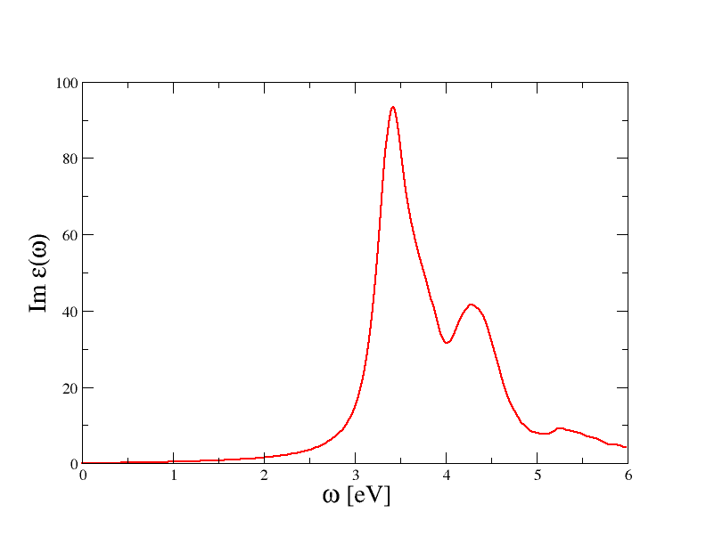
For figures with a caption use the markdown-figures extension:
```md Convergence of BSE optical spectrum wrt \\(\\kk\\)-point sampling. See also ngkpt and shiftk.```
Convergence of BSE optical spectrum wrt \\(\\kk\\)-point sampling. See also ngkpt and shiftk.The caption can contain Latex equations as well as Abinit wikilinks. <img> and <figure> elements are automatically centered via CSS directives declared in extra.css.
If you need to customize the height and width of the image, use
md 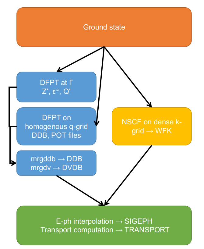{: style=\"height:500px;width:400px\"}
Note that this is not standard markdown but an extension provided by Attribute Lists extension that adds a syntax to define attributes on the various HTML elements in markdown\u2019s output.
"},{"location":"developers/markdown/#pdf-files","title":"Pdf Files","text":"Links to internal pdf files shipped with the Abinit documentation are inserted using the base name of the pdf file and the wikilink syntax:
Please consult the [[pdf:howto_chebfi]] document.
that gives: Please consult the howto_chebfi.pdf document.
Note
The .pdf extension at the end of the file is optional.
This is the recommended approach to link pdf documents in the description of the input variables. In the tutorials and in the theory notes, on the other hand, you may want to display the pdf file directly in the HTML page. In this case, use the HTML embed element:
html <embed src=\"../howto_chebfi.pdf\" type=\"application/pdf\" width=\"100%\" height=\"480px\">`
See the automatically generated pdf gallery for examples.
"},{"location":"developers/markdown/#videos","title":"Videos","text":"Links to videos can be included with the standard Markdown syntax:
``md The video below gives an overwiew of the command line options ofruntests.py`
```
that produces:
The video below gives an overwiew of the command line options of runtests.py
More advanced features such as video galleries require a bit of HTML/CSS/JS code in the Markdown page. See for example the Abinit video gallery built with lightGallery.
"},{"location":"developers/markdown/#links","title":"Links","text":""},{"location":"developers/markdown/#markdown-links","title":"Markdown links","text":"To create a link, enclose the link text in brackets (e.g., [Duck Duck Go]) and then follow it immediately with the URL in parentheses (e.g., (https://duckduckgo.com)). Alternatively, one can enclose the URLs directly between <>. The table below shows typical scenarios:
[Duck Duck Go](https://duckduckgo.com) Duck Duck Go <https://www.abinit.org> https://www.abinit.org [Links for videos section in the same page](#videos) Links to videos section in the same page Note
Links to external websites are signaled with the fontawesome \u00a0 icon: . See CSS rules in extra.css.
Markdown can also be used for creating internal links to other pages of the ABINIT website. The main problem is that you need to know the relative URL (or the root-relative URL) of the HTML page you want to refer to. Unfortunately, this is not so easy since the HTML pages are automatically generated by mksite.py and mkdocs hence you need to understand how these tools work internally. Just to make things even more complicated, there are different ways to achieve the same result (relative urls, root-relative urls, mkdocs md syntax). Let\u2019s try to clarify this point using a very pragmatic approach.
First of all, it is very important to understand that in the mkdocs.yml configuration file, the use_directory_urls option is set to True. This means that mkdocs creates a directory with an index.html file for each md page included in the ABINIT documentation. For instance, the abimkdocs.md and markdown.md files located in ~abinit/doc/developers are converted by mkdocs into the following hierarchy of HTML files:
in which the content of e.g. abimkdocs.md is used to generate abimkdocs/index.html.
Important
In these examples the / symbol does not correspond to the root of your filesystem but to the root directory used by the web-server for serving HTML files. Roughly speaking, your ~abinit/doc/ directory is consired as the root node.
We use this convention because it leads to more user-friendly URLs as the abimkdocs page is now served by the local web server at http://127.0.0.1:8000/developers/abimkdocs instead of the lengthier http://127.0.0.1:8000/developers/abimkdocs.html. Once the website is deployed in production, the same page will be served at https://docs.abinit.org/developers/abimkdocs instead of https://docs.abinit.org/developers/abimkdocs.html.
At this point it should be clear that the relative path you see on your file system is not the same as the relative URL seen by the web-server. In other words, you should add an extra \u201c../\u201d to the relative path you have on your file system to account for the creation of the directory. This syntax is clearly unintuitive and error-prone but it is worth knowing especially if, for some reason, you need to inject in the md page HTML code with relative hrefs.
Fortunately, you are not obliged to use relative URLs in markdown links since there are two other approaches that are much more user-friendly and much easier to maintain. The first one is based on root-relative URLs while the second one relies on preprocessing operations performed by mkdocs.
In brief, root-relative URLs can be seen as paths relative to your ~abinit/doc/ directory provided you add a / at the beginning of the string while the mkdocs syntax is activated by using relative paths as seen on your files system with the crucial difference that you must include the .md extension at the end of the URL. As usual, it is much easier to explain the different cases by examples:
[MBPT document](../theory/mbt.md) MBPT document relative URL (recommended) [MBPT document](../theory/mbt.md) MBPT document root-relative URL [MBPT document](../theory/mbt.md) MBPT document mkdocs preprocessed relative URL [About topics](abimkdocs.md#topics) About topics relative + HTML fragment (recommended) [About topics](../developers/abimkdocs.md#topics) About topics root-relative + HTML fragment [About topics](abimkdocs.md#topics) About topics mkdocs preprocessed relative URL + HTML fragment Important
Relative URLs obviously depend on the location of the page containg the link whereas root-relative URLs are invariant. It is evident that absolute (file-system dependent) paths such as ~gmatteo/abinit/doc/theory/mbt won\u2019t work when the website is deployed so don\u2019t use them.
At this point you may ask why do we have all these different approaches and which one should I use when writing the documentation? To make a long story short, we strongly suggest to use relative URLs. The reason is that relative URLs avoid link breakage across different hosting environments. While root-relative URLs look like \u201cabsolute paths\u201d, they can break if the documentation is not deployed at the root of a domain. Using relative URLs ensures that the links remain robust regardless of the deployment path.
Furthermore, using standard relative URLs correctly maps to the built directories when use_directory_urls is enabled. While MkDocs provides its own .md preprocessing syntax, adopting plain relative URLs is simpler and is the current recommended practice in Abinit.
There are however cases in which we would like to have an even simpler syntax to automatically generate links within our documentation, in particular links to:
abimkdocs directory.abiref.bib.For this reason, we use the extensions API \u00a0 provided by python Markdown to extend the syntax of the parser, using the Wikilink syntax so that you don\u2019t need to know the root-relative or the relative URL of the HTML page you want to link. Typical cases are discussed in the next sections.
"},{"location":"developers/markdown/#wikilinks","title":"Wikilinks","text":"The wikilink syntax \u00a0 is used with two pairs of square brackets and possible separators (:, # and |). In the simple case, this gives [ [name] ] although the more general form is
[ [namespace:name#section|text] ]
where namespace, section and text are optional (in such case, the adequate separator should not be mentioned). The namespace is not echoed in the Web page, while if a text is given, it will supercede the echo of the name in the Web page (see examples below).
Warning
Do not use parentheses within the pair of double brackets, the whole expression will not be recognized.
When an internal link is recognized, the wikilink string is replaced by the adequate HTML link There are a couple of names immediately recognized:
variables_abinit.py)abiref.bib)~abinit/tests/*/Input directoryExamples:
Markdown Result[[ecut]] ecut [[abinit:ecut]] ecut [[anaddb:dipdip]] dipdip [[dipdip@anaddb]] dipdip@anaddb [[cite:Amadon2008]] [Amadon2008] [[~abinit/tests/tutorial/Input/tbase1_1.abi]] ~abinit/tests/tutorial/Input/tbase1_1.abi [[tests/tutorial/Input/tbase1_1.abi]] tests/tutorial/Input/tbase1_1.abi [[test:libxc_41]] libxc[41] [[tests/tutorial/Refs/tbase1_1.abo]] tests/tutorial/Refs/tbase1_1.abo [[~abinit/tests/tutorial/Refs/tbase1_1.abo]] ~abinit/tests/tutorial/Refs/tbase1_1.abo [[~abinit/tests/Pspdir/6c_lda.paw]] ~abinit/tests/Pspdir/6c_lda.paw [[tests/Pspdir/6c_lda.paw]] tests/Pspdir/6c_lda.paw [[:digit:]]' :digit: The input variables for anaddb, optic and aim will be recognized if they are used with the namespaces anaddb, optic and aim. One has thus also the choice between the syntax [[anaddb:dipdip]] and [[dipdip@anaddb]]. In the first case, only dipdip is echoed, while in the second case, dipdip@anaddb is echoed. This syntax is needed because there\u2019s also a dipdip variable in Abinit.
A wikilink that starts with # is interpreted as an internal link within the page hence
md See [[#markdown-quick-reference|this section]] for more info
becomes: See this section for more info
although the same result can be obtained with the more readable Markdown syntax:
md See [this section](#markdown-quick-reference) for more info
To specify the name of the anchor in a bibliographic citation use the syntax with the | separator:
Please consult [[cite:Gonze2016 | the last generic ABINIT article]].\nthat is rendered in HTML as: Please consult the last generic ABINIT article.
The script does a bit of formatting in these examples: it keeps one pair of square brackets in the case of a bibliographic reference, and addd ~abinit/ in the case of a path. The syntax [[test:libxc_41]] is preferable when documenting new tests in the release notes. The python code issues a warning in the terminal if the link cannot be established.
Note
Links to input files have a popover with the description of the test. Hovering on a citation opens a popover with the title reported in the Bibtex entry. Links to variables and internal files use a different font declared in extra.css.
"},{"location":"developers/markdown/#internal-links-with-namespace","title":"Internal links with namespace","text":"Other internal links can be recognized thanks to the namespace.
Examples:
Namespace Markdown Resulttutorial [[tutorial:gw1]] gw1 tutorial tutorial [[tutorial:index]] tutorial home page topic [[topic:BSE]] topic_BSE topic [[topic:index]] Topics index help [[help:abinit]] abinit help file help [[help:abinit#files-file]] abinit help file theory [[theory:mbt]] mbt varset [[varset:bse]] bse varset cite [[cite:Amadon2008]] [Amadon2008] ac [[ac:abiref_nag_7.0_openmpi.ac]] pdf [[pdf:howto_chebfi.pdf]] howto_chebfi.pdf pdf [[pdf:howto_chebfi]] howto_chebfi.pdf src [[src:94_scfcv/m_scfcv.F90]] 94_scfcv/m_scfcv.F90 #files-file is an HTML id defined in ~abinit/doc/guide/abinit.md with:
```html
"},{"location":"developers/markdown/#4-more-detailed-presentation-of-the-files-file","title":"4 More detailed presentation of the files file","text":"```
Also in this case, it\u2019s possible to specify the name of the link with the | separator so [[topic:PIMD#1|Introduction]] becomes Introduction.
Important
Internal links are automatically generated by the Markdown parser as discussed in the Permalinks section.
Be careful when including a wikilink inside other square brackets e.g. [2+ [ [ecut] ] ]**2 as the occurrence of ]]] confuses the parser. The problem is easily solved by inserting whitespaces in the expression:
[ 2 + [[ecut]] ] ** 2\nThis version if much more readable and it also avoids possible problems with the ** that has a special meaning in Markdown.
To refer to a particular git commit inside a Markdown document use:
Solved in [[gitsha:f74dba1ed8346ca586dc95fd10fe4b8ced108d5e]]\nthat produces: f74dba1. This extension is useful to generate nice changelogs and release notes.
"},{"location":"developers/markdown/#external-links","title":"External links","text":"As for the internal wikilinks, some external links are also recognized. The following case are treated:
www.http, https, ftp, file[[https://www.abinit.org]] https://www.abinit.org https://www.abinit.org https://www.abinit.org It is also possible to specify the name of the link with the | separator: For example, [[https://wiki.abinit.org|The ABINIT Wiki]] produces The ABINIT Wiki
The markdown parser supports aliases for commonly used links. The aliases are defined in the mkdocs.yml configuration file (abimkdocs_aliases):
|AbiPy| AbiPy |AbipyStructureNb| AbiPy structure notebook |xmgrace| xmgrace |gnuplot| gnuplot |today| August 16, 2026"},{"location":"developers/markdown/#permalinks","title":"Permalinks","text":"Permalinks are a feature of the Table of Contents extension \u00a0, which is part of the standard Markdown library. The extension inserts an anchor at the end of each headline, which makes it possible to directly link to a subpart of the document.
By default, all headers will automatically have unique id attributes generated based upon the text of the header. The name of the anchor is constructed from the header by converting the string to lower-case ASCII, removing dots and other symbols such as & and replacing white spaces with a dash -. For instance, #pdf-files is the anchor associated to the \u201cPdf Files\u201d section in this page and we can thus refer to it with the Markdown syntax:
md As we have seen in the [previous section](#pdf-files)
that produces: As we have seen in the previous section
Tip
Hover with the mouse on the header in the HTML page to show the permalink in the browser. You can also copy the link and use the last part to generate the reference.
Note
It is also possible to generate automatically the Table of Contents by just placing the [TOC] marker in the document where you would like the Table of Contents to appear. Then, a nested list of all the headers in the document will replace the marker. Note, however, that the use of [TOC] in our pages is not recomended as the Table of Contents is automatically generated by the Mkdocs theme and displayed in the navigation bar on the right.
SmartSymbols \u00a0 adds syntax for creating special characters such as trademarks, arrows, fractions, etc. The list of symbols supported by the extension is:
Markdown Result(tm) \u2122 (c) (c) (r) (r) c/o c/o +/- \u00b1 --> \u2192 <-- \u2190 <--> \u2194 =/= \u2260 1/4, etc. \u00bc, etc. 1st 2nd etc. 1st 2nd etc."},{"location":"developers/markdown/#definition-lists","title":"Definition Lists","text":"The Definition Lists \u00a0 extension adds the ability to create definition lists in Markdown documents. This extension is included in the standard Markdown library. The following text:
```md Apple Pomaceous fruit of plants of the genus Malus in the family Rosaceae. Orange The fruit of an evergreen tree of the genus Citrus. ```will be rendered as:
Apple Pomaceous fruit of plants of the genus Malus in the family Rosaceae. Orange The fruit of an evergreen tree of the genus Citrus."},{"location":"developers/markdown/#admonitions","title":"Admonitions","text":"Admonitions \u00a0 are useful to stress important sections (useful e.g. in the Abinit tutorials). Admonition are created using the Markdown syntax:
```md
Note
Here is a note for you.
```
and
```md
Don\u2019t try this at home!
Stand back. I\u2019m about to try science!
```
for an admonition with a custom title (make sure to quote the title).
The types of admonitions available for use in MkDocs depend on the theme being used. The Material theme supports \u00a0 the following types:
Note
I am a \u201cnote\u201d admonition and look the same as \u201cseealso\u201d.
Tip
I am a \u201ctip\u201d admonition and look the same as \u201chint\u201d and \u201cimportant\u201d.
Warning
I am a \u201cwarning\u201d admonition and look the same as \u201cattention\u201d and \u201ccaution\u201d.
Danger
I am a \u201cdanger\u201d admonition and look the same as \u201cerror\u201d.
Summary
I am a \u201csummary\u201d admonition and look the same as \u201ctldr\u201d.
Success
I am a \u201csuccess\u201d admonition and look the same as \u201ccheck\u201d and \u201cdone\u201d.
Failure
I am a \u201cfailure\u201d admonition and look the same as \u201cfail\u201d and \u201cmissing\u201d.
Bug
I am a \u201cbug\u201d admonition.
For the complete list, please consult the mkdocs-material documentation.
"},{"location":"developers/markdown/#details","title":"Details","text":"Detail \u00a0 is an extension that creates collapsible elements that hide their content. It uses the HTML5 <details><summary> tags to accomplish this. It supports nesting and you can also force the default state to be open. This extension is used in the documentation of the input variable to generate a container with the list of tests associated to the variable but it can also be used for long FAQs of Q&A sections in the tutorials.
Examples:
```md
List of variablesecut asr@anaddb
```
produces the open element:
List of variablesecut asr@anaddb
while
```md
Click to open!ecut asr@anaddb
```
creates a closed element:
Click to open!ecut asr@anaddb
"},{"location":"developers/markdown/#abinit-extensions","title":"Abinit extensions","text":"To create a button that opens a dialog containing an input file, use:
{% dialog tests/v1/Input/t01.abi %}
that produces:
View tests/v1/Input/t01.abi# FCC Al; 2 special points\n\n#nband 8\n#nspinor 2\n\n acell 3*7.60\n ecut 10\n enunit 2\n intxc 1\n kptopt 0\n kpt 1 1 1 1 2 2 kptnrm 4\n natom 1\n nband 4\n nkpt 2\n nline 3\n nstep 8\n nsym 24 ntypat 1\n occopt 4 prtvol 10\n rprim 0 .5 .5 .5 0 .5 .5 .5 0\n symrel\n 1 0 0 0 1 0 0 0 1\n 0 1 -1 1 0 -1 0 0 -1\n -1 0 0 -1 0 1 -1 1 0\n 0 -1 1 0 -1 0 1 -1 0\n -1 0 1 -1 0 0 -1 1 0\n 0 -1 0 0 -1 1 1 -1 0\n 0 -1 1 1 -1 0 0 -1 0\n 0 1 -1 0 0 -1 1 0 -1\n 0 0 -1 1 0 -1 0 1 -1\n -1 1 0 -1 0 1 -1 0 0\n 1 0 -1 0 1 -1 0 0 -1\n 1 -1 0 0 -1 0 0 -1 1\n -1 0 0 -1 1 0 -1 0 1\n 0 1 0 1 0 0 0 0 1\n 0 0 1 0 1 0 1 0 0\n 1 0 0 0 0 1 0 1 0\n 0 0 1 1 0 0 0 1 0\n 0 1 0 0 0 1 1 0 0\n -1 0 1 -1 1 0 -1 0 0\n 0 0 -1 0 1 -1 1 0 -1\n 1 0 -1 0 0 -1 0 1 -1\n 1 -1 0 0 -1 1 0 -1 0\n 0 -1 0 1 -1 0 0 -1 1\n -1 1 0 -1 0 0 -1 0 1\n tnons 72*0.0d0\n tolwfr 1.0d-16\n tsmear 0.05\n typat 1\n wtk 1 3\n xred 0.0 0.0 0.0\n znucl 13.0\n\n\n#%%<BEGIN TEST_INFO>\n#%% [setup]\n#%% executable = abinit\n#%% use_files_file = yes\n#%% [files]\n#%% files_to_test = t01.abo, tolnlines=0, tolabs=0.0, tolrel=0.0\n#%% psp_files=PseudosGTH_pwteter/13al.pspgth\n#%% [paral_info]\n#%% max_nprocs = 2\n#%% [extra_info]\n#%% keywords = NC\n#%% description = \n#%% Bulk Aluminium, FCC, with 2 special points, occopt=4 and tsmear=0.05 .\n#%% Designed to test the treatment of metals, using the \"cold smearing\"\n#%% of N. Marzari , with a=-.5634 (minimization of the bump). \n#%%<END TEST_INFO>\n
If multiple files are used such as in:
{% dialog tests/v1/Input/t01.abi tests/v1/Input/t02.abi tests/v1/Input/t03.abi %}\nmultiple buttons are produced:
View tests/v1/Input/t01.abi View tests/v1/Input/t02.abi View tests/v1/Input/t03.abi# FCC Al; 2 special points\n\n#nband 8\n#nspinor 2\n\n acell 3*7.60\n ecut 10\n enunit 2\n intxc 1\n kptopt 0\n kpt 1 1 1 1 2 2 kptnrm 4\n natom 1\n nband 4\n nkpt 2\n nline 3\n nstep 8\n nsym 24 ntypat 1\n occopt 4 prtvol 10\n rprim 0 .5 .5 .5 0 .5 .5 .5 0\n symrel\n 1 0 0 0 1 0 0 0 1\n 0 1 -1 1 0 -1 0 0 -1\n -1 0 0 -1 0 1 -1 1 0\n 0 -1 1 0 -1 0 1 -1 0\n -1 0 1 -1 0 0 -1 1 0\n 0 -1 0 0 -1 1 1 -1 0\n 0 -1 1 1 -1 0 0 -1 0\n 0 1 -1 0 0 -1 1 0 -1\n 0 0 -1 1 0 -1 0 1 -1\n -1 1 0 -1 0 1 -1 0 0\n 1 0 -1 0 1 -1 0 0 -1\n 1 -1 0 0 -1 0 0 -1 1\n -1 0 0 -1 1 0 -1 0 1\n 0 1 0 1 0 0 0 0 1\n 0 0 1 0 1 0 1 0 0\n 1 0 0 0 0 1 0 1 0\n 0 0 1 1 0 0 0 1 0\n 0 1 0 0 0 1 1 0 0\n -1 0 1 -1 1 0 -1 0 0\n 0 0 -1 0 1 -1 1 0 -1\n 1 0 -1 0 0 -1 0 1 -1\n 1 -1 0 0 -1 1 0 -1 0\n 0 -1 0 1 -1 0 0 -1 1\n -1 1 0 -1 0 0 -1 0 1\n tnons 72*0.0d0\n tolwfr 1.0d-16\n tsmear 0.05\n typat 1\n wtk 1 3\n xred 0.0 0.0 0.0\n znucl 13.0\n\n\n#%%<BEGIN TEST_INFO>\n#%% [setup]\n#%% executable = abinit\n#%% use_files_file = yes\n#%% [files]\n#%% files_to_test = t01.abo, tolnlines=0, tolabs=0.0, tolrel=0.0\n#%% psp_files=PseudosGTH_pwteter/13al.pspgth\n#%% [paral_info]\n#%% max_nprocs = 2\n#%% [extra_info]\n#%% keywords = NC\n#%% description = \n#%% Bulk Aluminium, FCC, with 2 special points, occopt=4 and tsmear=0.05 .\n#%% Designed to test the treatment of metals, using the \"cold smearing\"\n#%% of N. Marzari , with a=-.5634 (minimization of the bump). \n#%%<END TEST_INFO>\n
# FCC Al; 2 special points\n\n acell 3*7.60\n ecut 10\n enunit 2\n intxc 1\n kptopt 0\n kpt 1 1 1 1 2 2 kptnrm 4\n natom 1 nband 4\n nkpt 2\n nline 3 nstep 8\n nsym 24 ntypat 1\n occopt 5 prtvol 10\n rprim 0 .5 .5 .5 0 .5 .5 .5 0\n symrel\n 1 0 0 0 1 0 0 0 1\n 0 1 -1 1 0 -1 0 0 -1\n -1 0 0 -1 0 1 -1 1 0\n 0 -1 1 0 -1 0 1 -1 0\n -1 0 1 -1 0 0 -1 1 0\n 0 -1 0 0 -1 1 1 -1 0\n 0 -1 1 1 -1 0 0 -1 0\n 0 1 -1 0 0 -1 1 0 -1\n 0 0 -1 1 0 -1 0 1 -1\n -1 1 0 -1 0 1 -1 0 0\n 1 0 -1 0 1 -1 0 0 -1\n 1 -1 0 0 -1 0 0 -1 1\n -1 0 0 -1 1 0 -1 0 1\n 0 1 0 1 0 0 0 0 1\n 0 0 1 0 1 0 1 0 0\n 1 0 0 0 0 1 0 1 0\n 0 0 1 1 0 0 0 1 0\n 0 1 0 0 0 1 1 0 0\n -1 0 1 -1 1 0 -1 0 0\n 0 0 -1 0 1 -1 1 0 -1\n 1 0 -1 0 0 -1 0 1 -1\n 1 -1 0 0 -1 1 0 -1 0\n 0 -1 0 1 -1 0 0 -1 1\n -1 1 0 -1 0 0 -1 0 1\n tnons 72*0.0d0\n tolwfr 1.0d-16\n tsmear 0.05\n typat 1\n wtk 1 3\n xred 0.0 0.0 0.0\n znucl 13.0\n\n\n pp_dirpath \"$ABI_PSPDIR\"\n pseudos \"PseudosGTH_pwteter/13al.pspgth\"\n\n#%%<BEGIN TEST_INFO>\n#%% [setup]\n#%% executable = abinit\n#%% [files]\n#%% files_to_test = t02.abo, tolnlines= 1, tolabs= 1.001e-09, tolrel= 1.100e-04\n#%% [paral_info]\n#%% max_nprocs = 2\n#%% [extra_info]\n#%% keywords = NC\n#%% description = \n#%% Bulk Aluminium, FCC, with 2 special points, occopt=5 and tsmear=0.05.\n#%% Designed to test the treatment of metals, using the \"cold smearing\"\n#%% of N. Marzari , with a=-.8165 (monotonic function in the tail).\n#%% topics = BandOcc\n#%%<END TEST_INFO>\n
# FCC Al; 2 special points\n\n acell 3*7.60\n ecut 10\n enunit 2\n intxc 1\n fband 2.0d0\n#nband 4\n#\n istatr 2\n kptopt 0\n kpt 1 1 1 1 2 2 kptnrm 4\n natom 1\n nkpt 2\n nline 3 nstep 8\n nsym 24 ntypat 1\n occopt 6 prtvol 10\n rprim 0 .5 .5 .5 0 .5 .5 .5 0\n symrel\n 1 0 0 0 1 0 0 0 1\n 0 1 -1 1 0 -1 0 0 -1\n -1 0 0 -1 0 1 -1 1 0\n 0 -1 1 0 -1 0 1 -1 0\n -1 0 1 -1 0 0 -1 1 0\n 0 -1 0 0 -1 1 1 -1 0\n 0 -1 1 1 -1 0 0 -1 0\n 0 1 -1 0 0 -1 1 0 -1\n 0 0 -1 1 0 -1 0 1 -1\n -1 1 0 -1 0 1 -1 0 0\n 1 0 -1 0 1 -1 0 0 -1\n 1 -1 0 0 -1 0 0 -1 1\n -1 0 0 -1 1 0 -1 0 1\n 0 1 0 1 0 0 0 0 1\n 0 0 1 0 1 0 1 0 0\n 1 0 0 0 0 1 0 1 0\n 0 0 1 1 0 0 0 1 0\n 0 1 0 0 0 1 1 0 0\n -1 0 1 -1 1 0 -1 0 0\n 0 0 -1 0 1 -1 1 0 -1\n 1 0 -1 0 0 -1 0 1 -1\n 1 -1 0 0 -1 1 0 -1 0\n 0 -1 0 1 -1 0 0 -1 1\n -1 1 0 -1 0 0 -1 0 1\n tnons 72*0.0d0\n tolwfr 1.0d-16\n tsmear 0.05\n typat 1\n wtk 1 3\n xred 0.0 0.0 0.0\n znucl 13.0\n\n\n pp_dirpath \"$ABI_PSPDIR\"\n pseudos \"PseudosGTH_pwteter/13al.pspgth\"\n\n#%%<BEGIN TEST_INFO>\n#%% [setup]\n#%% executable = abinit\n#%% [files]\n#%% files_to_test = t03.abo ,tolnlines = 1, tolabs = 1.100e-09, tolrel = 1.100e-04\n#%% [paral_info]\n#%% max_nprocs = 2\n#%% [extra_info]\n#%% authors = Unknown\n#%% keywords = NC\n#%% description = \n#%% Bulk Aluminium, FCC, with 2 special points, occopt=6 and tsmear=0.05.\n#%% Designed to test the treatment of metals, \n#%% with the Gaussian-Hermite smearing of Methfessel and Paxton.\n#%% Also test the use of fband instead of nband.\n#%%<END TEST_INFO>\n"},{"location":"developers/markdown/#mathjax","title":"MathJax","text":"
Formulas written in LaTeX are interpreted automatically (at visualization time) thanks to the MathJax \u00a0 on-the-flight processor while the math extension for Python-Markdown is provided by python-markdown-math.
Latex equations can be used everywhere including the description of the variables reported in abinit_vars.yml and the description of the tests gives in the TEST_INFO section. For the Abinit documentation, the conventions are:
$...$ yields an onlinecite translation of the LaTeX formula.$$...$$ yields display mode, the LaTeX formula being rendered on one dedicated line (moreover, centered).\\begin{equation}...\\end{equation} markers.$ sign is inside a <pre>...</pre> HTML section, MathJax does not interpret it.\\$ to prevent a real $ to be interpreted.For instance $|\\Phi\\rangle$ produces \\(|\\Phi\\rangle\\) while $$\\Phi_\\kq(\\rr)$$ produces
Equations enclosed by $$...$$ or \\begin{equation}...\\end{equation} markers are automatically numbered and can be referenced inside the Markdown text using the standard Latex syntax:
latex \\begin{equation} G(12) = -i \\langle \\Theta^N_0|T\\bigl[\\Psi(1)\\Psi^\\dagger(2)\\bigr]|\\Theta^N_0 \\rangle \\label{eq:GreenDef} \\end{equation}
that produces:
\\[\\begin{equation} G(12) = -i \\langle \\Theta^N_0|T\\bigl[\\Psi(1)\\Psi^\\dagger(2)\\bigr]|\\Theta^N_0 \\rangle \\label{eq:GreenDef} \\end{equation}\\]Equations can be referenced with:
The propagator in Eq.(\\ref{eq:GreenDef})\nthat produces: The propagator in Eq.(\\ref{eq:GreenDef})
Note that MathJax is configured with Latex macros to facilitate the insertion of symbols commonly used in our domain:
Markdown Result$\\rr$ \\(\\rr\\) $\\GG$ \\(\\GG\\) $\\kk$ \\(\\kk\\) $\\qq$ \\(\\qq\\) $\\kq$ \\(\\kq\\) Please consult the preamble in abinit_theme/main.html for the complete list of macros.
Bug
It seems that the plotly javascript library does not play well with MathJax as equations sometimes are not displayed when plotly is activated. This problem can be fixed by reloading the page. It should not represent a serious issue since plotly is used only in selected pages (like this one).
"},{"location":"developers/markdown/#unicode","title":"Unicode","text":"Unicode characters in particular Greek symbols and accented characters can be used in the documentation. The websites uses the Google\u2019s Roboto font \u00a0 so Greek symbols can be included without using MathJax either by specifying the HTML entity or by copying the unicode character given in the two tables below. This could be useful if the page does not contain Latex equations and there are just a few Greek symbols to be inserted. Please do not use unicode characters in Latex equations.
Character Name Character Entity Hex Entity HTML Entity GREEK CAPITAL LETTER ALPHA \u0391 &\u200c#913; &\u200c#x0391 &\u200cAlpha; GREEK CAPITAL LETTER BETA \u0392 &\u200c#914; &\u200c#x0392 &\u200cBeta; GREEK CAPITAL LETTER GAMMA \u0393 &\u200c#915; &\u200c#x0393 &\u200cGamma; GREEK CAPITAL LETTER DELTA \u0394 &\u200c#916; &\u200c#x0394 &\u200cDelta; GREEK CAPITAL LETTER EPSILON \u0395 &\u200c#917; &\u200c#x0395 &\u200cEpsilon; GREEK CAPITAL LETTER ZETA \u0396 &\u200c#918; &\u200c#x0396 &\u200cZeta; GREEK CAPITAL LETTER ETA \u0397 &\u200c#919; &\u200c#x0397 &\u200cEta; GREEK CAPITAL LETTER THETA \u0398 &\u200c#920; &\u200c#x0398 &\u200cTheta; GREEK CAPITAL LETTER IOTA \u0399 &\u200c#921; &\u200c#x0399 &\u200cIota; GREEK CAPITAL LETTER KAPPA \u039a &\u200c#922; &\u200c#x039A &\u200cKappa; GREEK CAPITAL LETTER LAM(B)DA \u039b &\u200c#923; &\u200c#x039B &\u200cLambda; GREEK CAPITAL LETTER MU \u039c &\u200c#924; &\u200c#x039C &\u200cMu; GREEK CAPITAL LETTER NU \u039d &\u200c#925; &\u200c#x039D &\u200cNu; GREEK CAPITAL LETTER XI \u039e &\u200c#926; &\u200c#x039E &\u200cXi; GREEK CAPITAL LETTER OMICRON \u039f &\u200c#927; &\u200c#x039F &\u200cOmicron; GREEK CAPITAL LETTER PI \u03a0 &\u200c#928; &\u200c#x03A0 &\u200cPi; GREEK CAPITAL LETTER RHO \u03a1 &\u200c#929; &\u200c#x03A1 &\u200cRho; GREEK CAPITAL LETTER SIGMA \u03a3 &\u200c#931; &\u200c#x03A3 &\u200cSigma; GREEK CAPITAL LETTER TAU \u03a4 &\u200c#932; &\u200c#x03A4 &\u200cTau; GREEK CAPITAL LETTER UPSILON \u03a5 &\u200c#933; &\u200c#x03A5 &\u200cUpsilon; GREEK CAPITAL LETTER PHI \u03a6 &\u200c#934; &\u200c#x03A6 &\u200cPhi; GREEK CAPITAL LETTER CHI \u03a7 &\u200c#935; &\u200c#x03A7 &\u200cChi; GREEK CAPITAL LETTER PSI \u03a8 &\u200c#936; &\u200c#x03A8 &\u200cPsi; GREEK CAPITAL LETTER OMEGA \u03a9 &\u200c#937; &\u200c#x03A9 &\u200cOmega; Character Name Character Entity Hex Entity HTML Entity GREEK SMALL LETTER ALPHA \u03b1 &\u200c#945; &\u200c#x03B1 &\u200calpha; GREEK SMALL LETTER BETA \u03b2 &\u200c#946; &\u200c#x03B2 &\u200cbeta; GREEK SMALL LETTER GAMMA \u03b3 &\u200c#947; &\u200c#x03B3 &\u200cgamma; GREEK SMALL LETTER DELTA \u03b4 &\u200c#948; &\u200c#x03B4 &\u200cdelta; GREEK SMALL LETTER EPSILON \u03b5 &\u200c#949; &\u200c#x03B5 &\u200cepsilon; GREEK SMALL LETTER ZETA \u03b6 &\u200c#950; &\u200c#x03B6 &\u200czeta; GREEK SMALL LETTER ETA \u03b7 &\u200c#951; &\u200c#x03B7 &\u200ceta; GREEK SMALL LETTER THETA \u03b8 &\u200c#952; &\u200c#x03B8 &\u200ctheta; GREEK SMALL LETTER IOTA \u03b9 &\u200c#953; &\u200c#x03B9 &\u200ciota; GREEK SMALL LETTER KAPPA \u03ba &\u200c#954; &\u200c#x03BA &\u200ckappa; GREEK SMALL LETTER LAM(B)DA \u03bb &\u200c#955; &\u200c#x03BB &\u200clambda; GREEK SMALL LETTER MU \u03bc &\u200c#956; &\u200c#x03BC &\u200cmu; GREEK SMALL LETTER NU \u03bd &\u200c#957; &\u200c#x03BD &\u200cnu; GREEK SMALL LETTER XI \u03be &\u200c#958; &\u200c#x03BE &\u200cxi; GREEK SMALL LETTER OMICRON \u03bf &\u200c#959; &\u200c#x03BF &\u200comicron; GREEK SMALL LETTER PI \u03c0 &\u200c#960; &\u200c#x03C0 &\u200cpi; GREEK SMALL LETTER RHO \u03c1 &\u200c#961; &\u200c#x03C1 &\u200crho; GREEK SMALL LETTER FINAL SIGMA \u03c2 &\u200c#962; &\u200c#x03C2 GREEK SMALL LETTER SIGMA \u03c3 &\u200c#963; &\u200c#x03C3 &\u200csigma; GREEK SMALL LETTER TAU \u03c4 &\u200c#964; &\u200c#x03C4 &\u200ctau; GREEK SMALL LETTER UPSILON \u03c5 &\u200c#965; &\u200c#x03C5 &\u200cupsilon; GREEK SMALL LETTER PHI \u03c6 &\u200c#966; &\u200c#x03C6 &\u200cphi; GREEK SMALL LETTER CHI \u03c7 &\u200c#967; &\u200c#x03C7 &\u200cchi; GREEK SMALL LETTER PSI \u03c8 &\u200c#968; &\u200c#x03C8 &\u200cpsi; GREEK SMALL LETTER OMEGA \u03c9 &\u200c#969; &\u200c#x03C9 &\u200comega;Taken from https://sites.psu.edu/symbolcodes/languages/ancient/greek/greekchart/
"},{"location":"developers/markdown/#plotly","title":"Plotly","text":"plotly \u00a0 is a high-level, declarative charting library built on top of d3.js and stack.gl. plotly.js ships with over 20 chart types, including scientific charts, 3D graphs, statistical charts, SVG maps, financial charts, and more. Note that plotly is deactivated by default so you have to activate it inside the Markdown page by adding
"},{"location":"developers/markdown/#yaml","title":"```yaml","text":""},{"location":"developers/markdown/#plotly-true","title":"plotly: true","text":"```
to the front matter. This option will tell the browser to load the javascript library in the HTML page so that it\u2019s possible to include HTML+javascript code to generate nice interactive plots inside the Markdown documentation. For example the HTML + javascript code:
```html
Here's a simple Plotly plot - plotly.js documentation
```
produces the following plot:
Here's a simple Plotly plot - plotly.js documentation
plotly is used to plot the code statistics but it is not required for the proper functioning of the website.
Bug
It seems that the plotly javascript library does not play well with MathJax as equations sometimes are not displayed when plotly is activated. This problem can be fixed by reloading the page. It should not represent a serious issue since plotly is used only in selected pages (like this one).
"},{"location":"developers/markdown/#using-html-directly","title":"Using HTML directly","text":"HTML code can be used in Markdown but keep in mind that standard Markdown parsers ignore text inside block-level HTML tags so
```html
*Emphasized* text.```
won\u2019t work (but this situation only occurs if you are trying to write some advanced HTML code).
Another thing worth noticing is that Mkdocs (by default) generates a directory with an index.html file for every markdown page declared in mkdocs.yml (see also the official documentation). This means that a local webserver will serve this page at http://127.0.0.1:8000/developers/markdown/index.html that can be equivalently reached from the more user friendly URL http://127.0.0.1:8000/developers/markdown/.
This implementation detail does not affect links specified either with wikilink or markdown syntax because the python code will perform the automatic translation of the URLs. It does affect, however, the way you should specify src or href in HTML code because one should take into account the extra directory created by Mkdocs. In a nutshell, prepend a ../ to the relative path you would use inside the shell to specify the location of that resource with respect to the present page.
Among tools that analyze MPI usage and performance, it is possible to annotate source code using NVTX (NVIDIA Tools Extension Library) and trace an MPI job execution as a timeline of API events per process using the profiler NVIDIA Nsight Systems. Code annotation libraries are activated by default in ABINIT when compiled on GPU, because NVIDIA CUDA Toolkit includes NVTX (and AMD includes ROCTX). As of ABINIT version 10.3.6, NVTX annotation is also supported on CPU (see with_gpu_markers input variable). A guide for minimal installation of selected NVIDIA developer tools required to use NVTX on CPUs is provided here. Note that we don\u2019t need to install the entire NVIDIA CUDA Toolkit to profile code on CPU.
The NVIDIA Tools Extensions (NVTX) API can be installed on Linux with:
sudo dnf install cuda-nvtx-12\nYou can check the location of the installed library using the command locate nvToolsExt. Environment variables must be set by adding the following lines to your .bashrc (assuming here version 12.8 has been installed):
export PATH=/usr/local/cuda-12.8/bin:$PATH\nexport LD_LIBRARY_PATH=/usr/local/cuda-12.8/lib64:$LD_LIBRARY_PATH\nNsight Systems installer can be directly downloaded from NVIDIA website. We recommend to download the Full Version for profiling from the GUI. A minimal installation for profiling from the CLI only is also available but not used here. To use NVTX API you need to link ABINIT with nvToolsExt .so library and activate the NVTX markers macros. This can be achieved by adding the following lines to your autoconf configuration file when compiling ABINIT on CPU with autotools:
with_gpu_markers=\"yes\"\nabi_gpu_nvtx_v3=\"yes\"\nGPU_LIBS=\"-L/usr/local/cuda-12.8/lib64 -lnvToolsExt\"\nNote that these lines are not needed when GPU is enabled because marker libraries are configured automatically from the CUDA library root. The serial profiler can be attached to individual MPI processes for generating a timeline of selected API events using the following command, for example here tracing MPI and NVTX events of a parallel ABINIT calculation:
mpirun -n 4 nsys profile --trace=mpi,nvtx path_to_abinit_exe path_to_input_abi\nOnce a report has been generated on your machine for each process, it can be opened (in single or multi-report view) in Nsight GUI with:
nsys-ui report1.nsys-rep\nAn output example of tracing NVTX/MPI API events on a single MPI process using NVIDIA Nsight Systems:
"},{"location":"developers/new_testsuite/","title":"YAML-based tests: design principles and implementation details","text":"This document discusses the new YAML-based format used to represent physical results in the main output file. The connection with the ABINIT test suite and the yaml syntax used to define tolerances, parameters and constraints is also discussed.
The new infrastructure consists of a set of Fortran modules to output structured data in YAML format and Python code to parse the output files and analyze data.
"},{"location":"developers/new_testsuite/#motivations","title":"Motivations","text":"In ABINITv8 and previous versions, the ABINIT test suite is based on input files with the associated reference output files. Roughly speaking, an automatic test consists in comparing the reference file with the output file in a line-oriented fashion by computing differences between floating-point numbers without any knowledge about the meaning and the importance of the numerical values. This approach is very rigid and rather limited because it obliges developers to use a single (usually large) tolerance to account for possibly large fluctuations in the intermediate results whereas the tolerance criteria should be ideally applied only to the final results that are (hopefully) independent of details such as hardware, optimization level and parallelism.
This limitation is clearly seen when comparing the results of iterative algorithms. The number of iterations required to converge, indeed, may depend on several factors especially when the input parameters are far from convergence or when different parallelization schemes or stochastic methods are used. From the point of view of code validation, what really matters is the final converged value plus the time to solution if performance ends up being of concern. Unfortunately, any line-by-line comparison algorithm will miserably fail in such conditions because it will continue to insist on having the same number of iterations (lines) in the two calculations to consider the test succeeded. It is therefore clear that the approach used so far to validate new developments in Abinit is not able to cope with the challenges posed by high-performance computing and that smarter and more flexible approaches are needed to address these limitations. Ideally, we would like to be able to
In what follows, we present this new infrastructure, the design principles and the steps required to define YAML-based tests.
Important
The new YAML-based testsuite relies on libraries that are not provided by the python standard library. To install these dependencies in user mode, use:
pip install numpy pyyaml pandas --user\nIf these dependencies are not available, the new test system will be disabled and a warning message is printed to the terminal.
"},{"location":"developers/new_testsuite/#implementation-details","title":"Implementation details","text":"For reasons that will be clear later, implementing smart algorithms requires metadata and context. In other words, the python code needs to have some basic understanding of the meaning of the numerical values extracted from the output file and must be able to locate a particular property by name or by its \u201cposition\u201d inside the output file. For this reason, the most important physical results are now written in the main output file (ab_out) using machine-readable YAML documents.
A YAML document starts with three hyphens (\u2014) followed by an optional tag beginning with an exclamation mark (e.g. !ETOT). Three periods (\u2026) signals the end of the document. Following these rules, one can easily write a dictionary containing the different contributions to the total free energy using:
yaml --- !EnergyTerms comment : Components of total free energy (in Hartree) kinetic : 4.323825067238190201E+01 hartree : 3.133994553363548619E+01 xc : -2.246182631222462689E+01 Ewald energy : -1.142203169790575572E+02 psp_core : 6.536925226004570710E+00 local_psp : -9.852521179991468614E+01 spherical_terms : 2.587718945528139081E+00 internal : -1.515045147136467563E+02 '-kT*entropy' : -3.174881766478041684E-03 total_energy : -1.515076895954132397E+02 total_energy_eV : -4.122733899322517573E+03 ...
Further details about the meaning of tags, labels and their connection with the testing infrastructure will be given in the below sections. For the time being, it is sufficient to say that we opted for YAML because it is a human-readable data serialization language already used in the log file to record important events such as WARNINGs, ERRORs and COMMENTs (this is indeed the protocol employed by AbiPy to monitor the status of Abinit calculations). Many programming languages, including python, provide support for YAML hence it is relatively easy to implement post processing tools based on well-established python libraries for scientific computing such as NumPy, SciPy, Matplotlib and Pandas. Last but not least, writing YAML in Fortran does not represent an insurmountable problem provided one keeps the complexity of the YAML document at a reasonable level. Our Fortran implementation, indeed, supports only a subset of the YAML specifications:
Important
YAML is not designed to handle large amount of data therefore it should not be used to represent large arrays for which performance is critical and human-readability is lost by definition (do you really consider a YAML list with one thousand numbers human-readable?). Following this philosophy, YAML is supposed to be used to print the most important results in the main output file and should not be considered as a replacement for binary netcdf files when it comes to storing large data structures with lots of metadata.
Note also that we do not plan to rewrite entirely the main output file in YAML syntax but we prefer to focus on those physical properties that will be used by the new test procedure to validate new developments. This approach, indeed, will facilitate the migration to the new YAML-based approach as only selected portions of the output file will be ported to the new format thus maintaining the look and the feel relatively close to the previous unstructured format.
"},{"location":"developers/new_testsuite/#yaml-configuration-file","title":"YAML configuration file","text":""},{"location":"developers/new_testsuite/#how-to-activate-the-yaml-mode","title":"How to activate the YAML mode","text":"The parameters governing the execution of the test are specified in the TEST_INFO section located at the end of the input file. The options are given in the INI file format. The integration of the new YAML-based tests with the pre-existent infrastructure is obtained via two modifications of the current specifications. More specifically:
the files_to_test section now accepts the optional argument use_yaml. The allowed values are:
a new optional section [yaml_test] has been added. This section contains two mutually exclusive fields:
file \u2192 path of the YAML configuration file. The path is relative to the input file. A natural choice would be to use the same prefix as the input file e.g. \u201c./t21.yaml\u201d is the configuration file associated to the input file \u201ct21.in\u201d.
test \u2192 multi-line string with the YAML specifications. This option may be used for really short configurations heavily relying on the default values.
An example of TEST_INFO section that activates the YAML mode can be found in paral[86]:
```sh
"},{"location":"developers/new_testsuite/#_1","title":"%%","text":""},{"location":"developers/new_testsuite/#setup","title":"%% [setup]","text":""},{"location":"developers/new_testsuite/#executable-abinit","title":"%% executable = abinit","text":""},{"location":"developers/new_testsuite/#files","title":"%% [files]","text":""},{"location":"developers/new_testsuite/#psp_files-23vpaw-38srpaw-8opaw","title":"%% psp_files = 23v.paw, 38sr.paw, 8o.paw","text":""},{"location":"developers/new_testsuite/#paral_info","title":"%% [paral_info]","text":""},{"location":"developers/new_testsuite/#nprocs_to_test-4","title":"%% nprocs_to_test = 4","text":""},{"location":"developers/new_testsuite/#max_nprocs-4","title":"%% max_nprocs = 4","text":""},{"location":"developers/new_testsuite/#ncpu_4","title":"%% [NCPU_4]","text":""},{"location":"developers/new_testsuite/#files_to_test","title":"%% files_to_test =","text":""},{"location":"developers/new_testsuite/#t86_mpi4out-use_yaml-yes-tolnlines-4-tolabs-20e-2-tolrel-10-fld_options-easy","title":"%% t86_MPI4.out, use_yaml = yes, tolnlines = 4, tolabs = 2.0e-2, tolrel = 1.0, fld_options = -easy;","text":""},{"location":"developers/new_testsuite/#extra_info","title":"%% [extra_info]","text":""},{"location":"developers/new_testsuite/#authors-b-amadon-t-cavignac","title":"%% authors = B. Amadon, T. Cavignac","text":""},{"location":"developers/new_testsuite/#keywords-dmft-fails_ifmpi","title":"%% keywords = DMFT, FAILS_IFMPI","text":""},{"location":"developers/new_testsuite/#description-dftdmft-for-srvo3-using-hubard-i-code-with-kgb-parallelism","title":"%% description = DFT+DMFT for SrVO3 using Hubard I code with KGB parallelism","text":""},{"location":"developers/new_testsuite/#topics-dmft-parallelism","title":"%% topics = DMFT, parallelism","text":""},{"location":"developers/new_testsuite/#yaml_test","title":"%% [yaml_test]","text":""},{"location":"developers/new_testsuite/#file-t86yaml","title":"%% file = ./t86.yaml","text":""},{"location":"developers/new_testsuite/#_2","title":"%%```
with the associated YAML configuration file given by:
View tests/paral/Input/t86.yaml\ntol_eq: 1.0e-6\ntol_vec: 1.0e-5\n\nks:\n # tolvrs 1.0e-7\n tol_abs: 5.0e-6\n tol_rel: 5.0e-6\n ResultsGS!:\n convergence:\n ceil: 1.0e-6\n cartesian_stress_tensor:\n tol_vec: 1.0e-7\n\n# EtotSteps:\n# data:\n# callback:\n# method: last_iter\n# tol_iter: 3\n# Etot(hartree):\n# tol: 1.0e-7\n# deltaE(h):\n# ceil: 2.0e-8\n# residm:\n# ceil: 5.0e-7\n# nres2:\n# ceil: 2.0e-8\n\ndmft:\n tol_abs: 2.0e-8\n tol_rel: 5.0e-9\n ResultsGS!: # hard reset result_gs\n convergence:\n ceil: 1.0e-6\n deltae:\n ceil: 2.0e-3\n res2:\n ignore: true\n fermie:\n tol_abs: 1.0e-7\n tol_rel: 1.0e-8\n cartesian_stress_tensor:\n ignore: true\n EnergyTerms:\n total_energy_eV:\n tol_abs: 1.0e-4\n tol_rel: 1.0e-8\n EnergyTermsDC:\n tol_abs: 1.0e-7\n total_energy_dc_eV:\n tol_abs: 1.0e-4\n tol_rel: 1.0e-8\n\n# EtotSteps:\n# data:\n# callback:\n# method: last_iter\n# tol_iter: 3\n# Etot(hartree):\n# tol: 1.0e-7\n# deltaE(h):\n# ceil: 2.0e-4\n# residm:\n# ceil: 1.0e-12\n# nres2:\n# ceil: 2.0e-1\n\n\nfilters:\n ks:\n dtset: 1\n dmft:\n dtset: 2\n\n","text":""},{"location":"developers/new_testsuite/#our-first-example-of-yaml-configuration-file","title":"Our first example of YAML configuration file","text":"
Let us start with a minimalistic example in which we compare the components of the total free energy in the Etot document with an absolute tolerance of 1.0e-7 Ha. The YAML configuration file will look like:
yaml Etot: tol_abs: 1.0e-7
The tol_abs keyword defines the constraint that will applied to all the children of the Etot document. In other words, all the entries in the Etot dictionary will be compared with an absolute tolerance of 1.0e-7 and the default value for the relative difference tol_rel as this tolerance is not explicitly specified.
There are however cases in which we would like to specify different tolerances for particular entries instead of relying on the global tolerances. The Etot document, for example, contains the total energy in eV in the Total energy (eV) entry. To use a different absolute tolerance for this property, we specialize the rule with the syntax:
yaml Etot: tol_abs: 1.0e-7 Total energy (eV): tol_abs: 1.0e-5
To change the default value for the relative difference, it is sufficient to specify the constraint outside of the document:
```yaml tol_rel: 1.0e-2
Etot: tol_abs: 1.0e-7 Total energy (eV): tol_abs: 1.0e-5 ```
"},{"location":"developers/new_testsuite/#basic-concepts","title":"Basic concepts","text":"In the previous section, we presented a minimal example of configuration file. In the next paragraphs we will discuss in more detail how to implement more advanced test but before proceeding with the examples, we need to introduce some basic terminology to facilitate the discussion.
Document tree The YAML document is a dictionary that can be treated as a tree whose nodes have a label and leaf are scalars or special data structures identified by a tag (note however that not all tags mark a leaf). The top-level nodes are the YAML documents and their labels are the names of their tag. Config tree The YAML configuration also takes the form of a tree where nodes are specializations and its leaf represent parameters or constraints. Its structure matches the structure of the document tree thus one can define rules (constraint and parameters) that will be applied to a specific part of the document tree. Specialization The rules defined under a specialization will apply only on the matching node of the document tree and its children. Constraint A constraint is a condition one imposes for the test to succeed. Constraints can apply to leafs of the document tree or to nodes depending of the nature of the constraint. Parameter A parameter is a value that can be used by the constraints to modify their behavior. Iteration state An iteration state describes how many iterations of each possible level are present in the run (e.g. idtset = 2, itimimage = not used, image = 5, time = not used). It gives information on the current state of the run. Documents are implicitly associated to their iteration state. This information is made available to the test engine through specialized YAML documents withIterStart tag. Tip
To get the list of constraints and parameters, run:
~abinit/tests/testtools.py explore\nand type show *. You can then type for example show tol_eq to learn more about a specific constraint or parameter.
The Etot document is the simplest possible document. It only contains fields with real values. Now we will have a look at the ResultsGS document that represents the results stored in the corresponding Fortran datatype used in Abinit. The YAML document is now given by:
```yaml \u2014 !ResultsGS comment : Summary of ground states results. natom : 5 nsppol : 1 cut : {\u201cecut\u201d: 1.20000000000000000E+01, \u201cpawecutdg\u201d: 2.00000000000000000E+01, } convergence: { \u201cdeltae\u201d: 2.37409381043107715E-09, \u201cres2\u201d: 1.41518780109792898E-08, \u201cresidm\u201d: 2.60254842131463755E-07, \u201cdiffor\u201d: 0.00000000000000000E+00, } etotal : -1.51507711707660150E+02 entropy : 0.00000000000000000E+00 fermie : 3.09658145725792422E-01 stress tensor: !Tensor - [ 3.56483996349480498E-03, 0.00000000000000000E+00, 0.00000000000000000E+00, ] - [ 0.00000000000000000E+00, 3.56483996349480151E-03, 0.00000000000000000E+00, ] - [ 0.00000000000000000E+00, 0.00000000000000000E+00, 3.56483996349478416E-03, ]
cartesian forces: !CartForces - [ -0.00000000000000000E+00, -0.00000000000000000E+00, -0.00000000000000000E+00, ] - [ -0.00000000000000000E+00, -0.00000000000000000E+00, -0.00000000000000000E+00, ] - [ -0.00000000000000000E+00, -0.00000000000000000E+00, -0.00000000000000000E+00, ] - [ -0.00000000000000000E+00, -0.00000000000000000E+00, -0.00000000000000000E+00, ] - [ -0.00000000000000000E+00, -0.00000000000000000E+00, -0.00000000000000000E+00, ] \u2026 ```
This YAML document is more complicated as it contains scalar fields, dictionaries and even 2D arrays. MG: Are integer values always compared without tolerance? Still, the parsers will be able to locate the entire document via its tag/label and address all the entries by name. To specify the tolerance for the relative difference for all the scalar quantities in ResultsGS, we just add a new entry to the YAML configuration file similarly to what we did for EnergyTerms:
```yaml EnergyTerms: tol_abs: 1.0e-7 total_energy_eV: tol_abs: 1.0e-5 tol_rel: 1.0e-10
ResultsGS: tol_rel: 1.0e-8 ```
At this point we have to precise that there are implicit top-level settings that are applied on all quantities that are not subject to a more specific rule. For example in the above example ResultsGS is subject to the default absolute tolerance, whereas the default relative tolerance have been overridden.
Unfortunately, such a strict value for tol_rel will become very problematic when we have to compare the residues stored in the convergence dictionary! In this case, it makes more sense to check that all the residues are below a certain threshold. This is what the ceil constraint is for:
yaml ResultsGS: tol_rel: 1.0e-8 convergence: ceil: 3.0e-7
Now the test will fail if one of the components of the convergence dictionary is above 3.0e-7. Note that the ceil constraint automatically disables the check for tol_rel and tol_abs inside convergence. In other words, all the scalar entries in ResultsGS will be compared with our tol_rel and the default tol_abs whereas the entries in the convergence dictionary will be tested against ceil.
Tip
Within the explore shell show ceil will list the constraints that are disabled by the use of ceil in the exclude field.
Up to now we have been focusing on scalar quantities for which the concept of relative and absolute difference is unambiguously defined but how do we compare vectors and matrices? Fields with the !TensorCart tags are leafs of the tree. The tester routine won\u2019t try to compare each individual coefficient with tol_rel. However we still want to check that it does not change too much. For that purpose we use the tol_vec constraint which apply to all arrays derived from BaseArray (most arrays with a tag). BaseArray let us use the capabilities of Numpy arrays with YAML defined arrays. tol_vec check the euclidean distance between the reference and the output arrays. Since we also want to apply this constraint to cartesian_force, we will define the constraint at the top level of ResultsGS.
yaml ResultsGS: tol_rel: 1.0e-8 tol_vec: 1.0e-5 convergence: ceil: 3.0e-7
Thanks to the syntax presented in the previous sections, one can customize tolerances for different documents and different entries. Note however that these rules will be applied to all the documents found in the output file. This means that we are implicitly assuming that all the different steps of the calculation have similar numerical stability. There are however cases in which the results of particular datasets are less numerically stable than the others. An example will help clarify.
The test paral[86] uses two datasets to perform two different computations. The first dataset computes the DFT density with LDA while the second dataset uses the LDA density to perform a DMFT computation. The entire calculation is supposed to take less than ~3-5 minutes hence the input parameters are severely under converged and the numerical noise propagates quickly through the different steps. As a consequence, one cannot expect the DFMT results to have the same numerical stability as the LDA part. Fortunately, one can use filters to specify different convergence criteria for the two datasets.
A filter is a mechanism that allows one to associate a specific configuration to a set of iteration states. A filter is defined in a separated section of the configuration file under the node filters. Let\u2019s declare two filters with the syntax:
yaml filters: ks: dtset: 1 dmft: dtset: 2
Here we are simply saying that we want to associate the label ks to all documents created in the first dataset and the label dmft to all document created in the second dataset. The chose of the names ks and dmft are absolutely arbitrary. Pick anything that make sense to your test. This is the simplest filter declaration possible. See here for more info on filter declarations. Now we can use our filters. First of all we will associate the configuration we already wrote to the ks filter so we can have a different configuration for the second dataset. The YAML file now reads
```yaml filters: ks: dtset: 1 dmft: dtset: 2
ks: EnergyTerms: tol_abs: 1.0e-7 total_energy_eV: tol_abs: 1.0e-5 tol_rel: 1.0e-10
ResultsGS:\n tol_rel: 1.0e-8\n tol_vec: 1.0e-5\n convergence:\n ceil: 3.0e-7\n```
By inserting the configuration options under the ks node, we specify that these rules apply only to the first dataset. We will then create a new dmft node and create a configuration following the same procedure as before. We end up with something like this:
```yaml filters: ks: dtset: 1 dmft: dtset: 2
ks: EnergyTerms: tol_abs: 1.0e-7 total_energy_eV: tol_abs: 1.0e-5 tol_rel: 1.0e-10
ResultsGS:\n tol_rel: 1.0e-8\n tol_vec: 1.0e-5\n convergence:\n ceil: 3.0e-7\ndmft: tol_abs: 2.0e-8 tol_rel: 5.0e-9
ResultsGS:\n convergence:\n ceil: 1.0e-6\n diffor:\n ignore: true\n fermie:\n tol_abs: 1.0e-7\n tol_rel: 1.0e-8\n\n stress tensor:\n ignore: true\nEnergyTerms:\n total_energy_eV:\n tol_abs: 1.0e-5\n tol_rel: 1.0e-8\n\nEnergyTermsDC:\n tol_abs: 1.0e-7\n total_energy_dc_eV:\n tol_abs: 1.0e-5\n tol_rel: 1.0e-8\n```
"},{"location":"developers/new_testsuite/#filters-api","title":"Filters API","text":"Filters provide a practical way to specify different configuration for different states of iterations without having to rewrite everything from scratch.
"},{"location":"developers/new_testsuite/#filter-declaration","title":"Filter declaration","text":"A filter can specify all currently known iterators: dtset, timimage, image, and time. For each iterator, a set of integers can be defined with three different methods:
dtset: 1dtset: [1, 2, 5]dtset: {from: 1, to: 5}. If \u201cfrom\u201d is omitted, the default is 1. If \u201cto\u201d is omitted the default is no upper boundary. Tip
The order is never relevant in parsing YAML (unless you are writing a list of course). As a consequence you can define filter wherever you want in the file.
"},{"location":"developers/new_testsuite/#filter-overlapping","title":"Filter overlapping","text":"Several filters can apply to the same document even when they overlap. Note, however, that overlapping filters must have a trivial order of specificity. In other words, one filter must be a subset of the other one. The example below is OK because f2 is included in f1 i.e. is more specific:
```yaml
"},{"location":"developers/new_testsuite/#this-is-fine","title":"this is finefilters: f1: dtset: from: 2 to: 7 image: from: 4
f2:\n dtset: 7\n image:\n - 4\n - 5\n - 6\n```
whereas this second example will raise an error because f4 is not included in f3.
```yaml
","text":""},{"location":"developers/new_testsuite/#this-will-raise-an-error","title":"this will raise an errorfilters: f3: dtset: from: 2 to: 7 image: from: 4
f4:\n dtset: 7\n image:\n from: 1\n to: 5\n```
When a test is defined, the default tree is overridden by the user-defined tree. When a filtered tree is used, it overrides the less specific tree. Trees are sequentially applied to the tree from the most general to the most specific one. The overriding process is often used, though it is important to know how it works. By default, only what is explicitly specified in the file is overridden which means that if a constraint is defined at a deeper level on the default tree than what is done on the new tree, the original constraints will be kept. For example let f1 and f2 be two filters such that f2 is included in f1.
```yaml filters: f1: dtset: 1 f2: dtset: 1 image: 5
f1: ResultsGS: tol_abs: 1.0e-6 convergence: ceil: 1.0e-6 diffor: 1.0e-4
f2: ResultsGS: tol_rel: 1.0e-7 convergence: ceil: 1.0e-7 ```
When the tester will reach the fifth image of the first dataset, the config tree used will be the following:
yaml ResultsGS: tol_abs: 1.0e-6 # this come from application of f1 tol_rel: 1.0e-7 # this has been appended without modifying anything else when appling f2 convergence: ceil: 1.0e-7 # this one have been overridden diffor: 1.0e-4 # this one have been kept
If this is not the behavior you need, you can use the \u201chard reset marker\u201d. Append ! to the name of the specialization you want to override to completely replace it. Let the f2 tree be:
yaml f2: ResultsGS: convergence!: ceil: 1.0e-7
and now the resulting tree for the fifth image of the first dataset is:
yaml ResultsGS: tol_abs: 1.0e-6 convergence: # the whole convergence node have been overriden ceil: 1.0e-7
Tip
Here again the explore shell could be of great help to know what is inherited from the other trees and what is overridden.
equation and callback are special constraints because their actual effects are defined directly in the configuration file. They have been introduced to increase the flexibility of the configuration file without having to change the python code.
equation takes a string in input. This string will be interpreted as a python expression that must return in a number. The absolute value of this number will be compared to the value of the tol_eq parameter and if tol_eq is greater the test will succeed. The expression can also result in a numpy array. In this case, the returned value if the euclidean norm of the array that will be compared to tol_eq value. A minimal example:
yaml EnergyTerms: tol_eq: 1.0e-6 equation: 'this[\"Etotal\"] - this[\"Total energy(eV)\"]/27.2114'
equations works exactly the same but has a list of string as value. Each string is a different expression that will be tested independently from the others. In both case the tested object can be referred as this and the reference object can be referred as ref.
callback requires a bit of python coding since it will invoke a method of the structure. Suppose we have a tag !AtomSpeeds associated to a document and a class AtomSpeeds. The AtomSpeeds class have a method not_going_anywhere that checks that the atoms are not going to try to leave the box. We would like to pass some kind of tolerance d_min the minimal distance atoms can approach the border of the box. The signature of the method have to be not_going_anywhere(self, tested, d_min=DEFAULT_VALUE) and should return True, False or an instance of FailDetail (see Add a new constraint for explanations about those). Note that self will be the reference instance. We can then use it by with the following configuration:
yaml AtomSpeeds: callback: method: not_going_anywhere d_min: 1.0e-2
The ~abinit/tests/testtools.py script provides a command line interface to facilitate the creation of new tests and the exploration of the YAML configuration file. The syntax is:
./testtools.py COMMAND [options]\nRun the script without arguments to get the list of possible commands and use:
./testtools.py COMMAND --help\nto display the options supported by COMMAND. The list of available commands is:
Interface to the fldiff.py module. This command can be used to compare output and reference files without executing ABINIT. It is also possible to specify the YAML configuration file with the --yaml-conf option so that one can employ the same parameters as those used by runtests.py
This command allows the user to explore and validate a YAML configuration file. It provides a shell like interface in which the user can explore the tree defined by the configuration file and print the constraints. It also provides documentation about constraints and parameters via the show command.
"},{"location":"developers/overview_development/","title":"An overview of ABINIT development","text":"This page provides an overview of the strategy, tools and procedures followed for the development of the ABINIT package through collaboration of different groups of persons, based in different places in the world.
"},{"location":"developers/overview_development/#introduction","title":"Introduction","text":"The ABINIT package is used by many researchers worldwide, without mandatory control of their work by the main contributors to ABINIT (thanks to its licensing policy). In the same way, the ABINIT development project is fundamentally open to the worldwide contributions of people. The set of people contributing to ABINIT is refered to as the \u201cABINIT developers\u201d.
People using the code might consider managing their personal subroutines, without trying to make them part of the official ABINIT package. However, this has two drawbacks for them : in subsequent versions, their modifications will not be incorporated, so that they might have to check and modify the interface for each new version ; moreover, their contribution is not tested by other users of the code, so that bugs might remain unnoticed. It is also nicer to share the result of their coding efforts with other users of the code.
Of course, a collaborative effort has also some drawbacks. In particular, the work of distant developers might generate orthogonal modifications of the same piece of code by two different people at the same time, generating \u201cnegative progress\u201d, i.e. a large waste of time when synchronization is to be done. Also, it is required to use a well-defined coding style, to provide test case files, and to comment the modifications and additions as much as possible, with the aim to facilitate the maintenance, and the future modifications.
This document aims at providing a broad introduction to the techniques to be followed by the ABINIT developers. The analogy with the procedures to be used for the parallelization of a code is obvious. The aim is that each external \u2018node\u2019 does not waste its time, that communications are kept at the lowest level possible, and that the final result is correct ! The coding style has to be specified, as well as the development environment\u2026
"},{"location":"developers/overview_development/#basic-philosophy-for-developers","title":"Basic philosophy for developers","text":"One can distinguish between \u201cDebugging or fixes\u201d contributions and \u201cDevelopment\u201d contributions.
\u201cDebugging or fixes\u201d contributions are typically modifications of a few lines, in one or relatively few routines, needed for the code to work properly, or to be properly documented. Sometimes, they are related to comments within routines, or corrections to documents. Such modification might be eventually sent directly to the coordinator info@abinit.org in the form of a patch. However, most developers use the Version Control System of ABINIT, called \u201cgit\u201d. Both \u201cDebugging\u201d and \u201cDevelopment\u201d contributions are easier in this model.
\u201cDevelopment\u201d contributions usually involve the addition of new capabilities to the code. Despite the use of git, synchronization with the other developers is needed : one has to make sure nobody else is already working on a similar project. The development contributions might be quite localized (basically adding one routine, called by a few lines from an existing routine), or, on the contrary, involve modifications of many existing routines. Even for the localized type of modifications, discussion with the other developers is mandatory. Git deals with conflicts only at a formal level, so that semantic conflicts must be avoided from the very beginning. However, git is complemented with a Web application, gitlab, that is centralized, and allows the developers to quickly and easily communicate with each others (combining capabilities like commenting upon code modifications, managing the merge of branches, etc). For other contributors to ABINIT, a forum is available.
It will be the responsibility of the developer to make enough checks of the correctness of their modifications or additions. The developer should provide adequate documentation (basically the description of the input variables and output data, as well as a possible update of the bibliography). They should also provide one (maybe two) test(s) to be added to the standard suite of tests. This is needed to ensure that the transfer to the official version of the code has been done properly, and also that the new capabilities will be preserved by the subsequent modifications of the code. Finally, they have to show that their modifications have not suppressed existing capabilities of the codes, by running the set of already existing automatic tests.
When there is a git \u201cmerge request\u201d from a developer, the coordinator merges the result of the development effort to a shared abinit repository, called \u201ctrunk\u201d, in such a way that the test is reproduced in a satisfactory way. The subsequent maintenance will be automatically done by checking that the corresponding test is still working despite modifications.
"},{"location":"developers/overview_development/#developer-environment","title":"Developer environment","text":"In order to implement this basic philosophy of development within ABINIT, different languages/tools are used, and mastered at different levels by different people (depending the kind of development contribution) : the Autotools (autoconf, automake, \u2026), buildbot, git, gitlab, CPP, Fortran90, HTML, markdown, MPI, Python. These, with the developer\u2019s Web pages of the ABINIT web site, constitute the ABINIT developer environment. For some of these languages/tools, the Web site ABINIT developer\u2019s corner and the ABINIT package developer documentation provides documentation: external links (like the language reference, repository, tutorials), some internal links (additional tutorials), and the particulars of the use of such language/tools within ABINIT.
These languages/tools do not have to be known or used at the same level. For some of them, only a rudimentary understanding of such languages/tools is sufficient. For others, the knowledge must be deeper.
Here follows some more information, concerning the way the ABINIT community is working.
"},{"location":"developers/overview_development/#code-repositories","title":"Code repositories","text":"As mentioned above, managing different versions of ABINIT is done thanks to a a tool called git. For an introduction to this useful tool, you should look at the git dedicated pages.
Thanks to git, tracking the development of a project becomes completely transparent, since all the changes in the files are registered: the latest version is of course available, but one can come backwards in time to track bugs easily or to know what anybody did. The development of different branches is also managed, as well as the subsequent merging procedure. This feature is important to allow development by many different people. The place where all the files are stored, including their history, is called a repository.
For developers, using the repository is a privileged way of managing their contributions, since the coordinator is automatically and instantly informed of their progress. For ABINIT, branches and versions have been normalized, whereas commit indexing are managed by GNU Arch.
"},{"location":"developers/overview_development/#protocol-for-the-developer","title":"Protocol for the developer","text":"After installation on the development machine (e.g. //makemake ; configure ; make), and prior to any modification, the developer runs the suite of sequential tests on his machine (e.g. ./runtests.py command in the tests directory). The developer might check that the parallel tests are also OK. Checking against previous reference files is done automatically. All these steps are explained in the developer\u2019s Web pages . Then, the development effort can begin.
The source files are contained in subdirectories of the src directory. Supposing the developer initiate some new routines, introduce new input variables, and add some new tests :
the new routine(s) should be placed in a subdirectory of the src directory, and the \u201cabinit.src\u201d file in the same subdirectory should be updated (because the new routines must be listed there), followed by the commands //makemake ; configure ; make ;
the documentation about the new input variables (as well as new options of input variables) should be updated, see README.md in doc/input_variables
When one developer modifies or introduces a F90 routine, the ABINIT coding style must be followed. This will allow several automatic tool to process the routine. Also the developer should mention her/his initials in the header (copyright) of the new or modified routines. This will be useful if somebody needs information about this routine some time later.
At the end of the development effort, it is mandatory that the developer runs again the test suite (same command as for the initial checking), to be sure that the developments have not spoiled some other feature of the code. It is recommended to run this test suite more often, of course.
"},{"location":"developers/pseudos_nc_header/","title":"File format for ABINIT : Norm-Conserving Pseudopotentials","text":"The pseudopotential files for ABINIT consist of a number of header lines, followed by the data on a radial grid. The three first lines of the header have the same format and meaning for all norm-conserving pseudopotential files that can be read by ABINIT. They are :
title (single 80 character line)\n zatom, zion, pspdat\n pspcod, pspxc, lmax, lloc, mmax, r2well\nThe data may be located anywhere on the line as long as it is provided in the order indicated (it is read with free format). In the case of Si with lmax=2, the header may look like the following three lines:
Si Fri Oct 08 11:18:59 1993\n 14.00000 4.00000 930920 zatom, zion, pspdat\n 1 1 2 2 2001 .00050 pspcod,pspxc,lmax,lloc,mmax,r2well\nThe first line is free, and might contain information useful for the pseudopotential generator only. In the present case, it means that this silicon pseudopotential was created in 1993. The next two lines are important for ABINIT, with the following meaning:
zatom : atomic number of the atom (14 for Si)\n zion : number of valence electrons (4 for Si)\n pspdat : code revision date (930920 for this case)\n pspcod : identifier for the pseudopotential format (crucial for further reading, see below !)\n pspxc : the choice of exchange-correlation, coherent with the ABINIT nomenclature\n lmax : highest angular momentum for which a pseudopotential\n is defined, which is also used for the local potential\n lloc : angular momentum used for the local potential\n mmax : number of grid points\n r2well : prefactor of a harmonic well sometimes used to bind\n electrons which would otherwise be unbound in lda (usually 0.000)\nAt this point, differences might appear in the different file formats, that are described in the following pages:
By far, the most used format for NC pseudopotentials for ABINIT is psp8.
"},{"location":"developers/psp1_info/","title":"psp1","text":"Information on the format 1 for pseudopotentials.
The format 1 for ABINIT pseudopotentials allows to use pseudopotentials from the set of LDA pseudotentials for the whole periodic table, build by DC Allan and A.Khein. They have been generated according to the Troullier-Martins technique. See ~abinit/doc/users/bibliography.html for the corresponding references.
The pspcod=1 psp files are formatted data files which give potentials and projector functions on a real space radial grid.
Firstly, the radial grid runs from index 0 to 2000 (2001 points), with grid points given by the following equation (given as fortran):
nmax=2000\n do j=0,nmax\n x=dble(j)/dble(nmax)\n r(j)=100.d0*(x+.01d0)**5-1.d-8\n enddo\nThe psp file consists of a number of header lines followed by the data on the radial grid. The header section is as follows:
title (single 80 character line)\n zatom, zion, pspdat\n pspcod, pspxc, lmax, lloc, mmax, r2well\n ...then, for l=0 to lmax, the following 2 lines:\n l,e99.0,e99.9,nproj,rcpsp\n rms,ekb1,ekb2,epsatm\n ...finally one more line:\n rchrg,fchrg,qchrg\nThe data may be located anywhere on the line as long as it is provided in the order indicated (it is read with free format). In the case of Si with lmax=2, the header may look like the following 10 lines:
Si Fri Oct 08 11:18:59 1993\n14.00000 4.00000 930920 zatom, zion, pspdat\n 1 1 2 2 2001 .00050 pspcod,pspxc,lmax,lloc,mmax,r2well\n 0 19.464 25.000 2 1.8971118 l,e99.0,e99.9,nproj,rcpsp\n .00112760 6.1457108933 4.4765165955 29.74712295 rms,ekb1,ekb2,epsatm\n 1 21.459 28.812 2 1.8971118 l,e99.0,e99.9,nproj,rcpsp\n .00119946 3.2090654032 2.0935248528 19.11150542 rms,ekb1,ekb2,epsatm\n 2 8.223 21.459 0 1.8971118 l,e99.0,e99.9,nproj,rcpsp\n .00098688 .0000000000 .0000000000 -3.97301006 rms,ekb1,ekb2,epsatm\n 1.70000000000000 .22513330685109 .96523597101781 rchrg,fchrg,qchrg\nzatom is the atomic number of the atom (14 for Si) zion is the number of valence electrons (4 for Si) pspdat is a code revision date (930920 for this case) pspcod is another index describing the code (1 for this case) pspxc is an index showing the choice of exchange-correlation (1) lmax is the highest angular momentum for which a pseudopotential is defined, which is also used for the local potential (2) lloc is the angular momentum used for the local potential (2) mmax is the number of grid points (2001) r2well is the prefactor of a harmonic well sometimes used to bind electrons which would otherwise be unbound in lda (.00050) l is the angular momentum (0, 1, or 2 for Si for this case) e99.0 is the planewave cutoff needed to converge to within 99.0% of the kinetic energy of the atom (various numbers for various l) e99.9 is the planewave cutoff needed to converge to within 99.9% of the kinetic energy of the atom (various numbers for various l) nproj is the number of projection functions used for each l (2) rcpsp is the pseudopotential core radius rms is a measure of pseudopotential quality reflecting the value of the penalty function in designing the potential ekb1, ekb2 are the Kleinman-Bylander energies for each projection function for each l epsatm is the integral Int[0 to Inf] (4*Pi*r*(r*V(r)+Zion)) rchrg is the core charge radius for additional core charge used to match the xc contribution to the hardness matrix fchrg is the prefactor of the core charge expression qchrg is the total (integrated) core charge
Following the header are, for l=0 to lmax, the pseudopotentials in the form of a title line followed by 667 lines of data, each line containing three numbers so that the radial grid values from 0 to 2000 are given. The title line gives the value of l first followed by some text. For the case of Si, e.g., for l=0, this line is
0 =l for Teter pseudopotential\nfollowed by the 667 lines, 3 numbers each, giving the l=0 potential on the radial grid described above.
Following the pseudopotentials are the first projection functions, again given for each l with a title line followed by 667 data lines.
Following the first projection functions for each l are the second projection functions, if any (determined by nproj).
Following the second projection functions, if any, are several lines of additional data which is not read by plane_wave but is provided to describe more about the details of the construction of the pseudopotential. Omission of these lines does not affect the running of plane_wave (at this time).
If you do not wish to use core charges, simply set fchrg to 0 and use rchrg=1, qchrg=0.
If you wish to make a local potential, use lmax=lloc=0, nproj=0, and you need not provide any projection function(s) (at this time). The values of rms, ekb1, ekb2, epsatm, e99.0, e99.9 are used only for information (at this time) so may be set to 0 when creating a pseudopotential file. rcpsp is still used as the definition of the pseudopotential core radius so it must be provided.
To best understand this data structure, it is recommended to study several pseudopotential files and compare their contents with the description given here.
Inside ABINIT, a pseudopotential with format 1 will be treated by the routine psp1in.f, that calls psp1lo.f (local part), psp1nl.f (non-local part), and psp1cc.f (XC core correction).
As a matter of numerical accuracy, note that the integral of (V(r)+Zion/r) r^2 in psp1lo.f is performed from 0 to the highest allowed radius (usually about 100 a.u.), without cut-off. V(r)+Zion/r should tend rapidly to zero for large radii (beyond 5 a.u.), but this correct behaviour will not be enforced by the routine. If the tail of V(r) is inaccurate (i.e. if the pseudopotential is in single precision), there will be large inaccuracies in the integral, because of the r^2 factor.
"},{"location":"developers/psp3_info/","title":"psp3","text":"Information on the format 3 for pseudopotentials (also useful for format 2).
(Note: the implementation of format 3 was done by Fr. Detraux).
The format 3 for ABINIT pseudopotentials allows to use pseudopotentials from the table I in the Phys. Rev. B 58, 3641 (1998) paper by C. Hartwigsen, S. Goedecker and J. Hutter (HGH [Hartwigsen1998]). This paper presents LDA pseudopotentials for all elements from H to Rn. Some of them are even presented twice, because of the possibility to include semi-core states. Their accuracy has been demonstrated in the HGH paper, but note that the energy cut-off needed to get this high accuracy might be larger than the one usually needed for Troullier-Martins or other pseudopotentials. So, convergence studies are very important !
The format 2 for ABINIT pseudopotentials corresponds to the earlier paper S. Goedecker, M. Teter, and J. Hutter (GTH [Goedecker1996]), Phys; Rev. B 54, 1703 (1996), that presents pseudopotentials without spin-orbit. The \u201ck**p\u201d information mentioned in the format 3 is missing in the format 2.
A few lines must be added to the data mentioned in that table, and are described in the present file. ABINITv1.5 is able to read format 3 pseudopotential files, as well as later versions of ABINIT.
We will suppose that the user has the HGH table. For the description that follows, we will focus on the Sn pseudopotential. In the table (p. 3651), one finds:
Sn 4 0.605000 4.610912\n 0.663544 1.648791 -.141974 -.576546\n 0.745865 0.769355 -.445070\n 0.103931 0.005057\n 0.944459 0.225115\n 0.007066\nThese data must be put in the following format to be read by ABINIT (this file is also found in the ~abinit/tests/Pspdir directory, with the name 50sn.psphgh):
Hartwigsen-Goedecker-Hutter psp for Tin, from PRB58, 3641 (1998) paper\n50 4 980509 zatom,zion,pspdat\n3 1 2 0 2001 0 pspcod,pspxc,lmax,lloc,mmax,r2well\n0.605000 4.610912 0 0 0 rloc, c1, c2, c3, c4\n0.663544 1.648791 -.141974 -.576546 rs, h11s, h22s, h33s\n0.745865 0.769355 -.445070 0 rp, h11p, h22p, h33p\n 0.103931 0.005057 0 k11p, k22p, k33p\n0.944459 0.225115 0 0 rd, h11d, h23d, h33d\n 0.007066 0 0 k11d, k22d, k33d\nFirst, the following three lines have been added at the beginning of the data from the table:
Hartwigsen-Goedecker-Hutter psp for Tin, from PRB58, 3641 (1998) paper\n50 4 980509 zatom,zion,pspdat\n3 1 2 0 2001 0 pspcod,pspxc,lmax,lloc,mmax,r2well\nSimilar lines must be added to the data for other elements, in order to make them readable by ABINIT.
Line 1 is simply a header, that might include any information, and that will be printed without modification in the output of ABINIT.
Line 2 describes:
The two first information are crucial, the third one is not really important. The atomic number is 1 for Hydrogen, 8 for Oxygen, and so on. The ionic charge should be the same number as the second number mentioned in the data table (described as \u2018Zion\u2019 in section VI of the paper)
Line 3 describes:
The lines that follow these three lines are generated from the data in the table, though the name of the element and Zion are not reproduced. Note also that each line has to be completed with zeroes, to give the format presented at the beginning of the section VI of the HGH paper : five columns for the first of these lines, then 4 columns for each projector, and 3 columns for the spin-orbit splitting. For readability, the meaning of each number has also been added in our example pseudopotential file (for example, \u2018rloc, c1, c2, c3, c4\u2019 ) but these are NOT read by ABINIT. Thus, unlike the zeroes, it is not important to add them to the data from the table.
Inside ABINIT, the pseudopotential with format 1 will be treated by the routine psp2in.f, that calls psp2lo.f (local part) and psp2nl.f (non-local part).
As a matter of numerical accuracy, note that the integral of (V(r)+Zion/r) r^2 in psp2lo.f is performed analytically without cut-off.
"},{"location":"developers/psp45_info/","title":"psp45","text":""},{"location":"developers/psp45_info/#this-file-contains-information-about-formats-of-pspcod4-and-pspcod5-pseudopotentials","title":"This file contains information about formats of pspcod=4 and pspcod=5 pseudopotentials.","text":"Pspcod=4 corresponds to the case of Teter pseudopotentials generated in Louvain-La-Neuve using the code ATOM. Pspcod=5 corresponds to \u201cPhoney\u201d pseudopotentials built on a Hamman grid. At this stage (22 July 1998) it is possible to treat these pseudopotentials (in the version 1.5 and later). However, one has to be careful about the formats of these pseudopotentials. Indeed, to be read by the ABINIT code, they have to be slightly modified. Let\u2019s take examples to explain these modifications:
"},{"location":"developers/psp45_info/#pspcod-4-case-teter-pseudopotentials","title":"pspcod = 4 case (Teter pseudopotentials).","text":"The example corresponds to Lead.
OLD HEADER
(Xe+4f14)+6s1.8 5d10 6p0.2 5f0.05;rcs=rcd=2.0(exnc11),rcp=2.0(26),rcf=1.3(11) no chem-hard; ecut 19/25\n 82.00000 14.00000 0.000000000000000000E+00 z,zion,etot(wrong)\n 4 3 2 2001 iexc,ipsp,lmax-1,ngrid\n .000 .000000000000000000E+00 .000000000000000000E+00 rchrg,fchrg,qchrg\n2.00426660272461010 2.00426660272461010 2.00426660272461010 1.29915156996312131\n2 2 2 0\nNEW HEADER (READABLE BY ABINIT)
(Xe+4f14)+6s1.8 5d10 6p0.2 5f0.05;rcs=rcd=2.0(exnc11),rcp=2.0(26),rcf=1.3(11) no chem-hard; ecut 19/25\n 82.00000 14.00000 960808 zatom,zion,pspdat\n 4 3 3 3 2001 0 pspcod,pspxc,lmax,lloc,mmax,r2well\n 0 0 0 2 2.00426660272461010 l,e99.0,e99.9,nproj,rcpsp\n .000 .000 .000 .000 rms,ekb1,ekb2,epsatm\n 1 0 0 2 2.00426660272461010 l,e99.0,e99.9,nproj,rcpsp\n .000 .000 .000 .000 rms,ekb1,ekb2,epsatm\n 2 0 0 2 2.00426660272461010 l,e99.0,e99.9,nproj,rcpsp\n .000 .000 .000 .000 rms,ekb1,ekb2,epsatm\n 3 0 0 0 1.29915156996312131 l,e99.0,e99.9,nproj,rcpsp\n .000 .000 .000 .000 rms,ekb1,ekb2,epsatm\n .000 .000 .000 rchrg,fchrg,qchrg\nThis header corresponds exactly to these of the TM pseudoptentials (pspcod=1). In addition, in the new form of the Teter pseudopotentials, one indicates the number of angular momentum before each set of data corresponding to the considered angular momentum. This allows a clearer pseudopotential file.
"},{"location":"developers/psp45_info/#pspcod-5-case-phoney-pseudopotentials","title":"pspcod = 5 case (\u201cPhoney\u201d pseudopotentials).","text":"The example corresponds to Oxygen.
OLD HEADER
Compromise psp for oxygen with rc=1.5 ec=25 double reference\n 8.00000000000000000 6.00000000000000000 -15.6648128583845843\n 4 2 0 600\n 0.999999999999999955E-06 0.307523885541775704E-01\n 1.49157651759552068 1.49157651759552068\n 2 0\nNEW HEADER (READABLE BY ABINIT)
Compromise psp for oxygen with rc=1.5 ec=25 double reference\n 8.000 6.000 980710 zatom,zion,pspdat\n 5 3 1 1 600 0 pspcod,pspxc,lmax,lloc,mmax,r2well\n 0.999999999999999955E-06 0.307523885541775704E-01 r1,al\n 0 0 0 2 1.49157651759552068 l,e99.0,e99.9,nproj,rcpsp\n 0 0 0 0 rms,ekb1,ekb2,epsatm\n 1 0 0 0 1.49157651759552068 l,e99.0,e99.9,nproj,rcpsp\n 0 0 0 0 rms,ekb1,ekb2,epsatm\n 0 0 0 rchrg,fchrg,qchrg\nNote that this header is almost the same as for the pspcod=1 and pspcod=4 case. The only difference lies in the presence of \u201cr1\u201d and \u201cal\u201d parameters (defining the Hamman grid). Here also, we indicate in addition the number of each angular momentum before the set of data corresponding to the considered angular momentum.
Inside ABINIT, a pseudopotential with format 4 will be treated by the routine psp1in.f, that calls psp1lo.f (local part), psp1nl.f (non-local part), and psp1cc (core correction).
As a matter of numerical accuracy, note that the integral of (V(r)+Zion/r) r^2 in psp1lo.f is performed from 0 to the highest allowed radius (usually about 100 a.u.), without cut-off. V(r)+Zion/r should tend rapidly to zero for large radii (beyond 5 a.u.), but this correct behaviour will not be enforced by psp1lo . If the tail of V(r) is inaccurate (i.e. if the pseudopotential is in single precision), there will be large inaccuracies in the integral, because of the r^2 factor.
By contrast, a pseudopotential with format 5 will be treated by the routine psp5in.f, that calls psp5lo.f (local part), psp5nl.f (non-local part), and psp5cc (core correction).
The integral of (V(r)+Zion/r) r^2 in psp5lo.f is performed from 0 to the highest allowed radius (usually about 100 a.u.), except that beyond 20 a.u. no value of abs(V(r)) larger than 2.0d-8 is tolerated. This will allow to cut off spurious behaviour of pseudopotential whose data file is written in single precision.
"},{"location":"developers/psp5spinorbit_info/","title":"psp5spinorbit","text":"This file contains information about the use of spin-orbit for format pspcod=5 of pseudopotentials. For the main pspcod=5 information, see the file psp45 format
The first line containing Haman grid parameters must be completed by an information about the spin-orbit format of the pseudopotential. So, one replaces:
2.508991628593723E-4 0.0125 r1,al\nby
2.508991628593723E-4 0.0125 2 r1,al,pspso\npspso is 1 for non spin-orbit (optional), 2 for spin-orbit
The next lines describing the number of projectors and some of their characteristics must be duplicated, as soon as l/=0. The number of projectors must be 2.
So, one replaces
0 0 0 1 2.76 l,e99.0,e99.9,nproj,rcpsp\n.00000000 .0000000000 .0000000000 .00000000 rms,ekb1,ekb2,epsatm\n1 0 0 1 3.91 l,e99.0,e99.9,nproj,rcpsp\n.00000000 .0000000000 .0000000000 .00000000 rms,ekb1,ekb2,epsatm\n2 0 0 1 1.57 l,e99.0,e99.9,nproj,rcpsp\n.00000000 .0000000000 .0000000000 .00000000 rms,ekb1,ekb2,epsatm\nby
0 0 0 1 2.76 l,e99.0,e99.9,nproj,rcpsp\n.00000000 .0000000000 .0000000000 .00000000 rms,ekb1,ekb2,epsatm\n1 0 0 2 3.91 l,e99.0,e99.9,nproj,rcpsp\n.00000000 .0000000000 .0000000000 .00000000 rms,ekb1,ekb2,epsatm\n1 0 0 2 3.91 l,e99.0,e99.9,nproj,rcpsp\n.00000000 .0000000000 .0000000000 .00000000 rms,ekb1,ekb2,epsatm\n2 0 0 2 1.57 l,e99.0,e99.9,nproj,rcpsp\n.00000000 .0000000000 .0000000000 .00000000 rms,ekb1,ekb2,epsatm\n2 0 0 2 1.57 l,e99.0,e99.9,nproj,rcpsp\n.00000000 .0000000000 .0000000000 .00000000 rms,ekb1,ekb2,epsatm\nThe pseudopotentials and pseudowavefunctions are then entered, in the order s, p\u00bd, p3/2, d3/2, d5/2, f5/2, f7/2.
The local potential is specified by lloc with the following values:
lloc=0 refers to the s potential\nlloc=1 refers to the p3/2 potential\nlloc=2 refers to the d5/2 potential\nlloc=3 refers to the f7/2 potential\nlloc=-1 refers to the p1/2 potential\nlloc=-2 refers to the d3/2 potential\nlloc=-3 refers to the f5/2 potential\nThe format 6 for ABINIT pseudopotentials allows to use pseudopotentials generated from the FHI98PP code (Fritz-Haber-Institute, Berlin). This code is available at this URL.
A few lines must be added to the file generated by the FHI98PP code, and are described in the present file. ABINITv1.9 is able to read format 6 pseudopotential files without core correction. ABINITv2.2 is able to read them with core correction (thanks to AF).
"},{"location":"developers/psp6_info/#the-original-cpi-file","title":"The original cpi file","text":"We will suppose that the user has been able to generate a cpi file from the FHI98PP code. There is one such file in the ~abinit/tests/Pspdir directory, with the name al_h.cpi (the FHI98PP code generated a file named al:h.cpi, but the name was changed, to allow portability under DOS/Windows) . It begins by:
0.30000000000000E+01 3\n0.0000 0.0000 0.0000 0.0000 0.0000 .00e+00 .00e+00 0.0000 .00e+00 .00e+00 0.0000 .00e+00 .00e+00 0.0000 .00e+00 .00e+00 0.0000 .00e+00 .00e+00 0.0000 .00e+00 .00e+00 0.0000 .00e+00 .00e+00 0.0000 .00e+00 .00e+00 0.0000 .00e+00 .00e+00 493 0.10247000000000E+01 1 0.48076923076923E-03 0.91926957204792E-04 0.72762392428392E+00 2 0.49264423076923E-03 0.94197553047751E-04 0.72762434262851E+00 3 0.50481254326923E-03 0.96524232608030E-04 0.72762477651319E+00 \u2026 \u2026
From these numbers, we will make direct use of:
For the purpose of generating the corresponding file readable by ABINIT (also found in the ~abinit/tests/Pspdir directory, with the name 13al.981214.fhi), the following seven lines have been added at the beginning of the al_h.cpi file:
Aluminum, fhi98PP : Hamann-type, LDA CA PerdewWang, l=2 local\n13.000 3.000 981214 zatom,zion,pspdat 6 7 2 2 493 0 pspcod,pspxc,lmax,lloc,mmax,r2well 0.0 0.0 0.0 rchrg, fchrg, qchrg 5\u2014 These two lines are available for giving more information, later 6 7-Here follows the cpi file from the fhi98pp code-
Similar lines must be added at the beginning of other cpi files, in order to make them readable by ABINIT.
Line 1 is simply a header, that might include any information, and that will be printed without modification in the output of ABINIT.
Line 2 describes:
The two first information are crucial, the third one is not really important. The atomic number is 1 for Hydrogen, 8 for Oxygen, and so on. The ionic charge should be the same number as the first number mentioned in the cpi file (called \u2018number of valence electrons\u2019).
Line 3 describes:
~abinit/doc/users/abinit_help.html)Line 4 describes 3 parameters needed to read the model core-charge if core correction is needed. - rchrg: radius at which the core charge vanish (i.e. cut-off in a.u.) - fchrg: amplitude of core charge (if =0 non core-correction performed, if >0 core-correction is applied). The specific value of fchrg has no physical meaning in fhi98pp scheme of core correction. - qchrg: integrated model core charge (it\u2019s not actually used by abinit, and can be set to any value)
rchrg can be inferred by the pp file. Indeed, if the pp has been generated with the core-correction option, at the end of \u2018cpi\u2019 file there will be:
do i=1,mmax\n rad(i), f(i), f1(i), f2(i)\n end do\nthat is, the radial grid, the core charge (f), and their first(f1) and second (f2) derivative on the radial mesh; rchrg can be equal to any value of rad(i) to which f,f1 and f2 are reasonably vanished.
Line 5-7 have no interest up to now.
A pseudopotential with format 6 will be treated by the routine psp6in.f, that calls psp5lo.f (local part) and psp5nl.f (non-local part). There is no psp6lo.f or psp6nl.f.
The integral of (V(r)+Zion/r) r^2 in psp5lo.f is performed from 0 to the highest allowed radius (usually about 100 a.u.), except that beyond 20 a.u. no value of abs(V(r)) larger than 2.0d-8 is tolerated. This will allow to cut off spurious behaviour of pseudopotential whose data file is written in single precision.
"},{"location":"developers/psp8_info/","title":"psp8","text":""},{"location":"developers/psp8_info/#information-on-the-format-8-for-pseudopotentials","title":"Information on the format 8 for pseudopotentials.","text":"(Note: the implementation of format 8 was done by D. R. Hamann).
The format 8 for ABINIT norm-conserving separable pseudopotentials ([Hamann1979], [Hamann1989] and [Kleinman1982]) is designed to allow users who wish to experiment with pseudopotentials, possibly with non-standard features, to have great flexibility in doing so. It does not correspond to any publicly available tabulation. The open-source ONCVPSP package available at www.mat-simresearch.com produces pseudopotentials in this format.
An annotated example is presented in detail below, followed by a second example incorporating spin-orbit coupling. An extended discussion follows below the examples, with a separate section discussing spin-orbit as produced by ONCVPSP.
When first producing a pseudopotential in this format, it would be a very good idea to do a well-converged calculation of an isolated atom in a big box to confirm that you are correctly recreating the atomic valence levels you intend.
The format is best explained by an example, which is presented in detail below. (The example is excerpted from Pspdir/20ca_sic.drh. Another example of pspcod=8 is Pspdir/8o_sic.drh.) All but the last data block of this file are read in subroutine psp8in.f. The \u201ccomment\u201d (#) lines below are not permitted in the actual file. Nor are blank lines.
Header\n\nline 1: Title\nline 2: atomic number, pseudoion charge, date\nline 3: pspcod=8 identifies this format\n pspxc=2 identifies the exchange-correlation functional (see\n ixc list in the input variables documentation)\n lmax=2 gives the largest angular momentum potential present\n lloc=4 (which is >lmax) indicates that the local potential\n is independent of that for any angular momentum. In other\n cases, it can be <=lmax, and the local potential can be\n that of a particular angular momentum channel. (The choice\n of 4 is arbitrary, but the index of the corresponding data block\n below must be consistent with the value assigned in the header.)\n mmax=313, giving the number of radial grid points (arbitrary).\n r2well=0 is an historical header holdover, and is not used\n line 4: rchrg=6.18.. is the radius beyond which the model core\n charge (if used) is zero or negligible. The maximum\n radial mesh point must equal or exceed this value.\n fchrg=1.0 signals that a model core charge is present. Any\n value >0.0 will do, and the value is not used otherwise.\n qchrg=0.0 is a historical holdover, not used.\n line 5: number of Bloechl-Kleinman-Bylander projectors nproj for each\n angular momentum l=0 to l=lmax. The value of nproj for lloc\n must be 0 (if lloc <= lmax).\n line 6: extension_switch=0, not initially used, but values >0 may\n be utilized to signal the presence of additonal lines of header\n information for special-purpose use in the future.\n The value 2 is now used to indicate the presence of spin-orbit\n projectors (see SPIN-ORBIT section below).\nEXPERIMENTAL self-interaction-corrected psp for calcium (D. R. Hamann):
20.0000 2.0000 040701 zatom,zion,pspd\n8 2 2 4 313 0 pspcod,pspxc,lmax,lloc,mmax,r2well\n6.18295050 1.00000000 0.00000000 rchrg fchrg qchrg\n2 1 1 0 0 nproj\n0 extension_switch\nFirst data block
first line: angular momentum l=0, ekb(ii) for ii=1,2(=nproj(1)) following lines labeled 1,2,\u2026,mmax -
The projectors should go smoothly to zero, or decay to negligible values within the range of the radial grid. In general there are nproj ekb and projector columns for each l, as many as you want. If nproj is zero, AND lloc/= the current l, this block is omitted. While some may be absent, l blocks must be in ascending order.
0 1.8442549429363D+01 -1.5467656752626D+01\n1 0.0000000000000D+00 0.0000000000000D+00 0.0000000000000D+00\n2 2.0000000000000D-02 3.2695476840515D-03 -7.7803072439537D-05\n3 4.0000000000000D-02 6.5413292698932D-03 -1.5573364986856D-04\n.....\n.....\nSecond data block
first line - angular momentum l=1, ekb(ii) for ii=1,1(=nproj(2)) following lines labeled 1,2,\u2026,mmax -
1 1.0250215833500D+01 1 0.0000000000000D+00 0.0000000000000D+00 2 2.0000000000000D-02 4.1259561971920D-05 3 4.0000000000000D-02 1.6501618805883D-04 ..... .....
Third data block as above, for l=2
2 -4.9318560092991D-01\n1 0.0000000000000D+00 0.0000000000000D+00\n2 2.0000000000000D-02 -2.8426374194219D-04\n3 4.0000000000000D-02 -2.2672423014226D-03\n.....\n.....\nFourth data block
first line - index corresponding to lloc in header. In this case, the local potential does not correspond to that for any angular momentum. lloc can be arbitrary in this case, but MUST be >lmax, and this block must follow the blocks for projectors with l <=lmax. following lines labeled 1,2,\u2026,mmax -
If lloc<lmax, the corresponding block must occur in its proper l order among the blocks of nonlocal projectors. The last line should, ideally, be equal to -zion/rad(mmax), and the numerical data should approach -zion/r as continuously as possible, since the Fourier transform is extended to infinity analytically assumming this functional form. This is not precisely satisfied for the experimental potential in the example, and the result will be a small-amplitude Gibbs oscillation as a function of the Q of the Fourier-transformed local potential with a period of 2*Pi/rad(mmax).
4\n1 0.0000000000000D+00 -9.3285752771727D-01\n2 2.0000000000000D-02 -9.3284556214441D-01\n3 4.0000000000000D-02 -9.3280966542583D-01\n.....\n.....\n313 6.2400000000000D+00 -3.3275722650983D-01\nFifth (last) data block (read in subroutine psp8cc)
lines labeled 1,2,\u2026,mmax -
This block is only read if the header variable fchrg >0.0.
1 0.0000000000000D+00 1.8263604328455D+00 -1.3822038662342D-06 -3.4248477651502D-05 2.2949926081983D-05 -1.3721984594931D+01\n 2 2.0000000000000D-02 1.8263581757935D+00 -1.8290946429655D-05 -2.7430630291457D-03 -2.7416158741933D-01 -1.3679142685104D+01\n 3 4.0000000000000D-02 1.8263568047539D+00 -1.4618869292620D-04 -1.0954897796014D-02 -5.4658870398836D-01 -1.3549201500559D+01\n.....\n.....\nSpin-orbit coupling is present in the file Pspdir/78_Pt_r.oncvpsp.psp8. This pseudopotential treats the 5s and 5p core states as valence. More details are given in the spin-orbit portion of the discussion section
Header: lines 1-4 as above\nline 5: number of Vanderbilt-Kleinman-Bylander projectors nproj for\n the scalar-relativistic non-local potential for each\n angular momentum l=0 to l=lmax. The value of nproj for lloc\n must be 0 (if lloc <= lmax).\nline 6: extension_switch=2 indicating spin-orbit projectors are present\nline 7: number of Vanderbilt-Kleinman-Bylander projectors nprojso for\n the spin-orbit non-local potential for each angular momentum\n l=1 to l=lmax.\n\nPt NOPTPSP r_core= 2.21 2.52 2.40 3.02\n 78.0000 18.0000 140202 zatom,zion,pspd\n 8 2 3 4 500 0 pspcod,pspxc,lmax,lloc,mmax,r2well\n 4.99000000 0.00000000 0.00000000 rchrg fchrg qchrg\n 2 4 3 3 nproj\n 2 extension_switch\n 4 4 3 nprojso\n\nData blocks 1-4 are as-above for the scalar-relativistic non-local projector\ncoefficients (\"ekb\"), grid indices, grid points, and projectors.\n\nData block 5 is the local potential lloc=4 as above.\n\nData blocks 6-8 are as-above for the spin-orbit non-local projector\ncoefficients (\"ekb\"), grid indices, grid points, and projectors.\n\nNon-linear core corrections are not used in this example, but if they\nwere, the model core charge and its derivatives would be the last data block\nThis introduces a norm-conserving pseudopotential input file format designed by D. R. Hamann which offers additional flexibility over previously available Abinit psp formats, as well as possible improvements in performance in certain respects. Its new features are:
Numerical psp\u2019s, which offer the ability to experiment beyond existing tabulated collections. Available psp\u2019s given as basis function sums are easily convertible to this format.
Linear radial grids, which have the following advantages:
(a) Computational efficiency compared to log grids because the core region of those grids is highly redundant for psp\u2019s.
(b) Increased accuracy at large ecut values. The spacing of mesh points for log grids at larger radii, where there are usually still significant contributions to the psp\u2019s, becomes too large and introduces aliasing noise into the Fourier- transform psp\u2019s. In fact, this code is written to double, triple, etc. the linear grid and interpolate prior to performing the transform to ensure accuracy, based on ecut.
(c) Storage economy (probably not important in modern computers, but the files are easier to read).
(d) While redundant, repeating the grid in the data block with each function facilitates inspection and plotting of the various inputs.
Allowance for any number of nonlocal projectors for each anugular momentum channel, previously available for several formats but without the current flexibility.
Direct input of the Bloechl-Kleinman-Bylander projectors rather than wave functions and semi-local potenials. This allows greater flexibility important for some exploratory applications such as self-interaction-corrected psp\u2019s. The projectors are applied to the wave functions as the following operators Sum |fkb(n,l),m> ekb(n,l) <fkb(n,l),m| (nlm) The conventional Kleinman-Bylander [2] choice for a single projector (single n) would be fkb(r,l) = (V(r,l) - V_loc(r))u(r,l), where V(r,l) is the semi-local norm-conserving pseudopotential for angular momentum l, V_loc(r) is the local potential, and u(r,l) is the radial Schroedinger equation solution (bound or scattering).[1,2] Note that u(r) has the conventional r factor, u(r)=r psi(r). In this case, the \u201cenergies\u201d ekb (which have dimensions 1/energy for the above definition of fkb) are ekb(l) = 1 / [Integral fkb(r,l)*u(r,l) dr], (0,inf) (no 4*Pi factor). For the Bloechl generalization, see [Bloechl1990]. Other possible generalizations include the treatment of self- interaction corrections as additional projectors, see [Vogel1995]. Finally, creating numerical projectors as part of the psp generation process (rather than within Abinit) allows one to solve the radial Schrodinger equation in its fully nonlocal form and compare logarithmic derivatives of the pseudo and all-electron wave functions over a wide energy range. This is a superior test of transferability, and will locate shallow \u201cghost resonances\u201d above the reference valence states, which would be missed in the standard ghost tests [Gonze1990a], [Gonze1991], but can lead to poor results.
Ability to use an arbitrary local potential rather than that for one particular angular momentum channel. This can be helpful in eliminating ghost states [Gonze1990a], [Gonze1991]. In the example above, a calcium pseudopotential, the \u201cconventional\u201d choice of the d-channel (lloc=2) for the local potential is particuarly bad because the incipient d shell represented by a shallow d resonance leads to a very deep d potential. With this potential as local, it is nearly impossible to avoid ghost states. Using p as the local potential would avoid this, but would place a spurious core-orthogonalization repulsive term in channels for higher angular momenta (f, g, h, \u2026) which could lead to errors in, for example, lattice constants. The local potential here was formed by a smooth (polynomial) extrapolation of the tail-region all-electron potential to the origin. While some other Abinit psp formats include the ability to form the local potential as a simple average over semi-local potentials, the d potential would likely still cause problems in this case.
Spherical bessel functions for Fourier transforms in the psp8*.f routines are computed by a highly accurate recursion method in sbf8.f, and all angular momentum channels are treated simultaneously, increasing accuracy and efficiency compared to sin/cos formulations, especially for large and small arguments.
The ability to experiment with various model core charges for the non-linear core correction [Louie1982] is advantageous. Functions that are not sufficiently smooth can lead to potentially severe convergence errors, especially in response function calculations. For other formats, Abinit internally generates higher derivatives of the model core charge up to the 4th derivative, and piecewise-constructed model functions that LOOK smooth can cause havoc. The requirement that all the derivatives to be present in the input file permits early detection of such problems, and aids their remediation.
Release 7.x introduces the ablity to include spin-orbit coupling. The Pt pseudopotential used as an example above was initially generated with two non-local projectors each from Dirac wave functions with j=l+\u00bd and j=l-\u00bd using Vanderbilt generalized norm conservation, which gives much greater accuracy than the Bloechl construction discussed above.[Hamann2013] Weighted sums and differences of these non-local operators were separately re-diagonalized to produce efficient orthonormal projectors for the scalar-relativistic and spin-orbit terms which are required internally by abinit. For a detailed description of the projectors, see Ref. 7. The operation of SR and SO terms on the spinor wave functions is a straightforward generalization of Sum |fkb(n,l),m> ekb(n,l) <fkb(n,l),m| (nlm) where \u201cfkb\u201d and \u201cekb\u201d are appropriately reinterpreted. Since the \u201cfkb\u201d for the Pt example are orthonormal, the \u201cekb\u201d have the dimensions energy. Projectors with negligibly small energies (<2E-5 Ha at present) are neglected. There is full flexibility to use other methods to generate the SR and SO terms.
This page contains some link errors that must be detected by LinkChecker
"},{"location":"developers/testlink/#errors-in-abirefbib-file","title":"Errors in abiref.bib file","text":"entry [Testlink2019] : link error -> dx.doi.orgg instead of dx.doi.org
entry [Testlink2019a] : diff between doi (10.1103) and url (10.1102)
entry [Testlink2019b] : diff between doi (physrevb.87.085322) and url (physrevb.87.085323)
"},{"location":"developers/testlink/#citation-error","title":"Citation error","text":"Error in citation (\u2018c\u2019 at the end of \u2018Testlink2019c\u2019 ) : FAKE_URL
"},{"location":"developers/testlink/#broken-external-links","title":"Broken external links","text":"Error in link \u2018en.wwikipedia.org\u2019 ( 2 \u2018ww\u2019 ) : https://en.wwikipedia.org/wiki/Markdown
Error in link \u2018https://github.com/abinit/abiconfigg\u2019 ( 2 \u2018gg\u2019 ) : https://github.com/abinit/abiconfigg
"},{"location":"developers/testlink/#variable-name-error","title":"Variable name error","text":"Error in the name of rfphon -> \u2018rfphongg\u2019 : FAKE_URL
"},{"location":"developers/testsuite/","title":"Test list","text":""},{"location":"developers/testsuite/#atdep","title":"atdep","text":""},{"location":"developers/testsuite/#testsatdepinputt01abi","title":"tests/atdep/Input/t01.abi","text":"test aTDEP (2nd order) Aluminum (fcc) with 108 atoms at T = 900 K. Primitive cell. Write and read IFC.
Executable: atdep Keywords(s): atdep Topic(s): topic_aTDEP Author(s): F. Bottin & J. Bouchet
"},{"location":"developers/testsuite/#testsatdepinputt02abi","title":"tests/atdep/Input/t02.abi","text":"test aTDEP (2nd order) Aluminum (fcc) with 108 atoms at T = 900 K. Conventional cell
Executable: atdep Keywords(s): atdep Topic(s): topic_aTDEP Author(s): F. Bottin & J. Bouchet
"},{"location":"developers/testsuite/#testsatdepinputt03abi","title":"tests/atdep/Input/t03.abi","text":"test aTDEP (2nd order) Aluminum (orthorombic with 4 atoms) with 144 atoms at T = 500 K.
Executable: atdep Keywords(s): atdep Topic(s): topic_aTDEP Author(s): F. Bottin & J. Bouchet
"},{"location":"developers/testsuite/#testsatdepinputt04abi","title":"tests/atdep/Input/t04.abi","text":"test aTDEP (2nd order) Iron (hcp) with 180 atoms at T = 5000 K.
Executable: atdep Keywords(s): atdep Topic(s): topic_aTDEP Author(s): F. Bottin & J. Bouchet
"},{"location":"developers/testsuite/#testsatdepinputt05abi","title":"tests/atdep/Input/t05.abi","text":"test aTDEP (2nd order) MgO (B1) with 128 atoms at T = 2000 K. With LOTO. Debug mode.
Executable: atdep Keywords(s): atdep Topic(s): topic_aTDEP Author(s): F. Bottin & J. Bouchet; G. Antonius
"},{"location":"developers/testsuite/#testsatdepinputt06abi","title":"tests/atdep/Input/t06.abi","text":"test aTDEP (2nd order) MgO (B2) with 128 atoms at T = 2000 K. With LOTO.
Executable: atdep Keywords(s): atdep Topic(s): topic_aTDEP Author(s): F. Bottin & J. Bouchet; G. Antonius
"},{"location":"developers/testsuite/#testsatdepinputt07abi","title":"tests/atdep/Input/t07.abi","text":"test aTDEP (2nd order) Plutonium (monoclinic with 16 atoms) with 64 atoms at T = 300 K.
Executable: atdep Keywords(s): atdep Topic(s): topic_aTDEP Author(s): F. Bottin & J. Bouchet
"},{"location":"developers/testsuite/#testsatdepinputt08abi","title":"tests/atdep/Input/t08.abi","text":"test aTDEP (2nd order) Plutonium (fcc) with 54 atoms at T = 1200 K. The supercell in a SQS.
Executable: atdep Keywords(s): atdep Topic(s): topic_aTDEP Author(s): F. Bottin & J. Bouchet
"},{"location":"developers/testsuite/#testsatdepinputt09abi","title":"tests/atdep/Input/t09.abi","text":"test aTDEP (2nd order) Silicon (diamond) with 216 atoms at T = 1000 K.
Executable: atdep Keywords(s): atdep Topic(s): topic_aTDEP Author(s): F. Bottin & J. Bouchet
"},{"location":"developers/testsuite/#testsatdepinputt10abi","title":"tests/atdep/Input/t10.abi","text":"test aTDEP (2nd order) Silicon (diamond) with 216 atoms at T = 1000 K. With a NetCDF file.
Executable: atdep Keywords(s): atdep Topic(s): topic_aTDEP Author(s): F. Bottin & J. Bouchet
"},{"location":"developers/testsuite/#testsatdepinputt11abi","title":"tests/atdep/Input/t11.abi","text":"test aTDEP (2nd order) Titanium (hcp) with 128 atoms at T = 300 K.
Executable: atdep Keywords(s): atdep Topic(s): topic_aTDEP Author(s): F. Bottin & J. Bouchet
"},{"location":"developers/testsuite/#testsatdepinputt12abi","title":"tests/atdep/Input/t12.abi","text":"test aTDEP (2nd order) Titanium (hcp) with 512 atoms at T = 300 K. Restart with IFC coming from ANADDB.
Executable: atdep Keywords(s): atdep Topic(s): topic_aTDEP Author(s): F. Bottin & J. Bouchet
"},{"location":"developers/testsuite/#testsatdepinputt13abi","title":"tests/atdep/Input/t13.abi","text":"test aTDEP (2nd order) Uranium (C-face centered orthorombic with 2 atoms) with 96 atoms at T = 300 K.
Executable: atdep Keywords(s): atdep Topic(s): topic_aTDEP Author(s): F. Bottin & J. Bouchet
"},{"location":"developers/testsuite/#testsatdepinputt14abi","title":"tests/atdep/Input/t14.abi","text":"test aTDEP (2nd order) Uranium (C-face centered orthorombic with 2 atoms) with 144 atoms at T = 300 K.
Executable: atdep Keywords(s): atdep Topic(s): topic_aTDEP Author(s): F. Bottin & J. Bouchet
"},{"location":"developers/testsuite/#testsatdepinputt15abi","title":"tests/atdep/Input/t15.abi","text":"test aTDEP (2nd order) Uranium (orthorombic with 8 atoms) with 96 atoms at T = 50 K. Debug mode.
Executable: atdep Keywords(s): atdep Topic(s): topic_aTDEP Author(s): F. Bottin & J. Bouchet
"},{"location":"developers/testsuite/#testsatdepinputt16abi","title":"tests/atdep/Input/t16.abi","text":"test aTDEP (2nd order) Uranium (bcc) with 128 atoms at T = 900 K. Primitive cell. Write and read IFC.
Executable: atdep Keywords(s): atdep Topic(s): topic_aTDEP Author(s): F. Bottin & J. Bouchet
"},{"location":"developers/testsuite/#testsatdepinputt17abi","title":"tests/atdep/Input/t17.abi","text":"test aTDEP (2nd order) Uranium (bcc) with 128 atoms at T = 900 K. Conventional cell.
Executable: atdep Keywords(s): atdep Topic(s): topic_aTDEP Author(s): F. Bottin & J. Bouchet
"},{"location":"developers/testsuite/#testsatdepinputt18abi","title":"tests/atdep/Input/t18.abi","text":"test aTDEP (2nd order) Uranium (bct) with 128 atoms at T = 2000 K.
Executable: atdep Keywords(s): atdep Topic(s): topic_aTDEP Author(s): F. Bottin & J. Bouchet
"},{"location":"developers/testsuite/#testsatdepinputt19abi","title":"tests/atdep/Input/t19.abi","text":"test aTDEP (2nd order) Uranium (bct) with 128 atoms at T = 2000 K. With a NetCDF file.
Executable: atdep Keywords(s): atdep Topic(s): topic_aTDEP Author(s): F. Bottin & J. Bouchet
"},{"location":"developers/testsuite/#testsatdepinputt20abi","title":"tests/atdep/Input/t20.abi","text":"test aTDEP (2nd order) UO2 (fluorite) with 192 atoms at T = 1200 K. With LOTO.
Executable: atdep Keywords(s): atdep Topic(s): topic_aTDEP Author(s): F. Bottin & J. Bouchet; G. Antonius
"},{"location":"developers/testsuite/#testsatdepinputt21abi","title":"tests/atdep/Input/t21.abi","text":"test aTDEP (3rd order) Gold (fcc) with 256 atoms at T = 300 K.
Executable: atdep Keywords(s): atdep Topic(s): topic_aTDEP Author(s): F. Bottin & J. Bouchet
"},{"location":"developers/testsuite/#testsatdepinputt22abi","title":"tests/atdep/Input/t22.abi","text":"test aTDEP (3rd order) Bismuth (rhombohedral) with 128 atoms at T = 300 K.
Executable: atdep Keywords(s): atdep Topic(s): topic_aTDEP Author(s): F. Bottin & J. Bouchet
"},{"location":"developers/testsuite/#testsatdepinputt24abi","title":"tests/atdep/Input/t24.abi","text":"test aTDEP (3rd order) MgO (B2) with 128 atoms at T = 2000 K. With LOTO.
Executable: atdep Keywords(s): atdep Topic(s): topic_aTDEP Author(s): F. Bottin & J. Bouchet
"},{"location":"developers/testsuite/#testsatdepinputt25abi","title":"tests/atdep/Input/t25.abi","text":"test aTDEP (3rd order) Silicon (diamond) with 216 atoms at T = 300 K. With a NetCDF file.
Executable: atdep Keywords(s): atdep Topic(s): topic_aTDEP Author(s): F. Bottin & J. Bouchet
"},{"location":"developers/testsuite/#testsatdepinputt26abi","title":"tests/atdep/Input/t26.abi","text":"test aTDEP (3rd order) Uranium (orthorombic with 2 atoms) with 144 atoms at T = 300 K.
Executable: atdep Keywords(s): atdep Topic(s): topic_aTDEP Author(s): F. Bottin & J. Bouchet
"},{"location":"developers/testsuite/#testsatdepinputt27abi","title":"tests/atdep/Input/t27.abi","text":"test aTDEP (3rd order) UO2 (fluorite) with 192 atoms at T = 1200 K.
Executable: atdep Keywords(s): atdep Topic(s): topic_aTDEP Author(s): F. Bottin & J. Bouchet
"},{"location":"developers/testsuite/#testsatdepinputt28abi","title":"tests/atdep/Input/t28.abi","text":"test aTDEP (4th order) Gold (fcc) with 256 atoms at T = 300 K.
Executable: atdep Keywords(s): atdep Topic(s): topic_aTDEP Author(s): F. Bottin & J. Bouchet
"},{"location":"developers/testsuite/#testsatdepinputt29abi","title":"tests/atdep/Input/t29.abi","text":"test aTDEP (4th order) Bismuth (rhombohedral) with 128 atoms at T = 300 K.
Executable: atdep Keywords(s): atdep Topic(s): topic_aTDEP Author(s): F. Bottin & J. Bouchet
"},{"location":"developers/testsuite/#testsatdepinputt30abi","title":"tests/atdep/Input/t30.abi","text":"test aTDEP (4th order) Iron (hcp) with 180 atoms at T = 5000 K.
Executable: atdep Keywords(s): atdep Topic(s): topic_aTDEP Author(s): F. Bottin & J. Bouchet
"},{"location":"developers/testsuite/#testsatdepinputt31abi","title":"tests/atdep/Input/t31.abi","text":"test aTDEP (4th order) MgO (B2) with 128 atoms at T = 2000 K. With LOTO.
Executable: atdep Keywords(s): atdep Topic(s): topic_aTDEP Author(s): F. Bottin & J. Bouchet
"},{"location":"developers/testsuite/#testsatdepinputt33abi","title":"tests/atdep/Input/t33.abi","text":"test aTDEP (4th order) Uranium (orthorombic with 2 atoms) with 144 atoms at T = 300 K.
Executable: atdep Keywords(s): atdep Topic(s): topic_aTDEP Author(s): F. Bottin & J. Bouchet
"},{"location":"developers/testsuite/#testsatdepinputt34abi","title":"tests/atdep/Input/t34.abi","text":"test aTDEP (4th order) UO2 (fluorite) with 192 atoms at T = 1200 K.
Executable: atdep Keywords(s): atdep Topic(s): topic_aTDEP Author(s): F. Bottin & J. Bouchet
"},{"location":"developers/testsuite/#testsatdepinputt35abi","title":"tests/atdep/Input/t35.abi","text":"test aTDEP (4th order) Gold (fcc) with 256 atoms at T = 300 K. With reweighting.
Executable: atdep Keywords(s): atdep Topic(s): topic_aTDEP Author(s): F. Bottin & J. Bouchet
"},{"location":"developers/testsuite/#testsatdepinputt36abi","title":"tests/atdep/Input/t36.abi","text":"test aTDEP (4th order) UO2 (fluorite) with 192 atoms at T = 1200 K. Same test as t34 but with together=0.
Executable: atdep Keywords(s): atdep Topic(s): topic_aTDEP Author(s): F. Bottin & J. Bouchet
"},{"location":"developers/testsuite/#testsatdepinputt37abi","title":"tests/atdep/Input/t37.abi","text":"test aTDEP (2nd order) UMo (bcc) with 128 atoms at T = 900 K with 75% of U atoms and 25% of Mo atoms using VCA
Executable: atdep Keywords(s): atdep Topic(s): topic_aTDEP Author(s): F. Bottin & J. Bouchet
"},{"location":"developers/testsuite/#testsatdepinputt38abi","title":"tests/atdep/Input/t38.abi","text":"test aTDEP (2nd order) GeTe (rhombohedral) with 512 atoms at T = 300 K
Executable: atdep Keywords(s): atdep Topic(s): topic_aTDEP Author(s): F. Bottin & J. Bouchet
"},{"location":"developers/testsuite/#testsatdepinputt39abi","title":"tests/atdep/Input/t39.abi","text":"Test initial translation of atoms. Magnesium (fcc) with 32 atoms at T=300K. With a NetCDF file.
Executable: atdep Keywords(s): atdep Topic(s): topic_aTDEP Author(s): G. Antonius
"},{"location":"developers/testsuite/#testsatdepinputt40abi","title":"tests/atdep/Input/t40.abi","text":"Test crystal rotation when the crystal is not aligned conventionally. Magnesium (fcc) with 32 atoms at T=300K. With a NetCDF file.
Executable: atdep Keywords(s): atdep Topic(s): topic_aTDEP Author(s): G. Antonius
"},{"location":"developers/testsuite/#atompaw","title":"atompaw","text":""},{"location":"developers/testsuite/#testsatompawinputt01abi","title":"tests/atompaw/Input/t01.abi","text":"Generation of an atomic data file (pseudopotential file) from ATOMPAW for Carbon
Executable: atompaw Keywords(s): PAW, atompaw Author(s): M. Torrent
"},{"location":"developers/testsuite/#testsatompawinputt02abi","title":"tests/atompaw/Input/t02.abi","text":"Bulk diamond, using the atomic data file generated in test 01
Executable: abinit Keywords(s): PAW, abinit Author(s): M. Torrent
"},{"location":"developers/testsuite/#testsatompawinputt03abi","title":"tests/atompaw/Input/t03.abi","text":"Generation of an atomic data file (pseudopotential file) from ATOMPAW for Nickel Same file as the one used in tutorial#paw2 , Bloechl\u2019s flavor. One difference : the number of points is 2000 here, while it is 495 in the file Ni.PBE-paw.abinit.bloechl . This is coherent with the content of the tutorials \u2026
Executable: atompaw Keywords(s): PAW, atompaw Author(s): M. Torrent
"},{"location":"developers/testsuite/#testsatompawinputt04abi","title":"tests/atompaw/Input/t04.abi","text":"Bulk Nickel, using the atomic data file generated in test 03
Executable: abinit Keywords(s): PAW, abinit Author(s): M. Torrent
"},{"location":"developers/testsuite/#bigdft","title":"bigdft","text":""},{"location":"developers/testsuite/#testsbigdftinputt00abi","title":"tests/bigdft/Input/t00.abi","text":"H atom within BigDFT. Very quick built-in test, to check that BigDFT is installed.
Executable: abinit Keywords(s): WVL, abinit, bigdft Author(s): D. Caliste
"},{"location":"developers/testsuite/#testsbigdftinputt01abi","title":"tests/bigdft/Input/t01.abi","text":"H2 molecule with default parameters. No forces are computed, with steepest decent for the direct minimisation of the wavefunctions.
Executable: abinit Keywords(s): WVL, abinit Topic(s): topic_Wavelets Author(s): D. Caliste
"},{"location":"developers/testsuite/#testsbigdftinputt02abi","title":"tests/bigdft/Input/t02.abi","text":"H2 molecule with default parameters. No forces are computed, with DIIS for the direct minimisation of the wavefunctions.
Executable: abinit Keywords(s): WVL, abinit Topic(s): topic_Wavelets Author(s): D. Caliste
"},{"location":"developers/testsuite/#testsbigdftinputt03abi","title":"tests/bigdft/Input/t03.abi","text":"H2 molecule with default parameters. Forces are computed.
Executable: abinit Keywords(s): WVL, abinit Topic(s): topic_Wavelets Author(s): D. Caliste
"},{"location":"developers/testsuite/#testsbigdftinputt04abi","title":"tests/bigdft/Input/t04.abi","text":"SiH4 molecule with default parameters. This routine tests the program with several different atoms.
Executable: abinit Keywords(s): WVL, abinit Topic(s): topic_Wavelets Author(s): D. Caliste
"},{"location":"developers/testsuite/#testsbigdftinputt05abi","title":"tests/bigdft/Input/t05.abi","text":"Executable: abinit Keywords(s): WVL, abinit Topic(s): topic_Wavelets Author(s): D. Caliste
"},{"location":"developers/testsuite/#testsbigdftinputt06abi","title":"tests/bigdft/Input/t06.abi","text":"Water molecule in a big box
Executable: abinit Keywords(s): WVL, abinit Topic(s): topic_Wavelets Author(s): D. Caliste
"},{"location":"developers/testsuite/#testsbigdftinputt07abi","title":"tests/bigdft/Input/t07.abi","text":"Graphene. Test wavelet run on surface
Executable: abinit Keywords(s): WVL, abinit Topic(s): topic_Wavelets Author(s): D. Caliste
"},{"location":"developers/testsuite/#testsbigdftinputt09abi","title":"tests/bigdft/Input/t09.abi","text":"SiH4 molecule with truncated convergence to test the computation of the tail correction (see the tl_radius) parameter in the input file.
Executable: abinit Keywords(s): WVL, abinit Topic(s): topic_Wavelets Author(s): D. Caliste
"},{"location":"developers/testsuite/#testsbigdftinputt10abi","title":"tests/bigdft/Input/t10.abi","text":"H2 molecule with geometry optimisation using BFGS (test the reformating part of the code).
Executable: abinit Keywords(s): WVL, abinit Topic(s): topic_Wavelets Author(s): D. Caliste
"},{"location":"developers/testsuite/#testsbigdftinputt11abi","title":"tests/bigdft/Input/t11.abi","text":"Si single atom with fractional occupation.
Executable: abinit Keywords(s): WVL, abinit Topic(s): topic_Wavelets Author(s): D. Caliste
"},{"location":"developers/testsuite/#testsbigdftinputt12abi","title":"tests/bigdft/Input/t12.abi","text":"Pt single atom with semi-core electrons, Krack pseudopotentials (pspcod = 10), and colinear spin polarisation (GGA functional).
Executable: abinit Keywords(s): WVL, abinit Topic(s): topic_Wavelets Author(s): D. Caliste
"},{"location":"developers/testsuite/#testsbigdftinputt14abi","title":"tests/bigdft/Input/t14.abi","text":"Hypothetical NaTi molecule. Test the diagonalisation scheme with wavelets
Executable: abinit Keywords(s): WVL, abinit Topic(s): topic_Wavelets Author(s): D. Caliste
"},{"location":"developers/testsuite/#testsbigdftinputt20abi","title":"tests/bigdft/Input/t20.abi","text":"Simple test for real space computation (using a wavelet based poisson solver), no forces, just an H atom in an empty box. The cut-off is unrealistic. This test tests the following part of the code : * psp spline generation for real space ; * local part of potential from pseudo ; * ion-ion interaction computation (instead of Ewald) ; * Hartree potential with Poisson\u2019s solver.
Executable: abinit Keywords(s): WVL, abinit Author(s): D. Caliste
"},{"location":"developers/testsuite/#testsbigdftinputt21abi","title":"tests/bigdft/Input/t21.abi","text":"H in isolated boundary conditions (plane waves, NC). Similar to t20.in but check that non cubic boxs can be used with equivalent x, y and z directions.
Executable: abinit Keywords(s): WVL, abinit Author(s): D. Caliste
"},{"location":"developers/testsuite/#testsbigdftinputt22abi","title":"tests/bigdft/Input/t22.abi","text":"H2O in isolated boundary conditions (plane waves, NC), try tu use Damiens Poisson cutoff. Water molecule with HGH pseudo-potentials. This checks that a negative value in rhor will not make the Poisson solver crashes on XC computation.
Executable: abinit Keywords(s): WVL, abinit Author(s): D. Caliste
"},{"location":"developers/testsuite/#testsbigdftinputt23abi","title":"tests/bigdft/Input/t23.abi","text":"H in isolated boundary conditions (plane waves, PAW). Tests free boundary conditions Poisson solver for PAW.
Executable: abinit Keywords(s): PAW, WVL, abinit Author(s): T. Rangel
"},{"location":"developers/testsuite/#testsbigdftinputt31abi","title":"tests/bigdft/Input/t31.abi","text":"H in a box (PAW). PAW projectors are fitted to Gaussians.
Executable: abinit Keywords(s): PAW, WVL, abinit Topic(s): topic_Wavelets Author(s): T. Rangel
"},{"location":"developers/testsuite/#testsbigdftinputt32abi","title":"tests/bigdft/Input/t32.abi","text":"H in a box (PAW). PAW projectors are fitted to Gaussians.
Executable: abinit Keywords(s): PAW, WVL, abinit Topic(s): topic_Wavelets Author(s): T. Rangel
"},{"location":"developers/testsuite/#bigdft_paral","title":"bigdft_paral","text":""},{"location":"developers/testsuite/#testsbigdft_paralinputt01abi","title":"tests/bigdft_paral/Input/t01.abi","text":"O2 in a box (NC). ABINIT routines are used (wvl_bigdft_comp=0) Test: DIIS, potential/density mixing and parallelism
Executable: abinit Keywords(s): NC, WVL, abinit Topic(s): topic_Wavelets Author(s): M. Torrent, T. Rangel
"},{"location":"developers/testsuite/#testsbigdft_paralinputt02abi","title":"tests/bigdft_paral/Input/t02.abi","text":"CO2 in a box (PAW). ABINIT routines are used (wvl_bigdft_comp=0) Test: DIIS, density mixing
Executable: abinit Keywords(s): PAW, WVL, abinit Topic(s): topic_Wavelets Author(s): M. Torrent, T. Rangel
"},{"location":"developers/testsuite/#built-in","title":"built-in","text":""},{"location":"developers/testsuite/#testsbuilt-ininputtestin_bigdftabi","title":"tests/built-in/Input/testin_bigdft.abi","text":"H atom within BigDFT
Executable: abinit Keywords(s): abinit, bigdft
"},{"location":"developers/testsuite/#testsbuilt-ininputtestin_etsf_ioabi","title":"tests/built-in/Input/testin_etsf_io.abi","text":"Ca atom with PAW, writing a ETSF_IO wavefunction file.
Executable: abinit Keywords(s): abinit
"},{"location":"developers/testsuite/#testsbuilt-ininputtestin_fastabi","title":"tests/built-in/Input/testin_fast.abi","text":"H2 molecule, determination of the H-H distance by the Broyden algorithm.
Executable: abinit Keywords(s): NC, abinit
"},{"location":"developers/testsuite/#testsbuilt-ininputtestin_libxcabi","title":"tests/built-in/Input/testin_libxc.abi","text":"Bi atom with GGA PBE from LibXC
Executable: abinit Keywords(s): abinit
"},{"location":"developers/testsuite/#testsbuilt-ininputtestin_v1abi","title":"tests/built-in/Input/testin_v1.abi","text":"Yb cristal, self-consistent
Executable: abinit Keywords(s): NC, abinit
"},{"location":"developers/testsuite/#testsbuilt-ininputtestin_v5abi","title":"tests/built-in/Input/testin_v5.abi","text":"HBe molecule, spin-polarized, determination of forces
Executable: abinit Keywords(s): NC, abinit
"},{"location":"developers/testsuite/#testsbuilt-ininputtestin_wannier90abi","title":"tests/built-in/Input/testin_wannier90.abi","text":"GaAs crystal with few bands.
Executable: abinit Keywords(s): abinit, bigdft
"},{"location":"developers/testsuite/#etsf_io","title":"etsf_io","text":""},{"location":"developers/testsuite/#testsetsf_ioinputt00abi","title":"tests/etsf_io/Input/t00.abi","text":"Ca atom with PAW, writing a ETSF_IO wavefunction file. Very quick built-in test, to check that ETSF_IO is installed.
Executable: abinit Keywords(s): abinit, netcdf Author(s): D. Caliste
"},{"location":"developers/testsuite/#testsetsf_ioinputt01abi","title":"tests/etsf_io/Input/t01.abi","text":"Bulk water ice 1h, made-up with 8 water molecules. Density is exported using the ETSF I/O file format. Should be a nice system to look at with visualisation tools.
Executable: abinit Keywords(s): abinit, netcdf Author(s): D. Caliste
"},{"location":"developers/testsuite/#testsetsf_ioinputt02abi","title":"tests/etsf_io/Input/t02.abi","text":"Simple Li-F structure with KSS output. This is a two data set run, the first dataset being a ground state calculation and the second put nbandkss to non-null value to compute the Kohn-Sham structure. The KSS file is generated by ETSF-IO. The density of the first dataset also use ETSF-IO and dataset two is a good test for density restart.
Executable: abinit Keywords(s): GW, abinit, netcdf Author(s): D. Caliste
"},{"location":"developers/testsuite/#testsetsf_ioinputt03abi","title":"tests/etsf_io/Input/t03.abi","text":"Read the density from test #1 and plot it along [1 1 1] direction using cut3d. This tests the reading part of cut3d with ETSF support.
Executable: cut3d Keywords(s): cut3d, netcdf Author(s): D. Caliste
"},{"location":"developers/testsuite/#testsetsf_ioinputt04abi","title":"tests/etsf_io/Input/t04.abi","text":"KSS file generation for silicon with a different number of bands in the KSS computation compared to ground-state.
Executable: abinit Keywords(s): GW, abinit, netcdf Author(s): D. Caliste
"},{"location":"developers/testsuite/#testsetsf_ioinputt09abi","title":"tests/etsf_io/Input/t09.abi","text":"Ca atom in PAW. Test the output of density in PAW formalism with ETSF_IO. Also test the output of the wavefunctions in PAW formalism with ETSF_IO.
Executable: abinit Keywords(s): PAW, abinit, netcdf Author(s): D. Caliste
"},{"location":"developers/testsuite/#testsetsf_ioinputt21abi","title":"tests/etsf_io/Input/t21.abi","text":"Si2 molecule, static, spin-polarized. Same system as test 49 of v2, except that nctime is non-zero. Test ionmov=6 (Verlet) as well as ionmov=7.
Executable: abinit Keywords(s): abinit, netcdf Author(s): D. Caliste
"},{"location":"developers/testsuite/#testsetsf_ioinputt22abi","title":"tests/etsf_io/Input/t22.abi","text":"Single H atom in a box.. Test of prtvol = -2, so stop after init, and echo in a NETCDF file.
Executable: abinit Keywords(s): abinit, netcdf Author(s): D. Caliste
"},{"location":"developers/testsuite/#testsetsf_ioinputt30abi","title":"tests/etsf_io/Input/t30.abi","text":"Simple Li-F structure writting the KB form factors to output. This is a two data set run, the first dataset being a ground state calculation and the writes the WFs + KB form factors
Executable: abinit Keywords(s): GW, abinit, netcdf Author(s): H. Miranda
"},{"location":"developers/testsuite/#fast","title":"fast","text":""},{"location":"developers/testsuite/#testsfastinputt00abi","title":"tests/fast/Input/t00.abi","text":"H2 molecule, determination of the H-H distance by the Broyden algorithm. Very quick built-in test, to check that ABINIT is working.
Executable: abinit Keywords(s): NC, abinit
"},{"location":"developers/testsuite/#testsfastinputt01abi","title":"tests/fast/Input/t01.abi","text":"Single H atom in box. Uses local psp, which makes initialization time much shorter. This calculation is iterated to convergence. This test case is a good choice for running alone just to get something working fast.
Executable: abinit Keywords(s): abinit
"},{"location":"developers/testsuite/#testsfastinputt02abi","title":"tests/fast/Input/t02.abi","text":"H2 diatomic molecule, static, to check accurate forces.
Executable: abinit Keywords(s): abinit
"},{"location":"developers/testsuite/#testsfastinputt03abi","title":"tests/fast/Input/t03.abi","text":"2 special k point Si in 2-atom diamond unit cell. Uses symmetry. mkmem=mkpt, mffmem=1 (\u201cin core\u201d solution), This calculation is also iterated to convergence. ecut too small. Uses original Teter extended norm conserving psp 14si.psp.
Executable: abinit Keywords(s): abinit
"},{"location":"developers/testsuite/#testsfastinputt04abi","title":"tests/fast/Input/t04.abi","text":"Same as case03, but with mkmem = 0, and mffmem=0 (out-of-core).
Executable: abinit Keywords(s): abinit
"},{"location":"developers/testsuite/#testsfastinputt05abi","title":"tests/fast/Input/t05.abi","text":"Same as 03 but run with newer Troullier-Martins psp with core density PseudosTM_pwteter/14si.pspnc. Start from wf.03 and run irdwfk=1. Also iterated to convergence.
Executable: abinit Keywords(s): abinit
"},{"location":"developers/testsuite/#testsfastinputt06abi","title":"tests/fast/Input/t06.abi","text":"Restart 05 with wf.05 (irdwfk=1). Instant convergence.
Executable: abinit Keywords(s): abinit
"},{"location":"developers/testsuite/#testsfastinputt07abi","title":"tests/fast/Input/t07.abi","text":"Restart 05 again, but use ALL 48 cubic symmetries (the above tests don\u2019t bother with the nonsymmorphic ones) to test nonsymmorphic symmetrization.
Executable: abinit Keywords(s): abinit
"},{"location":"developers/testsuite/#testsfastinputt08abi","title":"tests/fast/Input/t08.abi","text":"Run with frozen wf (wf.05 again)\u2013irdwfk=1, nstep=0. Use same job to produce density file t08o_DEN using prtden=1. Note that energy and stresses should agree among 05, 06, and 08. Slightly different result for stress in case 06 shows evidence of the sensitivity of stress to convergence.
Executable: abinit Keywords(s): abinit
"},{"location":"developers/testsuite/#testsfastinputt09abi","title":"tests/fast/Input/t09.abi","text":"Run non-scf (iscf=-2) on 2 special points by reading t5o_DEN. Eigenvalues should now agree among 05, 06, and 08, except that 08 will include some unoccupied bands.
Executable: abinit Keywords(s): abinit
"},{"location":"developers/testsuite/#testsfastinputt11abi","title":"tests/fast/Input/t11.abi","text":"Run non-scf (iscf=-2) for Gamma, X, L band structure for Si.
Executable: abinit Keywords(s): abinit
"},{"location":"developers/testsuite/#testsfastinputt12abi","title":"tests/fast/Input/t12.abi","text":"Same as 11 but with mkmem = 0, mffmem=0 (out-of-core).
Executable: abinit Keywords(s): abinit
"},{"location":"developers/testsuite/#testsfastinputt14abi","title":"tests/fast/Input/t14.abi","text":"Same as 05 but with ecut raised, reading wf.13 to start. Tests boxcut<2.
Executable: abinit Keywords(s): abinit
"},{"location":"developers/testsuite/#testsfastinputt16abi","title":"tests/fast/Input/t16.abi","text":"Same as 03 but with slightly larger acell. Again has boxcut<2.
Executable: abinit Keywords(s): abinit
"},{"location":"developers/testsuite/#testsfastinputt17abi","title":"tests/fast/Input/t17.abi","text":"Si2 molecule, static, spin-polarized. Write t17o_DEN (prtden=1).
Executable: abinit Keywords(s): abinit
"},{"location":"developers/testsuite/#testsfastinputt19abi","title":"tests/fast/Input/t19.abi","text":"Re-run 17 but in slightly larger box, same ecut, larger ng. (Box is still too small for proper model of Si2.)
Executable: abinit Keywords(s): abinit
"},{"location":"developers/testsuite/#testsfastinputt20abi","title":"tests/fast/Input/t20.abi","text":"Conduct relaxation of molecule starting from wf.19, using ionmov=2. (Broyden method).
Executable: abinit Keywords(s): abinit
"},{"location":"developers/testsuite/#testsfastinputt21abi","title":"tests/fast/Input/t21.abi","text":"Executable: abinit Keywords(s): abinit Topic(s): topic_MolecularDynamics
"},{"location":"developers/testsuite/#testsfastinputt23abi","title":"tests/fast/Input/t23.abi","text":"Executable: abinit Keywords(s): abinit
"},{"location":"developers/testsuite/#testsfastinputt24abi","title":"tests/fast/Input/t24.abi","text":"Test an ionic system: KCl. 2 sp k-points.
Executable: abinit Keywords(s): abinit
"},{"location":"developers/testsuite/#testsfastinputt25abi","title":"tests/fast/Input/t25.abi","text":"Same as 24 but with mkmem = 0, mffmem=0.
Executable: abinit Keywords(s): abinit
"},{"location":"developers/testsuite/#testsfastinputt26abi","title":"tests/fast/Input/t26.abi","text":"Test an f-electron system: fcc Yb (Z=70). 2 sp
Executable: abinit Keywords(s): abinit
"},{"location":"developers/testsuite/#testsfastinputt27abi","title":"tests/fast/Input/t27.abi","text":"8-atom Si cube to set up brdmin and MD runs with natfix. Output also DEN, POT and GEO files
Executable: abinit Keywords(s): abinit
"},{"location":"developers/testsuite/#testsfastinputt28abi","title":"tests/fast/Input/t28.abi","text":"brdmin with natfix. Output also DEN, POT and GEO files
Executable: abinit Keywords(s): abinit
"},{"location":"developers/testsuite/#testsfastinputt29abi","title":"tests/fast/Input/t29.abi","text":"move with natfix. Output also GEO files
Executable: abinit Keywords(s): abinit Topic(s): topic_MolecularDynamics
"},{"location":"developers/testsuite/#testsfastinputt30abi","title":"tests/fast/Input/t30.abi","text":"This test is due to Z. Levine. It is a run on Si with the bond center at the origin. Also write density and potential with prtden=9 and prtpot=2 .
Executable: abinit Keywords(s): abinit
"},{"location":"developers/testsuite/#gpu","title":"gpu","text":""},{"location":"developers/testsuite/#testsgpuinputt01abi","title":"tests/gpu/Input/t01.abi","text":"GaAs phonons calculation - norm-conserving psp Test the automatic detection of the GPU and the automatic setting of gpu_option keyword according to the requested calculation. Ground-states calculations should be run with gpu_option activated (except if set to 0 in input file) while response fonction calculations should be run with gpu_option deactivated (at present : ABINIT v9.10).
Executable: abinit Keywords(s): DFPT, NC, abinit Author(s): M. Torrent
"},{"location":"developers/testsuite/#testsgpuinputt02abi","title":"tests/gpu/Input/t02.abi","text":"hcp iron - non magnetic - 2 atoms (metal) Test the use of GPU within Norm-Conserving PseupoPotential formalism. Test multidataset mode with different gpu_option values. paral_kgb is activated.
Executable: abinit Keywords(s): NC, abinit Author(s): M. Torrent
"},{"location":"developers/testsuite/#testsgpuinputt03abi","title":"tests/gpu/Input/t03.abi","text":"NiO - DFT+U - fcc structure Test the use of GPU within Projector Augmented-Wave formalism. Test ferromagnetic and non-collinear magnetism. ABINIT v7.0: GPU is not used when nspinor=2
Executable: abinit Keywords(s): DFTU, PAW, abinit Author(s): M. Torrent
"},{"location":"developers/testsuite/#testsgpuinputt04abi","title":"tests/gpu/Input/t04.abi","text":"Silicon - diamond structure - PAW - volume relaxation Test the use of GPU within Projector Augmented-Wave formalism. Test structure relaxation (multiple calls to gstate routine).
Executable: abinit Keywords(s): PAW, abinit Author(s): M. Torrent
"},{"location":"developers/testsuite/#testsgpuinputt05abi","title":"tests/gpu/Input/t05.abi","text":"NiO - DFT+U - fcc structure - anitferro - PAW Test the use of MPI+GPU
Executable: abinit Keywords(s): DFTU, PAW, abinit Author(s): M. Torrent
"},{"location":"developers/testsuite/#testsgpuinputt06abi","title":"tests/gpu/Input/t06.abi","text":"NiO - DFT+U - fcc structure Test the use of GPU within Projector Augmented-Wave formalism. Test ferromagnetic and non-collinear magnetism. ABINIT v7.0: GPU is not used when nspinor=2
Executable: abinit Keywords(s): DFTU, PAW, abinit Author(s): M. Torrent
"},{"location":"developers/testsuite/#gpu_kokkos","title":"gpu_kokkos","text":""},{"location":"developers/testsuite/#testsgpu_kokkosinputt02abi","title":"tests/gpu_kokkos/Input/t02.abi","text":"31 gold atoms (one vacancy) - HPC test
Executable: abinit Keywords(s): HPC, PAW, abinit Author(s): M. Sarraute, M. Torrent
"},{"location":"developers/testsuite/#gpu_omp","title":"gpu_omp","text":""},{"location":"developers/testsuite/#testsgpu_ompinputt01abi","title":"tests/gpu_omp/Input/t01.abi","text":"Silicon - diamond structure - PAW - volume relaxation Test the use of GPU within Projector Augmented-Wave formalism. Test structure relaxation (multiple calls to gstate routine).
Executable: abinit Keywords(s): GPU_OMP, PAW, abinit Author(s): M. Sarraute, M. Torrent
"},{"location":"developers/testsuite/#testsgpu_ompinputt02abi","title":"tests/gpu_omp/Input/t02.abi","text":"NiO - DFT+U - fcc structure - anitferro - PAW Test the use of MPI+GPU
Executable: abinit Keywords(s): DFTU, GPU_OMP, PAW, abinit Author(s): M. Sarraute, M. Torrent
"},{"location":"developers/testsuite/#testsgpu_ompinputt03abi","title":"tests/gpu_omp/Input/t03.abi","text":"Chebyshev, C-diamond, Bulk, 2 atoms, paral_kgb, mono-GPU, istwfk==1, with PAW.
Executable: abinit Keywords(s): GPU_OMP, PAW, abinit Topic(s): topic_GPU Author(s): M. Sarraute
"},{"location":"developers/testsuite/#testsgpu_ompinputt04abi","title":"tests/gpu_omp/Input/t04.abi","text":"Chebyshev, C-diamond, Bulk, 2 atoms, paral_kgb, mono-GPU, istwfk==2, with PAW.
Executable: abinit Keywords(s): GPU_OMP, PAW, abinit Author(s): M. Sarraute
"},{"location":"developers/testsuite/#testsgpu_ompinputt05abi","title":"tests/gpu_omp/Input/t05.abi","text":"LOBPCG, C-diamond, Bulk, 2 atoms, paral_kgb, mono-GPU, istwfk==1, with PAW.
Executable: abinit Keywords(s): GPU_OMP, PAW, abinit Author(s): M. Sarraute
"},{"location":"developers/testsuite/#testsgpu_ompinputt06abi","title":"tests/gpu_omp/Input/t06.abi","text":"LOBPCG, C-diamond, Bulk, 2 atoms, paral_kgb, mono-GPU, istwfk==2, with PAW.
Executable: abinit Keywords(s): GPU_OMP, PAW, abinit Author(s): M. Sarraute
"},{"location":"developers/testsuite/#testsgpu_ompinputt07abi","title":"tests/gpu_omp/Input/t07.abi","text":"Chebyshev, C-diamond, Bulk, 2 atoms, paral_kgb, multi-GPU, istwfk==1, with PAW.
Executable: abinit Keywords(s): GPU_OMP, PAW, abinit Author(s): M. Sarraute
"},{"location":"developers/testsuite/#testsgpu_ompinputt08abi","title":"tests/gpu_omp/Input/t08.abi","text":"Chebyshev, C-diamond, Bulk, 2 atoms, paral_kgb, multi-GPU, istwfk==2, with PAW.
Executable: abinit Keywords(s): GPU_OMP, PAW, abinit Topic(s): topic_GPU Author(s): M. Sarraute
"},{"location":"developers/testsuite/#testsgpu_ompinputt09abi","title":"tests/gpu_omp/Input/t09.abi","text":"LOBPCG, C-diamond, Bulk, 2 atoms, paral_kgb, multi-GPU, istwfk==1, with PAW.
Executable: abinit Keywords(s): GPU_OMP, PAW, abinit Author(s): M. Sarraute
"},{"location":"developers/testsuite/#testsgpu_ompinputt10abi","title":"tests/gpu_omp/Input/t10.abi","text":"LOBPCG, C-diamond, Bulk, 2 atoms, paral_kgb, multi-GPU, istwfk==2, with PAW.
Executable: abinit Keywords(s): GPU_OMP, PAW, abinit Author(s): M. Sarraute
"},{"location":"developers/testsuite/#testsgpu_ompinputt11abi","title":"tests/gpu_omp/Input/t11.abi","text":"Chebyshev, C-diamond, Bulk, 2 atoms, mono-GPU, istwfk==1, with PAW.
Executable: abinit Keywords(s): GPU_OMP, PAW, abinit Author(s): M. Sarraute
"},{"location":"developers/testsuite/#testsgpu_ompinputt12abi","title":"tests/gpu_omp/Input/t12.abi","text":"Chebyshev, C-diamond, Bulk, 2 atoms, mono-GPU, istwfk==2, with PAW.
Executable: abinit Keywords(s): GPU_OMP, PAW, abinit Author(s): M. Sarraute
"},{"location":"developers/testsuite/#testsgpu_ompinputt13abi","title":"tests/gpu_omp/Input/t13.abi","text":"LOBPCG, C-diamond, Bulk, 2 atoms, mono-GPU, istwfk==1, with PAW.
Executable: abinit Keywords(s): GPU_OMP, PAW, abinit Author(s): M. Sarraute
"},{"location":"developers/testsuite/#testsgpu_ompinputt14abi","title":"tests/gpu_omp/Input/t14.abi","text":"LOBPCG, C-diamond, Bulk, 2 atoms, mono-GPU, istwfk==2, with PAW.
Executable: abinit Keywords(s): GPU_OMP, PAW, abinit Author(s): M. Sarraute
"},{"location":"developers/testsuite/#testsgpu_ompinputt15abi","title":"tests/gpu_omp/Input/t15.abi","text":"Chebyshev, C-diamond, Bulk, 2 atoms, paral_kgb, mono-GPU, istwfk==1, with PAW.
Executable: abinit Keywords(s): GPU_OMP, PAW, abinit Author(s): M. Sarraute
"},{"location":"developers/testsuite/#testsgpu_ompinputt16abi","title":"tests/gpu_omp/Input/t16.abi","text":"LOBPCG, C-diamond, Bulk, 2 atoms, paral_kgb, mono-GPU, istwfk==1, with PAW.
Executable: abinit Keywords(s): GPU_OMP, PAW, abinit Author(s): M. Sarraute
"},{"location":"developers/testsuite/#testsgpu_ompinputt17abi","title":"tests/gpu_omp/Input/t17.abi","text":"LOBPCG, C-diamond, Bulk, 2 atoms, mono-GPU, istwfk==1, with PAW.
Executable: abinit Keywords(s): GPU_OMP, PAW, abinit Author(s): M. Sarraute
"},{"location":"developers/testsuite/#testsgpu_ompinputt18abi","title":"tests/gpu_omp/Input/t18.abi","text":"LOBPCG, C-diamond, Bulk, 2 atoms, mono-GPU, istwfk==2, with PAW.
Executable: abinit Keywords(s): GPU_OMP, PAW, abinit Author(s): M. Sarraute
"},{"location":"developers/testsuite/#testsgpu_ompinputt19abi","title":"tests/gpu_omp/Input/t19.abi","text":"LOBPCG, C-diamond, Bulk, 2 atoms, mono-GPU, istwfk==1, with PAW.
Executable: abinit Keywords(s): GPU_OMP, PAW, abinit Author(s): M. Sarraute
"},{"location":"developers/testsuite/#testsgpu_ompinputt20abi","title":"tests/gpu_omp/Input/t20.abi","text":"LOBPCG, C-diamond, Bulk, 2 atoms, mono-GPU, istwfk==2, with PAW.
Executable: abinit Keywords(s): GPU_OMP, PAW, abinit Author(s): M. Sarraute
"},{"location":"developers/testsuite/#testsgpu_ompinputt21abi","title":"tests/gpu_omp/Input/t21.abi","text":"Preparation for a nonlinear calculation : GS + linear response (ddk+phonon+efield), using GEMM nonlop. Related tests: v8 83 and gpu_omp t25
Executable: abinit Keywords(s): DFPT, GPU_OMP, PAW, abinit Topic(s): topic_GPU Author(s): L. Baguet, M. Sarraute
"},{"location":"developers/testsuite/#testsgpu_ompinputt22abi","title":"tests/gpu_omp/Input/t22.abi","text":"BCC iron, ferromagnetic, GGA, PAW. Test DFPT phonon q/=0.5 . Works with 26fe.paw, where usexcnhat/=0 . See test v9#41 for the usexcnhat==0 case. The portability is very low (see tolabs). There is a suspicion of initializing problem. The convergence seems OK though.
Executable: abinit Keywords(s): DFPT, GPU_OMP, PAW, abinit Topic(s): topic_PAW Author(s): M. Sarraute, X. Gonze
"},{"location":"developers/testsuite/#testsgpu_ompinputt23abi","title":"tests/gpu_omp/Input/t23.abi","text":"BCC iron, ferromagnetic, GGA, PAW. Test DFPT phonon q/=0.5, using GEMM nonlop. Works with 26fe.paw, where usexcnhat/=0 . See test v9#41 for the usexcnhat==0 case. The portability is very low (see tolabs). There is a suspicion of initializing problem. The convergence seems OK though.
Executable: abinit Keywords(s): DFPT, GPU_OMP, PAW, abinit Topic(s): topic_PAW Author(s): M. Sarraute, X. Gonze
"},{"location":"developers/testsuite/#testsgpu_ompinputt24abi","title":"tests/gpu_omp/Input/t24.abi","text":"BCC iron, ferromagnetic, GGA, PAW. Test DFPT phonon q/=0.5, using OpenMP GPU. Works with 26fe.paw, where usexcnhat/=0 . See test v9#41 for the usexcnhat==0 case. The portability is very low (see tolabs). There is a suspicion of initializing problem. The convergence seems OK though.
Executable: abinit Keywords(s): DFPT, GPU_OMP, PAW, abinit Topic(s): topic_PAW Author(s): M. Sarraute, X. Gonze
"},{"location":"developers/testsuite/#testsgpu_ompinputt25abi","title":"tests/gpu_omp/Input/t25.abi","text":"Preparation for a nonlinear calculation : GS + linear response (stresses), using GEMM nonlop. Related tests: v8 t83 and gpu_omp t21 .
Executable: abinit Keywords(s): DFPT, GPU_OMP, PAW, abinit Author(s): L. Baguet, M. Sarraute
"},{"location":"developers/testsuite/#testsgpu_ompinputt26abi","title":"tests/gpu_omp/Input/t26.abi","text":"Test of PBE0 with GPU, norm conserving, from LibXC
Executable: abinit Keywords(s): GPU_OMP, HF, PBE0, abinit Author(s): C. Martins, X. Gonze
"},{"location":"developers/testsuite/#testsgpu_ompinputt27abi","title":"tests/gpu_omp/Input/t27.abi","text":"Test of PBE0 with GPU, PAW, from LibXC
Executable: abinit Keywords(s): GPU_OMP, HF, PBE0, abinit Author(s): M. Sarraute
"},{"location":"developers/testsuite/#testsgpu_ompinputt28abi","title":"tests/gpu_omp/Input/t28.abi","text":"CH molecule NON-spin-polarized, in a big box, without tetragonal symmetry, in order to avoid spurious degeneracy effects coupled to occupation numbers rapidly changing. GPU PAW : first PBE, then PBE0, then HSE06. Interatomic distance optimization.
Executable: abinit Keywords(s): GPU_OMP, abinit Topic(s): topic_GPU Author(s): X. Gonze
"},{"location":"developers/testsuite/#testsgpu_ompinputt29abi","title":"tests/gpu_omp/Input/t29.abi","text":"Helium atom in a box. NC, only local potential (too smooth to reproduce experiment). Simple system for testing Hartree-Fock and the SCF algorithms with OpenMP GPU. Start from PBE.
Executable: abinit Keywords(s): GPU_OMP, NC, abinit Topic(s): topic_xc Author(s): M.Sarraute, X. Gonze
"},{"location":"developers/testsuite/#testsgpu_ompinputt30abi","title":"tests/gpu_omp/Input/t30.abi","text":"Same as t206 but with nspinor=2. Compare chebfi2 with respect to other algorithms.
Executable: abinit Keywords(s): GPU_OMP, PAW, SOC, abinit Author(s): L. Baguet
"},{"location":"developers/testsuite/#testsgpu_ompinputt31abi","title":"tests/gpu_omp/Input/t31.abi","text":"Orbital magnetism with nspinor 2
Executable: abinit Keywords(s): GPU_OMP, PAW, abinit Topic(s): topic_NMR, topic_MagField Author(s): J. Zwanziger, M. Sarraute
"},{"location":"developers/testsuite/#testsgpu_ompinputt32abi","title":"tests/gpu_omp/Input/t32.abi","text":"NiO: 2 Ni and 2 O atoms in an fcc supercell, using OpenMP GPU. Different combinations of nsppol/nspden/nspinor/pawspnorb are tested in the PAW+U formalism: 1- non-magnetic nsppol/nspden/nspinor=1/1/1 2- non-magnetic DFT+U nsppol/nspden/nspinor=1/1/1 3- ferro-magnetic DFT+U nsppol/nspden/nspinor=2/2/1 4- antiferro-magnetic DFT+U nsppol/nspden/nspinor=\u00bd/1 Cut-off and k-points are unrealistic.
Executable: abinit Keywords(s): DFTU, GPU_OMP, PAW, abinit Topic(s): topic_DFT+U, topic_spinpolarisation Author(s): M. Sarraute
"},{"location":"developers/testsuite/#testsgpu_ompinputt33abi","title":"tests/gpu_omp/Input/t33.abi","text":"NiO: 2 Ni and 2 O atoms in an fcc supercell, using OpenMP GPU. Different combinations of nsppol/nspden/nspinor/pawspnorb are tested in the PAW+U formalism: 5- non-collinear magnetism nsppol/nspden/nspinor=\u00bc/2 6- non-collinear magnetism DFT+U nsppol/nspden/nspinor=\u00bc/2 7- non-collinear magnetism DFT+U+SO nsppol/nspden/nspinor=\u00bc/2 8- non-magnetic DFT+U+SO nsppol/nspden/nspinor=1/\u00bd Cut-off and k-points are unrealistic.
Executable: abinit Keywords(s): DFTU, GPU_OMP, PAW, abinit Topic(s): topic_DFT+U, topic_spinpolarisation Author(s): M. Sarraute
"},{"location":"developers/testsuite/#testsgpu_ompinputt34abi","title":"tests/gpu_omp/Input/t34.abi","text":"NiO: 2 Ni and 2 O atoms in an fcc supercell, using OpenMP GPU. Different combinations of nsppol/nspden/nspinor/pawspnorb are tested in the PAW+U formalism: 5- non-collinear magnetism nsppol/nspden/nspinor=\u00bc/2 6- non-collinear magnetism DFT+U nsppol/nspden/nspinor=\u00bc/2 7- non-collinear magnetism DFT+U+SO nsppol/nspden/nspinor=\u00bc/2 8- non-magnetic DFT+U+SO nsppol/nspden/nspinor=1/\u00bd Cut-off and k-points are unrealistic.
Executable: abinit Keywords(s): DFTU, GPU_OMP, PAW, abinit Topic(s): topic_DFT+U, topic_spinpolarisation Author(s): M. Sarraute
"},{"location":"developers/testsuite/#testsgpu_ompinputt35abi","title":"tests/gpu_omp/Input/t35.abi","text":"Fe2 dimer in a big box, treated with non-collinear magnetism. First dataset is the metallic treatment, second dataset is a fixed occupation number treatment. Dataset 3 to 5 start from other initial magnetization direction Only 5 or 2 steps. The run is not invariant against changing the initial magnetization direction. If the wavefunctions were completely optimized in the first fixed potential, the run should be invariant \u2026
Executable: abinit Keywords(s): GPU_OMP, PAW, abinit Author(s): M. Sarraute
"},{"location":"developers/testsuite/#testsgpu_ompinputt36abi","title":"tests/gpu_omp/Input/t36.abi","text":"Tests series for the mGGA implementation (from 31 to 33) Silicon bulk. Two datasets are run. One (classic) LDA calculation with ixc 7. One with a fake native mGGA (fake1, i.e. ixc 31) and using effmass_free=1.01. Both calculation should give the same total energy (change in kinetic energy due to effmass_free is compensated by the fake mGGA using kinetic energy density: taur). (Two other datasets are also run for spin polarized case)
Executable: abinit Keywords(s): GPU_OMP, abinit Author(s): M. Sarraute
"},{"location":"developers/testsuite/#testsgpu_ompinputt37abi","title":"tests/gpu_omp/Input/t37.abi","text":"H2 diatomic molecule, static, to check the constrained DFT implementation in case nspden=4 Check jointly the charge and vector magnetization constraints, with differing vector orientations.
Executable: abinit Keywords(s): GPU_OMP, abinit Author(s): M. Sarraute
"},{"location":"developers/testsuite/#testsgpu_ompinputt38abi","title":"tests/gpu_omp/Input/t38.abi","text":"Tests pawxcdev and usepawu together. GGA. Note that usepawu/=4 and pawxcdev=0 is not implemented. Similar to v9/78.
Executable: abinit Keywords(s): DFTU, GPU_OMP, PAW, abinit Topic(s): topic_DFT+U Author(s): L. Baguet
"},{"location":"developers/testsuite/#testsgpu_ompinputt39abi","title":"tests/gpu_omp/Input/t39.abi","text":"CaO polaron effective mass on GPU along different direction: 100,110,111. Method available only for cubic materials.
Executable: abinit Keywords(s): DFPT, GPU_OMP, NC, abinit Author(s): M. Sarraute
"},{"location":"developers/testsuite/#testsgpu_ompinputt40abi","title":"tests/gpu_omp/Input/t40.abi","text":"AlAs, zinc-blende structure (Test of Na Sai\u2019s technique) To compute the polarization, the finite difference expression of the ddk and the second-order energy derivatives.
Executable: abinit Keywords(s): DFPT, GPU_OMP, NC, abinit Topic(s): topic_Berry Author(s): M. Sarraute
"},{"location":"developers/testsuite/#testsgpu_ompinputt41abi","title":"tests/gpu_omp/Input/t41.abi","text":"NiO: 2 Ni and 2 O atoms in an fcc supercell, using OpenMP GPU. Different combinations of nsppol/nspden/nspinor/pawspnorb are tested in the PAW+U formalism: 5- non-collinear magnetism nsppol/nspden/nspinor=\u00bc/2 6- non-collinear magnetism DFT+U nsppol/nspden/nspinor=\u00bc/2 7- non-collinear magnetism DFT+U+SO nsppol/nspden/nspinor=\u00bc/2 8- non-magnetic DFT+U+SO nsppol/nspden/nspinor=1/\u00bd Cut-off and k-points are unrealistic.
Executable: abinit Keywords(s): DFTU, GPU_OMP, PAW, abinit Topic(s): topic_DFT+U, topic_spinpolarisation Author(s): M. Sarraute
"},{"location":"developers/testsuite/#testsgpu_ompinputt42abi","title":"tests/gpu_omp/Input/t42.abi","text":"Chebyshev with MPI GEMM nonlop splitting, C-diamond, Bulk, 2 atoms, paral_kgb, mono-GPU, istwfk==1, with PAW.
Executable: abinit Keywords(s): GPU_OMP, PAW, abinit Author(s): M. Sarraute
"},{"location":"developers/testsuite/#testsgpu_ompinputt43abi","title":"tests/gpu_omp/Input/t43.abi","text":"Chebyshev with MPI GEMM nonlop splitting, C-diamond, Bulk, 2 atoms, paral_kgb, mono-GPU, istwfk==2, with PAW.
Executable: abinit Keywords(s): GPU_OMP, PAW, abinit Author(s): M. Sarraute
"},{"location":"developers/testsuite/#testsgpu_ompinputt44abi","title":"tests/gpu_omp/Input/t44.abi","text":"Chebyshev, local splitted GEMM nonlop, C-diamond, Bulk, 2 atoms, paral_kgb, mono-GPU, istwfk==1, with PAW.
Executable: abinit Keywords(s): GPU_OMP, PAW, abinit Topic(s): topic_GPU Author(s): M. Sarraute
"},{"location":"developers/testsuite/#testsgpu_ompinputt45abi","title":"tests/gpu_omp/Input/t45.abi","text":"Chebyshev, local splitted GEMM nonlop, C-diamond, Bulk, 2 atoms, paral_kgb, mono-GPU, istwfk==2, with PAW.
Executable: abinit Keywords(s): GPU_OMP, PAW, abinit Author(s): M. Sarraute
"},{"location":"developers/testsuite/#testsgpu_ompinputt46abi","title":"tests/gpu_omp/Input/t46.abi","text":"DMFT tests on Antiferromagnetic NiO (4 atoms), check DMFT loop with Hubbard I, DMFT self-consistency and density self-consistency : computes occupations and energy.
Executable: abinit Keywords(s): DMFT, GPU_OMP, PAW, abinit Author(s): B. Amadon, M. Sarraute
"},{"location":"developers/testsuite/#testsgpu_ompinputt47abi","title":"tests/gpu_omp/Input/t47.abi","text":"DMFT on Gd (f-orbitals) without spin-orbit coupling : compute occupations and energy.
Executable: abinit Keywords(s): DMFT, GPU_OMP, PAW, abinit Topic(s): topic_DMFT Author(s): B. Amadon, M. Sarraute
"},{"location":"developers/testsuite/#testsgpu_ompinputt48abi","title":"tests/gpu_omp/Input/t48.abi","text":"(Apparently the documentation section of this test has been lost)
Executable: abinit Keywords(s): DMFT, GPU_OMP, PAW, abinit Topic(s): topic_GPU, topic_DFT+U, topic_DMFT Author(s): B. Amadon, M. Sarraute
"},{"location":"developers/testsuite/#testsgpu_ompinputt49abi","title":"tests/gpu_omp/Input/t49.abi","text":"Test CT-QMC options only. Not realistic
Executable: abinit Keywords(s): CTQMC, DMFT, GPU_OMP, PAW, abinit Topic(s): topic_DMFT Author(s): B. Amadon, J. Bieder, M. Sarraute
"},{"location":"developers/testsuite/#testsgpu_ompinputt50abi","title":"tests/gpu_omp/Input/t50.abi","text":"Test CT-QMC options only. Not realistic
Executable: abinit Keywords(s): CTQMC, DMFT, GPU_OMP, PAW, abinit Author(s): B. Amadon, J. Bieder, M. Sarraute
"},{"location":"developers/testsuite/#testsgpu_ompinputt51abi","title":"tests/gpu_omp/Input/t51.abi","text":"Chebyshev, C-diamond, Bulk, 2 atoms, paral_kgb, mono-GPU, istwfk==1, with PAW.
Executable: abinit Keywords(s): GPU_OMP, PAW, abinit Author(s): M. Sarraute
"},{"location":"developers/testsuite/#testsgpu_ompinputt52abi","title":"tests/gpu_omp/Input/t52.abi","text":"Fe2 dimer in a big box, treated with non-collinear magnetism. First dataset is the metallic treatment, second dataset is a fixed occupation number treatment. Dataset 3 to 5 start from other initial magnetization direction Only 5 or 2 steps. The run is not invariant against changing the initial magnetization direction. If the wavefunctions were completely optimized in the first fixed potential, the run should be invariant \u2026
Executable: abinit Keywords(s): GPU_OMP, PAW, abinit Author(s): M. Sarraute
"},{"location":"developers/testsuite/#testsgpu_ompinputt53abi","title":"tests/gpu_omp/Input/t53.abi","text":"Chebyshev, local splitted fourwf, C-diamond, Bulk, 2 atoms, paral_kgb, mono-GPU, istwfk==1, with PAW.
Executable: abinit Keywords(s): GPU_OMP, PAW, abinit Author(s): M. Sarraute
"},{"location":"developers/testsuite/#testsgpu_ompinputt54abi","title":"tests/gpu_omp/Input/t54.abi","text":"Chebyshev, local splitted fourwf & GEMM nonlop, C-diamond, Bulk, 2 atoms, paral_kgb, mono-GPU, istwfk==1, with PAW.
Executable: abinit Keywords(s): GPU_OMP, PAW, abinit Author(s): M. Sarraute
"},{"location":"developers/testsuite/#testsgpu_ompinputt55abi","title":"tests/gpu_omp/Input/t55.abi","text":"Diamond: hybrid functional calculation with the GW code Self-consistent approach to the HSE06 band structure based on a unitary transform of a subset of LDA wavefunctions Copy of libxc/42 to check GPU enablement doesn\u2019t break things
Executable: abinit Keywords(s): GPU_OMP, GW, abinit Author(s): M. Sarraute
"},{"location":"developers/testsuite/#testsgpu_ompinputt56abi","title":"tests/gpu_omp/Input/t56.abi","text":"Arsenic in rhombohedral structure, with GPU enabled. Optimization of unit cell size and shape. With 4x4x4 k point grid, ecut 3.0, occopt 4 and tsmear 0.06d0, one get acell 3*7.325 angdeg 3*57.36 and xred 0.2277 These input parameters are too small, but still give a realistic geometry, since with the much better parameters 12x12x12 k point grid, ecut 12.0, occopt 4 and tsmear 0.04d0, one gets acell 3*7.633 angdeg 3*54.95 and xred 0.2296, while the experimental values are acell 3*7.751 angdeg 3*54.554 and xred 0.2276
Executable: abinit Keywords(s): GPU_OMP, abinit Topic(s): topic_k-points, topic_GeoOpt Author(s): M. Sarraute
"},{"location":"developers/testsuite/#testsgpu_ompinputt57abi","title":"tests/gpu_omp/Input/t57.abi","text":"Test of input variable \u201caccuracy\u201d with GPU enabled (copy of v7/64)
Executable: abinit Keywords(s): GPU_OMP, PAW, XML, abinit Author(s): M. Sarraute
"},{"location":"developers/testsuite/#testsgpu_ompinputt58abi","title":"tests/gpu_omp/Input/t58.abi","text":"Interpolation of electronic bands with two different techniques (star functions and B-spline interpolation)
Executable: abinit Keywords(s): GPU_OMP, NC, abinit Topic(s): topic_ElecBandStructure Author(s): M. Sarraute
"},{"location":"developers/testsuite/#testsgpu_ompinputt59abi","title":"tests/gpu_omp/Input/t59.abi","text":"Test tolwfr_diago with lobpcg (114) and GPU.
Executable: abinit Keywords(s): GPU_OMP, PAW, abinit Topic(s): topic_DFT+U Author(s): L. Baguet
"},{"location":"developers/testsuite/#testsgpu_ompinputt60abi","title":"tests/gpu_omp/Input/t60.abi","text":"GS calculation with LOBPGS + RMM-DIIS eigensolver, NC pseudos and GPU
Executable: abinit Keywords(s): GPU_OMP, NC, RMM-DIIS, abinit Author(s): M. Giantomassi
"},{"location":"developers/testsuite/#testsgpu_ompinputt61abi","title":"tests/gpu_omp/Input/t61.abi","text":"test supercell_latt construction
Executable: abinit Keywords(s): GPU_OMP, LDA, PAW, abinit Author(s): F. Ricci
"},{"location":"developers/testsuite/#testsgpu_ompinputt62abi","title":"tests/gpu_omp/Input/t62.abi","text":"Copper atom isolated in a box, mGGA Norm conserving Tests the reading of the upf2 potential, and inputs related to the model core kinetic energy density, then their usage. nc_xccc_gspace 0 calculates model core contribution in real space, and is much cleaner (0 kinE and density outside NLCC radius) Density (+kinE) mixing works much better than potential mixing: in the vacuum the mGGA potential is very sensitive
Executable: abinit Keywords(s): GPU_OMP, abinit, metaGGA Topic(s): topic_xc Author(s): M. Verstraete
"},{"location":"developers/testsuite/#testsgpu_ompinputt63abi","title":"tests/gpu_omp/Input/t63.abi","text":"Tests metaGGA + PAW + cprj_in_memory + paral_kgb + istwf + nspinor + npband. All datasets should give the same results.
Executable: abinit Keywords(s): CPRJ, GPU_OMP, PAW, abinit, metaGGA Author(s): J. Boust
"},{"location":"developers/testsuite/#gwpt_suite","title":"gwpt_suite","text":""},{"location":"developers/testsuite/#testsgwpt_suiteinputt01abi","title":"tests/gwpt_suite/Input/t01.abi","text":"Merge precomputed DFPT POT files stored in diamond_eph_gwpt git submodule
Executable: mrgdv Keywords(s): DFPT, EPH, GWPT, NC, mrgdv Author(s): M. Giantomassi
"},{"location":"developers/testsuite/#testsgwpt_suiteinputt02abi","title":"tests/gwpt_suite/Input/t02.abi","text":"Merge precomputed DFPT DEN files stored in diamond_eph_gwpt git submodule
Executable: mrgdv Keywords(s): DFPT, EPH, GWPT, NC, mrgdv Author(s): M. Giantomassi
"},{"location":"developers/testsuite/#testsgwpt_suiteinputt03abi","title":"tests/gwpt_suite/Input/t03.abi","text":"NSCF computation of WFK file with empty states to prepare ZPR calculation in diamond.
Executable: abinit Keywords(s): DFPT, EPH, GWPT, NC, abinit Author(s): M. Giantomassi
"},{"location":"developers/testsuite/#testsgwpt_suiteinputt04abi","title":"tests/gwpt_suite/Input/t04.abi","text":"Calculation of GWPT e-ph matrix elements with precomputed SCR file. Preparatory run for ZPR computation.
Executable: abinit Keywords(s): DFPT, EPH, GSTORE, GWPT, NC, abinit Author(s): M. Giantomassi
"},{"location":"developers/testsuite/#testsgwpt_suiteinputt05abi","title":"tests/gwpt_suite/Input/t05.abi","text":"ZPR computation for Diamond with GWPT e-ph matrix elements.
Executable: abinit Keywords(s): DFPT, EPH, GSTORE, GWPT, NC, abinit Author(s): M. Giantomassi
"},{"location":"developers/testsuite/#testsgwpt_suiteinputt06abi","title":"tests/gwpt_suite/Input/t06.abi","text":"ZPR calculation for diamond using KS electron\u2013phonon (e-ph) matrix elements. This example is similar to gwpt_suite/t05.abi, but here the KS matrix elements are read from the GSTORE file (eph_task = 24) in dataset 1. In dataset 2, eph_task = 4 is used to perform the same KS-level calculation, with the e-ph matrix elements computed on the fly. Both approaches are expected to yield identical results.
Executable: abinit Keywords(s): DFPT, EPH, GSTORE, GWPT, NC, abinit Author(s): M. Giantomassi
"},{"location":"developers/testsuite/#testsgwpt_suiteinputt07abi","title":"tests/gwpt_suite/Input/t07.abi","text":"Merge precomputed DFPT POT files stored in diamond_eph_gwpt_nosym git submodule
Executable: mrgdv Keywords(s): DFPT, EPH, GWPT, NC, mrgdv Author(s): M. Giantomassi
"},{"location":"developers/testsuite/#testsgwpt_suiteinputt08abi","title":"tests/gwpt_suite/Input/t08.abi","text":"Merge precomputed DFPT DEN files stored in diamond_eph_gwpt_nosym git submodule
Executable: mrgdv Keywords(s): DFPT, EPH, GWPT, NC, mrgdv Author(s): M. Giantomassi
"},{"location":"developers/testsuite/#testsgwpt_suiteinputt09abi","title":"tests/gwpt_suite/Input/t09.abi","text":"NSCF computation of WFK file with empty states to prepare ZPR calculation in diamond without symmetries
Executable: abinit Keywords(s): DFPT, EPH, GWPT, NC, abinit Author(s): M. Giantomassi
"},{"location":"developers/testsuite/#testsgwpt_suiteinputt10abi","title":"tests/gwpt_suite/Input/t10.abi","text":"Calculation of GWPT e-ph matrix elements with precomputed SCR file without symmetries Preparatory run for ZPR computation.
Executable: abinit Keywords(s): DFPT, EPH, GSTORE, GWPT, NC, abinit Author(s): M. Giantomassi
"},{"location":"developers/testsuite/#testsgwpt_suiteinputt11abi","title":"tests/gwpt_suite/Input/t11.abi","text":"ZPR computation for Diamond with GWPT e-ph matrix elements without symmetries
Executable: abinit Keywords(s): DFPT, EPH, GSTORE, GWPT, NC, abinit Author(s): M. Giantomassi
"},{"location":"developers/testsuite/#testsgwpt_suiteinputt12abi","title":"tests/gwpt_suite/Input/t12.abi","text":"ZPR calculation for diamond using KS electron\u2013phonon (e-ph) matrix elements. This example is similar to gwpt_suite/t11.abi, but here the KS matrix elements are read from the GSTORE file (eph_task = 24) in dataset 1. In dataset 2, eph_task = 4 is used to perform the same KS-level calculation, with the e-ph matrix elements computed on the fly. Both approaches are expected to yield identical results. Note nsym 1
Executable: abinit Keywords(s): DFPT, EPH, GSTORE, GWPT, NC, abinit Author(s): M. Giantomassi
"},{"location":"developers/testsuite/#gwr_suite","title":"gwr_suite","text":""},{"location":"developers/testsuite/#testsgwr_suiteinputt01abi","title":"tests/gwr_suite/Input/t01.abi","text":"Crystalline silicon Calculation of the GW corrections with GWR code.
Executable: abinit Keywords(s): GWR, NC, abinit Author(s): M. Giantomassi
"},{"location":"developers/testsuite/#testsgwr_suiteinputt02abi","title":"tests/gwr_suite/Input/t02.abi","text":"Crystalline silicon Calculation of the GW corrections with GWR code. Similar to t01.abi but with nsppol 2. Should produce similar results
Executable: abinit Keywords(s): GWR, NC, abinit Author(s): M. Giantomassi
"},{"location":"developers/testsuite/#testsgwr_suiteinputt03abi","title":"tests/gwr_suite/Input/t03.abi","text":"Crystalline silicon Calculation of the GW corrections with GWR code. Similar to t01.abi but with nspinor 2 and SOC.
Executable: abinit Keywords(s): GWR, NC, abinit Author(s): M. Giantomassi
"},{"location":"developers/testsuite/#testsgwr_suiteinputt04abi","title":"tests/gwr_suite/Input/t04.abi","text":"Crystalline silicon Calculation of the GW corrections with GWR code and energy-only self-consistency
Executable: abinit Keywords(s): GWR, NC, abinit Author(s): M. Giantomassi
"},{"location":"developers/testsuite/#testsgwr_suiteinputt05abi","title":"tests/gwr_suite/Input/t05.abi","text":"SiC in zinc-blende structure Calculation of the GW corrections with GWR code. Test symmetrization with time-reversal and umklapp g0 vectors
Executable: abinit Keywords(s): GWR, NC, abinit Author(s): M. Giantomassi
"},{"location":"developers/testsuite/#testsgwr_suiteinputt06abi","title":"tests/gwr_suite/Input/t06.abi","text":"SiC in zinc-blende structure Calculation of the GW corrections with GWR code. Test symmetrization with time-reversal and umklapp g0 vectors Similar to t05.abi but here Sigma is computed with convolutions in k-space.
Executable: abinit Keywords(s): GWR, NC, abinit Author(s): M. Giantomassi
"},{"location":"developers/testsuite/#testsgwr_suiteinputt07abi","title":"tests/gwr_suite/Input/t07.abi","text":"LiF. Interface with CC4S code with NC pseudos
Executable: abinit Keywords(s): CC4S, GWR, NC, abinit Author(s): M. Giantomassi
"},{"location":"developers/testsuite/#testsgwr_suiteinputt08abi","title":"tests/gwr_suite/Input/t08.abi","text":"LiF. Interface with CC4S code with PAW pseudos
Executable: abinit Keywords(s): CC4S, GWR, PAW, abinit Author(s): M. Giantomassi
"},{"location":"developers/testsuite/#testsgwr_suiteinputt09abi","title":"tests/gwr_suite/Input/t09.abi","text":"LiF. Interface with CC4S code with NC pseudos. Use CC4S_FROM_WFK to read the orbitals from an external file produced with istwfk 2 (real orbitals)
Executable: abinit Keywords(s): CC4S, GWR, NC, abinit Author(s): M. Giantomassi
"},{"location":"developers/testsuite/#testsgwr_suiteinputt10abi","title":"tests/gwr_suite/Input/t10.abi","text":"Hartree-Fock with time-reversal, then CC4S output
Executable: abinit Keywords(s): CC4S, GWR, NC, abinit Author(s): F. Bruneval, M. Giantomassi
"},{"location":"developers/testsuite/#testsgwr_suiteinputt11abi","title":"tests/gwr_suite/Input/t11.abi","text":"Hartree-Fock without time-reversal, then CC4S output
Executable: abinit Keywords(s): CC4S, GWR, NC, abinit Author(s): F. Bruneval, M. Giantomassi
"},{"location":"developers/testsuite/#testsgwr_suiteinputt12abi","title":"tests/gwr_suite/Input/t12.abi","text":"Crystalline silicon Calculation of the GW corrections with GWR code (convolutions in the BZ for polarizability and Sigma)
Executable: abinit Keywords(s): GWR, NC, abinit Author(s): M. Giantomassi
"},{"location":"developers/testsuite/#testsgwr_suiteinputt13abi","title":"tests/gwr_suite/Input/t13.abi","text":"Crystalline silicon Calculation of the GW corrections with GWR code.
Executable: abinit Keywords(s): GPU_OMP, GWR, NC, abinit Author(s): M. Giantomassi
"},{"location":"developers/testsuite/#testsgwr_suiteinputt14abi","title":"tests/gwr_suite/Input/t14.abi","text":"Crystalline silicon Calculation of the GW corrections with GWR code (convolutions in the BZ for polarizability and Sigma)
Executable: abinit Keywords(s): GPU_OMP, GWR, NC, abinit Author(s): M. Giantomassi
"},{"location":"developers/testsuite/#hpc_gpu_omp","title":"hpc_gpu_omp","text":""},{"location":"developers/testsuite/#testshpc_gpu_ompinputt01abi","title":"tests/hpc_gpu_omp/Input/t01.abi","text":"Uranim oxide (UO2) - 54 atoms (GGA) - HPC test
Executable: abinit Keywords(s): HPC, PAW, abinit Author(s): M. Sarraute, M. Torrent
"},{"location":"developers/testsuite/#testshpc_gpu_ompinputt02abi","title":"tests/hpc_gpu_omp/Input/t02.abi","text":"31 gold atoms (one vacancy) - HPC test
Executable: abinit Keywords(s): HPC, PAW, abinit Author(s): M. Sarraute, M. Torrent
"},{"location":"developers/testsuite/#testshpc_gpu_ompinputt03abi","title":"tests/hpc_gpu_omp/Input/t03.abi","text":"31 gold atoms (one vacancy) - HPC test
Executable: abinit Keywords(s): HPC, PAW, abinit Author(s): M. Sarraute, M. Torrent
"},{"location":"developers/testsuite/#testshpc_gpu_ompinputt04abi","title":"tests/hpc_gpu_omp/Input/t04.abi","text":"31 gold atoms (one vacancy) - HPC test
Executable: abinit Keywords(s): HPC, PAW, abinit Author(s): M. Sarraute, M. Torrent
"},{"location":"developers/testsuite/#testshpc_gpu_ompinputt05abi","title":"tests/hpc_gpu_omp/Input/t05.abi","text":"31 gold atoms (one vacancy) - HPC test
Executable: abinit Keywords(s): HPC, PAW, abinit Author(s): M. Sarraute, M. Torrent
"},{"location":"developers/testsuite/#testshpc_gpu_ompinputt06abi","title":"tests/hpc_gpu_omp/Input/t06.abi","text":"31 gold atoms (one vacancy) - HPC test
Executable: abinit Keywords(s): HPC, PAW, abinit Author(s): M. Sarraute, M. Torrent
"},{"location":"developers/testsuite/#testshpc_gpu_ompinputt07abi","title":"tests/hpc_gpu_omp/Input/t07.abi","text":"31 gold atoms (one vacancy) - HPC test
Executable: abinit Keywords(s): HPC, PAW, abinit Author(s): M. Sarraute, M. Torrent
"},{"location":"developers/testsuite/#testshpc_gpu_ompinputt08abi","title":"tests/hpc_gpu_omp/Input/t08.abi","text":"31 gold atoms (one vacancy) - HPC test
Executable: abinit Keywords(s): HPC, PAW, abinit Author(s): M. Sarraute, M. Torrent
"},{"location":"developers/testsuite/#testshpc_gpu_ompinputt09abi","title":"tests/hpc_gpu_omp/Input/t09.abi","text":"31 gold atoms (one vacancy) - HPC test
Executable: abinit Keywords(s): HPC, PAW, abinit Author(s): M. Sarraute, M. Torrent
"},{"location":"developers/testsuite/#testshpc_gpu_ompinputt10abi","title":"tests/hpc_gpu_omp/Input/t10.abi","text":"31 gold atoms (one vacancy) - HPC test
Executable: abinit Keywords(s): HPC, PAW, abinit Author(s): M. Sarraute, M. Torrent
"},{"location":"developers/testsuite/#testshpc_gpu_ompinputt11abi","title":"tests/hpc_gpu_omp/Input/t11.abi","text":"31 gold atoms (one vacancy) - HPC test
Executable: abinit Keywords(s): HPC, PAW, abinit Author(s): M. Sarraute, M. Torrent
"},{"location":"developers/testsuite/#testshpc_gpu_ompinputt12abi","title":"tests/hpc_gpu_omp/Input/t12.abi","text":"31 gold atoms (one vacancy) - HPC test
Executable: abinit Keywords(s): HPC, PAW, abinit Author(s): M. Sarraute, M. Torrent
"},{"location":"developers/testsuite/#testshpc_gpu_ompinputt13abi","title":"tests/hpc_gpu_omp/Input/t13.abi","text":"31 gold atoms (one vacancy) - HPC test
Executable: abinit Keywords(s): HPC, PAW, abinit Author(s): M. Sarraute, M. Torrent
"},{"location":"developers/testsuite/#libxc","title":"libxc","text":""},{"location":"developers/testsuite/#testslibxcinputt00abi","title":"tests/libxc/Input/t00.abi","text":"Bi atom with GGA PBE from LibXC Very quick built-in test, to check that LibXC is installed.
Executable: abinit Keywords(s): abinit
"},{"location":"developers/testsuite/#testslibxcinputt01abi","title":"tests/libxc/Input/t01.abi","text":"Isolated Helium atom Compare the results using the native XC library and the corresponding ones of LibXC, in the non-spin-polarized case : 5 LDAs (Teter93, Perdew-Zunger, Wigner, Hedin-Ludqvist, PW92) 7 GGAs (PBE, RPBE, HCTH93, HCTH120, HCTH147, HCTH407, WuCohen) Results are excellent (better than 10 microHa).
Executable: abinit Keywords(s): abinit
"},{"location":"developers/testsuite/#testslibxcinputt02abi","title":"tests/libxc/Input/t02.abi","text":"Isolated Bismuth atom Compare the results using the native XC library and the corresponding ones of LibXC, in the spin-polarized case : 2 LDAs (Teter93, PW92) 7 GGAs (PBE, RPBE, HCTH93, HCTH120, HCTH147, HCTH407, WuCohen) Results are excellent (better than 10 microHa), except for Wu Cohen (must be a bug somewhere).
Executable: abinit Keywords(s): abinit
"},{"location":"developers/testsuite/#testslibxcinputt03abi","title":"tests/libxc/Input/t03.abi","text":"Isolated Oxygen atom Test a few functionals for which HGH pseudopotentials are available (from M. Krack), that are present also in the lib XC, but not in the native ABINIT set of functionals.
Executable: abinit Keywords(s): abinit
"},{"location":"developers/testsuite/#testslibxcinputt04abi","title":"tests/libxc/Input/t04.abi","text":"Isolated Helium atom Test functionals from libXC that were present in ABINITv5 (LDAs and GGAs). This is to check the portability for different platform. Extremely quick (nstep=1, nline=1). Less than 15 secs to test 45 functionals \u2026
Executable: abinit Keywords(s): abinit
"},{"location":"developers/testsuite/#testslibxcinputt05abi","title":"tests/libxc/Input/t05.abi","text":"Isolated Bismuth atom Test functionals from libXC that were present in ABINITv5 (LDAs and GGAs). This is to check the portability for different platform. Extremely quick (nstep=1, nline=1). Less than 20 secs to test 45 functionals \u2026
Executable: abinit Keywords(s): abinit
"},{"location":"developers/testsuite/#testslibxcinputt06abi","title":"tests/libxc/Input/t06.abi","text":"Isolated Helium atom Test functionals from libXC that have been added in ABINITv6 or were untested in ABINITv5 (LDAs and GGAs). This is to check the portability for different platform. Extremely quick (nstep=1, nline=1). Less than 10 secs to test 2 functionals \u2026
Executable: abinit Keywords(s): abinit
"},{"location":"developers/testsuite/#testslibxcinputt07abi","title":"tests/libxc/Input/t07.abi","text":"Isolated Bismuth atom Test functionals from libXC that have been added in ABINITv6 or were untested in ABINITv5 (LDAs and GGAs). Spin-polarized case. This is to check the portability for different platform. Extremely quick (nstep=1, nline=1). Less than 2 secs to test 10 functionals \u2026
Executable: abinit Keywords(s): abinit
"},{"location":"developers/testsuite/#testslibxcinputt08abi","title":"tests/libxc/Input/t08.abi","text":"Isolated Carbon atom Test the Becke-Johnson mGGA functional, generating directly XC potentials. Convergence parameters are quite high, and the test is reasonably portable. To make the test more portable, we generate GGA-PBE wave functions as starting point.
Executable: abinit Keywords(s): abinit Author(s): M. Oliveira
"},{"location":"developers/testsuite/#testslibxcinputt09abi","title":"tests/libxc/Input/t09.abi","text":"Diamond. Test the mGGA functional from Tran and Blaha (correction to Becke-Johnson). To make the test more portable, we generate GGA-PBE wave functions as starting point.
Executable: abinit Keywords(s): abinit
"},{"location":"developers/testsuite/#testslibxcinputt10abi","title":"tests/libxc/Input/t10.abi","text":"Stishovite (a polymorph of SiO2) Test PBEsol in the PAW formalism, using PAW datasets created with atompaw linked with libxc. Note that the value of ixc is not present in the input file, but it is present in the ATOMPAW dataset (pspxc = -116133)
Executable: abinit Keywords(s): PAW, abinit Author(s): J. Zwanziger
"},{"location":"developers/testsuite/#testslibxcinputt13abi","title":"tests/libxc/Input/t13.abi","text":"Isolated Carbon atom Test the mGGA functionals generating directly XC potentials. To make the test more portable, we generate GGA-PBE wave functions as starting point. Similar to test 08, but with smaller acell and ecut. Without the use of a \u201clarge\u201d xc_denpos, Tran-Blaha is hard to converge. Hypothesis : there is a strong non-linear region, preventing the Anderson method to work effectively. Note that the default iscf (=7) does not allow to converge with the default xc_denpos ! By contrast, things are much better behaved with xc_denpos on the order of 1.0e-7 .
Executable: abinit Keywords(s): abinit
"},{"location":"developers/testsuite/#testslibxcinputt17abi","title":"tests/libxc/Input/t17.abi","text":"Isolated Helium atom Test functionals from libXC 1.1 that were untested before ABINIT v6.12 (libxc 1.0.0.1 was used). This is to check the portability for different platform. Extremely quick (nstep=1, nline=1). Less than 5 secs to test 18 functionals \u2026
Executable: abinit Keywords(s): abinit
"},{"location":"developers/testsuite/#testslibxcinputt18abi","title":"tests/libxc/Input/t18.abi","text":"Isolated Bismuth atom Test functionals from libXC that were untested before ABINIT v6.12 (libxc 1.0.0.1 was used). Spin-polarized case. This is to check the portability for different platform. Extremely quick (nstep=1, nline=1). Less than 5 secs to test 18 functionals \u2026
Executable: abinit Keywords(s): abinit
"},{"location":"developers/testsuite/#testslibxcinputt19abi","title":"tests/libxc/Input/t19.abi","text":"Argon solid, experimental lattice parameter. Realistic parameters are used (ecut=20, ngkpt=2x2x2 shifted 4 times, but centered on Gamma). Test the mGGA functional from Tran and Blaha (correction to Becke-Johnson). The LDA gap is observed at Gamma : 8.071 eV, is in reasonable agreement with the gap from the TB paper PRL 102, 226401 (2009), where it is mentioned to be 8.16 eV. The mGGa gap is 14.688 eV. The TB paper mentions 13.91 eV. The experimental value is 14.20 eV. The reading of the kinetic energy density, to start a non-SCF calculation is not yet implemented, as of ABINITv6.12.0 . This test was used to examine the speed of the convergence in case of elongated cells, up to 16 atoms. The mGGA convergence was found to be similar to the LDA convergence. Also, test non-self-consistent mGGA calculation, with reading of the previously produced _DEN and _KDEN files.
Executable: abinit Keywords(s): abinit
"},{"location":"developers/testsuite/#testslibxcinputt20abi","title":"tests/libxc/Input/t20.abi","text":"Isolated Helium atom Test functionals from libXC 2.0.1 that were untested before ABINIT v7.2 (libxc 1.1 was used). This is to check the portability for different platform. Extremely quick (nstep=1, nline=1). Less than 10 secs to test 40 functionals \u2026
Executable: abinit Keywords(s): abinit
"},{"location":"developers/testsuite/#testslibxcinputt21abi","title":"tests/libxc/Input/t21.abi","text":"Isolated Bismuth atom Test functionals from libXC 2.0.1 that were untested before ABINIT v7.2 (libxc 1.1 was used). Spin-polarized case. This is to check the portability for different platform. Extremely quick (nstep=1, nline=1). Less than 10 secs to test 40 functionals \u2026
Executable: abinit Keywords(s): abinit
"},{"location":"developers/testsuite/#testslibxcinputt22abi","title":"tests/libxc/Input/t22.abi","text":"Crystalline aluminum, primitive cell. Testing temperature-dependent libxc functionals. Several XC functionals, several electronic temperatures.
Executable: abinit Keywords(s): PAW, abinit, libxc Author(s): M. Torrent
"},{"location":"developers/testsuite/#testslibxcinputt23abi","title":"tests/libxc/Input/t23.abi","text":"Testing TB09 XC functional within PAW approach. Cristalline silicon Also testing the following variables: - xc_taupos : filtering of the kinetic energy density - getkden : read KE density from previous dataset - irdkden : read KE density from an external file
Executable: abinit Keywords(s): PAW, abinit Author(s): M. Torrent
"},{"location":"developers/testsuite/#testslibxcinputt24abi","title":"tests/libxc/Input/t24.abi","text":"Testing TB09 XC functional within PAW approach. Cristalline silicon Also testing the following variables: - xc_taupos : filtering of the kinetic energy density - getkden : read KE density from previous dataset - irdkden : read KE density from an external file
Executable: abinit Keywords(s): PAW, abinit Author(s): M. Torrent
"},{"location":"developers/testsuite/#testslibxcinputt41abi","title":"tests/libxc/Input/t41.abi","text":"Diamond: hybrid functional calculation with the GW code Perturbative approach to the HSE06, PBE0, and B3LYP band gaps HSE06 and PBE0 tests temporarily disabled, waiting for the next version of the libxc.
Executable: abinit Keywords(s): GW, abinit Author(s): F. Bruneval
"},{"location":"developers/testsuite/#testslibxcinputt42abi","title":"tests/libxc/Input/t42.abi","text":"Diamond: hybrid functional calculation with the GW code Self-consistent approach to the HSE06 band structure based on a unitary transform of a subset of LDA wavefunctions
Executable: abinit Keywords(s): GW, abinit Author(s): F. Bruneval
"},{"location":"developers/testsuite/#testslibxcinputt43abi","title":"tests/libxc/Input/t43.abi","text":"Diamond: hybrid functional calculation HSE with the GW code. The Fock exchange mixing parameter is tunable.
Executable: abinit Keywords(s): GW, abinit Author(s): F. Bruneval, W. Chen
"},{"location":"developers/testsuite/#testslibxcinputt44abi","title":"tests/libxc/Input/t44.abi","text":"Diamond: G0W0 @ scHSE06 calculation. Monitor the direct gap at Gamma.
First, with the scGW methodology based on a Kohn-Sham basis, then doing the scHSE06 using the planewave basis, followed by a one-shot G0W0. The agreement is reasonable with the parameters used in the automatic test, but can be improved with better parameters (esp. nband), see later. At the PBE level, the (KS) band gap is 5.231 eV, At the scHSE06 level, the Kohn-Sham basis delivers 6.834 eV, while the plane wave basis delivers 6.850 eV. At the G0W0-scHSE06 level, the Kohn-Sham basis delivers 7.314 eV, while the plane wave basis delivers 7.344 eV. The macroscopic dielectric constant (at Gamma) is 9.3698 from PBE, 5.8309 from scHSE06(KS) and 5.8202 from scHSE06(planewaves).
These calculations have also been done with better parameters, in order to observe a better agreement between the KS basis set and the planewave basis set (ecut 20 ecutsigx 20 nband 30 gw_qprange 30 - note however that ecuteps 2 is low), at the expense of CPU time.. At the PBE level, the (KS) band gap was 5.661 eV, At the scHSE06 level, the Kohn-Sham basis delivered 7.340 eV, while the plane wave basis delivered 7.341 eV. At the G0W0-scHSE06 level, the Kohn-Sham basis delivered 7.806 eV, while the plane wave basis delivered 7.807 eV. The macroscopic dielectric constant (at Gamma) was 7.845 from PBE, 5.033 from scHSE06(KS) and 5.032 from scHSE06(planewaves).
Executable: abinit Keywords(s): GW, abinit Topic(s): topic_Hybrids, topic_Susceptibility, topic_SelfEnergy Author(s): F. Bruneval and X. Gonze
"},{"location":"developers/testsuite/#testslibxcinputt45abi","title":"tests/libxc/Input/t45.abi","text":"Diamond: G0W0 @ scHSE06 calculation. Monitor the direct gap at Gamma. The pseudopotential includes a non-linear XC core correction.
Executable: abinit Keywords(s): GW, abinit Topic(s): topic_Hybrids, topic_Susceptibility, topic_SelfEnergy Author(s): X. Gonze
"},{"location":"developers/testsuite/#testslibxcinputt51abi","title":"tests/libxc/Input/t51.abi","text":"Test of PBE0 in sequential case, norm conserving, from LibXC
Executable: abinit Keywords(s): HF, PBE0, abinit Author(s): C. Martins, X. Gonze
"},{"location":"developers/testsuite/#testslibxcinputt52abi","title":"tests/libxc/Input/t52.abi","text":"Test of HSE06 and HSE03 in sequential case, norm conserving, from LibXC XG170501 : I would have expected HSE06 and HSE03 total energies to be quite close to each other, which is not true, as LDA gives -7.867332Ha, HSE06 gives -7.887495 Ha and HSE03 gives -7.963222 Ha . Might be a problem ?
Executable: abinit Keywords(s): HF, abinit Author(s): C. Martins, X. Gonze
"},{"location":"developers/testsuite/#testslibxcinputt53abi","title":"tests/libxc/Input/t53.abi","text":"Test of HSE06 in PAW
Executable: abinit Keywords(s): HF, abinit Author(s): F. Jollet
"},{"location":"developers/testsuite/#testslibxcinputt67abi","title":"tests/libxc/Input/t67.abi","text":"N2 molecule non-spin-polarized, in a big box. PAW : first PBE, then PBE0, then HSE06. Interatomic distance optimization. Test the geometry convergence in the hybrid functional case The results obtained with underconverged ecut (ecut 18) and box size (5 4 4 Angstrom) compare favourably with those mentioned in Arnardi\u2019s report, as well as with those of VASP. Values for the distance d, in Angstrom, for PBE, PBE0 and HSE06 respectively : Present calculation (ecut 18, 5 4 4 box) : 1.101, 1.084, 1.085 Angstrom Better calculation (ecut 22, 6 5 5 box) : 1.102, 1.086, 1.086 Angstrom ABINIT Arnardi report (ecut acell unknown): 1.103, 1.091, 1.092 Angstrom VASP Arnardi report (ecut acell unknown) : 1.103, 1.089, NA Angstrom Experimental : 1.098 Angstrom.
Executable: abinit Keywords(s): abinit Topic(s): topic_Hybrids Author(s): X. Gonze
"},{"location":"developers/testsuite/#testslibxcinputt68abi","title":"tests/libxc/Input/t68.abi","text":"CH molecule spin-polarized, in a big box. Norm conserving : first PBE, then PBE0, then HSE06. Interatomic distance optimization. Test the geometry convergence in the hybrid functional case The results obtained with underconverged ecut (ecut 15) and box size (4 3 3 Angstrom) compare favourably with those mentioned in Arnardi\u2019s report, as well as with those of VASP. Values for the distance d, in Angstrom, for PBE, PBE0 and HSE06 respectively : Present calculation (ecut 13, 5 4 4 box) : 1.138, 1.130, 1.131 Angstrom Better calculation (ecut 18, 7 6 6 box) : 1.135, 1.124, 1.125 Angstrom ABINIT Arnardi report (ecut acell unknown): 1.136, 1.124, 1.124 Angstrom VASP Arnardi report (ecut acell unknown) : 1.136, 1.124, NA Angstrom Experimental : 1.120 Angstrom.
Executable: abinit Keywords(s): abinit Topic(s): topic_Hybrids Author(s): X. Gonze
"},{"location":"developers/testsuite/#testslibxcinputt69abi","title":"tests/libxc/Input/t69.abi","text":"CH molecule spin-polarized, in a big box. PAW : first PBE, then PBE0, then HSE06. Interatomic distance optimization. Test the geometry convergence in the hybrid functional case The results obtained with slightly better converged ecut (ecut 15) and box size (6 5 5 Angstrom) compare favourably with those mentioned in Arnardi\u2019s report, as well as with those of VASP. Values for the distance d, in Angstrom, for PBE, PBE0 and HSE06 respectively : Present calculation (ecut 13, 5 4 4 box) : 1.130, 1.121, 1.122 Angstrom Better calculation (ecut 15, 6 5 5 box) : 1.136, 1.125, 1.126 Angstrom Even better calculation (ecut 18, 7 6 6 box) : 1.138, 1.126, 1.127 Angstrom ABINIT Arnardi report (ecut acell unknown) : 1.136, 1.124, 1.124 Angstrom VASP Arnardi report (ecut acell unknown) : 1.136, 1.124, NA Angstrom Experimental : 1.120 Angstrom.
Executable: abinit Keywords(s): abinit Topic(s): topic_Hybrids Author(s): X. Gonze
"},{"location":"developers/testsuite/#testslibxcinputt70abi","title":"tests/libxc/Input/t70.abi","text":"CH molecule NON-spin-polarized, in a big box, without tetragonal symmetry, in order to avoid spurious degeneracy effects coupled to occupation numbers rapidly changing. PAW : first PBE, then PBE0, then HSE06. Interatomic distance optimization.
Executable: abinit Keywords(s): abinit Author(s): X. Gonze
"},{"location":"developers/testsuite/#testslibxcinputt71abi","title":"tests/libxc/Input/t71.abi","text":"CH molecule NON-spin-polarized, in a big box, without tetragonal symmetry, in order to avoid spurious degeneracy effects coupled to occupation numbers rapidly changing. PAW : first PBE, then PBE0, then HSE06. Interatomic distance optimization.
Executable: abinit Keywords(s): abinit Author(s): X. Gonze
"},{"location":"developers/testsuite/#testslibxcinputt72abi","title":"tests/libxc/Input/t72.abi","text":"Crystalline aluminum, primitive cell. Test of downsampling for HSE06, PBE0, HSE03. 2x2x2 with 4 shifts for the k point grid in the FBZ 1x1x1 with 4 shifts for the k point grid for the Fock operator in the FBZ Testing of many hybrid functionals (variations of the hyb_* input variables), Tests were performed with a k-point grid 16x16x16 (without additional shift), to try to recover the nice behaviour of the HSE03 with down sampling shown in Marsman et al JPCM 20, 064201 (2008), Fig. 1 (there, the reference was 24x24x24) In all the cases (HSE03 libxc, HSE03 VASP, HSE06 - even clearing the issue with the definition of HSE03 dataset 4&5) the downsampling does NOT perform well \u2026
Executable: abinit Keywords(s): abinit Author(s): X. Gonze
"},{"location":"developers/testsuite/#testslibxcinputt73abi","title":"tests/libxc/Input/t73.abi","text":"Crystalline aluminum, conventional cell. Test of downsampling for HSE06, PBE0, HSE03. 2x2x2 for the k point grid in the FBZ 1x1x1 for the k point grid for the Fock operator in the FBZ The results can be directly compared with those of the test libxc#72, which use a primitive cell, instead of the conventional one here. The k point sampling (and down sampling) perfectly match. The observed difference is only due to the differing xc correlation real space sampling. Of course, the total energy from the present test is to be divided by 4, to find a total energy per atom. The results are, in Ha/atom (present test for conventional cell / previous for primitive cell / difference): LDA -2.075 716 / -2.075 718 / 0.000 002 HSE06 -2.095 513 / -2.095 539 / 0.000 026 PBE0 -2.081 192 / -2.081 193 / 0.000 001 HSE03 -2.123 089 / -2.123 117 / 0.000 028 The real space grid sampling cannot appear at the level of the Fock operator, that is completely formulated in reciprocal space. The real space functional from HSE06 and HSE03 is apparently more affected by the real space sampling than the one from LDA and PBE0 \u2026
Executable: abinit Keywords(s): abinit Author(s): X. Gonze
"},{"location":"developers/testsuite/#testslibxcinputt74abi","title":"tests/libxc/Input/t74.abi","text":"Crystalline aluminum, primitive cell. Test of downsampling for HSE06, PBE0, HSE03. Testing of many hybrid functionals (variations of the hyb_* input variables). See more information in test libxc#72. The present test differs by the use of a different pseudopotential, that includes a non-linear core correction.
Executable: abinit Keywords(s): abinit Author(s): X. Gonze
"},{"location":"developers/testsuite/#testslibxcinputt81abi","title":"tests/libxc/Input/t81.abi","text":"Silicon Test the equivalence between the internal and LibXC implementations of various XC functionals for the response functions (thus, the XC kernel is also tested). The test includes 3 different functionals: 1) Perdew-Zunger: ixc=2 and ixc=-001009 2) PBE: ixc=11 and ixc=-101130 3) Perdew-Wang92: ixc=7, ixc=-001012, and ixc=-001013 The results for PBE and Perdew-Wang92 (ixc=-001013) are not equivalent unless some constants are changed in 56_xc/xcpbe.F90 by uncommenting some lines indicated by GMR. Note that the underlying FFT grid does not have the symmetry of the lattice.
Executable: abinit Keywords(s): DFPT, NC, abinit Author(s): G.-M. Rignanese
"},{"location":"developers/testsuite/#testslibxcinputt82abi","title":"tests/libxc/Input/t82.abi","text":"Silicon Test the equivalence between the internal and LibXC implementations of the Perdew-Zunger XC functionals for the response functions (thus, the XC kernel is also tested) in PAW.
Executable: abinit Keywords(s): DFPT, PAW, abinit Author(s): G.-M. Rignanese
"},{"location":"developers/testsuite/#mpiio","title":"mpiio","text":""},{"location":"developers/testsuite/#testsmpiioinputt01abi","title":"tests/mpiio/Input/t01.abi","text":"Si in diamond structure; 60 special points in core; low ecut. Test localrdwf=1
Executable: abinit Keywords(s): NC, abinit
"},{"location":"developers/testsuite/#testsmpiioinputt21abi","title":"tests/mpiio/Input/t21.abi","text":"Si, Bulk, 2 atoms , paral_kgb. Test of ground state with different occs(7 and 0), and also ionmov 2. Only with 0 and 4 procs.
Executable: abinit Keywords(s): NC, abinit Topic(s): topic_MolecularDynamics
"},{"location":"developers/testsuite/#testsmpiioinputt22abi","title":"tests/mpiio/Input/t22.abi","text":"C-diamond, Bulk, 2 atoms, paral_kgb, with PAW. Test of ground state with different occs(7 and 0), and also ionmov 2. Only with 0 and 4 procs.
Executable: abinit Keywords(s): PAW, abinit Topic(s): topic_MolecularDynamics
"},{"location":"developers/testsuite/#testsmpiioinputt24abi","title":"tests/mpiio/Input/t24.abi","text":"C-diamond, Bulk, 2 atoms, paral_kgb, with PAW. Test the triple parallelisation. We cannot check the distribution npband*npfft*np_spkpt=2*2*2=8 processors, this number being not allowed in the test procedure. Here, we only test the parallelisation over FFT and kpoints: npband*npfft*np_spkpt=1*2*2=4 processors. In test tY.in we check other distributions for guarantee.
Executable: abinit Keywords(s): PAW, abinit
"},{"location":"developers/testsuite/#testsmpiioinputt25abi","title":"tests/mpiio/Input/t25.abi","text":"C-diamond, Bulk, 2 atoms, paral_kgb, with PAW. Test the triple parallelisation. We cannot check the distribution npband*npfft*np_spkpt=2*2*2=8 processors, this number being not allowed in the test procedure. Here, we only test the parallelisation over bands and spins: npband*npfft*np_spkpt=2*1*2=4 processors. In addition, we also test here various features of bandfft-kpt parallelisation In particular istwfk=2 and wfoptalg=14 variables.
Executable: abinit Keywords(s): PAW, abinit
"},{"location":"developers/testsuite/#testsmpiioinputt26abi","title":"tests/mpiio/Input/t26.abi","text":"C-diamond, Bulk, 2 atoms, with PAW. Test the IO routines with paral_kgb in [1, 0] and different combinations of parameters (npfft, npband, np_spkpt). Test the plane wave load balancing procedure (pw_unbal_thresh). Test also the computation of PJDOS.
Executable: abinit Keywords(s): PAW, abinit Author(s): M. Giantomassi
"},{"location":"developers/testsuite/#testsmpiioinputt27abi","title":"tests/mpiio/Input/t27.abi","text":"C-diamond, Bulk, 2 atoms, with NC pseudo generated with oncvps-3.2.3. Test the IO routines with paral_kgb in [1, 0] and different combinations of parameters (npfft, npband, np_spkpt). Test also prtdos (PJDOS) in parallel with MPI-FFT. Similar to t26.in
Executable: abinit Keywords(s): NC, PSP8, abinit Author(s): M. Giantomassi
"},{"location":"developers/testsuite/#testsmpiioinputt28abi","title":"tests/mpiio/Input/t28.abi","text":"GaAs with PAW and spin-orbit coupling. 2x2x2 K grid; low cut-off for test Test paral_kgb==1 with MPI-FFT/spinor parallelization, the IO of the WFK file, the output of potential files and the calculation of PJDOS in parallel (PW term + on-site contributions)
Executable: abinit Keywords(s): PAW, abinit Author(s): M. Giantomassi
"},{"location":"developers/testsuite/#testsmpiioinputt42abi","title":"tests/mpiio/Input/t42.abi","text":"He FCC solid in conventional cell (4 atoms). Test the recursion algorithm (for high-temperature calculations). Only with 0 and 4 procs.
Executable: abinit Keywords(s): NC, abinit Topic(s): topic_Recursion
"},{"location":"developers/testsuite/#testsmpiioinputt49abi","title":"tests/mpiio/Input/t49.abi","text":"Si, Bulk, 2 atoms , parallel IO. Test of ground state Only with 4 procs, no sequential version (tests accesswf 1)
Executable: abinit Keywords(s): NC, abinit
"},{"location":"developers/testsuite/#testsmpiioinputt51abi","title":"tests/mpiio/Input/t51.abi","text":"C-diamond, Bulk, 2 atoms, NC pseudopotentials. Test the IO routines for a typical DFPT calculation Use paral_kgb==1 in the GS part in band-fft mode. Read the WFK part to perform phonon calculations at Gamma. Output the 1st order wavefunction file in parallel and read it in the last dataset Exclude manneback_gnu_14.2_hpc because of completely wrong results with MPI 4 \u2026 To be debugged \u2026 See also test paral#60 MPI4.
Executable: abinit Keywords(s): DFPT, NC, abinit Author(s): M. Giantomassi
"},{"location":"developers/testsuite/#testsmpiioinputt62abi","title":"tests/mpiio/Input/t62.abi","text":"This test check the parallelization over atomic sites both for the ground state and response function features (within PAW formalism), together with parallelization over perturbations. Computation of phonons and response to electric field within PAW (both q=0 and q/=0) Test on AlAs structure inspired by v6/t62. Ground state, DDK, effective charges and dielectric tensor are computed. Phonon modes at q=0 are computed. Phonon modes at q=(\u00bc,0,0) and q=(-\u00bc,\u00bd/\u00bc) are computed. Note: Charge neutrality is not achieved with the present dataset, but can be easily reached by increasing some parameters; for instance: (ngkpt 8 8 8, ecut 15., pawecutdg 30.) gives Z(Al)=2.1184310, Z(As)=-2.1184804
Executable: abinit Keywords(s): DDK, DFPT, PAW, abinit Author(s): M. Delaveau, M. Torrent
"},{"location":"developers/testsuite/#testsmpiioinputt69abi","title":"tests/mpiio/Input/t69.abi","text":"GaAs linear response with NC. Test the parallelisation on perturbations
Executable: abinit Keywords(s): DFPT, NC, abinit
"},{"location":"developers/testsuite/#paral","title":"paral","text":""},{"location":"developers/testsuite/#testsparalinputt01abi","title":"tests/paral/Input/t01.abi","text":"Si in diamond structure; 60 special points in core; low ecut.
Executable: abinit Keywords(s): NC, abinit
"},{"location":"developers/testsuite/#testsparalinputt02abi","title":"tests/paral/Input/t02.abi","text":"Si in diamond structure; 60 special points, not in core; low ecut.
Executable: abinit Keywords(s): NC, abinit
"},{"location":"developers/testsuite/#testsparalinputt03abi","title":"tests/paral/Input/t03.abi","text":"Molybdenum slab (5 atoms+3 vacuum), with ixc=1. 4 k-points, in core. Use iprcel=45 for SCF cycle.
Executable: abinit Keywords(s): NC, abinit
"},{"location":"developers/testsuite/#testsparalinputt05abi","title":"tests/paral/Input/t05.abi","text":"N2 molecule Test TDDFT in parallel, with nsppol=2 even if the molecule is non spin-polarized
Executable: abinit Keywords(s): NC, TDDFT, abinit Topic(s): topic_TDDFT
"},{"location":"developers/testsuite/#testsparalinputt06abi","title":"tests/paral/Input/t06.abi","text":"LiNbO3, parallelism over k points (coming from test v4#55 written by MVeithen, then modified by DHamann) Test parallelism of the Berry phase calculation, and finite electric field calculation.
Executable: abinit Keywords(s): DFPT, NC, abinit Author(s): D.R. Hamann, M. Veithen
"},{"location":"developers/testsuite/#testsparalinputt07abi","title":"tests/paral/Input/t07.abi","text":"PAW Berrys Phase calculation of Born effective charge in AlAs by finite electric fields (contributed by J. Zwanziger, adapted from efield tutorial). The need to have the number of points a multiple of the number of processor is not convenient \u2026
Executable: abinit Keywords(s): DFPT, PAW, abinit Topic(s): topic_Berry Author(s): J. Zwanziger
"},{"location":"developers/testsuite/#testsparalinputt08abi","title":"tests/paral/Input/t08.abi","text":"Test the string method within parallelization over images Inspired by test v6#22. Hydrogen diatomic molecule in a cell, close to BCC 7 images, exploring the transition path. Three datasets, testing each value of prtvolimg. Processors distribution automatically determined:
Executable: abinit Keywords(s): IMAGES, PAW, abinit Topic(s): topic_parallelism, topic_TransPath Author(s): M. Torrent
"},{"location":"developers/testsuite/#testsparalinputt09abi","title":"tests/paral/Input/t09.abi","text":"Crystalline aluminum, conventional cell. Test of downsampling for PBE0. Examine grids whose density of points increase by steps of 2. Results for the full set (including datasets 24 to 27, not allowed by default) etotal22 -8.4795130935E+00 etotal23 -8.3994691038E+00 etotal24 -8.2706392613E+00 etotal25 -8.3398116419E+00 etotal26 -8.3799857985E+00 etotal27 -8.3581360592E+00 etotal28 -8.3742420892E+00 Note that dataset 23 corresponds to a non-symmetris 4 point grid. So, it is not expected to perform well, but is included for testing purposes only. Interestingly, the dataset 25 performs apparently better than the dataset 26.
Executable: abinit Keywords(s): abinit Author(s): X. Gonze
"},{"location":"developers/testsuite/#testsparalinputt100abi","title":"tests/paral/Input/t100.abi","text":"Test local susceptibility from CTQMC at scalar level. Not realistic
Executable: abinit Keywords(s): CTQMC, DMFT, abinit Topic(s): topic_DMFT Author(s): F. Gendron
"},{"location":"developers/testsuite/#testsparalinputt101abi","title":"tests/paral/Input/t101.abi","text":"Test local susceptibility from CTQMC at spin-orbit level. Not realistic
Executable: abinit Keywords(s): CTQMC, DMFT, abinit Topic(s): topic_DMFT Author(s): F. Gendron
"},{"location":"developers/testsuite/#testsparalinputt102abi","title":"tests/paral/Input/t102.abi","text":"Test for the k-resolved spectral function with self-energy in real frequency
Executable: abinit Keywords(s): DMFT, abinit, dmft_kspectralfunc Author(s): F. Gendron
"},{"location":"developers/testsuite/#testsparalinputt103abi","title":"tests/paral/Input/t103.abi","text":"Test apply magnetic field in KS states for DMFT. Not realistic
Executable: abinit Keywords(s): DMFT, abinit, dmft_magnfield Topic(s): topic_DMFT Author(s): F. Gendron
"},{"location":"developers/testsuite/#testsparalinputt104abi","title":"tests/paral/Input/t104.abi","text":"Test apply magnetic field in impurity for DMFT. Not realistic.
Executable: abinit Keywords(s): DMFT, abinit, dmft_magnfield Topic(s): topic_DMFT Author(s): F. Gendron
"},{"location":"developers/testsuite/#testsparalinputt105abi","title":"tests/paral/Input/t105.abi","text":"DFT+DMFT for V with TRIQS: test KGB parallelization, Wannier functions and exact DC with spinors, in the JmJ basis with off-diagonal elements
Executable: abinit Keywords(s): DMFT, TRIQS, abinit Topic(s): topic_DMFT Author(s): B. Amadon, E. Castiel, T. Cavignac
"},{"location":"developers/testsuite/#testsparalinputt106abi","title":"tests/paral/Input/t106.abi","text":"DFT+DMFT for NiO with TRIQS: test Maxent files and exact DC with Legendre measurement, off-diagonal elements and several correlated atoms
Executable: abinit Keywords(s): DMFT, PAW, TRIQS, abinit Author(s): B. Amadon, E. Castiel
"},{"location":"developers/testsuite/#testsparalinputt107abi","title":"tests/paral/Input/t107.abi","text":"DFT+DMFT for Ce with TRIQS: test parallelization, exact DC and charge self-consistency with off-diagonal elements in the cubic basis
Executable: abinit Keywords(s): DMFT, TRIQS, abinit Author(s): B. Amadon, E. Castiel, J. Bieder
"},{"location":"developers/testsuite/#testsparalinputt108abi","title":"tests/paral/Input/t108.abi","text":"DFT+DMFT for Fe with TRIQS: test entropy and orbital from file
Executable: abinit Keywords(s): DMFT, TRIQS, abinit Topic(s): topic_DMFT Author(s): E. Castiel, F. Gendron
"},{"location":"developers/testsuite/#testsparalinputt109abi","title":"tests/paral/Input/t109.abi","text":"DFT+DMFT for Fe with TRIQS: test entropy with spinors
Executable: abinit Keywords(s): DMFT, TRIQS, abinit Topic(s): topic_DMFT Author(s): E. Castiel, F. Gendron
"},{"location":"developers/testsuite/#testsparalinputt110abi","title":"tests/paral/Input/t110.abi","text":"DFT+DMFT for Ce with TRIQS: test all basis with spinors and off-diagonal components
Executable: abinit Keywords(s): DMFT, TRIQS, abinit Author(s): B. Amadon, E. Castiel, J. Bieder
"},{"location":"developers/testsuite/#testsparalinputt111abi","title":"tests/paral/Input/t111.abi","text":"DFT+DMFT for Fe with TRIQS: test basis with magnetic DFT
Executable: abinit Keywords(s): DMFT, TRIQS, abinit Topic(s): topic_DMFT Author(s): E. Castiel, F. Gendron
"},{"location":"developers/testsuite/#testsparalinputt112abi","title":"tests/paral/Input/t112.abi","text":"DFT+DMFT for Fe with TRIQS: test spectral function
Executable: abinit Keywords(s): DMFT, TRIQS, abinit, dmft_kspectralfunc Author(s): E. Castiel, F. Gendron
"},{"location":"developers/testsuite/#testsparalinputt113abi","title":"tests/paral/Input/t113.abi","text":"DFT+DMFT for Fe : test exact DC in GGA
Executable: abinit Keywords(s): DMFT, TRIQS, abinit Topic(s): topic_DMFT Author(s): E. Castiel, F. Gendron
"},{"location":"developers/testsuite/#testsparalinputt114abi","title":"tests/paral/Input/t114.abi","text":"DFT+DMFT for SrVO3 with TRIQS: test different correlated types
Executable: abinit Keywords(s): DMFT, TRIQS, abinit Topic(s): topic_DMFT, topic_parallelism Author(s): B. Amadon, E. Castiel
"},{"location":"developers/testsuite/#testsparalinputt115abi","title":"tests/paral/Input/t115.abi","text":"DFT+DMFT for SrVO3 with TRIQS: test different correlated types with spinors
Executable: abinit Keywords(s): DMFT, TRIQS, abinit Topic(s): topic_DMFT, topic_parallelism Author(s): B. Amadon, E. Castiel
"},{"location":"developers/testsuite/#testsparalinputt116abi","title":"tests/paral/Input/t116.abi","text":"Test Correlated and non-Correlated atoms with dmft_solv 8.
Executable: abinit Keywords(s): CTQMC, DMFT, abinit Topic(s): topic_DMFT Author(s): F. Gendron
"},{"location":"developers/testsuite/#testsparalinputt117abi","title":"tests/paral/Input/t117.abi","text":"Test Correlated and non-Correlated atoms with dmft_solv 8 and different order than test t116
Executable: abinit Keywords(s): CTQMC, DMFT, abinit Topic(s): topic_DMFT Author(s): F. Gendron
"},{"location":"developers/testsuite/#testsparalinputt118abi","title":"tests/paral/Input/t118.abi","text":"Test local susceptibility from CTQMC at spin-orbit level in Jmj local basis
Executable: abinit Keywords(s): CTQMC, DMFT, abinit Topic(s): topic_DMFT Author(s): F. Gendron
"},{"location":"developers/testsuite/#testsparalinputt119abi","title":"tests/paral/Input/t119.abi","text":"Test CT-QMC abinit (dmft_solv=10) and dmft_hybri_limit=1
Executable: abinit Keywords(s): CTQMC, DMFT, abinit Topic(s): topic_DMFT Author(s): F. Gendron
"},{"location":"developers/testsuite/#testsparalinputt120abi","title":"tests/paral/Input/t120.abi","text":"Tests metaGGA + PAW + cprj_in_memory + paral_kgb + istwf + nspinor . All datasets should give the same results.
Executable: abinit Keywords(s): CPRJ, PAW, abinit, metaGGA Author(s): F. Brieuc
"},{"location":"developers/testsuite/#testsparalinputt121abi","title":"tests/paral/Input/t121.abi","text":"Test apply magnetic field in KS states for DMFT with 4 Ct-QMC chains. Not realistic.
Executable: abinit Keywords(s): DMFT, abinit, dmft_magnfield Topic(s): topic_DMFT Author(s): F. Gendron
"},{"location":"developers/testsuite/#testsparalinputt122abi","title":"tests/paral/Input/t122.abi","text":"Tests metaGGA + PAW + cprj_in_memory + paral_kgb + istwf + nspinor + npband. All datasets should give the same results.
Executable: abinit Keywords(s): CPRJ, PAW, abinit, metaGGA Author(s): J. Boust
"},{"location":"developers/testsuite/#testsparalinputt150abi","title":"tests/paral/Input/t150.abi","text":"Test sequential slice execution with 1 and 4 MPI in spectrum slicing algorithm for ground state energy.
Executable: abinit Keywords(s): PAW, SLICING, abinit Author(s): I.-M. Lygatsika
"},{"location":"developers/testsuite/#testsparalinputt151abi","title":"tests/paral/Input/t151.abi","text":"Test parallel slice execution with 4 MPI in spectrum slicing algorithm for ground state energy.
Executable: abinit Keywords(s): PAW, SLICING, abinit Author(s): I.-M. Lygatsika
"},{"location":"developers/testsuite/#testsparalinputt18abi","title":"tests/paral/Input/t18.abi","text":"Compare cprj_in_memory=1 with cprj_in_memory=0 (chebfi2). Test atoms not ordered by types. PAW,istwfk=1.
Executable: abinit Keywords(s): CPRJ, PAW, abinit Author(s): L. Baguet
"},{"location":"developers/testsuite/#testsparalinputt19abi","title":"tests/paral/Input/t19.abi","text":"Compare cprj_in_memory=1 with cprj_in_memory=0 (lobpcg2 and chebfi2). PAW,istwfk>1,dilatmx>1,npband=4
Executable: abinit Keywords(s): CPRJ, PAW, abinit Author(s): L. Baguet
"},{"location":"developers/testsuite/#testsparalinputt20abi","title":"tests/paral/Input/t20.abi","text":"Compare cprj_in_memory=1 with cprj_in_memory=0 (lobpcg2 and chebfi2). PAW,istwfk>1,dilatmx>1,npband=4
Executable: abinit Keywords(s): CPRJ, PAW, abinit Author(s): L. Baguet
"},{"location":"developers/testsuite/#testsparalinputt21abi","title":"tests/paral/Input/t21.abi","text":"Si, Bulk, 2 atoms , paral_kgb. Test of ground state with different occs(7 and 0), and also ionmov 2. Only with 0 and 4 procs.
Executable: abinit Keywords(s): NC, abinit Topic(s): topic_parallelism, topic_MolecularDynamics
"},{"location":"developers/testsuite/#testsparalinputt22abi","title":"tests/paral/Input/t22.abi","text":"C-diamond, Bulk, 2 atoms, paral_kgb, with PAW. Test of ground state with different occs(7 and 0), and also ionmov 2. Only with 0 and 4 procs.
Executable: abinit Keywords(s): PAW, abinit Topic(s): topic_parallelism, topic_MolecularDynamics
"},{"location":"developers/testsuite/#testsparalinputt24abi","title":"tests/paral/Input/t24.abi","text":"C-diamond, Bulk, 2 atoms, paral_kgb, with PAW. Test the triple parallelisation. We cannot check the distribution npband*npfft*np_spkpt=2*2*2=8 processors, this number being not allowed in the test procedure. Here, we only test the parallelisation over FFT and kpoints: npband*npfft*np_spkpt=1*2*2=4 processors. In test tY.in we check other distributions for guarantee.
Executable: abinit Keywords(s): PAW, abinit Topic(s): topic_parallelism
"},{"location":"developers/testsuite/#testsparalinputt25abi","title":"tests/paral/Input/t25.abi","text":"C-diamond, Bulk, 2 atoms, paral_kgb, with PAW. Test the triple parallelisation. We cannot check the distribution npband*npfft*np_spkpt=2*2*2=8 processors, this number being not allowed in the test procedure. Here, we only test the parallelisation over bands and spins: npband*npfft*np_spkpt=2*1*2=4 processors. In addition, we also test here various features of bandfft-kpt parallelisation In particular istwfk=2 and wfoptalg=14 variables.
Executable: abinit Keywords(s): PAW, abinit Topic(s): topic_parallelism Author(s): A. Levitt
"},{"location":"developers/testsuite/#testsparalinputt26abi","title":"tests/paral/Input/t26.abi","text":"C-diamond, Bulk, 2 atoms, paral_kgb, with PAW. Test of ground state with different occs(7 and 0), and also ionmov 2. Only with 4 procs. Similar to test paral_22 but test the automatic parallelisation
Executable: abinit Keywords(s): PAW, abinit Topic(s): topic_parallelism
"},{"location":"developers/testsuite/#testsparalinputt27abi","title":"tests/paral/Input/t27.abi","text":"C-diamond, Bulk, 2 atoms, with PAW. Test of ground state with different occs(7 and 0), and also ionmov 2. Only with 4 procs. test the automatic parallelisation when a processor is unoccupied.
Executable: abinit Keywords(s): PAW, abinit
"},{"location":"developers/testsuite/#testsparalinputt28abi","title":"tests/paral/Input/t28.abi","text":"Test the parallelization over spinorial components of WF Bi A7 structure (2 atoms, treated as semi-conductor), using PAW, within LDA and spin-orbit coupling. - with zero magnetization (nspden=1, nspinor=2) - with non-collinear magnetism (nspden=4, nspinor=2)
Executable: abinit Keywords(s): PAW, abinit Author(s): M. Torrent
"},{"location":"developers/testsuite/#testsparalinputt29abi","title":"tests/paral/Input/t29.abi","text":"C-diamond, Bulk, 2 atoms, paral_kgb, with PAW. Test MPI-FFT with 2 processors, istwfk=2
Executable: abinit Keywords(s): PAW, abinit Topic(s): topic_parallelism Author(s): M. Giantomassi
"},{"location":"developers/testsuite/#testsparalinputt30abi","title":"tests/paral/Input/t30.abi","text":"Chebyshev, C-diamond, Bulk, 2 atoms, paral_kgb, with PAW. Also test gemm_nonlop
Executable: abinit Keywords(s): PAW, abinit Topic(s): topic_parallelism Author(s): A. Levitt
"},{"location":"developers/testsuite/#testsparalinputt31abi","title":"tests/paral/Input/t31.abi","text":"Test for input variable slk_rankpp
Executable: abinit Keywords(s): abinit Author(s): J. Bieder
"},{"location":"developers/testsuite/#testsparalinputt32abi","title":"tests/paral/Input/t32.abi","text":"GaAs with NC and spin-orbit coupling. Test RMM-DIIS eigensolver with paral_kgb == 1 and band-spinor MPI parallelization.
Executable: abinit Keywords(s): NC, RMM-DIIS, SOC, abinit Author(s): M. Giantomassi
"},{"location":"developers/testsuite/#testsparalinputt33abi","title":"tests/paral/Input/t33.abi","text":"Test LOBPCG with npband>1 for norm-conserving pseudo, without explicit wfoptalg in the input.
Executable: abinit Keywords(s): NC, abinit Author(s): L. Baguet
"},{"location":"developers/testsuite/#testsparalinputt34abi","title":"tests/paral/Input/t34.abi","text":"Test oracle and nbdbuf=-101 in chebfi. cprj_in_memory=0 or 1. PAW,istwfk=1. npband=4.
Executable: abinit Keywords(s): CPRJ, PAW, abinit Author(s): L. Baguet
"},{"location":"developers/testsuite/#testsparalinputt35abi","title":"tests/paral/Input/t35.abi","text":"Compare xg_nonlop_option=0 and 1 (chebfi2 only). PAW,istwfk=1,npband=4
Executable: abinit Keywords(s): CPRJ, PAW, abinit Author(s): L. Baguet
"},{"location":"developers/testsuite/#testsparalinputt36abi","title":"tests/paral/Input/t36.abi","text":"Compare cprj_in_memory=1 with cprj_in_memory=0 (lobpcg2 and chebfi2). PAW,istwfk>1,npband=4
Executable: abinit Keywords(s): CPRJ, PAW, abinit Author(s): L. Baguet
"},{"location":"developers/testsuite/#testsparalinputt37abi","title":"tests/paral/Input/t37.abi","text":"Compare cprj_in_memory=1 with cprj_in_memory=0 (lobpcg2 and chebfi2). NC,istwfk>1,npband=4
Executable: abinit Keywords(s): CPRJ, NC, abinit Author(s): L. Baguet
"},{"location":"developers/testsuite/#testsparalinputt38abi","title":"tests/paral/Input/t38.abi","text":"Test cprj_in_memory=1 with xg_nonlop_option=0 or 1 (relevant for chebfi2 only). PAW,nspinor=2,npband=4
Executable: abinit Keywords(s): CPRJ, PAW, abinit Author(s): L. Baguet
"},{"location":"developers/testsuite/#testsparalinputt39abi","title":"tests/paral/Input/t39.abi","text":"Compare cprj_in_memory=1 with cprj_in_memory=0 (lobpcg2 and chebfi2). PAW,istwfk=1,npkpt=2,npband=2
Executable: abinit Keywords(s): CPRJ, PAW, abinit Author(s): L. Baguet
"},{"location":"developers/testsuite/#testsparalinputt40abi","title":"tests/paral/Input/t40.abi","text":"Compare cprj_in_memory=1 with cprj_in_memory=0 (lobpcg2 and chebfi2). PAW,nspinor=2,npband=4
Executable: abinit Keywords(s): CPRJ, PAW, abinit Author(s): L. Baguet
"},{"location":"developers/testsuite/#testsparalinputt41abi","title":"tests/paral/Input/t41.abi","text":"Gold, 8 atom supercell, with PAW. Test lotf_nitex, lotf_classic, lotf_version, lotf_nneigx. These variables, concerning LOTF method, are taken into account only if the enable_lotf=\u201dyes\u201d is used in configuration.
Executable: abinit Keywords(s): PAW, abinit Author(s): M. Mancini, S. Mazevet
"},{"location":"developers/testsuite/#testsparalinputt43abi","title":"tests/paral/Input/t43.abi","text":"Same as v9[207] but with npband=4. Compare chebfi2 with respect to other algorithms.
Executable: abinit Keywords(s): PAW, SOC, abinit Author(s): L. Baguet
"},{"location":"developers/testsuite/#testsparalinputt44abi","title":"tests/paral/Input/t44.abi","text":"Same as v9[208] but with npband=4. Compare chebfi2 with respect to other algorithms (istwfk>1).
Executable: abinit Keywords(s): PAW, abinit Author(s): L. Baguet
"},{"location":"developers/testsuite/#testsparalinputt45abi","title":"tests/paral/Input/t45.abi","text":"Same as v9[209] but with npband=4. Compare chebfi2 with respect to other algorithms (istwfk>1,NC).
Executable: abinit Keywords(s): NC, abinit Author(s): L. Baguet
"},{"location":"developers/testsuite/#testsparalinputt46abi","title":"tests/paral/Input/t46.abi","text":"Same as v9[208] but with npband=4. Compare chebfi2 with respect to other algorithms (istwfk>1).
Executable: abinit Keywords(s): PAW, abinit Author(s): L. Baguet
"},{"location":"developers/testsuite/#testsparalinputt47abi","title":"tests/paral/Input/t47.abi","text":"Same as v9[209] but with npband=4. Compare chebfi2 with respect to other algorithms (istwfk>1,NC).
Executable: abinit Keywords(s): NC, abinit Author(s): L. Baguet
"},{"location":"developers/testsuite/#testsparalinputt48abi","title":"tests/paral/Input/t48.abi","text":"Compare cprj_in_memory=1 with cprj_in_memory=0 (lobpcg2 and chebfi2). PAW,istwfk>1,npband=4
Executable: abinit Keywords(s): CPRJ, PAW, abinit Author(s): L. Baguet
"},{"location":"developers/testsuite/#testsparalinputt49abi","title":"tests/paral/Input/t49.abi","text":"Compare cprj_in_memory=1 with cprj_in_memory=0 (lobpcg2 and chebfi2). NC,istwfk>1,npband=4
Executable: abinit Keywords(s): CPRJ, NC, abinit Author(s): L. Baguet
"},{"location":"developers/testsuite/#testsparalinputt51abi","title":"tests/paral/Input/t51.abi","text":"FCC Al metallic; 10 special points
Executable: abinit Keywords(s): NC, abinit Topic(s): topic_parallelism
"},{"location":"developers/testsuite/#testsparalinputt52abi","title":"tests/paral/Input/t52.abi","text":"FCC Al; non-selfconsistent computation of wavefunctions
Executable: abinit Keywords(s): NC, abinit
"},{"location":"developers/testsuite/#testsparalinputt53abi","title":"tests/paral/Input/t53.abi","text":"FCC Al metallic; 10 phonon at \u00bc \u215b \u215b
Executable: abinit Keywords(s): DFPT, NC, abinit
"},{"location":"developers/testsuite/#testsparalinputt54abi","title":"tests/paral/Input/t54.abi","text":"GaAs in zinc-blende structure; GS and RF calculation (similar to test v2 #30, except that only two q points are considered) the 5-th dataset compute 3DTE. localrdwf=1 Also check parallelism for Raman calculations.
Executable: abinit Keywords(s): DFPT, NC, NONLINEAR, abinit Topic(s): topic_nonlinear
"},{"location":"developers/testsuite/#testsparalinputt55abi","title":"tests/paral/Input/t55.abi","text":"GaAs in zinc-blende structure; GS and RF calculation (similar to set E, except that localrdwf=0)
Executable: abinit Keywords(s): DFPT, NC, abinit
"},{"location":"developers/testsuite/#testsparalinputt56abi","title":"tests/paral/Input/t56.abi","text":"Fe in FCC structure; GS and RF calculation (RF at q=0 0 0) Test the parallelism on both spin and k points
Executable: abinit Keywords(s): DFPT, NC, abinit
"},{"location":"developers/testsuite/#testsparalinputt57abi","title":"tests/paral/Input/t57.abi","text":"GaAs in zinc-blende structure; GS and RF calculation (similar to set E, except that mkmem,mkqmem,mk1mem=0)
Executable: abinit Keywords(s): DFPT, NC, abinit
"},{"location":"developers/testsuite/#testsparalinputt59abi","title":"tests/paral/Input/t59.abi","text":"Calculation of the electron-phonon band structure renormalisation for Diamond, due to the phonon at the Gamma point. The computation with ecut=20 Ha and elph2_imagden 0.0 gives 24.482 meV for the HOMO shift at Gamma, while the finite-difference of phonon frequencies gives 28.975 meV, in excellent agreement with frozen-phonon changes of HOMO eigenenergy. The difference is due to the Non-Site-Diagonal Debye-Waller contribution, that was explicitly obtained by a finite-difference approach.
Executable: abinit Keywords(s): DFPT, EPH_OLD, NC, abinit
"},{"location":"developers/testsuite/#testsparalinputt60abi","title":"tests/paral/Input/t60.abi","text":"Diamond. Diamond dynamical temperature-dependent of the electronic structure. Three q-points are computed. Test of the parallelization. Must be compared with v7/Refs/t55.abo Exclude manneback_gnu_14.2_hpc because of completely wrong results with MPI 4 OK with NCPU 2 or 1 \u2026 To be debugged \u2026 See also test mpiio#51 MPI4.
Executable: abinit Keywords(s): DFPT, EPH_OLD, NC, abinit Author(s): S. Ponc'e
"},{"location":"developers/testsuite/#testsparalinputt62abi","title":"tests/paral/Input/t62.abi","text":"Test paral_kgb 0 eigensolver and IO routines with idle processors.
Executable: abinit Keywords(s): PAW, abinit Author(s): M. Giantomassi
"},{"location":"developers/testsuite/#testsparalinputt63abi","title":"tests/paral/Input/t63.abi","text":"Crystalline alpha-quartz. Ground state with LOBPCG + RMM-DIIS eigensolver and paral_kgb parallelism with 4 MPI procs.
Executable: abinit Keywords(s): NC, RMM-DIIS, abinit Author(s): M. Giantomassi
"},{"location":"developers/testsuite/#testsparalinputt64abi","title":"tests/paral/Input/t64.abi","text":"Crystalline silicon Ground state with LOBPCG + RMM-DIIS eigensolver and paral_kgb parallelism with 4 MPI procs.
Executable: abinit Keywords(s): PAW, RMM-DIIS, abinit Author(s): M. Giantomassi
"},{"location":"developers/testsuite/#testsparalinputt65abi","title":"tests/paral/Input/t65.abi","text":"Test band parallelism in DFPT with NC pseudos
Executable: abinit Keywords(s): DFPT, NC, abinit Author(s): M. Giantomassi
"},{"location":"developers/testsuite/#testsparalinputt66abi","title":"tests/paral/Input/t66.abi","text":"Test band parallelism in DFPT with PAW Exclude manneback_gnu_14.2_hpc because of completely wrong results with MPI 4 \u2026 To be debugged \u2026 See also test paral#60 and mpiio#51 MPI4.
Executable: abinit Keywords(s): DFPT, NC, abinit Author(s): M. Giantomassi
"},{"location":"developers/testsuite/#testsparalinputt71abi","title":"tests/paral/Input/t71.abi","text":"Si, Bulk, 2 atoms, one-shot GW calculation, parallelism over k points.
Executable: abinit Keywords(s): GW, NC, abinit Author(s): R. Shaltaf
"},{"location":"developers/testsuite/#testsparalinputt72abi","title":"tests/paral/Input/t72.abi","text":"Si, Bulk, 2 atoms, one-shot GW calculation, parallelism over bands
Executable: abinit Keywords(s): GW, NC, abinit Author(s): M. Giantomassi
"},{"location":"developers/testsuite/#testsparalinputt73abi","title":"tests/paral/Input/t73.abi","text":"Si, Bulk, 2 atoms, qp-SC calculation, parallelism over k points
Executable: abinit Keywords(s): GW, NC, abinit Author(s): F. Bruneval
"},{"location":"developers/testsuite/#testsparalinputt74abi","title":"tests/paral/Input/t74.abi","text":"Si, Bulk, 2 atoms, parallelism over k-points for the WFK file creation parallelism over bands for GW without PPM
Executable: abinit Keywords(s): GW, NC, abinit Author(s): F. Bruneval
"},{"location":"developers/testsuite/#testsparalinputt75abi","title":"tests/paral/Input/t75.abi","text":"Na2, Molecule, 2 atoms, parallelism over bands for scfGW with a cutoffed interaction
Executable: abinit Keywords(s): GW, NC, abinit Author(s): F. Bruneval
"},{"location":"developers/testsuite/#testsparalinputt76abi","title":"tests/paral/Input/t76.abi","text":"Bethe-Salpeter equation (BSE) with norm-conserving pseudopotentials.
Executable: abinit Keywords(s): BSE, GW, NC, abinit Topic(s): topic_BSE Author(s): M. Giantomassi
"},{"location":"developers/testsuite/#testsparalinputt77abi","title":"tests/paral/Input/t77.abi","text":"Molecular SiH4 in GWLS (G0W0 with Lanczos basis and Sternheimer equations)
Executable: abinit Keywords(s): GW, GWLS, abinit Topic(s): topic_GWls Author(s): J. Laflamme Janssen
"},{"location":"developers/testsuite/#testsparalinputt78abi","title":"tests/paral/Input/t78.abi","text":"GWR calculations for crystalline alpha-quartz.Test g/tau parallelism.
Executable: abinit Keywords(s): GWR, NC, abinit Author(s): M. Giantomassi
"},{"location":"developers/testsuite/#testsparalinputt80abi","title":"tests/paral/Input/t80.abi","text":"read xml and generate effective potential in XML file and run NPT MD
Executable: multibinit Keywords(s): Effective potential, multibinit Topic(s): topic_LatticeModel, topic_DynamicsMultibinit Author(s): A. MARTIN
"},{"location":"developers/testsuite/#testsparalinputt81abi","title":"tests/paral/Input/t81.abi","text":"read ddb and HIST, fit the anharmonic part and generate effective potential
Executable: multibinit Keywords(s): Effective potential, multibinit Topic(s): topic_LatticeModel, topic_FitProcess Author(s): A. MARTIN
"},{"location":"developers/testsuite/#testsparalinputt82abi","title":"tests/paral/Input/t82.abi","text":"read ddb and HIST, fit the anharmonic part and generate effective potential
Executable: multibinit Keywords(s): Effective potential, multibinit Topic(s): topic_LatticeModel, topic_FitProcess Author(s): A. MARTIN, M.M. Schmitt
"},{"location":"developers/testsuite/#testsparalinputt83abi","title":"tests/paral/Input/t83.abi","text":"DFT+DMFT for Vanadium using off diag CTQMC code
Executable: abinit Keywords(s): CTQMC, DMFT, FAILS_IFMPI, abinit Topic(s): topic_DMFT Author(s): B. Amadon
"},{"location":"developers/testsuite/#testsparalinputt84abi","title":"tests/paral/Input/t84.abi","text":"DFT+DMFT for Vanadium using off diag CTQMC code with KGB parallelism
Executable: abinit Keywords(s): CTQMC, DMFT, FAILS_IFMPI, abinit Topic(s): topic_DMFT Author(s): B. Amadon, T. Cavignac
"},{"location":"developers/testsuite/#testsparalinputt86abi","title":"tests/paral/Input/t86.abi","text":"DFT+DMFT for SrVO3 using Hubard I code with KGB parallelism
Executable: abinit Keywords(s): DMFT, FAILS_IFMPI, abinit Topic(s): topic_DMFT, topic_parallelism Author(s): B. Amadon, T. Cavignac
"},{"location":"developers/testsuite/#testsparalinputt91abi","title":"tests/paral/Input/t91.abi","text":"Test k-point parallelization for selfconsistent DFT+DMFT calculations. NiO
Executable: abinit Keywords(s): DMFT, PAW, abinit Author(s): B. Amadon
"},{"location":"developers/testsuite/#testsparalinputt92abi","title":"tests/paral/Input/t92.abi","text":"Test CT-QMC parallelism
Executable: abinit Keywords(s): CTQMC, DMFT, abinit Author(s): B. Amadon, J. Bieder
"},{"location":"developers/testsuite/#testsparalinputt93abi","title":"tests/paral/Input/t93.abi","text":"Test of HF in parallel. NB: HF does not support MPI-IO. gmatteo will add support for HDF5 when this test will succeed with MPI-IO. For the time being, this test is disabled when we are in netcdf mode.
Executable: abinit Keywords(s): HF, abinit Topic(s): topic_Hybrids Author(s): C. Martins
"},{"location":"developers/testsuite/#testsparalinputt94abi","title":"tests/paral/Input/t94.abi","text":"Test of PBE0-\u2153 in parallel NB: HF does not support MPI-IO. gmatteo will add support for HDF5 when this test will succeed with MPI-IO. For the time being, this test is disabled when we are in netcdf mode.
Executable: abinit Keywords(s): HF, PBE0, abinit Topic(s): topic_Hybrids Author(s): C. Martins
"},{"location":"developers/testsuite/#testsparalinputt95abi","title":"tests/paral/Input/t95.abi","text":"Computation of elastic tensor and internal strain in DFPT+PAW Ground state is computed. DFPT is computed
Executable: abinit Keywords(s): DFPT, ELASTIC, PAW, abinit Topic(s): topic_LatticeModel, topic_DynamicsMultibinit Author(s): A. MARTIN
"},{"location":"developers/testsuite/#testsparalinputt96abi","title":"tests/paral/Input/t96.abi","text":"reed ddb and generate effective potential in XML file
Executable: multibinit Keywords(s): Effective potential, multibinit Author(s): A. MARTIN
"},{"location":"developers/testsuite/#testsparalinputt97abi","title":"tests/paral/Input/t97.abi","text":"read xml and generate effective potential in XML file
Executable: multibinit Keywords(s): Effective potential, multibinit Author(s): A. MARTIN
"},{"location":"developers/testsuite/#testsparalinputt98abi","title":"tests/paral/Input/t98.abi","text":"read xml and generate effective potential in XML file
Executable: multibinit Keywords(s): Effective potential, multibinit Author(s): A. MARTIN
"},{"location":"developers/testsuite/#testsparalinputt99abi","title":"tests/paral/Input/t99.abi","text":"DFT+DMFT for SrVO3 with TRIQS: test KGB parallelization and Wannier functions with t2g orbitals
Executable: abinit Keywords(s): DMFT, TRIQS, abinit Topic(s): topic_DMFT, topic_parallelism Author(s): B. Amadon, E. Castiel
"},{"location":"developers/testsuite/#psml","title":"psml","text":""},{"location":"developers/testsuite/#testspsmlinputt01abi","title":"tests/psml/Input/t01.abi","text":"Bulk silicon, in the diamond structure, to compare with PSML results from t05 and t09
Executable: abinit Keywords(s): NC, PSML, abinit Author(s): M. Verstraete, Y. Pouillon
"},{"location":"developers/testsuite/#testspsmlinputt02abi","title":"tests/psml/Input/t02.abi","text":"Bulk iron, with and without spin-polarization, to compare with the PSML results of t06 and t10
Executable: abinit Keywords(s): NC, PSML, abinit Author(s): M. Verstraete, Y. Pouillon
"},{"location":"developers/testsuite/#testspsmlinputt03abi","title":"tests/psml/Input/t03.abi","text":"Partial cut-off energy convergence study of bulk FCC aluminium, to compare with the PSML results of t07 and t11
Executable: abinit Keywords(s): NC, PSML, abinit Author(s): Y. Pouillon
"},{"location":"developers/testsuite/#testspsmlinputt04abi","title":"tests/psml/Input/t04.abi","text":"Total energy vs. cell size for bulk FCC aluminium, to compare with the PSML results of t08 and t12
Executable: abinit Keywords(s): NC, PSML, abinit Author(s): Y. Pouillon
"},{"location":"developers/testsuite/#testspsmlinputt05abi","title":"tests/psml/Input/t05.abi","text":"Bulk silicon, in the diamond structure
Executable: abinit Keywords(s): NC, PSML, abinit Author(s): M. Verstraete, Y. Pouillon
"},{"location":"developers/testsuite/#testspsmlinputt06abi","title":"tests/psml/Input/t06.abi","text":"Bulk iron, with and without spin-polarization
Executable: abinit Keywords(s): NC, PSML, abinit Author(s): M. Verstraete, Y. Pouillon
"},{"location":"developers/testsuite/#testspsmlinputt07abi","title":"tests/psml/Input/t07.abi","text":"Partial cut-off energy convergence study of bulk FCC aluminium
Executable: abinit Keywords(s): NC, PSML, abinit Author(s): Y. Pouillon
"},{"location":"developers/testsuite/#testspsmlinputt08abi","title":"tests/psml/Input/t08.abi","text":"Total energy vs. cell size for bulk FCC aluminium
Executable: abinit Keywords(s): NC, PSML, abinit Author(s): Y. Pouillon
"},{"location":"developers/testsuite/#testspsmlinputt09abi","title":"tests/psml/Input/t09.abi","text":"Bulk silicon, in the diamond structure
Executable: abinit Keywords(s): NC, PSML, abinit Author(s): J. Junquera, M. Verstraete, Y. Pouillon
"},{"location":"developers/testsuite/#testspsmlinputt10abi","title":"tests/psml/Input/t10.abi","text":"Bulk iron, with and without spin-polarization
Executable: abinit Keywords(s): NC, PSML, abinit Author(s): J. Junquera, M. Verstraete, Y. Pouillon
"},{"location":"developers/testsuite/#testspsmlinputt11abi","title":"tests/psml/Input/t11.abi","text":"Partial cut-off energy convergence study of bulk FCC aluminium
Executable: abinit Keywords(s): NC, PSML, abinit Author(s): J. Junquera, Y. Pouillon
"},{"location":"developers/testsuite/#testspsmlinputt12abi","title":"tests/psml/Input/t12.abi","text":"Total energy vs. cell size for bulk FCC aluminium
Executable: abinit Keywords(s): NC, PSML, abinit Author(s): J. Junquera, Y. Pouillon
"},{"location":"developers/testsuite/#testspsmlinputt13abi","title":"tests/psml/Input/t13.abi","text":"Total energy vs. cell size for bulk FCC gold
Executable: abinit Keywords(s): NC, PSML, abinit Author(s): J. Junquera, Y. Pouillon
"},{"location":"developers/testsuite/#testspsmlinputt14abi","title":"tests/psml/Input/t14.abi","text":"Total energy vs. cell size for bulk FCC gold
Executable: abinit Keywords(s): NC, PSML, abinit Author(s): J. Junquera, Y. Pouillon
"},{"location":"developers/testsuite/#rttddft_suite","title":"rttddft_suite","text":""},{"location":"developers/testsuite/#testsrttddft_suiteinputt01abi","title":"tests/rttddft_suite/Input/t01.abi","text":"FCC Ni, nonmagnetic, GGA, PAW. Tests RT-TDDFT using ER and EMR propagator in PAW.
Executable: abinit Keywords(s): GGA, PAW, RTTDDFT, abinit Topic(s): topic_RTTDDFT Author(s): F. Brieuc
"},{"location":"developers/testsuite/#testsrttddft_suiteinputt02abi","title":"tests/rttddft_suite/Input/t02.abi","text":"FCC Al, GGA, NC. Tests RT-TDDFT using ER and EMR propagator in NC.
Executable: abinit Keywords(s): GGA, NC, RTTDDFT, abinit Topic(s): topic_RTTDDFT Author(s): F. Brieuc
"},{"location":"developers/testsuite/#testsrttddft_suiteinputt03abi","title":"tests/rttddft_suite/Input/t03.abi","text":"FCC Al, GGA, NC. Tests RT-TDDFT restart capabilities.
Executable: abinit Keywords(s): GGA, NC, RTTDDFT, abinit Topic(s): topic_RTTDDFT Author(s): F. Brieuc
"},{"location":"developers/testsuite/#testsrttddft_suiteinputt04abi","title":"tests/rttddft_suite/Input/t04.abi","text":"FCC Ni, nonmagnetic, GGA, PAW. Tests RT-TDDFT restart capabilities.
Executable: abinit Keywords(s): GGA, PAW, RTTDDFT, abinit Topic(s): topic_RTTDDFT Author(s): F. Brieuc
"},{"location":"developers/testsuite/#testsrttddft_suiteinputt05abi","title":"tests/rttddft_suite/Input/t05.abi","text":"Diamond, LDA, PAW Tests RT-TDDFT with time-dependent electric field
Executable: abinit Keywords(s): RTTDDFT, abinit Topic(s): topic_RTTDDFT Author(s): F. Brieuc
"},{"location":"developers/testsuite/#testsrttddft_suiteinputt06abi","title":"tests/rttddft_suite/Input/t06.abi","text":"Diamond, LDA, PAW Tests RT-TDDFT with time-dependent electric field and induced vector potential
Executable: abinit Keywords(s): RTTDDFT, abinit Topic(s): topic_RTTDDFT Author(s): F. Brieuc
"},{"location":"developers/testsuite/#seq","title":"seq","text":""},{"location":"developers/testsuite/#testsseqinputtsv2_81abi","title":"tests/seq/Input/tsv2_81.abi","text":"Executable: abinit Keywords(s): NC, abinit
"},{"location":"developers/testsuite/#testsseqinputtsv2_82abi","title":"tests/seq/Input/tsv2_82.abi","text":"GaAs, zinc-blende structure. Compute Berry phase along 0 0 1, using a 4x4x10 sampling.
Executable: abinit Keywords(s): DFPT, NC, abinit
"},{"location":"developers/testsuite/#testsseqinputtsv3_03abi","title":"tests/seq/Input/tsv3_03.abi","text":"Zinc-blende GaAs (2 atoms per unit cell), using HGH psps. Test the computation of the Berry phase. Grid sampling is very rough, for speed. 8 dataset, testing all combinations of location of wfs (memory or disk), spin polarisation, use (or non-use) of time-reversal symmetry.
Executable: abinit Keywords(s): NC, abinit Author(s): M. Veithen
"},{"location":"developers/testsuite/#testsseqinputtsv3_04abi","title":"tests/seq/Input/tsv3_04.abi","text":"Zinc-blende GaAs (2 atoms per unit cell), using old, rather inaccurate psps. Computation of the Berry phase. Test the doubling of the step of the sampling.
Executable: abinit Keywords(s): NC, abinit
"},{"location":"developers/testsuite/#testsseqinputtsv3_05abi","title":"tests/seq/Input/tsv3_05.abi","text":"Si in diamond structure; 2 special points; low ecut. With a 4x4x4 k point grid (!only one shift, but OK because symmetry is imposed), compute the dielectric constant by two different techniques
Executable: abinit Keywords(s): DFPT, NC, abinit
"},{"location":"developers/testsuite/#testsseqinputtsv4_55abi","title":"tests/seq/Input/tsv4_55.abi","text":"LiNbO3, rhombohedral. Test finite electric field Check the corectness of the symmetry operations with non-zero tnons.
Executable: abinit Keywords(s): DFPT, NC, abinit Author(s): M. Veithen
"},{"location":"developers/testsuite/#testsseqinputtsv4_78abi","title":"tests/seq/Input/tsv4_78.abi","text":"AlAs, zinc-blende structure. Finite electric field calculation In order to perform a first-principles calculation in an electric field, the wavefunctions must be initialized properly. Therefore, I do first a GS calculation to obtain the WF in the whole BZ under zero electric field. Then, I increase the electric field slowly in successive datasets. The calculation for each dataset is initialized using the WF of a previous one. I consider both positive and negative electric fields. WARNING : HAS BEEN TRANSFERRED TO tests/seq
Executable: abinit Keywords(s): DFPT, NC, abinit Author(s): M. Veithen
"},{"location":"developers/testsuite/#testsseqinputtsv4_80abi","title":"tests/seq/Input/tsv4_80.abi","text":"CrystallIne AlAs first three runs are for calculation of ground state at finite electric field the fourth run gets the gs wavefunction and then do response calculation the wavevector q is commensurate with lattice so gs wfs at q+k are not needed.
Executable: abinit Keywords(s): DFPT, NC, abinit
"},{"location":"developers/testsuite/#testsseqinputtsv4_90abi","title":"tests/seq/Input/tsv4_90.abi","text":"Crystalline silicon : print the pwfn.data file, for use in a subsequent run of the CASINO code.
Executable: abinit Keywords(s): NC, abinit
"},{"location":"developers/testsuite/#testsseqinputtsv5_112abi","title":"tests/seq/Input/tsv5_112.abi","text":"NaF Sodium Fluoride FCC (rocksalt structure) with 2 atoms per cell. Test computation of the Berry phase in PAW.
Executable: abinit Keywords(s): DFPT, PAW, abinit Author(s): P. Hermet
"},{"location":"developers/testsuite/#testsseqinputtsv5_113abi","title":"tests/seq/Input/tsv5_113.abi","text":"GaAs with 2 atoms per cell. Test computation of the Berry phase in PAW, with GGA functional. WARNING : HAS BEEN TRANSFERRED TO tests/seq
Executable: abinit Keywords(s): DFPT, PAW, abinit Author(s): P. Hermet
"},{"location":"developers/testsuite/#testsseqinputtsv6_121abi","title":"tests/seq/Input/tsv6_121.abi","text":"PbTiO3 in the tetragonal geometry. Test berryopt=14 (finite reduced electric field calculation,relaxing cell parameters, e.g. optcell=2) (XG120616 : tranferred to tests/seq)
Executable: abinit Keywords(s): abinit
"},{"location":"developers/testsuite/#testsseqinputtsv6_122abi","title":"tests/seq/Input/tsv6_122.abi","text":"PbTiO3 in the tetragonal geometry. Test berryopt=16 (finite reduced electric displacement field calculation, relaxing cell parameters, e.g. optcell=2) (XG120616 : tranferred to tests/seq)
Executable: abinit Keywords(s): abinit
"},{"location":"developers/testsuite/#testsseqinputtsv6_123abi","title":"tests/seq/Input/tsv6_123.abi","text":"PbTiO3 in the tetragonal geometry. Test berryopt=4 (finite electric field calculation, relaxing cell parameters, e.g. optcell=2) (XG120616 : tranferred to tests/seq)
Executable: abinit Keywords(s): abinit
"},{"location":"developers/testsuite/#testsseqinputtsv6_124abi","title":"tests/seq/Input/tsv6_124.abi","text":"PbTiO3 in the tetragonal geometry. Test berryopt=6 (finite electric displacement field calculation, relaxing cell perameters, e.g. optcell=2) (XG120616 : tranferred to tests/seq)
Executable: abinit Keywords(s): abinit
"},{"location":"developers/testsuite/#testsseqinputtsv6_125abi","title":"tests/seq/Input/tsv6_125.abi","text":"Test berryopt=17 (mixed finite electric field and electric displacement field boundary condition, relaxing cell parameters, e.g. optcell=2) (XG120616 : tranferred to tests/seq)
Executable: abinit Keywords(s): abinit
"},{"location":"developers/testsuite/#testsseqinputtsv6_126abi","title":"tests/seq/Input/tsv6_126.abi","text":"AlAs case, to test the \u201cpolcen\u201d in finite reduced electric field calculation. (XG120616 : tranferred to tests/seq)
Executable: abinit Keywords(s): abinit
"},{"location":"developers/testsuite/#testsseqinputtsv7_70abi","title":"tests/seq/Input/tsv7_70.abi","text":"PAW Berrys Phase calculation of forces in finite electric fields (contributed by J. Zwanziger, adapted from efield tutorial.) Cannot be executed with more than 1 MPI node.
Executable: abinit Keywords(s): DFPT, PAW, abinit Author(s): J. Zwanziger
"},{"location":"developers/testsuite/#tutoatdep","title":"tutoatdep","text":""},{"location":"developers/testsuite/#teststutoatdepinputtatdep1_1abi","title":"tests/tutoatdep/Input/tatdep1_1.abi","text":"test aTDEP
Executable: atdep Keywords(s): atdep Topic(s): topic_aTDEP Author(s): F. Bottin & J. Bouchet
"},{"location":"developers/testsuite/#teststutoatdepinputtatdep1_2abi","title":"tests/tutoatdep/Input/tatdep1_2.abi","text":"test aTDEP
Executable: atdep Keywords(s): atdep Topic(s): topic_aTDEP Author(s): F. Bottin & J. Bouchet
"},{"location":"developers/testsuite/#teststutoatdepinputtatdep1_3abi","title":"tests/tutoatdep/Input/tatdep1_3.abi","text":"test aTDEP
Executable: atdep Keywords(s): atdep Topic(s): topic_aTDEP Author(s): F. Bottin & J. Bouchet
"},{"location":"developers/testsuite/#teststutoatdepinputtatdep1_4abi","title":"tests/tutoatdep/Input/tatdep1_4.abi","text":"test aTDEP
Executable: atdep Keywords(s): atdep Topic(s): topic_aTDEP Author(s): F. Bottin & J. Bouchet
"},{"location":"developers/testsuite/#teststutoatdepinputtatdep1_5abi","title":"tests/tutoatdep/Input/tatdep1_5.abi","text":"test aTDEP
Executable: atdep Keywords(s): atdep Topic(s): topic_aTDEP Author(s): F. Bottin & J. Bouchet
"},{"location":"developers/testsuite/#tutomultibinit","title":"tutomultibinit","text":""},{"location":"developers/testsuite/#teststutomultibinitinputtmulti1_1abi","title":"tests/tutomultibinit/Input/tmulti1_1.abi","text":"read ddb and generate effective potential
Executable: multibinit Keywords(s): Effective potential, multibinit Topic(s): topic_LatticeModel Author(s): A. MARTIN
"},{"location":"developers/testsuite/#teststutomultibinitinputtmulti1_2abi","title":"tests/tutomultibinit/Input/tmulti1_2.abi","text":"read xml file and generate effective potential
Executable: multibinit Keywords(s): Effective potential, multibinit Topic(s): topic_LatticeModel Author(s): A. MARTIN
"},{"location":"developers/testsuite/#teststutomultibinitinputtmulti1_3abi","title":"tests/tutomultibinit/Input/tmulti1_3.abi","text":"read xml file and run a molecular dynamics
Executable: multibinit Keywords(s): Effective potential, multibinit Topic(s): topic_LatticeModel Author(s): A. MARTIN
"},{"location":"developers/testsuite/#teststutomultibinitinputtmulti5_1abi","title":"tests/tutomultibinit/Input/tmulti5_1.abi","text":"read xml and run spin dynamics. The system is a simple cubic system with one spin per uc. The exchange is defined so that the Tc is about 620 K. Note: ncell, spin_ntime_pre, and spin_ntime are small.
Executable: multibinit Keywords(s): Effective potential, multibinit, spinpot Topic(s): topic_SpinDynamicsMultibinit Author(s): X. He
"},{"location":"developers/testsuite/#teststutomultibinitinputtmulti5_2abi","title":"tests/tutomultibinit/Input/tmulti5_2.abi","text":"read xml and run spin dynamics. MvT calculation. LaFeO3 Pnma with U(Fe)=4 eV; PBEsol; exchange parameter generated with TB2J. Parameters in this file does not give reasonable results and should be tuned, which is designed for the tutorial. It also serve the purpose of limiting the test run to a short enough time.
Executable: multibinit Keywords(s): Effective potential, multibinit, spinpot Topic(s): topic_SpinDynamicsMultibinit Author(s): X. He
"},{"location":"developers/testsuite/#teststutomultibinitinputtmulti5_3abi","title":"tests/tutomultibinit/Input/tmulti5_3.abi","text":"1-D spin chain, with 1st nearest neighbor AFM exchange and DMI. 1NN J=5 meV, 1NN D=(0, 0, 2) meV with two neighboring D opposite. This is to show how to see the spin canting.
Executable: multibinit Keywords(s): Effective potential, MINIMAL, multibinit, spinpot Topic(s): topic_SpinDynamicsMultibinit Author(s): X. He
"},{"location":"developers/testsuite/#teststutomultibinitinputtmulti6_1abi","title":"tests/tutomultibinit/Input/tmulti6_1.abi","text":"read xml and run lattice wannier function dynamics The ncellmat parameters are small.
Disabled on nag@abiref because integer overflow (-C=intovf option of NAG compiler) is detected, which is needed by the random number generator. The random number generator in in 28_numeric_noabirule/m_random_xoroshiro128plus.F90
Diabled on manneback_gnu_14.2_hpc because of out of memory.
Executable: multibinit Keywords(s): Effective potential, LWF, multibinit Author(s): X. He
"},{"location":"developers/testsuite/#teststutomultibinitinputtmulti_l_6_1abi","title":"tests/tutomultibinit/Input/tmulti_l_6_1.abi","text":"read ddb and generate effective potential by fitting a training set
Executable: multibinit Keywords(s): Effective potential, multibinit Topic(s): topic_LatticeModel Author(s): L. BASTOGNE
"},{"location":"developers/testsuite/#teststutomultibinitinputtmulti_l_7_1abi","title":"tests/tutomultibinit/Input/tmulti_l_7_1.abi","text":"Bounding an existing model TODO: Test disabled on FC_INTEL_ONEAPI, FC_NVHPC : the m_fit_polynomial_coeff_fit has several incompatibility issues with ifx/nvhpc, It may require a full rework of the code as some Fortran features (blocks, subsubroutines, assiciations) are extensively used. Not sure why as the compiler gives unuseful/misleading error messages. This part of the code is disabled on these compilers and the related tests are disabled too.
Executable: multibinit Keywords(s): Effective potential, effpot, multibinit Topic(s): topic_LatticeModel Author(s): L. BASTOGNE
"},{"location":"developers/testsuite/#teststutomultibinitinputtmulti_l_8_1abi","title":"tests/tutomultibinit/Input/tmulti_l_8_1.abi","text":"running a molecular dynamics using an effective lattice model
Executable: multibinit Keywords(s): Effective potential, multibinit Topic(s): topic_LatticeModel Author(s): L. BASTOGNE
"},{"location":"developers/testsuite/#tutoparal","title":"tutoparal","text":""},{"location":"developers/testsuite/#teststutoparalinputtdfpt_01abi","title":"tests/tutoparal/Input/tdfpt_01.abi","text":"FCC Al linear response with k point parallelism
Executable: abinit Keywords(s): abinit Author(s): X. Gonze
"},{"location":"developers/testsuite/#teststutoparalinputtdfpt_02abi","title":"tests/tutoparal/Input/tdfpt_02.abi","text":"FCC Al linear response with k point parallelism
Executable: abinit Keywords(s): abinit Author(s): X. Gonze
"},{"location":"developers/testsuite/#teststutoparalinputtdfpt_03abi","title":"tests/tutoparal/Input/tdfpt_03.abi","text":"BaTiO3 linear response calculation
Executable: abinit Keywords(s): NC, abinit
"},{"location":"developers/testsuite/#teststutoparalinputtdfpt_04abi","title":"tests/tutoparal/Input/tdfpt_04.abi","text":"BaTiO3 linear response calculation
Executable: abinit Keywords(s): NC, abinit
"},{"location":"developers/testsuite/#teststutoparalinputtdmft_1abi","title":"tests/tutoparal/Input/tdmft_1.abi","text":"For SrVO3, compute band structure
Executable: abinit Keywords(s): FATBANDS, LDA, abinit Author(s): B. Amadon, O. Gingras
"},{"location":"developers/testsuite/#teststutoparalinputtdmft_2abi","title":"tests/tutoparal/Input/tdmft_2.abi","text":"Tutorial DFT+DMFT on SrVO3
Executable: abinit Keywords(s): CTQMC, DMFT, abinit Author(s): B. Amadon, O. Gingras
"},{"location":"developers/testsuite/#teststutoparalinputtgswvl_1abi","title":"tests/tutoparal/Input/tgswvl_1.abi","text":"Input for PARAL_GSWVL tutorial 14 atom boron cluster, parallel calculation
Executable: abinit Keywords(s): NC, WVL, abinit Author(s): D. Caliste
"},{"location":"developers/testsuite/#teststutoparalinputtgswvl_2abi","title":"tests/tutoparal/Input/tgswvl_2.abi","text":"Input for PARAL_GSWVL tutorial 65-atom alkane chain of 65 atoms, parallel calculation WARNING : This test might not be functional anymore. It has not been tested since the final v10.3.0 of ABINIT due to unexplained failure at the merge between v10.2.2 and previous commits in v10.3.0, both working.
Executable: abinit Keywords(s): NC, WVL, abinit Author(s): D. Caliste
"},{"location":"developers/testsuite/#teststutoparalinputtimages_01abi","title":"tests/tutoparal/Input/timages_01.abi","text":"Hydronium ion + NH3 molecule Ground state calculation keeping O and H atoms fixed
Executable: abinit Keywords(s): abinit Author(s): G. Genestes, J. Bieder, M. Torrent
"},{"location":"developers/testsuite/#teststutoparalinputtimages_02abi","title":"tests/tutoparal/Input/timages_02.abi","text":"Hydronium ion + NH3 molecule Ground state calculation keeping O and H atoms fixed
Executable: abinit Keywords(s): abinit Author(s): G. Genestes, J. Bieder, M. Torrent
"},{"location":"developers/testsuite/#teststutoparalinputtimages_03abi","title":"tests/tutoparal/Input/timages_03.abi","text":"Hydronium ion + NH3 molecule String method Moving the proton from H2O to NH3 keeping O and H atoms fixed
Executable: abinit Keywords(s): abinit
"},{"location":"developers/testsuite/#teststutoparalinputtimages_04abi","title":"tests/tutoparal/Input/timages_04.abi","text":"Hydronium ion + NH3 molecule String method Moving the proton from H2O to NH3 keeping O and H atoms fixed
Executable: abinit Keywords(s): abinit
"},{"location":"developers/testsuite/#teststutoparalinputtmbt_1abi","title":"tests/tutoparal/Input/tmbt_1.abi","text":"GW calculation for crystalline alpha-quartz. Preparatory GS run.
Executable: abinit Keywords(s): GW, abinit Author(s): M. Giantomassi
"},{"location":"developers/testsuite/#teststutoparalinputtmbt_2abi","title":"tests/tutoparal/Input/tmbt_2.abi","text":"GW calculation for crystalline alpha-quartz. Screening calculation
Executable: abinit Keywords(s): GW, abinit Author(s): M. Giantomassi
"},{"location":"developers/testsuite/#teststutoparalinputtmbt_3abi","title":"tests/tutoparal/Input/tmbt_3.abi","text":"GW calculation for crystalline alpha-quartz. Screening calculation with Hilbert transform
Executable: abinit Keywords(s): GW, abinit Author(s): M. Giantomassi
"},{"location":"developers/testsuite/#teststutoparalinputtmoldyn_01abi","title":"tests/tutoparal/Input/tmoldyn_01.abi","text":"Molecular dynamics for Al
Executable: abinit Keywords(s): abinit Author(s): J. Bieder
"},{"location":"developers/testsuite/#teststutoparalinputtparal_bandpw_01abi","title":"tests/tutoparal/Input/tparal_bandpw_01.abi","text":"Gold with one vacancy (107 atoms of gold).
Executable: abinit Keywords(s): abinit Author(s): F. Bottin, J. Bieder
"},{"location":"developers/testsuite/#teststutoparalinputtparal_bandpw_02abi","title":"tests/tutoparal/Input/tparal_bandpw_02.abi","text":"No description available
Executable: abinit Keywords(s): abinit Author(s): F. Bottin, J. Bieder
"},{"location":"developers/testsuite/#teststutoparalinputtparal_bandpw_03abi","title":"tests/tutoparal/Input/tparal_bandpw_03.abi","text":"No description available
Executable: abinit Keywords(s): abinit Author(s): F. Bottin, J. Bieder
"},{"location":"developers/testsuite/#teststutoparalinputtparal_bandpw_04abi","title":"tests/tutoparal/Input/tparal_bandpw_04.abi","text":"No description available
Executable: abinit Keywords(s): abinit Author(s): F. Bottin, J. Bieder
"},{"location":"developers/testsuite/#teststutoparalinputtparal_gpu_01abi","title":"tests/tutoparal/Input/tparal_gpu_01.abi","text":"128 titane atoms - CPU
Executable: abinit Keywords(s): PAW, abinit Author(s): M. Sarraute
"},{"location":"developers/testsuite/#teststutoparalinputtparal_gpu_02abi","title":"tests/tutoparal/Input/tparal_gpu_02.abi","text":"128 titane atoms - GPU
Executable: abinit Keywords(s): PAW, abinit Author(s): M. Sarraute
"},{"location":"developers/testsuite/#teststutoparalinputtparal_gpu_03abi","title":"tests/tutoparal/Input/tparal_gpu_03.abi","text":"31 gold atoms (one vacancy) - CPU
Executable: abinit Keywords(s): PAW, abinit Author(s): M. Sarraute
"},{"location":"developers/testsuite/#teststutoparalinputtparal_gpu_04abi","title":"tests/tutoparal/Input/tparal_gpu_04.abi","text":"31 gold atoms (one vacancy) on GPU
Executable: abinit Keywords(s): PAW, abinit Author(s): M. Sarraute
"},{"location":"developers/testsuite/#teststutoparalinputtparal_gpu_05abi","title":"tests/tutoparal/Input/tparal_gpu_05.abi","text":"31 gold atoms (one vacancy) - many K-points per GPU
Executable: abinit Keywords(s): PAW, abinit Author(s): M. Sarraute
"},{"location":"developers/testsuite/#teststutoparalinputtpsic_01abi","title":"tests/tutoparal/Input/tpsic_01.abi","text":"NaI with a sligthly expanded lattice, to allow self-localisation of a hole polaron, using pSIC technique. Realistic ecut and reasonable k point sampling, but small cell of only 8 atoms for testing. The present test at the fixed, symmetric geometry, for reference. Of course, the cell is not primitive. Parallelism until 12 procs is quite efficient. However, setting npband 2 does not bring noticeable improvement. Although this is still subject for further investigation, the hypothesis is that the density/xc/potential part is not improved with npband 2, while it is actually a major contribution, even with 32 bands. Timing analysis is to be performed.
Executable: abinit Keywords(s): abinit, pSIC Topic(s): topic_CrossingBarriers Author(s): C. Tantardini, X. Gonze
"},{"location":"developers/testsuite/#teststutoparalinputtpsic_02abi","title":"tests/tutoparal/Input/tpsic_02.abi","text":"NaI with a sligthly expanded lattice, to allow self-localisation of a hole polaron, using pSIC technique. Realistic ecut and reasonable k point sampling, but small cell of only 8 atoms for testing. The present test at a set of decreasing I-I interatomic distances Parallelism until 12 procs is quite efficient. However, setting npband 2 does not bring noticeable improvement. Although this is still subject for further investigation, the hypothesis is that the density/xc/potential part is not improved with npband 2, while it is actually a major contribution, even with 32 bands. Timing analysis is to be performed.
Executable: abinit Keywords(s): abinit, pSIC Topic(s): topic_CrossingBarriers Author(s): C. Tantardini, X. Gonze
"},{"location":"developers/testsuite/#teststutoparalinputtpsic_03abi","title":"tests/tutoparal/Input/tpsic_03.abi","text":"NaI with a sligthly expanded lattice, to allow self-localisation of a hole polaron, using pSIC technique. Realistic ecut and reasonable k point sampling, but small cell of only 8 atoms for testing. The present test starts from a reasonable I-I interatomic distance, and search for the optimized polaron geometry, without constraint. Parallelism until 12 procs is quite efficient. However, setting npband 2 does not bring noticeable improvement. Although this is still subject for further investigation, the hypothesis is that the density/xc/potential part is not improved with npband 2, while it is actually a major contribution, even with 32 bands. Timing analysis is to be performed.
Executable: abinit Keywords(s): abinit, pSIC Topic(s): topic_CrossingBarriers Author(s): C. Tantardini, X. Gonze
"},{"location":"developers/testsuite/#teststutoparalinputtucalc_crpa_1abi","title":"tests/tutoparal/Input/tucalc_crpa_1.abi","text":"For SrVO3, compute band structure
Executable: abinit Keywords(s): FATBANDS, LDA, abinit Author(s): B. Amadon
"},{"location":"developers/testsuite/#teststutoparalinputtucalc_crpa_2abi","title":"tests/tutoparal/Input/tucalc_crpa_2.abi","text":"For SrVO3, compute U The results of this test with 24 procs are non-reproducible at present ! See the huge tolerance. There must be a bug \u2026
Executable: abinit Keywords(s): CRPA, LDA, abinit Author(s): B. Amadon, R. Outerovitch
"},{"location":"developers/testsuite/#tutoplugs","title":"tutoplugs","text":""},{"location":"developers/testsuite/#teststutoplugsinputtw90_1abi","title":"tests/tutoplugs/Input/tw90_1.abi","text":"Test interface with Wannier90 (NC pseudopotentials)
Executable: abinit Keywords(s): abinit
"},{"location":"developers/testsuite/#teststutoplugsinputtw90_2abi","title":"tests/tutoplugs/Input/tw90_2.abi","text":"Test interface with Wannier90 (PAW calculation)
Executable: abinit Keywords(s): PAW, abinit
"},{"location":"developers/testsuite/#teststutoplugsinputtw90_3abi","title":"tests/tutoplugs/Input/tw90_3.abi","text":"Silane SiH4. Generation of Wannier functions via Wannier90 code.
Executable: abinit Keywords(s): NC, abinit
"},{"location":"developers/testsuite/#teststutoplugsinputtw90_4abi","title":"tests/tutoplugs/Input/tw90_4.abi","text":"Test Wannier90 interface with NC pseudopotentials
Executable: abinit Keywords(s): NC, abinit
"},{"location":"developers/testsuite/#teststutoplugsinputtw90_5abi","title":"tests/tutoplugs/Input/tw90_5.abi","text":"Test interface with Wannier90 (PAW pseudopotentials)
Executable: abinit Keywords(s): PAW, abinit Author(s): O. Gingras
"},{"location":"developers/testsuite/#teststutoplugsinputtw90_6abi","title":"tests/tutoplugs/Input/tw90_6.abi","text":"Test interface with Wannier90 (PAW pseudopotentials)
Executable: abinit Keywords(s): PAW, abinit, wannier90 Author(s): O. Gingras
"},{"location":"developers/testsuite/#teststutoplugsinputtw90_7abi","title":"tests/tutoplugs/Input/tw90_7.abi","text":"Gallium Arsenide, zinc-blende. 8 bands. prtwant=2 Should still be completed by the call to wannier90, and subsequent fldiff use\u2026 example for post-processing mode of ABINIT-Wannier90 with wfk_task
Executable: abinit Keywords(s): NC, abinit Topic(s): topic_Wannier
"},{"location":"developers/testsuite/#teststutoplugsinputtz2_2abi","title":"tests/tutoplugs/Input/tz2_2.abi","text":"Test interface with Z2Pack (NC pseudopotentials)
Executable: abinit Keywords(s): FATBANDS, abinit, wannier90, z2pack Author(s): O. Gingras, V. Brousseau-Couture
"},{"location":"developers/testsuite/#tutorespfn","title":"tutorespfn","text":""},{"location":"developers/testsuite/#teststutorespfninputtcdfpt_1abi","title":"tests/tutorespfn/Input/tcdfpt_1.abi","text":"Noncolinear ground state and ddk response functions for MnF2
Executable: abinit Keywords(s): CDFPT, abinit Author(s): M. Royo
"},{"location":"developers/testsuite/#teststutorespfninputtcdfpt_10abi","title":"tests/tutorespfn/Input/tcdfpt_10.abi","text":"Input file for mrgddb of 2nd and 3rd (Berry Curvs.) derivatives of ETOT
Executable: mrgddb Keywords(s): CDFPT, mrgddb Author(s): M. Royo
"},{"location":"developers/testsuite/#teststutorespfninputtcdfpt_11abi","title":"tests/tutorespfn/Input/tcdfpt_11.abi","text":"anaddb input file for switching between constrained magnetic functionals and frequency interpolation
Executable: anaddb Keywords(s): CDFPT, anaddb Author(s): M. Royo
"},{"location":"developers/testsuite/#teststutorespfninputtcdfpt_2abi","title":"tests/tutorespfn/Input/tcdfpt_2.abi","text":"Constrained DFPT calculation for MnF2 at two values of omega
Executable: abinit Keywords(s): CDFPT, abinit Author(s): M. Royo
"},{"location":"developers/testsuite/#teststutorespfninputtcdfpt_3abi","title":"tests/tutorespfn/Input/tcdfpt_3.abi","text":"Berry curvatures calculation for adiabatic dynamics of MnF2
Executable: abinit Keywords(s): CDFPT, abinit Author(s): M. Royo
"},{"location":"developers/testsuite/#teststutorespfninputtcdfpt_4abi","title":"tests/tutorespfn/Input/tcdfpt_4.abi","text":"Input file for mrgddb of 2nd derivatives of ETOT at different frequencies
Executable: mrgddb Keywords(s): CDFPT, mrgddb Author(s): M. Royo
"},{"location":"developers/testsuite/#teststutorespfninputtcdfpt_5abi","title":"tests/tutorespfn/Input/tcdfpt_5.abi","text":"anaddb input file for switching between constrained magnetic functionals and frequency interpolation
Executable: anaddb Keywords(s): CDFPT, anaddb Author(s): M. Royo
"},{"location":"developers/testsuite/#teststutorespfninputtcdfpt_6abi","title":"tests/tutorespfn/Input/tcdfpt_6.abi","text":"Input file for mrgddb of 2nd and 3rd (Berry Curvs.) derivatives of ETOT
Executable: mrgddb Keywords(s): CDFPT, mrgddb Author(s): M. Royo
"},{"location":"developers/testsuite/#teststutorespfninputtcdfpt_7abi","title":"tests/tutorespfn/Input/tcdfpt_7.abi","text":"anaddb input file for switching between constrained magnetic functionals and frequency interpolation
Executable: anaddb Keywords(s): CDFPT, anaddb Author(s): M. Royo
"},{"location":"developers/testsuite/#teststutorespfninputtcdfpt_8abi","title":"tests/tutorespfn/Input/tcdfpt_8.abi","text":"Noncolinear ground state and response functions for MnF2 at finite q
Executable: abinit Keywords(s): CDFPT, abinit Author(s): M. Royo
"},{"location":"developers/testsuite/#teststutorespfninputtcdfpt_9abi","title":"tests/tutorespfn/Input/tcdfpt_9.abi","text":"Berry curvatures calculation for adiabatic dynamics of MnF2
Executable: abinit Keywords(s): CDFPT, abinit Author(s): M. Royo
"},{"location":"developers/testsuite/#teststutorespfninputtelast_1abi","title":"tests/tutorespfn/Input/telast_1.abi","text":"AlAs in hypothetical wurzite (hexagonal) structure Structural optimization run
Executable: abinit Keywords(s): abinit Author(s): D. Hamann
"},{"location":"developers/testsuite/#teststutorespfninputtelast_2abi","title":"tests/tutorespfn/Input/telast_2.abi","text":"AlP in hypothetical wurzite (hexagonal) structure Response function calculation for: * rigid-atom elastic tensor * rigid-atom piezoelectric tensor * interatomic force constants at gamma * Born effective charges
Executable: abinit Keywords(s): DFPT, NC, abinit Author(s): D. Hamann
"},{"location":"developers/testsuite/#teststutorespfninputtelast_3abi","title":"tests/tutorespfn/Input/telast_3.abi","text":"The input file for the anaddb code
Executable: anaddb Keywords(s): DFPT, NC, anaddb Author(s): D. Hamann
"},{"location":"developers/testsuite/#teststutorespfninputtelast_4abi","title":"tests/tutorespfn/Input/telast_4.abi","text":"AlP in hypothetical wurzite (hexagonal) structure Finite-difference calculation for c-axis strain increment \u00b1 0.0001
Executable: abinit Keywords(s): DFPT, NC, abinit Author(s): D. Hamann
"},{"location":"developers/testsuite/#teststutorespfninputtelast_5abi","title":"tests/tutorespfn/Input/telast_5.abi","text":"AlP in hypothetical wurzite (hexagonal) structure Alternative response function calculation for some rigid-atom piezoelectric tensor elements.
Executable: abinit Keywords(s): DFPT, NC, abinit Author(s): D. Hamann
"},{"location":"developers/testsuite/#teststutorespfninputtelast_6abi","title":"tests/tutorespfn/Input/telast_6.abi","text":"Al fcc metal - elastic constant calculation
Executable: abinit Keywords(s): DFPT, NC, abinit Author(s): D. Hamann
"},{"location":"developers/testsuite/#teststutorespfninputteph4isotc_1abi","title":"tests/tutorespfn/Input/teph4isotc_1.abi","text":"Merge precomputed DFPT POT files stored in the MgB2_eph4isotc git submodule
Executable: mrgdv Keywords(s): DFPT, EPH, NC, mrgdv Author(s): M. Giantomassi
"},{"location":"developers/testsuite/#teststutorespfninputteph4isotc_2abi","title":"tests/tutorespfn/Input/teph4isotc_2.abi","text":"Computation of the isotropic Migdal-Eliashberg Tc
Executable: abinit Keywords(s): DFPT, EPH, NC, abinit Author(s): M. Giantomassi
"},{"location":"developers/testsuite/#teststutorespfninputteph4isotc_3abi","title":"tests/tutorespfn/Input/teph4isotc_3.abi","text":"Computation of isotropic Migdal-Eliashberg Tc
Executable: abinit Keywords(s): DFPT, EPH, NC, abinit Author(s): M. Giantomassi
"},{"location":"developers/testsuite/#teststutorespfninputteph4isotc_4abi","title":"tests/tutorespfn/Input/teph4isotc_4.abi","text":"Computation of isotropic Migdal-Eliashberg Tc
Executable: abinit Keywords(s): DFPT, EPH, NC, abinit Author(s): M. Giantomassi
"},{"location":"developers/testsuite/#teststutorespfninputteph4isotc_5abi","title":"tests/tutorespfn/Input/teph4isotc_5.abi","text":"Computation of the isotropic Migdal-Eliashberg Tc
Executable: abinit Keywords(s): DFPT, EPH, NC, abinit Author(s): M. Giantomassi
"},{"location":"developers/testsuite/#teststutorespfninputteph4isotc_6abi","title":"tests/tutorespfn/Input/teph4isotc_6.abi","text":"Generation of GSTORE.nc file
Executable: abinit Keywords(s): DFPT, EPH, GSTORE, NC, abinit Author(s): M. Giantomassi
"},{"location":"developers/testsuite/#teststutorespfninputteph4isotc_7abi","title":"tests/tutorespfn/Input/teph4isotc_7.abi","text":"Solution of the isotropic Migdal-Eliashberg equations alog the imaginary axis
Executable: abinit Keywords(s): DFPT, EPH, NC, abinit Author(s): M. Giantomassi
"},{"location":"developers/testsuite/#teststutorespfninputteph4mob_1abi","title":"tests/tutorespfn/Input/teph4mob_1.abi","text":"Preparatory steps for computing phonon-limited mobility in semiconductors
Executable: abinit Keywords(s): DFPT, EPH, NC, abinit Author(s): G. Brunin, M. Giantomassi
"},{"location":"developers/testsuite/#teststutorespfninputteph4mob_2abi","title":"tests/tutorespfn/Input/teph4mob_2.abi","text":"Merge DDB files
Executable: mrgddb Keywords(s): DFPT, EPH, NC, mrgddb Author(s): G. Brunin, M. Giantomassi
"},{"location":"developers/testsuite/#teststutorespfninputteph4mob_3abi","title":"tests/tutorespfn/Input/teph4mob_3.abi","text":"Merge DFPT potentials to generate DVDB database.
Executable: mrgdv Keywords(s): DFPT, EPH, NC, mrgdv Author(s): G. Brunin, M. Giantomassi
"},{"location":"developers/testsuite/#teststutorespfninputteph4mob_4abi","title":"tests/tutorespfn/Input/teph4mob_4.abi","text":"Generation of WFK files on dense k-meshes to prepare mobility calculations
Executable: abinit Keywords(s): DFPT, EPH, NC, abinit Author(s): G. Brunin, M. Giantomassi
"},{"location":"developers/testsuite/#teststutorespfninputteph4mob_5abi","title":"tests/tutorespfn/Input/teph4mob_5.abi","text":"E-ph for mobility in semiconductors
Executable: abinit Keywords(s): DFPT, EPH, NC, RTA, abinit Author(s): G. Brunin, M. Giantomassi
"},{"location":"developers/testsuite/#teststutorespfninputteph4mob_6abi","title":"tests/tutorespfn/Input/teph4mob_6.abi","text":"E-ph for mobility in semiconductors
Executable: abinit Keywords(s): DFPT, EPH, NC, RTA, abinit Author(s): G. Brunin, M. Giantomassi
"},{"location":"developers/testsuite/#teststutorespfninputteph4mob_7abi","title":"tests/tutorespfn/Input/teph4mob_7.abi","text":"E-ph for mobility in semiconductors
Executable: abinit Keywords(s): DFPT, EPH, NC, RTA, abinit Author(s): G. Brunin, M. Giantomassi
"},{"location":"developers/testsuite/#teststutorespfninputteph4vpq_1abi","title":"tests/tutorespfn/Input/teph4vpq_1.abi","text":"LiF, Fm-3m space group. Preparatory run for VarPEq calculations. Merge precomputed DFPT POT files stored in the LiF_eph_varpeq git submodule.
Executable: mrgdv Keywords(s): DFPT, EPH, POLARON, mrgdv Author(s): V. Vasilchenko
"},{"location":"developers/testsuite/#teststutorespfninputteph4vpq_10abi","title":"tests/tutorespfn/Input/teph4vpq_10.abi","text":"LiF, Fm-3m space group. Visualization of a large electron polaron computed on a 13x13x13 k/q-grid. with energy filtering.
Executable: abinit Keywords(s): DFPT, EPH, POLARON, abinit Author(s): V. Vasilchenko
"},{"location":"developers/testsuite/#teststutorespfninputteph4vpq_2abi","title":"tests/tutorespfn/Input/teph4vpq_2.abi","text":"LiF, Fm-3m space group. Preparatory run for VarPEq calculations. Non-SCF computation of groundstate wavefunctions.
Executable: abinit Keywords(s): DFPT, EPH, POLARON, abinit Author(s): V. Vasilchenko
"},{"location":"developers/testsuite/#teststutorespfninputteph4vpq_3abi","title":"tests/tutorespfn/Input/teph4vpq_3.abi","text":"LiF, Fm-3m space group. Preparatory run for VarPEq calculations (hole polaron). Computation of electron-phonon matrix elements on 3x3x3, 4x4x4, 5x5x5 k/q-grids using GSTORE.
Executable: abinit Keywords(s): DFPT, EPH, GSTORE, POLARON, abinit Author(s): V. Vasilchenko
"},{"location":"developers/testsuite/#teststutorespfninputteph4vpq_4abi","title":"tests/tutorespfn/Input/teph4vpq_4.abi","text":"LiF, Fm-3m space group. Computation of a small hole polaron on 3x3x3, 4x4x4, 5x5x5 k/q-grids via Variational Polaron Equations with long-range Frohlich correction.
Executable: abinit Keywords(s): DFPT, EPH, POLARON, abinit Author(s): V. Vasilchenko
"},{"location":"developers/testsuite/#teststutorespfninputteph4vpq_5abi","title":"tests/tutorespfn/Input/teph4vpq_5.abi","text":"LiF, Fm-3m space group. Computation of a small hole polaron on 3x3x3, 4x4x4, 5x5x5 k/q-grids via Variational Polaron Equations without long-range Frohlich correction.
Executable: abinit Keywords(s): DFPT, EPH, POLARON, abinit Author(s): V. Vasilchenko
"},{"location":"developers/testsuite/#teststutorespfninputteph4vpq_6abi","title":"tests/tutorespfn/Input/teph4vpq_6.abi","text":"LiF, Fm-3m space group. Computation of a small hole polaron on 3x3x3 k/q-grid via Variational Polaron Equations with long-range Frohlich correction. Multiple polaronic states.
Executable: abinit Keywords(s): DFPT, EPH, POLARON, abinit Author(s): V. Vasilchenko
"},{"location":"developers/testsuite/#teststutorespfninputteph4vpq_7abi","title":"tests/tutorespfn/Input/teph4vpq_7.abi","text":"LiF, Fm-3m space group. Visualization of a small hole polaron computed on a 3x3x3 k/q-grid. Multiple polaronic states.
Executable: abinit Keywords(s): DFPT, EPH, POLARON, abinit Author(s): V. Vasilchenko
"},{"location":"developers/testsuite/#teststutorespfninputteph4vpq_8abi","title":"tests/tutorespfn/Input/teph4vpq_8.abi","text":"LiF, Fm-3m space group. Preparatory run for VarPEq calculations (electron polaron). Computation of electron-phonon matrix elements on 13x13x13, k/q-grid using GSTORE with energy filtering.
Executable: abinit Keywords(s): DFPT, EPH, GSTORE, POLARON, abinit Author(s): V. Vasilchenko
"},{"location":"developers/testsuite/#teststutorespfninputteph4vpq_9abi","title":"tests/tutorespfn/Input/teph4vpq_9.abi","text":"LiF, Fm-3m space group. Computation of a large electron polaron on 13x13x13 k/q-grid via Variational Polaron Equations with long-range Frohlich correction and energy filtering.
Executable: abinit Keywords(s): DFPT, EPH, POLARON, abinit Author(s): V. Vasilchenko
"},{"location":"developers/testsuite/#teststutorespfninputteph4zpr_1abi","title":"tests/tutorespfn/Input/teph4zpr_1.abi","text":"Merge precomputed DDB files stored in the MgO_eph_zpr git submodule
Executable: mrgddb Keywords(s): DFPT, EPH, NC, mrgddb Author(s): M. Giantomassi
"},{"location":"developers/testsuite/#teststutorespfninputteph4zpr_10abi","title":"tests/tutorespfn/Input/teph4zpr_10.abi","text":"ZPR computation from GSTORE file. Should reproduce the results of teph4zpr_7.abi in which a different routine that computes the e-ph matrix elements on-the-fly is used.
Executable: abinit Keywords(s): DFPT, EPH, GSTORE, NC, abinit Author(s): M. Giantomassi
"},{"location":"developers/testsuite/#teststutorespfninputteph4zpr_2abi","title":"tests/tutorespfn/Input/teph4zpr_2.abi","text":"Merge precomputed DFPT POT files stored in the MgO_eph_zpr git submodule
Executable: mrgdv Keywords(s): DFPT, EPH, NC, mrgdv Author(s): M. Giantomassi
"},{"location":"developers/testsuite/#teststutorespfninputteph4zpr_3abi","title":"tests/tutorespfn/Input/teph4zpr_3.abi","text":"NSCF computation of WFK files with empty states to prepare convergence studies for ZPR calculation
Executable: abinit Keywords(s): DFPT, EPH, NC, abinit Author(s): M. Giantomassi
"},{"location":"developers/testsuite/#teststutorespfninputteph4zpr_4abi","title":"tests/tutorespfn/Input/teph4zpr_4.abi","text":"ZPR computation at the Gamma point for MgO.
Executable: abinit Keywords(s): DFPT, EPH, NC, abinit Author(s): M. Giantomassi
"},{"location":"developers/testsuite/#teststutorespfninputteph4zpr_5abi","title":"tests/tutorespfn/Input/teph4zpr_5.abi","text":"ZPR computation at Gamma for MgO. Convergence of ZPR wrt nband
Executable: abinit Keywords(s): DFPT, EPH, NC, abinit Author(s): M. Giantomassi
"},{"location":"developers/testsuite/#teststutorespfninputteph4zpr_6abi","title":"tests/tutorespfn/Input/teph4zpr_6.abi","text":"Convergence of ZPR wrt nband with the Sternheimer method
Executable: abinit Keywords(s): DFPT, EPH, NC, abinit Author(s): M. Giantomassi
"},{"location":"developers/testsuite/#teststutorespfninputteph4zpr_7abi","title":"tests/tutorespfn/Input/teph4zpr_7.abi","text":"Convergence of ZPR wrt q-sampling with Sternheimer method
Executable: abinit Keywords(s): DFPT, EPH, NC, abinit Author(s): M. Giantomassi
"},{"location":"developers/testsuite/#teststutorespfninputteph4zpr_8abi","title":"tests/tutorespfn/Input/teph4zpr_8.abi","text":"Convergence of ZPR wrt q-sampling with Sternheimer method
Executable: abinit Keywords(s): DFPT, EPH, NC, abinit Author(s): M. Giantomassi
"},{"location":"developers/testsuite/#teststutorespfninputteph4zpr_9abi","title":"tests/tutorespfn/Input/teph4zpr_9.abi","text":"Computation of e-ph matrix g(k,q) along high-symmetry path.
Executable: abinit Keywords(s): DFPT, EPH, NC, abinit Author(s): M. Giantomassi
"},{"location":"developers/testsuite/#teststutorespfninputteph4zpr_gwpt_1abi","title":"tests/tutorespfn/Input/teph4zpr_gwpt_1.abi","text":"Merge precomputed DDB files stored in the MgO_eph_zpr git submodule
Executable: mrgddb Keywords(s): DFPT, EPH, GWPT, NC, mrgddb Author(s): M. Giantomassi
"},{"location":"developers/testsuite/#teststutorespfninputteph4zpr_gwpt_2abi","title":"tests/tutorespfn/Input/teph4zpr_gwpt_2.abi","text":"Merge precomputed DFPT POT files stored in the MgO_eph_zpr git submodule
Executable: mrgdv Keywords(s): DFPT, EPH, GWPT, NC, mrgdv Author(s): M. Giantomassi
"},{"location":"developers/testsuite/#teststutorespfninputteph4zpr_gwpt_3abi","title":"tests/tutorespfn/Input/teph4zpr_gwpt_3.abi","text":"Merge precomputed DFPT DEN files stored in the MgO_eph_zpr git submodule
Executable: mrgdv Keywords(s): DFPT, EPH, GWPT, NC, mrgdv Author(s): M. Giantomassi
"},{"location":"developers/testsuite/#teststutorespfninputteph4zpr_gwpt_4abi","title":"tests/tutorespfn/Input/teph4zpr_gwpt_4.abi","text":"NSCF computation of WFK files with empty states
Executable: abinit Keywords(s): DFPT, EPH, GWPT, NC, abinit Author(s): M. Giantomassi
"},{"location":"developers/testsuite/#teststutorespfninputteph4zpr_gwpt_5abi","title":"tests/tutorespfn/Input/teph4zpr_gwpt_5.abi","text":"SCR computation for MgO compatible with Godby-Needs plasmon-pole model
Executable: abinit Keywords(s): DFPT, EPH, GWPT, NC, abinit Author(s): M. Giantomassi
"},{"location":"developers/testsuite/#teststutorespfninputteph4zpr_gwpt_6abi","title":"tests/tutorespfn/Input/teph4zpr_gwpt_6.abi","text":"G0W0 computation at k=Gamma for MgO.
Executable: abinit Keywords(s): DFPT, EPH, GWPT, NC, abinit Author(s): M. Giantomassi
"},{"location":"developers/testsuite/#teststutorespfninputteph4zpr_gwpt_7abi","title":"tests/tutorespfn/Input/teph4zpr_gwpt_7.abi","text":"Convergence of ZPR wrt nband with the Sternheimer method
Executable: abinit Keywords(s): DFPT, EPH, GWPT, NC, abinit Author(s): M. Giantomassi
"},{"location":"developers/testsuite/#teststutorespfninputteph4zpr_gwpt_8abi","title":"tests/tutorespfn/Input/teph4zpr_gwpt_8.abi","text":"Computation of ZPR from GSTORE file with GWPT matrix elements.
Executable: abinit Keywords(s): DFPT, EPH, GWPT, NC, abinit Author(s): M. Giantomassi
"},{"location":"developers/testsuite/#teststutorespfninputteph_legacy_1abi","title":"tests/tutorespfn/Input/teph_legacy_1.abi","text":"the sequence of datasets makes the ground states and all of the explicit perturbations of the single Al atom in all directions, for the irreducible qpoints in a 2x2x2 grid. Note that the q-point grid must be a sub-grid of the k-point grid (here 4x4x4)
Executable: abinit Keywords(s): DFPT, EPH_OLD, NC, abinit Author(s): M. Verstraete
"},{"location":"developers/testsuite/#teststutorespfninputteph_legacy_2abi","title":"tests/tutorespfn/Input/teph_legacy_2.abi","text":"Input file for anaddb
Executable: mrgddb Keywords(s): DFPT, EPH_OLD, NC, mrgddb Author(s): M. Verstraete
"},{"location":"developers/testsuite/#teststutorespfninputteph_legacy_3abi","title":"tests/tutorespfn/Input/teph_legacy_3.abi","text":"Input file for mrggkk
Executable: mrggkk Keywords(s): DFPT, EPH_OLD, NC, mrggkk Author(s): M. Verstraete
"},{"location":"developers/testsuite/#teststutorespfninputteph_legacy_4abi","title":"tests/tutorespfn/Input/teph_legacy_4.abi","text":"anaddb input file for electron-phonon calculation.
Executable: anaddb Keywords(s): EPH_OLD, anaddb Topic(s): topic_PhononWidth Author(s): M. Verstraete
"},{"location":"developers/testsuite/#teststutorespfninputteph_legacy_5abi","title":"tests/tutorespfn/Input/teph_legacy_5.abi","text":"anaddb Input file for electron-phonon calculations.
Executable: anaddb Keywords(s): EPH_OLD, anaddb Topic(s): topic_PhononWidth Author(s): M. Verstraete
"},{"location":"developers/testsuite/#teststutorespfninputteph_legacy_6abi","title":"tests/tutorespfn/Input/teph_legacy_6.abi","text":"anaddb input file for electron phonon calculations.
Executable: anaddb Keywords(s): EPH_OLD, anaddb Author(s): M. Verstraete
"},{"location":"developers/testsuite/#teststutorespfninputteph_tdep_legacy_1abi","title":"tests/tutorespfn/Input/teph_tdep_legacy_1.abi","text":"Temperature dependence calculation of diamond.
Executable: abinit Keywords(s): DFPT, EPH_OLD, NC, abinit Author(s): S. Ponc'e
"},{"location":"developers/testsuite/#teststutorespfninputteph_tdep_legacy_2abi","title":"tests/tutorespfn/Input/teph_tdep_legacy_2.abi","text":"Temperature dependence calculation of diamond. Quick determination of the k-point grid in the IBZ.
Executable: abinit Keywords(s): DFPT, EPH_OLD, NC, abinit Author(s): S. Ponc'e
"},{"location":"developers/testsuite/#teststutorespfninputteph_tdep_legacy_3abi","title":"tests/tutorespfn/Input/teph_tdep_legacy_3.abi","text":"Temperature dependence calculation of diamond.
Executable: abinit Keywords(s): DFPT, EPH_OLD, NC, abinit Author(s): S. Ponc'e
"},{"location":"developers/testsuite/#teststutorespfninputteph_tdep_legacy_4abi","title":"tests/tutorespfn/Input/teph_tdep_legacy_4.abi","text":"Temperature dependence calculation of diamond.
Executable: abinit Keywords(s): DFPT, EPH_OLD, NC, abinit Author(s): S. Ponc'e
"},{"location":"developers/testsuite/#teststutorespfninputteph_tdep_legacy_5abi","title":"tests/tutorespfn/Input/teph_tdep_legacy_5.abi","text":"Input file for mrgddb
Executable: mrgddb Keywords(s): DFPT, EPH_OLD, NC, mrgddb Author(s): G. Antonius
"},{"location":"developers/testsuite/#teststutorespfninputtlw_1abi","title":"tests/tutorespfn/Input/tlw_1.abi","text":"Linear response function and long-wave magnitudes calculation for Silicon
Executable: abinit Keywords(s): DFPT, LONGWAVE, abinit Topic(s): topic_longwave Author(s): M. Royo
"},{"location":"developers/testsuite/#teststutorespfninputtlw_2abi","title":"tests/tutorespfn/Input/tlw_2.abi","text":"Input file for mrgddb Apparently, there is a (minor, erratic) problem with openmp (2 procs), for the echo of pseudopotential data in the tlw_2.ddb.out file
Executable: mrgddb Keywords(s): DFPT, LONGWAVE, mrgddb Topic(s): topic_longwave Author(s): M. Royo
"},{"location":"developers/testsuite/#teststutorespfninputtlw_3abi","title":"tests/tutorespfn/Input/tlw_3.abi","text":"anaddb input file for flexoelectric tensor calculation.
Executable: anaddb Keywords(s): DFPT, LONGWAVE, anaddb Author(s): M. Royo
"},{"location":"developers/testsuite/#teststutorespfninputtlw_4abi","title":"tests/tutorespfn/Input/tlw_4.abi","text":"Dynamic Quadrupoles Calculation for GaP
Executable: abinit Keywords(s): DFPT, LONGWAVE, abinit Topic(s): topic_longwave Author(s): M. Royo
"},{"location":"developers/testsuite/#teststutorespfninputtlw_5abi","title":"tests/tutorespfn/Input/tlw_5.abi","text":"Input file for mrgddb Apparently, there is a (minor, erratic) problem with openmp (2 procs), for the echo of pseudopotential data in the tlw_5.ddb.out file
Executable: mrgddb Keywords(s): DFPT, LONGWAVE, mrgddb Topic(s): topic_longwave Author(s): M. Royo
"},{"location":"developers/testsuite/#teststutorespfninputtlw_6abi","title":"tests/tutorespfn/Input/tlw_6.abi","text":"Input file for the anaddb code with dipole-quadrupole and quadrupole-quadrupole interactions.
Executable: anaddb Keywords(s): DFPT, LONGWAVE, anaddb Topic(s): topic_longwave Author(s): M. Royo
"},{"location":"developers/testsuite/#teststutorespfninputtlw_7abi","title":"tests/tutorespfn/Input/tlw_7.abi","text":"Input file for \u2018band2eps.\u2019 This data layout must be used, line-by-line.
Executable: band2eps Keywords(s): band2eps Topic(s): topic_longwave Author(s): M. Royo
"},{"location":"developers/testsuite/#teststutorespfninputtlw_8abi","title":"tests/tutorespfn/Input/tlw_8.abi","text":"Natural optical activity of quartz
Executable: abinit Keywords(s): DFPT, LONGWAVE, abinit Topic(s): topic_longwave Author(s): M. Royo and A. Zabalo
"},{"location":"developers/testsuite/#teststutorespfninputtnlo_1abi","title":"tests/tutorespfn/Input/tnlo_1.abi","text":"Structural optimisation
Executable: abinit Keywords(s): abinit Author(s): J. Zwanziger, M. Veithen, P. Ghosez
"},{"location":"developers/testsuite/#teststutorespfninputtnlo_2abi","title":"tests/tutorespfn/Input/tnlo_2.abi","text":"Linear and nonlinear response calculation for AlP Perturbations: electric fields & atomic displacements
Executable: abinit Keywords(s): DFPT, NC, NONLINEAR, abinit Author(s): J. Zwanziger, L. Baguet, M. Veithen
"},{"location":"developers/testsuite/#teststutorespfninputtnlo_3abi","title":"tests/tutorespfn/Input/tnlo_3.abi","text":"mrgddb input file
Executable: mrgddb Keywords(s): mrgddb Author(s): J. Zwanziger, M. Veithen, P. Ghosez
"},{"location":"developers/testsuite/#teststutorespfninputtnlo_4abi","title":"tests/tutorespfn/Input/tnlo_4.abi","text":"anaddb input file.
Executable: anaddb Keywords(s): anaddb Author(s): J. Zwanziger, M. Veithen, P. Ghosez
"},{"location":"developers/testsuite/#teststutorespfninputtnlo_5abi","title":"tests/tutorespfn/Input/tnlo_5.abi","text":"Finite difference calculation of d chi / d tau of AlP
Executable: abinit Keywords(s): DFPT, NC, abinit Author(s): J. Zwanziger, M. Veithen
"},{"location":"developers/testsuite/#teststutorespfninputtnlo_6abi","title":"tests/tutorespfn/Input/tnlo_6.abi","text":"Linear and nonlinear response calculation for AlP Perturbations: electric fields & atomic displacements. \u2018Full\u2019 DFPT computation of third derivatives in Nonlinear (dataset 7). Preceded by resolution of Second-order Sternheimer equations (dataset 5 and 6).
Executable: abinit Keywords(s): DFPT, NC, NONLINEAR, abinit Author(s): L. Baguet
"},{"location":"developers/testsuite/#teststutorespfninputtoptic_1abi","title":"tests/tutorespfn/Input/toptic_1.abi","text":"Prepare the computation of linear and non-linear optic properties of GaAs crystal: ground-state with few bands, then non-SCF with a larger number of bands, then ddk for different directions Note that the k point sampling shoud be finer for significant results. The cut-off energy is also too low.
Executable: abinit Keywords(s): DFPT, NC, abinit Author(s): S. Sharma, X. Gonze
"},{"location":"developers/testsuite/#teststutorespfninputtoptic_2abi","title":"tests/tutorespfn/Input/toptic_2.abi","text":"Input file for optic code.
Executable: optic Keywords(s): optic Author(s): S. Sharma, X. Gonze
"},{"location":"developers/testsuite/#teststutorespfninputtoptic_3abi","title":"tests/tutorespfn/Input/toptic_3.abi","text":"Prepare the computation of linear optic properties (for the imaginary spectrum only) of GaAs crystal: ground-state with few bands, then non-SCF with a larger number of bands, then ddk for different directions Note that the k point sampling shoud be finer for significant results. The cut-off energy is also too low.
Executable: abinit Keywords(s): DFPT, NC, abinit Author(s): S. Sharma, X. Gonze
"},{"location":"developers/testsuite/#teststutorespfninputtoptic_4abi","title":"tests/tutorespfn/Input/toptic_4.abi","text":"Input file for optic code.
Executable: optic Keywords(s): optic Author(s): S. Sharma, X. Gonze
"},{"location":"developers/testsuite/#teststutorespfninputtoptic_5abi","title":"tests/tutorespfn/Input/toptic_5.abi","text":"Input file for optic code to calculate the linear electro-optical coefficient
Executable: optic Keywords(s): linear-electro-optical, optic Author(s): N. A. Pike, S. Sharma, X. Gonze
"},{"location":"developers/testsuite/#teststutorespfninputtpolarization_1abi","title":"tests/tutorespfn/Input/tpolarization_1.abi","text":"Finite difference calculation of the Born effective charges of AlP
Executable: abinit Keywords(s): DFPT, NC, abinit Author(s): J. Zwanziger, M. Veithen
"},{"location":"developers/testsuite/#teststutorespfninputtpolarization_2abi","title":"tests/tutorespfn/Input/tpolarization_2.abi","text":"Linear response calculation for AlP Perturbation: atomic displacements, strains, electric fields Finite difference calculation of the ddk
Executable: abinit Keywords(s): DFPT, NC, abinit Author(s): J. Zwanziger, M. Veithen
"},{"location":"developers/testsuite/#teststutorespfninputtpolarization_3abi","title":"tests/tutorespfn/Input/tpolarization_3.abi","text":"Anaddb input file.
Executable: anaddb Keywords(s): anaddb Author(s): J. Zwanziger, M. Veithen, P. Ghosez
"},{"location":"developers/testsuite/#teststutorespfninputtpolarization_4abi","title":"tests/tutorespfn/Input/tpolarization_4.abi","text":"Finite difference calculation of the clamped-ion piezoelectric constants of AlP
Executable: abinit Keywords(s): DFPT, NC, abinit Author(s): J. Zwanziger, M. Veithen
"},{"location":"developers/testsuite/#teststutorespfninputtpolarization_5abi","title":"tests/tutorespfn/Input/tpolarization_5.abi","text":"Finite difference calculation of the clamped-ion piezoelectric constants of AlP
Executable: abinit Keywords(s): DFPT, NC, abinit Author(s): J. Zwanziger, M. Veithen
"},{"location":"developers/testsuite/#teststutorespfninputtpolarization_6abi","title":"tests/tutorespfn/Input/tpolarization_6.abi","text":"Finite electric field calculation of AlP at clamped atomic positions
Executable: abinit Keywords(s): DFPT, NC, abinit Author(s): J. Zwanziger, M. Veithen
"},{"location":"developers/testsuite/#teststutorespfninputtquad_1abi","title":"tests/tutorespfn/Input/tquad_1.abi","text":"Dynamic Quadrupoles Calculation for AlAs
Executable: abinit Keywords(s): DFPT, LONGWAVE, abinit Topic(s): topic_longwave Author(s): S. Ponce
"},{"location":"developers/testsuite/#teststutorespfninputtrf1_1abi","title":"tests/tutorespfn/Input/trf1_1.abi","text":"Crystalline AlAs : computation of the total energy
Executable: abinit Keywords(s): abinit Author(s): X. Gonze
"},{"location":"developers/testsuite/#teststutorespfninputtrf1_2abi","title":"tests/tutorespfn/Input/trf1_2.abi","text":"Crystalline AlAs : computation of the total energy and forces in a distorted geometry
Executable: abinit Keywords(s): abinit Author(s): X. Gonze
"},{"location":"developers/testsuite/#teststutorespfninputtrf1_3abi","title":"tests/tutorespfn/Input/trf1_3.abi","text":"Crystalline AlAs : computation of the second derivative of the total energy
Executable: abinit Keywords(s): DFPT, NC, abinit Author(s): X. Gonze
"},{"location":"developers/testsuite/#teststutorespfninputtrf1_4abi","title":"tests/tutorespfn/Input/trf1_4.abi","text":"Crystalline AlAs : computation of the dynamical matrix at Gamma
Executable: abinit Keywords(s): DFPT, NC, abinit Author(s): X. Gonze
"},{"location":"developers/testsuite/#teststutorespfninputtrf1_5abi","title":"tests/tutorespfn/Input/trf1_5.abi","text":"Crystalline AlAs : computation of the response to homogeneous electric field and atomic displacements, at q=0
Executable: abinit Keywords(s): DFPT, NC, abinit Author(s): X. Gonze
"},{"location":"developers/testsuite/#teststutorespfninputtrf1_6abi","title":"tests/tutorespfn/Input/trf1_6.abi","text":"Crystalline AlAs : computation of the response to homogeneous electric field and atomic displacements, at q=X, q=L and an acoustic mode close to q=Gamma
Executable: abinit Keywords(s): DFPT, NC, abinit Author(s): X. Gonze
"},{"location":"developers/testsuite/#teststutorespfninputtrf2_1abi","title":"tests/tutorespfn/Input/trf2_1.abi","text":"Crystalline AlAs : computation of the phonon spectrum
Executable: abinit Keywords(s): DFPT, NC, abinit Author(s): J. Zwanziger, X. Gonze
"},{"location":"developers/testsuite/#teststutorespfninputtrf2_2abi","title":"tests/tutorespfn/Input/trf2_2.abi","text":"Crystalline AlAs : computation of the phonon spectrum
Executable: abinit Keywords(s): DFPT, NC, abinit Author(s): J. Zwanziger, X. Gonze
"},{"location":"developers/testsuite/#teststutorespfninputtrf2_3abi","title":"tests/tutorespfn/Input/trf2_3.abi","text":"Input file for anaddb
Executable: mrgddb Keywords(s): mrgddb Author(s): J. Zwanziger, X. Gonze
"},{"location":"developers/testsuite/#teststutorespfninputtrf2_4abi","title":"tests/tutorespfn/Input/trf2_4.abi","text":"!Input file for the anaddb code. Analysis of the AlAs DDB
Executable: anaddb Keywords(s): anaddb Author(s): J. Zwanziger, X. Gonze
"},{"location":"developers/testsuite/#teststutorespfninputtrf2_5abi","title":"tests/tutorespfn/Input/trf2_5.abi","text":"Input file for the anaddb code. Analysis of the AlAs DDB
Executable: anaddb Keywords(s): anaddb Author(s): J. Zwanziger, X. Gonze
"},{"location":"developers/testsuite/#teststutorespfninputtrf2_6abi","title":"tests/tutorespfn/Input/trf2_6.abi","text":"Input file for the anaddb code. Analysis of the SiO2 DDB
Executable: anaddb Keywords(s): anaddb Author(s): J. Zwanziger, X. Gonze
"},{"location":"developers/testsuite/#tutorial","title":"tutorial","text":""},{"location":"developers/testsuite/#teststutorialinputtbase1_1abi","title":"tests/tutorial/Input/tbase1_1.abi","text":"H2 molecule in a big box
Executable: abinit Keywords(s): abinit Author(s): X. Gonze
"},{"location":"developers/testsuite/#teststutorialinputtbase1_2abi","title":"tests/tutorial/Input/tbase1_2.abi","text":"H2 molecule in a big box This file to compute the total energy and forces as a function of the interatomic distance
Executable: abinit Keywords(s): abinit Author(s): X. Gonze
"},{"location":"developers/testsuite/#teststutorialinputtbase1_3abi","title":"tests/tutorial/Input/tbase1_3.abi","text":"H2 molecule in a big box This file will optimize automatically the interatomic distance
Executable: abinit Keywords(s): abinit Author(s): X. Gonze
"},{"location":"developers/testsuite/#teststutorialinputtbase1_4abi","title":"tests/tutorial/Input/tbase1_4.abi","text":"H2 molecule in a big box Print the charge density that corresponds to optimized interatomic distance.
Executable: abinit Keywords(s): abinit Author(s): X. Gonze
"},{"location":"developers/testsuite/#teststutorialinputtbase1_5abi","title":"tests/tutorial/Input/tbase1_5.abi","text":"H atom in a big box Same file as tbase1_1.abi, except that natom, typat, and xcart were changed, and that the input variables nband, nsppol, occ and occopt are used.
Executable: abinit Keywords(s): abinit Author(s): X. Gonze
"},{"location":"developers/testsuite/#teststutorialinputtbase2_1abi","title":"tests/tutorial/Input/tbase2_1.abi","text":"H2 molecule in a big box This file to optimize the H2 bond length, compute the associated total energy, then to compute the total energy of the isolated H atom.
Executable: abinit Keywords(s): abinit Author(s): X. Gonze
"},{"location":"developers/testsuite/#teststutorialinputtbase2_2abi","title":"tests/tutorial/Input/tbase2_2.abi","text":"H2 molecule in a big box This file to optimize the H2 bond length, compute the associated total energy, then to compute the total energy of the isolated H atom. Here, a double loop has been used.
Executable: abinit Keywords(s): abinit Author(s): X. Gonze
"},{"location":"developers/testsuite/#teststutorialinputtbase2_3abi","title":"tests/tutorial/Input/tbase2_3.abi","text":"H2 molecule in a big box This file to optimize the H2 bond length, compute the associated total energy, then to compute the total energy of the isolated H atom. Here, a double loop has been used.
Executable: abinit Keywords(s): abinit Author(s): X. Gonze
"},{"location":"developers/testsuite/#teststutorialinputtbase2_4abi","title":"tests/tutorial/Input/tbase2_4.abi","text":"H2 molecule in a big box This file to optimize the H2 bond length, compute the associated total energy, then to compute the total energy of the isolated H atom. Here, the ecut and acell are fixed : the double loop reduces effectively to a single loop.
Executable: abinit Keywords(s): abinit Author(s): X. Gonze
"},{"location":"developers/testsuite/#teststutorialinputtbase2_5abi","title":"tests/tutorial/Input/tbase2_5.abi","text":"H2 molecule in a big box Like tbase2_4.abi, except that GGA is used instead of LDA.
Executable: abinit Keywords(s): abinit Author(s): X. Gonze
"},{"location":"developers/testsuite/#teststutorialinputtbase3_1abi","title":"tests/tutorial/Input/tbase3_1.abi","text":"Crystalline silicon: computation of the total energy
Executable: abinit Keywords(s): abinit
"},{"location":"developers/testsuite/#teststutorialinputtbase3_2abi","title":"tests/tutorial/Input/tbase3_2.abi","text":"Crystalline silicon: computation of the total energy This input file will NOT work: nkpt does not agree with ngkpt and shiftk. The error message will be given in the \u201clog\u201d file.
Executable: abinit Keywords(s): abinit
"},{"location":"developers/testsuite/#teststutorialinputtbase3_3abi","title":"tests/tutorial/Input/tbase3_3.abi","text":"Crystalline silicon : computation of the total energy Convergence with respect to the number of k points.
Executable: abinit Keywords(s): abinit
"},{"location":"developers/testsuite/#teststutorialinputtbase3_4abi","title":"tests/tutorial/Input/tbase3_4.abi","text":"Crystalline silicon : computation of the optimal lattice parameter Convergence with respect to the number of k points.
Executable: abinit Keywords(s): abinit
"},{"location":"developers/testsuite/#teststutorialinputtbase3_5abi","title":"tests/tutorial/Input/tbase3_5.abi","text":"Crystalline silicon Computation of the band structure. First, a SCF density computation, then a non-SCF band structure calculation.
Executable: abinit Keywords(s): abinit
"},{"location":"developers/testsuite/#teststutorialinputtbase4_1abi","title":"tests/tutorial/Input/tbase4_1.abi","text":"Crystalline aluminum : optimization of the lattice parameter at fixed number of k points and broadening.
Executable: abinit Keywords(s): abinit
"},{"location":"developers/testsuite/#teststutorialinputtbase4_2abi","title":"tests/tutorial/Input/tbase4_2.abi","text":"Crystalline aluminum : optimization of the lattice parameter
Convergence with respect to k points.
Executable: abinit Keywords(s): abinit
"},{"location":"developers/testsuite/#teststutorialinputtbase4_3abi","title":"tests/tutorial/Input/tbase4_3.abi","text":"Crystalline aluminum : computation of the total energy
Convergence with respect to k points
Executable: abinit Keywords(s): abinit
"},{"location":"developers/testsuite/#teststutorialinputtbase4_4abi","title":"tests/tutorial/Input/tbase4_4.abi","text":"Crystalline aluminum
A first step in the determination of the surface energy of aluminum : changing the orientation of the cell.
Executable: abinit Keywords(s): abinit Topic(s): topic_UnitCell
"},{"location":"developers/testsuite/#teststutorialinputtbase4_5abi","title":"tests/tutorial/Input/tbase4_5.abi","text":"Crystalline aluminum slab
Determination of the surface energy of aluminum : a minimal slab.
Executable: abinit Keywords(s): abinit
"},{"location":"developers/testsuite/#teststutorialinputtbase4_6abi","title":"tests/tutorial/Input/tbase4_6.abi","text":"Crystalline aluminum : computation of the total energy
Determination of the surface energy of aluminum : convergence with respect to the number of vacuum layers.
Executable: abinit Keywords(s): abinit
"},{"location":"developers/testsuite/#teststutorialinputtbase4_7abi","title":"tests/tutorial/Input/tbase4_7.abi","text":"Crystalline aluminum : computation of the total energy Determination of the surface energy of aluminum : convergence with respect to the number of vacuum layers.
Executable: abinit Keywords(s): abinit
"},{"location":"developers/testsuite/#teststutorialinputtbase4_8abi","title":"tests/tutorial/Input/tbase4_8.abi","text":"Crystalline aluminum : computation of the total energy
Determination of the surface energy of aluminum : convergence with respect to the number of vacuum layers.
Executable: abinit Keywords(s): abinit
"},{"location":"developers/testsuite/#teststutorialinputtbasepar_1abi","title":"tests/tutorial/Input/tbasepar_1.abi","text":"Lead crystal. Parallelism over k-points
Executable: abinit Keywords(s): NC, abinit
"},{"location":"developers/testsuite/#teststutorialinputtbasepar_2abi","title":"tests/tutorial/Input/tbasepar_2.abi","text":"FCC Fe (ferromagnetic for fun) with four atoms per cell Distorted with a A1 phonon, so as to keep the symmetry \u2026 Only one k point in the IBZ Test the parallelism over the spins
Executable: abinit Keywords(s): NC, abinit
"},{"location":"developers/testsuite/#teststutorialinputtbs_1abi","title":"tests/tutorial/Input/tbs_1.abi","text":"Crystalline silicon Preparatory run for BS calculations
There are four datasets specified in this input: 1) Ground-state calculation to get the density. 2) NSCF run to generate the WFK file on a symmetric k-mesh (4x4x4, gamma-centered) 3) NSCF run to generate another WFK file on a shifted 4x4x4 k-mesh that breaks the symmetry of the BZ sampling 4) SCR calculation with the WFK file generated in the second dataset
Executable: abinit Keywords(s): BSE, GW, abinit Author(s): M. Giantomassi
"},{"location":"developers/testsuite/#teststutorialinputtbs_2abi","title":"tests/tutorial/Input/tbs_2.abi","text":"Crystalline silicon BS run: Tamm-Dancoff approximation solved with the Haydock algorithm.
Executable: abinit Keywords(s): BSE, GW, abinit Author(s): M. Giantomassi
"},{"location":"developers/testsuite/#teststutorialinputtbs_3abi","title":"tests/tutorial/Input/tbs_3.abi","text":"Crystalline silicon Convergence of the number of bands in the transition space.
Executable: abinit Keywords(s): BSE, GW, abinit Author(s): M. Giantomassi
"},{"location":"developers/testsuite/#teststutorialinputtbs_4abi","title":"tests/tutorial/Input/tbs_4.abi","text":"Crystalline silicon BS run: convergence in ecuteps
Executable: abinit Keywords(s): BSE, GW, abinit Author(s): M. Giantomassi
"},{"location":"developers/testsuite/#teststutorialinputtdftu_1abi","title":"tests/tutorial/Input/tdftu_1.abi","text":"first run of the DFT+U tutorial
Executable: abinit Keywords(s): DFTU, PAW, abinit
"},{"location":"developers/testsuite/#teststutorialinputtdftu_2abi","title":"tests/tutorial/Input/tdftu_2.abi","text":"second run of the DFT+U tutorial
Executable: abinit Keywords(s): DFTU, PAW, abinit
"},{"location":"developers/testsuite/#teststutorialinputtdftu_3abi","title":"tests/tutorial/Input/tdftu_3.abi","text":"third run of the DFT+U tutorial
Executable: abinit Keywords(s): DFTU, PAW, abinit
"},{"location":"developers/testsuite/#teststutorialinputtdftu_4abi","title":"tests/tutorial/Input/tdftu_4.abi","text":"Fourth run of the DFT+U tutorial
Executable: abinit Keywords(s): DFTU, PAW, abinit
"},{"location":"developers/testsuite/#teststutorialinputtfold2bloch_1abi","title":"tests/tutorial/Input/tfold2bloch_1.abi","text":"H6 Supercell Generates a 6 atom Hydrogen supercell with the multiplicity of 1:2:3 (x:y:z) Produces a WFK file to be analyzed with fold2bloch
Executable: abinit Keywords(s): FOLD2BLOCH, PAW, abinit Author(s): O. Rubel
"},{"location":"developers/testsuite/#teststutorialinputtfold2bloch_2abi","title":"tests/tutorial/Input/tfold2bloch_2.abi","text":"H6 Supercell Generates a 6 atom Hydrogen supercell with the multiplicity of 1:2:3 (x:y:z) Produce WFK file to be analyzed with fold2bloch
Executable: fold2Bloch Keywords(s): FOLD2BLOCH, fold2Bloch Author(s): O. Rubel
"},{"location":"developers/testsuite/#teststutorialinputtgw1_1abi","title":"tests/tutorial/Input/tgw1_1.abi","text":"Crystalline silicon Calculation of the GW corrections Dataset 1: ground state calculation to get the density Dataset 2: NSCF run to produce the WFK file for 10 k-points in IBZ Dataset 3: calculation of the screening (epsilon^-1 matrix for W) Dataset 4: calculation of the Self-Energy matrix elements (GW corrections)
Executable: abinit Keywords(s): GW, abinit Author(s): F. Bruneval, M. Giantomassi, V. Olevano
"},{"location":"developers/testsuite/#teststutorialinputtgw1_2abi","title":"tests/tutorial/Input/tgw1_2.abi","text":"Crystalline silicon Calculation of the GW corrections Dataset 1: ground state calculation Dataset 2: calculation of the WFK file for only Gamma point Dataset 3: calculation of the screening (epsilon^-1 matrix for W)
Executable: abinit Keywords(s): GW, abinit Author(s): F. Bruneval, M. Giantomassi, V. Olevano
"},{"location":"developers/testsuite/#teststutorialinputtgw1_3abi","title":"tests/tutorial/Input/tgw1_3.abi","text":"Crystalline silicon Calculation of the GW corrections
Executable: abinit Keywords(s): GW, abinit
"},{"location":"developers/testsuite/#teststutorialinputtgw1_4abi","title":"tests/tutorial/Input/tgw1_4.abi","text":"Crystalline silicon Calculation of the GW corrections
Executable: abinit Keywords(s): GW, abinit
"},{"location":"developers/testsuite/#teststutorialinputtgw1_5abi","title":"tests/tutorial/Input/tgw1_5.abi","text":"Crystalline silicon Calculation of the GW corrections
Executable: abinit Keywords(s): GW, abinit
"},{"location":"developers/testsuite/#teststutorialinputtgw1_6abi","title":"tests/tutorial/Input/tgw1_6.abi","text":"Crystalline silicon Calculation of the GW correction to the direct band gap in Gamma Dataset 1: ground state calculation Dataset 2: calculation of the WFK file Dataset 3: calculation of the screening (epsilon^-1 matrix for W) Dataset 4: calculation of the Self-Energy matrix elements (GW corrections)
Executable: abinit Keywords(s): GW, abinit Author(s): F. Bruneval, M. Giantomassi, V. Olevano
"},{"location":"developers/testsuite/#teststutorialinputtgw2_1abi","title":"tests/tutorial/Input/tgw2_1.abi","text":"Crystalline aluminum Create the WFK file for the GW calculation.
Executable: abinit Keywords(s): GW, abinit Author(s): F. Bruneval
"},{"location":"developers/testsuite/#teststutorialinputtgw2_2abi","title":"tests/tutorial/Input/tgw2_2.abi","text":"Crystalline aluminum: create the screening file
Executable: abinit Keywords(s): GW, abinit Author(s): F. Bruneval
"},{"location":"developers/testsuite/#teststutorialinputtgw2_3abi","title":"tests/tutorial/Input/tgw2_3.abi","text":"Crystalline aluminum: calculation of the quasi-particle Fermi energy
Executable: abinit Keywords(s): GW, abinit Author(s): F. Bruneval
"},{"location":"developers/testsuite/#teststutorialinputtgw2_4abi","title":"tests/tutorial/Input/tgw2_4.abi","text":"Crystalline aluminum : perform the GW calculation at the bottom of the valence band Obtain the corresponding spectral function
Executable: abinit Keywords(s): GW, abinit Author(s): F. Bruneval
"},{"location":"developers/testsuite/#teststutorialinputtgwr_1abi","title":"tests/tutorial/Input/tgwr_1.abi","text":"Crystalline silicon. Preparatory run for GWR code Dataset 1: ground state calculation to compute the density. Dataset 2: KS band structure calculation along a k-path.
Executable: abinit Keywords(s): GWR, NC, abinit Author(s): M. Giantomassi
"},{"location":"developers/testsuite/#teststutorialinputtgwr_2abi","title":"tests/tutorial/Input/tgwr_2.abi","text":"Calculation of WFK files with empty states with direct diagonalization
Executable: abinit Keywords(s): GWR, NC, abinit Author(s): M. Giantomassi
"},{"location":"developers/testsuite/#teststutorialinputtgwr_3abi","title":"tests/tutorial/Input/tgwr_3.abi","text":"Crystalline silicon Calculation of one-shot GW corrections with GWR code.
Executable: abinit Keywords(s): GWR, NC, abinit Author(s): M. Giantomassi
"},{"location":"developers/testsuite/#teststutorialinputtgwr_4abi","title":"tests/tutorial/Input/tgwr_4.abi","text":"Crystalline silicon Calculation of the GW corrections with GWR code with 4x4x4 k-mesh.
Executable: abinit Keywords(s): GWR, NC, abinit Author(s): M. Giantomassi
"},{"location":"developers/testsuite/#teststutorialinputtgwr_5abi","title":"tests/tutorial/Input/tgwr_5.abi","text":"Crystalline silicon Calculation of the GW corrections with GWR code for all k-points in the IBZ.
Executable: abinit Keywords(s): GWR, NC, abinit Author(s): M. Giantomassi
"},{"location":"developers/testsuite/#teststutorialinputtlruj_1abi","title":"tests/tutorial/Input/tlruj_1.abi","text":"AFII NiO 4-atom cell | LRUJ utility | LMac 2022 Linear Response Hubbard U and Hund\u2019s J (LRUJ) post-processing utility for the determination of said parameters in situ and ab initio
Executable: abinit Keywords(s): DFTU, Hubbard-U, Hunds-J, LRUJ, PAW, abinit Author(s): L. MacEnulty
"},{"location":"developers/testsuite/#teststutorialinputtlruj_2abi","title":"tests/tutorial/Input/tlruj_2.abi","text":"AFII NiO 4-atom cell | LRUJ utility | LMac 2022 Linear Response Hubbard U and Hund\u2019s J (LRUJ) post-processing utility for the determination of said parameters in situ and ab initio
Executable: abinit Keywords(s): DFTU, Hunds-J, LRUJ, PAW, abinit Author(s): L. MacEnulty
"},{"location":"developers/testsuite/#teststutorialinputtlruj_3abi","title":"tests/tutorial/Input/tlruj_3.abi","text":"AFII NiO 4-atom cell | LRUJ utility | LMac 2022 Linear Response Hubbard U and Hund\u2019s J (LRUJ) post-processing utility for the determination of said parameters in situ and ab initio
Executable: lruj Keywords(s): DFTU, Hubbard-U, LRUJ, PAW, lruj Author(s): L. MacEnulty
"},{"location":"developers/testsuite/#teststutorialinputtlwf_1abi","title":"tests/tutorial/Input/tlwf_1.abi","text":"Construct Lattice Wannier functions from phonon with SCDM-k method.
Executable: anaddb Keywords(s): anaddb Topic(s): topic_LatticeWannier Author(s): X. He
"},{"location":"developers/testsuite/#teststutorialinputtnuc_1abi","title":"tests/tutorial/Input/tnuc_1.abi","text":"Computation of the electric field gradient at the atomic sites in stishovite Stishovite is a polymorph of SiO2 and has the rutile structure.
Executable: abinit Keywords(s): PAW, abinit Topic(s): topic_EFG, topic_SmartSymm Author(s): J. Zwanziger
"},{"location":"developers/testsuite/#teststutorialinputtnuc_2abi","title":"tests/tutorial/Input/tnuc_2.abi","text":"Computation of the Fermi contact term at the atomic sites in SnO2
Executable: abinit Keywords(s): PAW, abinit Topic(s): topic_EFG, topic_SmartSymm Author(s): J. Zwanziger
"},{"location":"developers/testsuite/#teststutorialinputtnuc_3abi","title":"tests/tutorial/Input/tnuc_3.abi","text":"Computation of the Fermi contact term at the atomic sites in \\alpha-Sn Nonmetallic form of tin
Executable: abinit Keywords(s): PAW, abinit Topic(s): topic_EFG, topic_SmartSymm Author(s): J. Zwanziger
"},{"location":"developers/testsuite/#teststutorialinputtnuc_4abi","title":"tests/tutorial/Input/tnuc_4.abi","text":"example of orbmag calculation of chemical shielding. system is Ne atom at center of an empty box.
Executable: abinit Keywords(s): PAW, abinit Topic(s): topic_NMR, topic_DFPT Author(s): J. Zwanziger
"},{"location":"developers/testsuite/#teststutorialinputtnuc_5abi","title":"tests/tutorial/Input/tnuc_5.abi","text":"example of energy calculations leading to indirect nuclear spin coupling. ClF molecule at center of an empty box.
Executable: abinit Keywords(s): PAW, abinit Topic(s): topic_NMR Author(s): J. Zwanziger
"},{"location":"developers/testsuite/#teststutorialinputtpaw1_1abi","title":"tests/tutorial/Input/tpaw1_1.abi","text":"Input for PAW1 tutorial Diamond at experimental volume
Executable: abinit Keywords(s): PAW, abinit Author(s): M. Torrent
"},{"location":"developers/testsuite/#teststutorialinputtpaw1_2abi","title":"tests/tutorial/Input/tpaw1_2.abi","text":"Input for PAW1 tutorial Diamond at experimental volume Convergence with respect to the plane-wave cut-off
Executable: abinit Keywords(s): PAW, abinit Author(s): M. Torrent
"},{"location":"developers/testsuite/#teststutorialinputtpaw1_3abi","title":"tests/tutorial/Input/tpaw1_3.abi","text":"Input for PAW1 tutorial Diamond at experimental volume Convergence with respect to the Double Grid plane-wave cut-off
Executable: abinit Keywords(s): PAW, abinit Author(s): M. Torrent
"},{"location":"developers/testsuite/#teststutorialinputtpaw1_4abi","title":"tests/tutorial/Input/tpaw1_4.abi","text":"Input for PAW1 tutorial Diamond at experimental volume Computation of Density of States
Executable: abinit Keywords(s): PAW, abinit Author(s): M. Torrent
"},{"location":"developers/testsuite/#teststutorialinputtpaw1_5abi","title":"tests/tutorial/Input/tpaw1_5.abi","text":"Input for PAW1 tutorial Diamond: etotal vs acell curve around equilibrium
Executable: abinit Keywords(s): PAW, abinit Author(s): M. Torrent
"},{"location":"developers/testsuite/#teststutorialinputtpaw2_1abi","title":"tests/tutorial/Input/tpaw2_1.abi","text":"Input for PAW2 tutorial Nickel ferromagnetic fcc structure Testing ecut convergence
Executable: abinit Keywords(s): PAW, abinit Author(s): M. Torrent
"},{"location":"developers/testsuite/#teststutorialinputtpaw2_2abi","title":"tests/tutorial/Input/tpaw2_2.abi","text":"Input for PAW2 tutorial Nickel ferromagnetic fcc structure Testing ecut convergence
Executable: abinit Keywords(s): PAW, abinit Author(s): M. Torrent
"},{"location":"developers/testsuite/#teststutorialinputtpositron_1abi","title":"tests/tutorial/Input/tpositron_1.abi","text":"Input for Positron tutorial First step of the tutorial on electron-positron annihilation Positron lifetime calculation within PAW Si, 2 atoms in the box
Executable: abinit Keywords(s): PAW, POSITRON, abinit Author(s): J. Wiktor
"},{"location":"developers/testsuite/#teststutorialinputtpositron_2abi","title":"tests/tutorial/Input/tpositron_2.abi","text":"Input for Positron tutorial Second step of the tutorial on electron-positron annihilation Positron lifetime calculation within PAW Si monovacancy, \u201cconventional\u201d scheme
Executable: abinit Keywords(s): PAW, POSITRON, abinit Author(s): J. Wiktor
"},{"location":"developers/testsuite/#teststutorialinputtpositron_3abi","title":"tests/tutorial/Input/tpositron_3.abi","text":"Input for Positron tutorial Third step of the tutorial on electron-positron annihilation Positron lifetime calculation within PAW Si monovacancy, self-consistent scheme
Executable: abinit Keywords(s): PAW, POSITRON, abinit Author(s): J. Wiktor
"},{"location":"developers/testsuite/#teststutorialinputtpositron_4abi","title":"tests/tutorial/Input/tpositron_4.abi","text":"Input for Positron tutorial Fourth step of the tutorial on electron-positron annihilation Positron lifetime calculation within PAW Si monovacancy, relaxation effect
Executable: abinit Keywords(s): PAW, POSITRON, abinit Author(s): J. Wiktor
"},{"location":"developers/testsuite/#teststutorialinputtpositron_5abi","title":"tests/tutorial/Input/tpositron_5.abi","text":"Input for Positron tutorial Fifth step of the tutorial on electron-positron annihilation Doppler spectrum calculation within PAW Si, 2 atoms in the box
Executable: abinit Keywords(s): PAW, POSITRON, abinit Author(s): J. Wiktor
"},{"location":"developers/testsuite/#teststutorialinputtpositron_6abi","title":"tests/tutorial/Input/tpositron_6.abi","text":"Input for Positron tutorial Sixth step (part 1) of the tutorial on electron-positron annihilation Positron lifetime calculation within PAW - 12 valence electrons Si, 2 atoms in the box
Executable: abinit Keywords(s): PAW, POSITRON, abinit Author(s): J. Wiktor
"},{"location":"developers/testsuite/#teststutorialinputtpositron_7abi","title":"tests/tutorial/Input/tpositron_7.abi","text":"Input for Positron tutorial Sixth step (part 2) of the tutorial on electron-positron annihilation Doppler spectrum calculation within PAW - 12 valence electrons Si, 2 atoms in the box
Executable: abinit Keywords(s): PAW, POSITRON, abinit Author(s): J. Wiktor
"},{"location":"developers/testsuite/#teststutorialinputtrttddft_1abi","title":"tests/tutorial/Input/trttddft_1.abi","text":"Input for RT-TDDFT tutorial Diamond at equilibrium volume Ground-state calculation
Executable: abinit Keywords(s): PAW, RTTDDFT, abinit Author(s): F. Brieuc
"},{"location":"developers/testsuite/#teststutorialinputtrttddft_2abi","title":"tests/tutorial/Input/trttddft_2.abi","text":"Input for RT-TDDFT tutorial Diamond at equilibrium volume RT-TDDFT calculation with default values for all parameters
Executable: abinit Keywords(s): PAW, RTTDDFT, abinit Author(s): F. Brieuc
"},{"location":"developers/testsuite/#teststutorialinputtrttddft_3abi","title":"tests/tutorial/Input/trttddft_3.abi","text":"Input for RT-TDDFT tutorial Diamond at equilibrium volume RT-TDDFT calculation with different values of dtele
Executable: abinit Keywords(s): PAW, RTTDDFT, abinit Author(s): F. Brieuc
"},{"location":"developers/testsuite/#teststutorialinputtrttddft_4abi","title":"tests/tutorial/Input/trttddft_4.abi","text":"Input for RT-TDDFT tutorial Diamond at equilibrium volume RT-TDDFT calculation with TD electric field
Executable: abinit Keywords(s): PAW, RTTDDFT, abinit Author(s): F. Brieuc
"},{"location":"developers/testsuite/#teststutorialinputtspin_1abi","title":"tests/tutorial/Input/tspin_1.abi","text":"Fe normal bcc structure for test of a ferromagnetic calculation The first dataset is without magnetization for comparison
Executable: abinit Keywords(s): NC, abinit
"},{"location":"developers/testsuite/#teststutorialinputtspin_2abi","title":"tests/tutorial/Input/tspin_2.abi","text":"Fe fcc structure with two atoms per unit cell for test of antiferromagnetic This is the simplest fcc structure compatible with a X point spiral
Executable: abinit Keywords(s): NC, abinit
"},{"location":"developers/testsuite/#teststutorialinputtspin_3abi","title":"tests/tutorial/Input/tspin_3.abi","text":"Fe fcc structure with two atoms per unit cell for test of antiferromagnetic This is the simplest fcc structure compatible with a X point spiral
Executable: abinit Keywords(s): NC, abinit Topic(s): topic_ElecDOS, topic_AtomCentered
"},{"location":"developers/testsuite/#teststutorialinputtspin_5abi","title":"tests/tutorial/Input/tspin_5.abi","text":"Single Ta atom in a big box (BCC), treated with spin-orbit coupling.
Executable: abinit Keywords(s): NC, abinit
"},{"location":"developers/testsuite/#teststutorialinputtspin_6abi","title":"tests/tutorial/Input/tspin_6.abi","text":"Bismuth atom, isolated, in a supercell - with and without spin-orbit coupling.
Executable: abinit Keywords(s): PAW, abinit
"},{"location":"developers/testsuite/#teststutorialinputttddft_1abi","title":"tests/tutorial/Input/ttddft_1.abi","text":"N2 system. Excited state computation, using LDA/TDLDA
Executable: abinit Keywords(s): TDDFT, abinit
"},{"location":"developers/testsuite/#unitary","title":"unitary","text":""},{"location":"developers/testsuite/#testsunitaryinputtfftfftw3_01abi","title":"tests/unitary/Input/tfftfftw3_01.abi","text":"Unit tests for FFTW3 routines (fftalg=312, ndat=1, nthreads=1)
Executable: fftprof Keywords(s): fftprof Author(s): M. Giantomassi
"},{"location":"developers/testsuite/#testsunitaryinputtfftfftw3_02abi","title":"tests/unitary/Input/tfftfftw3_02.abi","text":"Unit tests for FFTW3 routines (fftalg=312, ndat=4, nthreads=1)
Executable: fftprof Keywords(s): fftprof Author(s): M. Giantomassi
"},{"location":"developers/testsuite/#testsunitaryinputtfftfftw3_03abi","title":"tests/unitary/Input/tfftfftw3_03.abi","text":"Unit tests for FFTW3 routines (fftalg=312, ndat=1, nthreads=4)
Executable: fftprof Keywords(s): fftprof Author(s): M. Giantomassi
"},{"location":"developers/testsuite/#testsunitaryinputtfftfftw3_04abi","title":"tests/unitary/Input/tfftfftw3_04.abi","text":"Unit tests for FFTW3 routines (fftalg=112, ndat=4, nthreads=4)
Executable: fftprof Keywords(s): fftprof Author(s): M. Giantomassi
"},{"location":"developers/testsuite/#testsunitaryinputtfftfftw3_05abi","title":"tests/unitary/Input/tfftfftw3_05.abi","text":"Unit tests for MPI-FFTW3 routines (fftalg=312, ndat=1, nthreads=0)
Executable: fftprof Keywords(s): MPI_FFT, fftprof Author(s): M. Giantomassi
"},{"location":"developers/testsuite/#testsunitaryinputtfftfftw3_06abi","title":"tests/unitary/Input/tfftfftw3_06.abi","text":"Unit tests for MPI-FFTW3 routines (fftalg=312, ndat=3, nthreads=0)
Executable: fftprof Keywords(s): MPI_FFT, fftprof Author(s): M. Giantomassi
"},{"location":"developers/testsuite/#testsunitaryinputtfftgw_01abi","title":"tests/unitary/Input/tfftgw_01.abi","text":"Test the FFT routines used in the GW code with (complex arguments, no threads).
Executable: fftprof Keywords(s): GW, fftprof Author(s): M. Giantomassi
"},{"location":"developers/testsuite/#testsunitaryinputtfftgw_02abi","title":"tests/unitary/Input/tfftgw_02.abi","text":"Test the FFT routines used in the GW code with (complex arguments, up to 4 threads).
Executable: fftprof Keywords(s): GW, fftprof Author(s): M. Giantomassi
"},{"location":"developers/testsuite/#testsunitaryinputtfftgw_03abi","title":"tests/unitary/Input/tfftgw_03.abi","text":"Test the FFT routines used in the GW code with complex arguments, ndat=4, up to 4 threads.
Executable: fftprof Keywords(s): GW, fftprof Author(s): M. Giantomassi
"},{"location":"developers/testsuite/#testsunitaryinputtfftmkl_01abi","title":"tests/unitary/Input/tfftmkl_01.abi","text":"Unit tests for DFTI-MKL routines (fftalg=512, ndat=1, nthreads=1)
Executable: fftprof Keywords(s): fftprof Author(s): M. Giantomassi
"},{"location":"developers/testsuite/#testsunitaryinputtfftmkl_02abi","title":"tests/unitary/Input/tfftmkl_02.abi","text":"Unit tests for DFTI-MKL routines (fftalg=512, ndat=4, nthreads=1)
Executable: fftprof Keywords(s): fftprof Author(s): M. Giantomassi
"},{"location":"developers/testsuite/#testsunitaryinputtfftmkl_03abi","title":"tests/unitary/Input/tfftmkl_03.abi","text":"Unit tests for MKL-DFTI routines (fftalg=512, ndat=1, nthreads=4)
Executable: fftprof Keywords(s): fftprof Author(s): M. Giantomassi
"},{"location":"developers/testsuite/#testsunitaryinputtfftmkl_04abi","title":"tests/unitary/Input/tfftmkl_04.abi","text":"Unit tests for MKL-DFTI routines (fftalg=112, ndat=4, nthreads=4)
Executable: fftprof Keywords(s): fftprof Author(s): M. Giantomassi
"},{"location":"developers/testsuite/#testsunitaryinputtfftsg_01abi","title":"tests/unitary/Input/tfftsg_01.abi","text":"Unit tests for Goedecker routines (fftalg=112, ndat=1, nthreads=1)
Executable: fftprof Keywords(s): fftprof Author(s): M. Giantomassi
"},{"location":"developers/testsuite/#testsunitaryinputtfftsg_02abi","title":"tests/unitary/Input/tfftsg_02.abi","text":"Unit tests for Goedecker routines (fftalg=112, ndat=4, nthreads=1)
Executable: fftprof Keywords(s): fftprof Author(s): M. Giantomassi
"},{"location":"developers/testsuite/#testsunitaryinputtfftsg_03abi","title":"tests/unitary/Input/tfftsg_03.abi","text":"Unit tests for Goedecker routines (fftalg=112, ndat=1, nthreads=4)
Executable: fftprof Keywords(s): fftprof Author(s): M. Giantomassi
"},{"location":"developers/testsuite/#testsunitaryinputtfftsg_04abi","title":"tests/unitary/Input/tfftsg_04.abi","text":"Unit tests for Goedecker routines (fftalg=112, ndat=4, nthreads=4)
Executable: fftprof Keywords(s): fftprof Author(s): M. Giantomassi
"},{"location":"developers/testsuite/#testsunitaryinputtfftsg_05abi","title":"tests/unitary/Input/tfftsg_05.abi","text":"Test SG2002 MPI-FFT library with ndat=1.
Executable: fftprof Keywords(s): MPI_FFT, fftprof Author(s): M. Giantomassi
"},{"location":"developers/testsuite/#testsunitaryinputtfftsg_06abi","title":"tests/unitary/Input/tfftsg_06.abi","text":"Test SG2002 MPI-FFT library with ndat=3.
Executable: fftprof Keywords(s): MPI_FFT, fftprof Author(s): M. Giantomassi
"},{"location":"developers/testsuite/#testsunitaryinputtfourdp_01abi","title":"tests/unitary/Input/tfourdp_01.abi","text":"Test fourdp with 1 thread and ndat=1
Executable: fftprof Keywords(s): fftprof Author(s): M. Giantomassi
"},{"location":"developers/testsuite/#testsunitaryinputtfourdp_02abi","title":"tests/unitary/Input/tfourdp_02.abi","text":"Test fourdp up to 4 threads (ndat=1)
Executable: fftprof Keywords(s): fftprof Author(s): M. Giantomassi
"},{"location":"developers/testsuite/#testsunitaryinputtfourwf_01abi","title":"tests/unitary/Input/tfourwf_01.abi","text":"Test fourwf with 1 thread, ndat=1 and istwfk = 1
Executable: fftprof Keywords(s): fftprof Author(s): M. Giantomassi
"},{"location":"developers/testsuite/#testsunitaryinputtfourwf_02abi","title":"tests/unitary/Input/tfourwf_02.abi","text":"Test fourwf with 1 thread, ndat=1 and istwfk = 2
Executable: fftprof Keywords(s): fftprof Author(s): M. Giantomassi
"},{"location":"developers/testsuite/#testsunitaryinputtfourwf_03abi","title":"tests/unitary/Input/tfourwf_03.abi","text":"Test fourwf up to 4 threads, ndat=1 and istwfk = 1
Executable: fftprof Keywords(s): fftprof Author(s): M. Giantomassi
"},{"location":"developers/testsuite/#testsunitaryinputtfourwf_04abi","title":"tests/unitary/Input/tfourwf_04.abi","text":"Test fourwf with ndat=4, nthreads=1 and istwfk = 1 TODO: fftalg 410 is still buggy when ndat > 1.
Executable: fftprof Keywords(s): fftprof Author(s): M. Giantomassi
"},{"location":"developers/testsuite/#testsunitaryinputtfourwf_05abi","title":"tests/unitary/Input/tfourwf_05.abi","text":"Test fourwf with ndat=4, up to nthreads=4 and istwfk = 1 TODO: fftalg 410 is still buggy when ndat > 1.
Executable: fftprof Keywords(s): fftprof Author(s): M. Giantomassi
"},{"location":"developers/testsuite/#testsunitaryinputtfourwf_06abi","title":"tests/unitary/Input/tfourwf_06.abi","text":"Test fourwf with ndat=1 and istwfk = 2
Executable: fftprof Keywords(s): fftprof Author(s): M. Giantomassi
"},{"location":"developers/testsuite/#testsunitaryinputtfourwf_07abi","title":"tests/unitary/Input/tfourwf_07.abi","text":"Test fourwf with ndat=1 and istwfk = 3 TODO: 411, 412 are buggy
Executable: fftprof Keywords(s): fftprof Author(s): M. Giantomassi
"},{"location":"developers/testsuite/#testsunitaryinputtfourwf_08abi","title":"tests/unitary/Input/tfourwf_08.abi","text":"Test fourwf with ndat=1 and istwfk = 4 TODO: 411, 412 are buggy
Executable: fftprof Keywords(s): fftprof Author(s): M. Giantomassi
"},{"location":"developers/testsuite/#testsunitaryinputtfourwf_09abi","title":"tests/unitary/Input/tfourwf_09.abi","text":"Test fourwf with ndat=1 and istwfk = 5 TODO: 411, 412 are buggy
Executable: fftprof Keywords(s): fftprof Author(s): M. Giantomassi
"},{"location":"developers/testsuite/#testsunitaryinputtfourwf_10abi","title":"tests/unitary/Input/tfourwf_10.abi","text":"Test fourwf with ndat=1 and istwfk = 6 TODO: 411, 412 are buggy
Executable: fftprof Keywords(s): fftprof Author(s): M. Giantomassi
"},{"location":"developers/testsuite/#testsunitaryinputtfourwf_11abi","title":"tests/unitary/Input/tfourwf_11.abi","text":"Test fourwf with ndat=1 and istwfk = 7 TODO: 411, 412 are buggy
Executable: fftprof Keywords(s): fftprof Author(s): M. Giantomassi
"},{"location":"developers/testsuite/#testsunitaryinputtfourwf_12abi","title":"tests/unitary/Input/tfourwf_12.abi","text":"Test fourwf with ndat=1 and istwfk = 8 TODO: 411, 412 are buggy
Executable: fftprof Keywords(s): fftprof Author(s): M. Giantomassi
"},{"location":"developers/testsuite/#testsunitaryinputtfourwf_13abi","title":"tests/unitary/Input/tfourwf_13.abi","text":"Test fourwf with ndat=1 and istwfk = 9 TODO: 411, 412 are buggy
Executable: fftprof Keywords(s): fftprof Author(s): M. Giantomassi
"},{"location":"developers/testsuite/#testsunitaryinputttransposer_01abi","title":"tests/unitary/Input/ttransposer_01.abi","text":"Test the transposer for linear algebra to KGB parallelisation.
Executable: testtransposer Keywords(s): testtransposer Author(s): J. Bieder
"},{"location":"developers/testsuite/#v1","title":"v1","text":""},{"location":"developers/testsuite/#testsv1inputt00abi","title":"tests/v1/Input/t00.abi","text":"Yb cristal, self-consistent Very quick built-in test, to check that ABINIT works.
Executable: abinit Keywords(s): NC, abinit
"},{"location":"developers/testsuite/#testsv1inputt01abi","title":"tests/v1/Input/t01.abi","text":"Bulk Aluminium, FCC, with 2 special points, occopt=4 and tsmear=0.05 . Designed to test the treatment of metals, using the \u201ccold smearing\u201d of N. Marzari , with a=-.5634 (minimization of the bump).
Executable: abinit Keywords(s): NC, abinit
"},{"location":"developers/testsuite/#testsv1inputt02abi","title":"tests/v1/Input/t02.abi","text":"Bulk Aluminium, FCC, with 2 special points, occopt=5 and tsmear=0.05. Designed to test the treatment of metals, using the \u201ccold smearing\u201d of N. Marzari , with a=-.8165 (monotonic function in the tail).
Executable: abinit Keywords(s): NC, abinit Topic(s): topic_BandOcc
"},{"location":"developers/testsuite/#testsv1inputt03abi","title":"tests/v1/Input/t03.abi","text":"Bulk Aluminium, FCC, with 2 special points, occopt=6 and tsmear=0.05. Designed to test the treatment of metals, with the Gaussian-Hermite smearing of Methfessel and Paxton. Also test the use of fband instead of nband.
Executable: abinit Keywords(s): NC, abinit
"},{"location":"developers/testsuite/#testsv1inputt04abi","title":"tests/v1/Input/t04.abi","text":"Bulk Aluminium, FCC, with 2 special points, occopt=7 and tsmear=0.05. Designed to test the treatment of metals, with the Gaussian smearing
Executable: abinit Keywords(s): NC, abinit Topic(s): topic_BandOcc
"},{"location":"developers/testsuite/#testsv1inputt05abi","title":"tests/v1/Input/t05.abi","text":"Bulk Aluminium, FCC, with 2 special points, occopt=3 and tsmear=0.02. Designed to test the treatment of metals, with a finite temperature corresponding to about 6300 Kelvin. Use fftalg=400
Executable: abinit Keywords(s): NC, abinit
"},{"location":"developers/testsuite/#testsv1inputt07abi","title":"tests/v1/Input/t07.abi","text":"Bulk Aluminium, FCC, with 10 special points, occopt=7 and tsmear=0.05 . Start from the wavefunctions of case 4, reformatted by case 6. Ask to compute the DOS. See the WARNING described in case 6. Cannot use more that 2 processors due to t04.abi
Executable: abinit Keywords(s): NC, abinit Topic(s): topic_ElecDOS
"},{"location":"developers/testsuite/#testsv1inputt08abi","title":"tests/v1/Input/t08.abi","text":"O2 molecule, treated like a metal (there is a degeneracy at the Fermi level), occopt=4 and tsmear=0.04 , with nsppol=2 . Use spinat to polarize the molecule at start. Gives total energy of -32.09317 Hartree This test can be used to check the accuracy of stresses in the spin-polarized case. Setting acell(1:2) to 7.005 and 6.995 gives ETOT -32.090846193972 and -32.095501753750, ucvol 441.63023 and 440.37023 so that the estimation of stress by d(Etot)/d(Vol) gives 3.6948887E-03, to be compared with sigma(1)=3.6949713786E-03 and sigma(2)=3.6949681083E-03 from the present test (the degeneracy is slightly lifted because of incomplete convergence, using tolvrs 1.0d-12 instead of toldfe gives at least 8 identical digits for both sigma values).
Executable: abinit Keywords(s): NC, abinit
"},{"location":"developers/testsuite/#testsv1inputt09abi","title":"tests/v1/Input/t09.abi","text":"O2 molecule, treated as a spin-polarized molecule, with fixed occupation numbers (occopt=2), with nsppol=2 . Gives total energy of -32.09792 Hartree
Executable: abinit Keywords(s): NC, abinit
"},{"location":"developers/testsuite/#testsv1inputt10abi","title":"tests/v1/Input/t10.abi","text":"Isolated Helium atom (see below). Treated without any XC energy (ixc=0). The total energy is -1.9442 Ha. 10.-20. Isolated Helium atom tests. These tests exercise different xc functionals, in the spin-unpolarized case. The helium atom is isolated in a box of size 5x5x5, with one special point (\u00bc \u00bc \u00bc), 200 Ha cut-off, used with a potential close to the bare He potential (erfc with 0.001 bohr decay length). Errors due to the smallness of the supercell size are on the order of 1 mHa, as well as those due to the representation of the Coulomb potential by a erfc function. The remaining is due to finiteness of the basis set. The estimation of the latter errors is presented in the test_cases 17 and 18. In all these tests, intxc=0.
Executable: abinit Keywords(s): NC, abinit Topic(s): topic_xc
"},{"location":"developers/testsuite/#testsv1inputt11abi","title":"tests/v1/Input/t11.abi","text":"Isolated Helium atom. Treated with LDA, Teter rational polynomial parametrization (4/93) (ixc=1). The total energy is -2.8275 Ha.
Executable: abinit Keywords(s): NC, abinit Topic(s): topic_xc
"},{"location":"developers/testsuite/#testsv1inputt12abi","title":"tests/v1/Input/t12.abi","text":"Isolated Helium atom. Treated with LDA, Perdew-Zunger-Ceperley-Alder (ixc=2). The total energy is -2.8278 Ha. For speed-up, it begins with the wavefunctions from test 11.
Executable: abinit Keywords(s): NC, abinit Topic(s): topic_xc
"},{"location":"developers/testsuite/#testsv1inputt13abi","title":"tests/v1/Input/t13.abi","text":"Isolated Helium atom. Treated with LDA, old Teter rational polynomial parametrization (4/91) (ixc=3). The total energy is -2.8279 Ha. For speed-up, it begins with the wavefunctions from test 11.
Executable: abinit Keywords(s): NC, abinit Topic(s): topic_xc
"},{"location":"developers/testsuite/#testsv1inputt14abi","title":"tests/v1/Input/t14.abi","text":"Isolated Helium atom Treated with LDA, Wigner functional (ixc=4). The total energy is -2.8126 Ha. For speed-up, it begins with the wavefunctions from test 11.
Executable: abinit Keywords(s): NC, abinit Topic(s): topic_xc
"},{"location":"developers/testsuite/#testsv1inputt15abi","title":"tests/v1/Input/t15.abi","text":"Isolated Helium atom (see above). Treated with LDA, Hedin-Lundqvist functional (ixc=5). The total energy is -2.8335 Ha. For speed-up, it begins with the wavefunctions from test 11.
Executable: abinit Keywords(s): NC, abinit Topic(s): topic_xc
"},{"location":"developers/testsuite/#testsv1inputt16abi","title":"tests/v1/Input/t16.abi","text":"Isolated Helium atom (see above). Treated with LDA, \u201cX-alpha\u201d functional (ixc=6). The total energy is -2.7172 Ha. For speed-up, it begins with the wavefunctions from test 11.
Executable: abinit Keywords(s): NC, abinit Topic(s): topic_xc
"},{"location":"developers/testsuite/#testsv1inputt17abi","title":"tests/v1/Input/t17.abi","text":"Isolated Helium atom (see above) Treated with LDA, Perdew-Wang 92 (ixc=7). The one dimensional treatment of this He in the LDA gives the total energy of -2.834 Ha (atom0 code). Here, the answer is -2.8280 Ha. Going to 250 Ha cut-off gives -2.8302 Ha. Going to 300 Ha cut-off gives -2.8316 Ha. Going to 350 Ha cut-off gives -2.8325 Ha. For speed-up, it begins with the wavefunctions from test 11.
Executable: abinit Keywords(s): NC, abinit Topic(s): topic_xc
"},{"location":"developers/testsuite/#testsv1inputt18abi","title":"tests/v1/Input/t18.abi","text":"Isolated Helium atom (see above) Treated with the exchange-only part of Perdew-Wang 92 (ixc=8). For speed-up, it begins with the wavefunctions from test 11.
Executable: abinit Keywords(s): NC, abinit Topic(s): topic_xc
"},{"location":"developers/testsuite/#testsv1inputt19abi","title":"tests/v1/Input/t19.abi","text":"Isolated Helium atom (see above). Treated with PBE GGA (ixc=11). The one dimensional treatment of this He in the PBE GGA gives the total energy of -2.893 Ha see Y. Zhang, W. Yang, Phys. Rev. Lett. 80, 890 (1998). Here, the answer is -2.8853 Ha. Going to 250 Ha cut-off gives -2.8877 Ha. Going to 300 Ha cut-off gives -2.8892 Ha. Going to 350 Ha cut-off gives -2.8901 Ha. For speed-up, it begins with the wavefunctions from test 11.
Executable: abinit Keywords(s): NC, abinit Topic(s): topic_xc
"},{"location":"developers/testsuite/#testsv1inputt20abi","title":"tests/v1/Input/t20.abi","text":"Isolated Helium atom (see above). Treated with the exchange-only part of PBE (ixc=12). For speed-up, it begins with the wavefunctions from test 11.
Executable: abinit Keywords(s): NC, abinit Topic(s): topic_xc
"},{"location":"developers/testsuite/#testsv1inputt21abi","title":"tests/v1/Input/t21.abi","text":"Isolated Hydrogen atom (see above) Treated with LSD, Teter rational polynomial parametrization (4/93) (ixc=1). The total energy is -0.4792 Ha. Also additional tests concerning the kinetic energy density calculation, the gradient of electronic density calculation and the Laplacian of electronic density calculation are performed.
Executable: abinit Keywords(s): NC, abinit Topic(s): topic_spinpolarisation, topic_xc
"},{"location":"developers/testsuite/#testsv1inputt22abi","title":"tests/v1/Input/t22.abi","text":"Isolated Hydrogen atom (see above) Treated with LSD, Perdew-Wang 92 (ixc=7). The one dimensional treatment of H in the LSD gives the total energy of -13.00 eV, that is -0.478 Ha see J.P. Perdew et al , Phys. Rev. B 46, 6671 (1992) (maybe not very accurate!) Here, the answer is -0.4792 Ha. Going to 100 Ha cut-off gives -0.4795 Ha. Going to 150 Ha cut-off gives -0.4798 Ha. Keeping 70 Ha cut-off, but going to 0.002 bohr decay length gives a lowering in energy on the order of 0.00003 Ha. Increasing the cell size to 8x8x8, while keeping ecut to 70 Ha cut-off and 0.005 bohr decay length gives -0.4783 Ha. For speed-up, it begins with the wavefunctions from test 21.
Executable: abinit Keywords(s): NC, abinit Topic(s): topic_xc
"},{"location":"developers/testsuite/#testsv1inputt23abi","title":"tests/v1/Input/t23.abi","text":"Isolated Hydrogen atom (see above) Treated with PBE GGA (ixc=11). The one dimensional treatment of H in the PW91 GGA-II gives the total energy of -13.63 eV, that is -0.501 Ha see J.P. Perdew et al , Phys. Rev. B 46, 6671 (1992) (maybe not very accurate!) Here, the answer is -0.499583 Ha. Going to 100 Ha cut-off gives -0.5001 Ha. Going to 150 Ha cut-off gives -0.5002 Ha. For speed-up, it begins with the wavefunctions from test 21.
Executable: abinit Keywords(s): NC, abinit Topic(s): topic_xc
"},{"location":"developers/testsuite/#testsv1inputt24abi","title":"tests/v1/Input/t24.abi","text":"Isolated Hydrogen atom (see above) Treated with PBE GGA (ixc=11), with intxc=1. The total energy is -0.499588 Ha For speed-up, it begins with the wavefunctions from test 23.
Executable: abinit Keywords(s): NC, abinit Topic(s): topic_xc
"},{"location":"developers/testsuite/#testsv1inputt25abi","title":"tests/v1/Input/t25.abi","text":"Isolated Hydrogen atom. Treated with the Fermi-Amaldi correction (ixc=20), so that this corresponds to exact cancellation of the Hartree and XC contributions, as it should for Hydrogen atom. Examine the 1s-2s splitting, that should be equal to 0.375 Ha, and is obtained at 0.368 Ha (so within 2%), with the chosen ecut and acell. This quantity converges much faster to the correct value than either the total energy or the 1s eigenenergy. Also test effmass_free. A value 10 times bigger than the usual electron mass leads to a 10-fold contraction of the system. The 1s-2s splitting is multiplied by 10 exactly, provided ecut, acell and the smearing of the potential at origin are scaled appropriately.
Executable: abinit Keywords(s): NC, abinit Topic(s): topic_xc, topic_Artificial
"},{"location":"developers/testsuite/#testsv1inputt28abi","title":"tests/v1/Input/t28.abi","text":"Helium FCC solid, using bare potential, but a relatively low cut-off. Cell parameter is 6.505 Bohr , 2 k points are used. PBE GGA. Combined with test 29, it is used to test the accuracy of the stress calculation. Output of the code are as follows : Energy=-2.835212586 Ha, volume=68.814809 Bohr^3, stress=6.03381838E-04 Ha/Bohr^3
Executable: abinit Keywords(s): NC, abinit Topic(s): topic_xc
"},{"location":"developers/testsuite/#testsv1inputt29abi","title":"tests/v1/Input/t29.abi","text":"Helium FCC solid, treated like tests 28, but with slightly different acell. Cell parameter is 3* 6.495 Bohr. Output of the code are as follows : Energy=-2.835403622 Ha, volume=68.497934 Bohr^3, stress=6.02356634E-04 Ha/Bohr^3 Now, we combine test 28 and 29, to get estimation of the stress at cell parameter 6.500 Bohr. From the energy and volume, the stress is evaluated by a finite difference formula ( stress=d(Etot)/d(Vol) ), giving 6.0287495E-04 Ha/Bohr^3 . From the stresses, the interpolation is 6.0286924E-04 Ha/Bohr^3 .
Executable: abinit Keywords(s): NC, abinit Topic(s): topic_xc
"},{"location":"developers/testsuite/#testsv1inputt30abi","title":"tests/v1/Input/t30.abi","text":"Helium atom in a box, with Fermi-Amaldi correction (ixc=20), that for Z=2, is equivalent to OEP or Hartree-Fock. Otherwise, similar to test 11.
Executable: abinit Keywords(s): NC, abinit Topic(s): topic_xc
"},{"location":"developers/testsuite/#testsv1inputt31abi","title":"tests/v1/Input/t31.abi","text":"Isolated tin atom, with PseudosTM_pwteter/50sn.pspnc pseudopotential (Troullier-Martins), to be compared with the result of test 32. The size of the box is 12x12x12, One k-point (\u00bc \u00bc \u00bc) is used. 8 elements of symmetry are present. The cut-off is 14 Hartree. The energy levels (eV) are found at -7.162, -0.273 and -0.228 (two-fold deg) The difference between these energy levels is 6.889 and 0.045. Going to larger unit cells decrease the latter difference (14x14x14 makes it 0.010).
Executable: abinit Keywords(s): NC, abinit
"},{"location":"developers/testsuite/#testsv1inputt32abi","title":"tests/v1/Input/t32.abi","text":"Isolated tin atom, with PseudosHGH_pwteter/50sn.4.hgh pseudopotential (Hartwigsen-Goedecker-Hutter), to be compared with the result of test 31. Same geometry, same cut-off. The energy levels (eV) are found at -7.019, -0.131, and -0.085 (two-fold deg) The difference between these energy levels is 6.888 and 0.046. For speed-up, it begins with the wavefunctions from test 31.
Executable: abinit Keywords(s): NC, abinit
"},{"location":"developers/testsuite/#testsv1inputt33abi","title":"tests/v1/Input/t33.abi","text":"Isolated carbon atom, with PseudosTM_pwteter/6c.pspnc pseudopotential Test a non-spherical, spin-polarized atom, with nsym=2. In order to have a fast computation, the cut-off, 19Ha, is not large enough for good convergence, as well as the box size 9x9x9. With better convergence parameters, it can be used to find the atomization energy of carbon-containing molecules.
Executable: abinit Keywords(s): NC, abinit
"},{"location":"developers/testsuite/#testsv1inputt34abi","title":"tests/v1/Input/t34.abi","text":"Isolated lead atom, with pseudopotential generated in LLN, from the code of Mike Teter. 6 6 6 box and 5 Ha , for speed. Spherically symmetric, without spin-polarization. ixc=3.
Executable: abinit Keywords(s): NC, abinit
"},{"location":"developers/testsuite/#testsv1inputt35abi","title":"tests/v1/Input/t35.abi","text":"Isolated silicon atom, with phoney pseudopotential (back in 1991 !). 6 6 6 box and 5 Ha, for speed. Spherically symmetric, without spin-polarization. ixc=3.
Executable: abinit Keywords(s): NC, abinit
"},{"location":"developers/testsuite/#testsv1inputt36abi","title":"tests/v1/Input/t36.abi","text":"Isolated oxygen atom, with pspnc pseudopotential. 6 6 6 box and 15 Ha, for speed. Spherically symmetric, without spin-polarization. ixc=1. It has non-linear core correction, but because of an insufficient cut-off, and the use of intxc=1, the density is slightly negative at few points. The present test makes sure that this is properly handled.
Executable: abinit Keywords(s): NC, abinit
"},{"location":"developers/testsuite/#testsv1inputt37abi","title":"tests/v1/Input/t37.abi","text":"Isolated aluminum atom, with fhi pseudopotential. kpt=\u00bc \u00bc \u00bc Spherically symmetric, without spin-polarisation. ixc=7 (CA Perdew Wang). Here, computed with a 12x12x12 box, and ecut=13.5, one gets a minimum sp separation of 4.959 eV, and a p-degeneracy lifting of 0.090 eV. The sp separation from an atomic code is 5.046 eV. Computed in ABINIT with a 16x16x16 box, and ecut=20, one gets a minimum sp separation of 5.039 eV, and a p-degeneracy lifting of 0.008 eV.
Executable: abinit Keywords(s): NC, abinit
"},{"location":"developers/testsuite/#testsv1inputt38abi","title":"tests/v1/Input/t38.abi","text":"Ytterbium, fcc structure, one atom per primitive cell, similar to test #4 of built-in, except that nstep=1, and the pseudopotential differs : format 5, translated from PseudosTM_pwteter/70yb.pspnc (format 1). The translation slightly changes the result, at the level of 2 microHa.
Executable: abinit Keywords(s): NC, abinit Author(s): G. Zerah
"},{"location":"developers/testsuite/#testsv1inputt39abi","title":"tests/v1/Input/t39.abi","text":"3H2 molecule with distant atoms : probe the use of the spinat variable Use spin-polarized mode, spinor mode, as well as antiferromagnetic mode. Even consider an initialization with reather crazy, nearly ferromagnetic spinat. Use PseudosGTH_pwteter/01h.pspgth, in a 8 8 16 box, with 15 Ha cut-off. Separation is 4 bohr. Consider anti-parallel spin configuration, which is the favoured one for this distance. Get total energy of -0.981 839 Ha . Note that the spin-polarization is not complete. Non-spin -polarized configuration (nsppol=1) gives -0.976 126 Ha .
Executable: abinit Keywords(s): NC, abinit Topic(s): topic_spinpolarisation
"},{"location":"developers/testsuite/#testsv1inputt40abi","title":"tests/v1/Input/t40.abi","text":"Diamond : vacancy. This test is for testing a large number of atoms (63 atoms), with a large number of plane waves (unlike test42). Small number of line minimisations, of course.
Executable: abinit Keywords(s): CML, NC, abinit Topic(s): topic_AtomManipulator
"},{"location":"developers/testsuite/#testsv1inputt41abi","title":"tests/v1/Input/t41.abi","text":"Mo surface, with 10 atom per cell. Not very large, but the number of bands make it a medium-size problem : 36 bands.
Executable: abinit Keywords(s): CML, NC, abinit
"},{"location":"developers/testsuite/#testsv1inputt42abi","title":"tests/v1/Input/t42.abi","text":"Test the geometry builder : - H2O molecule repeated four times, with rotations and translations - Si (100) unreconstructed surface : 2*2*2 objects of eight atoms - 16 H atoms at the bottom This test is not realistic (it would take too much time).
Executable: abinit Keywords(s): CML, NC, abinit Topic(s): topic_AtomManipulator
"},{"location":"developers/testsuite/#testsv1inputt43abi","title":"tests/v1/Input/t43.abi","text":"Test the geometry builder, and the non-ordering of atoms : Same thing as test 42, but with an other order for the input of atoms. Also permutes objects a and b , to check whether everything is OK.
Executable: abinit Keywords(s): NC, abinit Topic(s): topic_AtomManipulator
"},{"location":"developers/testsuite/#testsv1inputt44abi","title":"tests/v1/Input/t44.abi","text":"Test the option ionmov=4. 8-atom Si cube, non spin-polarized. Same test as number 22a of fast, except for the change of ionmov, no reading of wavefunctions, iscf to 2, and different tolerance criteria.
Executable: abinit Keywords(s): NC, abinit Topic(s): topic_GeoOpt
"},{"location":"developers/testsuite/#testsv1inputt45abi","title":"tests/v1/Input/t45.abi","text":"Test the option ionmov=4. Si2 molecule, spin-polarized. Same test as number 16 of fast, except for the change of ionmov, no reading of wavefunctions, iscf to 2, and different tolerance criteria.
Cannot be executed in parallel: \u2014 !ERROR message: | the number of bands in the spin up case must be equal to the number of bands in the spin down case. This is not the case for the k point number : 1 The number of bands spin up and down are : 5 3 Action : change nband, or use the sequential version of ABINIT. src_file: chkinp.F90 src_line: 1181 \u2026
Executable: abinit Keywords(s): NC, abinit
"},{"location":"developers/testsuite/#testsv1inputt46abi","title":"tests/v1/Input/t46.abi","text":"Si2 molecule, spin-polarized. Take the wavefunctions from test 45, and converge them further for initialisation of test 47. Cannot be executed in parallel: \u2014 !ERROR message: | the number of bands in the spin up case must be equal to the number of bands in the spin down case. This is not the case for the k point number : 1 The number of bands spin up and down are : 5 3 Action : change nband, or use the sequential version of ABINIT. src_file: chkinp.F90 src_line: 1181 \u2026
Executable: abinit Keywords(s): NC, abinit
"},{"location":"developers/testsuite/#testsv1inputt47abi","title":"tests/v1/Input/t47.abi","text":"Si2 molecule, spin-polarized. Test the option iscf=1 (eigenvalues of the SCF cycle). Start from the wavefunctions of test 46. Cannot be executed in parallel: \u2014 !ERROR message: | the number of bands in the spin up case must be equal to the number of bands in the spin down case. This is not the case for the k point number : 1 The number of bands spin up and down are : 5 3 Action : change nband, or use the sequential version of ABINIT. src_file: chkinp.F90 src_line: 1181 \u2026
Executable: abinit Keywords(s): NC, abinit
"},{"location":"developers/testsuite/#testsv1inputt48abi","title":"tests/v1/Input/t48.abi","text":"Si2 molecule, spin-polarized Same as test 45, but use ithe default densfor_pred=2 instead of densfor_pred=1. Cannot be executed in parallel: \u2014 !ERROR message: | the number of bands in the spin up case must be equal to the number of bands in the spin down case. This is not the case for the k point number : 1 The number of bands spin up and down are : 5 3 Action : change nband, or use the sequential version of ABINIT. src_file: chkinp.F90 src_line: 1181 \u2026
Executable: abinit Keywords(s): NC, abinit
"},{"location":"developers/testsuite/#testsv1inputt49abi","title":"tests/v1/Input/t49.abi","text":"Si2 molecule, spin-polarized. Same as test 45, but use densfor_pred=3 instead of densfor_pred=1. Cannot be executed in parallel: \u2014 !ERROR message: | the number of bands in the spin up case must be equal to the number of bands in the spin down case. This is not the case for the k point number : 1 The number of bands spin up and down are : 5 3 Action : change nband, or use the sequential version of ABINIT. src_file: chkinp.F90 src_line: 1181 \u2026
Executable: abinit Keywords(s): NC, abinit
"},{"location":"developers/testsuite/#testsv1inputt50abi","title":"tests/v1/Input/t50.abi","text":"Si2 molecule, spin-polarized Same as test 45, but use densfor_pred=3 instead of densfor_pred=1, and iscf=7 instead of iscf=2. Si2 molecule, spin-polarized. Same as test 45, but use densfor_pred=3 instead of densfor_pred=1. Cannot be executed in parallel: \u2014 !ERROR message: | the number of bands in the spin up case must be equal to the number of bands in the spin down case. This is not the case for the k point number : 1 The number of bands spin up and down are : 5 3 Action : change nband, or use the sequential version of ABINIT. src_file: chkinp.F90 src_line: 1181 \u2026
Executable: abinit Keywords(s): NC, abinit
"},{"location":"developers/testsuite/#testsv1inputt51abi","title":"tests/v1/Input/t51.abi","text":"Al2 molecule, inversion point shifted from the origin, ixc=0, kpt=\u00bc \u00bc \u00bc, nsym=4. Large number of bands (20 instead of 3). 8 first SCF steps with simple mixing algorithm, mixing factor \u2155. Slow convergence. Computation of the hermitian dielectric matrix at the 8th step. The inverse of the dielectric matrix is then used as preconditioning. A factor of 20 is gained on each step. Largest eigenvalue value of the dielectric matrix is 5.712 (a mixing factor of \u2153 would have been enough, but \u2155 is faster). A second eigenvalue is close : 5.531 .
Executable: abinit Keywords(s): NC, abinit
"},{"location":"developers/testsuite/#testsv1inputt52abi","title":"tests/v1/Input/t52.abi","text":"Same system as for case 51. Determination of the largest SCF eigenvalue by brute force : iscf=1 . Get 5.647 . The symmetries make the largest eigenvalue of the Hermitian TC dielectric matrix not appear here, so that this value is to be compared with 5.531.
Executable: abinit Keywords(s): NC, abinit
"},{"location":"developers/testsuite/#testsv1inputt53abi","title":"tests/v1/Input/t53.abi","text":"Si2 molecule, spin-polarized. ixc=0. 7 states for each spin. First, converge using mixing factor, then evaluate RPA dielectric matrix, and use it for convergence.
Executable: abinit Keywords(s): abinit
"},{"location":"developers/testsuite/#testsv1inputt54abi","title":"tests/v1/Input/t54.abi","text":"Same as case 53, but exchange-correlation included. The convergence is not as good as in case 53, but still much better than simple mixing.
Executable: abinit Keywords(s): NC, abinit
"},{"location":"developers/testsuite/#testsv1inputt55abi","title":"tests/v1/Input/t55.abi","text":"Molybdenum slab : 5 layers of Mo + 3 layers of vacuum, ixc=0 . Central layer is slightly displaced, to break the symmetry. Metallic occupation numbers. Only 20 bands, while at least 15 are needed. Use iscf=2, start with default metallic preconditioner, damped (diemix=0.5d0). A factor of 2 is gained at each iteration. Then evaluate RPA matrix eigenvalues using the extrapolation, and including the metallic correction. Largest are 3.2541E+01 1.2089E+01 6.1305E+00 . Then, uses the dielectric matrix preconditioning to converge. No damping is needed. A factor of about 10 is gained at each iteration on average.
Executable: abinit Keywords(s): NC, abinit
"},{"location":"developers/testsuite/#testsv1inputt56abi","title":"tests/v1/Input/t56.abi","text":"Same system as for case 55. Evaluate eigenvalue of the standard SCF cycle. Find -2.68. This explains the damping needed in case 55.
Executable: abinit Keywords(s): NC, abinit
"},{"location":"developers/testsuite/#testsv1inputt57abi","title":"tests/v1/Input/t57.abi","text":"Again Molybdenum slab, with ixc=1. 3 k-points. 20 bands. Use iprcel=45 for SCF cycle. toldff=5.0d-5 is reached in only 8 cycles. With iscf=5, it is reached in 10 cycles.
Executable: abinit Keywords(s): NC, abinit
"},{"location":"developers/testsuite/#testsv1inputt58abi","title":"tests/v1/Input/t58.abi","text":"Same as test 57, but with mkmem=0.
Executable: abinit Keywords(s): NC, abinit
"},{"location":"developers/testsuite/#testsv1inputt59abi","title":"tests/v1/Input/t59.abi","text":"Test multi-dataset mode. Si diamond. 2 datasets, with index 2 and 57 (!). No advanced features like get variables. Rather fast.
Executable: abinit Keywords(s): NC, abinit
"},{"location":"developers/testsuite/#testsv1inputt60abi","title":"tests/v1/Input/t60.abi","text":"Test multi-dataset mode. H2 molecule in a box (psp PseudosTM_pwteter/1h.pspnc). acell constant, small (7 5 5). 10 different values of ecut (convergence study). Use getxred=-1.
Executable: abinit Keywords(s): NC, abinit
"},{"location":"developers/testsuite/#testsv1inputt61abi","title":"tests/v1/Input/t61.abi","text":"Test multi-dataset mode. H2 molecule in a box of increasing size. Use ecut=12 (see previous test). 5 different values of acell (convergence study). Use getxcart=-1.
Executable: abinit Keywords(s): NC, abinit
"},{"location":"developers/testsuite/#testsv1inputt62abi","title":"tests/v1/Input/t62.abi","text":"Test multi-dataset mode. Al metal, 10 k points. Vary tsmear (0.08; 0.08; 0.04; 0.02). Start from the output wfs of the previous dataset.
Executable: abinit Keywords(s): NC, abinit
"},{"location":"developers/testsuite/#testsv1inputt63abi","title":"tests/v1/Input/t63.abi","text":"Test multi-dataset mode. Al metal, 10 k points. Start from the output wfs of the previous dataset. Compute tsmear=0.01. Test the idea of using one input file for different runs. The input file is the same as for test 63, except for the addition of one dataset.
Executable: abinit Keywords(s): NC, abinit
"},{"location":"developers/testsuite/#testsv1inputt64abi","title":"tests/v1/Input/t64.abi","text":"Test multi-dataset mode. H2 molecule in a box of increasing size. Same as test 61, except that it reads previous wavefunctions (use getxcart=-1 and getwfk=-1). mkmem/=0 .
Executable: abinit Keywords(s): NC, abinit
"},{"location":"developers/testsuite/#testsv1inputt65abi","title":"tests/v1/Input/t65.abi","text":"Test multi-dataset mode. H2 molecule with 1 and 4 k points. (use getxcart=-1 and getwfk=-1). Convergence study with k points.
Executable: abinit Keywords(s): NC, abinit
"},{"location":"developers/testsuite/#testsv1inputt66abi","title":"tests/v1/Input/t66.abi","text":"Test multi-dataset mode. H2 molecule with 1 k points. Use getxcart=-1 and getwfk=-1 : first perform a geometry optimization, with minimal number of bands, then compute more bands at fixed geometry, with an increased ecut.
Executable: abinit Keywords(s): NC, abinit
"},{"location":"developers/testsuite/#testsv1inputt67abi","title":"tests/v1/Input/t67.abi","text":"Compute an optimal densty parameter for N. Atomic computation, using multi-dataset mode.
Executable: abinit Keywords(s): NC, abinit
"},{"location":"developers/testsuite/#testsv1inputt68abi","title":"tests/v1/Input/t68.abi","text":"Compute an optimal densty parameter for N2. Molecular computation, using multi-dataset mode.
Executable: abinit Keywords(s): NC, abinit
"},{"location":"developers/testsuite/#testsv1inputt69abi","title":"tests/v1/Input/t69.abi","text":"Excited states of the Mg atom, with (ixc=1, spin-polarized Teter functional). Use the multi-dataset mode. Can be compared with the results in Vasiliev et al, PRL 82, 1919 (1999). With the values acell 18, ecut 3.5, nband2 10, the present test generates KS diff=3.46eV, TDLDA(1S1P)=4.48eV, TDLDA(1S3P)=2.81eV With the values acell 22, ecut 3.5, nband2 22, ABINIT generates KS diff=3.40eV , TDLDA(1S1P)=4.35eV, TDLDA(1S3P)=2.77eV Vasiliev gets KS diff=3.39eV, TDLDA(1S1P)=4.34eV, TDLDA(1S3P)=2.79eV
Executable: abinit Keywords(s): NC, TDDFT, abinit Topic(s): topic_TDDFT
"},{"location":"developers/testsuite/#testsv1inputt70abi","title":"tests/v1/Input/t70.abi","text":"Same as test 69, but with another xc functional (ixc=7, PW92 LSD) With the values acell 18, ecut 3.5, nband2 10, the present test generates KS diff=3.46eV, TDLDA(1S1P)=4.45eV, TDLDA(1S3P)=2.84eV
Executable: abinit Keywords(s): NC, TDDFT, abinit Topic(s): topic_TDDFT
"},{"location":"developers/testsuite/#testsv1inputt71abi","title":"tests/v1/Input/t71.abi","text":"Same as test 57, but with iprcel=55 (RPA dielectric matrix)
Executable: abinit Keywords(s): NC, abinit
"},{"location":"developers/testsuite/#testsv1inputt72abi","title":"tests/v1/Input/t72.abi","text":"Same as test 57, but with ixc=1, and iprcel=65 (electronic dielectric matrix)
Executable: abinit Keywords(s): NC, abinit
"},{"location":"developers/testsuite/#testsv1inputt73abi","title":"tests/v1/Input/t73.abi","text":"Same as test 57, but with ixc=7, and iprcel=65 (electronic dielectric matrix)
Executable: abinit Keywords(s): NC, abinit
"},{"location":"developers/testsuite/#testsv1inputt74abi","title":"tests/v1/Input/t74.abi","text":"Test multi-dataset mode. H2 molecule with 1 k points. Convergence study, using a geometric series for ecut.
Executable: abinit Keywords(s): NC, abinit
"},{"location":"developers/testsuite/#testsv1inputt75abi","title":"tests/v1/Input/t75.abi","text":"Same as test 66, H2 molecule with 1 k points, but uses the restartxf=-1 option to test the output of the HIST.nc file. Note that HIST.nc is not read since one should introduce a getrestartxf variable.
Executable: abinit Keywords(s): abinit
"},{"location":"developers/testsuite/#testsv1inputt76abi","title":"tests/v1/Input/t76.abi","text":"2 special k point Si in 2-atom diamond unit cell. Test ecutsm. Determine a smooth etot vs acel curve (one can try with ecutsm=0.0d0 to see the difference !) Stress is correct. For example, at acell=10.10 (volume=2.5757525E+02), one obtains etotal=-8.7850566628 at acell=10.12 (volume=2.5910843E+02), one obtains etotal=-8.7851433215, giving a finite-difference estimate of the stress ( d(etotal)/d(volume) ) at 10.11 to be -5.6522d-5, while the code gives -5.6582015717E-05
Executable: abinit Keywords(s): NC, abinit
"},{"location":"developers/testsuite/#testsv1inputt77abi","title":"tests/v1/Input/t77.abi","text":"2 special k point Si in 2-atom diamond unit cell. Test dilatmx. Increase it, the number of planewaves increases, but the total energy stays practically the same. The small fluctuations (-8.7967199088907, -8.7967198524822, -8.7967198520954 ) come from varying the FFT grid size, with effect on the xc functional. It has been checked that using exactly the same FFT grid for the three cases gives the same energy. It has been checked also that larger fluctuations arise with intxc=0.
Executable: abinit Keywords(s): NC, abinit
"},{"location":"developers/testsuite/#testsv1inputt78abi","title":"tests/v1/Input/t78.abi","text":"2 special k point Si in 2-atom diamond unit cell. Optimization of unit cell volume (optcell=1). Use 2 datasets, and the variable getcell.
Executable: abinit Keywords(s): NC, abinit Topic(s): topic_GeoOpt
"},{"location":"developers/testsuite/#testsv1inputt79abi","title":"tests/v1/Input/t79.abi","text":"H2 molecule in a cell of variable size along the H2 chain => H polymer. Optimization of cell size and atomic distances (optcell=4).
Executable: abinit Keywords(s): NC, abinit Topic(s): topic_GeoOpt
"},{"location":"developers/testsuite/#testsv1inputt80abi","title":"tests/v1/Input/t80.abi","text":"Mg crystal, 1 atom per unit cell. Start with deformed FCC lattice, optimize the lattice towards FCC (optcell=2). Also test the output of the HIST.nc file (restartxf==-1)
Executable: abinit Keywords(s): NC, abinit Topic(s): topic_GeoOpt
"},{"location":"developers/testsuite/#testsv1inputt81abi","title":"tests/v1/Input/t81.abi","text":"Mg crystal, 1 atom per unit cell. Start with deformed FCC lattice, optimize the lattice towards FCC, with conservation of volume (optcell=3).
Executable: abinit Keywords(s): NC, abinit Topic(s): topic_GeoOpt
"},{"location":"developers/testsuite/#testsv1inputt82abi","title":"tests/v1/Input/t82.abi","text":"Mg bi-dimensional layer, 1 atom per unit cell. Start with deformed 2D hexagonal lattice, optimize the lattice towards hexagonal, with conservation of inter-layer distance (optcell=7).
Executable: abinit Keywords(s): NC, abinit Topic(s): topic_GeoOpt
"},{"location":"developers/testsuite/#testsv1inputt83abi","title":"tests/v1/Input/t83.abi","text":"2 special k point Si in 2-atom diamond unit cell. Double-loop over acell and ecut using series
Executable: abinit Keywords(s): NC, abinit Topic(s): topic_multidtset
"},{"location":"developers/testsuite/#testsv1inputt84abi","title":"tests/v1/Input/t84.abi","text":"2 special k point Si in 2-atom diamond unit cell. Double-loop over acell and ecut using metacharacters only.
Executable: abinit Keywords(s): NC, abinit Topic(s): topic_multidtset
"},{"location":"developers/testsuite/#testsv1inputt85abi","title":"tests/v1/Input/t85.abi","text":"SiH4 : optimize the geometry with partially constrained atomic positions. 1 special k-point, in a box 8x8x8 (too small), and 8Ha cut-off. Test ionmov=2 Permutes the three axes x,y,z in three datasets. Since the initialization is different, the three datasets deliver slightly different results, though quite close to each others. Should be identical at convergence.
Executable: abinit Keywords(s): NC, abinit
"},{"location":"developers/testsuite/#testsv1inputt86abi","title":"tests/v1/Input/t86.abi","text":"SiH4 : molecular dynamics with partially constrained atomic positions. 1 special k-point, in a box 8x8x8 (too small), and 8Ha cut-off. Test ionmov=1
Executable: abinit Keywords(s): NC, abinit
"},{"location":"developers/testsuite/#testsv1inputt87abi","title":"tests/v1/Input/t87.abi","text":"H atom (spin-unpolarized in a medium size cubic box, k=0 0 0 similar to test 1 of fast) Using multi-dataset mode, examine the following combinations of fftalg and istwfk : (112,2),(112,1),(111,1),(111,2),(110,2),(110,1), (100,1), then compute the energy with nstep=0 for (112,2) and (112,1). Then again SCF test for (400,1), (401,1), (402,1). For the second dataset, reads the wavefunctions of the first dataset.
Executable: abinit Keywords(s): abinit Topic(s): topic_multidtset
"},{"location":"developers/testsuite/#testsv1inputt88abi","title":"tests/v1/Input/t88.abi","text":"H atom, similar to test 87, except that the box is not cubic, but only parallelipipedic (not even a rectangle parallelipiped). However, the primitive vectors describe the same lattice as in case 87, so that the results must be identical to those of test 87, even if a different FFT grid is used. That is what is observed.
Executable: abinit Keywords(s): NC, abinit
"},{"location":"developers/testsuite/#testsv1inputt89abi","title":"tests/v1/Input/t89.abi","text":"Mg atom, in a big box, displaced from the center, test different k points with time-reversal symmetry, and different fftalg values.
Executable: abinit Keywords(s): NC, abinit
"},{"location":"developers/testsuite/#testsv1inputt90abi","title":"tests/v1/Input/t90.abi","text":"Si 8-atom cube. Test the symmetrizer : generate the full set of atoms from the symmetry operations and an irreducible set of atoms.
Executable: abinit Keywords(s): NC, abinit
"},{"location":"developers/testsuite/#testsv1inputt91abi","title":"tests/v1/Input/t91.abi","text":"Crazy 4-atom Si cell. Test the symmetrizer. Dataset 1 : Full set of symmetries and full set of atoms, Dataset 2 : Spatial group index is given, with an irreducible set of atoms Dataset 3 : Spatial group index is given, with a full set of atoms, and checks are performed.
Executable: abinit Keywords(s): NC, abinit
"},{"location":"developers/testsuite/#testsv1inputt92abi","title":"tests/v1/Input/t92.abi","text":"Crazy 8-atom Si cell. Test the symmetrizer: Fast test for the same orthorhombic group, uses different orientations. Note : since the sets of atoms generated for different orientations are not equivalent, the final energies also differ.
Executable: abinit Keywords(s): NC, abinit
"},{"location":"developers/testsuite/#testsv1inputt93abi","title":"tests/v1/Input/t93.abi","text":"Crazy orthorhombic 16-atoms Si cell. Test the symmetrizer. Long test for all possible orientations and origin choices. Dataset 1-6 : space group origin choice 1 Dataset 7-12 : space group origin choice 2 Dataset 1,7; 2,8; 3,9; 4,10; 5,11; and 6,12 all the possible orientations. Note : since the sets of atoms generated for different orientations are not equivalent, the final energies also differ.
Executable: abinit Keywords(s): NC, abinit
"},{"location":"developers/testsuite/#testsv1inputt94abi","title":"tests/v1/Input/t94.abi","text":"Crazy tetragonal Si cell with 8 atoms. Test the symmetrizer. Used to test the generation of symmetry matrices from input spatial group, P42/mnm Dataset 1 : Full set of atoms Dataset 2 : Irreducible unit cell.
Executable: abinit Keywords(s): NC, abinit
"},{"location":"developers/testsuite/#testsv1inputt95abi","title":"tests/v1/Input/t95.abi","text":"Crazy cubic Si cell with 4 atoms. Test the symmetrizer. Test for cubic space group with two possible origin choices: Dataset 1 and 2 : first origin choice Dataset 1 : Irreducible unit cell and space group Dataset 2 : Full set of atoms and space group Dataset 3 and 4 : second origin choice Dataset 3 : Irreducible unit cell and space group Dataset 4 : Full set of atoms and full set of symmetry.
Executable: abinit Keywords(s): NC, abinit
"},{"location":"developers/testsuite/#testsv1inputt96abi","title":"tests/v1/Input/t96.abi","text":"Al2O3 cell in rhombohedric cell with different axes. Dataset 1 : Rhombohedral axes; full set of symmetries and full set of atoms Dataset 2 : Rhombohedral axes; irreducible unit cell and space group Dataset 3 : Hexagonal axes; irreducible unit cell and space group Dataset 4 : Hexagonal axes; full unit cell and space group The results are equivalent for Dataset 1 and 2 and Dataset 3 and 4.
Executable: abinit Keywords(s): NC, abinit Topic(s): topic_UnitCell
"},{"location":"developers/testsuite/#v10","title":"v10","text":""},{"location":"developers/testsuite/#testsv10inputt01abi","title":"tests/v10/Input/t01.abi","text":"Test the post identification of more symmetric structures obtained after geometry optimization Consider diamond and graphene, with low ecut and number of k points.
Executable: abinit Keywords(s): abinit Author(s): X. Gonze
"},{"location":"developers/testsuite/#testsv10inputt02abi","title":"tests/v10/Input/t02.abi","text":"Test Wyckoff positions of trigonal group
Executable: abinit Keywords(s): abinit Author(s): J. Zwanziger
"},{"location":"developers/testsuite/#testsv10inputt03abi","title":"tests/v10/Input/t03.abi","text":"Compare chebfi2 with respect to other algorithms (istwfk>1,NC).
Executable: abinit Keywords(s): NC, abinit Author(s): L. Baguet
"},{"location":"developers/testsuite/#testsv10inputt04abi","title":"tests/v10/Input/t04.abi","text":"Compare chebfi2 with respect to other algorithms (istwfk>1,PAW).
Executable: abinit Keywords(s): PAW, abinit Author(s): L. Baguet
"},{"location":"developers/testsuite/#testsv10inputt05abi","title":"tests/v10/Input/t05.abi","text":"Compare chebfi2 with respect to other algorithms (istwfk>1,NC).
Executable: abinit Keywords(s): NC, abinit Author(s): L. Baguet
"},{"location":"developers/testsuite/#testsv10inputt06abi","title":"tests/v10/Input/t06.abi","text":"Compare chebfi2 with respect to other algorithms (istwfk>1). Should give same results than v9[206].
Executable: abinit Keywords(s): PAW, abinit Author(s): L. Baguet
"},{"location":"developers/testsuite/#testsv10inputt07abi","title":"tests/v10/Input/t07.abi","text":"Test oracle and nbdbuf=-101 in chebfi. cprj_in_memory=0 or 1. PAW,istwfk=1.
Executable: abinit Keywords(s): CPRJ, PAW, abinit Author(s): L. Baguet
"},{"location":"developers/testsuite/#testsv10inputt08abi","title":"tests/v10/Input/t08.abi","text":"Test oracle and nbdbuf=-101 in chebfi. cprj_in_memory=0 or 1. PAW,istwfk=1.
Executable: abinit Keywords(s): CPRJ, PAW, abinit Author(s): L. Baguet
"},{"location":"developers/testsuite/#testsv10inputt09abi","title":"tests/v10/Input/t09.abi","text":"Test oracle and nbdbuf=-101 in chebfi. cprj_in_memory=0 or 1. PAW,nspinor=2.
Executable: abinit Keywords(s): CPRJ, PAW, abinit Author(s): L. Baguet
"},{"location":"developers/testsuite/#testsv10inputt10abi","title":"tests/v10/Input/t10.abi","text":"Compare cprj_in_memory=1 with cprj_in_memory=0 (lobpcg2 and chebfi2). Should give same results than v10[04]. PAW,istwfk=1. Also test nattyp(i)=0.
Executable: abinit Keywords(s): CPRJ, PAW, abinit Author(s): L. Baguet
"},{"location":"developers/testsuite/#testsv10inputt104abi","title":"tests/v10/Input/t104.abi","text":"Preparatory run for the calculation of the Fan-Migdal + Debye-Waller self-energy in Si structure. Very rough 2x2x2 q-point grid (3 qpoints); low ecut.
Executable: abinit Keywords(s): DFPT, EPH, NC, abinit Author(s): R Gupta M. Verstraete
"},{"location":"developers/testsuite/#testsv10inputt105abi","title":"tests/v10/Input/t105.abi","text":"Merge the DDB files produced in t104.abi
Executable: mrgddb Keywords(s): DFPT, EPH, NC, mrgddb Author(s): R. Gupta M. Verstraete
"},{"location":"developers/testsuite/#testsv10inputt106abi","title":"tests/v10/Input/t106.abi","text":"Merge the DFPT POT files produced in t104.abi
Executable: mrgdv Keywords(s): DFPT, EPH, NC, mrgdv Author(s): R. Gupta M. Verstraete
"},{"location":"developers/testsuite/#testsv10inputt107abi","title":"tests/v10/Input/t107.abi","text":"Calculation of the Fan-Migdal + Debye-Waller self-energy matrix elements and Cumulant + DM mobilities in Silicon.
Executable: abinit Keywords(s): DFPT, EPH, NC, abinit Author(s): R. Gupta M. Verstraete
"},{"location":"developers/testsuite/#testsv10inputt108abi","title":"tests/v10/Input/t108.abi","text":"Test for RCPAW. Ground state calculation for 2 Al atoms The number of bands and k-points are unrealistic. It tests the following parts of the code: rcpaw_relax, atompaw_solve Note that, in addition to the psp file, the core wave functions file is needed
Executable: abinit Keywords(s): PAW, abinit Author(s): J. BOUST
"},{"location":"developers/testsuite/#testsv10inputt109abi","title":"tests/v10/Input/t109.abi","text":"Testing paw_add_core flag, when using XML PAW atomic data. Ground state calculation for 2 Al atoms
Executable: abinit Keywords(s): PAW, abinit Author(s): M. TORRENT
"},{"location":"developers/testsuite/#testsv10inputt11abi","title":"tests/v10/Input/t11.abi","text":"Compare cprj_in_memory=1 with cprj_in_memory=0 (lobpcg2 and chebfi2). PAW,istwfk=1,nsppol=2.
Executable: abinit Keywords(s): CPRJ, PAW, abinit Author(s): L. Baguet
"},{"location":"developers/testsuite/#testsv10inputt110abi","title":"tests/v10/Input/t110.abi","text":"Response of magnetic metal to external magnetic field. First, ground state wf is computed, then dfpt calculation.
Executable: abinit Keywords(s): DFPT, abinit Topic(s): topic_DFPT Author(s): S. Rostami
"},{"location":"developers/testsuite/#testsv10inputt12abi","title":"tests/v10/Input/t12.abi","text":"Compare cprj_in_memory=1 with cprj_in_memory=0 (lobpcg2 and chebfi2). PAW,nspinor=2
Executable: abinit Keywords(s): CPRJ, PAW, abinit Author(s): L. Baguet
"},{"location":"developers/testsuite/#testsv10inputt121abi","title":"tests/v10/Input/t121.abi","text":"Diamond: PAW hybrid functionals: PBE0 with manually tuned fock_rcut, fock_icutcoul
Executable: abinit Keywords(s): PAW, abinit Author(s): F. Bruneval
"},{"location":"developers/testsuite/#testsv10inputt122abi","title":"tests/v10/Input/t122.abi","text":"Bulk silicon, diamond structure, meta-GGA R2SCAN01 with norm-conserving pseudopotentials. Two datasets comparing UPF (dataset 1) and PSML (dataset 2) formats for the same pseudopotential. Tests reading of pseudocore and valence kinetic energy densities from PSML files.
Executable: abinit Keywords(s): NC, PSML, abinit, metaGGA Topic(s): topic_xc Author(s): M. Verstraete
"},{"location":"developers/testsuite/#testsv10inputt13abi","title":"tests/v10/Input/t13.abi","text":"Compare cprj_in_memory=1 with cprj_in_memory=0 (lobpcg2 and chebfi2). PAW,istwfk>1
Executable: abinit Keywords(s): CPRJ, PAW, abinit Author(s): L. Baguet
"},{"location":"developers/testsuite/#testsv10inputt132abi","title":"tests/v10/Input/t132.abi","text":"Ground state calculation for Cu The number of bands is unrealistic. It tests the following parts of the code: PAW l>=4
Executable: abinit Keywords(s): abinit Author(s): J. Boust
"},{"location":"developers/testsuite/#testsv10inputt14abi","title":"tests/v10/Input/t14.abi","text":"Compare cprj_in_memory=1 with cprj_in_memory=0 (lobpcg2 and chebfi2). Should give same results than v10[04]. NC,istwfk=1
Executable: abinit Keywords(s): CPRJ, NC, abinit Author(s): L. Baguet
"},{"location":"developers/testsuite/#testsv10inputt150abi","title":"tests/v10/Input/t150.abi","text":"Test sequential slice execution with 1 and 4 MPI in spectrum slicing algorithm for ground state energy.
Executable: abinit Keywords(s): PAW, SLICING, abinit Author(s): I.-M. Lygatsika
"},{"location":"developers/testsuite/#testsv10inputt16abi","title":"tests/v10/Input/t16.abi","text":"Compare cprj_in_memory=1 with cprj_in_memory=0 (lobpcg2 and chebfi2). NC,istwfk>1
Executable: abinit Keywords(s): CPRJ, NC, abinit Author(s): L. Baguet
"},{"location":"developers/testsuite/#testsv10inputt161abi","title":"tests/v10/Input/t161.abi","text":"Test chi0-based preconditioning schemes - LDOS: iprcel = 200
Executable: abinit Keywords(s): GS, abinit Author(s): C. Barat
"},{"location":"developers/testsuite/#testsv10inputt162abi","title":"tests/v10/Input/t162.abi","text":"Test chi0-based preconditioning schemes - Hybrid: iprcel = 202
Executable: abinit Keywords(s): GS, abinit Author(s): C. Barat
"},{"location":"developers/testsuite/#testsv10inputt17abi","title":"tests/v10/Input/t17.abi","text":"Compare cprj_in_memory=1 with cprj_in_memory=0 (lobpcg2 and chebfi2). PAW,istwfk>1
Executable: abinit Keywords(s): CPRJ, PAW, abinit Author(s): L. Baguet
"},{"location":"developers/testsuite/#testsv10inputt18abi","title":"tests/v10/Input/t18.abi","text":"Compare cprj_in_memory=1 with cprj_in_memory=0 (lobpcg2 and chebfi2). NC,istwfk>1
Executable: abinit Keywords(s): CPRJ, NC, abinit Author(s): L. Baguet
"},{"location":"developers/testsuite/#testsv10inputt19abi","title":"tests/v10/Input/t19.abi","text":"Compare cprj_in_memory=1 with cprj_in_memory=0 (lobpcg2 and chebfi2) for cell optimization. PAW,istwfk=1.
Executable: abinit Keywords(s): CPRJ, PAW, abinit Author(s): L. Baguet
"},{"location":"developers/testsuite/#testsv10inputt20abi","title":"tests/v10/Input/t20.abi","text":"H2 molecule: MD simulation with Langevin thermostat.
Executable: abinit Keywords(s): MD, abinit Author(s): A. Blanchet
"},{"location":"developers/testsuite/#testsv10inputt21abi","title":"tests/v10/Input/t21.abi","text":"H2 molecule: MD simulation with Langevin thermostat.
Executable: abinit Keywords(s): MD, abinit Author(s): A. Blanchet
"},{"location":"developers/testsuite/#testsv10inputt22abi","title":"tests/v10/Input/t22.abi","text":"Test finite-temperature exchange-correlation functionals (corrKSDT and KDT16) and calculation of entropy and internal energy, on the hydrogen atom: NC case
Executable: abinit Keywords(s): WDM, abinit, ftxc Author(s): A. Blanchet
"},{"location":"developers/testsuite/#testsv10inputt23abi","title":"tests/v10/Input/t23.abi","text":"Test finite-temperature exchange-correlation functionals (corrKSDT and KDT16) and calculation of entropy and internal energy, on the hydrogen atom: PAW case
Executable: abinit Keywords(s): WDM, abinit, ftxc Author(s): A. Blanchet
"},{"location":"developers/testsuite/#testsv10inputt24abi","title":"tests/v10/Input/t24.abi","text":"Compare cprj_in_memory=1 with cprj_in_memory=0 (lobpcg2 and chebfi2). PAW,istwfk>1,dilatmx>1
Executable: abinit Keywords(s): CPRJ, PAW, abinit Author(s): L. Baguet
"},{"location":"developers/testsuite/#testsv10inputt25abi","title":"tests/v10/Input/t25.abi","text":"Compare cprj_in_memory=1 with cprj_in_memory=0 (lobpcg2 and chebfi2). PAW,istwfk>1,dilatmx>1
Executable: abinit Keywords(s): CPRJ, PAW, abinit Author(s): L. Baguet
"},{"location":"developers/testsuite/#testsv10inputt26abi","title":"tests/v10/Input/t26.abi","text":"Compare cprj_in_memory=1 with cprj_in_memory=0 (chebfi2). Test atoms not ordered by types and cprj_in_memory set to 1 by default for alg=111. PAW,istwfk=1.
Executable: abinit Keywords(s): CPRJ, PAW, abinit Author(s): L. Baguet
"},{"location":"developers/testsuite/#testsv10inputt27abi","title":"tests/v10/Input/t27.abi","text":"Crystalline fcc Fe: GBT calculation
Executable: abinit Keywords(s): GBT, abinit Author(s): L. Shu
"},{"location":"developers/testsuite/#testsv10inputt28abi","title":"tests/v10/Input/t28.abi","text":"Crystalline bcc Fe: Finite difference calculation for stress under GBT
Executable: abinit Keywords(s): GBT, abinit Author(s): L. Shu
"},{"location":"developers/testsuite/#testsv10inputt29abi","title":"tests/v10/Input/t29.abi","text":"Crystalline bcc Fe: Finite difference calculation for force under GBT
Executable: abinit Keywords(s): GBT, abinit Author(s): L. Shu
"},{"location":"developers/testsuite/#testsv10inputt30abi","title":"tests/v10/Input/t30.abi","text":"Cr2O3 total energy under hspinfield in x/y/z direction, with and without enforcing nsym=1 (identity symmetry only). Used to verify correct axial vector symmetry handling.
Executable: abinit Keywords(s): abinit
"},{"location":"developers/testsuite/#testsv10inputt39abi","title":"tests/v10/Input/t39.abi","text":"Tests the overlaping of a PAW sphere with itself (rare case, but possible\u2026).
Executable: abinit Keywords(s): PAW, abinit Author(s): L. Baguet
"},{"location":"developers/testsuite/#testsv10inputt40abi","title":"tests/v10/Input/t40.abi","text":"Calculate chemical shielding in solid AlP, with symmetries
Executable: abinit Keywords(s): PAW, abinit Topic(s): topic_NMR, topic_MagField Author(s): J. Zwanziger
"},{"location":"developers/testsuite/#testsv10inputt41abi","title":"tests/v10/Input/t41.abi","text":"Calculate chemical shielding in solid AlP using mGGA
Executable: abinit Keywords(s): PAW, abinit Topic(s): topic_NMR, topic_MagField Author(s): J. Zwanziger
"},{"location":"developers/testsuite/#testsv10inputt42abi","title":"tests/v10/Input/t42.abi","text":"Orbital magnetism with nspinor 2 and mGGA
Executable: abinit Keywords(s): PAW, abinit Topic(s): topic_NMR, topic_MagField Author(s): J. Zwanziger
"},{"location":"developers/testsuite/#testsv10inputt43abi","title":"tests/v10/Input/t43.abi","text":"Dynamic Quadrupoles Calculation for BaTiO3
Executable: abinit Keywords(s): DFPT, LONGWAVE, MINIMAL, abinit Topic(s): topic_longwave Author(s): M. Royo
"},{"location":"developers/testsuite/#testsv10inputt44abi","title":"tests/v10/Input/t44.abi","text":"Test ZORA terms on chemical shielding in solid AlP
Executable: abinit Keywords(s): PAW, abinit Topic(s): topic_NMR, topic_MagField Author(s): J. Zwanziger
"},{"location":"developers/testsuite/#testsv10inputt50abi","title":"tests/v10/Input/t50.abi","text":"Rhombohedral Bi: projected SOC for GBT calculation
Executable: abinit Keywords(s): GBT, abinit Author(s): L. Shu
"},{"location":"developers/testsuite/#testsv10inputt51abi","title":"tests/v10/Input/t51.abi","text":"Crystalline fcc Fe: spin quantization axis
Executable: abinit Keywords(s): GBT, abinit Author(s): L. Shu
"},{"location":"developers/testsuite/#testsv10inputt52abi","title":"tests/v10/Input/t52.abi","text":"Linear response to phonons and electric field with the 2D Coulomb cutoff kernel
Executable: abinit Keywords(s): DFPT, abinit Author(s): M. Royo
"},{"location":"developers/testsuite/#testsv10inputt53abi","title":"tests/v10/Input/t53.abi","text":"Linear response to phonons and electric field with the 2D short-range Coulomb kernel
Executable: abinit Keywords(s): DFPT, abinit Author(s): M. Royo
"},{"location":"developers/testsuite/#testsv10inputt54abi","title":"tests/v10/Input/t54.abi","text":"Noncolinear linear-response to finite-q scalar potential with PCM BCs in MnF2
Executable: abinit Keywords(s): DFPT, abinit Topic(s): topic_DFPT Author(s): M. Royo
"},{"location":"developers/testsuite/#testsv10inputt61abi","title":"tests/v10/Input/t61.abi","text":"Test to compute the electron-phonon contribution to total energy. Consider diamond with low ecut and number of k points. These are underconverged calculations, and e.g. the IFC matrix at q=(0.5 0 0) is not perfectly hermitian, with complex elements, while they should be real. Modifying the tolerances as indicated above get rid off the imaginary contributions.
Executable: abinit Keywords(s): EPH, abinit Author(s): S. Ponce\u2019
"},{"location":"developers/testsuite/#testsv10inputt62abi","title":"tests/v10/Input/t62.abi","text":"Test to compute the electron-phonon contribution to total energy. This part is the quadrupole part. Consider diamond with low ecut and number of k points.
Executable: abinit Keywords(s): EPH, abinit Author(s): S. Ponce\u2019
"},{"location":"developers/testsuite/#testsv10inputt63abi","title":"tests/v10/Input/t63.abi","text":"Input file for mrgddb
Executable: mrgddb Keywords(s): DFPT, EPH, mrgddb Topic(s): topic_ElPhonInt Author(s): S. Ponce\u2019
"},{"location":"developers/testsuite/#testsv10inputt64abi","title":"tests/v10/Input/t64.abi","text":"Input file for mrgdv
Executable: mrgdv Keywords(s): DFPT, EPH, mrgdv Topic(s): topic_ElPhonInt Author(s): S. Ponce\u2019
"},{"location":"developers/testsuite/#testsv10inputt65abi","title":"tests/v10/Input/t65.abi","text":"Test to compute the electron-phonon contribution to total energy. Consider diamond with low ecut and number of k points.
Executable: abinit Keywords(s): EPH, abinit Author(s): S. Ponce\u2019
"},{"location":"developers/testsuite/#testsv10inputt81abi","title":"tests/v10/Input/t81.abi","text":"Short MD traj to test restarxf -1
Executable: abinit Keywords(s): PAW, abinit Topic(s): topic_MolecularDynamics Author(s): F. Brieuc
"},{"location":"developers/testsuite/#testsv10inputt82abi","title":"tests/v10/Input/t82.abi","text":"Short MD traj restarting from HIST file using restarxf -1
Executable: abinit Keywords(s): PAW, abinit Topic(s): topic_MolecularDynamics Author(s): F. Brieuc
"},{"location":"developers/testsuite/#testsv10inputt83abi","title":"tests/v10/Input/t83.abi","text":"Test the GSS-NEB method (Nudged Elastic Band with variable cell) Cubic cristal of beryllium 7 images, exploring the distortion of a cell when moving an atom
Executable: abinit Keywords(s): NEB, abinit Topic(s): topic_TransPath Author(s): M. Torrent
"},{"location":"developers/testsuite/#testsv10inputt84abi","title":"tests/v10/Input/t84.abi","text":"compute spin dipole couplings by energy difference
Executable: abinit Keywords(s): PAW, abinit Topic(s): topic_NMR, topic_MagField Author(s): J. Zwanziger
"},{"location":"developers/testsuite/#v2","title":"v2","text":""},{"location":"developers/testsuite/#testsv2inputt01abi","title":"tests/v2/Input/t01.abi","text":"Linear chain of Ge2 molecules (2 atoms per unit cell), using a local (Starkloff-Joannopoulos) pseudopotential, and no exchange-correlation (ixc=0). Uses 4 k-points. Computation of the second derivative of the total energy with respect to a atomic displacement along the chain, with q(0 0 0) wavevector. (see test.ge.xc0 of RESPFN)
Executable: abinit Keywords(s): DFPT, NC, abinit
"},{"location":"developers/testsuite/#testsv2inputt02abi","title":"tests/v2/Input/t02.abi","text":"Linear chain of Ge2 molecules (2 atoms per unit cell), using a local (Starkloff-Joannopoulos) pseudopotential, with exchange-correlation (ixc=3). Uses 2 k-points. Computation of the second derivative of the total energy with respect to a atomic displacement along the chain, with q(0 0 0) wavevector. Same as test 1, except ixc and the k-points, and except that it doesn\u2019t uses multi-data mode, so GS and RF calculations are separated. (see test.ge.xc5 of RESPFN)
Executable: abinit Keywords(s): NC, abinit
"},{"location":"developers/testsuite/#testsv2inputt03abi","title":"tests/v2/Input/t03.abi","text":"Linear chain of Ge2 molecules (2 atoms per unit cell), using a local (Starkloff-Joannopoulos) pseudopotential, with exchange-correlation (ixc=3). Uses 2 k-points. Computation of the second derivative of the total energy with respect to a atomic displacement along the chain, with q(0 0 0) wavevector. Same as test 1, except ixc and the k-points, and except that it doesn\u2019t uses multi-data mode, so GS and RF calculations are separated. (see test.ge.xc5 of RESPFN)
Executable: abinit Keywords(s): DFPT, MINIMAL, NC, abinit
"},{"location":"developers/testsuite/#testsv2inputt04abi","title":"tests/v2/Input/t04.abi","text":"Linear chain of Si2 molecules (2 atoms per unit cell), using a separable pseudopotential, with ixc=3. Computation of the second derivative of the total energy with respect to a atomic displacement perpendicular to the chain, with q(0 0 \u00bd) wavevector. (see test.si.chain of RESPFN)
Executable: abinit Keywords(s): DFPT, NC, abinit
"},{"location":"developers/testsuite/#testsv2inputt05abi","title":"tests/v2/Input/t05.abi","text":"Linear chain of Si2 molecules (2 atoms per unit cell), using a separable pseudopotential, with ixc=3. Computation of the second derivatives of the total energy with respect to a atomic displacement along the chain, with q(0 0 0) wavevector, as well as to an homogeneous electric field. The computed derivatives include the mixed derivative wrt the two perturbations. (see test.si.elfd of RESPFN)
Executable: abinit Keywords(s): DFPT, NC, abinit
"},{"location":"developers/testsuite/#testsv2inputt06abi","title":"tests/v2/Input/t06.abi","text":"Si crystal (diamond structure), 2 atoms per unit cell. Computation of responses to atomic displacements and homogeneous electric field at Gamma, giving access to the dynamical matrix at q(0 0 0), including its non-analytical behaviour (effective charges do not vanish completely due to lack of convergence), the associated phonon frequencies, and the macroscopic dielectric constant. (see test.si.gamma of RESPFN)
Executable: abinit Keywords(s): DFPT, NC, abinit
"},{"location":"developers/testsuite/#testsv2inputt07abi","title":"tests/v2/Input/t07.abi","text":"GaAs crystal (zinc-blende structure), 2 atoms per unit cell. Computation of responses to atomic displacements with X-point wavevector, giving the dynamical matrix and the associated phonon frequencies. Can be compared to the test gaas.x of RESPFN, provided the cut-off energy is changed (here 3Ha, in RESPFN, 6Ha).
Executable: abinit Keywords(s): DFPT, NC, abinit
"},{"location":"developers/testsuite/#testsv2inputt08abi","title":"tests/v2/Input/t08.abi","text":"Linear chain of Si2 molecules (2 atoms per unit cell), using a separable pseudopotential, with ixc=5 and non-linear XC core correction. Computation of the second derivatives of the total energy with respect to a atomic displacement along the chain, with q(0 0 0) wavevector. (see test.si.core0 of RESPFN)
Executable: abinit Keywords(s): DFPT, NC, abinit
"},{"location":"developers/testsuite/#testsv2inputt09abi","title":"tests/v2/Input/t09.abi","text":"Same as test 2-3 (Germanium linear chain, with a local psp), but at non-zero 0 : q=(0 0 0.5). Similar to test4, actually, with Si changed to Ge.
Executable: abinit Keywords(s): DFPT, NC, abinit
"},{"location":"developers/testsuite/#testsv2inputt11abi","title":"tests/v2/Input/t11.abi","text":"Orthorhombic Al system, q(\u00bd 0 0), partial occupation numbers. Compares with frozen-phonon calculations. Examine two cases: varying occupation numbers, and fixed occupation numbers. A. Varying occupation numbers (occopt=4): RF calculation in dataset 5 gives 2DE equal to -3.812577 Ha, while finite difference of \u201cTOTAL\u201d energy (datasets 6 and 7, including entropy term) gives -3.812230 Ha (the agreement could be better with better finite difference) B. Fixed occupation numbers (occopt=2): RF calculation in dataset 8 gives 2DE equal to +5.431807 Ha, while finite difference of total energy (no entropy term is present with occopt=2) gives +5.431857 Ha (the agreement could be better with better finite difference)
Executable: abinit Keywords(s): DFPT, NC, abinit
"},{"location":"developers/testsuite/#testsv2inputt12abi","title":"tests/v2/Input/t12.abi","text":"BCC Helium q close to Gamma, along Gamma-H There is a problem with kptopt=1 or 3 for the NSC step.
Executable: abinit Keywords(s): DFPT, NC, abinit
"},{"location":"developers/testsuite/#testsv2inputt13abi","title":"tests/v2/Input/t13.abi","text":"Analyze a simple DDB for quartz, but do not test interatomic force constants (see test 15 for this). Compute phonon frequencies at gamma with and without LO-TO splitting.
Executable: anaddb Keywords(s): anaddb Topic(s): topic_Phonons
"},{"location":"developers/testsuite/#testsv2inputt14abi","title":"tests/v2/Input/t14.abi","text":"Generates a DDB for quartz containing the 2DTEs at three q-points : (0 0 0), (0 0 \u00bc) and (\u00bd 0 \u00bc). This is a standalone test of MRGDDB.
Executable: mrgddb Keywords(s): MINIMAL, mrgddb
"},{"location":"developers/testsuite/#testsv2inputt15abi","title":"tests/v2/Input/t15.abi","text":"Analyze the DDB for quartz build in test 14. Compute the interatomic force constants, the phonon Density of States, different thermodynamical functions of temperature, phonon frequencies in the whole Brillouin zone, oscillator strengths and mode effective charges at q(0 0 0), the electronic dielectric tensor, and the (full) dielectric tensor at zero frequency (so including atomic displacements and related polarization).
Executable: anaddb Keywords(s): MINIMAL, anaddb Topic(s): topic_PhononBands, topic_Phonons, topic_Temperature
"},{"location":"developers/testsuite/#testsv2inputt16abi","title":"tests/v2/Input/t16.abi","text":"Analyze a DDB for Silicon. Lattice parameter = 10.18 Angstrom. Here, IFCs are obtained, and can be compared to those published in Table I of Rignanese et al, PRB53, 4488 (1996). For example, the atoms numbers for NN=0,1,2,5 in Table I are found as atoms 1,5,17,20. The numbers are equal in the paper or in the output of the code. The frequencies at X and L points are also computed. They can be compared with those provided in TABLE II (TA(X) mode at 140.466 cm-1) and TABLE III (TA(L) mode at 108.626 cm-1) in the above-mentioned paper. The numbers are equal in the paper or in the output of the code. Thermodynamic quantities are also obtained. The input parameters of the code does not give particularly well converged quantities (one needs reasonable CPU time for testing !), but it is OK for comparison with the paper. In the output of the code, a mole corresponds to the number of Avogadro times one CELL. As a Silicon cell contains 2 atoms, caution must be taken in the comparison with experiment ! We will refer to the numbers given by the code as being given for a mole-cell (in short a mol-c). The distinction between the usual definition of a mole (Avogadro number times 1 Silicon atom) and a mole-cell (Avogadro number times 2 Silicon atom) was unfortunately the source of errors in the paper by Rignanese et al (our thanks to Steve Erwin for noticing this - an errata should be written). From the output of the code ( zero Kelvin is approximated by results at 1 Kelvin) : the zero point contribution to the Helmholtz free energy is 11.90 kJ/mol-c , so 5.95 kJ/mole ; the entropy at 298.15K is 38.25 J/(mol-c.K), so 19.12 J/(mole.K) ; the constant-volume specific heat at 298.15K is 39.59 J/(mol-c.K), so 19.80 J/(mole.K) ; the change in F (Helmholtz free energy) from 1 K to 298.15 K is -4.91 kJ/mol-c, so -2.45 kJ/mole ; the change in E (internal energy) from 1 K to 298.15 K is 6.49 kJ/mol-c, so 3.25 kJ/mole. Supposing that we take the usual definition of a mole (Avogadro number times 1 Silicon atom), then, in the above-mentioned paper, the FIG. 3, 5 and 8 should be rescaled, as well as the zero-point contribution to the Helmholtz free energy (5.95 kJ/mole, and not 12 J/mole - the \u2018k\u2019 was also missing), that is only 1.25% of the cohesive energy. The output of the code is now more clear than in 1995, and this kind of error should not appear anymore.
Executable: anaddb Keywords(s): anaddb Topic(s): topic_Phonons, topic_PhononBands, topic_Temperature
"},{"location":"developers/testsuite/#testsv2inputt17abi","title":"tests/v2/Input/t17.abi","text":"Analyze a DDB for Silicon. Lattice parameter = 10.18 Angstrom. IFCs are computed as in test 16, but by limiting artificially the number of allowed interacting shells to 2. The total number of atoms to be taken into account is 17 (1 for the shell 0, 4 for the shell 1, and 12 for the shell 2). The frequencies at X and L points are again computed. They can be compared with those provided in TABLE II (TA(X) mode at 161.684 cm-1) and TABLE III (TA(L) mode at 127.508 cm-1) in the above-mentioned paper. The number are close, with small differences at the level of 0.001 cm-1 .
Executable: anaddb Keywords(s): anaddb Topic(s): topic_Phonons, topic_PhononBands
"},{"location":"developers/testsuite/#testsv2inputt18abi","title":"tests/v2/Input/t18.abi","text":"Analyze a DDB for BaTiO3 (see also tests 19 and 20). Here, no use of IFCs is done. Phonon frequencies at the Gamma, X, M, R and along the Gamma-R line are obtained directly from the DDB. They are to be compared with the data in the TABLE II of Ghosez et al, Ferroelectrics, 206-207, 205 (1998), as well as FIGURE I. At q(\u215b \u215b \u215b), the lowest frequency is i 136.7 cm-1 .
Executable: anaddb Keywords(s): anaddb Topic(s): topic_Phonons
"},{"location":"developers/testsuite/#testsv2inputt19abi","title":"tests/v2/Input/t19.abi","text":"Analyze a DDB for BaTiO3, same as test18, but IFCs are obtained from a 2x2x2 non-shifted grid (referred to as M1 in the above-mentioned paper by Ghosez et al). At q(\u215b \u215b \u215b), the lowest frequency is i 178.8 cm-1 .
Executable: anaddb Keywords(s): anaddb Topic(s): topic_Phonons, topic_PhononBands
"},{"location":"developers/testsuite/#testsv2inputt20abi","title":"tests/v2/Input/t20.abi","text":"Analyze a DDB for BaTiO3, same as test18, but IFCs are obtained from a 2x2x2 BCC grid (referred to as M2 in the above-mentioned paper by Ghosez et al). At q(\u215b \u215b \u215b), the lowest mode is i 153.5 cm-1 . The error, compared with the reference result of test 18, is still 10%, but much less than with the grid of test 19. Also, the IFCs are obtained and can be compared with those provided in TABLE III-V of the Ghosez et al paper. Note the decomposition between dipole-dipole contribution and short-ranged contribution.
Executable: anaddb Keywords(s): anaddb Topic(s): topic_Phonons, topic_PhononBands
"},{"location":"developers/testsuite/#testsv2inputt21abi","title":"tests/v2/Input/t21.abi","text":"Analyze a DDB for BaTiO3, same as test18. Compute the phonon frequencies at Gamma, and also output the corresponing eigenvectors. These data can be compared with those published by Ghosez et al, Ferroelectrics 194, 39 (1997), TABLE II, although the normalisation factor is different. For example, the z displacement of mode 1 given by the code is ( .25d-4 , .158d-2 , -.261d-2, -.118d-2 , -.118d-2 ), that multiplied by -60.54 and rounded to the third digit, gives values that appear in the first line of that TABLE II : ( -0.002 , -0.096 , 0.158 , 0.071 , 0.071 )
Executable: anaddb Keywords(s): anaddb Topic(s): topic_Phonons
"},{"location":"developers/testsuite/#testsv2inputt22abi","title":"tests/v2/Input/t22.abi","text":"Analyze a DDB for ZrO2, containing only the dynamical matrices at Gamma, X and L. Generate the IFC using a rough sampling, based on Gamma and X only, then produces the phonon band structure along Gamma-X, as well as in L. The degeneracies can be compared with those of Detraux et al, Phys. Rev. Lett. 81, 3297 (1998). The errors produced with this sampling are still large, as can be judged from the comparison at L. The frequencies (in cm-1) from the DDB are 128.8 (2-deg), 271.4, 413.7 (2-deg), 518.2, 521.8 (2-deg), 598.1 ; while from the IFCs, using the interpolation, they are 152.5 (2-deg), 290.8, 429.6 (2-deg), 434.6 (2-deg), 551.9, 576.0 . The same DDB allows to generate a slightly better sampling, by using nqshft=2 and two shifts (0.0 0.0 0.0) and (0.5 0.5 0.5). In this case, the L point is used for the interpolation. The comparison can be done at the level of the mid-point between Gamma and X : from the GX grid, one gets 107.0 (2-deg), 260.3, 295.5 (2-deg), 394.3, 577.0 (2-deg), 682.1 ; from the GXL grid, one gets 106.3 (2-deg), 262.6, 302.7 (2-deg), 403.8, 582.5 (2-deg), 684.2 ; while directly from the ABINIT code, one gets 106.3 (2-deg), 270.0, 277.9 (2-deg), 443.2, 581.6 (2-deg), 681.6 . This is not yet satisfactory. More points are needed for better results, the next interesting grid being obtained by changing ngqpt from 2 2 2 to 4 4 4 in the t22.in file. Two additional dynamical matrices are then needed.
Executable: anaddb Keywords(s): anaddb Topic(s): topic_PhononBands Author(s): F. Detraux
"},{"location":"developers/testsuite/#testsv2inputt23abi","title":"tests/v2/Input/t23.abi","text":"Generates a DDB for BaTiO3 containing only the 2DTEs at the (0 0 0) and (\u00bd 0 0) q-points. This is a standalone test of MRGDDB.
Executable: mrgddb Keywords(s): mrgddb
"},{"location":"developers/testsuite/#testsv2inputt24abi","title":"tests/v2/Input/t24.abi","text":"Analyze the DDB of test23. Uses asr=0. If asr is set to 1, the results of test 18 are recovered. The effect of asr choice is important in the case of BaTiO3, with the pseudopotentials that were used, see Ph. Ghosez\u2019s thesis. The option asr is shown to work on both Gamma and X points : the correction is obtained at Gamma, and transferred to X. Note that a DDB MUST include the Gamma point.
Executable: anaddb Keywords(s): anaddb
"},{"location":"developers/testsuite/#testsv2inputt25abi","title":"tests/v2/Input/t25.abi","text":"Analyze a DDB for PbZrO3. It is also a ABO3 compound, like BaTiO3 (see tests 18 to 21), but the DDB contains the q-wavevectors on a 2x2x2 FCC grid, finer than those tested for BaTiO3. Output : analysis of IFCs, as well as a few phonon frequencies.
Executable: anaddb Keywords(s): anaddb Topic(s): topic_PhononBands
"},{"location":"developers/testsuite/#testsv2inputt26abi","title":"tests/v2/Input/t26.abi","text":"Generate first-order responses for FCC Aluminum. Very low cut-off, to keep CPU the lowest possible Aim at a regular sampling of phonon wavevectors, needed to interpolate the dynamical matrix over the whole Brillouin Zone, in test 28. The chosen grid (too coarse, though) is (0 0 0), (\u00bc \u00bc 0), (\u00bd \u00bd 0), (\u00bd 0 0), (\u00bd \u00bc \u00bc), (\u00bd -\u00bc \u00bc) (in reduced coordinates). The ecut and nkpt parameters are really too low (see test 28), but parameters suitable for physical results (see test 29) are also provided in the input files.
Executable: abinit Keywords(s): DFPT, NC, abinit
"},{"location":"developers/testsuite/#testsv2inputt27abi","title":"tests/v2/Input/t27.abi","text":"Combines the DDBs of test 26.
Executable: mrgddb Keywords(s): mrgddb
"},{"location":"developers/testsuite/#testsv2inputt28abi","title":"tests/v2/Input/t28.abi","text":"Phonon band structure of Al, from DDB of test 27. The parameters were really too low in test 26, so that some phonon unstabilities are present close to Gamma. These do not appear anymore in test 29.
Executable: anaddb Keywords(s): anaddb Topic(s): topic_PhononBands
"},{"location":"developers/testsuite/#testsv2inputt29abi","title":"tests/v2/Input/t29.abi","text":"Phonon band structure of Al. Similar to test 28, except that the DDB was generated with parameters much better than those of test 26, the better parameters are mentioned in the t26.in file, for information. The convergence is not complete though, but the frequencies compare already rather well with those in Quong and Klein, PRB 46, 10734 (1992), except close to Gamma (still, no instability is observed, unlike in test 28).
Executable: anaddb Keywords(s): anaddb Topic(s): topic_PhononBands
"},{"location":"developers/testsuite/#testsv2inputt30abi","title":"tests/v2/Input/t30.abi","text":"Generate first-order responses for GaAs (zinc-blende). Aim at a regular sampling of phonon wavevectors, needed to interpolate the dynamical matrix over the whole Brillouin Zone, in test 32. The chosen grid (too coarse, though) has only two special q points : \u00bc \u00bc \u00bc and \u00bc \u00bd \u00bd (in reduced coordinates). The Gamma point is also needed, especially for the computation of dielectric matric and effective charges, needed to get the asymptotic behaviour of the interatomic force constants. To generate the different responses, the following steps are followed, with each of them corresponding to a different dataset (the multi-dataset mode allows to have only one input file) : 1) ground state calculation, with a k-point sampling in the irreducible Brillouin zone only; 2) using the density of 1), computation of the wavefunctions for the grid of k-points in the full Brillouin zone; (not really needed in v3.0) 3) computation of the ddk response, in preparation to the electric field response ; 4) computation of the dynamical matrix at Gamma, as well as the Born effective charges, and the dielectric tensor ; 5) using the density of 1), computation of the GS wavefunctions at k+q where q is \u00bc \u00bc \u00bc ; 6) computation of the dynamical matrix at \u00bc \u00bc \u00bc ; 7) using the density of 1), computation of the GS wavefunctions at k+q where q is \u00bc \u00bd \u00bd ; 8) computation of the dynamical matrix at \u00bc \u00bd \u00bd .
Executable: abinit Keywords(s): DFPT, NC, abinit
"},{"location":"developers/testsuite/#testsv2inputt31abi","title":"tests/v2/Input/t31.abi","text":"mrgddb input file.
Executable: mrgddb Keywords(s): mrgddb
"},{"location":"developers/testsuite/#testsv2inputt32abi","title":"tests/v2/Input/t32.abi","text":"The derivative database generated by case 31 is now analyzed, and serves to compute a phonon band structure. There is a very small breaking of the symmetry-induced degeneracy of modes along the (x x x) direction. This is due to an incomplete convergence. Indeed, if one makes tolwfr more stringent for response calculations (from 1.0d-16 to 1.0d-20), the lowest acoustic modes at (0.1 0.1 0.1), that are 4.042cm-1 and 4.067cm-1, becomes 4.05398 cm-1 and 4.05400 cm-1 . Of course, this effect cannot be seen for other modes, since only the acoustic modes are sensitive to that level of accuracy !
Executable: anaddb Keywords(s): anaddb Topic(s): topic_PhononBands
"},{"location":"developers/testsuite/#testsv2inputt33abi","title":"tests/v2/Input/t33.abi","text":"H2 molecule in a big box : compute VERY accurately the derivatives of the energy, by both symmetric finite-differences and direct computation of forces and 2DTE. Also test the interplay between istwfk/=1 in the GS calculation and istwfk==1 in the RF calculation (istwfk/=1 is not yet-991020- allowed for RF, which is a shame) 1) Computation of the first-order derivative of the total energy With delta(xred)=0.0002, one gets delta(etot)/delta(xred)=-3.145846551 With delta(xred)=0.0001, one gets delta(etot)/delta(xred)=-3.145836932 The combination of both results, in a higher-order finite difference formula gives -3.145833726 . The direct computation of forces at the target geometry gives -3.145833725869 . The agreement is perfect, taking into account the \u201climited\u201d number of digits (10) of the finite-difference result. 2) Computation of the second-order derivative of the total energy With delta(xred)=0.0002, one gets delta(dedt)/delta(xred)=188.73875 With delta(xred)=0.0001, one gets delta(dedt)/delta(xred)=188.73837 The combination of both results, in a higher-order finite difference formula gives 188.73824613 . The direct computation of 2DTE at the target geometry gives 188.73824613046 . The agreement at the level of 11 digits is also perfect.
Executable: abinit Keywords(s): DFPT, NC, abinit
"},{"location":"developers/testsuite/#testsv2inputt34abi","title":"tests/v2/Input/t34.abi","text":"Again H2 molecule in a big box (like test 33). With the same configuration and parameters as test 33, investigate the treatment of unoccupied states : use nband 2 and occopt 1 , causing occ 2.0 1.0 . The same results as with test 33 are obtained.
Executable: abinit Keywords(s): DFPT, NC, abinit
"},{"location":"developers/testsuite/#testsv2inputt35abi","title":"tests/v2/Input/t35.abi","text":"Al2 molecule in a big box. Treat 8 bands, with some of them partially occupied. The occupation numbers are fixed, with occopt 0 . Computation of the second-order derivative of the total energy. With delta(xred)=0.0001, one gets delta(etot)/delta(xred)=3.32914893 The direct computation of 2DTE at the target geometry gives 3.3291477145164 . The agreement is good, and can be improved if a higher-order finite difference estimation is used.
Executable: abinit Keywords(s): DFPT, NC, abinit
"},{"location":"developers/testsuite/#testsv2inputt36abi","title":"tests/v2/Input/t36.abi","text":"Al2 molecule in a big box. Treat 8 bands, occupied using occopt=4. For a metallic occopt, the frozen-phonon (finite-difference) approach is strictly equivalent to the RF approach only at q/=Gamma. Here, computes the result at q=(0 0 \u00bd). With delta(xred)=0.0001 (DATASET 5), one gets delta(etot)/delta(xred)=0.42807994 . The direct computation of 2DTE at the target geometry gives 0.428080350 .
Executable: abinit Keywords(s): DFPT, NC, abinit
"},{"location":"developers/testsuite/#testsv2inputt37abi","title":"tests/v2/Input/t37.abi","text":"MgO FCC crystal, with very low cut-off, and 32 k points. Pseudopotentials WITHOUT a non-linear core correction. Compute the dynamical matrices at q(0.25 0.5 0.498) and q(0.25 0.5 0.5). The results should be very close to each other, but were not in pre v2.1 versions, because the symmetry was not treated correctly for the highest-symmetry q vector q(0.25 0.5 0.5) (test case found by PTepesch).
Executable: abinit Keywords(s): DFPT, NC, abinit Author(s): P. Tepesch
"},{"location":"developers/testsuite/#testsv2inputt38abi","title":"tests/v2/Input/t38.abi","text":"MgO FCC crystal, with very low cut-off, and 32 k points. Pseudopotentials WITH a non-linear core correction. Compute the dynamical matrix at q(0.5 0.5 0.5) . Also test the non-type-ordering of atoms.
Executable: abinit Keywords(s): DFPT, NC, abinit
"},{"location":"developers/testsuite/#testsv2inputt39abi","title":"tests/v2/Input/t39.abi","text":"BaSr(TiO3)2 FCC unit cell. Show how to use only the q Gamma point to obtain symmetric IFCs using Anaddb.
Executable: anaddb Keywords(s): anaddb Topic(s): topic_Phonons, topic_PhononBands
"},{"location":"developers/testsuite/#testsv2inputt40abi","title":"tests/v2/Input/t40.abi","text":"O2 (non-spin-polarized, non-linear XC core correction, GGA) Computation of forces in the GGA, and comparison with a finite difference of energy. The direct computation of force (dataset 2) gives 0.627251486 Ha/Bohr A simple finite-difference estimation (dataset 1 and 3) gives 0.627251265 Ha/Bohr. The agreement can be improved if a better finite-difference estimation is used.
Executable: abinit Keywords(s): abinit
"},{"location":"developers/testsuite/#testsv2inputt41abi","title":"tests/v2/Input/t41.abi","text":"O2 (non-spin-polarized, non-linear XC core correction, GGA) Computation of uniaxial stresses in the GGA, and comparison with a finite difference of energy. The direct computation of sigma(zz) stress (dataset 2) gives 0.964267876d-3 Ha/Bohr**3 A simple finite-difference estimation (dataset 1 and 3) gives a difference in total energy of 0.085048409d-3 Ha, for a difference of volume of 0.0882 Bohr**3 leading to a stress estimation of 0.96426768d-3 Ha/Bohr**3 The agreement can be improved if a better finite-difference estimation is used.
Executable: abinit Keywords(s): abinit
"},{"location":"developers/testsuite/#testsv2inputt42abi","title":"tests/v2/Input/t42.abi","text":"(HeH)+ in a big box. Computation of excitation energies in TDDFT, in the following approximations : TDxOEP/xOEP, TDLDA/xOEP, BPG hybrid/xOEP.
Executable: abinit Keywords(s): abinit Topic(s): topic_TDDFT
"},{"location":"developers/testsuite/#testsv2inputt43abi","title":"tests/v2/Input/t43.abi","text":"BCC Molybdenum. Test the k point generator : Monkhorst-Pack grid, then band structure.
Executable: abinit Keywords(s): abinit Topic(s): topic_k-points
"},{"location":"developers/testsuite/#testsv2inputt44abi","title":"tests/v2/Input/t44.abi","text":"Arsenic in rhombohedral structure. Optimization of unit cell size and shape. With 4x4x4 k point grid, ecut 3.0, occopt 4 and tsmear 0.06d0, one get acell 3*7.325 angdeg 3*57.36 and xred 0.2277 These input parameters are too small, but still give a realistic geometry, since with the much better parameters 12x12x12 k point grid, ecut 12.0, occopt 4 and tsmear 0.04d0, one gets acell 3*7.633 angdeg 3*54.95 and xred 0.2296, while the experimental values are acell 3*7.751 angdeg 3*54.554 and xred 0.2276
Executable: abinit Keywords(s): abinit Topic(s): topic_k-points, topic_GeoOpt
"},{"location":"developers/testsuite/#testsv2inputt45abi","title":"tests/v2/Input/t45.abi","text":"Aluminum in FCC structure. For occopt=4,5,6,7 , determination of the total energy at slightly different tsmear values, and check of the dE/d(tsmear)=-kT.entropy relationship. For example, for occopt=4, the difference between tsmear=0.101 and tsmear=0.099 is -11.149450d-6 Ha , while the value of -kT.entropy is -5.574709d-4Ha, that is about 500 larger, as expected.
Executable: abinit Keywords(s): abinit Topic(s): topic_BandOcc
"},{"location":"developers/testsuite/#testsv2inputt46abi","title":"tests/v2/Input/t46.abi","text":"Aluminum in FCC structure. At fixed tsmear (=0.04), check the convergence with respect to the number of k points, for different occopt. The grids that are tested have respectively 10, 28, and 60 k points in the IZB (ngkpt values are 4 4 4 4, 6 6 6 4 and 8 8 8 4 For occopt=4, the total energy (or the enthalpy) is -2.079770 Ha, -2.080534 Ha, -2.080672 Ha ; for occopt=5, it is -2.079787 Ha, -2.080563 Ha, -2.080693 Ha ; for occopt=7, it is -2.084211 Ha, -2.084861 Ha, -2.084916 Ha. The latter values can be corrected by computing the mean of the total energy and the internal energy, as described in Marzari\u2019s thesis, for example. Thanks to this procedure, one gets : -2.079732 Ha, -2.080470 Ha, and -2.080626 Ha. For information, with a 12 12 12 4 grid (182 k points) and occopt=4, one gets -2.080648 Ha.
Executable: abinit Keywords(s): abinit Topic(s): topic_BandOcc
"},{"location":"developers/testsuite/#testsv2inputt47abi","title":"tests/v2/Input/t47.abi","text":"Si in diamond structure. 2 k points, low ecut. Output the SCF density, then partial densities that correspond to the 1st, 2nd, 3rd and 4th valence bands, then the density that corresponds to the 1st conduction band, then the density of the lowest conduction state at \u00bc \u00bc \u00bc, then the density of the highest valence state at 0 0 0 . Also test the symmetry finder.
Executable: abinit Keywords(s): abinit
"},{"location":"developers/testsuite/#testsv2inputt48abi","title":"tests/v2/Input/t48.abi","text":"H2 molecule in a big box. Comparison of the modified Broyden algorithm (ionmov=3) with the original one (ionmov=2). Start with different values of xcart, from 0.6 to 1.1, by step of 0.1 . The number of Broyden steps needed to reach acceptable residual forces with the ionmov=3 algorithm are : 3, 2, 2, 3, 3, 4, while with the ionmov=2 algorithms, one get : 4, 3, 2, 5, and then, either the algorithm does not converge within 8 steps, or it converges to a saddle point of the energy ! This test was hard to make portable. This is why the tolerance for fldiff is very large.
Executable: abinit Keywords(s): abinit Topic(s): topic_GeoOpt
"},{"location":"developers/testsuite/#testsv2inputt49abi","title":"tests/v2/Input/t49.abi","text":"Si2 molecule, static, spin-polarized. Same system as test 17 of fast, except lower ecut. Test ionmov=6 (Verlet) as well as ionmov=7. Cannot be executed in parallel: \u2014 !ERROR message: | the number of bands in the spin up case must be equal to the number of bands in the spin down case. This is not the case for the k point number : 1 The number of bands spin up and down are : 5 3 Action : change nband, or use the sequential version of ABINIT. src_file: chkinp.F90 src_line: 1181
Executable: abinit Keywords(s): abinit
"},{"location":"developers/testsuite/#testsv2inputt50abi","title":"tests/v2/Input/t50.abi","text":"O2 (nsppol=2, non-linear XC core correction, GGA) Some similarities with test 41, except that nsppol=2 instead of 1. Computation of uniaxial stresses in the GGA, and comparison with a finite difference of energy. The estimation of sigma(zz) stress at acell(3)=9.0 from acell(3)=8.9991 and 9.0009 gives 1.62867d-3 Ha/Bohr**3 A simple finite-difference estimation gives a difference in total energy of 0.123861d-3 Ha, for a difference of volume of 0.07605 Bohr**3 leading to a stress estimation of 1.62867d-3 Ha/Bohr**3
Executable: abinit Keywords(s): abinit Topic(s): topic_ForcesStresses
"},{"location":"developers/testsuite/#testsv2inputt51abi","title":"tests/v2/Input/t51.abi","text":"O2 (nsppol=2, non-linear XC core correction, GGA) Similar to test50, except use iscf=6 .
Executable: abinit Keywords(s): abinit Topic(s): topic_SCFAlgorithms
"},{"location":"developers/testsuite/#testsv2inputt52abi","title":"tests/v2/Input/t52.abi","text":"Test the symmetry finder for all the Bravais lattices, with different input formats (rprim or angdeg), and for non-conventional choices of axes as well. Uses only one atom, placed at (0 0 0)
Executable: abinit Keywords(s): abinit
"},{"location":"developers/testsuite/#testsv2inputt53abi","title":"tests/v2/Input/t53.abi","text":"Test the symmetry finder for all the Bravais lattices, with different input formats (rprim or angdeg), and for non-conventional choices of axes as well. Uses two different atoms, placed at (0 0 0) and (0.1 0 0), thus breaking many symmetries.
Executable: abinit Keywords(s): abinit
"},{"location":"developers/testsuite/#testsv2inputt54abi","title":"tests/v2/Input/t54.abi","text":"Test the symmetry finder for all the Bravais lattices, with different input formats (rprim or angdeg), and for non-conventional choices of axes as well. Uses two atoms of the same type, placed at (0 0 0) and (0.1 0 0), thus breaking many symmetries, while the inversion needs a non-symmorphic translation.
Executable: abinit Keywords(s): abinit
"},{"location":"developers/testsuite/#testsv2inputt55abi","title":"tests/v2/Input/t55.abi","text":"Test different additional features of the symmetry finder : - handling non-primitive cells - handling glide planes - handling screw axes
Executable: abinit Keywords(s): abinit
"},{"location":"developers/testsuite/#testsv2inputt56abi","title":"tests/v2/Input/t56.abi","text":"Test a FHI pseudopotential for Chromium, with non-linear XC core correction. The ecut is too low, the box is too small. Use metallic occupation numbers. The convergence is not enough to make finite-difference of energy.
Executable: abinit Keywords(s): abinit
"},{"location":"developers/testsuite/#testsv2inputt58abi","title":"tests/v2/Input/t58.abi","text":"Test the mechanism for checking the presence of vacuum. Use H2 molecule, placed in a big box.
Executable: abinit Keywords(s): abinit
"},{"location":"developers/testsuite/#testsv2inputt59abi","title":"tests/v2/Input/t59.abi","text":"Space group number 225 : FCC Aluminum, in both conventional and primitive unit cells.
Executable: abinit Keywords(s): abinit Topic(s): topic_UnitCell, topic_SmartSymm
"},{"location":"developers/testsuite/#testsv2inputt60abi","title":"tests/v2/Input/t60.abi","text":"Space group number 139 : elongated aluminum, BCT
Executable: abinit Keywords(s): abinit Topic(s): topic_UnitCell, topic_SmartSymm
"},{"location":"developers/testsuite/#testsv2inputt61abi","title":"tests/v2/Input/t61.abi","text":"2D hexagonal lattice: test the sets of k points generated automatically
Executable: abinit Keywords(s): abinit Topic(s): topic_k-points
"},{"location":"developers/testsuite/#testsv2inputt62abi","title":"tests/v2/Input/t62.abi","text":"2D square lattice: test the sets of k points generated automatically
Executable: abinit Keywords(s): abinit Topic(s): topic_k-points
"},{"location":"developers/testsuite/#testsv2inputt63abi","title":"tests/v2/Input/t63.abi","text":"2D 4 point symmetry: test the sets of k points generated automatically
Executable: abinit Keywords(s): abinit Topic(s): topic_k-points
"},{"location":"developers/testsuite/#testsv2inputt64abi","title":"tests/v2/Input/t64.abi","text":"2D rectangular lattice: test the sets of k points generated automatically
Executable: abinit Keywords(s): abinit Topic(s): topic_k-points
"},{"location":"developers/testsuite/#testsv2inputt65abi","title":"tests/v2/Input/t65.abi","text":"2D centered lattice: test the sets of k points generated automatically
Executable: abinit Keywords(s): abinit
"},{"location":"developers/testsuite/#testsv2inputt66abi","title":"tests/v2/Input/t66.abi","text":"2D oblique lattice: test the sets of k points generated automatically
Executable: abinit Keywords(s): abinit
"},{"location":"developers/testsuite/#testsv2inputt67abi","title":"tests/v2/Input/t67.abi","text":"3D cP lattice: test the sets of k points generated automatically
Executable: abinit Keywords(s): abinit
"},{"location":"developers/testsuite/#testsv2inputt68abi","title":"tests/v2/Input/t68.abi","text":"3D cF lattice: test the sets of k points generated automatically
Executable: abinit Keywords(s): abinit
"},{"location":"developers/testsuite/#testsv2inputt69abi","title":"tests/v2/Input/t69.abi","text":"3D cI lattice: test the sets of k points generated automatically
Executable: abinit Keywords(s): abinit
"},{"location":"developers/testsuite/#testsv2inputt70abi","title":"tests/v2/Input/t70.abi","text":"3D tP lattice: test the sets of k points generated automatically
Executable: abinit Keywords(s): abinit
"},{"location":"developers/testsuite/#testsv2inputt71abi","title":"tests/v2/Input/t71.abi","text":"3D tI lattice: test the sets of k points generated automatically
Executable: abinit Keywords(s): abinit
"},{"location":"developers/testsuite/#testsv2inputt72abi","title":"tests/v2/Input/t72.abi","text":"3D hR lattice: test the sets of k points generated automatically
Executable: abinit Keywords(s): abinit
"},{"location":"developers/testsuite/#testsv2inputt73abi","title":"tests/v2/Input/t73.abi","text":"3D hP lattice: test the sets of k points generated automatically
Executable: abinit Keywords(s): abinit
"},{"location":"developers/testsuite/#testsv2inputt74abi","title":"tests/v2/Input/t74.abi","text":"Tin in the diamond structure, with 2 special points Test the effect of spin-orbit coupling, especially the electronic structure. Degeneracies at Gamma are correct ! (note that ecut and nkpt are too low for quantitative accuracy) Without spin-orbit (in eV), dataset 4: -8.82682 1.26955 (x3) 1.30262 3.45296 (x3) With spin-orbit (in eV), dataset 6: -8.82682 0.75225 1.30262 1.50965 (x2) 3.07128 3.62556 (x2)
Executable: abinit Keywords(s): abinit Topic(s): topic_spinpolarisation
"},{"location":"developers/testsuite/#testsv2inputt75abi","title":"tests/v2/Input/t75.abi","text":"Bismuth, treated as a metal, with 2 special points Test the effect of spin-orbit coupling, especially the forces. The dataset 1 to 3 are related to the nspinor=1 case. The forces are computed from finite differences of energy : abs(etotal3-etotal1)=0.00090461 Ha abs(xcart3-xcart1)=0.089970092 (taking into account both atoms) Their ratio is 0.01005456 Ha/Bohr, to be compared with fcart2=1.0049850156E-02 Ha/Bohr The dataset 4 checks the case nspinor=2, pspso=1 (no spin-orbit yet) The dataset 5 to 7 try to reproduce the comparison of forces with spin-orbit : abs(etotal7-etotal5)=0.000445155 Ha abs(xcart7-xcart5)=0.089970092 (taking into account both atoms) Their ratio is 3.83633E-03 Ha/Bohr \u2026 A better finite-difference scheme incorporating also data from half-displacement, lead to 3.81832E-03 Ha/Bohr. This is in excellent agreement with fcart6=3.8183150850E-03 Ha/Bohr
Executable: abinit Keywords(s): abinit Topic(s): topic_spinpolarisation
"},{"location":"developers/testsuite/#testsv2inputt76abi","title":"tests/v2/Input/t76.abi","text":"Silicon, diamond structure. Test the ability to read an input wavefunction and to generate from it any other wavefunction, changing different parameters. One of the _DEN file is also used as starting point of the cut3D tests.
Executable: abinit Keywords(s): abinit
"},{"location":"developers/testsuite/#testsv2inputt77abi","title":"tests/v2/Input/t77.abi","text":"Cut3d code. Silicon, diamond structure. Using the unformatted density file generated in test #76, compute the density along the diagonal of the primitive cell, accross more than one cell. Also generate a formatted density file, to be read in the next run.
Executable: cut3d Keywords(s): cut3d
"},{"location":"developers/testsuite/#testsv2inputt83abi","title":"tests/v2/Input/t83.abi","text":"Ni, FCC structure. Ferromagnetic phase, compute the magnetic moment in GGA. Check the convergence, and make a restart. Note that the pseudopotential is NOT a GGA psp.
Executable: abinit Keywords(s): abinit
"},{"location":"developers/testsuite/#testsv2inputt84abi","title":"tests/v2/Input/t84.abi","text":"Ta, single atom in a box (1k point). HGH pseudopotential Ecut and acell are NOT realistic. One would need 20 Ha and a 20x20x20 box, while here we have 5 Ha and a 12x12x12 box. The small box size changes the degeneracy of levels. The all-electron values derived from another code, for comparison, are level degeneracy energy (Ha) spin-orbit splitting 6s 2 -0.194573 5d3/2 4 -0.141779 5d5/2 6 -0.119933 0.0218 6p\u00bd 2 -0.050542 6p3/2 4 -0.031281 0.0193
Executable: abinit Keywords(s): abinit Author(s): F. Jollet
"},{"location":"developers/testsuite/#testsv2inputt85abi","title":"tests/v2/Input/t85.abi","text":"Ta, single atom in a box (1k point). Same test as t84, but with a different pseudopotential. HGH semi-core pseudopotential (so more bands than test 84) Ecut (5Ha) and acell (12 Bohr) are NOT realistic. The all-electron values derived from another code, for comparison, are level degeneracy energy (Ha) spin-orbit splitting 5s 2 -2.673078 5p\u00bd 2 -1.676933 5p3/2 4 -1.352138 0.3248 6s 2 -0.194573 5d3/2 4 -0.141779 5d5/2 6 -0.119933 0.0218 6p\u00bd 2 -0.050542 6p3/2 4 -0.031281 0.0193
Executable: abinit Keywords(s): abinit Author(s): F. Jollet
"},{"location":"developers/testsuite/#testsv2inputt86abi","title":"tests/v2/Input/t86.abi","text":"Ta, single atom in a box (1k point). Same test as t84, but with a different pseudopotential. Troullier pseudopotential. Same number of bands as test 84. Ecut (5Ha) and acell (12 Bohr) are NOT realistic.
Executable: abinit Keywords(s): abinit Author(s): F. Jollet
"},{"location":"developers/testsuite/#testsv2inputt87abi","title":"tests/v2/Input/t87.abi","text":"Ge liquid. Test of Nose and Langevin dynamics. 2 atoms in a cell. Allows 10 time steps.
Executable: abinit Keywords(s): abinit Author(s): J.Y. Raty
"},{"location":"developers/testsuite/#testsv2inputt88abi","title":"tests/v2/Input/t88.abi","text":"Basic test of geometry optimization for water First computing the ground state of a close configuration Uses 5 different methods to find the relaxed positions
Executable: abinit Keywords(s): abinit Topic(s): topic_MolecularDynamics, topic_GeoOpt
"},{"location":"developers/testsuite/#testsv2inputt90abi","title":"tests/v2/Input/t90.abi","text":"H, compressed simple cubic, to test accurately RF in the metallic case. No linear XC core correction. The total energy of the 1-atom cell is -.559361014386 Ha The 2DTE with respect to a q(0 0 0) phonon is 4.6E-10 . The 2DTE with respect to a transverse q(\u00bd 0 0) phonon is 1.75340771040435E-02. The 2DTE with respect to a transverse q(\u00bc 0 0) phonon is 9.38555654208462E-03.
Executable: abinit Keywords(s): DFPT, NC, abinit
"},{"location":"developers/testsuite/#testsv2inputt91abi","title":"tests/v2/Input/t91.abi","text":"H, compressed simple cubic, frozen-phonon calculations corresponding to test 90. No linear XC core correction. The total energy of the quadruple cell is -2.237444057546 Ha, in excellent agreement with the result of test 90. The frozen-phonon (from forces) calculation of the 2DTE for the q(\u00bd 0 0) case gives 1.7535588d-2 . A better finite-difference scheme, using a doubled displacement to cancel the finite-difference error, gives 1.7534196d-2. The frozen-phonon (from forces) calculation of the 2DTE for the q(\u00bc 0 0) case gives 9.386061d-3 . A better finite-difference scheme, using a half displacement to cancel the finite-difference error, gives 9.385565d-3 .
Executable: abinit Keywords(s): abinit
"},{"location":"developers/testsuite/#testsv2inputt92abi","title":"tests/v2/Input/t92.abi","text":"Li, simple cubic, to test accurately RF in the metallic case. With non-linear XC core correction. The total energy of the 1-atom cell is -.29350020247929 Ha The 2DTE with respect to a q(0 0 0) phonon is 1.557063518d-7 . The 2DTE with respect to a transverse q(\u00bd 0 0) phonon is -0.1426599618 Ha. The 2DTE with respect to a transverse q(\u00bc 0 0) phonon is -0.6978404630E-01 Ha.
Executable: abinit Keywords(s): DFPT, NC, abinit
"},{"location":"developers/testsuite/#testsv2inputt93abi","title":"tests/v2/Input/t93.abi","text":"Li, simple cubic, frozen-phonon calculations corresponding to test 92. The total energy of the quadruple cell is -1.1740008099174 Ha, in excellent agreement with the result of test 92. The frozen-phonon (from forces) calculation of the 2DTE for the q(\u00bd 0 0) case gives -0.142648808 Ha . A better finite-difference scheme, using a doubled displacement to cancel the finite-difference error, gives -0.142653130 Ha . This is a bit better, but not sufficiently. The frozen-phonon (from forces) calculation of the 2DTE for the q(\u00bc 0 0) case gives -6.9781822d-2 Ha. A better finite-difference scheme, using a half displacement to cancel the finite-difference error, gives -6.9783661d-2 Ha.
Executable: abinit Keywords(s): abinit
"},{"location":"developers/testsuite/#testsv2inputt94abi","title":"tests/v2/Input/t94.abi","text":"Ni, simple cubic, with a 4x4x4 grid, many bands test RF in the metallic case. With non-linear XC core correction. q(\u00bd 0 0) The total energy of the 1-atom cell is -41.644007152348 Ha . The 2DTE with respect to a longitudinal q(\u00bd 0 0) phonon is 1.90867182 Ha .
Executable: abinit Keywords(s): DFPT, NC, abinit
"},{"location":"developers/testsuite/#testsv2inputt95abi","title":"tests/v2/Input/t95.abi","text":"Ni, supercell of simple cubic, corresponding to test 94. The total energy of the double cell is -83.288014304694 Ha, in excellent agreement with the result of test 94. The frozen-phonon (from energies) calculation of the 2DTE for the q(\u00bd 0 0) case gives 1.903623 Ha . A better finite-difference scheme, using a doubled displacement to cancel the finite-difference error, gives 1.908658 Ha . The frozen-phonon (from forces) calculation of the 2DTE gives 1.8985 Ha. A better finite-difference scheme, using a doubled displacement to cancel the finite-difference error, gives 1.9086 Ha . The agreement is excellent.
Executable: abinit Keywords(s): abinit
"},{"location":"developers/testsuite/#testsv2inputt96abi","title":"tests/v2/Input/t96.abi","text":"Li, simple cubic, to test accurately RF in the metallic case. With non-linear XC core correction and non-zero ecutsm and dilatmx. Similar to test 92, except ecutsm and dilatmx, and no q(\u00bc 0 0). The total energy of the 1-atom cell is -.29337493523588 Ha The 2DTE with respect to a q(0 0 0) phonon is 5.5619d-8 . The 2DTE with respect to a transverse q(\u00bd 0 0) phonon is -0.12068188927 Ha.
Executable: abinit Keywords(s): DFPT, NC, abinit
"},{"location":"developers/testsuite/#testsv2inputt97abi","title":"tests/v2/Input/t97.abi","text":"Li, simple cubic, frozen-phonon calculations corresponding to test 96 (with non-zero ecutsm and dilatmx). The total energy of the double cell is -0.58674987047187 Ha, in excellent agreement with the result of test 96. The frozen-phonon (from energy) calculation of the 2DTE for the q(\u00bd 0 0) case gives -0.1206807 Ha . The frozen-phonon (from forces) calculation of the 2DTE for the q(\u00bd 0 0) case gives -0.1206794 Ha . Both are in rather good agreement with the result of test 96.
Executable: abinit Keywords(s): abinit
"},{"location":"developers/testsuite/#testsv2inputt98abi","title":"tests/v2/Input/t98.abi","text":"Generate first-order responses for GaAs (zinc-blende). Compute responses at Gamma, in the presence of a non-zero ecutsm and dilatmx. 1) ground state calculation, with a k-point sampling in the irreducible Brillouin zone only; 2) computation of the ddk response, in preparation to the electric field response ; 3) computation of the dynamical matrix at Gamma, as well as the Born effective charges, and the dielectric tensor ;
Executable: abinit Keywords(s): DFPT, NC, abinit
"},{"location":"developers/testsuite/#testsv2inputt99abi","title":"tests/v2/Input/t99.abi","text":"Nb BCC along the Gamma-H direction Remnant of the bug search of winter 2000-2001.
Executable: abinit Keywords(s): DFPT, NC, abinit
"},{"location":"developers/testsuite/#v3","title":"v3","text":""},{"location":"developers/testsuite/#testsv3inputt01abi","title":"tests/v3/Input/t01.abi","text":"BCC Tantalum (1 atoms per unit cell), using the HGH pseudopotential, within LDA. Fixed cell dimensions: 2 slightly different cell sizes. Use only one k point. Test whether the stress is correctly given, even with spin-orbit coupling. Difference of total energies : 0.0000588977 Ha Difference of unit cell volume : 0.05861 Bohr^3 Stress from finite difference : 1.0049 Ha/Bohr^3 Average stress : 1.0062 Ha/Bohr^3
Executable: abinit Keywords(s): abinit Author(s): F. Jollet., M. Torrent
"},{"location":"developers/testsuite/#testsv3inputt02abi","title":"tests/v3/Input/t02.abi","text":"Bi A7 structure (2 atoms per unit cell), using the HGH pseudopotential, within LDA. Fixed cell dimensions. Treated as a semi-conductor Test the response to atomic displacements, with and without spin-orbit. Perform first computation without spin-orbit. Datasets 1-3 : frozen-phonon, without SO Datasets 4 : RF, without SO the comparison between frozen-phonon from dataset 1 and 3 (2DTE=2.35465660) and RF from dataset 4(2DTE=2.35465792) is excellent. Dataset 5 : GS, with nspinor=2, but no spin-orbit yet. Dataset 6 : RF, with nspinor=2, but no spin-orbit yet. The agreement with nspinor=1 RF is excellent. Dataset 7-9 : frozen-phonon with spin-orbit Dataset 10 : RF with spin-orbit. The agreement is as good as without spin-orbit ! Frozen-phonon 2DTE=2.48156, RF 2DTE=2.48156 . NOTE : the old t02.in file, which was giving troubles in v3.1.2 is now called t02a.in
Executable: abinit Keywords(s): DFPT, NC, abinit
"},{"location":"developers/testsuite/#testsv3inputt07abi","title":"tests/v3/Input/t07.abi","text":"H2 molecule, using a local pseudopotential, and GGA. Similar to test 33 of v2. Use the x-only PBE functional. Compute the interatomic force constant for the displacement of the second atom along x. RF calculation of the 2DTE gives 189.10691 Ha while finite differences gives : with delta(xred)=0.0002, 189.10790 Ha with delta(xred)=0.0001, 189.10703 Ha . Combining the results gives 189.10675 Ha. The agreement is quite good, and might likely be improved by increasing tolvrs.
Executable: abinit Keywords(s): DFPT, NC, abinit
"},{"location":"developers/testsuite/#testsv3inputt08abi","title":"tests/v3/Input/t08.abi","text":"H2 molecule, using a local pseudopotential, and GGA. Similar to test 33 of v2, and preceeding test, but use the full XC PBE functional. Also, tolvrs is better. Compute the interatomic force constant for the displacement of the second atom along x. RF calculation of the 2DTE gives 188.81162533 Ha while finite differences gives : with delta(xred)=0.0002, 188.81213804 Ha with delta(xred)=0.0001, 188.81175352 Ha . Combining the results gives 188.81162525 Ha.
Executable: abinit Keywords(s): DFPT, NC, abinit
"},{"location":"developers/testsuite/#testsv3inputt09abi","title":"tests/v3/Input/t09.abi","text":"FCC Yb (1 atom per unit cell), using a l=3 psp with s local part. Crazy cut-off and number of k points. Shows that the derivative of the eigenenergies with respect to the wavevector can be obtained both by finite differences and analytical means (from a preliminary computation in the treatment of the ddk perturbation). For the (0.25,0.25,0.25) k point, the tenth band eigenvalue is -3.01209 eV. Going to the (0.251,0.251,0.251) k point it becomes -3.00562 eV, with finite-difference estimation of the derivative with respect to ONE wavevector change (all three components changed) being 0.00647 eV/0.001/3=2.157 eV This value is unchanged when using the data at the (0.253,0.253,0.253) k point. The analytical value is 2.15566 eV.
Executable: abinit Keywords(s): DFPT, NC, abinit
"},{"location":"developers/testsuite/#testsv3inputt10abi","title":"tests/v3/Input/t10.abi","text":"Si2 diatomic molecule. Spin-polarized (ferromagnetic). Test phonon RF for spin-polarized case. ixc=1 (Teter LSDA) From dataset 2 and 3, one gets the derivatives with respect to the atomic displacement along x. The simple finite-difference formula gives the 2DTE 10.88934274 Ha, while the direct computation, in dataset 4 gives 10.88933963 Ha .
Cannot be executed in parallel
chkinp: Checking input parameters for consistency, jdtset= 3.
\u2014 !ERROR message: | the number of bands in the spin up case must be equal to the number of bands in the spin down case. This is not the case for the k point number : 1 The number of bands spin up and down are : 5 3 Action : change nband, or use the sequential version of ABINIT. src_file: chkinp.F90 src_line: 1181 \u2026
Executable: abinit Keywords(s): DFPT, NC, abinit
"},{"location":"developers/testsuite/#testsv3inputt11abi","title":"tests/v3/Input/t11.abi","text":"Si2 diatomic molecule. Spin-polarized (ferromagnetic). Test phonon RF for spin-polarized case. ixc=7 (Perdew-Wang 92 LSDA) From dataset 2 and 3, one gets the derivatives with respect to the atomic displacement along x. The simple finite-difference formula gives the 2DTE 10.88283478 Ha, while the direct computation, in dataset 4 gives 10.882832 Ha .
Cannot be executed in parallel \u2014 !ERROR message: | the number of bands in the spin up case must be equal to the number of bands in the spin down case. This is not the case for the k point number : 1 The number of bands spin up and down are : 5 3 Action : change nband, or use the sequential version of ABINIT. src_file: chkinp.F90 src_line: 1181 \u2026
Executable: abinit Keywords(s): DFPT, NC, abinit
"},{"location":"developers/testsuite/#testsv3inputt12abi","title":"tests/v3/Input/t12.abi","text":"H2 diatomic molecule. Spin-polarized (anti-ferromagnetic). Test phonon RF for spin-polarized case. ixc=1 (Teter LSDA) From datasets 3 and 4, one gets the derivatives with respect to the atomic displacement along x. The simple finite-difference formula gives the 2DTE 6.283100652 Ha, while the direct computation, without using Shubnikov symmetries, gives 6.282967527 Ha.
Executable: abinit Keywords(s): DFPT, NC, abinit
"},{"location":"developers/testsuite/#testsv3inputt13abi","title":"tests/v3/Input/t13.abi","text":"Bi A7 structure (2 atoms per unit cell), using the HGH pseudopotential, within LDA. Fixed cell dimensions. Treated as a semi-conductor First dataset : compute the density Second dataset : compute the spinor wfs at one k point, non-self consistently Third dataset : use the spinor wfs of the previous dataset to restart computations at symmetric k points.
Executable: abinit Keywords(s): abinit
"},{"location":"developers/testsuite/#testsv3inputt14abi","title":"tests/v3/Input/t14.abi","text":"Bi A7 structure (2 atoms per unit cell), using the HGH pseudopotential, within LDA. Fixed cell dimensions. Treated as a semi-conductor Test the response to atomic displacements, with spin-orbit. Should give the same answer than test 2, except that the k point grid is now defined automatically. Dataset 8 : frozen-phonon with spin-orbit Dataset 10 : RF with spin-orbit. The agreement is as good as without spin-orbit ! Frozen-phonon 2DTE=2.48156, RF 2DTE=2.48156 . Warning : the output file of this test is machine-dependent, although the final result is not. This is because the degeneracy of the GS wavefunctions with different spin orientation has not been broken.
Executable: abinit Keywords(s): DFPT, NC, abinit
"},{"location":"developers/testsuite/#testsv3inputt15abi","title":"tests/v3/Input/t15.abi","text":"Fe FCC, spin-polarized (ferro), with only the Gamma point. Test spin-polarized GS and RF calculation, at varying occupation number (occopt=4). Check acoustic sum rule.
Executable: abinit Keywords(s): DFPT, NC, abinit
"},{"location":"developers/testsuite/#testsv3inputt16abi","title":"tests/v3/Input/t16.abi","text":"Si crystal. GGA + non-linear XC core correction. Compute the interatomic force constant for the displacement of the second atom along (111). RF calculation of the 2DTE gives 7.51663417 Ha while finite differences gives: with delta(xred)=0.0001, 7.15663267 Ha. The agreement is quite good, and might likely be improved by combining finite differences. Also compute the ddk and electric field responses. The number of k points is much too small to obtain physical values, but are quite comparable to the result of test v2 #6
Executable: abinit Keywords(s): DFPT, NC, abinit
"},{"location":"developers/testsuite/#testsv3inputt17abi","title":"tests/v3/Input/t17.abi","text":"Si2 diatomic molecule. Spin-polarized (ferromagnetic). Test phonon RF for spin-polarized case. ixc=11 (PBE GGA) From dataset 2 and 3, one gets the derivatives with respect to the atomic displacement along x. The simple finite-difference formula gives the 2DTE 10.56548267 Ha, while the direct computation, in dataset 4 gives 10.565831 Ha . The difference is quite small, but does NOT go away when a better finite-difference formula is used. TO BE EXAMINED \u2026 Cannot be executed in parellel \u2014 !ERROR message: | the number of bands in the spin up case must be equal to the number of bands in the spin down case. This is not the case for the k point number : 1 The number of bands spin up and down are : 5 3 Action : change nband, or use the sequential version of ABINIT. src_file: chkinp.F90 src_line: 1181 \u2026
Executable: abinit Keywords(s): DFPT, NC, abinit
"},{"location":"developers/testsuite/#testsv3inputt18abi","title":"tests/v3/Input/t18.abi","text":"Orthorhombic Al system, q(\u00bd 0 0), partial occupation numbers. Compares with frozen-phonon calculations. Similar to test v2 #11, except use of PBE GGA. Examine two cases: varying occupation numbers, and fixed occupation numbers. A. Varying occupation numbers (occopt=4): RF calculation in dataset 5 gives 2DE equal to -4.053115 Ha, while finite difference of \u201cTOTAL\u201d energy (datasets 6 and 7, including entropy term) gives -4.0475002 Ha. This is fair, BUT it does not improve with a better finite-difference, so there is a problem. B. Fixed occupation numbers (occopt=2): RF calculation in dataset 8 gives 2DE equal to +5.394365 Ha, while finite difference of total energy (no entropy term is present with occopt=2) gives +5.3998556 Ha This is fair, BUT it does not improve with a better finite-difference, so there is a problem. Then, in dataset 11, compute phonon frequencies at Gamma of the doubled cell. The 2DTE is 10.7997781 Ha, which corresponds to 5.3998890 Ha, so in much better agreement with the frozen-phonon calculation. TO BE UNDERSTOOD \u2026
Executable: abinit Keywords(s): DFPT, NC, abinit
"},{"location":"developers/testsuite/#testsv3inputt19abi","title":"tests/v3/Input/t19.abi","text":"Fe, one atom in a big box. Test spin-polarized GS and RF calculation, at fixed occupation number. Check acoustic sum rule. The ecut is 18 Hartree. It seems quite low, but gives phonon frequency of 3.83i cm-1, which is quite small, while increasing it to 22 Ha or 26 Ha, respectively, gives 4.73i cm-1 and 1.32i cm-1, respectively.
Executable: abinit Keywords(s): DFPT, NC, abinit
"},{"location":"developers/testsuite/#testsv3inputt20abi","title":"tests/v3/Input/t20.abi","text":"H diatomic molecule in the antiferromagnetic regime. Different data sets. Test Shubnikov symmetries.
Executable: abinit Keywords(s): abinit
"},{"location":"developers/testsuite/#testsv3inputt21abi","title":"tests/v3/Input/t21.abi","text":"H based fake crystals. Test the recognition of several enantiomorph space groups : 76, 151, 152, 178 and 180.
Executable: abinit Keywords(s): abinit Topic(s): topic_crystal
"},{"location":"developers/testsuite/#testsv3inputt22abi","title":"tests/v3/Input/t22.abi","text":"Test different ways to obtain the NiO antiferromagnetic structure
Executable: abinit Keywords(s): PAW, abinit Topic(s): topic_spinpolarisation
"},{"location":"developers/testsuite/#testsv3inputt23abi","title":"tests/v3/Input/t23.abi","text":"H based fake crystals : magnetic groups, Shubnikov type III Test the generation and recognition of the triclinic and monoclinic space groups
Executable: abinit Keywords(s): abinit Topic(s): topic_crystal, topic_spinpolarisation, topic_UnitCell
"},{"location":"developers/testsuite/#testsv3inputt24abi","title":"tests/v3/Input/t24.abi","text":"H based fake crystals : magnetic groups, Shubnikov type III Test the generation and recognition of the cubic space groups
Executable: abinit Keywords(s): abinit
"},{"location":"developers/testsuite/#testsv3inputt25abi","title":"tests/v3/Input/t25.abi","text":"H based fake crystals. Test the generation and recognition of the triclinic and monoclinic space groups, from spgroup 1 to 15.
Executable: abinit Keywords(s): abinit
"},{"location":"developers/testsuite/#testsv3inputt26abi","title":"tests/v3/Input/t26.abi","text":"H based fake crystals. Test the generation and recognition of the orthorhombic space groups, from spgroup 16 to 74.
Executable: abinit Keywords(s): abinit
"},{"location":"developers/testsuite/#testsv3inputt27abi","title":"tests/v3/Input/t27.abi","text":"H based fake crystals. Test the generation and recognition of the tetragonal space groups, from spgroup 75 to 142.
Executable: abinit Keywords(s): abinit
"},{"location":"developers/testsuite/#testsv3inputt28abi","title":"tests/v3/Input/t28.abi","text":"H based fake crystals. Test the generation of the trigonal and hexagonal space groups, from spgroup 143 to 194. Recognition of these positions is coded in t98
Executable: abinit Keywords(s): abinit
"},{"location":"developers/testsuite/#testsv3inputt29abi","title":"tests/v3/Input/t29.abi","text":"H based fake crystals. Test the generation and recognition of the cubic space groups, from spgroup 195 to 230.
Executable: abinit Keywords(s): abinit
"},{"location":"developers/testsuite/#testsv3inputt30abi","title":"tests/v3/Input/t30.abi","text":"Si in 2-atom diamond unit cell (nkpt 2; ecut 6) In dataset 1, ABINIT finds the ground state KS wavefunctions (tolwfr 1.0d-16). the eigenvectors necessary for the GW calculation being stored in _WFK. In dataset 2, ABINIT computes the eps^-1 matrix (optdriver 3) nband 10) for the GW calculation and stores it in _SCR. In dataset 3-6, ABINIT computes the GW correction for bands 4 and 5 with different plasmon-pole models.
Executable: abinit Keywords(s): GW, abinit Topic(s): topic_GW
"},{"location":"developers/testsuite/#testsv3inputt31abi","title":"tests/v3/Input/t31.abi","text":"SiC in zinc-blende structure (nkpt 2; ecut 6) In dataset 1, ABINIT finds the ground state wavefunctions (tolwfr 1.0d-16) the eigenvectors necessary for the GW calculation being stored in _WFK. In dataset 2, ABINIT computes the eps^-1 matrix (optdriver 3, nband 10) for the GW calculation and stores it in _SCR. In dataset 3, ABINIT computes the GW correction for bands 4 and 5
Executable: abinit Keywords(s): GW, abinit Topic(s): topic_GW
"},{"location":"developers/testsuite/#testsv3inputt32abi","title":"tests/v3/Input/t32.abi","text":"H based fake crystals : magnetic groups, Shubnikov type IV Test the generation and recognition of the triclinic and monoclinic space groups
Executable: abinit Keywords(s): abinit
"},{"location":"developers/testsuite/#testsv3inputt33abi","title":"tests/v3/Input/t33.abi","text":"H based fake crystals : magnetic groups, Shubnikov type IV Test the generation and recognition of the orthorhombic space groups (part I)
Executable: abinit Keywords(s): abinit
"},{"location":"developers/testsuite/#testsv3inputt34abi","title":"tests/v3/Input/t34.abi","text":"H based fake crystals : magnetic groups, Shubnikov type IV Test the generation and recognition of the orthorhombic space groups (part II)
Executable: abinit Keywords(s): abinit
"},{"location":"developers/testsuite/#testsv3inputt35abi","title":"tests/v3/Input/t35.abi","text":"H based fake crystals : magnetic groups, Shubnikov type IV Test the generation and recognition of the orthorhombic space groups (part III)
Executable: abinit Keywords(s): abinit
"},{"location":"developers/testsuite/#testsv3inputt36abi","title":"tests/v3/Input/t36.abi","text":"H based fake crystals : magnetic groups, Shubnikov type IV Test the generation and recognition of the tetragonal space groups (part I)
Executable: abinit Keywords(s): abinit
"},{"location":"developers/testsuite/#testsv3inputt37abi","title":"tests/v3/Input/t37.abi","text":"H based fake crystals : magnetic groups, Shubnikov type IV Test the generation and recognition of the tetragonal space groups (part II)
Executable: abinit Keywords(s): abinit
"},{"location":"developers/testsuite/#testsv3inputt38abi","title":"tests/v3/Input/t38.abi","text":"H based fake crystals : magnetic groups, Shubnikov type IV Test the generation and recognition of the trigonal and hexagonal space groups
Executable: abinit Keywords(s): abinit
"},{"location":"developers/testsuite/#testsv3inputt39abi","title":"tests/v3/Input/t39.abi","text":"H based fake crystals : magnetic groups, Shubnikov type IV Test the generation and recognition of the cubic space groups
Executable: abinit Keywords(s): abinit Topic(s): topic_crystal
"},{"location":"developers/testsuite/#testsv3inputt40abi","title":"tests/v3/Input/t40.abi","text":"8 atoms of Si in an elongated box. 4 of them are fixed, while atoms 5 and 6 and 7 and 8 are grouped by pair, such as the sum of their relative separations along y is constrained to 8.0 . This is a crazy constraint, just to show that it can be done !
Executable: abinit Keywords(s): abinit Topic(s): topic_GeoOpt, topic_MolecularDynamics Author(s): S. Erwin
"},{"location":"developers/testsuite/#testsv3inputt42abi","title":"tests/v3/Input/t42.abi","text":"Magnesium HCP. Optimize the cell volume and shape using different constraints. Checks whether the stresses are symmetric, and whether the optimisation algorithm does not break the symmetry. Also checks the possibility to disable the stop after violation of the condition related to dilatmx. This is done in dataset 6. The optimization delivers acell values slightly different from those of dataset 2.
Executable: abinit Keywords(s): abinit Topic(s): topic_GeoOpt
"},{"location":"developers/testsuite/#testsv3inputt43abi","title":"tests/v3/Input/t43.abi","text":"No description available
Executable: abinit Keywords(s): abinit Topic(s): topic_TuningSpeedMem
"},{"location":"developers/testsuite/#testsv3inputt45abi","title":"tests/v3/Input/t45.abi","text":"8 Silicon atoms + 1 interstitial Mg atom. Try to get the inner bands (close to the Fermi energy), not the lower ones, thanks to wfoptalg=2. It works, but it does not seem very efficient. Still subject of study.
Executable: abinit Keywords(s): abinit
"},{"location":"developers/testsuite/#testsv3inputt46abi","title":"tests/v3/Input/t46.abi","text":"2 Silicon atoms, in a diamond structure. Test the computation of the DOS, using the linear tetrahedron method.
Executable: abinit Keywords(s): abinit Topic(s): topic_ElecDOS
"},{"location":"developers/testsuite/#testsv3inputt47abi","title":"tests/v3/Input/t47.abi","text":"Fe2 dimer in a big box, treated with non-collinear magnetism. First dataset is the metallic treatment, second dataset is a fixed occupation number treatment. Dataset 3 to 5 start from other initial magnetization direction Only 5 or 2 steps. The run is not invariant against changing the initial magnetization direction. If the wavefunctions were completely optimized in the first fixed potential, the run should be invariant \u2026
Executable: abinit Keywords(s): abinit Author(s): G. Zerah
"},{"location":"developers/testsuite/#testsv3inputt48abi","title":"tests/v3/Input/t48.abi","text":"H2 molecule, using a local pseudopotential, and the HTCH GGA. Compute the total energy and force as a displacement of the second atom along x. Direct calculation of the gradient with respect to reduced coordinates gives -2.927435141005 Ha while finite differences gives : with delta(xred)=0.0002, -2.9274480325 Ha with delta(xred)=0.0001, -2.9274332229 Ha . Combining the results gives -2.9274351408 Ha. Excellent.
Executable: abinit Keywords(s): abinit
"},{"location":"developers/testsuite/#testsv3inputt49abi","title":"tests/v3/Input/t49.abi","text":"Si2 diatomic molecule. Spin-polarized (ferromagnetic). Test the HTCH GGA functional. Direct calculation of the gradient with respect to reduced coordinates gives 0.244706637148 Ha while finite differences gives : with delta(xred)=0.002, -0.2447071033 Ha Better finite-difference estimation leads to better agreement. Cannot be executed in parallel. \u2014 !ERROR message: | the number of bands in the spin up case must be equal to the number of bands in the spin down case. This is not the case for the k point number : 1 The number of bands spin up and down are : 5 3 Action : change nband, or use the sequential version of ABINIT. src_file: chkinp.F90 src_line: 1181 \u2026
Executable: abinit Keywords(s): DFPT, NC, abinit
"},{"location":"developers/testsuite/#testsv3inputt50abi","title":"tests/v3/Input/t50.abi","text":"Mg atom, in a big box, displaced from the center, test different k points with time-reversal symmetry, and different fftalg values (4xx) corresponding to the 2002 FFT of SGoedecker.
Executable: abinit Keywords(s): abinit
"},{"location":"developers/testsuite/#testsv3inputt51abi","title":"tests/v3/Input/t51.abi","text":"Fe BCC crystal. Constraint the magnetic moment, using the input variable spinmagntarget.
Executable: abinit Keywords(s): abinit Topic(s): topic_spinpolarisation
"},{"location":"developers/testsuite/#testsv3inputt52abi","title":"tests/v3/Input/t52.abi","text":"Bulk Aluminium, FCC, with 2 special points, occopt=4 and tsmear=0.05 . Same as test v1 #1, except use different energy and length units. Test the use of dimensional input variables.
Executable: abinit Keywords(s): abinit
"},{"location":"developers/testsuite/#testsv3inputt53abi","title":"tests/v3/Input/t53.abi","text":"O2 molecule, treated like a metal (there is a degeneracy at the Fermi level), occopt=4 and tsmear=0.04 , with nsppol=2 . Use spinat to polarize the molecule at start. Same as test v1 #8, except use different energy and length units. Test the use of dimensional and logical input variables.
Executable: abinit Keywords(s): abinit
"},{"location":"developers/testsuite/#testsv3inputt54abi","title":"tests/v3/Input/t54.abi","text":"(HeH)+ in a big box. Computation of oscillator strengths, in the TDxOEP/xOEP approximation. Use a different geometry than in test 42 of test/v2. The Thomas-Reiche-Kuhn sum rule (sum of oscillator strengths should be the number of electrons, that is, two in this case) should be valid, since we are using local pseudopotentials. However, the number of bands needed to get it is huge : nbands sum rule 20 1.34 (present case) 30 1.45 40 1.61 60 1.68 80 1.74 100 1.77 120 1.82 160 1.88 200 1.90 240 1.92
Executable: abinit Keywords(s): abinit
"},{"location":"developers/testsuite/#testsv3inputt55abi","title":"tests/v3/Input/t55.abi","text":"N2 molecule non-spin-polarized, in a big box. Compute excitation energies, as well as Cauchy coefficients. The Cauchy (-2) coefficient is the low-frequency optical polarisability. The present test uses a small box (6x5x5 Angstrom), a small energy cut-off (25 Ha), and only 12 states. Two different exchange-correlation functionals are treated : ixc=1 (Teter93), and ixc=7 (PW92). Experimental values are taken from Goerling at al, J. Chem. Phys. 110, 2785 (1999)). Experimental values for the singlet excitation energies are : 1pi_g 9.31eV 1sig_u- 9.92eV 1del_u 10.27eV The present test gives 1pi_g 9.47eV 1sig_u- 9.91eV 1del_u 10.45eV With a larger box (8x7x7) 1pi_g 9.33eV 1sig_u- 9.84eV 1del_u 10.38eV With a larger cutoff (60Ha) 1pi_g 9.38eV 1sig_u- 9.77eV 1del_u 10.31eV With a larger number of states (30) 1pi_g 9.44eV 1sig_u- 9.91eV 1del_u 10.45eV Experimental values for the Cauchy coefficients are: (These values should be updated, the real ones are smaller by a few percent, because a buffer has been introduced in tddft.f) (-2) 11.74au, (-4) 30.11au, (-6) 101.8au The present test gives (-2) 8.012au, (-4) 27.83au, (-6) 108.4au With a larger box (8x7x7) (-2) 7.112au, (-4) 25.51au, (-6) 102.2au With a larger cutoff (60Ha) (-2) 7.717au, (-4) 26.87au, (-6) 104.6au With a larger number of states (30) (-2) 11.70au, (-4) 34.56au, (-6) 123.3au (The larger number of states is important to give reasonable values \u2026) Experimental values for the triplet excitation energies are : 3pi_g 7.75eV 3sig_u+ 8.04eV 3del_u 8.88eV 3sig_u- 9.67eV 3pi_u 11.19eV The present test gives 3pi_g 7.83eV 3sig_u+ 8.11eV 3del_u 9.06eV 3sig_u- 9.91eV 3pi_u 10.91eV With a larger box (8x7x7) 3pi_g 7.70eV 3sig_u+ 8.13eV 3del_u 9.04eV 3sig_u- 9.85eV 3pi_u 10.71eV With a larger cutoff (60Ha) 3pi_g 7.73eV 3sig_u+ 7.88eV 3del_u 8.88eV 3sig_u- 9.77eV 3pi_u 10.44eV With a larger number of states (30) 3pi_g 7.83eV 3sig_u+ 8.04eV 3del_u 9.04eV 3sig_u- 9.91eV 3pi_u 10.90eV Note that the use of the PW92 functional instead of the Teter93 functional does not affect the singlet values, but have some effects on the triplet values: they change from 3pi_g 7.83eV 3sig_u+ 8.11eV 3del_u 9.06eV 3sig_u- 9.91eV 3pi_u 10.91eV to 3pi_g 7.85eV 3sig_u+ 8.16eV 3del_u 9.08eV 3sig_u- 9.91eV 3pi_u 10.93eV In the Goerling paper, still another functional was used, the Vosko-Wilk-Nussair one, whose spin dependence is not very accurate, hence the large differences for the triplet states. When this functional will be coded in ABINIT, it will be worth to complete the present test.
Executable: abinit Keywords(s): abinit Topic(s): topic_TDDFT
"},{"location":"developers/testsuite/#testsv3inputt56abi","title":"tests/v3/Input/t56.abi","text":"MgO FCC crystal, with low cut-off, and 32 k points. Pseudopotentials WITHOUT a non-linear core correction. Prepare the Bader density analysis
Executable: abinit Keywords(s): abinit Topic(s): topic_Bader
"},{"location":"developers/testsuite/#testsv3inputt57abi","title":"tests/v3/Input/t57.abi","text":"MgO FCC crystal, Bader analysis. Examine the Oxygen atom only. Determine correctly 18 bonding critical points, 24 ring critical points, and 8 cage critical points. (In agreement with Euler\u2019s relation : #BCP-#RCP+#CCP=2) The bonding critical points are quite accurate, while for the ring critical points, the criteria defined by the input variables lstep and lgrad are not fulfilled for all the CP. The coordinates are rather inaccurate. In particular, the symmetry between RCP is broken. This is seen the most clearly at the level of the laplacian eigenvalues. This breaking of symmetry naturally originates from the fact that the FFT grid is not symmetric (the lattice was chosen primitive FCC), so that the finite elements used for the interpolation are also not symmetric. This cannot be improved by just tuning the numerical parameters. Instead, one should consider the Bader analysis in a FCC conventional cell, instead of the primitive one. Get 2 core electrons, 7.6796 valence electrons. The nucleus charge is +8. The Oxygen atom-in-molecule has a net charge of -1.6796.
Executable: aim Keywords(s): NC, aim Topic(s): topic_Bader
"},{"location":"developers/testsuite/#testsv3inputt58abi","title":"tests/v3/Input/t58.abi","text":"Diamond Si in an orthorhombic cell, in preparation of cut3d analysis, see test 59.
Executable: abinit Keywords(s): NC, abinit Author(s): JF. Briere
"},{"location":"developers/testsuite/#testsv3inputt59abi","title":"tests/v3/Input/t59.abi","text":"Analysis of the output WF of the preceeding test by cut3d : output the wavefunction for second k point, third band.
Executable: cut3d Keywords(s): NC, cut3d Author(s): JF. Briere
"},{"location":"developers/testsuite/#testsv3inputt60abi","title":"tests/v3/Input/t60.abi","text":"NaCl FCC crystal, with low cut-off, and 32 k points. Prepare the Hirshfeld density analysis.
Executable: abinit Keywords(s): abinit
"},{"location":"developers/testsuite/#testsv3inputt61abi","title":"tests/v3/Input/t61.abi","text":"NaCl FCC crystal. Perform Hirshfeld analysis of the density file generated by test 60.
Executable: cut3d Keywords(s): cut3d
"},{"location":"developers/testsuite/#testsv3inputt62abi","title":"tests/v3/Input/t62.abi","text":"Si diamond. Usual geometry, psps. Low ecut (3 Ha) With a 4x4x4 k point grid (!only one shift, but OK because symmetry is imposed). Then, non-self-consistent calculation for k points that have special istwfk values, for further analysis by cut3d in the next tests.
Executable: abinit Keywords(s): abinit
"},{"location":"developers/testsuite/#testsv3inputt63abi","title":"tests/v3/Input/t63.abi","text":"Analysis of the output WF of the preceeding test by cut3d : output the wavefunction for 0 0 0), 1st band
Executable: cut3d Keywords(s): cut3d
"},{"location":"developers/testsuite/#testsv3inputt64abi","title":"tests/v3/Input/t64.abi","text":"Analysis of the output WF of the preceeding test by cut3d : output the wavefunction for (\u00bd 0 0), 2nd band
Executable: cut3d Keywords(s): cut3d
"},{"location":"developers/testsuite/#testsv3inputt65abi","title":"tests/v3/Input/t65.abi","text":"One aluminum atom in a big box. For further analysis by cut3d in the next tests.
Executable: abinit Keywords(s): abinit
"},{"location":"developers/testsuite/#testsv3inputt66abi","title":"tests/v3/Input/t66.abi","text":"Analysis of the output WFs of the preceeding test by cut3d : angular analysis. istwfk=1
Executable: cut3d Keywords(s): cut3d
"},{"location":"developers/testsuite/#testsv3inputt67abi","title":"tests/v3/Input/t67.abi","text":"Analysis of the output WFs of the test#66 by cut3d : angular analysis. istwfk/=1
Executable: cut3d Keywords(s): cut3d
"},{"location":"developers/testsuite/#testsv3inputt70abi","title":"tests/v3/Input/t70.abi","text":"H2 molecule, using a local pseudopotential, and GGA. Similar to test 8 of v3 but use the revPBE XC functional. Compute the interatomic force constant for the displacement of the second atom along x. RF calculation of the 2DTE gives 188.66748730880 Ha while finite differences gives : with delta(xred)=0.0002, 188.66799915 Ha with delta(xred)=0.0001, 188.66761529 Ha . Combining the results gives 188.66748734 Ha. Excellent.
Executable: abinit Keywords(s): DFPT, NC, abinit
"},{"location":"developers/testsuite/#testsv3inputt71abi","title":"tests/v3/Input/t71.abi","text":"H2 molecule, using a local pseudopotential, and GGA. Similar to test 8 of v3 but use the RPBE XC functional. Compute the interatomic force constant for the displacement of the second atom along x. RF calculation of the 2DTE gives 188.92567363225 Ha while finite differences gives : with delta(xred)=0.0002, 188.92618485 Ha with delta(xred)=0.0001, 188.92580145 Ha Combining the results gives 188.92567365 Ha Excellent
Executable: abinit Keywords(s): DFPT, NC, abinit
"},{"location":"developers/testsuite/#testsv3inputt72abi","title":"tests/v3/Input/t72.abi","text":"H, compressed simple cubic, to test accurately RF in the GGA with non-zero q. Similar to Tv2#90, except for GGA. No linear XC core correction. The total energy of the 1-atom cell is -0.56144810109 Ha The 2DTE with respect to a q(0 0 0) phonon is 4.3E-6 . The 2DTE with respect to a transverse q(\u00bd 0 0) phonon is 2.076817E-02 . The 2DTE with respect to a transverse q(\u00bc 0 0) phonon is 1.105266E-02.
Executable: abinit Keywords(s): DFPT, NC, abinit
"},{"location":"developers/testsuite/#testsv3inputt73abi","title":"tests/v3/Input/t73.abi","text":"H, compressed simple cubic, frozen-phonon calculations corresponding to test 72. No linear XC core correction. The total energy of the quadruple cell is -2.2457924013451 Ha, in excellent agreement with the result of test 72. The frozen-phonon (from forces) calculation of the 2DTE for the q(\u00bd 0 0) case gives 2.0769790d-2 . A better finite-difference scheme, using a doubled displacement to cancel the finite-difference error, gives 2.076834d-2. The frozen-phonon (from forces) calculation of the 2DTE for the q(\u00bc 0 0) case gives 1.105321d-2 . A better finite-difference scheme, using a doubled displacement to cancel the finite-difference error, gives 1.105275d-2 .
Executable: abinit Keywords(s): abinit
"},{"location":"developers/testsuite/#testsv3inputt74abi","title":"tests/v3/Input/t74.abi","text":"O2 (non-spin-polarized, non-linear XC core correction, LDA) Fixed occupation numbers This is to demonstrate a subtlety of the analysis of finite differences : the effect of the symmetrization. In dataset 1-3, one computes the total energy and forces, with automatic computation of symmetries, including symmetrization of the forces (or reduced gradients). The reduced gradients with respect to displacements of the first atom along z in datasets 1 and 3 are -5.705435136802 Ha and -5.692472863816 Ha, giving the 2DTE of 129.62 Ha. In dataset 4, the RF 2DTE is computed, and the agreement with finite-differences of datasets 1 and 3 is quite bad: 127.90998027 Ha, 1.5% error ! However, the agreement with the finite differences of forces in datasets 5 and 6 (-5.705349696912 Ha and -5.692558689744 Ha), where the symmetrization of forces is not done, is excellent : the finite-difference gives 127.91007168 Ha, less than 0.0001 Ha error. Explanation : forces in the geometry of datasets 1,3,5 and 6 are not really symmetric, because of the underlying FFT grid, used for the evaluation of the XC functional ! This can be seen in the fulfillment of the acoustic sum rule. With the present low-cutoff, the frequency of the acoustic mode is 264i cm-1, a strong breaking of the sum rule. With 20Ha, the frequency is 43.18 cm-1, much better. Other values : 25 Ha, 19.03i cm-1, 30 Ha, 21.02i cm-1, 35 Ha, 20.14i cm-1, 50 Ha, 3.57 cm-1 Note the (misleading) plateau between 25 Ha and 35 Ha : the convergence towards 0 cm-1 start again only beyond 35 Ha. The influence of the FFT grid depends strongly on the pseudopotential.
Executable: abinit Keywords(s): DFPT, NC, abinit
"},{"location":"developers/testsuite/#testsv3inputt75abi","title":"tests/v3/Input/t75.abi","text":"O2 (non-spin-polarized, non-linear XC core correction, LDA) Metallic occupation numbers. For metallic occupation numbers, RF computation of 2DTE at Gamma, when taking Fermi energy changes (frzfermi=0), will give the same answer than finite-difference of GS computations. However, prior to v4.4, the change of Fermi energy due to the perturbation was not computed. This corresponds to calculations performed with frzfermi=1 (should be used only for testing purposes). In dataset 1-3, one computes the total energy and forces, without symmetries, as it should be for accurate finite-difference tests. The reduced gradients with respect to displacements of the first atom along z in datasets 1 and 3 are -5.705344113253 Ha and -5.692553418498 Ha, giving the 2DTE of 127.90 Ha. In dataset 4, RF is computed with the Fermi energy correction, and the agreement with finite-differences of datasets 1 and 3 is good : one gets 127.9068 Ha . In dataset 5, RF is computed with frozen Fermi energy and the disagreement with finite-differences of datasets 1 and 3 is large: one gets 100.9991668 Ha .
Executable: abinit Keywords(s): DFPT, NC, abinit
"},{"location":"developers/testsuite/#testsv3inputt76abi","title":"tests/v3/Input/t76.abi","text":"Al2 molecule in a big box. Treat 8 bands, occupied using occopt=4. Similar to test 36 of v2, except use PBE GGA. For a metallic occopt, the frozen-phonon (finite-difference) approach is strictly equivalent to the RF approach only at q/=Gamma. Here, computes the result at q=(0 0 \u00bd). With delta(xred)=0.0001 (DATASET 5), one gets delta(etot)/delta(xred)=0.41050702 . The direct computation of 2DTE at the target geometry gives 0.410506 .
Executable: abinit Keywords(s): DFPT, NC, abinit
"},{"location":"developers/testsuite/#testsv3inputt77abi","title":"tests/v3/Input/t77.abi","text":"BaO crystal. Computation of band-by-band decomposition of Born effective charges. Also, computation of the electronic localization tensor, and its band-by-band decomposition.
Executable: abinit Keywords(s): DFPT, NC, abinit Author(s): M. Veithen
"},{"location":"developers/testsuite/#testsv3inputt78abi","title":"tests/v3/Input/t78.abi","text":"Aluminum FCC. Only one k point. Preparation of the conductivity test number 79. Of course, 1 k point is much to small to allow to get the correct conductivity, but it is for testing purposes only.
Executable: abinit Keywords(s): DFPT, NC, abinit Author(s): V. Recoules
"},{"location":"developers/testsuite/#testsv3inputt79abi","title":"tests/v3/Input/t79.abi","text":"Aluminum FCC : test the conductivity. Only for testing purposes : no physical meaning !!
Executable: conducti Keywords(s): NC, conducti Author(s): V. Recoules
"},{"location":"developers/testsuite/#testsv3inputt80abi","title":"tests/v3/Input/t80.abi","text":"H2 molecule : examine the rotational freedom. The present test produces the following vibrational frequencies (with degeneracies indicated): 56.89 i cm-1 (2) 0.41 cm-1 (2) 1.05 cm-1 3800 cm-1 The large frequency corresponds to the stretching mode, and has the right order of magnitude. The frequencies close to 1 cm-1 corresponds to translation modes, and are small enough for usual applications. The 56.89 i cm-1 mode corresponds to rotation of the H2 molecule. The magnitude of this frequency might seem quite large. Here are the results of tests made to understand this phenomenon. First, note that ecut 12 acell 3*14 Increasing the value of ecut to 25 decreases the magnitude of the frequency to 36.8 cm-1 . However, in order to continue to make it smaller, the cell size must be increased , and an oscillatory behaviour is observed : 3*16 45.6 i cm-1 3*18 22.7 cm-1 3*20 19.1 i cm-1 3*22 15.7 i cm-1 3*24 13.7 cm-1 Many other tests have been set up. In particular, it was observed that the frequency of the oscillatory behaviour changes with the ecut, and also that using the Gamma point, instead of the \u00bc \u00bc \u00bc k point (used in this test) degrades the convergence. The overall picture is as follows. There are different reasons for the translation and rotation modes to acquire a non-zero frequency when plane waves and supercells are used. Still, as concerns translations, only the existence of a discretization of the XC grid is important. For rotations, supercell effects are also present : - alignement of dipole or quadrupoles - interaction between tails of wavefunctions, accross cells Since the convergence in supercell size is oscillatory, we infer that the breaking of the rotational invariance is mostly due to interaction between wavefunction tails. This will be checked by confining the system in a spherical well, in a forthcoming test.
Executable: abinit Keywords(s): DFPT, NC, abinit
"},{"location":"developers/testsuite/#testsv3inputt81abi","title":"tests/v3/Input/t81.abi","text":"Ice VIII (H2O centered tetragonal), with only the Gamma point, and a low ecut, and small number of steps. Test GS and RF (only one perturbation). This is to check that local and non-local (so, varying number of projectors) psps can be merged LDA
Executable: abinit Keywords(s): DFPT, NC, abinit Author(s): D. Klug
"},{"location":"developers/testsuite/#testsv3inputt82abi","title":"tests/v3/Input/t82.abi","text":"Ice VIII (H2O centered tetragonal), with only the Gamma point, and a low ecut, and small number of steps. Test GS and RF (only one perturbation). This is to check that local and non-local (so, varying number of projectors) psps can be merged. Same as test 81, except GGA. Note that the underlying FFT grid does not respect the symmetry of the lattice. Contirbuted by
Executable: abinit Keywords(s): DFPT, NC, abinit Author(s): D. Klug
"},{"location":"developers/testsuite/#testsv3inputt83abi","title":"tests/v3/Input/t83.abi","text":"AlAs (zinc-blende structure). Compute different response functions, then perform a computation of 3rd derivative of total energy. (to be described in more detail)
Executable: abinit Keywords(s): DFPT, MINIMAL, NC, NONLINEAR, abinit Topic(s): topic_nonlinear
"},{"location":"developers/testsuite/#testsv3inputt84abi","title":"tests/v3/Input/t84.abi","text":"Bi A7 structure (2 atoms per unit cell), using the HGH pseudopotential, within LDA. Fixed cell dimensions. Treated as a semi-conductor Test the response to atomic displacements, and electric field, without spin-orbit. Check the invariance with respect to cartesian coordinates. Datasets 1-3 : GS, ddk, phonon+ elfd with the trigonal axis aligned with z Datasets 4-6 : GS, ddk, phonon+ elfd with the trigonal axis aligned with (111)
In v3.3 and previous, there was an error of sign in cart29.f, for the off-diagonal elements of the dielectric tensor. The present dielectric tensor gives (z dir) perp 5.998365 parallel 5.606745 (111 dir) diagonal 5.867825 off-diag -0.130540 This is coherent: perp=diagonal-off-diag, para=diagonal+2*off-diag
Executable: abinit Keywords(s): DFPT, NC, abinit
"},{"location":"developers/testsuite/#testsv3inputt85abi","title":"tests/v3/Input/t85.abi","text":"NiTi simple cubic (RockSalt) Metallic. Different mems are zero. The second perturbation does not converge well ! Should be improved.
Executable: abinit Keywords(s): DFPT, NC, abinit Author(s): M. Tijssens
"},{"location":"developers/testsuite/#testsv3inputt86abi","title":"tests/v3/Input/t86.abi","text":"Si diamond Spin-polarized calculation (nspden=2) RF phonon with q=0.5 0 0
Executable: abinit Keywords(s): DFPT, NC, abinit Author(s): T. Hasegawa
"},{"location":"developers/testsuite/#testsv3inputt87abi","title":"tests/v3/Input/t87.abi","text":"Test on splitting screening calculation using nqptdm and qptdm Si in 2-atom diamond unit cell (nkpt 2; ecut 6) In dataset 1, ABINIT finds the ground state (tolwfr 1.0d-16) the eigenvectors necessary for the GW calculation being stored in _WFK. In datasets 2-4, ABINIT computes the eps^-1 matrix for 1 qpt , 2 qpts, 3qpts respectively
Executable: abinit Keywords(s): GW, MINIMAL, abinit Author(s): R. Shaltaf
"},{"location":"developers/testsuite/#testsv3inputt88abi","title":"tests/v3/Input/t88.abi","text":"Test of mrgscr utility Merging the screening files already generated in the test 87 in a single file.
Executable: mrgscr Keywords(s): GW, MINIMAL, mrgscr Author(s): R. Shaltaf
"},{"location":"developers/testsuite/#testsv3inputt89abi","title":"tests/v3/Input/t89.abi","text":"Test of mrgscr utility mrgscr is used here to check the status of screening file (from test 88), what is there and what is needed.
Executable: mrgscr Keywords(s): GW, MINIMAL, mrgscr Author(s): R. Shaltaf
"},{"location":"developers/testsuite/#testsv3inputt90abi","title":"tests/v3/Input/t90.abi","text":"Test of mrgscr utility. Option for q-point recovery
Executable: mrgscr Keywords(s): GW, MINIMAL, mrgscr Author(s): M. Giantomassi
"},{"location":"developers/testsuite/#testsv3inputt91abi","title":"tests/v3/Input/t91.abi","text":"Test of mrgscr utility Merging the screening files already generated in the test 87 in a single file.
Executable: mrgscr Keywords(s): GW, MINIMAL, mrgscr Author(s): R. Shaltaf
"},{"location":"developers/testsuite/#testsv3inputt92abi","title":"tests/v3/Input/t92.abi","text":"Linear chain of X2 molecules (2 atoms per unit cell), using alchemical atoms (well, with no mixing, just for a test) Computation of the second derivative of the total energy with respect to a atomic displacement perpendicular to the chain, with q(0 0 \u00bd) wavevector. The first psp is Si, the second one is Ge, but the mixing coefficients are 1.0 and 0.0 . See test 4 of v2, except with alchemy.
Executable: abinit Keywords(s): DFPT, NC, abinit Topic(s): topic_AtomTypes
"},{"location":"developers/testsuite/#testsv3inputt93abi","title":"tests/v3/Input/t93.abi","text":"Linear chain of X2 molecules (2 atoms per unit cell), using alchemical atoms, GS only. The first psp is Ge, the second one is Si, but the mixing coefficients are 0.0 and 1.0 . See previous test, except GS only, and the two atoms are switched.
Executable: abinit Keywords(s): abinit Topic(s): topic_AtomTypes
"},{"location":"developers/testsuite/#testsv3inputt94abi","title":"tests/v3/Input/t94.abi","text":"Linear chain of X2 molecules (2 atoms per unit cell), using alchemical atoms, GS only. The first psp is Si, the second one is Si, the mixing coefficients are 0.2 and 0.8 , then, in a second dataset, they are 0.5 and 0.5 . Should give same numerical results as the previous test.
Executable: abinit Keywords(s): abinit Topic(s): topic_AtomTypes
"},{"location":"developers/testsuite/#testsv3inputt95abi","title":"tests/v3/Input/t95.abi","text":"Linear chain of X2 molecules (2 atoms per unit cell), using alchemical atoms, GS only. The first psp is Si, the second one is Ge, the mixing coefficients are 0.2 and 0.8, then 0.5 and 0.5 , then 0.001 and 0.999 .
Executable: abinit Keywords(s): abinit Topic(s): topic_AtomTypes
"},{"location":"developers/testsuite/#testsv3inputt96abi","title":"tests/v3/Input/t96.abi","text":"Linear chain of X2 molecules (2 atoms per unit cell), using alchemical atoms, GS only. The first psp is Si, the second one is Ge, the mixing coefficients are 0.5 and 0.5 . The pseudopotentials differ from the ones of test #93 .
Executable: abinit Keywords(s): abinit Topic(s): topic_AtomTypes
"},{"location":"developers/testsuite/#testsv3inputt97abi","title":"tests/v3/Input/t97.abi","text":"Fake MoSixO(1-x) molecule along the diagonal of a cube, using alchemical pseudopotentials. Si and O are not isovalent, so might not be physically meaningful. 4 pairs of mixing coefficients are studied, including one for which the occupation numbers becomes fractionary.
Executable: abinit Keywords(s): abinit Topic(s): topic_AtomTypes
"},{"location":"developers/testsuite/#testsv3inputt98abi","title":"tests/v3/Input/t98.abi","text":"H based fake crystals, checking the output of t28. Test the recognition of the trigonal and hexagonal space groups, from spgroup 143 to 194.
Executable: abinit Keywords(s): abinit
"},{"location":"developers/testsuite/#v4","title":"v4","text":""},{"location":"developers/testsuite/#testsv4inputt01abi","title":"tests/v4/Input/t01.abi","text":"Executable: abinit Keywords(s): abinit
"},{"location":"developers/testsuite/#testsv4inputt02abi","title":"tests/v4/Input/t02.abi","text":"Executable: abinit Keywords(s): DFPT, NC, abinit
"},{"location":"developers/testsuite/#testsv4inputt03abi","title":"tests/v4/Input/t03.abi","text":"Si in diamond structure. 2 k points, low ecut. Perform a test of \u201cPhoney pseudopotential with Hamann grid\u201d, using spherical harmonics in the computation of the nonlocal operator. Perform two datasets: First dataset with the use of Legendre Polynomials, Second dataset with the use of spherical harmonics (useylm=1). Both datasets must give the same results.
Executable: abinit Keywords(s): abinit
"},{"location":"developers/testsuite/#testsv4inputt04abi","title":"tests/v4/Input/t04.abi","text":"Ca in orthorhombic structure. 1 k point, low ecut. Perform a test of GS total energy computation, using an experimental PAW pseudopotential (pspcod=7).
Executable: abinit Keywords(s): PAW, abinit
"},{"location":"developers/testsuite/#testsv4inputt05abi","title":"tests/v4/Input/t05.abi","text":"O in orthorhombic structure. 1 k point, low ecut. Experimental PAW pseudopotential. The aim of this test is to verify that different values of input variable \u2018ortalg\u2019 give the same results for total energy. \u2018ortalg\u2019 is use in the conjugate gradient algorithm which solves, in the case of PAW calculations, a generalized eigenproblem (H.|Psi>=Lambda.S|Psi>). Three datasets are perfomed ; they must give the same total energies values (when converged).
Executable: abinit Keywords(s): PAW, abinit
"},{"location":"developers/testsuite/#testsv4inputt06abi","title":"tests/v4/Input/t06.abi","text":"O in orthorhombic structure. 1 k point, low ecut. Experimental PAW pseudopotential. The aim of this test is to mesure the convergence of the total energy versus the variable \u2018ecut\u2019. 6 datasets are performed with ecut varying from 8 Ha to 18 Ha Cut-off for the fine grid (used to transfer data from spherical meshes to FFt meshes) remain constant.
Executable: abinit Keywords(s): PAW, abinit Topic(s): topic_PAW
"},{"location":"developers/testsuite/#testsv4inputt07abi","title":"tests/v4/Input/t07.abi","text":"O in arbitrary structure. 1 k point, low ecut. Experimental PAW pseudopotential. The aim of this test is to test the differents mixing scheme in PAW formalism. Different values of iscf, pawmixdg and pawoptmix are choosen. Features tested: - mixing on density or potential (mod(iscf,10)) - different mixing schemes (iscf) - inclusion of spherical part in residual (pawoptmix) - mixing on coarse or fine grid (pawmixdg) - mixing factor for spherical part (pawsphmix) All mixing schemes give the same total energy.
Executable: abinit Keywords(s): PAW, abinit
"},{"location":"developers/testsuite/#testsv4inputt08abi","title":"tests/v4/Input/t08.abi","text":"Fe in BCC structure. Low cut-offs and few k-points. This test is done within GGA and (ferro-)magnetism in PAW formalism. The same job is done twice with two differents PAW datasets. First PAW dataset is Fe with a \u201cBessel\u201d compensation charge shape function expressed analytically. SecondPAW dataset is Fe with a \u201cBessel\u201d compensation charge shape function expressed numerically.
Executable: abinit Keywords(s): PAW, abinit Topic(s): topic_PAW
"},{"location":"developers/testsuite/#testsv4inputt09abi","title":"tests/v4/Input/t09.abi","text":"Fe in HCP structure. Low cut-offs and few k-points. This test is done within GGA and no magnetism in PAW formalism. The same job is done twice with two differents values of mkmem.
Executable: abinit Keywords(s): PAW, abinit
"},{"location":"developers/testsuite/#testsv4inputt17abi","title":"tests/v4/Input/t17.abi","text":"PAW: test of some variables reserved to experienced users Silicon with few k-points and low cut-off
Executable: abinit Keywords(s): PAW, abinit Topic(s): topic_PAW Author(s): M. Torrent
"},{"location":"developers/testsuite/#testsv4inputt20abi","title":"tests/v4/Input/t20.abi","text":"Test of the pspcod=8 input format (contributed by D.R. Hamann) This format is primarily intended to offer a flexible platform for those who wish to experiment with their own features in norm-conserving pseudopotentials. is given on the ABINIT web site, in https://docs.abinit.org/developers/psp8_info. This test case, CaO, is an example of self-interaction-corrected pseudopotentials in the style of D. Vogel, P. Krueger, and J. Pollmann, Phys. Rev. B 52, 14 316 (1995). The bandgap (direct) in the test example, 11.2eV, is in excellent agreement with experiment, but is rather strongly dependent on the radius at which the self-interaction-correction of Ca is (smoothly) cut off. The sic pseudopotentials used in this test should not be considered anything but early-stage experiments and should not be used for any other purpose.
Executable: abinit Keywords(s): abinit, psp8 Author(s): D.R. Hamann
"},{"location":"developers/testsuite/#testsv4inputt21abi","title":"tests/v4/Input/t21.abi","text":"H based fake crystals : magnetic groups, Shubnikov type III Test the generation and recognition of the orthorhombic space groups (part I : spgroup 16 to 46)
Executable: abinit Keywords(s): abinit
"},{"location":"developers/testsuite/#testsv4inputt22abi","title":"tests/v4/Input/t22.abi","text":"H based fake crystals : magnetic groups, Shubnikov type III Test the generation and recognition of the orthorhombic space groups (part II : spgroup 47 to 62)
Executable: abinit Keywords(s): abinit
"},{"location":"developers/testsuite/#testsv4inputt23abi","title":"tests/v4/Input/t23.abi","text":"H based fake crystals : magnetic groups, Shubnikov type III Test the generation and recognition of the orthorhombic space groups (part III : spgroup 63 to 74)
Executable: abinit Keywords(s): abinit
"},{"location":"developers/testsuite/#testsv4inputt24abi","title":"tests/v4/Input/t24.abi","text":"H based fake crystals : magnetic groups, Shubnikov type III Test the generation and recognition of the tetragonal space groups (part I : spgroup 75 to 98)
Executable: abinit Keywords(s): abinit
"},{"location":"developers/testsuite/#testsv4inputt25abi","title":"tests/v4/Input/t25.abi","text":"H based fake crystals : magnetic groups, Shubnikov type III Test the generation and recognition of the tetragonal space groups (part II : spgroup 99 to 122)
Executable: abinit Keywords(s): abinit
"},{"location":"developers/testsuite/#testsv4inputt26abi","title":"tests/v4/Input/t26.abi","text":"H based fake crystals : magnetic groups, Shubnikov type III Test the generation and recognition of the tetragonal space groups (part III : spgroup 123 to 130)
Executable: abinit Keywords(s): abinit
"},{"location":"developers/testsuite/#testsv4inputt27abi","title":"tests/v4/Input/t27.abi","text":"H based fake crystals : magnetic groups, Shubnikov type III Test the generation and recognition of the tetragonal space groups (part IV : spgroup 131 to 142)
Executable: abinit Keywords(s): abinit
"},{"location":"developers/testsuite/#testsv4inputt28abi","title":"tests/v4/Input/t28.abi","text":"H based fake crystals : magnetic groups, Shubnikov type III Test the generation and recognition of the rhombohedral sub system (spgroup 143 to 167)
Executable: abinit Keywords(s): abinit
"},{"location":"developers/testsuite/#testsv4inputt29abi","title":"tests/v4/Input/t29.abi","text":"H based fake crystals : magnetic groups, Shubnikov type III Test the generation and recognition of the hexagonal sub system (spgroup 168 to 194)
Executable: abinit Keywords(s): abinit
"},{"location":"developers/testsuite/#testsv4inputt30abi","title":"tests/v4/Input/t30.abi","text":"Simple cubic lattice of Mg atoms, with low cut-off. Pseudopotentials WITHOUT a non-linear core correction. Prepare the Bader density analysis
Executable: abinit Keywords(s): abinit Topic(s): topic_Bader
"},{"location":"developers/testsuite/#testsv4inputt31abi","title":"tests/v4/Input/t31.abi","text":"Simple cubic lattice of Mg atoms, Bader analysis. Determine correctly 6 bonding critical points, 12 ring critical points, and 8 cage critical points. (In agreement with Euler\u2019s relation : #BCP-#RCP+#CCP=2) The positions are very accurate (and fully coherent with symmetries). The eigenvalues of laplacian also fulfill the requirements symmetry. Bader charge is 12.0357, while it should be exactly 12 (10 core electrons and 2 valence electrons). The error is mostly due to insufficient angular sampling (only 5 theta and 5 phi in an octant). Going to (10,10) gives 11.9928, and (20,20) gives 11.9980. But in the latter case, the CPU time required is multiplied by about 10 when compared to the present setting.
Executable: aim Keywords(s): aim Topic(s): topic_Bader
"},{"location":"developers/testsuite/#testsv4inputt32abi","title":"tests/v4/Input/t32.abi","text":"MgO molecule, with low cut-off, in a big box, and one k point. Pseudopotentials WITHOUT a non-linear core correction. Prepare the Bader density analysis
Executable: abinit Keywords(s): abinit Topic(s): topic_Bader
"},{"location":"developers/testsuite/#testsv4inputt33abi","title":"tests/v4/Input/t33.abi","text":"MgO molecule, Bader analysis. Examine the Oxygen atom only. Determine 2 bonding critical points (only !), 8 ring critical points, and 8 cage critical points. (In agreement with Euler\u2019s relation : #BCP-#RCP+#CCP=2) The ecut that was used in test case 32 is quite low, so that the accuracy of the critical points is not too good. Especially, symmetries are broken at the level of 0.0003. Get 2 core electrons, 6.8043 valence electrons. The nucleus charge is +8. The Oxygen atom-in-molecule has a net charge of -0.8043. Additional explanation about the weak number of BCP for oxygen. One might expect the O atom to be connected through the other O atoms in neighbouring cells (x and y directions - hence 4 BCPs in these directions), but one sees that the only existing BCPs are towards the Mg atoms. This is surprising, but correct ! Indeed, the density at the middle of the segment between two O atoms along x (or y) is LOWER than the density at the middle of the segment between two Mg atoms along x (or y). Indeed, although the O atoms attract electrons from the Mg atoms, they become negatively charged, and the potential, in DISTANT regions of the molecule, is lower (so more attractive) on the side of the Mg atoms than on the side of the O atoms ! This means that the tail of the density extends further in the x-y plane containing the Mg atoms, than in the x-y plane containing the O atoms. So, the middle of the segment connecting the O atoms actually belongs to the Mg basin of attraction, and is close to a Cage Critical Point shared by Oxygen and Magnesium atoms. By contrast, the middle of the segment connecting the Mg atoms is, as expected, close to a Bond Critical Point.
Executable: aim Keywords(s): aim Topic(s): topic_Bader
"},{"location":"developers/testsuite/#testsv4inputt34abi","title":"tests/v4/Input/t34.abi","text":"MgO molecule, Bader analysis. Examine the Magnesium atom only. This is a pathological case for the currently implemented algorithm : the Bader volume is not convex ! Determine correctly 6 bonding critical points, but only finds 4 ring critical points, and not even one cage critical point ! (Euler\u2019s relation #BCP-#RCP+#CCP=2 is fulfilled, but the number of RCP or CCP is not right) Despite that fact that the critical points are not all found, one can proceed with the other steps of the Bader approach : the CP are only used to get an estimation of the minimal and maximal radii of the Bader surface ! Get 9.8533 core electrons, 1.3388 valence electrons, for a total of 11.1922 electrons. The nucleus charge is +12. The Magnesium atom-in-molecule has a net charge of -0.8078 . Comparing with case 33, one sees that the charge neutrality is violated at the level of 0.0035 electron charge. This is quite good, but a bit lucky. For a better charge neutrality, one has to integrate better on the angles phi and theta (increase nphi and ntheta), and also to increase the ecut of the preliminary abinit run. In any case, with the pathology of the Mg Bader volume (being not convex), one will miss some charge. It should be pretty small, and might even be neglected for all practical purposes (the Bader analysis is just a trend analysis, anyhow) Nevertheless, in this particular case of the MgO molecule, there is a fundamental limit of this algorithm\u2026
Executable: aim Keywords(s): aim Topic(s): topic_Bader
"},{"location":"developers/testsuite/#testsv4inputt35abi","title":"tests/v4/Input/t35.abi","text":"One He atom in a big simple cubic box Compute the DOS using the tetrahedron method. Also compute the partial DOS. There is a quite surprising feature of this very simple DOS, that might seem to be due to a bug, but is NOT one. Indeed, the obtained DOS is not continuous (vizualize the result of DATASET 2): at two energies, there is a small, but sizeable jump. This feature is associated with a rather sparse sampling of the Brillouin zone. Indeed, some of the tetrahedra have three corners with perfectly identical energies. Such a set of corners belong to two different tetrahedra. If there is not an equal slope of energy when moving away from each sides of the triangles, in the different tetrahedra, the DOS is discontinuous at the energy of the three shared corners. (explanation found by M. Verstraete)
Executable: abinit Keywords(s): abinit
"},{"location":"developers/testsuite/#testsv4inputt36abi","title":"tests/v4/Input/t36.abi","text":"Ta, single atom in a box (1k point). Same as test v2 #84 HGH pseudopotential Ecut and acell are NOT realistic. One would need 20 Ha and a 20x20x20 box, while here we have 5 Ha and a 12x12x12 box. Prepare the analysis of next test level degeneracy energy (Ha) spin-orbit splitting 6s 2 -0.194573 5d3/2 4 -0.141779 5d5/2 6 -0.119933 0.0218 6p\u00bd 2 -0.050542 6p3/2 4 -0.031281 0.0193
Executable: abinit Keywords(s): abinit
"},{"location":"developers/testsuite/#testsv4inputt38abi","title":"tests/v4/Input/t38.abi","text":"Test the computation of the partial DOS, using the linear tetrahedron method. 2 Silicon atoms, in a diamond structure.
Executable: abinit Keywords(s): abinit Topic(s): topic_AtomCentered
"},{"location":"developers/testsuite/#testsv4inputt39abi","title":"tests/v4/Input/t39.abi","text":"Analysis of the angular momentum content of the wavefunctions of the previous test (Silicon), at Gamma, X and L, using cut3d .
Executable: cut3d Keywords(s): cut3d
"},{"location":"developers/testsuite/#testsv4inputt40abi","title":"tests/v4/Input/t40.abi","text":"8-atom Si cube with one atom displaced from the equilibrium position, to set up DEN file for next test.
Executable: abinit Keywords(s): NC, abinit
"},{"location":"developers/testsuite/#testsv4inputt41abi","title":"tests/v4/Input/t41.abi","text":"Test of macroave, on the basis of the density of the previous run.
Executable: macroave Keywords(s): NC, macroave Topic(s): topic_Macroave
"},{"location":"developers/testsuite/#testsv4inputt42abi","title":"tests/v4/Input/t42.abi","text":"Si/Ge heterojunction : 4 layer each. Output the density and potential. Prepare the macroaverage analysis, see next tests.
Executable: abinit Keywords(s): NC, abinit
"},{"location":"developers/testsuite/#testsv4inputt43abi","title":"tests/v4/Input/t43.abi","text":"Si/Ge heterojunction, see test 42 Analyze the Hartree and XC potential : one filter function, using the average width of a layer, and spline interpolation.
Executable: macroave Keywords(s): NC, macroave Topic(s): topic_Macroave
"},{"location":"developers/testsuite/#testsv4inputt44abi","title":"tests/v4/Input/t44.abi","text":"Si/Ge heterojunction, see test 42 Analyze the Hartree and XC potential : two filter functions, using two distinct values (on the order of the average layer width, but otherwise arbitrary), and spline interpolation.
Executable: macroave Keywords(s): NC, macroave Topic(s): topic_Macroave
"},{"location":"developers/testsuite/#testsv4inputt45abi","title":"tests/v4/Input/t45.abi","text":"Si/Ge heterojunction, see test 42 Analyze the charge density : one filter function, using the average width of a layer, and linear interpolation.
Executable: macroave Keywords(s): NC, macroave Topic(s): topic_Macroave
"},{"location":"developers/testsuite/#testsv4inputt46abi","title":"tests/v4/Input/t46.abi","text":"5-atom Al slab, with three vacuum layers. First, converge the wavefunctions, then compute the STM charge density below and above the Fermi energy, within a 2eV range. Also compute band-by-band decomposition of STM charge density below the Fermi energy, within a 2eV range.
Executable: abinit Keywords(s): abinit Topic(s): topic_STM
"},{"location":"developers/testsuite/#testsv4inputt50abi","title":"tests/v4/Input/t50.abi","text":"BaTiO3, cubic structure. Test the use of eivec=4, to produces files from which the phonon band structure can be plotted (test 51). However, due to problems of portability, the output files of this tests are NOT used for the next one. Rather, files produced on one specific platforms have been fixed as input of the next test, and are present as t51_band2eps.displ and t51_band2eps.freq.
Executable: anaddb Keywords(s): anaddb Author(s): M. Veithen
"},{"location":"developers/testsuite/#testsv4inputt51abi","title":"tests/v4/Input/t51.abi","text":"Code band2eps: Produce the phonon band structure, in a eps file. BaTiO3, cubic structure.
Executable: band2eps Keywords(s): band2eps Author(s): M. Veithen
"},{"location":"developers/testsuite/#testsv4inputt52abi","title":"tests/v4/Input/t52.abi","text":"AlAs, zinc-blende structure. Code abinit (gstate+respfn+nonlinear) Generate the linear and non-linear coefficients, in two DDBs, to be merged and analysed in the tests 53 and 54.
Executable: abinit Keywords(s): DFPT, NC, NONLINEAR, abinit Topic(s): topic_nonlinear Author(s): M. Veithen
"},{"location":"developers/testsuite/#testsv4inputt53abi","title":"tests/v4/Input/t53.abi","text":"AlAs, zinc-blende structure. Code mrgddb Merge the two DDBs generated by test 52, for further use in test 54.
Executable: mrgddb Keywords(s): mrgddb Author(s): M. Veithen
"},{"location":"developers/testsuite/#testsv4inputt54abi","title":"tests/v4/Input/t54.abi","text":"AlAs, zinc-blende structure. Code anaddb Analyse the DDB from test 53, for the generation of the electro-optic tensor, and Raman susceptibility coefficients.
Executable: anaddb Keywords(s): anaddb Topic(s): topic_nonlinear Author(s): M. Veithen
"},{"location":"developers/testsuite/#testsv4inputt56abi","title":"tests/v4/Input/t56.abi","text":"GaAs, zinc-blende structure. Generate the data for optic (linear and non-linear coefficients). to be analysed in the test 57.
Executable: abinit Keywords(s): DFPT, NC, abinit Topic(s): topic_Optic
"},{"location":"developers/testsuite/#testsv4inputt57abi","title":"tests/v4/Input/t57.abi","text":"GaAs, zinc-blende structure. Code optic.
Executable: optic Keywords(s): optic Topic(s): topic_Optic
"},{"location":"developers/testsuite/#testsv4inputt58abi","title":"tests/v4/Input/t58.abi","text":"Test of the strain perturbation with the GGA Note that this test and the following one, 59, address more advanced features of strain perturbation than the ones going with number 60 to 79, and were developed later, but were placed here for convenience). AlAs in the zincblende structure, with a choice of pseudopotenials that include model core charges. In the LDA, the strain perturbation simply introduces perturbing charge densities leading to perturbing first-order potentials in a straightforward manner. (This perturbation does act differently on the valence and model core charges.) The GGA is a non-trivial extension, since strain perturbs the gradient operator itself. This test is a symmetrized and stripped-down version of a test case used in development which yielded agreement between such RF calculations and numerical derivatives of GS stresses and forces to 1.e-8 to 1.e-9 atomic units for the elastic tensor and intenal strain coupling parameters. Acheiving this agreement does require forcing a considerably more dense fft grid than the default which is accepted here. (ngfft= 50 50 50 was used.) While only the PBE GGA is tested here, all forms present in Abinit should give comparably accurate results.
Executable: abinit Keywords(s): DFPT, NC, abinit Author(s): D. R. Hamann
"},{"location":"developers/testsuite/#testsv4inputt59abi","title":"tests/v4/Input/t59.abi","text":"Test of the strain perturbation with GGA and spin polarization This is the same as t79, bcc Fe, but with the PBE GGA. This calculation is restricted to one unaxial strain, which adequately tests the polarization-dependent parts of the strain GGA code.
Executable: abinit Keywords(s): DFPT, NC, abinit Author(s): D. R. Hamann
"},{"location":"developers/testsuite/#testsv4inputt60abi","title":"tests/v4/Input/t60.abi","text":"Test of the the effect of the first-order Fermi energy on a Q=0 phonon calculation in metals. The example is for a hypothetical intermetallic compound MgAl2, in a structure which can be thought of as fcc Al with every third (111) layer replaced by Mg. Technically, this is the hexagonal CdI2 structure, space group #164, P-3 m 1. For this case, neglect of this contribution yields approximately a 2% error in the largest interatomic force constants. Its effect on many force constants for this system cancels because of symmetry. This calculation is not particularly well converged, especially with respect to k sample. A well-converged version is in excellent agreement with interatomic force constants calculated by numerical differentiation of ground-state forces.
Executable: abinit Keywords(s): DFPT, NC, abinit Author(s): D. R. Hamann
"},{"location":"developers/testsuite/#testsv4inputt61abi","title":"tests/v4/Input/t61.abi","text":"Test of the strain perturbation. Si in the usual diamond structrure using a Troullier-Martins potential including a model core charge. The datasets include an initial ground state run, 2 pairs of 5 ground state runs with incrementally strained lattice vectors rprim (xx and yz strains -0.00004, -0.00002, 0, 0.00002, 0.00004), and one response function run for the strain 2nd derivatives. This set is illustrative of the kind of testing used extensively in developing the strain perturbation portions of the code. The numerical 2nd derivatives of the energy wrt strains were computed by applying a 5-point derivative formula to ucvol*sigma(i,j), where the sigmas are the stresses calculated in the series of ground state calculations. These agree with the analytic 2nd derivatives calculated in the response function run to ~1.E-7 for the data given here. The cartesian internal strain (mixed second derivative wrt strain and atomic coordinate) agrees to ~1E-8. Note that such numerical tests of the internal strain are only valid if the forces are zero (relaxed or by symmetry). Otherwise, the reduced-coordinate 2nd derivatives must be used for such tests because the conversion to cartesian coordinates is itself strain- dependent and will introduce changes in the computed derivatives. In the actual development tests, stricter converence criteria were used (tolvrs=1.E-24) as well as larger cutoffs, and agreement was obtained at the 1.E-9 level. The model core charge contributes the largest component of the error. ADDITIONAL NOTE : It should be noted that numerical derivative tests of the internal strain should be done by comparing the \u201c2nd-order matrix\u201d with numerical strain derivatives of the gradients wrt reduced atomic coordinates. These are not normally part of the GS output, but can be obtained by uncommenting the DEBUG section at the end of prtxf.F90. Comparisons between numerical strain derivatives of the cartesian forces and the cartesian internal strain tensor will be incorrect unless the coordinates have been relaxed and the forces are zero within a tight tolerance.
Executable: abinit Keywords(s): DFPT, NC, abinit Author(s): D. R. Hamann
"},{"location":"developers/testsuite/#testsv4inputt62abi","title":"tests/v4/Input/t62.abi","text":"Test of the strain perturbation. LaAs in a randomly distorted version of its normal rocksalt structure using a non-standard norm conserving potential produced by DRH for this test. Distorted structures were used for most development work so that no components of the strain 2nd derivatives would be zero by symmetry. A La compound was chosen because its f nonlocal potential makes a significant contribution to the result (10% for a well-converged result although only 1% for the low value of ecut used here), so it tests that the very complex routines for the strain derivatives of the nonlocal energy are behaving properly. (Choices in constructing this La potential were restricted by current limitations of the treatment of fhi- format potentials, and it should not be used for physics results.)
Executable: abinit Keywords(s): DFPT, NC, abinit Author(s): D. R. Hamann
"},{"location":"developers/testsuite/#testsv4inputt63abi","title":"tests/v4/Input/t63.abi","text":"Test of the strain perturbation. GaAs in a hypothetical wurzite (hexagonal) strucure, using HGH potentials. The main point here is to test the strain derivatives in a hexagonal symmetry situation. The indexing of the strain components is pert=natom+3 for 3 uniaxial components, and pert=natom+4 for 3 shear components, translating in this case to (dir, pert, cartesian strain) triplets 1 7 xx 1 8 yz 2 7 yy 2 8 xz 3 7 zz 3 8 xy We see that the cartesian 2nd-order matrix has the expected symmetry despite the lack of any x<->y symmetry operations in this space group. A curious user might wish to extend this test to all strain components (rfstrs2 3; rfdir2 1 1 1) and observe an unexpected symmetry among the cartesian internal strain terms. In particular, certain diagonal and shear terms are identical, such as 1 1 1 7 (x, xx) and 2 1 3 8 (y, xy) where (.,.) means (force, strain).
Executable: abinit Keywords(s): DFPT, NC, abinit Topic(s): topic_DFPT Author(s): D. R. Hamann
"},{"location":"developers/testsuite/#testsv4inputt64abi","title":"tests/v4/Input/t64.abi","text":"Test of the strain perturbation for metals. Al in the standard fcc structure using the gth potential. An issue with metals is that the fermi energy has a non-zero derivative wrt at least some of the strain perturbations. Modifications of the \u201cactive space\u201d content restored to the first-order wavefunction (in vtowfk3.f) were implemented to reflect the resulting strain contributions. The fermi energy derivative (itself a 1st-order quantity) depends on the self- consistent first-order potential, and thus plays a role in the response-function self-consistency loop. As of 4.4.x, a new treatment of the first-order fermi energy significantly improves the rate of convergence and allows all self-consistency algorithms. The results here are in very good agreement with numerical derivatives of ground state calculations with the same input parameters. However, the kpt sample is far from converged and completely inadequate for real calculations.
Executable: abinit Keywords(s): DFPT, NC, abinit Author(s): D. R. Hamann
"},{"location":"developers/testsuite/#testsv4inputt65abi","title":"tests/v4/Input/t65.abi","text":"Test of the strain perturbation for the rigid-ion piezoelectric tensor. AlP in the zincblende structure but incorporating a rhombohedral distortion of the unit cell to make more tensor components non-zero. The values of ecut and ngkpt are much too small for convergence, and tolwfs should be set smaller, probably 1.E-18 to 1.E-24. A full calculation of the set of d/dk wave functions in dataset 2 is needed, idir2 = 1 1 1, even though idir3 = 1 0 0 in dataset 3, since all d/dk components are needed to compute the cartesian piezoelectric tensor. The only execptions to this are primitive orthorhombic, tetragonal, or cubic lattices with their primitive lattice vectors aligned with the cartesian axes.
Executable: abinit Keywords(s): DFPT, NC, abinit Author(s): D. R. Hamann
"},{"location":"developers/testsuite/#testsv4inputt66abi","title":"tests/v4/Input/t66.abi","text":"Test of the strain perturbation for the rigid-ion piezoelectric tensor. Rhombohedrally distorted AlP as in the previous test, but using a ground-state finite- difference calculation of the d/dk wave functions. Such calculations were used extensively to test the response function piezoelectric tensor by comparison to numerical derivatives of the ground-state polarization. Using the same k sample in the ground state and response function calculations, excellent agreement has been obtained in a variety of cases (including a better-converged version of this one). Results using the finite- diffrence d/dk and the analytic d/dk as in the preceeding test agree in the limit of large k sample. The analytic form converges much more rapidly, and is consistent with the slowly converging polarization numerical derivatives. The present version of this calculation uses berryopt = -2 to utilize the routine berryphase_new.f The ground-state polarization calculations used to compute the numerical derivatives in such tests should also be computed using berryphase_new.f setting berryopt = -1 and rfdir = 1 1 1 so that the cartesian polarization is automatically generated. This eliminates several issues that needed special attention using berryopt = 1 and the original berryphase.f routine. The resulting cartesian polarization derivatives represent the \u201cimproper\u201d piezoelectric tensor, and have to be corrected to yield the \u201cproper\u201d tensor as described in D. Vanderbilt, J. Phys. Chem. Solids 61, 147 (2000), using Eq.(15). The response-function calculation gives the proper piezoelectric tensor. Only the electron response, and not the strain-induced movement of the rigid ions contributes to the proper tensor.
Executable: abinit Keywords(s): DFPT, NC, abinit Topic(s): topic_Berry, topic_DFPT Author(s): D. R. Hamann
"},{"location":"developers/testsuite/#testsv4inputt67abi","title":"tests/v4/Input/t67.abi","text":"This is a DDB file generating run which prepares for the calculation #68. The material is GaAs in hypothetical wurzite (hexagonal) structure, with ecut=5 Hartree, kpoint sampling=2,2,2. The response function calculations are with respect to electric field, strain, and displacement. Notice that the result has not converged yet, due to the low cutoff and k point grid.
Executable: abinit Keywords(s): DFPT, NC, abinit Author(s): X. Wu
"},{"location":"developers/testsuite/#testsv4inputt68abi","title":"tests/v4/Input/t68.abi","text":"This is the anaddb calculation for the case #67 ,which uses DDB file generated by previous calculation. In this run, several tensors under different boundary conditions are computed. They are respectly: relaxed ion dielectric tensor, free-stress dielectric tensor; relaxed ion elastic (and compliance) tensors under fixed-electric and under fixed- displacement field boundary conditions; internal strain tensors ( force response and displacement response); relaxed ion piezoelectric tensors of several different definations (e, d, g, h tensors). Please refer to doc/theory/vanderbilt-anaddb-notes.pdf for details. In the previous version, only relaxed(clamped) ion dielectric, piezoelectric, elastic tensors and internal strain tensors were computed. In this new version, piezoelectric (d, g, h tensors), free-stress dielectric tensor, elastic tensors at fixed displacement filed and elastic tensor with stress correction are the new abilities of anaddb.
Executable: anaddb Keywords(s): anaddb Topic(s): topic_Elastic Author(s): X. Wu
"},{"location":"developers/testsuite/#testsv4inputt69abi","title":"tests/v4/Input/t69.abi","text":"This is a DDB file generating run which prepares for the calculation #70. The material is Crystalline AlAs (face-center cubic), with ecut=3 Hartree. Response function calculations are with respect to electric field, strain, and displacement.
Executable: abinit Keywords(s): DFPT, NC, abinit Author(s): X. Wu
"},{"location":"developers/testsuite/#testsv4inputt70abi","title":"tests/v4/Input/t70.abi","text":"This is the anaddb calculation for the case #69, which uses DDB file generated by previous calculation. In this run, several tensors under different boundary conditions are computed. They are respectly: relaxed ion dielectric tensor, free-stress dielectric tensor; relaxed ion elastic (and compliance) tensors under fixed-electric and under fixed- displacement field boundary conditions; internal strain tensors ( force response and displacement response); relaxed ion piezoelectric tensors of several different definations (e, d, g, h tensors). Please refer to Infos/Theory/vanderbilt-anaddb-notes.pdf for details. In the previous version, only relaxed(clamped) ion dielectric, piezoelectric, elastic tensors and internal strain tensors were computed. In this new version, piezoelectric (d, g, h tensors), free-stress dielectric tensor, elastic tensors at fixed displacement filed and elastic tensor with stress correction are the new abilities of anaddb.
Executable: anaddb Keywords(s): anaddb Topic(s): topic_Elastic Author(s): X. Wu
"},{"location":"developers/testsuite/#testsv4inputt71abi","title":"tests/v4/Input/t71.abi","text":"Tetragonal PbTiO3. Use ANADDB to impose a polarization with fixed in-plane lattice constant
Executable: anaddb Keywords(s): anaddb Topic(s): topic_ConstrainedPol Author(s): M. Veithen
"},{"location":"developers/testsuite/#testsv4inputt72abi","title":"tests/v4/Input/t72.abi","text":"AlAs, zinc-blende structure Compute the polarization along strings of k-points parallel to the primitive vectors of the reciprocal lattice. The Berry phase calculations are performed in three different datasets. For each datatset, ABINIT writes the polarization in reduced coordinates to a DDB.
Executable: abinit Keywords(s): DFPT, NC, abinit Topic(s): topic_Berry Author(s): M. Veithen
"},{"location":"developers/testsuite/#testsv4inputt73abi","title":"tests/v4/Input/t73.abi","text":"Merge the DDB obtained in the previous test
Executable: mrgddb Keywords(s): mrgddb Author(s): M. Veithen
"},{"location":"developers/testsuite/#testsv4inputt74abi","title":"tests/v4/Input/t74.abi","text":"AlAs, zinc-blende structure. Use ANADDB to compute the polarization of the previous two tests in cartesian coordinates.
Executable: anaddb Keywords(s): anaddb Topic(s): topic_ConstrainedPol Author(s): M. Veithen
"},{"location":"developers/testsuite/#testsv4inputt75abi","title":"tests/v4/Input/t75.abi","text":"AlAs, zinc-blende structure (Test of Na Sai\u2019s technique) To compute the polarization, the finite difference expression of the ddk and the second-order energy derivatives.
Executable: abinit Keywords(s): DFPT, NC, abinit Topic(s): topic_Berry Author(s): M. Veithen
"},{"location":"developers/testsuite/#testsv4inputt76abi","title":"tests/v4/Input/t76.abi","text":"Test of Na Sai\u2019s technique). Merge the DDB obtained in the previous test.
Executable: mrgddb Keywords(s): mrgddb Author(s): M. Veithen
"},{"location":"developers/testsuite/#testsv4inputt77abi","title":"tests/v4/Input/t77.abi","text":"AlAs, zinc-blende structure. (Test of Na Sai\u2019s technique) To impose a polarization on AlAs: compute new values of the cell parameters and atomic positions. (in practical calculations, these operations must be repeated until convergence is reached)
Executable: anaddb Keywords(s): anaddb Topic(s): topic_ConstrainedPol Author(s): M. Veithen
"},{"location":"developers/testsuite/#testsv4inputt79abi","title":"tests/v4/Input/t79.abi","text":"Test of the strain perturbation with spin polarization and metallic occupation of states Fe in the bcc structure. This tests both the introduction of spin polarization into strain response function calculations and an improved treatment of the first-order fermi energy for Q=0 metallic calculations. Similar data (with much larger cutoffs, tighter convergence tolerances, and larger k sample) was used test the elastic tensor in comparison with numerical derivatives of the stress from GS calculations.
Executable: abinit Keywords(s): DFPT, NC, abinit Author(s): D. R. Hamann
"},{"location":"developers/testsuite/#testsv4inputt81abi","title":"tests/v4/Input/t81.abi","text":"Highly Strained Si (diamond) structure. Self-consistent and response function calculations with respect to strains and displacements in 3 direction are computed. The structure is obtained from relaxing atoms only, after 5% strains eta_3 and eta_6 were applied on purpose. In this run, two DDB files are generated, which are first order and second order derivative data base respectively.
Executable: abinit Keywords(s): DFPT, NC, abinit Author(s): X. Wu
"},{"location":"developers/testsuite/#testsv4inputt82abi","title":"tests/v4/Input/t82.abi","text":"Highly Strained Si (diamond) structure. Two DDB files generated by test1 are merged into one DDB file.
Executable: mrgddb Keywords(s): mrgddb Author(s): X. Wu
"},{"location":"developers/testsuite/#testsv4inputt83abi","title":"tests/v4/Input/t83.abi","text":"Highly Strained Si (diamond) structure. Using the DDB file merged by test2, this test computed the elastic constant (relaxed ion) considering the correction from remaining stresses in the unit cell. Voigt symmetry will be broken. Please refer to: doc/theory/elasticity-oganov.pdf.
Executable: anaddb Keywords(s): anaddb Topic(s): topic_Elastic Author(s): X. Wu
"},{"location":"developers/testsuite/#testsv4inputt84abi","title":"tests/v4/Input/t84.abi","text":"Si FCC, in primitive cell (2 atoms/cell). Test GW calculation with and without plasmon-pole model.
Executable: abinit Keywords(s): GW, abinit Topic(s): topic_GW Author(s): F. Bruneval
"},{"location":"developers/testsuite/#testsv4inputt85abi","title":"tests/v4/Input/t85.abi","text":"Al FCC, in primitive cell (1 atom/cell). Test GW calculation with and without plasmon-pole model for a metal.
Executable: abinit Keywords(s): GW, abinit Topic(s): topic_GW Author(s): F. Bruneval.
"},{"location":"developers/testsuite/#testsv4inputt86abi","title":"tests/v4/Input/t86.abi","text":"Si FCC, in primitive cell (2 atoms/cell). Test HF, SEX, and COHSEX calculations.
Executable: abinit Keywords(s): GW, abinit Author(s): F. Bruneval.
"},{"location":"developers/testsuite/#testsv4inputt87abi","title":"tests/v4/Input/t87.abi","text":"Si FCC, in primitive cell (2 atoms/cell). Test self-consistent HF (3 iterations).
Executable: abinit Keywords(s): GW, abinit Author(s): F. Bruneval
"},{"location":"developers/testsuite/#testsv4inputt88abi","title":"tests/v4/Input/t88.abi","text":"Si FCC, in primitive cell (2 atoms/cell). Test self-consistent model GW (2 iterations) following Faleev et al. [PRL 93, 126406 (2004)].
Executable: abinit Keywords(s): GW, abinit Author(s): F. Bruneval
"},{"location":"developers/testsuite/#testsv4inputt89abi","title":"tests/v4/Input/t89.abi","text":"Au linear chain. Test the output of a launch.dat file for WanT Note: the file that is produced is not tested, Only the usual output file of ABINIT. Want output does not support MPI with ncpus > 1.
Executable: abinit Keywords(s): WanT, abinit Author(s): C. Morari
"},{"location":"developers/testsuite/#testsv4inputt91abi","title":"tests/v4/Input/t91.abi","text":"Test of Mg2 molecule chains, in a slab supercell geometry. Symmetries are broken. k point (\u00bc \u00bc \u00bc) Use of default values of fftalg and exchn2n3 Reference for test #92.
Executable: abinit Keywords(s): abinit
"},{"location":"developers/testsuite/#testsv4inputt92abi","title":"tests/v4/Input/t92.abi","text":"Test of Mg2 molecule chains, in a slab supercell geometry. Symmetries are broken. k point (\u00bc \u00bc \u00bc) Use fftalg 412 and exchn2n3 1. Suitable for tests of space parallelisation.
Executable: abinit Keywords(s): abinit
"},{"location":"developers/testsuite/#testsv4inputt93abi","title":"tests/v4/Input/t93.abi","text":"Test of Ca, simple cubic , 2 k-point. Testing GS energy and lobpcg algorithm.
Executable: abinit Keywords(s): abinit
"},{"location":"developers/testsuite/#testsv4inputt94abi","title":"tests/v4/Input/t94.abi","text":"Test of Ca, simple cubic , 2 k-point. Testing GS PAW energy and lobpcg algorithm.
Executable: abinit Keywords(s): PAW, abinit Topic(s): topic_PAW
"},{"location":"developers/testsuite/#testsv4inputt95abi","title":"tests/v4/Input/t95.abi","text":"Al FCC, in conventional cell (4 atoms/cell). Preparation of the positron calculation, test#96.
Executable: abinit Keywords(s): abinit Topic(s): topic_positron
"},{"location":"developers/testsuite/#testsv4inputt96abi","title":"tests/v4/Input/t96.abi","text":"Al FCC, in conventional cell (4 atoms/cell). Positron calculation : lifetime and decay rate.
Executable: abinit Keywords(s): abinit Topic(s): topic_positron
"},{"location":"developers/testsuite/#testsv4inputt97abi","title":"tests/v4/Input/t97.abi","text":"Test of molecular dynamics of B atoms, in the isokinetic ensemble, based on the Thomas-Fermi functional (very fast, even with 32 atoms).
Executable: abinit Keywords(s): abinit Topic(s): topic_Recursion Author(s): JF. Danel, L. Kazandjian
"},{"location":"developers/testsuite/#testsv4inputt98abi","title":"tests/v4/Input/t98.abi","text":"Test a fake H system, with Cm symmetry, that ABINIT is unable to recognize as such (it finds Pm). The problem comes from the very high symmetry of the cell, coupled with the very low symmetry of the atomic positions. Contributed by N. Choudhury (see the mail of 7 Jan 2005).
Executable: abinit Keywords(s): abinit Author(s): N. Choudhury
"},{"location":"developers/testsuite/#testsv4inputt99abi","title":"tests/v4/Input/t99.abi","text":"Test a fake antiferromagnetic Fe crystal : recognition of symmetries when there is a small set of non-magnetic atoms, and a larger set of antiferromagnetic atoms. There was a bug in pre-4.5.3 versions.
Executable: abinit Keywords(s): abinit Author(s): A. Dick
"},{"location":"developers/testsuite/#v5","title":"v5","text":""},{"location":"developers/testsuite/#testsv5inputt00abi","title":"tests/v5/Input/t00.abi","text":"HBe molecule, spin-polarized, determination of forces Very quick built-in test, to check that ABINIT is working.
Executable: abinit Keywords(s): NC, abinit
"},{"location":"developers/testsuite/#testsv5inputt01abi","title":"tests/v5/Input/t01.abi","text":"This is a test, in the norm conserving case, of the Molecular Dynamics flag ionmov==13. With the values of optcell=0, 1, 2 (isothermal (0) , isothermal/isenthalpic with homogeneous cell deformations (1) or full cell deformations (2).) This is the reversible integrator of Martyna, Tuckerman, Tobias and Klein. (Mol. Phys., 1996, p 1117). XG20090912 : Why is the result of dataset 1 and dataset 4 equivalent, while the bmass varies by a factor of 2 ?
Executable: abinit Keywords(s): abinit Topic(s): topic_MolecularDynamics
"},{"location":"developers/testsuite/#testsv5inputt02abi","title":"tests/v5/Input/t02.abi","text":"Test of geometry optimization using using ionmov=1,4,5 and 7 Hydrogen molecule inside a box of 12 Bohr This test was created to test ionmov=5
Executable: abinit Keywords(s): abinit Topic(s): topic_GeoOpt
"},{"location":"developers/testsuite/#testsv5inputt03abi","title":"tests/v5/Input/t03.abi","text":"uses ionmov 14 : a 14-step time integration by Blanes and Moan.
Executable: abinit Keywords(s): abinit Topic(s): topic_MolecularDynamics
"},{"location":"developers/testsuite/#testsv5inputt05abi","title":"tests/v5/Input/t05.abi","text":"PAW response function calculation of derivative of wavefunction (DDK) Si with PAW dataset generated from uspp code. Computes derivative with DFPT formalism, and also computes energies with displaced k+q so that energies can be checked by finite differences.
Executable: abinit Keywords(s): DDK, DFPT, PAW, abinit Topic(s): topic_DFPT Author(s): J. Zwanziger
"},{"location":"developers/testsuite/#testsv5inputt06abi","title":"tests/v5/Input/t06.abi","text":"PAW: test of some variables reserved to experienced users or developers BCC iron, ferromagnetic, GGA, PAW. Also tests maxnsym keyword.
Executable: abinit Keywords(s): PAW, abinit Topic(s): topic_PAW Author(s): M. Torrent
"},{"location":"developers/testsuite/#testsv5inputt07abi","title":"tests/v5/Input/t07.abi","text":"Test of the computation of the positron lifetime (using the two-component DFT) within PAW. A cubic box with 4 Al atoms at experimental volume. Low cut-offs, few k-points. Datasets 2 to 3 use ixcpositron=2 i.e. LDA electron-positron correlation provided by Puska, Seitsonen, and Nieminen (PRB 52, 10947). Datasets 4 to 5 use ixcpositron=11 i.e. LDA zero positron density limit parametrized by Arponen and Pajanne and fitted by Sterne and Kaiser (PRB 43, 13892). Dataset 1 performs a simple electronic GS calculation and store the density. Dataset 2 performs a positronic GS calculation in presence of the electronic density computed by dataset 1 (positron=1). Dataset 3 performs an electronic GS calculation in presence of the positronic density computed by dataset 2 (positron=2). Dataset 4 performs an automatic electronic/positronic GS calculation without storage of the wave-functions (positron=-1). Dataset 5 performs an automatic electronic/positronic GS calculation with storage of the wave-functions (positron=-10). Each dataset computes the positron lifetime and annihilation rate after the SCF iterations.
Executable: abinit Keywords(s): PAW, abinit, positron Topic(s): topic_positron Author(s): M. Torrent
"},{"location":"developers/testsuite/#testsv5inputt08abi","title":"tests/v5/Input/t08.abi","text":"Simple test for DFT+U implementation. no forces, 2 Ni and 2 O atoms in an fcc supercell. The cut-off is unrealistic. This test tests the following part of the code : * paw DFT+U (pawpupot, pawpuenergy, pawpuinit)
Executable: abinit Keywords(s): DFTU, PAW, abinit Topic(s): topic_DFT+U Author(s): B. Amadon
"},{"location":"developers/testsuite/#testsv5inputt09abi","title":"tests/v5/Input/t09.abi","text":"Test to prepare a conductivity calculation (test v5#t10) Ground state calculation for 4 Al atoms The number of bands is unrealistic. This test produces files that are inputs for test 10. It tests the following parts of the code: optic_paw, optic_paw_core Note that, in addition to the psp file, the core wave functions file is needed.
Executable: abinit Keywords(s): PAW, abinit Author(s): M. Torrent, S. Mazevet
"},{"location":"developers/testsuite/#testsv5inputt10abi","title":"tests/v5/Input/t10.abi","text":"Tests a PAW conductivity calculation. It tests the following parts of the code: conducti, conducti_paw, conducti_paw_core, emispec_paw
Executable: conducti Keywords(s): PAW, conducti Author(s): M. Torrent, S. Mazevet
"},{"location":"developers/testsuite/#testsv5inputt11abi","title":"tests/v5/Input/t11.abi","text":"Generate both DEN and PAWDEN files for silicon. Note that in the PAW case, DEN files include the valence density and compensation charge, while PAWDEN files include the valence and on-site corrections, but not the compensation charge. Therefore, DEN files are needed for further computations, while PAWDEN files are useful for visualization, AIM, and other post-processing of the density. PAW AE DEN not compatible with parallelization over atoms.
Executable: abinit Keywords(s): PAW, abinit Topic(s): topic_PAW Author(s): M. Stankovski
"},{"location":"developers/testsuite/#testsv5inputt12abi","title":"tests/v5/Input/t12.abi","text":"cut3d treatment of DEN file from 11. Checks that DEN is properly generated.
Executable: cut3d Keywords(s): cut3d
"},{"location":"developers/testsuite/#testsv5inputt13abi","title":"tests/v5/Input/t13.abi","text":"cut3d treatment of PAWDEN file from 11. Checks that PAWDEN is properly generated.
Executable: cut3d Keywords(s): PAW, cut3d
"},{"location":"developers/testsuite/#testsv5inputt14abi","title":"tests/v5/Input/t14.abi","text":"Ni atom in a big box. Test the use of the atvshift variable : change the potential of the d orbitals.
Executable: abinit Keywords(s): DFTU, PAW, abinit Topic(s): topic_DFT+U, topic_crystal Author(s): X. Gonze
"},{"location":"developers/testsuite/#testsv5inputt15abi","title":"tests/v5/Input/t15.abi","text":"Ni molecule in a big box. Test the use of the atvshift variable First dataset : no shift, the ten states number 9 to 18 come from the 3d atomic states, the state number 19 is a bonding 4s state. States number 16 and 17 are degenerate 3d pi antibonding states (m=1 and -1). State number 18 is a 3d sigma antibonding state (m=0). Second dataset : add a 0.001 atomic shift to the m=0 potential. Most of the levels change by less than 0.0002 (and their energy decrease), except state number 9 (a 3d sigma bonding state (m=0)), that goes from -0.24020 to -0.23982 (+0.0004) and state number 18, that goes from -0.15439 to 0.15399 (+0.0004). Third dataset : add a 0.001 atomic shift to the m=1 and m=-1 potentials. All the levels are affected (likely the m=1 and -1 orbitals adjust, and cause modification of the potential), but the states 10, 11, 16, and 17 increase their energy, while the other state see their energy decrease. Acting separately on the m=1 potential or the m=-1 cause (correctly) the breaking of the degeneracy. This test was not easy to make portable. The problem lies in the fact that when the density becomes negative, due to Bragg oscillations, the xc kernel can be extremely large, and when use for the prediction of the residual of the forces, the differences between machines can be extremely large. IN order to see this effect, put ecut 7 and npulayit 7 (its default value).
Executable: abinit Keywords(s): DFTU, PAW, abinit Topic(s): topic_DFT+U Author(s): X. Gonze
"},{"location":"developers/testsuite/#testsv5inputt16abi","title":"tests/v5/Input/t16.abi","text":"NiO: 2 Ni and 2 O atoms in an fcc supercell. Different combinations of nsppol/nspden/nspinor/pawspnorb are tested in the PAW+U formalism: 1- non-magnetic nsppol/nspden/nspinor=1/1/1 2- non-magnetic DFT+U nsppol/nspden/nspinor=1/1/1 3- ferro-magnetic DFT+U nsppol/nspden/nspinor=2/2/1 4- antiferro-magnetic DFT+U nsppol/nspden/nspinor=\u00bd/1 5- non-collinear magnetism nsppol/nspden/nspinor=\u00bc/2 6- non-collinear magnetism DFT+U nsppol/nspden/nspinor=\u00bc/2 7- non-collinear magnetism DFT+U+SO nsppol/nspden/nspinor=\u00bc/2 8- non-magnetic DFT+U+SO nsppol/nspden/nspinor=1/\u00bd Cut-off and k-points are unrealistic.
Executable: abinit Keywords(s): DFTU, PAW, abinit Topic(s): topic_DFT+U, topic_spinpolarisation Author(s): M. Torrent
"},{"location":"developers/testsuite/#testsv5inputt17abi","title":"tests/v5/Input/t17.abi","text":"Bi A7 structure (2 atoms per unit cell), using PAW, within LDA. Fixed cell dimensions. Treated as a semi-conductor Test the spin-orbit coupling - with zero magnetization (nspden=1, nspinor=2) - with non-collinear magnetism (nspden=4, nspinor=2) Also tests spnorbscl and pawcpxocc variables reserved to exp. users.
Executable: abinit Keywords(s): PAW, SOC, abinit Topic(s): topic_spinpolarisation, topic_PAW Author(s): M. Torrent
"},{"location":"developers/testsuite/#testsv5inputt18abi","title":"tests/v5/Input/t18.abi","text":"NiO with 4 atoms per cell Test computation of the local exact exchange (PBE0) in PAW.
Executable: abinit Keywords(s): LEXX, PAW, abinit Topic(s): topic_xc Author(s): F. Jollet
"},{"location":"developers/testsuite/#testsv5inputt19abi","title":"tests/v5/Input/t19.abi","text":"FCC Gadolinium. PAW + U calculation Test the imposition of the density matrix (10 first steps) and related variables. Test of partial DOS is also done (through the diff of DOS_AT0001)
Executable: abinit Keywords(s): DFTU, PAW, abinit Topic(s): topic_DFT+U, topic_AtomCentered Author(s): B. Amadon
"},{"location":"developers/testsuite/#testsv5inputt20abi","title":"tests/v5/Input/t20.abi","text":"NiO antiferromagnetic. Test of prtfatbnd==2 2 Ni and 2 O atoms in an fcc supercell. The cut-offs are unrealistic. The aim of this test is to verify: * Computation of band structure in PAW+U * Calculation of partial DOS (diffs of partial DOS is not done) * Calculation of Fatbands (diff of a fatband file is done)
Executable: abinit Keywords(s): DFTU, PAW, abinit Topic(s): topic_PAW, topic_DFT+U, topic_ElecBandStructure, topic_AtomCentered Author(s): B. Amadon
"},{"location":"developers/testsuite/#testsv5inputt21abi","title":"tests/v5/Input/t21.abi","text":"PbFCl in the matlockite structure P4/nmm. 6 atoms per cell. Compute a set of matrix elements of the dynamical matrix, for q wavevector 0.5 0.5 0.5 . In this test case, the symmetry operations have an important non-symmorphic character. There was a bug in the treatment of this material, prior to v5.2.4 .
Executable: abinit Keywords(s): DFPT, NC, abinit
"},{"location":"developers/testsuite/#testsv5inputt22abi","title":"tests/v5/Input/t22.abi","text":"SiO2 alpha-quartz with 9 atoms per cell. Compute the atomic temperature factors.
Executable: anaddb Keywords(s): anaddb Author(s): P. Boulanger
"},{"location":"developers/testsuite/#testsv5inputt23abi","title":"tests/v5/Input/t23.abi","text":"AlAs in Zincblende structure. Test calculation of the Born effective charge and dielectric constant tensor at finite electric fields. The first dataset is for normal ground-state calculation at zero electric field. The second dataset is for ground-state calculation at finite electric field. The final datasetis the linear-response calculation at finite electric field.
Executable: abinit Keywords(s): DFPT, FAILS_IFMPI, NC, abinit Topic(s): topic_Berry Author(s): X. Wang
"},{"location":"developers/testsuite/#testsv5inputt24abi","title":"tests/v5/Input/t24.abi","text":"GeTe in rhombohedral structure Test the computation of phonons, dielectric tensor and Born effective charges, with and without spin-orbit coupling.
Executable: abinit Keywords(s): DFPT, NC, abinit
"},{"location":"developers/testsuite/#testsv5inputt25abi","title":"tests/v5/Input/t25.abi","text":"PbTe in rocksalt structure Test the computation of phonons, dielectric tensor and Born effective charges, with and without spin-obit coupling. BUG : even without spin-orbit coupling, with ngkpt 2 2 2 the Born effective charges are not symmetric, why ?? BUG : even with only Gamma point, the dynamical matrix is not symmetric : 3 2 1 1 -0.0488343140 0.0000000000
Executable: abinit Keywords(s): DFPT, NC, SOC, abinit
"},{"location":"developers/testsuite/#testsv5inputt26abi","title":"tests/v5/Input/t26.abi","text":"Crystalline Silicon Test the computation of second order eigenvalues for two qpoints, (0 0 0) and (\u00bd 0 0), contained in the EIGR2D files. Parameters are far from convergence, nband=5 and nkpt=16.
Executable: abinit Keywords(s): DFPT, NC, abinit Author(s): P. Boulanger
"},{"location":"developers/testsuite/#testsv5inputt27abi","title":"tests/v5/Input/t27.abi","text":"Crystalline Silicon Test the merging, with mrgddb, of the two second order eigenvalues files, _EIGR2D files, produced in test 26.
Executable: mrgddb Keywords(s): mrgddb Author(s): P. Boulanger
"},{"location":"developers/testsuite/#testsv5inputt28abi","title":"tests/v5/Input/t28.abi","text":"Crystalline Silicon Test the computation of the thermal eigenvalue corrections using anaddb and the merged second order eigenvalue file, from test 27. NOTE : the DDB is actually taken from the Input directory, not from the test 26. - I find this a bit misleading, XG -.
Executable: anaddb Keywords(s): anaddb Topic(s): topic_TDepES Author(s): P. Boulanger
"},{"location":"developers/testsuite/#testsv5inputt29abi","title":"tests/v5/Input/t29.abi","text":"H2 molecule, using a local pseudopotential, and Wu-Cohen GGA. Similar to test v3#08 Compute the interatomic force constant for the displacement of the second atom along x. RF calculation of the 2DTE gives 189.49410411 Ha while finite differences gives : with delta(xred)=0.0002, 189.4945677 Ha with delta(xred)=0.0001, 189.49422003 Ha . Combining the results gives 189.4941041 Ha. Perfect !
Executable: abinit Keywords(s): DFPT, NC, abinit
"},{"location":"developers/testsuite/#testsv5inputt30abi","title":"tests/v5/Input/t30.abi","text":"Compute DDK response in PAW formalism for two different but equivalent input variables: rfddk 1, rfelfd 2
Executable: abinit Keywords(s): DDK, DFPT, PAW, abinit Topic(s): topic_DFPT Author(s): J. Zwanziger
"},{"location":"developers/testsuite/#testsv5inputt31abi","title":"tests/v5/Input/t31.abi","text":"Stishovite, high-pressure polymorph of SiO2. LDA. Computation of the electric field gradient at each atomic site. This tests the implementation of the PAW-based efg algorithm as outlined in Profeta, Mauri, and Pickard, J. Am. Chem. Soc. 125, 541-548 (2003). Coded by J. Zwanziger and M. Torrent.
Executable: abinit Keywords(s): PAW, abinit Topic(s): topic_EFG Author(s): J. Zwanziger
"},{"location":"developers/testsuite/#testsv5inputt32abi","title":"tests/v5/Input/t32.abi","text":"Stishovite, high-pressure polymorph of SiO2. GGA (PBE). Computation of the electric field gradient at each atomic site. This tests the implementation of the PAW-based efg algorithm as outlined in Profeta, Mauri, and Pickard, J. Am. Chem. Soc. 125, 541-548 (2003).
Executable: abinit Keywords(s): EFG, PAW, abinit Topic(s): topic_EFG Author(s): J. Zwanziger.
"},{"location":"developers/testsuite/#testsv5inputt33abi","title":"tests/v5/Input/t33.abi","text":"Crystalline Cu2O Computation of the total energy and EFG tensors in DFT+U formalism Note: Cu2O is a nonmagnetic insulator. However, DFT+U as implemented requires nspden=2 in all cases.
Executable: abinit Keywords(s): DFTU, PAW, abinit Topic(s): topic_DFT+U, topic_EFG Author(s): J. Zwanziger
"},{"location":"developers/testsuite/#testsv5inputt34abi","title":"tests/v5/Input/t34.abi","text":"Stishovite, high-pressure polymorph of SiO2. LDA. Computation of the Fermi contact term at each atomic site. Coded and contributed by J. Zwanziger.
Executable: abinit Keywords(s): PAW, abinit Topic(s): topic_EFG Author(s): J. Zwanziger
"},{"location":"developers/testsuite/#testsv5inputt35abi","title":"tests/v5/Input/t35.abi","text":"Stishovite, high-pressure polymorph of SiO2. LDA. Computation of the electric field gradient at each site using both PAW and a simple point charge model. Coded and contributed by J. Zwanziger.
Executable: abinit Keywords(s): abinit Topic(s): topic_EFG Author(s): J. Zwanziger
"},{"location":"developers/testsuite/#testsv5inputt36abi","title":"tests/v5/Input/t36.abi","text":"BCC iron, ferromagnetic, computation of Fermi contact term with two spin densities. Coded and contributed by J. Zwanziger.
Executable: abinit Keywords(s): PAW, abinit Topic(s): topic_EFG Author(s): J. Zwanziger
"},{"location":"developers/testsuite/#testsv5inputt37abi","title":"tests/v5/Input/t37.abi","text":"Simple test for DFT+U features. 2 Ni and 2 O atoms in an fcc supercell. The cut-offs are unrealistic. The aim of this test is to verify: * Antiferromagnetism and PAW+U * Use of an initial and constant density matrix during the first SCF iterations
Executable: abinit Keywords(s): DFTU, PAW, abinit Topic(s): topic_DFT+U Author(s): M. Torrent
"},{"location":"developers/testsuite/#testsv5inputt41abi","title":"tests/v5/Input/t41.abi","text":"Al2 molecule in a big box. Treat 8 bands, occupied using occopt=4. Compare tolrff and toldff stopping criteria
Executable: abinit Keywords(s): abinit Author(s): M. Verstraete
"},{"location":"developers/testsuite/#testsv5inputt42abi","title":"tests/v5/Input/t42.abi","text":"NH3 and NH2-CH3 molecules , supercell geometry Show the computations needed to obtain the differential pseudopotentials PseudosTM_pwteter/7n.pspnc (just usual atomic configuration) and 7n.1s_psp.mod (with a hole in state 1s). The differential core-level shift is obtained by comparing difference in the total energies of the NH3 molecule with both pseudopotentials with the one of the NH2CH3 molecule : 0.41522 Ha for the NH3 molecule 0.41768 Ha for the NH2-CH3 molecule, making for a shift of 2.46 mHa=0.0669 eV due to the replacement of one H atom of the NH3 molecule by a CH3 group. Note that these are completely non converged values. Parameters like ecut and acell should be the subject of a convergence study. For applications of this technique, see Rignanese GM et al, Phys. Rev. Lett. 79, 5174 (1997), or Travaly Y et al, Phys. Rev. B 61, 7716 (2000).
Executable: abinit Keywords(s): abinit Author(s): G.-M. Rignanese.
"},{"location":"developers/testsuite/#testsv5inputt43abi","title":"tests/v5/Input/t43.abi","text":"H atom, non-spin-polarized. Test a very large grid in x direction.
Executable: abinit Keywords(s): abinit
"},{"location":"developers/testsuite/#testsv5inputt44abi","title":"tests/v5/Input/t44.abi","text":"Bismuth atom, isolated, in a supercell. Try alchemical pseudopotentials with spin-orbit. Spinor calculation (nspinor=2, nspden=1, nsppol=1) Metallic occupations. Also compare the halved spin-orbit interaction alchemical mixing with a pseudopotential directly prepared with halved spin-orbit interaction. The agreement is perfect.
Executable: abinit Keywords(s): abinit Topic(s): topic_AtomTypes
"},{"location":"developers/testsuite/#testsv5inputt45abi","title":"tests/v5/Input/t45.abi","text":"diamond Si. Compare 2 pseudopotentials made with the APE code, in fhi and UPF formats.
Executable: abinit Keywords(s): abinit Author(s): M. Verstraete
"},{"location":"developers/testsuite/#testsv5inputt46abi","title":"tests/v5/Input/t46.abi","text":"preliminary spin current output test: output x y z- spin current density in x,y,z directions
Executable: abinit Keywords(s): abinit Author(s): M. Verstraete
"},{"location":"developers/testsuite/#testsv5inputt48abi","title":"tests/v5/Input/t48.abi","text":"H2 molecule, using a local pseudopotential, and the Wu-Cohen GGA. Similar to Test v3#48 Compute the total energy and force as a displacement of the second atom along x. Direct calculation of the gradient with respect to reduced coordinates gives -3.469435369425Ha while finite differences gives : with delta(xred)=0.0002, -3.4694479488 Ha with delta(xred)=0.0001, -3.4694385143 Ha . Combining the results gives -3.4694353695 Ha. Excellent.
Executable: abinit Keywords(s): abinit
"},{"location":"developers/testsuite/#testsv5inputt49abi","title":"tests/v5/Input/t49.abi","text":"Si2 diatomic molecule. Spin-polarized (ferromagnetic). Test the Wu-Cohen GGA functional. Similar to Test v3#49 Direct calculation of the gradient with respect to reduced coordinates gives 0.344935232634 Ha while finite differences gives : with delta(xred)=0.002, 0.34493521 Ha
Cannot be executed in parallel \u2014 !ERROR message: | the number of bands in the spin up case must be equal to the number of bands in the spin down case. This is not the case for the k point number : 1 The number of bands spin up and down are : 5 3 Action : change nband, or use the sequential version of ABINIT. src_file: chkinp.F90 src_line: 1181 \u2026
Executable: abinit Keywords(s): DFPT, NC, abinit
"},{"location":"developers/testsuite/#testsv5inputt50abi","title":"tests/v5/Input/t50.abi","text":"Lithium atom, isolated, in a supercell. Test all current ELF output in different cases - no spin - spin-polarized collinear (nspinor=1, nspden=2, nsppol=2, no spin-orbit) Both with fixed occupation numbers.
Executable: abinit Keywords(s): abinit
"},{"location":"developers/testsuite/#testsv5inputt51abi","title":"tests/v5/Input/t51.abi","text":"Bismuth atom, isolated, in a supercell. Compares different spin treatments : - spin-polarized collinear (nspinor=1, nspden=2, nsppol=2, no spin-orbit) - spinor (nspinor=2, nspden=4, nsppol=1, no spin-orbit) Both with fixed occupation numbers and metallic occupations. This test has been contributed by L.E. Diaz. Additional test added for kinetic energy density by A. Lherbier
Executable: abinit Keywords(s): abinit Topic(s): topic_spinpolarisation Author(s): A. Lherbier, L.E. Diaz
"},{"location":"developers/testsuite/#testsv5inputt52abi","title":"tests/v5/Input/t52.abi","text":"Bismuth atom, isolated, in a supercell. Analyse the collinear spin-density obtained in test 51 , using cut3d
Executable: cut3d Keywords(s): cut3d
"},{"location":"developers/testsuite/#testsv5inputt53abi","title":"tests/v5/Input/t53.abi","text":"Bismuth atom, isolated, in a supercell. Analyse the non-collinear spin-density obtained in test 51 , using cut3d
Executable: cut3d Keywords(s): cut3d
"},{"location":"developers/testsuite/#testsv5inputt54abi","title":"tests/v5/Input/t54.abi","text":"Crystalline Silicon to test the CP2K pseudopotential implementation with the new pseudo type: pspcod 10 (same formalism as HGH pseudopotentials, pspcod 3). Same input file as t35.in of tests/tutorial, the only difference is that in the test the used pseudo is taken from the CP2K library. (http://cvs.berlios.de/cgi-bin/viewcvs.cgi/cp2k/potentials/Goedecker/abinit/) The bandstructure is in agreement with that calculated in the tutorial example with the pspcod=1 pseudopotential.
Executable: abinit Keywords(s): abinit Author(s): S. Caravati
"},{"location":"developers/testsuite/#testsv5inputt55abi","title":"tests/v5/Input/t55.abi","text":"Crystalline rhombohedral Antimonium. CP2K PBE pseudopotential. Optimization of the atomic positions with ionmov 2. In the input file several datasets are defined but actually only one of them is chosen for the calculation. The provided xred (one for each dataset) are already the equilibrium position, so the calculation should use only one optimization step per dataset.
Executable: abinit Keywords(s): abinit Author(s): S. Caravati
"},{"location":"developers/testsuite/#testsv5inputt56abi","title":"tests/v5/Input/t56.abi","text":"Bulk jellium (the slab fills up the entire cell): computation of the total energy. Tested 3 Wigner-Seitz radii: 1.5, 2 (~aluminum), 4. For each Wigner-Seitz radius the energy per particle agrees with that analytically calculated using the Teter-Pade functional form. The number of k points has been much reduced, for the purpose of the automatic testing.
Executable: abinit Keywords(s): abinit Author(s): S. Caravati
"},{"location":"developers/testsuite/#testsv5inputt57abi","title":"tests/v5/Input/t57.abi","text":"Jellium slab (50 jellium/ 50 vacuum) with Wigner-Seitz radius=4. Computation of the total energy The number of k points has been much reduced
Executable: abinit Keywords(s): abinit Author(s): S. Caravati
"},{"location":"developers/testsuite/#testsv5inputt58abi","title":"tests/v5/Input/t58.abi","text":"Jellium thin slab with Wigner-Seitz radius=2.56 (~copper) + 1 Na adatom. Computation of the total energy and force on the Na atom. Its position with respect to the slab already is the equilibrium position so the calculation should use only one optimization step.
Executable: abinit Keywords(s): abinit Author(s): S. Caravati
"},{"location":"developers/testsuite/#testsv5inputt59abi","title":"tests/v5/Input/t59.abi","text":"Jellium thin slab with Wigner-Seitz radius=2.56 (~copper) + 1 Na adatom. Computation of the total energy at the Na equilibrium distance from the jellium edge and two other ones, slightly farther and slightly closer. The total energies should indicate as more stable the equilibrium distance. The number of k points has been much reduced
Executable: abinit Keywords(s): abinit Author(s): S. Caravati
"},{"location":"developers/testsuite/#testsv5inputt60abi","title":"tests/v5/Input/t60.abi","text":"Crystalline Silicon Computation of the non-self-consistent kinetic energy at fixed density.
Executable: abinit Keywords(s): abinit
"},{"location":"developers/testsuite/#testsv5inputt61abi","title":"tests/v5/Input/t61.abi","text":"N2 molecule non-spin-polarized, but treated with nsppol=2, in a big box. Similar to test 55 of tests/v3. There should be only small numerical differences with respect to datasets 1 and 2 of this test, due to the fact that the tetragonal symmetry was here slightly broken for sake of portability of the automatic test. Note however that the singlet and triplet states cannot be disentagled, so one gets a big list of excitations, the merge of singlet and triplet excitations.
Executable: abinit Keywords(s): abinit Topic(s): topic_TDDFT
"},{"location":"developers/testsuite/#testsv5inputt62abi","title":"tests/v5/Input/t62.abi","text":"BeH spin-polarized, in a supercell Test the spin-polarized TDDFT implementation. nband 20 , ecut 8 , acell 14 14 14 . For the first two excitations, one finds : 2.40967E+00 eV , doubly degenerate (Pi excitation) 3.94165E+00 eV (Sigma+ excitation) They come mainly from the 2nd occupied Kohn-Sham state, spin up. The third excitation, at 5.11592E+00 eV (Sigma+ excitation) comes mainly from the 1st occupied Kohn-Sham state, spin down. Then, come excitations that are in the continuum, or close to it (depending on the parameters of the calculation), so, harder to converge, In order to have a calculation converged at the level of 0.1 eV, one needs parameters like nband 40 , ecut 10 , acell 30. In that case, the three above-mentioned excitations become 2.388 eV (Pi), 4.432 eV (Sigma+), 5.357 eV (Sigma+). In this case, the latter is no more the third excitation, as other ones, coupled to the vacuum have a lower energy. These numbers can be compared to the values given by J. Guan, ME Casida, DR Salahub, J. of Mol. Structure - Theochem 527, 229, Sp. Iss. SI (2000) : 2.391 eV (1Pi), 4.593 eV (2Sigma+), 5.418 eV (5Sigma+), and to the experimental values (see the above paper) 2.56 eV/2.484 eV , 5.51 eV , 6.71 eV.
Executable: abinit Keywords(s): abinit Topic(s): topic_TDDFT Author(s): D. Sangalli
"},{"location":"developers/testsuite/#testsv5inputt63abi","title":"tests/v5/Input/t63.abi","text":"Bcc Hydrogen, r_s=2.6 a.u AF Check the GW+spin calculation with and without symmetries
Executable: abinit Keywords(s): GW, NC, abinit Author(s): M. Giantomassi
"},{"location":"developers/testsuite/#testsv5inputt64abi","title":"tests/v5/Input/t64.abi","text":"Crystalline alpha-quartz Calculation of the GW corrections with and without non-symmorphic operations
Executable: abinit Keywords(s): GW, NC, abinit Author(s): M. Giantomassi
"},{"location":"developers/testsuite/#testsv5inputt65abi","title":"tests/v5/Input/t65.abi","text":"Beta-SiC Calculation of the GW corrections with out-of-core solutions and extrapolar approximation.
Executable: abinit Keywords(s): GW, abinit Topic(s): topic_GW Author(s): F. Bruneval
"},{"location":"developers/testsuite/#testsv5inputt66abi","title":"tests/v5/Input/t66.abi","text":"Silicon One-shot GW calculations within the PAW formalism
Executable: abinit Keywords(s): GW, PAW, abinit Topic(s): topic_GW Author(s): M. Giantomassi
"},{"location":"developers/testsuite/#testsv5inputt67abi","title":"tests/v5/Input/t67.abi","text":"SiC in zinc-blende structure G0W0 calculation updating G and W by a scissor operator
Executable: abinit Keywords(s): GW, abinit Author(s): R. Shaltaf
"},{"location":"developers/testsuite/#testsv5inputt68abi","title":"tests/v5/Input/t68.abi","text":"Bcc Hydrogen, r_s=2.6 a.u AF To check a G0W0+spin calculation with AFM symmetries (same as test t63 but only spin up wavefunctions, non-symmorphic symmetries are obviously included)
Executable: abinit Keywords(s): GW, abinit Author(s): M. Giantomassi
"},{"location":"developers/testsuite/#testsv5inputt69abi","title":"tests/v5/Input/t69.abi","text":"Beta-SiC Calculation of the GW corrections with extrapolar approximation and in-core solution. Similar to t65, the main difference is that symmetries are used both in chi0 and sigma and also the extrapolar term is symmetrized. Using a larger G-sphere for wavefunctions wrt t65 in order to reduce the number of G1-G2 vectors falling outside the \u201cecutwfn\u201d sphere (see completchi0_deltapart.F90).
Executable: abinit Keywords(s): GW, NC, abinit Topic(s): topic_GW Author(s): M. Giantomassi
"},{"location":"developers/testsuite/#testsv5inputt70abi","title":"tests/v5/Input/t70.abi","text":"Silicon One-shot GW calculation starting either from the SCR file or from the SUSC file. In the later case both the in-core solution and the out-of-core solution for the storage of the inverse dielectric matrix are tested.
Executable: abinit Keywords(s): GW, NC, abinit Author(s): M. Giantomassi
"},{"location":"developers/testsuite/#testsv5inputt71abi","title":"tests/v5/Input/t71.abi","text":"Silicon One-shot GW with contour deformation. Hilbert transform is used to calculate the irreducible polarizability starting from the imaginary part. The delta distribution is approximated by means of a triangular function as in PRB 74, 035101 (2006).
Executable: abinit Keywords(s): GW, NC, abinit Author(s): M. Giantomassi
"},{"location":"developers/testsuite/#testsv5inputt72abi","title":"tests/v5/Input/t72.abi","text":"Extrapolar approximation for GW calculations on metals. Norm-conserving. PRB 78, 085125 (2008)
Executable: abinit Keywords(s): GW, MINIMAL, NC, abinit Author(s): T. Rangel
"},{"location":"developers/testsuite/#testsv5inputt73abi","title":"tests/v5/Input/t73.abi","text":"Simple test for rsprc preconditionner (not already effective) simple scf calculation following part of the code are tested: 04rsprc/prcrscgres.F90 01cg/*
Executable: abinit Keywords(s): abinit Author(s): PM. Anglade
"},{"location":"developers/testsuite/#testsv5inputt74abi","title":"tests/v5/Input/t74.abi","text":"Simple test for rsprc preconditionner (not already effective) simple scf calculation following part of the code are tested: 04rsprc/prcrscgres2.F90 01cg/*
Executable: abinit Keywords(s): abinit Author(s): PM. Anglade
"},{"location":"developers/testsuite/#testsv5inputt75abi","title":"tests/v5/Input/t75.abi","text":"Simple test for double grid (fine/coarse) system, the cutting radius and the initial fermi energy in recursion method Corresponding variables: recgratio, recrcut,recefermi respectively Corresponding code: 68_recursion Other test: paral/tT,v5/t76
Executable: abinit Keywords(s): abinit Topic(s): topic_Recursion Author(s): M. Mancini
"},{"location":"developers/testsuite/#testsv5inputt76abi","title":"tests/v5/Input/t76.abi","text":"Test for an electron gas by recursion method (Vtrial is set to zero) Corresponding variable: rectesteg Corresponding code: 68_recursion Other test: paral/tT,v5/t76
Executable: abinit Keywords(s): abinit Topic(s): topic_Recursion Author(s): M. Mancini
"},{"location":"developers/testsuite/#testsv5inputt77abi","title":"tests/v5/Input/t77.abi","text":"White tin, body-centered tetragonal. This test checks that in an optcell 2 run, the symmetry of the body-centered case is not broken. This test is run for two values of strprecon also, to test the strprecon variable. Coded and contributed by J. Zwanziger.
Executable: abinit Keywords(s): PAW, abinit Topic(s): topic_GeoOpt, topic_UnitCell, topic_SmartSymm Author(s): J. Zwanziger
"},{"location":"developers/testsuite/#testsv5inputt78abi","title":"tests/v5/Input/t78.abi","text":"FeCO3, rhombohedral. This test checks the capability of ABINIT to identify a numerically broken symmetry, using the tolsym input variables.
Executable: abinit Keywords(s): abinit
"},{"location":"developers/testsuite/#testsv5inputt79abi","title":"tests/v5/Input/t79.abi","text":"Make a simple geometry relaxation and validate the XML output (testing prtxml).
Executable: abinit Keywords(s): NC, XML, abinit Topic(s): topic_GeoOpt
"},{"location":"developers/testsuite/#testsv5inputt80abi","title":"tests/v5/Input/t80.abi","text":"Test tphysel input, which convolutes a physical temperature (tphysel) dependence with an artificial cold-smearing (Marzari) to further improve k-point convergence. Physical T dependence should be preserved, while k-point convergence is sped up.
Executable: abinit Keywords(s): NC, abinit Author(s): M. Verstraete
"},{"location":"developers/testsuite/#testsv5inputt81abi","title":"tests/v5/Input/t81.abi","text":"Compute silicon GS and DDK files, in preparation for reading in next test using irdwfk and irdddk.
Executable: abinit Keywords(s): DDK, DFPT, NC, abinit
"},{"location":"developers/testsuite/#testsv5inputt82abi","title":"tests/v5/Input/t82.abi","text":"Compute silicon electric field perturbation, using WFK and DDK files produced in previous test.
Executable: abinit Keywords(s): DDK, DFPT, NC, abinit
"},{"location":"developers/testsuite/#testsv5inputt83abi","title":"tests/v5/Input/t83.abi","text":"Tests asr=3, 1D - rotational invariance for anaddb. This algorithm has never been finalized.
Executable: anaddb Keywords(s): anaddb
"},{"location":"developers/testsuite/#testsv5inputt84abi","title":"tests/v5/Input/t84.abi","text":"Tests asr=4, 0D - rotational invariance for anaddb. NOTE : This algorithm has never been finalized.
Executable: anaddb Keywords(s): anaddb
"},{"location":"developers/testsuite/#testsv5inputt85abi","title":"tests/v5/Input/t85.abi","text":"FCC Aluminium - get phonons and ddk in preparation for an electron-phonon coupling run. a few extra features are used compared to the tutorial.
Executable: abinit Keywords(s): DDK, DFPT, NC, abinit
"},{"location":"developers/testsuite/#testsv5inputt86abi","title":"tests/v5/Input/t86.abi","text":"mrggkk: merge the 1WF files from t85
Executable: mrgddb Keywords(s): mrgddb
"},{"location":"developers/testsuite/#testsv5inputt87abi","title":"tests/v5/Input/t87.abi","text":"mrggkk: merge the 1WF files from t85
Executable: mrggkk Keywords(s): mrggkk
"},{"location":"developers/testsuite/#testsv5inputt88abi","title":"tests/v5/Input/t88.abi","text":"anaddb run for Al, from t85 t86 t87. Calculate e-p coupling
Executable: anaddb Keywords(s): anaddb Topic(s): topic_PhononWidth, topic_ElPhonTransport
"},{"location":"developers/testsuite/#testsv5inputt89abi","title":"tests/v5/Input/t89.abi","text":"anaddb electron-phonon run with transport
Executable: anaddb Keywords(s): anaddb Topic(s): topic_PhononWidth, topic_ElPhonTransport
"},{"location":"developers/testsuite/#testsv5inputt90abi","title":"tests/v5/Input/t90.abi","text":"anaddb electron-phonon run: no symmetrization of e-p matrix elements
Executable: anaddb Keywords(s): anaddb Topic(s): topic_PhononWidth, topic_ElPhonTransport
"},{"location":"developers/testsuite/#testsv5inputt91abi","title":"tests/v5/Input/t91.abi","text":"anaddb electron-phonon run: output auxiliary files and change default smearings
Executable: anaddb Keywords(s): anaddb Topic(s): topic_PhononWidth, topic_ElPhonTransport
"},{"location":"developers/testsuite/#testsv5inputt92abi","title":"tests/v5/Input/t92.abi","text":"anaddb electron-phonon run: integrate over window of bands instead of energies
Executable: anaddb Keywords(s): anaddb Topic(s): topic_PhononWidth, topic_ElPhonTransport
"},{"location":"developers/testsuite/#testsv5inputt93abi","title":"tests/v5/Input/t93.abi","text":"anaddb electron-phonon run: change Fermi energy reference to probe e-p coupling of unocc states
Executable: anaddb Keywords(s): anaddb Topic(s): topic_PhononWidth, topic_ElPhonTransport
"},{"location":"developers/testsuite/#testsv5inputt94abi","title":"tests/v5/Input/t94.abi","text":"anaddb electron-phonon run: instead of using uniform grid of q-points, treat only a given list
Executable: anaddb Keywords(s): EPH_OLD, anaddb Topic(s): topic_PhononWidth, topic_ElPhonTransport Author(s): M. Verstraete
"},{"location":"developers/testsuite/#testsv5inputt95abi","title":"tests/v5/Input/t95.abi","text":"Test rifcsph cutoff radius for IFC Fourier transform. Use output from t85-87
Executable: anaddb Keywords(s): anaddb Topic(s): topic_PhononBands, topic_PhononWidth, topic_ElPhonTransport
"},{"location":"developers/testsuite/#testsv5inputt96abi","title":"tests/v5/Input/t96.abi","text":"FCC Ni - get phonons and ddk in preparation for an electron-phonon coupling run. a few extra features are used compared to the tutorial.
Executable: abinit Keywords(s): DFPT, NC, abinit Topic(s): topic_ElPhonInt
"},{"location":"developers/testsuite/#testsv5inputt97abi","title":"tests/v5/Input/t97.abi","text":"mrgddb: merge the ddb files from t96
Executable: mrgddb Keywords(s): mrgddb Topic(s): topic_ElPhonInt
"},{"location":"developers/testsuite/#testsv5inputt98abi","title":"tests/v5/Input/t98.abi","text":"mrggkk: merge the 1WF files from t96
Executable: mrggkk Keywords(s): mrggkk Topic(s): topic_ElPhonInt
"},{"location":"developers/testsuite/#testsv5inputt99abi","title":"tests/v5/Input/t99.abi","text":"anaddb run for Ni, from t96 t97 t98. Calculate e-p coupling
Executable: anaddb Keywords(s): anaddb Topic(s): topic_PhononWidth, topic_ElPhonTransport
"},{"location":"developers/testsuite/#v6","title":"v6","text":""},{"location":"developers/testsuite/#testsv6inputt01abi","title":"tests/v6/Input/t01.abi","text":"Chain of Silicon diatomic molecules (4 Si2 molecules in the cell) Freeze oscillatory perturbations with different wavelengths and intensities, thanks to the qprtrb and vprtrb input variables. This should be linked with the computation of the dielectric constant, test v2#05, that uses directly the RF capabilities of ABINIT, for one diatomic molecule. For dataset 1, one reproduces the results obtained in Tv2#05, multiplied by 4. The total energy is consistent up to more than 10 digits : -6.6499924738006 Ha for Tv2#05, -26.599969895203 Ha for the present calculation. For dataset 2, the perturbation qprtrb 0 0 1 is frozen in, with vprtrb 100. The total energy is -26.600317638775 Ha. The difference wrt the unperturbed situation is 0.000348743572 Ha. For dataset 3, a much smaller perturbation (10 times smaller) is taken, giving total energy -26.599973367786 Ha. The difference wrt the unperturbed situation is 0.3472583 microHa. For dataset 4, an even smaller perturbation (100 times smaller) is taken, giving total energy -26.599969929928 Ha. The difference wrt the unperturbed situation is 0.000034725 microHa. With datasets 3 and 4, we are in the linear regime. The previous amplitude is better for such studies. Dataset 5 is the same as 3, with reversed amplitude. Results are similar to dataset 3. I had no sufficient time to analyze these data correctly and make the connection with the results of Tv2#05, unfortunately. The following (also test 02 below) gives some more data, and raise questions. There might be some problem with the use of qprtrb and vprtrb. For dataset 2, the group of the four lowest eigenenergies (each corresponding to a different molecule) is : -0.47198 -0.46381 -0.46091 -0.45266 , whose spread is 0.01932 Ha. One might think that the maximum and minimum of the potential are separated roughly by 0.02 Ha. The value vprtrb 100 corresponds to a cosine wave whose amplitude is 100, divided by the volume of the cell, that is 5000 Bohr^3 : 0.02 Ha. The maximum and minimum of the potential should thus be separated by 0.04 Ha. There seems to be a factor of 2 off.
Executable: abinit Keywords(s): abinit
"},{"location":"developers/testsuite/#testsv6inputt02abi","title":"tests/v6/Input/t02.abi","text":"Chain of Silicon diatomic molecules (4 Si2 molecules in the cell) Freeze oscillatory perturbations with different wavelengths and intensities, thanks to the qprtrb and vprtrb input variables. Compute the dielectric constant. Similar to test v6#01, but uses a more symmetric geometry, to examine invariance of the response with respect to shifts of potential, and also a shorter wavelength. I do not understand why vprtrb 0 10.0 leads to no response. Such a sine wave should cause similar response as for the cosine wave. No time presently to investigate this problem (XG090909)
Executable: abinit Keywords(s): abinit Author(s): X. Gonze
"},{"location":"developers/testsuite/#testsv6inputt03abi","title":"tests/v6/Input/t03.abi","text":"Chain of Silicon diatomic molecules (1 Si2 molecule in the cell) Uses different values of fftcache. Test similar to B3 of the cpu series (case with ecut=112 and ngfft=3*96). The default fftcache=16 seems OK : With fftcache=1, the tcpu/ncalls/ndata is 0.028 on testf (the reference machine, 20090912) With fftcache=16 (the default), the tcpu/ncalls/ndata is 0.021 With fftcache=128, the tcpu/ncalls/ndata is 0.021
Executable: abinit Keywords(s): abinit
"},{"location":"developers/testsuite/#testsv6inputt04abi","title":"tests/v6/Input/t04.abi","text":"Hydrogen dimer in a big cell. Produce different files (_DEN, _POT, _VHXC, _VHA), for subsequent analysis by CUT3D (see next run). Note the following values, that will allow to check the correctness of the subsequent analysis : Kinetic energy = 1.02998395409183E+00 Hartree energy = 8.05073794254872E-01 Loc. psp. energy= -2.53949740885919E+00 Band energy (Ha)= -7.2732761066E-01 Also, the mean of the Vxc potential is announced to be Average Vxc (hartree)= -0.05293
Executable: abinit Keywords(s): MINIMAL, abinit
"},{"location":"developers/testsuite/#testsv6inputt05abi","title":"tests/v6/Input/t05.abi","text":"Hydrogen dimer in a big cell. Read the previously generated files, and analyze them separately, as well as jointly. Remarkable values of the separate analysis : - the integral of the charge density over the volume of the unit cell is 2.0 - the mean of the Hartree potential vanishes (G=0) component - the mean of the Kohn-Sham and XC potentials are the same (as their difference would come from non-zero G=0 contributions from the local potential and Hartree potential), that is Sum of values, mean, mean times cell volume= -6.859211E+03 -5.292601E-02 -7.938901E+01 - the mean of the XC potential -5.292601E-02 is in perfect agreement with the one from the previous run. Remarkable values of the joint analysis : - the integral of the product of charge density and Hartree potential over the volume of the unit cell is 1.610148E+00, correctly twice the Hartree energy. - the integral of the product of charge density and Kohn-Sham potential over the volume of the unit cell is -1.757312E+00, correctly, the difference between the band energy and kinetic energy.
Executable: cut3d Keywords(s): MINIMAL, cut3d
"},{"location":"developers/testsuite/#testsv6inputt06abi","title":"tests/v6/Input/t06.abi","text":"NaCl molecule in a big box. Test of the computation of the polarisation with the routine berryphase_new, for different k-point grids : only 1 k-point, a line of k-points, and a full mesh of k-points. Results with acell 20 10 10 are : -9.727 C/m^2, -9.975 C/m^2, -9.503 C/m^2 multiplied by the volume (in a.u.), gives -19454, -19950, -19006 Test provided by S. Leroux Going to bigger cells make these results converge to the same value : Results with acell 30 20 20 are : -1.771 C/m^2, -1.746 C/m^2, -1.747 C/m^2 multiplied by the volume (in a.u.), gives -21252, -20952, -20964 Results with acell 40 20 20 are : -1.3167C/m^2, -1.3057C/m^2, -1.3062C/m^2 multiplied by the volume (in a.u.), gives -21067, -20891, -20899 Results with acell 50 20 20 are : -1.0502C/m^2, -1.0444C/m^2, -1.0450C/m^2 multiplied by the volume (in a.u.), gives -21004, -20888, -20900
Executable: abinit Keywords(s): DFPT, NC, abinit
"},{"location":"developers/testsuite/#testsv6inputt07abi","title":"tests/v6/Input/t07.abi","text":"NiO with 4 atoms. Check of the modified self-consistent loop over electronic density for DMFT. This calculation use LDA occupations for the test and is not running the DMFT part (dmftcheck2=-1).
Executable: abinit Keywords(s): DMFT, PAW, abinit
"},{"location":"developers/testsuite/#testsv6inputt08abi","title":"tests/v6/Input/t08.abi","text":"Print out CIF file for titanium bulk crystal prtcif variable. Hexagonal close packed Ti unit cell
Executable: abinit Keywords(s): CIF, abinit Author(s): M. Verstraete
"},{"location":"developers/testsuite/#testsv6inputt09abi","title":"tests/v6/Input/t09.abi","text":"Print out CIF file for simple cubic Ti crystal, for reference purposes (conventional = primitive unit cell for symmetry ops)
Executable: abinit Keywords(s): CIF, abinit Author(s): M. Verstraete
"},{"location":"developers/testsuite/#testsv6inputt10abi","title":"tests/v6/Input/t10.abi","text":"Read in Silane positions and znucl from an .xyz format file t10.in.xyz Demonstrates the use of the xyzfile input variable
Executable: abinit Keywords(s): abinit Author(s): M. Verstraete
"},{"location":"developers/testsuite/#testsv6inputt11abi","title":"tests/v6/Input/t11.abi","text":"Print out geometry and eigenvalue files for analysis by the BoltzTraP code, for transport coefficients, Seebeck, etc\u2026 Tests the prtbltztrp input variable
Executable: abinit Keywords(s): abinit Author(s): M. Verstraete
"},{"location":"developers/testsuite/#testsv6inputt12abi","title":"tests/v6/Input/t12.abi","text":"Isolated Hydrogen atom. Treated with GGA C09x exchange functional (ixc=24). The total energy is -0.429523 Ha. Also additional tests concerning the kinetic energy density calculation, the gradient of electronic density calculation and the Laplacian of electronic density calculation are performed. Test taken from v1/t21.in.
Executable: abinit Keywords(s): abinit
"},{"location":"developers/testsuite/#testsv6inputt13abi","title":"tests/v6/Input/t13.abi","text":"Isolated Helium atom. Treated with GGA C09x exchange functional (ixc=24). The total energy is -2.7881 Ha. Test taken from v1/t10.in.
Executable: abinit Keywords(s): abinit
"},{"location":"developers/testsuite/#testsv6inputt14abi","title":"tests/v6/Input/t14.abi","text":"MgB2, space group P6/m m m (#191); Bravais hP (primitive hexag.) GS calculation followed by a band structure calculation in which the k-path is automatically defined via the ndivsm input variable. The third dataset tests the calculation and the output of the Fermi surface (prtfsurf=1) in the Xcrysden format.
Executable: abinit Keywords(s): abinit Topic(s): topic_ElecBandStructure Author(s): M. Giantomassi
"},{"location":"developers/testsuite/#testsv6inputt15abi","title":"tests/v6/Input/t15.abi","text":"Test the symmetry finder for all the Bravais lattices, with different input formats (rprim or angdeg), and for non-conventional choices of axes as well. Uses only one atom, placed at (0.6 0 0) Similar to test v2#52, except for the choice of the location
Executable: abinit Keywords(s): abinit
"},{"location":"developers/testsuite/#testsv6inputt16abi","title":"tests/v6/Input/t16.abi","text":"Set of Hydrogen atoms in a body-centered, or face-centered tetragonal, of body-centered orthorhombic lattice. This is to test the scalecart input variable.
Executable: abinit Keywords(s): abinit Topic(s): topic_UnitCell
"},{"location":"developers/testsuite/#testsv6inputt17abi","title":"tests/v6/Input/t17.abi","text":"Bi atom in a big supercell. Test the application of hspinfield.
Executable: abinit Keywords(s): abinit Topic(s): topic_MagField
"},{"location":"developers/testsuite/#testsv6inputt18abi","title":"tests/v6/Input/t18.abi","text":"HI 8 molecule per cell, the cell is triclinic (has to change tolsym as default is too permissive) Prepare the density for the next Bader analysis.
Executable: abinit Keywords(s): abinit Topic(s): topic_Bader
"},{"location":"developers/testsuite/#testsv6inputt19abi","title":"tests/v6/Input/t19.abi","text":"HI 8 molecule per cell, the cell is triclinic. Bader analysis for the first atom. Previously, there was a bug, not active when the cell has symmetric axes.
Executable: aim Keywords(s): aim Topic(s): topic_Bader
"},{"location":"developers/testsuite/#testsv6inputt20abi","title":"tests/v6/Input/t20.abi","text":"Test of berrystep Al-As cristal, zinc-blende structure Compute the polarization along strings of k-points parallel to the primitive vectors of the reciprocal lattice, and using multiple step berry phase calculation. (Tests 21-30 are related to geometry optimization, molecular dynamics, etc)
Cannot be executed in parallel: chkint_prt: ERROR - Context : the value of the variable nproc is 2. The value of the input variable berrystep is 5, while it must be equal to 1
Executable: abinit Keywords(s): DFPT, NC, abinit
"},{"location":"developers/testsuite/#testsv6inputt21abi","title":"tests/v6/Input/t21.abi","text":"Bismuth, rhombohedral, two atoms per unit cell Scalar relativistic. Relax four different images, using the steepest descent algorithm.
Executable: abinit Keywords(s): abinit
"},{"location":"developers/testsuite/#testsv6inputt22abi","title":"tests/v6/Input/t22.abi","text":"Hydrogen diatomic molecule in a cell, close to BCC. One hydrogen atom is at the origin. The other lies initially along the 1 1 1 direction, at a distance close to the one of the free dimer distance. The final position is the mirror with respect to the plane perpendicular to x, passing at \u00bd 0 0 . The cell parameter is less than twice the H2 interatomic distance, so that the transition path come close to the x axis, although it never reaches it (the closest being in the mirror plane). Test the images : 6 images, exploring the transition path by a simple algorithm. MG: Does it work in parallel. I tried 2 CPUs and the run get stuck!
Executable: abinit Keywords(s): abinit
"},{"location":"developers/testsuite/#testsv6inputt23abi","title":"tests/v6/Input/t23.abi","text":"Delocalized internals test. Si diamond bulk with displaced atom Unconverged in all variables
Executable: abinit Keywords(s): abinit Author(s): MJ. Verstraete
"},{"location":"developers/testsuite/#testsv6inputt24abi","title":"tests/v6/Input/t24.abi","text":"Hydrogen diatomic molecule in a cell, close to BCC Test the string method : 6 images, exploring the transition path. Similar to test 22 (but with string).
Executable: abinit Keywords(s): STRING, abinit Topic(s): topic_TransPath
"},{"location":"developers/testsuite/#testsv6inputt25abi","title":"tests/v6/Input/t25.abi","text":"Hydrogen diatomic molecule in a cell, close to BCC Test the string method : 6 images, exploring the transition path but keeping X coordinated fixed. Similar to test 24
Executable: abinit Keywords(s): STRING, abinit Topic(s): topic_TransPath
"},{"location":"developers/testsuite/#testsv6inputt26abi","title":"tests/v6/Input/t26.abi","text":"Hydrogen diatomic molecule in a cell, close to BCC Test the NEB method : 6 images, exploring the transition path. Similar to test 22 (but with NEB). First dataset with neb_algo=0 (original NEB method), and second dataset with neb_algo=1 (improved tangent).
Executable: abinit Keywords(s): NEB, abinit Topic(s): topic_TransPath
"},{"location":"developers/testsuite/#testsv6inputt27abi","title":"tests/v6/Input/t27.abi","text":"Genetic algorithm structure random search. Hydrogen has been used as an example. No physical meaning. Number of images is only 10 but experience shows that at least 20 are fine.
Executable: abinit Keywords(s): STRING, abinit Topic(s): topic_GeoOpt
"},{"location":"developers/testsuite/#testsv6inputt28abi","title":"tests/v6/Input/t28.abi","text":"Ga Al(1-x) Asx Test of alchemical calculations with images. Mostly checking the treatment of input variables and their echo. (Tests 30-36 are more slots for testing the ground state)
Executable: abinit Keywords(s): STRING, abinit Topic(s): topic_AtomTypes
"},{"location":"developers/testsuite/#testsv6inputt29abi","title":"tests/v6/Input/t29.abi","text":"Hydrogen diatomic molecule in a cell, close to BCC Test the CI-NEB method : 7 images, exploring the transition path. Use the climbing image method to refine the position of the saddle point. Except the number of images, similar to test 22 (but with NEB).
Executable: abinit Keywords(s): NEB, abinit Topic(s): topic_TransPath
"},{"location":"developers/testsuite/#testsv6inputt30abi","title":"tests/v6/Input/t30.abi","text":"Hydrure of Lithium-Boron, in a face-centered monoclinic cell. Test the recognition of the space group (C2/c (# 15)). Was lacking a case before Dec 2011.
Executable: abinit Keywords(s): abinit Topic(s): topic_UnitCell, topic_SmartSymm Author(s): D. Klug
"},{"location":"developers/testsuite/#testsv6inputt31abi","title":"tests/v6/Input/t31.abi","text":"Tests series for the mGGA implementation (from 31 to 33) Silicon bulk. Two datasets are run. One (classic) LDA calculation with ixc 7. One with a fake native mGGA (fake1, i.e. ixc 31) and using effmass_free=1.01. Both calculation should give the same total energy (change in kinetic energy due to effmass_free is compensated by the fake mGGA using kinetic energy density: taur). (Two other datasets are also run for spin polarized case)
Executable: abinit Keywords(s): abinit
"},{"location":"developers/testsuite/#testsv6inputt32abi","title":"tests/v6/Input/t32.abi","text":"Test the mGGA implementation. Silicon bulk. Two datasets are run. One with a fake native mGGA (fake2, i.e. ixc 32) involving laplacian of the density. One with a fake native mGGA (fake3, i.e. ixc 33) involving gradient of the density. Both calculation should give the same total and exchange-correlation energies. (Two other datasets are also run for spin polarized case)
Executable: abinit Keywords(s): abinit
"},{"location":"developers/testsuite/#testsv6inputt33abi","title":"tests/v6/Input/t33.abi","text":"Test the mGGA implementation. Isolated Hydrogen atom. Two datasets are run. One with a fake native mGGA (fake3, i.e. ixc 33) involving gradient of the density. One with a fake native mGGA (fake4, i.e. ixc 34) involving kinetic energy density (and its gradient). Both calculation should give the same total and exchange-correlation energies. (Two other datasets are also run for spin polarized case)
Executable: abinit Keywords(s): abinit
"},{"location":"developers/testsuite/#testsv6inputt34abi","title":"tests/v6/Input/t34.abi","text":"Crystalline silicon. Diamond structure. Quick test of the use of datasets with a numbering beyond 1000 (the last one is 1022). (Tests 35-40 are for response-function)
Executable: abinit Keywords(s): abinit
"},{"location":"developers/testsuite/#testsv6inputt35abi","title":"tests/v6/Input/t35.abi","text":"Generate first-order responses for FCC Aluminum. Very low cut-off, to keep CPU the lowest possible Aim at a regular sampling of phonon wavevectors, needed to interpolate the dynamical matrix over the whole Brillouin Zone. Use the definition through qptrlatt. Otherwise, similar to Tv2#26 and Tv6#78.
Executable: abinit Keywords(s): DFPT, NC, abinit
"},{"location":"developers/testsuite/#testsv6inputt36abi","title":"tests/v6/Input/t36.abi","text":"ZrO2 FCC (fluorite structure). Compute the phonon frequencies at the X point. This worked correctly before 5.2.4, but then, an erroneous bug fix (correcting v5#21) was introduced. Final (correct) fixing in v6.0.4. (Contributed by I. Lukacevic, trying to reproduce results by Detraux et al 1997)
Executable: abinit Keywords(s): DFPT, NC, abinit Author(s): I. Lukacevic
"},{"location":"developers/testsuite/#testsv6inputt37abi","title":"tests/v6/Input/t37.abi","text":"Diamond. Test temperature-dependent of the electronic structure, with reduction of the number of q points to be computed, thanks to thmflag=7 . Warning : only valid for Gamma, AND the temperature-dependent shifts must be averaged over degenerate states.
Executable: abinit Keywords(s): DFPT, NC, abinit Topic(s): topic_TDepES
"},{"location":"developers/testsuite/#testsv6inputt38abi","title":"tests/v6/Input/t38.abi","text":"Merge the DDB from test 37
Executable: mrgddb Keywords(s): mrgddb
"},{"location":"developers/testsuite/#testsv6inputt39abi","title":"tests/v6/Input/t39.abi","text":"Merge the EIGR2D files from test 37
Executable: mrgddb Keywords(s): mrgddb
"},{"location":"developers/testsuite/#testsv6inputt40abi","title":"tests/v6/Input/t40.abi","text":"Use anaddb to compute the T-dependent correction.
Executable: anaddb Keywords(s): anaddb Topic(s): topic_TDepES
"},{"location":"developers/testsuite/#testsv6inputt42abi","title":"tests/v6/Input/t42.abi","text":"PAW Berrys Phase calculation of Born effective charge in AlAs by finite differences (contributed by J. Zwanziger, adapted from efield tutorial).
MG: Very problematic in parallel (run get stuck!)
Executable: abinit Keywords(s): DFPT, PAW, abinit Author(s): J. Zwanziger
"},{"location":"developers/testsuite/#testsv6inputt43abi","title":"tests/v6/Input/t43.abi","text":"PAW Berrys Phase calculation of Born effective charge in AlAs by finite electric fields (contributed by J. Zwanziger, adapted from efield tutorial.) Cannot be executed with more than 1 MPI node.
Executable: abinit Keywords(s): DFPT, PAW, abinit Topic(s): topic_Berry Author(s): J. Zwanziger
"},{"location":"developers/testsuite/#testsv6inputt44abi","title":"tests/v6/Input/t44.abi","text":"Electric field gradient of indium metal, body-centered tetragonal, included to check EFG symmetry in this case.
Executable: abinit Keywords(s): PAW, abinit Topic(s): topic_EFG Author(s): J. Zwanziger
"},{"location":"developers/testsuite/#testsv6inputt45abi","title":"tests/v6/Input/t45.abi","text":"DMFT tests on ferromagnetic NiO (2 atoms), check DMFT for several values of dmft_solv : computes occupations and energy.
Executable: abinit Keywords(s): DMFT, PAW, abinit Author(s): B. Amadon
"},{"location":"developers/testsuite/#testsv6inputt46abi","title":"tests/v6/Input/t46.abi","text":"DMFT tests on Antiferromagnetic NiO (4 atoms), check DMFT loop with Hubbard I, DMFT self-consistency and density self-consistency : computes occupations and energy.
Executable: abinit Keywords(s): DMFT, PAW, abinit Author(s): B. Amadon
"},{"location":"developers/testsuite/#testsv6inputt47abi","title":"tests/v6/Input/t47.abi","text":"DMFT on Gd (f-orbitals) without spin-orbit coupling : compute occupations and energy.
Executable: abinit Keywords(s): DMFT, PAW, abinit Topic(s): topic_DMFT Author(s): B. Amadon
"},{"location":"developers/testsuite/#testsv6inputt49abi","title":"tests/v6/Input/t49.abi","text":"Electric field gradients in ICl molecule, with and without spin orbit coupling.
Executable: abinit Keywords(s): PAW, abinit Topic(s): topic_EFG Author(s): J. Zwanziger
"},{"location":"developers/testsuite/#testsv6inputt50abi","title":"tests/v6/Input/t50.abi","text":"He BCC primitive cell. Fake smooth pseudopotential. For testing the electron-phonon modification of the electronic structure. To be compared with the results of tests 51 to 59. Use a 2x2x2 grid of k (shifted) and q (non-shifted) points. No imaginary frequences for the phonons with this choice. Computation of the electronic eigenvalues as well as phonon eigenfrequencies, and corresponding ingredients for the computation of the electron-phonon effect, in the next tests 51-53.
Executable: abinit Keywords(s): DFPT, NC, abinit Topic(s): topic_TDepES
"},{"location":"developers/testsuite/#testsv6inputt51abi","title":"tests/v6/Input/t51.abi","text":"He BCC primitive cell. Fake smooth pseudopotential. Follow-up of test 50. Merge the DDB files.
Executable: mrgddb Keywords(s): mrgddb
"},{"location":"developers/testsuite/#testsv6inputt52abi","title":"tests/v6/Input/t52.abi","text":"He BCC primitive cell. Fake smooth pseudopotential. Follow-up of test 50. Merge the EIGR2D files.
Executable: mrgddb Keywords(s): mrgddb
"},{"location":"developers/testsuite/#testsv6inputt53abi","title":"tests/v6/Input/t53.abi","text":"He BCC primitive cell. Fake smooth pseudopotential. Follow-up of test 50. Analyse (anaddb) the DDB and EIGR2D files. Compute the electron-phonon modifications of the electronic structure. Result to be compared with test 57 and 59. For the lowest eigenenergy, with -0.19671 Ha, ZP correction is -1.775400E-03 (kpt 2, band 1) For the HOMO, with 0.09747 Ha, ZP correction is 1.970638E-03 (kpt 1, band 1) For the LUMO, with 0.46242 Ha, ZP correction is -3.291344E-03 (kpt 1, bands 2 to 4) Note that the k point grid is shifted, but not the q point grid.
Executable: anaddb Keywords(s): anaddb Topic(s): topic_TDepES
"},{"location":"developers/testsuite/#testsv6inputt54abi","title":"tests/v6/Input/t54.abi","text":"He BCC conventional cell. Fake smooth pseudopotential. For testing the electron-phonon modification of the electronic structure. To be compared with the results of tests 50 to 59. Use a FCC grid of k (shifted) and q (non-shifted) points. No imaginary frequences for the phonons with this choice. Computation of the electronic eigenvalues as well as phonon eigenfrequencies, and corresponding ingredients for the computation of the electron-phonon effect, in the next tests 55-57.
Executable: abinit Keywords(s): DFPT, NC, abinit
"},{"location":"developers/testsuite/#testsv6inputt55abi","title":"tests/v6/Input/t55.abi","text":"He BCC conventional cell. Fake smooth pseudopotential. Follow-up of test 54. Merge the DDB files.
Executable: mrgddb Keywords(s): mrgddb
"},{"location":"developers/testsuite/#testsv6inputt56abi","title":"tests/v6/Input/t56.abi","text":"He BCC conventional cell. Fake smooth pseudopotential. Follow-up of test 54. Merge the EIGR2D files.
Executable: mrgddb Keywords(s): mrgddb
"},{"location":"developers/testsuite/#testsv6inputt57abi","title":"tests/v6/Input/t57.abi","text":"He BCC primitive cell. Fake smooth pseudopotential. Follow-up of test 54. Analyse (anaddb) the DDB and EIGR2D files. Compute the electron-phonon modifications of the electronic structure. Result to be compared with test 53 and 59. Agreement at the level of the sixth digit. For the lowest eigenenergy, with -0.19671 Ha, ZP correction is -1.775406E-03 (kpt 1, bands 1 and 2) For the HOMO, with 0.09747 Ha, ZP correction is 1.970635E-03 (kpt 4, bands 1 and 2) For the LUMO, with 0.46242 Ha, ZP correction is -3.291346E-03 (kpt 1, bands 3 to 8)
Executable: anaddb Keywords(s): anaddb Topic(s): topic_TDepES
"},{"location":"developers/testsuite/#testsv6inputt58abi","title":"tests/v6/Input/t58.abi","text":"He BCC 8-atom supercell. Fake smooth pseudopotential. For testing the electron-phonon modification of the electronic structure. To be compared with the results of tests 50 to 59. Use \u00bd \u00bd \u00bd for electronice wavevector and Gamma point for phonon wavevector Computation of the electronic eigenvalues as well as phonon eigenfrequencies, and corresponding ingredients for the computation of the electron-phonon effect, in the next test 59 (no need of mrgddb with only one q point.
Executable: abinit Keywords(s): DFPT, NC, abinit
"},{"location":"developers/testsuite/#testsv6inputt59abi","title":"tests/v6/Input/t59.abi","text":"He BCC 8-atom supercell. Fake smooth pseudopotential. Follow-up of test 58. Analyse (anaddb) the DDB and EIGR2D files. Compute the electron-phonon modifications of the electronic structure. Result to be compared with test 53 and 57. Agreement at the level of the sixth digit. For the lowest eigenenergy, with -0.19671 Ha, ZP correction is -1.775401E-03 (bands 1 to 6) For the HOMO, with 0.09747 Ha, ZP correction is 1.970636E-03 (bands 7 and 8) For the LUMO, with 0.46242 Ha, ZP correction is -3.291344E-03 (bands 9 to 14)
Executable: anaddb Keywords(s): anaddb Topic(s): topic_TDepES
"},{"location":"developers/testsuite/#testsv6inputt60abi","title":"tests/v6/Input/t60.abi","text":"Crystalline Silicon Test the smearing parameter ESMEAR of the imaginary second order eigenvalues for Q-point (0 0 0), contained in the EIGI2D files. Parameters are far from convergence, nband=5 and nkpt=16.
Executable: abinit Keywords(s): DFPT, NC, abinit Author(s): P. Boulanger
"},{"location":"developers/testsuite/#testsv6inputt61abi","title":"tests/v6/Input/t61.abi","text":"H2 Molecule in a small box Second-order eigenvalue calculation using a small number of bands, testing bdeigrf.
Executable: abinit Keywords(s): DFPT, NC, abinit Author(s): P. Boulanger
"},{"location":"developers/testsuite/#testsv6inputt62abi","title":"tests/v6/Input/t62.abi","text":"Computation of phonons and response to electric field within PAW (both q=0 and q/=0) Test on AlAs structure inspired by tutorespfn/trf2 tutorial. Ground state is computed. DDK is computed. Dielectric tensor is computed. Phonon modes at q=0 are computed. Phonons modes at q=(\u00bc,0,0) and q=(-\u00bc,\u00bd/\u00bc) are computed. Note: Charge neutrality is not achieved with the present dataset, but can be easily reached by increasing some parameters; for instance: (ngkpt 8 8 8, ecut 15., pawecutdg 30.) gives Z(Al)=2.1184310, Z(As)=-2.1184804
Executable: abinit Keywords(s): DDK, DFPT, PAW, abinit Topic(s): topic_DFPT Author(s): M. Torrent
"},{"location":"developers/testsuite/#testsv6inputt63abi","title":"tests/v6/Input/t63.abi","text":"Si diatomic molecule Test of linear and non-linear response in the non-spin-polarized case. Only four bands are allowed, both spin-up and spin-down, so that the molecule is non spin polarized. However nsppol=2 for testing purposes. Over 1200 WARNINGS. This test must give the same results of the test 64 non-linear response with nsppol=1 does not support MPI with nprocs > 1
Executable: abinit Keywords(s): DFPT, NC, NONLINEAR, abinit Topic(s): topic_nonlinear, topic_DFPT Author(s): F. Da Pieve
"},{"location":"developers/testsuite/#testsv6inputt64abi","title":"tests/v6/Input/t64.abi","text":"Si diatomic molecule Test of linear and non-linear response in the non-spin-polarized case. Only four bands are allowed, both spin-up and spin-down, so that the molecule is non spin polarized Over 1200 WARNINGS. This test must give the same results of the test 63
Executable: abinit Keywords(s): DFPT, NC, NONLINEAR, abinit Topic(s): topic_nonlinear Author(s): F. Da Pieve
"},{"location":"developers/testsuite/#testsv6inputt65abi","title":"tests/v6/Input/t65.abi","text":"NaCl Molecule in a big box 3DTE calculation with only one k-point
Executable: abinit Keywords(s): DFPT, NC, abinit Topic(s): topic_nonlinear Author(s): S. Le Roux
"},{"location":"developers/testsuite/#testsv6inputt66abi","title":"tests/v6/Input/t66.abi","text":"He dimer, with bare pseudopotential ixc=0 Compute Raman intensity, showing essentially perfect agreement between DFPT and finite-differences, when the number of k points is extended to infinity. The present test use ngkpt 10 1 1, giving DFPT: 0.039868 Finite-differences: 1.6318415296 - 1.6216781815 = 0.0101633077 to be divided by 0.02 (the difference in xcart) and 4pi => 0.040439 Going to ngkpt 80 1 1, gives: DFPT: 0.040052 Finite-differences: 0.040054 The DFPT with ngkpt 320 1 1 gives 0.040055.
Executable: abinit Keywords(s): DFPT, NC, abinit Topic(s): topic_nonlinear
"},{"location":"developers/testsuite/#testsv6inputt67abi","title":"tests/v6/Input/t67.abi","text":"Charged (He dimer)+, with bare pseudopotential. ixc=7 Compute Raman intensity, showing essentially perfect agreement between DFPT and finite-differences, when the number of k points is extended to infinity. The present test use ngkpt 10 1 1 , like the previous one. Going to ngkpt 80 1 1 gives Finite-differences: 0.022275 The DFPT with ngkpt 320 1 1 gives 0.022279 . (To obtain the finite-difference results, one has to reactivate the dtset 15 case) Cannot be executed on more that 1 MPI proc due to different values of nband_k
Executable: abinit Keywords(s): DFPT, NC, abinit Topic(s): topic_nonlinear
"},{"location":"developers/testsuite/#testsv6inputt68abi","title":"tests/v6/Input/t68.abi","text":"H2 molecule in a reasonably large box Compute the Fan and Diagonal Debye-Waller corrections to the eigenenergies.
Executable: abinit Keywords(s): DFPT, NC, abinit
"},{"location":"developers/testsuite/#testsv6inputt69abi","title":"tests/v6/Input/t69.abi","text":"H2 molecule in a reasonably large box Analysis of the test 68 results, using anaddb.
Executable: anaddb Keywords(s): anaddb Topic(s): topic_TDepES
"},{"location":"developers/testsuite/#testsv6inputt70abi","title":"tests/v6/Input/t70.abi","text":"VN in FCC. Phonon analysis using ANADDB.
Executable: anaddb Keywords(s): anaddb
"},{"location":"developers/testsuite/#testsv6inputt71abi","title":"tests/v6/Input/t71.abi","text":"VN in FCC. Phonon analysis using ANADDB. Differs from test 70 by the modification of acell and rprim inside the DDB.
Executable: anaddb Keywords(s): anaddb
"},{"location":"developers/testsuite/#testsv6inputt72abi","title":"tests/v6/Input/t72.abi","text":"Ground state and phonons of hcp TiNb alloy Note that this test has been made very fast for the purpose of non-regression. Not all results are meaningful. For example, using nstep 1 nline 1 in DS 7 to 12 is a problem, e.g. the hermiticity of the echoed dynamical matrix is broken\u2026
Executable: abinit Keywords(s): DFPT, NC, abinit Author(s): M. Verstraete
"},{"location":"developers/testsuite/#testsv6inputt73abi","title":"tests/v6/Input/t73.abi","text":"mrgddb of test 72
Executable: mrgddb Keywords(s): mrgddb Author(s): M. Verstraete
"},{"location":"developers/testsuite/#testsv6inputt74abi","title":"tests/v6/Input/t74.abi","text":"mrggkk of test 72
Executable: mrggkk Keywords(s): mrggkk Author(s): M. Verstraete
"},{"location":"developers/testsuite/#testsv6inputt75abi","title":"tests/v6/Input/t75.abi","text":"Executable: mrggkk Keywords(s): mrggkk Author(s): M. Verstraete
"},{"location":"developers/testsuite/#testsv6inputt76abi","title":"tests/v6/Input/t76.abi","text":"anaddb run using standard integration method also tests the *atprj_bs variables, for atomic projections of the phonon band structure
Executable: anaddb Keywords(s): anaddb Topic(s): topic_PhononBands, topic_ElPhonTransport Author(s): M. Verstraete
"},{"location":"developers/testsuite/#testsv6inputt78abi","title":"tests/v6/Input/t78.abi","text":"Generate first-order responses for FCC Aluminum. Very low cut-off, to keep CPU the lowest possible Aim at a regular sampling of phonon wavevectors, needed to interpolate the dynamical matrix over the whole Brillouin Zone. Use the definition through ngqpt and nshiftq. Otherwise, similar to Tv2#26
Executable: abinit Keywords(s): DFPT, NC, abinit
"},{"location":"developers/testsuite/#testsv6inputt79abi","title":"tests/v6/Input/t79.abi","text":"Combines the DDBs of test 78.
Executable: mrgddb Keywords(s): mrgddb
"},{"location":"developers/testsuite/#testsv6inputt80abi","title":"tests/v6/Input/t80.abi","text":"Phonon band structure of Al, from DDB of test 78. The parameters were really too low in test 78, so that some phonon unstabilities are present close to Gamma. Similar to Tv2#28
Executable: anaddb Keywords(s): anaddb
"},{"location":"developers/testsuite/#testsv6inputt81abi","title":"tests/v6/Input/t81.abi","text":"Use output from t78 to test qrefine: trivially start with 1x1x1 q-point grid and add the 2x2x2 q-points after the method of Gaal Nagy. Not working yet.
Executable: anaddb Keywords(s): anaddb Author(s): M. Verstraete
"},{"location":"developers/testsuite/#testsv6inputt89abi","title":"tests/v6/Input/t89.abi","text":"Computation of phonons frequencies for metallic occupations at q=0 0 0 within PAW O2 (nsppol=1); this test is directly inspired by test v3#75. In datasets 1-3, one computes the total energy and forces, without symmetries, as it should be for accurate finite-difference tests. From the reduced gradients with respect to displacements, one can deduce a 2DTE of 149.9614 Ha. In dataset 4, RF is computed with the Fermi energy correction, and the agreement with finite-differences of datasets 1 and 3 is good : one gets 149.9612 Ha. In dataset 5, RF is computed with frozen Fermi energy and the disagreement with finite-differences of datasets 1 and 3 is large: one gets 124.9787 Ha.
Executable: abinit Keywords(s): DFPT, PAW, abinit Topic(s): topic_DFPT Author(s): M. Torrent
"},{"location":"developers/testsuite/#testsv6inputt90abi","title":"tests/v6/Input/t90.abi","text":"Ground state and phonons of hcp Ti (similar to test 72, but grid 2 2 4)
Executable: abinit Keywords(s): DFPT, NC, abinit Author(s): M. Verstraete
"},{"location":"developers/testsuite/#testsv6inputt91abi","title":"tests/v6/Input/t91.abi","text":"mrgddb of test 90
Executable: mrgddb Keywords(s): mrgddb Author(s): M. Verstraete
"},{"location":"developers/testsuite/#testsv6inputt92abi","title":"tests/v6/Input/t92.abi","text":"mrggkk of test 90
Executable: mrggkk Keywords(s): mrggkk Author(s): M. Verstraete
"},{"location":"developers/testsuite/#testsv6inputt93abi","title":"tests/v6/Input/t93.abi","text":"anaddb test electron phonon coupling with shifted fermi level of hcp Ti
Executable: anaddb Keywords(s): EPH_OLD, anaddb Topic(s): topic_PhononWidth, topic_ElPhonTransport Author(s): B. Xu
"},{"location":"developers/testsuite/#testsv6inputt94abi","title":"tests/v6/Input/t94.abi","text":"anaddb test electron phonon coupling with extra number of electons of hcp Ti
Executable: anaddb Keywords(s): anaddb Topic(s): topic_PhononWidth, topic_ElPhonTransport Author(s): B. Xu
"},{"location":"developers/testsuite/#v67mbpt","title":"v67mbpt","text":""},{"location":"developers/testsuite/#testsv67mbptinputt01abi","title":"tests/v67mbpt/Input/t01.abi","text":"SiC in zinc-blende structure Calculation of the GW corrections with 4 different plasmon-pole models. The following variables are tested: inclvkb=2, nomegasrd and omegasrd.
Executable: abinit Keywords(s): GW, NC, abinit Author(s): M. Giantomassi
"},{"location":"developers/testsuite/#testsv67mbptinputt02abi","title":"tests/v67mbpt/Input/t02.abi","text":"GW calculation in Si: Hilbert transform method for the irreducible polarizability (gaussian approximant) and analytic continuation of sigma from imaginary- to real-axis. The spectral function is also obtained via Pade extrapolation. The following variables are tested spmeth=2, spbroad, nomegasi, and omegasimax
Executable: abinit Keywords(s): AC, GW, NC, abinit Author(s): M. Giantomassi
"},{"location":"developers/testsuite/#testsv67mbptinputt03abi","title":"tests/v67mbpt/Input/t03.abi","text":"Isolated H chain: GW calculation with cylindrical cutoff in the Coulomb interaction in order to speed up the convergence wrt the size of the super cell. The following variables are tested gw_icutcoul=1, gw_rcut, vcutgeo, gw_nqlwl and gw_qlwl.
Executable: abinit Keywords(s): GW, abinit Author(s): M. Giantomassi
"},{"location":"developers/testsuite/#testsv67mbptinputt04abi","title":"tests/v67mbpt/Input/t04.abi","text":"Carbon in diamond structure. Chained GW calculation: The first run produces the WFK, the SCR, the SUSC and the QPS file. These file are subsequently read and used in t537 using irdwfk, irdscr, irdsuscep and irdqps In the second dataset of t85, the screened interaction W is approximated using the test-electron expression with the TDDFT ALDA kernel (gwgamma==1).
Executable: abinit Keywords(s): GW, NC, abinit Author(s): M. Giantomassi
"},{"location":"developers/testsuite/#testsv67mbptinputt05abi","title":"tests/v67mbpt/Input/t05.abi","text":"Carbon in diamond structure. Chained GW calculation: The first run produces the KSS, the SCR, the SUSC and the QPS file. These file are subsequently read and used in t537 using irdwfk, irdscr, irdsuscep and irdqps In the second dataset of t85, the screened interaction W is approximated using the test-electron expression with the TDDFT ALDA kernel (gwgamma==1).
Executable: abinit Keywords(s): GW, NC, abinit Author(s): M. Giantomassi
"},{"location":"developers/testsuite/#testsv67mbptinputt06abi","title":"tests/v67mbpt/Input/t06.abi","text":"Crystalline alpha-quartz Calculation of the GW corrections with non-symmorphic operations, PAW case. but with a set of translated atoms. PAW case. Ordered set of atoms ; non-ordered set of atoms ; translated atoms. Similar to v5#64, for PAW.
Executable: abinit Keywords(s): GW, PAW, abinit Author(s): X. Gonze
"},{"location":"developers/testsuite/#testsv67mbptinputt07abi","title":"tests/v67mbpt/Input/t07.abi","text":"Crystalline alpha-quartz Calculation of the GW corrections with non-symmorphic operations, but with a non-ordered set of atoms. Norm-conserving case. Similar to v6#97.
Executable: abinit Keywords(s): GW, NC, abinit Author(s): X. Gonze
"},{"location":"developers/testsuite/#testsv67mbptinputt08abi","title":"tests/v67mbpt/Input/t08.abi","text":"Crystalline alpha-quartz Calculation of the GW corrections with non-symmorphic operations, but with a set of translated atoms. Norm-conserving case. Similar to v6#97.
Executable: abinit Keywords(s): GW, NC, abinit Author(s): X. Gonze
"},{"location":"developers/testsuite/#testsv67mbptinputt09abi","title":"tests/v67mbpt/Input/t09.abi","text":"Isolated hydrogen atom Calculation of the HF levels with different ways to integrate the Coulomb divergence
Executable: abinit Keywords(s): GW, abinit Author(s): F. Bruneval
"},{"location":"developers/testsuite/#testsv67mbptinputt11abi","title":"tests/v67mbpt/Input/t11.abi","text":"Silicon: Solution of the Bethe-Salpeter equation (BSE) with norm-conserving pseudopotentials. W is calculated at the RPA level while the scissors operator is used to open the gap by 0.8 eV. First the BSE is solved with the direct diagonalization of the two-particle Hamiltonian, then the Haydock iterative method is employed to calculate the macroscopic dielectric function. The last dataset solves the BSE problem including the coupling between resonant and anti-resonant transition via brute force diagonalization.
Executable: abinit Keywords(s): BSE, GW, NC, abinit Topic(s): topic_BSE Author(s): M. Giantomassi
"},{"location":"developers/testsuite/#testsv67mbptinputt12abi","title":"tests/v67mbpt/Input/t12.abi","text":"FCC Argon QPscGW calculation (only 1 iteration) meant to prepare the following cut3d analysis
Executable: abinit Keywords(s): GW, NC, abinit Author(s): F. Bruneval
"},{"location":"developers/testsuite/#testsv67mbptinputt13abi","title":"tests/v67mbpt/Input/t13.abi","text":"FCC Argon cut3d analysis and output of a cube file of a QPscGW conduction state. The previous WFK and QPS files are read.
Executable: cut3d Keywords(s): GW, cut3d Author(s): F. Bruneval
"},{"location":"developers/testsuite/#testsv67mbptinputt14abi","title":"tests/v67mbpt/Input/t14.abi","text":"LiF. Optical properties within BSE and PAW (Haydock method).
Executable: abinit Keywords(s): BSE, GW, PAW, abinit Topic(s): topic_BSE Author(s): M. Giantomassi
"},{"location":"developers/testsuite/#testsv67mbptinputt15abi","title":"tests/v67mbpt/Input/t15.abi","text":"Molecular SiH4 in GWLS (G0W0 with Lanczos basis and Sternheimer equations)
Executable: abinit Keywords(s): GW, GWLS, abinit Topic(s): topic_GWls, topic_BSE Author(s): J. Laflamme Janssen
"},{"location":"developers/testsuite/#testsv67mbptinputt16abi","title":"tests/v67mbpt/Input/t16.abi","text":"Silicon: Computation of the excitonic levels with the Bethe-Salpeter equation. Dataset3 uses the band-by-band conjugate gradient method to compute the lowest 10 states Dataset4 performs the same task with partial direct diagonalization (Lapack)
Executable: abinit Keywords(s): BSE, GW, NC, abinit Topic(s): topic_BSE Author(s): M. Giantomassi
"},{"location":"developers/testsuite/#testsv67mbptinputt19abi","title":"tests/v67mbpt/Input/t19.abi","text":"RPA correlation energy calculation in Si: using exact or numerical integration over the coupling constant, using extrapolar trick or not, using the full or long-range only Coulomb interaction
Executable: abinit Keywords(s): GW, abinit Topic(s): topic_RPACorrEn Author(s): F. Bruneval
"},{"location":"developers/testsuite/#testsv67mbptinputt21abi","title":"tests/v67mbpt/Input/t21.abi","text":"Test the cd_custom_imfrq, cd_imfrqs and cd_full_grid options
Executable: abinit Keywords(s): GW, NC, abinit Author(s): M. Stankovski
"},{"location":"developers/testsuite/#testsv67mbptinputt22abi","title":"tests/v67mbpt/Input/t22.abi","text":"Test new integration method and grid options for the integral along the imaginary axis in contour deformation calculations.
Executable: abinit Keywords(s): GW, abinit Author(s): M. Stankovski
"},{"location":"developers/testsuite/#testsv67mbptinputt29abi","title":"tests/v67mbpt/Input/t29.abi","text":"Silicon: Solution of the Bethe-Salpeter equation (BSE) with PAW and nsppol = 2. Use model dielectric function computed from AE PAW density (denfgr.F90).
Executable: abinit Keywords(s): BSE, GW, PAW, abinit Topic(s): topic_BSE Author(s): M. Giantomassi
"},{"location":"developers/testsuite/#testsv67mbptinputt31abi","title":"tests/v67mbpt/Input/t31.abi","text":"Silicon: Solution of the Bethe-Salpeter equation (BSE) with the interpolation technique In t31, preparation, BSE equation with Model dielectric function and Haydock (only resonant + W + v), then full BSE In t32, bs_interp_mode 1 In t33, bs_interp_mode 2 In t34, bs_interp_mode 3 In t35, Rohlfing-Louie
Executable: abinit Keywords(s): BSE, GW, NC, abinit Topic(s): topic_BSE Author(s): Y. Gillet
"},{"location":"developers/testsuite/#testsv67mbptinputt32abi","title":"tests/v67mbpt/Input/t32.abi","text":"Silicon: Solution of the Bethe-Salpeter equation (BSE) with the interpolation technique In t31, preparation, BSE equation with Model dielectric function and Haydock (only resonant + W + v), then full BSE In t32, bs_interp_mode 1 In t33, bs_interp_mode 2 In t34, bs_interp_mode 3 In t35, Rohlfing-Louie
Executable: abinit Keywords(s): BSE, GW, NC, abinit Topic(s): topic_BSE Author(s): Y. Gillet
"},{"location":"developers/testsuite/#testsv67mbptinputt33abi","title":"tests/v67mbpt/Input/t33.abi","text":"Silicon: Solution of the Bethe-Salpeter equation (BSE) with the interpolation technique In t31, preparation, BSE equation with Model dielectric function and Haydock (only resonant + W + v), then full BSE In t32, bs_interp_mode 1 In t33, bs_interp_mode 2 In t34, bs_interp_mode 3 In t35, Rohlfing-Louie
Executable: abinit Keywords(s): BSE, GW, NC, abinit Topic(s): topic_BSE Author(s): Y. Gillet
"},{"location":"developers/testsuite/#testsv67mbptinputt34abi","title":"tests/v67mbpt/Input/t34.abi","text":"Silicon: Solution of the Bethe-Salpeter equation (BSE) with the interpolation technique In t31, preparation, BSE equation with Model dielectric function and Haydock (only resonant + W + v), then full BSE In t32, bs_interp_mode 1 In t33, bs_interp_mode 2 In t34, bs_interp_mode 3 In t35, Rohlfing-Louie
Executable: abinit Keywords(s): BSE, GW, NC, abinit Topic(s): topic_BSE Author(s): Y. Gillet
"},{"location":"developers/testsuite/#testsv67mbptinputt35abi","title":"tests/v67mbpt/Input/t35.abi","text":"Silicon: Solution of the Bethe-Salpeter equation (BSE) with the interpolation technique In t31, preparation, BSE equation with Model dielectric function and Haydock (only resonant + W + v), then full BSE In t32, bs_interp_mode 1 In t33, bs_interp_mode 2 In t34, bs_interp_mode 3 In t35, Rohlfing-Louie
Executable: abinit Keywords(s): BSE, GW, MINIMAL, NC, abinit Topic(s): topic_BSE Author(s): Y. Gillet
"},{"location":"developers/testsuite/#testsv67mbptinputt36abi","title":"tests/v67mbpt/Input/t36.abi","text":"Diamond: GW band gap with vertex corrections in W; Gygi-Baldereschi aux function
Executable: abinit Keywords(s): GW, GWGamma, NC, abinit Author(s): W. Chen
"},{"location":"developers/testsuite/#testsv67mbptinputt37abi","title":"tests/v67mbpt/Input/t37.abi","text":"LiF. Hilbert transform for chi0. Use nfreqre and freqremin, freqremax to split the calculation along the real axis. The SCR files produced in dataset 3 and 4 are then merged my mrgscr in the next test.
Executable: abinit Keywords(s): GW, NC, abinit Author(s): M. Giantomassi
"},{"location":"developers/testsuite/#testsv67mbptinputt38abi","title":"tests/v67mbpt/Input/t38.abi","text":"Test of mrgscr utility. Option for merging frequency points.
Executable: mrgscr Keywords(s): GW, mrgscr Author(s): M. Giantomassi
"},{"location":"developers/testsuite/#testsv67mbptinputt39abi","title":"tests/v67mbpt/Input/t39.abi","text":"Test of mrgscr utility. Option for removing frequency points.
Executable: mrgscr Keywords(s): GW, mrgscr Author(s): M. Giantomassi
"},{"location":"developers/testsuite/#testsv67mbptinputt40abi","title":"tests/v67mbpt/Input/t40.abi","text":"Crystalline alpha-quartz GW calculations with istwfk /= 1 and NC pseudopotentials with multiple projectors.
Executable: abinit Keywords(s): GW, NC, abinit, psp8 Author(s): M. Giantomassi
"},{"location":"developers/testsuite/#testsv67mbptinputt41abi","title":"tests/v67mbpt/Input/t41.abi","text":"TiO2 GW calculations with PPM-HL treating invalid frequencies in different ways.
Executable: abinit Keywords(s): GW, abinit Author(s): T. Rangel
"},{"location":"developers/testsuite/#testsv67mbptinputt50abi","title":"tests/v67mbpt/Input/t50.abi","text":"Silicon: Solution of the Bethe-Salpeter equation (BSE) with temperature-dependent renormalization WARNING: This feature is still under testing, files and variables could change in the next versions
Executable: abinit Keywords(s): BSE, GW, NC, abinit Author(s): Y. Gillet
"},{"location":"developers/testsuite/#testsv67mbptinputt51abi","title":"tests/v67mbpt/Input/t51.abi","text":"Silicon: Solution of the Bethe-Salpeter equation (BSE) with temperature-dependent renormalization WARNING: This feature is still under testing, files and variables could change in the next versions
Executable: abinit Keywords(s): BSE, GW, NC, abinit Author(s): Y. Gillet
"},{"location":"developers/testsuite/#testsv67mbptinputt52abi","title":"tests/v67mbpt/Input/t52.abi","text":"Silicon: Solution of optic with temperature-dependent renormalization WARNING: This feature is still under testing, files and variables could change in the next versions
Executable: abinit Keywords(s): NC, abinit, optic Topic(s): topic_Optic Author(s): Y. Gillet
"},{"location":"developers/testsuite/#testsv67mbptinputt53abi","title":"tests/v67mbpt/Input/t53.abi","text":"Silicon: Solution of optic with temperature-dependent renormalization WARNING: This feature is still under testing, files and variables could change in the next versions
Executable: optic Keywords(s): NC, optic Topic(s): topic_Optic Author(s): Y. Gillet
"},{"location":"developers/testsuite/#testsv67mbptinputt54abi","title":"tests/v67mbpt/Input/t54.abi","text":"Crystalline silicon calculation of the GW corrections. Using analytic continuation for Screening Dataset 1: ground state calculation for 6 k-points in IBZ Dataset 2: calculation of the screening for imaginary freqs (1-10) Dataset 3: calculation of the screening for imaginary freqs (11-21)
Executable: abinit Keywords(s): GW, abinit Author(s): H. Tsai, M. Giantomassi
"},{"location":"developers/testsuite/#testsv67mbptinputt55abi","title":"tests/v67mbpt/Input/t55.abi","text":"Test of mrgscr utility. Option for merging frequency points.
Executable: mrgscr Keywords(s): GW, mrgscr Author(s): H. Tsai, M. Giantomassi
"},{"location":"developers/testsuite/#testsv67mbptinputt56abi","title":"tests/v67mbpt/Input/t56.abi","text":"Calculation of the Self-Energy matrix elements with Analytic Continuation
Executable: abinit Keywords(s): AC, GW, abinit Author(s): H. Tsai, M. Giantomassi
"},{"location":"developers/testsuite/#testsv67mbptinputt57abi","title":"tests/v67mbpt/Input/t57.abi","text":"Crystalline silicon calculation of the GW corrections. Using contour deformation for Screening Dataset 1: ground state calculation for 6 k-points in IBZ Dataset 2: calculation of the screening for imaginary freqs (1-10) Dataset 3: calculation of the screening for imaginary freqs (11-21)
Executable: abinit Keywords(s): GW, abinit Author(s): H. Tsai, M. Giantomassi
"},{"location":"developers/testsuite/#testsv67mbptinputt58abi","title":"tests/v67mbpt/Input/t58.abi","text":"Test of mrgscr utility. Option for merging frequency points.
Executable: mrgscr Keywords(s): GW, mrgscr Author(s): H. Tsai, M. Giantomassi
"},{"location":"developers/testsuite/#testsv67mbptinputt59abi","title":"tests/v67mbpt/Input/t59.abi","text":"Calculation of the Self-Energy matrix elements with Contour Deformation
Executable: abinit Keywords(s): CD, GW, abinit Author(s): H. Tsai, M. Giantomassi
"},{"location":"developers/testsuite/#testsv67mbptinputt60abi","title":"tests/v67mbpt/Input/t60.abi","text":"Testing interpolation method for convolution.
Executable: abinit Keywords(s): GW, abinit Author(s): H. Tsai, M. Giantomassi
"},{"location":"developers/testsuite/#v7","title":"v7","text":""},{"location":"developers/testsuite/#testsv7inputt01abi","title":"tests/v7/Input/t01.abi","text":"Test prtposcar input variable. For simple SiO2 with 1 displaced atom, output POSCAR and FORCES files.
Executable: abinit Keywords(s): abinit Author(s): M. Verstraete
"},{"location":"developers/testsuite/#testsv7inputt02abi","title":"tests/v7/Input/t02.abi","text":"Test the possibility to include a file into an input file Diamond silicon with few k-points and low cut-off The set of k-points is included in input file from another file
Executable: abinit Keywords(s): PAW, abinit Author(s): M. Torrent
"},{"location":"developers/testsuite/#testsv7inputt03abi","title":"tests/v7/Input/t03.abi","text":"Test berryopt -1 and berryopt 4, with NCPP, with spinors and spin-orbit coupling. This test computes the polarization of GaAs in zero and finite electric field, in three cases: nspinor 1, nspinor 2, and nspinor 2 with spin-orbit coupling (so_psp). HGH norm-conserving pseudopotentials are used.
Executable: abinit Keywords(s): NC, abinit Topic(s): topic_Berry Author(s): J. Zwanziger
"},{"location":"developers/testsuite/#testsv7inputt04abi","title":"tests/v7/Input/t04.abi","text":"Test natsph_extra, ratsph_extra, and xredsph_extra for STS calculation. Al (111) surface slab with very low ecut and ngkpt in the plane.
Executable: abinit Keywords(s): DOS, STS, abinit Author(s): M. Verstraete
"},{"location":"developers/testsuite/#testsv7inputt05abi","title":"tests/v7/Input/t05.abi","text":"Test magnetic constraint code. Variables magconon and magcon_lambda. BCC iron with low cutoff and kpts, non collinear spin case with nspden=4 imposed. First normal case then constrain direction only along z (DS2), along y (DS3) and impose value of vector (DS4). Then work in the collinear case, unconstrained (DS5), with constrained direction (DS6), and constrained direction and value (DS7). Total energy in DS1, DS2, DS3 and DS5 are identical (good). Should be also identical in DS6, but not the case at present. Also, the results for DS3 are NOT really portable, hence the very large tolerances. Revised by XG
Executable: abinit Keywords(s): abinit, magnetic_constraint Topic(s): topic_spinpolarisation, topic_MagMom Author(s): M. Verstraete
"},{"location":"developers/testsuite/#testsv7inputt06abi","title":"tests/v7/Input/t06.abi","text":"test partial dos calculation with spinors (previously not enabled) and spin polarization while we are at it
Executable: abinit Keywords(s): PARTIAL_DOS, abinit Topic(s): topic_spinpolarisation Author(s): M. Verstraete
"},{"location":"developers/testsuite/#testsv7inputt07abi","title":"tests/v7/Input/t07.abi","text":"Test of the extension of the pspcod=8 input format to include spin-orbit coupling with multiple non-local projectors. The band structure of fcc Pt is computed at Gamma, X, and L. The pseudopotential used in the test is generated by the open-source ONCVPSP code, which is available at www.mat-simresearch.com, and described in D. R. Hamann, Phys. Rev. B 88, 085177 (2013). The relativistic extension is documented in the code package. The Pt 5s and 5p semi-cores are treated as valence, and the band structure is well-converged at the ecut used in the test (20 Ha). A complete description of the input format is avaiable in doc/psp_infos/psp8_info.txt.
Executable: abinit Keywords(s): SOC, abinit, psp8 Topic(s): topic_spinpolarisation Author(s): D.R. Hamann
"},{"location":"developers/testsuite/#testsv7inputt08abi","title":"tests/v7/Input/t08.abi","text":"Hydrogen molecule: Test the Path-Integral Molecular Dynamics (PIMD) implementation in (N,V,T) ensemble. THe two thermostats (Nose-Hoover chains and Langevin) are tested together with the three coordinate systems (primitive, normal mode, staging). NOTE: MPI run with 2 procs is ok but fldiff comparison fails due to an extra section with \u2014 Pseudopotential description \u2013
Executable: abinit Keywords(s): NVT, PIMD, abinit Topic(s): topic_PIMD Author(s): G. Geneste
"},{"location":"developers/testsuite/#testsv7inputt09abi","title":"tests/v7/Input/t09.abi","text":"Test the extrapolation of then wave functions from one structural relaxation (time) step to the other: extrapwf=1 WARNING: this feature is stil experimental and probably buggy. Si, Bulk, 2 atoms
Executable: abinit Keywords(s): PAW, abinit Author(s): M. Torrent
"},{"location":"developers/testsuite/#testsv7inputt10abi","title":"tests/v7/Input/t10.abi","text":"Nickel ferromagnetic fcc structure with an ONCVPSP pseudo containing valence density. We test several improvements that are available when the NC file contains the PS valence charge. More specifically, we test the initialization of the density from atomic quantities (initro.F90), the correction to the forces due to the residuals and the extrapolation of the density for structural relaxations (well, xred is fixed by symmetry). We also test the treatment of the core charge in G-space in the case of GS calculations By default, abinit handles XCCC in real space, here we use nc_xccc_gspace==1 to treat it in G-space using the same approach as the one used in PAW.
Executable: abinit Keywords(s): NC, abinit, psp8 Topic(s): topic_GeoOpt Author(s): M. Giantomassi
"},{"location":"developers/testsuite/#testsv7inputt11abi","title":"tests/v7/Input/t11.abi","text":"Boron, 32 atoms - Thomas-Fermi method (without orbitals) Test the temperature-dependent XC functional (ixc=50) Ichimaru et al Phys. Rep. 149, 91-205 (1987) Test the von Weizsacker gradient correction (tfkinfunc=11 or 12)
Executable: abinit Keywords(s): abinit Topic(s): topic_Recursion Author(s): JF. Danel, M. Torrent
"},{"location":"developers/testsuite/#testsv7inputt12abi","title":"tests/v7/Input/t12.abi","text":"Similar to v7[07]. Here we test optdriver 8 (WFK post-processing) with NC and SO. More specifically, we reconstruct the wavefunctions in the full BZ in dataset 2 and we use this WFK to restart the calculation in dataset 3 with the full k-mesh (kptopt 3). The SCF cycle should exit at the first iteration since the wavefunctions are already converged.
Executable: abinit Keywords(s): SOC, abinit, psp8 Author(s): M. Giantomassi
"},{"location":"developers/testsuite/#testsv7inputt13abi","title":"tests/v7/Input/t13.abi","text":"Fake body-centered tetragonal crystal This test checks the capability of ABINIT to identify and correct inaccurate primitive vectors using the tolsym input variable.
Executable: abinit Keywords(s): abinit
"},{"location":"developers/testsuite/#testsv7inputt14abi","title":"tests/v7/Input/t14.abi","text":"Fake c-face-centered orthorhombic lattice This test checks the capability of ABINIT to treat homogeneous sets of shiftk values, and to recover the correct kptrlen value
Executable: abinit Keywords(s): abinit Author(s): X. Gonze
"},{"location":"developers/testsuite/#testsv7inputt15abi","title":"tests/v7/Input/t15.abi","text":"Test tolmxde input variable. For silicon supercell with atomic positions randomly displaced
Executable: abinit Keywords(s): abinit Author(s): D. Waroquiers
"},{"location":"developers/testsuite/#testsv7inputt16abi","title":"tests/v7/Input/t16.abi","text":"Random stopping power within RPA and TD-LDA
Executable: abinit Keywords(s): GW, abinit Topic(s): topic_RandStopPow Author(s): A. Shukri, F. Bruneval
"},{"location":"developers/testsuite/#testsv7inputt17abi","title":"tests/v7/Input/t17.abi","text":"Test of the extension of the pspcod=8 input format to include spin-orbit coupling with multiple non-local projectors and pseudized valence charge density The relativistic extension is documented in the code package. The Pt 5s and 5p semi-cores are treated as valence. A complete description of the input format is avaiable in doc/psp_infos/psp8_info.txt.
Executable: abinit Keywords(s): SOC, abinit, psp8 Topic(s): topic_ElecDOS Author(s): M. Giantomassi
"},{"location":"developers/testsuite/#testsv7inputt21abi","title":"tests/v7/Input/t21.abi","text":"(Apparently the documentation section of this test has been lost)
Executable: abinit Keywords(s): DMFT, PAW, abinit Topic(s): topic_DFT+U, topic_DMFT Author(s): B. Amadon
"},{"location":"developers/testsuite/#testsv7inputt22abi","title":"tests/v7/Input/t22.abi","text":"EuO rock salt structure. 27-electron PAW pseudo (4f and 5d are explicitly treated : 4d10 4f7 5s2 5p6 (5d0) 6s2 ) Test of initialisation using occopt=1 (the default) with non-zero spinmagntarget, and also metallic occopt. Also test pawxcdev=0
Executable: abinit Keywords(s): PAW, abinit Topic(s): topic_DFT+U Author(s): B. Amadon
"},{"location":"developers/testsuite/#testsv7inputt23abi","title":"tests/v7/Input/t23.abi","text":"For SrVO3, compute density, WFC and KSS files.
Executable: abinit Keywords(s): DMFT, FAILS_IFMPI, GW, abinit, cRPA Topic(s): topic_CalcUJ Author(s): B. Amadon, R. Outerovitch, T. Applencourt
"},{"location":"developers/testsuite/#testsv7inputt24abi","title":"tests/v7/Input/t24.abi","text":"Test the calculation of dielectric function in constrained RPA for SrVO3. Uses KSS file from test 23
Executable: abinit Keywords(s): DMFT, GW, abinit, cRPA Topic(s): topic_CalcUJ Author(s): B. Amadon, R. Outerovitch, T. Applencourt
"},{"location":"developers/testsuite/#testsv7inputt25abi","title":"tests/v7/Input/t25.abi","text":"Test the computation of U in CRPA for SrVO3 for t2g and eg orbitals. Uses KSS and SCR file from tests 23 and 24.
Executable: abinit Keywords(s): DMFT, FAILS_IFMPI, GW, abinit, cRPA Topic(s): topic_CalcUJ Author(s): B. Amadon, R. Outerovitch, T. Applencourt
"},{"location":"developers/testsuite/#testsv7inputt26abi","title":"tests/v7/Input/t26.abi","text":"LiH rocksalt structure with a negative lithium vacancy test thee potential alignement usepotzero=0,1
Executable: abinit Keywords(s): PAW, abinit Topic(s): topic_Coulomb Author(s): F. Bruneval
"},{"location":"developers/testsuite/#testsv7inputt27abi","title":"tests/v7/Input/t27.abi","text":"Test CT-QMC within DMFT for VSrO3 NSCF over density
Executable: abinit Keywords(s): CTQMC, DMFT, abinit Topic(s): topic_DMFT Author(s): B. Amadon, J. Bieder
"},{"location":"developers/testsuite/#testsv7inputt28abi","title":"tests/v7/Input/t28.abi","text":"Test CT-QMC options only. Not realistic
Executable: abinit Keywords(s): CTQMC, DMFT, PAW, abinit Topic(s): topic_DMFT Author(s): B. Amadon, J. Bieder
"},{"location":"developers/testsuite/#testsv7inputt29abi","title":"tests/v7/Input/t29.abi","text":"Test CT-QMC options only. Not realistic
Executable: abinit Keywords(s): CTQMC, DMFT, PAW, abinit Author(s): B. Amadon, J. Bieder
"},{"location":"developers/testsuite/#testsv7inputt30abi","title":"tests/v7/Input/t30.abi","text":"Test entropy calculation for SrVO3 within DMFT
Executable: abinit Keywords(s): CTQMC, DMFT, PAW, abinit Author(s): B. Amadon, J. Bieder
"},{"location":"developers/testsuite/#testsv7inputt31abi","title":"tests/v7/Input/t31.abi","text":"Test restart of entropy calculation for SrVO3 within DMFT
Executable: abinit Keywords(s): CTQMC, DMFT, abinit Author(s): B. Amadon, J. Bieder
"},{"location":"developers/testsuite/#testsv7inputt32abi","title":"tests/v7/Input/t32.abi","text":"Test presence of nuclear magnetic dipole moments on atomic sites
Executable: abinit Keywords(s): PAW, abinit Topic(s): topic_NMR, topic_MagField Author(s): J. Zwanziger
"},{"location":"developers/testsuite/#testsv7inputt35abi","title":"tests/v7/Input/t35.abi","text":"Test of the computation of the electron-positron Doppler broadening (using the two-component DFT) within PAW. A cubic box with 4 Al atoms at experimental volume. Low cut-offs, few k-points. Computes the positron lifetime and well as the electron-positron pairs momentum distributions, after the SCF iterations.
Executable: abinit Keywords(s): PAW, abinit, positron Topic(s): topic_positron Author(s): M. Torrent
"},{"location":"developers/testsuite/#testsv7inputt36abi","title":"tests/v7/Input/t36.abi","text":"Si in diamond structure. Test ABINIT \u2192 LOBSTER converter. The first dataset performs a standard SCF run with symmetries. The second dataset calls the converter to generate a new WFK in the full BZ with istwfk==1. The third dataset reads the WFK in the full BZ and it\u2019s expected to exit after the first iteration since wavefunctions are already converged.
Executable: abinit Keywords(s): LOBSTER, MINIMAL, PAW, abinit Author(s): M. Giantomassi
"},{"location":"developers/testsuite/#testsv7inputt41abi","title":"tests/v7/Input/t41.abi","text":"Silicon, DDK computation to prepare \u2018optic\u2019
Executable: abinit Keywords(s): DDK, DFPT, MINIMAL, NC, abinit Topic(s): topic_Optic Author(s): Y. Gillet
"},{"location":"developers/testsuite/#testsv7inputt42abi","title":"tests/v7/Input/t42.abi","text":"Silicon, \u2018optic\u2019 test with scissor
Executable: optic Keywords(s): MINIMAL, optic Topic(s): topic_Optic Author(s): Y. Gillet
"},{"location":"developers/testsuite/#testsv7inputt43abi","title":"tests/v7/Input/t43.abi","text":"EuO rock salt structure. 20-electron PAW pseudo (4f in the core, but 4d10 as semi-core : 4d10 5s2 5p6 (5d0) 6s2 ) Test of computation of dielectric tensor, Born effective charges, dynamical matrix. To keep the CPU time to a reasonable level, the responses are computed with minimal parameters (nstep and the kpoint grid are too small, ecut might be increased, and also pawecutdg). Note: Charge neutrality is not achieved with the present dataset for Born Effective Charges, but can be easily reached by increasing some parameters; for instance: (ngkpt 6 6 6, ecut 40. pawecutdg 40.) gives Z(Eu)=2.5085, Z(O)=-2.4982
Executable: abinit Keywords(s): DFPT, PAW, abinit Topic(s): topic_DFPT
"},{"location":"developers/testsuite/#testsv7inputt45abi","title":"tests/v7/Input/t45.abi","text":"This tests uses psps8 files with model core charges and valence charge densities. We test the initialization of rhor1, rhog1 from atomic quantities and the treatment of the non-linear core correction in G-space (nc_xccc_gspace).
Executable: abinit Keywords(s): DFPT, NC, abinit, psp8 Topic(s): topic_DFPT Author(s): M. Giantomassi
"},{"location":"developers/testsuite/#testsv7inputt46abi","title":"tests/v7/Input/t46.abi","text":"Si in diamond structure; 2 special points; low ecut. With a 4x4x4 k point grid (!only one shift, but OK because symmetry is imposed), compute the dielectric constant with a scissor . Note that the fulfilment of the charge neutrality sum rule, already broken without a scissor operator, is strongly affected by a scissor
Executable: abinit Keywords(s): DFPT, NC, abinit
"},{"location":"developers/testsuite/#testsv7inputt47abi","title":"tests/v7/Input/t47.abi","text":"GaAs, zinc-blende structure. Generate the data for optic (linear and non-linear coefficients). to be analysed in the test 48 (Fortran files) and test 49 (netcdf files with h1 matrix elements).
Executable: abinit Keywords(s): DFPT, NC, abinit Topic(s): topic_Optic Author(s): Y. Gillet
"},{"location":"developers/testsuite/#testsv7inputt48abi","title":"tests/v7/Input/t48.abi","text":"GaAs, zinc-blende structure. Code optic.
Executable: optic Keywords(s): optic Topic(s): topic_Optic Author(s): Y. Gillet
"},{"location":"developers/testsuite/#testsv7inputt49abi","title":"tests/v7/Input/t49.abi","text":"GaAs, zinc-blende structure. Code optic. Use DDK files in netcdf format. Should produce same results as t48
Executable: optic Keywords(s): optic Topic(s): topic_Optic Author(s): M. Giantomassi
"},{"location":"developers/testsuite/#testsv7inputt50abi","title":"tests/v7/Input/t50.abi","text":"Diamond. Test temperature-dependent of the electronic structure, with reduction of the number of q points to be computed, thanks to thmflag=7 . The temperature-dependent shifts must be averaged over degenerate states. This temperature-dependent calculation make use of a k-point interpolation to speed up the convergence study with respect to the q-points integration. Two q-points are computed.
Executable: abinit Keywords(s): DFPT, EPH_OLD, NC, abinit Topic(s): topic_TDepES Author(s): S. Ponc'e
"},{"location":"developers/testsuite/#testsv7inputt51abi","title":"tests/v7/Input/t51.abi","text":"This tests make use of the irdwfkfine variable instead of the getwfkfine variable used in the previous test. The third q-point is computed here.
Executable: abinit Keywords(s): DFPT, EPH_OLD, NC, abinit Topic(s): topic_TDepES Author(s): S. Ponc'e
"},{"location":"developers/testsuite/#testsv7inputt52abi","title":"tests/v7/Input/t52.abi","text":"Merge the EIGR2D files from test 50 and 51.
Executable: mrgddb Keywords(s): mrgddb Topic(s): topic_TDepES Author(s): S. Ponc'e
"},{"location":"developers/testsuite/#testsv7inputt53abi","title":"tests/v7/Input/t53.abi","text":"Merge the EIGR2D files from test 50 and 51.
Executable: mrgddb Keywords(s): mrgddb Topic(s): topic_TDepES Author(s): S. Ponc'e
"},{"location":"developers/testsuite/#testsv7inputt54abi","title":"tests/v7/Input/t54.abi","text":"Use anaddb to compute the T-dependent correction of electronic structure.
Executable: anaddb Keywords(s): anaddb Topic(s): topic_TDepES Author(s): S. Ponc'e
"},{"location":"developers/testsuite/#testsv7inputt55abi","title":"tests/v7/Input/t55.abi","text":"Diamond. Diamond dynamical temperature-dependent of the electronic structure. Three q-points are computed.
Executable: abinit Keywords(s): DFPT, EPH_OLD, NC, abinit Topic(s): topic_TDepES Author(s): S. Ponc'e
"},{"location":"developers/testsuite/#testsv7inputt57abi","title":"tests/v7/Input/t57.abi","text":"Diamond. The wtq variable is introduced to be able to reproduce the q-point weight obtained with ngqpt and qptopt. The main reason being that the initialization of large q-point (same for k-point) grid is extremely slow. Inputing manually the qpt and wtq in the input file avoid such inefficient initialization.
Executable: abinit Keywords(s): DFPT, EPH_OLD, NC, abinit Topic(s): topic_TDepES Author(s): S. Ponc'e
"},{"location":"developers/testsuite/#testsv7inputt58abi","title":"tests/v7/Input/t58.abi","text":"Diamond. Test the getddb variable that cancels the divergence in el-ph for small q-points Such divergence is induced by a residual electric field. Note: The Fan terms in DATASET 6 should be different (renormalized) from the one of DATASET 5.
Executable: abinit Keywords(s): DFPT, EPH_OLD, NC, abinit Topic(s): topic_TDepES Author(s): S. Ponc'e
"},{"location":"developers/testsuite/#testsv7inputt59abi","title":"tests/v7/Input/t59.abi","text":"Diamond. Test the getddb variable that cancels the divergence in el-ph for small q-points Such divergence is induced by a residual electric field. Note: DATASET 7 test the irdddb that should behave exactly as getddb.
Executable: abinit Keywords(s): DFPT, EPH_OLD, NC, abinit Topic(s): topic_TDepES Author(s): S. Ponc'e
"},{"location":"developers/testsuite/#testsv7inputt60abi","title":"tests/v7/Input/t60.abi","text":"Bulk aluminum, with and without PAW XML data (FJollet)
Executable: abinit Keywords(s): PAW, abinit Author(s): F. Jollet
"},{"location":"developers/testsuite/#testsv7inputt61abi","title":"tests/v7/Input/t61.abi","text":"Bulk aluminum, with PAW XML data designed for PWPAW (F Jollet)
Executable: abinit Keywords(s): PAW, abinit Author(s): F. Jollet
"},{"location":"developers/testsuite/#testsv7inputt62abi","title":"tests/v7/Input/t62.abi","text":"Bulk aluminum, with PAW XML data designed for GPAW (F Jollet)
Executable: abinit Keywords(s): PAW, abinit Author(s): F. Jollet
"},{"location":"developers/testsuite/#testsv7inputt63abi","title":"tests/v7/Input/t63.abi","text":"Fe bcc structure (ferromagnetic metal), with numerical shape function with and without PAW XML data.
Executable: abinit Keywords(s): PAW, abinit Author(s): F. Jollet
"},{"location":"developers/testsuite/#testsv7inputt64abi","title":"tests/v7/Input/t64.abi","text":"Test of input variable \u201caccuracy\u201d (F. Jollet)
Executable: abinit Keywords(s): PAW, XML, abinit Author(s): F. Jollet
"},{"location":"developers/testsuite/#testsv7inputt65abi","title":"tests/v7/Input/t65.abi","text":"Test of PBE0 in sequential case
Executable: abinit Keywords(s): HF, PBE0, abinit Topic(s): topic_Hybrids Author(s): C. Martins
"},{"location":"developers/testsuite/#testsv7inputt66abi","title":"tests/v7/Input/t66.abi","text":"Test of PBE0 in sequential case
Executable: abinit Keywords(s): HF, PBE0, abinit Topic(s): topic_Hybrids Author(s): C. Martins
"},{"location":"developers/testsuite/#testsv7inputt67abi","title":"tests/v7/Input/t67.abi","text":"Test of Fock in sequential case, with auxiliary XC functional.
Executable: abinit Keywords(s): HF, PBE0, abinit Topic(s): topic_Hybrids Author(s): X. Gonze
"},{"location":"developers/testsuite/#testsv7inputt68abi","title":"tests/v7/Input/t68.abi","text":"Diamond: G0W0 @ scPBE0-\u2153 calculation. Monitor the direct gap at Gamma.
First, with the scGW methodology based on a Kohn-Sham basis, then doing the scPBE0 using the planewave basis, followed by a one-shot G0W0. The agreement is reasonable with the parameters used in the automatic test, but can be improved with better parameters (esp. nband), see later. At the PBE level, the (KS) band gap is 5.231 eV, At the scPBE0-\u2153 level, the Kohn-Sham basis delivers 8.101 eV, while the plane wave basis delivers 8.122 eV. At the G0W0-scPBE0-\u2153 level, the Kohn-Sham basis delivers 7.638 eV, while the plane wave basis delivers 7.659 eV. The macroscopic dielectric constant (at Gamma) is 9.3698 from PBE, 4.4126 from scPBE0-\u2153(KS) and 4.4105 from scPBE0-\u2153(planewaves).
These calculations have also been done with better parameters, in order to observe a better agreement between the KS basis set and the planewave basis set (ecut 20 ecutsigx 20 nband 30 gw_qprange 30 - note however that ecuteps 2 is low), at the expense of CPU time.. In this case, one used the PBE0 functional (ixc_sigma=41 or ixc_sigma=-406, of even isc_sigma=42 with hyb_mixing=0.25 - all the cases were checked). At the PBE level, the (KS) band gap was 5.661 eV, At the scPBE0 level, the Kohn-Sham basis delivered 7.882 eV, while the plane wave basis delivered 7.884 eV. At the G0W0-scPBE0 level, the Kohn-Sham basis delivered 7.820 eV, while the plane wave basis delivered 7.827 eV. The macroscopic dielectric constant (at Gamma) was 7.845 from PBE, 4.483 from scPBE0(KS) and 4.490 from scPBE0(planewaves).
Executable: abinit Keywords(s): GW, abinit Author(s): F. Bruneval and X. Gonze
"},{"location":"developers/testsuite/#testsv7inputt69abi","title":"tests/v7/Input/t69.abi","text":"Test of Fock in sequential case, with simple mixing and NC psps
Executable: abinit Keywords(s): HF, PBE0, abinit Topic(s): topic_Hybrids Author(s): X. Gonze
"},{"location":"developers/testsuite/#testsv7inputt70abi","title":"tests/v7/Input/t70.abi","text":"Test of HF in PAW
Executable: abinit Keywords(s): HF, PAW, abinit Author(s): F. Jollet
"},{"location":"developers/testsuite/#testsv7inputt71abi","title":"tests/v7/Input/t71.abi","text":"Test of Fock in sequential case, with simple mixing and PAW
Executable: abinit Keywords(s): HF, PBE0, abinit Topic(s): topic_Hybrids Author(s): X. Gonze
"},{"location":"developers/testsuite/#testsv7inputt72abi","title":"tests/v7/Input/t72.abi","text":"Test of Fock in sequential case, with RMM-DIIS and NC psps The energy computation is not variational. While residm and vres2 converge quite fast, the total energy convergence is lagging behind \u2026
Executable: abinit Keywords(s): HF, PBE0, abinit Topic(s): topic_Hybrids Author(s): X. Gonze
"},{"location":"developers/testsuite/#testsv7inputt73abi","title":"tests/v7/Input/t73.abi","text":"Helium atom in a box. NC, only local potential (too smooth to reproduce experiment). Simple system for testing Hartree-Fock and the SCF algorithms. Start from PBE.
Executable: abinit Keywords(s): NC, abinit Topic(s): topic_xc Author(s): X. Gonze
"},{"location":"developers/testsuite/#testsv7inputt76abi","title":"tests/v7/Input/t76.abi","text":"Calculation of Projected Wannier functions and compute band structure in the d orbital Wannier basis
Executable: abinit Keywords(s): PAW, Projected_Wannier, abinit Topic(s): topic_Wannier, topic_ElecBandStructure Author(s): A. Gerossier, B. Amadon
"},{"location":"developers/testsuite/#testsv7inputt77abi","title":"tests/v7/Input/t77.abi","text":"Calculation of Projected Wannier functions and compute a simplified interpolated band structure
Executable: abinit Keywords(s): PAW, Projected_Wannier, abinit Topic(s): topic_Wannier, topic_ElecBandStructure Author(s): A. Gerossier and B. Amadon
"},{"location":"developers/testsuite/#testsv7inputt78abi","title":"tests/v7/Input/t78.abi","text":"For SrVO3, compute cRPA screened interaction U in the d-dp(b) model
Executable: abinit Keywords(s): DMFT, GW, abinit, cRPA Topic(s): topic_CalcUJ Author(s): B. Amadon
"},{"location":"developers/testsuite/#testsv7inputt79abi","title":"tests/v7/Input/t79.abi","text":"For SrVO3, compute cRPA screened interaction U by excluding an energy window to compute epsilon
Executable: abinit Keywords(s): DMFT, GW, abinit, cRPA Topic(s): topic_CalcUJ Author(s): B. Amadon
"},{"location":"developers/testsuite/#testsv7inputt80abi","title":"tests/v7/Input/t80.abi","text":"Germanium. Germanium effective mass tensor at \\Gamma and 0.25 0.00 0.00.
Executable: abinit Keywords(s): DFPT, abinit Topic(s): topic_EffectiveMass Author(s): J. Laflamme Janssen
"},{"location":"developers/testsuite/#testsv7inputt81abi","title":"tests/v7/Input/t81.abi","text":"Silicon. Silicon effective mass tensor in PAW for multiple bands and k-points.
Executable: abinit Keywords(s): DFPT, PAW, abinit Topic(s): topic_EffectiveMass Author(s): J. Laflamme Janssen
"},{"location":"developers/testsuite/#testsv7inputt82abi","title":"tests/v7/Input/t82.abi","text":"Silicon. Silicon effective mass tensor in PAW with Spin-Orbit coupling.
Executable: abinit Keywords(s): DFPT, PAW, abinit Author(s): J. Laflamme Janssen
"},{"location":"developers/testsuite/#testsv7inputt83abi","title":"tests/v7/Input/t83.abi","text":"O2 Oxygen spin-temperature-dependent of the band energies
Executable: abinit Keywords(s): DFPT, EPH_OLD, NC, abinit Author(s): Y. Gillet
"},{"location":"developers/testsuite/#testsv7inputt85abi","title":"tests/v7/Input/t85.abi","text":"Preparatory run for E-PH calculations. The sequence of datasets makes the ground states and all of the independent perturbations of the single Al atom for the irreducible qpoints in a 4x4x4 grid. Note that the q-point grid must be a sub-grid of the k-point grid (here 8x8x8)
Executable: abinit Keywords(s): DFPT, EPH, NC, abinit Author(s): M. Giantomassi
"},{"location":"developers/testsuite/#testsv7inputt86abi","title":"tests/v7/Input/t86.abi","text":"Merge the DDB files for Al produced on a 4x4x4 q-mesh.
Executable: mrgddb Keywords(s): DFPT, EPH, NC, mrgddb Author(s): M. Giantomassi
"},{"location":"developers/testsuite/#testsv7inputt87abi","title":"tests/v7/Input/t87.abi","text":"Merge the DFPT POT files for Al produced on a 4x4x4 q-mesh.
Executable: mrgdv Keywords(s): DFPT, EPH, NC, mrgdv Author(s): M. Giantomassi
"},{"location":"developers/testsuite/#testsv7inputt88abi","title":"tests/v7/Input/t88.abi","text":"Calculation of phonon linewidths and e-ph coupling parameter lambda.
Executable: abinit Keywords(s): DFPT, EPH, NC, abinit Topic(s): topic_PhononWidth, topic_ElPhonTransport Author(s): M. Giantomassi
"},{"location":"developers/testsuite/#testsv7inputt89abi","title":"tests/v7/Input/t89.abi","text":"Calculation of e-ph coupling matrix elements and output of the GKK and GKQ files.
Executable: abinit Keywords(s): DFPT, EPH, NC, abinit Topic(s): topic_ElPhonInt Author(s): G. Antonius
"},{"location":"developers/testsuite/#testsv7inputt90abi","title":"tests/v7/Input/t90.abi","text":"Ground state and phonons of bcc Li
Executable: abinit Keywords(s): DFPT, NC, abinit Topic(s): topic_ElPhonInt Author(s): B. Xu
"},{"location":"developers/testsuite/#testsv7inputt91abi","title":"tests/v7/Input/t91.abi","text":"mrgddb of test 90
Executable: mrgddb Keywords(s): mrgddb Topic(s): topic_ElPhonInt Author(s): B. Xu
"},{"location":"developers/testsuite/#testsv7inputt92abi","title":"tests/v7/Input/t92.abi","text":"mrggkk of test 90
Executable: mrggkk Keywords(s): mrggkk Topic(s): topic_ElPhonInt Author(s): B. Xu
"},{"location":"developers/testsuite/#testsv7inputt95abi","title":"tests/v7/Input/t95.abi","text":"Computation of elastic tensor and internal strain in DFPT+PAW Ground state is computed. Finite-difference runs with strain component 1 (1def) is computed DFPT is computed Comparaison with Finite Diferrences give excellent agreement ~1e-5% DFPT is computed with usexcnhat==0 (Just for test)
Executable: abinit Keywords(s): DFPT, ELASTIC, PAW, abinit Topic(s): topic_Elastic Author(s): A. MARTIN
"},{"location":"developers/testsuite/#testsv7inputt96abi","title":"tests/v7/Input/t96.abi","text":"MG Note that this test fails with np=4, wrong results or SIGSEV (np=2 is ok). Computation of elastic tensor and internal strain in DFPT+PAW Ground state is computed. Finite-difference runs with strain direction 1 is computed Finite-difference runs with atom displacement 1 is computed DFPT is computed Comparaison with Finite Diferrences give excellent agreement DFPT is computed with usexcnhat==0 (Just for test)
Executable: abinit Keywords(s): DFPT, ELASTIC, FAILS_IFMPI, INTERNAL_STRAIN, PAW, abinit Topic(s): topic_Elastic Author(s): A. MARTIN
"},{"location":"developers/testsuite/#testsv7inputt97abi","title":"tests/v7/Input/t97.abi","text":"Relaxation of FCC Argon crystal with DFT-D3 dispersion correction Both the pair-wise term and the 3-body term are included In this test the following properties are thus tested: contribution to the energy and to the stress of DFT-D3 including the 3-body term
Executable: abinit Keywords(s): 3-BODY_TERM, DFT-D3, RELAXATION, VDW, abinit Topic(s): topic_vdw Author(s): B. VAN TROEYE
"},{"location":"developers/testsuite/#testsv7inputt98abi","title":"tests/v7/Input/t98.abi","text":"Computation of the dynamical matrix at different q-vector including vdW-DFT-D3 corrections with Becke-Jonhson damping (DFT-D3(BJ)) Only the pair-wise is computed (3-body term not implemented) In this test the following properties are thus tested: contribution to the energy and to the stress of DFT-D3(BJ) as well as the contribution to the dynamical matrix
Executable: abinit Keywords(s): DFPT, DFT-D3(BJ), VDW, abinit Topic(s): topic_vdw Author(s): B. VAN TROEYE
"},{"location":"developers/testsuite/#testsv7inputt99abi","title":"tests/v7/Input/t99.abi","text":"Computation of the elastic constants and internal strains for distorded h-BN (to get non-zero internal strains) vdW-DFT-D3 corrections with Becke-Jonhson damping (DFT-D3(BJ)) Only the pair-wise is computed (3-body term not implemented) In this test the following properties are thus tested: contribution to the energy and to the stress of DFT-D3(BJ) as well as the contribution to the elastic constants and internal strains
Executable: abinit Keywords(s): DFPT, DFT-D3(BJ), ELASTIC, VDW, abinit Topic(s): topic_vdw Author(s): B. VAN TROEYE
"},{"location":"developers/testsuite/#v8","title":"v8","text":""},{"location":"developers/testsuite/#testsv8inputt01abi","title":"tests/v8/Input/t01.abi","text":"Test CT-QMC within DMFT in ABINIT and QMC solver from TRIQS for VSrO3 NSCF over density
Executable: abinit Keywords(s): CTQMC, DMFT, TRIQS, abinit Author(s): B. Amadon, V. Planes
"},{"location":"developers/testsuite/#testsv8inputt01_triqs2_0abi","title":"tests/v8/Input/t01_triqs2_0.abi","text":"Test CT-QMC within DMFT in ABINIT and QMC solver from TRIQS for VSrO3 NSCF over density. This test is different the t01.in because the reference for triqs1.4 and triqs2.0 are different.
Executable: abinit Keywords(s): CTQMC, DMFT, TRIQS, abinit Author(s): B. Amadon, V. Planes
"},{"location":"developers/testsuite/#testsv8inputt02abi","title":"tests/v8/Input/t02.abi","text":"Geometry optimization with LBFGS
Executable: abinit Keywords(s): NC, abinit Author(s): F. Bruneval
"},{"location":"developers/testsuite/#testsv8inputt03abi","title":"tests/v8/Input/t03.abi","text":"Test generation of k-point mesh with kptrlatt and shiftk. version 8.0.8b was stopping at the level of the parser.
Executable: abinit Keywords(s): abinit Author(s): M. Giantomassi
"},{"location":"developers/testsuite/#testsv8inputt04abi","title":"tests/v8/Input/t04.abi","text":"Interpolation of electronic bands with two different techniques (star functions and B-spline interpolation)
Executable: abinit Keywords(s): NC, abinit Topic(s): topic_ElecBandStructure Author(s): M. Giantomassi
"},{"location":"developers/testsuite/#testsv8inputt05abi","title":"tests/v8/Input/t05.abi","text":"H2 molecule: PIMD simulation with Langevin thermostat. Test of restart with HIST.nc file. Test of linear constraint.
Executable: abinit Keywords(s): PAW, PIMD, abinit Author(s): M. Torrent
"},{"location":"developers/testsuite/#testsv8inputt06abi","title":"tests/v8/Input/t06.abi","text":"read xml and generate effective potential and run NPT simulation
Executable: multibinit Keywords(s): Effective potential, multibinit Topic(s): topic_LatticeModel, topic_DynamicsMultibinit Author(s): A. MARTIN
"},{"location":"developers/testsuite/#testsv8inputt07abi","title":"tests/v8/Input/t07.abi","text":"Computation of elastic tensor and internal strain in DFPT+PAW Ground state is computed. DFPT is computed
Executable: abinit Keywords(s): DFPT, ELASTIC, PAW, abinit Topic(s): topic_DFPT, topic_LatticeModel Author(s): A. MARTIN
"},{"location":"developers/testsuite/#testsv8inputt08abi","title":"tests/v8/Input/t08.abi","text":"mrgddb
Executable: mrgddb Keywords(s): mrgddb Author(s): A. Martin
"},{"location":"developers/testsuite/#testsv8inputt09abi","title":"tests/v8/Input/t09.abi","text":"read ddb and generate effective potential in XML file
Executable: multibinit Keywords(s): Effective potential, multibinit Topic(s): topic_LatticeModel, topic_DynamicsMultibinit Author(s): A. MARTIN
"},{"location":"developers/testsuite/#testsv8inputt10abi","title":"tests/v8/Input/t10.abi","text":"read xml and generate effective potential in XML file
Executable: multibinit Keywords(s): Effective potential, multibinit Topic(s): topic_LatticeModel, topic_DynamicsMultibinit Author(s): A. MARTIN
"},{"location":"developers/testsuite/#testsv8inputt100abi","title":"tests/v8/Input/t100.abi","text":"Test the bound_model option 3: Create the equivalent high order terms for diverging low order terms. The test is excluded on scope_gnu_12.2_mpich, because there is memory leakage and the debug is still not finished. FIXME: debug the memory leakage.
Executable: multibinit Keywords(s): Effective potential, multibinit Topic(s): topic_LatticeModel, topic_DynamicsMultibinit Author(s): M. M. Schmitt
"},{"location":"developers/testsuite/#testsv8inputt101abi","title":"tests/v8/Input/t101.abi","text":"Impose p4mbm symmetry to relaxation with Broyden algoritm and effective potential in Multibinit
Executable: multibinit Keywords(s): Effective potential, multibinit Topic(s): topic_LatticeModel, topic_DynamicsMultibinit Author(s): M. M. Schmitt
"},{"location":"developers/testsuite/#testsv8inputt102abi","title":"tests/v8/Input/t102.abi","text":"Impose a few random constraints to relaxation with Broyden and effective potential
Executable: multibinit Keywords(s): Effective potential, multibinit Topic(s): topic_LatticeModel, topic_DynamicsMultibinit Author(s): M. M. Schmitt
"},{"location":"developers/testsuite/#testsv8inputt103abi","title":"tests/v8/Input/t103.abi","text":"Read ddb and HIST, fit the anharmonic part on energies and generate effective potential Disabled checking of GF_values_iatom2_proc000_iter002.csv, as there name of the coefficient is not determinant and can have multiple correct value. In the future, the priority of the coefficient name should be included so that we choose the name according to a rule rather than using the first in the list of terms.
Executable: multibinit Keywords(s): Effective potential, multibinit Topic(s): topic_FitProcess, topic_LatticeModel Author(s): A. Martin, M.M. Schmitt
"},{"location":"developers/testsuite/#testsv8inputt104abi","title":"tests/v8/Input/t104.abi","text":"read ddb and HIST, fit the anharmonic part and generate effective potential. use fit_max_nbody
Executable: multibinit Keywords(s): Effective potential, multibinit Topic(s): topic_FitProcess, topic_LatticeModel Author(s): A. MARTIN, M.M. Schmitt X.He
"},{"location":"developers/testsuite/#testsv8inputt11abi","title":"tests/v8/Input/t11.abi","text":"read xml and generate effective potential in XML file
Executable: multibinit Keywords(s): Effective potential, multibinit Topic(s): topic_LatticeModel, topic_DynamicsMultibinit Author(s): A. MARTIN
"},{"location":"developers/testsuite/#testsv8inputt12abi","title":"tests/v8/Input/t12.abi","text":"Simple test of velocity verlet integrator
Executable: abinit Keywords(s): MD, abinit Topic(s): topic_MolecularDynamics Author(s): S. PROKHORENKO
"},{"location":"developers/testsuite/#testsv8inputt13abi","title":"tests/v8/Input/t13.abi","text":"read ddb and HIST, fit the anharmonic part and generate effective potential
Executable: multibinit Keywords(s): Effective potential, multibinit Topic(s): topic_FitProcess, topic_LatticeModel Author(s): A. MARTIN, M.M. Schmitt
"},{"location":"developers/testsuite/#testsv8inputt14abi","title":"tests/v8/Input/t14.abi","text":"read ddb and HIST, fit the anharmonic part and generate effective potential
Executable: multibinit Keywords(s): Effective potential, multibinit Topic(s): topic_FitProcess, topic_LatticeModel Author(s): A. MARTIN
"},{"location":"developers/testsuite/#testsv8inputt15abi","title":"tests/v8/Input/t15.abi","text":"read ddb and HIST, fit and enforce that the anharmonic part is bounded from below.
Executable: multibinit Keywords(s): Effective potential, multibinit Topic(s): topic_FitProcess, topic_BoundingProcess, topic_LatticeModel Author(s): A. MARTIN, M.M. SCHMITT
"},{"location":"developers/testsuite/#testsv8inputt16abi","title":"tests/v8/Input/t16.abi","text":"read xml and run spin dynamics Disabled on nag@abiref because integer overflow (-C=intovf option of NAG compiler) is detected, which is needed by the random number generator. The random number generator in in 28_numeric_noabirule/m_random_xoroshiro128plus.F90
Executable: multibinit Keywords(s): Effective potential, multibinit Author(s): X. He
"},{"location":"developers/testsuite/#testsv8inputt17abi","title":"tests/v8/Input/t17.abi","text":"Geometry optimization with FIRE (ionmov 15)
Executable: abinit Keywords(s): NC, abinit Author(s): X. He
"},{"location":"developers/testsuite/#testsv8inputt18abi","title":"tests/v8/Input/t18.abi","text":"O2 (spin-polarized, non-linear XC core correction, LDA) Fixed occupation numbers. The parameters have been artifically tuned with the goal to find a small system that reproduces the typical 1D-configuration coordinate diagram, with a first total energy curve that shows a minimum, a second (different occupations) total energy curve that shows a slightly higher minimum, at a slightly larger interatomic distance, and then the two total energy curves cross at an even slightly larger interatomic distance. This system will be used as a test bed for the next tests
Executable: abinit Keywords(s): NC, abinit Author(s): X. Gonze
"},{"location":"developers/testsuite/#testsv8inputt19abi","title":"tests/v8/Input/t19.abi","text":"O2 (spin-polarized, non-linear XC core correction, LDA) Test the input variable imgwfstor. In itimimage=2, the SCF cycle and the Broyden optimization are indeed immediately fulfilled.
Executable: abinit Keywords(s): NC, abinit Author(s): X. Gonze
"},{"location":"developers/testsuite/#testsv8inputt20abi","title":"tests/v8/Input/t20.abi","text":"O2 (spin-polarized, non-linear XC core correction, LDA) Fixed occupation numbers. imgmov 6 + ionmov 2 algorithm. dataset 1 : Broyden for one image dataset 2 : Broyden for two images, but only the first one has non-zero weight. dataset 3 : Broyden for two images, but only the second one has non-zero weight. dataset 4 : Broyden for two images, with weights such that the first image has still lower energy than the second dataset 5 : Broyden for two images, with weights such that the second image has now lower energy than the first. Geometries that mimimize the linear combination of energy at fixed Lagrange parameters can thus be found.
Executable: abinit Keywords(s): NC, abinit Author(s): X. Gonze
"},{"location":"developers/testsuite/#testsv8inputt21abi","title":"tests/v8/Input/t21.abi","text":"Test of molecular dynamics of B atoms, in the isokinetic ensemble, based on the Thomas-Fermi functional (very fast, even with 32 atoms). Fix the position of one atom.
Executable: abinit Keywords(s): abinit Topic(s): topic_Recursion Author(s): JF. Danel, L. Kazandjian, X. Gonze
"},{"location":"developers/testsuite/#testsv8inputt22abi","title":"tests/v8/Input/t22.abi","text":"Test of molecular dynamics of B atoms, in the isokinetic ensemble, based on the Thomas-Fermi functional (very fast, even with 32 atoms). Fix the position of one atom along one direction.
Executable: abinit Keywords(s): abinit Topic(s): topic_Recursion Author(s): JF. Danel, L. Kazandjian
"},{"location":"developers/testsuite/#testsv8inputt23abi","title":"tests/v8/Input/t23.abi","text":"read xml and run spin dynamics. This is to test spin_dynamics=2 (Depondt-Mertens method of spin rotation.) The ncell, spin_ntime_pre, spin_ntime parameters are small.
Disabled on nag@abiref because integer overflow (-C=intovf option of NAG compiler) is detected, which is needed by the random number generator. The random number generator in in 28_numeric_noabirule/m_random_xoroshiro128plus.F90
Executable: multibinit Keywords(s): Effective potential, multibinit Author(s): X. He
"},{"location":"developers/testsuite/#testsv8inputt24abi","title":"tests/v8/Input/t24.abi","text":"H2 diatomic molecule, static, to check the constrained DFT implementation with constrained charges Constrain the charge around atom 1 to the value 0.5, then work with both atoms and larger spheres
For dataset 2, the derivative wrt the constraint, the derivative of the total energy with respect to atomic displacement and the stress calculations have been checked, as follows.
Initially, the total energy is -0.99164352451, the target charge is 0.5, and the gradient wrt the charge is computed -0.58356219787. Changing the target charge by +0.001 gives etotal -0.99222576777 Changing the target charge by -0.001 gives etotal -0.99105864425 Finite-difference gives -0.5835617, in excellent agreement for that level of methodology.
For atom 1, dE/dtau (=-force in reduced coordinate) is computed 8.330114676. Changing the atomic position of the first atom from -1.1 to -1.10015 gives etotal -0.99172669330, to -1.09985 gives etotal -0.99156009221, delivering 8.330054. The result of a similar finite-difference estimation with twice bigger values gives 8.329896. Combining both results to eliminate the quadratic error gives 8.330107, with an agreement of 5 digits with dE/dtau.
The stress is computed 2.755820639e-4 . Multiplying both acell and xcart by 1.001 gives etotal -0.99122698240. Multiplying both acell and xcart by 0.999 gives etotal -0.99205366103. The derivative of total energy wrt to strain is thus 0.41333932. Dividing by the unit cell volume (1500) gives 2.75559e-4 , in excellent agreement for that level of methodology.
Executable: abinit Keywords(s): abinit Author(s): X. Gonze
"},{"location":"developers/testsuite/#testsv8inputt25abi","title":"tests/v8/Input/t25.abi","text":"H2 diatomic molecule, static, to check the constrained DFT implementation in case nspden=2 DS2 Constrains the collinear magnetization around atom 1 to be +0.08 and around atom 2 to be -0.08 DS3 Constrains the collinear magnetization around atom 1 to be +0.08 and around atom 2 to be -0.08, and the total charge of both to be 0.69. DS4 Constrains the collinear magnetization amplitude around atom 1 to be +0.08 and around atom 2 to be -0.08. Same result as DS2. DS5 Constrains the collinear magnetization along axis z - not really useful simple sanity check
Executable: abinit Keywords(s): abinit Author(s): X. Gonze
"},{"location":"developers/testsuite/#testsv8inputt26abi","title":"tests/v8/Input/t26.abi","text":"H2 diatomic molecule, static, to check the constrained DFT implementation in case nspden=4 Check jointly the charge and vector magnetization constraints, with differing vector orientations.
Executable: abinit Keywords(s): abinit Author(s): X. Gonze
"},{"location":"developers/testsuite/#testsv8inputt27abi","title":"tests/v8/Input/t27.abi","text":"H2 diatomic molecule, static, to check the constrained DFT implementation in case nspden=4 with mixed constraints (different for different atomic types), and also fixing the amplitude or the direction
Executable: abinit Keywords(s): abinit Author(s): X. Gonze
"},{"location":"developers/testsuite/#testsv8inputt28abi","title":"tests/v8/Input/t28.abi","text":"H2 diatomic molecule, static, to check the constrained DFT implementation in case nspden=2 with sphere overlap DS2 Constrains the collinear magnetization around atom 1 to be +0.70 and around atom 2 to be -0.70 DS3 Constrains the collinear magnetization around atom 1 to be +0.70 and around atom 2 to be -0.70, and the total charge of both to be 0.00. DS4 Constrains the collinear magnetization amplitude around atom 1 to be +0.70 and around atom 2 to be -0.70. Same result as DS2. DS5 and DS6 are not really useful, simply sanity checks for imposition of axis or direction of magnetization for collinear magnetism
Executable: abinit Keywords(s): abinit Author(s): X. Gonze
"},{"location":"developers/testsuite/#testsv8inputt29abi","title":"tests/v8/Input/t29.abi","text":"H2 diatomic molecule, static, to check the constrained DFT implementation in case nspden=4 with mixed constraints (different for different atomic types), and also fixing the amplitude or the direction. Case where the spheres overlap Interestingly, in the case where only the magnitude of the magnetization on the second atom is fixed, without fixing its charge, the optimal configuration gives a 90 degree difference of magnetization direction for both atoms. It would be interesting to understand the meaning of such results, and see whether one is not in a local minimum. A full mapping of the energy as a function of both magnitude and direction of the magnetization of the second atom would be interesting \u2026
Executable: abinit Keywords(s): abinit Author(s): X. Gonze
"},{"location":"developers/testsuite/#testsv8inputt30abi","title":"tests/v8/Input/t30.abi","text":"LiH molecule test the use of spatial chemical potential. The molecule starts aligned along the x direction, while the Li chemical potential pulls the Li nucleus. The z coordinate of the molecule is changed from 0 to 5 Bohr. There is a linear part to the chemical potential. The energy and force should be the same in datasets 11 to 15 (without chemical potentiel). One sees that this is not completely the case. The force along z vanishes in these cases, because the translational invariance is imposed by ABINIT. In datasets 21 to 23, the energy should increase linearly, and the force along z should be non-zero and constant. Small fluctuations are observed. Dataset 24 and 25 corresponds to the cubic part of the chemical potential. Dataset 26 places the molecule at a symmetric value of z. The total energy should be the same as with dataset 11, 16, or 21.
Executable: abinit Keywords(s): abinit Author(s): X. Gonze
"},{"location":"developers/testsuite/#testsv8inputt31abi","title":"tests/v8/Input/t31.abi","text":"LiH molecule test the use of spatial chemical potential. The molecule starts aligned along the x direction, while the Li chemical potential pulls the Li nucleus toward -z, and the H chemical potential pushes the H nucleus toward +z. See whether the optimization runs properly.
Executable: abinit Keywords(s): abinit Author(s): X. Gonze
"},{"location":"developers/testsuite/#testsv8inputt32abi","title":"tests/v8/Input/t32.abi","text":"test the use of LDA-\u00bd on silicon.
Executable: abinit Keywords(s): PAW, abinit Topic(s): topic_LDAminushalf Author(s): F. Jollet
"},{"location":"developers/testsuite/#testsv8inputt34abi","title":"tests/v8/Input/t34.abi","text":"Hybrid Monte Carlo Sampling for NPT ensemble
Executable: multibinit Keywords(s): MD, MD-MonteCarlo, multibinit Topic(s): topic_MolecularDynamics Author(s): M. Schmitt, S. PROKHORENKO
"},{"location":"developers/testsuite/#testsv8inputt35abi","title":"tests/v8/Input/t35.abi","text":"Test to use usepawu=4 Test done in comparison to [Chen2016a].
Executable: abinit Keywords(s): DFTU, PAW, abinit Topic(s): topic_DFT+U Author(s): B. Amadon
"},{"location":"developers/testsuite/#testsv8inputt36abi","title":"tests/v8/Input/t36.abi","text":"Test printing out the full perturbed wavefunction
Executable: abinit Keywords(s): DFPT, EPH, NC, abinit Author(s): G. Antonius
"},{"location":"developers/testsuite/#testsv8inputt37abi","title":"tests/v8/Input/t37.abi","text":"test aTDEP
Executable: atdep Keywords(s): atdep Topic(s): topic_aTDEP Author(s): J. Bieder
"},{"location":"developers/testsuite/#testsv8inputt38abi","title":"tests/v8/Input/t38.abi","text":"Restart a Molecular-Dynamics run from a _HIST.nc file with one step in it.
Executable: multibinit Keywords(s): Effective potential, multibinit Topic(s): topic_LatticeModel, topic_DynamicsMultibinit Author(s): M. M. Schmitt
"},{"location":"developers/testsuite/#testsv8inputt41abi","title":"tests/v8/Input/t41.abi","text":"Preparatory run for the calculation of the Fan-Migdal + Debye-Waller self-energy C in diamond structure. Very rough 2x2x2 q-point grid (3 qpoints); low ecut.
Executable: abinit Keywords(s): DFPT, EPH, NC, abinit Author(s): M. Giantomassi
"},{"location":"developers/testsuite/#testsv8inputt42abi","title":"tests/v8/Input/t42.abi","text":"Merge the DDB files produced in t41.abi
Executable: mrgddb Keywords(s): DFPT, EPH, NC, mrgddb Author(s): M. Giantomassi
"},{"location":"developers/testsuite/#testsv8inputt43abi","title":"tests/v8/Input/t43.abi","text":"Merge the DFPT POT files produced in t41.abi
Executable: mrgdv Keywords(s): DFPT, EPH, NC, mrgdv Author(s): M. Giantomassi
"},{"location":"developers/testsuite/#testsv8inputt44abi","title":"tests/v8/Input/t44.abi","text":"Calculation of the Fan-Migdal + Debye-Waller self-energy matrix elements in Diamond.
Executable: abinit Keywords(s): DFPT, EPH, NC, abinit Author(s): M. Giantomassi
"},{"location":"developers/testsuite/#testsv8inputt45abi","title":"tests/v8/Input/t45.abi","text":"Calculation of Gruneisen parameters.
Executable: anaddb Keywords(s): Gruneisen, anaddb Author(s): M. Giantomassi
"},{"location":"developers/testsuite/#testsv8inputt46abi","title":"tests/v8/Input/t46.abi","text":"Test cutoff of IFCs with nsphere - 1. The vibrational spectrum obtained without cutoff shows instabilities around Gamma and unphysical oscillation due to the long-range behavior. A cutoff is needed in order to recover the linear dispersion of the acoustic modes and nsphere -1 gives the first value of nsphere that does not lead to vibrational instabilites.
Executable: anaddb Keywords(s): anaddb Author(s): M. Giantomassi
"},{"location":"developers/testsuite/#testsv8inputt47abi","title":"tests/v8/Input/t47.abi","text":"AlAs, zinc-blende structure. Code abinit (gstate+respfn+nonlinear) Generate the linear and non-linear coefficients, in two DDBs, to be merged and analysed in the tests 48, 49 and 50.
Executable: abinit Keywords(s): DFPT, NC, NONLINEAR, abinit Author(s): F. Naccarato
"},{"location":"developers/testsuite/#testsv8inputt48abi","title":"tests/v8/Input/t48.abi","text":"AlAs, zinc-blende structure. Code mrgddb Merge the two DDBs generated by test 47, for further use in test 49 and 50.
Executable: mrgddb Keywords(s): mrgddb Author(s): F. Naccarato
"},{"location":"developers/testsuite/#testsv8inputt49abi","title":"tests/v8/Input/t49.abi","text":"AlAs, zinc-blende structure. Code anaddb Analyse the DDB from test t48, for the generation of the nonlinear coefficients and the first order change of the dielectric tensor.
Executable: anaddb Keywords(s): anaddb Topic(s): topic_nonlinear Author(s): F. Naccarato
"},{"location":"developers/testsuite/#testsv8inputt50abi","title":"tests/v8/Input/t50.abi","text":"AlAs, zinc-blende structure. Code anaddb Analyse the DDB from test 48, for the generation of the nonlinear coefficients only.
Executable: anaddb Keywords(s): anaddb Topic(s): topic_nonlinear Author(s): F. Naccarato
"},{"location":"developers/testsuite/#testsv8inputt51abi","title":"tests/v8/Input/t51.abi","text":"Computation of phonons and response to electric field within PAW and GGA (both q=0 and q/=0) Test on AlAs structure; Ground state, DDK and Dielectric tensor are computed. Note: Charge neutrality is not achieved with the present dataset, but can be easily reached by increasing some parameters (ngkpt, ecut and pawecutdg).
Executable: abinit Keywords(s): DDK, DFPT, PAW, abinit Topic(s): topic_DFPT, topic_PAW Author(s): M. Torrent
"},{"location":"developers/testsuite/#testsv8inputt52abi","title":"tests/v8/Input/t52.abi","text":"Test tolerance in the new integration weights
Executable: anaddb Keywords(s): DFPT, anaddb Author(s): H. Miranda, M. Giantomassi
"},{"location":"developers/testsuite/#testsv8inputt53abi","title":"tests/v8/Input/t53.abi","text":"Test tolerance in the new inteergration weights
Executable: anaddb Keywords(s): DFPT, anaddb Author(s): H. Miranda, M. Giantomassi
"},{"location":"developers/testsuite/#testsv8inputt54abi","title":"tests/v8/Input/t54.abi","text":"Test tolerance in the new inteergration weights
Executable: anaddb Keywords(s): DFPT, anaddb Author(s): H. Miranda, M. Giantomassi
"},{"location":"developers/testsuite/#testsv8inputt55abi","title":"tests/v8/Input/t55.abi","text":"MgO MgO effective mass tensor at \\Gamma, published in Nery2018. From present calculation, hole effective masses (ordered by increasing mass) are m*(100)= -0.382, -2.171, -2.171 to be compared with Nery2018 Table I, -0.387, -2.164 (two-fold degenerate) m*(111)= -0.331, -3.826, -3.826 to be compared with Nery2018 Table I, -0.335, -3.822 (two-fold degenerate) m*(110)= -0.342, -2.171, -6.181 with angular average effective mass for Frohlich model is 1.923. From present calculation, electron effective mass is m*= 0.334 to be compared with Nery2018 Table I, -0.340. Setting kpt to 8 8 8 and ecut to 50 allows one to reproduce the published values.
Executable: abinit Keywords(s): DFPT, abinit Topic(s): topic_EffectiveMass Author(s): X. Gonze
"},{"location":"developers/testsuite/#testsv8inputt56abi","title":"tests/v8/Input/t56.abi","text":"CaO effective mass tensor at \\Gamma and X. Also compute the Frohlich average of the effective mass.
Executable: abinit Keywords(s): DFPT, abinit Topic(s): topic_EffectiveMass Author(s): X. Gonze
"},{"location":"developers/testsuite/#testsv8inputt57abi","title":"tests/v8/Input/t57.abi","text":"CaO effective mass tensor at \\Gamma and X. Also compute the Frohlich average of the effective mass and also the Frohlich ZPR from the general formula.
Executable: abinit Keywords(s): DFPT, EPH, abinit Topic(s): topic_EffectiveMass Author(s): X. Gonze
"},{"location":"developers/testsuite/#testsv8inputt58abi","title":"tests/v8/Input/t58.abi","text":"Calculation of Debye-Waller tensor.
Executable: anaddb Keywords(s): anaddb Topic(s): topic_Phonons Author(s): M. Giantomassi
"},{"location":"developers/testsuite/#testsv8inputt59abi","title":"tests/v8/Input/t59.abi","text":"Calculation of velocity matrix elements (DDK) with optdriver 8 and wfk_task4 \u201cwfk_ddk\u201d.
Executable: abinit Keywords(s): DFPT, NC, abinit Author(s): M. Giantomassi
"},{"location":"developers/testsuite/#testsv8inputt60abi","title":"tests/v8/Input/t60.abi","text":"ZrS2 effective mass tensor at \\Gamma. Also compute the Frohlich average of the effective mass and also the Frohlich ZPR from the general formula. Taken after v8/t57
Executable: abinit Keywords(s): DFPT, EPH, abinit Topic(s): topic_EffectiveMass Author(s): B. Guster
"},{"location":"developers/testsuite/#testsv8inputt61abi","title":"tests/v8/Input/t61.abi","text":"Testing of the phonon potential interpolation routines.
Executable: abinit Keywords(s): DFPT, EPH, NC, abinit Author(s): G. Antonius
"},{"location":"developers/testsuite/#testsv8inputt62abi","title":"tests/v8/Input/t62.abi","text":"Merge the DDB files produced in t61.abi
Executable: mrgddb Keywords(s): DFPT, EPH, NC, mrgddb Author(s): G. Antonius
"},{"location":"developers/testsuite/#testsv8inputt63abi","title":"tests/v8/Input/t63.abi","text":"Merge the DFPT POT files produced in t61.abi
Executable: mrgdv Keywords(s): DFPT, EPH, NC, mrgdv Author(s): G. Antonius
"},{"location":"developers/testsuite/#testsv8inputt64abi","title":"tests/v8/Input/t64.abi","text":"Diamond structure. Interpolation of the DDB from a 2x2x2 q-points grid onto a 4x4x4 q-points grid using the interatomic force constants.
Executable: anaddb Keywords(s): anaddb, ddb_interpolation Author(s): G. Antonius
"},{"location":"developers/testsuite/#testsv8inputt65abi","title":"tests/v8/Input/t65.abi","text":"Testing of the phonon potential interpolation routines.
Executable: abinit Keywords(s): DFPT, EPH, MINIMAL, NC, abinit Author(s): G. Antonius
"},{"location":"developers/testsuite/#testsv8inputt66abi","title":"tests/v8/Input/t66.abi","text":"Response of magnetic metal to external magnetic field. First, ground state wf is computed, then dfpt calculation.
Executable: abinit Keywords(s): DFPT, abinit Topic(s): topic_DFPT Author(s): S. PROKHORENKO
"},{"location":"developers/testsuite/#testsv8inputt67abi","title":"tests/v8/Input/t67.abi","text":"Response of magnetic metal to external magnetic field at q/=0. In t67 the ground state wfs are computed, t68 is for dfpt calculation
Executable: abinit Keywords(s): DFPT, abinit Topic(s): topic_DFPT Author(s): S. PROKHORENKO
"},{"location":"developers/testsuite/#testsv8inputt68abi","title":"tests/v8/Input/t68.abi","text":"Response of magnetic metal to external magnetic field at q/=0. First, ground state wfs are computed, then dfpt calculation is performed.
Executable: abinit Keywords(s): DFPT, abinit Topic(s): topic_DFPT Author(s): S. PROKHORENKO
"},{"location":"developers/testsuite/#testsv8inputt69abi","title":"tests/v8/Input/t69.abi","text":"Response of magnetic metal to external magnetic field at q/=0. First, ground state wfs are computed, then dfpt calculation is performed.
Executable: abinit Keywords(s): DFPT, abinit Topic(s): topic_DFPT Author(s): S. PROKHORENKO
"},{"location":"developers/testsuite/#testsv8inputt70abi","title":"tests/v8/Input/t70.abi","text":"Response of magnetic metal to external magnetic field at q/=0. First, ground state wfs are computed, then dfpt calculation is performed.
Executable: abinit Keywords(s): DFPT, abinit Topic(s): topic_DFPT Author(s): S. PROKHORENKO
"},{"location":"developers/testsuite/#testsv8inputt71abi","title":"tests/v8/Input/t71.abi","text":"DFPT in non-collinear magnetism, ground state WF
Executable: abinit Keywords(s): DFPT, SOC, abinit, non-collinear Author(s): E. Bousquet
"},{"location":"developers/testsuite/#testsv8inputt72abi","title":"tests/v8/Input/t72.abi","text":"DFPT in non-collinear magnetism: ddk with ixcrot=1
Executable: abinit Keywords(s): DFPT, SOC, abinit, non-collinear Author(s): E. Bousquet
"},{"location":"developers/testsuite/#testsv8inputt73abi","title":"tests/v8/Input/t73.abi","text":"DFPT in non-collinear magnetism: ddk with ixcrot=2
Executable: abinit Keywords(s): DFPT, SOC, abinit, non-collinear Author(s): E. Bousquet
"},{"location":"developers/testsuite/#testsv8inputt74abi","title":"tests/v8/Input/t74.abi","text":"DFPT in non-collinear magnetism: ddk with ixcrot=3
Executable: abinit Keywords(s): DFPT, SOC, abinit, non-collinear Author(s): E. Bousquet
"},{"location":"developers/testsuite/#testsv8inputt75abi","title":"tests/v8/Input/t75.abi","text":"DFPT in non-collinear magnetism, electric field perturbation with ixcrot=1
Executable: abinit Keywords(s): DFPT, SOC, abinit, non-collinear Author(s): E. Bousquet
"},{"location":"developers/testsuite/#testsv8inputt76abi","title":"tests/v8/Input/t76.abi","text":"DFPT in non-collinear magnetism, electric field perturbation with ixcrot=2
Executable: abinit Keywords(s): DFPT, SOC, abinit, non-collinear Author(s): E. Bousquet
"},{"location":"developers/testsuite/#testsv8inputt77abi","title":"tests/v8/Input/t77.abi","text":"DFPT in non-collinear magnetism, electric field perturbation with ixcrot=3
Executable: abinit Keywords(s): DFPT, SOC, abinit, non-collinear Author(s): E. Bousquet
"},{"location":"developers/testsuite/#testsv8inputt78abi","title":"tests/v8/Input/t78.abi","text":"DFPT in non-collinear magnetism, atomic perturbation with ixcrot=1
Executable: abinit Keywords(s): DFPT, SOC, abinit, non-collinear Author(s): E. Bousquet
"},{"location":"developers/testsuite/#testsv8inputt79abi","title":"tests/v8/Input/t79.abi","text":"DFPT in non-collinear magnetism, atomic perturbation with ixcrot=2
Executable: abinit Keywords(s): DFPT, SOC, abinit, non-collinear Author(s): E. Bousquet
"},{"location":"developers/testsuite/#testsv8inputt80abi","title":"tests/v8/Input/t80.abi","text":"DFPT in non-collinear magnetism, atomic perturbation with ixcrot=3
Executable: abinit Keywords(s): DFPT, SOC, abinit, non-collinear Author(s): E. Bousquet
"},{"location":"developers/testsuite/#testsv8inputt81abi","title":"tests/v8/Input/t81.abi","text":"\u2018Full\u2019 DFPT computation of third derivatives in Nonlinear (dataset 7). Preceded by resolution of Second-order Sternheimer equations (dataset 5 and 6).
Executable: abinit Keywords(s): DFPT, NC, NONLINEAR, abinit Author(s): L. Baguet
"},{"location":"developers/testsuite/#testsv8inputt82abi","title":"tests/v8/Input/t82.abi","text":"\u2018Full\u2019 DFPT computation of third derivatives in Nonlinear (dataset 7). Preceded by resolution of Second-order Sternheimer equations (dataset 5 and 6). Test the polarized case (with a non-polarized system). Must give same results than t81.in
Executable: abinit Keywords(s): DFPT, NC, NONLINEAR, abinit Author(s): L. Baguet
"},{"location":"developers/testsuite/#testsv8inputt83abi","title":"tests/v8/Input/t83.abi","text":"Preparation for a nonlinear calculation : GS + linear response (ddk+phonon+efield).
Executable: abinit Keywords(s): DFPT, PAW, abinit Author(s): L. Baguet
"},{"location":"developers/testsuite/#testsv8inputt84abi","title":"tests/v8/Input/t84.abi","text":"\u2018Full\u2019 DFPT computation of third derivatives in Nonlinear (dataset 7). Preceded by resolution of Second-order Sternheimer equations (dataset 5 and 6).
Executable: abinit Keywords(s): DFPT, NONLINEAR, PAW, abinit Author(s): L. Baguet
"},{"location":"developers/testsuite/#testsv8inputt85abi","title":"tests/v8/Input/t85.abi","text":"Preparation for a nonlinear calculation : GS + linear response (ddk+phonon+efield). Test the polarized case (with a non-polarized system). Must give same results than t83.in
Executable: abinit Keywords(s): DFPT, PAW, abinit Author(s): L. Baguet
"},{"location":"developers/testsuite/#testsv8inputt86abi","title":"tests/v8/Input/t86.abi","text":"\u2018Full\u2019 DFPT computation of third derivatives in Nonlinear (dataset 7). Preceded by resolution of Second-order Sternheimer equations (dataset 5 and 6). Test the polarized case (with a non-polarized system). Must give same results than t84.in
Executable: abinit Keywords(s): DFPT, NONLINEAR, PAW, abinit Author(s): L. Baguet
"},{"location":"developers/testsuite/#testsv8inputt87abi","title":"tests/v8/Input/t87.abi","text":"Preparation for a nonlinear calculation : GS + linear response (ddk+phonon+efield). Give same results than t83.in if tolwfr is increased and the Monkhorst-Pack k-grid is used.
Executable: abinit Keywords(s): DFPT, PAW, abinit Author(s): L. Baguet
"},{"location":"developers/testsuite/#testsv8inputt88abi","title":"tests/v8/Input/t88.abi","text":"\u2018Full\u2019 DFPT computation of third derivatives in Nonlinear (dataset 7). Preceded by resolution of Second-order Sternheimer equations (dataset 5 and 6). Give same results than t84.in if tolwfr is increased and the Monkhorst-Pack k-grid is used.
Executable: abinit Keywords(s): DFPT, NONLINEAR, PAW, abinit Author(s): L. Baguet
"},{"location":"developers/testsuite/#testsv8inputt89abi","title":"tests/v8/Input/t89.abi","text":"\u2018Full\u2019 DFPT computation of third derivatives in Nonlinear (dataset 7). Preceded by resolution of Second-order Sternheimer equations (dataset 5 and 6). Give same results than t84.in if tolwfr is increased and the Monkhorst-Pack k-grid is used.
Executable: abinit Keywords(s): DFPT, NONLINEAR, PAW, abinit Author(s): L. Baguet
"},{"location":"developers/testsuite/#testsv8inputt90abi","title":"tests/v8/Input/t90.abi","text":"HF calculation with NC pseudopotentials, different combinations of nspinor in [1, 2], with/wo SOC Test WFK IO and wafunction conversion nspinor 1 \u2192 nspinor 2 HF results in dataset 4-5 should be identical, dataset 6 should show SOC splitting.
Executable: abinit Keywords(s): GW, NC, SOC, abinit Author(s): M. Giantomassi
"},{"location":"developers/testsuite/#testsv8inputt91abi","title":"tests/v8/Input/t91.abi","text":"Test sigma driver with nspinor == 2. Use screening computed with nspinor 1 and nspden 1
Executable: abinit Keywords(s): GW, NC, SOC, abinit Author(s): M. Giantomassi
"},{"location":"developers/testsuite/#testsv8inputt92abi","title":"tests/v8/Input/t92.abi","text":"Test G0W0 with nspinor and plasmon-pole model, no SOC
Executable: abinit Keywords(s): GW, NC, SOC, abinit Author(s): M. Giantomassi
"},{"location":"developers/testsuite/#testsv8inputt93abi","title":"tests/v8/Input/t93.abi","text":"Test G0W0 with nspinor, Contour-deformation and Hilbert transform, no SOC
Executable: abinit Keywords(s): GW, NC, SOC, abinit Author(s): M. Giantomassi
"},{"location":"developers/testsuite/#testsv8inputt94abi","title":"tests/v8/Input/t94.abi","text":"test supercell_latt construction
Executable: abinit Keywords(s): LDA, PAW, abinit Author(s): F. Ricci
"},{"location":"developers/testsuite/#testsv8inputt95abi","title":"tests/v8/Input/t95.abi","text":"Hydrogen systems for tests of symmetry recognition in the non-collinear case. Constrained DFT calculations for the magnetization.
Executable: abinit Keywords(s): abinit Author(s): X. Gonze
"},{"location":"developers/testsuite/#testsv8inputt96abi","title":"tests/v8/Input/t96.abi","text":"Hydrogen systems for tests of symmetry recognition in the non-collinear case. Constrained DFT calculations for the magnetization. At present DS31 and DS32 do not work as expected \u2026
Executable: abinit Keywords(s): abinit Author(s): X. Gonze
"},{"location":"developers/testsuite/#testsv8inputt97abi","title":"tests/v8/Input/t97.abi","text":"Hydrogen systems for tests of symmetry recognition in the non-collinear case. Constrained DFT calculations for the magnetization. At present DS21, 31 and 32 do not work as expected. Hence the huge tolerance.
Executable: abinit Keywords(s): abinit Author(s): X. Gonze
"},{"location":"developers/testsuite/#testsv8inputt98abi","title":"tests/v8/Input/t98.abi","text":"Test the test set option. Evaluate a given effective potential on a set of configurations.
Executable: multibinit Keywords(s): Effective potential, multibinit Topic(s): topic_LatticeModel, topic_DynamicsMultibinit Author(s): M. M. Schmitt
"},{"location":"developers/testsuite/#testsv8inputt99abi","title":"tests/v8/Input/t99.abi","text":"Test the optimize effective potential option. Optimize the value of 2 coefficients with respect to a training set.
Executable: multibinit Keywords(s): Effective potential, multibinit Topic(s): topic_LatticeModel, topic_DynamicsMultibinit Author(s): M. M. Schmitt
"},{"location":"developers/testsuite/#v9","title":"v9","text":""},{"location":"developers/testsuite/#testsv9inputt01abi","title":"tests/v9/Input/t01.abi","text":"BCC iron, nonmagnetic, GGA, PAW. Test constrained DFT in non magnetic case.
Executable: abinit Keywords(s): ConstrainedDFT, PAW, abinit Topic(s): topic_PAW, topic_ConstrainedDFT Author(s): X. Gonze
"},{"location":"developers/testsuite/#testsv9inputt02abi","title":"tests/v9/Input/t02.abi","text":"BCC iron, ferromagnetic, GGA, PAW. Test constrained DFT in the PAW + collinear spin case. In dataset 1, unconstrained calculation, the atomic spin on atom 1 and 2 is 2.291834 In dataset 2, symmetric constrained calculation, the atomic spin on atoms 1 and 2 is 2.280003 with very minor deviation from the target 2.28 In dataset 2, unsymmetric constrained calculation, the atomic spin on atoms 1 and 2 are 2.250002 and 2.299998 with very minor deviations from the targets 2.28 and 2.30 At present the test does not work with the constraints on the charge.
Executable: abinit Keywords(s): ConstrainedDFT, PAW, abinit Topic(s): topic_PAW, topic_ConstrainedDFT Author(s): X. Gonze
"},{"location":"developers/testsuite/#testsv9inputt03abi","title":"tests/v9/Input/t03.abi","text":"BCC iron, ferromagnetic, GGA, PAW. Test constrained DFT in the PAW + non-collinear spin case (still collinear constraint, to start with). At present the test does not work with the constraints on the charge.
Executable: abinit Keywords(s): ConstrainedDFT, PAW, abinit Topic(s): topic_PAW, topic_ConstrainedDFT Author(s): X. Gonze
"},{"location":"developers/testsuite/#testsv9inputt04abi","title":"tests/v9/Input/t04.abi","text":"Test the structure variable used to specify the crystalline structure without having to enter explicitly natom, ntypat, typat and znucl. Different options are tested. Initialize structure from:
1) An external POSCAR file with symbols (VASP5 format) 2) An external netcdf file produced by Abinit. 3) An external txt file with Abinit variables.
Test also the prefix variables that replace the old files file.
Executable: abinit Keywords(s): POSCAR, abinit Topic(s): topic_UnitCell Author(s): M. Giantomassi
"},{"location":"developers/testsuite/#testsv9inputt05abi","title":"tests/v9/Input/t05.abi","text":"GaAs, zinc-blende structure. GGA-PBE. Treated with nsppol=1. Generate the data for optic (linear coefficients). to be analysed in test 06 (netcdf files with h1 matrix elements).
Executable: abinit Keywords(s): DFPT, NC, abinit Topic(s): topic_Optic Author(s): X. Gonze, Y. Gillet
"},{"location":"developers/testsuite/#testsv9inputt06abi","title":"tests/v9/Input/t06.abi","text":"GaAs, zinc-blende structure. GGA-PBE. nsppol=1. Code optic. Use DDK files in netcdf format.
Executable: optic Keywords(s): optic Topic(s): topic_Optic Author(s): M. Giantomassi
"},{"location":"developers/testsuite/#testsv9inputt07abi","title":"tests/v9/Input/t07.abi","text":"GaAs, zinc-blende structure. GGA-PBE. Treated with nsppol=2. Generate the data for optic (linear coefficients). to be analysed in test 08 (netcdf files with h1 matrix elements).
Executable: abinit Keywords(s): DFPT, NC, abinit Topic(s): topic_Optic Author(s): X. Gonze, Y. Gillet
"},{"location":"developers/testsuite/#testsv9inputt08abi","title":"tests/v9/Input/t08.abi","text":"GaAs, zinc-blende structure. GGA-PBE. nsppol=2. Code optic. Use DDK files in netcdf format.
Executable: optic Keywords(s): optic Topic(s): topic_Optic Author(s): M. Giantomassi
"},{"location":"developers/testsuite/#testsv9inputt09abi","title":"tests/v9/Input/t09.abi","text":"GaAs, zinc-blende structure. PAW. GGA-PBE. Treated with nsppol=1. Generate the data for optic (linear coefficients). to be analysed in test 10 (netcdf files with h1 matrix elements).
Executable: abinit Keywords(s): DFPT, NC, abinit Topic(s): topic_Optic Author(s): X. Gonze, Y. Gillet
"},{"location":"developers/testsuite/#testsv9inputt10abi","title":"tests/v9/Input/t10.abi","text":"GaAs, zinc-blende structure. PAW. GGA-PBE. nsppol=1. Code optic. Use DDK files in netcdf format.
Executable: optic Keywords(s): optic Topic(s): topic_Optic Author(s): M. Giantomassi
"},{"location":"developers/testsuite/#testsv9inputt100abi","title":"tests/v9/Input/t100.abi","text":"Test to prepare a SOC conductivity calculation (test v9#t101) Ground state calculation for 4 Al atoms The number of bands is unrealistic. This test produces files that are inputs for test 101. It tests the following parts of the code: optic_paw, optic_paw_core, optic_paw_soc Note that, in addition to the psp file, the spinor core wave functions file is needed.
Executable: abinit Keywords(s): abinit Author(s): M. Torrent, N. Brouwer
"},{"location":"developers/testsuite/#testsv9inputt101abi","title":"tests/v9/Input/t101.abi","text":"Tests a PAW conductivity calculation. It tests the following parts of the code: conducti, conducti_paw
Executable: conducti Keywords(s): conducti Author(s): M. Torrent, N. Brouwer
"},{"location":"developers/testsuite/#testsv9inputt102abi","title":"tests/v9/Input/t102.abi","text":"Test to prepare a SOC conductivity calculation (test v9#t102) Ground state calculation for 4 Al atoms The number of bands is unrealistic. This test produces files that are inputs for test 103. It tests the following parts of the code: optic_paw_core Note that, in addition to the psp file, the spinor core wave functions file is needed.
Executable: abinit Keywords(s): abinit Author(s): M. Torrent, N. Brouwer
"},{"location":"developers/testsuite/#testsv9inputt103abi","title":"tests/v9/Input/t103.abi","text":"Tests a PAW conductivity calculation. It tests the following parts of the code: conducti, conducti_paw_core
Executable: conducti Keywords(s): conducti Author(s): M. Torrent, N. Brouwer
"},{"location":"developers/testsuite/#testsv9inputt104abi","title":"tests/v9/Input/t104.abi","text":"PbTiO3 with in-plane strain. Relaxing the third vector using optcell 6
Executable: abinit Keywords(s): abinit Topic(s): topic_crystal Author(s): Ch. Paillard
"},{"location":"developers/testsuite/#testsv9inputt105abi","title":"tests/v9/Input/t105.abi","text":"Preliminary step for test 108: bcc Fe ferromagnetic structure. Relatively low cut-offs and few k-points. This test is done within GGA and magnetism in PAW formalism. Wavefunction printed to be used in v9#106 and v9#107 tests. Density is printed out to prepare v9#108 test.
Executable: abinit Keywords(s): DFTU, PAW, abinit, lruj, ujdet Topic(s): topic_DFT+U Author(s): D.J. Adams, L. MacEnulty, M. Torrent
"},{"location":"developers/testsuite/#testsv9inputt106abi","title":"tests/v9/Input/t106.abi","text":"Compute U in bcc Fe in 2 atomic supercell with the ujdet intrinsic subroutine (using a two-point linear regression).
Executable: abinit Keywords(s): PAW, abinit, lruj, ujdet Topic(s): topic_DFT+U Author(s): D.J. Adams, L. MacEnulty, M. Torrent
"},{"location":"developers/testsuite/#testsv9inputt107abi","title":"tests/v9/Input/t107.abi","text":"Compute the Hund\u2019s J in bcc Fe in 2 atom cell with ujdet intrinsic subroutine (using a two-point linear regression); generate input LRUJ.nc files for lruj post-processing utility
Executable: abinit Keywords(s): DFTU, PAW, abinit, lruj, ujdet Topic(s): topic_DFT+U Author(s): D.J. Adams, L. MacEnulty, M. Torrent
"},{"location":"developers/testsuite/#testsv9inputt108abi","title":"tests/v9/Input/t108.abi","text":"Density from test 105 is read; then a non self-consistent calculation is done and the m-decomposed LDOS on the first atom is printed out. The BCC structure is slightly distorted, in order to decrease the symmetry and the degeneracies, and allow better portability. (perhaps PROCAR file could be tested again).
Executable: abinit Keywords(s): PAW, abinit Topic(s): topic_DFT+U, topic_AtomCentered Author(s): M. Torrent
"},{"location":"developers/testsuite/#testsv9inputt109abi","title":"tests/v9/Input/t109.abi","text":"Compute the Hund\u2019s J in bcc Fe in 2 atom cell with lruj post-processing utility. Read in four *LRUJ.nc files generated by v9#t107.
Executable: lruj Keywords(s): DFTU, PAW, lruj, ujdet Topic(s): topic_DFT+U Author(s): L. MacEnulty
"},{"location":"developers/testsuite/#testsv9inputt11abi","title":"tests/v9/Input/t11.abi","text":"GaAs, zinc-blende structure. PAW. GGA-PBE. Treated with nsppol=2. Generate the data for optic (linear coefficients). to be analysed in test 12 (netcdf files with h1 matrix elements).
Executable: abinit Keywords(s): DFPT, NC, abinit Topic(s): topic_Optic Author(s): X. Gonze, Y. Gillet
"},{"location":"developers/testsuite/#testsv9inputt110abi","title":"tests/v9/Input/t110.abi","text":"Construct Lattice Wannier functions from phonon with SCDM-k method, disentangle function 2 (Erfc),and generate PHFRQ file.
Executable: anaddb Keywords(s): anaddb Topic(s): topic_LatticeWannier Author(s): X. He
"},{"location":"developers/testsuite/#testsv9inputt111abi","title":"tests/v9/Input/t111.abi","text":"Construct Lattice Wannier functions from phonon with projected WF method, disentangle function 2 (Erfc),and generate PHFRQ file.
Executable: anaddb Keywords(s): anaddb Topic(s): topic_LatticeWannier Author(s): X. He
"},{"location":"developers/testsuite/#testsv9inputt112abi","title":"tests/v9/Input/t112.abi","text":"Test for the printing of the local orbital magnetic moment (prt_lorbmag) of NiO (fcc supercell with 2 Ni and 2 O atoms). Cut-off and k-points are unrealistic. Works only in the case of PAW and DFT+U
Executable: abinit Keywords(s): DFTU, PAW, abinit Author(s): A. Sasani, E. Bousquet.
"},{"location":"developers/testsuite/#testsv9inputt12abi","title":"tests/v9/Input/t12.abi","text":"GaAs, zinc-blende structure. PAW. GGA-PBE. nsppol=2. Code optic. Use DDK files in netcdf format.
Executable: optic Keywords(s): optic Topic(s): topic_Optic Author(s): M. Giantomassi
"},{"location":"developers/testsuite/#testsv9inputt120abi","title":"tests/v9/Input/t120.abi","text":"Diamond: PAW hybrid functionals: PBE, PBE0 with vanishing alpha (=PBE), PBE0, PBE0 with manually tuned alpha =0.25
Executable: abinit Keywords(s): GW, abinit Author(s): F. Bruneval and M. Torrent
"},{"location":"developers/testsuite/#testsv9inputt13abi","title":"tests/v9/Input/t13.abi","text":"BCC iron, ferromagnetic, GGA, PAW. Test collinear treatment as well as non-collinear, with different starting spinat See test v9#41 for DFPT, with PAW atomic data.
Executable: abinit Keywords(s): PAW, abinit Topic(s): topic_PAW Author(s): X. Gonze
"},{"location":"developers/testsuite/#testsv9inputt130abi","title":"tests/v9/Input/t130.abi","text":"Crystalline alpha-quartz: GS calculations with UPF2 pseudos. Test scalar-relativistic pseudos with useylm 0 and 1.
Executable: abinit Keywords(s): NC, UPF2, abinit Author(s): M. Giantomassi
"},{"location":"developers/testsuite/#testsv9inputt131abi","title":"tests/v9/Input/t131.abi","text":"GaAs in zinc-blende structure
Executable: abinit Keywords(s): NC, UPF2, abinit Author(s): M. Giantomassi
"},{"location":"developers/testsuite/#testsv9inputt132abi","title":"tests/v9/Input/t132.abi","text":"h-BN single layer using 2D cut-off method of Beigi: compute the first order derivative of the total energy With delta(xred)=0.0002, one gets delta(etot)/delta(xred)=-0,0050208160 With delta(xred)=0.0001, one gets delta(etot)/delta(xred)=-0,0050213750 The combination of both results, in a higher-order finite difference formula gives -0,0050215613 . The direct computation of forces at the target geometry gives -0,0050217263 when converged values are used. The agreement falls within (6) digits of the finite-difference result.
Executable: abinit Keywords(s): 2d-cutoff, NC, abinit Author(s): B. Guster
"},{"location":"developers/testsuite/#testsv9inputt14abi","title":"tests/v9/Input/t14.abi","text":"BCC iron, ferromagnetic, GGA, PAW. Test collinear treatment as well as non-collinear, with different starting spinat See test v9#41 for DFPT, with the same PAW atomic data, however defaulting to usexcnhat=0.
Executable: abinit Keywords(s): PAW, abinit Topic(s): topic_PAW Author(s): X. Gonze
"},{"location":"developers/testsuite/#testsv9inputt140abi","title":"tests/v9/Input/t140.abi","text":"Calculate chemical shielding in solid AlP
Executable: abinit Keywords(s): PAW, abinit Topic(s): topic_NMR, topic_MagField Author(s): J. Zwanziger
"},{"location":"developers/testsuite/#testsv9inputt141abi","title":"tests/v9/Input/t141.abi","text":"Orbital magnetism with nspinor 2
Executable: abinit Keywords(s): PAW, abinit Topic(s): topic_NMR, topic_MagField Author(s): J. Zwanziger
"},{"location":"developers/testsuite/#testsv9inputt142abi","title":"tests/v9/Input/t142.abi","text":"Orbital magnetism with nsppol 2
Executable: abinit Keywords(s): PAW, abinit Topic(s): topic_NMR, topic_MagField Author(s): J. Zwanziger
"},{"location":"developers/testsuite/#testsv9inputt143abi","title":"tests/v9/Input/t143.abi","text":"Orbital magnetism in metallic sodium
Executable: abinit Keywords(s): PAW, abinit Topic(s): topic_NMR, topic_MagField Author(s): J. Zwanziger
"},{"location":"developers/testsuite/#testsv9inputt144abi","title":"tests/v9/Input/t144.abi","text":"Calculate chemical shielding in solid AlP with discretized wavefunctions
Executable: abinit Keywords(s): PAW, abinit Topic(s): topic_NMR, topic_MagField Author(s): J. Zwanziger
"},{"location":"developers/testsuite/#testsv9inputt145abi","title":"tests/v9/Input/t145.abi","text":"Dynamic Quadrupoles Calculation for AlAs
Executable: abinit Keywords(s): DFPT, LONGWAVE, MINIMAL, abinit Topic(s): topic_longwave Author(s): M. Royo
"},{"location":"developers/testsuite/#testsv9inputt146abi","title":"tests/v9/Input/t146.abi","text":"Antisymmetric vector potential response and quadrupoles of HF molecule
Executable: abinit Keywords(s): DFPT, LONGWAVE, abinit Topic(s): topic_longwave Author(s): A. Zabalo and M. Royo
"},{"location":"developers/testsuite/#testsv9inputt147abi","title":"tests/v9/Input/t147.abi","text":"Vector potential response and quadrupoles of HF molecule
Executable: abinit Keywords(s): DFPT, LONGWAVE, abinit Topic(s): topic_longwave Author(s): A. Zabalo and M. Royo
"},{"location":"developers/testsuite/#testsv9inputt148abi","title":"tests/v9/Input/t148.abi","text":"Linear response function and long-wave magnitudes calculation for Silicon
Executable: abinit Keywords(s): DFPT, LONGWAVE, abinit Topic(s): topic_longwave Author(s): M. Royo
"},{"location":"developers/testsuite/#testsv9inputt150abi","title":"tests/v9/Input/t150.abi","text":"Test different printing option with supravariable write_files. Except for DTSET 1, each option should print only one file. TODO: Modify this test file when other prt options are added to ABINIT.
Executable: abinit Keywords(s): NC, abinit Author(s): B. Guster
"},{"location":"developers/testsuite/#testsv9inputt160abi","title":"tests/v9/Input/t160.abi","text":"Convert a DDB file from text to netcdf format.
Executable: mrgddb Keywords(s): DDB_TO_NC, DFPT, NC, mrgddb Author(s): G. Antonius
"},{"location":"developers/testsuite/#testsv9inputt161abi","title":"tests/v9/Input/t161.abi","text":"Convert a DDB file from netcdf to text format.
Executable: mrgddb Keywords(s): DDB_TO_NC, DFPT, NC, mrgddb Author(s): G. Antonius
"},{"location":"developers/testsuite/#testsv9inputt180abi","title":"tests/v9/Input/t180.abi","text":"Li two atoms per cell, HCP, inaccurate parameters. Test inaccurate POSCAR and symmetry recognition
Executable: abinit Keywords(s): POSCAR, abinit Topic(s): topic_crystal Author(s): X. Gonze
"},{"location":"developers/testsuite/#testsv9inputt181abi","title":"tests/v9/Input/t181.abi","text":"Ba2 Ag2 Sb2 six atoms per cell, hexagonal, inaccurate parameters. Test inaccurate POSCAR and symmetry recognition
Executable: abinit Keywords(s): POSCAR, abinit Topic(s): topic_crystal Author(s): X. Gonze
"},{"location":"developers/testsuite/#testsv9inputt183abi","title":"tests/v9/Input/t183.abi","text":"Mg4 Mn4 O8 sixteen atoms per cell, inaccurate parameters. Test inaccurate POSCAR and symmetry recognition
Executable: abinit Keywords(s): POSCAR, abinit Topic(s): topic_crystal Author(s): X. Gonze
"},{"location":"developers/testsuite/#testsv9inputt184abi","title":"tests/v9/Input/t184.abi","text":"Li5 Mn2 Co1 O8 sixteen atoms per cell, inaccurate parameters. Test inaccurate POSCAR and symmetry recognition
Executable: abinit Keywords(s): POSCAR, abinit Topic(s): topic_crystal Author(s): X. Gonze
"},{"location":"developers/testsuite/#testsv9inputt185abi","title":"tests/v9/Input/t185.abi","text":"Sc1, inaccurate parameters. Test inaccurate POSCAR and symmetry recognition
Executable: abinit Keywords(s): POSCAR, abinit Topic(s): topic_crystal Author(s): X. Gonze
"},{"location":"developers/testsuite/#testsv9inputt186abi","title":"tests/v9/Input/t186.abi","text":"Ti4 O8 twelve atoms per cell, inaccurate parameters. Test inaccurate POSCAR and symmetry recognition
Executable: abinit Keywords(s): POSCAR, abinit Topic(s): topic_crystal Author(s): X. Gonze
"},{"location":"developers/testsuite/#testsv9inputt187abi","title":"tests/v9/Input/t187.abi","text":"Be4 Cr8 O16 twenty-eight atoms per cell, inaccurate parameters. Test inaccurate POSCAR and symmetry recognition
Executable: abinit Keywords(s): POSCAR, abinit Topic(s): topic_crystal Author(s): X. Gonze
"},{"location":"developers/testsuite/#testsv9inputt188abi","title":"tests/v9/Input/t188.abi","text":"Sr2 Cr1 Os1 O6, inaccurate parameters. Test inaccurate POSCAR and symmetry recognition
Executable: abinit Keywords(s): POSCAR, abinit Topic(s): topic_crystal Author(s): X. Gonze
"},{"location":"developers/testsuite/#testsv9inputt189abi","title":"tests/v9/Input/t189.abi","text":"Test the post identification of more symmetric structures obtained after geometry optimization Consider diamond and graphene, with low ecut and number of k points.
Executable: abinit Keywords(s): abinit Author(s): X. Gonze
"},{"location":"developers/testsuite/#testsv9inputt19abi","title":"tests/v9/Input/t19.abi","text":"InN non-primitive cell, doubled wurtzite, rather inaccurate rprimd and xred. Test disabling all checks and fixes of atomic positions or cell parameters. Otherwise, similar to v9#192 (previously v9#17)
Executable: abinit Keywords(s): abinit Topic(s): topic_crystal Author(s): X. Gonze
"},{"location":"developers/testsuite/#testsv9inputt190abi","title":"tests/v9/Input/t190.abi","text":"Ga75In25N, GGA, PAW. Test correct treatment of primitive vectors that are slightly misaligned with cartesian axes. Was mistreated by LibPAW prior to ABINITv9.2
Executable: abinit Keywords(s): PAW, abinit Topic(s): topic_PAW Author(s): X. Gonze
"},{"location":"developers/testsuite/#testsv9inputt191abi","title":"tests/v9/Input/t191.abi","text":"Ga50In50N, GGA, PAW. Test correct treatment of atomic positions that are slightly inaccurate Was mistreated prior to ABINITv9.2
Executable: abinit Keywords(s): PAW, abinit Topic(s): topic_PAW Author(s): X. Gonze
"},{"location":"developers/testsuite/#testsv9inputt192abi","title":"tests/v9/Input/t192.abi","text":"InN non-primitive cell, doubled wurtzite, rather inaccurate rprimd and xred. Test automatic correction of rprimd, tnons and xred, as well as final proposal of atomic positions that would given tolerated values of tnons if chksymtnons is not set to zero. WARNING XG20201109: the xred is presently too symmetric (with respect to symrel), so that it is fully matching the FFT grid at the end. One should shift the xred by 0.01. I tried this, but then the symmetrize_xred was unable to select the correcting proposal. In order to debug, one should likely select a simpler case, with orthogonal rprim So, at present there is no test of properly working chksymtnons 2 .
Executable: abinit Keywords(s): abinit Topic(s): topic_crystal Author(s): X. Gonze
"},{"location":"developers/testsuite/#testsv9inputt193abi","title":"tests/v9/Input/t193.abi","text":"ZnSe wurtzite, rather inaccurate rprimd and xred. Test automatic correction of rprimd, tnons and xred, as well as automatic alignment of xred with the FFT grid, within the allowed tolsym tolerance.
Executable: abinit Keywords(s): abinit Topic(s): topic_crystal Author(s): X. Gonze
"},{"location":"developers/testsuite/#testsv9inputt195abi","title":"tests/v9/Input/t195.abi","text":"Lu3 Mn1 Fe3 O10 inaccurate parameters Test inaccurate POSCAR and symmetry recognition
Executable: abinit Keywords(s): POSCAR, abinit Topic(s): topic_crystal Author(s): X. Gonze
"},{"location":"developers/testsuite/#testsv9inputt196abi","title":"tests/v9/Input/t196.abi","text":"Sr3 Nd1 Cu1 Ru1 O8, inaccurate parameters. Test inaccurate POSCAR and symmetry recognition
Executable: abinit Keywords(s): POSCAR, abinit Topic(s): topic_crystal Author(s): X. Gonze
"},{"location":"developers/testsuite/#testsv9inputt197abi","title":"tests/v9/Input/t197.abi","text":"Be4 Cr8 O16, inaccurate parameters. Test inaccurate POSCAR and symmetry recognition
Executable: abinit Keywords(s): POSCAR, abinit Topic(s): topic_crystal Author(s): X. Gonze
"},{"location":"developers/testsuite/#testsv9inputt198abi","title":"tests/v9/Input/t198.abi","text":"Cr2 Cu2 O4, inaccurate parameters. Test inaccurate POSCAR and symmetry recognition
Executable: abinit Keywords(s): POSCAR, abinit Topic(s): topic_crystal Author(s): X. Gonze
"},{"location":"developers/testsuite/#testsv9inputt199abi","title":"tests/v9/Input/t199.abi","text":"Mg2 Sc2 V2 S8, inaccurate parameters. Test inaccurate POSCAR and symmetry recognition
Executable: abinit Keywords(s): POSCAR, abinit Topic(s): topic_crystal Author(s): X. Gonze
"},{"location":"developers/testsuite/#testsv9inputt200abi","title":"tests/v9/Input/t200.abi","text":"H2 molecule. Quick test of tolwfr coupled with other tolerances
Executable: abinit Keywords(s): NC, abinit Author(s): L. Baguet
"},{"location":"developers/testsuite/#testsv9inputt201abi","title":"tests/v9/Input/t201.abi","text":"Test various values of nbdbuf with lobpcg (114).
Executable: abinit Keywords(s): PAW, abinit Topic(s): topic_DFT+U Author(s): L. Baguet
"},{"location":"developers/testsuite/#testsv9inputt202abi","title":"tests/v9/Input/t202.abi","text":"Test tolwfr_diago with lobpcg (114).
Executable: abinit Keywords(s): PAW, abinit Topic(s): topic_DFT+U Author(s): L. Baguet
"},{"location":"developers/testsuite/#testsv9inputt205abi","title":"tests/v9/Input/t205.abi","text":"Simple input (from fast/t03) to test nblock_lobpcg variable
Executable: abinit Keywords(s): abinit Author(s): L. Baguet
"},{"location":"developers/testsuite/#testsv9inputt206abi","title":"tests/v9/Input/t206.abi","text":"Compare chebfi2 with respect to other algorithms (istwfk=1).
Executable: abinit Keywords(s): PAW, abinit Author(s): L. Baguet
"},{"location":"developers/testsuite/#testsv9inputt207abi","title":"tests/v9/Input/t207.abi","text":"Same as t206 but with nspinor=2. Compare chebfi2 with respect to other algorithms.
Executable: abinit Keywords(s): PAW, SOC, abinit Author(s): L. Baguet
"},{"location":"developers/testsuite/#testsv9inputt210abi","title":"tests/v9/Input/t210.abi","text":"New implementation of electric fields in Multibinit
Executable: multibinit Keywords(s): multibinit Author(s): F. Gomez-Ortiz
"},{"location":"developers/testsuite/#testsv9inputt211abi","title":"tests/v9/Input/t211.abi","text":"New implementation of electric fields in Multibinit
Executable: multibinit Keywords(s): multibinit Author(s): F. Gomez-Ortiz
"},{"location":"developers/testsuite/#testsv9inputt212abi","title":"tests/v9/Input/t212.abi","text":"New implementation of electric fields in Multibinit
Executable: multibinit Keywords(s): multibinit Author(s): F. Gomez-Ortiz
"},{"location":"developers/testsuite/#testsv9inputt213abi","title":"tests/v9/Input/t213.abi","text":"New implementation of electric fields in Multibinit
Executable: multibinit Keywords(s): multibinit Author(s): F. Gomez-Ortiz
"},{"location":"developers/testsuite/#testsv9inputt214abi","title":"tests/v9/Input/t214.abi","text":"New implementation of electric fields in Multibinit
Executable: multibinit Keywords(s): multibinit Author(s): F. Gomez-Ortiz
"},{"location":"developers/testsuite/#testsv9inputt215abi","title":"tests/v9/Input/t215.abi","text":"New implementation of electric fields in Multibinit, efieldtype6.
Executable: multibinit Keywords(s): multibinit Author(s): F. Gomez-Ortiz
"},{"location":"developers/testsuite/#testsv9inputt216abi","title":"tests/v9/Input/t216.abi","text":"read ddb and HIST, fit the anharmonic part and generate effective potential adapted from test v8/t13. Using a fit_weight_T
Executable: multibinit Keywords(s): Effective potential, multibinit Author(s): Xu. He
"},{"location":"developers/testsuite/#testsv9inputt22abi","title":"tests/v9/Input/t22.abi","text":"NaI with a sligthly expanded lattice, to allow self-localisation of a hole polaron, using pSIC technique. Realistic ecut and reasonable k point sampling, but small cell of only 8 atoms for testing.
Executable: abinit Keywords(s): abinit, pSIC Topic(s): topic_CrossingBarriers Author(s): C. Tantardini, X. Gonze
"},{"location":"developers/testsuite/#testsv9inputt29abi","title":"tests/v9/Input/t29.abi","text":"GS calculation with the CG + RMM-DIIS eigensolver and NC pseudos
Executable: abinit Keywords(s): NC, RMM-DIIS, abinit Author(s): M. Giantomassi
"},{"location":"developers/testsuite/#testsv9inputt30abi","title":"tests/v9/Input/t30.abi","text":"GaAs, zinc-blende structure. GS calculation with the CG + RMM-DIIS eigensolver and PAW GGA-PBE pseudos.
Executable: abinit Keywords(s): PAW, RMM-DIIS, abinit Author(s): M. Giantomassi
"},{"location":"developers/testsuite/#testsv9inputt31abi","title":"tests/v9/Input/t31.abi","text":"HF in GW code with the miniBZ integration of the coulomb singularity
Executable: abinit Keywords(s): GW, NC, abinit Author(s): F. Bruneval
"},{"location":"developers/testsuite/#testsv9inputt32abi","title":"tests/v9/Input/t32.abi","text":"Silicon One-shot GW with analytic continuation of Sigma(iw) convolution is performed on the imaginary axis = \\int dz G(iw+iz) W(iz) low-rank approximation is used in the last dataset
Executable: abinit Keywords(s): AC, GW, NC, abinit Author(s): F. Bruneval
"},{"location":"developers/testsuite/#testsv9inputt33abi","title":"tests/v9/Input/t33.abi","text":"GW.at.KS density matrix test (Print new WFK and DEN files and compute energies)
Executable: abinit Keywords(s): AC, GW, NC, abinit Author(s): M. Rodriguez-Mayorga
"},{"location":"developers/testsuite/#testsv9inputt34abi","title":"tests/v9/Input/t34.abi","text":"Same as t33.out but reading some checkpoint (i.e. 1, 2, and 5) files
Executable: abinit Keywords(s): AC, GW, NC, abinit Author(s): M. Rodriguez-Mayorga
"},{"location":"developers/testsuite/#testsv9inputt35abi","title":"tests/v9/Input/t35.abi","text":"GW 1RDM update BUT using only Sigma_X (not including Sigma_c term).
Executable: abinit Keywords(s): AC, GW, NC, abinit Author(s): M. Rodriguez-Mayorga
"},{"location":"developers/testsuite/#testsv9inputt36abi","title":"tests/v9/Input/t36.abi","text":"GW.at.KS density matrix test for Silicon
Executable: abinit Keywords(s): AC, GW, NC, abinit Author(s): M. Rodriguez-Mayorga
"},{"location":"developers/testsuite/#testsv9inputt37abi","title":"tests/v9/Input/t37.abi","text":"GW.at.KS density matrix test for Silicon with diff. bdgw values
Executable: abinit Keywords(s): AC, GW, NC, abinit Author(s): M. Rodriguez-Mayorga
"},{"location":"developers/testsuite/#testsv9inputt40abi","title":"tests/v9/Input/t40.abi","text":"Silicon check numerical stability of Chi0 with inclvkb=2
Executable: abinit Keywords(s): GW, NC, abinit Author(s): F. Bruneval, M. Rodriguez-Mayorga
"},{"location":"developers/testsuite/#testsv9inputt41abi","title":"tests/v9/Input/t41.abi","text":"BCC iron, ferromagnetic, GGA, PAW. Test DFPT phonon q=0.5 . Works with pseudo Psdj_paw_pbe_std/Fe.xml , where usexcnhat=0 . See test v9#42 for the usexcnhat==1 case.
Executable: abinit Keywords(s): DFPT, PAW, abinit Topic(s): topic_PAW Author(s): X. Gonze
"},{"location":"developers/testsuite/#testsv9inputt42abi","title":"tests/v9/Input/t42.abi","text":"BCC iron, ferromagnetic, GGA, PAW. Test DFPT phonon q/=0.5 . Works with 26fe.paw, where usexcnhat/=0 . See test v9#41 for the usexcnhat==0 case. The portability is very low (see tolabs). There is a suspicion of initializing problem. The convergence seems OK though.
Executable: abinit Keywords(s): DFPT, PAW, abinit Topic(s): topic_PAW Author(s): X. Gonze
"},{"location":"developers/testsuite/#testsv9inputt43abi","title":"tests/v9/Input/t43.abi","text":"Calculation of phonon frequncies at Gamma. The selected DDB can raise an error for large tolsym in symanal, that is called for symmetry analysis at gamma.
Executable: anaddb Keywords(s): anaddb Author(s): G. Petretto
"},{"location":"developers/testsuite/#testsv9inputt44abi","title":"tests/v9/Input/t44.abi","text":"Calculate chemical shielding for isolated neon atom
Executable: abinit Keywords(s): PAW, abinit Topic(s): topic_NMR, topic_MagField Author(s): J. Zwanziger
"},{"location":"developers/testsuite/#testsv9inputt46abi","title":"tests/v9/Input/t46.abi","text":"GGA Linear response function and long-wave magnitudes calculation for Silicon
Executable: abinit Keywords(s): DFPT, LONGWAVE, abinit Topic(s): topic_longwave Author(s): M. Royo
"},{"location":"developers/testsuite/#testsv9inputt47abi","title":"tests/v9/Input/t47.abi","text":"PAW: prepare optic for magnetic metallic Iron BCC iron, ferromagnetic, GGA, PAW.
Executable: abinit Keywords(s): PAW, abinit Topic(s): topic_PAW Author(s): M. Torrent, X. Gonze
"},{"location":"developers/testsuite/#testsv9inputt48abi","title":"tests/v9/Input/t48.abi","text":"Iron BCC, ferromagnetic. PAW. GGA-PBE. nsppol=2. Code optic. Use DDK files in netcdf format.
Executable: optic Keywords(s): optic Topic(s): topic_Optic Author(s): M. Giantomassi
"},{"location":"developers/testsuite/#testsv9inputt49abi","title":"tests/v9/Input/t49.abi","text":"Iron BCC, ferromagnetic. PAW. GGA-PBE. nsppol=2. Code optic. Use DDK files in netcdf format. Same as t48 but with \u2018prtlincompmatrixelements = 1\u2019.
Executable: optic Keywords(s): optic Topic(s): topic_Optic Author(s): F. Goudreault
"},{"location":"developers/testsuite/#testsv9inputt50abi","title":"tests/v9/Input/t50.abi","text":"Preparatory run for the calculation of the Fan-Migdal self-energy C in diamond structure. Very rough 2x2x2 q-point grid (3 qpoints); low ecut.
Executable: abinit Keywords(s): DFPT, EPH, NC, abinit Author(s): G. Brunin, M. Giantomassi
"},{"location":"developers/testsuite/#testsv9inputt51abi","title":"tests/v9/Input/t51.abi","text":"Merge the DDB files produced in t50.abi
Executable: mrgddb Keywords(s): DFPT, EPH, NC, mrgddb Author(s): M. Giantomassi
"},{"location":"developers/testsuite/#testsv9inputt52abi","title":"tests/v9/Input/t52.abi","text":"Merge the DFPT POT files produced in t50.abi
Executable: mrgdv Keywords(s): DFPT, EPH, NC, mrgdv Author(s): M. Giantomassi
"},{"location":"developers/testsuite/#testsv9inputt53abi","title":"tests/v9/Input/t53.abi","text":"Calculation of the imaginary part of the Fan-Migdal self-energy matrix elements.
Executable: abinit Keywords(s): DFPT, EPH, NC, RTA, abinit Author(s): G. Brunin, M. Giantomassi
"},{"location":"developers/testsuite/#testsv9inputt54abi","title":"tests/v9/Input/t54.abi","text":"Calculation of the imaginary part of the Fan-Migdal self-energy matrix elements. Use of the tetrahedron method for the electron linewidth
Executable: abinit Keywords(s): DFPT, EPH, NC, RTA, abinit Author(s): G. Brunin, M. Giantomassi
"},{"location":"developers/testsuite/#testsv9inputt55abi","title":"tests/v9/Input/t55.abi","text":"Calculation of the imaginary part of the Fan-Migdal self-energy matrix elements. Use of the two-grids technique
Executable: abinit Keywords(s): DFPT, EPH, NC, RTA, abinit Author(s): G. Brunin, M. Giantomassi
"},{"location":"developers/testsuite/#testsv9inputt56abi","title":"tests/v9/Input/t56.abi","text":"Calculation of the imaginary part of the Fan-Migdal self-energy matrix elements. Test of the calculation of the Fermi level under different conditions
Executable: abinit Keywords(s): DFPT, EPH, NC, RTA, abinit Author(s): G. Brunin, M. Giantomassi
"},{"location":"developers/testsuite/#testsv9inputt57abi","title":"tests/v9/Input/t57.abi","text":"Calculation of the Fan-Migdal + Debye-Waller self-energy matrix elements.
Executable: abinit Keywords(s): DFPT, EPH, NC, abinit Author(s): M. Giantomassi
"},{"location":"developers/testsuite/#testsv9inputt58abi","title":"tests/v9/Input/t58.abi","text":"Merge the DDB files produced in t57.abi
Executable: mrgddb Keywords(s): DFPT, EPH, NC, mrgddb Author(s): M. Giantomassi
"},{"location":"developers/testsuite/#testsv9inputt59abi","title":"tests/v9/Input/t59.abi","text":"Merge the DFPT POT files produced in t57.abi
Executable: mrgdv Keywords(s): DFPT, EPH, NC, mrgdv Author(s): M. Giantomassi
"},{"location":"developers/testsuite/#testsv9inputt60abi","title":"tests/v9/Input/t60.abi","text":"Calculation of the Fan-Migdal self-energy matrix elements in LiF.
Executable: abinit Keywords(s): DFPT, EPH, NC, RTA, abinit Author(s): M. Giantomassi
"},{"location":"developers/testsuite/#testsv9inputt61abi","title":"tests/v9/Input/t61.abi","text":"Calculation of the imaginary part of the Fan-Migdal self-energy matrix elements.
Executable: abinit Keywords(s): DFPT, EPH, NC, RTA, abinit Author(s): M. Giantomassi
"},{"location":"developers/testsuite/#testsv9inputt62abi","title":"tests/v9/Input/t62.abi","text":"Calculation of the Fan-Migdal + Debye-Waller self-energy matrix elements.
Executable: abinit Keywords(s): DFPT, EPH, NC, abinit Author(s): O. Nadeau
"},{"location":"developers/testsuite/#testsv9inputt63abi","title":"tests/v9/Input/t63.abi","text":"Merge the DDB files produced in t62.abi
Executable: mrgddb Keywords(s): DFPT, EPH, NC, mrgddb Author(s): O. Nadeau
"},{"location":"developers/testsuite/#testsv9inputt64abi","title":"tests/v9/Input/t64.abi","text":"Merge the DFPT POT files produced in t62.abi
Executable: mrgdv Keywords(s): DFPT, EPH, NC, mrgdv Author(s): O. Nadeau
"},{"location":"developers/testsuite/#testsv9inputt65abi","title":"tests/v9/Input/t65.abi","text":"Calculation of conductivity in metals, including the IBTE solver.
Executable: abinit Keywords(s): DFPT, EPH, IBTE, NC, RTA, abinit Author(s): O. Nadeau
"},{"location":"developers/testsuite/#testsv9inputt66abi","title":"tests/v9/Input/t66.abi","text":"CaO polaron effective mass along different direction: 100,110,111. Frohlich ZPR is also computed. Method available only for cubic materials.
Executable: abinit Keywords(s): DFPT, EPH, NC, abinit Author(s): B. Guster
"},{"location":"developers/testsuite/#testsv9inputt67abi","title":"tests/v9/Input/t67.abi","text":"Test whether one can read a DDB with the dynamical quadrupole section that is not the last block. The order of the blocks indeed depend on the list of files passed to mrgddb and the internal implementation should not assume any particular order
Executable: anaddb Keywords(s): LONGWAVE, anaddb Author(s): M. Giantomassi
"},{"location":"developers/testsuite/#testsv9inputt71abi","title":"tests/v9/Input/t71.abi","text":"Quick test on AlAs (PAW) to check that different nloc_alg options give the correct energy. Case istwfk=1.
Executable: abinit Keywords(s): PAW, abinit Author(s): L. Baguet
"},{"location":"developers/testsuite/#testsv9inputt72abi","title":"tests/v9/Input/t72.abi","text":"Quick test on AlAs (PAW) to check that different nloc_alg options give the correct energy. Case istwfk>=2.
Executable: abinit Keywords(s): PAW, abinit Author(s): L. Baguet
"},{"location":"developers/testsuite/#testsv9inputt73abi","title":"tests/v9/Input/t73.abi","text":"Quick test on AlAs (PAW) to check that different cprj_update_lvl options give the correct energy. Compute forces and stress at the end of the run.
Executable: abinit Keywords(s): PAW, abinit Author(s): L. Baguet
"},{"location":"developers/testsuite/#testsv9inputt74abi","title":"tests/v9/Input/t74.abi","text":"Quick test on AlAs (PAW) to check that different cprj_update_lvl options give the correct energy. Compute forces at every iteration, compute stress at the end of the run.
Executable: abinit Keywords(s): PAW, abinit Author(s): L. Baguet
"},{"location":"developers/testsuite/#testsv9inputt75abi","title":"tests/v9/Input/t75.abi","text":"LiH molecule in a big box
Executable: abinit Keywords(s): abinit Author(s): M. Royo
"},{"location":"developers/testsuite/#testsv9inputt76abi","title":"tests/v9/Input/t76.abi","text":"Tests various usepawu on Fe. usepaw=X should give the same result than usepawu=-X.
Executable: abinit Keywords(s): DFTU, PAW, abinit Topic(s): topic_DFT+U Author(s): L. Baguet
"},{"location":"developers/testsuite/#testsv9inputt77abi","title":"tests/v9/Input/t77.abi","text":"Tests various usepawu on Fe. usepaw=X should give the same result than usepawu=-X.
Executable: abinit Keywords(s): DFTU, PAW, abinit Topic(s): topic_DFT+U Author(s): L. Baguet
"},{"location":"developers/testsuite/#testsv9inputt78abi","title":"tests/v9/Input/t78.abi","text":"Tests various usepawu on Fe. usepaw=X should give the same result than usepawu=-X.
Executable: abinit Keywords(s): DFTU, PAW, abinit Topic(s): topic_DFT+U Author(s): L. Baguet
"},{"location":"developers/testsuite/#testsv9inputt79abi","title":"tests/v9/Input/t79.abi","text":"NiO: 2 Ni and 2 O atoms in an fcc supercell. Different versions of PAW+U formalism are tested. Negative values of usepawu should give exactly the same results as with positive values. Cut-off and k-points are unrealistic.
Executable: abinit Keywords(s): DFTU, PAW, abinit Topic(s): topic_DFT+U, topic_spinpolarisation Author(s): L. Baguet
"},{"location":"developers/testsuite/#testsv9inputt81abi","title":"tests/v9/Input/t81.abi","text":"This is to test the spin_init_state 3 option for spin dynamics in Multibinit. The initial spin state is set using three variables spin_init_*. Disabled on nag@abiref because integer overflow (-C=intovf option of NAG compiler) is detected, which is needed by the random number generator. The random number generator in in 28_numeric_noabirule/m_random_xoroshiro128plus.F90
Executable: multibinit Keywords(s): Effective potential, multibinit, spinpot Author(s): X. He
"},{"location":"developers/testsuite/#testsv9inputt82abi","title":"tests/v9/Input/t82.abi","text":"read xml and run spin dynamics. This is to test the spin_damping option. Disabled on nag@abiref because integer overflow (-C=intovf option of NAG compiler) is detected, which is needed by the random number generator. The random number generator in in 28_numeric_noabirule/m_random_xoroshiro128plus.F90
Executable: multibinit Keywords(s): Effective potential, multibinit, spinpot Author(s): X. He
"},{"location":"developers/testsuite/#testsv9inputt83abi","title":"tests/v9/Input/t83.abi","text":"Read netcdf and run lattice dynamics using Langevin NVT (dynamics=102) need to run multibinit \u2013F03 to use the new implementation. Disabled on nag@abiref because integer overflow (-C=intovf option of NAG compiler) is detected, which is needed by the random number generator. The random number generator is in 28_numeric_noabirule/m_random_xoroshiro128plus.F90
Executable: multibinit Keywords(s): Effective potential, multibinit, spinpot Author(s): X. He
"},{"location":"developers/testsuite/#testsv9inputt84abi","title":"tests/v9/Input/t84.abi","text":"Read netcdf and run lattice dynamics using Berendsen NVT (dynamics=103) Disabled on nag@abiref because integer overflow (-C=intovf option of NAG compiler) is detected, which is needed by the random number generator. The random number generator in in 28_numeric_noabirule/m_random_xoroshiro128plus.F90
Executable: multibinit Keywords(s): Effective potential, lattpot, multibinit Author(s): X. He
"},{"location":"developers/testsuite/#testsv9inputt85abi","title":"tests/v9/Input/t85.abi","text":"Read netcdf and run lattice dynamics using Velocity Verlet NVE (dynamics=101) Disabled on nag@abiref because integer overflow (-C=intovf option of NAG compiler) is detected, which is needed by the random number generator. The random number generator is in 28_numeric_noabirule/m_random_xoroshiro128plus.F90
Executable: multibinit Keywords(s): Effective potential, lattpot, multibinit Author(s): X. He
"},{"location":"developers/testsuite/#testsv9inputt86abi","title":"tests/v9/Input/t86.abi","text":"read netcdf and run coupled spin lattice dynamics. Only Oiju terms activated (slc_coupling=0010) Disabled on nag@alps because integer overflow (-C=intovf option of NAG compiler) is detected, which is needed by the random number generator. The random number generator in in 28_numeric_noabirule/m_random_xoroshiro128plus.F90
Executable: multibinit Keywords(s): Effective potential, lattpot, multibinit, spinpot Author(s): X. He
"},{"location":"developers/testsuite/#testsv9inputt87abi","title":"tests/v9/Input/t87.abi","text":"read netcdf and run coupled spin lattice dynamics. Oiju terms and Tijuv terms are both activated. Disabled on nag@alps because integer overflow (-C=intovf option of NAG compiler) is detected, which is needed by the random number generator. The random number generator in in 28_numeric_noabirule/m_random_xoroshiro128plus.F90
Executable: multibinit Keywords(s): Effective potential, lattpot, multibinit, spinpot Author(s): X. He
"},{"location":"developers/testsuite/#testsv9inputt88abi","title":"tests/v9/Input/t88.abi","text":"Tests pawxcdev and usepawu together. LDA. Similar to v9/78.
Executable: abinit Keywords(s): DFTU, PAW, abinit Topic(s): topic_DFT+U Author(s): L. Baguet
"},{"location":"developers/testsuite/#testsv9inputt89abi","title":"tests/v9/Input/t89.abi","text":"Tests pawxcdev and usepawu together. GGA. Note that usepawu/=4 and pawxcdev=0 is not implemented. Similar to v9/78.
Executable: abinit Keywords(s): DFTU, PAW, abinit Topic(s): topic_DFT+U Author(s): L. Baguet
"},{"location":"developers/testsuite/#testsv9inputt90abi","title":"tests/v9/Input/t90.abi","text":"Test the 0D and 2D Coulomb cut-off functionality in the ground state for graphene.
Executable: abinit Keywords(s): abinit Author(s): B. Guster
"},{"location":"developers/testsuite/#testsv9inputt91abi","title":"tests/v9/Input/t91.abi","text":"2 Silicon atoms, in a diamond structure. Test the computation of occopt 9.
Executable: abinit Keywords(s): abinit Topic(s): topic_PAW Author(s): Ch. Paillard
"},{"location":"developers/testsuite/#testsv9inputt92abi","title":"tests/v9/Input/t92.abi","text":"Check Extended FPMD routines with low number of bands for Aluminum FCC lattice at high temperature.
Executable: abinit Keywords(s): abinit, ext-fpmd Topic(s): topic_ExtFPMD Author(s): A. Blanchet
"},{"location":"developers/testsuite/#testsv9inputt93abi","title":"tests/v9/Input/t93.abi","text":"BCC iron, ferromagnetic, GGA, PAW. Conventional cell, frozen phonon along 1 1 1 Test collinear treatment as well as non-collinear, with different starting spinat
Executable: abinit Keywords(s): PAW, abinit Topic(s): topic_PAW Author(s): X. Gonze
"},{"location":"developers/testsuite/#testsv9inputt94abi","title":"tests/v9/Input/t94.abi","text":"BCC iron, ferromagnetic, GGA, PAW. Test collinear treatment as well as non-collinear, with different starting spinat See test v9#41 for DFPT, with the same PAW atomic data, and same usexcnhat=0 (default). The total energy and stress change very little between all calculations. Good ! Note however that the SCF convergence is quite slow. Thus the good match was not obtained with the initial value of nstep 12 (now nstep 30). Also, note that the restart from a collinear calculation of a non-collinear calculation along z does not work well with getwfk alone (DS3). After tuning the test, the use of getden -1 has been tried (in addition to getwfk -1), and was observed to help significantly, although not being perfect as in DS2 or DS4. Also, the portability of the restart is rather poor. This warrants further investigation.
Executable: abinit Keywords(s): PAW, abinit Topic(s): topic_PAW Author(s): X. Gonze
"},{"location":"developers/testsuite/#testsv9inputt95abi","title":"tests/v9/Input/t95.abi","text":"Copper atom isolated in a box, mGGA Norm conserving Tests the reading of the upf2 potential, and inputs related to the model core kinetic energy density, then their usage. nc_xccc_gspace 0 calculates model core contribution in real space, and is much cleaner (0 kinE and density outside NLCC radius) Density (+kinE) mixing works much better than potential mixing: in the vacuum the mGGA potential is very sensitive
Executable: abinit Keywords(s): abinit, metaGGA Topic(s): topic_xc Author(s): M. Verstraete
"},{"location":"developers/testsuite/#vdwxc","title":"vdwxc","text":""},{"location":"developers/testsuite/#testsvdwxcinputt10abi","title":"tests/vdwxc/Input/t10.abi","text":"Argon FCC. Test the vdW-DFT-D2 (Grimme) semi-empirical potential.
Executable: abinit Keywords(s): abinit Topic(s): topic_vdw Author(s): M. Torrent
"},{"location":"developers/testsuite/#wannier90","title":"wannier90","text":""},{"location":"developers/testsuite/#testswannier90inputt00abi","title":"tests/wannier90/Input/t00.abi","text":"GaAs crystal with few bands. Very quick built-in test, to check that Wannier90 is installed.
Executable: abinit Keywords(s): MINIMAL, abinit, wannier90
"},{"location":"developers/testsuite/#testswannier90inputt01abi","title":"tests/wannier90/Input/t01.abi","text":"Gallium Arsenide, zinc-blende. 8 bands. prtwant=2 Should still be completed by the call to wannier90, and subsequent fldiff use\u2026
Executable: abinit Keywords(s): NC, abinit, wannier90 Topic(s): topic_Wannier
"},{"location":"developers/testsuite/#testswannier90inputt02abi","title":"tests/wannier90/Input/t02.abi","text":"The same as in 01 but using PAW.
Executable: abinit Keywords(s): PAW, abinit, wannier90 Topic(s): topic_Wannier
"},{"location":"developers/testsuite/#testswannier90inputt03abi","title":"tests/wannier90/Input/t03.abi","text":"Cannot be executed in parallel (mlwfovl_qp) Si fcc, in primitive cell (2 atoms/cell) Test of self-consistent model GW (2 iterations) following Faleev et al., [PRL 93, 126406 (2004)] followed by construction of quasiparticle maximally-localized wannier functions [Hamann & Vanderbilt, arXiv:0810.3616v1 (cond-mat.mtrl-sci)]. Cutoffs are set for test- acceptable speed, and the results are poorly converged. The input file is sufficiently annotated to serve as a model. Note that well- converged GW calculations are extremely time consuming, and in general it is advisable to run the SCGW part separately on a parallel system, and then run a separate serial job modeled on the last dataset, substituting \u201cirdwfk\u201d and \u201cirdqps\u201d for \u201cgetwfk\u201d and \u201cgetqps,\u201d with appropriate links to the files produced in the serial run. Note that the _DEN file from the first dataset is also needed as input, although the discontinued \u201cirdden\u201d input variable is not needed or supported. Note that acceptable names for the secondary input file needed by the wannier90 library are wannier90.win, w90.win, abo_DSn_w90.win (ndtset
0) and abo_w90.win (ndtset=0), where abo is the 4th line of the .files file and n is the wannier dataset.
Executable: abinit Keywords(s): GW, abinit, wannier90 Topic(s): topic_Wannier Author(s): D. Hamann
"},{"location":"developers/testsuite/#testswannier90inputt04abi","title":"tests/wannier90/Input/t04.abi","text":"Wannier function for bcc Fe. To check whether wannier90 interface works properly with nsppol=2 and nspden=2. Small accuracy parameters, small k-mesh and large test tolerance are used.
Executable: abinit Keywords(s): PAW, Wannier90, abinit, wannier90 Author(s): X. He
"},{"location":"developers/testsuite/#testswannier90inputt05abi","title":"tests/wannier90/Input/t05.abi","text":"Wannier function for bcc Fe. To check whether wannier90 interface works properly with nspinor=2 and nspden=4 Small accuracy parameters, small k-mesh and large test tolerance are used.
Executable: abinit Keywords(s): PAW, Wannier90, abinit, wannier90 Author(s): MJV and X. He
"},{"location":"developers/testsuite/#testswannier90inputt11abi","title":"tests/wannier90/Input/t11.abi","text":"Argon FCC. Test the approach of Silvestrelli to access van der Waals interactions.
Executable: abinit Keywords(s): abinit, wannier90 Topic(s): topic_vdw, topic_Wannier Author(s): C. Espejo, Y. Pouillon
"},{"location":"developers/testsuite/#testswannier90inputt12abi","title":"tests/wannier90/Input/t12.abi","text":"Argon FCC Test the approach of Ambrosetti and Silvestrelli to assess van der Waals interactions.
Executable: abinit Keywords(s): FAILS_IFMPI, abinit, wannier90 Topic(s): topic_vdw, topic_Wannier Author(s): C. Espejo, Y. Pouillon
"},{"location":"developers/testsuite/#testswannier90inputt13abi","title":"tests/wannier90/Input/t13.abi","text":"Argon FCC Test the approach of Silvestrelli to assess van der Waals interactions, combining the QHO model with Wannier functions.
Executable: abinit Keywords(s): FAILS_IFMPI, abinit, wannier90 Topic(s): topic_vdw, topic_Wannier Author(s): C. Espejo, Y. Pouillon
"},{"location":"developers/testsuite/#testswannier90inputt14abi","title":"tests/wannier90/Input/t14.abi","text":"Gallium Arsenide, zinc-blende. 8 bands. prtwant=2 Should still be completed by the call to wannier90, and subsequent fldiff use\u2026 Adapted from t01, to test wfd-wannier interface
Executable: abinit Keywords(s): NC, abinit, wannier90 Topic(s): topic_Wannier
"},{"location":"developers/testsuite_howto/","title":"Test Suite Howto","text":""},{"location":"developers/testsuite_howto/#design","title":"Design","text":"The ABINIT test suite is a collection of input and output files organized in a hierarchical structure of directories. Each directory contains tests sharing some kind of property such as the ABINIT major version in which the test was added or the external libraries whose presence is required for the execution of the test.
The purpose of the test suite is two-fold: developers use the test farm to validate their code before pushing their developments to the trunk whereas users can use the test suite to validate the executable before using it for production calculations.
The code that drives the execution of the tests and the validation of the final results in written in python (version >= 2.7 is required) and relies on the following principles:
Each test is self-describing, in the sense that the input file provides all the information needed to run the test and analyze/validate the final results.
Each test has keywords so that it is possible to select and run only the tests containing these tags.
It should be possible to run the entire suite in parallel with MPI/OpenMP and an arbitrary number of processors (not only the tests in the paral directory)
The execution of the tests can be distributed among python processes in order to reduce the execution time.
The configuration parameters of the test suite are defined in the __init__.py files located in the test suite directories. These files are standard python files and the parameters are specified with the standard python syntax for list of strings.
tests/__init__.py is the top level configuration file. This file defines the list of directories containing the ABINIT tests:
```python cat tests/init.py
testsuite_dirs = [ \u201catompaw\u201d, \u201cbigdft\u201d, \u201cbuilt-in\u201d, \u201cetsf_io\u201d, \u201cfast\u201d, #\u201dcpu\u201d, <<< disabled ] ```
To add a new directory to the test suite, it is sufficient to add its name to the python list.
Each directory listed in testsuite_dirs contains an additional __init__.py file with the list of input files associated to the tests and (optional) global attributes::
```python cat tests/libxc/init.py
"},{"location":"developers/testsuite_howto/#cpp-variables","title":"CPP variables","text":"need_cpp_vars = [ \u201cHAVE_LIBXC\u201d, ]
"},{"location":"developers/testsuite_howto/#list-of-input-files","title":"List of input files","text":"inp_files = [ \u201ct00.in\u201d, \u201ct01.in\u201d, \u201ct02.in\u201d, \u201ct03.in\u201d, \u201c-t11.in\u201d, # Disabled ] ```
inp_files is the list with the names of the input files contained in the Input directory. One can prepend a dash to the name of file (e.g. \u201c-t11.in\u201d) to signal to the python code that this test has been disabled.
The variable need_cpp_vars is a list of CPP variables that must be defined in the include file config.h in order to activate the tests in this directory. In this case, for example, the libxc tests are executed only if HAVE_LIBXC is defined in config.h. Note that one can prepend the character ! to the name of the CPP variable to specify that the tests should not be executed if the variable is not defined in the build.
Each input file contains all the information needed to run the test and to analyze the final results. These meta-variables are gathered in the TEST_INFO section.
"},{"location":"developers/testsuite_howto/#conventions","title":"Conventions","text":"This paragraph summarizes the conventions used for the names of the tests. The ABINIT tests are grouped in suites whose name is given by the name of the directory as specified in tests/__init__.py. Each suite can be optionally divided into sub-suites whose names must be registered in dirname/__init__.py To each test is therefore assigned a suite, a sub-suite and an integer number (>= 0)
Important
The name of the suite/subsuite must be unique.
The organization in terms of suites/sub-suites allows one to select easily the tests with the command line interface runtests.py. The name of the input file must match one of the two possible regular expressions:
t11.intgw1_1.inThe latter syntax is used, for example, in the tutorial directory to group the tests associated to a particular lesson. The name of sub-suite can be passed as argument to runtests.py to specify that only the tests in that particular sub-suite should be executed.
For example, the command:
runtests.py gw1[1:3]\nwill run the tests tgw1_1.in, tgw1_2.in.
Warning
Each test has a standard input, a standard output and a standard error whose names are tgw1_1.stdin, tgw1.stdout, and tgw1.stderr, respectively. These names are constructed automatically by the python code hence developers should avoid creating similar file names in the Fortran executables at runtime.
"},{"location":"developers/testsuite_howto/#the-test_info-section","title":"The TEST_INFO section","text":"Each input file contains, in addition to the parameters passed to the Fortran code, an additional section (<TEST_INFO>) that provides all the information needed to run the test and to analyze the final results.
The <TEST_INFO> section is placed at the end of the input file in order to avoid problems with executables reading from standard input. The XML-like markers <BEGIN_TEST_INFO> and <END_TEST_INFO> enclose the section. Each line starts with the sentinel #%% that will be removed during the parsing. What is left is a standard INI configuration file providing all the information needed to run the test and to analyze the final results. The figure below shows how options are grouped in different sections:
A simple example of TEST_INFO section is reported in the figure below:
Note that tokens are separated by a comma (e.g. tolabs=1.0, tolrel=0.0), while fields are separated by a colon
Tip
Use testlint.py to validate a new TEST_INFO section
"},{"location":"developers/testsuite_howto/#important-options","title":"Important options","text":"This paragraph discusses in more detail the most important options present in the TEST_INFO section. For the complete documentation of the options, one can execute the script tests/pymods/testsuite.py.
executable The name of the binary file e.g. abinit (mandatory) max_nprocs the maximum number of MPI processes that can be used (mandatory) pre_commands and post_commandsList of shell commands ([shell] section) that are executed before and after running executable. At present only the commands cp, mv, and touch are supported. Since the python code uses absolute pathnames to deal with files, one has to specify where the files are located (we cannot use relative paths as the python function os.curdir is not thread-safe).
Example: ww_mv foo bar corresponds mv workdir/foo wordir/bar while iw_cp twan.in wannier.in corresponds to cp Input/twan.in workdir/wannier.in
keywords List of keywords that can be used to select the tests. Note that the name of executable is always added to the list of keywords, henceruntests.py -k cut3d run all the tests associated to the executable cut3d"},{"location":"developers/testsuite_howto/#chained-tests","title":"Chained Tests","text":"In some cases, one has to connect different steps. A typical case is depicted in the figure below:
In this case, test t95.in produces a density file DEN that is needed to start the second calculation in test t96.in. The python code must be aware of this dependency so that t95.in and t96.in can be executed in the correct order.
The TEST_INFO section defines the option test_chain with the name of the tests forming the chain. The sequence is ordered in the sense that the python script will execute the tests starting from the first item of the list.
Note
All the input files belonging to a test chain must contain the test_chain option (obviously with the same list of tests)
During the execution of a test chain, one usually has to perform basic operations such as file renaming or file copying in order to connect the different steps (for example, we may want to rename the DEN file produced in t95.in so that the output density is automatically read in test t96.in). The shell section contains two options that are used to specify the list of shell commands that are executed before and after running the test. A typical example is shown below:
Note the peculiar syntax for the shell commands:
"},{"location":"developers/testsuite_howto/#multi-parallel-tests","title":"Multi-parallel Tests","text":"A multi-parallel test is a test that can be executed in parallel with different numbers of MPI processes (e.g. the tests in tests/paral). The ABINIT test suite is designed so that it is possible to define a single input file from which multiple parallel tests are automatically generated. In what follows, we describe how to specify a multi-parallel test in a TEST_INFO section.
The most important option is nprocs_to_tests (defined in the [mpi] section) that lists the number of MPI processes to use for the different tests. max_nprocs is the maximum number of MPI processes that are supported by the calculation (just set it to the maximum value present in nprocs_to_test)
Then for each possible number of MPI processes we have a section whose name is constructed with the rule: NCPU_#nproc. A simplified example of TEST_INFO section for a multi-parallel test is reported below
The abinit/tests/runtests.py script provides a user-friendly command line interface that allows the user to select tests by keywords, authors, suite name, input variables etc. It also provides options for controlling the number of MPI processes, the number of OpenMP threads as well as the number of python threads (task parallelism).
The syntax is:
runtests.py [suite_args] [options].\nwhere suite_args is a list of suite names that can be optionally selected (sliced) using python syntax. For example:
runtests v3[:4] v4[45:] v5[3]\nexecutes all the tests in v3 from 0 up to 4 (excluded), all the tests in v4 starting from 45 and v5/t3
Warning
If suite_args is not given, the script will execute the entire Test suite.
The most useful options are:
-j specifies the number of python processes (task parallelism) -n specifies the number of MPI nodes for e.g. abinit -o specifies the number of OpenMP threads for e.g. abinit -k selects tests by keywordsTip
For the complete list of options supported, use runtests -h
In the simplest case, one can run MPI tests by just issuing:
runtests.py -n 2 paral\nwhere n specifies the number of MPI processes. runtests.py employs very simple rules to guess the MPI implementation to be invoked. In particular, it assumes that:
The environment is properly setup (PATH, LD_LIBRARY_PATH)
MPI demons (e.g. mpd) are already running in the background (you have to initialize the demon manually before launching the tests)
It uses the mpirnuner in PATH (default: mpirun) and assumes the standard syntax for specifying the number of processors (i.e. mpirun -n 4 executable < stdin > stdout)
If you need to override the default settings, you can pass options to the script via a configuration file in the INI format (-c options):
runtests.py -n 2 -c mpi.cfg\n\ncat mpi.cfg\n\n [mpi]\n mpi_prefix = /usr/local/openmpi-gcc47/\n mpirun_np = %(mpi_prefix)s/bin/mpirun -np\nmpirun_np is the string with the path to the mpirunner, followed by any additional option you may want to use. The option used to specifying the number of MPI nodes that must be added at the end of the string.
Tip
For more examples, consult the configuration files in abinit/tests/mpi_cfg.
"},{"location":"developers/testsuite_howto/#how-to-run-testbotpy-on-a-buildbot-slave","title":"How to run testbot.py on a buildbot slave","text":"This section is intended for developers who may want to run interactively the entire test suite on a slave builder (example: one or more tests are failing on a slave. You have already modified the source code to fix the problem and you want avoid to launch a full buildbot build just to check that your changes are OK)
In this case, one can re-rerun the entire test suite (or part of it) by just executing the following two steps
cd abinit/tests\ntestbot.py\nThe script testbot.py reads the configuration file testbot.cfg (already present in the working directory), runs the entire set of tests and produces the final report.
Note that one modify the configuration options defined in testbot.cfg in order to speed-up the execution of the tests. In particular one can use the options:
# with_tdirs = list of directories to execute\n# without_tdirs = list of directories that will be excluded\nIn order to introduce a test, one needs to:
Provide a new input file in e.g. tests/v9/Input (or modify an existing one, possibly in another directory, but please do not suppress the existing capability testing!).
Provide a new reference file in the corresponding tests/v9/Refs, that might possibly come from your machine, but better (it will avoid problems with tolnlines, see below) from the reference machine currently present in the test farm (alps at the time of writing).
Insert the test in the list of tests to be done, by adding its name in tests/v9/__init__.py.
Document the test by adding a commented section inside the input file (edit an existing input file to follow its style).
Declare the pseudopotentials, the flow of actions, the files to be analyzed, the tolerances for the test, inside this documentation. For the tolerances, start with
tolnlines = 0, tolabs = 0.000e+00, tolrel = 0.000e+00\nThe different fields control how strictly the test results will be analysed:
If this procedure fails, contact the code maintainers in order adjust the test case. This might mean modifying the tolerances files. Unless you are really expert, let the maintainer do the final adjustment.
Important
Please, try to keep preferably the total time per test case to less than 10 seconds. 30 seconds is a maximum for most test cases. Going being this needs exceptional reasons.
Supposing now that you have introduced a new test case. It can be used, with the other tests of the ABINIT test suite, through different channels:
these tests can be triggered on the test farm Web Page.
locally (on your machine), the whole set of sequential tests, or particular tests or series of tests, can be triggered by issuing, in the ABINIT/tests directory, the command ./runtests.py. (see the many capabilities of this scripts by issuing ./runtests.py \u2013help). Other sets of calculations can be triggered, as described by issuing make help. The result will appear in a new subdirectory Test_suite
Last but not least: are you sure that your modifications do not deteriorate the performance of the code in the regime where your modifications are not used? You should inspect your modifications for both memory use and CPU time.
Adding a chain of tests is slightly more involved, and imply to register the name of the sub-suite to the list of sub-suites in __init__.py (this step can be skipped if the test does not belong to a sub-suite)
Warning
The code uses a pickle file (test_suite.cpkl) to store the set of objects representing the tests of the test suite. Remember to regenerate the database after any change to the TEST_INFO section or any modification of the configuration parameters of the test suite (__init__.py files). runtests.py provides the handy option -r (regenerate) to automatically regenerate the database before running the tests.
"},{"location":"developers/testsuite_howto/#how-to-add-support-for-a-new-executable","title":"How to add support for a new executable","text":"Let\u2019s assume that you have a new executable named foo.x and you want to change the python code so that the results of foo.x are automatically tested. What are the modifications needed to integrate foo.x in the ABINIT test suite?
First you have to provide an input file for foo.x with a <TEST_INFO> section that provides all the information needed to run the executable. If foo.x requires some kind of input data or extra rules that are not supported, you will have to modify the parser so that the new options are stored in BaseTest.
Then you have to tell the code how to construct the standard input that will be passed to foo.x. This is the most complicated part as it requires some understanding of the internal implementation.
The code uses three different objects:
to represent the tests of the test suite.
BaseTest is the base class that provides methods to run and analyze the results of the test (you should try to reuse this piece of code as much as possible).
ChainOfTests is a list of BaseTest instances that cannot be executed separately. Typical example: t1.in produces an output result that is used as the input of tests t2.in.
TestSuite is a list of (BaseTest, ChainOfTests) instances and provides user-friendly methods to extract tests according to some rule (e.g. keywords) and to run these tests with Python threads.
The BaseTest class provides the make_stdin method that returns a string with the standard input that should be passed to the Fortran executable. Since each executable has its own format for the input file, the BaseTest is not able to handle all the different cases. Hopefully, you only need to replace the make_stdin method of BaseTest so that the appropriate standard input is constructed from the values specified in the <TEST_INFO> section.
This page gives an overview of the internal implementation in order to facilitate future developments and extensions. In the first part we discuss how to write new Yaml documents using the low-level Fortran API. In the second part, we describe the python implementation and the steps required to register a new Yaml document in the framework. Finally, we provide recommendations for the name of the variables used in Yaml documents in order to improve readability and facilitate the integration between Yaml documents and the python code.
"},{"location":"developers/yaml_tools_api/#fortran-api","title":"Fortran API","text":"The low-level Fortran API consists of the following modules:
m_pair_list.F90:a Fortran module for constructing dictionaries mapping strings to values. Internally, the dictionary is implemented in C in terms of a list of key-value pairs. The pair list can dynamically hold either real, integer or string values. It implements the basic getter and setter methods and an iterator system to allow looping over the key-value pairs easily in Fortran.
m_stream_string.F90:a Fortran module providing tools to manipulate variable length strings with a file like interface (stream object)
m_yaml_out.F90:a Fortran module to easily output YAML documents from Fortran. This module represents the main entry point for client code and may be used to implement methods to output Fortran objects. It provides basic routines to produce YAML documents based on a mapping at the root and containing well formatted (as human readable as possible and valid YAML) 1D and 2D arrays of numbers (integer or real), key-value mapping (using pair lists), list of key-value mapping and scalar fields. Routines support tags for specifying special data structures.
m_neat.F90 (NEw Abinit Test system):a higher level module providing Fortran procedures to create specific documents associated to important physical properties. Currently routines for total energy components and ground state results are implemented.
From the perspective of the developer, adding a new YAML document requires three steps:
Implement the output of the YAML document in Fortran using the pre-existent API. Associate a unique tag to the new document. The tag identify the document and its structure.
register the tag and the associated class in the python code. Further details about this procedure can be found below.
Create a YAML configuration file defining the quantities that should be compared with the corresponding tolerances.
An example will help clarify. Let\u2019s assume we want to implement the output of the !Etot document with the different components of the total free energy.
The Fortran code that builds the list of (key, values) entries will look like: MG: The Fortran examples should be refactored and merged with the text in Creating a new document in Fortran
```fortran ! Import modules use m_neat, only: neat_etot use m_pair_list, only: pair_list
real(dp) :: etot type(pair_list) :: e_components ! List of (key, value) entries
call e_components%set(\u201ccomment\u201d, s=\u201dTotal energie and its components\u201d) call e_components%set(\u201cTotal Energy\u201d, r=etot)
! footer of the routine, once all data have been stored call neat_etot(e_components, unit) ```
In 47_neat/m_neat.F90 we will implement neat_etot:
```fortran subroutine neat_etot(components, unit)
type(pair_list), intent(in) :: components integer, intent(in) :: unit
call yaml_single_dict(\u201cEtot\u201d, \u201c\u201d, components, 35, 500, width=20, & file=unit, real_fmt=\u2019(ES20.13)\u2019) ! ! 35 -> max size of the labels, needed to extract from the pairlist, ! 500 -> max size of the strings, needed to extract the comment ! ! width -> width of the field name side, permit a nice alignment of the values
end subroutine neat_etot ```
"},{"location":"developers/yaml_tools_api/#creating-a-new-document-in-fortran","title":"Creating a new document in Fortran","text":"Developers are invited to browse the sources of m_neat and m_yaml_out to have a comprehensive overview of the available tools. Indeed the routines are documented and commented and creating a hand-written reference is likely to go out of sync quicker than on-site documentation. Here we show a little example to give the feeling of the process.
The simplest way to create a YAML document have been introduced above with the use of yaml_single_dict. However this method is limited to scalars only. It is possible to put 1D and 2D arrays, dictionaries and even tabular data. The best way to create a new document is to have a routine neat_my_new_document that will take all required data in argument and will do all the formatting work at once. This routine will declare a stream_string object to build the YAML document inside, open the document with yaml_open_doc, fill it, close it with yaml_close_doc and finally print it with wrtout_stream. Here come a basic skeleton of neat routine:
```fortran subroutine neat_my_new_document(data_1, data_2,\u2026 , iout) ! declare your pieces of data\u2026 (arrays, numbers, pair_list\u2026) \u2026 integer,intent(in) :: iout ! this is the output file descriptor !Local variables------------------------------- type(stream_string) :: stream
! open the document call yaml_open_doc(\u2018my label\u2019, \u2018some comments on the document\u2019, stream=stream)
! fill the document \u2026
! close and output the document call yaml_close_doc(stream=stream) call wrtout_stream(stream, iout)
end subroutine neat_my_new_document ```
Suppose we want a 2D matrix of real number with the tag !NiceMatrix in our document for the field name \u2018that matrix\u2019 we will add the following to the middle section:
fortran call yaml_add_real2d('that matrix', dimension_1, dimension_2, mat_data, & tag='NiceMatrix', stream=stream)
Other m_yaml_out routines provide a similar interface: first the label, then the data and its structural metadata, then a bunch of optional arguments for formatting, adding tags, tweaking spacing etc.
The fldiff algorithm has been slightly modified to extract YAML documents from the output file and store them for later treatment.
Newt tools have been written to facilitate the creation of new python classes corresponding to YAML tags for implementing new logic operating on the extracted data. These tools are very easy to use via class decorators.
These tools have been used to create basic classes for futures tags, among other classes that directly convert YAML list of numbers into NumPy arrays. These classes may be used as examples for the creation of further tags.
A parser for test configuration have been added and all facilities to do tests are in place.
A command line tool testtools.py to allow doing different manual actions (see Test CLI)
The machinery used to extract data from the output file is defined in ~abinit/tests/pymods/data_extractor.py. This module takes cares of the identification of the YAML documents inside the output file including the treatment of the meta-characters found in the first column following the original fldiff.pl implementation.
~abinit/tests/pymods/fldiff.py is the main driver called by testsuite.py. This part implements the legacy fldiff algorithm and uses the objects defined in yaml_tools to perform the YAML-based tests and produce the final report.
"},{"location":"developers/yaml_tools_api/#interface-with-the-pyyaml-library","title":"Interface with the PyYAML library","text":"The interface with the PyYAML library is implemented in ~abinit/tests/pymods/yaml_tools/. The __init__.py module exposes the public API that consists in:
yaml_parse function that parses documents from the output filesDocument class that gives an interface to an extracted document with its metadata.The logic used to parse configuration files is defined in meta_conf_parser.py. It contains the creation of config trees, the logic to register constraints and parameters and the logic to apply constraints. The Constraint class hosts the code to build a constraint, to identify candidates to its application and to apply it. The identification is based on the type of the candidate which is compared to a reference type or as set of types.
There are three main entry points to the system that are discussed in order of increasing complexity. The first one is the YAML configuration file. It does not require any Python knowledge, only a basic comprehension of the conventions used for writing tests. Being fully declarative (no logic) it should be quite easy to learn its usage from the available examples. The second one is the ~abinit/tests/pymods/yaml_tests/conf_parser.py file. It contains the declarations of the available constraints and parameters. A basic python understanding is required in order to modify this file. Comments and doc strings should help users to grasp the meaning of this file. More details available in this section.
The third one is the file ~abinit/tests/pymods/yaml_tests/structures/. It defines the structures used by the YAML parser when encountering a tag (starting with !), or in some cases when reaching a given pattern (undef for example). The structures directory is a package organised by features (ex: there is a file structures/ground_state.py). Each file define structures for a given feature. All files are imported by the main script structures/__init__.py. Even if the abstraction layer on top of the yaml module should help, it is better to have a good understanding of more \u201cadvanced\u201d python concepts like inheritance, decorators, classmethod etc.
The register_tag.py module defines python decorators that are used to build python classes associated to Yaml documents.
yaml_map Registers a structure based on a YAML mapping. The class must provide a method from_map that receives a dict object as argument and returns an instance of the class. from_map should be a class method, but might be a normal method if the constructor accepts zero arguments. yaml_seq Register a structure based on a YAML sequence/list. The class must provide a from_seq method that takes a list as input and returns an instance of the class. yaml_scalar Register a structure based on a YAML scalar/anything that does not fit in the two other types but can be a string. The class must provide a from_scalar method that takes a string in argument and returns an instance of the class. It is useful to have complex parsing. A practical case is the CSV table parsed by pandas. yaml_implicit_scalar Provide the possibility to have special parsing without explicit tags. The class it is applied to should meet the same requirements than for yaml_scalar but should also provide a class attribute named yaml_pattern. It can be either a string or a compile regex and it should match the expected structure of the scalar. auto_map Provide a basic general purpose interface for map objects: - dict-like interface inherited from BaseDictWrapper (get, __contains__, __getitem__, __setitem__, __delitem__, __iter__, keys and items) - a from_map method that accept any key from the dictionary and add them as attributes. - a __repr__ method that show all attributes yaml_auto_map equivalent to auto_map followed by yaml_map yaml_not_available_tag This is a normal function (not a decorator) that take a tag name and a message as arguments and will register the tag but will raise a warning each time the tag is used. An optional third argument fatal replace the warning by an error if set to True."},{"location":"developers/yaml_tools_api/#implicit-methods-and-attributes","title":"Implicit methods and attributes","text":"Some class attributes and methods are used here and there in the tester logic when available. They are never required but can change some behaviour when provided.
_is_base_array Boolean class attribute Assert that the object derived from BaseArray when set to True (isinstance is not reliable because of the manipulation of the sys.path) _not_available Boolean class attribute set to True in object returned when a tag is registered with yaml_not_available_tag to make all constraints fail with a more useful message. is_dict_like Boolean class attribute Assert that the object provide a full dict like interface when set to True. Used in BaseDictWrapper. __iter__ method Standard python implicit method for iterables. If an object has it the test driver will crawl its elements. get_children method Easy way to allow the test driver to crawl the children of the object. It does not take any argument and return a dictionary {child_name: child_object ...}. has_no_child Boolean class attribute Prevent the test driver to crawl the children even if it has an __iter__ method (not needed for strings). short_str method Used (if available) when the string representation of the object is too long for error messages. It should return a string representing the object and not too long. There is no constraints on the output length but one should keep things readable."},{"location":"developers/yaml_tools_api/#constraints-and-parameters-registration","title":"Constraints and parameters registration","text":""},{"location":"developers/yaml_tools_api/#add-a-new-parameter","title":"Add a new parameter","text":"To have the parser recognise a new token as a parameter, one should edit the ~abinit/tests/pymods/conf_parser.py.
The conf_parser variable in this file have a method parameter to register a new parameter. Arguments are the following:
token: mandatory, the name used in configuration for this parameterdefault: optional (None), the default value used when the parameter is not available in the configuration.value_type: optional (float), the expected type of the value found in the configuration.inherited: optional (True), whether or not an explicit value in the configuration should be propagated to deeper levels.Example:
python conf_parser.parameter('tol_eq', default=1e-8, inherited=True)
To have the parser recognise a new token as a constraint, one should also edit ~abinit/tests/pymods/conf_parser.py.
conf_parser has a method constraint to register a new constraint. It is supposed to be used as a decorator (on a function) that takes keywords arguments. The arguments are all optional and are the following:
name: (str) the name to be used in config files. If not specified, the name of the function is used.value_type: (float) the expected type of the value found in the configuration.inherited: (True), whether or not the constraint should be propagated to deeper levels.apply_to: ('number'), the type of data this constraint can be applied to. This can be a type or one of the special strings ('number', 'real', 'integer', 'complex', 'Array' (refer to numpy arrays), 'this') 'this' is used when the constraint should be applied to the structure where it is defined and not be inherited.use_params: ([]) a list of names of parameters to be passed as argument to the test function.exclude: (set()) a set of names of constraints that should not be applied when this one is.handle_undef: (True) whether or not the special value undef should be handled before calling the test function. If True and a undef value is present in the data the test will fail or succeed depending on the value of the special parameter allow_undef. If False, undef values won\u2019t be checked. They are equivalent to NaN.The decorated function contains the actual test code. It should return True if the test succeed and either False or an instance of FailDetail (from common.py) if the test failed.
If the test is simple enough one should use False. However if the test is compound of several non-trivial checks FailDetail come in handy to tell the user which part failed. When you want to signal a failed test and explaining what happened return FailDetail('some explanations'). The message passed to FailDetail will be transmitted to the final report for the user.
Example with FailDetail:
python @conf_parser.constraint(exclude={'ceil', 'tol_abs', 'tol_rel', 'ignore'}) def tol(tolv, ref, tested): ''' Valid if both relative and absolute differences between the values are below the given tolerance. ''' if abs(ref) + abs(tested) == 0.0: return True elif abs(ref - tested) / (abs(ref) + abs(tested)) >= tolv: return FailDetail('Relative error above tolerance.') elif abs(ref - tested) >= tolv: return FailDetail('Absolute error above tolerance.') else: return True
Pyyaml offer the possibility to directly convert YAML documents to a Python class using tags. To register a new tag, edit the file ~abinit/tests/pymods/yaml_tools/structures.py. In this file there are several classes that are decorated with one of @yaml_map, @yaml_scalar, @yaml_seq or @yaml_auto_map. These decorators are the functions that actually register the class as a known tag. Whether you should use one or another depend on the organization of the data in the YAML document. Is it a dictionary, a scalar or a list/sequence ?
In the majority of the cases, one wants the tester to browse the children of the structure and apply the relevant constraints on it and to access attributes through their original name from the data. In this case, the simpler way to register a new tag is to use yaml_auto_map. For example to register a tag Etot that simply register all fields from the data tree and let the tester check them with tol_abs or tol_rel we would put the following in ~abinit/tests/pymods/yaml_tools/structures/ground_state.py:
python @yaml_auto_map class Etot(object): pass
Now the name of the class \u201cEtot\u201d is associated with a tag recognized by the YAML parser.
yaml_auto_map does several things for us:
dict like interface by defining relevant methods, which allows the tester to browse the childrenmy_object.my_attribute_unit) with a normalized name (basically remove characters that cannot be in a python identifier like spaces and punctuation characters) or through the dictionary syntax with their original name (ex: my_object['my attribute (unit)'])Sometimes one wants more control over the building of the class instance. This is what yaml_map is for. Let suppose we still want to register tag but we want to select only a subset of the components for example. We will use yaml_map to gives us control over the building of the instance. This is done by implementing the from_map class method (a class method is a method that is called from the class instead of being called from an instance). This method take in argument a dictionary built from the data tree by the YAML parser and should return an instance of our class.
```python @yaml_map class EnergyTerms(object): def init(self, kin, hart, xc, ew): self.kinetic = kin self.hartree = hart self.xc = xc self.ewald = ew
@classmethod\ndef from_map(cls, d):\n # cls is the class (Etot here but it can be\n # something else if we subclass Etot)\n # d is a dictionary built from the data tree\n\n kin = d['kinetic']\n hart = d['hartree']\n xc = d['xc']\n ew = d['Ewald energy']\n return cls(kin, hart, xc, ew)\n```
Now we fully control the building of the structure, however we lost the ability for the tester to browse the components to check them. If we want to only make our custom check it is fine. For example we can define a method check_components and use the callback constraint like this:
In ~abinit/tests/pymods/yaml_tools/structure/ground_state.py
```python @yaml_map class EnergyTerms(object): # same code as the previous example
def check_components(self, tested):\n # self will always be the reference object\n return (\n abs(self.kinetic - other.kinetic) < 1.0e-10\n and abs(self.hartree - other.hartree) < 1.0e-10\n and abs(self.xc - other.xc) < 1.0e-10\n and abs(self.ewald - other.ewald) < 1.0e-10\n )\n```
In the configuration file
yaml EnergyTerms: callback: method: check_components
However it can be better to give back the control to tester. For that purpose we can implement the method get_children that should return a dictionary of the data to be checked automatically. tester will detect it and use it to check what you gave him.
```python @yaml_map class EnergyTerms(object): # same code as the previous example
def get_children(self):\n return {\n 'kin': self.kinetic,\n 'hart': self.hartree,\n 'xc': self.xc,\n 'ew': self.ewald\n }\n```
Now tester will be able to apply tol_abs and friends to the components we gave him.
If the class has a complete dict-like read interface (__iter__ yielding keys, __contains__, __getitem__, keys and items) then it can have a class attribute is_dict_like set to True and it will be treated as any other node (it not longer need get_children). yaml_auto_map registered classes automatically address these requirements.
yaml_seq is analogous to yaml_map however to_map became to_seq and the YAML source data have to match the YAML sequence structure that is either [a, b, c] or
yaml - a - b - c
The argument passed to to_seq is a list. If one wants tester to browse the elements of the resulting object one can either implement a get_children method or implement the __iter__ python special method.
If for some reason a class have the __iter__ method implemented but one does not want tester to browse its children (BaseArray and its subclasses are such a case) one can defined the has_no_child attribute and set it to True. Then tester won\u2019t try to browse it. Strings are a particular case. They have the __iter__ method but will never been browsed.
To associate a tag to anything else than a YAML mapping or sequence one can use yaml_scalar. This decorator expect the class to have a method from_scalar that takes the raw source as a string in argument and return an instance of the class. It can be used to create custom parsers of new number representation. For example to create a 3D vector with unit tag:
```python @yaml_scalar class Vec3Unit(object):
def __init__(self, x, y, z, unit):\n self.x, self.y, self.z = x, y, z\n self.unit = unit\n\n@classmethod\ndef from_scalar(cls, raw):\n sx, sy, sz, unit, *_ = raw.split() # split on blanks\n return cls(float(sx), float(sy), float(sz), unit)\n```
With that new tag registered the YAML parser will happily parse something like
yaml kpt: !Vec3Unit 0.5 0.5 0.5 Bohr^-1
Finally when the scalar have a easily detectable form one can create an implicit scalar. An implicit scalar have the advantage to be detected by the YAML parser without the need of writing the tag before as soon as it match a given regular expression. For example to parse directly complex numbers we could (naively) do the following:
```python @yaml_implicit_scalar class YAMLComplex(complex):
# A (quite rigid) regular expression matching complex numbers\nyaml_pattern = r'[+-]?\\d+\\.\\d+) [+-] (\\d+\\.\\d+)i'\n\n# this have nothing to do with yam_implicit_scalar, it is just the way to\n# create a subclass of a python *native* object\n@staticmethod\ndef __new__(*args, **kwargs):\n return complex.__new__(*args, **kwargs)\n\n@classmethod\ndef from_scalar(cls, scal):\n # few adjustment to match the python restrictions on complex number\n # writing\n return cls(scal.replace('i', 'j').replace(' ', ''))\n```
"},{"location":"developers/yaml_tools_api/#recommend-conventions-for-yaml-documents","title":"Recommend conventions for Yaml documents","text":"This section discusses the basic conventions that should be followed when writing YAML documents in Fortran. Note that these conventions are motivated by technical aspects that will facilitate the integration with the python language as well as the implementation of post-processing tools.
The tag name should use CamelCase so that one can directly map tag names to python classes that are usually given following this convention (see also PEP8).
The tag name should be self-explanatory.
Whenever possible, the keywords should be a valid python identifier. This means one should avoid white spaces as much possible and avoid names starting with non-alphabetic characters. White spaces should be replaced by underscores. Prefer lower-case names whenever possible.
By default, quantities are supposed to be given in atomic units. If the document contains quantities given in other units, we recommended to encode this information in the name using the syntax: foo_eV.
Avoid names starting with an underscore because these names are reserved for future additions in the python infrastructure.
tol_abs, tol_rel, tol_vec, tol_eq, ceil, ignore, equation, equations, callback and callbacks are reserved keywords that shall not be used in Yaml documents.
The comment field is optional but it is recommended especially when the purpose of the document is not obvious.
An example of well-formed document
yaml --- !EnergyTerms comment : Components of total free energy (in Hartree) kinetic_energy : 5.279019930263079807E+00 hartree_energy : 8.846303409910728499E-01 xc_energy : -4.035286123400158687E+00 total_energy_eV : -2.756386620520307815E+02 ...
An example of Yaml document that does not follow our guidelines:
yaml --- !ETOT Kinetic energy : 5.279019930263079807E+00 Hartree energy : 8.846303409910728499E-01 _XC energy : -4.035286123400158687E+00 Total energy(eV) : -2.756386620520307815E+02 equation : 1 + 1 = 3 ...
Something going wrong ? Better to realize this than to think everything is OK \u2026
In this page, the user will find tips to fix several problems with ABINIT.
Many other tips might be found on the forum, or by looking in the extensive abimkdocs documentation on the Web
"},{"location":"faq/Troubleshooting/#configure-problems","title":"Configure problems","text":"config.status: error: cannot find input file: `tests/Makefile.in'\nThis problem might come from the unpacking of the tar.gz. It was reported that using the Krusader file manager does not unpack correctly the tar.gz, so some files are missing. A manual unpack (tar -xvf \u2026) should solve the problem.
configure script won't accept hostnames containing a hyphen\nAlso apparently an error due to incorrect unpacking of the tar.gz .
"},{"location":"faq/Troubleshooting/#abinit-does-not-run","title":"ABINIT does not run","text":"(to be filled \u2026)
"},{"location":"faq/Troubleshooting/#abinit-stops-without-finishing-its-tasks","title":"ABINIT stops without finishing its tasks","text":"Make sure you get and read the error messages. They are usually written at the end of the log file, and look like:
\u2014 !ERROR src_file: m_kg.F90 src_line: 179 mpi_rank: 1 message: (here follows the error message)
If you do not see such error message at the end of the log file, the error message might be found alternatively in an \u201cerror\u201d file, depending on the command that you used to launch ABINIT. Also, if you are running in batch, the behaviour might be different, and error messages might end up in another file than the log file. If you run in parallel, the error messages might have been written in still another, separate file, entitled ABI_MPIABORTFILE
If ABINIT stops quickly, consider to run in sequential, interactively (not in parallel neither in batch) to ease the understanding of what is happening.
Sometimes, the error message is prepared by another message giving preliminary information. Please, be sure to have identified the relevant information in the log file.
If you think to have obtained all information that ABINIT was supposed to give you, try to identify whether ABINIT stops because of geometry optimization problem or SCF problem. In the first case, your input geometry is perhaps crazy. Anyhow, see the next items in this troubleshooting page.
By the way, there might also be memory problems \u2026 See the tuning speed and memory topic.
"},{"location":"faq/Troubleshooting/#incorrect-initial-geometry","title":"Incorrect initial geometry","text":"Many mistakes done by beginners are related to incorrect starting geometry.
Here is a check list :
The default ABINIT algorithm for SCF (see input variable iscf) is an excellent compromise between speed and robustness. It is referred to as Pulay II in Fig. 10 of N. D. Woods and M. C. Payne and P. J. Hasnip, J. Phys.: Condens. Matter 31, 453001 (2019), and appear on the Pareto frontier. Some parameters in the Kerker preconditioning have also an effect on the balance between speed and robustness, and the ABINIT default values are good for metallic systems. As thouroughly discussed in this reference, there is no fool-proof fast algorithm.
If your SCF cycle do not converge (see nres2 or vres2 column in the output file), the reasons can be: (1) Insufficient underlying accuracy in the solution of the Schr\u00f6dinger at fixed potential (2) Transient non-linear behaviour of the SCF, due either to (2a) sudden change of occupation numbers (usually only for metals), or (2b) long-wavelength fluctuations of potential, bigger than the gap.
Start first to address (2), by some tuning which can come without significantly slowing ABINIT. Test different values of diemac. The default is very large, and suitable fo metals. Try running with a small value (perhaps 5) if your system is a bulk semiconductor or a molecule. If it is a doped solid, some intermediate value (perhaps 50) might be appropriate.
If this does not work, try to address (1), set tolrde to 0.001, increase the value of nline (e.g. 6 or 8 instead of the default 4), as well as of nnsclo (e.g. 2 instead of the default). Your residm should be significantly lower than without such modifications, and perhaps your problem will be solved.
If this still does not work, but your residm did not look bad after all before addressing (1), then revert back to the default values of tolrde, nline an nnsclo, as this indeed slows down ABINIT.
Then, try to use iscf 2. This is a very slow but inconditionally convergent algorithm provided diemix is small enough. At some stage of convergence, you might restart with the obtained _DEN a better algorithm, as non-linear effects should have been eliminated at some stage.
"},{"location":"faq/Troubleshooting/#geometry-optimization-does-not-converge","title":"Geometry optimization does not converge","text":"(to be filled)
"},{"location":"faq/Troubleshooting/#abinit-delivers-strange-results","title":"ABINIT delivers strange results","text":"(to be filled)
"},{"location":"faq/configuration_and_compilation/","title":"Configuration and compilation","text":"This page collects FAQs related to
"},{"location":"faq/configuration_and_compilation/#im-new-to-configure-can-you-explain-how-to-use-it","title":"I\u2019m new to configure. Can you explain how to use it?","text":"Please consult https://docs.abinit.org/installation/
To obtain the full list of available options and their documentation, use
./configure --help
As an example, the option to specify the Fortran compiler vendor appears as with_fc_vendor in the config file, while it is typed \u2013with-fc-vendor on the command line.
You will find detailed instructions on how to set the various options of the configure script in the template file ~abinit/doc/build/config-template.ac, including how to have your config file included automatically each time you build Abinit.
There are only 2 undocumented options in this template:
the \u2013with-config-file option, which lets you use arbitrary names for your config files, as long as you specify it each time on the command line; the \u2013disable-config-file option, to force Abinit not to use any config file. For obvious reasons, they are the only options that cannot be stored in a config file.
"},{"location":"faq/configuration_and_compilation/#configure-complains-that-abinit-cannot-be-built","title":"Configure complains that Abinit cannot be built!","text":"Well, there are many reasons why configure can fail.
First of all, make sure that your LD_LIBRARY_PATH (DYLD_LIBRARY_PATH on MacOs), PATH environment variables are properly set before running configure. By the same token, one should load all the modules before configuring. If your environment is propertly set and configure keeps on failing, you will need to search for inside config.log.
"},{"location":"faq/configuration_and_compilation/#compilation-stops-with-internal-compiler-error","title":"Compilation stops with \u201cinternal compiler error\u201d","text":"This usually indicates a bug in the compiler that should be reported to the compiler vendor. To bypass the problem, reduce the optimization level from e.g. -O2 (default) to -O1 or even -O0. If you don\u2019t like the idea of compiling all the source file with suboptimal options, you may try to disable optimation only for the problematic source files using this quick and dirty recipe:
-O0 to the compiler options and execute this command line to compile the module.This means that your Abinit executable is dynamically linked with external libraries but the OS cannot find these libraries at runtime. Please make sure that LD_LIBRARY_PATH (DYLD_LIBRARY_PATH on MacOs) is properly set that is you have the same value as the one used when configuring/compiling ABINIT. The same error message may show up if you forgot to load modules before trying to run the executable. Again, you are supposed to load the same modules that were used for configuring/compiling Abinit.
"},{"location":"faq/configuration_and_compilation/#is-there-any-precompiled-package-for-abinit","title":"Is there any precompiled package for Abinit?","text":"Yes, please consult the different subsections available in the installation page.
"},{"location":"faq/configuration_and_compilation/#where-can-i-find-examples-of-configuration-files-for-hpc-clusters","title":"Where can I find examples of configuration files for HPC clusters?","text":"The abiconfig package provides configuration files used to configure and compile Abinit on HPC clusters. Each configuration file contains a header with metadata in json format followed by the configure options supported by the Abinit build system. Examples for Abinit v9 are available here.
"},{"location":"faq/configuration_and_compilation/#is-there-any-easybuild-recipe-for-abinit","title":"Is there any EasyBuild recipe for Abinit?","text":"Yes. An HowTo tutorial is also available here
"},{"location":"faq/configuration_and_compilation/#is-there-any-spack-recipe-for-abinit","title":"Is there any Spack recipe for Abinit?","text":"Yes but, at present, only Abinit8 is supported.
"},{"location":"faq/configuration_and_compilation/#is-there-any-conda-package-for-abinit","title":"Is there any conda package for Abinit?","text":"Yes. conda install abinit \u2013channel conda-forge
Note, however, we do not reccomend using precompiled version on HPC clusters. The version provided by Spack/EasyBuild pa
"},{"location":"faq/configuration_and_compilation/#why-do-we-provide-fallbacks","title":"Why do we provide fallbacks?","text":"Abinit Fallbacks is a package builder for the external dependencies of ABINIT in environments lacking these components. Note, indeed, that all the external libraries should be compiled with the same MPI wrapper/compiler used to build ABINIT. Unfortunately, not all HPC centers provide a complete set modules covering the external dependencies required by ABINIT.
Important
Feel free to contact the sysadmin of your cluster to ask him/her to install these libraries.
"},{"location":"faq/configuration_and_compilation/#how-can-i-compile-abinit-with-openmp-support","title":"How can I compile Abinit with OpenMP support?","text":"Compiling ABINIT with OpenMP support is not that difficult once we understand that OpenMP can be activated at two different levels.
To activate OpenMP in 1), add to the .ac file
``` enable_openmp=\u201dyes\u201d FCFLAGS_OPENMP=\u201d-fopenmp\u201d # for the GFORTRAN compiler
"},{"location":"faq/configuration_and_compilation/#fcflags_openmp-qopenmp-for-the-intel-fortran-compiler","title":"FCFLAGS_OPENMP=\u201d-qopenmp\u201d # for the INTEL FORTRAN compiler","text":"```
Finally, remember to set the environment variable
export OMP_NUM_THREADS=1
Important
Do not mix MKL with FFTW3, especially when activating OpenMP.
"},{"location":"faq/dfpt/","title":"DFPT FAQs","text":"This page collects FAQs related to the DFPT part of Abinit.
"},{"location":"faq/dfpt/#can-i-use-paral_kgb-1-in-the-dfpt-part","title":"Can I use paral_kgb 1 in the DFPT part?","text":"No, the DFPT code uses a completely different parallel algorithm in which the workload and memory is automatically distributed at runtime depending on the number of MPI processes and the perburbation to be computed. The parallelism is over the k points and the bands, so whatever the size of the system, one can use several dozen processors efficiently.
In principle it is also possible to parallelize over the perturbations (see paral_rf and nppert) but keep in mind that this approach is not optimal from the point of view of the worload distribution as each perturbation has its own list of irreducible k-points (see discussion below). Moreover if one perturbation does not converge withing nstep iterations, ABINIT will abort and we may end up with zero DDB files produced! Finally, it is also possible to run different d points concurrently (with different ABINIT runs), and to merge their DDB files. The workflows with Abipy can do the launch of many concurrent jobs for you.
"},{"location":"faq/dfpt/#how-to-get-the-irreducible-q-points-for-phonon-calculations","title":"How to get the irreducible q-points for phonon calculations","text":"When doing a phonon calculation, only the irreducible perturbations need to be calculated, and abinit and anaddb will complete them by symmetry. In particular, the dynamical matrix will be completed and symmetrized at each q-point.
To get the irreducible q-points for your system, you can do a small auxiliary calculation (with low ecut and minimal nband). Make a new directory, and copy your input file for the ground state there. If you set the k-point grid ngkpt to be equal to the q-point grid you want for the phonons, and set kptopt to 1. Also, don\u2019t forget to set shiftk to 0 0 0, in order to get a non-shifted grid with the Gamma point. From the header of the log or output file, the kpt points can be copied directly to the phonon input file, as q-points.
One can also use this one, but one should change the output format
abistruct.py abikmesh si.cif --ngkpt 2 2 2 --shiftk 0 0 0\nI am getting the following warning in phonon calculations: The dynamical matrix was incomplete : phonon frequencies may be wrong Does anyone knows what is wrong and how can I fix it?
This warning is given by abinit but is not a problem: when you calculate certain perturbations at a given q-point abinit tries to immediately complete and diagonalize the dynamical matrix. In general this is not possible, as you have not done a full set of irreducible perturbations all at once (hence the warning). The frequencies are output, but many may be zero because certain dynamical matrices have not been calculated yet.
You need to continue the calculations and use mrgddb to merge the DDB files, and then anaddb to do the reconstruction of the dynamical matrix. Follow out the whole of the rf tutorials and you will see the phonon frequencies will come out when anaddb is run.
"},{"location":"faq/dfpt/#why-some-perturbations-are-faster-to-compute-than-others","title":"Why some perturbations are faster to compute than others?","text":"Each perturbation breaks the initial symmetry of the crystal thus only a subset of the crystalline symmetries can be used to define the irreducible set of wavevectors used in the DFPT equations. For instance, phonon calculations at \\(\\Gamma\\) are much faster that calculations done at non-zero \\(\\qq\\)-points since more symmetries can be exploited. Note, however, that even perturbations with the same \\(\\qq\\)-point may have a different workload. For best performance, each perturbation should be in principle computed in a different run and with a different number of MPI procs.
"},{"location":"faq/dfpt/#what-to-do-if-a-perturbation-does-not-converge","title":"What to do if a perturbation does not converge?","text":"First of all, try to restart from the first-order WFK file using ird1wf, get1wf. In principle, it is also possible to restart from the first-order density via get1den but use this approach only if the first-order WFK file is not available. You may want to use prtwf = -1 in the DFPT part to produce the first-order WFK file only when the DFPT SCF cycle does not converge in order to reduce the amount of data written to disk.
You may also try to increase nline.
"},{"location":"faq/dfpt/#is-it-a-good-idea-to-compute-all-the-perturbations-in-parallel-with-a-single-input-file","title":"Is it a good idea to compute all the perturbations in parallel with a single input file?","text":"If you care about perfomance, the answer is definitely NO! As already mentioned, each perturbation has a different workload so it is much better the compute the different perturbations with separate input file and use more MPI processes for the heaviest perturbations.
"},{"location":"faq/dfpt/#is-there-an-easy-way-to-compute-the-phonon-band-structure-from-the-ddb-file","title":"Is there an easy way to compute the phonon band structure from the DDB file?","text":"abiview.py ddb DDB_FILE
abiview.py ddb_asr DDB_FILE
Yes, but you will need to use AbiPy to convert from the two formats.
"},{"location":"faq/general_questions/","title":"General questions","text":"This page gives a beginner\u2019s introduction to the ABINIT resources, the package, and the main ABINIT applications.
"},{"location":"faq/general_questions/#how-can-i-print-the-abinit-version","title":"How can I print the Abinit version?","text":"abinit --version
See abinit --help for additional command line options.
abinit --dry-run run.abi
Many mistakes done by beginners are related to incorrect starting geometry. Here is a check list:
Try to visualize your primitive cell. There are numerous possibilities, using Abipy, VESTA, XCrysDen (to be documented).
ABINIT can read VASP POSCAR or Netcdf external files containing unit cell parameters and atomic positions. See the input variable structure. This might help in setting the geometry correctly.
Relax first the atomic positions at fixed primitive vectors before optimizing the cell. Explicitly, use a first datadet with optcell = 0, then a second dataset with non-zero optcell, in which you tell ABINIT to read optimized atomic positions using getxred or getxcart. In this second dataset, do not forget to use dilatmx bigger than 1 if you expect the volume of the cell to increase during the optimization. Possibly after the atomic position relaxation, make a run with chkdilatmx = 0, then a third run with dilatmx = 1. See the additional suggestions in the documentation of optcell.
Make sure you get and read the error messages. They are usually written at the end of the log file, and look like:
yaml --- !ERROR src_file: m_kg.F90 src_line: 179 mpi_rank: 1 message: (here follows the error message) ...
If you do not see such error message at the end of the log file, the error message might be found alternatively in an \u201cerror\u201d file, depending on the command that you used to launch ABINIT. Also, if you are running in batch, the behaviour might be different, and error messages might end up in another file than the log file. If you run in parallel, the error messages might have been written in still another, separate file, entitled
ABI_MPIABORTFILE
If ABINIT stops quickly, consider to run in sequential, interactively (not in parallel neither in batch) to ease the understanding of what is happening. Sometimes, the error message is prepared by another message giving preliminary information. Please, be sure to have identified the relevant information in the log file.
If you think to have obtained all information that ABINIT was supposed to give you, try to identify whether ABINIT stops because of geometry optimization problem or SCF problem. In the first case, your input geometry is perhaps crazy. Anyhow, see the next items in this troubleshooting page.
"},{"location":"faq/general_questions/#is-the-memory-estimate-provided-by-abinit-at-the-beginning-of-the-run-reliable","title":"Is the memory estimate provided by Abinit at the beginning of the run reliable?","text":"Well, it depends. The value reported by the code in the case of ground-state or DFPT calculations should represent a reasonable estimate. Very likely, it is smaller than the real value because not all workspace arrays are taken into account.
Unfortunately, it is not easy to estimate the memory requirements for GW, BSE, EPH calculations so do not rely on the values printed by the code at the beginning. To have a better idea of the memory footprint, we suggest to use the log file:
grep \"<<< MEM\" run.log -A 3
No, paral_kgb = 1 refers to a particular MPI-distribution of the wavefunctions that is only available for GS calculations (total energy calculations, relaxations, molecular dynamics as well as NSCF band structure calculations). Variables such as np_spkpt, npband, npfft, npspinor are relevant only if paral_kgb = 1. All the other Abinit drivers (e.g. DFPT, GW, BSE, EPH) use a completely different approach to parallelize the calculation and distribute memory.
"},{"location":"faq/general_questions/#can-i-enforce-a-time-limit","title":"Can I enforce a time limit?","text":""},{"location":"faq/general_questions/#where-can-i-find-old-pseudos","title":"Where can I find \u201cold pseudos\u201d?","text":"Legacy pseudopotential files are available here
"},{"location":"faq/general_questions/#can-i-mix-nc-pseudos-with-paw","title":"Can I mix NC-pseudos with PAW?","text":"No, the two implementations are mutually exclusive.
"},{"location":"faq/general_questions/#can-i-use-upf-pseudos-with-abinit","title":"Can I use UPF pseudos with Abinit?","text":"Pseudos in UPF2 format are supported but only for norm-conserving. For PAW, indeed, there are fundamental differences between the formalism implemented in Abinit and QE.
"},{"location":"faq/general_questions/#can-i-run-calculations-with-an-xc-functional-different-from-the-one-used-to-generate-the-pseudos","title":"Can I run calculations with an XC functional different from the one used to generate the pseudos?","text":"Yes, use ixc to change the XC functional in the input file.
"},{"location":"faq/general_questions/#is-there-any-tool-to-print-a-pseudo-in-a-more-human-readable-format","title":"Is there any tool to print a pseudo in a more human-readable format?","text":"Use abipy :
abiopen.py PSEUDO_FILE -p
In highly symmetric crystals you may end up with the following error message:
``` chkprimit : ERROR - According to the symmetry finder, the unit cell is NOT primitive. The multiplicity is 4 . The use of non-primitive unit cells is allowed only when the input variable chkprim is 0. Action : either change your unit cell (rprim or angdeg), or set chkprim to 0.
leave_new : decision taken to exit \u2026 ```
By default abinit checks that the unit cell is primitive i.e. that it contains the smallest possible number of atoms. For example, instead of the conventional cubic FCC unit cell with 4 atoms
rprim 1 0 0 0 1 0 0 0 1 natom 4 xred 0 0 0 0 0.5 0.5 0.5 0 0.5 0.5 0.5 0
you should be using the following unit cell vectors:
rprim 0.0 0.5 0.5 0.5 0.0 0.5 0.5 0.5 0.0 natom 1 xred 0 0 0
to get a primitive unit cell with 3 axes separated by angles of 60 degrees. Another possibility is:
angdeg 3*60. natom 1 xred 0 0 0
Using the primitive cell ensures the fastest calculation and the best use of symmetry operations, so in general you should listen to abinit and reduce your unit cell. If you have a good reason not to use the primitive cell, you can override abinit and force it to use a non-primitive unit cell, by setting chkprim 1 in the input file.
One possible reason to do this is, for example, making a large supercell of a crystal (say 3x3x3 primitive unit cells) in which you want to introduce a defect. Doing the pristine crystal calculation in the 3x3x3 supercell is possible, but not useful (you will just get 27 times the energy). Moreover, the pure translation symmetries will be incorporated in the symmetry recognition algorithm, and you might end up with a number of symmetry operations that exceeds ABINIT internal maximum. Once you have introduced the defect, of course, you will lower the supercell\u2019s symmetry and abinit will no longer complain that the cell is not primitive. chkprim 1 is no longer to be used for the defected cell.
"},{"location":"faq/general_questions/#pspxc-from-pseudopotential-not-equal-to-ixc","title":"pspxc from pseudopotential not equal to ixc","text":"Abinit complains if the exchange correlation functional (variable ixc) used in the input is not the same as that specified in the pseudopotential / atomic data files used.
pspatm: WARNING - Pseudopotential file pspxc= 7, not equal to input ixc= 1. These parameters must agree to get the same xc in ABINIT code as in psp construction. Action : check psp design or input file. Assume experienced user. Execution will continue.
This is usually dangerous, as you are making uncontrollable errors in compensating for the Vxc of the core in the pseudopotential with a different functional.
However, there is an important exception: all the LDA functionals (ixc 1-7) are basically identical, but with different functional forms to fit the same data. As a result, mixing these ixc is mostly harmless (as above). The warning appears often, as the many pseudopotentials on the web site are created with a variety of ixc, not necessarily the default value 1.
"},{"location":"faq/general_questions/#abinit-does-not-find-the-spacegroup-i-would-expect","title":"ABINIT does not find the spacegroup I would expect","text":"Firt of all, make sure that the atomic positions are given with enough digits (let\u2019s say more than six digits). Prefer xred over xcart and remember that one can use fractions in the input file using the syntax:
natom 3 xred 0 0 0 1/2 2/3 1/2 2/3 1/3 1/2
Note that whitespaces between tokens are not allowed i.e. 1 / 2 is not accepted by the parser.
Also, the lattice can be specified in terms of angdeg and acell rather than rprim. This may help solve possible problems with hexagonal or rhombohedral lattices that seem to be more sensitive to truncation errors.
If this does not solve your problem, you may try to gradually increase the value of tolsym.
The abistruct.py script provides a simplied command line interface that allows you to invoke Abinit compute the space group:
abistruct.py abispg FILE --tolsym=1e-8
It is also possible to use the |spglib| library with the command:
abistruct.py spglib FILE
although spglib does not take into account the symafm magnetic symmetries.
"},{"location":"faq/ground_state/","title":"Ground-state FAQs","text":"This page collects FAQs related to the GS part of Abinit.
"},{"location":"faq/ground_state/#what-are-the-dimensions-defining-the-workload-of-a-standard-gs-run","title":"What are the dimensions defining the workload of a standard GS run?","text":"In a GS run, we have to find the set of KS orbitals \\(\\psi_\\nks\\) that solve the self-consistent problem:
\\[\\begin{align*} H_\\KS[n] \\psi_\\nks &= \\epsilon_\\nks \\psi_\\nks \\\\ n(\\rr) &= \\sum_\\nks f_\\nks \\psi_\\nks(\\rr) \\end{align*}\\]where the number of bands \\(n\\) is given by nband, the number of k-points (in the IBZ) is nkpt and the number of spin components \\(\\sigma\\) is given by nsppol (note that we are assuming scalar wavefunctions, that are either spin up or spin down. Two-component spinors require nspinor == 2). The periodic part of the Bloch state is expanded in a planewave basis set according to:
\\[ u_\\nks(\\rr) = \\sum_{\\GG}^{\\text{npw}_\\kk} u_\\nks(\\GG) e^{i\\GG.\\rr} \\]For a given \\(\\kk\\) point only the \\(\\text{npw}_\\kk\\) \\(\\GG\\)-vectors with kinetic energy \\(|\\kG|^2/2 <= \\text{ecut}_\\text{eff}\\) are included in the Fourier series where \\(\\text{ecut}_\\text{eff} =\\) ecut * dilatmx ** 2. The maximum number of \\(\\GG\\)-vectors over all the k-points is called %mpw. Time-reversal symmetry is automatically exploited to halve the number of planewaves for particular k-points, see the istwfk input variable.
The GS code stores in memory the Fourier components \\(u_\\nks(\\GG)\\) and Fast Fourier Transforms are used to go from \\(u_\\nks(\\GG)\\) to \\(u_\\nks(\\rr)\\). The FFT mesh is defined by the first three entries of the ngfft array that are automatically computed from ecut and boxcutmin. There are also other additional arrays that depend on natom, especially if PAW is used. All these variables are reported at the beginning of the main output file.
Keep in mind that there is a strong interplay between these dimensions and the MPI parallelization. The parallelism over k-points and (collinear) spins is rather efficient whereas the parallelism over bands and \\(\\GG\\)-vectors is more network intensive.
Warning
The conjugate gradient solver (default algorithm for GS calculations) cannot use more than nkpt * nsppol MPI processes. To take advantage of the band + \\(\\GG\\) parallelim use paral_kgb == 1 in the input file, possibly with autoparal = 1
"},{"location":"faq/ground_state/#is-it-a-good-idea-to-set-the-number-of-bands-to-the-highest-occupied-state-to-accelerate-a-gs-calculation","title":"Is it a good idea to set the number of bands to the highest occupied state to accelerate a GS calculation?","text":"Usually, the answer is NO and the explanation requires some technical discussion about the KS solver. In principle, the workload as well as the memory footprint are proportional to nband so, at first sight, reducing the number of KS states seems to be a smart choice. On the other hand, a larger number of bands allows the eigenvalue solver to operate on a larger Hilbert subspace and this can make a huge difference at the level of the number of iterations required to convergence. This is especially true for algorithms such as the RMM-DIIS method (rmm_diis = 1).
In other words, more bands means more wall-time per SCF iteration but, on the other hand, the SCF cycle is expected to reach converge in less iterations.
Important
In the case of metals, one needs partially occupied states to account for the tail of the occupation function occopt with the broadening parameter tsmear. Decreasing the number of bands is therefore a very bad idea and ABINIT will stop if there are not enough partially occupied states.
"},{"location":"faq/ground_state/#which-convergence-criterion-do-you-recommend-for-the-scf-cycle","title":"Which convergence criterion do you recommend for the SCF cycle?","text":"Well, the answer depends on the physical properties you are interested in.
Using toldfe to stop the SCF cycle is an excellent choice if you are interested in total energies, but the other convergence criteria are much better if you are interested in other physical properties.
tolvrs is an excellent choice when computing the DEN file needed for a NSCF band structure calculation since we want to make sure that our KS potential is well converged before using it in the NSCF run.
For structural relaxations or MD runs, one can use toldff or tolrff to obtain accurate forces so that atoms are moved in the right direction at each relaxation step. Note, however, that in high-symmetry systems the forces may be zero by symmetry. To avoid this problem, use tolvrs
tolwfr is the most stringent convergence criterion since it takes into account the convergence of all the nband - nbdbuf states (including empty states, if any). This is the recommended approach when computing GS wavefunctions to be used in the DFPT code or in the many-body part. Keep in mind, however, that the last states usually require many more iterations to converge than the low-energy states so we strongly recommend using tolwfr in conjunction with a nbdbuf.
In the case of NSCF run, tolwfr is the only available convergence criterion
"},{"location":"faq/ground_state/#the-scf-cycle-does-not-converge","title":"The SCF cycle does not converge","text":"The default SCF algorithm for SCF (see iscf) is an excellent compromise between speed and robustness. It is referred to as Pulay II in Fig. 10 of N. D. Woods and M. C. Payne and P. J. Hasnip, J. Phys.: Condens. Matter 31, 453001 (2019), and appears on the Pareto frontier. Some parameters in the Kerker preconditioning have also an effect on the balance between speed and robustness, and the default values are good for metallic systems. As thoroughly discussed in this reference, there is no fool-proof fast algorithm.
If your SCF cycle do not converge (see nres2 or vres2 column in the output file), the reasons can be: (1) Insufficient underlying accuracy in the solution of the Schr\u00f6dinger at fixed potential (2) Transient non-linear behaviour of the SCF, due either to (2a) sudden change of occupation numbers (usually only for metals), or (2b) long-wavelength fluctuations of potential, bigger than the gap.
Start first to address (2), by some tuning which can come without significantly slowing ABINIT. Test different values of diemac. The default is very large, and suitable fo metals. Try running with a small value (perhaps 5) if your system is a bulk semiconductor or a molecule. If it is a doped solid, some intermediate value (perhaps 50) might be appropriate.
If this does not work, try to address (1), set tolrde to 0.001, increase the value of nline (e.g. 6 or 8 instead of the default 4), as well as of nnsclo (e.g. 2 instead of the default). Your residm should be significantly lower than without such modifications, and perhaps your problem will be solved.
If this still does not work, but your residm did not look bad after all before addressing (1), then revert back to the default values of tolrde, nline and nnsclo, as this indeed slows down ABINIT.
Then, try to use iscf 2. This is a very slow but unconditionally convergent algorithm provided diemix is small enough. At some stage of convergence, you might restart with the obtained DEN a better algorithm, as non-linear effects should have been eliminated at some stage.
"},{"location":"faq/pre_and_post_processing/","title":"Pre-processing and post-processing FAQs","text":"This page collects FAQs related to pre-processing and post-processing tools as well as tricks to be more productive when preparing ABINIT input files.
"},{"location":"faq/pre_and_post_processing/#can-i-use-a-xyx-file-to-specify-the-unit-cell","title":"Can I use a xyx file to specify the unit cell?","text":"Yes, see xyzfile
"},{"location":"faq/pre_and_post_processing/#can-i-use-a-cif-file-to-specify-the-unit-cell","title":"Can I use a cif file to specify the unit cell?","text":"ABINIT does not accept cif files in input but it is possible to convert cif to a format that ABINIT understands. Perhaps, the easiest solution is to use the AbiPy abistruct.py script:
abistruct.py convert CIF_FILE
It is also possible to generate a cif file at the end of the GS calculation with the prtcif variable, although it is much easier to use AbiPy to perform such task with the command line interface.
abistruct.py convert FILE -f cif
where FILE is any file with a structural info such as the GSR.nc, the DDB file, an ABINIT input file, etc.
Important
In the cif format, the lattice is usually specified in terms of the three angles formed by the direct lattice vectors (\\(\\alpha, \\beta, \\gamma\\) and their lengths). Note that these six parameters are not enough to specify the nine entries of the lattice matrix %rprimd expected by Abinit since any rigid rotation of the lattice will give the same angles and the lengths reported in the CIF file. The CIF parser implemented in pymatgen fixed this arbitrariness using some conventions.
This can lead to unexpected behaviour if one tries to convert an Abinit structure to CIF format and then reuse this CIF file to reconstruct the structure since you are not guranteed to get that same orientation of the lattice. Vectors or tensors components expressed in the reduced coordinates obviously depend on the value of %rprimd used in the calculation. Obviously one can always transform from one lattice to the other one but, in order to be on the safe side, we suggest using CIF files only when specifying the initial lattice and then rely on the ABINIT usual variables.
"},{"location":"faq/pre_and_post_processing/#can-i-use-poscar-files-with-abinit","title":"Can I use POSCAR files with ABINIT?","text":"Yes, please consult the documentation of the structure variable. Note that it is also possible to convert a POSCAR to the Abinit format with:
abistruct.py convert POSCAR
Use abipy :
abistruct.py primitive FILE
Use abipy :
abistruct.py wyckoff FILE
Use abipy :
abistruct.py mp_match FILE
With abitk, one can read a DEN/WFK file and produce an xsf file
abistruct.py visualize FILE -a vesta
``` abistruct.py visualize \u2013help
\u2026
-a APPNAME, \u2013appname APPNAME Application name. Possible options: avogadro, ovito, v_sim, vesta, xcrysden, mpl (matplotlib), mayavi, vtk ```
"},{"location":"faq/pre_and_post_processing/#can-i-include-external-files-in-the-input","title":"Can I include external files in the input?","text":"Sure you can. Abinit supports the include statement that can be used to include external files. In your input file, add a line with the syntax:
include \"name_of_file_to_be_included_in_the_input_file\"
where you must obviously change the argument name_of_file\u2026 but keep the quotation marks.
Note
include is not a standard variable thus it not listed in the variables page.
"},{"location":"faq/pre_and_post_processing/#is-there-an-easy-way-to-print-the-warningscomments-in-the-log-file","title":"Is there an easy way to print the warnings/comments in the log file?","text":"Warnings, Comments and Errors are written in Yaml format.
abiopen.py LOG_FILE --print # or -p
Use abipy :
abistruct.py kpath FILE
The most important results of a GS run, including the KS energies, are stored in the GSR.nc output file. To plot the band structure with matplotlib, use the abiopen.py script and the syntax:
abiopen.py GSR_FILE --expose # or -e
Other options are available. See abiopen.py --help.
To generate an xmgrace file with electron bands, use abiview.py and the command:
abiview.py ebands out_GSR.nc --xmgrace
The lattice paramenters, atomic positions, forces at each relaxation step are stored in the HIST.nc output file.
To print
abiopen.py HIST_FILE -p
To visualize the results with matplotlib, use:
abiopen.py HIST_FILE -e
To visualize the results with matplotlib, use:
abiview.py hist out_HIST.nc -a ovito ==> Visualize relaxation/molecular dynamics results with ovito. abiview.py hist out_HIST.nc --xdatcar ==> Convert HIST.nc into XDATCAR format (caveat: assume fixed unit
See tuning_abinit.pdf
GW calculations can be made less memory and CPU time consuming, at the expense of numerical precision, by compiling ABINIT with the option enable_gw_dpc=\u201cno\u201d in the *.ac9 file.
This document explains the IO parameters and format needed for the main code (abinit) in the ABINIT package.
The new user is advised to read first the new user\u2019s guide, before reading the present file. It will be easier to discover the present file with the help of the tutorial. Many user guides are also present on the Web. As an example, for calculating response properties using abinit, the complementary respfn help file is needed. Some additional specialized documentation is not available on the Web, but inside the package, but this should be for advanced users only.
"},{"location":"guide/abinit/#1-how-to-run-the-code","title":"1 How to run the code","text":"
The main executable file is called abinit. Supposing that the input file is called run.abi, and that the executable is placed in your working directory, abinit is run interactively (in Unix) with the command
abinit run.abi >& log\nor, in the background, with the command
abinit run.abi >& log &\nwhere standard out and standard error are piped to the log file called \u201clog\u201d (piping the standard error, thanks to the \u2018&\u2019 sign placed after \u2018>\u2019 is really important for the analysis of eventual failures, when not due to ABINIT, but to other sources, like disk quota issues). It is also possible to separate the standard error file from the standard output file with the command
abinit run.abi > log 2> err &\nor even more explicitly
abinit run.abi > run.log 2> run.err &\nActually, the user can specify any names he/she wishes for any of these files. The suffix .abi is the most usual for the abinit input file, likewise the suffix .abo for the main output file. Nevertheless, the names of all input/output/temporary abinit files can also be tuned. See e.g. output_file or topic_Control.
Variations of the above commands could be needed, depending on the flavor of Unix that is used on the platform that is considered for running the code. If you do not understand the standard Unix syntax above, please get familiarized with Unix before continuing.
"},{"location":"guide/abinit/#2-the-underlying-theoretical-framework-and-algorithms","title":"2 The underlying theoretical framework and algorithms","text":"The methods employed in this computer code to solve the electronic structure problem are described in part in different review papers as well as research papers. The code is an implementation of the Local Density Approximation to the Density Functional Theory, based upon a plane wave basis set and separable pseudopotentials. The iterative minimization algorithm is a combination of fixed potential preconditioned conjugate gradient optimization of wavefunction and a choice of different algorithms for the update of the potential, one of which is a potential-based conjugate gradient algorithm.
The representation of potential, density and wavefunctions in real space will be done on a regular 3D grid of points. Its spacing will be determined by the cut-off energy ecut of the planewave basis in reciprocal space. This grid of points will also be the starting point of Fast Fourier Transforms between real and reciprocal space. The number of such points, called ngfft, should be sufficiently large for adequate representation of the functions, but not too large, for reasons of computational efficiency. The trade-off between accuracy and computational efficiency is present in many places of the code, and addressed briefly at the end of the present help file.
We recommend a good introduction to many different concepts valid for this code, available in this Reviews of Modern Physics article. Note that this paper does NOT reflect the present status of the code. ABINIT is closer in spirit to the paper of Kresse and Furthmuller. If you have never used another electronic structure code or a Quantum Chemistry package, you should browse through the Chaps. 1 to 13, and appendices L and M of this book by R. M. Martin
"},{"location":"guide/abinit/#3-the-input-file","title":"3 The input file","text":""},{"location":"guide/abinit/#31-format-of-the-input-file","title":"3.1 Format of the input file","text":"Note that this input file was called ab_in in the example of the introduction. We first explain the content of the input file without use of the multi-dataset possibility that will be explained in section 3.3.
The parameters are input to the code from a single input file. Each parameter is provided by giving the name of the input variable and then placing the numerical value(s) after the name, separated by one or more spaces, or even an equal sign (equal signs are replaced by blanks by the parser). Depending on the input variable, the numerical value may be an integer or a real number (internal representation as double precision number), or a character string (delimited with double quotes) and may actually represent an array of values. If it represents an array, the next set of numbers separated by spaces are taken as the values for the array.
The names of all the parameters can be found in the input variable database. The list of input variables present in the latter file links them to their definitions, contained in different \u201cvariable set\u201d files, some of which are listed here:
In the actual input file, these parameters may be given in any desired order, and more than one may be given per line. Spaces are used to separate values and additional spaces are ignored. An as example of input, the parameter for length scales is called acell and is an array acell(3) for the lengths of the primitive translations in Bohr atomic units. To input a typical Si diamond lattice one would have the line
acell 10.25311 10.25311 10.25311\nin the input file. This may equivalently be written
acell 3*10.25311\nand will still be parsed correctly: it is equivalent to the above line. Even
acell *10.25311\nwill work. In the latter case the \u2018\u2019 sign means that the parser should use the given value to fill the array, by repeating it as **many time as needed*. Multiple spaces are ignored, as is any text which does not contain the character strings which correspond to some input parameters. In case of arrays, only the needed numbers will be considered, and the eventual numbers after those needed will also be ignored. For example,
natom 3 # This gives the number of atoms\ntypat 1 1 2 2 3 # typat(1:natom) gives the type of each atom: only\n # the first three data are read, since [[natom]]=3 `\nA given variable is identified by the parser by having at least one blank before it and after it (again, multiple blanks are irrelevant). ABINIT has also some (very limited) interpreter capabilities:
It can identify one slash sign (/) being placed between two numbers (without a separating blank) as being the definition of a fraction (e.g. \u2153 will be interpreted as 0.33333333333333d0);
It can identify sqrt(\u2026) or -sqrt(\u2026) as being the definition of a square root, when applied to one valid number - also without a separating blank - (e.g. -sqrt(0.75) will be interpreted as -0.8660254038d0);
Note, however, that these capabilities are NOT recursive. At most, a sqrt identifier can contain an expression that uses a fraction (e.g. sqrt(\u00be) is OK), but two fractions (or two sqrt) cannot be used in one expression, and a sqrt cannot be present in the numerator or denominator of a fraction.
A string might be formed by concatenating two strings with the // operator (even blanks before or after // are accepted)
Environment variables are accepted, in the form $VAR where VAR is the name of the environment variable. The end of the name of the environment variable, VAR, is determined by finding the closest separator among a blank, a slash, or a double quote. The parser will automatically substitute the value of the environment variable to the $VAR string. As an example, \u201c$PSPDIR/PseudosHGH_pwteter\u201d with PSPDIR being Pspdir will give \u201cPspdir/PseudosHGH_pwteter\u201d.
Comments should be placed to the right of the comment characters # or !; anything to the right of a \u201c#\u201d or a \u201c!\u201d on any line is simply ignored by the parser. Additional text, not preceded by a \u201c#\u201d or a \u201c!\u201d would not otherwise cause trouble unless the text inadvertently contained character strings which were the same as variable names (e.g. acell). The characters \u201c#\u201d or \u201c!\u201d can also be used to \u201cstore\u201d old values of variables or place anything else of convenience into the file in such a way as to be ignored by the parser when the data is read.
Case is irrelevant as the entire input string is mapped to upper case before parsing, to remove case sensitivity. More than one parameter per line may be given. If a given parameter name is given more than once in the input file, an error message is printed, and the code stops.
External input files can be included with the syntax:
include \"geometry.inc\"\nwhere geometry.inc gives the crystalline structure in the Abinit format:
cat geometry.in\n\n# Si in diamond structure\nacell 3*10.25\nrprim\n 0.0 0.5 0.5\n 0.5 0.0 0.5\n 0.5 0.5 0.0\nnatom 2\nntypat 1\ntypat 2*1\nxred 0.00 0.00 0.00\n 0.25 0.25 0.25\nznucl 14.0\nAlternatively, one can use the structure variable to read the structure from POSCAR files, netcdf files produced by Abinit or text files with a reduced set of ABINIT variables.
"},{"location":"guide/abinit/#32-file-names-in-abinit","title":"3.2 File names in ABINIT","text":"
File names in ABINIT are either given automatically by ABINIT, or build from different input variables, like output_file, pseudos, indata_prefix, outdata_prefix or tmpdata_prefix.
output_file
Filename of the main file in which formatted output will be placed (the main output file). Error messages and other diagnostics will NOT be placed in this file, but sent to unit 06 (terminal or log file); the unit 06 output can be ignored unless something goes wrong. The code repeats a lot of information to both unit 06 and to the main output file. The unit 06 output is intended to be discarded if the run completes successfully, with the main output file keeping the record of the run in a nicer looking format.
pseudos
Give filenames of the different pseudopotential input files. The pseudopotential data files are formatted. There must be as many filenames provided sequentially here as there are types of atoms in the system, and the order in which the names are given establishes the identity of the atoms in the unit cell, as listed in typat.
abi or indata_prefix
The other files READ by the code will have a name that is constructed from the root \u201cabi\u201d or another root defined by indata_prefix. This apply to optionally read wavefunction, density or potential files. In the multi-dataset mode, this root will be complemented by _DS and the dataset index. The list of possible input files, with their name created from the root \u2018abi\u2019, is the following (a similar list exist when _DS and the dataset index are appended to \u2018abi\u2019):
abi_WFK filename of file containing input wavefunction coefficients created from an earlier run (with nqpt=0). Will be opened and read if irdwfk is 1. The wavefunction file is unformatted and can be very large. Warning: in the multi dataset mode, if getwfk is non-zero, a wavefunction file build from abo will be read.
abi_WFQ filename of file containing input wavefunction coefficients created from an earlier run (with nqpt=1), as needed for response function calculations. The wavefunction file is unformatted and can be very large. Warning: in the multi dataset mode, if getwfk is non-zero, a wavefunction file build from abo will be read.
abi_1WFxx filename of file containing input first-order wavefunctions created from an earlier RF run. xx is the index of the perturbation
abi_DEN filename of file containing density created from an earlier run. See explanations related to negative values of iscf. This file is also unformatted. Warning: in the multi dataset mode, if getwfk is non-zero, a density file build from abo will be read.
abi_HES filename of file containing an approximate hessian, for eventual (re)initialisation of Broyden minimisation. See brdmin.F90 routine. The use of restartxf is preferred.
abo or outdata_prefix
Except output_file and \u201clog\u201d, the other files WRITTEN by the code will have a name that is constructed from the root \u201cabo\u201d or outdata_prefix. This applies to optionally written wavefunction, density, potential, or density of states files. In the multi- dataset mode, this root will be complemented by _DS and the dataset index. Also in the multi-dataset mode, the root \u201cabo\u201d can be used to build the name of input files, thanks to the \u2018get\u2019 variables. The list of possible output files, with their name created from the root \u2018abo\u2019 is the following (a similar list exists when _DS and the dataset index are appended to \u2018abo\u2019):
abo_WFK Filename of file containing output wavefunction coefficients, if nqpt=0. The wavefunction file is unformatted and can be very large.
abo_WFQ Same as abo_WFK, but for the case nqpt=1. The wavefunctions are always output, either with the name abo_WFK, or with the name abo_WFQ.
abo_1WFxx Same as abo_WFK, but for first-order wavefunctions, xx is the index of the perturbation, see the section section 6.3 of the respfn help file.
abo_DDB The derivative database, produced by a response-function dataset, see this section of the respfn help file.
abo_DEN filename of file containing density, in the case of ions are fixed. See the keyword prtden. This file is unformatted, but can be read by cut3d.
abo_TIMx_DEN filenames of files containing density, in the case of ions are not fixed. The value of \u201cx\u201d after \u201d TIM \u201d is described hereafter. See the keyword prtden. This file is unformatted, but can be read by cut3d.
abo_POT filename of file containing Kohn-Sham potential See the keyword prtpot. This file is unformatted, but can be read by cut3d.
abo_TIMx_POT filenames of files containing Kohn-Sham potential in the case of ions are not fixed. The value of \u201cx\u201d after \u201cTIM\u201d is described hereafter. See the keyword prtpot. This file is unformatted, but can be read by cut3d.
abo_DOS filename of file containing density of states. See the keyword prtdos. This file is formatted.
abo_TIMx_DOS filenames of files containing the density of states in the case prtdos=2 and geoopt=\u201dviscous\u201d or \u201cbfgs\u201d (also corresponding to ionmov=1 or 2). The value of \u201cx\u201d after \u201cTIM\u201d is described hereafter. See also the keyword prtdos. This file is formatted.
abo_GEO filename of file containing the geometrical analysis (bond lengths and bond angles) in the case of ions are fixed. See the keyword prtgeo. This file is formatted.
abo_TIMx_GEO filenames of files containing the geometrical analysis (bond lengths and bond angles) in the case geoopt=\u201dviscous\u201d or \u201cbfgs\u201d (also corresponding to ionmov=1 or 2). The value of \u201cx\u201d after \u201cTIM\u201d is described hereafter. See also the keyword prtgeo. This file is formatted.
abo_KSS filename of file containing output wavefunction coefficients, if nbandkss/=0. This wavefunction file is unformatted and can be very large. Its purpose is to start a GW calculation using M.Torrent\u2019s code. A different format than for abo_WFK is used, see the file ~abinit/doc/developers/format_KSS.txt.
abo_EIG A file containing the electronic eigenvalues, for subsequent plotting of band structure.
When ions are not fixed, the POT, DEN, or GEO files are output each time that a SCF cycle is finished. The \u201d x \u201d of TIMx aims at giving each of these files a different name. It is attributed as follows: - case ionmov==1 or geoopt==\u201dviscous\u201d: there is an initialization phase, that takes 4 calls to the SCF calculation. The value of x will be A, B, C, and D. Then, x will be 1, 2, 3 \u2026, actually in agreement with the value of itime (see the keyword ntime) - other ionmov, geoopt or moldyn cases: the initialisation phase take only one SCF call. The value of x will be 0 for that call. Then, the value of x is 1, 2, 3\u2026 in agreement with the value of itime (see the keyword ntime)
tmp or tmpdata_prefix
The temporary files created by the codes will have a name that is constructed from the root \u201d tmp \u201d or tmpdata_prefix. tmp should usually be chosen such as to give access to a disk of the machine that is running the job, not a remote (NFS) disk. Under Unix, the name might be something like /tmp/user_name/temp. As an example, tmp_STATUS gives the status of advancement of the calculation, and is updated very frequently
In each section of the ABINIT input variables files, a generic information on the input variable is given: a mnemonics, possibly some characteristics, the variable type (integer, real, string), and the default value. Then, follows the description of the variable.
The characteristics can be one of the following:
The ENERGY, LENGTH and MAGNETIC FIELD characteristics indicate that the physical meaning of the variable is known by ABINIT, so that ABINIT can treat its physical dimensions with some units.
The use of the atomic unit system (e.g. the Hartree for energy, about 27.211 eV, and the Bohr for lengths about 0.529 Angstroms) is strictly enforced within the code. However, the dimension of some input variables can be specified and read correctly.
At present, this applies to three types of variables: those that have the dimension of an energy, those that have a dimension of length, those that have a dimension of magnetic field, those that have a dimension of time. i
The first class of variables have the characteristics ENERGY, and can be specified in atomic units (Ha or Hartree), or electron-volts (eV), or milli electron-volts (meV) or Rydbergs (Ry or Rydberg), or Kelvin (K or Kelvin), the latter being a temperature converted to energy thanks to Boltzmann constant..
The second class of variables have the characteristics LENGTH, and can be specified in atomic units (Bohr), nm (nanometer) and Angstrom (Angstr).
The third class of variables have the characteristics MAGNETIC FIELD, and can be specified in atomic units and Tesla.
The fourth class of variables have the characteristics TIME, and can be specified in atomic units, seconds, attoseconds and femtoseconds..
The abinit parser recognize a dimension if it is specified after the list of numbers following the input variable keyword, in the input file.
The specification can be upper or lower case, or a mix thereof. Here is the list of recognized chains of characters:
Some other character chains, like \u201cau\u201d (for atomic units) or \u201cHartree\u201d, or \u201cBohr\u201d are not really treated, as the parser choose (by default) atomic units, which is the correct behaviour. Example:
acell 8 8 8 angstrom\n ecut 8 Ry\n tsmear 1000 K\nor
acell 3*10 Bohr ecut 270 eV tsmear 0.01\nThe use of the atomic units is mandatory for other dimensioned input variables, like the tolerance on forces (toldff), parameters that define an \u2018object\u2019 (objaax, objaax, objbax, objatr, objbtr), and the initial velocity of atoms (vel if needed).
The initial atomic positions can be input in Bohr or Angstrom through xcart (possibly use the Angstrom unit), or even in reduced coordinates, through xred.
"},{"location":"guide/abinit/#flow-information","title":"Flow information","text":"Most of the variables can be used in the multi-dataset mode (see section 3.3), but those that must have a unique value throughout all the datasets are signaled with the indication NO_MULTI.
Some of the input variables, with characteristics INPUT_ONLY are only used by the parser, to initialize other input variables, but are not transmitted inside the code, beyond the parser. In particular, they are not echoed in the output file.
At variance, some internal variables, with characteristics INTERNAL_ONLY are documented in the help files, but are not accessible as input variables. The documentation is provided because such variables are sometimes mentioned in the output file.
Most of the input variables do not change while a run is performed. Some of them, by contrast, may evolve, like the atomic positions, the atomic velocities, the cell shape, and the occupation numbers. Their echo, after the run has proceeded, will of course differ from their input value. They are signaled by the indication EVOLVING.
"},{"location":"guide/abinit/#other-information","title":"Other information","text":"DEVELOP refers to input variables that are not used in production runs, but have been introduced during development time, of a feature that is likely not finalized. For non ABINIT developers, it is strongly advised to skip them.
In addition to giving the input variables, the input file can be useful for another purpose: placing the word \u201d exit \u201d on the top line will cause the job to end smoothly on the very next iteration, if the chkexit input variable is non-zero. This functions because the program closes and reopens the input file on every iteration and checks the top line for the keyword \u201cexit\u201d. THE WORD MUST BE PLACED WITH SPACES (BLANKS) ON BOTH SIDES. Thus placing exit on the top line of the input file WHILE THE JOB IS ALREADY RUNNING will force the job to end smoothly on the very next iteration. On some machines, this does not work always (we do not know why\u2026). Another possibility is offered: one can create a file named \u201cabinit.exit\u201d in the directory where the job was started. The code should also smoothly end. In both cases, the stop is not immediate. It can take a significant fraction (about 20% at most) of one SCF step to execute properly the instruction still needed.
"},{"location":"guide/abinit/#34-the-multi-dataset-mode","title":"3.4 The multi-dataset mode","text":"
Until now, we have assumed that the user wants to make computations corresponding to one set of data: for example, determination of the total energy for some geometry, with some set of plane waves and some set of k-points.
It is often needed to redo the calculations for different values of some parameter, letting all the other things equal. As typical examples, we have convergence studies needed to determine which cut-off energy gives the needed accuracy. In other cases, one makes chains of calculations in order to compute the band structure: first a self-consistent calculation of the density and potential, then the eigenenergy computation along different lines.
For that purpose, the multi-dataset mode has been implemented.
It allows the code to treat, in one run, different sets of data, and to chain them. The number of datasets to be treated is specified by the variable ndtset, while the indices of the datasets (by default 1, 2, 3, and so on) can be eventually provided by the array jdtset.
For each dataset to be treated, characterized by some index, each input variable will determined by the following rules (actually, it is easier to understand when one looks at examples, see below):
(1) ABINIT looks whether the variable name (e.g. ecut ), appended with the index of the dataset (e.g. jdtset=2), exists (e.g. \u201cecut2\u201d ). It will take the data that follows this keyword, if it exists.
(2) If this modified variable name does not exist, it will look whether a metacharacter, a series or a double-loop data set has been defined, see sections 3.4 or 3.5.
(3) If the variable name appended with the index of the dataset does not exist, and if there is no series nor double-loop dataset for this keyword, it looks for an occurrence of the variable name without any index appended, and take the corresponding data. (This corresponds to the single dataset mode)
(4) If such occurrences do not exist, it takes the default value. (Also, similar to the single dataset mode)
---------------\n\n1st example.\n\nndtset 2\nacell 8 8 8\necut1 10\necut2 15\nmeans that there are 2 datasets: a first in which
acell 8 8 8 ecut 10\nhas to be used, and a second in which
acell 8 8 8 ecut 15\nhas to be used.
------------------\n\n 2nd example\n\n ndtset 2 jdtset 4 5\n\n acell 8 8 8\n acell5 10 10 10\n ecut1 10\n ecut2 15\n ecut3 20\n ecut4 25\n ecut5 30\nthis means that there are still two datasets, but now characterized by the indices 4 and 5, so that the first run will use the generic \u201cacell\u201d, and \u201cecut4\u201d:
acell 8 8 8 ecut 25\nand the second run will use \u201cacell5\u201d and \u201cecut5\u201d:
acell 10 10 10 ecut 30\nNote that ecut1, ecut2 and ecut3 are not used.
"},{"location":"guide/abinit/#35-defining-a-series","title":"3.5 Defining a series","text":"Rule (2) is split in three parts: (2a), (2b) and (2c). Series relate with (2b):
(2b) If the variable name appended with the index of the dataset does not exist, the code looks whether a series has been defined for this keyword.
There are two kinds of series:
arithmetic series (constant increment between terms of the series)
geometric series (constant ratio between terms of the series)
The first term of the series is defined by the keyword appended with a colon (e.g. ecut: ), while the increment of an arithmetic series is defined by the keyword appended with a plus (e.g. ecut+ ), and the factor of a geometric series is defined by the keyword appended with a times (e.g. ecut* ).
If the index of the dataset is 1, the first term of the series is used, while for index N, the appropriate input data is obtained by considering the Nth term of the series.
------------------\n\n 3rd example\n\n ndtset 6\n ecut1 10\n ecut2 15\n ecut3 20\n ecut4 25\n ecut5 30\n ecut6 35\nis equivalent to
ndtset 6 ecut: 10 ecut+ 5\nIn both cases, there are six datasets, with increasing values of ecut.
"},{"location":"guide/abinit/#36-defining-a-double-loop-dataset","title":"3.6 Defining a double loop dataset","text":"
To define a double loop dataset, one has first to define the upper limit of two loop counters, thanks to the variable udtset. The inner loop will execute from 1 to udtset(2), and the outer loop will execute from 1 to udtset(1). Note that the largest value for udtset(1) is presently 999, while it is 9 for udtset(2) (so, only the last digit for the inner loop).
The value of ndtset must be coherent with udtset (it must equal the product udtset(1) * udtset(2)).
A dataset index is created by the concatenation of the outer loop index and the inner loop index. For example, if udtset(1) is 2 and udtset(2) is 4, the index will assume the following values: 11, 12, 13, 14, 21, 22, 23, and 24.
Independently of the use of udtset, rules (2a) and (2c) will be used to define the value of an input variable:
(2a) The question mark \u201d ? \u201d can be used as a metacharacter, replacing any digit from 1 to 9, to define an index of a dataset. For example, ecut? 1 means that the input value that follows it can be used for ecut for the datasets 01, 11, 21, 31, 41, 51, 61, 71, 81, and 91.
(2c) If the variable name appended with the index of the dataset does not exist, the code looks whether a double-loop series has been defined for this keyword. Series can be defined for the inner loop index or the outer loop index. Two signs will be appended to the variable name (instead of one in the simple series case). One of these signs must be a question mark \u201d ? \u201c, again used as a metacharacter able to assume the values 1 to 9. If it is found in the first of the two positions, it means that the series does not care about the outer loop index (so the values generated are equal for all outer loop index values). If it is found in the second of the two positions, the series does not care about the inner loop index. The other sign can be a colon, a plus or a times, as in the case of the series defined in (2a), with the same meaning.
Rule (1) has precedence over them, they have precedence over rules (3) or (4), rule (2a) has precedence over rules (2b) or (2c) and the two latter cannot be used simultaneously for the same variable.
------------------\n\n 4th example\n ndtset 6 udtset 2 3\n acell1? 10 10 10\n acell2? 15 15 15\n ecut?: 5 ecut?+ 1\nis equivalent to
ndtset 6 jdtset 11 12 13 21 22 23\n acell11 10 10 10 ecut11 5\n acell12 10 10 10 ecut12 6\n acell13 10 10 10 ecut13 7\n acell21 15 15 15 ecut21 5\n acell22 15 15 15 ecut22 6\n acell23 15 15 15 ecut23 7\nTip
More examples can be found in the directory ~abinit/tests/v1, cases 59 and later.
"},{"location":"guide/abinit/#37-file-names-in-the-multi-dataset-mode","title":"3.7 File names in the multi-dataset mode","text":"The root names for input and output files (potential, density, wavefunctions and so on) will receive an appendix: _DS followed by the index of the dataset. See section 4.
The get variables can be used to chain the calculations.
Let us mention a few of them: getwfk, getwfq, getddk, get1wf, getden, getcell, getxred and getxcart.
The different variables corresponding to each dataset are echoed using the same indexing convention as for the input step. For the last echo of the code variables, some output variables are also summarized, using the same conventions:
Actually, no real understanding of these files is needed to run the code. The recommended pseudopotentials can be downloaded from the ABINIT Web site at https://www.abinit.org/psp-tables. Documentation is provided there as well as in the dedicated topic_PseudosPAW. Note that it is not possible to mix norm-conserving pseudopotentials and PAW atomic data sets in the same run. Also, every such file has been generated for a particular choice of the exchange-correlation functional ixc. It is in principle incorrect to use a pseudopotential (or PAW data) with another exchange-correlation functional than the one it has been generated for, but ABINIT will only send a warning.
For different other reasons, it might nevertheless be useful to be able to grasp some information from the file. For norm-conserving pseudopotentials different format are possible (labelled 1 to 8 presently). The associated internal variable is called pspcod. Information on the header of these pseudopotential files can be found here that you should read now (quickly, do not pursue with the description of each format, though).
"},{"location":"guide/abinit/#5-the-different-output-files","title":"5 The different output files","text":"Explanation of the output from the code
Output from the code goes to several places listed below.
"},{"location":"guide/abinit/#51-the-log-file","title":"5.1 The log file","text":"The \u201clog\u201d file (this is the standard UNIX output file, and corresponds to Fortran unit number 06): a file which echoes the values of the input parameters and describes various steps of the calculation, typically in much more detail than is desired as a permanent record of the run. This log file is intended to be informative in case of an error or for a fuller description of the run. For a successful run the user will generally delete the log file afterwards. There are four types of exception messages: ERROR, BUG, WARNING and COMMENT messages.
ERROR and BUG messages cause the code to stop, immediately, or after a very small delay. An ERROR is attributed to the user, while a BUG is attributed to the developer.
A WARNING message indicates that something happened that is not as expected, but this something is not so important as to make the code stop. A COMMENT message gives some information to the user, concerning something unusual. None of them should appear when the run is completely normal.
After a run is completed, always have a look at the end of the log file, to see whether an ERROR or a BUG occurred.
Also, the code gives the number of WARNING or COMMENT it issued. It is advised to read at least the WARNING messages, during the first month of ABINIT use.
"},{"location":"guide/abinit/#52-the-main-output-file","title":"5.2 The main output file","text":"The main output file is a formatted output file to be kept as the permanent record of the run.
Note that it is expected not to exist at the beginning of the run: If a file with the same name as the one specified by the input variable output_file (see also the default output file name description) already exists, the code will generate, from the given one, another name, appended with .A. If this new name already exists, it will try to append .B, and so on, until .Z. Then, the code stops, and asks you to clean the directory.
The main output file starts with a heading:
Then, for each dataset, it reports the point symmetry group and Bravais lattice, and the expected memory needs. It echoes the input data, and report on checks of data consistency for each dataset.
"},{"location":"guide/abinit/#53-more-on-the-main-output-file","title":"5.3 More on the main output file","text":"Then, for each dataset, the real computation is done, and the code will report on some initialisations, the SCF convergence, and the final analysis of results for this dataset. Each of these phases is now described in more details.
The code reports:
Until here, the output of a ground-state computation is identical to the one of a response-function calculation. See the respfn help file for the latter, especially section 6.2.
Next the code reports information for each SCF iteration:
This ends the content of a fixed atomic position calculation.
Many such blocks can follow.
When the atomic positions have been eventually relaxed, according to the value of ntime, the code output more information:
NOTE that the average electrostatic potential of a periodically repeated cell is UNDEFINED. In the present implementation, the average Hartree potential and local potential are imposed to be zero, but not the average exchange-correlation potential. This definition gives some meaning to the absolute values of eigenenergies, thanks to Janak\u2019s theorem: they are derivatives of the total energy with respect to occupation number. Indeed, the G=0 contributions of the Hartree, local potential and ion-ion to the total energy is independent of the occupation number in the present implementation. With this noticeable exception, one should always work with differences in eigenenergies, as well as differences between eigenenergies and the potential. For example, the absolute eigenenergies of a bulk cell should not be used to try to predict a work function. The latter quantity should be obtained in a supercell geometry, by comparing the Fermi energy in a slab and the potential in the vacuum in the same supercell.
Next are the minimum and maximum values for charge density, and next smaller or larger values (in order to see degeneracies).
Next are the total energy (Ha and eV) and its components:
Next is the stress tensor, (1/ucvol) d(Etot)/d(strain(a,b)) for Etot=total energy per unit cell and a, b are x, y, or z components of strain. The stress tensor is given in cartesian coordinates in Hartree/Bohr 3 and GPa. The basics of the stress tensor are described in [Nielsen1985] and [Nielsen1985a].
Having finished all the calculations for the different datasets, the code echoes the parameters listed in the input file, using the latest values e.g. for xred, vel, and xcart, and supplement them with the values obtained for the total energy, the forces and stresses, as well as occupation numbers. The latter echoes are very convenient for a quick look at the result of calculation!
This is followed finally by the timing output: both \u201ccpu\u201d time and \u201cwall clock\u201d time as provided by calls within the code. The total cpu and wall clock times are reported first, in seconds, minutes, and hours for convenient checking at a glance. Next are the cpu and wall times for the principal time-consuming subroutine calls, each of which is independent of the others. The sum of these times usually accounts for about 90% of the run time.
The main subroutines, for BIG jobs, are
xc:pot/=fourdp.In case of small jobs, other (initialisation) routines may take a larger share, and the sum of the times for the principal time-consuming subroutine calls will not make 90% of the run time.
If the long printing option has been selected (prtvol=1), the code gives much more information in the whole output file. These should be rather self-explanatory, usually. Some need more explanation. In particular the cpu and wall times for major subroutines which are NOT independent of each other; for example vtorho conducts the loop over k points and calls practically everything else. In case of a ground state calculation, at fixed atomic positions, these subroutines are:
The wavefunction files, density files, and potential files are not plain text files (as they are quite big, and need some kind of compressed storage mode), but either binary files (from FORTRAN write statements), or netcdf files. See the input variable iomode. FORTRAN binary format is the default, and will be the focus of the following sections. Reading a netcdf file is actually much easier than reading a FORTRAN binary file, as netcdf files can be addressed by content.
In order to provide the relevant metadata about the run that generated such numerical data, the wavefunction files, density files, and potential files (irrespective of the format) contain standardized basic information. In case of FORTRAN, such files begin with the same records, called the \u201cheader\u201d. This header is treated using the hdr_type Fortran data structure inside ABINIT. There are dedicated routines inside ABINIT for initializing a header, updating it, reading the header of an unformatted disk file, writing a header to an unformatted disk file, echoing a header to a formatted disk file, cleaning a header data structure.
The header is made of 4 + ntypat unformatted records, obtained by the following Fortran90 instructions (format 9.0):
```fortran write(unit=header) codvsn,headform,fform
write(unit=header) bantot,date,intxc,ixc,natom,ngfft(1:3),&\n nkpt,nspden,nspinor,nsppol,nsym,npsp,ntypat,occopt,pertcase,usepaw,&\n ecut,ecutdg,ecutsm,ecut_eff,qptn(1:3),rprimd(1:3,1:3),stmbias,&\n tphysel,tsmear,usewvl,nshiftk_orig,nshiftk,mband\n\n write(unit=header) istwfk(1:nkpt),nband(1:nkpt*nsppol),&\n npwarr(1:nkpt),so_psp(1:npsp),symafm(1:nsym),symrel(1:3,1:3,1:nsym),&\n typat(1:natom),kpt(1:3,1:nkpt),occ(1:bantot),tnons(1:3,1:nsym),&\n znucltypat(1:ntypat),wtk(1:nkpt)\n\n write(unit=unit) residm,xred(1:3,1:natom),etotal,fermie,amu(1:ntypat)\n\n write(unit=unit) kptopt,pawcpxocc,nelect,cellcharge,icoulomb,&\n kptrlatt(3,3),kptrlatt_orig(3,3),shiftk_orig(3),shiftk(3)\n\n do ipsp=1,npsp\n! (npsp lines, 1 for each pseudo; npsp=ntypat, except if alchemical pseudo-atoms)\n write(unit=unit) title,znuclpsp,zionpsp,pspso,&\n pspdat,pspcod,pspxc,lmn_size,md5_pseudos\n enddo\n\n!(in case of usepaw==1, there are some additional records)\n if (usepaw==1)then\n write(unit=unit)( pawrhoij(iatom)%nrhoijsel(1:nspden),iatom=1,natom), cplex, nspden\n write(unit=unit)((pawrhoij(iatom)%rhoijselect(1: nrhoijsel(ispden),ispden),ispden=1,nspden),iatom=1,natom),&\n ((pawrhoij(iatom)%rhoijp (1:cplex*nrhoijsel(ispden),ispden),ispden=1,nspden),iatom=1,natom)\n endif\n```
where the type of the different variables is:
fortran character*8 :: codvsn integer :: headform,fform integer :: bantot,cplex,date,icoulomb,intxc,ixc,kptopt,mband,natom,ngfft(3),& nkpt,npsp,nshiftk_orig,nshiftk,nspden,nspinor,nsppol,nsym,ntypat,occopt,& pawcpxocc,pertcase,usepaw,usewvl double precision :: acell(3),cellcharge,ecut,ecutdg,ecutsm,ecut_eff,etotal,& fermie,nelect,qptn(3),residm,rprimd(3,3),shiftk(3),shiftk_orig(3),& stmbias,tphysel,tsmear integer :: istwfk(nkpt),kptrlatt(3,3),kptrlatt_orig(3,3),nband(nkpt*nsppol),& npwarr(nkpt),so_psp(npsp),symafm(nsym),symrel(3,3,nsym),typat(natom),& nrhoijsel(nspden),rhoijselect(*,nspden) double precision :: amu(ntypat),kpt(3,nkpt),occ(bantot),tnons(3,nsym),& znucltypat(ntypat),wtk(nkpt),xred(3,natom) character*132 :: title character*32 :: md5_pseudos double precision :: znuclpsp,zionpsp integer :: pspso,pspdat,pspcod,pspxc,lmn_size double precision :: rhoij(*,nspden)
NOTE: etotal is set to its true value only for density and potential files. For other files, it is set to 1.0d20 NOTE: ecut_eff= ecut*(dilatmx)\\(^2\\) NOTE: For all cases where occupation numbers are defined (that is, positive iscf, and iscf=-3), and for non-metallic occupation numbers, the Fermi energy is set to the highest occupied eigenenergy. This might not correspond to the expected Fermi energy for a later non-self-consistent calculation (e.g. the band structure)
The header might differ for different versions of ABINIT. One pre-v5.3 format is described below. Note however, that the current version of ABINIT should be able to read all the previous formats (not to write them), with the exception of wavefunction files for which the ecutsm value was non-zero (there has been a change of definition of the smearing function in v4.4).
The format for ABINIT versions 8.0 to 8.11 was:
```fortran write(unit=header) codvsn,headform,fform write(unit=header) bantot,date,intxc,ixc,natom,ngfft(1:3),& & nkpt,nspden,nspinor,nsppol,nsym,npsp,ntypat,occopt,pertcase,usepaw,& & ecut,ecutdg,ecutsm,ecut_eff,qptn(1:3),rprimd(1:3,1:3),stmbias,tphysel,tsmear,usewvl
write(unit=header) istwfk(1:nkpt),nband(1:nkpt*nsppol),&\n& npwarr(1:nkpt),so_psp(1:npsp),symafm(1:nsym),symrel(1:3,1:3,1:nsym),typat(1:natom),&\n& kpt(1:3,1:nkpt),occ(1:bantot),tnons(1:3,1:nsym),znucltypat(1:ntypat),wtk(1:nkpt)\n do ipsp=1,npsp\n! (npsp lines, 1 for each pseudopotential; npsp=ntypat, except if alchemical pseudo-atoms)\n write(unit=unit) title,znuclpsp,zionpsp,pspso,pspdat,pspcod,pspxc,lmn_size\n enddo\n!(in case of usepaw==0, final record: residm, coordinates, total energy, Fermi energy)\n write(unit=unit) residm,xred(1:3,1:natom),etotal,fermie\n!(in case of usepaw==1, there are some additional records)\n if (usepaw==1)then\n write(unit=unit)( pawrhoij(iatom)%nrhoijsel(1:nspden),iatom=1,natom), cplex, nspden\n write(unit=unit)((pawrhoij(iatom)%rhoijselect(1: nrhoijsel(ispden),ispden),ispden=1,nspden),iatom=1,natom),&\n& ((pawrhoij(iatom)%rhoijp (1:cplex*nrhoijsel(ispden),ispden),ispden=1,nspden),iatom=1,natom)\n endif\n```
where the type of the different variables was:
fortran character*6 :: codvsn integer :: headform,fform integer :: bantot,date,intxc,ixc,natom,ngfft(3),nkpt,npsp, nspden,nspinor,nsppol,nsym,ntypat,occopt,pertcase,usepaw integer :: usewvl, cplex, nspden double precision :: acell(3),ecut,ecutdg,ecutsm,ecut_eff,qptn(3),rprimd(3,3),stmbias,tphysel,tsmear integer :: istwfk(nkpt),nband(nkpt*nsppol),npwarr(nkpt),so_psp(npsp),& & symafm(nsym),symrel(3,3,nsym),typat(natom),nrhoijsel(nspden),rhoijselect(*,nspden) double precision :: kpt(3,nkpt),occ(bantot),tnons(3,nsym),znucltypat(ntypat),wtk(nkpt) character*132 :: title double precision :: znuclpsp,zionpsp integer :: pspso,pspdat,pspcod,pspxc,lmax,lloc,mmax=integers double precision :: residm,xred(3,natom),etotal,fermie,rhoij(*,nspden)
This is an unformatted data file containing the electron density on the real space FFT grid. It consists of the header records followed by
fortran do ispden=1,nspden write(unit) (rhor(ir),ir=1,cplex*ngfft(1)*ngfft(2)*ngfft(3)) enddo
where rhor is the electron density in electrons/Bohr^3, and cplex is the number of complex components of the density (cplex=1 for GS calculations -the density is real-, and cplex=1 or 2 for RF). The input variable nspden describes the number of components of the density. The first component (the only one present when nspden=1) is always the total charge density. When nspden=2, the second component is the density associated with spin-up electrons. When nspden=4, the second, third and fourth components correspond to the x, y and z projections of the local magnetization, in units of \\(\\hbar/2\\). Note that the meaning of the different components of the density differs for the density array (rhor) and for the different potential arrays (vxc\u2026), see the next section.
To identify the points in real space which correspond with the index \u201cir\u201d above, consider the following. The first array value (ir=1) corresponds with the first grid point which is at the origin of the unit cell, (x=0, y=0, z=0). The next grid point (ir=2) lies along the first primitive translation at the next fft grid point, which is (1/ngfft(1))acell(1)rprim(mu,1). This is 1/ngfft(1) of the way along the first primitive translation. The rest of the values up to ir=ngfft(1) lie along this vector, at (ir-1)/ngfft(1) of the way along the first primitive translation. The point at ir=ngfft(1)+1 lies at 1/ngfft(2) along the second primitive translation. The next points up to ir=ngfft(1)+ngfft(1) are displaced in the direction of the second primitive translation by 1/ngfft(2) and in the first translation by (ir-ngfft(1)-1)/ngfft(1). This pattern continues until ir=ngfft(1)ngfft(2). The next point after that is displaced along the third primitive translation by 1/ngfft(3), and so forth until ir varies all the way from 1 to ngfft(1)ngfft(2)*ngfft(3). This last point is in the corner diagonally opposite from the origin, or right alongside the origin if the whole grid is viewed as being periodically repeated.
"},{"location":"guide/abinit/#56-the-potential-files","title":"5.6 The potential files","text":"Also unformatted files consisting of the header records and
fortran do ispden=1,nspden write(unit) (potential(ir),ir=1,cplex*ngfft(1)*ngfft(2)*ngfft(3)) enddo
where potential can be either the sum of the Hartree potential, exchange- correlation and local pseudopotential (see prtpot), the Hartree potential (see prtvha), the Hartree+XC potential (see prtvhxc), the local pseudopotential (see prtvpsp) or the XC potential (see prtvxc), These are defined on the real space grid in Hartree energy units. The underlying grid is as described above. cplex is the number of complex components of the potential (cplex=1 for GS calculations -the density is real-, and cplex=1 or 2 for RF, depending on whether q=0 or not). If nspden=2, the different components are the spin-up potential and the spin-down potential.
In the case nspden=4, for the ground-state, and also for the RF with q=0, the components (all real) correspond to the up-up potential, the down-down potential, the real part of the up-down potential (also equal to the real part of the down-up potential), and the imaginary part of the up-down potential (also equal to minus the imaginary part of the up-down potential). Note that the Hartree potential is NOT spin-dependent, but in order to use the same format as for the other potential files, the spin-independent array is written twice, once for spin-up and one for spin-down.
In the case nspden=4, for the response function case, and if q is non-zero (so, cplex=2), the components (all complex) corresponds to the up-up potential, the down-down potential, the up-down potential, and i times the down-up potential.
"},{"location":"guide/abinit/#57-the-wavefunction-output-file","title":"5.7 The wavefunction output file","text":"This is an unformatted data file containing the planewaves coefficients of all the wavefunctions, and different supplementary data.
The ground-state wf file consists of the header records, and data written with the following lines of FORTRAN:
fortran bantot=0 <-- counts over all bands index=0 <-- index for the wavefunction location do isppol=1,nsppol do ikpt=1,nkpt write(unit) npw,nspinor,nband <-- for each k point write(unit) kg(1:3,1:npw) <-- plane wave reduced coordinates write(unit) eigen(1+bantot:nband+bantot), <-- eigenvalues for this k point occ(1+bantot:nband+bantot) <-- occupation numbers for this k point do iband=1,nband write(unit) (cg(ii+index),ii=1,2*npw*nspinor) <-- wavefunction coefficients enddo for a single band and k point bantot=bantot+nband index=index+2*npw*nspinor*nband enddo enddo
If the job ended without problem, a few supplementary lines are added, in order to give the history of atomic positions and corresponding forces. The integer nxfh gives the number of pairs (x,f) of positions and forces in reduced coordinates:
fortran write(unit)nxfh do ixfh=1,nxfh write(unit) xred(1:3,1:natom,ixfh),dummy(1:3,1:4),& & fred(1:3,1:natom,ixfh),dummy(1:3,1:4) enddo
The dummy variables might contain, in the future, the description of the unit cell, and the stresses. The type of the different variables is:
fortran integer :: kg,nband,npw,nspinor,nxfh double precision :: cg,dummy,eigen,fred,occ,xred
The response-function wf file consists of the header records, and data written with the following lines of FORTRAN:
fortran bantot=0 <-- counts over all bands do isppol=1,nsppol do ikpt=1,nkpt write(unit) npw,nspinor,nband <-- for each k point write(unit) kg(1:3,1:npw) <-- plane wave reduced coordinates do iband=1,nband write(unit) (eigen(jband+(iband-1)*nband+bantot),jband=1,2*nband) <-- column of eigenvalue matrix write(unit) (cg(ii+index),ii=1,2*npw*nspinor) <-- wavefunction coefficients enddo for a single band and k point bantot=bantot+nband enddo enddo
Note that there is an alternative format (_KSS) for the output of the wavefunction coefficients, activated by a non-zero value of nbandkss.
"},{"location":"guide/abinit/#58-other-output-files","title":"5.8 Other output files","text":"There are many other output files, optionally written, all formatted files at present. Their use is usually governed by a specific input variable. Please consult the description of this input variable, in order to have more information on such files:
For massively parallel runs, one cannot afford to have some of the output files that are usually created. Explicitly, the log file and also the status file become problematic. By default, with \\(N=2\\) processors or less than \\(N=2\\) processors, they are created, but beyond \\(N=2\\) processors, they are deactivated except for the main log file (master processor).
This default behaviour can be changed as follows. If a file named \u201c_NOLOG\u201d exists in the current directory, then no log file and no status file will be created, even with less than \\(N=2\\) processors. By contrast, if a file \u201c_LOG\u201d exists in the current directory, then a log file and the status files will be created, even with more than \\(N=2\\) processors. Alternatively, if a file named \u201c_MAINLOG\u201d exists and there are less than \\(N=2\\) processors, only the master processor writes the log and status files (this mimic the default behavior when using more than \\(N=2\\) processors but with less than \\(N=2\\) processors)
In ABINITv7, \\(N\\) was set at \\(N=100\\). However, with ABINITv8, \\(N\\) has been switched to \\(2\\). It can be changed \u201cby hand\u201d, though: modify NPROC_NO_EXTRA_LOG in src/10_defs/defs_basis.F90 and recompile. See 44_abitypes_defs/m_dtfil.F90 for more explanation.
"},{"location":"guide/abinit/#6-numerical-quality-of-the-calculations","title":"6 Numerical quality of the calculations","text":"The following section describes various parameters which affect convergence and the numerical quality of calculations.
The list of these input parameters is
The technical design of the pseudopotential also affects the quality of the results.
(1) The first issue regarding convergence is the number of planewaves in the basis for a given set of atoms. Some atoms (notably those in the first row or first transition series row) have relatively deep pseudopotentials which require many planewaves for convergence. In contrast are atoms like Si for which fewer planewaves are needed. A typical value of ecut for silicon with a norm-conserving pseudopotential might be 10\u202615 Hartree for quite good convergence, while the value for oxygen might be 35\u202640 Hartree or more depending on the convergence desired and the design of the pseudo-potential. With PAW, the ecut to be used is usually smaller, e.g. 17 Hartree for oxygen. The pseudo-dojo http://www.pseudo-dojo.org/ provides hints with the available pseudopotentials.
NOTE: It is necessary in every new problem to TEST the convergence, by RAISING ecut for a given calculation, until the results being computed are constant to within some tolerance. This is up to the user and is very important. For a given acell and rprim, ecut is the parameter which controls the number of planewaves. Of course if rprim or acell is varied then the number of planewaves will also change.
Let us reiterate that extremely careful pseudopotential design can optimize the convergence of e.g. the total energy within some range of planewave number or ecut. It is appropriate to attempt to optimize this convergence, especially for difficult atoms like oxygen or copper, as long as one does not significantly compromise the quality or transferability of the pseudopotential.
For information on optimizing the convergence of pseudopotentials, see [Rappe1990]. For the generation of ONCVPSP pseudopotentials, see [Hamann2013]. For the pseudodojo, see [Vansetten2018]. For the JTH table of PAW atomic data, see [Jollet2014].
(2) In addition to achieving convergence in the number of planewaves in the basis, one must ensure that the SCF iterations which solve the electronic structure for a given set of atomic coordinates are also converged. This convergence is controlled by the parameters toldfe, toldff, tolwfr, and tolvrs, as well as the parameter nstep. One of the \u201ctolerance\u201d parameters must be chosen, and, when the required level of tolerance is fulfilled, the SCF cycles will stop. The nstep variable also controls convergence in preconditioned conjugate gradient iterations by forcing the calculation to stop whenever the number of such iterations exceeds nstep. Usually one wants nstep to be set larger than needed to reach a given tolerance, or else one wants to restart insufficiently converged calculations until the required tolerance is reached.
Note that, if the gap in the system closes (e.g. due to defect formation or if the system is metallic in the first place), the presently coded algorithm will be slower to converge than for insulating materials. Convergence trouble during iterations usually signals closure of the gap. The code will suggest to treat at least one unoccupied state (or band) in order to be able to monitor such a closure.
(3) For self consistent calculations (iscf positive) it is important to test the adequacy of the k point integration. If symmetry is used then one usually tests a set of \u201cspecial point\u201d grids. Otherwise one tests the addition of more and more k points, presumably on uniform grids, to ensure that a sufficient number has been included for good k point integration. The parameter nkpt indicates how many k points are being used, and their coordinates are given by kpt and kptnrm, described above. The weight given to each k point is provided by input variable wtk. Systematic tests of k point integration are much more difficult than tests of the adequacy of the number of planewaves. The difficulty I refer to is simply the lack of a very systematic method for generating k point grids for tests.
(4) It is possible to run calculations for which the fft box is not quite large enough to avoid aliasing error in fft convolutions. An aliasing error, or a Fourier filter approximation, is occurring when the output variable \u201d boxcut \u201d is less than 2. boxcut is the smallest ratio of the fft box side to the planewave basis sphere diameter. If this ratio is 2 or larger then e.g. the calculation of the Hartree potential from the charge density is done without approximation.
NOTE: the values of ngfft(1:3) are chosen automatically by the code to give boxcut > 2, if ngfft has not been set by hand. At ratios smaller than 2, certain of the highest Fourier components are corrupted in the convolution. If the basis is nearly complete, this Fourier filter can be an excellent approximation. In this case values of boxcut can be as small as about 1.5 without incurring significant error. For a given ecut, acell, and rprim, one should run tests for which ngfft is large enough to give boxcut >= 2, and then one may try smaller values of ngfft if the results are not significantly altered. See the descriptions of these variables above.
(5) If you are running calculations to relax or equilibrate structures, i.e. with geoopt=\u201dviscous\u201d and possibly vis>0, then the quality of your molecular dynamics or relaxation will be affected by the parameters amu, dtion, vis, ntime, tolmxf. Clearly if you want a relaxed structure you must either run long enough or make repeated runs until the largest force in the problem (output as fmax) is smaller than what you will tolerate (see tolmxf). If dtion is too large for the given values of masses (amu) and viscosity (vis) then the molecular dynamics will be unstable. If dtion is too small, then the molecular dynamics will move inefficiently slowly. A consensus exists in the community that forces larger than about 0.1 eV/Angstrom are really too large to consider the relaxation to be converged. It is best for the user to get experience with this in his/her own application. The option geoopt=\u201dbfgs\u201d or quenched are also available This uses the Broyden (BFGS) scheme for structural optimization and is much more efficient than viscous damping for structural relaxation.
(6) If you are running supercell calculations (i.e. an isolated atom or molecule in a big box, or a defect in a solid, or a slab calculation) you must check the convergence of your calculation with respect to the supercell and system size.
The user is advised to be familiar with the main abinit help file help file before reading the present file.
"},{"location":"guide/abitk/#1-introduction","title":"1 Introduction","text":"This simple utility, which is built along with ABINIT during the compilation phase, simply reads output files and displays selected information. It is designed primarily to read output files saved in netcdf format. The options can be seen by running
abitk -h\nIn a typical ABINIT run, an input file run.abi produces a number of output files, including run.abo and run.abo_GSR.nc. The latter of these contains information about the Ground State Run in netcdf format. One can examine this file with
abitk crystal_print run.abo_GSR.nc\nfor example, which will extract and print information about the crystal structure used in the run.
"},{"location":"guide/aim/","title":"the AIM utility","text":"This file explains the use and i/o parameters needed for the Atom-In-Molecule (AIM - Bader analysis) utility of the ABINIT package. The AIM utility allows to analyse charge densities produced by the ABINIT code. The AIM analysis (Atom-In-Molecule) has been proposed by Bader. Thanks to topological properties of the charge density, the space is partitioned in non-overlapping regions, each containing a nucleus. The charge density of each region is attributed to the corresponding nucleus, hence the concept of Atom- In-Molecule.
"},{"location":"guide/aim/#1-introduction","title":"1 Introduction","text":"The Bader technique allows to partition the space in attraction regions. Each of these regions is centered on one atom. The only input for this technique is the total charge density: the density gradient line starting from one point in space leads to one unique attracting atom. (References to the relevant literature are to be provided).
Around each atom, the basin of attraction forms a irregular, curved polyhedron. Different polyhedra might have faces, vertices of apices in common. Altogether, these polyhedra span the whole space.
The points where the density gradient vanishes are called \u201ccritical points\u201d (CP). They all belong to the surface of some Bader polyhedra. According to the number of positive eigenvalues of the Hessian of the density, one will distinguish:
\u201cBonding CPs\u201d (a minimum along one eigenvector of the Hessian, but a maximum along the two other eigenvectors of the Hessian), that belong to a face of the Bader volume (one BCP per face)
\u201cRing CPs\u201d (a minimum along two eigenvectors of the Hessian, but a maximum along the remaining eigenvector of the Hessian), that belong to a vertex of the Bader volume (one RCP per vertex)
\u201cCage CPs\u201d (a global minimum, defining an apex of the Bader volume).
The Euler relation must be fulfilled: the number of BCPs minus the number of RCPs plus the number of CCPs must equal 2. The Bader polyhedra might be convex (this is the usual case), but might as well not be convex.
In the present implementation, the user is required to specify one atom for which he/she wants to compute the Bader volume, surfaces or critical points. Different runs are needed for different atoms.
In case of the search for critical points, one start from the middle of the segment with a neighbouring atom (all neighbouring atoms are examined in turn), and evolves towards a nearby point with zero gradient.
Then, in case crit equals 2, one checks that the CP that has been found belongs to the attraction region of the desired atom. This last step is by no means trivial. In the present implementation, the check is done by means of the straight line (radius) connecting the point with the atom. In case the Bader volume is not convex, it might be that a correctly identified CP of the Bader volume defines a radius that goes through a region that does not belong to the Bader volume: the CP is \u201chidden\u201d from the atom defining the attraction region. In this case, the CP is considered as NOT being part of the Bader volume, unfortunately. The reader is advised to look at the automatic test of the MgO molecule to see such a pathology : no cage critical point is found for the Mg atom. By chance, this problem is not a severe one, when the user is interested by other aspects of the Bader analysis, as described below.
In case of the search for the Bader surface, or the integral of the charge within the Bader surface, the user should define a series of radii of integration, equally spread over the theta and phi angular variables. Symmetries can be used to decrease the angular region to be sampled. Along each of these radii, the algorithm will determine at which distance the radius crosses the Bader surface. The integral of the charge will be done up to this distance. For this search of the Bader surface, the information needed from the critical points analysis is rather restricted : only an estimation of the minimal and maximal radii of the Bader surface. This is why the fact that not all CP have been determined is rather unimportant. On the other hand, the fact that some part of the Bader surface might not be \u201cseen\u201d by the defining atom must be known by the user. There might be a small amount of \u201chidden\u201d charge as well. Numerical tests show that the amount of hidden charge is quite small, likely less than 0.01 electron.
The determination of density, gradient of density and hessian of the density is made thanks to an interpolation scheme, within each (small) parallelepiped of the FFT grid (there are n1*n2*n3 such parallelepiped). Numerical subtleties associated with such a finite element scheme are more delicate than for the usual treatment of the density within the main ABINIT code ! There are many more parameters to be adjusted, defining the criteria for stopping the search for a CP, or the distance beyond which CPs are considered different. The user is strongly advised to experiment with the different parameters, in order to have some feeling about the robustness of his/her calculations against variation of these. Examples from the automatic tests should help him/her, as well as the associated comments in the corresponding README files.
Note that the AIM program can also determine the Bader distance for one given angular direction, or determine the density and laplacian at several, given, points in space, according to the user will.
"},{"location":"guide/aim/#2-input-and-output-files","title":"2 Input and output files","text":"To run the program one needs to prepare two files:
[files-file] file which contains the name of the input file, the root for the names of the different output files, and the name of other data files.
[input-file] file which gives the values of the input variables
Except these files you need the valence density in real space (_DEN file, output of ABINIT) and the core density files (.fc file, output of the FHI pseudopotential generator code, actually available from the ABINIT Web page)
The files file (called for example aim.files) could look like:
aim.in # input-file\n abo_DEN # valence density (output of ABINIT)\n aim # the root of the different output files\n at1.fc # core density files (in the same order as\n at2.fc # in the ABINIT files-file )\n ...\nAbout the _DEN file: Usually, the grid in the real space for the valence density should be finer than the one proposed by ABINIT. (For example for the lattice parameter 7-8~a.u. , ngfft at least 64 gives the precision of the Bader charge estimated to be better than 0.003~electrons).
About the core density files: LDA core density files have been generated for the whole periodic table, and are available on the ABINIT web site. Since the densities are weakly dependent on the choice of the XC functional, and moreover, the charge density analysis is mostly a qualitative tool, these files can be used for other functionals. Still, if really accurate values for the Bader charge analysis are needed, one should generate core density files with the same XC functional as for the valence density.
The main executable file is called aim. Supposing that the \u201cfiles\u201d file is called aim.files, and that the executable is placed in your working directory, aim is run interactively (in Unix) with the command
aim < aim.files >& log\nor, in the background, with the command
aim < aim.files >& log &\nwhere standard out and standard error are piped to the log file called \u201clog\u201d (piping the standard error, thanks to the \u2018&\u2019 sign placed after \u2018>\u2019 is really important for the analysis of eventual failures, when not due to AIM, but to other sources, like disk full problem \u2026).
The user can specify any names he/she wishes for any of these files. Variations of the above commands could be needed, depending on the flavor of UNIX that is used on the platform that is considered for running the code.
The syntax of the input file is quite similar to the syntax of the main abinit input files: the file is parsed, keywords are identified, comments are also identified. However, the multidataset mode is not available.
Note that you have to specify what you want to calculate (default = nothing). An example of the simple input file for Oxygen in bulk MgO is given in ~abinit/test/v3/Input/t57.in. There are also corresponding output files in this directory.
Before giving the description of the input variables for the aim input file, we give some explanation concerning the output file.
The atomic units and cartesian coordinates are used for all output parameters. The names of the output files are of the form root+suffix. There are different output files:
[.out] - the central output file - there are many informations which are clearly described. Here is some additional information on the integration - there is separated integrations of the core and the valence density. In both cases the radial integration is performed using cubic splines and the angular ones by Gauss quadrature. However the principal part of the core density **of the considered atom* is integrated in the sphere of minimal Bader radius using spherical symmetry. The rest of the core density (of this atom, out of this sphere) together with all the core contributions of the neighbors are added to the valence density integration. In the output file, there is the result of the complete integration of the core density of the atom, then the two contributions (spherical integration vs. the others) and then the total Bader charge.
[*.crit] - the file with the critical points (CPs) - they are listed in the order Bond CPs (BCPs), Ring CPs (RCPs) and Cage CPs (CCPs). The line of the output contains these informations: $$ position \\quad \\frac{eigenvalues}{of Hessian} \\quad \\frac{index of}{bonded atom} \\quad \\Delta \\rho_c \\quad \\rho_c $$ (note: position is evaluated with respect to the considered atom, while the index of bonded atom is listed only for BCPs).
[*.surf] - the file with the Bader surface - there is a head of the form (in latex):
latex \\begin{tabular}{ccc} index of the atom & \\multicolumn{2}{c}{position} \\\\ ntheta & thetamin & thetamax \\\\ nphi & phimin & phimax \\\\ \\end{tabular}
and the list of the Bader surface radii: $$ \\theta \\quad \\phi \\quad r(\\theta,\\phi) \\quad W(\\theta,\\phi)$$ (note : \\(W(\\theta,\\phi)\\) is the weight for the Gauss quadrature). The minimal and maximal radii are given at the last line.
The gnuplot scripts are made in the manner that one needs type only
load 'file'\n(quotes are necessary). Note, that this isn\u2019t considered as the visualization (it is only for working purpose)!
"},{"location":"guide/aim/#3-list-of-input-variables","title":"3 List of input variables","text":"The list of input variables for the aim input file is presented in the aim set of input variables.
"},{"location":"guide/anaddb/","title":"The anaddb utility","text":"This file explains the use and i/o parameters needed for the \u201cAnalysis of Derivative DataBase\u201d code.
This code is able to compute interatomic force constants, but also, more generally, many different physical properties from databases containing derivatives of the total energy (Derivative DataBases - DDB). The user is not supposed to know how the Derivative DataBase (DBB) has been generated. He/she should simply know what material is described by the DDB he/she wants to use.
If he/she is interested in the generation of DDB, and wants to know more about this topic, he/she will read different help files of the ABINIT package, related to the main ABINIT executable, to the DFPT features of ABINIT, and to the DDB merge tool.
It will be easier to discover the present file with the help of the tutorials, especially the tutorials on DFPT1 and DFPT2.
"},{"location":"guide/anaddb/#1-introduction","title":"1 Introduction","text":"In short, a Derivative DataBase contains a list of derivatives of the total energy with respect to three kind of perturbations: phonons, electric field and stresses. The present code analyses the DDB, and directly gives properties of the material under investigation, like phonon spectrum, frequency-dependent dielectric tensor, thermal properties.
Given an input file (parameters described below), the user must create a \u201cfiles\u201d file which lists names for the files the job will require, including the main input file, the main output file, the name of the DDB, and some other file names optionally used for selected capabilities of the code.
The files file (called for example ab.files) could look like:
anaddb.in\n anaddb.out\n ddb\n band_eps\n gkk\n anaddb.ep\n ddk\nIn this example:
Other examples are given in the ~abinit/test/v2 directory. The latter three filename information is often not used by anaddb. The maximal length of names for the main input or output files is presently 264 characters.
The main executable file is called anaddb. Supposing that the \u201cfiles\u201d file is called anaddb.files, and that the executable is placed in your working directory, anaddb is run interactively (in Unix) with the command:
anaddb < anaddb.files >& log\nor, in the background, with the command
anaddb < anaddb.files >& log &\nwhere standard out and standard error are piped to the log file called \u201clog\u201d
Tip
Piping the standard error, thanks to the \u2018&\u2019 sign placed after \u2018>\u2019 is really important for the analysis of eventual failures, when not due to ABINIT, but to other sources, like disk full problem.
The user can specify any names he/she wishes for any of these files. Variations of the above commands could be needed, depending on the flavor of UNIX that is used on the platform that is considered for running the code.
The syntax of the input file is strictly similar to the syntax of the main abinit input files: the file is parsed, keywords are identified, comments are also identified. However, the multidataset mode is not available.
"},{"location":"guide/anaddb/#2-input-variables","title":"2 Input variables","text":"This ANADDB utility is able to perform many different tasks, each governed by a selected set of input variables, with also some input variables common to many of the different tasks. The \u2018flag\u2019 variables activates the different tasks e.g. dieflag@anaddb, thmflag@anaddb, elphflag@anaddb
The list of input variables for the anaddb input file are presented in the anaddb varset variable set. In order to discover them, it is easier to use the different tutorials: start with the second DFPT tutorial, then follow the tutorial on elasticity and piezoelectricity, and the tutorial on non-linear properties. If you are interested in electron-phonon interaction, use the new tutorial on electron-phonon interaction, while the legacy tutorial on electron-phonon interaction is still available.
"},{"location":"guide/atdep/","title":"The aTDEP utility","text":"The Temperature Dependent Effective Potential (TDEP) method has been developped by O. Hellman et al. [Hellman2011], [Hellman2013], [Hellman2013a] in 2011 and the aTDEP implementation in ABINIT has been performed and used for the first time in 2015 by J. Bouchet and F. Bottin [Bouchet2015], [Bouchet2017].
The approach used in this code is detailed in a publication dedicated to the development of all formula (see aTDEP_Paper). We strongly encourage all the users to carefully read this paper before beginning. All the vibrational, elastic and thermodynamic quantities computed by aTDEP are presented with the same writing conventions as the ones used in the output files of aTDEP. In the same manner, a comprehensive understanding of some ABINIT basic variables is also required in order to fill the input file and read the output file of aTDEP.
In addition, this paper is also useful to understand the limitations and convergences which are inherent to the present method. These particular points are sometimes discussed in the article, with some references and illustrating examples.
"},{"location":"guide/atdep/#the-abinit-computation","title":"The ABINIT computation","text":"To run aTDEP, a preliminary ABINIT simulation is needed. This one could be a molecular dynamic trajectory or a set of \u201cground state\u201d calculations on specific configurations (representative of a given thermodynamic state). After that, all the configurations have to be merged: (i) in a single NetCDF file HIST.nc or (ii) in three separated ASCII files fcart.dat, xred.dat and etot.dat (forces in cartesian coordinates, positions in reduced coordinates, total energies in Ha), as they are written in the output file of ABINIT. In the later case, the 3 files can be built easily by concatenating in each one all the time steps or configurations (using agrep shell instruction, for example).
In a same manner as performed for ABINIT, the use of aTDEP is quite simple. One can execute atdep as follows:
sh atdep < input.files > log
with the input.files file containing 3 lines. The first one defines the input file, the second one is the NetCDF file (if present, see above) and the third one defines the root of all the output files:
input.in\nHIST.nc\noutput\nThe detection of the HIST.nc file is performed at the beginning; so, if this one is absent, the code will automatically search the 3 ASCII.dat files.
Alternatively, aTDEP can be invoked from the command line interface as sh atdep input.in > log
In this case, name of the output file, the root name for the input data files, and the root name for the output data files can be specified with the variables output_file, indata_prefix, and outdata_prefix, respectively.
"},{"location":"guide/atdep/#the-input-files","title":"The input files","text":"An example of a aTDEP calculation (in the special case where the NetCDF file HIST.nc is employed) can be found in v8[37]. The 2 input files are given in the tests/v8/Input directory. Let us describe briefly this v8[37] file:
# Unit cell definition\nbrav 7 0\nnatom_unitcell 5\nxred_unitcell\n0.000000000e+00 0.000000000e+00 0.000000000e+00\n5.000000000e-01 5.000000000e-01 5.000000000e-01\n0.000000000e+00 5.000000000e-01 5.000000000e-01\n5.000000000e-01 0.000000000e+00 5.000000000e-01\n5.000000000e-01 5.000000000e-01 0.000000000e+00\ntypat_unitcell 3 2 1 1 1\n\n# Supercell definition\nmultiplicity 2.00 0.00 0.00 0.00 2.00 0.00 0.00 0.00 2.00\n\n# Computation details\nnstep_max 101\nnstep_min 1\nrcut 7.426\ntemperature 495.05\n\n# Optional inputs\nngqpt2 2 2 2\n\n# XG20191126 : the comparison of the omega.dat file has been suppressed, because on the new reference machine,\n# the results were not reproducible. Strange ... And to be clarified ...\n# t37_omega.dat, tolnlines = 2, tolabs = 2e-5, tolrel = 1.01, fld_options = -medium;\n#%%<BEGIN TEST_INFO>\n#%% [setup]\n#%% executable = atdep\n#%% md_hist = t37_\n#%% [files]\n#%% files_to_test = \n#%% t37.abo, tolnlines = 1, tolabs = 0, tolrel = 0, fld_options = -medium;\n#%% t37_thermo.dat, tolnlines = 0, tolabs = 0, tolrel = 0, fld_options = -medium;\n#%% [paral_info]\n#%% max_nprocs = 10\n#%% [extra_info]\n#%% authors = J. Bieder\n#%% keywords = atdep\n#%% description = \n#%% test aTDEP \n#%% topics = aTDEP\n#%%<END TEST_INFO>\n
The input file format is free, but we organize the input variables by sections as follow:
More details:
# Unit cell definition defines the bravais lattice brav (here, a simple cubic), the number of atoms in the unit cell natom_unitcell (here, 5 atoms), their reduced coordinates in the unit cell xred_unitcell (here, a perovskite) and the type of atoms in the unit cell typat_unitcell (here, one atom A, one atom B and 3 atoms C).# Supercell definition defines the multiplicity of the supercell with respect to the unit cell multiplicity (here, it is a simple 2x2x2 multiplication of the unit cell).# Computation details defines the range nstep_max\u2026nstep_min of time steps or configurations (here, 100 time steps), the cutoff radius for the pair interactions Rcut (here, all the interaction pairs with a bond length larger than 7.426 bohr will not be considered), and the temperature of the system (here, 495.05 K).# Optional inputs regroups a number of optional keywords (here ngqpt2 defining the q-point grid for the vDOS integration is set to 2 2 2 in order to have a test sufficiently fast, which means that all the thermodynamic quantities have no sense.) All the input variables are defined in the aTDEP section of the input variables description. Note that some input variables, not defined in the input.in file, are obtained from the HIST.nc file. In particular, the features of the supercell.TODO: Explain the extra input variables when the 3 ASCII files are employed.
"},{"location":"guide/atdep/#the-output-files","title":"The output files","text":"A large number of output files are obtained after an execution of aTDEP.
View tests/v8/Refs/t37.abo\n\n.Version 4.0 of ATDEP\n.Copyright (C) 1998-2026 ABINIT group (FB,JB,GA).\n ABINIT comes with ABSOLUTELY NO WARRANTY.\n It is free software, and you are welcome to redistribute it\n under certain conditions (GNU General Public License,\n see ~abinit/COPYING or http://www.gnu.org/copyleft/gpl.txt).\n\n ABINIT is a project of the Universite Catholique de Louvain,\n Corning Inc. and other collaborators, see\n ~abinit/doc/developers/contributors.txt .\n Please read https://docs.abinit.org/theory/acknowledgments for suggested\n acknowledgments of the ABINIT effort.\n For more information, see http://www.abinit.org .\n\n.Starting date : 21 Dec 2025.\n\n #############################################################################\n ######################### ECHO OF INPUT FILE ################################\n #############################################################################\n ======================= Define the unitcell =================================\n brav 7 0\n natom_unitcell 5\n xred_unitcell\n 0.0000000000 0.0000000000 0.0000000000\n 0.5000000000 0.5000000000 0.5000000000\n 0.0000000000 0.5000000000 0.5000000000\n 0.5000000000 0.0000000000 0.5000000000\n 0.5000000000 0.5000000000 0.0000000000\n typat_unitcell 3 2 1 1 1\n ntypat 3\n amu 15.9994000000 101.0700000000 87.6200000000\n ======================= Define the supercell ================================\n rprimd\n 14.8529572410 0.0000000000 0.0000000000\n 0.0000000000 14.8529572410 0.0000000000\n 0.0000000000 0.0000000000 14.8529572410\n multiplicity\n 2.0000000000 0.0000000000 0.0000000000\n 0.0000000000 2.0000000000 0.0000000000\n 0.0000000000 0.0000000000 2.0000000000\n natom 40\n typat\n 3 2 1 1 1 3 2 1 1 1\n 3 2 1 1 1 3 2 1 1 1\n 3 2 1 1 1 3 2 1 1 1\n 3 2 1 1 1 3 2 1 1 1\n ======================= Define computational details ========================\n nstep_max 101\n nstep_min 1\n rcut 7.4260000000\n temperature 495.0500000000\n ======================= Optional input variables ============================\n ngqpt2 2 2 2\n USE AVERAGE POSITIONS TO COMPUTE SPECTRUM\n-Number of processors 1 1\n\n All quantities are computed from nstep_min= 1\n to nstep_max= 101\n So, the real number of time steps is nstep= 101\n\n The positions, forces and energies are extracted from the NetCDF file: HIST.nc\n\n #############################################################################\n ########################## Computed quantities ##############################\n #############################################################################\n acell_unitcell= 7.4264786205 7.4264786205 7.4264786205\n rprimd_md= 14.8529572410 0.0000000000 0.0000000000\n rprimd_md= 0.0000000000 14.8529572410 0.0000000000\n rprimd_md= 0.0000000000 0.0000000000 14.8529572410\n bravais= 7 0 1 0 0 0 1 0 0 0 1\n See the sym.dat file\n\n #############################################################################\n ########################## Q points generation #############################\n #############################################################################\n Generate the BZ path using the Q points defined by default\n See the qpt.dat file\n\n #############################################################################\n ###### Find the matching between ideal and average positions ###############\n #############################################################################\n Determine ideal positions and distances...\n Compute average positions...\n Search the unitcell basis of atoms in the MD trajectory...\n Compare ideal and average positions using PBC...\n Write the xred_average.xyz file with ideal and average positions...\n Compute cartesian coordinates and forces...\n\n #############################################################################\n ###################### Find the symetry operations ##########################\n #################### (connecting the atoms together) ########################\n #############################################################################\n Search the matrix transformation going from (k) to (i)...\n Search the matrix transformation going from (k,l) to (i,j)...\n See the Indsym*.dat files (if debug)\n\n #############################################################################\n ####### FIRST ORDER : find the number of coefficients #######################\n #############################################################################\n Build the ref1at and Isym1at tables...\n Build the Shell1at datatype...\n Number of shells= 3\n ============================================================================\n Shell number: 1\n For atom 1:\n Number of independant coefficients in this shell= 0\n Number of interactions in this shell= 0\n ============================================================================\n Shell number: 2\n For atom 2:\n Number of independant coefficients in this shell= 0\n Number of interactions in this shell= 0\n ============================================================================\n Shell number: 3\n For atom 3:\n Number of independant coefficients in this shell= 0\n Number of interactions in this shell= 0\n ============================================================================\n >>>>>> Total number of coefficients at the first order= 0\n\n #############################################################################\n ###### SECOND ORDER : find the number of coefficients #######################\n #############################################################################\n Build the ref2at and Isym2at tables...\n Build the Shell2at datatype...\n Number of shells= 7\n ============================================================================\n Shell number: 1\n Between atom 1 and 1 the distance is= 0.0000000000\n Number of independant coefficients in this shell= 0\n Number of interactions in this shell= 1\n ============================================================================\n Shell number: 2\n Between atom 1 and 2 the distance is= 6.4315191460\n Number of independant coefficients in this shell= 2\n Number of interactions in this shell= 8\n ============================================================================\n Shell number: 3\n Between atom 1 and 3 the distance is= 5.2513133929\n Number of independant coefficients in this shell= 3\n Number of interactions in this shell= 12\n ============================================================================\n Shell number: 4\n Between atom 2 and 2 the distance is= 0.0000000000\n Number of independant coefficients in this shell= 0\n Number of interactions in this shell= 1\n ============================================================================\n Shell number: 5\n Between atom 2 and 3 the distance is= 3.7132393103\n Number of independant coefficients in this shell= 2\n Number of interactions in this shell= 6\n ============================================================================\n Shell number: 6\n Between atom 3 and 3 the distance is= 0.0000000000\n Number of independant coefficients in this shell= 0\n Number of interactions in this shell= 1\n ============================================================================\n Shell number: 7\n Between atom 3 and 4 the distance is= 5.2513133929\n Number of independant coefficients in this shell= 4\n Number of interactions in this shell= 8\n ============================================================================\n >>>>>> Total number of coefficients at the second order= 11\n\n #############################################################################\n ############## Fill the matrices used in the pseudo-inverse #################\n #############################################################################\n Compute the coefficients (at the 1st order) used in the Moore-Penrose...\n ------- achieved\n Compute the coefficients (at the 2nd order) used in the Moore-Penrose...\n ------- achieved\n\n #############################################################################\n ###################### Compute the constraints ##############################\n ########################## At the 1st order #################################\n ########################## At the 2nd order #################################\n ################## Reduce the number of constraints #########################\n ############### (Solve simultaneously all the orders) #######################\n ################### And compute the pseudo-inverse ##########################\n #############################################################################\n The problem is solved\n\n\n #############################################################################\n #### For each shell, list of coefficients (IFC), number of neighbours... ####\n #############################################################################\n ############# List of (first order) IFC for the reference atom= 1\n 0.000000 0.000000 0.000000\n\n ############# List of (first order) IFC for the reference atom= 2\n 0.000000 0.000000 0.000000\n\n ############# List of (first order) IFC for the reference atom= 3\n 0.000000 0.000000 0.000000\n\n ############# List of (first order) IFC for the reference atom= 4\n 0.000000 0.000000 0.000000\n\n ############# List of (first order) IFC for the reference atom= 5\n 0.000000 0.000000 0.000000\n\n\n #############################################################################\n #### For each shell, list of coefficients (IFC), number of neighbours... ####\n #############################################################################\n ############# List of (second order) IFC for the reference atom= 1\n ======== NEW SHELL (ishell= 1): There are 1 atoms on this shell at distance= 0.000000\n For jatom= 1 ,with type= 1\n 0.047138 0.000000 0.000000\n 0.000000 0.047138 0.000000\n 0.000000 0.000000 0.047138\n The components of the vector are: 0.000000 0.000000 0.000000\n Trace= 0.141413\n\n ======== NEW SHELL (ishell= 3): There are 12 atoms on this shell at distance= 5.251313\n For jatom= 3 ,with type= 3\n -0.000677 0.000000 0.000000\n 0.000000 -0.001162 0.000483\n 0.000000 0.000483 -0.001162\n The components of the vector are: 0.000000 3.713239 3.713239\n Trace= -0.003001\n\n For jatom= 4 ,with type= 4\n -0.001162 0.000000 0.000483\n 0.000000 -0.000677 0.000000\n 0.000483 0.000000 -0.001162\n The components of the vector are: 3.713239 0.000000 3.713239\n Trace= -0.003001\n\n For jatom= 5 ,with type= 5\n -0.001162 0.000483 0.000000\n 0.000483 -0.001162 0.000000\n 0.000000 0.000000 -0.000677\n The components of the vector are: 3.713239 3.713239 0.000000\n Trace= -0.003001\n\n For jatom= 8 ,with type= 3\n -0.000677 0.000000 0.000000\n 0.000000 -0.001162 -0.000483\n 0.000000 -0.000483 -0.001162\n The components of the vector are: 0.000000 3.713239 -3.713239\n Trace= -0.003001\n\n For jatom= 9 ,with type= 4\n -0.001162 0.000000 -0.000483\n 0.000000 -0.000677 0.000000\n -0.000483 0.000000 -0.001162\n The components of the vector are: 3.713239 0.000000 -3.713239\n Trace= -0.003001\n\n For jatom= 13 ,with type= 3\n -0.000677 0.000000 0.000000\n 0.000000 -0.001162 -0.000483\n 0.000000 -0.000483 -0.001162\n The components of the vector are: 0.000000 -3.713239 3.713239\n Trace= -0.003001\n\n For jatom= 15 ,with type= 5\n -0.001162 -0.000483 0.000000\n -0.000483 -0.001162 0.000000\n 0.000000 0.000000 -0.000677\n The components of the vector are: 3.713239 -3.713239 0.000000\n Trace= -0.003001\n\n For jatom= 18 ,with type= 3\n -0.000677 0.000000 0.000000\n 0.000000 -0.001162 0.000483\n 0.000000 0.000483 -0.001162\n The components of the vector are: 0.000000 -3.713239 -3.713239\n Trace= -0.003001\n\n For jatom= 24 ,with type= 4\n -0.001162 0.000000 -0.000483\n 0.000000 -0.000677 0.000000\n -0.000483 0.000000 -0.001162\n The components of the vector are: -3.713239 0.000000 3.713239\n Trace= -0.003001\n\n For jatom= 25 ,with type= 5\n -0.001162 -0.000483 0.000000\n -0.000483 -0.001162 0.000000\n 0.000000 0.000000 -0.000677\n The components of the vector are: -3.713239 3.713239 0.000000\n Trace= -0.003001\n\n For jatom= 29 ,with type= 4\n -0.001162 0.000000 0.000483\n 0.000000 -0.000677 0.000000\n 0.000483 0.000000 -0.001162\n The components of the vector are: -3.713239 0.000000 -3.713239\n Trace= -0.003001\n\n For jatom= 35 ,with type= 5\n -0.001162 0.000483 0.000000\n 0.000483 -0.001162 0.000000\n 0.000000 0.000000 -0.000677\n The components of the vector are: -3.713239 -3.713239 0.000000\n Trace= -0.003001\n\n ======== NEW SHELL (ishell= 2): There are 8 atoms on this shell at distance= 6.431519\n For jatom= 2 ,with type= 2\n -0.004392 -0.007005 -0.007005\n -0.007005 -0.004392 -0.007005\n -0.007005 -0.007005 -0.004392\n The components of the vector are: 3.713239 3.713239 3.713239\n Trace= -0.013175\n\n For jatom= 7 ,with type= 2\n -0.004392 -0.007005 0.007005\n -0.007005 -0.004392 0.007005\n 0.007005 0.007005 -0.004392\n The components of the vector are: 3.713239 3.713239 -3.713239\n Trace= -0.013175\n\n For jatom= 12 ,with type= 2\n -0.004392 0.007005 -0.007005\n 0.007005 -0.004392 0.007005\n -0.007005 0.007005 -0.004392\n The components of the vector are: 3.713239 -3.713239 3.713239\n Trace= -0.013175\n\n For jatom= 17 ,with type= 2\n -0.004392 0.007005 0.007005\n 0.007005 -0.004392 -0.007005\n 0.007005 -0.007005 -0.004392\n The components of the vector are: 3.713239 -3.713239 -3.713239\n Trace= -0.013175\n\n For jatom= 22 ,with type= 2\n -0.004392 0.007005 0.007005\n 0.007005 -0.004392 -0.007005\n 0.007005 -0.007005 -0.004392\n The components of the vector are: -3.713239 3.713239 3.713239\n Trace= -0.013175\n\n For jatom= 27 ,with type= 2\n -0.004392 0.007005 -0.007005\n 0.007005 -0.004392 0.007005\n -0.007005 0.007005 -0.004392\n The components of the vector are: -3.713239 3.713239 -3.713239\n Trace= -0.013175\n\n For jatom= 32 ,with type= 2\n -0.004392 -0.007005 0.007005\n -0.007005 -0.004392 0.007005\n 0.007005 0.007005 -0.004392\n The components of the vector are: -3.713239 -3.713239 3.713239\n Trace= -0.013175\n\n For jatom= 37 ,with type= 2\n -0.004392 -0.007005 -0.007005\n -0.007005 -0.004392 -0.007005\n -0.007005 -0.007005 -0.004392\n The components of the vector are: -3.713239 -3.713239 -3.713239\n Trace= -0.013175\n\n ############# List of (second order) IFC for the reference atom= 2\n ======== NEW SHELL (ishell= 4): There are 1 atoms on this shell at distance= 0.000000\n For jatom= 2 ,with type= 2\n 0.236797 0.000000 0.000000\n 0.000000 0.236797 0.000000\n 0.000000 0.000000 0.236797\n The components of the vector are: 0.000000 0.000000 0.000000\n Trace= 0.710390\n\n ======== NEW SHELL (ishell= 5): There are 6 atoms on this shell at distance= 3.713239\n For jatom= 3 ,with type= 3\n -0.071530 0.000000 0.000000\n 0.000000 -0.014650 0.000000\n 0.000000 0.000000 -0.014650\n The components of the vector are: -3.713239 0.000000 0.000000\n Trace= -0.100831\n\n For jatom= 4 ,with type= 4\n -0.014650 0.000000 0.000000\n 0.000000 -0.071530 0.000000\n 0.000000 0.000000 -0.014650\n The components of the vector are: 0.000000 -3.713239 0.000000\n Trace= -0.100831\n\n For jatom= 5 ,with type= 5\n -0.014650 0.000000 0.000000\n 0.000000 -0.014650 0.000000\n 0.000000 0.000000 -0.071530\n The components of the vector are: 0.000000 0.000000 -3.713239\n Trace= -0.100831\n\n For jatom= 10 ,with type= 5\n -0.014650 0.000000 0.000000\n 0.000000 -0.014650 0.000000\n 0.000000 0.000000 -0.071530\n The components of the vector are: 0.000000 0.000000 3.713239\n Trace= -0.100831\n\n For jatom= 14 ,with type= 4\n -0.014650 0.000000 0.000000\n 0.000000 -0.071530 0.000000\n 0.000000 0.000000 -0.014650\n The components of the vector are: 0.000000 3.713239 0.000000\n Trace= -0.100831\n\n For jatom= 23 ,with type= 3\n -0.071530 0.000000 0.000000\n 0.000000 -0.014650 0.000000\n 0.000000 0.000000 -0.014650\n The components of the vector are: 3.713239 0.000000 0.000000\n Trace= -0.100831\n\n ======== NEW SHELL (ishell= 2): There are 8 atoms on this shell at distance= 6.431519\n For jatom= 1 ,with type= 1\n -0.004392 -0.007005 -0.007005\n -0.007005 -0.004392 -0.007005\n -0.007005 -0.007005 -0.004392\n The components of the vector are: -3.713239 -3.713239 -3.713239\n Trace= -0.013175\n\n For jatom= 6 ,with type= 1\n -0.004392 -0.007005 0.007005\n -0.007005 -0.004392 0.007005\n 0.007005 0.007005 -0.004392\n The components of the vector are: -3.713239 -3.713239 3.713239\n Trace= -0.013175\n\n For jatom= 11 ,with type= 1\n -0.004392 0.007005 -0.007005\n 0.007005 -0.004392 0.007005\n -0.007005 0.007005 -0.004392\n The components of the vector are: -3.713239 3.713239 -3.713239\n Trace= -0.013175\n\n For jatom= 16 ,with type= 1\n -0.004392 0.007005 0.007005\n 0.007005 -0.004392 -0.007005\n 0.007005 -0.007005 -0.004392\n The components of the vector are: -3.713239 3.713239 3.713239\n Trace= -0.013175\n\n For jatom= 21 ,with type= 1\n -0.004392 0.007005 0.007005\n 0.007005 -0.004392 -0.007005\n 0.007005 -0.007005 -0.004392\n The components of the vector are: 3.713239 -3.713239 -3.713239\n Trace= -0.013175\n\n For jatom= 26 ,with type= 1\n -0.004392 0.007005 -0.007005\n 0.007005 -0.004392 0.007005\n -0.007005 0.007005 -0.004392\n The components of the vector are: 3.713239 -3.713239 3.713239\n Trace= -0.013175\n\n For jatom= 31 ,with type= 1\n -0.004392 -0.007005 0.007005\n -0.007005 -0.004392 0.007005\n 0.007005 0.007005 -0.004392\n The components of the vector are: 3.713239 3.713239 -3.713239\n Trace= -0.013175\n\n For jatom= 36 ,with type= 1\n -0.004392 -0.007005 -0.007005\n -0.007005 -0.004392 -0.007005\n -0.007005 -0.007005 -0.004392\n The components of the vector are: 3.713239 3.713239 3.713239\n Trace= -0.013175\n\n ############# List of (second order) IFC for the reference atom= 3\n ======== NEW SHELL (ishell= 6): There are 1 atoms on this shell at distance= 0.000000\n For jatom= 3 ,with type= 3\n 0.193549 0.000000 0.000000\n 0.000000 0.042487 0.000000\n 0.000000 0.000000 0.042487\n The components of the vector are: 0.000000 0.000000 0.000000\n Trace= 0.278523\n\n ======== NEW SHELL (ishell= 5): There are 2 atoms on this shell at distance= 3.713239\n For jatom= 2 ,with type= 2\n -0.071530 0.000000 0.000000\n 0.000000 -0.014650 0.000000\n 0.000000 0.000000 -0.014650\n The components of the vector are: 3.713239 0.000000 0.000000\n Trace= -0.100831\n\n For jatom= 22 ,with type= 2\n -0.071530 0.000000 0.000000\n 0.000000 -0.014650 0.000000\n 0.000000 0.000000 -0.014650\n The components of the vector are: -3.713239 0.000000 0.000000\n Trace= -0.100831\n\n ======== NEW SHELL (ishell= 7): There are 8 atoms on this shell at distance= 5.251313\n For jatom= 4 ,with type= 4\n -0.005973 0.003099 0.000000\n 0.007949 -0.005973 0.000000\n 0.000000 0.000000 0.003838\n The components of the vector are: 3.713239 -3.713239 0.000000\n Trace= -0.008107\n\n For jatom= 5 ,with type= 5\n -0.005973 0.000000 0.003099\n 0.000000 0.003838 0.000000\n 0.007949 0.000000 -0.005973\n The components of the vector are: 3.713239 0.000000 -3.713239\n Trace= -0.008107\n\n For jatom= 10 ,with type= 5\n -0.005973 0.000000 -0.003099\n 0.000000 0.003838 0.000000\n -0.007949 0.000000 -0.005973\n The components of the vector are: 3.713239 0.000000 3.713239\n Trace= -0.008107\n\n For jatom= 14 ,with type= 4\n -0.005973 -0.003099 0.000000\n -0.007949 -0.005973 0.000000\n 0.000000 0.000000 0.003838\n The components of the vector are: 3.713239 3.713239 0.000000\n Trace= -0.008107\n\n For jatom= 24 ,with type= 4\n -0.005973 -0.003099 0.000000\n -0.007949 -0.005973 0.000000\n 0.000000 0.000000 0.003838\n The components of the vector are: -3.713239 -3.713239 0.000000\n Trace= -0.008107\n\n For jatom= 25 ,with type= 5\n -0.005973 0.000000 -0.003099\n 0.000000 0.003838 0.000000\n -0.007949 0.000000 -0.005973\n The components of the vector are: -3.713239 0.000000 -3.713239\n Trace= -0.008107\n\n For jatom= 30 ,with type= 5\n -0.005973 0.000000 0.003099\n 0.000000 0.003838 0.000000\n 0.007949 0.000000 -0.005973\n The components of the vector are: -3.713239 0.000000 3.713239\n Trace= -0.008107\n\n For jatom= 34 ,with type= 4\n -0.005973 0.003099 0.000000\n 0.007949 -0.005973 0.000000\n 0.000000 0.000000 0.003838\n The components of the vector are: -3.713239 3.713239 0.000000\n Trace= -0.008107\n\n ======== NEW SHELL (ishell= 3): There are 4 atoms on this shell at distance= 5.251313\n For jatom= 1 ,with type= 1\n -0.000677 0.000000 0.000000\n 0.000000 -0.001162 0.000483\n 0.000000 0.000483 -0.001162\n The components of the vector are: 0.000000 -3.713239 -3.713239\n Trace= -0.003001\n\n For jatom= 6 ,with type= 1\n -0.000677 0.000000 0.000000\n 0.000000 -0.001162 -0.000483\n 0.000000 -0.000483 -0.001162\n The components of the vector are: 0.000000 -3.713239 3.713239\n Trace= -0.003001\n\n For jatom= 11 ,with type= 1\n -0.000677 0.000000 0.000000\n 0.000000 -0.001162 -0.000483\n 0.000000 -0.000483 -0.001162\n The components of the vector are: 0.000000 3.713239 -3.713239\n Trace= -0.003001\n\n For jatom= 16 ,with type= 1\n -0.000677 0.000000 0.000000\n 0.000000 -0.001162 0.000483\n 0.000000 0.000483 -0.001162\n The components of the vector are: 0.000000 3.713239 3.713239\n Trace= -0.003001\n\n ############# List of (second order) IFC for the reference atom= 4\n ======== NEW SHELL (ishell= 6): There are 1 atoms on this shell at distance= 0.000000\n For jatom= 4 ,with type= 4\n 0.042487 0.000000 0.000000\n 0.000000 0.193549 0.000000\n 0.000000 0.000000 0.042487\n The components of the vector are: 0.000000 0.000000 0.000000\n Trace= 0.278523\n\n ======== NEW SHELL (ishell= 5): There are 2 atoms on this shell at distance= 3.713239\n For jatom= 2 ,with type= 2\n -0.014650 0.000000 0.000000\n 0.000000 -0.071530 0.000000\n 0.000000 0.000000 -0.014650\n The components of the vector are: 0.000000 3.713239 0.000000\n Trace= -0.100831\n\n For jatom= 12 ,with type= 2\n -0.014650 0.000000 0.000000\n 0.000000 -0.071530 0.000000\n 0.000000 0.000000 -0.014650\n The components of the vector are: 0.000000 -3.713239 0.000000\n Trace= -0.100831\n\n ======== NEW SHELL (ishell= 7): There are 8 atoms on this shell at distance= 5.251313\n For jatom= 3 ,with type= 3\n -0.005973 0.007949 0.000000\n 0.003099 -0.005973 0.000000\n 0.000000 0.000000 0.003838\n The components of the vector are: -3.713239 3.713239 0.000000\n Trace= -0.008107\n\n For jatom= 5 ,with type= 5\n 0.003838 0.000000 0.000000\n 0.000000 -0.005973 0.003099\n 0.000000 0.007949 -0.005973\n The components of the vector are: 0.000000 3.713239 -3.713239\n Trace= -0.008107\n\n For jatom= 10 ,with type= 5\n 0.003838 0.000000 0.000000\n 0.000000 -0.005973 -0.003099\n 0.000000 -0.007949 -0.005973\n The components of the vector are: 0.000000 3.713239 3.713239\n Trace= -0.008107\n\n For jatom= 13 ,with type= 3\n -0.005973 -0.007949 0.000000\n -0.003099 -0.005973 0.000000\n 0.000000 0.000000 0.003838\n The components of the vector are: -3.713239 -3.713239 0.000000\n Trace= -0.008107\n\n For jatom= 15 ,with type= 5\n 0.003838 0.000000 0.000000\n 0.000000 -0.005973 -0.003099\n 0.000000 -0.007949 -0.005973\n The components of the vector are: 0.000000 -3.713239 -3.713239\n Trace= -0.008107\n\n For jatom= 20 ,with type= 5\n 0.003838 0.000000 0.000000\n 0.000000 -0.005973 0.003099\n 0.000000 0.007949 -0.005973\n The components of the vector are: 0.000000 -3.713239 3.713239\n Trace= -0.008107\n\n For jatom= 23 ,with type= 3\n -0.005973 -0.007949 0.000000\n -0.003099 -0.005973 0.000000\n 0.000000 0.000000 0.003838\n The components of the vector are: 3.713239 3.713239 0.000000\n Trace= -0.008107\n\n For jatom= 33 ,with type= 3\n -0.005973 0.007949 0.000000\n 0.003099 -0.005973 0.000000\n 0.000000 0.000000 0.003838\n The components of the vector are: 3.713239 -3.713239 0.000000\n Trace= -0.008107\n\n ======== NEW SHELL (ishell= 3): There are 4 atoms on this shell at distance= 5.251313\n For jatom= 1 ,with type= 1\n -0.001162 0.000000 0.000483\n 0.000000 -0.000677 0.000000\n 0.000483 0.000000 -0.001162\n The components of the vector are: -3.713239 0.000000 -3.713239\n Trace= -0.003001\n\n For jatom= 6 ,with type= 1\n -0.001162 0.000000 -0.000483\n 0.000000 -0.000677 0.000000\n -0.000483 0.000000 -0.001162\n The components of the vector are: -3.713239 0.000000 3.713239\n Trace= -0.003001\n\n For jatom= 21 ,with type= 1\n -0.001162 0.000000 -0.000483\n 0.000000 -0.000677 0.000000\n -0.000483 0.000000 -0.001162\n The components of the vector are: 3.713239 0.000000 -3.713239\n Trace= -0.003001\n\n For jatom= 26 ,with type= 1\n -0.001162 0.000000 0.000483\n 0.000000 -0.000677 0.000000\n 0.000483 0.000000 -0.001162\n The components of the vector are: 3.713239 0.000000 3.713239\n Trace= -0.003001\n\n ############# List of (second order) IFC for the reference atom= 5\n ======== NEW SHELL (ishell= 6): There are 1 atoms on this shell at distance= 0.000000\n For jatom= 5 ,with type= 5\n 0.042487 0.000000 0.000000\n 0.000000 0.042487 0.000000\n 0.000000 0.000000 0.193549\n The components of the vector are: 0.000000 0.000000 0.000000\n Trace= 0.278523\n\n ======== NEW SHELL (ishell= 5): There are 2 atoms on this shell at distance= 3.713239\n For jatom= 2 ,with type= 2\n -0.014650 0.000000 0.000000\n 0.000000 -0.014650 0.000000\n 0.000000 0.000000 -0.071530\n The components of the vector are: 0.000000 0.000000 3.713239\n Trace= -0.100831\n\n For jatom= 7 ,with type= 2\n -0.014650 0.000000 0.000000\n 0.000000 -0.014650 0.000000\n 0.000000 0.000000 -0.071530\n The components of the vector are: 0.000000 0.000000 -3.713239\n Trace= -0.100831\n\n ======== NEW SHELL (ishell= 7): There are 8 atoms on this shell at distance= 5.251313\n For jatom= 3 ,with type= 3\n -0.005973 0.000000 0.007949\n 0.000000 0.003838 0.000000\n 0.003099 0.000000 -0.005973\n The components of the vector are: -3.713239 0.000000 3.713239\n Trace= -0.008107\n\n For jatom= 4 ,with type= 4\n 0.003838 0.000000 0.000000\n 0.000000 -0.005973 0.007949\n 0.000000 0.003099 -0.005973\n The components of the vector are: 0.000000 -3.713239 3.713239\n Trace= -0.008107\n\n For jatom= 8 ,with type= 3\n -0.005973 0.000000 -0.007949\n 0.000000 0.003838 0.000000\n -0.003099 0.000000 -0.005973\n The components of the vector are: -3.713239 0.000000 -3.713239\n Trace= -0.008107\n\n For jatom= 9 ,with type= 4\n 0.003838 0.000000 0.000000\n 0.000000 -0.005973 -0.007949\n 0.000000 -0.003099 -0.005973\n The components of the vector are: 0.000000 -3.713239 -3.713239\n Trace= -0.008107\n\n For jatom= 14 ,with type= 4\n 0.003838 0.000000 0.000000\n 0.000000 -0.005973 -0.007949\n 0.000000 -0.003099 -0.005973\n The components of the vector are: 0.000000 3.713239 3.713239\n Trace= -0.008107\n\n For jatom= 19 ,with type= 4\n 0.003838 0.000000 0.000000\n 0.000000 -0.005973 0.007949\n 0.000000 0.003099 -0.005973\n The components of the vector are: 0.000000 3.713239 -3.713239\n Trace= -0.008107\n\n For jatom= 23 ,with type= 3\n -0.005973 0.000000 -0.007949\n 0.000000 0.003838 0.000000\n -0.003099 0.000000 -0.005973\n The components of the vector are: 3.713239 0.000000 3.713239\n Trace= -0.008107\n\n For jatom= 28 ,with type= 3\n -0.005973 0.000000 0.007949\n 0.000000 0.003838 0.000000\n 0.003099 0.000000 -0.005973\n The components of the vector are: 3.713239 0.000000 -3.713239\n Trace= -0.008107\n\n ======== NEW SHELL (ishell= 3): There are 4 atoms on this shell at distance= 5.251313\n For jatom= 1 ,with type= 1\n -0.001162 0.000483 0.000000\n 0.000483 -0.001162 0.000000\n 0.000000 0.000000 -0.000677\n The components of the vector are: -3.713239 -3.713239 0.000000\n Trace= -0.003001\n\n For jatom= 11 ,with type= 1\n -0.001162 -0.000483 0.000000\n -0.000483 -0.001162 0.000000\n 0.000000 0.000000 -0.000677\n The components of the vector are: -3.713239 3.713239 0.000000\n Trace= -0.003001\n\n For jatom= 21 ,with type= 1\n -0.001162 -0.000483 0.000000\n -0.000483 -0.001162 0.000000\n 0.000000 0.000000 -0.000677\n The components of the vector are: 3.713239 -3.713239 0.000000\n Trace= -0.003001\n\n For jatom= 31 ,with type= 1\n -0.001162 0.000483 0.000000\n 0.000483 -0.001162 0.000000\n 0.000000 0.000000 -0.000677\n The components of the vector are: 3.713239 3.713239 0.000000\n Trace= -0.003001\n\n\n #############################################################################\n ############## Compute the phonon spectrum, the DOS, ########################\n ############## the dynamical matrix and write them ########################\n #############################################################################\n\n #############################################################################\n ################### vibrational Density OF States (vDOS) ####################\n #############################################################################\n See the vdos.dat and TDEP_PHDOS* files\n Write the IFC of TDEP in ifc_out.dat (and ifc_out.nc)\n ------- achieved\n Compute the vDOS\n ------- achieved\n (Please, pay attention to convergency wrt the BZ mesh : the ngqpt2 input variable)\n See the dij.dat, omega.dat and eigenvectors files\n See also the DDB file\n\n #############################################################################\n ######################### Elastic constants #################################\n ################ Bulk and Shear modulus--Sound velocities ###################\n #############################################################################\n\n ========== Using the formulation proposed by Wallace (using the IFC) =========\n Cijkl [in GPa]=\n | C11 C12 C13 C14 C15 C16 | 233.014 71.383 71.383 0.000 0.000 0.000\n | C21 C22 C23 C24 C25 C26 | 71.383 233.014 71.383 0.000 0.000 0.000\n | C31 C32 C33 C34 C35 C36 | 71.383 71.383 233.014 0.000 0.000 0.000\n | C41 C42 C43 C44 C45 C46 | = 0.000 0.000 0.000 79.559 0.000 0.000\n | C51 C52 C53 C54 C55 C56 | 0.000 0.000 0.000 0.000 79.559 0.000\n | C61 C62 C63 C64 C65 C66 | 0.000 0.000 0.000 0.000 0.000 79.559\n\n ========== For an Anisotropic Material =======================================\n Sijkl [in GPa-1]=\n | S11 S12 S13 S14 S15 S16 | 0.005 -0.001 -0.001 0.000 0.000 -0.000\n | S21 S22 S23 S24 S25 S26 | -0.001 0.005 -0.001 0.000 0.000 -0.000\n | S31 S32 S33 S34 S35 S36 | -0.001 -0.001 0.005 0.000 0.000 -0.000\n | S41 S42 S43 S44 S45 S46 | = 0.000 0.000 0.000 0.013 0.000 -0.000\n | S51 S52 S53 S54 S55 S56 | 0.000 0.000 0.000 0.000 0.013 -0.000\n | S61 S62 S63 S64 S65 S66 | 0.000 0.000 0.000 0.000 0.000 0.013\n\n ========== For an Orthotropic Material (see B. M. Lempriere (1968)) ==========\n Young modulus E1, E2 and E3 [in GPa]= 199.534 199.534 199.534\n Poisson ratio Nu21, Nu31, Nu23, Nu12, Nu13 and Nu32= 0.235 0.235 0.235 0.235 0.235 0.235\n Shear modulus G23, G13 and G12 [in GPa]= 79.559 79.559 79.559\n Sijkl [in GPa-1]=\n | S11 S12 S13 S14 S15 S16 | 0.005 -0.001 -0.001 0.000 0.000 0.000\n | S21 S22 S23 S24 S25 S26 | -0.001 0.005 -0.001 0.000 0.000 0.000\n | S31 S32 S33 S34 S35 S36 | -0.001 -0.001 0.005 0.000 0.000 0.000\n | S41 S42 S43 S44 S45 S46 | = 0.000 0.000 0.000 0.013 0.000 0.000\n | S51 S52 S53 S54 S55 S56 | 0.000 0.000 0.000 0.000 0.013 0.000\n | S61 S62 S63 S64 S65 S66 | 0.000 0.000 0.000 0.000 0.000 0.013\n For density rho [in kg.m-3]= 6475.503\n\n ========================= Voigt average (constant strain) ===================\n ISOTHERMAL modulus [in GPa]: Bulk Kt= 125.260 and Shear G= 80.061\n Average of Young modulus E [in GPa]= 198.000 Lame modulus Lambda [in GPa]= 71.886 and Poisson ratio Nu= 0.237\n Velocities [in m.s-1]: compressional Vp= 5985.709 shear Vs= 3516.212 and bulk Vphi= 4398.149\n Debye velocity [in m.s-1]= 3897.592 and temperature [in K]= 504.908\n\n ========================= Reuss average (constant stress) ===================\n ISOTHERMAL modulus [in GPa]: Bulk Kt= 125.260 and Shear G= 80.057\n Average of Young modulus E [in GPa]= 197.990 Lame modulus Lambda [in GPa]= 71.889 and Poisson ratio Nu= 0.237\n Velocities [in m.s-1]: compressional Vp= 5985.628 shear Vs= 3516.109 and bulk Vphi= 4398.149\n Debye velocity [in m.s-1]= 3897.483 and temperature [in K]= 504.894\n\n ============================== Hill average =================================\n ISOTHERMAL modulus [in GPa]: Bulk Kt= 125.260 and Shear G= 80.059\n Average of Young modulus E [in GPa]= 197.995 Lame modulus Lambda [in GPa]= 71.887 and Poisson ratio Nu= 0.237\n Velocities [in m.s-1]: compressional Vp= 5985.668 shear Vs= 3516.161 and bulk Vphi= 4398.149\n Debye velocity [in m.s-1]= 3897.538 and temperature [in K]= 504.901\n\n ========================= Elastic anisotropy =================================\n Elastic anisotropy index : A_U= 5*G_V/G_R + K_V/K_R - 6 = 0.000\n Bulk anisotropy ratio : A_B= (B_V-B_R)/(B_V+B_R) = -0.000\n Shear anisotropy ratio : A_G= (G_V-G_R)/(G_V+G_R) = 0.000\n\n #############################################################################\n ######################### Energies, errors,... #############################\n #############################################################################\n Thermodynamic quantities and convergence parameters of THE MODEL,\n as a function of the step number (energies in eV/atom and forces in Ha/bohr) :\n <U_TDEP> = U_0 + U_1 + U_2\n with U_0 = < U_MD - sum_i Phi1 ui - 1/2 sum_ij Phi2 ui uj >\n and U_1 = < sum_i Phi1 ui >\n and U_2 = < 1/2 sum_ij Phi2 ui uj >\n Delta_U = < U_MD - U_TDEP >\n Delta_U2= (< (U_MD - U_TDEP)^2 >)**0.5\n Delta_F2= (< (F_MD - F_TDEP)^2 >)**0.5\n Sigma = (< (F_MD - F_TDEP)^2 >/<F_MD**2>)**0.5\n <U_MD> U_0 U_1 U_2 Delta_U Delta_U2 Delta_F2 Sigma\n -944.32359 -944.38384 0.00000 0.06026 0.00000 0.12286 0.00561 0.43732\n NOTE : in the harmonic and classical limit (T>>T_Debye), U_2=3/2*kB*T= 0.06399\n\n See the etotMDvsTDEP.dat & fcartMDvsTDEP.dat files\n\n #############################################################################\n ################# Thermodynamic quantities: Free energy,...##################\n #############################################################################\n See the thermo.dat file\n\n #############################################################################\n ######################### CALCULATION COMPLETED #############################\n #############################################################################\n Suggested references for the acknowledgment of ABINIT usage.\n\n The users of ABINIT have little formal obligations with respect to the ABINIT group\n (those specified in the GNU General Public License, http://www.gnu.org/copyleft/gpl.txt).\n However, it is common practice in the scientific literature,\n to acknowledge the efforts of people that have made the research possible.\n In this spirit, please find below suggested citations of work written by ABINIT developers,\n corresponding to implementations inside of ABINIT that you have used in the present run.\n Note also that it will be of great value to readers of publications presenting these results,\n to read papers enabling them to understand the theoretical formalism and details\n of the ABINIT implementation.\n For information on why they are suggested, see also https://docs.abinit.org/theory/acknowledgments.\n\n [1] a-TDEP: Temperature Dependent Effective Potential for Abinit\n -- Lattice dynamic properties including anharmonicity\n F. Bottin, J. Bieder and J. Bouchet, Comput. Phys. Comm. 254, 107301 (2020).\n Strong suggestion to cite this paper in your publications.\n\n [2] Thermal evolution of vibrational properties of alpha-U\n J. Bouchet and F. Bottin, Phys. Rev. B 92, 174108 (2015).\n Strong suggestion to cite this paper in your publications.\n\n [3] Lattice dynamics of anharmonic solids from first principles\n O. Hellman, I.A. Abrikosov and S.I. Simak, Phys. Rev. B 84, 180301(R) (2011).\n\n [4] Temperature dependent effective potential method for accurate free energy calculations of solids\n O. Hellman, P. Steneteg, I.A. Abrikosov and S.I. Simak, Phys. Rev. B 87, 104111 (2013).\n\nView tests/v8/Refs/t37_omega.dat
\n 1 -0.000001 -0.000000 0.000001 18.616366 18.616366 18.616366 26.247284 26.247284 26.247284 41.252239 41.252239 41.252239 74.190706 74.190706 74.190706\n 2 0.184428 0.184428 0.315612 18.616146 18.616146 18.617175 26.247284 26.248200 26.248200 41.251538 41.251538 41.252239 74.189832 74.190598 74.190598\n 3 0.368822 0.368822 0.631087 18.615485 18.615485 18.619605 26.247284 26.250949 26.250949 41.249433 41.249433 41.252240 74.187209 74.190275 74.190275\n 4 0.553151 0.553151 0.946286 18.614382 18.614382 18.623661 26.247284 26.255530 26.255530 41.245924 41.245924 41.252240 74.182840 74.189735 74.189735\n 5 0.737381 0.737381 1.261070 18.612832 18.612832 18.629353 26.247284 26.261945 26.261945 41.241013 41.241013 41.252241 74.176727 74.188981 74.188981\n 6 0.921479 0.921479 1.575301 18.610833 18.610833 18.636696 26.247284 26.270195 26.270195 41.234700 41.234700 41.252242 74.168873 74.188013 74.188013\n 7 1.105412 1.105412 1.888838 18.608378 18.608378 18.645708 26.247284 26.280282 26.280282 41.226984 41.226984 41.252242 74.159285 74.186832 74.186832\n 8 1.289148 1.289148 2.201540 18.605460 18.605460 18.656412 26.247284 26.292209 26.292209 41.217867 41.217867 41.252244 74.147968 74.185439 74.185439\n 9 1.472654 1.472654 2.513264 18.602072 18.602072 18.668834 26.247284 26.305977 26.305977 41.207349 41.207349 41.252245 74.134929 74.183835 74.183835\n 10 1.655899 1.655899 2.823866 18.598205 18.598205 18.683004 26.247284 26.321589 26.321589 41.195432 41.195432 41.252247 74.120176 74.182021 74.182021\n 11 1.838850 1.838850 3.133199 18.593848 18.593848 18.698959 26.247284 26.339049 26.339049 41.182115 41.182115 41.252248 74.103719 74.180001 74.180001\n 12 2.021475 2.021475 3.441115 18.588991 18.588991 18.716738 26.247284 26.358359 26.358359 41.167400 41.167400 41.252250 74.085569 74.177775 74.177775\n 13 2.203742 2.203742 3.747463 18.583621 18.583621 18.736384 26.247284 26.379522 26.379522 41.151289 41.151289 41.252253 74.065736 74.175346 74.175346\n 14 2.385622 2.385622 4.052091 18.577725 18.577725 18.757945 26.247284 26.402542 26.402542 41.133782 41.133782 41.252255 74.044235 74.172716 74.172716\n 15 2.567083 2.567083 4.354841 18.571291 18.571291 18.781476 26.247284 26.427422 26.427422 41.114881 41.114881 41.252258 74.021078 74.169889 74.169889\n 16 2.748094 2.748094 4.655557 18.564303 18.564303 18.807032 26.247284 26.454164 26.454164 41.094587 41.094587 41.252261 73.996280 74.166865 74.166865\n 17 2.928625 2.928625 4.954075 18.556746 18.556746 18.834676 26.247284 26.482772 26.482772 41.072903 41.072903 41.252265 73.969859 74.163650 74.163650\n 18 3.108647 3.108647 5.250231 18.548604 18.548604 18.864473 26.247284 26.513248 26.513248 41.049830 41.049830 41.252269 73.941830 74.160245 74.160245\n 19 3.288131 3.288131 5.543858 18.539861 18.539861 18.896495 26.247284 26.545595 26.545595 41.025370 41.025370 41.252273 73.912213 74.156654 74.156654\n 20 3.467047 3.467047 5.834785 18.530500 18.530500 18.930816 26.247284 26.579814 26.579814 40.999525 40.999525 41.252278 73.881028 74.152881 74.152881\n 21 3.645368 3.645368 6.122837 18.520504 18.520504 18.967516 26.247284 26.615907 26.615907 40.972298 40.972298 41.252283 73.848294 74.148929 74.148929\n 22 3.823066 3.823066 6.407837 18.509855 18.509855 19.006678 26.247284 26.653875 26.653875 40.943691 40.943691 41.252289 73.814035 74.144802 74.144802\n 23 4.000113 4.000113 6.689606 18.498535 18.498535 19.048389 26.247284 26.693718 26.693718 40.913707 40.913707 41.252295 73.778272 74.140505 74.140505\n 24 4.176483 4.176483 6.967961 18.486527 18.486527 19.092739 26.247284 26.735435 26.735435 40.882348 40.882348 41.252301 73.741031 74.136041 74.136041\n 25 4.352149 4.352149 7.242716 18.473812 18.473812 19.139823 26.247284 26.779026 26.779026 40.849618 40.849618 41.252308 73.702337 74.131415 74.131415\n 26 4.527087 4.527087 7.513684 18.460372 18.460372 19.189736 26.247284 26.824487 26.824487 40.815520 40.815520 41.252316 73.662217 74.126632 74.126632\n 27 4.701271 4.701271 7.780678 18.446189 18.446189 19.242577 26.247284 26.871816 26.871816 40.780058 40.780058 41.252324 73.620698 74.121695 74.121695\n 28 4.874676 4.874676 8.043507 18.431245 18.431245 19.298445 26.247284 26.921009 26.921009 40.743235 40.743235 41.252333 73.577811 74.116611 74.116611\n 29 5.047280 5.047280 8.301983 18.415522 18.415522 19.357441 26.247284 26.972060 26.972060 40.705055 40.705055 41.252343 73.533584 74.111384 74.111384\n 30 5.219060 5.219060 8.555917 18.399002 18.399002 19.419665 26.247284 27.024963 27.024963 40.665522 40.665522 41.252353 73.488050 74.106019 74.106019\n 31 5.389992 5.389992 8.805122 18.381669 18.381669 19.485214 26.247284 27.079711 27.079711 40.624641 40.624641 41.252364 73.441241 74.100521 74.100521\n 32 5.560055 5.560055 9.049414 18.363505 18.363505 19.554183 26.247284 27.136295 27.136295 40.582416 40.582416 41.252376 73.393192 74.094896 74.094896\n 33 5.729229 5.729229 9.288616 18.344493 18.344493 19.626664 26.247284 27.194705 27.194705 40.538853 40.538853 41.252389 73.343938 74.089150 74.089150\n 34 5.897493 5.897493 9.522552 18.324617 18.324617 19.702742 26.247284 27.254929 27.254929 40.493957 40.493957 41.252402 73.293516 74.083288 74.083288\n 35 6.064828 6.064828 9.751058 18.303862 18.303862 19.782495 26.247284 27.316954 27.316954 40.447733 40.447733 41.252417 73.241963 74.077315 74.077315\n 36 6.231214 6.231214 9.973976 18.282212 18.282212 19.865992 26.247284 27.380767 27.380767 40.400187 40.400187 41.252432 73.189318 74.071238 74.071238\n 37 6.396634 6.396634 10.191160 18.259653 18.259653 19.953292 26.247284 27.446351 27.446351 40.351326 40.351326 41.252448 73.135621 74.065063 74.065063\n 38 6.561070 6.561070 10.402476 18.236170 18.236170 20.044441 26.247284 27.513690 27.513690 40.301156 40.301156 41.252466 73.080915 74.058796 74.058796\n 39 6.724506 6.724506 10.607805 18.211750 18.211750 20.139470 26.247284 27.582765 27.582765 40.249685 40.249685 41.252484 73.025242 74.052443 74.052443\n 40 6.886926 6.886926 10.807042 18.186380 18.186380 20.238396 26.247284 27.653555 27.653555 40.196919 40.196919 41.252503 72.968647 74.046010 74.046010\n 41 7.048315 7.048315 11.000101 18.160047 18.160047 20.341217 26.247284 27.726039 27.726039 40.142867 40.142867 41.252523 72.911174 74.039504 74.039504\n 42 7.208658 7.208658 11.186913 18.132740 18.132740 20.447913 26.247284 27.800193 27.800193 40.087538 40.087538 41.252545 72.852870 74.032930 74.032930\n 43 7.367941 7.367941 11.367430 18.104447 18.104447 20.558444 26.247284 27.875993 27.875993 40.030939 40.030939 41.252567 72.793783 74.026296 74.026296\n 44 7.526152 7.526152 11.541623 18.075158 18.075158 20.672750 26.247284 27.953413 27.953413 39.973080 39.973080 41.252591 72.733963 74.019608 74.019608\n 45 7.683279 7.683279 11.709486 18.044863 18.044863 20.790748 26.247284 28.032423 28.032423 39.913972 39.913972 41.252616 72.673459 74.012873 74.012873\n 46 7.839310 7.839310 11.871033 18.013552 18.013552 20.912336 26.247284 28.112996 28.112996 39.853624 39.853624 41.252642 72.612324 74.006097 74.006097\n 47 7.994234 7.994234 12.026299 17.981218 17.981218 21.037388 26.247284 28.195099 28.195099 39.792048 39.792048 41.252669 72.550610 73.999287 73.999287\n 48 8.148041 8.148041 12.175341 17.947851 17.947851 21.165759 26.247284 28.278699 28.278699 39.729256 39.729256 41.252698 72.488371 73.992450 73.992450\n 49 8.300722 8.300722 12.318233 17.913444 17.913444 21.297283 26.247284 28.363763 28.363763 39.665259 39.665259 41.252727 72.425662 73.985592 73.985592\n 50 8.452268 8.452268 12.455070 17.877991 17.877991 21.431776 26.247284 28.450255 28.450255 39.600072 39.600072 41.252758 72.362541 73.978720 73.978720\n 51 8.602671 8.602671 12.585964 17.841485 17.841485 21.569035 26.247284 28.538138 28.538138 39.533707 39.533707 41.252791 72.299064 73.971841 73.971841\n 52 8.751924 8.751924 12.711043 17.803920 17.803920 21.708843 26.247284 28.627371 28.627371 39.466180 39.466180 41.252824 72.235291 73.964963 73.964963\n 53 8.900019 8.900019 12.830446 17.765291 17.765291 21.850967 26.247284 28.717915 28.717915 39.397507 39.397507 41.252859 72.171281 73.958090 73.958090\n 54 9.046952 9.046952 12.944327 17.725592 17.725592 21.995163 26.247284 28.809727 28.809727 39.327703 39.327703 41.252895 72.107095 73.951231 73.951231\n 55 9.192715 9.192715 13.052849 17.684820 17.684820 22.141177 26.247284 28.902764 28.902764 39.256788 39.256788 41.252932 72.042794 73.944392 73.944392\n 56 9.337305 9.337305 13.156183 17.642971 17.642971 22.288746 26.247284 28.996980 28.996980 39.184779 39.184779 41.252971 71.978443 73.937580 73.937580\n 57 9.480717 9.480717 13.254505 17.600040 17.600040 22.437601 26.247284 29.092328 29.092328 39.111696 39.111696 41.253011 71.914105 73.930801 73.930801\n 58 9.622948 9.622948 13.347997 17.556026 17.556026 22.587471 26.247284 29.188759 29.188759 39.037561 39.037561 41.253052 71.849844 73.924063 73.924063\n 59 9.763993 9.763993 13.436842 17.510925 17.510925 22.738078 26.247284 29.286223 29.286223 38.962397 38.962397 41.253094 71.785726 73.917372 73.917372\n 60 9.903850 9.903850 13.521223 17.464735 17.464735 22.889148 26.247284 29.384666 29.384666 38.886228 38.886228 41.253138 71.721819 73.910734 73.910734\n 61 10.042517 10.042517 13.601325 17.417453 17.417453 23.040403 26.247284 29.484035 29.484035 38.809079 38.809079 41.253183 71.658188 73.904157 73.904157\n 62 10.179992 10.179992 13.677329 17.369079 17.369079 23.191572 26.247284 29.584274 29.584274 38.730978 38.730978 41.253228 71.594902 73.897646 73.897646\n 63 10.316274 10.316274 13.749414 17.319611 17.319611 23.342382 26.247284 29.685324 29.685324 38.651955 38.651955 41.253275 71.532030 73.891208 73.891208\n 64 10.451361 10.451361 13.817753 17.269047 17.269047 23.492569 26.247284 29.787124 29.787124 38.572043 38.572043 41.253323 71.469640 73.884850 73.884850\n 65 10.585253 10.585253 13.882518 17.217388 17.217388 23.641869 26.247284 29.889611 29.889611 38.491274 38.491274 41.253371 71.407803 73.878577 73.878577\n 66 10.717951 10.717951 13.943872 17.164631 17.164631 23.790028 26.247284 29.992720 29.992720 38.409686 38.409686 41.253421 71.346587 73.872396 73.872396\n 67 10.849453 10.849453 14.001973 17.110777 17.110777 23.936796 26.247284 30.096382 30.096382 38.327320 38.327320 41.253471 71.286064 73.866313 73.866313\n 68 10.979761 10.979761 14.056976 17.055825 17.055825 24.081931 26.247284 30.200526 30.200526 38.244217 38.244217 41.253522 71.226303 73.860334 73.860334\n 69 11.108875 11.108875 14.109024 16.999775 16.999775 24.225196 26.247284 30.305077 30.305077 38.160424 38.160424 41.253574 71.167374 73.854465 73.854465\n 70 11.236797 11.236797 14.158258 16.942628 16.942628 24.366363 26.247284 30.409957 30.409957 38.075992 38.075992 41.253626 71.109350 73.848712 73.848712\n 71 11.363527 11.363527 14.204810 16.884383 16.884383 24.505212 26.247284 30.515082 30.515082 37.990976 37.990976 41.253679 71.052299 73.843080 73.843080\n 72 11.489068 11.489068 14.248806 16.825040 16.825040 24.641528 26.247284 30.620365 30.620365 37.905437 37.905437 41.253731 70.996292 73.837576 73.837576\n 73 11.613421 11.613421 14.290365 16.764601 16.764601 24.775106 26.247284 30.725715 30.725715 37.819439 37.819439 41.253784 70.941399 73.832203 73.832203\n 74 11.736588 11.736588 14.329601 16.703065 16.703065 24.905748 26.247284 30.831032 30.831032 37.733055 37.733055 41.253837 70.887688 73.826969 73.826969\n 75 11.858571 11.858571 14.366619 16.640433 16.640433 25.033263 26.247284 30.936211 30.936211 37.646364 37.646364 41.253891 70.835229 73.821877 73.821877\n 76 11.979372 11.979372 14.401520 16.576706 16.576706 25.157469 26.247284 31.041141 31.041141 37.559454 37.559454 41.253943 70.784090 73.816933 73.816933\n 77 12.098994 12.098994 14.434397 16.511884 16.511884 25.278189 26.247284 31.145699 31.145699 37.472420 37.472420 41.253996 70.734337 73.812142 73.812142\n 78 12.217439 12.217439 14.465341 16.445968 16.445968 25.395256 26.247284 31.249755 31.249755 37.385370 37.385370 41.254048 70.686036 73.807509 73.807509\n 79 12.334711 12.334711 14.494432 16.378959 16.378959 25.508509 26.247284 31.353166 31.353166 37.298423 37.298423 41.254099 70.639252 73.803038 73.803038\n 80 12.450810 12.450810 14.521749 16.310858 16.310858 25.617794 26.247284 31.455778 31.455778 37.211711 37.211711 41.254150 70.594049 73.798733 73.798733\n 81 12.565740 12.565740 14.547364 16.241665 16.241665 25.722966 26.247284 31.557420 31.557420 37.125382 37.125382 41.254199 70.550489 73.794599 73.794599\n 82 12.679503 12.679503 14.571344 16.171381 16.171381 25.823885 26.247284 31.657906 31.657906 37.039603 37.039603 41.254248 70.508632 73.790641 73.790641\n 83 12.792102 12.792102 14.593753 16.100007 16.100007 25.920418 26.247284 31.757029 31.757029 36.954558 36.954558 41.254295 70.468536 73.786861 73.786861\n 84 12.903539 12.903539 14.614648 16.027545 16.027545 26.012442 26.247284 31.854560 31.854560 36.870459 36.870459 41.254341 70.430260 73.783263 73.783263\n 85 13.013816 13.013816 14.634083 15.953996 15.953996 26.099838 26.247284 31.950245 31.950245 36.787540 36.787540 41.254386 70.393856 73.779852 73.779852\n 86 13.122934 13.122934 14.652108 15.879361 15.879361 26.182494 26.247284 32.043802 32.043802 36.706066 36.706066 41.254428 70.359378 73.776630 73.776630\n 87 13.230895 13.230895 14.668769 15.803642 15.803642 26.247284 26.260305 32.134914 32.134914 36.626337 36.626337 41.254469 70.326877 73.773601 73.773601\n 88 13.337700 13.337700 14.684109 15.726842 15.726842 26.247284 26.333175 32.223230 32.223230 36.548689 36.548689 41.254507 70.296399 73.770768 73.770768\n 89 13.443349 13.443349 14.698165 15.648963 15.648963 26.247284 26.401013 32.308358 32.308358 36.473499 36.473499 41.254544 70.267989 73.768133 73.768133\n 90 13.547840 13.547840 14.710973 15.570009 15.570009 26.247284 26.463733 32.389863 32.389863 36.401188 36.401188 41.254578 70.241691 73.765699 73.765699\n 91 13.651169 13.651169 14.722565 15.489987 15.489987 26.247284 26.521259 32.467263 32.467263 36.332226 36.332226 41.254610 70.217543 73.763468 73.763468\n 92 13.753333 13.753333 14.732970 15.408904 15.408904 26.247284 26.573519 32.540032 32.540032 36.267126 36.267126 41.254639 70.195582 73.761444 73.761444\n 93 13.854319 13.854319 14.742212 15.326772 15.326772 26.247284 26.620451 32.607600 32.607600 36.206449 36.206449 41.254665 70.175841 73.759627 73.759627\n 94 13.954110 13.954110 14.750315 15.243613 15.243613 26.247284 26.661996 32.669359 32.669359 36.150792 36.150792 41.254689 70.158350 73.758019 73.758019\n 95 14.052675 14.052675 14.757298 15.159458 15.159458 26.247284 26.698104 32.724674 32.724674 36.100783 36.100783 41.254709 70.143136 73.756623 73.756623\n 96 14.149956 14.149956 14.763179 15.074369 15.074369 26.247284 26.728731 32.772903 32.772903 36.057056 36.057056 41.254727 70.130223 73.755439 73.755439\n 97 14.245833 14.245833 14.767971 14.988464 14.988464 26.247284 26.753841 32.813416 32.813416 36.020235 36.020235 41.254741 70.119630 73.754469 73.754469\n 98 14.340032 14.340032 14.771687 14.902020 14.902020 26.247284 26.773402 32.845630 32.845630 35.990898 35.990898 41.254753 70.111375 73.753713 73.753713\n 99 14.431762 14.431762 14.774334 14.815829 14.815829 26.247284 26.787391 32.869039 32.869039 35.969547 35.969547 41.254761 70.105468 73.753173 73.753173\n 100 14.517617 14.517617 14.733298 14.733298 14.775920 26.247284 26.795791 32.883251 32.883251 35.956571 35.956571 41.254766 70.101921 73.752849 73.752849\n 101 14.569318 14.569318 14.682704 14.682704 14.776448 26.247284 26.798592 32.888017 32.888017 35.952217 35.952217 41.254767 70.100738 73.752741 73.752741\n 102 14.532139 14.571122 14.681821 14.682728 14.816673 26.244347 26.798341 32.888006 32.890282 35.951673 35.952321 41.255308 70.100442 73.752236 73.752650\n 103 14.458073 14.576530 14.679173 14.682802 14.899872 26.235511 26.797627 32.887973 32.897060 35.950040 35.952631 41.256929 70.099555 73.750724 73.752377\n 104 14.376030 14.585535 14.674765 14.682925 14.997117 26.220714 26.796565 32.887918 32.908300 35.947319 35.953148 41.259629 70.098075 73.748206 73.751923\n 105 14.293176 14.598127 14.668602 14.683098 15.101213 26.199869 26.795323 32.887841 32.923922 35.943511 35.953871 41.263407 70.096001 73.744687 73.751288\n 106 14.211545 14.614289 14.660693 14.683319 15.210090 26.172888 26.794102 32.887742 32.943812 35.938616 35.954801 41.268257 70.093332 73.740172 73.750472\n 107 14.131863 14.634002 14.651049 14.683589 15.322970 26.139704 26.793108 32.887621 32.967833 35.932636 35.955938 41.274177 70.090063 73.734668 73.749477\n 108 14.054424 14.639682 14.657240 14.683907 15.439498 26.100293 26.792531 32.887479 32.995820 35.925573 35.957282 41.281161 70.086192 73.728185 73.748303\n 109 13.979348 14.626610 14.683975 14.684274 15.559486 26.054681 26.792527 32.887316 33.027593 35.917428 35.958832 41.289202 70.081716 73.720732 73.746952\n 110 13.906671 14.611848 14.684688 14.714173 15.682816 26.002953 26.793214 32.887131 33.062950 35.908205 35.960589 41.298294 70.076629 73.712323 73.745425\n 111 13.836387 14.595419 14.685150 14.747798 15.809405 25.945244 26.794669 32.886925 33.101682 35.897905 35.962552 41.308427 70.070926 73.702970 73.743722\n 112 13.768464 14.577344 14.685658 14.784808 15.939185 25.881736 26.796933 32.886697 33.143567 35.886532 35.964722 41.319594 70.064603 73.692690 73.741847\n 113 13.702857 14.557647 14.686213 14.825159 16.072094 25.812644 26.800021 32.886450 33.188381 35.874088 35.967099 41.331783 70.057653 73.681498 73.739801\n 114 13.639511 14.536357 14.686814 14.868802 16.208072 25.738206 26.803925 32.886181 33.235894 35.860577 35.969682 41.344984 70.050070 73.669413 73.737585\n 115 13.578364 14.513501 14.687461 14.915685 16.347057 25.658676 26.808624 32.885893 33.285882 35.846004 35.972472 41.359185 70.041847 73.656455 73.735202\n 116 13.519352 14.489110 14.688151 14.965753 16.488983 25.574312 26.814087 32.885584 33.338118 35.830372 35.975468 41.374371 70.032975 73.642646 73.732655\n 117 13.462406 14.463218 14.688886 15.018947 16.633781 25.485376 26.820279 32.885256 33.392384 35.813687 35.978671 41.390530 70.023449 73.628007 73.729945\n 118 13.407459 14.435859 14.689664 15.075205 16.781378 25.392125 26.827162 32.884908 33.448467 35.795953 35.982080 41.407646 70.013258 73.612564 73.727076\n 119 13.354440 14.407070 14.690484 15.134464 16.931695 25.294811 26.834696 32.884542 33.506161 35.777176 35.985695 41.425702 70.002396 73.596342 73.724049\n 120 13.303280 14.376889 14.691346 15.196655 17.084649 25.193678 26.842844 32.884157 33.565272 35.757361 35.989517 41.444682 69.990852 73.579368 73.720869\n 121 13.253910 14.345357 14.692249 15.261710 17.240152 25.088958 26.851566 32.883753 33.625610 35.736515 35.993546 41.464567 69.978618 73.561670 73.717538\n 122 13.206260 14.312516 14.693192 15.329556 17.398111 24.980877 26.860829 32.883332 33.686999 35.714645 35.997780 41.485339 69.965685 73.543279 73.714060\n 123 13.160264 14.278408 14.694174 15.400120 17.558428 24.869648 26.870597 32.882894 33.749271 35.691757 36.002221 41.506977 69.952043 73.524224 73.710437\n 124 13.115855 14.243080 14.695194 15.473325 17.721003 24.755475 26.880836 32.882438 33.812268 35.667860 36.006867 41.529460 69.937682 73.504538 73.706674\n 125 13.072969 14.206577 14.696250 15.549093 17.885731 24.638553 26.891516 32.881966 33.875841 35.642961 36.011720 41.552766 69.922594 73.484254 73.702773\n 126 13.031543 14.168948 14.697343 15.627345 18.052502 24.519064 26.902607 32.881477 33.939853 35.617068 36.016779 41.576871 69.906769 73.463405 73.698740\n 127 12.991517 14.130241 14.698471 15.707999 18.221204 24.397186 26.914078 32.880973 34.004174 35.590192 36.022044 41.601753 69.890197 73.442028 73.694577\n 128 12.952830 14.090507 14.699632 15.790973 18.391721 24.273084 26.925903 32.880454 34.068683 35.562342 36.027514 41.627386 69.872871 73.420158 73.690290\n 129 12.915426 14.049798 14.700826 15.876183 18.563936 24.146917 26.938055 32.879920 34.133269 35.533527 36.033190 41.653744 69.854780 73.397831 73.685881\n 130 12.879250 14.008167 14.702051 15.963544 18.737727 24.018836 26.950507 32.879372 34.197828 35.503758 36.039071 41.680801 69.835917 73.375086 73.681356\n 131 12.844250 13.965668 14.703307 16.052970 18.912971 23.888985 26.963235 32.878811 34.262264 35.473047 36.045157 41.708529 69.816274 73.351960 73.676718\n 132 12.810374 13.922356 14.704592 16.144376 19.089543 23.757502 26.976214 32.878236 34.326489 35.441406 36.051449 41.736900 69.795844 73.328491 73.671973\n 133 12.777574 13.878286 14.705904 16.237672 19.267316 23.624519 26.989421 32.877649 34.390421 35.408848 36.057944 41.765884 69.774621 73.304718 73.667125\n 134 12.745804 13.833516 14.707243 16.332771 19.446162 23.490161 27.002833 32.877050 34.453984 35.375385 36.064644 41.795452 69.752599 73.280681 73.662178\n 135 12.715020 13.788103 14.708607 16.429584 19.625952 23.354550 27.016429 32.876440 34.517110 35.341031 36.071548 41.825574 69.729775 73.256418 73.657138\n 136 12.685179 13.742106 14.709994 16.528023 19.806553 23.217803 27.030185 32.875819 34.579735 35.305803 36.078654 41.856217 69.706145 73.231969 73.652010\n 137 12.656241 13.695584 14.711404 16.627996 19.987836 23.080031 27.044082 32.875188 34.641801 35.269713 36.085964 41.887351 69.681706 73.207374 73.646798\n 138 12.628169 13.648596 14.712835 16.729415 20.169668 22.941344 27.058099 32.874548 34.703256 35.232780 36.093475 41.918941 69.656460 73.182670 73.641507\n 139 12.600925 13.601202 14.714286 16.832189 20.351915 22.801846 27.072216 32.873899 34.764050 35.195021 36.101188 41.950957 69.630405 73.157896 73.636144\n 140 12.574477 13.553464 14.715755 16.936228 20.534446 22.661641 27.086415 32.873241 34.824140 35.156452 36.109101 41.983363 69.603545 73.133091 73.630712\n 141 12.548792 13.505444 14.717240 17.041440 20.717126 22.520826 27.100676 32.872576 34.883487 35.117094 36.117213 42.016126 69.575885 73.108291 73.625218\n 142 12.523840 13.457201 14.718741 17.147736 20.899824 22.379500 27.114981 32.871904 34.942053 35.076966 36.125523 42.049211 69.547431 73.083534 73.619667\n 143 12.499591 13.408799 14.720256 17.255024 21.082405 22.237758 27.129313 32.871226 34.999806 35.036088 36.134029 42.082584 69.518190 73.058854 73.614064\n 144 12.476018 13.360299 14.721782 17.363212 21.264739 22.095691 27.143655 32.870542 34.994483 35.056718 36.142731 42.116210 69.488174 73.034288 73.608415\n 145 12.453097 13.311763 14.723320 17.472211 21.446691 21.953391 27.157990 32.869854 34.952174 35.112760 36.151626 42.150052 69.457394 73.009867 73.602725\n 146 12.430804 13.263254 14.724867 17.581928 21.628131 21.810948 27.172303 32.869161 34.909184 35.167911 36.160712 42.184077 69.425867 72.985626 73.597000\n 147 12.409115 13.214835 14.726421 17.692272 21.668451 21.808928 27.186577 32.868464 34.865539 35.222148 36.169988 42.218248 69.393609 72.961594 73.591246\n 148 12.388011 13.166566 14.727982 17.803151 21.525987 21.988952 27.200797 32.867765 34.821265 35.275454 36.179449 42.252529 69.360640 72.937801 73.585467\n 149 12.367471 13.118510 14.729547 17.914475 21.383642 22.168072 27.214950 32.867064 34.776390 35.327810 36.189095 42.286884 69.326982 72.914277 73.579671\n 150 12.347478 13.070729 14.731116 18.026151 21.241504 22.346162 27.229020 32.866361 34.730942 35.379204 36.198920 42.321278 69.292661 72.891047 73.573863\n 151 12.328014 13.023284 14.732686 18.138087 21.099657 22.523092 27.242996 32.865657 34.684952 35.429623 36.208923 42.355676 69.257704 72.868137 73.568047\n 152 12.309063 12.976235 14.734256 18.250192 20.958187 22.698737 27.256863 32.864953 34.638452 35.479055 36.219098 42.390041 69.222140 72.845570 73.562231\n 153 12.290612 12.929642 14.735824 18.362372 20.817179 22.872973 27.270609 32.864250 34.591474 35.527491 36.229441 42.424338 69.186004 72.823369 73.556420\n 154 12.272645 12.883565 14.737389 18.474535 20.676719 23.045674 27.284221 32.863548 34.544054 35.574923 36.239948 42.458532 69.149330 72.801553 73.550619\n 155 12.255151 12.838062 14.738950 18.586589 20.536890 23.216718 27.297689 32.862848 34.496227 35.621344 36.250613 42.492588 69.112156 72.780140 73.544835\n 156 12.238118 12.793190 14.740505 18.698440 20.397780 23.385986 27.311002 32.862151 34.448031 35.666750 36.261429 42.526471 69.074523 72.759149 73.539073\n 157 12.221536 12.749005 14.742051 18.809994 20.259474 23.553356 27.324147 32.861457 34.399506 35.711135 36.272392 42.560147 69.036474 72.738594 73.533338\n 158 12.205393 12.705562 14.743589 18.921158 20.122059 23.718712 27.337116 32.860767 34.350693 35.754495 36.283492 42.593583 68.998053 72.718488 73.527637\n 159 12.189682 12.662916 14.745116 19.031837 19.985621 23.881936 27.349898 32.860082 34.301634 35.796830 36.294723 42.626744 68.959310 72.698845 73.521975\n 160 12.174393 12.621116 14.746630 19.141935 19.850249 24.042916 27.362483 32.859402 34.252376 35.838135 36.306075 42.659599 68.920294 72.679673 73.516358\n 161 12.159520 12.580214 14.748131 19.251358 19.716031 24.201538 27.374863 32.858729 34.202963 35.878411 36.317540 42.692113 68.881057 72.660984 73.510790\n 162 12.145055 12.540258 14.749617 19.360008 19.583058 24.357692 27.387029 32.858062 34.153445 35.917656 36.329107 42.724256 68.841652 72.642783 73.505279\n 163 12.130992 12.501293 14.751085 19.451421 19.467789 24.511270 27.398973 32.857403 34.103872 35.955871 36.340765 42.755997 68.802137 72.625078 73.499829\n 164 12.117325 12.463363 14.752536 19.321211 19.574604 24.662165 27.410687 32.856751 34.054298 35.993056 36.352504 42.787303 68.762569 72.607873 73.494445\n 165 12.104050 12.426509 14.753967 19.192521 19.680354 24.810273 27.422163 32.856109 34.004775 36.029211 36.364308 42.818146 68.723006 72.591173 73.489133\n 166 12.091161 12.390770 14.755377 19.065448 19.784939 24.955493 27.433395 32.855476 33.955361 36.064339 36.376167 42.848495 68.683510 72.574980 73.483899\n 167 12.078654 12.356181 14.756765 18.940087 19.888261 25.097725 27.444374 32.854852 33.906115 36.098441 36.388064 42.878322 68.644142 72.559296 73.478747\n 168 12.066526 12.322775 14.758129 18.816537 19.990217 25.236872 27.455096 32.854240 33.857096 36.131517 36.399984 42.907599 68.604966 72.544122 73.473682\n 169 12.054774 12.290581 14.759468 18.694896 20.090708 25.372841 27.465553 32.853638 33.808369 36.163572 36.411910 42.936298 68.566045 72.529458 73.468710\n 170 12.043394 12.259625 14.760780 18.575266 20.189629 25.505539 27.475740 32.853049 33.759997 36.194605 36.423827 42.964393 68.527444 72.515302 73.463836\n 171 12.032383 12.229928 14.762065 18.457752 20.286879 25.634878 27.485651 32.852471 33.712048 36.224621 36.435713 42.991858 68.489229 72.501653 73.459064\n 172 12.021741 12.201510 14.763320 18.342456 20.382354 25.760772 27.495281 32.851907 33.664590 36.253621 36.447552 43.018667 68.451464 72.488510 73.454399\n 173 12.011464 12.174384 14.764546 18.229487 20.475948 25.883138 27.504625 32.851356 33.617695 36.281608 36.459321 43.044796 68.414215 72.475869 73.449846\n 174 12.001552 12.148560 14.765740 18.118953 20.567557 26.001896 27.513678 32.850820 33.571434 36.308584 36.471000 43.070222 68.377549 72.463727 73.445409\n 175 11.992002 12.124044 14.766901 18.010964 20.657075 26.116968 27.522436 32.850298 33.525883 36.334552 36.482567 43.094922 68.341531 72.452080 73.441093\n 176 11.982814 12.100838 14.768029 17.905634 20.744396 26.228281 27.530894 32.849791 33.481116 36.359515 36.493998 43.118873 68.306226 72.440925 73.436902\n 177 11.973987 12.078939 14.769122 17.803076 20.829413 26.335764 27.539049 32.849300 33.437213 36.383476 36.505270 43.142055 68.271698 72.430258 73.432840\n 178 11.965520 12.058338 14.770178 17.703407 20.912021 26.439349 27.546897 32.848824 33.394251 36.406436 36.516358 43.164447 68.238013 72.420073 73.428912\n 179 11.957412 12.039022 14.771198 17.606744 20.992112 26.538972 27.554434 32.848366 33.352311 36.428399 36.527237 43.186030 68.205232 72.410366 73.425120\n 180 11.949664 12.020976 14.772180 17.513206 21.069580 26.634571 27.561657 32.847924 33.311474 36.449366 36.537882 43.206785 68.173418 72.401133 73.421470\n 181 11.942274 12.004178 14.773123 17.422914 21.144319 26.726088 27.568563 32.847500 33.271820 36.469341 36.548265 43.226693 68.142631 72.392369 73.417964\n 182 11.935243 11.988601 14.774025 17.335989 21.216226 26.813468 27.575149 32.847094 33.233433 36.488326 36.558362 43.245739 68.112930 72.384069 73.414606\n 183 11.928570 11.974215 14.774888 17.252552 21.285195 26.896659 27.581412 32.846706 33.196393 36.506323 36.568145 43.263905 68.084374 72.376228 73.411400\n 184 11.922257 11.960985 14.775708 17.172727 21.351125 26.975614 27.587350 32.846337 33.160783 36.523334 36.577587 43.281176 68.057018 72.368841 73.408349\n 185 11.916301 11.948874 14.776486 17.096635 21.413916 27.050285 27.592960 32.845987 33.126684 36.539361 36.586663 43.297538 68.030915 72.361904 73.405455\n 186 11.910705 11.937840 14.777221 17.024397 21.473468 27.120632 27.598241 32.845657 33.094175 36.554407 36.595345 43.312977 68.006118 72.355412 73.402721\n 187 11.905468 11.927838 14.777912 16.956134 21.529686 27.186615 27.603190 32.845346 33.063335 36.568473 36.603609 43.327481 67.982675 72.349361 73.400151\n 188 11.900591 11.918822 14.778558 16.891965 21.582478 27.248198 27.607805 32.845055 33.034241 36.581561 36.611428 43.341036 67.960635 72.343747 73.397747\n 189 11.896073 11.910743 14.779159 16.832004 21.631755 27.305346 27.612085 32.844785 33.006966 36.593673 36.618779 43.353632 67.940040 72.338566 73.395511\n 190 11.891915 11.903551 14.779714 16.776364 21.677432 27.358031 27.616028 32.844535 32.981582 36.604810 36.625638 43.365258 67.920934 72.333813 73.393446\n 191 11.888117 11.897196 14.780222 16.725154 21.719427 27.406223 27.619633 32.844306 32.958157 36.614974 36.631982 43.375906 67.903354 72.329487 73.391553\n 192 11.884680 11.891629 14.780684 16.678476 21.757667 27.449899 27.622898 32.844099 32.936754 36.624166 36.637790 43.385565 67.887337 72.325582 73.389835\n 193 11.881603 11.886800 14.781098 16.636427 21.792080 27.489035 27.625823 32.843912 32.917433 36.632387 36.643044 43.394229 67.872916 72.322097 73.388293\n 194 11.878888 11.882664 14.781465 16.599097 21.822602 27.523612 27.628406 32.843747 32.900249 36.639639 36.647723 43.401890 67.860121 72.319028 73.386929\n 195 11.876534 11.879176 14.781783 16.566569 21.849176 27.553614 27.630646 32.843604 32.885252 36.645921 36.651814 43.408542 67.848977 72.316373 73.385744\n 196 11.874542 11.876298 14.782053 16.538915 21.871750 27.579024 27.632543 32.843482 32.872486 36.651236 36.655300 43.414180 67.839508 72.314130 73.384739\n 197 11.872912 11.873994 14.782275 16.516199 21.890281 27.599831 27.634095 32.843383 32.861988 36.655583 36.658170 43.418799 67.831734 72.312298 73.383916\n 198 11.871644 11.872234 14.782447 16.498474 21.904732 27.616024 27.635304 32.843305 32.853789 36.658964 36.660412 43.422396 67.825670 72.310874 73.383274\n 199 11.870738 11.870994 14.782570 16.485784 21.915075 27.627597 27.636167 32.843250 32.847915 36.661379 36.662020 43.424967 67.821330 72.309858 73.382816\n 200 11.870195 11.870258 14.782644 16.478157 21.921289 27.634542 27.636685 32.843216 32.844384 36.662827 36.662987 43.426510 67.818722 72.309249 73.382541\n 201 11.870013 11.870013 14.782669 16.475612 21.923362 27.636858 27.636858 32.843205 32.843205 36.663310 36.663310 43.427025 67.817852 72.309046 73.382449\n 202 11.869425 11.871036 14.782643 16.478208 21.921247 27.635468 27.635709 32.842458 32.845166 36.662314 36.663484 43.426500 67.818740 72.309253 73.382542\n 203 11.867663 11.874102 14.782567 16.485989 21.914909 27.631299 27.632261 32.840218 32.851042 36.659325 36.664007 43.424925 67.821402 72.309874 73.382823\n 204 11.864738 11.879208 14.782435 16.498932 21.904366 27.624350 27.626516 32.836484 32.860818 36.654344 36.664882 43.422303 67.825838 72.310910 73.383292\n 205 11.860667 11.886346 14.782244 16.516998 21.889648 27.614623 27.618475 32.831260 32.874465 36.647369 36.666112 43.418638 67.832043 72.312360 73.383947\n 206 11.855471 11.895507 14.781985 16.540136 21.870800 27.602117 27.608140 32.824545 32.891947 36.638399 36.667703 43.413935 67.840013 72.314223 73.384789\n 207 11.849181 11.906678 14.781650 16.568279 21.847875 27.586835 27.595515 32.816344 32.913215 36.627432 36.669663 43.408200 67.849742 72.316501 73.385818\n 208 11.841828 11.919844 14.781226 16.601349 21.820938 27.568776 27.580601 32.806659 32.938212 36.614467 36.672001 43.401441 67.861223 72.319191 73.387032\n 209 11.833450 11.934986 14.780701 16.639255 21.790066 27.547944 27.563404 32.795493 32.966873 36.599502 36.674727 43.393668 67.874449 72.322294 73.388432\n 210 11.824087 11.952086 14.780057 16.681895 21.755345 27.524338 27.543928 32.782851 32.999122 36.582535 36.677853 43.384892 67.889409 72.325809 73.390018\n 211 11.813781 11.971119 14.779275 16.729158 21.716869 27.497962 27.522180 32.768737 33.034878 36.563562 36.681393 43.375125 67.906093 72.329736 73.391788\n 212 11.802577 11.992059 14.778336 16.780922 21.674744 27.468817 27.498164 32.753157 33.074052 36.542581 36.685361 43.364382 67.924488 72.334073 73.393741\n 213 11.790520 12.014880 14.777216 16.837062 21.629079 27.436905 27.471889 32.736116 33.116549 36.519589 36.689773 43.352676 67.944582 72.338821 73.395878\n 214 11.777652 12.039549 14.775888 16.897441 21.579995 27.402229 27.443364 32.717621 33.162269 36.494583 36.694647 43.340025 67.966360 72.343978 73.398197\n 215 11.764019 12.066035 14.774324 16.961922 21.527617 27.364793 27.412596 32.697678 33.211109 36.467559 36.700001 43.326446 67.989806 72.349543 73.400697\n 216 11.749661 12.094302 14.772491 17.030358 21.472075 27.324598 27.379597 32.676295 33.262961 36.438515 36.705853 43.311958 68.014905 72.355514 73.403378\n 217 11.734619 12.124313 14.770356 17.102602 21.413507 27.281649 27.344378 32.653479 33.317713 36.407446 36.712225 43.296582 68.041639 72.361892 73.406238\n 218 11.718929 12.156030 14.767880 17.178504 21.352052 27.235950 27.306952 32.629240 33.375255 36.374350 36.719137 43.280339 68.069988 72.368675 73.409276\n 219 11.702627 12.189409 14.765022 17.257909 21.287857 27.187503 27.267332 32.603587 33.435470 36.339223 36.726611 43.263251 68.099933 72.375860 73.412492\n 220 11.685742 12.224409 14.761738 17.340664 21.221070 27.136314 27.225534 32.576528 33.498245 36.302062 36.734670 43.245343 68.131454 72.383447 73.415883\n 221 11.668302 12.260984 14.757980 17.426611 21.151842 27.082387 27.181575 32.548074 33.563465 36.262864 36.743337 43.226638 68.164528 72.391433 73.419449\n 222 11.650332 12.299088 14.753696 17.515596 21.080330 27.025727 27.135473 32.518236 33.631015 36.221626 36.752635 43.207163 68.199133 72.399818 73.423187\n 223 11.631851 12.338671 14.748829 17.607461 21.006691 26.966339 27.087248 32.487025 33.700780 36.178345 36.762588 43.186944 68.235245 72.408598 73.427098\n 224 11.612877 12.379684 14.743321 17.702049 20.931084 26.904229 27.036921 32.454453 33.772649 36.133021 36.773220 43.166009 68.272840 72.417772 73.431179\n 225 11.593422 12.422074 14.737106 17.799205 20.853673 26.839403 26.984515 32.420532 33.846510 36.085650 36.784555 43.144386 68.311893 72.427338 73.435428\n 226 11.573496 12.465790 14.730116 17.898773 20.774621 26.771868 26.930056 32.385275 33.922253 36.036231 36.796617 43.122105 68.352377 72.437292 73.439844\n 227 11.553104 12.510776 14.722278 18.000599 20.694096 26.701631 26.873570 32.348695 33.999771 35.984765 36.809430 43.099195 68.394266 72.447632 73.444425\n 228 11.532250 12.556976 14.713512 18.104528 20.612267 26.628698 26.815088 32.310807 34.078960 35.931252 36.823019 43.075687 68.437532 72.458356 73.449169\n 229 11.510932 12.604334 14.703734 18.210408 20.529304 26.553079 26.754639 32.271624 34.159716 35.875691 36.837406 43.051611 68.482147 72.469459 73.454075\n 230 11.489146 12.652790 14.692857 18.318088 20.445381 26.474781 26.692258 32.231163 34.241939 35.818085 36.852616 43.027000 68.528081 72.480940 73.459140\n 231 11.466886 12.702286 14.680786 18.427417 20.360673 26.393813 26.627981 32.189437 34.325533 35.758436 36.868670 43.001885 68.575305 72.492794 73.464362\n 232 11.444143 12.752761 14.667421 18.538246 20.275359 26.310186 26.561846 32.146465 34.410403 35.696748 36.885591 42.976299 68.623789 72.505018 73.469740\n 233 11.420903 12.804153 14.652658 18.650428 20.189617 26.223909 26.493893 32.102261 34.496457 35.633026 36.903400 42.950273 68.673502 72.517607 73.475271\n 234 11.397152 12.856400 14.636384 18.763815 20.103631 26.134994 26.424168 32.056844 34.583606 35.567274 36.922119 42.923841 68.724413 72.530559 73.480952\n 235 11.372873 12.909437 14.618486 18.878262 20.017584 26.043453 26.352716 32.010232 34.671764 35.499502 36.941767 42.897035 68.776490 72.543867 73.486782\n 236 11.348046 12.963200 14.598841 18.993624 19.931663 25.949297 26.279587 31.962441 34.760849 35.429716 36.962363 42.869888 68.829701 72.557529 73.492759\n 237 11.322650 13.017624 14.577323 19.109759 19.846056 25.852542 26.204835 31.913493 34.850778 35.357926 36.983925 42.842434 68.884012 72.571539 73.498878\n 238 11.296662 13.072640 14.553802 19.226522 19.760953 25.753201 26.128516 31.863405 34.941476 35.284144 37.006471 42.814703 68.939392 72.585892 73.505139\n 239 11.270057 13.128182 14.528144 19.343771 19.676543 25.651291 26.050691 31.812197 35.032866 35.208383 37.030015 42.786729 68.995806 72.600582 73.511538\n 240 11.242806 13.184180 14.500211 19.461365 19.593018 25.546828 25.971425 31.759891 35.124876 35.130657 37.054574 42.758545 69.053220 72.615605 73.518073\n 241 11.214883 13.240564 14.469864 19.510567 19.579161 25.439831 25.890787 31.706506 35.050983 35.217437 37.080160 42.730180 69.111600 72.630955 73.524741\n 242 11.186256 13.297262 14.436960 19.429379 19.697017 25.330319 25.808851 31.652065 34.969378 35.310480 37.106785 42.701667 69.170912 72.646625 73.531539\n 243 11.156894 13.354202 14.401360 19.349640 19.814788 25.218313 25.725697 31.596590 34.885862 35.403942 37.134460 42.673037 69.231122 72.662610 73.538465\n 244 11.126764 13.411310 14.362923 19.271532 19.932330 25.103837 25.641412 31.540103 34.800457 35.497758 37.163194 42.644320 69.292194 72.678902 73.545515\n 245 11.095833 13.468511 14.321513 19.195232 20.049495 24.986916 25.556087 31.482627 34.713186 35.591869 37.192995 42.615545 69.354093 72.695496 73.552686\n 246 11.064064 13.525726 14.276995 19.120911 20.166133 24.867577 25.469824 31.424186 34.624076 35.686216 37.223870 42.586741 69.416783 72.712384 73.559975\n 247 11.031421 13.582876 14.229245 19.048728 20.282088 24.745848 25.382733 31.364803 34.533154 35.780743 37.255823 42.557937 69.480230 72.729560 73.567379\n 248 10.997866 13.639881 14.178143 18.978837 20.397200 24.621762 25.294934 31.304504 34.440450 35.875395 37.288857 42.529160 69.544397 72.747015 73.574895\n 249 10.963362 13.696657 14.123581 18.911376 20.511300 24.495354 25.206559 31.243314 34.345995 35.970121 37.322974 42.500436 69.609250 72.764742 73.582520\n 250 10.927868 13.753118 14.065461 18.846473 20.624211 24.366661 25.117755 31.181258 34.249824 36.064869 37.358173 42.471792 69.674751 72.782733 73.590249\n 251 10.891344 13.809175 14.003699 18.784238 20.735743 24.235726 25.028685 31.118362 34.151972 36.159591 37.394452 42.443252 69.740866 72.800981 73.598081\n 252 10.853748 13.864737 13.938224 18.724766 20.845690 24.102592 24.939532 31.054654 34.052478 36.254240 37.431808 42.414840 69.807558 72.819476 73.606010\n 253 10.815040 13.868982 13.919707 18.668137 20.953828 23.967310 24.850504 30.990160 33.951383 36.348770 37.470235 42.386580 69.874791 72.838211 73.614034\n 254 10.775175 13.795934 13.973987 18.614411 21.059908 23.829934 24.761837 30.924908 33.848729 36.443138 37.509726 42.358493 69.942530 72.857176 73.622149\n 255 10.734111 13.719057 14.027472 18.563629 21.163650 23.690523 24.673804 30.858926 33.744560 36.537300 37.550272 42.330601 70.010738 72.876362 73.630352\n 256 10.691804 13.638346 14.080054 18.515817 21.264736 23.549143 24.586718 30.792242 33.638923 36.631216 37.591862 42.302923 70.079379 72.895761 73.638638\n 257 10.648208 13.553813 14.131618 18.470981 21.362799 23.405866 24.500948 30.724887 33.531867 36.724847 37.634483 42.275479 70.148418 72.915362 73.647004\n 258 10.603279 13.465482 14.182043 18.429110 21.457413 23.260771 24.416923 30.656889 33.423443 36.818153 37.678121 42.248287 70.217819 72.935157 73.655445\n 259 10.556971 13.373397 14.231202 18.390177 21.548081 23.113945 24.335152 30.588279 33.313703 36.911098 37.722759 42.221364 70.287545 72.955136 73.663959\n 260 10.509238 13.277612 14.278959 18.354142 21.634216 22.965485 24.256234 30.519086 33.202703 37.003646 37.768379 42.194727 70.357561 72.975287 73.672540\n 261 10.460034 13.178194 14.325168 18.320947 21.715129 22.815498 24.180877 30.449343 33.090499 37.095762 37.814961 42.168390 70.427832 72.995603 73.681186\n 262 10.409312 13.075223 14.369674 18.290528 21.790014 22.664101 24.109909 30.379080 32.977149 37.187413 37.862484 42.142367 70.498322 73.016071 73.689891\n 263 10.357026 12.968785 14.412312 18.262806 21.857939 22.511424 24.044285 30.308330 32.862714 37.278566 37.910924 42.116673 70.568995 73.036682 73.698652\n 264 10.303129 12.858975 14.452902 18.237696 21.917858 22.357612 23.985084 30.237124 32.747256 37.369188 37.960256 42.091319 70.639816 73.057425 73.707465\n 265 10.247574 12.745895 14.491251 18.215106 21.968638 22.202823 23.933471 30.165496 32.630838 37.459251 38.010453 42.066317 70.710751 73.078289 73.716325\n 266 10.190315 12.629650 14.527150 18.194936 22.009125 22.047236 23.890636 30.093479 32.513525 37.548724 38.061485 42.041677 70.781764 73.099264 73.725228\n 267 10.131304 12.510348 14.560374 18.177087 21.891044 22.038257 23.857680 30.021106 32.395385 37.637578 38.113324 42.017409 70.852820 73.120338 73.734170\n 268 10.070497 12.388101 14.590675 18.161453 21.734465 22.055202 23.835480 29.948411 32.276485 37.725785 38.165937 41.993521 70.923885 73.141500 73.743146\n 269 10.007847 12.263020 14.617787 18.147928 21.577737 22.059501 23.824540 29.875428 32.156895 37.813318 38.219291 41.970022 70.994925 73.162739 73.752152\n 270 9.943309 12.135214 14.641421 18.136407 21.421124 22.051175 23.824888 29.802193 32.036685 37.900152 38.273350 41.946919 71.065905 73.184044 73.761184\n 271 9.876838 12.004795 14.661260 18.126785 21.264916 22.030740 23.836058 29.728741 31.915927 37.986260 38.328079 41.924218 71.136791 73.205402 73.770236\n 272 9.808392 11.871868 14.676963 18.118958 21.109431 21.999134 23.857167 29.655107 31.794694 38.071618 38.383440 41.901924 71.207549 73.226804 73.779305\n 273 9.737926 11.736540 14.688161 18.112823 20.955018 21.957583 23.887045 29.581326 31.673060 38.156201 38.439395 41.880043 71.278146 73.248236 73.788386\n 274 9.665400 11.598913 14.694453 18.108281 20.802056 21.907439 23.924396 29.507436 31.551099 38.239987 38.495902 41.858578 71.348548 73.269688 73.797474\n 275 9.590772 11.459085 14.695411 18.105236 20.650954 21.850055 23.967926 29.433472 31.428886 38.322952 38.552920 41.837533 71.418723 73.291148 73.806565\n 276 9.514003 11.317152 14.690580 18.103594 20.502154 21.786695 24.016434 29.359472 31.306499 38.405075 38.610408 41.816911 71.488637 73.312603 73.815654\n 277 9.435056 11.173206 14.679475 18.103264 20.356122 21.718485 24.068853 29.285473 31.184012 38.486333 38.668321 41.796714 71.558257 73.334043 73.824736\n 278 9.353895 11.027334 14.661592 18.104161 20.213351 21.646404 24.124269 29.211511 31.061505 38.566708 38.726616 41.776944 71.627553 73.355455 73.833807\n 279 9.270485 10.879621 14.636409 18.106201 20.074352 21.571281 24.181915 29.137625 30.939053 38.646177 38.785247 41.757602 71.696490 73.376827 73.842862\n 280 9.184793 10.730147 14.603397 18.109305 19.939645 21.493819 24.241153 29.063853 30.816736 38.724721 38.844167 41.738688 71.765038 73.398148 73.851896\n 281 9.096789 10.578988 14.562030 18.113395 19.809748 21.414603 24.301461 28.990233 30.694630 38.802322 38.903332 41.720203 71.833166 73.419406 73.860905\n 282 9.006445 10.426218 14.511798 18.118400 19.685168 21.334128 24.362408 28.916802 30.572814 38.878960 38.962693 41.702145 71.900841 73.440588 73.869884\n 283 8.913734 10.271906 14.452219 18.124249 19.566381 21.252807 24.423644 28.843600 30.451367 38.954618 39.022202 41.684514 71.968033 73.461684 73.878827\n 284 8.818634 10.116117 14.382862 18.130878 19.453818 21.170993 24.484882 28.770666 30.330366 39.029278 39.081811 41.667309 72.034712 73.482681 73.887731\n 285 8.721124 9.958916 14.303358 18.138222 19.347851 21.088981 24.545885 28.698038 30.209889 39.102923 39.141473 41.650528 72.100847 73.503567 73.896591\n 286 8.621184 9.800360 14.213414 18.146222 19.248775 21.007027 24.606461 28.625756 30.090014 39.175536 39.201137 41.634168 72.166408 73.524332 73.905401\n 287 8.518800 9.640507 14.112828 18.154821 19.156795 20.925350 24.666451 28.553858 29.970818 39.247101 39.260756 41.618228 72.231366 73.544962 73.914157\n 288 8.413959 9.479412 14.001497 18.163963 19.072026 20.844138 24.725726 28.482383 29.852379 39.317602 39.320279 41.602704 72.295691 73.565447 73.922854\n 289 8.306652 9.317123 13.879417 18.173599 18.994478 20.763555 24.784177 28.411372 29.734772 39.379659 39.387025 41.587594 72.359355 73.585776 73.931488\n 290 8.196871 9.153692 13.746684 18.183678 18.924070 20.683745 24.841717 28.340864 29.618073 39.438845 39.455353 41.572894 72.422329 73.605935 73.940053\n 291 8.084614 8.989163 13.603485 18.194153 18.860627 20.604835 24.898274 28.270897 29.502357 39.497789 39.522574 41.558599 72.484585 73.625915 73.948546\n 292 7.969879 8.823581 13.450088 18.204980 18.803899 20.526933 24.953788 28.201511 29.387700 39.556443 39.588673 41.544707 72.546094 73.645705 73.956961\n 293 7.852670 8.656987 13.286827 18.216116 18.753570 20.450139 25.008212 28.132746 29.274174 39.614757 39.653636 41.531213 72.606830 73.665291 73.965293\n 294 7.732992 8.489422 13.114090 18.227521 18.709274 20.374538 25.061507 28.064641 29.161852 39.672684 39.717449 41.518113 72.666766 73.684665 73.973539\n 295 7.610855 8.320924 12.932298 18.239156 18.670612 20.300207 25.113641 27.997236 29.050806 39.730177 39.780102 41.505402 72.725875 73.703815 73.981693\n 296 7.486271 8.151530 12.741896 18.250984 18.637165 20.227211 25.164590 27.930568 28.941107 39.787188 39.841579 41.493075 72.784130 73.722729 73.989751\n 297 7.359255 7.981273 12.543340 18.262971 18.608506 20.155612 25.214335 27.864678 28.832823 39.843669 39.901871 41.481127 72.841507 73.741398 73.997708\n 298 7.229825 7.810188 12.337082 18.275082 18.584212 20.085461 25.262861 27.799604 28.726025 39.899577 39.960964 41.469554 72.897978 73.759811 74.005559\n 299 7.098004 7.638305 12.123568 18.287287 18.563871 20.016803 25.310159 27.735385 28.620778 39.954863 40.018848 41.458350 72.953521 73.777957 74.013301\n 300 6.963815 7.465657 11.903227 18.299554 18.547088 19.949679 25.356221 27.672059 28.517148 40.009485 40.075512 41.447509 73.008109 73.795826 74.020929\n 301 6.827286 7.292272 11.676470 18.311854 18.533489 19.884123 25.401044 27.609664 28.415201 40.063399 40.130944 41.437027 73.061720 73.813409 74.028439\n 302 6.688447 7.118178 11.443685 18.324159 18.522726 19.820166 25.444625 27.548238 28.314999 40.116559 40.185135 41.426898 73.114328 73.830694 74.035825\n 303 6.547330 6.943402 11.205237 18.336444 18.514475 19.757831 25.486965 27.487819 28.216604 40.168926 40.238074 41.417117 73.165912 73.847673 74.043084\n 304 6.403972 6.767971 10.961469 18.348682 18.508437 19.697141 25.528066 27.428444 28.120075 40.220456 40.289752 41.407677 73.216449 73.864336 74.050212\n 305 6.258411 6.591910 10.712700 18.360850 18.504340 19.638114 25.567933 27.370149 28.025472 40.271109 40.340159 41.398574 73.265915 73.880673 74.057205\n 306 6.110686 6.415243 10.459228 18.372923 18.501934 19.580763 25.606569 27.312972 27.932850 40.320845 40.389286 41.389801 73.314291 73.896676 74.064058\n 307 5.960840 6.237994 10.201327 18.384881 18.500994 19.525099 25.643982 27.256947 27.842266 40.369626 40.437125 41.381353 73.361553 73.912335 74.070767\n 308 5.808917 6.060186 9.939256 18.396702 18.501317 19.471132 25.680179 27.202110 27.753773 40.417413 40.483666 41.373224 73.407682 73.927641 74.077329\n 309 5.654966 5.881840 9.673252 18.408365 18.502717 19.418867 25.715166 27.148497 27.667421 40.464170 40.528903 41.365409 73.452658 73.942586 74.083739\n 310 5.499034 5.702978 9.403539 18.419852 18.505029 19.368306 25.748952 27.096142 27.583262 40.509861 40.572826 41.357902 73.496460 73.957161 74.089994\n 311 5.341171 5.523621 9.130323 18.431143 18.508105 19.319453 25.781546 27.045077 27.501342 40.554451 40.615428 41.350697 73.539069 73.971359 74.096090\n 312 5.181430 5.343790 8.853800 18.442222 18.511811 19.272306 25.812957 26.995337 27.421708 40.597906 40.656702 41.343790 73.580467 73.985171 74.102023\n 313 5.019864 5.163503 8.574149 18.453072 18.516028 19.226863 25.843194 26.946954 27.344405 40.640194 40.696640 41.337174 73.620636 73.998589 74.107791\n 314 4.856528 4.982781 8.291543 18.463675 18.520651 19.183121 25.872266 26.899960 27.269474 40.681282 40.735237 41.330845 73.659558 74.011606 74.113389\n 315 4.691479 4.801641 8.006142 18.474018 18.525585 19.141075 25.900183 26.854385 27.196955 40.721141 40.772485 41.324796 73.697216 74.024215 74.118814\n 316 4.524772 4.620103 7.718098 18.484086 18.530746 19.100719 25.926955 26.810260 27.126888 40.759741 40.808378 41.319023 73.733593 74.036409 74.124062\n 317 4.356468 4.438184 7.427556 18.493864 18.536058 19.062046 25.952590 26.767614 27.059309 40.797053 40.842911 41.313521 73.768674 74.048180 74.129132\n 318 4.186625 4.255902 7.134652 18.503340 18.541457 19.025048 25.977099 26.726476 26.994252 40.833051 40.876077 41.308285 73.802443 74.059522 74.134018\n 319 4.015303 4.073275 6.839518 18.512500 18.546885 18.989718 26.000490 26.686874 26.931750 40.867708 40.907871 41.303309 73.834885 74.070430 74.138720\n 320 3.842564 3.890318 6.542279 18.521334 18.552290 18.956046 26.022773 26.648835 26.871834 40.900999 40.938288 41.298590 73.865987 74.080896 74.143233\n 321 3.668468 3.707050 6.243056 18.529829 18.557628 18.924023 26.043956 26.612383 26.814532 40.932900 40.967322 41.294123 73.895734 74.090914 74.147555\n 322 3.493079 3.523486 5.941964 18.537975 18.562860 18.893639 26.064048 26.577545 26.759872 40.963389 40.994970 41.289903 73.924113 74.100481 74.151684\n 323 3.316459 3.339642 5.639115 18.545763 18.567951 18.864886 26.083058 26.544344 26.707879 40.992443 41.021226 41.285926 73.951113 74.109589 74.155616\n 324 3.138670 3.155535 5.334618 18.553182 18.572873 18.837753 26.100992 26.512804 26.658576 41.020044 41.046087 41.282188 73.976722 74.118234 74.159350\n 325 2.959777 2.971180 5.028577 18.560223 18.577600 18.812231 26.117859 26.482945 26.611985 41.046170 41.069548 41.278685 74.000927 74.126410 74.162883\n 326 2.779844 2.786592 4.721096 18.566879 18.582111 18.788310 26.133666 26.454789 26.568127 41.070804 41.091606 41.275414 74.023719 74.134115 74.166213\n 327 2.598934 2.601787 4.412274 18.573141 18.586388 18.765981 26.148421 26.428355 26.527019 41.093928 41.112257 41.272371 74.045088 74.141342 74.169338\n 328 2.416781 2.417113 4.102209 18.579003 18.590414 18.745235 26.162128 26.403662 26.488679 41.115527 41.131498 41.269553 74.065023 74.148089 74.172256\n 329 2.231587 2.234444 3.790996 18.584457 18.594178 18.726063 26.174795 26.380728 26.453121 41.135586 41.149326 41.266956 74.083518 74.154351 74.174965\n 330 2.046222 2.050993 3.478731 18.589497 18.597667 18.708458 26.186428 26.359567 26.420361 41.154091 41.165737 41.264577 74.100562 74.160125 74.177463\n 331 1.860699 1.866824 3.165505 18.594117 18.600875 18.692411 26.197031 26.340196 26.390409 41.171029 41.180731 41.262415 74.116150 74.165408 74.179750\n 332 1.675033 1.682002 2.851409 18.598313 18.603792 18.677915 26.206609 26.322628 26.363278 41.186389 41.194303 41.260466 74.130274 74.170197 74.181823\n 333 1.489240 1.496593 2.536534 18.602080 18.606414 18.664964 26.215167 26.306876 26.338978 41.200159 41.206452 41.258729 74.142927 74.174488 74.183681\n 334 1.303333 1.310662 2.220968 18.605414 18.608736 18.653551 26.222709 26.292950 26.317517 41.212332 41.217177 41.257200 74.154106 74.178281 74.185323\n 335 1.117326 1.124274 1.904801 18.608310 18.610754 18.643671 26.229238 26.280861 26.298903 41.222898 41.226475 41.255879 74.163803 74.181572 74.186749\n 336 0.931235 0.937494 1.588118 18.610766 18.612465 18.635319 26.234758 26.270617 26.283141 41.231851 41.234345 41.254764 74.172016 74.184360 74.187956\n 337 0.745072 0.750387 1.271007 18.612779 18.613868 18.628492 26.239270 26.262225 26.270238 41.239184 41.240786 41.253854 74.178741 74.186643 74.188945\n 338 0.558854 0.563019 0.953554 18.614347 18.614960 18.623185 26.242778 26.255692 26.260199 41.244893 41.245796 41.253147 74.183974 74.188420 74.189715\n 339 0.372593 0.375455 0.635845 18.615468 18.615741 18.619396 26.245282 26.251022 26.253025 41.248973 41.249375 41.252643 74.187713 74.189690 74.190266\n 340 0.186303 0.187760 0.317965 18.616142 18.616210 18.617124 26.246784 26.248219 26.248720 41.251423 41.251523 41.252340 74.189958 74.190452 74.190596\n 341 -0.000001 -0.000000 0.000001 18.616366 18.616366 18.616366 26.247284 26.247284 26.247284 41.252239 41.252239 41.252239 74.190706 74.190706 74.190706\n 342 0.185614 0.185614 0.314862 18.615891 18.616789 18.616789 26.246629 26.248530 26.248530 41.251470 41.251470 41.252371 74.190180 74.190180 74.190665\n 343 0.371183 0.371183 0.629664 18.614467 18.618056 18.618056 26.244662 26.252267 26.252267 41.249163 41.249163 41.252767 74.188602 74.188602 74.190543\n 344 0.556661 0.556661 0.944348 18.612095 18.620168 18.620168 26.241385 26.258491 26.258491 41.245319 41.245319 41.253427 74.185972 74.185972 74.190340\n 345 0.742005 0.742005 1.258853 18.608780 18.623125 18.623125 26.236797 26.267198 26.267198 41.239940 41.239940 41.254352 74.182292 74.182292 74.190056\n 346 0.927169 0.927169 1.573120 18.604526 18.626928 18.626928 26.230900 26.278381 26.278381 41.233030 41.233030 41.255542 74.177563 74.177563 74.189692\n 347 1.112108 1.112108 1.887087 18.599340 18.631575 18.631575 26.223694 26.292030 26.292030 41.224593 41.224593 41.256998 74.171786 74.171786 74.189248\n 348 1.296779 1.296779 2.200695 18.593230 18.637068 18.637068 26.215182 26.308134 26.308134 41.214633 41.214633 41.258721 74.164964 74.164964 74.188725\n 349 1.481135 1.481135 2.513881 18.586206 18.643405 18.643405 26.205364 26.326681 26.326681 41.203157 41.203157 41.260712 74.157098 74.157098 74.188124\n 350 1.665133 1.665133 2.826583 18.578280 18.650588 18.650588 26.194242 26.347654 26.347654 41.190170 41.190170 41.262973 74.148193 74.148193 74.187445\n 351 1.848728 1.848728 3.138736 18.569464 18.658617 18.658617 26.181819 26.371036 26.371036 41.175681 41.175681 41.265504 74.138249 74.138249 74.186691\n 352 2.031878 2.031878 3.450277 18.559775 18.667491 18.667491 26.168096 26.396809 26.396809 41.159699 41.159699 41.268307 74.127273 74.127273 74.185862\n 353 2.214537 2.214537 3.761139 18.549230 18.677210 18.677210 26.153077 26.424951 26.424951 41.142233 41.142233 41.271384 74.115266 74.115266 74.184959\n 354 2.396662 2.396662 4.071255 18.537849 18.687775 18.687775 26.136763 26.455438 26.455438 41.123294 41.123294 41.274737 74.102233 74.102233 74.183985\n 355 2.578210 2.578210 4.380554 18.525655 18.699185 18.699185 26.119158 26.488244 26.488244 41.102893 41.102893 41.278367 74.088179 74.088179 74.182940\n 356 2.759139 2.759139 4.688966 18.512673 18.711440 18.711440 26.100264 26.523344 26.523344 41.081044 41.081044 41.282276 74.073109 74.073109 74.181826\n 357 2.939405 2.939405 4.996417 18.498932 18.724541 18.724541 26.080087 26.560705 26.560705 41.057760 41.057760 41.286467 74.057028 74.057028 74.180646\n 358 3.118966 3.118966 5.302830 18.484464 18.738487 18.738487 26.058628 26.600298 26.600298 41.033056 41.033056 41.290940 74.039942 74.039942 74.179401\n 359 3.297780 3.297780 5.608127 18.469305 18.753278 18.753278 26.035892 26.642087 26.642087 41.006949 41.006949 41.295700 74.021856 74.021856 74.178093\n 360 3.475806 3.475806 5.912224 18.453494 18.768913 18.768913 26.011883 26.686038 26.686038 40.979456 40.979456 41.300746 74.002777 74.002777 74.176725\n 361 3.653002 3.653002 6.215035 18.437077 18.785392 18.785392 25.986606 26.732112 26.732112 40.950595 40.950595 41.306082 73.982711 73.982711 74.175299\n 362 3.829329 3.829329 6.516470 18.420102 18.802714 18.802714 25.960065 26.780268 26.780268 40.920388 40.920388 41.311710 73.961666 73.961666 74.173817\n 363 4.004745 4.004745 6.816434 18.402625 18.820878 18.820878 25.932264 26.830465 26.830465 40.888855 40.888855 41.317631 73.939649 73.939649 74.172281\n 364 4.179210 4.179210 7.114825 18.384709 18.839884 18.839884 25.903211 26.882658 26.882658 40.856018 40.856018 41.323848 73.916667 73.916667 74.170695\n 365 4.352687 4.352687 7.411536 18.366421 18.859731 18.859731 25.872908 26.936800 26.936800 40.821904 40.821904 41.330362 73.892729 73.892729 74.169061\n 366 4.525136 4.525136 7.706454 18.347840 18.880416 18.880416 25.841363 26.992842 26.992842 40.786536 40.786536 41.337176 73.867842 73.867842 74.167381\n 367 4.696518 4.696518 7.999455 18.329052 18.901938 18.901938 25.808581 27.050733 27.050733 40.749943 40.749943 41.344292 73.842016 73.842016 74.165660\n 368 4.866797 4.866797 8.290410 18.310152 18.924295 18.924295 25.774568 27.110420 27.110420 40.712153 40.712153 41.351710 73.815259 73.815259 74.163899\n 369 5.035936 5.035936 8.579175 18.291248 18.947486 18.947486 25.739330 27.171847 27.171847 40.673198 40.673198 41.359433 73.787580 73.787580 74.162101\n 370 5.203898 5.203898 8.865598 18.272463 18.971506 18.971506 25.702875 27.234956 27.234956 40.633111 40.633111 41.367462 73.758989 73.758989 74.160271\n 371 5.370648 5.370648 9.149510 18.253930 18.996354 18.996354 25.665208 27.299687 27.299687 40.591925 40.591925 41.375798 73.729496 73.729496 74.158410\n 372 5.536151 5.536151 9.430730 18.235803 19.022025 19.022025 25.626338 27.365977 27.365977 40.549678 40.549678 41.384443 73.699112 73.699112 74.156523\n 373 5.700373 5.700373 9.709058 18.218253 19.048515 19.048515 25.586271 27.433760 27.433760 40.506408 40.506408 41.393397 73.667845 73.667845 74.154613\n 374 5.863280 5.863280 9.984271 18.201474 19.075821 19.075821 25.545015 27.502969 27.502969 40.462157 40.462157 41.402660 73.635708 73.635708 74.152683\n 375 6.024840 6.024840 10.256127 18.185681 19.103936 19.103936 25.502578 27.573535 27.573535 40.416966 40.416966 41.412234 73.602710 73.602710 74.150736\n 376 6.185022 6.185022 10.524356 18.171120 19.132855 19.132855 25.458968 27.645384 27.645384 40.370883 40.370883 41.422119 73.568864 73.568864 74.148776\n 377 6.343794 6.343794 10.788658 18.158066 19.162572 19.162572 25.414193 27.718441 27.718441 40.323954 40.323954 41.432314 73.534181 73.534181 74.146807\n 378 6.501127 6.501127 11.048700 18.146832 19.193080 19.193080 25.368263 27.792628 27.792628 40.276232 40.276232 41.442820 73.498673 73.498673 74.144833\n 379 6.656991 6.656991 11.304111 18.137767 19.224369 19.224369 25.321185 27.867865 27.867865 40.227769 40.227769 41.453636 73.462351 73.462351 74.142856\n 380 6.811359 6.811359 11.554477 18.131265 19.256433 19.256433 25.272970 27.944067 27.944067 40.178621 40.178621 41.464761 73.425229 73.425229 74.140881\n 381 6.964202 6.964202 11.799341 18.127768 19.289259 19.289259 25.223626 28.021150 28.021150 40.128848 40.128848 41.476194 73.387318 73.387318 74.138912\n 382 7.115496 7.115496 12.038192 18.127767 19.322839 19.322839 25.173163 28.099023 28.099023 40.078513 40.078513 41.487934 73.348632 73.348632 74.136951\n 383 7.265216 7.265216 12.270468 18.131812 19.357160 19.357160 25.121592 28.177595 28.177595 40.027681 40.027681 41.499980 73.309183 73.309183 74.135004\n 384 7.413336 7.413336 12.495555 18.140505 19.392209 19.392209 25.068922 28.256771 28.256771 39.976421 39.976421 41.512328 73.268986 73.268986 74.133073\n 385 7.559834 7.559834 12.712782 18.154504 19.427972 19.427972 25.015163 28.336452 28.336452 39.924807 39.924807 41.524978 73.228052 73.228052 74.131163\n 386 7.704689 7.704689 12.921433 18.174516 19.464434 19.464434 24.960328 28.416537 28.416537 39.872914 39.872914 41.537927 73.186397 73.186397 74.129277\n 387 7.847880 7.847880 13.120754 18.201289 19.501577 19.501577 24.904426 28.496922 28.496922 39.820823 39.820823 41.551171 73.144034 73.144034 74.127420\n 388 7.989388 7.989388 13.309968 18.235591 19.539384 19.539384 24.847469 28.577499 28.577499 39.768617 39.768617 41.564709 73.100977 73.100977 74.125595\n 389 8.129193 8.129193 13.488301 18.278195 19.577834 19.577834 24.789468 28.658157 28.658157 39.716385 39.716385 41.578536 73.057241 73.057241 74.123805\n 390 8.267281 8.267281 13.655011 18.329840 19.616907 19.616907 24.730436 28.738782 28.738782 39.664219 39.664219 41.592648 73.012839 73.012839 74.122056\n 391 8.403633 8.403633 13.809424 18.391198 19.656580 19.656580 24.670384 28.819256 28.819256 39.612216 39.612216 41.607042 72.967788 72.967788 74.120350\n 392 8.538237 8.538237 13.950977 18.462835 19.696828 19.696828 24.609325 28.899459 28.899459 39.560477 39.560477 41.621714 72.922102 72.922102 74.118691\n 393 8.671080 8.671080 14.079258 18.545166 19.737624 19.737624 24.547272 28.979266 28.979266 39.509106 39.509106 41.636659 72.875796 72.875796 74.117084\n 394 8.802148 8.802148 14.194036 18.638426 19.778940 19.778940 24.484238 29.058551 29.058551 39.458213 39.458213 41.651871 72.828885 72.828885 74.115532\n 395 8.931433 8.931433 14.295286 18.742648 19.820745 19.820745 24.420235 29.137183 29.137183 39.407913 39.407913 41.667347 72.781385 72.781385 74.114038\n 396 9.058924 9.058924 14.383198 18.857652 19.863009 19.863009 24.355278 29.215029 29.215029 39.358324 39.358324 41.683081 72.733312 72.733312 74.112606\n 397 9.184614 9.184614 14.458160 18.983059 19.905695 19.905695 24.289380 29.291952 29.291952 39.309569 39.309569 41.699066 72.684681 72.684681 74.111241\n 398 9.308497 9.308497 14.520738 19.118316 19.948767 19.948767 24.222555 29.367814 29.367814 39.261774 39.261774 41.715297 72.635508 72.635508 74.109944\n 399 9.430568 9.430568 14.571638 19.262731 19.992186 19.992186 24.154819 29.442474 29.442474 39.215070 39.215070 41.731769 72.585810 72.585810 74.108721\n 400 9.550822 9.550822 14.611664 19.415518 20.035910 20.035910 24.086184 29.515789 29.515789 39.169592 39.169592 41.748474 72.535602 72.535602 74.107575\n 401 9.669259 9.669259 14.641677 19.575834 20.079897 20.079897 24.016668 29.587615 29.587615 39.125478 39.125478 41.765406 72.484901 72.484901 74.106508\n 402 9.785876 9.785876 14.662558 19.742817 20.124099 20.124099 23.946284 29.657806 29.657806 39.082869 39.082869 41.782559 72.433724 72.433724 74.105525\n 403 9.900674 9.900674 14.675177 19.915619 20.168468 20.168468 23.875049 29.726217 29.726217 39.041909 39.041909 41.799925 72.382087 72.382087 74.104628\n 404 10.013656 10.013656 14.680375 20.093425 20.212952 20.212952 23.802979 29.792702 29.792702 39.002742 39.002742 41.817498 72.330007 72.330007 74.103821\n 405 10.124823 10.124823 14.678941 20.257497 20.257497 20.275469 23.730089 29.857117 29.857117 38.965515 38.965515 41.835270 72.277500 72.277500 74.103107\n 406 10.234181 10.234181 14.671611 20.302047 20.302047 20.461043 23.656397 29.919320 29.919320 38.930376 38.930376 41.853233 72.224585 72.224585 74.102488\n 407 10.341735 10.341735 14.659060 20.346540 20.346540 20.649500 23.581919 29.979170 29.979170 38.897470 38.897470 41.871380 72.171277 72.171277 74.101969\n 408 10.447492 10.447492 14.641906 20.390915 20.390915 20.840254 23.506673 30.036533 30.036533 38.866943 38.866943 41.889704 72.117594 72.117594 74.101551\n 409 10.551459 10.551459 14.620707 20.435106 20.435106 21.032780 23.430676 30.091278 30.091278 38.838938 38.838938 41.908197 72.063554 72.063554 74.101238\n 410 10.653647 10.653647 14.595966 20.479045 20.479045 21.226605 23.353945 30.143282 30.143282 38.813594 38.813594 41.926851 72.009173 72.009173 74.101032\n 411 10.754066 10.754066 14.568141 20.522660 20.522660 21.421311 23.276500 30.192429 30.192429 38.791043 38.791043 41.945657 71.954470 71.954470 74.100935\n 412 10.852726 10.852726 14.537643 20.565877 20.565877 21.616521 23.198358 30.238611 30.238611 38.771416 38.771416 41.964609 71.899461 71.899461 74.100951\n 413 10.949641 10.949641 14.504842 20.608618 20.608618 21.811903 23.119538 30.281733 30.281733 38.754831 38.754831 41.983697 71.844164 71.844164 74.101081\n 414 11.044825 11.044825 14.470075 20.650803 20.650803 22.007159 23.040060 30.321709 30.321709 38.741401 38.741401 42.002915 71.788597 71.788597 74.101327\n 415 11.138291 11.138291 14.433648 20.692348 20.692348 22.202025 22.959944 30.358470 30.358470 38.731227 38.731227 42.022253 71.732778 71.732778 74.101693\n 416 11.230055 11.230055 14.395838 20.733167 20.733167 22.396266 22.879208 30.391957 30.391957 38.724399 38.724399 42.041704 71.676725 71.676725 74.102178\n 417 11.320133 11.320133 14.356898 20.773171 20.773171 22.589669 22.797873 30.422131 30.422131 38.720997 38.720997 42.061259 71.620454 71.620454 74.102787\n 418 11.408542 11.408542 14.317063 20.812267 20.812267 22.715960 22.782046 30.448966 30.448966 38.721083 38.721083 42.080911 71.563985 71.563985 74.103519\n 419 11.495301 11.495301 14.276545 20.850359 20.850359 22.633489 22.973227 30.472455 30.472455 38.724710 38.724710 42.100652 71.507335 71.507335 74.104378\n 420 11.580426 11.580426 14.235543 20.887351 20.887351 22.550482 23.163060 30.492610 30.492610 38.731912 38.731912 42.120473 71.450522 71.450522 74.105363\n 421 11.663939 11.663939 14.194239 20.923140 20.923140 22.466961 23.351407 30.509460 30.509460 38.742711 38.742711 42.140367 71.393564 71.393564 74.106477\n 422 11.745857 11.745857 14.152805 20.957625 20.957625 22.382947 23.538144 30.523055 30.523055 38.757110 38.757110 42.160325 71.336479 71.336479 74.107720\n 423 11.826201 11.826201 14.111400 20.990699 20.990699 22.298462 23.723159 30.533461 30.533461 38.775100 38.775100 42.180340 71.279286 71.279286 74.109094\n 424 11.904993 11.904993 14.070172 21.022254 21.022254 22.213530 23.906350 30.540763 30.540763 38.796654 38.796654 42.200405 71.222001 71.222001 74.110599\n 425 11.982251 11.982251 14.029261 21.052181 21.052181 22.128172 24.087625 30.545066 30.545066 38.821732 38.821732 42.220511 71.164645 71.164645 74.112236\n 426 12.057999 12.057999 13.988800 21.080369 21.080369 22.042414 24.266899 30.546490 30.546490 38.850277 38.850277 42.240651 71.107234 71.107234 74.114006\n 427 12.132257 12.132257 13.948910 21.106704 21.106704 21.956278 24.444095 30.545170 30.545170 38.882223 38.882223 42.260818 71.049786 71.049786 74.115908\n 428 12.205048 12.205048 13.909711 21.131073 21.131073 21.869788 24.619143 30.541259 30.541259 38.917487 38.917487 42.281004 70.992321 70.992321 74.117944\n 429 12.276393 12.276393 13.871310 21.153360 21.153360 21.782969 24.791980 30.534921 30.534921 38.955977 38.955977 42.301201 70.934856 70.934856 74.120112\n 430 12.346314 12.346314 13.833814 21.173452 21.173452 21.695846 24.962547 30.526332 30.526332 38.997591 38.997591 42.321404 70.877409 70.877409 74.122413\n 431 12.414833 12.414833 13.797321 21.191233 21.191233 21.608444 25.130791 30.515679 30.515679 39.042215 39.042215 42.341604 70.819998 70.819998 74.124847\n 432 12.481973 12.481973 13.761922 21.206589 21.206589 21.520788 25.296663 30.503156 30.503156 39.089732 39.089732 42.361796 70.762642 70.762642 74.127413\n 433 12.547756 12.547756 13.727707 21.219408 21.219408 21.432905 25.460118 30.488965 30.488965 39.140014 39.140014 42.381971 70.705359 70.705359 74.130110\n 434 12.612203 12.612203 13.694757 21.229579 21.229579 21.344822 25.621115 30.473314 30.473314 39.192931 39.192931 42.402124 70.648166 70.648166 74.132937\n 435 12.675337 12.675337 13.663151 21.236994 21.236994 21.256563 25.779619 30.456411 30.456411 39.248347 39.248347 42.422248 70.591083 70.591083 74.135895\n 436 12.737179 12.737179 13.632961 21.168158 21.241548 21.241548 25.935594 30.438468 30.438468 39.306123 39.306123 42.442337 70.534127 70.534127 74.138980\n 437 12.797751 12.797751 13.604255 21.079633 21.243140 21.243140 26.089012 30.419697 30.419697 39.366119 39.366119 42.462383 70.477316 70.477316 74.142192\n 438 12.857075 12.857075 13.577097 20.991015 21.241673 21.241673 26.239843 30.400305 30.400305 39.428195 39.428195 42.482382 70.420668 70.420668 74.145530\n 439 12.915172 12.915172 13.551545 20.902335 21.237057 21.237057 26.388065 30.380499 30.380499 39.492209 39.492209 42.502326 70.364202 70.364202 74.148992\n 440 12.972062 12.972062 13.527652 20.813619 21.229207 21.229207 26.533654 30.360479 30.360479 39.558020 39.558020 42.522210 70.307935 70.307935 74.152575\n 441 13.027765 13.027765 13.505468 20.724897 21.218047 21.218047 26.676592 30.340438 30.340438 39.625489 39.625489 42.542028 70.251885 70.251885 74.156278\n 442 13.082304 13.082304 13.485037 20.636198 21.203507 21.203507 26.816861 30.320564 30.320564 39.694478 39.694478 42.561775 70.196070 70.196070 74.160098\n 443 13.135696 13.135696 13.466399 20.547553 21.185525 21.185525 26.954447 30.301034 30.301034 39.764853 39.764853 42.581443 70.140509 70.140509 74.164033\n 444 13.187962 13.187962 13.449589 20.458991 21.164049 21.164049 27.089338 30.282016 30.282016 39.836481 39.836481 42.601028 70.085218 70.085218 74.168081\n 445 13.239120 13.239120 13.434637 20.370542 21.139039 21.139039 27.221524 30.263665 30.263665 39.909234 39.909234 42.620524 70.030216 70.030216 74.172238\n 446 13.289190 13.289190 13.421567 20.282238 21.110463 21.110463 27.350997 30.246128 30.246128 39.982986 39.982986 42.639926 69.975520 69.975520 74.176502\n 447 13.338190 13.338190 13.410401 20.194110 21.078299 21.078299 27.477750 30.229537 30.229537 40.057614 40.057614 42.659227 69.921148 69.921148 74.180870\n 448 13.386137 13.386137 13.401154 20.106189 21.042540 21.042540 27.601781 30.214013 30.214013 40.133001 40.133001 42.678423 69.867117 69.867117 74.185338\n 449 13.393838 13.433050 13.433050 20.018507 21.003187 21.003187 27.723087 30.199662 30.199662 40.209032 40.209032 42.697508 69.813446 69.813446 74.189903\n 450 13.388457 13.478944 13.478944 19.931096 20.960255 20.960255 27.841668 30.186579 30.186579 40.285596 40.285596 42.716477 69.760151 69.760151 74.194560\n 451 13.385013 13.523836 13.523836 19.843990 20.913771 20.913771 27.957526 30.174843 30.174843 40.362587 40.362587 42.735324 69.707250 69.707250 74.199308\n 452 13.383503 13.567743 13.567743 19.757220 20.863772 20.863772 28.070666 30.164522 30.164522 40.439902 40.439902 42.754044 69.654760 69.654760 74.204141\n 453 13.383918 13.610680 13.610680 19.670821 20.810308 20.810308 28.181092 30.155670 30.155670 40.517442 40.517442 42.772631 69.602698 69.602698 74.209055\n 454 13.386246 13.652661 13.652661 19.584826 20.753441 20.753441 28.288813 30.148327 30.148327 40.595111 40.595111 42.791081 69.551082 69.551082 74.214047\n 455 13.390468 13.693702 13.693702 19.499268 20.693244 20.693244 28.393837 30.142522 30.142522 40.672818 40.672818 42.809388 69.499928 69.499928 74.219111\n 456 13.396563 13.733817 13.733817 19.414182 20.629801 20.629801 28.496176 30.138273 30.138273 40.750476 40.750476 42.827546 69.449253 69.449253 74.224243\n 457 13.404503 13.773020 13.773020 19.329603 20.563206 20.563206 28.595842 30.135584 30.135584 40.827999 40.827999 42.845551 69.399075 69.399075 74.229440\n 458 13.414258 13.811322 13.811322 19.245565 20.493562 20.493562 28.692851 30.134452 30.134452 40.905307 40.905307 42.863396 69.349409 69.349409 74.234695\n 459 13.425791 13.848738 13.848738 19.162103 20.420983 20.420983 28.787216 30.134859 30.134859 40.982323 40.982323 42.881076 69.300273 69.300273 74.240004\n 460 13.439064 13.885279 13.885279 19.079252 20.345590 20.345590 28.878958 30.136784 30.136784 41.058971 41.058971 42.898586 69.251682 69.251682 74.245362\n 461 13.454032 13.920957 13.920957 18.997048 20.267513 20.267513 28.968095 30.140193 30.140193 41.135180 41.135180 42.915921 69.203653 69.203653 74.250763\n 462 13.470647 13.955783 13.955783 18.915527 20.186889 20.186889 29.054647 30.145046 30.145046 41.210883 41.210883 42.933074 69.156203 69.156203 74.256203\n 463 13.488859 13.989768 13.989768 18.834724 20.103861 20.103861 29.138638 30.151297 30.151297 41.286013 41.286013 42.950040 69.109347 69.109347 74.261676\n 464 13.508612 14.022923 14.022923 18.754676 20.018578 20.018578 29.220092 30.158894 30.158894 41.360507 41.360507 42.966813 69.063102 69.063102 74.267177\n 465 13.529846 14.055257 14.055257 18.675419 19.931195 19.931195 29.299033 30.167779 30.167779 41.434306 41.434306 42.983388 69.017482 69.017482 74.272700\n 466 13.552501 14.086779 14.086779 18.596989 19.841871 19.841871 29.375489 30.177891 30.177891 41.507352 41.507352 42.999759 68.972504 68.972504 74.278239\n 467 13.576511 14.117499 14.117499 18.519424 19.750768 19.750768 29.449489 30.189163 30.189163 41.579589 41.579589 43.015919 68.928184 68.928184 74.283789\n 468 13.601808 14.147426 14.147426 18.442758 19.658054 19.658054 29.521062 30.201527 30.201527 41.650964 41.650964 43.031864 68.884535 68.884535 74.289344\n 469 13.628320 14.176566 14.176566 18.367030 19.563897 19.563897 29.590239 30.214912 30.214912 41.721428 41.721428 43.047587 68.841574 68.841574 74.294898\n 470 13.655974 14.204928 14.204928 18.292276 19.468468 19.468468 29.657052 30.229246 30.229246 41.790931 41.790931 43.063082 68.799315 68.799315 74.300445\n 471 13.684694 14.232520 14.232520 18.218532 19.371941 19.371941 29.721535 30.244455 30.244455 41.859427 41.859427 43.078344 68.757774 68.757774 74.305980\n 472 13.714403 14.259348 14.259348 18.145836 19.274491 19.274491 29.783723 30.260463 30.260463 41.926871 41.926871 43.093365 68.716964 68.716964 74.311495\n 473 13.745019 14.285418 14.285418 18.074225 19.176293 19.176293 29.843652 30.277196 30.277196 41.993221 41.993221 43.108141 68.676900 68.676900 74.316986\n 474 13.776461 14.310738 14.310738 18.003734 19.077524 19.077524 29.901358 30.294579 30.294579 42.058436 42.058436 43.122664 68.637597 68.637597 74.322446\n 475 13.808645 14.335311 14.335311 17.934401 18.978360 18.978360 29.956879 30.312537 30.312537 42.122477 42.122477 43.136930 68.599067 68.599067 74.327869\n 476 13.841486 14.359144 14.359144 17.866262 18.878978 18.878978 30.010255 30.330997 30.330997 42.185307 42.185307 43.150931 68.561325 68.561325 74.333250\n 477 13.874898 14.382242 14.382242 17.799353 18.779555 18.779555 30.061524 30.349885 30.349885 42.246889 42.246889 43.164662 68.524384 68.524384 74.338581\n 478 13.908794 14.404609 14.404609 17.733711 18.680265 18.680265 30.110727 30.369130 30.369130 42.307189 42.307189 43.178116 68.488258 68.488258 74.343857\n 479 13.943086 14.426251 14.426251 17.669372 18.581285 18.581285 30.157906 30.388661 30.388661 42.366175 42.366175 43.191288 68.452959 68.452959 74.349073\n 480 13.977685 14.447170 14.447170 17.606370 18.482788 18.482788 30.203102 30.408409 30.408409 42.423815 42.423815 43.204171 68.418500 68.418500 74.354221\n 481 14.012503 14.467370 14.467370 17.544742 18.384947 18.384947 30.246357 30.428308 30.428308 42.480079 42.480079 43.216760 68.384894 68.384894 74.359296\n 482 14.047450 14.486856 14.486856 17.484521 18.287934 18.287934 30.287715 30.448292 30.448292 42.534939 42.534939 43.229047 68.352153 68.352153 74.364293\n 483 14.082438 14.505630 14.505630 17.425744 18.191918 18.191918 30.327217 30.468299 30.468299 42.588367 42.588367 43.241028 68.320289 68.320289 74.369205\n 484 14.117378 14.523697 14.523697 17.368443 18.097067 18.097067 30.364908 30.488265 30.488265 42.640337 42.640337 43.252696 68.289313 68.289313 74.374026\n 485 14.152182 14.541058 14.541058 17.312654 18.003546 18.003546 30.400831 30.508133 30.508133 42.690824 42.690824 43.264046 68.259237 68.259237 74.378752\n 486 14.186763 14.557716 14.557716 17.258407 17.911520 17.911520 30.435029 30.527844 30.527844 42.739805 42.739805 43.275071 68.230073 68.230073 74.383375\n 487 14.221032 14.573676 14.573676 17.205737 17.821150 17.821150 30.467547 30.547344 30.547344 42.787256 42.787256 43.285767 68.201829 68.201829 74.387892\n 488 14.254906 14.588939 14.588939 17.154676 17.732592 17.732592 30.498426 30.566580 30.566580 42.833156 42.833156 43.296127 68.174519 68.174519 74.392296\n 489 14.288299 14.603509 14.603509 17.105254 17.646003 17.646003 30.527712 30.585500 30.585500 42.877484 42.877484 43.306146 68.148150 68.148150 74.396582\n 490 14.321128 14.617390 14.617390 17.057502 17.561535 17.561535 30.555445 30.604056 30.604056 42.920221 42.920221 43.315818 68.122734 68.122734 74.400745\n 491 14.353312 14.630585 14.630585 17.011450 17.479335 17.479335 30.581669 30.622202 30.622202 42.961349 42.961349 43.325139 68.098280 68.098280 74.404779\n 492 14.384771 14.643097 14.643097 16.967127 17.399547 17.399547 30.606426 30.639892 30.639892 43.000848 43.000848 43.334104 68.074797 68.074797 74.408681\n 493 14.415427 14.654932 14.654932 16.924562 17.322312 17.322312 30.629755 30.657085 30.657085 43.038704 43.038704 43.342707 68.052293 68.052293 74.412445\n 494 14.445205 14.666095 14.666095 16.883781 17.247765 17.247765 30.651698 30.673740 30.673740 43.074900 43.074900 43.350943 68.030778 68.030778 74.416066\n 495 14.474032 14.676592 14.676592 16.844812 17.176036 17.176036 30.672293 30.689818 30.689818 43.109421 43.109421 43.358809 68.010260 68.010260 74.419541\n 496 14.501835 14.686429 14.686429 16.807679 17.107251 17.107251 30.691580 30.705285 30.705285 43.142253 43.142253 43.366299 67.990746 67.990746 74.422864\n 497 14.528548 14.695615 14.695615 16.772408 17.041529 17.041529 30.709594 30.720105 30.720105 43.173383 43.173383 43.373410 67.972243 67.972243 74.426032\n 498 14.554104 14.704159 14.704159 16.739021 16.978982 16.978982 30.726372 30.734246 30.734246 43.202798 43.202798 43.380136 67.954760 67.954760 74.429041\n 499 14.578441 14.712071 14.712071 16.707541 16.919718 16.919718 30.741947 30.747679 30.747679 43.230488 43.230488 43.386476 67.938302 67.938302 74.431887\n 500 14.601499 14.719362 14.719362 16.677990 16.863838 16.863838 30.756354 30.760375 30.760375 43.256440 43.256440 43.392424 67.922876 67.922876 74.434567\n 501 14.623221 14.726046 14.726046 16.650386 16.811433 16.811433 30.769624 30.772307 30.772307 43.280645 43.280645 43.397977 67.908487 67.908487 74.437076\n 502 14.643555 14.732136 14.732136 16.624750 16.762591 16.762591 30.781785 30.783452 30.783452 43.303094 43.303094 43.403132 67.895142 67.895142 74.439413\n 503 14.662450 14.737647 14.737647 16.601098 16.717389 16.717389 30.792867 30.793788 30.793788 43.323778 43.323778 43.407886 67.882846 67.882846 74.441574\n 504 14.679861 14.742597 14.742597 16.579448 16.675899 16.675899 30.802894 30.803292 30.803292 43.342689 43.342689 43.412237 67.871603 67.871603 74.443556\n 505 14.695745 14.747003 14.747003 16.559813 16.638183 16.638183 30.811892 30.811948 30.811948 43.359820 43.359820 43.416181 67.861417 67.861417 74.445357\n 506 14.710063 14.750881 14.750881 16.542208 16.604299 16.604299 30.819737 30.819737 30.819882 43.375166 43.375166 43.419716 67.852293 67.852293 74.446974\n 507 14.722780 14.754250 14.754250 16.526645 16.574294 16.574294 30.826645 30.826645 30.826884 43.388719 43.388719 43.422840 67.844234 67.844234 74.448407\n 508 14.733865 14.757127 14.757127 16.513134 16.548211 16.548211 30.832659 30.832659 30.832916 43.400475 43.400475 43.425552 67.837243 67.837243 74.449651\n 509 14.743290 14.759529 14.759529 16.501686 16.526085 16.526085 30.837767 30.837767 30.837993 43.410430 43.410430 43.427849 67.831323 67.831323 74.450707\n 510 14.751034 14.761472 14.761472 16.492308 16.507944 16.507944 30.841959 30.841959 30.842129 43.418580 43.418580 43.429730 67.826476 67.826476 74.451573\n 511 14.757076 14.762967 14.762967 16.485008 16.493811 16.493811 30.845228 30.845228 30.845334 43.424921 43.424921 43.431195 67.822704 67.822704 74.452248\n 512 14.761403 14.764028 14.764028 16.479789 16.483705 16.483705 30.847567 30.847567 30.847618 43.429453 43.429453 43.432241 67.820009 67.820009 74.452730\n 513 14.764003 14.764660 14.764660 16.476657 16.477636 16.477636 30.848972 30.848972 30.848986 43.432172 43.432172 43.432870 67.818392 67.818392 74.453020\n 514 14.764871 14.764871 14.764871 16.475612 16.475612 16.475612 30.849441 30.849441 30.849441 43.433079 43.433079 43.433079 67.817852 67.817852 74.453117\n\nView tests/v8/Refs/t37_thermo.dat
\n============= Direct results (without any inter/extrapolation) ==================\n For present temperature (in Kelvin): T= 495.050\n The cold contribution (in eV/atom): U_0 = -944.384\n The specific heat (in k_b/atom): C_v= 2.794\n The vibrational entropy (in k_b/atom): S_vib = 4.217\n The internal energy (in eV/atom): U_vib = 0.137\n The vibrational contribution (in eV/atom): F_vib = U_vib -T.S_vib = -0.043\n The harmonic free energy (in eV/atom) --> F_tot^HA = U_0 + F_vib = -944.426\n Useful quantities for melting :\n The mean square displacement (in a.u.): sqrt(<u^2>) = 0.294\n The <Omega^(-2)> factor (in THz^(-2)) = 0.108\n The Wigner-Seitz radius (in a.u.) : d_at = 5.388\n The average mass / proton-electron mass ratio (in a.u.) = 47.338\n The Lindemann constant : sqrt(<u^2>)/d_at = 0.055\n The integral of vDOS = 1.000\n\n============= Harmonic Approximation (HA) ==================\n Note that the following results come from an EXTRAPOLATION:\n 1/ F_vib^HA(T) is computed for each T using vDOS(T= 495)\n 2/ F_tot^HA(T) = F_vib^HA(T) + U_0\n T F_vib^HA(T) F_tot^HA(T) C_v(T) S_vib(T) U_vib(T) MSD(T)\n 100 0.050 -944.333 1.266 0.742 0.057 0.157\n 200 0.039 -944.345 2.137 1.931 0.072 0.196\n 300 0.018 -944.366 2.516 2.878 0.092 0.233\n 400 -0.010 -944.394 2.700 3.630 0.115 0.266\n 500 -0.044 -944.428 2.798 4.244 0.139 0.296\n 600 -0.083 -944.467 2.856 4.760 0.163 0.323\n 700 -0.126 -944.510 2.892 5.203 0.188 0.348\n 800 -0.173 -944.557 2.917 5.591 0.213 0.372\n 900 -0.222 -944.606 2.934 5.936 0.238 0.394\n 1000 -0.275 -944.659 2.946 6.246 0.263 0.415\n 1100 -0.330 -944.714 2.955 6.527 0.289 0.435\n 1200 -0.387 -944.771 2.962 6.784 0.314 0.454\n 1300 -0.447 -944.831 2.968 7.021 0.340 0.472\n 1400 -0.508 -944.892 2.972 7.242 0.365 0.490\n 1500 -0.572 -944.955 2.976 7.447 0.391 0.507\n 1600 -0.637 -945.020 2.979 7.639 0.417 0.524\n 1700 -0.703 -945.087 2.981 7.820 0.442 0.540\n 1800 -0.771 -945.155 2.983 7.990 0.468 0.556\n 1900 -0.841 -945.225 2.985 8.151 0.494 0.571\n 2000 -0.912 -945.296 2.986 8.304 0.519 0.586\n 2100 -0.984 -945.368 2.987 8.450 0.545 0.600\n 2200 -1.057 -945.441 2.989 8.589 0.571 0.614\n 2300 -1.132 -945.516 2.990 8.722 0.597 0.628\n 2400 -1.208 -945.592 2.990 8.849 0.622 0.641\n 2500 -1.285 -945.668 2.991 8.971 0.648 0.654\n 2600 -1.362 -945.746 2.992 9.089 0.674 0.667\n 2700 -1.441 -945.825 2.992 9.202 0.700 0.680\n 2800 -1.521 -945.905 2.993 9.310 0.726 0.693\n 2900 -1.602 -945.985 2.993 9.416 0.751 0.705\n 3000 -1.683 -946.067 2.994 9.517 0.777 0.717\n 3100 -1.766 -946.149 2.994 9.615 0.803 0.729\n 3200 -1.849 -946.233 2.995 9.710 0.829 0.740\n 3300 -1.933 -946.317 2.995 9.802 0.855 0.752\n 3400 -2.018 -946.402 2.995 9.892 0.880 0.763\n 3500 -2.103 -946.487 2.995 9.979 0.906 0.774\n 3600 -2.190 -946.574 2.996 10.063 0.932 0.785\n 3700 -2.277 -946.661 2.996 10.145 0.958 0.796\n 3800 -2.365 -946.748 2.996 10.225 0.984 0.807\n 3900 -2.453 -946.837 2.996 10.303 1.009 0.817\n 4000 -2.542 -946.926 2.997 10.379 1.035 0.828\n 4100 -2.632 -947.016 2.997 10.453 1.061 0.838\n 4200 -2.722 -947.106 2.997 10.525 1.087 0.848\n 4300 -2.813 -947.197 2.997 10.595 1.113 0.858\n 4400 -2.905 -947.289 2.997 10.664 1.139 0.868\n 4500 -2.997 -947.381 2.997 10.732 1.164 0.878\n 4600 -3.090 -947.474 2.997 10.798 1.190 0.888\n 4700 -3.183 -947.567 2.997 10.862 1.216 0.897\n 4800 -3.277 -947.661 2.998 10.925 1.242 0.907\n 4900 -3.372 -947.755 2.998 10.987 1.268 0.916\n 5000 -3.466 -947.850 2.998 11.048 1.294 0.925\n 5100 -3.562 -947.946 2.998 11.107 1.319 0.934\n 5200 -3.658 -948.042 2.998 11.165 1.345 0.944\n 5300 -3.754 -948.138 2.998 11.222 1.371 0.953\n 5400 -3.851 -948.235 2.998 11.278 1.397 0.962\n 5500 -3.949 -948.333 2.998 11.333 1.423 0.970\n 5600 -4.047 -948.430 2.998 11.387 1.449 0.979\n 5700 -4.145 -948.529 2.998 11.440 1.474 0.988\n 5800 -4.244 -948.628 2.998 11.493 1.500 0.997\n 5900 -4.343 -948.727 2.998 11.544 1.526 1.005\n 6000 -4.443 -948.827 2.998 11.594 1.552 1.014\n 6100 -4.543 -948.927 2.999 11.644 1.578 1.022\n 6200 -4.643 -949.027 2.999 11.692 1.604 1.030\n 6300 -4.744 -949.128 2.999 11.740 1.629 1.039\n 6400 -4.846 -949.230 2.999 11.788 1.655 1.047\n 6500 -4.948 -949.331 2.999 11.834 1.681 1.055\n 6600 -5.050 -949.434 2.999 11.880 1.707 1.063\n 6700 -5.152 -949.536 2.999 11.925 1.733 1.071\n 6800 -5.255 -949.639 2.999 11.969 1.759 1.079\n 6900 -5.359 -949.742 2.999 12.013 1.784 1.087\n 7000 -5.462 -949.846 2.999 12.056 1.810 1.095\n 7100 -5.566 -949.950 2.999 12.099 1.836 1.103\n 7200 -5.671 -950.055 2.999 12.141 1.862 1.110\n 7300 -5.776 -950.159 2.999 12.182 1.888 1.118\n 7400 -5.881 -950.265 2.999 12.223 1.914 1.126\n 7500 -5.986 -950.370 2.999 12.263 1.940 1.133\n 7600 -6.092 -950.476 2.999 12.303 1.965 1.141\n 7700 -6.198 -950.582 2.999 12.342 1.991 1.148\n 7800 -6.305 -950.689 2.999 12.381 2.017 1.156\n 7900 -6.412 -950.795 2.999 12.419 2.043 1.163\n 8000 -6.519 -950.903 2.999 12.457 2.069 1.170\n 8100 -6.626 -951.010 2.999 12.494 2.095 1.178\n 8200 -6.734 -951.118 2.999 12.531 2.120 1.185\n 8300 -6.842 -951.226 2.999 12.567 2.146 1.192\n 8400 -6.951 -951.335 2.999 12.603 2.172 1.199\n 8500 -7.060 -951.443 2.999 12.639 2.198 1.206\n 8600 -7.169 -951.552 2.999 12.674 2.224 1.213\n 8700 -7.278 -951.662 2.999 12.708 2.250 1.220\n 8800 -7.388 -951.771 2.999 12.743 2.276 1.227\n 8900 -7.498 -951.881 2.999 12.777 2.301 1.234\n 9000 -7.608 -951.992 2.999 12.810 2.327 1.241\n 9100 -7.718 -952.102 2.999 12.843 2.353 1.248\n 9200 -7.829 -952.213 2.999 12.876 2.379 1.255\n 9300 -7.940 -952.324 2.999 12.908 2.405 1.262\n 9400 -8.052 -952.435 2.999 12.941 2.431 1.269\n 9500 -8.163 -952.547 2.999 12.972 2.456 1.275\n 9600 -8.275 -952.659 2.999 13.004 2.482 1.282\n 9700 -8.387 -952.771 2.999 13.035 2.508 1.289\n 9800 -8.500 -952.884 2.999 13.066 2.534 1.295\n 9900 -8.613 -952.996 2.999 13.096 2.560 1.302\n 10000 -8.726 -953.109 2.999 13.126 2.586 1.308\n\n
*.abo is the main output file. It includes an echo of the input variables, some intermediary results, the definition of the various shells of interaction, the second order IFCs for all the atoms in each shell, the elastic constants and moduli, the energy of the model\u2026*omega.dat contains the dispersion of phonon frequencies (in meV) along a path in the Brillouin Zone.*thermo.dat lists all the thermodynamic quantities obtained by considering the system as a quantum harmonic crystal: specific heat, vibrational energy, entropy and free energy. It also gives all these contributions as a function of temperature in the harmonic approximation.sym.dat details all the symmetry operations of the bravais lattice,qpt.dat defines the q-point grid used to compute the phonon frequencies contained in the omega.dat file.xredaverage.xyz includes the ideal and average positions in the supercell.Indym*.dat contain all the symmetry relations between one or two atoms in the unit cell or the supercell.vdos.dat displays the vibrational density of states (in meV).dij.dat lists the dynamical matrices for a particular set of q-points.etotMDvsTDEP2.dat compares the MD trajectory with the one computed using the second order IFCs (these ones must be superimposed, as much as possible).fcartMDvsTDEP2.dat plots the MD forces wrt the forces computed using the second order IFCs (the cloud of points must be closer to the first bisector).eigenvectors.dat lists all the eigenvectors for a particular set of q-points.nbcoeff-phij.dat shows how the number of IFC coefficients are reduced (for each shell and each symmetry).This file explains the use and i/o parameters needed for the \u201cCut 3-Dimensional files\u201d post-processor of the ABINIT package.
This code is able to analyse the files produced by ABINIT, that contain 3-Dimensional real space data, like all types of potential files, density files. Wavefunction files data can also be analysed: first, a k-point number, and the band number must be given, then, the corresponding wavefunction is transformed to real space.
In all these cases, thanks to Cut3D, one can obtain 2-Dimensional data corresponding to a cut by a plane, or 1-Dimensional data along a line. One can also translate the original formatting into many different ones.
Finally, one can also perform angular momenta analysis of wavefunctions with respect to any given atom, computation of the Hirshfeld atomic charge (starting from a density file).
"},{"location":"guide/cut3d/#1-how-to-run-cut3d","title":"1 How to run cut3d","text":"To run cut3d, simply type:
cut3d\nthen, provide answer to the questions. You will have to give first the name of the unformatted file. For example, t1xo_DEN.
"},{"location":"guide/cut3d/#2-analyze-most-types-of-files-excluding-wavefunction-files","title":"2 Analyze most types of files, excluding wavefunction files","text":"Supposing that you are not treating a wavefunction file, you will have to choose between different possibilities:
For option 1) you will have the possibility to specify a point in reduced or cartesian coordinates. For option 2) you will have the possibility to specify a line by its two end-points in reduced or cartesian coordinates, or by it being perpendicular to some plane. For option 3) and 4) many possibilities are offered, including specifications thanks to points defined in reduced coordinates, cartesian coordinates, or atomic positions. To continue the analysis, simply answer the questions of the code, that should be sufficiently self-explanatory.
"},{"location":"guide/cut3d/#3-analyze-wavefunction-files","title":"3 Analyze wavefunction files","text":"Instead, supposing that you are treating a wavefunction file, you will be able to perform the analysis of one wave function. You will have to define the k point, the number of the band, and possibly the spin-polarization or the spinor component. Then, you will be asked whether you want to perform the angular component analysis. You will have to provide the radius of the sphere(s) around each atom, for which the angular analysis will be performed. Finally, you will be given the choice between different formatting of the wavefunction real-space data, including bare files, or XCrysDen formatted file.
"},{"location":"guide/fold2bloch/","title":"the Fold2Bloch utility","text":"This file explains the use and i/o parameters needed for the \u201cfold2Bloch\u201d post-processor of the ABINIT package.
This program generates an unfolded spectrum in a small cell, from a folded spectrum of eigenvalues in a supercell. The new k-wavevectors and the weights for the range of energies (standard postscript file _fold2Bloch.out_ ) are based on the user\u2019s input of number and direction of folds as one of the execution arguments (x:y:z). For the calculations program uses coefficients and their vectors, K values, and eigenvalues found in the __WFK_ file. Fold2Bloch uses wfk_open_read, wfk_read_band_block and hdr_io routines from the ABINIT package to read the _WFK file header and information about the element structure which is used for our calculations.
It will be easier to discover the present file with the help of the tutorial (fold2bloch tutorial).
"},{"location":"guide/fold2bloch/#1-compiling-instructions","title":"1 Compiling instructions","text":"Compiled as part of abinit package. Fold2Bloch does not differentiate between parallel and serial configuration so it always compiles for serial operation.
"},{"location":"guide/fold2bloch/#2-execution","title":"2 Execution","text":"The program fold2Bloch is executed by invoking the following command from the directory of the case file :
fold2Bloch case_WFK x:y:z
Where:
case is the name of the file that comes before _WFK identification x:y:z are integer values( >0) that represent a multiplicity in the corresponding direction used when constructing the super-cell; separated by a colon (:).
Ex.
fold2Bloch Ga8As7Bi1_WFK 2:2:2
NOTE: If cell structure is spin polarized then there are two output files: fold2Block_up.out and fold2Bloch_down.out
"},{"location":"guide/fold2bloch/#3-output-sample","title":"3 Output sample","text":"Output Sample
Below are three randomly selected parts from an output file. The data is presented as follows (from left to right columns):
New K Values (x, y, z) Eigenvalue(Ht) Weight
0.000000 0.000000 0.000000 -0.884864 1.000000
0.000000 0.000000 1.000000 -0.884864 0.000000
0.000000 0.000000 -1.000000 -0.884864 0.000000
0.000000 1.000000 0.000000 -0.884864 0.000000
0.000000 1.000000 1.000000 -0.884864 0.000000
0.000000 1.000000 -1.000000 -0.884864 0.000000
0.000000 0.000000 0.000000 -0.432062 0.000000
0.000000 0.000000 1.000000 -0.432062 0.500000
0.000000 0.000000 -1.000000 -0.432062 0.500000
0.000000 1.000000 0.000000 -0.432062 0.000000
0.000000 1.000000 1.000000 -0.432062 0.000000
0.000000 1.000000 -1.000000 -0.432062 0.000000
0.000000 0.000000 0.000000 -0.432062 0.000000
0.000000 0.000000 1.000000 -0.432062 0.500000
0.000000 0.000000 -1.000000 -0.432062 0.500000
0.000000 1.000000 0.000000 -0.432062 0.000000
0.000000 1.000000 1.000000 -0.432062 0.000000
0.000000 1.000000 -1.000000 -0.432062 0.000000
-0.333333 0.666667 0.500000 1.574788 0.499999
-0.333333 0.666667 1.500000 1.574788 0.000000
-0.333333 0.666667 -0.500000 1.574788 0.500001
-0.333333 -0.333333 0.500000 1.574788 0.000000
-0.333333 -0.333333 1.500000 1.574788 0.000000
-0.333333 -0.333333 -0.500000 1.574788 0.000000
-0.333333 0.666667 0.500000 1.574788 0.500001
-0.333333 0.666667 1.500000 1.574788 0.000000
-0.333333 0.666667 -0.500000 1.574788 0.499999
-0.333333 -0.333333 0.500000 1.574788 0.000000
-0.333333 -0.333333 1.500000 1.574788 0.000000
-0.333333 -0.333333 -0.500000 1.574788 0.000000
-0.333333 -0.166667 0.000000 -0.403296 1.000000
-0.333333 -0.166667 1.000000 -0.403296 0.000000
-0.333333 -0.166667 -1.000000 -0.403296 0.000000
-0.333333 0.833333 0.000000 0.040617 0.000000
-0.333333 0.833333 1.000000 0.040617 0.000000
-0.333333 0.833333 -1.000000 0.040617 0.000000
-0.333333 -0.166667 0.000000 0.040617 0.000000
-0.333333 -0.166667 1.000000 0.040617 0.500003
-0.333333 -0.166667 -1.000000 0.040617 0.499997
-0.333333 0.833333 0.000000 0.040617 0.000000
-0.333333 0.833333 1.000000 0.040617 0.000000
-0.333333 0.833333 -1.000000 0.040617 0.000000
-0.333333 -0.166667 0.000000 0.040617 0.000000
-0.333333 -0.166667 1.000000 0.040617 0.499997
-0.333333 -0.166667 -1.000000 0.040617 0.500003
"},{"location":"guide/fold2bloch/#4-subroutines-and-functions","title":"4 Subroutines and functions","text":"Subroutines and Functions
Subroutine Getargs (getargs.F90)
This routine read in the arguments from the command line, checks them for correct format, and checks whether the input file exists. All the values are assigned to their appropriate variables and are passed back to fold2Bloch.
Parameters
Input:
folds, fname
folds : empty array(1,3) fname : empty string
Output:
folds, fname
folds : array containing number of folds in x, y, and z directions. from command argument fname : string containing the name of the input file. from the command arguments
Local:
num_args, argcount, ii, ios, args, argfolds, dir
num_args : integer containing the number of command arguments sent argcount : integer counter used to iterate through all arguments ii : index used to indicate \u2018:\u2019 position in the folds argument ios : integer used with iostat to check if folds are digits args : array containing all the arguments argfolds : temp string containing folds argument dir : boolean use to check if input file exists
Subroutine Progress (Progress.F90)
Progress compares K point currently being process with the total number of K points and calculates percent complete. It then outputs the results and the current K point that is being processed to the screen for the user to know.
Parameters
Input:
ikpt, nkpt, kpt
ikpt : current K point number nkpt : total number of K points kpt : current K point being processed
Output:
NONE
Local:
NONE
Subroutine NewK (NewK.F90)
This subroutine finds new K values for the unfolded spectrum. The K values are determined based on how many times and in what direction the function needs to be unfolded, which gives us the shape and size of the unfolded Brillouin zone.
Parameters
Input:
XX, YY, ZZ, FX, FY, FZ
XX : Original K point coordinate in the x-plane YY : Original K point coordinate in the y-plane ZZ : Original K point coordinate in the z-plane FX : Number of folds in the X direction FY : Number of folds in the Y direction FZ : Number of folds in the Z direction
Output:
NKVal
NKVal : 2D array containing x-y-z coordinates of new K points.
Local:
field_x, field_y, field_z, TX, TY, TZ, loop, ii, jj, kk, size
field_x : size of unfolded Brillouin zone in X direction field_y : size of unfolded Brillouin zone in Y direction field_z : size of unfolded Brillouin zone in Z direction TX : temporary holds the X coordinate of a new K point TY : temporary holds the Y coordinate of a new K point TZ : temporary holds the Z coordinate of a new K point loop : points to a place in NKVal to store a new K point I, j, k : counters for x, y, and z directions respectively size : number of new K points, used for NKVal allocation
Subroutine SortC (SortC.F90)
This subroutine sorts energy coefficients into appropriate groups and finds each group\u2019s weight on the unfolded spectrum. Number of groups corresponds to the number of new K points found in NewK. The coefficients are sorted based on their relative position to the Gamma point.
Parameters
Input:
FX, FY, FZ, Vector, CoefC, NV
FX, FY, FZ : number of folds in each directions (see NewK ) Vector : array containing x-y-z coordinates of each energy coefficient Coef : array containing energy coefficients for a specific Eigenvalue NV : number of vectors, and coefficients (one vector per coefficient)
Output
Weights
Weights : an array containing weights of each group
Local
TGroupc, Sums, counter, sumtot, remainder_x, remainder_y, remainder_z, jj, kk, ll, pp, el
TGroupC : an array containing groups of sorted coefficients Sums : an array containing sums of squared coefficients in each group counter : an array that keeps track of number of coefficients in each group sumtot : total sum of sums of each group reminader_x : relative position of each coefficient in x-axis reminader_y : relative position of each coefficient in y-axis reminader_z : relative position of each coefficient in z-axis jj, kk, ll : counters cycling through each group p : counter for elements in each group el : points to a location in Sums to store the next value
MAIN (fol2Bloch.F90)
Parameters
Input
fname, folds, nkval, nkpt, kpts, cg, kg, eig, weight, nsppol, nspinor, npwarr, nband.
fname : case name inputted as part of the initial arguments by user, from getargs() folds : initial argument (x:y:z), indicating number and direction of folds, from getargs() nkval : array of new k points after the unfolding, from newk() nkpt : total number of K points, from hdr%nkpt kpts : K points coordinates, from hdr%kptns cg : kg : array of vectors per K point, from wfk_read_band_bloch() ** **eig : array of eigenvalues per K point, from wfk_read_band_bloch() ** **weight : weights calculate by sortc() nsppol : integer indicating up/down polarization (1 if none, 2 if polarized) nspinor : number of local orbitals, from hdr%nspinor npwarr : number of vectors in each kpoint, from hdr%npwarr nband : number of bands in K point, from hdr%nband
Output
nkval, eig, weights (written to fold2Bloch.out or fold2Bloch_up.out and fold2Bloch_down.out if spin polarized)
nkval : new K points after unfolding eigval : original eigenvalues weights : weight of each new K point for a certain eigenvalue
Local
ikpt, iband, csppol, cg_b, count, infile, outfile, coefc, mband, mcg, outname
ikpt : integer number of current K point being processed iband : integer current band being processed csppol : integer current spin polarization being processed infile : integer input file number outfile : integer output file number coefc : array containing coefficient for the band being processed mband : integer maximum number of bands mcg : integer maximum possible number of coefficients to allocate them all
"},{"location":"guide/mrgddb/","title":"The mrgddb utility","text":"The user is advised to be familiar with the main abinit help file help file before reading the present file. It is important to read also the anaddb help file to complement the present reading.
"},{"location":"guide/mrgddb/#1-introduction","title":"1 Introduction","text":"The mrgddb code has the purpose to merge \u201ctransfer\u201d DDBs (that were generated from the ABINIT code) to make a complete DDB that can be exploited by the Anaddb code.
The input is very simple, and could be given directly at the screen, or more conveniently, piped from a file. The user should provide first the name of the new (output) DDB. He/she should then give a short description (one line) of this new DDB that will be created. This line will be printed at the beginning of the DDB.
The user should then give the number of DDBs that will be merged, then the whole set of filenames for the DDBs to be merged, one on each line.
"},{"location":"guide/mrgddb/#2-what-is-the-usefulness-of-a-merging-code","title":"2 What is the usefulness of a merging code ?","text":"The ABINIT code in its present version is only able to produce results for one q wavevector for each dataset. A database for more than one q point can thus be created using MRGDDB. Also, it is useful to be able to merge different DDBs if they are produced independently on different machines.
"},{"location":"guide/mrgddb/#3-how-does-the-merging-code-work","title":"3 How does the merging code work ?","text":"The DDBs are made of two parts. The first part is a list of the parameters that were used to make the DDB, and the second part lists the 2DTEs and 3DTEs. The merging code will check if the following variables are exactly the same in the different input DDB: natom, ntypat, nband, acell, amu, ecut, ixc, lloc, ngfft, occ, rprim, typat, xred, zion. For nband and occ, the value of occopt is taken into account (see abinit help file). If possible, MRGDDB will produce a DDB with occopt=0.
In case of two different data sets, the code will print an error message and stop. The code cannot merge two DDB that have been generated using two different geometries or convergence (ecut, \u2026) parameters. The only exception is connected to the possibility to use Time-reversal symmetry to decrease the number of special k points when the wavevector of the perturbation is Gamma. In that case, the code will merge the DDBs and put the largest set of k-points inside the new DDB. MRGDDB will copy the latest date of the transfer or current DDB and copy it in the new DDB. It will also take the less accurate tolwfr and copy it in the new DDB. This ends the first part of the action of MRGDDB, namely to compare the information of the two different DDB.
When the checking is done, MRGDDB will check the content of the different data blocks and constitute the new DDB by copying sequentially the non-identical blocks and merging the identical blocks. In case two elements are identical, MRGDDB copies the value of the transfer DDB. (This latter property makes it easy to get rid of old, erroneous data and put new, correct data in its place) Finally, the summary of the block content of the DDB is provided at the end of the DDB file.
"},{"location":"guide/mrgscr/","title":"the Mrgscr utility","text":"This file explains the i/o parameters needed for the screening files (SCR) merging code (MRGSCR).
The user is advised to be familiar with the main abinit help file especially the GW part before reading the present file.
"},{"location":"guide/mrgscr/#1-introduction","title":"1 Introduction","text":"The mrgscr is a utility that comes with the ABINIT code. It is used to merge partial screening files. These files contain the screening calculated on some selected q points generated using the input variables \u2018nqptdm\u2019 and \u2018qptdm\u2019. The mrgscr utility merge these files into a single file that contain the screening on the full list of q points.
Like other utilities within ABINIT (e.g. mrgddb, mrgkk), the input is very simple, and could be given directly at the screen, or more conveniently, piped from a file.
The user should give the number of SCRs that will be merged in the first line, then the name of the output file in the second line, after what he/she shall write the whole set of filenames for the SCRs to be merged, one on each line.
"},{"location":"guide/mrgscr/#2-why-such-utility-can-be-useful","title":"2 Why such utility can be useful?","text":"The GW part of ABINIT code in its present version (5.x) is not yet parallelized. The input variables \u2018nqptdm\u2019 and \u2018qptdm\u2019 are meant to be used as a kind of manual parallelization by splitting the whole screening calculation into several smaller jobs which can be submitted into several machines simultaneously. mrgscr later can be used to merge the several output SCRs into a single file.
"},{"location":"guide/mrgscr/#3-how-does-the-mrgscr-code-work","title":"3 How does the mrgscr code work ?","text":"First the code reads the header of the first partial file, then it calculates the full list of q points that should exist in the full screening file. Then it checks the consistency of the other files and the existing q points in each file. Last it merges the files into a single file, but it worth to say here that merging WILL NOT be successful and no output file will be generated if:
1) the files are not consistent, i.e, different PPs, different DM size etc.; usually the files MUST be generated under same conditions for every single input variable, except of course for \u2018nqptdm\u2019 and =20 \u2018qptdm\u2019.
2) the various input partial screening files can not form a complete file via merging. This often happen if the user still have one or =20 more q points on which screening still need to be calculated.
"},{"location":"guide/mrgscr/#4-what-if-there-is-a-repetition-of-one-or-more-q-points-through-different-input-partial-screening-files","title":"4 What if there is a repetition of one or more q points through different input partial screening files?","text":"No problem, the code will include only one q point from every two repeated q points, and will report it in the log file.
"},{"location":"guide/mrgscr/#5-how-to-check-the-status-of-the-resulting-screening-file-or-partial-files-what-is-there-what-is-needed-etc","title":"5 How to check the status of the resulting screening file, or partial files, what is there, what is needed, etc.?","text":"mrgscr can do it, the user only need to use a two-line input file. The first line of the input file should be 0, then the second line should contain the name of the file to be checked. The result of the checking is reported through the log file.
Examples
merging case\n3 <== the number of files to be merged\nout <== name of out put file\n1_SCR <== start:name of the files, to be merged\n2_SCR\n3_SCR\n1 <== to merge q-points (2 = to merge frequencies)\n\n\nchecking case\n\n0 <== just write zero\n1_SCR <== the name of the file to be checked\nThe MULTIBINIT software implements a second-principles approach for lattice dynamics simulations based on atomic potentials fitted on first-principles calculations [Wojdel2013]. The second-principles effective potential accounts for harmonic (short-range and long-range dipole-dipole interactions) and anharmonic contributions, as well as the explicit treatment of homogeneous strain and its coupling with the lattice. On the one hand, parameters associated to second energy derivatives (harmonic interatomic force constants -IFC-, elastic constants, strain-phonon coupling, etc.) are determined exactly and provided by the Density Functional Perturbation Theory (DFPT). On the other hand, the anharmonic lattice contribution is restricted to a limited number of terms (short-range interaction and low order) and treated in a more effective way: it is fitted [Escorihuela-Sayalero2017] to reproduce stresses and forces on a training set which should include representative configurations properly sampling the phase space.
"},{"location":"guide/multibinit/#0-installation","title":"0 Installation","text":"The MULTIBINIT software is included in the ABINIT package, thus to install this code, you can follow the instructions of the installation guide of the package.
However, in order to be able to use all the MULTIBINIT features, you might need to recompile ABINIT if you have not activated some flags in the configure (config.ac) file:
MULTIBINIT generates the output of the molecular dynamics in the NetCDF format: the NetCDF library is linked by using the flag:
with_trio_flavor=\"netcdf\"\nMULTIBINIT uses Libxml2 to parse the XML files (not mandatory, but more efficient for heavy XML files). In principle, the configure script should automatically detect libxml2. If needed, specify the options with:
enable_xml=\"yes\"\nCFLAGS_EXTRA=\"`xml2-config --cflags`\"\nFC_LIBS_EXTRA=\"`xml2-config --libs`\"\nOnce you have prepared the input file (see below for the parameters description) and the required files for the generation of the model, you must create a \u201c.files\u201d file which lists (one for each line) the filenames the job will require: the main input file, the main output file, the file for the model (model.DDB or model.XML), the XML file for the anharmonic part of the model and the NetCDF file for the training set. The files file (called for example multibinit.files) looks like:
multibinit.in\n multibinit.out\n model.DDB or model.XML\n model_anharmonic.XML\n training_set_HIST.nc\nIn this example:
The model.DDB (or model.XML) file contains the system definition and the list of the total energy derivatives with respect to three kind of perturbations: phonons, electric field and strain. The optional XML file contains the list of coefficients obtained by fitting a polynomial to the energy. The last file is mandatory to obtain the \u201cmodel_anharmonic.XML\u201d file.
"},{"location":"guide/multibinit/#12-running-the-code","title":"1.2 Running the code","text":"The main executable file is called \u201cmultibinit\u201d. Supposing that the executable is located in your working directory, you can run it interactively (in Unix) with the command:
multibinit < multibinit.files > log\nor, in the background, with the command:
multibinit < multibinit.files > log &\nHere, the standard output and standard error are piped to the file called \u201clog\u201d.
The user has the full freedom to change the filenames. Moreover, modifications of the above commands could be needed, depending on the UNIX flavour that is used on the platform supposed to execute the code.
The syntax of the input file is completely similar to the one of the main ABINIT: this file is parsed, keywords are identified, comments are also identified. However, the multidataset mode is not available.
"},{"location":"guide/multibinit/#2-input-variables","title":"2 Input variables","text":"Multibinit is able to perform many different tasks. For example, it is possible to generate a second principles model by extracting the harmonic part from a DFPT calculation and fitting the related anharmonic part with a polynomial expression. Such a model can contain phonons instabilities and can be bound with an automatic procedure. In addition, for a given model, it is also possible to perform a molecular dynamics using MULTIBINIT. Each feature can be selected by a set of input variables for which the corresponding \u2018flag\u2019 variables activate the different tasks, e.g. prt_model, fit_coeff, bound_model and dynamics. The full list of the input variables are presented in the multibinit variable set.
"},{"location":"guide/multibinit/#3-how-to-generate-a-model","title":"3 How to generate a model","text":"Before learning how to generate a model, we encourage you to read the papers [Wojdel2013] and [Escorihuela-Sayalero2017].
"},{"location":"guide/multibinit/#31-how-to-compute-the-harmonic-contribution-using-abinit","title":"3.1 How to compute the harmonic contribution using ABINIT","text":"MULTIBINIT requires a DDB file from ABINIT to build the harmonic part of the potential. To produce this file, you are first supposed to learn how to perform DFPT calculations with ABINIT. For this purpose, it is useful to follow the different tutorials: start with the second lesson about response functions (rf2 lesson) to compute the phonon dispersion and build the related DDB file, then follow the lesson on elasticity (elastic lesson) to compute elastic contribution and build the related DDB. At the end, use the DDB merge tool to generate the \u201cmodel.DDB\u201d file seen before.
To learn the procedure to compute the harmonic part of the potential, have a look at the topic_LatticeModel, where input variables and selected input files are mentioned. Later, a tutorial will be available.
"},{"location":"guide/multibinit/#32-how-to-compute-the-anharmonic-contribution-using-a-training-set","title":"3.2 How to compute the anharmonic contribution using a training set","text":"To compute the anharmonic part of the model, MULTIBINIT requires a training set containing several DFT calculations. Such training set will contain an ensemble of atomic configurations sampling the potential energy surface. This file will be used to fit a polynomial following the method developed by [Escorihuela-Sayalero2017]. To generate the training set, the user requires to get some experience in molecular dynamics simulation within ABINIT. Alternatively, the user can generate the training set configurations by means of phonon population procedure at fixed temperature (DDB file mandatory) activated by imposing ionmov=27.
"},{"location":"guide/multibinit/#33-how-to-set-bounds-on-a-model","title":"3.3 How to set bounds on a model","text":"MULTIBINIT includes an automatic process to set bounds on a model. Have a look at the topic_BoundingProcess, where input variables and selected input files are mentioned. Later, a tutorial will be available.
"},{"location":"guide/multibinit/#34-how-to-run-a-dynamics","title":"3.4 How to run a dynamics","text":"MULTIBINIT uses routines of ABINIT which perform atomic relaxation, molecular dynamics, and Monte Carlo simulations. Have a look at the topic_DynamicsMultibinit, where input variables and selected input files are mentioned. Later, a tutorial will be available.
"},{"location":"guide/new_user/","title":"New user","text":""},{"location":"guide/new_user/#new-user-help-file","title":"New user help file","text":"This page gives a beginner\u2019s introduction to the ABINIT resources, the package, and the main ABINIT applications.
"},{"location":"guide/new_user/#foreword","title":"Foreword","text":"The ABINIT project is a group effort of dozens of people worldwide, who develop the main ABINIT application which is delivered with many other files (post-processors, tests, documentation, \u2026) in the ABINIT package. The ABINIT project includes also resources provided on the ABINIT Web site and the github organization.
Before reading the present page, and get some grasp about the main ABINIT application, you should get some theoretical background. In case you have already used another electronic structure code, or a quantum chemistry code, it might be sufficient to read the introduction of [Payne1992]. If you have never used another electronic structure code or a Quantum Chemistry package, you should complete such reading by going (at your own pace) through the Chaps. 1 to 13 , and appendices L and M of R.M. Martin\u2019s book [Martin2004].
After having gone through the present New User\u2019s Guide, you should follow the ABINIT tutorials.
"},{"location":"guide/new_user/#introduction","title":"Introduction","text":"ABINIT is a package whose main program allows to find the total energy, charge density and electronic structure of systems made of electrons and nuclei (molecules and periodic solids) within Density Functional Theory, using pseudopotentials and a planewave basis, or augmented plane waves, or even wavelets.
Some possibilities of ABINIT go beyond Density Functional Theory, i.e. the many-body perturbation theory (GW approximation the Bethe-Salpeter equation), Time-Dependent Density Functional Theory, Dynamical Mean-Field Theory, the Allen-Heine-Cardona theory to find temperature-dependent electronic structure.
ABINIT also includes options to optimize the geometry according to the DFT forces and stresses, or to perform molecular dynamics simulation using these forces, or to generate dynamical (vibrations - phonons) properties, dielectric properties, mechanical properties, thermodynamical properties, etc. In addition to the main ABINIT code, different utility programs are provided.
We suppose that you have downloaded the ABINIT package from the Web site, unpacked it and installed it. If not, you might nevertheless continue reading the present Web page, just to get an overview, but it might prove more fruitful to have first downloaded the ABINIT package and at least unpacked it, see the installation notes.
Note
We will use the name \u201c~abinit\u201d to refer to the directory that contains the ABINIT package after download. In practice, a version number is appended to this name, to give for example: abinit-10.6.3. The ABINIT package versioning scheme is explained later in this file.
~abinit contains different subdirectories. For example, the present file, as well as other descriptive files, should be found in ~abinit/doc/. Other subdirectories will be described later.
"},{"location":"guide/new_user/#the-main-executable-abinit","title":"The main executable: abinit","text":"After compilation, the main code will be present in the package as ~abinit/src/98_main/abinit (or perhaps at another place, depending on your installation).
To run abinit you need three things:
With these items a job can be run.
The full list of input variables, all of which are provided in the single input file, is given in the ABINIT list of all variable. The detailed description of input variables is given in many \u201cVariable Set\u201d files, including:
A set of examples aimed at guiding the beginner is available in the tutorials.
Other test cases (more than 1000 input files) can be found in the ~abinit/test subdirectories, e.g. \u201cfast\u201d, the \u201cvX\u201d series (v1, v2, \u2026 v67mbpt, v7, .., v9, v10), \u201clibxc\u201d, \u201cparal\u201d, the \u201ctutoX\u201d series \u2026
Many different sorts of pseudopotentials can be used with ABINIT. Most of them can be found on the atomic data files page of the ABINIT web site. There are official recommended pseudopotentials tables (the PAW JTH table, and the norm-conserving table from ONCVPSP), and also some older sets of pseudopotentials. Information on pseudopotential files can be found in the ABINIT help file, the Pseudopotential theory document, the Description of the format for the norm-conserving pseudopotential header, and in the PseudosPAW topics.
Warning
A subset of existing pseudopotentials are used for test cases, and are located in the ~abinit/tests/Pspdir directory but they are not recommended for production.
"},{"location":"guide/new_user/#other-programs-in-the-package","title":"Other programs in the package","text":"In addition to abinit, there are utility programs provided in the package. Some utility programs are written in Fortran (like the main abinit program), and their sources is also in ~abinit/src/98_main. These include:
mrgddb and anaddb They allow one to post-process responses to atomic displacements and/or to homogeneous electric field, and/or to strain perturbation, as generated by abinit, to produce full phonon band structures, thermodynamical functions, piezoelectric properties, superconducting properties, to name a few.mrgddb is for \u201cMerge of Derivative DataBases\u201d, while anaddb is for \u201cAnalysis of Derivative DataBases\u201d. abitk This simple tool is used to parse and supply descriptive output concerning a completed run, and is designed primarily to examine output files in netcdf format. The name stands for \u201cAbinit Tool Kit\u201d. Running abitk -h gives the various options. cut3d It can be used to post-process the three-dimensional density (or potential) files generated by abinit. It allows one to deduce charge density in selected planes (for isodensity plots), along selected lines, or at selected points. It allows one also to make the Hirshfeld decomposition of the charge density in \u201catomic\u201d contributions. fold2Bloch It is used for unfolding first-principle electronic band structures aim It is also a post-processor of the three-dimensional density files generated by abinit. It performs the Bader Atom-In-Molecule decomposition of the charge density in \u201catomic\u201d contributions. conducti It allows one to compute the frequency-dependent optical conductivity. Some utility programs are not written in Fortran, but in Python. They are contained in ~abinit/scripts, where post-processing (numerous tools) and pre- processing scripts are distinguished. Some allows one to visualize ABINIT outputs, like abinit_eignc_to_bandstructure.py.
"},{"location":"guide/new_user/#other-resources-outside-the-abinit-package","title":"Other resources outside the ABINIT package","text":"In addition to the ABINIT package, other resources can be obtained from the ABINIT github site. The sources of the latest version of the ABINIT package are actually mirrored on this site, but for other resources (not in the package) this is the only download point.
AbiPy is an open-source library for analyzing the results produced by ABINIT (including visualisation), and for preparing input files and workflows to automate calculations (so-called high-throughput calculations). It provides interface with pymatgen, developed by the Materials Project. Abinit tutorials based on AbiPy are available in the abitutorials repository. PseudoDojo is a Python framework for generating and validating pseudopotentials (or PAW atomic data files). Normal ABINIT users benefit a lot from this project, since the ABINIT recommended table of norm-conserving pseudopotentials has been generated thanks to it. The recommended PAW table is also provided via the pseudo-dojo interface. abiconfig is a holding area for configuration files used to configure/compile Abinit on clusters. You might benefit from it if you are installing Abinit on a cluster. abiflows provides flows for high-throughput calculations with ABINIT. abiconda contains conda recipes to build Abinit-related packages (like AbiPy). You might benefit from it if you install Abipy on your machine.In addition to the resources that the ABINIT developer provide to the community through the ABINIT packages, portal and Github, many ABINIT-independent commercial or free applications can be used to visualize ABINIT outputs or interact with ABINIT. We provide a (not very well maintained) list of links in the last section of http://www.abinit.org/sponsors. Of course, you might get more by browsing the Web.
"},{"location":"guide/new_user/#input-variables-to-abinit","title":"Input variables to abinit","text":"As an overview, the most important input variables, to be provided in the input file, are listed below:
Specification of the geometry of the problem, and types of atoms:
natomtotal number of atoms in unit cell
ntypat number of types of atoms typat(natom): sequence of integers, specifying the type of each atom. NOTE: the atomic coordinates (xcart or xred) must be specified in the same order rprim(3,3) unscaled primitive translations of periodic cell; each COLUMN of this array is one primitive translation xcart(3,natom) cartesian coordinates (Bohr) of atoms in unit cell; NOTE: only used when xred is absent xred(3,natom) fractional coordinates for atomic locations; NOTE: leave out if xcart is used znucl(ntypat) Nuclear charge of each type of element; must agree with nuclear charge found in psp file.Specification of the planewave basis set, Brillouin zone wavevector sampling, and occupation of the bands:
ecutplanewave kinetic energy cutoff in Hartree
kptoptoption for specifying the k-point grid; if kptopt=1, automatic generation, using ngkpt and shiftk.
ngkpt(3)dimensions of the three-dimensional grid of k-points
occoptset the occupation of electronic levels: =1 for semiconductors; =3 \u2026 7 for metals
Specification of the type of calculation to be done:
moldynwhen moldyn is \u201cnone\u201d: the ions and cell shape are fixed ; when moldyn is \u201cnve_verlet\u201d: molecular dynamics (NVE)
geooptwhen geoopt is \u201cnone\u201d: the ions and cell shape are fixed ; when moldyn is \u201cbfgs\u201d: search for the equilibrium geometry
iscfeither a positive number for defining self-consistent algorithm (usual), or -2 for band structure in fixed potential
optdriverwhen == 3 and 4: will do GW calculations (many-body perturbation theory)
rfelfdwhen /= 0: will do response calculation to electric field
rfphonwhen = 1: will do response calculation to atomic displacements
Specification of the numerical convergence of the calculation:
nstep maximal number of self-consistent cycles (on the order of 20) tolvrs tolerance on self-consistent convergence ntimenumber of molecular dynamics or relaxation steps
tolmxfforce tolerance for structural relaxation in Hartree/Bohr
"},{"location":"guide/new_user/#output-files","title":"Output files","text":"Output from an abinit run shows up in several files and in the standard output. Usually one runs the command with a pipe of standard output to a log file, which can be inspected for warnings or error messages if anything goes wrong or otherwise can be discarded at the end of a run. The more easily readable formatted output goes to the standard output file, generated by abinit with default extension .abo . No error message is reported in the latter file. On the other hand, this is the file that is usually kept for archival purposes.
In addition, wavefunctions can be input (starting point) or output (result of the calculation), and possibly, charge density and/or electrostatic potential, if they have been asked for. These three sets of data are stored in unformatted binary files (native Fortran), or in NetCDF format.
The Density Of States (DOS) can also be an output as a formatted (readable) file. An analysis of geometry can also be provided (GEO file). The name of these files is constructed from a \u201croot\u201d name, that might be different for input files and output files, and that is either provided by ABINIT or provided by the user, to which the code will append a descriptor, like WFK for wavefunctions, DEN for the density, POT for the potential, DOS for the density of states\u2026
There are also different temporary files, also constructed from a \u201croot\u201d name. Amongst these files, there is a \u201cstatus\u201d file, summarizing the current status of advancement of the code, in long jobs. The ABINIT help file contains more details.
"},{"location":"guide/new_user/#what-the-code-does","title":"What the code does","text":"The simplest sort of job computes an electronic structure for a fixed set of atomic positions within a periodic unit cell. By electronic structure, we mean a set of eigenvalues and wavefunctions which achieve the lowest DFT energy possible for that basis set (that number of planewaves).
The code takes the description of the unit cell and atomic positions and assembles a crystal potential from the input atomic pseudopotentials, then uses either an input wavefunction or simple gaussians to generate the initial charge density and screening potential, then uses a self-consistent algorithm to iteratively adjust the planewave coefficients until a sufficient convergence is reached in the energy.
Analytic derivatives of the energy with respect to atomic positions and unit cell primitive translations yield atomic forces and the stress tensor. The code can optionally adjust atomic positions to move the forces toward zero and adjust unit cell parameters to move toward zero stress. It can performs molecular dynamics. It can also be used to find responses to atomic displacements and homogeneous electric field, so that the full phonon band structure can be constructed.
"},{"location":"guide/new_user/#versioning-logic","title":"Versioning logic","text":"We finish this \u201chelp for new user\u201d with a brief explanation of the logic of ABINIT version releases.
The full name of a version has three digits (for example, 10.6.3). The first digit is the slowly varying one (in average, it is changed after two or three years). It indicates the major efforts and trends in that version. At the level of 1.x.y ABINIT (before 2000 !), the major effort was placed on the \u201cground-state\u201d properties (total energy, forces, geometry optimisation, molecular dynamics \u2026). With version 2.x.y , response-function features (phonons, dielectric response, effective charges, interatomic force constants \u2026) were included. The main additional characteristics of version 3.x.y were the distribution under the GNU General Public Licence, the set-up of the documentation and help to the user through the Web site in html format, and the availability of GW capabilities. The version 4.x.y put a lot of effort in the speed of ABINIT (e.g. PAW), and its parallelisation. These historical developments explain why the tests are gathered in directories \u201cv1\u201d, \u201cv2\u201d, \u201cv3\u201d, etc. Every 4 to 8 months, we release a \u201cproduction version\u201d of ABINIT in which the second digit, an even number, is incremented, which usually goes with additional features. A release notes document is issued, with the list of additional capabilities, and other information with respect to modifications with the previous release. The odd second digits are used for internal management only, so-called \u201cdevelopment versions\u201d of ABINIT (for example 10.7.0). Two versions differing by the last (third) digit have the same capabilities, but the one with the largest last digit is more debugged than the other: version 10.6.5 is more debugged than 10.6.3, but no new features has been added (so likely, no additional bug!).
In order to start using ABINIT, please follow the tutorials. The tutorials also include information about how to compile the code from source.
"},{"location":"guide/optic/","title":"The optic utility","text":"Frequency dependent linear optical dielectric function and second order nonlinear optical susceptibility.
This file explains the i/o parameters needed for the calculation of the frequency-dependent linear optical dielectric function and second-order nonlinear optical susceptibility, in the independet particle approximation (IPA, that is, sum-over-states using independent electronic states) thanks to the Optic utility of the Abinit package. The user is advised to be familiar with the main abinit help file before reading the present file.
A knowledge of the computation of the linear response \\(\\partial /\\partial k\\) perturbation, explained in the respfn help file, is also advised.
It will be easier to discover the present file with the help of the optic tutorial.
"},{"location":"guide/optic/#1-introduction","title":"1 Introduction","text":"The Optic utility allows the computation of the frequency-dependent linear optical dielectric function and second-order nonlinear optical susceptibility including the nonlinear susceptibility and the linear electro-optical coefficient. An introduction to such computations is given in [Sharma2004], online at http://arxiv.org/abs/cond-mat/0305016. Other useful references include [Hughes1996], [Draxl2006], online at http://arxiv.org/abs/cond-mat/0402523, and [Sharma2003], online at http://arxiv.org/abs/cond-mat/0211512.
Before going to the detailed explanation of the Optic utility, the user is advised to become familiar to the theory behind it, explained in these references. Familiarity at least with [Sharma2004] is strongly advised.
The specific purpose of the Optic utility is to read in the momentum matrix elements generated by Abinit (actually matrix elements of the \\(\\partial H/\\partial k\\) operator), and then use the approach of [Sharma2004] to determine the linear (Eq. 46) and nonlinear (Eqs. 49-51) optical response of the material under investigation.
Note that optic works in the independent-particle approximation (no excitons), and without local-field effects. For higher level of theories, use the Bethe-Salpeter equation, see the BSE tutorial. The intraband Drude term (for metals only) is also not included. Usually it has only small effect at visible frequencies, but important effect at smaller frequencies. See e.g. [Cazzaniga2010], Fig. 3.
"},{"location":"guide/optic/#2-how-to-run-optic","title":"2 How to run Optic","text":"The use of Optic is quite simple:
optic optic.abi > optic.log 2>\u00a0optic.stderr\nHowever, before being able to use Optic, you must have obtained, from the main Abinit program, four different files, corresponding to the physical system that you want to study:
The ground state wavefunction file, indexed with _WFK
Three files containing the matrix elements of the \\(\\partial H/ \\partial k\\) operators of the unperturbed wavefunctions, one for each direction of space
Supposing you have read the main Abinit help file, the production of the first file should not require any additional explanation. However, the way to obtain the three other files, containing the matrix elements of the dH/dk operators is worth explaining.
A straightforward relationship exists between the dH/dk matrix elements and the matrix elements of the momentum operator. The computation of the dH/dk matrix elements is the initializing step in the treatment of the response to an electric field in DFPT. The long-wave method as well as the Berry-phase treatment of electric field, allow to establish the equivalence between the off-diagonal matrix elements of the position operator, and the off-diagonal matrix elements of the derivative with respect to the wavevector (\\(\\partial /\\partial k\\)), for the periodic part of the Bloch functions (see for example section VI of [Gonze1997], and [Nunes2001]). Such calculation involve applying the dH/dk operator to the unperturbed wavefunctions, in the Sternheimer equation.
The main Abinit program has the capability to compute derivatives of wavefunctions with respect to their wavevector. This is explained in respfn help file. Such a calculation implies treating three d/dk perturbations, indexed by the numbers 3*natom+1, 3*natom+2 and 3*natom+3 (thus for example, for a unit cell with 2 atoms, perturbations number 7, 8 and 9). In the two-atom case, the associated files needed for Optic have the index _1WF7 , _1WF8 , and _1WF9. However, as mentioned above, the computation of the dH/dk matrix elements is only the initializing step in such calculations. Still, the \\(\\partial H/\\partial k\\) will be made available in such files.
The formalism implemented in Optic treats explicitly the eigenstates lying in the range of energy between the lowest occupied wavefunction and the highest one plus the maximal excitation energy (chosen by the user). All the other ones are neglected. This has two important consequences for the preliminary runs:
The ground calculation must produce explicitly all the eigenstates and eigenvalues for that target range of energy, so it cannot be restricted to the occupied wavefunctions only
One does not need the full change of Bloch wavefunctions with respect to \\(\\partial /\\partial k\\), but only the matrix elements of \\(\\partial H/\\partial k\\) between the wavefunctions of this range of energy
Because of the latter, the computation of the response to \\(\\partial /\\partial k\\) perturbations is much shorter than usual: indeed, the matrix elements between the explicitly ground-state wavefunctions are computed at the very beginning of the abinit(respfn) run. It is not necessary to make a full calculation of the modification of the wavefunctions due to a change of wavevector. This explains why nstep has been set to 0 in such calculations.
"},{"location":"guide/optic/#3-optic-input-file-and-input-variables","title":"3 Optic input file and input variables","text":"Please note that the format of input files for Optic has changed as of Abinit v8.0. Since very few input parameters are required for Optic, the optic.in file contains them with the namelist format. The order of the three parts, namely FILES, PARAMETERS and COMPUTATIONS must be kept unaltered.
fortran &FILES ddkfile_1 = 'toptic_1o_DS4_1WF7', ddkfile_2 = 'toptic_1o_DS5_1WF8', ddkfile_3 = 'toptic_1o_DS6_1WF9', wfkfile = 'toptic_1o_DS3_WFK' / &PARAMETERS broadening = 0.002, domega = 0.0003, maxomega = 0.3, scissor = 0.000, tolerance = 0.002 / &COMPUTATIONS num_lin_comp = 1, lin_comp = 11, num_nonlin_comp = 2, nonlin_comp = 123,222, num_linel_comp = 1, linel_comp = 123, /
The list of input variables for the optic input file is presented in topic_Optic.
"},{"location":"guide/optic/#4-optic-output-files","title":"4 Optic output files","text":""},{"location":"guide/optic/#41-linear-optical-response-data-files","title":"4.1. Linear optical response data files","text":"Name: case_a_b-linopt.out Contains the following 3 data sets
In the header of the file you can find information about the calculation.
In case nsppol==2, the spin-decomposition of items 1 and 2 above is provided in columns 3-4 for the imaginary part, and 3-5 for the real part (the spin-independent contribution \\(\\delta(ab)\\) is mentioned as well).
"},{"location":"guide/optic/#42-non-linear-optical-response-data-files","title":"4.2. Non-linear optical response data files","text":"Name: case_a_b_c-ChiKIND1.out KIND1:This can be TotIm, TotRe or TotAbs Contains: column 1 - energy(eV), column 2 and 3 - imaginary (KIND1=TotIm), real (KIND1=TotRe) or absolute (KIND1=TotAbs) value of the abc component of the nonlinear optical susceptibility. Second column contains values in electro-static units (esu) and third column contains values in the SI units.
Name: case_a_b_c-ChiKIND2.out KIND2:This can be Im, Re or abs Contains: column 1 - energy(eV), column 2, 3 inter and column 4, 5 intra band contributions to the imaginary (KIND2=Im), real (KIND2=Re) or absolute (KIND2=Abs) value of the abc component of the nonlinear optical susceptibility. These components are labeled as inter and intra in Eqs. 49-51 in [Sharma2004]
All the values are in electro-static units (esu). In the header of all the above files you can find information about the calculation.
"},{"location":"guide/optic/#5-troubleshooting","title":"5 Troubleshooting","text":"1) All I get are zeros in my *-linopt.out file. Why?
There are several possibilities. Let us explore some of them here:
(i) The component of the dielectric tensor that you are looking at could be zero due to symmetry of the crystal. Normally zz component is a good place to start. It is almost never zero. So check the file case__0003_0003-linopt.out.
(ii) If the components zz is zero this is more serious, if you are using the default input file t57.in then please check that on the line number 10 the second number is 33. If you are not using the default input file please calculate the 33 (or zz) component and make sure it is not zero.
(iii) If even zz component is zero then possibilities are endless maximum frequency on line number 6 of t57.in is too small, or the number of bands used for performing ground state calculation are too small.
2) All I get is zeros in my *-ChiKIND.out file. Why?
The two most common mistakes are:
(i) You are calculating the second order response for material with inversion symmetry, so in this case all the components will be correctly zero or very small (order \\(10^{-15}\\)).
(ii) Most components out of the 27 are zero due to the symmetry of the crystal. Please calculate a different component.
This page complements the main abinit help file, for matters related to responses to perturbations computed with DFPT. This file is complementary to the DFPT1 tutorial, and it might be easiest to read through both at the same time.
"},{"location":"guide/respfn/#0-introducing-the-computation-of-responses","title":"0 Introducing the computation of responses","text":"ABINIT can compute the response to different perturbations, and provide access to quantities that are second derivatives of the total energy (2DTE) with respect to these perturbations. Presently, five types of perturbations are treated:
The physical properties connected to 2DTE with respect to perturbations (1) and (2) are the phonon dynamical matrices, the dielectric tensor, and the Born effective charges, while the additional strain perturbation (3), mixed with phonon and electric field leads to elastic constant, internal strain, and piezoelectricity. The magnetic field perturbation is a recent addition to ABINIT, and will not be detailed at present.
More functionalities of the computation of responses should be implemented eventually. Some third derivatives of the total energy (3DTE) are also implemented. The 3DTE gives access to quantities such as phonon-phonon coupling, non-linear electric response, anharmonic elastic constants, Gruneisen parameters, and so forth.
The basic quantities that ABINIT will compute are the first-order derivatives of the wavefunctions (1WF) with respect to these perturbations. The later calculation of the 2DTE and 3DTE from these 1WF is an easy computational task: the construction of the 2DTE with respect to perturbations j1 and j2 involves mainly evaluating matrix elements between the 1WF of j1 and/or the 1WF of j2.
A basic introduction to the theory is given in [Gonze2005]. You might also benefit from reading the longer review [Baroni2001]. Further details are in [Gonze1997] and [Gonze1997a].
The calculation of the 1WF for a particular perturbation is done using a variational principle and an algorithm rather similar to the one used to find the unperturbed ground-state wavefunctions. Thus, a lot of technical details and parameters are the same for both ground-state and response-function calculations. This justifies the development of one unique code for these two classes of properties: many of the routines of abinit are common in these calculations, or had to be duplicated, but with relatively small modifications.
The ABINIT code performs a rather simple analysis of the calculated 2DTEs. For example, it gives the phonon frequencies, electronic dielectric tensor and effective charges. But the main output of the code is the Derivative DataBase (DDB): a file that contains the set of all 2DTEs and 3DTEs calculated by the code. This DDB can be manipulated by the MRGDDB code, and fully analyzed by the Anaddb code. See the corresponding mrgddb help file and anaddb help file.
"},{"location":"guide/respfn/#1-description-of-perturbations","title":"1 Description of perturbations","text":"Perturbations are described by two indices, ipert and idir, and possibly a wavevector. The first index runs (at present) from 1 to natom+11, while the second one runs from 1 to 3 in some cases, and 1 to 6 or 1 to 9 for perturbations with multiple indices. We also define the index of the perturbation, called pertcase, which combines ipert and idir into a single unique index. This index will be needed to identify output and input files, see section 6.
"},{"location":"guide/respfn/#11-atomic-displacements-phonons","title":"1.1 Atomic displacements / phonons","text":"The perturbation of the phonon type is the displacement of one atom along one of the axis of the unit cell, by a unit of length (in reduced coordinates). It is characterized by the above-mentioned two integer numbers and one wavevector. The two integer numbers are the number of the moved atom, which will be noted ipert, and the number of the axis of the unit cell, which will be noted idir, for the direction of the displacement of the moved atom.
Important
ipert for phonon perturbation can have values between 1 and natom, idir can have values between 1 and 3.
The set of all possible phonon perturbations for one wavevector has thus 3 * natom elements. From this basis set, all phonons can be constructed by linear combination. The set of atoms to be moved in one dataset of ABINIT is determined by the input variable rfatpol. The set of directions to be considered in one dataset of ABINIT is determined by the input variable rfdir. The wavevector to be considered in one dataset of ABINIT is determined by the input variables nqpt, qpt, and qptnrm.
"},{"location":"guide/respfn/#12-electric-field-and-associated-change-of-wavevector","title":"1.2 Electric field (and associated change of wavevector)","text":"The perturbations of the electric field type are
These electric-type perturbations are also characterized by two numbers: ipert being natom + 1 for the ddk perturbation and natom + 2 for the electric field, and idir being 1, 2 or 3, as for phonon perturbations. Although the possibility of electric field characterized by a non-zero wavevector is envisioned for a future version of the code, at present only homogeneous fields are considered. So the wavevector of the electric field type perturbations is \\(\\Gamma\\) (q=0).
"},{"location":"guide/respfn/#13-strain","title":"1.3 Strain","text":"The perturbations of the strain type are either an uniaxial strain or a shear strain. The strain perturbations are considered in cartesian coordinates (x,y,z). They are characterized by two numbers, with ipert being natom + 3 for the uniaxial strains, and natom + 4 for the shear strains, and idir describes the particular component.
Explicitly, for uniaxial strains:
while for shear strains:
Note that the \u201crigid-atom\u201d elastic constants, as output of ABINIT, are those obtained with frozen internal coordinates. The internal coordinate relaxation, needed to give \u201cphysical\u201d elastic constants can be handled through the knowledge of the internal strain and dynamical matrix at \\(\\Gamma\\), in ANADDB. Of course, if all the internal coordinate are fixed by symmetry, all the internal strains vanish, and the \u201crigid-atom\u201d and \u201cphysical\u201d elastic constants are equal. Limitations of the present implementation (as of v5.7):
The perturbations of the Zeeman magnetic field type couple to the spin of the electrons, not to their orbital moment. They are considered in cartesian coordinates (x,y,z). They are characterized by two numbers, with ipert being natom+5, and idir being 1 for the x direction, 2 for the y direction and 3 for the z direction. Calculations for such perturbations are driven by the input variable rfmagn. Such perturbation only have a relevance in the non-collinear-spin case, with nspinor=2.
"},{"location":"guide/respfn/#15-long-wave-type-perturbations","title":"1.5 Long-wave type perturbations.","text":"Long-wave type perturbations are related to the long-wave formalism developed by M. Stengel, M. Royo, and coworkers over the years. See for example [Royo2019]. Also, similar quantities have been used (and implemented before) by L. Baguet and M. Torrent for the specific computation of Raman spectra, see the section 3.2.3 of [Gonze2020] and the section 5 of [Romero2020]. The description of the long-wave formalism goes beyond this introductory user guide. If interested, the user should consult the above references, as well as the description of the rf2_dkdk and rf2_dkde input variables. This formalism allows one to define a magnetic field that couples with the orbital motion, complementary to the one that couples to the spin-magnetization.
The associated values of ipert are natom+8 (ddq), natom+10 (dkdk) and natom+11 (dkde).
The values natom+6 and natom+7 had been booked, but their implementation has been halted in 2015 and these values are not currently used.
Summary
To summarize, the perturbations are characterized by two numbers, ipert from 1 to natom + 11, and idir, from 1 to 3, 6, or 9, as well as one wavevector (that is gamma when a non-phonon perturbation is considered). A number called pertcase combines ipert and idir, into a single unique index. Not all values of ipert in the range from 1 to natom+11 are attributed, though.
The 2DTE, being derivative of the total energy with respect to two perturbations, will be characterized by two sets of (idir,ipert), or by two pertcase numbers, while 3DTE will need three such sets or pertcase numbers. In addition they will depend on one wavevector (for 2DTE) or two wavevectors (for 3DTE).
In the non-stationary implementation of the 2DTE, used for off-diagonal elements in ABINIT, the first pertcase corresponds to the perturbation that gives the derivative of the potential, and the second pertcase corresponds to the perturbation that gives the derivative of the wavefunctions.
"},{"location":"guide/respfn/#2-filenames-and-input-of-ground-state-wavefunctions","title":"2 Filenames and input of ground-state wavefunctions","text":"The same \u2018files\u2019 file as for GS calculations is used for RF calculations. Actually, in the multi-dataset mode, one will be able to make in one ABINIT run, ground-state computations as well as response-function computations, so that the \u2018files\u2019 file must be the same.... The \u2018input\u2019 file will have many common input variables for these different cases, but also some separate ones.
Two ground-state wavefunction files might be needed:
These files also contain the corresponding eigenvalues.
Note that the second file (k+q) will be identical to the first one (k), in the case of zero-wavevector perturbation. Also, if the q-wavevector maps the k-point grid onto itself (q being the difference between points that belong to the grid), all the information on the k+q grid is contained in the k grid, a fact that ABINIT is able to exploit.
One should have a look at the input variables irdwfk, and irdwfq, for a description of the ground-state wavefunction file names generated from the root names provided in the \u2018files\u2019 file. In the multi-dataset mode, the following input variables will be relevant: getwfk, and getwfq. The file names of the ground-state wavefunction file follow the same convention as for the ground-state case. Thus, read the corresponding section of the abinit help file, if needed.
In the case of an electric field perturbation, the output 1WF of the corresponding ddk perturbation is needed as input. If the option rfelfd=1 is used, then the code will take care of doing first the derivative dk perturbation calculation, then write the 1WF at the correct place, as an output file, then begin the homogeneous field perturbation calculation. Usually, the use of rfelfd=1 is not recommended, as the ddk computation is the most often done with different parameters as the electric field perturbation, a dataset with rfelfd=2 being followed with a dataset with rfelfd=3.
The nomenclature for first-order wavefunction files is also given in the abinit help file, but it is worth to specify it in more detail here. The root name is formed from the string of character in the third line of the \u2018files\u2019 file (for an input file) or the fourth line of the \u2018files\u2019 file (for an output file), that is complemented, in the multi-dataset mode, by \u2019 _DS \u2019 and the dataset number, and then, the string \u2019 _1WF \u2019 is added, followed by pertcase (the index of the perturbation). This gives, e.g., for a \u2018files\u2019 file whose fourth line is \u2018/tmp/o\u2019, for the dataset number 3, and a perturbation corresponding to the displacement of the second atom in the x direction (pertcase=4), the following name of the corresponding 1st-order wavefunction output file:
/tmp/o_DS3_1WF4\nSuch a file might be used as input of another computation, or of another dataset.
The relevant input variables are: ird1wf, and irdddk, as well as get1wf, and getddk, in the multi-dataset mode.
"},{"location":"guide/respfn/#3-the-use-of-symmetries","title":"3 The use of symmetries","text":"In order to understand correctly the behaviour of response-function runs, some information on the use of symmetries must be given.
Some perturbations (including their wavevector) may be invariant for some symmetries. The code is able to use symmetries to skip perturbations of which a symmetric has already been calculated (except in the case of strain perturbations). ABINIT is also able to use the symmetries that keeps the perturbations invariant, to reduce the number of k points needed for the sampling of electronic wavefunctions in the Brillouin zone (although this feature is not optimal yet). There is one exception to this, the ddk perturbation, for which the spatial symmetries cannot be used yet.
In any case, unlike for the ground-state, the input k-point set for response function should NOT have been decreased by using spatial symmetries, prior to the loop over perturbations (see section 4). Only the time-reversal symmetry, retained by calculations at q=0, ought to be used to decrease this input k-point set. Considering each perturbation in turn, ABINIT will be able to select from this non-reduced set of k-points, the proper k-point set, automatically, by using the symmetries that leave each perturbation invariant.
Accordingly, the preferred way to generate the k-point grid is of course to use the ngkpt or kptrlatt input variables, with different values of kptopt:
In agreement with the information provided in the previous sections, different cases can be distinguished.
When one considers the response to an atomic displacement with q=0, the following procedure is suggested:
first, a self-consistent ground-state computation with the restricted set of k-points in the Irreducible Brillouin Zone (with kptopt=1)
second, a self-consistent response-function computation with the atomic displacement perturbation, with the half set of k-points (with kptopt=2)
When one considers the response to an electric field (with q=0), the following procedure is suggested:
first, a self-consistent ground-state computation with the restricted set of k-points in the Irreducible Brillouin Zone (with kptopt=1)
second, a non-self-consistent response-function computation of the d/dk perturbation, with the half set of k-points (with kptopt=2, and iscf=-3)
third, a self-consistent response-function computation of the electric field perturbation, with the half set of k-points (with kptopt=2)
When one considers the response to an atomic displacement in the special case where q connects k-points that both belong to the special k-point grid, the following procedure is suggested:
first, a self-consistent ground-state computation with the restricted set of k-points in the Irreducible Brillouin Zone (with kptopt=1)
second, a self-consistent response-function computation of the atomic displacement perturbation, with the full set of k-points (with kptopt=3)
When one considers the response to an atomic displacement for a general q point, the following procedure is suggested:
first, a self-consistent ground-state computation with the restricted set of k-points in the Irreducible Brillouin Zone (with kptopt=1)
second, a non-self-consistent ground-state run with the set of k+q points, that might be reduced thanks to symmetries (with kptopt=1)
third, a self-consistent response-function computation of the atomic displacement perturbation, with the full set of k-points (with kptopt=3)
Of course, these different steps can be combined when a set of responses is looked for. In particular, the computations of responses at gamma, in the case where the full dynamical matrix as well as the dielectric tensor and the Born effective charges are needed, can be combined as follows:
first, a self-consistent ground-state computation with the restricted set of k-points in the Irreducible Brillouin Zone (with kptopt=1)
second, the three non-self-consistent response-function computations (one for each direction) of the d/dk perturbation, with the half set of k-points (with kptopt=2, and iscf=-3)
third, all the self-consistent response-function computations of the electric field perturbations and of the atomic displacements, with the half set of k-points (with kptopt=2)
Still, computations of perturbations at different q wavevectors cannot be mixed. But they can follow the other computations. Supposing that perturbations at q=0 and a general q point are to be performed, they will be combined as follows:
first, a self-consistent ground-state computation with the restricted set of k-points in the Irreducible Brillouin Zone (with kptopt=1)
second, the three non-self-consistent response-function computations (one for each direction) of the d/dk perturbation, with the half set of k-points (with kptopt=2, and iscf=-3)
third, all q=0 self-consistent response-function computations of the electric field perturbations and of the atomic displacements, with the half set of k-points (with kptopt=2)
fourth, a non-self-consistent ground-state computation with the set of k+q points, that might be reduced thanks to symmetries (with kptopt=1)
fifth, the self-consistent response-function computations of the atomic displacement perturbations with a q wavevector, with the full set of k-points (with kptopt=3)
Note that the error in the 2DTE is linear in the ground-state wavefunction error (unlike the error due to the 1WFs). Moreover, a large prefactor is associated with this source of error (it can even cause cause the instability of the SCF procedure). As a consequence, the convergence of the ground-state wavefunction should be very good. The same is true at the level of the ddk wavefunctions.
As mentioned in the introduction, inside the response-function part of the code, the calculation proceeds in two steps: first the calculation of the first-order derivative of the wavefunctions (1WF), then the combinations of these 1WF to build the 2DTE and 3DTE.
In an initialisation part, the input file and all the ground-state files are read, and a few basic quantities are constructed.
In the first part, every perturbation is examined, one at a time, separately:
A file containing previous RF wavefunctions is eventually read.
The minimisation of the variational expression is performed, and this procedure generates the 1WF as well as the first-order density and potential.
It is possible, knowing these quantities for the perturbation ipert1, to construct all the 2DTE with respect to this perturbation and any ipert2, except for ipert2 being an homogeneous electric field, in which case the derivative of the ground-state wavefunctions with respect to their wavevector (ddk) is also needed. This feature has been implemented for ipert2 being any phonon (of the same wavevector than ipert1), or an homogeneous electric field.
The first-order wavefunctions (1WF) are written as well as the first-order density or potential (if requested).
Some input variables are new for RF calculations. Also, a subset of the ABINIT input variables have a modified meaning or a modified behaviour in case of such calculations. Here is the list of the most relevant input variables. Note that the code will do a RF calculation (optdriver=1) when one of rfphon or rfelfd or rfstrs is non-zero.
Output from the code goes to several places listed below.
6.1. The log file
This file is the same as the log file of the abinit code when computing ground state (GS) results. Possibly, the output of datasets related to response functions will be intertwined with those concerned with ground-state case. The purpose of this file is the same as in the GS case, and the use of error messages is unchanged.
6.2. The main output file
This file is the same as the main output file of the abinit code when computing ground state (GS) results. Possibly, the output of datasets related to response functions will be intertwined with those concerned with ground-state case. We explain here the parts related to the RF computation.
The initialisation part is the same as for the GS. So, the reader is advised to read section 5.2 of the abinit help file, as well as the first paragraph of section 6.3 of this file. Afterwards, the content of the main output file differs a bit.
The main output file reports on the initialisation of the ground-state wavefunctions at k+q, then the loop on the perturbations begins. For each perturbation, there is:
After the computation of each perturbation, the output file reports on the 2DTE matrix elements. This part is not executed if the only perturbation is the derivative dk perturbation. It will give the following information:
For this last analysis, the code assumes that the whole set of perturbations in a class has been calculated, either all the phonon perturbations or the homogeneous electric field perturbation, or both. If this is not true, the code will give results that may be wrong in the case that the reduced system of coordinates is not cartesian (for the dynamical matrix, the effective charge tensor of the dielectric matrix), or in all case wrong (the phonon frequencies); also the code will put zero in the matrix elements that have not been calculated. A Warning message is issued if the above information cannot be trusted.
Finally, the code provides the timing information.
6.3. The first-order wavefunction (1WF) files
These are unformatted data files containing the planewaves coefficients of all the wavefunctions, written in the following format. First, the header (see section 6.4 of the abinit help file), followed by
fortran bantot=0 <-- counts over all bands index=0 <-- index for the wavefunctions do isppol=1,nsppol do ikpt=1,nkpt write(unit) npw1,nspinor,nband <-- for each k point write(unit) kg(1:3,1:npw1) <-- plane wave reduced coordinates do iband=1,nband1 write(unit) (eigen1(jband+(iband-1)*nband+bantot),jband=1,2*nband) <-- column of eigenvalue matrix write(unit) (cg(ii+index),ii=1,2*npw1*nspinor) <-- wavefunction coefficients enddo for a single band and k point bantot=bantot+nband index=index+2*npw1*nspinor*nband1 enddo enddo
In this code section, npw1(ikpt) is the number of planewaves in the basis at the k+q point, nband1(ikpt) is likewise the number of bands at the k point (which may vary among k points depending on occopt), and the factor of 2 in writing the wavefunction results from the fact that it is complex. eigen1 is the array that contains the matrix element of the first-order Hamiltonian between the different ground-state wavefunctions. It could be used to build the electron-phonon coupling and deformation potentials. Note that the format for first-order WF file differs from the format used for the ground-state WF file by the fact that eigen1 is now an array, and no more a vector, and is written with the corresponding wf, and no more before the writing of all wf for one k point.
6.4. The first-order density files
They consist of the header lines, followed by
fortran write(unit) (rhor1(ir),ir=1,cplex*ngfft(1)*ngfft(2)*ngfft(3))
Here, rhor1 is the change of electron density in electrons/Bohr^3. The parameter cplex is 1 when q=0 and 2 when q/=0 . Indeed, for q=0, the density change is a real quantity, while it is complex in general when q/=0 .
6.5. Summary of output file numbering
As noted in Section 1, the various perturbations and directions are indexed by a combination of ipert and idir, to form a unique index ipertcase. This index is used in the output file naming. The following table summarizes the various output possibilities.
Perturbation ipert idir ipertcase Phonons 1..natom 1..3 1..3*natom DDK (natom+1) 1..3 (3*natom+1)..(3*natom+3) E-field (natom+2) 1..3 (3*natom+4)..(3*natom+6) Strain (long.) (natom+3) 1..3 (3*natom+7)..(3*natom+9) Strain (shear) (natom+4) 1..3 (3*natom+10)..(3*natom+12) Zeeman magn. (natom+5) 1..3 (3*natom+13)..(3*natom+15) Unused (natom+6) Unused (natom+7) DDQ (natom+8) 1..3 (3*natom+16)..(3*natom+18) Unused (natom+9) DKDK (natom+10) 1..9 (3*natom+19)..(3*natom+27) DKDE (natom+11) 1..9 (3*natom+28)..(3*natom+36)As an example, consider a compound like AlP, with two atoms in the unit cell. Then there are 6 possible phonon perturbations (each of two atoms can move in any of three directions), with output wavefunction files abo_1WF1, abo_1WF2, \u2026 , abo_1WF6. The DDK output files would be named abo_1WF7, abo_1WF8, and abo_1WF9. The electric field files would be abo_1WF10, abo_1WF11, and abo_1WF12, and so forth.
Note that because of ABINIT\u2019s intelligent use of symmetry, not every one of these files is always produced, because some of them would be redundant.
6.6. The derivative database (DDB)
It is made of two parts. The first should allow one to unambiguously identify the run that has generated the DDB, while the second part contains the 2DTE, grouped by blocks of data.
Note that the DDB output of the ABINIT code can be merged with other DDBs as described in the Mrgddb help file.
The first part contains:
Note: the format and content of this first part of the DDBs have to be updated in the future \u2026
The second part contains:
The elements of a 2DTE block are described by 4 integers and 2 real numbers. The 2 first integers define a first perturbation in the form (idir1,ipert1), the two next define a second perturbation in the form (idir2,ipert2). The matrix element corresponds to the derivative of the total energy with respect to the parameters corresponding to these perturbations. The real numbers are the real and imaginary parts of the 2DTE. Sometimes, the code uses spatial symmetries, the time-reversal symmetry, or even the permutation of first and second perturbations to deduce the value of non-computed matrix elements. This behaviour might be improved, as it is sometimes confusing \u2026
"},{"location":"guide/respfn/#7-numerical-quality-of-the-calculations","title":"7 Numerical quality of the calculations","text":"It is possible to get from the RF calculations essentially EXACT derivatives of the total energy with respect to perturbations. There is a published account of this fact in [Gonze1995]. An agreement of 8 digits or more was obtained in the comparison with finite-difference derivatives of GS data.
The accuracy of these calculations are thus entirely determined by the input parameters the user choose for the RF run, and the preparatory GS runs.
We will now review the convergence parameters, usually the same as for the GS calculations, indicating only the specific features related to RF calculations.
Input parameters that could influence the accuracy of the calculation are:
The input parameters ecut, ecutsm, ixc, intxc, the set of k-wavevectors, as well as the related variables have to be the SAME in the ground-state calculations that go before a RF run and this RF run.
Namely: do not try to use ground-state wavefunction files produced with ecut=10Ha for a RF run with ecut=20Ha. In some cases, the code will complain and stop, but in other cases, it might simply produce garbage !
If the value of ngfft is input by hand, its value must also be equal in the GS and RF cases. ALWAYS use ngfft large enough to have boxcut=2 or larger, in order to avoid any FFT filter error. In the GS case, boxcut as small as 1.5 could be allowed in some cases. It is not allowed with RF calculations, because they are more sensitive to that error.
The convergence tests with respect to ecut, and the k-point grid should be done carefully. This was already emphasized in the abinit help file and is re- emphasized here. The user should test the convergence DIRECTLY on the property he or she is interested in. For example, if the user wants a phonon frequency accurate to 10 cm^-1, he/she could be lead to do a full calculation (GS+RF) of phonons at 30Ha, then another full calculation at 35Ha, then another at 40Ha\u2026 It is an error to rely on tolerance on the total energy (for example 1mHa/atom) or geometry (accuracy of one part per thousand on the bond lengths) to draw \u2018a priori\u2019 conclusions on the convergence of other quantities, and not monitor the convergence of these directly. To be clear: if phonon frequencies are needed, check the convergence of phonon frequencies !
The user should note that for bands with very small occupancy in the metallic case as well as unoccupied bands for insulators, the ground state run preceeding response function runs will not necessarily converge these wavefunctions using usual ground-state tests such as toldfe or (better) tolvrs. To be sure that inaccuracies are not introduced into the response function calculation by poorly converged unoccupied bands, a separate run starting from a saved charge density (prtden=1 in the self-consistent run) and using iscf=-2 and tolwfr may be needed.
"},{"location":"guide/spacegroup/","title":"List of 230 3D symmetry space groups","text":"This page presents the list of the 230 3D symmetry space groups with characteristics, and also, if applicable, derivatives of the space group.
This list of symmetry groups is part of the on-line help of the ABINIT code. Besides classical crystallographic information, it provides the values of certain symmetry-related variables used in the input file of the ABINIT code.
The table entries are as follows:
SPGROUP SPace GROUP number as found in the International Tables of Crystallography, 1983 edition [Hahn1983]. SPGAXORSPace Group AXis ORientation, the orientation of the unit cell axis. The allowed values are:
BRaVais LaTTice, the type of Bravais lattice. The allowed values are:
This section presents the list of the 230 3D symmetry space groups with characteristics, and also, if applicable, derivatives of the space group.
SPGROUP SPGAXOR SPGORIG BRVLTT INTERNATIONAL SCHOENFLIES ORDER 1 1 1 1 P1 C11 1 2 1 1 1 P-1 Ci1 2 3 1 1 1 P2_b = P121 C21 2 3 3 1 1 P2_c = P112 C21 2 3 2 1 1 P2_a = P211 C21 2 4 1 1 1 P21_b = P1211 C22 2 4 3 1 1 P21_c = P1121 C22 2 4 2 1 1 P21_a = P2111 C22 2 5 1 1 4 C2_b1 = C121 C23 4 5 5 1 5 C2_b2 = A121 C23 4 5 6 1 2 C2_b3 = I121 C23 4 5 7 1 5 C2_c1 = A112 C23 4 5 8 1 6 C2_c2 = B112 = B2 C23 4 5 9 1 2 C2_c3 = I112 C23 4 5 2 1 6 C2_a1 = B211 C23 4 5 3 1 4 C2_a2 = C211 C23 4 5 4 1 2 C2_a3 = I211 C23 4 6 1 1 1 Pm_b = P1m1 Cs1 2 6 3 1 1 Pm_c = P11m Cs1 2 6 2 1 1 Pm_a = Pm11 Cs1 2 7 1 1 1 Pc_b1 = P1c1 Cs2 2 7 5 1 1 Pc_b2 = P1n1 Cs2 2 7 6 1 1 Pc_b3 = P1a1 Cs2 2 7 7 1 1 Pc_c1 = P11a Cs2 2 7 8 1 1 Pc_c2 = P11n Cs2 2 7 9 1 1 Pc_c3 = P11b = Pb Cs2 2 7 2 1 1 Pc_a1 = Pb11 Cs2 2 7 3 1 1 Pc_a2 = Pn11 Cs2 2 7 4 1 1 Pc_a3 = Pc11 Cs2 2 8 1 1 4 Cm_b1 = C1m1 Cs3 4 8 5 1 5 Cm_b2 = A1m1 Cs3 4 8 6 1 2 Cm_b3 = I1m1 Cs3 4 8 7 1 5 Cm_c1 = A11m Cs3 4 8 8 1 6 Cm_c2 = B11m = Bm Cs3 4 8 9 1 2 Cm_c3 = I11m Cs3 4 8 2 1 6 Cm_a1 = Bm11 Cs3 4 8 3 1 4 Cm_a2 = Cm11 Cs3 4 8 4 1 2 Cm_a3 = Im11 Cs3 4 9 1 1 4 Cc_b1 = C1c1 Cs4 4 9 5 1 5 Cc_b2 = A1n1 Cs4 4 9 6 1 2 Cc_b3 = I1a1 Cs4 4 9 7 1 5 Cc_c1 = A11a Cs4 4 9 8 1 6 Cc_c2 = B11n Cs4 4 9 9 1 2 Cc_c3 = I11b Cs4 4 9 2 1 6 Cc_a1 = Bb11 Cs4 4 9 3 1 4 Cc_a2 = Cn11 Cs4 4 9 4 1 2 Cc_a3 = Ic11 Cs4 4 10 1 1 1 P2/m_b = P12/m1 C2h1 4 10 3 1 1 P2/m_c = P112/m C2h1 4 10 2 1 1 P2/m_a = P2/m11 C2h1 4 11 1 1 1 P21/m_b = P121/m1 C2h2 4 11 3 1 1 P21/m_c = P1121/m C2h2 4 11 2 1 1 P21/m_a = P21/m11 C2h2 4 12 1 1 4 C2/m_b1 = C12/m1 C2h3 8 12 5 1 5 C2/m_b2 = A12/m1 C2h3 8 12 6 1 2 C2/m_b3 = I12/m1 C2h3 8 12 7 1 5 C2/m_c1 = A112/m C2h3 8 12 8 1 6 C2/m_c2 = B112/m = B2/m C2h3 8 12 9 1 2 C2/m_c3 = I112/m C2h3 8 12 2 1 6 C2/m_a1 = B2/m11 C2h3 8 12 3 1 4 C2/m_a2 = C2/m11 C2h3 8 12 4 1 2 C2/m_a3 = I2/m11 C2h3 8 13 1 1 1 P2/c_b1 = P12/c1 C2h4 4 13 5 1 1 P2/c_b2 = P12/n1 C2h4 4 13 6 1 1 P2/c_b3 = P12/a1 C2h4 4 13 7 1 1 P2/c_c1 = P112/a C2h4 4 13 8 1 1 P2/c_c2 = P112/n C2h4 4 13 9 1 1 P2/c_c3 = P112/b = P2/b C2h4 4 13 2 1 1 P2/c_a1 = P2/b11 C2h4 4 13 3 1 1 P2/c_a2 = P2/n11 C2h4 4 13 4 1 1 P2/c_a3 = P2/c11 C2h4 4 14 1 1 1 P21/c_b1 = P121/c1 C2h5 4 14 5 1 1 P21/c_b2 = P121/n1 C2h5 4 14 6 1 1 P21/c_b3 = P121/a1 C2h5 4 14 7 1 1 P21/c_c1 = P1121/a C2h5 4 14 8 1 1 P21/c_c2 = P1121/n C2h5 4 14 9 1 1 P21/c_c3 = P1121/b = P21/b C2h5 4 14 2 1 1 P21/c_a1 = P21/b11 C2h5 4 14 3 1 1 P21/c_a2 = P21/n11 C2h5 4 14 4 1 1 P21/c_a3 = P21/c11 C2h5 4 15 1 1 4 C2/c_b1 = C12/c1 C2h6 8 15 5 1 5 C2/c_b2 = A12/n1 C2h6 8 15 6 1 2 C2/c_b3 = I12/a1 C2h6 8 15 7 1 4 C2/c_c1 = A112/a C2h6 8 15 8 1 6 C2/c_c2 = B112/n C2h6 8 15 9 1 2 C2/c_c3 = I112/b C2h6 8 15 2 1 6 C2/c_a1 = B2/b11 C2h6 8 15 3 1 4 C2/c_a2 = C2/n11 C2h6 8 15 4 1 2 C2/c_a3 = I2/c11 C2h6 8 16 1 1 1 P222 D21 4 17 1 1 1 P2221 D22 4 17 2 1 1 P2122 D22 4 17 3 1 1 P2212 D22 4 18 1 1 1 P21212 D23 4 18 2 1 1 P22121 D23 4 18 3 1 1 P21221 D23 4 19 1 1 1 P212121 D24 4 20 1 1 4 C2221 D25 8 20 2 1 5 A2122 D25 8 20 3 1 6 B2212 D25 8 21 1 1 4 C222 D26 8 21 2 1 5 A222 D26 8 21 3 1 6 B222 D26 8 22 1 1 3 F222 D27 16 23 1 1 2 I222 D28 8 24 1 1 2 I212121 D29 8 25 1 1 1 Pmm2 C2v1 4 25 2 1 1 P2mm C2v1 4 25 3 1 1 Pm2m C2v1 4 26 1 1 1 Pmc21 C2v2 4 26 5 1 1 Pcm21 C2v2 4 26 2 1 1 P21ma C2v2 4 26 6 1 1 P21am C2v2 4 26 3 1 1 Pb21m C2v2 4 26 4 1 1 Pm21b C2v2 4 27 1 1 1 Pcc2 C2v3 4 27 2 1 1 P2aa C2v3 4 27 3 1 1 Pb2b C2v3 4 28 1 1 1 Pma2 C2v4 4 28 5 1 1 Pbm2 C2v4 4 28 2 1 1 P2mb C2v4 4 28 6 1 1 P2cm C2v4 4 28 3 1 1 Pc2m C2v4 4 28 4 1 1 Pm2a C2v4 4 29 1 1 1 Pca21 C2v5 4 29 5 1 1 Pbc21 C2v5 4 29 2 1 1 P21ab C2v5 4 29 6 1 1 P21ca C2v5 4 29 3 1 1 Pc21b C2v5 4 29 4 1 1 Pb21a C2v5 4 30 1 1 1 Pnc2 C2v6 4 30 5 1 1 Pcn2 C2v6 4 30 2 1 1 P2na C2v6 4 30 6 1 1 P2an C2v6 4 30 3 1 1 Pb2n C2v6 4 30 4 1 1 Pn2b C2v6 4 31 1 1 1 Pmn21 C2v7 4 31 5 1 1 Pnm21 C2v7 4 31 2 1 1 P21mn C2v7 4 31 6 1 1 P21nm C2v7 4 31 3 1 1 Pn21m C2v7 4 31 4 1 1 Pm21n C2v7 4 32 1 1 1 Pba2 C2v8 4 32 2 1 1 P2cb C2v8 4 32 3 1 1 Pc2a C2v8 4 33 1 1 1 Pna21 C2v9 4 33 5 1 1 Pbn21 C2v9 4 33 2 1 1 P21nb C2v9 4 33 6 1 1 P21cn C2v9 4 33 3 1 1 Pc21n C2v9 4 33 4 1 1 Pn21a C2v9 4 34 1 1 1 Pnn2 C2v10 4 34 2 1 1 P2nn C2v10 4 34 3 1 1 Pn2n C2v10 4 35 1 1 4 Cmm2 C2v11 8 35 2 1 5 A2mm C2v11 8 35 3 1 6 Bm2m C2v11 8 36 1 1 4 Cmc21 C2v12 8 36 5 1 4 Ccm21 C2v12 8 36 2 1 5 A21ma C2v12 8 36 6 1 5 A21am C2v12 8 36 3 1 6 Bb21m C2v12 8 36 4 1 6 Bm21b C2v12 8 37 1 1 4 Ccc2 C2v13 8 37 2 1 5 A2aa C2v13 8 37 3 1 6 Bb2b C2v13 8 38 1 1 5 Amm2 C2v14 8 38 5 1 6 Bmm2 C2v14 8 38 2 1 6 B2mm C2v14 8 38 6 1 4 C2mm C2v14 8 38 3 1 4 Cm2m C2v14 8 38 4 1 5 Am2m C2v14 8 39 1 1 5 Abm2 C2v15 8 39 5 1 6 Bma2 C2v15 8 39 2 1 6 B2cm C2v15 8 39 6 1 4 C2mb C2v15 8 39 3 1 4 Cm2a C2v15 8 39 4 1 5 Ac2m C2v15 8 40 1 1 5 Ama2 C2v16 8 40 5 1 6 Bbm2 C2v16 8 40 2 1 6 B2mb C2v16 8 40 6 1 4 C2cm C2v16 8 40 3 1 4 Cc2m C2v16 8 40 4 1 5 Am2a C2v16 8 41 1 1 5 Aba2 C2v17 8 41 5 1 6 Bba2 C2v17 8 41 2 1 6 B2cb C2v17 8 41 6 1 4 C2cb C2v17 8 41 3 1 4 Cc2a C2v17 8 41 4 1 5 Ac2a C2v17 8 42 1 1 3 Fmm2 C2v18 16 42 2 1 3 F2mm C2v18 16 42 3 1 3 Fm2m C2v18 16 43 1 1 3 Fdd2 C2v19 16 43 2 1 3 F2dd C2v19 16 43 3 1 3 Fd2d C2v19 16 44 1 1 2 Imm2 C2v20 8 44 2 1 2 I2mm C2v20 8 44 3 1 2 Im2m C2v20 8 45 1 1 2 Iba2 C2v21 8 45 2 1 2 I2cb C2v21 8 45 3 1 2 Ic2a C2v21 8 46 1 1 2 Ima2 C2v22 8 46 5 1 2 Ibm2 C2v22 8 46 2 1 2 I2mb C2v22 8 46 6 1 2 I2cm C2v22 8 46 3 1 2 Ic2m C2v22 8 46 4 1 2 Im2a C2v22 8 47 1 1 1 Pmmm D2h1 8 48 1 1 1 Pnnn_1 D2h2 8 48 1 2 1 Pnnn_2 D2h2 8 49 1 1 1 Pccm D2h3 8 49 2 1 1 Pmaa D2h3 8 49 3 1 1 Pbmb D2h3 8 50 1 1 1 Pban_1 D2h4 8 50 5 2 1 Pban_2 D2h4 8 50 2 1 1 Pncb_1 D2h4 8 50 6 2 1 Pncb_2 D2h4 8 50 3 1 1 Pcna_1 D2h4 8 50 4 2 1 Pcna_2 D2h4 8 51 1 1 1 Pmma D2h5 8 51 5 1 1 Pmmb D2h5 8 51 2 1 1 Pbmm D2h5 8 51 6 1 1 Pcmm D2h5 8 51 3 1 1 Pmcm D2h5 8 51 4 1 1 Pmam D2h5 8 52 1 1 1 Pnna D2h6 8 52 5 1 1 Pnnb D2h6 8 52 2 1 1 Pbnn D2h6 8 52 6 1 1 Pcnn D2h6 8 52 3 1 1 Pncn D2h6 8 52 4 1 1 Pnan D2h6 8 53 1 1 1 Pmna D2h7 8 53 5 1 1 Pnmb D2h7 8 53 2 1 1 Pbmn D2h7 8 53 6 1 1 Pcnm D2h7 8 53 3 1 1 Pncm D2h7 8 53 4 1 1 Pman D2h7 8 54 1 1 1 Pcca D2h8 8 54 5 1 1 Pccb D2h8 8 54 2 1 1 Pbaa D2h8 8 54 6 1 1 Pcaa D2h8 8 54 3 1 1 Pbcb D2h8 8 54 4 1 1 Pbab D2h8 8 55 1 1 1 Pbam D2h9 8 55 2 1 1 Pmcb D2h9 8 55 3 1 1 Pcma D2h9 8 56 1 1 1 Pccn D2h10 8 56 2 1 1 Pnaa D2h10 8 56 3 1 1 Pbnb D2h10 8 57 1 1 1 Pbcm D2h11 8 57 5 1 1 Pcam D2h11 8 57 2 1 1 Pmca D2h11 8 57 6 1 1 Pmab D2h11 8 57 3 1 1 Pbma D2h11 8 57 4 1 1 Pcmb D2h11 8 58 1 1 1 Pnnm D2h12 8 58 2 1 1 Pmnn D2h12 8 58 3 1 1 Pnmn D2h12 8 59 1 1 1 Pmmn_1 D2h13 8 59 5 2 1 Pmmn_2 D2h13 8 59 2 1 1 Pnmm_1 D2h13 8 59 6 2 1 Pnmm_2 D2h13 8 59 3 1 1 Pmnm_1 D2h13 8 59 4 2 1 Pmnm_2 D2h13 8 60 1 1 1 Pbcn D2h14 8 60 5 1 1 Pcan D2h14 8 60 2 1 1 Pnca D2h14 8 60 6 1 1 Pnab D2h14 8 60 3 1 1 Pbna D2h14 8 60 4 1 1 Pcnb D2h14 8 61 1 1 1 Pbca D2h15 8 61 2 1 1 Pcab D2h15 8 62 1 1 1 Pnma D2h16 8 62 5 1 1 Pmnb D2h16 8 62 2 1 1 Pbnm D2h16 8 62 6 1 1 Pcmn D2h16 8 62 3 1 1 Pmcn D2h16 8 62 4 1 1 Pnam D2h16 8 63 1 1 4 Cmcm D2h17 16 63 5 1 4 Ccmm D2h17 16 63 2 1 5 Amma D2h17 16 63 6 1 5 Amam D2h17 16 63 3 1 6 Bbmm D2h17 16 63 4 1 6 Bmmb D2h17 16 64 1 1 4 Cmca D2h18 16 64 5 1 4 Ccmb D2h18 16 64 2 1 5 Abma D2h18 16 64 6 1 5 Acam D2h18 16 64 3 1 6 Bbcm D2h18 16 64 4 1 6 Bmab D2h18 16 65 1 1 4 Cmmm D2h19 16 65 2 1 5 Ammm D2h19 16 65 3 1 6 Bmmm D2h19 16 66 1 1 6 Cccm D2h20 16 66 2 1 5 Amaa D2h20 16 66 3 1 6 Bbmb D2h20 16 67 1 1 4 Cmma D2h21 16 67 5 1 4 Cmmb D2h21 16 67 2 1 5 Abmm D2h21 16 67 6 1 5 Acmm D2h21 16 67 3 1 6 Bmcm D2h21 16 67 4 1 6 Bmam D2h21 16 68 1 1 4 Ccca_1 D2h22 16 68 1 2 4 Ccca_2 D2h22 16 68 5 1 4 Cccb_1 D2h22 16 68 5 2 4 Cccb_2 D2h22 16 68 2 1 5 Abaa_1 D2h22 16 68 2 2 5 Abaa_2 D2h22 16 68 6 1 5 Acaa_1 D2h22 16 68 6 2 5 Acaa_2 D2h22 16 68 3 1 6 Bbcb_1 D2h22 16 68 3 2 6 Bbcb_2 D2h22 16 68 4 1 6 Bbab_1 D2h22 16 68 4 2 6 Bbab_2 D2h22 16 69 1 1 3 Fmmm D2h23 32 70 1 1 3 Fddd_1 D2h24 32 70 1 2 3 Fddd_2 D2h24 32 71 1 1 2 Immm D2h25 16 72 1 1 2 Ibam D2h26 16 72 2 1 2 Imcb D2h26 16 72 3 1 2 Icma D2h26 16 73 1 1 2 Ibca D2h27 16 73 2 1 2 Icab D2h27 16 74 1 1 2 Imma D2h28 16 74 5 1 2 Immb D2h28 16 74 2 1 2 Ibmm D2h28 16 74 6 1 2 Icmm D2h28 16 74 3 1 2 Imcm D2h28 16 74 4 1 2 Imam D2h28 16 75 1 1 1 P4 C41 4 76 1 1 1 P41 C42 4 77 1 1 1 P42 C43 4 78 1 1 1 P43 C44 4 79 1 1 2 I4 C45 8 80 1 1 2 I41 C46 8 81 1 1 1 P-4 S41 4 82 1 1 2 I-4 S42 8 83 1 1 1 P4/m C4h1 8 84 1 1 1 P42/m C4h2 8 85 1 1 1 P4/n_1 C4h3 8 85 1 2 1 P4/n_2 C4h3 8 86 1 1 1 P42/n_1 C4h4 8 86 1 2 1 P42/n_2 C4h4 8 87 1 1 2 I4/m C4h5 16 88 1 1 2 I41/a_1 C4h6 16 88 1 2 2 I41/a_2 C4h6 16 89 1 1 1 P422 D41 8 90 1 1 1 P4212 D42 8 91 1 1 1 P4122 D43 8 92 1 1 1 P41212 D44 8 93 1 1 1 P4222 D45 8 94 1 1 1 P42212 D46 8 95 1 1 1 P4322 D47 8 96 1 1 1 P43212 D48 8 97 1 1 2 I422 D49 16 98 1 1 2 I4122 D410 16 99 1 1 1 P4mm C4v1 8 100 1 1 1 P4bm C4v2 8 101 1 1 1 P42cm C4v3 8 102 1 1 1 P42nm C4v4 8 103 1 1 1 P4cc C4v5 8 104 1 1 1 P4nc C4v6 8 105 1 1 1 P42mc C4v7 8 106 1 1 1 P42bc C4v8 8 107 1 1 2 I4mm C4v9 16 108 1 1 2 I4cm C4v10 16 109 1 1 2 I41md C4v11 16 110 1 1 2 I41cd C4v12 16 111 1 1 1 P-42m D2d1 8 112 1 1 1 P-42c D2d2 8 113 1 1 1 P-421m D2d3 8 114 1 1 1 P-421c D2d4 8 115 1 1 1 P-4m2 D2d5 8 116 1 1 1 P-4c2 D2d6 8 117 1 1 1 P-4b2 D2d7 8 118 1 1 1 P-4n2 D2d8 8 119 1 1 2 I-4m2 D2d9 16 120 1 1 2 I-4c2 D2d10 16 121 1 1 2 I-42m D2d11 16 122 1 1 2 I-42d D2d12 16 123 1 1 1 P4/mmm D4h1 16 124 1 1 1 P4/mcc D4h2 16 125 1 1 1 P4/nbm_1 D4h3 16 125 1 2 1 P4/nbm_2 D4h3 16 126 1 1 1 P4/nnc_1 D4h4 16 126 1 2 1 P4/nnc_2 D4h4 16 127 1 1 1 P4/mbm D4h5 16 128 1 1 1 P4/mnc D4h6 16 129 1 1 1 P4/nmm_1 D4h7 16 129 1 2 1 P4/nmm_2 D4h7 16 130 1 1 1 P4/ncc_1 D4h8 16 130 1 2 1 P4/ncc_2 D4h8 16 131 1 1 1 P42/mmc D4h9 16 132 1 1 1 P42/mcm D4h10 16 133 1 1 1 P42/nbc_1 D4h11 16 133 1 2 1 P42/nbc_2 D4h11 16 134 1 1 1 P42/nnm_1 D4h12 16 134 1 2 1 P42/nnm_2 D4h12 16 135 1 1 1 P42/mbc D4h13 16 136 1 1 1 P42/mnm D4h14 16 137 1 1 1 P42/nmc_1 D4h15 16 137 1 2 1 P42/nmc_2 D4h15 16 138 1 1 1 P42/ncm_1 D4h16 16 138 1 2 1 P42/ncm_2 D4h16 16 139 1 1 2 I4/mmm D4h17 32 140 1 1 2 I4/mcm D4h18 32 141 1 1 2 I41/amd_1 D4h19 32 141 1 2 2 I41/amd_2 D4h19 32 142 1 1 2 I41/acd_1 D4h20 32 142 1 2 2 I41/acd_2 D4h20 32 143 1 1 1 P3 C31 3 144 1 1 1 P31 C32 3 145 1 1 1 P32 C33 3 146 1 1 7 R3_H C34 9 146 2 1 7 R3_R C34 3 147 1 1 1 P-3 C3i1 6 148 1 1 7 R-3_H C3i2 18 148 2 1 7 R-3_R C3i2 6 149 1 1 1 P312 D31 6 150 1 1 1 P321 D32 6 151 1 1 1 P3112 D33 6 152 1 1 1 P3121 D34 6 153 1 1 1 P3212 D35 6 154 1 1 1 P3221 D36 6 155 1 1 7 R32_H D37 18 155 2 1 7 R32_R D37 6 156 1 1 1 P3m1 C3v1 6 157 1 1 1 P31m C3v2 6 158 1 1 1 P3c1 C3v3 6 159 1 1 1 P31c C3v4 6 160 1 1 7 R3m_H C3v5 18 160 2 1 7 R3m_R C3v5 6 161 1 1 7 R3c_H C3v6 18 161 2 1 7 R3c_R C3v6 6 162 1 1 1 P-31m D3d1 12 163 1 1 1 P-31c D3d2 12 164 1 1 1 P-3m1 D3d3 12 165 1 1 1 P-3c1 D3d4 12 166 1 1 7 R-3m_H D3d5 36 166 2 1 7 R-3m_R D3d5 12 167 1 1 7 R-3c_H D3d6 36 167 2 1 7 R-3c_R D3d6 12 168 1 1 1 P6 C61 6 169 1 1 1 P61 C62 6 170 1 1 1 P65 C63 6 171 1 1 1 P62 C64 6 172 1 1 1 P64 C65 6 173 1 1 1 P63 C66 6 174 1 1 1 P-6 C3h1 6 175 1 1 1 P6/m C6h1 12 176 1 1 1 P63/m C6h2 12 177 1 1 1 P622 D61 12 178 1 1 1 P6122 D62 12 179 1 1 1 P6522 D63 12 180 1 1 1 P6222 D64 12 181 1 1 1 P6422 D65 12 182 1 1 1 P6322 D66 12 183 1 1 1 P6mm C6v1 12 184 1 1 1 P6cc C6v2 12 185 1 1 1 P63cm C6v3 12 186 1 1 1 P63mc C6v4 12 187 1 1 1 P-6m2 D3h1 12 188 1 1 1 P-6c2 D3h2 12 189 1 1 1 P-62m D3h3 12 190 1 1 1 P-62c D3h4 12 191 1 1 1 P6/mmm D6h1 24 192 1 1 1 P6/mcc D6h2 24 193 1 1 1 P63/mcm D6h3 24 194 1 1 1 P63/mmc D6h4 24 195 1 1 1 P23 T1 12 196 1 1 3 F23 T2 48 197 1 1 2 I23 T3 24 198 1 1 1 P213 T4 12 199 1 1 2 I213 T5 24 200 1 1 1 Pm-3 Th1 24 201 1 1 1 Pn-3_1 Th2 24 201 1 2 1 Pn-3_2 Th2 24 202 1 1 3 Fm-3 Th3 96 203 1 1 3 Fd-3_1 Th4 96 203 1 2 3 Fd-3_2 Th4 96 204 1 1 2 Im-3 Th5 48 205 1 1 1 Pa-3 Th6 24 206 1 1 2 Ia-3 Th7 48 207 1 1 1 P432 O1 24 208 1 1 1 P4232 O2 24 209 1 1 3 F432 O3 96 210 1 1 3 F4132 O4 96 211 1 1 2 I432 O5 48 212 1 1 1 P4332 O6 24 213 1 1 1 P4132 O7 24 214 1 1 2 I4132 O8 48 215 1 1 1 P-43m Td1 24 216 1 1 3 F-43m Td2 96 217 1 1 2 I-43m Td3 48 218 1 1 1 P-43n Td4 24 219 1 1 3 F-43c Td5 96 220 1 1 2 I-43d Td6 48 221 1 1 1 Pm-3m Oh1 48 222 1 1 1 Pn-3n_1 Oh2 48 222 1 2 1 Pn-3n_2 Oh2 48 223 1 1 1 Pm-3n Oh3 48 224 1 1 1 Pn-3m_1 Oh4 48 224 1 2 1 Pn-3m_2 Oh4 48 225 1 1 3 Fm-3m Oh5 192 226 1 1 3 Fm-3c Oh6 192 227 1 1 3 Fd-3m_1 Oh7 192 227 1 2 3 Fd-3m_2 Oh7 192 228 1 1 3 Fd-3c_1 Oh8 192 228 1 2 3 Fd-3c_2 Oh8 192 229 1 1 2 Im-3m Oh9 96 230 1 1 2 Ia-3d Oh10 96 "},{"location":"tests/","title":"Index","text":"This directory, tests, contains tests which exercise parts of the ABINIT package.
These tests are designed primarily to exercise parts of the code quickly, NOT necessarily to give physically sensible results. For greater speed, some tests are not run to full convergence. Also the quality parameters (especially ecut) are minimal, i.e. the calculations are underconverged.
Most of them are ran through the runtests.py utility. Type
$ runtests.py --help\nto get help.
There is a small README file in the subdirectories that contain the input and reference files. The documentation related specifically to one test is appended to the input file of this test, and can also be accessed through runtests.py (aka runtests.py -l).
Also, typing
$ make help\nwill give information on the use of the make command in the present directory. make mostly relies on runtests.py, but also triggers some other actions, in which runtests.py is not used.
The video below gives an overwiew of the command line options of runtests.py
These files have been generated with pspxc 8, Perdew-Wang 1992. They have been downloaded from the page https://www.abinit.org/all_core_electron on 22 July 2020.
"},{"location":"tests/Pspdir/DensityCore_pw/","title":"Information about the core density files in this directory","text":"These files have been generated with pspxc 8, Perdew-Wang 1992. They have been downloaded from the page https://www.abinit.org/core_electron on 22 July 2020.
"},{"location":"tests/Pspdir/Psdj_nc_fr_04_pbe_std_psp8/","title":"Information about the pseudopotentials in this directory","text":"These pseudodojo NC-FR v0.4 pseudopotentials have the same characteristics:
Same pseudopotential generator (ONCVPSP-3.3.0)
Same pseudopotential format (pspcod 8)
Same exchange-correlation functional (pspxc 11 , PBE - Perdew-Burke-Ernzerhof)
Standard accuracy
Fully relativistic (so, with spin-orbit information)
They have been downloaded on July 21, 2020 from the page http://www.pseudo-dojo.org/, with the settings NC FR (ONCVPSP v0.4), PBE, standard, psp8
"},{"location":"tests/Pspdir/Psdj_nc_sr_04_pbe_std_psp8/","title":"Information about the pseudopotentials in this directory","text":"These pseudodojo NC-SR v0.4 pseudopotentials have the same characteristics:
Same pseudopotential generator (ONCVPSP-3.3.0)
Same pseudopotential format (pspcod 8)
Same exchange-correlation functional (pspxc 11 , PBE - Perdew-Burke-Ernzerhof)
Standard accuracy
Several (As.psp8 Ca.psp8 Ga.psp8 In.psp8 N.psp8 O.psp8) have been downloaded on July 21, 2020 from the page http://www.pseudo-dojo.org/, with the settings NC SR (ONCVPSP v0.4), PBE, standard, psp8
Se-d.psp8 and Zn-sp.psp8 have been downloaded on November 1, 2020 from https://github.com/abinit/pseudo_dojo/tree/master/pseudo_dojo/pseudos/ONCVPSP-PBE-PDv0.4
H.psp8 has been downloaded on December 30, 2020 from the page http://www.pseudo-dojo.org/, with the settings NC SR (ONCVPSP v0.4), PBE, standard, psp8
"},{"location":"tests/Pspdir/Psdj_nc_sr_04_pw_lrgcore_psp8/","title":"Information about the pseudopotentials in this directory","text":"These pseudodojo NC-SR v0.4 large core pseudopotentials have the same characteristics:
Same pseudopotential generator (ONCVPSP-3.3.0)
Same pseudopotential format (pspcod 8)
Same exchange-correlation functional (pspxc -1012 , PW - Perdew-Wang LDA)
Standard accuracy
They have been downloaded on September 26, 2020 from the Github directory in https://github.com/abinit/pseudo_dojo/tree/master/pseudo_dojo/pseudos . They were NOT available on the pseudodojo Web site, because of lower accuracy than the standard small core pseudopotentials delivered on the pseudodojo Web page.
"},{"location":"tests/Pspdir/Psdj_nc_sr_04_pw_std_psp8/","title":"Information about the pseudopotentials in this directory","text":"These pseudodojo NC-SR v0.4 pseudopotentials have the same characteristics:
Same pseudopotential generator (ONCVPSP-3.3.0)
Same pseudopotential format (pspcod 8)
Same exchange-correlation functional (pspxc -1012 , PW - Perdew-Wang LDA)
Standard accuracy
Most have been downloaded on July 21, 2020 from the page http://www.pseudo-dojo.org/, with the settings NC SR (ONCVPSP v0.4), LDA, standard, psp8
The O.psp8 has been downloaded on September 26, 2020 from Github https://github.com/abinit/pseudo_dojo/blob/master/pseudo_dojo/pseudos/ONCVPSP-PW-PDv0.4/O/O.psp8 At that time, it was not available on the pseudodojo Web site.
"},{"location":"tests/Pspdir/Psdj_paw_pbe_std/","title":"Information about the pseudopotentials in this directory","text":"These JTH v1.0 pseudopotentials have the same characteristics:
Same pseudopotential generator (Atompaw 4.0.0.12)
Same pseudopotential format (XML for PAW)
Same exchange-correlation functional (pspxc 11 , PBE - Perdew-Burke-Ernzerhof)
Standard accuracy
They have been downloaded on July 21, 2020 from the page http://www.pseudo-dojo.org/, with the settings PAW, PBE, standard, xml . Most are JTH v1.0, except JTH v1.1 for Fe.xml, Ni.xml, Sn-sp.xml and Sn.xml .
Na.xml and I.xml have been downloaded on February 11, 2021, from the same page with the same settings. They are JTH v1.0 .
"},{"location":"tests/Pspdir/Psdj_paw_pw_std/","title":"Information about the pseudopotentials in this directory","text":"These JTH v1.0 pseudopotentials have the same characteristics:
Same pseudopotential generator (Atompaw 4.0.0.12)
Same pseudopotential format (XML for PAW)
Same exchange-correlation functional (pspxc 7 , Perdew-Wang 1992)
Standard accuracy
They have been downloaded on July 21, 2020 from the page http://www.pseudo-dojo.org/, with the settings PAW (JTH v1.0), LDA, standard, xml
"},{"location":"tests/Pspdir/Psdj_paw_pw_stringent/","title":"Information about the pseudopotentials in this directory","text":"These JTH v1.0 pseudopotentials have the same characteristics:
Same pseudopotential generator (Atompaw 4.0.0.12)
Same pseudopotential format (XML for PAW)
Same exchange-correlation functional (pspxc 7 , Perdew-Wang 1992)
Stringent accuracy
They have been downloaded on July 21, 2020 from the page http://www.pseudo-dojo.org/, with the settings PAW (JTH v1.0), LDA, stringent, xml
"},{"location":"tests/Pspdir/PseudosGTH_pwteter/","title":"Information about the pseudopotentials in this directory","text":"These pseudopotentials have the same characteristics:
Same pseudopotential generator (GTH, see Phys. Rev. B 54, 1703 (1996))
Same pseudopotential format (pspcod 2)
Same exchange-correlation functional (pspxc 1 , Perdew-Wang parameterized by Teter)
They can also be found at the page https://www.abinit.org/sites/default/files/PrevAtomicData/psp-links/hgh.html WARNING : BigDFT try to read an additional line giving rcutoff and rloc, present in some pseudopotentials. If such a line exist after the value defined by lmax, but does NOT contain proper rcutoff and rloc (e.g. 0.0), BigDFT might fail by hanging or SEGFAULT, without giving proper error message. This is difficult to debug.
"},{"location":"tests/Pspdir/PseudosHGH_pwteter/","title":"Information about the pseudopotentials in this directory","text":"These pseudopotentials have the same characteristics:
Same pseudopotential generator (HGH, see Phys. Rev. B 58, 3641 (1998))
Same pseudopotential format (pspcod 3)
Same exchange-correlation functional (pspxc 1 , Perdew-Wang parameterized by Teter)
They can also be found at the page https://www.abinit.org/sites/default/files/PrevAtomicData/psp-links/hgh.html WARNING : BigDFT try to read an additional line giving rcutoff and rloc, present in some pseudopotentials. If such a line exist after the value defined by lmax, but does NOT contain proper rcutoff and rloc (e.g. 0.0), BigDFT might fail by hanging or SEGFAULT, without giving proper error message. This is difficult to debug.
"},{"location":"tests/Pspdir/PseudosTM_pwteter/","title":"Information about the pseudopotentials in this directory","text":"These pseudopotentials have the same characteristics:
Same pseudopotential generator (Troullier-Martins, generated by A. Khein and D.C. Allan)
Same pseudopotential format (pspcod 1)
Same exchange-correlation functional (pspxc 1 , Perdew-Wang parameterized by Teter)
They have been downloaded from the page https://www.abinit.org/sites/default/files/PrevAtomicData/psp-links/lda_tm.html on 21 July 2020.
"},{"location":"theory/acknowledgments/","title":"Acknowledgments","text":"This file provides a description of suggested acknowledgments and references to be inserted in scientific papers whose results have been obtained thanks to ABINIT. It discusses also briefly the problem of co-authorship.
"},{"location":"theory/acknowledgments/#introduction","title":"Introduction","text":"In the next section, you will find several references we suggest you to cite in your papers that have benefited from ABINIT. However, we wish first to clarify the spirit in which the present document has been written. The users of the code have no formal obligations with respect to the ABINIT group (within the limits of the GNU General Public License). However, it is common practice in the scientific literature, to acknowledge the efforts of people that have made the research possible. Please note the following:
The ABINIT project, in order to be viable, should be known as a robust tool, that has been tested, and that has allowed good scientific research. This will be facilitated if the ABINIT project is mentioned properly in research papers.
Some recent ideas and algorithms are coded, and it would be fair to cite these.
You might also register on the ABINIT discourse forum. Indirectly, this also helps the ABINIT developer group, because the total number of registered people on the forum is often cited as an indicator of the user community size. In agreement with the GNU General Public License, there is no request for co-authorship of articles whose scientific results have been obtained thanks to ABINIT, by any ABINIT developer. This applies even for recently implemented features, as their availability in a public version is governed by the GNU GPL license. If you think your work could benefit from collaboration with ABINIT developers, you can contact the ABINIT group for a possible arrangement, in which case co-authorship should be discussed. (Of course, the ABINIT developers also have the right to decline giving assistance to users).
The 2025 ABINIT article Gen.1, that describe the recent developments in ABINIT, first in the list of suggestions below, should be cited in papers that have benefited from the ABINIT project, irrespective of their content. There are six other ABINIT articles, Gen.2, Gen.3, Gen.4, Gen.5, Gen.6, and Gen.7 that might as well be considered, irrespective of ther content, because these publications are quite general as well, although they are older (two in 2020, then one in 2016, 2009, 2005 and 2002).
There are also many articles that are more focused: they describe some specific capability of ABINIT. The following list is actually not complete\u2026 More references will be proposed by ABINIT itself (see the end of the output file), see the database of information on the input variables, in the topics files, as well as in the references of the seven general papers.
- Gen.1 The most recent article [Verstraete2025] that describes the ABINIT project (impact, environment and recent developments) should be cited in the bibliography section of your paper.
- Gen.2 At least, the most recent article [Gonze2020] that describes the ABINIT project (impact, environment and recent developments) is a strong suggestion for citation in the bibliography section of your paper. A version of this paper, that is not formatted for Computer Phys. Comm. is available here. The licence allows the authors to put it on the Web.
- Gen.3 The other 2020 ABINIT article [Romero2020] that describes the ABINIT project (overview and specific developments) is also a strong suggestion for citation in the bibliography section of your paper. A version of this paper, that is not formatted for J. Chem. Phys. is available here. The licence allows the authors to put it on the Web.
- Gen.4 A version of the 2016 ABINIT article [Gonze2016], that is not formatted for Computer Phys. Comm. is available here. The licence allows the authors to put it on the Web.
- Gen.5. The 2009 ABINIT article [Gonze2009] is especially detailed. A version of this paper, that is not formatted for Computer Phys. Comm. is available here. The licence allows the authors to put it on the Web.
- Gen.6. The 2005 ABINIT article [Gonze2005] is quite short. The .pdf of the latter paper is available here. Note that it should not redistributed (Copyright by Oldenburg Wissenshaftverlag, the licence allows the authors to put it on the Web).
- Gen.7. The very first paper on the ABINIT project [Gonze2002] might also be considered for citation.
- Spe.1. If the Projector-Augmented Wave method as implemented in ABINIT is used, [Torrent2008] should be mentioned.
- Spe.2. Many ingredients needed for the calculations of responses to atomic displacements or homogeneous electric fields (dynamical matrices, effective charges and dielectric constants), as well as the Fourier interpolation implemented in the \u2018anaddb\u2019 code are described in [Gonze1997] and [Gonze1997a].
- Spe.3. The methods used for the calculation of responses to homogeneous strain (elastic tensors, piezoelectric tensors, and internal force-response tensors) are described in [Hamann2005].
- Spe.4. If the \u201cstatic\u201d non-linear capabilities of ABINIT are used (Raman efficiencies, electro-optic coefficients \u2026 ), cite [Veithen2005]
- Spe.5. If the integration over the phonon degrees of freedom is used (thmflag), cite [Lee1995].
- Spe.6. If the self-consistent capabilities of ABINIT beyond DFT are used (GW, COHSEX, HF, etc), cite [Bruneval2006].
- Spe.7. If the completeness relationship is used to speed up the convergence with respect to the number of bands in a GW calculation (input variables gwcomp and gwencomp), cite [Bruneval2008]
- Spe.8. If the massive parallelism of ABINIT (coupled band/FFT or even coupled band/FFT/k-points ) is used, cite [Bottin2008] (available on Arxiv.org).
- Spe.9. If the DFT+U method as implemented in ABINIT is used, cite [Amadon2008].
- Spe.10. If the ONCVPSP pseudopotentials are used, cite [Hamann2013].
- Spe.11. If the Van Der Waals DFT-D (Grimme) functionals are used, cite [Vantroeye2016].
- Spe.12. If the temperature dependence of the electronic structure or the zero-point motion effect on the electronic structure are computed, cite [Ponce2014] and [Ponce2015].
- Spe.13. If the direct (DFPT) computation of effective masses is used, see topic_EffectiveMass, cite [Laflamme2016].
- Spe.14. If flexoelectricity or dynamical quadrupoles are computed, cite [Royo2019].
- Spe.15. If the new procedure for electron-phonon calculations optdriver=7 is used, cite [Brunin2020] and/or [Brunin2020b].
- Spe.16. If the Linear Response UJ (lrUJ) utility or the renovated aspects of the UJ Determination (UJdet) implementation are used, cite [MacEnulty2024] and, if relevant, [MacEnulty2023].
"},{"location":"theory/acronyms/","title":"Acronyms and other shortenings","text":"Acronym Meaning BSE Bethe-Salpether Equation cRPA constrained Random-Phase Approximation DDB Derivative DataBase DFPT Density Functional Perturbation Theory DFT Density Functional Theory DFT+U Density Functional Theory + U (Hubbard interaction). DMFT Dynamical Mean Field Theory DOS Density Of States EFG Electric Field Gradient EPH Electron-Phonon interaction FFT Fast Fourier Transform GGA Generalized Gradient Approximation GKK (This is not an acronym. Denotes the electron-phonon matrix elements.) GW (This is not an acronym. G and W stand for \u2018Green Function\u2019 and \u2018Screened Interaction\u2019) LDA Local Density Approximation LR Linear Response LWF Lattice Wannier Function MBPT Many-Body Perturbation Theory MBT Many-Body Theory MD Molecular Dynamics MRG Merge (postprocessors like MRGDDB, MRGGKK, \u2026) PAW Projector-Augmented Waves PIMD Path-Integral Molecular Dynamics RF Response Function RPA Random-Phase Approximation SCF Self-Consistent Field TD-DFT Time-Dependent Density Functional Theory TDEP Temperature Dependence (or Dependent) - also the name of a methodology to deal with anharmonicities. WF Wannier Function - or sometimes - WaveFunction"},{"location":"theory/bibliography/","title":"Bibliography","text":""},{"location":"theory/bibliography/#bibliography","title":"Bibliography","text":"This document lists all the bibliographical references mentioned in the ABINIT documentation, with link(s) to the Web pages where such references are mentioned, as well as to the bibtex formatted reference. The full bibtex file is available here.
"},{"location":"theory/bibliography/#ai4science2023","title":"AI4Science2023","text":"{AI4Science}, {Microsoft Research \\& Quantum}, {Microsoft Azure} The Impact of Large Language Models on Scientific Discovery: A Preliminary Study Using GPT-4 (2023) URL: https://arxiv.org/abs/2311.07361 bibtex
@misc{AI4Science2023,\n author = \"{AI4Science} and {Microsoft Research \\\\& Quantum} and {Microsoft Azure}\",\n title = \"The {{Impact}} of {{Large Language Models}} on {{Scientific Discovery}}: A {{Preliminary Study}} Using {{GPT-4}}\",\n shorttitle = \"The {{Impact}} of {{Large Language Models}} on {{Scientific Discovery}}\",\n OPTIONS = \"uniquename=full\",\n year = \"2023\",\n eprint = \"2311.07361\",\n eprinttype = \"arXiv\",\n eprintclass = \"cs\",\n journal = \"arxiv\",\n url = \"https://arxiv.org/abs/2311.07361\"\n}\n Close"},{"location":"theory/bibliography/#abragam1961","title":"Abragam1961","text":"Anatole Abragam The principles of nuclear magnetism Oxford university press (1961)
bibtex
@book{Abragam1961,\n author = \"Abragam, Anatole\",\n title = \"The principles of nuclear magnetism\",\n number = \"32\",\n year = \"1961\",\n publisher = \"Oxford university press\"\n}\n Close"},{"location":"theory/bibliography/#abreu2022","title":"Abreu2022","text":"Joao C. de Abreu, Jean Paul Nery, Matteo Giantomassi, Xavier Gonze, Matthieu J. Verstraete Spectroscopic signatures of nonpolarons: the case of diamond Phys. Chem. Chem. Phys. 24, 12580 (2022) URL: https://pubs.rsc.org/en/content/articlelanding/2022/cp/d2cp01012g bibtex
@article{Abreu2022,\n author = \"de Abreu, Joao C. and Nery, Jean Paul and Giantomassi, Matteo and Gonze, Xavier and Verstraete, Matthieu J.\",\n journal = \"Phys. Chem. Chem. Phys.\",\n url = \"https://pubs.rsc.org/en/content/articlelanding/2022/cp/d2cp01012g\",\n doi = \"10.1039/D2CP01012G\",\n pages = \"12580\",\n title = \"Spectroscopic signatures of nonpolarons: the case of diamond\",\n volume = \"24\",\n year = \"2022\"\n}\n Close"},{"location":"theory/bibliography/#abrikosov1975","title":"Abrikosov1975","text":"A.A. Abrikosov, L.P. Gorkov, E. Dzyaloshinskii Methods of quantum field theory in statistical physics Dover, New-York (1975) DOI: https://doi.org/ bibtex
@book{Abrikosov1975,\n author = \"Abrikosov, A.A. and Gorkov, L.P. and Dzyaloshinskii, E.\",\n title = \"Methods of quantum field theory in statistical physics\",\n journal = \"Dover, New-York\",\n year = \"1975\",\n volume = \"\",\n pages = \"\",\n doi = \"\",\n numpages = \"\",\n publisher = \"Dover, New-York\"\n}\n Close"},{"location":"theory/bibliography/#adamo1998","title":"Adamo1998","text":"Carlo Adamo, Vincenzo Barone Exchange functionals with improved long-range behavior and adiabatic connection methods without adjustable parameters: The m\\(PW\\) and m\\(PW1PW\\) models J. Chem. Phys. 108, 664-675 (1998) URL: https://dx.doi.org/10.1063/1.475428 bibtex
@article{Adamo1998,\n author = \"Adamo, Carlo and Barone, Vincenzo\",\n publisher = \"AIP Publishing\",\n doi = \"10.1063/1.475428\",\n title = \"Exchange functionals with improved long-range behavior and adiabatic connection methods without adjustable parameters: The m${PW}$ and m${PW1PW}$ models\",\n url = \"https://dx.doi.org/10.1063/1.475428\",\n journal = \"J. Chem. Phys.\",\n issn = \"0021-9606, 1089-7690\",\n number = \"2\",\n month = \"January\",\n volume = \"108\",\n source = \"Crossref\",\n year = \"1998\",\n pages = \"664-675\"\n}\n Close"},{"location":"theory/bibliography/#adamo1999","title":"Adamo1999","text":"Carlo Adamo, Vincenzo Barone Toward reliable density functional methods without adjustable parameters: The PBE0 model J. Chem. Phys. 110, 6158-6170 (1999) URL: https://dx.doi.org/10.1063/1.478522 bibtex
@article{Adamo1999,\n author = \"Adamo, Carlo and Barone, Vincenzo\",\n publisher = \"AIP Publishing\",\n doi = \"10.1063/1.478522\",\n title = \"Toward reliable density functional methods without adjustable parameters: {The} {PBE0} model\",\n url = \"https://dx.doi.org/10.1063/1.478522\",\n journal = \"J. Chem. Phys.\",\n issn = \"0021-9606, 1089-7690\",\n number = \"13\",\n month = \"April\",\n volume = \"110\",\n source = \"Crossref\",\n year = \"1999\",\n pages = \"6158-6170\"\n}\n Close"},{"location":"theory/bibliography/#adamo2002","title":"Adamo2002","text":"Carlo Adamo, Vincenzo Barone Physically motivated density functionals with improved performances: The modified Perdew\u2013Burke\u2013Ernzerhof model J. Chem. Phys. 116, 5933-5940 (2002) URL: https://dx.doi.org/10.1063/1.1458927 bibtex
@article{Adamo2002,\n author = \"Adamo, Carlo and Barone, Vincenzo\",\n publisher = \"AIP Publishing\",\n doi = \"10.1063/1.1458927\",\n title = \"Physically motivated density functionals with improved performances: {The} modified Perdew--{Burke}--Ernzerhof model\",\n url = \"https://dx.doi.org/10.1063/1.1458927\",\n journal = \"J. Chem. Phys.\",\n issn = \"0021-9606, 1089-7690\",\n number = \"14\",\n month = \"April\",\n volume = \"116\",\n source = \"Crossref\",\n year = \"2002\",\n pages = \"5933-5940\"\n}\n Close"},{"location":"theory/bibliography/#adamson1998","title":"Adamson1998","text":"Ross D Adamson, Peter M.W Gill, John A Pople Empirical density functionals Chemical Physics Letters 284, 6-11 (1998) URL: https://dx.doi.org/10.1016/s0009-2614(97)01282-7 bibtex
@article{Adamson1998,\n author = \"Adamson, Ross D and Gill, Peter M.W and Pople, John A\",\n publisher = \"Elsevier BV\",\n doi = \"10.1016/s0009-2614(97)01282-7\",\n title = \"Empirical density functionals\",\n url = \"https://dx.doi.org/10.1016/s0009-2614(97)01282-7\",\n journal = \"Chemical Physics Letters\",\n issn = \"0009-2614\",\n number = \"1-2\",\n month = \"February\",\n volume = \"284\",\n source = \"Crossref\",\n year = \"1998\",\n pages = \"6-11\"\n}\n Close"},{"location":"theory/bibliography/#adler1962","title":"Adler1962","text":"Stephen L. Adler Quantum Theory of the Dielectric Constant in Real Solids Phys. Rev. 126, 413-420 (1962) URL: https://doi.org/10.1103/physrev.126.413 bibtex
@article{Adler1962,\n author = \"Adler, Stephen L.\",\n doi = \"10.1103/physrev.126.413\",\n issn = \"0031-899X\",\n journal = \"Phys. Rev.\",\n month = \"April\",\n number = \"2\",\n pages = \"413-420\",\n publisher = \"American Physical Society (APS)\",\n source = \"Crossref\",\n title = \"Quantum Theory of the Dielectric Constant in Real Solids\",\n url = \"https://doi.org/10.1103/physrev.126.413\",\n volume = \"126\",\n year = \"1962\"\n}\n Close"},{"location":"theory/bibliography/#aichhorn2016","title":"Aichhorn2016","text":"Markus Aichhorn, Leonid Pourovskii, Priyanka Seth, Veronica Vildosola, Manuel Zingl, Oleg E. Peil, Xiaoyu Deng, Jernej Mravlje, Gernot J. Kraberger, Cyril Martins, Michel Ferrero, Olivier Parcollet TRIQS/DFTTools: A TRIQS application for ab initio calculations of correlated materials Comput. Phys. Commun. 204, 200-208 (2016) URL: https://www.sciencedirect.com/science/article/pii/S0010465516300728 bibtex
@article{Aichhorn2016,\n author = \"Aichhorn, Markus and Pourovskii, Leonid and Seth, Priyanka and Vildosola, Veronica and Zingl, Manuel and Peil, Oleg E. and Deng, Xiaoyu and Mravlje, Jernej and Kraberger, Gernot J. and Martins, Cyril and Ferrero, Michel and Parcollet, Olivier\",\n title = \"TRIQS/DFTTools: A TRIQS application for ab initio calculations of correlated materials\",\n journal = \"Comput. Phys. Commun.\",\n volume = \"204\",\n pages = \"200-208\",\n year = \"2016\",\n issn = \"0010-4655\",\n doi = \"https://doi.org/10.1016/j.cpc.2016.03.014\",\n url = \"https://www.sciencedirect.com/science/article/pii/S0010465516300728\",\n keywords = \"Many-body physics, Strongly-correlated electrons, Dynamical mean-field theory, calculations\"\n}\n Close"},{"location":"theory/bibliography/#al-lehaibi1987","title":"Al-Lehaibi1987","text":"Abdrabuh Al-Lehaibi, James C. Swihart, William H. Butler, Frank J. Pinski Electron-phonon interaction effects in tantalum Phys. Rev. B 36, 4103\u20134111 (1987) URL: https://link.aps.org/doi/10.1103/PhysRevB.36.4103 bibtex
@article{Al-Lehaibi1987,\n author = \"Al-Lehaibi, Abdrabuh and Swihart, James C. and Butler, William H. and Pinski, Frank J.\",\n title = \"Electron-phonon interaction effects in tantalum\",\n journal = \"Phys. Rev. B\",\n volume = \"36\",\n issue = \"8\",\n pages = \"4103--4111\",\n numpages = \"0\",\n year = \"1987\",\n month = \"Sep\",\n publisher = \"American Physical Society\",\n doi = \"10.1103/PhysRevB.36.4103\",\n url = \"https://link.aps.org/doi/10.1103/PhysRevB.36.4103\"\n}\n Close"},{"location":"theory/bibliography/#albrecht1998","title":"Albrecht1998","text":"Stefan Albrecht, Lucia Reining, Rodolfo Del Sole, Giovanni Onida Ab InitioCalculation of Excitonic Effects in the Optical Spectra of Semiconductors Phys. Rev. Lett. 80, 4510-4513 (1998) URL: https://doi.org/10.1103/physrevlett.80.4510 bibtex
@article{Albrecht1998,\n author = \"Albrecht, Stefan and Reining, Lucia and Del Sole, Rodolfo and Onida, Giovanni\",\n doi = \"10.1103/physrevlett.80.4510\",\n issn = \"0031-9007, 1079-7114\",\n journal = \"Phys. Rev. Lett.\",\n month = \"May\",\n number = \"20\",\n pages = \"4510-4513\",\n publisher = \"American Physical Society (APS)\",\n source = \"Crossref\",\n title = \"Ab {InitioCalculation} of Excitonic Effects in the Optical Spectra of Semiconductors\",\n url = \"https://doi.org/10.1103/physrevlett.80.4510\",\n volume = \"80\",\n year = \"1998\"\n}\n Close"},{"location":"theory/bibliography/#alexander2025","title":"Alexander2025","text":"Duncan T. L. Alexander, Hugo Meley, Michael Marcus Schmitt, Bernat Mundet, Jean-Marc Triscone, Philippe Ghosez, Stefano Gariglio Engineering Symmetry Breaking Interfaces by Nanoscale Structural-Energetics in Orthorhombic Perovskite Thin Films ACS Nano 19, 10126-10137 (2025) URL: https://doi.org/10.1021/acsnano.4c17020 bibtex
@article{Alexander2025,\n author = \"Alexander, Duncan T. L. and Meley, Hugo and Schmitt, Michael Marcus and Mundet, Bernat and Triscone, Jean-Marc and Ghosez, Philippe and Gariglio, Stefano\",\n title = \"Engineering Symmetry Breaking Interfaces by Nanoscale Structural-Energetics in Orthorhombic Perovskite Thin Films\",\n journal = \"ACS Nano\",\n volume = \"19\",\n number = \"10\",\n pages = \"10126-10137\",\n year = \"2025\",\n optdoi = \"10.1021/acsnano.4c17020\",\n optnote = \"PMID: 40049618\",\n URL = \"https://doi.org/10.1021/acsnano.4c17020\"\n}\n Close"},{"location":"theory/bibliography/#alfe1999","title":"Alfe1999","text":"Dario Alf\u00e8 Ab initio molecular dynamics, a simple algorithm for charge extrapolation Comput. Phys. Commun. 118, 31-33 (1999) URL: https://dx.doi.org/10.1016/s0010-4655(98)00195-7 bibtex
@article{Alfe1999,\n author = \"Alf\u00e8, Dario\",\n doi = \"10.1016/s0010-4655(98)00195-7\",\n number = \"1\",\n pages = \"31-33\",\n source = \"Crossref\",\n url = \"https://dx.doi.org/10.1016/s0010-4655(98)00195-7\",\n volume = \"118\",\n journal = \"Comput. Phys. Commun.\",\n publisher = \"Elsevier BV\",\n title = \"Ab initio molecular dynamics, a simple algorithm for charge extrapolation\",\n issn = \"0010-4655\",\n year = \"1999\",\n month = \"April\"\n}\n Close"},{"location":"theory/bibliography/#alkauskas2014","title":"Alkauskas2014","text":"Audrius Alkauskas, Bob B Buckley, David D Awschalom, Chris G Van de Walle First-principles theory of the luminescence lineshape for the triplet transition in diamond NV centres New J. Phys. 16, 073026 (2014) URL: https://dx.doi.org/10.1088/1367-2630/16/7/073026 bibtex
@article{Alkauskas2014,\n author = \"Alkauskas, Audrius and Buckley, Bob B and Awschalom, David D and Van de Walle, Chris G\",\n title = \"{First-principles theory of the luminescence lineshape for the triplet transition in diamond NV centres}\",\n journal = \"New J. Phys.\",\n url = \"https://dx.doi.org/10.1088/1367-2630/16/7/073026\",\n doi = \"10.1088/1367-2630/16/7/073026\",\n volume = \"16\",\n number = \"7\",\n pages = \"073026\",\n year = \"2014\",\n publisher = \"IOP Publishing\"\n}\n Close"},{"location":"theory/bibliography/#allan1996","title":"Allan1996","text":"N. L. Allan, T. H. K. Barron, J. A. O. Bruno The zero static internal stress approximation in lattice dynamics, and the calculation of isotope effects on molar volumes J. Chem. Phys. 105, 8300 (1996) URL: https://doi.org/10.1063/1.472684 bibtex
@article{Allan1996,\n author = \"Allan, N. L. and Barron, T. H. K. and Bruno, J. A. O.\",\n journal = \"J. Chem. Phys.\",\n url = \"https://doi.org/10.1063/1.472684\",\n doi = \"10.1063/1.472684\",\n pages = \"8300\",\n title = \"The zero static internal stress approximation in lattice dynamics, and the calculation of isotope effects on molar volumes\",\n volume = \"105\",\n year = \"1996\"\n}\n Close"},{"location":"theory/bibliography/#allemand2025","title":"Allemand2025","text":"Guillaume E. Allemand, Matteo Giantomassi, Matthieu J. Verstraete First-principles calculations of transport coefficients in the Weyl semimetal TaAs Phys. Rev. B 112, 125122 (2025) URL: https://link.aps.org/doi/10.1103/7lnq-snmp bibtex
@article{Allemand2025,\n author = \"Allemand, Guillaume E. and Giantomassi, Matteo and Verstraete, Matthieu J.\",\n title = \"First-principles calculations of transport coefficients in the Weyl semimetal TaAs\",\n journal = \"Phys. Rev. B\",\n volume = \"112\",\n issue = \"12\",\n pages = \"125122\",\n numpages = \"12\",\n year = \"2025\",\n month = \"Sep\",\n publisher = \"American Physical Society\",\n doi = \"10.1103/7lnq-snmp\",\n url = \"https://link.aps.org/doi/10.1103/7lnq-snmp\"\n}\n Close"},{"location":"theory/bibliography/#allen1972","title":"Allen1972","text":"Philip B. Allen Neutron Spectroscopy of Superconductors Phys. Rev. B 6, 2577\u20132579 (1972) URL: https://link.aps.org/doi/10.1103/PhysRevB.6.2577 bibtex
@article{Allen1972,\n author = \"Allen, Philip B.\",\n title = \"Neutron Spectroscopy of Superconductors\",\n journal = \"Phys. Rev. B\",\n volume = \"6\",\n issue = \"7\",\n pages = \"2577--2579\",\n numpages = \"0\",\n year = \"1972\",\n month = \"Oct\",\n publisher = \"American Physical Society\",\n doi = \"10.1103/PhysRevB.6.2577\",\n url = \"https://link.aps.org/doi/10.1103/PhysRevB.6.2577\"\n}\n Close"},{"location":"theory/bibliography/#allen1975","title":"Allen1975","text":"P. B. Allen, R. C. Dynes Transition temperature of strong-coupled superconductors reanalyzed Phys. Rev. B 12, 905-922 (1975) URL: https://dx.doi.org/10.1103/physrevb.12.905 bibtex
@article{Allen1975,\n author = \"Allen, P. B. and Dynes, R. C.\",\n doi = \"10.1103/physrevb.12.905\",\n number = \"3\",\n pages = \"905-922\",\n source = \"Crossref\",\n url = \"https://dx.doi.org/10.1103/physrevb.12.905\",\n volume = \"12\",\n journal = \"Phys. Rev. B\",\n publisher = \"American Physical Society (APS)\",\n title = \"Transition temperature of strong-coupled superconductors reanalyzed\",\n issn = \"0556-2805\",\n year = \"1975\",\n month = \"August\"\n}\n Close"},{"location":"theory/bibliography/#allen1976","title":"Allen1976","text":"P B Allen, V Heine Theory of the temperature dependence of electronic band structures J. Phys. C: Solid State Phys. 9, 2305-2312 (1976) URL: https://doi.org/10.1088/0022-3719/9/12/013 bibtex
@article{Allen1976,\n author = \"Allen, P B and Heine, V\",\n doi = \"10.1088/0022-3719/9/12/013\",\n issn = \"0022-3719\",\n journal = \"J. Phys. C: Solid State Phys.\",\n month = \"June\",\n number = \"12\",\n pages = \"2305-2312\",\n publisher = \"IOP Publishing\",\n source = \"Crossref\",\n title = \"Theory of the temperature dependence of electronic band structures\",\n url = \"https://doi.org/10.1088/0022-3719/9/12/013\",\n volume = \"9\",\n year = \"1976\"\n}\n Close"},{"location":"theory/bibliography/#allen1976b","title":"Allen1976b","text":"Philip B. Allen Fermi-surface harmonics: A general method for nonspherical problems. Application to Boltzmann and Eliashberg equations Phys. Rev. B 13, 1416\u20131427 (1976) URL: https://link.aps.org/doi/10.1103/PhysRevB.13.1416 bibtex
@article{Allen1976b,\n author = \"Allen, Philip B.\",\n title = \"Fermi-surface harmonics: A general method for nonspherical problems. Application to Boltzmann and Eliashberg equations\",\n journal = \"Phys. Rev. B\",\n volume = \"13\",\n issue = \"4\",\n pages = \"1416--1427\",\n numpages = \"0\",\n year = \"1976\",\n month = \"Feb\",\n publisher = \"American Physical Society\",\n doi = \"10.1103/PhysRevB.13.1416\",\n url = \"https://link.aps.org/doi/10.1103/PhysRevB.13.1416\"\n}\n Close"},{"location":"theory/bibliography/#allen1978","title":"Allen1978","text":"P. B. Allen New method for solving Boltzmann\u2019s equation for electrons in metals Phys. Rev. B 17, 3725-3734 (1978) URL: https://doi.org/10.1103/physrevb.17.3725 bibtex
@article{Allen1978,\n author = \"Allen, P. B.\",\n doi = \"10.1103/physrevb.17.3725\",\n issn = \"0163-1829\",\n journal = \"Phys. Rev. B\",\n month = \"May\",\n number = \"10\",\n pages = \"3725-3734\",\n publisher = \"American Physical Society (APS)\",\n source = \"Crossref\",\n title = \"New method for solving Boltzmann's equation for electrons in metals\",\n url = \"https://doi.org/10.1103/physrevb.17.3725\",\n volume = \"17\",\n year = \"1978\"\n}\n Close"},{"location":"theory/bibliography/#allen1981","title":"Allen1981","text":"P. B. Allen, M. Cardona Theory of the temperature dependence of the direct gap of germanium Phys. Rev. B 23, 1495-1505 (1981) URL: https://doi.org/10.1103/physrevb.23.1495 bibtex
@article{Allen1981,\n author = \"Allen, P. B. and Cardona, M.\",\n doi = \"10.1103/physrevb.23.1495\",\n issn = \"0163-1829\",\n journal = \"Phys. Rev. B\",\n month = \"February\",\n number = \"4\",\n pages = \"1495-1505\",\n publisher = \"American Physical Society (APS)\",\n source = \"Crossref\",\n title = \"Theory of the temperature dependence of the direct gap of germanium\",\n url = \"https://doi.org/10.1103/physrevb.23.1495\",\n volume = \"23\",\n year = \"1981\"\n}\n Close"},{"location":"theory/bibliography/#allen1983","title":"Allen1983","text":"P. B. Allen, M. Cardona Temperature dependence of the direct gap of Si and Ge Phys. Rev. B 27, 4760-4769 (1983) URL: https://doi.org/10.1103/physrevb.27.4760 bibtex
@article{Allen1983,\n author = \"Allen, P. B. and Cardona, M.\",\n doi = \"10.1103/physrevb.27.4760\",\n issn = \"0163-1829\",\n journal = \"Phys. Rev. B\",\n month = \"April\",\n number = \"8\",\n pages = \"4760-4769\",\n publisher = \"American Physical Society (APS)\",\n source = \"Crossref\",\n title = \"Temperature dependence of the direct gap of Si and Ge\",\n url = \"https://doi.org/10.1103/physrevb.27.4760\",\n volume = \"27\",\n year = \"1983\"\n}\n Close"},{"location":"theory/bibliography/#allen1983a","title":"Allen1983a","text":"Philip B. Allen, Bo\u017eidar Mitrovi\u0107 Theory of Superconducting Tc Elsevier (1983)isbn: 9780126077377 URL: https://doi.org/10.1016/s0081-1947(08)60665-7 bibtex
@incollection{Allen1983a,\n editor = \"Ehrenreich, Henry and Seitz, Frederick and Turnbull, David\",\n author = \"Allen, Philip B. and Mitrovi\u0107, Bo\u017eidar\",\n title = \"Theory of Superconducting {Tc}\",\n series = \"Solid State Physics\",\n publisher = \"Elsevier\",\n volume = \"37\",\n pages = \"1-92\",\n year = \"1983\",\n issn = \"0081-1947\",\n doi = \"10.1016/s0081-1947(08)60665-7\",\n url = \"https://doi.org/10.1016/s0081-1947(08)60665-7\",\n source = \"Crossref\",\n booktitle = \"Solid State Physics\",\n isbn = \"9780126077377\"\n}\n Close"},{"location":"theory/bibliography/#allen1983b","title":"Allen1983b","text":"Allen P. B. A Tetrahedron Method for Doubly Constrained Brillouin Zone Integrals Application to Silicon Optic Phonon Decay physica status solidi (b) 120, 529-538 (1983) URL: https://onlinelibrary.wiley.com/doi/abs/10.1002/pssb.2221200209 bibtex
@article{Allen1983b,\n author = \"B., Allen P.\",\n title = \"A Tetrahedron Method for Doubly Constrained {Brillouin Zone} Integrals Application to Silicon Optic Phonon Decay\",\n journal = \"physica status solidi (b)\",\n volume = \"120\",\n number = \"2\",\n pages = \"529-538\",\n doi = \"10.1002/pssb.2221200209\",\n url = \"https://onlinelibrary.wiley.com/doi/abs/10.1002/pssb.2221200209\",\n year = \"1983\"\n}\n Close"},{"location":"theory/bibliography/#allen1983c","title":"Allen1983c","text":"Philip B. Allen, Bo\u017eidar Mitrovi\u0107 Theory of Superconducting Tc Academic Press (1983) URL: https://www.sciencedirect.com/science/article/pii/S0081194708606657 bibtex
@incollection{Allen1983c,\n editor = \"Ehrenreich, Henry and Seitz, Frederick and Turnbull, David\",\n author = \"Allen, Philip B. and Mitrovi\u0107, Bo\u017eidar\",\n title = \"Theory of Superconducting Tc\",\n series = \"Solid State Physics\",\n publisher = \"Academic Press\",\n volume = \"37\",\n pages = \"1 - 92\",\n year = \"1983\",\n issn = \"0081-1947\",\n doi = \"https://doi.org/10.1016/S0081-1947(08)60665-7\",\n url = \"https://www.sciencedirect.com/science/article/pii/S0081194708606657\"\n}\n Close"},{"location":"theory/bibliography/#allen1987","title":"Allen1987","text":"Philip B. Allen Theory of thermal relaxation of electrons in metals Phys. Rev. Lett. 59, 1460\u20131463 (1987) URL: https://link.aps.org/doi/10.1103/PhysRevLett.59.1460 bibtex
@article{Allen1987,\n author = \"Allen, Philip B.\",\n title = \"Theory of thermal relaxation of electrons in metals\",\n journal = \"Phys. Rev. Lett.\",\n volume = \"59\",\n issue = \"13\",\n pages = \"1460--1463\",\n numpages = \"0\",\n year = \"1987\",\n month = \"Sep\",\n publisher = \"American Physical Society\",\n doi = \"10.1103/PhysRevLett.59.1460\",\n url = \"https://link.aps.org/doi/10.1103/PhysRevLett.59.1460\"\n}\n Close"},{"location":"theory/bibliography/#allen1987a","title":"Allen1987a","text":"M. P. Allen, D. J. Tildesley Computer Simulation of Liquids Oxford University Press (1987)
bibtex
@book{Allen1987a,\n author = \"Allen, M. P. and Tildesley, D. J.\",\n title = \"Computer Simulation of Liquids\",\n publisher = \"Oxford University Press\",\n year = \"1987\"\n}\n Close"},{"location":"theory/bibliography/#allen1996","title":"Allen1996","text":"Philip B. Allen Boltzmann Theory and Resistivity of Metals Springer US (1996) URL: https://www.springer.com/la/book/9780792396666 bibtex
@incollection{Allen1996,\n author = \"Allen, Philip B.\",\n booktitle = \"Quantum Theory of Real Materials\",\n issn = \"0893-3405\",\n pages = \"219-250\",\n publisher = \"Springer US\",\n editors = \"Chelikowski, J.R. and Louie, S.G.\",\n source = \"Crossref\",\n title = \"Boltzmann Theory and Resistivity of Metals\",\n url = \"https://www.springer.com/la/book/9780792396666\",\n year = \"1996\"\n}\n Close"},{"location":"theory/bibliography/#allen2013","title":"Allen2013","text":"P. B. Allen, T. Berlijn, D. A. Casavant, J. M. Soler Recovering hidden Bloch character: Unfolding electrons, phonons, and slabs Phys. Rev. B 87, 085322 (2013) URL: https://doi.org/10.1103/physrevb.87.085322 bibtex
@article{Allen2013,\n author = \"Allen, P. B. and Berlijn, T. and Casavant, D. A. and Soler, J. M.\",\n doi = \"10.1103/physrevb.87.085322\",\n issn = \"1098-0121, 1550-235X\",\n journal = \"Phys. Rev. B\",\n month = \"February\",\n number = \"8\",\n pages = \"085322\",\n publisher = \"American Physical Society (APS)\",\n source = \"Crossref\",\n title = \"Recovering hidden Bloch character: {Unfolding} electrons, phonons, and slabs\",\n url = \"https://doi.org/10.1103/physrevb.87.085322\",\n volume = \"87\",\n year = \"2013\"\n}\n Close"},{"location":"theory/bibliography/#amadon2006","title":"Amadon2006","text":"B. Amadon, S. Biermann, A. Georges, F. Aryasetiawan The \u03b1\u2212\u03b3 Transition of Cerium Is Entropy Driven Phys. Rev. Lett. 96, 066402 (2006) URL: https://doi.org/10.1103/physrevlett.96.066402 bibtex
@article{Amadon2006,\n author = \"Amadon, B. and Biermann, S. and Georges, A. and Aryasetiawan, F.\",\n doi = \"10.1103/physrevlett.96.066402\",\n issn = \"0031-9007, 1079-7114\",\n journal = \"Phys. Rev. Lett.\",\n month = \"February\",\n number = \"6\",\n pages = \"066402\",\n publisher = \"American Physical Society (APS)\",\n source = \"Crossref\",\n title = \"{The \u03b1\u2212\u03b3 Transition} of Cerium Is Entropy Driven\",\n url = \"https://doi.org/10.1103/physrevlett.96.066402\",\n volume = \"96\",\n year = \"2006\"\n}\n Close"},{"location":"theory/bibliography/#amadon2008","title":"Amadon2008","text":"B. Amadon, F. Lechermann, A. Georges, F. Jollet, T. O. Wehling, A. I. Lichtenstein Plane-wave based electronic structure calculations for correlated materials using dynamical mean-field theory and projected local orbitals Phys. Rev. B 77, 205112 (2008) URL: https://doi.org/10.1103/physrevb.77.205112 bibtex
@article{Amadon2008,\n author = \"Amadon, B. and Lechermann, F. and Georges, A. and Jollet, F. and Wehling, T. O. and Lichtenstein, A. I.\",\n doi = \"10.1103/physrevb.77.205112\",\n issn = \"1098-0121, 1550-235X\",\n journal = \"Phys. Rev. B\",\n month = \"May\",\n number = \"20\",\n publisher = \"American Physical Society (APS)\",\n source = \"Crossref\",\n title = \"Plane-wave based electronic structure calculations for correlated materials using dynamical mean-field theory and projected local orbitals\",\n url = \"https://doi.org/10.1103/physrevb.77.205112\",\n volume = \"77\",\n year = \"2008\",\n pages = \"205112\"\n}\n Close"},{"location":"theory/bibliography/#amadon2008a","title":"Amadon2008a","text":"B. Amadon, F. Jollet, M. Torrent \u03b3 and \u03b2 cerium: LDA+U calculations of ground-state parameters Phys. Rev. B 77, 155104 (2008) URL: https://doi.org/10.1103/physrevb.77.155104 bibtex
@article{Amadon2008a,\n author = \"Amadon, B. and Jollet, F. and Torrent, M.\",\n doi = \"10.1103/physrevb.77.155104\",\n issn = \"1098-0121, 1550-235X\",\n journal = \"Phys. Rev. B\",\n month = \"April\",\n number = \"15\",\n publisher = \"American Physical Society (APS)\",\n source = \"Crossref\",\n title = \"{\u03b3 and \u03b2 cerium: LDA+U calculations} of ground-state parameters\",\n url = \"https://doi.org/10.1103/physrevb.77.155104\",\n volume = \"77\",\n year = \"2008\",\n pages = \"155104\"\n}\n Close"},{"location":"theory/bibliography/#amadon2012","title":"Amadon2012","text":"B Amadon A self-consistent DFT + DMFT scheme in the projector augmented wave method: Applications to cerium, \\(Ce_2O_3\\) and Pu2O3with the Hubbard I solver and comparison to DFT +U J. Phys.: Condens. Matter 24, 075604 (2012) URL: https://doi.org/10.1088/0953-8984/24/7/075604 bibtex
@article{Amadon2012,\n author = \"Amadon, B\",\n doi = \"10.1088/0953-8984/24/7/075604\",\n issn = \"0953-8984, 1361-648X\",\n journal = \"J. Phys.: Condens. Matter\",\n month = \"February\",\n number = \"7\",\n pages = \"075604\",\n publisher = \"IOP Publishing\",\n source = \"Crossref\",\n title = \"A self-consistent {DFT} + {DMFT} scheme in the projector augmented wave method: {Applications} to cerium, $Ce\\_{2}O\\_3$ and {Pu2O3with} the Hubbard {I} solver and comparison to {DFT} {+U}\",\n url = \"https://doi.org/10.1088/0953-8984/24/7/075604\",\n volume = \"24\",\n year = \"2012\"\n}\n Close"},{"location":"theory/bibliography/#amadon2014","title":"Amadon2014","text":"Bernard Amadon, Thomas Applencourt, Fabien Bruneval Screened Coulomb interaction calculations: CRPA implementation and applications to dynamical screening and self-consistency in uranium dioxide and cerium Phys. Rev. B 89, 125110 (2014) URL: https://doi.org/10.1103/physrevb.89.125110 bibtex
@article{Amadon2014,\n author = \"Amadon, Bernard and Applencourt, Thomas and Bruneval, Fabien\",\n doi = \"10.1103/physrevb.89.125110\",\n issn = \"1098-0121, 1550-235X\",\n journal = \"Phys. Rev. B\",\n month = \"March\",\n number = \"12\",\n publisher = \"American Physical Society (APS)\",\n source = \"Crossref\",\n title = \"Screened Coulomb interaction calculations: {CRPA} implementation and applications to dynamical screening and self-consistency in uranium dioxide and cerium\",\n url = \"https://doi.org/10.1103/physrevb.89.125110\",\n volume = \"89\",\n year = \"2014\",\n pages = \"125110\"\n}\n Close"},{"location":"theory/bibliography/#amadon2015","title":"Amadon2015","text":"Bernard Amadon, Alexis Gerossier Comparative analysis of models for the \u03b1\u2212\u03b3 phase transition in cerium: A DFT+DMFT study using Wannier orbitals Phys. Rev. B 91, 161103 (2015) URL: https://doi.org/10.1103/physrevb.91.161103 bibtex
@article{Amadon2015,\n author = \"Amadon, Bernard and Gerossier, Alexis\",\n doi = \"10.1103/physrevb.91.161103\",\n issn = \"1098-0121, 1550-235X\",\n journal = \"Phys. Rev. B\",\n month = \"April\",\n number = \"16\",\n publisher = \"American Physical Society (APS)\",\n source = \"Crossref\",\n title = \"Comparative analysis of models for the \u03b1\u2212\u03b3 phase transition in cerium: {A} {DFT+DMFT} study using Wannier orbitals\",\n url = \"https://doi.org/10.1103/physrevb.91.161103\",\n volume = \"91\",\n year = \"2015\",\n pages = \"161103\"\n}\n Close"},{"location":"theory/bibliography/#amadon2016","title":"Amadon2016","text":"Bernard Amadon First-principles DFT+DMFT calculations of structural properties of actinides: Role of Hund\u2019s exchange, spin-orbit coupling, and crystal structure Phys. Rev. B 94, 115148 (2016) DOI: https://doi.org/10.1103/PhysRevB.94.115148 bibtex
@article{Amadon2016,\n author = \"Amadon, Bernard\",\n journal = \"Phys. Rev. B\",\n volume = \"94\",\n pages = \"115148\",\n year = \"2016\",\n title = \"First-principles DFT+DMFT calculations of structural properties of actinides: Role of Hund\u2019s exchange, spin-orbit coupling, and crystal structure\",\n doi = \"10.1103/PhysRevB.94.115148\"\n}\n Close"},{"location":"theory/bibliography/#ambrosetti2012","title":"Ambrosetti2012","text":"A. Ambrosetti, P. L. Silvestrelli van der Waals interactions in density functional theory using Wannier functions: Improved \\(C_6\\) and \\(C_3\\) coefficients by a different approach Phys. Rev. B 85, 073101 (2012) URL: https://doi.org/10.1103/physrevb.85.073101 bibtex
@article{Ambrosetti2012,\n author = \"Ambrosetti, A. and Silvestrelli, P. L.\",\n title = \"van der {Waals} interactions in density functional theory using Wannier functions: Improved $C\\_6$ and $C\\_3$ coefficients by a different approach\",\n journal = \"Phys. Rev. B\",\n volume = \"85\",\n issue = \"7\",\n pages = \"073101\",\n numpages = \"4\",\n year = \"2012\",\n month = \"February\",\n publisher = \"American Physical Society (APS)\",\n doi = \"10.1103/physrevb.85.073101\",\n url = \"https://doi.org/10.1103/physrevb.85.073101\",\n number = \"7\",\n source = \"Crossref\",\n issn = \"1098-0121, 1550-235X\"\n}\n Close"},{"location":"theory/bibliography/#andrinopoulos2011","title":"Andrinopoulos2011","text":"Lampros Andrinopoulos, Nicholas D. M. Hine, Arash A. Mostofi Calculating dispersion interactions using maximally localized Wannier functions J. Chem. Phys. 135, 154105 (2011) URL: https://doi.org/10.1063/1.3647912 bibtex
@article{Andrinopoulos2011,\n author = \"Andrinopoulos, Lampros and Hine, Nicholas D. M. and Mostofi, Arash A.\",\n title = \"Calculating dispersion interactions using maximally localized Wannier functions\",\n journal = \"J. Chem. Phys.\",\n volume = \"135\",\n number = \"15\",\n pages = \"154105\",\n year = \"2011\",\n doi = \"10.1063/1.3647912\",\n URL = \"https://doi.org/10.1063/1.3647912\"\n}\n Close"},{"location":"theory/bibliography/#anglade2008","title":"Anglade2008","text":"P.-M. Anglade, X. Gonze Preconditioning of self-consistent-field cycles in density-functional theory: The extrapolar method Phys. Rev. B 78, 045126 (2008) URL: https://link.aps.org/doi/10.1103/PhysRevB.78.045126 bibtex
@article{Anglade2008,\n author = \"Anglade, P.-M. and Gonze, X.\",\n title = \"Preconditioning of self-consistent-field cycles in density-functional theory: The extrapolar method\",\n journal = \"Phys. Rev. B\",\n volume = \"78\",\n issue = \"4\",\n pages = \"045126\",\n numpages = \"11\",\n year = \"2008\",\n month = \"Jul\",\n publisher = \"American Physical Society\",\n doi = \"10.1103/PhysRevB.78.045126\",\n url = \"https://link.aps.org/doi/10.1103/PhysRevB.78.045126\"\n}\n Close"},{"location":"theory/bibliography/#angyan2006","title":"Angyan2006","text":"J\u00e1nos G \u00c1ngy\u00e1n, Iann Gerber, Martijn Marsman Spherical harmonic expansion of short-range screened Coulomb interactions Journal of Physics A: Mathematical and General 39, 8613 (2006) URL: https://stacks.iop.org/0305-4470/39/i=27/a=005 bibtex
@article{Angyan2006,\n author = \"\u00c1ngy\u00e1n, J\u00e1nos G and Gerber, Iann and Marsman, Martijn\",\n title = \"Spherical harmonic expansion of short-range screened Coulomb interactions\",\n journal = \"Journal of Physics A: Mathematical and General\",\n volume = \"39\",\n number = \"27\",\n pages = \"8613\",\n url = \"https://stacks.iop.org/0305-4470/39/i=27/a=005\",\n year = \"2006\"\n}\n Close"},{"location":"theory/bibliography/#anisimov1991","title":"Anisimov1991","text":"V. I. Anisimov, O. Gunnarsson Density-functional calculation of effective Coulomb interactions in metals Phys. Rev. B 43, 7570-7574 (1991) URL: https://doi.org/10.1103/physrevb.43.7570 bibtex
@article{Anisimov1991,\n author = \"Anisimov, V. I. and Gunnarsson, O.\",\n doi = \"10.1103/physrevb.43.7570\",\n issn = \"0163-1829, 1095-3795\",\n journal = \"Phys. Rev. B\",\n month = \"April\",\n number = \"10\",\n pages = \"7570-7574\",\n publisher = \"American Physical Society (APS)\",\n source = \"Crossref\",\n title = \"Density-functional calculation of effective Coulomb interactions in metals\",\n url = \"https://doi.org/10.1103/physrevb.43.7570\",\n volume = \"43\",\n year = \"1991\"\n}\n Close"},{"location":"theory/bibliography/#anisimov1991a","title":"Anisimov1991a","text":"Vladimir I. Anisimov, Jan Zaanen, Ole K. Andersen Band theory and Mott insulators: Hubbard U instead of Stoner I Phys. Rev. B 44, 943\u2013954 (1991) URL: https://link.aps.org/doi/10.1103/PhysRevB.44.943 bibtex
@article{Anisimov1991a,\n author = \"Anisimov, Vladimir I. and Zaanen, Jan and Andersen, Ole K.\",\n title = \"Band theory and Mott insulators: Hubbard U instead of Stoner I\",\n journal = \"Phys. Rev. B\",\n volume = \"44\",\n issue = \"3\",\n pages = \"943--954\",\n numpages = \"0\",\n year = \"1991\",\n month = \"Jul\",\n publisher = \"American Physical Society\",\n doi = \"10.1103/PhysRevB.44.943\",\n url = \"https://link.aps.org/doi/10.1103/PhysRevB.44.943\"\n}\n Close"},{"location":"theory/bibliography/#antipov2012","title":"Antipov2012","text":"A. E. Antipov, I. S. Krivenko, V. I. Anisimov, A. I. Lichtenstein, A. N. Rubtsov Role of rotational symmetry in the magnetism of a multiorbital model Phys. Rev. B 86, 155107 (2012) URL: https://link.aps.org/doi/10.1103/PhysRevB.86.155107 bibtex
@article{Antipov2012,\n author = \"Antipov, A. E. and Krivenko, I. S. and Anisimov, V. I. and Lichtenstein, A. I. and Rubtsov, A. N.\",\n title = \"Role of rotational symmetry in the magnetism of a multiorbital model\",\n journal = \"Phys. Rev. B\",\n volume = \"86\",\n issue = \"15\",\n pages = \"155107\",\n numpages = \"10\",\n year = \"2012\",\n month = \"Oct\",\n publisher = \"American Physical Society\",\n doi = \"10.1103/PhysRevB.86.155107\",\n url = \"https://link.aps.org/doi/10.1103/PhysRevB.86.155107\"\n}\n Close"},{"location":"theory/bibliography/#antonius2014","title":"Antonius2014","text":"G. Antonius, S. Ponc\u00e9, P. Boulanger, M. C\u00f4t\u00e9, X. Gonze Many-Body Effects on the Zero-Point Renormalization of the Band Structure Phys. Rev. Lett. 112, 215501 (2014) URL: https://doi.org/10.1103/physrevlett.112.215501 bibtex
@article{Antonius2014,\n author = \"Antonius, G. and Ponc\u00e9, S. and Boulanger, P. and C\u00f4t\u00e9, M. and Gonze, X.\",\n doi = \"10.1103/physrevlett.112.215501\",\n issn = \"0031-9007, 1079-7114\",\n journal = \"Phys. Rev. Lett.\",\n month = \"May\",\n number = \"21\",\n pages = \"215501\",\n publisher = \"American Physical Society (APS)\",\n source = \"Crossref\",\n title = \"Many-Body Effects on the Zero-Point Renormalization of the Band Structure\",\n url = \"https://doi.org/10.1103/physrevlett.112.215501\",\n volume = \"112\",\n year = \"2014\"\n}\n Close"},{"location":"theory/bibliography/#antonius2015","title":"Antonius2015","text":"G. Antonius, S. Ponc\u00e9, E. Lantagne-Hurtubise, G. Auclair, X. Gonze, M. C\u00f4t\u00e9 Dynamical and anharmonic effects on the electron-phonon coupling and the zero-point renormalization of the electronic structure Phys. Rev. B 92, 085137 (2015) URL: https://doi.org/10.1103/physrevb.92.085137 bibtex
@article{Antonius2015,\n author = \"Antonius, G. and Ponc\u00e9, S. and Lantagne-Hurtubise, E. and Auclair, G. and Gonze, X. and C\u00f4t\u00e9, M.\",\n doi = \"10.1103/physrevb.92.085137\",\n issn = \"1098-0121, 1550-235X\",\n journal = \"Phys. Rev. B\",\n month = \"August\",\n number = \"8\",\n publisher = \"American Physical Society (APS)\",\n source = \"Crossref\",\n title = \"Dynamical and anharmonic effects on the electron-phonon coupling and the zero-point renormalization of the electronic structure\",\n url = \"https://doi.org/10.1103/physrevb.92.085137\",\n volume = \"92\",\n year = \"2015\",\n pages = \"085137\"\n}\n Close"},{"location":"theory/bibliography/#anzellini2020","title":"Anzellini2020","text":"Simone Anzellini, Francois Bottin, Johann Bouchet, Agn`es Dewaele Phase transitions and equation of state of zirconium under high pressure Phys. Rev. B 102, 184105 (2020) URL: https://link.aps.org/doi/10.1103/PhysRevB.102.184105 bibtex
@article{Anzellini2020,\n author = \"Anzellini, Simone and Bottin, Francois and Bouchet, Johann and Dewaele, Agn\\`es\",\n title = \"Phase transitions and equation of state of zirconium under high pressure\",\n journal = \"Phys. Rev. B\",\n volume = \"102\",\n issue = \"18\",\n pages = \"184105\",\n numpages = \"9\",\n year = \"2020\",\n month = \"Nov\",\n publisher = \"American Physical Society\",\n doi = \"10.1103/PhysRevB.102.184105\",\n url = \"https://link.aps.org/doi/10.1103/PhysRevB.102.184105\"\n}\n Close"},{"location":"theory/bibliography/#arias1992","title":"Arias1992","text":"T. A. Arias, M. C. Payne, J. D. Joannopoulos Ab initio molecular-dynamics techniques extended to large-length-scale systems Phys. Rev. B 45, 1538-1549 (1992) URL: https://dx.doi.org/10.1103/physrevb.45.1538 bibtex
@article{Arias1992,\n author = \"Arias, T. A. and Payne, M. C. and Joannopoulos, J. D.\",\n doi = \"10.1103/physrevb.45.1538\",\n number = \"4\",\n pages = \"1538-1549\",\n source = \"Crossref\",\n url = \"https://dx.doi.org/10.1103/physrevb.45.1538\",\n volume = \"45\",\n journal = \"Phys. Rev. B\",\n publisher = \"American Physical Society (APS)\",\n title = \"Ab initio molecular-dynamics techniques extended to large-length-scale systems\",\n issn = \"0163-1829, 1095-3795\",\n year = \"1992\",\n month = \"January\"\n}\n Close"},{"location":"theory/bibliography/#armiento2005","title":"Armiento2005","text":"R. Armiento, A. E. Mattsson Functional designed to include surface effects in self-consistent density functional theory Phys. Rev. B 72, 085108 (2005) URL: https://dx.doi.org/10.1103/physrevb.72.085108 bibtex
@article{Armiento2005,\n author = \"Armiento, R. and Mattsson, A. E.\",\n publisher = \"American Physical Society (APS)\",\n doi = \"10.1103/physrevb.72.085108\",\n title = \"Functional designed to include surface effects in self-consistent density functional theory\",\n url = \"https://dx.doi.org/10.1103/physrevb.72.085108\",\n journal = \"Phys. Rev. B\",\n issn = \"1098-0121, 1550-235X\",\n number = \"8\",\n month = \"August\",\n volume = \"72\",\n source = \"Crossref\",\n year = \"2005\",\n pages = \"085108\"\n}\n Close"},{"location":"theory/bibliography/#arnaud2000","title":"Arnaud2000","text":"B. Arnaud, M. Alouani All-electron projector-augmented-wave \\(GW\\) approximation: Application to the electronic properties of semiconductors Phys. Rev. B 62, 4464\u20134476 (2000) URL: https://link.aps.org/doi/10.1103/PhysRevB.62.4464 bibtex
@article{Arnaud2000,\n author = \"Arnaud, B. and Alouani, M.\",\n title = \"All-electron projector-augmented-wave ${GW}$ approximation: Application to the electronic properties of semiconductors\",\n journal = \"Phys. Rev. B\",\n volume = \"62\",\n issue = \"7\",\n pages = \"4464--4476\",\n numpages = \"0\",\n year = \"2000\",\n month = \"Aug\",\n publisher = \"American Physical Society\",\n doi = \"10.1103/PhysRevB.62.4464\",\n url = \"https://link.aps.org/doi/10.1103/PhysRevB.62.4464\"\n}\n Close"},{"location":"theory/bibliography/#arnaud2013","title":"Arnaud2013","text":"B. Arnaud, Y. Giret Electron Cooling and Debye-Waller Effect in Photoexcited Bismuth Phys. Rev. Lett. 110, 016405 (2013) URL: https://link.aps.org/doi/10.1103/PhysRevLett.110.016405 bibtex
@article{Arnaud2013,\n author = \"Arnaud, B. and Giret, Y.\",\n title = \"Electron Cooling and Debye-Waller Effect in Photoexcited Bismuth\",\n journal = \"Phys. Rev. Lett.\",\n volume = \"110\",\n issue = \"1\",\n pages = \"016405\",\n numpages = \"5\",\n year = \"2013\",\n month = \"Jan\",\n publisher = \"American Physical Society\",\n doi = \"10.1103/PhysRevLett.110.016405\",\n url = \"https://link.aps.org/doi/10.1103/PhysRevLett.110.016405\"\n}\n Close"},{"location":"theory/bibliography/#arponen1979","title":"Arponen1979","text":"J Arponen, E Pajanne Angular correlation in positron annihilation J. Phys. F: Met. Phys. 9, 2359-2376 (1979) URL: https://doi.org/10.1088/0305-4608/9/12/009 bibtex
@article{Arponen1979,\n author = \"Arponen, J and Pajanne, E\",\n doi = \"10.1088/0305-4608/9/12/009\",\n issn = \"0305-4608\",\n journal = \"J. Phys. F: Met. Phys.\",\n month = \"December\",\n number = \"12\",\n pages = \"2359-2376\",\n publisher = \"IOP Publishing\",\n source = \"Crossref\",\n title = \"Angular correlation in positron annihilation\",\n url = \"https://doi.org/10.1088/0305-4608/9/12/009\",\n volume = \"9\",\n year = \"1979\"\n}\n Close"},{"location":"theory/bibliography/#arponen1979a","title":"Arponen1979a","text":"J Arponen, E Pajanne Electron liquid in collective description. III. Positron annihilation Annals of Physics 121, 343 - 389 (1979) URL: https://www.sciencedirect.com/science/article/pii/0003491679901015 bibtex
@article{Arponen1979a,\n author = \"Arponen, J and Pajanne, E\",\n title = \"Electron liquid in collective description. III. Positron annihilation\",\n journal = \"Annals of Physics\",\n volume = \"121\",\n number = \"1\",\n pages = \"343 - 389\",\n year = \"1979\",\n issn = \"0003-4916\",\n doi = \"https://doi.org/10.1016/0003-4916(79)90101-5\",\n url = \"https://www.sciencedirect.com/science/article/pii/0003491679901015\"\n}\n Close"},{"location":"theory/bibliography/#aryasetiawan2004","title":"Aryasetiawan2004","text":"F. Aryasetiawan, M. Imada, A. Georges, G. Kotliar, S. Biermann, A. I. Lichtenstein Frequency-dependent local interactions and low-energy effective models from electronic structure calculations Phys. Rev. B 70, 195104 (2004) URL: https://doi.org/10.1103/physrevb.70.195104 bibtex
@article{Aryasetiawan2004,\n author = \"Aryasetiawan, F. and Imada, M. and Georges, A. and Kotliar, G. and Biermann, S. and Lichtenstein, A. I.\",\n doi = \"10.1103/physrevb.70.195104\",\n issn = \"1098-0121, 1550-235X\",\n journal = \"Phys. Rev. B\",\n month = \"November\",\n number = \"19\",\n publisher = \"American Physical Society (APS)\",\n source = \"Crossref\",\n title = \"Frequency-dependent local interactions and low-energy effective models from electronic structure calculations\",\n url = \"https://doi.org/10.1103/physrevb.70.195104\",\n volume = \"70\",\n year = \"2004\",\n pages = \"195104\"\n}\n Close"},{"location":"theory/bibliography/#aryasetiawan2006","title":"Aryasetiawan2006","text":"F. Aryasetiawan, K. Karlsson, O. Jepsen, U. Sch\"{o}nberger Calculations of Hubbard U from first-principles Phys. Rev. B 74, 125106 (2006) URL: https://doi.org/10.1103/physrevb.74.125106 bibtex
@article{Aryasetiawan2006,\n author = {Aryasetiawan, F. and Karlsson, K. and Jepsen, O. and Sch\\\"{o}nberger, U.},\n doi = \"10.1103/physrevb.74.125106\",\n issn = \"1098-0121, 1550-235X\",\n journal = \"Phys. Rev. B\",\n month = \"September\",\n number = \"12\",\n publisher = \"American Physical Society (APS)\",\n source = \"Crossref\",\n title = \"Calculations of Hubbard U from first-principles\",\n url = \"https://doi.org/10.1103/physrevb.74.125106\",\n volume = \"74\",\n year = \"2006\",\n pages = \"125106\"\n}\n Close"},{"location":"theory/bibliography/#ashcroft1976","title":"Ashcroft1976","text":"N. W. Ashcroft, D. Mermin Solid State Physics Brooks Cole (1976)isbn: 978-0030839931 URL: https://www.scribd.com/doc/207078972/Solid-State-Physics-Neil-W-Ashcroft-N-David-Mermin-Brooks-Cole-1976 bibtex
@book{Ashcroft1976,\n author = \"Ashcroft, N. W. and Mermin, D.\",\n address = \"Pacific Grove\",\n edition = \"1$^{st}$\",\n isbn = \"978-0030839931\",\n numpages = \"848\",\n pages = \"\",\n publisher = \"Brooks Cole\",\n title = \"Solid State Physics\",\n url = \"https://www.scribd.com/doc/207078972/Solid-State-Physics-Neil-W-Ashcroft-N-David-Mermin-Brooks-Cole-1976\",\n year = \"1976\"\n}\n Close"},{"location":"theory/bibliography/#audouze2006","title":"Audouze2006","text":"Christophe Audouze, Fran\u00e7ois Jollet, Marc Torrent, Xavier Gonze Projector augmented-wave approach to density-functional perturbation theory Phys. Rev. B 73, 235101 (2006) URL: https://doi.org/10.1103/physrevb.73.235101 bibtex
@article{Audouze2006,\n author = \"Audouze, Christophe and Jollet, Fran\u00e7ois and Torrent, Marc and Gonze, Xavier\",\n doi = \"10.1103/physrevb.73.235101\",\n issn = \"1098-0121, 1550-235X\",\n journal = \"Phys. Rev. B\",\n month = \"June\",\n number = \"23\",\n publisher = \"American Physical Society (APS)\",\n source = \"Crossref\",\n title = \"Projector augmented-wave approach to density-functional perturbation theory\",\n url = \"https://doi.org/10.1103/physrevb.73.235101\",\n volume = \"73\",\n year = \"2006\",\n pages = \"235101\"\n}\n Close"},{"location":"theory/bibliography/#audouze2008","title":"Audouze2008","text":"Christophe Audouze, Fran\u00e7ois Jollet, Marc Torrent, Xavier Gonze Comparison between projector augmented-wave and ultrasoft pseudopotential formalisms at the density-functional perturbation theory level Phys. Rev. B 78, 035105 (2008) URL: https://doi.org/10.1103/physrevb.78.035105 bibtex
@article{Audouze2008,\n author = \"Audouze, Christophe and Jollet, Fran\u00e7ois and Torrent, Marc and Gonze, Xavier\",\n doi = \"10.1103/physrevb.78.035105\",\n issn = \"1098-0121, 1550-235X\",\n journal = \"Phys. Rev. B\",\n month = \"July\",\n number = \"3\",\n publisher = \"American Physical Society (APS)\",\n source = \"Crossref\",\n title = \"Comparison between projector augmented-wave and ultrasoft pseudopotential formalisms at the density-functional perturbation theory level\",\n url = \"https://doi.org/10.1103/physrevb.78.035105\",\n volume = \"78\",\n year = \"2008\",\n pages = \"035105\"\n}\n Close"},{"location":"theory/bibliography/#aulbur2001","title":"Aulbur2001","text":"Wilfried G. Aulbur, Lars {J\"{o}nsson}, John W. Wilkins Quasiparticle Calculations in Solids Academic Press (2000) URL: https://www.sciencedirect.com/science/article/pii/S0081194708602489 bibtex
@incollection{Aulbur2001,\n editor = \"Ehrenreich, Henry and Spaepen, Frans\",\n author = {Aulbur, Wilfried G. and {J\\\"{o}nsson}, Lars and Wilkins, John W.},\n title = \"Quasiparticle Calculations in Solids\",\n series = \"Solid State Physics\",\n publisher = \"Academic Press\",\n volume = \"54\",\n pages = \"1 - 218\",\n year = \"2000\",\n issn = \"0081-1947\",\n doi = \"https://doi.org/10.1016/S0081-1947(08)60248-9\",\n url = \"https://www.sciencedirect.com/science/article/pii/S0081194708602489\"\n}\n Close"},{"location":"theory/bibliography/#autschbach2013","title":"Autschbach2013","text":"Jochen Autschbach High Resolution NMR Spectroscopy: Chapter 4. Relativistic Effects on NMR Parameters Elsevier Inc. Chapters (2013)
bibtex
@book{Autschbach2013,\n author = \"Autschbach, Jochen\",\n title = \"High Resolution NMR Spectroscopy: Chapter 4. Relativistic Effects on NMR Parameters\",\n volume = \"3\",\n year = \"2013\",\n publisher = \"Elsevier Inc. Chapters\"\n}\n Close"},{"location":"theory/bibliography/#azizi2023","title":"Azizi2023","text":"Maryam Azizi, Jan Wilhelm, Dorothea Golze, Matteo Giantomassi, Ram{'o}n L. Panad{'e}s-Barrueta, Francisco A. Delesma, Alexander Buccheri, Andris Gulans, Patrick Rinke, Claudia Draxl, Xavier Gonze Time-frequency component of the GreenX library: minimax grids for efficient RPA and GW calculations J. of Open Source Software 8, 5570 (2023)
bibtex
@article{Azizi2023,\n author = \"Azizi, Maryam and Wilhelm, Jan and Golze, Dorothea and Giantomassi, Matteo and Panad{\\'e}s-Barrueta, Ram{\\'o}n L. and Delesma, Francisco A. and Buccheri, Alexander and Gulans, Andris and Rinke, Patrick and Draxl, Claudia and Gonze, Xavier\",\n journal = \"J. of Open Source Software\",\n pages = \"5570\",\n title = \"Time-frequency component of the GreenX library: minimax grids for efficient {RPA} and {GW} calculations\",\n volume = \"8\",\n year = \"2023\"\n}\n Close"},{"location":"theory/bibliography/#azizi2024","title":"Azizi2024","text":"Maryam Azizi, Jan Wilhelm, Dorothea Golze, Francisco A. Delesma, Ram'on L. Panad'es-Barrueta, Patrick Rinke, Matteo Giantomassi, Xavier Gonze Validation of the GreenX library time-frequency component for efficient \\(GW\\) and RPA calculations Phys. Rev. B 109, 245101 (2024) URL: https://link.aps.org/doi/10.1103/PhysRevB.109.245101 bibtex
@article{Azizi2024,\n author = \"Azizi, Maryam and Wilhelm, Jan and Golze, Dorothea and Delesma, Francisco A. and Panad\\'es-Barrueta, Ram\\'on L. and Rinke, Patrick and Giantomassi, Matteo and Gonze, Xavier\",\n title = \"Validation of the GreenX library time-frequency component for efficient $GW$ and {RPA} calculations\",\n journal = \"Phys. Rev. B\",\n volume = \"109\",\n issue = \"24\",\n pages = \"245101\",\n numpages = \"15\",\n year = \"2024\",\n month = \"Jun\",\n publisher = \"American Physical Society\",\n doi = \"10.1103/PhysRevB.109.245101\",\n url = \"https://link.aps.org/doi/10.1103/PhysRevB.109.245101\"\n}\n Close"},{"location":"theory/bibliography/#bachelet1982","title":"Bachelet1982","text":"G. B. Bachelet, D. R. Hamann, M. Schl\"{u}ter Pseudopotentials that work: From H to Pu Phys. Rev. B 26, 4199-4228 (1982) URL: https://doi.org/10.1103/physrevb.26.4199 bibtex
@article{Bachelet1982,\n author = {Bachelet, G. B. and Hamann, D. R. and Schl\\\"{u}ter, M.},\n doi = \"10.1103/physrevb.26.4199\",\n issn = \"0163-1829\",\n journal = \"Phys. Rev. B\",\n month = \"October\",\n number = \"8\",\n pages = \"4199-4228\",\n publisher = \"American Physical Society (APS)\",\n source = \"Crossref\",\n title = \"Pseudopotentials that work: {From} H to Pu\",\n url = \"https://doi.org/10.1103/physrevb.26.4199\",\n volume = \"26\",\n year = \"1982\"\n}\n Close"},{"location":"theory/bibliography/#bader1994","title":"Bader1994","text":"R.F.W. Bader Atoms in Molecules: A Quantum Theory Clarendon Press (1994) URL: https://books.google.be/books?id=sDptAQAACAAJ bibtex
@book{Bader1994,\n author = \"Bader, R.F.W.\",\n title = \"Atoms in Molecules: {A} Quantum Theory\",\n series = \"International series of monographs on chemistry\",\n url = \"https://books.google.be/books?id=sDptAQAACAAJ\",\n year = \"1994\",\n publisher = \"Clarendon Press\"\n}\n Close"},{"location":"theory/bibliography/#baer2013","title":"Baer2013","text":"Roi Baer, Daniel Neuhauser, Eran Rabani Self-Averaging Stochastic Kohn\u2013Sham Density-Functional Theory Phys. Rev. Lett. 111, 106402 (2013) URL: https://link.aps.org/doi/10.1103/PhysRevLett.111.106402 bibtex
@article{Baer2013,\n author = \"Baer, Roi and Neuhauser, Daniel and Rabani, Eran\",\n title = \"Self-{Averaging} {Stochastic} {Kohn--Sham} {Density}-{Functional} {Theory}\",\n volume = \"111\",\n issn = \"0031-9007, 1079-7114\",\n url = \"https://link.aps.org/doi/10.1103/PhysRevLett.111.106402\",\n doi = \"10.1103/PhysRevLett.111.106402\",\n number = \"10\",\n urldate = \"2023-07-26\",\n journal = \"Phys. Rev. Lett.\",\n month = \"September\",\n year = \"2013\",\n pages = \"106402\"\n}\n Close"},{"location":"theory/bibliography/#baldereschi1978","title":"Baldereschi1978","text":"A. Baldereschi, E. Tosatti Mean-value point and dielectric properties of semiconductors and insulators Phys. Rev. B 17, 4710\u20134717 (1978) URL: https://link.aps.org/doi/10.1103/PhysRevB.17.4710 bibtex
@article{Baldereschi1978,\n author = \"Baldereschi, A. and Tosatti, E.\",\n title = \"Mean-value point and dielectric properties of semiconductors and insulators\",\n journal = \"Phys. Rev. B\",\n volume = \"17\",\n issue = \"12\",\n pages = \"4710--4717\",\n numpages = \"0\",\n year = \"1978\",\n month = \"Jun\",\n publisher = \"American Physical Society\",\n doi = \"10.1103/PhysRevB.17.4710\",\n url = \"https://link.aps.org/doi/10.1103/PhysRevB.17.4710\"\n}\n Close"},{"location":"theory/bibliography/#baldereschi1988","title":"Baldereschi1988","text":"Alfonso Baldereschi, Stefano Baroni, Raffaele Resta Band Offsets in Lattice-Matched Heterojunctions: A Model and First-Principles Calculations for GaAs/AlAs Phys. Rev. Lett. 61, 734\u2013737 (1988) URL: https://link.aps.org/doi/10.1103/PhysRevLett.61.734 bibtex
@article{Baldereschi1988,\n author = \"Baldereschi, Alfonso and Baroni, Stefano and Resta, Raffaele\",\n title = \"Band Offsets in Lattice-Matched Heterojunctions: A Model and First-Principles Calculations for GaAs/AlAs\",\n journal = \"Phys. Rev. Lett.\",\n volume = \"61\",\n issue = \"6\",\n pages = \"734--737\",\n numpages = \"0\",\n year = \"1988\",\n month = \"Aug\",\n publisher = \"American Physical Society\",\n doi = \"10.1103/PhysRevLett.61.734\",\n url = \"https://link.aps.org/doi/10.1103/PhysRevLett.61.734\"\n}\n Close"},{"location":"theory/bibliography/#barbiellini1995","title":"Barbiellini1995","text":"B. Barbiellini, M. J. Puska, T. Torsti, R. M. Nieminen Gradient correction for positron states in solids Phys. Rev. B 51, 7341\u20137344 (1995) URL: https://link.aps.org/doi/10.1103/PhysRevB.51.6773 bibtex
@article{Barbiellini1995,\n author = \"Barbiellini, B. and Puska, M. J. and Torsti, T. and Nieminen, R. M.\",\n title = \"Gradient correction for positron states in solids\",\n journal = \"Phys. Rev. B\",\n volume = \"51\",\n issue = \"11\",\n pages = \"7341--7344\",\n numpages = \"0\",\n year = \"1995\",\n month = \"Mar\",\n publisher = \"American Physical Society\",\n doi = \"10.1103/PhysRevB.51.6773\",\n url = \"https://link.aps.org/doi/10.1103/PhysRevB.51.6773\"\n}\n Close"},{"location":"theory/bibliography/#barbiellini1996","title":"Barbiellini1996","text":"B. Barbiellini, M. J. Puska, T. Korhonen, A. Harju, T. Torsti, R. M. Nieminen Calculation of positron states and annihilation in solids: A density-gradient-correction scheme Phys. Rev. B 53, 16201-16213 (1996) URL: https://doi.org/10.1103/physrevb.53.16201 bibtex
@article{Barbiellini1996,\n author = \"Barbiellini, B. and Puska, M. J. and Korhonen, T. and Harju, A. and Torsti, T. and Nieminen, R. M.\",\n doi = \"10.1103/physrevb.53.16201\",\n issn = \"0163-1829, 1095-3795\",\n journal = \"Phys. Rev. B\",\n month = \"June\",\n number = \"24\",\n pages = \"16201-16213\",\n publisher = \"American Physical Society (APS)\",\n source = \"Crossref\",\n title = \"Calculation of positron states and annihilation in solids: {A} density-gradient-correction scheme\",\n url = \"https://doi.org/10.1103/physrevb.53.16201\",\n volume = \"53\",\n year = \"1996\"\n}\n Close"},{"location":"theory/bibliography/#baroni1986","title":"Baroni1986","text":"Stefano Baroni, Raffaele Resta Ab initio calculation of the macroscopic dielectric constant in silicon Phys. Rev. B 33, 7017-7021 (1986) URL: https://doi.org/10.1103/physrevb.33.7017 bibtex
@article{Baroni1986,\n author = \"Baroni, Stefano and Resta, Raffaele\",\n doi = \"10.1103/physrevb.33.7017\",\n issn = \"0163-1829\",\n journal = \"Phys. Rev. B\",\n month = \"May\",\n number = \"10\",\n pages = \"7017-7021\",\n publisher = \"American Physical Society (APS)\",\n source = \"Crossref\",\n title = \"Ab initio calculation of the macroscopic dielectric constant in silicon\",\n url = \"https://doi.org/10.1103/physrevb.33.7017\",\n volume = \"33\",\n year = \"1986\"\n}\n Close"},{"location":"theory/bibliography/#baroni1987","title":"Baroni1987","text":"Stefano Baroni, Paolo Giannozzi, Andrea Testa Green\u2019s-function approach to linear response in solids Phys. Rev. Lett. 58, 1861-1864 (1987) URL: https://doi.org/10.1103/physrevlett.58.1861 bibtex
@article{Baroni1987,\n author = \"Baroni, Stefano and Giannozzi, Paolo and Testa, Andrea\",\n doi = \"10.1103/physrevlett.58.1861\",\n issn = \"0031-9007\",\n journal = \"Phys. Rev. Lett.\",\n month = \"May\",\n number = \"18\",\n pages = \"1861-1864\",\n publisher = \"American Physical Society (APS)\",\n source = \"Crossref\",\n title = \"Green's-function approach to linear response in solids\",\n url = \"https://doi.org/10.1103/physrevlett.58.1861\",\n volume = \"58\",\n year = \"1987\"\n}\n Close"},{"location":"theory/bibliography/#baroni2001","title":"Baroni2001","text":"Stefano Baroni, Stefano de Gironcoli, Andrea Dal Corso, Paolo Giannozzi Phonons and related crystal properties from density-functional perturbation theory Rev. Mod. Phys. 73, 515-562 (2001) URL: https://doi.org/10.1103/revmodphys.73.515 bibtex
@article{Baroni2001,\n author = \"Baroni, Stefano and de Gironcoli, Stefano and Dal Corso, Andrea and Giannozzi, Paolo\",\n journal = \"Rev. Mod. Phys.\",\n pages = \"515-562\",\n title = \"Phonons and related crystal properties from density-functional perturbation theory\",\n volume = \"73\",\n year = \"2001\",\n doi = \"10.1103/revmodphys.73.515\",\n number = \"2\",\n source = \"Crossref\",\n url = \"https://doi.org/10.1103/revmodphys.73.515\",\n publisher = \"American Physical Society (APS)\",\n issn = \"0034-6861, 1539-0756\",\n month = \"July\"\n}\n Close"},{"location":"theory/bibliography/#barth1972","title":"Barth1972","text":"U von Barth, L Hedin A local exchange-correlation potential for the spin polarized case. i J. Phys. C: Solid State Phys. 5, 1629-1642 (1972) URL: https://dx.doi.org/10.1088/0022-3719/5/13/012 bibtex
@article{Barth1972,\n author = \"Barth, U von and Hedin, L\",\n publisher = \"IOP Publishing\",\n doi = \"10.1088/0022-3719/5/13/012\",\n title = \"A local exchange-correlation potential for the spin polarized case. i\",\n url = \"https://dx.doi.org/10.1088/0022-3719/5/13/012\",\n journal = \"J. Phys. C: Solid State Phys.\",\n issn = \"0022-3719\",\n number = \"13\",\n month = \"July\",\n volume = \"5\",\n source = \"Crossref\",\n year = \"1972\",\n pages = \"1629-1642\"\n}\n Close"},{"location":"theory/bibliography/#bassani1975","title":"Bassani1975","text":"G.F. Bassani, G.P. Parravicini Electronic states and optical transitions in solids Pergamon Press (1975)isbn: 9780080168463 URL: https://books.google.be/books?id=cGh5AAAAIAAJ bibtex
@book{Bassani1975,\n author = \"Bassani, G.F. and Parravicini, G.P.\",\n title = \"Electronic states and optical transitions in solids\",\n isbn = \"9780080168463\",\n lccn = \"gb75022672\",\n series = \"International series of monographs in the science of the solid state\",\n url = \"https://books.google.be/books?id=cGh5AAAAIAAJ\",\n year = \"1975\",\n publisher = \"Pergamon Press\"\n}\n Close"},{"location":"theory/bibliography/#bastogne2024a","title":"Bastogne2024a","text":"Louis Bastogne, Fernando G\u00f3mez-Ortiz, Sriram Anand, Philippe Ghosez Dynamical Manipulation of Polar Topologies from Acoustic Phonon Excitations Nano Letters 24, 13783-13789 (2024) URL: https://doi.org/10.1021/acs.nanolett.4c04125 bibtex
@article{Bastogne2024a,\n author = \"Bastogne, Louis and G\u00f3mez-Ortiz, Fernando and Anand, Sriram and Ghosez, Philippe\",\n journal = \"Nano Letters\",\n url = \"https://doi.org/10.1021/acs.nanolett.4c04125\",\n doi = \"10.1021/acs.nanolett.4c04125\",\n number = \"43\",\n pages = \"13783-13789\",\n title = \"Dynamical Manipulation of Polar Topologies from Acoustic Phonon Excitations\",\n volume = \"24\",\n year = \"2024\"\n}\n Close"},{"location":"theory/bibliography/#bastogne2025a","title":"Bastogne2025a","text":"Louis Bastogne, Jordan Bieder, Alexandre Martin, Marcus Schmitt, Alireza Sasani, Huazhang Zhang, Fernando G{'o}mez-Ortiz, Subhadeep Bandyopadhyay, Xu He, Philippe Ghosez Second-principles effective interatomic potentials with \\sc Multibinit (2025)
bibtex
@misc{Bastogne2025a,\n author = \"Bastogne, Louis and Bieder, Jordan and Martin, Alexandre and Schmitt, Marcus and Sasani, Alireza and Zhang, Huazhang and G{\\'o}mez-Ortiz, Fernando and Bandyopadhyay, Subhadeep and He, Xu and Ghosez, Philippe\",\n title = \"Second-principles effective interatomic potentials with {\\sc Multibinit}\",\n note = \"Unpublished\",\n year = \"2025\",\n month = \"apr\"\n}\n Close"},{"location":"theory/bibliography/#bastogne2025b","title":"Bastogne2025b","text":"Louis Bastogne, Philippe Ghosez Ferroelectric Properties and Topological Textures in \\cePbTiO3 from a Second-Principles Open-Source interatomic potential (2025) URL: https://arxiv.org/abs/2505.02624 bibtex
@misc{Bastogne2025b,\n author = \"Bastogne, Louis and Ghosez, Philippe\",\n title = \"Ferroelectric Properties and Topological Textures in \\ce{PbTiO3} from a Second-Principles Open-Source interatomic potential\",\n year = \"2025\",\n eprint = \"2505.02624\",\n archivePrefix = \"arXiv\",\n primaryClass = \"cond-mat.mtrl-sci\",\n url = \"https://arxiv.org/abs/2505.02624\"\n}\n Close"},{"location":"theory/bibliography/#bechstedt1992","title":"Bechstedt1992","text":"F. Bechstedt, R. Del Sole, G. Cappellini, Lucia Reining An efficient method for calculating quasiparticle energies in semiconductors Solid State Communications 84, 765 - 770 (1992) URL: https://www.sciencedirect.com/science/article/pii/003810989290476P bibtex
@article{Bechstedt1992,\n author = \"Bechstedt, F. and Sole, R. Del and Cappellini, G. and Reining, Lucia\",\n title = \"An efficient method for calculating quasiparticle energies in semiconductors\",\n journal = \"Solid State Communications\",\n volume = \"84\",\n number = \"7\",\n pages = \"765 - 770\",\n year = \"1992\",\n issn = \"0038-1098\",\n doi = \"https://doi.org/10.1016/0038-1098(92)90476-P\",\n url = \"https://www.sciencedirect.com/science/article/pii/003810989290476P\"\n}\n Close"},{"location":"theory/bibliography/#becke1986","title":"Becke1986","text":"A. D. Becke Density functional calculations of molecular bond energies J. Chem. Phys. 84, 4524-4529 (1986) URL: https://dx.doi.org/10.1063/1.450025 bibtex
@article{Becke1986,\n author = \"Becke, A. D.\",\n publisher = \"AIP Publishing\",\n doi = \"10.1063/1.450025\",\n title = \"Density functional calculations of molecular bond energies\",\n url = \"https://dx.doi.org/10.1063/1.450025\",\n journal = \"J. Chem. Phys.\",\n issn = \"0021-9606, 1089-7690\",\n number = \"8\",\n month = \"April\",\n volume = \"84\",\n source = \"Crossref\",\n year = \"1986\",\n pages = \"4524-4529\"\n}\n Close"},{"location":"theory/bibliography/#becke1986a","title":"Becke1986a","text":"A. D. Becke On the large-gradient behavior of the density functional exchange energy J. Chem. Phys. 85, 7184-7187 (1986) URL: https://doi.org/10.1063/1.451353 bibtex
@article{Becke1986a,\n author = \"Becke, A. D.\",\n title = \"On the large-gradient behavior of the density functional exchange energy\",\n journal = \"J. Chem. Phys.\",\n volume = \"85\",\n number = \"12\",\n pages = \"7184-7187\",\n year = \"1986\",\n doi = \"10.1063/1.451353\",\n URL = \"https://doi.org/10.1063/1.451353\"\n}\n Close"},{"location":"theory/bibliography/#becke1988","title":"Becke1988","text":"A. D. Becke Density-functional exchange-energy approximation with correct asymptotic behavior Phys. Rev. A 38, 3098-3100 (1988) URL: https://dx.doi.org/10.1103/physreva.38.3098 bibtex
@article{Becke1988,\n author = \"Becke, A. D.\",\n publisher = \"American Physical Society (APS)\",\n doi = \"10.1103/physreva.38.3098\",\n title = \"Density-functional exchange-energy approximation with correct asymptotic behavior\",\n url = \"https://dx.doi.org/10.1103/physreva.38.3098\",\n journal = \"Phys. Rev. A\",\n issn = \"0556-2791\",\n number = \"6\",\n month = \"September\",\n volume = \"38\",\n source = \"Crossref\",\n year = \"1988\",\n pages = \"3098-3100\"\n}\n Close"},{"location":"theory/bibliography/#becke1990","title":"Becke1990","text":"A. D. Becke, K. E. Edgecombe A simple measure of electron localization in atomic and molecular systems J. Chem. Phys. 92, 5397-5403 (1990) URL: https://doi.org/10.1063/1.458517 bibtex
@article{Becke1990,\n author = \"Becke, A. D. and Edgecombe, K. E.\",\n doi = \"10.1063/1.458517\",\n issn = \"0021-9606, 1089-7690\",\n journal = \"J. Chem. Phys.\",\n month = \"May\",\n number = \"9\",\n pages = \"5397-5403\",\n publisher = \"AIP Publishing\",\n source = \"Crossref\",\n title = \"A simple measure of electron localization in atomic and molecular systems\",\n url = \"https://doi.org/10.1063/1.458517\",\n volume = \"92\",\n year = \"1990\"\n}\n Close"},{"location":"theory/bibliography/#becke1997","title":"Becke1997","text":"Axel D. Becke Density-functional thermochemistry. V. Systematic optimization of exchange-correlation functionals J. Chem. Phys. 107, 8554-8560 (1997) URL: https://dx.doi.org/10.1063/1.475007 bibtex
@article{Becke1997,\n author = \"Becke, Axel D.\",\n publisher = \"AIP Publishing\",\n doi = \"10.1063/1.475007\",\n title = \"Density-functional thermochemistry. V. Systematic optimization of exchange-correlation functionals\",\n url = \"https://dx.doi.org/10.1063/1.475007\",\n journal = \"J. Chem. Phys.\",\n issn = \"0021-9606, 1089-7690\",\n number = \"20\",\n month = \"November\",\n volume = \"107\",\n source = \"Crossref\",\n year = \"1997\",\n pages = \"8554-8560\"\n}\n Close"},{"location":"theory/bibliography/#becke2006","title":"Becke2006","text":"Axel D. Becke, Erin R. Johnson A simple effective potential for exchange J. Chem. Phys. 124, 221101 (2006) URL: https://doi.org/10.1063/1.2213970 bibtex
@article{Becke2006,\n author = \"Becke, Axel D. and Johnson, Erin R.\",\n title = \"A simple effective potential for exchange\",\n journal = \"J. Chem. Phys.\",\n volume = \"124\",\n number = \"22\",\n pages = \"221101\",\n year = \"2006\",\n doi = \"10.1063/1.2213970\",\n URL = \"https://doi.org/10.1063/1.2213970\"\n}\n Close"},{"location":"theory/bibliography/#belinicher1980","title":"Belinicher1980","text":"V I Belinicher, B I Sturman The photogalvanic effect in media lacking a center of symmetry Soviet Physics Uspekhi 23, 199\u2013223 (1980) URL: https://doi.org/10.1070%2Fpu1980v023n03abeh004703 bibtex
@article{Belinicher1980,\n author = \"Belinicher, V I and Sturman, B I\",\n doi = \"10.1070/pu1980v023n03abeh004703\",\n journal = \"Soviet Physics Uspekhi\",\n month = \"mar\",\n number = \"3\",\n pages = \"199\u2013223\",\n publisher = \"{IOP} Publishing\",\n title = \"The photogalvanic effect in media lacking a center of symmetry\",\n url = \"https://doi.org/10.1070\\%2Fpu1980v023n03abeh004703\",\n volume = \"23\",\n year = \"1980\"\n}\n Close"},{"location":"theory/bibliography/#benedict1998","title":"Benedict1998","text":"Lorin X. Benedict, Eric L. Shirley, Robert B. Bohn Optical Absorption of Insulators and the Electron-Hole Interaction: An ab initio Calculation Phys. Rev. Lett. 80, 4514-4517 (1998) URL: https://doi.org/10.1103/physrevlett.80.4514 bibtex
@article{Benedict1998,\n author = \"Benedict, Lorin X. and Shirley, Eric L. and Bohn, Robert B.\",\n doi = \"10.1103/physrevlett.80.4514\",\n issn = \"0031-9007, 1079-7114\",\n journal = \"Phys. Rev. Lett.\",\n month = \"May\",\n number = \"20\",\n pages = \"4514-4517\",\n publisher = \"American Physical Society (APS)\",\n source = \"Crossref\",\n title = \"Optical Absorption of Insulators and the Electron-Hole Interaction: An ab initio Calculation\",\n url = \"https://doi.org/10.1103/physrevlett.80.4514\",\n volume = \"80\",\n year = \"1998\"\n}\n Close"},{"location":"theory/bibliography/#bengone2000","title":"Bengone2000","text":"O. Bengone, M. Alouani, P. Bl\"{o}chl, J. Hugel Implementation of the projector augmented-wave LDA+U method: Application to the electronic structure of NiO Phys. Rev. B 62, 16392-16401 (2000) URL: https://doi.org/10.1103/physrevb.62.16392 bibtex
@article{Bengone2000,\n author = {Bengone, O. and Alouani, M. and Bl\\\"{o}chl, P. and Hugel, J.},\n doi = \"10.1103/physrevb.62.16392\",\n issn = \"0163-1829, 1095-3795\",\n journal = \"Phys. Rev. B\",\n month = \"December\",\n number = \"24\",\n pages = \"16392-16401\",\n publisher = \"American Physical Society (APS)\",\n source = \"Crossref\",\n title = \"Implementation of the projector augmented-wave {LDA+U} method: {Application} to the electronic structure of {NiO}\",\n url = \"https://doi.org/10.1103/physrevb.62.16392\",\n volume = \"62\",\n year = \"2000\"\n}\n Close"},{"location":"theory/bibliography/#benshalom2022","title":"Benshalom2022","text":"Nimrod Benshalom, Guy Reuveni, Roman Korobko, Omer Yaffe, Olle Hellman Dielectric response of rock-salt crystals at finite temperatures from first principles Phys. Rev. Mater. 6, 033607 (2022) URL: https://link.aps.org/doi/10.1103/PhysRevMaterials.6.033607 bibtex
@article{Benshalom2022,\n author = \"Benshalom, Nimrod and Reuveni, Guy and Korobko, Roman and Yaffe, Omer and Hellman, Olle\",\n title = \"Dielectric response of rock-salt crystals at finite temperatures from first principles\",\n journal = \"Phys. Rev. Mater.\",\n volume = \"6\",\n issue = \"3\",\n pages = \"033607\",\n numpages = \"15\",\n year = \"2022\",\n month = \"Mar\",\n publisher = \"American Physical Society\",\n doi = \"10.1103/PhysRevMaterials.6.033607\",\n url = \"https://link.aps.org/doi/10.1103/PhysRevMaterials.6.033607\"\n}\n Close"},{"location":"theory/bibliography/#berendsen1984","title":"Berendsen1984","text":"Herman JC Berendsen, JPM van Postma, Wilfred F Van Gunsteren, ARHJ DiNola, Jan R Haak Molecular dynamics with coupling to an external bath J. Chem. Phys. 81, 3684\u20133690 (1984) DOI: https://doi.org/10.1063/1.448118 bibtex
@article{Berendsen1984,\n author = \"Berendsen, Herman JC and Postma, JPM van and Van Gunsteren, Wilfred F and DiNola, ARHJ and Haak, Jan R\",\n title = \"Molecular dynamics with coupling to an external bath\",\n journal = \"J. Chem. Phys.\",\n volume = \"81\",\n number = \"8\",\n pages = \"3684--3690\",\n year = \"1984\",\n publisher = \"AIP Publishing\",\n doi = \"10.1063/1.448118\"\n}\n Close"},{"location":"theory/bibliography/#berger2015","title":"Berger2015","text":"J. A. Berger Fully Parameter-Free Calculation of Optical Spectra for Insulators, Semiconductors, and Metals from a Simple Polarization Functional Phys. Rev. Lett. 115, 137402 (2015) URL: https://link.aps.org/doi/10.1103/PhysRevLett.115.137402 bibtex
@article{Berger2015,\n author = \"Berger, J. A.\",\n title = \"Fully Parameter-Free Calculation of Optical Spectra for Insulators, Semiconductors, and Metals from a Simple Polarization Functional\",\n journal = \"Phys. Rev. Lett.\",\n volume = \"115\",\n issue = \"13\",\n pages = \"137402\",\n numpages = \"5\",\n year = \"2015\",\n month = \"Sep\",\n publisher = \"American Physical Society\",\n doi = \"10.1103/PhysRevLett.115.137402\",\n url = \"https://link.aps.org/doi/10.1103/PhysRevLett.115.137402\"\n}\n Close"},{"location":"theory/bibliography/#bergeron2016","title":"Bergeron2016","text":"Dominic Bergeron, A.-M. S. Tremblay Algorithms for optimized maximum entropy and diagnostic tools for analytic continuation Phys. Rev. E 94, 023303 (2016) URL: https://doi.org/10.1103/physreve.94.023303 bibtex
@article{Bergeron2016,\n author = \"Bergeron, Dominic and Tremblay, A.-M. S.\",\n doi = \"10.1103/physreve.94.023303\",\n issn = \"2470-0045, 2470-0053\",\n journal = \"Phys. Rev. E\",\n month = \"August\",\n number = \"2\",\n publisher = \"American Physical Society (APS)\",\n source = \"Crossref\",\n title = \"Algorithms for optimized maximum entropy and diagnostic tools for analytic continuation\",\n url = \"https://doi.org/10.1103/physreve.94.023303\",\n volume = \"94\",\n year = \"2016\",\n pages = \"023303\"\n}\n Close"},{"location":"theory/bibliography/#bernasconi1995","title":"Bernasconi1995","text":"M. Bernasconi, G. L. Chairotti, P. Focher, S. Scandolo, E. Tosatti, M. Parrinello First-Principles-constant pressure molecular dynamics J. Phys. Chem. Solids 56, 501-505 (1995) URL: https://doi.org/10.1016/0022-3697(94)00228-2 bibtex
@article{Bernasconi1995,\n author = \"Bernasconi, M. and Chairotti, G. L. and Focher, P. and Scandolo, S. and Tosatti, E. and Parrinello, M.\",\n title = \"First-Principles-constant pressure molecular dynamics\",\n journal = \"J. Phys. Chem. Solids\",\n year = \"1995\",\n pages = \"501-505\",\n volume = \"56\",\n url = \"https://doi.org/10.1016/0022-3697(94)00228-2\"\n}\n Close"},{"location":"theory/bibliography/#berne1998","title":"Berne1998","text":"Classical and Quantum Dynamics in Condensed Phase Simulations World Scientific, Singapore (1998)
bibtex
@book{Berne1998,\n editor = \"Berne, B. J. and Ciccotti, G. and Cocker, D. F.\",\n title = \"Classical and Quantum Dynamics in Condensed Phase Simulations\",\n publisher = \"World Scientific, Singapore\",\n year = \"1998\"\n}\n Close"},{"location":"theory/bibliography/#bethkenhagen2023","title":"Bethkenhagen2023","text":"Mandy Bethkenhagen, Abhiraj Sharma, Phanish Suryanarayana, John E. Pask, Babak Sadigh, Sebastien Hamel Properties of carbon up to 10 million kelvin from Kohn\u2013Sham density functional theory molecular dynamics Phys. Rev. E 107, 015306 (2023) URL: https://link.aps.org/doi/10.1103/PhysRevE.107.015306 bibtex
@article{Bethkenhagen2023,\n author = \"Bethkenhagen, Mandy and Sharma, Abhiraj and Suryanarayana, Phanish and Pask, John E. and Sadigh, Babak and Hamel, Sebastien\",\n title = \"Properties of carbon up to 10 million kelvin from {Kohn--Sham} density functional theory molecular dynamics\",\n volume = \"107\",\n issn = \"2470-0045, 2470-0053\",\n url = \"https://link.aps.org/doi/10.1103/PhysRevE.107.015306\",\n doi = \"10.1103/PhysRevE.107.015306\",\n number = \"1\",\n urldate = \"2023-07-26\",\n journal = \"Phys. Rev. E\",\n month = \"January\",\n year = \"2023\",\n pages = \"015306\"\n}\n Close"},{"location":"theory/bibliography/#bhagavantam1964","title":"Bhagavantam1964","text":"S. Bhagavantam, P. V. Pantulu Crystal symmetry and physical properties: Application of group theory Proceedings of the Indian Academy of Sciences - Section A 60, 1\u201310 (1964) URL: https://www.ias.ac.in/article/fulltext/seca/060/01/0001-0010 bibtex
@article{Bhagavantam1964,\n author = \"Bhagavantam, S. and Pantulu, P. V.\",\n title = \"Crystal symmetry and physical properties: Application of group theory\",\n journal = \"Proceedings of the Indian Academy of Sciences - Section A\",\n year = \"1964\",\n month = \"Jul\",\n day = \"01\",\n volume = \"60\",\n number = \"1\",\n pages = \"1--10\",\n abstract = \"A group theoretical method given by one of us in earlier publications for studying the effect of crystal symmetry on physical properties is now extended to cover the galvanomagnetic, thermomagnetic and piezo-galvanomagnetic effects in single crystals. These effects have gained importance in semi-conductor physics and such studies are therefore of current interest and may be expected to yield valuable new information.\",\n issn = \"0370-0089\",\n url = \"https://www.ias.ac.in/article/fulltext/seca/060/01/0001-0010\"\n}\n Close"},{"location":"theory/bibliography/#bieder2014","title":"Bieder2014","text":"J. Bieder, B. Amadon Thermodynamics of the \u03b1-\u03b3 transition in cerium from first principles Phys. Rev. B 89, 195132 (2014) URL: https://doi.org/10.1103/physrevb.89.195132 bibtex
@article{Bieder2014,\n author = \"Bieder, J. and Amadon, B.\",\n doi = \"10.1103/physrevb.89.195132\",\n issn = \"1098-0121, 1550-235X\",\n journal = \"Phys. Rev. B\",\n month = \"May\",\n number = \"19\",\n publisher = \"American Physical Society (APS)\",\n source = \"Crossref\",\n title = \"Thermodynamics of the \u03b1-\u03b3 transition in cerium from first principles\",\n url = \"https://doi.org/10.1103/physrevb.89.195132\",\n volume = \"89\",\n year = \"2014\",\n pages = \"195132\"\n}\n Close"},{"location":"theory/bibliography/#bitzek2006","title":"Bitzek2006","text":"Erik Bitzek, Pekka Koskinen, Franz G\"{a}hler, Michael Moseler, Peter Gumbsch Structural Relaxation Made Simple Phys. Rev. Lett. 97, 170201 (2006) URL: https://link.aps.org/doi/10.1103/PhysRevLett.97.170201 bibtex
@article{Bitzek2006,\n author = {Bitzek, Erik and Koskinen, Pekka and G\\\"{a}hler, Franz and Moseler, Michael and Gumbsch, Peter},\n title = \"Structural Relaxation Made Simple\",\n journal = \"Phys. Rev. Lett.\",\n volume = \"97\",\n issue = \"17\",\n pages = \"170201\",\n numpages = \"4\",\n year = \"2006\",\n month = \"Oct\",\n publisher = \"American Physical Society\",\n doi = \"10.1103/PhysRevLett.97.170201\",\n url = \"https://link.aps.org/doi/10.1103/PhysRevLett.97.170201\"\n}\n Close"},{"location":"theory/bibliography/#blanchet2020","title":"Blanchet2020","text":"A. Blanchet, M. Torrent, J. Cl\u00e9rouin Requirements for very high temperature Kohn\u2013Sham DFT simulations and how to bypass them Phys. Plasma 27, 122706 (2020) DOI: https://doi.org/10.1063/5.0016538 bibtex
@article{Blanchet2020,\n author = \"Blanchet, A. and Torrent, M. and Cl\u00e9rouin, J.\",\n doi = \"10.1063/5.0016538\",\n number = \"12\",\n pages = \"122706\",\n source = \"Crossref\",\n volume = \"27\",\n journal = \"Phys. Plasma\",\n publisher = \"AIP Publishing\",\n title = \"Requirements for very high temperature {Kohn--Sham} {DFT} simulations and how to bypass them\",\n issn = \"1070-664X, 1089-7674\",\n year = \"2020\",\n month = \"December\"\n}\n Close"},{"location":"theory/bibliography/#blanchet2022","title":"Blanchet2022","text":"A. Blanchet, J. Cl\u00e9rouin, M. Torrent, F. Soubiran Extended first-principles molecular dynamics model for high temperature simulations in the Abinit code: Application to warm dense aluminum Comput. Phys. Commun. 271, 108215 (2022) DOI: https://doi.org/10.1016/j.cpc.2021.108215 bibtex
@article{Blanchet2022,\n author = \"Blanchet, A. and Cl\u00e9rouin, J. and Torrent, M. and Soubiran, F.\",\n doi = \"10.1016/j.cpc.2021.108215\",\n pages = \"108215\",\n source = \"Crossref\",\n volume = \"271\",\n journal = \"Comput. Phys. Commun.\",\n publisher = \"Elsevier BV\",\n title = \"Extended first-principles molecular dynamics model for high temperature simulations in the {Abinit} code: {Application} to warm dense aluminum\",\n issn = \"0010-4655\",\n year = \"2022\",\n month = \"February\"\n}\n Close"},{"location":"theory/bibliography/#blanchet2022b","title":"Blanchet2022b","text":"Augustin Blanchet, Fran\u00e7ois Soubiran, Marc Torrent, Jean Cl\u00e9rouin Extended first-principles molecular dynamics simulations of hot dense boron: equation of state and ionization Contributions to Plasma Physics 62, e202100234 (2022) DOI: https://doi.org/10.1002/ctpp.202100234 bibtex
@article{Blanchet2022b,\n author = \"Blanchet, Augustin and Soubiran, Fran\u00e7ois and Torrent, Marc and Cl\u00e9rouin, Jean\",\n title = \"Extended first-principles molecular dynamics simulations of hot dense boron: equation of state and ionization\",\n journal = \"Contributions to Plasma Physics\",\n volume = \"62\",\n number = \"10\",\n pages = \"e202100234\",\n keywords = \"equation of state, plasmas\",\n doi = \"https://doi.org/10.1002/ctpp.202100234\",\n year = \"2022\"\n}\n Close"},{"location":"theory/bibliography/#blanchet2022c","title":"Blanchet2022c","text":"Augustin Blanchet De la surface au c\\oeur des 'etoiles : vers une mod'elisation unifi'ee de la mati`ere condens'ee aux plasmas {Universit{'e} Paris-Saclay} (2022) URL: https://theses.hal.science/tel-03613174 bibtex
@phdthesis{Blanchet2022c,\n AUTHOR = \"Blanchet, Augustin\",\n TITLE = \"{De la surface au c{\\oe}ur des {\\'e}toiles : vers une mod{\\'e}lisation unifi{\\'e}e de la mati{\\`e}re condens{\\'e}e aux plasmas}\",\n URL = \"https://theses.hal.science/tel-03613174\",\n NUMBER = \"2022UPASP017\",\n SCHOOL = \"{Universit{\\'e} Paris-Saclay}\",\n YEAR = \"2022\",\n MONTH = \"February\",\n KEYWORDS = \"Plasma ; Condensed matter ; Dft ; Extended ; Equations of state ; Universal ; Plasmas ; Mati{\\`e}re condens{\\'e}e ; Dft ; {\\'E}tendu ; {\\'E}quations d'{\\'e}tat ; Universel\",\n TYPE = \"Theses\",\n PDF = \"https://theses.hal.science/tel-03613174v1/file/108995\\_BLANCHET\\_2022\\_archivage.pdf\",\n HAL_ID = \"tel-03613174\",\n HAL_VERSION = \"v1\"\n}\n Close"},{"location":"theory/bibliography/#blanchet2024","title":"Blanchet2024","text":"Augustin Blanchet, Vanina Recoules, Fran\u00e7ois Soubiran, Mikael Tacu Computation of transport properties of warm dense matter using Abinit Phys. Plasma 31, 062703 (2024) DOI: https://doi.org/10.1063/5.0204198 bibtex
@article{Blanchet2024,\n author = \"Blanchet, Augustin and Recoules, Vanina and Soubiran, Fran\u00e7ois and Tacu, Mikael\",\n title = \"Computation of transport properties of warm dense matter using Abinit\",\n journal = \"Phys. Plasma\",\n volume = \"31\",\n number = \"6\",\n pages = \"062703\",\n year = \"2024\",\n month = \"06\",\n issn = \"1070-664X\",\n doi = \"10.1063/5.0204198\"\n}\n Close"},{"location":"theory/bibliography/#blanchet2025","title":"Blanchet2025","text":"Augustin Blanchet, Fran\\c{c}ois Soubiran, Marc Torrent, Jean Cl'erouin First-principles molecular-dynamics equation of state of liquid to dense plasma iron Phys. Rev. E 111, 015206 (2025) URL: https://link.aps.org/doi/10.1103/PhysRevE.111.015206 bibtex
@article{Blanchet2025,\n author = \"Blanchet, Augustin and Soubiran, Fran\\c{c}ois and Torrent, Marc and Cl\\'erouin, Jean\",\n title = \"First-principles molecular-dynamics equation of state of liquid to dense plasma iron\",\n journal = \"Phys. Rev. E\",\n volume = \"111\",\n issue = \"1\",\n pages = \"015206\",\n numpages = \"6\",\n year = \"2025\",\n month = \"Jan\",\n publisher = \"American Physical Society\",\n doi = \"10.1103/PhysRevE.111.015206\",\n url = \"https://link.aps.org/doi/10.1103/PhysRevE.111.015206\"\n}\n Close"},{"location":"theory/bibliography/#blanco1997","title":"Blanco1997","text":"Miguel A. Blanco, M. Fl\u00f3rez, M. Bermejo Evaluation of the rotation matrices in the basis of real spherical harmonics J. Mol. Struct. THEOCHEM 419, 19-27 (1997) URL: https://doi.org/10.1016/s0166-1280(97)00185-1 bibtex
@article{Blanco1997,\n author = \"Blanco, Miguel A. and Fl\u00f3rez, M. and Bermejo, M.\",\n title = \"Evaluation of the rotation matrices in the basis of real spherical harmonics\",\n journal = \"J. Mol. Struct. THEOCHEM\",\n volume = \"419\",\n number = \"1-3\",\n pages = \"19-27\",\n year = \"1997\",\n issn = \"0166-1280\",\n doi = \"10.1016/s0166-1280(97)00185-1\",\n url = \"https://doi.org/10.1016/s0166-1280(97)00185-1\",\n keywords = \"Wigner functions, Real spherical harmonics, Electronic structure calculations, Rotation matrices\",\n source = \"Crossref\",\n publisher = \"Elsevier BV\",\n month = \"December\"\n}\n Close"},{"location":"theory/bibliography/#blancoa1997","title":"Blancoa1997","text":"Miguel A. Blanco, M. Fl\u00f3rez, M. Bermejo Evaluation of the rotation matrices in the basis of real spherical harmonics J. Mol. Struct. THEOCHEM 419, 19-27 (1997) URL: https://doi.org/10.1016/s0166-1280(97)00185-1 bibtex
@article{Blancoa1997,\n author = \"Blanco, Miguel A. and Fl\u00f3rez, M. and Bermejo, M.\",\n doi = \"10.1016/s0166-1280(97)00185-1\",\n issn = \"0166-1280\",\n journal = \"J. Mol. Struct. THEOCHEM\",\n month = \"December\",\n number = \"1-3\",\n pages = \"19-27\",\n publisher = \"Elsevier BV\",\n source = \"Crossref\",\n title = \"Evaluation of the rotation matrices in the basis of real spherical harmonics\",\n url = \"https://doi.org/10.1016/s0166-1280(97)00185-1\",\n volume = \"419\",\n year = \"1997\"\n}\n Close"},{"location":"theory/bibliography/#blanes2002","title":"Blanes2002","text":"S. Blanes, P. C. Moan Practical symplectic partitioned Runge\u2013Kutta and Runge\u2013Kutta\u2013Nystrom methods J. Comp. and Appl. Math. 142, 313-330 (2002) URL: https://doi.org/10.1016/S0377-0427(01)00492-7 bibtex
@article{Blanes2002,\n author = \"Blanes, S. and Moan, P. C.\",\n title = \"Practical symplectic partitioned Runge--Kutta and Runge--Kutta--Nystrom methods\",\n journal = \"J. Comp. and Appl. Math.\",\n year = \"2002\",\n pages = \"313-330\",\n volume = \"142\",\n url = \"https://doi.org/10.1016/S0377-0427(01)00492-7\"\n}\n Close"},{"location":"theory/bibliography/#bloch1929","title":"Bloch1929","text":"F. Bloch Bemerkung zur Elektronentheorie des Ferromagnetismus und der elektrischen Leitf\"ahigkeit Zeitschrift f\"{u}r Physik 57, 545-555 (1929) URL: https://doi.org/10.1007/BF01340281 bibtex
@article{Bloch1929,\n author = \"Bloch, F.\",\n title = {Bemerkung zur Elektronentheorie des Ferromagnetismus und der elektrischen Leitf\\\"{a}higkeit},\n journal = {Zeitschrift f\\\"{u}r Physik},\n volume = \"57\",\n number = \"7\",\n pages = \"545-555\",\n year = \"1929\",\n url = \"https://doi.org/10.1007/BF01340281\",\n doi = \"10.1007/BF01340281\"\n}\n Close"},{"location":"theory/bibliography/#bloechl1990","title":"Bloechl1990","text":"Peter E. Bl\"{o}chl Generalized separable potentials for electronic-structure calculations Phys. Rev. B 41, 5414\u20135416 (1990) URL: https://link.aps.org/doi/10.1103/PhysRevB.41.5414 bibtex
@article{Bloechl1990,\n author = {Bl\\\"{o}chl, Peter E.},\n title = \"Generalized separable potentials for electronic-structure calculations\",\n journal = \"Phys. Rev. B\",\n volume = \"41\",\n issue = \"8\",\n pages = \"5414--5416\",\n numpages = \"0\",\n year = \"1990\",\n month = \"Mar\",\n publisher = \"American Physical Society\",\n doi = \"10.1103/PhysRevB.41.5414\",\n url = \"https://link.aps.org/doi/10.1103/PhysRevB.41.5414\"\n}\n Close"},{"location":"theory/bibliography/#bloechl1994","title":"Bloechl1994","text":"Peter E. Bl\"{o}chl Projector augmented-wave method Phys. Rev. B 50, 17953-17979 (1994) URL: https://doi.org/10.1103/physrevb.50.17953 bibtex
@article{Bloechl1994,\n author = {Bl\\\"{o}chl, Peter E.},\n doi = \"10.1103/physrevb.50.17953\",\n issn = \"0163-1829, 1095-3795\",\n journal = \"Phys. Rev. B\",\n month = \"December\",\n number = \"24\",\n pages = \"17953-17979\",\n publisher = \"American Physical Society (APS)\",\n source = \"Crossref\",\n title = \"Projector augmented-wave method\",\n url = \"https://doi.org/10.1103/physrevb.50.17953\",\n volume = \"50\",\n year = \"1994\"\n}\n Close"},{"location":"theory/bibliography/#bloechl1994a","title":"Bloechl1994a","text":"Peter E. Bl\"{o}chl, O. Jepsen, O. K. Andersen Improved tetrahedron method for Brillouin-zone integrations Phys. Rev. B 49, 16223-16233 (1994) URL: https://doi.org/10.1103/physrevb.49.16223 bibtex
@article{Bloechl1994a,\n author = {Bl\\\"{o}chl, Peter E. and Jepsen, O. and Andersen, O. K.},\n doi = \"10.1103/physrevb.49.16223\",\n issn = \"0163-1829, 1095-3795\",\n journal = \"Phys. Rev. B\",\n month = \"June\",\n number = \"23\",\n pages = \"16223-16233\",\n publisher = \"American Physical Society (APS)\",\n source = \"Crossref\",\n title = \"Improved tetrahedron method for Brillouin-zone integrations\",\n url = \"https://doi.org/10.1103/physrevb.49.16223\",\n volume = \"49\",\n year = \"1994\"\n}\n Close"},{"location":"theory/bibliography/#bochkarev2024","title":"Bochkarev2024","text":"Anton Bochkarev, Yury Lysogorskiy, Ralf Drautz Graph Atomic Cluster Expansion for Semilocal Interactions beyond Equivariant Message Passing Phys. Rev. X 14, 021036 (2024) URL: https://dx.doi.org/10.1103/PhysRevX.14.021036 bibtex
@article{Bochkarev2024,\n author = \"Bochkarev, Anton and Lysogorskiy, Yury and Drautz, Ralf\",\n title = \"Graph Atomic Cluster Expansion for Semilocal Interactions beyond Equivariant Message Passing\",\n volume = \"14\",\n ISSN = \"2160-3308\",\n url = \"https://dx.doi.org/10.1103/PhysRevX.14.021036\",\n pages = \"021036\",\n number = \"2\",\n journal = \"Phys. Rev. X\",\n publisher = \"American Physical Society (APS)\",\n year = \"2024\",\n month = \"June\"\n}\n Close"},{"location":"theory/bibliography/#bockstedte1997","title":"Bockstedte1997","text":"Michel Bockstedte, Alexander Kley, J\"{o}rg Neugebauer, Matthias Scheffler Density-functional theory calculations for poly-atomic systems: Electronic structure, static and elastic properties and ab initio molecular dynamics Comput. Phys. Commun. 107, 187-222 (1997) URL: https://doi.org/10.1016/s0010-4655(97)00117-3 bibtex
@article{Bockstedte1997,\n author = {Bockstedte, Michel and Kley, Alexander and Neugebauer, J\\\"{o}rg and Scheffler, Matthias},\n doi = \"10.1016/s0010-4655(97)00117-3\",\n issn = \"0010-4655\",\n journal = \"Comput. Phys. Commun.\",\n month = \"December\",\n number = \"1-3\",\n pages = \"187-222\",\n publisher = \"Elsevier BV\",\n source = \"Crossref\",\n title = \"Density-functional theory calculations for poly-atomic systems: {Electronic} structure, static and elastic properties and ab initio molecular dynamics\",\n url = \"https://doi.org/10.1016/s0010-4655(97)00117-3\",\n volume = \"107\",\n year = \"1997\"\n}\n Close"},{"location":"theory/bibliography/#boehnke2011","title":"Boehnke2011","text":"Lewin Boehnke, Hartmut Hafermann, Michel Ferrero, Frank Lechermann, Olivier Parcollet Orthogonal polynomial representation of imaginary-time Green\u2019s functions Phys. Rev. B 84, 075145 (2011) URL: https://link.aps.org/doi/10.1103/PhysRevB.84.075145 bibtex
@article{Boehnke2011,\n author = \"Boehnke, Lewin and Hafermann, Hartmut and Ferrero, Michel and Lechermann, Frank and Parcollet, Olivier\",\n title = \"Orthogonal polynomial representation of imaginary-time Green's functions\",\n journal = \"Phys. Rev. B\",\n volume = \"84\",\n issue = \"7\",\n pages = \"075145\",\n numpages = \"13\",\n year = \"2011\",\n month = \"Aug\",\n publisher = \"American Physical Society\",\n doi = \"10.1103/PhysRevB.84.075145\",\n url = \"https://link.aps.org/doi/10.1103/PhysRevB.84.075145\"\n}\n Close"},{"location":"theory/bibliography/#boese2000","title":"Boese2000","text":"A. Daniel Boese, Nikos L. Doltsinis, Nicholas C. Handy, Michiel Sprik New generalized gradient approximation functionals J. Chem. Phys. 112, 1670-1678 (2000) URL: https://dx.doi.org/10.1063/1.480732 bibtex
@article{Boese2000,\n author = \"Boese, A. Daniel and Doltsinis, Nikos L. and Handy, Nicholas C. and Sprik, Michiel\",\n publisher = \"AIP Publishing\",\n doi = \"10.1063/1.480732\",\n title = \"New generalized gradient approximation functionals\",\n url = \"https://dx.doi.org/10.1063/1.480732\",\n journal = \"J. Chem. Phys.\",\n issn = \"0021-9606, 1089-7690\",\n number = \"4\",\n month = \"January\",\n volume = \"112\",\n source = \"Crossref\",\n year = \"2000\",\n pages = \"1670-1678\"\n}\n Close"},{"location":"theory/bibliography/#boese2001","title":"Boese2001","text":"A. Daniel Boese, Nicholas C. Handy A new parametrization of exchange\u2013correlation generalized gradient approximation functionals J. Chem. Phys. 114, 5497-5503 (2001) URL: https://dx.doi.org/10.1063/1.1347371 bibtex
@article{Boese2001,\n author = \"Boese, A. Daniel and Handy, Nicholas C.\",\n publisher = \"AIP Publishing\",\n doi = \"10.1063/1.1347371\",\n title = \"A new parametrization of exchange--correlation generalized gradient approximation functionals\",\n url = \"https://dx.doi.org/10.1063/1.1347371\",\n journal = \"J. Chem. Phys.\",\n issn = \"0021-9606, 1089-7690\",\n number = \"13\",\n month = \"April\",\n volume = \"114\",\n source = \"Crossref\",\n year = \"2001\",\n pages = \"5497-5503\"\n}\n Close"},{"location":"theory/bibliography/#boese2002","title":"Boese2002","text":"A. Daniel Boese, Nicholas C. Handy New exchange-correlation density functionals: The role of the kinetic-energy density J. Chem. Phys. 116, 9559-9569 (2002) URL: https://dx.doi.org/10.1063/1.1476309 bibtex
@article{Boese2002,\n author = \"Boese, A. Daniel and Handy, Nicholas C.\",\n publisher = \"AIP Publishing\",\n doi = \"10.1063/1.1476309\",\n title = \"New exchange-correlation density functionals: {The} role of the kinetic-energy density\",\n url = \"https://dx.doi.org/10.1063/1.1476309\",\n journal = \"J. Chem. Phys.\",\n issn = \"0021-9606, 1089-7690\",\n number = \"22\",\n month = \"June\",\n volume = \"116\",\n source = \"Crossref\",\n year = \"2002\",\n pages = \"9559-9569\"\n}\n Close"},{"location":"theory/bibliography/#boese2003","title":"Boese2003","text":"A. Daniel Boese, Amalendu Chandra, Jan M. L. Martin, Dominik Marx From ab initio quantum chemistry to molecular dynamics: The delicate case of hydrogen bonding in ammonia J. Chem. Phys. 119, 5965-5980 (2003) URL: https://dx.doi.org/10.1063/1.1599338 bibtex
@article{Boese2003,\n author = \"Boese, A. Daniel and Chandra, Amalendu and Martin, Jan M. L. and Marx, Dominik\",\n publisher = \"AIP Publishing\",\n doi = \"10.1063/1.1599338\",\n title = \"From ab initio quantum chemistry to molecular dynamics: {The} delicate case of hydrogen bonding in ammonia\",\n url = \"https://dx.doi.org/10.1063/1.1599338\",\n journal = \"J. Chem. Phys.\",\n issn = \"0021-9606, 1089-7690\",\n number = \"12\",\n month = \"September\",\n volume = \"119\",\n source = \"Crossref\",\n year = \"2003\",\n pages = \"5965-5980\"\n}\n Close"},{"location":"theory/bibliography/#boese2004","title":"Boese2004","text":"A. Daniel Boese, Jan M. L. Martin Development of density functionals for thermochemical kinetics J. Chem. Phys. 121, 3405-3416 (2004) URL: https://dx.doi.org/10.1063/1.1774975 bibtex
@article{Boese2004,\n author = \"Boese, A. Daniel and Martin, Jan M. L.\",\n publisher = \"AIP Publishing\",\n doi = \"10.1063/1.1774975\",\n title = \"Development of density functionals for thermochemical kinetics\",\n url = \"https://dx.doi.org/10.1063/1.1774975\",\n journal = \"J. Chem. Phys.\",\n issn = \"0021-9606, 1089-7690\",\n number = \"8\",\n month = \"August\",\n volume = \"121\",\n source = \"Crossref\",\n year = \"2004\",\n pages = \"3405-3416\"\n}\n Close"},{"location":"theory/bibliography/#bonini2023","title":"Bonini2023","text":"John Bonini, Shang Ren, David Vanderbilt, Massimiliano Stengel, Cyrus E. Dreyer, Sinisa Coh Frequency Splitting of Chiral Phonons from Broken Time-Reversal Symmetry in \\(\\mathrmCrI_3\\) Phys. Rev. Lett. 130, 086701 (2023) URL: https://link.aps.org/doi/10.1103/PhysRevLett.130.086701 bibtex
@article{Bonini2023,\n author = \"Bonini, John and Ren, Shang and Vanderbilt, David and Stengel, Massimiliano and Dreyer, Cyrus E. and Coh, Sinisa\",\n title = \"Frequency Splitting of Chiral Phonons from Broken Time-Reversal Symmetry in ${\\mathrm{CrI}}\\_{3}$\",\n journal = \"Phys. Rev. Lett.\",\n volume = \"130\",\n issue = \"8\",\n pages = \"086701\",\n numpages = \"6\",\n year = \"2023\",\n month = \"Feb\",\n publisher = \"American Physical Society\",\n doi = \"10.1103/PhysRevLett.130.086701\",\n url = \"https://link.aps.org/doi/10.1103/PhysRevLett.130.086701\"\n}\n Close"},{"location":"theory/bibliography/#born1954","title":"Born1954","text":"Max Born, Kun Huang Dynamical Theory of Crystal Lattices Oxford University Press (1954)
bibtex
@book{Born1954,\n author = \"Born, Max and Huang, Kun\",\n address = \"Oxford\",\n note = \"\",\n pages = \"\",\n publisher = \"Oxford University Press\",\n title = \"Dynamical Theory of Crystal Lattices\",\n year = \"1954\"\n}\n Close"},{"location":"theory/bibliography/#boronski1986","title":"Boronski1986","text":"E. Boro'nski, R. M. Nieminen Electron-positron density-functional theory Phys. Rev. B 34, 3820-3831 (1986) URL: https://doi.org/10.1103/physrevb.34.3820 bibtex
@article{Boronski1986,\n author = \"Boro\\'nski, E. and Nieminen, R. M.\",\n doi = \"10.1103/physrevb.34.3820\",\n issn = \"0163-1829\",\n journal = \"Phys. Rev. B\",\n month = \"September\",\n number = \"6\",\n pages = \"3820-3831\",\n publisher = \"American Physical Society (APS)\",\n source = \"Crossref\",\n title = \"Electron-positron density-functional theory\",\n url = \"https://doi.org/10.1103/physrevb.34.3820\",\n volume = \"34\",\n year = \"1986\"\n}\n Close"},{"location":"theory/bibliography/#bosoni2023","title":"Bosoni2023","text":"Emanuele Bosoni, Louis Beal, Marnik Bercx, Peter Blaha, Stefan Bl\"{u}gel, Jens Br\"{o}der, Martin Callsen, Stefaan Cottenier, Augustin Degomme, Vladimir Dikan, Kristjan Eimre, Espen Flage-Larsen, Marco Fornari, Alberto Garcia, Luigi Genovese, Matteo Giantomassi, Sebastiaan P. Huber, Henning Janssen, Georg Kastlunger, Matthias Krack, Georg Kresse, Thomas D. K\"{u}hne, Kurt Lejaeghere, Georg K. H. Madsen, Martijn Marsman, Nicola Marzari, Gregor Michalicek, Hossein Mirhosseini, Tiziano M. A. M\"{u}ller, Guido Petretto, Chris J. Pickard, Samuel Ponc\u00e9, Gian-Marco Rignanese, Oleg Rubel, Thomas Ruh, Michael Sluydts, Danny E. P. Vanpoucke, Sudarshan Vijay, Michael Wolloch, Daniel Wortmann, Aliaksandr V. Yakutovich, Jusong Yu, Austin Zadoks, Bonan Zhu, Giovanni Pizzi How to verify the precision of density-functional-theory implementations via reproducible and universal workflows Nat. Rev. Phys. 6, 45\u201358 (2023) URL: https://dx.doi.org/10.1038/s42254-023-00655-3 bibtex
@article{Bosoni2023,\n author = {Bosoni, Emanuele and Beal, Louis and Bercx, Marnik and Blaha, Peter and Bl\\\"{u}gel, Stefan and Br\\\"{o}der, Jens and Callsen, Martin and Cottenier, Stefaan and Degomme, Augustin and Dikan, Vladimir and Eimre, Kristjan and Flage-Larsen, Espen and Fornari, Marco and Garcia, Alberto and Genovese, Luigi and Giantomassi, Matteo and Huber, Sebastiaan P. and Janssen, Henning and Kastlunger, Georg and Krack, Matthias and Kresse, Georg and K\\\"{u}hne, Thomas D. and Lejaeghere, Kurt and Madsen, Georg K. H. and Marsman, Martijn and Marzari, Nicola and Michalicek, Gregor and Mirhosseini, Hossein and M\\\"{u}ller, Tiziano M. A. and Petretto, Guido and Pickard, Chris J. and Ponc\u00e9, Samuel and Rignanese, Gian-Marco and Rubel, Oleg and Ruh, Thomas and Sluydts, Michael and Vanpoucke, Danny E. P. and Vijay, Sudarshan and Wolloch, Michael and Wortmann, Daniel and Yakutovich, Aliaksandr V. and Yu, Jusong and Zadoks, Austin and Zhu, Bonan and Pizzi, Giovanni},\n title = \"How to verify the precision of density-functional-theory implementations via reproducible and universal workflows\",\n volume = \"6\",\n ISSN = \"2522-5820\",\n url = \"https://dx.doi.org/10.1038/s42254-023-00655-3\",\n DOI = \"10.1038/s42254-023-00655-3\",\n number = \"1\",\n journal = \"Nat. Rev. Phys.\",\n publisher = \"Springer Science and Business Media LLC\",\n year = \"2023\",\n month = \"November\",\n pages = \"45\u201358\"\n}\n Close"},{"location":"theory/bibliography/#bosoni2024","title":"Bosoni2024","text":"Emanuele Bosoni, Louis Beal, Marnik Bercx, Peter Blaha, Stefan Bl\"{u}gel, Jens Br\"{o}der, Martin Callsen, Stefaan Cottenier, Augustin Degomme, Vladimir Dikan, Kristjan Eimre, Espen Flage-Larsen, Marco Fornari, Alberto Garcia, Luigi Genovese, Matteo Giantomassi, Sebastiaan P. Huber, Henning Janssen, Georg Kastlunger, Matthias Krack, Georg Kresse, Thomas D. K\"{u}hne, Kurt Lejaeghere, Georg K. H. Madsen, Martijn Marsman, Nicola Marzari, Gregor Michalicek, Hossein Mirhosseini, Tiziano M. A. M\"{u}ller, Guido Petretto, Chris J. Pickard, Samuel Ponc\u00e9, Gian-Marco Rignanese, Oleg Rubel, Thomas Ruh, Michael Sluydts, Danny E. P. Vanpoucke, Sudarshan Vijay, Michael Wolloch, Daniel Wortmann, Aliaksandr V. Yakutovich, Jusong Yu, Austin Zadoks, Bonan Zhu, Giovanni Pizzi How to verify the precision of density-functional-theory implementations via reproducible and universal workflows Nat. Rev. Phys. 6, 45\u201358 (2023) URL: https://dx.doi.org/10.1038/s42254-023-00655-3 bibtex
@article{Bosoni2024,\n author = {Bosoni, Emanuele and Beal, Louis and Bercx, Marnik and Blaha, Peter and Bl\\\"{u}gel, Stefan and Br\\\"{o}der, Jens and Callsen, Martin and Cottenier, Stefaan and Degomme, Augustin and Dikan, Vladimir and Eimre, Kristjan and Flage-Larsen, Espen and Fornari, Marco and Garcia, Alberto and Genovese, Luigi and Giantomassi, Matteo and Huber, Sebastiaan P. and Janssen, Henning and Kastlunger, Georg and Krack, Matthias and Kresse, Georg and K\\\"{u}hne, Thomas D. and Lejaeghere, Kurt and Madsen, Georg K. H. and Marsman, Martijn and Marzari, Nicola and Michalicek, Gregor and Mirhosseini, Hossein and M\\\"{u}ller, Tiziano M. A. and Petretto, Guido and Pickard, Chris J. and Ponc\u00e9, Samuel and Rignanese, Gian-Marco and Rubel, Oleg and Ruh, Thomas and Sluydts, Michael and Vanpoucke, Danny E. P. and Vijay, Sudarshan and Wolloch, Michael and Wortmann, Daniel and Yakutovich, Aliaksandr V. and Yu, Jusong and Zadoks, Austin and Zhu, Bonan and Pizzi, Giovanni},\n title = \"How to verify the precision of density-functional-theory implementations via reproducible and universal workflows\",\n volume = \"6\",\n ISSN = \"2522-5820\",\n url = \"https://dx.doi.org/10.1038/s42254-023-00655-3\",\n DOI = \"10.1038/s42254-023-00655-3\",\n number = \"1\",\n journal = \"Nat. Rev. Phys.\",\n publisher = \"Springer Science and Business Media LLC\",\n year = \"2023\",\n month = \"November\",\n pages = \"45\u201358\"\n}\n Close"},{"location":"theory/bibliography/#botti2004","title":"Botti2004","text":"Silvana Botti, Francesco Sottile, Nathalie Vast, Valerio Olevano, Lucia Reining, Hans-Christian Weissker, Angel Rubio, Giovanni Onida, Rodolfo Del Sole, R. W. Godby Long-range contribution to the exchange-correlation kernel of time-dependent density functional theory Phys. Rev. B 69, 155112 (2004) URL: https://link.aps.org/doi/10.1103/PhysRevB.69.155112 bibtex
@article{Botti2004,\n author = \"Botti, Silvana and Sottile, Francesco and Vast, Nathalie and Olevano, Valerio and Reining, Lucia and Weissker, Hans-Christian and Rubio, Angel and Onida, Giovanni and Del Sole, Rodolfo and Godby, R. W.\",\n title = \"Long-range contribution to the exchange-correlation kernel of time-dependent density functional theory\",\n journal = \"Phys. Rev. B\",\n volume = \"69\",\n issue = \"15\",\n pages = \"155112\",\n year = \"2004\",\n doi = \"10.1103/PhysRevB.69.155112\",\n url = \"https://link.aps.org/doi/10.1103/PhysRevB.69.155112\"\n}\n Close"},{"location":"theory/bibliography/#bottin2008","title":"Bottin2008","text":"Fran\u00e7ois Bottin, St\u00e9phane Leroux, Andrew Knyazev, Gilles Z\u00e9rah Large-scale ab initio calculations based on three levels of parallelization Comput. Mater. Sci. 42, 329-336 (2008) URL: https://doi.org/10.1016/j.commatsci.2007.07.019 bibtex
@article{Bottin2008,\n author = \"Bottin, Fran\u00e7ois and Leroux, St\u00e9phane and Knyazev, Andrew and Z\u00e9rah, Gilles\",\n doi = \"10.1016/j.commatsci.2007.07.019\",\n issn = \"0927-0256\",\n journal = \"Comput. Mater. Sci.\",\n month = \"April\",\n number = \"2\",\n pages = \"329-336\",\n publisher = \"Elsevier BV\",\n source = \"Crossref\",\n title = \"Large-scale ab initio calculations based on three levels of parallelization\",\n url = \"https://doi.org/10.1016/j.commatsci.2007.07.019\",\n volume = \"42\",\n year = \"2008\"\n}\n Close"},{"location":"theory/bibliography/#bottin2020","title":"Bottin2020","text":"Fran\u00e7ois Bottin, Jordan Bieder, Johann Bouchet a-TDEP: Temperature Dependent Effective Potential for Abinit \u2013 Lattice dynamic properties including anharmonicity Comput. Phys. Commun. 254, 107301 (2020) URL: https://dx.doi.org/10.1016/j.cpc.2020.107301 bibtex
@article{Bottin2020,\n author = \"Bottin, Fran\u00e7ois and Bieder, Jordan and Bouchet, Johann\",\n doi = \"10.1016/j.cpc.2020.107301\",\n pages = \"107301\",\n source = \"Crossref\",\n url = \"https://dx.doi.org/10.1016/j.cpc.2020.107301\",\n volume = \"254\",\n journal = \"Comput. Phys. Commun.\",\n publisher = \"Elsevier BV\",\n title = \"a-TDEP: Temperature Dependent Effective Potential for Abinit -- Lattice dynamic properties including anharmonicity\",\n issn = \"0010-4655\",\n year = \"2020\",\n month = \"September\"\n}\n Close"},{"location":"theory/bibliography/#bottin2024","title":"Bottin2024","text":"Fran\\c{c}ois Bottin, Romuald B'ejaud, Bernard Amadon, Lucas Baguet, Marc Torrent, Alo\"{\\i}s Castellano, Johann Bouchet Huge anharmonic effects in delta plutonium Phys. Rev. B 109, L060304 (2024) URL: https://link.aps.org/doi/10.1103/PhysRevB.109.L060304 bibtex
@article{Bottin2024,\n author = {Bottin, Fran\\c{c}ois and B\\'ejaud, Romuald and Amadon, Bernard and Baguet, Lucas and Torrent, Marc and Castellano, Alo\\\"{\\i}s and Bouchet, Johann},\n title = \"Huge anharmonic effects in delta plutonium\",\n journal = \"Phys. Rev. B\",\n volume = \"109\",\n issue = \"6\",\n pages = \"L060304\",\n numpages = \"7\",\n year = \"2024\",\n month = \"Feb\",\n publisher = \"American Physical Society\",\n doi = \"10.1103/PhysRevB.109.L060304\",\n url = \"https://link.aps.org/doi/10.1103/PhysRevB.109.L060304\"\n}\n Close"},{"location":"theory/bibliography/#bouchet2015","title":"Bouchet2015","text":"J. Bouchet, F. Bottin Thermal evolution of vibrational properties of \\(\\alpha\\)-U Phys. Rev. B 92, 174108 (2015) URL: https://link.aps.org/doi/10.1103/PhysRevB.92.174108 bibtex
@article{Bouchet2015,\n author = \"Bouchet, J. and Bottin, F.\",\n title = \"Thermal evolution of vibrational properties of $\\alpha$-U\",\n journal = \"Phys. Rev. B\",\n volume = \"92\",\n issue = \"17\",\n pages = \"174108\",\n numpages = \"6\",\n year = \"2015\",\n month = \"Nov\",\n publisher = \"American Physical Society\",\n doi = \"10.1103/PhysRevB.92.174108\",\n url = \"https://link.aps.org/doi/10.1103/PhysRevB.92.174108\"\n}\n Close"},{"location":"theory/bibliography/#bouchet2017","title":"Bouchet2017","text":"J. Bouchet, F. Bottin High-temperature and high-pressure phase transitions in uranium Phys. Rev. B 95, 054113 (2017) URL: https://dx.doi.org/10.1103/physrevb.95.054113 bibtex
@article{Bouchet2017,\n author = \"Bouchet, J. and Bottin, F.\",\n title = \"High-temperature and high-pressure phase transitions in uranium\",\n journal = \"Phys. Rev. B\",\n volume = \"95\",\n issue = \"5\",\n pages = \"054113\",\n numpages = \"6\",\n year = \"2017\",\n month = \"Feb\",\n publisher = \"American Physical Society\",\n doi = \"10.1103/physrevb.95.054113\",\n url = \"https://dx.doi.org/10.1103/physrevb.95.054113\"\n}\n Close"},{"location":"theory/bibliography/#bouchet2019","title":"Bouchet2019","text":"J. Bouchet, F. Bottin, V. Recoules, F. Remus, G. Morard, R. M. Bolis, A. Benuzzi-Mounaix Ab initio calculations of the B1-B2 phase transition in MgO Phys. Rev. B 99, 094113 (2019) URL: https://link.aps.org/doi/10.1103/PhysRevB.99.094113 bibtex
@article{Bouchet2019,\n author = \"Bouchet, J. and Bottin, F. and Recoules, V. and Remus, F. and Morard, G. and Bolis, R. M. and Benuzzi-Mounaix, A.\",\n title = \"Ab initio calculations of the B1-B2 phase transition in MgO\",\n journal = \"Phys. Rev. B\",\n volume = \"99\",\n issue = \"9\",\n pages = \"094113\",\n numpages = \"10\",\n year = \"2019\",\n month = \"Mar\",\n publisher = \"American Physical Society\",\n doi = \"10.1103/PhysRevB.99.094113\",\n url = \"https://link.aps.org/doi/10.1103/PhysRevB.99.094113\"\n}\n Close"},{"location":"theory/bibliography/#bouchet2022","title":"Bouchet2022","text":"J. Bouchet, F. Bottin, D. Antonangeli, G. Morard Sound velocities and thermodynamical properties of hcp iron at high pressure and temperature J. Phys.: Condens. Matter 34, 344002 (2022) URL: https://dx.doi.org/10.1088/1361-648X/ac792f bibtex
@article{Bouchet2022,\n author = \"Bouchet, J. and Bottin, F. and Antonangeli, D. and Morard, G.\",\n doi = \"10.1088/1361-648X/ac792f\",\n url = \"https://dx.doi.org/10.1088/1361-648X/ac792f\",\n year = \"2022\",\n month = \"jun\",\n publisher = \"IOP Publishing\",\n volume = \"34\",\n number = \"34\",\n pages = \"344002\",\n title = \"Sound velocities and thermodynamical properties of hcp iron at high pressure and temperature\",\n journal = \"J. Phys.: Condens. Matter\"\n}\n Close"},{"location":"theory/bibliography/#bouquiaux2021","title":"Bouquiaux2021","text":"Julien Bouquiaux, Samuel Ponc{'e}, Yongchao Jia, Anna Miglio, Masayoshi Mikami, Xavier Gonze Importance of Long-Range Channel Sr Displacements for the Narrow Emission in Sr [Li2Al2O2N2]: Eu2+ Phosphor Advanced Optical Materials 9, 2100649 (2021) URL: https://onlinelibrary.wiley.com/doi/abs/10.1002/adom.202100649 bibtex
@article{Bouquiaux2021,\n author = \"Bouquiaux, Julien and Ponc{\\'e}, Samuel and Jia, Yongchao and Miglio, Anna and Mikami, Masayoshi and Gonze, Xavier\",\n title = \"Importance of Long-Range Channel Sr Displacements for the Narrow Emission in Sr [Li2Al2O2N2]: Eu2+ Phosphor\",\n journal = \"Advanced Optical Materials\",\n url = \"https://onlinelibrary.wiley.com/doi/abs/10.1002/adom.202100649\",\n doi = \"10.1002/adom.202100649\",\n volume = \"9\",\n number = \"20\",\n pages = \"2100649\",\n year = \"2021\",\n publisher = \"Wiley Online Library\"\n}\n Close"},{"location":"theory/bibliography/#bouquiaux2023","title":"Bouquiaux2023","text":"Julien Bouquiaux, Samuel Ponc{'e}, Yongchao Jia, Anna Miglio, Masayoshi Mikami, Xavier Gonze A first-principles explanation of the luminescent line shape of SrLiAl3N4: Eu2+ phosphor for light-emitting diode applications Chem. Mater. 35, 5353\u20135361 (2023) URL: https://doi.org/10.1021/acs.chemmater.3c00537 bibtex
@article{Bouquiaux2023,\n author = \"Bouquiaux, Julien and Ponc{\\'e}, Samuel and Jia, Yongchao and Miglio, Anna and Mikami, Masayoshi and Gonze, Xavier\",\n title = \"A first-principles explanation of the luminescent line shape of SrLiAl3N4: Eu2+ phosphor for light-emitting diode applications\",\n journal = \"Chem. Mater.\",\n url = \"https://doi.org/10.1021/acs.chemmater.3c00537\",\n doi = \"10.1021/acs.chemmater.3c00537\",\n volume = \"35\",\n number = \"14\",\n pages = \"5353--5361\",\n year = \"2023\",\n publisher = \"ACS Publications\"\n}\n Close"},{"location":"theory/bibliography/#bousquet2011","title":"Bousquet2011","text":"Eric Bousquet, Nicola A. Spaldin, Kris T. Delaney Unexpectedly Large Electronic Contribution to Linear Magnetoelectricity Phys. Rev. Lett. 106, 107202 (2011) URL: https://doi.org/10.1103/physrevlett.106.107202 bibtex
@article{Bousquet2011,\n author = \"Bousquet, Eric and Spaldin, Nicola A. and Delaney, Kris T.\",\n doi = \"10.1103/physrevlett.106.107202\",\n issn = \"0031-9007, 1079-7114\",\n journal = \"Phys. Rev. Lett.\",\n month = \"March\",\n number = \"10\",\n publisher = \"American Physical Society (APS)\",\n source = \"Crossref\",\n title = \"Unexpectedly Large Electronic Contribution to Linear Magnetoelectricity\",\n url = \"https://doi.org/10.1103/physrevlett.106.107202\",\n volume = \"106\",\n year = \"2011\",\n pages = \"107202\"\n}\n Close"},{"location":"theory/bibliography/#bousquet2024","title":"Bousquet2024","text":"Eric Bousquet, Mauro Fava, Zachary Romestan, Fernando G{'o}mez-Ortiz, Emma E McCabe, Aldo H Romero Structural chirality and related properties in the periodic inorganic solids: Review and perspectives J. Phys.: Condens. Matter 37, 163004 (2024) URL: https://iopscience.iop.org/article/10.1088/1361-648X/adb674/meta bibtex
@article{Bousquet2024,\n author = \"Bousquet, Eric and Fava, Mauro and Romestan, Zachary and G{\\'o}mez-Ortiz, Fernando and McCabe, Emma E and Romero, Aldo H\",\n title = \"Structural chirality and related properties in the periodic inorganic solids: Review and perspectives\",\n doi = \"10.1088/1361-648X/adb674\",\n number = \"16\",\n pages = \"163004\",\n url = \"https://iopscience.iop.org/article/10.1088/1361-648X/adb674/meta\",\n volume = \"37\",\n journal = \"J. Phys.: Condens. Matter\",\n year = \"2024\"\n}\n Close"},{"location":"theory/bibliography/#boyd2020","title":"Boyd2020","text":"Robert W Boyd Nonlinear optics Academic press (2020)
bibtex
@book{Boyd2020,\n author = \"Boyd, Robert W\",\n title = \"Nonlinear optics\",\n year = \"2020\",\n publisher = \"Academic press\"\n}\n Close"},{"location":"theory/bibliography/#bradley1972","title":"Bradley1972","text":"C.J. Bradley, A.P. Cracknell The mathematical theory of symmetry in solids: representation theory for point groups and space groups Oxford, Clarendon Press (1972)
bibtex
@book{Bradley1972,\n author = \"Bradley, C.J. and Cracknell, A.P.\",\n title = \"The mathematical theory of symmetry in solids: representation theory for point groups and space groups\",\n publisher = \"Oxford, Clarendon Press\",\n year = \"1972\"\n}\n Close"},{"location":"theory/bibliography/#bran2024","title":"Bran2024","text":"Andres M. Bran, Sam Cox, Oliver Schilter, Carlo Baldassari, Andrew D. White, Philippe Schwaller Augmenting Large Language Models with Chemistry Tools Nature Machine Intelligence 6, 525\u2013535 (2024) URL: https://www.nature.com/articles/s42256-024-00832-8 bibtex
@article{Bran2024,\n author = \"M. Bran, Andres and Cox, Sam and Schilter, Oliver and Baldassari, Carlo and White, Andrew D. and Schwaller, Philippe\",\n title = \"Augmenting Large Language Models with Chemistry Tools\",\n year = \"2024\",\n journal = \"Nature Machine Intelligence\",\n shortjournal = \"Nat Mach Intell\",\n volume = \"6\",\n number = \"5\",\n pages = \"525--535\",\n publisher = \"Nature Publishing Group\",\n issn = \"2522-5839\",\n optdoi = \"10.1038/s42256-024-00832-8\",\n url = \"https://www.nature.com/articles/s42256-024-00832-8\"\n}\n Close"},{"location":"theory/bibliography/#braun2024","title":"Braun2024","text":"Maxime Braun, Bogdan Guster, Andrea Urru, Houria Kabbour, Eric Bousquet Large dynamical magnetic effective charges and antimagnetoelectricity from spin and orbital origin in multiferroic \\ceBiCoO3 Phys. Rev. B 110, 144442 (2024) DOI: https://doi.org/10.1103/PhysRevB.110.144442 bibtex
@article{Braun2024,\n author = \"Braun, Maxime and Guster, Bogdan and Urru, Andrea and Kabbour, Houria and Bousquet, Eric\",\n title = \"Large dynamical magnetic effective charges and antimagnetoelectricity from spin and orbital origin in multiferroic \\ce{BiCoO3}\",\n journal = \"Phys. Rev. B\",\n volume = \"110\",\n issue = \"14\",\n pages = \"144442\",\n numpages = \"14\",\n year = \"2024\",\n month = \"Oct\",\n publisher = \"American Physical Society\",\n doi = \"10.1103/PhysRevB.110.144442\"\n}\n Close"},{"location":"theory/bibliography/#bremond2012","title":"Bremond2012","text":"\u00c9ric Br\u00e9mond, Diane Pilard, Ilaria Ciofini, Henry Chermette, Carlo Adamo, Pietro Cortona Generalized gradient exchange functionals based on the gradient-regulated connection: A new member of the TCA family Theor Chem Acc 131, 1184 (2012) URL: https://dx.doi.org/10.1007/s00214-012-1184-0 bibtex
@article{Bremond2012,\n author = \"Br\u00e9mond, \u00c9ric and Pilard, Diane and Ciofini, Ilaria and Chermette, Henry and Adamo, Carlo and Cortona, Pietro\",\n publisher = \"Springer Nature\",\n doi = \"10.1007/s00214-012-1184-0\",\n title = \"Generalized gradient exchange functionals based on the gradient-regulated connection: {A} new member of the {TCA} family\",\n url = \"https://dx.doi.org/10.1007/s00214-012-1184-0\",\n journal = \"Theor Chem Acc\",\n issn = \"1432-881X, 1432-2234\",\n number = \"3\",\n month = \"March\",\n pages = \"1184\",\n volume = \"131\",\n source = \"Crossref\",\n year = \"2012\"\n}\n Close"},{"location":"theory/bibliography/#brieuc2016","title":"Brieuc2016","text":"Fabien Brieuc, Hichem Dammak, Marc Hayoun Quantum Thermal Bath for Path Integral Molecular Dynamics Simulation Journal of Chemical Theory and Computation 12, 1351-1359 (2016) URL: https://doi.org/10.1021/acs.jctc.5b01146 bibtex
@article{Brieuc2016,\n author = \"Brieuc, Fabien and Dammak, Hichem and Hayoun, Marc\",\n doi = \"10.1021/acs.jctc.5b01146\",\n journal = \"Journal of Chemical Theory and Computation\",\n month = \"January\",\n number = \"3\",\n pages = \"1351-1359\",\n publisher = \"American Chemical Society (ACS)\",\n source = \"Crossref\",\n title = \"Quantum Thermal Bath for Path Integral Molecular Dynamics Simulation\",\n url = \"https://doi.org/10.1021/acs.jctc.5b01146\",\n volume = \"12\",\n year = \"2016\"\n}\n Close"},{"location":"theory/bibliography/#brousseau-couture2020","title":"Brousseau-Couture2020","text":"Gabriel Antonius Veronique Brousseau-Couture, Michel Cote Temperature dependence of the topological phase transition of BiTeI from first principles Phys. Rev. Res. 2, 023185\u2013023202 (2020) URL: https://journals.aps.org/prresearch/abstract/10.1103/PhysRevResearch.2.023185 bibtex
@article{Brousseau-Couture2020,\n author = \"Veronique Brousseau-Couture, Gabriel Antonius and Cote, Michel\",\n title = \"{Temperature dependence of the topological phase transition of BiTeI from first principles}\",\n journal = \"Phys. Rev. Res.\",\n volume = \"2\",\n issue = \"2\",\n pages = \"023185--023202\",\n numpages = \"0\",\n year = \"2020\",\n month = \"May\",\n publisher = \"American Physical Society\",\n doi = \"10.1103/PhysRevResearch.2.023185\",\n url = \"https://journals.aps.org/prresearch/abstract/10.1103/PhysRevResearch.2.023185\"\n}\n Close"},{"location":"theory/bibliography/#brousseau-couture2023","title":"Brousseau-Couture2023","text":"V{'e}ronique Brousseau-Couture, Xavier Gonze, Michel C{^o}t{'e} Effect of spin-orbit coupling on the zero-point renormalization of the electronic band gap in cubic materials: First-principles calculations and generalized Fr\"ohlich model Phys. Rev. B 107, 115173 (2023) URL: https://link.aps.org/doi/10.1103/PhysRevB.107.115173 bibtex
@article{Brousseau-Couture2023,\n author = \"Brousseau-Couture, V{\\'e}ronique and Gonze, Xavier and C{\\^o}t{\\'e}, Michel\",\n journal = \"Phys. Rev. B\",\n url = \"https://link.aps.org/doi/10.1103/PhysRevB.107.115173\",\n doi = \"10.1103/PhysRevB.107.115173\",\n pages = \"115173\",\n title = {Effect of spin-orbit coupling on the zero-point renormalization of the electronic band gap in cubic materials: First-principles calculations and generalized {Fr\\\"ohlich} model},\n volume = \"107\",\n year = \"2023\"\n}\n Close"},{"location":"theory/bibliography/#brouwer2021","title":"Brouwer2021","text":"Nils Brouwer, Vanina Recoules, Natalie Holzwarth, Marc Torrent Calculation of optical properties with spin-orbit coupling for warm dense matter Comput. Phys. Commun. 266, 108029 (2021)
bibtex
@article{Brouwer2021,\n author = \"Brouwer, Nils and Recoules, Vanina and Holzwarth, Natalie and Torrent, Marc\",\n journal = \"Comput. Phys. Commun.\",\n pages = \"108029\",\n title = \"Calculation of optical properties with spin-orbit coupling for warm dense matter\",\n volume = \"266\",\n year = \"2021\"\n}\n Close"},{"location":"theory/bibliography/#bruneval2006","title":"Bruneval2006","text":"Fabien Bruneval, Nathalie Vast, Lucia Reining Effect of self-consistency on quasiparticles in solids Phys. Rev. B 74, 045102 (2006) URL: https://doi.org/10.1103/physrevb.74.045102 bibtex
@article{Bruneval2006,\n author = \"Bruneval, Fabien and Vast, Nathalie and Reining, Lucia\",\n doi = \"10.1103/physrevb.74.045102\",\n issn = \"1098-0121, 1550-235X\",\n journal = \"Phys. Rev. B\",\n month = \"July\",\n number = \"4\",\n publisher = \"American Physical Society (APS)\",\n source = \"Crossref\",\n title = \"Effect of self-consistency on quasiparticles in solids\",\n url = \"https://doi.org/10.1103/physrevb.74.045102\",\n volume = \"74\",\n year = \"2006\",\n pages = \"045102\"\n}\n Close"},{"location":"theory/bibliography/#bruneval2008","title":"Bruneval2008","text":"Fabien Bruneval, Xavier Gonze Accurate GW self-energies in a plane-wave basis using only a few empty states: Towards large systems Phys. Rev. B 78, 085125 (2008) URL: https://doi.org/10.1103/physrevb.78.085125 bibtex
@article{Bruneval2008,\n author = \"Bruneval, Fabien and Gonze, Xavier\",\n doi = \"10.1103/physrevb.78.085125\",\n issn = \"1098-0121, 1550-235X\",\n journal = \"Phys. Rev. B\",\n month = \"August\",\n number = \"8\",\n publisher = \"American Physical Society (APS)\",\n source = \"Crossref\",\n title = \"{Accurate GW self}-energies in a plane-wave basis using only a few empty states: {Towards} large systems\",\n url = \"https://doi.org/10.1103/physrevb.78.085125\",\n volume = \"78\",\n year = \"2008\",\n pages = \"085125\"\n}\n Close"},{"location":"theory/bibliography/#bruneval2012","title":"Bruneval2012","text":"Fabien Bruneval Range-Separated Approach to the RPA Correlation Applied to the van der Waals Bond and to Diffusion of Defects Phys. Rev. Lett. 108, 256403 (2012) URL: https://doi.org/10.1103/physrevlett.108.256403 bibtex
@article{Bruneval2012,\n author = \"Bruneval, Fabien\",\n doi = \"10.1103/physrevlett.108.256403\",\n issn = \"0031-9007, 1079-7114\",\n journal = \"Phys. Rev. Lett.\",\n month = \"June\",\n number = \"25\",\n publisher = \"American Physical Society (APS)\",\n source = \"Crossref\",\n title = \"Range-Separated Approach to the {RPA} Correlation Applied to the van der Waals Bond and to Diffusion of Defects\",\n url = \"https://doi.org/10.1103/physrevlett.108.256403\",\n volume = \"108\",\n year = \"2012\",\n pages = \"256403\"\n}\n Close"},{"location":"theory/bibliography/#bruneval2014","title":"Bruneval2014","text":"Fabien Bruneval, Jean-Paul Crocombette, Xavier Gonze, Boris Dorado, Marc Torrent, Fran\u00e7ois Jollet Consistent treatment of charged systems within periodic boundary conditions: The projector augmented-wave and pseudopotential methods revisited Phys. Rev. B 89, 045116 (2014) URL: https://doi.org/10.1103/physrevb.89.045116 bibtex
@article{Bruneval2014,\n author = \"Bruneval, Fabien and Crocombette, Jean-Paul and Gonze, Xavier and Dorado, Boris and Torrent, Marc and Jollet, Fran\u00e7ois\",\n doi = \"10.1103/physrevb.89.045116\",\n issn = \"1098-0121, 1550-235X\",\n journal = \"Phys. Rev. B\",\n month = \"January\",\n number = \"4\",\n publisher = \"American Physical Society (APS)\",\n source = \"Crossref\",\n title = \"Consistent treatment of charged systems within periodic boundary conditions: {The} projector augmented-wave and pseudopotential methods revisited\",\n url = \"https://doi.org/10.1103/physrevb.89.045116\",\n volume = \"89\",\n year = \"2014\",\n pages = \"045116\"\n}\n Close"},{"location":"theory/bibliography/#bruneval2019","title":"Bruneval2019","text":"Fabien Bruneval Improved density matrices for accurate molecular ionization potentials Phys. Rev. B 99, 041118 (2019) URL: https://doi.org/10.1103/PhysRevLett.103.176403 bibtex
@article{Bruneval2019,\n author = \"Bruneval, Fabien\",\n title = \"Improved density matrices for accurate molecular ionization potentials\",\n journal = \"Phys. Rev. B\",\n url = \"https://doi.org/10.1103/PhysRevLett.103.176403\",\n volume = \"99\",\n number = \"4\",\n pages = \"041118\",\n year = \"2019\",\n publisher = \"APS\"\n}\n Close"},{"location":"theory/bibliography/#bruneval2021","title":"Bruneval2021","text":"Fabien Bruneval, Mauricio Rodriguez-Mayorga, Patrick Rinke, Marc Dvorak Improved one-shot total energies from the linearized GW density matrix J. Chem. Theory Comput. 17, 2126\u20132136 (2021) URL: https://doi.org/10.1021/acs.jctc.0c01264 bibtex
@article{Bruneval2021,\n author = \"Bruneval, Fabien and Rodriguez-Mayorga, Mauricio and Rinke, Patrick and Dvorak, Marc\",\n title = \"Improved one-shot total energies from the linearized {GW} density matrix\",\n journal = \"J. Chem. Theory Comput.\",\n url = \"https://doi.org/10.1021/acs.jctc.0c01264\",\n volume = \"17\",\n number = \"4\",\n pages = \"2126--2136\",\n year = \"2021\",\n publisher = \"ACS Publications\"\n}\n Close"},{"location":"theory/bibliography/#brunin2020","title":"Brunin2020","text":"Guillaume Brunin, Henrique Pereira Coutada Miranda, Matteo Giantomassi, Miquel Royo, Massimiliano Stengel, Matthieu J. Verstraete, Xavier Gonze, Gian-Marco Rignanese, Geoffroy Hautier Electron-Phonon beyond Fr\"ohlich: Dynamical Quadrupoles in Polar and Covalent Solids Phys. Rev. Lett. 125, 136601 (2020) URL: https://link.aps.org/doi/10.1103/PhysRevLett.125.136601 bibtex
@article{Brunin2020,\n author = \"Brunin, Guillaume and Miranda, Henrique Pereira Coutada and Giantomassi, Matteo and Royo, Miquel and Stengel, Massimiliano and Verstraete, Matthieu J. and Gonze, Xavier and Rignanese, Gian-Marco and Hautier, Geoffroy\",\n title = {Electron-Phonon beyond {Fr\\\"ohlich}: Dynamical Quadrupoles in Polar and Covalent Solids},\n journal = \"Phys. Rev. Lett.\",\n volume = \"125\",\n issue = \"13\",\n pages = \"136601\",\n numpages = \"6\",\n year = \"2020\",\n month = \"Sep\",\n publisher = \"American Physical Society\",\n doi = \"10.1103/PhysRevLett.125.136601\",\n url = \"https://link.aps.org/doi/10.1103/PhysRevLett.125.136601\"\n}\n Close"},{"location":"theory/bibliography/#brunin2020b","title":"Brunin2020b","text":"Guillaume Brunin, Henrique Pereira Coutada Miranda, Matteo Giantomassi, Miquel Royo, Massimiliano Stengel, Matthieu J. Verstraete, Xavier Gonze, Gian-Marco Rignanese, Geoffroy Hautier Phonon-limited electron mobility in Si, GaAs, and GaP with exact treatment of dynamical quadrupoles Phys. Rev. B 102, 094308 (2020) URL: https://link.aps.org/doi/10.1103/PhysRevB.102.094308 bibtex
@article{Brunin2020b,\n author = \"Brunin, Guillaume and Miranda, Henrique Pereira Coutada and Giantomassi, Matteo and Royo, Miquel and Stengel, Massimiliano and Verstraete, Matthieu J. and Gonze, Xavier and Rignanese, Gian-Marco and Hautier, Geoffroy\",\n title = \"Phonon-limited electron mobility in Si, GaAs, and GaP with exact treatment of dynamical quadrupoles\",\n journal = \"Phys. Rev. B\",\n volume = \"102\",\n issue = \"9\",\n pages = \"094308\",\n numpages = \"16\",\n year = \"2020\",\n month = \"Sep\",\n publisher = \"American Physical Society\",\n doi = \"10.1103/PhysRevB.102.094308\",\n url = \"https://link.aps.org/doi/10.1103/PhysRevB.102.094308\"\n}\n Close"},{"location":"theory/bibliography/#bryce2000","title":"Bryce2000","text":"David L Bryce, Roderick E Wasylishen Indirect nuclear spin- spin coupling tensors in diatomic Molecules: A comparison of results obtained by experiment and first principles calculations J. Am. Chem. Soc. 122, 3197\u20133205 (2000) DOI: https://doi.org/10.1021/ja9942134 bibtex
@article{Bryce2000,\n author = \"Bryce, David L and Wasylishen, Roderick E\",\n title = \"Indirect nuclear spin- spin coupling tensors in diatomic Molecules: A comparison of results obtained by experiment and first principles calculations\",\n journal = \"J. Am. Chem. Soc.\",\n volume = \"122\",\n number = \"13\",\n pages = \"3197--3205\",\n year = \"2000\",\n publisher = \"ACS Publications\",\n doi = \"10.1021/ja9942134\"\n}\n Close"},{"location":"theory/bibliography/#bylander1990","title":"Bylander1990","text":"D. M. Bylander, Leonard Kleinman, Seongbok Lee Self-consistent calculations of the energy bands and bonding properties of \\(B_1\\)\\(_2\\)\\(C_3\\) Phys. Rev. B 42, 1394\u20131403 (1990) URL: https://link.aps.org/doi/10.1103/PhysRevB.42.1394 bibtex
@article{Bylander1990,\n author = \"Bylander, D. M. and Kleinman, Leonard and Lee, Seongbok\",\n title = \"Self-consistent calculations of the energy bands and bonding properties of $B\\_1$$\\_2$$C\\_3$\",\n journal = \"Phys. Rev. B\",\n volume = \"42\",\n issue = \"2\",\n pages = \"1394--1403\",\n numpages = \"0\",\n year = \"1990\",\n month = \"Jul\",\n publisher = \"American Physical Society\",\n doi = \"10.1103/PhysRevB.42.1394\",\n url = \"https://link.aps.org/doi/10.1103/PhysRevB.42.1394\"\n}\n Close"},{"location":"theory/bibliography/#caliste2008","title":"Caliste2008","text":"D. Caliste, Y. Pouillon, M.J. Verstraete, V. Olevano, X. Gonze Sharing electronic structure and crystallographic data with ETSF_IO Comput. Phys. Commun. 179, 748-758 (2008) URL: https://dx.doi.org/10.1016/j.cpc.2008.05.007 bibtex
@article{Caliste2008,\n author = \"Caliste, D. and Pouillon, Y. and Verstraete, M.J. and Olevano, V. and Gonze, X.\",\n doi = \"10.1016/j.cpc.2008.05.007\",\n number = \"10\",\n pages = \"748-758\",\n source = \"Crossref\",\n url = \"https://dx.doi.org/10.1016/j.cpc.2008.05.007\",\n volume = \"179\",\n journal = \"Comput. Phys. Commun.\",\n publisher = \"Elsevier BV\",\n title = \"Sharing electronic structure and crystallographic data with {ETSF\\\\_IO}\",\n issn = \"0010-4655\",\n year = \"2008\",\n month = \"November\"\n}\n Close"},{"location":"theory/bibliography/#calloni2005","title":"Calloni2005","text":"A. Calloni, A. Dupasquier, R. Ferragut, P. Folegati, M. M. Iglesias, I. Makkonen, M. J. Puska Positron localization effects on the Doppler broadening of the annihilation line: Aluminum as a case study Phys. Rev. B 72, 054112 (2005) URL: https://doi.org/10.1103/physrevb.72.054112 bibtex
@article{Calloni2005,\n author = \"Calloni, A. and Dupasquier, A. and Ferragut, R. and Folegati, P. and Iglesias, M. M. and Makkonen, I. and Puska, M. J.\",\n doi = \"10.1103/physrevb.72.054112\",\n issn = \"1098-0121, 1550-235X\",\n journal = \"Phys. Rev. B\",\n month = \"August\",\n number = \"5\",\n publisher = \"American Physical Society (APS)\",\n source = \"Crossref\",\n title = \"Positron localization effects on the Doppler broadening of the annihilation line: {Aluminum} as a case study\",\n url = \"https://doi.org/10.1103/physrevb.72.054112\",\n volume = \"72\",\n year = \"2005\",\n pages = \"054112\"\n}\n Close"},{"location":"theory/bibliography/#campillo1998","title":"Campillo1998","text":"I. Campillo, J. M. Pitarke, A. G. Eguiluz Electronic stopping power of aluminum crystal Phys. Rev. B 58, 10307-10314 (1998) URL: https://doi.org/10.1103/physrevb.58.10307 bibtex
@article{Campillo1998,\n author = \"Campillo, I. and Pitarke, J. M. and Eguiluz, A. G.\",\n doi = \"10.1103/physrevb.58.10307\",\n issn = \"0163-1829, 1095-3795\",\n journal = \"Phys. Rev. B\",\n month = \"October\",\n number = \"16\",\n pages = \"10307-10314\",\n publisher = \"American Physical Society (APS)\",\n source = \"Crossref\",\n title = \"Electronic stopping power of aluminum crystal\",\n url = \"https://doi.org/10.1103/physrevb.58.10307\",\n volume = \"58\",\n year = \"1998\"\n}\n Close"},{"location":"theory/bibliography/#cappellini1993","title":"Cappellini1993","text":"G. Cappellini, R. Del Sole, Lucia Reining, F. Bechstedt Model dielectric function for semiconductors Phys. Rev. B 47, 9892-9895 (1993) URL: https://doi.org/10.1103/physrevb.47.9892 bibtex
@article{Cappellini1993,\n author = \"Cappellini, G. and Del Sole, R. and Reining, Lucia and Bechstedt, F.\",\n doi = \"10.1103/physrevb.47.9892\",\n issn = \"0163-1829, 1095-3795\",\n journal = \"Phys. Rev. B\",\n month = \"April\",\n number = \"15\",\n pages = \"9892-9895\",\n publisher = \"American Physical Society (APS)\",\n source = \"Crossref\",\n title = \"Model dielectric function for semiconductors\",\n url = \"https://doi.org/10.1103/physrevb.47.9892\",\n volume = \"47\",\n year = \"1993\"\n}\n Close"},{"location":"theory/bibliography/#caracas2006","title":"Caracas2006","text":"Razvan Caracas, Ronald E Cohen Theoretical determination of the Raman spectra of MgSiO\\(_3\\) perovskite and post-perovskite at high pressure Geophysical Research Letters 33, L12S05 (2006) URL: https://doi.org/10.1029/2006GL025736 bibtex
@article{Caracas2006,\n author = \"Caracas, Razvan and Cohen, Ronald E\",\n title = \"Theoretical determination of the Raman spectra of MgSiO$\\_3$ perovskite and post-perovskite at high pressure\",\n journal = \"Geophysical Research Letters\",\n volume = \"33\",\n pages = \"L12S05\",\n number = \"12\",\n year = \"2006\",\n url = \"https://doi.org/10.1029/2006GL025736\",\n doi = \"doi.org/10.1029/2006GL025736\",\n publisher = \"Wiley Online Library\"\n}\n Close"},{"location":"theory/bibliography/#caracas2007","title":"Caracas2007","text":"Razvan Caracas, R. E. Cohen Prediction of polar ordered oxynitride perovskites Appl. Phys. Lett. 91, 092902 (2007) URL: https://doi.org/10.1063/1.2776370 bibtex
@article{Caracas2007,\n author = \"Caracas, Razvan and Cohen, R. E.\",\n doi = \"10.1063/1.2776370\",\n issn = \"0003-6951, 1077-3118\",\n journal = \"Appl. Phys. Lett.\",\n month = \"August\",\n number = \"9\",\n pages = \"092902\",\n publisher = \"AIP Publishing\",\n source = \"Crossref\",\n title = \"Prediction of polar ordered oxynitride perovskites\",\n url = \"https://doi.org/10.1063/1.2776370\",\n volume = \"91\",\n year = \"2007\"\n}\n Close"},{"location":"theory/bibliography/#caracas2007a","title":"Caracas2007a","text":"Razvan Caracas, R. E. Cohen Post-perovskite phase in selected sesquioxides from density-functional calculations Phys. Rev. B 76, 184101 (2007) URL: https://doi.org/10.1103/physrevb.76.184101 bibtex
@article{Caracas2007a,\n author = \"Caracas, Razvan and Cohen, R. E.\",\n doi = \"10.1103/physrevb.76.184101\",\n issn = \"1098-0121, 1550-235X\",\n journal = \"Phys. Rev. B\",\n month = \"November\",\n number = \"18\",\n publisher = \"American Physical Society (APS)\",\n source = \"Crossref\",\n title = \"Post-perovskite phase in selected sesquioxides from density-functional calculations\",\n url = \"https://doi.org/10.1103/physrevb.76.184101\",\n volume = \"76\",\n year = \"2007\",\n pages = \"184101\"\n}\n Close"},{"location":"theory/bibliography/#caracas2008","title":"Caracas2008","text":"Razvan Caracas Dynamical Instabilities of Ice X Phys. Rev. Lett. 101, 085502 (2008) URL: https://doi.org/10.1103/physrevlett.101.085502 bibtex
@article{Caracas2008,\n author = \"Caracas, Razvan\",\n doi = \"10.1103/physrevlett.101.085502\",\n issn = \"0031-9007, 1079-7114\",\n journal = \"Phys. Rev. Lett.\",\n month = \"August\",\n number = \"8\",\n publisher = \"American Physical Society (APS)\",\n source = \"Crossref\",\n title = \"Dynamical Instabilities of Ice {X}\",\n url = \"https://doi.org/10.1103/physrevlett.101.085502\",\n volume = \"101\",\n year = \"2008\",\n pages = \"085502\"\n}\n Close"},{"location":"theory/bibliography/#carrier2007","title":"Carrier2007","text":"Pierre Carrier, Stefan Rohra, Andreas G\"{o}rling General treatment of the singularities in Hartree-Fock and exact-exchange Kohn\u2013Sham methods for solids Phys. Rev. B 75, 205126 (2007) URL: https://link.aps.org/doi/10.1103/PhysRevB.75.205126 bibtex
@article{Carrier2007,\n author = {Carrier, Pierre and Rohra, Stefan and G\\\"{o}rling, Andreas},\n title = \"General treatment of the singularities in Hartree-Fock and exact-exchange {Kohn--Sham} methods for solids\",\n journal = \"Phys. Rev. B\",\n volume = \"75\",\n issue = \"20\",\n pages = \"205126\",\n numpages = \"10\",\n year = \"2007\",\n month = \"May\",\n publisher = \"American Physical Society\",\n doi = \"10.1103/PhysRevB.75.205126\",\n url = \"https://link.aps.org/doi/10.1103/PhysRevB.75.205126\"\n}\n Close"},{"location":"theory/bibliography/#casida1995","title":"Casida1995","text":"Mark E. Casida Time-Dependent Density Functional Response Theory for Molecules WORLD SCIENTIFIC (1995)isbn: 9789810224424, 9789812830586 URL: https://dx.doi.org/10.1142/9789812830586_0005 bibtex
@incollection{Casida1995,\n author = \"Casida, Mark E.\",\n doi = \"10.1142/9789812830586\\_0005\",\n pages = \"155-192\",\n source = \"Crossref\",\n url = \"https://dx.doi.org/10.1142/9789812830586\\_0005\",\n booktitle = \"Recent Advances in Density Functional Methods\",\n publisher = \"WORLD SCIENTIFIC\",\n title = \"Time-Dependent Density Functional Response Theory for Molecules\",\n issn = \"2010-197X\",\n isbn = \"9789810224424, 9789812830586\",\n year = \"1995\",\n month = \"November\"\n}\n Close"},{"location":"theory/bibliography/#casida1998","title":"Casida1998","text":"Mark E. Casida, Christine Jamorski, Kim C. Casida, Dennis R. Salahub Molecular excitation energies to high-lying bound states from time-dependent density-functional response theory: Characterization and correction of the time-dependent local density approximation ionization threshold J. Chem. Phys. 108, 4439-4449 (1998) URL: https://doi.org/10.1063/1.475855 bibtex
@article{Casida1998,\n author = \"Casida, Mark E. and Jamorski, Christine and Casida, Kim C. and Salahub, Dennis R.\",\n doi = \"10.1063/1.475855\",\n issn = \"0021-9606, 1089-7690\",\n journal = \"J. Chem. Phys.\",\n month = \"March\",\n number = \"11\",\n pages = \"4439-4449\",\n publisher = \"AIP Publishing\",\n source = \"Crossref\",\n title = \"Molecular excitation energies to high-lying bound states from time-dependent density-functional response theory: {Characterization} and correction of the time-dependent local density approximation ionization threshold\",\n url = \"https://doi.org/10.1063/1.475855\",\n volume = \"108\",\n year = \"1998\"\n}\n Close"},{"location":"theory/bibliography/#casida1998a","title":"Casida1998a","text":"Mark E. Casida, Kim C. Casida, Dennis R. Salahub Excited-state potential energy curves from time-dependent density-functional theory: A cross section of formaldehyde\u2019s 1A1 manifold International Journal of Quantum Chemistry 70, 933\u2013941 (1998) URL: https://doi.org/10.1002/(SICI)1097-461X(1998)70:\u2158%3C933::AID-QUA39%3E3.0.CO;2-Z bibtex
@article{Casida1998a,\n author = \"Casida, Mark E. and Casida, Kim C. and Salahub, Dennis R.\",\n title = \"Excited-state potential energy curves from time-dependent density-functional theory: A cross section of formaldehyde's 1A1 manifold\",\n journal = \"International Journal of Quantum Chemistry\",\n volume = \"70\",\n number = \"4-5\",\n publisher = \"John Wiley \\& Sons, Inc.\",\n issn = \"1097-461X\",\n url = \"https://doi.org/10.1002/(SICI)1097-461X(1998)70:4/5\\%3C933::AID-QUA39\\%3E3.0.CO;2-Z\",\n pages = \"933--941\",\n keywords = \"time-dependent density-functional theory, excited state surfaces, avoided crossings\",\n year = \"1998\"\n}\n Close"},{"location":"theory/bibliography/#castellano2020","title":"Castellano2020","text":"Alo\"{\\i}s Castellano, Francois Bottin, Boris Dorado, Johann Bouchet Thermodynamic stabilization of \\(\\ensuremath\\gamma\\text\\ensuremath-\\mathrmU\\ensuremath-\\mathrmMo\\) alloys: Effect of Mo content and temperature Phys. Rev. B 101, 184111 (2020) URL: https://link.aps.org/doi/10.1103/PhysRevB.101.184111 bibtex
@article{Castellano2020,\n author = {Castellano, Alo\\\"{\\i}s and Bottin, Francois and Dorado, Boris and Bouchet, Johann},\n title = \"Thermodynamic stabilization of $\\ensuremath{\\gamma}\\text{\\ensuremath{-}}\\mathrm{U}\\ensuremath{-}\\mathrm{Mo}$ alloys: Effect of Mo content and temperature\",\n journal = \"Phys. Rev. B\",\n volume = \"101\",\n issue = \"18\",\n pages = \"184111\",\n numpages = \"11\",\n year = \"2020\",\n month = \"May\",\n publisher = \"American Physical Society\",\n doi = \"10.1103/PhysRevB.101.184111\",\n url = \"https://link.aps.org/doi/10.1103/PhysRevB.101.184111\"\n}\n Close"},{"location":"theory/bibliography/#castellano2022","title":"Castellano2022","text":"Alo\"{\\i}s Castellano, Fran\u00e7ois Bottin, Johann Bouchet, Antoine Levitt, Gabriel Stoltz \\(Ab\\) initio canonical sampling based on variational inference Phys. Rev. B 106, L161110 (2022) URL: https://link.aps.org/doi/10.1103/PhysRevB.106.L161110 bibtex
@article{Castellano2022,\n author = {Castellano, Alo\\\"{\\i}s and Bottin, Fran\u00e7ois and Bouchet, Johann and Levitt, Antoine and Stoltz, Gabriel},\n title = \"$Ab$ initio canonical sampling based on variational inference\",\n journal = \"Phys. Rev. B\",\n volume = \"106\",\n issue = \"16\",\n pages = \"L161110\",\n numpages = \"6\",\n year = \"2022\",\n month = \"Oct\",\n publisher = \"American Physical Society\",\n doi = \"10.1103/PhysRevB.106.L161110\",\n url = \"https://link.aps.org/doi/10.1103/PhysRevB.106.L161110\"\n}\n Close"},{"location":"theory/bibliography/#castellano2025","title":"Castellano2025","text":"Alo\u00efs Castellano, Romuald B\u00e9jaud, Pauline Richard, Olivier Nadeau, Cl\u00e9ment Duval, Gr\u00e9gory Geneste, Gabriel Antonius, Johann Bouchet, Antoine Levitt, Gabriel Stoltz, Fran\u00e7ois Bottin Machine learning assisted canonical sampling (Mlacs) Computer Physics Communications 316, 109730 (2025) URL: https://www.sciencedirect.com/science/article/pii/S0010465525002322 bibtex
@article{Castellano2025,\n author = \"Castellano, Alo\u00efs and B\u00e9jaud, Romuald and Richard, Pauline and Nadeau, Olivier and Duval, Cl\u00e9ment and Geneste, Gr\u00e9gory and Antonius, Gabriel and Bouchet, Johann and Levitt, Antoine and Stoltz, Gabriel and Bottin, Fran\u00e7ois\",\n title = \"Machine learning assisted canonical sampling (Mlacs)\",\n journal = \"Computer Physics Communications\",\n volume = \"316\",\n pages = \"109730\",\n year = \"2025\",\n issn = \"0010-4655\",\n doi = \"https://doi.org/10.1016/j.cpc.2025.109730\",\n url = \"https://www.sciencedirect.com/science/article/pii/S0010465525002322\"\n}\n Close"},{"location":"theory/bibliography/#castro2004","title":"Castro2004","text":"Alberto Castro, Miguel A.L. Marques, Angel Rubio Propagators for the time-dependent Kohn\u2013Sham equations J. Chem. Phys. 121, 3425-3433 (2004) URL: https://doi.org/10.1063/1.1774980 bibtex
@article{Castro2004,\n author = \"Castro, Alberto and Marques, Miguel A.L. and Rubio, Angel\",\n title = \"Propagators for the time-dependent {Kohn--Sham} equations\",\n journal = \"J. Chem. Phys.\",\n volume = \"121\",\n number = \"8\",\n pages = \"3425-3433\",\n year = \"2004\",\n doi = \"10.1063/1.1774980\",\n url = \"https://doi.org/10.1063/1.1774980\"\n}\n Close"},{"location":"theory/bibliography/#cazzaniga2010","title":"Cazzaniga2010","text":"Marco Cazzaniga, Lucia Caramella, Nicola Manini, Giovanni Onida Ab initio intraband contributions to the optical properties of metals Phys. Rev. B 82, 035104 (2010) URL: https://link.aps.org/doi/10.1103/PhysRevB.82.035104 bibtex
@article{Cazzaniga2010,\n Author = \"Cazzaniga, Marco and Caramella, Lucia and Manini, Nicola and Onida, Giovanni\",\n journal = \"Phys. Rev. B\",\n Pages = \"035104\",\n Title = \"Ab initio intraband contributions to the optical properties of metals\",\n Volume = \"82\",\n Year = \"2010\",\n url = \"https://link.aps.org/doi/10.1103/PhysRevB.82.035104\"\n}\n Close"},{"location":"theory/bibliography/#ceperley1980","title":"Ceperley1980","text":"D. M. Ceperley, B. J. Alder Ground State of the Electron Gas by a Stochastic Method Phys. Rev. Lett. 45, 566\u2013569 (1980) URL: https://link.aps.org/doi/10.1103/PhysRevLett.45.566 bibtex
@article{Ceperley1980,\n author = \"Ceperley, D. M. and Alder, B. J.\",\n title = \"Ground State of the Electron Gas by a Stochastic Method\",\n journal = \"Phys. Rev. Lett.\",\n volume = \"45\",\n issue = \"7\",\n pages = \"566--569\",\n numpages = \"0\",\n year = \"1980\",\n month = \"Aug\",\n publisher = \"American Physical Society\",\n doi = \"10.1103/PhysRevLett.45.566\",\n url = \"https://link.aps.org/doi/10.1103/PhysRevLett.45.566\"\n}\n Close"},{"location":"theory/bibliography/#ceresoli2006","title":"Ceresoli2006","text":"Davide Ceresoli, T. Thonhauser, David Vanderbilt, R. Resta Orbital magnetization in crystalline solids: Multi-band insulators, Chern insulators, and metals Phys. Rev. B 74, 024408 (2006) URL: https://doi.org/10.1103/physrevb.74.024408 bibtex
@article{Ceresoli2006,\n author = \"Ceresoli, Davide and Thonhauser, T. and Vanderbilt, David and Resta, R.\",\n journal = \"Phys. Rev. B\",\n pages = \"024408\",\n title = \"Orbital magnetization in crystalline solids: {Multi-band} insulators, Chern insulators, and metals\",\n volume = \"74\",\n year = \"2006\",\n url = \"https://doi.org/10.1103/physrevb.74.024408\",\n doi = \"10.1103/physrevb.74.024408\",\n number = \"2\",\n source = \"Crossref\",\n publisher = \"American Physical Society (APS)\",\n issn = \"1098-0121, 1550-235X\",\n month = \"July\"\n}\n Close"},{"location":"theory/bibliography/#ceresoli2010","title":"Ceresoli2010","text":"Davide Ceresoli, Uwe Gerstmann, Ari P. Seitsonen, Francesco Mauri First-principles theory of orbital magnetization Phys. Rev. B 81, 060409 (2010) DOI: https://doi.org/10.1103/PhysRevB.81.060409 bibtex
@article{Ceresoli2010,\n author = \"Ceresoli, Davide and Gerstmann, Uwe and Seitsonen, Ari P. and Mauri, Francesco\",\n title = \"First-principles theory of orbital magnetization\",\n journal = \"Phys. Rev. B\",\n volume = \"81\",\n issue = \"6\",\n pages = \"060409\",\n numpages = \"4\",\n year = \"2010\",\n month = \"Feb\",\n publisher = \"American Physical Society\",\n doi = \"10.1103/PhysRevB.81.060409\"\n}\n Close"},{"location":"theory/bibliography/#ceresoli2010b","title":"Ceresoli2010b","text":"D. Ceresoli, N. Marzari, M. G. Lopez, T. Thonhauser Ab initio converse NMR approach for pseudopotentials Phys. Rev. B 81, 184424 (2010) URL: https://dx.doi.org/10.1103/physrevb.81.184424 bibtex
@article{Ceresoli2010b,\n author = \"Ceresoli, D. and Marzari, N. and Lopez, M. G. and Thonhauser, T.\",\n pages = \"184424\",\n number = \"18\",\n source = \"Crossref\",\n url = \"https://dx.doi.org/10.1103/physrevb.81.184424\",\n volume = \"81\",\n journal = \"Phys. Rev. B\",\n publisher = \"American Physical Society (APS)\",\n title = \"Ab initio converse {NMR} approach for pseudopotentials\",\n issn = \"1098-0121, 1550-235X\",\n year = \"2010\",\n month = \"May\"\n}\n Close"},{"location":"theory/bibliography/#ceriotti2014","title":"Ceriotti2014","text":"Michele Ceriotti, Joshua More, David E. Manolopoulos i-PI: A Python interface for ab initio path integral molecular dynamics simulations Comput. Phys. Commun. 185, 1019-1026 (2014) URL: https://www.sciencedirect.com/science/article/pii/S001046551300372X bibtex
@article{Ceriotti2014,\n author = \"Ceriotti, Michele and More, Joshua and Manolopoulos, David E.\",\n title = \"i-PI: A Python interface for ab initio path integral molecular dynamics simulations\",\n journal = \"Comput. Phys. Commun.\",\n volume = \"185\",\n number = \"3\",\n pages = \"1019-1026\",\n year = \"2014\",\n issn = \"0010-4655\",\n doi = \"https://doi.org/10.1016/j.cpc.2013.10.027\",\n url = \"https://www.sciencedirect.com/science/article/pii/S001046551300372X\",\n keywords = \"Path integral, Molecular dynamics,\",\n abstract = \"Recent developments in path integral methodology have significantly reduced the computational expense of including quantum mechanical effects in the nuclear motion in ab initio molecular dynamics simulations. However, the implementation of these developments requires a considerable programming effort, which has hindered their adoption. Here we describe i-PI, an interface written in Python that has been designed to minimise the effort required to bring state-of-the-art path integral techniques to an electronic structure program. While it is best suited to first principles calculations and path integral molecular dynamics, i-PI can also be used to perform classical molecular dynamics simulations, and can just as easily be interfaced with an empirical forcefield code. To give just one example of the many potential applications of the interface, we use it in conjunction with the CP2K electronic structure package to showcase the importance of nuclear quantum effects in high-pressure water. Program summary Program title: i-PI Catalogue identifier: AERN\\_v1\\_0 Program summary URL: https://cpc.cs.qub.ac.uk/summaries/AERN\\_v1\\_0.html Program obtainable from: CPC Program Library, Queen\u2019s University, Belfast, N. Ireland Licensing provisions: GNU General Public License, version 3 No. of lines in distributed program, including test data, etc.: 138626 No. of bytes in distributed program, including test data, etc.: 3128618 Distribution format: tar.gz Programming language: Python. Computer: Multiple architectures. Operating system: Linux, Mac OSX, Windows. RAM: Less than 256 Mb Classification: 7.7. External routines: NumPy Nature of problem: Bringing the latest developments in the modelling of nuclear quantum effects with path integral molecular dynamics to ab initio electronic structure programs with minimal implementational effort. Solution method: State-of-the-art path integral molecular dynamics techniques are implemented in a Python interface. Any electronic structure code can be patched to receive the atomic coordinates from the Python interface, and to return the forces and energy that are used to integrate the equations of motion. Restrictions: This code only deals with distinguishable particles. It does not include fermonic or bosonic exchanges between equivalent nuclei, which can become important at very low temperatures. Running time: Depends dramatically on the nature of the simulation being performed. A few minutes for short tests with empirical force fields, up to several weeks for production calculations with ab initio forces. The examples provided with the code run in less than an hour.\"\n}\n Close"},{"location":"theory/bibliography/#chabrier2019","title":"Chabrier2019","text":"G Chabrier, S Mazevet, Fran{\\c{c}}ois Soubiran A new equation of state for dense hydrogen\u2013helium mixtures Astrophys. J. 872, 51 (2019)
bibtex
@article{Chabrier2019,\n author = \"Chabrier, G and Mazevet, S and Soubiran, Fran{\\c{c}}ois\",\n title = \"A new equation of state for dense hydrogen--helium mixtures\",\n journal = \"Astrophys. J.\",\n volume = \"872\",\n number = \"1\",\n pages = \"51\",\n year = \"2019\",\n publisher = \"IOP Publishing\"\n}\n Close"},{"location":"theory/bibliography/#charraud2021","title":"Charraud2021","text":"Jean-Baptiste Charraud Studies of Superhydrides by Ab-Initio and Machine Learning Accelerated Random Structure Searching Universit'e Paris-Saclay (2021) URL: https://tel.archives-ouvertes.fr/tel-03405328 bibtex
@phdthesis{Charraud2021,\n author = \"Charraud, Jean-Baptiste\",\n title = \"Studies of Superhydrides by {Ab-Initio} and Machine Learning Accelerated Random Structure Searching\",\n school = \"Universit\\'e Paris-Saclay\",\n url = \"https://tel.archives-ouvertes.fr/tel-03405328\",\n langid = \"english\",\n year = \"2021\"\n}\n Close"},{"location":"theory/bibliography/#cheetham1983","title":"Cheetham1983","text":"A. K. Cheetham, D. A. O. Hope Magnetic ordering and exchange effects in the antiferromagnetic solid solutions Mn\\(_x\\)Ni\\(_1\\)\\(_-\\)\\(_x\\)O Phys. Rev. B 27, 6964\u20136967 (1983) URL: https://link.aps.org/doi/10.1103/PhysRevB.27.6964 bibtex
@article{Cheetham1983,\n author = \"Cheetham, A. K. and Hope, D. A. O.\",\n title = \"Magnetic ordering and exchange effects in the antiferromagnetic solid solutions Mn$\\_{x}$Ni$\\_1$$\\_-$$\\_x$O\",\n journal = \"Phys. Rev. B\",\n volume = \"27\",\n issue = \"11\",\n pages = \"6964--6967\",\n numpages = \"0\",\n year = \"1983\",\n month = \"Jun\",\n publisher = \"American Physical Society\",\n doi = \"10.1103/PhysRevB.27.6964\",\n url = \"https://link.aps.org/doi/10.1103/PhysRevB.27.6964\"\n}\n Close"},{"location":"theory/bibliography/#chelikowsky2000","title":"Chelikowsky2000","text":"James R Chelikowsky The pseudopotential-density functional method applied to nanostructures Journal of Physics D: Applied Physics 33, R33 (2000) URL: https://stacks.iop.org/0022-3727/33/i=8/a=201 bibtex
@article{Chelikowsky2000,\n author = \"Chelikowsky, James R\",\n title = \"The pseudopotential-density functional method applied to nanostructures\",\n journal = \"Journal of Physics D: Applied Physics\",\n year = \"2000\",\n pages = \"R33\",\n volume = \"33\",\n number = \"8\",\n abstract = \"In this review, I will describe the combination of pseudopotentials and density functional theory to determine the electronic structure of matter. This combination, called the pseudopotential-density functional method (PDFM), represents the most popular technique for examining a wide range of structural and electronic properties. I will illustrate applications of the PDFM to problems of current interest: nanostructures and other complex confined systems.\",\n url = \"https://stacks.iop.org/0022-3727/33/i=8/a=201\"\n}\n Close"},{"location":"theory/bibliography/#chen2015","title":"Chen2015","text":"Wei Chen, Alfredo Pasquarello Accurate band gaps of extended systems via efficient vertex corrections in \\(GW\\) Phys. Rev. B 92, 041115 (2015) URL: https://link.aps.org/doi/10.1103/PhysRevB.92.041115 bibtex
@article{Chen2015,\n author = \"Chen, Wei and Pasquarello, Alfredo\",\n title = \"Accurate band gaps of extended systems via efficient vertex corrections in $GW$\",\n journal = \"Phys. Rev. B\",\n volume = \"92\",\n issue = \"4\",\n pages = \"041115\",\n numpages = \"5\",\n year = \"2015\",\n month = \"Jul\",\n publisher = \"American Physical Society\",\n doi = \"10.1103/PhysRevB.92.041115\",\n url = \"https://link.aps.org/doi/10.1103/PhysRevB.92.041115\"\n}\n Close"},{"location":"theory/bibliography/#chen2016","title":"Chen2016","text":"Wei Chen, Francesco Ambrosio, Giacomo Miceli, Alfredo Pasquarello Ab initio Electronic Structure of Liquid Water Phys. Rev. Lett. 117, 186401 (2016) URL: https://link.aps.org/doi/10.1103/PhysRevLett.117.186401 bibtex
@article{Chen2016,\n author = \"Chen, Wei and Ambrosio, Francesco and Miceli, Giacomo and Pasquarello, Alfredo\",\n title = \"Ab initio Electronic Structure of Liquid Water\",\n journal = \"Phys. Rev. Lett.\",\n volume = \"117\",\n issue = \"18\",\n pages = \"186401\",\n numpages = \"6\",\n year = \"2016\",\n month = \"Oct\",\n publisher = \"American Physical Society\",\n doi = \"10.1103/PhysRevLett.117.186401\",\n url = \"https://link.aps.org/doi/10.1103/PhysRevLett.117.186401\"\n}\n Close"},{"location":"theory/bibliography/#chen2016a","title":"Chen2016a","text":"Hanghui Chen, Andrew J. Millis Spin-density functional theories and their \\(+U\\) and \\(+J\\) extensions: A comparative study of transition metals and transition metal oxides Phys. Rev. B 93, 045133 (2016) URL: https://link.aps.org/doi/10.1103/PhysRevB.93.045133 bibtex
@article{Chen2016a,\n author = \"Chen, Hanghui and Millis, Andrew J.\",\n title = \"Spin-density functional theories and their $+U$ and $+J$ extensions: A comparative study of transition metals and transition metal oxides\",\n journal = \"Phys. Rev. B\",\n volume = \"93\",\n issue = \"4\",\n pages = \"045133\",\n numpages = \"8\",\n year = \"2016\",\n month = \"Jan\",\n publisher = \"American Physical Society\",\n doi = \"10.1103/PhysRevB.93.045133\",\n url = \"https://link.aps.org/doi/10.1103/PhysRevB.93.045133\"\n}\n Close"},{"location":"theory/bibliography/#chester1959","title":"Chester1959","text":"G. V. Chester, A. Thellung On the Electrical Conductivity of Metals Proc. Phys. Soc. 73, 745\u2013766 (1959) URL: https://doi.org/10.1088%2F0370-1328%2F73%2F5%2F308 bibtex
@article{Chester1959,\n author = \"Chester, G. V. and Thellung, A.\",\n title = \"On the {{Electrical Conductivity}} of {{Metals}}\",\n year = \"1959\",\n journal = \"Proc. Phys. Soc.\",\n shortjournal = \"Proc. Phys. Soc.\",\n volume = \"73\",\n number = \"5\",\n pages = \"745--766\",\n publisher = \"IOP Publishing\",\n issn = \"0370-1328\",\n doi = \"10.1088/0370-1328/73/5/308\",\n url = \"https://doi.org/10.1088\\%2F0370-1328\\%2F73\\%2F5\\%2F308\",\n langid = \"english\"\n}\n Close"},{"location":"theory/bibliography/#chiang2024","title":"Chiang2024","text":"Yuan Chiang, Elvis Hsieh, Chia-Hong Chou, Janosh Riebesell LLaMP: Large Language Model Made Powerful for High-fidelity Materials Knowledge Retrieval and Distillation (2024) URL: https://arxiv.org/abs/2401.17244 bibtex
@misc{Chiang2024,\n author = \"Chiang, Yuan and Hsieh, Elvis and Chou, Chia-Hong and Riebesell, Janosh\",\n title = \"{{LLaMP}}: {{Large Language Model Made Powerful}} for {{High-fidelity Materials Knowledge Retrieval}} and {{Distillation}}\",\n shorttitle = \"{{LLaMP}}\",\n year = \"2024\",\n eprint = \"2401.17244\",\n eprinttype = \"arXiv\",\n doi = \"10.48550/arXiv.2401.17244\",\n url = \"https://arxiv.org/abs/2401.17244\"\n}\n Close"},{"location":"theory/bibliography/#chiang2025","title":"Chiang2025","text":"Yuan Chiang, Giuseppe Fisicaro, Jan Janssen, Greg Juhasz, Sarom Leang, Bernadette Mohr, Utkarsh Pratiush, Francesco Ricci, Leopold Talirz, Pablo Andres Unzueta, Trung Vo, Gabriel Vogel, Luke Zondagh, Sebastian Pagel LangSim (2025) URL: https://github.com/jan-janssen/LangSim/blob/main/notebooks/demonstration.ipynb bibtex
@misc{Chiang2025,\n author = \"Chiang, Yuan and Fisicaro, Giuseppe and Janssen, Jan and Juhasz, Greg and Leang, Sarom and Mohr, Bernadette and Pratiush, Utkarsh and Ricci, Francesco and Talirz, Leopold and Unzueta, Pablo Andres and Vo, Trung and Vogel, Gabriel and Zondagh, Luke and Pagel, Sebastian\",\n title = \"{LangSim}\",\n url = \"https://github.com/jan-janssen/LangSim/blob/main/notebooks/demonstration.ipynb\",\n howpublished = \"\\url{https://github.com/jan-janssen/LangSim/blob/main/notebooks/demonstration.ipynb}\",\n year = \"2025\"\n}\n Close"},{"location":"theory/bibliography/#claes2022","title":"Claes2022","text":"Romain Claes, Guillaume Brunin, Matteo Giantomassi, Gian-Marco Rignanese, Geoffroy Hautier Assessing the quality of relaxation-time approximations with fully automated computations of phonon-limited mobilities Phys. Rev. B 106, 094302 (2022) URL: https://link.aps.org/doi/10.1103/PhysRevB.106.094302 bibtex
@article{Claes2022,\n author = \"Claes, Romain and Brunin, Guillaume and Giantomassi, Matteo and Rignanese, Gian-Marco and Hautier, Geoffroy\",\n title = \"Assessing the quality of relaxation-time approximations with fully automated computations of phonon-limited mobilities\",\n journal = \"Phys. Rev. B\",\n volume = \"106\",\n issue = \"9\",\n pages = \"094302\",\n numpages = \"6\",\n year = \"2022\",\n month = \"Sep\",\n publisher = \"American Physical Society\",\n doi = \"10.1103/PhysRevB.106.094302\",\n url = \"https://link.aps.org/doi/10.1103/PhysRevB.106.094302\"\n}\n Close"},{"location":"theory/bibliography/#clerouin2022","title":"Clerouin2022","text":"Jean Cl'erouin, Augustin Blanchet, Christophe Blancard, G'erald Faussurier, Fran\\c{c}ois Soubiran, Mandy Bethkenhagen Equivalence between pressure- and structure-defined ionization in hot dense carbon Phys. Rev. E 106, 045204 (2022) URL: https://link.aps.org/doi/10.1103/PhysRevE.106.045204 bibtex
@article{Clerouin2022,\n author = \"Cl\\'erouin, Jean and Blanchet, Augustin and Blancard, Christophe and Faussurier, G\\'erald and Soubiran, Fran\\c{c}ois and Bethkenhagen, Mandy\",\n title = \"Equivalence between pressure- and structure-defined ionization in hot dense carbon\",\n journal = \"Phys. Rev. E\",\n volume = \"106\",\n issue = \"4\",\n pages = \"045204\",\n numpages = \"11\",\n year = \"2022\",\n month = \"Oct\",\n publisher = \"American Physical Society\",\n doi = \"10.1103/PhysRevE.106.045204\",\n url = \"https://link.aps.org/doi/10.1103/PhysRevE.106.045204\"\n}\n Close"},{"location":"theory/bibliography/#cococcioni2002","title":"Cococcioni2002","text":"M. Cococcioni A LDA+U study of selected iron compounds SISSA (2002) URL: https://iris.sissa.it/handle/20.500.11767/3939# bibtex
@PHDTHESIS{Cococcioni2002,\n author = \"Cococcioni, M.\",\n title = \"A {LDA+U} study of selected iron compounds\",\n school = \"SISSA\",\n year = \"2002\",\n owner = \"amadonb\",\n timestamp = \"2018.06.12\",\n url = \"https://iris.sissa.it/handle/20.500.11767/3939\\#\"\n}\n Close"},{"location":"theory/bibliography/#cococcioni2005","title":"Cococcioni2005","text":"Matteo Cococcioni, Stefano de Gironcoli Linear response approach to the calculation of the effective interaction parameters in the LDA+U method Phys. Rev. B 71, 035105 (2005) URL: https://doi.org/10.1103/physrevb.71.035105 bibtex
@article{Cococcioni2005,\n author = \"Cococcioni, Matteo and de Gironcoli, Stefano\",\n doi = \"10.1103/physrevb.71.035105\",\n issn = \"1098-0121, 1550-235X\",\n journal = \"Phys. Rev. B\",\n month = \"January\",\n number = \"3\",\n publisher = \"American Physical Society (APS)\",\n source = \"Crossref\",\n title = \"Linear response approach to the calculation of the effective interaction parameters in the {LDA+U} method\",\n url = \"https://doi.org/10.1103/physrevb.71.035105\",\n volume = \"71\",\n year = \"2005\",\n pages = \"035105\"\n}\n Close"},{"location":"theory/bibliography/#coh2023","title":"Coh2023","text":"Sinisa Coh Classification of Materials with Phonon Angular Momentum and Microscopic Origin of Angular Momentum Phys. Rev. B 108, 134307 (2023) DOI: https://doi.org/10.1103/PhysRevB.108.134307 bibtex
@article{Coh2023,\n author = \"Coh, Sinisa\",\n title = \"Classification of Materials with Phonon Angular Momentum and Microscopic Origin of Angular Momentum\",\n year = \"2023\",\n journal = \"Phys. Rev. B\",\n volume = \"108\",\n number = \"13\",\n pages = \"134307\",\n publisher = \"American Physical Society\",\n doi = \"10.1103/PhysRevB.108.134307\"\n}\n Close"},{"location":"theory/bibliography/#cohen1988","title":"Cohen1988","text":"Marvin L. Cohen, James R. Chelikowsky Electronic Structure and Optical Properties of Semiconductors Springer Berlin Heidelberg (1988)isbn: 9783642970825, 9783642970801 URL: https://doi.org/10.1007/978-3-642-97080-1 bibtex
@book{Cohen1988,\n author = \"Cohen, Marvin L. and Chelikowsky, James R.\",\n title = \"Electronic Structure and Optical Properties of Semiconductors\",\n volume = \"75\",\n year = \"1988\",\n publisher = \"Springer Berlin Heidelberg\",\n isbn = \"9783642970825, 9783642970801\",\n source = \"Crossref\",\n issn = \"0171-1873\",\n doi = \"10.1007/978-3-642-97080-1\",\n url = \"https://doi.org/10.1007/978-3-642-97080-1\"\n}\n Close"},{"location":"theory/bibliography/#cohen2000","title":"Cohen2000","text":"Aron J Cohen, Nicholas C Handy Assessment of exchange correlation functionals Chemical Physics Letters 316, 160-166 (2000) URL: https://dx.doi.org/10.1016/s0009-2614(99)01273-7 bibtex
@article{Cohen2000,\n author = \"Cohen, Aron J and Handy, Nicholas C\",\n publisher = \"Elsevier BV\",\n doi = \"10.1016/s0009-2614(99)01273-7\",\n title = \"Assessment of exchange correlation functionals\",\n url = \"https://dx.doi.org/10.1016/s0009-2614(99)01273-7\",\n journal = \"Chemical Physics Letters\",\n issn = \"0009-2614\",\n number = \"1-2\",\n month = \"January\",\n volume = \"316\",\n source = \"Crossref\",\n year = \"2000\",\n pages = \"160-166\"\n}\n Close"},{"location":"theory/bibliography/#cohen2001","title":"Cohen2001","text":"Aron J. Cohen, Nicholas C. Handy Dynamic correlation Molecular Physics 99, 607-615 (2001) URL: https://dx.doi.org/10.1080/00268970010023435 bibtex
@article{Cohen2001,\n author = \"Cohen, Aron J. and Handy, Nicholas C.\",\n publisher = \"Informa UK Limited\",\n doi = \"10.1080/00268970010023435\",\n title = \"Dynamic correlation\",\n url = \"https://dx.doi.org/10.1080/00268970010023435\",\n journal = \"Molecular Physics\",\n issn = \"0026-8976, 1362-3028\",\n number = \"7\",\n month = \"April\",\n volume = \"99\",\n source = \"Crossref\",\n year = \"2001\",\n pages = \"607-615\"\n}\n Close"},{"location":"theory/bibliography/#coleman2015","title":"Coleman2015","text":"Piers Coleman Introduction to Many-Body Physics Cambridge University Press (2015)isbn: 9781139020916 URL: https://doi.org/10.1017/cbo9781139020916 bibtex
@book{Coleman2015,\n author = \"Coleman, Piers\",\n doi = \"10.1017/cbo9781139020916\",\n publisher = \"Cambridge University Press\",\n source = \"Crossref\",\n title = \"Introduction to Many-Body Physics\",\n url = \"https://doi.org/10.1017/cbo9781139020916\",\n year = \"2015\",\n isbn = \"9781139020916\"\n}\n Close"},{"location":"theory/bibliography/#colombo1991","title":"Colombo1991","text":"L. Colombo, R. Resta, S. Baroni Valence-band offsets at strained Si/Ge interfaces Phys. Rev. B 44, 5572\u20135579 (1991) URL: https://link.aps.org/doi/10.1103/PhysRevB.44.5572 bibtex
@article{Colombo1991,\n author = \"Colombo, L. and Resta, R. and Baroni, S.\",\n title = \"Valence-band offsets at strained {Si/Ge} interfaces\",\n journal = \"Phys. Rev. B\",\n volume = \"44\",\n issue = \"11\",\n pages = \"5572--5579\",\n numpages = \"0\",\n year = \"1991\",\n month = \"Sep\",\n publisher = \"American Physical Society\",\n doi = \"10.1103/PhysRevB.44.5572\",\n url = \"https://link.aps.org/doi/10.1103/PhysRevB.44.5572\"\n}\n Close"},{"location":"theory/bibliography/#constantin2009","title":"Constantin2009","text":"Lucian A. Constantin, Adrienn Ruzsinszky, John P. Perdew Exchange-correlation energy functional based on the Airy-gas reference system Phys. Rev. B 80, 035125 (2009) URL: https://dx.doi.org/10.1103/physrevb.80.035125 bibtex
@article{Constantin2009,\n author = \"Constantin, Lucian A. and Ruzsinszky, Adrienn and Perdew, John P.\",\n publisher = \"American Physical Society (APS)\",\n doi = \"10.1103/physrevb.80.035125\",\n title = \"Exchange-correlation energy functional based on the Airy-gas reference system\",\n url = \"https://dx.doi.org/10.1103/physrevb.80.035125\",\n journal = \"Phys. Rev. B\",\n issn = \"1098-0121, 1550-235X\",\n number = \"3\",\n month = \"July\",\n volume = \"80\",\n source = \"Crossref\",\n year = \"2009\",\n pages = \"035125\"\n}\n Close"},{"location":"theory/bibliography/#constantin2011","title":"Constantin2011","text":"Lucian A. Constantin, E. Fabiano, S. Laricchia, F. Della Sala Semiclassical Neutral Atom as a Reference System in Density Functional Theory Phys. Rev. Lett. 106, 186406 (2011) URL: https://dx.doi.org/10.1103/physrevlett.106.186406 bibtex
@article{Constantin2011,\n author = \"Constantin, Lucian A. and Fabiano, E. and Laricchia, S. and Della Sala, F.\",\n publisher = \"American Physical Society (APS)\",\n doi = \"10.1103/physrevlett.106.186406\",\n title = \"Semiclassical Neutral Atom as a Reference System in Density Functional Theory\",\n url = \"https://dx.doi.org/10.1103/physrevlett.106.186406\",\n journal = \"Phys. Rev. Lett.\",\n issn = \"0031-9007, 1079-7114\",\n number = \"18\",\n month = \"May\",\n volume = \"106\",\n source = \"Crossref\",\n year = \"2011\",\n pages = \"186406\"\n}\n Close"},{"location":"theory/bibliography/#cooper2010","title":"Cooper2010","text":"Valentino R. Cooper Van der Waals density functional: An appropriate exchange functional Phys. Rev. B 81, 161104 (2010) URL: https://dx.doi.org/10.1103/physrevb.81.161104 bibtex
@article{Cooper2010,\n author = \"Cooper, Valentino R.\",\n publisher = \"American Physical Society (APS)\",\n doi = \"10.1103/physrevb.81.161104\",\n title = \"Van der {Waals} density functional: {An} appropriate exchange functional\",\n url = \"https://dx.doi.org/10.1103/physrevb.81.161104\",\n journal = \"Phys. Rev. B\",\n issn = \"1098-0121, 1550-235X\",\n number = \"16\",\n month = \"April\",\n volume = \"81\",\n source = \"Crossref\",\n year = \"2010\",\n pages = \"161104\"\n}\n Close"},{"location":"theory/bibliography/#cortona2012","title":"Cortona2012","text":"Pietro Cortona Note: Theoretical mixing coefficients for hybrid functionals J. Chem. Phys. 136, 086101 (2012) URL: https://dx.doi.org/10.1063/1.3690462 bibtex
@article{Cortona2012,\n author = \"Cortona, Pietro\",\n publisher = \"AIP Publishing\",\n doi = \"10.1063/1.3690462\",\n title = \"Note: {Theoretical} mixing coefficients for hybrid functionals\",\n url = \"https://dx.doi.org/10.1063/1.3690462\",\n journal = \"J. Chem. Phys.\",\n issn = \"0021-9606, 1089-7690\",\n number = \"8\",\n month = \"February\",\n volume = \"136\",\n source = \"Crossref\",\n year = \"2012\",\n pages = \"086101\"\n}\n Close"},{"location":"theory/bibliography/#czyzyk1994","title":"Czyzyk1994","text":"M. T. Czy\u017cyk, G. A. Sawatzky Local-density functional and on-site correlations: The electronic structure of La2CuO4 and LaCuO3 Phys. Rev. B 49, 14211-14228 (1994) URL: https://doi.org/10.1103/physrevb.49.14211 bibtex
@article{Czyzyk1994,\n author = \"Czy\u017cyk, M. T. and Sawatzky, G. A.\",\n doi = \"10.1103/physrevb.49.14211\",\n issn = \"0163-1829, 1095-3795\",\n journal = \"Phys. Rev. B\",\n month = \"May\",\n number = \"20\",\n pages = \"14211-14228\",\n publisher = \"American Physical Society (APS)\",\n source = \"Crossref\",\n title = \"Local-density functional and on-site correlations: The electronic structure of La2CuO4 and LaCuO3\",\n url = \"https://doi.org/10.1103/physrevb.49.14211\",\n volume = \"49\",\n year = \"1994\"\n}\n Close"},{"location":"theory/bibliography/#dahlke2005","title":"Dahlke2005","text":"Erin E. Dahlke, Donald G. Truhlar Improved Density Functionals for Water J. Phys. Chem. B 109, 15677-15683 (2005) DOI: https://doi.org/10.1021/jp052436c bibtex
@article{Dahlke2005,\n author = \"Dahlke, Erin E. and Truhlar, Donald G.\",\n publisher = \"American Chemical Society (ACS)\",\n doi = \"10.1021/jp052436c\",\n title = \"Improved Density Functionals for Water\",\n journal = \"J. Phys. Chem. B\",\n issn = \"1520-6106, 1520-5207\",\n number = \"33\",\n month = \"August\",\n volume = \"109\",\n source = \"Crossref\",\n year = \"2005\",\n pages = \"15677-15683\"\n}\n Close"},{"location":"theory/bibliography/#dalcorso1994","title":"Dalcorso1994","text":"Andrea Dal Corso, Raffaele Resta Density-functional theory of macroscopic stress: Gradient-corrected calculations for crystalline Se Phys. Rev. B 50, 4327\u20134331 (1994) URL: https://link.aps.org/doi/10.1103/PhysRevB.50.4327 bibtex
@article{Dalcorso1994,\n author = \"Dal Corso, Andrea and Resta, Raffaele\",\n title = \"Density-functional theory of macroscopic stress: Gradient-corrected calculations for crystalline {Se}\",\n journal = \"Phys. Rev. B\",\n volume = \"50\",\n issue = \"7\",\n pages = \"4327--4331\",\n numpages = \"0\",\n year = \"1994\",\n month = \"Aug\",\n publisher = \"American Physical Society\",\n doi = \"10.1103/PhysRevB.50.4327\",\n url = \"https://link.aps.org/doi/10.1103/PhysRevB.50.4327\"\n}\n Close"},{"location":"theory/bibliography/#damle2015","title":"Damle2015","text":"Anil Damle, Lin Lin, Lexing Ying Compressed representation of Kohn\u2013Sham orbitals via selected columns of the density matrix Journal of Chemical Theory and Computation 11, 1463\u20131469 (2015)
bibtex
@article{Damle2015,\n author = \"Damle, Anil and Lin, Lin and Ying, Lexing\",\n title = \"Compressed representation of {Kohn--Sham} orbitals via selected columns of the density matrix\",\n journal = \"Journal of Chemical Theory and Computation\",\n volume = \"11\",\n number = \"4\",\n pages = \"1463--1469\",\n year = \"2015\",\n publisher = \"ACS Publications\"\n}\n Close"},{"location":"theory/bibliography/#damle2017","title":"Damle2017","text":"Anil Damle, Lin Lin, Lexing Ying SCDM-k: Localized orbitals for solids via selected columns of the density matrix Journal of Computational Physics 334, 1\u201315 (2017)
bibtex
@article{Damle2017,\n author = \"Damle, Anil and Lin, Lin and Ying, Lexing\",\n title = \"SCDM-k: Localized orbitals for solids via selected columns of the density matrix\",\n journal = \"Journal of Computational Physics\",\n volume = \"334\",\n pages = \"1--15\",\n year = \"2017\",\n publisher = \"Elsevier\"\n}\n Close"},{"location":"theory/bibliography/#damle2018","title":"Damle2018","text":"Anil Damle, Lin Lin Disentanglement via entanglement: A unified method for Wannier localization Multiscale Modeling \\& Simulation 16, 1392\u20131410 (2018)
bibtex
@article{Damle2018,\n author = \"Damle, Anil and Lin, Lin\",\n title = \"Disentanglement via entanglement: A unified method for Wannier localization\",\n journal = \"Multiscale Modeling \\\\& Simulation\",\n volume = \"16\",\n number = \"3\",\n pages = \"1392--1410\",\n year = \"2018\",\n publisher = \"SIAM\"\n}\n Close"},{"location":"theory/bibliography/#dammak2009","title":"Dammak2009","text":"Hichem Dammak, Yann Chalopin, Marine Laroche, Marc Hayoun, Jean-Jacques Greffet Quantum Thermal Bath for Molecular Dynamics Simulation Phys. Rev. Lett. 103, 190601 (2009) URL: https://link.aps.org/doi/10.1103/PhysRevLett.103.190601 bibtex
@article{Dammak2009,\n author = \"Dammak, Hichem and Chalopin, Yann and Laroche, Marine and Hayoun, Marc and Greffet, Jean-Jacques\",\n doi = \"10.1103/PhysRevLett.103.190601\",\n issn = \"1079-7114, 0031-9007\",\n journal = \"Phys. Rev. Lett.\",\n month = \"November\",\n number = \"19\",\n pages = \"190601\",\n publisher = \"American Physical Society\",\n source = \"Crossref\",\n title = \"Quantum Thermal Bath for Molecular Dynamics Simulation\",\n url = \"https://link.aps.org/doi/10.1103/PhysRevLett.103.190601\",\n volume = \"103\",\n year = \"2009\"\n}\n Close"},{"location":"theory/bibliography/#daubechies1992","title":"Daubechies1992","text":"Ingrid Daubechies Ten Lectures on Wavelets Society for Industrial and Applied Mathematics (1992)isbn: 9780898712742, 9781611970104 URL: https://doi.org/10.1137/1.9781611970104 bibtex
@book{Daubechies1992,\n author = \"Daubechies, Ingrid\",\n title = \"Ten Lectures on Wavelets\",\n isbn = \"9780898712742, 9781611970104\",\n lccn = \"lc92013201\",\n series = \"CBMS-NSF Regional Conference Series in Applied Mathematics\",\n url = \"https://doi.org/10.1137/1.9781611970104\",\n year = \"1992\",\n publisher = \"Society for Industrial and Applied Mathematics\",\n doi = \"10.1137/1.9781611970104\",\n source = \"Crossref\",\n month = \"January\"\n}\n Close"},{"location":"theory/bibliography/#degironcoli1995","title":"DeGironcoli1995","text":"Stefano de Gironcoli Lattice dynamics of metals from density-functional perturbation theory Phys. Rev. B 51, 6773\u20136776 (1995) URL: https://link.aps.org/doi/10.1103/PhysRevB.51.6773 bibtex
@article{DeGironcoli1995,\n author = \"de Gironcoli, Stefano\",\n title = \"Lattice dynamics of metals from density-functional perturbation theory\",\n journal = \"Phys. Rev. B\",\n volume = \"51\",\n issue = \"10\",\n pages = \"6773--6776\",\n numpages = \"0\",\n year = \"1995\",\n month = \"Mar\",\n publisher = \"American Physical Society\",\n doi = \"10.1103/PhysRevB.51.6773\",\n url = \"https://link.aps.org/doi/10.1103/PhysRevB.51.6773\"\n}\n Close"},{"location":"theory/bibliography/#demelo2023","title":"DeMelo2023","text":"Pedro Miguel M. C. de Melo, Joao C. de Abreu, Bogdan Guster, Matteo Giantomassi, Zeila Zanolli, Xavier Gonze, Matthieu J. Verstraete High-throughput analysis of Fr\"ohlich-type polaron models npj Comput. Mater. 9, 147 (2023) URL: https://dx.doi.org/10.1038/s41524-023-01083-8 bibtex
@article{DeMelo2023,\n author = \"de Melo, Pedro Miguel M. C. and de Abreu, Joao C. and Guster, Bogdan and Giantomassi, Matteo and Zanolli, Zeila and Gonze, Xavier and Verstraete, Matthieu J.\",\n title = {High-throughput analysis of {F}r\\\"{o}hlich-type polaron models},\n volume = \"9\",\n ISSN = \"2057-3960\",\n pages = \"147\",\n url = \"https://dx.doi.org/10.1038/s41524-023-01083-8\",\n DOI = \"10.1038/s41524-023-01083-8\",\n number = \"1\",\n journal = \"npj Comput. Mater.\",\n publisher = \"Springer Science and Business Media LLC\",\n year = \"2023\",\n month = \"August\"\n}\n Close"},{"location":"theory/bibliography/#depristo1987","title":"DePristo1987","text":"Andrew E. DePristo, Joel D. Kress Rational function representation for accurate exchange energy functionals J. Chem. Phys. 86, 1425-1428 (1987) URL: https://dx.doi.org/10.1063/1.452230 bibtex
@article{DePristo1987,\n author = \"DePristo, Andrew E. and Kress, Joel D.\",\n publisher = \"AIP Publishing\",\n doi = \"10.1063/1.452230\",\n title = \"Rational function representation for accurate exchange energy functionals\",\n url = \"https://dx.doi.org/10.1063/1.452230\",\n journal = \"J. Chem. Phys.\",\n issn = \"0021-9606, 1089-7690\",\n number = \"3\",\n month = \"February\",\n volume = \"86\",\n source = \"Crossref\",\n year = \"1987\",\n pages = \"1425-1428\"\n}\n Close"},{"location":"theory/bibliography/#dederichs1984","title":"Dederichs1984","text":"P. H. Dederichs, S. Bl\"ugel, R. Zeller, H. Akai Ground States of Constrained Systems: Application to Cerium Impurities Phys. Rev. Lett. 53, 2512\u20132515 (1984) URL: https://link.aps.org/doi/10.1103/PhysRevLett.53.2512 bibtex
@article{Dederichs1984,\n author = {Dederichs, P. H. and Bl\\\"ugel, S. and Zeller, R. and Akai, H.},\n title = \"Ground States of Constrained Systems: Application to Cerium Impurities\",\n journal = \"Phys. Rev. Lett.\",\n volume = \"53\",\n issue = \"26\",\n pages = \"2512--2515\",\n numpages = \"0\",\n year = \"1984\",\n month = \"Dec\",\n publisher = \"American Physical Society\",\n doi = \"10.1103/PhysRevLett.53.2512\",\n url = \"https://link.aps.org/doi/10.1103/PhysRevLett.53.2512\"\n}\n Close"},{"location":"theory/bibliography/#denawi2023","title":"Denawi2023","text":"Adam Hassan Denawi, Fabien Bruneval, Marc Torrent, Mauricio Rodr{'\\i}guez-Mayorga GW density matrix for estimation of self-consistent GW total energies in solids Phys. Rev. B 108, 125107 (2023)
bibtex
@article{Denawi2023,\n author = \"Denawi, Adam Hassan and Bruneval, Fabien and Torrent, Marc and Rodr{\\'\\i}guez-Mayorga, Mauricio\",\n title = \"{GW} density matrix for estimation of self-consistent {GW} total energies in solids\",\n journal = \"Phys. Rev. B\",\n urs = \"https://doi.org/10.1103/PhysRevB.108.125107\",\n volume = \"108\",\n number = \"12\",\n pages = \"125107\",\n year = \"2023\",\n publisher = \"APS\"\n}\n Close"},{"location":"theory/bibliography/#depondt2009","title":"Depondt2009","text":"Ph Depondt, FG Mertens Spin dynamics simulations of two-dimensional clusters with Heisenberg and dipole\u2013dipole interactions J. Phys.: Condens. Matter 21, 336005 (2009)
bibtex
@article{Depondt2009,\n author = \"Depondt, Ph and Mertens, FG\",\n title = \"Spin dynamics simulations of two-dimensional clusters with Heisenberg and dipole--dipole interactions\",\n journal = \"J. Phys.: Condens. Matter\",\n volume = \"21\",\n number = \"33\",\n pages = \"336005\",\n year = \"2009\",\n publisher = \"IOP Publishing\"\n}\n Close"},{"location":"theory/bibliography/#deslippe2013","title":"Deslippe2013","text":"Jack Deslippe, Georgy Samsonidze, Manish Jain, Marvin L. Cohen, Steven G. Louie Coulomb-hole summations and energies for \\(GW\\) calculations with limited number of empty orbitals: A modified static remainder approach Phys. Rev. B 87, 165124 (2013) URL: https://link.aps.org/doi/10.1103/PhysRevB.87.165124 bibtex
@article{Deslippe2013,\n author = \"Deslippe, Jack and Samsonidze, Georgy and Jain, Manish and Cohen, Marvin L. and Louie, Steven G.\",\n title = \"Coulomb-hole summations and energies for $GW$ calculations with limited number of empty orbitals: A modified static remainder approach\",\n journal = \"Phys. Rev. B\",\n volume = \"87\",\n issue = \"16\",\n pages = \"165124\",\n numpages = \"6\",\n year = \"2013\",\n month = \"Apr\",\n publisher = \"American Physical Society\",\n doi = \"10.1103/PhysRevB.87.165124\",\n url = \"https://link.aps.org/doi/10.1103/PhysRevB.87.165124\"\n}\n Close"},{"location":"theory/bibliography/#dewaele2008","title":"Dewaele2008","text":"Agn\u00e8s Dewaele, Marc Torrent, Paul Loubeyre, Mohamed Mezouar Compression curves of transition metals in the Mbar range: Experiments and projector augmented-wave calculations Phys. Rev. B 78, 104102 (2008) URL: https://dx.doi.org/10.1103/physrevb.78.104102 bibtex
@article{Dewaele2008,\n author = \"Dewaele, Agn\u00e8s and Torrent, Marc and Loubeyre, Paul and Mezouar, Mohamed\",\n publisher = \"American Physical Society (APS)\",\n doi = \"10.1103/physrevb.78.104102\",\n title = \"Compression curves of transition metals in the Mbar range: {Experiments} and projector augmented-wave calculations\",\n url = \"https://dx.doi.org/10.1103/physrevb.78.104102\",\n journal = \"Phys. Rev. B\",\n pages = \"104102\",\n numpages = \"13\",\n issn = \"1098-0121, 1550-235X\",\n number = \"10\",\n month = \"September\",\n volume = \"78\",\n source = \"Crossref\",\n year = \"2008\"\n}\n Close"},{"location":"theory/bibliography/#dewaele2015","title":"Dewaele2015","text":"Agn`es Dewaele, Vincent Stutzmann, Johann Bouchet, Fran\\ifmmode \\mbox{\\c{c}}\\else \\c{c}\\fi{}ois Bottin, Florent Occelli, Mohamed Mezouar High pressure-temperature phase diagram and equation of state of titanium Phys. Rev. B 91, 134108 (2015) URL: https://link.aps.org/doi/10.1103/PhysRevB.91.134108 bibtex
@article{Dewaele2015,\n author = \"Dewaele, Agn\\`es and Stutzmann, Vincent and Bouchet, Johann and Bottin, Fran\\ifmmode \\mbox{\\c{c}}\\else \\c{c}\\fi{}ois and Occelli, Florent and Mezouar, Mohamed\",\n title = \"High pressure-temperature phase diagram and equation of state of titanium\",\n journal = \"Phys. Rev. B\",\n volume = \"91\",\n issue = \"13\",\n pages = \"134108\",\n numpages = \"10\",\n year = \"2015\",\n month = \"Apr\",\n publisher = \"American Physical Society\",\n doi = \"10.1103/PhysRevB.91.134108\",\n url = \"https://link.aps.org/doi/10.1103/PhysRevB.91.134108\"\n}\n Close"},{"location":"theory/bibliography/#dion2004","title":"Dion2004","text":"M. Dion, H. Rydberg, E. Schr\"{o}der, D. C. Langreth, B. I. Lundqvist Van der Waals Density Functional for General Geometries Phys. Rev. Lett. 92, 246401 (2004) URL: https://doi.org/10.1103/physrevlett.92.246401 bibtex
@article{Dion2004,\n author = {Dion, M. and Rydberg, H. and Schr\\\"{o}der, E. and Langreth, D. C. and Lundqvist, B. I.},\n doi = \"10.1103/physrevlett.92.246401\",\n issn = \"0031-9007, 1079-7114\",\n journal = \"Phys. Rev. Lett.\",\n month = \"June\",\n number = \"24\",\n publisher = \"American Physical Society (APS)\",\n source = \"Crossref\",\n title = \"Van der Waals Density Functional for General Geometries\",\n url = \"https://doi.org/10.1103/physrevlett.92.246401\",\n volume = \"92\",\n year = \"2004\",\n pages = \"246401\"\n}\n Close"},{"location":"theory/bibliography/#dirac1930","title":"Dirac1930","text":"P. A. M. Dirac Note on Exchange Phenomena in the Thomas Atom Math. Proc. Camb. Phil. Soc. 26, 376 (1930) URL: https://dx.doi.org/10.1017/s0305004100016108 bibtex
@article{Dirac1930,\n author = \"Dirac, P. A. M.\",\n publisher = \"Cambridge University Press (CUP)\",\n doi = \"10.1017/s0305004100016108\",\n title = \"Note on Exchange Phenomena in the {Thomas} Atom\",\n url = \"https://dx.doi.org/10.1017/s0305004100016108\",\n journal = \"Math. Proc. Camb. Phil. Soc.\",\n issn = \"0305-0041, 1469-8064\",\n number = \"03\",\n month = \"July\",\n volume = \"26\",\n source = \"Crossref\",\n year = \"1930\",\n pages = \"376\"\n}\n Close"},{"location":"theory/bibliography/#djani2012","title":"Djani2012","text":"Hania Djani, Eric Bousquet, Abdelhafid Kellou, Philippe Ghosez First-principles study of the ferroelectric Aurivillius phase Bi\\(_2\\)WO\\(_6\\) Phys. Rev. B 86, 054107 (2012) URL: https://dx.doi.org/10.1103/physrevb.86.054107 bibtex
@article{Djani2012,\n author = \"Djani, Hania and Bousquet, Eric and Kellou, Abdelhafid and Ghosez, Philippe\",\n doi = \"10.1103/physrevb.86.054107\",\n number = \"5\",\n source = \"Crossref\",\n url = \"https://dx.doi.org/10.1103/physrevb.86.054107\",\n volume = \"86\",\n journal = \"Phys. Rev. B\",\n publisher = \"American Physical Society (APS)\",\n title = \"First-principles study of the ferroelectric Aurivillius phase Bi$\\_2$WO$\\_6$\",\n issn = \"1098-0121, 1550-235X\",\n year = \"2012\",\n month = \"August\",\n pages = \"054107\"\n}\n Close"},{"location":"theory/bibliography/#dobson2000","title":"Dobson2000","text":"John F. Dobson, Jun Wang Energy-optimized local exchange-correlation kernel for the electron gas: Application to van der Waals forces Phys. Rev. B 62, 10038\u201310045 (2000) URL: https://link.aps.org/doi/10.1103/PhysRevB.62.10038 bibtex
@article{Dobson2000,\n author = \"Dobson, John F. and Wang, Jun\",\n title = \"Energy-optimized local exchange-correlation kernel for the electron gas: Application to van der Waals forces\",\n journal = \"Phys. Rev. B\",\n volume = \"62\",\n issue = \"15\",\n pages = \"10038--10045\",\n numpages = \"0\",\n year = \"2000\",\n month = \"Oct\",\n publisher = \"American Physical Society\",\n doi = \"10.1103/PhysRevB.62.10038\",\n url = \"https://link.aps.org/doi/10.1103/PhysRevB.62.10038\"\n}\n Close"},{"location":"theory/bibliography/#dolg2005","title":"Dolg2005","text":"Michael Dolg Improved relativistic energy-consistent pseudopotentials for 3d-transition metals Theoretical Chemistry Accounts 114, 297\u2013304 (2005) URL: https://doi.org/10.1007/s00214-005-0679-3 bibtex
@article{Dolg2005,\n author = \"Dolg, Michael\",\n title = \"Improved relativistic energy-consistent pseudopotentials for 3d-transition metals\",\n journal = \"Theoretical Chemistry Accounts\",\n year = \"2005\",\n month = \"Oct\",\n volume = \"114\",\n number = \"4\",\n pages = \"297--304\",\n doi = \"10.1007/s00214-005-0679-3\",\n url = \"https://doi.org/10.1007/s00214-005-0679-3\"\n}\n Close"},{"location":"theory/bibliography/#dorado2009","title":"Dorado2009","text":"Boris Dorado, Bernard Amadon, Michel Freyss, Marjorie Bertolus DFT+U calculations of the ground state and metastable states of uranium dioxide Phys. Rev. B 79, 235125 (2009) URL: https://link.aps.org/doi/10.1103/PhysRevB.79.235125 bibtex
@article{Dorado2009,\n author = \"Dorado, Boris and Amadon, Bernard and Freyss, Michel and Bertolus, Marjorie\",\n title = \"{DFT+U} calculations of the ground state and metastable states of uranium dioxide\",\n journal = \"Phys. Rev. B\",\n volume = \"79\",\n issue = \"23\",\n pages = \"235125\",\n numpages = \"8\",\n year = \"2009\",\n month = \"Jun\",\n publisher = \"American Physical Society\",\n doi = \"10.1103/PhysRevB.79.235125\",\n url = \"https://link.aps.org/doi/10.1103/PhysRevB.79.235125\"\n}\n Close"},{"location":"theory/bibliography/#drautz2019","title":"Drautz2019","text":"Ralf Drautz Atomic cluster expansion for accurate and transferable interatomic potentials Phys. Rev. B 99, 014104 (2019) URL: https://dx.doi.org/10.1103/PhysRevB.99.014104 bibtex
@article{Drautz2019,\n author = \"Drautz, Ralf\",\n title = \"Atomic cluster expansion for accurate and transferable interatomic potentials\",\n volume = \"99\",\n ISSN = \"2469-9969\",\n url = \"https://dx.doi.org/10.1103/PhysRevB.99.014104\",\n pages = \"014104\",\n number = \"1\",\n journal = \"Phys. Rev. B\",\n publisher = \"American Physical Society (APS)\",\n year = \"2019\",\n month = \"January\"\n}\n Close"},{"location":"theory/bibliography/#draxl2006","title":"Draxl2006","text":"Claudia Ambrosch-Draxl, Jorge O. Sofo Linear optical properties of solids within the full-potential linearized augmented planewave method Comput. Phys. Commun. 175, 1-14 (2006) URL: https://dx.doi.org/10.1016/j.cpc.2006.03.005 bibtex
@article{Draxl2006,\n author = \"Ambrosch-Draxl, Claudia and Sofo, Jorge O.\",\n doi = \"10.1016/j.cpc.2006.03.005\",\n number = \"1\",\n pages = \"1-14\",\n source = \"Crossref\",\n url = \"https://dx.doi.org/10.1016/j.cpc.2006.03.005\",\n volume = \"175\",\n journal = \"Comput. Phys. Commun.\",\n publisher = \"Elsevier BV\",\n title = \"Linear optical properties of solids within the full-potential linearized augmented planewave method\",\n issn = \"0010-4655\",\n year = \"2006\",\n month = \"July\"\n}\n Close"},{"location":"theory/bibliography/#duane1987","title":"Duane1987","text":"S. Duane, A.D. Kennedy, B. J. Pendleton, D. Roweth Hybrid Monte Carlo Phys. Lett. B 195, 216 (1987) URL: https://doi.org/10.1016/0370-2693(87)91197-X bibtex
@article{Duane1987,\n author = \"Duane, S. and Kennedy, A.D. and Pendleton, B. J. and Roweth, D.\",\n title = \"Hybrid Monte Carlo\",\n journal = \"Phys. Lett. B\",\n year = \"1987\",\n pages = \"216\",\n volume = \"195\",\n url = \"https://doi.org/10.1016/0370-2693(87)91197-X\"\n}\n Close"},{"location":"theory/bibliography/#edwards1985","title":"Edwards1985","text":"D. Edwards, H. Philipp Handbook of Optical Constants of Solids Academic Press (1985)isbn: 978-0-08-054721-3 URL: https://doi.org/10.1016/C2009-0-20920-2 bibtex
@book{Edwards1985,\n author = \"Edwards, D. and Philipp, H.\",\n title = \"Handbook of Optical Constants of Solids\",\n isbn = \"978-0-08-054721-3\",\n publisher = \"Academic Press\",\n year = \"1985\",\n doi = \"10.1016/C2009-0-20920-2\",\n url = \"https://doi.org/10.1016/C2009-0-20920-2\"\n}\n Close"},{"location":"theory/bibliography/#eiguren2008","title":"Eiguren2008","text":"Asier Eiguren, Claudia Ambrosch-Draxl Wannier interpolation scheme for phonon-induced potentials: Application to bulk \\(\\textMgB_2\\), W, and the \\((1\\ifmmode\\times\\else\\texttimes\\fi1)\\) H-covered W(110) surface Phys.Rev.B 78, 045124 (2008) URL: https://link.aps.org/doi/10.1103/PhysRevB.78.045124 bibtex
@article{Eiguren2008,\n author = \"Eiguren, Asier and Ambrosch-Draxl, Claudia\",\n title = \"Wannier interpolation scheme for phonon-induced potentials: Application to bulk ${\\text{MgB}}\\_{2}$, W, and the $(1\\ifmmode\\times\\else\\texttimes\\fi{}1)$ H-covered W(110) surface\",\n journal = \"Phys.\\textasciitilde Rev.\\textasciitilde B\",\n volume = \"78\",\n issue = \"4\",\n pages = \"045124\",\n numpages = \"8\",\n year = \"2008\",\n month = \"Jul\",\n publisher = \"American Physical Society\",\n doi = \"10.1103/PhysRevB.78.045124\",\n url = \"https://link.aps.org/doi/10.1103/PhysRevB.78.045124\"\n}\n Close"},{"location":"theory/bibliography/#engel1993","title":"Engel1993","text":"G. E. Engel, Behnam Farid Generalized plasmon-pole model and plasmon band structures of crystals Phys. Rev. B 47, 15931\u201315934 (1993) URL: https://link.aps.org/doi/10.1103/PhysRevB.47.15931 bibtex
@article{Engel1993,\n author = \"Engel, G. E. and Farid, Behnam\",\n title = \"Generalized plasmon-pole model and plasmon band structures of crystals\",\n journal = \"Phys. Rev. B\",\n volume = \"47\",\n issue = \"23\",\n pages = \"15931--15934\",\n numpages = \"0\",\n year = \"1993\",\n month = \"Jun\",\n publisher = \"American Physical Society\",\n doi = \"10.1103/PhysRevB.47.15931\",\n url = \"https://link.aps.org/doi/10.1103/PhysRevB.47.15931\"\n}\n Close"},{"location":"theory/bibliography/#eriksson2017","title":"Eriksson2017","text":"Olle Eriksson, Anders Bergman, Lars Bergqvist, Johan Hellsvik Atomistic spin dynamics: foundations and applications Oxford university press (2017)
bibtex
@book{Eriksson2017,\n author = \"Eriksson, Olle and Bergman, Anders and Bergqvist, Lars and Hellsvik, Johan\",\n title = \"Atomistic spin dynamics: foundations and applications\",\n year = \"2017\",\n publisher = \"Oxford university press\"\n}\n Close"},{"location":"theory/bibliography/#ernzerhof1999","title":"Ernzerhof1999","text":"Matthias Ernzerhof, Gustavo E. Scuseria Assessment of the Perdew\u2013Burke\u2013Ernzerhof exchange-correlation functional J. Chem. Phys. 110, 5029-5036 (1999) URL: https://dx.doi.org/10.1063/1.478401 bibtex
@article{Ernzerhof1999,\n author = \"Ernzerhof, Matthias and Scuseria, Gustavo E.\",\n publisher = \"AIP Publishing\",\n doi = \"10.1063/1.478401\",\n title = \"Assessment of the Perdew--{Burke}--Ernzerhof exchange-correlation functional\",\n url = \"https://dx.doi.org/10.1063/1.478401\",\n journal = \"J. Chem. Phys.\",\n issn = \"0021-9606, 1089-7690\",\n number = \"11\",\n month = \"March\",\n volume = \"110\",\n source = \"Crossref\",\n year = \"1999\",\n pages = \"5029-5036\"\n}\n Close"},{"location":"theory/bibliography/#escorihuela-sayalero2017","title":"Escorihuela-Sayalero2017","text":"Carlos Escorihuela-Sayalero, Jacek C. Wojde\u0142, Jorge Iniguez Efficient systematic scheme to construct second-principles lattice dynamical models Phys. Rev. B 95, 094115 (2017) URL: https://journals.aps.org/prb/pdf/10.1103/PhysRevB.95.094115 bibtex
@article{Escorihuela-Sayalero2017,\n author = \"Escorihuela-Sayalero, Carlos and Wojde\u0142, Jacek C. and Iniguez, Jorge\",\n title = \"Efficient systematic scheme to construct second-principles lattice dynamical models\",\n journal = \"Phys. Rev. B\",\n volume = \"95\",\n pages = \"094115\",\n numpages = \"20\",\n year = \"2017\",\n publisher = \"American Physical Society\",\n url = \"https://journals.aps.org/prb/pdf/10.1103/PhysRevB.95.094115\"\n}\n Close"},{"location":"theory/bibliography/#espejo2012","title":"Espejo2012","text":"C. Espejo, T. Rangel, Y. Pouillon, A.H. Romero, X. Gonze Wannier functions approach to van der Waals interactions in ABINIT Comput. Phys. Commun. 183, 480-485 (2012) URL: https://doi.org/10.1016/j.cpc.2011.11.003 bibtex
@article{Espejo2012,\n author = \"Espejo, C. and Rangel, T. and Pouillon, Y. and Romero, A.H. and Gonze, X.\",\n doi = \"10.1016/j.cpc.2011.11.003\",\n issn = \"0010-4655\",\n journal = \"Comput. Phys. Commun.\",\n month = \"March\",\n number = \"3\",\n pages = \"480-485\",\n publisher = \"Elsevier BV\",\n source = \"Crossref\",\n title = \"Wannier functions approach to van der Waals interactions in {ABINIT}\",\n url = \"https://doi.org/10.1016/j.cpc.2011.11.003\",\n volume = \"183\",\n year = \"2012\"\n}\n Close"},{"location":"theory/bibliography/#essin2010","title":"Essin2010","text":"Andrew M. Essin, Ari M. Turner, Joel E. Moore, David Vanderbilt Orbital magnetoelectric coupling in band insulators Phys. Rev. B 81, 205104 (2010) URL: https://dx.doi.org/10.1103/physrevb.81.205104 bibtex
@article{Essin2010,\n author = \"Essin, Andrew M. and Turner, Ari M. and Moore, Joel E. and Vanderbilt, David\",\n doi = \"10.1103/physrevb.81.205104\",\n number = \"20\",\n source = \"Crossref\",\n url = \"https://dx.doi.org/10.1103/physrevb.81.205104\",\n volume = \"81\",\n journal = \"Phys. Rev. B\",\n publisher = \"American Physical Society (APS)\",\n title = \"Orbital magnetoelectric coupling in band insulators\",\n issn = \"1098-0121, 1550-235X\",\n year = \"2010\",\n pages = \"205104\",\n numpages = \"13\",\n month = \"May\"\n}\n Close"},{"location":"theory/bibliography/#essin2010a","title":"Essin2010a","text":"Andrew M Essin, Ari M Turner, Joel E Moore, David Vanderbilt Orbital magnetoelectric coupling in band insulators Phys. Rev. B 81, 205104 (2010) URL: https://link.aps.org/doi/10.1103/PhysRevB.81.205104 bibtex
@article{Essin2010a,\n author = \"Essin, Andrew M and Turner, Ari M and Moore, Joel E and Vanderbilt, David\",\n title = \"Orbital magnetoelectric coupling in band insulators\",\n journal = \"Phys. Rev. B\",\n url = \"https://link.aps.org/doi/10.1103/PhysRevB.81.205104\",\n doi = \"10.1103/PhysRevB.81.205104\",\n volume = \"81\",\n number = \"20\",\n pages = \"205104\",\n year = \"2010\",\n publisher = \"APS\"\n}\n Close"},{"location":"theory/bibliography/#euwema1969","title":"Euwema1969","text":"R. N. Euwema, D. J. Stukel, T. C. Collins, J. S. Dewitt, D. G. Shankland Crystalline Interpolation with Applications to Brillouin-Zone Averages and Energy-Band Interpolation Phys. Rev. 178, 1419-1423 (1969) URL: https://dx.doi.org/10.1103/physrev.178.1419 bibtex
@article{Euwema1969,\n author = \"Euwema, R. N. and Stukel, D. J. and Collins, T. C. and Dewitt, J. S. and Shankland, D. G.\",\n doi = \"10.1103/physrev.178.1419\",\n number = \"3\",\n pages = \"1419-1423\",\n source = \"Crossref\",\n url = \"https://dx.doi.org/10.1103/physrev.178.1419\",\n volume = \"178\",\n journal = \"Phys. Rev.\",\n publisher = \"American Physical Society (APS)\",\n title = \"Crystalline Interpolation with Applications to {Brillouin}-Zone Averages and Energy-Band Interpolation\",\n issn = \"0031-899X\",\n year = \"1969\",\n month = \"February\"\n}\n Close"},{"location":"theory/bibliography/#evans1983","title":"Evans1983","text":"Denis J. Evans, G.P. Morriss The isothermal/isobaric molecular dynamics ensemble Physics Letters A 98, 433 - 436 (1983) URL: https://www.sciencedirect.com/science/article/pii/0375960183902566 bibtex
@article{Evans1983,\n author = \"Evans, Denis J. and Morriss, G.P.\",\n title = \"The isothermal/isobaric molecular dynamics ensemble\",\n journal = \"Physics Letters A\",\n volume = \"98\",\n number = \"8\",\n pages = \"433 - 436\",\n year = \"1983\",\n issn = \"0375-9601\",\n doi = \"https://doi.org/10.1016/0375-9601(83)90256-6\",\n url = \"https://www.sciencedirect.com/science/article/pii/0375960183902566\"\n}\n Close"},{"location":"theory/bibliography/#evans2014","title":"Evans2014","text":"Richard FL Evans, Weijia J Fan, Phanwadee Chureemart, Thomas A Ostler, Matthew OA Ellis, Roy W Chantrell Atomistic spin model simulations of magnetic nanomaterials J. Phys.: Condens. Matter 26, 103202 (2014) URL: https://iopscience.iop.org/article/10.1088/0953-8984/26/10/103202/meta bibtex
@article{Evans2014,\n author = \"Evans, Richard FL and Fan, Weijia J and Chureemart, Phanwadee and Ostler, Thomas A and Ellis, Matthew OA and Chantrell, Roy W\",\n title = \"Atomistic spin model simulations of magnetic nanomaterials\",\n journal = \"J. Phys.: Condens. Matter\",\n volume = \"26\",\n number = \"10\",\n pages = \"103202\",\n year = \"2014\",\n publisher = \"IOP Publishing\",\n url = \"https://iopscience.iop.org/article/10.1088/0953-8984/26/10/103202/meta\"\n}\n Close"},{"location":"theory/bibliography/#evarestov1983","title":"Evarestov1983","text":"Evarestov R. A., Smirnov V. P. Special points of the brillouin zone and their use in the solid state theory physica status solidi (b) 119, 9-40 (1983) URL: https://onlinelibrary.wiley.com/doi/abs/10.1002/pssb.2221190102 bibtex
@article{Evarestov1983,\n author = \"A., Evarestov R. and P., Smirnov V.\",\n title = \"Special points of the brillouin zone and their use in the solid state theory\",\n journal = \"physica status solidi (b)\",\n volume = \"119\",\n number = \"1\",\n year = \"1983\",\n pages = \"9-40\",\n doi = \"10.1002/pssb.2221190102\",\n url = \"https://onlinelibrary.wiley.com/doi/abs/10.1002/pssb.2221190102\"\n}\n Close"},{"location":"theory/bibliography/#faleev2004","title":"Faleev2004","text":"Sergey V. Faleev, Mark van Schilfgaarde, Takao Kotani All-Electron Self-Consistent GW Approximation: Application to Si, MnO, and NiO Phys. Rev. Lett. 93, 126406 (2004) URL: https://dx.doi.org/10.1103/physrevlett.93.126406 bibtex
@article{Faleev2004,\n author = \"Faleev, Sergey V. and van Schilfgaarde, Mark and Kotani, Takao\",\n doi = \"10.1103/physrevlett.93.126406\",\n number = \"12\",\n source = \"Crossref\",\n url = \"https://dx.doi.org/10.1103/physrevlett.93.126406\",\n volume = \"93\",\n pages = \"126406\",\n journal = \"Phys. Rev. Lett.\",\n publisher = \"American Physical Society (APS)\",\n title = \"All-Electron Self-{Consistent GW Approximation:} {Application} to Si, {MnO,} and {NiO}\",\n issn = \"0031-9007, 1079-7114\",\n year = \"2004\",\n month = \"September\"\n}\n Close"},{"location":"theory/bibliography/#falletta2022","title":"Falletta2022","text":"Stefano Falletta, Alfredo Pasquarello Polarons free from many-body self-interaction in density functional theory Physical Review B 106, (2022) URL: https://dx.doi.org/10.1103/PhysRevB.106.125119 bibtex
@article{Falletta2022,\n author = \"Falletta, Stefano and Pasquarello, Alfredo\",\n title = \"Polarons free from many-body self-interaction in density functional theory\",\n volume = \"106\",\n ISSN = \"2469-9969\",\n url = \"https://dx.doi.org/10.1103/PhysRevB.106.125119\",\n DOI = \"10.1103/physrevb.106.125119\",\n number = \"12\",\n journal = \"Physical Review B\",\n publisher = \"American Physical Society (APS)\",\n year = \"2022\",\n month = \"September\"\n}\n Close"},{"location":"theory/bibliography/#falletta2022a","title":"Falletta2022a","text":"Stefano Falletta, Alfredo Pasquarello Many-Body Self-Interaction and Polarons Physical Review Letters 129, (2022) URL: https://dx.doi.org/10.1103/PhysRevLett.129.126401 bibtex
@article{Falletta2022a,\n author = \"Falletta, Stefano and Pasquarello, Alfredo\",\n title = \"Many-Body Self-Interaction and Polarons\",\n volume = \"129\",\n ISSN = \"1079-7114\",\n url = \"https://dx.doi.org/10.1103/PhysRevLett.129.126401\",\n DOI = \"10.1103/physrevlett.129.126401\",\n number = \"12\",\n journal = \"Physical Review Letters\",\n publisher = \"American Physical Society (APS)\",\n year = \"2022\",\n month = \"September\"\n}\n Close"},{"location":"theory/bibliography/#fang2022","title":"Fang2022","text":"Mu-Huai Fang, Zhen Bao, Wen-Tse Huang, Ru-Shi Liu Evolutionary generation of phosphor materials and their progress in future applications for light-emitting diodes Chem. Rev. 122, 11474\u201311513 (2022) URL: https://doi.org/10.1021/acs.chemrev.1c00952 bibtex
@article{Fang2022,\n author = \"Fang, Mu-Huai and Bao, Zhen and Huang, Wen-Tse and Liu, Ru-Shi\",\n title = \"Evolutionary generation of phosphor materials and their progress in future applications for light-emitting diodes\",\n journal = \"Chem. Rev.\",\n url = \"https://doi.org/10.1021/acs.chemrev.1c00952\",\n doi = \"10.1021/acs.chemrev.1c00952\",\n volume = \"122\",\n number = \"13\",\n pages = \"11474--11513\",\n year = \"2022\",\n publisher = \"ACS Publications\"\n}\n Close"},{"location":"theory/bibliography/#ferreira2008","title":"Ferreira2008","text":"Luiz G. Ferreira, Marcelo Marques, Lara K. Teles Approximation to density functional theory for the calculation of band gaps of semiconductors Phys. Rev. B 78, 125116 (2008) URL: https://doi.org/10.1103/physrevb.78.125116 bibtex
@article{Ferreira2008,\n author = \"Ferreira, Luiz G. and Marques, Marcelo and Teles, Lara K.\",\n doi = \"10.1103/physrevb.78.125116\",\n issn = \"1098-0121, 1550-235X\",\n journal = \"Phys. Rev. B\",\n month = \"September\",\n number = \"12\",\n publisher = \"American Physical Society (APS)\",\n source = \"Crossref\",\n title = \"Approximation to density functional theory for the calculation of band gaps of semiconductors\",\n url = \"https://doi.org/10.1103/physrevb.78.125116\",\n volume = \"78\",\n year = \"2008\",\n pages = \"125116\"\n}\n Close"},{"location":"theory/bibliography/#fetter1971","title":"Fetter1971","text":"A.L. Fetter, J.D. Walecka Quantum Theory of Many-Particle Systems McGraw-Hill, New York (1971)
bibtex
@book{Fetter1971,\n author = \"Fetter, A.L. and Walecka, J.D.\",\n journal = \"McGraw-Hill, New York\",\n pages = \"\",\n publisher = \"McGraw-Hill, New York\",\n title = \"Quantum Theory of Many-Particle Systems\",\n volume = \"\",\n year = \"1971\"\n}\n Close"},{"location":"theory/bibliography/#filatov1997","title":"Filatov1997","text":"Filatov Michael, Thiel Walter A nonlocal correlation energy density functional from a Coulomb hole model International Journal of Quantum Chemistry 62, 603-616 (1997) URL: https://doi.org/10.1002/(SICI)1097-461X(1997)62:6%3C603::AID-QUA4%3E3.0.CO;2-%23 bibtex
@article{Filatov1997,\n author = \"Michael, Filatov and Walter, Thiel\",\n title = \"A nonlocal correlation energy density functional from a Coulomb hole model\",\n journal = \"International Journal of Quantum Chemistry\",\n volume = \"62\",\n number = \"6\",\n pages = \"603-616\",\n year = \"1997\",\n url = \"https://doi.org/10.1002/(SICI)1097-461X(1997)62:6\\%3C603::AID-QUA4\\%3E3.0.CO;2-\\%23\"\n}\n Close"},{"location":"theory/bibliography/#filatov1997a","title":"Filatov1997a","text":"Michael Filatov, Walter Thiel A new gradient-corrected exchange-correlation density functional Molecular Physics 91, 847-860 (1997) URL: https://dx.doi.org/10.1080/002689797170950 bibtex
@article{Filatov1997a,\n author = \"Filatov, Michael and Thiel, Walter\",\n publisher = \"Informa UK Limited\",\n doi = \"10.1080/002689797170950\",\n title = \"A new gradient-corrected exchange-correlation density functional\",\n url = \"https://dx.doi.org/10.1080/002689797170950\",\n journal = \"Molecular Physics\",\n issn = \"0026-8976, 1362-3028\",\n number = \"5\",\n month = \"August\",\n volume = \"91\",\n source = \"Crossref\",\n year = \"1997\",\n pages = \"847-860\"\n}\n Close"},{"location":"theory/bibliography/#folegati2007","title":"Folegati2007","text":"P. Folegati, I. Makkonen, R. Ferragut, M. J. Puska Analysis of electron-positron momentum spectra of metallic alloys as supported by first-principles calculations Phys. Rev. B 75, 054201 (2007) URL: https://doi.org/10.1103/physrevb.75.054201 bibtex
@article{Folegati2007,\n author = \"Folegati, P. and Makkonen, I. and Ferragut, R. and Puska, M. J.\",\n doi = \"10.1103/physrevb.75.054201\",\n issn = \"1098-0121, 1550-235X\",\n journal = \"Phys. Rev. B\",\n month = \"February\",\n number = \"5\",\n publisher = \"American Physical Society (APS)\",\n source = \"Crossref\",\n title = \"Analysis of electron-positron momentum spectra of metallic alloys as supported by first-principles calculations\",\n url = \"https://doi.org/10.1103/physrevb.75.054201\",\n volume = \"75\",\n year = \"2007\",\n pages = \"054201\"\n}\n Close"},{"location":"theory/bibliography/#francis1990","title":"Francis1990","text":"G P Francis, M C Payne Finite basis set corrections to total energy pseudopotential calculations J. Phys.: Condens. Matter 2, 4395 (1990) URL: https://stacks.iop.org/0953-8984/2/i=19/a=007 bibtex
@article{Francis1990,\n author = \"Francis, G P and Payne, M C\",\n title = \"Finite basis set corrections to total energy pseudopotential calculations\",\n journal = \"J. Phys.: Condens. Matter\",\n volume = \"2\",\n number = \"19\",\n pages = \"4395\",\n url = \"https://stacks.iop.org/0953-8984/2/i=19/a=007\",\n year = \"1990\"\n}\n Close"},{"location":"theory/bibliography/#fresard1997","title":"Fresard1997","text":"Raymond Fr\u00e9sard, Gabriel Kotliar Interplay of Mott transition and ferromagnetism in the orbitally degenerate Hubbard model Phys. Rev. B 56, 12909-12915 (1997) URL: https://doi.org/10.1103/physrevb.56.12909 bibtex
@article{Fresard1997,\n author = \"Fr\u00e9sard, Raymond and Kotliar, Gabriel\",\n doi = \"10.1103/physrevb.56.12909\",\n issn = \"0163-1829, 1095-3795\",\n journal = \"Phys. Rev. B\",\n month = \"November\",\n number = \"20\",\n pages = \"12909-12915\",\n publisher = \"American Physical Society (APS)\",\n source = \"Crossref\",\n title = \"Interplay of Mott transition and ferromagnetism in the orbitally degenerate Hubbard model\",\n url = \"https://doi.org/10.1103/physrevb.56.12909\",\n volume = \"56\",\n year = \"1997\"\n}\n Close"},{"location":"theory/bibliography/#freund1995","title":"Freund1995","text":"Roland W. Freund, No\u00ebl M. Nachtigal Software for simplified Lanczos and QMR algorithms Applied Numerical Mathematics 19, 319-341 (1995) URL: https://doi.org/10.1016/0168-9274(95)00089-5 bibtex
@article{Freund1995,\n author = \"Freund, Roland W. and Nachtigal, No\u00ebl M.\",\n doi = \"10.1016/0168-9274(95)00089-5\",\n issn = \"0168-9274\",\n journal = \"Applied Numerical Mathematics\",\n month = \"December\",\n number = \"3\",\n pages = \"319-341\",\n publisher = \"Elsevier BV\",\n source = \"Crossref\",\n title = \"Software for simplified {Lanczos} and {QMR} algorithms\",\n url = \"https://doi.org/10.1016/0168-9274(95)00089-5\",\n volume = \"19\",\n year = \"1995\"\n}\n Close"},{"location":"theory/bibliography/#fuchs1999","title":"Fuchs1999","text":"Martin Fuchs, Matthias Scheffler Ab initio pseudopotentials for electronic structure calculations of poly-atomic systems using density-functional theory Comput. Phys. Commun. 119, 67-98 (1999) URL: https://doi.org/10.1016/s0010-4655(98)00201-x bibtex
@article{Fuchs1999,\n author = \"Fuchs, Martin and Scheffler, Matthias\",\n doi = \"10.1016/s0010-4655(98)00201-x\",\n issn = \"0010-4655\",\n journal = \"Comput. Phys. Commun.\",\n month = \"June\",\n number = \"1\",\n pages = \"67-98\",\n publisher = \"Elsevier BV\",\n source = \"Crossref\",\n title = \"Ab initio pseudopotentials for electronic structure calculations of poly-atomic systems using density-functional theory\",\n url = \"https://doi.org/10.1016/s0010-4655(98)00201-x\",\n volume = \"119\",\n year = \"1999\"\n}\n Close"},{"location":"theory/bibliography/#fuentealba1995","title":"Fuentealba1995","text":"P. Fuentealba, O. Reyes Further evidence of the conjoint correction to the local kinetic and exchange energy density functionals Chemical Physics Letters 232, 31-34 (1995) URL: https://dx.doi.org/10.1016/0009-2614(94)01321-l bibtex
@article{Fuentealba1995,\n author = \"Fuentealba, P. and Reyes, O.\",\n publisher = \"Elsevier BV\",\n doi = \"10.1016/0009-2614(94)01321-l\",\n title = \"Further evidence of the conjoint correction to the local kinetic and exchange energy density functionals\",\n url = \"https://dx.doi.org/10.1016/0009-2614(94)01321-l\",\n journal = \"Chemical Physics Letters\",\n issn = \"0009-2614\",\n number = \"1-2\",\n month = \"January\",\n volume = \"232\",\n source = \"Crossref\",\n year = \"1995\",\n pages = \"31-34\"\n}\n Close"},{"location":"theory/bibliography/#furness2020","title":"Furness2020","text":"James W. Furness, Aaron D. Kaplan, Jinliang Ning, John P. Perdew, Jianwei Sun Accurate and Numerically Efficient r\\(^2\\)SCAN Meta-Generalized Gradient Approximation J. Phys. Chem. Lett. 11, 8208\u20138215 (2020) URL: https://doi.org/10.1021/acs.jpclett.0c02405 bibtex
@article{Furness2020,\n author = \"Furness, James W. and Kaplan, Aaron D. and Ning, Jinliang and Perdew, John P. and Sun, Jianwei\",\n title = \"Accurate and {{Numerically Efficient {r$^2$SCAN} Meta-Generalized Gradient Approximation}}\",\n year = \"2020\",\n journal = \"J. Phys. Chem. Lett.\",\n shortjournal = \"J. Phys. Chem. Lett.\",\n volume = \"11\",\n number = \"19\",\n pages = \"8208--8215\",\n publisher = \"American Chemical Society\",\n doi = \"10.1021/acs.jpclett.0c02405\",\n url = \"https://doi.org/10.1021/acs.jpclett.0c02405\"\n}\n Close"},{"location":"theory/bibliography/#gaalnagy2006","title":"GaalNagy2006","text":"Katalin Ga'al-Nagy, Dieter Strauch Phonons in the \\(\\beta\\)-tin,Imma, and sh phases of silicon from ab initio calculations Phys. Rev. B 73, 014117 (2006) URL: https://dx.doi.org/10.1103/physrevb.73.014117 bibtex
@article{GaalNagy2006,\n author = \"Ga\\'al-Nagy, Katalin and Strauch, Dieter\",\n publisher = \"American Physical Society (APS)\",\n doi = \"10.1103/physrevb.73.014117\",\n title = \"Phonons in the $\\beta$-{tin,Imma,} and sh phases of silicon from ab initio calculations\",\n url = \"https://dx.doi.org/10.1103/physrevb.73.014117\",\n journal = \"Phys. Rev. B\",\n issn = \"1098-0121, 1550-235X\",\n number = \"1\",\n month = \"January\",\n volume = \"73\",\n source = \"Crossref\",\n year = \"2006\",\n pages = \"014117\"\n}\n Close"},{"location":"theory/bibliography/#gajdo2006","title":"Gajdo2006","text":"M. Gajdo\u0161, K. Hummer, G. Kresse, J. Furthm\"uller, F. Bechstedt Linear optical properties in the projector-augmented wave methodology Phys. Rev. B 73, 045112 (2006) URL: https://link.aps.org/doi/10.1103/PhysRevB.73.045112 bibtex
@article{Gajdo2006,\n author = {Gajdo\u0161, M. and Hummer, K. and Kresse, G. and Furthm\\\"uller, J. and Bechstedt, F.},\n title = \"Linear optical properties in the projector-augmented wave methodology\",\n journal = \"Phys. Rev. B\",\n volume = \"73\",\n issue = \"4\",\n pages = \"045112\",\n numpages = \"9\",\n year = \"2006\",\n month = \"Jan\",\n publisher = \"American Physical Society\",\n doi = \"10.1103/PhysRevB.73.045112\",\n url = \"https://link.aps.org/doi/10.1103/PhysRevB.73.045112\"\n}\n Close"},{"location":"theory/bibliography/#ganose2025","title":"Ganose2025","text":"Alex M. Ganose, Hrushikesh Sahasrabuddhe, Mark Asta, Kevin Beck, Tathagata Biswas, Alexander Bonkowski, Joana Bustamante, Xin Chen, Yuan Chiang, Daryl C. Chrzan, Jacob Clary, Orion A. Cohen, Christina Ertural, Max C. Gallant, Janine George, Sophie Gerits, Rhys E. A. Goodall, Rishabh D. Guha, Geoffroy Hautier, Matthew Horton, T. J. Inizan, Aaron D. Kaplan, Ryan S. Kingsbury, Matthew C. Kuner, Bryant Li, Xavier Linn, Matthew J. McDermott, Rohith Srinivaas Mohanakrishnan, Aakash N. Naik, Jeffrey B. Neaton, Shehan M. Parmar, Kristin A. Persson, Guido Petretto, Thomas A. R. Purcell, Francesco Ricci, Benjamin Rich, Janosh Riebesell, Gian-Marco Rignanese, Andrew S. Rosen, Matthias Scheffler, Jonathan Schmidt, Jimmy-Xuan Shen, Andrei Sobolev, Ravishankar Sundararaman, Cooper Tezak, Victor Trinquet, Joel B. Varley, Derek Vigil-Fowler, Duo Wang, David Waroquiers, Mingjian Wen, Han Yang, Hui Zheng, Jiongzhi Zheng, Zhuoying Zhu, Anubhav Jain Atomate2: modular workflows for materials science Digital Discovery 4, 1944\u20131973 (2025) DOI: https://doi.org/10.1039/D5DD00019J bibtex
@article{Ganose2025,\n author = \"Ganose, Alex M. and Sahasrabuddhe, Hrushikesh and Asta, Mark and Beck, Kevin and Biswas, Tathagata and Bonkowski, Alexander and Bustamante, Joana and Chen, Xin and Chiang, Yuan and Chrzan, Daryl C. and Clary, Jacob and Cohen, Orion A. and Ertural, Christina and Gallant, Max C. and George, Janine and Gerits, Sophie and Goodall, Rhys E. A. and Guha, Rishabh D. and Hautier, Geoffroy and Horton, Matthew and Inizan, T. J. and Kaplan, Aaron D. and Kingsbury, Ryan S. and Kuner, Matthew C. and Li, Bryant and Linn, Xavier and McDermott, Matthew J. and Mohanakrishnan, Rohith Srinivaas and Naik, Aakash N. and Neaton, Jeffrey B. and Parmar, Shehan M. and Persson, Kristin A. and Petretto, Guido and Purcell, Thomas A. R. and Ricci, Francesco and Rich, Benjamin and Riebesell, Janosh and Rignanese, Gian-Marco and Rosen, Andrew S. and Scheffler, Matthias and Schmidt, Jonathan and Shen, Jimmy-Xuan and Sobolev, Andrei and Sundararaman, Ravishankar and Tezak, Cooper and Trinquet, Victor and Varley, Joel B. and Vigil-Fowler, Derek and Wang, Duo and Waroquiers, David and Wen, Mingjian and Yang, Han and Zheng, Hui and Zheng, Jiongzhi and Zhu, Zhuoying and Jain, Anubhav\",\n title = \"{Atomate2: modular workflows for materials science}\",\n journal = \"Digital Discovery\",\n volume = \"4\",\n number = \"7\",\n pages = \"1944--1973\",\n year = \"2025\",\n month = \"July\",\n issn = \"2635-098X\",\n publisher = \"RSC\",\n doi = \"10.1039/D5DD00019J\"\n}\n Close"},{"location":"theory/bibliography/#gao2024","title":"Gao2024","text":"Yunfan Gao, Yun Xiong, Xinyu Gao, Kangxiang Jia, Jinliu Pan, Yuxi Bi, Yi Dai, Jiawei Sun, Meng Wang, Haofen Wang Retrieval-Augmented Generation for Large Language Models: A Survey (2024) URL: https://arxiv.org/abs/2312.10997 bibtex
@misc{Gao2024,\n author = \"Gao, Yunfan and Xiong, Yun and Gao, Xinyu and Jia, Kangxiang and Pan, Jinliu and Bi, Yuxi and Dai, Yi and Sun, Jiawei and Wang, Meng and Wang, Haofen\",\n title = \"Retrieval-{{Augmented Generation}} for {{Large Language Models}}: {{A Survey}}\",\n shorttitle = \"Retrieval-{{Augmented Generation}} for {{Large Language Models}}\",\n year = \"2024\",\n eprint = \"2312.10997\",\n eprinttype = \"arXiv\",\n doi = \"10.48550/arXiv.2312.10997\",\n url = \"https://arxiv.org/abs/2312.10997\"\n}\n Close"},{"location":"theory/bibliography/#garcia2018","title":"Garcia2018","text":"Alberto Garc\u00eda, Matthieu J. Verstraete, Yann Pouillon, Javier Junquera The psml format and library for norm-conserving pseudopotential data curation and interoperability Comput. Phys. Commun. 227, 51-71 (2018) URL: https://dx.doi.org/10.1016/j.cpc.2018.02.011 bibtex
@article{Garcia2018,\n author = \"Garc\u00eda, Alberto and Verstraete, Matthieu J. and Pouillon, Yann and Junquera, Javier\",\n doi = \"10.1016/j.cpc.2018.02.011\",\n pages = \"51-71\",\n source = \"Crossref\",\n url = \"https://dx.doi.org/10.1016/j.cpc.2018.02.011\",\n volume = \"227\",\n journal = \"Comput. Phys. Commun.\",\n publisher = \"Elsevier BV\",\n title = \"The psml format and library for norm-conserving pseudopotential data curation and interoperability\",\n issn = \"0010-4655\",\n year = \"2018\",\n month = \"June\"\n}\n Close"},{"location":"theory/bibliography/#garcia2020","title":"Garcia2020","text":"Alberto Garc\u00eda, Nick Papior, Arsalan Akhtar, Emilio Artacho, Volker Blum, Emanuele Bosoni, Pedro Brandimarte, Mads Brandbyge, J. I. Cerd\u00e1, Fabiano Corsetti, Ram\u00f3n Cuadrado, Vladimir Dikan, Jaime Ferrer, Julian Gale, Pablo Garc\u00eda-Fern\u00e1ndez, V. M. Garc\u00eda-Su\u00e1rez, Sandra Garc\u00eda, Georg Huhs, Sergio Illera, Richard Koryt\u00e1r, Peter Koval, Irina Lebedeva, Lin Lin, Pablo L\u00f3pez-Tarifa, Sara G. Mayo, Stephan Mohr, Pablo Ordej\u00f3n, Andrei Postnikov, Yann Pouillon, Miguel Pruneda, Roberto Robles, Daniel S\u00e1nchez-Portal, Jose M. Soler, Rafi Ullah, Victor Wen-zhe Yu, Javier Junquera Siesta: Recent developments and applications J. Chem. Phys. 152, 204108 (2020) URL: https://doi.org/10.1063/5.0005077 bibtex
@article{Garcia2020,\n author = \"Garc\u00eda, Alberto and Papior, Nick and Akhtar, Arsalan and Artacho, Emilio and Blum, Volker and Bosoni, Emanuele and Brandimarte, Pedro and Brandbyge, Mads and Cerd\u00e1, J. I. and Corsetti, Fabiano and Cuadrado, Ram\u00f3n and Dikan, Vladimir and Ferrer, Jaime and Gale, Julian and Garc\u00eda-Fern\u00e1ndez, Pablo and Garc\u00eda-Su\u00e1rez, V. M. and Garc\u00eda, Sandra and Huhs, Georg and Illera, Sergio and Koryt\u00e1r, Richard and Koval, Peter and Lebedeva, Irina and Lin, Lin and L\u00f3pez-Tarifa, Pablo and Mayo, Sara G. and Mohr, Stephan and Ordej\u00f3n, Pablo and Postnikov, Andrei and Pouillon, Yann and Pruneda, Miguel and Robles, Roberto and S\u00e1nchez-Portal, Daniel and Soler, Jose M. and Ullah, Rafi and Yu, Victor Wen-zhe and Junquera, Javier\",\n title = \"Siesta: Recent developments and applications\",\n journal = \"J. Chem. Phys.\",\n volume = \"152\",\n number = \"20\",\n pages = \"204108\",\n year = \"2020\",\n month = \"05\",\n issn = \"0021-9606\",\n doi = \"10.1063/5.0005077\",\n url = \"https://doi.org/10.1063/5.0005077\"\n}\n Close"},{"location":"theory/bibliography/#garrity2014","title":"Garrity2014","text":"Kevin F. Garrity, Joseph W. Bennett, Karin M. Rabe, David Vanderbilt Pseudopotentials for high-throughput DFT calculations Comput. Mater. Sci. 81, 446-452 (2014) URL: https://doi.org/10.1016/j.commatsci.2013.08.053 bibtex
@article{Garrity2014,\n author = \"Garrity, Kevin F. and Bennett, Joseph W. and Rabe, Karin M. and Vanderbilt, David\",\n doi = \"10.1016/j.commatsci.2013.08.053\",\n issn = \"0927-0256\",\n journal = \"Comput. Mater. Sci.\",\n month = \"January\",\n pages = \"446-452\",\n publisher = \"Elsevier BV\",\n source = \"Crossref\",\n title = \"Pseudopotentials for high-throughput {DFT} calculations\",\n url = \"https://doi.org/10.1016/j.commatsci.2013.08.053\",\n volume = \"81\",\n year = \"2014\"\n}\n Close"},{"location":"theory/bibliography/#gavini2023","title":"Gavini2023","text":"Vikram Gavini, Stefano Baroni, Volker Blum, David R Bowler, Alexander Buccheri, James R Chelikowsky, Sambit Das, William Dawson, Pietro Delugas, Mehmet Dogan, Claudia Draxl, Giulia Galli, Luigi Genovese, Paolo Giannozzi, Matteo Giantomassi, Xavier Gonze, Marco Govoni, Fran\\c{c}ois Gygi, Andris Gulans, John M Herbert, Sebastian Kokott, Thomas D K\"{u}hne, Kai-Hsin Liou, Tsuyoshi Miyazaki, Phani Motamarri, Ayako Nakata, John E Pask, Christian Plessl, Laura E Ratcliff, Ryan M Richard, Mariana Rossi, Robert Schade, Matthias Scheffler, Ole Sch\"{u}tt, Phanish Suryanarayana, Marc Torrent, Lionel Truflandier, Theresa L Windus, Qimen Xu, Victor W-Z Yu, D Perez Roadmap on electronic structure codes in the exascale era Modell. Simul. Mater. Sci. Eng. 31, 063301 (2023) URL: https://dx.doi.org/10.1088/1361-651X/acdf06 bibtex
@article{Gavini2023,\n author = {Gavini, Vikram and Baroni, Stefano and Blum, Volker and Bowler, David R and Buccheri, Alexander and Chelikowsky, James R and Das, Sambit and Dawson, William and Delugas, Pietro and Dogan, Mehmet and Draxl, Claudia and Galli, Giulia and Genovese, Luigi and Giannozzi, Paolo and Giantomassi, Matteo and Gonze, Xavier and Govoni, Marco and Gygi, Fran\\c{c}ois and Gulans, Andris and Herbert, John M and Kokott, Sebastian and K\\\"{u}hne, Thomas D and Liou, Kai-Hsin and Miyazaki, Tsuyoshi and Motamarri, Phani and Nakata, Ayako and Pask, John E and Plessl, Christian and Ratcliff, Laura E and Richard, Ryan M and Rossi, Mariana and Schade, Robert and Scheffler, Matthias and Sch\\\"{u}tt, Ole and Suryanarayana, Phanish and Torrent, Marc and Truflandier, Lionel and Windus, Theresa L and Xu, Qimen and Yu, Victor W-Z and Perez, D},\n title = \"Roadmap on electronic structure codes in the exascale era\",\n volume = \"31\",\n ISSN = \"1361-651X\",\n url = \"https://dx.doi.org/10.1088/1361-651X/acdf06\",\n DOI = \"10.1088/1361-651x/acdf06\",\n number = \"6\",\n journal = \"Modell. Simul. Mater. Sci. Eng.\",\n publisher = \"IOP Publishing\",\n year = \"2023\",\n month = \"August\",\n pages = \"063301\"\n}\n Close"},{"location":"theory/bibliography/#gellmann1957","title":"GellMann1957","text":"Murray Gell-Mann, Keith A. Brueckner Correlation Energy of an Electron Gas at High Density Phys. Rev. 106, 364-368 (1957) URL: https://dx.doi.org/10.1103/physrev.106.364 bibtex
@article{GellMann1957,\n author = \"Gell-Mann, Murray and Brueckner, Keith A.\",\n publisher = \"American Physical Society (APS)\",\n doi = \"10.1103/physrev.106.364\",\n title = \"Correlation Energy of an Electron Gas at High Density\",\n url = \"https://dx.doi.org/10.1103/physrev.106.364\",\n journal = \"Phys. Rev.\",\n issn = \"0031-899X\",\n number = \"2\",\n month = \"April\",\n volume = \"106\",\n source = \"Crossref\",\n year = \"1957\",\n pages = \"364-368\"\n}\n Close"},{"location":"theory/bibliography/#gendron2022","title":"Gendron2022","text":"F Gendron, N Cliche, B Amadon Role of pressure on electronic, magnetic and structural properties at iron\u2019s Curie temperature: a DFT + DMFT study J. Phys.: Condens. Matter 34, 464003 (2022) URL: https://dx.doi.org/10.1088/1361-648X/ac8fd0 bibtex
@article{Gendron2022,\n author = \"Gendron, F and Cliche, N and Amadon, B\",\n abstract = \"We use the combination of density functional theory and dynamical mean-field theory to compute the Curie temperature of the iron body-centered cubic \u03b1 phase and probe its pressure dependence. Our calculations reveal that shows a decrease which is very weak over a domain of pressures that is much larger than the stability domain of the \u03b1 phase. This is consistent with the experimental results. We highlight the importance of the Hund\u2019s coupling J not only on the electronic and magnetic properties but also on the structural properties. Lastly, we analyze the electronic and magnetic properties under pressure and discuss the evolution of magnetic moments in both phases in relation to the change of Curie temperature.\",\n doi = \"10.1088/1361-648X/ac8fd0\",\n journal = \"J. Phys.: Condens. Matter\",\n month = \"sep\",\n number = \"46\",\n pages = \"464003\",\n publisher = \"IOP Publishing\",\n title = \"Role of pressure on electronic, magnetic and structural properties at iron\u2019s Curie temperature: a {DFT + DMFT} study\",\n url = \"https://dx.doi.org/10.1088/1361-648X/ac8fd0\",\n volume = \"34\",\n year = \"2022\"\n}\n Close"},{"location":"theory/bibliography/#geneste2012","title":"Geneste2012","text":"Gr\u00e9gory Geneste, Marc Torrent, Fran\u00e7ois Bottin, Paul Loubeyre Strong Isotope Effect in Phase II of Dense Solid Hydrogen and Deuterium Phys. Rev. Lett. 109, 155303 (2012) URL: https://doi.org/10.1103/physrevlett.109.155303 bibtex
@article{Geneste2012,\n author = \"Geneste, Gr\u00e9gory and Torrent, Marc and Bottin, Fran\u00e7ois and Loubeyre, Paul\",\n doi = \"10.1103/physrevlett.109.155303\",\n issn = \"0031-9007, 1079-7114\",\n journal = \"Phys. Rev. Lett.\",\n month = \"October\",\n number = \"15\",\n publisher = \"American Physical Society (APS)\",\n source = \"Crossref\",\n title = \"Strong Isotope Effect in Phase {II} of Dense Solid Hydrogen and Deuterium\",\n url = \"https://doi.org/10.1103/physrevlett.109.155303\",\n volume = \"109\",\n year = \"2012\",\n pages = \"155303\"\n}\n Close"},{"location":"theory/bibliography/#geneste2015","title":"Geneste2015","text":"Gr\u00e9gory Geneste, Alistar Ottochian, Jessica Hermet, Guilhem Dezanneau Proton transport in barium stannate: Classical, semi-classical and quantum regimes Phys. Chem. Chem. Phys. 17, 19104-19118 (2015) URL: https://doi.org/10.1039/c5cp01216c bibtex
@article{Geneste2015,\n author = \"Geneste, Gr\u00e9gory and Ottochian, Alistar and Hermet, Jessica and Dezanneau, Guilhem\",\n doi = \"10.1039/c5cp01216c\",\n issn = \"1463-9076, 1463-9084\",\n journal = \"Phys. Chem. Chem. Phys.\",\n number = \"29\",\n pages = \"19104-19118\",\n publisher = \"Royal Society of Chemistry (RSC)\",\n source = \"Crossref\",\n title = \"Proton transport in barium stannate: {Classical,} semi-classical and quantum regimes\",\n url = \"https://doi.org/10.1039/c5cp01216c\",\n volume = \"17\",\n year = \"2015\"\n}\n Close"},{"location":"theory/bibliography/#geneste2017","title":"Geneste2017","text":"Gr'egory Geneste, Bernard Amadon, Marc Torrent, Guilhem Dezanneau DFT+\\(U\\) study of self-trapping, trapping, and mobility of oxygen-type hole polarons in barium stannate Phys. Rev. B 96, 134123 (2017) URL: https://link.aps.org/doi/10.1103/PhysRevB.96.134123 bibtex
@article{Geneste2017,\n author = \"Geneste, Gr\\'egory and Amadon, Bernard and Torrent, Marc and Dezanneau, Guilhem\",\n title = \"DFT+$U$ study of self-trapping, trapping, and mobility of oxygen-type hole polarons in barium stannate\",\n journal = \"Phys. Rev. B\",\n volume = \"96\",\n issue = \"13\",\n pages = \"134123\",\n numpages = \"13\",\n year = \"2017\",\n month = \"Oct\",\n publisher = \"American Physical Society\",\n doi = \"10.1103/PhysRevB.96.134123\",\n url = \"https://link.aps.org/doi/10.1103/PhysRevB.96.134123\"\n}\n Close"},{"location":"theory/bibliography/#genovese2008","title":"Genovese2008","text":"Luigi Genovese, Alexey Neelov, Stefan Goedecker, Thierry Deutsch, Seyed Alireza Ghasemi, Alexander Willand, Damien Caliste, Oded Zilberberg, Mark Rayson, Anders Bergman, Reinhold Schneider Daubechies wavelets as a basis set for density functional pseudopotential calculations J. Chem. Phys. 129, 014109 (2008) URL: https://doi.org/10.1063/1.2949547 bibtex
@article{Genovese2008,\n author = \"Genovese, Luigi and Neelov, Alexey and Goedecker, Stefan and Deutsch, Thierry and Ghasemi, Seyed Alireza and Willand, Alexander and Caliste, Damien and Zilberberg, Oded and Rayson, Mark and Bergman, Anders and Schneider, Reinhold\",\n doi = \"10.1063/1.2949547\",\n issn = \"0021-9606, 1089-7690\",\n journal = \"J. Chem. Phys.\",\n month = \"July\",\n number = \"1\",\n pages = \"014109\",\n publisher = \"AIP Publishing\",\n source = \"Crossref\",\n title = \"Daubechies wavelets as a basis set for density functional pseudopotential calculations\",\n url = \"https://doi.org/10.1063/1.2949547\",\n volume = \"129\",\n year = \"2008\"\n}\n Close"},{"location":"theory/bibliography/#genovese2009","title":"Genovese2009","text":"Luigi Genovese, Matthieu Ospici, Thierry Deutsch, Jean-Fran\u00e7ois M\u00e9haut, Alexey Neelov, Stefan Goedecker Density functional theory calculation on many-cores hybrid central processing unit-graphic processing unit architectures J. Chem. Phys. 131, 034103 (2009) URL: https://doi.org/10.1063/1.3166140 bibtex
@article{Genovese2009,\n author = \"Genovese, Luigi and Ospici, Matthieu and Deutsch, Thierry and M\u00e9haut, Jean-Fran\u00e7ois and Neelov, Alexey and Goedecker, Stefan\",\n doi = \"10.1063/1.3166140\",\n issn = \"0021-9606, 1089-7690\",\n journal = \"J. Chem. Phys.\",\n month = \"July\",\n number = \"3\",\n pages = \"034103\",\n publisher = \"AIP Publishing\",\n source = \"Crossref\",\n title = \"Density functional theory calculation on many-cores hybrid central processing unit-graphic processing unit architectures\",\n url = \"https://doi.org/10.1063/1.3166140\",\n volume = \"131\",\n year = \"2009\"\n}\n Close"},{"location":"theory/bibliography/#georges1996","title":"Georges1996","text":"Antoine Georges, Gabriel Kotliar, Werner Krauth, Marcelo J. Rozenberg Dynamical mean-field theory of strongly correlated fermion systems and the limit of infinite dimensions Rev. Mod. Phys. 68, 13-125 (1996) URL: https://doi.org/10.1103/revmodphys.68.13 bibtex
@article{Georges1996,\n author = \"Georges, Antoine and Kotliar, Gabriel and Krauth, Werner and Rozenberg, Marcelo J.\",\n doi = \"10.1103/revmodphys.68.13\",\n issn = \"0034-6861, 1539-0756\",\n journal = \"Rev. Mod. Phys.\",\n month = \"January\",\n number = \"1\",\n pages = \"13-125\",\n publisher = \"American Physical Society (APS)\",\n source = \"Crossref\",\n title = \"Dynamical mean-field theory of strongly correlated fermion systems and the limit of infinite dimensions\",\n url = \"https://doi.org/10.1103/revmodphys.68.13\",\n volume = \"68\",\n year = \"1996\"\n}\n Close"},{"location":"theory/bibliography/#georges2004","title":"Georges2004","text":"Antoine Georges Strongly Correlated Electron Materials: Dynamical Mean-Field Theory and Electronic Structure AIP (2004) URL: https://dx.doi.org/10.1063/1.1800733 bibtex
@inproceedings{Georges2004,\n author = \"Georges, Antoine\",\n booktitle = \"AIP Conference Proceedings\",\n doi = \"10.1063/1.1800733\",\n issn = \"0094-243X\",\n publisher = \"AIP\",\n source = \"Crossref\",\n title = \"Strongly Correlated Electron Materials: {Dynamical} Mean-Field Theory and Electronic Structure\",\n url = \"https://dx.doi.org/10.1063/1.1800733\",\n year = \"2004\"\n}\n Close"},{"location":"theory/bibliography/#gervais1975","title":"Gervais1975","text":"F. Gervais, B. Piriou Temperature dependence of transverse and longitudinal optic modes in the \\(\\alpha\\) and \\(\\beta\\) phases of quartz Phys. Rev. B 11, 3944\u20133950 (1975) URL: https://link.aps.org/doi/10.1103/PhysRevB.11.3944 bibtex
@article{Gervais1975,\n author = \"Gervais, F. and Piriou, B.\",\n title = \"Temperature dependence of transverse and longitudinal optic modes in the $\\alpha$ and $\\beta$ phases of quartz\",\n journal = \"Phys. Rev. B\",\n volume = \"11\",\n issue = \"10\",\n pages = \"3944--3950\",\n numpages = \"0\",\n year = \"1975\",\n month = \"May\",\n publisher = \"American Physical Society\",\n doi = \"10.1103/PhysRevB.11.3944\",\n url = \"https://link.aps.org/doi/10.1103/PhysRevB.11.3944\"\n}\n Close"},{"location":"theory/bibliography/#ghosez1996","title":"Ghosez1996","text":"Ph Ghosez, X Gonze, J.-P Michenaud Coulomb interaction and ferroelectric instability of BaTiO3 Europhys. Lett. 33, 713-718 (1996) URL: https://dx.doi.org/10.1209/epl/i1996-00404-8 bibtex
@article{Ghosez1996,\n author = \"Ghosez, Ph and Gonze, X and Michenaud, J.-P\",\n publisher = \"IOP Publishing\",\n doi = \"10.1209/epl/i1996-00404-8\",\n title = \"Coulomb interaction and ferroelectric instability of {BaTiO3}\",\n url = \"https://dx.doi.org/10.1209/epl/i1996-00404-8\",\n journal = \"Europhys. Lett.\",\n issn = \"0295-5075, 1286-4854\",\n number = \"9\",\n month = \"March\",\n volume = \"33\",\n source = \"Crossref\",\n year = \"1996\",\n pages = \"713-718\"\n}\n Close"},{"location":"theory/bibliography/#ghosez1998","title":"Ghosez1998","text":"Ph. Ghosez, J.-P. Michenaud, X. Gonze Dynamical atomic charges: The case of ABO\\(_3\\) compounds Phys. Rev. B 58, 6224-6240 (1998) URL: https://doi.org/10.1103/physrevb.58.6224 bibtex
@article{Ghosez1998,\n author = \"Ghosez, Ph. and Michenaud, J.-P. and Gonze, X.\",\n journal = \"Phys. Rev. B\",\n pages = \"6224-6240\",\n title = \"Dynamical atomic charges: The case of {ABO$\\_3$} compounds\",\n url = \"https://doi.org/10.1103/physrevb.58.6224\",\n volume = \"58\",\n year = \"1998\",\n doi = \"10.1103/physrevb.58.6224\",\n number = \"10\",\n source = \"Crossref\",\n publisher = \"American Physical Society (APS)\",\n issn = \"0163-1829, 1095-3795\",\n month = \"September\"\n}\n Close"},{"location":"theory/bibliography/#ghosez2000","title":"Ghosez2000","text":"Philippe Ghosez, Xavier Gonze Band-by-band decompositions of the Born effective charges J. Phys.: Condens. Matter 12, 9179-9188 (2000) URL: https://dx.doi.org/10.1088/0953-8984/12/43/308 bibtex
@article{Ghosez2000,\n author = \"Ghosez, Philippe and Gonze, Xavier\",\n doi = \"10.1088/0953-8984/12/43/308\",\n number = \"43\",\n pages = \"9179-9188\",\n source = \"Crossref\",\n url = \"https://dx.doi.org/10.1088/0953-8984/12/43/308\",\n volume = \"12\",\n journal = \"J. Phys.: Condens. Matter\",\n publisher = \"IOP Publishing\",\n title = \"Band-by-band decompositions of the Born effective charges\",\n issn = \"0953-8984, 1361-648X\",\n year = \"2000\",\n month = \"October\"\n}\n Close"},{"location":"theory/bibliography/#giannozzi1991","title":"Giannozzi1991","text":"Paolo Giannozzi, Stefano de Gironcoli, Pasquale Pavone, Stefano Baroni Ab initio calculation of phonon dispersions in semiconductors Phys. Rev. B 43, 7231 (1991) URL: https://doi.org/10.1103/PhysRevB.43.7231 bibtex
@article{Giannozzi1991,\n author = \"Giannozzi, Paolo and de Gironcoli, Stefano and Pavone, Pasquale and Baroni, Stefano\",\n journal = \"Phys. Rev. B\",\n pages = \"7231\",\n title = \"Ab initio calculation of phonon dispersions in semiconductors\",\n url = \"https://doi.org/10.1103/PhysRevB.43.7231\",\n volume = \"43\",\n year = \"1991\"\n}\n Close"},{"location":"theory/bibliography/#giannozzi2009","title":"Giannozzi2009","text":"Paolo Giannozzi, Stefano Baroni, Nicola Bonini, Matteo Calandra, Roberto Car, Carlo Cavazzoni, Davide Ceresoli, Guido L Chiarotti, Matteo Cococcioni, Ismaila Dabo, Andrea Dal Corso, Stefano de Gironcoli, Stefano Fabris, Guido Fratesi, Ralph Gebauer, Uwe Gerstmann, Christos Gougoussis, Anton Kokalj, Michele Lazzeri, Layla Martin-Samos, Nicola Marzari, Francesco Mauri, Riccardo Mazzarello, Stefano Paolini, Alfredo Pasquarello, Lorenzo Paulatto, Carlo Sbraccia, Sandro Scandolo, Gabriele Sclauzero, Ari P Seitsonen, Alexander Smogunov, Paolo Umari, Renata M Wentzcovitch QUANTUM ESPRESSO: A modular and open-source software project for quantum simulations of materials J. Phys.: Condens. Matter 21, 395502 (2009) URL: https://doi.org/10.1088/0953-8984/21/39/395502 bibtex
@article{Giannozzi2009,\n author = \"Giannozzi, Paolo and Baroni, Stefano and Bonini, Nicola and Calandra, Matteo and Car, Roberto and Cavazzoni, Carlo and Ceresoli, Davide and Chiarotti, Guido L and Cococcioni, Matteo and Dabo, Ismaila and Dal Corso, Andrea and de Gironcoli, Stefano and Fabris, Stefano and Fratesi, Guido and Gebauer, Ralph and Gerstmann, Uwe and Gougoussis, Christos and Kokalj, Anton and Lazzeri, Michele and Martin-Samos, Layla and Marzari, Nicola and Mauri, Francesco and Mazzarello, Riccardo and Paolini, Stefano and Pasquarello, Alfredo and Paulatto, Lorenzo and Sbraccia, Carlo and Scandolo, Sandro and Sclauzero, Gabriele and Seitsonen, Ari P and Smogunov, Alexander and Umari, Paolo and Wentzcovitch, Renata M\",\n doi = \"10.1088/0953-8984/21/39/395502\",\n issn = \"0953-8984, 1361-648X\",\n journal = \"J. Phys.: Condens. Matter\",\n month = \"September\",\n number = \"39\",\n pages = \"395502\",\n publisher = \"IOP Publishing\",\n source = \"Crossref\",\n title = \"{QUANTUM} {ESPRESSO:} {A} modular and open-source software project for quantum simulations of materials\",\n url = \"https://doi.org/10.1088/0953-8984/21/39/395502\",\n volume = \"21\",\n year = \"2009\"\n}\n Close"},{"location":"theory/bibliography/#giantomassi2011","title":"Giantomassi2011","text":"M. Giantomassi, M. Stankovski, R. Shaltaf, M. Gr\"{u}ning, F. Bruneval, P. Rinke, G.-M. Rignanese Electronic properties of interfaces and defects from many-body perturbation theory: Recent developments and applications phys. stat. sol. (b) 248, 275-289 (2011) URL: https://doi.org/10.1002/pssb.201046094 bibtex
@article{Giantomassi2011,\n author = {Giantomassi, M. and Stankovski, M. and Shaltaf, R. and Gr\\\"{u}ning, M. and Bruneval, F. and Rinke, P. and Rignanese, G.-M.},\n doi = \"10.1002/pssb.201046094\",\n issn = \"0370-1972\",\n journal = \"phys. stat. sol. (b)\",\n month = \"January\",\n number = \"2\",\n pages = \"275-289\",\n publisher = \"Wiley-Blackwell\",\n source = \"Crossref\",\n title = \"Electronic properties of interfaces and defects from many-body perturbation theory: {Recent} developments and applications\",\n url = \"https://doi.org/10.1002/pssb.201046094\",\n volume = \"248\",\n year = \"2011\"\n}\n Close"},{"location":"theory/bibliography/#gilgien1994","title":"Gilgien1994","text":"Lise Gilgien, Giulia Galli, Fran\u00e7ois Gygi, Roberto Car Ab initio study of positron trapping at a vacancy in GaAs Phys. Rev. Lett. 72, 3214-3217 (1994) URL: https://dx.doi.org/10.1103/physrevlett.72.3214 bibtex
@article{Gilgien1994,\n author = \"Gilgien, Lise and Galli, Giulia and Gygi, Fran\u00e7ois and Car, Roberto\",\n publisher = \"American Physical Society (APS)\",\n doi = \"10.1103/physrevlett.72.3214\",\n title = \"Ab initio study of positron trapping at a vacancy in {GaAs}\",\n url = \"https://dx.doi.org/10.1103/physrevlett.72.3214\",\n journal = \"Phys. Rev. Lett.\",\n issn = \"0031-9007\",\n number = \"20\",\n month = \"May\",\n volume = \"72\",\n source = \"Crossref\",\n year = \"1994\",\n pages = \"3214-3217\"\n}\n Close"},{"location":"theory/bibliography/#gill1996","title":"Gill1996","text":"Peter M. W. Gill A new gradient-corrected exchange functional Molecular Physics 89, 433-445 (1996) URL: https://dx.doi.org/10.1080/002689796173813 bibtex
@article{Gill1996,\n author = \"Gill, Peter M. W.\",\n publisher = \"Informa UK Limited\",\n doi = \"10.1080/002689796173813\",\n title = \"A new gradient-corrected exchange functional\",\n url = \"https://dx.doi.org/10.1080/002689796173813\",\n journal = \"Molecular Physics\",\n issn = \"0026-8976, 1362-3028\",\n number = \"2\",\n month = \"October\",\n volume = \"89\",\n source = \"Crossref\",\n year = \"1996\",\n pages = \"433-445\"\n}\n Close"},{"location":"theory/bibliography/#gillet2013","title":"Gillet2013","text":"Yannick Gillet, Matteo Giantomassi, Xavier Gonze First-principles study of excitonic effects in Raman intensities Phys. Rev. B 88, 094305 (2013) URL: https://doi.org/10.1103/physrevb.88.094305 bibtex
@article{Gillet2013,\n author = \"Gillet, Yannick and Giantomassi, Matteo and Gonze, Xavier\",\n doi = \"10.1103/physrevb.88.094305\",\n issn = \"1098-0121, 1550-235X\",\n journal = \"Phys. Rev. B\",\n month = \"September\",\n number = \"9\",\n publisher = \"American Physical Society (APS)\",\n source = \"Crossref\",\n title = \"First-principles study of excitonic effects in Raman intensities\",\n url = \"https://doi.org/10.1103/physrevb.88.094305\",\n volume = \"88\",\n year = \"2013\",\n pages = \"094305\"\n}\n Close"},{"location":"theory/bibliography/#gillet2016","title":"Gillet2016","text":"Yannick Gillet, Matteo Giantomassi, Xavier Gonze Efficient on-the-fly interpolation technique for Bethe\u2013Salpeter calculations of optical spectra Comput. Phys. Commun. 203, 83-93 (2016) URL: https://doi.org/10.1016/j.cpc.2016.02.008 bibtex
@article{Gillet2016,\n author = \"Gillet, Yannick and Giantomassi, Matteo and Gonze, Xavier\",\n doi = \"10.1016/j.cpc.2016.02.008\",\n issn = \"0010-4655\",\n journal = \"Comput. Phys. Commun.\",\n month = \"June\",\n pages = \"83-93\",\n publisher = \"Elsevier BV\",\n source = \"Crossref\",\n title = \"Efficient on-the-fly interpolation technique for {Bethe\u2013Salpeter} calculations of optical spectra\",\n url = \"https://doi.org/10.1016/j.cpc.2016.02.008\",\n volume = \"203\",\n year = \"2016\"\n}\n Close"},{"location":"theory/bibliography/#gillet2017","title":"Gillet2017","text":"Yannick Gillet, Stefan Kontur, Matteo Giantomassi, Claudia Draxl, Xavier Gonze Ab Initio Approach to Second-order Resonant Raman Scattering Including Exciton-Phonon Interaction Sci Rep 7, 7344 (2017) URL: https://doi.org/10.1038/s41598-017-07682-y bibtex
@article{Gillet2017,\n author = \"Gillet, Yannick and Kontur, Stefan and Giantomassi, Matteo and Draxl, Claudia and Gonze, Xavier\",\n doi = \"10.1038/s41598-017-07682-y\",\n issn = \"2045-2322\",\n journal = \"Sci Rep\",\n month = \"August\",\n number = \"1\",\n publisher = \"Springer Nature\",\n source = \"Crossref\",\n title = \"Ab Initio Approach to Second-order Resonant Raman Scattering Including Exciton-Phonon Interaction\",\n url = \"https://doi.org/10.1038/s41598-017-07682-y\",\n volume = \"7\",\n year = \"2017\",\n pages = \"7344\"\n}\n Close"},{"location":"theory/bibliography/#giustino2007","title":"Giustino2007","text":"Feliciano Giustino, Marvin L. Cohen, Steven G. Louie Electron-phonon interaction using Wannier functions Phys. Rev. B 76, 165108 (2007) URL: https://link.aps.org/doi/10.1103/PhysRevB.76.165108 bibtex
@article{Giustino2007,\n author = \"Giustino, Feliciano and Cohen, Marvin L. and Louie, Steven G.\",\n title = \"Electron-phonon interaction using Wannier functions\",\n journal = \"Phys. Rev. B\",\n volume = \"76\",\n issue = \"16\",\n pages = \"165108\",\n numpages = \"19\",\n year = \"2007\",\n month = \"Oct\",\n publisher = \"American Physical Society\",\n doi = \"10.1103/PhysRevB.76.165108\",\n url = \"https://link.aps.org/doi/10.1103/PhysRevB.76.165108\"\n}\n Close"},{"location":"theory/bibliography/#giustino2014","title":"Giustino2014","text":"F. Giustino Materials Modelling using Density Functional Theory Oxford University Press (2014)isbn: 9780199662432
bibtex
@book{Giustino2014,\n author = \"Giustino, F.\",\n publisher = \"Oxford University Press\",\n title = \"Materials Modelling using Density Functional Theory\",\n isbn = \"9780199662432\",\n year = \"2014\"\n}\n Close"},{"location":"theory/bibliography/#giustino2017","title":"Giustino2017","text":"Feliciano Giustino Electron-phonon interactions from first principles Rev. Mod. Phys. 89, 015003 (2017) URL: https://link.aps.org/doi/10.1103/RevModPhys.89.015003 bibtex
@article{Giustino2017,\n author = \"Giustino, Feliciano\",\n title = \"Electron-phonon interactions from first principles\",\n journal = \"Rev. Mod. Phys.\",\n volume = \"89\",\n issue = \"1\",\n pages = \"015003\",\n numpages = \"63\",\n year = \"2017\",\n month = \"Feb\",\n publisher = \"American Physical Society\",\n doi = \"10.1103/RevModPhys.89.015003\",\n url = \"https://link.aps.org/doi/10.1103/RevModPhys.89.015003\"\n}\n Close"},{"location":"theory/bibliography/#godby1989","title":"Godby1989","text":"R. W. Godby, R. J. Needs Metal-insulator transition in Kohn\u2013Sham theory and quasiparticle theory Phys. Rev. Lett. 62, 1169-1172 (1989) URL: https://doi.org/10.1103/physrevlett.62.1169 bibtex
@article{Godby1989,\n author = \"Godby, R. W. and Needs, R. J.\",\n doi = \"10.1103/physrevlett.62.1169\",\n issn = \"0031-9007\",\n journal = \"Phys. Rev. Lett.\",\n month = \"March\",\n number = \"10\",\n pages = \"1169-1172\",\n publisher = \"American Physical Society (APS)\",\n source = \"Crossref\",\n title = \"Metal-insulator transition in {Kohn--Sham} theory and quasiparticle theory\",\n url = \"https://doi.org/10.1103/physrevlett.62.1169\",\n volume = \"62\",\n year = \"1989\"\n}\n Close"},{"location":"theory/bibliography/#goedecker1996","title":"Goedecker1996","text":"S. Goedecker, M. Teter, J. Hutter Separable dual-space Gaussian pseudopotentials Phys. Rev. B 54, 1703-1710 (1996) URL: https://doi.org/10.1103/physrevb.54.1703 bibtex
@article{Goedecker1996,\n author = \"Goedecker, S. and Teter, M. and Hutter, J.\",\n doi = \"10.1103/physrevb.54.1703\",\n issn = \"0163-1829, 1095-3795\",\n journal = \"Phys. Rev. B\",\n month = \"July\",\n number = \"3\",\n pages = \"1703-1710\",\n publisher = \"American Physical Society (APS)\",\n source = \"Crossref\",\n title = \"Separable dual-space {Gaussian} pseudopotentials\",\n url = \"https://doi.org/10.1103/physrevb.54.1703\",\n volume = \"54\",\n year = \"1996\"\n}\n Close"},{"location":"theory/bibliography/#golze2019","title":"Golze2019","text":"Dorothea Golze, Marc Dvorak, Patrick Rinke The GW Compendium: A Practical Guide to Theoretical Photoemission Spectroscopy Frontiers in Chemistry 7, 00377 (2019) URL: https://www.frontiersin.org/journals/chemistry/articles/10.3389/fchem.2019.00377 bibtex
@ARTICLE{Golze2019,\n AUTHOR = \"Golze, Dorothea and Dvorak, Marc and Rinke, Patrick\",\n TITLE = \"The {GW} Compendium: A Practical Guide to Theoretical Photoemission Spectroscopy\",\n JOURNAL = \"Frontiers in Chemistry\",\n VOLUME = \"7\",\n PAGES = \"00377\",\n YEAR = \"2019\",\n URL = \"https://www.frontiersin.org/journals/chemistry/articles/10.3389/fchem.2019.00377\",\n DOI = \"10.3389/fchem.2019.00377\",\n ISSN = \"2296-2646\"\n}\n Close"},{"location":"theory/bibliography/#gombas1967","title":"Gombas1967","text":"P. Gomb\u00e1s Pseudopotentiale Springer Vienna (1967)isbn: 9783709179512, 9783709179505 URL: https://dx.doi.org/10.1007/978-3-7091-7950-5 bibtex
@book{Gombas1967,\n author = \"Gomb\u00e1s, P.\",\n publisher = \"Springer Vienna\",\n doi = \"10.1007/978-3-7091-7950-5\",\n isbn = \"9783709179512, 9783709179505\",\n title = \"Pseudopotentiale\",\n url = \"https://dx.doi.org/10.1007/978-3-7091-7950-5\",\n source = \"Crossref\",\n year = \"1967\"\n}\n Close"},{"location":"theory/bibliography/#gomez2025a","title":"Gomez2025a","text":"Fernando G'omez-Ortiz, Louis Bastogne, Xu He, Philippe Ghosez Precise control and displacement of polar textures from inhomogeneous and time-dependent electric fields Phys. Rev. B 111, 134107 (2025) URL: https://link.aps.org/doi/10.1103/PhysRevB.111.134107 bibtex
@article{Gomez2025a,\n author = \"G\\'omez-Ortiz, Fernando and Bastogne, Louis and He, Xu and Ghosez, Philippe\",\n doi = \"10.1103/PhysRevB.111.134107\",\n issue = \"13\",\n journal = \"Phys. Rev. B\",\n month = \"Apr\",\n numpages = \"8\",\n pages = \"134107\",\n publisher = \"American Physical Society\",\n title = \"Precise control and displacement of polar textures from inhomogeneous and time-dependent electric fields\",\n url = \"https://link.aps.org/doi/10.1103/PhysRevB.111.134107\",\n volume = \"111\",\n year = \"2025\"\n}\n Close"},{"location":"theory/bibliography/#gomez2025b","title":"Gomez2025b","text":"Fernando G'omez-Ortiz, Louis Bastogne, Sriram Anand, Miao Yu, Xu He, Philippe Ghosez Switchable skyrmion\u2013antiskyrmion tubes in rhombohedral BaTiO\\(_3\\) and related materials Phys. Rev. B 111, L180104 (2025) URL: https://link.aps.org/doi/10.1103/PhysRevB.111.L180104 bibtex
@article{Gomez2025b,\n author = \"G\\'omez-Ortiz, Fernando and Bastogne, Louis and Anand, Sriram and Yu, Miao and He, Xu and Ghosez, Philippe\",\n title = \"Switchable skyrmion--antiskyrmion tubes in rhombohedral {B}a{T}i{O}$\\_{3}$ and related materials\",\n journal = \"Phys. Rev. B\",\n volume = \"111\",\n issue = \"18\",\n pages = \"L180104\",\n numpages = \"6\",\n year = \"2025\",\n month = \"May\",\n publisher = \"American Physical Society\",\n doi = \"10.1103/PhysRevB.111.L180104\",\n url = \"https://link.aps.org/doi/10.1103/PhysRevB.111.L180104\"\n}\n Close"},{"location":"theory/bibliography/#gong2026","title":"Gong2026","text":"Xiaoxun Gong, Zhenglu Li, Steven G. Louie Large Many-Electron Effects in the Temperature-Dependent Electron-Phonon Renormalization of Semiconductor Band Gaps Phys. Rev. Lett. 136, 216401 (2026)
bibtex
@article{Gong2026,\n author = \"Gong, Xiaoxun and Li, Zhenglu and Louie, Steven G.\",\n journal = \"Phys. Rev. Lett.\",\n pages = \"216401\",\n title = \"Large Many-Electron Effects in the Temperature-Dependent Electron-Phonon Renormalization of Semiconductor Band Gaps\",\n volume = \"136\",\n year = \"2026\"\n}\n Close"},{"location":"theory/bibliography/#gonze1989","title":"Gonze1989","text":"X. Gonze, J.-P. Vigneron Density-functional approach to nonlinear-response coefficients of solids Phys. Rev. B 39, 13120\u201313128 (1989) URL: https://link.aps.org/doi/10.1103/PhysRevB.39.13120 bibtex
@article{Gonze1989,\n author = \"Gonze, X. and Vigneron, J.-P.\",\n title = \"Density-functional approach to nonlinear-response coefficients of solids\",\n journal = \"Phys. Rev. B\",\n volume = \"39\",\n issue = \"18\",\n pages = \"13120--13128\",\n numpages = \"0\",\n year = \"1989\",\n doi = \"10.1103/PhysRevB.39.13120\",\n url = \"https://link.aps.org/doi/10.1103/PhysRevB.39.13120\"\n}\n Close"},{"location":"theory/bibliography/#gonze1990","title":"Gonze1990","text":"X. Gonze, J.-P. Michenaud, J.-P. Vigneron First-principles study of As, Sb, and Bi electronic properties Phys. Rev. B 41, 11827\u201311836 (1990) URL: https://link.aps.org/doi/10.1103/PhysRevB.41.11827 bibtex
@article{Gonze1990,\n author = \"Gonze, X. and Michenaud, J.-P. and Vigneron, J.-P.\",\n title = \"First-principles study of As, Sb, and Bi electronic properties\",\n journal = \"Phys. Rev. B\",\n volume = \"41\",\n issue = \"17\",\n pages = \"11827--11836\",\n numpages = \"0\",\n year = \"1990\",\n month = \"Jun\",\n publisher = \"American Physical Society\",\n doi = \"10.1103/PhysRevB.41.11827\",\n url = \"https://link.aps.org/doi/10.1103/PhysRevB.41.11827\"\n}\n Close"},{"location":"theory/bibliography/#gonze1990a","title":"Gonze1990a","text":"Xavier Gonze, Peter K\"ackell, Matthias Scheffler Ghost states for separable, norm-conserving, ab initio pseudopotentials Phys. Rev. B 41, 12264\u201312267 (1990) URL: https://link.aps.org/doi/10.1103/PhysRevB.41.12264 bibtex
@article{Gonze1990a,\n author = {Gonze, Xavier and K\\\"ackell, Peter and Scheffler, Matthias},\n title = \"Ghost states for separable, norm-conserving, ab initio pseudopotentials\",\n journal = \"Phys. Rev. B\",\n volume = \"41\",\n issue = \"17\",\n pages = \"12264--12267\",\n numpages = \"0\",\n year = \"1990\",\n month = \"Jun\",\n publisher = \"American Physical Society\",\n doi = \"10.1103/PhysRevB.41.12264\",\n url = \"https://link.aps.org/doi/10.1103/PhysRevB.41.12264\"\n}\n Close"},{"location":"theory/bibliography/#gonze1991","title":"Gonze1991","text":"Xavier Gonze, Roland Stumpf, Matthias Scheffler Analysis of separable potentials Phys. Rev. B 44, 8503-8513 (1991) URL: https://doi.org/10.1103/physrevb.44.8503 bibtex
@article{Gonze1991,\n author = \"Gonze, Xavier and Stumpf, Roland and Scheffler, Matthias\",\n doi = \"10.1103/physrevb.44.8503\",\n issn = \"0163-1829, 1095-3795\",\n journal = \"Phys. Rev. B\",\n month = \"October\",\n number = \"16\",\n pages = \"8503-8513\",\n publisher = \"American Physical Society (APS)\",\n source = \"Crossref\",\n title = \"Analysis of separable potentials\",\n url = \"https://doi.org/10.1103/physrevb.44.8503\",\n volume = \"44\",\n year = \"1991\"\n}\n Close"},{"location":"theory/bibliography/#gonze1995","title":"Gonze1995","text":"Xavier Gonze Adiabatic density-functional perturbation theory Phys. Rev. A 52, 1096-1114 (1995) URL: https://doi.org/10.1103/physreva.52.1096 bibtex
@article{Gonze1995,\n author = \"Gonze, Xavier\",\n doi = \"10.1103/physreva.52.1096\",\n issn = \"1050-2947, 1094-1622\",\n journal = \"Phys. Rev. A\",\n month = \"August\",\n number = \"2\",\n pages = \"1096-1114\",\n publisher = \"American Physical Society (APS)\",\n source = \"Crossref\",\n title = \"Adiabatic density-functional perturbation theory\",\n url = \"https://doi.org/10.1103/physreva.52.1096\",\n volume = \"52\",\n year = \"1995\"\n}\n Close"},{"location":"theory/bibliography/#gonze1995a","title":"Gonze1995a","text":"X. Gonze, Ph. Ghosez, R. W. Godby Density-Polarization Functional Theory of the Response of a Periodic Insulating Solid to an Electric Field Phys. Rev. Lett. 74, 4035-4038 (1995) URL: https://doi.org/10.1103/physrevlett.74.4035 bibtex
@article{Gonze1995a,\n author = \"Gonze, X. and Ghosez, Ph. and Godby, R. W.\",\n journal = \"Phys. Rev. Lett.\",\n pages = \"4035-4038\",\n title = \"Density-Polarization Functional Theory of the Response of a Periodic Insulating Solid to an Electric Field\",\n url = \"https://doi.org/10.1103/physrevlett.74.4035\",\n volume = \"74\",\n year = \"1995\",\n doi = \"10.1103/physrevlett.74.4035\",\n number = \"20\",\n source = \"Crossref\",\n publisher = \"American Physical Society (APS)\",\n issn = \"0031-9007, 1079-7114\",\n month = \"May\"\n}\n Close"},{"location":"theory/bibliography/#gonze1996","title":"Gonze1996","text":"Xavier Gonze Towards a potential-based conjugate gradient algorithm for order-N self-consistent total energy calculations Phys. Rev. B 54, 4383\u20134386 (1996) URL: https://link.aps.org/doi/10.1103/PhysRevB.54.4383 bibtex
@article{Gonze1996,\n author = \"Gonze, Xavier\",\n title = \"Towards a potential-based conjugate gradient algorithm for order-N self-consistent total energy calculations\",\n journal = \"Phys. Rev. B\",\n volume = \"54\",\n issue = \"7\",\n pages = \"4383--4386\",\n numpages = \"0\",\n year = \"1996\",\n month = \"Aug\",\n publisher = \"American Physical Society\",\n doi = \"10.1103/PhysRevB.54.4383\",\n url = \"https://link.aps.org/doi/10.1103/PhysRevB.54.4383\"\n}\n Close"},{"location":"theory/bibliography/#gonze1997","title":"Gonze1997","text":"Xavier Gonze First-principles responses of solids to atomic displacements and homogeneous electric fields: Implementation of a conjugate-gradient algorithm Phys. Rev. B 55, 10337-10354 (1997) URL: https://doi.org/10.1103/physrevb.55.10337 bibtex
@article{Gonze1997,\n author = \"Gonze, Xavier\",\n doi = \"10.1103/physrevb.55.10337\",\n issn = \"0163-1829, 1095-3795\",\n journal = \"Phys. Rev. B\",\n month = \"April\",\n number = \"16\",\n pages = \"10337-10354\",\n publisher = \"American Physical Society (APS)\",\n source = \"Crossref\",\n title = \"First-principles responses of solids to atomic displacements and homogeneous electric fields: {Implementation} of a conjugate-gradient algorithm\",\n url = \"https://doi.org/10.1103/physrevb.55.10337\",\n volume = \"55\",\n year = \"1997\"\n}\n Close"},{"location":"theory/bibliography/#gonze1997a","title":"Gonze1997a","text":"Xavier Gonze, Changyol Lee Dynamical matrices, Born effective charges, dielectric permittivity tensors, and interatomic force constants from density-functional perturbation theory Phys. Rev. B 55, 10355-10368 (1997) URL: https://doi.org/10.1103/physrevb.55.10355 bibtex
@article{Gonze1997a,\n author = \"Gonze, Xavier and Lee, Changyol\",\n doi = \"10.1103/physrevb.55.10355\",\n issn = \"0163-1829, 1095-3795\",\n journal = \"Phys. Rev. B\",\n month = \"April\",\n number = \"16\",\n pages = \"10355-10368\",\n publisher = \"American Physical Society (APS)\",\n source = \"Crossref\",\n title = \"Dynamical matrices, Born effective charges, dielectric permittivity tensors, and interatomic force constants from density-functional perturbation theory\",\n url = \"https://doi.org/10.1103/physrevb.55.10355\",\n volume = \"55\",\n year = \"1997\"\n}\n Close"},{"location":"theory/bibliography/#gonze2002","title":"Gonze2002","text":"X. Gonze, J.-M. Beuken, R. Caracas, F. Detraux, M. Fuchs, G.-M. Rignanese, L. Sindic, M. Verstraete, G. Z\u00e9rah, F. Jollet, M. Torrent, A. Roy, M. Mikami, Ph. Ghosez, J.-Y. Raty, D.C. Allan First-principles computation of material properties: The ABINIT software project Comput. Mater. Sci. 25, 478-492 (2002) URL: https://doi.org/10.1016/s0927-0256(02)00325-7 bibtex
@article{Gonze2002,\n author = \"Gonze, X. and Beuken, J.-M. and Caracas, R. and Detraux, F. and Fuchs, M. and Rignanese, G.-M. and Sindic, L. and Verstraete, M. and Z\u00e9rah, G. and Jollet, F. and Torrent, M. and Roy, A. and Mikami, M. and Ghosez, Ph. and Raty, J.-Y. and Allan, D.C.\",\n doi = \"10.1016/s0927-0256(02)00325-7\",\n issn = \"0927-0256\",\n journal = \"Comput. Mater. Sci.\",\n month = \"November\",\n number = \"3\",\n pages = \"478-492\",\n publisher = \"Elsevier BV\",\n source = \"Crossref\",\n title = \"First-principles computation of material properties: {The} {ABINIT} software project\",\n url = \"https://doi.org/10.1016/s0927-0256(02)00325-7\",\n volume = \"25\",\n year = \"2002\"\n}\n Close"},{"location":"theory/bibliography/#gonze2005","title":"Gonze2005","text":"X. Gonze, G.-M. Rignanese, M. Verstraete, J.-M. Beuken, Y. Pouillon, R. Caracas, F. Jollet, M. Torrent, G. Z\u00e9rah, M. Mikami, Ph. Ghosez, M. Veithen, J.-Y. Raty, V. Olevano, F. Bruneval, L. Reining, R. Godby, G. Onida, D.R. Hamann D.C. Allan A brief introduction to the ABINIT software package Zeitschrift f\"{u}r Kristallographie - Crystalline Materials 220, 558-562 (2005) DOI: https://doi.org/10.1524/zkri.220.5.558.65066 bibtex
@article{Gonze2005,\n author = \"Gonze, X. and Rignanese, G.-M. and Verstraete, M. and Beuken, J.-M. and Pouillon, Y. and Caracas, R. and Jollet, F. and Torrent, M. and Z\u00e9rah, G. and Mikami, M. and Ghosez, Ph. and Veithen, M. and Raty, J.-Y. and Olevano, V. and Bruneval, F. and Reining, L. and Godby, R. and Onida, G. and D.C. Allan, D.R. Hamann\",\n doi = \"10.1524/zkri.220.5.558.65066\",\n issn = \"2196-7105, 2194-4946\",\n journal = {Zeitschrift f\\\"{u}r Kristallographie - Crystalline Materials},\n month = \"January\",\n number = \"5/6\",\n pages = \"558-562\",\n publisher = \"Walter de Gruyter GmbH\",\n source = \"Crossref\",\n title = \"A brief introduction to the {ABINIT} software package\",\n volume = \"220\",\n year = \"2005\"\n}\n Close"},{"location":"theory/bibliography/#gonze2005a","title":"Gonze2005a","text":"X. Gonze, G. -M. Rignanese, R. Caracas First-principle studies of the lattice dynamics of crystals, and related properties Zeitschrift fur Kristallographie 220, 458\u2013472 (2005) URL: https://www.scopus.com/inward/record.url?eid=2-s2.0-20144382232&partnerID=40&md5=f08289872ffcea1ea1ca9fdfdd1042f2 bibtex
@article{Gonze2005a,\n author = \"Gonze, X. and Rignanese, G. -M. and Caracas, R.\",\n journal = \"Zeitschrift fur Kristallographie\",\n pages = \"458--472\",\n title = \"First-principle studies of the lattice dynamics of crystals, and related properties\",\n url = \"https://www.scopus.com/inward/record.url?eid=2-s2.0-20144382232\\&partnerID=40\\&md5=f08289872ffcea1ea1ca9fdfdd1042f2\",\n volume = \"220\",\n year = \"2005\"\n}\n Close"},{"location":"theory/bibliography/#gonze2008","title":"Gonze2008","text":"X. Gonze, C.-O. Almbladh, A. Cucca, D. Caliste, C. Freysoldt, M.A.L. Marques, V. Olevano, Y. Pouillon, M.J. Verstraete Specification of an extensible and portable file format for electronic structure and crystallographic data Comput. Mater. Sci. 43, 1056-1065 (2008) URL: https://dx.doi.org/10.1016/j.commatsci.2008.02.023 bibtex
@article{Gonze2008,\n author = \"Gonze, X. and Almbladh, C.-O. and Cucca, A. and Caliste, D. and Freysoldt, C. and Marques, M.A.L. and Olevano, V. and Pouillon, Y. and Verstraete, M.J.\",\n doi = \"10.1016/j.commatsci.2008.02.023\",\n number = \"4\",\n pages = \"1056-1065\",\n source = \"Crossref\",\n url = \"https://dx.doi.org/10.1016/j.commatsci.2008.02.023\",\n volume = \"43\",\n journal = \"Comput. Mater. Sci.\",\n publisher = \"Elsevier BV\",\n title = \"Specification of an extensible and portable file format for electronic structure and crystallographic data\",\n issn = \"0927-0256\",\n year = \"2008\",\n month = \"October\"\n}\n Close"},{"location":"theory/bibliography/#gonze2009","title":"Gonze2009","text":"X. Gonze, B. Amadon, P.-M. Anglade, J.-M. Beuken, F. Bottin, P. Boulanger, F. Bruneval, D. Caliste, R. Caracas, M. C\u00f4t\u00e9, T. Deutsch, L. Genovese, Ph. Ghosez, M. Giantomassi, S. Goedecker, D.R. Hamann, P. Hermet, F. Jollet, G. Jomard, S. Leroux, M. Mancini, S. Mazevet, M.J.T. Oliveira, G. Onida, Y. Pouillon, T. Rangel, G.-M. Rignanese, D. Sangalli, R. Shaltaf, M. Torrent, M.J. Verstraete, G. Z\u00e9rah, J.W. Zwanziger ABINIT: First-principles approach to material and nanosystem properties Comput. Phys. Commun. 180, 2582-2615 (2009) URL: https://doi.org/10.1016/j.cpc.2009.07.007 bibtex
@article{Gonze2009,\n author = \"Gonze, X. and Amadon, B. and Anglade, P.-M. and Beuken, J.-M. and Bottin, F. and Boulanger, P. and Bruneval, F. and Caliste, D. and Caracas, R. and C\u00f4t\u00e9, M. and Deutsch, T. and Genovese, L. and Ghosez, Ph. and Giantomassi, M. and Goedecker, S. and Hamann, D.R. and Hermet, P. and Jollet, F. and Jomard, G. and Leroux, S. and Mancini, M. and Mazevet, S. and Oliveira, M.J.T. and Onida, G. and Pouillon, Y. and Rangel, T. and Rignanese, G.-M. and Sangalli, D. and Shaltaf, R. and Torrent, M. and Verstraete, M.J. and Z\u00e9rah, G. and Zwanziger, J.W.\",\n doi = \"10.1016/j.cpc.2009.07.007\",\n issn = \"0010-4655\",\n journal = \"Comput. Phys. Commun.\",\n month = \"December\",\n number = \"12\",\n pages = \"2582-2615\",\n publisher = \"Elsevier BV\",\n source = \"Crossref\",\n title = \"{ABINIT:} {{First}-principles} approach to material and nanosystem properties\",\n url = \"https://doi.org/10.1016/j.cpc.2009.07.007\",\n volume = \"180\",\n year = \"2009\"\n}\n Close"},{"location":"theory/bibliography/#gonze2011","title":"Gonze2011","text":"X. Gonze, P. Boulanger, M. C\u00f4t\u00e9 Theoretical approaches to the temperature and zero-point motion effects on the electronic band structure Ann. Phys. 523, 168-178 (2010) URL: https://doi.org/10.1002/andp.201000100 bibtex
@article{Gonze2011,\n author = \"Gonze, X. and Boulanger, P. and C\u00f4t\u00e9, M.\",\n doi = \"10.1002/andp.201000100\",\n issn = \"0003-3804\",\n journal = \"Ann. Phys.\",\n month = \"November\",\n number = \"1-2\",\n pages = \"168-178\",\n publisher = \"Wiley-Blackwell\",\n source = \"Crossref\",\n title = \"Theoretical approaches to the temperature and zero-point motion effects on the electronic band structure\",\n url = \"https://doi.org/10.1002/andp.201000100\",\n volume = \"523\",\n year = \"2010\"\n}\n Close"},{"location":"theory/bibliography/#gonze2011a","title":"Gonze2011a","text":"X. Gonze, J. W. Zwanziger Density-operator theory of orbital magnetic susceptibility in periodic insulators Phys. Rev. B 84, 064445 (2011) URL: https://link.aps.org/doi/10.1103/PhysRevB.84.064445 bibtex
@article{Gonze2011a,\n author = \"Gonze, X. and Zwanziger, J. W.\",\n title = \"Density-operator theory of orbital magnetic susceptibility in periodic insulators\",\n journal = \"Phys. Rev. B\",\n volume = \"84\",\n issue = \"6\",\n pages = \"064445\",\n numpages = \"5\",\n year = \"2011\",\n month = \"Aug\",\n publisher = \"American Physical Society\",\n doi = \"10.1103/PhysRevB.84.064445\",\n url = \"https://link.aps.org/doi/10.1103/PhysRevB.84.064445\"\n}\n Close"},{"location":"theory/bibliography/#gonze2016","title":"Gonze2016","text":"X. Gonze, F. Jollet, F. Abreu Araujo, D. Adams, B. Amadon, T. Applencourt, C. Audouze, J.-M. Beuken, J. Bieder, A. Bokhanchuk, E. Bousquet, F. Bruneval, D. Caliste, M. C\u00f4t\u00e9, F. Dahm, F. Da Pieve, M. Delaveau, M. Di Gennaro, B. Dorado, C. Espejo, G. Geneste, L. Genovese, A. Gerossier, M. Giantomassi, Y. Gillet, D.R. Hamann, L. He, G. Jomard, J. Laflamme Janssen, S. Le Roux, A. Levitt, A. Lherbier, F. Liu, I. Luka\u010devi\u0107, A. Martin, C. Martins, M.J.T. Oliveira, S. Ponc\u00e9, Y. Pouillon, T. Rangel, G.-M. Rignanese, A.H. Romero, B. Rousseau, O. Rubel, A.A. Shukri, M. Stankovski, M. Torrent, M.J. Van Setten, B. Van Troeye, M.J. Verstraete, D. Waroquiers, J. Wiktor, B. Xu, A. Zhou, J.W. Zwanziger Recent developments in the ABINIT software package Comput. Phys. Commun. 205, 106-131 (2016) URL: https://doi.org/10.1016/j.cpc.2016.04.003 bibtex
@article{Gonze2016,\n author = \"Gonze, X. and Jollet, F. and Abreu Araujo, F. and Adams, D. and Amadon, B. and Applencourt, T. and Audouze, C. and Beuken, J.-M. and Bieder, J. and Bokhanchuk, A. and Bousquet, E. and Bruneval, F. and Caliste, D. and C\u00f4t\u00e9, M. and Dahm, F. and Da Pieve, F. and Delaveau, M. and Di Gennaro, M. and Dorado, B. and Espejo, C. and Geneste, G. and Genovese, L. and Gerossier, A. and Giantomassi, M. and Gillet, Y. and Hamann, D.R. and He, L. and Jomard, G. and Laflamme Janssen, J. and Le Roux, S. and Levitt, A. and Lherbier, A. and Liu, F. and Luka\u010devi\u0107, I. and Martin, A. and Martins, C. and Oliveira, M.J.T. and Ponc\u00e9, S. and Pouillon, Y. and Rangel, T. and Rignanese, G.-M. and Romero, A.H. and Rousseau, B. and Rubel, O. and Shukri, A.A. and Stankovski, M. and Torrent, M. and Van Setten, M.J. and Van Troeye, B. and Verstraete, M.J. and Waroquiers, D. and Wiktor, J. and Xu, B. and Zhou, A. and Zwanziger, J.W.\",\n doi = \"10.1016/j.cpc.2016.04.003\",\n issn = \"0010-4655\",\n journal = \"Comput. Phys. Commun.\",\n month = \"August\",\n pages = \"106-131\",\n publisher = \"Elsevier BV\",\n source = \"Crossref\",\n title = \"Recent developments in the {ABINIT} software package\",\n url = \"https://doi.org/10.1016/j.cpc.2016.04.003\",\n volume = \"205\",\n year = \"2016\"\n}\n Close"},{"location":"theory/bibliography/#gonze2019","title":"Gonze2019","text":"Xavier Gonze, Bernard Amadon, Gabriel Antonius, Fr{'e}d{'e}ric Arnardi, Lucas Baguet, Jean-Michel Beuken, Jordan Bieder, Fran{\\c{c}}ois Bottin, Johann Bouchet, Eric Bousquet, others The Abinit project: Impact, environment and recent developments Comput.Phys.Commun. 248, 107042 (2019) DOI: https://doi.org/10.1016/j.cpc.2019.107042 bibtex
@article{Gonze2019,\n author = \"Gonze, Xavier and Amadon, Bernard and Antonius, Gabriel and Arnardi, Fr{\\'e}d{\\'e}ric and Baguet, Lucas and Beuken, Jean-Michel and Bieder, Jordan and Bottin, Fran{\\c{c}}ois and Bouchet, Johann and Bousquet, Eric and others\",\n title = \"The Abinit project: Impact, environment and recent developments\",\n journal = \"Comput.\\textasciitilde Phys.\\textasciitilde Commun.\",\n pages = \"107042\",\n year = \"2019\",\n volume = \"248\",\n publisher = \"Elsevier\",\n doi = \"https://doi.org/10.1016/j.cpc.2019.107042\"\n}\n Close"},{"location":"theory/bibliography/#gonze2020","title":"Gonze2020","text":"Xavier Gonze, Bernard Amadon, Gabriel Antonius, Fr\u00e9d\u00e9ric Arnardi, Lucas Baguet, Jean-Michel Beuken, Jordan Bieder, Fran\u00e7ois Bottin, Johann Bouchet, Eric Bousquet, Nils Brouwer, Fabien Bruneval, Guillaume Brunin, Th\u00e9o Cavignac, Jean-Baptiste Charraud, Wei Chen, Michel C\u00f4t\u00e9, Stefaan Cottenier, Jules Denier, Gr\u00e9gory Geneste, Philippe Ghosez, Matteo Giantomassi, Yannick Gillet, Olivier Gingras, Donald R. Hamann, Geoffroy Hautier, Xu He, Nicole Helbig, Natalie Holzwarth, Yongchao Jia, Fran\u00e7ois Jollet, William Lafargue-Dit-Hauret, Kurt Lejaeghere, Miguel A. L. Marques, Alexandre Martin, Cyril Martins, Henrique P. C. Miranda, Francesco Naccarato, Kristin Persson, Guido Petretto, Valentin Planes, Yann Pouillon, Sergei Prokhorenko, Fabio Ricci, Gian-Marco Rignanese, Aldo H. Romero, Michael Marcus Schmitt, Marc Torrent, Michiel J. van Setten, Benoit Van Troeye, Matthieu J. Verstraete, Gilles Z\u00e9rah, Josef W. Zwanziger The Abinit project: Impact, environment and recent developments Comput. Phys. Commun. 248, 107042 (2020) URL: https://doi.org/10.1016/j.cpc.2019.107042 bibtex
@article{Gonze2020,\n Author = \"Gonze, Xavier and Amadon, Bernard and Antonius, Gabriel and Arnardi, Fr\u00e9d\u00e9ric and Baguet, Lucas and Beuken, Jean-Michel and Bieder, Jordan and Bottin, Fran\u00e7ois and Bouchet, Johann and Bousquet, Eric and Brouwer, Nils and Bruneval, Fabien and Brunin, Guillaume and Cavignac, Th\u00e9o and Charraud, Jean-Baptiste and Chen, Wei and C\u00f4t\u00e9, Michel and Cottenier, Stefaan and Denier, Jules and Geneste, Gr\u00e9gory and Ghosez, Philippe and Giantomassi, Matteo and Gillet, Yannick and Gingras, Olivier and Hamann, Donald R. and Hautier, Geoffroy and He, Xu and Helbig, Nicole and Holzwarth, Natalie and Jia, Yongchao and Jollet, Fran\u00e7ois and Lafargue-Dit-Hauret, William and Lejaeghere, Kurt and Marques, Miguel A. L. and Martin, Alexandre and Martins, Cyril and Miranda, Henrique P. C. and Naccarato, Francesco and Persson, Kristin and Petretto, Guido and Planes, Valentin and Pouillon, Yann and Prokhorenko, Sergei and Ricci, Fabio and Rignanese, Gian-Marco and Romero, Aldo H. and Schmitt, Michael Marcus and Torrent, Marc and van Setten, Michiel J. and Troeye, Benoit Van and Verstraete, Matthieu J. and Z\u00e9rah, Gilles and Zwanziger, Josef W.\",\n Journal = \"Comput. Phys. Commun.\",\n Pages = \"107042\",\n Title = \"The {Abinit} project: Impact, environment and recent developments\",\n Volume = \"248\",\n Year = \"2020\",\n url = \"https://doi.org/10.1016/j.cpc.2019.107042\"\n}\n Close"},{"location":"theory/bibliography/#gonze2022","title":"Gonze2022","text":"X. Gonze, B. Seddon, J.A. Elliott, Ch. Tantardini, A.V. Shapeev Constrained Density Functional Theory: A Potential-Based Self-Consistency Approach J. Chem. Theory Comput. 18, 6099 (2022) URL: https://doi.org/10.1021/acs.jctc.2c00673 bibtex
@article{Gonze2022,\n author = \"Gonze, X. and Seddon, B. and Elliott, J.A. and Tantardini, Ch. and Shapeev, A.V.\",\n journal = \"J. Chem. Theory Comput.\",\n pages = \"6099\",\n url = \"https://doi.org/10.1021/acs.jctc.2c00673\",\n doi = \"10.1021/acs.jctc.2c00673\",\n title = \"Constrained {Density Functional Theory: A } Potential-Based Self-Consistency Approach\",\n volume = \"18\",\n year = \"2022\"\n}\n Close"},{"location":"theory/bibliography/#gonze2024","title":"Gonze2024","text":"Xavier Gonze, Samare Rostami, Christian Tantardini Variational density functional perturbation theory for metals Phys. Rev. B 109, 014317 (2024)
bibtex
@article{Gonze2024,\n author = \"Gonze, Xavier and Rostami, Samare and Tantardini, Christian\",\n title = \"Variational density functional perturbation theory for metals\",\n journal = \"Phys. Rev. B\",\n volume = \"109\",\n pages = \"014317\",\n year = \"2024\"\n}\n Close"},{"location":"theory/bibliography/#goodrow2009","title":"Goodrow2009","text":"A. Goodrow, A. T. Bell, M. Head-Gordon Transition state-finding strategies for use with the growing string method J. Chem. Phys. 130, 244108 (2009) URL: https://doi.org/10.1063/1.3156312 bibtex
@article{Goodrow2009,\n author = \"Goodrow, A. and Bell, A. T. and Head-Gordon, M.\",\n title = \"Transition state-finding strategies for use with the growing string method\",\n journal = \"J. Chem. Phys.\",\n year = \"2009\",\n pages = \"244108\",\n volume = \"130\",\n url = \"https://doi.org/10.1063/1.3156312\"\n}\n Close"},{"location":"theory/bibliography/#grazulis2011","title":"Grazulis2011","text":"Saulius Gra\u017eulis, Adriana Da\u0161kevi\u010d, Andrius Merkys, Daniel Chateigner, Luca Lutterotti, Miguel Quir\u00f3s, Nadezhda R. Serebryanaya, Peter Moeck, Robert T. Downs, Armel Le Bail Crystallography Open Database (COD): An open-access collection of crystal structures and platform for world-wide collaboration Nucleic Acids Research 40, D420-D427 (2011) URL: https://dx.doi.org/10.1093/nar/gkr900 bibtex
@article{Grazulis2011,\n author = \"Gra\u017eulis, Saulius and Da\u0161kevi\u010d, Adriana and Merkys, Andrius and Chateigner, Daniel and Lutterotti, Luca and Quir\u00f3s, Miguel and Serebryanaya, Nadezhda R. and Moeck, Peter and Downs, Robert T. and Le Bail, Armel\",\n doi = \"10.1093/nar/gkr900\",\n number = \"D1\",\n pages = \"D420-D427\",\n source = \"Crossref\",\n url = \"https://dx.doi.org/10.1093/nar/gkr900\",\n volume = \"40\",\n journal = \"Nucleic Acids Research\",\n publisher = \"Oxford University Press (OUP)\",\n title = \"Crystallography Open Database {(COD):} {An} open-access collection of crystal structures and platform for world-wide collaboration\",\n issn = \"1362-4962, 0305-1048\",\n year = \"2011\",\n month = \"November\"\n}\n Close"},{"location":"theory/bibliography/#greenwood1958","title":"Greenwood1958","text":"D. A. Greenwood The Boltzmann Equation in the Theory of Electrical Conduction in Metals Proc. Phys. Soc. 71, 585\u2013596 (1958) URL: https://doi.org/10.1088%2F0370-1328%2F71%2F4%2F306 bibtex
@article{Greenwood1958,\n author = \"Greenwood, D. A.\",\n title = \"The {{Boltzmann Equation}} in the {{Theory}} of {{Electrical Conduction}} in {{Metals}}\",\n year = \"1958\",\n journal = \"Proc. Phys. Soc.\",\n shortjournal = \"Proc. Phys. Soc.\",\n volume = \"71\",\n number = \"4\",\n pages = \"585--596\",\n publisher = \"IOP Publishing\",\n issn = \"0370-1328\",\n doi = \"10.1088/0370-1328/71/4/306\",\n url = \"https://doi.org/10.1088\\%2F0370-1328\\%2F71\\%2F4\\%2F306\",\n langid = \"english\"\n}\n Close"},{"location":"theory/bibliography/#greenwood1971","title":"Greenwood1971","text":"N. N. Greenwood, T. C. Gibb M\"ossbauer Spectroscopy Springer Netherlands (1971)isbn: 9789400956995, 9789400956971 URL: https://doi.org/10.1007/978-94-009-5697-1 bibtex
@book{Greenwood1971,\n author = \"Greenwood, N. N. and Gibb, T. C.\",\n title = {M\\\"ossbauer Spectroscopy},\n publisher = \"Springer Netherlands\",\n year = \"1971\",\n address = \"London\",\n source = \"Crossref\",\n doi = \"10.1007/978-94-009-5697-1\",\n isbn = \"9789400956995, 9789400956971\",\n url = \"https://doi.org/10.1007/978-94-009-5697-1\"\n}\n Close"},{"location":"theory/bibliography/#gresch2017","title":"Gresch2017","text":"Dominik Gresch, Gabriel Autes, Oleg Yazyev, Matthias Troyer, David Vanderbilt, B. Andrei Bernevig, Alexey A. Soluyanov Z2Pack: Numerical implementation of hybrid Wannier centers for identifying topological materials Phys. Rev. B 95, 075146 (2017) URL: https://journals.aps.org/prb/abstract/10.1103/PhysRevB.95.075146 bibtex
@article{Gresch2017,\n author = \"Gresch, Dominik and Autes, Gabriel and Yazyev, Oleg and Troyer, Matthias and Vanderbilt, David and Bernevig, B. Andrei and Soluyanov, Alexey A.\",\n title = \"Z2Pack: Numerical implementation of hybrid Wannier centers for identifying topological materials\",\n journal = \"Phys. Rev. B\",\n volume = \"95\",\n issue = \"7\",\n pages = \"075146\",\n numpages = \"0\",\n year = \"2017\",\n month = \"February\",\n publisher = \"American Physical Society\",\n doi = \"10.1103/PhysRevB.95.075146\",\n url = \"https://journals.aps.org/prb/abstract/10.1103/PhysRevB.95.075146\"\n}\n Close"},{"location":"theory/bibliography/#gresch2018","title":"Gresch2018","text":"Dominik Gresch, Alexey Soluyanov Calculating Topological Invariants with Z2Pack Topological Matter 190, 63\u201392 (2018) URL: https://link.springer.com/chapter/10.1007/978-3-319-76388-0_3 bibtex
@article{Gresch2018,\n author = \"Gresch, Dominik and Soluyanov, Alexey\",\n title = \"Calculating Topological Invariants with Z2Pack\",\n journal = \"Topological Matter\",\n volume = \"190\",\n pages = \"63--92\",\n year = \"2018\",\n month = \"October\",\n publisher = \"Springer\",\n doi = \"10.1007/978-3-319-76388-0\\_3\",\n url = \"https://link.springer.com/chapter/10.1007/978-3-319-76388-0\\_3\"\n}\n Close"},{"location":"theory/bibliography/#grimme2006","title":"Grimme2006","text":"Stefan Grimme Semiempirical GGA-type density functional constructed with a long-range dispersion correction J. Comput. Chem. 27, 1787-1799 (2006) URL: https://doi.org/10.1002/jcc.20495 bibtex
@article{Grimme2006,\n author = \"Grimme, Stefan\",\n doi = \"10.1002/jcc.20495\",\n issn = \"0192-8651, 1096-987X\",\n journal = \"J. Comput. Chem.\",\n number = \"15\",\n pages = \"1787-1799\",\n publisher = \"Wiley-Blackwell\",\n source = \"Crossref\",\n title = \"Semiempirical {GGA}-type density functional constructed with a long-range dispersion correction\",\n url = \"https://doi.org/10.1002/jcc.20495\",\n volume = \"27\",\n year = \"2006\"\n}\n Close"},{"location":"theory/bibliography/#grimme2010","title":"Grimme2010","text":"Stefan Grimme, Jens Antony, Stephan Ehrlich, Helge Krieg A consistent and accurate ab initio parametrization of density functional dispersion correction (DFT-D) for the 94 elements H-Pu J. Chem. Phys. 132, 154104 (2010) URL: https://doi.org/10.1063/1.3382344 bibtex
@article{Grimme2010,\n author = \"Grimme, Stefan and Antony, Jens and Ehrlich, Stephan and Krieg, Helge\",\n doi = \"10.1063/1.3382344\",\n issn = \"0021-9606, 1089-7690\",\n journal = \"J. Chem. Phys.\",\n month = \"April\",\n number = \"15\",\n pages = \"154104\",\n publisher = \"AIP Publishing\",\n source = \"Crossref\",\n title = \"A consistent and accurate ab initio parametrization of density functional dispersion correction {(DFT}-D) for the 94 elements H-Pu\",\n url = \"https://doi.org/10.1063/1.3382344\",\n volume = \"132\",\n year = \"2010\"\n}\n Close"},{"location":"theory/bibliography/#grimme2011","title":"Grimme2011","text":"Stefan Grimme, Stephan Ehrlich, Lars Goerigk Effect of the damping function in dispersion corrected density functional theory J. Comput. Chem. 32, 1456-1465 (2011) URL: https://doi.org/10.1002/jcc.21759 bibtex
@article{Grimme2011,\n author = \"Grimme, Stefan and Ehrlich, Stephan and Goerigk, Lars\",\n doi = \"10.1002/jcc.21759\",\n issn = \"0192-8651\",\n journal = \"J. Comput. Chem.\",\n month = \"March\",\n number = \"7\",\n pages = \"1456-1465\",\n publisher = \"Wiley-Blackwell\",\n source = \"Crossref\",\n title = \"Effect of the damping function in dispersion corrected density functional theory\",\n url = \"https://doi.org/10.1002/jcc.21759\",\n volume = \"32\",\n year = \"2011\"\n}\n Close"},{"location":"theory/bibliography/#grimvall1981","title":"Grimvall1981","text":"G. Grimvall The electron-phonon interaction in metals North-Holland Pub. Co. : sole distributors for the U.S.A. and Canada, Elsevier North-Holland (1981)isbn: 9780444861054 URL: https://books.google.be/books?id=CkR9AAAAIAAJ bibtex
@book{Grimvall1981,\n author = \"Grimvall, G.\",\n title = \"The electron-phonon interaction in metals\",\n isbn = \"9780444861054\",\n lccn = \"lc81000365\",\n series = \"Selected topics in solid state physics\",\n url = \"https://books.google.be/books?id=CkR9AAAAIAAJ\",\n year = \"1981\",\n publisher = \"North-Holland Pub. Co. : sole distributors for the U.S.A. and Canada, Elsevier North-Holland\"\n}\n Close"},{"location":"theory/bibliography/#grosse-kunstleve2002","title":"Grosse-Kunstleve2002","text":"R. W. Grosse-Kunstleve, P. D. Adams On the handling of atomic anisotropic displacement parameters Journal of Applied Crystallography 35, 477\u2013480 (2002) URL: https://doi.org/10.1107/S0021889802008580 bibtex
@article{Grosse-Kunstleve2002,\n author = \"Grosse-Kunstleve, R. W. and Adams, P. D.\",\n title = \"{On the handling of atomic anisotropic displacement parameters}\",\n journal = \"Journal of Applied Crystallography\",\n year = \"2002\",\n volume = \"35\",\n number = \"4\",\n pages = \"477--480\",\n month = \"Aug\",\n doi = \"10.1107/S0021889802008580\",\n url = \"https://doi.org/10.1107/S0021889802008580\"\n}\n Close"},{"location":"theory/bibliography/#groth2017","title":"Groth2017","text":"Simon Groth, Tobias Dornheim, Travis Sjostrom, Fionn D. Malone, W. M. C. Foulkes, Michael Bonitz Ab initio Exchange-Correlation Free Energy of the Uniform Electron Gas at Warm Dense Matter Conditions Phys. Rev. Lett. 119, 135001 (2017) URL: https://link.aps.org/doi/10.1103/PhysRevLett.119.135001 bibtex
@article{Groth2017,\n author = \"Groth, Simon and Dornheim, Tobias and Sjostrom, Travis and Malone, Fionn D. and Foulkes, W. M. C. and Bonitz, Michael\",\n title = \"Ab initio Exchange-Correlation Free Energy of the Uniform Electron Gas at Warm Dense Matter Conditions\",\n journal = \"Phys. Rev. Lett.\",\n volume = \"119\",\n issue = \"13\",\n pages = \"135001\",\n year = \"2017\",\n month = \"Sep\",\n publisher = \"American Physical Society\",\n doi = \"10.1103/PhysRevLett.119.135001\",\n url = \"https://link.aps.org/doi/10.1103/PhysRevLett.119.135001\"\n}\n Close"},{"location":"theory/bibliography/#gruning2009","title":"Gruning2009","text":"Myrta Gr\"{u}ning, Andrea Marini, Xavier Gonze Exciton-Plasmon States in Nanoscale Materials: Breakdown of the Tamm\u2212Dancoff Approximation Nano Lett. 9, 2820-2824 (2009) URL: https://doi.org/10.1021/nl803717g bibtex
@article{Gruning2009,\n author = {Gr\\\"{u}ning, Myrta and Marini, Andrea and Gonze, Xavier},\n doi = \"10.1021/nl803717g\",\n issn = \"1530-6984, 1530-6992\",\n journal = \"Nano Lett.\",\n month = \"August\",\n number = \"8\",\n pages = \"2820-2824\",\n publisher = \"American Chemical Society (ACS)\",\n source = \"Crossref\",\n title = \"Exciton-Plasmon States in Nanoscale Materials: {Breakdown} of the {Tamm\u2212Dancoff} Approximation\",\n url = \"https://doi.org/10.1021/nl803717g\",\n volume = \"9\",\n year = \"2009\"\n}\n Close"},{"location":"theory/bibliography/#guido2013","title":"Guido2013","text":"Ciro A. Guido, Eric Br\u00e9mond, Carlo Adamo, Pietro Cortona Communication: One third: A new recipe for the PBE0 paradigm J. Chem. Phys. 138, 021104 (2013) URL: https://dx.doi.org/10.1063/1.4775591 bibtex
@article{Guido2013,\n author = \"Guido, Ciro A. and Br\u00e9mond, Eric and Adamo, Carlo and Cortona, Pietro\",\n publisher = \"AIP Publishing\",\n doi = \"10.1063/1.4775591\",\n title = \"Communication: {One} third: {A} new recipe for the {PBE0} paradigm\",\n url = \"https://dx.doi.org/10.1063/1.4775591\",\n journal = \"J. Chem. Phys.\",\n issn = \"0021-9606, 1089-7690\",\n number = \"2\",\n month = \"January\",\n volume = \"138\",\n source = \"Crossref\",\n year = \"2013\",\n pages = \"021104\"\n}\n Close"},{"location":"theory/bibliography/#gulans2014","title":"Gulans2014","text":"Andris Gulans, Stefan Kontur, Christian Meisenbichler, Dmitrii Nabok, Pasquale Pavone, Santiago Rigamonti, Stephan Sagmeister, Ute Werner, Claudia Draxl exciting: a full-potential all-electron package implementing density-functional theory and many-body perturbation theory J. Phys.: Condens. Matter 26, 363202 (2014) URL: https://dx.doi.org/10.1088/0953-8984/26/36/363202 bibtex
@article{Gulans2014,\n author = \"Gulans, Andris and Kontur, Stefan and Meisenbichler, Christian and Nabok, Dmitrii and Pavone, Pasquale and Rigamonti, Santiago and Sagmeister, Stephan and Werner, Ute and Draxl, Claudia\",\n doi = \"10.1088/0953-8984/26/36/363202\",\n url = \"https://dx.doi.org/10.1088/0953-8984/26/36/363202\",\n year = \"2014\",\n month = \"aug\",\n publisher = \"IOP Publishing\",\n volume = \"26\",\n number = \"36\",\n pages = \"363202\",\n title = \"exciting: a full-potential all-electron package implementing density-functional theory and many-body perturbation theory\",\n journal = \"J. Phys.: Condens. Matter\"\n}\n Close"},{"location":"theory/bibliography/#gull2011","title":"Gull2011","text":"Emanuel Gull, Andrew J. Millis, Alexander I. Lichtenstein, Alexey N. Rubtsov, Matthias Troyer, Philipp Werner Continuous-time Monte Carlo methods for quantum impurity models Rev. Mod. Phys. 83, 349-404 (2011) URL: https://doi.org/10.1103/revmodphys.83.349 bibtex
@article{Gull2011,\n author = \"Gull, Emanuel and Millis, Andrew J. and Lichtenstein, Alexander I. and Rubtsov, Alexey N. and Troyer, Matthias and Werner, Philipp\",\n doi = \"10.1103/revmodphys.83.349\",\n issn = \"0034-6861, 1539-0756\",\n journal = \"Rev. Mod. Phys.\",\n month = \"May\",\n number = \"2\",\n pages = \"349-404\",\n publisher = \"American Physical Society (APS)\",\n source = \"Crossref\",\n title = \"Continuous-time Monte Carlo methods for quantum impurity models\",\n url = \"https://doi.org/10.1103/revmodphys.83.349\",\n volume = \"83\",\n year = \"2011\"\n}\n Close"},{"location":"theory/bibliography/#gunnarsson1976","title":"Gunnarsson1976","text":"O. Gunnarsson, B. I. Lundqvist Exchange and correlation in atoms, molecules, and solids by the spin-density-functional formalism Phys. Rev. B 13, 4274-4298 (1976) URL: https://dx.doi.org/10.1103/physrevb.13.4274 bibtex
@article{Gunnarsson1976,\n author = \"Gunnarsson, O. and Lundqvist, B. I.\",\n publisher = \"American Physical Society (APS)\",\n doi = \"10.1103/physrevb.13.4274\",\n title = \"Exchange and correlation in atoms, molecules, and solids by the spin-density-functional formalism\",\n url = \"https://dx.doi.org/10.1103/physrevb.13.4274\",\n journal = \"Phys. Rev. B\",\n issn = \"0556-2805\",\n number = \"10\",\n month = \"May\",\n volume = \"13\",\n source = \"Crossref\",\n year = \"1976\",\n pages = \"4274-4298\"\n}\n Close"},{"location":"theory/bibliography/#guster2021","title":"Guster2021","text":"Bogdan Guster, Pedro Melo, Bradley A. A. Martin, V'eronique Brousseau-Couture, Joao C. de Abreu, Anna Miglio, Matteo Giantomassi, Michel C^ot'e, Jarvist M. Frost, Matthieu J. Verstraete, Xavier Gonze Fr\"ohlich polaron effective mass and localization length in cubic materials: Degenerate and anisotropic electronic bands Phys. Rev. B 104, 235123 (2021) URL: https://link.aps.org/doi/10.1103/PhysRevB.104.235123 bibtex
@article{Guster2021,\n author = \"Guster, Bogdan and Melo, Pedro and Martin, Bradley A. A. and Brousseau-Couture, V\\'eronique and de Abreu, Joao C. and Miglio, Anna and Giantomassi, Matteo and C\\^ot\\'e, Michel and Frost, Jarvist M. and Verstraete, Matthieu J. and Gonze, Xavier\",\n title = {Fr\\\"ohlich polaron effective mass and localization length in cubic materials: {D}egenerate and anisotropic electronic bands},\n journal = \"Phys. Rev. B\",\n volume = \"104\",\n issue = \"23\",\n pages = \"235123\",\n numpages = \"16\",\n year = \"2021\",\n month = \"Dec\",\n publisher = \"American Physical Society\",\n doi = \"10.1103/PhysRevB.104.235123\",\n url = \"https://link.aps.org/doi/10.1103/PhysRevB.104.235123\"\n}\n Close"},{"location":"theory/bibliography/#gygi1986","title":"Gygi1986","text":"F. Gygi, A. Baldereschi Self-consistent Hartree-Fock and screened-exchange calculations in solids: Application to silicon Phys. Rev. B 34, 4405\u20134408 (1986) URL: https://link.aps.org/doi/10.1103/PhysRevB.34.4405 bibtex
@article{Gygi1986,\n author = \"Gygi, F. and Baldereschi, A.\",\n title = \"Self-consistent Hartree-Fock and screened-exchange calculations in solids: Application to silicon\",\n journal = \"Phys. Rev. B\",\n volume = \"34\",\n issue = \"6\",\n pages = \"4405--4408\",\n numpages = \"0\",\n year = \"1986\",\n month = \"Sep\",\n publisher = \"American Physical Society\",\n doi = \"10.1103/PhysRevB.34.4405\",\n url = \"https://link.aps.org/doi/10.1103/PhysRevB.34.4405\"\n}\n Close"},{"location":"theory/bibliography/#haas2011","title":"Haas2011","text":"Philipp Haas, Fabien Tran, Peter Blaha, Karlheinz Schwarz Construction of an optimal GGA functional for molecules and solids Phys. Rev. B 83, 205117 (2011) URL: https://dx.doi.org/10.1103/physrevb.83.205117 bibtex
@article{Haas2011,\n author = \"Haas, Philipp and Tran, Fabien and Blaha, Peter and Schwarz, Karlheinz\",\n publisher = \"American Physical Society (APS)\",\n doi = \"10.1103/physrevb.83.205117\",\n title = \"Construction of an optimal {GGA} functional for molecules and solids\",\n url = \"https://dx.doi.org/10.1103/physrevb.83.205117\",\n journal = \"Phys. Rev. B\",\n issn = \"1098-0121, 1550-235X\",\n number = \"20\",\n month = \"May\",\n volume = \"83\",\n source = \"Crossref\",\n year = \"2011\",\n pages = \"205117\"\n}\n Close"},{"location":"theory/bibliography/#hahn1983","title":"Hahn1983","text":"T. Hahn International tables for ctystallography D. Reidel Publushing Company (1983)
bibtex
@book{Hahn1983,\n author = \"Hahn, T.\",\n publisher = \"D. Reidel Publushing Company\",\n title = \"International tables for ctystallography\",\n year = \"1983\"\n}\n Close"},{"location":"theory/bibliography/#hairer2003","title":"Hairer2003","text":"E. Hairer, C. Lubich, G. Wanner Geometric numerical integration illustrated by the Stomer-Verlet Method Acta Numerica 12, 399-450 (2003) URL: https://doi.org/10.1017/S0962492902000144 bibtex
@article{Hairer2003,\n author = \"Hairer, E. and Lubich, C. and Wanner, G.\",\n title = \"Geometric numerical integration illustrated by the Stomer-Verlet Method\",\n journal = \"Acta Numerica\",\n year = \"2003\",\n pages = \"399-450\",\n volume = \"12\",\n url = \"https://doi.org/10.1017/S0962492902000144\"\n}\n Close"},{"location":"theory/bibliography/#hamann1979","title":"Hamann1979","text":"D. R. Hamann, M. Schl\"{u}ter, C. Chiang Norm-Conserving Pseudopotentials Phys. Rev. Lett. 43, 1494-1497 (1979) URL: https://doi.org/10.1103/physrevlett.43.1494 bibtex
@article{Hamann1979,\n author = {Hamann, D. R. and Schl\\\"{u}ter, M. and Chiang, C.},\n doi = \"10.1103/physrevlett.43.1494\",\n issn = \"0031-9007\",\n journal = \"Phys. Rev. Lett.\",\n month = \"November\",\n number = \"20\",\n pages = \"1494-1497\",\n publisher = \"American Physical Society (APS)\",\n source = \"Crossref\",\n title = \"Norm-Conserving Pseudopotentials\",\n url = \"https://doi.org/10.1103/physrevlett.43.1494\",\n volume = \"43\",\n year = \"1979\"\n}\n Close"},{"location":"theory/bibliography/#hamann1989","title":"Hamann1989","text":"D. R. Hamann Generalized norm-conserving pseudopotentials Phys. Rev. B 40, 2980-2987 (1989) URL: https://doi.org/10.1103/physrevb.40.2980 bibtex
@article{Hamann1989,\n author = \"Hamann, D. R.\",\n doi = \"10.1103/physrevb.40.2980\",\n issn = \"0163-1829\",\n journal = \"Phys. Rev. B\",\n month = \"August\",\n number = \"5\",\n pages = \"2980-2987\",\n publisher = \"American Physical Society (APS)\",\n source = \"Crossref\",\n title = \"Generalized norm-conserving pseudopotentials\",\n url = \"https://doi.org/10.1103/physrevb.40.2980\",\n volume = \"40\",\n year = \"1989\"\n}\n Close"},{"location":"theory/bibliography/#hamann2005","title":"Hamann2005","text":"D. R. Hamann, Xifan Wu, Karin M. Rabe, David Vanderbilt Metric tensor formulation of strain in density-functional perturbation theory Phys. Rev. B 71, 035117 (2005) URL: https://doi.org/10.1103/physrevb.71.035117 bibtex
@article{Hamann2005,\n author = \"Hamann, D. R. and Wu, Xifan and Rabe, Karin M. and Vanderbilt, David\",\n doi = \"10.1103/physrevb.71.035117\",\n issn = \"1098-0121, 1550-235X\",\n journal = \"Phys. Rev. B\",\n month = \"January\",\n number = \"3\",\n publisher = \"American Physical Society (APS)\",\n source = \"Crossref\",\n title = \"Metric tensor formulation of strain in density-functional perturbation theory\",\n url = \"https://doi.org/10.1103/physrevb.71.035117\",\n volume = \"71\",\n year = \"2005\",\n pages = \"035117\"\n}\n Close"},{"location":"theory/bibliography/#hamann2009","title":"Hamann2009","text":"D. R. Hamann, David Vanderbilt Maximally localized Wannier functions for GW quasiparticles Phys. Rev. B 79, 045109 (2009) URL: https://dx.doi.org/10.1103/physrevb.79.045109 bibtex
@article{Hamann2009,\n author = \"Hamann, D. R. and Vanderbilt, David\",\n doi = \"10.1103/physrevb.79.045109\",\n number = \"4\",\n source = \"Crossref\",\n url = \"https://dx.doi.org/10.1103/physrevb.79.045109\",\n volume = \"79\",\n pages = \"045109\",\n journal = \"Phys. Rev. B\",\n publisher = \"American Physical Society (APS)\",\n title = \"Maximally localized Wannier functions for {GW} quasiparticles\",\n issn = \"1098-0121, 1550-235X\",\n year = \"2009\",\n month = \"January\"\n}\n Close"},{"location":"theory/bibliography/#hamann2013","title":"Hamann2013","text":"D. R. Hamann Optimized norm-conserving Vanderbilt pseudopotentials Phys. Rev. B 88, 085117 (2013) URL: https://doi.org/10.1103/physrevb.88.085117 bibtex
@article{Hamann2013,\n author = \"Hamann, D. R.\",\n doi = \"10.1103/physrevb.88.085117\",\n issn = \"1098-0121, 1550-235X\",\n journal = \"Phys. Rev. B\",\n month = \"August\",\n number = \"8\",\n publisher = \"American Physical Society (APS)\",\n source = \"Crossref\",\n title = \"Optimized norm-conserving Vanderbilt pseudopotentials\",\n url = \"https://doi.org/10.1103/physrevb.88.085117\",\n volume = \"88\",\n year = \"2013\",\n pages = \"085117\"\n}\n Close"},{"location":"theory/bibliography/#hamann2025","title":"Hamann2025","text":"Donald R. Hamann The METAPSP project (2025) URL: https://mat-simresearch.com/ bibtex
@misc{Hamann2025,\n author = \"Hamann, Donald R.\",\n title = \"The METAPSP project\",\n url = \"https://mat-simresearch.com/\",\n howpublished = \"\\url{https://mat-simresearch.com/}\",\n year = \"2025\"\n}\n Close"},{"location":"theory/bibliography/#hammer1999","title":"Hammer1999","text":"B. Hammer, L. B. Hansen, J. K. N\u00f8rskov Improved adsorption energetics within density-functional theory using revised Perdew-Burke-Ernzerhof functionals Phys. Rev. B 59, 7413-7421 (1999) URL: https://dx.doi.org/10.1103/physrevb.59.7413 bibtex
@article{Hammer1999,\n author = \"Hammer, B. and Hansen, L. B. and N\u00f8rskov, J. K.\",\n publisher = \"American Physical Society (APS)\",\n doi = \"10.1103/physrevb.59.7413\",\n title = \"Improved adsorption energetics within density-functional theory using revised Perdew-{Burke}-Ernzerhof functionals\",\n url = \"https://dx.doi.org/10.1103/physrevb.59.7413\",\n journal = \"Phys. Rev. B\",\n issn = \"0163-1829, 1095-3795\",\n number = \"11\",\n month = \"March\",\n volume = \"59\",\n source = \"Crossref\",\n year = \"1999\",\n pages = \"7413-7421\"\n}\n Close"},{"location":"theory/bibliography/#hamprecht1998","title":"Hamprecht1998","text":"Fred A. Hamprecht, Aron J. Cohen, David J. Tozer, Nicholas C. Handy Development and assessment of new exchange-correlation functionals J. Chem. Phys. 109, 6264-6271 (1998) URL: https://dx.doi.org/10.1063/1.477267 bibtex
@article{Hamprecht1998,\n author = \"Hamprecht, Fred A. and Cohen, Aron J. and Tozer, David J. and Handy, Nicholas C.\",\n publisher = \"AIP Publishing\",\n doi = \"10.1063/1.477267\",\n title = \"Development and assessment of new exchange-correlation functionals\",\n url = \"https://dx.doi.org/10.1063/1.477267\",\n journal = \"J. Chem. Phys.\",\n issn = \"0021-9606, 1089-7690\",\n number = \"15\",\n month = \"October\",\n volume = \"109\",\n source = \"Crossref\",\n year = \"1998\",\n pages = \"6264-6271\"\n}\n Close"},{"location":"theory/bibliography/#han1988","title":"Han1988","text":"Oc Hee Han, Hye Kyung C Timken, Eric Oldfield Solid-state \u2018\u2018magic-angle\u2019\u2019 sample-spinning nuclear magnetic resonance spectroscopic study of group III\u2013V (13\u201315) semiconductors J. Chem. Phys. 89, 6046\u20136052 (1988)
bibtex
@article{Han1988,\n author = \"Han, Oc Hee and Timken, Hye Kyung C and Oldfield, Eric\",\n title = \"Solid-state \u2018\u2018magic-angle\u2019\u2019 sample-spinning nuclear magnetic resonance spectroscopic study of group {III--V} (13--15) semiconductors\",\n journal = \"J. Chem. Phys.\",\n volume = \"89\",\n number = \"10\",\n pages = \"6046--6052\",\n year = \"1988\",\n publisher = \"American Institute of Physics\"\n}\n Close"},{"location":"theory/bibliography/#han2018","title":"Han2018","text":"Turan Birol Qiang Han, Kristjan Haule Phonon softening due to melting of the ferromagnetic order in elemental iron Phys. Rev. Lett. 120, 187203 (2018) DOI: https://doi.org/10.1103/PhysRevLett.120.187203 bibtex
@article{Han2018,\n author = \"Qiang Han, Turan Birol and Haule, Kristjan\",\n title = \"Phonon softening due to melting of the ferromagnetic order in elemental iron\",\n journal = \"Phys. Rev. Lett.\",\n volume = \"120\",\n number = \"18\",\n pages = \"187203\",\n year = \"2018\",\n publisher = \"APS\",\n doi = \"https://doi.org/10.1103/PhysRevLett.120.187203\"\n}\n Close"},{"location":"theory/bibliography/#handy1998","title":"Handy1998","text":"Nicholas C. Handy, David J. Tozer The development of new exchange-correlation functionals: 3 Molecular Physics 94, 707-715 (1998) URL: https://dx.doi.org/10.1080/002689798167863 bibtex
@article{Handy1998,\n author = \"Handy, Nicholas C. and Tozer, David J.\",\n publisher = \"Informa UK Limited\",\n doi = \"10.1080/002689798167863\",\n title = \"The development of new exchange-correlation functionals: {3}\",\n url = \"https://dx.doi.org/10.1080/002689798167863\",\n journal = \"Molecular Physics\",\n issn = \"0026-8976, 1362-3028\",\n number = \"4\",\n month = \"July\",\n volume = \"94\",\n source = \"Crossref\",\n year = \"1998\",\n pages = \"707-715\"\n}\n Close"},{"location":"theory/bibliography/#handy2001","title":"Handy2001","text":"Nicholas C. Handy, Aron J. Cohen Left-right correlation energy Molecular Physics 99, 403-412 (2001) URL: https://dx.doi.org/10.1080/00268970010018431 bibtex
@article{Handy2001,\n author = \"Handy, Nicholas C. and Cohen, Aron J.\",\n publisher = \"Informa UK Limited\",\n doi = \"10.1080/00268970010018431\",\n title = \"Left-right correlation energy\",\n url = \"https://dx.doi.org/10.1080/00268970010018431\",\n journal = \"Molecular Physics\",\n issn = \"0026-8976, 1362-3028\",\n number = \"5\",\n month = \"March\",\n volume = \"99\",\n source = \"Crossref\",\n year = \"2001\",\n pages = \"403-412\"\n}\n Close"},{"location":"theory/bibliography/#handy2002","title":"Handy2002","text":"Nicholas C. Handy, Aron J. Cohen A dynamical correlation functional J. Chem. Phys. 116, 5411-5418 (2002) URL: https://doi.org/10.1063/1.1457432 bibtex
@article{Handy2002,\n author = \"Handy, Nicholas C. and Cohen, Aron J.\",\n title = \"A dynamical correlation functional\",\n journal = \"J. Chem. Phys.\",\n volume = \"116\",\n number = \"13\",\n pages = \"5411-5418\",\n year = \"2002\",\n doi = \"10.1063/1.1457432\",\n URL = \"https://doi.org/10.1063/1.1457432\"\n}\n Close"},{"location":"theory/bibliography/#harju2013","title":"Harju2013","text":"Ari Harju, Topi Siro, Filippo Federici Canova, Samuli Hakala, Teemu Rantalaiho Computational Physics on Graphics Processing Units Springer-Verlag (2013)isbn: 978-3-642-36802-8 URL: https://dx.doi.org/10.1007/978-3-642-36803-5_1 bibtex
@inproceedings{Harju2013,\n author = \"Harju, Ari and Siro, Topi and Canova, Filippo Federici and Hakala, Samuli and Rantalaiho, Teemu\",\n title = \"Computational Physics on Graphics Processing Units\",\n booktitle = \"Proceedings of the 11th International Conference on Applied Parallel and Scientific Computing\",\n series = \"PARA'12\",\n year = \"2013\",\n isbn = \"978-3-642-36802-8\",\n location = \"Helsinki, Finland\",\n pages = \"3--26\",\n numpages = \"24\",\n url = \"https://dx.doi.org/10.1007/978-3-642-36803-5\\_1\",\n doi = \"10.1007/978-3-642-36803-5\\_1\",\n acmid = \"2451766\",\n publisher = \"Springer-Verlag\",\n address = \"Berlin, Heidelberg\",\n keywords = \"computational physics, graphics processing units\"\n}\n Close"},{"location":"theory/bibliography/#harl2010","title":"Harl2010","text":"Judith Harl, Laurids Schimka, Georg Kresse Assessing the quality of the random phase approximation for lattice constants and atomization energies of solids Phys. Rev. B 81, 115126 (2010) URL: https://doi.org/10.1103/physrevb.81.115126 bibtex
@article{Harl2010,\n author = \"Harl, Judith and Schimka, Laurids and Kresse, Georg\",\n doi = \"10.1103/physrevb.81.115126\",\n issn = \"1098-0121, 1550-235X\",\n journal = \"Phys. Rev. B\",\n month = \"March\",\n number = \"11\",\n publisher = \"American Physical Society (APS)\",\n source = \"Crossref\",\n title = \"Assessing the quality of the random phase approximation for lattice constants and atomization energies of solids\",\n url = \"https://doi.org/10.1103/physrevb.81.115126\",\n volume = \"81\",\n year = \"2010\",\n pages = \"115126\"\n}\n Close"},{"location":"theory/bibliography/#hartwigsen1998","title":"Hartwigsen1998","text":"C. Hartwigsen, S. Goedecker, J. Hutter Relativistic separable dual-space Gaussian pseudopotentials from H to Rn Phys. Rev. B 58, 3641-3662 (1998) URL: https://doi.org/10.1103/physrevb.58.3641 bibtex
@article{Hartwigsen1998,\n author = \"Hartwigsen, C. and Goedecker, S. and Hutter, J.\",\n doi = \"10.1103/physrevb.58.3641\",\n issn = \"0163-1829, 1095-3795\",\n journal = \"Phys. Rev. B\",\n month = \"August\",\n number = \"7\",\n pages = \"3641-3662\",\n publisher = \"American Physical Society (APS)\",\n source = \"Crossref\",\n title = \"Relativistic separable dual-space {Gaussian} pseudopotentials from H to Rn\",\n url = \"https://doi.org/10.1103/physrevb.58.3641\",\n volume = \"58\",\n year = \"1998\"\n}\n Close"},{"location":"theory/bibliography/#haule2015","title":"Haule2015","text":"Kristjan Haule, Turan Birol Free Energy from Stationary Implementation of the \\(\\mathrmDFT+\\mathrmDMFT\\) Functional Phys. Rev. Lett. 115, 256402 (2015) URL: https://link.aps.org/doi/10.1103/PhysRevLett.115.256402 bibtex
@article{Haule2015,\n author = \"Haule, Kristjan and Birol, Turan\",\n title = \"Free Energy from Stationary Implementation of the $\\mathrm{DFT}+\\mathrm{DMFT}$ Functional\",\n journal = \"Phys. Rev. Lett.\",\n volume = \"115\",\n issue = \"25\",\n pages = \"256402\",\n numpages = \"6\",\n year = \"2015\",\n month = \"Dec\",\n publisher = \"American Physical Society\",\n doi = \"10.1103/PhysRevLett.115.256402\",\n url = \"https://link.aps.org/doi/10.1103/PhysRevLett.115.256402\"\n}\n Close"},{"location":"theory/bibliography/#haule2015a","title":"Haule2015a","text":"Kristjan Haule Exact double counting in combining the dynamical mean field theory and the density functional theory Phys. Rev. Lett. 115, 196403 (2015) DOI: https://doi.org/10.1103/PhysRevLett.115.196403 bibtex
@article{Haule2015a,\n author = \"Haule, Kristjan\",\n title = \"Exact double counting in combining the dynamical mean field theory and the density functional theory\",\n journal = \"Phys. Rev. Lett.\",\n volume = \"115\",\n number = \"19\",\n pages = \"196403\",\n year = \"2015\",\n publisher = \"APS\",\n doi = \"https://doi.org/10.1103/PhysRevLett.115.196403\"\n}\n Close"},{"location":"theory/bibliography/#haydock1980","title":"Haydock1980","text":"Roger Haydock The recursive solution of the Schr\"odinger equation Comput. Phys. Commun. 20, 11-16 (1980) URL: https://doi.org/10.1016/0010-4655(80)90101-0 bibtex
@article{Haydock1980,\n author = \"Haydock, Roger\",\n doi = \"10.1016/0010-4655(80)90101-0\",\n issn = \"0010-4655\",\n journal = \"Comput. Phys. Commun.\",\n month = \"September\",\n number = \"1\",\n pages = \"11-16\",\n publisher = \"Elsevier BV\",\n source = \"Crossref\",\n title = {The recursive solution of the {Schr\\\"{o}dinger} equation},\n url = \"https://doi.org/10.1016/0010-4655(80)90101-0\",\n volume = \"20\",\n year = \"1980\"\n}\n Close"},{"location":"theory/bibliography/#he2014","title":"He2014","text":"Lianhua He, Fang Liu, Geoffroy Hautier, Micael J. T. Oliveira, Miguel A. L. Marques, Fernando D. Vila, J. J. Rehr, G.-M. Rignanese, Aihui Zhou Accuracy of generalized gradient approximation functionals for density-functional perturbation theory calculations Phys. Rev. B 89, 064305 (2014) URL: https://doi.org/10.1103/physrevb.89.064305 bibtex
@article{He2014,\n author = \"He, Lianhua and Liu, Fang and Hautier, Geoffroy and Oliveira, Micael J. T. and Marques, Miguel A. L. and Vila, Fernando D. and Rehr, J. J. and Rignanese, G.-M. and Zhou, Aihui\",\n doi = \"10.1103/physrevb.89.064305\",\n issn = \"1098-0121, 1550-235X\",\n journal = \"Phys. Rev. B\",\n month = \"February\",\n number = \"6\",\n publisher = \"American Physical Society (APS)\",\n source = \"Crossref\",\n title = \"Accuracy of generalized gradient approximation functionals for density-functional perturbation theory calculations\",\n url = \"https://doi.org/10.1103/physrevb.89.064305\",\n volume = \"89\",\n year = \"2014\",\n pages = \"064305\"\n}\n Close"},{"location":"theory/bibliography/#he_2021","title":"He_2021","text":"Xu He, Nicole Helbig, Matthieu J. Verstraete, Eric Bousquet TB2J: A python package for computing magnetic interaction parameters Comput. Phys. Commun. 264, 107938 (2021) URL: https://www.sciencedirect.com/science/article/pii/S0010465521000679 bibtex
@article{He_2021,\n author = \"He, Xu and Helbig, Nicole and Verstraete, Matthieu J. and Bousquet, Eric\",\n doi = \"https://doi.org/10.1016/j.cpc.2021.107938\",\n issn = \"0010-4655\",\n journal = \"Comput. Phys. Commun.\",\n keywords = \"Heisenberg model, Exchange, Anisotropic exchange, Dzyaloshinskii\u2013Moriya interaction, Green\u2019s function\",\n pages = \"107938\",\n title = \"TB2J: A python package for computing magnetic interaction parameters\",\n url = \"https://www.sciencedirect.com/science/article/pii/S0010465521000679\",\n volume = \"264\",\n year = \"2021\"\n}\n Close"},{"location":"theory/bibliography/#he_2025","title":"He_2025","text":"Xu He, Gian-Marco Rignanese, Philippe Ghosez LaWaF: a package for the flexible construction of lattice Wannier functions (2025)
bibtex
@misc{He_2025,\n author = \"He, Xu and Rignanese, Gian-Marco and Ghosez, Philippe\",\n title = \"{LaWaF}: a package for the flexible construction of lattice Wannier functions\",\n year = \"2025\",\n howpublished = \"\\url{https://github.com/mailhexu/lawaf}\"\n}\n Close"},{"location":"theory/bibliography/#hedin1965","title":"Hedin1965","text":"Lars Hedin New Method for Calculating the One-Particle Green\u2019s Function with Application to the Electron-Gas Problem Phys. Rev. 139, A796-A823 (1965) URL: https://doi.org/10.1103/physrev.139.a796 bibtex
@article{Hedin1965,\n author = \"Hedin, Lars\",\n doi = \"10.1103/physrev.139.a796\",\n issn = \"0031-899X\",\n journal = \"Phys. Rev.\",\n month = \"August\",\n number = \"3A\",\n pages = \"A796-A823\",\n publisher = \"American Physical Society (APS)\",\n source = \"Crossref\",\n title = \"New Method for Calculating the One-Particle Green's Function with Application to the Electron-Gas Problem\",\n url = \"https://doi.org/10.1103/physrev.139.a796\",\n volume = \"139\",\n year = \"1965\"\n}\n Close"},{"location":"theory/bibliography/#hedin1971","title":"Hedin1971","text":"L Hedin, B I Lundqvist Explicit local exchange-correlation potentials J. Phys. C: Solid State Phys. 4, 2064-2083 (1971) URL: https://dx.doi.org/10.1088/0022-3719/4/14/022 bibtex
@article{Hedin1971,\n author = \"Hedin, L and Lundqvist, B I\",\n publisher = \"IOP Publishing\",\n doi = \"10.1088/0022-3719/4/14/022\",\n title = \"Explicit local exchange-correlation potentials\",\n url = \"https://dx.doi.org/10.1088/0022-3719/4/14/022\",\n journal = \"J. Phys. C: Solid State Phys.\",\n issn = \"0022-3719\",\n number = \"14\",\n month = \"October\",\n volume = \"4\",\n source = \"Crossref\",\n year = \"1971\",\n pages = \"2064-2083\"\n}\n Close"},{"location":"theory/bibliography/#heide2009","title":"Heide2009","text":"M. Heide, G.Bihlmayer, S.Bl{\"u}gel Describing Dzyaloshinskii\u2013Moriya spirals from first principles Physica B 404, 2678 (2009) DOI: https://doi.org/10.1016/j.physb.2009.06.059 bibtex
@article{Heide2009,\n author = {Heide, M. and G.Bihlmayer and S.Bl{\\\"u}gel},\n journal = \"Physica B\",\n pages = \"2678\",\n title = \"Describing Dzyaloshinskii--Moriya spirals from first principles\",\n volume = \"404\",\n year = \"2009\",\n doi = \"10.1016/j.physb.2009.06.059\"\n}\n Close"},{"location":"theory/bibliography/#hellman2011","title":"Hellman2011","text":"O. Hellman, I. A. Abrikosov, S. I. Simak Lattice dynamics of anharmonic solids from first principles Phys. Rev. B 84, 180301 (2011) URL: https://link.aps.org/doi/10.1103/PhysRevB.84.180301 bibtex
@article{Hellman2011,\n author = \"Hellman, O. and Abrikosov, I. A. and Simak, S. I.\",\n title = \"Lattice dynamics of anharmonic solids from first principles\",\n journal = \"Phys. Rev. B\",\n volume = \"84\",\n issue = \"18\",\n pages = \"180301\",\n numpages = \"4\",\n year = \"2011\",\n month = \"Nov\",\n publisher = \"American Physical Society\",\n doi = \"10.1103/PhysRevB.84.180301\",\n url = \"https://link.aps.org/doi/10.1103/PhysRevB.84.180301\"\n}\n Close"},{"location":"theory/bibliography/#hellman2013","title":"Hellman2013","text":"O. Hellman, P. Steneteg, I. A. Abrikosov, S. I. Simak Temperature dependent effective potential method for accurate free energy calculations of solids Phys. Rev. B 87, 104111 (2013) URL: https://link.aps.org/doi/10.1103/PhysRevB.87.104111 bibtex
@article{Hellman2013,\n author = \"Hellman, O. and Steneteg, P. and Abrikosov, I. A. and Simak, S. I.\",\n title = \"Temperature dependent effective potential method for accurate free energy calculations of solids\",\n journal = \"Phys. Rev. B\",\n volume = \"87\",\n issue = \"10\",\n pages = \"104111\",\n numpages = \"8\",\n year = \"2013\",\n month = \"Mar\",\n publisher = \"American Physical Society\",\n doi = \"10.1103/PhysRevB.87.104111\",\n url = \"https://link.aps.org/doi/10.1103/PhysRevB.87.104111\"\n}\n Close"},{"location":"theory/bibliography/#hellman2013a","title":"Hellman2013a","text":"O. Hellman, I. A. Abrikosov Temperature-dependent effective third-order interatomic force constants from first principles Phys. Rev. B 88, 144301 (2013) URL: https://dx.doi.org/10.1103/physrevb.88.144301 bibtex
@article{Hellman2013a,\n author = \"Hellman, O. and Abrikosov, I. A.\",\n title = \"Temperature-dependent effective third-order interatomic force constants from first principles\",\n journal = \"Phys. Rev. B\",\n volume = \"88\",\n issue = \"14\",\n pages = \"144301\",\n numpages = \"5\",\n year = \"2013\",\n month = \"Oct\",\n publisher = \"American Physical Society\",\n doi = \"10.1103/physrevb.88.144301\",\n url = \"https://dx.doi.org/10.1103/physrevb.88.144301\"\n}\n Close"},{"location":"theory/bibliography/#hellwege1985","title":"Hellwege1985","text":"Electrical Resistivity, Thermoelectrical Power and Optical Properties Springer-Verlag (1985)isbn: 354011694X URL: https://doi.org/10.1007/b19992 bibtex
@book{Hellwege1985,\n doi = \"10.1007/b19992\",\n publisher = \"Springer-Verlag\",\n source = \"Crossref\",\n title = \"Electrical Resistivity, Thermoelectrical Power and Optical Properties\",\n url = \"https://doi.org/10.1007/b19992\",\n year = \"1985\",\n isbn = \"354011694X\"\n}\n Close"},{"location":"theory/bibliography/#henderson2008","title":"Henderson2008","text":"Thomas M. Henderson, Benjamin G. Janesko, Gustavo E. Scuseria Generalized gradient approximation model exchange holes for range-separated hybrids J. Chem. Phys. 128, 194105 (2008) URL: https://dx.doi.org/10.1063/1.2921797 bibtex
@article{Henderson2008,\n author = \"Henderson, Thomas M. and Janesko, Benjamin G. and Scuseria, Gustavo E.\",\n publisher = \"AIP Publishing\",\n doi = \"10.1063/1.2921797\",\n title = \"Generalized gradient approximation model exchange holes for range-separated hybrids\",\n url = \"https://dx.doi.org/10.1063/1.2921797\",\n journal = \"J. Chem. Phys.\",\n issn = \"0021-9606, 1089-7690\",\n number = \"19\",\n month = \"May\",\n volume = \"128\",\n source = \"Crossref\",\n year = \"2008\",\n pages = \"194105\"\n}\n Close"},{"location":"theory/bibliography/#hendrikse1995","title":"Hendrikse1995","text":"Z.W. Hendrikse, M.O. Elout, W.J.A. Maaskant Computation of the independent elements of the dynamical matrix Comput. Phys. Commun. 86, 297 - 311 (1995) URL: https://www.sciencedirect.com/science/article/pii/001046559400164W bibtex
@article{Hendrikse1995,\n author = \"Hendrikse, Z.W. and Elout, M.O. and Maaskant, W.J.A.\",\n title = \"Computation of the independent elements of the dynamical matrix\",\n journal = \"Comput. Phys. Commun.\",\n volume = \"86\",\n number = \"3\",\n pages = \"297 - 311\",\n year = \"1995\",\n issn = \"0010-4655\",\n doi = \"https://doi.org/10.1016/0010-4655(94)00164-W\",\n url = \"https://www.sciencedirect.com/science/article/pii/001046559400164W\"\n}\n Close"},{"location":"theory/bibliography/#henkelman2000","title":"Henkelman2000","text":"Graeme Henkelman, Hannes J\u00f3nsson Improved tangent estimate in the nudged elastic band method for finding minimum energy paths and saddle points J. Chem. Phys. 113, 9978-9985 (2000) URL: https://doi.org/10.1063/1.1323224 bibtex
@article{Henkelman2000,\n author = \"Henkelman, Graeme and J\u00f3nsson, Hannes\",\n doi = \"10.1063/1.1323224\",\n issn = \"0021-9606, 1089-7690\",\n journal = \"J. Chem. Phys.\",\n month = \"December\",\n number = \"22\",\n pages = \"9978-9985\",\n publisher = \"AIP Publishing\",\n source = \"Crossref\",\n title = \"Improved tangent estimate in the nudged elastic band method for finding minimum energy paths and saddle points\",\n url = \"https://doi.org/10.1063/1.1323224\",\n volume = \"113\",\n year = \"2000\"\n}\n Close"},{"location":"theory/bibliography/#henkelman2000a","title":"Henkelman2000a","text":"G. Henkelman, B. P. Uberuaga, H. Jonsson A climbing image nudged elastic band method for finding saddle points and minimum energy paths The Journal of Chem. Phys. 113, 9901 (2000) DOI: https://doi.org/10.1063/1.1329672 bibtex
@article{Henkelman2000a,\n author = \"Henkelman, G. and Uberuaga, B. P. and Jonsson, H.\",\n title = \"A climbing image nudged elastic band method for finding saddle points and minimum energy paths\",\n journal = \"The Journal of Chem. Phys.\",\n year = \"2000\",\n pages = \"9901\",\n volume = \"113\",\n doi = \"10.1063/1.1329672\"\n}\n Close"},{"location":"theory/bibliography/#henkelman2006","title":"Henkelman2006","text":"Graeme Henkelman, Andri Arnaldsson, Hannes J\u00f3nsson A fast and robust algorithm for Bader decomposition of charge density Comput. Mater. Sci. 36, 354-360 (2006) URL: https://dx.doi.org/10.1016/j.commatsci.2005.04.010 bibtex
@article{Henkelman2006,\n author = \"Henkelman, Graeme and Arnaldsson, Andri and J\u00f3nsson, Hannes\",\n doi = \"10.1016/j.commatsci.2005.04.010\",\n number = \"3\",\n pages = \"354-360\",\n source = \"Crossref\",\n url = \"https://dx.doi.org/10.1016/j.commatsci.2005.04.010\",\n volume = \"36\",\n journal = \"Comput. Mater. Sci.\",\n publisher = \"Elsevier BV\",\n title = \"A fast and robust algorithm for Bader decomposition of charge density\",\n issn = \"0927-0256\",\n year = \"2006\",\n month = \"June\"\n}\n Close"},{"location":"theory/bibliography/#herbst2020","title":"Herbst2020","text":"Michael F Herbst, Antoine Levitt Black-box inhomogeneous preconditioning for self-consistent field iterations in density functional theory Journal of Physics: Condensed Matter 33, 085503 (2020) URL: https://dx.doi.org/10.1088/1361-648X/abcbdb bibtex
@article{Herbst2020,\n author = \"Herbst, Michael F and Levitt, Antoine\",\n doi = \"10.1088/1361-648X/abcbdb\",\n journal = \"Journal of Physics: Condensed Matter\",\n month = \"December\",\n number = \"8\",\n pages = \"085503\",\n publisher = \"IOP Publishing\",\n title = \"Black-box inhomogeneous preconditioning for self-consistent field iterations in density functional theory\",\n url = \"https://dx.doi.org/10.1088/1361-648X/abcbdb\",\n volume = \"33\",\n year = \"2020\"\n}\n Close"},{"location":"theory/bibliography/#herman1969","title":"Herman1969","text":"Frank Herman, John P. Van Dyke, Irene B. Ortenburger Improved Statistical Exchange Approximation for Inhomogeneous Many-Electron Systems Phys. Rev. Lett. 22, 807-811 (1969) URL: https://dx.doi.org/10.1103/physrevlett.22.807 bibtex
@article{Herman1969,\n author = \"Herman, Frank and Van Dyke, John P. and Ortenburger, Irene B.\",\n publisher = \"American Physical Society (APS)\",\n doi = \"10.1103/physrevlett.22.807\",\n title = \"Improved Statistical Exchange Approximation for Inhomogeneous Many-Electron Systems\",\n url = \"https://dx.doi.org/10.1103/physrevlett.22.807\",\n journal = \"Phys. Rev. Lett.\",\n issn = \"0031-9007\",\n number = \"16\",\n month = \"April\",\n volume = \"22\",\n source = \"Crossref\",\n year = \"1969\",\n pages = \"807-811\"\n}\n Close"},{"location":"theory/bibliography/#herman2009","title":"Herman2009","text":"F. Herman, I. B. Ortenburger, J. P. Van Dyke A method for improving the physical realism of first-principles band structure calculations Int. J. Quantum Chem. 4, 827-846 (2009) URL: https://dx.doi.org/10.1002/qua.560040746 bibtex
@article{Herman2009,\n author = \"Herman, F. and Ortenburger, I. B. and Van Dyke, J. P.\",\n publisher = \"Wiley\",\n doi = \"10.1002/qua.560040746\",\n title = \"A method for improving the physical realism of first-principles band structure calculations\",\n url = \"https://dx.doi.org/10.1002/qua.560040746\",\n journal = \"Int. J. Quantum Chem.\",\n issn = \"0020-7608, 1097-461X\",\n number = \"S3B\",\n month = \"June\",\n volume = \"4\",\n source = \"Crossref\",\n year = \"2009\",\n pages = \"827-846\"\n}\n Close"},{"location":"theory/bibliography/#hermet2009","title":"Hermet2009","text":"P Hermet, M Veithen, Ph Ghosez Raman scattering intensities in BaTiO3 and PbTiO3 prototypical ferroelectrics from density functional theory J. Phys.: Condens. Matter 21, 215901 (2009) URL: https://doi.org/10.1088/0953-8984/21/21/215901 bibtex
@article{Hermet2009,\n author = \"Hermet, P and Veithen, M and Ghosez, Ph\",\n doi = \"10.1088/0953-8984/21/21/215901\",\n issn = \"0953-8984, 1361-648X\",\n journal = \"J. Phys.: Condens. Matter\",\n month = \"April\",\n number = \"21\",\n pages = \"215901\",\n publisher = \"IOP Publishing\",\n source = \"Crossref\",\n title = \"Raman scattering intensities in BaTiO3 and PbTiO3 prototypical ferroelectrics from density functional theory\",\n url = \"https://doi.org/10.1088/0953-8984/21/21/215901\",\n volume = \"21\",\n year = \"2009\"\n}\n Close"},{"location":"theory/bibliography/#heyd2003","title":"Heyd2003","text":"Jochen Heyd, Gustavo E. Scuseria, Matthias Ernzerhof Hybrid functionals based on a screened Coulomb potential J. Chem. Phys. 118, 8207-8215 (2003) URL: https://dx.doi.org/10.1063/1.1564060 bibtex
@article{Heyd2003,\n author = \"Heyd, Jochen and Scuseria, Gustavo E. and Ernzerhof, Matthias\",\n publisher = \"AIP Publishing\",\n doi = \"10.1063/1.1564060\",\n title = \"Hybrid functionals based on a screened Coulomb potential\",\n url = \"https://dx.doi.org/10.1063/1.1564060\",\n journal = \"J. Chem. Phys.\",\n issn = \"0021-9606, 1089-7690\",\n number = \"18\",\n month = \"May\",\n volume = \"118\",\n source = \"Crossref\",\n year = \"2003\",\n pages = \"8207-8215\"\n}\n Close"},{"location":"theory/bibliography/#heyd2006","title":"Heyd2006","text":"Jochen Heyd, Gustavo E. Scuseria, Matthias Ernzerhof Erratum: hybrid functionals based on a screened Coulomb potential - J. Chem. Phys. 118, 8207 (2003) J. Chem. Phys. 124, 219906 (2006) URL: https://dx.doi.org/10.1063/1.2204597 bibtex
@article{Heyd2006,\n author = \"Heyd, Jochen and Scuseria, Gustavo E. and Ernzerhof, Matthias\",\n publisher = \"AIP Publishing\",\n doi = \"10.1063/1.2204597\",\n title = \"Erratum: hybrid functionals based on a screened Coulomb potential - J. Chem. Phys. 118, 8207 (2003)\",\n url = \"https://dx.doi.org/10.1063/1.2204597\",\n journal = \"J. Chem. Phys.\",\n issn = \"0021-9606, 1089-7690\",\n number = \"21\",\n month = \"June\",\n volume = \"124\",\n source = \"Crossref\",\n year = \"2006\",\n pages = \"219906\"\n}\n Close"},{"location":"theory/bibliography/#hjorthlarsen2017","title":"HjorthLarsen2017","text":"Ask Hjorth Larsen, Jens J\u00f8rgen Mortensen, Jakob Blomqvist, Ivano E Castelli, Rune Christensen, Marcin Du\u0142ak, Jesper Friis, Michael N Groves, Bj\u00f8rk Hammer, Cory Hargus, Eric D Hermes, Paul C Jennings, Peter Bjerre Jensen, James Kermode, John R Kitchin, Esben Leonhard Kolsbjerg, Joseph Kubal, Kristen Kaasbjerg, Steen Lysgaard, J\u00f3n Bergmann Maronsson, Tristan Maxson, Thomas Olsen, Lars Pastewka, Andrew Peterson, Carsten Rostgaard, Jakob Schi\u00f8tz, Ole Sch\"{u}tt, Mikkel Strange, Kristian S Thygesen, Tejs Vegge, Lasse Vilhelmsen, Michael Walter, Zhenhua Zeng, Karsten W Jacobsen The atomic simulation environment\u2014a Python library for working with atoms J. Phys.: Condens. Matter 29, 273002 (2017) URL: https://dx.doi.org/10.1088/1361-648X/aa680e bibtex
@article{HjorthLarsen2017,\n author = {Hjorth Larsen, Ask and J\u00f8rgen Mortensen, Jens and Blomqvist, Jakob and Castelli, Ivano E and Christensen, Rune and Du\u0142ak, Marcin and Friis, Jesper and Groves, Michael N and Hammer, Bj\u00f8rk and Hargus, Cory and Hermes, Eric D and Jennings, Paul C and Bjerre Jensen, Peter and Kermode, James and Kitchin, John R and Leonhard Kolsbjerg, Esben and Kubal, Joseph and Kaasbjerg, Kristen and Lysgaard, Steen and Bergmann Maronsson, J\u00f3n and Maxson, Tristan and Olsen, Thomas and Pastewka, Lars and Peterson, Andrew and Rostgaard, Carsten and Schi\u00f8tz, Jakob and Sch\\\"{u}tt, Ole and Strange, Mikkel and Thygesen, Kristian S and Vegge, Tejs and Vilhelmsen, Lasse and Walter, Michael and Zeng, Zhenhua and Jacobsen, Karsten W},\n title = \"The atomic simulation environment\u2014a Python library for working with atoms\",\n volume = \"29\",\n ISSN = \"1361-648X\",\n url = \"https://dx.doi.org/10.1088/1361-648X/aa680e\",\n DOI = \"10.1088/1361-648x/aa680e\",\n number = \"27\",\n journal = \"J. Phys.: Condens. Matter\",\n publisher = \"IOP Publishing\",\n year = \"2017\",\n month = \"June\",\n pages = \"273002\"\n}\n Close"},{"location":"theory/bibliography/#hobbs2000","title":"Hobbs2000","text":"D. Hobbs, G. Kresse, J. Hafner Fully unconstrained noncollinear magnetism within the projector augmented-wave method Phys. Rev. B 62, 11556-11570 (2000) URL: https://dx.doi.org/10.1103/physrevb.62.11556 bibtex
@article{Hobbs2000,\n author = \"Hobbs, D. and Kresse, G. and Hafner, J.\",\n doi = \"10.1103/physrevb.62.11556\",\n number = \"17\",\n pages = \"11556-11570\",\n source = \"Crossref\",\n url = \"https://dx.doi.org/10.1103/physrevb.62.11556\",\n volume = \"62\",\n journal = \"Phys. Rev. B\",\n publisher = \"American Physical Society (APS)\",\n title = \"Fully unconstrained noncollinear magnetism within the projector augmented-wave method\",\n issn = \"0163-1829, 1095-3795\",\n year = \"2000\",\n month = \"November\"\n}\n Close"},{"location":"theory/bibliography/#hohenberg1964","title":"Hohenberg1964","text":"P. Hohenberg, W. Kohn Inhomogeneous Electron Gas Phys. Rev. 136, B864-B871 (1964) URL: https://doi.org/10.1103/physrev.136.b864 bibtex
@article{Hohenberg1964,\n author = \"Hohenberg, P. and Kohn, W.\",\n doi = \"10.1103/physrev.136.b864\",\n issn = \"0031-899X\",\n journal = \"Phys. Rev.\",\n month = \"November\",\n number = \"3B\",\n pages = \"B864-B871\",\n publisher = \"American Physical Society (APS)\",\n source = \"Crossref\",\n title = \"Inhomogeneous Electron Gas\",\n url = \"https://doi.org/10.1103/physrev.136.b864\",\n volume = \"136\",\n year = \"1964\"\n}\n Close"},{"location":"theory/bibliography/#hollebon2022","title":"Hollebon2022","text":"P. Hollebon, T. Sjostrom Hybrid Kohn\u2013Sham + Thomas\u2013Fermi scheme for high-temperature density functional theory Phy. Rev. B 105, 235114 (2022)
bibtex
@article{Hollebon2022,\n author = \"Hollebon, P. and Sjostrom, T.\",\n journal = \"Phy. Rev. B\",\n pages = \"235114\",\n title = \"Hybrid {Kohn--Sham} + {Thomas--Fermi} scheme for high-temperature density functional theory\",\n volume = \"105\",\n year = \"2022\"\n}\n Close"},{"location":"theory/bibliography/#holzwarth1997","title":"Holzwarth1997","text":"N. A. W. Holzwarth, G. E. Matthews, R. B. Dunning, A. R. Tackett, Y. Zeng Comparison of the projector augmented-wave, pseudopotential, and linearized augmented-plane-wave formalisms for density-functional calculations of solids Phys. Rev. B 55, 2005-2017 (1997) URL: https://dx.doi.org/10.1103/physrevb.55.2005 bibtex
@article{Holzwarth1997,\n author = \"Holzwarth, N. A. W. and Matthews, G. E. and Dunning, R. B. and Tackett, A. R. and Zeng, Y.\",\n publisher = \"American Physical Society (APS)\",\n doi = \"10.1103/physrevb.55.2005\",\n title = \"Comparison of the projector augmented-wave, pseudopotential, and linearized augmented-plane-wave formalisms for density-functional calculations of solids\",\n url = \"https://dx.doi.org/10.1103/physrevb.55.2005\",\n journal = \"Phys. Rev. B\",\n issn = \"0163-1829, 1095-3795\",\n number = \"4\",\n month = \"January\",\n volume = \"55\",\n source = \"Crossref\",\n year = \"1997\",\n pages = \"2005-2017\"\n}\n Close"},{"location":"theory/bibliography/#holzwarth2001","title":"Holzwarth2001","text":"N.A.W. Holzwarth, A.R. Tackett, G.E. Matthews A Projector Augmented Wave (PAW) code for electronic structure calculations, Part I: Atompaw for generating atom-centered functions Comput. Phys. Commun. 135, 329-347 (2001) URL: https://doi.org/10.1016/s0010-4655(00)00244-7 bibtex
@article{Holzwarth2001,\n author = \"Holzwarth, N.A.W. and Tackett, A.R. and Matthews, G.E.\",\n doi = \"10.1016/s0010-4655(00)00244-7\",\n issn = \"0010-4655\",\n journal = \"Comput. Phys. Commun.\",\n month = \"April\",\n number = \"3\",\n pages = \"329-347\",\n publisher = \"Elsevier BV\",\n source = \"Crossref\",\n title = \"A Projector Augmented Wave {(PAW)} code for electronic structure calculations, Part I: {Atompaw} for generating atom-centered functions\",\n url = \"https://doi.org/10.1016/s0010-4655(00)00244-7\",\n volume = \"135\",\n year = \"2001\"\n}\n Close"},{"location":"theory/bibliography/#holzwarth2022","title":"Holzwarth2022","text":"N. A. W. Holzwarth, Marc Torrent, Jean-Baptiste Charraud, Michel C^ot'e Cubic Spline Solver for Generalized Density Functional Treatments of Atoms and Generation of Atomic Datasets for Use with Exchange-Correlation Functionals Including Meta-GGA Phys. Rev. B 105, 125144 (2022) URL: https://link.aps.org/doi/10.1103/PhysRevB.105.125144 bibtex
@article{Holzwarth2022,\n author = \"Holzwarth, N. A. W. and Torrent, Marc and Charraud, Jean-Baptiste and C\\^ot\\'e, Michel\",\n title = \"Cubic Spline Solver for Generalized Density Functional Treatments of Atoms and Generation of Atomic Datasets for Use with Exchange-Correlation Functionals Including Meta-{{GGA}}\",\n year = \"2022\",\n journal = \"Phys. Rev. B\",\n shortjournal = \"Phys. Rev. B\",\n volume = \"105\",\n number = \"12\",\n pages = \"125144\",\n publisher = \"American Physical Society\",\n doi = \"10.1103/PhysRevB.105.125144\",\n url = \"https://link.aps.org/doi/10.1103/PhysRevB.105.125144\"\n}\n Close"},{"location":"theory/bibliography/#honma1977","title":"Honma1977","text":"Akio Honma Dipolar Lattice-Sums with Applications to the Exciton Bands of Anthracene Crystal and the Crystal Field due to Point Charges Journal of the Physical Society of Japan 42, 1129-1135 (1977) URL: https://doi.org/10.1143/JPSJ.42.1129 bibtex
@article{Honma1977,\n author = \"Honma, Akio\",\n title = \"Dipolar Lattice-Sums with Applications to the Exciton Bands of Anthracene Crystal and the Crystal Field due to Point Charges\",\n journal = \"Journal of the Physical Society of Japan\",\n volume = \"42\",\n number = \"4\",\n pages = \"1129-1135\",\n year = \"1977\",\n doi = \"10.1143/JPSJ.42.1129\",\n URL = \"https://doi.org/10.1143/JPSJ.42.1129\"\n}\n Close"},{"location":"theory/bibliography/#huang1950","title":"Huang1950","text":"Kun Huang, Avril Rhys Theory of light absorption and non-radiative transitions in F-centres Proc. R. Soc. London, Ser. A 204, 406\u2013423 (1950) URL: https://royalsocietypublishing.org/doi/abs/10.1098/rspa.1950.0184 bibtex
@article{Huang1950,\n author = \"Huang, Kun and Rhys, Avril\",\n title = \"Theory of light absorption and non-radiative transitions in F-centres\",\n journal = \"Proc. R. Soc. London, Ser. A\",\n url = \"https://royalsocietypublishing.org/doi/abs/10.1098/rspa.1950.0184\",\n doi = \"10.1098/rspa.1950.0184\",\n volume = \"204\",\n number = \"1078\",\n pages = \"406--423\",\n year = \"1950\",\n publisher = \"The Royal Society London\"\n}\n Close"},{"location":"theory/bibliography/#huang1993","title":"Huang1993","text":"Ming-Zhu Huang, W. Y. Ching Calculation of optical excitations in cubic semiconductors. I. Electronic structure and linear response Phys. Rev. B 47, 9449-9463 (1993) URL: https://doi.org/10.1103/physrevb.47.9449 bibtex
@article{Huang1993,\n author = \"Huang, Ming-Zhu and Ching, W. Y.\",\n title = \"Calculation of optical excitations in cubic semiconductors. I. Electronic structure and linear response\",\n journal = \"Phys. Rev. B\",\n volume = \"47\",\n number = \"15\",\n pages = \"9449-9463\",\n year = \"1993\",\n publisher = \"American Physical Society (APS)\",\n source = \"Crossref\",\n doi = \"10.1103/physrevb.47.9449\",\n issn = \"0163-1829, 1095-3795\",\n url = \"https://doi.org/10.1103/physrevb.47.9449\",\n month = \"April\"\n}\n Close"},{"location":"theory/bibliography/#huber2020","title":"Huber2020","text":"Sebastiaan P Huber, Spyros Zoupanos, Martin Uhrin, Leopold Talirz, Leonid Kahle, Rico H\"{a}uselmann, Dominik Gresch, Tiziano M\"{u}ller, Aliaksandr V Yakutovich, Casper W Andersen, Francisco F Ramirez, Carl S Adorf, Fernando Gargiulo, Snehal Kumbhar, Elsa Passaro, Conrad Johnston, Andrius Merkys, Andrea Cepellotti, Nicolas Mounet, Nicola Marzari, Boris Kozinsky, Giovanni Pizzi AiiDA 1.0, a scalable computational infrastructure for automated reproducible workflows and data provenance Scientific Data 7, 300 (2020) URL: https://www.nature.com/articles/s41597-020-00638-4 bibtex
@article{Huber2020,\n author = {Huber, Sebastiaan P and Zoupanos, Spyros and Uhrin, Martin and Talirz, Leopold and Kahle, Leonid and H\\\"{a}uselmann, Rico and Gresch, Dominik and M\\\"{u}ller, Tiziano and Yakutovich, Aliaksandr V and Andersen, Casper W and Ramirez, Francisco F and Adorf, Carl S and Gargiulo, Fernando and Kumbhar, Snehal and Passaro, Elsa and Johnston, Conrad and Merkys, Andrius and Cepellotti, Andrea and Mounet, Nicolas and Marzari, Nicola and Kozinsky, Boris and Pizzi, Giovanni},\n title = \"AiiDA 1.0, a scalable computational infrastructure for automated reproducible workflows and data provenance\",\n journal = \"Scientific Data\",\n issue = \"1\",\n volume = \"7\",\n pages = \"300\",\n number = \"300\",\n year = \"2020\",\n publisher = \"Nature\",\n url = \"https://www.nature.com/articles/s41597-020-00638-4\",\n doi = \"10.1038/s41597-020-00638-4\",\n optdoi = \"10.1038/s41597-020-00638-4\"\n}\n Close"},{"location":"theory/bibliography/#hufner1984","title":"Hufner1984","text":"S. H\"ufner, J. Osterwalder, T. Riesterer, F. Hulliger Photoemission and inverse photoemission spectroscopy of NiO Solid State Communications 52, 793-796 (1984) URL: https://dx.doi.org/10.1016/0038-1098(84)90007-3 bibtex
@article{Hufner1984,\n author = {H\\\"ufner, S. and Osterwalder, J. and Riesterer, T. and Hulliger, F.},\n publisher = \"Elsevier BV\",\n doi = \"10.1016/0038-1098(84)90007-3\",\n title = \"Photoemission and inverse photoemission spectroscopy of {NiO}\",\n url = \"https://dx.doi.org/10.1016/0038-1098(84)90007-3\",\n journal = \"Solid State Communications\",\n issn = \"0038-1098\",\n number = \"9\",\n month = \"December\",\n volume = \"52\",\n source = \"Crossref\",\n year = \"1984\",\n pages = \"793-796\"\n}\n Close"},{"location":"theory/bibliography/#hughes1996","title":"Hughes1996","text":"James L. P. Hughes, J. E. Sipe Calculation of second-order optical response in semiconductors Phys. Rev. B 53, 10751-10763 (1996) URL: https://doi.org/10.1103/physrevb.53.10751 bibtex
@article{Hughes1996,\n author = \"Hughes, James L. P. and Sipe, J. E.\",\n doi = \"10.1103/physrevb.53.10751\",\n issn = \"0163-1829, 1095-3795\",\n journal = \"Phys. Rev. B\",\n month = \"April\",\n number = \"16\",\n pages = \"10751-10763\",\n publisher = \"American Physical Society (APS)\",\n source = \"Crossref\",\n title = \"Calculation of second-order optical response in semiconductors\",\n url = \"https://doi.org/10.1103/physrevb.53.10751\",\n volume = \"53\",\n year = \"1996\"\n}\n Close"},{"location":"theory/bibliography/#hybertsen1985","title":"Hybertsen1985","text":"Mark S. Hybertsen, Steven G. Louie First-Principles Theory of Quasiparticles: Calculation of Band Gaps in Semiconductors and Insulators Phys. Rev. Lett. 55, 1418-1421 (1985) URL: https://doi.org/10.1103/physrevlett.55.1418 bibtex
@article{Hybertsen1985,\n author = \"Hybertsen, Mark S. and Louie, Steven G.\",\n doi = \"10.1103/physrevlett.55.1418\",\n issn = \"0031-9007\",\n journal = \"Phys. Rev. Lett.\",\n month = \"September\",\n number = \"13\",\n pages = \"1418-1421\",\n publisher = \"American Physical Society (APS)\",\n source = \"Crossref\",\n title = \"First-Principles Theory of Quasiparticles: {Calculation} of Band Gaps in Semiconductors and Insulators\",\n url = \"https://doi.org/10.1103/physrevlett.55.1418\",\n volume = \"55\",\n year = \"1985\"\n}\n Close"},{"location":"theory/bibliography/#hybertsen1986","title":"Hybertsen1986","text":"Mark S. Hybertsen, Steven G. Louie Electron correlation in semiconductors and insulators: Band gaps and quasiparticle energies Phys. Rev. B 34, 5390-5413 (1986) URL: https://doi.org/10.1103/physrevb.34.5390 bibtex
@article{Hybertsen1986,\n author = \"Hybertsen, Mark S. and Louie, Steven G.\",\n doi = \"10.1103/physrevb.34.5390\",\n issn = \"0163-1829\",\n journal = \"Phys. Rev. B\",\n month = \"October\",\n number = \"8\",\n pages = \"5390-5413\",\n publisher = \"American Physical Society (APS)\",\n source = \"Crossref\",\n title = \"Electron correlation in semiconductors and insulators: {Band} gaps and quasiparticle energies\",\n url = \"https://doi.org/10.1103/physrevb.34.5390\",\n volume = \"34\",\n year = \"1986\"\n}\n Close"},{"location":"theory/bibliography/#hybertsen1989","title":"Hybertsen1989","text":"Mark S. Hybertsen, Michael Schl\"uter, Niels E. Christensen Calculation of Coulomb-interaction parameters for \\(La_2\\)\\(CuO_4\\) using a constrained-density-functional approach Phys. Rev. B 39, 9028\u20139041 (1989) URL: https://link.aps.org/doi/10.1103/PhysRevB.39.9028 bibtex
@article{Hybertsen1989,\n author = {Hybertsen, Mark S. and Schl\\\"uter, Michael and Christensen, Niels E.},\n title = \"Calculation of {C}oulomb-interaction parameters for ${{La}}\\_{2}$${{CuO}}\\_{4}$ using a constrained-density-functional approach\",\n journal = \"Phys. Rev. B\",\n volume = \"39\",\n issue = \"13\",\n pages = \"9028--9041\",\n numpages = \"0\",\n year = \"1989\",\n month = \"May\",\n publisher = \"American Physical Society\",\n doi = \"10.1103/PhysRevB.39.9028\",\n url = \"https://link.aps.org/doi/10.1103/PhysRevB.39.9028\"\n}\n Close"},{"location":"theory/bibliography/#iupac1988","title":"IUPAC1988","text":"IUPAC Atomic weights of the elements 1987 Pure Appl. Chem. 60, 841 (1988) DOI: https://doi.org/10.1351/pac198860060841 bibtex
@article{IUPAC1988,\n author = \"IUPAC\",\n title = \"Atomic weights of the elements 1987\",\n journal = \"Pure Appl. Chem.\",\n volume = \"60\",\n pages = \"841\",\n year = \"1988\",\n doi = \"10.1351/pac198860060841\"\n}\n Close"},{"location":"theory/bibliography/#ichimaru1987","title":"Ichimaru1987","text":"Setsuo Ichimaru, Hiroshi Iyetomi, Shigenori Tanaka Statistical physics of dense plasmas: Thermodynamics, transport coefficients and dynamic correlations Physics Reports 149, 91 - 205 (1987) URL: https://www.sciencedirect.com/science/article/pii/0370157387901256 bibtex
@article{Ichimaru1987,\n author = \"Ichimaru, Setsuo and Iyetomi, Hiroshi and Tanaka, Shigenori\",\n title = \"Statistical physics of dense plasmas: Thermodynamics, transport coefficients and dynamic correlations\",\n journal = \"Physics Reports\",\n volume = \"149\",\n number = \"2\",\n pages = \"91 - 205\",\n year = \"1987\",\n issn = \"0370-1573\",\n doi = \"https://doi.org/10.1016/0370-1573(87)90125-6\",\n url = \"https://www.sciencedirect.com/science/article/pii/0370157387901256\"\n}\n Close"},{"location":"theory/bibliography/#iikura2001","title":"Iikura2001","text":"Hisayoshi Iikura, Takao Tsuneda, Takeshi Yanai, Kimihiko Hirao A long-range correction scheme for generalized-gradient-approximation exchange functionals J. Chem. Phys. 115, 3540-3544 (2001) URL: https://dx.doi.org/10.1063/1.1383587 bibtex
@article{Iikura2001,\n author = \"Iikura, Hisayoshi and Tsuneda, Takao and Yanai, Takeshi and Hirao, Kimihiko\",\n publisher = \"AIP Publishing\",\n doi = \"10.1063/1.1383587\",\n title = \"A long-range correction scheme for generalized-gradient-approximation exchange functionals\",\n url = \"https://dx.doi.org/10.1063/1.1383587\",\n journal = \"J. Chem. Phys.\",\n issn = \"0021-9606, 1089-7690\",\n number = \"8\",\n month = \"August\",\n volume = \"115\",\n source = \"Crossref\",\n year = \"2001\",\n pages = \"3540-3544\"\n}\n Close"},{"location":"theory/bibliography/#ismail-beigi2006","title":"Ismail-Beigi2006","text":"Sohrab Ismail-Beigi Truncation of periodic image interactions for confined systems Phys. Rev. B 73, 233103 (2006) URL: https://link.aps.org/doi/10.1103/PhysRevB.73.233103 bibtex
@article{Ismail-Beigi2006,\n author = \"Ismail-Beigi, Sohrab\",\n title = \"Truncation of periodic image interactions for confined systems\",\n journal = \"Phys. Rev. B\",\n volume = \"73\",\n issue = \"23\",\n pages = \"233103\",\n numpages = \"4\",\n year = \"2006\",\n month = \"Jun\",\n publisher = \"American Physical Society\",\n doi = \"10.1103/PhysRevB.73.233103\",\n url = \"https://link.aps.org/doi/10.1103/PhysRevB.73.233103\"\n}\n Close"},{"location":"theory/bibliography/#jablonka2023","title":"Jablonka2023","text":"Kevin Maik Jablonka, Qianxiang Ai, Alexander Al-Feghali, Shruti Badhwar, Joshua D. Bocarsly, Andres M. Bran, Stefan Bringuier, L. Catherine Brinson, Kamal Choudhary, Defne Circi, Sam Cox, Wibe A. de Jong, Matthew L. Evans, Nicolas Gastellu, Jerome Genzling, Mar\u00eda Victoria Gil, Ankur K. Gupta, Zhi Hong, Alishba Imran, Sabine Kruschwitz, Anne Labarre, Jakub L\u00e1la, Tao Liu, Steven Ma, Sauradeep Majumdar, Garrett W. Merz, Nicolas Moitessier, Elias Moubarak, Beatriz Mouri\u00f1o, Brenden Pelkie, Michael Pieler, Mayk Caldas Ramos, Bojana Rankovi'{c}, Samuel G. Rodriques, Jacob N. Sanders, Philippe Schwaller, Marcus Schwarting, Jiale Shi, Berend Smit, Ben E. Smith, Joren Van Herck, Christoph V\"{o}lker, Logan Ward, Sean Warren, Benjamin Weiser, Sylvester Zhang, Xiaoqi Zhang, Ghezal Ahmad Zia, Aristana Scourtas, K. J. Schmidt, Ian Foster, Andrew D. White, Ben Blaiszik 14 Examples of How LLMs Can Transform Materials Science and Chemistry: A Reflection on a Large Language Model Hackathon Digital Discovery 2, 1233\u20131250 (2023) URL: https://pubs.rsc.org/en/content/articlelanding/2023/dd/d3dd00113j bibtex
@article{Jablonka2023,\n author = {Jablonka, Kevin Maik and Ai, Qianxiang and Al-Feghali, Alexander and Badhwar, Shruti and Bocarsly, Joshua D. and Bran, Andres M. and Bringuier, Stefan and Brinson, L. Catherine and Choudhary, Kamal and Circi, Defne and Cox, Sam and de Jong, Wibe A. and Evans, Matthew L. and Gastellu, Nicolas and Genzling, Jerome and Gil, Mar\u00eda Victoria and Gupta, Ankur K. and Hong, Zhi and Imran, Alishba and Kruschwitz, Sabine and Labarre, Anne and L\u00e1la, Jakub and Liu, Tao and Ma, Steven and Majumdar, Sauradeep and Merz, Garrett W. and Moitessier, Nicolas and Moubarak, Elias and Mouri\u00f1o, Beatriz and Pelkie, Brenden and Pieler, Michael and Ramos, Mayk Caldas and Rankovi\\'{c}, Bojana and Rodriques, Samuel G. and Sanders, Jacob N. and Schwaller, Philippe and Schwarting, Marcus and Shi, Jiale and Smit, Berend and Smith, Ben E. and Herck, Joren Van and V\\\"{o}lker, Christoph and Ward, Logan and Warren, Sean and Weiser, Benjamin and Zhang, Sylvester and Zhang, Xiaoqi and Zia, Ghezal Ahmad and Scourtas, Aristana and Schmidt, K. J. and Foster, Ian and White, Andrew D. and Blaiszik, Ben},\n title = \"14 Examples of How {{LLMs}} Can Transform Materials Science and Chemistry: A Reflection on a Large Language Model Hackathon\",\n year = \"2023\",\n journal = \"Digital Discovery\",\n volume = \"2\",\n number = \"5\",\n pages = \"1233--1250\",\n publisher = \"RSC\",\n issn = \"2635-098X\",\n doi = \"10.1039/D3DD00113J\",\n url = \"https://pubs.rsc.org/en/content/articlelanding/2023/dd/d3dd00113j\"\n}\n Close"},{"location":"theory/bibliography/#jain2013","title":"Jain2013","text":"Anubhav Jain, Shyue Ping Ong, Geoffroy Hautier, Wei Chen, William Davidson Richards, Stephen Dacek, Shreyas Cholia, Dan Gunter, David Skinner, Gerbrand Ceder, Kristin a. Persson The Materials Project: A materials genome approach to accelerating materials innovation APL Materials 1, 011002 (2013) URL: https://link.aip.org/link/AMPADS/v1/i1/p011002/s1\\&Agg=doi bibtex
@article{Jain2013,\n author = \"Jain, Anubhav and Ong, Shyue Ping and Hautier, Geoffroy and Chen, Wei and Richards, William Davidson and Dacek, Stephen and Cholia, Shreyas and Gunter, Dan and Skinner, David and Ceder, Gerbrand and Persson, Kristin a.\",\n doi = \"10.1063/1.4812323\",\n issn = \"2166532X\",\n journal = \"APL Materials\",\n number = \"1\",\n pages = \"011002\",\n title = \"{The Materials Project: A materials genome approach to accelerating materials innovation}\",\n url = \"https://link.aip.org/link/AMPADS/v1/i1/p011002/s1\\\\&Agg=doi\",\n volume = \"1\",\n year = \"2013\"\n}\n Close"},{"location":"theory/bibliography/#jain2015","title":"Jain2015","text":"Anubhav Jain, Shyue Ping Ong, Wei Chen, Bharat Medasani, Xiaohui Qu, Michael Kocher, Miriam Brafman, Guido Petretto, Gian-Marco Rignanese, Geoffroy Hautier, Daniel Gunter, Kristin A. Persson FireWorks: A dynamic workflow system designed for high-throughput applications Concurrency Computat.: Pract. Exper. 27, 5037-5059 (2015) URL: https://dx.doi.org/10.1002/cpe.3505 bibtex
@article{Jain2015,\n author = \"Jain, Anubhav and Ong, Shyue Ping and Chen, Wei and Medasani, Bharat and Qu, Xiaohui and Kocher, Michael and Brafman, Miriam and Petretto, Guido and Rignanese, Gian-Marco and Hautier, Geoffroy and Gunter, Daniel and Persson, Kristin A.\",\n doi = \"10.1002/cpe.3505\",\n number = \"17\",\n pages = \"5037-5059\",\n source = \"Crossref\",\n url = \"https://dx.doi.org/10.1002/cpe.3505\",\n volume = \"27\",\n journal = \"Concurrency Computat.: Pract. Exper.\",\n publisher = \"Wiley-Blackwell\",\n title = \"{FireWorks:} {A} dynamic workflow system designed for high-throughput applications\",\n issn = \"1532-0626\",\n year = \"2015\",\n month = \"May\"\n}\n Close"},{"location":"theory/bibliography/#jia2017","title":"Jia2017","text":"Yongchao Jia, Samuel Ponc\u00e9, Anna Miglio, Masayoshi Mikami, Xavier Gonze Assessment of First-Principles and Semiempirical Methodologies for Absorption and Emission Energies of Ce3+ -Doped Luminescent Materials Adv. Opt. Mater. 5, 1600997 (2017) URL: https://doi.org/10.1002/adom.201600997 bibtex
@article{Jia2017,\n author = \"Jia, Yongchao and Ponc\u00e9, Samuel and Miglio, Anna and Mikami, Masayoshi and Gonze, Xavier\",\n doi = \"10.1002/adom.201600997\",\n issn = \"2195-1071\",\n journal = \"Adv. Opt. Mater.\",\n month = \"March\",\n number = \"7\",\n pages = \"1600997\",\n publisher = \"Wiley\",\n source = \"Crossref\",\n title = \"Assessment of First-Principles and Semiempirical Methodologies for Absorption and Emission Energies of Ce3+ -Doped Luminescent Materials\",\n url = \"https://doi.org/10.1002/adom.201600997\",\n volume = \"5\",\n year = \"2017\"\n}\n Close"},{"location":"theory/bibliography/#jia2019","title":"Jia2019","text":"Yongchao Jia, Samuel Ponc{'e}, Anna Miglio, Masayoshi Mikami, Xavier Gonze Beyond the one-dimensional configuration coordinate model of photoluminescence Phys. Rev. B 100, 155109 (2019) DOI: https://doi.org/10.1103/PhysRevB.100.155109 bibtex
@article{Jia2019,\n author = \"Jia, Yongchao and Ponc{\\'e}, Samuel and Miglio, Anna and Mikami, Masayoshi and Gonze, Xavier\",\n journal = \"Phys. Rev. B\",\n pages = \"155109\",\n title = \"Beyond the one-dimensional configuration coordinate model of photoluminescence\",\n volume = \"100\",\n year = \"2019\",\n doi = \"10.1103/PhysRevB.100.155109\"\n}\n Close"},{"location":"theory/bibliography/#jia2022","title":"Jia2022","text":"Jiahui Jia, Xu He, Arsalan Akhtar, Gervasi Herranz, Miguel Pruneda Dynamic control of octahedral rotation in perovskites by defect engineering Phys. Rev. B 105, 224112 (2022) URL: https://link.aps.org/doi/10.1103/PhysRevB.105.224112 bibtex
@article{Jia2022,\n author = \"Jia, Jiahui and He, Xu and Akhtar, Arsalan and Herranz, Gervasi and Pruneda, Miguel\",\n title = \"Dynamic control of octahedral rotation in perovskites by defect engineering\",\n journal = \"Phys. Rev. B\",\n volume = \"105\",\n issue = \"22\",\n pages = \"224112\",\n numpages = \"11\",\n year = \"2022\",\n month = \"Jun\",\n publisher = \"American Physical Society\",\n doi = \"10.1103/PhysRevB.105.224112\",\n url = \"https://link.aps.org/doi/10.1103/PhysRevB.105.224112\"\n}\n Close"},{"location":"theory/bibliography/#jin2021","title":"Jin2021","text":"Yu Jin, Marco Govoni, Gary Wolfowicz, Sean E Sullivan, F Joseph Heremans, David D Awschalom, Giulia Galli Photoluminescence spectra of point defects in semiconductors: Validation of first-principles calculations Phys. Rev. Mater. 5, 084603 (2021) URL: https://link.aps.org/doi/10.1103/PhysRevMaterials.5.084603 bibtex
@article{Jin2021,\n author = \"Jin, Yu and Govoni, Marco and Wolfowicz, Gary and Sullivan, Sean E and Heremans, F Joseph and Awschalom, David D and Galli, Giulia\",\n title = \"Photoluminescence spectra of point defects in semiconductors: Validation of first-principles calculations\",\n journal = \"Phys. Rev. Mater.\",\n volume = \"5\",\n number = \"8\",\n pages = \"084603\",\n year = \"2021\",\n url = \"https://link.aps.org/doi/10.1103/PhysRevMaterials.5.084603\",\n doi = \"10.1103/PhysRevMaterials.5.084603\",\n publisher = \"APS\"\n}\n Close"},{"location":"theory/bibliography/#jollet2009","title":"Jollet2009","text":"F. Jollet, G. Jomard, B. Amadon, J. P. Crocombette, D. Torumba Hybrid functional for correlated electrons in the projector augmented-wave formalism: Study of multiple minima for actinide oxides Phys. Rev. B 80, 235109 (2009) URL: https://doi.org/10.1103/physrevb.80.235109 bibtex
@article{Jollet2009,\n author = \"Jollet, F. and Jomard, G. and Amadon, B. and Crocombette, J. P. and Torumba, D.\",\n doi = \"10.1103/physrevb.80.235109\",\n issn = \"1098-0121, 1550-235X\",\n journal = \"Phys. Rev. B\",\n month = \"December\",\n number = \"23\",\n publisher = \"American Physical Society (APS)\",\n source = \"Crossref\",\n title = \"Hybrid functional for correlated electrons in the projector augmented-wave formalism: {Study} of multiple minima for actinide oxides\",\n url = \"https://doi.org/10.1103/physrevb.80.235109\",\n volume = \"80\",\n year = \"2009\",\n pages = \"235109\"\n}\n Close"},{"location":"theory/bibliography/#jollet2014","title":"Jollet2014","text":"Fran\u00e7ois Jollet, Marc Torrent, Natalie Holzwarth Generation of Projector Augmented-Wave atomic data: A 71 element validated table in the XML format Comput. Phys. Commun. 185, 1246-1254 (2014) URL: https://doi.org/10.1016/j.cpc.2013.12.023 bibtex
@article{Jollet2014,\n author = \"Jollet, Fran\u00e7ois and Torrent, Marc and Holzwarth, Natalie\",\n doi = \"10.1016/j.cpc.2013.12.023\",\n issn = \"0010-4655\",\n journal = \"Comput. Phys. Commun.\",\n month = \"April\",\n number = \"4\",\n pages = \"1246-1254\",\n publisher = \"Elsevier BV\",\n source = \"Crossref\",\n title = \"Generation of Projector Augmented-Wave atomic data: {A} 71 element validated table in the {XML} format\",\n url = \"https://doi.org/10.1016/j.cpc.2013.12.023\",\n volume = \"185\",\n year = \"2014\"\n}\n Close"},{"location":"theory/bibliography/#jomard2008","title":"Jomard2008","text":"G\u00e9rald Jomard, Bernard Amadon, Fran\u00e7ois Bottin, Marc Torrent Structural, thermodynamic, and electronic properties of plutonium oxides from first principles Phys. Rev. B 78, 075125 (2008) URL: https://link.aps.org/doi/10.1103/PhysRevB.78.075125 bibtex
@article{Jomard2008,\n author = \"Jomard, G\u00e9rald and Amadon, Bernard and Bottin, Fran\u00e7ois and Torrent, Marc\",\n title = \"Structural, thermodynamic, and electronic properties of plutonium oxides from first principles\",\n journal = \"Phys. Rev. B\",\n volume = \"78\",\n issue = \"7\",\n pages = \"075125\",\n numpages = \"11\",\n year = \"2008\",\n month = \"Aug\",\n publisher = \"American Physical Society\",\n doi = \"10.1103/PhysRevB.78.075125\",\n url = \"https://link.aps.org/doi/10.1103/PhysRevB.78.075125\"\n}\n Close"},{"location":"theory/bibliography/#kaduk2012","title":"Kaduk2012","text":"Benjamin Kaduk, Tim Kowalczyk, Troy Van Voorhis Constrained Density Functional Theory Chem. Rev. 112, 321 (2012) DOI: https://doi.org/10.1021/cr200148b bibtex
@article{Kaduk2012,\n Author = \"Kaduk, Benjamin and Kowalczyk, Tim and Voorhis, Troy Van\",\n Journal = \"Chem. Rev.\",\n Pages = \"321\",\n Title = \"{Constrained Density Functional Theory}\",\n Volume = \"112\",\n Year = \"2012\",\n doi = \"10.1021/cr200148b\"\n}\n Close"},{"location":"theory/bibliography/#kaltak2014","title":"Kaltak2014","text":"Merzuk Kaltak, Ji\\ifmmode \\check{r}\\else \\v{r}\\fi{}'{\\i} Klime\\ifmmode \\check{s}\\else \\v{s}\\fi{}, Georg Kresse Cubic scaling algorithm for the random phase approximation: Self-interstitials and vacancies in Si Phys. Rev. B 90, 054115 (2014) URL: https://link.aps.org/doi/10.1103/PhysRevB.90.054115 bibtex
@article{Kaltak2014,\n author = \"Kaltak, Merzuk and Klime\\ifmmode \\check{s}\\else \\v{s}\\fi{}, Ji\\ifmmode \\check{r}\\else \\v{r}\\fi{}\\'{\\i} and Kresse, Georg\",\n title = \"Cubic scaling algorithm for the random phase approximation: Self-interstitials and vacancies in Si\",\n journal = \"Phys. Rev. B\",\n volume = \"90\",\n issue = \"5\",\n pages = \"054115\",\n numpages = \"11\",\n year = \"2014\",\n month = \"Aug\",\n publisher = \"American Physical Society\",\n doi = \"10.1103/PhysRevB.90.054115\",\n url = \"https://link.aps.org/doi/10.1103/PhysRevB.90.054115\"\n}\n Close"},{"location":"theory/bibliography/#kapil2019","title":"Kapil2019","text":"Venkat Kapil, Mariana Rossi, Ondrej Marsalek, Riccardo Petraglia, Yair Litman, Thomas Spura, Bingqing Cheng, Alice Cuzzocrea, Robert H. {Mei\\ss{}ner}, David M. Wilkins, Benjamin A. Helfrecht, {Przemys\\l{}aw} Juda, S\u00e9bastien P. Bienvenue, Wei Fang, Jan Kessler, Igor Poltavsky, Steven Vandenbrande, Jelle Wieme, Clemence Corminboeuf, Thomas D. {K\"{u}hne}, David E. Manolopoulos, Thomas E. Markland, Jeremy O. Richardson, Alexandre Tkatchenko, Gareth A. Tribello, Veronique {Van Speybroeck}, Michele Ceriotti i-PI 2.0: A universal force engine for advanced molecular simulations Comput. Phys. Commun. 236, 214 - 223 (2019) URL: https://www.sciencedirect.com/science/article/pii/S0010465518303436 bibtex
@article{Kapil2019,\n author = {Kapil, Venkat and Rossi, Mariana and Marsalek, Ondrej and Petraglia, Riccardo and Litman, Yair and Spura, Thomas and Cheng, Bingqing and Cuzzocrea, Alice and {Mei\\ss{}ner}, Robert H. and Wilkins, David M. and Helfrecht, Benjamin A. and Juda, {Przemys\\l{}aw} and Bienvenue, S\u00e9bastien P. and Fang, Wei and Kessler, Jan and Poltavsky, Igor and Vandenbrande, Steven and Wieme, Jelle and Corminboeuf, Clemence and {K\\\"{u}hne}, Thomas D. and Manolopoulos, David E. and Markland, Thomas E. and Richardson, Jeremy O. and Tkatchenko, Alexandre and Tribello, Gareth A. and {Van Speybroeck}, Veronique and Ceriotti, Michele},\n title = \"i-PI 2.0: A universal force engine for advanced molecular simulations\",\n journal = \"Comput. Phys. Commun.\",\n volume = \"236\",\n pages = \"214 - 223\",\n year = \"2019\",\n issn = \"0010-4655\",\n doi = \"https://doi.org/10.1016/j.cpc.2018.09.020\",\n url = \"https://www.sciencedirect.com/science/article/pii/S0010465518303436\",\n keywords = \"Accelerated sampling, Geometry optimizers, Path integral, Molecular dynamics,\"\n}\n Close"},{"location":"theory/bibliography/#karasiev2014","title":"Karasiev2014","text":"Valentin V. Karasiev, Travis Sjostrom, James Dufty, S. B. Trickey Accurate Homogeneous Electron Gas Exchange-Correlation Free Energy for Local Spin-Density Calculations Phys. Rev. Lett. 112, 076403 (2014) URL: https://link.aps.org/doi/10.1103/PhysRevLett.112.076403 bibtex
@article{Karasiev2014,\n author = \"Karasiev, Valentin V. and Sjostrom, Travis and Dufty, James and Trickey, S. B.\",\n title = \"Accurate Homogeneous Electron Gas Exchange-Correlation Free Energy for Local Spin-Density Calculations\",\n journal = \"Phys. Rev. Lett.\",\n volume = \"112\",\n issue = \"7\",\n pages = \"076403\",\n year = \"2014\",\n month = \"Feb\",\n publisher = \"American Physical Society\",\n doi = \"10.1103/PhysRevLett.112.076403\",\n url = \"https://link.aps.org/doi/10.1103/PhysRevLett.112.076403\"\n}\n Close"},{"location":"theory/bibliography/#karasiev2016","title":"Karasiev2016","text":"Valentin V. Karasiev, L'azaro Calder'{\\i}n, S. B. Trickey Importance of finite-temperature exchange correlation for warm dense matter calculations Phys. Rev. E 93, 063207 (2016) URL: https://link.aps.org/doi/10.1103/PhysRevE.93.063207 bibtex
@article{Karasiev2016,\n author = \"Karasiev, Valentin V. and Calder\\'{\\i}n, L\\'azaro and Trickey, S. B.\",\n title = \"Importance of finite-temperature exchange correlation for warm dense matter calculations\",\n journal = \"Phys. Rev. E\",\n volume = \"93\",\n issue = \"6\",\n pages = \"063207\",\n numpages = \"12\",\n year = \"2016\",\n month = \"Jun\",\n publisher = \"American Physical Society\",\n doi = \"10.1103/PhysRevE.93.063207\",\n url = \"https://link.aps.org/doi/10.1103/PhysRevE.93.063207\"\n}\n Close"},{"location":"theory/bibliography/#karasiev2018","title":"Karasiev2018","text":"Valentin V. Karasiev, James W. Dufty, S. B. Trickey Nonempirical Semilocal Free-Energy Density Functional for Matter under Extreme Conditions Phys. Rev. Lett. 120, 076401 (2018) URL: https://link.aps.org/doi/10.1103/PhysRevLett.120.076401 bibtex
@article{Karasiev2018,\n author = \"Karasiev, Valentin V. and Dufty, James W. and Trickey, S. B.\",\n title = \"Nonempirical Semilocal Free-Energy Density Functional for Matter under Extreme Conditions\",\n journal = \"Phys. Rev. Lett.\",\n volume = \"120\",\n issue = \"7\",\n pages = \"076401\",\n numpages = \"7\",\n year = \"2018\",\n month = \"Feb\",\n publisher = \"American Physical Society\",\n doi = \"10.1103/PhysRevLett.120.076401\",\n url = \"https://link.aps.org/doi/10.1103/PhysRevLett.120.076401\"\n}\n Close"},{"location":"theory/bibliography/#karasiev2022","title":"Karasiev2022","text":"Valentin V. Karasiev, D. I. Mihaylov, S. X. Hu Meta-GGA exchange-correlation free energy density functional to increase the accuracy of warm dense matter simulations Phys. Rev. B 105, L081109 (2022) URL: https://link.aps.org/doi/10.1103/PhysRevB.105.L081109 bibtex
@article{Karasiev2022,\n author = \"Karasiev, Valentin V. and Mihaylov, D. I. and Hu, S. X.\",\n title = \"{Meta-GGA} exchange-correlation free energy density functional to increase the accuracy of warm dense matter simulations\",\n journal = \"Phys. Rev. B\",\n volume = \"105\",\n issue = \"8\",\n pages = \"L081109\",\n numpages = \"7\",\n year = \"2022\",\n month = \"Feb\",\n publisher = \"American Physical Society\",\n doi = \"10.1103/PhysRevB.105.L081109\",\n url = \"https://link.aps.org/doi/10.1103/PhysRevB.105.L081109\"\n}\n Close"},{"location":"theory/bibliography/#katsnelson2000","title":"Katsnelson2000","text":"M. I. Katsnelson, A. I. Lichtenstein First-principles calculations of magnetic interactions in correlated systems Phys. Rev. B 61, 8906\u20138912 (2000) URL: https://link.aps.org/doi/10.1103/PhysRevB.61.8906 bibtex
@article{Katsnelson2000,\n author = \"Katsnelson, M. I. and Lichtenstein, A. I.\",\n title = \"First-principles calculations of magnetic interactions in correlated systems\",\n journal = \"Phys. Rev. B\",\n volume = \"61\",\n issue = \"13\",\n pages = \"8906--8912\",\n numpages = \"0\",\n year = \"2000\",\n month = \"Apr\",\n publisher = \"American Physical Society\",\n doi = \"10.1103/PhysRevB.61.8906\",\n url = \"https://link.aps.org/doi/10.1103/PhysRevB.61.8906\"\n}\n Close"},{"location":"theory/bibliography/#kawamura2014","title":"Kawamura2014","text":"Mitsuaki Kawamura, Yoshihiro Gohda, Shinji Tsuneyuki Improved tetrahedron method for the Brillouin-zone integration applicable to response functions Phys. Rev. B 89, 094515 (2014) URL: https://link.aps.org/doi/10.1103/PhysRevB.89.094515 bibtex
@article{Kawamura2014,\n author = \"Kawamura, Mitsuaki and Gohda, Yoshihiro and Tsuneyuki, Shinji\",\n title = \"Improved tetrahedron method for the Brillouin-zone integration applicable to response functions\",\n journal = \"Phys. Rev. B\",\n volume = \"89\",\n issue = \"9\",\n pages = \"094515\",\n numpages = \"8\",\n year = \"2014\",\n month = \"Mar\",\n publisher = \"American Physical Society\",\n doi = \"10.1103/PhysRevB.89.094515\",\n url = \"https://link.aps.org/doi/10.1103/PhysRevB.89.094515\"\n}\n Close"},{"location":"theory/bibliography/#kawasuso2005","title":"Kawasuso2005","text":"A. Kawasuso, M. Yoshikawa, H. Itoh, T. Chiba, T. Higuchi, K. Betsuyaku, F. Redmann, R. Krause-Rehberg Electron-positron momentum distributions associated with isolated silicon vacancies in3C\u2212SiC Phys. Rev. B 72, 045204 (2005) URL: https://doi.org/10.1103/physrevb.72.045204 bibtex
@article{Kawasuso2005,\n author = \"Kawasuso, A. and Yoshikawa, M. and Itoh, H. and Chiba, T. and Higuchi, T. and Betsuyaku, K. and Redmann, F. and Krause-Rehberg, R.\",\n doi = \"10.1103/physrevb.72.045204\",\n issn = \"1098-0121, 1550-235X\",\n journal = \"Phys. Rev. B\",\n month = \"July\",\n number = \"4\",\n publisher = \"American Physical Society (APS)\",\n source = \"Crossref\",\n title = \"Electron-positron momentum distributions associated with isolated silicon vacancies {in3C\u2212SiC}\",\n url = \"https://doi.org/10.1103/physrevb.72.045204\",\n volume = \"72\",\n year = \"2005\",\n pages = \"045204\"\n}\n Close"},{"location":"theory/bibliography/#kaye2022","title":"Kaye2022","text":"Jason Kaye, Kun Chen, Olivier Parcollet Discrete Lehmann representation of imaginary time Green\u2019s functions Phys. Rev. B 105, 235115 (2022) URL: https://link.aps.org/doi/10.1103/PhysRevB.105.235115 bibtex
@article{Kaye2022,\n author = \"Kaye, Jason and Chen, Kun and Parcollet, Olivier\",\n title = \"Discrete Lehmann representation of imaginary time Green's functions\",\n journal = \"Phys. Rev. B\",\n volume = \"105\",\n issue = \"23\",\n pages = \"235115\",\n numpages = \"18\",\n year = \"2022\",\n month = \"Jun\",\n publisher = \"American Physical Society\",\n doi = \"10.1103/PhysRevB.105.235115\",\n url = \"https://link.aps.org/doi/10.1103/PhysRevB.105.235115\"\n}\n Close"},{"location":"theory/bibliography/#keal2003","title":"Keal2003","text":"Thomas W. Keal, David J. Tozer The exchange-correlation potential in Kohn\u2013Sham nuclear magnetic resonance shielding calculations J. Chem. Phys. 119, 3015-3024 (2003) URL: https://dx.doi.org/10.1063/1.1590634 bibtex
@article{Keal2003,\n author = \"Keal, Thomas W. and Tozer, David J.\",\n publisher = \"AIP Publishing\",\n doi = \"10.1063/1.1590634\",\n title = \"The exchange-correlation potential in {Kohn--Sham} nuclear magnetic resonance shielding calculations\",\n url = \"https://dx.doi.org/10.1063/1.1590634\",\n journal = \"J. Chem. Phys.\",\n issn = \"0021-9606, 1089-7690\",\n number = \"6\",\n month = \"August\",\n volume = \"119\",\n source = \"Crossref\",\n year = \"2003\",\n pages = \"3015-3024\"\n}\n Close"},{"location":"theory/bibliography/#keal2005","title":"Keal2005","text":"Thomas W. Keal, David J. Tozer Semiempirical hybrid functional with improved performance in an extensive chemical assessment J. Chem. Phys. 123, 121103 (2005) URL: https://dx.doi.org/10.1063/1.2061227 bibtex
@article{Keal2005,\n author = \"Keal, Thomas W. and Tozer, David J.\",\n publisher = \"AIP Publishing\",\n doi = \"10.1063/1.2061227\",\n title = \"Semiempirical hybrid functional with improved performance in an extensive chemical assessment\",\n url = \"https://dx.doi.org/10.1063/1.2061227\",\n journal = \"J. Chem. Phys.\",\n issn = \"0021-9606, 1089-7690\",\n number = \"12\",\n month = \"September\",\n volume = \"123\",\n source = \"Crossref\",\n year = \"2005\",\n pages = \"121103\"\n}\n Close"},{"location":"theory/bibliography/#kingsmith1991","title":"KingSmith1991","text":"R. D. King-Smith, M. C. Payne, J. S. Lin Real-space implementation of nonlocal pseudopotentials for first-principles total-energy calculations Phys. Rev. B 44, 13063-13066 (1991) URL: https://dx.doi.org/10.1103/physrevb.44.13063 bibtex
@article{KingSmith1991,\n author = \"King-Smith, R. D. and Payne, M. C. and Lin, J. S.\",\n publisher = \"American Physical Society (APS)\",\n doi = \"10.1103/physrevb.44.13063\",\n title = \"Real-space implementation of nonlocal pseudopotentials for first-principles total-energy calculations\",\n url = \"https://dx.doi.org/10.1103/physrevb.44.13063\",\n journal = \"Phys. Rev. B\",\n issn = \"0163-1829, 1095-3795\",\n number = \"23\",\n month = \"December\",\n volume = \"44\",\n source = \"Crossref\",\n year = \"1991\",\n pages = \"13063-13066\"\n}\n Close"},{"location":"theory/bibliography/#kingsmith1993","title":"Kingsmith1993","text":"R. D. King-Smith, David Vanderbilt Theory of polarization of crystalline solids Phys. Rev. B 47, 1651-1654 (1993) URL: https://doi.org/10.1103/physrevb.47.1651 bibtex
@article{Kingsmith1993,\n author = \"King-Smith, R. D. and Vanderbilt, David\",\n doi = \"10.1103/physrevb.47.1651\",\n issn = \"0163-1829, 1095-3795\",\n journal = \"Phys. Rev. B\",\n month = \"January\",\n number = \"3\",\n pages = \"1651-1654\",\n publisher = \"American Physical Society (APS)\",\n source = \"Crossref\",\n title = \"Theory of polarization of crystalline solids\",\n url = \"https://doi.org/10.1103/physrevb.47.1651\",\n volume = \"47\",\n year = \"1993\"\n}\n Close"},{"location":"theory/bibliography/#kleinman1982","title":"Kleinman1982","text":"Leonard Kleinman, D. M. Bylander Efficacious Form for Model Pseudopotentials Phys. Rev. Lett. 48, 1425-1428 (1982) URL: https://dx.doi.org/10.1103/physrevlett.48.1425 bibtex
@article{Kleinman1982,\n author = \"Kleinman, Leonard and Bylander, D. M.\",\n doi = \"10.1103/physrevlett.48.1425\",\n number = \"20\",\n pages = \"1425-1428\",\n source = \"Crossref\",\n url = \"https://dx.doi.org/10.1103/physrevlett.48.1425\",\n volume = \"48\",\n journal = \"Phys. Rev. Lett.\",\n publisher = \"American Physical Society (APS)\",\n title = \"Efficacious Form for Model Pseudopotentials\",\n issn = \"0031-9007\",\n year = \"1982\",\n month = \"May\"\n}\n Close"},{"location":"theory/bibliography/#klimes2011","title":"Klimes2011","text":"Ji\u0159\u00ed Klime\u0161, David R. Bowler, Angelos Michaelides Van der Waals density functionals applied to solids Phys. Rev. B 83, 195131 (2011) URL: https://dx.doi.org/10.1103/physrevb.83.195131 bibtex
@article{Klimes2011,\n author = \"Klime\u0161, Ji\u0159\u00ed and Bowler, David R. and Michaelides, Angelos\",\n publisher = \"American Physical Society (APS)\",\n doi = \"10.1103/physrevb.83.195131\",\n title = \"Van der {Waals} density functionals applied to solids\",\n url = \"https://dx.doi.org/10.1103/physrevb.83.195131\",\n journal = \"Phys. Rev. B\",\n issn = \"1098-0121, 1550-235X\",\n number = \"19\",\n pages = \"195131\",\n numpages = \"13\",\n month = \"May\",\n volume = \"83\",\n source = \"Crossref\",\n year = \"2011\"\n}\n Close"},{"location":"theory/bibliography/#knyazev2001","title":"Knyazev2001","text":"Andrew V. Knyazev Toward the Optimal Preconditioned Eigensolver: Locally Optimal Block Preconditioned Conjugate Gradient Method SIAM J. Sci. Comput. 23, 517-541 (2001) URL: https://dx.doi.org/10.1137/s1064827500366124 bibtex
@article{Knyazev2001,\n author = \"Knyazev, Andrew V.\",\n doi = \"10.1137/s1064827500366124\",\n number = \"2\",\n pages = \"517-541\",\n source = \"Crossref\",\n url = \"https://dx.doi.org/10.1137/s1064827500366124\",\n volume = \"23\",\n journal = \"SIAM J. Sci. Comput.\",\n publisher = \"Society for Industrial \\\\& Applied Mathematics (SIAM)\",\n title = \"Toward the Optimal Preconditioned Eigensolver: {Locally} Optimal Block Preconditioned Conjugate Gradient Method\",\n issn = \"1064-8275, 1095-7197\",\n year = \"2001\",\n month = \"January\"\n}\n Close"},{"location":"theory/bibliography/#knyazev2007","title":"Knyazev2007","text":"A. V. Knyazev, M. E. Argentati, I. Lashuk, E. E. Ovtchinnikov Block Locally Optimal Preconditioned Eigenvalue Xolvers (BLOPEX) in Hypre and PETSc SIAM J. Sci. Comput. 29, 2224-2239 (2007) URL: https://dx.doi.org/10.1137/060661624 bibtex
@article{Knyazev2007,\n author = \"Knyazev, A. V. and Argentati, M. E. and Lashuk, I. and Ovtchinnikov, E. E.\",\n doi = \"10.1137/060661624\",\n number = \"5\",\n pages = \"2224-2239\",\n source = \"Crossref\",\n url = \"https://dx.doi.org/10.1137/060661624\",\n volume = \"29\",\n journal = \"SIAM J. Sci. Comput.\",\n publisher = \"Society for Industrial \\\\& Applied Mathematics (SIAM)\",\n title = \"Block Locally Optimal Preconditioned Eigenvalue Xolvers {(BLOPEX)} in Hypre and {PETSc}\",\n issn = \"1064-8275, 1095-7197\",\n year = \"2007\",\n month = \"January\"\n}\n Close"},{"location":"theory/bibliography/#koelling1986","title":"Koelling1986","text":"D.D Koelling, J.H Wood On the interpolation of eigenvalues and a resultant integration scheme Journal of Computational Physics 67, 253-262 (1986) URL: https://dx.doi.org/10.1016/0021-9991(86)90261-5 bibtex
@article{Koelling1986,\n author = \"Koelling, D.D and Wood, J.H\",\n doi = \"10.1016/0021-9991(86)90261-5\",\n number = \"2\",\n pages = \"253-262\",\n source = \"Crossref\",\n url = \"https://dx.doi.org/10.1016/0021-9991(86)90261-5\",\n volume = \"67\",\n journal = \"Journal of Computational Physics\",\n publisher = \"Elsevier BV\",\n title = \"On the interpolation of eigenvalues and a resultant integration scheme\",\n issn = \"0021-9991\",\n year = \"1986\",\n month = \"December\"\n}\n Close"},{"location":"theory/bibliography/#kohanoff2006","title":"Kohanoff2006","text":"Jorge Kohanoff Electronic Structure Calculations for Solids and Molecules Cambridge University Press (2006)isbn: 9780511755613 URL: https://doi.org/10.1017/CBO9780511755613 bibtex
@book{Kohanoff2006,\n author = \"Kohanoff, Jorge\",\n title = \"Electronic Structure Calculations for Solids and Molecules\",\n isbn = \"9780511755613\",\n url = \"https://doi.org/10.1017/CBO9780511755613\",\n year = \"2006\",\n publisher = \"Cambridge University Press\",\n doi = \"10.1017/CBO9780511755613\",\n subtitle = \"Theory and Computational Methods\"\n}\n Close"},{"location":"theory/bibliography/#kohn1959","title":"Kohn1959","text":"W. Kohn Image of the Fermi Surface in the Vibration Spectrum of a Metal Phys.Rev.Lett. 2, 393\u2013394 (1959) URL: https://link.aps.org/doi/10.1103/PhysRevLett.2.393 bibtex
@article{Kohn1959,\n author = \"Kohn, W.\",\n title = \"Image of the Fermi Surface in the Vibration Spectrum of a Metal\",\n journal = \"Phys.\\textasciitilde Rev.\\textasciitilde Lett.\",\n volume = \"2\",\n issue = \"9\",\n pages = \"393--394\",\n numpages = \"0\",\n year = \"1959\",\n month = \"May\",\n publisher = \"American Physical Society\",\n doi = \"10.1103/PhysRevLett.2.393\",\n url = \"https://link.aps.org/doi/10.1103/PhysRevLett.2.393\"\n}\n Close"},{"location":"theory/bibliography/#kohn1965","title":"Kohn1965","text":"W. Kohn, L. J. Sham Self-Consistent Equations Including Exchange and Correlation Effects Phys. Rev. 140, A1133-A1138 (1965) URL: https://doi.org/10.1103/physrev.140.a1133 bibtex
@article{Kohn1965,\n author = \"Kohn, W. and Sham, L. J.\",\n doi = \"10.1103/physrev.140.a1133\",\n issn = \"0031-899X\",\n journal = \"Phys. Rev.\",\n month = \"November\",\n number = \"4A\",\n pages = \"A1133-A1138\",\n publisher = \"American Physical Society (APS)\",\n source = \"Crossref\",\n title = \"Self-Consistent Equations Including Exchange and Correlation Effects\",\n url = \"https://doi.org/10.1103/physrev.140.a1133\",\n volume = \"140\",\n year = \"1965\"\n}\n Close"},{"location":"theory/bibliography/#kolos1960","title":"Kolos1960","text":"W. Kolos, C. C. J. Roothaan Accurate Electronic Wave Functions for the H\\(_2\\) Molecule Rev. Mod. Phys. 32, 219\u2013232 (1960) URL: https://link.aps.org/doi/10.1103/RevModPhys.32.219 bibtex
@article{Kolos1960,\n author = \"Kolos, W. and Roothaan, C. C. J.\",\n title = \"Accurate Electronic Wave Functions for the H$\\_2$ Molecule\",\n journal = \"Rev. Mod. Phys.\",\n volume = \"32\",\n issue = \"2\",\n pages = \"219--232\",\n numpages = \"0\",\n year = \"1960\",\n month = \"Apr\",\n publisher = \"American Physical Society\",\n doi = \"10.1103/RevModPhys.32.219\",\n url = \"https://link.aps.org/doi/10.1103/RevModPhys.32.219\"\n}\n Close"},{"location":"theory/bibliography/#komeiji2007","title":"Komeiji2007","text":"Y. Komeiji Implementation of the blue moon ensemble method Chem-bio informations Journal 7, 12-23 (2007) URL: https://doi.org/10.1273/cbij.7.12 bibtex
@article{Komeiji2007,\n author = \"Komeiji, Y.\",\n title = \"Implementation of the blue moon ensemble method\",\n journal = \"Chem-bio informations Journal\",\n year = \"2007\",\n pages = \"12-23\",\n volume = \"7\",\n url = \"https://doi.org/10.1273/cbij.7.12\"\n}\n Close"},{"location":"theory/bibliography/#korotin2015","title":"Korotin2015","text":"Dm. M. Korotin, V. V. Mazurenko, V. I. Anisimov, S. V. Streltsov Calculation of exchange constants of the Heisenberg model in plane-wave-based methods using the Green\u2019s function approach Phys. Rev. B 91, 224405 (2015) URL: https://link.aps.org/doi/10.1103/PhysRevB.91.224405 bibtex
@article{Korotin2015,\n author = \"Korotin, Dm. M. and Mazurenko, V. V. and Anisimov, V. I. and Streltsov, S. V.\",\n title = \"Calculation of exchange constants of the Heisenberg model in plane-wave-based methods using the Green's function approach\",\n journal = \"Phys. Rev. B\",\n volume = \"91\",\n issue = \"22\",\n pages = \"224405\",\n numpages = \"7\",\n year = \"2015\",\n month = \"Jun\",\n publisher = \"American Physical Society\",\n doi = \"10.1103/PhysRevB.91.224405\",\n url = \"https://link.aps.org/doi/10.1103/PhysRevB.91.224405\"\n}\n Close"},{"location":"theory/bibliography/#kotliar2006","title":"Kotliar2006","text":"G. Kotliar, S. Y. Savrasov, K. Haule, V. S. Oudovenko, O. Parcollet, C. A. Marianetti Electronic structure calculations with dynamical mean-field theory Rev. Mod. Phys. 78, 865-951 (2006) URL: https://doi.org/10.1103/revmodphys.78.865 bibtex
@article{Kotliar2006,\n author = \"Kotliar, G. and Savrasov, S. Y. and Haule, K. and Oudovenko, V. S. and Parcollet, O. and Marianetti, C. A.\",\n doi = \"10.1103/revmodphys.78.865\",\n issn = \"0034-6861, 1539-0756\",\n journal = \"Rev. Mod. Phys.\",\n month = \"August\",\n number = \"3\",\n pages = \"865-951\",\n publisher = \"American Physical Society (APS)\",\n source = \"Crossref\",\n title = \"Electronic structure calculations with dynamical mean-field theory\",\n url = \"https://doi.org/10.1103/revmodphys.78.865\",\n volume = \"78\",\n year = \"2006\"\n}\n Close"},{"location":"theory/bibliography/#kotykhov2023a","title":"Kotykhov2023a","text":"Alexey S. Kotykhov, Konstantin Gubaev, Max Hodapp, Christian Tantardini, Alexander V. Shapeev, Ivan S. Novikov Constrained DFT\u2011based magnetic machine\u2011learning potentials for magnetic alloys: a case study of Fe\u2013Al Scientific reports 13, 19728 (2023) URL: https://www.nature.com/articles/s41598-023-46951-x bibtex
@article{Kotykhov2023a,\n author = \"Kotykhov, Alexey S. and Gubaev, Konstantin and Hodapp, Max and Tantardini, Christian and Shapeev, Alexander V. and Novikov, Ivan S.\",\n journal = \"Scientific reports\",\n url = \"https://www.nature.com/articles/s41598-023-46951-x\",\n doi = \"10.1038/s41598-023-46951-x\",\n pages = \"19728\",\n title = \"Constrained {DFT}\u2011based magnetic machine\u2011learning potentials for magnetic alloys: a case study of {Fe--Al}\",\n volume = \"13\",\n year = \"2023\"\n}\n Close"},{"location":"theory/bibliography/#kotykhov2024","title":"Kotykhov2024","text":"Alexey S. Kotykhov, Konstantin Gubaev, Vadim Sotskov, Christian Tantardini, Max Hodapp, Alexander V. Shapeev, Ivan S. Novikov Fitting to magnetic forces improves the reliability of magnetic Moment Tensor Potentials Comput. Mater. Sci. 245, 113331 (2024) URL: https://www.sciencedirect.com/science/article/pii/S0927025624005524 bibtex
@article{Kotykhov2024,\n author = \"Kotykhov, Alexey S. and Gubaev, Konstantin and Sotskov, Vadim and Tantardini, Christian and Hodapp, Max and Shapeev, Alexander V. and Novikov, Ivan S.\",\n journal = \"Comput. Mater. Sci.\",\n url = \"https://www.sciencedirect.com/science/article/pii/S0927025624005524\",\n doi = \"10.1016/j.commatsci.2024.113331\",\n pages = \"113331\",\n title = \"Fitting to magnetic forces improves the reliability of magnetic Moment Tensor Potentials\",\n volume = \"245\",\n year = \"2024\"\n}\n Close"},{"location":"theory/bibliography/#kotykhov2025","title":"Kotykhov2025","text":"Alexey S. Kotykhov, Max Hodapp, Christian Tantardini, Konstantin Kravtsov, Ivan Kruglov, Alexander V. Shapeev, Ivan S. Novikov Actively trained magnetic moment tensor potentials for mechanical, dynamical, and thermal properties of paramagnetic \\ceCrN Phys. Rev. B 111, 094438 (2025) URL: https://link.aps.org/doi/10.1103/PhysRevB.111.094438 bibtex
@article{Kotykhov2025,\n author = \"Kotykhov, Alexey S. and Hodapp, Max and Tantardini, Christian and Kravtsov, Konstantin and Kruglov, Ivan and Shapeev, Alexander V. and Novikov, Ivan S.\",\n journal = \"Phys. Rev. B\",\n url = \"https://link.aps.org/doi/10.1103/PhysRevB.111.094438\",\n doi = \"10.1103/PhysRevB.111.094438\",\n pages = \"094438\",\n title = \"Actively trained magnetic moment tensor potentials for mechanical, dynamical, and thermal properties of paramagnetic \\ce{CrN}\",\n volume = \"111\",\n year = \"2025\"\n}\n Close"},{"location":"theory/bibliography/#krack2005","title":"Krack2005","text":"M. Krack Pseudopotentials for H to Kr optimized for gradient-corrected exchange-correlation functionals Theor Chem Acc 114, 145-152 (2005) URL: https://dx.doi.org/10.1007/s00214-005-0655-y bibtex
@article{Krack2005,\n author = \"Krack, M.\",\n publisher = \"Springer Nature\",\n doi = \"10.1007/s00214-005-0655-y\",\n title = \"Pseudopotentials for H to {Kr} optimized for gradient-corrected exchange-correlation functionals\",\n url = \"https://dx.doi.org/10.1007/s00214-005-0655-y\",\n journal = \"Theor Chem Acc\",\n issn = \"1432-881X, 1432-2234\",\n number = \"1-3\",\n month = \"May\",\n volume = \"114\",\n source = \"Crossref\",\n year = \"2005\",\n pages = \"145-152\"\n}\n Close"},{"location":"theory/bibliography/#kresse1996","title":"Kresse1996","text":"G. Kresse, J. Furthm\"{u}ller Efficient iterative schemes for ab initio total-energy calculations using a plane-wave basis set Phys. Rev. B 54, 11169-11186 (1996) URL: https://dx.doi.org/10.1103/physrevb.54.11169 bibtex
@article{Kresse1996,\n author = {Kresse, G. and Furthm\\\"{u}ller, J.},\n doi = \"10.1103/physrevb.54.11169\",\n number = \"16\",\n pages = \"11169-11186\",\n source = \"Crossref\",\n url = \"https://dx.doi.org/10.1103/physrevb.54.11169\",\n volume = \"54\",\n journal = \"Phys. Rev. B\",\n publisher = \"American Physical Society (APS)\",\n title = \"Efficient iterative schemes for ab initio total-energy calculations using a plane-wave basis set\",\n issn = \"0163-1829, 1095-3795\",\n year = \"1996\",\n month = \"October\"\n}\n Close"},{"location":"theory/bibliography/#kresse1999","title":"Kresse1999","text":"G. Kresse, D. Joubert From ultrasoft pseudopotentials to the projector augmented-wave method Phys. Rev. B 59, 1758-1775 (1999) URL: https://doi.org/10.1103/physrevb.59.1758 bibtex
@article{Kresse1999,\n author = \"Kresse, G. and Joubert, D.\",\n doi = \"10.1103/physrevb.59.1758\",\n issn = \"0163-1829, 1095-3795\",\n journal = \"Phys. Rev. B\",\n month = \"January\",\n number = \"3\",\n pages = \"1758-1775\",\n publisher = \"American Physical Society (APS)\",\n source = \"Crossref\",\n title = \"From ultrasoft pseudopotentials to the projector augmented-wave method\",\n url = \"https://doi.org/10.1103/physrevb.59.1758\",\n volume = \"59\",\n year = \"1999\"\n}\n Close"},{"location":"theory/bibliography/#krukau2006","title":"Krukau2006","text":"Aliaksandr V. Krukau, Oleg A. Vydrov, Artur F. Izmaylov, Gustavo E. Scuseria Influence of the exchange screening parameter on the performance of screened hybrid functionals J. Chem. Phys. 125, 224106 (2006) URL: https://dx.doi.org/10.1063/1.2404663 bibtex
@article{Krukau2006,\n author = \"Krukau, Aliaksandr V. and Vydrov, Oleg A. and Izmaylov, Artur F. and Scuseria, Gustavo E.\",\n publisher = \"AIP Publishing\",\n doi = \"10.1063/1.2404663\",\n title = \"Influence of the exchange screening parameter on the performance of screened hybrid functionals\",\n url = \"https://dx.doi.org/10.1063/1.2404663\",\n journal = \"J. Chem. Phys.\",\n issn = \"0021-9606, 1089-7690\",\n number = \"22\",\n month = \"December\",\n volume = \"125\",\n source = \"Crossref\",\n year = \"2006\",\n pages = \"224106\"\n}\n Close"},{"location":"theory/bibliography/#kubo1957","title":"Kubo1957","text":"Ryogo Kubo Statistical-Mechanical Theory of Irreversible Processes. I. General Theory and Simple Applications to Magnetic and Conduction Problems J. Phys. Soc. Jpn. 12, 570\u2013586 (1957) URL: https://journals.jps.jp/doi/10.1143/JPSJ.12.570 bibtex
@article{Kubo1957,\n author = \"Kubo, Ryogo\",\n title = \"Statistical-{{Mechanical Theory}} of {{Irreversible Processes}}. {{I}}. {{General Theory}} and {{Simple Applications}} to {{Magnetic}} and {{Conduction Problems}}\",\n year = \"1957\",\n journal = \"J. Phys. Soc. Jpn.\",\n shortjournal = \"J. Phys. Soc. Jpn.\",\n volume = \"12\",\n number = \"6\",\n pages = \"570--586\",\n publisher = \"The Physical Society of Japan\",\n issn = \"0031-9015\",\n doi = \"10.1143/JPSJ.12.570\",\n url = \"https://journals.jps.jp/doi/10.1143/JPSJ.12.570\"\n}\n Close"},{"location":"theory/bibliography/#kurz2004","title":"Kurz2004","text":"Ph. Kurz, F. F{\"o}rster, L. Nordstr{\"o}m, G. Bohlmayer, S. Bl{\"u}gel Ab initio treatment of noncollinear magnets with the full-potential linearized augmented plane wave method Phys. Rev. B 69, 024415 (2004) DOI: https://doi.org/10.1103/PhysRevB.69.024415 bibtex
@article{Kurz2004,\n author = {Kurz, Ph. and F{\\\"o}rster, F. and Nordstr{\\\"o}m, L. and Bohlmayer, G. and Bl{\\\"u}gel, S.},\n journal = \"Phys. Rev. B\",\n pages = \"024415\",\n title = \"Ab initio treatment of noncollinear magnets with the full-potential linearized augmented plane wave method\",\n volume = \"69\",\n year = \"2004\",\n doi = \"10.1103/PhysRevB.69.024415\"\n}\n Close"},{"location":"theory/bibliography/#lacks1993","title":"Lacks1993","text":"Daniel J. Lacks, Roy G. Gordon Pair interactions of rare-gas atoms as a test of exchange-energy-density functionals in regions of large density gradients Phys. Rev. A 47, 4681-4690 (1993) URL: https://dx.doi.org/10.1103/physreva.47.4681 bibtex
@article{Lacks1993,\n author = \"Lacks, Daniel J. and Gordon, Roy G.\",\n publisher = \"American Physical Society (APS)\",\n doi = \"10.1103/physreva.47.4681\",\n title = \"Pair interactions of rare-gas atoms as a test of exchange-energy-density functionals in regions of large density gradients\",\n url = \"https://dx.doi.org/10.1103/physreva.47.4681\",\n journal = \"Phys. Rev. A\",\n issn = \"1050-2947, 1094-1622\",\n number = \"6\",\n month = \"June\",\n volume = \"47\",\n source = \"Crossref\",\n year = \"1993\",\n pages = \"4681-4690\"\n}\n Close"},{"location":"theory/bibliography/#laflamme2015","title":"Laflamme2015","text":"Jonathan Laflamme Janssen, Bruno Rousseau, Michel C\u00f4t\u00e9 Efficient dielectric matrix calculations using the Lanczos algorithm for fast many-body \\(G_0W_0\\) implementations Phys. Rev. B 91, 125120 (2015) URL: https://doi.org/10.1103/physrevb.91.125120 bibtex
@article{Laflamme2015,\n author = \"Laflamme Janssen, Jonathan and Rousseau, Bruno and C\u00f4t\u00e9, Michel\",\n doi = \"10.1103/physrevb.91.125120\",\n issn = \"1098-0121, 1550-235X\",\n journal = \"Phys. Rev. B\",\n month = \"March\",\n number = \"12\",\n publisher = \"American Physical Society (APS)\",\n source = \"Crossref\",\n title = \"Efficient dielectric matrix calculations using the {Lanczos} algorithm for fast many-body ${G}\\_{0}{W}\\_{0}$ implementations\",\n url = \"https://doi.org/10.1103/physrevb.91.125120\",\n volume = \"91\",\n year = \"2015\",\n pages = \"125120\"\n}\n Close"},{"location":"theory/bibliography/#laflamme2016","title":"Laflamme2016","text":"J. Laflamme Janssen, Y. Gillet, S. Ponc\u00e9, A. Martin, M. Torrent, X. Gonze Precise effective masses from density functional perturbation theory Phys. Rev. B 93, 205147 (2016) URL: https://doi.org/10.1103/physrevb.93.205147 bibtex
@article{Laflamme2016,\n author = \"Laflamme Janssen, J. and Gillet, Y. and Ponc\u00e9, S. and Martin, A. and Torrent, M. and Gonze, X.\",\n doi = \"10.1103/physrevb.93.205147\",\n issn = \"2469-9950, 2469-9969\",\n journal = \"Phys. Rev. B\",\n month = \"May\",\n number = \"20\",\n publisher = \"American Physical Society (APS)\",\n source = \"Crossref\",\n title = \"Precise effective masses from density functional perturbation theory\",\n url = \"https://doi.org/10.1103/physrevb.93.205147\",\n volume = \"93\",\n year = \"2016\",\n pages = \"205147\"\n}\n Close"},{"location":"theory/bibliography/#lam1986","title":"Lam1986","text":"Pui K. Lam, Michel M. Dacorogna, Marvin L. Cohen Self-consistent calculation of electron-phonon couplings Phys. Rev. B 34, 5065\u20135069 (1986) URL: https://link.aps.org/doi/10.1103/PhysRevB.34.5065 bibtex
@article{Lam1986,\n author = \"Lam, Pui K. and Dacorogna, Michel M. and Cohen, Marvin L.\",\n title = \"Self-consistent calculation of electron-phonon couplings\",\n journal = \"Phys. Rev. B\",\n volume = \"34\",\n issue = \"8\",\n pages = \"5065--5069\",\n numpages = \"0\",\n year = \"1986\",\n month = \"Oct\",\n publisher = \"American Physical Society\",\n doi = \"10.1103/PhysRevB.34.5065\",\n url = \"https://link.aps.org/doi/10.1103/PhysRevB.34.5065\"\n}\n Close"},{"location":"theory/bibliography/#lambert2023","title":"Lambert2023","text":"D. S. Lambert, D. D. O\u2019Regan Use of \\(\\mathrmDFT+\\mathrmU+\\mathrmJ\\) with linear response parameters to predict non-magnetic oxide band gaps with hybrid-functional accuracy Phys. Rev. Res. 5, 013160 (2023) URL: https://link.aps.org/doi/10.1103/PhysRevResearch.5.013160 bibtex
@article{Lambert2023,\n author = \"Lambert, D. S. and O'Regan, D. D.\",\n title = \"Use of $\\mathrm{DFT}+\\mathrm{U}+\\mathrm{J}$ with linear response parameters to predict non-magnetic oxide band gaps with hybrid-functional accuracy\",\n journal = \"Phys. Rev. Res.\",\n volume = \"5\",\n issue = \"1\",\n pages = \"013160\",\n numpages = \"25\",\n year = \"2023\",\n month = \"Mar\",\n publisher = \"American Physical Society\",\n doi = \"10.1103/PhysRevResearch.5.013160\",\n url = \"https://link.aps.org/doi/10.1103/PhysRevResearch.5.013160\"\n}\n Close"},{"location":"theory/bibliography/#landau1984","title":"Landau1984","text":"L.D. Landau, E.M. Lifshit\u0361s, E.M. Lifshit\ufe20s\ufe21, L.P. Pitaevski{\\u\\i} Electrodynamics of continuous media: Pergamon (1984)isbn: 9780080302751 URL: https://books.google.be/books?id=j7nvAAAAMAAJ bibtex
@book{Landau1984,\n author = \"Landau, L.D. and Lifshit\u0361s, E.M. and Lifshit\ufe20s\ufe21, E.M. and Pitaevski{\\u\\i}, L.P.\",\n title = \"Electrodynamics of continuous media:\",\n isbn = \"9780080302751\",\n lccn = \"83024997\",\n series = \"Pergamon international library of science, technology, engineering, and social studies\",\n url = \"https://books.google.be/books?id=j7nvAAAAMAAJ\",\n year = \"1984\",\n publisher = \"Pergamon\"\n}\n Close"},{"location":"theory/bibliography/#lang1970","title":"Lang1970","text":"N. D. Lang, W. Kohn Theory of Metal Surfaces: Charge Density and Surface Energy Phys. Rev. B 1, 4555\u20134568 (1970) URL: https://link.aps.org/doi/10.1103/PhysRevB.1.4555 bibtex
@article{Lang1970,\n author = \"Lang, N. D. and Kohn, W.\",\n title = \"Theory of Metal Surfaces: Charge Density and Surface Energy\",\n journal = \"Phys. Rev. B\",\n volume = \"1\",\n issue = \"12\",\n pages = \"4555--4568\",\n numpages = \"0\",\n year = \"1970\",\n month = \"Jun\",\n publisher = \"American Physical Society\",\n doi = \"10.1103/PhysRevB.1.4555\",\n url = \"https://link.aps.org/doi/10.1103/PhysRevB.1.4555\"\n}\n Close"},{"location":"theory/bibliography/#langreth1981","title":"Langreth1981","text":"David C. Langreth, M. J. Mehl Easily Implementable Nonlocal Exchange-Correlation Energy Functional Phys. Rev. Lett. 47, 446-450 (1981) URL: https://dx.doi.org/10.1103/physrevlett.47.446 bibtex
@article{Langreth1981,\n author = \"Langreth, David C. and Mehl, M. J.\",\n publisher = \"American Physical Society (APS)\",\n doi = \"10.1103/physrevlett.47.446\",\n title = \"Easily Implementable Nonlocal Exchange-Correlation Energy Functional\",\n url = \"https://dx.doi.org/10.1103/physrevlett.47.446\",\n journal = \"Phys. Rev. Lett.\",\n issn = \"0031-9007\",\n number = \"6\",\n month = \"August\",\n volume = \"47\",\n source = \"Crossref\",\n year = \"1981\",\n pages = \"446-450\"\n}\n Close"},{"location":"theory/bibliography/#larsen2017","title":"Larsen2017","text":"Ask Hjorth Larsen, Jens J\u00f8rgen Mortensen, Jakob Blomqvist, Ivano E Castelli, Rune Christensen, Marcin Du\u0142ak, Jesper Friis, Michael N Groves, Bj\u00f8rk Hammer, Cory Hargus, Eric D Hermes, Paul C Jennings, Peter Bjerre Jensen, James Kermode, John R Kitchin, Esben Leonhard Kolsbjerg, Joseph Kubal, Kristen Kaasbjerg, Steen Lysgaard, J\u00f3n Bergmann Maronsson, Tristan Maxson, Thomas Olsen, Lars Pastewka, Andrew Peterson, Carsten Rostgaard, Jakob Schi\u00f8tz, Ole Sch\"{u}tt, Mikkel Strange, Kristian S Thygesen, Tejs Vegge, Lasse Vilhelmsen, Michael Walter, Zhenhua Zeng, Karsten W Jacobsen The atomic simulation environment\u2014a Python library for working with atoms J. Phys.: Condens. Matter 29, 273002 (2017) URL: https://stacks.iop.org/0953-8984/29/i=27/a=273002 bibtex
@article{Larsen2017,\n author = {Larsen, Ask Hjorth and Mortensen, Jens J\u00f8rgen and Blomqvist, Jakob and Castelli, Ivano E and Christensen, Rune and Du\u0142ak, Marcin and Friis, Jesper and Groves, Michael N and Hammer, Bj\u00f8rk and Hargus, Cory and Hermes, Eric D and Jennings, Paul C and Jensen, Peter Bjerre and Kermode, James and Kitchin, John R and Kolsbjerg, Esben Leonhard and Kubal, Joseph and Kaasbjerg, Kristen and Lysgaard, Steen and Maronsson, J\u00f3n Bergmann and Maxson, Tristan and Olsen, Thomas and Pastewka, Lars and Peterson, Andrew and Rostgaard, Carsten and Schi\u00f8tz, Jakob and Sch\\\"{u}tt, Ole and Strange, Mikkel and Thygesen, Kristian S and Vegge, Tejs and Vilhelmsen, Lasse and Walter, Michael and Zeng, Zhenhua and Jacobsen, Karsten W},\n title = \"The atomic simulation environment\u2014a Python library for working with atoms\",\n journal = \"J. Phys.: Condens. Matter\",\n volume = \"29\",\n number = \"27\",\n pages = \"273002\",\n url = \"https://stacks.iop.org/0953-8984/29/i=27/a=273002\",\n year = \"2017\"\n}\n Close"},{"location":"theory/bibliography/#lebedev1975","title":"Lebedev1975","text":"V.I. Lebedev Values of the nodes and weights of ninth to seventeenth order gauss-markov quadrature formulae invariant under the octahedron group with inversion USSR Computational Mathematics and Mathematical Physics 15, 44 - 51 (1975) URL: https://www.sciencedirect.com/science/article/pii/0041555375901330 bibtex
@article{Lebedev1975,\n author = \"Lebedev, V.I.\",\n title = \"Values of the nodes and weights of ninth to seventeenth order gauss-markov quadrature formulae invariant under the octahedron group with inversion\",\n journal = \"USSR Computational Mathematics and Mathematical Physics\",\n volume = \"15\",\n number = \"1\",\n pages = \"44 - 51\",\n year = \"1975\",\n issn = \"0041-5553\",\n doi = \"https://doi.org/10.1016/0041-5553(75)90133-0\",\n url = \"https://www.sciencedirect.com/science/article/pii/0041555375901330\"\n}\n Close"},{"location":"theory/bibliography/#lebedev1976","title":"Lebedev1976","text":"V.I. Lebedev Quadratures on a sphere USSR Computational Mathematics and Mathematical Physics 16, 10 - 24 (1976) URL: https://www.sciencedirect.com/science/article/pii/0041555376901002 bibtex
@article{Lebedev1976,\n author = \"Lebedev, V.I.\",\n title = \"Quadratures on a sphere\",\n journal = \"USSR Computational Mathematics and Mathematical Physics\",\n volume = \"16\",\n number = \"2\",\n pages = \"10 - 24\",\n year = \"1976\",\n issn = \"0041-5553\",\n doi = \"https://doi.org/10.1016/0041-5553(76)90100-2\",\n url = \"https://www.sciencedirect.com/science/article/pii/0041555376901002\"\n}\n Close"},{"location":"theory/bibliography/#lebedev1977","title":"Lebedev1977","text":"V. I. Lebedev Spherical quadrature formulas exact to orders 25\u201329 Siberian Mathematical Journal 18, 99\u2013107 (1977) URL: https://doi.org/10.1007/BF00966954 bibtex
@article{Lebedev1977,\n author = \"Lebedev, V. I.\",\n title = \"Spherical quadrature formulas exact to orders 25--29\",\n journal = \"Siberian Mathematical Journal\",\n year = \"1977\",\n month = \"Jan\",\n day = \"01\",\n volume = \"18\",\n number = \"1\",\n pages = \"99--107\",\n issn = \"1573-9260\",\n doi = \"10.1007/BF00966954\",\n url = \"https://doi.org/10.1007/BF00966954\"\n}\n Close"},{"location":"theory/bibliography/#lebedev1992","title":"Lebedev1992","text":"V.I. Lebedev, A.L. Skorokhodov Quadrature formulas of orders 41, 47, and 53 for the sphere Russian Acad. Sci. Dokl. Math. 45, 587-592 (1992)
bibtex
@article{Lebedev1992,\n author = \"Lebedev, V.I. and Skorokhodov, A.L.\",\n title = \"Quadrature formulas of orders 41, 47, and 53 for the sphere\",\n journal = \"Russian Acad. Sci. Dokl. Math.\",\n volume = \"45\",\n pages = \"587-592\",\n year = \"1992\"\n}\n Close"},{"location":"theory/bibliography/#lebedev1995","title":"Lebedev1995","text":"V.I. Lebedev A quadrature formula for the sphere of 59th algebraic order of accuracy Russian Acad. Sci. Dokl. Math. 50, 283-286 (1995)
bibtex
@article{Lebedev1995,\n author = \"Lebedev, V.I.\",\n title = \"A quadrature formula for the sphere of 59th algebraic order of accuracy\",\n journal = \"Russian Acad. Sci. Dokl. Math.\",\n volume = \"50\",\n pages = \"283-286\",\n year = \"1995\"\n}\n Close"},{"location":"theory/bibliography/#lebedev1999","title":"Lebedev1999","text":"V.I. Lebedev, D.N. Laikov A quadrature formula for the sphere of the 131st algebraic order of accuracy Doklady Mathematics 59, 477\u2013481 (1999)
bibtex
@article{Lebedev1999,\n author = \"Lebedev, V.I. and Laikov, D.N.\",\n title = \"A quadrature formula for the sphere of the 131st algebraic order of accuracy\",\n journal = \"Doklady Mathematics\",\n volume = \"59\",\n issue = \"3\",\n pages = \"477--481\",\n year = \"1999\"\n}\n Close"},{"location":"theory/bibliography/#lebegue2003","title":"Lebegue2003","text":"S. Leb\u00e8gue, B. Arnaud, M. Alouani, P. E. Bloechl Implementation of an all-electron GW approximation based on the projector augmented wave method without plasmon pole approximation: Application to Si, SiC, AlAs, InAs, NaH, and KH Phys. Rev. B 67, 155208 (2003) URL: https://doi.org/10.1103/physrevb.67.155208 bibtex
@article{Lebegue2003,\n author = \"Leb\u00e8gue, S. and Arnaud, B. and Alouani, M. and Bloechl, P. E.\",\n doi = \"10.1103/physrevb.67.155208\",\n issn = \"0163-1829, 1095-3795\",\n journal = \"Phys. Rev. B\",\n month = \"April\",\n number = \"15\",\n publisher = \"American Physical Society (APS)\",\n source = \"Crossref\",\n title = \"Implementation of an all-electron {GW} approximation based on the projector augmented wave method without plasmon pole approximation: {Application} to Si, {SiC,} {AlAs,} {InAs,} {NaH,} and {KH}\",\n url = \"https://doi.org/10.1103/physrevb.67.155208\",\n volume = \"67\",\n year = \"2003\",\n pages = \"155208\"\n}\n Close"},{"location":"theory/bibliography/#lebegue2010","title":"Lebegue2010","text":"S. Leb\u00e8gue, J. Harl, Tim Gould, J. G. \u00c1ngy\u00e1n, G. Kresse, J. F. Dobson Cohesive Properties and Asymptotics of the Dispersion Interaction in Graphite by the Random Phase Approximation Phys. Rev. Lett. 105, 196401 (2010) URL: https://doi.org/10.1103/physrevlett.105.196401 bibtex
@article{Lebegue2010,\n author = \"Leb\u00e8gue, S. and Harl, J. and Gould, Tim and \u00c1ngy\u00e1n, J. G. and Kresse, G. and Dobson, J. F.\",\n doi = \"10.1103/physrevlett.105.196401\",\n issn = \"0031-9007, 1079-7114\",\n journal = \"Phys. Rev. Lett.\",\n month = \"November\",\n number = \"19\",\n publisher = \"American Physical Society (APS)\",\n source = \"Crossref\",\n title = \"Cohesive Properties and Asymptotics of the Dispersion Interaction in Graphite by the Random Phase Approximation\",\n url = \"https://doi.org/10.1103/physrevlett.105.196401\",\n volume = \"105\",\n year = \"2010\",\n pages = \"196401\"\n}\n Close"},{"location":"theory/bibliography/#lechermann2006","title":"Lechermann2006","text":"F. Lechermann, A. Georges, A. Poteryaev, S. Biermann, M. Posternak, A. Yamasaki, O. K. Andersen Dynamical mean-field theory using Wannier functions: A flexible route to electronic structure calculations of strongly correlated materials Phys. Rev. B 74, 125120 (2006) URL: https://doi.org/10.1103/physrevb.74.125120 bibtex
@article{Lechermann2006,\n author = \"Lechermann, F. and Georges, A. and Poteryaev, A. and Biermann, S. and Posternak, M. and Yamasaki, A. and Andersen, O. K.\",\n doi = \"10.1103/physrevb.74.125120\",\n issn = \"1098-0121, 1550-235X\",\n journal = \"Phys. Rev. B\",\n month = \"September\",\n number = \"12\",\n publisher = \"American Physical Society (APS)\",\n source = \"Crossref\",\n title = \"Dynamical mean-field theory using Wannier functions: {A} flexible route to electronic structure calculations of strongly correlated materials\",\n url = \"https://doi.org/10.1103/physrevb.74.125120\",\n volume = \"74\",\n year = \"2006\",\n pages = \"125120\"\n}\n Close"},{"location":"theory/bibliography/#lee1988","title":"Lee1988","text":"Chengteh Lee, Weitao Yang, Robert G. Parr Development of the Colle-Salvetti correlation-energy formula into a functional of the electron density Phys. Rev. B 37, 785-789 (1988) URL: https://dx.doi.org/10.1103/physrevb.37.785 bibtex
@article{Lee1988,\n author = \"Lee, Chengteh and Yang, Weitao and Parr, Robert G.\",\n publisher = \"American Physical Society (APS)\",\n doi = \"10.1103/physrevb.37.785\",\n title = \"Development of the Colle-Salvetti correlation-energy formula into a functional of the electron density\",\n url = \"https://dx.doi.org/10.1103/physrevb.37.785\",\n journal = \"Phys. Rev. B\",\n issn = \"0163-1829\",\n number = \"2\",\n month = \"January\",\n volume = \"37\",\n source = \"Crossref\",\n year = \"1988\",\n pages = \"785-789\"\n}\n Close"},{"location":"theory/bibliography/#lee1995","title":"Lee1995","text":"Changyol Lee, Xavier Gonze Ab initio calculation of the thermodynamic properties and atomic temperature factors ofSiO2\u03b1-quartz and stishovite Phys. Rev. B 51, 8610-8613 (1995) URL: https://doi.org/10.1103/physrevb.51.8610 bibtex
@article{Lee1995,\n author = \"Lee, Changyol and Gonze, Xavier\",\n doi = \"10.1103/physrevb.51.8610\",\n issn = \"0163-1829, 1095-3795\",\n journal = \"Phys. Rev. B\",\n month = \"April\",\n number = \"13\",\n pages = \"8610-8613\",\n publisher = \"American Physical Society (APS)\",\n source = \"Crossref\",\n title = \"Ab initio calculation of the thermodynamic properties and atomic temperature factors {ofSiO2\u03b1}-quartz and stishovite\",\n url = \"https://doi.org/10.1103/physrevb.51.8610\",\n volume = \"51\",\n year = \"1995\"\n}\n Close"},{"location":"theory/bibliography/#lee2010","title":"Lee2010","text":"Kyuho Lee, 'Eamonn D. Murray, Lingzhu Kong, Bengt I. Lundqvist, David C. Langreth Higher-accuracy van der Waals density functional Phys. Rev. B 82, 081101 (2010) URL: https://link.aps.org/doi/10.1103/PhysRevB.82.081101 bibtex
@article{Lee2010,\n author = \"Lee, Kyuho and Murray, \\'Eamonn D. and Kong, Lingzhu and Lundqvist, Bengt I. and Langreth, David C.\",\n title = \"Higher-accuracy van der Waals density functional\",\n journal = \"Phys. Rev. B\",\n volume = \"82\",\n issue = \"8\",\n pages = \"081101\",\n numpages = \"4\",\n year = \"2010\",\n month = \"Aug\",\n publisher = \"American Physical Society\",\n doi = \"10.1103/PhysRevB.82.081101\",\n url = \"https://link.aps.org/doi/10.1103/PhysRevB.82.081101\"\n}\n Close"},{"location":"theory/bibliography/#lehtola2018","title":"Lehtola2018","text":"Susi Lehtola, Conrad Steigemann, Micael J.T. Oliveira, Miguel A.L. Marques Recent developments in libxc \u2014 A comprehensive library of functionals for density functional theory SoftwareX 7, 1-5 (2018) URL: https://www.sciencedirect.com/science/article/pii/S2352711017300602 bibtex
@article{Lehtola2018,\n author = \"Lehtola, Susi and Steigemann, Conrad and Oliveira, Micael J.T. and Marques, Miguel A.L.\",\n title = \"Recent developments in libxc \u2014 A comprehensive library of functionals for density functional theory\",\n journal = \"SoftwareX\",\n volume = \"7\",\n pages = \"1-5\",\n year = \"2018\",\n issn = \"2352-7110\",\n doi = \"https://doi.org/10.1016/j.softx.2017.11.002\",\n url = \"https://www.sciencedirect.com/science/article/pii/S2352711017300602\"\n}\n Close"},{"location":"theory/bibliography/#lejaeghere2014","title":"Lejaeghere2014","text":"K. Lejaeghere, V. Van Speybroeck, G. Van Oost, S. Cottenier Error Estimates for Solid-State Density-Functional Theory Predictions: An Overview by Means of the Ground-State Elemental Crystals Crit. Rev. Solid State Mater. Sci. 39, 1-24 (2013) URL: https://doi.org/10.1080/10408436.2013.772503 bibtex
@article{Lejaeghere2014,\n author = \"Lejaeghere, K. and Van Speybroeck, V. and Van Oost, G. and Cottenier, S.\",\n doi = \"10.1080/10408436.2013.772503\",\n issn = \"1040-8436, 1547-6561\",\n journal = \"Crit. Rev. Solid State Mater. Sci.\",\n month = \"October\",\n number = \"1\",\n pages = \"1-24\",\n publisher = \"Informa UK Limited\",\n source = \"Crossref\",\n title = \"Error Estimates for Solid-State Density-Functional Theory Predictions: {An} Overview by Means of the Ground-State Elemental Crystals\",\n url = \"https://doi.org/10.1080/10408436.2013.772503\",\n volume = \"39\",\n year = \"2013\"\n}\n Close"},{"location":"theory/bibliography/#lejaeghere2016","title":"Lejaeghere2016","text":"Kurt Lejaeghere, Gustav Bihlmayer, Torbj\"{o}rn Bj\"{o}rkman, Peter Blaha, Stefan Bl\"{u}gel, Volker Blum, Damien Caliste, Ivano E. Castelli, Stewart J. Clark, Andrea Dal Corso, Stefano de Gironcoli, Thierry Deutsch, John Kay Dewhurst, Igor Di Marco, Claudia Draxl, Marcin Du\\l{}ak, Olle Eriksson, Jos'{e} A. Flores-Livas, Kevin F. Garrity, Luigi Genovese, Paolo Giannozzi, Matteo Giantomassi, Stefan Goedecker, Xavier Gonze, Oscar Gr\\r{a}n\"{a}s, E. K. U. Gross, Andris Gulans, Fran\u00e7ois Gygi, D. R. Hamann, Phil J. Hasnip, N. A. W. Holzwarth, Diana Iu\u015fan, Dominik B. Jochym, Fran\u00e7ois Jollet, Daniel Jones, Georg Kresse, Klaus Koepernik, Emine K\"{u}\u00e7\"{u}kbenli, Yaroslav O. Kvashnin, Inka L. M. Locht, Sven Lubeck, Martijn Marsman, Nicola Marzari, Ulrike Nitzsche, Lars Nordstr\"{o}m, Taisuke Ozaki, Lorenzo Paulatto, Chris J. Pickard, Ward Poelmans, Matt I. J. Probert, Keith Refson, Manuel Richter, Gian-Marco Rignanese, Santanu Saha, Matthias Scheffler, Martin Schlipf, Karlheinz Schwarz, Sangeeta Sharma, Francesca Tavazza, Patrik Thunstr\"{o}m, Alexandre Tkatchenko, Marc Torrent, David Vanderbilt, Michiel J. van Setten, Veronique Van Speybroeck, John M. Wills, Jonathan R. Yates, Guo-Xu Zhang, Stefaan Cottenier Reproducibility in density functional theory calculations of solids Science 351, aad3000 (2016) URL: https://dx.doi.org/10.1126/science.aad3000 bibtex
@article{Lejaeghere2016,\n author = {Lejaeghere, Kurt and Bihlmayer, Gustav and Bj\\\"{o}rkman, Torbj\\\"{o}rn and Blaha, Peter and Bl\\\"{u}gel, Stefan and Blum, Volker and Caliste, Damien and Castelli, Ivano E. and Clark, Stewart J. and Dal Corso, Andrea and de Gironcoli, Stefano and Deutsch, Thierry and Dewhurst, John Kay and Di Marco, Igor and Draxl, Claudia and Du\\l{}ak, Marcin and Eriksson, Olle and Flores-Livas, Jos\\'{e} A. and Garrity, Kevin F. and Genovese, Luigi and Giannozzi, Paolo and Giantomassi, Matteo and Goedecker, Stefan and Gonze, Xavier and Gr\\r{a}n\\\"{a}s, Oscar and Gross, E. K. U. and Gulans, Andris and Gygi, Fran\u00e7ois and Hamann, D. R. and Hasnip, Phil J. and Holzwarth, N. A. W. and Iu\u015fan, Diana and Jochym, Dominik B. and Jollet, Fran\u00e7ois and Jones, Daniel and Kresse, Georg and Koepernik, Klaus and K\\\"{u}\u00e7\\\"{u}kbenli, Emine and Kvashnin, Yaroslav O. and Locht, Inka L. M. and Lubeck, Sven and Marsman, Martijn and Marzari, Nicola and Nitzsche, Ulrike and Nordstr\\\"{o}m, Lars and Ozaki, Taisuke and Paulatto, Lorenzo and Pickard, Chris J. and Poelmans, Ward and Probert, Matt I. J. and Refson, Keith and Richter, Manuel and Rignanese, Gian-Marco and Saha, Santanu and Scheffler, Matthias and Schlipf, Martin and Schwarz, Karlheinz and Sharma, Sangeeta and Tavazza, Francesca and Thunstr\\\"{o}m, Patrik and Tkatchenko, Alexandre and Torrent, Marc and Vanderbilt, David and van Setten, Michiel J. and Van Speybroeck, Veronique and Wills, John M. and Yates, Jonathan R. and Zhang, Guo-Xu and Cottenier, Stefaan},\n title = \"Reproducibility in density functional theory calculations of solids\",\n volume = \"351\",\n ISSN = \"1095-9203\",\n url = \"https://dx.doi.org/10.1126/science.aad3000\",\n DOI = \"10.1126/science.aad3000\",\n number = \"6280\",\n journal = \"Science\",\n publisher = \"American Association for the Advancement of Science (AAAS)\",\n year = \"2016\",\n pages = \"aad3000\",\n month = \"March\"\n}\n Close"},{"location":"theory/bibliography/#levine1989","title":"Levine1989","text":"Zachary H Levine, Douglas C Allan Linear Optical Response in Silicon and Germanium Including Self-Energy Effects Phys. Rev. Lett. 63, 1719 (1989)
bibtex
@article{Levine1989,\n author = \"Levine, Zachary H and Allan, Douglas C\",\n journal = \"Phys. Rev. Lett.\",\n pages = \"1719\",\n title = \"Linear Optical Response in Silicon and Germanium Including Self-Energy Effects\",\n volume = \"63\",\n year = \"1989\"\n}\n Close"},{"location":"theory/bibliography/#levitt2015","title":"Levitt2015","text":"Antoine Levitt, Marc Torrent Parallel eigensolvers in plane-wave Density Functional Theory Comput. Phys. Commun. 187, 98-105 (2015) URL: https://doi.org/10.1016/j.cpc.2014.10.015 bibtex
@article{Levitt2015,\n author = \"Levitt, Antoine and Torrent, Marc\",\n doi = \"10.1016/j.cpc.2014.10.015\",\n issn = \"0010-4655\",\n journal = \"Comput. Phys. Commun.\",\n month = \"February\",\n pages = \"98-105\",\n publisher = \"Elsevier BV\",\n source = \"Crossref\",\n title = \"Parallel eigensolvers in plane-wave Density Functional Theory\",\n url = \"https://doi.org/10.1016/j.cpc.2014.10.015\",\n volume = \"187\",\n year = \"2015\"\n}\n Close"},{"location":"theory/bibliography/#li2015","title":"Li2015","text":"Wu Li Electrical transport limited by electron-phonon coupling from Boltzmann transport equation: An ab initio study of Si, Al, and \\(\\mathrmMoS_2\\) Phys. Rev. B 92, 075405 (2015) URL: https://link.aps.org/doi/10.1103/PhysRevB.92.075405 bibtex
@article{Li2015,\n author = \"Li, Wu\",\n title = \"Electrical transport limited by electron-phonon coupling from Boltzmann transport equation: An ab initio study of Si, Al, and ${\\mathrm{MoS}}\\_{2}$\",\n journal = \"Phys. Rev. B\",\n volume = \"92\",\n issue = \"7\",\n pages = \"075405\",\n numpages = \"10\",\n year = \"2015\",\n month = \"Aug\",\n publisher = \"American Physical Society\",\n doi = \"10.1103/PhysRevB.92.075405\",\n url = \"https://link.aps.org/doi/10.1103/PhysRevB.92.075405\"\n}\n Close"},{"location":"theory/bibliography/#li2019","title":"Li2019","text":"Zhenglu Li, Gabriel Antonius, Meng Wu, Felipe H. {da Jornada}, Steven G. Louie Electron-Phonon Coupling from \\emphAb Initio Linear-Response Theory within the \\(GW\\) Method: Correlation-Enhanced Interactions and Superconductivity in Ba\\(_1 - x\\)K\\(_x\\)BiO\\(_3\\) Phys. Rev. Lett. 122, 186402 (2019) DOI: https://doi.org/10.1103/PhysRevLett.122.186402 bibtex
@article{Li2019,\n author = \"Li, Zhenglu and Antonius, Gabriel and Wu, Meng and {da Jornada}, Felipe H. and Louie, Steven G.\",\n title = \"Electron-Phonon Coupling from {\\emph{Ab Initio}} Linear-Response Theory within the {$GW$} Method: Correlation-Enhanced Interactions and Superconductivity in {Ba$\\_{1 - x}$K$\\_x$BiO$\\_3$}\",\n year = \"2019\",\n month = \"May\",\n journal = \"Phys. Rev. Lett.\",\n volume = \"122\",\n number = \"18\",\n pages = \"186402\",\n issn = \"0031-9007, 1079-7114\",\n doi = \"10.1103/PhysRevLett.122.186402\"\n}\n Close"},{"location":"theory/bibliography/#li2021","title":"Li2021","text":"Zhenglu Li, Meng Wu, Yang-Hao Chan, Steven G. Louie Unmasking the Origin of Kinks in the Photoemission Spectra of Cuprate Superconductors Phys. Rev. Lett. 126, 146401 (2021) URL: https://link.aps.org/doi/10.1103/PhysRevLett.126.146401 bibtex
@article{Li2021,\n author = \"Li, Zhenglu and Wu, Meng and Chan, Yang-Hao and Louie, Steven G.\",\n title = \"Unmasking the Origin of Kinks in the Photoemission Spectra of Cuprate Superconductors\",\n journal = \"Phys. Rev. Lett.\",\n volume = \"126\",\n issue = \"14\",\n pages = \"146401\",\n numpages = \"7\",\n year = \"2021\",\n month = \"Apr\",\n publisher = \"American Physical Society\",\n doi = \"10.1103/PhysRevLett.126.146401\",\n url = \"https://link.aps.org/doi/10.1103/PhysRevLett.126.146401\"\n}\n Close"},{"location":"theory/bibliography/#li2022","title":"Li2022","text":"Zhenglu Li, Steven G. Louie Two-Gap Superconductivity and the Decisive Role of Rare-Earth \\(d\\) Electrons in Infinite-Layer Nickelates Phys. Rev. Lett. 133, 126401 (2024) URL: https://link.aps.org/doi/10.1103/PhysRevLett.133.126401 bibtex
@article{Li2022,\n author = \"Li, Zhenglu and Louie, Steven G.\",\n title = \"Two-Gap Superconductivity and the Decisive Role of Rare-Earth $d$ Electrons in Infinite-Layer Nickelates\",\n journal = \"Phys. Rev. Lett.\",\n volume = \"133\",\n issue = \"12\",\n pages = \"126401\",\n numpages = \"9\",\n year = \"2024\",\n month = \"Sep\",\n publisher = \"American Physical Society\",\n doi = \"10.1103/PhysRevLett.133.126401\",\n url = \"https://link.aps.org/doi/10.1103/PhysRevLett.133.126401\"\n}\n Close"},{"location":"theory/bibliography/#li2024","title":"Li2024","text":"Zhenglu Li, Gabriel Antonius, Yang-Hao Chan, Steven G. Louie Electron-phonon coupling from GW perturbation theory: Practical workflow combining BerkeleyGW, ABINIT, and EPW Computer Physics Communications 295, 109003 (2024) URL: https://dx.doi.org/10.1016/j.cpc.2023.109003 bibtex
@article{Li2024,\n author = \"Li, Zhenglu and Antonius, Gabriel and Chan, Yang-Hao and Louie, Steven G.\",\n title = \"Electron-phonon coupling from GW perturbation theory: Practical workflow combining BerkeleyGW, ABINIT, and EPW\",\n volume = \"295\",\n ISSN = \"0010-4655\",\n url = \"https://dx.doi.org/10.1016/j.cpc.2023.109003\",\n DOI = \"10.1016/j.cpc.2023.109003\",\n journal = \"Computer Physics Communications\",\n publisher = \"Elsevier BV\",\n year = \"2024\",\n month = \"February\",\n pages = \"109003\"\n}\n Close"},{"location":"theory/bibliography/#li2025","title":"Li2025","text":"Zewei Li, Jiahao Xie, Muhammad Faizan, Shengqiao Wang, Xiankai Chen, Lijun Zhang Luminescence From Localized States in Solids: A First-Principles Perspective Adv. Funct. Mater. 35, 2422716 (2025) URL: https://onlinelibrary.wiley.com/doi/abs/10.1002/adfm.202422716 bibtex
@article{Li2025,\n author = \"Li, Zewei and Xie, Jiahao and Faizan, Muhammad and Wang, Shengqiao and Chen, Xiankai and Zhang, Lijun\",\n title = \"Luminescence From Localized States in Solids: A First-Principles Perspective\",\n journal = \"Adv. Funct. Mater.\",\n url = \"https://onlinelibrary.wiley.com/doi/abs/10.1002/adfm.202422716\",\n doi = \"10.1002/adfm.202422716\",\n volume = \"35\",\n pages = \"2422716\",\n year = \"2025\",\n publisher = \"Wiley Online Library\"\n}\n Close"},{"location":"theory/bibliography/#liechtenstein1983","title":"Liechtenstein1983","text":"A.I. Liechtenstein, V.A. Gubanov, M.I. Katsnelson, V.I. Anisimov Magnetic transition state approach to ferromagnetism of metals: Ni Journal of Magnetism and Magnetic Materials 36, 125 - 130 (1983) URL: https://www.sciencedirect.com/science/article/pii/0304885383910545 bibtex
@article{Liechtenstein1983,\n author = \"Liechtenstein, A.I. and Gubanov, V.A. and Katsnelson, M.I. and Anisimov, V.I.\",\n title = \"Magnetic transition state approach to ferromagnetism of metals: Ni\",\n journal = \"Journal of Magnetism and Magnetic Materials\",\n volume = \"36\",\n number = \"1\",\n pages = \"125 - 130\",\n year = \"1983\",\n issn = \"0304-8853\",\n doi = \"https://doi.org/10.1016/0304-8853(83)91054-5\",\n url = \"https://www.sciencedirect.com/science/article/pii/0304885383910545\"\n}\n Close"},{"location":"theory/bibliography/#liechtenstein1995","title":"Liechtenstein1995","text":"A. I. Liechtenstein, V. I. Anisimov, J. Zaanen Density-functional theory and strong interactions: Orbital ordering in Mott-Hubbard insulators Phys. Rev. B 52, R5467-R5470 (1995) URL: https://doi.org/10.1103/physrevb.52.r5467 bibtex
@article{Liechtenstein1995,\n author = \"Liechtenstein, A. I. and Anisimov, V. I. and Zaanen, J.\",\n doi = \"10.1103/physrevb.52.r5467\",\n issn = \"0163-1829, 1095-3795\",\n journal = \"Phys. Rev. B\",\n month = \"August\",\n number = \"8\",\n pages = \"R5467-R5470\",\n publisher = \"American Physical Society (APS)\",\n source = \"Crossref\",\n title = \"Density-functional theory and strong interactions: {Orbital} ordering in Mott-Hubbard insulators\",\n url = \"https://doi.org/10.1103/physrevb.52.r5467\",\n volume = \"52\",\n year = \"1995\"\n}\n Close"},{"location":"theory/bibliography/#lihm2020","title":"Lihm2020","text":"Jae-Mo Lihm, Cheol-Hwan Park Phonon-induced renormalization of electron wave functions Phys. Rev. B 101, 121102 (2020) URL: https://link.aps.org/doi/10.1103/PhysRevB.101.121102 bibtex
@article{Lihm2020,\n author = \"Lihm, Jae-Mo and Park, Cheol-Hwan\",\n title = \"Phonon-induced renormalization of electron wave functions\",\n journal = \"Phys. Rev. B\",\n volume = \"101\",\n issue = \"12\",\n pages = \"121102\",\n numpages = \"6\",\n year = \"2020\",\n month = \"Mar\",\n publisher = \"American Physical Society\",\n doi = \"10.1103/PhysRevB.101.121102\",\n url = \"https://link.aps.org/doi/10.1103/PhysRevB.101.121102\"\n}\n Close"},{"location":"theory/bibliography/#lin2016","title":"Lin2016","text":"Lin Lin Adaptively Compressed Exchange Operator J. Chem. Theory Comput. 12, 2242 (2016) DOI: https://doi.org/10.1021/acs.jctc.6b00092 bibtex
@article{Lin2016,\n Author = \"Lin, Lin\",\n Journal = \"J. Chem. Theory Comput.\",\n Pages = \"2242\",\n Title = \"Adaptively Compressed Exchange Operator\",\n Volume = \"12\",\n Year = \"2016\",\n doi = \"10.1021/acs.jctc.6b00092\"\n}\n Close"},{"location":"theory/bibliography/#lindhard1954","title":"Lindhard1954","text":"J. Lindhard On the Properties of a Gas of Charged Particles, by J. Lindhard E. Munksgaard (1954) URL: https://books.google.be/books?id=hmRuQwAACAAJ bibtex
@book{Lindhard1954,\n author = \"Lindhard, J.\",\n title = \"On the Properties of a Gas of Charged Particles, by J. Lindhard\",\n url = \"https://books.google.be/books?id=hmRuQwAACAAJ\",\n year = \"1954\",\n publisher = \"E. Munksgaard\"\n}\n Close"},{"location":"theory/bibliography/#linscott2018","title":"Linscott2018","text":"Edward B. Linscott, Daniel J. Cole, Michael C. Payne, David D. O\u2019Regan Role of spin in the calculation of Hubbard \\(U\\) and Hund\u2019s \\(J\\) parameters from first principles Phys. Rev. B 98, 235157 (2018) URL: https://link.aps.org/doi/10.1103/PhysRevB.98.235157 bibtex
@article{Linscott2018,\n author = \"Linscott, Edward B. and Cole, Daniel J. and Payne, Michael C. and O'Regan, David D.\",\n title = \"Role of spin in the calculation of Hubbard {$U$} and Hund's {$J$} parameters from first principles\",\n journal = \"Phys. Rev. B\",\n volume = \"98\",\n issue = \"23\",\n pages = \"235157\",\n numpages = \"17\",\n year = \"2018\",\n month = \"Dec\",\n publisher = \"American Physical Society\",\n doi = \"10.1103/PhysRevB.98.235157\",\n url = \"https://link.aps.org/doi/10.1103/PhysRevB.98.235157\"\n}\n Close"},{"location":"theory/bibliography/#liu1996","title":"Liu1996","text":"Amy Y. Liu, Andrew A. Quong Linear-response calculation of electron-phonon coupling parameters Phys. Rev. B 53, R7575-R7579 (1996) URL: https://dx.doi.org/10.1103/physrevb.53.r7575 bibtex
@article{Liu1996,\n author = \"Liu, Amy Y. and Quong, Andrew A.\",\n doi = \"10.1103/physrevb.53.r7575\",\n number = \"12\",\n pages = \"R7575-R7579\",\n source = \"Crossref\",\n url = \"https://dx.doi.org/10.1103/physrevb.53.r7575\",\n volume = \"53\",\n journal = \"Phys. Rev. B\",\n publisher = \"American Physical Society (APS)\",\n title = \"Linear-response calculation of electron-phonon coupling parameters\",\n issn = \"0163-1829, 1095-3795\",\n year = \"1996\",\n month = \"March\"\n}\n Close"},{"location":"theory/bibliography/#liu2016","title":"Liu2016","text":"Peitao Liu, Merzuk Kaltak, Jiri Klimes, Georg Kresse Cubic scaling GW: Towards fast quasiparticle calculations Phys. Rev. B 94, 165109 (2016) URL: https://link.aps.org/doi/10.1103/PhysRevB.94.165109 bibtex
@article{Liu2016,\n author = \"Liu, Peitao and Kaltak, Merzuk and Klimes, Jiri and Kresse, Georg\",\n journal = \"Phys. Rev. B\",\n url = \"https://link.aps.org/doi/10.1103/PhysRevB.94.165109\",\n doi = \"10.1103/PhysRevB.94.165109\",\n pages = \"165109\",\n title = \"Cubic scaling {GW}: Towards fast quasiparticle calculations\",\n volume = \"94\",\n year = \"2016\"\n}\n Close"},{"location":"theory/bibliography/#louie1982","title":"Louie1982","text":"Steven G. Louie, Sverre Froyen, Marvin L. Cohen Nonlinear ionic pseudopotentials in spin-density-functional calculations Phys. Rev. B 26, 1738\u20131742 (1982) URL: https://link.aps.org/doi/10.1103/PhysRevB.26.1738 bibtex
@article{Louie1982,\n author = \"Louie, Steven G. and Froyen, Sverre and Cohen, Marvin L.\",\n title = \"Nonlinear ionic pseudopotentials in spin-density-functional calculations\",\n journal = \"Phys. Rev. B\",\n volume = \"26\",\n issue = \"4\",\n pages = \"1738--1742\",\n numpages = \"0\",\n year = \"1982\",\n month = \"Aug\",\n publisher = \"American Physical Society\",\n doi = \"10.1103/PhysRevB.26.1738\",\n url = \"https://link.aps.org/doi/10.1103/PhysRevB.26.1738\"\n}\n Close"},{"location":"theory/bibliography/#luttinger1955","title":"Luttinger1955","text":"J. M. Luttinger, W. Kohn Motion of Electrons and Holes in Perturbed Periodic Fields Phys. Rev. 97, 869-883 (1955) URL: https://doi.org/10.1103/physrev.97.869 bibtex
@article{Luttinger1955,\n author = \"Luttinger, J. M. and Kohn, W.\",\n doi = \"10.1103/physrev.97.869\",\n issn = \"0031-899X\",\n journal = \"Phys. Rev.\",\n month = \"February\",\n number = \"4\",\n pages = \"869-883\",\n publisher = \"American Physical Society (APS)\",\n source = \"Crossref\",\n title = \"Motion of Electrons and Holes in Perturbed Periodic Fields\",\n url = \"https://doi.org/10.1103/physrev.97.869\",\n volume = \"97\",\n year = \"1955\"\n}\n Close"},{"location":"theory/bibliography/#lygatsika2026","title":"Lygatsika2026","text":"Ioanna-Maria Lygatsika, Marc Sarraute, Lucas Baguet, Pierre Kestener, Marc Torrent GPU acceleration of plane-wave density functional theory calculations in Abinit arXiv: cond-mat.mtrl-sci 2604, 11139 (2026)
bibtex
@article{Lygatsika2026,\n author = \"Lygatsika, Ioanna-Maria and Sarraute, Marc and Baguet, Lucas and Kestener, Pierre and Torrent, Marc\",\n journal = \"arXiv: cond-mat.mtrl-sci\",\n pages = \"11139\",\n title = \"GPU acceleration of plane-wave density functional theory calculations in Abinit\",\n volume = \"2604\",\n year = \"2026\"\n}\n Close"},{"location":"theory/bibliography/#ma2015","title":"Ma2015","text":"Pui-Wai Ma, S. L. Dudarev Constrained density functional for noncollinear magnetism Phys. Rev. B 91, 054420 (2015) URL: https://doi.org/10.1103/physrevb.91.054420 bibtex
@article{Ma2015,\n author = \"Ma, Pui-Wai and Dudarev, S. L.\",\n doi = \"10.1103/physrevb.91.054420\",\n issn = \"1098-0121, 1550-235X\",\n journal = \"Phys. Rev. B\",\n month = \"February\",\n number = \"5\",\n publisher = \"American Physical Society (APS)\",\n source = \"Crossref\",\n title = \"Constrained density functional for noncollinear magnetism\",\n url = \"https://doi.org/10.1103/physrevb.91.054420\",\n volume = \"91\",\n year = \"2015\",\n pages = \"054420\"\n}\n Close"},{"location":"theory/bibliography/#macdonald1978","title":"MacDonald1978","text":"A. H. MacDonald Comment on special points for Brillouin-zone integrations Phys. Rev. B 18, 5897\u20135899 (1978) URL: https://link.aps.org/doi/10.1103/PhysRevB.18.5897 bibtex
@article{MacDonald1978,\n author = \"MacDonald, A. H.\",\n title = \"Comment on special points for Brillouin-zone integrations\",\n journal = \"Phys. Rev. B\",\n volume = \"18\",\n issue = \"10\",\n pages = \"5897--5899\",\n numpages = \"0\",\n year = \"1978\",\n month = \"Nov\",\n publisher = \"American Physical Society\",\n doi = \"10.1103/PhysRevB.18.5897\",\n url = \"https://link.aps.org/doi/10.1103/PhysRevB.18.5897\"\n}\n Close"},{"location":"theory/bibliography/#macenulty2023","title":"MacEnulty2023","text":"L'orien MacEnulty, David D. O\u2019Regan Optimization strategies developed on NiO for Heisenberg exchange coupling calculations using projector augmented wave based first-principles DFT+U+J Phys. Rev. B 108, 245137 (2023) URL: https://link.aps.org/doi/10.1103/PhysRevB.108.245137 bibtex
@article{MacEnulty2023,\n author = \"MacEnulty, L\\'orien and O'Regan, David D.\",\n title = \"Optimization strategies developed on NiO for Heisenberg exchange coupling calculations using projector augmented wave based first-principles DFT+U+J\",\n journal = \"Phys. Rev. B\",\n volume = \"108\",\n issue = \"24\",\n pages = \"245137\",\n numpages = \"24\",\n year = \"2023\",\n month = \"Dec\",\n publisher = \"American Physical Society\",\n doi = \"10.1103/PhysRevB.108.245137\",\n url = \"https://link.aps.org/doi/10.1103/PhysRevB.108.245137\"\n}\n Close"},{"location":"theory/bibliography/#macenulty2024","title":"MacEnulty2024","text":"L\u00f3rien MacEnulty, Matteo Giantomassi, Bernard Amadon, Gian-Marco Rignanese, David D O\u2019Regan Facilities and practices for linear response Hubbard parameters U and J in Abinit Electronic Structure 6, 037003 (2024) URL: https://dx.doi.org/10.1088/2516-1075/ad610f bibtex
@article{MacEnulty2024,\n author = \"MacEnulty, L\u00f3rien and Giantomassi, Matteo and Amadon, Bernard and Rignanese, Gian-Marco and O\u2019Regan, David D\",\n title = \"{Facilities and practices for linear response Hubbard parameters U and J in Abinit}\",\n journal = \"Electronic Structure\",\n publisher = \"IOP Publishing\",\n url = \"https://dx.doi.org/10.1088/2516-1075/ad610f\",\n year = \"2024\",\n month = \"jul\",\n volume = \"6\",\n number = \"3\",\n pages = \"037003\",\n doi = \"10.1088/2516-1075/ad610f\"\n}\n Close"},{"location":"theory/bibliography/#madsen2006","title":"Madsen2006","text":"Georg K.H. Madsen, David J. Singh BoltzTraP. A code for calculating band-structure dependent quantities Comput. Phys. Commun. 175, 67-71 (2006) URL: https://dx.doi.org/10.1016/j.cpc.2006.03.007 bibtex
@article{Madsen2006,\n author = \"Madsen, Georg K.H. and Singh, David J.\",\n doi = \"10.1016/j.cpc.2006.03.007\",\n number = \"1\",\n pages = \"67-71\",\n source = \"Crossref\",\n url = \"https://dx.doi.org/10.1016/j.cpc.2006.03.007\",\n volume = \"175\",\n journal = \"Comput. Phys. Commun.\",\n publisher = \"Elsevier BV\",\n title = \"{BoltzTraP.} A code for calculating band-structure dependent quantities\",\n issn = \"0010-4655\",\n year = \"2006\",\n month = \"July\"\n}\n Close"},{"location":"theory/bibliography/#madsen2007","title":"Madsen2007","text":"Georg K. H. Madsen Functional form of the generalized gradient approximation for exchange: The PBE \\(\\alpha\\) functional Phys. Rev. B 75, 195108 (2007) URL: https://dx.doi.org/10.1103/physrevb.75.195108 bibtex
@article{Madsen2007,\n author = \"Madsen, Georg K. H.\",\n publisher = \"American Physical Society (APS)\",\n doi = \"10.1103/physrevb.75.195108\",\n title = \"Functional form of the generalized gradient approximation for exchange: The PBE $\\alpha$ functional\",\n url = \"https://dx.doi.org/10.1103/physrevb.75.195108\",\n journal = \"Phys. Rev. B\",\n issn = \"1098-0121, 1550-235X\",\n number = \"19\",\n month = \"May\",\n volume = \"75\",\n pages = \"195108\",\n numpages = \"5\",\n source = \"Crossref\",\n year = \"2007\"\n}\n Close"},{"location":"theory/bibliography/#madsen2018","title":"Madsen2018","text":"Georg K. H. Madsen, Jes{'u}s Carrete, Matthieu J Verstraete BoltzTraP2, a program for interpolating band structures and calculating semi-classical transport coefficients Comput.Phys.Commun. 231, 140\u2013145 (2018) DOI: https://doi.org/10.1016/j.cpc.2018.05.010 bibtex
@article{Madsen2018,\n author = \"Madsen, Georg K. H. and Carrete, Jes{\\'u}s and Verstraete, Matthieu J\",\n title = \"{BoltzTraP2, a program for interpolating band structures and calculating semi-classical transport coefficients}\",\n journal = \"Comput.\\textasciitilde Phys.\\textasciitilde Commun.\",\n volume = \"231\",\n pages = \"140--145\",\n year = \"2018\",\n publisher = \"Elsevier\",\n doi = \"10.1016/j.cpc.2018.05.010\"\n}\n Close"},{"location":"theory/bibliography/#mahan2000","title":"Mahan2000","text":"Gerald D. Mahan Many-particle physics. Third edition. Springer US (2000)isbn: 978-1-4419-3339-3 URL: https://doi.org/10.1007/978-1-4757-5714-9 bibtex
@book{Mahan2000,\n author = \"Mahan, Gerald D.\",\n title = \"Many-particle physics. Third edition.\",\n isbn = \"978-1-4419-3339-3\",\n url = \"https://doi.org/10.1007/978-1-4757-5714-9\",\n year = \"2000\",\n publisher = \"Springer US\",\n doi = \"10.1007/978-1-4757-5714-9\"\n}\n Close"},{"location":"theory/bibliography/#maintz2012","title":"Maintz2012","text":"Stefan Maintz, Bernhard Eck, Richard Dronskowski Speeding up plane-wave electronic-structure calculations using graphics-processing units Comput. Phys. Commun. 182, 1421-1427 (2011) URL: https://doi.org/10.1016/j.cpc.2011.03.010 bibtex
@article{Maintz2012,\n author = \"Maintz, Stefan and Eck, Bernhard and Dronskowski, Richard\",\n doi = \"10.1016/j.cpc.2011.03.010\",\n issn = \"0010-4655\",\n journal = \"Comput. Phys. Commun.\",\n month = \"July\",\n number = \"7\",\n pages = \"1421-1427\",\n publisher = \"Elsevier BV\",\n source = \"Crossref\",\n title = \"Speeding up plane-wave electronic-structure calculations using graphics-processing units\",\n url = \"https://doi.org/10.1016/j.cpc.2011.03.010\",\n volume = \"182\",\n year = \"2011\"\n}\n Close"},{"location":"theory/bibliography/#maintz2016","title":"Maintz2016","text":"Stefan Maintz, Volker L. Deringer, Andrei L. Tchougr\u00e9eff, Richard Dronskowski LOBSTER: A tool to extract chemical bonding from plane-wave based DFT J. Comput. Chem. 37, 1030-1035 (2016) URL: https://dx.doi.org/10.1002/jcc.24300 bibtex
@article{Maintz2016,\n author = \"Maintz, Stefan and Deringer, Volker L. and Tchougr\u00e9eff, Andrei L. and Dronskowski, Richard\",\n doi = \"10.1002/jcc.24300\",\n number = \"11\",\n pages = \"1030-1035\",\n source = \"Crossref\",\n url = \"https://dx.doi.org/10.1002/jcc.24300\",\n volume = \"37\",\n journal = \"J. Comput. Chem.\",\n publisher = \"Wiley\",\n title = \"{LOBSTER:} {A} tool to extract chemical bonding from plane-wave based {DFT}\",\n subtitle = \"Tool to Extract Chemical Bonding\",\n issn = \"0192-8651\",\n year = \"2016\",\n month = \"February\"\n}\n Close"},{"location":"theory/bibliography/#malashevich2010","title":"Malashevich2010","text":"Andrei Malashevich, Ivo Souza Band theory of spatial dispersion in magnetoelectrics Phys. Rev. B 82, 245118 (2010) URL: https://link.aps.org/doi/10.1103/PhysRevB.82.245118 bibtex
@article{Malashevich2010,\n author = \"Malashevich, Andrei and Souza, Ivo\",\n title = \"Band theory of spatial dispersion in magnetoelectrics\",\n journal = \"Phys. Rev. B\",\n volume = \"82\",\n issue = \"24\",\n pages = \"245118\",\n numpages = \"9\",\n year = \"2010\",\n month = \"Dec\",\n publisher = \"American Physical Society\",\n doi = \"10.1103/PhysRevB.82.245118\",\n url = \"https://link.aps.org/doi/10.1103/PhysRevB.82.245118\"\n}\n Close"},{"location":"theory/bibliography/#marek2014","title":"Marek2014","text":"A Marek, V Blum, R Johanni, V Havu, B Lang, T Auckenthaler, A Heinecke, H-J Bungartz, H Lederer The ELPA library: Scalable parallel eigenvalue solutions for electronic structure theory and computational science J. Phys.: Condens. Matter 26, 213201 (2014) URL: https://doi.org/10.1088/0953-8984/26/21/213201 bibtex
@article{Marek2014,\n author = \"Marek, A and Blum, V and Johanni, R and Havu, V and Lang, B and Auckenthaler, T and Heinecke, A and Bungartz, H-J and Lederer, H\",\n doi = \"10.1088/0953-8984/26/21/213201\",\n issn = \"0953-8984, 1361-648X\",\n journal = \"J. Phys.: Condens. Matter\",\n month = \"May\",\n number = \"21\",\n pages = \"213201\",\n publisher = \"IOP Publishing\",\n source = \"Crossref\",\n title = \"The {ELPA} library: {Scalable} parallel eigenvalue solutions for electronic structure theory and computational science\",\n url = \"https://doi.org/10.1088/0953-8984/26/21/213201\",\n volume = \"26\",\n year = \"2014\"\n}\n Close"},{"location":"theory/bibliography/#margine2013","title":"Margine2013","text":"E. R. Margine, F. Giustino Anisotropic Migdal-Eliashberg theory using Wannier functions Phys. Rev. B 87, 024505 (2013) URL: https://link.aps.org/doi/10.1103/PhysRevB.87.024505 bibtex
@article{Margine2013,\n author = \"Margine, E. R. and Giustino, F.\",\n title = \"Anisotropic Migdal-Eliashberg theory using Wannier functions\",\n journal = \"Phys. Rev. B\",\n volume = \"87\",\n issue = \"2\",\n pages = \"024505\",\n numpages = \"12\",\n year = \"2013\",\n month = \"Jan\",\n publisher = \"American Physical Society\",\n doi = \"10.1103/PhysRevB.87.024505\",\n url = \"https://link.aps.org/doi/10.1103/PhysRevB.87.024505\"\n}\n Close"},{"location":"theory/bibliography/#marini2021","title":"Marini2021","text":"Giovanni Marini, Matteo Calandra Lattice dynamics of photoexcited insulators from constrained density-functional perturbation theory Phys. Rev. B 104, 144103 (2021) URL: https://arxiv.org/abs/2106.11709 https://link.aps.org/doi/10.1103/PhysRevB.104.144103 bibtex
@article{Marini2021,\n author = \"Marini, Giovanni and Calandra, Matteo\",\n doi = \"10.1103/PhysRevB.104.144103\",\n issn = \"2469-9950\",\n issue = \"14\",\n journal = \"Phys. Rev. B\",\n keywords = \"doi:10.1103/PhysRevB.104.144103 url:https://doi.or\",\n month = \"4\",\n pages = \"144103\",\n publisher = \"American Physical Society\",\n title = \"Lattice dynamics of photoexcited insulators from constrained density-functional perturbation theory\",\n volume = \"104\",\n url = \"https://arxiv.org/abs/2106.11709 https://link.aps.org/doi/10.1103/PhysRevB.104.144103\",\n year = \"2021\"\n}\n Close"},{"location":"theory/bibliography/#marques2012","title":"Marques2012","text":"Miguel A.L. Marques, Micael J.T. Oliveira, Tobias Burnus Libxc: A library of exchange and correlation functionals for density functional theory Comput. Phys. Commun. 183, 2272-2281 (2012) URL: https://doi.org/10.1016/j.cpc.2012.05.007 bibtex
@article{Marques2012,\n author = \"Marques, Miguel A.L. and Oliveira, Micael J.T. and Burnus, Tobias\",\n doi = \"10.1016/j.cpc.2012.05.007\",\n issn = \"0010-4655\",\n journal = \"Comput. Phys. Commun.\",\n month = \"October\",\n number = \"10\",\n pages = \"2272-2281\",\n publisher = \"Elsevier BV\",\n source = \"Crossref\",\n title = \"Libxc: {A} library of exchange and correlation functionals for density functional theory\",\n url = \"https://doi.org/10.1016/j.cpc.2012.05.007\",\n volume = \"183\",\n year = \"2012\"\n}\n Close"},{"location":"theory/bibliography/#martin1987","title":"Martin1987","text":"R. L. Martin et al. Atomic Weights of the Elements Pure \\(\\&\\) Appl. Chem. 60, 841-854 (1987) DOI: https://doi.org/10.1351/pac198860060841 bibtex
@article{Martin1987,\n author = \"et al., R. L. Martin\",\n title = \"Atomic Weights of the Elements\",\n journal = \"Pure $\\\\&$ Appl. Chem.\",\n year = \"1987\",\n pages = \"841-854\",\n volume = \"60\",\n doi = \"10.1351/pac198860060841\"\n}\n Close"},{"location":"theory/bibliography/#martin2004","title":"Martin2004","text":"Richard M. Martin Electronic Structure Cambridge University Press (2004)isbn: 9780511805769 URL: https://doi.org/10.1017/cbo9780511805769 bibtex
@book{Martin2004,\n author = \"Martin, Richard M.\",\n title = \"Electronic Structure\",\n isbn = \"9780511805769\",\n lccn = \"2009285532\",\n url = \"https://doi.org/10.1017/cbo9780511805769\",\n year = \"2004\",\n publisher = \"Cambridge University Press\",\n doi = \"10.1017/cbo9780511805769\",\n source = \"Crossref\",\n subtitle = \"Basic Theory and Practical Methods\"\n}\n Close"},{"location":"theory/bibliography/#martin2016","title":"Martin2016","text":"Richard M. Martin, Lucia Reining, David Ceperley Interacting electrons Cambridge University Press (2016)isbn: 9780521871501
bibtex
@book{Martin2016,\n author = \"Martin, Richard M. and Reining, Lucia and Ceperley, David\",\n title = \"Interacting electrons\",\n isbn = \"9780521871501\",\n lccn = \"2015041121\",\n year = \"2016\",\n publisher = \"Cambridge University Press\",\n subtitle = \"Theory and computational approaches\"\n}\n Close"},{"location":"theory/bibliography/#martin2019","title":"Martin2019","text":"A. Martin, M. Torrent, R. Caracas Projector augmented-wave formulation of response to strain and electric-field perturbation within density functional perturbation theory Phys. Rev. B 99, 094112 (2019) URL: https://dx.doi.org/10.1103/physrevb.99.094112 bibtex
@article{Martin2019,\n author = \"Martin, A. and Torrent, M. and Caracas, R.\",\n doi = \"10.1103/physrevb.99.094112\",\n issn = \"2469-9950, 2469-9969\",\n journal = \"Phys. Rev. B\",\n month = \"March\",\n number = \"9\",\n publisher = \"American Physical Society (APS)\",\n source = \"Crossref\",\n title = \"Projector augmented-wave formulation of response to strain and electric-field perturbation within density functional perturbation theory\",\n url = \"https://dx.doi.org/10.1103/physrevb.99.094112\",\n volume = \"99\",\n year = \"2019\",\n pages = \"094112\"\n}\n Close"},{"location":"theory/bibliography/#martyna1992","title":"Martyna1992","text":"Glenn J. Martyna, Michael L. Klein, Mark Tuckerman Nos\u00e9\u2013Hoover chains: The canonical ensemble via continuous dynamics J. Chem. Phys. 97, 2635-2643 (1992) URL: https://doi.org/10.1063/1.463940 bibtex
@article{Martyna1992,\n author = \"Martyna, Glenn J. and Klein, Michael L. and Tuckerman, Mark\",\n title = \"Nos\u00e9\u2013Hoover chains: The canonical ensemble via continuous dynamics\",\n journal = \"J. Chem. Phys.\",\n volume = \"97\",\n number = \"4\",\n pages = \"2635-2643\",\n year = \"1992\",\n doi = \"10.1063/1.463940\",\n URL = \"https://doi.org/10.1063/1.463940\"\n}\n Close"},{"location":"theory/bibliography/#martyna1996","title":"Martyna1996","text":"G. J. Martyna, M. E. Tuckerman, D. J. Tobias, M. K. Klein Explict reversible integrators for extended systems dynamics Mol. Phys. 87, 1117-1157 (1996) URL: https://doi.org/10.1080/00268979600100761 bibtex
@article{Martyna1996,\n author = \"Martyna, G. J. and Tuckerman, M. E. and Tobias, D. J. and Klein, M. K.\",\n title = \"Explict reversible integrators for extended systems dynamics\",\n journal = \"Mol. Phys.\",\n year = \"1996\",\n pages = \"1117-1157\",\n volume = \"87\",\n url = \"https://doi.org/10.1080/00268979600100761\"\n}\n Close"},{"location":"theory/bibliography/#marx1996","title":"Marx1996","text":"Dominik Marx, Michele Parrinello Ab initio path integral molecular dynamics: Basic ideas J. Chem. Phys. 104, 4077-4082 (1996) URL: https://doi.org/10.1063/1.471221 bibtex
@article{Marx1996,\n author = \"Marx, Dominik and Parrinello, Michele\",\n doi = \"10.1063/1.471221\",\n issn = \"0021-9606, 1089-7690\",\n journal = \"J. Chem. Phys.\",\n month = \"March\",\n number = \"11\",\n pages = \"4077-4082\",\n publisher = \"AIP Publishing\",\n source = \"Crossref\",\n title = \"Ab initio path integral molecular dynamics: {Basic} ideas\",\n url = \"https://doi.org/10.1063/1.471221\",\n volume = \"104\",\n year = \"1996\"\n}\n Close"},{"location":"theory/bibliography/#marzari1997","title":"Marzari1997","text":"Nicola Marzari, David Vanderbilt Maximally localized generalized Wannier functions for composite energy bands Phys. Rev. B 56, 12847-12865 (1997) URL: https://dx.doi.org/10.1103/physrevb.56.12847 bibtex
@article{Marzari1997,\n author = \"Marzari, Nicola and Vanderbilt, David\",\n doi = \"10.1103/physrevb.56.12847\",\n number = \"20\",\n pages = \"12847-12865\",\n source = \"Crossref\",\n url = \"https://dx.doi.org/10.1103/physrevb.56.12847\",\n volume = \"56\",\n journal = \"Phys. Rev. B\",\n publisher = \"American Physical Society (APS)\",\n title = \"Maximally localized generalized Wannier functions for composite energy bands\",\n issn = \"0163-1829, 1095-3795\",\n year = \"1997\",\n month = \"November\"\n}\n Close"},{"location":"theory/bibliography/#mattsson2008","title":"Mattsson2008","text":"Ann E. Mattsson, Rickard Armiento, Joachim Paier, Georg Kresse, John M. Wills, Thomas R. Mattsson The AM05 density functional applied to solids J. Chem. Phys. 128, 084714 (2008) URL: https://dx.doi.org/10.1063/1.2835596 bibtex
@article{Mattsson2008,\n author = \"Mattsson, Ann E. and Armiento, Rickard and Paier, Joachim and Kresse, Georg and Wills, John M. and Mattsson, Thomas R.\",\n publisher = \"AIP Publishing\",\n doi = \"10.1063/1.2835596\",\n title = \"The {AM05} density functional applied to solids\",\n url = \"https://dx.doi.org/10.1063/1.2835596\",\n journal = \"J. Chem. Phys.\",\n issn = \"0021-9606, 1089-7690\",\n number = \"8\",\n month = \"February\",\n volume = \"128\",\n source = \"Crossref\",\n year = \"2008\",\n pages = \"084714\"\n}\n Close"},{"location":"theory/bibliography/#mattuck1976","title":"Mattuck1976","text":"R.D. Mattuck A Guide to Feynman Diagrams in the Many-body Problem Dover Publications, Incorporated (1976)isbn: 9780486670478 URL: https://books.google.co.uk/books?id=pe-v8zfxE68C bibtex
@book{Mattuck1976,\n author = \"Mattuck, R.D.\",\n isbn = \"9780486670478\",\n lccn = \"92004895\",\n publisher = \"Dover Publications, Incorporated\",\n series = \"Dover Books on Physics Series\",\n title = \"A Guide to Feynman Diagrams in the Many-body Problem\",\n url = \"https://books.google.co.uk/books?id=pe-v8zfxE68C\",\n year = \"1976\"\n}\n Close"},{"location":"theory/bibliography/#mazevet2010","title":"Mazevet2010","text":"S. Mazevet, M. Torrent, V. Recoules, F. Jollet Calculations of the transport properties within the PAW formalism High Energy Density Physics 6, 84 - 88 (2010) URL: https://www.sciencedirect.com/science/article/pii/S1574181809000664 bibtex
@article{Mazevet2010,\n author = \"Mazevet, S. and Torrent, M. and Recoules, V. and Jollet, F.\",\n title = \"Calculations of the transport properties within the {PAW} formalism\",\n journal = \"High Energy Density Physics\",\n volume = \"6\",\n number = \"1\",\n pages = \"84 - 88\",\n year = \"2010\",\n issn = \"1574-1818\",\n doi = \"https://doi.org/10.1016/j.hedp.2009.06.004\",\n url = \"https://www.sciencedirect.com/science/article/pii/S1574181809000664\"\n}\n Close"},{"location":"theory/bibliography/#mazin2003","title":"Mazin2003","text":"I.I. Mazin, V.P. Antropov Electronic structure, electron\u2013phonon coupling, and multiband effects in MgB2 Physica C: Superconductivity 385, 49 - 65 (2003) URL: https://www.sciencedirect.com/science/article/pii/S0921453402022992 bibtex
@article{Mazin2003,\n author = \"Mazin, I.I. and Antropov, V.P.\",\n title = \"Electronic structure, electron\u2013phonon coupling, and multiband effects in MgB2\",\n journal = \"Physica C: Superconductivity\",\n volume = \"385\",\n number = \"1\",\n pages = \"49 - 65\",\n year = \"2003\",\n issn = \"0921-4534\",\n doi = \"https://doi.org/10.1016/S0921-4534(02)02299-2\",\n url = \"https://www.sciencedirect.com/science/article/pii/S0921453402022992\",\n keywords = \"Band theory, Electron\u2013phonon interaction, Multi-gap superconductivity\",\n abstract = \"We review the current situation in the theory of superconducting and transport properties of MgB2. First principle calculations of the electronic structure and electron\u2013phonon coupling are discussed and compared with the experiment. We also present a brief description of the multiband effects in superconductivity and transport, and how these manifest themselves in MgB2.\"\n}\n Close"},{"location":"theory/bibliography/#mcmillan1968","title":"McMillan1968","text":"W. L. McMillan Transition Temperature of Strong-Coupled Superconductors Phys. Rev. 167, 331-344 (1968) URL: https://dx.doi.org/10.1103/physrev.167.331 bibtex
@article{McMillan1968,\n author = \"McMillan, W. L.\",\n doi = \"10.1103/physrev.167.331\",\n number = \"2\",\n pages = \"331-344\",\n source = \"Crossref\",\n url = \"https://dx.doi.org/10.1103/physrev.167.331\",\n volume = \"167\",\n journal = \"Phys. Rev.\",\n publisher = \"American Physical Society (APS)\",\n title = \"Transition Temperature of Strong-Coupled Superconductors\",\n issn = \"0031-899X\",\n year = \"1968\",\n month = \"March\"\n}\n Close"},{"location":"theory/bibliography/#mead1979","title":"Mead1979","text":"C. Alden Mead, Donald G. Truhlar On the determination of Born\u2013Oppenheimer nuclear motion wave functions including complications due to conical intersections and identical nuclei The Journal of Chemical Physics 70, 2284-2296 (1979) URL: https://doi.org/10.1063/1.437734 bibtex
@article{Mead1979,\n author = \"Mead, C. Alden and Truhlar, Donald G.\",\n title = \"On the determination of Born\u2013Oppenheimer nuclear motion wave functions including complications due to conical intersections and identical nuclei\",\n journal = \"The Journal of Chemical Physics\",\n volume = \"70\",\n number = \"5\",\n pages = \"2284-2296\",\n year = \"1979\",\n month = \"03\",\n doi = \"10.1063/1.437734\",\n url = \"https://doi.org/10.1063/1.437734\"\n}\n Close"},{"location":"theory/bibliography/#mecholsky2014","title":"Mecholsky2014","text":"Nicholas A. Mecholsky, Lorenzo Resca, Ian L. Pegg, Marco Fornari Theory of band warping and its effects on thermoelectronic transport properties Phys. Rev. B 89, 155131 (2014) URL: https://doi.org/10.1103/physrevb.89.155131 bibtex
@article{Mecholsky2014,\n author = \"Mecholsky, Nicholas A. and Resca, Lorenzo and Pegg, Ian L. and Fornari, Marco\",\n doi = \"10.1103/physrevb.89.155131\",\n issn = \"1098-0121, 1550-235X\",\n journal = \"Phys. Rev. B\",\n month = \"April\",\n number = \"15\",\n pages = \"155131\",\n publisher = \"American Physical Society (APS)\",\n source = \"Crossref\",\n title = \"Theory of band warping and its effects on thermoelectronic transport properties\",\n url = \"https://doi.org/10.1103/physrevb.89.155131\",\n volume = \"89\",\n year = \"2014\"\n}\n Close"},{"location":"theory/bibliography/#medeiros2014","title":"Medeiros2014","text":"Paulo V. C. Medeiros, Sven Stafstr\"{o}m, Jonas Bj\"{o}rk Effects of extrinsic and intrinsic perturbations on the electronic structure of graphene: Retaining an effective primitive cell band structure by band unfolding Phys. Rev. B 89, 041407 (2014) URL: https://doi.org/10.1103/physrevb.89.041407 bibtex
@article{Medeiros2014,\n author = {Medeiros, Paulo V. C. and Stafstr\\\"{o}m, Sven and Bj\\\"{o}rk, Jonas},\n doi = \"10.1103/physrevb.89.041407\",\n issn = \"1098-0121, 1550-235X\",\n journal = \"Phys. Rev. B\",\n month = \"January\",\n number = \"4\",\n pages = \"041407\",\n publisher = \"American Physical Society (APS)\",\n source = \"Crossref\",\n title = \"Effects of extrinsic and intrinsic perturbations on the electronic structure of graphene: {Retaining} an effective primitive cell band structure by band unfolding\",\n url = \"https://doi.org/10.1103/physrevb.89.041407\",\n volume = \"89\",\n year = \"2014\"\n}\n Close"},{"location":"theory/bibliography/#menahem2023","title":"Menahem2023","text":"Matan Menahem, Nimrod Benshalom, Maor Asher, Sigalit Aharon, Roman Korobko, Olle Hellman, Omer Yaffe Disorder origin of Raman scattering in perovskite single crystals Phys. Rev. Mater. 7, 044602 (2023) URL: https://link.aps.org/doi/10.1103/PhysRevMaterials.7.044602 bibtex
@article{Menahem2023,\n author = \"Menahem, Matan and Benshalom, Nimrod and Asher, Maor and Aharon, Sigalit and Korobko, Roman and Hellman, Olle and Yaffe, Omer\",\n title = \"Disorder origin of Raman scattering in perovskite single crystals\",\n journal = \"Phys. Rev. Mater.\",\n volume = \"7\",\n issue = \"4\",\n pages = \"044602\",\n numpages = \"10\",\n year = \"2023\",\n month = \"Apr\",\n publisher = \"American Physical Society\",\n doi = \"10.1103/PhysRevMaterials.7.044602\",\n url = \"https://link.aps.org/doi/10.1103/PhysRevMaterials.7.044602\"\n}\n Close"},{"location":"theory/bibliography/#menconi2001","title":"Menconi2001","text":"Giuseppina Menconi, Philip J. Wilson, David J. Tozer Emphasizing the exchange-correlation potential in functional development J. Chem. Phys. 114, 3958-3967 (2001) URL: https://dx.doi.org/10.1063/1.1342776 bibtex
@article{Menconi2001,\n author = \"Menconi, Giuseppina and Wilson, Philip J. and Tozer, David J.\",\n publisher = \"AIP Publishing\",\n doi = \"10.1063/1.1342776\",\n title = \"Emphasizing the exchange-correlation potential in functional development\",\n url = \"https://dx.doi.org/10.1063/1.1342776\",\n journal = \"J. Chem. Phys.\",\n issn = \"0021-9606, 1089-7690\",\n number = \"9\",\n month = \"March\",\n volume = \"114\",\n source = \"Crossref\",\n year = \"2001\",\n pages = \"3958-3967\"\n}\n Close"},{"location":"theory/bibliography/#methfessel1989","title":"Methfessel1989","text":"M. Methfessel, A. T. Paxton High-precision sampling for Brillouin-zone integration in metals Phys. Rev. B 40, 3616-3621 (1989) URL: https://doi.org/10.1103/physrevb.40.3616 bibtex
@article{Methfessel1989,\n author = \"Methfessel, M. and Paxton, A. T.\",\n doi = \"10.1103/physrevb.40.3616\",\n issn = \"0163-1829\",\n journal = \"Phys. Rev. B\",\n month = \"August\",\n number = \"6\",\n pages = \"3616-3621\",\n publisher = \"American Physical Society (APS)\",\n source = \"Crossref\",\n title = \"High-precision sampling for Brillouin-zone integration in metals\",\n url = \"https://doi.org/10.1103/physrevb.40.3616\",\n volume = \"40\",\n year = \"1989\"\n}\n Close"},{"location":"theory/bibliography/#miao-25","title":"Miao-25","text":"Miao Yu, Fernando G\u00f3mez-Ortiz, Louis Bastogne, Jin-Zhu Zhao, Philippe Ghosez Role of long-range dipolar interactions in the simulation of the properties of polar crystals using effective atomic potentials (2025) URL: https://arxiv.org/abs/2506.22337 bibtex
@misc{Miao-25,\n author = \"Yu, Miao and G\u00f3mez-Ortiz, Fernando and Bastogne, Louis and Zhao, Jin-Zhu and Ghosez, Philippe\",\n title = \"Role of long-range dipolar interactions in the simulation of the properties of polar crystals using effective atomic potentials\",\n year = \"2025\",\n eprint = \"2506.22337\",\n archivePrefix = \"arXiv\",\n primaryClass = \"cond-mat.mtrl-sci\",\n url = \"https://arxiv.org/abs/2506.22337\"\n}\n Close"},{"location":"theory/bibliography/#miehlich1989","title":"Miehlich1989","text":"Burkhard Miehlich, Andreas Savin, Hermann Stoll, Heinzwerner Preuss Results obtained with the correlation energy density functionals of becke and Lee, Yang and Parr Chemical Physics Letters 157, 200-206 (1989) URL: https://dx.doi.org/10.1016/0009-2614(89)87234-3 bibtex
@article{Miehlich1989,\n author = \"Miehlich, Burkhard and Savin, Andreas and Stoll, Hermann and Preuss, Heinzwerner\",\n publisher = \"Elsevier BV\",\n doi = \"10.1016/0009-2614(89)87234-3\",\n title = \"Results obtained with the correlation energy density functionals of becke and Lee, Yang and {Parr}\",\n url = \"https://dx.doi.org/10.1016/0009-2614(89)87234-3\",\n journal = \"Chemical Physics Letters\",\n issn = \"0009-2614\",\n number = \"3\",\n month = \"May\",\n volume = \"157\",\n source = \"Crossref\",\n year = \"1989\",\n pages = \"200-206\"\n}\n Close"},{"location":"theory/bibliography/#miglio2020","title":"Miglio2020","text":"Anna Miglio, V\u00e9ronique Brousseau-Couture, Emile Godbout, Gabriel Antonius, Yang-Hao Chan, Steven G. Louie, Michel C\u00f4t\u00e9, Matteo Giantomassi, Xavier Gonze Predominance of non-adiabatic effects in zero-point renormalization of the electronic band gap npj Comput. Mater. 6, 167 (2020) URL: https://www.nature.com/articles/s41524-020-00434-z bibtex
@article{Miglio2020,\n author = \"Miglio, Anna and Brousseau-Couture, V\u00e9ronique and Godbout, Emile and Antonius, Gabriel and Chan, Yang-Hao and Louie, Steven G. and C\u00f4t\u00e9, Michel and Giantomassi, Matteo and Gonze, Xavier\",\n journal = \"npj Comput. Mater.\",\n pages = \"167\",\n title = \"Predominance of non-adiabatic effects in zero-point renormalization of the electronic band gap\",\n url = \"https://www.nature.com/articles/s41524-020-00434-z\",\n doi = \"10.1038/s41524-020-00434-z\",\n volume = \"6\",\n year = \"2020\"\n}\n Close"},{"location":"theory/bibliography/#militzer2021","title":"Militzer2021","text":"Burkhard Militzer, Felipe Gonzalez-Cataldo, Shuai Zhang, Kevin P. Driver, Fran\u00e7ois Soubiran First-principles equation of state database for warm dense matter computation Phys. Rev. E 103, 013203 (2021) URL: https://link.aps.org/doi/10.1103/PhysRevE.103.013203 bibtex
@article{Militzer2021,\n author = \"Militzer, Burkhard and Gonzalez-Cataldo, Felipe and Zhang, Shuai and Driver, Kevin P. and Soubiran, Fran\u00e7ois\",\n title = \"First-principles equation of state database for warm dense matter computation\",\n volume = \"103\",\n issn = \"2470-0045, 2470-0053\",\n url = \"https://link.aps.org/doi/10.1103/PhysRevE.103.013203\",\n doi = \"10.1103/PhysRevE.103.013203\",\n number = \"1\",\n urldate = \"2022-07-13\",\n journal = \"Phys. Rev. E\",\n month = \"January\",\n year = \"2021\",\n pages = \"013203\"\n}\n Close"},{"location":"theory/bibliography/#mills1994","title":"Mills1994","text":"Greg Mills, Hannes J\u00f3nsson Quantum and thermal effects in H\\(_2\\) dissociative adsorption: Evaluation of free energy barriers in multidimensional quantum systems Phys. Rev. Lett. 72, 1124-1127 (1994) URL: https://doi.org/10.1103/physrevlett.72.1124 bibtex
@article{Mills1994,\n author = \"Mills, Greg and J\u00f3nsson, Hannes\",\n doi = \"10.1103/physrevlett.72.1124\",\n issn = \"0031-9007\",\n journal = \"Phys. Rev. Lett.\",\n month = \"February\",\n number = \"7\",\n pages = \"1124-1127\",\n publisher = \"American Physical Society (APS)\",\n source = \"Crossref\",\n title = \"Quantum and thermal effects {in H$\\_2$ dissociative} adsorption: {Evaluation} of free energy barriers in multidimensional quantum systems\",\n url = \"https://doi.org/10.1103/physrevlett.72.1124\",\n volume = \"72\",\n year = \"1994\"\n}\n Close"},{"location":"theory/bibliography/#minary2003","title":"Minary2003","text":"P. Minary, G. J. Martyna, M. E. Tuckerman Algorithms and novel applications based on the isokinetic ensemble. I. Biophysical and path integral molecular dynamics J. Chem. Phys. 118, 2510 (2003) URL: https://doi.org/10.1063/1.1534582 bibtex
@article{Minary2003,\n author = \"Minary, P. and Martyna, G. J. and Tuckerman, M. E.\",\n title = \"Algorithms and novel applications based on the isokinetic ensemble. I. Biophysical and path integral molecular dynamics\",\n journal = \"J. Chem. Phys.\",\n year = \"2003\",\n pages = \"2510\",\n volume = \"118\",\n url = \"https://doi.org/10.1063/1.1534582\"\n}\n Close"},{"location":"theory/bibliography/#miret2024","title":"Miret2024","text":"Santiago Miret, N. M. Anoop Krishnan Are LLMs Ready for Real-World Materials Discovery? (2024) URL: https://arxiv.org/abs/2402.05200 bibtex
@misc{Miret2024,\n author = \"Miret, Santiago and Krishnan, N. M. Anoop\",\n title = \"Are {{LLMs Ready}} for {{Real-World Materials Discovery}}?\",\n year = \"2024\",\n eprint = \"2402.05200\",\n eprinttype = \"arXiv\",\n journal = \"arxiv\",\n optdoi = \"10.48550/arXiv.2402.05200\",\n url = \"https://arxiv.org/abs/2402.05200\"\n}\n Close"},{"location":"theory/bibliography/#miyake2000","title":"Miyake2000","text":"T. Miyake, F. Aryasetiawan Efficient algorithm for calculating noninteracting frequency-dependent linear response functions Phys. Rev. B 61, 7172-7175 (2000) URL: https://doi.org/10.1103/physrevb.61.7172 bibtex
@article{Miyake2000,\n author = \"Miyake, T. and Aryasetiawan, F.\",\n doi = \"10.1103/physrevb.61.7172\",\n issn = \"0163-1829, 1095-3795\",\n journal = \"Phys. Rev. B\",\n month = \"March\",\n number = \"11\",\n pages = \"7172-7175\",\n publisher = \"American Physical Society (APS)\",\n source = \"Crossref\",\n title = \"Efficient algorithm for calculating noninteracting frequency-dependent linear response functions\",\n url = \"https://doi.org/10.1103/physrevb.61.7172\",\n volume = \"61\",\n year = \"2000\"\n}\n Close"},{"location":"theory/bibliography/#momma2011","title":"Momma2011","text":"Koichi Momma, Fujio Izumi VESTA 3for three-dimensional visualization of crystal, volumetric and morphology data J Appl Cryst 44, 1272-1276 (2011) URL: https://doi.org/10.1107/s0021889811038970 bibtex
@article{Momma2011,\n author = \"Momma, Koichi and Izumi, Fujio\",\n doi = \"10.1107/s0021889811038970\",\n issn = \"0021-8898\",\n journal = \"J Appl Cryst\",\n month = \"October\",\n number = \"6\",\n pages = \"1272-1276\",\n publisher = \"International Union of Crystallography (IUCr)\",\n source = \"Crossref\",\n title = \"{VESTA} 3for three-dimensional visualization of crystal, volumetric and morphology data\",\n url = \"https://doi.org/10.1107/s0021889811038970\",\n volume = \"44\",\n year = \"2011\"\n}\n Close"},{"location":"theory/bibliography/#monkhorst1976","title":"Monkhorst1976","text":"Hendrik J. Monkhorst, James D. Pack Special points for Brillouin-zone integrations Phys. Rev. B 13, 5188-5192 (1976) URL: https://dx.doi.org/10.1103/physrevb.13.5188 bibtex
@article{Monkhorst1976,\n author = \"Monkhorst, Hendrik J. and Pack, James D.\",\n doi = \"10.1103/physrevb.13.5188\",\n number = \"12\",\n pages = \"5188-5192\",\n source = \"Crossref\",\n url = \"https://dx.doi.org/10.1103/physrevb.13.5188\",\n volume = \"13\",\n journal = \"Phys. Rev. B\",\n publisher = \"American Physical Society (APS)\",\n title = \"Special points for {Brillouin}-zone integrations\",\n issn = \"0556-2805\",\n year = \"1976\",\n month = \"June\"\n}\n Close"},{"location":"theory/bibliography/#moree2021","title":"Moree2021","text":"Jean-Baptiste Mor'ee, Robinson Outerovitch, Bernard Amadon First-principles calculation of the Coulomb interaction parameters U and J for actinide dioxides Phys. Rev. B 103, 045113 (2021) URL: https://link.aps.org/doi/10.1103/PhysRevB.103.045113 bibtex
@article{Moree2021,\n author = \"Mor\\'ee, Jean-Baptiste and Outerovitch, Robinson and Amadon, Bernard\",\n title = \"First-principles calculation of the Coulomb interaction parameters {U} and {J} for actinide dioxides\",\n journal = \"Phys. Rev. B\",\n volume = \"103\",\n issue = \"4\",\n pages = \"045113\",\n numpages = \"15\",\n year = \"2021\",\n month = \"Jan\",\n publisher = \"American Physical Society\",\n doi = \"10.1103/PhysRevB.103.045113\",\n url = \"https://link.aps.org/doi/10.1103/PhysRevB.103.045113\"\n}\n Close"},{"location":"theory/bibliography/#mortensen2005","title":"Mortensen2005","text":"J. J. Mortensen, K. Kaasbjerg, S. L. Frederiksen, J. K. N\u00f8rskov, J. P. Sethna, K. W. Jacobsen Bayesian Error Estimation in Density-Functional Theory Phys. Rev. Lett. 95, 216401 (2005) URL: https://dx.doi.org/10.1103/physrevlett.95.216401 bibtex
@article{Mortensen2005,\n author = \"Mortensen, J. J. and Kaasbjerg, K. and Frederiksen, S. L. and N\u00f8rskov, J. K. and Sethna, J. P. and Jacobsen, K. W.\",\n publisher = \"American Physical Society (APS)\",\n doi = \"10.1103/physrevlett.95.216401\",\n title = \"{Bayesian} Error Estimation in Density-Functional Theory\",\n url = \"https://dx.doi.org/10.1103/physrevlett.95.216401\",\n journal = \"Phys. Rev. Lett.\",\n issn = \"0031-9007, 1079-7114\",\n number = \"21\",\n month = \"November\",\n pages = \"216401\",\n numpages = \"4\",\n volume = \"95\",\n source = \"Crossref\",\n year = \"2005\"\n}\n Close"},{"location":"theory/bibliography/#moscaconte2007","title":"Moscaconte2007","text":"A. Mosca Conte Quantum mechanical modeling of nano magnetism SISSA (2007)
bibtex
@phdthesis{Moscaconte2007,\n author = \"Mosca Conte, A.\",\n title = \"Quantum mechanical modeling of nano magnetism\",\n school = \"SISSA\",\n year = \"2007\",\n address = \"Trieste Italy\",\n opturi = \"https://hdl.handle.net/20.500.11767/3935\"\n}\n Close"},{"location":"theory/bibliography/#mostofi2014","title":"Mostofi2014","text":"Arash A. Mostofi, Jonathan R. Yates, Giovanni Pizzi, Young-Su Lee, Ivo Souza, David Vanderbilt, Nicola Marzari An updated version of wannier90: A tool for obtaining maximally-localised Wannier functions Comput. Phys. Commun. 185, 2309-2310 (2014) URL: https://dx.doi.org/10.1016/j.cpc.2014.05.003 bibtex
@article{Mostofi2014,\n author = \"Mostofi, Arash A. and Yates, Jonathan R. and Pizzi, Giovanni and Lee, Young-Su and Souza, Ivo and Vanderbilt, David and Marzari, Nicola\",\n doi = \"10.1016/j.cpc.2014.05.003\",\n number = \"8\",\n pages = \"2309-2310\",\n source = \"Crossref\",\n url = \"https://dx.doi.org/10.1016/j.cpc.2014.05.003\",\n volume = \"185\",\n journal = \"Comput. Phys. Commun.\",\n publisher = \"Elsevier BV\",\n title = \"An updated version of wannier90: {A} tool for obtaining maximally-localised Wannier functions\",\n issn = \"0010-4655\",\n year = \"2014\",\n month = \"August\"\n}\n Close"},{"location":"theory/bibliography/#murray2009","title":"Murray2009","text":"E\u0301amonn D. Murray, Kyuho Lee, David C. Langreth Investigation of Exchange Energy Density Functional Accuracy for Interacting Molecules J. Chem. Theory Comput. 5, 2754-2762 (2009) DOI: https://doi.org/10.1021/ct900365q bibtex
@article{Murray2009,\n author = \"Murray, E\u0301amonn D. and Lee, Kyuho and Langreth, David C.\",\n publisher = \"American Chemical Society (ACS)\",\n doi = \"10.1021/ct900365q\",\n title = \"Investigation of Exchange Energy Density Functional Accuracy for Interacting Molecules\",\n journal = \"J. Chem. Theory Comput.\",\n issn = \"1549-9618, 1549-9626\",\n number = \"10\",\n month = \"October\",\n volume = \"5\",\n source = \"Crossref\",\n year = \"2009\",\n pages = \"2754-2762\"\n}\n Close"},{"location":"theory/bibliography/#nery2018","title":"Nery2018","text":"Jean Paul Nery, Philip B. Allen, Gabriel Antonius, Lucia Reining, Anna Miglio, Xavier Gonze Quasiparticles and phonon satellites in spectral functions of semiconductors and insulators: Cumulants applied to the full first-principles theory and the Fr\"ohlich polaron Phys. Rev. B 97, 115145 (2018) URL: https://link.aps.org/doi/10.1103/PhysRevB.97.115145 bibtex
@article{Nery2018,\n author = \"Nery, Jean Paul and Allen, Philip B. and Antonius, Gabriel and Reining, Lucia and Miglio, Anna and Gonze, Xavier\",\n title = {Quasiparticles and phonon satellites in spectral functions of semiconductors and insulators: Cumulants applied to the full first-principles theory and the {Fr\\\"ohlich} polaron},\n journal = \"Phys. Rev. B\",\n volume = \"97\",\n issue = \"11\",\n pages = \"115145\",\n numpages = \"19\",\n year = \"2018\",\n month = \"Mar\",\n publisher = \"American Physical Society\",\n doi = \"10.1103/PhysRevB.97.115145\",\n url = \"https://link.aps.org/doi/10.1103/PhysRevB.97.115145\"\n}\n Close"},{"location":"theory/bibliography/#neubeck1999","title":"Neubeck1999","text":"W. Neubeck, C. Vettier, V. Fernandez, F. de Bergevin, C. Giles Observation of orbital moment in NiO using magnetic x-ray scattering Journal of Applied Physics 85, 4847-4849 (1999) URL: https://dx.doi.org/10.1063/1.370041 bibtex
@article{Neubeck1999,\n author = \"Neubeck, W. and Vettier, C. and Fernandez, V. and de Bergevin, F. and Giles, C.\",\n publisher = \"AIP Publishing\",\n doi = \"10.1063/1.370041\",\n title = \"Observation of orbital moment in {NiO} using magnetic x-ray scattering\",\n url = \"https://dx.doi.org/10.1063/1.370041\",\n journal = \"Journal of Applied Physics\",\n issn = \"0021-8979, 1089-7550\",\n number = \"8\",\n month = \"April\",\n volume = \"85\",\n source = \"Crossref\",\n year = \"1999\",\n pages = \"4847-4849\"\n}\n Close"},{"location":"theory/bibliography/#nielsen1985","title":"Nielsen1985","text":"O. H. Nielsen, Richard M. Martin Quantum-mechanical theory of stress and force Phys. Rev. B 32, 3780-3791 (1985) URL: https://dx.doi.org/10.1103/physrevb.32.3780 bibtex
@article{Nielsen1985,\n author = \"Nielsen, O. H. and Martin, Richard M.\",\n doi = \"10.1103/physrevb.32.3780\",\n number = \"6\",\n pages = \"3780-3791\",\n source = \"Crossref\",\n url = \"https://dx.doi.org/10.1103/physrevb.32.3780\",\n volume = \"32\",\n journal = \"Phys. Rev. B\",\n publisher = \"American Physical Society (APS)\",\n title = \"Quantum-mechanical theory of stress and force\",\n issn = \"0163-1829\",\n year = \"1985\",\n month = \"September\"\n}\n Close"},{"location":"theory/bibliography/#nielsen1985a","title":"Nielsen1985a","text":"O. H. Nielsen, Richard M. Martin Stresses in semiconductors: Ab initio calculations on Si, Ge, and GaAs Phys. Rev. B 32, 3792\u20133805 (1985) URL: https://link.aps.org/doi/10.1103/PhysRevB.32.3792 bibtex
@article{Nielsen1985a,\n author = \"Nielsen, O. H. and Martin, Richard M.\",\n title = \"Stresses in semiconductors: Ab initio calculations on Si, Ge, and GaAs\",\n journal = \"Phys. Rev. B\",\n volume = \"32\",\n issue = \"6\",\n pages = \"3792--3805\",\n numpages = \"0\",\n year = \"1985\",\n month = \"Sep\",\n publisher = \"American Physical Society\",\n doi = \"10.1103/PhysRevB.32.3792\",\n url = \"https://link.aps.org/doi/10.1103/PhysRevB.32.3792\"\n}\n Close"},{"location":"theory/bibliography/#nieminen1985","title":"Nieminen1985","text":"R. M. Nieminen, E. Boronski, L. J. Lantto Two-component density-functional theory: Application to positron states Phys. Rev. B 32, 1377-1379 (1985) URL: https://doi.org/10.1103/physrevb.32.1377 bibtex
@article{Nieminen1985,\n author = \"Nieminen, R. M. and Boronski, E. and Lantto, L. J.\",\n doi = \"10.1103/physrevb.32.1377\",\n issn = \"0163-1829\",\n journal = \"Phys. Rev. B\",\n month = \"July\",\n number = \"2\",\n pages = \"1377-1379\",\n publisher = \"American Physical Society (APS)\",\n source = \"Crossref\",\n title = \"Two-component density-functional theory: {Application} to positron states\",\n url = \"https://doi.org/10.1103/physrevb.32.1377\",\n volume = \"32\",\n year = \"1985\"\n}\n Close"},{"location":"theory/bibliography/#nocedal1980","title":"Nocedal1980","text":"Jorge Nocedal Updating Quasi-Newton Matrices with Limited Storage Mathematics of Computation 35, 773 (1980) URL: https://www.jstor.org/stable/2006193 bibtex
@article{Nocedal1980,\n author = \"Nocedal, Jorge\",\n title = \"Updating Quasi-Newton Matrices with Limited Storage\",\n journal = \"Mathematics of Computation\",\n volume = \"35\",\n pages = \"773\",\n year = \"1980\",\n publisher = \"American Mathematical Society\",\n doi = \"10.2307/2006193\",\n url = \"https://www.jstor.org/stable/2006193\"\n}\n Close"},{"location":"theory/bibliography/#novikov2021","title":"Novikov2021","text":"Ivan S Novikov, Konstantin Gubaev, Evgeny V Podryabinkin, Alexander V Shapeev The MLIP package: moment tensor potentials with MPI and active learning Machine Learning: Science and Technology 2, 025002 (2021) URL: https://dx.doi.org/10.1088/2632-2153/abc9fe bibtex
@article{Novikov2021,\n author = \"Novikov, Ivan S and Gubaev, Konstantin and Podryabinkin, Evgeny V and Shapeev, Alexander V\",\n title = \"The MLIP package: moment tensor potentials with MPI and active learning\",\n volume = \"2\",\n ISSN = \"2632-2153\",\n url = \"https://dx.doi.org/10.1088/2632-2153/abc9fe\",\n DOI = \"10.1088/2632-2153/abc9fe\",\n number = \"2\",\n journal = \"Machine Learning: Science and Technology\",\n publisher = \"IOP Publishing\",\n year = \"2021\",\n month = \"January\",\n pages = \"025002\"\n}\n Close"},{"location":"theory/bibliography/#nunes1994","title":"Nunes1994","text":"R. W. Nunes, David Vanderbilt Real-Space Approach to Calculation of Electric Polarization and Dielectric Constants Phys. Rev. Lett. 73, 712-715 (1994) URL: https://dx.doi.org/10.1103/physrevlett.73.712 bibtex
@article{Nunes1994,\n author = \"Nunes, R. W. and Vanderbilt, David\",\n doi = \"10.1103/physrevlett.73.712\",\n number = \"5\",\n pages = \"712-715\",\n source = \"Crossref\",\n url = \"https://dx.doi.org/10.1103/physrevlett.73.712\",\n volume = \"73\",\n journal = \"Phys. Rev. Lett.\",\n publisher = \"American Physical Society (APS)\",\n title = \"Real-Space Approach to Calculation of Electric Polarization and Dielectric Constants\",\n issn = \"0031-9007\",\n year = \"1994\",\n month = \"August\"\n}\n Close"},{"location":"theory/bibliography/#nunes2001","title":"Nunes2001","text":"R. W. Nunes, Xavier Gonze Berry-phase treatment of the homogeneous electric field perturbation in insulators Phys. Rev. B 63, 155107 (2001) URL: https://doi.org/10.1103/physrevb.63.155107 bibtex
@article{Nunes2001,\n author = \"Nunes, R. W. and Gonze, Xavier\",\n doi = \"10.1103/physrevb.63.155107\",\n issn = \"0163-1829, 1095-3795\",\n journal = \"Phys. Rev. B\",\n month = \"March\",\n number = \"15\",\n pages = \"155107\",\n publisher = \"American Physical Society (APS)\",\n source = \"Crossref\",\n title = \"Berry-phase treatment of the homogeneous electric field perturbation in insulators\",\n url = \"https://doi.org/10.1103/physrevb.63.155107\",\n volume = \"63\",\n year = \"2001\"\n}\n Close"},{"location":"theory/bibliography/#nye1985","title":"Nye1985","text":"J.F. Nye Physical Properties of Crystals Clarendon Press - Oxford (1985) DOI: https://doi.org/10.1002/crat.2170211204 bibtex
@book{Nye1985,\n author = \"Nye, J.F.\",\n title = \"Physical Properties of Crystals\",\n publisher = \"Clarendon Press - Oxford\",\n year = \"1985\",\n doi = \"10.1002/crat.2170211204\"\n}\n Close"},{"location":"theory/bibliography/#ocana2023","title":"Ocana2023","text":"\u00d3scar Pozo Oca\u00f1a, Ivo Souza Multipole theory of optical spatial dispersion in crystals SciPost Phys. 14, 118 (2023) URL: https://scipost.org/10.21468/SciPostPhys.14.5.118 bibtex
@Article{Ocana2023,\n author = \"Oca\u00f1a, \u00d3scar Pozo and Souza, Ivo\",\n title = \"{Multipole theory of optical spatial dispersion in crystals}\",\n journal = \"SciPost Phys.\",\n volume = \"14\",\n pages = \"118\",\n year = \"2023\",\n publisher = \"SciPost\",\n doi = \"10.21468/SciPostPhys.14.5.118\",\n url = \"https://scipost.org/10.21468/SciPostPhys.14.5.118\"\n}\n Close"},{"location":"theory/bibliography/#ong2008","title":"Ong2008","text":"Shyue Ping Ong, Lei Wang, Byoungwoo Kang, Gerbrand Ceder Li\u2212Fe\u2212P\u2212O2Phase Diagram from First Principles Calculations Chem. Mater. 20, 1798-1807 (2008) URL: https://dx.doi.org/10.1021/cm702327g bibtex
@article{Ong2008,\n author = \"Ping Ong, Shyue and Wang, Lei and Kang, Byoungwoo and Ceder, Gerbrand\",\n doi = \"10.1021/cm702327g\",\n number = \"5\",\n pages = \"1798-1807\",\n source = \"Crossref\",\n url = \"https://dx.doi.org/10.1021/cm702327g\",\n volume = \"20\",\n journal = \"Chem. Mater.\",\n publisher = \"American Chemical Society (ACS)\",\n title = \"{Li\u2212Fe\u2212P\u2212O2Phase} Diagram from First Principles Calculations\",\n issn = \"0897-4756, 1520-5002\",\n year = \"2008\",\n month = \"March\"\n}\n Close"},{"location":"theory/bibliography/#ong2010","title":"Ong2010","text":"Shyue Ping Ong, Anubhav Jain, Geoffroy Hautier, Byoungwoo Kang, Gerbrand Ceder Thermal stabilities of delithiated olivine MPO4 (M=Fe, Mn) cathodes investigated using first principles calculations Electrochemistry Communications 12, 427-430 (2010) URL: https://dx.doi.org/10.1016/j.elecom.2010.01.010 bibtex
@article{Ong2010,\n author = \"Ong, Shyue Ping and Jain, Anubhav and Hautier, Geoffroy and Kang, Byoungwoo and Ceder, Gerbrand\",\n doi = \"10.1016/j.elecom.2010.01.010\",\n number = \"3\",\n pages = \"427-430\",\n source = \"Crossref\",\n url = \"https://dx.doi.org/10.1016/j.elecom.2010.01.010\",\n volume = \"12\",\n journal = \"Electrochemistry Communications\",\n publisher = \"Elsevier BV\",\n title = \"Thermal stabilities of delithiated olivine {MPO4} {(M=Fe, Mn)} cathodes investigated using first principles calculations\",\n issn = \"1388-2481\",\n year = \"2010\",\n month = \"March\"\n}\n Close"},{"location":"theory/bibliography/#ong2013","title":"Ong2013","text":"Shyue Ping Ong, William Davidson Richards, Anubhav Jain, Geoffroy Hautier, Michael Kocher, Shreyas Cholia, Dan Gunter, Vincent L. Chevrier, Kristin A. Persson, Gerbrand Ceder Python Materials Genomics (pymatgen): A robust, open-source python library for materials analysis Comput. Mater. Sci. 68, 314-319 (2013) URL: https://doi.org/10.1016/j.commatsci.2012.10.028 bibtex
@article{Ong2013,\n author = \"Ong, Shyue Ping and Richards, William Davidson and Jain, Anubhav and Hautier, Geoffroy and Kocher, Michael and Cholia, Shreyas and Gunter, Dan and Chevrier, Vincent L. and Persson, Kristin A. and Ceder, Gerbrand\",\n doi = \"10.1016/j.commatsci.2012.10.028\",\n issn = \"0927-0256\",\n journal = \"Comput. Mater. Sci.\",\n month = \"February\",\n pages = \"314-319\",\n publisher = \"Elsevier BV\",\n source = \"Crossref\",\n title = \"Python Materials Genomics (pymatgen): {A} robust, open-source python library for materials analysis\",\n url = \"https://doi.org/10.1016/j.commatsci.2012.10.028\",\n volume = \"68\",\n year = \"2013\"\n}\n Close"},{"location":"theory/bibliography/#ong2015","title":"Ong2015","text":"Shyue Ping Ong, Shreyas Cholia, Anubhav Jain, Miriam Brafman, Dan Gunter, Gerbrand Ceder, Kristin A. Persson The Materials Application Programming Interface (API): A simple, flexible and efficient API for materials data based on REpresentational State Transfer (REST) principles Comput. Mater. Sci. 97, 209-215 (2015) URL: https://dx.doi.org/10.1016/j.commatsci.2014.10.037 bibtex
@article{Ong2015,\n author = \"Ong, Shyue Ping and Cholia, Shreyas and Jain, Anubhav and Brafman, Miriam and Gunter, Dan and Ceder, Gerbrand and Persson, Kristin A.\",\n doi = \"10.1016/j.commatsci.2014.10.037\",\n pages = \"209-215\",\n source = \"Crossref\",\n url = \"https://dx.doi.org/10.1016/j.commatsci.2014.10.037\",\n volume = \"97\",\n journal = \"Comput. Mater. Sci.\",\n publisher = \"Elsevier BV\",\n title = \"The Materials Application Programming Interface {(API):} {A} simple, flexible and efficient {API} for materials data based on {REpresentational} State Transfer {(REST)} principles\",\n issn = \"0927-0256\",\n year = \"2015\",\n month = \"February\"\n}\n Close"},{"location":"theory/bibliography/#onida2002","title":"Onida2002","text":"Giovanni Onida, Lucia Reining, Angel Rubio Electronic excitations: Density-functional versus many-body Green\u2019s-function approaches Rev. Mod. Phys. 74, 601-659 (2002) URL: https://doi.org/10.1103/revmodphys.74.601 bibtex
@article{Onida2002,\n author = \"Onida, Giovanni and Reining, Lucia and Rubio, Angel\",\n doi = \"10.1103/revmodphys.74.601\",\n issn = \"0034-6861, 1539-0756\",\n journal = \"Rev. Mod. Phys.\",\n month = \"June\",\n number = \"2\",\n pages = \"601-659\",\n publisher = \"American Physical Society (APS)\",\n source = \"Crossref\",\n title = \"Electronic excitations: {{Density}-functional} versus many-body Green\u2019s-function approaches\",\n url = \"https://doi.org/10.1103/revmodphys.74.601\",\n volume = \"74\",\n year = \"2002\"\n}\n Close"},{"location":"theory/bibliography/#ortiz1994","title":"Ortiz1994","text":"G. Ortiz, P. Ballone Correlation energy, structure factor, radial distribution function, and momentum distribution of the spin-polarized uniform electron gas Phys. Rev. B 50, 1391-1405 (1994) URL: https://dx.doi.org/10.1103/physrevb.50.1391 bibtex
@article{Ortiz1994,\n author = \"Ortiz, G. and Ballone, P.\",\n publisher = \"American Physical Society (APS)\",\n doi = \"10.1103/physrevb.50.1391\",\n title = \"Correlation energy, structure factor, radial distribution function, and momentum distribution of the spin-polarized uniform electron gas\",\n url = \"https://dx.doi.org/10.1103/physrevb.50.1391\",\n journal = \"Phys. Rev. B\",\n issn = \"0163-1829, 1095-3795\",\n number = \"3\",\n month = \"July\",\n volume = \"50\",\n source = \"Crossref\",\n year = \"1994\",\n pages = \"1391-1405\"\n}\n Close"},{"location":"theory/bibliography/#ortiz1997","title":"Ortiz1997","text":"G. Ortiz, P. Ballone Erratum: Correlation energy, structure factor, radial distribution function, and momentum distribution of the spin-polarized uniform electron gas [Phys. Rev. B50, 1391 (1994)] Phys. Rev. B 56, 9970-9970 (1997) URL: https://dx.doi.org/10.1103/physrevb.56.9970 bibtex
@article{Ortiz1997,\n author = \"Ortiz, G. and Ballone, P.\",\n publisher = \"American Physical Society (APS)\",\n doi = \"10.1103/physrevb.56.9970\",\n title = \"Erratum: {Correlation} energy, structure factor, radial distribution function, and momentum distribution of the spin-polarized uniform electron gas {[Phys.} Rev. B50, 1391 (1994)]\",\n url = \"https://dx.doi.org/10.1103/physrevb.56.9970\",\n journal = \"Phys. Rev. B\",\n issn = \"0163-1829, 1095-3795\",\n number = \"15\",\n month = \"October\",\n volume = \"56\",\n source = \"Crossref\",\n year = \"1997\",\n pages = \"9970-9970\"\n}\n Close"},{"location":"theory/bibliography/#ouyang1991","title":"OuYang1991","text":"Hui Ou-Yang, Mel Levy Approximate noninteracting kinetic energy functionals from a nonuniform scaling requirement Int. J. Quantum Chem. 40, 379-388 (1991) URL: https://dx.doi.org/10.1002/qua.560400309 bibtex
@article{OuYang1991,\n author = \"Ou-Yang, Hui and Levy, Mel\",\n publisher = \"Wiley\",\n doi = \"10.1002/qua.560400309\",\n title = \"Approximate noninteracting kinetic energy functionals from a nonuniform scaling requirement\",\n url = \"https://dx.doi.org/10.1002/qua.560400309\",\n journal = \"Int. J. Quantum Chem.\",\n issn = \"0020-7608, 1097-461X\",\n number = \"3\",\n month = \"September\",\n volume = \"40\",\n source = \"Crossref\",\n year = \"1991\",\n pages = \"379-388\"\n}\n Close"},{"location":"theory/bibliography/#outerovitch2023","title":"Outerovitch2023","text":"Robinson Outerovitch, Bernard Amadon Electronic interaction \\(U_pp\\) on oxygen \\(p\\) orbitals in oxides: Role of correlated orbitals on the example of \\ceUO2 and \\ceTiO2 Phys. Rev. B 107, 235126 (2023) URL: https://link.aps.org/doi/10.1103/PhysRevB.107.235126 bibtex
@article{Outerovitch2023,\n author = \"Outerovitch, Robinson and Amadon, Bernard\",\n title = \"Electronic interaction ${U}\\_{pp}$ on oxygen $p$ orbitals in oxides: Role of correlated orbitals on the example of \\ce{UO2} and \\ce{TiO2}\",\n journal = \"Phys. Rev. B\",\n volume = \"107\",\n issue = \"23\",\n pages = \"235126\",\n numpages = \"13\",\n year = \"2023\",\n month = \"Jun\",\n publisher = \"American Physical Society\",\n doi = \"10.1103/PhysRevB.107.235126\",\n url = \"https://link.aps.org/doi/10.1103/PhysRevB.107.235126\"\n}\n Close"},{"location":"theory/bibliography/#pack1977","title":"Pack1977","text":"James D. Pack, Hendrik J. Monkhorst \u201cSpecial points for Brillouin-zone integrations\u201d\u2014a reply Phys. Rev. B 16, 1748\u20131749 (1977) URL: https://link.aps.org/doi/10.1103/PhysRevB.16.1748 bibtex
@article{Pack1977,\n author = \"Pack, James D. and Monkhorst, Hendrik J.\",\n title = {\"Special points for Brillouin-zone integrations\"---a reply},\n journal = \"Phys. Rev. B\",\n volume = \"16\",\n issue = \"4\",\n pages = \"1748--1749\",\n numpages = \"0\",\n year = \"1977\",\n month = \"Aug\",\n publisher = \"American Physical Society\",\n doi = \"10.1103/PhysRevB.16.1748\",\n url = \"https://link.aps.org/doi/10.1103/PhysRevB.16.1748\"\n}\n Close"},{"location":"theory/bibliography/#paillard2019","title":"Paillard2019","text":"Charles Paillard, Engin Torun, Ludger Wirtz, Jorge \u00cd\u00f1iguez, Laurent Bellaiche Photoinduced Phase Transitions in Ferroelectrics Phys. Rev. Lett. 123, 087601 (2019) URL: https://dx.doi.org/10.1103/physrevlett.123.087601 bibtex
@article{Paillard2019,\n author = \"Paillard, Charles and Torun, Engin and Wirtz, Ludger and \u00cd\u00f1iguez, Jorge and Bellaiche, Laurent\",\n doi = \"10.1103/physrevlett.123.087601\",\n number = \"8\",\n source = \"Crossref\",\n url = \"https://dx.doi.org/10.1103/physrevlett.123.087601\",\n volume = \"123\",\n pages = \"087601\",\n journal = \"Phys. Rev. Lett.\",\n publisher = \"American Physical Society (APS)\",\n title = \"Photoinduced Phase Transitions in Ferroelectrics\",\n issn = \"0031-9007, 1079-7114\",\n year = \"2019\",\n month = \"August\"\n}\n Close"},{"location":"theory/bibliography/#panda1997","title":"Panda1997","text":"B. K. Panda, W. LiMing, S. Fung, C. D. Beling Electron-positron momentum distributions and positron lifetime in semiconductors in the generalized gradient approximation Phys. Rev. B 56, 7356-7362 (1997) URL: https://dx.doi.org/10.1103/physrevb.56.7356 bibtex
@article{Panda1997,\n author = \"Panda, B. K. and LiMing, W. and Fung, S. and Beling, C. D.\",\n publisher = \"American Physical Society (APS)\",\n doi = \"10.1103/physrevb.56.7356\",\n title = \"Electron-positron momentum distributions and positron lifetime in semiconductors in the generalized gradient approximation\",\n url = \"https://dx.doi.org/10.1103/physrevb.56.7356\",\n journal = \"Phys. Rev. B\",\n issn = \"0163-1829, 1095-3795\",\n number = \"12\",\n month = \"September\",\n volume = \"56\",\n source = \"Crossref\",\n year = \"1997\",\n pages = \"7356-7362\"\n}\n Close"},{"location":"theory/bibliography/#parcollet2015","title":"Parcollet2015","text":"Olivier Parcollet, Michel Ferrero, Thomas Ayral, Hartmut Hafermann, Igor Krivenko, Laura Messio, Priyanka Seth TRIQS: A toolbox for research on interacting quantum systems Comput. Phys. Commun. 196, 398 - 415 (2015) URL: https://www.sciencedirect.com/science/article/pii/S0010465515001666 bibtex
@article{Parcollet2015,\n author = \"Parcollet, Olivier and Ferrero, Michel and Ayral, Thomas and Hafermann, Hartmut and Krivenko, Igor and Messio, Laura and Seth, Priyanka\",\n title = \"{TRIQS}: A toolbox for research on interacting quantum systems\",\n journal = \"Comput. Phys. Commun.\",\n volume = \"196\",\n pages = \"398 - 415\",\n year = \"2015\",\n url = \"https://www.sciencedirect.com/science/article/pii/S0010465515001666\"\n}\n Close"},{"location":"theory/bibliography/#park2015","title":"Park2015","text":"Hyowon Park, Andrew J. Millis, Chris A. Marianetti Density functional versus spin-density functional and the choice of correlated subspace in multivariable effective action theories of electronic structure Phys. Rev. B 92, 035146 (2015) URL: https://link.aps.org/doi/10.1103/PhysRevB.92.035146 bibtex
@article{Park2015,\n author = \"Park, Hyowon and Millis, Andrew J. and Marianetti, Chris A.\",\n title = \"Density functional versus spin-density functional and the choice of correlated subspace in multivariable effective action theories of electronic structure\",\n journal = \"Phys. Rev. B\",\n volume = \"92\",\n issue = \"3\",\n pages = \"035146\",\n numpages = \"14\",\n year = \"2015\",\n month = \"Jul\",\n publisher = \"American Physical Society\",\n doi = \"10.1103/PhysRevB.92.035146\",\n url = \"https://link.aps.org/doi/10.1103/PhysRevB.92.035146\"\n}\n Close"},{"location":"theory/bibliography/#payne1992","title":"Payne1992","text":"M. C. Payne, M. P. Teter, D. C. Allan, T. A. Arias, J. D. Joannopoulos Iterative minimization techniques for ab initio total-energy calculations: Molecular dynamics and conjugate gradients Rev. Mod. Phys. 64, 1045-1097 (1992) URL: https://doi.org/10.1103/revmodphys.64.1045 bibtex
@article{Payne1992,\n author = \"Payne, M. C. and Teter, M. P. and Allan, D. C. and Arias, T. A. and Joannopoulos, J. D.\",\n doi = \"10.1103/revmodphys.64.1045\",\n issn = \"0034-6861, 1539-0756\",\n journal = \"Rev. Mod. Phys.\",\n month = \"October\",\n number = \"4\",\n pages = \"1045-1097\",\n publisher = \"American Physical Society (APS)\",\n source = \"Crossref\",\n title = \"Iterative minimization techniques for ab initio total-energy calculations: {Molecular} dynamics and conjugate gradients\",\n url = \"https://doi.org/10.1103/revmodphys.64.1045\",\n volume = \"64\",\n year = \"1992\"\n}\n Close"},{"location":"theory/bibliography/#pedroza2009","title":"Pedroza2009","text":"Luana S. Pedroza, Antonio J. R. da Silva, K. Capelle Gradient-dependent density functionals of the Perdew-Burke-Ernzerhof type for atoms, molecules, and solids Phys. Rev. B 79, 201106 (2009) URL: https://dx.doi.org/10.1103/physrevb.79.201106 bibtex
@article{Pedroza2009,\n author = \"Pedroza, Luana S. and da Silva, Antonio J. R. and Capelle, K.\",\n publisher = \"American Physical Society (APS)\",\n doi = \"10.1103/physrevb.79.201106\",\n title = \"Gradient-dependent density functionals of the Perdew-{Burke}-Ernzerhof type for atoms, molecules, and solids\",\n url = \"https://dx.doi.org/10.1103/physrevb.79.201106\",\n journal = \"Phys. Rev. B\",\n issn = \"1098-0121, 1550-235X\",\n number = \"20\",\n month = \"May\",\n pages = \"201106\",\n numpages = \"4\",\n volume = \"79\",\n source = \"Crossref\",\n year = \"2009\"\n}\n Close"},{"location":"theory/bibliography/#pemmaraju2018","title":"Pemmaraju2018","text":"C.D. Pemmaraju, F.D. Vila, J.J. Kas, S.A. Sato, J.J. Rehr, K. Yabana, David Prendergast Velocity-gauge real-time TDDFT within a numerical atomic orbital basis set Comput. Phys. Commun. 226, 30-38 (2018) URL: https://doi.org/10.1016/j.cpc.2018.01.013 bibtex
@article{Pemmaraju2018,\n author = \"Pemmaraju, C.D. and Vila, F.D. and Kas, J.J. and Sato, S.A. and Rehr, J.J. and Yabana, K. and Prendergast, David\",\n title = \"Velocity-gauge real-time {TDDFT} within a numerical atomic orbital basis set\",\n journal = \"Comput. Phys. Commun.\",\n volume = \"226\",\n pages = \"30-38\",\n year = \"2018\",\n doi = \"10.1016/j.cpc.2018.01.013\",\n url = \"https://doi.org/10.1016/j.cpc.2018.01.013\"\n}\n Close"},{"location":"theory/bibliography/#peng2018","title":"Peng2018","text":"Wanyue Peng, Guido Petretto, Gian-Marco Rignanese, Geoffroy Hautier, Alexandra Zevalkink An Unlikely Route to Low Lattice Thermal Conductivity: Small Atoms in a Simple Layered Structure Joule 2, 1879-1893 (2018) URL: https://dx.doi.org/10.1016/j.joule.2018.06.014 bibtex
@article{Peng2018,\n author = \"Peng, Wanyue and Petretto, Guido and Rignanese, Gian-Marco and Hautier, Geoffroy and Zevalkink, Alexandra\",\n doi = \"10.1016/j.joule.2018.06.014\",\n number = \"9\",\n pages = \"1879-1893\",\n source = \"Crossref\",\n url = \"https://dx.doi.org/10.1016/j.joule.2018.06.014\",\n volume = \"2\",\n journal = \"Joule\",\n publisher = \"Elsevier BV\",\n title = \"An Unlikely Route to Low Lattice Thermal Conductivity: {Small} Atoms in a Simple Layered Structure\",\n issn = \"2542-4351\",\n year = \"2018\",\n month = \"September\"\n}\n Close"},{"location":"theory/bibliography/#perdew1981","title":"Perdew1981","text":"J. P. Perdew, Alex Zunger Self-interaction correction to density-functional approximations for many-electron systems Phys. Rev. B 23, 5048-5079 (1981) URL: https://doi.org/10.1103/physrevb.23.5048 bibtex
@article{Perdew1981,\n author = \"Perdew, J. P. and Zunger, Alex\",\n doi = \"10.1103/physrevb.23.5048\",\n issn = \"0163-1829\",\n journal = \"Phys. Rev. B\",\n month = \"May\",\n number = \"10\",\n pages = \"5048-5079\",\n publisher = \"American Physical Society (APS)\",\n source = \"Crossref\",\n title = \"Self-interaction correction to density-functional approximations for many-electron systems\",\n url = \"https://doi.org/10.1103/physrevb.23.5048\",\n volume = \"23\",\n year = \"1981\"\n}\n Close"},{"location":"theory/bibliography/#perdew1986","title":"Perdew1986","text":"John P. Perdew Density-functional approximation for the correlation energy of the inhomogeneous electron gas Phys. Rev. B 33, 8822-8824 (1986) URL: https://dx.doi.org/10.1103/physrevb.33.8822 bibtex
@article{Perdew1986,\n author = \"Perdew, John P.\",\n publisher = \"American Physical Society (APS)\",\n doi = \"10.1103/physrevb.33.8822\",\n title = \"Density-functional approximation for the correlation energy of the inhomogeneous electron gas\",\n url = \"https://dx.doi.org/10.1103/physrevb.33.8822\",\n journal = \"Phys. Rev. B\",\n issn = \"0163-1829\",\n number = \"12\",\n month = \"June\",\n volume = \"33\",\n source = \"Crossref\",\n year = \"1986\",\n pages = \"8822-8824\"\n}\n Close"},{"location":"theory/bibliography/#perdew1986a","title":"Perdew1986a","text":"John P. Perdew, Wang Yue Accurate and simple density functional for the electronic exchange energy: Generalized gradient approximation Phys. Rev. B 33, 8800-8802 (1986) URL: https://dx.doi.org/10.1103/physrevb.33.8800 bibtex
@article{Perdew1986a,\n author = \"Perdew, John P. and Yue, Wang\",\n publisher = \"American Physical Society (APS)\",\n doi = \"10.1103/physrevb.33.8800\",\n title = \"Accurate and simple density functional for the electronic exchange energy: {Generalized} gradient approximation\",\n url = \"https://dx.doi.org/10.1103/physrevb.33.8800\",\n journal = \"Phys. Rev. B\",\n issn = \"0163-1829\",\n number = \"12\",\n month = \"June\",\n volume = \"33\",\n source = \"Crossref\",\n year = \"1986\",\n pages = \"8800-8802\"\n}\n Close"},{"location":"theory/bibliography/#perdew1992","title":"Perdew1992","text":"John P. Perdew, J. A. Chevary, S. H. Vosko, Koblar A. Jackson, Mark R. Pederson, D. J. Singh, Carlos Fiolhais Atoms, molecules, solids, and surfaces: Applications of the generalized gradient approximation for exchange and correlation Phys. Rev. B 46, 6671-6687 (1992) URL: https://dx.doi.org/10.1103/physrevb.46.6671 bibtex
@article{Perdew1992,\n author = \"Perdew, John P. and Chevary, J. A. and Vosko, S. H. and Jackson, Koblar A. and Pederson, Mark R. and Singh, D. J. and Fiolhais, Carlos\",\n doi = \"10.1103/physrevb.46.6671\",\n number = \"11\",\n pages = \"6671-6687\",\n source = \"Crossref\",\n url = \"https://dx.doi.org/10.1103/physrevb.46.6671\",\n volume = \"46\",\n journal = \"Phys. Rev. B\",\n publisher = \"American Physical Society (APS)\",\n title = \"Atoms, molecules, solids, and surfaces: {Applications} of the generalized gradient approximation for exchange and correlation\",\n issn = \"0163-1829, 1095-3795\",\n year = \"1992\",\n month = \"September\"\n}\n Close"},{"location":"theory/bibliography/#perdew1992a","title":"Perdew1992a","text":"John P. Perdew, Yue Wang Accurate and simple analytic representation of the electron-gas correlation energy Phys. Rev. B 45, 13244-13249 (1992) URL: https://dx.doi.org/10.1103/physrevb.45.13244 bibtex
@article{Perdew1992a,\n author = \"Perdew, John P. and Wang, Yue\",\n publisher = \"American Physical Society (APS)\",\n doi = \"10.1103/physrevb.45.13244\",\n title = \"Accurate and simple analytic representation of the electron-gas correlation energy\",\n url = \"https://dx.doi.org/10.1103/physrevb.45.13244\",\n journal = \"Phys. Rev. B\",\n issn = \"0163-1829, 1095-3795\",\n number = \"23\",\n month = \"June\",\n volume = \"45\",\n source = \"Crossref\",\n year = \"1992\",\n pages = \"13244-13249\"\n}\n Close"},{"location":"theory/bibliography/#perdew1993","title":"Perdew1993","text":"John P. Perdew, J. A. Chevary, S. H. Vosko, Koblar A. Jackson, Mark R. Pederson, D. J. Singh, Carlos Fiolhais Erratum: Atoms, molecules, solids, and surfaces: Applications of the generalized gradient approximation for exchange and correlation Phys. Rev. B 48, 4978-4978 (1993) URL: https://dx.doi.org/10.1103/physrevb.48.4978.2 bibtex
@article{Perdew1993,\n author = \"Perdew, John P. and Chevary, J. A. and Vosko, S. H. and Jackson, Koblar A. and Pederson, Mark R. and Singh, D. J. and Fiolhais, Carlos\",\n publisher = \"American Physical Society (APS)\",\n doi = \"10.1103/physrevb.48.4978.2\",\n title = \"Erratum: {Atoms,} molecules, solids, and surfaces: {Applications} of the generalized gradient approximation for exchange and correlation\",\n url = \"https://dx.doi.org/10.1103/physrevb.48.4978.2\",\n journal = \"Phys. Rev. B\",\n issn = \"0163-1829, 1095-3795\",\n number = \"7\",\n month = \"August\",\n volume = \"48\",\n source = \"Crossref\",\n year = \"1993\",\n pages = \"4978-4978\"\n}\n Close"},{"location":"theory/bibliography/#perdew1996","title":"Perdew1996","text":"John P. Perdew, Kieron Burke, Matthias Ernzerhof Generalized Gradient Approximation Made Simple Phys. Rev. Lett. 77, 3865-3868 (1996) URL: https://dx.doi.org/10.1103/physrevlett.77.3865 bibtex
@article{Perdew1996,\n author = \"Perdew, John P. and Burke, Kieron and Ernzerhof, Matthias\",\n doi = \"10.1103/physrevlett.77.3865\",\n number = \"18\",\n pages = \"3865-3868\",\n source = \"Crossref\",\n url = \"https://dx.doi.org/10.1103/physrevlett.77.3865\",\n volume = \"77\",\n journal = \"Phys. Rev. Lett.\",\n publisher = \"American Physical Society (APS)\",\n title = \"Generalized Gradient Approximation Made Simple\",\n issn = \"0031-9007, 1079-7114\",\n year = \"1996\",\n month = \"October\"\n}\n Close"},{"location":"theory/bibliography/#perdew1997","title":"Perdew1997","text":"John P. Perdew, Kieron Burke, Matthias Ernzerhof Generalized Gradient Approximation Made Simple [Phys. Rev. Lett. 77, 3865 (1996)] Phys. Rev. Lett. 78, 1396-1396 (1997) URL: https://dx.doi.org/10.1103/physrevlett.78.1396 bibtex
@article{Perdew1997,\n author = \"Perdew, John P. and Burke, Kieron and Ernzerhof, Matthias\",\n publisher = \"American Physical Society (APS)\",\n doi = \"10.1103/physrevlett.78.1396\",\n title = \"Generalized Gradient Approximation Made Simple {[Phys.} Rev. Lett. 77, 3865 (1996)]\",\n url = \"https://dx.doi.org/10.1103/physrevlett.78.1396\",\n journal = \"Phys. Rev. Lett.\",\n issn = \"0031-9007, 1079-7114\",\n number = \"7\",\n month = \"February\",\n volume = \"78\",\n source = \"Crossref\",\n year = \"1997\",\n pages = \"1396-1396\"\n}\n Close"},{"location":"theory/bibliography/#perdew2004","title":"Perdew2004","text":"John P. Perdew, Jianmin Tao, Viktor N. Staroverov, Gustavo E. Scuseria Meta-generalized gradient approximation: Explanation of a realistic nonempirical density functional J. Chem. Phys. 120, 6898-6911 (2004) URL: https://dx.doi.org/10.1063/1.1665298 bibtex
@article{Perdew2004,\n author = \"Perdew, John P. and Tao, Jianmin and Staroverov, Viktor N. and Scuseria, Gustavo E.\",\n publisher = \"AIP Publishing\",\n doi = \"10.1063/1.1665298\",\n title = \"Meta-generalized gradient approximation: {Explanation} of a realistic nonempirical density functional\",\n url = \"https://dx.doi.org/10.1063/1.1665298\",\n journal = \"J. Chem. Phys.\",\n issn = \"0021-9606, 1089-7690\",\n number = \"15\",\n month = \"April\",\n volume = \"120\",\n source = \"Crossref\",\n year = \"2004\",\n pages = \"6898-6911\"\n}\n Close"},{"location":"theory/bibliography/#perdew2008","title":"Perdew2008","text":"John P. Perdew, Adrienn Ruzsinszky, G\u00e1bor I. Csonka, Oleg A. Vydrov, Gustavo E. Scuseria, Lucian A. Constantin, Xiaolan Zhou, Kieron Burke Restoring the Density-Gradient Expansion for Exchange in Solids and Surfaces Phys. Rev. Lett. 100, 136406 (2008) URL: https://dx.doi.org/10.1103/physrevlett.100.136406 bibtex
@article{Perdew2008,\n author = \"Perdew, John P. and Ruzsinszky, Adrienn and Csonka, G\u00e1bor I. and Vydrov, Oleg A. and Scuseria, Gustavo E. and Constantin, Lucian A. and Zhou, Xiaolan and Burke, Kieron\",\n publisher = \"American Physical Society (APS)\",\n doi = \"10.1103/physrevlett.100.136406\",\n title = \"Restoring the Density-Gradient Expansion for Exchange in Solids and Surfaces\",\n url = \"https://dx.doi.org/10.1103/physrevlett.100.136406\",\n journal = \"Phys. Rev. Lett.\",\n issn = \"0031-9007, 1079-7114\",\n number = \"13\",\n pages = \"136406\",\n numpages = \"4\",\n month = \"April\",\n volume = \"100\",\n source = \"Crossref\",\n year = \"2008\"\n}\n Close"},{"location":"theory/bibliography/#perrot1979","title":"Perrot1979","text":"F. Perrot Gradient correction to the statistical electronic free energy at nonzero temperatures: Application to equation-of-state calculations Phys. Rev. A 20, 586-594 (1979) URL: https://doi.org/10.1103/physreva.20.586 bibtex
@article{Perrot1979,\n author = \"Perrot, F.\",\n doi = \"10.1103/physreva.20.586\",\n issn = \"0556-2791\",\n journal = \"Phys. Rev. A\",\n month = \"August\",\n number = \"2\",\n pages = \"586-594\",\n publisher = \"American Physical Society (APS)\",\n source = \"Crossref\",\n title = \"Gradient correction to the statistical electronic free energy at nonzero temperatures: {Application} to equation-of-state calculations\",\n url = \"https://doi.org/10.1103/physreva.20.586\",\n volume = \"20\",\n year = \"1979\"\n}\n Close"},{"location":"theory/bibliography/#petersilka1996","title":"Petersilka1996","text":"M. Petersilka, U. J. Gossmann, E. K. U. Gross Excitation Energies from Time-Dependent Density-Functional Theory Phys. Rev. Lett. 76, 1212\u20131215 (1996) URL: https://link.aps.org/doi/10.1103/PhysRevLett.76.1212 bibtex
@article{Petersilka1996,\n author = \"Petersilka, M. and Gossmann, U. J. and Gross, E. K. U.\",\n title = \"Excitation Energies from Time-Dependent Density-Functional Theory\",\n journal = \"Phys. Rev. Lett.\",\n volume = \"76\",\n issue = \"8\",\n pages = \"1212--1215\",\n numpages = \"0\",\n year = \"1996\",\n month = \"Feb\",\n publisher = \"American Physical Society\",\n doi = \"10.1103/PhysRevLett.76.1212\",\n url = \"https://link.aps.org/doi/10.1103/PhysRevLett.76.1212\"\n}\n Close"},{"location":"theory/bibliography/#petretto2018","title":"Petretto2018","text":"Guido Petretto, Xavier Gonze, Geoffroy Hautier, Gian-Marco Rignanese Convergence and pitfalls of density functional perturbation theory phonons calculations from a high-throughput perspective Comput. Mater. Sci. 144, 331-337 (2018) URL: https://dx.doi.org/10.1016/j.commatsci.2017.12.040 bibtex
@article{Petretto2018,\n author = \"Petretto, Guido and Gonze, Xavier and Hautier, Geoffroy and Rignanese, Gian-Marco\",\n doi = \"10.1016/j.commatsci.2017.12.040\",\n pages = \"331-337\",\n source = \"Crossref\",\n url = \"https://dx.doi.org/10.1016/j.commatsci.2017.12.040\",\n volume = \"144\",\n journal = \"Comput. Mater. Sci.\",\n publisher = \"Elsevier BV\",\n title = \"Convergence and pitfalls of density functional perturbation theory phonons calculations from a high-throughput perspective\",\n issn = \"0927-0256\",\n year = \"2018\",\n month = \"March\"\n}\n Close"},{"location":"theory/bibliography/#petretto2018a","title":"Petretto2018a","text":"Guido Petretto, Shyam Dwaraknath, Henrique P.C. Miranda, Donald Winston, Matteo Giantomassi, Michiel J. van Setten, Xavier Gonze, Kristin A. Persson, Geoffroy Hautier, Gian-Marco Rignanese High-throughput density-functional perturbation theory phonons for inorganic materials Sci. Data 5, 180065 (2018) URL: https://dx.doi.org/10.1038/sdata.2018.65 bibtex
@article{Petretto2018a,\n author = \"Petretto, Guido and Dwaraknath, Shyam and P.C. Miranda, Henrique and Winston, Donald and Giantomassi, Matteo and van Setten, Michiel J. and Gonze, Xavier and Persson, Kristin A. and Hautier, Geoffroy and Rignanese, Gian-Marco\",\n doi = \"10.1038/sdata.2018.65\",\n pages = \"180065\",\n source = \"Crossref\",\n url = \"https://dx.doi.org/10.1038/sdata.2018.65\",\n volume = \"5\",\n journal = \"Sci. Data\",\n publisher = \"Springer Nature\",\n title = \"High-throughput density-functional perturbation theory phonons for inorganic materials\",\n issn = \"2052-4463\",\n year = \"2018\",\n month = \"May\"\n}\n Close"},{"location":"theory/bibliography/#petrilli1998","title":"Petrilli1998","text":"Helena M. Petrilli, Peter E. Bl\"{o}chl, Peter Blaha, Karlheinz Schwarz Electric-field-gradient calculations using the projector augmented wave method Phys. Rev. B 57, 14690-14697 (1998) URL: https://doi.org/10.1103/physrevb.57.14690 bibtex
@article{Petrilli1998,\n author = {Petrilli, Helena M. and Bl\\\"{o}chl, Peter E. and Blaha, Peter and Schwarz, Karlheinz},\n doi = \"10.1103/physrevb.57.14690\",\n issn = \"0163-1829, 1095-3795\",\n journal = \"Phys. Rev. B\",\n month = \"June\",\n number = \"23\",\n pages = \"14690-14697\",\n publisher = \"American Physical Society (APS)\",\n source = \"Crossref\",\n title = \"Electric-field-gradient calculations using the projector augmented wave method\",\n url = \"https://doi.org/10.1103/physrevb.57.14690\",\n volume = \"57\",\n year = \"1998\"\n}\n Close"},{"location":"theory/bibliography/#peverati2011","title":"Peverati2011","text":"Roberto Peverati, Yan Zhao, Donald G. Truhlar Generalized Gradient Approximation That Recovers the Second-Order Density-Gradient Expansion with Optimized Across-the-Board Performance J. Phys. Chem. Lett. 2, 1991-1997 (2011) URL: https://dx.doi.org/10.1021/jz200616w bibtex
@article{Peverati2011,\n author = \"Peverati, Roberto and Zhao, Yan and Truhlar, Donald G.\",\n publisher = \"American Chemical Society (ACS)\",\n doi = \"10.1021/jz200616w\",\n title = \"Generalized Gradient Approximation That Recovers the Second-Order Density-Gradient Expansion with Optimized Across-the-Board Performance\",\n url = \"https://dx.doi.org/10.1021/jz200616w\",\n journal = \"J. Phys. Chem. Lett.\",\n issn = \"1948-7185\",\n number = \"16\",\n month = \"July\",\n volume = \"2\",\n source = \"Crossref\",\n year = \"2011\",\n pages = \"1991-1997\"\n}\n Close"},{"location":"theory/bibliography/#peverati2011a","title":"Peverati2011a","text":"Roberto Peverati, Donald G. Truhlar Communication: A global hybrid generalized gradient approximation to the exchange-correlation functional that satisfies the second-order density-gradient constraint and has broad applicability in chemistry J. Chem. Phys. 135, 191102 (2011) URL: https://dx.doi.org/10.1063/1.3663871 bibtex
@article{Peverati2011a,\n author = \"Peverati, Roberto and Truhlar, Donald G.\",\n publisher = \"AIP Publishing\",\n doi = \"10.1063/1.3663871\",\n title = \"Communication: {A} global hybrid generalized gradient approximation to the exchange-correlation functional that satisfies the second-order density-gradient constraint and has broad applicability in chemistry\",\n url = \"https://dx.doi.org/10.1063/1.3663871\",\n journal = \"J. Chem. Phys.\",\n issn = \"0021-9606, 1089-7690\",\n number = \"19\",\n month = \"November\",\n volume = \"135\",\n source = \"Crossref\",\n year = \"2011\",\n pages = \"191102\"\n}\n Close"},{"location":"theory/bibliography/#philipp1963","title":"Philipp1963","text":"H. R. Philipp, H. Ehrenreich Optical Properties of Semiconductors Phys. Rev. 129, 1550-1560 (1963) URL: https://doi.org/10.1103/physrev.129.1550 bibtex
@article{Philipp1963,\n author = \"Philipp, H. R. and Ehrenreich, H.\",\n title = \"Optical Properties of Semiconductors\",\n journal = \"Phys. Rev.\",\n volume = \"129\",\n pages = \"1550-1560\",\n year = \"1963\",\n url = \"https://doi.org/10.1103/physrev.129.1550\",\n issn = \"0031-899X\",\n source = \"Crossref\",\n publisher = \"American Physical Society (APS)\",\n month = \"February\",\n doi = \"10.1103/physrev.129.1550\",\n number = \"4\"\n}\n Close"},{"location":"theory/bibliography/#pick1970","title":"Pick1970","text":"Robert M. Pick, Morrel H. Cohen, Richard M. Martin Microscopic Theory of Force Constants in the Adiabatic Approximation Phys. Rev. B 1, 910\u2013920 (1970) URL: https://link.aps.org/doi/10.1103/PhysRevB.1.910 bibtex
@article{Pick1970,\n author = \"Pick, Robert M. and Cohen, Morrel H. and Martin, Richard M.\",\n title = \"Microscopic Theory of Force Constants in the Adiabatic Approximation\",\n journal = \"Phys. Rev. B\",\n volume = \"1\",\n issue = \"2\",\n pages = \"910--920\",\n numpages = \"0\",\n year = \"1970\",\n month = \"Jan\",\n publisher = \"American Physical Society\",\n doi = \"10.1103/PhysRevB.1.910\",\n url = \"https://link.aps.org/doi/10.1103/PhysRevB.1.910\"\n}\n Close"},{"location":"theory/bibliography/#pickard2001","title":"Pickard2001","text":"Chris J. Pickard, Francesco Mauri All-electron magnetic response with pseudopotentials: Nmr chemical shifts Phys. Rev. B 63, 245101 (2001) URL: https://doi.org/10.1103/physrevb.63.245101 bibtex
@article{Pickard2001,\n author = \"Pickard, Chris J. and Mauri, Francesco\",\n doi = \"10.1103/physrevb.63.245101\",\n issn = \"0163-1829, 1095-3795\",\n journal = \"Phys. Rev. B\",\n month = \"May\",\n number = \"24\",\n publisher = \"American Physical Society (APS)\",\n source = \"Crossref\",\n title = \"All-electron magnetic response with pseudopotentials: {Nmr} chemical shifts\",\n url = \"https://doi.org/10.1103/physrevb.63.245101\",\n volume = \"63\",\n year = \"2001\",\n pages = \"245101\"\n}\n Close"},{"location":"theory/bibliography/#pickett1988","title":"Pickett1988","text":"Warren E. Pickett, Henry Krakauer, Philip B. Allen Smooth Fourier interpolation of periodic functions Phys. Rev. B 38, 2721-2726 (1988) URL: https://doi.org/10.1103/physrevb.38.2721 bibtex
@article{Pickett1988,\n author = \"Pickett, Warren E. and Krakauer, Henry and Allen, Philip B.\",\n doi = \"10.1103/physrevb.38.2721\",\n issn = \"0163-1829\",\n journal = \"Phys. Rev. B\",\n month = \"August\",\n number = \"4\",\n pages = \"2721-2726\",\n publisher = \"American Physical Society (APS)\",\n source = \"Crossref\",\n title = \"Smooth {Fourier} interpolation of periodic functions\",\n url = \"https://doi.org/10.1103/physrevb.38.2721\",\n volume = \"38\",\n year = \"1988\"\n}\n Close"},{"location":"theory/bibliography/#pickett1998","title":"Pickett1998","text":"W. E. Pickett, S. C. Erwin, E. C. Ethridge Reformulation of the \\(LDA+U\\) method for a local-orbital basis Phys. Rev. B 58, 1201\u20131209 (1998) URL: https://link.aps.org/doi/10.1103/PhysRevB.58.1201 bibtex
@article{Pickett1998,\n author = \"Pickett, W. E. and Erwin, S. C. and Ethridge, E. C.\",\n title = \"Reformulation of the ${LDA}+U$ method for a local-orbital basis\",\n journal = \"Phys. Rev. B\",\n volume = \"58\",\n issue = \"3\",\n pages = \"1201--1209\",\n numpages = \"0\",\n year = \"1998\",\n month = \"Jul\",\n publisher = \"American Physical Society\",\n doi = \"10.1103/PhysRevB.58.1201\",\n url = \"https://link.aps.org/doi/10.1103/PhysRevB.58.1201\"\n}\n Close"},{"location":"theory/bibliography/#pizzi2020","title":"Pizzi2020","text":"Giovanni Pizzi, Valerio Vitale, Ryotaro Arita, Stefan Bl\"{u}gel, Frank Freimuth, Guillaume G\u00e9ranton, Marco Gibertini, Dominik Gresch, Charles Johnson, Takashi Koretsune, Julen Iba\u00f1ez-Azpiroz, Hyungjun Lee, Jae-Mo Lihm, Daniel Marchand, Antimo Marrazzo, Yuriy Mokrousov, Jamal I Mustafa, Yoshiro Nohara, Yusuke Nomura, Lorenzo Paulatto, Samuel Ponc\u00e9, Thomas Ponweiser, Junfeng Qiao, Florian Th\"{o}le, Stepan S Tsirkin, Ma\u0142gorzata Wierzbowska, Nicola Marzari, David Vanderbilt, Ivo Souza, Arash A Mostofi, Jonathan R Yates Wannier90 as a community code: new features and applications J. Phys.: Condens. Matter 32, 165902 (2020) URL: https://dx.doi.org/10.1088/1361-648X/ab51ff bibtex
@article{Pizzi2020,\n author = {Pizzi, Giovanni and Vitale, Valerio and Arita, Ryotaro and Bl\\\"{u}gel, Stefan and Freimuth, Frank and G\u00e9ranton, Guillaume and Gibertini, Marco and Gresch, Dominik and Johnson, Charles and Koretsune, Takashi and Iba\u00f1ez-Azpiroz, Julen and Lee, Hyungjun and Lihm, Jae-Mo and Marchand, Daniel and Marrazzo, Antimo and Mokrousov, Yuriy and Mustafa, Jamal I and Nohara, Yoshiro and Nomura, Yusuke and Paulatto, Lorenzo and Ponc\u00e9, Samuel and Ponweiser, Thomas and Qiao, Junfeng and Th\\\"{o}le, Florian and Tsirkin, Stepan S and Wierzbowska, Ma\u0142gorzata and Marzari, Nicola and Vanderbilt, David and Souza, Ivo and Mostofi, Arash A and Yates, Jonathan R},\n doi = \"10.1088/1361-648X/ab51ff\",\n url = \"https://dx.doi.org/10.1088/1361-648X/ab51ff\",\n year = \"2020\",\n month = \"jan\",\n publisher = \"IOP Publishing\",\n volume = \"32\",\n number = \"16\",\n pages = \"165902\",\n title = \"Wannier90 as a community code: new features and applications\",\n journal = \"J. Phys.: Condens. Matter\"\n}\n Close"},{"location":"theory/bibliography/#ponce2014","title":"Ponce2014","text":"S. Ponc\u00e9, G. Antonius, P. Boulanger, E. Cannuccia, A. Marini, M. C\u00f4t\u00e9, X. Gonze Verification of first-principles codes: Comparison of total energies, phonon frequencies, electron\u2013phonon coupling and zero-point motion correction to the gap between ABINIT and QE/Yambo Comput. Mater. Sci. 83, 341-348 (2014) URL: https://doi.org/10.1016/j.commatsci.2013.11.031 bibtex
@article{Ponce2014,\n author = \"Ponc\u00e9, S. and Antonius, G. and Boulanger, P. and Cannuccia, E. and Marini, A. and C\u00f4t\u00e9, M. and Gonze, X.\",\n doi = \"10.1016/j.commatsci.2013.11.031\",\n issn = \"0927-0256\",\n journal = \"Comput. Mater. Sci.\",\n month = \"February\",\n pages = \"341-348\",\n publisher = \"Elsevier BV\",\n source = \"Crossref\",\n title = \"Verification of first-principles codes: {Comparison} of total energies, phonon frequencies, electron\u2013phonon coupling and zero-point motion correction to the gap between {ABINIT} and {QE/Yambo}\",\n url = \"https://doi.org/10.1016/j.commatsci.2013.11.031\",\n volume = \"83\",\n year = \"2014\"\n}\n Close"},{"location":"theory/bibliography/#ponce2014a","title":"Ponce2014a","text":"S. Ponc\u00e9, G. Antonius, Y. Gillet, P. Boulanger, J. Laflamme Janssen, A. Marini, M. C\u00f4t\u00e9, X. Gonze Temperature dependence of electronic eigenenergies in the adiabatic harmonic approximation Phys. Rev. B 90, 214304 (2014) URL: https://doi.org/10.1103/physrevb.90.214304 bibtex
@article{Ponce2014a,\n author = \"Ponc\u00e9, S. and Antonius, G. and Gillet, Y. and Boulanger, P. and Laflamme Janssen, J. and Marini, A. and C\u00f4t\u00e9, M. and Gonze, X.\",\n doi = \"10.1103/physrevb.90.214304\",\n issn = \"1098-0121, 1550-235X\",\n journal = \"Phys. Rev. B\",\n month = \"December\",\n number = \"21\",\n publisher = \"American Physical Society (APS)\",\n source = \"Crossref\",\n title = \"Temperature dependence of electronic eigenenergies in the adiabatic harmonic approximation\",\n url = \"https://doi.org/10.1103/physrevb.90.214304\",\n volume = \"90\",\n year = \"2014\",\n pages = \"214304\"\n}\n Close"},{"location":"theory/bibliography/#ponce2015","title":"Ponce2015","text":"S. Ponc\u00e9, Y. Gillet, J. Laflamme Janssen, A. Marini, M. Verstraete, X. Gonze Temperature dependence of the electronic structure of semiconductors and insulators J. Chem. Phys. 143, 102813 (2015) URL: https://doi.org/10.1063/1.4927081 bibtex
@article{Ponce2015,\n author = \"Ponc\u00e9, S. and Gillet, Y. and Laflamme Janssen, J. and Marini, A. and Verstraete, M. and Gonze, X.\",\n doi = \"10.1063/1.4927081\",\n issn = \"0021-9606, 1089-7690\",\n journal = \"J. Chem. Phys.\",\n month = \"September\",\n number = \"10\",\n pages = \"102813\",\n publisher = \"AIP Publishing\",\n source = \"Crossref\",\n title = \"Temperature dependence of the electronic structure of semiconductors and insulators\",\n url = \"https://doi.org/10.1063/1.4927081\",\n volume = \"143\",\n year = \"2015\"\n}\n Close"},{"location":"theory/bibliography/#ponce2020","title":"Ponce2020","text":"Samuel Ponc{'{e}}, Wenbin Li, Sven Reichardt, Feliciano Giustino First-principles calculations of charge carrier mobility and conductivity in bulk semiconductors and two-dimensional materials Reports on Progress in Physics 83, 036501 (2020) URL: https://doi.org/10.1088%2F1361-6633%2Fab6a43 bibtex
@article{Ponce2020,\n author = \"Ponc{\\'{e}}, Samuel and Li, Wenbin and Reichardt, Sven and Giustino, Feliciano\",\n doi = \"10.1088/1361-6633/ab6a43\",\n url = \"https://doi.org/10.1088\\%2F1361-6633\\%2Fab6a43\",\n year = \"2020\",\n month = \"feb\",\n publisher = \"{IOP} Publishing\",\n volume = \"83\",\n number = \"3\",\n pages = \"036501\",\n title = \"First-principles calculations of charge carrier mobility and conductivity in bulk semiconductors and two-dimensional materials\",\n journal = \"Reports on Progress in Physics\"\n}\n Close"},{"location":"theory/bibliography/#ponce2021","title":"Ponce2021","text":"Samuel Ponc\u00e9, Francesco Macheda, Elena Roxana Margine, Nicola Marzari, Nicola Bonini, Feliciano Giustino First-principles predictions of Hall and drift mobilities in semiconductors Phys. Rev. Res. 3, 043022 (2021) URL: https://dx.doi.org/10.1103/PhysRevResearch.3.043022 bibtex
@article{Ponce2021,\n author = \"Ponc\u00e9, Samuel and Macheda, Francesco and Margine, Elena Roxana and Marzari, Nicola and Bonini, Nicola and Giustino, Feliciano\",\n title = \"First-principles predictions of Hall and drift mobilities in semiconductors\",\n volume = \"3\",\n ISSN = \"2643-1564\",\n url = \"https://dx.doi.org/10.1103/PhysRevResearch.3.043022\",\n DOI = \"10.1103/physrevresearch.3.043022\",\n number = \"4\",\n journal = \"Phys. Rev. Res.\",\n pages = \"043022\",\n numpages = \"36\",\n publisher = \"American Physical Society (APS)\",\n year = \"2021\",\n month = \"October\"\n}\n Close"},{"location":"theory/bibliography/#ponce2023","title":"Ponce2023","text":"Samuel Ponc\u00e9, Miquel Royo, Massimiliano Stengel, Nicola Marzari, Marco Gibertini Long-range electrostatic contribution to electron-phonon couplings and mobilities of two-dimensional and bulk materials Phys. Rev. B 107, 155424 (2023) URL: https://dx.doi.org/10.1103/PhysRevB.107.155424 bibtex
@article{Ponce2023,\n author = \"Ponc\u00e9, Samuel and Royo, Miquel and Stengel, Massimiliano and Marzari, Nicola and Gibertini, Marco\",\n title = \"Long-range electrostatic contribution to electron-phonon couplings and mobilities of two-dimensional and bulk materials\",\n volume = \"107\",\n ISSN = \"2469-9969\",\n url = \"https://dx.doi.org/10.1103/PhysRevB.107.155424\",\n pages = \"155424\",\n number = \"15\",\n journal = \"Phys. Rev. B\",\n publisher = \"American Physical Society (APS)\",\n year = \"2023\",\n month = \"April\"\n}\n Close"},{"location":"theory/bibliography/#popescu2010","title":"Popescu2010","text":"Voicu Popescu, Alex Zunger Effective Band Structure of Random Alloys Phys. Rev. Lett. 104, 236403 (2010) URL: https://doi.org/10.1103/physrevlett.104.236403 bibtex
@article{Popescu2010,\n author = \"Popescu, Voicu and Zunger, Alex\",\n doi = \"10.1103/physrevlett.104.236403\",\n issn = \"0031-9007, 1079-7114\",\n journal = \"Phys. Rev. Lett.\",\n month = \"June\",\n number = \"23\",\n publisher = \"American Physical Society (APS)\",\n source = \"Crossref\",\n title = \"Effective Band Structure of Random Alloys\",\n url = \"https://doi.org/10.1103/physrevlett.104.236403\",\n volume = \"104\",\n year = \"2010\",\n pages = \"236403\"\n}\n Close"},{"location":"theory/bibliography/#popescu2012","title":"Popescu2012","text":"Voicu Popescu, Alex Zunger Extracting E versus k\u20d7 effective band structure from supercell calculations on alloys and impurities Phys. Rev. B 85, 085201 (2012) URL: https://doi.org/10.1103/physrevb.85.085201 bibtex
@article{Popescu2012,\n author = \"Popescu, Voicu and Zunger, Alex\",\n doi = \"10.1103/physrevb.85.085201\",\n issn = \"1098-0121, 1550-235X\",\n journal = \"Phys. Rev. B\",\n month = \"February\",\n number = \"8\",\n publisher = \"American Physical Society (APS)\",\n source = \"Crossref\",\n title = \"Extracting E versus k\u20d7 effective band structure from supercell calculations on alloys and impurities\",\n url = \"https://doi.org/10.1103/physrevb.85.085201\",\n volume = \"85\",\n year = \"2012\",\n pages = \"085201\"\n}\n Close"},{"location":"theory/bibliography/#pouillon2011","title":"Pouillon2011","text":"Yann Pouillon, Jean-Michel Beuken, Thierry Deutsch, Marc Torrent, Xavier Gonze Organizing Software Growth and Distributed Development: The Case of Abinit Comput. Sci. Eng. 13, 62-69 (2011) URL: https://doi.org/10.1109/mcse.2011.13 bibtex
@article{Pouillon2011,\n author = \"Pouillon, Yann and Beuken, Jean-Michel and Deutsch, Thierry and Torrent, Marc and Gonze, Xavier\",\n doi = \"10.1109/mcse.2011.13\",\n issn = \"1521-9615\",\n journal = \"Comput. Sci. Eng.\",\n month = \"January\",\n number = \"1\",\n pages = \"62-69\",\n publisher = \"Institute of Electrical and Electronics Engineers (IEEE)\",\n source = \"Crossref\",\n title = \"Organizing Software Growth and Distributed Development: {The} Case of Abinit\",\n url = \"https://doi.org/10.1109/mcse.2011.13\",\n volume = \"13\",\n year = \"2011\"\n}\n Close"},{"location":"theory/bibliography/#prandini2018","title":"Prandini2018","text":"Gianluca Prandini, Antimo Marrazzo, Ivano E Castelli, Nicolas Mounet, Nicola Marzari Precision and efficiency in solid-state pseudopotential calculations npj Comput. Mater. 4, 72 (2018)
bibtex
@article{Prandini2018,\n author = \"Prandini, Gianluca and Marrazzo, Antimo and Castelli, Ivano E and Mounet, Nicolas and Marzari, Nicola\",\n title = \"Precision and efficiency in solid-state pseudopotential calculations\",\n journal = \"npj Comput. Mater.\",\n volume = \"4\",\n number = \"1\",\n pages = \"72\",\n year = \"2018\",\n publisher = \"Nature Publishing Group UK London\"\n}\n Close"},{"location":"theory/bibliography/#profeta2003","title":"Profeta2003","text":"Mickael Profeta, Francesco Mauri, Chris J. Pickard Accurate First Principles Prediction of \\(^1\\)\\(^7\\)O NMR Parameters in SiO\\(_2\\) : Assignment of the Zeolite Ferrierite Spectrum J. Am. Chem. Soc. 125, 541-548 (2003) URL: https://doi.org/10.1021/ja027124r bibtex
@article{Profeta2003,\n author = \"Profeta, Mickael and Mauri, Francesco and Pickard, Chris J.\",\n doi = \"9.1021/ja027124r\",\n issn = \"0002-7863, 1520-5126\",\n journal = \"J. Am. Chem. Soc.\",\n month = \"January\",\n number = \"2\",\n pages = \"541-548\",\n publisher = \"American Chemical Society (ACS)\",\n source = \"Crossref\",\n title = \"Accurate First Principles Prediction of $^1$$^7$O NMR Parameters in SiO$\\_2$ : Assignment of the Zeolite Ferrierite Spectrum\",\n url = \"https://doi.org/10.1021/ja027124r\",\n volume = \"125\",\n year = \"2003\"\n}\n Close"},{"location":"theory/bibliography/#prokhorenko2018","title":"Prokhorenko2018","text":"S. Prokhorenko, K. Kalke, Y. Nahas, L. Bellaiche Large scale hybrid Monte Carlo simulations for structure and property prediction npj Comput. Mater. 4, 80 (2018) URL: https://doi.org/10.1038/s41524-018-0137-0 bibtex
@article{Prokhorenko2018,\n author = \"Prokhorenko, S. and Kalke, K. and Nahas, Y. and Bellaiche, L.\",\n title = \"Large scale hybrid Monte Carlo simulations for structure and property prediction\",\n journal = \"npj Comput. Mater.\",\n year = \"2018\",\n pages = \"80\",\n volume = \"4\",\n url = \"https://doi.org/10.1038/s41524-018-0137-0\"\n}\n Close"},{"location":"theory/bibliography/#proynov1994","title":"Proynov1994","text":"Emil I. Proynov, Dennis R. Salahub Simple but efficient correlation functional from a model pair-correlation function Phys. Rev. B 49, 7874-7886 (1994) URL: https://dx.doi.org/10.1103/physrevb.49.7874 bibtex
@article{Proynov1994,\n author = \"Proynov, Emil I. and Salahub, Dennis R.\",\n publisher = \"American Physical Society (APS)\",\n doi = \"10.1103/physrevb.49.7874\",\n title = \"Simple but efficient correlation functional from a model pair-correlation function\",\n url = \"https://dx.doi.org/10.1103/physrevb.49.7874\",\n journal = \"Phys. Rev. B\",\n issn = \"0163-1829, 1095-3795\",\n number = \"12\",\n month = \"March\",\n volume = \"49\",\n source = \"Crossref\",\n year = \"1994\",\n pages = \"7874-7886\"\n}\n Close"},{"location":"theory/bibliography/#puska1994","title":"Puska1994","text":"M. J. Puska, R. M. Nieminen Theory of positrons in solids and on solid surfaces Rev. Mod. Phys. 66, 841-897 (1994) URL: https://doi.org/10.1103/revmodphys.66.841 bibtex
@article{Puska1994,\n author = \"Puska, M. J. and Nieminen, R. M.\",\n doi = \"10.1103/revmodphys.66.841\",\n issn = \"0034-6861, 1539-0756\",\n journal = \"Rev. Mod. Phys.\",\n month = \"July\",\n number = \"3\",\n pages = \"841-897\",\n publisher = \"American Physical Society (APS)\",\n source = \"Crossref\",\n title = \"Theory of positrons in solids and on solid surfaces\",\n url = \"https://doi.org/10.1103/revmodphys.66.841\",\n volume = \"66\",\n year = \"1994\"\n}\n Close"},{"location":"theory/bibliography/#puska1995","title":"Puska1995","text":"M. J. Puska, Ari P. Seitsonen, R. M. Nieminen Electron-positron Car-Parrinello methods: Self-consistent treatment of charge densities and ionic relaxations Phys. Rev. B 52, 10947-10961 (1995) URL: https://doi.org/10.1103/physrevb.52.10947 bibtex
@article{Puska1995,\n author = \"Puska, M. J. and Seitsonen, Ari P. and Nieminen, R. M.\",\n doi = \"10.1103/physrevb.52.10947\",\n issn = \"0163-1829, 1095-3795\",\n journal = \"Phys. Rev. B\",\n month = \"October\",\n number = \"15\",\n pages = \"10947-10961\",\n publisher = \"American Physical Society (APS)\",\n source = \"Crossref\",\n title = \"Electron-positron Car-Parrinello methods: {{Self}-consistent} treatment of charge densities and ionic relaxations\",\n url = \"https://doi.org/10.1103/physrevb.52.10947\",\n volume = \"52\",\n year = \"1995\"\n}\n Close"},{"location":"theory/bibliography/#pyykko2008","title":"Pyykko2008","text":"Pekka Pyykk\"{o} Year-2008 nuclear quadrupole moments Mol. Phys. 106, 1965-1974 (2008) URL: https://doi.org/10.1080/00268970802018367 bibtex
@article{Pyykko2008,\n author = {Pyykk\\\"{o}, Pekka},\n title = \"Year-2008 nuclear quadrupole moments\",\n journal = \"Mol. Phys.\",\n year = \"2008\",\n volume = \"106\",\n pages = \"1965-1974\",\n publisher = \"Informa UK Limited\",\n number = \"16-18\",\n month = \"August\",\n doi = \"10.1080/00268970802018367\",\n source = \"Crossref\",\n url = \"https://doi.org/10.1080/00268970802018367\",\n issn = \"0026-8976, 1362-3028\"\n}\n Close"},{"location":"theory/bibliography/#qian2013","title":"Qian2013","text":"Guang-Rui Qian, Xiao Dong, Xiang-Feng Zhou, Yongjun Tian, Artem R. Oganov, Hui-Tian Wang Variable cell nudged elastic band method for studying solid\u2013solid structural phase transitions Comput. Phys. Commun. 184, 2111-2118 (2013) URL: https://www.sciencedirect.com/science/article/pii/S0010465513001392 bibtex
@article{Qian2013,\n author = \"Qian, Guang-Rui and Dong, Xiao and Zhou, Xiang-Feng and Tian, Yongjun and Oganov, Artem R. and Wang, Hui-Tian\",\n doi = \"https://doi.org/10.1016/j.cpc.2013.04.004\",\n issn = \"0010-4655\",\n journal = \"Comput. Phys. Commun.\",\n month = \"September\",\n number = \"9\",\n pages = \"2111-2118\",\n publisher = \"Elsevier BV\",\n source = \"Crossref\",\n title = \"Variable cell nudged elastic band method for studying solid\u2013solid structural phase transitions\",\n url = \"https://www.sciencedirect.com/science/article/pii/S0010465513001392\",\n volume = \"184\",\n year = \"2013\"\n}\n Close"},{"location":"theory/bibliography/#quigley2004","title":"Quigley2004","text":"D. Quigley, M. I. J. Probert Langevin dynamics in constant pressure extended systems J. Chem. Phys. 120, 11432-11441 (2004) URL: https://doi.org/10.1063/1.1755657 bibtex
@article{Quigley2004,\n author = \"Quigley, D. and Probert, M. I. J.\",\n title = \"Langevin dynamics in constant pressure extended systems\",\n journal = \"J. Chem. Phys.\",\n volume = \"120\",\n number = \"24\",\n pages = \"11432-11441\",\n year = \"2004\",\n doi = \"10.1063/1.1755657\",\n URL = \"https://doi.org/10.1063/1.1755657\"\n}\n Close"},{"location":"theory/bibliography/#quigley2005","title":"Quigley2005","text":"D. Quigley, M.I.J. Probert Constant pressure Langevin dynamics: theory and application Comput. Phys. Commun. 169, 322 - 325 (2005) URL: https://www.sciencedirect.com/science/article/pii/S0010465505001694 bibtex
@article{Quigley2005,\n author = \"Quigley, D. and Probert, M.I.J.\",\n title = \"Constant pressure Langevin dynamics: theory and application\",\n journal = \"Comput. Phys. Commun.\",\n volume = \"169\",\n number = \"1\",\n pages = \"322 - 325\",\n year = \"2005\",\n note = \"Proceedings of the Europhysics Conference on Computational Physics 2004\",\n issn = \"0010-4655\",\n doi = \"https://doi.org/10.1016/j.cpc.2005.03.072\",\n url = \"https://www.sciencedirect.com/science/article/pii/S0010465505001694\"\n}\n Close"},{"location":"theory/bibliography/#rabe1995","title":"Rabe1995","text":"K. M. Rabe, U. V. Waghmare Localized basis for effective lattice Hamiltonians: Lattice Wannier functions Phys. Rev. B 52, 13236\u201313246 (1995) URL: https://link.aps.org/doi/10.1103/PhysRevB.52.13236 bibtex
@article{Rabe1995,\n author = \"Rabe, K. M. and Waghmare, U. V.\",\n title = \"{Localized basis for effective lattice Hamiltonians: Lattice Wannier functions}\",\n journal = \"Phys. Rev. B\",\n volume = \"52\",\n issue = \"18\",\n pages = \"13236--13246\",\n numpages = \"0\",\n year = \"1995\",\n month = \"Nov\",\n publisher = \"American Physical Society\",\n doi = \"10.1103/PhysRevB.52.13236\",\n url = \"https://link.aps.org/doi/10.1103/PhysRevB.52.13236\"\n}\n Close"},{"location":"theory/bibliography/#ragot2004","title":"Ragot2004","text":"Se\u0301bastien Ragot, Pietro Cortona Correlation energy of many-electron systems: A modified Colle\u2013Salvetti approach J. Chem. Phys. 121, 7671 (2004) URL: https://dx.doi.org/10.1063/1.1792153 bibtex
@article{Ragot2004,\n author = \"Ragot, Se\u0301bastien and Cortona, Pietro\",\n publisher = \"AIP Publishing\",\n doi = \"10.1063/1.1792153\",\n title = \"Correlation energy of many-electron systems: {A} modified Colle--Salvetti approach\",\n url = \"https://dx.doi.org/10.1063/1.1792153\",\n journal = \"J. Chem. Phys.\",\n issn = \"0021-9606\",\n number = \"16\",\n volume = \"121\",\n source = \"Crossref\",\n year = \"2004\",\n pages = \"7671\"\n}\n Close"},{"location":"theory/bibliography/#rangel2016","title":"Rangel2016","text":"T. Rangel, D. Caliste, L. Genovese, M. Torrent A wavelet-based Projector Augmented-Wave (PAW) method: Reaching frozen-core all-electron precision with a systematic, adaptive and localized wavelet basis set Comput. Phys. Commun. 208, 1-8 (2016) URL: https://doi.org/10.1016/j.cpc.2016.06.012 bibtex
@article{Rangel2016,\n author = \"Rangel, T. and Caliste, D. and Genovese, L. and Torrent, M.\",\n doi = \"10.1016/j.cpc.2016.06.012\",\n issn = \"0010-4655\",\n journal = \"Comput. Phys. Commun.\",\n month = \"November\",\n pages = \"1-8\",\n publisher = \"Elsevier BV\",\n source = \"Crossref\",\n title = \"A wavelet-based Projector Augmented-Wave {(PAW)} method: {Reaching} frozen-core all-electron precision with a systematic, adaptive and localized wavelet basis set\",\n url = \"https://doi.org/10.1016/j.cpc.2016.06.012\",\n volume = \"208\",\n year = \"2016\"\n}\n Close"},{"location":"theory/bibliography/#rangel2020","title":"Rangel2020","text":"Tonatiuh Rangel, Mauro Del Ben, Daniele Varsano, Gabriel Antonius, Fabien Bruneval, Felipe H. da Jornada, Michiel J. van Setten, Okan K. Orhan, David D. O\u2019Regan, Andrew Canning, Andrea Ferretti, Andrea Marini, Gian-Marco Rignanese, Jack Deslippe, Steven G. Louie, Jeffrey B. Neaton Reproducibility in G0W0 calculations for solids Comput. Phys. Commun. 255, 107242 (2020)
bibtex
@article{Rangel2020,\n author = \"Rangel, Tonatiuh and Ben, Mauro Del and Varsano, Daniele and Antonius, Gabriel and Bruneval, Fabien and da Jornada, Felipe H. and van Setten, Michiel J. and Orhan, Okan K. and O'Regan, David D. and Canning, Andrew and Ferretti, Andrea and Marini, Andrea and Rignanese, Gian-Marco and Deslippe, Jack and Louie, Steven G. and Neaton, Jeffrey B.\",\n journal = \"Comput. Phys. Commun.\",\n pages = \"107242\",\n title = \"Reproducibility in G0W0 calculations for solids\",\n volume = \"255\",\n year = \"2020\"\n}\n Close"},{"location":"theory/bibliography/#rappe1990","title":"Rappe1990","text":"Andrew M. Rappe, Karin M. Rabe, Efthimios Kaxiras, J. D. Joannopoulos Optimized pseudopotentials Phys. Rev. B 41, 1227-1230 (1990) URL: https://doi.org/10.1103/physrevb.41.1227 bibtex
@article{Rappe1990,\n author = \"Rappe, Andrew M. and Rabe, Karin M. and Kaxiras, Efthimios and Joannopoulos, J. D.\",\n doi = \"10.1103/physrevb.41.1227\",\n issn = \"0163-1829, 1095-3795\",\n journal = \"Phys. Rev. B\",\n month = \"January\",\n number = \"2\",\n pages = \"1227-1230\",\n publisher = \"American Physical Society (APS)\",\n source = \"Crossref\",\n title = \"Optimized pseudopotentials\",\n url = \"https://doi.org/10.1103/physrevb.41.1227\",\n volume = \"41\",\n year = \"1990\"\n}\n Close"},{"location":"theory/bibliography/#rasanen2010","title":"Rasanen2010","text":"E. R\"{a}s\"{a}nen, S. Pittalis, C. R. Proetto Universal correction for the Becke\u2013Johnson exchange potential J. Chem. Phys. 132, 044112 (2010) URL: https://dx.doi.org/10.1063/1.3300063 bibtex
@article{Rasanen2010,\n author = {R\\\"{a}s\\\"{a}nen, E. and Pittalis, S. and Proetto, C. R.},\n publisher = \"AIP Publishing\",\n doi = \"10.1063/1.3300063\",\n title = \"Universal correction for the Becke--{Johnson} exchange potential\",\n url = \"https://dx.doi.org/10.1063/1.3300063\",\n journal = \"J. Chem. Phys.\",\n issn = \"0021-9606, 1089-7690\",\n number = \"4\",\n month = \"January\",\n volume = \"132\",\n source = \"Crossref\",\n year = \"2010\",\n pages = \"044112\"\n}\n Close"},{"location":"theory/bibliography/#rauch2011","title":"Rauch2011","text":"Christian Rauch, Ilja Makkonen, Filip Tuomisto Identifying vacancy complexes in compound semiconductors with positron annihilation spectroscopy: A case study of InN Phys. Rev. B 84, 125201 (2011) URL: https://doi.org/10.1103/physrevb.84.125201 bibtex
@article{Rauch2011,\n author = \"Rauch, Christian and Makkonen, Ilja and Tuomisto, Filip\",\n doi = \"10.1103/physrevb.84.125201\",\n issn = \"1098-0121, 1550-235X\",\n journal = \"Phys. Rev. B\",\n month = \"September\",\n number = \"12\",\n publisher = \"American Physical Society (APS)\",\n source = \"Crossref\",\n title = \"Identifying vacancy complexes in compound semiconductors with positron annihilation spectroscopy: {A} case study of {InN}\",\n url = \"https://doi.org/10.1103/physrevb.84.125201\",\n volume = \"84\",\n year = \"2011\",\n pages = \"125201\"\n}\n Close"},{"location":"theory/bibliography/#reckien2012","title":"Reckien2012","text":"Werner Reckien, Florian Janetzko, Michael F. Peintinger, Thomas Bredow Implementation of Empirical Dispersion Corrections to Density Functional Theory for Periodic Systems J. Comp. Chem. 33, 2023 (2012)
bibtex
@article{Reckien2012,\n Author = \"Reckien, Werner and Janetzko, Florian and Peintinger, Michael F. and Bredow, Thomas\",\n Journal = \"J. Comp. Chem.\",\n Pages = \"2023\",\n Title = \"Implementation of Empirical Dispersion Corrections to Density Functional Theory for Periodic Systems\",\n Volume = \"33\",\n Year = \"2012\"\n}\n Close"},{"location":"theory/bibliography/#ren2024","title":"Ren2024","text":"Shang Ren, John Bonini, Massimiliano Stengel, Cyrus E. Dreyer, David Vanderbilt Adiabatic Dynamics of Coupled Spins and Phonons in Magnetic Insulators Phys. Rev. X 14, 011041 (2024) URL: https://link.aps.org/doi/10.1103/PhysRevX.14.011041 bibtex
@article{Ren2024,\n author = \"Ren, Shang and Bonini, John and Stengel, Massimiliano and Dreyer, Cyrus E. and Vanderbilt, David\",\n title = \"Adiabatic Dynamics of Coupled Spins and Phonons in Magnetic Insulators\",\n journal = \"Phys. Rev. X\",\n volume = \"14\",\n issue = \"1\",\n pages = \"011041\",\n numpages = \"30\",\n year = \"2024\",\n month = \"Mar\",\n publisher = \"American Physical Society\",\n doi = \"10.1103/PhysRevX.14.011041\",\n url = \"https://link.aps.org/doi/10.1103/PhysRevX.14.011041\"\n}\n Close"},{"location":"theory/bibliography/#resta1994","title":"Resta1994","text":"Raffaele Resta Macroscopic polarization in crystalline dielectrics: The geometric phase approach Rev. Mod. Phys. 66, 899-915 (1994) URL: https://doi.org/10.1103/revmodphys.66.899 bibtex
@article{Resta1994,\n author = \"Resta, Raffaele\",\n doi = \"10.1103/revmodphys.66.899\",\n issn = \"0034-6861, 1539-0756\",\n journal = \"Rev. Mod. Phys.\",\n month = \"July\",\n number = \"3\",\n pages = \"899-915\",\n publisher = \"American Physical Society (APS)\",\n source = \"Crossref\",\n title = \"Macroscopic polarization in crystalline dielectrics: {The} geometric phase approach\",\n url = \"https://doi.org/10.1103/revmodphys.66.899\",\n volume = \"66\",\n year = \"1994\"\n}\n Close"},{"location":"theory/bibliography/#restrepo2009","title":"Restrepo2009","text":"O. D. Restrepo, K. Varga, S. T. Pantelides First-principles calculations of electron mobilities in silicon: Phonon and Coulomb scattering Appl. Phys. Lett. 94, 212103 (2009) URL: https://doi.org/10.1063/1.3147189 bibtex
@article{Restrepo2009,\n author = \"Restrepo, O. D. and Varga, K. and Pantelides, S. T.\",\n doi = \"10.1063/1.3147189\",\n issn = \"0003-6951, 1077-3118\",\n journal = \"Appl. Phys. Lett.\",\n month = \"May\",\n number = \"21\",\n pages = \"212103\",\n publisher = \"AIP Publishing\",\n source = \"Crossref\",\n title = \"First-principles calculations of electron mobilities in silicon: {Phonon} and Coulomb scattering\",\n url = \"https://doi.org/10.1063/1.3147189\",\n volume = \"94\",\n year = \"2009\"\n}\n Close"},{"location":"theory/bibliography/#ricci2019","title":"Ricci2019","text":"Fabio Ricci, Sergei Prokhorenko, Marc Torrent, Matthieu J. Verstraete, Eric Bousquet Density functional perturbation theory within noncollinear magnetism Phys. Rev. B 99, 184404 (2019) URL: https://link.aps.org/doi/10.1103/PhysRevB.99.184404 bibtex
@article{Ricci2019,\n author = \"Ricci, Fabio and Prokhorenko, Sergei and Torrent, Marc and Verstraete, Matthieu J. and Bousquet, Eric\",\n title = \"Density functional perturbation theory within noncollinear magnetism\",\n journal = \"Phys. Rev. B\",\n volume = \"99\",\n issue = \"18\",\n pages = \"184404\",\n numpages = \"11\",\n year = \"2019\",\n month = \"May\",\n publisher = \"American Physical Society\",\n doi = \"10.1103/PhysRevB.99.184404\",\n url = \"https://link.aps.org/doi/10.1103/PhysRevB.99.184404\"\n}\n Close"},{"location":"theory/bibliography/#richard2023","title":"Richard2023","text":"P. Richard, A. Castellano, R. B'ejaud, L. Baguet, J. Bouchet, G. Geneste, F. Bottin Ab Initio Phase Diagram of Gold in Extreme Conditions Phys. Rev. Lett. 131, 206101 (2023) URL: https://link.aps.org/doi/10.1103/PhysRevLett.131.206101 bibtex
@article{Richard2023,\n author = \"Richard, P. and Castellano, A. and B\\'ejaud, R. and Baguet, L. and Bouchet, J. and Geneste, G. and Bottin, F.\",\n title = \"Ab Initio Phase Diagram of Gold in Extreme Conditions\",\n journal = \"Phys. Rev. Lett.\",\n volume = \"131\",\n issue = \"20\",\n pages = \"206101\",\n numpages = \"6\",\n year = \"2023\",\n month = \"Nov\",\n publisher = \"American Physical Society\",\n doi = \"10.1103/PhysRevLett.131.206101\",\n url = \"https://link.aps.org/doi/10.1103/PhysRevLett.131.206101\"\n}\n Close"},{"location":"theory/bibliography/#rieger1999","title":"Rieger1999","text":"Martin M. Rieger, L. Steinbeck, I.D. White, H.N. Rojas, R.W. Godby The GW space-time method for the self-energy of large systems Comput. Phys. Commun. 117, 211-228 (1999) URL: https://doi.org/10.1016/s0010-4655(98)00174-x bibtex
@article{Rieger1999,\n author = \"Rieger, Martin M. and Steinbeck, L. and White, I.D. and Rojas, H.N. and Godby, R.W.\",\n doi = \"10.1016/s0010-4655(98)00174-x\",\n issn = \"0010-4655\",\n journal = \"Comput. Phys. Commun.\",\n month = \"March\",\n number = \"3\",\n pages = \"211-228\",\n publisher = \"Elsevier BV\",\n source = \"Crossref\",\n title = \"The {GW} space-time method for the self-energy of large systems\",\n url = \"https://doi.org/10.1016/s0010-4655(98)00174-x\",\n volume = \"117\",\n year = \"1999\"\n}\n Close"},{"location":"theory/bibliography/#rigamonti2015","title":"Rigamonti2015","text":"Santiago Rigamonti, Silvana Botti, Val'erie Veniard, Claudia Draxl, Lucia Reining, Francesco Sottile Estimating Excitonic Effects in the Absorption Spectra of Solids: Problems and Insight from a Guided Iteration Scheme Phys. Rev. Lett. 114, 146402 (2015) URL: https://link.aps.org/doi/10.1103/PhysRevLett.114.146402 bibtex
@article{Rigamonti2015,\n author = \"Rigamonti, Santiago and Botti, Silvana and Veniard, Val\\'erie and Draxl, Claudia and Reining, Lucia and Sottile, Francesco\",\n title = \"Estimating Excitonic Effects in the Absorption Spectra of Solids: Problems and Insight from a Guided Iteration Scheme\",\n journal = \"Phys. Rev. Lett.\",\n volume = \"114\",\n issue = \"14\",\n pages = \"146402\",\n numpages = \"5\",\n year = \"2015\",\n month = \"Apr\",\n publisher = \"American Physical Society\",\n doi = \"10.1103/PhysRevLett.114.146402\",\n url = \"https://link.aps.org/doi/10.1103/PhysRevLett.114.146402\"\n}\n Close"},{"location":"theory/bibliography/#rocca2008","title":"Rocca2008","text":"Dario Rocca, Ralph Gebauer, Yousef Saad, Stefano Baroni Turbo charging time-dependent density-functional theory with Lanczos chains J. Chem. Phys. 128, 154105 (2008) URL: https://dx.doi.org/10.1063/1.2899649 bibtex
@article{Rocca2008,\n author = \"Rocca, Dario and Gebauer, Ralph and Saad, Yousef and Baroni, Stefano\",\n doi = \"10.1063/1.2899649\",\n number = \"15\",\n pages = \"154105\",\n source = \"Crossref\",\n url = \"https://dx.doi.org/10.1063/1.2899649\",\n volume = \"128\",\n journal = \"J. Chem. Phys.\",\n publisher = \"AIP Publishing\",\n title = \"Turbo charging time-dependent density-functional theory with Lanczos chains\",\n issn = \"0021-9606, 1089-7690\",\n year = \"2008\",\n month = \"April\"\n}\n Close"},{"location":"theory/bibliography/#rodriguespela2021","title":"RodriguesPela2021","text":"Ronaldo Rodrigues Pela, Claudia Draxl All-electron full-potential implementation of real-time TDDFT in exciting Electron. Struct. 3, 037001 (2021) URL: https://doi.org/10.1088/2516-1075/ac0c26 bibtex
@article{RodriguesPela2021,\n author = \"Rodrigues Pela, Ronaldo and Draxl, Claudia\",\n title = \"All-electron full-potential implementation of real-time {TDDFT} in exciting\",\n journal = \"Electron. Struct.\",\n volume = \"3\",\n number = \"3\",\n pages = \"037001\",\n year = \"2021\",\n doi = \"10.1088/2516-1075/ac0c26\",\n url = \"https://doi.org/10.1088/2516-1075/ac0c26\"\n}\n Close"},{"location":"theory/bibliography/#rohlfing2000","title":"Rohlfing2000","text":"Michael Rohlfing, Steven G. Louie Electron-hole excitations and optical spectra from first principles Phys. Rev. B 62, 4927-4944 (2000) URL: https://doi.org/10.1103/physrevb.62.4927 bibtex
@article{Rohlfing2000,\n author = \"Rohlfing, Michael and Louie, Steven G.\",\n doi = \"10.1103/physrevb.62.4927\",\n issn = \"0163-1829, 1095-3795\",\n journal = \"Phys. Rev. B\",\n month = \"August\",\n number = \"8\",\n pages = \"4927-4944\",\n publisher = \"American Physical Society (APS)\",\n source = \"Crossref\",\n title = \"Electron-hole excitations and optical spectra from first principles\",\n url = \"https://doi.org/10.1103/physrevb.62.4927\",\n volume = \"62\",\n year = \"2000\"\n}\n Close"},{"location":"theory/bibliography/#rojas1995","title":"Rojas1995","text":"H. N. Rojas, R. W. Godby, R. J. Needs Space-Time Method for Ab Initio Calculations of Self-Energies and Dielectric Response Functions of Solids Phys. Rev. Lett. 74, 1827\u20131830 (1995) URL: https://link.aps.org/doi/10.1103/PhysRevLett.74.1827 bibtex
@article{Rojas1995,\n author = \"Rojas, H. N. and Godby, R. W. and Needs, R. J.\",\n title = \"Space-Time Method for Ab Initio Calculations of Self-Energies and Dielectric Response Functions of Solids\",\n journal = \"Phys. Rev. Lett.\",\n volume = \"74\",\n issue = \"10\",\n pages = \"1827--1830\",\n numpages = \"0\",\n year = \"1995\",\n month = \"Mar\",\n publisher = \"American Physical Society\",\n doi = \"10.1103/PhysRevLett.74.1827\",\n url = \"https://link.aps.org/doi/10.1103/PhysRevLett.74.1827\"\n}\n Close"},{"location":"theory/bibliography/#romanperez2009","title":"Romanperez2009","text":"Guillermo Rom\u00e1n-P\u00e9rez, Jos\u00e9 M. Soler Efficient Implementation of a van der Waals Density Functional: Application to Double-Wall Carbon Nanotubes Phys. Rev. Lett. 103, 096102 (2009) URL: https://doi.org/10.1103/physrevlett.103.096102 bibtex
@article{Romanperez2009,\n author = \"Rom\u00e1n-P\u00e9rez, Guillermo and Soler, Jos\u00e9 M.\",\n doi = \"10.1103/physrevlett.103.096102\",\n issn = \"0031-9007, 1079-7114\",\n journal = \"Phys. Rev. Lett.\",\n month = \"August\",\n number = \"9\",\n publisher = \"American Physical Society (APS)\",\n source = \"Crossref\",\n title = \"Efficient Implementation of a van der Waals Density Functional: {Application} to Double-Wall Carbon Nanotubes\",\n url = \"https://doi.org/10.1103/physrevlett.103.096102\",\n volume = \"103\",\n year = \"2009\",\n pages = \"096102\"\n}\n Close"},{"location":"theory/bibliography/#romero2020","title":"Romero2020","text":"Aldo H. Romero, Douglas C. Allan, Bernard Amadon, Gabriel Antonius, Thomas Applencourt, Lucas Baguet, Jordan Bieder, Fran{\\c c}ois Bottin, Johann Bouchet, Eric Bousquet, Fabien Bruneval, Guillaume Brunin, Damien Caliste, Michel C{^o}t{'e}, Jules Denier, Cyrus Dreyer, Philippe Ghosez, Matteo Giantomassi, Yannick Gillet, Olivier Gingras, Donald R. Hamann, Geoffroy Hautier, Fran{\\c c}ois Jollet, G{'e}rald Jomard, Alexandre Martin, Henrique P. C. Miranda, Francesco Naccarato, Guido Petretto, Nicholas A. Pike, Valentin Planes, Sergei Prokhorenko, Tonatiuh Rangel, Fabio Ricci, Gian-Marco Rignanese, Miquel Royo, Massimiliano Stengel, Marc Torrent, Michiel J. van Setten, Benoit Van Troeye, Matthieu J. Verstraete, Julia Wiktor, Josef W. Zwanziger, Xavier Gonze ABINIT: Overview, and focus on selected capabilities J. Chem. Phys. 152, 124102 (2020) URL: https://aip.scitation.org/doi/10.1063/1.5144261 bibtex
@article{Romero2020,\n Author = \"Romero, Aldo H. and Allan, Douglas C. and Amadon, Bernard and Antonius, Gabriel and Applencourt, Thomas and Baguet, Lucas and Bieder, Jordan and Bottin, Fran{\\c c}ois and Bouchet, Johann and Bousquet, Eric and Bruneval, Fabien and Brunin, Guillaume and Caliste, Damien and C{\\^o}t{\\'e}, Michel and Denier, Jules and Dreyer, Cyrus and Ghosez, Philippe and Giantomassi, Matteo and Gillet, Yannick and Gingras, Olivier and Hamann, Donald R. and Hautier, Geoffroy and Jollet, Fran{\\c c}ois and Jomard, G{\\'e}rald and Martin, Alexandre and Miranda, Henrique P. C. and Naccarato, Francesco and Petretto, Guido and Pike, Nicholas A. and Planes, Valentin and Prokhorenko, Sergei and Rangel, Tonatiuh and Ricci, Fabio and Rignanese, Gian-Marco and Royo, Miquel and Stengel, Massimiliano and Torrent, Marc and van Setten, Michiel J. and Troeye, Benoit Van and Verstraete, Matthieu J. and Wiktor, Julia and Zwanziger, Josef W. and Gonze, Xavier\",\n Journal = \"J. Chem. Phys.\",\n url = \"https://aip.scitation.org/doi/10.1063/1.5144261\",\n doi = \"10.1063/1.5144261\",\n Pages = \"124102\",\n Title = \"ABINIT: Overview, and focus on selected capabilities\",\n Volume = \"152\",\n Year = \"2020\"\n}\n Close"},{"location":"theory/bibliography/#rosen2024","title":"Rosen2024","text":"Andrew S. Rosen, Max Gallant, Janine George, Janosh Riebesell, Hrushikesh Sahasrabuddhe, Jimmy-Xuan Shen, Mingjian Wen, Matthew L. Evans, Guido Petretto, David Waroquiers, Gian-Marco Rignanese, Kristin A. Persson, Anubhav Jain, Alex M. Ganose Jobflow: Computational Workflows Made Simple Journal of Open Source Software 9, 5995 (2024) URL: https://doi.org/10.21105/joss.05995 bibtex
@article{Rosen2024,\n author = \"Rosen, Andrew S. and Gallant, Max and George, Janine and Riebesell, Janosh and Sahasrabuddhe, Hrushikesh and Shen, Jimmy-Xuan and Wen, Mingjian and Evans, Matthew L. and Petretto, Guido and Waroquiers, David and Rignanese, Gian-Marco and Persson, Kristin A. and Jain, Anubhav and Ganose, Alex M.\",\n doi = \"10.21105/joss.05995\",\n url = \"https://doi.org/10.21105/joss.05995\",\n year = \"2024\",\n publisher = \"The Open Journal\",\n volume = \"9\",\n number = \"93\",\n pages = \"5995\",\n title = \"Jobflow: Computational Workflows Made Simple\",\n journal = \"Journal of Open Source Software\"\n}\n Close"},{"location":"theory/bibliography/#rostami2024","title":"Rostami2024","text":"S. Rostami, X. Gonze Approximations in first-principles volumetric thermal expansion determination Phys. Rev. B 110, 014103 (2024) URL: https://dx.doi.org/10.1103/PhysRevB.110.014103 bibtex
@article{Rostami2024,\n author = \"Rostami, S. and Gonze, X.\",\n title = \"Approximations in first-principles volumetric thermal expansion determination\",\n volume = \"110\",\n ISSN = \"2469-9969\",\n url = \"https://dx.doi.org/10.1103/PhysRevB.110.014103\",\n pages = \"014103\",\n number = \"1\",\n journal = \"Phys. Rev. B\",\n publisher = \"American Physical Society (APS)\",\n year = \"2024\",\n month = \"July\"\n}\n Close"},{"location":"theory/bibliography/#rostami2025","title":"Rostami2025","text":"Samare Rostami, Matteo Giantomassi, Xavier Gonze Anisotropic temperature-dependent lattice parameters and elastic constants from first principles npj Comp. Mater. 11, 271 (2025) URL: https://dx.doi.org/10.1038/s41524-025-01765-5 bibtex
@article{Rostami2025,\n author = \"Rostami, Samare and Giantomassi, Matteo and Gonze, Xavier\",\n title = \"Anisotropic temperature-dependent lattice parameters and elastic constants from first principles\",\n volume = \"11\",\n issn = \"2057-3960\",\n url = \"https://dx.doi.org/10.1038/s41524-025-01765-5\",\n optdoi = \"10.1038/s41524-025-01765-5\",\n pages = \"271\",\n number = \"1\",\n journal = \"npj Comp. Mater.\",\n publisher = \"Springer Science and Business Media LLC\",\n year = \"2025\"\n}\n Close"},{"location":"theory/bibliography/#rostgaard2006","title":"Rostgaard2006","text":"C. Rostgaard Exact exchange in density functional calculations Technical University of Denmark (2006) URL: https://wiki.fysik.dtu.dk/gpaw/_downloads/rostgaard_master.pdf bibtex
@mastersthesis{Rostgaard2006,\n Author = \"Rostgaard, C.\",\n Title = \"Exact exchange in density functional calculations\",\n School = \"Technical University of Denmark\",\n Address = \"Lyngby\",\n year = \"2006\",\n url = \"https://wiki.fysik.dtu.dk/gpaw/\\_downloads/rostgaard\\_master.pdf\"\n}\n Close"},{"location":"theory/bibliography/#royo2019","title":"Royo2019","text":"Miquel Royo, Massimiliano Stengel First-Principles Theory of Spatial Dispersion: Dynamical Quadrupoles and Flexoelectricity Phys. Rev. X 9, 021050 (2019)
bibtex
@article{Royo2019,\n Author = \"Royo, Miquel and Stengel, Massimiliano\",\n Journal = \"Phys. Rev. X\",\n Pages = \"021050\",\n Title = \"First-Principles Theory of Spatial Dispersion: Dynamical Quadrupoles and Flexoelectricity\",\n Volume = \"9\",\n Year = \"2019\"\n}\n Close"},{"location":"theory/bibliography/#royo2020","title":"Royo2020","text":"Miquel Royo, Konstanze R. Hahn, Massimiliano Stengel Using high multipolar orders to reconstruct the sound velocity in piezoelectrics from lattice dynamics Phys. Rev. Lett. 125, 217602 (2020) DOI: https://doi.org/10.1103/PhysRevLett.125.217602 bibtex
@article{Royo2020,\n author = \"Royo, Miquel and Hahn, Konstanze R. and Stengel, Massimiliano\",\n journal = \"Phys. Rev. Lett.\",\n Pages = \"217602\",\n title = \"Using high multipolar orders to reconstruct the sound velocity in piezoelectrics from lattice dynamics\",\n Volume = \"125\",\n year = \"2020\",\n doi = \"10.1103/PhysRevLett.125.217602\"\n}\n Close"},{"location":"theory/bibliography/#royo2021","title":"Royo2021","text":"Miquel Royo, Massimiliano Stengel Exact Long-Range Dielectric Screening and Interatomic Force Constants in Quasi-Two-Dimensional Crystals Phys. Rev. X 11, 041027 (2021) URL: https://link.aps.org/doi/10.1103/PhysRevX.11.041027 bibtex
@article{Royo2021,\n author = \"Royo, Miquel and Stengel, Massimiliano\",\n title = \"Exact Long-Range Dielectric Screening and Interatomic Force Constants in Quasi-Two-Dimensional Crystals\",\n journal = \"Phys. Rev. X\",\n volume = \"11\",\n issue = \"4\",\n pages = \"041027\",\n numpages = \"22\",\n year = \"2021\",\n month = \"Nov\",\n publisher = \"American Physical Society\",\n doi = \"10.1103/PhysRevX.11.041027\",\n url = \"https://link.aps.org/doi/10.1103/PhysRevX.11.041027\"\n}\n Close"},{"location":"theory/bibliography/#royo2022","title":"Royo2022","text":"Miquel Royo, Massimiliano Stengel Lattice-mediated bulk flexoelectricity from first principles Phys. Rev. B 105, 064101 (2022) URL: https://dx.doi.org/10.1103/physrevb.105.064101 bibtex
@article{Royo2022,\n author = \"Royo, Miquel and Stengel, Massimiliano\",\n pages = \"064101\",\n number = \"6\",\n source = \"Crossref\",\n url = \"https://dx.doi.org/10.1103/physrevb.105.064101\",\n volume = \"105\",\n journal = \"Phys. Rev. B\",\n publisher = \"American Physical Society (APS)\",\n title = \"Lattice-mediated bulk flexoelectricity from first principles\",\n issn = \"2469-9950, 2469-9969\",\n year = \"2022\",\n month = \"February\"\n}\n Close"},{"location":"theory/bibliography/#royo2026","title":"Royo2026","text":"Miquel Royo, Massimiliano Stengel Dynamical Response of Noncollinear Spin Systems at Constrained Magnetic Moments Phys. Rev. X 16, 011049 (2026) URL: https://link.aps.org/doi/10.1103/c68v-8tkb bibtex
@article{Royo2026,\n author = \"Royo, Miquel and Stengel, Massimiliano\",\n title = \"Dynamical Response of Noncollinear Spin Systems at Constrained Magnetic Moments\",\n journal = \"Phys. Rev. X\",\n volume = \"16\",\n issue = \"1\",\n pages = \"011049\",\n numpages = \"32\",\n year = \"2026\",\n month = \"Mar\",\n publisher = \"American Physical Society\",\n doi = \"10.1103/c68v-8tkb\",\n url = \"https://link.aps.org/doi/10.1103/c68v-8tkb\"\n}\n Close"},{"location":"theory/bibliography/#rozzi2006","title":"Rozzi2006","text":"Carlo A. Rozzi, Daniele Varsano, Andrea Marini, Eberhard K. U. Gross, Angel Rubio Exact Coulomb cutoff technique for supercell calculations Phys. Rev. B 73, 205119 (2006) URL: https://link.aps.org/doi/10.1103/PhysRevB.73.205119 bibtex
@article{Rozzi2006,\n author = \"Rozzi, Carlo A. and Varsano, Daniele and Marini, Andrea and Gross, Eberhard K. U. and Rubio, Angel\",\n title = \"Exact Coulomb cutoff technique for supercell calculations\",\n journal = \"Phys. Rev. B\",\n volume = \"73\",\n issue = \"20\",\n pages = \"205119\",\n numpages = \"13\",\n year = \"2006\",\n month = \"May\",\n publisher = \"American Physical Society\",\n doi = \"10.1103/PhysRevB.73.205119\",\n url = \"https://link.aps.org/doi/10.1103/PhysRevB.73.205119\"\n}\n Close"},{"location":"theory/bibliography/#rubel2014","title":"Rubel2014","text":"O. Rubel, A. Bokhanchuk, S. J. Ahmed, E. Assmann Unfolding the band structure of disordered solids: From bound states to high-mobility Kane fermions Phys. Rev. B 90, 115202 (2014) URL: https://doi.org/10.1103/physrevb.90.115202 bibtex
@article{Rubel2014,\n author = \"Rubel, O. and Bokhanchuk, A. and Ahmed, S. J. and Assmann, E.\",\n doi = \"10.1103/physrevb.90.115202\",\n issn = \"1098-0121, 1550-235X\",\n journal = \"Phys. Rev. B\",\n month = \"September\",\n number = \"11\",\n publisher = \"American Physical Society (APS)\",\n source = \"Crossref\",\n title = \"Unfolding the band structure of disordered solids: {From} bound states to high-mobility Kane fermions\",\n url = \"https://doi.org/10.1103/physrevb.90.115202\",\n volume = \"90\",\n year = \"2014\",\n pages = \"115202\"\n}\n Close"},{"location":"theory/bibliography/#runge1984","title":"Runge1984","text":"Erich Runge, E.K.U. Gross Density-Functional Theory for Time-Dependent Systems Phys. Rev. Lett. 52, 997-1000 (1984) URL: https://doi.org/10.1103/physrevlett.52.997 bibtex
@article{Runge1984,\n author = \"Runge, Erich and Gross, E.K.U.\",\n title = \"Density-Functional Theory for Time-Dependent Systems\",\n journal = \"Phys. Rev. Lett.\",\n volume = \"52\",\n number = \"12\",\n pages = \"997-1000\",\n year = \"1984\",\n doi = \"10.1103/physrevlett.52.997\",\n url = \"https://doi.org/10.1103/physrevlett.52.997\"\n}\n Close"},{"location":"theory/bibliography/#rutishauser1970","title":"Rutishauser1970","text":"H. Rutishauser Simultaneous iteration method for symmetric matrices Numer. Math. 16, 205-223 (1970) URL: https://doi.org/10.1007/bf02219773 bibtex
@article{Rutishauser1970,\n author = \"Rutishauser, H.\",\n doi = \"10.1007/bf02219773\",\n issn = \"0029-599X, 0945-3245\",\n journal = \"Numer. Math.\",\n month = \"December\",\n number = \"3\",\n pages = \"205-223\",\n publisher = \"Springer Nature\",\n source = \"Crossref\",\n title = \"Simultaneous iteration method for symmetric matrices\",\n url = \"https://doi.org/10.1007/bf02219773\",\n volume = \"16\",\n year = \"1970\"\n}\n Close"},{"location":"theory/bibliography/#ruzsinszky2009","title":"Ruzsinszky2009","text":"Adrienn Ruzsinszky, G\u00e1bor I. Csonka, Gustavo E. Scuseria Regularized Gradient Expansion for Atoms, Molecules, and Solids J. Chem. Theory Comput. 5, 763-769 (2009) URL: https://dx.doi.org/10.1021/ct8005369 bibtex
@article{Ruzsinszky2009,\n author = \"Ruzsinszky, Adrienn and Csonka, G\u00e1bor I. and Scuseria, Gustavo E.\",\n publisher = \"American Chemical Society (ACS)\",\n doi = \"10.1021/ct8005369\",\n title = \"Regularized Gradient Expansion for Atoms, Molecules, and Solids\",\n url = \"https://dx.doi.org/10.1021/ct8005369\",\n journal = \"J. Chem. Theory Comput.\",\n issn = \"1549-9618, 1549-9626\",\n number = \"4\",\n month = \"April\",\n volume = \"5\",\n source = \"Crossref\",\n year = \"2009\",\n pages = \"763-769\"\n}\n Close"},{"location":"theory/bibliography/#sadigh2015","title":"Sadigh2015","text":"Babak Sadigh, Paul Erhart, Daniel Aberg Variational polaron self-interaction corrected total-energy functional for charge excitations in insulators Phys. Rev. B 92, 075202 (2015) DOI: https://doi.org/10.1103/PhysRevB.92.075202 bibtex
@article{Sadigh2015,\n author = \"Sadigh, Babak and Erhart, Paul and Aberg, Daniel\",\n journal = \"Phys. Rev. B\",\n pages = \"075202\",\n title = \"Variational polaron self-interaction corrected total-energy functional for charge excitations in insulators\",\n volume = \"92\",\n year = \"2015\",\n doi = \"10.1103/PhysRevB.92.075202\"\n}\n Close"},{"location":"theory/bibliography/#sadigh2015a","title":"Sadigh2015a","text":"Babak Sadigh, Paul Erhart, Daniel {\\AA}berg Erratum: Variational polaron self-interaction-corrected total-energy functional for charge excitations in insulators [Phys. Rev. B 92, 075202 (2015)] Phys. Rev. B 92, 199905 (2015) DOI: https://doi.org/10.1103/PhysRevB.92.199905 bibtex
@article{Sadigh2015a,\n author = \"Sadigh, Babak and Erhart, Paul and {\\AA}berg, Daniel\",\n journal = \"Phys. Rev. B\",\n pages = \"199905\",\n title = \"Erratum: Variational polaron self-interaction-corrected total-energy functional for charge excitations in insulators [Phys. Rev. B 92, 075202 (2015)]\",\n volume = \"92\",\n year = \"2015\",\n doi = \"10.1103/PhysRevB.92.199905\"\n}\n Close"},{"location":"theory/bibliography/#sai2002","title":"Sai2002","text":"N. Sai, K. M. Rabe, D. Vanderbilt Theory of structural response to macroscopic electric fields in ferroelectric systems Phys. Rev. B 66, 104108 (2002) URL: https://link.aps.org/doi/10.1103/PhysRevB.66.104108 bibtex
@article{Sai2002,\n author = \"Sai, N. and Rabe, K. M. and Vanderbilt, D.\",\n title = \"Theory of structural response to macroscopic electric fields in ferroelectric systems\",\n journal = \"Phys. Rev. B\",\n volume = \"66\",\n issue = \"10\",\n pages = \"104108\",\n numpages = \"17\",\n year = \"2002\",\n month = \"Sep\",\n publisher = \"American Physical Society\",\n doi = \"10.1103/PhysRevB.66.104108\",\n url = \"https://link.aps.org/doi/10.1103/PhysRevB.66.104108\"\n}\n Close"},{"location":"theory/bibliography/#sakuma2013","title":"Sakuma2013","text":"R. Sakuma, F. Aryasetiawan First-principles calculations of dynamical screened interactions for the transition metal oxidesMO (M=Mn, Fe, Co, Ni) Phys. Rev. B 87, 165118 (2013) URL: https://doi.org/10.1103/physrevb.87.165118 bibtex
@article{Sakuma2013,\n author = \"Sakuma, R. and Aryasetiawan, F.\",\n doi = \"10.1103/physrevb.87.165118\",\n issn = \"1098-0121, 1550-235X\",\n journal = \"Phys. Rev. B\",\n month = \"April\",\n number = \"16\",\n publisher = \"American Physical Society (APS)\",\n source = \"Crossref\",\n title = \"First-principles calculations of dynamical screened interactions for the transition metal {oxidesMO} {(M=Mn,} Fe, Co, Ni)\",\n url = \"https://doi.org/10.1103/physrevb.87.165118\",\n volume = \"87\",\n year = \"2013\",\n pages = \"165118\"\n}\n Close"},{"location":"theory/bibliography/#sakuma2013a","title":"Sakuma2013a","text":"R. Sakuma, Ph. Werner, F. Aryasetiawan Electronic structure of SrVO\\(_3\\) within \\(GW\\)+DMFT Phys. Rev. B 88, 235110 (2013) URL: https://link.aps.org/doi/10.1103/PhysRevB.88.235110 bibtex
@article{Sakuma2013a,\n author = \"Sakuma, R. and Werner, Ph. and Aryasetiawan, F.\",\n title = \"Electronic structure of SrVO${}\\_{3}$ within $GW$+DMFT\",\n journal = \"Phys. Rev. B\",\n volume = \"88\",\n issue = \"23\",\n pages = \"235110\",\n numpages = \"8\",\n year = \"2013\",\n month = \"Dec\",\n publisher = \"American Physical Society\",\n doi = \"10.1103/PhysRevB.88.235110\",\n url = \"https://link.aps.org/doi/10.1103/PhysRevB.88.235110\"\n}\n Close"},{"location":"theory/bibliography/#sandratskii1986","title":"Sandratskii1986","text":"L. M. Sandratskii Energy Band Structure Calculations for Crystals with Spiral Magnetic Structure phys. stat. sol. (b) 135, 167 (1986) DOI: https://doi.org/10.1002/pssb.2221360119 bibtex
@article{Sandratskii1986,\n author = \"Sandratskii, L. M.\",\n journal = \"phys. stat. sol. (b)\",\n pages = \"167\",\n title = \"Energy Band Structure Calculations for Crystals with Spiral Magnetic Structure\",\n volume = \"135\",\n year = \"1986\",\n doi = \"10.1002/pssb.2221360119\"\n}\n Close"},{"location":"theory/bibliography/#sandratskii2017","title":"Sandratskii2017","text":"L. M. Sandratskii Insight into the Dzyaloshinskii-Moriya interaction through first-principles study of chiral magnetic structures Phys. Rev. B 96, 024450 (2017) DOI: https://doi.org/10.1103/PhysRevB.96.024450 bibtex
@article{Sandratskii2017,\n author = \"Sandratskii, L. M.\",\n journal = \"Phys. Rev. B\",\n pages = \"024450\",\n title = \"Insight into the Dzyaloshinskii-Moriya interaction through first-principles study of chiral magnetic structures\",\n volume = \"96\",\n year = \"2017\",\n doi = \"10.1103/PhysRevB.96.024450\"\n}\n Close"},{"location":"theory/bibliography/#santos2023","title":"Santos2023","text":"Flaviano Jos\u00e9 dos Santos, Nicola Marzari Fermi energy determination for advanced smearing techniques Phys. Rev. B 107, 195122 (2023) URL: https://journals.aps.org/prb/abstract/10.1103/PhysRevB.107.195122 bibtex
@article{Santos2023,\n author = \"dos Santos, Flaviano Jos\u00e9 and Marzari, Nicola\",\n journal = \"Phys. Rev. B\",\n pages = \"195122\",\n title = \"Fermi energy determination for advanced smearing techniques\",\n volume = \"107\",\n year = \"2023\",\n url = \"https://journals.aps.org/prb/abstract/10.1103/PhysRevB.107.195122\"\n}\n Close"},{"location":"theory/bibliography/#saparov2022","title":"Saparov2022","text":"Daniyar Saparov, Bangguo Xiong, Yafei Ren, Qian Niu Lattice Dynamics with Molecular Berry Curvature: Chiral Optical Phonons Phys. Rev. B 105, 064303 (2022) DOI: https://doi.org/10.1103/PhysRevB.105.064303 bibtex
@article{Saparov2022,\n author = \"Saparov, Daniyar and Xiong, Bangguo and Ren, Yafei and Niu, Qian\",\n title = \"Lattice Dynamics with Molecular {{Berry}} Curvature: {{Chiral}} Optical Phonons\",\n journal = \"Phys. Rev. B\",\n volume = \"105\",\n number = \"6\",\n year = \"2022\",\n pages = \"064303\",\n publisher = \"American Physical Society\",\n doi = \"10.1103/PhysRevB.105.064303\"\n}\n Close"},{"location":"theory/bibliography/#sato2021","title":"Sato2021","text":"Shunsuke A. Sato First-principles calculations for attosecond electron dynamics in solids Comput. Mater. Sci. 194, 110274 (2021) URL: https://doi.org/10.1016/j.commatsci.2020.110274 bibtex
@article{Sato2021,\n author = \"Sato, Shunsuke A.\",\n title = \"First-principles calculations for attosecond electron dynamics in solids\",\n journal = \"Comput. Mater. Sci.\",\n volume = \"194\",\n pages = \"110274\",\n year = \"2021\",\n doi = \"10.1016/j.commatsci.2020.110274\",\n url = \"https://doi.org/10.1016/j.commatsci.2020.110274\"\n}\n Close"},{"location":"theory/bibliography/#savin1992","title":"Savin1992","text":"Andreas Savin, Ove Jepsen, J\"{u}rgen Flad, Ole Krogh Andersen, Heinzwerner Preuss, Hans Georg von Schnering Electron Localization in Solid-State Structures of the Elements: The Diamond Structure Angew. Chem. Int. Ed. Engl. 31, 187-188 (1992) URL: https://doi.org/10.1002/anie.199201871 bibtex
@article{Savin1992,\n author = {Savin, Andreas and Jepsen, Ove and Flad, J\\\"{u}rgen and Andersen, Ole Krogh and Preuss, Heinzwerner and von Schnering, Hans Georg},\n doi = \"10.1002/anie.199201871\",\n issn = \"0570-0833, 1521-3773\",\n journal = \"Angew. Chem. Int. Ed. Engl.\",\n month = \"February\",\n number = \"2\",\n pages = \"187-188\",\n publisher = \"Wiley-Blackwell\",\n source = \"Crossref\",\n title = \"Electron Localization in Solid-State Structures of the Elements: {The} Diamond Structure\",\n url = \"https://doi.org/10.1002/anie.199201871\",\n volume = \"31\",\n year = \"1992\"\n}\n Close"},{"location":"theory/bibliography/#savrasov1996","title":"Savrasov1996","text":"S. Y. Savrasov, D. Y. Savrasov Electron-phonon interactions and related physical properties of metals from linear-response theory Phys. Rev. B 54, 16487-16501 (1996) URL: https://doi.org/10.1103/physrevb.54.16487 bibtex
@article{Savrasov1996,\n author = \"Savrasov, S. Y. and Savrasov, D. Y.\",\n doi = \"10.1103/physrevb.54.16487\",\n issn = \"0163-1829, 1095-3795\",\n journal = \"Phys. Rev. B\",\n month = \"December\",\n number = \"23\",\n pages = \"16487-16501\",\n publisher = \"American Physical Society (APS)\",\n source = \"Crossref\",\n title = \"Electron-phonon interactions and related physical properties of metals from linear-response theory\",\n url = \"https://doi.org/10.1103/physrevb.54.16487\",\n volume = \"54\",\n year = \"1996\"\n}\n Close"},{"location":"theory/bibliography/#sawatzky1984","title":"Sawatzky1984","text":"G. A. Sawatzky, J. W. Allen Magnitude and Origin of the Band Gap in NiO Phys. Rev. Lett. 53, 2339\u20132342 (1984) URL: https://link.aps.org/doi/10.1103/PhysRevLett.53.2339 bibtex
@article{Sawatzky1984,\n author = \"Sawatzky, G. A. and Allen, J. W.\",\n title = \"Magnitude and Origin of the Band Gap in NiO\",\n journal = \"Phys. Rev. Lett.\",\n volume = \"53\",\n issue = \"24\",\n pages = \"2339--2342\",\n numpages = \"0\",\n year = \"1984\",\n month = \"Dec\",\n publisher = \"American Physical Society\",\n doi = \"10.1103/PhysRevLett.53.2339\",\n url = \"https://link.aps.org/doi/10.1103/PhysRevLett.53.2339\"\n}\n Close"},{"location":"theory/bibliography/#schlegel1982","title":"Schlegel1982","text":"H. B. Schlegel Optimization of equilibrium geometries and transition structures J. Comp. Chem. 3, 214-218 (1982)
bibtex
@article{Schlegel1982,\n author = \"Schlegel, H. B.\",\n title = \"Optimization of equilibrium geometries and transition structures\",\n journal = \"J. Comp. Chem.\",\n year = \"1982\",\n pages = \"214-218\",\n volume = \"3\"\n}\n Close"},{"location":"theory/bibliography/#schmider1998","title":"Schmider1998","text":"Hartmut L. Schmider, Axel D. Becke Optimized density functionals from the extended G2 test set J. Chem. Phys. 108, 9624-9631 (1998) URL: https://dx.doi.org/10.1063/1.476438 bibtex
@article{Schmider1998,\n author = \"Schmider, Hartmut L. and Becke, Axel D.\",\n publisher = \"AIP Publishing\",\n doi = \"10.1063/1.476438\",\n title = \"Optimized density functionals from the extended G2 test set\",\n url = \"https://dx.doi.org/10.1063/1.476438\",\n journal = \"J. Chem. Phys.\",\n issn = \"0021-9606, 1089-7690\",\n number = \"23\",\n month = \"June\",\n volume = \"108\",\n source = \"Crossref\",\n year = \"1998\",\n pages = \"9624-9631\"\n}\n Close"},{"location":"theory/bibliography/#schultz2005","title":"Schultz2005","text":"Nathan E. Schultz, Yan Zhao, Donald G. Truhlar Density Functionals for Inorganometallic and Organometallic Chemistry J. Phys. Chem. A 109, 11127-11143 (2005) DOI: https://doi.org/10.1021/jp0539223 bibtex
@article{Schultz2005,\n author = \"Schultz, Nathan E. and Zhao, Yan and Truhlar, Donald G.\",\n publisher = \"American Chemical Society (ACS)\",\n doi = \"10.1021/jp0539223\",\n title = \"Density Functionals for Inorganometallic and Organometallic Chemistry\",\n journal = \"J. Phys. Chem. A\",\n issn = \"1089-5639, 1520-5215\",\n number = \"49\",\n month = \"December\",\n volume = \"109\",\n source = \"Crossref\",\n year = \"2005\",\n pages = \"11127-11143\"\n}\n Close"},{"location":"theory/bibliography/#seth2016","title":"Seth2016","text":"Priyanka Seth, Igor Krivenko, Michel Ferrero, Olivier Parcollet TRIQS/CTHYB: A continuous-time quantum Monte Carlo hybridisation expansion solver for quantum impurity problems Comput. Phys. Commun. 200, 274 - 284 (2016) URL: https://www.sciencedirect.com/science/article/pii/S001046551500404X bibtex
@article{Seth2016,\n author = \"Seth, Priyanka and Krivenko, Igor and Ferrero, Michel and Parcollet, Olivier\",\n title = \"TRIQS/CTHYB: A continuous-time quantum Monte Carlo hybridisation expansion solver for quantum impurity problems\",\n journal = \"Comput. Phys. Commun.\",\n volume = \"200\",\n pages = \"274 - 284\",\n year = \"2016\",\n issn = \"0010-4655\",\n doi = \"https://doi.org/10.1016/j.cpc.2015.10.023\",\n url = \"https://www.sciencedirect.com/science/article/pii/S001046551500404X\",\n keywords = \"Many-body physics, Impurity solvers, Strongly-correlated systems, DMFT, Monte Carlo, C++, Python\"\n}\n Close"},{"location":"theory/bibliography/#setten2017","title":"Setten2017","text":"M. J. van Setten, M. Giantomassi, X. Gonze, G.-M. Rignanese, G. Hautier Automation methodologies and large-scale validation for GW: Towards high-throughput GW calculations Phys. Rev. B 96, 155207 (2017) URL: https://dx.doi.org/10.1103/physrevb.96.155207 bibtex
@article{Setten2017,\n author = \"van Setten, M. J. and Giantomassi, M. and Gonze, X. and Rignanese, G.-M. and Hautier, G.\",\n doi = \"10.1103/physrevb.96.155207\",\n number = \"15\",\n source = \"Crossref\",\n url = \"https://dx.doi.org/10.1103/physrevb.96.155207\",\n volume = \"96\",\n pages = \"155207\",\n journal = \"Phys. Rev. B\",\n publisher = \"American Physical Society (APS)\",\n title = \"Automation methodologies and large-scale validation for {GW}: {Towards} high-throughput {GW} calculations\",\n issn = \"2469-9950, 2469-9969\",\n year = \"2017\",\n month = \"October\"\n}\n Close"},{"location":"theory/bibliography/#setten2018","title":"Setten2018","text":"M.J. van Setten, M. Giantomassi, E. Bousquet, M.J. Verstraete, D.R. Hamann, X. Gonze, G.-M. Rignanese The PseudoDojo: Training and grading a 85 element optimized norm-conserving pseudopotential table Comput. Phys. Commun. 226, 39-54 (2018) URL: https://dx.doi.org/10.1016/j.cpc.2018.01.012 bibtex
@article{Setten2018,\n author = \"van Setten, M.J. and Giantomassi, M. and Bousquet, E. and Verstraete, M.J. and Hamann, D.R. and Gonze, X. and Rignanese, G.-M.\",\n doi = \"10.1016/j.cpc.2018.01.012\",\n pages = \"39-54\",\n source = \"Crossref\",\n url = \"https://dx.doi.org/10.1016/j.cpc.2018.01.012\",\n volume = \"226\",\n journal = \"Comput. Phys. Commun.\",\n publisher = \"Elsevier BV\",\n title = \"The {PseudoDojo}: {Training} and grading a 85 element optimized norm-conserving pseudopotential table\",\n issn = \"0010-4655\",\n year = \"2018\",\n month = \"May\"\n}\n Close"},{"location":"theory/bibliography/#setyawan2010","title":"Setyawan2010","text":"Wahyu Setyawan, Stefano Curtarolo High-throughput electronic band structure calculations: Challenges and tools Comput. Mater. Sci. 49, 299-312 (2010) URL: https://dx.doi.org/10.1016/j.commatsci.2010.05.010 bibtex
@article{Setyawan2010,\n author = \"Setyawan, Wahyu and Curtarolo, Stefano\",\n doi = \"10.1016/j.commatsci.2010.05.010\",\n number = \"2\",\n pages = \"299-312\",\n source = \"Crossref\",\n url = \"https://dx.doi.org/10.1016/j.commatsci.2010.05.010\",\n volume = \"49\",\n journal = \"Comput. Mater. Sci.\",\n publisher = \"Elsevier BV\",\n title = \"High-throughput electronic band structure calculations: {Challenges} and tools\",\n issn = \"0927-0256\",\n year = \"2010\",\n month = \"August\"\n}\n Close"},{"location":"theory/bibliography/#shaltaf2008","title":"Shaltaf2008","text":"R. Shaltaf, G.-M. Rignanese, X. Gonze, Feliciano Giustino, Alfredo Pasquarello Band Offsets at the Si/SiO\\(_2\\) Interface from Many-Body Perturbation Theory Phys. Rev. Lett. 100, 186401 (2008) URL: https://link.aps.org/doi/10.1103/PhysRevLett.100.186401 bibtex
@article{Shaltaf2008,\n author = \"Shaltaf, R. and Rignanese, G.-M. and Gonze, X. and Giustino, Feliciano and Pasquarello, Alfredo\",\n title = \"Band Offsets at the Si/SiO$\\_{2}$ Interface from Many-Body Perturbation Theory\",\n journal = \"Phys. Rev. Lett.\",\n volume = \"100\",\n issue = \"18\",\n pages = \"186401\",\n numpages = \"4\",\n year = \"2008\",\n month = \"May\",\n publisher = \"American Physical Society\",\n doi = \"10.1103/PhysRevLett.100.186401\",\n url = \"https://link.aps.org/doi/10.1103/PhysRevLett.100.186401\"\n}\n Close"},{"location":"theory/bibliography/#shankland1971","title":"Shankland1971","text":"D. G. Shankland Fourier transformation by smooth interpolation International Journal of Quantum Chemistry 5, 497\u2013500 (1971) DOI: https://doi.org/10.1002/qua.560050857 bibtex
@article{Shankland1971,\n author = \"Shankland, D. G.\",\n title = \"Fourier transformation by smooth interpolation\",\n journal = \"International Journal of Quantum Chemistry\",\n volume = \"5\",\n number = \"S5\",\n pages = \"497--500\",\n year = \"1971\",\n publisher = \"Wiley Online Library\",\n doi = \"10.1002/qua.560050857\"\n}\n Close"},{"location":"theory/bibliography/#sharma2003","title":"Sharma2003","text":"S. Sharma, J. K. Dewhurst, C. Ambrosch-Draxl Linear and second-order optical response of III-V monolayer superlattices Phys. Rev. B 67, 165332 (2003) URL: https://doi.org/10.1103/physrevb.67.165332 bibtex
@article{Sharma2003,\n author = \"Sharma, S. and Dewhurst, J. K. and Ambrosch-Draxl, C.\",\n doi = \"10.1103/physrevb.67.165332\",\n issn = \"0163-1829, 1095-3795\",\n journal = \"Phys. Rev. B\",\n month = \"April\",\n number = \"16\",\n publisher = \"American Physical Society (APS)\",\n source = \"Crossref\",\n title = \"Linear and second-order optical response of {III}-{V} monolayer superlattices\",\n url = \"https://doi.org/10.1103/physrevb.67.165332\",\n volume = \"67\",\n year = \"2003\",\n pages = \"165332\"\n}\n Close"},{"location":"theory/bibliography/#sharma2004","title":"Sharma2004","text":"S. Sharma, C. Ambrosch-Draxl Second-Harmonic Optical Response from First Principles Phys. Scr. T109, 128 (2004) URL: https://dx.doi.org/10.1238/physica.topical.109a00128 bibtex
@article{Sharma2004,\n author = \"Sharma, S. and Ambrosch-Draxl, C.\",\n doi = \"10.1238/physica.topical.109a00128\",\n issn = \"0031-8949\",\n journal = \"Phys. Scr.\",\n pages = \"128\",\n publisher = \"IOP Publishing\",\n source = \"Crossref\",\n title = \"Second-Harmonic Optical Response from First Principles\",\n url = \"https://dx.doi.org/10.1238/physica.topical.109a00128\",\n volume = \"T109\",\n year = \"2004\"\n}\n Close"},{"location":"theory/bibliography/#sharma2011","title":"Sharma2011","text":"S. Sharma, J. K. Dewhurst, A. Sanna, E. K. U. Gross Bootstrap Approximation for the Exchange-Correlation Kernel of Time-Dependent Density-Functional Theory Phys. Rev. Lett. 107, 186401 (2011) URL: https://link.aps.org/doi/10.1103/PhysRevLett.107.186401 bibtex
@article{Sharma2011,\n author = \"Sharma, S. and Dewhurst, J. K. and Sanna, A. and Gross, E. K. U.\",\n title = \"Bootstrap Approximation for the Exchange-Correlation Kernel of Time-Dependent Density-Functional Theory\",\n journal = \"Phys. Rev. Lett.\",\n volume = \"107\",\n issue = \"18\",\n pages = \"186401\",\n numpages = \"5\",\n year = \"2011\",\n month = \"Oct\",\n publisher = \"American Physical Society\",\n doi = \"10.1103/PhysRevLett.107.186401\",\n url = \"https://link.aps.org/doi/10.1103/PhysRevLett.107.186401\"\n}\n Close"},{"location":"theory/bibliography/#sharma2023","title":"Sharma2023","text":"Vidushi Sharma, Lee A. Collins, Alexander J. White Stochastic and mixed density functional theory within the projector augmented wave formalism for simulation of warm dense matter Phys. Rev. E 108, L023201 (2023) URL: https://link.aps.org/doi/10.1103/PhysRevE.108.L023201 bibtex
@article{Sharma2023,\n author = \"Sharma, Vidushi and Collins, Lee A. and White, Alexander J.\",\n title = \"Stochastic and mixed density functional theory within the projector augmented wave formalism for simulation of warm dense matter\",\n journal = \"Phys. Rev. E\",\n volume = \"108\",\n issue = \"2\",\n pages = \"L023201\",\n numpages = \"7\",\n year = \"2023\",\n month = \"Aug\",\n publisher = \"American Physical Society\",\n doi = \"10.1103/PhysRevE.108.L023201\",\n url = \"https://link.aps.org/doi/10.1103/PhysRevE.108.L023201\"\n}\n Close"},{"location":"theory/bibliography/#sheppard2008","title":"Sheppard2008","text":"D. Sheppard, R. Terrell, G. Henkelman Optimization methods for finding minimum energy paths J. Chem. Phys. 128, 134106 (2008)
bibtex
@article{Sheppard2008,\n author = \"Sheppard, D. and Terrell, R. and Henkelman, G.\",\n title = \"Optimization methods for finding minimum energy paths\",\n journal = \"J. Chem. Phys.\",\n year = \"2008\",\n pages = \"134106\",\n volume = \"128\"\n}\n Close"},{"location":"theory/bibliography/#sheppard2012","title":"Sheppard2012","text":"Daniel Sheppard, Penghao Xiao, William Chemelewski, Duane D. Johnson, Graeme Henkelman A generalized solid-state nudged elastic band method J. Chem. Phys. 136, 074103 (2012) URL: https://doi.org/10.1063/1.3684549 bibtex
@article{Sheppard2012,\n author = \"Sheppard, Daniel and Xiao, Penghao and Chemelewski, William and Johnson, Duane D. and Henkelman, Graeme\",\n title = \"A generalized solid-state nudged elastic band method\",\n journal = \"J. Chem. Phys.\",\n volume = \"136\",\n number = \"7\",\n pages = \"074103\",\n year = \"2012\",\n doi = \"10.1063/1.3684549\",\n URL = \"https://doi.org/10.1063/1.3684549\"\n}\n Close"},{"location":"theory/bibliography/#shih2012","title":"Shih2012","text":"Bi-Ching Shih, Yubo Zhang, Wenqing Zhang, Peihong Zhang Screened Coulomb interaction of localized electrons in solids from first principles Phys. Rev. B 85, 045132 (2012) URL: https://doi.org/10.1103/physrevb.85.045132 bibtex
@article{Shih2012,\n author = \"Shih, Bi-Ching and Zhang, Yubo and Zhang, Wenqing and Zhang, Peihong\",\n doi = \"10.1103/physrevb.85.045132\",\n issn = \"1098-0121, 1550-235X\",\n journal = \"Phys. Rev. B\",\n month = \"January\",\n number = \"4\",\n publisher = \"American Physical Society (APS)\",\n source = \"Crossref\",\n title = \"Screened Coulomb interaction of localized electrons in solids from first principles\",\n url = \"https://doi.org/10.1103/physrevb.85.045132\",\n volume = \"85\",\n year = \"2012\",\n pages = \"045132\"\n}\n Close"},{"location":"theory/bibliography/#shirts2008","title":"Shirts2008","text":"Michael R. Shirts, John D. Chodera Statistically optimal analysis of samples from multiple equilibrium states J. Chem. Phys. 129, 124105 (2008) URL: https://doi.org/10.1063/1.2978177 bibtex
@article{Shirts2008,\n author = \"Shirts, Michael R. and Chodera, John D.\",\n doi = \"10.1063/1.2978177\",\n url = \"https://doi.org/10.1063/1.2978177\",\n year = \"2008\",\n month = \"September\",\n publisher = \"{AIP} Publishing\",\n volume = \"129\",\n number = \"12\",\n pages = \"124105\",\n title = \"Statistically optimal analysis of samples from multiple equilibrium states\",\n journal = \"J. Chem. Phys.\"\n}\n Close"},{"location":"theory/bibliography/#shirts2017","title":"Shirts2017","text":"Michael R. Shirts Reweighting from the mixture distribution as a better way to describe the Multistate Bennett Acceptance Ratio (2017)
bibtex
@misc{Shirts2017,\n author = \"Shirts, Michael R.\",\n title = \"Reweighting from the mixture distribution as a better way to describe the {Multistate Bennett Acceptance Ratio}\",\n year = \"2017\",\n eprint = \"1704.00891\",\n archivePrefix = \"arXiv\"\n}\n Close"},{"location":"theory/bibliography/#shishkin2006","title":"Shishkin2006","text":"M. Shishkin, G. Kresse Implementation and performance of the frequency-dependent GW method within the PAW framework Phys. Rev. B 74, 035101 (2006) URL: https://doi.org/10.1103/physrevb.74.035101 bibtex
@article{Shishkin2006,\n author = \"Shishkin, M. and Kresse, G.\",\n doi = \"10.1103/physrevb.74.035101\",\n issn = \"1098-0121, 1550-235X\",\n journal = \"Phys. Rev. B\",\n month = \"July\",\n number = \"3\",\n publisher = \"American Physical Society (APS)\",\n source = \"Crossref\",\n title = \"Implementation and performance of the frequency-{dependent GW method} within the {PAW} framework\",\n url = \"https://doi.org/10.1103/physrevb.74.035101\",\n volume = \"74\",\n year = \"2006\",\n pages = \"035101\"\n}\n Close"},{"location":"theory/bibliography/#shorikov2005","title":"Shorikov2005","text":"A. O. Shorikov, A. V. Lukoyanov, M. A. Korotin, V. I. Anisimov Magnetic state and electronic structure of the \\(\\delta\\) and \\(\\alpha\\) phases of metallic Pu and its compounds Phys. Rev. B 72, 024458 (2005) URL: https://link.aps.org/doi/10.1103/PhysRevB.72.024458 bibtex
@article{Shorikov2005,\n author = \"Shorikov, A. O. and Lukoyanov, A. V. and Korotin, M. A. and Anisimov, V. I.\",\n title = \"Magnetic state and electronic structure of the ${\\delta}$ and ${\\alpha}$ phases of metallic Pu and its compounds\",\n journal = \"Phys. Rev. B\",\n volume = \"72\",\n issue = \"2\",\n pages = \"024458\",\n numpages = \"18\",\n year = \"2005\",\n month = \"Jul\",\n publisher = \"American Physical Society\",\n doi = \"10.1103/PhysRevB.72.024458\",\n url = \"https://link.aps.org/doi/10.1103/PhysRevB.72.024458\"\n}\n Close"},{"location":"theory/bibliography/#siberchicot2025","title":"Siberchicot2025","text":"Bruno Siberchicot, Romuald B\u00e9jaud First-principles simulations of liquid lead, bismuth and lead\u2013bismuth eutectic structures: Evaluation of isobaric specific heats Comput. Mater. Sci. 249, 113637 (2025) URL: https://www.sciencedirect.com/science/article/pii/S0927025624008589 bibtex
@article{Siberchicot2025,\n author = \"Siberchicot, Bruno and B\u00e9jaud, Romuald\",\n title = \"First-principles simulations of liquid lead, bismuth and lead\u2013bismuth eutectic structures: Evaluation of isobaric specific heats\",\n journal = \"Comput. Mater. Sci.\",\n volume = \"249\",\n pages = \"113637\",\n year = \"2025\",\n issn = \"0927-0256\",\n doi = \"https://doi.org/10.1016/j.commatsci.2024.113637\",\n url = \"https://www.sciencedirect.com/science/article/pii/S0927025624008589\"\n}\n Close"},{"location":"theory/bibliography/#silvestrelli2008","title":"Silvestrelli2008","text":"Pier Luigi Silvestrelli Van der Waals Interactions in DFT Made Easy by Wannier Functions Phys. Rev. Lett. 100, 053002 (2008) URL: https://doi.org/10.1103/physrevlett.100.053002 bibtex
@article{Silvestrelli2008,\n author = \"Silvestrelli, Pier Luigi\",\n doi = \"10.1103/physrevlett.100.053002\",\n issn = \"0031-9007, 1079-7114\",\n journal = \"Phys. Rev. Lett.\",\n month = \"February\",\n number = \"5\",\n publisher = \"American Physical Society (APS)\",\n source = \"Crossref\",\n title = \"Van der Waals Interactions in {DFT} Made Easy by Wannier Functions\",\n url = \"https://doi.org/10.1103/physrevlett.100.053002\",\n volume = \"100\",\n year = \"2008\",\n pages = \"053002\"\n}\n Close"},{"location":"theory/bibliography/#silvestrelli2009","title":"Silvestrelli2009","text":"Pier Luigi Silvestrelli van der Waals Interactions in Density Functional Theory Using Wannier Functions J. Phys. Chem. A 113, 5224-5234 (2009) DOI: https://doi.org/10.1021/jp811138n bibtex
@article{Silvestrelli2009,\n author = \"Silvestrelli, Pier Luigi\",\n doi = \"10.1021/jp811138n\",\n issn = \"1089-5639, 1520-5215\",\n journal = \"J. Phys. Chem. A\",\n month = \"April\",\n number = \"17\",\n pages = \"5224-5234\",\n publisher = \"American Chemical Society (ACS)\",\n source = \"Crossref\",\n title = \"van der Waals Interactions in Density Functional Theory Using Wannier Functions\",\n volume = \"113\",\n year = \"2009\"\n}\n Close"},{"location":"theory/bibliography/#silvestrelli2013","title":"Silvestrelli2013","text":"Pier Luigi Silvestrelli Van der Waals interactions in density functional theory by combining the quantum harmonic oscillator-model with localized Wannier functions J. Chem. Phys. 139, 054106 (2013) URL: https://doi.org/10.1063/1.4816964 bibtex
@article{Silvestrelli2013,\n author = \"Silvestrelli, Pier Luigi\",\n doi = \"10.1063/1.4816964\",\n issn = \"0021-9606, 1089-7690\",\n journal = \"J. Chem. Phys.\",\n month = \"August\",\n number = \"5\",\n pages = \"054106\",\n publisher = \"AIP Publishing\",\n source = \"Crossref\",\n title = \"Van der Waals interactions in density functional theory by combining the quantum harmonic oscillator-model with localized Wannier functions\",\n url = \"https://doi.org/10.1063/1.4816964\",\n volume = \"139\",\n year = \"2013\"\n}\n Close"},{"location":"theory/bibliography/#sio2019","title":"Sio2019","text":"Weng Hong Sio, Carla Verdi, Samuel Ponc\u00e9, Feliciano Giustino Ab initio theory of polarons: Formalism and applications Physical Review B 99, (2019) URL: https://dx.doi.org/10.1103/PhysRevB.99.235139 bibtex
@article{Sio2019,\n author = \"Sio, Weng Hong and Verdi, Carla and Ponc\u00e9, Samuel and Giustino, Feliciano\",\n title = \"Ab initio theory of polarons: Formalism and applications\",\n volume = \"99\",\n ISSN = \"2469-9969\",\n url = \"https://dx.doi.org/10.1103/PhysRevB.99.235139\",\n DOI = \"10.1103/physrevb.99.235139\",\n number = \"23\",\n journal = \"Physical Review B\",\n publisher = \"American Physical Society (APS)\",\n year = \"2019\",\n month = \"June\"\n}\n Close"},{"location":"theory/bibliography/#sio2019a","title":"Sio2019a","text":"Weng Hong Sio, Carla Verdi, Samuel Ponc\u00e9, Feliciano Giustino Polarons from First Principles, without Supercells Physical Review Letters 122, (2019) URL: https://dx.doi.org/10.1103/PhysRevLett.122.246403 bibtex
@article{Sio2019a,\n author = \"Sio, Weng Hong and Verdi, Carla and Ponc\u00e9, Samuel and Giustino, Feliciano\",\n title = \"Polarons from First Principles, without Supercells\",\n volume = \"122\",\n ISSN = \"1079-7114\",\n url = \"https://dx.doi.org/10.1103/PhysRevLett.122.246403\",\n DOI = \"10.1103/physrevlett.122.246403\",\n number = \"24\",\n journal = \"Physical Review Letters\",\n publisher = \"American Physical Society (APS)\",\n year = \"2019\",\n month = \"June\"\n}\n Close"},{"location":"theory/bibliography/#sipe1993","title":"Sipe1993","text":"J. E. Sipe, Ed Ghahramani Nonlinear optical response of semiconductors in the independent-particle approximation Phys. Rev. B 48, 11705-11722 (1993) URL: https://doi.org/10.1103/physrevb.48.11705 bibtex
@article{Sipe1993,\n author = \"Sipe, J. E. and Ghahramani, Ed\",\n doi = \"10.1103/physrevb.48.11705\",\n issn = \"0163-1829, 1095-3795\",\n journal = \"Phys. Rev. B\",\n month = \"October\",\n number = \"16\",\n pages = \"11705-11722\",\n publisher = \"American Physical Society (APS)\",\n source = \"Crossref\",\n title = \"Nonlinear optical response of semiconductors in the independent-particle approximation\",\n url = \"https://doi.org/10.1103/physrevb.48.11705\",\n volume = \"48\",\n year = \"1993\"\n}\n Close"},{"location":"theory/bibliography/#sjakste2015","title":"Sjakste2015","text":"J. Sjakste, N. Vast, M. Calandra, F. Mauri Wannier interpolation of the electron-phonon matrix elements in polar semiconductors: Polar-optical coupling in GaAs Phys.Rev.B 92, 054307 (2015) URL: https://link.aps.org/doi/10.1103/PhysRevB.92.054307 bibtex
@article{Sjakste2015,\n author = \"Sjakste, J. and Vast, N. and Calandra, M. and Mauri, F.\",\n title = \"Wannier interpolation of the electron-phonon matrix elements in polar semiconductors: {Polar}-optical coupling in {GaAs}\",\n volume = \"92\",\n shorttitle = \"Wannier interpolation of the electron-phonon matrix elements in polar semiconductors\",\n url = \"https://link.aps.org/doi/10.1103/PhysRevB.92.054307\",\n doi = \"10.1103/PhysRevB.92.054307\",\n number = \"5\",\n urldate = \"2019-06-28\",\n journal = \"Phys.\\textasciitilde Rev.\\textasciitilde B\",\n month = \"August\",\n year = \"2015\",\n pages = \"054307\"\n}\n Close"},{"location":"theory/bibliography/#slater1951","title":"Slater1951","text":"J. C. Slater A Simplification of the Hartree-Fock Method Phys. Rev. 81, 385\u2013390 (1951) URL: https://link.aps.org/doi/10.1103/PhysRev.81.385 bibtex
@article{Slater1951,\n author = \"Slater, J. C.\",\n title = \"A Simplification of the Hartree-Fock Method\",\n journal = \"Phys. Rev.\",\n volume = \"81\",\n issue = \"3\",\n pages = \"385--390\",\n numpages = \"0\",\n year = \"1951\",\n month = \"Feb\",\n publisher = \"American Physical Society\",\n doi = \"10.1103/PhysRev.81.385\",\n url = \"https://link.aps.org/doi/10.1103/PhysRev.81.385\"\n}\n Close"},{"location":"theory/bibliography/#slater1958","title":"Slater1958","text":"J. C. Slater Exchange in Spin-Polarized Energy Bands Phys. Rev. 165, 658\u2013669 (1968) URL: https://link.aps.org/doi/10.1103/PhysRev.165.658 bibtex
@article{Slater1958,\n author = \"Slater, J. C.\",\n title = \"Exchange in Spin-Polarized Energy Bands\",\n journal = \"Phys. Rev.\",\n volume = \"165\",\n issue = \"2\",\n pages = \"658--669\",\n numpages = \"0\",\n year = \"1968\",\n month = \"Jan\",\n publisher = \"American Physical Society\",\n doi = \"10.1103/PhysRev.165.658\",\n url = \"https://link.aps.org/doi/10.1103/PhysRev.165.658\"\n}\n Close"},{"location":"theory/bibliography/#slichter1978","title":"Slichter1978","text":"Charles P. Slichter Principles of Magnetic Resonance Springer Berlin Heidelberg (1978)isbn: 9783662127865, 9783662127841 URL: https://doi.org/10.1007/978-3-662-12784-1 bibtex
@book{Slichter1978,\n author = \"Slichter, Charles P.\",\n title = \"Principles of Magnetic Resonance\",\n edition = \"3rd\",\n year = \"1978\",\n address = \"New York\",\n publisher = \"Springer Berlin Heidelberg\",\n url = \"https://doi.org/10.1007/978-3-662-12784-1\",\n source = \"Crossref\",\n issn = \"0171-1873\",\n doi = \"10.1007/978-3-662-12784-1\",\n isbn = \"9783662127865, 9783662127841\"\n}\n Close"},{"location":"theory/bibliography/#snyder2008","title":"Snyder2008","text":"G. Jeffrey Snyder, Eric S. Toberer Complex thermoelectric materials Nature Mater 7, 105-114 (2008) URL: https://doi.org/10.1038/nmat2090 bibtex
@article{Snyder2008,\n author = \"Snyder, G. Jeffrey and Toberer, Eric S.\",\n doi = \"10.1038/nmat2090\",\n issn = \"1476-1122, 1476-4660\",\n journal = \"Nature Mater\",\n month = \"February\",\n number = \"2\",\n pages = \"105-114\",\n publisher = \"Springer Nature\",\n source = \"Crossref\",\n title = \"Complex thermoelectric materials\",\n url = \"https://doi.org/10.1038/nmat2090\",\n volume = \"7\",\n year = \"2008\"\n}\n Close"},{"location":"theory/bibliography/#solomonik2014","title":"Solomonik2014","text":"Edgar Solomonik, Devin Matthews, Jeff R. Hammond, John F. Stanton, James Demmel A Massively Parallel Tensor Contraction Framework for Coupled-Cluster Computations J. Parallel Distrib. Comput. 74, 3176\u20133190 (2014) URL: https://dx.doi.org/10.21236/ada614387 bibtex
@article{Solomonik2014,\n author = \"Solomonik, Edgar and Matthews, Devin and Hammond, Jeff R. and Stanton, John F. and Demmel, James\",\n doi = \"10.21236/ada614387\",\n journal = \"J. Parallel Distrib. Comput.\",\n month = \"8\",\n number = \"12\",\n pages = \"3176--3190\",\n publisher = \"Defense Technical Information Center\",\n title = \"A Massively Parallel Tensor Contraction Framework for Coupled-Cluster Computations\",\n url = \"https://dx.doi.org/10.21236/ada614387\",\n volume = \"74\",\n year = \"2014\"\n}\n Close"},{"location":"theory/bibliography/#solovyev_2021","title":"Solovyev_2021","text":"I. V. Solovyev Exchange interactions and magnetic force theorem Phys. Rev. B 103, 104428 (2021) URL: https://link.aps.org/doi/10.1103/PhysRevB.103.104428 bibtex
@article{Solovyev_2021,\n author = \"Solovyev, I. V.\",\n title = \"Exchange interactions and magnetic force theorem\",\n journal = \"Phys. Rev. B\",\n volume = \"103\",\n issue = \"10\",\n pages = \"104428\",\n numpages = \"14\",\n year = \"2021\",\n month = \"Mar\",\n publisher = \"American Physical Society\",\n doi = \"10.1103/PhysRevB.103.104428\",\n url = \"https://link.aps.org/doi/10.1103/PhysRevB.103.104428\"\n}\n Close"},{"location":"theory/bibliography/#souvatzis2008","title":"Souvatzis2008","text":"P. Souvatzis, O. Eriksson, M. I. Katsnelson, S. P. Rudin Entropy Driven Stabilization of Energetically Unstable Crystal Structures Explained from First Principles Theory Phys. Rev. Lett. 100, 095901 (2008) URL: https://dx.doi.org/10.1103/physrevlett.100.095901 bibtex
@article{Souvatzis2008,\n author = \"Souvatzis, P. and Eriksson, O. and Katsnelson, M. I. and Rudin, S. P.\",\n publisher = \"American Physical Society (APS)\",\n doi = \"10.1103/physrevlett.100.095901\",\n title = \"Entropy Driven Stabilization of Energetically Unstable Crystal Structures Explained from First Principles Theory\",\n url = \"https://dx.doi.org/10.1103/physrevlett.100.095901\",\n journal = \"Phys. Rev. Lett.\",\n issn = \"0031-9007, 1079-7114\",\n number = \"9\",\n month = \"March\",\n volume = \"100\",\n pages = \"095901\",\n numpages = \"4\",\n source = \"Crossref\",\n year = \"2008\"\n}\n Close"},{"location":"theory/bibliography/#souza2002","title":"Souza2002","text":"Ivo Souza, Jorge \u00cd\u00f1iguez, David Vanderbilt First-Principles Approach to Insulators in Finite Electric Fields Phys. Rev. Lett. 89, 117602 (2002) URL: https://doi.org/10.1103/physrevlett.89.117602 bibtex
@article{Souza2002,\n author = \"Souza, Ivo and \u00cd\u00f1iguez, Jorge and Vanderbilt, David\",\n doi = \"10.1103/physrevlett.89.117602\",\n issn = \"0031-9007, 1079-7114\",\n journal = \"Phys. Rev. Lett.\",\n month = \"August\",\n number = \"11\",\n publisher = \"American Physical Society (APS)\",\n source = \"Crossref\",\n title = \"First-Principles Approach to Insulators in Finite Electric Fields\",\n url = \"https://doi.org/10.1103/physrevlett.89.117602\",\n volume = \"89\",\n year = \"2002\",\n pages = \"117602\"\n}\n Close"},{"location":"theory/bibliography/#souza2002a","title":"Souza2002a","text":"Ivo Souza, Nicola Marzari, David Vanderbilt Maximally localized Wannier functions for entangled energy bands Phys. Rev. B 65, 035109 (2001) URL: https://dx.doi.org/10.1103/physrevb.65.035109 bibtex
@article{Souza2002a,\n author = \"Souza, Ivo and Marzari, Nicola and Vanderbilt, David\",\n doi = \"10.1103/physrevb.65.035109\",\n number = \"3\",\n source = \"Crossref\",\n url = \"https://dx.doi.org/10.1103/physrevb.65.035109\",\n volume = \"65\",\n journal = \"Phys. Rev. B\",\n publisher = \"American Physical Society (APS)\",\n title = \"Maximally localized Wannier functions for entangled energy bands\",\n issn = \"0163-1829, 1095-3795\",\n year = \"2001\",\n month = \"December\",\n pages = \"035109\"\n}\n Close"},{"location":"theory/bibliography/#spencer2008","title":"Spencer2008","text":"James Spencer, Ali Alavi Efficient calculation of the exact exchange energy in periodic systems using a truncated Coulomb potential Phys. Rev. B 77, 193110 (2008) URL: https://link.aps.org/doi/10.1103/PhysRevB.77.193110 bibtex
@article{Spencer2008,\n author = \"Spencer, James and Alavi, Ali\",\n title = \"Efficient calculation of the exact exchange energy in periodic systems using a truncated Coulomb potential\",\n journal = \"Phys. Rev. B\",\n volume = \"77\",\n issue = \"19\",\n pages = \"193110\",\n numpages = \"4\",\n year = \"2008\",\n month = \"May\",\n publisher = \"American Physical Society\",\n doi = \"10.1103/PhysRevB.77.193110\",\n url = \"https://link.aps.org/doi/10.1103/PhysRevB.77.193110\"\n}\n Close"},{"location":"theory/bibliography/#springolo2021","title":"Springolo2021","text":"Matteo Springolo, Miquel Royo, Massimiliano Stengel Direct and Converse Flexoelectricity in Two-Dimensional Materials Phys. Rev. Lett. 127, 216801 (2021) URL: https://dx.doi.org/10.1103/physrevlett.127.216801 bibtex
@article{Springolo2021,\n author = \"Springolo, Matteo and Royo, Miquel and Stengel, Massimiliano\",\n pages = \"216801\",\n number = \"21\",\n source = \"Crossref\",\n url = \"https://dx.doi.org/10.1103/physrevlett.127.216801\",\n volume = \"127\",\n journal = \"Phys. Rev. Lett.\",\n publisher = \"American Physical Society (APS)\",\n title = \"Direct and Converse Flexoelectricity in Two-Dimensional Materials\",\n issn = \"0031-9007, 1079-7114\",\n year = \"2021\",\n month = \"November\"\n}\n Close"},{"location":"theory/bibliography/#springolo2023","title":"Springolo2023","text":"Matteo Springolo, Miquel Royo, Massimiliano Stengel In-Plane Flexoelectricity in Two-Dimensional \\(D_3d\\) Crystals Phys. Rev. Lett. 131, 236203 (2023) URL: https://link.aps.org/doi/10.1103/PhysRevLett.131.236203 bibtex
@article{Springolo2023,\n author = \"Springolo, Matteo and Royo, Miquel and Stengel, Massimiliano\",\n title = \"In-Plane Flexoelectricity in Two-Dimensional ${D}\\_{3d}$ Crystals\",\n journal = \"Phys. Rev. Lett.\",\n volume = \"131\",\n issue = \"23\",\n pages = \"236203\",\n numpages = \"7\",\n year = \"2023\",\n month = \"Dec\",\n publisher = \"American Physical Society\",\n doi = \"10.1103/PhysRevLett.131.236203\",\n url = \"https://link.aps.org/doi/10.1103/PhysRevLett.131.236203\"\n}\n Close"},{"location":"theory/bibliography/#sriram-25","title":"Sriram-25","text":"Sriram Anand, Jingtong Zhang, Miao Yu, Alireza Sasani, Louis Bastogne, Fernando G\u00f3mez-Ortiz, He Xu, Philippe Ghosez Second-Principles Model of \\ceBaTiO3 used on ``Switchable Skyrmion-Antiskyrmion Tubes in Rhombohedral \\ceBaTiO3 and Related Materials\u2019\u2018 (2025) URL: https://doi.org/10.58119/ULG/M8BCYC bibtex
@misc{Sriram-25,\n author = \"Anand, Sriram and Zhang, Jingtong and Yu, Miao and Sasani, Alireza and Bastogne, Louis and G\u00f3mez-Ortiz, Fernando and Xu, He and Ghosez, Philippe\",\n publisher = \"ULi\u00e8ge Open Data Repository\",\n title = \"{Second-Principles Model of \\ce{BaTiO3} used on ``Switchable Skyrmion-Antiskyrmion Tubes in Rhombohedral \\ce{BaTiO3} and Related Materials''}\",\n year = \"2025\",\n version = \"V1\",\n url = \"https://doi.org/10.58119/ULG/M8BCYC\",\n howpublished = \"\\url{https://doi.org/10.58119/ULG/M8BCYC}\"\n}\n Close"},{"location":"theory/bibliography/#stanek2024","title":"Stanek2024","text":"Lucas J. Stanek, Alina Kononov, Stephanie B. Hansen, Brian M. Haines, S. X. Hu, Patrick F. Knapp, Michael S. Murillo, Liam G. Stanton, Heather D. Whitley, Scott D. Baalrud, Lucas J. Babati, Andrew D. Baczewski, Mandy Bethkenhagen, Augustin Blanchet, Raymond C., III Clay, Kyle R. Cochrane, Lee A. Collins, Amanda Dumi, Gerald Faussurier, Martin French, Zachary A. Johnson, Valentin V. Karasiev, Shashikant Kumar, Meghan K. Lentz, Cody A. Melton, Katarina A. Nichols, George M. Petrov, Vanina Recoules, Ronald Redmer, Gerd R\"{o}pke, Maximilian Sch\"{o}rner, Nathaniel R. Shaffer, Vidushi Sharma, Luciano G. Silvestri, Fran\u00e7ois Soubiran, Phanish Suryanarayana, Mikael Tacu, Joshua P. Townsend, Alexander J. White Review of the second charged-particle transport coefficient code comparison workshop Phys. Plasma 31, 052104 (2024) DOI: https://doi.org/10.1063/5.0198155 bibtex
@article{Stanek2024,\n author = {Stanek, Lucas J. and Kononov, Alina and Hansen, Stephanie B. and Haines, Brian M. and Hu, S. X. and Knapp, Patrick F. and Murillo, Michael S. and Stanton, Liam G. and Whitley, Heather D. and Baalrud, Scott D. and Babati, Lucas J. and Baczewski, Andrew D. and Bethkenhagen, Mandy and Blanchet, Augustin and Clay, Raymond C., III and Cochrane, Kyle R. and Collins, Lee A. and Dumi, Amanda and Faussurier, Gerald and French, Martin and Johnson, Zachary A. and Karasiev, Valentin V. and Kumar, Shashikant and Lentz, Meghan K. and Melton, Cody A. and Nichols, Katarina A. and Petrov, George M. and Recoules, Vanina and Redmer, Ronald and R\\\"{o}pke, Gerd and Sch\\\"{o}rner, Maximilian and Shaffer, Nathaniel R. and Sharma, Vidushi and Silvestri, Luciano G. and Soubiran, Fran\u00e7ois and Suryanarayana, Phanish and Tacu, Mikael and Townsend, Joshua P. and White, Alexander J.},\n title = \"Review of the second charged-particle transport coefficient code comparison workshop\",\n journal = \"Phys. Plasma\",\n volume = \"31\",\n number = \"5\",\n pages = \"052104\",\n year = \"2024\",\n month = \"05\",\n issn = \"1070-664X\",\n doi = \"10.1063/5.0198155\"\n}\n Close"},{"location":"theory/bibliography/#steinbeck2000","title":"Steinbeck2000","text":"L. Steinbeck, A. Rubio, L. Reining, M. Torrent, I.D. White, R.W. Godby Enhancements to the GW space-time method Comput. Phys. Commun. 125, 105-118 (2000) URL: https://www.sciencedirect.com/science/article/pii/S001046559900466X bibtex
@article{Steinbeck2000,\n author = \"Steinbeck, L. and Rubio, A. and Reining, L. and Torrent, M. and White, I.D. and Godby, R.W.\",\n title = \"Enhancements to the GW space-time method\",\n journal = \"Comput. Phys. Commun.\",\n volume = \"125\",\n number = \"1\",\n pages = \"105-118\",\n year = \"2000\",\n issn = \"0010-4655\",\n doi = \"https://doi.org/10.1016/S0010-4655(99)00466-X\",\n url = \"https://www.sciencedirect.com/science/article/pii/S001046559900466X\",\n keywords = \"Electronic structure, Quasiparticle energies, Self-energy calculations, approximation\",\n abstract = \"We describe the following new features which significantly enhance the power of the recently developed real-space imaginary-time GW scheme (Rieger et al., Comp. Phys. Commun. 117 (1999) 211) for the calculation of self-energies and related quantities of solids: (i) to fit the smoothly decaying time/energy tails of the dynamically screened Coulomb interaction and other quantities to model functions, treating only the remaining time/energy region close to zero numerically and performing the Fourier transformation from time to energy and vice versa by a combination of analytic integration of the tails and Gauss\u2013Legendre quadrature of the remaining part and (ii) to accelerate the convergence of the band sum in the calculation of the Green's function by replacing higher unoccupied eigenstates by free electron states (plane waves). These improvements make the calculation of larger systems (surfaces, clusters, defects etc.) accessible.\"\n}\n Close"},{"location":"theory/bibliography/#stengel2009","title":"Stengel2009","text":"Massimiliano Stengel, Nicola A. Spaldin, David Vanderbilt Electric displacement as the fundamental variable in electronic-structure calculations Nature Phys 5, 304-308 (2009) URL: https://dx.doi.org/10.1038/nphys1185 bibtex
@article{Stengel2009,\n author = \"Stengel, Massimiliano and Spaldin, Nicola A. and Vanderbilt, David\",\n doi = \"10.1038/nphys1185\",\n number = \"4\",\n pages = \"304-308\",\n source = \"Crossref\",\n url = \"https://dx.doi.org/10.1038/nphys1185\",\n volume = \"5\",\n journal = \"Nature Phys\",\n publisher = \"Springer Nature\",\n title = \"Electric displacement as the fundamental variable in electronic-structure calculations\",\n issn = \"1745-2473, 1745-2481\",\n year = \"2009\",\n month = \"February\"\n}\n Close"},{"location":"theory/bibliography/#stengel2013","title":"Stengel2013","text":"Massimiliano Stengel Flexoelectricity from density-functional perturbation theory Phys. Rev. B 88, 174106 (2013) URL: https://link.aps.org/doi/10.1103/PhysRevB.88.174106 bibtex
@article{Stengel2013,\n author = \"Stengel, Massimiliano\",\n doi = \"10.1103/PhysRevB.88.174106\",\n issn = \"1098-0121\",\n journal = \"Phys. Rev. B\",\n month = \"nov\",\n number = \"17\",\n pages = \"174106\",\n publisher = \"American Physical Society\",\n title = \"Flexoelectricity from density-functional perturbation theory\",\n url = \"https://link.aps.org/doi/10.1103/PhysRevB.88.174106\",\n volume = \"88\",\n year = \"2013\"\n}\n Close"},{"location":"theory/bibliography/#stengel2014","title":"Stengel2014","text":"Massimiliano Stengel Surface control of flexoelectricity Phys. Rev. B 90, 201112 (2014) URL: https://link.aps.org/doi/10.1103/PhysRevB.90.201112 bibtex
@article{Stengel2014,\n author = \"Stengel, Massimiliano\",\n doi = \"10.1103/PhysRevB.90.201112\",\n issn = \"1098-0121\",\n journal = \"Phys. Rev. B\",\n month = \"nov\",\n number = \"20\",\n pages = \"201112\",\n publisher = \"American Physical Society\",\n title = \"Surface control of flexoelectricity\",\n url = \"https://link.aps.org/doi/10.1103/PhysRevB.90.201112\",\n volume = \"90\",\n year = \"2014\"\n}\n Close"},{"location":"theory/bibliography/#stengel2015","title":"Stengel2015","text":"Massimiliano Stengel From flexoelectricity to absolute deformation potentials: The case ofSrTiO3 Phys. Rev. B 92, 205115 (2015) URL: https://dx.doi.org/10.1103/physrevb.92.205115 bibtex
@article{Stengel2015,\n author = \"Stengel, Massimiliano\",\n doi = \"10.1103/physrevb.92.205115\",\n number = \"20\",\n source = \"Crossref\",\n url = \"https://dx.doi.org/10.1103/physrevb.92.205115\",\n volume = \"92\",\n journal = \"Phys. Rev. B\",\n publisher = \"American Physical Society (APS)\",\n title = \"From flexoelectricity to absolute deformation potentials: The case ofSrTiO3\",\n issn = \"1098-0121, 1550-235X\",\n year = \"2015\",\n pages = \"205115\",\n numpages = \"7\",\n month = \"November\"\n}\n Close"},{"location":"theory/bibliography/#stengel2016","title":"Stengel2016","text":"Massimiliano Stengel, David Vanderbilt First-principles theory of flexoelectricity World Scientific Publishing Co. (2016)
bibtex
@incollection{Stengel2016,\n author = \"Stengel, Massimiliano and Vanderbilt, David\",\n editor = \"Tagantsev, Alexander K. and Yudin, Petr V.\",\n address = \"Singapore\",\n booktitle = \"Flexoelectricity in Solids From Theory to Applications\",\n chapter = \"2\",\n pages = \"31\u2013110\",\n publisher = \"World Scientific Publishing Co.\",\n title = \"First-principles theory of flexoelectricity\",\n year = \"2016\"\n}\n Close"},{"location":"theory/bibliography/#stengel2016a","title":"Stengel2016a","text":"Massimiliano Stengel Unified \\emphab initio formulation of flexoelectricity and strain-gradient elasticity Phys. Rev. B 93, 245107 (2016) URL: https://link.aps.org/doi/10.1103/PhysRevB.93.245107 bibtex
@article{Stengel2016a,\n author = \"Stengel, Massimiliano\",\n doi = \"10.1103/PhysRevB.93.245107\",\n issn = \"2469-9950\",\n journal = \"Phys. Rev. B\",\n month = \"jun\",\n number = \"24\",\n pages = \"245107\",\n publisher = \"American Physical Society\",\n title = \"Unified \\emph{ab initio} formulation of flexoelectricity and strain-gradient elasticity\",\n url = \"https://link.aps.org/doi/10.1103/PhysRevB.93.245107\",\n volume = \"93\",\n year = \"2016\"\n}\n Close"},{"location":"theory/bibliography/#stephens1994","title":"Stephens1994","text":"P. J. Stephens, F. J. Devlin, C. F. Chabalowski, M. J. Frisch Ab Initio Calculation of Vibrational Absorption and Circular Dichroism Spectra Using Density Functional Force Fields J. Phys. Chem. 98, 11623-11627 (1994) URL: https://dx.doi.org/10.1021/j100096a001 bibtex
@article{Stephens1994,\n author = \"Stephens, P. J. and Devlin, F. J. and Chabalowski, C. F. and Frisch, M. J.\",\n publisher = \"American Chemical Society (ACS)\",\n doi = \"10.1021/j100096a001\",\n title = \"Ab Initio Calculation of Vibrational Absorption and Circular Dichroism Spectra Using Density Functional Force Fields\",\n url = \"https://dx.doi.org/10.1021/j100096a001\",\n journal = \"J. Phys. Chem.\",\n issn = \"0022-3654, 1541-5740\",\n number = \"45\",\n month = \"November\",\n volume = \"98\",\n source = \"Crossref\",\n year = \"1994\",\n pages = \"11623-11627\"\n}\n Close"},{"location":"theory/bibliography/#sterne1991","title":"Sterne1991","text":"P. A. Sterne, J. H. Kaiser First-principles calculation of positron lifetimes in solids Phys. Rev. B 43, 13892-13898 (1991) URL: https://doi.org/10.1103/physrevb.43.13892 bibtex
@article{Sterne1991,\n author = \"Sterne, P. A. and Kaiser, J. H.\",\n doi = \"10.1103/physrevb.43.13892\",\n issn = \"0163-1829, 1095-3795\",\n journal = \"Phys. Rev. B\",\n month = \"June\",\n number = \"17\",\n pages = \"13892-13898\",\n publisher = \"American Physical Society (APS)\",\n source = \"Crossref\",\n title = \"First-principles calculation of positron lifetimes in solids\",\n url = \"https://doi.org/10.1103/physrevb.43.13892\",\n volume = \"43\",\n year = \"1991\"\n}\n Close"},{"location":"theory/bibliography/#sternheimer1954","title":"Sternheimer1954","text":"R. M. Sternheimer Electronic Polarizabilities of Ions from the Hartree-Fock Wave Functions Phys. Rev. 96, 951-968 (1954) URL: https://link.aps.org/doi/10.1103/PhysRev.96.951 bibtex
@ARTICLE{Sternheimer1954,\n author = \"Sternheimer, R. M.\",\n title = \"Electronic Polarizabilities of Ions from the Hartree-Fock Wave Functions\",\n journal = \"Phys. Rev.\",\n url = \"https://link.aps.org/doi/10.1103/PhysRev.96.951\",\n doi = \"10.1103/PhysRev.96.951\",\n year = \"1954\",\n volume = \"96\",\n pages = \"951-968\"\n}\n Close"},{"location":"theory/bibliography/#sun2011","title":"Sun2011","text":"Jianwei Sun, Martijn Marsman, G'abor I. Csonka, Adrienn Ruzsinszky, Pan Hao, Yoon-Suk Kim, Georg Kresse, John P. Perdew Self-consistent meta-generalized gradient approximation within the projector-augmented-wave method Phys. Rev. B 84, 035117 (2011) URL: https://link.aps.org/doi/10.1103/PhysRevB.84.035117 bibtex
@article{Sun2011,\n author = \"Sun, Jianwei and Marsman, Martijn and Csonka, G\\'abor I. and Ruzsinszky, Adrienn and Hao, Pan and Kim, Yoon-Suk and Kresse, Georg and Perdew, John P.\",\n title = \"Self-consistent meta-generalized gradient approximation within the projector-augmented-wave method\",\n journal = \"Phys. Rev. B\",\n volume = \"84\",\n issue = \"3\",\n pages = \"035117\",\n numpages = \"12\",\n year = \"2011\",\n month = \"Jul\",\n publisher = \"American Physical Society\",\n doi = \"10.1103/PhysRevB.84.035117\",\n url = \"https://link.aps.org/doi/10.1103/PhysRevB.84.035117\"\n}\n Close"},{"location":"theory/bibliography/#sun2016","title":"Sun2016","text":"Jianwei Sun, Richard C. Remsing, Yubo Zhang, Zhaoru Sun, Adrienn Ruzsinszky, Haowei Peng, Zenghui Yang, Arpita Paul, Umesh Waghmare, Xifan Wu, Michael L. Klein, John P. Perdew Accurate First-Principles Structures and Energies of Diversely Bonded Systems from an Efficient Density Functional Nature Chemistry 8, 831\u2013836 (2016) URL: https://www.nature.com/articles/nchem.2535 bibtex
@article{Sun2016,\n author = \"Sun, Jianwei and Remsing, Richard C. and Zhang, Yubo and Sun, Zhaoru and Ruzsinszky, Adrienn and Peng, Haowei and Yang, Zenghui and Paul, Arpita and Waghmare, Umesh and Wu, Xifan and Klein, Michael L. and Perdew, John P.\",\n title = \"Accurate First-Principles Structures and Energies of Diversely Bonded Systems from an Efficient Density Functional\",\n journal = \"Nature Chemistry\",\n shortjournal = \"Nature Chem\",\n volume = \"8\",\n number = \"9\",\n pages = \"831--836\",\n publisher = \"Nature Publishing Group\",\n issn = \"1755-4349\",\n doi = \"10.1038/nchem.2535\",\n url = \"https://www.nature.com/articles/nchem.2535\",\n issue = \"9\",\n year = \"2016\"\n}\n Close"},{"location":"theory/bibliography/#suryanarayana2018","title":"Suryanarayana2018","text":"Phanish Suryanarayana, Phanisri P. Pratapa, Abhiraj Sharma, John E. Pask SQDFT: Spectral Quadrature method for large-scale parallel \\(O(N)\\) Kohn\u2013Sham calculations at high temperature Comput. Phys. Commun. 224, 288\u2013298 (2018) URL: https://linkinghub.elsevier.com/retrieve/pii/S0010465517304022 bibtex
@article{Suryanarayana2018,\n author = \"Suryanarayana, Phanish and Pratapa, Phanisri P. and Sharma, Abhiraj and Pask, John E.\",\n title = \"{SQDFT}: {Spectral Quadrature} method for large-scale parallel {$O(N)$} {Kohn--Sham} calculations at high temperature\",\n volume = \"224\",\n issn = \"00104655\",\n shorttitle = \"{SQDFT}\",\n url = \"https://linkinghub.elsevier.com/retrieve/pii/S0010465517304022\",\n doi = \"10.1016/j.cpc.2017.12.003\",\n urldate = \"2023-07-26\",\n journal = \"Comput. Phys. Commun.\",\n month = \"March\",\n year = \"2018\",\n pages = \"288--298\"\n}\n Close"},{"location":"theory/bibliography/#sutton1953","title":"Sutton1953","text":"Paul M. Sutton The Variation of the Elastic Constants of Crystalline Aluminum with Temperature between 63\\(^\\circ\\) K and 773\\(^\\circ\\) K Phys. Rev. 91, 816\u2013821 (1953) URL: https://link.aps.org/doi/10.1103/PhysRev.91.816 bibtex
@article{Sutton1953,\n author = \"Sutton, Paul M.\",\n title = \"The Variation of the Elastic Constants of Crystalline Aluminum with Temperature between 63$^\\circ$ K and 773$^\\circ$ K\",\n journal = \"Phys. Rev.\",\n volume = \"91\",\n issue = \"4\",\n pages = \"816--821\",\n numpages = \"0\",\n year = \"1953\",\n month = \"Aug\",\n publisher = \"American Physical Society\",\n doi = \"10.1103/PhysRev.91.816\",\n url = \"https://link.aps.org/doi/10.1103/PhysRev.91.816\"\n}\n Close"},{"location":"theory/bibliography/#svane1987","title":"Svane1987","text":"A. Svane, E. Antoncik Theoretical investigation of the isomer shifts of the \\(Sn^1\\)\\(^1\\)\\(^9\\) M\"ossbauer isotope Phys. Rev. B 35, 4611-4624 (1987) URL: https://dx.doi.org/10.1103/physrevb.35.4611 bibtex
@article{Svane1987,\n author = \"Svane, A. and Antoncik, E.\",\n source = \"Crossref\",\n url = \"https://dx.doi.org/10.1103/physrevb.35.4611\",\n month = \"April\",\n issn = \"0163-1829\",\n pages = \"4611-4624\",\n volume = \"35\",\n doi = \"10.1103/physrevb.35.4611\",\n publisher = \"American Physical Society (APS)\",\n number = \"10\",\n year = \"1987\",\n title = {Theoretical investigation of the isomer shifts of the $Sn^1$$^1$$^9$ M\\\"{o}ssbauer isotope},\n journal = \"Phys. Rev. B\"\n}\n Close"},{"location":"theory/bibliography/#svane1997","title":"Svane1997","text":"A. Svane, N. E. Christensen, C. O. Rodriguez, M. Methfessel Calculations of hyperfine parameters in tin compounds Phys. Rev. B 55, 12572-12577 (1997) URL: https://dx.doi.org/10.1103/physrevb.55.12572 bibtex
@article{Svane1997,\n author = \"Svane, A. and Christensen, N. E. and Rodriguez, C. O. and Methfessel, M.\",\n volume = \"55\",\n month = \"May\",\n publisher = \"American Physical Society (APS)\",\n doi = \"10.1103/physrevb.55.12572\",\n number = \"18\",\n pages = \"12572-12577\",\n url = \"https://dx.doi.org/10.1103/physrevb.55.12572\",\n source = \"Crossref\",\n journal = \"Phys. Rev. B\",\n year = \"1997\",\n issn = \"0163-1829, 1095-3795\",\n title = \"Calculations of hyperfine parameters in tin compounds\"\n}\n Close"},{"location":"theory/bibliography/#swart2009","title":"Swart2009","text":"Marcel Swart, Miquel Sola\u0300, F. Matthias Bickelhaupt A new all-round density functional based on spin states and \\(S_N2\\) barriers J. Chem. Phys. 131, 094103 (2009) URL: https://dx.doi.org/10.1063/1.3213193 bibtex
@article{Swart2009,\n author = \"Swart, Marcel and Sola\u0300, Miquel and Bickelhaupt, F. Matthias\",\n publisher = \"AIP Publishing\",\n doi = \"10.1063/1.3213193\",\n title = \"A new all-round density functional based on spin states and ${S}\\_{N}{2}$ barriers\",\n url = \"https://dx.doi.org/10.1063/1.3213193\",\n journal = \"J. Chem. Phys.\",\n issn = \"0021-9606\",\n number = \"9\",\n volume = \"131\",\n source = \"Crossref\",\n year = \"2009\",\n pages = \"094103\"\n}\n Close"},{"location":"theory/bibliography/#swart2009a","title":"Swart2009a","text":"Marcel Swart, Miquel Sol\u00e0, F. Matthias Bickelhaupt Switching between OPTX and PBE exchange functionals Journal of Computational Methods in Sciences and Engineering 9, 69-77 (2009) URL: https://content.iospress.com/articles/journal-of-computational-methods-in-sciences-and-engineering/jcm00230 bibtex
@article{Swart2009a,\n author = \"Swart, Marcel and Sol\u00e0, Miquel and Bickelhaupt, F. Matthias\",\n title = \"Switching between OPTX and PBE exchange functionals\",\n journal = \"Journal of Computational Methods in Sciences and Engineering\",\n volume = \"9\",\n number = \"1\",\n pages = \"69-77\",\n year = \"2009\",\n url = \"https://content.iospress.com/articles/journal-of-computational-methods-in-sciences-and-engineering/jcm00230\"\n}\n Close"},{"location":"theory/bibliography/#swope1982","title":"Swope1982","text":"William C Swope, Hans C Andersen, Peter H Berens, Kent R Wilson A computer simulation method for the calculation of equilibrium constants for the formation of physical clusters of molecules: Application to small water clusters J. Chem. Phys. 76, 637\u2013649 (1982)
bibtex
@article{Swope1982,\n author = \"Swope, William C and Andersen, Hans C and Berens, Peter H and Wilson, Kent R\",\n title = \"A computer simulation method for the calculation of equilibrium constants for the formation of physical clusters of molecules: Application to small water clusters\",\n journal = \"J. Chem. Phys.\",\n volume = \"76\",\n number = \"1\",\n pages = \"637--649\",\n year = \"1982\",\n publisher = \"AIP\"\n}\n Close"},{"location":"theory/bibliography/#tal2021","title":"Tal2021","text":"Alexey Tal, Wei Chen, Alfredo Pasquarello Vertex function compliant with the Ward identity for quasiparticle self-consistent calculations beyond \\(GW\\) Phys. Rev. B 103, L161104 (2021) DOI: https://doi.org/10.1103/PhysRevB.103.L161104 bibtex
@article{Tal2021,\n author = \"Tal, Alexey and Chen, Wei and Pasquarello, Alfredo\",\n title = \"Vertex function compliant with the Ward identity for quasiparticle self-consistent calculations beyond $GW$\",\n journal = \"Phys. Rev. B\",\n volume = \"103\",\n pages = \"L161104\",\n year = \"2021\",\n doi = \"10.1103/PhysRevB.103.L161104\"\n}\n Close"},{"location":"theory/bibliography/#tantardini2024","title":"Tantardini2024","text":"Christian Tantardini, Miroslav Ilia\u0161, Matteo Giantomassi, Alexander G. Kvashnin, Valeria Pershina, Xavier Gonze Generating and grading 34 optimised norm-conserving Vanderbilt pseudopotentials for actinides and super-heavy elements in the PseudoDojo Comput. Phys. Commun. 295, 109002 (2024) URL: https://www.sciencedirect.com/science/article/pii/S0010465523003478 bibtex
@article{Tantardini2024,\n author = \"Tantardini, Christian and Ilia\u0161, Miroslav and Giantomassi, Matteo and Kvashnin, Alexander G. and Pershina, Valeria and Gonze, Xavier\",\n title = \"Generating and grading 34 optimised norm-conserving Vanderbilt pseudopotentials for actinides and super-heavy elements in the PseudoDojo\",\n journal = \"Comput. Phys. Commun.\",\n volume = \"295\",\n pages = \"109002\",\n year = \"2024\",\n issn = \"0010-4655\",\n doi = \"https://doi.org/10.1016/j.cpc.2023.109002\",\n url = \"https://www.sciencedirect.com/science/article/pii/S0010465523003478\"\n}\n Close"},{"location":"theory/bibliography/#tantardinin2025","title":"Tantardinin2025","text":"Christian Tantardini, Darina Fazylbekova, Sergey V. Levchenko, Ivan S. Novikov Quantum modelling of magnetism in strongly correlated materials: Evaluating constrained DFT and the Hubbard model for Y114 Comput. Mater. Sci. 246, 113465 (2025) URL: https://www.sciencedirect.com/science/article/pii/S0927025624006864 bibtex
@article{Tantardinin2025,\n author = \"Tantardini, Christian and Fazylbekova, Darina and Levchenko, Sergey V. and Novikov, Ivan S.\",\n title = \"Quantum modelling of magnetism in strongly correlated materials: Evaluating constrained {DFT} and the {Hubbard} model for {Y114}\",\n journal = \"Comput. Mater. Sci.\",\n volume = \"246\",\n pages = \"113465\",\n year = \"2025\",\n issn = \"0927-0256\",\n doi = \"https://doi.org/10.1016/j.commatsci.2024.113465\",\n url = \"https://www.sciencedirect.com/science/article/pii/S0927025624006864\",\n keywords = \"Strongly correlated material, Constrained density functional theory, Hubbard model, Magnetism\"\n}\n Close"},{"location":"theory/bibliography/#tao2003","title":"Tao2003","text":"Jianmin Tao, John P. Perdew, Viktor N. Staroverov, Gustavo E. Scuseria Climbing the Density Functional Ladder: Nonempirical Meta\u2013Generalized Gradient Approximation Designed for Molecules and Solids Phys. Rev. Lett. 91, 146401 (2003) URL: https://link.aps.org/doi/10.1103/PhysRevLett.91.146401 bibtex
@article{Tao2003,\n author = \"Tao, Jianmin and Perdew, John P. and Staroverov, Viktor N. and Scuseria, Gustavo E.\",\n title = \"Climbing the Density Functional Ladder: Nonempirical Meta--Generalized Gradient Approximation Designed for Molecules and Solids\",\n journal = \"Phys. Rev. Lett.\",\n volume = \"91\",\n issue = \"14\",\n pages = \"146401\",\n numpages = \"4\",\n year = \"2003\",\n month = \"Sep\",\n publisher = \"American Physical Society\",\n doi = \"10.1103/PhysRevLett.91.146401\",\n url = \"https://link.aps.org/doi/10.1103/PhysRevLett.91.146401\"\n}\n Close"},{"location":"theory/bibliography/#taut1985","title":"Taut1985","text":"M Taut Frequency moments of the dielectric function for an inhomogeneous electron gas Journal of Physics C: Solid State Physics 18, 2677 (1985)
bibtex
@article{Taut1985,\n author = \"Taut, M\",\n title = \"Frequency moments of the dielectric function for an inhomogeneous electron gas\",\n journal = \"Journal of Physics C: Solid State Physics\",\n volume = \"18\",\n number = \"13\",\n pages = \"2677\",\n year = \"1985\",\n publisher = \"IOP Publishing\"\n}\n Close"},{"location":"theory/bibliography/#taylor1997","title":"Taylor1997","text":"M. B. Taylor, G. D. Barrera, N. L. Allan, T. H. K. Barron Free-energy derivatives and structure optimization within quasiharmonic lattice dynamics Phys. Rev. B 56, 14380 (1997) URL: https://link.aps.org/doi/10.1103/PhysRevB.56.14380 bibtex
@article{Taylor1997,\n author = \"Taylor, M. B. and Barrera, G. D. and Allan, N. L. and Barron, T. H. K.\",\n journal = \"Phys. Rev. B\",\n url = \"https://link.aps.org/doi/10.1103/PhysRevB.56.14380\",\n doi = \"10.1103/PhysRevB.56.14380\",\n pages = \"14380\",\n title = \"Free-energy derivatives and structure optimization within quasiharmonic lattice dynamics\",\n volume = \"56\",\n year = \"1997\"\n}\n Close"},{"location":"theory/bibliography/#taylor1999","title":"Taylor1999","text":"M. B. Taylor, C. E. Sims, G. D. Barrera, N. L. Allan, W. C. Mackrodt Quasiharmonic free energy and derivatives for slabs: Oxide surfaces at elevated temperatures Phys. Rev. B 59, 6742 (1999) URL: https://link.aps.org/doi/10.1103/PhysRevB.59.6742 bibtex
@article{Taylor1999,\n author = \"Taylor, M. B. and Sims, C. E. and Barrera, G. D. and Allan, N. L. and Mackrodt, W. C.\",\n journal = \"Phys. Rev. B\",\n url = \"https://link.aps.org/doi/10.1103/PhysRevB.59.6742\",\n doi = \"10.1103/PhysRevB.59.6742\",\n pages = \"6742\",\n title = \"Quasiharmonic free energy and derivatives for slabs: Oxide surfaces at elevated temperatures\",\n volume = \"59\",\n year = \"1999\"\n}\n Close"},{"location":"theory/bibliography/#testlink2019","title":"Testlink2019","text":"B builbot Block Locally Optimal Preconditioned Eigenvalue Xolvers (BLOPEX) in Hypre and PETSc SIAM J. Sci. Comput. 29, 2224-2239 (2019) URL: https://dx.doi.orgg/10.1137/060661624 bibtex
@article{Testlink2019,\n author = \"builbot, B\",\n doi = \"10.1137/060661624\",\n number = \"5\",\n pages = \"2224-2239\",\n source = \"Crossref\",\n url = \"https://dx.doi.orgg/10.1137/060661624\",\n volume = \"29\",\n journal = \"SIAM J. Sci. Comput.\",\n publisher = \"Society for Industrial \\\\& Applied Mathematics (SIAM)\",\n title = \"Block Locally Optimal Preconditioned Eigenvalue Xolvers {(BLOPEX)} in Hypre and {PETSc}\",\n issn = \"1064-8275, 1095-7197\",\n year = \"2019\",\n month = \"January\"\n}\n Close"},{"location":"theory/bibliography/#testlink2019a","title":"Testlink2019a","text":"P. B. Allen, M. Cardona Temperature dependence of the direct gap of Si and Ge Phys. Rev. B 27, 4760-4769 (1983) URL: https://doi.org/10.1102/physrevb.27.4760 bibtex
@article{Testlink2019a,\n author = \"Allen, P. B. and Cardona, M.\",\n doi = \"10.1103/physrevb.27.4760\",\n issn = \"0163-1829\",\n journal = \"Phys. Rev. B\",\n month = \"April\",\n number = \"8\",\n pages = \"4760-4769\",\n publisher = \"American Physical Society (APS)\",\n source = \"Crossref\",\n title = \"Temperature dependence of the direct gap of Si and Ge\",\n url = \"https://doi.org/10.1102/physrevb.27.4760\",\n volume = \"27\",\n year = \"1983\"\n}\n Close"},{"location":"theory/bibliography/#testlink2019b","title":"Testlink2019b","text":"P. B. Allen, T. Berlijn, D. A. Casavant, J. M. Soler Recovering hidden Bloch character: Unfolding electrons, phonons, and slabs Phys. Rev. B 87, 085322 (2013) URL: https://doi.org/10.1103/physrevb.87.085323 bibtex
@article{Testlink2019b,\n author = \"Allen, P. B. and Berlijn, T. and Casavant, D. A. and Soler, J. M.\",\n doi = \"10.1103/physrevb.87.085322\",\n issn = \"1098-0121, 1550-235X\",\n journal = \"Phys. Rev. B\",\n month = \"February\",\n number = \"8\",\n pages = \"085322\",\n publisher = \"American Physical Society (APS)\",\n source = \"Crossref\",\n title = \"Recovering hidden Bloch character: {Unfolding} electrons, phonons, and slabs\",\n url = \"https://doi.org/10.1103/physrevb.87.085323\",\n volume = \"87\",\n year = \"2013\"\n}\n Close"},{"location":"theory/bibliography/#thompson2015","title":"Thompson2015","text":"A.P. Thompson, L.P. Swiler, C.R. Trott, S.M. Foiles, G.J. Tucker Spectral neighbor analysis method for automated generation of quantum-accurate interatomic potentials J. Comput. Phys. 285, 316\u2013330 (2015) URL: https://dx.doi.org/10.1016/j.jcp.2014.12.018 bibtex
@article{Thompson2015,\n author = \"Thompson, A.P. and Swiler, L.P. and Trott, C.R. and Foiles, S.M. and Tucker, G.J.\",\n title = \"Spectral neighbor analysis method for automated generation of quantum-accurate interatomic potentials\",\n volume = \"285\",\n ISSN = \"0021-9991\",\n url = \"https://dx.doi.org/10.1016/j.jcp.2014.12.018\",\n DOI = \"10.1016/j.jcp.2014.12.018\",\n journal = \"J. Comput. Phys.\",\n publisher = \"Elsevier BV\",\n year = \"2015\",\n month = \"March\",\n pages = \"316\u2013330\"\n}\n Close"},{"location":"theory/bibliography/#thompson2022","title":"Thompson2022","text":"Aidan P. Thompson, H. Metin Aktulga, Richard Berger, Dan S. Bolintineanu, W. Michael Brown, Paul S. Crozier, Pieter J. in \u2019t Veld, Axel Kohlmeyer, Stan G. Moore, Trung Dac Nguyen, Ray Shan, Mark J. Stevens, Julien Tranchida, Christian Trott, Steven J. Plimpton LAMMPS - a flexible simulation tool for particle-based materials modeling at the atomic, meso, and continuum scales Comput. Phys. Commun. 271, 108171 (2022) URL: https://dx.doi.org/10.1016/j.cpc.2021.108171 bibtex
@article{Thompson2022,\n author = \"Thompson, Aidan P. and Aktulga, H. Metin and Berger, Richard and Bolintineanu, Dan S. and Brown, W. Michael and Crozier, Paul S. and in \u2019t Veld, Pieter J. and Kohlmeyer, Axel and Moore, Stan G. and Nguyen, Trung Dac and Shan, Ray and Stevens, Mark J. and Tranchida, Julien and Trott, Christian and Plimpton, Steven J.\",\n title = \"LAMMPS - a flexible simulation tool for particle-based materials modeling at the atomic, meso, and continuum scales\",\n volume = \"271\",\n ISSN = \"0010-4655\",\n url = \"https://dx.doi.org/10.1016/j.cpc.2021.108171\",\n DOI = \"10.1016/j.cpc.2021.108171\",\n journal = \"Comput. Phys. Commun.\",\n publisher = \"Elsevier BV\",\n year = \"2022\",\n month = \"February\",\n pages = \"108171\"\n}\n Close"},{"location":"theory/bibliography/#thonhauser2009","title":"Thonhauser2009","text":"T. Thonhauser, D. Ceresoli, A. A. Mostofi, N. Marzari, R. Resta, D. Vanderbilt A converse approach to the calculation of NMR shielding tensors J. Chem. Phys. 131, 101101 (2009) URL: https://aip.scitation.org/doi/abs/10.1063/1.3216028 bibtex
@article{Thonhauser2009,\n author = \"Thonhauser, T. and Ceresoli, D. and Mostofi, A. A. and Marzari, N. and Resta, R. and Vanderbilt, D.\",\n journal = \"J. Chem. Phys.\",\n pages = \"101101\",\n title = \"A converse approach to the calculation of {NMR} shielding tensors\",\n volume = \"131\",\n year = \"2009\",\n url = \"https://aip.scitation.org/doi/abs/10.1063/1.3216028\",\n doi = \"10.1063/1.3216028\"\n}\n Close"},{"location":"theory/bibliography/#thonhauser2009a","title":"Thonhauser2009a","text":"Timo Thonhauser, Davide Ceresoli, Arash A Mostofi, Nicola Marzari, Raffaele Resta, David Vanderbilt A converse approach to the calculation of NMR shielding tensors J. Chem. Phys. 131, 101101 (2009) URL: https://doi.org/10.1063/1.3216028 bibtex
@article{Thonhauser2009a,\n author = \"Thonhauser, Timo and Ceresoli, Davide and Mostofi, Arash A and Marzari, Nicola and Resta, Raffaele and Vanderbilt, David\",\n title = \"A converse approach to the calculation of {NMR} shielding tensors\",\n journal = \"J. Chem. Phys.\",\n url = \"https://doi.org/10.1063/1.3216028\",\n doi = \"10.1063/1.3216028\",\n volume = \"131\",\n number = \"10\",\n year = \"2009\",\n pages = \"101101\",\n publisher = \"AIP Publishing\"\n}\n Close"},{"location":"theory/bibliography/#tognetti2008","title":"Tognetti2008","text":"Vincent Tognetti, Pietro Cortona, Carlo Adamo Increasing physical constraints and improving performances in a parameter-free GGA functional Chemical Physics Letters 460, 536-539 (2008) URL: https://dx.doi.org/10.1016/j.cplett.2008.06.032 bibtex
@article{Tognetti2008,\n author = \"Tognetti, Vincent and Cortona, Pietro and Adamo, Carlo\",\n publisher = \"Elsevier BV\",\n doi = \"10.1016/j.cplett.2008.06.032\",\n title = \"Increasing physical constraints and improving performances in a parameter-free {GGA} functional\",\n url = \"https://dx.doi.org/10.1016/j.cplett.2008.06.032\",\n journal = \"Chemical Physics Letters\",\n issn = \"0009-2614\",\n number = \"4-6\",\n month = \"July\",\n volume = \"460\",\n source = \"Crossref\",\n year = \"2008\",\n pages = \"536-539\"\n}\n Close"},{"location":"theory/bibliography/#tognetti2008a","title":"Tognetti2008a","text":"Vincent Tognetti, Pietro Cortona, Carlo Adamo A new parameter-free correlation functional based on an average atomic reduced density gradient analysis J. Chem. Phys. 128, 034101 (2008) URL: https://dx.doi.org/10.1063/1.2816137 bibtex
@article{Tognetti2008a,\n author = \"Tognetti, Vincent and Cortona, Pietro and Adamo, Carlo\",\n publisher = \"AIP Publishing\",\n doi = \"10.1063/1.2816137\",\n title = \"A new parameter-free correlation functional based on an average atomic reduced density gradient analysis\",\n url = \"https://dx.doi.org/10.1063/1.2816137\",\n journal = \"J. Chem. Phys.\",\n issn = \"0021-9606, 1089-7690\",\n number = \"3\",\n month = \"January\",\n volume = \"128\",\n source = \"Crossref\",\n year = \"2008\",\n pages = \"034101\"\n}\n Close"},{"location":"theory/bibliography/#tognetti2009","title":"Tognetti2009","text":"Vincent Tognetti, Carlo Adamo Optimized GGA Functional for Proton Transfer Reactions J. Phys. Chem. A 113, 14415-14419 (2009) URL: https://dx.doi.org/10.1021/jp903672e bibtex
@article{Tognetti2009,\n author = \"Tognetti, Vincent and Adamo, Carlo\",\n publisher = \"American Chemical Society (ACS)\",\n doi = \"10.1021/jp903672e\",\n title = \"Optimized {GGA} Functional for Proton Transfer Reactions\",\n url = \"https://dx.doi.org/10.1021/jp903672e\",\n journal = \"J. Phys. Chem. A\",\n issn = \"1089-5639, 1520-5215\",\n number = \"52\",\n month = \"December\",\n volume = \"113\",\n source = \"Crossref\",\n year = \"2009\",\n pages = \"14415-14419\"\n}\n Close"},{"location":"theory/bibliography/#torrent2008","title":"Torrent2008","text":"Marc Torrent, Fran\u00e7ois Jollet, Fran\u00e7ois Bottin, Gilles Z\u00e9rah, Xavier Gonze Implementation of the projector augmented-wave method in the ABINIT code: Application to the study of iron under pressure Comput. Mater. Sci. 42, 337-351 (2008) URL: https://doi.org/10.1016/j.commatsci.2007.07.020 bibtex
@article{Torrent2008,\n author = \"Torrent, Marc and Jollet, Fran\u00e7ois and Bottin, Fran\u00e7ois and Z\u00e9rah, Gilles and Gonze, Xavier\",\n doi = \"10.1016/j.commatsci.2007.07.020\",\n issn = \"0927-0256\",\n journal = \"Comput. Mater. Sci.\",\n month = \"April\",\n number = \"2\",\n pages = \"337-351\",\n publisher = \"Elsevier BV\",\n source = \"Crossref\",\n title = \"Implementation of the projector augmented-wave method in the {ABINIT} code: {Application} to the study of iron under pressure\",\n url = \"https://doi.org/10.1016/j.commatsci.2007.07.020\",\n volume = \"42\",\n year = \"2008\"\n}\n Close"},{"location":"theory/bibliography/#torrent2010","title":"Torrent2010","text":"Marc Torrent, N.A.W. Holzwarth, Fran\u00e7ois Jollet, David Harris, Nicholas Lepley, Xiao Xu Electronic structure packages: Two implementations of the projector augmented wave (PAW) formalism Comput. Phys. Commun. 181, 1862-1867 (2010) URL: https://dx.doi.org/10.1016/j.cpc.2010.07.036 bibtex
@article{Torrent2010,\n author = \"Torrent, Marc and Holzwarth, N.A.W. and Jollet, Fran\u00e7ois and Harris, David and Lepley, Nicholas and Xu, Xiao\",\n publisher = \"Elsevier BV\",\n doi = \"10.1016/j.cpc.2010.07.036\",\n title = \"Electronic structure packages: {Two} implementations of the projector augmented wave {(PAW)} formalism\",\n url = \"https://dx.doi.org/10.1016/j.cpc.2010.07.036\",\n journal = \"Comput. Phys. Commun.\",\n issn = \"0010-4655\",\n number = \"11\",\n month = \"November\",\n volume = \"181\",\n source = \"Crossref\",\n year = \"2010\",\n pages = \"1862-1867\"\n}\n Close"},{"location":"theory/bibliography/#tozer1997","title":"Tozer1997","text":"David J. Tozer, Nicholas C. Handy, William H. Green Exchange-correlation functionals from ab initio electron densities Chemical Physics Letters 273, 183-194 (1997) URL: https://dx.doi.org/10.1016/s0009-2614(97)00586-1 bibtex
@article{Tozer1997,\n author = \"Tozer, David J. and Handy, Nicholas C. and Green, William H.\",\n publisher = \"Elsevier BV\",\n doi = \"10.1016/s0009-2614(97)00586-1\",\n title = \"Exchange-correlation functionals from ab initio electron densities\",\n url = \"https://dx.doi.org/10.1016/s0009-2614(97)00586-1\",\n journal = \"Chemical Physics Letters\",\n issn = \"0009-2614\",\n number = \"3-4\",\n month = \"July\",\n volume = \"273\",\n source = \"Crossref\",\n year = \"1997\",\n pages = \"183-194\"\n}\n Close"},{"location":"theory/bibliography/#tozer1998","title":"Tozer1998","text":"David J. Tozer, Nicholas C. Handy The development of new exchange-correlation functionals J. Chem. Phys. 108, 2545-2555 (1998) URL: https://dx.doi.org/10.1063/1.475638 bibtex
@article{Tozer1998,\n author = \"Tozer, David J. and Handy, Nicholas C.\",\n publisher = \"AIP Publishing\",\n doi = \"10.1063/1.475638\",\n title = \"The development of new exchange-correlation functionals\",\n url = \"https://dx.doi.org/10.1063/1.475638\",\n journal = \"J. Chem. Phys.\",\n issn = \"0021-9606, 1089-7690\",\n number = \"6\",\n month = \"February\",\n volume = \"108\",\n source = \"Crossref\",\n year = \"1998\",\n pages = \"2545-2555\"\n}\n Close"},{"location":"theory/bibliography/#tozer1998a","title":"Tozer1998a","text":"David J. Tozer, Nicholas C. Handy Development of New Exchange-Correlation Functionals. 2 J. Phys. Chem. A 102, 3162-3168 (1998) URL: https://dx.doi.org/10.1021/jp980259s bibtex
@article{Tozer1998a,\n author = \"Tozer, David J. and Handy, Nicholas C.\",\n publisher = \"American Chemical Society (ACS)\",\n doi = \"10.1021/jp980259s\",\n title = \"Development of New Exchange-Correlation Functionals. 2\",\n url = \"https://dx.doi.org/10.1021/jp980259s\",\n journal = \"J. Phys. Chem. A\",\n issn = \"1089-5639, 1520-5215\",\n number = \"18\",\n month = \"April\",\n volume = \"102\",\n source = \"Crossref\",\n year = \"1998\",\n pages = \"3162-3168\"\n}\n Close"},{"location":"theory/bibliography/#tran2009","title":"Tran2009","text":"Fabien Tran, Peter Blaha Accurate Band Gaps of Semiconductors and Insulators with a Semilocal Exchange-Correlation Potential Phys. Rev. Lett. 102, 226401 (2009) URL: https://doi.org/10.1103/physrevlett.102.226401 bibtex
@article{Tran2009,\n author = \"Tran, Fabien and Blaha, Peter\",\n doi = \"10.1103/physrevlett.102.226401\",\n issn = \"0031-9007, 1079-7114\",\n journal = \"Phys. Rev. Lett.\",\n month = \"June\",\n number = \"22\",\n publisher = \"American Physical Society (APS)\",\n source = \"Crossref\",\n title = \"Accurate Band Gaps of Semiconductors and Insulators with a Semilocal Exchange-Correlation Potential\",\n url = \"https://doi.org/10.1103/physrevlett.102.226401\",\n volume = \"102\",\n year = \"2009\",\n pages = \"226401\"\n}\n Close"},{"location":"theory/bibliography/#tremblay2017","title":"Tremblay2017","text":"Andr'e-Marie Tremblay Probl'eme 'a N-corps (2017) URL: https://www.physique.usherbrooke.ca/pages/en/node/3436 bibtex
@misc{Tremblay2017,\n author = \"Tremblay, Andr\\'e-Marie\",\n title = \"Probl\\'eme \\'a N-corps\",\n note = \"Notes de cours\",\n howpublished = {available <a href=\"https://www.physique.usherbrooke.ca/pages/en/node/3436\">here</a>},\n url = \"https://www.physique.usherbrooke.ca/pages/en/node/3436\",\n year = \"2017\"\n}\n Close"},{"location":"theory/bibliography/#trinquet2025aug","title":"Trinquet2025Aug","text":"Victor Trinquet, Matthew L. Evans, Gian-Marco Rignanese Accelerating the discovery of high-performance nonlinear optical materials using active learning and high-throughput screening J. Mater. Chem. C 13, 18197\u201318212 (2025) DOI: https://doi.org/10.1039/D5TC01335F bibtex
@article{Trinquet2025Aug,\n author = \"Trinquet, Victor and Evans, Matthew L. and Rignanese, Gian-Marco\",\n title = \"{Accelerating the discovery of high-performance nonlinear optical materials using active learning and high-throughput screening}\",\n journal = \"J. Mater. Chem. C\",\n volume = \"13\",\n number = \"35\",\n pages = \"18197--18212\",\n year = \"2025\",\n month = \"September\",\n issn = \"2050-7526\",\n publisher = \"The Royal Society of Chemistry\",\n doi = \"10.1039/D5TC01335F\"\n}\n Close"},{"location":"theory/bibliography/#troullier1991","title":"Troullier1991","text":"N. Troullier, Jos\u00e9 Luriaas Martins Efficient pseudopotentials for plane-wave calculations Phys. Rev. B 43, 1993-2006 (1991) URL: https://doi.org/10.1103/physrevb.43.1993 bibtex
@article{Troullier1991,\n author = \"Troullier, N. and Martins, Jos\u00e9 Luriaas\",\n title = \"Efficient pseudopotentials for plane-wave calculations\",\n journal = \"Phys. Rev. B\",\n volume = \"43\",\n issue = \"3\",\n pages = \"1993-2006\",\n numpages = \"0\",\n year = \"1991\",\n month = \"January\",\n publisher = \"American Physical Society (APS)\",\n doi = \"10.1103/physrevb.43.1993\",\n url = \"https://doi.org/10.1103/physrevb.43.1993\",\n number = \"3\",\n source = \"Crossref\",\n issn = \"0163-1829, 1095-3795\"\n}\n Close"},{"location":"theory/bibliography/#trueblood1996","title":"Trueblood1996","text":"K. N. Trueblood, H.-B. B{\"{u}}rgi, H. Burzlaff, J. D. Dunitz, C. M. Gramaccioli, H. H. Schulz, U. Shmueli, S. C. Abrahams Atomic Dispacement Parameter Nomenclature. Report of a Subcommittee on Atomic Displacement Parameter Nomenclature Acta Crystallographica Section A 52, 770\u2013781 (1996) URL: https://doi.org/10.1107/S0108767396005697 bibtex
@article{Trueblood1996,\n author = {Trueblood, K. N. and B{\\\"{u}}rgi, H.-B. and Burzlaff, H. and Dunitz, J. D. and Gramaccioli, C. M. and Schulz, H. H. and Shmueli, U. and Abrahams, S. C.},\n title = \"{Atomic Dispacement Parameter Nomenclature. Report of a Subcommittee on Atomic Displacement Parameter Nomenclature}\",\n journal = \"Acta Crystallographica Section A\",\n year = \"1996\",\n volume = \"52\",\n number = \"5\",\n pages = \"770--781\",\n month = \"Sep\",\n doi = \"10.1107/S0108767396005697\",\n url = \"https://doi.org/10.1107/S0108767396005697\"\n}\n Close"},{"location":"theory/bibliography/#tsuneda1999","title":"Tsuneda1999","text":"Takao Tsuneda, Toshihisa Suzumura, Kimihiko Hirao A reexamination of exchange energy functionals J. Chem. Phys. 111, 5656-5667 (1999) URL: https://dx.doi.org/10.1063/1.479954 bibtex
@article{Tsuneda1999,\n author = \"Tsuneda, Takao and Suzumura, Toshihisa and Hirao, Kimihiko\",\n publisher = \"AIP Publishing\",\n doi = \"10.1063/1.479954\",\n title = \"A reexamination of exchange energy functionals\",\n url = \"https://dx.doi.org/10.1063/1.479954\",\n journal = \"J. Chem. Phys.\",\n issn = \"0021-9606, 1089-7690\",\n number = \"13\",\n month = \"October\",\n volume = \"111\",\n source = \"Crossref\",\n year = \"1999\",\n pages = \"5656-5667\"\n}\n Close"},{"location":"theory/bibliography/#tuckerman1996","title":"Tuckerman1996","text":"Mark E. Tuckerman, Dominik Marx, Michael L. Klein, Michele Parrinello Efficient and general algorithms for path integral Car\u2013Parrinello molecular dynamics J. Chem. Phys. 104, 5579-5588 (1996) URL: https://doi.org/10.1063/1.471771 bibtex
@article{Tuckerman1996,\n author = \"Tuckerman, Mark E. and Marx, Dominik and Klein, Michael L. and Parrinello, Michele\",\n doi = \"10.1063/1.471771\",\n issn = \"0021-9606, 1089-7690\",\n journal = \"J. Chem. Phys.\",\n month = \"April\",\n number = \"14\",\n pages = \"5579-5588\",\n publisher = \"AIP Publishing\",\n source = \"Crossref\",\n title = \"Efficient and general algorithms for path integral {Car\u2013Parrinello} molecular dynamics\",\n url = \"https://doi.org/10.1063/1.471771\",\n volume = \"104\",\n year = \"1996\"\n}\n Close"},{"location":"theory/bibliography/#tuomisto2013","title":"Tuomisto2013","text":"Filip Tuomisto, Ilja Makkonen Defect identification in semiconductors with positron annihilation: Experiment and theory Rev. Mod. Phys. 85, 1583-1631 (2013) URL: https://doi.org/10.1103/revmodphys.85.1583 bibtex
@article{Tuomisto2013,\n author = \"Tuomisto, Filip and Makkonen, Ilja\",\n doi = \"10.1103/revmodphys.85.1583\",\n issn = \"0034-6861, 1539-0756\",\n journal = \"Rev. Mod. Phys.\",\n month = \"November\",\n number = \"4\",\n pages = \"1583-1631\",\n publisher = \"American Physical Society (APS)\",\n source = \"Crossref\",\n title = \"Defect identification in semiconductors with positron annihilation: {Experiment} and theory\",\n url = \"https://doi.org/10.1103/revmodphys.85.1583\",\n volume = \"85\",\n year = \"2013\"\n}\n Close"},{"location":"theory/bibliography/#uehara2000","title":"Uehara2000","text":"Kentaro Uehara, John S. Tse Calculations of transport properties with the linearized augmented plane-wave method Phys. Rev. B 61, 1639-1642 (2000) URL: https://doi.org/10.1103/physrevb.61.1639 bibtex
@article{Uehara2000,\n author = \"Uehara, Kentaro and Tse, John S.\",\n doi = \"10.1103/physrevb.61.1639\",\n issn = \"0163-1829, 1095-3795\",\n journal = \"Phys. Rev. B\",\n month = \"January\",\n number = \"3\",\n pages = \"1639-1642\",\n publisher = \"American Physical Society (APS)\",\n source = \"Crossref\",\n title = \"Calculations of transport properties with the linearized augmented plane-wave method\",\n url = \"https://doi.org/10.1103/physrevb.61.1639\",\n volume = \"61\",\n year = \"2000\"\n}\n Close"},{"location":"theory/bibliography/#uhrin2021","title":"Uhrin2021","text":"Martin Uhrin, Sebastiaan P Huber, Jusong Yu, Nicola Marzari, Giovanni Pizzi Workflows in AiiDA: Engineering a high-throughput, event-based engine for robust and modular computational workflows Comput. Mater. Sci. 187, 110086 (2021) DOI: https://doi.org/10.1016/j.commatsci.2020.110086 bibtex
@article{Uhrin2021,\n author = \"Uhrin, Martin and Huber, Sebastiaan P and Yu, Jusong and Marzari, Nicola and Pizzi, Giovanni\",\n title = \"Workflows in AiiDA: Engineering a high-throughput, event-based engine for robust and modular computational workflows\",\n journal = \"Comput. Mater. Sci.\",\n volume = \"187\",\n pages = \"110086\",\n year = \"2021\",\n doi = \"10.1016/j.commatsci.2020.110086\"\n}\n Close"},{"location":"theory/bibliography/#ullrich2011","title":"Ullrich2011","text":"Carsten A. Ullrich Time-Dependent Density-Functional Theory Oxford University Press (2011)isbn: 9780199563029 URL: https://doi.org/10.1093/acprof:oso/9780199563029.001.0001 bibtex
@book{Ullrich2011,\n author = \"Ullrich, Carsten A.\",\n title = \"Time-Dependent Density-Functional Theory\",\n subtitle = \"Concepts and Applications\",\n publisher = \"Oxford University Press\",\n year = \"2011\",\n isbn = \"9780199563029\",\n doi = \"10.1093/acprof:oso/9780199563029.001.0001\",\n url = \"https://doi.org/10.1093/acprof:oso/9780199563029.001.0001\"\n}\n Close"},{"location":"theory/bibliography/#umari2003","title":"Umari2003","text":"P. Umari, Xavier Gonze, Alfredo Pasquarello Concentration of Small Ring Structures in Vitreous Silica from a First-Principles Analysis of the Raman Spectrum Phys. Rev. Lett. 90, 027401 (2003) URL: https://dx.doi.org/10.1103/physrevlett.90.027401 bibtex
@article{Umari2003,\n author = \"Umari, P. and Gonze, Xavier and Pasquarello, Alfredo\",\n doi = \"10.1103/physrevlett.90.027401\",\n number = \"2\",\n source = \"Crossref\",\n url = \"https://dx.doi.org/10.1103/physrevlett.90.027401\",\n volume = \"90\",\n journal = \"Phys. Rev. Lett.\",\n publisher = \"American Physical Society (APS)\",\n title = \"Concentration of Small Ring Structures in Vitreous Silica from a First-Principles Analysis of the {Raman} Spectrum\",\n issn = \"0031-9007, 1079-7114\",\n year = \"2003\",\n pages = \"027401\",\n numpages = \"4\",\n month = \"January\"\n}\n Close"},{"location":"theory/bibliography/#umari2004","title":"Umari2004","text":"P. Umari, Xavier Gonze, Alfredo Pasquarello Density-functional perturbational theory for dielectric tensors in the ultrasoft pseudopotential scheme Phys. Rev. B 69, 235102 (2004) URL: https://link.aps.org/doi/10.1103/PhysRevB.69.235102 bibtex
@article{Umari2004,\n author = \"Umari, P. and Gonze, Xavier and Pasquarello, Alfredo\",\n title = \"Density-functional perturbational theory for dielectric tensors in the ultrasoft pseudopotential scheme\",\n journal = \"Phys. Rev. B\",\n volume = \"69\",\n issue = \"23\",\n pages = \"235102\",\n numpages = \"11\",\n year = \"2004\",\n month = \"Jun\",\n publisher = \"American Physical Society\",\n doi = \"10.1103/PhysRevB.69.235102\",\n url = \"https://link.aps.org/doi/10.1103/PhysRevB.69.235102\"\n}\n Close"},{"location":"theory/bibliography/#vaara2003","title":"Vaara2003","text":"Juha Vaara, Pekka Pyykk\"{o} Relativistic, nearly basis-set-limit nuclear magnetic shielding constants of the rare gases He\u2013Rn: A way to absolute nuclear magnetic resonance shielding scales J. Chem. Phys. 118, 2973\u20132976 (2003) URL: https://doi.org/10.1063/1.1545718 bibtex
@article{Vaara2003,\n author = {Vaara, Juha and Pyykk\\\"{o}, Pekka},\n title = \"Relativistic, nearly basis-set-limit nuclear magnetic shielding constants of the rare gases {He--Rn}: A way to absolute nuclear magnetic resonance shielding scales\",\n journal = \"J. Chem. Phys.\",\n volume = \"118\",\n number = \"7\",\n pages = \"2973--2976\",\n year = \"2003\",\n publisher = \"American Institute of Physics\",\n url = \"https://doi.org/10.1063/1.1545718\"\n}\n Close"},{"location":"theory/bibliography/#vanleeuwen1994","title":"VanLeeuwen1994","text":"R. van Leeuwen, E. J. Baerends Exchange-correlation potential with correct asymptotic behavior Phys. Rev. A 49, 2421\u20132431 (1994) URL: https://link.aps.org/doi/10.1103/PhysRevA.49.2421 bibtex
@article{VanLeeuwen1994,\n author = \"van Leeuwen, R. and Baerends, E. J.\",\n title = \"Exchange-correlation potential with correct asymptotic behavior\",\n journal = \"Phys. Rev. A\",\n volume = \"49\",\n issue = \"4\",\n pages = \"2421--2431\",\n numpages = \"0\",\n year = \"1994\",\n month = \"Apr\",\n publisher = \"American Physical Society\",\n doi = \"10.1103/PhysRevA.49.2421\",\n url = \"https://link.aps.org/doi/10.1103/PhysRevA.49.2421\"\n}\n Close"},{"location":"theory/bibliography/#vanleeuwen1999","title":"VanLeeuwen1999","text":"R. van Leeuwen Mapping from Densities to Potentials in Time-Dependent Density-Functional Theory Phys. Rev. Lett. 82, 3863 (1999) URL: https://doi.org/10.1103/PhysRevLett.82.3863 bibtex
@article{VanLeeuwen1999,\n author = \"van Leeuwen, R.\",\n title = \"Mapping from Densities to Potentials in Time-Dependent Density-Functional Theory\",\n journal = \"Phys. Rev. Lett.\",\n volume = \"82\",\n pages = \"3863\",\n year = \"1999\",\n doi = \"10.1103/PhysRevLett.82.3863\",\n url = \"https://doi.org/10.1103/PhysRevLett.82.3863\"\n}\n Close"},{"location":"theory/bibliography/#vanden2006","title":"Vanden2006","text":"Eric Vanden-Eijnden, Giovanni Ciccotti Second-order integrators for Langevin equations with holonomic constraints Chemical physics letters 429, 310\u2013316 (2006)
bibtex
@article{Vanden2006,\n author = \"Vanden-Eijnden, Eric and Ciccotti, Giovanni\",\n title = \"Second-order integrators for Langevin equations with holonomic constraints\",\n journal = \"Chemical physics letters\",\n volume = \"429\",\n number = \"1-3\",\n pages = \"310--316\",\n year = \"2006\",\n publisher = \"Elsevier\"\n}\n Close"},{"location":"theory/bibliography/#vanderbilt1993","title":"Vanderbilt1993","text":"David Vanderbilt, R. D. King-Smith Electric polarization as a bulk quantity and its relation to surface charge Phys. Rev. B 48, 4442-4455 (1993) URL: https://dx.doi.org/10.1103/physrevb.48.4442 bibtex
@article{Vanderbilt1993,\n author = \"Vanderbilt, David and King-Smith, R. D.\",\n doi = \"10.1103/physrevb.48.4442\",\n number = \"7\",\n pages = \"4442-4455\",\n source = \"Crossref\",\n url = \"https://dx.doi.org/10.1103/physrevb.48.4442\",\n volume = \"48\",\n journal = \"Phys. Rev. B\",\n publisher = \"American Physical Society (APS)\",\n title = \"Electric polarization as a bulk quantity and its relation to surface charge\",\n issn = \"0163-1829, 1095-3795\",\n year = \"1993\",\n month = \"August\"\n}\n Close"},{"location":"theory/bibliography/#vanderbilt1998","title":"Vanderbilt1998","text":"D. Vanderbilt, R. D. King-Smith Electronic polarization in the ultrasoft pseudopotential formalism arXiv/cond-mat 9801, (1998) URL: https://arxiv.org/abs/cond-mat/9801177 bibtex
@article{Vanderbilt1998,\n author = \"Vanderbilt, D. and King-Smith, R. D.\",\n journal = \"arXiv/cond-mat\",\n title = \"Electronic polarization in the ultrasoft pseudopotential formalism\",\n url = \"https://arxiv.org/abs/cond-mat/9801177\",\n volume = \"9801\",\n year = \"1998\"\n}\n Close"},{"location":"theory/bibliography/#vanderbilt2000","title":"Vanderbilt2000","text":"D Vanderbilt Berry-phase theory of proper piezoelectric response Journal of Physics and Chemistry of Solids 61, 147 - 151 (2000) URL: https://www.sciencedirect.com/science/article/pii/S0022369799002735 bibtex
@article{Vanderbilt2000,\n author = \"Vanderbilt, D\",\n title = \"Berry-phase theory of proper piezoelectric response\",\n journal = \"Journal of Physics and Chemistry of Solids\",\n volume = \"61\",\n number = \"2\",\n pages = \"147 - 151\",\n year = \"2000\",\n issn = \"0022-3697\",\n doi = \"https://doi.org/10.1016/S0022-3697(99)00273-5\",\n url = \"https://www.sciencedirect.com/science/article/pii/S0022369799002735\",\n keywords = \"Berry phase\"\n}\n Close"},{"location":"theory/bibliography/#vanderbilt2018","title":"Vanderbilt2018","text":"David Vanderbilt Berry Phases in Electronic Structure Theory: Electric Polarization, Orbital Magnetization and Topological Insulators Cambridge University Press (2018)
bibtex
@book{Vanderbilt2018,\n author = \"Vanderbilt, David\",\n title = \"Berry Phases in Electronic Structure Theory: Electric Polarization, Orbital Magnetization and Topological Insulators\",\n year = \"2018\",\n publisher = \"Cambridge University Press\"\n}\n Close"},{"location":"theory/bibliography/#vansetten2018","title":"Vansetten2018","text":"M. J. Van Setten, Matteo Giantomassi, Eric Bousquet, Matthieu J Verstraete, Donald R Hamann, Xavier Gonze, G-M Rignanese The PseudoDojo: Training and grading a 85 element optimized norm-conserving pseudopotential table Comput. Phys. Commun. 226, 39\u201354 (2018) DOI: https://doi.org/10.1016/j.cpc.2018.01.012 bibtex
@article{Vansetten2018,\n author = \"Van Setten, M. J. and Giantomassi, Matteo and Bousquet, Eric and Verstraete, Matthieu J and Hamann, Donald R and Gonze, Xavier and Rignanese, G-M\",\n title = \"The PseudoDojo: Training and grading a 85 element optimized norm-conserving pseudopotential table\",\n journal = \"Comput. Phys. Commun.\",\n volume = \"226\",\n pages = \"39--54\",\n year = \"2018\",\n publisher = \"Elsevier\",\n doi = \"10.1016/j.cpc.2018.01.012\"\n}\n Close"},{"location":"theory/bibliography/#vantroeye2016","title":"Vantroeye2016","text":"Benoit Van Troeye, Marc Torrent, Xavier Gonze Interatomic force constants including the DFT-D dispersion contribution Phys. Rev. B 93, 144304 (2016) URL: https://doi.org/10.1103/physrevb.93.144304 bibtex
@article{Vantroeye2016,\n author = \"Van Troeye, Benoit and Torrent, Marc and Gonze, Xavier\",\n doi = \"10.1103/physrevb.93.144304\",\n issn = \"2469-9950, 2469-9969\",\n journal = \"Phys. Rev. B\",\n month = \"April\",\n number = \"14\",\n publisher = \"American Physical Society (APS)\",\n source = \"Crossref\",\n title = \"Interatomic force constants including the {DFT}-D dispersion contribution\",\n url = \"https://doi.org/10.1103/physrevb.93.144304\",\n volume = \"93\",\n year = \"2016\",\n pages = \"144304\"\n}\n Close"},{"location":"theory/bibliography/#vasilchenko2022","title":"Vasilchenko2022","text":"Vasilii Vasilchenko, Andriy Zhugayevych, Xavier Gonze Variational Polaron Equations Applied to the Anisotropic Fr\"ohlich Model Phys. Rev. B 105, 214301 (2022) URL: https://link.aps.org/doi/10.1103/PhysRevB.105.214301 bibtex
@article{Vasilchenko2022,\n author = \"Vasilchenko, Vasilii and Zhugayevych, Andriy and Gonze, Xavier\",\n journal = \"Phys. Rev. B\",\n url = \"https://link.aps.org/doi/10.1103/PhysRevB.105.214301\",\n doi = \"10.1103/PhysRevB.105.214301\",\n pages = \"214301\",\n title = {Variational Polaron Equations Applied to the Anisotropic {F}r\\\"ohlich Model},\n volume = \"105\",\n year = \"2022\"\n}\n Close"},{"location":"theory/bibliography/#vasilchenko2024","title":"Vasilchenko2024","text":"Vasilii Vasilchenko, Xavier Gonze Polarons in the cubic generalized Fr\"ohlich model: Spontaneous symmetry breaking Physical Review B 109, (2024) URL: https://dx.doi.org/10.1103/PhysRevB.109.184301 bibtex
@article{Vasilchenko2024,\n author = \"Vasilchenko, Vasilii and Gonze, Xavier\",\n title = {Polarons in the cubic generalized Fr\\\"{o}hlich model: Spontaneous symmetry breaking},\n volume = \"109\",\n ISSN = \"2469-9969\",\n url = \"https://dx.doi.org/10.1103/PhysRevB.109.184301\",\n DOI = \"10.1103/physrevb.109.184301\",\n number = \"18\",\n journal = \"Physical Review B\",\n publisher = \"American Physical Society (APS)\",\n year = \"2024\",\n month = \"May\"\n}\n Close"},{"location":"theory/bibliography/#vasilchenko2025","title":"Vasilchenko2025","text":"Vasilii Vasilchenko, Matteo Giantomassi, Samuel Ponc'e, Xavier Gonze Variational first-principles approach to self-trapped polarons Phys. Rev. B 112, 014314 (2025) URL: https://link.aps.org/doi/10.1103/12b6-yj6n bibtex
@article{Vasilchenko2025,\n author = \"Vasilchenko, Vasilii and Giantomassi, Matteo and Ponc\\'e, Samuel and Gonze, Xavier\",\n title = \"Variational first-principles approach to self-trapped polarons\",\n journal = \"Phys. Rev. B\",\n volume = \"112\",\n issue = \"1\",\n pages = \"014314\",\n numpages = \"17\",\n year = \"2025\",\n month = \"Jul\",\n publisher = \"American Physical Society\",\n doi = \"10.1103/12b6-yj6n\",\n url = \"https://link.aps.org/doi/10.1103/12b6-yj6n\"\n}\n Close"},{"location":"theory/bibliography/#vasiliev1998","title":"Vasiliev1998","text":"Igor Vasiliev, Serdar \"{O}\\u{g}\"{u}t, James R. Chelikowsky Ab InitioExcitation Spectra and Collective Electronic Response in Atoms and Clusters Phys. Rev. Lett. 82, 1919-1922 (1999) URL: https://doi.org/10.1103/physrevlett.82.1919 bibtex
@article{Vasiliev1998,\n author = {Vasiliev, Igor and \\\"{O}\\u{g}\\\"{u}t, Serdar and Chelikowsky, James R.},\n doi = \"10.1103/physrevlett.82.1919\",\n issn = \"0031-9007, 1079-7114\",\n journal = \"Phys. Rev. Lett.\",\n month = \"March\",\n number = \"9\",\n pages = \"1919-1922\",\n publisher = \"American Physical Society (APS)\",\n source = \"Crossref\",\n title = \"Ab {InitioExcitation} Spectra and Collective Electronic Response in Atoms and Clusters\",\n url = \"https://doi.org/10.1103/physrevlett.82.1919\",\n volume = \"82\",\n year = \"1999\"\n}\n Close"},{"location":"theory/bibliography/#vaugier2012","title":"Vaugier2012","text":"Lo\u00efg Vaugier, Hong Jiang, Silke Biermann HubbardUand Hund exchangeJin transition metal oxides: Screening versus localization trends from constrained random phase approximation Phys. Rev. B 86, 165105 (2012) URL: https://doi.org/10.1103/physrevb.86.165105 bibtex
@article{Vaugier2012,\n author = \"Vaugier, Lo\u00efg and Jiang, Hong and Biermann, Silke\",\n doi = \"10.1103/physrevb.86.165105\",\n issn = \"1098-0121, 1550-235X\",\n journal = \"Phys. Rev. B\",\n month = \"October\",\n number = \"16\",\n publisher = \"American Physical Society (APS)\",\n source = \"Crossref\",\n title = \"{HubbardUand} Hund {exchangeJin} transition metal oxides: {Screening} versus localization trends from constrained random phase approximation\",\n url = \"https://doi.org/10.1103/physrevb.86.165105\",\n volume = \"86\",\n year = \"2012\",\n pages = \"165105\"\n}\n Close"},{"location":"theory/bibliography/#veithen2002","title":"Veithen2002","text":"M. Veithen, X. Gonze, Ph. Ghosez Electron localization: Band-by-band decomposition and application to oxides Phys. Rev. B 66, 235113 (2002) URL: https://doi.org/10.1103/physrevb.66.235113 bibtex
@article{Veithen2002,\n author = \"Veithen, M. and Gonze, X. and Ghosez, Ph.\",\n doi = \"10.1103/physrevb.66.235113\",\n issn = \"0163-1829, 1095-3795\",\n journal = \"Phys. Rev. B\",\n month = \"December\",\n number = \"23\",\n publisher = \"American Physical Society (APS)\",\n source = \"Crossref\",\n title = \"Electron localization: {{Band}-by-band} decomposition and application to oxides\",\n url = \"https://doi.org/10.1103/physrevb.66.235113\",\n volume = \"66\",\n year = \"2002\",\n pages = \"235113\"\n}\n Close"},{"location":"theory/bibliography/#veithen2005","title":"Veithen2005","text":"M. Veithen, X. Gonze, Ph. Ghosez Nonlinear optical susceptibilities, Raman efficiencies, and electro-optic tensors from first-principles density functional perturbation theory Phys. Rev. B 71, 125107 (2005) URL: https://doi.org/10.1103/physrevb.71.125107 bibtex
@article{Veithen2005,\n author = \"Veithen, M. and Gonze, X. and Ghosez, Ph.\",\n doi = \"10.1103/physrevb.71.125107\",\n issn = \"1098-0121, 1550-235X\",\n journal = \"Phys. Rev. B\",\n month = \"March\",\n number = \"12\",\n publisher = \"American Physical Society (APS)\",\n source = \"Crossref\",\n title = \"Nonlinear optical susceptibilities, Raman efficiencies, and electro-optic tensors from first-principles density functional perturbation theory\",\n url = \"https://doi.org/10.1103/physrevb.71.125107\",\n volume = \"71\",\n year = \"2005\",\n pages = \"125107\"\n}\n Close"},{"location":"theory/bibliography/#veithen2005a","title":"Veithen2005a","text":"M. Veithen, Ph. Ghosez Temperature dependence of the electro-optic tensor and refractive indices of \\(BaTiO_3\\) from first principles Phys. Rev. B 71, 132101 (2005) URL: https://doi.org/10.1103/physrevb.71.132101 bibtex
@article{Veithen2005a,\n author = \"Veithen, M. and Ghosez, Ph.\",\n doi = \"10.1103/physrevb.71.132101\",\n issn = \"1098-0121, 1550-235X\",\n journal = \"Phys. Rev. B\",\n month = \"April\",\n number = \"13\",\n publisher = \"American Physical Society (APS)\",\n source = \"Crossref\",\n title = \"Temperature dependence of the electro-optic tensor and refractive indices of ${{BaTiO}}\\_{3}$ from first principles\",\n url = \"https://doi.org/10.1103/physrevb.71.132101\",\n volume = \"71\",\n year = \"2005\",\n pages = \"132101\"\n}\n Close"},{"location":"theory/bibliography/#verdi2015","title":"Verdi2015","text":"Carla Verdi, Feliciano Giustino Fr\"ohlich Electron-Phonon Vertex from First Principles Phys. Rev. Lett. 115, 176401 (2015) URL: https://link.aps.org/doi/10.1103/PhysRevLett.115.176401 bibtex
@article{Verdi2015,\n author = \"Verdi, Carla and Giustino, Feliciano\",\n title = {Fr\\\"ohlich Electron-Phonon Vertex from First Principles},\n journal = \"Phys. Rev. Lett.\",\n volume = \"115\",\n issue = \"17\",\n pages = \"176401\",\n numpages = \"5\",\n year = \"2015\",\n month = \"Oct\",\n publisher = \"American Physical Society\",\n doi = \"10.1103/PhysRevLett.115.176401\",\n url = \"https://link.aps.org/doi/10.1103/PhysRevLett.115.176401\"\n}\n Close"},{"location":"theory/bibliography/#verstraete2002","title":"Verstraete2002","text":"Matthieu Verstraete, Xavier Gonze Smearing scheme for finite-temperature electronic-structure calculations Phys. Rev. B 65, 035111 (2001) URL: https://link.aps.org/doi/10.1103/PhysRevB.65.035111 bibtex
@article{Verstraete2002,\n author = \"Verstraete, Matthieu and Gonze, Xavier\",\n title = \"Smearing scheme for finite-temperature electronic-structure calculations\",\n journal = \"Phys. Rev. B\",\n volume = \"65\",\n issue = \"3\",\n pages = \"035111\",\n numpages = \"6\",\n year = \"2001\",\n month = \"Dec\",\n publisher = \"American Physical Society\",\n doi = \"10.1103/PhysRevB.65.035111\",\n url = \"https://link.aps.org/doi/10.1103/PhysRevB.65.035111\"\n}\n Close"},{"location":"theory/bibliography/#verstraete2025","title":"Verstraete2025","text":"Matthieu J. Verstraete, Joao Abreu, Guillaume Allemand, Bernard Amadon, Gabriel Antonius, Maryam Azizi, Lucas Baguet, Cl{'e}mentine Barat, Louis Bastogne, Romuald B{'e}jaud, Jean-Michel Beuken, Jordan Bieder, Augustin Blanchet, Francois Bottin, Johann Bouchet, Julien Bouquiaux, Eric Bousquet, James Boust, Fabien Brieuc, V{'e}ronique Brousseau-Couture, Nils Brouwer, Fabien Bruneval, Alo{\"\\i}s Castellano, Emmanuel Castiel, Jean-Baptiste Charraud, Jean Cl{'e}rouin, Michel C{^o}t{'e}, Cl{'e}ment Duval, Alejandro Gallo, Frederic Gendron, Gregory Geneste, Philippe Ghosez, Matteo Giantomassi, Olivier Gingras, Fernando G{'o}mez-Ortiz, Xavier Gonze, F{'e}lix Antoine Goudreault, Andreas Gr{\"u}neis, Raveena Gupta, Bogdan Guster, Donald R. Hamann, Xu He, Olle Hellman, Natalie Holzwarth, Francois Jollet, Pierre Kestener, Ioanna-Maria Lygatsika, Olivier Nadeau, L{'o}rien MacEnulty, Enrico Marazzi, Maxime Mignolet, David D. O\u2019Regan, Robinson Outerovitch, Charles Paillard, Guido Petretto, Samuel Ponc{'e}, Francesco Ricci, Gian-Marco Rignanese, Mauricio Rodriguez-Mayorga, Aldo H. Romero, Samare Rostami, Miquel Royo, Marc Sarraute, Alireza Sasani, Fran{\\c c}ois Soubiran, Massimiliano Stengel, Christian Tantardini, Marc Torrent, Victor Trinquet, Vasilii Vasilchencko, David Waroquiers, Asier Zabalo, Austin Zadoks, Huazhang Zhang, Josef Zwanziger Abinit 2025: New Capabilities for the Predictive Modeling of Solids and Nanomaterials J. Chem. Phys. 163, 164126 (2025) DOI: https://doi.org/10.1063/5.028827 bibtex
@article{Verstraete2025,\n author = {Verstraete, Matthieu J. and Abreu, Joao and Allemand, Guillaume and Amadon, Bernard and Antonius, Gabriel and Azizi, Maryam and Baguet, Lucas and Barat, Cl{\\'e}mentine and Bastogne, Louis and B{\\'e}jaud, Romuald and Beuken, Jean-Michel and Bieder, Jordan and Blanchet, Augustin and Bottin, Francois and Bouchet, Johann and Bouquiaux, Julien and Bousquet, Eric and Boust, James and Brieuc, Fabien and Brousseau-Couture, V{\\'e}ronique and Brouwer, Nils and Bruneval, Fabien and Castellano, Alo{\\\"\\i}s and Castiel, Emmanuel and Charraud, Jean-Baptiste and Cl{\\'e}rouin, Jean and C{\\^o}t{\\'e}, Michel and Duval, Cl{\\'e}ment and Gallo, Alejandro and Gendron, Frederic and Geneste, Gregory and Ghosez, Philippe and Giantomassi, Matteo and Gingras, Olivier and G{\\'o}mez-Ortiz, Fernando and Gonze, Xavier and Goudreault, F{\\'e}lix Antoine and Gr{\\\"u}neis, Andreas and Gupta, Raveena and Guster, Bogdan and Hamann, Donald R. and He, Xu and Hellman, Olle and Holzwarth, Natalie and Jollet, Francois and Kestener, Pierre and Lygatsika, Ioanna-Maria and Nadeau, Olivier and MacEnulty, L{\\'o}rien and Marazzi, Enrico and Mignolet, Maxime and O'Regan, David D. and Outerovitch, Robinson and Paillard, Charles and Petretto, Guido and Ponc{\\'e}, Samuel and Ricci, Francesco and Rignanese, Gian-Marco and Rodriguez-Mayorga, Mauricio and Romero, Aldo H. and Rostami, Samare and Royo, Miquel and Sarraute, Marc and Sasani, Alireza and Soubiran, Fran{\\c c}ois and Stengel, Massimiliano and Tantardini, Christian and Torrent, Marc and Trinquet, Victor and Vasilchencko, Vasilii and Waroquiers, David and Zabalo, Asier and Zadoks, Austin and Zhang, Huazhang and Zwanziger, Josef},\n journal = \"J. Chem. Phys.\",\n pages = \"164126\",\n title = \"Abinit 2025: New Capabilities for the Predictive Modeling of Solids and Nanomaterials\",\n volume = \"163\",\n year = \"2025\",\n doi = \"10.1063/5.028827\"\n}\n Close"},{"location":"theory/bibliography/#vietahn2019","title":"VietAhn2019","text":"Viet-Anh Ha, Guodong Yu, Francesco Ricci, Diana Dahliah, Michiel J. van Setten, Matteo Giantomassi, Gian-Marco Rignanese, Geoffroy Hautier Computationally driven high-throughput identification of CaTe and \\(\\mathrmLi_3\\mathrmSb\\) as promising candidates for high-mobility \\(p\\)-type transparent conducting materials Phys. Rev. Materials 3, 034601 (2019) URL: https://link.aps.org/doi/10.1103/PhysRevMaterials.3.034601 bibtex
@article{VietAhn2019,\n author = \"Ha, Viet-Anh and Yu, Guodong and Ricci, Francesco and Dahliah, Diana and van Setten, Michiel J. and Giantomassi, Matteo and Rignanese, Gian-Marco and Hautier, Geoffroy\",\n title = \"Computationally driven high-throughput identification of CaTe and ${\\mathrm{Li}}\\_{3}\\mathrm{Sb}$ as promising candidates for high-mobility $p$-type transparent conducting materials\",\n journal = \"Phys. Rev. Materials\",\n volume = \"3\",\n issue = \"3\",\n pages = \"034601\",\n numpages = \"11\",\n year = \"2019\",\n month = \"Mar\",\n publisher = \"American Physical Society\",\n doi = \"10.1103/PhysRevMaterials.3.034601\",\n url = \"https://link.aps.org/doi/10.1103/PhysRevMaterials.3.034601\"\n}\n Close"},{"location":"theory/bibliography/#vitos2000","title":"Vitos2000","text":"L. Vitos, B. Johansson, J. Koll\u00e1r, H. L. Skriver Exchange energy in the local Airy gas approximation Phys. Rev. B 62, 10046-10050 (2000) URL: https://dx.doi.org/10.1103/physrevb.62.10046 bibtex
@article{Vitos2000,\n author = \"Vitos, L. and Johansson, B. and Koll\u00e1r, J. and Skriver, H. L.\",\n publisher = \"American Physical Society (APS)\",\n doi = \"10.1103/physrevb.62.10046\",\n title = \"Exchange energy in the local Airy gas approximation\",\n url = \"https://dx.doi.org/10.1103/physrevb.62.10046\",\n journal = \"Phys. Rev. B\",\n issn = \"0163-1829, 1095-3795\",\n number = \"15\",\n month = \"October\",\n volume = \"62\",\n source = \"Crossref\",\n year = \"2000\",\n pages = \"10046-10050\"\n}\n Close"},{"location":"theory/bibliography/#vogel1995","title":"Vogel1995","text":"Dirk Vogel, Peter Kr\"uger, Johannes Pollmann Ab initio electronic-structure calculations for II-VI semiconductors using self-interaction-corrected pseudopotentials Phys. Rev. B 52, R14316\u2013R14319 (1995) URL: https://link.aps.org/doi/10.1103/PhysRevB.52.R14316 bibtex
@article{Vogel1995,\n author = {Vogel, Dirk and Kr\\\"uger, Peter and Pollmann, Johannes},\n title = \"Ab initio electronic-structure calculations for II-VI semiconductors using self-interaction-corrected pseudopotentials\",\n journal = \"Phys. Rev. B\",\n volume = \"52\",\n issue = \"20\",\n pages = \"R14316--R14319\",\n numpages = \"0\",\n year = \"1995\",\n month = \"Nov\",\n publisher = \"American Physical Society\",\n doi = \"10.1103/PhysRevB.52.R14316\",\n url = \"https://link.aps.org/doi/10.1103/PhysRevB.52.R14316\"\n}\n Close"},{"location":"theory/bibliography/#vogl1976","title":"Vogl1976","text":"P. Vogl Microscopic theory of electron-phonon interaction in insulators or semiconductors Phys.Rev.B 13, 694\u2013704 (1976) URL: https://link.aps.org/doi/10.1103/PhysRevB.13.694 bibtex
@article{Vogl1976,\n author = \"Vogl, P.\",\n title = \"Microscopic theory of electron-phonon interaction in insulators or semiconductors\",\n volume = \"13\",\n url = \"https://link.aps.org/doi/10.1103/PhysRevB.13.694\",\n doi = \"10.1103/PhysRevB.13.694\",\n number = \"2\",\n urldate = \"2019-07-23\",\n journal = \"Phys.\\textasciitilde Rev.\\textasciitilde B\",\n month = \"January\",\n year = \"1976\",\n pages = \"694--704\"\n}\n Close"},{"location":"theory/bibliography/#vonderlinden1988","title":"VonDerLinden1988","text":"Wolfgang von der Linden, Peter Horsch Precise quasiparticle energies and Hartree-Fock bands of semiconductors and insulators Phys. Rev. B 37, 8351\u20138362 (1988) URL: https://link.aps.org/doi/10.1103/PhysRevB.37.8351 bibtex
@article{VonDerLinden1988,\n author = \"von der Linden, Wolfgang and Horsch, Peter\",\n title = \"Precise quasiparticle energies and Hartree-Fock bands of semiconductors and insulators\",\n journal = \"Phys. Rev. B\",\n volume = \"37\",\n issue = \"14\",\n pages = \"8351--8362\",\n numpages = \"0\",\n year = \"1988\",\n month = \"May\",\n publisher = \"American Physical Society\",\n doi = \"10.1103/PhysRevB.37.8351\",\n url = \"https://link.aps.org/doi/10.1103/PhysRevB.37.8351\"\n}\n Close"},{"location":"theory/bibliography/#voorhis1998","title":"Voorhis1998","text":"Troy Van Voorhis, Gustavo E. Scuseria A novel form for the exchange-correlation energy functional J. Chem. Phys. 109, 400-410 (1998) URL: https://dx.doi.org/10.1063/1.476577 bibtex
@article{Voorhis1998,\n author = \"Van Voorhis, Troy and Scuseria, Gustavo E.\",\n publisher = \"AIP Publishing\",\n doi = \"10.1063/1.476577\",\n title = \"A novel form for the exchange-correlation energy functional\",\n url = \"https://dx.doi.org/10.1063/1.476577\",\n journal = \"J. Chem. Phys.\",\n issn = \"0021-9606, 1089-7690\",\n number = \"2\",\n month = \"July\",\n volume = \"109\",\n source = \"Crossref\",\n year = \"1998\",\n pages = \"400-410\"\n}\n Close"},{"location":"theory/bibliography/#vosko1980","title":"Vosko1980","text":"S. H. Vosko, L. Wilk, M. Nusair Accurate spin-dependent electron liquid correlation energies for local spin density calculations: A critical analysis Can. J. Phys. 58, 1200-1211 (1980) URL: https://dx.doi.org/10.1139/p80-159 bibtex
@article{Vosko1980,\n author = \"Vosko, S. H. and Wilk, L. and Nusair, M.\",\n publisher = \"Canadian Science Publishing\",\n doi = \"10.1139/p80-159\",\n title = \"Accurate spin-dependent electron liquid correlation energies for local spin density calculations: {A} critical analysis\",\n url = \"https://dx.doi.org/10.1139/p80-159\",\n journal = \"Can. J. Phys.\",\n issn = \"0008-4204, 1208-6045\",\n number = \"8\",\n month = \"August\",\n volume = \"58\",\n source = \"Crossref\",\n year = \"1980\",\n pages = \"1200-1211\"\n}\n Close"},{"location":"theory/bibliography/#vydrov2010","title":"Vydrov2010","text":"Oleg A. Vydrov, Troy Van Voorhis Dispersion interactions from a local polarizability model Phys. Rev. A 81, 062708 (2010) URL: https://link.aps.org/doi/10.1103/PhysRevA.81.062708 bibtex
@article{Vydrov2010,\n author = \"Vydrov, Oleg A. and Van Voorhis, Troy\",\n title = \"Dispersion interactions from a local polarizability model\",\n journal = \"Phys. Rev. A\",\n volume = \"81\",\n issue = \"6\",\n pages = \"062708\",\n numpages = \"6\",\n year = \"2010\",\n month = \"Jun\",\n publisher = \"American Physical Society\",\n doi = \"10.1103/PhysRevA.81.062708\",\n url = \"https://link.aps.org/doi/10.1103/PhysRevA.81.062708\"\n}\n Close"},{"location":"theory/bibliography/#wang1998","title":"Wang1998","text":"L.-W. Wang, L. Bellaiche, S.-H. Wei, A. Zunger \u201cMajority Representation\u201d of Alloy Electronic States Phys. Rev. Lett. 80, 4725-4728 (1998) URL: https://doi.org/10.1103/physrevlett.80.4725 bibtex
@article{Wang1998,\n author = \"Wang, L.-W. and Bellaiche, L. and Wei, S.-H. and Zunger, A.\",\n doi = \"10.1103/physrevlett.80.4725\",\n issn = \"0031-9007, 1079-7114\",\n journal = \"Phys. Rev. Lett.\",\n month = \"May\",\n number = \"21\",\n pages = \"4725-4728\",\n publisher = \"American Physical Society (APS)\",\n source = \"Crossref\",\n title = \"{\u201cMajority} Representation\u201d of Alloy Electronic States\",\n url = \"https://doi.org/10.1103/physrevlett.80.4725\",\n volume = \"80\",\n year = \"1998\"\n}\n Close"},{"location":"theory/bibliography/#wang2007","title":"Wang2007","text":"Xinjie Wang, David Vanderbilt First-principles perturbative computation of dielectric and Born charge tensors in finite electric fields Phys. Rev. B 75, 115116 (2007) URL: https://link.aps.org/doi/10.1103/PhysRevB.75.115116 bibtex
@article{Wang2007,\n author = \"Wang, Xinjie and Vanderbilt, David\",\n title = \"First-principles perturbative computation of dielectric and Born charge tensors in finite electric fields\",\n journal = \"Phys. Rev. B\",\n volume = \"75\",\n issue = \"11\",\n pages = \"115116\",\n numpages = \"6\",\n year = \"2007\",\n month = \"Mar\",\n publisher = \"American Physical Society\",\n doi = \"10.1103/PhysRevB.75.115116\",\n url = \"https://link.aps.org/doi/10.1103/PhysRevB.75.115116\"\n}\n Close"},{"location":"theory/bibliography/#wang2013","title":"Wang2013","text":"Heng Wang, Aaron D. LaLonde, Yanzhong Pei, G. Jeffery Snyder The Criteria for Beneficial Disorder in Thermoelectric Solid Solutions Adv. Funct. Mater. 23, 1586-1596 (2012) URL: https://doi.org/10.1002/adfm.201201576 bibtex
@article{Wang2013,\n author = \"Wang, Heng and LaLonde, Aaron D. and Pei, Yanzhong and Snyder, G. Jeffery\",\n doi = \"10.1002/adfm.201201576\",\n issn = \"1616-301X\",\n journal = \"Adv. Funct. Mater.\",\n month = \"October\",\n number = \"12\",\n pages = \"1586-1596\",\n publisher = \"Wiley-Blackwell\",\n source = \"Crossref\",\n title = \"The Criteria for Beneficial Disorder in Thermoelectric Solid Solutions\",\n url = \"https://doi.org/10.1002/adfm.201201576\",\n volume = \"23\",\n year = \"2012\"\n}\n Close"},{"location":"theory/bibliography/#wang2025","title":"Wang2025","text":"Ziqi Wang, Hongshuo Huang, Hancheng Zhao, Changwen Xu, Shang Zhu, Jan Janssen, Venkatasubramanian Viswanathan DREAMS: Density Functional Theory Based Research Engine for Agentic Materials Simulation (2025) URL: https://arxiv.org/abs/2507.14267 bibtex
@misc{Wang2025,\n author = \"Wang, Ziqi and Huang, Hongshuo and Zhao, Hancheng and Xu, Changwen and Zhu, Shang and Janssen, Jan and Viswanathan, Venkatasubramanian\",\n title = \"{{DREAMS}}: {{Density Functional Theory Based Research Engine}} for {{Agentic Materials Simulation}}\",\n shorttitle = \"{{DREAMS}}\",\n year = \"2025\",\n eprint = \"2507.14267\",\n eprinttype = \"arXiv\",\n eprintclass = \"cs\",\n doi = \"10.48550/arXiv.2507.14267\",\n url = \"https://arxiv.org/abs/2507.14267\"\n}\n Close"},{"location":"theory/bibliography/#waroquiers2013","title":"Waroquiers2013","text":"David Waroquiers, Aur\u00e9lien Lherbier, Anna Miglio, Martin Stankovski, Samuel Ponc\u00e9, Micael J. T. Oliveira, Matteo Giantomassi, Gian-Marco Rignanese, Xavier Gonze Band widths and gaps from the Tran-Blaha functional: Comparison with many-body perturbation theory Phys. Rev. B 87, 075121 (2013) URL: https://doi.org/10.1103/physrevb.87.075121 bibtex
@article{Waroquiers2013,\n author = \"Waroquiers, David and Lherbier, Aur\u00e9lien and Miglio, Anna and Stankovski, Martin and Ponc\u00e9, Samuel and Oliveira, Micael J. T. and Giantomassi, Matteo and Rignanese, Gian-Marco and Gonze, Xavier\",\n doi = \"10.1103/physrevb.87.075121\",\n issn = \"1098-0121, 1550-235X\",\n journal = \"Phys. Rev. B\",\n month = \"February\",\n number = \"7\",\n publisher = \"American Physical Society (APS)\",\n source = \"Crossref\",\n title = \"Band widths and gaps from the Tran-Blaha functional: {Comparison} with many-body perturbation theory\",\n url = \"https://doi.org/10.1103/physrevb.87.075121\",\n volume = \"87\",\n year = \"2013\",\n pages = \"075121\"\n}\n Close"},{"location":"theory/bibliography/#weinan2002","title":"Weinan2002","text":"E. Weinan, W. Ren, E. Vanden-Eijnden String Method for the study of rare events Phys. Rev. B 66, 052301 (2002) URL: https://doi.org/10.1103/PhysRevB.66.052301 bibtex
@article{Weinan2002,\n author = \"Weinan, E. and Ren, W. and Vanden-Eijnden, E.\",\n title = \"String Method for the study of rare events\",\n journal = \"Phys. Rev. B\",\n year = \"2002\",\n pages = \"052301\",\n volume = \"66\",\n url = \"https://doi.org/10.1103/PhysRevB.66.052301\"\n}\n Close"},{"location":"theory/bibliography/#weinan2007","title":"Weinan2007","text":"Weinan E, Weiqing Ren, Eric Vanden-Eijnden Simplified and improved string method for computing the minimum energy paths in barrier-crossing events J. Chem. Phys. 126, 164103 (2007) URL: https://doi.org/10.1063/1.2720838 bibtex
@article{Weinan2007,\n author = \"E, Weinan and Ren, Weiqing and Vanden-Eijnden, Eric\",\n doi = \"10.1063/1.2720838\",\n issn = \"0021-9606, 1089-7690\",\n journal = \"J. Chem. Phys.\",\n month = \"April\",\n number = \"16\",\n pages = \"164103\",\n publisher = \"AIP Publishing\",\n source = \"Crossref\",\n title = \"Simplified and improved string method for computing the minimum energy paths in barrier-crossing events\",\n url = \"https://doi.org/10.1063/1.2720838\",\n volume = \"126\",\n year = \"2007\"\n}\n Close"},{"location":"theory/bibliography/#werner2006","title":"Werner2006","text":"Philipp Werner, Armin Comanac, Luca de Medici, Matthias Troyer, Andrew J. Millis Continuous-Time Solver for Quantum Impurity Models Phys. Rev. Lett. 97, 076405 (2006) URL: https://link.aps.org/doi/10.1103/PhysRevLett.97.076405 bibtex
@article{Werner2006,\n author = \"Werner, Philipp and Comanac, Armin and de Medici, Luca and Troyer, Matthias and Millis, Andrew J.\",\n title = \"Continuous-Time Solver for Quantum Impurity Models\",\n journal = \"Phys. Rev. Lett.\",\n volume = \"97\",\n issue = \"7\",\n pages = \"076405\",\n numpages = \"4\",\n year = \"2006\",\n month = \"Aug\",\n publisher = \"American Physical Society\",\n doi = \"10.1103/PhysRevLett.97.076405\",\n url = \"https://link.aps.org/doi/10.1103/PhysRevLett.97.076405\"\n}\n Close"},{"location":"theory/bibliography/#white2020","title":"White2020","text":"A. J. White, L. A. Collins Fast and Universal Kohn\u2013Sham Density Functional Theory Algorithm for Warm Dense Matter to Hot Dense Plasma Phys. Rev. Lett. 125, 055002 (2020) URL: https://link.aps.org/doi/10.1103/PhysRevLett.125.055002 bibtex
@article{White2020,\n author = \"White, A. J. and Collins, L. A.\",\n title = \"Fast and {Universal} {Kohn--Sham} {Density} {Functional} {Theory} {Algorithm} for {Warm} {Dense} {Matter} to {Hot} {Dense} {Plasma}\",\n volume = \"125\",\n issn = \"0031-9007, 1079-7114\",\n url = \"https://link.aps.org/doi/10.1103/PhysRevLett.125.055002\",\n doi = \"10.1103/PhysRevLett.125.055002\",\n number = \"5\",\n journal = \"Phys. Rev. Lett.\",\n year = \"2020\",\n pages = \"055002\"\n}\n Close"},{"location":"theory/bibliography/#wigner1938","title":"Wigner1938","text":"E. Wigner Effects of the electron interaction on the energy levels of electrons in metals Trans. Faraday Soc. 34, 678 (1938) URL: https://dx.doi.org/10.1039/tf9383400678 bibtex
@article{Wigner1938,\n author = \"Wigner, E.\",\n publisher = \"Royal Society of Chemistry (RSC)\",\n doi = \"10.1039/tf9383400678\",\n title = \"Effects of the electron interaction on the energy levels of electrons in metals\",\n url = \"https://dx.doi.org/10.1039/tf9383400678\",\n journal = \"Trans. Faraday Soc.\",\n issn = \"0014-7672\",\n volume = \"34\",\n source = \"Crossref\",\n year = \"1938\",\n pages = \"678\"\n}\n Close"},{"location":"theory/bibliography/#wiktor2013","title":"Wiktor2013","text":"Julia Wiktor, G\u00e9rald Jomard, Marc Torrent, Marjorie Bertolus Electronic structure investigation of energetics and positron lifetimes of fully relaxed monovacancies with various charge states in 3C-SiC and 6H-SiC Phys. Rev. B 87, 235207 (2013) URL: https://doi.org/10.1103/physrevb.87.235207 bibtex
@article{Wiktor2013,\n author = \"Wiktor, Julia and Jomard, G\u00e9rald and Torrent, Marc and Bertolus, Marjorie\",\n doi = \"10.1103/physrevb.87.235207\",\n issn = \"1098-0121, 1550-235X\",\n journal = \"Phys. Rev. B\",\n month = \"June\",\n number = \"23\",\n publisher = \"American Physical Society (APS)\",\n source = \"Crossref\",\n title = \"Electronic structure investigation of energetics and positron lifetimes of fully relaxed monovacancies with various charge states in {3C}-{SiC} and {6H}-{SiC}\",\n url = \"https://doi.org/10.1103/physrevb.87.235207\",\n volume = \"87\",\n year = \"2013\",\n pages = \"235207\"\n}\n Close"},{"location":"theory/bibliography/#wiktor2014","title":"Wiktor2014","text":"Julia Wiktor, Xavier Kerbiriou, G\u00e9rald Jomard, St\u00e9phane Esnouf, Marie-France Barthe, Marjorie Bertolus Positron annihilation spectroscopy investigation of vacancy clusters in silicon carbide: Combining experiments and electronic structure calculations Phys. Rev. B 89, 155203 (2014) URL: https://doi.org/10.1103/physrevb.89.155203 bibtex
@article{Wiktor2014,\n author = \"Wiktor, Julia and Kerbiriou, Xavier and Jomard, G\u00e9rald and Esnouf, St\u00e9phane and Barthe, Marie-France and Bertolus, Marjorie\",\n doi = \"10.1103/physrevb.89.155203\",\n issn = \"1098-0121, 1550-235X\",\n journal = \"Phys. Rev. B\",\n month = \"April\",\n number = \"15\",\n publisher = \"American Physical Society (APS)\",\n source = \"Crossref\",\n title = \"Positron annihilation spectroscopy investigation of vacancy clusters in silicon carbide: {Combining} experiments and electronic structure calculations\",\n url = \"https://doi.org/10.1103/physrevb.89.155203\",\n volume = \"89\",\n year = \"2014\",\n pages = \"155203\"\n}\n Close"},{"location":"theory/bibliography/#wiktor2014a","title":"Wiktor2014a","text":"Julia Wiktor, Marie-France Barthe, G\u00e9rald Jomard, Marc Torrent, Michel Freyss, Marjorie Bertolus Coupled experimental andi DFT+U investigation of positron lifetimes in \\(UO_2\\) Phys. Rev. B 90, 184101 (2014) URL: https://doi.org/10.1103/physrevb.90.184101 bibtex
@article{Wiktor2014a,\n author = \"Wiktor, Julia and Barthe, Marie-France and Jomard, G\u00e9rald and Torrent, Marc and Freyss, Michel and Bertolus, Marjorie\",\n doi = \"10.1103/physrevb.90.184101\",\n issn = \"1098-0121, 1550-235X\",\n journal = \"Phys. Rev. B\",\n month = \"November\",\n number = \"18\",\n publisher = \"American Physical Society (APS)\",\n source = \"Crossref\",\n title = \"Coupled experimental andi DFT+U investigation of positron lifetimes in $UO\\_{2}$\",\n url = \"https://doi.org/10.1103/physrevb.90.184101\",\n volume = \"90\",\n year = \"2014\",\n pages = \"184101\"\n}\n Close"},{"location":"theory/bibliography/#wiktor2014b","title":"Wiktor2014b","text":"J. Wiktor, G. Jomard, M. Bertolus Electronic structure calculations of positron lifetimes in SiC: Self-consistent schemes and relaxation effect Nucl. Instrum. Methods Phys. Res., Sect. B 327, 63-67 (2014) URL: https://doi.org/10.1016/j.nimb.2013.09.050 bibtex
@article{Wiktor2014b,\n author = \"Wiktor, J. and Jomard, G. and Bertolus, M.\",\n doi = \"10.1016/j.nimb.2013.09.050\",\n issn = \"0168-583X\",\n journal = \"Nucl. Instrum. Methods Phys. Res., Sect. B\",\n month = \"May\",\n pages = \"63-67\",\n publisher = \"Elsevier BV\",\n source = \"Crossref\",\n title = \"Electronic structure calculations of positron lifetimes in {SiC:} {{Self}-consistent} schemes and relaxation effect\",\n url = \"https://doi.org/10.1016/j.nimb.2013.09.050\",\n volume = \"327\",\n year = \"2014\"\n}\n Close"},{"location":"theory/bibliography/#wiktor2015","title":"Wiktor2015","text":"Julia Wiktor, G\u00e9rald Jomard, Marc Torrent Two-component density functional theory within the projector augmented-wave approach: Accurate and self-consistent computations of positron lifetimes and momentum distributions Phys. Rev. B 92, 125113 (2015) URL: https://doi.org/10.1103/physrevb.92.125113 bibtex
@article{Wiktor2015,\n author = \"Wiktor, Julia and Jomard, G\u00e9rald and Torrent, Marc\",\n doi = \"10.1103/physrevb.92.125113\",\n issn = \"1098-0121, 1550-235X\",\n journal = \"Phys. Rev. B\",\n month = \"September\",\n number = \"12\",\n publisher = \"American Physical Society (APS)\",\n source = \"Crossref\",\n title = \"Two-component density functional theory within the projector augmented-wave approach: {Accurate} and self-consistent computations of positron lifetimes and momentum distributions\",\n url = \"https://doi.org/10.1103/physrevb.92.125113\",\n volume = \"92\",\n year = \"2015\",\n pages = \"125113\"\n}\n Close"},{"location":"theory/bibliography/#willis2023","title":"Willis2023","text":"Joe Willis, Romain Claes, Qi Zhou, Matteo Giantomassi, Gian-Marco Rignanese, Geoffroy Hautier, David O. Scanlon Limits to Hole Mobility and Doping in Copper Iodide Chem. Mater. 35, 8995-9006 (2023) DOI: https://doi.org/10.1021/acs.chemmater.3c01628 bibtex
@article{Willis2023,\n author = \"Willis, Joe and Claes, Romain and Zhou, Qi and Giantomassi, Matteo and Rignanese, Gian-Marco and Hautier, Geoffroy and Scanlon, David O.\",\n title = \"Limits to Hole Mobility and Doping in Copper Iodide\",\n journal = \"Chem. Mater.\",\n volume = \"35\",\n number = \"21\",\n pages = \"8995-9006\",\n year = \"2023\",\n doi = \"10.1021/acs.chemmater.3c01628\"\n}\n Close"},{"location":"theory/bibliography/#wilson1990","title":"Wilson1990","text":"Leslie C. Wilson, Mel Levy Nonlocal Wigner-like correlation-energy density functional through coordinate scaling Phys. Rev. B 41, 12930-12932 (1990) URL: https://dx.doi.org/10.1103/physrevb.41.12930 bibtex
@article{Wilson1990,\n author = \"Wilson, Leslie C. and Levy, Mel\",\n publisher = \"American Physical Society (APS)\",\n doi = \"10.1103/physrevb.41.12930\",\n title = \"Nonlocal {Wigner}-like correlation-energy density functional through coordinate scaling\",\n url = \"https://dx.doi.org/10.1103/physrevb.41.12930\",\n journal = \"Phys. Rev. B\",\n issn = \"0163-1829, 1095-3795\",\n number = \"18\",\n month = \"June\",\n volume = \"41\",\n source = \"Crossref\",\n year = \"1990\",\n pages = \"12930-12932\"\n}\n Close"},{"location":"theory/bibliography/#wilson1998","title":"Wilson1998","text":"Wilson Leslie C., Ivanov Stanislav A new Wigner-like correlation-energy functional from coordinate scaling requirements International Journal of Quantum Chemistry 69, 523-532 (1998) URL: https://doi.org/10.1002/(SICI)1097-461X(1998)69:4%3C523::AID-QUA9%3E3.0.CO;2-X bibtex
@article{Wilson1998,\n author = \"C., Wilson Leslie and Stanislav, Ivanov\",\n title = \"A new Wigner-like correlation-energy functional from coordinate scaling requirements\",\n journal = \"International Journal of Quantum Chemistry\",\n volume = \"69\",\n number = \"4\",\n pages = \"523-532\",\n year = \"1998\",\n month = \"December\",\n url = \"https://doi.org/10.1002/(SICI)1097-461X(1998)69:4\\%3C523::AID-QUA9\\%3E3.0.CO;2-X\"\n}\n Close"},{"location":"theory/bibliography/#wiser1963","title":"Wiser1963","text":"Nathan Wiser Dielectric Constant with Local Field Effects Included Phys. Rev. 129, 62-69 (1963) URL: https://doi.org/10.1103/physrev.129.62 bibtex
@article{Wiser1963,\n author = \"Wiser, Nathan\",\n doi = \"10.1103/physrev.129.62\",\n issn = \"0031-899X\",\n journal = \"Phys. Rev.\",\n month = \"January\",\n number = \"1\",\n pages = \"62-69\",\n publisher = \"American Physical Society (APS)\",\n source = \"Crossref\",\n title = \"Dielectric Constant with Local Field Effects Included\",\n url = \"https://doi.org/10.1103/physrev.129.62\",\n volume = \"129\",\n year = \"1963\"\n}\n Close"},{"location":"theory/bibliography/#wojdel2013","title":"Wojdel2013","text":"Jacek C Wojde\u0142, Patrick Hermet, Mathias P Ljungberg, Philippe Ghosez, Jorge \u00cd\u00f1iguez First-principles model potentials for lattice-dynamical studies: general methodology and example of application to ferroic perovskite oxides J. Phys.: Condens. Matter 25, 305401 (2013) URL: https://stacks.iop.org/0953-8984/25/i=30/a=305401 bibtex
@article{Wojdel2013,\n author = \"Wojde\u0142, Jacek C and Hermet, Patrick and Ljungberg, Mathias P and Ghosez, Philippe and \u00cd\u00f1iguez, Jorge\",\n journal = \"J. Phys.: Condens. Matter\",\n number = \"30\",\n pages = \"305401\",\n title = \"First-principles model potentials for lattice-dynamical studies: general methodology and example of application to ferroic perovskite oxides\",\n url = \"https://stacks.iop.org/0953-8984/25/i=30/a=305401\",\n volume = \"25\",\n year = \"2013\"\n}\n Close"},{"location":"theory/bibliography/#wolfowicz2021","title":"Wolfowicz2021","text":"Gary Wolfowicz, F Joseph Heremans, Christopher P Anderson, Shun Kanai, Hosung Seo, Adam Gali, Giulia Galli, David D Awschalom Quantum guidelines for solid-state spin defects Nat. Rev. Mater. 6, 906\u2013925 (2021) URL: https://www.nature.com/articles/s41578-021-00306-y bibtex
@article{Wolfowicz2021,\n author = \"Wolfowicz, Gary and Heremans, F Joseph and Anderson, Christopher P and Kanai, Shun and Seo, Hosung and Gali, Adam and Galli, Giulia and Awschalom, David D\",\n title = \"Quantum guidelines for solid-state spin defects\",\n journal = \"Nat. Rev. Mater.\",\n url = \"https://www.nature.com/articles/s41578-021-00306-y\",\n doi = \"10.1038/s41578-021-00306-y\",\n volume = \"6\",\n number = \"10\",\n pages = \"906--925\",\n year = \"2021\",\n publisher = \"Nature Publishing Group UK London\"\n}\n Close"},{"location":"theory/bibliography/#worlton1972","title":"Worlton1972","text":"T.G. Worlton, J.L. Warren Group-theoretical analysis of lattice vibrations Comput. Phys. Commun. 3, 88 - 117 (1972) URL: https://www.sciencedirect.com/science/article/pii/0010465572900586 bibtex
@article{Worlton1972,\n author = \"Worlton, T.G. and Warren, J.L.\",\n title = \"Group-theoretical analysis of lattice vibrations\",\n journal = \"Comput. Phys. Commun.\",\n volume = \"3\",\n number = \"2\",\n pages = \"88 - 117\",\n year = \"1972\",\n issn = \"0010-4655\",\n doi = \"https://doi.org/10.1016/0010-4655(72)90058-6\",\n url = \"https://www.sciencedirect.com/science/article/pii/0010465572900586\"\n}\n Close"},{"location":"theory/bibliography/#wu2005","title":"Wu2005","text":"Xifan Wu, David Vanderbilt, D. R. Hamann Systematic treatment of displacements, strains, and electric fields in density-functional perturbation theory Phys. Rev. B 72, 035105 (2005) URL: https://dx.doi.org/10.1103/physrevb.72.035105 bibtex
@article{Wu2005,\n author = \"Wu, Xifan and Vanderbilt, David and Hamann, D. R.\",\n doi = \"10.1103/physrevb.72.035105\",\n number = \"3\",\n source = \"Crossref\",\n url = \"https://dx.doi.org/10.1103/physrevb.72.035105\",\n volume = \"72\",\n journal = \"Phys. Rev. B\",\n publisher = \"American Physical Society (APS)\",\n title = \"Systematic treatment of displacements, strains, and electric fields in density-functional perturbation theory\",\n issn = \"1098-0121, 1550-235X\",\n year = \"2005\",\n month = \"July\",\n pages = \"035105\"\n}\n Close"},{"location":"theory/bibliography/#wu2005a","title":"Wu2005a","text":"Qin Wu, Troy Van Voorhis Direct optimization method to study constrained systems within density-functional theory Phys. Rev. A 72, 024502 (2005) DOI: https://doi.org/10.1103/PhysRevA.72.024502 bibtex
@article{Wu2005a,\n Author = \"Wu, Qin and Voorhis, Troy Van\",\n Journal = \"Phys. Rev. A\",\n Pages = \"024502\",\n Title = \"Direct optimization method to study constrained systems within density-functional theory\",\n Volume = \"72\",\n Year = \"2005\",\n doi = \"10.1103/PhysRevA.72.024502\"\n}\n Close"},{"location":"theory/bibliography/#wu2006","title":"Wu2006","text":"Zhigang Wu, R. E. Cohen More accurate generalized gradient approximation for solids Phys. Rev. B 73, 235116 (2006) URL: https://dx.doi.org/10.1103/physrevb.73.235116 bibtex
@article{Wu2006,\n author = \"Wu, Zhigang and Cohen, R. E.\",\n publisher = \"American Physical Society (APS)\",\n doi = \"10.1103/physrevb.73.235116\",\n title = \"More accurate generalized gradient approximation for solids\",\n url = \"https://dx.doi.org/10.1103/physrevb.73.235116\",\n journal = \"Phys. Rev. B\",\n issn = \"1098-0121, 1550-235X\",\n number = \"23\",\n month = \"June\",\n volume = \"73\",\n pages = \"235116\",\n numpages = \"6\",\n source = \"Crossref\",\n year = \"2006\"\n}\n Close"},{"location":"theory/bibliography/#xianyuxue1994","title":"Xianyuxue1994","text":"X. Xue, J. F. Stebbins, M. Kanzaki Correlations between \\(^17O\\) NMR parameters and local structure around oxygen in high-pressure silicates: Implications for the structure of silicate melts at high pressure Am. Mineral. 79, 31\u201342 (1994) URL: https://pubs.geoscienceworld.org/msa/ammin/article-abstract/79/1-2/31/42852/correlations-between-17o-nmr-parameters-and-local bibtex
@article{Xianyuxue1994,\n author = \"Xue, X. and Stebbins, J. F. and Kanzaki, M.\",\n journal = \"Am. Mineral.\",\n pages = \"31--42\",\n title = \"Correlations between ${^{17}O}$ NMR parameters and local structure around oxygen in high-pressure silicates: {Implications} for the structure of silicate melts at high pressure\",\n volume = \"79\",\n year = \"1994\",\n url = \"https://pubs.geoscienceworld.org/msa/ammin/article-abstract/79/1-2/31/42852/correlations-between-17o-nmr-parameters-and-local\"\n}\n Close"},{"location":"theory/bibliography/#xu2004","title":"Xu2004","text":"Xin Xu, William A. Goddard The extended Perdew-Burke-Ernzerhof functional with improved accuracy for thermodynamic and electronic properties of molecular systems J. Chem. Phys. 121, 4068-4082 (2004) URL: https://dx.doi.org/10.1063/1.1771632 bibtex
@article{Xu2004,\n author = \"Xu, Xin and Goddard, William A.\",\n publisher = \"AIP Publishing\",\n doi = \"10.1063/1.1771632\",\n title = \"The extended Perdew-{Burke}-Ernzerhof functional with improved accuracy for thermodynamic and electronic properties of molecular systems\",\n url = \"https://dx.doi.org/10.1063/1.1771632\",\n journal = \"J. Chem. Phys.\",\n issn = \"0021-9606, 1089-7690\",\n number = \"9\",\n month = \"September\",\n volume = \"121\",\n source = \"Crossref\",\n year = \"2004\",\n pages = \"4068-4082\"\n}\n Close"},{"location":"theory/bibliography/#xu2004a","title":"Xu2004a","text":"X. Xu, W. A. Goddard From The Cover: The X3LYP extended density functional for accurate descriptions of nonbond interactions, spin states, and thermochemical properties Proceedings of the National Academy of Sciences 101, 2673-2677 (2004) URL: https://dx.doi.org/10.1073/pnas.0308730100 bibtex
@article{Xu2004a,\n author = \"Xu, X. and Goddard, W. A.\",\n publisher = \"Proceedings of the National Academy of Sciences\",\n doi = \"10.1073/pnas.0308730100\",\n title = \"From The Cover: {The} {X3LYP} extended density functional for accurate descriptions of nonbond interactions, spin states, and thermochemical properties\",\n url = \"https://dx.doi.org/10.1073/pnas.0308730100\",\n journal = \"Proceedings of the National Academy of Sciences\",\n issn = \"0027-8424, 1091-6490\",\n number = \"9\",\n month = \"February\",\n volume = \"101\",\n source = \"Crossref\",\n year = \"2004\",\n pages = \"2673-2677\"\n}\n Close"},{"location":"theory/bibliography/#xu2014","title":"Xu2014","text":"Bin Xu, Matthieu J. Verstraete First Principles Explanation of the Positive Seebeck Coefficient of Lithium Phys. Rev. Lett. 112, 196603 (2014) URL: https://doi.org/10.1103/physrevlett.112.196603 bibtex
@article{Xu2014,\n author = \"Xu, Bin and Verstraete, Matthieu J.\",\n doi = \"10.1103/physrevlett.112.196603\",\n issn = \"0031-9007, 1079-7114\",\n journal = \"Phys. Rev. Lett.\",\n month = \"May\",\n number = \"19\",\n publisher = \"American Physical Society (APS)\",\n source = \"Crossref\",\n title = \"First Principles Explanation of the Positive Seebeck Coefficient of Lithium\",\n url = \"https://doi.org/10.1103/physrevlett.112.196603\",\n volume = \"112\",\n year = \"2014\",\n pages = \"196603\"\n}\n Close"},{"location":"theory/bibliography/#yabana2012","title":"Yabana2012","text":"K. Yabana, T. Sugiyama, Y. Shinohara, T. Otobe, G.F. Bertsch Time-dependent density functional theory for strong electromagnetic fields in crystalline solids Phys. Rev. B 85, 045134 (2012) URL: https://doi.org/10.1103/physrevb.85.045134 bibtex
@article{Yabana2012,\n author = \"Yabana, K. and Sugiyama, T. and Shinohara, Y. and Otobe, T. and Bertsch, G.F.\",\n title = \"Time-dependent density functional theory for strong electromagnetic fields in crystalline solids\",\n journal = \"Phys. Rev. B\",\n volume = \"85\",\n number = \"4\",\n pages = \"045134\",\n year = \"2012\",\n doi = \"10.1103/physrevb.85.045134\",\n url = \"https://doi.org/10.1103/physrevb.85.045134\"\n}\n Close"},{"location":"theory/bibliography/#yang2016","title":"Yang2016","text":"Zeng-Hui Yang, Haowei Peng, Jianwei Sun, John P. Perdew More realistic band gaps from meta-generalized gradient approximations: Only in a generalized Kohn\u2013Sham scheme Phys. Rev. B 93, 205205 (2016) URL: https://link.aps.org/doi/10.1103/PhysRevB.93.205205 bibtex
@article{Yang2016,\n author = \"Yang, Zeng-Hui and Peng, Haowei and Sun, Jianwei and Perdew, John P.\",\n title = \"More realistic band gaps from meta-generalized gradient approximations: Only in a generalized {Kohn--Sham} scheme\",\n journal = \"Phys. Rev. B\",\n volume = \"93\",\n issue = \"20\",\n pages = \"205205\",\n numpages = \"9\",\n year = \"2016\",\n month = \"May\",\n publisher = \"American Physical Society\",\n doi = \"10.1103/PhysRevB.93.205205\",\n url = \"https://link.aps.org/doi/10.1103/PhysRevB.93.205205\"\n}\n Close"},{"location":"theory/bibliography/#yoshida1990","title":"Yoshida1990","text":"H. Yoshida Construction of higher order sympletic integrators Phys. Lett. A 150, 262-268 (1990) URL: https://doi.org/10.1016/0375-9601(90)90092-3 bibtex
@article{Yoshida1990,\n author = \"Yoshida, H.\",\n title = \"Construction of higher order sympletic integrators\",\n journal = \"Phys. Lett. A\",\n year = \"1990\",\n pages = \"262-268\",\n volume = \"150\",\n url = \"https://doi.org/10.1016/0375-9601(90)90092-3\"\n}\n Close"},{"location":"theory/bibliography/#yu2024","title":"Yu2024","text":"Haochen Yu, Matteo Giantomassi, Giuliana Materzanini, Junjie Wang, Gian\u2010Marco Rignanese Systematic assessment of various universal machine\u2010learning interatomic potentials Materials Genome Engineering Advances 2, e58 (2024) URL: http://dx.doi.org/10.1002/mgea.58 bibtex
@article{Yu2024,\n author = \"Yu, Haochen and Giantomassi, Matteo and Materzanini, Giuliana and Wang, Junjie and Rignanese, Gian\u2010Marco\",\n title = \"Systematic assessment of various universal machine\u2010learning interatomic potentials\",\n volume = \"2\",\n ISSN = \"2940-9497\",\n url = \"http://dx.doi.org/10.1002/mgea.58\",\n DOI = \"10.1002/mgea.58\",\n number = \"3\",\n journal = \"Materials Genome Engineering Advances\",\n publisher = \"Wiley\",\n year = \"2024\",\n pages = \"e58\",\n month = \"July\"\n}\n Close"},{"location":"theory/bibliography/#yu2024a","title":"Yu2024a","text":"Songlin Yu, Nian Ran, Jianjun Liu Large-Language Models: The Game-Changers for Materials Science Research Artificial Intelligence Chemistry 2, 100076 (2024) DOI: https://doi.org/10.1016/j.aichem.2024.100076 bibtex
@article{Yu2024a,\n author = \"Yu, Songlin and Ran, Nian and Liu, Jianjun\",\n title = \"Large-Language Models: {{The}} Game-Changers for Materials Science Research\",\n shorttitle = \"Large-Language Models\",\n year = \"2024\",\n month = \"December\",\n journal = \"Artificial Intelligence Chemistry\",\n volume = \"2\",\n number = \"2\",\n pages = \"100076\",\n issn = \"2949-7477\",\n doi = \"10.1016/j.aichem.2024.100076\"\n}\n Close"},{"location":"theory/bibliography/#zabalo2022","title":"Zabalo2022","text":"Asier Zabalo, Cyrus E. Dreyer, Massimiliano Stengel Rotational \\(g\\) factors and Lorentz forces of molecules and solids from density functional perturbation theory Phys. Rev. B 105, 094305 (2022) URL: https://link.aps.org/doi/10.1103/PhysRevB.105.094305 bibtex
@article{Zabalo2022,\n author = \"Zabalo, Asier and Dreyer, Cyrus E. and Stengel, Massimiliano\",\n title = \"Rotational $g$ factors and Lorentz forces of molecules and solids from density functional perturbation theory\",\n journal = \"Phys. Rev. B\",\n volume = \"105\",\n issue = \"9\",\n pages = \"094305\",\n numpages = \"13\",\n year = \"2022\",\n month = \"Mar\",\n publisher = \"American Physical Society\",\n doi = \"10.1103/PhysRevB.105.094305\",\n url = \"https://link.aps.org/doi/10.1103/PhysRevB.105.094305\"\n}\n Close"},{"location":"theory/bibliography/#zabalo2023","title":"Zabalo2023","text":"Asier Zabalo, Massimiliano Stengel Natural Optical Activity from Density-Functional Perturbation Theory Phys. Rev. Lett. 131, 086902 (2023) URL: https://link.aps.org/doi/10.1103/PhysRevLett.131.086902 bibtex
@article{Zabalo2023,\n author = \"Zabalo, Asier and Stengel, Massimiliano\",\n title = \"Natural Optical Activity from Density-Functional Perturbation Theory\",\n journal = \"Phys. Rev. Lett.\",\n volume = \"131\",\n issue = \"8\",\n pages = \"086902\",\n numpages = \"6\",\n year = \"2023\",\n month = \"Aug\",\n publisher = \"American Physical Society\",\n doi = \"10.1103/PhysRevLett.131.086902\",\n url = \"https://link.aps.org/doi/10.1103/PhysRevLett.131.086902\"\n}\n Close"},{"location":"theory/bibliography/#zacharias2016","title":"Zacharias2016","text":"Marios Zacharias, Feliciano Giustino One-shot calculation of temperature-dependent optical spectra and phonon-induced band-gap renormalization Phys. Rev. B 94, 075125 (2016) URL: https://dx.doi.org/10.1103/physrevb.94.075125 bibtex
@article{Zacharias2016,\n author = \"Zacharias, Marios and Giustino, Feliciano\",\n publisher = \"American Physical Society (APS)\",\n doi = \"10.1103/physrevb.94.075125\",\n title = \"One-shot calculation of temperature-dependent optical spectra and phonon-induced band-gap renormalization\",\n url = \"https://dx.doi.org/10.1103/physrevb.94.075125\",\n journal = \"Phys. Rev. B\",\n issn = \"2469-9950, 2469-9969\",\n number = \"7\",\n pages = \"075125\",\n numpages = \"19\",\n month = \"August\",\n volume = \"94\",\n source = \"Crossref\",\n year = \"2016\"\n}\n Close"},{"location":"theory/bibliography/#zatterin2024","title":"Zatterin2024","text":"Edoardo Zatterin, Petr Ondrejkovic, Louis Bastogne, C'eline Lichtensteiger, Ludovica Tovaglieri, Daniel A. Chaney, Alireza Sasani, Tobias Sch\"ulli, Alexei Bosak, Steven Leake, Pavlo Zubko, Philippe Ghosez, Jirka Hlinka, Jean-Marc Triscone, Marios Hadjimichael Assessing the Ubiquity of Bloch Domain Walls in Ferroelectric Lead Titanate Superlattices Phys. Rev. X 14, 041052 (2024) URL: https://link.aps.org/doi/10.1103/PhysRevX.14.041052 bibtex
@article{Zatterin2024,\n author = {Zatterin, Edoardo and Ondrejkovic, Petr and Bastogne, Louis and Lichtensteiger, C\\'eline and Tovaglieri, Ludovica and Chaney, Daniel A. and Sasani, Alireza and Sch\\\"ulli, Tobias and Bosak, Alexei and Leake, Steven and Zubko, Pavlo and Ghosez, Philippe and Hlinka, Jirka and Triscone, Jean-Marc and Hadjimichael, Marios},\n title = \"Assessing the Ubiquity of Bloch Domain Walls in Ferroelectric Lead Titanate Superlattices\",\n journal = \"Phys. Rev. X\",\n volume = \"14\",\n issue = \"4\",\n pages = \"041052\",\n numpages = \"18\",\n year = \"2024\",\n month = \"Nov\",\n publisher = \"American Physical Society\",\n doi = \"10.1103/PhysRevX.14.041052\",\n url = \"https://link.aps.org/doi/10.1103/PhysRevX.14.041052\"\n}\n Close"},{"location":"theory/bibliography/#zhang1997","title":"Zhang1997","text":"F. Zhang Operator-splitting integrators for constant-temperature molecular dynamics J. Chem. Phys. 106, 6102 (1997) URL: https://doi.org/10.1063/1.473273 bibtex
@article{Zhang1997,\n author = \"Zhang, F.\",\n title = \"Operator-splitting integrators for constant-temperature molecular dynamics\",\n journal = \"J. Chem. Phys.\",\n year = \"1997\",\n pages = \"6102\",\n volume = \"106\",\n url = \"https://doi.org/10.1063/1.473273\"\n}\n Close"},{"location":"theory/bibliography/#zhang1998","title":"Zhang1998","text":"Yingkai Zhang, Weitao Yang Comment on Generalized Gradient Approximation Made Simple Phys. Rev. Lett. 80, 890-890 (1998) URL: https://dx.doi.org/10.1103/physrevlett.80.890 bibtex
@article{Zhang1998,\n author = \"Zhang, Yingkai and Yang, Weitao\",\n publisher = \"American Physical Society (APS)\",\n doi = \"10.1103/physrevlett.80.890\",\n title = \"Comment on Generalized Gradient Approximation Made Simple\",\n url = \"https://dx.doi.org/10.1103/physrevlett.80.890\",\n journal = \"Phys. Rev. Lett.\",\n issn = \"0031-9007, 1079-7114\",\n number = \"4\",\n month = \"January\",\n volume = \"80\",\n source = \"Crossref\",\n year = \"1998\",\n pages = \"890-890\"\n}\n Close"},{"location":"theory/bibliography/#zhang2014","title":"Zhang2014","text":"Lifa Zhang, Qian Niu Angular Momentum of Phonons and the Einstein\u2013de Haas Effect Phys. Rev. Lett. 112, 085503 (2014)
bibtex
@article{Zhang2014,\n author = \"Zhang, Lifa and Niu, Qian\",\n title = \"Angular {{Momentum}} of {{Phonons}} and the {{Einstein--de Haas Effect}}\",\n journal = \"Phys. Rev. Lett.\",\n volume = \"112\",\n pages = \"085503\",\n year = \"2014\"\n}\n Close"},{"location":"theory/bibliography/#zhang2016","title":"Zhang2016","text":"Shen Zhang, Hongwei Wang, Wei Kang, Ping Zhang, X. T. He Extended application of Kohn-Sham first-principles molecular dynamics method with plane wave approximation at high energy\u2014From cold materials to hot dense plasmas Phys. Plasma 23, 042707 (2016) DOI: https://doi.org/10.1063/1.4947212 bibtex
@article{Zhang2016,\n author = \"Zhang, Shen and Wang, Hongwei and Kang, Wei and Zhang, Ping and He, X. T.\",\n title = \"Extended application of {Kohn-Sham} first-principles molecular dynamics method with plane wave approximation at high energy\u2014From cold materials to hot dense plasmas\",\n journal = \"Phys. Plasma\",\n volume = \"23\",\n number = \"4\",\n pages = \"042707\",\n year = \"2016\",\n month = \"04\",\n issn = \"1070-664X\",\n doi = \"10.1063/1.4947212\"\n}\n Close"},{"location":"theory/bibliography/#zhang2023","title":"Zhang2023","text":"Yajun Zhang, Jingtong Zhang, Xu He, Jie Wang, Philippe Ghosez Rare-earth control of phase transitions in infinite-layer nickelates PNAS Nexus 2, 1 (2023) URL: https://doi.org/10.1093/pnasnexus/pgad108 bibtex
@article{Zhang2023,\n author = \"Zhang, Yajun and Zhang, Jingtong and He, Xu and Wang, Jie and Ghosez, Philippe\",\n optdoi = \"10.1093/pnasnexus/pgad108\",\n opteprint = \"https://academic.oup.com/pnasnexus/article-pdf/2/5/pgad108/52222065/pgad108.pdf\",\n journal = \"PNAS Nexus\",\n month = \"03\",\n number = \"5\",\n pages = \"1\",\n title = \"Rare-earth control of phase transitions in infinite-layer nickelates\",\n url = \"https://doi.org/10.1093/pnasnexus/pgad108\",\n volume = \"2\",\n year = \"2023\"\n}\n Close"},{"location":"theory/bibliography/#zhang2023a","title":"Zhang2023a","text":"Jingtong Zhang, Louis Bastogne, Xu He, Gang Tang, Yajun Zhang, Philippe Ghosez, Jie Wang Structural phase transitions and dielectric properties of \\ceBaTiO3 from a second-principles method Phys. Rev. B 108, 134117 (2023) URL: https://link.aps.org/doi/10.1103/PhysRevB.108.134117 bibtex
@article{Zhang2023a,\n author = \"Zhang, Jingtong and Bastogne, Louis and He, Xu and Tang, Gang and Zhang, Yajun and Ghosez, Philippe and Wang, Jie\",\n doi = \"10.1103/PhysRevB.108.134117\",\n issue = \"13\",\n journal = \"Phys. Rev. B\",\n month = \"Oct\",\n numpages = \"11\",\n pages = \"134117\",\n publisher = \"American Physical Society\",\n title = \"Structural phase transitions and dielectric properties of \\ce{BaTiO3} from a second-principles method\",\n url = \"https://link.aps.org/doi/10.1103/PhysRevB.108.134117\",\n volume = \"108\",\n year = \"2023\"\n}\n Close"},{"location":"theory/bibliography/#zhang2023b","title":"Zhang2023b","text":"Yajun Zhang, Jingtong Zhang, Jiahang Li, M. P. K. Sahoo, Xu He, Jie Wang, Philippe Ghosez Displacive phase transitions in infinite-layer nickelates from first- and second-principles calculations Phys. Rev. B 108, 165117 (2023) URL: https://link.aps.org/doi/10.1103/PhysRevB.108.165117 bibtex
@article{Zhang2023b,\n author = \"Zhang, Yajun and Zhang, Jingtong and Li, Jiahang and Sahoo, M. P. K. and He, Xu and Wang, Jie and Ghosez, Philippe\",\n doi = \"10.1103/PhysRevB.108.165117\",\n issue = \"16\",\n journal = \"Phys. Rev. B\",\n month = \"Oct\",\n numpages = \"10\",\n pages = \"165117\",\n publisher = \"American Physical Society\",\n title = \"Displacive phase transitions in infinite-layer nickelates from first- and second-principles calculations\",\n url = \"https://link.aps.org/doi/10.1103/PhysRevB.108.165117\",\n volume = \"108\",\n year = \"2023\"\n}\n Close"},{"location":"theory/bibliography/#zhang2023c","title":"Zhang2023c","text":"Huazhang Zhang, Chih-Hsuan Chao, Louis Bastogne, Alireza Sasani, Philippe Ghosez Tuning the energy landscape of \\ceCaTiO3 into that of antiferroelectric \\cePbZrO3 Phys. Rev. B 108, L140304 (2023) URL: https://link.aps.org/doi/10.1103/PhysRevB.108.L140304 bibtex
@article{Zhang2023c,\n author = \"Zhang, Huazhang and Chao, Chih-Hsuan and Bastogne, Louis and Sasani, Alireza and Ghosez, Philippe\",\n title = \"Tuning the energy landscape of \\ce{CaTiO3} into that of antiferroelectric \\ce{PbZrO3}\",\n journal = \"Phys. Rev. B\",\n volume = \"108\",\n issue = \"14\",\n pages = \"L140304\",\n numpages = \"7\",\n year = \"2023\",\n month = \"Oct\",\n publisher = \"American Physical Society\",\n doi = \"10.1103/PhysRevB.108.L140304\",\n url = \"https://link.aps.org/doi/10.1103/PhysRevB.108.L140304\"\n}\n Close"},{"location":"theory/bibliography/#zhang2024","title":"Zhang2024","text":"Huazhang Zhang, Hao-Cheng Thong, Louis Bastogne, Churen Gui, Xu He, Philippe Ghosez Finite-temperature properties of the antiferroelectric perovskite \\(\\mathrmPbZrO_3\\) from a deep-learning interatomic potential Phys. Rev. B 110, 054109 (2024) URL: https://link.aps.org/doi/10.1103/PhysRevB.110.054109 bibtex
@article{Zhang2024,\n author = \"Zhang, Huazhang and Thong, Hao-Cheng and Bastogne, Louis and Gui, Churen and He, Xu and Ghosez, Philippe\",\n doi = \"10.1103/PhysRevB.110.054109\",\n issue = \"5\",\n journal = \"Phys. Rev. B\",\n month = \"Aug\",\n numpages = \"16\",\n pages = \"054109\",\n publisher = \"American Physical Society\",\n title = \"Finite-temperature properties of the antiferroelectric perovskite ${\\mathrm{PbZrO}}\\_{3}$ from a deep-learning interatomic potential\",\n url = \"https://link.aps.org/doi/10.1103/PhysRevB.110.054109\",\n volume = \"110\",\n year = \"2024\"\n}\n Close"},{"location":"theory/bibliography/#zhang2025","title":"Zhang2025","text":"Yajun Zhang, Xu He, Huadong Yong, Jie Wang, Xingyi Zhang, Philippe Ghosez Electronic and magnetic transitions in infinite-layer nickelates by strain-orbital engineering Phys. Rev. B 111, 045133 (2025) URL: https://link.aps.org/doi/10.1103/PhysRevB.111.045133 bibtex
@article{Zhang2025,\n author = \"Zhang, Yajun and He, Xu and Yong, Huadong and Wang, Jie and Zhang, Xingyi and Ghosez, Philippe\",\n doi = \"10.1103/PhysRevB.111.045133\",\n issue = \"4\",\n journal = \"Phys. Rev. B\",\n month = \"Jan\",\n numpages = \"10\",\n pages = \"045133\",\n publisher = \"American Physical Society\",\n title = \"Electronic and magnetic transitions in infinite-layer nickelates by strain-orbital engineering\",\n url = \"https://link.aps.org/doi/10.1103/PhysRevB.111.045133\",\n volume = \"111\",\n year = \"2025\"\n}\n Close"},{"location":"theory/bibliography/#zhang2025a","title":"Zhang2025a","text":"Huazhang Zhang, Michael Marcus Schmitt, Louis Bastogne, Xu He, Philippe Ghosez Finite-temperature properties of the prototypical perovskite \\ceCaTiO3 from second-principles effective interatomic potential (2025) URL: https://arxiv.org/abs/2505.03129 bibtex
@misc{Zhang2025a,\n author = \"Zhang, Huazhang and Schmitt, Michael Marcus and Bastogne, Louis and He, Xu and Ghosez, Philippe\",\n title = \"Finite-temperature properties of the prototypical perovskite \\ce{CaTiO3} from second-principles effective interatomic potential\",\n year = \"2025\",\n eprint = \"2505.03129\",\n archivePrefix = \"arXiv\",\n primaryClass = \"cond-mat.mtrl-sci\",\n url = \"https://arxiv.org/abs/2505.03129\"\n}\n Close"},{"location":"theory/bibliography/#zhao2006","title":"Zhao2006","text":"Yan Zhao, Donald G. Truhlar A new local density functional for main-group thermochemistry, transition metal bonding, thermochemical kinetics, and noncovalent interactions J. Chem. Phys. 125, 194101 (2006) URL: https://dx.doi.org/10.1063/1.2370993 bibtex
@article{Zhao2006,\n author = \"Zhao, Yan and Truhlar, Donald G.\",\n publisher = \"AIP Publishing\",\n doi = \"10.1063/1.2370993\",\n title = \"A new local density functional for main-group thermochemistry, transition metal bonding, thermochemical kinetics, and noncovalent interactions\",\n url = \"https://dx.doi.org/10.1063/1.2370993\",\n journal = \"J. Chem. Phys.\",\n issn = \"0021-9606, 1089-7690\",\n number = \"19\",\n month = \"November\",\n volume = \"125\",\n source = \"Crossref\",\n year = \"2006\",\n pages = \"194101\"\n}\n Close"},{"location":"theory/bibliography/#zhao2007","title":"Zhao2007","text":"Yan Zhao, Donald G. Truhlar The M06 suite of density functionals for main group thermochemistry, thermochemical kinetics, noncovalent interactions, excited states, and transition elements: Two new functionals and systematic testing of four M06-class functionals and 12 other functionals Theor Chem Account 120, 215-241 (2007) URL: https://dx.doi.org/10.1007/s00214-007-0310-x bibtex
@article{Zhao2007,\n author = \"Zhao, Yan and Truhlar, Donald G.\",\n publisher = \"Springer Nature\",\n doi = \"10.1007/s00214-007-0310-x\",\n title = \"The M06 suite of density functionals for main group thermochemistry, thermochemical kinetics, noncovalent interactions, excited states, and transition elements: {Two} new functionals and systematic testing of four M06-class functionals and 12 other functionals\",\n url = \"https://dx.doi.org/10.1007/s00214-007-0310-x\",\n journal = \"Theor Chem Account\",\n issn = \"1432-881X, 1432-2234\",\n number = \"1-3\",\n month = \"July\",\n volume = \"120\",\n source = \"Crossref\",\n year = \"2007\",\n pages = \"215-241\"\n}\n Close"},{"location":"theory/bibliography/#zhao2008","title":"Zhao2008","text":"Yan Zhao, Donald G. Truhlar Construction of a generalized gradient approximation by restoring the density-gradient expansion and enforcing a tight Lieb\u2013Oxford bound J. Chem. Phys. 128, 184109 (2008) URL: https://dx.doi.org/10.1063/1.2912068 bibtex
@article{Zhao2008,\n author = \"Zhao, Yan and Truhlar, Donald G.\",\n publisher = \"AIP Publishing\",\n doi = \"10.1063/1.2912068\",\n title = \"Construction of a generalized gradient approximation by restoring the density-gradient expansion and enforcing a tight Lieb--Oxford bound\",\n url = \"https://dx.doi.org/10.1063/1.2912068\",\n journal = \"J. Chem. Phys.\",\n issn = \"0021-9606, 1089-7690\",\n number = \"18\",\n month = \"May\",\n volume = \"128\",\n source = \"Crossref\",\n year = \"2008\",\n pages = \"184109\"\n}\n Close"},{"location":"theory/bibliography/#zhao2024","title":"Zhao2024","text":"Siyun Zhao, Yuqing Yang, Zilong Wang, Zhiyuan He, Luna K. Qiu, Lili Qiu Retrieval Augmented Generation (RAG) and Beyond: A Comprehensive Survey on How to Make Your LLMs Use External Data More Wisely (2024) URL: https://arxiv.org/abs/2409.14924 bibtex
@misc{Zhao2024,\n author = \"Zhao, Siyun and Yang, Yuqing and Wang, Zilong and He, Zhiyuan and Qiu, Luna K. and Qiu, Lili\",\n title = \"Retrieval {{Augmented Generation}} ({{RAG}}) and {{Beyond}}: {{A Comprehensive Survey}} on {{How}} to {{Make}} Your {{LLMs}} Use {{External Data More Wisely}}\",\n shorttitle = \"Retrieval {{Augmented Generation}} ({{RAG}}) and {{Beyond}}\",\n year = \"2024\",\n eprint = \"2409.14924\",\n eprinttype = \"arXiv\",\n eprintclass = \"cs\",\n optdoi = \"10.48550/arXiv.2409.14924\",\n url = \"https://arxiv.org/abs/2409.14924\"\n}\n Close"},{"location":"theory/bibliography/#zheng2009","title":"Zheng2009","text":"Jingjing Zheng, Yan Zhao, Donald G. Truhlar The DBH24/08 Database and Its Use to Assess Electronic Structure Model Chemistries for Chemical Reaction Barrier Heights J. Chem. Theory Comput. 5, 808-821 (2009) URL: https://dx.doi.org/10.1021/ct800568m bibtex
@article{Zheng2009,\n author = \"Zheng, Jingjing and Zhao, Yan and Truhlar, Donald G.\",\n publisher = \"American Chemical Society (ACS)\",\n doi = \"10.1021/ct800568m\",\n title = \"The {DBH24/08} Database and Its Use to Assess Electronic Structure Model Chemistries for Chemical Reaction Barrier Heights\",\n url = \"https://dx.doi.org/10.1021/ct800568m\",\n journal = \"J. Chem. Theory Comput.\",\n issn = \"1549-9618, 1549-9626\",\n number = \"4\",\n month = \"April\",\n volume = \"5\",\n source = \"Crossref\",\n year = \"2009\",\n pages = \"808-821\"\n}\n Close"},{"location":"theory/bibliography/#zhou2006","title":"Zhou2006","text":"Yunkai Zhou, Yousef Saad, Murilo L. Tiago, James R. Chelikowsky Parallel self-consistent-field calculations via Chebyshev-filtered subspace acceleration Phys. Rev. E 74, 066704 (2006) URL: https://doi.org/10.1103/physreve.74.066704 bibtex
@article{Zhou2006,\n author = \"Zhou, Yunkai and Saad, Yousef and Tiago, Murilo L. and Chelikowsky, James R.\",\n doi = \"10.1103/physreve.74.066704\",\n issn = \"1539-3755, 1550-2376\",\n journal = \"Phys. Rev. E\",\n month = \"December\",\n number = \"6\",\n publisher = \"American Physical Society (APS)\",\n source = \"Crossref\",\n title = \"Parallel self-consistent-field calculations via {Chebyshev}-filtered subspace acceleration\",\n url = \"https://doi.org/10.1103/physreve.74.066704\",\n volume = \"74\",\n year = \"2006\",\n pages = \"066704\"\n}\n Close"},{"location":"theory/bibliography/#zhou2006a","title":"Zhou2006a","text":"Yunkai Zhou, Yousef Saad, Murilo L. Tiago, James R. Chelikowsky Self-consistent-field calculations using Chebyshev-filtered subspace iteration J. Comput. Phys. 219, 172-184 (2006) URL: https://doi.org/10.1016/j.jcp.2006.03.017 bibtex
@article{Zhou2006a,\n author = \"Zhou, Yunkai and Saad, Yousef and Tiago, Murilo L. and Chelikowsky, James R.\",\n doi = \"10.1016/j.jcp.2006.03.017\",\n issn = \"0021-9991\",\n journal = \"J. Comput. Phys.\",\n month = \"November\",\n number = \"1\",\n pages = \"172-184\",\n publisher = \"Elsevier BV\",\n source = \"Crossref\",\n title = \"Self-consistent-field calculations using {Chebyshev}-filtered subspace iteration\",\n url = \"https://doi.org/10.1016/j.jcp.2006.03.017\",\n volume = \"219\",\n year = \"2006\"\n}\n Close"},{"location":"theory/bibliography/#zhou2019","title":"Zhou2019","text":"Jin-Jian Zhou, Marco Bernardi Predicting charge transport in the presence of polarons: The beyond-quasiparticle regime in \\ceSrTiO3 Phys. Rev. Res. 1, 033138 (2019) URL: https://link.aps.org/doi/10.1103/PhysRevResearch.1.033138 bibtex
@article{Zhou2019,\n author = \"Zhou, Jin-Jian and Bernardi, Marco\",\n title = \"Predicting charge transport in the presence of polarons: The beyond-quasiparticle regime in \\ce{SrTiO3}\",\n journal = \"Phys. Rev. Res.\",\n volume = \"1\",\n issue = \"3\",\n pages = \"033138\",\n numpages = \"10\",\n year = \"2019\",\n month = \"Dec\",\n publisher = \"American Physical Society\",\n doi = \"10.1103/PhysRevResearch.1.033138\",\n url = \"https://link.aps.org/doi/10.1103/PhysRevResearch.1.033138\"\n}\n Close"},{"location":"theory/bibliography/#zhou2025","title":"Zhou2025","text":"Lianhao Zhou, Hongyi Ling, Keqiang Yan, Kaiji Zhao, Xiaoning Qian, Raymundo Arr\u00f3yave, Xiaofeng Qian, Shuiwang Ji Toward Greater Autonomy in Materials Discovery Agents: Unifying Planning, Physics, and Scientists (2025) URL: https://arxiv.org/abs/2506.05616v2 bibtex
@misc{Zhou2025,\n author = \"Zhou, Lianhao and Ling, Hongyi and Yan, Keqiang and Zhao, Kaiji and Qian, Xiaoning and Arr\u00f3yave, Raymundo and Qian, Xiaofeng and Ji, Shuiwang\",\n title = \"Toward {{Greater Autonomy}} in {{Materials Discovery Agents}}: {{Unifying Planning}}, {{Physics}}, and {{Scientists}}\",\n shorttitle = \"Toward {{Greater Autonomy}} in {{Materials Discovery Agents}}\",\n year = \"2025\",\n url = \"https://arxiv.org/abs/2506.05616v2\",\n urldate = \"2025-06-19\"\n}\n Close"},{"location":"theory/bibliography/#zhu2024","title":"Zhu2024","text":"Yutao Zhu, Huaying Yuan, Shuting Wang, Jiongnan Liu, Wenhan Liu, Chenlong Deng, Haonan Chen, Zheng Liu, Zhicheng Dou, Ji-Rong Wen Large Language Models for Information Retrieval: A Survey (2024) URL: https://arxiv.org/abs/2308.07107 bibtex
@misc{Zhu2024,\n author = \"Zhu, Yutao and Yuan, Huaying and Wang, Shuting and Liu, Jiongnan and Liu, Wenhan and Deng, Chenlong and Chen, Haonan and Liu, Zheng and Dou, Zhicheng and Wen, Ji-Rong\",\n title = \"Large {{Language Models}} for {{Information Retrieval}}: {{A Survey}}\",\n shorttitle = \"Large {{Language Models}} for {{Information Retrieval}}\",\n year = \"2024\",\n eprint = \"2308.07107\",\n eprinttype = \"arXiv\",\n doi = \"10.48550/arXiv.2308.07107\",\n url = \"https://arxiv.org/abs/2308.07107\"\n}\n Close"},{"location":"theory/bibliography/#ziman1960","title":"Ziman1960","text":"J.M. Ziman Electrons and Phonons Oxford University Press (2001)isbn: 9780198507796 URL: https://doi.org/10.1093/acprof:oso/9780198507796.001.0001 bibtex
@book{Ziman1960,\n author = \"Ziman, J.M.\",\n doi = \"10.1093/acprof:oso/9780198507796.001.0001\",\n month = \"February\",\n publisher = \"Oxford University Press\",\n source = \"Crossref\",\n title = \"Electrons and Phonons\",\n url = \"https://doi.org/10.1093/acprof:oso/9780198507796.001.0001\",\n year = \"2001\",\n isbn = \"9780198507796\"\n}\n Close"},{"location":"theory/bibliography/#zimmermann2024","title":"Zimmermann2024","text":"Yoel Zimmermann, Adib Bazgir, Zartashia Afzal, Fariha Agbere, Qianxiang Ai, Nawaf Alampara, Alexander Al-Feghali, Mehrad Ansari, Dmytro Antypov, Amro Aswad, Jiaru Bai, Viktoriia Baibakova, Devi Dutta Biswajeet, Erik Bitzek, Joshua D. Bocarsly, Anna Borisova, Andres M. Bran, L. Catherine Brinson, Marcel Moran Calderon, Alessandro Canalicchio, Victor Chen, Yuan Chiang, Defne Circi, Benjamin Charmes, Vikrant Chaudhary, Zizhang Chen, Min-Hsueh Chiu, Judith Clymo, Kedar Dabhadkar, Nathan Daelman, Archit Datar, Matthew L. Evans, Maryam Ghazizade Fard, Giuseppe Fisicaro, Abhijeet Sadashiv Gangan, Janine George, Jose D. Cojal Gonzalez, Michael G\"{o}tte, Ankur K. Gupta, Hassan Harb, Pengyu Hong, Abdelrahman Ibrahim, Ahmed Ilyas, Alishba Imran, Kevin Ishimwe, Ramsey Issa, Kevin Maik Jablonka, Colin Jones, Tyler R. Josephson, Greg Juhasz, Sarthak Kapoor, Rongda Kang, Ghazal Khalighinejad, Sartaaj Khan, Sascha Klawohn, Suneel Kuman, Alvin Noe Ladines, Sarom Leang, Magdalena Lederbauer, Sheng-Lun Mark Liao, Hao Liu, Xuefeng Liu, Stanley Lo, Sandeep Madireddy, Piyush Ranjan Maharana, Shagun Maheshwari, Soroush Mahjoubi, Jos\u00e9 A. M\u00e1rquez, Rob Mills, Trupti Mohanty, Bernadette Mohr, Seyed Mohamad Moosavi, Alexander Mo\\ss{}hammer, Amirhossein D. Naghdi, Aakash Naik, Oleksandr Narykov, Hampus N\"{a}sstr\"{o}m, Xuan Vu Nguyen, Xinyi Ni, Dana O\u2019Connor, Teslim Olayiwola, Federico Ottomano, Aleyna Beste Ozhan, Sebastian Pagel, Chiku Parida, Jaehee Park, Vraj Patel, Elena Patyukova, Martin Hoffmann Petersen, Luis Pinto, Jos'{e} M. Pizarro, Dieter Plessers, Tapashree Pradhan, Utkarsh Pratiush, Charishma Puli, Andrew Qin, Mahyar Rajabi, Francesco Ricci, Elliot Risch, Marti\u00f1o R'{i}os-Garc'{i}a, Aritra Roy, Tehseen Rug, Hasan M. Sayeed, Markus Scheidgen, Mara Schilling-Wilhelmi, Marcel Schloz, Fabian Sch\"{o}ppach, Julia Schumann, Philippe Schwaller, Marcus Schwarting, Samiha Sharlin, Kevin Shen, Jiale Shi, Pradip Si, Jennifer D\u2019Souza, Taylor Sparks, Suraj Sudhakar, Leopold Talirz, Dandan Tang, Olga Taran, Carla Terboven, Mark Tropin, Anastasiia Tsymbal, Katharina Ueltzen, Pablo Andres Unzueta, Archit Vasan, Tirtha Vinchurkar, Trung Vo, Gabriel Vogel, Christoph V\"{o}lker, Jan Weinreich, Faradawn Yang, Mohd Zaki, Chi Zhang, Sylvester Zhang, Weijie Zhang, Ruijie Zhu, Shang Zhu, Jan Janssen, Ian Foster, Ben Blaiszik Reflections from the 2024 Large Language Model (LLM) Hackathon for Applications in Materials Science and Chemistry (2024) URL: https://arxiv.org/abs/2411.15221 bibtex
@misc{Zimmermann2024,\n author = {Zimmermann, Yoel and Bazgir, Adib and Afzal, Zartashia and Agbere, Fariha and Ai, Qianxiang and Alampara, Nawaf and Al-Feghali, Alexander and Ansari, Mehrad and Antypov, Dmytro and Aswad, Amro and Bai, Jiaru and Baibakova, Viktoriia and Biswajeet, Devi Dutta and Bitzek, Erik and Bocarsly, Joshua D. and Borisova, Anna and Bran, Andres M. and Brinson, L. Catherine and Calderon, Marcel Moran and Canalicchio, Alessandro and Chen, Victor and Chiang, Yuan and Circi, Defne and Charmes, Benjamin and Chaudhary, Vikrant and Chen, Zizhang and Chiu, Min-Hsueh and Clymo, Judith and Dabhadkar, Kedar and Daelman, Nathan and Datar, Archit and Evans, Matthew L. and Fard, Maryam Ghazizade and Fisicaro, Giuseppe and Gangan, Abhijeet Sadashiv and George, Janine and Gonzalez, Jose D. Cojal and G\\\"{o}tte, Michael and Gupta, Ankur K. and Harb, Hassan and Hong, Pengyu and Ibrahim, Abdelrahman and Ilyas, Ahmed and Imran, Alishba and Ishimwe, Kevin and Issa, Ramsey and Jablonka, Kevin Maik and Jones, Colin and Josephson, Tyler R. and Juhasz, Greg and Kapoor, Sarthak and Kang, Rongda and Khalighinejad, Ghazal and Khan, Sartaaj and Klawohn, Sascha and Kuman, Suneel and Ladines, Alvin Noe and Leang, Sarom and Lederbauer, Magdalena and Liao, Sheng-Lun Mark and Liu, Hao and Liu, Xuefeng and Lo, Stanley and Madireddy, Sandeep and Maharana, Piyush Ranjan and Maheshwari, Shagun and Mahjoubi, Soroush and M\u00e1rquez, Jos\u00e9 A. and Mills, Rob and Mohanty, Trupti and Mohr, Bernadette and Moosavi, Seyed Mohamad and Mo\\ss{}hammer, Alexander and Naghdi, Amirhossein D. and Naik, Aakash and Narykov, Oleksandr and N\\\"{a}sstr\\\"{o}m, Hampus and Nguyen, Xuan Vu and Ni, Xinyi and O'Connor, Dana and Olayiwola, Teslim and Ottomano, Federico and Ozhan, Aleyna Beste and Pagel, Sebastian and Parida, Chiku and Park, Jaehee and Patel, Vraj and Patyukova, Elena and Petersen, Martin Hoffmann and Pinto, Luis and Pizarro, Jos\\'{e} M. and Plessers, Dieter and Pradhan, Tapashree and Pratiush, Utkarsh and Puli, Charishma and Qin, Andrew and Rajabi, Mahyar and Ricci, Francesco and Risch, Elliot and R\\'{i}os-Garc\\'{i}a, Marti\u00f1o and Roy, Aritra and Rug, Tehseen and Sayeed, Hasan M. and Scheidgen, Markus and Schilling-Wilhelmi, Mara and Schloz, Marcel and Sch\\\"{o}ppach, Fabian and Schumann, Julia and Schwaller, Philippe and Schwarting, Marcus and Sharlin, Samiha and Shen, Kevin and Shi, Jiale and Si, Pradip and D'Souza, Jennifer and Sparks, Taylor and Sudhakar, Suraj and Talirz, Leopold and Tang, Dandan and Taran, Olga and Terboven, Carla and Tropin, Mark and Tsymbal, Anastasiia and Ueltzen, Katharina and Unzueta, Pablo Andres and Vasan, Archit and Vinchurkar, Tirtha and Vo, Trung and Vogel, Gabriel and V\\\"{o}lker, Christoph and Weinreich, Jan and Yang, Faradawn and Zaki, Mohd and Zhang, Chi and Zhang, Sylvester and Zhang, Weijie and Zhu, Ruijie and Zhu, Shang and Janssen, Jan and Foster, Ian and Blaiszik, Ben},\n title = \"Reflections from the 2024 {{Large Language Model}} ({{LLM}}) {{Hackathon}} for {{Applications}} in {{Materials Science}} and {{Chemistry}}\",\n year = \"2024\",\n eprint = \"2411.15221\",\n eprinttype = \"arXiv\",\n doi = \"10.48550/arXiv.2411.15221\",\n url = \"https://arxiv.org/abs/2411.15221\"\n}\n Close"},{"location":"theory/bibliography/#zubko2013","title":"Zubko2013","text":"Pavlo Zubko, Gustau Catalan, Alexander K. Tagantsev Flexoelectric Effect in Solids Annual Review of Materials Research 43, 387\u2013421 (2013) URL: https://doi.org/10.1146/annurev-matsci-071312-121634 bibtex
@article{Zubko2013,\n author = \"Zubko, Pavlo and Catalan, Gustau and Tagantsev, Alexander K.\",\n doi = \"10.1146/annurev-matsci-071312-121634\",\n journal = \"Annual Review of Materials Research\",\n number = \"1\",\n pages = \"387\u2013421\",\n title = \"Flexoelectric Effect in Solids\",\n url = \"https://doi.org/10.1146/annurev-matsci-071312-121634\",\n volume = \"43\",\n year = \"2013\"\n}\n Close"},{"location":"theory/bibliography/#zwanziger2008","title":"Zwanziger2008","text":"J. W. Zwanziger, M. Torrent First-Principles Calculation of Electric Field Gradients in Metals, Semiconductors, and Insulators Appl Magn Reson 33, 447-456 (2008) URL: https://doi.org/10.1007/s00723-008-0080-1 bibtex
@article{Zwanziger2008,\n author = \"Zwanziger, J. W. and Torrent, M.\",\n doi = \"10.1007/s00723-008-0080-1\",\n issn = \"0937-9347, 1613-7507\",\n journal = \"Appl Magn Reson\",\n month = \"May\",\n number = \"4\",\n pages = \"447-456\",\n publisher = \"Springer Nature\",\n source = \"Crossref\",\n title = \"First-Principles Calculation of Electric Field Gradients in Metals, Semiconductors, and Insulators\",\n url = \"https://doi.org/10.1007/s00723-008-0080-1\",\n volume = \"33\",\n year = \"2008\"\n}\n Close"},{"location":"theory/bibliography/#zwanziger2009","title":"Zwanziger2009","text":"J W Zwanziger Computation of M\"ossbauer isomer shifts from first principles J. Phys.: Condens. Matter 21, 195501 (2009) URL: https://doi.org/10.1088/0953-8984/21/19/195501 bibtex
@article{Zwanziger2009,\n author = \"Zwanziger, J W\",\n doi = \"10.1088/0953-8984/21/19/195501\",\n issn = \"0953-8984, 1361-648X\",\n journal = \"J. Phys.: Condens. Matter\",\n month = \"April\",\n number = \"19\",\n pages = \"195501\",\n publisher = \"IOP Publishing\",\n source = \"Crossref\",\n title = {Computation of M\\\"{o}ssbauer isomer shifts from first principles},\n url = \"https://doi.org/10.1088/0953-8984/21/19/195501\",\n volume = \"21\",\n year = \"2009\"\n}\n Close"},{"location":"theory/bibliography/#zwanziger2009a","title":"Zwanziger2009a","text":"J. W. Zwanziger First-principles study of the nuclear quadrupole resonance parameters and orbital ordering inLaTiO3 Phys. Rev. B 79, 033112 (2009) URL: https://doi.org/10.1103/physrevb.79.033112 bibtex
@article{Zwanziger2009a,\n author = \"Zwanziger, J. W.\",\n doi = \"10.1103/physrevb.79.033112\",\n issn = \"1098-0121, 1550-235X\",\n journal = \"Phys. Rev. B\",\n month = \"January\",\n number = \"3\",\n publisher = \"American Physical Society (APS)\",\n source = \"Crossref\",\n title = \"First-principles study of the nuclear quadrupole resonance parameters and orbital ordering {inLaTiO3}\",\n url = \"https://doi.org/10.1103/physrevb.79.033112\",\n volume = \"79\",\n year = \"2009\",\n pages = \"033112\"\n}\n Close"},{"location":"theory/bibliography/#zwanziger2012","title":"Zwanziger2012","text":"J.W. Zwanziger, J. Galbraith, Y. Kipouros, M. Torrent, M. Giantomassi, X. Gonze Finite homogeneous electric fields in the projector augmented wave formalism: Applications to linear and nonlinear response Comput. Mater. Sci. 58, 113-118 (2012) URL: https://doi.org/10.1016/j.commatsci.2012.01.028 bibtex
@article{Zwanziger2012,\n author = \"Zwanziger, J.W. and Galbraith, J. and Kipouros, Y. and Torrent, M. and Giantomassi, M. and Gonze, X.\",\n doi = \"10.1016/j.commatsci.2012.01.028\",\n issn = \"0927-0256\",\n journal = \"Comput. Mater. Sci.\",\n month = \"June\",\n pages = \"113-118\",\n publisher = \"Elsevier BV\",\n source = \"Crossref\",\n title = \"Finite homogeneous electric fields in the projector augmented wave formalism: {Applications} to linear and nonlinear response\",\n url = \"https://doi.org/10.1016/j.commatsci.2012.01.028\",\n volume = \"58\",\n year = \"2012\"\n}\n Close"},{"location":"theory/bibliography/#zwanziger2016","title":"Zwanziger2016","text":"J.W. Zwanziger Computation of NMR observables: Consequences of projector-augmented wave sphere overlap Solid State Nuclear Magnetic Resonance 80, 14-18 (2016) URL: https://dx.doi.org/10.1016/j.ssnmr.2016.10.005 bibtex
@article{Zwanziger2016,\n author = \"Zwanziger, J.W.\",\n doi = \"10.1016/j.ssnmr.2016.10.005\",\n pages = \"14-18\",\n source = \"Crossref\",\n url = \"https://dx.doi.org/10.1016/j.ssnmr.2016.10.005\",\n volume = \"80\",\n journal = \"Solid State Nuclear Magnetic Resonance\",\n publisher = \"Elsevier BV\",\n title = \"Computation of NMR observables: Consequences of projector-augmented wave sphere overlap\",\n issn = \"0926-2040\",\n year = \"2016\",\n month = \"November\"\n}\n Close"},{"location":"theory/bibliography/#zwanziger2023","title":"Zwanziger2023","text":"J. W. Zwanziger, M. Torrent, X. Gonze Orbital magnetism and chemical shielding in the projector augmented-wave formalism Phys. Rev. B 107, 165157 (2023) URL: https://link.aps.org/doi/10.1103/PhysRevB.107.165157 bibtex
@article{Zwanziger2023,\n author = \"Zwanziger, J. W. and Torrent, M. and Gonze, X.\",\n title = \"Orbital magnetism and chemical shielding in the projector augmented-wave formalism\",\n journal = \"Phys. Rev. B\",\n volume = \"107\",\n issue = \"16\",\n pages = \"165157\",\n numpages = \"15\",\n year = \"2023\",\n month = \"Apr\",\n publisher = \"American Physical Society\",\n doi = \"10.1103/PhysRevB.107.165157\",\n url = \"https://link.aps.org/doi/10.1103/PhysRevB.107.165157\"\n}\n Close"},{"location":"theory/bibliography/#zwanziger2025a","title":"Zwanziger2025a","text":"J.W. Zwanziger, A.R. Farrant, U. Werner-Zwanziger Relativistic effects on the magnetic shielding in solids: first-principles computation in a plane wave code J. Magn. Reson. 374, 107861 (2025) URL: https://www.sciencedirect.com/science/article/pii/S1090780725000333 bibtex
@article{Zwanziger2025a,\n author = \"Zwanziger, J.W. and Farrant, A.R. and Werner-Zwanziger, U.\",\n title = \"Relativistic effects on the magnetic shielding in solids: first-principles computation in a plane wave code\",\n journal = \"J. Magn. Reson.\",\n url = \"https://www.sciencedirect.com/science/article/pii/S1090780725000333\",\n doi = \"10.1016/j.jmr.2025.107861\",\n volume = \"374\",\n pages = \"107861\",\n year = \"2025\"\n}\n Close"},{"location":"theory/bibliography/#abinit_website","title":"abinit_website","text":"The \\textscABINIT website (2025) URL: https://www.abinit.org bibtex
@misc{abinit_website,\n title = \"The \\textsc{ABINIT} website\",\n url = \"https://www.abinit.org\",\n year = \"2025\",\n howpublished = \"\\url{https://www.abinit.org}\"\n}\n Close"},{"location":"theory/bibliography/#abipy_website","title":"abipy_website","text":"AbiPy (2025) URL: https://github.com/abinit/abipy bibtex
@misc{abipy_website,\n title = \"AbiPy\",\n year = \"2025\",\n url = \"https://github.com/abinit/abipy\",\n howpublished = \"\\url{https://github.com/abinit/abipy}\"\n}\n Close"},{"location":"theory/bibliography/#anaconda_website","title":"anaconda_website","text":"anaconda (2025) URL: https://anaconda.org/conda-forge/abinit bibtex
@misc{anaconda_website,\n title = \"anaconda\",\n year = \"2025\",\n url = \"https://anaconda.org/conda-forge/abinit\",\n howpublished = \"\\url{https://anaconda.org/conda-forge/abinit}\"\n}\n Close"},{"location":"theory/bibliography/#atompaw_website","title":"atompaw_website","text":"Atompaw (2025) URL: https://github.com/atompaw bibtex
@misc{atompaw_website,\n title = \"Atompaw\",\n year = \"2025\",\n url = \"https://github.com/atompaw\",\n howpublished = \"\\url{https://github.com/atompaw}\"\n}\n Close"},{"location":"theory/bibliography/#autotools_website","title":"autotools_website","text":"Autotools (2025) URL: https://www.gnu.org/software/automake bibtex
@misc{autotools_website,\n title = \"Autotools\",\n year = \"2025\",\n url = \"https://www.gnu.org/software/automake\",\n howpublished = \"\\url{https://www.gnu.org/software/automake}\"\n}\n Close"},{"location":"theory/bibliography/#cc4s_website","title":"cc4s_website","text":"Cc4s (2025) URL: https://manuals.cc4s.org/user-manual bibtex
@misc{cc4s_website,\n title = \"{Cc4s}\",\n year = \"2025\",\n url = \"https://manuals.cc4s.org/user-manual\",\n howpublished = \"\\url{https://manuals.cc4s.org/user-manual}\"\n}\n Close"},{"location":"theory/bibliography/#cmake_website","title":"cmake_website","text":"CMake (2025) URL: https://cmake.org bibtex
@misc{cmake_website,\n title = \"CMake\",\n year = \"2025\",\n url = \"https://cmake.org\",\n howpublished = \"\\url{https://cmake.org}\"\n}\n Close"},{"location":"theory/bibliography/#cublas_website","title":"cublas_website","text":"cuBLAS (2025) URL: https://developer.nvidia.com/cublas bibtex
@misc{cublas_website,\n title = \"cuBLAS\",\n year = \"2025\",\n url = \"https://developer.nvidia.com/cublas\",\n howpublished = \"\\url{https://developer.nvidia.com/cublas}\"\n}\n Close"},{"location":"theory/bibliography/#cufft_website","title":"cufft_website","text":"cuFFT (2025) URL: https://developer.nvidia.com/cufft bibtex
@misc{cufft_website,\n title = \"cuFFT\",\n year = \"2025\",\n url = \"https://developer.nvidia.com/cufft\",\n howpublished = \"\\url{https://developer.nvidia.com/cufft}\"\n}\n Close"},{"location":"theory/bibliography/#cusolver_website","title":"cusolver_website","text":"cuSolver (2025) URL: https://developer.nvidia.com/cusolver bibtex
@misc{cusolver_website,\n title = \"cuSolver\",\n year = \"2025\",\n url = \"https://developer.nvidia.com/cusolver\",\n howpublished = \"\\url{https://developer.nvidia.com/cusolver}\"\n}\n Close"},{"location":"theory/bibliography/#easybuild_website","title":"easybuild_website","text":"Easybuild (2025) URL: https://easybuild.io bibtex
@misc{easybuild_website,\n title = \"Easybuild\",\n year = \"2025\",\n url = \"https://easybuild.io\",\n howpublished = \"\\url{https://easybuild.io}\"\n}\n Close"},{"location":"theory/bibliography/#elk_website","title":"elk_website","text":"The Elk Code (2025) URL: https://elk.sourceforge.net/ bibtex
@misc{elk_website,\n title = \"{The Elk Code}\",\n url = \"https://elk.sourceforge.net/\",\n howpublished = \"\\url{https://elk.sourceforge.net/}\",\n year = \"2025\"\n}\n Close"},{"location":"theory/bibliography/#homebrew_website","title":"homebrew_website","text":"Homebrew (2025) URL: https://brew.sh bibtex
@misc{homebrew_website,\n title = \"Homebrew\",\n year = \"2025\",\n url = \"https://brew.sh\",\n howpublished = \"\\url{https://brew.sh}\"\n}\n Close"},{"location":"theory/bibliography/#kokkos_website","title":"kokkos_website","text":"Kokkos performance libray (2025) URL: https://kokkos.org bibtex
@misc{kokkos_website,\n title = \"Kokkos performance libray\",\n year = \"2025\",\n url = \"https://kokkos.org\",\n howpublished = \"\\url{https://kokkos.org}\"\n}\n Close"},{"location":"theory/bibliography/#lruj_tutorial","title":"lruj_tutorial","text":"L\u00f3rien MacEnulty, Donat Adams Abinit \\textttlrUJ Tutorial (2024) URL: https://docs.abinit.org/tutorial/lruj/ bibtex
@misc{lruj_tutorial,\n author = \"MacEnulty, L\u00f3rien and Adams, Donat\",\n title = \"Abinit \\texttt{lrUJ} Tutorial\",\n year = \"2024\",\n url = \"https://docs.abinit.org/tutorial/lruj/\",\n note = \"{A}ccessed: 10-04-2025, {URL}: https://docs.abinit.org/tutorial/lruj\",\n howpublished = \"\\url{https://docs.abinit.org/tutorial/lruj}\"\n}\n Close"},{"location":"theory/bibliography/#openmp_website","title":"openmp_website","text":"OpenMP (2025) URL: https://www.openmp.org bibtex
@misc{openmp_website,\n title = \"OpenMP\",\n year = \"2025\",\n url = \"https://www.openmp.org\",\n howpublished = \"\\url{https://www.openmp.org}\"\n}\n Close"},{"location":"theory/bibliography/#rocblas_website","title":"rocblas_website","text":"rocBLAS (2025) URL: https://github.com/ROCm/rocblas bibtex
@misc{rocblas_website,\n title = \"rocBLAS\",\n year = \"2025\",\n url = \"https://github.com/ROCm/rocblas\",\n howpublished = \"\\url{https://github.com/ROCm/rocblas}\"\n}\n Close"},{"location":"theory/bibliography/#rocfft_website","title":"rocfft_website","text":"rocFFT (2025) URL: https://github.com/ROCm/rocfft bibtex
@misc{rocfft_website,\n title = \"rocFFT\",\n year = \"2025\",\n url = \"https://github.com/ROCm/rocfft\",\n howpublished = \"\\url{https://github.com/ROCm/rocfft}\"\n}\n Close"},{"location":"theory/bibliography/#rocsolver_website","title":"rocsolver_website","text":"rocSolver (2025) URL: https://github.com/ROCm/rocsolver bibtex
@misc{rocsolver_website,\n title = \"rocSolver\",\n year = \"2025\",\n url = \"https://github.com/ROCm/rocsolver\",\n howpublished = \"\\url{https://github.com/ROCm/rocsolver}\"\n}\n Close"},{"location":"theory/bibliography/#spack_website","title":"spack_website","text":"Spack (2025) URL: https://spack.io bibtex
@misc{spack_website,\n title = \"Spack\",\n year = \"2025\",\n url = \"https://spack.io\",\n howpublished = \"\\url{https://spack.io}\"\n}\n Close"},{"location":"theory/bibliography/#tgcc_website","title":"tgcc_website","text":"TGCC supercomputing center (2025) URL: https://www-hpc.cea.fr/en/TGCC.html bibtex
@misc{tgcc_website,\n title = \"TGCC supercomputing center\",\n year = \"2025\",\n url = \"https://www-hpc.cea.fr/en/TGCC.html\",\n howpublished = \"\\url{https://www-hpc.cea.fr/en/TGCC.html}\"\n}\n Close"},{"location":"theory/bibliography/#yaml_website","title":"yaml_website","text":"YAML (2025) URL: https://yaml.org bibtex
@misc{yaml_website,\n title = \"YAML\",\n year = \"2025\",\n url = \"https://yaml.org\",\n howpublished = \"\\url{https://yaml.org}\"\n}\n Close"},{"location":"theory/bse/","title":"Bethe-Salpeter equation in ABINIT","text":""},{"location":"theory/bse/#_1","title":"Bethe-Salpeter","text":"These notes provide a brief introduction to the Bethe-Salpeter (BS) formalism outlining the most important equations involved in the theory. The approach used to compute the BS kernel and the macroscopic dielectric in an implementation based on planewaves and norm-conserving pseudopotentials is also discussed.
The conventions used in the equations are explained in the Many-body theory notes. A much more consistent discussion of the theoretical aspects of the Bethe-Salpeter equation can be found in [Onida2002] and references therein.
"},{"location":"theory/bse/#1-optical-properties-and-local-field-effects","title":"1 Optical properties and local field effects","text":"Before discussing the Bethe-Salpeter problem, it is worth reminding some basic results concerning the ab initio description of optical properties.
In frequency and reciprocal space, the microscopic dielectric function is related to the irreducible polarizability by the following relation
\\[\\begin{equation} \\ee_{\\GG_1\\GG_2}(\\qq;\\ww) = \\delta_{\\GG_1,\\GG_2} - v(\\qq, \\GG_1) \\tchi_{\\GG_1\\GG_2}(\\qq;\\ww) \\end{equation}\\]from which the inverse dielectric function is obtained via matrix inversion.
The macroscopic dielectric function, \\(\\ee_M^{\\text{LF}}(\\ww)\\), can be directly related to the inverse of a single element, the first (\\(\\GG_1 = 0, \\GG_2 =0\\)) element of the inverse of the microscopic dielectric matrix by means of:
\\[\\begin{equation}\\label{eq:abs_LFE} \\ee_M^{\\text{LF}}(\\ww) = \\lim_{\\qq \\rightarrow 0} \\dfrac{1}{\\ee^{-1}_{0 0}(\\qq,\\ww)} \\end{equation}\\]The microscopic dielectric matrix is the one usually calculated within the RPA in a GW calculation. The optical absorption spectrum is simply given by the imaginary part of \\(\\ee_M^{\\text{LF}}(\\ww)\\). Sometimes, especially when comparing with experimental spectra, the real part is simply called \\(\\ee_1\\) and the imaginary part \\(\\ee_2\\).
Note that above equation differs from
\\[\\begin{equation} \\label{eq:abs_NLFE} \\ee_M^{\\text{NLF}}(\\ww) = \\lim_{\\qq \\rightarrow 0} {\\ee_{0 0}(\\qq,\\ww)} \\end{equation}\\]due to the so called local-field effects introduced by the presence of the crystalline environment. The former quantity with local fields (LF) is more accurate than the latter one without local field (NLF).
Important
The reason the two equations are different is because in the first, the expression in the denominator is the first element of the inverse of the whole microscopic dielectric matrix. This element depends on the entire matrix and cannot simply be calculated by taking the inverse of the first element of the non-inverted matrix.
In the GW_notes, we have discussed how to calculate the irreducible polarizability and thus the absorption spectrum within the random phase approximation (RPA). It turns out, however, that the RPA dielectric function evaluated with Kohn-Sham orbitals and eigenvalues yields absorption spectra that are in quantitative, and sometimes even in qualitative, disagreement with experiments. This is not surprising since the polarizability of the Kohn-Sham system is not expected to reproduce the response of the fully interacting system.
Important discrepancies with experiment are found even when the DFT gap is corrected by replacing the KS eigenvalues by quasiparticle energies calculated in the GW approximation. This indicates that, as far as optical properties are concerned, there is some important physics that is not correctly captured by the GW approximation.
The fundamental reason for the failure of the RPA can be traced back to the neglect of the electron-hole interaction that, in the many-body language, should be included through the vertex function. Replacing the vertex function with a local and instantaneous function is a too crude and unrealistic approximation for the many-body polarizability.
In the next section we will discuss how to obtain an improved approximation for the vertex and therefore an improved approximation for the polarizability that takes into account many- body effects due to the electron-hole interaction
"},{"location":"theory/bse/#2-the-bethe-salpeter-equation-in-a-nutshell","title":"2 The Bethe-Salpeter equation in a nutshell","text":"A schematic picture of the different levels of the description of optical spectra available in ABINIT is given below.
The Bethe-Salpeter theory is formulated in terms of two-particle propagators. These are four-point functions describing the motion through the system of two particles at once. We will label them \\(L^0\\) and \\(L\\), where the subscript zero indicates that the particles are non-interacting. By restricting the starting and ending point of the particles, the two-point contraction of \\(L^0\\) gives the reducible independent-particle polarizability according to
$$ \\chi^0(12) = L^0(11, 22) $$ while the two-point contraction of \\(L\\) gives the reducible many-body polarizability $$ \\hat\\chi(12) = L(11, 22) $$ that should not be confused with the irreducible polarizability of the many-body system (denoted with a tilde in the formulas in the GW_notes).
The utility of working in terms of the reducible quantities is that the macroscopic dielectric function with local field effects is obtained directly from the reducible polarizability using
\\[\\begin{equation} \\ee_M^{\\text{LF}}(\\ww) = 1 - \\lim_{\\qq \\rightarrow 0} v(\\qq)\\,\\tchi_{00}(\\qq;\\ww) \\end{equation}\\]Computing the reducible \\(L\\) directly, if possible, thus allows one to avoid the costly matrix inversion of the dielectric function that should otherwise be performed for each frequency.
One can show that \\(L\\) satisfies the Dyson-like equation:
\\[\\begin{equation} L = L^0 + L^0 K L \\Longrightarrow L = \\bigl [ 1 - L^0 K]^{-1} L^0 \\end{equation}\\]that involves the Bethe-Salpeter kernel \\(K\\):
\\[\\begin{equation}\\label{eq:BSE_kernel_LF} K(1234) = \\underbrace{\\delta(12)\\delta(34)\\bar v(13)}_{Exchange} - \\underbrace{\\delta(13)\\delta(24)W(12)}_{Coulomb} \\end{equation}\\]where the bar symbol signifies that the Coulomb interaction has to be taken without its long-range Fourier component at \\(\\GG =0\\):
\\[\\begin{equation} \\begin{cases} {\\bar v(\\qq)} = v(\\qq) \\quad {\\text{if}}\\; \\qq \\neq 0 \\\\\\ \\\\\\ {\\bar v(\\qq=0)} = 0 \\end{cases} \\end{equation}\\]As discussed in [Onida2002], local field effects (LF) are included in the formalism through the exchange term while the Coulomb term describes the screened electron-hole interaction that is responsible for the creation of the excitons. All interaction is in principle already contained in \\(W\\), and the rewriting of the kernel in this way is mostly an algebraic trick which allows one to easily separate the contributions and calculate the optical spectrum both with and without the LF.
The Dyson-like equation for \\(L\\) becomes a matrix problem once a particular basis set is chosen to expand the four-point functions involved in the problem. In the standard approach, the polarisabilities and the BS kernel are expressed in the so-called transition space (i.e. as products of single-particle orbitals) using:
\\[\\begin{equation} F(1234) = \\sum_{ \\substack{(n_1 n_2) \\\\\\ (n_3 n_4)} } \\psi_{n_1}^\\*(1) \\psi_{n_2}(2)\\, F_{ (n_1 n_2) (n_3 n_4) }\\, \\psi_{n_3}(3) \\psi_{n_4}^\\*(4) \\end{equation}\\]and
\\[\\begin{equation} F_{ (n_1 n_2) (n_3 n_4) } = \\int F(1234) \\psi_{n_1}(1) \\psi_{n_2}^\\*(2) \\psi_{n_3}^\\*(3) \\psi_{n_4}(4) \\dd (1234) \\end{equation}\\]where \\(n_i\\) is a shorthand notation to denote band, k-point and spin index. The expansion is exact provided that the set of single-particle orbitals from a complete basis set in the Hilbert space.
The main advantage of using the transition space for solving the problem is that the RPA polarizability is diagonal in this representation
\\[\\begin{equation} \\chi^0_{ (n_1 n_2) (n_3 n_4) } (\\ww) = \\dfrac{ (f_{n_2} - f_{n_1}) } { (\\ee_{n_2} - \\ee_{n_1} - \\ww)} \\delta_{n_1 n_3} \\delta_{n_2 n_4} \\end{equation}\\]thus leading to a considerable simplification in the mathematical formalism.
After some algebra (see [Onida2002] for a more complete derivation) one finds that, in a system with an energy gap, the Dyson-like equation for \\(L\\) can be expressed in terms of an effective two-particle Hamiltonian, \\(H\\) , according to
\\[\\begin{equation} L = \\bigl [ H-\\ww \\bigr]^{-1}\\,F \\end{equation}\\]The explicit form for \\(H\\) and \\(F\\) in the transition space is given by
\\[\\begin{equation} H = \\left( \\begin{array}{c|cc} & |v'c'\\kk'\\rangle & |c'v'\\kk'\\rangle \\\\ \\hline \\langle vc\\kk| & R & C \\\\ %\\hline \\langle cv\\kk| & -C^* & -R^* \\\\ \\end{array} \\right) \\end{equation}\\] \\[\\begin{equation} F = \\left( \\begin{array}{c|cc} & |v'c'\\kk'\\rangle & |c'v'\\kk'\\rangle \\\\ \\hline \\langle vc\\kk| & 1 & 0 \\\\ %\\hline \\langle cv\\kk| & 0 & -1 \\\\ \\end{array} \\right) \\end{equation}\\]where valence states are indicated by the indices \\(v\\) , \\(v'\\) while \\(c\\) , \\(c'\\) are used for conduction bands. The \\(R\\) sub-matrix is Hermitian and is usually referred to as the resonant block while \\(C\\) (the so-called coupling block) is a complex symmetric sub-matrix. Note that, due to the presence of the coupling term, the BS Hamiltonian is non-Hermitian although the operator possesses a real spectrum.
The inclusion of spin in the formalism would require an extensive discussion on its own. Here, for simplicity, we limit the analysis to the case of spin unpolarized semiconductors (nsppol=1). In this particular case, the matrix elements of the resonant block are given by
\\[\\begin{equation} R_{vc\\kk,v'c'\\kk'} = ( \\ee_{c\\kk} - \\ee_{v\\kk})\\delta_{vv'}\\delta_{cc'}\\delta_{\\kk\\kk'} + 2 \\bar v_{(vc\\kk)(v'c'\\kk')} - W_{(vc\\kk)(v'c'\\kk')} \\end{equation}\\]with single particle transition energies on the diagonal.
The matrix elements of \\(v\\) and \\(W\\) are defined as:
\\[\\begin{equation} {\\bar v}_{(n_1 n_2) (n_3 n_4)} = \\delta_{\\sigma_1 \\sigma_2}\\, \\delta_{\\sigma_3 \\sigma_4} \\iint \\psi_{n_1}(\\rr) \\psi^*_{n_2}(\\rr) {\\bar v(\\rr-\\rr')} \\psi_{n_3}^*(\\rr') \\psi_{n_4}(\\rr') \\dd \\rr \\dd \\rr' \\end{equation}\\] \\[\\begin{equation} W_{(n_1 n_2) (n_3 n_4)} = \\delta_{\\sigma_1 \\sigma_3}\\, \\delta_{\\sigma_2 \\sigma_4} \\iint \\psi_{n_1}(\\rr) \\psi^*_{n_3}(\\rr) {W(\\rr,\\rr',\\ww=0)} \\psi^*_{n_2}(\\rr') \\psi_{n_4}(\\rr') \\dd \\rr \\dd \\rr' \\end{equation}\\]Note, in particular, that only the static limit (\\(\\omega = 0\\)) of \\(W\\) is involved in the last expression.
The coupling matrix elements are usually smaller than the resonant ones. This is especially true in bulk systems due to the different spatial behavior of conduction and valence states. In solid state calculations, it is therefore common practice to ignore the \\(C\\) block (the so-called Tamm-Dancoff approximation). Under this assumption the excitonic Hamiltonian is given by a Hermitian operator.
The variable bs_coupling defines whether the coupling block should be included in the calculation.
The macroscopic dielectric function is obtained by contracting the many-body \\(L\\) and then taking the optical limit of the \\(\\GG = \\GG' = 0\\) component along a particular direction in \\(\\qq\\)-space. The final result reads:
\\[\\begin{equation} \\ee_M(\\ww) = 1 - \\lim_{\\qq \\rightarrow 0} v(\\qq)\\,\\langle P(\\qq)|\\bigl[ H - \\ww \\bigr]^{-1}\\,F |P(\\qq)\\rangle \\end{equation}\\]where
\\[\\begin{equation} P(\\qq)_{n_1 n_2} = \\langle n_2|e^{i\\qq\\cdot\\rr}|n_1 \\rangle \\underset{\\qq \\rightarrow 0}{ \\approx} \\delta_{n_1 n_2} + i \\qq \\cdot \\langle n_2|\\rr|n_1 \\rangle + O(q^2) \\end{equation}\\]is the matrix element of the dipole operator in transition space.
By default the code calculates the macroscopic dielectric function taking the limit along six different directions in q -space (the three basis vectors of the reciprocal lattice and the three Cartesian axis). It is possible to change the default directions using the variables gw_nqlwl and gw_qlwl.
"},{"location":"theory/bse/#3-solving-the-bethe-salpeter-problem","title":"3 Solving the Bethe-Salpeter problem","text":"At this point it is clear that the evaluation of the macroscopic dielectric function within the BS formalism is a two-step process:
Construction of the \\(H\\) matrix in the transition space.
Computation of the macroscopic dielectric function using the two equations reported at the end of the previous section.
The flowchart of a typical Bethe-Salpeter run is schematically depicted in the diagram below:
The WFK file is represented with an ellipsis. The path on the left indicated with blue arrows represents the RPA calculation (optdriver=3) that produces the SCR file (see also the GW1 tutorial). Once the WFK and the SCR file are available, we can finally construct the Hamiltonian and solve the Bethe-Salpeter problem (the rectangle at the bottom of the flowchart).
For BS computations, it is common practice to simulate the self-energy corrections by employing the scissors operator whose value can be obtained either from experiments or from ab-initio calculations. The scissors operator allows one to avoid a costly GW calculation that should performed for all the \\(\\kk\\)-points and bands included in the transition space (the optional path on the right indicated with yellow arrows that corresponds to optdriver=4).
The construction of the Hamiltonian matrix represents a significant portion of the overall CPU time due to the large number of transitions needed for an accurate description of the frequency-dependence of the polarizability. On the other hand, also the calculation of the macroscopic dielectric function poses numerical difficulties since an expensive matrix inversion should be performed for each frequency.
The code implements different methods proposed in the literature to avoid the matrix inversion for each frequency. The variable bs_algorithm is used to select among the different possibilities.
bs_algorithm=1 employs standard (Sca)LAPACK routines to obtain the spectral representation of \\(H\\) in terms of eigenvalues and right eigenvectors of \\(H\\):
\\[\\begin{equation} \\begin{cases} H |\\lambda\\rangle = \\ee_\\lambda |\\lambda\\rangle \\\\\\ \\\\\\ O_{\\lambda\\lambda'} = \\langle\\lambda|\\lambda'\\rangle \\\\\\ \\\\\\ H = \\sum_{\\lambda \\lambda'} \\ee_\\lambda |\\lambda\\rangle O_{\\lambda \\lambda'} \\langle\\lambda'| \\end{cases} \\end{equation}\\]Then, as discussed in [Albrecht1998], the inverse of \\(H - \\ww\\) is obtained according to
\\[\\begin{equation} \\bigl[ H -\\ww \\bigr]^{-1} = \\sum_{\\lambda \\lambda'} |\\lambda\\rangle \\dfrac{O_{\\lambda \\lambda'}^{-1}}{(\\ee_\\lambda - \\ww)} \\langle\\lambda'| \\end{equation}\\]We do not elaborate this point further since the direct diagonalization is advantageous only in particular circumstances, as explained in the documentation.
bs_algorithm = 2 avoids the diagonalization using an iterative algorithm that constructs a basis set in which \\(H\\) is represented by a real symmetric tridiagonal matrix [Haydock1980]. Without entering into detail, one can schematically represent the Haydock technique as an algorithmic procedure that transforms a dense (hermitian) matrix into a sparse (tridiagonal) one:
\\[\\begin{equation} R = R^\\* = \\begin{pmatrix} * & * & * & * & * \\\\ * & * & * & * & * \\\\ * & * & * & * & * \\\\ * & * & * & * & * \\\\ * & * & * & * & * \\end{pmatrix} \\Longrightarrow \\begin{pmatrix} a_1 & b_2 & & & \\\\ b_2 & a_2 & b_3 & & \\\\ & b_3 & * & * & \\\\ & & * & * & * \\\\ & & & * & * \\end{pmatrix} \\end{equation}\\]Once the coefficient of the tridiagonal form are know, the macroscopic dielectric function is evaluated in terms of the continued fraction:
\\[\\begin{equation} \\ee(\\ww) \\propto \\cfrac{1} {\\ww - a_1 - \\cfrac{b_2^2}{\\ww - a_2 - \\cfrac{b_3^2}{\\cdots}}} \\end{equation}\\]where a small complex shift, defined by zcut, is used to avoid the singularities along the real axis. The number of iteration required to converge is almost independent on the size of the problem, usually of the order of 100-200 iterations. The algorithm involves simple matrix-vector multiplications that are efficiently performed with BLAS calls and, most importantly, are easy to parallelize. Another distinct advantage is that the Haydock method is less memory demanding than the direct diagonalization since only three temporary vectors are required instead of the full set of eigenvectors.
Note that the original formulation of the method presented in [Haydock1980] assumes an Hermitian operator thus it can be used only for TDA calculations. We refer the reader to [Gruning2009] for a generalization of the method to the case in which the coupling term cannot be neglected. The main drawback of the method is that it does not give direct access to the excitonic spectrum hence it cannot be used to calculate binding energies or to plot the excitonic wavefunctions. Moreover, for the time being, bs_algorithm = 2 cannot be used for calculations in which the coupling term is included.
bs_algorithm = 3 employs a standard conjugate-gradient method to calculate the lowest eigenstates of the Hamiltonian. At present, this method is still under testing and does not support calculations with the coupling term.
"},{"location":"theory/bse/#4-kernel-matrix-elements-in-reciprocal-space","title":"4 Kernel matrix elements in reciprocal space","text":"Our implementation employs planewaves to expand the periodic part of the Bloch states, \\(u\\) , and the two-point function \\(W(\\rr,\\rr')\\) that becomes a \\(\\qq\\)-dependent matrix in reciprocal-space. The conventions used for the transforms are documented in this section of the \\(GW\\) notes.
The matrix elements of the exchange term are evaluated in reciprocal space using:
\\[\\begin{equation} {\\bar v}_{(vc\\kk) (v'c'\\kk')} = \\dfrac{1}{V} \\sum_{\\GG \\neq 0} {\\bar v}(\\GG) \\; \\langle c\\kk |e^{i\\GG\\cdot\\rr} |v\\kk \\rangle \\langle v'\\kk'|e^{-i\\GG\\cdot\\rr}|c'\\kk' \\rangle \\end{equation}\\]while the Coulomb term is calculated according to
\\[\\begin{equation} W_{(vc\\kk) (v'c'\\kk')} = \\dfrac{1}{V} \\sum_{\\GG_1\\GG_2} W_{\\GG_1\\GG_2}(\\kk'-\\kk,\\ww=0) \\langle v'\\kk'|e^{i(\\qq +\\GG_1)\\cdot \\rr}|v\\kk \\rangle \\langle c \\kk |e^{-i(\\qq+\\GG_2)\\cdot\\rr} |c'\\kk' \\rangle \\end{equation}\\]The number of \\(\\GG\\)-vectors in \\(W\\) and in the modified Coulomb interaction is specified through ecuteps while the wavefuctions entering the oscillator matrix elements are expanded on a \\(\\GG\\)-sphere of energy ecutwfn. The computation of the oscillator matrix elements is discussed in this section of the GW Notes.
The input variable bs_exchange_term can be used to disable the computation of the exchange term, this option is mainly used for performing optical calculations without local field effects. The variable bs_coulomb_term governs the computation of the Coulomb term, the most CPU-demanding part due to the presence of the double sum over \\(\\GG\\) -vectors.
It is also important to stress that, in the two equations above, the k-point index runs over the full Brillouin zone hence the size of the Hamiltonian is defined by the number of point in the full Brillouin zone and not by the number of points in the irreducible wedge.
"},{"location":"theory/bse/#5-matrix-elements-of-the-dipole-operator","title":"5 Matrix elements of the dipole operator","text":"The accurate calculation of optical properties require the correct treatment of the optical limit (\\(\\GG = 0, |\\qq| \\rightarrow 0\\)) of the oscillator matrix elements. The computation of these terms deserves some clarification, due to the presence of the fully nonlocal pseudopotential term in the Kohn-Sham Hamiltonian.
A linear expansion up to the first order in q of the oscillator matrix element results in:
\\[\\begin{equation} \\langle b_1,\\kmq|e^{-i\\qq\\cdot\\rr}|b_2,\\kk \\rangle \\underset{\\qq \\rightarrow 0}{\\approx} -i\\,\\qq\\cdot \\langle b_1,\\kk|\\rr|b_2,\\kk \\rangle + \\mcO(q^2) \\end{equation}\\]where we have assumed \\(b_1 \\neq b_2\\) and the difference between the two wave functions at \\(\\kk - \\qq\\) and \\(\\kk\\) has been neglected because it only introduces terms that are quadratic in \\(\\qq\\).
Unfortunately, the above expression cannot be directly used because the matrix elements of the position operator are ill-defined when wavefunctions obey Born-von Karman periodic boundary conditions. For this reason, the first order contribution has to be evaluated using the equivalent expression [Baroni1986]
\\[\\begin{equation} \\langle b_1,\\kmq|e^{-i\\qq\\cdot\\rr}|b_2,\\kk\\rangle \\underset{\\qq \\rightarrow 0}{\\approx} \\dfrac{ \\langle b_1,\\kk|-i\\qq\\cdot\\nabla + i\\qq\\cdot \\bigl[V_{\\text{nl}},\\rr\\bigr]|b_2,\\kk \\rangle } { \\varepsilon_{b_2\\kk} - \\varepsilon_{b_1\\kk} } \\end{equation}\\]The term involving the momentum operator is efficiently evaluated in reciprocal space with linear scaling in %npwwfn while the treatment of the nonlocal part of the pseudopotential is more involved and much more CPU-demanding.
The role played by this additional term is usually marginal in the case of GW calculations: the QP corrections are obtained by performing an integration in \\(\\qq\\)-space and only the \\(\\qq \\rightarrow 0\\) component of the inverse dielectric matrix is affected by the commutator of the non-local part of the pseudopotential.
For this reason it is common practice, especially during the GW convergence tests, to neglect this contribution by setting inclvkb = 0. Strictly speaking, however, this approximation is justified only in the case of calculations in bulk crystals provided that the BZ sampling is well converged. Particular care has to be taken when performing GW calculations in non-periodic systems due to the reduced dimensionality of the BZ.
Important
The commutator of the nonlocal part should ALWAYS be included when studying optical properties, both at the RPA and at the BS level.
"},{"location":"theory/documents/","title":"Documents","text":""},{"location":"theory/documents/#pdf-files","title":"PDF files","text":""},{"location":"theory/documents/#heatingrotpdf","title":"HeatingRot.pdf","text":""},{"location":"theory/documents/#phonon_symmetrypdf","title":"Phonon_symmetry.pdf","text":""},{"location":"theory/documents/#speeduppdf","title":"Speedup.pdf","text":""},{"location":"theory/documents/#atdep_guidepdf","title":"aTDEP_Guide.pdf","text":""},{"location":"theory/documents/#atdep_paperpdf","title":"aTDEP_Paper.pdf","text":""},{"location":"theory/documents/#atompaw-usersguidepdf","title":"atompaw-usersguide.pdf","text":""},{"location":"theory/documents/#comp-aw-spect-elementspdf","title":"comp-AW-spect-elements.pdf","text":""},{"location":"theory/documents/#comp-aw-spectpdf","title":"comp-AW-spect.pdf","text":""},{"location":"theory/documents/#conducti_manual_pawpdf","title":"conducti_manual_paw.pdf","text":""},{"location":"theory/documents/#elasticity-oganovpdf","title":"elasticity-oganov.pdf","text":""},{"location":"theory/documents/#elphon_manualpdf","title":"elphon_manual.pdf","text":""},{"location":"theory/documents/#geometrypdf","title":"geometry.pdf","text":""},{"location":"theory/documents/#gwapdf","title":"gwa.pdf","text":""},{"location":"theory/documents/#highlight_90pdf","title":"highlight_90.pdf","text":""},{"location":"theory/documents/#howto_chebfipdf","title":"howto_chebfi.pdf","text":""},{"location":"theory/documents/#hybrids-2017pdf","title":"hybrids-2017.pdf","text":""},{"location":"theory/documents/#noncolpdf","title":"noncol.pdf","text":""},{"location":"theory/documents/#report_mggapdf","title":"report_MGGA.pdf","text":""},{"location":"theory/documents/#responsepdf","title":"response.pdf","text":""},{"location":"theory/documents/#strainpertpdf","title":"strainpert.pdf","text":""},{"location":"theory/documents/#test_report_elfpdf","title":"test_report_elf.pdf","text":""},{"location":"theory/documents/#test_report_kdenpdf","title":"test_report_kden.pdf","text":""},{"location":"theory/documents/#tuning_abinitpdf","title":"tuning_abinit.pdf","text":""},{"location":"theory/documents/#wf_elecden_kinden_elfpdf","title":"wf_elecden_kinden_elf.pdf","text":""},{"location":"theory/geometry/","title":"Geometric considerations","text":""},{"location":"theory/geometry/#real-space","title":"Real space","text":"The three primitive translation vectors are \\(\\RR_1\\), \\(\\RR_2\\), \\(\\RR_3\\). Their representation in Cartesian coordinates (atomic units) is:
\\[ \\RR_1 \\rightarrow {rprimd(:, 1)} \\,, \\] \\[ \\RR_2 \\rightarrow {rprimd(:, 2)} \\,, \\] \\[ \\RR_3 \\rightarrow {rprimd(:, 3)} \\,. \\]Related input variables: acell, rprim, angdeg.
The atomic positions are specified by the coordinates \\({\\bf x}_{\\tau}\\) for \\(\\tau=1 \\dots N_{atom}\\) where \\(N_{atom}\\) is the number of atoms natom.
Representation in reduced coordinates:
\\[\\begin{eqnarray*} {\\bf x}_{\\tau} &=& x^{red}_{1\\tau} \\cdot {\\bf R}_{1} + x^{red}_{2\\tau} \\cdot {\\bf R}_{2} + x^{red}_{3\\tau} \\cdot {\\bf R}_{3} \\,, \\\\ \\text{where} \\, \\tau &\\rightarrow& {iatom} \\,, \\\\ N_{atom} &\\rightarrow& {natom} \\,, \\\\ x^{red}_{1\\tau} &\\rightarrow& {xred(1,iatom)} \\,, \\\\ x^{red}_{2\\tau} &\\rightarrow& {xred(2,iatom)} \\,, \\\\ x^{red}_{3\\tau} &\\rightarrow& {xred(3,iatom)} \\,. \\end{eqnarray*}\\]Related input variables: xcart, xred.
The volume of the primitive unit cell (called ucvol in the code) is
\\[\\begin{eqnarray*} \\Omega &=& {\\bf R}_1 \\cdot ({\\bf R}_2 \\times {\\bf R}_3) \\,. \\end{eqnarray*}\\]The scalar products in the reduced representation are valuated thanks to
\\[ {\\bf r} \\cdot {\\bf r'} =\\left( \\begin{array}{ccc} r^{red}_{1} & r^{red}_{2} & r^{red}_{1} \\end{array} \\right) \\left( \\begin{array}{ccc} {\\bf R}_{1} \\cdot {\\bf R}_{1} & {\\bf R}_{1} \\cdot {\\bf R}_{2} & {\\bf R}_{1} \\cdot {\\bf R}_{3} \\\\ {\\bf R}_{2} \\cdot {\\bf R}_{1} & {\\bf R}_{2} \\cdot {\\bf R}_{2} & {\\bf R}_{2} \\cdot {\\bf R}_{3} \\\\ {\\bf R}_{3} \\cdot {\\bf R}_{1} & {\\bf R}_{3} \\cdot {\\bf R}_{2} & {\\bf R}_{3} \\cdot {\\bf R}_{3} \\end{array} \\right) \\left( \\begin{array}{c} r^{red \\prime}_{1} \\\\ r^{red \\prime}_{2} \\\\ r^{red \\prime}_{3} \\end{array} \\right) \\,, \\]that is
\\[ {\\bf r} \\cdot {\\bf r'} = \\sum_{ij} r^{red}_{i} {\\bf R}^{met}_{ij} r^{red \\prime}_{j} \\,, \\]where \\({\\bf R}^{met}_{ij}\\) is the metric tensor in real space stored in rmet array:
The three primitive translation vectors in reciprocal space are \\(\\GG_1\\), \\(\\GG_2\\),\\(\\GG_3\\)
\\[\\begin{eqnarray*} {\\bf G}_{1}&=&\\frac{2\\pi}{\\Omega}({\\bf R}_{2}\\times{\\bf R}_{3}) \\rightarrow {2\\pi\\, gprimd(:,1)} \\,, \\\\ {\\bf G}_{2}&=&\\frac{2\\pi}{\\Omega}({\\bf R}_{3}\\times{\\bf R}_{1}) \\rightarrow {2\\pi\\, gprimd(:,2)} \\,, \\\\ {\\bf G}_{3}&=&\\frac{2\\pi}{\\Omega}({\\bf R}_{1}\\times{\\bf R}_{2}) \\rightarrow {2\\pi\\, gprimd(:,3)} \\,. \\end{eqnarray*}\\]This definition is such that \\(\\GG_i \\cdot \\RR_j = 2\\pi\\delta_{ij}\\) .
Warning
For historical reasons, the internal implementation uses the convention \\(\\GG_i \\cdot \\RR_j = \\delta_{ij}\\). This means that a factor \\(2\\pi\\) must be taken into account in the Fortran code. We don\u2019t use this convention in the theory notes to keep the equations as simple as possible.
Reduced representation of vectors (K) in reciprocal space
\\[ {\\bf K}=K^{red}_{1}{\\bf G}_{1}+K^{red}_{2}{\\bf G}_{2} +K^{red}_{3}{\\bf G}^{red}_{3} \\rightarrow (K^{red}_{1},K^{red}_{2},K^{red}_{3}) \\]e.g. the reduced representation of \\({\\bf G}_{1}\\) is (1, 0, 0).
Important
The reduced representation of the vectors of the reciprocal space lattice is made of triplets of integers.
The scalar products in the reduced representation are evaluated thanks to
\\[ {\\bf K} \\cdot {\\bf K'}=\\left( \\begin{array}{ccc} K^{red}_{1} & K^{red}_{2} & K^{red}_{1} \\end{array} \\right) \\left( \\begin{array}{ccc} {\\bf G}_{1} \\cdot {\\bf G}_{1} & {\\bf G}_{1} \\cdot {\\bf G}_{2} & {\\bf G}_{1} \\cdot {\\bf G}_{3} \\\\ {\\bf G}_{2} \\cdot {\\bf G}_{1} & {\\bf G}_{2} \\cdot {\\bf G}_{2} & {\\bf G}_{2} \\cdot {\\bf G}_{3} \\\\ {\\bf G}_{3} \\cdot {\\bf G}_{1} & {\\bf G}_{3} \\cdot {\\bf G}_{2} & {\\bf G}_{3} \\cdot {\\bf G}_{3} \\end{array} \\right) \\left( \\begin{array}{c} K^{red \\prime}_{1} \\\\ K^{red \\prime}_{2} \\\\ K^{red \\prime}_{3} \\end{array} \\right) \\,, \\]that is
\\[ {\\bf K} \\cdot {\\bf K'} = \\sum_{ij} K^{red}_{i}{\\bf G}^{met}_{ij}K^{red \\prime}_{j} \\,, \\]where \\({\\bf G}^{met}_{ij}\\) is the metric tensor in reciprocal space called gmet inside the code. Taking into account the internal conventions used by the code, we have the correspondence:
Any function with the periodicity of the lattice i.e. any function fullfilling the property
\\[ u(\\rr + \\RR) = u(\\rr) \\]can be represented with the discrete Fourier series:
\\[ u(\\rr)= \\sum_\\GG u(\\GG)e^{i\\GG\\cdot\\rr} \\,, \\]where the Fourier coefficient, \\(u(\\GG)\\), is given by:
\\[ u(\\GG) = \\frac{1}{\\Omega} \\int_\\Omega u(\\rr)e^{-i\\GG\\cdot\\rr}\\dd\\rr \\,. \\]"},{"location":"theory/mbt/","title":"Many-Body Theory in ABINIT","text":"The aim of this section is to introduce the Green\u2019s function formalism, the concept of self-energy and the set of coupled equations proposed by Hedin. The self-consistent solution of these Hedin equations, in principle, gives the exact Green\u2019s function of the interacting system.
We mainly focus on the aspects of the theory that are important for understanding the different steps of the calculation and the role played by the input variables used to control the run. A much more consistent and rigorous introduction to the physical concept of Green\u2019s function and self-energy can be found in any standard textbook on Many-Body theory, see for example [Abrikosov1975], [Fetter1971], [Mattuck1976].
"},{"location":"theory/mbt/#greens-function-and-self-energy","title":"Green\u2019s function and self-energy","text":"The time-ordered Green\u2019s function \\(G(12)\\), also called the propagator, defines the probability amplitude for the propagation of an added or removed electron in a many-body system. Since the probability amplitude is simply given by the overlap between the final and the initial state, \\(G(12)\\) can be expressed as
\\[\\begin{equation} G(1,2) = -i\\left\\langle \\Theta_0^N \\left| \\hat{T} \\left[ \\hat{\\psi}(1)\\hat{\\psi}^{\\dagger}(2) \\right] \\right| \\Theta_0^N \\right\\rangle, \\end{equation}\\]where the matrix element is taken in the Heisenberg representation. \\(\\hat{T}\\) is the time-ordering operator and the creation and annihilation field operators act on the ground state of the \\(N\\)-electron many-body Hamiltonian. The conventions used in the equations are explained in the section on notation. The Green\u2019s function contains only a part of the full information carried by the many-body wave function, but it includes the relevant part for the study of charged excitations. In addition, any single-particle operator acting on the system can be evaluated once the Green\u2019s function is known.
Useful physical information about the charged excitation energies of the many-body system can be obtained by expressing the propagator in the so-called Lehmann representation. [Abrikosov1975], [Fetter1971], [Mattuck1976]. To this purpose it is useful to introduce the following notation to denote the charged excitation energies of the \\(N\\)-electron system [Onida2002]:
\\[\\begin{equation} \\varepsilon_i = \\begin{cases} E_i^{(N+1)} - E_0^N & \\text{if}\\,\\varepsilon_i > \\mu \\\\\\ E_0^N-E_i^{(N-1)} & \\text{if}\\,\\varepsilon_i < \\mu, \\end{cases} \\end{equation}\\]where \\(E_0^N\\) is the ground state energy of the electron system with \\(N\\) electrons, and \\(i\\) is the set of quantum numbers labeling the excited states with \\(N \\pm 1\\) electrons. Finally, \\(\\mu\\) is the chemical potential of the system. Other important quantities that will be used in the following are the so-called Lehmann amplitudes. In the Schrodinger representation, they are defined by
\\[\\begin{equation} \\label{eq:Lehmann_amplitudes} \\Psi_i (\\rr) \\equiv \\begin{cases} \\langle\\Theta_0^N|\\hat\\psi(\\rr) |\\Theta_i^{N+1}\\rangle \\quad\\qquad \\ee_i > \\mu \\\\\\ \\\\\\ \\langle\\Theta_i^{N-1}| \\hat\\psi(\\rr) |\\Theta_0^N\\rangle \\quad\\qquad \\ee_i < \\mu \\end{cases} \\end{equation}\\]The Lehmann representation of the Green\u2019s function
\\[\\begin{equation} \\label{eq:Lehmann_representation} G (\\rr_1,\\rr_2;\\ww) = \\sum_i \\frac{\\Psi_i(\\rr_1)\\Psi_i^\\*(\\rr_2)} {\\ww-\\ee_i +i\\eta\\,\\sign(\\ee_i-\\mu)} \\qquad\\eta \\rightarrow 0^+, \\end{equation}\\]makes clear that, in the frequency domain, the time-ordered Green\u2019s function contains the complete excitation spectrum corresponding to excitations of an \\((N-1)\\)-particle and an \\((N+1)\\)-particle system. Hence, locating the poles of the Green\u2019s function in the complex plane provides the information needed to interpret those processes measured in experiments in which a single electron is inserted to or removed from the system. The figure below gives a schematic representation of the location of the poles of the time-ordered Green\u2019s function.
The ionization potential is the energy required to remove an electron from the system, the electron affinity to add an electron, and the chemical potential is typically taken to be in the middle of the gap. For a metallic system these energies are all equal to each other, and there is no gap.
The Dyson equation
\\[\\begin{equation} \\label{eq:G_eq_G0SG} G(12) = \\Go(12) + \\int \\Go(13)\\,\\Sigma(34)\\,G(42)\\dd34. \\end{equation}\\]establishes the connection between the fully interacting \\(G\\) and \\(\\Go\\), the Green\u2019s of an approximate non-interacting system through a (non-local, non-Hermitian and time dependent) potential called the self-energy, \\(\\Sigma\\). Since \\(\\Go\\) is supposed to be known exactly, the problem of calculating \\(G (12)\\) has now been reduced to the calculation of the self-energy.
The self-energy is not a mere mathematical device used in a roundabout way to obtain \\(G\\), but it has a direct physical meaning. The knowledge of the self-energy operator, allows one to describe the quantum-mechanical state of a renormalized electron in the many-body system by solving the quasiparticle (QP) equation [Onida2002]:
\\[\\begin{equation} \\label{eq:QP_equation} \\Bigl[ {\\hat h}_0(\\rr_1) + v_H(\\rr_1) \\Bigr] \\Psi(\\rr_1) + \\int\\,\\Sigma(\\rr_1,\\rr_2;\\ee^\\QP)\\Psi(\\rr_2)\\dd\\rr_2 = \\ee^\\QP \\Psi(\\rr_1) \\end{equation}\\]The QP eigenstates obtained in this way can be used to construct \\(G\\) according to the Lehmann representation. Note that the QP equation differs from the Kohn Sham equation since the QP eigenvectors and eigenvalues do have a direct physical meaning: they can be used to obtain both the charge density of the interacting system and to describe the properties of charged excitations.
"},{"location":"theory/mbt/#hedins-equations","title":"Hedin\u2019s equations","text":"In 1965 Hedin [Hedin1965] showed how to derive a set of coupled integro- differential equations whose self-consistent solution, in principle, gives the exact self-energy of the system and therefore the exact \\(G\\).
The fundamental building blocks employed in the formalism are the irreducible polarizability:
\\[\\begin{equation}\\label{eq:chi_tilde_def} \\tchi(12) \\equiv \\dfrac{\\delta n (1)}{\\delta \\Ueff (2)} = -i\\frac{\\delta G(11^+)}{\\delta \\Ueff(2)}, \\end{equation}\\]which describes the linear response of the density to changes in the total effective potential (the superposition of the external potential plus the internal classical Hartree potential) and the dynamically screened interaction, \\(W\\) , that is related to the bare Coulomb interaction, \\(v\\) , and to the inverse dielectric function through:
\\[\\begin{equation} \\label{W_def} W(12) \\equiv \\int \\ee^{-1}(13)\\,v(32)\\dd3. \\end{equation}\\]The dielectric matrix \\(\\ee(12)\\) is related to the irreducible polarizability \\(\\tchi(12)\\) by the following relation:
\\[\\begin{equation} \\ee(1, 2) = \\delta(1, 2) - \\int v(1, 3)\\tchi(3, 2)\\dd 3 \\end{equation}\\]The pentagon sketched in the figure below shows how the various physical quantities are interrelated:
The polarization function renormalizes the bare interaction resulting in the screened interaction \\(W (12)\\). The screened interaction, \\(W (12)\\), the many- body propagator \\(G (12)\\), and the vertex function, \\(\\Gamma(12;3)\\), which describe the interactions between virtual hole and electron excitations [Onida2002], are the essential ingredients for the determination of \\(\\Sigma(12)\\).
The iteration starts by setting \\(G = \\Go\\). Then the set of equations should in principle be iterated until self-consistency in all terms is reached.
"},{"location":"theory/mbt/#the-gw-approximation","title":"The GW approximation","text":"The practical solution of Hedin\u2019s equations is extremely complicated as they are not just numerical relations but contain a functional derivative in the equation for the vertex. The direct evaluation of the vertex function is very challenging. The set of equations can, however, be iterated assuming that only a few iterations are actually needed to obtain physically meaningful results.
A widely used approach to the approximate solution of Hedin\u2019s equations is the so-called \\(GW\\) approximation [Hedin1965], which consists in approximating the vertex function with a local and instantaneous function:
\\[\\begin{equation} \\Gamma(12;3) \\approx \\delta(1,2)\\delta(1,3) \\equiv \\Gamma^{GW}(12;3). \\end{equation}\\]This approximated vertex, once inserted in the full set of Hedin\u2019s equations, leads to a considerable simplification in the set of equations:
Thanks to the neglect of vertex corrections, the irreducible polarizability \\(\\tchi (12)\\) is now given by
\\[\\begin{equation}\\label{eq:RPA_with_G} \\tchi = -i\\,G(12)G(21^+). \\end{equation}\\]which, once rewritten in terms of orbitals and energies, reduces to the RPA expression proposed by Adler [Adler1962] and Wiser [Wiser1963].
In real space, the self-energy reduces to a simple direct product of the dressed electron propagator, \\(G (12)\\), and the dynamically screened interaction, \\(W (12)\\):
\\[\\begin{equation} \\Sigma(12) = i G(12)\\,W(1^+2). \\end{equation}\\]The self-energy, a simple product in the space-time domain, becomes a convolution when expressed in frequency-space:
\\[\\begin{equation} \\Sigma(\\rr_1,\\rr_2;\\ww) = \\frac{i}{2\\pi} \\int G(\\rr_1,\\rr_2;\\ww+\\ww') W(\\rr_1,\\rr_2;\\ww')e^{i\\ww'\\delta^+}\\dd\\ww'. \\end{equation}\\]Ideally, the set of GW equations should still be iterated until self- consistency in all terms is reached; this is the fully self-consistent GW method (SCGW). However SCGW calculations for real systems are still very challenging, and very few have been reported in the literature Moreover, the utility of fully SCGW results are still under debate within the scientific community.
The problem is that self-consistency typically improves total energies, but worsens spectral properties (such as band gaps and optical spectra). Since obtaining the spectral information is often the main reason for doing such difficult calculations in the first place, many authors agree that a useful self-consistent approach would need the inclusion of some kind of vertex correction during the solution of the equations.
For this reason, the most common approach employed in the ab initio community consists of using the best available approximation for \\(G\\) and \\(W\\) as a starting point and performing only a single-iteration of the parallelogram (the so-called one-shot \\(GW\\) method, or \\(\\Go\\Wo\\)). In this case the self-energy is simply given by:
\\[\\begin{equation} \\Sigma(12) = i\\Go^\\KS(12)\\Wo(1^+2) \\end{equation}\\]where \\(\\Go^\\KS(12)\\) is the independent-particle propagator of the Kohn-Sham (KS) Hamiltonian, and the screened interaction is approximated with the RPA calculated with KS energies and wave functions:
\\[\\begin{equation} \\chi^0(12) = -i \\Go^\\KS(12)\\Go^\\KS(12). \\end{equation}\\]"},{"location":"theory/mbt/#perturbative-approach","title":"Perturbative approach","text":"Despite all the fundamental differences between many-body theory and DFT, the Kohn-Sham exchange-correlation potential can be seen as a static, local and Hermitian approximation to the self-energy. Indeed, in many cases the Kohn- Sham energies already provide a reasonable estimate of the band structure and are usually in qualitative agreement with experiment.
This observation suggests that a simple, albeit accurate, solution for the QP energies can be obtained using first-order perturbation theory, treating the exchange and correlation potential, \\(V_{xc}\\), as a zeroth-order approximation to the non-local and energy dependent self-energy [Hybertsen1985], [Hybertsen1986]
Under the assumption that the QP wavefunctions equal the KS orbitals, we can expand the self-energy operator around \\(\\ee^\\KS\\) obtaining a closed expression for \\(\\ee^\\QP\\):
\\[\\begin{equation} \\label{eq:implicit_QP_energy} \\ee^\\QP = \\ee^\\KS + Z \\langle\\Psi^\\KS|\\Sigma(\\ee^\\KS)-\\vxc|\\Psi^\\KS\\rangle. \\end{equation}\\]where
\\[\\begin{equation} \\label{eq:Z_factor} Z \\equiv \\left[ 1- \\langle \\Psi^\\KS| \\PDER{\\Sigma}{\\ee^\\KS}|\\Psi^\\KS\\rangle \\right]^{-1} \\end{equation}\\]is the so-called renormalization factor where the derivative of the self-energy is computed at the KS energy. This corresponds to making a Taylor expansion of the self-energy matrix element around the KS energy, as depicted below.
"},{"location":"theory/mbt/#the-rpa-polarizability-in-fourier-space","title":"The RPA polarizability in Fourier space","text":"
In the reciprocal space and frequency domain (implying a Fourier transform (FT) of the real space coordinates and time variables), the independent- particle polarizability assumes the form:
where only the transitions between valence (\\(v\\)) and conduction states (\\(c\\)) contribute (for simplicity we have assumed a semiconductor with time-reversal invariance, the conventions used for the Fourier transform are discussed in the notation section).
The number of bands used to compute the polarizability is specified by nband, while zcut gives the small complex shift used to avoid the divergences in the denominators. The frequency mesh is defined by the set of variables nfreqre, nfreqim, freqremax, and freqremin (a number of more exotic grid choices are available through input variables beginning with gw_... or cd_..., e.g. gw_frqim_inzgrid).
\\(M\\) is a shorthand notation to denote the matrix element of a plane wave sandwiched between two wavefunctions (i.e. oscillator matrix elements). The number of planewaves (PW) used to describe the wavefunctions is determined by ecutwfn while the number of \\(\\GG\\)-vectors used to describe the polarizability (i.e. the number of G vectors in the oscillator matrix elements) is determined by ecuteps.
The oscillators are ubiquitous in the Many-Body part of ABINIT and their calculation represents one of the most CPU intensive part of the execution. For this reason we devote a separate section to the discussion of some important technical details concerning their computation.
In principle, the set of \\(\\qq\\)-points in the screening matrix is given by all the possible differences between two crystalline momenta of the wavefunctions stored in the KSS file, so it is controlled by the chosen \\(\\kk\\)-point grid. The code, however, exploits the invariance of the two-point function under the action of any symmetry operation of the crystalline space group:
\\[\\begin{equation} \\chi^0(\\rr_1,\\rr_2) = \\chi^0 \\bigl(\\Ri(\\rr_1-\\tt),\\Ri(\\rr_2-\\tt)\\bigr) \\end{equation}\\]so that only the \\(\\qq\\)-points in the irreducible Brillouin zone (IBZ) have to be calculated explicitly.
In frequency and reciprocal space, the microscopic dielectric function is related to the irreducible polarizability by the following relation
\\[\\begin{equation} \\ee_{\\GG_1\\GG_2}(\\qq;\\ww) = \\delta_{\\GG_1,\\GG_2} - v(\\qq, \\GG_1) \\tchi_{\\GG_1\\GG_2}(\\qq;\\ww) \\end{equation}\\]from which the inverse dielectric function is obtained via matrix inversion. Following Adler [Adler1962], the macroscopic dielectric function, \\(\\ee_M^{\\text{LF}}(\\ww)\\), can be directly related to the inverse of the microscopic dielectric matrix by means of:
\\[\\begin{equation} \\label{eq:abs_LFE} \\ee_M^{\\text{LF}}(\\ww) = \\lim_{\\qq \\rightarrow 0} \\dfrac{1}{\\ee^{-1}_{0 0}(\\qq,\\ww)} \\end{equation}\\]The optical absorption spectrum \u2013 the quantity one can compare with experiments \u2013 is given by the imaginary part.
Note that the equation above differs from
\\[\\begin{equation} \\label{eq:abs_NLFE} \\ee_M^{\\text{NLF}}(\\ww) = \\lim_{\\qq \\rightarrow 0} {\\ee_{0 0}(\\qq,\\ww)} \\end{equation}\\]due to the so called local-field effects introduced by the presence of the crystalline environment. These spectra, if calculated, are typically output as \u2026 _LF and \u2026 _NLF files during the course of a calculation.
"},{"location":"theory/mbt/#notes-on-the-calculation-of-the-oscillator-matrix-elements","title":"Notes on the calculation of the oscillator matrix elements","text":"
Many body calculations require the evaluation of integrals involving the oscillator matrix elements
where the k -point belongs to the full Brillouin zone.
These terms are evaluated by performing a Fast Fourier Transform (FFT) of the real space product of the two wavefunctions (the second expression in the equation above). Thanks to the FFT algorithm, the CPU-time requirement scales almost linearly with the number of points in the FFT box, moreover the code implements refined algorithms (for instance zero-padded FFTs, FFTW3 interface) to optimize the computation.
There can be a significant speed-up in this component depending on the numerical FFT library used. If possible, it should always be advantageous to link and use the FFTW3 library in GW calculations (controlled by setting fftalg 312). The performance of the various FFT libraries for a given type of calculation can be benchmarked with the fftprof utility.
For a given set of indices ( \\(b_1\\), \\(b_2\\), \\(\\kk\\), \\(\\qq\\) ), the calculation of the oscillator is done in four different steps:
Each oscillator thus requires three different FFTs (two transforms to construct the product, one FFT to get M). The number of FFTs can be significantly reduced by pre-computing and storing in memory the real space representation of the orbitals at the price of a reasonable increase of the memory allocated. However, for very memory demanding calculations, the real space orbitals can be calculated on the fly with an increase in computational time instead. This option is controlled by the second digit of the input variable gwmem.
The third term in the equation defining the oscillators makes it clear that the product of the periodic part of the orbitals has non-zero Fourier components in a sphere whose radius is \\(2 \u00d7 R_{wfn}\\) where \\(R_{wfn}\\) is the radius of the \\(\\GG\\)-sphere used for the wavefunctions (set by ecutwfn). To avoid aliasing errors in the FFT one should therefore use an FFT box that encloses the sphere with radius \\(2 \u00d7 R_{wfn}\\), but this leads to a significant increase in the computing effort as well as in the memory requirements. The input variable fftgw specifies how to setup the FFT box for the oscillators and should be used to test how the aliasing errors affect the final results. The default setting of fftgw 21 is safe, a setting of fftgw 11 is fast but can be inaccurate, and a setting of fftgw 31 gives the maximum possible accuracy at a significant computational cost.
"},{"location":"theory/mbt/#hilbert-transform-method","title":"Hilbert transform method","text":"The computational effort for the evaluation of the RPA polarizability with the Adler-Wiser expression scales linearly with the number of frequencies computed (nfreqre and nfreqim), albeit with a large prefactor which increases with the fourth power of the number of atoms. The main reason for the linear scaling is that the frequency dependence cannot be factorized out of the sum over transitions, hence a distinct and expensive summation over transitions has to be performed separately for each frequency.
This linear scaling represents a serious problem, especially when many frequencies are wanted, for example when computing QP corrections within the contour deformation technique described in the GW2 tutorial.
This computational bottleneck can be removed, under certain circumstances, by employing an efficient algorithm proposed in [Miyake2000] and subsequently revisited in [Shishkin2006], in which only the spectral function
has to be evaluated in terms of electronic transitions between valence and conduction states. The Dirac delta function can be approximated either by means of a triangular function centered at the energy transition following [Shishkin2006] or a gaussian approximant following [Miyake2000] (see the related input variables spmeth, and spbroad). The spectral function is evaluated on a linear frequency mesh which covers the entire set of transition energies included in the calculation. The number of points in the mesh is given by nomegasf.
The evaluation of the spectral function is rather efficient thanks to the presence of the delta-function in the expression above. For example, when spmeth=1, the CPU time required to compute the spectral function on an arbitrarily dense frequency mesh is just twice that required by a single static computation based on the standard Adler-Wiser expression.
The full polarizability is then efficiently retrieved by means of a less expensive frequency integration (a Hilbert transform):
\\[\\begin{equation} \\label{eq:chi0_Hilbert_transform} {\\chi^0}_{\\GG_1\\GG_2} (\\qq,\\ww) = \\int_0^{+\\infty} \\tchi^\\mcS_{\\GG_1\\GG_2} (\\qq,\\ww') \\times \\biggl(\\frac{1}{\\ww-\\ww'+i\\delta}-\\frac{1}{\\ww+\\ww'-i\\delta}\\biggr)\\dd\\ww' \\end{equation}\\]The price to be paid, however, is that a large table for the spectral function has to be stored in memory and a Hilbert transform has to be performed for each pair ( \\(\\GG_1, \\GG_2\\)). Since the computing time required for the transform scales quadratically with the number of vectors in the polarizability (governed by ecuteps), the CPU time spent in this part will overcome the computing time of the standard Adler-Wiser formalism for large ecuteps. A theoretical estimate of the crossover point is hard to give because it depends on many factors. However, if many frequencies are needed, such as for the evaluation of optical spectra, or accurate contour deformation integrations, or even mapping full grids in the complex plane, the Hilbert transform method can be significantly faster, and its use is well worth considering.
"},{"location":"theory/mbt/#evaluation-of-the-gw-self-energy","title":"Evaluation of the GW self-energy","text":"Following the standard approach, we separate the screened interaction into the static bare Coulomb term and a frequency-dependent contribution according to:
\\[\\begin{equation} W = v + (\\ee^{-1} - 1) v \\end{equation}\\]where matrix notation is used.
This particular decomposition of \\(W\\) , once inserted in the convolution defining \\(\\Sigma\\), leads to the split of the self-energy into two different contributions (exchange and correlation):
\\[\\begin{equation} \\Sigma(\\rr_1,\\rr_2;\\ww) \\equiv \\Sigma_x(\\rr_1,\\rr_2) + \\Sigma_c(\\rr_1,\\rr_2;\\ww), \\end{equation}\\]The exchange part is static and turns out to have the same mathematical structure as the Fock operator in Hartree-Fock theory, albeit constructed with quasiparticle amplitudes
\\[\\begin{equation}\\label{eq:Sigma_x} \\Sigma_x(\\rr_1,\\rr_2)= -\\sum_\\kk^\\BZ \\sum_\\nu^\\text{occ} \\Psi_{n\\kk}(\\rr_1){\\Psi^\\*_{n\\kk}}(\\rr_2)\\,v(\\rr_1,\\rr_2) \\end{equation}\\]while the dynamic part \\(\\Sigma_c(\\ww)\\) accounts for correlation effects beyond \\(\\Sigma_x\\).
It is important to stress that, for computational efficiency, the code does not compute the full self-energy operator by default. Only its matrix elements for the states specified by kptgw and bdgw are computed and used to obtain the QP corrections.
When expressed in reciprocal space, the diagonal matrix elements of the exchange part are given by:
The evaluation of these terms represents a minor fraction of the overall CPU time since only occupied states are involved. However we should always keep in mind that, due to the long range of the bare Coulomb interaction, the convergence with respect to the number of plane waves used in the oscillators M (ecutsigx) is usually slow, much slower than the convergence of the correlation part, which is short-ranged. This plane wave cutoff can be converged independently of others if necessary, and given a much larger value in comparison to ecut, ecutwfn and ecuteps.
Another point worth noting is the presence in the expression of the Coulomb singularity for \\(| \\qq + \\GG | \\rightarrow 0\\) . From a mathematical point of view, the integral is well-defined since the singularity is integrable in three- dimensional space once the thermodynamic limit, \\(N_\\qq \\rightarrow \\infty\\), is reached.
On the other hand, only a finite number of \\(\\qq\\)-points can be used for practical applications, and a careful numerical treatment is needed to avoid an exceedingly slow convergence with respect to the BZ sampling. To accelerate the convergence in the number of \\(\\qq\\)-points, the code implements several techniques proposed in the literature. We refer to the documentation of icutcoul for a more extensive discussion.
The expression for the matrix elements of the correlation part is instead given by:
where all dynamical effects are now contained in the frequency convolution integral J.
The explicit expression for J depends on the method used to treat the screened interaction. The code implements four different plasmon-pole techniques to model the frequency dependence of W in an efficient but approximate way, alternatively, it is possible to use the more sophisticated frequency integration of the contour deformation method [Lebegue2003] for accurate QP calculations (see the related variables ppmodel and gwcalctyp).
The double sum over \\(\\GG\\)-vectors is performed for all the plane waves contained within a sphere of energy ecuteps (it cannot be larger than the value used to generate the SCR file). For each state, the correlated matrix elements are evaluated on a linear frequency mesh centered around the initial KS energy and the derivative needed for the renormalization factor is obtained numerically (see nomegasrd and omegasrdmax).
Note that here, in contrast to the exchange term, the sum over the band index \\(n\\) should extend up to infinity although in practice only a finite number of states can be used (specified by nband).
Important
It is also advised to take special care of the convergence with respect to nband and ecuteps. In a GW calculation these two parameters tend not to be independent. Converging one at a low value of the other and vice versa can easily lead to under converged results [Setten2017].
"},{"location":"theory/mbt/#plasmon-pole-models","title":"Plasmon-pole models","text":"One of the major computational efforts in self-energy calculations is represented by the calculation of the frequency dependence of the screened interaction, which is needed for the evaluation of the convolution. Due to the ragged behavior of \\(G(\\ww)\\) and \\(W (\\ww)\\) along the real axis, numerous real frequencies are in principle required to converge the results (note that the maximum frequencies needed are now reported if prtvol > 9). On the other hand, since the fine details of \\(W(\\ww)\\) are integrated over, it is reasonable to expect that approximate models, able to capture the main physical features of the screened interaction, should give sufficiently accurate results with a considerably reduction of computational effort. This is the basic idea behind the so-called plasmon-pole models in which the frequency dependence of \\(W(\\ww)\\) is modelled in terms of analytic expressions depending on coefficients that are derived from first principles, i.e. without any adjustable external parameters.
Four different plasmon-pole techniques are available in ABINIT and the input variable ppmodel selects the method to be used.
When ppmodel=1,2 the frequency dependence of the inverse dielectric function is modeled according to
\\[\\begin{equation} \\label{eq:ppmodel_imag} \\text{Im}\\,\\ee^{-1}_{\\GG_1\\GG_2}(\\qq,\\ww) = A_{\\GG_1\\GG_2}(\\qq)\\, \\bigl[ \\delta(\\ww-\\tww_{\\GG_1\\GG_2}(\\qq)) - \\delta(\\ww+\\tww_{\\GG_1\\GG_2}(\\qq)) \\bigr] \\end{equation}\\] \\[\\begin{equation} \\label{eq:ppmodel_real} \\text{Re}\\,\\ee^{-1}_{\\GG_1 \\GG_2} (\\qq,\\ww) = \\delta_{\\GG_1 \\GG_2} + \\dfrac{\\Omega_{\\GG_1\\GG_2}^2(\\qq)}{\\ww^2-\\tww^2_{\\GG_1\\GG_2}(\\qq)} \\end{equation}\\]The two models differ in the approach used to compute the parameters. ppmodel=1 derives the parameters such that the inverse dielectric matrix is correctly reproduced at two different explicitly calculated frequencies: the static limit (\\(\\ww = 0\\)) and an additional imaginary point located at ppmfrq. Unless the user overrides this, the default value is calculated from the average electronic density of the system. The plasmon- pole parameters of ppmodel=2 are calculated so as to reproduce the static limit exactly and to fulfill a generalized frequency sum rule relating the imaginary part of the many-body inverse dielectric matrix to the plasma frequency and the charge density [Hybertsen1986]
For a discussion of the models corresponding to ppmodel=3,4 we refer the reader to the original papers cited in the documentation of the variable.
"},{"location":"theory/mbt/#contour-deformation-technique","title":"Contour deformation technique","text":"The contour deformation method was proposed in order to avoid having to deal with quantities close to the real axis as much as possible [Lebegue2003]. The integral over the real frequency axis can be transformed into an integral over the contour depicted in red in the figure below. The integral over real frequency is traded with an integration along the imaginary axis plus contributions coming from the poles of the integrand lying inside the contour:
\\[\\begin{equation} \\label{eq:GW_CD} \\Sigma_c(\\ww) = \\dfrac{i}{2\\pi} \\Bigl\\{ 2\\pi\\,i \\sum_{z_p}^\\mcC \\lim_{z\\rightarrow z_p} G(z)\\,{W}^{\\text{c}}(z)\\,(z-z_p) -\\int_{-\\infty}^{+\\infty} G(\\ww+i\\ww')\\,{W}^{\\text{c}}(i\\ww') \\dd(i\\ww') \\Bigr\\}. \\end{equation}\\]In the above equation, the first sum is restricted to the poles lying inside the path \\(\\mcC\\). \\(W^c(z)\\) represents the frequency dependent part of the screened interaction, whose expression in reciprocal space is given by:
\\[\\begin{equation} W^{\\text{c}}(\\qq,\\ww)_{\\GG_1\\GG_2} \\equiv \\bigl(\\tee^{-1}_{\\GG_1\\GG_2}(\\qq,\\ww) -\\delta_{\\GG_1,\\GG_2}\\bigr) \\,{\\tilde v}_{\\GG_1\\GG_2}(\\qq) \\end{equation}\\]The integration along the imaginary axis is expected to converge quickly with respect to the number of sampled frequencies since the integrand is typically very smooth. Only the residues of the integrand have to be evaluated at the complex poles contributed by the Green\u2019s function whose frequency dependence is known.
"},{"location":"theory/mbt/#notations","title":"Notations","text":"The following shorthand notations are employed:
\\[ (1) \\equiv (\\rr_1,t_1) \\] \\[ \\delta(12) = \\delta(\\rr_1-\\rr_2)\\,\\delta(t_1-t_2) \\] \\[ \\int \\dd1 = \\int \\dd\\rr_1 \\int_{-\\infty}^{+\\infty} \\dd t_1 \\] \\[ v(12)= v(\\rr_1,\\rr_2)\\,\\delta(t_1-t_2) \\] \\[ 1^+ = (\\rr_1,t_1 + \\eta)_{\\eta \\rightarrow 0^+} \\]where \\(v(\\rr_1, \\rr_2)\\) represents the bare Coulomb interaction, and \\(\\eta\\) is a positive infinitesimal.
The Fourier transforms for periodic lattice quantities are defined as
\\[\\begin{alignat}{2}\\label{eq:FT_1point_convention} u(\\rr)= \\sum_\\GG u(\\GG)e^{i\\GG\\cdot\\rr}, &\\quad u(\\GG) = \\frac{1}{\\Omega} \\int_\\Omega u(\\rr)e^{-i\\GG\\cdot\\rr}\\dd\\rr \\end{alignat}\\] \\[\\begin{equation}\\label{eq:IFT_2points_convention} f(\\rr_1,\\rr_2)= \\frac{1}{V} \\sum_{\\substack{\\qq \\\\\\ \\GG_1 \\GG_2}} e^{i (\\qq +\\GG_1) \\cdot \\rr_1}\\,f_{\\GG_1 \\GG_2}(\\qq)\\,e^{-i (\\qq+\\GG_2) \\cdot \\rr_2} \\end{equation}\\] \\[\\begin{equation}\\label{eq:FT_2points_convention} f_{\\GG_1\\GG_2}(\\qq) = \\frac{1}{V} \\iint_V e^{-i(\\qq+\\GG_1) \\cdot \\rr_1}\\,f(\\rr_1, \\rr_2)\\,e^{i (\\qq+\\GG_2) \\cdot \\rr_2}\\dd\\rr_1\\dd\\rr_2 \\end{equation}\\]The volume of the unit cell is denoted with \\(\\Omega\\), while \\(V\\) is the total volume of the crystal simulated employing Born-von Karman periodic boundary condition. Unless otherwise specified, Hartree atomic units will be used throughout.
"},{"location":"theory/noncollinear/","title":"Noncollinear","text":""},{"location":"theory/noncollinear/#non-colinear-magnetism","title":"Non colinear magnetism","text":""},{"location":"theory/noncollinear/#notations-and-theoretical-considerations","title":"Notations and theoretical considerations","text":"We will denote the spinor by \\(\\Psi^{\\alpha\\beta}\\), \\({\\alpha, \\beta}\\) being the two spin indexes. The magnetic properties are well represented by introducing the spin density matrix:
\\[ \\rho^{\\alpha\\beta}(\\rr) = \\sum_n f_n \\la \\rr|\\Psi_n^\\alpha\\ra \\la\\Psi_n^\\beta|\\rr\\ra ,\\]where the sum runs over all states and \\(f_n\\) is the occupation of state \\(n\\).
With \\(\\rho^{\\alpha\\beta}(\\rr)\\), we can express the scalar density by
\\[ \\rho(\\rr)=\\sum_{\\alpha} \\rho^{\\alpha\\alpha}(\\rr) \\]and the magnetization density \\(\\vec m(\\rr)\\) (in units of \\(\\hbar /2\\)) whose components are:
\\[ m_i(\\rr) = \\sum_{\\alpha\\beta} \\rho^{\\alpha\\beta}(\\rr) \\sigma_i^{\\alpha\\beta}, \\]where the \\(\\sigma_i\\) are the Pauli matrices.
In general, \\(E_{xc}\\) is a functional of \\(\\rho^{\\alpha\\beta}(\\rr)\\), or equivalently of \\(\\vec m(\\rr)\\) and \\(\\rho(\\rr)\\). It is therefore denoted as \\(E_{xc}[n(\\rr), \\vec m(\\rr)]\\).
The expression of \\(V_{xc}\\) taking into account the above expression of \\(E_{xc}\\) is:
\\[ V_{xc}^{\\alpha\\beta}(\\rr)={\\delta E_{xc} \\over \\delta \\rho (\\rr)} \\delta_{\\alpha\\beta} + \\sum_{i=1}^3 {\\delta E_{xc} \\over \\delta m_i (\\rr) }\\sigma_i^{\\alpha\\beta}. \\]In the LDA approximation, due to its rotational invariance, \\(E_{xc}\\) is a functional of \\(n(\\rr)\\) and the norm of the magnetization vector \\(|m(\\rr)|\\) only. In the GGA approximation, however, we assume that it is a functional of \\(n(\\rr)\\) and \\(|m(\\rr)|\\) and their gradients. (This is not the most general functional of \\(\\vec m(\\rr)\\) dependent upon first order derivatives, and rotationally invariant.) We therefore use exactly the same functional as in the spin polarized situation, using the local direction of \\(\\vec m(\\rr)\\) as polarization direction.
We then have
\\[ {\\delta E_{xc} \\over \\delta m_i (\\rr) }={\\delta E_{xc} \\over \\delta |m (\\rr)| } \\Big( \\widehat {m(\\rr)} \\Big)_i, \\]where we define \\(\\widehat {m(\\rr)} = {\\vec m(\\rr) \\over |m(\\rr)|}\\), the unit vector along the magnetization direction. Now, in the LDA-GGA formulations, \\(n_\\uparrow + n_\\downarrow =n\\) and \\(|n_\\uparrow-n_\\downarrow|=|m|\\) and therefore, if we set \\(n_\\uparrow = (n+m)/2\\) and \\(n_\\downarrow=(n-n_\\uparrow)\\), we have:
\\[ {\\delta E_{xc} \\over \\delta \\rho (\\rr)} = {1 \\over 2} \\Bigl( {\\delta E_{xc} \\over \\delta n_\\uparrow(\\rr)}+ {\\delta E_{xc} \\over \\delta n_\\downarrow(\\rr)} \\Bigr ) \\]and
\\[ {\\delta E_{xc} \\over \\delta |m (\\rr)| }={1 \\over 2} \\Bigl ( {\\delta E_{xc} \\over \\delta n_\\uparrow(\\rr)} - {\\delta E_{xc} \\over \\delta n_\\downarrow(\\rr)} \\Bigr ) . \\]This makes the connection with the more usual spin polarized case.
Expression of \\(V_{xc}\\) in LDA-GGA :
\\[ V_{xc}(\\rr) = {\\delta E_{xc} \\over \\delta \\rho (\\rr)} \\delta_{\\alpha\\beta}+ {\\delta E_{xc} \\over \\delta |m (\\rr)| } \\big( {\\widehat m(\\rr)}.\\sigma \\big) . \\]"},{"location":"theory/noncollinear/#implementation","title":"Implementation","text":"Computation of \\(\\rho^{\\alpha\\beta}(\\rr) = \\sum_n f_n \\la \\rr|\\Psi^\\alpha\\ra \\la\\Psi^\\beta|\\rr\\ra\\)
One would like to use the routine mkrho which does precisely this but this routine transforms only real quantities, whereas \\(\\rho^{\\alpha\\beta}(\\rr)\\) is hermitian and can have complex elements. The trick is to use only the real quantities:
\\[\\begin{eqnarray*} \\rho^{11}(\\rr)& = &\\sum_n f_n \\la \\rr|\\Psi^1\\ra \\la\\Psi^1\\ra \\\\ \\rho^{22}(\\rr)&=&\\sum_n f_n \\la \\rr|\\Psi^2\\ra \\la\\Psi^2\\ra \\\\ \\rho(\\rr)+m_x(\\rr)&=&\\sum_{n} f_n (\\Psi^{1}+\\Psi^{2})^*_n (\\Psi^{1}+\\Psi^{2})_n \\\\ \\rho(\\rr)+m_y(\\rr)&=&\\sum_{n} f_n (\\Psi^{1}-i \\Psi^{2})^*_n (\\Psi^{1}-i \\Psi^{2})_n \\end{eqnarray*}\\]and compute \\(\\rho(\\rr)\\) and \\(\\vec m(\\rr)\\) with the help of:
\\[\\begin{eqnarray*} \\rho(\\rr)&=&\\rho^{11}(\\rr)+\\rho^{22}(\\rr) \\\\ m_z(\\rr)&=&\\rho^{11}(\\rr) - \\rho^{22}(\\rr) \\end{eqnarray*}\\]For more information about noncollinear magnetism see [Hobbs2000] and [Perdew1992] for the xc functional.
"},{"location":"theory/pseudopotentials/","title":"Pseudopotentials","text":"\\[ \\newcommand{\\aa}{\\alpha} \\newcommand{\\PS}{{\\text{PS}}} \\newcommand{\\Ylm}{{Y_m^l}} \\newcommand{\\Vloc}{V_{\\text{loc}}} \\newcommand{\\vv}{\\hat v} \\newcommand{\\vloc}{\\vv_{\\text{loc}}} \\newcommand{\\Vnl}{V_{\\text{nl}}} \\newcommand{\\lm}{{lm}} \\newcommand{\\KK}{{\\bf K}} \\newcommand{\\KKp}{{\\bf{K'}}} \\newcommand{\\KKhat}{\\widehat \\KK} \\newcommand{\\KKphat}{\\widehat{\\KK}'} \\newcommand{\\jl}{j_l} \\newcommand{\\rrhat}{{\\widehat\\rr}} \\newcommand{\\dd}{{\\,\\text{d}}} \\]"},{"location":"theory/pseudopotentials/#pseudopotentials-in-the-kleynman-bylander-form","title":"Pseudopotentials in the Kleynman Bylander form","text":"This page reports the basic definitions and equations needed to evaluate the nonlocal part of the Hamiltonian. We mainly focus on norm-conserving pseudopotentials. Providing a consistent introduction to the theory of pseudopotentials is beyond the purpose of this section, a more complete discussion of the topic can be found in specialized articles available in the literature [Hamann1979], [Bachelet1982], [Kleinman1982], [Hamann1989], [Troullier1991] [Gonze1991], [Fuchs1999]. For the generalization of norm conservation to multiple projectors (Optimized norm-conserving Vanderbilt pseudopotentials) we refer the reader to [Hamann2013]. The generation and validation of ONCVPSP pseudopotentials is described in the PseudoDojo paper [Setten2018].
For our purpose, we can summarize by saying that a pseudopotential is constructed in order to replace the atomic all-electron potential such that core states are eliminated and valence electrons are described by pseudo wavefunctions whose representation in the Fourier space decays rapidly.
Modern norm-conserving pseudopotentials are constructed such that the scattering properties of the all-electron atom are reproduced around the reference energy configuration up to first order in energy, following the procedure described in [Hamann1979], [Hamann1989], and [Troullier1991]. In modern ab initio codes, the fully separable KB form, proposed by Kleynman and Bylander, is usually employed as it drastically reduces the number of operations required for the application of the nonlocal part of the Hamiltonian as well as the memory required to store the operator [Kleinman1982]. In the KB form, the interaction between a valence electron and an ion of type \\(\\aa\\) is described by means of the operator:
\\[\\begin{equation}\\label{eq:KBsingleatom} \\vv_\\PS^\\aa = \\vloc^\\aa(r) + \\sum_\\lm |\\chi_\\lm^\\aa\\ra\\,E_l^\\aa\\,\\la\\chi_\\lm^\\aa|, % \\vloc_\\aa(\\rr) + \\sum_\\lm |\\Ylm\\,u_{l\\aa}^\\KB\\ra E_{l\\aa}^\\KB \\lau_{l\\aa}^\\KB\\,\\Ylm| \\end{equation}\\]where \\(\\vloc^\\aa(r)\\) is a purely local potential with a Coulomb tail \\(\\gamma/r\\).
Note
For simplicity, the discussion is limited to pseudopotentials with a single projector per angular channel. The generalization to multi-projector pseudopotentials requires introducing an additional \\(n\\) index in the KB energies i.e. \\(E_{nl}^\\aa\\) and in the projectors \\(\\chi_{n\\lm}^\\aa(\\rr)\\).
The so-called Kleinman-Bylander energies, \\(E_l^\\aa\\), measure the strength of the nonlocal component with respect to the local part. The projectors \\(\\chi_\\lm^\\aa(\\rr)\\) are short-ranged functions, expressed in terms of a complex spherical harmonic \\(\\Ylm(\\theta,\\phi)\\) multiplied by an \\(l\\)- and atom-dependent radial function:
\\[\\begin{equation} \\label{eq:KB_projectors} \\chi_\\lm^\\aa(\\rr) = \\dfrac{1}{r}\\,\\chi_l^\\aa(r)\\,\\Ylm(\\theta,\\phi). \\end{equation}\\]The total nonlocal part of the Hamiltonian is obtained by summing the different atom-centered contributions. The final expression in real space reads:
\\[\\begin{equation} \\Vnl(\\rr_1,\\rr_2)= \\sum_{\\substack{\\RR \\\\ \\aa\\tt_\\aa}} \\sum_\\lm \\la\\rr_1-\\RR-\\tt_\\aa|\\chi_\\lm^\\aa\\ra E_l^\\aa\\la\\chi_\\lm^\\aa|\\rr_2-\\RR-\\tt_\\aa\\ra, \\end{equation}\\]where \\(\\RR\\) runs over the sites of the Bravais lattice, and \\(\\tt_\\aa\\) over the positions of the atoms with the same type \\(\\aa\\) located inside the unit cell. Due to the nonlocality of the operator, its Fourier transform depends on two separate indices, \\(\\kk+\\GG_1\\) and \\(\\kk+\\GG_2\\), instead of the simple difference \\(\\GG_1-\\GG_2\\). The shorthand notation \\(\\KK = \\kk + \\GG\\) is used in the following to simplify the derivation.
Using the Rayleigh expansion of planewaves in terms of spherical harmonics \\(\\Ylm(\\theta,\\phi)\\) and spherical Bessel functions \\(\\jl(Kr)\\):
\\[\\begin{equation}\\label{eq:PWinYlmPl} e^{i\\KK\\cdot\\rr} = 4\\pi\\,\\sum_\\lm i^l \\jl(Kr) \\Ylm^\\*(\\KKhat)\\,\\Ylm(\\rrhat), \\end{equation}\\]the Fourier representation of the projector, defined by \\ref{eq:KB_projectors}, can be expressed as:
\\[\\begin{equation} \\la\\KK|\\chi_\\lm^\\aa\\ra = \\frac{4\\pi}{\\Omega^{1/2}}\\, (-1)^l\\,\\Ylm(\\KKhat) \\int_0^\\infty\\, r\\jl(Kr)\\,\\chi_l^\\aa(r)r\\,\\dd r = \\frac{4\\pi}{\\Omega^{1/2}}\\, (-1)^l\\,\\Ylm(\\KKhat) F_l^\\aa(K). \\end{equation}\\]Finally, the expression for the total nonlocal operator in reciprocal space is:
\\[\\begin{equation} \\label{eq:VnlKBmatrixelements} \\Vnl(\\KK,\\KKp)= \\frac{(4\\pi)^2}{\\Omega} \\sum_{\\aa \\tt_\\aa} \\sum_\\lm \\,e^{-i(\\KK-\\KKp)\\cdot\\tt_\\aa}\\, \\Ylm(\\KKhat)\\Ylm^\\*(\\KKphat)\\, E_l^\\aa F_l^\\aa(K) F_l^\\aa(K'). \\end{equation}\\]For developers, more information about the pseudopotential formats that can be used with ABINIT can be found in several documents with formats numbered between 1 and 8 (7 missing): formats 1, formats 2 and 3, formats 4 and 5, formats 6, formats 8.
Note
Abinit employs iterative eigenvalue solvers to solve the KS equations. This means that we only need to compute \\(\\Vnl |\\Psi\\ra\\), i.e., we only need to apply the Hamiltonian onto a set of trial eigenvectors. Therefore the full \\(\\Vnl(\\KK,\\KKp)\\) matrix is never constructed explicitly.
"},{"location":"theory/spherical_harmonics/","title":"Spherical Harmonics","text":"\\[ \\newcommand{\\lm}{{lm}} \\newcommand{\\Ylm}{{Y_m^l}} \\newcommand{\\rY}{{\\mathcal Y}} \\newcommand{\\rYlm}{{\\mathcal Y}_m^l} \\newcommand{\\rYLM}{{\\mathcal Y}_M^L} \\newcommand{\\lp}{{l'}} \\newcommand{\\rrhat}{{\\widehat\\rr}} \\newcommand{\\rrphat}{{{\\widehat\\rr}'}} \\newcommand{\\mcP}{{\\mathcal{P}}} \\newcommand{\\df}{\\equiv} %this required mathtools := \\newcommand{\\li}{{l_i}} \\newcommand{\\mi}{{m_i}} \\newcommand{\\nj}{{n_j}} \\newcommand{\\lj}{{l_j}} \\newcommand{\\mj}{{m_j}} \\renewcommand{\\mp}{{m'}} \\newcommand{\\mcG}{{\\mathcal G}} \\newcommand{\\omcR}{{\\hat\\mcR}} \\newcommand{\\mcR}{{\\mathcal{R}}} \\newcommand{\\ddO}{{\\dd\\Omega}} \\newcommand{\\LM}{{LM}} \\newcommand{\\mcRm}{\\mcR^{-1}} \\newcommand{\\kpGhat}{\\widehat{\\kpG}} \\newcommand{\\rrp}{{\\bf r'}} \\newcommand{\\Gaunt}{{\\mathcal G}} \\]"},{"location":"theory/spherical_harmonics/#complex-and-real-spherical-harmonics","title":"Complex and Real Spherical Harmonics","text":""},{"location":"theory/spherical_harmonics/#complex-spherical-harmonics","title":"Complex Spherical Harmonics","text":"Complex spherical harmonics, \\(\\Ylm\\), are defined as the eigenfunctions of the orbital angular momentum operators, \\(\\hat L^2\\) and \\(\\hat L_z\\). They can be labeled by two quantum numbers, \\(l\\) and \\(m\\), related to the eigenvalues of \\(\\hat L^2\\) and \\(\\hat L_z\\):
\\[\\begin{equation} \\hat L^2 \\Ylm(\\theta,\\phi) = l(l+1) \\Ylm(\\theta,\\phi), \\end{equation}\\]and
\\[\\begin{equation} \\hat L_z \\Ylm(\\theta,\\phi) = m \\Ylm(\\theta,\\phi). \\end{equation}\\]Their explicit expression is:
\\[\\begin{equation} \\Ylm(\\theta,\\phi) = (-1)^m N_\\lm P_m^l(\\cos\\theta) e^{im\\phi}, \\end{equation}\\]where \\(l\\) takes non-negative integer values and the possible values for \\(m\\) are integers from \\(-l\\) to \\(l\\). The two symbols \\(\\theta\\) and \\(\\phi\\) are used to denote angular spherical coordinates. \\(N_\\lm\\) is the normalization factor:
\\[\\begin{equation} N_\\lm = \\sqrt{\\frac{2l+1}{4\\pi} \\dfrac{(l-m)!}{(l+m)!}} \\end{equation}\\]with \\(P_m^l\\) being the associated Legendre polynomials. Complex spherical harmonics are orthogonal functions on the sphere, i.e.:
\\[\\begin{equation} \\la\\Ylm|Y_\\mp^\\lp\\ra_\\Omega = \\delta_{l\\lp}\\delta_{m\\mp}, \\end{equation}\\]where \\(\\la.|.\\ra_\\Omega\\) denotes the integration over the unit sphere. Furthermore, they form a complete basis set since any square-integrable function \\(f(\\theta,\\phi)\\) can be expanded in series according to:
\\[\\begin{equation} f(\\theta,\\phi) = \\sum_{l=0}^\\infty \\sum_{m=-l}^l a_{\\lm}\\Ylm(\\theta,\\phi). \\end{equation}\\]Complex spherical harmonics satisfy two useful properties commonly employed in practical applications. The parity properties:
\\[\\begin{equation}\\label{eq:parity_property_Ylm} {Y_m^l}^\\dagger(\\rrhat) = (-1)^m Y_{-m}^l (\\rrhat), \\end{equation}\\] \\[\\begin{equation} \\Ylm(-\\rrhat) = (-1)^l \\Ylm(\\rrhat), \\end{equation}\\]and the addition theorem:
\\[\\begin{equation}\\label{eq:addition_theorem_CSH} \\sum_m \\Ylm(\\rrhat)\\, \\Ylm^\\*(\\rrphat) = \\dfrac{2l+1}{4\\pi}\\,\\mcP_l (\\rrhat\\cdot\\rrphat), \\end{equation}\\]where \\(\\mcP_l(q)\\) are Legendre polynomials. Equation \\ref{eq:addition_theorem_CSH} is generally employed in the application of the nonlocal part of the Hamiltonian in the case of norm-conserving pseudopotentials when useylm = 0.
"},{"location":"theory/spherical_harmonics/#real-spherical-harmonics","title":"Real spherical harmonicsReal spherical harmonics (RSH) are obtained by combining complex conjugate functions associated to opposite values of \\(m\\). RSH are the most adequate basis functions for calculations in which atomic symmetry is important since they can be directly related to the irreducible representations of the subgroups of \\(D_3\\) [Blanco1997]. Moreover, being real, they have half the memory requirement of complex spherical harmonics. This is clearly an advantage if high angular momenta are needed or several RHS values have to be stored in memory. A possible definition for RHS is [Blanco1997]:
\\[\\begin{equation}\\label{eq:Definition_real_harmonics} \\rYlm \\df \\begin{cases} \\quad \\dfrac{(-1)^m}{\\sqrt{2}}\\,(\\Ylm + \\Ylm^\\*) \\quad m > 0 \\\\\\\\ \\quad Y_0^l \\quad m = 0 \\\\\\\\ \\quad \\dfrac{(-1)^m}{i\\sqrt{2}}\\,(Y_{\\lvert{m}\\rvert}^l - {Y_{\\lvert{m}\\rvert}^l}^\\*) \\quad m < 0. \\end{cases} \\end{equation}\\]Equation \\ref{eq:Definition_real_harmonics} can be rewritten in matrix notation as
\\[\\begin{equation}\\label{eq:Unitaty_transformation_Y_Re2Cmplx} \\underline\\rY^l = U^l \\underline{Y}^l, \\end{equation}\\]where \\(\\underline\\rY^l\\) and \\(\\underline{Y}^l\\) are column vectors containing real and spherical harmonics ordered by increasing \\(m\\) values. \\(U^l\\) is a unitary matrix whose explicit expression can be found in [Blanco1997].
The basic properties of RSH can be easily derived from the properties of complex spherical harmonics by means of \\ref{eq:Definition_real_harmonics}.
Reality : \\begin{equation} {\\rYlm}^*(\\rrhat) = \\rYlm(\\rrhat), \\end{equation}
Parity property : \\begin{equation} \\rYlm(-\\rrhat) = (-1)^l \\rYlm (\\rrhat), \\end{equation}
Orthonormality : \\begin{equation} \\la\\rYlm|\\rY_{\\mp}^\\lp\\ra_\\Omega = \\delta_{l\\lp} \\delta_{m\\mp}. \\end{equation}
Certain on-site matrix elements include the integration of three real spherical harmonics, which can be evaluated exactly:
\\[\\begin{equation}\\label{eq:Gaunt_def} \\Gaunt_{\\li\\mi\\lj\\mj}^{\\LM} \\df \\int \\rY_\\mi^\\li\\,\\rY_M^L\\,\\rY_\\mj^\\lj\\ddO. \\end{equation}\\]The above integral is known in the literature under the name of Gaunt coefficient. Due to selection rules, the integral in equation \\ref{eq:Gaunt_def} is nonzero only if \\(\\mi+\\mj = M\\) and \\(\\lvert{\\li+\\lj}\\rvert \\ge (L,L+2,L+4, \\dots) \\ge \\lvert{\\li-\\lj}\\rvert\\).
Note
The expression for \\(\\mcG\\) follows the internal conventions used inside the ABINIT code and slightly differs from the one reported in standard text-books.
","text":""},{"location":"theory/spherical_harmonics/#symmetry-transformation-of-rsh","title":"Symmetry transformation of RSHThe use of symmetry properties is of fundamental importance to simplify the determination of electronic structure as it greatly reduces the number of non-equivalent integrals that have to be computed, as well as the size of any tables stored in memory.
Frequently one has to evaluate the value of a RSH at a rotated point after the application of a symmetry operation belonging to the space group of the crystal. This usually occurs when \\(\\kk\\)-dependent matrix elements have to be symmetrized in the full Brillouin zone starting from the knowledge of their symmetrical image in the irreducible wedge. The effect of a proper or improper rotation on a RSH can be deduced from:
\\[\\begin{equation} \\label{eq:RSH_rotation} \\omcR\\,\\rYlm(\\rrhat) = \\rYlm(\\mcRm \\rrhat) = \\sum_\\alpha D^l_{\\alpha m}(\\mcR)\\,\\rYl\\alpha(\\rrhat). \\end{equation}\\]That is, spherical harmonics of given \\(l\\) are transformed into a linear combination of RHS of same \\(l\\) where the coefficients are given by:
\\[\\begin{equation} D^l_{\\alpha m}(\\mcR) \\df \\la\\rY^l_\\alpha|\\hat\\mcR|\\rYlm\\ra. \\end{equation}\\]","text":""},{"location":"theory/spherical_harmonics/#useful-expansions-in-terms-of-rsh","title":"Useful expansions in terms of RSHBy means of the unitary transformation given in \\ref{eq:Definition_real_harmonics}, it is possible to rewrite the Rayleigh expansion of a plane wave in terms of RSH as
\\[\\begin{equation} \\label{eq:Rayleigh_expansion_real_Ylm} e^{i(\\kpG)\\cdot\\rr} = 4\\pi \\sum_\\lm i^l j_l(\\lvert{\\kpG}\\rvert r)\\,\\rYlm(\\kpGhat)\\,\\rYlm(\\rrhat) \\end{equation}\\]with \\(j_l(x)\\) the spherical Bessel function of order \\(l\\). In a similar way, the electrostatic potentials can be expanded in a real spherical harmonics basis set. The final expression is very similar to the one obtained in the case of complex spherical harmonics:
\\[\\begin{equation}\\label{eq:Expansion_Coulombian_RSH} \\dfrac{1}{\\lvert{\\rr-\\rrp}\\rvert} = \\sum_{l=0}^\\infty \\dfrac{4\\pi}{2l+1} \\sum_{m=-l}^{m=l} \\dfrac{r_<^l}{r_>^{l+1}} \\rYlm(\\rrhat)\\rYlm(\\rrphat), \\end{equation}\\]with \\(r_< \\df \\min(r,r')\\) and \\(r_> \\df \\max(r,r')\\).
","text":""},{"location":"theory/wavefunctions/","title":"Wavefunctions","text":"\\[ \\newcommand{\\mcR}{{\\mathcal{R}}} \\newcommand{\\omcR}{{\\hat\\mcR}} \\newcommand{\\Atm}{{\\bf A}} \\newcommand{\\AFMomcR}{{\\underline{\\omcR}}} \\newcommand{\\AFMmcR}{{\\underline{\\mcR}}} \\newcommand{\\HH}{{\\hat H}} \\newcommand{\\nk}{{n\\kk}} \\newcommand{\\RRm}{\\mcR^{-1}} \\newcommand{\\Rit}{\\mcR^{-1T}} \\newcommand{\\rmt}{{\\rr-\\tt}} \\newcommand{\\aa}{\\alpha} \\newcommand{\\bb}{\\beta} \\newcommand{\\ss}{\\sigma} \\newcommand{\\mcJ}{{\\mathcal{J}}} \\newcommand{\\omcA}{{\\hat\\mcA}} \\newcommand{\\thalf}{{\\tfrac{1}{2}}} \\newcommand{\\mcE}{{\\mathcal{E}}} \\newcommand{\\mcA}{{\\mathcal{A}}} \\]Representation and convension of one wavefunction ABINIT data structures and their theoretical justifications.
"},{"location":"theory/wavefunctions/#notations-and-theoretical-considerations","title":"Notations and theoretical considerations","text":"A Bloch wavefunction characterized by a wavevector \\(\\kk\\) is such that
\\[ \\psi_{\\bf k}({\\bf r}) = e^{i{\\bf k}\\cdot{\\bf r}} u_{\\bf k}({\\bf r}) \\,, \\]where \\(u_{\\bf k}({\\bf r})\\) is periodic, that is
\\[ u_{\\bf k}({\\bf r}+{\\bf R})=u_{\\bf k}({\\bf r}) \\,, \\]where \\({\\bf R}\\) is a vector of the real space lattice.
Its representation by plane waves reads:
\\[\\begin{eqnarray*} u_{\\bf k}({\\bf r})&=&\\sum_{\\bf G}u_{\\bf k}({\\bf G})e^{i{\\bf G}\\cdot{\\bf r}} \\,, \\\\ \\psi_{\\bf k}({\\bf r})&=&\\sum_{\\bf G}u_{\\bf k}({\\bf G}) e^{i ({\\bf k}+{\\bf G})\\cdot{\\bf r}} \\,. \\end{eqnarray*}\\]Normalization of \\({u_k}\\) reads:
\\[ \\sum_{\\bf G}|u_{\\bf k}({\\bf G})|^2 = 1 \\,.\\]For a spinor wavefunction, there is an additional variable, the spin \\(\\sigma\\) that can take two values, that is \\(\\sigma=\\uparrow\\) (spin up) or \\(\\sigma=\\downarrow\\) (spin down). The following relations hold:
\\[ u_{\\bf k}({\\bf r},\\sigma) = \\sum_{\\bf G}u_{\\bf k}({\\bf G},\\sigma) e^{i{\\bf G} \\cdot {\\bf r}} \\,, \\] \\[ \\psi_{\\bf k}({\\bf r},\\sigma) = \\sum_{\\bf G}u_{\\bf k}({\\bf G},\\sigma) e^{i({\\bf k}+{\\bf G})\\cdot{\\bf r}} \\,, \\] \\[ \\sum_{\\sigma}\\sum_{\\bf G}|u_{\\bf k}({\\bf G},\\sigma)|^2 = 1 \\,. \\]"},{"location":"theory/wavefunctions/#properties-of-the-wavefunctions-scalar-case","title":"Properties of the wavefunctions (scalar case)","text":"For ground-state wavefunctions, we have to solve the Schr\u00f6dinger equation
\\[ H |\\psi_{n{\\bf k}}\\ra = \\varepsilon_{n{\\bf k}}|\\psi_{n{\\bf k}}\\ra \\,, \\]where \\(H\\) is the Hamiltonian operator, \\(n\\) labels the state (or the band), \\(\\varepsilon_{n{\\bf k}}\\) is the eigenvalue.
As the wavevector labelling of an eigenstate comes from the property
\\[ \\psi_{\\bf k}({\\bf r}+{\\bf R}) = e^{i{\\bf k}{\\bf R}} \\psi_{\\bf k}({\\bf r}) \\,, \\]in which \\(\\kk\\) can be replaced by \\(\\kk + \\GG\\) where \\(\\GG\\) is any reciprocal space lattice vector, we can choose the wavefunctions at \\(\\kk\\) and \\(\\kk + \\GG\\) to be equal, or to make a linear combination of wavefunctions with the same energy. This is a choice of gauge that does not affect the value of physical observables. In what follows we prefer to work with the gauge
\\[ \\psi_{\\kk + \\GG}(\\rr) = \\psi_\\kk(\\rr) \\]to keep the notation as simple as possible,
The time-reversal symmetry (non-magnetic case) of the Hamiltonian gives the following relation:
\\[ \\psi_{n{\\bf k}}({\\bf r}) = \\psi^{*}_{n-\\bf k}({\\bf r}) \\,. \\]For the \\({\\bf k}\\) wavevectors that are half a reciprocal lattice vector \\((2{\\bf k}={\\bf G}_{0})\\), there is a special relationship between the Fourier coefficients of the wavefunction:
\\[ u_{n{\\bf k}}({\\bf G}) = u_{n{\\bf k}-{\\bf G}_{0}}({\\bf G}+{\\bf G}_{0}) = u_{n-{\\bf k}}({\\bf G}+{\\bf G}_{0}) = u^{*}_{n{\\bf k}}(-{\\bf G}-{\\bf G}_{0}) \\,. \\]That is, coefficients at \\(\\GG\\) and \\(-{\\bf G}-{\\bf G}_{0}\\) are related. This will allow to decrease by a factor of 2 the storage space for these specific \\({\\bf k}\\) points and accelerate CPU-intensive parts such as the application of the non-local part and the Fourier transform.
"},{"location":"theory/wavefunctions/#properties-of-the-wavefunctions-spinor-case","title":"Properties of the wavefunctions (spinor case)","text":"One must distinguish two classes of Hamiltonians:
In the first class, one finds usual non-spin-polarized, non-spin-orbit Hamiltonians, in which case the spin up-spin up and spin down-spin down parts of the Hamiltonian are equal, as well as spin-polarized Hamiltonian when the magnetic field varies in strength but not in direction. In the second class, one finds Hamiltonians that include the spin-orbit splitting as well as non-collinear spin systems.
In the first class, the wavefunctions can be made entirely of either spin-up components or spin-down components, and treated independently of those made of opposite spin. This corresponds to nsppol = 2. In the second class, one must stay with spinor wavefunctions. This corresponds to nspinor = 2.
These two classes are mutually exclusive. The possibilities are thus:
nsppol nspinor wavefunction type 1 1 scalar wavefunctions 2 1 spin-polarized wavefunctions 1 2 spinor wavefunctionsThe inclusion of spin-orbit coupling in the Hamiltonian requires nspinor = 2.
"},{"location":"theory/wavefunctions/#plane-wave-basis-set-sphere","title":"Plane wave basis set sphere","text":"In order to avoid dealing with an infinite number of plane waves to represent Bloch wavefunctions, one selects those with a kinetic energy lower than some cutoff energy \\(E_{\\rm cut}\\). The set of allowed \\({\\bf G}\\) vectors will be denoted by \\(\\mcS_{\\kk}(E_{\\rm cut})\\) such that
\\[ \\GG\\,\\in \\mcS_{\\kk}(E_{\\rm cut}) \\;\\mbox{if}\\; \\dfrac{\\lvert{\\bf k + G}\\rvert^{2}}{2} \\leq E_{\\rm cut} \\,. \\]The kinetic energy cutoff is computed from the input variables ecut and dilatmx to give the effective value
\\[ {\\text{ecut_eff}} = {\\text ecut} * ({\\text dilatmx})^2 \\]For special \\(\\kk\\)-points satisfying the condition \\(2 \\kk = \\GG_0\\), not all coefficients must be stored. A specific storage mode, governed by the input variable istwfk has been introduced for the following \\(\\kk\\) points:
\\[ \\Bigl(0, 0, 0\\Bigr), \\left(0, 0, \\frac{1}{2}\\right), \\left(0, \\frac{1}{2}, 0\\right), \\left(0, \\frac{1}{2}, \\frac{1}{2}\\right), \\left(\\frac{1}{2}, 0, 0,\\right), \\left(\\frac{1}{2}, 0, \\frac{1}{2}\\right), \\left(\\frac{1}{2}, \\frac{1}{2}, 0\\right), \\left(\\frac{1}{2}, \\frac{1}{2}, \\frac{1}{2}\\right) \\]For these points, the number of \\(\\GG\\) vectors to be taken into account, is decreased by about a factor of 2. For the \\(\\GG\\)\u2019s that are not treated, the coefficients \\(u_{n{\\bf k}}({\\bf G})\\) can be recovered from those that are treated, thanks to
\\[ u_{n{\\bf k}}({\\bf G}) = u^{*}_{n{\\bf k}}(-{\\bf G}-{\\bf G}_0) \\]The value of istwfk is automatically computed by the code on the basis of the k-point coordinates and the treatment of time-reversal symmetry as specified by kptopt. One can disable the time-reversal trick in the input file by setting explicitly the value of istwfk with the syntax:
istwfk *1
The maximum number of \\(\\GG\\)-vectors over all k-points is called %mpw inside the code.
"},{"location":"theory/wavefunctions/#fft-grid-and-fft-box","title":"FFT grid and FFT box","text":"For the generation of the density from wavefunctions, as well as for the application of the local part of the potential, one needs to be able to compute \\(u_{n\\kk}(\\rr)\\) for a 3D-mesh of \\(\\rr\\)-points, extremely fast, from the values \\(u_{n\\kk}(\\GG)\\).
Note
spin up and spin down parts can be treated separately in this operation, so they do not need to be specified otherwise in this section.
The FFT algorithm starts from values of a function
\\[ \\begin{aligned} z (j_{1},j_{2},j_{3}) \\, \\mbox{for} \\, &j_{1}=0\\cdots(N_{1}-1) \\,, \\\\ &j_{2}=0\\cdots(N_{2}-1) \\,, &j_{3}=0\\cdots(N_{3}-1) \\end{aligned} \\]and compute fast the transformed
\\[ \\begin{aligned} \\tilde{z}(l_{1},l_{2},l_{3}) \\, \\mbox{for} \\, &l_{1}=0\\cdots(N_{1}-1)\\,, \\\\ &l_{2}=0\\cdots(N_{2}-1)\\,, \\\\ &l_{3}=0\\cdots(N_{3}-1) \\\\ \\end{aligned} \\]with
\\[ \\tilde{z}(l_{1},l_{2},l_{3})=\\sum_{j_{1},j_{2},j_{3}} z(j_{1},j_{2},j_{3}) e^{i2\\pi\\left(\\frac{j_{1}l_{1}}{N_{1}}+\\frac{j_{2}l_{2}}{N_{2}}+\\frac{j_{3}l_{3}}{N_{3}}\\right)} \\,. \\]We want the values of \\(u_{\\bf k}({\\bf r})\\) on a FFT grid with:
\\[\\begin{eqnarray*} r^{red}_{1}&=&\\frac{0}{N_{1}},\\frac{1}{N_{1}},\\cdots \\frac{N_{1}-1}{N_{1}}\\left(=\\frac{l_{1}}{N_{1}}\\right) \\,, \\\\ r^{red}_{2}&=&\\frac{0}{N_{2}},\\frac{1}{N_{1}},\\cdots \\frac{N_{2}-1}{N_{2}}\\left(=\\frac{l_{2}}{N_{2}}\\right) \\,, \\\\ r^{red}_{3}&=&\\frac{0}{N_{3}},\\frac{1}{N_{3}},\\cdots \\frac{N_{3}-1}{N_{3}}\\left(=\\frac{l_{3}}{N_{3}}\\right) \\,. \\end{eqnarray*}\\]The FFT algorithm has a computational cost that scales as \\(N\\log(N)\\) where \\(N\\) is the total number of points in the mesh. Note, however, that we cannot obtain \\(u_\\kk(\\rr)\\) everywhere but only on the discrete set of FFT points given in the above equations. The choice of \\(N_{1},N_{2},N_{3}\\) is not discussed here.
For FFT efficiency (minimisation of cache conflicts), the arrays are not dimensioned with \\((N_1, N_2, N_3)\\) but with \\((N_4, N_5, N_6)\\) where:
\\[\\begin{eqnarray*} N_4 = N_1 + 1\\;{\\text{if}}\\; N_1\\; {\\text{is even else}}\\; N_1, \\\\ N_5 = N_2 + 1\\;{\\text{if}}\\; N_2\\; {\\text{is even else}}\\; N_2, \\\\ N_6 = N_3 + 1\\;{\\text{if}}\\; N_3\\; {\\text{is even else}}\\; N_3. \\end{eqnarray*}\\]The FFT mesh is given by ngfft. PAW requires an additional dense FFT mesh for densities and potentials called ngfftdg.
"},{"location":"theory/wavefunctions/#symmetry-properties","title":"Symmetry Properties","text":""},{"location":"theory/wavefunctions/#effect-of-space-group-symmetries-on-electron-energies-and-wavefunctions","title":"Effect of space group symmetries on electron energies and wavefunctions","text":"All the symmetry operations which leave the crystal unchanged constitute a space group. Besides the translation symmetry operations, a space group contains proper or improper rotations followed by an appropriate fractional displacement. There are 230 in total [Bassani1975].
A generic element of the space group will be denoted in the following with \\(\\hat\\mcR_\\tt\\) where \\(\\mcR\\) is a real orthonormal matrix associated to a proper or improper rotation while \\(\\tt\\) is the corresponding fractional translation. If all the fractional translations are zero the space group is said to be symmorphic. In Abinit, the rotations in real space are called symrel, while the corresponding fractional translation are stored in the tnons array. Note that both symrel and tnons are given in reduced coordinates.
The application of a symmetry operation \\(\\hat\\mcR_\\tt\\) to a vector \\(\\Atm_i\\) defining the position of an atom in the unit cell gives:
\\[\\begin{equation} \\omcR_\\tt\\, \\Atm_i \\equiv \\mcR^{-1} (\\Atm_i -\\tt) = \\Atm_j + \\RR, \\end{equation}\\]where \\(\\Atm_j\\) indicates an atom in the same unit cell of the same type as \\(\\Atm_i\\) which may be coincident with \\(\\Atm_i\\), and \\(\\RR\\) is a suitable lattice translation (possibly zero). The application of the symmetry operation \\(\\hat \\mcR_\\tt\\) on a generic function \\(F(\\rr)\\) of the three spatial coordinates is conventionally defined by:
\\[\\begin{equation} \\omcR_\\tt\\, F (\\rr) \\equiv F(\\Ri (\\rr-\\tt)). \\end{equation}\\]Since \\(\\omcR_\\tt\\) commutes with the Hamiltonian \\(\\HH\\) of the crystal, it readily follows that, given \\(\\Psi_{n\\kk}(\\rr)\\) being eigenstate of \\(\\HH\\), \\(\\omcR_\\tt\\, \\Psi_{n\\kk}(\\rr)\\) is also eigenstate of the Schr\u00f6dinger problem with the same eigenvalue:
\\[\\begin{equation} \\begin{cases} \\bigl[ \\hat\\mcR_\\tt, \\HH \\bigr] =0 & \\\\ \\\\ \\HH \\Psi_{n\\kk}(\\rr) = \\ee_{n\\kk}\\Psi_{n\\kk}(\\rr) & \\end{cases} \\Longrightarrow \\HH\\hat\\mcR_\\tt\\, \\Psi_{n\\kk}= \\omcR_\\tt\\HH\\,\\Psi_{n\\kk} = \\ee_{n\\kk}\\,\\omcR_\\tt\\Psi_{n\\kk}. \\end{equation}\\]Although \\(\\omcR_\\tt\\,\\Psi_{n\\kk}(\\rr)\\) has the same eigenenergy as \\(\\Psi_{n\\kk}(\\rr)\\), its crystalline momentum is different. The operation \\(\\hat\\mcR_\\tt\\) of the space group transforms a Bloch function with vector \\(\\kk\\) into a new Bloch wave function of crystalline momentum \\(\\mcR \\kk\\). This important property can be seen as follows:
\\[\\begin{equation} \\label{eq:Rotation_of_psi} \\begin{aligned} \\Bigl[ \\omcR_\\tt\\Psi_\\nk \\Bigr] (\\rr+\\RR) = \\quad & \\Psi_\\nk \\bigl( \\Ri (\\rr+\\RR-\\tt) \\bigr) \\\\ = & e^{i \\kk\\cdot\\Ri (\\rr+\\RR-\\tt)}\\, u_\\nk \\bigl( \\Ri(\\rr-\\tt) \\bigr) \\\\ = & \\quad e^{i\\Rit \\kk\\cdot\\rr}\\, \\Psi_\\nk \\bigl( \\Ri (\\rr-\\tt)\\bigr ) \\\\ = & e^{i\\,\\mcR \\kk \\cdot \\rr}\\, \\omcR_\\tt \\Psi_\\nk(\\rr), \\end{aligned} \\end{equation}\\]where \\(\\RR\\) is an arbitrary vector of the direct Bravais lattice and the invariance of the periodic part of the Bloch wave function has been exploited.
Note
The last equality in follows from the orthogonality of the \\(\\mcR\\) matrix when referred to in a Cartesian frame of reference. The orthogonality of the rotation matrix does not hold anymore if, as usually done in the ABINIT code, the symmetry operations are expressed in reduced coordinates. In this case, the correct matrix to use for operations in reciprocal space is given by the transpose of \\(\\Ri\\). (called symrec in the Fortran code)
For a nondegenerate state, one obtains:
\\[\\begin{equation} \\label{eq:rotation_wfn} \\Psi_{\\mcR\\kk}(\\rr) = \\Psi_{\\kk} (\\Ri(\\rr-\\tt)). %u_{\\mcR^{-1}\\kk}(\\GG) & = u_\\kk(\\mcR^{-1}\\GG) \\end{equation}\\]The above equation can be used to reduce the number of \\(\\kk\\)-points and matrix elements that have to be evaluated and stored since the information in the full Brillouin zone can be reconstructed by symmetry from an appropriate irreducible wedge. The set of equations below summarizes the most useful relationships commonly employed:
\\[\\begin{eqnarray} \\label{eq:space_group_symmetry} \\begin{cases} \\ee_{\\mcR\\kk} & = \\quad \\ee_{\\kk} \\\\ u_{\\mcR\\kk}(\\rr) & = \\quad e^{-i \\mcR\\kk \\cdot\\tt}\\, u_{\\kk}\\bigl(\\RRm(\\rmt)\\bigr) \\\\ u_{\\mcR\\kk}(\\GG) & = \\quad e^{-i(\\mcR\\kk+\\GG)\\cdot\\tt}\\, u_{\\kk}(\\RRm\\GG). \\end{cases} \\end{eqnarray}\\]The time invariance of the Hamiltonian, \\(\\HH^\\* = \\HH\\), might introduce additional constraints:
\\[\\begin{eqnarray} \\label{eq:time_reversal_symmetry} \\begin{cases} \\ee_\\nk & = \\quad \\ee_{-\\kk}, \\\\ u_\\nk(\\rr)& = \\quad u^\\*_{n-\\kk}(\\rr), \\\\ u_\\nk(\\GG)& = \\quad u_{n-\\kk}^\\*(-\\GG). \\end{cases} \\end{eqnarray}\\]It is important to stress that the set of equations in \\ref{eq:space_group_symmetry} hold only in case of nondegenerate states. In the presence of degeneracy, the application of a symmetry operation on a Bloch wave function with momentum \\(\\kk\\) belonging to the set of degenerate states \\(\\mcC_{\\nk}\\), produces a new eigenstate with same energy and crystalline momentum \\(\\mcR \\kk\\). The new eigenstate is given by an appropriate linear combination of the degenerate states with wave vector \\(\\mcR\\kk\\). More explicitly:
\\[\\begin{equation} \\label{eq:symmetry_for_degenerate_states} \\omcR_\\tt\\Psi_\\nk (\\rr) = \\Psi_\\nk(\\mcR^{-1}(\\rr-\\tt)) = \\sum_{\\aa \\in\\,\\mcC_\\nk} D_{\\aa n}(\\mcR)\\,\\Psi_{\\aa\\mcR\\kk}(\\rr), %\\psi_{n\\mcR\\kk}(\\rr)% u_{\\mcR^{-1}\\kk}(\\GG) & = u_\\kk(\\mcR^{-1}\\GG) \\end{equation}\\]where \\(D_{\\aa\\bb}(\\mcR)\\) is the unitary transformation associated with \\(\\mcR\\) [Bassani1975]. Equation \\ref{eq:symmetry_for_degenerate_states} reduces to \\ref{eq:rotation_wfn} if the state \\(\\Psi_\\nk(\\rr)\\) is nondegenerate since, in this particular case, \\(D_{\\aa\\bb}(\\mcR) = \\delta_{\\aa\\bb}\\).
"},{"location":"theory/wavefunctions/#magnetic-space-groups","title":"Magnetic Space Groups","text":"An extension of the concept of symmetry is needed in order to explain the magnetic properties of crystals [Landau1984]. In addition to the spatial arrangement of atoms, the orientation of the atomic magnetic moment also becomes important in such systems. It may turn out that the usual spatial operation, while leaving the crystal unchanged in regard to its geometrical structure, will reverse the orientation of spins.
Let the symbol \\(\\mcJ\\) indicate the operation of reversing all spins, and let \\(\\mcE\\) denote the identity operator. A combined operation consisting of an ordinary symmetry operation followed by \\(\\mcJ\\) is a new type of symmetry operation called a complementary operation. The rules for operator composition in the standard nonmagnetic group can be easily extended to include \\(\\mcJ\\):
\\[\\begin{equation} \\text{If}\\;\\; \\omcA_1 \\cdot \\omcA_2 = \\omcA_3 \\;\\;\\text{then} \\begin{cases} (\\mcJ \\omcA_1) \\cdot (\\mcJ\\omcA_2) = \\omcA_3 \\\\\\\\ (\\mcJ \\omcA_1) \\cdot \\omcA_2 = \\mcJ\\omcA_3 \\\\\\\\ \\omcA_1 \\cdot (\\mcJ\\omcA_2) = \\mcJ\\omcA_3. \\end{cases} \\end{equation}\\]Magnetic groups are obtained by replacing some of the symmetry elements of the initial non-magnetic space group by their complementary operations so that the resulting ensemble forms a group with respect to the new algebra. Magnetic space groups are sometimes referred to as Shubnikov groups, and can be classified according to three different categories [Bhagavantam1964].
Shubnikov type IV Groups which include \\(\\mcJ\\) explicitly, so-called grey groups or Shubnikov type IV (230 in number). Each group can be obtained by taking the direct product of each of the conventional space groups with the group \\((\\mcE,\\mcJ)\\) Shubnikov type III Groups which do not include \\(\\mcJ\\) explicitly, but which contain complementary symmetry operations. Also called mixed groups or Shubnikov type III. There are 1191 in total. Colorless Groups which do not include \\(\\mcJ\\) either explicitly or in conjunction with a conventional symmetry operation, also named colorless groups. There are 230 and they are indistinguishable from the conventional space groupsHenceforth, in order to keep the notation as simple as possible, a symmetry operation containing \\(\\mcJ\\) will be denoted with an underlined symbol \\(\\AFMomcR_\\tt\\), and will be said to have anti-ferromagnetic character. On the contrary, symmetry operations which preserve the orientation of the spin projection will be denoted using the standard notation \\(\\omcR_\\tt\\), and will be said to have ferromagnetic character. The action of a magnetic symmetry on a nondegenerate Bloch state has to be generalized according to:
\\[\\begin{eqnarray} \\label{eq:AFM_symmetries_wfs} \\omcR_\\tt\\, \\Psi^\\ss_\\kk(\\rr) \\equiv & \\Psi^\\ss_\\kk(\\Ri(\\rr-\\tt)) & = \\Psi_{\\mcR\\kk}^\\ss(\\rr), \\\\ \\AFMomcR_\\tt\\, \\Psi^\\ss_\\kk(\\rr) \\equiv & \\Psi^{-\\ss}_\\kk(\\Ri(\\rr-\\tt)) & = \\Psi_{\\mcR\\kk}^{-\\ss}(\\rr), \\end{eqnarray}\\]where \\(\\ss = \\pm \\thalf\\). Using the above symmetry relations, one can verify that the two spin components of the electron density transform according to:
\\[\\begin{eqnarray} \\label{eq:rho_vxc_AFM_symmetry} \\omcR_\\tt\\, n^\\ss(\\rr) = & n^\\ss \\bigl(\\mcR^{-1}(\\rr-\\tt)\\bigr) & = n^\\ss (\\rr), \\\\ \\AFMomcR_\\tt\\, n^\\ss(\\rr) = & n^\\ss \\bigl(\\mcR^{-1}(\\rr-\\tt)\\bigr) & = n^{-\\ss}(\\rr), \\end{eqnarray}\\]from which it follows that the total charge and, consequently, the Hartree potential are invariant under the application of any operation of the magnetic group. Similar symmetry relationships hold for the two components of the exchange-correlation potential.
The magnetic character of the symmetry operation is stored in the symafm array.
"},{"location":"topics/","title":"Topic List","text":""},{"location":"topics/#alphabetical-list-of-topics","title":"Alphabetical list of topics","text":""},{"location":"topics/#a","title":"A","text":"This page gives hints on how to use the APPA post-processing tool for the analysis of molecular dynamics output files (trajectories) with the ABINIT package.
"},{"location":"topics/APPA/#introduction","title":"Introduction","text":"APPA is a graphical (or text) post-processor for ABINIT dedicated to the analysis of Molecular Dynamics output files (trajectories).
Output files from large scale molecular dynamics simulations are not easy to manage. All the data can be extracted from output files in NetCDF or ACSCII(text) formats. APPA is a graphical tool written in python (PyQt4 library) able to read ABINIT output, easy to use in order to follow a trajectory from molecular dynamics simulation (total energy, pressure\u2026). It is also possible to calculate velocity autocorrelation function from the simulation, radial pair distribution, vibrational density of states, etc.... If Python is able to handle efficiently these kinds of output files, this one is not suited to compute some quantities coming from large-scale MD simulation. That?s why APPA also uses Fortran, and thanks to the F2PY library, the connection between these both languages is possible.
"},{"location":"topics/APPA/#related-input-variables","title":"Related Input Variables","text":"No variable associated to this topic.
"},{"location":"topics/APPA/#selected-input-files","title":"Selected Input Files","text":"No input file associated to this topic.
"},{"location":"topics/Abipy/","title":"Abipy","text":"This page gives hints on how to use the Abipy python package with the ABINIT package.
"},{"location":"topics/Abipy/#introduction","title":"Introduction","text":"AbiPy is a Python library to analyze the results produced by Abinit, It also provides tools to generate input files and workflows to automate ab-initio calculations and typical convergence studies. AbiPy is interfaced with pymatgen and this allows users to benefit from the different tools and python objects available in the pymatgen ecosystem. AbiPy can be used in conjunction with matplotlib, pandas, ipython and jupyter thus providing a powerful and user-friendly environment for data analysis and visualization.
The official documentation of the stable version is available at. Check out our gallery of plotting scripts and the gallery of AbiPy workflows. To learn more about the integration between jupyter and AbiPy, visit our collection of notebooks
"},{"location":"topics/Abipy/#related-input-variables","title":"Related Input Variables","text":"No variable associated to this topic.
"},{"location":"topics/Abipy/#selected-input-files","title":"Selected Input Files","text":"No input file associated to this topic.
"},{"location":"topics/Artificial/","title":"Artificial","text":"This page gives hints on how to perform some artificial modifications of the physics with the ABINIT package.
"},{"location":"topics/Artificial/#introduction","title":"Introduction","text":"With a computer, one can consider non-physical modifications of the system to help the understanding the physics.
The nuclear masses and free electron mass can be modified. A fake space dependent chemical potenial can be added, see chempot, as well as the electrostatic potential of a slab, jellslab. A simple sine/cosine potential with a wavevector compatible with the (super)call can also be added, see qprtrb.
"},{"location":"topics/Artificial/#related-input-variables","title":"Related Input Variables","text":"basic:
useful:
expert:
v1:
This page gives hints on how to compute atom-centered properties like the integral of the charge within a sphere, or orbital magnetization within a sphere, etc, with the ABINIT package.
"},{"location":"topics/AtomCentered/#introduction","title":"Introduction","text":"For the purpose of understanding a material, it is interesting to be able to integrate the density, the spin-magnetization, or the orbital magnetization in a sphere around an atom. Also, taking into account only s-, p-, or d- contributions might be desirable.
The definition of the list of atoms and the radii of the spheres is made through natsph, iatsph and ratsph, and apply to all such sphere-based calculations. In the PAW case, ratsph is the PAW sphere cut-off from the PAW atomic dataset, but can be adjusted in the NC case. It is even possible to define spheres that are not centered on an atom, using the inptut variables natsph_extra, xredsph_extra and ratsph_extra.
The computed integrated charges or magnetizations are printed inside the main output file of ABINIT.
For the DOS, use the intput variable prtdos with value 3 or 4, possibly m-decomposed if prtdosm is activated. In the PAW case, use pawprtdos.
To perform an atom-by-atom orbital magnetization integration inside the PAW spheres, use the prt_lorbmag input variable.
A band structure can even be represented using weights proportional to the orbital content (so-called \u201cFat Bands\u201d), in case of PAW calculation, see pawfatbnd, and related variables.
This topic is also strongly related to the two topics topic_ConstrainedDFT and topic_MagMom.
"},{"location":"topics/AtomCentered/#related-input-variables","title":"Related Input Variables","text":"compulsory:
basic:
useful:
tutorial:
v4:
v5:
v9:
This page gives hints on how to manipulate atoms and groups of atoms to generate the set of atomic positions with the ABINIT package.
"},{"location":"topics/AtomManipulator/#introduction","title":"Introduction","text":"ABINIT has some (non-graphical) capabilities to manipulate atoms and group of atoms, to help establishing the set of atomic positions in the input file when big cells are considered.
Explicitly, one or two groups of atoms, forming e.g. a molecule, a cluster, or a small primitive cell, can be repeated in arbitrary number, then translated and rotated. Then, atoms can be removed, to form e.g. vacancies. See nobj as entry point.
The related input variables being used for preprocessing of the input file, they are not echoed in the output file (INPUT_ONLY characteristics).
"},{"location":"topics/AtomManipulator/#related-input-variables","title":"Related Input Variables","text":"compulsory:
basic:
useful:
v1:
This page gives hints on how to specify the types of atoms that form the system.
"},{"location":"topics/AtomTypes/#introduction","title":"Introduction","text":"ABINIT needs to know the different types of atoms that form the system. The atoms assembled in a molecule or a solid are physically specified by their nuclear charge (and their mass for dynamical properties).
However, in a pseudopotential or PAW approach, the knowledge of the nuclear charge does not define the potential felt by the electron, only the atomic data file (pseudopotential or PAW) defines it. Thus, in addition to the number of types of atoms ntypat, and their nuclear charge znucl, ABINIT requires to know the pseudopotential/PAW to use for each type of atom. The latters are specified in the \u201cfiles\u201d file. Unless alchemical potentials are used (see later), the number of pseudopotentials to be read, npsp, is the same as ntypat. Note that one cannot mix norm- conserving pseudopotentials with PAW atomic data files in a single ABINIT run, even for different datasets. One has to stick either to norm-conserving pseudopotentials or to PAW. More on the pseudos/PAW in topic_PseudosPAW.
ABINIT also has a default table of the atomic masses, but this can be superceded by specifying amu.
Alchemical potentials
For norm-conserving pseudopotentials, ABINIT can mix the pseudopotentials (see the formats at this page), to create so-called \u201calchemical potentials\u201d, see mixalch. In this case, the number of pseudopotentials to be given, npsp, will usually be larger than the number of types of atoms, ntypat. Using alchemical potentials makes sense to treat alloys in which similar ions are present, and whose specific chemical properties are not crucial for the property of interest. Usually it is done only for isovalent species, and ions of quite similar radii. It is a reasonable interpolation technique for the electronic properties.
"},{"location":"topics/AtomTypes/#related-input-variables","title":"Related Input Variables","text":"compulsory:
basic:
useful:
expert:
internal:
v3:
v5:
v6:
This page gives hints on how to perform a Bethe-Salpeter calculation of neutral excitation energies and dielectric function with the ABINIT package.
"},{"location":"topics/BSE/#introduction","title":"Introduction","text":"Many-Body Perturbation Theory (MBPT [Onida2002]) defines a rigorous framework for the description of excited-state properties based on the Green\u2019s function formalism. Within MBPT, one can calculate charged excitations (i.e. electron addition and removal energies), using for example Hedin\u2019s GW approximation [Hedin1965] for the electron self-energy. In the same framework, neutral excitations (experimentally related to optical absorption spectra) are also well described through the solution of the Bethe-Salpeter equation (BSE [Onida2002],[Albrecht1998]). At present, the BSE represents the most accurate approach for the ab initio study of neutral excitations in crystalline systems as it includes the attractive interaction between electrons and holes thus going beyond the random-phase approximation (RPA) employed in the GW approximation.
The BSE implementation in ABINIT is discussed in the review article [Giantomassi2011].
BSE calculations are activated by setting optdriver= 99. The number of valence and conduction states in the e-h basis set is controlled by the variables bs_loband and nband, respectively. By default, the code solves the BSE in the so-called Tamm-Dancoff approximation (TDA) in which the coupling between resonant and anti-resonant transitions is ignored. A full BSE calculation including the coupling term can be done by setting bs_coupling= 1 in the input file. The variable bs_coulomb_term specifies the treatment of the screened interaction in the BSE kernel. By default, the code reads the W matrix from the SCR file generated by the GW code (optdriver= 3). Alternatively, one can model the spatial dependency of W with the model dielectric function proposed by Cappellini [Cappellini1993]. This option requires the specification of bs_coulomb_term= 21 and mdf_epsinf. The contribution due to the exchange term can be optionally excluded by using bs_exchange_term= 0. This is equivalent to computing the macroscopic dielectric function without local field effects. The frequency mesh for the macroscopic dielectric function is specified by bs_freq_mesh while zcut defines the complex shift to avoid the divergences due to the presence of poles along the real axis (from a physical standpoint, this parameter is related to the electron lifetimes). In addition, a scissor operator of energy mbpt_sciss can be used to correct the initial band energies and mimic the opening of the KS gap introduced by the GW approximation.
Three different algorithms for the solution of the BSE are implemented:
The bs_algorithm input variable allows the user to choose among them. The Haydock algorithm [Haydock1980],[Benedict1998] is the recommended approach for the computation of optical spectra. The variables bs_haydock_niter and bs_haydock_tol control the Haydock iterative method.
Unfortunately, the Haydock solver does not give direct access to the eigenstates of the Hamiltonian, hence it cannot be used for the study of the excitonic wavefunctions. The conjugate gradient (CG) method employs standard iterative techniques [Payne1992] to compute the lowest eigenstates of the BSE Hamiltonian. This solver is more memory demanding than the Haydock approach since the eigenstates must be stored in memory, but it gives direct access to the excitonic states.
The CG algorithm should be preferred over the direct diagonalization especially when the number of eigenstates is much smaller than the size of the BSE Hamiltonian.
Note, however, that CG has been implemented only for TDA calculations (Hermitian matrices).
The most important results of the calculation are saved in five different files. The BSR file stores the upper triangle of the BSE resonant block in Fortran binary format (BSC for the coupling matrix). The HAYDR_SAVE file contains the coefficients of the tridiagonal matrix and the three vectors employed in the iterative algorithm. This file can be used to restart the calculation if convergence has not been achieved (related input variables gethaydock and irdhaydock). Finally, the macroscopic dielectric function with excitonic effects is reported in the EXC_MDF file while RPA_NLF_MDF and GW_NLF_MDF contain the RPA spectrum without local field effects obtained with KS energies and the GW energies, respectively.
Different schemes with different degrees of accuracy and computational load are available in ABINIT [Gillet2016] in order to improve the convergence rate of BSE calculations. They are are available in ABINITv8 with the bs_interp_* input variables.
In the non-spin-polarized case, spin-singlet as well as spin-triplet excitations are computed. Spin-polarized case is also available.
"},{"location":"topics/BSE/#related-input-variables","title":"Related Input Variables","text":"compulsory:
basic:
useful:
expert:
paral:
v67mbpt:
This page gives hints on how to perform a Bader analysis with the ABINIT package.
"},{"location":"topics/Bader/#introduction","title":"Introduction","text":"The postprocessor of ABINIT, called AIM (Atom-In-Molecule), performs the Bader analysis on the basis of the charge density, norm-conserving pseudopotential cases only, complemented by the core charge densities provided in https://www.abinit.org/atomic_data/atomic_densities/core_electron.html. There is a specific aim help file for this ABINIT postprocessor.
"},{"location":"topics/Bader/#related-input-variables","title":"Related Input Variables","text":"compulsory:
basic:
useful:
expert:
v3:
v4:
v6:
This page gives hints on how to plot phonon band structures with the ABINIT package.
"},{"location":"topics/Band2eps/#introduction","title":"Introduction","text":"The post-processor band2eps (written in F90, it is one of the executables in src/98_main) allows one to draw phonon dispersion curves automatically, in a file written in Encapsulated PostScript (eps). Moreover, a color code allows to emphasize the contribution of individual atoms to the corresponding eigenvector (at most three types of atoms).
"},{"location":"topics/Band2eps/#related-input-variables","title":"Related Input Variables","text":"No variable associated to this topic.
"},{"location":"topics/Band2eps/#selected-input-files","title":"Selected Input Files","text":"No input file associated to this topic.
"},{"location":"topics/BandOcc/","title":"BandOcc","text":"This page gives hints on how to specify bands and occupation numbers, for metals or insulators with the ABINIT package.
"},{"location":"topics/BandOcc/#introduction","title":"Introduction","text":"Metallic as well as insulating systems can be treated, depending on the value of occopt. The default value of occopt corresponds to an insulator (or finite molecule): the number of bands (or states for a molecule) is deduced from the number of electrons brought by each pseudopotential ion, and then all the bands are occupied (by two electrons in case of a non-spin-polarized system, or by one electron in the case of a spin-polarized system), and a small number of empty bands are added, e.g. to obtain the band gap.
For a metallic system, use a value of occopt between 3 and 7. ABINIT will compute a default number of bands, including some nearly unoccupied ones, and find the occupation numbers. The different values of occopt correspond to different smearing schemes (smearning defined by tsmear for defining the occupation numbers, e.g. Fermi broadening, the Gaussian broadening, the Gaussian-Hermite broadening, as well as the modifications proposed by Marzari. Finite temperatures can also be treated thanks to a smearing scheme ([Verstraete2002] scheme) using tphysel.
For gapped materials, the treatment of quasi-Fermi energies in the valence and conduction band, with populations of electrons (in the conduction bands) and holes (in the valence bands) is available with occopt=9.
It is possible to define manually the number of bands (input variable nband) as well as the occupation numbers (input variable occ). This might be useful to perform a \u0394-SCF calculation for excited states.
"},{"location":"topics/BandOcc/#related-input-variables","title":"Related Input Variables","text":"basic:
useful:
internal:
v1:
v2:
This page gives hints on how to compute the polarisation and take into account a finite homogeneous electric field with the ABINIT package.
"},{"location":"topics/Berry/#introduction","title":"Introduction","text":"The effect of an homogeneous static electric field on an insulator may be treated in ABINIT from two perspectives. One is perturbative, and yields the susceptibility in the form of the second derivative of the total energy with respect to the electric field, at zero field strength (see topic_DFPT).
ABINIT can also be used to compute the effect of an electric field of finite amplitude, using techniques from the Modern Theory of Polarization [Resta1994],[Nunes2001],[Souza2002]. The latter is based on the notion of \u201cBerry phase\u201d. In this approach, the total energy to minimize includes the contribution due to the interaction of the external electric field with the material polarization P Tot, as follows:
E = E0 - \u03a9 P Tot .E , where E0 is the usual ground state energy obtained from Kohn-Sham DFT in the absence of the external field E , P Tot is the polarization, made up of an ionic contribution and an electronic contribution, and \u03a9 the volume of the unit cell.
Some details of the implementation of The Modern Theory of Polarization in ABINIT are given in the 2016 ABINIT publication.
In the NCPP case, the electric field has no additional contribution to the Hellmann-Feynman forces, because the electronic states do not depend explicitly on ionic position [Souza2002]. In the PAW case however, as the projectors do depend on ion location, an additional force and additional stresses terms arise [Zwanziger2012].
The generalisation to fixed D-field or fixed reduced fields are also available, as described in M. Stengel, N.A. Spaldin and D. Vanderbilt, Nat. Phys. 5,304 (2009).
The polarization and finite electric field calculation in ABINIT is accessed through the variables berryopt and efield. In addition, displacement fields and mixed boundary conditions (a mix of electric field and displacement field) can be computed as well.
"},{"location":"topics/Berry/#related-input-variables","title":"Related Input Variables","text":"compulsory:
basic:
useful:
expert:
gpu_omp:
paral:
v4:
v5:
v6:
v7:
This page gives hints on how to bound a model in multibinit.
"},{"location":"topics/BoundingProcess/#introduction","title":"Introduction","text":"When a model is build, it can contains phonons instabilities and may produce a divergence during the dynamics. To avoid such behaviour, multibinit includes an automatic procedure to bound the model.
Multibinit will first generate a set of coefficients with a power range defined by bound_rangepower and keep only the coefficients with even power. Then, the procedure is similar to the fit process with the constrains to only keep positive coefficients. Next, the bounding process will add the new coefficients to the model up to bound_maxcoeff checking if the model is bound in each step of the process.
"},{"location":"topics/BoundingProcess/#tutorials","title":"Tutorials","text":"The First lesson on Multibinit explains how to build a lattice model and to run a dynamics.
"},{"location":"topics/BoundingProcess/#related-input-variables","title":"Related Input Variables","text":"basic:
expert:
v8:
This page gives hints on how to calculate the effective Coulomb interaction with the ABINIT package.
"},{"location":"topics/CalcUJ/#introduction","title":"Introduction","text":"DFT+U as well as DFT+DMFT requires as input values the effective Coulomb interaction. Two ways to compute them are available in ABINIT.
Firstly, the constrained Random Phase Approximation [Aryasetiawan2004] ucrpa allows one to take into account the screening of the Coulomb interaction between correlated electrons, by non-interacting electrons. For non-entangled bands (ucrpa= 1), the bands excluded from the polarisability can be specified either by a band index (ucrpa_bands) or an energy window (ucrpa_window) [Amadon2014].
For entangled bands (ucrpa= 2}), the scheme used in ABINIT [Shih2012], [Sakuma2013],[Amadon2014] uses a band and k-point dependent weight to define the polarisability, using Wannier orbitals as correlated orbitals.
This method is well adapted to compute the effective interaction for the same orbitals used in DFT+DMFT. To use the same orbitals as in DFT+U, the Wannier functions can be ajusted such that the bare interaction is close to the bare interaction of atomic orbitals as used in DFT+ U (see tutorial).
Secondly, a linear response method [Cococcioni2005] is implemented. The implementation is not yet in production. The implementation in ABINIT takes into account the truncated atomic orbitals from PAW and therefore differs from the original work [Cococcioni2005] treating full atomic orbitals. In particular, considerably higher effective values for U are found.
"},{"location":"topics/CalcUJ/#related-input-variables","title":"Related Input Variables","text":"compulsory:
basic:
v7:
This page describes how to perform noncollinear DFPT calculations in magnetic insulators using the constrained magnetic moments formalism implemented in ABINIT. This approach, referred to as Constrained DFPT, allows one to compute static and dynamic (finite-frequency) response functions \u2013including interatomic force constants, dielectric tensors, Born effective charges, magnetic susceptibilities, magnetic Born charges, and magnetoelectric tensors\u2013 while enforcing parametric control over the local magnetic moments.
The implementation follows the theoretical framework introduced in [Royo2026].
It is intended for medium to advanced users familiar with noncollinear magnetism and DFPT.
"},{"location":"topics/ConstrainedDFPT/#introduction","title":"Introduction","text":"In systems where time-reversal (TR) symmetry is broken due to internal spin ordering, a standard static linear-response calculation yields unphysical response functions that are invariant under TR symmetry.
In the context of phonons, this issue was first noticed by Mead and Truhlar [Mead1979], who, by carefully considering the phases of the nuclear and electronic wavefunctions within the Born\u2013Oppenheimer approximation, introduced a vector-potential term in the effective Hamiltonian of the nuclei. This additional contribution enters the phonon equations of motion as a Berry curvature in the parameter space of nuclear displacements. Physically, it represents a velocity-induced force and restores the expected magnetic symmetries of the crystal [Bonini2023].
Magnetic materials can also host spin-wave excitations (magnons), which typically overlap in energy with phonons and introduce additional complications in the linear-response regime. On the one hand, magnons and phonons can interact, mutually influencing each other\u2019s spectra, and therefore must be treated simultaneously. This problem was addressed in [Ren2024] by working with a set of Hessians and Berry curvatures defined in an extended parameter space of atomic displacements, local spin cantings, and their mutual interactions. The resulting generalized equations of motion provide the eigenfrequencies and eigenvectors of the coupled magnon\u2013phonon system.
On the other hand, acoustic magnons typically have very low frequencies at the center of the Brillouin zone. This causes severe numerical instabilities in the self-consistent linear-response calculation whenever a perturbation couples to these magnon excitations.
The constrained DFPT method implemented in ABINIT resolves these convergence issues by introducing a penalty functional that stiffens the magnetic degrees of freedom during the linear-response calculation. The magnetic moments are constrained to remain close to their ground-state configuration, thereby eliminating problematic low-energy resonances from the self-consistent loop.
The physically meaningful response functions, i.e. those without the constraints, are subsequently reconstructed in ANADDB via exact linear-algebra relations derived from Legendre transformations.
The Constrained DFPT implementation is still under active development. Users are strongly encouraged to contact the developers (Miquel Royo and Massimiliano Stengel) before using it for production calculations.
"},{"location":"topics/ConstrainedDFPT/#theoretical-background","title":"Theoretical background","text":"The theoretical formalism is described in detail in [Royo2026]. Below we summarize its key aspects.
"},{"location":"topics/ConstrainedDFPT/#magnetic-functionals-and-legendre-transforms","title":"Magnetic functionals and Legendre transforms","text":"The formalism is based on four different magnetic energy functionals:
Penalty-based internal energy \\( \\tilde{U}(B_l) \\), with \\( B_l \\) the target magnetic moments (where \\( l = (\\kappa,\\alpha) \\) is a composite index running over magnetic sites and Cartesian directions).
Modified enthalpy \\( \\tilde{F}(H_l) \\), with \\( H_l \\) the local Zeeman fields.
Internal energy based on holonomic constraints \\( U(M_l) \\), with \\( M_l \\) the target magnetic moments.
Magnetic enthalpy \\( F(H_l) \\).
The two internal-energy functionals correspond to those introduced by Ma and Dudarev [Ma2015] and by Gonze et al. [Gonze2022], and are discussed in topic_ConstrainedDFT. The corresponding enthalpies are obtained via Legendre transformations.
In [Royo2026] it was demonstrated that the general response functions (second derivatives of the total energy with respect to two arbitrary perturbations) calculated using these four functionals are related by simple linear-algebra relations. Therefore, all four functionals contain the same physical information. In practice, however, it is more convenient to perform the linear-response calculation using the internal energies, as they are free from the problematic low-energy magnon resonances.
In the current ABINIT implementation of constrained DFPT, the linear-response calculation is performed with the penalty-based functional \\( \\tilde{U}(B_l) \\). The output of this calculation is written in DDB files that are subsequently used by ANADDB to extract the physical, spin-relaxed response functions defined in terms of the magnetic enthalpy \\( F(H_l) \\).
"},{"location":"topics/ConstrainedDFPT/#dynamical-regime","title":"Dynamical regime","text":"Two different approaches are available to treat dynamical linear-response effects in magnetic systems.
"},{"location":"topics/ConstrainedDFPT/#first-order-adiabatic-approximation","title":"First-order adiabatic approximation","text":"The first approach is the first-order adiabatic approximation (FOA) described in [Royo2026]. It arises from an adiabatic expansion of the frequency dependence of the second-order internal energies:
\\[ U_{\\lambda_1,\\lambda_2}(\\omega) = K_{\\lambda_1,\\lambda_2} + i\\omega G_{\\lambda_1,\\lambda_2} - \\omega^2 M_{\\lambda_1,\\lambda_2} + \\dots \\label{eq:adiab} \\]where \\( \\lambda_1 \\) and \\( \\lambda_2 \\) denote two possible perturbations (atomic displacements, electric or Zeeman fields, etc\u2026).
The FOA truncates the expansion at first order in frequency. Consequently, it requires the calculation of:
The Hessians are obtained via static constrained DFPT calculations. The Berry curvatures correspond to frequency derivatives of the second-order energies in the static limit \\( \\omega \\to 0 \\). In the most general case, their calculation reduces to
\\[ \\frac{dE_{ab}(\\mathbf{q},\\omega)}{d\\omega} = \\int [d^3 k] \\sum_n f_{n\\mathbf{k}} \\left( \\langle u_{n\\mathbf{k},-q}^{\\lambda_2} | u_{n\\mathbf{k},-q}^{\\lambda_1} \\rangle - \\langle u_{n\\mathbf{k},q}^{\\lambda_1} | u_{n\\mathbf{k},q}^{\\lambda_2} \\rangle \\right). \\]This expression, related to the calculation of a time-dispersion property, has been implemented in the longwave driver of ABINIT. This driver, originally designed to compute spatial-dispersion properties, has been generalized to treat time dispersion as well. It reads the first-order wavefunctions obtained in a constrained DFPT calculation and computes a set of constrained Berry curvatures.
Both Hessians and Berry curvatures are calculated using the penalty-based functional \\( \\tilde{U}(B_l) \\) and written in DDB files as second- and third-order total-energy derivatives, respectively. These files are then used by ANADDB to convert between the different Legendre-related magnetic functionals [Royo2026].
For example, ANADDB can reconstruct \\( U_{\\lambda_1,\\lambda_2}(\\omega) \\) through a linear interpolation in frequency using Eq. \\ref{eq:adiab} truncated at first order. One can also enforce causality by replacing \\( \\omega \\rightarrow \\omega + i\\eta \\), where \\( \\eta \\) is a positive infinitesimal.
The interpolated internal energies are then converted into the physical spin- and ion-relaxed enthalpies, yielding frequency-dependent susceptibilities (dielectric, magnetic, magnetoelectric, etc\u2026), including coupled phonon and magnon resonances.
"},{"location":"topics/ConstrainedDFPT/#frequency-dependent-dfpt","title":"Frequency-dependent DFPT","text":"The DFPT linear-response driver in ABINIT was originally developed to treat static perturbations [Gonze1997] [Gonze1997a] within the adiabatic approximation. Recently, it has been extended to handle time-dependent perturbations oscillating at a given frequency \\( \\omega \\).
Such perturbations intrinsically break time-reversal symmetry \u2013even in nonmagnetic materials\u2013 and therefore lift Kramers degeneracy. In practice, this means that the first-order wavefunctions at \\( (\\omega,\\mathbf{q}) \\) and \\( (-\\omega,-\\mathbf{q}) \\) are no longer related by simple complex conjugation. Instead, they must be computed independently by solving two coupled Sternheimer equations (or equivalently minimizing two second-order energy functionals, as implemented in ABINIT). These equations are coupled through the self-consistent fields (see Section III.A of [Royo2026] for details).
The current conjugate-gradient minimization algorithm implemented in ABINIT enables frequency-dependent DFPT calculations in frequency ranges where the perturbations do not couple to resonances of the system. This essentially corresponds to transparent regimes in insulators. For magnetic insulators, however, frequency-dependent DFPT calculations must be combined with the constrained functional \\( \\tilde{U}(B_l) \\) to avoid numerical instabilities caused by nearby magnon resonances.
Because the frequency dependence of the second-order internal energies \\( U_{\\lambda_1,\\lambda_2}(\\omega) \\) is smooth and free of resonances in the sub-gap regime, it is not necessary to perform DFPT calculations on a dense frequency grid. Instead, a small number of calculations \u2013typically fewer than five frequency points\u2013 across the frequency range of interest is sufficient. The resulting DDB files are then merged with MRGDDB into a single DDB file containing different blocks corresponding to the computed \\( (\\omega,\\mathbf{q}) \\) cases. ANADDB then performs a fast polynomial interpolation in frequency of \\( U_{\\lambda_1,\\lambda_2}(\\omega) \\), optionally including causality, and converts the results into spin- and ion-relaxed enthalpies.
"},{"location":"topics/ConstrainedDFPT/#limitations","title":"Limitations","text":"The current implementation is restricted to:
Some contributions are not yet included in the implementation (corresponding to the second term of Eq. (13) and Eq. (69) of [Royo2026]). These terms may become important when the atomic spheres depend on the perturbation \u2013for example when an atomic displacement moves the integration sphere along the atomic trajectory. These contributions vanish by symmetry in the systems studied in [Royo2026], but they may become finite in other magnetic systems, such as those with noncollinear magnetic ground states.
The current constrained DFPT implementation cannot yet be used on top of a constrained ground-state calculation corresponding to any of the flavors described in topic_ConstrainedDFT. In practice, the linear-response calculation must start from a ground state with a stable magnetic configuration.
Finally, as mentioned above, ANADDB allows interpolation of the calculated response functions in frequency. However, combined interpolation in both frequency and momentum \u2013needed, for instance, to obtain the Brillouin-zone dispersion of nonadiabatic coupled spin-phonon susceptibilities\u2013 has not yet been implemented. Development in this direction is currently ongoing.
"},{"location":"topics/ConstrainedDFPT/#related-input-variables","title":"Related Input Variables","text":"basic:
useful:
expert:
No input file associated to this topic.
"},{"location":"topics/ConstrainedDFPT/#tutorials","title":"Tutorials","text":"A dedicated tutorial on constrained DFPT calculations is currently in preparation.
"},{"location":"topics/ConstrainedDFT/","title":"ConstrainedDFT","text":"This page gives hints on how to perform calculation with constrained DFT (atomic charge, atomic magnetic moments) with the ABINIT package.
"},{"location":"topics/ConstrainedDFT/#introduction","title":"Introduction","text":"Constrained Density Functional Theory (cDFT) can be used to impose constraints on the atomic charges, and on the atomic magnetic moments. Usually integrals of the charge density and magnetization (real-space functions) inside spheres are constrained to user-defined values. This is described in e.g. [Kaduk2012] or [Ma2015].
Two algorithms are implemented in ABINIT. The most recent one, see [Gonze2022], is an improvement with respect to the algorithms reported in both [Kaduk2012] or [Ma2015] papers. It is activated thanks to the constraint_kind input variable. The algorithm in [Kaduk2012], initially reported in [Wu2005], implements a double-loop cycle, which is avoided in the present implementation. The algorithm presented in [Ma2015] is based on a penalty function (so this algorithm is NOT a Lagrange multiplier approach, unlike claimed by these authors). The latter is also implemented in ABINIT, but only for the atomic magnetic moments, see topic_MagMom. The recent algorithm is also superior to the latter, as the recent algorithm enforces the constraint to arbitrary numerical precision at convergence, instead of imposing it approximately with a tunable accuracy under the control of magcon_lambda. The present algorithm is also not subject to instabilities that have been observed when magcon_lambda becomes larger and larger in the [Wu2005] algorithm. Still, for GGA functionals, the recent algorithms is not unconditionally stable, and this is currently under analysis.
In the recent algorithm, ABINIT implements forces as well as stresses in cDFT. Also, derivatives of the total energy with respect to the constraint are delivered. For four types of contraints (the atomic charge constraint, the vector atomic magnetization constraint, the atomic magnetization length constraint and the atomic magnetization axis constraint), the derivative is computed with respect to the value of the constraint defined directly by the user, while for the magnetization direction constraint, the derivative is evaluated with respect to the change of angle.
"},{"location":"topics/ConstrainedDFT/#related-input-variables","title":"Related Input Variables","text":"basic:
useful:
v9:
This page gives hints on how to optimize the geometry under constrained polarization with the ABINIT package.
"},{"location":"topics/ConstrainedPol/#introduction","title":"Introduction","text":"Compute polarization in cartesian coordinates, and update lattice constants and atomic positions in order to perform a structural optimization at constrained polarization, following the formalism described in Na Sai et al, PRB 66, 104108 (2002). More details in polflag. The geometry optimization is done in ANADDB.
"},{"location":"topics/ConstrainedPol/#related-input-variables","title":"Related Input Variables","text":"compulsory:
useful:
v4:
This page gives hints on how to control the flow of ABINIT with the ABINIT package.
"},{"location":"topics/Control/#introduction","title":"Introduction","text":"A few input variables governs the naming or prefix of input/output/temporary files (e.g. pseudos, output_file \u2026), their path, the possible stopping of ABINIT (e.g. according to a maximal limit on CPU time), or the details of the ABINIT flow for specific cases.
"},{"location":"topics/Control/#related-input-variables","title":"Related Input Variables","text":"basic:
useful:
expert:
No input file associated to this topic.
"},{"location":"topics/Coulomb/","title":"Coulomb","text":"This page gives hints on how to treat adequately the Coulomb interaction, especially in charged cells, with the ABINIT package.
"},{"location":"topics/Coulomb/#introduction","title":"Introduction","text":"ABINIT can treat charged systems (e.g. either for molecules, or for dopants in a supercell), using the cellcharge input variable. A careful convergence study with respect to the cell size must however be done.
Depending on the dimension, different treatment of the Coulomb interaction can be enforced, governed by icutcoul for ground-state calculations (possibly alternatively icoulomb if the Coulomb interaction is to be computed in real space using wavelets), by gw_icutcoul for GW calculations, and fock_icutcoul for the specific evaluation of the Fock exchange energy in ground-state calculations with hybrid functionals.
For charged systems, we provide now additional information concerning usepotzero. It is well known that the electrostatic potential (arising from ion-ion, ion-electron, and electron- electron interactions) is ill-defined within periodic boundary conditions. However, it is less well known that the total energy of a charged cell is also ill-defined. In fact, after a careful derivation in [Bruneval2014], it was shown that the above two statements are tightly linked: when the number of electrons differs from the number of protons in a cell, the necessary compensating background that enforces the overall charge neutrality is sensitive to the arbitrary average electrostatic potential.
ABINIT offers the possibility to choose which convention to use for the average electrostatic potential with the keyword usepotzero.
In PAW, one can choose among 3 options:
Only options 1 and 3 are valid for the NCPP case.
None of these conventions is intrinsically more correct than the other ones. This is just an arbitrary choice, but ABINIT now permits a straight comparison to the other codes.
"},{"location":"topics/Coulomb/#related-input-variables","title":"Related Input Variables","text":"basic:
useful:
expert:
v7:
This page gives hints on how to calculate barriers for crossings with the ABINIT package, as well as ensemble DFT, or the pSIC approach to polaron formation.
"},{"location":"topics/CrossingBarriers/#introduction","title":"Introduction","text":"The knowledge of geometries at which crossings between two electronic states happen, with minimal energy, or geometries at which the energy difference between the ground state and the excited state is small, and the energy is still low, plays an important role in the study of non-radiative transitions.
It is possible to formulate the search for such geometries in terms of minimisation of a functional that is the linear combination of the energy of the two states at the same geometry, with Lagrange multipliers [Jia2019]. This is also related with a simple approach to Ensemble DFT: just make a linear combination of the DFT energies, the XC correlation energy being not computed with a single common density, but from each density separately. Also, the pSIC, polaron self-interaction corrected method [Sadigh2015], [Sadigh2015a], can be formulated in the same terms.
In ABINIT, with imgmov==6, it is possible to deal with such linear combination of systems with the same geometry, but differing occupation factors occ, and even with different cellcharge. It is possible to find the geometry at which the resulting energy is minimal, for a given value of the mixing factors mixesimgf. Set nimage=2, and set the occupation numbers for image 1 to the ground-state occupations, and for image 2 to the excited-state occupations.
"},{"location":"topics/CrossingBarriers/#related-input-variables","title":"Related Input Variables","text":"useful:
tutoparal:
v9:
This page gives hints on how to generically perform DFPT calculations with the ABINIT package.
"},{"location":"topics/DFPT/#introduction","title":"Introduction","text":"Density-Functional Perturbation Theory (DFPT) allows one to address a large variety of physical observables. Many properties of interest can be computed directly from the derivatives of the energy, without the use of finite differences: phonons modes, elastic tensors, effective charges, dielectric tensors, etc\u2026 Even non-linear properties can be computed, like the Raman intensities (for the latter, see topic_nonlinear)..
A DFPT calculation workflow is conducted as follows:
Note that for PAW calculation, when performing the post-processing with anaddb, it is recommended to include all the keywords enforcing the sum rules (acoustic sum and charge neutrality). Indeed the PAW formalism involves, for each atom, the calculation of a large number of real space integrals, whose numerical effect may be to break the translational invariance.
Thanks to the locality provided by PAW partial wave basis, it is possible to perform response function calculations for correlated electron materials. The DFT+U formalism is usable without any restriction for the PAW+DFPT calculations.
All the tutorials dedicated to response functions can be followed both with norm-conserving pseudopotentials and with PAW atomic datasets.
DFPT in ABINIT is implemented for non-magnetic, collinear as well as non-collinear systems nspden=1, 2 as well as 4. However, the treatment of the strain perturbation is not yet implemented with nspden=4 (non-collinear systems).
More detailed explanations to perform a response calculation are given in the respfn help file.
"},{"location":"topics/DFPT/#related-input-variables","title":"Related Input Variables","text":"compulsory:
basic:
useful:
expert:
internal:
tutorial:
v10:
v4:
v5:
v6:
v7:
v8:
This page gives hints on how to perform a DFT+U calculation with the ABINIT package.
"},{"location":"topics/DFT%2BU/#introduction","title":"Introduction","text":"This feature is available only in PAW. The DFT+U framework is described in [Anisimov1991] and [Liechtenstein1995]. In ABINIT, the DFT+U approximation is implemented inside the PAW atomic spheres only. Two choices of double counting are provided: the Full Localized limit and the Around Mean Field approximation. Our implementation is described in [Amadon2008a]. It follows the main lines of [Bengone2000]. See also [Czyzyk1994]. Forces and stress are implemented. For details on keywords (lpawu, upawu, jpawu, usedmatpu, dmatpuopt, dmatudiag) see keyword usepawu in input variables.
In both the output and log files, we can find:
The DFT+U contribution of energy which is contained inside the PAW Spherical terms in the output file.
The Decomposition of the DFT+U energy is given (Interaction energy, Double counting term, and sum of the two) in the log file.
The orbital density matrix (\\(n_{m,m'}^{\\sigma}\\)), also called occupation matrix (corresponding to Eq.(9) of [Bengone2000] and Eq.(1) of [Liechtenstein1995], see also [Amadon2008a] and variable dmatpuopt) is also given for each atom in the basis of real spherical harmonics. It is given at each SCF step in the log file: one can thus check the convergency of the calculation.
Consistency between total energy and forces in DFT+U have been checked.
The implementation of DFT+U in ABINIT allows also to impose a starting density matrix in order to compare the energy of various electronic configuration (see keywords usedmatpu and dmatpawu).
"},{"location":"topics/DFT%2BU/#related-input-variables","title":"Related Input Variables","text":"compulsory:
useful:
expert:
internal:
gpu_omp:
v5:
v7:
v8:
v9:
This page gives hints on how to perform a DMFT calculation with the ABINIT package.
"},{"location":"topics/DMFT/#introduction","title":"Introduction","text":"DFT fails to describe the ground state and/or the excited states such as many lanthanides, actinides or transition metals. Indeed, exchange correlation functionals are not (yet) able to describe the strong repulsive Coulomb interactions occurring among electrons in partly filled localized d or f orbitals.
A way to improve the description of strongly correlated systems is to explicitly include the strong repulsive Coulomb interactions in the Hamiltonian. Solving it in the static mean field approximation, gives the DFT+U method ([Anisimov1991], [Liechtenstein1995]), implemented in ABINIT [Amadon2008a]. The Dynamical Mean Field Theory [Georges1996] (DMFT), goes beyond, by solving exactly the local correlations for an atom in an effective field (i.e., an Anderson model). The effective field reproduces the effect of the surrounding correlated atoms and is thus self-consistently related to the solution of the Anderson model [Georges1996].
The combination of DFT with DMFT [Georges2004], [Kotliar2006] (usedmft= 1) relies on:
The definition of correlated orbitals. In ABINIT, we use Wannier functions built using projected local orbitals [Amadon2008]. Wannier functions are unitarily related to a selected set of Kohn Sham (KS) wavefunctions, specified in ABINIT by band indices dmftbandi and dmftbandf. As empty bands are necessary to build Wannier functions, it is required in DMFT calculations that the KS Hamiltonian is correctly diagonalized: use high values for nnsclo and nline. In order to make a first rough estimation of the orbital character of KS bands and choose the band index, the band structure with highlighted atomic orbital character (so called fatbands ) can be plotted, using the pawfatbnd variable. Band structures obtained from projected orbitals Wannier functions can also be plotted using plowan_compute and related variables.
The choice of the screened Coulomb interaction U (upawu) and J (jpawu). Note that up to version 7.10.5 (but not in later versions) jpawu= 0 is required if the density matrix in the correlated subspace is not diagonal.
The choice of the double counting correction [Amadon2012]. The current default choice in ABINIT is dmft_dc= 1 which corresponds to the full localized limit.
The method of resolution of the Anderson model. In ABINIT, it can be the Hubbard I method [Amadon2012] (dmft_solv= 2), the Continuous time Quantum Monte Carlo (CTQMC) method [Gull2011],[Bieder2014] (dmft_solv= 5) or the static mean field method (dmft_solv= 1), equivalent to usual DFT+U [Amadon2012]).
The practical solution of the DFT+DMFT scheme is usually presented as a double loop over, first, the local Green\u2019s function, and second the electronic local density [Amadon2012]. The number of iterations of the two loops are determined by dmft_iter and nstep. However, in the general case, the most efficient way to carry out fully consistent DFT+DMFT calculations is to keep only the loop governed by nstep, while dmft_iter=1 [Bieder2014], dmft_rslf= 1 (to read the self-energy file at each step of the DFT loop) and prtden= -1 (to be able to restart the calculation of each step of the DFT loop from the density file). Lastly, one linear and one logarithmic grid are used for Matsubara frequencies [Kotliar2006] determined by dmft_nwli and dmft_nwlo (Typical values are 10000 and 100, but convergence should be studied). More information can be obtained in the log file by setting pawprtvol=3.
The main output of the calculations are the imaginary time Green\u2019s function , from which spectral functions can be obtained using an external maximum entropy code [Bergeron2016], self-energies, from which quasiparticle renormalization weight can be extracted, the density matrix of correlated orbitals, and the internal energies [Amadon2006]. The electronic entropic contribution to the free energy can also be obtained using dmft_entropy and dmft_nlambda.
The efficient CTQMC code in ABINIT, which is the most time consuming part of DMFT, uses the hybridization expansion [Werner2006], [Gull2011] with a density-density multiorbital interaction [Gull2011]. Moreover, the hybridization function [Gull2011] is assumed to be diagonal in the orbital (or flavor) index. This is exact for cubic symmetry without spin orbit coupling but, in general, one should always check that the off-diagonal terms are much smaller than the diagonal ones. A link to the exact rotationally invariant interaction CTQMC code of the TRIQS library is also available using dmft_solv=7.
As the CTQMC solver uses a Fourier transform, the time grid dmftqmc_l in imaginary space must be chosen so that the Nyquist frequency, defined by \u03c0dmftqmc_l tsmear, is around 2 or 3 Ha. A convergence study should be performed on this variable. Moreover, the number of imaginary frequencies (dmft_nwlo) has to be set to at least twice the value of dmftqmc_l. Typical numbers of steps for the thermalization (dmftqmc_therm) and for the Monte carlo runs (dmftqmc_n) are 106 and 109 respectively. The random number generator can be initialized with the variable dmftqmc_seed. Several other variables are available. dmftctqmc_order gives a histogram of the perturbation orders during the simulation, dmftctqmc_gmove customizes the global move tries (mainly useful for systems with high/low spin configurations), and dmftctqmc_meas sets the frequency of measurement of quantities.
"},{"location":"topics/DMFT/#related-input-variables","title":"Related Input Variables","text":"compulsory:
basic:
useful:
expert:
gpu_omp:
paral:
v6:
v7:
This page gives hints on how to perform a \u0394-SCF calculation of neutral excitations with the ABINIT package.
"},{"location":"topics/DeltaSCF/#introduction","title":"Introduction","text":"Although formally not justified, difference in total energy using constrained occupation numbers sometimes results in surprisingly good agreement with experimental results, for neutral excitations, in molecules or doped solids. See e.g. [Jia2017].
The manual specification of the occupation numbers is needed in this case. This is accomplished with the input variable occ, coupled with occopt=0 for the homogeneous occupation of a band throughout the Brillouin Zone, or with occopt=2 for the specific occupation of a state for a selected k-wavevector. For very big cells, both should be equivalent, and occopt=0 is easier to use.
The \u201clinear combination of images\u201d algorithm allows one to work with a set of images of the same geometry, but with different electronic states, and even to optimize this geometry, according to the linear combination of forces, see imgmov=6 and mixesimgf.
"},{"location":"topics/DeltaSCF/#related-input-variables","title":"Related Input Variables","text":"expert:
No input file associated to this topic.
"},{"location":"topics/DensityPotential/","title":"DensityPotential","text":"This page gives hints on how to analyze the densities and potentials with the ABINIT package.
"},{"location":"topics/DensityPotential/#introduction","title":"Introduction","text":"All the files that have the density and potential format, see topic_printing can be analyzed with the \u201cCut3D\u201d postprocessor. In particular, it can produce two-dimensional cuts (or one-dimensional cuts) through the three-dimensional data, suitable for later visualisation using e.g. topic_Abipy. It can perform the Hirshfeld computation of atomic charges. It can analyse the charge contained in an atomic sphere, and determine the angular momentum projected charge (l=0 to 4) contained in that sphere. (only available for norm-conserving pseudopotentials)
See the cut3d help file, as well as the cut3d tutorial.
"},{"location":"topics/DensityPotential/#related-input-variables","title":"Related Input Variables","text":"No variable associated to this topic.
"},{"location":"topics/DensityPotential/#selected-input-files","title":"Selected Input Files","text":"No input file associated to this topic.
"},{"location":"topics/DensityPotential/#tutorials","title":"Tutorials","text":"This page gives hints on how to modify ABINIT behaviour for developers with the ABINIT package.
"},{"location":"topics/Dev/#introduction","title":"Introduction","text":"Specialized input variables to tune the inner behaviour of ABINIT freely.
"},{"location":"topics/Dev/#related-input-variables","title":"Related Input Variables","text":"expert:
No input file associated to this topic.
"},{"location":"topics/DmftTriqsCthyb/","title":"DmftTriqsCthyb","text":"This page gives some information on how to perform a DFT+DMFT calculation with the interface between ABINIT and TRIQS/CT-HYB.
"},{"location":"topics/DmftTriqsCthyb/#introduction","title":"Introduction","text":"DFT+DMFT is a method made to better describe correlated systems - like \\(3d\\) transition metals or \\(4f\\) rare earths - where some electrons stay pretty localized and show strong correlation effects.
Unlike regular DFT, which is based on the electronic density, DFT+DMFT works with the Green\u2019s function. This means it can describe one-particle excitations and gives you access to the spectral function directly.
In short, DFT+DMFT maps the complicated many-body problem of electron-electron interactions onto a simpler Anderson impurity model. In this model, the \u201cimpurity\u201d represents the correlated orbitals on a single lattice site, while the self-consistent \u201cbath\u201d represents all the other electrons - either on different sites or in other orbitals. The local interactions between the impurity electrons are treated exactly, while the bath\u2019s influence is captured through a dynamical mean field.
So, running a DFT+DMFT calculation means solving this impurity model, which is handled by an impurity solver - the most computationally demanding part of the process. ABINIT already includes its own solvers, but they use the density-density approximation, while TRIQS/CT-HYB is numerically exact.
We have built an interface between ABINIT and TRIQS/CT-HYB, so you can run fully charge self-consistent DFT+DMFT calculations on real materials. In this setup, TRIQS/CT-HYB acts as an external library that solves the impurity problem, while ABINIT handles everything else. You can activate this interface by setting dmft_solv to 6 or 7.
It is worth noting that this interface does not simply differ from ABINIT\u2019s internal DMFT in the impurity solver - there are also important changes in the formulas, algorithms, and even some input variables used in the self-consistent loop.
Our interface was specifically designed to compute the Baym-Kadanoff functional and implements a stationary version of DFT+DMFT. It includes features like the exact double counting formula and an analytical evaluation of the high-frequency moments of the Green\u2019s function - all of which are not available in ABINIT\u2019s internal DMFT implementation.
"},{"location":"topics/DmftTriqsCthyb/#related-input-variables","title":"Related Input Variables","text":"compulsory:
basic:
useful:
expert:
This page gives hints on how to perform a molecular dynamics calculation with the Multibinit package.
"},{"location":"topics/DynamicsMultibinit/#introduction","title":"Introduction","text":"Multibinit uses the molecular dynamics algorithms implemented in the Abinit software (see Molecular dynamics in Abinit). For now, only NPT (ionmov=13) and NVT (ionmov==12) simulations are available.
"},{"location":"topics/DynamicsMultibinit/#tutorials","title":"Tutorials","text":"The First lesson on Multibinit explains how to build a lattice model and to run a dynamics.
"},{"location":"topics/DynamicsMultibinit/#related-input-variables","title":"Related Input Variables","text":"basic:
paral:
v8:
This page gives hints on how to calculate electric fields gradients and Mossbauer Fermi contact interaction with the ABINIT package.
"},{"location":"topics/EFG/#introduction","title":"Introduction","text":"Because the PAW formalism provides a robust way to reconstruct the all-electron wavefunctions in the valence space, it is suitable for computing expectation values of observables localized even very close to the nuclei. Obtaining equivalent accuracy within the norm-conserving pseudopotential framework would require very small atomic radii for the pseudization procedure, and concomitantly high planewave cutoff energies and lengthy calculations. There remains the question of whether even all-electron accuracy in the valence space is sufficient for accurate representation of observables close to the nuclei, where conventional wisdom would suggest that deep core polarizations might be quite significant for properties such as the electric field gradient or Fermi contact interaction. Such concerns turn out to be unwarranted, however, as our experience and others have shown that the PAW formalism together with a typical chemical valence/core separation are sufficient for accurate description of nuclear point properties such as the electric field gradient [Petrilli1998], [Profeta2003], [Zwanziger2008], Fermi contact interaction [Zwanziger2009] and magnetic chemical shielding [Pickard2001], [Zwanziger2023].
Both the electric field gradient and Fermi contact interaction are ground- state observables, and their computation adds negligible time to a normal self-consistent ground state calculation. The total charge density in the PAW formalism contains the pseudovalence density, the nuclear ionic charges, and the all-electron and pseudo charge densities within the PAW spheres. As done in earlier work, the electric field gradient due to the pseudovalence density is computed in reciprocal space, and the gradient due to the (fixed) ionic charges is computed with an Ewald sum approach. The PAW sphere charge densities contribute matrix elements of \\((3x_\\alpha x_\\beta -r^2\\delta_{\\alpha\\beta})/r^5\\), weighted by the charge densities in each channel determined by the self-consistent minimization procedure. This treatment [Zwanziger2008] is more flexible than for example assuming all bands are doubly occupied, and permits the current approach to be used with more complex electronic and magnetic states than just insulators.
Within ABINIT, the electric field gradient computation is invoked with the key word nucefg (for NUClear site EFG), optionally together with the key word quadmom, at the end of a normal ground state calculation. The PAW formalism is required, and the EFG calculation adds only a negligible amount of time to the total. The nucefg key word takes the values 1\u20133. For value 1, the electric field gradient in atomic units and SI units (V/m\\(^2\\)) is reported, along with the eigenvectors showing its orientation in the crystal, and the contributions of the planewave density, the PAW on-site terms, and the ionic contributions. When nucefg is input as 2, the electric field gradient coupling in MHz and the asymmetry are also reported, where the conversion is made for each atom by combining the gradient with the nuclear quadrupole moments supplied by quadmom. Finally, nucefg input as 3 allows additional computation of a point-charge model of the gradient, for comparison purposes. The point charges by atom are supplied through the additional variable ptcharge. Detailed examples of the use of ABINIT to compute EFG\u2019s can be found in [Zwanziger2008], [Zwanziger2009a].
The Fermi contact interaction, which is just the electron density evaluated precisely at the nuclear location, is an important component of the isomer shift measured in Moessbauer spectroscopy. The isomer shift is directly proportional to \\(n_{\\mathrm{abs}}(\\mathbf{R})-n_{\\mathrm{src}}(\\mathbf{R})\\), the difference in electron density at the absorber (the sample) and the source. Evaluating the density at a nuclear position can be accomplished by treating \\(\\delta(\\mathbf{r}-\\mathbf{R})\\) as the observable, that is, the three-dimensional Dirac delta function centered on the nuclear position \\(\\mathbf{R}\\). Because of the short-range nature of the delta function, in the PAW-transformed version of the observable only matrix elements of the on-site all-electron valence functions are required [Zwanziger2009], and these are evaluated from a linear fit to the first few points of the PAW radial functions.
Within ABINIT the Fermi contact interaction is invoked by setting the key word nucfc (for NUClear site Fermi Contact) to the value 1. When called, the electron density at each nuclear position is reported, in atomic units (electrons per cubic Bohr). The isomer shift as measured in Moessbauer spectroscopy is typically reported in velocity units and is obtained from the formula
\\[\\delta = (2\\pi cZe^2E_\\gamma /3) [n_{\\mathrm{abs}}(\\mathbf{R})-n_{\\mathrm{src}}(\\mathbf{R})]\\Delta\\langle r^2\\rangle\\]where \\(c\\) is the speed of light, \\(E_\\gamma\\) the \\(\\gamma\\)-ray energy, \\(Z\\) the atomic number, \\(e\\) the electron charge, and \\(\\Delta\\langle r^2\\rangle\\) the change in the mean square nuclear radius for the transition. The electronic densities \\(n_{\\mathrm{abs}}\\) and \\(n_{\\mathrm{src}}\\) refer to the absorber and source respectively. Because of the linearity of this formula in the density at the absorber (sample) nucleus, the only unknown (\\(\\Delta\\langle r^2\\rangle\\)) can be obtained by comparing the calculated values in several standards to experiment and then the computations can be used to interpret the measurements of new materials. In [Zwanziger2009] it is shown how to perform such studies on a variety of compounds.
"},{"location":"topics/EFG/#related-input-variables","title":"Related Input Variables","text":"basic:
tutorial:
v5:
v6:
This page gives hints on how to perform an effective mass calculation with the ABINIT package.
"},{"location":"topics/EffectiveMass/#introduction","title":"Introduction","text":"The direct estimation of effective masses from DFT band curvature using topic_DFPT has been implemented within the linear response part of ABINIT [Laflamme2016]. This method avoids the use of finite differences to estimate these masses, which eliminates the associated numerical noise and convergence study. To compute the effective masses, one has to set the keyword efmas to 1 within a calculation of the derivative of ground-state wavefunctions with respect to wavevector (rfelfd = 1 or 2). The effective masses will then be computed for all k-points and bands present in the calculation. One can optionally specify the range of bands to be treated for each k-point with the keyword efmas_bands.
An additional feature of the effective mass implementation is the correct treatment of degenerate bands. Indeed, the concept of effective mass breaks down at degenerate band extrema since it is no longer possible to describe band curvature using a tensor [Luttinger1955], [Mecholsky2014]. However, using the concept of ``transport equivalent effective mass\u2019\u2019 [Mecholsky2014] and its adaptation to the k.p framework, the implementation is able to provide the user with effective mass tensors which, while not describing the band curvature, describe accurately the contribution of the individual bands to transport properties.
The implementation supports both NCPP and PAW schemes.
Spin-polarized systems (nspden = 2) as well as spinors (nspinor = 2) can be treated, although the spin-orbit interaction can only be treated in the PAW case.
The treatment of degeneracies is limited to the extremal points of the band structure (which are the most relevant in any case).
By the way, the first derivative of the eigenenergies is also computed and printed during a d/dk calculation, and corresponds to the electronic velocity.
"},{"location":"topics/EffectiveMass/#related-input-variables","title":"Related Input Variables","text":"compulsory:
basic:
useful:
expert:
v7:
v8:
This page gives hints on how to compute the matrix elements of the electron-phonon interaction with the ABINIT package.
"},{"location":"topics/ElPhonInt/#introduction","title":"Introduction","text":"The theory and details of the implementation are described in [Gonze2009] and [Gonze2016].
Basic calculations of electron-phonon interaction in ABINIT: one performs a normal ground state, then DFPT phonon calculations (using rfphon, with added keywords prepgkk and prtgkk, which saves the matrix elements to files suffixed GKK. The main change in this respect is that prtgkk now disables the use of symmetry in reducing q-points and perturbations. This avoids ambiguities in wave function phases due to band degeneracies. The resulting GKK files are merged using the mrggkk utility, and processed by anaddb.
With the implementation of phonons in PAW DFPT, the electron phonon coupling is also available in PAW, though this has not yet been tested extensively. The input variables for electron-phonon coupling in anaddb are described in [Gonze2009] and [Gonze2016].
Some details about the calculation of electron-phonon quantities in ABINIT and ANADDB can be found here.
Subsequently, the GKK file is used to compute many quantities, as explained in topic_PhononWidth, topic_TDepES and topic_ElPhonTransport.
A brand new ABINIT driver, focusing on the treatment of electron-phonon interaction is under heavy development. Most of the input variables for experts, with optdriver==7 are related to this development. It is operational as of v9.2, although the documentation is not yet fully upgraded.
"},{"location":"topics/ElPhonInt/#related-input-variables","title":"Related Input Variables","text":"compulsory:
basic:
useful:
expert:
v10:
v5:
v7:
The tutorial Response-Function 1 (RF1) presents the basics of DFPT calculations within ABINIT. The example given is the study of dynamical and dielectric properties of AlAs (an insulator): phonons at Gamma, dielectric constant, Born effective charges, LO-TO splitting, phonons in the whole Brillouin zone. The creation of the \u201cDerivative Data Base\u201d (DDB) is presented.
(Legacy implementation) The legacy tutorial on the electron-phonon interaction presents the use of the utility MRGKK and ANADDB to examine the electron-phonon interaction and the subsequent calculation of superconductivity temperature (for bulk systems). Also there is a tutorial for the temperature dependence of the electronic structure:.
(New implementation) Three tutorials for the new procedure are available at an overview of the EPH code, Zero-point renormalization of the band gap and temperature-dependent band gaps, Phonon-limited mobility and a fourth one is in preparation. :.
This page gives hints on how to compute transport properties that are determined by the electron-phonon interaction (electrical resistivity, superconductivity, thermal conductivity) with the ABINIT package.
"},{"location":"topics/ElPhonTransport/#introduction","title":"Introduction","text":"Warning : this topic concerns metals only.
The calculation of bulk transport quantities (electrical and thermal resistivities - the part that is determined by the electron-phonon interaction) is possible using anaddb. Analogous quantities are obtained from the conducti post-processor, but due to electron-electron scattering, instead of electron-phonon.
A preliminary calculation of the derivatives of the wavefunctions with respect to k-vector must be carried out. After generating a GKK file (see topic_ElPhonInt), the Electron-Phonon Coupling (EPC) analysis is performed in anaddb, setting elphflag variable to 1. Most of the procedure is automatic, but can be lengthy if a large number of k-points is being used.
While the legacy implementation of the transport properties in ABINIT is quite stable, there is a new implementation under heavy development. Most of the present information relates to the legacy implementation, although some also relates to the most recent procedure that relies on optdriver=7. The documentation of the new procedure is given mostly by the related tutorials (introduction and mobility), see below. Another tutorial for the new procedure for superconductivity calculations is still under development.
For the superconductivity calculations (legacy implementation), The electron-phonon interaction is interpolated in reciprocal space, then integrated over the Fermi surface to give the Eliashberg function. Several quadrature methods are available. The default (telphint=1) is to use Gaussian weighting, with a width elphsmear. Another option is the improved tetrahedron [Bloechl1994a] (telphint=0). Finally (telphint=2), one can integrate a given set of electron bands, between ep_b_max and ep_b_min. The resulting integrated quantities are the Eliashberg function (in a file suffixed _A2F), and the EPC strength \u03bb which is printed in the main output file.
The transport calculation is turned on by setting ifltransport to 1 in anaddb. The transport quantities depend on the Fermi velocity for each band, and the electronic band-dependence of the matrix elements must be preserved before integration, by setting ep_keepbands to 1. This increases the memory used, by the square of the number of bands crossing EF. The results are the transport Eliashberg function (in file _A2F_TR), the electrical resistivity (in file _RHO), and the thermal conductivity (in file _WTH).
It is also possible to consider the temperature dependence of the Fermi energy: cubic spline interpolation (ep_nspline) enables to linearly interpolate the transport arrays and reduce the memory usage. Besides setting the Fermi level with elph_fermie (in Hartree), it is also possible to specify the extra electrons per unit cell, (i.e., the doping concentration often expressed in cm-3) with ep_extrael.
Some details about the calculation of electron-phonon quantities in ABINIT and ANADDB can be found here.
"},{"location":"topics/ElPhonTransport/#related-input-variables","title":"Related Input Variables","text":"compulsory:
basic:
useful:
expert:
v5:
v6:
v7:
(Legacy approach) The legacy tutorial on the electron-phonon interaction presents the use of the utility MRGKK and ANADDB to examine the electron-phonon interaction and the subsequent calculation of superconductivity temperature (for bulk systems).
(New procedure) Two tutorials are available at an overview of the EPH code, and at Phonon-limited mobility:.
This page gives hints on how to compute elastic, piezoelectric and internal strain tensors from DFPT with the ABINIT package.
"},{"location":"topics/Elastic/#introduction","title":"Introduction","text":"The DFPT theory to compute the elastic, piezoelectric and internal strain tensors is presented in [Hamann2005].
See the generalities about DFPT as well as the tutorial elastic tutorial. For the preliminary runs of ABINIT, see rfstrs, while for ANADDB, see elaflag for the elastic tensor, and piezoflag for the piezoelectric tensor.
"},{"location":"topics/Elastic/#related-input-variables","title":"Related Input Variables","text":"compulsory:
basic:
v4:
v7:
This page gives hints on how to generate the electronic band structure related topics with the ABINIT package.
"},{"location":"topics/ElecBandStructure/#introduction","title":"Introduction","text":"The eigenenergies along a set of segments can be computed (non-self-consistent calculations with iscf = -2) using a negative value of kptopt, with kptbounds defining the end points of the segments, and ndivsm (or ndivk) defining the sampling. Choice of output unit in the main output file is governed by enunit.
A band structure can even be represented using weights proportional to the orbital content (so-called \u201cFat Bands\u201d), in case of PAW calculation, see pawfatbnd, and related variables.
Different interpolation schemes for the band energies can be defined thanks to einterp. The Wannier interpolation is also available through the use of the wannier90 tutorial post-processor.
The band structure from a supercell calculation can be unfolded to the (large) Brillouin zone of the (small) primitive cell thanks to the fold2bloch help file post-processor. See the related topic_Unfolding.
Different plotting postprocessors exist to produce graphical representations of electronic band structures from ABINIT. The most powerful is based on topic_Abipy that provides several tools to analyze band structures (more info available in the GsrFile notebook ).
Simpler tools also exist, and can be found in ~abinit/scripts/post_processing, e.g. AbinitBandStructureMaker.py, plot_bandstructure.py or abinit_eignc_to_bandstructure.py.
"},{"location":"topics/ElecBandStructure/#related-input-variables","title":"Related Input Variables","text":"basic:
useful:
gpu_omp:
v5:
v6:
v7:
v8:
This page gives hints on how to generate the electronic DOS and related topics with the ABINIT package.
"},{"location":"topics/ElecDOS/#introduction","title":"Introduction","text":"A _DOS file can be produced either using the tetrahedron method or smearing approaches. The partial (orbital weighted) DOS can also be obtained. See the detailed explanation in prtdos.
Different plotting post-processor allows one to represent the DOS, including Abipy.
"},{"location":"topics/ElecDOS/#related-input-variables","title":"Related Input Variables","text":"basic:
useful:
tutorial:
v1:
v3:
v7:
This page gives hints on how to perform calculation with the extended FPMD model.
"},{"location":"topics/ExtFPMD/#introduction","title":"Introduction","text":"Extended First-Principles Molecular Dynamics (Ext. FPMD) method allows to perform high temperature simulations from few Kelvins to thousands of eVs, by drastically reducing the needed number of bands for high temperature simulations [Blanchet2020]. The implementation and usage is described in [Blanchet2022].
High energy orbitals are replaced with pure single plane waves description based on the Fermi gas model. Bands from 1 to nband are treated with the complete plane waves basis set as usual, and the rest of occupied bands from nband to the infinity are treated with the Fermi gas model. Contributions to the energy, entropy, stresses, number of electrons and chemical potential are computed automatically after enabling the model with variable useextfpmd. Conventional convergency studies are still needed to get accurate results.
Contributions to the number of electrons and to the energy are explicitly shown in the _GSR.nc output file with key nelect_extfpmd and e_extfpmd (edc_extfpmd for the double counting term). The energy shift (resulting from the constant background potential) is also printed in the _GSR.nc output file with key extfpmd_eshift.
"},{"location":"topics/ExtFPMD/#related-input-variables","title":"Related Input Variables","text":"basic:
v9:
This page gives hints on how to manage file formats, and the interfacing with other applications outside of the ABINIT organisation with the ABINIT package.
"},{"location":"topics/FileFormats/#introduction","title":"Introduction","text":"For a long time, ABINIT has produced files in either text format or in Fortran binary format. This has the drawback of being difficult to read by other codes, and also being difficult to maintain in the long run, as any change must be propagated to the reading routines.
Following the advent of the Nanoquanta/ETSF file format, ABINIT has gradually shifted toward the use of file formats that are addressable by content, especially NetCDF and XML.
NetCDF is used to file that typically store a large amount of data, like wavefunctions, density, potentials, etc . One should even shift to HDF5 in due time for these files.
XML is used for smaller files. E.g. PSML pseudopotentials can be used, these being common with the SIESTA code. YAML files have allso recently appeared, for the ABINIT documentation.
"},{"location":"topics/FileFormats/#related-input-variables","title":"Related Input Variables","text":"No variable associated to this topic.
"},{"location":"topics/FileFormats/#selected-input-files","title":"Selected Input Files","text":"No input file associated to this topic.
"},{"location":"topics/FitProcess/","title":"FitProcess","text":"This page gives hints on how to fit the anharmonic part of a model in multibinit.
"},{"location":"topics/FitProcess/#introduction","title":"Introduction","text":"The fit process implemented in multibinit is based on [Escorihuela-Sayalero2017]. The fit process of multibinit contains two main options:
In the first option, multibinit will generate a set of coefficients only if fit_generatecoeff is set to one. This generation is mainly parametrized by fit_rangepower and fit_cutoff. You can avoid the generation by providing a list of coefficients with the model_anharmonic.XML file (see multibinit help file).
Then, the fit process will select the coefficients one by one up to fit_ncoeff according to the procedure details in [Escorihuela-Sayalero2017]. This process requires to provide the training_set_HIST.nc list file (see multibinit help file)
"},{"location":"topics/FitProcess/#tutorials","title":"Tutorials","text":"The First lesson on Multibinit explains how to build a lattice model and to run a dynamics.
"},{"location":"topics/FitProcess/#related-input-variables","title":"Related Input Variables","text":"basic:
useful:
expert:
paral:
v8:
This page gives hints on how to tune the computation of forces and stresses with the ABINIT package.
"},{"location":"topics/ForcesStresses/#introduction","title":"Introduction","text":"Hellman-Feynman forces are computed from an analytical formula, and corresponds exactly to the limit of finite differences of energy for infinitesimally small atomic displacements when the ground-state calculation is at convergence. This feature is available for all the cases where the total energy can be computed. A correction for non-converged cases allows to get accurate forces with less converged wavefunctions than without it. The decomposition of the forces in their different components can be provided.
Stress can also be computed. This feature is available for all the cases where the total energy can be computed (except wavelets). The decomposition of the stresses in their different components can be provided. A smearing scheme applied to the kinetic energy ecutsm allows one to get smooth energy curves as a function of lattice parameters and angles. A target stress can be given by the user (strtarget), the geometry optimization algorithm will try to find the primitive cell and atomic positions that deliver that target stress.
The computation of forces and stresses is optional, see optforces and optstress. They are used to define SCF stopping criteria (toldff, tolrff) or geometry optimization stopping criteria (tolmxf). For the geometry optimization, combined cell shape and atomic position optimization need a conversion scale, set by strprecon.
"},{"location":"topics/ForcesStresses/#related-input-variables","title":"Related Input Variables","text":"basic:
useful:
v2:
This page gives hints on how to define frequency meshes (on the imaginary and real axes) for MBPT calculations with the ABINIT package.
"},{"location":"topics/FrequencyMeshMBPT/#introduction","title":"Introduction","text":"In the contour deformation technique, and other cases, one has to define a set of frequencies on which different numerical operations will be performed (computation of susceptibility matrices, integration along the real+imaginary axes). In the present topic, the input variables connected to such definitions are gathered.
"},{"location":"topics/FrequencyMeshMBPT/#related-input-variables","title":"Related Input Variables","text":"basic:
expert:
No input file associated to this topic.
"},{"location":"topics/FrequencyMeshMBPT/#tutorials","title":"Tutorials","text":"This page provides guidance on how to configure parallel calculations using GPU acceleration in ABINIT.
It assumes that you already know the basics of parallelism in ABINIT.
GPU support must have been enabled when compiling ABINIT (details here).
IMPORTANT: Unless stated otherwise, this page only covers the OpenMP GPU Offload implementation (gpu_option=GPU_OPENMP).
"},{"location":"topics/GPU/#supported-use-cases","title":"Supported use cases","text":"The following use cases are supported when using gpu_option=GPU_OPENMP:
Basic Ground-State calculations, with ChebFI or LOBPCG as SCF solvers (wfoptalg={111,114}, described in [Lygatsika2026]), including LDA, GGA, meta-GGA and hybrid functionals
Response Function calculations (DFPT), with respect to atom displacement, electric fields and strain perturbation (rfphon, rfelfd and rfstrs, along rfddk)
DMFT calculations, with acceleration of Green\u2019s function calculation, and partial optimisation of Hubbard-One and CT-QMC solvers (dmft_solv={2,5})
For other values of gpu_option, GPU acceleration is limited to basic ground-state calculations, using ChebFI (gpu_option=GPU_KOKKOS) and the legacy LOBPCG implementation (gpu_option=GPU_LEGACY), respectively.
Running ABINIT in parallel using GPU requires setting a specific input parameter : gpu_option. As stated earlier, preferred value is GPU_OPENMP (other choices aren\u2019t actively maintained).
You can then run ABINIT with MPI as usual using mpirun. In most cases, using as many MPI tasks as GPUs generally provides good performance, each MPI task being bound to a single GPU.
For example, if you run on a single node having 4 GPUs, you would use 4 MPI tasks:
mpirun -n 4 abinit run.abi > log 2> err
You can also combine GPU acceleration with OpenMP thread parallelism:
export OMP_NUM_THREADS=8 mpirun -n 4 abinit run.abi > log 2> err
If paral_kgb is enabled and you have one K-point, npband should be only used to distribute MPI tasks.
As for SCF solver, Chebyshev Filtering algorithm (wfoptalg=111) should be preferred in most cases, while LOBPCG (wfoptalg=114) serves as a fallback.
In some cases, such as ground-state calculations with many k-points, it may be beneficial to run multiple MPI tasks per GPU, and distributing using np_spkpt.
"},{"location":"topics/GPU/#tuning-for-gpu","title":"Tuning for GPU","text":"Some use case or computing environments may require additional tuning to achieve optimal performance.
"},{"location":"topics/GPU/#tuning-options-at-compilation","title":"Tuning options at compilation","text":"Some compilation flags should be enabled to take advantage of some hardware features of your GPU nodes:
Usually, it is always a good idea to enable GPU-aware MPI directives. As for Unified memory, it may improve performance in some cases but is currently known to be penalizing on huge systems.
See the installation procedure for enabling GPU in ABINIT where those flags are documented.
"},{"location":"topics/GPU/#mpi-tasks-placementbinding-on-gpus","title":"MPI tasks placement/binding on GPUs","text":"Like CPUs, GPUs are assigned numerical identifiers and are addressed using those identifiers.. When using ABINIT, each MPI task will select a GPU to work with for the entirety of the computation. In a simple configuration, each MPI task selects the GPU whose ID satisfies modulo(mpi_rank/gpu_count).
WWhile explicit MPI task binding is often beneficial on CPU-only workloads, it becomes non-trivial on some GPU configurations, such as AMD Instinct MI250X nodes where GPU numbering does not match CPU topology.
Running multiple MPI tasks per GPU may also require a dedicated binding strategy to achieve good performance.
Please refer to your cluster documentation for advice on binding on GPU nodes.
"},{"location":"topics/GPU/#running-multiple-mpi-tasks-per-gpu-on-nvidia-gpus","title":"Running multiple MPI tasks per GPU on NVIDIA GPUs","text":"Some use cases may benefit from running using many MPI tasks per GPU. This approach is most useful for relatively small calculations where a single MPI task does not generate enough work to fully occupy the GPU.
On NVIDIA GPUs, a feature called MPS (Multi-Process Service) exists to accelerate this setting. MPS allows a GPU to be shared efficiently among multiple MPI tasks. A common approach is to allocate a fraction of the GPU resources to each task by specifying a percentage of the available GPU capacity.
For example, if you run with 4 MPI per GPU, you would specify a GPU share of 25 % to NVIDIA MPS, so that each MPI task would use its dedicated share of resources on the GPU without competing with others.
Because MPS deployment is system-dependent, you may need to refer to your cluster documentation for enabling this tuning feature.
"},{"location":"topics/GPU/#related-input-variables","title":"Related Input Variables","text":"useful:
expert:
gpu_omp:
This page gives hints on how to build an input file for a ground state calculation with the ABINIT package.
"},{"location":"topics/GSintroduction/#introduction","title":"Introduction","text":"The computation of the ground state energy of an assembly of nuclei and electrons placed in a repeated cell can be done using (1) plane waves and norm-conserving pseudopotentials, or, (2) so-called \u201cProjector-Augmented Waves\u201d (PAW method), with appropriate pseudoatomic data, or (3) wavelets. The wavelet framework is described here.
In the plane wave framework, the program admits many different types of pseudopotentials. There are several complete sets of norm-conserving pseudopotentials available for most elements of the periodic table.
The recommended tables (GGA-PBE, GGA-PBEsol and LDA) come from the pseudo-dojo project with ONCVPSP pseudopotentials ([Hamann2013]) both in scalar-relativistic format and fully-relativistic version with spin-orbit coupling. For PAW calculation,the recommended one (GGA-PBE and LDA) is the JTH table in the PAW XML format ([Jollet2014]).
The choice between norm-conserving pseudopotentials or PAW is deduced automatically by the choice of the pseudopotential in the \u201cfiles\u201d file. An input file must specify the following items:
An example of a minimal input file to calculate the ground state of crystalline aluminium is given here:
```
"},{"location":"topics/GSintroduction/#crystalline-aluminum-calculation-of-the-total-energy","title":"Crystalline aluminum. Calculation of the total energy","text":""},{"location":"topics/GSintroduction/#at-fixed-number-of-k-points-and-broadening","title":"at fixed number of k points and broadening.","text":""},{"location":"topics/GSintroduction/#definition-of-occupation-numbers","title":"Definition of occupation numbers","text":"occopt 4 tsmear 0.05
"},{"location":"topics/GSintroduction/#definition-of-the-unit-cell","title":"Definition of the unit cell","text":"acell 3*7.60 # This is equivalent to 7.60 7.60 7.60 rprim 0.0 0.5 0.5 # FCC primitive vectors (to be scaled by acell) 0.5 0.0 0.5 0.5 0.5 0.0
"},{"location":"topics/GSintroduction/#definition-of-the-atom-types","title":"Definition of the atom types","text":"ntypat 1 # There is only one type of atom znucl 13 # The keyword \u201cznucl\u201d refers to the atomic number of the # possible type(s) of atom. The pseudopotential(s) # mentioned in the \u201cfiles\u201d file must correspond # to the type(s) of atom. Here, the only type is Aluminum
"},{"location":"topics/GSintroduction/#definition-of-the-atoms","title":"Definition of the atoms","text":"natom 1 # There is only one atom per cell typat 1 # This atom is of type 1, that is, Aluminum xred 0.0 0.0 0.0 # This keyword indicate that the location of the atoms # will follow, one triplet of number for each atom # Triplet giving the REDUCED coordinate of atom 1.
"},{"location":"topics/GSintroduction/#definition-of-the-planewave-basis-set","title":"Definition of the planewave basis set","text":"ecut 6.0 # Maximal kinetic energy cut-off, in Hartree pawecutdg 10.0 #Maximal kinetic energy cut-off, in Hartree for the fine grid in case of PAW calculation
"},{"location":"topics/GSintroduction/#definition-of-the-k-point-grid","title":"Definition of the k-point grid","text":"ngkpt 2 2 2 # This is a 2x2x2 FCC grid, based on the primitive vectors chksymbreak 0
"},{"location":"topics/GSintroduction/#definition-of-the-scf-procedure","title":"Definition of the SCF procedure","text":"nstep 10 # Maximal number of SCF cycles toldfe 1.0d-6 # Will stop when, twice in a row, the difference # between two consecutive evaluations of total energy # differ by less than toldfe (in Hartree) # This value is way too large for most realistic studies of materials ```
"},{"location":"topics/GSintroduction/#related-input-variables","title":"Related Input Variables","text":"No variable associated to this topic.
"},{"location":"topics/GSintroduction/#selected-input-files","title":"Selected Input Files","text":"No input file associated to this topic.
"},{"location":"topics/GSintroduction/#tutorials","title":"Tutorials","text":"This page gives hints on how to perform a GW calculation, including self-consistency with the ABINIT package.
"},{"location":"topics/GW/#introduction","title":"Introduction","text":"DFT performs reasonably well for the determination of structural properties, but fails to predict accurate band gaps. A more rigorous framework for the description of excited states is provided by many-body perturbation theory (MBPT) [Fetter1971], [Abrikosov1975], based on the Green\u2019s functions formalism and the concept of quasi-particles [Onida2002].
Within MBPT, one can calculate the quasi-particle (QP) energies, E, and amplitudes, \u03a8, by solving a nonlinear equation involving the non-Hermitian, nonlocal and frequency dependent self-energy operator \u03a3.
This equation goes beyond the mean-field approximation of independent KS particles as it accounts for the dynamic many-body effects in the electron- electron interaction.
Details about the GW implementation in ABINIT can be found here
A typical GW calculation consists of two different steps (following a DFT calculation): first the screened interaction \u03b5-1 is calculated and stored on disk (optdriver=3), then the KS band structure and W are used to evaluate the matrix elements of \u03a3, finally obtaining the QP corrections (optdriver=4).
The computation of the screened interaction is described in topic_Susceptibility, while the computation of the self-energy is described in topic_SelfEnergy. The frequency meshes, used e.g. for integration along the real and imaginary axes are described in topic_FrequencyMeshMBPT.
GW calculations can be made less memory and CPU time consuming, at the expense of numerical precision, by compiling ABINIT with the option enable_gw_dpc=\u201cno\u201d in the *.ac9 file.
The GW 1-body reduced density matrix (1RDM) from the linearized Dyson equation can be computed, and when used self-consistently with the Galitskii-Migdal correlation, provides an approximation the self-consistent GW total energy.
"},{"location":"topics/GW/#related-input-variables","title":"Related Input Variables","text":"compulsory:
basic:
useful:
expert:
v3:
v4:
v5:
This page gives hints on how to perform GWR calculations
"},{"location":"topics/GWR/#introduction","title":"Introduction","text":"A cubic scaling real-space imaginary-time algorithm for GW and RPA is available. See the theory in [Liu2016] and related references. An overview is available in the tutorial An overview of the GWR code.
This implementation relies on the minimax time-frequency grids available in the GreenX library [Azizi2023]. At present, only norm-conserving pseudopotentials can be used. The implementation is restricted to non-magnetic materials, and without spin-orbit coupling. Still, different types of flows and algorithms (including self-consistency) are available, see gwr_task.
Activate it using optdriver=6, and specify gwr_task.
"},{"location":"topics/GWR/#related-input-variables","title":"Related Input Variables","text":"basic:
useful:
expert:
No input file associated to this topic.
"},{"location":"topics/GWR/#tutorials","title":"Tutorials","text":"This page gives hints on how to perform a GW- Lanczos-Sternheimer calculation with the ABINIT package.
"},{"location":"topics/GWls/#introduction","title":"Introduction","text":"This functionality is not in production.
A high performance G0W0 implementation [Laflamme2015] has been developed within ABINIT.
"},{"location":"topics/GWls/#related-input-variables","title":"Related Input Variables","text":"compulsory:
expert:
paral:
v67mbpt:
This page gives hints on how to constaint the geometry of the system in geometry optimization, molecular dynamics or searches with the ABINIT package.
"},{"location":"topics/GeoConstraints/#introduction","title":"Introduction","text":"There are two mechanisms to put constraints on the atom positions in ABINIT. They can be used in geometry optimization, molecular dynamics (including PIMD) or other geometry algorithms (e.g. transition path searches).
The simplest one (entry point iatfix) simply define a set of atoms that are fixed, either entirely, or only along one of the directions (for the latter, see the warning in iatfix)
A more complex one, but also much more powerful, allows to place constraints on linear combinations of atomic positions. Thanks to such constraint, the mean position of two atoms (or a fragment, like a molecule) can be fixed, or constrained to stay within an arbitrary plane. One can thus also sample different mean positions. See a complete description in wtatcon.
"},{"location":"topics/GeoConstraints/#related-input-variables","title":"Related Input Variables","text":"basic:
useful:
No input file associated to this topic.
"},{"location":"topics/GeoOpt/","title":"GeoOpt","text":"This page gives hints on how to perform a geometry optimization with the ABINIT package.
"},{"location":"topics/GeoOpt/#introduction","title":"Introduction","text":"Different algorithms (Broyden; modified Broyden; Verlet with sudden stop of atoms, FIRE) allows to find the equilibrium configuration of the nuclei, for which the forces vanish, see geoopt. The cell parameters can also be optimized concurrently with the atomic positions optcell, possibly with a state of given stress as a target, strtarget.
Specified lattice parameters, or angles, or atomic positions, can be kept fixed if needed, see topic_GeoConstraints.
A genetic algorithm has been coded, for global optimisation. See ga_rules. Not in production yet.
The results of the structural relaxation are saved in the HIST.nc file. This file can be used to restart the calculation or to analyze the results at the end of calculation. For further details about the AbiPy API please consult the HistFile notebook .
When performing cell parameter optimization, the default setting of ABINIT will not permit increase of the lattice parameters from the initial ones. One needs to set dilatmx to some value larger than the default 1.0 . If the starting lattice parameters are thought to be accurate and should not increase by more than 5%, set dilatmx to 1.05 , which will lead to a moderate increase of CPU time by about 15% . If the starting lattice parameters are just a guess, perform a first run with chkdilatmx=0 . This will yield an estimate of the correct lattice parameters, but such estimate are not the numerically exact ones for the ecut value. You are done if you do not need accurate geometry estimation anyhow. Otherwise, after this first run, perform a second run by restarting from the newly estimated value, with chkdilatmx=1 and dilatmx to 1.05 .
"},{"location":"topics/GeoOpt/#related-input-variables","title":"Related Input Variables","text":"compulsory:
basic:
useful:
expert:
gpu_omp:
v1:
v2:
v3:
v5:
v6:
v7:
This page gives hints on how to with the ABINIT package.
"},{"location":"topics/Git/#introduction","title":"Introduction","text":"ABINIT is developed under the control of git and the development is based on the Gitflow branching model. There is an official github mirror where we welcome bug fixes and improvements. Note, however, that most of the active developments are hosted on our internal Gitlab server. Before embarking on making significant changes, please contact the Abinit group.
See the many different projects linked to ABINIT on Github actually gathered in the Github ABINIT organization.
"},{"location":"topics/Git/#related-input-variables","title":"Related Input Variables","text":"No variable associated to this topic.
"},{"location":"topics/Git/#selected-input-files","title":"Selected Input Files","text":"No input file associated to this topic.
"},{"location":"topics/Hybrids/","title":"Hybrids","text":"This page gives hints on how to use hybrid functionals with the ABINIT package.
"},{"location":"topics/Hybrids/#introduction","title":"Introduction","text":"The Fock exchange term has been implemented in ABINIT, both in the norm- conserving pseudopotential framework and in the PAW one. Some details about the implementation in ABINIT can be found here. For an ABINIT user, to make a calculation of Fock exchange: - do a first GGA dataset for the ground state - do a second dataset for the Fock calculation choosing ixc=40-42 (HF, PBE0, PBE0-\u2153), -402 (B3LYP-Libxc), -406 (PBE0-Libxc), -456 (PBE0-\u2153 Libxc), or -427, -428 (HSE03, HSE06).
The energy, forces and stresses are available in the norm-conserving and PAW frameworks. A one-shot G0W0 calculation can follow, only in the norm-conserving case at present.
Parallelism is available for spin and k-points np_spkpt, as well as over occupied bands nphf.
Warning
Use istwfk=1, iscf=2, paral_kgb=0, paral_atom=0. The efficiency of the calculation is not optimal. Work is in progress concerning this point.
"},{"location":"topics/Hybrids/#related-input-variables","title":"Related Input Variables","text":"compulsory:
basic:
useful:
expert:
internal:
libxc:
paral:
v7:
This page gives hints on how to install ABINIT, mostly links to other files.
"},{"location":"topics/Install/#introduction","title":"Introduction","text":"There are two methodologies to build ABINIT from scratch (compile dependencies, compile ABINIT, make the links). The first, well-established one, is based on the Autotools (configure ; make ; make install). The second one is based on CMake. Instead of building ABINIT from scratch It is often more convenient to build ABINIT using a distribution, although such installation is not often up-to-date.
For the Autotools methodology, see the detailed tutorial How to build ABINIT using the Autotools. For the recent (v10.0) CMake methodology, see dedicated section of the documentation installation notes of ABINIT. For the installation of ABINIT on a computer with GPU(s) (v10.0, i.e. experimental), see the GPU installation notes.
For the installation from some linux distributions, see the generic installation notes of ABINIT.
"},{"location":"topics/Install/#related-input-variables","title":"Related Input Variables","text":"No variable associated to this topic.
"},{"location":"topics/Install/#selected-input-files","title":"Selected Input Files","text":"No input file associated to this topic.
"},{"location":"topics/Install/#tutorials","title":"Tutorials","text":"This page gives hints on how to perform a LDA-\u00bd calculation with the ABINIT package.
"},{"location":"topics/LDAminushalf/#introduction","title":"Introduction","text":"This feature is available only in PAW. The LDA-\u00bd framework is described in [Ferreira2008]. In ABINIT, the LDA-\u00bd approximation needs to use PAW data files that contain a small potential vminushalf that is added to the local potential inside the code. The LDA-\u00bd approach is based on Slater\u2019s half occupation technique to restore the band gap of semi-conductors and insulators.
"},{"location":"topics/LDAminushalf/#related-input-variables","title":"Related Input Variables","text":"compulsory:
v8:
This page gives hints on how to use the Learn-of-the-flight feature with the ABINIT package.
"},{"location":"topics/LOTF/#introduction","title":"Introduction","text":"Under development, for experts only.
"},{"location":"topics/LOTF/#related-input-variables","title":"Related Input Variables","text":"expert:
No input file associated to this topic.
"},{"location":"topics/LWFModel/","title":"LWFModel","text":"This page gives hints on how to run dynamics based on lattice Wannnier function (LWF) model in multibinit.
"},{"location":"topics/LWFModel/#tutorials","title":"Tutorials","text":"lwf_model tutorial : The tutorial on how to run LWF dynamics with MULTIBNIT.
"},{"location":"topics/LWFModel/#related-input-variables","title":"Related Input Variables","text":"basic:
expert:
No input file associated to this topic.
"},{"location":"topics/LatticeModel/","title":"LatticeModel","text":"This page gives hints on how to build a lattice model in multibinit.
"},{"location":"topics/LatticeModel/#introduction","title":"Introduction","text":"The MULTIBINIT software is based on a second-principles approach for lattice dynamics simulations using atomic potentials fitted on first-principles calculations [Wojdel2013]. See the MULTIBINIT user guide. The set up of a lattice model is the first step of the second-principles approach. It has a harmonic part and possibly an anharmonic part. For the harmonic part, see the tutorial below. For the anharmonic part, see other topics namely, the topic for the fit process and the topic for the bound process. Then, one can run a dynamics, see the topic how to run a dynamics.
"},{"location":"topics/LatticeModel/#tutorials","title":"Tutorials","text":"The First lesson on Multibinit explains how to build a lattice model and to run a dynamics.
"},{"location":"topics/LatticeModel/#related-input-variables","title":"Related Input Variables","text":"basic:
useful:
expert:
paral:
tutomultibinit:
v8:
This page gives hints on how to build and run lattice Wannier function (LWF\u2019s) models, including: * How to build LWF\u2019s from phonon calculations.
"},{"location":"topics/LatticeWannier/#introduction","title":"Introduction","text":"The lattice Wannier functions (LWF\u2019s) are localized functions of atomic displacements in crystal structures which are the analogue of electronic Wannier functions. They could be used as basis set of effective Hamiltonians for the description of lattice distortions.
In anaddb, we can use the \u201cselected cloumns of the density matrix\u201d (SCDM-k) algorithm for the construction of the LWF\u2019s, and the Hamiltonian of them within the harmonic approximation. Starting from that, we can build structures with various amplitudes of LWF\u2019s and compute the energies of them. Then the anharmonic interaction between the LWF\u2019s can be parameterized and added to the Hamiltonian. We can then run dynamics for the LWF\u2019s with the Hamiltonian. Since the LWF\u2019s can be constructed to give good description for a few phonon branches relevant to the phenomenons under study with the number of degrees of freedom largely reduced, it allows for simplification of the model without dropping the essential physics. The difficulty to fit of the anharmonic interaction, which grows with the number of degrees of freedoms, is thus much more easier. It also reduces the requirement for computational power when doing the dynamics.
"},{"location":"topics/LatticeWannier/#tutorials","title":"Tutorials","text":"[[tutorial:lattice_wannier][How to build Lattice Wannier functions]] : The tutorial on how to build LWF\u2019s with anaddb from phonon calculations.
"},{"location":"topics/LatticeWannier/#related-input-variables","title":"Related Input Variables","text":"basic:
tutorial:
v9:
This page explains how to perform macroscopic averages of the densities and potentials with the ABINIT package.
"},{"location":"topics/Macroave/#introduction","title":"Introduction","text":"The MACROAVE program implements the macroscopic average technique, introduced by A. Baldereschi et al [Baldereschi1988]. This powerful method relates microscopic quantities, typical outputs of first-principles codes, with macroscopic magnitudes, needed to perform electrostatic analysis. Within this methodology, one is able to wash out all the wiggles of the rapidly-varying functions of position (resembling the underlying atomic structure) of the microscopic quantities, blowing up only the macroscopic features. It can be used to compute band offsets, work functions, effective charges, and high frequency dielectric constants, among others.
See also [Colombo1991] as well as [Shaltaf2008], the latter for an application using the MACROAVE program delivered with ABINIT, see Fig.1 .
To use the MACROAVE program, prepare an input file named \u201cmacroave.in\u201d . No other name is admitted. The examples below should be renamed \u201cmacroave.in\u201d. Issue simply \u201cmacroave\u201d, without any argument. Two files will be generated, whose names are constructed from the name of the density or potential file in the third line of the input macroave.in file, let us take t41_DEN as an example. The first one will have been appended with .PAV , which is an abbreviation for Planar AVerage. Only the x-y average has been done to generate this file. From t41_DEN, one generates t41_DEN.PAV. The second one will have been appended with .MAV , which is an abbreviation for Macroscopic AVerage. The x-y average has been followed by the macroscopic average to generate this file. From t41_DEN, one generates t41_DEN.MAV. Note that the planar average is always done on the x-y plane, and the macroscopic average in the z direction.
Note that macroave works in reduced coordinates, so it will not encounter problems with non-orthogonal primitive vectors.
"},{"location":"topics/Macroave/#related-input-variables","title":"Related Input Variables","text":"No variable associated to this topic.
"},{"location":"topics/Macroave/#selected-input-files","title":"Selected Input Files","text":"v4:
This page gives hints on how to take into account an external magnetic field with the ABINIT package.
"},{"location":"topics/MagField/#introduction","title":"Introduction","text":"An applied external magnetic field has several types of interactions with a system of electrons and nuclei. In particular, it couples to the electronic spins (Zeeman term) as well as to the electronic orbital motion (orbital term). Input variables to deal with these two situations are decoupled in ABINIT. zeemanfield gives access to the Zeeman coupling. The coupling to the electronic orbital motion requires a more elaborate calculation, and is triggered by the input variable orbmag. It is implemented following the theory outlined in [Zwanziger2023]. For insulators, this calculation would typically be used in conjunction with an imposed nuclear magnetic dipole, see nucdipmom, in order to compute the chemical shielding as observed in NMR.
Input variables for both types of calculation are listed below, as well as relevant test files and the tutorial on properties at the nucleus.
"},{"location":"topics/MagField/#related-input-variables","title":"Related Input Variables","text":"basic:
expert:
gpu_omp:
v10:
v6:
v7:
v9:
This page gives hints on how to perform calculation with constrained atomic magnetic moments with the ABINIT package. It should be updated with the latest algorithm for Lagrangian constraints, using constraint_kind
"},{"location":"topics/MagMom/#introduction","title":"Introduction","text":"A complementary magnetic constraint method has been implemented in the ABINIT code, wherein the magnetization around each atom \\(I\\) is pushed to a desired (vectorial) value. The constraint can either be on the full vector quantity, \\(\\vec{M}_I\\), or only on the direction \\(\\vec{e}_I\\). This is mainly useful for non collinear systems, where the direction and amplitude of the magnetic moment can change. The method follows that used in
VASP [Ma2015]: a Lagrangian constraint is applied to the energy, and works through a resulting term in the potential, which acts on the different spin components. The magnetization in a sphere \\(\\Omega_I\\) around atom \\(I\\) at position \\(\\vec{R}_I\\) is calculated as:
\\[ \\vec{M}_I = \\int_{\\Omega_I} \\vec{m}(\\vec{r}) F_I(|\\vec{r}-\\vec{R_I}|) d\\vec{r} \\]and the corresponding potential for spin component \\(\\alpha\\) is written as:
\\[V_{\\alpha}(\\vec{r}) = -2 \\lambda F_I(|\\vec{r}-\\vec{R_I}|) \\vec{c} \\vec{\\sigma}_{\\alpha}. \\]The function \\(F_I\\) is zero outside of a sphere of radius ratsph for atom \\(I\\), and inside the sphere, the function \\(f(x) = x^2(3+x(1+x(-6+3x)))\\) (see Eq. (B4) in [Laflamme2016]), is applied to smooth the transition in a region of thickness \\(r_s\\) (fixed to 0.05 bohr), otherwise it is 1. This minimizes discontinuous variations of the potential from iteration to iteration.
The constraint is managed by the keyword magconon. Value 1 gives a constraint on the direction:
\\[\\vec{c} = (\\vec{M}_I/|\\vec{M}_I|)-(\\vec{M}^{spinat}_I / |\\vec{M}^{spinat}_I|),\\]while value 2 gives a full constraint on the vector
\\[\\vec{c} = \\vec{M}_I - \\vec{M}^{spinat}_I,\\]where in both cases \\(\\vec{M}^{spinat}_I\\) defined by spinat, giving a 3-vector magnetic potential for each atom. The latter is quite a stringent constraint, and often may not converge. The former value usually works, provided sufficient precision is given for the calculation of the magnetic moment (kinetic energy cutoff in particular).
The strength of the constraint is given by the keyword magcon_lambda (\\(\\lambda\\) above - real valued). Typical values are \\(10^{-2}\\) but vary strongly with system type: this value should be started small (here the constraint may not be enforced fully) and increased. A too large value leads to oscillations of the magnetization (the equivalent of charge sloshing) which do not converge. A corresponding Lagrange penalty term is added to the total energy, and is printed to the log file, along with the effective magnetic field being applied. In an ideal case the energy penalty term should go to 0 (the constraint is fully satisfied).
"},{"location":"topics/MagMom/#related-input-variables","title":"Related Input Variables","text":"useful:
v7:
This page gives hints on how to perform a molecular dynamics calculation with the ABINIT package.
"},{"location":"topics/MolecularDynamics/#introduction","title":"Introduction","text":"Three molecular dynamics algorithm (Numerov, Verlet, Blanes and Moanes) allow to perform simulations in real (simulated) time, see moldyn. The displacement of atoms may be computed according to Newton\u2019s law, or by adding a friction force to it. Nose-Hoover thermostat is available with Verlet algorithm. Langevin dynamics is also available.
Specified lattice parameters, or angles, or atomic positions, can be kept fixed if needed, see topic_GeoConstraints.
The trajectories can be analyzed thanks to the APPA postprocessor.
"},{"location":"topics/MolecularDynamics/#related-input-variables","title":"Related Input Variables","text":"compulsory:
basic:
useful:
expert:
fast:
mpiio:
paral:
v10:
v2:
v3:
v5:
v8:
This page gives hints on how to calculate NMR chemical shieldings with the ABINIT package.
"},{"location":"topics/NMR/#introduction","title":"Introduction","text":"A key observable measured in NMR spectroscopy is the chemical shielding, which is usually thought of as the shielding of the external magnetic field caused by the electrons in the sample, the effect of which is to reduce slightly the Zeeman splitting of the energy levels of the nuclear magnetic dipole from that of a bare nucleus [Slichter1978]. More precisely, the external magnetic field induces an orbital electronic current, which itself generates a small secondary magnetic field opposite to the bare field. One approach to computing this effect in a DFT context is provided by the Gauge Including Projector Augmented Wave formalism (GIPAW) to compute the induced current, and from that, the effective induced field [Pickard2001].
From an energetic perspective, though, chemical shielding is just the effect on the total energy of both a nuclear magnetic dipole and an external magnetic field:
\\[ \\sigma_{ij} = \\frac{\\partial^2 E}{\\partial \\mathbf{m}_i\\partial \\mathbf{B}_j} \\]for nuclear dipole \\(\\mathbf{m}\\) and magnetic field \\(\\mathbf{B}\\). From this perspective, the shielding is either the induced field acting on the bare dipole, or the induced dipole acting on the bare field [Thonhauser2009]. The latter approach is implemented in ABINIT, where the first order energy
\\[ E^{(1)} = \\frac{\\partial E}{\\partial\\mathbf{B}_j} \\]is computed in the presence of a small nuclear magnetic dipole [Zwanziger2023].
"},{"location":"topics/NMR/#execution","title":"Execution","text":"While not a true response function, \\(E^{(1)}\\) turns out to dependn on both the ground state wavefunctions and the DDK wavefunctions, \\(|\\partial u_{n\\mathbf{k}}/\\partial k\\rangle\\). Thus, to compute the effect in ABINIT, first, ground state wavefunctions are computed in the presence of a small nuclear magnetic dipole moment. The moment is described by the variable nucdipmom, which is input as a set of 3-vectors, one for each atom in the unit cell. Most of these will be zero, and typically just \u201c1 0 0\u201d or \u201c0 1 0\u201d or \u201c0 0 1\u201d will be input for the single atom one wishes to study. The triple of numbers are the Cartesian directions, so to compute the full spatial dependence, three separate calculations will be carried out.
Once the ground state is computed with a dipole on the atom and in the direction of interest, a DDK calculation is carried out, with rfddk 1 and rfdir 1 1 1, again with a dipole imposed with nucdipmom as in ground state. For this calculation in addition, set orbmag 2 to initiate computation of the orbital magnetization and hence shielding at the end of the DDK calculation.
"},{"location":"topics/NMR/#related-input-variables","title":"Related Input Variables","text":"basic:
gpu_omp:
tutorial:
v10:
v7:
v9:
This page gives hints on how to compute linear and non-linear optical properties in the independent-particle approximation with the Abinit package.
"},{"location":"topics/Optic/#introduction","title":"Introduction","text":"Optical and non-linear optical properties can be computed with different levels of approximation.
The simplest (and fastest) approach relies on the independent-particle approximation (IPA): the electrons are supposed independent of each other when reacting to the optical perturbation (even if the initial computation of the band structure includes interactions in a mean-field sense, like with DFT). This approximation is also referred to as a \u201cSum-Over-States\u201d approach (SOS). This neglects all electron-hole interaction (so no excitonic effects), but might provide meaningful results in many case, sometimes even quantitatively. A first problem is linked with the erroneous band gap of the material, but this can be corrected by a scissor approximation, see scissor@optic.
In Abinit one can either work in the IPA (see below), or take into account the excitonic effects, see topic_BSE.
In the Abinit package, there are two different utilities to compute optical responses in the independent-particle approximation: optic help file and conducti [Mazevet2010]. They have been developed independently of each other, and thus overlap significantly. The first one computes the linear and non- linear optical properties as a function of the frequency. It provides the optical dielectric tensor, the second-harmonic generation (SHG) as well as the optical rectification tensor (or electro-optic tensor) - without the contribution from the nuclear displacements. For the further inclusion of the contribution from nuclear displacements, see topic_nonlinear.
The second utility \u201cconducti\u201d has more capabilities but only at the linear level, providing the electronic conductivity, dielectric tensor, index of refraction, reflectivity, absorption, the thermal conductivity, and the thermopower (electron transport, high temperature, Kubo-Greenwood formalism), the real as well as imaginary parts.
"},{"location":"topics/Optic/#related-input-variables","title":"Related Input Variables","text":"basic:
v4:
v67mbpt:
v7:
v9:
This page gives hints on how to tune the output of computed quantities with the ABINIT package.
"},{"location":"topics/Output/#introduction","title":"Introduction","text":"The following input variables can be used to trigger or modify the output of some quantities in the main output file.
"},{"location":"topics/Output/#related-input-variables","title":"Related Input Variables","text":"basic:
useful:
No input file associated to this topic.
"},{"location":"topics/PAW/","title":"PAW","text":"This page gives hints on how to set parameters for a PAW calculation with the ABINIT package.
"},{"location":"topics/PAW/#introduction","title":"Introduction","text":"The PAW atomic data can be used with plane waves as well as with wavelets. Specificities of PAW for use with planewaves are presented here. See topic_Wavelets for its use with wavelets.
The way the PAW method is implemented with planewaves in ABINIT is described in [Torrent2008]. The use of PAW atomic data (equivalent to pseudopotential file for the norm- conserving case) automatically launch a PAW calculation. ABINIT is provided with the JTH [Jollet2014] PAW atomic data table on the ABINIT web site. To perform a standard PAW calculation, the input file is the same than for a norm-conserving one, except that the variable pawecutdg must be specified (see below). In the case the input variable accuracy is used, the input variable pawecutdg is automatically used. Some physical functionalities are available only in the PAW framework: DFT+U, DMFT, local exact exchange,\u2026
"},{"location":"topics/PAW/#related-input-variables","title":"Related Input Variables","text":"compulsory:
useful:
expert:
internal:
gpu_omp:
v4:
v5:
v8:
v9:
This page gives hints on how to perform a PIMD calculation with the ABINIT package.
"},{"location":"topics/PIMD/#introduction","title":"Introduction","text":"Path-Integral Molecular Dynamics (PIMD) is a technique allowing to simulate the quantum fluctuations of the nuclei at thermodynamic equilibrium [Marx1996]. It is implemented in ABINIT in the NVT ensemble since v7.8.2.
In the Path-Integral formalism of quantum statistical mechanics, the (quantum) nuclei are replaced by a set of images (beads) treated by means of classical mechanics, and interacting with each other through a specific effective potential. In the limit of an infinite number of beads, the quantum system and this many-beads classicle system have the same partition function, and thus the same static observables. In PIMD, the classical system of beads is simulated by standard Molecular Dynamics. The PIMD equations of motion are integrated by using the Verlet algorithm. At each time step, a ground state DFT calculation is performed for each image. PIMD can be used with any XC functional and works in the PAW framework as well as in the norm-conserving pseudopotential (NCPP) case.
PIMD in ABINIT follows the set of numerical schemes developed by several authors in the 90\u2019s [Marx1996], [Tuckerman1996]. PIMD in the canonical ensemble needs specific thermostats to ensure that the trajectories are ergodic: the Nose-Hoover chains are implemented, as well as the Langevin thermostat (controlled by the value of imgmov). Also, it is possible to use coordinate transformations (staging and normal mode), that are controlled by the keyword pitransform. In standard equilibrium PIMD, only static observables are relevant (quantum time-correlation functions are not accessible): the masses associated to the motion of the beads are controlled by the keyword pimass, whereas the true masses of the atoms are given by amu. The values given in pimass are used to fix the so-called fictitious masses [Marx1996]. In the case where a coordinate transformation is used, the fictitious masses are automatically fixed in the code to match the so-called staging masses or normal mode masses. The number of time steps of the trajectory is controlled by ntimimage, the initial and thermostat temperature by mdtemp. Except if specified, the images in the initial configuration are assumed to be at the same position, and a random distribution of velocities is applied (governed by mdtemp) to start the dynamics.
At each time step, ABINIT delivers in the output file:
The number of images (keyword nimage) is associated to a specific parallelization level (keyword npimage).
PIMD has been used with ABINIT to reproduce the large isotope effect on the phase transition between phase I and phase II of dense hydrogen [Geneste2012], and also some aspects of diffusion at low and room temperature in proton-conducting oxides for fuel cells [Geneste2015]. PIMD in the NPT ensemble is not available yet.
"},{"location":"topics/PIMD/#related-input-variables","title":"Related Input Variables","text":"compulsory:
basic:
useful:
expert:
internal:
v7:
This page gives hints on how to compute phonon bands, density of states, interatomic force constants, sound velocity \u2026 with the ABINIT package.
"},{"location":"topics/PhononBands/#introduction","title":"Introduction","text":"The Fourier transformation of the phonon dynamical matrices generates interatomic force constants in real space, as explained in [Gonze1997a]. Backtransforming to reciprocal space gives the Fourier interpolation of the initial phonon band structure. After such Fourier interpolation, the DOS can be produced (see [Lee1995]), the phonon eigenenergies plotted along lines, the slope of the energy versus cristalline momentum evaluated (to give sound velocity).
The two-phonon sum and difference spectra can also be obtained, see dossum.
For the related computation of temperature-dependent properties, see topic_Temperature.
"},{"location":"topics/PhononBands/#related-input-variables","title":"Related Input Variables","text":"compulsory:
basic:
useful:
expert:
v2:
v5:
v6:
This page gives hints on how to compute the linewidth (or lifetime) of phonons, due to the electron-phonon interaction with the ABINIT package.
"},{"location":"topics/PhononWidth/#introduction","title":"Introduction","text":"This topic concerns metals only.
After generating a GKK file (see topic_ElPhonInt), the Electron-Phonon Coupling (EPC) analysis is performed in anaddb, setting elphflag variable to 1. Most of the procedure is automatic, but can be lengthy if a large number of k-points is being used. The nqpath and qpath variables must be set, specifying a path in reciprocal space. anaddb generates files containing the phonon linewidths (suffixed _LWD) and frequencies \u03c9qj (suffixed _BST) along qpath. One can calculate the nesting function n(q) = \u2211kii\u2019 \u03b4(\u03b5k,i) \u03b4(\u03b5k+q,i\u2019) by setting prtnest to 1 (output to _NEST).
compulsory:
basic:
useful:
expert:
tutorespfn:
v5:
v6:
v7:
This page gives hints on how to compute phonon frequencies and modes, IR and Raman spectra, Born effective charges, IR reflectivity with the ABINIT package.
"},{"location":"topics/Phonons/#introduction","title":"Introduction","text":"The computation of the second-order derivative of the total energy with respect to atomic displacements at an arbitrary wavevector, using topic_DFPT, opens the possibility to compute the dynamical matrix at that wavevector, and hence, to compute the phonon eigenfrequency and eigendisplacements. When the wavevector is (0,0,0), usually denoted as the Gamma point, the combination of the atomic displacements and electric field type perturbations opens also the access to Born effective charges, electronic (for frequencies lower than the electronic band gap) dielectric constants, and then, to infra-red reflectivity of materials (in the infinite lifetime approximation). See [Gonze1997a] and [Baroni2001] for the presentation of the theory of DFPT, and [Gonze2024] for the specificities for metals.
In ABINIT, with one dataset for a fixed wavevector (see topic_q-points), one can compute all such second-order derivatives. ABINIT will already perform some post-processing treatment of the second-order derivatives (e.g. computation of the dynamical matrix, and corresponding eigenenergies and eigendisplacements), although the most extended post-processing treatment is provided by ANADDB. Thus, there is some overlap of the two executables, with some common input variables. Usually, the action of an input variable with the same name in the two executables is very similar, although there are some input variables that govern more options in ANADDB then in ABINIT, because of the previously mentioned difference in capabilities. In the database of input variables, the input variables related to ABINIT or ANADDB are clearly distinguished.
The band-by-band decomposition of the Born effective charge tensors can be computed thanks to prtbbb. The related localization tensor (see [Veithen2002] can also be computed.
Phonon calculations are arbitrary q-points can be done under finite electric field (topic_Berry).
It will be the easiest to discover the capabilities of these two executables through the rf1 tutorial of the tutorial.
See topic_DFPT for the general information about DFPT, topic_q-points for the specification of q-points, and topic_PhononBands for the computation of full phonon bands.
Important
More than 1500 phonon band structures for insulators, computed with ABINIT, are now available on the Materials Project web site, accompanied with derived thermodynamic quantities, Born effective charges, and dielectric tensor [Petretto2018a]. The DDB file can be downloaded automatically with AbiPy starting from the materials project identifier. For futher information, please consult the DdbFile notebook .
"},{"location":"topics/Phonons/#related-input-variables","title":"Related Input Variables","text":"compulsory:
basic:
useful:
expert:
v2:
v8:
This page gives hints on how to perform numerically precise calculations with planewaves or projector- augmented waves and pseudopotentials with the ABINIT package.
"},{"location":"topics/Planewaves/#introduction","title":"Introduction","text":"The numerical precision of the calculations depends on many settings, among which the definition of a basis set is likely the most important. With planewaves, there is one single parameter, ecut that governs the completeness of the basis set.
The wavefunction, density, potentials are represented in both reciprocal space (plane waves) and real space, on a homogeneous grid of points. The transformation from reciprocal space to real space and vice-versa is made thanks to the Fast Fourier Transform (FFT) algorithm. With norm-conserving pseudopotential, ecut is also the main parameter to define the real space FFT grid, In PAW, the sampling for such quantities is governed by a more independent variable, pawecutdg. More precise tuning might be done by using boxcutmin and ngfft.
Avoiding discontinuity issues with changing the size of the planewave basis set is made possible thanks to ecutsm.
The accuracy variable enables to tune the accuracy of a calculation by setting automatically up to seventeen variables.
Many more parameters govern a PAW computation than a norm-conserving pseudopotential calculation. They are described in a specific page topic_PAW. For the settings related to wavelets, see topic_Wavelets.
"},{"location":"topics/Planewaves/#related-input-variables","title":"Related Input Variables","text":"compulsory:
basic:
useful:
expert:
internal:
No input file associated to this topic.
"},{"location":"topics/Planewaves/#tutorials","title":"Tutorials","text":"Description: TBD
"},{"location":"topics/Polaron/#introduction","title":"Introduction","text":"TBD
"},{"location":"topics/Polaron/#related-input-variables","title":"Related Input Variables","text":"compulsory:
basic:
expert:
No input file associated to this topic.
"},{"location":"topics/Polaron/#tutorials","title":"Tutorials","text":"TBD.
"},{"location":"topics/PortabilityNonRegression/","title":"PortabilityNonRegression","text":"This page explains how portability and non-regression is managed in the ABINIT project.
"},{"location":"topics/PortabilityNonRegression/#introduction","title":"Introduction","text":"ABINIT is tested at each merge in the trunk, on a dedicated test farm, see https://github.com/abinit/abinit_web/blob/main/docs/servers.md and https://github.com/abinit/abinit_web/blob/main/docs/builder.md numerous tests contained in ~abinit/tests are executed, and compared with reference files.
"},{"location":"topics/PortabilityNonRegression/#related-input-variables","title":"Related Input Variables","text":"No variable associated to this topic.
"},{"location":"topics/PortabilityNonRegression/#selected-input-files","title":"Selected Input Files","text":"No input file associated to this topic.
"},{"location":"topics/PseudosPAW/","title":"PseudosPAW","text":"This page gives hints on how to master the use of norm-conserving pseudopotentials and PAW atomic data, and their consequences with the ABINIT package.
"},{"location":"topics/PseudosPAW/#introduction","title":"Introduction","text":"ABINIT can read many different types of norm-conserving (NC) pseudopotentials and PAW atomic data. The names of the files to be used in an ABINIT run are to be provided in the input file, one for each type of atom. The list of pseudopotentials with the pseudos input variable and (optionally) the directory where all pseudos are located with pp_dirpath.
Note that one cannot mix NC pseudopotentials with PAW atomic data files in a single ABINIT run, even for different datasets. One has to stick either to NC pseudopotentials or to PAW. The ultrasoft formalism is not implemented.
Norm-conserving pseudopotential tables
There are several sets of NC pseudopotentials available for most elements of the periodic table, either in LDA or in GGA-PBE. The recommended one (GGA-PBE, ixc=11) comes from the ONCVPSP generator. For the formalism please consult [Hamann2013]. The generation and validation of the table is discussed in [Setten2018].
Other tables are also available. The Goedecker HGH table (e.g. LDA, ixc=1), also including spin-orbit is rather accurate, but requires often large ecut. The old Troullier-Martins type tables are deprecated, because not accurate enough, and also not including spin-orbit coupling. The different formats for norm-conserving pseudopotentials are described in the Pseudos page of the developers section A much more flexible and powerful file format (PSML) has been recently proposed in [Garcia2018]. The format is supported by Abinit via the psml library that must be activated by user during the configuration of the package.
Abinit can read NC pseudos in different formats, including the psp8 format and the UPF1 and UPF2 formats. The ONCVPSP generator can produce pseudopotentials in these different formats. THe UPF2 format has the advantage that is contains atomic orbitals, from which ABINIT can compute a initial Hamiltonian, diagonalize it, and thus, generate a rather good starting density and potential. Activate this using wfinit=2 .
However, ultrasoft or PAW pseudos in UPF1/UPF2 format are not supported.
PAW atomic data tables
Five large sets of PAW atomic data can be read by ABINIT. The JTH table is recommended (GGA-PBE, ixc=11). It uses the PAW-XML format. Others are also available.
Validation
Many pseudopotentials (NC as well as PAW) have been tested against all-electron calculations, see the section \u201cDocuments and tools\u201d paragraph about the \u201cDelta\u201d project on the ABINIT web site PAW page. In paw3 tutorial it is explained How to perform more detailed comparisons with an all-electron code.
Generation
Six codes are available to generate new pseudopotentials when needed, see the related ABINIT web page. For norm-conserving pseudopotentials, ONCVPSP is the preferred one. The ultra-soft pseudopotentials generated by \u201cUSPP\u201d are approximations of the Projector Augmented Wave approach, and are treated within the PAW framework in ABINIT. The ATOMPAW generator is actually tightly connected to ABINIT such that there are ABINIT automatic tests in which a PAW atomic data is generated, and then used in ABINIT. There is also a dedicated tutorial to ATOMPAW/ABINIT.
Miscellaneous
Norm-conserving pseudopotentials can be mixed, to generate \u201calchemical\u201d pseudoatoms, see topic_AtomTypes. This feature is not available for PAW.
"},{"location":"topics/PseudosPAW/#related-input-variables","title":"Related Input Variables","text":"compulsory:
useful:
expert:
internal:
No input file associated to this topic.
"},{"location":"topics/PseudosPAW/#tutorials","title":"Tutorials","text":"This page gives hints on how to calculate the RPA correlation energy with the ABINIT package.
"},{"location":"topics/RPACorrEn/#introduction","title":"Introduction","text":"In the adiabatic-connection fluctuation-dissipation framework, the correlation energy of an electronic system can be related to the density-density correlation function, also known as the reducible polarizability. When further neglecting the exchange-correlation contribution to the polarizability, one obtains the celebrated random-phase approximation (RPA) correlation energy. This expression for the correlation energy can alternatively be derived from many-body perturbation theory. In this context, the RPA correlation energy corresponds to the GW total energy.
The RPA correlation energy can be expressed as an integral function of the dielectric matrix (see [Gonze2016]). The integral over the frequencies is performed along the imaginary axis, where the integrand function is very smooth. Only a few sampling frequencies are then necessary. In ABINIT, the RPA correlation energy is triggered by setting the keyword gwrpacorr to 1.
The RPA correlation energy is a post-processed quantity from the GW module of ABINIT, which takes care of evaluating the dielectric matrix for several imaginary frequencies.
The RPA correlation has been shown to capture the weak van der Waals interactions [Lebegue2010] and to drastically improve defect formation energies [Bruneval2012].
The convergence versus empty states and energy cutoff is generally very slow.
It requires a careful convergence study. The situation can be improved with the use of an extrapolation scheme ([Bruneval2008], [Harl2010]).
"},{"location":"topics/RPACorrEn/#related-input-variables","title":"Related Input Variables","text":"compulsory:
basic:
expert:
v67mbpt:
This page gives some information on how to perform a real-time time-dependent DFT (RT-TDDFT) calculation with the ABINIT package.
Warning
RT-TDDFT is under active development and should thus be used with caution!
"},{"location":"topics/RTTDDFT/#introduction","title":"Introduction","text":"The goal of TDDFT is usually to describe the electronic response to an external time-dependent perturbation. To do so, real-time TDDFT numerically integrates the time-dependent Kohn-Sham (TDKS) equations in real-time and thus gives access to the time evolution of the electronic density directly. Similarly to the widely used linear-response TDDFT approach (see topic_TDDFT), this method can be used to compute the electronic response in the linear regime giving access among others to transport coefficients, such as the electrical conductivity, and optical properties, such as the absorption spectrum. Moreover, RT-TDDFT is not restricted to the linear regime, and can thus be used to study the response to intense perturbations. This method is thus particularly suited to investigate the non-equilibrium electron dynamics following an intense excitation such as the response to high intensity lasers. It has been successfully used to study different phenomena including high-harmonics generation, electron stopping power, core electron excitations etc. A detailed description of TDDFT including real-time propagation schemes can be found for instance in the book of C. Ullrich [Ullrich2011].
"},{"location":"topics/RTTDDFT/#implementation-in-abinit","title":"Implementation in ABINIT","text":"ABINIT implements RT-TDDFT in the so-called adiabatic approximation using the standard XC functionals developed for ground state calculations. The implementation works with LDA and GGA functionals. It has not yet been tested for other types (meta-GGAs, hybrids) and is thus most probably not compatible for now. Moreover, the implementation has not been yet tested on all possible cases such as magnetic cases or with spin-orbit coupling and thus should not be used in theses cases for now. The integration of the TDKS equations works with both norm-conserving pseudopotentials and the projector augmented wave (PAW) method topic_PseudosPAW.
As of now only the simple Exponential Rule (ER) and the Exponential Mid-point Rule (EMR) propagators are implemented which seem to be sufficiently stable in most cases (see for instance [Castro2004] for more information on propagators for RT-TDDFT). It is possible to apply an external impulse electric field in order to compute the associated response functions, so typically the conductivity and the dielectric function. The Tutorial on real-time TDDFT describes how to run such calculations to compute the dielectric function of Diamond. Note that the application of an external electric field is only possible in PAW for now.
"},{"location":"topics/RTTDDFT/#related-input-variables","title":"Related Input Variables","text":"compulsory:
basic:
useful:
expert:
rttddft_suite:
This page gives hints on how to perform random stopping power calculation with the ABINIT package.
"},{"location":"topics/RandStopPow/#introduction","title":"Introduction","text":"The slowing down of a swift charged particle inside condensed matter has been a subject of intense interest since the advent of quantum-mechanics. The Lindhard formula [Lindhard1954] that gives the polarizability of the free electron gas has been developed specifically for this purpose. The kinetic energy lost by the impinging particle by unit of path length is named the stopping power. For large velocities, the stopping power is dominated by its electronic contribution: the arriving particle induces electronic excitations in the target. These electronic excitations in the target can be related to the inverse dielectric function \u03b5-1( q ,\u03c9) provided that linear response theory is valid.
As a consequence, the electronic stopping power randomized over all the possible impact parameters reads
S( v ) = (4\u03c0 Z2/N q \u03a9| v |)\u2211 q \u2211 G Im{- \u03b5-1[ q , v. ( q + G )]} ( v. ( q + G )/| q + G |2),
where Z and v are respectively the charge and the velocity of the impinging particle, \u03a9 is the unit cell volume, N q is the number of q -points in the first Brillouin zone, and G are reciprocal lattice vectors.
Apart from an overall factor of 2, this equation is identical to the formula published [Campillo1998].
The GW module of ABINIT gives access to the full inverse dielectric function for a grid of frequencies \u03c9. Then, the implementation of the above equation is a post-processing employing a spline interpolation of the inverse dielectric function in order to evaluate it at \u03c9= v. ( q + G ). The energy cutoff on G is governed by the ecuteps, as in the GW module. The integer npvel and the cartesian vector pvelmax control the discretization of the particle velocity.
Note that the absolute convergence of the random electronic stopping power is a delicate matter that generally requires thousands of empty states together with large values of the energy cutoff.
"},{"location":"topics/RandStopPow/#related-input-variables","title":"Related Input Variables","text":"compulsory:
basic:
v7:
This page gives hints on how to perform orbital-free calculations with the ABINIT package.
"},{"location":"topics/Recursion/#introduction","title":"Introduction","text":"It is possible to use Thomas-Fermi kinetic functional (explicit functional of the density) or Thomas-Fermi-Weizsacker kinetic functional (with Gradient Corrections) instead of Kohn-Sham kinetic energy functional (implicit functional of the density through Kohn-Sham wavefunctions). See [Perrot1979]. The Recursion Method may be used in order to compute electronic density, entropy, Fermi energy and eigenvalues energy. This method computes the density without computing any orbital, is efficient at high temperature, with a efficient parallelization (almost perfect scalability).
At present, it only works for local pseudopotentials, severely restricting the use of this method.
"},{"location":"topics/Recursion/#related-input-variables","title":"Related Input Variables","text":"compulsory:
basic:
useful:
expert:
internal:
mpiio:
v4:
v5:
v7:
v8:
This page gives hints on how to select the SCF algorithm with the ABINIT package.
"},{"location":"topics/SCFAlgorithms/#introduction","title":"Introduction","text":"Self-Consistent Field calculations allow to determine the solution of the Kohn-Sham equations, ending with converged \u201cself-consistent\u201d wavefunctions, density, and Kohn-Sham potentials.
Different algorithms can be chosen to converge to the solution of this set of equations. The input variables iscf governs the choice of density/potential self-consistency algorithms, while wfoptalg focuses on the determination of the wavefunctions through the solution of the Schrodinger equation with fixed Kohn-Sham potential.
In the first class of algorithms, selected by iscf), Pulay mixing is one of the most efficient. Also, an efficient preconditioner will speed up the convergence. Among different choices, a generalized Kerker preconditioner is implemented, see diemac, diemix and dielng. In order to perform a non-self-consistent calculations of wavefunctions and corresponding eigenvalues in a fixed potential, as for representing a full band structure, the loop over density/potentials self-consistency must be disabled, for which iscf=-2 must be chosen.
Among the algorithms to find the wavefunctions, selected by wfoptalg, the conjugate-gradient and the LOBPCG ones are the favourite. The RMM-DIIS algorithm is faster, but might be unstable. Use it for molecular dynamics run or long geometry optimizations. A new class of algorithms, spectral filtering algorithms, achieves very high levels of parallelization and is particularly efficient on hybrid architectures (using GPUs). Use them for massive parallel runs.
Inner electronic eigenvalues can be computed thanks to the minimisation of the residual with respect to a target energy value, see eshift.
"},{"location":"topics/SCFAlgorithms/#related-input-variables","title":"Related Input Variables","text":"basic:
useful:
expert:
v2:
This page gives hints on how to control the SCF cycle with the ABINIT package.
"},{"location":"topics/SCFControl/#introduction","title":"Introduction","text":"The numerical precision of the calculations depends on many settings, among which the precision in solving the Kohn-Sham self-consistent equation.
Several parameters govern the SCF loop. The maximum number of cycles is given by nstep, but the iterative procedure might be stopped earlier, as soon as the criterion chosen by the user is fulfilled. The user is asked to give a tolerance on some measure of the convergence. The user must choose among toldfe, toldff, tolrff, tolvrs and tolwfr.
Note that tolwfr (which controls the precision of wavefunctions), can be coupled with the other tolerances (which control the precision of physical quantities and/or the SCF loop).
Some input variables relate to the solution of the Schrodinger equation. However, usually the related iterative techniques are well-tuned, so that these input variables (nline, tolrde, mdeg_filter, or tolwfr_diago) are usually used only by experts. However, in cases where the convergence is difficult, it might be interesting to test improving them, as well as modifying nnsclo.
The accuracy variable enables one to tune the accuracy of a calculation by setting automatically up to seventeen variables.
"},{"location":"topics/SCFControl/#related-input-variables","title":"Related Input Variables","text":"basic:
useful:
expert:
No input file associated to this topic.
"},{"location":"topics/SCFControl/#tutorials","title":"Tutorials","text":"This page gives hints on how to obtain a Scanning Tunneling Microscopy map with the ABINIT package.
"},{"location":"topics/STM/#introduction","title":"Introduction","text":"The charge density of states close to the Fermi energy can be output, and provide a simple approach to STM image calculations (not for PAW). See input variable prtstm and stmbias for explanations. The example input file will also be useful. The angular momentum decomposed DOS can be evaluated in a sphere around any point, and provide STS analysis.
"},{"location":"topics/STM/#related-input-variables","title":"Related Input Variables","text":"compulsory:
basic:
v4:
This page gives hints on how to compute the electronic self-energy (due to electron-electron interaction) with the ABINIT package.
"},{"location":"topics/SelfEnergy/#introduction","title":"Introduction","text":"In principle, the exact self-energy can be obtained by solving self-consistently the set of coupled integro-differential equations proposed by Hedin [Hedin1965]. The fundamental building blocks of Hedin\u2019s equations are, besides \\(\\Sigma(1,2)\\), the Green\u2019s function of the interacting many-body system, \\(G(1,2)\\), the Green\u2019s function of an appropriate non-interacting system, \\(\\Go(1,2)\\), and the irreducible polarizability, \\(\\tchi(1,2)\\), which, through the inverse dielectric matrix \\(\\ee^{-1}(1,2)\\), re-normalizes the static Coulomb potential, resulting in the dynamical screened interaction \\(W(1,2)\\). Finally, the vertex function \\(\\Gamma(1,2,3)\\) describes the interactions between virtual holes and electrons.
A typical self-energy calculation combines a quasi-particle band structure with a screened interaction and possibly a vertex correction to the QP corrections (optdriver=4).
In the frequency domain, the GW self-energy \\(\\Sigma(\\omega)\\) can be evaluated in ABINIT with two different, more effective, techniques:
In the former case, the frequency dependence of \\(\\ee^{-1}(\\omega)\\), is modeled with a simple analytic form, and the frequency convolution is carried out analytically. In the latter approach, the integral is evaluated numerically extending the functions in the complex plane in order have a smoother integrand.
Four different plasmon pole models (PPMs) are available in ABINIT. The choice of the particular PPM to be used is controlled by the variable ppmodel. The first two options (ppmodel = 1, 2) refer to approximations employed in the pioneering implementations of the GW formalism: the plasmon-pole models of Godby-Needs [Godby1989] (GN) and Hybertsen and Louie [Hybertsen1986] (HL).
The contour deformation technique is activated by setting the input variable gwcalctyp to 2. The integration along the imaginary axis requires the calculation of \\(\\ee^{-1}(\\omega)\\), for purely imaginary frequencies. The frequency mesh for the quadrature is governed by the input variable nfreqim, and can be very coarse since the integrands is very smooth in this region.
The evaluation of the residue of the poles requires the calculation of \\(\\ee^{-1}(\\omega)\\) on a fine mesh along the real axis. This regular mesh, sampling the interval [0, +\u221e], is defined by the two input variables nfreqre and freqremax.
The CD approach requires many evaluations of \\(\\ee^{-1}(\\omega)\\) and can therefore be computationally highly demanding. On the other hand, it is the preferred approach for calculating the QP correction of low-lying states. Moreover, it is the only technique available in ABINIT to compute the imaginary part of \\(\\Sigma(\\omega)\\) and the spectral function \\(A(\\omega)\\).
It is possible to disable the full computation, and actually do an Hartree-Fock, screened exchange, COHSEX or hybrid functional calculation. The calculation is done in a precomputed basis set, that can be Kohn-Sham (e.g. PBE) or generalized Kohn-Sham (e.g. HSE06).
As vertex corrections, the bootstrap kernel and others can be included in the self-consistent W. The Faleev method ([Faleev2004]), is implemented.
Convergence over the number of unoccupied band is much improved with respect to usual implementations of GW, thanks to the \u201cextrapolar\u201d method.
The frequency meshes, used e.g. for integration along the real and imaginary axes are described in topic_FrequencyMeshMBPT.
"},{"location":"topics/SelfEnergy/#related-input-variables","title":"Related Input Variables","text":"compulsory:
basic:
useful:
expert:
internal:
libxc:
This page gives hints on how to use the symetry information to build the system from the irreducible part of the primitive cell with the ABINIT package.
"},{"location":"topics/SmartSymm/#introduction","title":"Introduction","text":"Sometimes, the user knows the space group of the system, the conventional cell vectors, as well as the positions of atoms in the asymmetric (irreducible) part of the cell. From such data, ABINIT can generate the usual primitive cell vectors, as well as the coordinates of all the atoms in this cell.
This is activated if spgroup!=0 and brvltt=-1. The user needs to specify the number of atoms to be read natrd in the asymmetric part of the cell, as well as the expected number of atoms natom in the primitive cell. Some additional information on the axes orientation spgaxor and the cell origin spgorig might also have to be given. See the space group help file
The specification of a magnetic space group is even possible (antiferromagnetic). See spgroupma and genafm.
See also the topic_UnitCell.
"},{"location":"topics/SmartSymm/#related-input-variables","title":"Related Input Variables","text":"basic:
useful:
expert:
internal:
tutorial:
v2:
v5:
v6:
This page gives hints on how to perform a spin dynamics calculation with the Multibinit package.
"},{"location":"topics/SpinDynamicsMultibinit/#introduction","title":"Introduction","text":"Multibinit uses the Landau-Lifshitz-Gilbert equation to perform spin dynamics at finite temperature. A more detailed description can be found in the tutorial page spin_model tutorial.
"},{"location":"topics/SpinDynamicsMultibinit/#tutorials","title":"Tutorials","text":"spin_model tutorial : the tutorial for running the spin dynamics with Multibinit can be found.
"},{"location":"topics/SpinDynamicsMultibinit/#related-input-variables","title":"Related Input Variables","text":"basic:
expert:
tutomultibinit:
This page gives hints on how to compute the frequency-dependent susceptibility matrix, and related screened interaction matrix, and inverse dielectric marix with the ABINIT package.
"},{"location":"topics/Susceptibility/#introduction","title":"Introduction","text":"In the independent-particle approximation, the frequency-dependent susceptibility matrix, and related screened interaction matrix, and inverse dielectric matrix can be computed.
This can be done on top of eigenfunctions and eigenvalues obtained from Kohn- Sham, generalized Kohn-Sham (e.g. hybrid functionals), as well as self- consistent quasiparticle methodology in the (generalized) Kohn-Sham basis.
This is a prerequisite to many-body perturbation theory calculations, see topic_GW and topic_BSE, to which we refer.
The frequency meshes, used e.g. for integration along the real and imaginary axes, on which the susceptibility matrices (and related matrices) have to be computed are described in topic_FrequencyMeshMBPT.
"},{"location":"topics/Susceptibility/#related-input-variables","title":"Related Input Variables","text":"compulsory:
basic:
useful:
expert:
internal:
libxc:
This page gives hints on how to perform time-dependent density-functional theory calculations of neutral excitation energies with the ABINIT package.
"},{"location":"topics/TDDFT/#introduction","title":"Introduction","text":"For finite systems (atoms and molecules), excited states can be computed within TDDFT (Casida approach - only norm-conserving pseudopotentials). See the explanations given in the tddft tutorial tutorial of tutorial. The iscf input variable must be set to -1.
In the non-spin-polarized case, spin-singlet as well as spin-triplet excitations are computed. Spin-polarized case is also available.
"},{"location":"topics/TDDFT/#related-input-variables","title":"Related Input Variables","text":"compulsory:
basic:
useful:
paral:
v1:
v2:
v3:
v5:
This page gives hints on how to calculate the temperature dependence of the electronic structure with the ABINIT package.
"},{"location":"topics/TDepES/#introduction","title":"Introduction","text":"The electronic structure changes with temperature. In most materials, such changes are mainly driven by the electron-phonon interaction, which is also present at zero Kelvin, inducing the so-called zero-point motion renormalization (ZPR) of the eigenvalues. These effects can be computed thanks to the Allen-Heine-Cardona (AHC) theory [Allen1976], [Allen1981], [Allen1983], which is based on diagrammatic method of many-body perturbation theory. An extension to the standard AHC theory also gives access to the electronic lifetime and decay rates. These physical properties are available from ABINIT since v7.10.4.
The AHC formalism and the implemented equations can be found in [Ponce2014a]. An extended verification and validation study (also versus other first-principle codes) of the ABINIT implementation can be found in [Ponce2014]. The AHC implementation can be used with any XC functional working with the response-function (RF) part of the code, and requires the use of norm-conserving pseudopotentials. NetCDF support is mandatory.
The AHC implementation in ABINIT is still under heavy development. Most of the present information relates to the legacy implementation, although some also relates to the most recent procedure that relies on optdriver=7. The documentation of the new procedure is given mostly by the related tutorials. We do not describe the Frohlich model computations.
In the oldest, well-established, AHC implementation in ABINIT, the sum over highly energetic bands appearing in the AHC equations [Gonze2011] is efficiently computed. Such behavior is controlled by the input variable ieig2rf.
The k -point convergence can be strongly improved by restoring the charge neutrality through the reading of the Born effective charge and dielectric tensor (controlled by the input variable getddb). More information on the importance of charge neutrality fulfillment can be found in [Ponce2015]. The value of elph2_imagden sets the imaginary shifts used to smooth numerical instabilities in the denominator of the sum-over- states expression.
We have checked that the implementation correctly holds for arbitrarily small elph2_imagden parameters, [Ponce2015]. The input variable smdelta triggers the calculation of the electronic lifetime and the value of the smearing delta function can be specified through esmear.
A double grid can be used to speed-up the calculations with getwfkfine or irdwfkfine. The variable getgam_eig2nkq gives the contribution at \u0393 so that the Debye-Waller term can be computed. This variable is only relevant for calculations of AHC using the abinit program only. It is nonetheless recommended to use the provided python post-processing script temperature_para.py with its module rf_mods.py in the directory scripts/post_processing/ to allow for more flexibility. The python scripts support multi-threading.
The following steps are required to perform an AHC calculation:
The outputs of the script are provided in text and NetCDF format to allow for later reading inside ABINIT. This could be used in the future developments of ABINIT to compute temperature-dependent optical properties for example.
For the temperature dependence of the Fermi energy, see topic_ElPhonTransport.
"},{"location":"topics/TDepES/#related-input-variables","title":"Related Input Variables","text":"compulsory:
basic:
useful:
v5:
v6:
v7:
This page gives hints on how to compute vibrational free energy, entropy, specific heat, thermal expansion, as well as atomic temperature factors with the ABINIT package.
"},{"location":"topics/Temperature/#introduction","title":"Introduction","text":"When the phonon band structure and corresponding eigenvectors are known over the whole Brillouin Zone, thanks fo Fourier interpolation (see topic_PhononBands), integrals can be performed, allowing to obtain a wealth of properties, like free energy, entropy, specific heat, as well as atomic temperature factors. For applications of this technique, see [Lee1995].
Moreover, knowing such information for different volumes allows one to compute the thermal expansion, see gruns_ddbs.
The input variables needed to perform the interpolation over the Brillouin Zone are described in topic_PhononBands and are not listed again in the present topic.
"},{"location":"topics/Temperature/#related-input-variables","title":"Related Input Variables","text":"compulsory:
basic:
useful:
v2:
This page gives hints on how to calculate transition paths with the ABINIT package.
"},{"location":"topics/TransPath/#introduction","title":"Introduction","text":"Similarly to the PIMD, finding minimum energy paths and in particular transition states for chemical transformations is of great importance in many different fields. In ABINIT we have implemented two different flavours based on interpolation methods [Weinan2007], [Henkelman2000], [Mills1994] and controlled by the keyword imgmov.
The calculation starts with the knowledge of the initial and final state (local minima in the configuration space) and an educated guess for the reaction pathway.
If the reaction path is not given, a linear interpolation between the reactants and final products is constructed by a series of images (configurations) that connect the two states, which are given by the keyword nimage.
The energy path that joins the series of images is then modified at each step to allow the search over the lowest energy path joining the reactants and products.
In the Nudged Elastic Band method (NEB), the images are connected through springs, with a spring constant that has to be chosen such that the images are uniformly spaced during the path search. The forces on each image come from the potential energy surface of that configuration and a spring force from the two closest configurations. The change in images is calculated by projecting out the true force perpendicular to the path and the parallel projection of the spring force with respect to the path [Henkelman2000]. The spring constant is obtained from the keyword neb_spring and the number of iterations is given by ntimimage.
In the String method, the system set up is exactly the same as in the NEB method with the difference that no spring constant needs to be defined. In this case, the forces are obtained as in the NEB method from the true force perpendicular but now the configurations are equally redistributed along the path at each iteration [Weinan2007]. In both methods, the search stops if the number of predefined iterations (ntimimage) or the tolerance convergence criteria (tolimg) is reached.
As in the PIMD, each of the images can be treated in parallel and the requested parallelization mode is set with the keyword npimage.
Specified lattice parameters, or angles, or atomic positions, can be kept fixed if needed, see topic_GeoConstraints.
"},{"location":"topics/TransPath/#related-input-variables","title":"Related Input Variables","text":"compulsory:
basic:
useful:
expert:
paral:
v10:
v6:
This page gives hints on how to tune the speed and memory usage with the ABINIT package.
"},{"location":"topics/TuningSpeedMem/#introduction","title":"Introduction","text":"The major factors governing the speed of an ABINIT run, for a given physical system, are:
For the two first factors, there is a trade-off between CPU time and precision of the computation, while for the third factor, there is some limit on the maximal speed-up that can be achieved (and also, the resources must be available.
Beyond these major factors, there is still room for some adjustment. The needed planewave basis set will depend on the pseudopotential (or PAW atomic dataset) that is used. Some might be softer than others and need a smaller planewave basis set. They might possibly be less accurate as well \u2026
If one is only interested in ground-state properties and forces, one might also get some speed up by using a real-space representation of density and potential on a real space FFT grid that does not allow their fine details to be taken into account (actually, filtering such quantities). This is achieved by lowering boxcutmin below its theoretically needed value of 2.0.
The choice of the FFT algorithm implementation, see fftalg might also lead to significant speed up, on specific machines.
For specific k-points, time-reversal symmetry can be used to represent the wavefunctions with their real part, instead of both their real and complex parts. This allows halving the memory needs, as well as the CPU time. See istwfk.
GW calculations can be made less memory and CPU time consuming, at the expense of numerical precision, by compiling ABINIT with the option enable_gw_dpc=\u201cno\u201d in the *.ac9 file.
Aside of using input variables, sometimes, to solve memory problems, the user has to increase the stack size limit. using Linux/Osx, one can get the stack size using \u201culimit -s\u201d, and set it to a larger limit using e.g. \u201culimit -s 16384\u201d for 16MB cache size, or \u201culimit -s unlimited\u201d if the OS allows you to do so. Note that in version 9.4.1, this operation is automatically performed by Abinit at the beginning of the run.
Other input variables related to tuning the speed or the memory usage are for expert users only.
"},{"location":"topics/TuningSpeedMem/#related-input-variables","title":"Related Input Variables","text":"basic:
useful:
expert:
v3:
This page gives hints on how to unfold supercell band structures with the ABINIT package.
"},{"location":"topics/Unfolding/#introduction","title":"Introduction","text":"Supercells are often used in ab initio calculations to model compound alloys, surfaces and defects. Band structure plots obtained from supercell calculations are difficult to interpret and compare to the reference band structure of a corresponding primitive crystallographic unit due to the zone folding. The purpose of the executable file fold2bloch help file is to assist with interpretation of supercell electronic structure calculations by recovering the Bloch character of electronic eigenstates perturbed by disorder. In general, there is no single wave-vector k associated with a particular eigenvalue E, but rather a distribution of k\u2019s. This distribution is also known as a Bloch spectral density or spectral weight. The spectral weight w n( k ) amounts to a Bloch k -character of the n\u2019th energy eigenstates \u03b5n and fulfills the normalization \u2211 k wn( k )=1. In the case of a non-local basis set, such as plane waves, the spectral weight can be constructed from the Fourier expansion coefficients by gathering them in groups associated with a particular Bloch wave vector in the primitive cell [Wang1998], [Popescu2010], [Popescu2012], [Allen2013], [Medeiros2014]
wn( k )= \u2211 G |C n, K ( G )|2 for all G that fulfill K + G = k + g ,
where Cn, K ( G ) refers to plane wave coefficients for nth eigenstate with the wave vector K within the first Brillouin zone (BZ) of the supercell, G and g are the reciprocal lattice vectors of the supercell and primitive cell, respectively. More technical details on this unfolding procedure are available in [Rubel2014]. It should be noted that the primitive and supercell reciprocal lattices should be commensurate as required by the above equation. This condition implies that a supercell needs to be generated by translation of the primitive cell along its lattice vectors in real space using a desired multiplicity N x\u00d7Ny\u00d7Nz . Care should be taken when working with lattices whose conventional unit cell is different from the primitive cell (e.g., zinc-blende or rock salt structures).
A prerequisite for unfolding is the presence of wave function files (e.g., abo_WFK) that can be generated in a way similar to standard band structure calculations. The only difference from the conventional band structure calculation is the k-path selection approach. For instance, when aiming for the band structure plot with \u0393(0,0,0)-Z(0,0,\u00bd) path in the primitive Brillouin zone (BZ), the kptbounds in supercell BZ should include Z-(0,0,-\u00bd)-\u0393(0,0,0)-Z(0,0,\u00bd). At first, the part Z\u2013\u0393 seems redundant lying outside of the range of interest. However, it is easy to show that those wave vectors contribute to the range \u0393-Z after unfolding. For instance, let us consider a k-point (0,0,-K) in the 1\u00d71\u00d73 supercell. This point ``unfolds\u201d into 3 k-points in the primitive BZ: (0,0,(-K-1)/3), (0,0,-K/3), and (0,0,(-K+1)/3). The first two points are irrelevant for the purpose of the plot as they do not belong to the \u0393-Z segment, but the last point falls into the range of interest and needs to be included.
Once the wave function file is prepared, the unfolding proceeds by invoking fold2Bloch abo_WFK Nx:Ny:Nz that generates an output file abo_WFK.f2b. The output file contains 5 columns: the list of unfolded wave vectors (kx,ky,kz) in the primitive BZ, the corresponding eigenvalue \u03b5n (Ha) and the Bloch spectral weight wn.
A MATLAB script ubs_dots.m is designed to assist with plotting the unfolded band structure. The unfolded band structure plot is represented as a scatter plot where the size and colour of the markers carry information about the Bloch character of energy bands. Users are asked to provide details about the k-path, name of the fold2Bloch output file abo_WFK.f2b, position of the Fermi energy, and reciprocal lattice vectors that can be found in the main output file ab_out.out.
"},{"location":"topics/Unfolding/#related-input-variables","title":"Related Input Variables","text":"No variable associated to this topic.
"},{"location":"topics/Unfolding/#selected-input-files","title":"Selected Input Files","text":"No input file associated to this topic.
"},{"location":"topics/Unfolding/#tutorials","title":"Tutorials","text":"This page gives hints on how to specify the unit cell with the ABINIT package.
"},{"location":"topics/UnitCell/#introduction","title":"Introduction","text":"ABINIT needs three dimensioned non-coplanar vectors, forming the unit cell, to set up the real space lattice.
An initial set of three vectors, specified in real space by rprim or as unit vectors with angles angdeg, are dimensioned in a second step using scaling factors as specified by acell or by rescaling their cartesian coordinates, as specified by scalecart. Internally, only the final result, %rprimd matters. The most detailed explanation can be found by looking at rprim.
Note that ABINIT expects the mixed product of the three vectors (R1xR2).R3 to be positive. If it is not the case, exchange two of them with the associated reduced coordinates. More information about the way the real space lattice, the reciprocal lattice, and symmetries are defined in ABINIT can be found here.
Also note that that Abinit space group routines uses by default strict tolerances for the recognition of the symmetry operations. This means that lattice vectors and atomic positions must be give with enough figures so that the code can detect the correct space group. This is especially true in the case of hexagonal or rhombohedral lattices. Remember that one can specify rational numbers with the syntax:
xred 1/3 1/3 1/3\ninstead of the less precise:
xred 0.33333 0.33333 0.33333\nUsing acell and angdeg instead of %rprimd may solve possible issues with the space group recognition.
If your input parameters correspond to a high-symmetry structure but the numerical values at hand are noisy, you may want to increase the value of tolsym in the input file so that Abinit will resymmetrize automatically the input parameters.
Finally, one can use the structure input variable to initialize the crystalline geometry from an external file. For instance, it is possible to read the crystalline structure from an external netcdf file or other formats such as POSCAR without having to specify the value of natom, ntypat, typat and znucl.
Smart symmetriser
ABINIT has also a smart symmetriser capability, when spgroup!=0 and brvltt=-1. In this case, the CONVENTIONAL unit cell must be input through the usual input variables rprim, angdeg, acell and/or scalecart. ABINIT will fold the conventional unit to the primitive cell, and also generate all the nuclei positions from the irreducible ones. See topic_SmartSymm.
"},{"location":"topics/UnitCell/#related-input-variables","title":"Related Input Variables","text":"basic:
useful:
expert:
internal:
tutorial:
v1:
v2:
v3:
v5:
v6:
v9:
This page gives hints on how to become convinced that results are numerically correct with the ABINIT package.
"},{"location":"topics/Verification/#introduction","title":"Introduction","text":"One can never be sure that an implementation of a complicated formalism is numerically correct. However, several studies have helped to gain confidence in selected properties computed within ABINIT, by making detailed comparisons with independently developed software applications.
The ground state total energy, geometry relaxation, phonon frequencies, electron-phonon matrix elements, temperature dependence of the electronic gap has been cross checked with Quantum Espresso and YAMBO. See [Ponce2014].
It is possible to choose the same convention for the definition of the average electrostatic potential, than Quantum Espresso, allowing verification of results for charged systems. See [Bruneval2014].
See the \u201cValidation\u201d section in topic_PseudosPAW.
"},{"location":"topics/Verification/#related-input-variables","title":"Related Input Variables","text":"useful:
No input file associated to this topic.
"},{"location":"topics/Wannier/","title":"Wannier","text":"This page gives hints on how to perform Wannier functions calculation with the ABINIT package.
"},{"location":"topics/Wannier/#introduction","title":"Introduction","text":"There are two ways to obtain Wannier functions with ABINIT:
In order to do Wannier interpolation or analysis of hopping integrals, real space Wannier functions can be built using the variables plowan_realspace and plowan_nt as well as plowan_it. Real space Hamiltonian for analysis is given in latex file whose name ending is \u201cwanniereigen\u201d and the band structure is given in the output and log file.
The second one is to use the external code wannier90 (www.wannier.org) that calculates Maximally Localized Wannier Functions (MLWF). After a ground state calculation the Wannier90 code will obtain the MLWFs requiring just two ingredients:
The overlaps between the cell periodic part of the Bloch states.
What ABINIT do is to take the Bloch functions from a ground state calculation and compute these two ingredients. Then, Wannier90 is run. Wannier90 is included as a library and ABINIT and the process is automatic, so that in a single run you can do both the ground state calculation and the computation of MLWFs. The input variables prtwant, w90iniprj and w90prtunk are related to the use of the wannier90 librairy.
"},{"location":"topics/Wannier/#related-input-variables","title":"Related Input Variables","text":"compulsory:
basic:
useful:
tutoplugs:
v7:
wannier90:
This page gives hints on how to perform calculations on a wavelet basis with the ABINIT package.
"},{"location":"topics/Wavelets/#introduction","title":"Introduction","text":"A wavelet basis (instead of a plane wave basis) can be used in ABINIT. With a wavelet basis, one can perform basic static DFT calculations with selected norm-conserving pseudopotentials (HGH or GTH pseudopotentials [Genovese2008]), but also with PAW atomic data [Rangel2016]). Available also : the finite size corrections to the total energy, restart on wavefunctions following the ETSF norm and geometry relaxation using BFGS. Molecular dynamic is also available for test purposes.
However, DFPT or excited-state calculations (except \u0394-SCF) cannot be performed.
"},{"location":"topics/Wavelets/#related-input-variables","title":"Related Input Variables","text":"compulsory:
basic:
useful:
expert:
bigdft:
bigdft_paral:
This page gives hints on how to use the APPA post-processing tool for the analysis of molecular dynamics output files (trajectories) with the ABINIT package.
"},{"location":"topics/_APPA/#introduction","title":"Introduction","text":"APPA is a graphical (or text) post-processor for ABINIT dedicated to the analysis of Molecular Dynamics output files (trajectories).
Output files from large scale molecular dynamics simulations are not easy to manage. All the data can be extracted from output files in NetCDF or ACSCII(text) formats. APPA is a graphical tool written in python (PyQt4 library) able to read ABINIT output, easy to use in order to follow a trajectory from molecular dynamics simulation (total energy, pressure\u2026). It is also possible to calculate velocity autocorrelation function from the simulation, radial pair distribution, vibrational density of states, etc.... If Python is able to handle efficiently these kinds of output files, this one is not suited to compute some quantities coming from large-scale MD simulation. That?s why APPA also uses Fortran, and thanks to the F2PY library, the connection between these both languages is possible.
"},{"location":"topics/_APPA/#related-input-variables","title":"Related Input Variables","text":"{{ related_variables }}
"},{"location":"topics/_APPA/#selected-input-files","title":"Selected Input Files","text":"{{ selected_input_files }}
"},{"location":"topics/_Abipy/","title":"Abipy","text":"This page gives hints on how to use the Abipy python package with the ABINIT package.
"},{"location":"topics/_Abipy/#introduction","title":"Introduction","text":"AbiPy is a Python library to analyze the results produced by Abinit, It also provides tools to generate input files and workflows to automate ab-initio calculations and typical convergence studies. AbiPy is interfaced with pymatgen and this allows users to benefit from the different tools and python objects available in the pymatgen ecosystem. AbiPy can be used in conjunction with matplotlib, pandas, ipython and jupyter thus providing a powerful and user-friendly environment for data analysis and visualization.
The official documentation of the stable version is available at. Check out our gallery of plotting scripts and the gallery of AbiPy workflows. To learn more about the integration between jupyter and AbiPy, visit our collection of notebooks
"},{"location":"topics/_Abipy/#related-input-variables","title":"Related Input Variables","text":"{{ related_variables }}
"},{"location":"topics/_Abipy/#selected-input-files","title":"Selected Input Files","text":"{{ selected_input_files }}
"},{"location":"topics/_Artificial/","title":"Artificial","text":"This page gives hints on how to perform some artificial modifications of the physics with the ABINIT package.
"},{"location":"topics/_Artificial/#introduction","title":"Introduction","text":"With a computer, one can consider non-physical modifications of the system to help the understanding the physics.
The nuclear masses and free electron mass can be modified. A fake space dependent chemical potenial can be added, see chempot, as well as the electrostatic potential of a slab, jellslab. A simple sine/cosine potential with a wavevector compatible with the (super)call can also be added, see qprtrb.
"},{"location":"topics/_Artificial/#related-input-variables","title":"Related Input Variables","text":"{{ related_variables }}
"},{"location":"topics/_Artificial/#selected-input-files","title":"Selected Input Files","text":"{{ selected_input_files }}
"},{"location":"topics/_AtomCentered/","title":"AtomCentered","text":"This page gives hints on how to compute atom-centered properties like the integral of the charge within a sphere, or orbital magnetization within a sphere, etc, with the ABINIT package.
"},{"location":"topics/_AtomCentered/#introduction","title":"Introduction","text":"For the purpose of understanding a material, it is interesting to be able to integrate the density, the spin-magnetization, or the orbital magnetization in a sphere around an atom. Also, taking into account only s-, p-, or d- contributions might be desirable.
The definition of the list of atoms and the radii of the spheres is made through natsph, iatsph and ratsph, and apply to all such sphere-based calculations. In the PAW case, ratsph is the PAW sphere cut-off from the PAW atomic dataset, but can be adjusted in the NC case. It is even possible to define spheres that are not centered on an atom, using the inptut variables natsph_extra, xredsph_extra and ratsph_extra.
The computed integrated charges or magnetizations are printed inside the main output file of ABINIT.
For the DOS, use the intput variable prtdos with value 3 or 4, possibly m-decomposed if prtdosm is activated. In the PAW case, use pawprtdos.
To perform an atom-by-atom orbital magnetization integration inside the PAW spheres, use the prt_lorbmag input variable.
A band structure can even be represented using weights proportional to the orbital content (so-called \u201cFat Bands\u201d), in case of PAW calculation, see pawfatbnd, and related variables.
This topic is also strongly related to the two topics topic_ConstrainedDFT and topic_MagMom.
"},{"location":"topics/_AtomCentered/#related-input-variables","title":"Related Input Variables","text":"{{ related_variables }}
"},{"location":"topics/_AtomCentered/#selected-input-files","title":"Selected Input Files","text":"{{ selected_input_files }}
"},{"location":"topics/_AtomManipulator/","title":"AtomManipulator","text":"This page gives hints on how to manipulate atoms and groups of atoms to generate the set of atomic positions with the ABINIT package.
"},{"location":"topics/_AtomManipulator/#introduction","title":"Introduction","text":"ABINIT has some (non-graphical) capabilities to manipulate atoms and group of atoms, to help establishing the set of atomic positions in the input file when big cells are considered.
Explicitly, one or two groups of atoms, forming e.g. a molecule, a cluster, or a small primitive cell, can be repeated in arbitrary number, then translated and rotated. Then, atoms can be removed, to form e.g. vacancies. See nobj as entry point.
The related input variables being used for preprocessing of the input file, they are not echoed in the output file (INPUT_ONLY characteristics).
"},{"location":"topics/_AtomManipulator/#related-input-variables","title":"Related Input Variables","text":"{{ related_variables }}
"},{"location":"topics/_AtomManipulator/#selected-input-files","title":"Selected Input Files","text":"{{ selected_input_files }}
"},{"location":"topics/_AtomTypes/","title":"AtomTypes","text":"This page gives hints on how to specify the types of atoms that form the system.
"},{"location":"topics/_AtomTypes/#introduction","title":"Introduction","text":"ABINIT needs to know the different types of atoms that form the system. The atoms assembled in a molecule or a solid are physically specified by their nuclear charge (and their mass for dynamical properties).
However, in a pseudopotential or PAW approach, the knowledge of the nuclear charge does not define the potential felt by the electron, only the atomic data file (pseudopotential or PAW) defines it. Thus, in addition to the number of types of atoms ntypat, and their nuclear charge znucl, ABINIT requires to know the pseudopotential/PAW to use for each type of atom. The latters are specified in the \u201cfiles\u201d file. Unless alchemical potentials are used (see later), the number of pseudopotentials to be read, npsp, is the same as ntypat. Note that one cannot mix norm- conserving pseudopotentials with PAW atomic data files in a single ABINIT run, even for different datasets. One has to stick either to norm-conserving pseudopotentials or to PAW. More on the pseudos/PAW in topic_PseudosPAW.
ABINIT also has a default table of the atomic masses, but this can be superceded by specifying amu.
Alchemical potentials
For norm-conserving pseudopotentials, ABINIT can mix the pseudopotentials (see the formats at this page), to create so-called \u201calchemical potentials\u201d, see mixalch. In this case, the number of pseudopotentials to be given, npsp, will usually be larger than the number of types of atoms, ntypat. Using alchemical potentials makes sense to treat alloys in which similar ions are present, and whose specific chemical properties are not crucial for the property of interest. Usually it is done only for isovalent species, and ions of quite similar radii. It is a reasonable interpolation technique for the electronic properties.
"},{"location":"topics/_AtomTypes/#related-input-variables","title":"Related Input Variables","text":"{{ related_variables }}
"},{"location":"topics/_AtomTypes/#selected-input-files","title":"Selected Input Files","text":"{{ selected_input_files }}
"},{"location":"topics/_AtomTypes/#tutorials","title":"Tutorials","text":"This page gives hints on how to perform a Bethe-Salpeter calculation of neutral excitation energies and dielectric function with the ABINIT package.
"},{"location":"topics/_BSE/#introduction","title":"Introduction","text":"Many-Body Perturbation Theory (MBPT [Onida2002]) defines a rigorous framework for the description of excited-state properties based on the Green\u2019s function formalism. Within MBPT, one can calculate charged excitations (i.e. electron addition and removal energies), using for example Hedin\u2019s GW approximation [Hedin1965] for the electron self-energy. In the same framework, neutral excitations (experimentally related to optical absorption spectra) are also well described through the solution of the Bethe-Salpeter equation (BSE [Onida2002],[Albrecht1998]). At present, the BSE represents the most accurate approach for the ab initio study of neutral excitations in crystalline systems as it includes the attractive interaction between electrons and holes thus going beyond the random-phase approximation (RPA) employed in the GW approximation.
The BSE implementation in ABINIT is discussed in the review article [Giantomassi2011].
BSE calculations are activated by setting optdriver= 99. The number of valence and conduction states in the e-h basis set is controlled by the variables bs_loband and nband, respectively. By default, the code solves the BSE in the so-called Tamm-Dancoff approximation (TDA) in which the coupling between resonant and anti-resonant transitions is ignored. A full BSE calculation including the coupling term can be done by setting bs_coupling= 1 in the input file. The variable bs_coulomb_term specifies the treatment of the screened interaction in the BSE kernel. By default, the code reads the W matrix from the SCR file generated by the GW code (optdriver= 3). Alternatively, one can model the spatial dependency of W with the model dielectric function proposed by Cappellini [Cappellini1993]. This option requires the specification of bs_coulomb_term= 21 and mdf_epsinf. The contribution due to the exchange term can be optionally excluded by using bs_exchange_term= 0. This is equivalent to computing the macroscopic dielectric function without local field effects. The frequency mesh for the macroscopic dielectric function is specified by bs_freq_mesh while zcut defines the complex shift to avoid the divergences due to the presence of poles along the real axis (from a physical standpoint, this parameter is related to the electron lifetimes). In addition, a scissor operator of energy mbpt_sciss can be used to correct the initial band energies and mimic the opening of the KS gap introduced by the GW approximation.
Three different algorithms for the solution of the BSE are implemented:
The bs_algorithm input variable allows the user to choose among them. The Haydock algorithm [Haydock1980],[Benedict1998] is the recommended approach for the computation of optical spectra. The variables bs_haydock_niter and bs_haydock_tol control the Haydock iterative method.
Unfortunately, the Haydock solver does not give direct access to the eigenstates of the Hamiltonian, hence it cannot be used for the study of the excitonic wavefunctions. The conjugate gradient (CG) method employs standard iterative techniques [Payne1992] to compute the lowest eigenstates of the BSE Hamiltonian. This solver is more memory demanding than the Haydock approach since the eigenstates must be stored in memory, but it gives direct access to the excitonic states.
The CG algorithm should be preferred over the direct diagonalization especially when the number of eigenstates is much smaller than the size of the BSE Hamiltonian.
Note, however, that CG has been implemented only for TDA calculations (Hermitian matrices).
The most important results of the calculation are saved in five different files. The BSR file stores the upper triangle of the BSE resonant block in Fortran binary format (BSC for the coupling matrix). The HAYDR_SAVE file contains the coefficients of the tridiagonal matrix and the three vectors employed in the iterative algorithm. This file can be used to restart the calculation if convergence has not been achieved (related input variables gethaydock and irdhaydock). Finally, the macroscopic dielectric function with excitonic effects is reported in the EXC_MDF file while RPA_NLF_MDF and GW_NLF_MDF contain the RPA spectrum without local field effects obtained with KS energies and the GW energies, respectively.
Different schemes with different degrees of accuracy and computational load are available in ABINIT [Gillet2016] in order to improve the convergence rate of BSE calculations. They are are available in ABINITv8 with the bs_interp_* input variables.
In the non-spin-polarized case, spin-singlet as well as spin-triplet excitations are computed. Spin-polarized case is also available.
"},{"location":"topics/_BSE/#related-input-variables","title":"Related Input Variables","text":"{{ related_variables }}
"},{"location":"topics/_BSE/#selected-input-files","title":"Selected Input Files","text":"{{ selected_input_files }}
"},{"location":"topics/_BSE/#tutorials","title":"Tutorials","text":"This page gives hints on how to perform a Bader analysis with the ABINIT package.
"},{"location":"topics/_Bader/#introduction","title":"Introduction","text":"The postprocessor of ABINIT, called AIM (Atom-In-Molecule), performs the Bader analysis on the basis of the charge density, norm-conserving pseudopotential cases only, complemented by the core charge densities provided in https://www.abinit.org/atomic_data/atomic_densities/core_electron.html. There is a specific aim help file for this ABINIT postprocessor.
"},{"location":"topics/_Bader/#related-input-variables","title":"Related Input Variables","text":"{{ related_variables }}
"},{"location":"topics/_Bader/#selected-input-files","title":"Selected Input Files","text":"{{ selected_input_files }}
"},{"location":"topics/_Band2eps/","title":"Band2eps","text":"This page gives hints on how to plot phonon band structures with the ABINIT package.
"},{"location":"topics/_Band2eps/#introduction","title":"Introduction","text":"The post-processor band2eps (written in F90, it is one of the executables in src/98_main) allows one to draw phonon dispersion curves automatically, in a file written in Encapsulated PostScript (eps). Moreover, a color code allows to emphasize the contribution of individual atoms to the corresponding eigenvector (at most three types of atoms).
"},{"location":"topics/_Band2eps/#related-input-variables","title":"Related Input Variables","text":"{{ related_variables }}
"},{"location":"topics/_Band2eps/#selected-input-files","title":"Selected Input Files","text":"{{ selected_input_files }}
"},{"location":"topics/_BandOcc/","title":"BandOcc","text":"This page gives hints on how to specify bands and occupation numbers, for metals or insulators with the ABINIT package.
"},{"location":"topics/_BandOcc/#introduction","title":"Introduction","text":"Metallic as well as insulating systems can be treated, depending on the value of occopt. The default value of occopt corresponds to an insulator (or finite molecule): the number of bands (or states for a molecule) is deduced from the number of electrons brought by each pseudopotential ion, and then all the bands are occupied (by two electrons in case of a non-spin-polarized system, or by one electron in the case of a spin-polarized system), and a small number of empty bands are added, e.g. to obtain the band gap.
For a metallic system, use a value of occopt between 3 and 7. ABINIT will compute a default number of bands, including some nearly unoccupied ones, and find the occupation numbers. The different values of occopt correspond to different smearing schemes (smearning defined by tsmear for defining the occupation numbers, e.g. Fermi broadening, the Gaussian broadening, the Gaussian-Hermite broadening, as well as the modifications proposed by Marzari. Finite temperatures can also be treated thanks to a smearing scheme ([Verstraete2002] scheme) using tphysel.
For gapped materials, the treatment of quasi-Fermi energies in the valence and conduction band, with populations of electrons (in the conduction bands) and holes (in the valence bands) is available with occopt=9.
It is possible to define manually the number of bands (input variable nband) as well as the occupation numbers (input variable occ). This might be useful to perform a \u0394-SCF calculation for excited states.
"},{"location":"topics/_BandOcc/#related-input-variables","title":"Related Input Variables","text":"{{ related_variables }}
"},{"location":"topics/_BandOcc/#selected-input-files","title":"Selected Input Files","text":"{{ selected_input_files }}
"},{"location":"topics/_BandOcc/#tutorials","title":"Tutorials","text":"This page gives hints on how to compute the polarisation and take into account a finite homogeneous electric field with the ABINIT package.
"},{"location":"topics/_Berry/#introduction","title":"Introduction","text":"The effect of an homogeneous static electric field on an insulator may be treated in ABINIT from two perspectives. One is perturbative, and yields the susceptibility in the form of the second derivative of the total energy with respect to the electric field, at zero field strength (see topic_DFPT).
ABINIT can also be used to compute the effect of an electric field of finite amplitude, using techniques from the Modern Theory of Polarization [Resta1994],[Nunes2001],[Souza2002]. The latter is based on the notion of \u201cBerry phase\u201d. In this approach, the total energy to minimize includes the contribution due to the interaction of the external electric field with the material polarization P Tot, as follows:
E = E0 - \u03a9 P Tot .E , where E0 is the usual ground state energy obtained from Kohn-Sham DFT in the absence of the external field E , P Tot is the polarization, made up of an ionic contribution and an electronic contribution, and \u03a9 the volume of the unit cell.
Some details of the implementation of The Modern Theory of Polarization in ABINIT are given in the 2016 ABINIT publication.
In the NCPP case, the electric field has no additional contribution to the Hellmann-Feynman forces, because the electronic states do not depend explicitly on ionic position [Souza2002]. In the PAW case however, as the projectors do depend on ion location, an additional force and additional stresses terms arise [Zwanziger2012].
The generalisation to fixed D-field or fixed reduced fields are also available, as described in M. Stengel, N.A. Spaldin and D. Vanderbilt, Nat. Phys. 5,304 (2009).
The polarization and finite electric field calculation in ABINIT is accessed through the variables berryopt and efield. In addition, displacement fields and mixed boundary conditions (a mix of electric field and displacement field) can be computed as well.
"},{"location":"topics/_Berry/#related-input-variables","title":"Related Input Variables","text":"{{ related_variables }}
"},{"location":"topics/_Berry/#selected-input-files","title":"Selected Input Files","text":"{{ selected_input_files }}
"},{"location":"topics/_Berry/#tutorials","title":"Tutorials","text":"This page gives hints on how to bound a model in multibinit.
"},{"location":"topics/_BoundingProcess/#introduction","title":"Introduction","text":"When a model is build, it can contains phonons instabilities and may produce a divergence during the dynamics. To avoid such behaviour, multibinit includes an automatic procedure to bound the model.
Multibinit will first generate a set of coefficients with a power range defined by bound_rangepower and keep only the coefficients with even power. Then, the procedure is similar to the fit process with the constrains to only keep positive coefficients. Next, the bounding process will add the new coefficients to the model up to bound_maxcoeff checking if the model is bound in each step of the process.
"},{"location":"topics/_BoundingProcess/#tutorials","title":"Tutorials","text":"The First lesson on Multibinit explains how to build a lattice model and to run a dynamics.
"},{"location":"topics/_BoundingProcess/#related-input-variables","title":"Related Input Variables","text":"{{ related_variables }}
"},{"location":"topics/_BoundingProcess/#selected-input-files","title":"Selected Input Files","text":"{{ selected_input_files }}
"},{"location":"topics/_CalcUJ/","title":"CalcUJ","text":"This page gives hints on how to calculate the effective Coulomb interaction with the ABINIT package.
"},{"location":"topics/_CalcUJ/#introduction","title":"Introduction","text":"DFT+U as well as DFT+DMFT requires as input values the effective Coulomb interaction. Two ways to compute them are available in ABINIT.
Firstly, the constrained Random Phase Approximation [Aryasetiawan2004] ucrpa allows one to take into account the screening of the Coulomb interaction between correlated electrons, by non-interacting electrons. For non-entangled bands (ucrpa= 1), the bands excluded from the polarisability can be specified either by a band index (ucrpa_bands) or an energy window (ucrpa_window) [Amadon2014].
For entangled bands (ucrpa= 2}), the scheme used in ABINIT [Shih2012], [Sakuma2013],[Amadon2014] uses a band and k-point dependent weight to define the polarisability, using Wannier orbitals as correlated orbitals.
This method is well adapted to compute the effective interaction for the same orbitals used in DFT+DMFT. To use the same orbitals as in DFT+U, the Wannier functions can be ajusted such that the bare interaction is close to the bare interaction of atomic orbitals as used in DFT+ U (see tutorial).
Secondly, a linear response method [Cococcioni2005] is implemented. The implementation is not yet in production. The implementation in ABINIT takes into account the truncated atomic orbitals from PAW and therefore differs from the original work [Cococcioni2005] treating full atomic orbitals. In particular, considerably higher effective values for U are found.
"},{"location":"topics/_CalcUJ/#related-input-variables","title":"Related Input Variables","text":"{{ related_variables }}
"},{"location":"topics/_CalcUJ/#selected-input-files","title":"Selected Input Files","text":"{{ selected_input_files }}
"},{"location":"topics/_CalcUJ/#tutorials","title":"Tutorials","text":"This page describes how to perform noncollinear DFPT calculations in magnetic insulators using the constrained magnetic moments formalism implemented in ABINIT. This approach, referred to as Constrained DFPT, allows one to compute static and dynamic (finite-frequency) response functions \u2013including interatomic force constants, dielectric tensors, Born effective charges, magnetic susceptibilities, magnetic Born charges, and magnetoelectric tensors\u2013 while enforcing parametric control over the local magnetic moments.
The implementation follows the theoretical framework introduced in [Royo2026].
It is intended for medium to advanced users familiar with noncollinear magnetism and DFPT.
"},{"location":"topics/_ConstrainedDFPT/#introduction","title":"Introduction","text":"In systems where time-reversal (TR) symmetry is broken due to internal spin ordering, a standard static linear-response calculation yields unphysical response functions that are invariant under TR symmetry.
In the context of phonons, this issue was first noticed by Mead and Truhlar [Mead1979], who, by carefully considering the phases of the nuclear and electronic wavefunctions within the Born\u2013Oppenheimer approximation, introduced a vector-potential term in the effective Hamiltonian of the nuclei. This additional contribution enters the phonon equations of motion as a Berry curvature in the parameter space of nuclear displacements. Physically, it represents a velocity-induced force and restores the expected magnetic symmetries of the crystal [Bonini2023].
Magnetic materials can also host spin-wave excitations (magnons), which typically overlap in energy with phonons and introduce additional complications in the linear-response regime. On the one hand, magnons and phonons can interact, mutually influencing each other\u2019s spectra, and therefore must be treated simultaneously. This problem was addressed in [Ren2024] by working with a set of Hessians and Berry curvatures defined in an extended parameter space of atomic displacements, local spin cantings, and their mutual interactions. The resulting generalized equations of motion provide the eigenfrequencies and eigenvectors of the coupled magnon\u2013phonon system.
On the other hand, acoustic magnons typically have very low frequencies at the center of the Brillouin zone. This causes severe numerical instabilities in the self-consistent linear-response calculation whenever a perturbation couples to these magnon excitations.
The constrained DFPT method implemented in ABINIT resolves these convergence issues by introducing a penalty functional that stiffens the magnetic degrees of freedom during the linear-response calculation. The magnetic moments are constrained to remain close to their ground-state configuration, thereby eliminating problematic low-energy resonances from the self-consistent loop.
The physically meaningful response functions, i.e. those without the constraints, are subsequently reconstructed in ANADDB via exact linear-algebra relations derived from Legendre transformations.
The Constrained DFPT implementation is still under active development. Users are strongly encouraged to contact the developers (Miquel Royo and Massimiliano Stengel) before using it for production calculations.
"},{"location":"topics/_ConstrainedDFPT/#theoretical-background","title":"Theoretical background","text":"The theoretical formalism is described in detail in [Royo2026]. Below we summarize its key aspects.
"},{"location":"topics/_ConstrainedDFPT/#magnetic-functionals-and-legendre-transforms","title":"Magnetic functionals and Legendre transforms","text":"The formalism is based on four different magnetic energy functionals:
Penalty-based internal energy \\( \\tilde{U}(B_l) \\), with \\( B_l \\) the target magnetic moments (where \\( l = (\\kappa,\\alpha) \\) is a composite index running over magnetic sites and Cartesian directions).
Modified enthalpy \\( \\tilde{F}(H_l) \\), with \\( H_l \\) the local Zeeman fields.
Internal energy based on holonomic constraints \\( U(M_l) \\), with \\( M_l \\) the target magnetic moments.
Magnetic enthalpy \\( F(H_l) \\).
The two internal-energy functionals correspond to those introduced by Ma and Dudarev [Ma2015] and by Gonze et al. [Gonze2022], and are discussed in topic_ConstrainedDFT. The corresponding enthalpies are obtained via Legendre transformations.
In [Royo2026] it was demonstrated that the general response functions (second derivatives of the total energy with respect to two arbitrary perturbations) calculated using these four functionals are related by simple linear-algebra relations. Therefore, all four functionals contain the same physical information. In practice, however, it is more convenient to perform the linear-response calculation using the internal energies, as they are free from the problematic low-energy magnon resonances.
In the current ABINIT implementation of constrained DFPT, the linear-response calculation is performed with the penalty-based functional \\( \\tilde{U}(B_l) \\). The output of this calculation is written in DDB files that are subsequently used by ANADDB to extract the physical, spin-relaxed response functions defined in terms of the magnetic enthalpy \\( F(H_l) \\).
"},{"location":"topics/_ConstrainedDFPT/#dynamical-regime","title":"Dynamical regime","text":"Two different approaches are available to treat dynamical linear-response effects in magnetic systems.
"},{"location":"topics/_ConstrainedDFPT/#first-order-adiabatic-approximation","title":"First-order adiabatic approximation","text":"The first approach is the first-order adiabatic approximation (FOA) described in [Royo2026]. It arises from an adiabatic expansion of the frequency dependence of the second-order internal energies:
\\[ U_{\\lambda_1,\\lambda_2}(\\omega) = K_{\\lambda_1,\\lambda_2} + i\\omega G_{\\lambda_1,\\lambda_2} - \\omega^2 M_{\\lambda_1,\\lambda_2} + \\dots \\label{eq:adiab} \\]where \\( \\lambda_1 \\) and \\( \\lambda_2 \\) denote two possible perturbations (atomic displacements, electric or Zeeman fields, etc\u2026).
The FOA truncates the expansion at first order in frequency. Consequently, it requires the calculation of:
The Hessians are obtained via static constrained DFPT calculations. The Berry curvatures correspond to frequency derivatives of the second-order energies in the static limit \\( \\omega \\to 0 \\). In the most general case, their calculation reduces to
\\[ \\frac{dE_{ab}(\\mathbf{q},\\omega)}{d\\omega} = \\int [d^3 k] \\sum_n f_{n\\mathbf{k}} \\left( \\langle u_{n\\mathbf{k},-q}^{\\lambda_2} | u_{n\\mathbf{k},-q}^{\\lambda_1} \\rangle - \\langle u_{n\\mathbf{k},q}^{\\lambda_1} | u_{n\\mathbf{k},q}^{\\lambda_2} \\rangle \\right). \\]This expression, related to the calculation of a time-dispersion property, has been implemented in the longwave driver of ABINIT. This driver, originally designed to compute spatial-dispersion properties, has been generalized to treat time dispersion as well. It reads the first-order wavefunctions obtained in a constrained DFPT calculation and computes a set of constrained Berry curvatures.
Both Hessians and Berry curvatures are calculated using the penalty-based functional \\( \\tilde{U}(B_l) \\) and written in DDB files as second- and third-order total-energy derivatives, respectively. These files are then used by ANADDB to convert between the different Legendre-related magnetic functionals [Royo2026].
For example, ANADDB can reconstruct \\( U_{\\lambda_1,\\lambda_2}(\\omega) \\) through a linear interpolation in frequency using Eq. \\ref{eq:adiab} truncated at first order. One can also enforce causality by replacing \\( \\omega \\rightarrow \\omega + i\\eta \\), where \\( \\eta \\) is a positive infinitesimal.
The interpolated internal energies are then converted into the physical spin- and ion-relaxed enthalpies, yielding frequency-dependent susceptibilities (dielectric, magnetic, magnetoelectric, etc\u2026), including coupled phonon and magnon resonances.
"},{"location":"topics/_ConstrainedDFPT/#frequency-dependent-dfpt","title":"Frequency-dependent DFPT","text":"The DFPT linear-response driver in ABINIT was originally developed to treat static perturbations [Gonze1997] [Gonze1997a] within the adiabatic approximation. Recently, it has been extended to handle time-dependent perturbations oscillating at a given frequency \\( \\omega \\).
Such perturbations intrinsically break time-reversal symmetry \u2013even in nonmagnetic materials\u2013 and therefore lift Kramers degeneracy. In practice, this means that the first-order wavefunctions at \\( (\\omega,\\mathbf{q}) \\) and \\( (-\\omega,-\\mathbf{q}) \\) are no longer related by simple complex conjugation. Instead, they must be computed independently by solving two coupled Sternheimer equations (or equivalently minimizing two second-order energy functionals, as implemented in ABINIT). These equations are coupled through the self-consistent fields (see Section III.A of [Royo2026] for details).
The current conjugate-gradient minimization algorithm implemented in ABINIT enables frequency-dependent DFPT calculations in frequency ranges where the perturbations do not couple to resonances of the system. This essentially corresponds to transparent regimes in insulators. For magnetic insulators, however, frequency-dependent DFPT calculations must be combined with the constrained functional \\( \\tilde{U}(B_l) \\) to avoid numerical instabilities caused by nearby magnon resonances.
Because the frequency dependence of the second-order internal energies \\( U_{\\lambda_1,\\lambda_2}(\\omega) \\) is smooth and free of resonances in the sub-gap regime, it is not necessary to perform DFPT calculations on a dense frequency grid. Instead, a small number of calculations \u2013typically fewer than five frequency points\u2013 across the frequency range of interest is sufficient. The resulting DDB files are then merged with MRGDDB into a single DDB file containing different blocks corresponding to the computed \\( (\\omega,\\mathbf{q}) \\) cases. ANADDB then performs a fast polynomial interpolation in frequency of \\( U_{\\lambda_1,\\lambda_2}(\\omega) \\), optionally including causality, and converts the results into spin- and ion-relaxed enthalpies.
"},{"location":"topics/_ConstrainedDFPT/#limitations","title":"Limitations","text":"The current implementation is restricted to:
Some contributions are not yet included in the implementation (corresponding to the second term of Eq. (13) and Eq. (69) of [Royo2026]). These terms may become important when the atomic spheres depend on the perturbation \u2013for example when an atomic displacement moves the integration sphere along the atomic trajectory. These contributions vanish by symmetry in the systems studied in [Royo2026], but they may become finite in other magnetic systems, such as those with noncollinear magnetic ground states.
The current constrained DFPT implementation cannot yet be used on top of a constrained ground-state calculation corresponding to any of the flavors described in topic_ConstrainedDFT. In practice, the linear-response calculation must start from a ground state with a stable magnetic configuration.
Finally, as mentioned above, ANADDB allows interpolation of the calculated response functions in frequency. However, combined interpolation in both frequency and momentum \u2013needed, for instance, to obtain the Brillouin-zone dispersion of nonadiabatic coupled spin-phonon susceptibilities\u2013 has not yet been implemented. Development in this direction is currently ongoing.
"},{"location":"topics/_ConstrainedDFPT/#related-input-variables","title":"Related Input Variables","text":"{{ related_variables }}
"},{"location":"topics/_ConstrainedDFPT/#selected-input-files","title":"Selected Input Files","text":"{{ selected_input_files }}
"},{"location":"topics/_ConstrainedDFPT/#tutorials","title":"Tutorials","text":"A dedicated tutorial on constrained DFPT calculations is currently in preparation.
"},{"location":"topics/_ConstrainedDFT/","title":"ConstrainedDFT","text":"This page gives hints on how to perform calculation with constrained DFT (atomic charge, atomic magnetic moments) with the ABINIT package.
"},{"location":"topics/_ConstrainedDFT/#introduction","title":"Introduction","text":"Constrained Density Functional Theory (cDFT) can be used to impose constraints on the atomic charges, and on the atomic magnetic moments. Usually integrals of the charge density and magnetization (real-space functions) inside spheres are constrained to user-defined values. This is described in e.g. [Kaduk2012] or [Ma2015].
Two algorithms are implemented in ABINIT. The most recent one, see [Gonze2022], is an improvement with respect to the algorithms reported in both [Kaduk2012] or [Ma2015] papers. It is activated thanks to the constraint_kind input variable. The algorithm in [Kaduk2012], initially reported in [Wu2005], implements a double-loop cycle, which is avoided in the present implementation. The algorithm presented in [Ma2015] is based on a penalty function (so this algorithm is NOT a Lagrange multiplier approach, unlike claimed by these authors). The latter is also implemented in ABINIT, but only for the atomic magnetic moments, see topic_MagMom. The recent algorithm is also superior to the latter, as the recent algorithm enforces the constraint to arbitrary numerical precision at convergence, instead of imposing it approximately with a tunable accuracy under the control of magcon_lambda. The present algorithm is also not subject to instabilities that have been observed when magcon_lambda becomes larger and larger in the [Wu2005] algorithm. Still, for GGA functionals, the recent algorithms is not unconditionally stable, and this is currently under analysis.
In the recent algorithm, ABINIT implements forces as well as stresses in cDFT. Also, derivatives of the total energy with respect to the constraint are delivered. For four types of contraints (the atomic charge constraint, the vector atomic magnetization constraint, the atomic magnetization length constraint and the atomic magnetization axis constraint), the derivative is computed with respect to the value of the constraint defined directly by the user, while for the magnetization direction constraint, the derivative is evaluated with respect to the change of angle.
"},{"location":"topics/_ConstrainedDFT/#related-input-variables","title":"Related Input Variables","text":"{{ related_variables }}
"},{"location":"topics/_ConstrainedDFT/#selected-input-files","title":"Selected Input Files","text":"{{ selected_input_files }}
"},{"location":"topics/_ConstrainedPol/","title":"ConstrainedPol","text":"This page gives hints on how to optimize the geometry under constrained polarization with the ABINIT package.
"},{"location":"topics/_ConstrainedPol/#introduction","title":"Introduction","text":"Compute polarization in cartesian coordinates, and update lattice constants and atomic positions in order to perform a structural optimization at constrained polarization, following the formalism described in Na Sai et al, PRB 66, 104108 (2002). More details in polflag. The geometry optimization is done in ANADDB.
"},{"location":"topics/_ConstrainedPol/#related-input-variables","title":"Related Input Variables","text":"{{ related_variables }}
"},{"location":"topics/_ConstrainedPol/#selected-input-files","title":"Selected Input Files","text":"{{ selected_input_files }}
"},{"location":"topics/_Control/","title":"Control","text":"This page gives hints on how to control the flow of ABINIT with the ABINIT package.
"},{"location":"topics/_Control/#introduction","title":"Introduction","text":"A few input variables governs the naming or prefix of input/output/temporary files (e.g. pseudos, output_file \u2026), their path, the possible stopping of ABINIT (e.g. according to a maximal limit on CPU time), or the details of the ABINIT flow for specific cases.
"},{"location":"topics/_Control/#related-input-variables","title":"Related Input Variables","text":"{{ related_variables }}
"},{"location":"topics/_Control/#selected-input-files","title":"Selected Input Files","text":"{{ selected_input_files }}
"},{"location":"topics/_Coulomb/","title":"Coulomb","text":"This page gives hints on how to treat adequately the Coulomb interaction, especially in charged cells, with the ABINIT package.
"},{"location":"topics/_Coulomb/#introduction","title":"Introduction","text":"ABINIT can treat charged systems (e.g. either for molecules, or for dopants in a supercell), using the cellcharge input variable. A careful convergence study with respect to the cell size must however be done.
Depending on the dimension, different treatment of the Coulomb interaction can be enforced, governed by icutcoul for ground-state calculations (possibly alternatively icoulomb if the Coulomb interaction is to be computed in real space using wavelets), by gw_icutcoul for GW calculations, and fock_icutcoul for the specific evaluation of the Fock exchange energy in ground-state calculations with hybrid functionals.
For charged systems, we provide now additional information concerning usepotzero. It is well known that the electrostatic potential (arising from ion-ion, ion-electron, and electron- electron interactions) is ill-defined within periodic boundary conditions. However, it is less well known that the total energy of a charged cell is also ill-defined. In fact, after a careful derivation in [Bruneval2014], it was shown that the above two statements are tightly linked: when the number of electrons differs from the number of protons in a cell, the necessary compensating background that enforces the overall charge neutrality is sensitive to the arbitrary average electrostatic potential.
ABINIT offers the possibility to choose which convention to use for the average electrostatic potential with the keyword usepotzero.
In PAW, one can choose among 3 options:
Only options 1 and 3 are valid for the NCPP case.
None of these conventions is intrinsically more correct than the other ones. This is just an arbitrary choice, but ABINIT now permits a straight comparison to the other codes.
"},{"location":"topics/_Coulomb/#related-input-variables","title":"Related Input Variables","text":"{{ related_variables }}
"},{"location":"topics/_Coulomb/#selected-input-files","title":"Selected Input Files","text":"{{ selected_input_files }}
"},{"location":"topics/_CrossingBarriers/","title":"CrossingBarriers","text":"This page gives hints on how to calculate barriers for crossings with the ABINIT package, as well as ensemble DFT, or the pSIC approach to polaron formation.
"},{"location":"topics/_CrossingBarriers/#introduction","title":"Introduction","text":"The knowledge of geometries at which crossings between two electronic states happen, with minimal energy, or geometries at which the energy difference between the ground state and the excited state is small, and the energy is still low, plays an important role in the study of non-radiative transitions.
It is possible to formulate the search for such geometries in terms of minimisation of a functional that is the linear combination of the energy of the two states at the same geometry, with Lagrange multipliers [Jia2019]. This is also related with a simple approach to Ensemble DFT: just make a linear combination of the DFT energies, the XC correlation energy being not computed with a single common density, but from each density separately. Also, the pSIC, polaron self-interaction corrected method [Sadigh2015], [Sadigh2015a], can be formulated in the same terms.
In ABINIT, with imgmov==6, it is possible to deal with such linear combination of systems with the same geometry, but differing occupation factors occ, and even with different cellcharge. It is possible to find the geometry at which the resulting energy is minimal, for a given value of the mixing factors mixesimgf. Set nimage=2, and set the occupation numbers for image 1 to the ground-state occupations, and for image 2 to the excited-state occupations.
"},{"location":"topics/_CrossingBarriers/#related-input-variables","title":"Related Input Variables","text":"{{ related_variables }}
"},{"location":"topics/_CrossingBarriers/#selected-input-files","title":"Selected Input Files","text":"{{ selected_input_files }}
"},{"location":"topics/_CrossingBarriers/#tutorials","title":"Tutorials","text":""},{"location":"topics/_DFPT/","title":"DFPT","text":"This page gives hints on how to generically perform DFPT calculations with the ABINIT package.
"},{"location":"topics/_DFPT/#introduction","title":"Introduction","text":"Density-Functional Perturbation Theory (DFPT) allows one to address a large variety of physical observables. Many properties of interest can be computed directly from the derivatives of the energy, without the use of finite differences: phonons modes, elastic tensors, effective charges, dielectric tensors, etc\u2026 Even non-linear properties can be computed, like the Raman intensities (for the latter, see topic_nonlinear)..
A DFPT calculation workflow is conducted as follows:
Note that for PAW calculation, when performing the post-processing with anaddb, it is recommended to include all the keywords enforcing the sum rules (acoustic sum and charge neutrality). Indeed the PAW formalism involves, for each atom, the calculation of a large number of real space integrals, whose numerical effect may be to break the translational invariance.
Thanks to the locality provided by PAW partial wave basis, it is possible to perform response function calculations for correlated electron materials. The DFT+U formalism is usable without any restriction for the PAW+DFPT calculations.
All the tutorials dedicated to response functions can be followed both with norm-conserving pseudopotentials and with PAW atomic datasets.
DFPT in ABINIT is implemented for non-magnetic, collinear as well as non-collinear systems nspden=1, 2 as well as 4. However, the treatment of the strain perturbation is not yet implemented with nspden=4 (non-collinear systems).
More detailed explanations to perform a response calculation are given in the respfn help file.
"},{"location":"topics/_DFPT/#related-input-variables","title":"Related Input Variables","text":"{{ related_variables }}
"},{"location":"topics/_DFPT/#selected-input-files","title":"Selected Input Files","text":"{{ selected_input_files }}
"},{"location":"topics/_DFPT/#tutorials","title":"Tutorials","text":"This page gives hints on how to perform a DFT+U calculation with the ABINIT package.
"},{"location":"topics/_DFT%2BU/#introduction","title":"Introduction","text":"This feature is available only in PAW. The DFT+U framework is described in [Anisimov1991] and [Liechtenstein1995]. In ABINIT, the DFT+U approximation is implemented inside the PAW atomic spheres only. Two choices of double counting are provided: the Full Localized limit and the Around Mean Field approximation. Our implementation is described in [Amadon2008a]. It follows the main lines of [Bengone2000]. See also [Czyzyk1994]. Forces and stress are implemented. For details on keywords (lpawu, upawu, jpawu, usedmatpu, dmatpuopt, dmatudiag) see keyword usepawu in input variables.
In both the output and log files, we can find:
The DFT+U contribution of energy which is contained inside the PAW Spherical terms in the output file.
The Decomposition of the DFT+U energy is given (Interaction energy, Double counting term, and sum of the two) in the log file.
The orbital density matrix (\\(n_{m,m'}^{\\sigma}\\)), also called occupation matrix (corresponding to Eq.(9) of [Bengone2000] and Eq.(1) of [Liechtenstein1995], see also [Amadon2008a] and variable dmatpuopt) is also given for each atom in the basis of real spherical harmonics. It is given at each SCF step in the log file: one can thus check the convergency of the calculation.
Consistency between total energy and forces in DFT+U have been checked.
The implementation of DFT+U in ABINIT allows also to impose a starting density matrix in order to compare the energy of various electronic configuration (see keywords usedmatpu and dmatpawu).
"},{"location":"topics/_DFT%2BU/#related-input-variables","title":"Related Input Variables","text":"{{ related_variables }}
"},{"location":"topics/_DFT%2BU/#selected-input-files","title":"Selected Input Files","text":"{{ selected_input_files }}
"},{"location":"topics/_DFT%2BU/#tutorials","title":"Tutorials","text":"This page gives hints on how to perform a DMFT calculation with the ABINIT package.
"},{"location":"topics/_DMFT/#introduction","title":"Introduction","text":"DFT fails to describe the ground state and/or the excited states such as many lanthanides, actinides or transition metals. Indeed, exchange correlation functionals are not (yet) able to describe the strong repulsive Coulomb interactions occurring among electrons in partly filled localized d or f orbitals.
A way to improve the description of strongly correlated systems is to explicitly include the strong repulsive Coulomb interactions in the Hamiltonian. Solving it in the static mean field approximation, gives the DFT+U method ([Anisimov1991], [Liechtenstein1995]), implemented in ABINIT [Amadon2008a]. The Dynamical Mean Field Theory [Georges1996] (DMFT), goes beyond, by solving exactly the local correlations for an atom in an effective field (i.e., an Anderson model). The effective field reproduces the effect of the surrounding correlated atoms and is thus self-consistently related to the solution of the Anderson model [Georges1996].
The combination of DFT with DMFT [Georges2004], [Kotliar2006] (usedmft= 1) relies on:
The definition of correlated orbitals. In ABINIT, we use Wannier functions built using projected local orbitals [Amadon2008]. Wannier functions are unitarily related to a selected set of Kohn Sham (KS) wavefunctions, specified in ABINIT by band indices dmftbandi and dmftbandf. As empty bands are necessary to build Wannier functions, it is required in DMFT calculations that the KS Hamiltonian is correctly diagonalized: use high values for nnsclo and nline. In order to make a first rough estimation of the orbital character of KS bands and choose the band index, the band structure with highlighted atomic orbital character (so called fatbands ) can be plotted, using the pawfatbnd variable. Band structures obtained from projected orbitals Wannier functions can also be plotted using plowan_compute and related variables.
The choice of the screened Coulomb interaction U (upawu) and J (jpawu). Note that up to version 7.10.5 (but not in later versions) jpawu= 0 is required if the density matrix in the correlated subspace is not diagonal.
The choice of the double counting correction [Amadon2012]. The current default choice in ABINIT is dmft_dc= 1 which corresponds to the full localized limit.
The method of resolution of the Anderson model. In ABINIT, it can be the Hubbard I method [Amadon2012] (dmft_solv= 2), the Continuous time Quantum Monte Carlo (CTQMC) method [Gull2011],[Bieder2014] (dmft_solv= 5) or the static mean field method (dmft_solv= 1), equivalent to usual DFT+U [Amadon2012]).
The practical solution of the DFT+DMFT scheme is usually presented as a double loop over, first, the local Green\u2019s function, and second the electronic local density [Amadon2012]. The number of iterations of the two loops are determined by dmft_iter and nstep. However, in the general case, the most efficient way to carry out fully consistent DFT+DMFT calculations is to keep only the loop governed by nstep, while dmft_iter=1 [Bieder2014], dmft_rslf= 1 (to read the self-energy file at each step of the DFT loop) and prtden= -1 (to be able to restart the calculation of each step of the DFT loop from the density file). Lastly, one linear and one logarithmic grid are used for Matsubara frequencies [Kotliar2006] determined by dmft_nwli and dmft_nwlo (Typical values are 10000 and 100, but convergence should be studied). More information can be obtained in the log file by setting pawprtvol=3.
The main output of the calculations are the imaginary time Green\u2019s function , from which spectral functions can be obtained using an external maximum entropy code [Bergeron2016], self-energies, from which quasiparticle renormalization weight can be extracted, the density matrix of correlated orbitals, and the internal energies [Amadon2006]. The electronic entropic contribution to the free energy can also be obtained using dmft_entropy and dmft_nlambda.
The efficient CTQMC code in ABINIT, which is the most time consuming part of DMFT, uses the hybridization expansion [Werner2006], [Gull2011] with a density-density multiorbital interaction [Gull2011]. Moreover, the hybridization function [Gull2011] is assumed to be diagonal in the orbital (or flavor) index. This is exact for cubic symmetry without spin orbit coupling but, in general, one should always check that the off-diagonal terms are much smaller than the diagonal ones. A link to the exact rotationally invariant interaction CTQMC code of the TRIQS library is also available using dmft_solv=7.
As the CTQMC solver uses a Fourier transform, the time grid dmftqmc_l in imaginary space must be chosen so that the Nyquist frequency, defined by \u03c0dmftqmc_l tsmear, is around 2 or 3 Ha. A convergence study should be performed on this variable. Moreover, the number of imaginary frequencies (dmft_nwlo) has to be set to at least twice the value of dmftqmc_l. Typical numbers of steps for the thermalization (dmftqmc_therm) and for the Monte carlo runs (dmftqmc_n) are 106 and 109 respectively. The random number generator can be initialized with the variable dmftqmc_seed. Several other variables are available. dmftctqmc_order gives a histogram of the perturbation orders during the simulation, dmftctqmc_gmove customizes the global move tries (mainly useful for systems with high/low spin configurations), and dmftctqmc_meas sets the frequency of measurement of quantities.
"},{"location":"topics/_DMFT/#related-input-variables","title":"Related Input Variables","text":"{{ related_variables }}
"},{"location":"topics/_DMFT/#selected-input-files","title":"Selected Input Files","text":"{{ selected_input_files }}
"},{"location":"topics/_DMFT/#tutorials","title":"Tutorials","text":"This page gives hints on how to perform a \u0394-SCF calculation of neutral excitations with the ABINIT package.
"},{"location":"topics/_DeltaSCF/#introduction","title":"Introduction","text":"Although formally not justified, difference in total energy using constrained occupation numbers sometimes results in surprisingly good agreement with experimental results, for neutral excitations, in molecules or doped solids. See e.g. [Jia2017].
The manual specification of the occupation numbers is needed in this case. This is accomplished with the input variable occ, coupled with occopt=0 for the homogeneous occupation of a band throughout the Brillouin Zone, or with occopt=2 for the specific occupation of a state for a selected k-wavevector. For very big cells, both should be equivalent, and occopt=0 is easier to use.
The \u201clinear combination of images\u201d algorithm allows one to work with a set of images of the same geometry, but with different electronic states, and even to optimize this geometry, according to the linear combination of forces, see imgmov=6 and mixesimgf.
"},{"location":"topics/_DeltaSCF/#related-input-variables","title":"Related Input Variables","text":"{{ related_variables }}
"},{"location":"topics/_DeltaSCF/#selected-input-files","title":"Selected Input Files","text":"{{ selected_input_files }}
"},{"location":"topics/_DensityPotential/","title":"DensityPotential","text":"This page gives hints on how to analyze the densities and potentials with the ABINIT package.
"},{"location":"topics/_DensityPotential/#introduction","title":"Introduction","text":"All the files that have the density and potential format, see topic_printing can be analyzed with the \u201cCut3D\u201d postprocessor. In particular, it can produce two-dimensional cuts (or one-dimensional cuts) through the three-dimensional data, suitable for later visualisation using e.g. topic_Abipy. It can perform the Hirshfeld computation of atomic charges. It can analyse the charge contained in an atomic sphere, and determine the angular momentum projected charge (l=0 to 4) contained in that sphere. (only available for norm-conserving pseudopotentials)
See the cut3d help file, as well as the cut3d tutorial.
"},{"location":"topics/_DensityPotential/#related-input-variables","title":"Related Input Variables","text":"{{ related_variables }}
"},{"location":"topics/_DensityPotential/#selected-input-files","title":"Selected Input Files","text":"{{ selected_input_files }}
"},{"location":"topics/_DensityPotential/#tutorials","title":"Tutorials","text":"This page gives hints on how to modify ABINIT behaviour for developers with the ABINIT package.
"},{"location":"topics/_Dev/#introduction","title":"Introduction","text":"Specialized input variables to tune the inner behaviour of ABINIT freely.
"},{"location":"topics/_Dev/#related-input-variables","title":"Related Input Variables","text":"{{ related_variables }}
"},{"location":"topics/_Dev/#selected-input-files","title":"Selected Input Files","text":"{{ selected_input_files }}
"},{"location":"topics/_DmftTriqsCthyb/","title":"DmftTriqsCthyb","text":"This page gives some information on how to perform a DFT+DMFT calculation with the interface between ABINIT and TRIQS/CT-HYB.
"},{"location":"topics/_DmftTriqsCthyb/#introduction","title":"Introduction","text":"DFT+DMFT is a method made to better describe correlated systems - like \\(3d\\) transition metals or \\(4f\\) rare earths - where some electrons stay pretty localized and show strong correlation effects.
Unlike regular DFT, which is based on the electronic density, DFT+DMFT works with the Green\u2019s function. This means it can describe one-particle excitations and gives you access to the spectral function directly.
In short, DFT+DMFT maps the complicated many-body problem of electron-electron interactions onto a simpler Anderson impurity model. In this model, the \u201cimpurity\u201d represents the correlated orbitals on a single lattice site, while the self-consistent \u201cbath\u201d represents all the other electrons - either on different sites or in other orbitals. The local interactions between the impurity electrons are treated exactly, while the bath\u2019s influence is captured through a dynamical mean field.
So, running a DFT+DMFT calculation means solving this impurity model, which is handled by an impurity solver - the most computationally demanding part of the process. ABINIT already includes its own solvers, but they use the density-density approximation, while TRIQS/CT-HYB is numerically exact.
We have built an interface between ABINIT and TRIQS/CT-HYB, so you can run fully charge self-consistent DFT+DMFT calculations on real materials. In this setup, TRIQS/CT-HYB acts as an external library that solves the impurity problem, while ABINIT handles everything else. You can activate this interface by setting dmft_solv to 6 or 7.
It is worth noting that this interface does not simply differ from ABINIT\u2019s internal DMFT in the impurity solver - there are also important changes in the formulas, algorithms, and even some input variables used in the self-consistent loop.
Our interface was specifically designed to compute the Baym-Kadanoff functional and implements a stationary version of DFT+DMFT. It includes features like the exact double counting formula and an analytical evaluation of the high-frequency moments of the Green\u2019s function - all of which are not available in ABINIT\u2019s internal DMFT implementation.
"},{"location":"topics/_DmftTriqsCthyb/#related-input-variables","title":"Related Input Variables","text":"{{ related_variables }}
"},{"location":"topics/_DmftTriqsCthyb/#tutorials","title":"Tutorials","text":"This page gives hints on how to perform a molecular dynamics calculation with the Multibinit package.
"},{"location":"topics/_DynamicsMultibinit/#introduction","title":"Introduction","text":"Multibinit uses the molecular dynamics algorithms implemented in the Abinit software (see Molecular dynamics in Abinit). For now, only NPT (ionmov=13) and NVT (ionmov==12) simulations are available.
"},{"location":"topics/_DynamicsMultibinit/#tutorials","title":"Tutorials","text":"The First lesson on Multibinit explains how to build a lattice model and to run a dynamics.
"},{"location":"topics/_DynamicsMultibinit/#related-input-variables","title":"Related Input Variables","text":"{{ related_variables }}
"},{"location":"topics/_DynamicsMultibinit/#selected-input-files","title":"Selected Input Files","text":"{{ selected_input_files }}
"},{"location":"topics/_EFG/","title":"EFG","text":"This page gives hints on how to calculate electric fields gradients and Mossbauer Fermi contact interaction with the ABINIT package.
"},{"location":"topics/_EFG/#introduction","title":"Introduction","text":"Because the PAW formalism provides a robust way to reconstruct the all-electron wavefunctions in the valence space, it is suitable for computing expectation values of observables localized even very close to the nuclei. Obtaining equivalent accuracy within the norm-conserving pseudopotential framework would require very small atomic radii for the pseudization procedure, and concomitantly high planewave cutoff energies and lengthy calculations. There remains the question of whether even all-electron accuracy in the valence space is sufficient for accurate representation of observables close to the nuclei, where conventional wisdom would suggest that deep core polarizations might be quite significant for properties such as the electric field gradient or Fermi contact interaction. Such concerns turn out to be unwarranted, however, as our experience and others have shown that the PAW formalism together with a typical chemical valence/core separation are sufficient for accurate description of nuclear point properties such as the electric field gradient [Petrilli1998], [Profeta2003], [Zwanziger2008], Fermi contact interaction [Zwanziger2009] and magnetic chemical shielding [Pickard2001], [Zwanziger2023].
Both the electric field gradient and Fermi contact interaction are ground- state observables, and their computation adds negligible time to a normal self-consistent ground state calculation. The total charge density in the PAW formalism contains the pseudovalence density, the nuclear ionic charges, and the all-electron and pseudo charge densities within the PAW spheres. As done in earlier work, the electric field gradient due to the pseudovalence density is computed in reciprocal space, and the gradient due to the (fixed) ionic charges is computed with an Ewald sum approach. The PAW sphere charge densities contribute matrix elements of \\((3x_\\alpha x_\\beta -r^2\\delta_{\\alpha\\beta})/r^5\\), weighted by the charge densities in each channel determined by the self-consistent minimization procedure. This treatment [Zwanziger2008] is more flexible than for example assuming all bands are doubly occupied, and permits the current approach to be used with more complex electronic and magnetic states than just insulators.
Within ABINIT, the electric field gradient computation is invoked with the key word nucefg (for NUClear site EFG), optionally together with the key word quadmom, at the end of a normal ground state calculation. The PAW formalism is required, and the EFG calculation adds only a negligible amount of time to the total. The nucefg key word takes the values 1\u20133. For value 1, the electric field gradient in atomic units and SI units (V/m\\(^2\\)) is reported, along with the eigenvectors showing its orientation in the crystal, and the contributions of the planewave density, the PAW on-site terms, and the ionic contributions. When nucefg is input as 2, the electric field gradient coupling in MHz and the asymmetry are also reported, where the conversion is made for each atom by combining the gradient with the nuclear quadrupole moments supplied by quadmom. Finally, nucefg input as 3 allows additional computation of a point-charge model of the gradient, for comparison purposes. The point charges by atom are supplied through the additional variable ptcharge. Detailed examples of the use of ABINIT to compute EFG\u2019s can be found in [Zwanziger2008], [Zwanziger2009a].
The Fermi contact interaction, which is just the electron density evaluated precisely at the nuclear location, is an important component of the isomer shift measured in Moessbauer spectroscopy. The isomer shift is directly proportional to \\(n_{\\mathrm{abs}}(\\mathbf{R})-n_{\\mathrm{src}}(\\mathbf{R})\\), the difference in electron density at the absorber (the sample) and the source. Evaluating the density at a nuclear position can be accomplished by treating \\(\\delta(\\mathbf{r}-\\mathbf{R})\\) as the observable, that is, the three-dimensional Dirac delta function centered on the nuclear position \\(\\mathbf{R}\\). Because of the short-range nature of the delta function, in the PAW-transformed version of the observable only matrix elements of the on-site all-electron valence functions are required [Zwanziger2009], and these are evaluated from a linear fit to the first few points of the PAW radial functions.
Within ABINIT the Fermi contact interaction is invoked by setting the key word nucfc (for NUClear site Fermi Contact) to the value 1. When called, the electron density at each nuclear position is reported, in atomic units (electrons per cubic Bohr). The isomer shift as measured in Moessbauer spectroscopy is typically reported in velocity units and is obtained from the formula
\\[\\delta = (2\\pi cZe^2E_\\gamma /3) [n_{\\mathrm{abs}}(\\mathbf{R})-n_{\\mathrm{src}}(\\mathbf{R})]\\Delta\\langle r^2\\rangle\\]where \\(c\\) is the speed of light, \\(E_\\gamma\\) the \\(\\gamma\\)-ray energy, \\(Z\\) the atomic number, \\(e\\) the electron charge, and \\(\\Delta\\langle r^2\\rangle\\) the change in the mean square nuclear radius for the transition. The electronic densities \\(n_{\\mathrm{abs}}\\) and \\(n_{\\mathrm{src}}\\) refer to the absorber and source respectively. Because of the linearity of this formula in the density at the absorber (sample) nucleus, the only unknown (\\(\\Delta\\langle r^2\\rangle\\)) can be obtained by comparing the calculated values in several standards to experiment and then the computations can be used to interpret the measurements of new materials. In [Zwanziger2009] it is shown how to perform such studies on a variety of compounds.
"},{"location":"topics/_EFG/#related-input-variables","title":"Related Input Variables","text":"{{ related_variables }}
"},{"location":"topics/_EFG/#selected-input-files","title":"Selected Input Files","text":"{{ selected_input_files }}
"},{"location":"topics/_EFG/#tutorials","title":"Tutorials","text":"This page gives hints on how to perform an effective mass calculation with the ABINIT package.
"},{"location":"topics/_EffectiveMass/#introduction","title":"Introduction","text":"The direct estimation of effective masses from DFT band curvature using topic_DFPT has been implemented within the linear response part of ABINIT [Laflamme2016]. This method avoids the use of finite differences to estimate these masses, which eliminates the associated numerical noise and convergence study. To compute the effective masses, one has to set the keyword efmas to 1 within a calculation of the derivative of ground-state wavefunctions with respect to wavevector (rfelfd = 1 or 2). The effective masses will then be computed for all k-points and bands present in the calculation. One can optionally specify the range of bands to be treated for each k-point with the keyword efmas_bands.
An additional feature of the effective mass implementation is the correct treatment of degenerate bands. Indeed, the concept of effective mass breaks down at degenerate band extrema since it is no longer possible to describe band curvature using a tensor [Luttinger1955], [Mecholsky2014]. However, using the concept of ``transport equivalent effective mass\u2019\u2019 [Mecholsky2014] and its adaptation to the k.p framework, the implementation is able to provide the user with effective mass tensors which, while not describing the band curvature, describe accurately the contribution of the individual bands to transport properties.
The implementation supports both NCPP and PAW schemes.
Spin-polarized systems (nspden = 2) as well as spinors (nspinor = 2) can be treated, although the spin-orbit interaction can only be treated in the PAW case.
The treatment of degeneracies is limited to the extremal points of the band structure (which are the most relevant in any case).
By the way, the first derivative of the eigenenergies is also computed and printed during a d/dk calculation, and corresponds to the electronic velocity.
"},{"location":"topics/_EffectiveMass/#related-input-variables","title":"Related Input Variables","text":"{{ related_variables }}
"},{"location":"topics/_EffectiveMass/#selected-input-files","title":"Selected Input Files","text":"{{ selected_input_files }}
"},{"location":"topics/_ElPhonInt/","title":"ElPhonInt","text":"This page gives hints on how to compute the matrix elements of the electron-phonon interaction with the ABINIT package.
"},{"location":"topics/_ElPhonInt/#introduction","title":"Introduction","text":"The theory and details of the implementation are described in [Gonze2009] and [Gonze2016].
Basic calculations of electron-phonon interaction in ABINIT: one performs a normal ground state, then DFPT phonon calculations (using rfphon, with added keywords prepgkk and prtgkk, which saves the matrix elements to files suffixed GKK. The main change in this respect is that prtgkk now disables the use of symmetry in reducing q-points and perturbations. This avoids ambiguities in wave function phases due to band degeneracies. The resulting GKK files are merged using the mrggkk utility, and processed by anaddb.
With the implementation of phonons in PAW DFPT, the electron phonon coupling is also available in PAW, though this has not yet been tested extensively. The input variables for electron-phonon coupling in anaddb are described in [Gonze2009] and [Gonze2016].
Some details about the calculation of electron-phonon quantities in ABINIT and ANADDB can be found here.
Subsequently, the GKK file is used to compute many quantities, as explained in topic_PhononWidth, topic_TDepES and topic_ElPhonTransport.
A brand new ABINIT driver, focusing on the treatment of electron-phonon interaction is under heavy development. Most of the input variables for experts, with optdriver==7 are related to this development. It is operational as of v9.2, although the documentation is not yet fully upgraded.
"},{"location":"topics/_ElPhonInt/#related-input-variables","title":"Related Input Variables","text":"{{ related_variables }}
"},{"location":"topics/_ElPhonInt/#selected-input-files","title":"Selected Input Files","text":"{{ selected_input_files }}
"},{"location":"topics/_ElPhonInt/#tutorials","title":"Tutorials","text":"The tutorial Response-Function 1 (RF1) presents the basics of DFPT calculations within ABINIT. The example given is the study of dynamical and dielectric properties of AlAs (an insulator): phonons at Gamma, dielectric constant, Born effective charges, LO-TO splitting, phonons in the whole Brillouin zone. The creation of the \u201cDerivative Data Base\u201d (DDB) is presented.
(Legacy implementation) The legacy tutorial on the electron-phonon interaction presents the use of the utility MRGKK and ANADDB to examine the electron-phonon interaction and the subsequent calculation of superconductivity temperature (for bulk systems). Also there is a tutorial for the temperature dependence of the electronic structure:.
(New implementation) Three tutorials for the new procedure are available at an overview of the EPH code, Zero-point renormalization of the band gap and temperature-dependent band gaps, Phonon-limited mobility and a fourth one is in preparation. :.
This page gives hints on how to compute transport properties that are determined by the electron-phonon interaction (electrical resistivity, superconductivity, thermal conductivity) with the ABINIT package.
"},{"location":"topics/_ElPhonTransport/#introduction","title":"Introduction","text":"Warning : this topic concerns metals only.
The calculation of bulk transport quantities (electrical and thermal resistivities - the part that is determined by the electron-phonon interaction) is possible using anaddb. Analogous quantities are obtained from the conducti post-processor, but due to electron-electron scattering, instead of electron-phonon.
A preliminary calculation of the derivatives of the wavefunctions with respect to k-vector must be carried out. After generating a GKK file (see topic_ElPhonInt), the Electron-Phonon Coupling (EPC) analysis is performed in anaddb, setting elphflag variable to 1. Most of the procedure is automatic, but can be lengthy if a large number of k-points is being used.
While the legacy implementation of the transport properties in ABINIT is quite stable, there is a new implementation under heavy development. Most of the present information relates to the legacy implementation, although some also relates to the most recent procedure that relies on optdriver=7. The documentation of the new procedure is given mostly by the related tutorials (introduction and mobility), see below. Another tutorial for the new procedure for superconductivity calculations is still under development.
For the superconductivity calculations (legacy implementation), The electron-phonon interaction is interpolated in reciprocal space, then integrated over the Fermi surface to give the Eliashberg function. Several quadrature methods are available. The default (telphint=1) is to use Gaussian weighting, with a width elphsmear. Another option is the improved tetrahedron [Bloechl1994a] (telphint=0). Finally (telphint=2), one can integrate a given set of electron bands, between ep_b_max and ep_b_min. The resulting integrated quantities are the Eliashberg function (in a file suffixed _A2F), and the EPC strength \u03bb which is printed in the main output file.
The transport calculation is turned on by setting ifltransport to 1 in anaddb. The transport quantities depend on the Fermi velocity for each band, and the electronic band-dependence of the matrix elements must be preserved before integration, by setting ep_keepbands to 1. This increases the memory used, by the square of the number of bands crossing EF. The results are the transport Eliashberg function (in file _A2F_TR), the electrical resistivity (in file _RHO), and the thermal conductivity (in file _WTH).
It is also possible to consider the temperature dependence of the Fermi energy: cubic spline interpolation (ep_nspline) enables to linearly interpolate the transport arrays and reduce the memory usage. Besides setting the Fermi level with elph_fermie (in Hartree), it is also possible to specify the extra electrons per unit cell, (i.e., the doping concentration often expressed in cm-3) with ep_extrael.
Some details about the calculation of electron-phonon quantities in ABINIT and ANADDB can be found here.
"},{"location":"topics/_ElPhonTransport/#related-input-variables","title":"Related Input Variables","text":"{{ related_variables }}
"},{"location":"topics/_ElPhonTransport/#selected-input-files","title":"Selected Input Files","text":"{{ selected_input_files }}
"},{"location":"topics/_ElPhonTransport/#tutorials","title":"Tutorials","text":"(Legacy approach) The legacy tutorial on the electron-phonon interaction presents the use of the utility MRGKK and ANADDB to examine the electron-phonon interaction and the subsequent calculation of superconductivity temperature (for bulk systems).
(New procedure) Two tutorials are available at an overview of the EPH code, and at Phonon-limited mobility:.
This page gives hints on how to compute elastic, piezoelectric and internal strain tensors from DFPT with the ABINIT package.
"},{"location":"topics/_Elastic/#introduction","title":"Introduction","text":"The DFPT theory to compute the elastic, piezoelectric and internal strain tensors is presented in [Hamann2005].
See the generalities about DFPT as well as the tutorial elastic tutorial. For the preliminary runs of ABINIT, see rfstrs, while for ANADDB, see elaflag for the elastic tensor, and piezoflag for the piezoelectric tensor.
"},{"location":"topics/_Elastic/#related-input-variables","title":"Related Input Variables","text":"{{ related_variables }}
"},{"location":"topics/_Elastic/#selected-input-files","title":"Selected Input Files","text":"{{ selected_input_files }}
"},{"location":"topics/_Elastic/#tutorials","title":"Tutorials","text":"This page gives hints on how to generate the electronic band structure related topics with the ABINIT package.
"},{"location":"topics/_ElecBandStructure/#introduction","title":"Introduction","text":"The eigenenergies along a set of segments can be computed (non-self-consistent calculations with iscf = -2) using a negative value of kptopt, with kptbounds defining the end points of the segments, and ndivsm (or ndivk) defining the sampling. Choice of output unit in the main output file is governed by enunit.
A band structure can even be represented using weights proportional to the orbital content (so-called \u201cFat Bands\u201d), in case of PAW calculation, see pawfatbnd, and related variables.
Different interpolation schemes for the band energies can be defined thanks to einterp. The Wannier interpolation is also available through the use of the wannier90 tutorial post-processor.
The band structure from a supercell calculation can be unfolded to the (large) Brillouin zone of the (small) primitive cell thanks to the fold2bloch help file post-processor. See the related topic_Unfolding.
Different plotting postprocessors exist to produce graphical representations of electronic band structures from ABINIT. The most powerful is based on topic_Abipy that provides several tools to analyze band structures (more info available in the GsrFile notebook ).
Simpler tools also exist, and can be found in ~abinit/scripts/post_processing, e.g. AbinitBandStructureMaker.py, plot_bandstructure.py or abinit_eignc_to_bandstructure.py.
"},{"location":"topics/_ElecBandStructure/#related-input-variables","title":"Related Input Variables","text":"{{ related_variables }}
"},{"location":"topics/_ElecBandStructure/#selected-input-files","title":"Selected Input Files","text":"{{ selected_input_files }}
"},{"location":"topics/_ElecDOS/","title":"ElecDOS","text":"This page gives hints on how to generate the electronic DOS and related topics with the ABINIT package.
"},{"location":"topics/_ElecDOS/#introduction","title":"Introduction","text":"A _DOS file can be produced either using the tetrahedron method or smearing approaches. The partial (orbital weighted) DOS can also be obtained. See the detailed explanation in prtdos.
Different plotting post-processor allows one to represent the DOS, including Abipy.
"},{"location":"topics/_ElecDOS/#related-input-variables","title":"Related Input Variables","text":"{{ related_variables }}
"},{"location":"topics/_ElecDOS/#selected-input-files","title":"Selected Input Files","text":"{{ selected_input_files }}
"},{"location":"topics/_ElecDOS/#tutorials","title":"Tutorials","text":"This page gives hints on how to perform calculation with the extended FPMD model.
"},{"location":"topics/_ExtFPMD/#introduction","title":"Introduction","text":"Extended First-Principles Molecular Dynamics (Ext. FPMD) method allows to perform high temperature simulations from few Kelvins to thousands of eVs, by drastically reducing the needed number of bands for high temperature simulations [Blanchet2020]. The implementation and usage is described in [Blanchet2022].
High energy orbitals are replaced with pure single plane waves description based on the Fermi gas model. Bands from 1 to nband are treated with the complete plane waves basis set as usual, and the rest of occupied bands from nband to the infinity are treated with the Fermi gas model. Contributions to the energy, entropy, stresses, number of electrons and chemical potential are computed automatically after enabling the model with variable useextfpmd. Conventional convergency studies are still needed to get accurate results.
Contributions to the number of electrons and to the energy are explicitly shown in the _GSR.nc output file with key nelect_extfpmd and e_extfpmd (edc_extfpmd for the double counting term). The energy shift (resulting from the constant background potential) is also printed in the _GSR.nc output file with key extfpmd_eshift.
"},{"location":"topics/_ExtFPMD/#related-input-variables","title":"Related Input Variables","text":"{{ related_variables }}
"},{"location":"topics/_ExtFPMD/#selected-input-files","title":"Selected Input Files","text":"{{ selected_input_files }}
"},{"location":"topics/_FileFormats/","title":"FileFormats","text":"This page gives hints on how to manage file formats, and the interfacing with other applications outside of the ABINIT organisation with the ABINIT package.
"},{"location":"topics/_FileFormats/#introduction","title":"Introduction","text":"For a long time, ABINIT has produced files in either text format or in Fortran binary format. This has the drawback of being difficult to read by other codes, and also being difficult to maintain in the long run, as any change must be propagated to the reading routines.
Following the advent of the Nanoquanta/ETSF file format, ABINIT has gradually shifted toward the use of file formats that are addressable by content, especially NetCDF and XML.
NetCDF is used to file that typically store a large amount of data, like wavefunctions, density, potentials, etc . One should even shift to HDF5 in due time for these files.
XML is used for smaller files. E.g. PSML pseudopotentials can be used, these being common with the SIESTA code. YAML files have allso recently appeared, for the ABINIT documentation.
"},{"location":"topics/_FileFormats/#related-input-variables","title":"Related Input Variables","text":"{{ related_variables }}
"},{"location":"topics/_FileFormats/#selected-input-files","title":"Selected Input Files","text":"{{ selected_input_files }}
"},{"location":"topics/_FitProcess/","title":"FitProcess","text":"This page gives hints on how to fit the anharmonic part of a model in multibinit.
"},{"location":"topics/_FitProcess/#introduction","title":"Introduction","text":"The fit process implemented in multibinit is based on [Escorihuela-Sayalero2017]. The fit process of multibinit contains two main options:
In the first option, multibinit will generate a set of coefficients only if fit_generatecoeff is set to one. This generation is mainly parametrized by fit_rangepower and fit_cutoff. You can avoid the generation by providing a list of coefficients with the model_anharmonic.XML file (see multibinit help file).
Then, the fit process will select the coefficients one by one up to fit_ncoeff according to the procedure details in [Escorihuela-Sayalero2017]. This process requires to provide the training_set_HIST.nc list file (see multibinit help file)
"},{"location":"topics/_FitProcess/#tutorials","title":"Tutorials","text":"The First lesson on Multibinit explains how to build a lattice model and to run a dynamics.
"},{"location":"topics/_FitProcess/#related-input-variables","title":"Related Input Variables","text":"{{ related_variables }}
"},{"location":"topics/_FitProcess/#selected-input-files","title":"Selected Input Files","text":"{{ selected_input_files }}
"},{"location":"topics/_ForcesStresses/","title":"ForcesStresses","text":"This page gives hints on how to tune the computation of forces and stresses with the ABINIT package.
"},{"location":"topics/_ForcesStresses/#introduction","title":"Introduction","text":"Hellman-Feynman forces are computed from an analytical formula, and corresponds exactly to the limit of finite differences of energy for infinitesimally small atomic displacements when the ground-state calculation is at convergence. This feature is available for all the cases where the total energy can be computed. A correction for non-converged cases allows to get accurate forces with less converged wavefunctions than without it. The decomposition of the forces in their different components can be provided.
Stress can also be computed. This feature is available for all the cases where the total energy can be computed (except wavelets). The decomposition of the stresses in their different components can be provided. A smearing scheme applied to the kinetic energy ecutsm allows one to get smooth energy curves as a function of lattice parameters and angles. A target stress can be given by the user (strtarget), the geometry optimization algorithm will try to find the primitive cell and atomic positions that deliver that target stress.
The computation of forces and stresses is optional, see optforces and optstress. They are used to define SCF stopping criteria (toldff, tolrff) or geometry optimization stopping criteria (tolmxf). For the geometry optimization, combined cell shape and atomic position optimization need a conversion scale, set by strprecon.
"},{"location":"topics/_ForcesStresses/#related-input-variables","title":"Related Input Variables","text":"{{ related_variables }}
"},{"location":"topics/_ForcesStresses/#selected-input-files","title":"Selected Input Files","text":"{{ selected_input_files }}
"},{"location":"topics/_ForcesStresses/#tutorials","title":"Tutorials","text":"This page gives hints on how to define frequency meshes (on the imaginary and real axes) for MBPT calculations with the ABINIT package.
"},{"location":"topics/_FrequencyMeshMBPT/#introduction","title":"Introduction","text":"In the contour deformation technique, and other cases, one has to define a set of frequencies on which different numerical operations will be performed (computation of susceptibility matrices, integration along the real+imaginary axes). In the present topic, the input variables connected to such definitions are gathered.
"},{"location":"topics/_FrequencyMeshMBPT/#related-input-variables","title":"Related Input Variables","text":"{{ related_variables }}
"},{"location":"topics/_FrequencyMeshMBPT/#selected-input-files","title":"Selected Input Files","text":"{{ selected_input_files }}
"},{"location":"topics/_FrequencyMeshMBPT/#tutorials","title":"Tutorials","text":"This page provides guidance on how to configure parallel calculations using GPU acceleration in ABINIT.
It assumes that you already know the basics of parallelism in ABINIT.
GPU support must have been enabled when compiling ABINIT (details here).
IMPORTANT: Unless stated otherwise, this page only covers the OpenMP GPU Offload implementation (gpu_option=GPU_OPENMP).
"},{"location":"topics/_GPU/#supported-use-cases","title":"Supported use cases","text":"The following use cases are supported when using gpu_option=GPU_OPENMP:
Basic Ground-State calculations, with ChebFI or LOBPCG as SCF solvers (wfoptalg={111,114}, described in [Lygatsika2026]), including LDA, GGA, meta-GGA and hybrid functionals
Response Function calculations (DFPT), with respect to atom displacement, electric fields and strain perturbation (rfphon, rfelfd and rfstrs, along rfddk)
DMFT calculations, with acceleration of Green\u2019s function calculation, and partial optimisation of Hubbard-One and CT-QMC solvers (dmft_solv={2,5})
For other values of gpu_option, GPU acceleration is limited to basic ground-state calculations, using ChebFI (gpu_option=GPU_KOKKOS) and the legacy LOBPCG implementation (gpu_option=GPU_LEGACY), respectively.
Running ABINIT in parallel using GPU requires setting a specific input parameter : gpu_option. As stated earlier, preferred value is GPU_OPENMP (other choices aren\u2019t actively maintained).
You can then run ABINIT with MPI as usual using mpirun. In most cases, using as many MPI tasks as GPUs generally provides good performance, each MPI task being bound to a single GPU.
For example, if you run on a single node having 4 GPUs, you would use 4 MPI tasks:
mpirun -n 4 abinit run.abi > log 2> err
You can also combine GPU acceleration with OpenMP thread parallelism:
export OMP_NUM_THREADS=8 mpirun -n 4 abinit run.abi > log 2> err
If paral_kgb is enabled and you have one K-point, npband should be only used to distribute MPI tasks.
As for SCF solver, Chebyshev Filtering algorithm (wfoptalg=111) should be preferred in most cases, while LOBPCG (wfoptalg=114) serves as a fallback.
In some cases, such as ground-state calculations with many k-points, it may be beneficial to run multiple MPI tasks per GPU, and distributing using np_spkpt.
"},{"location":"topics/_GPU/#tuning-for-gpu","title":"Tuning for GPU","text":"Some use case or computing environments may require additional tuning to achieve optimal performance.
"},{"location":"topics/_GPU/#tuning-options-at-compilation","title":"Tuning options at compilation","text":"Some compilation flags should be enabled to take advantage of some hardware features of your GPU nodes:
Usually, it is always a good idea to enable GPU-aware MPI directives. As for Unified memory, it may improve performance in some cases but is currently known to be penalizing on huge systems.
See the installation procedure for enabling GPU in ABINIT where those flags are documented.
"},{"location":"topics/_GPU/#mpi-tasks-placementbinding-on-gpus","title":"MPI tasks placement/binding on GPUs","text":"Like CPUs, GPUs are assigned numerical identifiers and are addressed using those identifiers.. When using ABINIT, each MPI task will select a GPU to work with for the entirety of the computation. In a simple configuration, each MPI task selects the GPU whose ID satisfies modulo(mpi_rank/gpu_count).
WWhile explicit MPI task binding is often beneficial on CPU-only workloads, it becomes non-trivial on some GPU configurations, such as AMD Instinct MI250X nodes where GPU numbering does not match CPU topology.
Running multiple MPI tasks per GPU may also require a dedicated binding strategy to achieve good performance.
Please refer to your cluster documentation for advice on binding on GPU nodes.
"},{"location":"topics/_GPU/#running-multiple-mpi-tasks-per-gpu-on-nvidia-gpus","title":"Running multiple MPI tasks per GPU on NVIDIA GPUs","text":"Some use cases may benefit from running using many MPI tasks per GPU. This approach is most useful for relatively small calculations where a single MPI task does not generate enough work to fully occupy the GPU.
On NVIDIA GPUs, a feature called MPS (Multi-Process Service) exists to accelerate this setting. MPS allows a GPU to be shared efficiently among multiple MPI tasks. A common approach is to allocate a fraction of the GPU resources to each task by specifying a percentage of the available GPU capacity.
For example, if you run with 4 MPI per GPU, you would specify a GPU share of 25 % to NVIDIA MPS, so that each MPI task would use its dedicated share of resources on the GPU without competing with others.
Because MPS deployment is system-dependent, you may need to refer to your cluster documentation for enabling this tuning feature.
"},{"location":"topics/_GPU/#related-input-variables","title":"Related Input Variables","text":"{{ related_variables }}
"},{"location":"topics/_GPU/#selected-input-files","title":"Selected Input Files","text":"{{ selected_input_files }}
"},{"location":"topics/_GPU/#tutorials","title":"Tutorials","text":"This page gives hints on how to build an input file for a ground state calculation with the ABINIT package.
"},{"location":"topics/_GSintroduction/#introduction","title":"Introduction","text":"The computation of the ground state energy of an assembly of nuclei and electrons placed in a repeated cell can be done using (1) plane waves and norm-conserving pseudopotentials, or, (2) so-called \u201cProjector-Augmented Waves\u201d (PAW method), with appropriate pseudoatomic data, or (3) wavelets. The wavelet framework is described here.
In the plane wave framework, the program admits many different types of pseudopotentials. There are several complete sets of norm-conserving pseudopotentials available for most elements of the periodic table.
The recommended tables (GGA-PBE, GGA-PBEsol and LDA) come from the pseudo-dojo project with ONCVPSP pseudopotentials ([Hamann2013]) both in scalar-relativistic format and fully-relativistic version with spin-orbit coupling. For PAW calculation,the recommended one (GGA-PBE and LDA) is the JTH table in the PAW XML format ([Jollet2014]).
The choice between norm-conserving pseudopotentials or PAW is deduced automatically by the choice of the pseudopotential in the \u201cfiles\u201d file. An input file must specify the following items:
An example of a minimal input file to calculate the ground state of crystalline aluminium is given here:
```
"},{"location":"topics/_GSintroduction/#crystalline-aluminum-calculation-of-the-total-energy","title":"Crystalline aluminum. Calculation of the total energy","text":""},{"location":"topics/_GSintroduction/#at-fixed-number-of-k-points-and-broadening","title":"at fixed number of k points and broadening.","text":""},{"location":"topics/_GSintroduction/#definition-of-occupation-numbers","title":"Definition of occupation numbers","text":"occopt 4 tsmear 0.05
"},{"location":"topics/_GSintroduction/#definition-of-the-unit-cell","title":"Definition of the unit cell","text":"acell 3*7.60 # This is equivalent to 7.60 7.60 7.60 rprim 0.0 0.5 0.5 # FCC primitive vectors (to be scaled by acell) 0.5 0.0 0.5 0.5 0.5 0.0
"},{"location":"topics/_GSintroduction/#definition-of-the-atom-types","title":"Definition of the atom types","text":"ntypat 1 # There is only one type of atom znucl 13 # The keyword \u201cznucl\u201d refers to the atomic number of the # possible type(s) of atom. The pseudopotential(s) # mentioned in the \u201cfiles\u201d file must correspond # to the type(s) of atom. Here, the only type is Aluminum
"},{"location":"topics/_GSintroduction/#definition-of-the-atoms","title":"Definition of the atoms","text":"natom 1 # There is only one atom per cell typat 1 # This atom is of type 1, that is, Aluminum xred 0.0 0.0 0.0 # This keyword indicate that the location of the atoms # will follow, one triplet of number for each atom # Triplet giving the REDUCED coordinate of atom 1.
"},{"location":"topics/_GSintroduction/#definition-of-the-planewave-basis-set","title":"Definition of the planewave basis set","text":"ecut 6.0 # Maximal kinetic energy cut-off, in Hartree pawecutdg 10.0 #Maximal kinetic energy cut-off, in Hartree for the fine grid in case of PAW calculation
"},{"location":"topics/_GSintroduction/#definition-of-the-k-point-grid","title":"Definition of the k-point grid","text":"ngkpt 2 2 2 # This is a 2x2x2 FCC grid, based on the primitive vectors chksymbreak 0
"},{"location":"topics/_GSintroduction/#definition-of-the-scf-procedure","title":"Definition of the SCF procedure","text":"nstep 10 # Maximal number of SCF cycles toldfe 1.0d-6 # Will stop when, twice in a row, the difference # between two consecutive evaluations of total energy # differ by less than toldfe (in Hartree) # This value is way too large for most realistic studies of materials ```
"},{"location":"topics/_GSintroduction/#related-input-variables","title":"Related Input Variables","text":"{{ related_variables }}
"},{"location":"topics/_GSintroduction/#selected-input-files","title":"Selected Input Files","text":"{{ selected_input_files }}
"},{"location":"topics/_GSintroduction/#tutorials","title":"Tutorials","text":"This page gives hints on how to perform a GW calculation, including self-consistency with the ABINIT package.
"},{"location":"topics/_GW/#introduction","title":"Introduction","text":"DFT performs reasonably well for the determination of structural properties, but fails to predict accurate band gaps. A more rigorous framework for the description of excited states is provided by many-body perturbation theory (MBPT) [Fetter1971], [Abrikosov1975], based on the Green\u2019s functions formalism and the concept of quasi-particles [Onida2002].
Within MBPT, one can calculate the quasi-particle (QP) energies, E, and amplitudes, \u03a8, by solving a nonlinear equation involving the non-Hermitian, nonlocal and frequency dependent self-energy operator \u03a3.
This equation goes beyond the mean-field approximation of independent KS particles as it accounts for the dynamic many-body effects in the electron- electron interaction.
Details about the GW implementation in ABINIT can be found here
A typical GW calculation consists of two different steps (following a DFT calculation): first the screened interaction \u03b5-1 is calculated and stored on disk (optdriver=3), then the KS band structure and W are used to evaluate the matrix elements of \u03a3, finally obtaining the QP corrections (optdriver=4).
The computation of the screened interaction is described in topic_Susceptibility, while the computation of the self-energy is described in topic_SelfEnergy. The frequency meshes, used e.g. for integration along the real and imaginary axes are described in topic_FrequencyMeshMBPT.
GW calculations can be made less memory and CPU time consuming, at the expense of numerical precision, by compiling ABINIT with the option enable_gw_dpc=\u201cno\u201d in the *.ac9 file.
The GW 1-body reduced density matrix (1RDM) from the linearized Dyson equation can be computed, and when used self-consistently with the Galitskii-Migdal correlation, provides an approximation the self-consistent GW total energy.
"},{"location":"topics/_GW/#related-input-variables","title":"Related Input Variables","text":"{{ related_variables }}
"},{"location":"topics/_GW/#selected-input-files","title":"Selected Input Files","text":"{{ selected_input_files }}
"},{"location":"topics/_GW/#tutorials","title":"Tutorials","text":"This page gives hints on how to perform GWR calculations
"},{"location":"topics/_GWR/#introduction","title":"Introduction","text":"A cubic scaling real-space imaginary-time algorithm for GW and RPA is available. See the theory in [Liu2016] and related references. An overview is available in the tutorial An overview of the GWR code.
This implementation relies on the minimax time-frequency grids available in the GreenX library [Azizi2023]. At present, only norm-conserving pseudopotentials can be used. The implementation is restricted to non-magnetic materials, and without spin-orbit coupling. Still, different types of flows and algorithms (including self-consistency) are available, see gwr_task.
Activate it using optdriver=6, and specify gwr_task.
"},{"location":"topics/_GWR/#related-input-variables","title":"Related Input Variables","text":"{{ related_variables }}
"},{"location":"topics/_GWR/#selected-input-files","title":"Selected Input Files","text":"{{ selected_input_files }}
"},{"location":"topics/_GWR/#tutorials","title":"Tutorials","text":"This page gives hints on how to perform a GW- Lanczos-Sternheimer calculation with the ABINIT package.
"},{"location":"topics/_GWls/#introduction","title":"Introduction","text":"This functionality is not in production.
A high performance G0W0 implementation [Laflamme2015] has been developed within ABINIT.
"},{"location":"topics/_GWls/#related-input-variables","title":"Related Input Variables","text":"{{ related_variables }}
"},{"location":"topics/_GWls/#selected-input-files","title":"Selected Input Files","text":"{{ selected_input_files }}
"},{"location":"topics/_GeoConstraints/","title":"GeoConstraints","text":"This page gives hints on how to constaint the geometry of the system in geometry optimization, molecular dynamics or searches with the ABINIT package.
"},{"location":"topics/_GeoConstraints/#introduction","title":"Introduction","text":"There are two mechanisms to put constraints on the atom positions in ABINIT. They can be used in geometry optimization, molecular dynamics (including PIMD) or other geometry algorithms (e.g. transition path searches).
The simplest one (entry point iatfix) simply define a set of atoms that are fixed, either entirely, or only along one of the directions (for the latter, see the warning in iatfix)
A more complex one, but also much more powerful, allows to place constraints on linear combinations of atomic positions. Thanks to such constraint, the mean position of two atoms (or a fragment, like a molecule) can be fixed, or constrained to stay within an arbitrary plane. One can thus also sample different mean positions. See a complete description in wtatcon.
"},{"location":"topics/_GeoConstraints/#related-input-variables","title":"Related Input Variables","text":"{{ related_variables }}
"},{"location":"topics/_GeoConstraints/#selected-input-files","title":"Selected Input Files","text":"{{ selected_input_files }}
"},{"location":"topics/_GeoOpt/","title":"GeoOpt","text":"This page gives hints on how to perform a geometry optimization with the ABINIT package.
"},{"location":"topics/_GeoOpt/#introduction","title":"Introduction","text":"Different algorithms (Broyden; modified Broyden; Verlet with sudden stop of atoms, FIRE) allows to find the equilibrium configuration of the nuclei, for which the forces vanish, see geoopt. The cell parameters can also be optimized concurrently with the atomic positions optcell, possibly with a state of given stress as a target, strtarget.
Specified lattice parameters, or angles, or atomic positions, can be kept fixed if needed, see topic_GeoConstraints.
A genetic algorithm has been coded, for global optimisation. See ga_rules. Not in production yet.
The results of the structural relaxation are saved in the HIST.nc file. This file can be used to restart the calculation or to analyze the results at the end of calculation. For further details about the AbiPy API please consult the HistFile notebook .
When performing cell parameter optimization, the default setting of ABINIT will not permit increase of the lattice parameters from the initial ones. One needs to set dilatmx to some value larger than the default 1.0 . If the starting lattice parameters are thought to be accurate and should not increase by more than 5%, set dilatmx to 1.05 , which will lead to a moderate increase of CPU time by about 15% . If the starting lattice parameters are just a guess, perform a first run with chkdilatmx=0 . This will yield an estimate of the correct lattice parameters, but such estimate are not the numerically exact ones for the ecut value. You are done if you do not need accurate geometry estimation anyhow. Otherwise, after this first run, perform a second run by restarting from the newly estimated value, with chkdilatmx=1 and dilatmx to 1.05 .
"},{"location":"topics/_GeoOpt/#related-input-variables","title":"Related Input Variables","text":"{{ related_variables }}
"},{"location":"topics/_GeoOpt/#selected-input-files","title":"Selected Input Files","text":"{{ selected_input_files }}
"},{"location":"topics/_Git/","title":"Git","text":"This page gives hints on how to with the ABINIT package.
"},{"location":"topics/_Git/#introduction","title":"Introduction","text":"ABINIT is developed under the control of git and the development is based on the Gitflow branching model. There is an official github mirror where we welcome bug fixes and improvements. Note, however, that most of the active developments are hosted on our internal Gitlab server. Before embarking on making significant changes, please contact the Abinit group.
See the many different projects linked to ABINIT on Github actually gathered in the Github ABINIT organization.
"},{"location":"topics/_Git/#related-input-variables","title":"Related Input Variables","text":"{{ related_variables }}
"},{"location":"topics/_Git/#selected-input-files","title":"Selected Input Files","text":"{{ selected_input_files }}
"},{"location":"topics/_Hybrids/","title":"Hybrids","text":"This page gives hints on how to use hybrid functionals with the ABINIT package.
"},{"location":"topics/_Hybrids/#introduction","title":"Introduction","text":"The Fock exchange term has been implemented in ABINIT, both in the norm- conserving pseudopotential framework and in the PAW one. Some details about the implementation in ABINIT can be found here. For an ABINIT user, to make a calculation of Fock exchange: - do a first GGA dataset for the ground state - do a second dataset for the Fock calculation choosing ixc=40-42 (HF, PBE0, PBE0-\u2153), -402 (B3LYP-Libxc), -406 (PBE0-Libxc), -456 (PBE0-\u2153 Libxc), or -427, -428 (HSE03, HSE06).
The energy, forces and stresses are available in the norm-conserving and PAW frameworks. A one-shot G0W0 calculation can follow, only in the norm-conserving case at present.
Parallelism is available for spin and k-points np_spkpt, as well as over occupied bands nphf.
Warning
Use istwfk=1, iscf=2, paral_kgb=0, paral_atom=0. The efficiency of the calculation is not optimal. Work is in progress concerning this point.
"},{"location":"topics/_Hybrids/#related-input-variables","title":"Related Input Variables","text":"{{ related_variables }}
"},{"location":"topics/_Hybrids/#selected-input-files","title":"Selected Input Files","text":"{{ selected_input_files }}
"},{"location":"topics/_Install/","title":"Install","text":"This page gives hints on how to install ABINIT, mostly links to other files.
"},{"location":"topics/_Install/#introduction","title":"Introduction","text":"There are two methodologies to build ABINIT from scratch (compile dependencies, compile ABINIT, make the links). The first, well-established one, is based on the Autotools (configure ; make ; make install). The second one is based on CMake. Instead of building ABINIT from scratch It is often more convenient to build ABINIT using a distribution, although such installation is not often up-to-date.
For the Autotools methodology, see the detailed tutorial How to build ABINIT using the Autotools. For the recent (v10.0) CMake methodology, see dedicated section of the documentation installation notes of ABINIT. For the installation of ABINIT on a computer with GPU(s) (v10.0, i.e. experimental), see the GPU installation notes.
For the installation from some linux distributions, see the generic installation notes of ABINIT.
"},{"location":"topics/_Install/#related-input-variables","title":"Related Input Variables","text":"{{ related_variables }}
"},{"location":"topics/_Install/#selected-input-files","title":"Selected Input Files","text":"{{ selected_input_files }}
"},{"location":"topics/_Install/#tutorials","title":"Tutorials","text":"This page gives hints on how to perform a LDA-\u00bd calculation with the ABINIT package.
"},{"location":"topics/_LDAminushalf/#introduction","title":"Introduction","text":"This feature is available only in PAW. The LDA-\u00bd framework is described in [Ferreira2008]. In ABINIT, the LDA-\u00bd approximation needs to use PAW data files that contain a small potential vminushalf that is added to the local potential inside the code. The LDA-\u00bd approach is based on Slater\u2019s half occupation technique to restore the band gap of semi-conductors and insulators.
"},{"location":"topics/_LDAminushalf/#related-input-variables","title":"Related Input Variables","text":"{{ related_variables }}
"},{"location":"topics/_LDAminushalf/#selected-input-files","title":"Selected Input Files","text":"{{ selected_input_files }}
"},{"location":"topics/_LOTF/","title":"LOTF","text":"This page gives hints on how to use the Learn-of-the-flight feature with the ABINIT package.
"},{"location":"topics/_LOTF/#introduction","title":"Introduction","text":"Under development, for experts only.
"},{"location":"topics/_LOTF/#related-input-variables","title":"Related Input Variables","text":"{{ related_variables }}
"},{"location":"topics/_LOTF/#selected-input-files","title":"Selected Input Files","text":"{{ selected_input_files }}
"},{"location":"topics/_LWFModel/","title":"LWFModel","text":"This page gives hints on how to run dynamics based on lattice Wannnier function (LWF) model in multibinit.
"},{"location":"topics/_LWFModel/#tutorials","title":"Tutorials","text":"lwf_model tutorial : The tutorial on how to run LWF dynamics with MULTIBNIT.
"},{"location":"topics/_LWFModel/#related-input-variables","title":"Related Input Variables","text":"{{ related_variables }}
"},{"location":"topics/_LWFModel/#selected-input-files","title":"Selected Input Files","text":"{{ selected_input_files }}
"},{"location":"topics/_LatticeModel/","title":"LatticeModel","text":"This page gives hints on how to build a lattice model in multibinit.
"},{"location":"topics/_LatticeModel/#introduction","title":"Introduction","text":"The MULTIBINIT software is based on a second-principles approach for lattice dynamics simulations using atomic potentials fitted on first-principles calculations [Wojdel2013]. See the MULTIBINIT user guide. The set up of a lattice model is the first step of the second-principles approach. It has a harmonic part and possibly an anharmonic part. For the harmonic part, see the tutorial below. For the anharmonic part, see other topics namely, the topic for the fit process and the topic for the bound process. Then, one can run a dynamics, see the topic how to run a dynamics.
"},{"location":"topics/_LatticeModel/#tutorials","title":"Tutorials","text":"The First lesson on Multibinit explains how to build a lattice model and to run a dynamics.
"},{"location":"topics/_LatticeModel/#related-input-variables","title":"Related Input Variables","text":"{{ related_variables }}
"},{"location":"topics/_LatticeModel/#selected-input-files","title":"Selected Input Files","text":"{{ selected_input_files }}
"},{"location":"topics/_LatticeWannier/","title":"LatticeWannier","text":"This page gives hints on how to build and run lattice Wannier function (LWF\u2019s) models, including: * How to build LWF\u2019s from phonon calculations.
"},{"location":"topics/_LatticeWannier/#introduction","title":"Introduction","text":"The lattice Wannier functions (LWF\u2019s) are localized functions of atomic displacements in crystal structures which are the analogue of electronic Wannier functions. They could be used as basis set of effective Hamiltonians for the description of lattice distortions.
In anaddb, we can use the \u201cselected cloumns of the density matrix\u201d (SCDM-k) algorithm for the construction of the LWF\u2019s, and the Hamiltonian of them within the harmonic approximation. Starting from that, we can build structures with various amplitudes of LWF\u2019s and compute the energies of them. Then the anharmonic interaction between the LWF\u2019s can be parameterized and added to the Hamiltonian. We can then run dynamics for the LWF\u2019s with the Hamiltonian. Since the LWF\u2019s can be constructed to give good description for a few phonon branches relevant to the phenomenons under study with the number of degrees of freedom largely reduced, it allows for simplification of the model without dropping the essential physics. The difficulty to fit of the anharmonic interaction, which grows with the number of degrees of freedoms, is thus much more easier. It also reduces the requirement for computational power when doing the dynamics.
"},{"location":"topics/_LatticeWannier/#tutorials","title":"Tutorials","text":"[[tutorial:lattice_wannier][How to build Lattice Wannier functions]] : The tutorial on how to build LWF\u2019s with anaddb from phonon calculations.
"},{"location":"topics/_LatticeWannier/#related-input-variables","title":"Related Input Variables","text":"{{ related_variables }}
"},{"location":"topics/_LatticeWannier/#selected-input-files","title":"Selected Input Files","text":"{{ selected_input_files }}
"},{"location":"topics/_Macroave/","title":"Macroave","text":"This page explains how to perform macroscopic averages of the densities and potentials with the ABINIT package.
"},{"location":"topics/_Macroave/#introduction","title":"Introduction","text":"The MACROAVE program implements the macroscopic average technique, introduced by A. Baldereschi et al [Baldereschi1988]. This powerful method relates microscopic quantities, typical outputs of first-principles codes, with macroscopic magnitudes, needed to perform electrostatic analysis. Within this methodology, one is able to wash out all the wiggles of the rapidly-varying functions of position (resembling the underlying atomic structure) of the microscopic quantities, blowing up only the macroscopic features. It can be used to compute band offsets, work functions, effective charges, and high frequency dielectric constants, among others.
See also [Colombo1991] as well as [Shaltaf2008], the latter for an application using the MACROAVE program delivered with ABINIT, see Fig.1 .
To use the MACROAVE program, prepare an input file named \u201cmacroave.in\u201d . No other name is admitted. The examples below should be renamed \u201cmacroave.in\u201d. Issue simply \u201cmacroave\u201d, without any argument. Two files will be generated, whose names are constructed from the name of the density or potential file in the third line of the input macroave.in file, let us take t41_DEN as an example. The first one will have been appended with .PAV , which is an abbreviation for Planar AVerage. Only the x-y average has been done to generate this file. From t41_DEN, one generates t41_DEN.PAV. The second one will have been appended with .MAV , which is an abbreviation for Macroscopic AVerage. The x-y average has been followed by the macroscopic average to generate this file. From t41_DEN, one generates t41_DEN.MAV. Note that the planar average is always done on the x-y plane, and the macroscopic average in the z direction.
Note that macroave works in reduced coordinates, so it will not encounter problems with non-orthogonal primitive vectors.
"},{"location":"topics/_Macroave/#related-input-variables","title":"Related Input Variables","text":"{{ related_variables }}
"},{"location":"topics/_Macroave/#selected-input-files","title":"Selected Input Files","text":"{{ selected_input_files }}
"},{"location":"topics/_MagField/","title":"MagField","text":"This page gives hints on how to take into account an external magnetic field with the ABINIT package.
"},{"location":"topics/_MagField/#introduction","title":"Introduction","text":"An applied external magnetic field has several types of interactions with a system of electrons and nuclei. In particular, it couples to the electronic spins (Zeeman term) as well as to the electronic orbital motion (orbital term). Input variables to deal with these two situations are decoupled in ABINIT. zeemanfield gives access to the Zeeman coupling. The coupling to the electronic orbital motion requires a more elaborate calculation, and is triggered by the input variable orbmag. It is implemented following the theory outlined in [Zwanziger2023]. For insulators, this calculation would typically be used in conjunction with an imposed nuclear magnetic dipole, see nucdipmom, in order to compute the chemical shielding as observed in NMR.
Input variables for both types of calculation are listed below, as well as relevant test files and the tutorial on properties at the nucleus.
"},{"location":"topics/_MagField/#related-input-variables","title":"Related Input Variables","text":"{{ related_variables }}
"},{"location":"topics/_MagField/#selected-input-files","title":"Selected Input Files","text":"{{ selected_input_files }}
"},{"location":"topics/_MagField/#tutorials","title":"Tutorials","text":"This page gives hints on how to perform calculation with constrained atomic magnetic moments with the ABINIT package. It should be updated with the latest algorithm for Lagrangian constraints, using constraint_kind
"},{"location":"topics/_MagMom/#introduction","title":"Introduction","text":"A complementary magnetic constraint method has been implemented in the ABINIT code, wherein the magnetization around each atom \\(I\\) is pushed to a desired (vectorial) value. The constraint can either be on the full vector quantity, \\(\\vec{M}_I\\), or only on the direction \\(\\vec{e}_I\\). This is mainly useful for non collinear systems, where the direction and amplitude of the magnetic moment can change. The method follows that used in
VASP [Ma2015]: a Lagrangian constraint is applied to the energy, and works through a resulting term in the potential, which acts on the different spin components. The magnetization in a sphere \\(\\Omega_I\\) around atom \\(I\\) at position \\(\\vec{R}_I\\) is calculated as:
\\[ \\vec{M}_I = \\int_{\\Omega_I} \\vec{m}(\\vec{r}) F_I(|\\vec{r}-\\vec{R_I}|) d\\vec{r} \\]and the corresponding potential for spin component \\(\\alpha\\) is written as:
\\[V_{\\alpha}(\\vec{r}) = -2 \\lambda F_I(|\\vec{r}-\\vec{R_I}|) \\vec{c} \\vec{\\sigma}_{\\alpha}. \\]The function \\(F_I\\) is zero outside of a sphere of radius ratsph for atom \\(I\\), and inside the sphere, the function \\(f(x) = x^2(3+x(1+x(-6+3x)))\\) (see Eq. (B4) in [Laflamme2016]), is applied to smooth the transition in a region of thickness \\(r_s\\) (fixed to 0.05 bohr), otherwise it is 1. This minimizes discontinuous variations of the potential from iteration to iteration.
The constraint is managed by the keyword magconon. Value 1 gives a constraint on the direction:
\\[\\vec{c} = (\\vec{M}_I/|\\vec{M}_I|)-(\\vec{M}^{spinat}_I / |\\vec{M}^{spinat}_I|),\\]while value 2 gives a full constraint on the vector
\\[\\vec{c} = \\vec{M}_I - \\vec{M}^{spinat}_I,\\]where in both cases \\(\\vec{M}^{spinat}_I\\) defined by spinat, giving a 3-vector magnetic potential for each atom. The latter is quite a stringent constraint, and often may not converge. The former value usually works, provided sufficient precision is given for the calculation of the magnetic moment (kinetic energy cutoff in particular).
The strength of the constraint is given by the keyword magcon_lambda (\\(\\lambda\\) above - real valued). Typical values are \\(10^{-2}\\) but vary strongly with system type: this value should be started small (here the constraint may not be enforced fully) and increased. A too large value leads to oscillations of the magnetization (the equivalent of charge sloshing) which do not converge. A corresponding Lagrange penalty term is added to the total energy, and is printed to the log file, along with the effective magnetic field being applied. In an ideal case the energy penalty term should go to 0 (the constraint is fully satisfied).
"},{"location":"topics/_MagMom/#related-input-variables","title":"Related Input Variables","text":"{{ related_variables }}
"},{"location":"topics/_MagMom/#selected-input-files","title":"Selected Input Files","text":"{{ selected_input_files }}
"},{"location":"topics/_MolecularDynamics/","title":"MolecularDynamics","text":"This page gives hints on how to perform a molecular dynamics calculation with the ABINIT package.
"},{"location":"topics/_MolecularDynamics/#introduction","title":"Introduction","text":"Three molecular dynamics algorithm (Numerov, Verlet, Blanes and Moanes) allow to perform simulations in real (simulated) time, see moldyn. The displacement of atoms may be computed according to Newton\u2019s law, or by adding a friction force to it. Nose-Hoover thermostat is available with Verlet algorithm. Langevin dynamics is also available.
Specified lattice parameters, or angles, or atomic positions, can be kept fixed if needed, see topic_GeoConstraints.
The trajectories can be analyzed thanks to the APPA postprocessor.
"},{"location":"topics/_MolecularDynamics/#related-input-variables","title":"Related Input Variables","text":"{{ related_variables }}
"},{"location":"topics/_MolecularDynamics/#selected-input-files","title":"Selected Input Files","text":"{{ selected_input_files }}
"},{"location":"topics/_MolecularDynamics/#tutorials","title":"Tutorials","text":"This page gives hints on how to calculate NMR chemical shieldings with the ABINIT package.
"},{"location":"topics/_NMR/#introduction","title":"Introduction","text":"A key observable measured in NMR spectroscopy is the chemical shielding, which is usually thought of as the shielding of the external magnetic field caused by the electrons in the sample, the effect of which is to reduce slightly the Zeeman splitting of the energy levels of the nuclear magnetic dipole from that of a bare nucleus [Slichter1978]. More precisely, the external magnetic field induces an orbital electronic current, which itself generates a small secondary magnetic field opposite to the bare field. One approach to computing this effect in a DFT context is provided by the Gauge Including Projector Augmented Wave formalism (GIPAW) to compute the induced current, and from that, the effective induced field [Pickard2001].
From an energetic perspective, though, chemical shielding is just the effect on the total energy of both a nuclear magnetic dipole and an external magnetic field:
\\[ \\sigma_{ij} = \\frac{\\partial^2 E}{\\partial \\mathbf{m}_i\\partial \\mathbf{B}_j} \\]for nuclear dipole \\(\\mathbf{m}\\) and magnetic field \\(\\mathbf{B}\\). From this perspective, the shielding is either the induced field acting on the bare dipole, or the induced dipole acting on the bare field [Thonhauser2009]. The latter approach is implemented in ABINIT, where the first order energy
\\[ E^{(1)} = \\frac{\\partial E}{\\partial\\mathbf{B}_j} \\]is computed in the presence of a small nuclear magnetic dipole [Zwanziger2023].
"},{"location":"topics/_NMR/#execution","title":"Execution","text":"While not a true response function, \\(E^{(1)}\\) turns out to dependn on both the ground state wavefunctions and the DDK wavefunctions, \\(|\\partial u_{n\\mathbf{k}}/\\partial k\\rangle\\). Thus, to compute the effect in ABINIT, first, ground state wavefunctions are computed in the presence of a small nuclear magnetic dipole moment. The moment is described by the variable nucdipmom, which is input as a set of 3-vectors, one for each atom in the unit cell. Most of these will be zero, and typically just \u201c1 0 0\u201d or \u201c0 1 0\u201d or \u201c0 0 1\u201d will be input for the single atom one wishes to study. The triple of numbers are the Cartesian directions, so to compute the full spatial dependence, three separate calculations will be carried out.
Once the ground state is computed with a dipole on the atom and in the direction of interest, a DDK calculation is carried out, with rfddk 1 and rfdir 1 1 1, again with a dipole imposed with nucdipmom as in ground state. For this calculation in addition, set orbmag 2 to initiate computation of the orbital magnetization and hence shielding at the end of the DDK calculation.
"},{"location":"topics/_NMR/#related-input-variables","title":"Related Input Variables","text":"{{ related_variables }}
"},{"location":"topics/_NMR/#selected-input-files","title":"Selected Input Files","text":"{{ selected_input_files }}
"},{"location":"topics/_NMR/#tutorials","title":"Tutorials","text":"This page gives hints on how to compute linear and non-linear optical properties in the independent-particle approximation with the Abinit package.
"},{"location":"topics/_Optic/#introduction","title":"Introduction","text":"Optical and non-linear optical properties can be computed with different levels of approximation.
The simplest (and fastest) approach relies on the independent-particle approximation (IPA): the electrons are supposed independent of each other when reacting to the optical perturbation (even if the initial computation of the band structure includes interactions in a mean-field sense, like with DFT). This approximation is also referred to as a \u201cSum-Over-States\u201d approach (SOS). This neglects all electron-hole interaction (so no excitonic effects), but might provide meaningful results in many case, sometimes even quantitatively. A first problem is linked with the erroneous band gap of the material, but this can be corrected by a scissor approximation, see scissor@optic.
In Abinit one can either work in the IPA (see below), or take into account the excitonic effects, see topic_BSE.
In the Abinit package, there are two different utilities to compute optical responses in the independent-particle approximation: optic help file and conducti [Mazevet2010]. They have been developed independently of each other, and thus overlap significantly. The first one computes the linear and non- linear optical properties as a function of the frequency. It provides the optical dielectric tensor, the second-harmonic generation (SHG) as well as the optical rectification tensor (or electro-optic tensor) - without the contribution from the nuclear displacements. For the further inclusion of the contribution from nuclear displacements, see topic_nonlinear.
The second utility \u201cconducti\u201d has more capabilities but only at the linear level, providing the electronic conductivity, dielectric tensor, index of refraction, reflectivity, absorption, the thermal conductivity, and the thermopower (electron transport, high temperature, Kubo-Greenwood formalism), the real as well as imaginary parts.
"},{"location":"topics/_Optic/#related-input-variables","title":"Related Input Variables","text":"{{ related_variables }}
"},{"location":"topics/_Optic/#selected-input-files","title":"Selected Input Files","text":"{{ selected_input_files }}
"},{"location":"topics/_Optic/#tutorials","title":"Tutorials","text":"This page gives hints on how to tune the output of computed quantities with the ABINIT package.
"},{"location":"topics/_Output/#introduction","title":"Introduction","text":"The following input variables can be used to trigger or modify the output of some quantities in the main output file.
"},{"location":"topics/_Output/#related-input-variables","title":"Related Input Variables","text":"{{ related_variables }}
"},{"location":"topics/_Output/#selected-input-files","title":"Selected Input Files","text":"{{ selected_input_files }}
"},{"location":"topics/_PAW/","title":"PAW","text":"This page gives hints on how to set parameters for a PAW calculation with the ABINIT package.
"},{"location":"topics/_PAW/#introduction","title":"Introduction","text":"The PAW atomic data can be used with plane waves as well as with wavelets. Specificities of PAW for use with planewaves are presented here. See topic_Wavelets for its use with wavelets.
The way the PAW method is implemented with planewaves in ABINIT is described in [Torrent2008]. The use of PAW atomic data (equivalent to pseudopotential file for the norm- conserving case) automatically launch a PAW calculation. ABINIT is provided with the JTH [Jollet2014] PAW atomic data table on the ABINIT web site. To perform a standard PAW calculation, the input file is the same than for a norm-conserving one, except that the variable pawecutdg must be specified (see below). In the case the input variable accuracy is used, the input variable pawecutdg is automatically used. Some physical functionalities are available only in the PAW framework: DFT+U, DMFT, local exact exchange,\u2026
"},{"location":"topics/_PAW/#related-input-variables","title":"Related Input Variables","text":"{{ related_variables }}
"},{"location":"topics/_PAW/#selected-input-files","title":"Selected Input Files","text":"{{ selected_input_files }}
"},{"location":"topics/_PAW/#tutorials","title":"Tutorials","text":"This page gives hints on how to perform a PIMD calculation with the ABINIT package.
"},{"location":"topics/_PIMD/#introduction","title":"Introduction","text":"Path-Integral Molecular Dynamics (PIMD) is a technique allowing to simulate the quantum fluctuations of the nuclei at thermodynamic equilibrium [Marx1996]. It is implemented in ABINIT in the NVT ensemble since v7.8.2.
In the Path-Integral formalism of quantum statistical mechanics, the (quantum) nuclei are replaced by a set of images (beads) treated by means of classical mechanics, and interacting with each other through a specific effective potential. In the limit of an infinite number of beads, the quantum system and this many-beads classicle system have the same partition function, and thus the same static observables. In PIMD, the classical system of beads is simulated by standard Molecular Dynamics. The PIMD equations of motion are integrated by using the Verlet algorithm. At each time step, a ground state DFT calculation is performed for each image. PIMD can be used with any XC functional and works in the PAW framework as well as in the norm-conserving pseudopotential (NCPP) case.
PIMD in ABINIT follows the set of numerical schemes developed by several authors in the 90\u2019s [Marx1996], [Tuckerman1996]. PIMD in the canonical ensemble needs specific thermostats to ensure that the trajectories are ergodic: the Nose-Hoover chains are implemented, as well as the Langevin thermostat (controlled by the value of imgmov). Also, it is possible to use coordinate transformations (staging and normal mode), that are controlled by the keyword pitransform. In standard equilibrium PIMD, only static observables are relevant (quantum time-correlation functions are not accessible): the masses associated to the motion of the beads are controlled by the keyword pimass, whereas the true masses of the atoms are given by amu. The values given in pimass are used to fix the so-called fictitious masses [Marx1996]. In the case where a coordinate transformation is used, the fictitious masses are automatically fixed in the code to match the so-called staging masses or normal mode masses. The number of time steps of the trajectory is controlled by ntimimage, the initial and thermostat temperature by mdtemp. Except if specified, the images in the initial configuration are assumed to be at the same position, and a random distribution of velocities is applied (governed by mdtemp) to start the dynamics.
At each time step, ABINIT delivers in the output file:
The number of images (keyword nimage) is associated to a specific parallelization level (keyword npimage).
PIMD has been used with ABINIT to reproduce the large isotope effect on the phase transition between phase I and phase II of dense hydrogen [Geneste2012], and also some aspects of diffusion at low and room temperature in proton-conducting oxides for fuel cells [Geneste2015]. PIMD in the NPT ensemble is not available yet.
"},{"location":"topics/_PIMD/#related-input-variables","title":"Related Input Variables","text":"{{ related_variables }}
"},{"location":"topics/_PIMD/#selected-input-files","title":"Selected Input Files","text":"{{ selected_input_files }}
"},{"location":"topics/_PhononBands/","title":"PhononBands","text":"This page gives hints on how to compute phonon bands, density of states, interatomic force constants, sound velocity \u2026 with the ABINIT package.
"},{"location":"topics/_PhononBands/#introduction","title":"Introduction","text":"The Fourier transformation of the phonon dynamical matrices generates interatomic force constants in real space, as explained in [Gonze1997a]. Backtransforming to reciprocal space gives the Fourier interpolation of the initial phonon band structure. After such Fourier interpolation, the DOS can be produced (see [Lee1995]), the phonon eigenenergies plotted along lines, the slope of the energy versus cristalline momentum evaluated (to give sound velocity).
The two-phonon sum and difference spectra can also be obtained, see dossum.
For the related computation of temperature-dependent properties, see topic_Temperature.
"},{"location":"topics/_PhononBands/#related-input-variables","title":"Related Input Variables","text":"{{ related_variables }}
"},{"location":"topics/_PhononBands/#selected-input-files","title":"Selected Input Files","text":"{{ selected_input_files }}
"},{"location":"topics/_PhononBands/#tutorials","title":"Tutorials","text":"This page gives hints on how to compute the linewidth (or lifetime) of phonons, due to the electron-phonon interaction with the ABINIT package.
"},{"location":"topics/_PhononWidth/#introduction","title":"Introduction","text":"This topic concerns metals only.
After generating a GKK file (see topic_ElPhonInt), the Electron-Phonon Coupling (EPC) analysis is performed in anaddb, setting elphflag variable to 1. Most of the procedure is automatic, but can be lengthy if a large number of k-points is being used. The nqpath and qpath variables must be set, specifying a path in reciprocal space. anaddb generates files containing the phonon linewidths (suffixed _LWD) and frequencies \u03c9qj (suffixed _BST) along qpath. One can calculate the nesting function n(q) = \u2211kii\u2019 \u03b4(\u03b5k,i) \u03b4(\u03b5k+q,i\u2019) by setting prtnest to 1 (output to _NEST).
{{ related_variables }}
"},{"location":"topics/_PhononWidth/#selected-input-files","title":"Selected Input Files","text":"{{ selected_input_files }}
"},{"location":"topics/_PhononWidth/#tutorials","title":"Tutorials","text":"This page gives hints on how to compute phonon frequencies and modes, IR and Raman spectra, Born effective charges, IR reflectivity with the ABINIT package.
"},{"location":"topics/_Phonons/#introduction","title":"Introduction","text":"The computation of the second-order derivative of the total energy with respect to atomic displacements at an arbitrary wavevector, using topic_DFPT, opens the possibility to compute the dynamical matrix at that wavevector, and hence, to compute the phonon eigenfrequency and eigendisplacements. When the wavevector is (0,0,0), usually denoted as the Gamma point, the combination of the atomic displacements and electric field type perturbations opens also the access to Born effective charges, electronic (for frequencies lower than the electronic band gap) dielectric constants, and then, to infra-red reflectivity of materials (in the infinite lifetime approximation). See [Gonze1997a] and [Baroni2001] for the presentation of the theory of DFPT, and [Gonze2024] for the specificities for metals.
In ABINIT, with one dataset for a fixed wavevector (see topic_q-points), one can compute all such second-order derivatives. ABINIT will already perform some post-processing treatment of the second-order derivatives (e.g. computation of the dynamical matrix, and corresponding eigenenergies and eigendisplacements), although the most extended post-processing treatment is provided by ANADDB. Thus, there is some overlap of the two executables, with some common input variables. Usually, the action of an input variable with the same name in the two executables is very similar, although there are some input variables that govern more options in ANADDB then in ABINIT, because of the previously mentioned difference in capabilities. In the database of input variables, the input variables related to ABINIT or ANADDB are clearly distinguished.
The band-by-band decomposition of the Born effective charge tensors can be computed thanks to prtbbb. The related localization tensor (see [Veithen2002] can also be computed.
Phonon calculations are arbitrary q-points can be done under finite electric field (topic_Berry).
It will be the easiest to discover the capabilities of these two executables through the rf1 tutorial of the tutorial.
See topic_DFPT for the general information about DFPT, topic_q-points for the specification of q-points, and topic_PhononBands for the computation of full phonon bands.
Important
More than 1500 phonon band structures for insulators, computed with ABINIT, are now available on the Materials Project web site, accompanied with derived thermodynamic quantities, Born effective charges, and dielectric tensor [Petretto2018a]. The DDB file can be downloaded automatically with AbiPy starting from the materials project identifier. For futher information, please consult the DdbFile notebook .
"},{"location":"topics/_Phonons/#related-input-variables","title":"Related Input Variables","text":"{{ related_variables }}
"},{"location":"topics/_Phonons/#selected-input-files","title":"Selected Input Files","text":"{{ selected_input_files }}
"},{"location":"topics/_Phonons/#tutorials","title":"Tutorials","text":"This page gives hints on how to perform numerically precise calculations with planewaves or projector- augmented waves and pseudopotentials with the ABINIT package.
"},{"location":"topics/_Planewaves/#introduction","title":"Introduction","text":"The numerical precision of the calculations depends on many settings, among which the definition of a basis set is likely the most important. With planewaves, there is one single parameter, ecut that governs the completeness of the basis set.
The wavefunction, density, potentials are represented in both reciprocal space (plane waves) and real space, on a homogeneous grid of points. The transformation from reciprocal space to real space and vice-versa is made thanks to the Fast Fourier Transform (FFT) algorithm. With norm-conserving pseudopotential, ecut is also the main parameter to define the real space FFT grid, In PAW, the sampling for such quantities is governed by a more independent variable, pawecutdg. More precise tuning might be done by using boxcutmin and ngfft.
Avoiding discontinuity issues with changing the size of the planewave basis set is made possible thanks to ecutsm.
The accuracy variable enables to tune the accuracy of a calculation by setting automatically up to seventeen variables.
Many more parameters govern a PAW computation than a norm-conserving pseudopotential calculation. They are described in a specific page topic_PAW. For the settings related to wavelets, see topic_Wavelets.
"},{"location":"topics/_Planewaves/#related-input-variables","title":"Related Input Variables","text":"{{ related_variables }}
"},{"location":"topics/_Planewaves/#selected-input-files","title":"Selected Input Files","text":"{{ selected_input_files }}
"},{"location":"topics/_Planewaves/#tutorials","title":"Tutorials","text":"Description: TBD
"},{"location":"topics/_Polaron/#introduction","title":"Introduction","text":"TBD
"},{"location":"topics/_Polaron/#related-input-variables","title":"Related Input Variables","text":"{{ related_variables }}
"},{"location":"topics/_Polaron/#selected-input-files","title":"Selected Input Files","text":"{{ selected_input_files }}
"},{"location":"topics/_Polaron/#tutorials","title":"Tutorials","text":"TBD.
"},{"location":"topics/_PortabilityNonRegression/","title":"PortabilityNonRegression","text":"This page explains how portability and non-regression is managed in the ABINIT project.
"},{"location":"topics/_PortabilityNonRegression/#introduction","title":"Introduction","text":"ABINIT is tested at each merge in the trunk, on a dedicated test farm, see https://github.com/abinit/abinit_web/blob/main/docs/servers.md and https://github.com/abinit/abinit_web/blob/main/docs/builder.md numerous tests contained in ~abinit/tests are executed, and compared with reference files.
"},{"location":"topics/_PortabilityNonRegression/#related-input-variables","title":"Related Input Variables","text":"{{ related_variables }}
"},{"location":"topics/_PortabilityNonRegression/#selected-input-files","title":"Selected Input Files","text":"{{ selected_input_files }}
"},{"location":"topics/_PseudosPAW/","title":"PseudosPAW","text":"This page gives hints on how to master the use of norm-conserving pseudopotentials and PAW atomic data, and their consequences with the ABINIT package.
"},{"location":"topics/_PseudosPAW/#introduction","title":"Introduction","text":"ABINIT can read many different types of norm-conserving (NC) pseudopotentials and PAW atomic data. The names of the files to be used in an ABINIT run are to be provided in the input file, one for each type of atom. The list of pseudopotentials with the pseudos input variable and (optionally) the directory where all pseudos are located with pp_dirpath.
Note that one cannot mix NC pseudopotentials with PAW atomic data files in a single ABINIT run, even for different datasets. One has to stick either to NC pseudopotentials or to PAW. The ultrasoft formalism is not implemented.
Norm-conserving pseudopotential tables
There are several sets of NC pseudopotentials available for most elements of the periodic table, either in LDA or in GGA-PBE. The recommended one (GGA-PBE, ixc=11) comes from the ONCVPSP generator. For the formalism please consult [Hamann2013]. The generation and validation of the table is discussed in [Setten2018].
Other tables are also available. The Goedecker HGH table (e.g. LDA, ixc=1), also including spin-orbit is rather accurate, but requires often large ecut. The old Troullier-Martins type tables are deprecated, because not accurate enough, and also not including spin-orbit coupling. The different formats for norm-conserving pseudopotentials are described in the Pseudos page of the developers section A much more flexible and powerful file format (PSML) has been recently proposed in [Garcia2018]. The format is supported by Abinit via the psml library that must be activated by user during the configuration of the package.
Abinit can read NC pseudos in different formats, including the psp8 format and the UPF1 and UPF2 formats. The ONCVPSP generator can produce pseudopotentials in these different formats. THe UPF2 format has the advantage that is contains atomic orbitals, from which ABINIT can compute a initial Hamiltonian, diagonalize it, and thus, generate a rather good starting density and potential. Activate this using wfinit=2 .
However, ultrasoft or PAW pseudos in UPF1/UPF2 format are not supported.
PAW atomic data tables
Five large sets of PAW atomic data can be read by ABINIT. The JTH table is recommended (GGA-PBE, ixc=11). It uses the PAW-XML format. Others are also available.
Validation
Many pseudopotentials (NC as well as PAW) have been tested against all-electron calculations, see the section \u201cDocuments and tools\u201d paragraph about the \u201cDelta\u201d project on the ABINIT web site PAW page. In paw3 tutorial it is explained How to perform more detailed comparisons with an all-electron code.
Generation
Six codes are available to generate new pseudopotentials when needed, see the related ABINIT web page. For norm-conserving pseudopotentials, ONCVPSP is the preferred one. The ultra-soft pseudopotentials generated by \u201cUSPP\u201d are approximations of the Projector Augmented Wave approach, and are treated within the PAW framework in ABINIT. The ATOMPAW generator is actually tightly connected to ABINIT such that there are ABINIT automatic tests in which a PAW atomic data is generated, and then used in ABINIT. There is also a dedicated tutorial to ATOMPAW/ABINIT.
Miscellaneous
Norm-conserving pseudopotentials can be mixed, to generate \u201calchemical\u201d pseudoatoms, see topic_AtomTypes. This feature is not available for PAW.
"},{"location":"topics/_PseudosPAW/#related-input-variables","title":"Related Input Variables","text":"{{ related_variables }}
"},{"location":"topics/_PseudosPAW/#selected-input-files","title":"Selected Input Files","text":"{{ selected_input_files }}
"},{"location":"topics/_PseudosPAW/#tutorials","title":"Tutorials","text":"This page gives hints on how to calculate the RPA correlation energy with the ABINIT package.
"},{"location":"topics/_RPACorrEn/#introduction","title":"Introduction","text":"In the adiabatic-connection fluctuation-dissipation framework, the correlation energy of an electronic system can be related to the density-density correlation function, also known as the reducible polarizability. When further neglecting the exchange-correlation contribution to the polarizability, one obtains the celebrated random-phase approximation (RPA) correlation energy. This expression for the correlation energy can alternatively be derived from many-body perturbation theory. In this context, the RPA correlation energy corresponds to the GW total energy.
The RPA correlation energy can be expressed as an integral function of the dielectric matrix (see [Gonze2016]). The integral over the frequencies is performed along the imaginary axis, where the integrand function is very smooth. Only a few sampling frequencies are then necessary. In ABINIT, the RPA correlation energy is triggered by setting the keyword gwrpacorr to 1.
The RPA correlation energy is a post-processed quantity from the GW module of ABINIT, which takes care of evaluating the dielectric matrix for several imaginary frequencies.
The RPA correlation has been shown to capture the weak van der Waals interactions [Lebegue2010] and to drastically improve defect formation energies [Bruneval2012].
The convergence versus empty states and energy cutoff is generally very slow.
It requires a careful convergence study. The situation can be improved with the use of an extrapolation scheme ([Bruneval2008], [Harl2010]).
"},{"location":"topics/_RPACorrEn/#related-input-variables","title":"Related Input Variables","text":"{{ related_variables }}
"},{"location":"topics/_RPACorrEn/#selected-input-files","title":"Selected Input Files","text":"{{ selected_input_files }}
"},{"location":"topics/_RTTDDFT/","title":"RTTDDFT","text":"This page gives some information on how to perform a real-time time-dependent DFT (RT-TDDFT) calculation with the ABINIT package.
Warning
RT-TDDFT is under active development and should thus be used with caution!
"},{"location":"topics/_RTTDDFT/#introduction","title":"Introduction","text":"The goal of TDDFT is usually to describe the electronic response to an external time-dependent perturbation. To do so, real-time TDDFT numerically integrates the time-dependent Kohn-Sham (TDKS) equations in real-time and thus gives access to the time evolution of the electronic density directly. Similarly to the widely used linear-response TDDFT approach (see topic_TDDFT), this method can be used to compute the electronic response in the linear regime giving access among others to transport coefficients, such as the electrical conductivity, and optical properties, such as the absorption spectrum. Moreover, RT-TDDFT is not restricted to the linear regime, and can thus be used to study the response to intense perturbations. This method is thus particularly suited to investigate the non-equilibrium electron dynamics following an intense excitation such as the response to high intensity lasers. It has been successfully used to study different phenomena including high-harmonics generation, electron stopping power, core electron excitations etc. A detailed description of TDDFT including real-time propagation schemes can be found for instance in the book of C. Ullrich [Ullrich2011].
"},{"location":"topics/_RTTDDFT/#implementation-in-abinit","title":"Implementation in ABINIT","text":"ABINIT implements RT-TDDFT in the so-called adiabatic approximation using the standard XC functionals developed for ground state calculations. The implementation works with LDA and GGA functionals. It has not yet been tested for other types (meta-GGAs, hybrids) and is thus most probably not compatible for now. Moreover, the implementation has not been yet tested on all possible cases such as magnetic cases or with spin-orbit coupling and thus should not be used in theses cases for now. The integration of the TDKS equations works with both norm-conserving pseudopotentials and the projector augmented wave (PAW) method topic_PseudosPAW.
As of now only the simple Exponential Rule (ER) and the Exponential Mid-point Rule (EMR) propagators are implemented which seem to be sufficiently stable in most cases (see for instance [Castro2004] for more information on propagators for RT-TDDFT). It is possible to apply an external impulse electric field in order to compute the associated response functions, so typically the conductivity and the dielectric function. The Tutorial on real-time TDDFT describes how to run such calculations to compute the dielectric function of Diamond. Note that the application of an external electric field is only possible in PAW for now.
"},{"location":"topics/_RTTDDFT/#related-input-variables","title":"Related Input Variables","text":"{{ related_variables }}
"},{"location":"topics/_RTTDDFT/#selected-input-files","title":"Selected Input Files","text":"{{ selected_input_files }}
"},{"location":"topics/_RTTDDFT/#tutorials","title":"Tutorials","text":"This page gives hints on how to perform random stopping power calculation with the ABINIT package.
"},{"location":"topics/_RandStopPow/#introduction","title":"Introduction","text":"The slowing down of a swift charged particle inside condensed matter has been a subject of intense interest since the advent of quantum-mechanics. The Lindhard formula [Lindhard1954] that gives the polarizability of the free electron gas has been developed specifically for this purpose. The kinetic energy lost by the impinging particle by unit of path length is named the stopping power. For large velocities, the stopping power is dominated by its electronic contribution: the arriving particle induces electronic excitations in the target. These electronic excitations in the target can be related to the inverse dielectric function \u03b5-1( q ,\u03c9) provided that linear response theory is valid.
As a consequence, the electronic stopping power randomized over all the possible impact parameters reads
S( v ) = (4\u03c0 Z2/N q \u03a9| v |)\u2211 q \u2211 G Im{- \u03b5-1[ q , v. ( q + G )]} ( v. ( q + G )/| q + G |2),
where Z and v are respectively the charge and the velocity of the impinging particle, \u03a9 is the unit cell volume, N q is the number of q -points in the first Brillouin zone, and G are reciprocal lattice vectors.
Apart from an overall factor of 2, this equation is identical to the formula published [Campillo1998].
The GW module of ABINIT gives access to the full inverse dielectric function for a grid of frequencies \u03c9. Then, the implementation of the above equation is a post-processing employing a spline interpolation of the inverse dielectric function in order to evaluate it at \u03c9= v. ( q + G ). The energy cutoff on G is governed by the ecuteps, as in the GW module. The integer npvel and the cartesian vector pvelmax control the discretization of the particle velocity.
Note that the absolute convergence of the random electronic stopping power is a delicate matter that generally requires thousands of empty states together with large values of the energy cutoff.
"},{"location":"topics/_RandStopPow/#related-input-variables","title":"Related Input Variables","text":"{{ related_variables }}
"},{"location":"topics/_RandStopPow/#selected-input-files","title":"Selected Input Files","text":"{{ selected_input_files }}
"},{"location":"topics/_Recursion/","title":"Recursion","text":"This page gives hints on how to perform orbital-free calculations with the ABINIT package.
"},{"location":"topics/_Recursion/#introduction","title":"Introduction","text":"It is possible to use Thomas-Fermi kinetic functional (explicit functional of the density) or Thomas-Fermi-Weizsacker kinetic functional (with Gradient Corrections) instead of Kohn-Sham kinetic energy functional (implicit functional of the density through Kohn-Sham wavefunctions). See [Perrot1979]. The Recursion Method may be used in order to compute electronic density, entropy, Fermi energy and eigenvalues energy. This method computes the density without computing any orbital, is efficient at high temperature, with a efficient parallelization (almost perfect scalability).
At present, it only works for local pseudopotentials, severely restricting the use of this method.
"},{"location":"topics/_Recursion/#related-input-variables","title":"Related Input Variables","text":"{{ related_variables }}
"},{"location":"topics/_Recursion/#selected-input-files","title":"Selected Input Files","text":"{{ selected_input_files }}
"},{"location":"topics/_SCFAlgorithms/","title":"SCFAlgorithms","text":"This page gives hints on how to select the SCF algorithm with the ABINIT package.
"},{"location":"topics/_SCFAlgorithms/#introduction","title":"Introduction","text":"Self-Consistent Field calculations allow to determine the solution of the Kohn-Sham equations, ending with converged \u201cself-consistent\u201d wavefunctions, density, and Kohn-Sham potentials.
Different algorithms can be chosen to converge to the solution of this set of equations. The input variables iscf governs the choice of density/potential self-consistency algorithms, while wfoptalg focuses on the determination of the wavefunctions through the solution of the Schrodinger equation with fixed Kohn-Sham potential.
In the first class of algorithms, selected by iscf), Pulay mixing is one of the most efficient. Also, an efficient preconditioner will speed up the convergence. Among different choices, a generalized Kerker preconditioner is implemented, see diemac, diemix and dielng. In order to perform a non-self-consistent calculations of wavefunctions and corresponding eigenvalues in a fixed potential, as for representing a full band structure, the loop over density/potentials self-consistency must be disabled, for which iscf=-2 must be chosen.
Among the algorithms to find the wavefunctions, selected by wfoptalg, the conjugate-gradient and the LOBPCG ones are the favourite. The RMM-DIIS algorithm is faster, but might be unstable. Use it for molecular dynamics run or long geometry optimizations. A new class of algorithms, spectral filtering algorithms, achieves very high levels of parallelization and is particularly efficient on hybrid architectures (using GPUs). Use them for massive parallel runs.
Inner electronic eigenvalues can be computed thanks to the minimisation of the residual with respect to a target energy value, see eshift.
"},{"location":"topics/_SCFAlgorithms/#related-input-variables","title":"Related Input Variables","text":"{{ related_variables }}
"},{"location":"topics/_SCFAlgorithms/#selected-input-files","title":"Selected Input Files","text":"{{ selected_input_files }}
"},{"location":"topics/_SCFControl/","title":"SCFControl","text":"This page gives hints on how to control the SCF cycle with the ABINIT package.
"},{"location":"topics/_SCFControl/#introduction","title":"Introduction","text":"The numerical precision of the calculations depends on many settings, among which the precision in solving the Kohn-Sham self-consistent equation.
Several parameters govern the SCF loop. The maximum number of cycles is given by nstep, but the iterative procedure might be stopped earlier, as soon as the criterion chosen by the user is fulfilled. The user is asked to give a tolerance on some measure of the convergence. The user must choose among toldfe, toldff, tolrff, tolvrs and tolwfr.
Note that tolwfr (which controls the precision of wavefunctions), can be coupled with the other tolerances (which control the precision of physical quantities and/or the SCF loop).
Some input variables relate to the solution of the Schrodinger equation. However, usually the related iterative techniques are well-tuned, so that these input variables (nline, tolrde, mdeg_filter, or tolwfr_diago) are usually used only by experts. However, in cases where the convergence is difficult, it might be interesting to test improving them, as well as modifying nnsclo.
The accuracy variable enables one to tune the accuracy of a calculation by setting automatically up to seventeen variables.
"},{"location":"topics/_SCFControl/#related-input-variables","title":"Related Input Variables","text":"{{ related_variables }}
"},{"location":"topics/_SCFControl/#selected-input-files","title":"Selected Input Files","text":"{{ selected_input_files }}
"},{"location":"topics/_SCFControl/#tutorials","title":"Tutorials","text":"This page gives hints on how to obtain a Scanning Tunneling Microscopy map with the ABINIT package.
"},{"location":"topics/_STM/#introduction","title":"Introduction","text":"The charge density of states close to the Fermi energy can be output, and provide a simple approach to STM image calculations (not for PAW). See input variable prtstm and stmbias for explanations. The example input file will also be useful. The angular momentum decomposed DOS can be evaluated in a sphere around any point, and provide STS analysis.
"},{"location":"topics/_STM/#related-input-variables","title":"Related Input Variables","text":"{{ related_variables }}
"},{"location":"topics/_STM/#selected-input-files","title":"Selected Input Files","text":"{{ selected_input_files }}
"},{"location":"topics/_SelfEnergy/","title":"SelfEnergy","text":"This page gives hints on how to compute the electronic self-energy (due to electron-electron interaction) with the ABINIT package.
"},{"location":"topics/_SelfEnergy/#introduction","title":"Introduction","text":"In principle, the exact self-energy can be obtained by solving self-consistently the set of coupled integro-differential equations proposed by Hedin [Hedin1965]. The fundamental building blocks of Hedin\u2019s equations are, besides \\(\\Sigma(1,2)\\), the Green\u2019s function of the interacting many-body system, \\(G(1,2)\\), the Green\u2019s function of an appropriate non-interacting system, \\(\\Go(1,2)\\), and the irreducible polarizability, \\(\\tchi(1,2)\\), which, through the inverse dielectric matrix \\(\\ee^{-1}(1,2)\\), re-normalizes the static Coulomb potential, resulting in the dynamical screened interaction \\(W(1,2)\\). Finally, the vertex function \\(\\Gamma(1,2,3)\\) describes the interactions between virtual holes and electrons.
A typical self-energy calculation combines a quasi-particle band structure with a screened interaction and possibly a vertex correction to the QP corrections (optdriver=4).
In the frequency domain, the GW self-energy \\(\\Sigma(\\omega)\\) can be evaluated in ABINIT with two different, more effective, techniques:
In the former case, the frequency dependence of \\(\\ee^{-1}(\\omega)\\), is modeled with a simple analytic form, and the frequency convolution is carried out analytically. In the latter approach, the integral is evaluated numerically extending the functions in the complex plane in order have a smoother integrand.
Four different plasmon pole models (PPMs) are available in ABINIT. The choice of the particular PPM to be used is controlled by the variable ppmodel. The first two options (ppmodel = 1, 2) refer to approximations employed in the pioneering implementations of the GW formalism: the plasmon-pole models of Godby-Needs [Godby1989] (GN) and Hybertsen and Louie [Hybertsen1986] (HL).
The contour deformation technique is activated by setting the input variable gwcalctyp to 2. The integration along the imaginary axis requires the calculation of \\(\\ee^{-1}(\\omega)\\), for purely imaginary frequencies. The frequency mesh for the quadrature is governed by the input variable nfreqim, and can be very coarse since the integrands is very smooth in this region.
The evaluation of the residue of the poles requires the calculation of \\(\\ee^{-1}(\\omega)\\) on a fine mesh along the real axis. This regular mesh, sampling the interval [0, +\u221e], is defined by the two input variables nfreqre and freqremax.
The CD approach requires many evaluations of \\(\\ee^{-1}(\\omega)\\) and can therefore be computationally highly demanding. On the other hand, it is the preferred approach for calculating the QP correction of low-lying states. Moreover, it is the only technique available in ABINIT to compute the imaginary part of \\(\\Sigma(\\omega)\\) and the spectral function \\(A(\\omega)\\).
It is possible to disable the full computation, and actually do an Hartree-Fock, screened exchange, COHSEX or hybrid functional calculation. The calculation is done in a precomputed basis set, that can be Kohn-Sham (e.g. PBE) or generalized Kohn-Sham (e.g. HSE06).
As vertex corrections, the bootstrap kernel and others can be included in the self-consistent W. The Faleev method ([Faleev2004]), is implemented.
Convergence over the number of unoccupied band is much improved with respect to usual implementations of GW, thanks to the \u201cextrapolar\u201d method.
The frequency meshes, used e.g. for integration along the real and imaginary axes are described in topic_FrequencyMeshMBPT.
"},{"location":"topics/_SelfEnergy/#related-input-variables","title":"Related Input Variables","text":"{{ related_variables }}
"},{"location":"topics/_SelfEnergy/#selected-input-files","title":"Selected Input Files","text":"{{ selected_input_files }}
"},{"location":"topics/_SelfEnergy/#tutorials","title":"Tutorials","text":"This page gives hints on how to use the symetry information to build the system from the irreducible part of the primitive cell with the ABINIT package.
"},{"location":"topics/_SmartSymm/#introduction","title":"Introduction","text":"Sometimes, the user knows the space group of the system, the conventional cell vectors, as well as the positions of atoms in the asymmetric (irreducible) part of the cell. From such data, ABINIT can generate the usual primitive cell vectors, as well as the coordinates of all the atoms in this cell.
This is activated if spgroup!=0 and brvltt=-1. The user needs to specify the number of atoms to be read natrd in the asymmetric part of the cell, as well as the expected number of atoms natom in the primitive cell. Some additional information on the axes orientation spgaxor and the cell origin spgorig might also have to be given. See the space group help file
The specification of a magnetic space group is even possible (antiferromagnetic). See spgroupma and genafm.
See also the topic_UnitCell.
"},{"location":"topics/_SmartSymm/#related-input-variables","title":"Related Input Variables","text":"{{ related_variables }}
"},{"location":"topics/_SmartSymm/#selected-input-files","title":"Selected Input Files","text":"{{ selected_input_files }}
"},{"location":"topics/_SpinDynamicsMultibinit/","title":"SpinDynamicsMultibinit","text":"This page gives hints on how to perform a spin dynamics calculation with the Multibinit package.
"},{"location":"topics/_SpinDynamicsMultibinit/#introduction","title":"Introduction","text":"Multibinit uses the Landau-Lifshitz-Gilbert equation to perform spin dynamics at finite temperature. A more detailed description can be found in the tutorial page spin_model tutorial.
"},{"location":"topics/_SpinDynamicsMultibinit/#tutorials","title":"Tutorials","text":"spin_model tutorial : the tutorial for running the spin dynamics with Multibinit can be found.
"},{"location":"topics/_SpinDynamicsMultibinit/#related-input-variables","title":"Related Input Variables","text":"{{ related_variables }}
"},{"location":"topics/_SpinDynamicsMultibinit/#selected-input-files","title":"Selected Input Files","text":"{{ selected_input_files }}
"},{"location":"topics/_Susceptibility/","title":"Susceptibility","text":"This page gives hints on how to compute the frequency-dependent susceptibility matrix, and related screened interaction matrix, and inverse dielectric marix with the ABINIT package.
"},{"location":"topics/_Susceptibility/#introduction","title":"Introduction","text":"In the independent-particle approximation, the frequency-dependent susceptibility matrix, and related screened interaction matrix, and inverse dielectric matrix can be computed.
This can be done on top of eigenfunctions and eigenvalues obtained from Kohn- Sham, generalized Kohn-Sham (e.g. hybrid functionals), as well as self- consistent quasiparticle methodology in the (generalized) Kohn-Sham basis.
This is a prerequisite to many-body perturbation theory calculations, see topic_GW and topic_BSE, to which we refer.
The frequency meshes, used e.g. for integration along the real and imaginary axes, on which the susceptibility matrices (and related matrices) have to be computed are described in topic_FrequencyMeshMBPT.
"},{"location":"topics/_Susceptibility/#related-input-variables","title":"Related Input Variables","text":"{{ related_variables }}
"},{"location":"topics/_Susceptibility/#selected-input-files","title":"Selected Input Files","text":"{{ selected_input_files }}
"},{"location":"topics/_TDDFT/","title":"TDDFT","text":"This page gives hints on how to perform time-dependent density-functional theory calculations of neutral excitation energies with the ABINIT package.
"},{"location":"topics/_TDDFT/#introduction","title":"Introduction","text":"For finite systems (atoms and molecules), excited states can be computed within TDDFT (Casida approach - only norm-conserving pseudopotentials). See the explanations given in the tddft tutorial tutorial of tutorial. The iscf input variable must be set to -1.
In the non-spin-polarized case, spin-singlet as well as spin-triplet excitations are computed. Spin-polarized case is also available.
"},{"location":"topics/_TDDFT/#related-input-variables","title":"Related Input Variables","text":"{{ related_variables }}
"},{"location":"topics/_TDDFT/#selected-input-files","title":"Selected Input Files","text":"{{ selected_input_files }}
"},{"location":"topics/_TDDFT/#tutorials","title":"Tutorials","text":"This page gives hints on how to calculate the temperature dependence of the electronic structure with the ABINIT package.
"},{"location":"topics/_TDepES/#introduction","title":"Introduction","text":"The electronic structure changes with temperature. In most materials, such changes are mainly driven by the electron-phonon interaction, which is also present at zero Kelvin, inducing the so-called zero-point motion renormalization (ZPR) of the eigenvalues. These effects can be computed thanks to the Allen-Heine-Cardona (AHC) theory [Allen1976], [Allen1981], [Allen1983], which is based on diagrammatic method of many-body perturbation theory. An extension to the standard AHC theory also gives access to the electronic lifetime and decay rates. These physical properties are available from ABINIT since v7.10.4.
The AHC formalism and the implemented equations can be found in [Ponce2014a]. An extended verification and validation study (also versus other first-principle codes) of the ABINIT implementation can be found in [Ponce2014]. The AHC implementation can be used with any XC functional working with the response-function (RF) part of the code, and requires the use of norm-conserving pseudopotentials. NetCDF support is mandatory.
The AHC implementation in ABINIT is still under heavy development. Most of the present information relates to the legacy implementation, although some also relates to the most recent procedure that relies on optdriver=7. The documentation of the new procedure is given mostly by the related tutorials. We do not describe the Frohlich model computations.
In the oldest, well-established, AHC implementation in ABINIT, the sum over highly energetic bands appearing in the AHC equations [Gonze2011] is efficiently computed. Such behavior is controlled by the input variable ieig2rf.
The k -point convergence can be strongly improved by restoring the charge neutrality through the reading of the Born effective charge and dielectric tensor (controlled by the input variable getddb). More information on the importance of charge neutrality fulfillment can be found in [Ponce2015]. The value of elph2_imagden sets the imaginary shifts used to smooth numerical instabilities in the denominator of the sum-over- states expression.
We have checked that the implementation correctly holds for arbitrarily small elph2_imagden parameters, [Ponce2015]. The input variable smdelta triggers the calculation of the electronic lifetime and the value of the smearing delta function can be specified through esmear.
A double grid can be used to speed-up the calculations with getwfkfine or irdwfkfine. The variable getgam_eig2nkq gives the contribution at \u0393 so that the Debye-Waller term can be computed. This variable is only relevant for calculations of AHC using the abinit program only. It is nonetheless recommended to use the provided python post-processing script temperature_para.py with its module rf_mods.py in the directory scripts/post_processing/ to allow for more flexibility. The python scripts support multi-threading.
The following steps are required to perform an AHC calculation:
The outputs of the script are provided in text and NetCDF format to allow for later reading inside ABINIT. This could be used in the future developments of ABINIT to compute temperature-dependent optical properties for example.
For the temperature dependence of the Fermi energy, see topic_ElPhonTransport.
"},{"location":"topics/_TDepES/#related-input-variables","title":"Related Input Variables","text":"{{ related_variables }}
"},{"location":"topics/_TDepES/#selected-input-files","title":"Selected Input Files","text":"{{ selected_input_files }}
"},{"location":"topics/_TDepES/#tutorials","title":"Tutorials","text":"This page gives hints on how to compute vibrational free energy, entropy, specific heat, thermal expansion, as well as atomic temperature factors with the ABINIT package.
"},{"location":"topics/_Temperature/#introduction","title":"Introduction","text":"When the phonon band structure and corresponding eigenvectors are known over the whole Brillouin Zone, thanks fo Fourier interpolation (see topic_PhononBands), integrals can be performed, allowing to obtain a wealth of properties, like free energy, entropy, specific heat, as well as atomic temperature factors. For applications of this technique, see [Lee1995].
Moreover, knowing such information for different volumes allows one to compute the thermal expansion, see gruns_ddbs.
The input variables needed to perform the interpolation over the Brillouin Zone are described in topic_PhononBands and are not listed again in the present topic.
"},{"location":"topics/_Temperature/#related-input-variables","title":"Related Input Variables","text":"{{ related_variables }}
"},{"location":"topics/_Temperature/#selected-input-files","title":"Selected Input Files","text":"{{ selected_input_files }}
"},{"location":"topics/_Temperature/#tutorials","title":"Tutorials","text":"This page gives hints on how to calculate transition paths with the ABINIT package.
"},{"location":"topics/_TransPath/#introduction","title":"Introduction","text":"Similarly to the PIMD, finding minimum energy paths and in particular transition states for chemical transformations is of great importance in many different fields. In ABINIT we have implemented two different flavours based on interpolation methods [Weinan2007], [Henkelman2000], [Mills1994] and controlled by the keyword imgmov.
The calculation starts with the knowledge of the initial and final state (local minima in the configuration space) and an educated guess for the reaction pathway.
If the reaction path is not given, a linear interpolation between the reactants and final products is constructed by a series of images (configurations) that connect the two states, which are given by the keyword nimage.
The energy path that joins the series of images is then modified at each step to allow the search over the lowest energy path joining the reactants and products.
In the Nudged Elastic Band method (NEB), the images are connected through springs, with a spring constant that has to be chosen such that the images are uniformly spaced during the path search. The forces on each image come from the potential energy surface of that configuration and a spring force from the two closest configurations. The change in images is calculated by projecting out the true force perpendicular to the path and the parallel projection of the spring force with respect to the path [Henkelman2000]. The spring constant is obtained from the keyword neb_spring and the number of iterations is given by ntimimage.
In the String method, the system set up is exactly the same as in the NEB method with the difference that no spring constant needs to be defined. In this case, the forces are obtained as in the NEB method from the true force perpendicular but now the configurations are equally redistributed along the path at each iteration [Weinan2007]. In both methods, the search stops if the number of predefined iterations (ntimimage) or the tolerance convergence criteria (tolimg) is reached.
As in the PIMD, each of the images can be treated in parallel and the requested parallelization mode is set with the keyword npimage.
Specified lattice parameters, or angles, or atomic positions, can be kept fixed if needed, see topic_GeoConstraints.
"},{"location":"topics/_TransPath/#related-input-variables","title":"Related Input Variables","text":"{{ related_variables }}
"},{"location":"topics/_TransPath/#selected-input-files","title":"Selected Input Files","text":"{{ selected_input_files }}
"},{"location":"topics/_TransPath/#tutorials","title":"Tutorials","text":"This page gives hints on how to tune the speed and memory usage with the ABINIT package.
"},{"location":"topics/_TuningSpeedMem/#introduction","title":"Introduction","text":"The major factors governing the speed of an ABINIT run, for a given physical system, are:
For the two first factors, there is a trade-off between CPU time and precision of the computation, while for the third factor, there is some limit on the maximal speed-up that can be achieved (and also, the resources must be available.
Beyond these major factors, there is still room for some adjustment. The needed planewave basis set will depend on the pseudopotential (or PAW atomic dataset) that is used. Some might be softer than others and need a smaller planewave basis set. They might possibly be less accurate as well \u2026
If one is only interested in ground-state properties and forces, one might also get some speed up by using a real-space representation of density and potential on a real space FFT grid that does not allow their fine details to be taken into account (actually, filtering such quantities). This is achieved by lowering boxcutmin below its theoretically needed value of 2.0.
The choice of the FFT algorithm implementation, see fftalg might also lead to significant speed up, on specific machines.
For specific k-points, time-reversal symmetry can be used to represent the wavefunctions with their real part, instead of both their real and complex parts. This allows halving the memory needs, as well as the CPU time. See istwfk.
GW calculations can be made less memory and CPU time consuming, at the expense of numerical precision, by compiling ABINIT with the option enable_gw_dpc=\u201cno\u201d in the *.ac9 file.
Aside of using input variables, sometimes, to solve memory problems, the user has to increase the stack size limit. using Linux/Osx, one can get the stack size using \u201culimit -s\u201d, and set it to a larger limit using e.g. \u201culimit -s 16384\u201d for 16MB cache size, or \u201culimit -s unlimited\u201d if the OS allows you to do so. Note that in version 9.4.1, this operation is automatically performed by Abinit at the beginning of the run.
Other input variables related to tuning the speed or the memory usage are for expert users only.
"},{"location":"topics/_TuningSpeedMem/#related-input-variables","title":"Related Input Variables","text":"{{ related_variables }}
"},{"location":"topics/_TuningSpeedMem/#selected-input-files","title":"Selected Input Files","text":"{{ selected_input_files }}
"},{"location":"topics/_Unfolding/","title":"Unfolding","text":"This page gives hints on how to unfold supercell band structures with the ABINIT package.
"},{"location":"topics/_Unfolding/#introduction","title":"Introduction","text":"Supercells are often used in ab initio calculations to model compound alloys, surfaces and defects. Band structure plots obtained from supercell calculations are difficult to interpret and compare to the reference band structure of a corresponding primitive crystallographic unit due to the zone folding. The purpose of the executable file fold2bloch help file is to assist with interpretation of supercell electronic structure calculations by recovering the Bloch character of electronic eigenstates perturbed by disorder. In general, there is no single wave-vector k associated with a particular eigenvalue E, but rather a distribution of k\u2019s. This distribution is also known as a Bloch spectral density or spectral weight. The spectral weight w n( k ) amounts to a Bloch k -character of the n\u2019th energy eigenstates \u03b5n and fulfills the normalization \u2211 k wn( k )=1. In the case of a non-local basis set, such as plane waves, the spectral weight can be constructed from the Fourier expansion coefficients by gathering them in groups associated with a particular Bloch wave vector in the primitive cell [Wang1998], [Popescu2010], [Popescu2012], [Allen2013], [Medeiros2014]
wn( k )= \u2211 G |C n, K ( G )|2 for all G that fulfill K + G = k + g ,
where Cn, K ( G ) refers to plane wave coefficients for nth eigenstate with the wave vector K within the first Brillouin zone (BZ) of the supercell, G and g are the reciprocal lattice vectors of the supercell and primitive cell, respectively. More technical details on this unfolding procedure are available in [Rubel2014]. It should be noted that the primitive and supercell reciprocal lattices should be commensurate as required by the above equation. This condition implies that a supercell needs to be generated by translation of the primitive cell along its lattice vectors in real space using a desired multiplicity N x\u00d7Ny\u00d7Nz . Care should be taken when working with lattices whose conventional unit cell is different from the primitive cell (e.g., zinc-blende or rock salt structures).
A prerequisite for unfolding is the presence of wave function files (e.g., abo_WFK) that can be generated in a way similar to standard band structure calculations. The only difference from the conventional band structure calculation is the k-path selection approach. For instance, when aiming for the band structure plot with \u0393(0,0,0)-Z(0,0,\u00bd) path in the primitive Brillouin zone (BZ), the kptbounds in supercell BZ should include Z-(0,0,-\u00bd)-\u0393(0,0,0)-Z(0,0,\u00bd). At first, the part Z\u2013\u0393 seems redundant lying outside of the range of interest. However, it is easy to show that those wave vectors contribute to the range \u0393-Z after unfolding. For instance, let us consider a k-point (0,0,-K) in the 1\u00d71\u00d73 supercell. This point ``unfolds\u201d into 3 k-points in the primitive BZ: (0,0,(-K-1)/3), (0,0,-K/3), and (0,0,(-K+1)/3). The first two points are irrelevant for the purpose of the plot as they do not belong to the \u0393-Z segment, but the last point falls into the range of interest and needs to be included.
Once the wave function file is prepared, the unfolding proceeds by invoking fold2Bloch abo_WFK Nx:Ny:Nz that generates an output file abo_WFK.f2b. The output file contains 5 columns: the list of unfolded wave vectors (kx,ky,kz) in the primitive BZ, the corresponding eigenvalue \u03b5n (Ha) and the Bloch spectral weight wn.
A MATLAB script ubs_dots.m is designed to assist with plotting the unfolded band structure. The unfolded band structure plot is represented as a scatter plot where the size and colour of the markers carry information about the Bloch character of energy bands. Users are asked to provide details about the k-path, name of the fold2Bloch output file abo_WFK.f2b, position of the Fermi energy, and reciprocal lattice vectors that can be found in the main output file ab_out.out.
"},{"location":"topics/_Unfolding/#related-input-variables","title":"Related Input Variables","text":"{{ related_variables }}
"},{"location":"topics/_Unfolding/#selected-input-files","title":"Selected Input Files","text":"{{ selected_input_files }}
"},{"location":"topics/_Unfolding/#tutorials","title":"Tutorials","text":"This page gives hints on how to specify the unit cell with the ABINIT package.
"},{"location":"topics/_UnitCell/#introduction","title":"Introduction","text":"ABINIT needs three dimensioned non-coplanar vectors, forming the unit cell, to set up the real space lattice.
An initial set of three vectors, specified in real space by rprim or as unit vectors with angles angdeg, are dimensioned in a second step using scaling factors as specified by acell or by rescaling their cartesian coordinates, as specified by scalecart. Internally, only the final result, %rprimd matters. The most detailed explanation can be found by looking at rprim.
Note that ABINIT expects the mixed product of the three vectors (R1xR2).R3 to be positive. If it is not the case, exchange two of them with the associated reduced coordinates. More information about the way the real space lattice, the reciprocal lattice, and symmetries are defined in ABINIT can be found here.
Also note that that Abinit space group routines uses by default strict tolerances for the recognition of the symmetry operations. This means that lattice vectors and atomic positions must be give with enough figures so that the code can detect the correct space group. This is especially true in the case of hexagonal or rhombohedral lattices. Remember that one can specify rational numbers with the syntax:
xred 1/3 1/3 1/3\ninstead of the less precise:
xred 0.33333 0.33333 0.33333\nUsing acell and angdeg instead of %rprimd may solve possible issues with the space group recognition.
If your input parameters correspond to a high-symmetry structure but the numerical values at hand are noisy, you may want to increase the value of tolsym in the input file so that Abinit will resymmetrize automatically the input parameters.
Finally, one can use the structure input variable to initialize the crystalline geometry from an external file. For instance, it is possible to read the crystalline structure from an external netcdf file or other formats such as POSCAR without having to specify the value of natom, ntypat, typat and znucl.
Smart symmetriser
ABINIT has also a smart symmetriser capability, when spgroup!=0 and brvltt=-1. In this case, the CONVENTIONAL unit cell must be input through the usual input variables rprim, angdeg, acell and/or scalecart. ABINIT will fold the conventional unit to the primitive cell, and also generate all the nuclei positions from the irreducible ones. See topic_SmartSymm.
"},{"location":"topics/_UnitCell/#related-input-variables","title":"Related Input Variables","text":"{{ related_variables }}
"},{"location":"topics/_UnitCell/#selected-input-files","title":"Selected Input Files","text":"{{ selected_input_files }}
"},{"location":"topics/_UnitCell/#tutorials","title":"Tutorials","text":"This page gives hints on how to become convinced that results are numerically correct with the ABINIT package.
"},{"location":"topics/_Verification/#introduction","title":"Introduction","text":"One can never be sure that an implementation of a complicated formalism is numerically correct. However, several studies have helped to gain confidence in selected properties computed within ABINIT, by making detailed comparisons with independently developed software applications.
The ground state total energy, geometry relaxation, phonon frequencies, electron-phonon matrix elements, temperature dependence of the electronic gap has been cross checked with Quantum Espresso and YAMBO. See [Ponce2014].
It is possible to choose the same convention for the definition of the average electrostatic potential, than Quantum Espresso, allowing verification of results for charged systems. See [Bruneval2014].
See the \u201cValidation\u201d section in topic_PseudosPAW.
"},{"location":"topics/_Verification/#related-input-variables","title":"Related Input Variables","text":"{{ related_variables }}
"},{"location":"topics/_Verification/#selected-input-files","title":"Selected Input Files","text":"{{ selected_input_files }}
"},{"location":"topics/_Wannier/","title":"Wannier","text":"This page gives hints on how to perform Wannier functions calculation with the ABINIT package.
"},{"location":"topics/_Wannier/#introduction","title":"Introduction","text":"There are two ways to obtain Wannier functions with ABINIT:
In order to do Wannier interpolation or analysis of hopping integrals, real space Wannier functions can be built using the variables plowan_realspace and plowan_nt as well as plowan_it. Real space Hamiltonian for analysis is given in latex file whose name ending is \u201cwanniereigen\u201d and the band structure is given in the output and log file.
The second one is to use the external code wannier90 (www.wannier.org) that calculates Maximally Localized Wannier Functions (MLWF). After a ground state calculation the Wannier90 code will obtain the MLWFs requiring just two ingredients:
The overlaps between the cell periodic part of the Bloch states.
What ABINIT do is to take the Bloch functions from a ground state calculation and compute these two ingredients. Then, Wannier90 is run. Wannier90 is included as a library and ABINIT and the process is automatic, so that in a single run you can do both the ground state calculation and the computation of MLWFs. The input variables prtwant, w90iniprj and w90prtunk are related to the use of the wannier90 librairy.
"},{"location":"topics/_Wannier/#related-input-variables","title":"Related Input Variables","text":"{{ related_variables }}
"},{"location":"topics/_Wannier/#selected-input-files","title":"Selected Input Files","text":"{{ selected_input_files }}
"},{"location":"topics/_Wannier/#tutorials","title":"Tutorials","text":"This page gives hints on how to perform calculations on a wavelet basis with the ABINIT package.
"},{"location":"topics/_Wavelets/#introduction","title":"Introduction","text":"A wavelet basis (instead of a plane wave basis) can be used in ABINIT. With a wavelet basis, one can perform basic static DFT calculations with selected norm-conserving pseudopotentials (HGH or GTH pseudopotentials [Genovese2008]), but also with PAW atomic data [Rangel2016]). Available also : the finite size corrections to the total energy, restart on wavefunctions following the ETSF norm and geometry relaxation using BFGS. Molecular dynamic is also available for test purposes.
However, DFPT or excited-state calculations (except \u0394-SCF) cannot be performed.
"},{"location":"topics/_Wavelets/#related-input-variables","title":"Related Input Variables","text":"{{ related_variables }}
"},{"location":"topics/_Wavelets/#selected-input-files","title":"Selected Input Files","text":"{{ selected_input_files }}
"},{"location":"topics/_Wavelets/#tutorials","title":"Tutorials","text":"This page gives hints on how to perform thermodynamic, elastic and transport properties calculations including explicit temperature effects with the ABINIT package.
The Temperature Dependent Effective Potential (TDEP) method has been developped by O. Hellman et al. [Hellman2011], [Hellman2013], [Hellman2013a] in 2011 and the |aTDEP| implementation in ABINIT has been performed and used for the first time in 2015 by J. Bouchet and F. Bottin [Bouchet2015], [Bouchet2017].
The capture of thermal effects in solid state physic is a long standing issue and several stand-alone or post-process computational codes are available. Using different theoretical frameworks, they propose to provide some thermodynamic quantities involving the so called anharmonic effects. |aTDEP| calculation can produce almost all the temperature-dependent thermodynamic quantities you want, from a single ab initio molecular dynamic (AIMD) trajectory and by means of a Graphical User Interface (GUI) very easy to use (AGATE).
The original TDEP method [Hellman2011] is implemented in ABINIT. In particular, various algorithms can be used to obtain the Interatomic Force Constants (IFC). The 2nd-order (and soon 3rd-order) IFCs are produced self-consistently using a least-square method fitting the AIMD forces on a model Hamiltonian function of the displacements. Numerous thermodynamic quantities can be computed starting from the 2nd order IFCs. The 1st one is the phonon spectra, from which a large number of other quantities flow : internal energy, entropy, free energy, specific heat\u2026 The elastic constants and other usual elastic moduli (the bulk, shear and Young moduli) can be also produced at this level. Using the 3rd order IFCs, we could extract the Gruneisen parameter, the thermal expansion, the sound velocities\u2026 and in particular, how to take into account the anisotropy of the system within.
"},{"location":"topics/_aTDEP/#related-input-variables","title":"Related Input Variables","text":"{{ related_variables }}
"},{"location":"topics/_aTDEP/#selected-input-files","title":"Selected Input Files","text":"{{ selected_input_files }}
"},{"location":"topics/_crystal/","title":"crystal","text":"This page gives hints on how to specify a crystal, with atomic positions and symmetries with the ABINIT package.
"},{"location":"topics/_crystal/#introduction","title":"Introduction","text":"In addition to the Specification of the unit cell and Atom types, ABINIT must know the number of atoms inside the cell, their type, and position. This is described by natom, typat and one of xred or xcart.
ABINIT can automatically detect the Bravais lattice and space group, and generate symmetries (e.g. nsym, symrel, tnons), from the primitive cell and the position of atoms (provided they are not too inaccurate, see tolsym). For this purpose, in the magnetic case, ABINIT will also take into account the input atomic spin, through the knowledge of spinat.
Alternatively, ABINIT can start from the specification of symmetries (either from spgroup or from the list of symmetries - nsym, symrel, tnons) and generate the atomic positions from the asymmetric (irreducible) part of the primitive cell. This is described in the Smart Symmetrizer topic.
ABINIT can treat antiferromagnetic symmetry operations, see symafm.
In ABINIT, a database with the 230 spatial groups of symmetry (see spgroup) and the 1191 Shubnikov anti-ferromagnetic space groups is present (see also spgroupma and genafm).
There is also a (non-graphical) atom manipulator in ABINIT, see topic_AtomManipulator.
ABINIT can read XYZ files, see xyzfile.
Atomic positions can also be generated at random, see random_atpos.
Details about the way the crystal structure is defined in ABINIT can be found here.
Tip
If AbiPy in installed on your machine, you can use the abistruct.py script to automate several operations related to crystalline structures. Further details about the python API are available in the AbiPy structure notebook .
"},{"location":"topics/_crystal/#related-input-variables","title":"Related Input Variables","text":"{{ related_variables }}
"},{"location":"topics/_crystal/#selected-input-files","title":"Selected Input Files","text":"{{ selected_input_files }}
"},{"location":"topics/_crystal/#tutorials","title":"Tutorials","text":"This page gives hints on how to set parameters related to the electronic wavevectors (k-points) with the ABINIT package.
"},{"location":"topics/_k-points/#introduction","title":"Introduction","text":"Since ABINIT is based on periodic boundary conditions, every wavefunction is characterized by a wavevector, usually denoted k-point. Any list of k-point can be specified, thanks to the keywords nkpt and kpt.
Still, k-points are used in two different contexts in the vast majority of cases:
In the first case, please complete the present topic by reading topic_BandOcc, while in the second case, please read topic_ElecBandStructure.
In the first case, the Brillouin zone must be sampled adequately, with grids that, in general will be homogeneous distributions of k-points throughout the Brillouin Zone (e.g. Monkhorst-Pack grids, or their generalisations). For such grids, see ngkpt, nshiftk, shiftk or even the more general kptrlatt. A list of interesting k point sets can be generated automatically, including a measure of their accuracy in term of integration within the Brillouin Zone, see prtkpt, kptrlen. For metals, a joint convergence study on tsmear and the k-point grid is important.
For the definition of a path of k-points, see topic_ElecBandStructure.
More detailed explanation concerning the convergence with respect to the k-point sampling. The number of k-points to be used for this sampling, in the full Brillouin zone, is inversely proportional to the unit cell volume, but may also vary a lot from system to system. As a rule of thumb, a system with a large band gap will need few k-points, while metals will need lot of k-points to produce converged results. For large systems, the inverse scale with respect to the unit cell volume is unfortunately stopped because at least one k-point must be used. The effective number of k-points to be used will be strongly influenced by the symmetries of the system, since only the irreducible part of the Brillouin zone must be sampled. Moreover the time-reversal symmetry (k equivalent to -k) can be used for ground-state calculations, to reduce sometimes even further the portion of the Brillouin zone to be sampled. The number of k points to be used in a calculation is named nkpt.
There is another way to take advantage of the time-reversal symmetry, in the specific case of k-points that are invariant under k => -k , or are sent to another vector distant of the original one by some vector of the reciprocal lattice. See below for more explanation about the advantages of using these k-points.
As a rule of thumb, for homogeneous systems, a reasonable accuracy may be reached when the product of the number of atoms by the number of k-points in the full Brillouin zone is on the order of 50 or larger, for wide gap insulators, on the order of 250 for small gap semiconductors like Si, and beyond 500 for metals, depending on the value of the input variable tsmear. As soon as there is some vacuum in the system, the product natom * nkpt can be much smaller than this (for an isolated molecule in a sufficiently large supercell, one k-point is enough).
"},{"location":"topics/_k-points/#related-input-variables","title":"Related Input Variables","text":"{{ related_variables }}
"},{"location":"topics/_k-points/#selected-input-files","title":"Selected Input Files","text":"{{ selected_input_files }}
"},{"location":"topics/_k-points/#tutorials","title":"Tutorials","text":"This page gives hints on how to compute spatial dispersion properties (e.g. flexoelectric tensor or dynamical quadrupoles) with the longwave DFPT driver of the ABINIT package.
"},{"location":"topics/_longwave/#introduction","title":"Introduction","text":"In condensed-matter physics, spatial dispersion refers to the dependence of many material properties on the wavevector q at which they are probed, or equivalently on the gradients of the external field (electric, magnetic, strain\u2026) and/or the response in real space. Remarkable examples of such gradient effects include the natural optical rotation, [Belinicher1980] whereby some crystals rotate the polarization plane of the transmitted light, or the flexoelectric tensor, [Zubko2013] which describes the polarization response to a gradient of applied strain.
Since ABINIT v9.0.2, the calculation of several spatial dispersion quantities is accessible via the longwave driver. The implementation, detailed in [Romero2020], follows the formalism developed in [Royo2019] that adapts the classic longwave method of Born and Huang [Born1954] with the modern tools of the DFPT. Technically, the driver computes analytical third-order energy derivatives (readily converted to physical spatial dispersion quantities) with respect to three of the standard perturbations (atomic displacements, electric field and strain) and to the wavevector q.
At present (August 16, 2026 ), ABINIT enables the calculation of four spatial dispersion tensors required in order to build all the contributions to the bulk flexoelectric tensor following the prescriptions exposed in [Stengel2013] and [Royo2022]. These include, the clamped-ion flexoelectric tensor (a purely electronic contribution) and the first real-space moment of three other tensors (entering the mixed and lattice mediated contributions): the polarization response to an atomic displacement, the interatomic force constants and the piezoelectric force-response tensor. The implementation also provides access, as a by-product of the flexoelectric formalism, to the dynamical quadrupoles, which can be considered as the spatial-dispersion counterpart of the Born effective charges (dynamical dipoles). After execution, the longwave routines generate a third-order derivative database that is subsequently used by ANADDB either to compute and print the different contributions to the flexoelectric tensor, or to consider quadrupolar fields within the Fourier interpolation procedure of the dynamical matrix [Royo2020].
The calculation of another spatial-dispersion tensor has been recently implemented. This is the natural optical activity tensor, which is obtained from the third-order energy derivative with respect to two electric fields and to the wavevector q.
The underlying theory of the long-wave DFPT approach [Royo2019] [Royo2022] has been developed for its application on time-reversal symmetric insulating crystals only. Therefore, the usage of the longwave driver is restricted to materials of this kind. An extension of the theoretical framework and the ABINIT implementation to magnetic insulators and/or metals will be hopefully pursued in the future.
Regarding the flexoelectric tensor that ABINIT provides, a few remarks are in order. First, recall that this is the bulk flexoelectric tensor and that a surface counterpart is still missing in order to obtain the total flexoelectric tensor of a system.[Stengel2016] Even though the implementation can be applied to slabs or low-dimensional systems (such as 2D materials), via a supercell approach, the outcome of such a calculation will not directly produce the total (i.e., bulk+surface) flexoelectric response. The procedure to incorporate surface effects from a set of quantities that are available as byproducs of the longwave calculation has been described in Ref. [Springolo2021] for the spefic case of a flexural deformation of a 2D monolayer. The same approach can be directly applied to obtain the total flexoelectric response of a bent material slab.
The interested user must be likewise aware of the physical ambiguities existing in the definition of the bulk flexoelectric tensor which inherently affect the longwave driver. One of them precludes its usage to obtain the flexoelectric tensor of non-centrosymmetric (i.e., piezoelectric) materials (see section VII.c of [Stengel2013]). The other one is related with the dependence of the bulk flexoelectric coefficients on the choice of an arbitrary reference energy. The average electrostatic potential has been taken as the energy reference within the longwave driver. Nonetheless, as illustrated in section IV.d of [Stengel2016a], other choices might lead to quantitatively and qualitatively different outcomes. On the other hand, such ambiguity is well known to disappear when the surface-specific part is accounted for, as done e.g. in [Stengel2014].
The longwave implementation is still under active development. It can be used with LDA and GGA XC functionals. Support for pseudopotentials with XC nonlinear core corrections was recently introduced in version 10.4, enabling the calculation of dynamic quadrupoles (lw_qdrpl=1) and the natural optical activity tensor (lw_natopt=1). However, to date the calculation of flexoelectric properties requires the use of norm-conserving pseudopotentials without XC nonlinear core corrections. The use of spherical harmonics for nonlocal projectors is mandatory and must be specified with the option useylm=1. However, useylm=0 can be used as an exception when calculating the natural optical activity tensor (lw_natopt=1).
Since ABINIT v9.x the longwave driver has been thoroughly modified. These changes, while being mostly devoted at optimizing the internal structure of the driver, do not entail big differences to the end user in terms of execution when compared with the previous version. Nonetheless, it is strongly recommended to take a look at the input files for the longwave tests indicated below. Particularly, in what refers to the new usage of the variables rf2_dkdk, prepalw and rfstrs_ref.
The following steps are required to perform a longwave DFPT calculation of the bulk flexoelectric tensor (see, e.g., tests lw[1] to lw[3]):
The following steps are required to perform a phonon dispersion calculation including quadrupolar fields in the nonanalytical part of the dynamical matrix (see, e.g., tests lw[4] to lw[6]):
The following steps are required to perform a longwave DFPT calculation of the natural optical activity tensor (see, e.g., test lw[8]):
{{ related_variables }}
"},{"location":"topics/_longwave/#selected-input-files","title":"Selected Input Files","text":"{{ selected_input_files }}
"},{"location":"topics/_longwave/#tutorials","title":"Tutorials","text":"A tutorial is in preparation.
"},{"location":"topics/_multidtset/","title":"multidtset","text":"This page gives hints on how to set parameters for a multi dataset calculation with the ABINIT package.
"},{"location":"topics/_multidtset/#introduction","title":"Introduction","text":"The simplest use of ABINIT corresponds to one task, with one set of data: for example, determination of the total energy for some geometry, with some set of plane waves and some set of k-points.
It is often needed to redo the calculations for different values of some parameter, letting all the other things equal. As typical examples, we have convergence studies needed to determine which cut-off energy gives the needed accuracy. In other cases, one makes chains of calculations in order to compute the band structure: first a self-consistent calculation of the density and potential, then the eigenenergy computation along different lines. Similarly, DFPT, GW or BSE calculations rely on a preliminary calculation of ground-state wavefunctions.
For such purpose, the multi-dataset mode has been implemented.
It allows the code to treat, in one run, different sets of data, and to chain them. The number of datasets to be treated is specified by the variable ndtset, while the indices of the datasets (by default 1, 2, 3, and so on) can be eventually provided by the arrays jdtset or udtset.
A full description of the multidataset capabilities of ABINIT can be found in the multidataset section of the ABINIT help file.
A very important mechanism allows to pass information obtained from some earlier calculation, by defining get* input variables. Important examples are getden for chaining a self-consistent determination of the density with a non-self-consistent calculation of the Kohn-Sham band structure, or getwfk for chaining a ground-state determination of wavefunctions with a DFPT or GW computation.
Tip
AbiPy provides a programmatic interface to generate input files from python. For futher detail, please consult the AbinitInput notebook .
"},{"location":"topics/_multidtset/#related-input-variables","title":"Related Input Variables","text":"{{ related_variables }}
"},{"location":"topics/_multidtset/#selected-input-files","title":"Selected Input Files","text":"{{ selected_input_files }}
"},{"location":"topics/_nonlinear/","title":"nonlinear","text":"This page gives hints on how to compute Raman intensity, and the related electro-optic coefficients with the ABINIT package.
"},{"location":"topics/_nonlinear/#introduction","title":"Introduction","text":"In Raman experiments, the incident light, usually a polarized or unpolarized laser, is scattered by the sample, and the energy as well as polarization of the outgoing light is measured. A Raman spectrum, presenting the energy of the outgoing photons, will consist of rather well-defined peaks, around an elastic peak.
At the lowest order of the theory, the dominant mechanism is the absorption or emission of a phonon by a photon. The energy of the absorbed or emitted phonon corresponds to the energy difference between the outgoing and incident photons. Thus, even more straightforwardly than the IR spectrum, a Raman spectrum is directly related to the energy of phonons at the Brillouin-zone center: when the zero of the energy scale is set at the incident light energy, the absolute value of the energy of the peaks corresponds to the energy of the phonons.
The computation of phonon energies is presented in topic_Phonons. Raman intensities due to one-phonon emission or absorption are not linked to second- order derivatives of the total energy, but, within the adiabatic approximation, to derivative of the dielectric phonon with respect to atomic displacements. Moreover, when the frequency of the incident light (usually in the 1.5 eV to 2.5 eV range) is small with respect to the band gap (e.g. for gaps larger than 4 eV), the static approximation can be made, in which the Raman intensity will be linked to the third-order derivative of the total energy with respect (twice) to an homogeneous electric field and (once) with respect to atomic displacements. Thus, DFPT can be used, see below. For the case in which the incident light frequency is not negligible with respect to the gap, the DFPT cannot be used, but, if the adiabatic approximation can be used (valid when the phonon frequency is much smaller than the gap, and also, as a consequence, features smaller than the largest phonon frequency are not resolved in the Raman spectrum), one can compute the Raman intensities thanks to finite differences of dielectric function, see [Gillet2013]. For the two-phonon Raman spectrum, see [Gillet2017].
Both the derivatives of the linear electronic dielectric susceptibilities with respect to atomic displacements and the non-linear electronic dielectric susceptibilities required to evaluate the Raman intensities are thus non- linear responses.
In the ABINIT implementation, they are computed within the density functional perturbation theory. A first formalism (PEAD) is described in [Veithen2005]. Thanks to the 2n+1 theorem, this formulation only requires the knowledge of the ground-state and first-order changes in the wavefunctions, but some quantity is evaluated thanks to a finite-difference in k-space. It is implemented only for NC pseudopotentials, within LDA. There is another formalism, based on 2nd-order Sternheimer equation, recently made available (L. Baguet, to be published). The latter is implemented both for NC pseudopotentials and for PAW, again only for LDA. Both work for nsppol=1 or 2.
The PEAD non-linear response formalism has been successfully applied to a large variety of systems. We have so far studied the Raman spectra of ferroelectric oxides ( BaTiO3 and PbTiO3 [Hermet2009]), different minerals under pressure conditions characteristic to the interior of the Earth [Caracas2007a] or molecular solids under extreme conditions [Caracas2008]. The computation of the non-linear optical susceptibilities has also been applied to several polar dielectrics [Caracas2007].
As a by-product of the calculation of the Raman tensor and non-linear optical coefficients, it is also possible to determine directly within ABINIT the electro-optic (EO) coefficients rij\u03b3 (Pockels effect) which describe the change of optical dielectric tensor in a (quasi-)static electric field through the following expression [Veithen2005]: \u0394(\u03b5-1)ij=\u2211\u03b3=1,3 rij\u03b3\u0395\u03b3
The clamped (zero strain) EO coefficients include an electronic and an ionic contribution directly accessible within ABINIT. The unclamped EO coefficients include an additional piezoelectric contribution which must be computed separately from the knowledge of the elasto-optic and piezoelectric strain coefficients. This formalism was for instance applied to different ferroelectric ABO3 compounds [Veithen2005a].
"},{"location":"topics/_nonlinear/#related-input-variables","title":"Related Input Variables","text":"{{ related_variables }}
"},{"location":"topics/_nonlinear/#selected-input-files","title":"Selected Input Files","text":"{{ selected_input_files }}
"},{"location":"topics/_nonlinear/#tutorials","title":"Tutorials","text":"The tutorial on static non-linear properties presents the computation of responses beyond the linear order, within Density-Functional Perturbation Theory (beyond the simple Sum-Over-State approximation): Raman scattering efficiencies (non-resonant case), non-linear electronic susceptibility, electro-optic effect. Comparison with the finite field technique (combining the computation of linear response functions with finite difference calculations), is also provided.
"},{"location":"topics/_parallelism/","title":"parallelism","text":"This page gives hints on how to set parameters for a parallel calculation with the ABINIT package.
"},{"location":"topics/_parallelism/#introduction","title":"Introduction","text":"Running ABINIT in parallel (MPI 10 processors) can be as simple as:
mpirun -n 10 abinit run.abi > log 2> err
or (MPI 10 processors + OpenMP 4 threads):
export OMP_NUM_THREADS=4 mpirun -n 10 abinit run.abi > log 2> err
The command mpirun might possibly be replaced by mpiexec depending on your system. In the latter, the standard output of the application is redirected to log while err collects the standard error. Note that the control of output in the parallel case needs to be adapted, as for massively parallel runs, one cannot afford to have some of the output files that are usually created, see the abinit help file for more explanation and how to change the default behavior (_LOG/_NOLOG files).
For ground-state calculations, the code has been parallelized (MPI-based parallelism) on the k-points, the spins, the spinor components, the bands, and the FFT grid and plane wave coefficients. For the k-point and spin parallelisations (using MPI), the communication load is generally very small. and the parallel efficiency very good provided the number of MPI procs divide the number of k-points in the IBZ. However, the number of nodes that can be used with this kind of k-point/spin distribution might be small, and depends strongly on the physics of the problem. A combined FFT / band parallelisation (LOBPCG with paral_kgb 1) is available [Bottin2008], and has shown very large speed up (>1000) on powerful computers with a large number of processors and high-speed interconnect. The combination of FFT / band / k point and spin parallelism is also available, and quite efficient for such computers. Available for norm-conserving as well as PAW cases. Automatic determination of the best combination of parallelism levels is available. Use of MPI-IO is mandatory for the largest speed ups to be observed.
Chebyshev filtering (Chebfi) is a method to solve the linear eigenvalue problem, and can be used as a SCF solver in Abinit. It is implemented in Abinit [Levitt2015]. The design goal is for Chebfi to replace LOBPCG as the solver of choice for large-scale computations in Abinit. By performing less orthogonalizations and diagonalizations than LOBPCG, scaling to higher processor counts is possible. A manual to use Chebfi is available here
For ground-state calculations, with a set of images (e.g. nudged elastic band method, the string method, the path-integral molecular dynamics, the genetic algorithm), MPI-based parallelism is used. The workload for the different images has been distributed. This parallelization level can be combined with the parallelism described above, leading to speed-up beyond 5000.
For ground-state calculations, GPUs can also be used to accelerate computation if ABINIT was compiled with GPU support. GPU accelaration is enabled by setting gpu_option to GPU_OPENMP and works best by setting SCF solver to ChebFI (favoured) or LOBPCG (see wfoptalg). You can learn more about how to compile ABINIT with support here.
For ground-state calculations, the wavelet part of ABINIT (BigDFT) is also very well parallelized: MPI band parallelism, combined with GPUs.
For response calculations, the code has been MPI-parallelized on k-points, spins, bands, as well as on perturbations. For the k-points, spins and bands parallelisation, the communication load is rather small also, and, unlike for the GS calculations, the number of nodes that can be used in parallel will be large, nearly independently of the physics of the problem. Parallelism on perturbations is very similar to the parallelism on images in the ground state case (so, very efficient), although the load balancing problem for perturbations with different number of k points is not adressed at present. Use of MPI-IO is mandatory for the largest speed ups to be observed.
GW calculations are MPI-parallelized over k-points. They are also parallelized over transitions (valence to conduction band pairs), but the two parallelisation cannot be used currently at present. The transition parallelism has been show to allow speed ups as large as 300.
Ground state, response function, and GW parallel calculations can be done also by using OpenMP parallelism, even combined with MPI parallelism.
{{ related_variables }}
"},{"location":"topics/_parallelism/#selected-input-files","title":"Selected Input Files","text":"{{ selected_input_files }}
"},{"location":"topics/_parallelism/#tutorials","title":"Tutorials","text":"This page gives hints on how to set parameters for a calculation with a positron in the system with the ABINIT package.
"},{"location":"topics/_positron/#introduction","title":"Introduction","text":"The lifetime of a positron, its annihilation rate and other associated properties can be computed, using the self-consistent two-component DFT formalism, including force and stress computation (and thus relaxation), LDA and GGA, wirhin norm-conserving pseudopotentials as well as PAW approach [Wiktor2015].
Doppler broadening can also be computed. The details of the way to perform such calculations are given in the description of the positron input variable, as well as in the tutorial on electron-positron annihilation.
Examples can be found in [Wiktor2013], [Wiktor2014], [Wiktor2014a] and [Wiktor2014b].
"},{"location":"topics/_positron/#related-input-variables","title":"Related Input Variables","text":"{{ related_variables }}
"},{"location":"topics/_positron/#selected-input-files","title":"Selected Input Files","text":"{{ selected_input_files }}
"},{"location":"topics/_positron/#tutorials","title":"Tutorials","text":"This page gives hints on how to print some useful quantities with the ABINIT package.
"},{"location":"topics/_printing/#introduction","title":"Introduction","text":"Many quantities are computed, but not reported in the main ABINIT output file. On demand, they can be printed thanks to the following prt\u27e8suffix\u27e9 input variables. Usually, a corresponding file suffixed with _\u27e8suffix\u27e9 will be printed. In other cases, the main output will be modified to contain the data.
"},{"location":"topics/_printing/#related-input-variables","title":"Related Input Variables","text":"{{ related_variables }}
"},{"location":"topics/_printing/#selected-input-files","title":"Selected Input Files","text":"{{ selected_input_files }}
"},{"location":"topics/_q-points/","title":"q points","text":"This page gives hints on how to set parameters related to the phonon wavevectors (q-points) in DFPT calculations with the ABINIT package.
"},{"location":"topics/_q-points/#introduction","title":"Introduction","text":"Like the electronic wavefunctions, the collective atomic displacements that are eigenmodes of the corresponding periodic Hamiltonian can be characterized by a wavevector, denoted q-point.
In ABINIT, DFPT calculations for one dataset are done for one specific q-point, that must be specified. In the simplest case, the user gives the corresponding q-point for each dataset, setting nqpt=1 and specifying the corresponding single qpt. However, very often, it is needed to run calculations for dozens or hundreds of q-points. Hence, the following mechanism has been set: the use can specify a set of q points, using input variables similar to the k-points, and then, for each dataset, the number of the q-point in the set is indicated thanks to iqpt. This applies to the generation of q-point grids as well as to q-point paths to produce phonon band structures.
The input variables for specifying q-points in ANADDB are specified in topic_Phonons and topic_PhononBands.
"},{"location":"topics/_q-points/#related-input-variables","title":"Related Input Variables","text":"{{ related_variables }}
"},{"location":"topics/_q-points/#selected-input-files","title":"Selected Input Files","text":"{{ selected_input_files }}
"},{"location":"topics/_spinpolarisation/","title":"spinpolarisation","text":"This page gives hints on how to set parameters for a spin-polarized calculation with the ABINIT package.
"},{"location":"topics/_spinpolarisation/#introduction","title":"Introduction","text":"The electronic system may be computed in the spin-unpolarized or spin-polarized case, with the possibility to impose occupation numbers of majority and minority spins, and the spins of the starting configuration. A specific option for efficient treatment of anti-ferromagnetism (Shubnikov groups) is available. The treatment of non-collinear magnetism is available (some details of the implementation can be found here. The total magnetic moment of the unit cell can be constrained. The local magnetization can also be constrained. Finally, the generalized Bloch theorem can be used to study spin spirals (see use_gbt).
"},{"location":"topics/_spinpolarisation/#related-input-variables","title":"Related Input Variables","text":"{{ related_variables }}
"},{"location":"topics/_spinpolarisation/#selected-input-files","title":"Selected Input Files","text":"{{ selected_input_files }}
"},{"location":"topics/_spinpolarisation/#tutorials","title":"Tutorials","text":"This page gives hints on how to use Van der Waals functionals with the ABINIT package.
"},{"location":"topics/_vdw/#introduction","title":"Introduction","text":"It is well known that long range correlations responsible of van der Waals interactions are out of reach for both LDA and GGA approximations to the exchange-correlation energy in DFT. In recent years several methods have been devised to include such interactions, which can be grouped into two strategies, namely ad hoc methods and self-consistent approaches. Currently ABINIT can perform calculations based on either the DFT-D methods or the vdW- WF methods, as described later, both belonging to the first group.
A fully customizable implementation of the vdW-DF method [Dion2004], a self-consistent approach, and an adaptation of the strategy followed by G.Roman-Perez et al. [Romanperez2009] to the case of ABINIT are under development. It will offer around 25 ajustable parameters and be delivered with graphical tools to help users assess the quality of their kernels. It does not only aim at performing production calculations with vdW-DF, but also at helping researchers who develop new density functionals optimised for systems requiring van-der-Waals interactions.
The DFT-D methods have been implemented inside ABINIT, namely DFT-D2 [Grimme2006], DFT-D3 [Grimme2010] and DFT-D3(BJ) [Grimme2011]. In these cases, pair-wise terms (and 3-body corrections for DFT-D3 and DFT-D3(BJ)) are added to the DFT energy, which are independent of the electronic density, in order to mimic the vdW interactions. The implementation includes the contributions of these methods to forces and stresses, in view of geometry optimization, as well as to first-order response functions like dynamical matrices, clamped elastic constants and internal strain coupling parameters.
To activate DFT-D dispersion correction, two keywords are in use: vdw_xc = \u215a/7 to choose between DFT-D2, DFT-D3 and DFT-D3(BJ), and vdw_tol, to control the inclusion of largely distant pairs (those giving a contribution below vdw_tol are ignored). It is also possible to include 3-body corrections [Grimme2010] (for ground-state only) with the keyword vdw_tol_3bt, which also controls the tolerance over this term.
Methods based on maximally localized Wannier functions (MLWFs) to calculate vdW energy corrections have also been implemented in ABINIT. In this case the pair-wise terms come from contributions of pairs of MLWFs rather than from atoms. Among the implemented methods in ABINIT it is found vdW-WF1 [Silvestrelli2008], [Silvestrelli2009] vdW-WF2 [Ambrosetti2012] and vdW-QHO-WF [Silvestrelli2013]. A full description of the implementation of vdW-WF1 is reported in [Espejo2012].
Selection of one of these 3 methods is achieved by using vdw_xc=10/11/14 respectivelly. Since vdW-WF1 and vdW-WF2 methods are approximations for the dispersion energy of non overlapping electronic densities, it is necessary to define the interacting fragments of the system whose dispersion energy is going to be calculated. The latter is achieved by using the input variables vdw_nfrag and vdw_typfrag to define the number of interacting fragments in the unit cell and to assign each atom to a fragment. A given MLWF belongs to the same fragment as its closer atom. The need for defining the interacting fragments is overridden in the vdW-QHO-WF, for which these input variables are not used. When dealing with periodic systems the input variable vdw_supercell controls the number of neighbor unit cells that will be included in the calculation. Each one of the 3 components of vdw_supercell indicates the maximum number of cells along both positive or negative directions of the corresponding primitive vector. This is useful for studying the spacial convergency of the vdW energy. It should be noticed that the user must set the variables associated to the calculation of MLWFs and that the resulting vdW energies strongly depend on the obtained Wannier functions.
"},{"location":"topics/_vdw/#related-input-variables","title":"Related Input Variables","text":"{{ related_variables }}
"},{"location":"topics/_vdw/#selected-input-files","title":"Selected Input Files","text":"{{ selected_input_files }}
"},{"location":"topics/_xc/","title":"xc","text":"This page gives hints on how to set parameters related to the exchange and correlation functionals with the ABINIT package.
"},{"location":"topics/_xc/#introduction","title":"Introduction","text":"Total energy computation in ABINIT is done according to Density Functional Theory (DFT). Although formally exact, an approximate exchange-correlation (XC) functional must be chosen. This is governed by the input variable ixc. However, the pseudopotentials (or PAW data sets) are constructed for one specific XC functional. If ixc is not specified, ABINIT will simply take the ixc of the given pseudopotential(s) - hoping they are coherent with each others. One introduces an error by using a pseudopotential generated with an XC functional that is not the same as the one explicitly specified by ixc. However, ABINIT will nevertheless do the calculation.
Many exchange-correlation functionals are available (see the list in the description of ixc), through two different implementations: one is the native ABINIT implementation, the other is the ETSF library of XC functionals (LibXC is a plug-in to ABINIT). In the native ABINIT set, most of the important local approximations (LDA) are available, including the Perdew- Zunger one. Two different local spin density (LSD) are available, including the Perdew Wang 92, and one due to M. Teter. The Perdew-Burke-Ernzerhof, the revPBE, the RPBE and the HCTH GGAs (spin unpolarized as well as polarized) are also available. Temperature-dependent exchange-correlation free energy functionals are also available natively (see the list in the description of ixc).
In the LibXC library (currently LibXC 7), as interfaced with ABINIT, there are about thirty functional forms of the 3D LDA type, and more than one hundred of functional forms of the GGA type. They can be used with norm-conserving pseudopotentials as well as PAW atomic data. Also, metaGGAs can be used with ABINIT (they need usekden=1). In particular, the TB09 (not delivering reliable total energies) allows one to get cheap corrected band structures (use ixc=-12208, with HGH pseudopotentials). For response-function type calculations, the native ABINIT LDA and GGA kernels can be used as well as the LibXC ones.
"},{"location":"topics/_xc/#hybrid-functionals","title":"Hybrid functionals:","text":"The exchange can also be computed on the basis of the Fock expression (exact exchange), and the correlation can be computed on the basis of the RPA approximation (see the GW section). Hybrid functionals calculations (HSE06, PBE0, B3LYP) can be performed.
"},{"location":"topics/_xc/#local-exact-exchange","title":"Local exact exchange:","text":"When useexexch=1, the hybrid functional PBE0 is used in PAW, inside PAW spheres only, and only for correlated orbitals given by lexexch. To change the ratio of exact exchange, see also exchmix. The implementation of local exact exchange in ABINIT is provided in [Jollet2009]. See useful input variables exchmix, lexexch and useexexch.
"},{"location":"topics/_xc/#van-der-waals-functionals","title":"Van der Waals functionals:","text":"Several Van der Waals functionals are available: Grimme (D2, D3, D3(Becke-Johnson)), Silvestrelli.
"},{"location":"topics/_xc/#related-input-variables","title":"Related Input Variables","text":"{{ related_variables }}
"},{"location":"topics/_xc/#selected-input-files","title":"Selected Input Files","text":"{{ selected_input_files }}
"},{"location":"topics/_xc/#tutorials","title":"Tutorials","text":"This page gives hints on how to perform thermodynamic, elastic and transport properties calculations including explicit temperature effects with the ABINIT package.
The Temperature Dependent Effective Potential (TDEP) method has been developped by O. Hellman et al. [Hellman2011], [Hellman2013], [Hellman2013a] in 2011 and the |aTDEP| implementation in ABINIT has been performed and used for the first time in 2015 by J. Bouchet and F. Bottin [Bouchet2015], [Bouchet2017].
The capture of thermal effects in solid state physic is a long standing issue and several stand-alone or post-process computational codes are available. Using different theoretical frameworks, they propose to provide some thermodynamic quantities involving the so called anharmonic effects. |aTDEP| calculation can produce almost all the temperature-dependent thermodynamic quantities you want, from a single ab initio molecular dynamic (AIMD) trajectory and by means of a Graphical User Interface (GUI) very easy to use (AGATE).
The original TDEP method [Hellman2011] is implemented in ABINIT. In particular, various algorithms can be used to obtain the Interatomic Force Constants (IFC). The 2nd-order (and soon 3rd-order) IFCs are produced self-consistently using a least-square method fitting the AIMD forces on a model Hamiltonian function of the displacements. Numerous thermodynamic quantities can be computed starting from the 2nd order IFCs. The 1st one is the phonon spectra, from which a large number of other quantities flow : internal energy, entropy, free energy, specific heat\u2026 The elastic constants and other usual elastic moduli (the bulk, shear and Young moduli) can be also produced at this level. Using the 3rd order IFCs, we could extract the Gruneisen parameter, the thermal expansion, the sound velocities\u2026 and in particular, how to take into account the anisotropy of the system within.
"},{"location":"topics/aTDEP/#related-input-variables","title":"Related Input Variables","text":"basic:
expert:
atdep:
tutoatdep:
v8:
This page gives hints on how to specify a crystal, with atomic positions and symmetries with the ABINIT package.
"},{"location":"topics/crystal/#introduction","title":"Introduction","text":"In addition to the Specification of the unit cell and Atom types, ABINIT must know the number of atoms inside the cell, their type, and position. This is described by natom, typat and one of xred or xcart.
ABINIT can automatically detect the Bravais lattice and space group, and generate symmetries (e.g. nsym, symrel, tnons), from the primitive cell and the position of atoms (provided they are not too inaccurate, see tolsym). For this purpose, in the magnetic case, ABINIT will also take into account the input atomic spin, through the knowledge of spinat.
Alternatively, ABINIT can start from the specification of symmetries (either from spgroup or from the list of symmetries - nsym, symrel, tnons) and generate the atomic positions from the asymmetric (irreducible) part of the primitive cell. This is described in the Smart Symmetrizer topic.
ABINIT can treat antiferromagnetic symmetry operations, see symafm.
In ABINIT, a database with the 230 spatial groups of symmetry (see spgroup) and the 1191 Shubnikov anti-ferromagnetic space groups is present (see also spgroupma and genafm).
There is also a (non-graphical) atom manipulator in ABINIT, see topic_AtomManipulator.
ABINIT can read XYZ files, see xyzfile.
Atomic positions can also be generated at random, see random_atpos.
Details about the way the crystal structure is defined in ABINIT can be found here.
Tip
If AbiPy in installed on your machine, you can use the abistruct.py script to automate several operations related to crystalline structures. Further details about the python API are available in the AbiPy structure notebook .
"},{"location":"topics/crystal/#related-input-variables","title":"Related Input Variables","text":"compulsory:
basic:
useful:
expert:
v3:
v5:
v9:
\u2192
The Periodic Table with tested pseudopotentials
VESTA
Materials Project
Card
Card
COHP - Crystal Orbital Hamilton Population * Download
"},{"location":"topics/features/","title":"ABINIT features","text":""},{"location":"topics/features/#an-overview-of-abinit-settings-and-features-for-beginners-and-more-experienced-users","title":"An overview of ABINIT settings and features, for beginners and more experienced users.","text":"This document gives an overview of the features implemented in the ABINIT package, grouped in different topics, for the beginner as well as more experienced user. It might answer the question \u201cHow to \u2026 with ABINIT ?\u201d, to some extent. It also gives a synthetic view on the needed settings.
"},{"location":"topics/features/#1-foreword","title":"1 Foreword","text":"Documenting the features of a large scientific code is a complex task. The present list of features refers to different \u201ctopics\u201d. Each topic has a dedicated page, which should be quick to read, unlike the lessons of the tutorial, each of which is usually at least one hour work. Many of the topics make the link between a physical property or quantity (including bibliographical references for the theory, and sometimes pointing to published work using this feature) and the way it is to be computed with ABINIT (e.g. corresponding input variable, example input files, and possibly tutorial(s)), and the associated post-processing tools (OPTIC, ANADDB, MULTIBINIT \u2026).
This \u201ctopic\u201d-based approach might be used by the beginner to get a broad overview of the capabilities of ABINIT applications as well as to the more expert user to quickly find the way to compute some existing quantity, or to remember which input variable is useful or mandatory for the calculation of a given property. Some topics are rather \u201cinput\u201d-oriented (e.g. how to specify the atomic geometry, the occupation numbers, etc), other are more \u201cproperty\u201d-oriented (e.g. how to compute the elastic constants, the temperature-dependence of the electronic structure, etc), other are related to proper/better usage of the code.
Care is taken not to duplicate existing more complete documentation in ABINIT, but to point to it if appropriate. Not all the ABINIT documentation is covered by the Web-accessible documents, there are still a few unlinked documents in the subdirectories of ~abinit/doc (work is in progress to make it all available). Discussions on the ABINIT discourse forum might also allow to get information.
"},{"location":"topics/features/#2-abinit-specifications-for-static-dft-calculations","title":"2 ABINIT specifications for static DFT calculations","text":"The topic Building an input file briefly explains the content of an ABINIT input file. The following topics go more into the details, however restricting to static DFT calculations, without doing anything fancy with the exchange-correlation functionals. Going beyond these is left for other sections (Section 3 and beyond). In particular, for any accurate electronic properties, e.g. correct band structure, optical response, or for strongly correlated electrons, please go beyond the present sec. 2. Also, topics related to global control parameters, that apply, generally speaking, to all types of calculations are explained later.
"},{"location":"topics/features/#21-settings-for-atoms-cell-atoms-atomic-positions-and-symmetries","title":"2.1 Settings for atoms: cell, atoms, atomic positions, and symmetries","text":"When correlated electrons are to be considered (in most cases, when d and f orbitals play an active role), it is necessary to go beyond the standard DFT framework. ABINIT enables the following possibilities:
Many properties can be obtained in the approximation that the electrons stay in their ground state (adiabatic responses). The poweful Density-Functional Perturbation Theory (DFPT) framework allows ABINIT to address directly all such properties in the case that are connected to derivatives of the total energy with respect to some perturbation. This includes all dynamical effects due to phonons and their coupling, thus also temperature-dependent properties due to phonons.
Excited-state calculations and frequency-dependent properties (for frequencies that are non-negligible with respect to the electronic gap), can be addressed by a variety of methodologies, usually trading accuracy for speed. At the lowest level, one encounters the independent-particle approximation, building upon some previously obtained band structure (e.g. Kohn-Sham band structure from DFT). For charged excitations, allowing to obtain a quasiparticle band structure without the well-known DFT band gap problem, one has to resort to (costly) GW calculations. For neutral excitations (i.e. optical), the (costly) Bethe-Salpeter approach is the most accurate formalism presently available. TDDFT and \u0394-SCF calculations are cheaper but will work well for molecules and for isolated defects in a solid, not for e.g. correcting the band gap.
By constructing model Hamiltonians whose linear and selected non-linear characteristics are identical to those from first-principles calculations, and simulating millions of atoms with these model Hamiltonians, one can study phase transitions, polarization boundaries, and other properties for large-scale systems that cannot be reached from first-principles algorithms implemented in ABINIT and most DFT codes. Even with respect to linear-scaling codes, the prefactor is much smaller. This is implemented in the MULTIBINIT application.
Many properties are directly deduced from the knowledge of the electronic wavefunctions, eigenenergies, density, potential, etc. Some necessitates additional tuning parameters or are linked to postprocessing tools and are described in the following topics. Some others are actually activated through a single printing parameter, such as the Electron Localization Function (ELF - see prtelf). See the list of \u201cprinting\u201d input variables in topic_printing.
This page gives hints on how to set parameters related to the electronic wavevectors (k-points) with the ABINIT package.
"},{"location":"topics/k-points/#introduction","title":"Introduction","text":"Since ABINIT is based on periodic boundary conditions, every wavefunction is characterized by a wavevector, usually denoted k-point. Any list of k-point can be specified, thanks to the keywords nkpt and kpt.
Still, k-points are used in two different contexts in the vast majority of cases:
In the first case, please complete the present topic by reading topic_BandOcc, while in the second case, please read topic_ElecBandStructure.
In the first case, the Brillouin zone must be sampled adequately, with grids that, in general will be homogeneous distributions of k-points throughout the Brillouin Zone (e.g. Monkhorst-Pack grids, or their generalisations). For such grids, see ngkpt, nshiftk, shiftk or even the more general kptrlatt. A list of interesting k point sets can be generated automatically, including a measure of their accuracy in term of integration within the Brillouin Zone, see prtkpt, kptrlen. For metals, a joint convergence study on tsmear and the k-point grid is important.
For the definition of a path of k-points, see topic_ElecBandStructure.
More detailed explanation concerning the convergence with respect to the k-point sampling. The number of k-points to be used for this sampling, in the full Brillouin zone, is inversely proportional to the unit cell volume, but may also vary a lot from system to system. As a rule of thumb, a system with a large band gap will need few k-points, while metals will need lot of k-points to produce converged results. For large systems, the inverse scale with respect to the unit cell volume is unfortunately stopped because at least one k-point must be used. The effective number of k-points to be used will be strongly influenced by the symmetries of the system, since only the irreducible part of the Brillouin zone must be sampled. Moreover the time-reversal symmetry (k equivalent to -k) can be used for ground-state calculations, to reduce sometimes even further the portion of the Brillouin zone to be sampled. The number of k points to be used in a calculation is named nkpt.
There is another way to take advantage of the time-reversal symmetry, in the specific case of k-points that are invariant under k => -k , or are sent to another vector distant of the original one by some vector of the reciprocal lattice. See below for more explanation about the advantages of using these k-points.
As a rule of thumb, for homogeneous systems, a reasonable accuracy may be reached when the product of the number of atoms by the number of k-points in the full Brillouin zone is on the order of 50 or larger, for wide gap insulators, on the order of 250 for small gap semiconductors like Si, and beyond 500 for metals, depending on the value of the input variable tsmear. As soon as there is some vacuum in the system, the product natom * nkpt can be much smaller than this (for an isolated molecule in a sufficiently large supercell, one k-point is enough).
"},{"location":"topics/k-points/#related-input-variables","title":"Related Input Variables","text":"basic:
useful:
expert:
internal:
gpu_omp:
v2:
This page gives hints on how to compute spatial dispersion properties (e.g. flexoelectric tensor or dynamical quadrupoles) with the longwave DFPT driver of the ABINIT package.
"},{"location":"topics/longwave/#introduction","title":"Introduction","text":"In condensed-matter physics, spatial dispersion refers to the dependence of many material properties on the wavevector q at which they are probed, or equivalently on the gradients of the external field (electric, magnetic, strain\u2026) and/or the response in real space. Remarkable examples of such gradient effects include the natural optical rotation, [Belinicher1980] whereby some crystals rotate the polarization plane of the transmitted light, or the flexoelectric tensor, [Zubko2013] which describes the polarization response to a gradient of applied strain.
Since ABINIT v9.0.2, the calculation of several spatial dispersion quantities is accessible via the longwave driver. The implementation, detailed in [Romero2020], follows the formalism developed in [Royo2019] that adapts the classic longwave method of Born and Huang [Born1954] with the modern tools of the DFPT. Technically, the driver computes analytical third-order energy derivatives (readily converted to physical spatial dispersion quantities) with respect to three of the standard perturbations (atomic displacements, electric field and strain) and to the wavevector q.
At present (August 16, 2026 ), ABINIT enables the calculation of four spatial dispersion tensors required in order to build all the contributions to the bulk flexoelectric tensor following the prescriptions exposed in [Stengel2013] and [Royo2022]. These include, the clamped-ion flexoelectric tensor (a purely electronic contribution) and the first real-space moment of three other tensors (entering the mixed and lattice mediated contributions): the polarization response to an atomic displacement, the interatomic force constants and the piezoelectric force-response tensor. The implementation also provides access, as a by-product of the flexoelectric formalism, to the dynamical quadrupoles, which can be considered as the spatial-dispersion counterpart of the Born effective charges (dynamical dipoles). After execution, the longwave routines generate a third-order derivative database that is subsequently used by ANADDB either to compute and print the different contributions to the flexoelectric tensor, or to consider quadrupolar fields within the Fourier interpolation procedure of the dynamical matrix [Royo2020].
The calculation of another spatial-dispersion tensor has been recently implemented. This is the natural optical activity tensor, which is obtained from the third-order energy derivative with respect to two electric fields and to the wavevector q.
The underlying theory of the long-wave DFPT approach [Royo2019] [Royo2022] has been developed for its application on time-reversal symmetric insulating crystals only. Therefore, the usage of the longwave driver is restricted to materials of this kind. An extension of the theoretical framework and the ABINIT implementation to magnetic insulators and/or metals will be hopefully pursued in the future.
Regarding the flexoelectric tensor that ABINIT provides, a few remarks are in order. First, recall that this is the bulk flexoelectric tensor and that a surface counterpart is still missing in order to obtain the total flexoelectric tensor of a system.[Stengel2016] Even though the implementation can be applied to slabs or low-dimensional systems (such as 2D materials), via a supercell approach, the outcome of such a calculation will not directly produce the total (i.e., bulk+surface) flexoelectric response. The procedure to incorporate surface effects from a set of quantities that are available as byproducs of the longwave calculation has been described in Ref. [Springolo2021] for the spefic case of a flexural deformation of a 2D monolayer. The same approach can be directly applied to obtain the total flexoelectric response of a bent material slab.
The interested user must be likewise aware of the physical ambiguities existing in the definition of the bulk flexoelectric tensor which inherently affect the longwave driver. One of them precludes its usage to obtain the flexoelectric tensor of non-centrosymmetric (i.e., piezoelectric) materials (see section VII.c of [Stengel2013]). The other one is related with the dependence of the bulk flexoelectric coefficients on the choice of an arbitrary reference energy. The average electrostatic potential has been taken as the energy reference within the longwave driver. Nonetheless, as illustrated in section IV.d of [Stengel2016a], other choices might lead to quantitatively and qualitatively different outcomes. On the other hand, such ambiguity is well known to disappear when the surface-specific part is accounted for, as done e.g. in [Stengel2014].
The longwave implementation is still under active development. It can be used with LDA and GGA XC functionals. Support for pseudopotentials with XC nonlinear core corrections was recently introduced in version 10.4, enabling the calculation of dynamic quadrupoles (lw_qdrpl=1) and the natural optical activity tensor (lw_natopt=1). However, to date the calculation of flexoelectric properties requires the use of norm-conserving pseudopotentials without XC nonlinear core corrections. The use of spherical harmonics for nonlocal projectors is mandatory and must be specified with the option useylm=1. However, useylm=0 can be used as an exception when calculating the natural optical activity tensor (lw_natopt=1).
Since ABINIT v9.x the longwave driver has been thoroughly modified. These changes, while being mostly devoted at optimizing the internal structure of the driver, do not entail big differences to the end user in terms of execution when compared with the previous version. Nonetheless, it is strongly recommended to take a look at the input files for the longwave tests indicated below. Particularly, in what refers to the new usage of the variables rf2_dkdk, prepalw and rfstrs_ref.
The following steps are required to perform a longwave DFPT calculation of the bulk flexoelectric tensor (see, e.g., tests lw[1] to lw[3]):
The following steps are required to perform a phonon dispersion calculation including quadrupolar fields in the nonanalytical part of the dynamical matrix (see, e.g., tests lw[4] to lw[6]):
The following steps are required to perform a longwave DFPT calculation of the natural optical activity tensor (see, e.g., test lw[8]):
compulsory:
basic:
useful:
expert:
tutorespfn:
v10:
v9:
A tutorial is in preparation.
"},{"location":"topics/multidtset/","title":"Multidtset","text":"This page gives hints on how to set parameters for a multi dataset calculation with the ABINIT package.
"},{"location":"topics/multidtset/#introduction","title":"Introduction","text":"The simplest use of ABINIT corresponds to one task, with one set of data: for example, determination of the total energy for some geometry, with some set of plane waves and some set of k-points.
It is often needed to redo the calculations for different values of some parameter, letting all the other things equal. As typical examples, we have convergence studies needed to determine which cut-off energy gives the needed accuracy. In other cases, one makes chains of calculations in order to compute the band structure: first a self-consistent calculation of the density and potential, then the eigenenergy computation along different lines. Similarly, DFPT, GW or BSE calculations rely on a preliminary calculation of ground-state wavefunctions.
For such purpose, the multi-dataset mode has been implemented.
It allows the code to treat, in one run, different sets of data, and to chain them. The number of datasets to be treated is specified by the variable ndtset, while the indices of the datasets (by default 1, 2, 3, and so on) can be eventually provided by the arrays jdtset or udtset.
A full description of the multidataset capabilities of ABINIT can be found in the multidataset section of the ABINIT help file.
A very important mechanism allows to pass information obtained from some earlier calculation, by defining get* input variables. Important examples are getden for chaining a self-consistent determination of the density with a non-self-consistent calculation of the Kohn-Sham band structure, or getwfk for chaining a ground-state determination of wavefunctions with a DFPT or GW computation.
Tip
AbiPy provides a programmatic interface to generate input files from python. For futher detail, please consult the AbinitInput notebook .
"},{"location":"topics/multidtset/#related-input-variables","title":"Related Input Variables","text":"compulsory:
basic:
useful:
v1:
This page gives hints on how to compute Raman intensity, and the related electro-optic coefficients with the ABINIT package.
"},{"location":"topics/nonlinear/#introduction","title":"Introduction","text":"In Raman experiments, the incident light, usually a polarized or unpolarized laser, is scattered by the sample, and the energy as well as polarization of the outgoing light is measured. A Raman spectrum, presenting the energy of the outgoing photons, will consist of rather well-defined peaks, around an elastic peak.
At the lowest order of the theory, the dominant mechanism is the absorption or emission of a phonon by a photon. The energy of the absorbed or emitted phonon corresponds to the energy difference between the outgoing and incident photons. Thus, even more straightforwardly than the IR spectrum, a Raman spectrum is directly related to the energy of phonons at the Brillouin-zone center: when the zero of the energy scale is set at the incident light energy, the absolute value of the energy of the peaks corresponds to the energy of the phonons.
The computation of phonon energies is presented in topic_Phonons. Raman intensities due to one-phonon emission or absorption are not linked to second- order derivatives of the total energy, but, within the adiabatic approximation, to derivative of the dielectric phonon with respect to atomic displacements. Moreover, when the frequency of the incident light (usually in the 1.5 eV to 2.5 eV range) is small with respect to the band gap (e.g. for gaps larger than 4 eV), the static approximation can be made, in which the Raman intensity will be linked to the third-order derivative of the total energy with respect (twice) to an homogeneous electric field and (once) with respect to atomic displacements. Thus, DFPT can be used, see below. For the case in which the incident light frequency is not negligible with respect to the gap, the DFPT cannot be used, but, if the adiabatic approximation can be used (valid when the phonon frequency is much smaller than the gap, and also, as a consequence, features smaller than the largest phonon frequency are not resolved in the Raman spectrum), one can compute the Raman intensities thanks to finite differences of dielectric function, see [Gillet2013]. For the two-phonon Raman spectrum, see [Gillet2017].
Both the derivatives of the linear electronic dielectric susceptibilities with respect to atomic displacements and the non-linear electronic dielectric susceptibilities required to evaluate the Raman intensities are thus non- linear responses.
In the ABINIT implementation, they are computed within the density functional perturbation theory. A first formalism (PEAD) is described in [Veithen2005]. Thanks to the 2n+1 theorem, this formulation only requires the knowledge of the ground-state and first-order changes in the wavefunctions, but some quantity is evaluated thanks to a finite-difference in k-space. It is implemented only for NC pseudopotentials, within LDA. There is another formalism, based on 2nd-order Sternheimer equation, recently made available (L. Baguet, to be published). The latter is implemented both for NC pseudopotentials and for PAW, again only for LDA. Both work for nsppol=1 or 2.
The PEAD non-linear response formalism has been successfully applied to a large variety of systems. We have so far studied the Raman spectra of ferroelectric oxides ( BaTiO3 and PbTiO3 [Hermet2009]), different minerals under pressure conditions characteristic to the interior of the Earth [Caracas2007a] or molecular solids under extreme conditions [Caracas2008]. The computation of the non-linear optical susceptibilities has also been applied to several polar dielectrics [Caracas2007].
As a by-product of the calculation of the Raman tensor and non-linear optical coefficients, it is also possible to determine directly within ABINIT the electro-optic (EO) coefficients rij\u03b3 (Pockels effect) which describe the change of optical dielectric tensor in a (quasi-)static electric field through the following expression [Veithen2005]: \u0394(\u03b5-1)ij=\u2211\u03b3=1,3 rij\u03b3\u0395\u03b3
The clamped (zero strain) EO coefficients include an electronic and an ionic contribution directly accessible within ABINIT. The unclamped EO coefficients include an additional piezoelectric contribution which must be computed separately from the knowledge of the elasto-optic and piezoelectric strain coefficients. This formalism was for instance applied to different ferroelectric ABO3 compounds [Veithen2005a].
"},{"location":"topics/nonlinear/#related-input-variables","title":"Related Input Variables","text":"compulsory:
basic:
useful:
expert:
paral:
v3:
v4:
v6:
v8:
The tutorial on static non-linear properties presents the computation of responses beyond the linear order, within Density-Functional Perturbation Theory (beyond the simple Sum-Over-State approximation): Raman scattering efficiencies (non-resonant case), non-linear electronic susceptibility, electro-optic effect. Comparison with the finite field technique (combining the computation of linear response functions with finite difference calculations), is also provided.
"},{"location":"topics/parallelism/","title":"Parallelism","text":"This page gives hints on how to set parameters for a parallel calculation with the ABINIT package.
"},{"location":"topics/parallelism/#introduction","title":"Introduction","text":"Running ABINIT in parallel (MPI 10 processors) can be as simple as:
mpirun -n 10 abinit run.abi > log 2> err
or (MPI 10 processors + OpenMP 4 threads):
export OMP_NUM_THREADS=4 mpirun -n 10 abinit run.abi > log 2> err
The command mpirun might possibly be replaced by mpiexec depending on your system. In the latter, the standard output of the application is redirected to log while err collects the standard error. Note that the control of output in the parallel case needs to be adapted, as for massively parallel runs, one cannot afford to have some of the output files that are usually created, see the abinit help file for more explanation and how to change the default behavior (_LOG/_NOLOG files).
For ground-state calculations, the code has been parallelized (MPI-based parallelism) on the k-points, the spins, the spinor components, the bands, and the FFT grid and plane wave coefficients. For the k-point and spin parallelisations (using MPI), the communication load is generally very small. and the parallel efficiency very good provided the number of MPI procs divide the number of k-points in the IBZ. However, the number of nodes that can be used with this kind of k-point/spin distribution might be small, and depends strongly on the physics of the problem. A combined FFT / band parallelisation (LOBPCG with paral_kgb 1) is available [Bottin2008], and has shown very large speed up (>1000) on powerful computers with a large number of processors and high-speed interconnect. The combination of FFT / band / k point and spin parallelism is also available, and quite efficient for such computers. Available for norm-conserving as well as PAW cases. Automatic determination of the best combination of parallelism levels is available. Use of MPI-IO is mandatory for the largest speed ups to be observed.
Chebyshev filtering (Chebfi) is a method to solve the linear eigenvalue problem, and can be used as a SCF solver in Abinit. It is implemented in Abinit [Levitt2015]. The design goal is for Chebfi to replace LOBPCG as the solver of choice for large-scale computations in Abinit. By performing less orthogonalizations and diagonalizations than LOBPCG, scaling to higher processor counts is possible. A manual to use Chebfi is available here
For ground-state calculations, with a set of images (e.g. nudged elastic band method, the string method, the path-integral molecular dynamics, the genetic algorithm), MPI-based parallelism is used. The workload for the different images has been distributed. This parallelization level can be combined with the parallelism described above, leading to speed-up beyond 5000.
For ground-state calculations, GPUs can also be used to accelerate computation if ABINIT was compiled with GPU support. GPU accelaration is enabled by setting gpu_option to GPU_OPENMP and works best by setting SCF solver to ChebFI (favoured) or LOBPCG (see wfoptalg). You can learn more about how to compile ABINIT with support here.
For ground-state calculations, the wavelet part of ABINIT (BigDFT) is also very well parallelized: MPI band parallelism, combined with GPUs.
For response calculations, the code has been MPI-parallelized on k-points, spins, bands, as well as on perturbations. For the k-points, spins and bands parallelisation, the communication load is rather small also, and, unlike for the GS calculations, the number of nodes that can be used in parallel will be large, nearly independently of the physics of the problem. Parallelism on perturbations is very similar to the parallelism on images in the ground state case (so, very efficient), although the load balancing problem for perturbations with different number of k points is not adressed at present. Use of MPI-IO is mandatory for the largest speed ups to be observed.
GW calculations are MPI-parallelized over k-points. They are also parallelized over transitions (valence to conduction band pairs), but the two parallelisation cannot be used currently at present. The transition parallelism has been show to allow speed ups as large as 300.
Ground state, response function, and GW parallel calculations can be done also by using OpenMP parallelism, even combined with MPI parallelism.
basic:
useful:
expert:
paral:
This page gives hints on how to set parameters for a calculation with a positron in the system with the ABINIT package.
"},{"location":"topics/positron/#introduction","title":"Introduction","text":"The lifetime of a positron, its annihilation rate and other associated properties can be computed, using the self-consistent two-component DFT formalism, including force and stress computation (and thus relaxation), LDA and GGA, wirhin norm-conserving pseudopotentials as well as PAW approach [Wiktor2015].
Doppler broadening can also be computed. The details of the way to perform such calculations are given in the description of the positron input variable, as well as in the tutorial on electron-positron annihilation.
Examples can be found in [Wiktor2013], [Wiktor2014], [Wiktor2014a] and [Wiktor2014b].
"},{"location":"topics/positron/#related-input-variables","title":"Related Input Variables","text":"compulsory:
basic:
v4:
v5:
v7:
This page gives hints on how to print some useful quantities with the ABINIT package.
"},{"location":"topics/printing/#introduction","title":"Introduction","text":"Many quantities are computed, but not reported in the main ABINIT output file. On demand, they can be printed thanks to the following prt\u27e8suffix\u27e9 input variables. Usually, a corresponding file suffixed with _\u27e8suffix\u27e9 will be printed. In other cases, the main output will be modified to contain the data.
"},{"location":"topics/printing/#related-input-variables","title":"Related Input Variables","text":"prpot:
prfermi:
prden:
prgeo:
prdos:
prgs:
prngs:
prmisc:
No input file associated to this topic.
"},{"location":"topics/q-points/","title":"Q points","text":"This page gives hints on how to set parameters related to the phonon wavevectors (q-points) in DFPT calculations with the ABINIT package.
"},{"location":"topics/q-points/#introduction","title":"Introduction","text":"Like the electronic wavefunctions, the collective atomic displacements that are eigenmodes of the corresponding periodic Hamiltonian can be characterized by a wavevector, denoted q-point.
In ABINIT, DFPT calculations for one dataset are done for one specific q-point, that must be specified. In the simplest case, the user gives the corresponding q-point for each dataset, setting nqpt=1 and specifying the corresponding single qpt. However, very often, it is needed to run calculations for dozens or hundreds of q-points. Hence, the following mechanism has been set: the use can specify a set of q points, using input variables similar to the k-points, and then, for each dataset, the number of the q-point in the set is indicated thanks to iqpt. This applies to the generation of q-point grids as well as to q-point paths to produce phonon band structures.
The input variables for specifying q-points in ANADDB are specified in topic_Phonons and topic_PhononBands.
"},{"location":"topics/q-points/#related-input-variables","title":"Related Input Variables","text":"basic:
useful:
No input file associated to this topic.
"},{"location":"topics/spinpolarisation/","title":"Spinpolarisation","text":"This page gives hints on how to set parameters for a spin-polarized calculation with the ABINIT package.
"},{"location":"topics/spinpolarisation/#introduction","title":"Introduction","text":"The electronic system may be computed in the spin-unpolarized or spin-polarized case, with the possibility to impose occupation numbers of majority and minority spins, and the spins of the starting configuration. A specific option for efficient treatment of anti-ferromagnetism (Shubnikov groups) is available. The treatment of non-collinear magnetism is available (some details of the implementation can be found here. The total magnetic moment of the unit cell can be constrained. The local magnetization can also be constrained. Finally, the generalized Bloch theorem can be used to study spin spirals (see use_gbt).
"},{"location":"topics/spinpolarisation/#related-input-variables","title":"Related Input Variables","text":"basic:
useful:
internal:
gpu_omp:
v1:
v2:
v3:
v5:
v7:
v9:
This page gives hints on how to use Van der Waals functionals with the ABINIT package.
"},{"location":"topics/vdw/#introduction","title":"Introduction","text":"It is well known that long range correlations responsible of van der Waals interactions are out of reach for both LDA and GGA approximations to the exchange-correlation energy in DFT. In recent years several methods have been devised to include such interactions, which can be grouped into two strategies, namely ad hoc methods and self-consistent approaches. Currently ABINIT can perform calculations based on either the DFT-D methods or the vdW- WF methods, as described later, both belonging to the first group.
A fully customizable implementation of the vdW-DF method [Dion2004], a self-consistent approach, and an adaptation of the strategy followed by G.Roman-Perez et al. [Romanperez2009] to the case of ABINIT are under development. It will offer around 25 ajustable parameters and be delivered with graphical tools to help users assess the quality of their kernels. It does not only aim at performing production calculations with vdW-DF, but also at helping researchers who develop new density functionals optimised for systems requiring van-der-Waals interactions.
The DFT-D methods have been implemented inside ABINIT, namely DFT-D2 [Grimme2006], DFT-D3 [Grimme2010] and DFT-D3(BJ) [Grimme2011]. In these cases, pair-wise terms (and 3-body corrections for DFT-D3 and DFT-D3(BJ)) are added to the DFT energy, which are independent of the electronic density, in order to mimic the vdW interactions. The implementation includes the contributions of these methods to forces and stresses, in view of geometry optimization, as well as to first-order response functions like dynamical matrices, clamped elastic constants and internal strain coupling parameters.
To activate DFT-D dispersion correction, two keywords are in use: vdw_xc = \u215a/7 to choose between DFT-D2, DFT-D3 and DFT-D3(BJ), and vdw_tol, to control the inclusion of largely distant pairs (those giving a contribution below vdw_tol are ignored). It is also possible to include 3-body corrections [Grimme2010] (for ground-state only) with the keyword vdw_tol_3bt, which also controls the tolerance over this term.
Methods based on maximally localized Wannier functions (MLWFs) to calculate vdW energy corrections have also been implemented in ABINIT. In this case the pair-wise terms come from contributions of pairs of MLWFs rather than from atoms. Among the implemented methods in ABINIT it is found vdW-WF1 [Silvestrelli2008], [Silvestrelli2009] vdW-WF2 [Ambrosetti2012] and vdW-QHO-WF [Silvestrelli2013]. A full description of the implementation of vdW-WF1 is reported in [Espejo2012].
Selection of one of these 3 methods is achieved by using vdw_xc=10/11/14 respectivelly. Since vdW-WF1 and vdW-WF2 methods are approximations for the dispersion energy of non overlapping electronic densities, it is necessary to define the interacting fragments of the system whose dispersion energy is going to be calculated. The latter is achieved by using the input variables vdw_nfrag and vdw_typfrag to define the number of interacting fragments in the unit cell and to assign each atom to a fragment. A given MLWF belongs to the same fragment as its closer atom. The need for defining the interacting fragments is overridden in the vdW-QHO-WF, for which these input variables are not used. When dealing with periodic systems the input variable vdw_supercell controls the number of neighbor unit cells that will be included in the calculation. Each one of the 3 components of vdw_supercell indicates the maximum number of cells along both positive or negative directions of the corresponding primitive vector. This is useful for studying the spacial convergency of the vdW energy. It should be noticed that the user must set the variables associated to the calculation of MLWFs and that the resulting vdW energies strongly depend on the obtained Wannier functions.
"},{"location":"topics/vdw/#related-input-variables","title":"Related Input Variables","text":"compulsory:
basic:
useful:
expert:
v7:
vdwxc:
wannier90:
This page gives hints on how to set parameters related to the exchange and correlation functionals with the ABINIT package.
"},{"location":"topics/xc/#introduction","title":"Introduction","text":"Total energy computation in ABINIT is done according to Density Functional Theory (DFT). Although formally exact, an approximate exchange-correlation (XC) functional must be chosen. This is governed by the input variable ixc. However, the pseudopotentials (or PAW data sets) are constructed for one specific XC functional. If ixc is not specified, ABINIT will simply take the ixc of the given pseudopotential(s) - hoping they are coherent with each others. One introduces an error by using a pseudopotential generated with an XC functional that is not the same as the one explicitly specified by ixc. However, ABINIT will nevertheless do the calculation.
Many exchange-correlation functionals are available (see the list in the description of ixc), through two different implementations: one is the native ABINIT implementation, the other is the ETSF library of XC functionals (LibXC is a plug-in to ABINIT). In the native ABINIT set, most of the important local approximations (LDA) are available, including the Perdew- Zunger one. Two different local spin density (LSD) are available, including the Perdew Wang 92, and one due to M. Teter. The Perdew-Burke-Ernzerhof, the revPBE, the RPBE and the HCTH GGAs (spin unpolarized as well as polarized) are also available. Temperature-dependent exchange-correlation free energy functionals are also available natively (see the list in the description of ixc).
In the LibXC library (currently LibXC 7), as interfaced with ABINIT, there are about thirty functional forms of the 3D LDA type, and more than one hundred of functional forms of the GGA type. They can be used with norm-conserving pseudopotentials as well as PAW atomic data. Also, metaGGAs can be used with ABINIT (they need usekden=1). In particular, the TB09 (not delivering reliable total energies) allows one to get cheap corrected band structures (use ixc=-12208, with HGH pseudopotentials). For response-function type calculations, the native ABINIT LDA and GGA kernels can be used as well as the LibXC ones.
"},{"location":"topics/xc/#hybrid-functionals","title":"Hybrid functionals:","text":"The exchange can also be computed on the basis of the Fock expression (exact exchange), and the correlation can be computed on the basis of the RPA approximation (see the GW section). Hybrid functionals calculations (HSE06, PBE0, B3LYP) can be performed.
"},{"location":"topics/xc/#local-exact-exchange","title":"Local exact exchange:","text":"When useexexch=1, the hybrid functional PBE0 is used in PAW, inside PAW spheres only, and only for correlated orbitals given by lexexch. To change the ratio of exact exchange, see also exchmix. The implementation of local exact exchange in ABINIT is provided in [Jollet2009]. See useful input variables exchmix, lexexch and useexexch.
"},{"location":"topics/xc/#van-der-waals-functionals","title":"Van der Waals functionals:","text":"Several Van der Waals functionals are available: Grimme (D2, D3, D3(Becke-Johnson)), Silvestrelli.
"},{"location":"topics/xc/#related-input-variables","title":"Related Input Variables","text":"basic:
useful:
expert:
internal:
gpu_omp:
v1:
v10:
v5:
v7:
v9:
These tutorials are aimed at teaching step-by-step the use of ABINIT, in the UNIX/Linux OS and its variants (MacOS, AIX etc.). They might be used for other operating systems, but the commands have to be adapted.
At present, more than forty tutorials are available. Each of them is at most two hours of student work. The set of tutorials is more structured and gradual than the user guides, but one need to invest more time to read them.
Dependencies between tutorials are present. To start with, four tutorials cover the basics of using ABINIT, and one tutorial explains in detail the build of ABINIT (as a complement to the easier user guide type documentation). Six tutorials are intermediate level ones, that might be prerequisite for some more advanced tutorials. The following schema should help to understand these dependencies (NB: it should be upgraded to include two new tutorials, eph4zpr_gwpt and paral_gpu). To access the tutorials, see the menu on the left, or click on the adequate tutorial in the schema\u2026
image/svg+xml basic tutorials ABINIT_build 1 2 3 4 6 tutorials on ABINIT postprocessors aTDEP1 fold2bloch wannier90 cut3d optic z2pack 6 advanced tutorials onparallelism paral_band_pw paral_MD paral_DFPT paral_wavelets paral_images paral_MBPT 4 tutorials onmulti-scalecalculations withMULTIBINT multibinit lattice_model spin_model lwf_model GW1 GW2 GWr_intro GWr1 Bethe-Salpeter DMFT TDDFT 8 tutorials on Many-Body Theory and excitation 10 advanced tutorials on DFPT and Electron-Phonon elastic quadrupoles nonlinear lattice-wannier eph-intro eph4mob eph4zpr eph4vpq 7 tutorials on DFT beyond basics prop_at_nucleus DFT+U U_calc_cRPA U_calc_LR PAW2 PAW3 eph-legacy eph-tdep-legacy positron Real-time TDDFT
The four basic tutorials are presented at the top, in one orange block. There is also an orange block for the ABINIT_build tutorial. Each block in brown represents one intermediate-level tutorial. The blocks in red gather by themes -one block per theme- the more advanced tutorials. The following themes are covered: ABINIT postprocessors, static DFT, Many-Body Theory and excitations, Density-Functional Perturbation Theory -DFPT- and electron-phonon interaction, multiscale calculations with MULTIBINIT, and parallelism. See the list of acronyms.
The basic tutorials are prerequisite for all other tutorials. Then, some relationships between intermediate-level and advanced-level tutorials are indicated, in brown. A heavy brown arrow indicates that the starting intermediate tutorial is mandatory for all the tutorials of the indicated theme, while a dashed brown arrow indicates that only some of the tutorials of the indicated theme will need it.
Inside a theme, there are also subsets of tutorials indicated with a light contour. They are logically related to each other, and usually to be done one after the other. Otherwise, advanced tutorials usually do not have mutual dependencies. There are however three exceptions: the GW1 tutorial is a prerequisite for the paral_MBPT tutorial, the parallelism tutorial is a prerequisite for the LRUJ tutorial, while the lattice_wannier tutorial is a prerequisite for the lwf_model tutorial.
Visualisation tools are NOT covered in the ABINIT tutorials. Powerful visualisation procedures have been developed in the Abipy context, relying on matplotlib. See the README of Abipy and the Abipy tutorials.
Before following the tutorials, you should have read the new user\u2019s guide, as well as the pages 1045-1058 of Rev. Mod. Phys. 64, 1045 (1992). If you have more time, you should browse through the Chaps. 1 to 13, and appendices L and M of the book this book by R. M. Martin. Alternatively, the book by J. Kohanoff can also be used (skip sections 5.3, 5.5, 5.6, 8.3-8.6, 9.4, 9.5, 10.2, 10.3, and the whole Chap.12). One of the latter references is a must if you have not yet used another electronic structure code or a Quantum Chemistry package.
After the tutorial, you might find it useful to learn about the test cases contained in the subdirectories of ~abinit/tests/, e.g. the directories fast, v1, v2, \u2026 , that provide many example input files. You should have a look at the README files of these directories.
"},{"location":"tutorial/#basic-tutorials-abinit_build","title":"Basic tutorials & ABINIT_build","text":"The basic tutorials 1-4 present the basic concepts, and form a global entity: you should not skip any of these.
The basic tutorial 1 deals with the H2 molecule: get the total energy, the electronic energies, the charge density, the bond length, the atomisation energy
The basic tutorial 2 deals again with the H2 molecule: convergence studies, LDA versus GGA
The basic tutorial 3 deals with crystalline silicon (an insulator): the definition of a k-point grid, the smearing of the cut-off energy, the computation of a band structure, and again, convergence studies \u2026
The basic tutorial 4 deals with crystalline aluminum (a metal), and its surface: occupation numbers, smearing the Fermi-Dirac distribution, the surface energy, and again, convergence studies \u2026
The ABINIT_build tutorial explains how to compile ABINIT from source including the external libraries. More advanced topics such as using modules in supercomputing centers, compiling and linking with the intel compilers and the MKL library as well as OpenMP threads are also discussed.
Tutorials in this group are prerequisite for several other tutorials. Whether it is worth to read them depend on what you are trying to compute with ABINIT.
The tutorial on the use of PAW (PAW1) presents the Projector-Augmented Wave method, implemented in ABINIT as an alternative to norm-conserving pseudopotentials, with a sizeable accuracy and CPU time advantage.
The tutorial on spin in ABINIT presents the properties related to spin: spin-polarized calculations and spin-orbit coupling.
The tutorial on polarization and finite electric field deals with the computation of the polarization of an insulator (e.g. ferroelectric, or dielectric material) thanks to the Berry phase approach, and also presents the computation of materials properties in the presence of a finite electric field (also thanks to the Berry phase approach).
An introduction on parallelism in ABINIT should be read before going to the next tutorials about parallelism. One simple example of parallelism in ABINIT will be shown.
The tutorial DFPT1 (RF1 - response function 1) presents the basics of DFPT within ABINIT. The example given is the study of dynamical and dielectric properties of AlAs (an insulator): phonons at Gamma, dielectric constant, Born effective charges, LO-TO splitting, phonons in the whole Brillouin zone. The creation of the \u201cDerivative Data Base\u201d (DDB) is presented.
The additional information given by tutorial DFPT1 opens the door to:
Other tutorials present more specialized topics.
"},{"location":"tutorial/#abinit-postprocessors","title":"ABINIT postprocessors","text":"Some ABINIT postprocessors have one dedicated tutorial. For some processors (ANADDB, MULTIBINIT), there are even more tutorials, presented under other themes. Alternatively, there are also specific User Guides for several postprocessors..
The tutorial on aTDEP (aTDEP1) shows how to capture anharmonicities by means of an harmonic Temperature Dependent Effective Potential (TDEP).
The tutorial on cut3d deals with the use of the CUT3D utility to analyse wavefunctions and densities.
The tutorial on the fold2bloch postprocessor deals with the use of the fold2Bloch utility to unfold band structures from supercell calculations.
The tutorial on Optic, the utility that allows one to obtain the frequency-dependent linear optical dielectric function and the frequency dependent second order nonlinear optical susceptibility, in the simple \u201cSum-Over-State\u201d approximation. Prerequisite: DFPT1.
The tutorial on Wannier90 deals with the Wannier90 library to obtain Maximally Localized Wannier Functions.
The tutorial on Z2Pack shows how to use the Z2Pack application with an interface to ABINIT, to compute the Z2 topological invariant and find topologically non-trivial insulators.
** Prerequisite: PAW1.**
The tutorial on the properties at nucleus shows how to compute the electric field gradient and isomer shift (at the nucleus position).
The tutorial on DFT+U shows how to perform a DFT+U calculation using ABINIT, and will lead to compute the projected DOS of NiO.
The tutorial U_calc_cRPA shows how to determine the U value for DFT+U with the constrained Random Phase Approximation (cRPA) using projected Wannier orbitals. Prerequisite: DFT+U. Require at least 8 cores.
The tutorial LRUJ shows how to determine the U value for DFT+U with the linear response method. Prerequisite: DFT+U.
The tutorial PAW2 presents the generation of atomic data for use with the PAW method.
The tutorial PAW3 demonstrates how to test a generated PAW dataset using ABINIT, against the ELK all-electron code, for diamond and magnesium. Prerequisite: PAW2.
The tutorial on electron-positron annihilation shows how to perform Two-Component Density-Functional Theory (TCDFT) calculations in the PAW framework to obtain the positron lifetime in the perfect material, the lifetime of a positron localized in a vacancy, the electron-positron momentum distribution wavefunctions and densities.
This group of three tutorials on Many-Body Perturbation Theory (GW approximation, Bethe-Salpeter equation) is to be done sequentially:
The first tutorial on GW (GW1) deals with the computation of the quasi-particle band gap of Silicon (semiconductor), in the GW approximation (much better than the Kohn-Sham LDA band structure), with a plasmon-pole model.
The second tutorial on GW (GW2) deals with the computation of the quasi-particle band structure of Aluminum, in the GW approximation (so, much better than the Kohn-Sham LDA band structure) without using the plasmon-pole model.
The tutorial on the Bethe-Salpeter Equation (BSE) deals with the computation of the macroscopic dielectric function of Silicon within the Bethe-Salpeter equation.
The two following tutorials do not rely on Many-Body Perturbation Theory
The tutorial on DFT+DMFT shows how to perform a DFT+DMFT calculation on SrVO3 using projected Wannier functions. Prerequisite: DFT+U.
The tutorial on DFT+DMFT with TRIQS/CT-HYB shows how to perform a self-consistent DFT+DMFT calculation on Fe using the interface with TRIQS/CT-HYB.
The tutorial on TDDFT deals with the computation of the excitation spectrum of finite systems, thanks to the Time-Dependent Density Functional Theory approach, in the Casida formalism.
The tutorial on Real-time TDDFT shows how to perform real-time TDDFT calculation to compute the response of Diamond to an impulse external electric field.
Prerequisite DFPT1 for all tutorials in this section. Also DFPT2 for all electron-phonon tutorials.
Density-functional perturbation theory gives access to many properties of materials (phonons, dielectric constant, electron-phonon interaction, elastic response, Raman coefficients, piezoelectricity \u2026)
The tutorial on the elastic properties presents the computation with respect to the strain perturbation and its responses: elastic constants, piezoelectricity.
The tutorial on static non-linear properties presents the computation of responses beyond the linear order, within Density-Functional Perturbation Theory (beyond the simple Sum-Over-State approximation): Raman scattering efficiencies (non-resonant case), non-linear electronic susceptibility, electro-optic effect. Comparison with the finite field technique (combining DFPT calculations with finite difference calculations), is also provided.
The tutorial on building Lattice wannier function presents how to use anaddb to build the lattice Wannier functions (LWF).
The tutorial on quadrupoles describes how to compute dynamical quadrupoles from DFPT.
Electron-phonon interaction has been the subject of major efforts in the last years. Four tutorials are already available to present the new implementations.
The introductive tutorial on the electron-phonon interaction presents the electron-phonon driver integrated with the ABINIT executable, discuss important technical details related to the implementation and the associated input variables. The drawbacks/advantages with respect to the implementation available in ANADDB are also discussed.
The tutorial on mobility calculations explains how to compute phonon-limited carrier mobilities in semiconductors within the relaxation time approximation (RTA)
The tutorial on zero-point renormalization and temperature-dependence of electronic structure explains how to obtain the electron self-energy due to phonons, compute the zero-point renormalization (ZPR) of the band gap as well as temperature-dependent band gaps (or the whole electronic structure).
The tutorial on zero-point renormalization and temperature-dependence of electronic structure base on GW Perturbation Theory - GWPT is similar to the previous one, but relies on GWPT to obtain the electron-phonon couplings, with better temperature-dependence of the band gap.
The tutorial on self-trapped polarons explains how to use Variational Polaron Equations framework to compute self-trapped polarons in semiconductors and insulators.
The tutorial on the GSTORE format explains the storage for the electron-phonon coupling elements, used by all previous tutorials.
Two legacy tutorials on electron-phonon interaction are still present. The implementations are still available at time of writing, but have been superseded by the new implementations, described in the above-mentioned tutorials.
The legacy tutorial on the electron-phonon interaction presents the use of the utility MRGKK and ANADDB to examine the electron-phonon interaction and the subsequent calculation of superconductivity temperature (for bulk systems).
The legacy tutorial on temperature dependence of the electronic structure presents the computation of the temperature dependence of the electronic structure, the zero-point motion effect, the lifetime/broadening of eigenenergies.
Prerequisite DFPT1 and DFPT2 for all tutorials in this section.
The introductory tutorial on MULTIBINIT presents the MULTIBINIT project
The first tutorial on MULTIBINIT presents the basic use of the MULTIBINIT application, how to build a harmonic model by using a second-principles approach for lattice dynamics simulations based on atomic potentials fitted on first-principles calculations. Prerequisite polarization.
The second tutorial on MULTIBINIT presents how to build a spin model and run spin dynamics in MULTIBINIT. Prerequisite spin.
The third tutorial on MULTIBINIT presents how to run a lattice Wannier function (LWF) dynamics in MULTIBINIT. Prerequisite lattice_wannier.
Prerequisite parallelism for all tutorials in this section.
For each of these tutorials, familiarization with the corresponding tutorial for the sequential calculation is mandatory, if it exists.
Parallelism for ground-state calculations, based on band and plane waves distribution - paral_bandpw presents the combined k-point (K), plane-wave (G), band (B), spin/spinor parallelism of ABINIT (so, the \u201cKGB\u201d parallelism), for the computation of total energy, density, and ground state properties
Parallelism for ground-state calculations, with wavelets presents the parallelism of ABINIT, when wavelets are used as a basis function instead of planewaves, for the computation of total energy, density, and ground state properties
Parallelism for molecular dynamics calculations - paral_MD
Parallelism based on \u201cimages\u201d, e.g. for the determination of transitions paths (NEB or string method), or for PIMD, that can be activated alone, or on top of other parallelisms, e.g. the \u201cKGB\u201d parallelism for force calculations.
Parallelism of DFPT calculations you need to be familiarized with the calculation of response properties within ABINIT, see the tutorial DFPT 1 (RF1)
Parallelism of Many-Body Perturbation calculations (GW) - paral_MBPT allows to speed up the calculation of accurate electronic structures (quasi-particle band structure, including many-body effects).
Note
Note that not all features of ABINIT are covered by these tutorials. For a complete feature list, please see the Topics page. For examples on how to use these features, please see the ~abinit/tests/* directories and their accompanying README files.
"},{"location":"tutorial/abinit_build/","title":"How to build ABINIT using the Autotools","text":"This tutorial explains how to build ABINIT including the external dependencies without relying on pre-compiled libraries, package managers and root privileges. You will learn how to use the standard configure and make Linux tools to build and install your own software stack including the MPI library and the associated mpif90 and mpicc wrappers required to compile MPI applications.
It is assumed that you already have a standard Unix-like installation that provides the basic tools needed to build software from source (Fortran/C compilers and make). The changes required for macOS are briefly mentioned when needed. Windows users should install cygwin that provides a POSIX-compatible environment or, alternatively, use a Windows Subsystem for Linux. Note that the procedure described in this tutorial has been tested with Linux/macOS hence feedback and suggestions from Windows users are welcome.
Tip
In the last part of the tutorial, we discuss more advanced topics such as using modules in supercomputing centers, compiling and linking with the intel compilers and the MKL library as well as OpenMP threads. You may want to jump directly to this section if you are already familiar with software compilation.
In the following, we will make extensive use of the bash shell hence familiarity with the terminal is assumed. For a quick introduction to the command line, please consult this Ubuntu tutorial. If this is the first time you use the configure && make approach to build software, we strongly recommend to read this guide before proceeding with the next steps.
If, on the other hand, you are not interested in compiling all the components from source, you may want to consider the following alternatives:
Compilation with external libraries provided by apt-based Linux distributions (e.g. Ubuntu). More info available here.
Compilation with external libraries on Fedora/RHEL/CentOS Linux distributions. More info available here.
Homebrew bottles or macports for macOS. More info available here.
Automatic compilation and generation of modules on clusters with EasyBuild. More info available here.
Compiling Abinit using the internal fallbacks and the build-abinit-fallbacks.sh script automatically generated by configure if the mandatory dependencies are not found.
Using precompiled binaries provided by conda-forge (for Linux and macOS users).
Before starting, it is also worth reading this document prepared by Marc Torrent that introduces important concepts and provides a detailed description of the configuration options supported by the ABINIT build system. Note that these slides have been written for Abinit v8 hence some examples should be changed in order to be compatible with the build system of version 9, yet the document represents a valuable source of information.
Important
The aim of this tutorial is to teach you how to compile code from source but we cannot guarantee that these recipes will work out of the box on every possible architecture. We will do our best to explain how to setup your environment and how to avoid the typical pitfalls but we cannot cover all the possible cases.
Fortunately, the internet provides lots of resources. Search engines and stackoverflow are your best friends and in some cases one can find the solution by just copying the error message in the search bar. For more complicated issues, you can ask for help on the ABINIT discourse forum or contact the sysadmin of your cluster but remember to provide enough information about your system and the problem you are encountering.
"},{"location":"tutorial/abinit_build/#getting-started","title":"Getting started","text":"Since ABINIT is written in Fortran, we need a recent Fortran compiler that supports the F2003 specifications as well as a C compiler. At the time of writing (August 16, 2026 ), the C++ compiler is optional and required only for advanced features that are not treated in this tutorial.
In what follows, we will be focusing on the GNU toolchain i.e. gcc for C and gfortran for Fortran. These \u201csequential\u201d compilers are adequate if you don\u2019t need to compile parallel MPI applications. The compilation of MPI code, indeed, requires the installation of additional libraries and specialized wrappers (mpicc, mpif90 or mpiifort ) replacing the \u201csequential\u201d compilers. This very important scenario is covered in more detail in the next sections. For the time being, we mainly focus on the compilation of sequential applications/libraries.
First of all, let\u2019s make sure the gfortran compiler is installed on your machine by issuing in the terminal the following command:
sh which gfortran /usr/bin/gfortran
Tip
The which command, returns the absolute path of the executable. This Unix tool is extremely useful to pinpoint possible problems and we will use it a lot in the rest of this tutorial.
In our case, we are lucky that the Fortran compiler is already installed in /usr/bin and we can immediately use it to build our software stack. If gfortran is not installed, you may want to use the package manager provided by your Linux distribution to install it. On Ubuntu, for instance, use:
sh sudo apt-get install gfortran
To get the version of the compiler, use the --version option:
sh gfortran --version GNU Fortran (GCC) 5.3.1 20160406 (Red Hat 5.3.1-6) Copyright (C) 2015 Free Software Foundation, Inc.
Starting with version 9, ABINIT requires gfortran >= v5.4. Consult the release notes to check whether your gfortran version is supported by the latest ABINIT releases.
Now let\u2019s check whether make is already installed using:
sh which make /usr/bin/make
Hopefully, the C compiler gcc is already installed on your machine.
sh which gcc /usr/bin/gcc
At this point, we have all the basic building blocks needed to compile ABINIT from source and we can proceed with the next steps.
Tip
Life gets hard if you are a macOS user as Apple does not officially support Fortran (\ud83d\ude1e) so you need to install gfortran and gcc either via homebrew or macport. Alternatively, one can install gfortran using one of the standalone DMG installers provided by the gfortran-for-macOS project. Note also that macOS users will need to install make via Xcode. More info can be found in this page.
"},{"location":"tutorial/abinit_build/#how-to-compile-blas-and-lapack","title":"How to compile BLAS and LAPACK","text":"BLAS and LAPACK represent the workhorse of many scientific codes and an optimized implementation is crucial for achieving good performance. In principle this step can be skipped as any decent Linux distribution already provides pre-compiled versions but, as already mentioned in the introduction, we are geeks and we prefer to compile everything from source. Moreover the compilation of BLAS/LAPACK represents an excellent exercise that gives us the opportunity to discuss some basic concepts that will reveal very useful in the other parts of this tutorial.
First of all, let\u2019s create a new directory inside your $HOME (let\u2019s call it local) using the command:
sh cd $HOME && mkdir local
Tip
$HOME is a standard shell variable that stores the absolute path to your home directory. Use:
sh echo My home directory is $HOME
to print the value of the variable.
The && syntax is used to chain commands together, such that the next command is executed if and only if the preceding command exited without errors (or, more accurately, exits with a return code of 0). We will use this trick a lot in the other examples to reduce the number of lines we have to type in the terminal so that one can easily cut and paste the examples in the terminal.
Now create the src subdirectory inside $HOME/local with:
sh cd $HOME/local && mkdir src && cd src
The src directory will be used to store the packages with the source files and compile code, whereas executables and libraries will be installed in $HOME/local/bin and $HOME/local/lib, respectively. We use $HOME/local because we are working as normal users and we cannot install software in /usr/local where root privileges are required and a sudo make install would be needed. Moreover, working inside $HOME/local allows us to keep our software stack well separated from the libraries installed by our Linux distribution so that we can easily test new libraries and/or different versions without affecting the software stack installed by our distribution.
Now download the tarball from the openblas website with:
sh wget https://github.com/xianyi/OpenBLAS/archive/v0.3.7.tar.gz
If wget is not available, use curl with the -o option to specify the name of the output file as in:
sh curl -L https://github.com/xianyi/OpenBLAS/archive/v0.3.7.tar.gz -o v0.3.7.tar.gz
Tip
To get the URL associated to a HTML link inside the browser, hover the mouse pointer over the link, press the right mouse button and then select Copy Link Address to copy the link to the system clipboard. Then paste the text in the terminal by selecting the Copy action in the menu activated by clicking on the right button. Alternatively, one can press the central button (mouse wheel) or use CMD + V on macOS. This trick is quite handy to fetch tarballs directly from the terminal.
Uncompress the tarball with:
sh tar -xvf v0.3.7.tar.gz
then cd to the directory with:
sh cd OpenBLAS-0.3.7
and execute
sh make -j2 USE_THREAD=0 USE_LOCKING=1
to build the single thread version.
Tip
By default, openblas activates threads (see FAQ page) but in our case we prefer to use the sequential version as Abinit is mainly optimized for MPI. The -j2 option tells make to use 2 processes to build the code in order to speed up the compilation. Adjust this value according to the number of physical cores available on your machine.
At the end of the compilation, you should get the following output (note Single threaded):
```md OpenBLAS build complete. (BLAS CBLAS LAPACK LAPACKE)
OS \u2026 Linux Architecture \u2026 x86_64 BINARY \u2026 64bit C compiler \u2026 GCC (command line : cc) Fortran compiler \u2026 GFORTRAN (command line : gfortran) Library Name \u2026 libopenblas_haswell-r0.3.7.a (Single threaded)
To install the library, you can run \u201cmake PREFIX=/path/to/your/installation install\u201d. ```
You may have noticed that, in this particular case, make is not just building the library but is also running unit tests to validate the build. This means that if make completes successfully, we can be confident that the build is OK and we can proceed with the installation. Other packages use a more standard approach and provide a make check option that should be executed after make in order to run the test suite before installing the package.
To install openblas in $HOME/local, issue:
sh make PREFIX=$HOME/local/ install
At this point, we should have the following include files installed in $HOME/local/include:
sh ls $HOME/local/include/ cblas.h f77blas.h lapacke.h lapacke_config.h lapacke_mangling.h lapacke_utils.h openblas_config.h
and the following libraries installed in $HOME/local/lib:
```sh ls $HOME/local/lib/libopenblas*
/home/gmatteo/local/lib/libopenblas.a /home/gmatteo/local/lib/libopenblas_haswell-r0.3.7.a /home/gmatteo/local/lib/libopenblas.so /home/gmatteo/local/lib/libopenblas_haswell-r0.3.7.so /home/gmatteo/local/lib/libopenblas.so.0 ```
Files ending with .so are shared libraries (.so stands for shared object) whereas .a files are static libraries. When compiling source code that relies on external libraries, the name of the library (without the lib prefix and the file extension) as well as the directory where the library is located must be passed to the linker.
The name of the library is usually specified with the -l option while the directory is given by -L. According to these simple rules, in order to compile source code that uses BLAS/LAPACK routines, one should use the following option:
-L$HOME/local/lib -lopenblas\nWe will use a similar syntax to help the ABINIT configure script locate the external linear algebra library.
Important
You may have noticed that we haven\u2019t specified the file extension in the library name. If both static and shared libraries are found, the linker gives preference to linking with the shared library unless the -static option is used. Dynamic is the default behaviour on several Linux distributions so we assume dynamic linking in what follows.
If you are compiling C or Fortran code that requires include files with the declaration of prototypes and the definition of named constants, you will need to specify the location of the include files via the -I option. In this case, the previous options should be augmented by:
sh -L$HOME/local/lib -lopenblas -I$HOME/local/include
This approach is quite common for C code where .h files must be included to compile properly. It is less common for modern Fortran code in which include files are usually replaced by .mod files i.e. Fortran modules produced by the compiler whose location is usually specified via the -J option. Still, the -I option for include files is valuable also when compiling Fortran applications as libraries such as FFTW and MKL rely on (Fortran) include files whose location should be passed to the compiler via -I instead of -J, see also the official gfortran documentation.
Do not worry if this rather technical point is not clear to you. Any external library has its own requirements and peculiarities and the ABINIT build system provides several options to automate the detection of external dependencies and the final linkage. The most important thing is that you are now aware that the compilation of ABINIT requires the correct specification of -L, -l for libraries, -I for include files, and -J for Fortran modules. We will elaborate more on this topic when we discuss the configuration options supported by the ABINIT build system.
Since we have installed the package in a non-standard directory ($HOME/local), we need to update two important shell variables: $PATH and $LD_LIBRARY_PATH. If this is the first time you hear about $PATH and $LD_LIBRARY_PATH, please take some time to learn about the meaning of these environment variables. More information about $PATH is available here. See this page for $LD_LIBRARY_PATH.
Add these two lines at the end of your $HOME/.bash_profile file
```sh export PATH=\\(HOME/local/bin:\\)PATH
export LD_LIBRARY_PATH=\\(HOME/local/lib:\\)LD_LIBRARY_PATH ```
then execute:
sh source $HOME/.bash_profile
to activate these changes without having to start a new terminal session. Now use:
sh echo $PATH echo $LD_LIBRARY_PATH
to print the value of these variables. On my Linux box, I get:
```sh echo $PATH /home/gmatteo/local/bin:/usr/local/bin:/usr/bin:/usr/local/sbin:/usr/sbin
echo $LD_LIBRARY_PATH /home/gmatteo/local/lib: ```
Note how /home/gmatteo/local/bin has been prepended to the previous value of $PATH. From now on, we can invoke any executable located in $HOME/local/bin by just typing its base name in the shell without having to the enter the full path.
Warning
Using:
sh export PATH=$HOME/local/bin
is not a very good idea as the shell will stop working. Can you explain why?
Tip
macOS users should replace LD_LIBRARY_PATH with DYLD_LIBRARY_PATH
Remember also that one can use env to print all the environment variables defined in your session and pipe the results to other Unix tools. Try e.g.:
sh env | grep LD_
to print only the variables whose name starts with LD_
We conclude this section with another tip. From time to time, some compilers complain or do not display important messages because language support is improperly configured on your computer. Should this happen, we recommend to export the two variables:
sh export LANG=C export LC_ALL=C
This will reset the language support to its most basic defaults and will make sure that you get all messages from the compilers in English.
"},{"location":"tutorial/abinit_build/#how-to-compile-libxc","title":"How to compile libxc","text":"At this point, it should not be so difficult to compile and install libxc, a library that provides many useful XC functionals (PBE, meta-GGA, hybrid functionals, etc). Libxc is written in C and can be built using the standard configure && make approach. No external dependency is needed, except for basic C libraries that are available on any decent Linux distribution.
Let\u2019s start by fetching the tarball from the internet:
```sh
"},{"location":"tutorial/abinit_build/#get-the-tarball","title":"Get the tarball.","text":""},{"location":"tutorial/abinit_build/#note-the-o-option-used-in-wget-to-specify-the-name-of-the-output-file","title":"Note the -O option used in wget to specify the name of the output file","text":"cd $HOME/local/src wget http://www.tddft.org/programs/libxc/down.php?file=4.3.4/libxc-4.3.4.tar.gz -O libxc.tar.gz tar -zxvf libxc.tar.gz ```
Now configure the package with the standard --prefix option to specify the location where all the libraries, executables, include files, Fortran modules, man pages, etc. will be installed when we execute make install (the default is /usr/local)
sh cd libxc-4.3.4 && ./configure --prefix=$HOME/local
Finally, build the library, run the tests and install it with:
sh make -j2 make check && make install
At this point, we should have the following include files in $HOME/local/include
sh [gmatteo@bob libxc-4.3.4]$ ls ~/local/include/*xc* /home/gmatteo/local/include/libxc_funcs_m.mod /home/gmatteo/local/include/xc_f90_types_m.mod /home/gmatteo/local/include/xc.h /home/gmatteo/local/include/xc_funcs.h /home/gmatteo/local/include/xc_f03_lib_m.mod /home/gmatteo/local/include/xc_funcs_removed.h /home/gmatteo/local/include/xc_f90_lib_m.mod /home/gmatteo/local/include/xc_version.h
where .mod are Fortran modules generated by the compiler that are needed when compiling Fortran source using the libxc Fortran API.
Warning
The .mod files are compiler- and version-dependent. In other words, one cannot use these .mod files to compile code with a different Fortran compiler. Moreover, you should not expect to be able to use modules compiled with a different version of the same compiler, especially if the major version has changed. This is one of the reasons why the version of the Fortran compiler employed to build our software stack is very important.
Finally, we have the following static libraries installed in ~/local/lib
sh ls ~/local/lib/libxc* /home/gmatteo/local/lib/libxc.a /home/gmatteo/local/lib/libxcf03.a /home/gmatteo/local/lib/libxcf90.a /home/gmatteo/local/lib/libxc.la /home/gmatteo/local/lib/libxcf03.la /home/gmatteo/local/lib/libxcf90.la
where:
Both libxcf90 and libxcf03 depend on the C library where most of the work is done. At present, ABINIT requires the F90 API only so we should use
-L$HOME/local/lib -lxcf90 -lxc\nfor the libraries and
-I$HOME/local/include\nfor the include files.
Note how libxcf90 comes before the C library libxc. This is done on purpose as libxcf90 depends on libxc (the Fortran API calls the C implementation). Inverting the order of the libraries will likely trigger errors (undefined references) in the last step of the compilation when the linker tries to build the final application.
Things become even more complicated when we have to build applications using many different interdependent libraries as the order of the libraries passed to the linker is of crucial importance. Fortunately the ABINIT build system is aware of this problem and all the dependencies (BLAS, LAPACK, FFT, LIBXC, MPI, etc) will be automatically put in the right order so you don\u2019t have to worry about this point although it is worth knowing about it.
"},{"location":"tutorial/abinit_build/#compiling-and-installing-fftw","title":"Compiling and installing FFTW","text":"FFTW is a C library for computing the Fast Fourier transform in one or more dimensions. ABINIT already provides an internal implementation of the FFT algorithm implemented in Fortran hence FFTW is considered an optional dependency. Nevertheless, we do not recommend the internal implementation if you really care about performance. The reason is that FFTW (or, even better, the DFTI library provided by intel MKL) is usually much faster than the internal version.
Important
FFTW is very easy to install on Linux machines once you have gcc and gfortran. The fftalg variable defines the implementation to be used and 312 corresponds to the FFTW implementation. The default value of fftalg is automatically set by the configure script via pre-preprocessing options. In other words, if you activate support for FFTW (DFTI) at configure time, ABINIT will use fftalg 312 (512) as default.
The FFTW source code can be downloaded from fftw.org, and the tarball of the latest version is available at http://www.fftw.org/fftw-3.3.8.tar.gz.
```sh cd $HOME/local/src
wget http://www.fftw.org/fftw-3.3.8.tar.gz tar -zxvf fftw-3.3.8.tar.gz && cd fftw-3.3.8 ```
The compilation procedure is very similar to the one already used for the libxc package. Note, however, that ABINIT needs both the single-precision and the double-precision version. This means that we need to configure, build and install the package twice.
To build the single precision version, use:
sh ./configure --prefix=$HOME/local --enable-single make -j2 make check && make install
During the configuration step, make sure that configure finds the Fortran compiler because ABINIT needs the Fortran interface.
md checking for gfortran... gfortran checking whether we are using the GNU Fortran 77 compiler... yes checking whether gfortran accepts -g... yes checking if libtool supports shared libraries... yes checking whether to build shared libraries... no checking whether to build static libraries... yes
Let\u2019s have a look at the libraries we\u2019ve just installed:
sh ls $HOME/local/lib/libfftw3* /home/gmatteo/local/lib/libfftw3f.a /home/gmatteo/local/lib/libfftw3f.la
the f at the end stands for float (C jargon for single precision). Note that only static libraries have been built. To build shared libraries, one should use --enable-shared when configuring.
Now we configure for the double precision version (this is the default behaviour so no extra option is needed)
sh ./configure --prefix=$HOME/local make -j2 make check && make install
After this step, you should have two libraries with the single and the double precision API:
sh ls $HOME/local/lib/libfftw3* /home/gmatteo/local/lib/libfftw3.a /home/gmatteo/local/lib/libfftw3f.a /home/gmatteo/local/lib/libfftw3.la /home/gmatteo/local/lib/libfftw3f.la
To compile ABINIT with FFTW3 support, one should use:
-L$HOME/local/lib -lfftw3f -lfftw3 -I$HOME/local/include\nNote that, unlike in libxc, here we don\u2019t have to specify different libraries for Fortran and C as FFTW3 bundles both the C and the Fortran API in the same library. The Fortran interface is included by default provided the FFTW3 configure script can find a Fortran compiler. In our case, we know that our FFTW3 library supports Fortran as gfortran was found by configure but this may not be true if you are using a precompiled library installed via your package manager.
To make sure we have the Fortran API, use the nm tool to get the list of symbols in the library and then use grep to search for the Fortran API. For instance we can check whether our library contains the Fortran routine for multiple single-precision FFTs (sfftw_plan_many_dft) and the version for multiple double-precision FFTs (dfftw_plan_many_dft)
```sh [gmatteo@bob fftw-3.3.8]$ nm $HOME/local/lib/libfftw3f.a | grep sfftw_plan_many_dft 0000000000000400 T sfftw_plan_many_dft_ 0000000000003570 T sfftw_plan_many_dft__ 0000000000001a90 T sfftw_plan_many_dft_c2r_ 0000000000004c00 T sfftw_plan_many_dft_c2r__ 0000000000000f60 T sfftw_plan_many_dft_r2c_ 00000000000040d0 T sfftw_plan_many_dft_r2c__
[gmatteo@bob fftw-3.3.8]$ nm $HOME/local/lib/libfftw3.a | grep dfftw_plan_many_dft 0000000000000400 T dfftw_plan_many_dft_ 0000000000003570 T dfftw_plan_many_dft__ 0000000000001a90 T dfftw_plan_many_dft_c2r_ 0000000000004c00 T dfftw_plan_many_dft_c2r__ 0000000000000f60 T dfftw_plan_many_dft_r2c_ 00000000000040d0 T dfftw_plan_many_dft_r2c__ ```
If you are using a FFTW3 library without Fortran support, the ABINIT configure script will complain that the library cannot be called from Fortran and you will need to dig into config.log to understand what\u2019s going on.
Note
At present, there is no need to compile FFTW with MPI support because ABINIT implements its own version of the MPI-FFT algorithm based on the sequential FFTW version. The MPI algorithm implemented in ABINIT is optimized for plane-waves codes as it supports zero-padding and composite transforms for the applications of the local part of the KS potential.
Also, do not use MKL with FFTW3 for the FFT as the MKL library exports the same symbols as FFTW. This means that the linker will receive multiple definitions for the same procedure and the behaviour is undefined! Use either MKL or FFTW3 with e.g. openblas.
"},{"location":"tutorial/abinit_build/#installing-mpi","title":"Installing MPI","text":"In this section, we discuss how to compile and install the MPI library. This step is required if you want to run ABINIT with multiple processes and/or you need to compile MPI-based libraries such as PBLAS/Scalapack or the HDF5 library with support for parallel IO.
It is worth stressing that the MPI installation provides two scripts (mpif90 and mpicc) that act as a sort of wrapper around the sequential Fortran and the C compilers, respectively. These scripts must be used to compile parallel software using MPI instead of the \u201csequential\u201d gfortran and gcc. The MPI library also provides launcher scripts installed in the bin directory (mpirun or mpiexec) that must be used to execute an MPI application EXEC with NUM_PROCS MPI processes with the syntax:
sh mpirun -n NUM_PROCS EXEC [EXEC_ARGS]
Warning
Keep in mind that there are several MPI implementations available around (openmpi, mpich, intel mpi, etc) and you must choose one implementation and stick to it when building your software stack. In other words, all the libraries and executables requiring MPI must be compiled, linked and executed with the same MPI library.
Don\u2019t try to link a library compiled with e.g. mpich if you are building the code with the mpif90 wrapper provided by e.g. openmpi. By the same token, don\u2019t try to run executables compiled with e.g. intel mpi with the mpirun launcher provided by openmpi unless you are looking for troubles! Again, the which command is quite handy to pinpoint possible problems especially if there are multiple installations of MPI in your $PATH (not a very good idea!).
In this tutorial, we employ the mpich implementation that can be downloaded from this webpage. In the terminal, issue:
sh cd $HOME/local/src wget http://www.mpich.org/static/downloads/3.3.2/mpich-3.3.2.tar.gz tar -zxvf mpich-3.3.2.tar.gz cd mpich-3.3.2/
to download and uncompress the tarball. Then configure/compile/test/install the library with:
sh ./configure --prefix=$HOME/local make -j2 make check && make install
Once the installation is completed, you should obtain this message (possibly not the last message, you might have to look for it).
"},{"location":"tutorial/abinit_build/#sh","title":"```sh","text":"Libraries have been installed in: /home/gmatteo/local/lib
If you ever happen to want to link against installed libraries in a given directory, LIBDIR, you must either use libtool, and specify the full pathname of the library, or use the \u2018-LLIBDIR\u2019 flag during linking and do at least one of the following: - add LIBDIR to the \u2018LD_LIBRARY_PATH\u2019 environment variable during execution - add LIBDIR to the \u2018LD_RUN_PATH\u2019 environment variable during linking - use the \u2018-Wl,-rpath -Wl,LIBDIR\u2019 linker flag - have your system administrator add LIBDIR to \u2018/etc/ld.so.conf\u2019
See any operating system documentation about shared libraries for more information, such as the ld(1) and ld.so(8) manual pages.
```
The reason why we should add $HOME/local/lib to $LD_LIBRARY_PATH now should be clear to you.
Let\u2019s have a look at the MPI executables we have just installed in $HOME/local/bin:
sh ls $HOME/local/bin/mpi* /home/gmatteo/local/bin/mpic++ /home/gmatteo/local/bin/mpiexec /home/gmatteo/local/bin/mpifort /home/gmatteo/local/bin/mpicc /home/gmatteo/local/bin/mpiexec.hydra /home/gmatteo/local/bin/mpirun /home/gmatteo/local/bin/mpichversion /home/gmatteo/local/bin/mpif77 /home/gmatteo/local/bin/mpivars /home/gmatteo/local/bin/mpicxx /home/gmatteo/local/bin/mpif90
Since we added $HOME/local/bin to $PATH, we should see that mpi90 is actually pointing to the version we have just installed:
sh which mpif90 ~/local/bin/mpif90
As already mentioned, mpif90 is a wrapper around the sequential Fortran compiler. To show the Fortran compiler invoked by mpif90, use:
```sh mpif90 -v
mpifort for MPICH version 3.3.2 Using built-in specs. COLLECT_GCC=gfortran COLLECT_LTO_WRAPPER=/usr/libexec/gcc/x86_64-redhat-linux/5.3.1/lto-wrapper Target: x86_64-redhat-linux Configured with: ../configure \u2013enable-bootstrap \u2013enable-languages=c,c++,objc,obj-c++,fortran,ada,go,lto \u2013prefix=/usr \u2013mandir=/usr/share/man \u2013infodir=/usr/share/info \u2013with-bugurl=http://bugzilla.redhat.com/bugzilla \u2013enable-shared \u2013enable-threads=posix \u2013enable-checking=release \u2013enable-multilib \u2013with-system-zlib \u2013enable-__cxa_atexit \u2013disable-libunwind-exceptions \u2013enable-gnu-unique-object \u2013enable-linker-build-id \u2013with-linker-hash-style=gnu \u2013enable-plugin \u2013enable-initfini-array \u2013disable-libgcj \u2013with-isl \u2013enable-libmpx \u2013enable-gnu-indirect-function \u2013with-tune=generic \u2013with-arch_32=i686 \u2013build=x86_64-redhat-linux Thread model: posix gcc version 5.3.1 20160406 (Red Hat 5.3.1-6) (GCC) ```
The C include files (.h) and the Fortran modules (.mod) have been installed in $HOME/local/include
```sh ls $HOME/local/include/mpi*
/home/gmatteo/local/include/mpi.h /home/gmatteo/local/include/mpicxx.h /home/gmatteo/local/include/mpi.mod /home/gmatteo/local/include/mpif.h /home/gmatteo/local/include/mpi_base.mod /home/gmatteo/local/include/mpio.h /home/gmatteo/local/include/mpi_constants.mod /home/gmatteo/local/include/mpiof.h /home/gmatteo/local/include/mpi_sizeofs.mod ```
In principle, the location of the directory must be passed to the Fortran compiler either with the -J (mpi.mod module for MPI2+) or the -I option (mpif.h include file for MPI1). Fortunately, the ABINIT build system can automatically detect your MPI installation and set all the compilation options automatically if you provide the installation root ($HOME/local).
Abinit developers are trying to move away from Fortran binary files as this format is not portable and difficult to read from high-level languages such as python. For this reason, in Abinit v9, HDF5 and netcdf4 have become hard-requirements. This means that the configure script will abort if these libraries are not found. In this section, we explain how to build HDF5 and netcdf4 from source including support for parallel IO.
Netcdf4 is built on top of HDF5 and consists of two different layers:
The low-level C library
The Fortran bindings i.e. Fortran routines calling the low-level C implementation. This is the high-level API used by ABINIT to perform all the IO operations on netcdf files.
To build the libraries required by ABINIT, we will compile the three different layers in a bottom-up fashion starting from the HDF5 package (HDF5 \u2192 netcdf-c \u2192 netcdf-fortran). Since we want to activate support for parallel IO, we need to compile the libraries using the wrappers provided by our MPI installation instead of using gcc or gfortran directly.
Let\u2019s start by downloading the HDF5 tarball from this download page. Uncompress the archive with tar as usual, then configure the package with:
sh ./configure --prefix=$HOME/local/ \\ CC=$HOME/local/bin/mpicc --enable-parallel --enable-shared
where we\u2019ve used the CC variable to specify the C compiler. This step is crucial in order to activate support for parallel IO.
Tip
A table with the more commonly-used predefined variables is available here
At the end of the configuration step, you should get the following output:
```sh AM C Flags: Shared C Library: yes Static C Library: yes
Fortran: no\n C++: no\n Java: no\n Parallel HDF5: yes\nParallel Filtered Dataset Writes: yes Large Parallel I/O: yes High-level library: yes Threadsafety: no Default API mapping: v110 With deprecated public symbols: yes I/O filters (external): deflate(zlib) MPE: Direct VFD: no dmalloc: no Packages w/ extra debug output: none API tracing: no Using memory checker: no Memory allocation sanity checks: no Function stack tracing: no Strict file format checks: no Optimization instrumentation: no ```
The line with:
sh Parallel HDF5: yes
tells us that our HDF5 build supports parallel IO. The Fortran API is not activated but this is not a problem as ABINIT will be interfaced with HDF5 through the Fortran bindings provided by netcdf-fortran. In other words, ABINIT requires netcdf-fortran and not the HDF5 Fortran bindings.
Again, issue make -j NUM followed by make check and finally make install. Note that make check may take some time so you may want to install immediately and run the tests in another terminal so that you can continue with the tutorial.
Now let\u2019s move to netcdf. Download the C version and the Fortran bindings from the netcdf website and unpack the tarball files as usual.
```sh wget ftp://ftp.unidata.ucar.edu/pub/netcdf/netcdf-c-4.7.3.tar.gz tar -xvf netcdf-c-4.7.3.tar.gz
wget ftp://ftp.unidata.ucar.edu/pub/netcdf/netcdf-fortran-4.5.2.tar.gz tar -xvf netcdf-fortran-4.5.2.tar.gz ```
To compile the C library, use:
sh cd netcdf-c-4.7.3 ./configure --prefix=$HOME/local/ \\ CC=$HOME/local/bin/mpicc \\ LDFLAGS=-L$HOME/local/lib CPPFLAGS=-I$HOME/local/include
where mpicc is used as C compiler (CC environment variable) and we have to specify LDFLAGS and CPPFLAGS as we want to link against our installation of hdf5. At the end of the configuration step, we should obtain
```sh
"},{"location":"tutorial/abinit_build/#netcdf-c-configuration-summary","title":"NetCDF C Configuration Summary","text":"==============================
"},{"location":"tutorial/abinit_build/#general","title":"General","text":"NetCDF Version: 4.7.3 Dispatch Version: 1 Configured On: Wed Apr 8 00:53:19 CEST 2020 Host System: x86_64-pc-linux-gnu Build Directory: /home/gmatteo/local/src/netcdf-c-4.7.3 Install Prefix: /home/gmatteo/local
"},{"location":"tutorial/abinit_build/#compiling-options","title":"Compiling Options","text":"C Compiler: /home/gmatteo/local/bin/mpicc CFLAGS: CPPFLAGS: -I/home/gmatteo/local/include LDFLAGS: -L/home/gmatteo/local/lib AM_CFLAGS: AM_CPPFLAGS: AM_LDFLAGS: Shared Library: yes Static Library: yes Extra libraries: -lhdf5_hl -lhdf5 -lm -ldl -lz -lcurl
"},{"location":"tutorial/abinit_build/#features_1","title":"Features","text":"NetCDF-2 API: yes HDF4 Support: no HDF5 Support: yes NetCDF-4 API: yes NC-4 Parallel Support: yes PnetCDF Support: no DAP2 Support: yes DAP4 Support: yes Byte-Range Support: no Diskless Support: yes MMap Support: no JNA Support: no CDF5 Support: yes ERANGE Fill Support: no Relaxed Boundary Check: yes ```
The section:
sh HDF5 Support: yes NetCDF-4 API: yes NC-4 Parallel Support: yes
tells us that configure detected our installation of hdf5 and that support for parallel-IO is activated.
Now use the standard sequence of commands to compile and install the package:
sh make -j2 make check && make install
Once the installation is completed, use the nc-config executable to inspect the features provided by the library we\u2019ve just installed.
```sh which nc-config /home/gmatteo/local/bin/nc-config
"},{"location":"tutorial/abinit_build/#installation-directory","title":"installation directory","text":"nc-config \u2013prefix /home/gmatteo/local/ ```
To get a summary of the options used to build the C layer and the available features, use
```sh nc-config \u2013all
This netCDF 4.7.3 has been built with the following features:
\u2013cc -> /home/gmatteo/local/bin/mpicc \u2013cflags -> -I/home/gmatteo/local/include \u2013libs -> -L/home/gmatteo/local/lib -lnetcdf \u2013static -> -lhdf5_hl -lhdf5 -lm -ldl -lz -lcurl .... ```
nc-config is quite useful as it prints the compiler options required to build C applications requiring netcdf-c (--cflags and --libs). Unfortunately, this tool is not enough for ABINIT as we need the Fortran bindings as well.
To compile the Fortran bindings, execute:
sh cd netcdf-fortran-4.5.2 ./configure --prefix=$HOME/local/ \\ FC=$HOME/local/bin/mpif90 \\ LDFLAGS=-L$HOME/local/lib FCFLAGS=-I$HOME/local/include
where FC points to our mpif90 wrapper (CC is not needed here). For further info on how to build netcdf-fortran, see the official documentation.
Now issue:
sh make -j2 make check && make install
To inspect the features activated in our Fortran library, use nf-config instead of nc-config (note the nf- prefix):
```sh which nf-config /home/gmatteo/local/bin/nf-config
"},{"location":"tutorial/abinit_build/#installation-directory_1","title":"installation directory","text":"nf-config \u2013prefix /home/gmatteo/local/ ```
To get a summary of the options used to build the Fortran bindings and the list of available features, use
```sh nf-config \u2013all
This netCDF-Fortran 4.5.2 has been built with the following features:
\u2013cc -> gcc \u2013cflags -> -I/home/gmatteo/local/include -I/home/gmatteo/local/include
\u2013fc -> /home/gmatteo/local/bin/mpif90 \u2013fflags -> -I/home/gmatteo/local/include \u2013flibs -> -L/home/gmatteo/local/lib -lnetcdff -L/home/gmatteo/local/lib -lnetcdf -lnetcdf -ldl -lm \u2013has-f90 -> \u2013has-f03 -> yes
\u2013has-nc2 -> yes \u2013has-nc4 -> yes
\u2013prefix -> /home/gmatteo/local \u2013includedir-> /home/gmatteo/local/include \u2013version -> netCDF-Fortran 4.5.2 ```
Tip
nf-config is quite handy to pass options to the ABINIT configure script. Instead of typing the full list of libraries (--flibs) and the location of the include files (--fflags) we can delegate this boring task to nf-config using backtick syntax:
sh NETCDF_FORTRAN_LIBS=`nf-config --flibs` NETCDF_FORTRAN_FCFLAGS=`nf-config --fflags`
Alternatively, one can simply pass the installation directory (here we use the $(...) syntax):
sh --with-netcdf-fortran=$(nf-config --prefix)
and then let configure detect NETCDF_FORTRAN_LIBS and NETCDF_FORTRAN_FCFLAGS for us.
"},{"location":"tutorial/abinit_build/#how-to-compile-abinit","title":"How to compile ABINIT","text":"In this section, we finally discuss how to compile ABINIT using the MPI compilers and the libraries installed previously. First of all, download the ABINIT tarball from this page using e.g.
sh wget https://www.abinit.org/sites/default/files/packages/abinit-9.10.3.tar.gz
Here we are using version 9.10.3 but you may want to download the latest production version to take advantage of new features and benefit from bug fixes.
Once you got the tarball, uncompress it by typing:
sh tar -xvzf abinit-9.10.3.tar.gz
Then cd into the newly created abinit-9.10.3 directory. Before actually starting the compilation, type:
sh ./configure --help
and take some time to read the documentation of the different options.
The documentation mentions the most important environment variables that can be used to specify compilers and compilation flags. We already encountered some of these variables in the previous examples:
md Some influential environment variables: CC C compiler command CFLAGS C compiler flags LDFLAGS linker flags, e.g. -L<lib dir> if you have libraries in a nonstandard directory <lib dir> LIBS libraries to pass to the linker, e.g. -l<library> CPPFLAGS (Objective) C/C++ preprocessor flags, e.g. -I<include dir> if you have headers in a nonstandard directory <include dir> CPP C preprocessor CXX C++ compiler command CXXFLAGS C++ compiler flags FC Fortran compiler command FCFLAGS Fortran compiler flags
Besides the standard environment variables: CC, CFLAGS, FC, FCFLAGS etc. the build system also provides specialized options to activate support for external libraries. For libxc, for instance, we have:
md LIBXC_CPPFLAGS C preprocessing flags for LibXC. LIBXC_CFLAGS C flags for LibXC. LIBXC_FCFLAGS Fortran flags for LibXC. LIBXC_LDFLAGS Linker flags for LibXC. LIBXC_LIBS Library flags for LibXC.
According to what we have seen during the compilation of libxc, one should pass to configure the following options:
sh LIBXC_LIBS=\"-L$HOME/local/lib -lxcf90 -lxc\" LIBXC_FCFLAGS=\"-I$HOME/local/include\"
Alternatively, one can use the high-level interface provided by the --with-LIBNAME options to specify the installation directory as in:
sh --with-libxc=\"$HOME/local/lib\"
In this case, configure will try to automatically detect the other options. This is the easiest approach but if configure cannot detect the dependency properly, you may need to inspect config.log for error messages and/or set the options manually.
In the previous examples, we executed configure in the top level directory of the package but for ABINIT we prefer to do things in a much cleaner way using a build directory The advantage of this approach is that we keep object files and executables separated from the source code and this allows us to build different executables using the same source tree. For example, one can have a build directory with a version compiled with gfortran and another build directory for the intel ifort compiler or other builds done with same compiler but different compilation options.
Let\u2019s call the build directory build_gfortran:
sh mkdir build_gfortran && cd build_gfortran
Now we should define the options that will be passed to the configure script. Instead of using the command line as done in the previous examples, we will be using an external file (myconf.ac9) to collect all our options. The syntax to read options from file is:
sh ../configure --with-config-file=\"myconf.ac9\"
where double quotation marks may be needed for portability reasons. Note the use of ../configure as we are working inside the build directory build_gfortran while the configure script is located in the top level directory of the package.
Important
The name of the options in myconf.ac9 is in normalized form that is the initial -- is removed from the option name and all the other - characters in the string are replaced by an underscore _. Following these simple rules, the configure option --with-mpi becomes with_mpi in the ac9 file.
Also note that in the configuration file it is possible to use shell variables and reuse the output of external tools using backtick syntax as is nf-config --flibs or, if you prefer, ${nf-config --flibs}. This tricks allow us to reduce the amount of typing and have configuration files that can be easily reused for other machines.
This is an example of configuration file in which we use the high-level interface (with_LIBNAME=dirpath) as much as possible, except for linalg and FFTW3. The explicit value of LIBNAME_LIBS and LIBNAME_FCFLAGS is also reported in the commented sections.
```sh
"},{"location":"tutorial/abinit_build/#-","title":"--------------------------------------------------------------------------","text":""},{"location":"tutorial/abinit_build/#mpi-support","title":"MPI support","text":""},{"location":"tutorial/abinit_build/#-_1","title":"--------------------------------------------------------------------------","text":""},{"location":"tutorial/abinit_build/#the-build-system-expects-to-find-subdirectories-named-bin-lib","title":"* the build system expects to find subdirectories named bin/, lib/,","text":""},{"location":"tutorial/abinit_build/#include-inside-the-with_mpi-directory","title":"include/ inside the with_mpi directory","text":""},{"location":"tutorial/abinit_build/#_1","title":"ABINIT_build","text":"with_mpi=$HOME/local/
"},{"location":"tutorial/abinit_build/#flavor-of-linear-algebra-libraries-to-use-default-is-netlib","title":"Flavor of linear algebra libraries to use (default is netlib)","text":""},{"location":"tutorial/abinit_build/#_2","title":"ABINIT_build","text":"with_linalg_flavor=\u201dopenblas\u201d
"},{"location":"tutorial/abinit_build/#library-flags-for-linear-algebra-default-is-unset","title":"Library flags for linear algebra (default is unset)","text":""},{"location":"tutorial/abinit_build/#_3","title":"ABINIT_build","text":"LINALG_LIBS=\u201d-L$HOME/local/lib -lopenblas\u201d
"},{"location":"tutorial/abinit_build/#-_2","title":"--------------------------------------------------------------------------","text":""},{"location":"tutorial/abinit_build/#optimized-fft-support","title":"Optimized FFT support","text":""},{"location":"tutorial/abinit_build/#-_3","title":"--------------------------------------------------------------------------","text":""},{"location":"tutorial/abinit_build/#flavor-of-fft-framework-to-support-default-is-auto","title":"Flavor of FFT framework to support (default is auto)","text":""},{"location":"tutorial/abinit_build/#_4","title":"ABINIT_build","text":""},{"location":"tutorial/abinit_build/#the-high-level-interface-does-not-work-yet-so-we-pass-options-explicitly","title":"The high-level interface does not work yet so we pass options explicitly","text":""},{"location":"tutorial/abinit_build/#with_fftw3homelocallib","title":"with_fftw3=\u201d$HOME/local/lib\u201d","text":""},{"location":"tutorial/abinit_build/#explicit-options-for-fftw3","title":"Explicit options for fftw3","text":"with_fft_flavor=\u201dfftw3\u201d FFTW3_LIBS=\u201d-L\\(HOME/local/lib -lfftw3f -lfftw3\" FFTW3_FCFLAGS=\"-L\\)HOME/local/include\u201d
"},{"location":"tutorial/abinit_build/#-_4","title":"--------------------------------------------------------------------------","text":""},{"location":"tutorial/abinit_build/#libxc","title":"LibXC","text":""},{"location":"tutorial/abinit_build/#-_5","title":"--------------------------------------------------------------------------","text":""},{"location":"tutorial/abinit_build/#install-prefix-for-libxc-default-is-unset","title":"Install prefix for LibXC (default is unset)","text":""},{"location":"tutorial/abinit_build/#_5","title":"ABINIT_build","text":"with_libxc=\u201d$HOME/local\u201d
"},{"location":"tutorial/abinit_build/#explicit-options-for-libxc","title":"Explicit options for libxc","text":""},{"location":"tutorial/abinit_build/#libxc_libs-lhomelocallib-lxcf90-lxc","title":"LIBXC_LIBS=\u201d-L$HOME/local/lib -lxcf90 -lxc\u201d","text":""},{"location":"tutorial/abinit_build/#libxc_fcflags-ihomelocalinclude","title":"LIBXC_FCFLAGS=\u201d-I$HOME/local/include\u201d","text":""},{"location":"tutorial/abinit_build/#-_6","title":"--------------------------------------------------------------------------","text":""},{"location":"tutorial/abinit_build/#netcdf","title":"NetCDF","text":""},{"location":"tutorial/abinit_build/#-_7","title":"--------------------------------------------------------------------------","text":""},{"location":"tutorial/abinit_build/#install-prefix-for-netcdf-default-is-unset","title":"install prefix for NetCDF (default is unset)","text":""},{"location":"tutorial/abinit_build/#_6","title":"ABINIT_build","text":"with_netcdf=\\((nc-config --prefix) with_netcdf_fortran=\\)(nf-config \u2013prefix)
"},{"location":"tutorial/abinit_build/#explicit-options-for-netcdf","title":"Explicit options for netcdf","text":""},{"location":"tutorial/abinit_build/#with_netcdfyes","title":"with_netcdf=\u201dyes\u201d","text":""},{"location":"tutorial/abinit_build/#netcdf_fortran_libsnf-config-flibs","title":"NETCDF_FORTRAN_LIBS=nf-config --flibs","text":""},{"location":"tutorial/abinit_build/#netcdf_fortran_fcflagsnf-config-fflags","title":"NETCDF_FORTRAN_FCFLAGS=nf-config --fflags","text":""},{"location":"tutorial/abinit_build/#install-prefix-for-hdf5-default-is-unset","title":"install prefix for HDF5 (default is unset)","text":""},{"location":"tutorial/abinit_build/#_7","title":"ABINIT_build","text":"with_hdf5=\u201d$HOME/local\u201d
"},{"location":"tutorial/abinit_build/#explicit-options-for-hdf5","title":"Explicit options for hdf5","text":""},{"location":"tutorial/abinit_build/#hdf5_libsnf-config-flibs","title":"HDF5_LIBS=nf-config --flibs","text":""},{"location":"tutorial/abinit_build/#hdf5_fcflagsnf-config-fflags","title":"HDF5_FCFLAGS=nf-config --fflags","text":""},{"location":"tutorial/abinit_build/#enable-openmp-default-is-no","title":"Enable OpenMP (default is no)","text":"enable_openmp=\u201dno\u201d ```
A documented template with all the supported options can be found here
View build/config-template.ac9\n#\n# Generic config file for ABINIT (documented template)\n#\n# After editing this file to suit your needs, you may save it as\n# \"~/.abinit/build/<hostname>.ac9\" to keep these parameters as per-user\n# defaults. Just replace \"<hostname>\" by the name of your machine,\n# excluding the domain name.\n#\n# Example: if your machine is called \"myhost.mydomain\", you will save\n# this file as \"~/.abinit/build/myhost.ac9\".\n#\n# You may put this file at the top level of an ABINIT source tree as well,\n# in which case its definitions will apply to this particular tree only. In\n# some situations, you may even want to put it at your current top build\n# directory, in which case it will replace any other config file.\n#\n# Hint: If you do not know the name of your machine, just type \"hostname\"\n# in a terminal, or \"hostname -s\" to obtain the name without domain name.\n#\n\n#\n# IMPORTANT NOTES\n#\n# 1. Setting CPPFLAGS, CFLAGS, CXXFLAGS, or FCFLAGS manually is not\n# recommended and will override any setting made by the build system.\n# A gentler way to do is to use the CFLAGS_EXTRA, CXXFLAGS_EXTRA and\n# FCFLAGS_EXTRA environment variables, or to override only one kind\n# of flags. See the sections dedicated to C, C++ and Fortran below\n# for details.\n#\n# 2. Do not forget to remove the leading \"#\" on a line when you customize\n# an option.\n#\n\n# -------------------------------------------------------------------------- #\n# Global build options #\n# -------------------------------------------------------------------------- #\n\n# Where to install ABINIT (default is /usr/local)\n#\n#prefix=\"${HOME}/hpc\"\n\n# Select debug level (default is basic)\n#\n# Allowed values:\n#\n# * none : strip debugging symbols\n# * custom : allow for user-defined debug flags\n# * basic : add '-g' option when the compiler allows for it\n# * verbose : like basic + definition of the DEBUG_VERBOSE CPP option\n# * enhanced : disable optimizations and debug verbosely\n# * paranoid : enhanced debugging with additional warnings\n# * naughty : paranoid debugging with array bound checks\n#\n# Levels other than no and yes are \"profile mode\" levels in which\n# user-defined flags are overriden and optimizations disabled (see\n# below)\n#\n# Note: debug levels are incremental, i.e. the flags of one level are\n# appended to those of the previous ones\n#\n#with_debug_flavor=\"custom\"\n\n# Select optimization level whenever possible (default is standard,\n# except when debugging is in profile mode - see above - in which case\n# optimizations are turned off)\n#\n# Supported levels:\n#\n# * none : disable optimizations\n# * custom : enable optimizations with user-defined flags\n# * safe : build slow and very reliable code\n# * standard : build fast and reliable code\n# * aggressive : build very fast code, regardless of reliability\n#\n# Levels other than no and yes are \"profile mode\" levels in which\n# user-defined flags are overriden\n#\n# Note:\n#\n# * this option is ignored when the debug is level is higher than basic\n#\n#with_optim_flavor=\"aggressive\"\n\n# Reduce AVX optimizations in sensitive subprograms (default is no)\n#\n#enable_avx_safe_mode=\"yes\"\n\n# Enable compiler hints (default is yes)\n#\n# Allowed values:\n#\n# * no : do not apply any hint\n# * yes : apply all available hints\n#\n#enable_hints=\"no\"\n\n# -------------------------------------------------------------------------- #\n# C support #\n# -------------------------------------------------------------------------- #\n\n# C preprocessor (should not be set in most cases)\n#\n#CPP=\"/usr/bin/cpp\"\n\n# C preprocessor custom debug flags (when with_debug_flavor=custom)\n#\n#CPPFLAGS_DEBUG=\"-DDEV_MG_DEBUG_MODE\"\n\n# C preprocessor custom optimization flags (when with_optim_flavor=custom)\n#\n#CPPFLAGS_OPTIM=\"-DDEV_DIAGO_DP\"\n\n# C preprocessor additional custom flags\n#\n#CPPFLAGS_EXTRA=\"-P\"\n\n# Forced C preprocessor flags\n# Note: will override build-system configuration - USE AT YOUR OWN RISKS!\n#\n#CPPFLAGS=\"-P\"\n\n # ------------------------------ #\n\n# C compiler\n#\n#CC=\"gcc\"\n\n# C compiler custom debug flags (when with_debug_flavor=custom)\n#\n#CFLAGS_DEBUG=\"-g3\"\n\n# C compiler custom optimization flags (when with_optim_flavor=custom)\n#\n#CFLAGS_OPTIM=\"-O5\"\n\n# C compiler additional custom flags\n#\n#CFLAGS_EXTRA=\"-O2\"\n\n# Forced C compiler flags\n# Note: will override build-system configuration - USE AT YOUR OWN RISKS!\n#\n#CFLAGS=\"-O2\"\n\n # ------------------------------ #\n\n# C linker custom debug flags (when with_debug_flavor=custom)\n#\n#CC_LDFLAGS_DEBUG=\"-Wl,-debug\"\n\n# C linker custom optimization flags (when with_optim_flavor=custom)\n#\n#CC_LDFLAGS_OPTIM=\"-Wl,-ipo\"\n\n# C linker additional custom flags\n#\n#CC_LDFLAGS_EXTRA=\"-Bstatic\"\n\n# Forced C linker flags\n# Note: will override build-system configuration - USE AT YOUR OWN RISKS!\n#\n#CC_LDFLAGS=\"-Bstatic\"\n\n# C linker custom debug libraries (when with_debug_flavor=custom)\n#\n#CC_LIBS_DEBUG=\"-ldebug\"\n\n# C linker custom optimization libraries (when with_optim_flavor=custom)\n#\n#CC_LIBS_OPTIM=\"-lopt_funcs\"\n\n# C linker additional custom libraries\n#\n#CC_LIBS_EXTRA=\"-lrt\"\n\n# Forced C linker libraries\n# Note: will override build-system configuration - USE AT YOUR OWN RISKS!\n#\n#CC_LIBS=\"-lrt\"\n\n# -------------------------------------------------------------------------- #\n# C++ support #\n# -------------------------------------------------------------------------- #\n\n# Note: the XPP* environment variables will likely have no effect\n\n# C++ preprocessor (should not be set in most cases)\n#\n#XPP=\"/usr/bin/cpp\"\n\n# C++ preprocessor custom debug flags (when with_debug_flavor=custom)\n#\n#XPPFLAGS_DEBUG=\"-DDEV_MG_DEBUG_MODE\"\n\n# C++ preprocessor custom optimization flags (when with_optim_flavor=custom)\n#\n#XPPFLAGS_OPTIM=\"-DDEV_DIAGO_DP\"\n\n# C++ preprocessor additional custom flags\n#\n#XPPFLAGS_EXTRA=\"-P\"\n\n# Forced C++ preprocessor flags\n# Note: will override build-system configuration - USE AT YOUR OWN RISKS!\n#\n#XPPFLAGS=\"-P\"\n\n # ------------------------------ #\n\n# C++ compiler\n#\n#CXX=\"g++\"\n\n# C++ compiler custom debug flags (when with_debug_flavor=custom)\n#\n#CXXFLAGS_DEBUG=\"-g3\"\n\n# C++ compiler custom optimization flags (when with_optim_flavor=custom)\n#\n#CXXFLAGS_OPTIM=\"-O5\"\n\n# C++ compiler additional custom flags\n#\n#CXXFLAGS_EXTRA=\"-O2\"\n\n# Forced C++ compiler flags\n# Note: will override build-system configuration - USE AT YOUR OWN RISKS!\n#\n#CXXFLAGS=\"-O2\"\n\n # ------------------------------ #\n\n# C++ linker custom debug flags (when with_debug_flavor=custom)\n#\n#CXX_LDFLAGS_DEBUG=\"-Wl,-debug\"\n\n# C++ linker custom optimization flags (when with_optim_flavor=custom)\n#\n#CXX_LDFLAGS_OPTIM=\"-Wl,-ipo\"\n\n# C++ linker additional custom flags\n#\n#CXX_LDFLAGS_EXTRA=\"-Bstatic\"\n\n# Forced C++ linker flags\n# Note: will override build-system configuration - USE AT YOUR OWN RISKS!\n#\n#CXX_LDFLAGS=\"-Bstatic\"\n\n# C++ linker custom debug libraries (when with_debug_flavor=custom)\n#\n#CXX_LIBS_DEBUG=\"-ldebug\"\n\n# C++ linker custom optimization libraries (when with_optim_flavor=custom)\n#\n#CXX_LIBS_OPTIM=\"-lopt_funcs\"\n\n# C++ linker additional custom libraries\n#\n#CXX_LIBS_EXTRA=\"-lblitz\"\n\n# Forced C++ linker libraries\n# Note: will override build-system configuration - USE AT YOUR OWN RISKS!\n#\n#CXX_LIBS=\"-lblitz\"\n\n# -------------------------------------------------------------------------- #\n# Fortran support #\n# -------------------------------------------------------------------------- #\n\n# Fortran preprocessor (should not be set in most cases)\n#\n#FPP=\"/usr/local/bin/fpp\"\n\n# Fortran preprocessor custom debug flags (when with_debug_flavor=custom)\n#\n#FPPFLAGS_DEBUG=\"-DDEV_MG_DEBUG_MODE\"\n\n# Fortran preprocessor custom optimization flags (when with_optim_flavor=custom)\n#\n#FPPFLAGS_OPTIM=\"-DDEV_DIAGO_DP\"\n\n# Fortran preprocessor additional custom flags\n#\n#FPPFLAGS_EXTRA=\"-P\"\n\n# Forced Fortran preprocessor flags\n# Note: will override build-system configuration - USE AT YOUR OWN RISKS!\n#\n#FPPFLAGS=\"-P\"\n\n # ------------------------------ #\n\n# Fortran compiler\n#\n#FC=\"gfortran\"\n\n# Fortran 77 compiler (addition for the Windows/Cygwin environment)\n#\n#F77=\"gfortran\"\n\n# Fortran compiler custom debug flags (when with_debug_flavor=custom)\n#\n#FCFLAGS_DEBUG=\"-g3\"\n\n# Fortran compiler custom OpenMP flags\n#\n#FCFLAGS_OPENMP=\"-fopenmp\"\n\n# Fortran compiler custom OpenMP GPU offload flags\n#\n#FCFLAGS_OPENMP_OFFLOAD=\"-fopenmp\"\n\n# Fortran compiler custom optimization flags (when with_optim_flavor=custom)\n#\n#FCFLAGS_OPTIM=\"-O5\"\n\n# Fortran compiler additional custom flags\n#\n#FCFLAGS_EXTRA=\"-O2\"\n\n# Forced Fortran compiler flags\n# Note: will override build-system configuration - USE AT YOUR OWN RISKS!\n#\n#FCFLAGS=\"-O2\"\n\n# Fortran flags for fixed-form source files\n#\n#FCFLAGS_FIXEDFORM=\"-ffixed-form\"\n\n# Fortran flags for free-form source files\n#\n#FCFLAGS_FREEFORM=\"-ffree-form\"\n\n# Fortran compiler flags to use a module directory\n#\n#FCFLAGS_MODDIR==\"-J$(abinit_moddir)\"\n\n# Tricky Fortran compiler flags\n#\n#FCFLAGS_HINTS=\"-ffree-line-length-none\"\n\n# Fortran linker custom debug flags (when with_debug_flavor=custom)\n#\n#FC_LDFLAGS_DEBUG=\"-Wl,-debug\"\n\n# Fortran linker custom optimization flags (when with_optim_flavor=custom)\n#\n#FC_LDFLAGS_OPTIM=\"-Wl,-ipo\"\n\n# Fortran linker custom flags\n#\n#FC_LDFLAGS_EXTRA=\"-Bstatic\"\n\n# Forced Fortran linker flags\n# Note: will override build-system configuration - USE AT YOUR OWN RISKS!\n#\n#FC_LDFLAGS=\"-Bstatic\"\n\n# Fortran linker custom debug libraries (when with_debug_flavor=custom)\n#\n#FC_LIBS_DEBUG=\"-ldebug\"\n\n# Fortran linker custom optimization libraries (when with_optim_flavor=custom)\n#\n#FC_LIBS_OPTIM=\"-lopt_funcs\"\n\n# Fortran linker additional custom libraries\n#\n#FC_LIBS_EXTRA=\"-lsvml\"\n\n# Forced Fortran linker libraries\n# Note: will override build-system configuration - USE AT YOUR OWN RISKS!\n#\n#FC_LIBS=\"-lsvml\"\n\n # ------------------------------ #\n\n# Use C clock instead of Fortran clock for timings (default is no)\n#\n#enable_cclock=\"yes\"\n\n# Wrap Fortran compiler calls (default is auto-detected)\n# Combine this option with with_debug_flavor=\"basic\" (or some other debug flavor) to keep preprocessed source\n# files (they are removed by default, except if their build fails)\n#\n#enable_fc_wrapper=\"yes\"\n\n# Choose whether to read file lists from standard input or \"ab.files\"\n# (default is yes = standard input)\n#\n#enable_stdin=\"no\"\n\n# Set per-directory Fortran optimizations (useful when a Fortran compiler\n# crashes during the build)\n#\n# Note: this option is not available through the command line\n#\n#fcflags_opt_95_drive=\"-O0\"\n\n# -------------------------------------------------------------------------- #\n# Python support #\n# -------------------------------------------------------------------------- #\n\n# Flags to pass to the Python interpreter (default is unset)\n#\n#PYFLAGS=\"-B\"\n\n# Preprocessing flags for C/Python bindings\n#\n#PYTHON_CPPFLAGS=\"-I/usr/local/include/numpy\"\n\n# -------------------------------------------------------------------------- #\n# Libraries and linking #\n# -------------------------------------------------------------------------- #\n\n# Set archiver name\n#\n#AR=\"xiar\"\n\n# Archiver custom debug flags (when with_debug_flavor=custom)\n#\n#ARFLAGS_DEBUG=\"\"\n\n# Archiver custom optimization flags (when with_optim_flavor=custom)\n#\n#ARFLAGS_OPTIM=\"\"\n\n# Archiver additional custom flags\n#\n#ARFLAGS_EXTRA=\"-X 64\"\n\n# Forced archiver flags\n# Note: will override build-system configuration - USE AT YOUR OWN RISKS!\n#\n#ARFLAGS=\"-X 32_64\"\n\n # ------------------------------ #\n\n# Note: the following definitions are necessary for MINGW/WINDOW$ only\n# and should be left unset on other architectures\n\n# Archive index generator\n#RANLIB=\"ranlib\"\n\n# Object symbols lister\n#NM=\"nm\"\n\n# Generic linker\n#LD=\"ld\"\n\n# Language-independent libraries to add to the build configuration\n#LIBS=\"-lstdc++ -lpython2.7\"\n\n# -------------------------------------------------------------------------- #\n# MPI support #\n# -------------------------------------------------------------------------- #\n\n# Determine whether to build parallel code (default is auto)\n#\n# Permitted values:\n#\n# * no : disable MPI support\n# * yes : enable MPI support, assuming the compiler is MPI-aware\n# * <prefix> : look for MPI in the <prefix> directory\n#\n# If left unset, the build system will take all appropriate decisions by\n# itself, and MPI will be enabled only if the build environment supports\n# it. If set to \"yes\", the configure script will stop if it does not find\n# a working MPI environment.\n#\n# Note:\n#\n# * the build system expects to find subdirectories named bin/, lib/,\n# include/ under the prefix.\n#\n#with_mpi=\"/usr/local/openmpi-gcc\"\n\n# Define MPI flavor (optional, only useful on some systems)\n#\n# Permitted values:\n#\n# * auto : Let the build system configure MPI (recommended).\n#\n# * double-wrap : Internally wrap the MPI compiler wrappers, only for\n# severely bugged and oldish MPI implementations.\n#\n# * flags : Do not look for MPI compiler wrappers, only use\n# compiler flags to enable MPI.\n#\n# * native : Assume that the compilers have native MPI support.\n#\n# * prefix : Assume that MPI wrappers are located under\n# specified prefix and exclude any other\n# configuration.\n#\n#with_mpi_flavor=\"native\"\n\n# Activate code branches to perform MPI operations on GPU buffers,\n# which allow performance gains on intra-node communications.\n# WARNING: this feature requires a MPI that is \"GPU-aware\", which usually\n# means \"compiled with CUDA/ROCm support\"\n#\n#enable_mpi_gpu_aware=\"no\"\n\n# Activate the MPI_IN_PLACE option whenever possible (default is no)\n# WARNING: this feature requires MPI2, ignored if the MPI library\n# is not MPI2 compliant.\n#\n#enable_mpi_inplace=\"no\"\n\n# Activate parallel I/O (default is auto)\n#\n# Permitted values:\n#\n# * auto : let the configure script auto-detect MPI I/O support\n# * no : disable MPI I/O support\n# * yes : enable MPI I/O support\n#\n# If left unset, the build system will take all appropriate decisions by\n# itself, and MPI I/O will be enabled only if the build environment supports\n# it. If set to \"yes\", the configure script will stop if it does not find\n# a working MPI I/O environment.\n#\n#enable_mpi_io=\"yes\"\n\n# Enable MPI-IO mode in Abinit (use MPI I/O as default I/O library,\n# change the default values of iomode)\n# Beware that not all the features of Abinit support MPI I/O,\n# This options is mainly used by developers for debugging purposes.\n#\n#enable_mpi_io_default=\"no\"\n\n# Set MPI standard level (default is auto-detected)\n# Note: all current implementations should support at least level 2\n#\n# Supported levels:\n#\n# * 1 : use 'mpif.h' header\n# * 2 : use mpi Fortran module\n# * 3 : use mpi_f08 Fortran module\n#\n#with_mpi_level=\"2\"\n\n# C preprocessor flags for MPI (default is unset)\n#\n#MPI_CPPFLAGS=\"-I/usr/local/include\"\n\n# C flags for MPI (default is unset)\n#\n#MPI_CFLAGS=\"\"\n\n# C++ flags for MPI (default is unset)\n#\n#MPI_CXXFLAGS=\"\"\n\n# Fortran flags for MPI (default is unset)\n#\n#MPI_FCFLAGS=\"\"\n\n# Link flags for MPI (default is unset)\n#\n#MPI_LDFLAGS=\"\"\n\n# Library flags for MPI (default is unset)\n#\n#MPI_LIBS=\"-L/usr/local/lib -lmpi\"\n\n# -------------------------------------------------------------------------- #\n# GPU support #\n# -------------------------------------------------------------------------- #\n\n# Requirement: go through README.GPU before doing anything\n#\n# Note: this is highly experimental - USE AT YOUR OWN RISKS!\n\n# Trigger and install prefix for NVIDIA CUDA libraries and compilers\n#\n# Permitted values:\n#\n# * no : disable CUDA support\n# * yes : enable CUDA support, assuming the build environment\n# is properly set\n# * <prefix> : look for CUDA in the <prefix> directory\n#\n# Note: The build system expects to find subdirectories named bin/, lib/,\n# include/ under the prefix.\n#\n#with_cuda=\"/usr/local/cuda\"\n\n# CUDA C preprocessor flags (default is unset)\n#\n#CUDA_CPPFLAGS=\"-I/usr/local/include/cuda\"\n\n# CUDA C flags (default is unset)\n#\n#CUDA_CFLAGS=\"-I/usr/local/include/cuda\"\n\n# CUDA C++ flags (default is unset)\n#\n#CUDA_CXXFLAGS=\"-std=c++11\"\n\n# CUDA Fortran flags (default is unset)\n#\n#CUDA_FCFLAGS=\"-I/usr/local/include/cuda\"\n\n# CUDA link flags (default is unset)\n#\n#CUDA_LDFLAGS=\"-L/usr/local/cuda/lib64 -lcublas -lcufft -lcudart\"\n\n# CUDA link flags (default is unset)\n#\n#CUDA_LIBS=\"-L/usr/local/cuda/lib64 -lcublas -lcufft -lcudart\"\n\n# Trigger and install prefix for AMD ROCM libraries and compilers\n#\n# Permitted values:\n#\n# * no : disable ROCM support\n# * yes : enable ROCM support, assuming the build environment\n# is properly set\n# * <prefix> : look for ROCM in the <prefix> directory\n#\n# Note: The build system expects to find subdirectories named bin/, lib/,\n# include/ under the prefix.\n#\n#with_rocm=\"/opt/rocm\"\n\n# ROCM C preprocessor flags (default is unset)\n#\n#ROCM_CPPFLAGS=\"-I/usr/local/include/cuda\"\n\n# ROCM C flags (default is unset)\n#\n#ROCM_CFLAGS=\"-I/usr/local/include/cuda\"\n\n# ROCM C++ flags (default is unset)\n#\n#ROCM_CXXFLAGS=\"-std=c++11\"\n\n# ROCM Fortran flags (default is unset)\n#\n#ROCM_FCFLAGS=\"-I/usr/local/include/cuda\"\n\n# ROCM link flags (default is unset)\n#\n#ROCM_LDFLAGS=\"-L/usr/local/cuda/lib64 -lcublas -lcufft -lcudart\"\n\n# ROCM link flags (default is unset)\n#\n#ROCM_LIBS=\"-L/usr/local/cuda/lib64 -lcublas -lcufft -lcudart\"\n\n# Trigger and install prefix for GPU (CUDA or ROCM) libraries and compilers - deprecated\n#\n# Permitted values:\n#\n# * no : disable GPU support\n# * yes : enable GPU support, assuming the build environment\n# is properly set\n# * <prefix> : look for GPU in the <prefix> directory\n#\n# Note: The build system expects to find subdirectories named bin/, lib/,\n# include/ under the prefix.\n#\n#with_gpu=\"/usr/local/cuda\"\n\n# Flavor of the GPU library to use (default is cuda-single) - deprecated\n#\n# Supported libraries:\n#\n# * cuda-single : Cuda with single-precision arithmetic\n# * cuda-double : Cuda with double-precision arithmetic\n# * hip-double : HIP with double-precision arithmetic\n# * none : not implemented (will replace enable_gpu)\n#\n#with_gpu_flavor=\"cuda-double\"\n\n# GPU C preprocessor flags (default is unset) - deprecated\n#\n#GPU_CPPFLAGS=\"-I/usr/local/include/cuda\"\n\n# GPU C flags (default is unset) - deprecated\n#\n#GPU_CFLAGS=\"-I/usr/local/include/cuda\"\n\n# GPU C++ flags (default is unset) - deprecated\n#\n#GPU_CXXFLAGS=\"-std=c++11\"\n\n# GPU Fortran flags (default is unset) - deprecated\n#\n#GPU_FCFLAGS=\"-I/usr/local/include/cuda\"\n\n# GPU link flags (default is unset) - deprecated\n#\n#GPU_LDFLAGS=\"-L/usr/local/cuda/lib64 -lcublas -lcufft -lcudart\"\n\n# GPU link flags (default is unset) - deprecated\n#\n#GPU_LIBS=\"-L/usr/local/cuda/lib64 -lcublas -lcufft -lcudart\"\n\n# GPU arch, useful for autosetting OpenMP offload flags (default is NVIDIA Ampere)\n# Example values : - 60 (NVIDIA Pascal)\n# - 70 (NVIDIA Volta)\n# - 75 (NVIDIA Turing)\n# - 80 (NVIDIA Ampere)\n# - 90 (NVIDIA Hopper)\n# - gfx90a (AMD Instinct MI250)\n#\n#GPU_ARCH=80\n\n# Enable Unified Memory for NVIDIA GPUs (exclusive to NVHPC)\n#\n#enable_gpu_nvidia_unified_memory=\"no\"\n\n # ------------------------------ #\n\n# Advanced GPU options (experts only)\n#\n# DO NOT EDIT THIS SECTION UNLESS YOU *TRULY* KNOW WHAT YOU ARE DOING!\n# In any case, the outcome of setting the following options is highly\n# impredictible.\n\n# nVidia C compiler (should not be set)\n#\n#NVCC=\"/usr/local/cuda/bin/nvcc\"\n\n# Forced nVidia C compiler preprocessing flags (should not be set)\n#\n#NVCC_CPPFLAGS=\"-DHAVE_CUDA_SDK\"\n\n# Forced nVidia C compiler flags (should not be set)\n#\n#NVCC_CFLAGS=\"-O3 -Xptxas=-v --use_fast_math --compiler-options -O3,-fPIC -DHAVE_CONFIG_H --forward-unknown-opts\"\n\n# Forced nVidia C compiler flags specific to arch (should not be set)\n#\n#NVCC_CFLAGS_ARCH=\"-arch=sm_13\"\n\n# Forced nVidia linker flags (should not be set)\n#\n#NVCC_LDFLAGS=\"\"\n\n# Forced nVidia linker libraries (should not be set)\n#\n#NVCC_LIBS=\"\"\n\n# -------------------------------------------------------------------------- #\n# Linear algebra support #\n# -------------------------------------------------------------------------- #\n\n# A large set of linear algebra libraries are available on the Web.\n# See e.g. https://hpc.llnl.gov/manuals/mathematical-software/math-libraries-and-interactive-tools\n# Among all those, many are supported by ABINIT.\n\n# WARNING: when setting the value of the linear algebra flavor to \"custom\",\n# the associated CPP options may be defined in an impredictable\n# manner by the build system. In such a case, checking which\n# CPP options are enabled by looking at the output of abinit\n# is thus highly recommended before running production\n# calculations.\n\n# Supported libraries:\n#\n# * aocl : AMD Optimizing CPU Libraries\n# https://developer.amd.com/amd-aocl/\n#\n# * atlas : Automatically Tuned Linear Algebra Software\n# http://math-atlas.sourceforge.net/\n#\n# * auto : automatically look for linear algebra libraries\n# depending on the build environment (default)\n#\n# * easybuild : EasyBuild - Building software with ease\n# https://easybuilders.github.io/easybuild/\n#\n# * elpa : Eigen soLvers for Petaflops Applications\n# http://elpa.rzg.mpg.de\n#\n# * magma : Matrix Algebra on GPU and Multicore Architectures\n# (MAGMA minimal version>=1.1.0, requires Cuda)\n# http://icl.cs.utk.edu/magma/\n#\n# * mkl : Intel Math Kernel Library\n# http://software.intel.com/en-us/articles/intel-mkl/\n#\n# * netlib : Netlib repository reference libraries\n# http://www.netlib.org/lapack/\n# http://www.netlib.org/scalapack/\n#\n# * none : just check user-specified libraries, do not try to\n# detect their type\n#\n#\n# * nvpl : Nvidia Performance Library (NVPL)\n# (only for ARM processors)\n# https://docs.nvidia.com/nvpl/\n#\n# * openblas : OpenBLAS - An Optimized BLAS Library\n# https://www.openblas.net/\n#\n# * plasma : Parallel Linear Algebra for Scalable Multicore\n# Architectures (requires MPI)\n# http://icl.cs.utk.edu/plasma/\n#\n# Notes:\n#\n# * you may combine \"magma\" and/or \"plasma\" with\n# any other flavor, using '+' as a separator\n#\n# * \"custom\" also works when the Fortran compiler provides a full\n# BLAS+LAPACK implementation internally (e.g. Lahey Fortran)\n#\n# * the include and link flags for MAGMA and ScaLAPACK have to be\n# specified together with those of BLAS and LAPACK (see options below)\n#\n# * please consult the MKL link line advisor if you experience\n# problems with MKL, by going to\n# http://software.intel.com/en-us/articles/intel-mkl-link-line-advisor/\n#\n# * if with_linalg is set to \"no\", linear algebra tests will be disabled\n# and the configuration will be assumed to work as-is by the build\n# system (USE AT YOUR OWN RISKS)\n#\n# * with_linalg_incs and with_linalg_libs systematically override the\n# contents of with_linalg\n#\n# * in order to enable SCALAPACK, you might have to specify -lscalapack\n# or use another appropriate syntax for your system.\n#\n\n# Install prefix for linear algebra\n#\n#with_linalg=\"/usr/local\"\n\n# Flavor of linear algebra libraries to use (default is netlib)\n#\n#with_linalg_flavor=\"openblas\"\n\n# C preprocessing flags for linear algebra (default is unset)\n#\n#LINALG_CPPFLAGS=\"-I/usr/local/include\"\n\n# C flags for linear algebra (default is unset)\n#\n#LINALG_CFLAGS=\"-m64\"\n\n# C++ flags for linear algebra (default is unset)\n#\n#LINALG_CXXFLAGS=\"-m64\"\n\n# Fortran flags for linear algebra (default is unset)\n#\n#LINALG_FCFLAGS=\"-I/usr/local/include\"\n\n# Link flags for linear algebra (default is unset)\n#\n#LINALG_LDFLAGS=\"\"\n\n# Library flags for linear algebra (default is unset)\n#\n#LINALG_LIBS=\"-L/usr/local/lib -llapack -lblas -lscalapack\"\n\n# -------------------------------------------------------------------------- #\n# Optimized FFT support #\n# -------------------------------------------------------------------------- #\n\n# Supported libraries:\n#\n# * auto : select library depending on build environment (default)\n# * custom : bypass build-system checks\n# * dfti : native MKL FFT library\n# * fftw3 : serial FFTW3 library\n# * fftw3-threads : threaded FFTW3 library\n# * nvpl : NVPL: Nvidia Performance Library (only for ARM)\n# * pfft : MPI-parallel PFFT library (for maintainers only)\n# * goedecker : Abinit internal FFT\n#\n# Notes:\n#\n# * only one flavor can be selected at a time, flavors being mutually\n# exclusive\n#\n\n# The following lines relate to a generic FFT library (e.g. they are used for dfti)\n\n# Install prefix for the FFT library\n#\n#with_fft=\"/usr/local\"\n\n# Flavor of FFT framework to support (default is auto)\n#\n#with_fft_flavor=\"fftw3\"\n\n# C preprocessor flags for the FFT framework (default is unset)\n#\n#FFT_CPPFLAGS=\"-I/usr/local/include/fftw\"\n\n# C flags for the FFT framework (default is unset)\n#\n#FFT_CFLAGS=\"-I/usr/local/include/fftw\"\n\n# Fortran flags for the FFT framework (default is unset)\n#\n#FFT_FCFLAGS=\"-I/usr/local/include/fftw\"\n\n# Link flags for the FFT framework (default is unset)\n#\n#FFT_LDFLAGS=\"-L/usr/local/lib/fftw -lfftw3\"\n\n# Library flags for the FFT framework (default is unset)\n#\n#FFT_LIBS=\"-L/usr/local/lib/fftw -lfftw3\"\n\n # ------------------------------ #\n\n# The following lines relate specifically to the FFTW3 library\n\n# Install prefix for the FFTW3 library\n#\n#with_fftw3=\"/usr/local\"\n\n# C preprocessor flags for the FFTW3 library (default is unset)\n#\n#FFTW3_CPPFLAGS=\"-I/usr/local/include/fftw\"\n\n# C flags for the FFTW3 library (default is unset)\n#\n#FFTW3_CFLAGS=\"-I/usr/local/include/fftw\"\n\n# Fortran flags for the FFTW3 library (default is unset)\n#\n#FFTW3_FCFLAGS=\"-I/usr/local/include/fftw\"\n\n# Link flags for the FFTW3 library (default is unset)\n#\n#FFTW3_LDFLAGS=\"-L/usr/local/lib/fftw -lfftw3\"\n\n# Library flags for the FFTW3 library (default is unset)\n#\n#FFTW3_LIBS=\"-L/usr/local/lib/fftw -lfftw3\"\n\n # ------------------------------ #\n\n# The following lines relate specifically to the PFFT library\n\n# Install prefix for the PFFT library\n#\n#with_pfft=\"/usr/local\"\n\n# C preprocessor flags for the PFFT library (default is unset)\n#\n#PFFT_CPPFLAGS=\"-I/usr/local/include/fftw\"\n\n# C flags for the PFFT library (default is unset)\n#\n#PFFT_CFLAGS=\"-I/usr/local/include/fftw\"\n\n# Fortran flags for the PFFT library (default is unset)\n#\n#PFFT_FCFLAGS=\"-I/usr/local/include/fftw\"\n\n# Link flags for the PFFT library (default is unset)\n#\n#PFFT_LDFLAGS=\"-L/usr/local/lib/fftw -lfftw3\"\n\n# Library flags for the PFFT library (default is unset)\n#\n#PFFT_LIBS=\"-L/usr/local/lib/fftw -lfftw3\"\n\n# -------------------------------------------------------------------------- #\n# Feature triggers #\n# -------------------------------------------------------------------------- #\n\n# Through feature triggers, the build system of Abinit tries to link\n# prioritarily with external libraries to provide the requested\n# functionality. When unsuccessful, Abinit will run in degraded mode,\n# which means that it will provide poor performance and scalability, as\n# well as refuse to run some standard calculations. However, in some\n# cases, for historical reasons, it can resort to a limited internal\n# implementation.\n#\n# Enabling feature triggers is necessary for packaging and is recommended\n# in most other cases. Relying upon external optimized libraries is always\n# smarter than embedding their source code, as their performance and\n# integration within the local environment are always significantly\n# better.\n#\n# The following optional dependencies are sorted by alphabetical order.\n# Please note that some of them may depend on others, as indicated.\n\n# Notes:\n#\n# * when specifying with_package=\"prefix\", the build system automatically\n# looks for the relevant libraries in prefix/include and prefix/lib\n#\n# * the 'with_package' options can also be set to yes or no, to let the\n# build system find out the corresponding parameters on plaftorms where\n# the external packages are available system-wide\n#\n# * the 'with_package_incs' and 'with_package_libs' options systematically\n# override the settings provided by corresponding 'with_package' options\n#\n\n # ------------------------------ #\n\n# BigDFT (depends on LibXC, see below)\n# Website: http://bigdft.org/\n\n# Enable BigDFT support (default is no)\n#\n#with_bigdft=\"yes\"\n\n# Fortran flags for BigDFT (default is unset)\n#\n#BIGDFT_FCFLAGS=\"-I/usr/local/include/bigdft\"\n\n# Link flags for BigDFT (default is unset)\n#\n#BIGDFT_LDFLAGS=\"\"\n\n# Library flags for BigDFT (default is unset)\n#\n#BIGDFT_LIBS=\"-L/usr/local/lib/bigdft -lbigdft -lpoissonsolver -labinit\"\n\n # ------------------------------ #\n\n# Kokkos Core library\n# Website: http://kokkos.org/\n\n# Enable Kokkos Core support (default is no)\n#\n#with_kokkos=\"yes\"\n\n# C++ flags for Kokkos Core (default is unset)\n#\n#KOKKOS_CXXFLAGS=\"-I/usr/local/include/kokkos\"\n\n# Fortran flags for Kokkos Core (default is unset)\n#\n#KOKKOS_FCFLAGS=\"-I/usr/local/include/kokkos\"\n\n# Link flags for Kokkos Core (default is unset)\n#\n#KOKKOS_LDFLAGS=\"\"\n\n# Library flags for Kokkos Core (default is unset)\n#\n#KOKKOS_LIBS=\"-L/usr/local/lib/kokkos -lkokkoscore\"\n\n # ------------------------------ #\n\n# Levenberg-Marquardt algorithm\n# Website: http://users.ics.forth.gr/~lourakis/levmar/\n\n# Trigger and install prefix for Levmar (default is unset)\n#\n#with_levmar=\"yes\"\n\n# C preprocessor flags for Levmar (default is unset)\n#\n#LEVMAR_CPPFLAGS=\"-I/opt/etsf/include\"\n\n# C flags for Levmar (default is unset)\n#\n#LEVMAR_CFLAGS=\"-I/opt/etsf/include\"\n\n# Fortran flags for Levmar (default is unset)\n#\n#LEVMAR_FCFLAGS=\"-I/opt/etsf/include\"\n\n# Link flags for Levmar (default is unset)\n#\n#LEVMAR_LDFLAGS=\"\"\n\n# Library flags for Levmar (default is unset)\n#\n#LEVMAR_LIBS=\"-L/opt/etsf/lib -llevmar\"\n\n # ------------------------------ #\n\n# LibXC\n# Website: http://www.tddft.org/programs/octopus/wiki/index.php/Libxc\n\n# Trigger and install prefix for LibXC (default is unset)\n#\n#with_libxc=\"/usr/local\"\n\n# C preprocessor flags for LibXC (default is unset)\n#\n#LIBXC_CPPFLAGS=\"-I/usr/local/include\"\n\n# C flags for LibXC (default is unset)\n#\n#LIBXC_CFLAGS=\"-I/usr/local/include\"\n\n# Fortran flags for LibXC (default is unset)\n#\n#LIBXC_FCFLAGS=\"-I/usr/local/include\"\n\n# Link flags for the LibXC library (default is unset)\n#\n#LIBXC_LDFLAGS=\"\"\n\n# Library flags for LibXC (default is unset)\n#\n#LIBXC_LIBS=\"-L/usr/local/lib -lxcf90 -lxc\"\n\n # ------------------------------ #\n\n# LibXML2\n# Website: http://www.xmlsoft.org/\n\n# Trigger and install prefix for LibXML2 (default is unset)\n#\n#with_libxml2=\"/usr/local\"\n\n# C preprocessor flags for LibXML2 (default is unset)\n#\n#LIBXML2_CPPFLAGS=\"-I/usr/local/include\"\n\n# C flags for LibXML2 (default is unset)\n#\n#LIBXML2_CFLAGS=\"-I/usr/local/include\"\n\n# Fortran flags for LibXML2 (default is unset)\n#\n#LIBXML2_FCFLAGS=\"-I/usr/local/include\"\n\n# Link flags for the LibXML2 library (default is unset)\n#\n#LIBXML2_LDFLAGS=\"\"\n\n# Library flags for LibXML2 (default is unset)\n#\n#LIBXML2_LIBS=\"-L/usr/local/lib -lxcf90 -lxc\"\n\n # ------------------------------ #\n\n# HDF5\n# Website: https://www.hdfgroup.org/\n\n# Trigger and install prefix for HDF5 (default is unset)\n#\n#with_hdf5=\"/usr/local\"\n\n# Location of the h5cc (or h5pcc) compiler (default is unset)\n#\n# Note: This parameter can greatly help the build system of ABINIT in\n# selecting the correct version of HDF5.\n#\n#H5CC=\"/opt/local/hdf5-serial/bin/h5cc\"\n\n# C preprocessing flags for HDF5 (default is unset)\n#\n#HDF5_CPPFLAGS=\"-I/usr/local/include/hdf5\"\n\n# C flags for HDF5 (default is unset)\n#\n#HDF5_CFLAGS=\"-std=c99\"\n\n# Fortran flags for HDF5 (default is unset)\n#\n#HDF5_FCFLAGS=\"-I/usr/local/include/hdf5\"\n\n# Link flags for HDF5 (default is unset)\n#\n#HDF5_LDFLAGS=\"\"\n\n# Library flags for HDF5 (default is unset)\n#\n#HDF5_LIBS=\"-L/usr/local/lib/hdf5 -lhdf5 -lhdf5_hl\"\n\n # ------------------------------ #\n\n# NetCDF\n# Website: http://www.unidata.ucar.edu/software/netcdf/\n\n# Trigger and install prefix for NetCDF (default is unset)\n#\n#with_netcdf=\"/usr/local\"\n\n# C preprocessing flags for NetCDF (default is unset)\n#\n#NETCDF_CPPFLAGS=\"-I/usr/local/include/netcdf\"\n\n# C flags for NetCDF (default is unset)\n#\n#NETCDF_CFLAGS=\"-std=c99\"\n\n# Fortran flags for NetCDF (default is unset)\n#\n#NETCDF_FCFLAGS=\"-I/usr/local/include/netcdf\"\n\n# Link flags for NetCDF (default is unset)\n#\n#NETCDF_LDFLAGS=\"\"\n\n# Library flags for NetCDF (default is unset)\n#\n#NETCDF_LIBS=\"-L/usr/local/lib/netcdf -lnetcdf\"\n\n# Enable Netcdf mode in Abinit (use netcdf as default I/O library,\n# change the default values of accesswff)\n#\n#enable_netcdf_default=\"no\"\n\n # ------------------------------ #\n\n# NetCDF-Fortran\n# Website: http://www.unidata.ucar.edu/software/netcdf/\n\n# Trigger and install prefix for NetCDF-Fortran (default is unset)\n#\n#with_netcdf_fortran=\"/usr/local\"\n\n# C preprocessing flags for NetCDF-Fortran (default is unset)\n#\n#NETCDF_FORTRAN_CPPFLAGS=\"-I/usr/local/include/netcdf_fortran\"\n\n# C flags for NetCDF-Fortran (default is unset)\n#\n#NETCDF_FORTRAN_CFLAGS=\"\"\n\n# Fortran flags for NetCDF-Fortran (default is unset)\n#\n#NETCDF_FORTRAN_FCFLAGS=\"-I/usr/local/include/netcdf_fortran\"\n\n# Link flags for NetCDF-Fortran (default is unset)\n#\n#NETCDF_FORTRAN_LDFLAGS=\"\"\n\n# Library flags for NetCDF-Fortran (default is unset)\n#\n#NETCDF_FORTRAN_LIBS=\"-L/usr/local/lib/netcdf_fortran -lnetcdff\"\n\n # ------------------------------ #\n\n# Enable LibPSML support (default is no)\n#\n#with_libpsml=\"yes\"\n\n# Fortran flags for the LibPSML library (default is unset)\n#\n#LIBPSML_FCFLAGS=\"-I/usr/local/libpsml-1.1.7/include\"\n\n# Link flags for the LibPSML library (default is unset)\n#\n#LIBPSML_LDFLAGS=\"\"\n\n# Library flags for LibPSML (default is unset)\n#\n#LIBPSML_LIBS=\"-L/usr/local/libpsml-1.1.7/lib -lpsml\"\n\n # ------------------------------ #\n\n# TRIQS DMFT library (for CTQMC and rotationally invariant interaction)\n# Website: https://triqs.ipht.cnrs.fr/1.x/index.html\n\n# Trigger and install prefix for TRIQS (default is unset)\n#\n#with_triqs=\"/usr/local\"\n\n# Allow Fortran programs to call Python\n#\n#enable_python_invocation=\"yes\"\n\n# Select the 1.4 version of TRIQS\n#\n#enable_triqs_v1_4=\"yes\"\n\n# Select the 2.0 version of TRIQS\n#\n#enable_triqs_v2_0=\"yes\"\n\n# Select the complex version of TRIQS\n#\n#enable_triqs_complex=\"yes\"\n\n# C++ flags for the TRIQS library (default is unset)\n#\n#TRIQS_CXXFLAGS=\"-I/usr/local/triqs/include -I/usr/local/cthyb/src/c++\"\n\n# Fortran flags for the TRIQS library (default is unset)\n#\n#TRIQS_FCFLAGS=\"-I/usr/local/triqs/include -I/usr/local/cthyb/src/c++\"\n\n# Link flags for the TRIQS library (default is unset)\n#\n#TRIQS_LDFLAGS=\"-L/usr/local/triqs/lib -ltriqs -lcthyb_c\"\n\n# Link flags for the TRIQS library (default is unset)\n#\n#TRIQS_LIBS=\"-L/usr/local/triqs/lib -ltriqs -lcthyb_c\"\n\n # ------------------------------ #\n\n# Enable Wannier90 support (default is no)\n#\n#with_wannier90=\"yes\"\n\n# Fortran flags for the Wannier90 library (default is unset)\n#\n#WANNIER90_FCFLAGS=\"-I/usr/local/include/wannier90\"\n\n# Link flags for the Wannier90 library (default is unset)\n#\n#WANNIER90_LDFLAGS=\"\"\n\n# Link flags for the Wannier90 library (default is unset)\n#\n#WANNIER90_LIBS=\"-L${HOME}/lib/wannier90 -lwannier90\"\n\n # ------------------------------ #\n\n# Enable XMLF90 support (default is no)\n#\n#with_xmlf90=\"yes\"\n\n# Fortran flags for the XMLF90 library (default is unset)\n#\n#XMLF90_FCFLAGS=\"-I/usr/local/include\"\n\n# Link flags for the LibPSML library (default is unset)\n#\n#XMLF90_LDFLAGS=\"\"\n\n# Link flags for the LibPSML library (default is unset)\n#\n#XMLF90_LIBS=\"-L/usr/local/lib -lxmlf90\"\n\n # ------------------------------ #\n\n# YAKL (Yet Another Kernel Launcher) library\n# Small C++ framework used in ABINIT for GPU memory pool allocation\n# Website: https://github.com/mrnorman/YAKL\n\n# Enable YAKL support (default is no)\n#\n#with_yakl=\"yes\"\n\n# Fortran flags for YAKL (default is unset)\n#\n#YAKL_FCFLAGS=\"-I/usr/local/include/yakl\"\n\n# Link flags for YAKL (default is unset)\n#\n#YAKL_LDFLAGS=\"\"\n\n# Library flags for YAKL (default is unset)\n#\n#YAKL_LIBS=\"-L/usr/local/lib/yakl -lyakl_fortran_interface\"\n\n# -------------------------------------------------------------------------- #\n# Profiling and performance analysis #\n# -------------------------------------------------------------------------- #\n\n# Enable internal Abinit timer (default is yes)\n#\n#enable_timer=\"no\"\n\n# Enable PAPI support (default is no)\n#\n#with_papi=\"yes\"\n\n# C preprocessor flags for the PAPI library (default is unset)\n#\n#PAPI_CPPFLAGS=\"-I/usr/local/include/papi\"\n\n# C flags for the PAPI library (default is unset)\n#\n#PAPI_CFLAGS=\"-I/usr/local/include/papi\"\n\n# Fortran flags for the PAPI library (default is unset)\n#\n#PAPI_FCFLAGS=\"-I/usr/local/include/papi\"\n\n# Link flags for the PAPI library (default is unset)\n#\n#PAPI_LDFLAGS=\"\"\n\n# Library flags for the PAPI library (default is unset)\n#\n#PAPI_LIBS=\"-L/usr/local/lib/papi -lpapi\"\n\n# -------------------------------------------------------------------------- #\n# Fallbacks #\n# -------------------------------------------------------------------------- #\n\n# Fallbacks are external packages pre-built together for Abinit, in order to\n# partly compensate for the absence of required external packages. If used,\n# they will provide lower reliability, performance and scalability than the\n# proper installation of the full-fledged corresponding packages. In any case,\n# they should not be used in production.\n#\n# Fallbacks are enabled when the \"with_fallbacks\" option below points to\n# an existing and readable directory. If this is not the case, failed\n# detections of external packages will cause configure to abort.\n#\n# Example: if you set with_fallbacks=\"/path/to/fallbacks\", the\n# build system of Abinit will look for:\n#\n# * executables in /path/to/fallbacks/bin/\n# * C headers and Fortran modules in /path/to/fallbacks/include/\n# * libraries in /path/to/fallbacks/lib/\n#\n# when it cannot detect properly installed external packages.\n#\n# Please note that this mechanism will work only if you have built and\n# installed the fallbacks you need beforehand. You can have a look at\n# the following helper script after running configure for more\n# information:\n#\n# ~abinit-builddir/fallbacks/build-abinit-fallbacks.sh\n#\n# Comprehensive documentation about how to use external packages properly\n# and build fallbacks can be found on the Abinit Wiki, at:\n#\n# https://wiki.abinit.org/\n#\n\n# Prefix for already installed fallbacks (default is unset)\n#\n#with_fallbacks=\"/opt/abinit-dev/fallbacks/gnu/4.9/mpi\"\n\n# -------------------------------------------------------------------------- #\n# Build workflow #\n# -------------------------------------------------------------------------- #\n\n# Note: if you do not know what the following is about, just leave it unset.\n\n# Use external ABINIT Common (default is no)\n#\n#with_abinit_common=\"yes\"\n\n# Fortran flags for ABINIT Common (default is unset)\n#\n#ABINIT_COMMON_FCFLAGS=\"-I/usr/local/include/abinit_common\"\n\n# Link flags for ABINIT Common (default is unset)\n#\n#ABINIT_COMMON_LDFLAGS=\"\"\n\n# Library flags for ABINIT Common (default is unset)\n#\n#ABINIT_COMMON_LIBS=\"-L${HOME}/abinit/lib -labinit_common\"\n\n # ------------------------------ #\n\n# Use external LibPAW (default is no)\n#\n#with_libpaw=\"yes\"\n\n# C preprocessing flags for LibPAW (default is unset)\n#\n#LIBPAW_CPPFLAGS=\"-I/usr/local/include/libpaw\"\n\n# C flags for LibPAW (default is unset)\n#\n#LIBPAW_CFLAGS=\"-std=c99\"\n\n# Fortran flags for LibPAW (default is unset)\n#\n#LIBPAW_FCFLAGS=\"-I/usr/local/include/libpaw\"\n\n# Link flags for LibPAW (default is unset)\n#\n#LIBPAW_LDFLAGS=\"\"\n\n# Library flags for LibPAW (default is unset)\n#\n#LIBPAW_LIBS=\"-L${HOME}/abinit_shared/lib -lpaw\"\n\n# -------------------------------------------------------------------------- #\n# Developer options #\n# -------------------------------------------------------------------------- #\n\n# Note: all the following options are disabled by default because they\n# enable the build of highly experimental code (i.e. they have\n# the complementary default values to those displayed below)\n#\n# Uncomment the following lines at your own risks\n\n# Enable optimized cRPA build for ifort <=17 (routerovitch)\n#\n#enable_crpa_optim=\"yes\"\n\n# Enable double precision for GW calculations (gmatteo)\n#\n#enable_gw_dpc=\"yes\"\n\n# Use tetrahedrons from Libtetra (torrent)\n#\n#enable_libtetra=\"yes\"\n\n# Enable lotf (mancini)\n#\n#enable_lotf=\"yes\"\n\n# Enable memory profiling (waroquiers)\n#\n#enable_memory_profiling=\"yes\"\n\n# Enable OpenMP (gmatteo, torrent)\n#\n#enable_openmp=\"yes\"\n\n# Enable OpenMP GPU offload (sarrautem, torrent)\n#\n#enable_openmp_offload=\"yes\"\n\n# Enable ZDOTC and ZDOTU bugfix (gmatteo)\n#\n#enable_zdot_bugfix=\"yes\"\n\n# Activate workaround for buggy MPI interfaces (not having interfaces for scalars)\n#\n#enable_mpi_interfaces_bugfix=\"yes\"\n\n# -------------------------------------------------------------------------- #\n# Maintainer options #\n# -------------------------------------------------------------------------- #\n\n# Fortran compiler vendor to be used by the build system (default is unset)\n#\n# Note: do not use if you do not know what it is about\n#\n#with_fc_vendor=\"dummy\"\n\n# Fortran compiler version to be used by the build system (default is unset)\n#\n# Note: do not use if you do not know what it is about\n#\n#with_fc_version=\"0.0\"\n\n# Build debugging instructions present in the source code\n#\n#enable_source_debug=\"yes\"\n\n Copy the content of the example in myconf.ac9, then run:
sh ../configure --with-config-file=\"myconf.ac9\"
If everything goes smoothly, you should obtain the following summary:
"},{"location":"tutorial/abinit_build/#md","title":"```md","text":""},{"location":"tutorial/abinit_build/#final-remarks","title":"=== Final remarks ===","text":""},{"location":"tutorial/abinit_build/#core-build-parameters","title":"Core build parameters","text":"optimizations : standard
OpenMP enabled : no (collapse: ignored)
GPU enabled : no (flavor: none)
LibXML2 enabled : no
NetCDF-F enabled : yes (MPI support: yes)
FFT flavor : fftw3 (libs: user-defined)
LINALG flavor : openblas (libs: user-defined)
Build workflow : monolith
0 deprecated options have been used:.
Configuration complete. You may now type \u201cmake\u201d to build Abinit. (or \u201cmake -j\u201c, where is the number of available processors) ```
Important
Please take your time to read carefully the final summary and make sure you are getting what you expect. A lot of typos or configuration errors can be easily spotted at this level.
You might then find useful to have a look at other examples available in this page. Additional configuration files for clusters can be found in the abiconfig package.
The configure script has generated several Makefiles required by make as well as the config.h include file with all the pre-processing options that will be used to build ABINIT. This file is included in every ABINIT source file and it defines the features that will be activated or deactivated at compilation-time depending on the libraries available on your machine. Let\u2019s have a look at a selected portion of config.h:
```c /* Define to 1 if you have a working MPI installation. */
"},{"location":"tutorial/abinit_build/#define-have_mpi-1","title":"define HAVE_MPI 1","text":"/* Define to 1 if you have a MPI-1 implementation (obsolete, broken). / / #undef HAVE_MPI1 */
/* Define to 1 if you have a MPI-2 implementation. */
"},{"location":"tutorial/abinit_build/#define-have_mpi2-1","title":"define HAVE_MPI2 1","text":"/* Define to 1 if you want MPI I/O support. */
"},{"location":"tutorial/abinit_build/#define-have_mpi_io-1","title":"define HAVE_MPI_IO 1","text":"/* Define to 1 if you have a parallel NetCDF library. / / #undef HAVE_NETCDF_MPI */ ```
This file tells us that
Of course, end users are mainly concerned with the final summary reported by the configure script to understand whether a particular feature has been activated or not but more advanced users may find the content of config.h valuable to understand what\u2019s going on.
Now we can finally compile the package with e.g. make -j2. If the compilation completes successfully (\ud83d\ude4c), you should end up with a bunch of executables inside src/98_main. Note, however, that the fact that the compilation completed successfully does not necessarily imply that the executables will work as expected as there are many different things that can go wrong at runtime.
First of all, let\u2019s try to execute:
sh abinit --version
Tip
If this is a parallel build, you may need to use
sh mpirun -n 1 abinit --version
even for a sequential run as certain MPI libraries are not able to bootstrap the MPI library without mpirun (mpiexec). On some clusters with Slurm, the syadmin may ask you to use srun instead of mpirun.
To get the summary of options activated during the build, run abinit with the -b option (or --build if you prefer the verbose version)
sh ./src/98_main/abinit -b
If the executable does not crash (\ud83d\ude4c), you may want to execute
sh make test_fast
to run some basic tests. If something goes wrong when executing the binary or when running the tests, checkout the Troubleshooting section for possible solutions.
Finally, you may want to execute the runtests.py python script in the tests directory in order to validate the build before running production calculations:
sh cd tests ../../tests/runtests.py v1 -j4
As usual, use:
sh ../../tests/runtests.py --help
to list the available options. A more detailed discussion is given in this page.
"},{"location":"tutorial/abinit_build/#dynamic-libraries-and-ldd","title":"Dynamic libraries and ldd","text":"Since we decided to compile with dynamic linking, the external libraries are not included in the final executables. Actually, the libraries will be loaded by the Operating System (OS) at runtime when we execute the binary. The OS will search for dynamic libraries using the list of directories specified in $LD_LIBRARY_PATH ($DYLD_LIBRARY_PATH for MacOs).
A typical mistake is to execute abinit with a wrong $LD_LIBRARY_PATH that is either empty or different from the one used when compiling the code (if it\u2019s different and it works, I assume you know what you are doing so you should not be reading this section!)
On Linux, one can use the ldd tool to print the shared objects (shared libraries) required by each program or shared object specified on the command line:
```sh ldd src/98_main/abinit
linux-vdso.so.1 (0x00007fffbe7a4000)\nlibopenblas.so.0 => /home/gmatteo/local/lib/libopenblas.so.0 (0x00007fc892155000)\nlibnetcdff.so.7 => /home/gmatteo/local/lib/libnetcdff.so.7 (0x00007fc891ede000)\nlibnetcdf.so.15 => /home/gmatteo/local/lib/libnetcdf.so.15 (0x00007fc891b62000)\nlibhdf5_hl.so.200 => /home/gmatteo/local/lib/libhdf5_hl.so.200 (0x00007fc89193c000)\nlibhdf5.so.200 => /home/gmatteo/local/lib/libhdf5.so.200 (0x00007fc891199000)\nlibz.so.1 => /lib64/libz.so.1 (0x00007fc890f74000)\nlibdl.so.2 => /lib64/libdl.so.2 (0x00007fc890d70000)\nlibgfortran.so.3 => /lib64/libgfortran.so.3 (0x00007fc890a43000)\nlibm.so.6 => /lib64/libm.so.6 (0x00007fc890741000)\nlibmpifort.so.12 => /home/gmatteo/local/lib/libmpifort.so.12 (0x00007fc89050a000)\nlibmpi.so.12 => /home/gmatteo/local/lib/libmpi.so.12 (0x00007fc88ffb9000)\nlibquadmath.so.0 => /lib64/libquadmath.so.0 (0x00007fc88fd7a000)\nlibgcc_s.so.1 => /lib64/libgcc_s.so.1 (0x00007fc88fb63000)\nlibc.so.6 => /lib64/libc.so.6 (0x00007fc88f7a1000)\n...\n<snip>\n```
As expected, our executable uses the openblas, netcdf, hdf5, mpi libraries installed in $HOME/local/lib plus other basic libs coming from lib64(e.g. libgfortran) added by the compiler.
Tip
On macOS, replace ldd with otool and the syntax:
sh otool -L abinit
If you see entries like:
sh /System/Library/Frameworks/Accelerate.framework/Versions/A/Frameworks/vecLib.framework/Versions/A/libLAPACK.dylib (compatibility version 1.0.0, current version 1.0.0) /System/Library/Frameworks/Accelerate.framework/Versions/A/Frameworks/vecLib.framework/Versions/A/libBLAS.dylib (compatibility version 1.0.0, current version 1.0.0)
it means that you are linking against macOS VECLIB. In this case, make sure to use --enable-zdot-bugfix=\"yes\" when configuring the package otherwise the code will crash at runtime due to ABI incompatibility (calling conventions for functions returning complex values). Did I tell you that macOS does not care about Fortran? If you wonder about the difference between API and ABI, please read this stackoverflow post.
To understand why LD_LIBRARY_PATH is so important, let\u2019s try to reset the value of this variable with
sh unset LD_LIBRARY_PATH echo $LD_LIBRARY_PATH
then rerun ldd (or otool) again. Do you understand what\u2019s happening here? Why it\u2019s not possible to execute abinit with an empty $LD_LIBRARY_PATH? How would you fix the problem?
Problems can appear at different levels:
Configuration-time errors are usually due to misconfiguration of the environment, missing (hard) dependencies or critical problems in the software stack that will make configure abort. Unfortunately, the error message reported by configure is not always self-explanatory. To pinpoint the source of the problem you will need to search for clues in config.log, especially the error messages associated to the feature/library that is triggering the error.
This is not as easy as it looks since configure sometimes performs multiple tests to detect your architecture and some of these tests are supposed to fail. As a consequence, not all the error messages reported in config.log are necessarily relevant. Even if you find the test that makes configure abort, the error message may be obscure and difficult to decipher. In this case, you can ask for help on the forum but remember to provide enough info on your architecture, the compilation options and, most importantly, a copy of config.log. Without this file, indeed, it is almost impossible to understand what\u2019s going on.
An example will help. Let\u2019s assume we are compiling on a cluster using modules provided by our sysadmin. More specifically, there is an openmpi_intel2013_sp1.1.106 module that is supposed to provide the openmpi implementation of the MPI library compiled with a particular version of the intel compiler (remember what we said about using the same version of the compiler). Obviously we need to load the modules before running configure in order to setup our environment so we issue:
sh module load openmpi_intel2013_sp1.1.106
The module seems to work as no error message is printed to the terminal and which mpicc shows that the compiler has been added to $PATH. At this point we try to configure ABINIT with:
sh with_mpi_prefix=\"${MPI_HOME}\"
where $MPI_HOME is a environment variable set by module load (use e.g. env | grep MPI). Unfortunately, the configure script aborts at the very beginning complaining that the C compiler does not work!
text checking for gcc... /cm/shared/apps/openmpi/1.7.5/intel2013_sp1.1.106/bin/mpicc checking for C compiler default output file name... configure: error: in `/home/gmatteo/abinit/build': configure: error: C compiler cannot create executables See `config.log' for more details.
Let\u2019s analyze the output of configure. The line:
md checking for gcc... /cm/shared/apps/openmpi/1.7.5/intel2013_sp1.1.106/bin/mpicc
indicates that configure was able to find mpicc in ${MPI_HOME}/bin. Then an internal test is executed to make sure the wrapper can compile a rather simple Fortran program using MPI but the test fails and configure aborts immediately with the pretty explanatory message:
md configure: error: C compiler cannot create executables See `config.log' for more details.
If we want to understand why configure failed, we have to open config.log in the editor and search for error messages towards the end of the log file. For example one can search for the string \u201cC compiler cannot create executables\u201d. Immediately above this line, we find the following section:
config.logsh configure:12104: checking whether the C compiler works configure:12126: /cm/shared/apps/openmpi/1.7.5/intel2013_sp1.1.106/bin/mpicc conftest.c >&5 /cm/shared/apps/openmpi/1.7.5/intel2013_sp1.1.106/lib/libmpi.so: undefined reference to `ibv_reg_xrc_rcv_qp@IBVERBS_1.1' /cm/shared/apps/openmpi/1.7.5/intel2013_sp1.1.106/lib/libmpi.so: undefined reference to `ibv_modify_xrc_rcv_qp@IBVERBS_1.1' /cm/shared/apps/openmpi/1.7.5/intel2013_sp1.1.106/lib/libmpi.so: undefined reference to `ibv_open_xrc_domain@IBVERBS_1.1' /cm/shared/apps/openmpi/1.7.5/intel2013_sp1.1.106/lib/libmpi.so: undefined reference to `ibv_unreg_xrc_rcv_qp@IBVERBS_1.1' /cm/shared/apps/openmpi/1.7.5/intel2013_sp1.1.106/lib/libmpi.so: undefined reference to `ibv_query_xrc_rcv_qp@IBVERBS_1.1' /cm/shared/apps/openmpi/1.7.5/intel2013_sp1.1.106/lib/libmpi.so: undefined reference to `ibv_create_xrc_rcv_qp@IBVERBS_1.1' /cm/shared/apps/openmpi/1.7.5/intel2013_sp1.1.106/lib/libmpi.so: undefined reference to `ibv_create_xrc_srq@IBVERBS_1.1' /cm/shared/apps/openmpi/1.7.5/intel2013_sp1.1.106/lib/libmpi.so: undefined reference to `ibv_close_xrc_domain@IBVERBS_1.1' configure:12130: $? = 1 configure:12168: result: no configure: failed program was: | /* confdefs.h */ | #define PACKAGE_NAME \"ABINIT\" | #define PACKAGE_TARNAME \"abinit\" | #define PACKAGE_VERSION \"9.1.2\" | #define PACKAGE_STRING \"ABINIT 9.1.2\" | #define PACKAGE_BUGREPORT \"https://bugs.launchpad.net/abinit/\" | #define PACKAGE_URL \"\" | #define PACKAGE \"abinit\" | #define VERSION \"9.1.2\" | #define ABINIT_VERSION \"9.1.2\" | #define ABINIT_VERSION_MAJOR \"9\" | #define ABINIT_VERSION_MINOR \"1\" | #define ABINIT_VERSION_MICRO \"2\" | #define ABINIT_VERSION_BUILD \"20200824\" | #define ABINIT_VERSION_BASE \"9.1\" | #define HAVE_OS_LINUX 1 | /* end confdefs.h. */ | | int | main () | { | | ; | return 0; | }
The line
sh configure:12126: /cm/shared/apps/openmpi/1.7.5/intel2013_sp1.1.106/bin/mpicc conftest.c >&5
tells us that configure tried to compile a C file named conftest.c and that the return value stored in the $? shell variable is non-zero thus indicating failure:
sh configure:12130: $? = 1 configure:12168: result: no
The failing program (the C main after the line \u201cconfigure: failed program was:\u201d) is a rather simple piece of code and our mpicc compiler is not able to compile it! If we look more carefully at the lines after the invocation of mpicc, we see lots of undefined references to functions of the libibverbs library:
sh configure:12126: /cm/shared/apps/openmpi/1.7.5/intel2013_sp1.1.106/bin/mpicc conftest.c >&5 /cm/shared/apps/openmpi/1.7.5/intel2013_sp1.1.106/lib/libmpi.so: undefined reference to `ibv_reg_xrc_rcv_qp@IBVERBS_1.1
This looks like some mess in the system configuration and not necessarily a problem in the ABINIT build system. Perhaps there have been changes to the environment, maybe a system upgrade or the module is simply broken. In this case you should send the config.log to the sysadmin so that he/she can fix the problem or just use another more recent module.
Obviously, one can encounter cases in which modules are properly configured yet the configure script aborts because it does not know how to deal with your software stack. In both cases, config.log is key to pinpoint the problem and sometimes you will find that the problem is rather simple to solve. For instance, you are using a Fortran module files produced by gfortran while trying to compile with the intel compiler or perhaps you are trying to use modules produced by a different version of the same compiler. Perhaps you forgot to add the include directory required by an external library and the compiler cannot find the include file or maybe there is a typo in the configuration options. The take-home message is that several mistakes can be detected by just inspecting the log messages reported in configure.log if you know how to search for them.
Compilation-time errors are usually due to syntax errors, portability issues or Fortran constructs that are not supported by that particular version of the compiler. In the first two cases, please report the problem on the forum. In the later case, you will need a more recent version of the compiler. Sometimes the compilation aborts with an internal compiler error that should be considered as a bug in the compiler rather than an error in the ABINIT source code. Decreasing the optimization level when compiling the particular routine that triggers the error (use -O1 or even -O0 for the most problematic cases) may solve the problem else try a more recent version of the compiler. If you have made non-trivial changes in code (modifications in the datatypes/interfaces), run make clean and recompile.
Runtime errors are more difficult to fix as they may require the use of a debugger and some basic understanding of Linux signals. Here we focus on two common scenarios: SIGILL and SIGSEGV.
If the code raises the SIGILL signal, it means that the CPU attempted to execute an instruction it didn\u2019t understand. Very likely, your executables/libraries have been compiled for the wrong architecture. This may happen on clusters when the CPU family available on the frontend differs from the one available on the compute node and aggressive optimization options (-O3, -march, -xHost, etc) are used. Removing the optimization options and using the much safer -O2 level may help. Alternatively, one can configure and compile the source directly on the compute node or use compilation options compatible both with the frontend and the compute node (ask your sysadmin for details).
Warning
Never ever run calculations on CPUs belonging to different families unless you know what you are doing. Many MPI codes assume reproducibility at the binary level: on different MPI processes the same set of bits in input should produce the same set of bits in output. If you are running on a heterogeneous cluster, select the queue with the same CPU family and make sure the code has been compiled with options that are compatibile with the compute node.
Segmentation faults (SIGSEGV) are usually due to bugs in the code but they may also be triggered by non-portable code or misconfiguration of the software stack. When reporting this kind of problem on the forum, please add an input file so that developers can try to reproduce the problem. Keep in mind, however, that the problem may not be reproducible on other architectures. The ideal solution would be to run the code under the control of the debugger, use the backtrace to locate the line of code where the segmentation fault occurs and then attach the backtrace to your issue on the forum.
How to run gdbUsing the debugger in sequential is really simple. First of all, make sure the code have been compiled with the -g option to generate source-level debug information. To use the gdb GNU debugger, perform the following operations:
Load the executable in the GNU debugger using the syntax:
sh gdb path_to_abinit_executable
Run the code with the run command and pass the input file as argument:
sh (gdb) run t02.in
Wait for the error e.g. SIGSEGV, then print the backtrace with:
sh (gdb) bt
PS: avoid debugging code compiled with -O3 or -Ofast as the backtrace may not be reliable. Sometimes, even -O2 (default) is not reliable and you have to resort to print statements and bisection to braket the problematic piece of code.
On intel-based clusters, we suggest to compile ABINIT with the intel compilers (icc and ifort) and MKL in order to achieve better performance. The MKL library, indeed, provides highly-optimized implementations for BLAS, LAPACK, FFT, and SCALAPACK that can lead to a significant speedup while simplifying considerably the compilation process. As concerns MPI, intel provides its own implementation (Intel MPI) but it is also possible to employ openmpi or mpich provided these libraries have been compiled with the same intel compilers.
In what follows, we assume a cluster in which scientific software is managed with modules and the EasyBuild framework. Before proceeding with the next steps, it is worth summarizing the most important module commands.
module commandsTo list the modules installed on the cluster, use:
sh module avail
The syntax to load the module MODULE_NAME is:
sh module load MODULE_NAME
while
sh module list
prints the list of modules currently loaded.
To list all modules containing \u201cstring\u201d, use:
sh module spider string # requires LMOD with LUA
Finally,
sh module show MODULE_NAME
shows the commands in the module file (useful for debugging). For a more complete introduction to environment modules, please consult this page.
On my cluster, I can activate intel MPI by executing:
sh module load releases/2018b module load intel/2018b module load iimpi/2018b
to load the 2018b intel MPI EasyBuild toolchain. On your cluster, you may need to load different modules but the effect at the level of the shell environment should be the same. More specifically, mpiifort is now in PATH (note how mpiifort wraps intel ifort):
sh mpiifort -v mpiifort for the Intel(R) MPI Library 2018 Update 3 for Linux* Copyright(C) 2003-2018, Intel Corporation. All rights reserved. ifort version 18.0.3
the directories with the libraries required by the compiler/MPI have been added to LD_LIBRARY_PATH while CPATH stores the locations to search for include file. Last but not least, the env should now define intel-specific variables whose name starts with I_:
sh $ env | grep I_ I_MPI_ROOT=/opt/cecisw/arch/easybuild/2018b/software/impi/2018.3.222-iccifort-2018.3.222-GCC-7.3.0-2.30
Since I_MPI_ROOT points to the installation directory of intel MPI, we can use this environment variable to tell configure how to locate our MPI installation:
```sh with_mpi=\u201d${I_MPI_ROOT}\u201d
FC=\u201dmpiifort\u201d # Use intel wrappers. Important! CC=\u201dmpiicc\u201d # See warning below CXX=\u201dmpiicpc\u201d
"},{"location":"tutorial/abinit_build/#with_optim_flavoraggressive","title":"with_optim_flavor=\u201daggressive\u201d","text":""},{"location":"tutorial/abinit_build/#fcflags-g-o2","title":"FCFLAGS=\u201d-g -O2\u201d","text":"```
Optionally, you can use with_optim_flavor=\"aggressive to let configure select compilations options tuned for performance or set the options explicitly via FCFLAGS.
Warning
Intel MPI installs two sets of MPI wrappers. (mpiicc, mpicpc, mpiifort) and (mpicc, mpicxx, mpif90) that use Intel compilers and GNU compilers, respectively. Use the -show option (e.g. mpif90 -show) to display the underlying compiler. As expected
```sh $ mpif90 -v
mpif90 for the Intel(R) MPI Library 2018 Update 3 for Linux* COLLECT_GCC=gfortran Thread model: posix gcc version 7.3.0 (GCC) ```
shows that mpif90 wraps GNU gfortran. Unless you really need to use GNU compilers, we strongly suggest the wrappers based on the Intel compilers (mpiicc, mpicpc, mpiifort)
If we run configure with these options, we should see a section at the beginning in which the build system is testing basic capabilities of the Fortran compiler. If configure stops at this level it means there\u2019s a severe problem with your toolchain.
```text ============================================================================== === Fortran support === ==============================================================================
checking for mpiifort\u2026 /opt/cecisw/arch/easybuild/2018b/software/impi/2018.3.222-iccifort-2018.3.222-GCC-7.3.0-2.30/bin64/mpiifort checking whether we are using the GNU Fortran compiler\u2026 no checking whether mpiifort accepts -g\u2026 yes checking which type of Fortran compiler we have\u2026 intel 18.0 ```
Then we have a section in which configure tests the MPI implementation:
Multicore architecture supportSo far so good. Our compilers and MPI seem to work so we can proceed with the setup of the external libraries.
On my cluster, module load intel/2018b has also defined the MKLROOT env variable
```sh env | grep MKL
MKLROOT=/opt/cecisw/arch/easybuild/2018b/software/imkl/2018.3.222-iimpi-2018b/mkl EBVERSIONIMKL=2018.3.222 ```
that can be used in conjunction with the highly recommended mkl-link-line-advisor to link with MKL. On other clusters, you may need load an mkl module explicitly (or composerxe or parallel-studio-xe)
Let\u2019s now discuss how to configure ABINIT with MKL starting from the simplest cases:
These are the options I have to select in the mkl-link-line-advisor to enable this configuration with my software stack:
The options should be self-explanatory. Perhaps the tricky part is Select interface layer where one should select 32-bit integer. This simply means that we are compiling and linking code in which default integer is 32-bits wide (default behaviour). Note how the threading layer is set to Sequential (no OpenMP threads) and how we chose to link with MKL libraries explicitly the get the full link line and compiler options.
Now we can use these options in our configuration file:
```sh
"},{"location":"tutorial/abinit_build/#text","title":"```text","text":""},{"location":"tutorial/abinit_build/#multicore-architecture-support","title":"=== Multicore architecture support ===","text":"checking whether to enable OpenMP support\u2026 no checking whether to enable MPI\u2026 yes checking how MPI parameters have been set\u2026 yon checking whether the MPI C compiler is set\u2026 yes checking whether the MPI C++ compiler is set\u2026 yes checking whether the MPI Fortran compiler is set\u2026 yes checking for MPI C preprocessing flags\u2026 checking for MPI C flags\u2026 checking for MPI C++ flags\u2026 checking for MPI Fortran flags\u2026 checking for MPI linker flags\u2026 checking for MPI library flags\u2026 checking whether the MPI C API works\u2026 yes checking whether the MPI C environment works\u2026 yes checking whether the MPI C++ API works\u2026 yes checking whether the MPI C++ environment works\u2026 yes checking whether the MPI Fortran API works\u2026 yes checking whether the MPI Fortran environment works\u2026 yes checking whether to build MPI I/O code\u2026 auto checking which level of MPI is supported by the Fortran compiler\u2026 2 configure: forcing MPI-2 standard level support checking whether the MPI library supports MPI_INTEGER16\u2026 yes checking whether the MPI library supports MPI_CREATE_TYPE_STRUCT\u2026 yes checking whether the MPI library supports MPI_IBCAST (MPI3)\u2026 yes checking whether the MPI library supports MPI_IALLGATHER (MPI3)\u2026 yes checking whether the MPI library supports MPI_IALLTOALL (MPI3)\u2026 yes checking whether the MPI library supports MPI_IALLTOALLV (MPI3)\u2026 yes checking whether the MPI library supports MPI_IGATHERV (MPI3)\u2026 yes checking whether the MPI library supports MPI_IALLREDUCE (MPI3)\u2026 yes configure: configure: dumping all MPI parameters for diagnostics configure: ------------------------------------------ configure: configure: Configure options: configure: configure: * enable_mpi_inplace = \u2018\u2019 configure: * enable_mpi_io = \u2018\u2019 configure: * with_mpi = \u2018yes\u2019 configure: * with_mpi_level = \u2018\u2019 configure: configure: Internal parameters configure: configure: * MPI enabled (required) : yes configure: * MPI C compiler is set (required) : yes configure: * MPI C compiler works (required) : yes configure: * MPI Fortran compiler is set (required) : yes configure: * MPI Fortran compiler works (required) : yes configure: * MPI environment usable (required) : yes configure: * MPI C++ compiler is set (optional) : yes configure: * MPI C++ compiler works (optional) : yes configure: * MPI-in-place enabled (optional) : no configure: * MPI-IO enabled (optional) : yes configure: * MPI configuration type (computed) : yon configure: * MPI Fortran level supported (detected) : 2 configure: * MPI_Get_library_version available (detected) : unknown configure: configure: All required parameters must be set to \u2018yes\u2019. configure: If not, the configuration and/or the build with configure: MPI support will very likely fail. configure: checking whether to activate GPU support\u2026 no ```
"},{"location":"tutorial/abinit_build/#blaslapack-with-mkl","title":"BLAS/LAPACK with MKL","text":"with_linalg_flavor=\u201dmkl\u201d
LINALG_CPPFLAGS=\u201d-I\\({MKLROOT}/include\" LINALG_FCFLAGS=\"-I\\)/include\u201d LINALG_LIBS=\u201d-L${MKLROOT}/lib/intel64 -lmkl_intel_lp64 -lmkl_core -lmkl_sequential -lpthread -lm -ldl\u201d
"},{"location":"tutorial/abinit_build/#fft-from-mkl","title":"FFT from MKL","text":"with_fft_flavor=\u201ddfti\u201d
FFT_CPPFLAGS=\u201d-I\\({MKLROOT}/include\" FFT_FCFLAGS=\"-I\\)/include\u201d FFT_LIBS=\u201d-L${MKLROOT}/lib/intel64 -lmkl_intel_lp64 -lmkl_core -lmkl_sequential -lpthread -lm -ldl\u201d ```
Warning
Do not use MKL with FFTW3 for the FFT as the MKL library exports the same symbols as FFTW. This means that the linker will receive multiple definitions for the same procedure and the behaviour is undefined! Use either MKL or FFTW3 with e.g. openblas.
If we run configure with these options, we should obtain the following output in the Linear algebra support section:
Linear algebra supportExcellent, configure detected a working BLAS/Lapack installation, plus some MKL extensions (mkl_imatcopy etc). BLACS and Scalapack (parallel linear algebra) have not been detected but this is expected as we haven\u2019t asked for these libraries in the mkl-link-line-advisor GUI.
This is the section in which configure checks the presence of the FFT library (DFTI from MKL, goedecker means internal Fortran version).
Optimized FFT supportThe line
text checking whether the DFTI library works... yes
tells us that DFTI has been found and we can link against it although this does not necessarily mean that the final executable will work out of the box.
Tip
You may have noticed that it is also possible to use MKL with GNU gfortran but in this case you need to use a different set of libraries including the so-called compatibility layer that allows GCC code to call MKL routines. Also, MKL Scalapack requires either Intel MPI or MPICH2.
Optional ExerciseCompile ABINIT with BLAS/ScalaPack from MKL. Scalapack (or ELPA) may lead to a significant speedup when running GS calculations with large nband. See also the np_slk input variable.
"},{"location":"tutorial/abinit_build/#text_1","title":"```text","text":""},{"location":"tutorial/abinit_build/#linear-algebra-support","title":"=== Linear algebra support ===","text":"checking for the requested linear algebra flavor\u2026 mkl checking for the serial linear algebra detection sequence\u2026 mkl checking for the MPI linear algebra detection sequence\u2026 mkl checking for the MPI acceleration linear algebra detection sequence\u2026 none checking how to detect linear algebra libraries\u2026 verify checking for BLAS support in the specified libraries\u2026 yes checking for AXPBY support in the BLAS libraries\u2026 yes checking for GEMM3M in the BLAS libraries\u2026 yes checking for mkl_imatcopy in the specified libraries\u2026 yes checking for mkl_omatcopy in the specified libraries\u2026 yes checking for mkl_omatadd in the specified libraries\u2026 yes checking for mkl_set/get_threads in the specified libraries\u2026 yes checking for LAPACK support in the specified libraries\u2026 yes checking for LAPACKE C API support in the specified libraries\u2026 no checking for PLASMA support in the specified libraries\u2026 no checking for BLACS support in the specified libraries\u2026 no checking for ELPA support in the specified libraries\u2026 no checking how linear algebra parameters have been set\u2026 env (flavor: kwd) checking for the actual linear algebra flavor\u2026 mkl checking for linear algebra C preprocessing flags\u2026 none checking for linear algebra C flags\u2026 none checking for linear algebra C++ flags\u2026 none checking for linear algebra Fortran flags\u2026 -I/opt/cecisw/arch/easybuild/2018b/software/imkl/2018.3.222-iimpi-2018b/mkl/include checking for linear algebra linker flags\u2026 none checking for linear algebra library flags\u2026 -L/opt/cecisw/arch/easybuild/2018b/software/imkl/2018.3.222-iimpi-2018b/mkl/lib/intel64 -lmkl_intel_lp64 -lmkl_core -lmkl_sequential -lpthread -lm -ldl configure: WARNING: parallel linear algebra is not available ```
"},{"location":"tutorial/abinit_build/#text_2","title":"```text","text":""},{"location":"tutorial/abinit_build/#optimized-fft-support_1","title":"=== Optimized FFT support ===","text":"checking which FFT flavors to enable\u2026 dfti goedecker checking for FFT flavor\u2026 dfti checking for FFT C preprocessing flags\u2026 checking for FFT C flags\u2026 checking for FFT Fortran flags\u2026 checking for FFT linker flags\u2026 checking for FFT library flags\u2026 checking for the FFT flavor to try\u2026 dfti checking whether to enable DFTI\u2026 yes checking how DFTI parameters have been set\u2026 mkl checking for DFTI C preprocessing flags\u2026 none checking for DFTI C flags\u2026 none checking for DFTI Fortran flags\u2026 -I/opt/cecisw/arch/easybuild/2018b/software/imkl/2018.3.222-iimpi-2018b/mkl/include checking for DFTI linker flags\u2026 none checking for DFTI library flags\u2026 -L/opt/cecisw/arch/easybuild/2018b/software/imkl/2018.3.222-iimpi-2018b/mkl/lib/intel64 -lmkl_intel_lp64 -lmkl_core -lmkl_sequential -lpthread -lm -ldl checking whether the DFTI library works\u2026 yes checking for the actual FFT flavor to use\u2026 dfti ```
"},{"location":"tutorial/abinit_build/#how-to-compile-libxc-netcdf4hdf5-with-intel","title":"How to compile libxc, netcdf4/hdf5 with intel","text":"At this point, one should check whether our cluster provides modules for libxc, netcdf-fortran, netcdf-c and hdf5 compiled with the same toolchain. Use module spider netcdf or module keyword netcdf to find the modules (if any).
Hopefully, you will find a pre-existent installation for netcdf and hdf5 (possibly with MPI-IO support) as these libraries are quite common on HPC centers. Load these modules to have nc-config and nf-config in your $PATH and then use the --prefix option to specify the installation directory as done in the previous examples. Unfortunately, libxc and hdf5 do not provide similar tools so you will have to find the installation directory for these libs and pass it to configure.
Tip
You may encounter problems with libxc as this library is rather domain-specific and not all the HPC centers install it. If your cluster does not provide libxc, it should not be that difficult to reuse the expertise acquired in this tutorial to build your version and then install the missing dependencies inside $HOME/local. Just remember to:
In the worst case scenario in which neither netcdf4/hdf5 nor libxc are installed, you may want to use the internal fallbacks. The procedure goes as follows.
Tip
For a quick introduction to MPI and OpenMP and a comparison between the two parallel programming paradigms, see this presentation.
Compiling ABINIT with OpenMP is not that difficult as everything boils down to:
On the contrary, answering the questions:
is much more difficult as there are several factors that should be taken into account.
Note
To keep a long story short, one should use OpenMP threads when we start to trigger limitations or bottlenecks in the MPI implementation, especially at the level of the memory requirements or in terms of parallel scalability. These problems are usually observed in calculations with large natom, %mpw, nband.
As a matter of fact, it does not make sense to compile ABINIT with OpenMP if your calculations are relatively small. Indeed, ABINIT is mainly designed with MPI-parallelism in mind. For instance, calculations done with a relatively large number of \\(\\kk\\)-points will benefit more of MPI than OpenMP, especially if the number of MPI processes divides the number of \\(\\kk\\)-points exactly. Even worse, do not compile the code with OpenMP support if you do not plan to use threads because the OpenMP version will have an additional overhead due to the creation of the threaded sections.
Remember also that increasing the number of threads does not necessarily leads to faster calculations (the same is true for MPI processes). There\u2019s always an optimal value for the number of threads (MPI processes) beyond which the parallel efficiency starts to deteriorate. Unfortunately, this value is strongly hardware and software dependent so you will need to benchmark the code before running production calculations.
Last but not least, OpenMP threads are not necessarily Posix threads. Hence if you have a library that provides both Open and Posix-threads, link with the OpenMP version.
After this necessary preamble, let\u2019s discuss how to compile a threaded version. To activate OpenMP support in the Fortran routines of ABINIT, pass
sh enable_openmp=\"yes\"
to the configure script via the configuration file. This will automatically activate the compilation option needed to enable OpenMP in the ABINIT source code (e..g. -fopenmp option for gfortran) and the CPP variable HAVE_OPENMP in config.h. Note that this option is just part of the story as a significant fraction of the wall-time is spent in the external BLAS/FFT routines so do not expect big speedups if you do not link against threaded libraries.
If you are building your own software stack for BLAS/LAPACK and FFT, you will have to reconfigure with the correct options for the OpenMP version and then issue make and make install again to build the threaded version. Also note that some libraries may change. FFTW3, for example, ships the OpenMP version in libfftw3_omp (see the official documentation) hence the list of libraries in FFTW3_LIBS should be changed accordingly.
Life is much easier if you are using intel MKL because in this case it is just a matter of selecting OpenMP threading as threading layer in the mkl-link-line-advisor interface and then pass these options to the ABINIT build system together with enable_openmp=\"yes\".
Important
When using threaded libraries remember to set explicitly the number of threads with e.g.
sh export OMP_NUM_THREADS=2
either in your bash_profile or in the submission script (or in both). By default, OpenMP uses all the available CPUs so it is very easy to overload the machine, especially if one uses threads in conjunction with MPI processes.
When running threaded applications with MPI, we suggest to allocate a number of physical CPUs that is equal to the number of MPI processes times the number of OpenMP threads. Computational intensive applications such as DFT codes have less chance to be improved in performance from Hyper-Threading technology (usually referred to as number of logical CPUs).
We also recommend to increase the stack size limit using e.g.
sh ulimit -s unlimited
if the sysadmin allows you to do so.
To run the ABINIT test suite with e.g. two OpenMP threads, use the -o2 option of runtests.py
This tutorial shows how to capture anharmonicities by means of an harmonic Temperature Dependent Effective Potential (TDEP) by using the ABINIT package. In practice, this requires to obtain the \\(2^{nd}\\) order effective IFC. Once obtained, almost all the dynamic (phonons\u2026), elastic (constants, moduli\u2026) and thermodynamic (entropy, free energy\u2026) desired quantities can be derived therefrom.
You will learn:
You are not supposed to know how to use ABINIT, but you are strongly encouraged to read the following documents:
This tutorial should take about 1.5 hour.
Note
Supposing you made your own installation of ABINIT, the input files to run the examples are in the ~abinit/tests/ directory where ~abinit is the absolute path of the abinit top-level directory. If you have NOT made your own install, ask your system administrator where to find the package, especially the executable and test files.
In case you work on your own PC or workstation, to make things easier, we suggest you define some handy environment variables by executing the following lines in the terminal:
bash export ABI_HOME=Replace_with_absolute_path_to_abinit_top_level_dir # Change this line export PATH=$ABI_HOME/src/98_main/:$PATH # Do not change this line: path to executable export ABI_TESTS=$ABI_HOME/tests/ # Do not change this line: path to tests dir export ABI_PSPDIR=$ABI_TESTS/Pspdir/ # Do not change this line: path to pseudos dir
Examples in this tutorial use these shell variables: copy and paste the code snippets into the terminal (remember to set ABI_HOME first!) or, alternatively, source the set_abienv.sh script located in the ~abinit directory:
sh source ~abinit/set_abienv.sh
The \u2018export PATH\u2019 line adds the directory containing the executables to your PATH so that you can invoke the code by simply typing abinit in the terminal instead of providing the absolute path.
To execute the tutorials, create a working directory (Work*) and copy there the input files of the lesson.
Most of the tutorials do not rely on parallelism (except specific tutorials on parallelism). However you can run most of the tutorial examples in parallel with MPI, see the topic on parallelism.
"},{"location":"tutorial/atdep1/#1-summary-of-the-atdep-method","title":"1. Summary of the aTDEP method","text":"The Temperature Dependent Effective Potential approach has been introduced by O. Hellman et al. [Hellman2011] in 2011. The purpose of this method is to capture the anharmonic effects in an effective way.
Let us consider that the potential energy \\(U\\) of a crystal can be rewritten as a Taylor expansion around the equilibrium:
\\[ U= U_0 + \\sum_{p\\ge 1} \\frac{1}{p\\ !} \\sum_{\\substack{\\alpha_1...\\alpha_p \\\\ i_1...i_p}}\\overset{(p)}{\\Phi}\\vphantom{\\Phi}_{i_1...i_p}^{\\alpha_1...\\alpha_p}\\prod_{k=1}^p u_{i_k}^{\\alpha_k} \\]In this equation, and in the following, the Latin letters in subscripts \\(i, j, k...\\) and the Greek letters in superscripts \\(\\alpha, \\beta, \\gamma\\)\u2026 will define the atoms and the cartesian directions, respectively.
with U\\(_0\\) the minimum of the potential energy, \\(u\\) the displacement with respect to equilibrium, and \\(\\overset{(p)}{\\Phi}=\\left(\\frac{\\partial^p U}{\\partial u_1 ... \\partial u_p}\\right)_0\\) the \\(p^{th}\\) order IFC, respectively. As a first approach (we will see in the second tutorial how to go beyond), let us assume that :
the previous equation is truncated at the \\(2^{nd}\\) order such as : $$ U= U_0 + \\frac{1}{2!}\\sum_{ij,\\alpha\\beta} \\overset{(2)}{\\Theta}\\vphantom{\\Theta}_{ij}^{\\alpha\\beta} u_i^\\alpha u_j^\\beta + 0(u^3) $$
a set of \\(N_t\\) forces \\(\\mathbf{F}_{AIMD}(t)\\) and displacements \\(\\mathbf{u}_{AIMD}(t)\\) is obtained using ab initio molecular dynamic (AIMD) simulations, leading to the following system of equations (\\(F=-\\nabla U\\)):
It is then possible to obtain the 2nd order effective IFC \\(\\overset{(2)}{\\Theta}\\) by using a least squares method : \\(\\mathbf{\\overset{(2)}{\\Theta}} = \\mathbf{F} . \\mathbf{u}^{-1}\\). This fitting procedure modifies the 2nd order IFC by including (in an effective way) the anharmonic contributions coming from the terms above the truncation. Therefore, the IFC are no longer constant and become temperature dependent. That is the reason why we change the notation: in the following, the \\(\\Phi\\) will be referred to as the \u2018\u2018true IFC\u2019\u2019 and the \\(\\Theta\\) as the \u2018\u2018effective IFC\u2019\u2019.
"},{"location":"tutorial/atdep1/#2-a-simple-case-al-fcc","title":"2. A simple case : Al-fcc","text":"Let us begin with the face centered cubic (fcc) phase of aluminum. This one is very simple for many reasons :
Before beginning, you might consider to work in a different subdirectory as for the other tutorials. Why not create Work_atdep1_1 in $ABI_TESTS/tutoatdep/Input? You can copy all the input files within.
sh cd $ABI_TESTS/tutoatdep/Input mkdir Work_atdep1_1 cd Work_atdep1_1 cp ../tatdep1_1.* .
Let us discuss the meaning of these five files :
"},{"location":"tutorial/atdep1/#211-the-data-files-tatdep1_1_xreddat-tatdep1_1_fcartdat-and-tatdep1_1_etotaldat","title":"2.1.1 The data files tatdep1_1_xred.dat, tatdep1_1_fcart.dat and tatdep1_1_etotal.dat","text":"These ones store some data coming from the AIMD simulations : the reduced coordinates, the cartesian forces and the total energy of all the atoms in the supercell, respectively. In the present example, only 20 snapshots are extracted from a very long trajectory with thousands molecular dynamic time steps.
"},{"location":"tutorial/atdep1/#212-the-input-file-tatdep1_1abi","title":"2.1.2 The input file tatdep1_1.abi","text":"View tests/tutoatdep/Input/tatdep1_1.abi#DEFINE_UNITCELL\nbrav 7 -3\nnatom_unitcell 1\nxred_unitcell 0.00000000000000000 0.00000000000000000 0.00000000000000000\ntypat_unitcell 1\nntypat 1\namu 2.6981539000000000000000E+01\nznucl 13\n\n#DEFINE_SUPERCELL\nrprimd\n22.908999800000000 0.000000000000000 0.000000000000000\n0.000000000000000 22.908999800000000 0.000000000000000\n0.000000000000000 0.000000000000000 22.908999800000000\nmultiplicity -3 3 3 3 -3 3 3 3 -3\nnatom 108\ntypat 108*1\n\n#DEFINE_COMPUTATIONAL_DETAILS\nnstep_max 20\nnstep_min 1\nrcut 11.450000000000000000000\ntemperature 9.000000000000000000E+02\n\n#OPTIONAL_INPUT_VARIABLES\nenunit 3\n \n#%%<BEGIN TEST_INFO>\n#%% [setup]\n#%% executable = atdep\n#%% exclude_builders = alps_intel_2025_elpa\n#%% md_hist = tatdep1_1\n#%% [files]\n#%% files_to_test = \n#%% tatdep1_1.abo, tolnlines = 1, tolabs = 2.e-3, tolrel = 1.e-4, fld_options = -medium;\n#%% tatdep1_1_omega.dat, tolnlines = 5, tolabs = 2.e-3, tolrel = 1.e-4, fld_options = -medium;\n#%% tatdep1_1_thermo.dat, tolnlines = 5, tolabs = 2.e-3, tolrel = 1.e-4, fld_options = -medium;\n#%% [paral_info]\n#%% max_nprocs = 10\n#%% [extra_info]\n#%% authors = F. Bottin & J. Bouchet\n#%% keywords = atdep\n#%% description = \n#%% test aTDEP \n#%% topics = aTDEP\n#%%<END TEST_INFO>\n
This one lists (in a formated way) all the input variables needed. In the following we will comment each variable and the value used for the present calculation. Many of them have the same meaning as in the ABINIT main code.
This one lists the input file name and the root of input and output files :
View tests/tutoatdep/Input/tatdep1_1.files\ntatdep1_1.abi\ntatdep1_1\ntatdep1_1\n\n
You can now execute atdep:
sh atdep < tatdep1_1.files > log 2> err &
The code should run very quickly.
"},{"location":"tutorial/atdep1/#22-the-output-files","title":"2.2 The output files","text":"The atdep code writes many output files (some of them are available in *$ABI_TESTS/tutoatdep/Refs/). The reason is twofold : to remove all the \u201cdetails\u201d of the calculations from the main output file and to give all the thermodynamic data in an handable format. Let us detail these output files in the following :
\n\n.Version 4.0 of ATDEP\n.Copyright (C) 1998-2026 ABINIT group (FB,JB,GA).\n ABINIT comes with ABSOLUTELY NO WARRANTY.\n It is free software, and you are welcome to redistribute it\n under certain conditions (GNU General Public License,\n see ~abinit/COPYING or http://www.gnu.org/copyleft/gpl.txt).\n\n ABINIT is a project of the Universite Catholique de Louvain,\n Corning Inc. and other collaborators, see\n ~abinit/doc/developers/contributors.txt .\n Please read https://docs.abinit.org/theory/acknowledgments for suggested\n acknowledgments of the ABINIT effort.\n For more information, see http://www.abinit.org .\n\n.Starting date : 21 Dec 2025.\n\n #############################################################################\n ######################### ECHO OF INPUT FILE ################################\n #############################################################################\n ======================= Define the unitcell =================================\n brav 7 -3\n natom_unitcell 1\n xred_unitcell\n 0.0000000000 0.0000000000 0.0000000000\n typat_unitcell 1\n ntypat 1\n amu 26.9815390000\n znucl 13.0000000000\n ======================= Define the supercell ================================\n rprimd\n 22.9089998000 0.0000000000 0.0000000000\n 0.0000000000 22.9089998000 0.0000000000\n 0.0000000000 0.0000000000 22.9089998000\n multiplicity\n -3.0000000000 3.0000000000 3.0000000000\n 3.0000000000 -3.0000000000 3.0000000000\n 3.0000000000 3.0000000000 -3.0000000000\n natom 108\n typat\n 1 1 1 1 1 1 1 1 1 1\n 1 1 1 1 1 1 1 1 1 1\n 1 1 1 1 1 1 1 1 1 1\n 1 1 1 1 1 1 1 1 1 1\n 1 1 1 1 1 1 1 1 1 1\n 1 1 1 1 1 1 1 1 1 1\n 1 1 1 1 1 1 1 1 1 1\n 1 1 1 1 1 1 1 1 1 1\n 1 1 1 1 1 1 1 1 1 1\n 1 1 1 1 1 1 1 1 1 1\n 1 1 1 1 1 1 1 1\n ======================= Define computational details ========================\n nstep_max 20\n nstep_min 1\n rcut 11.4500000000\n temperature 900.0000000000\n ======================= Optional input variables ============================\n enunit 3 (Phonon frequencies in THz)\n USE AVERAGE POSITIONS TO COMPUTE SPECTRUM\n-Number of processors 1 1\n\n All quantities are computed from nstep_min= 1\n to nstep_max= 20\n So, the real number of time steps is nstep= 20\n\n The positions, forces and energies are extracted from the ASCII files: xred.dat, fcart.dat & etot.dat\n\n #############################################################################\n ########################## Computed quantities ##############################\n #############################################################################\n acell_unitcell= 7.6363332667 7.6363332667 7.6363332667\n rprimd_md= 22.9089998000 0.0000000000 0.0000000000\n rprimd_md= 0.0000000000 22.9089998000 0.0000000000\n rprimd_md= 0.0000000000 0.0000000000 22.9089998000\n bravais= 7 -3 1 -1 0 1 0 1 0 -1 1\n See the sym.dat file\n\n #############################################################################\n ########################## Q points generation #############################\n #############################################################################\n Generate the BZ path using the Q points defined by default\n See the qpt.dat file\n\n #############################################################################\n ###### Find the matching between ideal and average positions ###############\n #############################################################################\n Determine ideal positions and distances...\n Compute average positions...\n Search the unitcell basis of atoms in the MD trajectory...\n Compare ideal and average positions using PBC...\n Write the xred_average.xyz file with ideal and average positions...\n Compute cartesian coordinates and forces...\n\n #############################################################################\n ###################### Find the symetry operations ##########################\n #################### (connecting the atoms together) ########################\n #############################################################################\n Search the matrix transformation going from (k) to (i)...\n Search the matrix transformation going from (k,l) to (i,j)...\n See the Indsym*.dat files (if debug)\n\n #############################################################################\n ####### FIRST ORDER : find the number of coefficients #######################\n #############################################################################\n Build the ref1at and Isym1at tables...\n Build the Shell1at datatype...\n Number of shells= 1\n ============================================================================\n Shell number: 1\n For atom 1:\n Number of independant coefficients in this shell= 0\n Number of interactions in this shell= 0\n ============================================================================\n >>>>>> Total number of coefficients at the first order= 0\n\n #############################################################################\n ###### SECOND ORDER : find the number of coefficients #######################\n #############################################################################\n Build the ref2at and Isym2at tables...\n Build the Shell2at datatype...\n Number of shells= 5\n ============================================================================\n Shell number: 1\n Between atom 1 and 1 the distance is= 0.0000000000\n Number of independant coefficients in this shell= 0\n Number of interactions in this shell= 1\n ============================================================================\n Shell number: 2\n Between atom 1 and 2 the distance is= 5.3997030363\n Number of independant coefficients in this shell= 3\n Number of interactions in this shell= 12\n ============================================================================\n Shell number: 3\n Between atom 1 and 4 the distance is= 7.6363332667\n Number of independant coefficients in this shell= 2\n Number of interactions in this shell= 6\n ============================================================================\n Shell number: 4\n Between atom 1 and 10 the distance is= 9.3525600046\n Number of independant coefficients in this shell= 4\n Number of interactions in this shell= 24\n ============================================================================\n Shell number: 5\n Between atom 1 and 16 the distance is= 10.7994060725\n Number of independant coefficients in this shell= 3\n Number of interactions in this shell= 12\n ============================================================================\n >>>>>> Total number of coefficients at the second order= 12\n\n #############################################################################\n ############## Fill the matrices used in the pseudo-inverse #################\n #############################################################################\n Compute the coefficients (at the 1st order) used in the Moore-Penrose...\n ------- achieved\n Compute the coefficients (at the 2nd order) used in the Moore-Penrose...\n ------- achieved\n\n #############################################################################\n ###################### Compute the constraints ##############################\n ########################## At the 1st order #################################\n ########################## At the 2nd order #################################\n ################## Reduce the number of constraints #########################\n ############### (Solve simultaneously all the orders) #######################\n ################### And compute the pseudo-inverse ##########################\n #############################################################################\n The problem is solved\n\n\n #############################################################################\n #### For each shell, list of coefficients (IFC), number of neighbours... ####\n #############################################################################\n ############# List of (first order) IFC for the reference atom= 1\n 0.000000 0.000000 0.000000\n\n\n #############################################################################\n #### For each shell, list of coefficients (IFC), number of neighbours... ####\n #############################################################################\n ############# List of (second order) IFC for the reference atom= 1\n ======== NEW SHELL (ishell= 1): There are 1 atoms on this shell at distance= 0.000000\n For jatom= 1 ,with type= 1\n 0.044568 0.000000 0.000000\n 0.000000 0.044568 0.000000\n 0.000000 0.000000 0.044568\n The components of the vector are: 0.000000 0.000000 0.000000\n Trace= 0.133703\n\n ======== NEW SHELL (ishell= 2): There are 12 atoms on this shell at distance= 5.399703\n For jatom= 2 ,with type= 1\n -0.006188 -0.007055 0.000000\n -0.007055 -0.006188 0.000000\n 0.000000 0.000000 0.001595\n The components of the vector are: 3.818167 3.818167 0.000000\n Trace= -0.010781\n\n For jatom= 3 ,with type= 1\n -0.006188 0.000000 -0.007055\n 0.000000 0.001595 0.000000\n -0.007055 0.000000 -0.006188\n The components of the vector are: 3.818167 0.000000 3.818167\n Trace= -0.010781\n\n For jatom= 5 ,with type= 1\n -0.006188 0.007055 0.000000\n 0.007055 -0.006188 0.000000\n 0.000000 0.000000 0.001595\n The components of the vector are: -3.818167 3.818167 0.000000\n Trace= -0.010781\n\n For jatom= 8 ,with type= 1\n -0.006188 0.000000 0.007055\n 0.000000 0.001595 0.000000\n 0.007055 0.000000 -0.006188\n The components of the vector are: -3.818167 0.000000 3.818167\n Trace= -0.010781\n\n For jatom= 9 ,with type= 1\n 0.001595 0.000000 0.000000\n 0.000000 -0.006188 -0.007055\n 0.000000 -0.007055 -0.006188\n The components of the vector are: 0.000000 3.818167 3.818167\n Trace= -0.010781\n\n For jatom= 19 ,with type= 1\n -0.006188 0.007055 0.000000\n 0.007055 -0.006188 0.000000\n 0.000000 0.000000 0.001595\n The components of the vector are: 3.818167 -3.818167 0.000000\n Trace= -0.010781\n\n For jatom= 34 ,with type= 1\n -0.006188 0.000000 0.007055\n 0.000000 0.001595 0.000000\n 0.007055 0.000000 -0.006188\n The components of the vector are: 3.818167 0.000000 -3.818167\n Trace= -0.010781\n\n For jatom= 38 ,with type= 1\n -0.006188 -0.007055 0.000000\n -0.007055 -0.006188 0.000000\n 0.000000 0.000000 0.001595\n The components of the vector are: -3.818167 -3.818167 0.000000\n Trace= -0.010781\n\n For jatom= 43 ,with type= 1\n 0.001595 0.000000 0.000000\n 0.000000 -0.006188 0.007055\n 0.000000 0.007055 -0.006188\n The components of the vector are: 0.000000 -3.818167 3.818167\n Trace= -0.010781\n\n For jatom= 59 ,with type= 1\n -0.006188 0.000000 -0.007055\n 0.000000 0.001595 0.000000\n -0.007055 0.000000 -0.006188\n The components of the vector are: -3.818167 0.000000 -3.818167\n Trace= -0.010781\n\n For jatom= 60 ,with type= 1\n 0.001595 0.000000 0.000000\n 0.000000 -0.006188 0.007055\n 0.000000 0.007055 -0.006188\n The components of the vector are: 0.000000 3.818167 -3.818167\n Trace= -0.010781\n\n For jatom= 101 ,with type= 1\n 0.001595 0.000000 0.000000\n 0.000000 -0.006188 -0.007055\n 0.000000 -0.007055 -0.006188\n The components of the vector are: 0.000000 -3.818167 -3.818167\n Trace= -0.010781\n\n ======== NEW SHELL (ishell= 3): There are 6 atoms on this shell at distance= 7.636333\n For jatom= 4 ,with type= 1\n -0.000579 0.000000 0.000000\n 0.000000 0.000955 0.000000\n 0.000000 0.000000 0.000955\n The components of the vector are: -7.636333 0.000000 0.000000\n Trace= 0.001331\n\n For jatom= 6 ,with type= 1\n 0.000955 0.000000 0.000000\n 0.000000 -0.000579 0.000000\n 0.000000 0.000000 0.000955\n The components of the vector are: 0.000000 7.636333 0.000000\n Trace= 0.001331\n\n For jatom= 11 ,with type= 1\n 0.000955 0.000000 0.000000\n 0.000000 0.000955 0.000000\n 0.000000 0.000000 -0.000579\n The components of the vector are: 0.000000 0.000000 7.636333\n Trace= 0.001331\n\n For jatom= 14 ,with type= 1\n -0.000579 0.000000 0.000000\n 0.000000 0.000955 0.000000\n 0.000000 0.000000 0.000955\n The components of the vector are: 7.636333 0.000000 0.000000\n Trace= 0.001331\n\n For jatom= 18 ,with type= 1\n 0.000955 0.000000 0.000000\n 0.000000 -0.000579 0.000000\n 0.000000 0.000000 0.000955\n The components of the vector are: 0.000000 -7.636333 0.000000\n Trace= 0.001331\n\n For jatom= 32 ,with type= 1\n 0.000955 0.000000 0.000000\n 0.000000 0.000955 0.000000\n 0.000000 0.000000 -0.000579\n The components of the vector are: 0.000000 0.000000 -7.636333\n Trace= 0.001331\n\n ======== NEW SHELL (ishell= 4): There are 24 atoms on this shell at distance= 9.352560\n For jatom= 10 ,with type= 1\n -0.000306 0.000038 -0.000026\n 0.000038 0.000006 0.000038\n -0.000026 0.000038 -0.000306\n The components of the vector are: 3.818167 7.636333 3.818167\n Trace= -0.000606\n\n For jatom= 12 ,with type= 1\n -0.000306 -0.000026 0.000038\n -0.000026 -0.000306 0.000038\n 0.000038 0.000038 0.000006\n The components of the vector are: 3.818167 3.818167 7.636333\n Trace= -0.000606\n\n For jatom= 21 ,with type= 1\n 0.000006 -0.000038 -0.000038\n -0.000038 -0.000306 -0.000026\n -0.000038 -0.000026 -0.000306\n The components of the vector are: -7.636333 3.818167 3.818167\n Trace= -0.000606\n\n For jatom= 22 ,with type= 1\n -0.000306 -0.000038 0.000026\n -0.000038 0.000006 0.000038\n 0.000026 0.000038 -0.000306\n The components of the vector are: -3.818167 7.636333 3.818167\n Trace= -0.000606\n\n For jatom= 24 ,with type= 1\n -0.000306 -0.000038 -0.000026\n -0.000038 0.000006 -0.000038\n -0.000026 -0.000038 -0.000306\n The components of the vector are: 3.818167 -7.636333 3.818167\n Trace= -0.000606\n\n For jatom= 26 ,with type= 1\n -0.000306 0.000026 -0.000038\n 0.000026 -0.000306 0.000038\n -0.000038 0.000038 0.000006\n The components of the vector are: -3.818167 3.818167 7.636333\n Trace= -0.000606\n\n For jatom= 33 ,with type= 1\n -0.000306 -0.000026 -0.000038\n -0.000026 -0.000306 -0.000038\n -0.000038 -0.000038 0.000006\n The components of the vector are: 3.818167 3.818167 -7.636333\n Trace= -0.000606\n\n For jatom= 39 ,with type= 1\n 0.000006 0.000038 0.000038\n 0.000038 -0.000306 -0.000026\n 0.000038 -0.000026 -0.000306\n The components of the vector are: 7.636333 3.818167 3.818167\n Trace= -0.000606\n\n For jatom= 42 ,with type= 1\n -0.000306 0.000038 0.000026\n 0.000038 0.000006 -0.000038\n 0.000026 -0.000038 -0.000306\n The components of the vector are: -3.818167 -7.636333 3.818167\n Trace= -0.000606\n\n For jatom= 49 ,with type= 1\n -0.000306 0.000026 0.000038\n 0.000026 -0.000306 -0.000038\n 0.000038 -0.000038 0.000006\n The components of the vector are: 3.818167 -3.818167 7.636333\n Trace= -0.000606\n\n For jatom= 56 ,with type= 1\n -0.000306 0.000026 0.000038\n 0.000026 -0.000306 -0.000038\n 0.000038 -0.000038 0.000006\n The components of the vector are: -3.818167 3.818167 -7.636333\n Trace= -0.000606\n\n For jatom= 61 ,with type= 1\n -0.000306 0.000038 0.000026\n 0.000038 0.000006 -0.000038\n 0.000026 -0.000038 -0.000306\n The components of the vector are: 3.818167 7.636333 -3.818167\n Trace= -0.000606\n\n For jatom= 66 ,with type= 1\n 0.000006 0.000038 -0.000038\n 0.000038 -0.000306 0.000026\n -0.000038 0.000026 -0.000306\n The components of the vector are: -7.636333 -3.818167 3.818167\n Trace= -0.000606\n\n For jatom= 70 ,with type= 1\n -0.000306 -0.000026 -0.000038\n -0.000026 -0.000306 -0.000038\n -0.000038 -0.000038 0.000006\n The components of the vector are: -3.818167 -3.818167 7.636333\n Trace= -0.000606\n\n For jatom= 81 ,with type= 1\n -0.000306 0.000026 -0.000038\n 0.000026 -0.000306 0.000038\n -0.000038 0.000038 0.000006\n The components of the vector are: 3.818167 -3.818167 -7.636333\n Trace= -0.000606\n\n For jatom= 83 ,with type= 1\n 0.000006 -0.000038 0.000038\n -0.000038 -0.000306 0.000026\n 0.000038 0.000026 -0.000306\n The components of the vector are: -7.636333 3.818167 -3.818167\n Trace= -0.000606\n\n For jatom= 84 ,with type= 1\n -0.000306 -0.000038 -0.000026\n -0.000038 0.000006 -0.000038\n -0.000026 -0.000038 -0.000306\n The components of the vector are: -3.818167 7.636333 -3.818167\n Trace= -0.000606\n\n For jatom= 86 ,with type= 1\n -0.000306 -0.000038 0.000026\n -0.000038 0.000006 0.000038\n 0.000026 0.000038 -0.000306\n The components of the vector are: 3.818167 -7.636333 -3.818167\n Trace= -0.000606\n\n For jatom= 87 ,with type= 1\n 0.000006 -0.000038 0.000038\n -0.000038 -0.000306 0.000026\n 0.000038 0.000026 -0.000306\n The components of the vector are: 7.636333 -3.818167 3.818167\n Trace= -0.000606\n\n For jatom= 96 ,with type= 1\n -0.000306 -0.000026 0.000038\n -0.000026 -0.000306 0.000038\n 0.000038 0.000038 0.000006\n The components of the vector are: -3.818167 -3.818167 -7.636333\n Trace= -0.000606\n\n For jatom= 97 ,with type= 1\n 0.000006 0.000038 -0.000038\n 0.000038 -0.000306 0.000026\n -0.000038 0.000026 -0.000306\n The components of the vector are: 7.636333 3.818167 -3.818167\n Trace= -0.000606\n\n For jatom= 100 ,with type= 1\n -0.000306 0.000038 -0.000026\n 0.000038 0.000006 0.000038\n -0.000026 0.000038 -0.000306\n The components of the vector are: -3.818167 -7.636333 -3.818167\n Trace= -0.000606\n\n For jatom= 107 ,with type= 1\n 0.000006 0.000038 0.000038\n 0.000038 -0.000306 -0.000026\n 0.000038 -0.000026 -0.000306\n The components of the vector are: -7.636333 -3.818167 -3.818167\n Trace= -0.000606\n\n For jatom= 108 ,with type= 1\n 0.000006 -0.000038 -0.000038\n -0.000038 -0.000306 -0.000026\n -0.000038 -0.000026 -0.000306\n The components of the vector are: 7.636333 -3.818167 -3.818167\n Trace= -0.000606\n\n ======== NEW SHELL (ishell= 5): There are 12 atoms on this shell at distance=10.799406\n For jatom= 16 ,with type= 1\n -0.000007 -0.000080 0.000000\n -0.000080 -0.000007 0.000000\n 0.000000 0.000000 0.000199\n The components of the vector are: -7.636333 7.636333 0.000000\n Trace= 0.000185\n\n For jatom= 25 ,with type= 1\n -0.000007 0.000000 -0.000080\n 0.000000 0.000199 0.000000\n -0.000080 0.000000 -0.000007\n The components of the vector are: -7.636333 0.000000 7.636333\n Trace= 0.000185\n\n For jatom= 27 ,with type= 1\n 0.000199 0.000000 0.000000\n 0.000000 -0.000007 0.000080\n 0.000000 0.000080 -0.000007\n The components of the vector are: 0.000000 7.636333 7.636333\n Trace= 0.000185\n\n For jatom= 35 ,with type= 1\n -0.000007 0.000080 0.000000\n 0.000080 -0.000007 0.000000\n 0.000000 0.000000 0.000199\n The components of the vector are: 7.636333 7.636333 0.000000\n Trace= 0.000185\n\n For jatom= 37 ,with type= 1\n -0.000007 0.000080 0.000000\n 0.000080 -0.000007 0.000000\n 0.000000 0.000000 0.000199\n The components of the vector are: -7.636333 -7.636333 0.000000\n Trace= 0.000185\n\n For jatom= 44 ,with type= 1\n -0.000007 0.000000 0.000080\n 0.000000 0.000199 0.000000\n 0.000080 0.000000 -0.000007\n The components of the vector are: 7.636333 0.000000 7.636333\n Trace= 0.000185\n\n For jatom= 48 ,with type= 1\n 0.000199 0.000000 0.000000\n 0.000000 -0.000007 -0.000080\n 0.000000 -0.000080 -0.000007\n The components of the vector are: 0.000000 -7.636333 7.636333\n Trace= 0.000185\n\n For jatom= 55 ,with type= 1\n -0.000007 0.000000 0.000080\n 0.000000 0.000199 0.000000\n 0.000080 0.000000 -0.000007\n The components of the vector are: -7.636333 0.000000 -7.636333\n Trace= 0.000185\n\n For jatom= 57 ,with type= 1\n 0.000199 0.000000 0.000000\n 0.000000 -0.000007 -0.000080\n 0.000000 -0.000080 -0.000007\n The components of the vector are: 0.000000 7.636333 -7.636333\n Trace= 0.000185\n\n For jatom= 62 ,with type= 1\n -0.000007 -0.000080 0.000000\n -0.000080 -0.000007 0.000000\n 0.000000 0.000000 0.000199\n The components of the vector are: 7.636333 -7.636333 0.000000\n Trace= 0.000185\n\n For jatom= 76 ,with type= 1\n -0.000007 0.000000 -0.000080\n 0.000000 0.000199 0.000000\n -0.000080 0.000000 -0.000007\n The components of the vector are: 7.636333 0.000000 -7.636333\n Trace= 0.000185\n\n For jatom= 80 ,with type= 1\n 0.000199 0.000000 0.000000\n 0.000000 -0.000007 0.000080\n 0.000000 0.000080 -0.000007\n The components of the vector are: 0.000000 -7.636333 -7.636333\n Trace= 0.000185\n\n\n #############################################################################\n ############## Compute the phonon spectrum, the DOS, ########################\n ############## the dynamical matrix and write them ########################\n #############################################################################\n\n #############################################################################\n ################### vibrational Density OF States (vDOS) ####################\n #############################################################################\n See the vdos.dat and TDEP_PHDOS* files\n Write the IFC of TDEP in ifc_out.dat (and ifc_out.nc)\n ------- achieved\n Compute the vDOS\n ------- achieved\n (Please, pay attention to convergency wrt the BZ mesh : the ngqpt2 input variable)\n See the dij.dat, omega.dat and eigenvectors files\n See also the DDB file\n\n #############################################################################\n ######################### Elastic constants #################################\n ################ Bulk and Shear modulus--Sound velocities ###################\n #############################################################################\n\n ========== Using the formulation proposed by Wallace (using the IFC) =========\n Cijkl [in GPa]=\n | C11 C12 C13 C14 C15 C16 | 113.760 61.649 61.649 0.000 0.000 0.000\n | C21 C22 C23 C24 C25 C26 | 61.649 113.760 61.649 0.000 0.000 0.000\n | C31 C32 C33 C34 C35 C36 | 61.649 61.649 113.760 0.000 0.000 0.000\n | C41 C42 C43 C44 C45 C46 | = 0.000 0.000 0.000 38.243 0.000 0.000\n | C51 C52 C53 C54 C55 C56 | 0.000 0.000 0.000 0.000 38.243 0.000\n | C61 C62 C63 C64 C65 C66 | 0.000 0.000 0.000 0.000 0.000 38.243\n\n ========== For an Anisotropic Material =======================================\n Sijkl [in GPa-1]=\n | S11 S12 S13 S14 S15 S16 | 0.014 -0.005 -0.005 0.000 0.000 -0.000\n | S21 S22 S23 S24 S25 S26 | -0.005 0.014 -0.005 0.000 0.000 -0.000\n | S31 S32 S33 S34 S35 S36 | -0.005 -0.005 0.014 0.000 0.000 -0.000\n | S41 S42 S43 S44 S45 S46 | = 0.000 0.000 0.000 0.026 0.000 -0.000\n | S51 S52 S53 S54 S55 S56 | 0.000 0.000 0.000 0.000 0.026 -0.000\n | S61 S62 S63 S64 S65 S66 | 0.000 0.000 0.000 0.000 0.000 0.026\n\n ========== For an Orthotropic Material (see B. M. Lempriere (1968)) ==========\n Young modulus E1, E2 and E3 [in GPa]= 70.427 70.427 70.427\n Poisson ratio Nu21, Nu31, Nu23, Nu12, Nu13 and Nu32= 0.351 0.351 0.351 0.351 0.351 0.351\n Shear modulus G23, G13 and G12 [in GPa]= 38.243 38.243 38.243\n Sijkl [in GPa-1]=\n | S11 S12 S13 S14 S15 S16 | 0.014 -0.005 -0.005 0.000 0.000 0.000\n | S21 S22 S23 S24 S25 S26 | -0.005 0.014 -0.005 0.000 0.000 0.000\n | S31 S32 S33 S34 S35 S36 | -0.005 -0.005 0.014 0.000 0.000 0.000\n | S41 S42 S43 S44 S45 S46 | = 0.000 0.000 0.000 0.026 0.000 0.000\n | S51 S52 S53 S54 S55 S56 | 0.000 0.000 0.000 0.000 0.026 0.000\n | S61 S62 S63 S64 S65 S66 | 0.000 0.000 0.000 0.000 0.000 0.026\n For density rho [in kg.m-3]= 2715.925\n\n ========================= Voigt average (constant strain) ===================\n ISOTHERMAL modulus [in GPa]: Bulk Kt= 79.019 and Shear G= 33.368\n Average of Young modulus E [in GPa]= 87.752 Lame modulus Lambda [in GPa]= 56.774 and Poisson ratio Nu= 0.315\n Velocities [in m.s-1]: compressional Vp= 6743.608 shear Vs= 3505.155 and bulk Vphi= 5393.956\n Debye velocity [in m.s-1]= 3922.664 and temperature [in K]= 458.766\n\n ========================= Reuss average (constant stress) ===================\n ISOTHERMAL modulus [in GPa]: Bulk Kt= 79.019 and Shear G= 32.216\n Average of Young modulus E [in GPa]= 85.084 Lame modulus Lambda [in GPa]= 57.542 and Poisson ratio Nu= 0.321\n Velocities [in m.s-1]: compressional Vp= 6701.527 shear Vs= 3444.093 and bulk Vphi= 5393.956\n Debye velocity [in m.s-1]= 3857.146 and temperature [in K]= 451.104\n\n ============================== Hill average =================================\n ISOTHERMAL modulus [in GPa]: Bulk Kt= 79.019 and Shear G= 32.792\n Average of Young modulus E [in GPa]= 86.421 Lame modulus Lambda [in GPa]= 57.158 and Poisson ratio Nu= 0.318\n Velocities [in m.s-1]: compressional Vp= 6722.600 shear Vs= 3474.759 and bulk Vphi= 5393.956\n Debye velocity [in m.s-1]= 3890.062 and temperature [in K]= 454.954\n\n ========================= Elastic anisotropy =================================\n Elastic anisotropy index : A_U= 5*G_V/G_R + K_V/K_R - 6 = 0.179\n Bulk anisotropy ratio : A_B= (B_V-B_R)/(B_V+B_R) = 0.000\n Shear anisotropy ratio : A_G= (G_V-G_R)/(G_V+G_R) = 0.018\n\n #############################################################################\n ######################### Energies, errors,... #############################\n #############################################################################\n Thermodynamic quantities and convergence parameters of THE MODEL,\n as a function of the step number (energies in eV/atom and forces in Ha/bohr) :\n <U_TDEP> = U_0 + U_1 + U_2\n with U_0 = < U_MD - sum_i Phi1 ui - 1/2 sum_ij Phi2 ui uj >\n and U_1 = < sum_i Phi1 ui >\n and U_2 = < 1/2 sum_ij Phi2 ui uj >\n Delta_U = < U_MD - U_TDEP >\n Delta_U2= (< (U_MD - U_TDEP)^2 >)**0.5\n Delta_F2= (< (F_MD - F_TDEP)^2 >)**0.5\n Sigma = (< (F_MD - F_TDEP)^2 >/<F_MD**2>)**0.5\n <U_MD> U_0 U_1 U_2 Delta_U Delta_U2 Delta_F2 Sigma\n -56.30134 -56.40726 0.00000 0.10592 0.00000 0.38259 0.00631 0.50615\n NOTE : in the harmonic and classical limit (T>>T_Debye), U_2=3/2*kB*T= 0.11633\n\n See the etotMDvsTDEP.dat & fcartMDvsTDEP.dat files\n\n #############################################################################\n ################# Thermodynamic quantities: Free energy,...##################\n #############################################################################\n See the thermo.dat file\n\n #############################################################################\n ######################### CALCULATION COMPLETED #############################\n #############################################################################\n Suggested references for the acknowledgment of ABINIT usage.\n\n The users of ABINIT have little formal obligations with respect to the ABINIT group\n (those specified in the GNU General Public License, http://www.gnu.org/copyleft/gpl.txt).\n However, it is common practice in the scientific literature,\n to acknowledge the efforts of people that have made the research possible.\n In this spirit, please find below suggested citations of work written by ABINIT developers,\n corresponding to implementations inside of ABINIT that you have used in the present run.\n Note also that it will be of great value to readers of publications presenting these results,\n to read papers enabling them to understand the theoretical formalism and details\n of the ABINIT implementation.\n For information on why they are suggested, see also https://docs.abinit.org/theory/acknowledgments.\n\n [1] a-TDEP: Temperature Dependent Effective Potential for Abinit\n -- Lattice dynamic properties including anharmonicity\n F. Bottin, J. Bieder and J. Bouchet, Comput. Phys. Comm. 254, 107301 (2020).\n Strong suggestion to cite this paper in your publications.\n\n [2] Thermal evolution of vibrational properties of alpha-U\n J. Bouchet and F. Bottin, Phys. Rev. B 92, 174108 (2015).\n Strong suggestion to cite this paper in your publications.\n\n [3] Lattice dynamics of anharmonic solids from first principles\n O. Hellman, I.A. Abrikosov and S.I. Simak, Phys. Rev. B 84, 180301(R) (2011).\n\n [4] Temperature dependent effective potential method for accurate free energy calculations of solids\n O. Hellman, P. Steneteg, I.A. Abrikosov and S.I. Simak, Phys. Rev. B 87, 104111 (2013).\n\n
This file reproduces all the steps encountered during the execution of atdep. You are strongly adviced to detect all the sequences listed below. The main output file :
.Version 3.0 of PHONONS .Copyright (C) 1998-2026 ABINIT group (FB,JB). ABINIT comes with ABSOLUTELY NO WARRANTY. It is free software, and you are welcome to redistribute it under certain conditions (GNU General Public License, see ~abinit/COPYING or http://www.gnu.org/copyleft/gpl.txt). ...
############################################################################# ######################### ECHO OF INPUT FILE ################################ ############################################################################# ======================= Define the unitcell ================================= brav 7 -3 natom_unitcell 1 ...
############################################################################# ########################## Computed quantities ############################## ############################################################################# acell_unitcell= 7.6363332667 7.6363332667 7.6363332667 ...
############################################################################# ########################## Q points generation ############################# ############################################################################# Generate the BZ path using the Q points defined by default See the qpt.dat file
############################################################################# ###### Find the matching between ideal and average positions ############### ############################################################################# Determine ideal positions and distances... Compute average positions... Search the unitcell basis of atoms in the MD trajectory... Compare ideal and average positions using PBC... Write the xred_average.xyz file with ideal and average positions... Compute cartesian coordinates and forces...
############################################################################# ###################### Find the symetry operations ########################## #################### (connecting the atoms together) ######################## ############################################################################# Search the matrix transformation going from (k) to (i)... Search the matrix transformation going from (k,l) to (i,j)... See the Indsym*.dat files (if debug)
############################################################################# ####### FIRST ORDER : find the number of coefficients ####################### ############################################################################# Build the ref1at and Isym1at tables... Build the Shell1at datatype... Number of shells= 1 ... ############################################################################# ###### SECOND ORDER : find the number of coefficients ####################### ############################################################################# Build the ref2at and Isym2at tables... Build the Shell2at datatype... Number of shells= 5 ...
############################################################################# ###################### Compute the constraints ############################## ########################## At the 1st order ################################# ########################## At the 2nd order ################################# ...
``` ############################################################################# #### For each shell, list of coefficients (IFC), number of neighbours\u2026 #### ############################################################################# ############# List of (first order) IFC for the reference atom= 1 0.000000 0.000000 0.000000
############################################################################# #### For each shell, list of coefficients (IFC), number of neighbours\u2026 #### ############################################################################# ############# List of (second order) IFC for the reference atom= 1 ======== NEW SHELL (ishell= 1): There are 1 atoms on this shell at distance= 0.000000 For jatom= 1 ,with type= 1 0.044568 0.000000 0.000000 0.000000 0.044568 0.000000 0.000000 0.000000 0.044568 \u2026 ```
``` ############################################################################# ############## Compute the phonon spectrum, the DOS, ######################## ############## the dynamical matrix and write them ######################## #############################################################################
############################################################################# ################### vibrational Density OF States (vDOS) #################### \u2026 ```
``` ############################################################################# ######################### Elastic constants ################################# ################ Bulk and Shear modulus\u2013Sound velocities ################### #############################################################################
========== Using the formulation proposed by Wallace (using the IFC) ========= Cijkl [in GPa]= | C11 C12 C13 C14 C15 C16 | 113.760 61.649 61.649 0.000 0.000 0.000 | C21 C22 C23 C24 C25 C26 | 61.649 113.760 61.649 0.000 0.000 0.000 | C31 C32 C33 C34 C35 C36 | 61.649 61.649 113.760 0.000 0.000 0.000 \u2026 ```
############################################################################# ######################### Energies, errors,... ############################# ############################################################################# Thermodynamic quantities and convergence parameters of THE MODEL, as a function of the step number (energies in eV/atom and forces in Ha/bohr) : <U_TDEP> = U_0 + U_1 + U_2 with U_0 = < U_MD - sum_i Phi1 ui - 1/2 sum_ij Phi2 ui uj > and U_1 = < sum_i Phi1 ui > and U_2 = < 1/2 sum_ij Phi2 ui uj > ...
``` ############################################################################# ################# Thermodynamic quantities: Free energy,\u2026################## ############################################################################# See the thermo.dat file
```
``` ############################################################################# ######################### CALCULATION COMPLETED ############################# ############################################################################# Suggested references for the acknowledgment of ABINIT usage.
The users of ABINIT have little formal obligations with respect to the ABINIT group (those specified in the GNU General Public License, http://www.gnu.org/copyleft/gpl.txt). However, it is common practice in the scientific literature, to acknowledge the efforts of people that have made the research possible. \u2026 ```
"},{"location":"tutorial/atdep1/#222-the-phonon-frequencies-file-tatdep1_1_omegadat","title":"2.2.2 The phonon frequencies file tatdep1_1_omega.dat","text":"View tests/tutoatdep/Refs/tatdep1_1_omega.dat\n# Phonon frequencies in THz\n 1 0.000 0.000 0.000\n 2 0.093 0.093 0.160\n 3 0.186 0.186 0.320\n 4 0.278 0.278 0.480\n 5 0.371 0.371 0.640\n 6 0.464 0.464 0.800\n 7 0.556 0.556 0.959\n 8 0.649 0.649 1.118\n 9 0.741 0.741 1.277\n 10 0.833 0.833 1.436\n 11 0.925 0.925 1.593\n 12 1.017 1.017 1.751\n 13 1.109 1.109 1.908\n 14 1.200 1.200 2.064\n 15 1.291 1.291 2.220\n 16 1.382 1.382 2.375\n 17 1.472 1.472 2.529\n 18 1.562 1.562 2.683\n 19 1.652 1.652 2.836\n 20 1.742 1.742 2.988\n 21 1.831 1.831 3.139\n 22 1.920 1.920 3.289\n 23 2.008 2.008 3.438\n 24 2.096 2.096 3.586\n 25 2.183 2.183 3.733\n 26 2.270 2.270 3.879\n 27 2.356 2.356 4.024\n 28 2.442 2.442 4.168\n 29 2.528 2.528 4.310\n 30 2.612 2.612 4.451\n 31 2.697 2.697 4.591\n 32 2.780 2.780 4.730\n 33 2.863 2.863 4.867\n 34 2.946 2.946 5.003\n 35 3.027 3.027 5.137\n 36 3.108 3.108 5.270\n 37 3.189 3.189 5.401\n 38 3.268 3.268 5.531\n 39 3.347 3.347 5.659\n 40 3.425 3.425 5.786\n 41 3.502 3.502 5.911\n 42 3.579 3.579 6.034\n 43 3.655 3.655 6.156\n 44 3.729 3.729 6.276\n 45 3.803 3.803 6.394\n 46 3.877 3.877 6.511\n 47 3.949 3.949 6.626\n 48 4.020 4.020 6.739\n 49 4.090 4.090 6.850\n 50 4.160 4.160 6.959\n 51 4.228 4.228 7.066\n 52 4.296 4.296 7.172\n 53 4.362 4.362 7.275\n 54 4.427 4.427 7.377\n 55 4.492 4.492 7.477\n 56 4.555 4.555 7.575\n 57 4.617 4.617 7.670\n 58 4.678 4.678 7.764\n 59 4.738 4.738 7.856\n 60 4.797 4.797 7.946\n 61 4.854 4.854 8.033\n 62 4.911 4.911 8.119\n 63 4.966 4.966 8.203\n 64 5.020 5.020 8.284\n 65 5.073 5.073 8.364\n 66 5.125 5.125 8.441\n 67 5.175 5.175 8.516\n 68 5.224 5.224 8.589\n 69 5.272 5.272 8.661\n 70 5.318 5.318 8.729\n 71 5.363 5.363 8.796\n 72 5.407 5.407 8.861\n 73 5.449 5.449 8.923\n 74 5.490 5.490 8.984\n 75 5.530 5.530 9.042\n 76 5.568 5.568 9.098\n 77 5.605 5.605 9.152\n 78 5.641 5.641 9.203\n 79 5.675 5.675 9.253\n 80 5.707 5.707 9.300\n 81 5.739 5.739 9.345\n 82 5.768 5.768 9.388\n 83 5.797 5.797 9.429\n 84 5.823 5.823 9.468\n 85 5.849 5.849 9.504\n 86 5.873 5.873 9.538\n 87 5.895 5.895 9.570\n 88 5.916 5.916 9.600\n 89 5.935 5.935 9.627\n 90 5.953 5.953 9.653\n 91 5.969 5.969 9.676\n 92 5.984 5.984 9.697\n 93 5.997 5.997 9.716\n 94 6.009 6.009 9.732\n 95 6.019 6.019 9.747\n 96 6.027 6.027 9.759\n 97 6.034 6.034 9.769\n 98 6.040 6.040 9.776\n 99 6.044 6.044 9.782\n 100 6.046 6.046 9.785\n 101 6.047 6.047 9.786\n 102 6.047 6.047 9.785\n 103 6.047 6.049 9.782\n 104 6.048 6.051 9.776\n 105 6.050 6.054 9.767\n 106 6.051 6.059 9.756\n 107 6.053 6.064 9.743\n 108 6.056 6.070 9.728\n 109 6.058 6.077 9.710\n 110 6.061 6.086 9.690\n 111 6.064 6.095 9.668\n 112 6.068 6.105 9.643\n 113 6.072 6.117 9.616\n 114 6.076 6.130 9.587\n 115 6.080 6.144 9.556\n 116 6.085 6.159 9.523\n 117 6.089 6.175 9.488\n 118 6.094 6.192 9.450\n 119 6.099 6.211 9.411\n 120 6.105 6.231 9.370\n 121 6.110 6.253 9.327\n 122 6.116 6.276 9.283\n 123 6.121 6.300 9.236\n 124 6.127 6.325 9.188\n 125 6.132 6.353 9.139\n 126 6.138 6.381 9.088\n 127 6.144 6.411 9.035\n 128 6.150 6.443 8.981\n 129 6.155 6.476 8.926\n 130 6.161 6.510 8.870\n 131 6.166 6.546 8.812\n 132 6.171 6.584 8.754\n 133 6.177 6.623 8.694\n 134 6.182 6.664 8.634\n 135 6.187 6.706 8.573\n 136 6.191 6.750 8.511\n 137 6.196 6.795 8.449\n 138 6.200 6.841 8.386\n 139 6.204 6.889 8.322\n 140 6.208 6.939 8.258\n 141 6.211 6.989 8.194\n 142 6.214 7.041 8.130\n 143 6.217 7.095 8.066\n 144 6.220 7.149 8.002\n 145 6.222 7.205 7.937\n 146 6.224 7.261 7.873\n 147 6.225 7.319 7.810\n 148 6.227 7.378 7.746\n 149 6.228 7.437 7.683\n 150 6.228 7.498 7.621\n 151 6.228 7.559 7.559\n 152 6.228 7.498 7.621\n 153 6.228 7.437 7.683\n 154 6.227 7.378 7.746\n 155 6.225 7.319 7.810\n 156 6.224 7.261 7.873\n 157 6.222 7.205 7.937\n 158 6.220 7.149 8.002\n 159 6.217 7.095 8.066\n 160 6.214 7.041 8.130\n 161 6.211 6.989 8.194\n 162 6.208 6.939 8.258\n 163 6.204 6.889 8.322\n 164 6.200 6.841 8.386\n 165 6.196 6.795 8.449\n 166 6.191 6.750 8.511\n 167 6.187 6.706 8.573\n 168 6.182 6.664 8.634\n 169 6.177 6.623 8.694\n 170 6.171 6.584 8.754\n 171 6.166 6.546 8.812\n 172 6.161 6.510 8.870\n 173 6.155 6.476 8.926\n 174 6.150 6.443 8.981\n 175 6.144 6.411 9.035\n 176 6.138 6.381 9.088\n 177 6.132 6.353 9.139\n 178 6.127 6.325 9.188\n 179 6.121 6.300 9.236\n 180 6.116 6.276 9.283\n 181 6.110 6.253 9.327\n 182 6.105 6.231 9.370\n 183 6.099 6.211 9.411\n 184 6.094 6.192 9.450\n 185 6.089 6.175 9.488\n 186 6.085 6.159 9.523\n 187 6.080 6.144 9.556\n 188 6.076 6.130 9.587\n 189 6.072 6.117 9.616\n 190 6.068 6.105 9.643\n 191 6.064 6.095 9.668\n 192 6.061 6.086 9.690\n 193 6.058 6.077 9.710\n 194 6.056 6.070 9.728\n 195 6.053 6.064 9.743\n 196 6.051 6.059 9.756\n 197 6.050 6.054 9.767\n 198 6.048 6.051 9.776\n 199 6.047 6.049 9.782\n 200 6.047 6.047 9.785\n 201 6.047 6.047 9.786\n 202 6.046 6.048 9.785\n 203 6.044 6.052 9.782\n 204 6.040 6.059 9.775\n 205 6.035 6.069 9.767\n 206 6.029 6.081 9.756\n 207 6.021 6.096 9.742\n 208 6.012 6.113 9.727\n 209 6.002 6.133 9.709\n 210 5.990 6.155 9.688\n 211 5.977 6.180 9.665\n 212 5.962 6.207 9.640\n 213 5.946 6.237 9.613\n 214 5.929 6.268 9.583\n 215 5.911 6.302 9.551\n 216 5.891 6.337 9.518\n 217 5.870 6.375 9.482\n 218 5.848 6.414 9.444\n 219 5.824 6.454 9.404\n 220 5.800 6.497 9.362\n 221 5.774 6.540 9.318\n 222 5.747 6.585 9.272\n 223 5.719 6.631 9.225\n 224 5.690 6.678 9.176\n 225 5.660 6.726 9.125\n 226 5.628 6.775 9.073\n 227 5.596 6.824 9.019\n 228 5.563 6.874 8.964\n 229 5.529 6.924 8.907\n 230 5.494 6.975 8.849\n 231 5.459 7.026 8.790\n 232 5.422 7.077 8.729\n 233 5.385 7.128 8.668\n 234 5.347 7.178 8.605\n 235 5.309 7.229 8.541\n 236 5.269 7.279 8.477\n 237 5.230 7.328 8.412\n 238 5.190 7.376 8.346\n 239 5.150 7.424 8.279\n 240 5.109 7.470 8.212\n 241 5.067 7.516 8.144\n 242 5.026 7.561 8.076\n 243 4.984 7.605 8.007\n 244 4.942 7.647 7.937\n 245 4.899 7.688 7.868\n 246 4.856 7.728 7.797\n 247 4.814 7.727 7.766\n 248 4.771 7.656 7.803\n 249 4.728 7.584 7.838\n 250 4.685 7.513 7.871\n 251 4.642 7.441 7.902\n 252 4.599 7.369 7.932\n 253 4.556 7.297 7.959\n 254 4.513 7.225 7.985\n 255 4.470 7.153 8.008\n 256 4.428 7.081 8.029\n 257 4.386 7.008 8.048\n 258 4.344 6.936 8.064\n 259 4.302 6.864 8.079\n 260 4.260 6.791 8.090\n 261 4.219 6.718 8.099\n 262 4.178 6.646 8.106\n 263 4.137 6.573 8.110\n 264 4.097 6.501 8.111\n 265 4.057 6.428 8.110\n 266 4.017 6.355 8.106\n 267 3.978 6.282 8.099\n 268 3.939 6.210 8.089\n 269 3.900 6.137 8.076\n 270 3.862 6.064 8.061\n 271 3.824 5.991 8.042\n 272 3.786 5.918 8.021\n 273 3.748 5.844 7.996\n 274 3.711 5.771 7.969\n 275 3.674 5.697 7.939\n 276 3.637 5.624 7.905\n 277 3.600 5.550 7.869\n 278 3.563 5.476 7.829\n 279 3.527 5.401 7.786\n 280 3.490 5.327 7.741\n 281 3.454 5.252 7.692\n 282 3.417 5.177 7.640\n 283 3.380 5.101 7.585\n 284 3.344 5.025 7.527\n 285 3.307 4.949 7.465\n 286 3.269 4.873 7.401\n 287 3.232 4.796 7.334\n 288 3.194 4.719 7.263\n 289 3.156 4.641 7.190\n 290 3.118 4.563 7.113\n 291 3.079 4.485 7.034\n 292 3.039 4.406 6.951\n 293 2.999 4.327 6.866\n 294 2.959 4.247 6.778\n 295 2.917 4.167 6.686\n 296 2.875 4.086 6.592\n 297 2.833 4.005 6.495\n 298 2.790 3.924 6.395\n 299 2.745 3.842 6.293\n 300 2.700 3.759 6.187\n 301 2.655 3.676 6.079\n 302 2.608 3.593 5.969\n 303 2.560 3.509 5.855\n 304 2.512 3.425 5.739\n 305 2.462 3.340 5.621\n 306 2.412 3.255 5.500\n 307 2.361 3.170 5.377\n 308 2.308 3.084 5.251\n 309 2.255 2.998 5.123\n 310 2.200 2.911 4.992\n 311 2.145 2.824 4.860\n 312 2.088 2.736 4.725\n 313 2.031 2.649 4.588\n 314 1.972 2.560 4.450\n 315 1.912 2.472 4.309\n 316 1.852 2.383 4.166\n 317 1.790 2.294 4.021\n 318 1.727 2.204 3.875\n 319 1.663 2.115 3.727\n 320 1.599 2.025 3.577\n 321 1.533 1.934 3.425\n 322 1.467 1.844 3.272\n 323 1.399 1.753 3.118\n 324 1.331 1.662 2.962\n 325 1.262 1.571 2.805\n 326 1.192 1.479 2.647\n 327 1.121 1.388 2.487\n 328 1.050 1.296 2.326\n 329 0.978 1.204 2.164\n 330 0.905 1.112 2.002\n 331 0.832 1.020 1.838\n 332 0.758 0.927 1.674\n 333 0.684 0.835 1.508\n 334 0.609 0.742 1.343\n 335 0.534 0.650 1.176\n 336 0.458 0.557 1.009\n 337 0.382 0.464 0.842\n 338 0.306 0.372 0.674\n 339 0.230 0.279 0.506\n 340 0.153 0.186 0.337\n 341 0.077 0.093 0.169\n 342 0.000 0.000 0.000\n 343 0.082 0.082 0.170\n 344 0.164 0.164 0.341\n 345 0.246 0.246 0.511\n 346 0.328 0.328 0.681\n 347 0.409 0.409 0.851\n 348 0.490 0.490 1.020\n 349 0.571 0.571 1.190\n 350 0.651 0.651 1.358\n 351 0.731 0.731 1.527\n 352 0.811 0.811 1.694\n 353 0.890 0.890 1.862\n 354 0.968 0.968 2.028\n 355 1.046 1.046 2.194\n 356 1.123 1.123 2.359\n 357 1.199 1.199 2.523\n 358 1.274 1.274 2.686\n 359 1.349 1.349 2.849\n 360 1.423 1.423 3.010\n 361 1.495 1.495 3.171\n 362 1.567 1.567 3.330\n 363 1.638 1.638 3.488\n 364 1.707 1.707 3.645\n 365 1.776 1.776 3.800\n 366 1.843 1.843 3.955\n 367 1.910 1.910 4.108\n 368 1.975 1.975 4.259\n 369 2.039 2.039 4.409\n 370 2.101 2.101 4.558\n 371 2.162 2.162 4.705\n 372 2.222 2.222 4.850\n 373 2.281 2.281 4.994\n 374 2.338 2.338 5.136\n 375 2.394 2.394 5.276\n 376 2.449 2.449 5.415\n 377 2.502 2.502 5.551\n 378 2.553 2.553 5.686\n 379 2.604 2.604 5.819\n 380 2.652 2.652 5.950\n 381 2.700 2.700 6.079\n 382 2.746 2.746 6.205\n 383 2.790 2.790 6.330\n 384 2.833 2.833 6.453\n 385 2.875 2.875 6.573\n 386 2.915 2.915 6.691\n 387 2.954 2.954 6.807\n 388 2.991 2.991 6.921\n 389 3.027 3.027 7.032\n 390 3.062 3.062 7.141\n 391 3.095 3.095 7.248\n 392 3.126 3.126 7.352\n 393 3.157 3.157 7.454\n 394 3.186 3.186 7.554\n 395 3.214 3.214 7.651\n 396 3.240 3.240 7.745\n 397 3.266 3.266 7.837\n 398 3.290 3.290 7.926\n 399 3.313 3.313 8.013\n 400 3.334 3.334 8.097\n 401 3.355 3.355 8.178\n 402 3.374 3.374 8.257\n 403 3.393 3.393 8.333\n 404 3.410 3.410 8.407\n 405 3.426 3.426 8.477\n 406 3.441 3.441 8.545\n 407 3.456 3.456 8.610\n 408 3.469 3.469 8.673\n 409 3.482 3.482 8.732\n 410 3.493 3.493 8.789\n 411 3.504 3.504 8.843\n 412 3.514 3.514 8.894\n 413 3.524 3.524 8.942\n 414 3.532 3.532 8.988\n 415 3.540 3.540 9.030\n 416 3.547 3.547 9.070\n 417 3.554 3.554 9.107\n 418 3.560 3.560 9.141\n 419 3.565 3.565 9.172\n 420 3.570 3.570 9.200\n 421 3.574 3.574 9.225\n 422 3.578 3.578 9.247\n 423 3.581 3.581 9.266\n 424 3.583 3.583 9.282\n 425 3.586 3.586 9.296\n 426 3.587 3.587 9.306\n 427 3.588 3.588 9.313\n 428 3.589 3.589 9.318\n 429 3.589 3.589 9.319\n\n
You can plot the phonon spectrum. If you use the xmgrace tool, launch:
xmgrace -nxy tatdep1_1_omega.dat\nYou should get this picture :
On the Y-axis, you have the frequencies (in THz, see the input file). On the X-axis, you have the q-points along a path in the Brillouin Zone (BZ). This one is defined by default and depends on the Bravais lattice.
Note
The path along the BZ can be changed using the bzpath input variable.
The BZ boundaries and all the q-points included in the path are available in the tatdep1_1_qpt.dat file :
View tests/tutoatdep/Refs/tatdep1_1_qpt.dat\n Generate the BZ path using the Q points defined by default\n In reduced coordinates:\nG 0.00000 0.00000 0.00000\nX 0.50000 0.00000 0.50000\nW 0.50000 0.25000 0.75000\nXp 0.50000 0.50000 1.00000\nK 0.37500 0.37500 0.75000\nG 0.00000 0.00000 0.00000\nL 0.50000 0.50000 0.50000\n\n In cartesian coordinates:\nG 0.00000 0.00000 0.00000\nX 0.00000 0.13095 0.00000\nW 0.06548 0.13095 0.00000\nXp 0.13095 0.13095 0.00000\nK 0.09821 0.09821 0.00000\nG 0.00000 0.00000 0.00000\nL 0.06548 0.06548 0.06548\n\n Using gprimt=\n -1.00000 1.00000 1.00000\n 1.00000 -1.00000 1.00000\n 1.00000 1.00000 -1.00000\n\n The number of points along each direction in the BZ=\nG -X 100\nX -W 50\nW -Xp 50\nXp-K 35\nK -G 106\nG -L 86\n\n Q-points path (in reduced coordinates) and (in cartesian coordinates)=\n 1 0.00000 0.00000 0.00000 0.00000 0.00000 0.00000\n 2 0.00500 0.00000 0.00500 0.00000 0.00131 0.00000\n 3 0.01000 0.00000 0.01000 0.00000 0.00262 0.00000\n 4 0.01500 0.00000 0.01500 0.00000 0.00393 0.00000\n 5 0.02000 0.00000 0.02000 0.00000 0.00524 0.00000\n 6 0.02500 0.00000 0.02500 0.00000 0.00655 0.00000\n 7 0.03000 0.00000 0.03000 0.00000 0.00786 0.00000\n 8 0.03500 0.00000 0.03500 0.00000 0.00917 0.00000\n 9 0.04000 0.00000 0.04000 0.00000 0.01048 0.00000\n 10 0.04500 0.00000 0.04500 0.00000 0.01179 0.00000\n 11 0.05000 0.00000 0.05000 0.00000 0.01310 0.00000\n 12 0.05500 0.00000 0.05500 0.00000 0.01440 0.00000\n 13 0.06000 0.00000 0.06000 0.00000 0.01571 0.00000\n 14 0.06500 0.00000 0.06500 0.00000 0.01702 0.00000\n 15 0.07000 0.00000 0.07000 0.00000 0.01833 0.00000\n 16 0.07500 0.00000 0.07500 0.00000 0.01964 0.00000\n 17 0.08000 0.00000 0.08000 0.00000 0.02095 0.00000\n 18 0.08500 0.00000 0.08500 0.00000 0.02226 0.00000\n 19 0.09000 0.00000 0.09000 0.00000 0.02357 0.00000\n 20 0.09500 0.00000 0.09500 0.00000 0.02488 0.00000\n 21 0.10000 0.00000 0.10000 0.00000 0.02619 0.00000\n 22 0.10500 0.00000 0.10500 0.00000 0.02750 0.00000\n 23 0.11000 0.00000 0.11000 0.00000 0.02881 0.00000\n 24 0.11500 0.00000 0.11500 0.00000 0.03012 0.00000\n 25 0.12000 0.00000 0.12000 0.00000 0.03143 0.00000\n 26 0.12500 0.00000 0.12500 0.00000 0.03274 0.00000\n 27 0.13000 0.00000 0.13000 0.00000 0.03405 0.00000\n 28 0.13500 0.00000 0.13500 0.00000 0.03536 0.00000\n 29 0.14000 0.00000 0.14000 0.00000 0.03667 0.00000\n 30 0.14500 0.00000 0.14500 0.00000 0.03798 0.00000\n 31 0.15000 0.00000 0.15000 0.00000 0.03929 0.00000\n 32 0.15500 0.00000 0.15500 0.00000 0.04060 0.00000\n 33 0.16000 0.00000 0.16000 0.00000 0.04190 0.00000\n 34 0.16500 0.00000 0.16500 0.00000 0.04321 0.00000\n 35 0.17000 0.00000 0.17000 0.00000 0.04452 0.00000\n 36 0.17500 0.00000 0.17500 0.00000 0.04583 0.00000\n 37 0.18000 0.00000 0.18000 0.00000 0.04714 0.00000\n 38 0.18500 0.00000 0.18500 0.00000 0.04845 0.00000\n 39 0.19000 0.00000 0.19000 0.00000 0.04976 0.00000\n 40 0.19500 0.00000 0.19500 0.00000 0.05107 0.00000\n 41 0.20000 0.00000 0.20000 0.00000 0.05238 0.00000\n 42 0.20500 0.00000 0.20500 0.00000 0.05369 0.00000\n 43 0.21000 0.00000 0.21000 0.00000 0.05500 0.00000\n 44 0.21500 0.00000 0.21500 0.00000 0.05631 0.00000\n 45 0.22000 0.00000 0.22000 0.00000 0.05762 0.00000\n 46 0.22500 0.00000 0.22500 0.00000 0.05893 0.00000\n 47 0.23000 0.00000 0.23000 0.00000 0.06024 0.00000\n 48 0.23500 0.00000 0.23500 0.00000 0.06155 0.00000\n 49 0.24000 0.00000 0.24000 0.00000 0.06286 0.00000\n 50 0.24500 0.00000 0.24500 0.00000 0.06417 0.00000\n 51 0.25000 0.00000 0.25000 0.00000 0.06548 0.00000\n 52 0.25500 0.00000 0.25500 0.00000 0.06679 0.00000\n 53 0.26000 0.00000 0.26000 0.00000 0.06810 0.00000\n 54 0.26500 0.00000 0.26500 0.00000 0.06941 0.00000\n 55 0.27000 0.00000 0.27000 0.00000 0.07071 0.00000\n 56 0.27500 0.00000 0.27500 0.00000 0.07202 0.00000\n 57 0.28000 0.00000 0.28000 0.00000 0.07333 0.00000\n 58 0.28500 0.00000 0.28500 0.00000 0.07464 0.00000\n 59 0.29000 0.00000 0.29000 0.00000 0.07595 0.00000\n 60 0.29500 0.00000 0.29500 0.00000 0.07726 0.00000\n 61 0.30000 0.00000 0.30000 0.00000 0.07857 0.00000\n 62 0.30500 0.00000 0.30500 0.00000 0.07988 0.00000\n 63 0.31000 0.00000 0.31000 0.00000 0.08119 0.00000\n 64 0.31500 0.00000 0.31500 0.00000 0.08250 0.00000\n 65 0.32000 0.00000 0.32000 0.00000 0.08381 0.00000\n 66 0.32500 0.00000 0.32500 0.00000 0.08512 0.00000\n 67 0.33000 0.00000 0.33000 0.00000 0.08643 0.00000\n 68 0.33500 0.00000 0.33500 0.00000 0.08774 0.00000\n 69 0.34000 0.00000 0.34000 0.00000 0.08905 0.00000\n 70 0.34500 0.00000 0.34500 0.00000 0.09036 0.00000\n 71 0.35000 0.00000 0.35000 0.00000 0.09167 0.00000\n 72 0.35500 0.00000 0.35500 0.00000 0.09298 0.00000\n 73 0.36000 0.00000 0.36000 0.00000 0.09429 0.00000\n 74 0.36500 0.00000 0.36500 0.00000 0.09560 0.00000\n 75 0.37000 0.00000 0.37000 0.00000 0.09691 0.00000\n 76 0.37500 0.00000 0.37500 0.00000 0.09821 0.00000\n 77 0.38000 0.00000 0.38000 0.00000 0.09952 0.00000\n 78 0.38500 0.00000 0.38500 0.00000 0.10083 0.00000\n 79 0.39000 0.00000 0.39000 0.00000 0.10214 0.00000\n 80 0.39500 0.00000 0.39500 0.00000 0.10345 0.00000\n 81 0.40000 0.00000 0.40000 0.00000 0.10476 0.00000\n 82 0.40500 0.00000 0.40500 0.00000 0.10607 0.00000\n 83 0.41000 0.00000 0.41000 0.00000 0.10738 0.00000\n 84 0.41500 0.00000 0.41500 0.00000 0.10869 0.00000\n 85 0.42000 0.00000 0.42000 0.00000 0.11000 0.00000\n 86 0.42500 0.00000 0.42500 0.00000 0.11131 0.00000\n 87 0.43000 0.00000 0.43000 0.00000 0.11262 0.00000\n 88 0.43500 0.00000 0.43500 0.00000 0.11393 0.00000\n 89 0.44000 0.00000 0.44000 0.00000 0.11524 0.00000\n 90 0.44500 0.00000 0.44500 0.00000 0.11655 0.00000\n 91 0.45000 0.00000 0.45000 0.00000 0.11786 0.00000\n 92 0.45500 0.00000 0.45500 0.00000 0.11917 0.00000\n 93 0.46000 0.00000 0.46000 0.00000 0.12048 0.00000\n 94 0.46500 0.00000 0.46500 0.00000 0.12179 0.00000\n 95 0.47000 0.00000 0.47000 0.00000 0.12310 0.00000\n 96 0.47500 0.00000 0.47500 0.00000 0.12441 0.00000\n 97 0.48000 0.00000 0.48000 0.00000 0.12571 0.00000\n 98 0.48500 0.00000 0.48500 0.00000 0.12702 0.00000\n 99 0.49000 0.00000 0.49000 0.00000 0.12833 0.00000\n 100 0.49500 0.00000 0.49500 0.00000 0.12964 0.00000\n 101 0.50000 0.00000 0.50000 0.00000 0.13095 0.00000\n 102 0.50000 0.00500 0.50500 0.00131 0.13095 0.00000\n 103 0.50000 0.01000 0.51000 0.00262 0.13095 0.00000\n 104 0.50000 0.01500 0.51500 0.00393 0.13095 0.00000\n 105 0.50000 0.02000 0.52000 0.00524 0.13095 0.00000\n 106 0.50000 0.02500 0.52500 0.00655 0.13095 0.00000\n 107 0.50000 0.03000 0.53000 0.00786 0.13095 0.00000\n 108 0.50000 0.03500 0.53500 0.00917 0.13095 0.00000\n 109 0.50000 0.04000 0.54000 0.01048 0.13095 0.00000\n 110 0.50000 0.04500 0.54500 0.01179 0.13095 0.00000\n 111 0.50000 0.05000 0.55000 0.01310 0.13095 0.00000\n 112 0.50000 0.05500 0.55500 0.01440 0.13095 0.00000\n 113 0.50000 0.06000 0.56000 0.01571 0.13095 0.00000\n 114 0.50000 0.06500 0.56500 0.01702 0.13095 0.00000\n 115 0.50000 0.07000 0.57000 0.01833 0.13095 0.00000\n 116 0.50000 0.07500 0.57500 0.01964 0.13095 0.00000\n 117 0.50000 0.08000 0.58000 0.02095 0.13095 0.00000\n 118 0.50000 0.08500 0.58500 0.02226 0.13095 0.00000\n 119 0.50000 0.09000 0.59000 0.02357 0.13095 0.00000\n 120 0.50000 0.09500 0.59500 0.02488 0.13095 0.00000\n 121 0.50000 0.10000 0.60000 0.02619 0.13095 0.00000\n 122 0.50000 0.10500 0.60500 0.02750 0.13095 0.00000\n 123 0.50000 0.11000 0.61000 0.02881 0.13095 0.00000\n 124 0.50000 0.11500 0.61500 0.03012 0.13095 0.00000\n 125 0.50000 0.12000 0.62000 0.03143 0.13095 0.00000\n 126 0.50000 0.12500 0.62500 0.03274 0.13095 0.00000\n 127 0.50000 0.13000 0.63000 0.03405 0.13095 0.00000\n 128 0.50000 0.13500 0.63500 0.03536 0.13095 0.00000\n 129 0.50000 0.14000 0.64000 0.03667 0.13095 0.00000\n 130 0.50000 0.14500 0.64500 0.03798 0.13095 0.00000\n 131 0.50000 0.15000 0.65000 0.03929 0.13095 0.00000\n 132 0.50000 0.15500 0.65500 0.04060 0.13095 0.00000\n 133 0.50000 0.16000 0.66000 0.04190 0.13095 0.00000\n 134 0.50000 0.16500 0.66500 0.04321 0.13095 0.00000\n 135 0.50000 0.17000 0.67000 0.04452 0.13095 0.00000\n 136 0.50000 0.17500 0.67500 0.04583 0.13095 0.00000\n 137 0.50000 0.18000 0.68000 0.04714 0.13095 0.00000\n 138 0.50000 0.18500 0.68500 0.04845 0.13095 0.00000\n 139 0.50000 0.19000 0.69000 0.04976 0.13095 0.00000\n 140 0.50000 0.19500 0.69500 0.05107 0.13095 0.00000\n 141 0.50000 0.20000 0.70000 0.05238 0.13095 0.00000\n 142 0.50000 0.20500 0.70500 0.05369 0.13095 0.00000\n 143 0.50000 0.21000 0.71000 0.05500 0.13095 0.00000\n 144 0.50000 0.21500 0.71500 0.05631 0.13095 0.00000\n 145 0.50000 0.22000 0.72000 0.05762 0.13095 0.00000\n 146 0.50000 0.22500 0.72500 0.05893 0.13095 0.00000\n 147 0.50000 0.23000 0.73000 0.06024 0.13095 0.00000\n 148 0.50000 0.23500 0.73500 0.06155 0.13095 0.00000\n 149 0.50000 0.24000 0.74000 0.06286 0.13095 0.00000\n 150 0.50000 0.24500 0.74500 0.06417 0.13095 0.00000\n 151 0.50000 0.25000 0.75000 0.06548 0.13095 0.00000\n 152 0.50000 0.25500 0.75500 0.06679 0.13095 0.00000\n 153 0.50000 0.26000 0.76000 0.06810 0.13095 0.00000\n 154 0.50000 0.26500 0.76500 0.06941 0.13095 0.00000\n 155 0.50000 0.27000 0.77000 0.07071 0.13095 0.00000\n 156 0.50000 0.27500 0.77500 0.07202 0.13095 0.00000\n 157 0.50000 0.28000 0.78000 0.07333 0.13095 0.00000\n 158 0.50000 0.28500 0.78500 0.07464 0.13095 0.00000\n 159 0.50000 0.29000 0.79000 0.07595 0.13095 0.00000\n 160 0.50000 0.29500 0.79500 0.07726 0.13095 0.00000\n 161 0.50000 0.30000 0.80000 0.07857 0.13095 0.00000\n 162 0.50000 0.30500 0.80500 0.07988 0.13095 0.00000\n 163 0.50000 0.31000 0.81000 0.08119 0.13095 0.00000\n 164 0.50000 0.31500 0.81500 0.08250 0.13095 0.00000\n 165 0.50000 0.32000 0.82000 0.08381 0.13095 0.00000\n 166 0.50000 0.32500 0.82500 0.08512 0.13095 0.00000\n 167 0.50000 0.33000 0.83000 0.08643 0.13095 0.00000\n 168 0.50000 0.33500 0.83500 0.08774 0.13095 0.00000\n 169 0.50000 0.34000 0.84000 0.08905 0.13095 0.00000\n 170 0.50000 0.34500 0.84500 0.09036 0.13095 0.00000\n 171 0.50000 0.35000 0.85000 0.09167 0.13095 0.00000\n 172 0.50000 0.35500 0.85500 0.09298 0.13095 0.00000\n 173 0.50000 0.36000 0.86000 0.09429 0.13095 0.00000\n 174 0.50000 0.36500 0.86500 0.09560 0.13095 0.00000\n 175 0.50000 0.37000 0.87000 0.09691 0.13095 0.00000\n 176 0.50000 0.37500 0.87500 0.09821 0.13095 0.00000\n 177 0.50000 0.38000 0.88000 0.09952 0.13095 0.00000\n 178 0.50000 0.38500 0.88500 0.10083 0.13095 0.00000\n 179 0.50000 0.39000 0.89000 0.10214 0.13095 0.00000\n 180 0.50000 0.39500 0.89500 0.10345 0.13095 0.00000\n 181 0.50000 0.40000 0.90000 0.10476 0.13095 0.00000\n 182 0.50000 0.40500 0.90500 0.10607 0.13095 0.00000\n 183 0.50000 0.41000 0.91000 0.10738 0.13095 0.00000\n 184 0.50000 0.41500 0.91500 0.10869 0.13095 0.00000\n 185 0.50000 0.42000 0.92000 0.11000 0.13095 0.00000\n 186 0.50000 0.42500 0.92500 0.11131 0.13095 0.00000\n 187 0.50000 0.43000 0.93000 0.11262 0.13095 0.00000\n 188 0.50000 0.43500 0.93500 0.11393 0.13095 0.00000\n 189 0.50000 0.44000 0.94000 0.11524 0.13095 0.00000\n 190 0.50000 0.44500 0.94500 0.11655 0.13095 0.00000\n 191 0.50000 0.45000 0.95000 0.11786 0.13095 0.00000\n 192 0.50000 0.45500 0.95500 0.11917 0.13095 0.00000\n 193 0.50000 0.46000 0.96000 0.12048 0.13095 0.00000\n 194 0.50000 0.46500 0.96500 0.12179 0.13095 0.00000\n 195 0.50000 0.47000 0.97000 0.12310 0.13095 0.00000\n 196 0.50000 0.47500 0.97500 0.12441 0.13095 0.00000\n 197 0.50000 0.48000 0.98000 0.12571 0.13095 0.00000\n 198 0.50000 0.48500 0.98500 0.12702 0.13095 0.00000\n 199 0.50000 0.49000 0.99000 0.12833 0.13095 0.00000\n 200 0.50000 0.49500 0.99500 0.12964 0.13095 0.00000\n 201 0.50000 0.50000 1.00000 0.13095 0.13095 0.00000\n 202 0.49643 0.49643 0.99286 0.13002 0.13002 0.00000\n 203 0.49286 0.49286 0.98571 0.12908 0.12908 0.00000\n 204 0.48929 0.48929 0.97857 0.12815 0.12815 0.00000\n 205 0.48571 0.48571 0.97143 0.12721 0.12721 0.00000\n 206 0.48214 0.48214 0.96429 0.12628 0.12628 0.00000\n 207 0.47857 0.47857 0.95714 0.12534 0.12534 0.00000\n 208 0.47500 0.47500 0.95000 0.12441 0.12441 0.00000\n 209 0.47143 0.47143 0.94286 0.12347 0.12347 0.00000\n 210 0.46786 0.46786 0.93571 0.12253 0.12253 0.00000\n 211 0.46429 0.46429 0.92857 0.12160 0.12160 0.00000\n 212 0.46071 0.46071 0.92143 0.12066 0.12066 0.00000\n 213 0.45714 0.45714 0.91429 0.11973 0.11973 0.00000\n 214 0.45357 0.45357 0.90714 0.11879 0.11879 0.00000\n 215 0.45000 0.45000 0.90000 0.11786 0.11786 0.00000\n 216 0.44643 0.44643 0.89286 0.11692 0.11692 0.00000\n 217 0.44286 0.44286 0.88571 0.11599 0.11599 0.00000\n 218 0.43929 0.43929 0.87857 0.11505 0.11505 0.00000\n 219 0.43571 0.43571 0.87143 0.11412 0.11412 0.00000\n 220 0.43214 0.43214 0.86429 0.11318 0.11318 0.00000\n 221 0.42857 0.42857 0.85714 0.11225 0.11225 0.00000\n 222 0.42500 0.42500 0.85000 0.11131 0.11131 0.00000\n 223 0.42143 0.42143 0.84286 0.11037 0.11037 0.00000\n 224 0.41786 0.41786 0.83571 0.10944 0.10944 0.00000\n 225 0.41429 0.41429 0.82857 0.10850 0.10850 0.00000\n 226 0.41071 0.41071 0.82143 0.10757 0.10757 0.00000\n 227 0.40714 0.40714 0.81429 0.10663 0.10663 0.00000\n 228 0.40357 0.40357 0.80714 0.10570 0.10570 0.00000\n 229 0.40000 0.40000 0.80000 0.10476 0.10476 0.00000\n 230 0.39643 0.39643 0.79286 0.10383 0.10383 0.00000\n 231 0.39286 0.39286 0.78571 0.10289 0.10289 0.00000\n 232 0.38929 0.38929 0.77857 0.10196 0.10196 0.00000\n 233 0.38571 0.38571 0.77143 0.10102 0.10102 0.00000\n 234 0.38214 0.38214 0.76429 0.10009 0.10009 0.00000\n 235 0.37857 0.37857 0.75714 0.09915 0.09915 0.00000\n 236 0.37500 0.37500 0.75000 0.09821 0.09821 0.00000\n 237 0.37146 0.37146 0.74292 0.09729 0.09729 0.00000\n 238 0.36792 0.36792 0.73585 0.09636 0.09636 0.00000\n 239 0.36439 0.36439 0.72877 0.09544 0.09544 0.00000\n 240 0.36085 0.36085 0.72170 0.09451 0.09451 0.00000\n 241 0.35731 0.35731 0.71462 0.09358 0.09358 0.00000\n 242 0.35377 0.35377 0.70755 0.09266 0.09266 0.00000\n 243 0.35024 0.35024 0.70047 0.09173 0.09173 0.00000\n 244 0.34670 0.34670 0.69340 0.09080 0.09080 0.00000\n 245 0.34316 0.34316 0.68632 0.08988 0.08988 0.00000\n 246 0.33962 0.33962 0.67925 0.08895 0.08895 0.00000\n 247 0.33608 0.33608 0.67217 0.08802 0.08802 0.00000\n 248 0.33255 0.33255 0.66509 0.08710 0.08710 0.00000\n 249 0.32901 0.32901 0.65802 0.08617 0.08617 0.00000\n 250 0.32547 0.32547 0.65094 0.08524 0.08524 0.00000\n 251 0.32193 0.32193 0.64387 0.08432 0.08432 0.00000\n 252 0.31840 0.31840 0.63679 0.08339 0.08339 0.00000\n 253 0.31486 0.31486 0.62972 0.08246 0.08246 0.00000\n 254 0.31132 0.31132 0.62264 0.08154 0.08154 0.00000\n 255 0.30778 0.30778 0.61557 0.08061 0.08061 0.00000\n 256 0.30425 0.30425 0.60849 0.07968 0.07968 0.00000\n 257 0.30071 0.30071 0.60142 0.07876 0.07876 0.00000\n 258 0.29717 0.29717 0.59434 0.07783 0.07783 0.00000\n 259 0.29363 0.29363 0.58726 0.07690 0.07690 0.00000\n 260 0.29009 0.29009 0.58019 0.07598 0.07598 0.00000\n 261 0.28656 0.28656 0.57311 0.07505 0.07505 0.00000\n 262 0.28302 0.28302 0.56604 0.07412 0.07412 0.00000\n 263 0.27948 0.27948 0.55896 0.07320 0.07320 0.00000\n 264 0.27594 0.27594 0.55189 0.07227 0.07227 0.00000\n 265 0.27241 0.27241 0.54481 0.07134 0.07134 0.00000\n 266 0.26887 0.26887 0.53774 0.07042 0.07042 0.00000\n 267 0.26533 0.26533 0.53066 0.06949 0.06949 0.00000\n 268 0.26179 0.26179 0.52358 0.06856 0.06856 0.00000\n 269 0.25825 0.25825 0.51651 0.06764 0.06764 0.00000\n 270 0.25472 0.25472 0.50943 0.06671 0.06671 0.00000\n 271 0.25118 0.25118 0.50236 0.06579 0.06579 0.00000\n 272 0.24764 0.24764 0.49528 0.06486 0.06486 0.00000\n 273 0.24410 0.24410 0.48821 0.06393 0.06393 0.00000\n 274 0.24057 0.24057 0.48113 0.06301 0.06301 0.00000\n 275 0.23703 0.23703 0.47406 0.06208 0.06208 0.00000\n 276 0.23349 0.23349 0.46698 0.06115 0.06115 0.00000\n 277 0.22995 0.22995 0.45991 0.06023 0.06023 0.00000\n 278 0.22642 0.22642 0.45283 0.05930 0.05930 0.00000\n 279 0.22288 0.22288 0.44575 0.05837 0.05837 0.00000\n 280 0.21934 0.21934 0.43868 0.05745 0.05745 0.00000\n 281 0.21580 0.21580 0.43160 0.05652 0.05652 0.00000\n 282 0.21226 0.21226 0.42453 0.05559 0.05559 0.00000\n 283 0.20873 0.20873 0.41745 0.05467 0.05467 0.00000\n 284 0.20519 0.20519 0.41038 0.05374 0.05374 0.00000\n 285 0.20165 0.20165 0.40330 0.05281 0.05281 0.00000\n 286 0.19811 0.19811 0.39623 0.05189 0.05189 0.00000\n 287 0.19458 0.19458 0.38915 0.05096 0.05096 0.00000\n 288 0.19104 0.19104 0.38208 0.05003 0.05003 0.00000\n 289 0.18750 0.18750 0.37500 0.04911 0.04911 0.00000\n 290 0.18396 0.18396 0.36792 0.04818 0.04818 0.00000\n 291 0.18042 0.18042 0.36085 0.04725 0.04725 0.00000\n 292 0.17689 0.17689 0.35377 0.04633 0.04633 0.00000\n 293 0.17335 0.17335 0.34670 0.04540 0.04540 0.00000\n 294 0.16981 0.16981 0.33962 0.04447 0.04447 0.00000\n 295 0.16627 0.16627 0.33255 0.04355 0.04355 0.00000\n 296 0.16274 0.16274 0.32547 0.04262 0.04262 0.00000\n 297 0.15920 0.15920 0.31840 0.04169 0.04169 0.00000\n 298 0.15566 0.15566 0.31132 0.04077 0.04077 0.00000\n 299 0.15212 0.15212 0.30425 0.03984 0.03984 0.00000\n 300 0.14858 0.14858 0.29717 0.03892 0.03892 0.00000\n 301 0.14505 0.14505 0.29009 0.03799 0.03799 0.00000\n 302 0.14151 0.14151 0.28302 0.03706 0.03706 0.00000\n 303 0.13797 0.13797 0.27594 0.03614 0.03614 0.00000\n 304 0.13443 0.13443 0.26887 0.03521 0.03521 0.00000\n 305 0.13090 0.13090 0.26179 0.03428 0.03428 0.00000\n 306 0.12736 0.12736 0.25472 0.03336 0.03336 0.00000\n 307 0.12382 0.12382 0.24764 0.03243 0.03243 0.00000\n 308 0.12028 0.12028 0.24057 0.03150 0.03150 0.00000\n 309 0.11675 0.11675 0.23349 0.03058 0.03058 0.00000\n 310 0.11321 0.11321 0.22642 0.02965 0.02965 0.00000\n 311 0.10967 0.10967 0.21934 0.02872 0.02872 0.00000\n 312 0.10613 0.10613 0.21226 0.02780 0.02780 0.00000\n 313 0.10259 0.10259 0.20519 0.02687 0.02687 0.00000\n 314 0.09906 0.09906 0.19811 0.02594 0.02594 0.00000\n 315 0.09552 0.09552 0.19104 0.02502 0.02502 0.00000\n 316 0.09198 0.09198 0.18396 0.02409 0.02409 0.00000\n 317 0.08844 0.08844 0.17689 0.02316 0.02316 0.00000\n 318 0.08491 0.08491 0.16981 0.02224 0.02224 0.00000\n 319 0.08137 0.08137 0.16274 0.02131 0.02131 0.00000\n 320 0.07783 0.07783 0.15566 0.02038 0.02038 0.00000\n 321 0.07429 0.07429 0.14858 0.01946 0.01946 0.00000\n 322 0.07075 0.07075 0.14151 0.01853 0.01853 0.00000\n 323 0.06722 0.06722 0.13443 0.01760 0.01760 0.00000\n 324 0.06368 0.06368 0.12736 0.01668 0.01668 0.00000\n 325 0.06014 0.06014 0.12028 0.01575 0.01575 0.00000\n 326 0.05660 0.05660 0.11321 0.01482 0.01482 0.00000\n 327 0.05307 0.05307 0.10613 0.01390 0.01390 0.00000\n 328 0.04953 0.04953 0.09906 0.01297 0.01297 0.00000\n 329 0.04599 0.04599 0.09198 0.01205 0.01205 0.00000\n 330 0.04245 0.04245 0.08491 0.01112 0.01112 0.00000\n 331 0.03892 0.03892 0.07783 0.01019 0.01019 0.00000\n 332 0.03538 0.03538 0.07075 0.00927 0.00927 0.00000\n 333 0.03184 0.03184 0.06368 0.00834 0.00834 0.00000\n 334 0.02830 0.02830 0.05660 0.00741 0.00741 0.00000\n 335 0.02476 0.02476 0.04953 0.00649 0.00649 0.00000\n 336 0.02123 0.02123 0.04245 0.00556 0.00556 0.00000\n 337 0.01769 0.01769 0.03538 0.00463 0.00463 0.00000\n 338 0.01415 0.01415 0.02830 0.00371 0.00371 0.00000\n 339 0.01061 0.01061 0.02123 0.00278 0.00278 0.00000\n 340 0.00708 0.00708 0.01415 0.00185 0.00185 0.00000\n 341 0.00354 0.00354 0.00708 0.00093 0.00093 0.00000\n 342 0.00000 0.00000 0.00000 0.00000 0.00000 0.00000\n 343 0.00581 0.00581 0.00581 0.00076 0.00076 0.00076\n 344 0.01163 0.01163 0.01163 0.00152 0.00152 0.00152\n 345 0.01744 0.01744 0.01744 0.00228 0.00228 0.00228\n 346 0.02326 0.02326 0.02326 0.00305 0.00305 0.00305\n 347 0.02907 0.02907 0.02907 0.00381 0.00381 0.00381\n 348 0.03488 0.03488 0.03488 0.00457 0.00457 0.00457\n 349 0.04070 0.04070 0.04070 0.00533 0.00533 0.00533\n 350 0.04651 0.04651 0.04651 0.00609 0.00609 0.00609\n 351 0.05233 0.05233 0.05233 0.00685 0.00685 0.00685\n 352 0.05814 0.05814 0.05814 0.00761 0.00761 0.00761\n 353 0.06395 0.06395 0.06395 0.00837 0.00837 0.00837\n 354 0.06977 0.06977 0.06977 0.00914 0.00914 0.00914\n 355 0.07558 0.07558 0.07558 0.00990 0.00990 0.00990\n 356 0.08140 0.08140 0.08140 0.01066 0.01066 0.01066\n 357 0.08721 0.08721 0.08721 0.01142 0.01142 0.01142\n 358 0.09302 0.09302 0.09302 0.01218 0.01218 0.01218\n 359 0.09884 0.09884 0.09884 0.01294 0.01294 0.01294\n 360 0.10465 0.10465 0.10465 0.01370 0.01370 0.01370\n 361 0.11047 0.11047 0.11047 0.01447 0.01447 0.01447\n 362 0.11628 0.11628 0.11628 0.01523 0.01523 0.01523\n 363 0.12209 0.12209 0.12209 0.01599 0.01599 0.01599\n 364 0.12791 0.12791 0.12791 0.01675 0.01675 0.01675\n 365 0.13372 0.13372 0.13372 0.01751 0.01751 0.01751\n 366 0.13953 0.13953 0.13953 0.01827 0.01827 0.01827\n 367 0.14535 0.14535 0.14535 0.01903 0.01903 0.01903\n 368 0.15116 0.15116 0.15116 0.01980 0.01980 0.01980\n 369 0.15698 0.15698 0.15698 0.02056 0.02056 0.02056\n 370 0.16279 0.16279 0.16279 0.02132 0.02132 0.02132\n 371 0.16860 0.16860 0.16860 0.02208 0.02208 0.02208\n 372 0.17442 0.17442 0.17442 0.02284 0.02284 0.02284\n 373 0.18023 0.18023 0.18023 0.02360 0.02360 0.02360\n 374 0.18605 0.18605 0.18605 0.02436 0.02436 0.02436\n 375 0.19186 0.19186 0.19186 0.02512 0.02512 0.02512\n 376 0.19767 0.19767 0.19767 0.02589 0.02589 0.02589\n 377 0.20349 0.20349 0.20349 0.02665 0.02665 0.02665\n 378 0.20930 0.20930 0.20930 0.02741 0.02741 0.02741\n 379 0.21512 0.21512 0.21512 0.02817 0.02817 0.02817\n 380 0.22093 0.22093 0.22093 0.02893 0.02893 0.02893\n 381 0.22674 0.22674 0.22674 0.02969 0.02969 0.02969\n 382 0.23256 0.23256 0.23256 0.03045 0.03045 0.03045\n 383 0.23837 0.23837 0.23837 0.03122 0.03122 0.03122\n 384 0.24419 0.24419 0.24419 0.03198 0.03198 0.03198\n 385 0.25000 0.25000 0.25000 0.03274 0.03274 0.03274\n 386 0.25581 0.25581 0.25581 0.03350 0.03350 0.03350\n 387 0.26163 0.26163 0.26163 0.03426 0.03426 0.03426\n 388 0.26744 0.26744 0.26744 0.03502 0.03502 0.03502\n 389 0.27326 0.27326 0.27326 0.03578 0.03578 0.03578\n 390 0.27907 0.27907 0.27907 0.03654 0.03654 0.03654\n 391 0.28488 0.28488 0.28488 0.03731 0.03731 0.03731\n 392 0.29070 0.29070 0.29070 0.03807 0.03807 0.03807\n 393 0.29651 0.29651 0.29651 0.03883 0.03883 0.03883\n 394 0.30233 0.30233 0.30233 0.03959 0.03959 0.03959\n 395 0.30814 0.30814 0.30814 0.04035 0.04035 0.04035\n 396 0.31395 0.31395 0.31395 0.04111 0.04111 0.04111\n 397 0.31977 0.31977 0.31977 0.04187 0.04187 0.04187\n 398 0.32558 0.32558 0.32558 0.04264 0.04264 0.04264\n 399 0.33140 0.33140 0.33140 0.04340 0.04340 0.04340\n 400 0.33721 0.33721 0.33721 0.04416 0.04416 0.04416\n 401 0.34302 0.34302 0.34302 0.04492 0.04492 0.04492\n 402 0.34884 0.34884 0.34884 0.04568 0.04568 0.04568\n 403 0.35465 0.35465 0.35465 0.04644 0.04644 0.04644\n 404 0.36047 0.36047 0.36047 0.04720 0.04720 0.04720\n 405 0.36628 0.36628 0.36628 0.04797 0.04797 0.04797\n 406 0.37209 0.37209 0.37209 0.04873 0.04873 0.04873\n 407 0.37791 0.37791 0.37791 0.04949 0.04949 0.04949\n 408 0.38372 0.38372 0.38372 0.05025 0.05025 0.05025\n 409 0.38953 0.38953 0.38953 0.05101 0.05101 0.05101\n 410 0.39535 0.39535 0.39535 0.05177 0.05177 0.05177\n 411 0.40116 0.40116 0.40116 0.05253 0.05253 0.05253\n 412 0.40698 0.40698 0.40698 0.05329 0.05329 0.05329\n 413 0.41279 0.41279 0.41279 0.05406 0.05406 0.05406\n 414 0.41860 0.41860 0.41860 0.05482 0.05482 0.05482\n 415 0.42442 0.42442 0.42442 0.05558 0.05558 0.05558\n 416 0.43023 0.43023 0.43023 0.05634 0.05634 0.05634\n 417 0.43605 0.43605 0.43605 0.05710 0.05710 0.05710\n 418 0.44186 0.44186 0.44186 0.05786 0.05786 0.05786\n 419 0.44767 0.44767 0.44767 0.05862 0.05862 0.05862\n 420 0.45349 0.45349 0.45349 0.05939 0.05939 0.05939\n 421 0.45930 0.45930 0.45930 0.06015 0.06015 0.06015\n 422 0.46512 0.46512 0.46512 0.06091 0.06091 0.06091\n 423 0.47093 0.47093 0.47093 0.06167 0.06167 0.06167\n 424 0.47674 0.47674 0.47674 0.06243 0.06243 0.06243\n 425 0.48256 0.48256 0.48256 0.06319 0.06319 0.06319\n 426 0.48837 0.48837 0.48837 0.06395 0.06395 0.06395\n 427 0.49419 0.49419 0.49419 0.06472 0.06472 0.06472\n 428 0.50000 0.50000 0.50000 0.06548 0.06548 0.06548\n\n
As you can see, in the present calculation the path is as follows : \\(\\Gamma\\) - X - W - X\u2019 - K - \\(\\Gamma\\) - L. Concerning the results, you can compare the phonon spectrum obtained in this tutorial with the first figure of this paper. As you can see, the overall agreement is very good but not perfect due the too small number of atomic configurations (20) and the difference between the experimental (80 K) and theoretical (900 K) temperatures. If you perform AIMD simulations at various temperatures and store more than 20 atomic configurations, you will obtain the following picture :
Warning
The tatdep1_1_qpt.dat file do not be confused with the tatdep1_1_qbz.dat file which defines the Monkhorst-Pack (MP) q-point mesh used to compute the vDOS : \\(g(\\omega)=\\frac{1}{3N_a}\\sum_{s=1}^{3N_a}\\sum_{\\mathbf{q}\\in BZ} \\delta(\\omega-\\omega_s(\\mathbf{q}))\\) such as \\(\\int_0^{\\omega_{max}} g(\\omega)d\\omega =1\\), with \\(\\omega_{max}\\) the highest phonon frequency of the system. The vDOS is written in the tatdep1_1_vdos.dat file. You may plot it to verify that the vDOS is consistent with the phonon spectrum.
"},{"location":"tutorial/atdep1/#223-the-thermodynamic-file-tatdep1_1_thermodat","title":"2.2.3 The thermodynamic file tatdep1_1_thermo.dat","text":"View tests/tutoatdep/Refs/tatdep1_1_thermo.dat\n============= Direct results (without any inter/extrapolation) ==================\n For present temperature (in Kelvin): T= 900.000\n The cold contribution (in eV/atom): U_0 = -56.407\n The specific heat (in k_b/atom): C_v= 2.972\n The vibrational entropy (in k_b/atom): S_vib = 6.637\n The internal energy (in eV/atom): U_vib = 0.235\n The vibrational contribution (in eV/atom): F_vib = U_vib -T.S_vib = -0.280\n The harmonic free energy (in eV/atom) --> F_tot^HA = U_0 + F_vib = -56.687\n Useful quantities for melting :\n The mean square displacement (in a.u.): sqrt(<u^2>) = 0.590\n The <Omega^(-2)> factor (in THz^(-2)) = 0.138\n The Wigner-Seitz radius (in a.u.) : d_at = 5.969\n The average mass / proton-electron mass ratio (in a.u.) = 26.982\n The Lindemann constant : sqrt(<u^2>)/d_at = 0.099\n The integral of vDOS = 1.000\n\n============= Harmonic Approximation (HA) ==================\n Note that the following results come from an EXTRAPOLATION:\n 1/ F_vib^HA(T) is computed for each T using vDOS(T= 900)\n 2/ F_tot^HA(T) = F_vib^HA(T) + U_0\n T F_vib^HA(T) F_tot^HA(T) C_v(T) S_vib(T) U_vib(T) MSD(T)\n 100 0.034 -56.373 1.618 0.908 0.042 0.229\n 200 0.020 -56.387 2.511 2.374 0.061 0.291\n 300 -0.005 -56.413 2.765 3.449 0.084 0.347\n 400 -0.039 -56.446 2.864 4.260 0.108 0.397\n 500 -0.078 -56.485 2.912 4.905 0.133 0.442\n 600 -0.123 -56.530 2.938 5.438 0.158 0.483\n 700 -0.172 -56.579 2.954 5.893 0.184 0.521\n 800 -0.224 -56.631 2.965 6.288 0.209 0.556\n 900 -0.280 -56.687 2.972 6.637 0.235 0.590\n 1000 -0.339 -56.746 2.978 6.951 0.260 0.621\n 1100 -0.400 -56.807 2.981 7.235 0.286 0.651\n 1200 -0.463 -56.870 2.984 7.494 0.312 0.680\n 1300 -0.529 -56.936 2.987 7.733 0.338 0.708\n 1400 -0.596 -57.004 2.989 7.955 0.363 0.734\n 1500 -0.666 -57.073 2.990 8.161 0.389 0.760\n 1600 -0.737 -57.144 2.991 8.354 0.415 0.785\n 1700 -0.810 -57.217 2.992 8.535 0.441 0.809\n 1800 -0.884 -57.291 2.993 8.707 0.466 0.832\n 1900 -0.960 -57.367 2.994 8.868 0.492 0.855\n 2000 -1.037 -57.444 2.994 9.022 0.518 0.877\n 2100 -1.115 -57.523 2.995 9.168 0.544 0.899\n 2200 -1.195 -57.602 2.995 9.307 0.570 0.920\n 2300 -1.276 -57.683 2.996 9.441 0.595 0.941\n 2400 -1.358 -57.765 2.996 9.568 0.621 0.961\n 2500 -1.441 -57.848 2.996 9.690 0.647 0.980\n 2600 -1.525 -57.932 2.997 9.808 0.673 1.000\n 2700 -1.610 -58.017 2.997 9.921 0.699 1.019\n 2800 -1.696 -58.103 2.997 10.030 0.725 1.038\n 2900 -1.782 -58.190 2.997 10.135 0.750 1.056\n 3000 -1.870 -58.277 2.997 10.237 0.776 1.074\n 3100 -1.959 -58.366 2.998 10.335 0.802 1.092\n 3200 -2.048 -58.456 2.998 10.430 0.828 1.109\n 3300 -2.139 -58.546 2.998 10.522 0.854 1.126\n 3400 -2.230 -58.637 2.998 10.612 0.880 1.143\n 3500 -2.321 -58.729 2.998 10.699 0.905 1.160\n 3600 -2.414 -58.821 2.998 10.783 0.931 1.176\n 3700 -2.507 -58.915 2.998 10.865 0.957 1.193\n 3800 -2.601 -59.009 2.998 10.945 0.983 1.209\n 3900 -2.696 -59.103 2.999 11.023 1.009 1.224\n 4000 -2.791 -59.199 2.999 11.099 1.035 1.240\n 4100 -2.887 -59.294 2.999 11.173 1.060 1.255\n 4200 -2.984 -59.391 2.999 11.246 1.086 1.271\n 4300 -3.081 -59.488 2.999 11.316 1.112 1.286\n 4400 -3.179 -59.586 2.999 11.385 1.138 1.300\n 4500 -3.277 -59.685 2.999 11.452 1.164 1.315\n 4600 -3.376 -59.783 2.999 11.518 1.190 1.330\n 4700 -3.476 -59.883 2.999 11.583 1.215 1.344\n 4800 -3.576 -59.983 2.999 11.646 1.241 1.358\n 4900 -3.676 -60.084 2.999 11.708 1.267 1.372\n 5000 -3.778 -60.185 2.999 11.768 1.293 1.386\n 5100 -3.879 -60.287 2.999 11.828 1.319 1.400\n 5200 -3.981 -60.389 2.999 11.886 1.345 1.414\n 5300 -4.084 -60.491 2.999 11.943 1.371 1.427\n 5400 -4.187 -60.595 2.999 11.999 1.396 1.441\n 5500 -4.291 -60.698 2.999 12.054 1.422 1.454\n 5600 -4.395 -60.802 2.999 12.108 1.448 1.467\n 5700 -4.500 -60.907 2.999 12.161 1.474 1.480\n 5800 -4.605 -61.012 2.999 12.214 1.500 1.493\n 5900 -4.710 -61.117 2.999 12.265 1.526 1.506\n 6000 -4.816 -61.223 2.999 12.315 1.551 1.519\n 6100 -4.922 -61.330 2.999 12.365 1.577 1.531\n 6200 -5.029 -61.436 2.999 12.414 1.603 1.544\n 6300 -5.136 -61.544 2.999 12.462 1.629 1.556\n 6400 -5.244 -61.651 2.999 12.509 1.655 1.568\n 6500 -5.352 -61.759 2.999 12.555 1.681 1.581\n 6600 -5.460 -61.868 2.999 12.601 1.707 1.593\n 6700 -5.569 -61.976 2.999 12.646 1.732 1.605\n 6800 -5.678 -62.086 3.000 12.691 1.758 1.617\n 6900 -5.788 -62.195 3.000 12.734 1.784 1.628\n 7000 -5.898 -62.305 3.000 12.778 1.810 1.640\n 7100 -6.008 -62.415 3.000 12.820 1.836 1.652\n 7200 -6.119 -62.526 3.000 12.862 1.862 1.663\n 7300 -6.230 -62.637 3.000 12.904 1.887 1.675\n 7400 -6.341 -62.748 3.000 12.944 1.913 1.686\n 7500 -6.453 -62.860 3.000 12.985 1.939 1.698\n 7600 -6.565 -62.972 3.000 13.024 1.965 1.709\n 7700 -6.677 -63.084 3.000 13.064 1.991 1.720\n 7800 -6.790 -63.197 3.000 13.102 2.017 1.731\n 7900 -6.903 -63.310 3.000 13.140 2.043 1.742\n 8000 -7.016 -63.424 3.000 13.178 2.068 1.753\n 8100 -7.130 -63.537 3.000 13.215 2.094 1.764\n 8200 -7.244 -63.651 3.000 13.252 2.120 1.775\n 8300 -7.359 -63.766 3.000 13.289 2.146 1.786\n 8400 -7.473 -63.880 3.000 13.325 2.172 1.797\n 8500 -7.588 -63.995 3.000 13.360 2.198 1.807\n 8600 -7.703 -64.111 3.000 13.395 2.223 1.818\n 8700 -7.819 -64.226 3.000 13.430 2.249 1.829\n 8800 -7.935 -64.342 3.000 13.464 2.275 1.839\n 8900 -8.051 -64.458 3.000 13.498 2.301 1.849\n 9000 -8.168 -64.575 3.000 13.531 2.327 1.860\n 9100 -8.284 -64.692 3.000 13.565 2.353 1.870\n 9200 -8.401 -64.809 3.000 13.597 2.379 1.880\n 9300 -8.519 -64.926 3.000 13.630 2.404 1.891\n 9400 -8.636 -65.044 3.000 13.662 2.430 1.901\n 9500 -8.754 -65.161 3.000 13.694 2.456 1.911\n 9600 -8.872 -65.280 3.000 13.725 2.482 1.921\n 9700 -8.991 -65.398 3.000 13.756 2.508 1.931\n 9800 -9.109 -65.517 3.000 13.787 2.534 1.941\n 9900 -9.228 -65.636 3.000 13.817 2.560 1.951\n 10000 -9.347 -65.755 3.000 13.848 2.585 1.960\n\n
In this file, we print all the thermodynamic data that we can compute by using the phonon spectrum and/or the vDOS. The main quantity is the free energy \\(\\mathcal{F}\\). This one can be splitted in two parts:
\\[ \\mathcal{F}(V,T)=U_0(V)+\\mathcal{F}_{\\rm vib}(V,T) \\]The first part is the cold contribution (at T = 0 K) whereas the second one is the vibrational contribution (with T \\(\\neq\\) 0). The cold contribution can be computed using a ground state specific calculation or using the following formulation :
\\[ U_0(V)=< U_{\\rm MD}(t)-\\frac{1}{2!}\\sum_{ij,\\alpha\\beta} \\overset{(2)}{\\Theta}\\vphantom{\\Theta}_{ij}^{\\alpha\\beta} u_i^\\alpha u_j^\\beta > \\]The vibrational contributions (free energy \\(F_{\\rm vib}\\), internal energy \\(U_{\\rm vib}\\), entropy \\(S_{\\rm vib}\\) and heat capacity \\(C_{\\rm vib,V}\\)) can be computed using the vDOS \\(g(\\omega)\\) in the harmonic approximation (see the paper of Lee & Gonze [Lee1995]) :
\\[ F_{\\rm vib} = \\frac{3N_a}{\\beta} \\int_0^{\\omega_{max}} \\ln \\left(2\\sinh(\\frac{\\beta\\hbar\\omega}{2})\\right) g(\\omega)d\\omega \\label{eq:Fvib} \\] \\[ U_{\\rm vib} = 3N_a \\int_0^{\\omega_{max}} \\frac{\\hbar\\omega}{2}\\coth(\\frac{\\beta\\hbar\\omega}{2}) g(\\omega)d\\omega \\] \\[ C_{\\rm vib,V} = 3N_a k_B \\int_0^{\\omega_{max}} \\left(\\frac{\\beta\\hbar\\omega}{2\\sinh(\\frac{\\beta\\hbar\\omega}{2})}\\right)^2 g(\\omega)d\\omega \\label{eq:Cv} \\] \\[ S_{\\rm vib} = 3N_a k_B \\int_0^{\\omega_{max}} \\left[\\frac{\\beta\\hbar\\omega}{2}\\coth(\\frac{\\beta\\hbar\\omega}{2}) - \\ln \\left(2\\sinh(\\frac{\\beta\\hbar\\omega}{2})\\right)\\right] g(\\omega)d\\omega \\]All these thermodynamic data are computed and written in the tatdep1_1_thermo.dat. Note that this file is divided in two parts :
============= Direct results (without any inter/extrapolation) ================== For present temperature (in Kelvin): T= 900.000 The cold contribution (in eV/atom): U_0 = -56.407 The specific heat (in k_b/atom): C_v= 2.972 The vibrational entropy (in k_b/atom): S_vib = 6.638 The internal energy (in eV/atom): U_vib = 0.235 The vibrational contribution (in eV/atom): F_vib = U_vib -T.S_vib = -0.280 The harmonic free energy (in eV/atom) --> F_tot^HA = U_0 + F_vib = -56.687 ...
============= Harmonic Approximation (HA) ================== Note that the following results come from an EXTRAPOLATION: 1/ F_vib^HA(T) is computed for each T using vDOS(T= 900) 2/ F_tot^HA(T) = F_vib^HA(T) + U_0 T F_vib^HA(T) F_tot^HA(T) C_v(T) S_vib(T) U_vib(T) MSD(T) 100 0.034 -56.373 1.618 0.909 0.042 0.230 200 0.020 -56.387 2.511 2.374 0.061 0.291 300 -0.005 -56.413 2.765 3.449 0.084 0.348 ...
Note
In the harmonic approximation (HA), the phonon frequencies do not depend on the temperature but only on the volume \\(V\\), so we have \\(\\omega_{\\rm HA} = \\omega(V)\\). Using a constant vDOS, it\u2019s then possible to compute all the thermodynamic data, whatever the temperature \u201c\\(\\beta\\)\u201d (see the equations above). In this case, the temperature variation of the thermodynamic quantities comes from the filling of phononic states using the Bose-Einstein statistics. To go beyond, and capture the thermal expansion for example, we can assume that the temperature effects are implicit through the variation of the volume \\(V(T)\\). This is the quasi-harmonic approximation (QHA) : \\(\\omega_{\\rm QHA}=\\omega(V(T))\\). If in many cases the QHA gives excellent results, it fails to reproduce an explicit variation of the thermodynamic data with respect to the temperature (by definition, using QHA, the phonon frequencies cannot vary at constant volume ; i.e. along an isochore). This explicit variation comes from anharmonic effects and only be captured by going beyond the second order in the energy expansion. That is the work done by aTDEP, by recasting all the 3rd, 4th\u2026 terms of the energy expansion within the 2nd order, in an effective way. Since the 2nd order effective IFC now takes into account all these terms, it captures the temperature effects and we have \\(\\omega_{\\rm Anh}=\\omega(T,V(T)\\).
In the tatdep1_1_thermo.dat file corresponding to the present calculation, several remarks can be done. You can see that the specific heat \\(C_{\\rm vib,V}\\) is equal to 2.972 (in \\(k_B\\) units) at \\(T\\) = 900 K. In the second part of this file, you see that this quantity converges towards 3 at high temperature, as expected by the Dulong-Petit law (in this part we are in HA, so this law is fulfilled). This result is consistent with the experimental Debye temperature \\(\\Theta_D \\approx\\) 400 K ; at \\(T\\) = 900 K the behaviour of aluminum is classical and no longer quantum, since all the phononic states are filled. This can be seen also for another quantity. Plot the vibrational internal energy \\(U_{\\rm vib}^{ \\rm HA}\\) as the function of temperature (see the second part of the file). And plot also \\(U_{\\rm vib}^{\\rm Classic}=3k_B T\\) corresponding to the classic formulation (in eV, so use the conversion factor 1 eV = 11 604 K). You will see that the classic limit is achieved between 400 and 600 K, as expected.
"},{"location":"tutorial/atdep1/#23-numerical-convergence-accuracy-and-precision","title":"2.3 Numerical convergence (accuracy and precision)","text":"Several input variables have strong impact on the convergence of the effective IFC, phonon frequencies and thermodynamic data. Two of them are in the tatdep1_1.abi input file (in the \u201cDEFINE_COMPUTATIONAL_DETAILS\u201d section) and others comes from the AIMD simulations.
"},{"location":"tutorial/atdep1/#231-the-cutoff-radius-rcut","title":"2.3.1 The cutoff radius rcut","text":"The first one is the cutoff radius used to compute the 2nd order effective IFC. In practice, it defines the number of coordination shells included in the calculation.
Let us see again the tatdep1_1.abo output file and go to the \u201cSECOND ORDER\u201d section. You will see the list of the five shells included in the present calculation and sorted as a function of the shell radius : 0.0000000000 (the onsite interaction), 5.3997030363 (the 2nd shell), 7.6363332667 (the 3rd), 9.3525600046 (the 4th) and 10.7994060725 a.u. (the 5th).
Shell number: 1 Between atom 1 and 1 the distance is= 0.0000000000 ... Shell number: 2 Between atom 1 and 2 the distance is= 5.3997030363 ... Shell number: 3 Between atom 1 and 4 the distance is= 7.6363332667 ... Shell number: 4 Between atom 1 and 10 the distance is= 9.3525600046 ... Shell number: 5 Between atom 1 and 16 the distance is= 10.7994060725 ...
In the tatdep1_1.abi input file the cutoff radius rcut equals to 11.45 (a.u.). Now, we will change this value to 6.0, 8.0 and 10.0 in order to have 2, 3 and 4 shells in the calculation, respectively. To do that, you can change the root of the output filename and replace the third line of the tatdep1_1.files file by \u201cRcut6\u201d,
tatdep1_1.abi tatdep1_1 Rcut6
then set \u201crcut 6.0\u201d in the input file *tatdep1_1.abi\u201d and finally launch atdep. Repeat this process for \u201cRcut8\u201d and \u201cRcut10\u201d and plot all the phonon spectra together :
xmgrace -nxy Rcut6_omega.dat -nxy Rcut8_omega.dat -nxy Rcut10_omega.dat -nxy tatdep1_1_omega.dat\nYou should get the following picture :
Concerning this very simple case, the frequencies are almost converged with only two shells (the onsite interaction and the 1st shell of coordination). In most situations, this is not the case. Here, we can see that some differences remain for rcut = 6.0 and 8.0 a.u. with respect to higher shell radii. With 4 shells and rcut = 10.0, the phonon spectrum seems to be converged and almost equal to 5 shells and rcut = 11.45. This is confirmed by AIMD simulations with 216 atoms in the supercell and a higher shell radius (see below).
Warning
The cutoff radius rcut cannot be greater than half the shortest dimension of the supercell. Otherwise, the shell will include spurious atomic vibrations. The only way to have a larger cutoff radius is to perform AIMD simulations with a larger supercell/number of atoms.
"},{"location":"tutorial/atdep1/#232-the-number-of-atomic-configurations","title":"2.3.2 The number of atomic configurations","text":"Another key quantity is the number of atomic configurations used in the calculation. This one is defined by the difference between two input variables : nstep_max - nstep_min. For simplicity, we generally use as input data files (etot.dat, xred.dat and fcart.dat) the whole trajectory coming from the AIMD simulations, with thousands of atomic configurations. So, for an AIMD trajectory with 5 000 time steps including a thermalization over 2 000 time steps, we can set nstep_max to 5 000 and nstep_min to 2 000. However, the 3 000 AIMD time steps really used are not uncorrelated and 99% of the information coming from them is in general useless.
The number of uncorrelated configurations needed for the calculation is direcly related to the number of non-zero and independent IFC coefficients which has to be computed. At the 2nd order, the whole effective IFC \\(\\mathbf{\\Theta}\\) is a \\((3N_a\\times 3N_a)\\) matrix. For instance, in the present calculation with \\(N_a\\) = 108 atoms, the whole IFC has 104 976 coefficients. So, if one wants to obtain them (using a least square method \\(\\mathbf{\\Theta} = \\mathbf{F} . \\mathbf{u}^{-1}\\)), it would require tens of thousands time steps, which is out of reach (see the seminal article of Hellman and coworkers [Hellman2011]),
Thanks to crystal symmetries, tensor symmetries (of the IFC, of the dynamical matrix, of the elastic tensor\u2026) and invariances (translational and rotational) this huge number can be drastically reduced. For example, in the present calculation, we only need to compute 12 IFC coefficients (see \u201cTotal number of coefficients at the second order\u201d in the tatdep1_1.abo output file) : 0 for the 1st shell then 3, 2, 4 and 3 coefficients for the higher shells. You can see their value in the output file (have a look at \u201cList of (second order) IFC\u201d). In fact, many of them are zero, symmetric or anti-symmetric, which gives the following picture of the whole IFC :
\\[ \\begin{pmatrix} \\begin{pmatrix} \\theta_{21} & 0 & 0 \\\\ 0 & \\theta_{21} & 0 \\\\ 0 & 0 & \\theta_{21} \\end{pmatrix} \\quad \\begin{pmatrix} \\theta_{22} & \\theta_{23} & \\theta_{24} \\\\ -\\theta_{23} & \\theta_{22} & \\theta_{26} \\\\ \\theta_{25} & \\theta_{26} & \\theta_{22} \\end{pmatrix} \\quad \\begin{matrix} ... \\\\ ... \\\\ ... \\end{matrix} \\\\ \\begin{pmatrix} \\theta_{22} &-\\theta_{23} & \\theta_{25} \\\\ \\theta_{23} & \\theta_{22} & \\theta_{26} \\\\ \\theta_{24} & \\theta_{26} & \\theta_{22} \\end{pmatrix} \\quad \\begin{pmatrix} \\theta_{27} & 0 & 0 \\\\ 0 & \\theta_{27} & 0 \\\\ 0 & 0 & \\theta_{27} \\end{pmatrix} \\quad \\begin{matrix} ... \\\\ ... \\\\ ... \\end{matrix} \\\\ \\quad \\begin{matrix} ... & ... & ... \\end{matrix} \\quad \\quad \\quad \\begin{matrix} ... & ... & ... \\end{matrix} \\quad \\quad \\begin{matrix} \\ddots \\end{matrix} \\end{pmatrix} \\]Thanks to this drastic reduction of the IFC coefficients, only 50 to 100 atomic uncorrelated configurations are generally needed to obtain converged properties at the 2nd order (in this example, and in the whole ABINIT package, we only propose examples with a maximum of 20 uncorrelated configurations in order to avoid a too huge amount of data). As previously discussed for the cutoff radius, we can study the convergence of the calculation with respect to the number of uncorrelated atomic configurations. Set nstep_max equal to 5 in tatdep1_1.abi, replace the root of the ouput file name by \u201cNtep5\u201d in the tatdep1_1.files and launch atdep. Do it again for 8 time steps then plot :
xmgrace -nxy Nstep5_omega.dat -nxy Nstep8_omega.dat -nxy tatdep1_1_omega.dat\nYou should get the following picture :
In conclusion, a too small number of uncorrelated atomic configurations leads to a large error in the phonon spectrum. Therefore, do not hesitate to pursue the AIMD simulation (in order to accumulate a larger number of configurations) until achieving the convergence of the phonon spectrum.
Note
Another input variable impacts the number of atomic configurations : slice. This optional variable selects one configuration over slice, so the calculation will have (nstep_max-nstep_min)/slice configurations at all. To test its utility, you can add a line \u201cslice 4\u201d in the section \u201coptional input variable\u201d, change the root of the output file name by \u201cslice\u201d and launch atdep. The value of this optional variable is now echoed at the begining of the output file and you can find that the \u201creal number of time steps\u201d is now 5 (and no longer 20). Finally, you can plot the phonon spectrum and see the differences with respect to have the 20 configurations (tatdep1_1_omega.dat) or only the 5 first (Nstep5_omega.dat).
The aTDEP results depend on the aTDEP input variables, but also on the features of the AIMD simulation. Three of them have a real impact on the computational cost of the AIMD simulation but also on the aTDEP results :
You can see that the \\(\\Gamma\\)-point is never sufficient, as well with 108 atoms as with 216 atoms. The \\((2\\times2\\times2)\\) k-point MP mesh gives an almost converged phonon spectrum (lower than 2% with respect to the \\((6\\times6\\times6)\\) one), except at the \\(\\Gamma\\) point (around 5%). This last point will have consequences on elastic constants (they are related to the slope of the acoustic branches at the \\(\\Gamma\\) point).
Note
You can see the impact of the k-point mesh on the phonon spectrum of \\(\\beta\\)-Zr in this recent paper [Anzellini2020]. All the calculations of this study are performed using ABINIT and aTDEP.
"},{"location":"tutorial/atdep1/#3-temperature-dependency-of-a-soft-mode-u-alpha","title":"3. Temperature dependency of a soft mode : U-\\(\\alpha\\)","text":"This calculation is similar to the one performed in the following article [Bouchet2015].
Before proceeding, you can copy the next three series of input files in the current directory.
sh cp ../tatdep1_2.* . cp ../tatdep1_3.* . cp ../tatdep1_4.* .
You can open the first input file :
View tests/tutoatdep/Input/tatdep1_2.abi#DEFINE_UNITCELL\nbrav 3 3\nnatom_unitcell 2\nxred_unitcell 0.0 0.0 0.0 -0.2022 0.2022 0.5\ntypat_unitcell 1 1\nntypat 1\namu 2.38028900E+02\nznucl 92\n\n#DEFINE_SUPERCELL\nrprimd\n21.5800000 0.0000000 0.0000000\n0.0000000 22.1860000 0.0000000\n0.0000000 0.0000000 28.1010000\nmultiplicity 4 4 0 -2 2 0 0 0 3\nnatom 96\ntypat 96*1\n\n#DEFINE_COMPUTATIONAL_DETAILS\nnstep_max 20\nnstep_min 1\nrcut 10.79\ntemperature 300\n\n#OPTIONAL_INPUT_VARIABLES\nuse_ideal_positions 1\nenunit 3\n \n#%%<BEGIN TEST_INFO>\n#%% [setup]\n#%% executable = atdep\n#%% md_hist = tatdep1_2\n#%% [files]\n#%% files_to_test = \n#%% tatdep1_2.abo, tolnlines = 1, tolabs = 2.e-3, tolrel = 1.e-4, fld_options = -medium;\n#%% tatdep1_2_omega.dat, tolnlines = 5, tolabs = 2.e-3, tolrel = 1.e-4, fld_options = -medium;\n#%% tatdep1_2_thermo.dat, tolnlines = 5, tolabs = 2.e-3, tolrel = 1.e-4, fld_options = -medium;\n#%% [paral_info]\n#%% max_nprocs = 10\n#%% [extra_info]\n#%% authors = F. Bottin & J. Bouchet\n#%% keywords = atdep\n#%% description = \n#%% test aTDEP \n#%% topics = aTDEP\n#%%<END TEST_INFO>\n
As can be seen in the first lines, U-\\(\\alpha\\) is an orthorombic (brav(1)=3) C-face centered (brav(2)=3) phase with two atoms in the unitcell : one at (0;0;0) and another at (-\\(y\\);\\(y\\);0.5) with \\(y\\) an internal parameter. Two optional input parameters are set : enunit=3 (the frequency unit is THz) and use_ideal_positions=1 (the atomic displacements are computed wrt the U-\\(\\alpha\\) ideal positions).
Note
The T\\(\\neq\\) 0 K equilibrium positions are not necessary equal to the T=0 K ideal positions. For instance, the \\(y\\) internal parameter of the U-\\(\\alpha\\) phase evolves as a function of the temperature. Therefore, it could be needed to compute the phonon spectrum using the T\\(\\neq\\) 0 K equilibrium positions (use_ideal_positions=0) rather than using a fixed \\(y\\)=0.2022 internal parameter. However, the the T\\(\\neq\\) 0 K equilibrium positions are computed by atdep as an average over all the AIMD steps. And to achieve a good accuracy, a long AIMD trajectory (with a good statistic) is needed. In the present case (U-\\(\\alpha\\)), with only 20 configurations, its impossible to evaluate the \u201cT\\(\\neq\\) 0 K equilibrium positions\u201d accurately. So, to avoid spurious effects coming from a too bad description of the new \u201cT\\(\\neq\\) 0 K equilibrium positions\u201d, we imposed the 0 K ideal positions whatever the temperature use_ideal_positions=1.
The \\(\\alpha\\) phase of uranium (C-face centered orthorombic) is stable from room temperature up to 900 K. However, at low temperature (below 50 K), U-\\(\\alpha\\) undergoes a phase transition towards the \\(\\alpha_1\\) structure (the \\(\\alpha\\) structure is twofold along the [100] direction). This feature can be seen on the following Figure :
This phase transition goes with a phonon mode softening in the middle of the [100] direction :
For a long time, this phenomenon was puzzling, especially from a computational of view. In particular, if the DFPT is able to reproduce the phonon spectrum of U-\\(\\alpha\\) at 300 K, the QHA fails to reproduce the correct behaviour of the soft mode at low temperature : in experiments the soft mode decreases as a function of the temperature, whereas using DFPT this mode increases when the volume decreases. At odds, this behaviour is correctly reproduced when performing simulations with an explicit treatment of the temperature (AIMD) and using a post-process able to capture the anharmonicity (atdep) :
Here, we will reproduce this temperature effect between 300 K and 50 K. The tatdep1_2.abi is the input file corresponding to T = 300 K, whereas tatdep1_3.abi is the one for T = 50 K. You can compare them :
vimdiff tatdep1_2.abi tatdep1_3.abi
Three lines are different : the ones corresponding to temperature, rprimd and rcut. The equilibrium volume reduces between 300 K and 50 K so rprimd has been changed. In conjunction, rcut has to be reduced in order to be lower than half the smallest supercell lattice parameter (which is the first dimension of the supercell). Now you can execute atdep for these two temperatures :
sh atdep < tatdep1_2.files > log 2> err & atdep < tatdep1_3.files > log 2> err &
For the moment, we are interested in the phonon spectra. You can plot them together :
xmgrace -nxy tatdep1_2_omega.dat -nxy tatdep1_3_omega.dat
You shoud obtain this picture :
By using only 20 configurations we are able to reproduce the softening of the \\(\\Sigma_4\\) branch of U-\\(\\alpha\\) as a function of the temperature. However, this agreement is more qualitative than quantitative. A strict comparison with the converged phonon spectrum displayed at the begining shows that the differences at 300 K are significative. Moreover, the elastic moduli obtained at T = 300 K (in the tatdep1_2.abo output file)_ are :
============================== Hill average ================================= ISOTHERMAL modulus [in GPa]: Bulk Kt= 51.471 and Shear G= 72.431 Average of Young modulus E [in GPa]= 147.911 Lame modulus Lambda [in GPa]= 3.184 and Poisson ratio Nu= 0.021 Velocities [in m.s-1]: compressional Vp= 2788.977 shear Vs= 1950.784 and bulk Vphi= 1644.481 Debye velocity [in m.s-1]= 2118.561 and temperature [in K]= 229.468
If we compare the bulk modulus to the one obtained by DFPT (see the PRB 88, 134202 (2013)) and experiments (see the PR 29, 1473 (1958)), we obtain :
Work K Present (300 K) 51 DFPT (0 K) 129 Expt (300 K) 115This quantity is very far from the ones obtained by DFPT and experiments.
"},{"location":"tutorial/atdep1/#33-elastic-moduli-and-size-effect","title":"3.3 Elastic moduli and size effect","text":"In this part we will focus on the bulk modulus and the discrepancies obtained previously. The tatdep1_4.abi is the same input file as tatdep1_2.abi except that the first dimension of the supercell is increased. You can compare them :
vimdiff tatdep1_2.abi tatdep1_4.abi
Along the [100] direction, the multiplicity is no longer 4 but 6. Consequently, the number of atoms natom is no longer 96 but 144 and rcut can be increased to 11.09 a.u. (half of the second dimension). This leads to have a supplementary shell of coordination in the calculation :
Shell number: 13 Between atom 1 and 49 the distance is= 10.7900000000 Number of independant coefficients in this shell= 4 Number of interactions in this shell= 2
This one is at a distance equal to 10.79 a.u., which is exactly twice the unitcell lattice parameter along the [100] direction (5.395 a.u.). There are only 2 atoms in this shell : at the [-200] and [200] positions. If you search the coefficients of this IFC using the keyword \u201cishell= 13\u201d, you will find :
``` ======== NEW SHELL (ishell= 13): There are 2 atoms on this shell at distance=10.790000 For jatom= 49 ,with type= 1 -0.008388 -0.000138 0.000000 0.000138 -0.000245 0.000000 0.000000 0.000000 -0.002201 The components of the vector are: 10.790000 0.000000 0.000000 Trace= -0.010834
For jatom= 97 ,with type= 1 -0.008388 0.000138 0.000000 -0.000138 -0.000245 0.000000 0.000000 0.000000 -0.002201 The components of the vector are: -10.790000 0.000000 0.000000 Trace= -0.010834
```
The contribution of this shell is very large compared to the others. This can be seen on the \u201cTrace\u201d of the IFC matrix, its absolute value (-0.010834) is lower than the one obtained for the 1st shell (the onsite contribution) and the 2nd shell, almost equal to the one obtained for the 4th shell but higher than all the others. This 13th shell contributes to the phase transition between U-\\(\\alpha\\) and U-\\(\\alpha_1\\). This one is reponsible for the twofold of the unitcell along the [100] direction at low temperature, so it was absolutely necessary to include it in the calculation.
Using only 20 atomic configurations, we cannot see any quantitative improvement of the phonon spectrum (more steps are needed). However we can note a significant effect on the elastic moduli :
============================== Hill average ================================= ISOTHERMAL modulus [in GPa]: Bulk Kt= 106.876 and Shear G= 85.533 Average of Young modulus E [in GPa]= 202.562 Lame modulus Lambda [in GPa]= 49.854 and Poisson ratio Nu= 0.184 Velocities [in m.s-1]: compressional Vp= 3406.949 shear Vs= 2119.896 and bulk Vphi= 2369.674 Debye velocity [in m.s-1]= 2336.400 and temperature [in K]= 253.063
In conclusion, we can have in mind that the elastic constants/moduli (fixed by the slope of the acoustic branches at the \\(\\Gamma\\) point ; i.e. at long range) need to have very large supercell. See the following paper for more details : Schnell et al., PRB 74, 054104 (2006).
"},{"location":"tutorial/atdep1/#4-dynamic-stabilization-due-to-anharmonic-effects-u-gamma","title":"4. Dynamic stabilization due to anharmonic effects : U-\\(\\gamma\\)","text":""},{"location":"tutorial/atdep1/#41-strong-anharmonicity","title":"4.1 Strong anharmonicity","text":"This calculation is similar to the one performed in the following article [Bouchet2017]. The U-\\(\\alpha\\) orthorombic phase is stable up to 940 K, then the U-\\(\\beta\\) body-centered tetragonal phase is stable up to 1050 K, and finally the U-\\(\\gamma\\) body-centered cubic phase is stable up to the melting point. In this section, we will focus on this later. Using DFPT, the phonon spectrum of the U-\\(\\gamma\\) phase shows many soft modes (see the Figure 4 of [Bouchet2017]). This phase is dynamically instable at T = 0 K. Consequently, it is impossible to deduce anything about its dynamic, elastic and thermodynamic properties. For a long time, the stability of this phase is expected to come from anharmonic effects. That\u2019s we will show in the following.
Before proceeding, you can copy the next series of input files in the current directory.
sh cp ../tatdep1_5.* .
You can now open the input file :
View tests/tutoatdep/Input/tatdep1_5.abi#DEFINE_UNITCELL\nbrav 7 -1\nnatom_unitcell 1\nxred_unitcell 0.0 0.0 0.0\ntypat_unitcell 1\nntypat 1\namu 2.38028900E+02\nznucl 92\n\n#DEFINE_SUPERCELL\nrprimd\n26.0647552 0.0000000 0.0000000\n0.0000000 26.0647552 0.0000000\n0.0000000 0.0000000 26.0647552\nmultiplicity 0 4 4 4 0 4 4 4 0\nnatom 128\ntypat 128*1\n\n#DEFINE_COMPUTATIONAL_DETAILS\nnstep_max 20\nnstep_min 1\nrcut 13.03\ntemperature 9.00000000E+02\n\n#OPTIONAL_INPUT_VARIABLES\nbzpath 5\nspecial_qpt \"G H P G N\"\nbzlength 4 100 88 88 71\nuse_ideal_positions 1\nenunit 1\n \n#%%<BEGIN TEST_INFO>\n#%% [setup]\n#%% executable = atdep\n#%% md_hist = tatdep1_5\n#%% [files]\n#%% files_to_test = \n#%% tatdep1_5.abo, tolnlines = 1, tolabs = 2.e-3, tolrel = 1.e-4, fld_options = -medium;\n#%% tatdep1_5_omega.dat, tolnlines = 5, tolabs = 2.e-3, tolrel = 1.e-4, fld_options = -medium;\n#%% tatdep1_5_thermo.dat, tolnlines = 5, tolabs = 2.e-3, tolrel = 1.e-4, fld_options = -medium;\n#%% [paral_info]\n#%% max_nprocs = 10\n#%% [extra_info]\n#%% authors = F. Bottin & J. Bouchet\n#%% keywords = atdep\n#%% description = \n#%% test aTDEP \n#%% topics = aTDEP\n#%%<END TEST_INFO>\n
As can be seen in the first lines, U-\\(\\gamma\\) is a cubic (brav(1)=7) body-centered (brav(2)=-1) phase with one atom in the unitcell. Four optional input parameters are set : enunit=1 (the frequency unit is cm\\(^{-1}\\)), bzpath=5 G H P G N (five special points define the following BZ path \\(\\Gamma-H-P-\\Gamma-N\\)), bzlength=4 100 88 88 71 (the length of the 4 elementary paths \\(\\Gamma-H\\), \\(H-P\\), \\(H-\\Gamma\\) and \\(\\Gamma-N\\) are 100, 88, 88 and 71, respectively), and use_ideal_positions=1 (the atomic displacements are computed wrt the bcc ideal positions). Now you can execute atdep :
sh atdep < tatdep1_5.files > log 2> err &
You can plot the phonon spectrum of U-\\(\\gamma\\) : tatdep1_5_omega.dat. This one is almost equal to the one published in [Bouchet2017]. All the soft modes (around \\(\\Gamma\\), N and H) obtained using DFPT are now positive. This shows that the phase is now dynamically stable at T = 900 K (even if this phase is not yet thermodynamically stable). However, we can see that the system is on the verge of instability. The transverse branches at the \\(N\\) point are very low and the Born criterion for cubic systems (C\\(_{11}\\)-C\\(_{12}\\)>0) highlighting the mechanical stability is hardly fulfilled.
"},{"location":"tutorial/atdep1/#42-thermodynamics","title":"4.2 Thermodynamics","text":"Since we have the phonon spectrum (and the vDOS) of the U-\\(\\gamma\\) phase, we can now compute its thermodynamic properties (see the tatdep1_5_thermo.dat file) and compare them to the ones obtained for the U-\\(\\alpha\\) phase (see the tatdep1_4_thermo.dat file). Let us evaluate the thermodynamic stability of U-\\(\\gamma\\) phase wrt to the U-\\(\\alpha\\) one. For this purpose, we will focus on the data extrapolated at the harmonic level (the second part of these two *thermo.dat files). If we plot the total free energy of these two phases, we obtain :
We otbain that the phase transition between the U-\\(\\alpha\\) and the U-\\(\\gamma\\) phases is around T = 900 K, which is in very good agreement with experiments. You can see that he stabilization of the U-\\(\\gamma\\) phase wrt the U-\\(\\alpha\\) one comes from the entropy :
sh vimdiff tatdep1_5_thermo.dat tatdep1_4_thermo.dat
Note
The previous approach is very rough. Indeed, we used the results obtained at T = 300 K for U-\\(\\alpha\\) and at T = 900 K for U-\\(\\gamma\\), and extrapolated their free energies using the harmonic approximation. Moreover, we neglected the thermal pressure coming from each calculation. To be more accurate, we should compute the Gibbs free energy of each phase at several temperatures, make an interpolation, then compare them together. That\u2019s done in the Figure 7 of [Bouchet2017].
"},{"location":"tutorial/atdep1/#43-u-gamma-with-2-atoms-in-the-unitcell","title":"4.3 U-\\(\\gamma\\) with 2 atoms in the unitcell.","text":"At last, we would ask the user to consider the U-\\(\\gamma\\) phase as a simple cubic phase with 2 atoms in the unitcell.
To do that, we suggest the user to copy the previous input file in tatdep1_6.abi and to modify the following input variables : brav(2)=0 since the system is now simple cubic, natom_unitcell=2 since there is two atoms in the unitcell, xred_unitcell=0 0 0 0.5 0.5 0.5, typat_unitcell=1 1, multiplicity=4 0 0 0 4 0 0 0 4 since the supercell is now just four times the conventional cell, and remove the line with bzpath since this path is no longer suited for a simple cubic.
You can now modify the files file tatdep1_5.files (in order to take into account the new input file and to prevent the previous output files from being overwritten) as follows :
tatdep1_6.abi tatdep1_5 tatdep1_6
and execute atdep :
sh atdep < tatdep1_5.files > log 2> err &
It\u2019s now possible to compare the thermodynamics of the \u201cbcc\u201d and \u201csc\u201d phases by doing :
sh vimdiff tatdep1_6_thermo.dat tatdep1_5_thermo.dat
You can see that the free energy, the entropy, the specific heat\u2026 are equal. The thermodynamics of the system is the same, whatever the \u201ccell description\u201d we can assume. This invariance is satisfactory from a scientific point of view.
The user can try to do the same job for Aluminum (note : the conventional cell has 4 atoms).
"},{"location":"tutorial/atdep2/","title":"Second tutorial on aTDEP","text":""},{"location":"tutorial/atdep2/#the-3rd-and-4th-order-effective-interatomic-force-constants-ifc","title":"The 3\\(^{rd}\\) and 4\\(^{th}\\) order effective Interatomic Force Constants (IFC)","text":"This tutorial shows how to build an anharmonic Temperature Dependent Effective Potential (TDEP) using the ABINIT package
In practice, this means to obtain the \\(3^{rd}\\) and 4\\(^{th}\\) order effective IFC. Many quantities (Gr\"uneisen parameter, thermal expansion\u2026) can be derived therefrom.
You will learn:
You are supposed to have performed the 1\\(^{st}\\) aTDEP tutorial and strongly encouraged to read the following documents:
This tutorial should take about 1.5 hour.
Note
Supposing you made your own installation of ABINIT, the input files to run the examples are in the ~abinit/tests/ directory where ~abinit is the absolute path of the abinit top-level directory. If you have NOT made your own install, ask your system administrator where to find the package, especially the executable and test files.
In case you work on your own PC or workstation, to make things easier, we suggest you define some handy environment variables by executing the following lines in the terminal:
bash export ABI_HOME=Replace_with_absolute_path_to_abinit_top_level_dir # Change this line export PATH=$ABI_HOME/src/98_main/:$PATH # Do not change this line: path to executable export ABI_TESTS=$ABI_HOME/tests/ # Do not change this line: path to tests dir export ABI_PSPDIR=$ABI_TESTS/Pspdir/ # Do not change this line: path to pseudos dir
Examples in this tutorial use these shell variables: copy and paste the code snippets into the terminal (remember to set ABI_HOME first!) or, alternatively, source the set_abienv.sh script located in the ~abinit directory:
sh source ~abinit/set_abienv.sh
The \u2018export PATH\u2019 line adds the directory containing the executables to your PATH so that you can invoke the code by simply typing abinit in the terminal instead of providing the absolute path.
To execute the tutorials, create a working directory (Work*) and copy there the input files of the lesson.
Most of the tutorials do not rely on parallelism (except specific tutorials on parallelism). However you can run most of the tutorial examples in parallel with MPI, see the topic on parallelism.
"},{"location":"tutorial/atdep2/#1-summary-of-the-atdep-method","title":"1. Summary of the aTDEP method","text":"In the previous tutorial, we have considered that the potential energy of a crystal can be rewritten using a Taylor expansion around the equilibrium. If this expansion is truncated at the 4\\(^{th}\\) order, we obtain: $$ U= U_0 + \\sum_{p\\ge 1}^4 \\frac{1}{p !} \\sum_{\\substack{\\alpha_1\u2026\\alpha_p \\ i_1\u2026i_p}}\\overset{(p)}{\\Theta}\\vphantom{\\Theta}{i_1\u2026i_p}{\\alpha_1\u2026\\alpha_p}\\prod_{k=1}p u $$}^{\\alpha_k
In the same way as previously, it is then possible to obtain the 3\\(^{rd}\\) and 4\\(^{th}\\) order effective IFC \\(\\overset{(3)}{\\Theta}\\vphantom{\\Theta}\\) and \\(\\overset{(4)}{\\Theta}\\vphantom{\\Theta}\\) by using a least squares method. These effective IFC are no longer constant and become temperature dependent by taking into account in an effective way all the terms neglected (above the truncation). The anharmonicity comes from both the presence of 3\\(^{rd}\\) and 4\\(^{th}\\) order effective IFC and their temperature dependancy.
"},{"location":"tutorial/atdep2/#2-negative-thermal-expansion-si-d","title":"2. Negative thermal expansion : Si-d","text":"This calculation is similar to the one performed in the following article [Bottin2020].
"},{"location":"tutorial/atdep2/#20-netcdf-input-files","title":"2.0 NetCDF input files","text":""},{"location":"tutorial/atdep2/#21-convergence-with-respect-to-rcut","title":"2.1 Convergence with respect to Rcut","text":""},{"location":"tutorial/atdep2/#22-etotfcatmdvstdep","title":"2.2 Etot/FcatMDvsTDEP","text":""},{"location":"tutorial/atdep2/#23-the-mode-gruneisen-parameters-and-the-thermal-expansion","title":"2.3 The mode Gr\"uneisen parameters and the thermal expansion","text":""},{"location":"tutorial/atdep2/#24-another-question","title":"2.4 Another question?","text":""},{"location":"tutorial/atdep2/#3-temperature-effect-on-the-gruneisen-parameters-mgo","title":"3. Temperature effect on the Gr\"uneisen parameters : MgO.","text":"This calculation is similar to the one performed in the following article [Bouchet2019].
"},{"location":"tutorial/atdep2/#31-convergence-with-respect-to-rcut","title":"3.1 Convergence with respect to Rcut","text":""},{"location":"tutorial/atdep2/#32-the-lo-to-splitting","title":"3.2 The LO-TO splitting","text":""},{"location":"tutorial/atdep2/#33-another-question","title":"3.3 Another question?","text":""},{"location":"tutorial/atdep2/#4-description-of-an-alloy-umo-gamma","title":"4. Description of an alloy : UMo-\\(\\gamma\\)","text":"This calculation is similar to the one performed in the following article [Castellano2020].
"},{"location":"tutorial/atdep2/#41-convergence-with-respect-to-rcut","title":"4.1 Convergence with respect to Rcut","text":""},{"location":"tutorial/atdep2/#42-the-vca-and-the-sifc-approaches","title":"4.2 The VCA and the SIFC approaches","text":""},{"location":"tutorial/atdep2/#43-another-question","title":"4.3 Another question?","text":""},{"location":"tutorial/atdep2/#5-howto-use-qtdep","title":"5. HOWTO useqtdep ?","text":""},{"location":"tutorial/base1/","title":"First tutorial","text":""},{"location":"tutorial/base1/#the-h2-molecule-without-convergence-studies","title":"The H2 molecule without convergence studies","text":"This tutorial aims at showing how to get the following physical properties:
You will learn about the two input files, the basic input variables, the existence of defaults, the actions of the parser, and the use of the multi-dataset feature. You will also learn about the two output files as well as the density file.
This first tutorial covers the first sections of the abinit help file. The very first step is a detailed tour of the input and output files: you are like a tourist, and you discover a town in a coach. You will have a bit more freedom after that first step. It is supposed that you have some good knowledge of UNIX/Linux.
Visualisation tools are NOT covered in the basic ABINIT tutorials. Powerful visualisation procedures have been developed in the Abipy context, relying on matplotlib. See the README of Abipy and the Abipy tutorials.
This tutorial should take about 2 hours.
Note
Supposing you made your own installation of ABINIT, the input files to run the examples are in the ~abinit/tests/ directory where ~abinit is the absolute path of the abinit top-level directory. If you have NOT made your own install, ask your system administrator where to find the package, especially the executable and test files.
In case you work on your own PC or workstation, to make things easier, we suggest you define some handy environment variables by executing the following lines in the terminal:
bash export ABI_HOME=Replace_with_absolute_path_to_abinit_top_level_dir # Change this line export PATH=$ABI_HOME/src/98_main/:$PATH # Do not change this line: path to executable export ABI_TESTS=$ABI_HOME/tests/ # Do not change this line: path to tests dir export ABI_PSPDIR=$ABI_TESTS/Pspdir/ # Do not change this line: path to pseudos dir
Examples in this tutorial use these shell variables: copy and paste the code snippets into the terminal (remember to set ABI_HOME first!) or, alternatively, source the set_abienv.sh script located in the ~abinit directory:
sh source ~abinit/set_abienv.sh
The \u2018export PATH\u2019 line adds the directory containing the executables to your PATH so that you can invoke the code by simply typing abinit in the terminal instead of providing the absolute path.
To execute the tutorials, create a working directory (Work*) and copy there the input files of the lesson.
Most of the tutorials do not rely on parallelism (except specific tutorials on parallelism). However you can run most of the tutorial examples in parallel with MPI, see the topic on parallelism.
"},{"location":"tutorial/base1/#computing-the-pseudo-total-energy-and-some-associated-quantities","title":"Computing the (pseudo) total energy and some associated quantities","text":"For this tutorial, one needs a working directory. So, you should create a Work subdirectory inside $ABI_TESTS/tutorial, e.g. with the commands:
cd $ABI_TESTS/tutorial/Input\nmkdir Work # ~abinit/tests/tutorial/Input/Work\ncd Work\nWe will do most of the actions of this tutorial in this working directory. Let us now run the code \u2026
Tip
The section 1.1 of the ABINIT help file explains how to run ABINIT. You might read it now, then follow the commands hereafter.
Copy $ABI_TESTS/tutorial/Input/tbase1_1.abi in Work:
cp ../tbase1_1.abi .\nLater, we will look at this file, and learn about its content. For now, you will try to run the code. In the Work directory, type:
abinit tbase1_1.abi >& log &\nWait a few seconds \u2026 it\u2019s done! You can look at the content of the Work directory with the ls command. You should get something like:
ls\nlog tbase1_1o_DDB tbase1_1o_EIG tbase1_1o_OUT.nc\ntbase1_1.abi tbase1_1o_DEN tbase1_1o_EIG.nc tbase1_1o_WFK\ntbase1_1.abo tbase1_1o_EBANDS.agr tbase1_1o_GSR.nc\nDifferent output files have been created, including a log file and the output file tbase1_1.abo. To check that everything is correct, you can make a diff of tbase1_1.abo with the reference file $ABI_TESTS/tutorial/Refs/tbase1_1.abo
sh diff tbase1_1.abo ../../Refs/tbase1_1.abo | less
That reference file uses slightly different file names. You should get some difference, but rather inoffensive ones, like differences in the name of input files, slightly different numerical results, or timing differences, e.g.:
```diff 2,3c2,3 < .Version 9.4.1 of ABINIT < .(MPI version, prepared for a x86_64_darwin18.7.0_gnu9.3 computer)
.Version 9.3.3 of ABINIT .(MPI version, prepared for a x86_64_linux_gnu9.3 computer) 17,18c17,18 < .Starting date : Mon 25 Jan 2021. < - ( at 21h07 )
.Starting date : Wed 30 Dec 2020. - ( at 19h15 ) 20,21c20,21 < - input file -> tbase1_1.abi < - output file -> tbase1_1.abo
1 -1.38336201933879 -0.00000000000000 -0.00000000000000\n2 1.38336201933879 -0.00000000000000 -0.00000000000000\n230,232c230,232 < kinetic : 1.01705426532945E+00 < hartree : 7.26359620833820E-01 < xc : -6.39065298290653E-01
kinetic : 1.01705426532942E+00 hartree : 7.26359620833802E-01 xc : -6.39065298290642E-01 239c239 < band_energy : -7.38843481479430E-01
band_energy : -7.38843481479398E-01 314c314 < - Total cpu time (s,m,h): 4.7 0.08 0.001
If you do not run on a PC under Linux with GNU Fortran compiler, e.g. the Intel compiler, you might also have small numerical differences, on the order of 1.0d-10 at most. You might also have other differences in the paths of files. Finally, it might also be that the default FFT algorithm differs from the one of the reference machine, in which case the line mentioning fftalg will differ (fftalg will not be 312). If you get something else, you should ask for help!
You can have a very quick look at the beginning of the output file tbase1_1.abo. In this part of the output file, note the dot . or dash - that is inserted in the first column. This is not important for the user: it is used to post-process the output file using some automatic tool. As a rule, you should ignore symbols placed in the first column of the abinit output file.
Supposing everything went well, we will now detail the different steps that took place: how to run the code, what is in the tbase1_1.abi input file, and, later, what is in the tbase1_1.abo and log output files.
Tip
If you have not read it, please read section 1.1 of the ABINIT help file.
It is now time to edit the tbase1_1.abi input file.
View tests/tutorial/Input/tbase1_1.abi# H2 molecule in a big box\n#\n# In this input file, the location of the information on this or that line\n# is not important : a keyword is located by the parser, and the related\n# information should follow. Still, this file is strongly structured, for pedagogical purpose.\n# The \"#\" symbol indicates the beginning of a comment : the remaining\n# of the line will be skipped.\n\n#Definition of the unit cell\nacell 10 10 10 # The keyword \"acell\" refers to the\n # lengths of the primitive vectors (in Bohr)\n#rprim 1 0 0 0 1 0 0 0 1 # This line, defining orthogonal primitive vectors,\n # is commented, because it is precisely the default value of rprim\n\n#Definition of the atom types and pseudopotentials\nntypat 1 # There is only one type of atom\nznucl 1 # The keyword \"znucl\" refers to the atomic number of the possible type(s) of atom.\n # Here, the only type is Hydrogen. The pseudopotential(s)\n # mentioned after the keyword \"pseudos\" should correspond to this type of atom.\npp_dirpath \"$ABI_PSPDIR\" # This is the path to the directory were pseudopotentials for tests are stored\npseudos \"Psdj_nc_sr_04_pw_std_psp8/H.psp8\" # Name and location of the pseudopotential\n # This pseudopotential comes from the pseudodojo site http://www.pseudo-dojo.org/ (NC SR LDA standard),\n # and was generated using the LDA exchange-correlation functional (PW=Perdew-Wang, ixc=-1012).\n # By default, abinit uses the same exchange-correlation functional than the one of the input pseudopotential(s)\n\n#Definition of the atoms\nnatom 2 # There are two atoms\ntypat 1 1 # They both are of type 1, that is, Hydrogen\nxcart # This keyword indicates that the location of the atoms\n # will follow, one triplet of number for each atom\n -0.7 0.0 0.0 # Triplet giving the cartesian coordinates of atom 1, in Bohr\n 0.7 0.0 0.0 # Triplet giving the cartesian coordinates of atom 2, in Bohr\n\n#Numerical parameters of the calculation : planewave basis set and k point grid\necut 10.0 # Maximal plane-wave kinetic energy cut-off, in Hartree\nkptopt 0 # Enter the k points manually\nnkpt 1 # Only one k point is needed for isolated system,\n # taken by default to be 0.0 0.0 0.0\n\n#Parameters for the SCF procedure\nnstep 10 # Maximal number of SCF cycles\ntoldfe 1.0d-6 # Will stop when, twice in a row, the difference\n # between two consecutive evaluations of total energy\n # differ by less than toldfe (in Hartree)\n # This value is way too large for most realistic studies of materials\ndiemac 2.0 # Although this is not mandatory, it is worth to\n # precondition the SCF cycle. The model dielectric\n # function used as the standard preconditioner\n # is described in the \"dielng\" input variable section.\n # Here, we follow the prescriptions for molecules in a big box\n\n##############################################################\n# This section is used only for regression testing of ABINIT #\n##############################################################\n#%%<BEGIN TEST_INFO>\n#%% [setup]\n#%% executable = abinit\n#%% [files]\n#%% files_to_test =\n#%% tbase1_1.abo, tolnlines= 0, tolabs= 0.000e+00, tolrel= 0.000e+00\n#%% [paral_info]\n#%% max_nprocs = 1\n#%% [extra_info]\n#%% authors = X. Gonze\n#%% keywords =\n#%% description = H2 molecule in a big box\n#%%<END TEST_INFO>\n
You can have a first glance at it. It is not very long: about 50 lines, mostly comments. Do not try to understand everything immediately. After having gone through it, you should read general explanation about its content, and the format of such input files in the section 3.1 of the abinit help file.
You might now examine in more details some input variables. An alphabetically ordered index of all variables is provided, and their description is found in different files (non-exhaustive list):
However, the number of such variables is rather large! Note that only a dozen of input variables were needed to run the first test case. This is possible because there are defaults values for the other input variables. When it exists, the default value is mentioned at the fourth line of the section related to each input variable. Some input variables are also preprocessed, in order to derive convenient values for other input variables. Defaults are not existing or were avoided for the few input variables that you find in tbase1_1.abi. These are particularly important input variables. So, take a few minutes to have a look at the input variables of tbase1_1.abi:
Have also a look at kpt and iscf.
It is now time to have a look at the two output files of the run.
First, open the log file. You can begin to read it. It is nasty. Jump to its end. Twenty lines before the end, you will find the number of WARNINGS and COMMENTS that were issued by the code during execution. You might try to find them in the file (localize the keywords WARNING or COMMENT in this file). Some of them are for the experienced user. For the present time, we will ignore them. You can find more information about messages in the log file in this section of the abinit help file.
Tip
If AbiPy is installed on your machine, you can use the abiopen.py script to extract the messages from the Abinit log file with the syntax:
abiopen.py log -p\nto get:
Events found in /Users/gonze/_Research/ABINIT_git/beauty/tests/tutorial/Input/Work/log\n\n[1] <AbinitComment at m_dtfil.F90:1470>\n Output file: tbase1_1.abo already exists.\n\n[2] <AbinitComment at m_dtfil.F90:1494>\n Renaming old: tbase1_1.abo to: tbase1_1.abo0001\n\n[3] <AbinitWarning at m_ingeo.F90:887>\n The tolerance on symmetries = 1.000E-05 is bigger than 1.0e-8.\n In order to avoid spurious effects, the atomic coordinates have been\n symmetrized before storing them in the dataset internal variable.\n So, do not be surprised by the fact that your input variables (xcart, xred, ...)\n do not correspond to the ones echoed by ABINIT, the latter being used to do the calculations.\n In order to avoid this symmetrization (e.g. for specific debugging/development), decrease tolsym to 1.0e-8 or lower.\n\n[4] <AbinitComment at m_symfind.F90:999>\n The Bravais lattice determined only from the primitive\n vectors, bravais(1)= 7, is more symmetric\n than the real one, iholohedry= 4, obtained by taking into\n account the atomic positions. Start deforming the primitive vector set.\n\n[5] <AbinitComment at m_memeval.F90:2397>\n Despite there is only a local part to pseudopotential(s),\n lmnmax and lnmax are set to 1.\n\n[6] <AbinitComment at m_xgScalapack.F90:236>\n xgScalapack in auto mode\n\n[7] <AbinitComment at m_memeval.F90:2397>\n Despite there is only a local part to pseudopotential(s),\n lmnmax and lnmax are set to 1.\n\n[8] <AbinitWarning at m_drivexc.F90:711>\n Density went too small (lower than xc_denpos) at 38 points\n and was set to xc_denpos = 1.00E-14. Lowest was -0.13E-13.\n This might be due to (1) too low boxcut or (2) too low ecut for\n pseudopotential core charge, or (3) too low ecut for estimated initial density.\n Possible workarounds : increase ecut, or define the input variable densty,\n with a value larger than the guess for the decay length, or initialize your,\n density with a preliminary LDA or GGA-PBE if you are using a more exotic xc functional.\n\nnum_errors: 0, num_warnings: 2, num_comments: 6, completed: True\nNow open the tbase1_1.abo file. Alternatively, you might have a look at the reference file we provide below.
View tests/tutorial/Refs/tbase1_1.abo\n\n.Version 10.5.8.2 of ABINIT, released Oct 2025.\n.(MPI version, prepared for a x86_64_linux_gnu13.2 computer)\n\n.Copyright (C) 1998-2026 ABINIT group .\n ABINIT comes with ABSOLUTELY NO WARRANTY.\n It is free software, and you are welcome to redistribute it\n under certain conditions (GNU General Public License,\n see ~abinit/COPYING or http://www.gnu.org/copyleft/gpl.txt).\n\n ABINIT is a project of the Universite Catholique de Louvain,\n Corning Inc. and other collaborators, see ~abinit/doc/developers/contributors.txt .\n Please read https://docs.abinit.org/theory/acknowledgments for suggested\n acknowledgments of the ABINIT effort.\n For more information, see https://www.abinit.org .\n\n.Starting date : Sat 20 Dec 2025.\n- ( at 17h05 )\n\n- input file -> /home/buildbot/ABINIT3/eos_gnu_13.2_mpich/trunk__codata2022/tests/TestBot_MPI1/tutorial_tbase1_1/tbase1_1.abi\n- output file -> tbase1_1.abo\n- root for input files -> tbase1_1i\n- root for output files -> tbase1_1o\n\n Symmetries : space group P4/m m m (#123); Bravais tP (primitive tetrag.)\n================================================================================\n Values of the parameters that define the memory need of the present run\n intxc = 0 ionmov = 0 iscf = 7 lmnmax = 3\n lnmax = 3 mgfft = 30 mpssoang = 2 mqgrid = 3001\n natom = 2 nloc_mem = 1 nspden = 1 nspinor = 1\n nsppol = 1 nsym = 16 n1xccc = 0 ntypat = 1\n occopt = 1 xclevel = 1\n- mband = 2 mffmem = 1 mkmem = 1\n mpw = 752 nfft = 27000 nkpt = 1\n================================================================================\nP This job should need less than 8.712 Mbytes of memory.\n Rough estimation (10% accuracy) of disk space for files :\n_ WF disk file : 0.025 Mbytes ; DEN or POT disk file : 0.208 Mbytes.\n================================================================================\n\n--------------------------------------------------------------------------------\n------------- Echo of variables that govern the present computation ------------\n--------------------------------------------------------------------------------\n-\n- outvars: echo of selected default values\n- iomode0 = 0 , fftalg0 =512 , wfoptalg0 = 0\n-\n- outvars: echo of global parameters not present in the input file\n- max_nthreads = 0\n-\n -outvars: echo values of preprocessed input variables --------\n acell 1.0000000000E+01 1.0000000000E+01 1.0000000000E+01 Bohr\n amu 1.00794000E+00\n diemac 2.00000000E+00\n ecut 1.00000000E+01 Hartree\n- fftalg 512\n istwfk 2\n ixc -1012\n kptopt 0\nP mkmem 1\n natom 2\n nband 2\n ngfft 30 30 30\n nkpt 1\n nstep 10\n nsym 16\n ntypat 1\n occ 2.000000 0.000000\n spgroup 123\n symrel 1 0 0 0 1 0 0 0 1 -1 0 0 0 -1 0 0 0 -1\n -1 0 0 0 1 0 0 0 -1 1 0 0 0 -1 0 0 0 1\n -1 0 0 0 -1 0 0 0 1 1 0 0 0 1 0 0 0 -1\n 1 0 0 0 -1 0 0 0 -1 -1 0 0 0 1 0 0 0 1\n 1 0 0 0 0 1 0 1 0 -1 0 0 0 0 -1 0 -1 0\n -1 0 0 0 0 1 0 -1 0 1 0 0 0 0 -1 0 1 0\n -1 0 0 0 0 -1 0 1 0 1 0 0 0 0 1 0 -1 0\n 1 0 0 0 0 -1 0 -1 0 -1 0 0 0 0 1 0 1 0\n toldfe 1.00000000E-06 Hartree\n typat 1 1\n xangst -3.7042404738E-01 0.0000000000E+00 0.0000000000E+00\n 3.7042404738E-01 0.0000000000E+00 0.0000000000E+00\n xcart -7.0000000000E-01 0.0000000000E+00 0.0000000000E+00\n 7.0000000000E-01 0.0000000000E+00 0.0000000000E+00\n xred -7.0000000000E-02 0.0000000000E+00 0.0000000000E+00\n 7.0000000000E-02 0.0000000000E+00 0.0000000000E+00\n znucl 1.00000\n\n================================================================================\n\n chkinp: Checking input parameters for consistency.\n\n================================================================================\n== DATASET 1 ==================================================================\n- mpi_nproc: 1, omp_nthreads: -1 (-1 if OMP is not activated)\n\n\n--- !DatasetInfo\niteration_state: {dtset: 1, }\ndimensions: {natom: 2, nkpt: 1, mband: 2, nsppol: 1, nspinor: 1, nspden: 1, mpw: 752, }\ncutoff_energies: {ecut: 10.0, pawecutdg: -1.0, }\nelectrons: {nelect: 2.00000000E+00, charge: 0.00000000E+00, occopt: 1.00000000E+00, tsmear: 1.00000000E-02, }\nmeta: {optdriver: 0, ionmov: 0, optcell: 0, iscf: 7, paral_kgb: 0, }\n...\n\n Real(R)+Recip(G) space primitive vectors, cartesian coordinates (Bohr,Bohr^-1):\n R(1)= 10.0000000 0.0000000 0.0000000 G(1)= 0.1000000 0.0000000 0.0000000\n R(2)= 0.0000000 10.0000000 0.0000000 G(2)= 0.0000000 0.1000000 0.0000000\n R(3)= 0.0000000 0.0000000 10.0000000 G(3)= 0.0000000 0.0000000 0.1000000\n Unit cell volume ucvol= 1.0000000E+03 bohr^3\n Angles (23,13,12)= 9.00000000E+01 9.00000000E+01 9.00000000E+01 degrees\n\n getcut: wavevector= 0.0000 0.0000 0.0000 ngfft= 30 30 30\n ecut(hartree)= 10.000 => boxcut(ratio)= 2.10744\n\n--- Pseudopotential description ------------------------------------------------\n- pspini: atom type 1 psp file is /home/buildbot/ABINIT3/eos_gnu_13.2_mpich/trunk__codata2022/tests/Pspdir/Psdj_nc_sr_04_pw_std_psp8/H.psp8\n- pspatm: opening atomic psp file /home/buildbot/ABINIT3/eos_gnu_13.2_mpich/trunk__codata2022/tests/Pspdir/Psdj_nc_sr_04_pw_std_psp8/H.psp8\n- H ONCVPSP-3.3.0 r_core= 1.00957 0.90680\n- 1.00000 1.00000 171101 znucl, zion, pspdat\n 8 -1012 1 4 300 0.00000 pspcod,pspxc,lmax,lloc,mmax,r2well\n 2.99000000000000 0.00000000000000 0.00000000000000 rchrg,fchrg,qchrg\n nproj 2 1\n extension_switch 1\n pspatm : epsatm= 0.35491505\n --- l ekb(1:nproj) -->\n 0 -1.665338 -0.519510\n 1 -0.275071\n pspatm: atomic psp has been read and splines computed\n\n 1.41966018E+00 ecore*ucvol(ha*bohr**3)\n--------------------------------------------------------------------------------\n\n_setup2: Arith. and geom. avg. npw (full set) are 1503.000 1503.000\n\n================================================================================\n\n--- !BeginCycle\niteration_state: {dtset: 1, }\nsolver: {iscf: 7, nstep: 10, nline: 4, wfoptalg: 0, }\ntolerances: {toldfe: 1.00E-06, }\n...\n\n iter Etot(hartree) deltaE(h) residm vres2\n ETOT 1 -1.1093804698962 -1.109E+00 6.384E-04 1.736E+01\n ETOT 2 -1.1170431098364 -7.663E-03 7.449E-08 2.737E-01\n ETOT 3 -1.1171736936408 -1.306E-04 5.867E-06 6.992E-02\n ETOT 4 -1.1171842773283 -1.058E-05 8.862E-07 5.492E-04\n ETOT 5 -1.1171843458762 -6.855E-08 1.683E-09 1.404E-05\n ETOT 6 -1.1171843463443 -4.681E-10 2.580E-11 3.672E-07\n\n At SCF step 6, etot is converged :\n for the second time, diff in etot= 4.681E-10 < toldfe= 1.000E-06\n\n Cartesian components of stress tensor (hartree/bohr^3)\n sigma(1 1)= -3.33791900E-06 sigma(3 2)= 0.00000000E+00\n sigma(2 2)= 3.45795063E-05 sigma(3 1)= 0.00000000E+00\n sigma(3 3)= 3.45795063E-05 sigma(2 1)= 0.00000000E+00\n\n\n--- !ResultsGS\niteration_state: {dtset: 1, }\ncomment : Summary of ground state results\nlattice_vectors:\n- [ 10.0000000, 0.0000000, 0.0000000, ]\n- [ 0.0000000, 10.0000000, 0.0000000, ]\n- [ 0.0000000, 0.0000000, 10.0000000, ]\nlattice_lengths: [ 10.00000, 10.00000, 10.00000, ]\nlattice_angles: [ 90.000, 90.000, 90.000, ] # degrees, (23, 13, 12)\nlattice_volume: 1.0000000E+03\nconvergence: {deltae: -4.681E-10, res2: 3.672E-07, residm: 2.580E-11, diffor: null, }\netotal : -1.11718435E+00\nentropy : 0.00000000E+00\nfermie : -3.69421741E-01\ncartesian_stress_tensor: # hartree/bohr^3\n- [ -3.33791900E-06, 0.00000000E+00, 0.00000000E+00, ]\n- [ 0.00000000E+00, 3.45795063E-05, 0.00000000E+00, ]\n- [ 0.00000000E+00, 0.00000000E+00, 3.45795063E-05, ]\npressure_GPa: -6.4551E-01\nxred :\n- [ -7.0000E-02, 0.0000E+00, 0.0000E+00, H]\n- [ 7.0000E-02, 0.0000E+00, 0.0000E+00, H]\ncartesian_forces: # hartree/bohr\n- [ -2.69021104E-02, -0.00000000E+00, -0.00000000E+00, ]\n- [ 2.69021104E-02, -0.00000000E+00, -0.00000000E+00, ]\nforce_length_stats: {min: 2.69021104E-02, max: 2.69021104E-02, mean: 2.69021104E-02, }\n...\n\n Integrated electronic density in atomic spheres:\n ------------------------------------------------\n Atom Sphere_radius Integrated_density\n 1 2.00000 1.44870285\n 2 2.00000 1.44870285\n================================================================================\n\n ----iterations are completed or convergence reached----\n\n Mean square residual over all n,k,spin= 25.224E-12; max= 25.802E-12\n reduced coordinates (array xred) for 2 atoms\n -0.070000000000 0.000000000000 0.000000000000\n 0.070000000000 0.000000000000 0.000000000000\n rms dE/dt= 1.5532E-01; max dE/dt= 2.6902E-01; dE/dt below (all hartree)\n 1 0.269021103678 0.000000000000 0.000000000000\n 2 -0.269021103678 0.000000000000 0.000000000000\n\n cartesian coordinates (angstrom) at end:\n 1 -0.37042404738080 0.00000000000000 0.00000000000000\n 2 0.37042404738080 0.00000000000000 0.00000000000000\n\n cartesian forces (hartree/bohr) at end:\n 1 -0.02690211036782 -0.00000000000000 -0.00000000000000\n 2 0.02690211036782 -0.00000000000000 -0.00000000000000\n frms,max,avg= 1.5531941E-02 2.6902110E-02 0.000E+00 0.000E+00 0.000E+00 h/b\n\n cartesian forces (eV/Angstrom) at end:\n 1 -1.38336213552785 -0.00000000000000 -0.00000000000000\n 2 1.38336213552785 -0.00000000000000 -0.00000000000000\n frms,max,avg= 7.9868450E-01 1.3833621E+00 0.000E+00 0.000E+00 0.000E+00 e/A\n length scales= 10.000000000000 10.000000000000 10.000000000000 bohr\n = 5.291772105440 5.291772105440 5.291772105440 angstroms\n prteigrs : about to open file tbase1_1o_EIG\n Fermi (or HOMO) energy (hartree) = -0.36942 Average Vxc (hartree)= -0.07352\n Eigenvalues (hartree) for nkpt= 1 k points:\n kpt# 1, nband= 2, wtk= 1.00000, kpt= 0.0000 0.0000 0.0000 (reduced coord)\n -0.36942 -0.01446\n\n--- !EnergyTerms\niteration_state : {dtset: 1, }\ncomment : Components of total free energy in Hartree\nkinetic : 1.01705426532946E+00\nhartree : 7.26359620833829E-01\nxc : -6.39065298290654E-01\nEwald energy : 1.51051118525613E-01\npsp_core : 1.41966018330111E-03\nlocal_psp : -2.21187993697866E+00\nnon_local_psp : -1.62123775947208E-01\ntotal_energy : -1.11718434634432E+00\ntotal_energy_eV : -3.04001347563390E+01\nband_energy : -7.38843481479434E-01\n...\n\n\n Cartesian components of stress tensor (hartree/bohr^3)\n sigma(1 1)= -3.33791900E-06 sigma(3 2)= 0.00000000E+00\n sigma(2 2)= 3.45795063E-05 sigma(3 1)= 0.00000000E+00\n sigma(3 3)= 3.45795063E-05 sigma(2 1)= 0.00000000E+00\n\n-Cartesian components of stress tensor (GPa) [Pressure= -6.4551E-01 GPa]\n- sigma(1 1)= -9.82049674E-02 sigma(3 2)= 0.00000000E+00\n- sigma(2 2)= 1.01736420E+00 sigma(3 1)= 0.00000000E+00\n- sigma(3 3)= 1.01736420E+00 sigma(2 1)= 0.00000000E+00\n\n== END DATASET(S) ==============================================================\n================================================================================\n\n -outvars: echo values of variables after computation --------\n acell 1.0000000000E+01 1.0000000000E+01 1.0000000000E+01 Bohr\n amu 1.00794000E+00\n diemac 2.00000000E+00\n ecut 1.00000000E+01 Hartree\n etotal -1.1171843463E+00\n fcart -2.6902110368E-02 -0.0000000000E+00 -0.0000000000E+00\n 2.6902110368E-02 -0.0000000000E+00 -0.0000000000E+00\n- fftalg 512\n istwfk 2\n ixc -1012\n kptopt 0\nP mkmem 1\n natom 2\n nband 2\n ngfft 30 30 30\n nkpt 1\n nstep 10\n nsym 16\n ntypat 1\n occ 2.000000 0.000000\n spgroup 123\n strten -3.3379189980E-06 3.4579506319E-05 3.4579506319E-05\n 0.0000000000E+00 0.0000000000E+00 0.0000000000E+00\n symrel 1 0 0 0 1 0 0 0 1 -1 0 0 0 -1 0 0 0 -1\n -1 0 0 0 1 0 0 0 -1 1 0 0 0 -1 0 0 0 1\n -1 0 0 0 -1 0 0 0 1 1 0 0 0 1 0 0 0 -1\n 1 0 0 0 -1 0 0 0 -1 -1 0 0 0 1 0 0 0 1\n 1 0 0 0 0 1 0 1 0 -1 0 0 0 0 -1 0 -1 0\n -1 0 0 0 0 1 0 -1 0 1 0 0 0 0 -1 0 1 0\n -1 0 0 0 0 -1 0 1 0 1 0 0 0 0 1 0 -1 0\n 1 0 0 0 0 -1 0 -1 0 -1 0 0 0 0 1 0 1 0\n toldfe 1.00000000E-06 Hartree\n typat 1 1\n xangst -3.7042404738E-01 0.0000000000E+00 0.0000000000E+00\n 3.7042404738E-01 0.0000000000E+00 0.0000000000E+00\n xcart -7.0000000000E-01 0.0000000000E+00 0.0000000000E+00\n 7.0000000000E-01 0.0000000000E+00 0.0000000000E+00\n xred -7.0000000000E-02 0.0000000000E+00 0.0000000000E+00\n 7.0000000000E-02 0.0000000000E+00 0.0000000000E+00\n znucl 1.00000\n\n================================================================================\n\n\n- Timing analysis has been suppressed with timopt=0\n\n\n\n================================================================================\n\n Suggested references for the acknowledgment of ABINIT usage.\n\n The users of ABINIT have little formal obligations with respect to the ABINIT group\n (those specified in the GNU General Public License, http://www.gnu.org/copyleft/gpl.txt).\n However, it is common practice in the scientific literature,\n to acknowledge the efforts of people that have made the research possible.\n In this spirit, please find below suggested citations of work written by ABINIT developers,\n corresponding to implementations inside of ABINIT that you have used in the present run.\n Note also that it will be of great value to readers of publications presenting these results,\n to read papers enabling them to understand the theoretical formalism and details\n of the ABINIT implementation.\n For information on why they are suggested, see also https://docs.abinit.org/theory/acknowledgments.\n-\n- [1] Libxc: A library of exchange and correlation functionals for density functional theory.\n- M.A.L. Marques, M.J.T. Oliveira, T. Burnus, Computer Physics Communications 183, 2227 (2012).\n- Comment: to be cited when LibXC is used (negative value of ixc)\n- Strong suggestion to cite this paper.\n- DOI and bibtex: see https://docs.abinit.org/theory/bibliography/#marques2012\n-\n- [2] The Abinit project: Impact, environment and recent developments.\n- Computer Phys. Comm. 248, 107042 (2020).\n- X.Gonze, B. Amadon, G. Antonius, F.Arnardi, L.Baguet, J.-M.Beuken,\n- J.Bieder, F.Bottin, J.Bouchet, E.Bousquet, N.Brouwer, F.Bruneval,\n- G.Brunin, T.Cavignac, J.-B. Charraud, Wei Chen, M.Cote, S.Cottenier,\n- J.Denier, G.Geneste, Ph.Ghosez, M.Giantomassi, Y.Gillet, O.Gingras,\n- D.R.Hamann, G.Hautier, Xu He, N.Helbig, N.Holzwarth, Y.Jia, F.Jollet,\n- W.Lafargue-Dit-Hauret, K.Lejaeghere, M.A.L.Marques, A.Martin, C.Martins,\n- H.P.C. Miranda, F.Naccarato, K. Persson, G.Petretto, V.Planes, Y.Pouillon,\n- S.Prokhorenko, F.Ricci, G.-M.Rignanese, A.H.Romero, M.M.Schmitt, M.Torrent,\n- M.J.van Setten, B.Van Troeye, M.J.Verstraete, G.Zerah and J.W.Zwanzig\n- Comment: the fifth generic paper describing the ABINIT project.\n- Note that a version of this paper, that is not formatted for Computer Phys. Comm.\n- is available at https://www.abinit.org/sites/default/files/ABINIT20.pdf .\n- The licence allows the authors to put it on the Web.\n- DOI and bibtex: see https://docs.abinit.org/theory/bibliography/#gonze2020\n-\n- [3] Optimized norm-conserving Vanderbilt pseudopotentials.\n- D.R. Hamann, Phys. Rev. B 88, 085117 (2013).\n- Comment: Some pseudopotential generated using the ONCVPSP code were used.\n- DOI and bibtex: see https://docs.abinit.org/theory/bibliography/#hamann2013\n-\n- [4] ABINIT: Overview, and focus on selected capabilities\n- J. Chem. Phys. 152, 124102 (2020).\n- A. Romero, D.C. Allan, B. Amadon, G. Antonius, T. Applencourt, L.Baguet,\n- J.Bieder, F.Bottin, J.Bouchet, E.Bousquet, F.Bruneval,\n- G.Brunin, D.Caliste, M.Cote,\n- J.Denier, C. Dreyer, Ph.Ghosez, M.Giantomassi, Y.Gillet, O.Gingras,\n- D.R.Hamann, G.Hautier, F.Jollet, G. Jomard,\n- A.Martin,\n- H.P.C. Miranda, F.Naccarato, G.Petretto, N.A. Pike, V.Planes,\n- S.Prokhorenko, T. Rangel, F.Ricci, G.-M.Rignanese, M.Royo, M.Stengel, M.Torrent,\n- M.J.van Setten, B.Van Troeye, M.J.Verstraete, J.Wiktor, J.W.Zwanziger, and X.Gonze.\n- Comment: a global overview of ABINIT, with focus on selected capabilities .\n- Note that a version of this paper, that is not formatted for J. Chem. Phys\n- is available at https://www.abinit.org/sites/default/files/ABINIT20_JPC.pdf .\n- The licence allows the authors to put it on the Web.\n- DOI and bibtex: see https://docs.abinit.org/theory/bibliography/#romero2020\n-\n- [5] Recent developments in the ABINIT software package.\n- Computer Phys. Comm. 205, 106 (2016).\n- X.Gonze, F.Jollet, F.Abreu Araujo, D.Adams, B.Amadon, T.Applencourt,\n- C.Audouze, J.-M.Beuken, J.Bieder, A.Bokhanchuk, E.Bousquet, F.Bruneval\n- D.Caliste, M.Cote, F.Dahm, F.Da Pieve, M.Delaveau, M.Di Gennaro,\n- B.Dorado, C.Espejo, G.Geneste, L.Genovese, A.Gerossier, M.Giantomassi,\n- Y.Gillet, D.R.Hamann, L.He, G.Jomard, J.Laflamme Janssen, S.Le Roux,\n- A.Levitt, A.Lherbier, F.Liu, I.Lukacevic, A.Martin, C.Martins,\n- M.J.T.Oliveira, S.Ponce, Y.Pouillon, T.Rangel, G.-M.Rignanese,\n- A.H.Romero, B.Rousseau, O.Rubel, A.A.Shukri, M.Stankovski, M.Torrent,\n- M.J.Van Setten, B.Van Troeye, M.J.Verstraete, D.Waroquier, J.Wiktor,\n- B.Xu, A.Zhou, J.W.Zwanziger.\n- Comment: the fourth generic paper describing the ABINIT project.\n- Note that a version of this paper, that is not formatted for Computer Phys. Comm.\n- is available at https://www.abinit.org/sites/default/files/ABINIT16.pdf .\n- The licence allows the authors to put it on the Web.\n- DOI and bibtex: see https://docs.abinit.org/theory/bibliography/#gonze2016\n-\n- Proc. 0 individual time (sec): cpu= 0.3 wall= 0.4\n\n================================================================================\n\n Calculation completed.\n.Delivered 1 WARNINGs and 4 COMMENTs to log file.\n+Overall time at end (sec) : cpu= 0.3 wall= 0.4\n\n You find some general information about the output file here . You should also:
until you reach the message:
chkinp: Checking input parameters for consistency.\nIf the code does not stop there, the input parameters are consistent. At this stage, many default values have been provided, and the preprocessing is finished.
It is worth to come back to the echo of preprocessed input data. You should first examine the tbase1_1.abi file in more details, and read the meaning of each of its variables in the corresponding input variables file, if it has not yet been done. Then, you should examine some variables that were not defined in the input file, but that appear in the echo written in tbase1_1.abo. Search for:
nband Its value is 2. It is the number of electronic states that will be treated by the code. It has been computed by counting the number of valence electrons in the unit cell (summing the valence electrons brought by each pseudopotential) then occupying the lowest states (look at the occ variable), and adding some states (at least one, maybe more, depending on the size of the system). ngfft Its value is 30 30 30. It is the number of points of the three-dimensional FFT grid. It has been derived from ecut and the dimension of the cell (acell).%mpw : The maximal number of plane waves (%mpw) is mentioned in the memory evaluation section: it is 752. Well, this is not completely right, as the code took advantage of the time-reversal symmetry, valid for the k-point (0, 0, 0), to decrease the number of planewave by about a factor of two. The full set of plane waves is 1503 (search for npw in the tbase1_1.abo file). The code indicates the time-reversal symmetry by a value of istwfk = 2, instead of the default istwfk = 1.
nsym It is the number of symmetries of the system. Its value is 16. The 3x3 matrices symrel define the symmetry operations. In this case, none of the symmetries is accompanied by a translation, that would appear in the variable tnons. The code did an automatic analysis of symmetries. They could alternatively be set by hand, or using the symmetry builder (to be described later). xred Alternative to xcart to specify the positions of atoms within the primitive cell.Now, you can start reading the description of the remaining of the tbase1_1.abo file in section 5.3 of the abinit help file. Look at the tbase1_1.abo file at the same time.
You have read completely an output file! Could you answer the following questions? (There might be numerical differences, from platform to platform, in the quoted results!)
Q1. How many SCF cycles were needed to have the toldfe criterion satisfied?6 SCF cycles were needed:
iter Etot(hartree) deltaE(h) residm vres2\n ETOT 1 -1.1093804698962 -1.109E+00 6.384E-04 1.736E+01\n ETOT 2 -1.1170431098364 -7.663E-03 7.449E-08 2.737E-01\n ETOT 3 -1.1171736936408 -1.306E-04 5.867E-06 6.992E-02\n ETOT 4 -1.1171842773283 -1.058E-05 8.862E-07 5.492E-04\n ETOT 5 -1.1171843458762 -6.855E-08 1.683E-09 1.404E-05\n ETOT 6 -1.1171843463443 -4.681E-10 2.580E-11 3.672E-07\n\n At SCF step 6, etot is converged :\n for the second time, diff in etot= 4.681E-10 < toldfe= 1.000E-06\nNote that the number of steps that were allowed, nstep = 10, is larger than the number of steps effectively needed to reach the stopping criterion. As a rule, you should always check that the number of steps that you allowed was sufficient to reach the target tolerance. You might now play a bit with nstep, as e.g. set it to 5, to see how abinit reacts.
Side note: in most of the tutorial examples, nstep will be enough to reach the target tolerance, defined by one of the tolXXX input variables. However, this is not always the case (e.g. the test case 1 of the tutorial DFPT1 because of some portability problems, that could only be solved by stopping the SCF cycles before the required tolerance.
Q2. Is the energy likely more converged than toldfe?The information is contained in the same piece of the output file. Yes, the energy is more converged than toldfe, since the stopping criterion asked for the difference between successive evaluations of the energy to be smaller than toldfe twice in a row, while the evolution of the energy is nice, and always decreasing by smaller and smaller amounts.
Q3. What is the value of the force on each atom, in Ha/Bohr?These values are:
cartesian_forces: # hartree/bohr\n - [ -2.69021104E-02, -0.00000000E+00, -0.00000000E+00, ]\n - [ 2.69021104E-02, -0.00000000E+00, -0.00000000E+00, ]\n force_length_stats: {min: 2.69021104E-02, max: 2.69021104E-02, mean: 2.69021104E-02, }\nOn the first atom (located at -0.7 0 0 in cartesian coordinates, in Bohr), the force vector is pointing in the \\(-x\\) direction, and in the \\(+x\\) direction for the second atom located at +0.7 0 0 . The H\\(_2\\) molecule would like to expand\u2026
Q4. What is the difference of eigenenergies between the two electronic states?The eigenvalues (in Hartree) are mentioned at the lines
Eigenvalues (hartree) for nkpt= 1 k points:\nkpt# 1, nband= 2, wtk= 1.00000, kpt= 0.0000 0.0000 0.0000 (reduced coord)\n-0.36942 -0.01446\nAs mentioned in the abinit help file the absolute value of eigenenergies is not meaningful. Only differences of eigenenergies, as well as differences with the potential. The difference is 0.35496 Hartree, that is 9.6588 eV . Moreover, remember that Kohn-Sham eigenenergies are formally not connected to experimental excitation energies! (Well, more is to be said later about this in the GW tutorials).
Q5. Can you set prtvol to 2 in the input file, run again abinit, and find where is located the maximum of the electronic density, and how much is it, in electrons/Bohr^3 ?The maximum electronic density in electron per Bohr cube is reached at the mid-point between the two H atoms:
Total charge density [el/Bohr^3]\n Maximum= 2.7281E-01 at reduced coord. 0.0000 0.0000 0.0000\nTip
If AbiPy is installed on your machine, you can use the abiopen.py script with the --expose option to visualize the SCF cycle from the main output file:
abiopen.py tbase1_1.abo --expose --seaborn\nFor further info, please consult this jupyter notebook that reformulates the present tutorial using AbiPy.
"},{"location":"tutorial/base1/#computation-of-the-interatomic-distance-method-1","title":"Computation of the interatomic distance (method 1)","text":"Starting from now, every time a new input variable is mentioned, you should read the corresponding descriptive section in the abinit help file.
We will now complete the description of the meaning of each term: there are still a few indications that you should be aware of, even if you will not use them in the tutorial. These might appear in the description of some input variables. For this, you should read the section 3.3 of the abinit help file.
There are three methodologies to compute the optimal distance between the two Hydrogen atoms. One could:
We will begin with the computation of energy and forces for different values of the interatomic distance. This exercise will allow you to learn how to use multiple datasets.
The interatomic distance in the tbase1_1.abi file was 1.4 Bohr. Suppose you decide to examine the interatomic distances from 1.0 Bohr to 2.0 Bohr, by steps of 0.05 Bohr. That is, 21 calculations. If you are a UNIX guru, it will be easy for you to write a script that will drive these 21 calculations, changing automatically the variable xcart in the input file, and then gather all the data, in a convenient form to be plotted.
Well, are you a UNIX guru? If not, there is an easier path, all within abinit! This is the multi-dataset mode. Detailed explanations about it can be found in sections 3.4, 3.5, 3.6 and 3.7 of the abinit help file.
Now, can you write an input file that will do the computation described above (interatomic distances from 1.0 Bohr to 2.0 Bohr, by steps of 0.05 Bohr)? You might start from tbase1_1.abi. Try to define a series, and to use the getwfk input variable (the latter will make the computation much faster).
You should likely have a look at the section that describes the irdwfk and getwfk input variables: in particular, look at the meaning of getwfk -1 Also, define explicitly the number of states (or supercell \u201cbands\u201d) to be one, using the input variable nband.
The input file $ABI_TESTS/tutorial/Input/tbase1_2.abi is an example of file that will do the job,
View tests/tutorial/Input/tbase1_2.abi# H2 molecule in a big box\n#\n# This file to compute the total energy and forces as a function\n# of the interatomic distance\n\n#Define the different datasets\nndtset 21 # 21 datasets\nxcart: -0.5 0.0 0.0 # The starting values of the\n 0.5 0.0 0.0 # atomic coordinates\nxcart+ -0.025 0.0 0.0 # The increment of xcart from one dataset to the other\n 0.025 0.0 0.0 #\ngetwfk -1 # Will use the converged wavefunction from the\n # previous dataset to start the new dataset computation\nnband 1 # Only one band is occupied. In order to get the energy,\n # there is no need to compute more than one band.\n\n#-------------------------------------------------------------------------------\n#The rest of this file is similar to the tbase1_1.in file, except\n#that xcart has been moved above ...\n\n#Definition of the unit cell\nacell 10 10 10 # The keyword \"acell\" refers to the\n # lengths of the primitive vectors (in Bohr)\n#rprim 1 0 0 0 1 0 0 0 1 # This line, defining orthogonal primitive vectors,\n # is commented, because it is precisely the default value of rprim\n\n#Definition of the atom types and pseudopotentials\nntypat 1 # There is only one type of atom\nznucl 1 # The keyword \"znucl\" refers to the atomic number of the possible type(s) of atom.\n # Here, the only type is Hydrogen. The pseudopotential(s)\n # mentioned after the keyword \"pseudos\" should correspond to this type of atom.\npp_dirpath \"$ABI_PSPDIR\" # This is the path to the directory were pseudopotentials for tests are stored\npseudos \"Psdj_nc_sr_04_pw_std_psp8/H.psp8\" # Name and location of the pseudopotential\n # This pseudopotential comes from the pseudodojo site http://www.pseudo-dojo.org/ (NC SR LDA standard),\n # and was generated using the LDA exchange-correlation functional (PW=Perdew-Wang, ixc=-1012).\n # By default, abinit uses the same exchange-correlation functional than the one of the input pseudopotential(s)\n\n#Definition of the atoms\nnatom 2 # There are two atoms\ntypat 1 1 # They both are of type 1, that is, Hydrogen\n\n#Numerical parameters of the calculation : planewave basis set and k point grid\necut 10.0 # Maximal plane-wave kinetic energy cut-off, in Hartree\nkptopt 0 # Enter the k points manually\nnkpt 1 # Only one k point is needed for isolated system,\n # taken by default to be 0.0 0.0 0.0\n\n#Parameters for the SCF procedure\nnstep 10 # Maximal number of SCF cycles\ntoldfe 1.0d-6 # Will stop when, twice in a row, the difference\n # between two consecutive evaluations of total energy\n # differ by less than toldfe (in Hartree)\n # This value is way too large for most realistic studies of materials\ndiemac 2.0 # Although this is not mandatory, it is worth to\n # precondition the SCF cycle. The model dielectric\n # function used as the standard preconditioner\n # is described in the \"dielng\" input variable section.\n # Here, we follow the prescriptions for molecules\n # in a big box\n\n##############################################################\n# This section is used only for regression testing of ABINIT #\n##############################################################\n#%%<BEGIN TEST_INFO>\n#%% [setup]\n#%% executable = abinit\n#%% [files]\n#%% files_to_test =\n#%% tbase1_2.abo, tolnlines= 0, tolabs= 0.000e+00, tolrel= 0.000e+00\n#%% [paral_info]\n#%% max_nprocs = 1\n#%% [extra_info]\n#%% authors = X. Gonze\n#%% keywords =\n#%% description =\n#%% H2 molecule in a big box\n#%% This file to compute the total energy and forces as a function\n#%% of the interatomic distance\n#%%<END TEST_INFO>\n
while $ABI_TESTS/tutorial/Refs/tbase1_2.abo is the reference output file.
View tests/tutorial/Refs/tbase1_2.abo\n\n.Version 10.5.8.2 of ABINIT, released Oct 2025.\n.(MPI version, prepared for a x86_64_linux_gnu13.2 computer)\n\n.Copyright (C) 1998-2026 ABINIT group .\n ABINIT comes with ABSOLUTELY NO WARRANTY.\n It is free software, and you are welcome to redistribute it\n under certain conditions (GNU General Public License,\n see ~abinit/COPYING or http://www.gnu.org/copyleft/gpl.txt).\n\n ABINIT is a project of the Universite Catholique de Louvain,\n Corning Inc. and other collaborators, see ~abinit/doc/developers/contributors.txt .\n Please read https://docs.abinit.org/theory/acknowledgments for suggested\n acknowledgments of the ABINIT effort.\n For more information, see https://www.abinit.org .\n\n.Starting date : Sat 20 Dec 2025.\n- ( at 17h05 )\n\n- input file -> /home/buildbot/ABINIT3/eos_gnu_13.2_mpich/trunk__codata2022/tests/TestBot_MPI1/tutorial_tbase1_2/tbase1_2.abi\n- output file -> tbase1_2.abo\n- root for input files -> tbase1_2i\n- root for output files -> tbase1_2o\n\n DATASET 1 : space group P4/m m m (#123); Bravais tP (primitive tetrag.)\n================================================================================\n Values of the parameters that define the memory need for DATASET 1.\n intxc = 0 ionmov = 0 iscf = 7 lmnmax = 3\n lnmax = 3 mgfft = 30 mpssoang = 2 mqgrid = 3001\n natom = 2 nloc_mem = 1 nspden = 1 nspinor = 1\n nsppol = 1 nsym = 16 n1xccc = 0 ntypat = 1\n occopt = 1 xclevel = 1\n- mband = 1 mffmem = 1 mkmem = 1\n mpw = 752 nfft = 27000 nkpt = 1\n================================================================================\nP This job should need less than 8.700 Mbytes of memory.\n Rough estimation (10% accuracy) of disk space for files :\n_ WF disk file : 0.013 Mbytes ; DEN or POT disk file : 0.208 Mbytes.\n================================================================================\n\n DATASET 2 : space group P4/m m m (#123); Bravais tP (primitive tetrag.)\n================================================================================\n Values of the parameters that define the memory need for DATASET 2.\n intxc = 0 ionmov = 0 iscf = 7 lmnmax = 3\n lnmax = 3 mgfft = 30 mpssoang = 2 mqgrid = 3001\n natom = 2 nloc_mem = 1 nspden = 1 nspinor = 1\n nsppol = 1 nsym = 16 n1xccc = 0 ntypat = 1\n occopt = 1 xclevel = 1\n- mband = 1 mffmem = 1 mkmem = 1\n mpw = 752 nfft = 27000 nkpt = 1\n================================================================================\nP This job should need less than 8.700 Mbytes of memory.\n Rough estimation (10% accuracy) of disk space for files :\n_ WF disk file : 0.013 Mbytes ; DEN or POT disk file : 0.208 Mbytes.\n================================================================================\n\n DATASET 3 : space group P4/m m m (#123); Bravais tP (primitive tetrag.)\n================================================================================\n Values of the parameters that define the memory need for DATASET 3.\n intxc = 0 ionmov = 0 iscf = 7 lmnmax = 3\n lnmax = 3 mgfft = 30 mpssoang = 2 mqgrid = 3001\n natom = 2 nloc_mem = 1 nspden = 1 nspinor = 1\n nsppol = 1 nsym = 16 n1xccc = 0 ntypat = 1\n occopt = 1 xclevel = 1\n- mband = 1 mffmem = 1 mkmem = 1\n mpw = 752 nfft = 27000 nkpt = 1\n================================================================================\nP This job should need less than 8.700 Mbytes of memory.\n Rough estimation (10% accuracy) of disk space for files :\n_ WF disk file : 0.013 Mbytes ; DEN or POT disk file : 0.208 Mbytes.\n================================================================================\n\n DATASET 4 : space group P4/m m m (#123); Bravais tP (primitive tetrag.)\n================================================================================\n Values of the parameters that define the memory need for DATASET 4.\n intxc = 0 ionmov = 0 iscf = 7 lmnmax = 3\n lnmax = 3 mgfft = 30 mpssoang = 2 mqgrid = 3001\n natom = 2 nloc_mem = 1 nspden = 1 nspinor = 1\n nsppol = 1 nsym = 16 n1xccc = 0 ntypat = 1\n occopt = 1 xclevel = 1\n- mband = 1 mffmem = 1 mkmem = 1\n mpw = 752 nfft = 27000 nkpt = 1\n================================================================================\nP This job should need less than 8.700 Mbytes of memory.\n Rough estimation (10% accuracy) of disk space for files :\n_ WF disk file : 0.013 Mbytes ; DEN or POT disk file : 0.208 Mbytes.\n================================================================================\n\n DATASET 5 : space group P4/m m m (#123); Bravais tP (primitive tetrag.)\n================================================================================\n Values of the parameters that define the memory need for DATASET 5.\n intxc = 0 ionmov = 0 iscf = 7 lmnmax = 3\n lnmax = 3 mgfft = 30 mpssoang = 2 mqgrid = 3001\n natom = 2 nloc_mem = 1 nspden = 1 nspinor = 1\n nsppol = 1 nsym = 16 n1xccc = 0 ntypat = 1\n occopt = 1 xclevel = 1\n- mband = 1 mffmem = 1 mkmem = 1\n mpw = 752 nfft = 27000 nkpt = 1\n================================================================================\nP This job should need less than 8.700 Mbytes of memory.\n Rough estimation (10% accuracy) of disk space for files :\n_ WF disk file : 0.013 Mbytes ; DEN or POT disk file : 0.208 Mbytes.\n================================================================================\n\n DATASET 6 : space group P4/m m m (#123); Bravais tP (primitive tetrag.)\n================================================================================\n Values of the parameters that define the memory need for DATASET 6.\n intxc = 0 ionmov = 0 iscf = 7 lmnmax = 3\n lnmax = 3 mgfft = 30 mpssoang = 2 mqgrid = 3001\n natom = 2 nloc_mem = 1 nspden = 1 nspinor = 1\n nsppol = 1 nsym = 16 n1xccc = 0 ntypat = 1\n occopt = 1 xclevel = 1\n- mband = 1 mffmem = 1 mkmem = 1\n mpw = 752 nfft = 27000 nkpt = 1\n================================================================================\nP This job should need less than 8.700 Mbytes of memory.\n Rough estimation (10% accuracy) of disk space for files :\n_ WF disk file : 0.013 Mbytes ; DEN or POT disk file : 0.208 Mbytes.\n================================================================================\n\n DATASET 7 : space group P4/m m m (#123); Bravais tP (primitive tetrag.)\n================================================================================\n Values of the parameters that define the memory need for DATASET 7.\n intxc = 0 ionmov = 0 iscf = 7 lmnmax = 3\n lnmax = 3 mgfft = 30 mpssoang = 2 mqgrid = 3001\n natom = 2 nloc_mem = 1 nspden = 1 nspinor = 1\n nsppol = 1 nsym = 16 n1xccc = 0 ntypat = 1\n occopt = 1 xclevel = 1\n- mband = 1 mffmem = 1 mkmem = 1\n mpw = 752 nfft = 27000 nkpt = 1\n================================================================================\nP This job should need less than 8.700 Mbytes of memory.\n Rough estimation (10% accuracy) of disk space for files :\n_ WF disk file : 0.013 Mbytes ; DEN or POT disk file : 0.208 Mbytes.\n================================================================================\n\n DATASET 8 : space group P4/m m m (#123); Bravais tP (primitive tetrag.)\n================================================================================\n Values of the parameters that define the memory need for DATASET 8.\n intxc = 0 ionmov = 0 iscf = 7 lmnmax = 3\n lnmax = 3 mgfft = 30 mpssoang = 2 mqgrid = 3001\n natom = 2 nloc_mem = 1 nspden = 1 nspinor = 1\n nsppol = 1 nsym = 16 n1xccc = 0 ntypat = 1\n occopt = 1 xclevel = 1\n- mband = 1 mffmem = 1 mkmem = 1\n mpw = 752 nfft = 27000 nkpt = 1\n================================================================================\nP This job should need less than 8.700 Mbytes of memory.\n Rough estimation (10% accuracy) of disk space for files :\n_ WF disk file : 0.013 Mbytes ; DEN or POT disk file : 0.208 Mbytes.\n================================================================================\n\n DATASET 9 : space group P4/m m m (#123); Bravais tP (primitive tetrag.)\n================================================================================\n Values of the parameters that define the memory need for DATASET 9.\n intxc = 0 ionmov = 0 iscf = 7 lmnmax = 3\n lnmax = 3 mgfft = 30 mpssoang = 2 mqgrid = 3001\n natom = 2 nloc_mem = 1 nspden = 1 nspinor = 1\n nsppol = 1 nsym = 16 n1xccc = 0 ntypat = 1\n occopt = 1 xclevel = 1\n- mband = 1 mffmem = 1 mkmem = 1\n mpw = 752 nfft = 27000 nkpt = 1\n================================================================================\nP This job should need less than 8.700 Mbytes of memory.\n Rough estimation (10% accuracy) of disk space for files :\n_ WF disk file : 0.013 Mbytes ; DEN or POT disk file : 0.208 Mbytes.\n================================================================================\n\n DATASET 10 : space group P4/m m m (#123); Bravais tP (primitive tetrag.)\n================================================================================\n Values of the parameters that define the memory need for DATASET 10.\n intxc = 0 ionmov = 0 iscf = 7 lmnmax = 3\n lnmax = 3 mgfft = 30 mpssoang = 2 mqgrid = 3001\n natom = 2 nloc_mem = 1 nspden = 1 nspinor = 1\n nsppol = 1 nsym = 16 n1xccc = 0 ntypat = 1\n occopt = 1 xclevel = 1\n- mband = 1 mffmem = 1 mkmem = 1\n mpw = 752 nfft = 27000 nkpt = 1\n================================================================================\nP This job should need less than 8.700 Mbytes of memory.\n Rough estimation (10% accuracy) of disk space for files :\n_ WF disk file : 0.013 Mbytes ; DEN or POT disk file : 0.208 Mbytes.\n================================================================================\n\n DATASET 11 : space group P4/m m m (#123); Bravais tP (primitive tetrag.)\n================================================================================\n Values of the parameters that define the memory need for DATASET 11.\n intxc = 0 ionmov = 0 iscf = 7 lmnmax = 3\n lnmax = 3 mgfft = 30 mpssoang = 2 mqgrid = 3001\n natom = 2 nloc_mem = 1 nspden = 1 nspinor = 1\n nsppol = 1 nsym = 16 n1xccc = 0 ntypat = 1\n occopt = 1 xclevel = 1\n- mband = 1 mffmem = 1 mkmem = 1\n mpw = 752 nfft = 27000 nkpt = 1\n================================================================================\nP This job should need less than 8.700 Mbytes of memory.\n Rough estimation (10% accuracy) of disk space for files :\n_ WF disk file : 0.013 Mbytes ; DEN or POT disk file : 0.208 Mbytes.\n================================================================================\n\n DATASET 12 : space group P4/m m m (#123); Bravais tP (primitive tetrag.)\n================================================================================\n Values of the parameters that define the memory need for DATASET 12.\n intxc = 0 ionmov = 0 iscf = 7 lmnmax = 3\n lnmax = 3 mgfft = 30 mpssoang = 2 mqgrid = 3001\n natom = 2 nloc_mem = 1 nspden = 1 nspinor = 1\n nsppol = 1 nsym = 16 n1xccc = 0 ntypat = 1\n occopt = 1 xclevel = 1\n- mband = 1 mffmem = 1 mkmem = 1\n mpw = 752 nfft = 27000 nkpt = 1\n================================================================================\nP This job should need less than 8.700 Mbytes of memory.\n Rough estimation (10% accuracy) of disk space for files :\n_ WF disk file : 0.013 Mbytes ; DEN or POT disk file : 0.208 Mbytes.\n================================================================================\n\n DATASET 13 : space group P4/m m m (#123); Bravais tP (primitive tetrag.)\n================================================================================\n Values of the parameters that define the memory need for DATASET 13.\n intxc = 0 ionmov = 0 iscf = 7 lmnmax = 3\n lnmax = 3 mgfft = 30 mpssoang = 2 mqgrid = 3001\n natom = 2 nloc_mem = 1 nspden = 1 nspinor = 1\n nsppol = 1 nsym = 16 n1xccc = 0 ntypat = 1\n occopt = 1 xclevel = 1\n- mband = 1 mffmem = 1 mkmem = 1\n mpw = 752 nfft = 27000 nkpt = 1\n================================================================================\nP This job should need less than 8.700 Mbytes of memory.\n Rough estimation (10% accuracy) of disk space for files :\n_ WF disk file : 0.013 Mbytes ; DEN or POT disk file : 0.208 Mbytes.\n================================================================================\n\n DATASET 14 : space group P4/m m m (#123); Bravais tP (primitive tetrag.)\n================================================================================\n Values of the parameters that define the memory need for DATASET 14.\n intxc = 0 ionmov = 0 iscf = 7 lmnmax = 3\n lnmax = 3 mgfft = 30 mpssoang = 2 mqgrid = 3001\n natom = 2 nloc_mem = 1 nspden = 1 nspinor = 1\n nsppol = 1 nsym = 16 n1xccc = 0 ntypat = 1\n occopt = 1 xclevel = 1\n- mband = 1 mffmem = 1 mkmem = 1\n mpw = 752 nfft = 27000 nkpt = 1\n================================================================================\nP This job should need less than 8.700 Mbytes of memory.\n Rough estimation (10% accuracy) of disk space for files :\n_ WF disk file : 0.013 Mbytes ; DEN or POT disk file : 0.208 Mbytes.\n================================================================================\n\n DATASET 15 : space group P4/m m m (#123); Bravais tP (primitive tetrag.)\n================================================================================\n Values of the parameters that define the memory need for DATASET 15.\n intxc = 0 ionmov = 0 iscf = 7 lmnmax = 3\n lnmax = 3 mgfft = 30 mpssoang = 2 mqgrid = 3001\n natom = 2 nloc_mem = 1 nspden = 1 nspinor = 1\n nsppol = 1 nsym = 16 n1xccc = 0 ntypat = 1\n occopt = 1 xclevel = 1\n- mband = 1 mffmem = 1 mkmem = 1\n mpw = 752 nfft = 27000 nkpt = 1\n================================================================================\nP This job should need less than 8.700 Mbytes of memory.\n Rough estimation (10% accuracy) of disk space for files :\n_ WF disk file : 0.013 Mbytes ; DEN or POT disk file : 0.208 Mbytes.\n================================================================================\n\n DATASET 16 : space group P4/m m m (#123); Bravais tP (primitive tetrag.)\n================================================================================\n Values of the parameters that define the memory need for DATASET 16.\n intxc = 0 ionmov = 0 iscf = 7 lmnmax = 3\n lnmax = 3 mgfft = 30 mpssoang = 2 mqgrid = 3001\n natom = 2 nloc_mem = 1 nspden = 1 nspinor = 1\n nsppol = 1 nsym = 16 n1xccc = 0 ntypat = 1\n occopt = 1 xclevel = 1\n- mband = 1 mffmem = 1 mkmem = 1\n mpw = 752 nfft = 27000 nkpt = 1\n================================================================================\nP This job should need less than 8.700 Mbytes of memory.\n Rough estimation (10% accuracy) of disk space for files :\n_ WF disk file : 0.013 Mbytes ; DEN or POT disk file : 0.208 Mbytes.\n================================================================================\n\n DATASET 17 : space group P4/m m m (#123); Bravais tP (primitive tetrag.)\n================================================================================\n Values of the parameters that define the memory need for DATASET 17.\n intxc = 0 ionmov = 0 iscf = 7 lmnmax = 3\n lnmax = 3 mgfft = 30 mpssoang = 2 mqgrid = 3001\n natom = 2 nloc_mem = 1 nspden = 1 nspinor = 1\n nsppol = 1 nsym = 16 n1xccc = 0 ntypat = 1\n occopt = 1 xclevel = 1\n- mband = 1 mffmem = 1 mkmem = 1\n mpw = 752 nfft = 27000 nkpt = 1\n================================================================================\nP This job should need less than 8.700 Mbytes of memory.\n Rough estimation (10% accuracy) of disk space for files :\n_ WF disk file : 0.013 Mbytes ; DEN or POT disk file : 0.208 Mbytes.\n================================================================================\n\n DATASET 18 : space group P4/m m m (#123); Bravais tP (primitive tetrag.)\n================================================================================\n Values of the parameters that define the memory need for DATASET 18.\n intxc = 0 ionmov = 0 iscf = 7 lmnmax = 3\n lnmax = 3 mgfft = 30 mpssoang = 2 mqgrid = 3001\n natom = 2 nloc_mem = 1 nspden = 1 nspinor = 1\n nsppol = 1 nsym = 16 n1xccc = 0 ntypat = 1\n occopt = 1 xclevel = 1\n- mband = 1 mffmem = 1 mkmem = 1\n mpw = 752 nfft = 27000 nkpt = 1\n================================================================================\nP This job should need less than 8.700 Mbytes of memory.\n Rough estimation (10% accuracy) of disk space for files :\n_ WF disk file : 0.013 Mbytes ; DEN or POT disk file : 0.208 Mbytes.\n================================================================================\n\n DATASET 19 : space group P4/m m m (#123); Bravais tP (primitive tetrag.)\n================================================================================\n Values of the parameters that define the memory need for DATASET 19.\n intxc = 0 ionmov = 0 iscf = 7 lmnmax = 3\n lnmax = 3 mgfft = 30 mpssoang = 2 mqgrid = 3001\n natom = 2 nloc_mem = 1 nspden = 1 nspinor = 1\n nsppol = 1 nsym = 16 n1xccc = 0 ntypat = 1\n occopt = 1 xclevel = 1\n- mband = 1 mffmem = 1 mkmem = 1\n mpw = 752 nfft = 27000 nkpt = 1\n================================================================================\nP This job should need less than 8.700 Mbytes of memory.\n Rough estimation (10% accuracy) of disk space for files :\n_ WF disk file : 0.013 Mbytes ; DEN or POT disk file : 0.208 Mbytes.\n================================================================================\n\n DATASET 20 : space group P4/m m m (#123); Bravais tP (primitive tetrag.)\n================================================================================\n Values of the parameters that define the memory need for DATASET 20.\n intxc = 0 ionmov = 0 iscf = 7 lmnmax = 3\n lnmax = 3 mgfft = 30 mpssoang = 2 mqgrid = 3001\n natom = 2 nloc_mem = 1 nspden = 1 nspinor = 1\n nsppol = 1 nsym = 16 n1xccc = 0 ntypat = 1\n occopt = 1 xclevel = 1\n- mband = 1 mffmem = 1 mkmem = 1\n mpw = 752 nfft = 27000 nkpt = 1\n================================================================================\nP This job should need less than 8.700 Mbytes of memory.\n Rough estimation (10% accuracy) of disk space for files :\n_ WF disk file : 0.013 Mbytes ; DEN or POT disk file : 0.208 Mbytes.\n================================================================================\n\n DATASET 21 : space group P4/m m m (#123); Bravais tP (primitive tetrag.)\n================================================================================\n Values of the parameters that define the memory need for DATASET 21.\n intxc = 0 ionmov = 0 iscf = 7 lmnmax = 3\n lnmax = 3 mgfft = 30 mpssoang = 2 mqgrid = 3001\n natom = 2 nloc_mem = 1 nspden = 1 nspinor = 1\n nsppol = 1 nsym = 16 n1xccc = 0 ntypat = 1\n occopt = 1 xclevel = 1\n- mband = 1 mffmem = 1 mkmem = 1\n mpw = 752 nfft = 27000 nkpt = 1\n================================================================================\nP This job should need less than 8.700 Mbytes of memory.\n Rough estimation (10% accuracy) of disk space for files :\n_ WF disk file : 0.013 Mbytes ; DEN or POT disk file : 0.208 Mbytes.\n================================================================================\n\n--------------------------------------------------------------------------------\n------------- Echo of variables that govern the present computation ------------\n--------------------------------------------------------------------------------\n-\n- outvars: echo of selected default values\n- iomode0 = 0 , fftalg0 =512 , wfoptalg0 = 0\n-\n- outvars: echo of global parameters not present in the input file\n- max_nthreads = 0\n-\n -outvars: echo values of preprocessed input variables --------\n acell 1.0000000000E+01 1.0000000000E+01 1.0000000000E+01 Bohr\n amu 1.00794000E+00\n diemac 2.00000000E+00\n ecut 1.00000000E+01 Hartree\n- fftalg 512\n getwfk -1\n istwfk 2\n ixc -1012\n jdtset 1 2 3 4 5 6 7 8 9 10\n 11 12 13 14 15 16 17 18 19 20\n 21\n kptopt 0\nP mkmem 1\n natom 2\n nband 1\n ndtset 21\n ngfft 30 30 30\n nkpt 1\n nstep 10\n nsym 16\n ntypat 1\n occ 2.000000\n spgroup 123\n symrel 1 0 0 0 1 0 0 0 1 -1 0 0 0 -1 0 0 0 -1\n -1 0 0 0 1 0 0 0 -1 1 0 0 0 -1 0 0 0 1\n -1 0 0 0 -1 0 0 0 1 1 0 0 0 1 0 0 0 -1\n 1 0 0 0 -1 0 0 0 -1 -1 0 0 0 1 0 0 0 1\n 1 0 0 0 0 1 0 1 0 -1 0 0 0 0 -1 0 -1 0\n -1 0 0 0 0 1 0 -1 0 1 0 0 0 0 -1 0 1 0\n -1 0 0 0 0 -1 0 1 0 1 0 0 0 0 1 0 -1 0\n 1 0 0 0 0 -1 0 -1 0 -1 0 0 0 0 1 0 1 0\n toldfe 1.00000000E-06 Hartree\n typat 1 1\n xangst1 -2.6458860527E-01 0.0000000000E+00 0.0000000000E+00\n 2.6458860527E-01 0.0000000000E+00 0.0000000000E+00\n xangst2 -2.7781803554E-01 0.0000000000E+00 0.0000000000E+00\n 2.7781803554E-01 0.0000000000E+00 0.0000000000E+00\n xangst3 -2.9104746580E-01 0.0000000000E+00 0.0000000000E+00\n 2.9104746580E-01 0.0000000000E+00 0.0000000000E+00\n xangst4 -3.0427689606E-01 0.0000000000E+00 0.0000000000E+00\n 3.0427689606E-01 0.0000000000E+00 0.0000000000E+00\n xangst5 -3.1750632633E-01 0.0000000000E+00 0.0000000000E+00\n 3.1750632633E-01 0.0000000000E+00 0.0000000000E+00\n xangst6 -3.3073575659E-01 0.0000000000E+00 0.0000000000E+00\n 3.3073575659E-01 0.0000000000E+00 0.0000000000E+00\n xangst7 -3.4396518685E-01 0.0000000000E+00 0.0000000000E+00\n 3.4396518685E-01 0.0000000000E+00 0.0000000000E+00\n xangst8 -3.5719461712E-01 0.0000000000E+00 0.0000000000E+00\n 3.5719461712E-01 0.0000000000E+00 0.0000000000E+00\n xangst9 -3.7042404738E-01 0.0000000000E+00 0.0000000000E+00\n 3.7042404738E-01 0.0000000000E+00 0.0000000000E+00\n xangst10 -3.8365347764E-01 0.0000000000E+00 0.0000000000E+00\n 3.8365347764E-01 0.0000000000E+00 0.0000000000E+00\n xangst11 -3.9688290791E-01 0.0000000000E+00 0.0000000000E+00\n 3.9688290791E-01 0.0000000000E+00 0.0000000000E+00\n xangst12 -4.1011233817E-01 0.0000000000E+00 0.0000000000E+00\n 4.1011233817E-01 0.0000000000E+00 0.0000000000E+00\n xangst13 -4.2334176844E-01 0.0000000000E+00 0.0000000000E+00\n 4.2334176844E-01 0.0000000000E+00 0.0000000000E+00\n xangst14 -4.3657119870E-01 0.0000000000E+00 0.0000000000E+00\n 4.3657119870E-01 0.0000000000E+00 0.0000000000E+00\n xangst15 -4.4980062896E-01 0.0000000000E+00 0.0000000000E+00\n 4.4980062896E-01 0.0000000000E+00 0.0000000000E+00\n xangst16 -4.6303005923E-01 0.0000000000E+00 0.0000000000E+00\n 4.6303005923E-01 0.0000000000E+00 0.0000000000E+00\n xangst17 -4.7625948949E-01 0.0000000000E+00 0.0000000000E+00\n 4.7625948949E-01 0.0000000000E+00 0.0000000000E+00\n xangst18 -4.8948891975E-01 0.0000000000E+00 0.0000000000E+00\n 4.8948891975E-01 0.0000000000E+00 0.0000000000E+00\n xangst19 -5.0271835002E-01 0.0000000000E+00 0.0000000000E+00\n 5.0271835002E-01 0.0000000000E+00 0.0000000000E+00\n xangst20 -5.1594778028E-01 0.0000000000E+00 0.0000000000E+00\n 5.1594778028E-01 0.0000000000E+00 0.0000000000E+00\n xangst21 -5.2917721054E-01 0.0000000000E+00 0.0000000000E+00\n 5.2917721054E-01 0.0000000000E+00 0.0000000000E+00\n xcart1 -5.0000000000E-01 0.0000000000E+00 0.0000000000E+00\n 5.0000000000E-01 0.0000000000E+00 0.0000000000E+00\n xcart2 -5.2500000000E-01 0.0000000000E+00 0.0000000000E+00\n 5.2500000000E-01 0.0000000000E+00 0.0000000000E+00\n xcart3 -5.5000000000E-01 0.0000000000E+00 0.0000000000E+00\n 5.5000000000E-01 0.0000000000E+00 0.0000000000E+00\n xcart4 -5.7500000000E-01 0.0000000000E+00 0.0000000000E+00\n 5.7500000000E-01 0.0000000000E+00 0.0000000000E+00\n xcart5 -6.0000000000E-01 0.0000000000E+00 0.0000000000E+00\n 6.0000000000E-01 0.0000000000E+00 0.0000000000E+00\n xcart6 -6.2500000000E-01 0.0000000000E+00 0.0000000000E+00\n 6.2500000000E-01 0.0000000000E+00 0.0000000000E+00\n xcart7 -6.5000000000E-01 0.0000000000E+00 0.0000000000E+00\n 6.5000000000E-01 0.0000000000E+00 0.0000000000E+00\n xcart8 -6.7500000000E-01 0.0000000000E+00 0.0000000000E+00\n 6.7500000000E-01 0.0000000000E+00 0.0000000000E+00\n xcart9 -7.0000000000E-01 0.0000000000E+00 0.0000000000E+00\n 7.0000000000E-01 0.0000000000E+00 0.0000000000E+00\n xcart10 -7.2500000000E-01 0.0000000000E+00 0.0000000000E+00\n 7.2500000000E-01 0.0000000000E+00 0.0000000000E+00\n xcart11 -7.5000000000E-01 0.0000000000E+00 0.0000000000E+00\n 7.5000000000E-01 0.0000000000E+00 0.0000000000E+00\n xcart12 -7.7500000000E-01 0.0000000000E+00 0.0000000000E+00\n 7.7500000000E-01 0.0000000000E+00 0.0000000000E+00\n xcart13 -8.0000000000E-01 0.0000000000E+00 0.0000000000E+00\n 8.0000000000E-01 0.0000000000E+00 0.0000000000E+00\n xcart14 -8.2500000000E-01 0.0000000000E+00 0.0000000000E+00\n 8.2500000000E-01 0.0000000000E+00 0.0000000000E+00\n xcart15 -8.5000000000E-01 0.0000000000E+00 0.0000000000E+00\n 8.5000000000E-01 0.0000000000E+00 0.0000000000E+00\n xcart16 -8.7500000000E-01 0.0000000000E+00 0.0000000000E+00\n 8.7500000000E-01 0.0000000000E+00 0.0000000000E+00\n xcart17 -9.0000000000E-01 0.0000000000E+00 0.0000000000E+00\n 9.0000000000E-01 0.0000000000E+00 0.0000000000E+00\n xcart18 -9.2500000000E-01 0.0000000000E+00 0.0000000000E+00\n 9.2500000000E-01 0.0000000000E+00 0.0000000000E+00\n xcart19 -9.5000000000E-01 0.0000000000E+00 0.0000000000E+00\n 9.5000000000E-01 0.0000000000E+00 0.0000000000E+00\n xcart20 -9.7500000000E-01 0.0000000000E+00 0.0000000000E+00\n 9.7500000000E-01 0.0000000000E+00 0.0000000000E+00\n xcart21 -1.0000000000E+00 0.0000000000E+00 0.0000000000E+00\n 1.0000000000E+00 0.0000000000E+00 0.0000000000E+00\n xred1 -5.0000000000E-02 0.0000000000E+00 0.0000000000E+00\n 5.0000000000E-02 0.0000000000E+00 0.0000000000E+00\n xred2 -5.2500000000E-02 0.0000000000E+00 0.0000000000E+00\n 5.2500000000E-02 0.0000000000E+00 0.0000000000E+00\n xred3 -5.5000000000E-02 0.0000000000E+00 0.0000000000E+00\n 5.5000000000E-02 0.0000000000E+00 0.0000000000E+00\n xred4 -5.7500000000E-02 0.0000000000E+00 0.0000000000E+00\n 5.7500000000E-02 0.0000000000E+00 0.0000000000E+00\n xred5 -6.0000000000E-02 0.0000000000E+00 0.0000000000E+00\n 6.0000000000E-02 0.0000000000E+00 0.0000000000E+00\n xred6 -6.2500000000E-02 0.0000000000E+00 0.0000000000E+00\n 6.2500000000E-02 0.0000000000E+00 0.0000000000E+00\n xred7 -6.5000000000E-02 0.0000000000E+00 0.0000000000E+00\n 6.5000000000E-02 0.0000000000E+00 0.0000000000E+00\n xred8 -6.7500000000E-02 0.0000000000E+00 0.0000000000E+00\n 6.7500000000E-02 0.0000000000E+00 0.0000000000E+00\n xred9 -7.0000000000E-02 0.0000000000E+00 0.0000000000E+00\n 7.0000000000E-02 0.0000000000E+00 0.0000000000E+00\n xred10 -7.2500000000E-02 0.0000000000E+00 0.0000000000E+00\n 7.2500000000E-02 0.0000000000E+00 0.0000000000E+00\n xred11 -7.5000000000E-02 0.0000000000E+00 0.0000000000E+00\n 7.5000000000E-02 0.0000000000E+00 0.0000000000E+00\n xred12 -7.7500000000E-02 0.0000000000E+00 0.0000000000E+00\n 7.7500000000E-02 0.0000000000E+00 0.0000000000E+00\n xred13 -8.0000000000E-02 0.0000000000E+00 0.0000000000E+00\n 8.0000000000E-02 0.0000000000E+00 0.0000000000E+00\n xred14 -8.2500000000E-02 0.0000000000E+00 0.0000000000E+00\n 8.2500000000E-02 0.0000000000E+00 0.0000000000E+00\n xred15 -8.5000000000E-02 0.0000000000E+00 0.0000000000E+00\n 8.5000000000E-02 0.0000000000E+00 0.0000000000E+00\n xred16 -8.7500000000E-02 0.0000000000E+00 0.0000000000E+00\n 8.7500000000E-02 0.0000000000E+00 0.0000000000E+00\n xred17 -9.0000000000E-02 0.0000000000E+00 0.0000000000E+00\n 9.0000000000E-02 0.0000000000E+00 0.0000000000E+00\n xred18 -9.2500000000E-02 0.0000000000E+00 0.0000000000E+00\n 9.2500000000E-02 0.0000000000E+00 0.0000000000E+00\n xred19 -9.5000000000E-02 0.0000000000E+00 0.0000000000E+00\n 9.5000000000E-02 0.0000000000E+00 0.0000000000E+00\n xred20 -9.7500000000E-02 0.0000000000E+00 0.0000000000E+00\n 9.7500000000E-02 0.0000000000E+00 0.0000000000E+00\n xred21 -1.0000000000E-01 0.0000000000E+00 0.0000000000E+00\n 1.0000000000E-01 0.0000000000E+00 0.0000000000E+00\n znucl 1.00000\n\n================================================================================\n\n chkinp: Checking input parameters for consistency, jdtset= 1.\n\n chkinp: Checking input parameters for consistency, jdtset= 2.\n\n chkinp: Checking input parameters for consistency, jdtset= 3.\n\n chkinp: Checking input parameters for consistency, jdtset= 4.\n\n chkinp: Checking input parameters for consistency, jdtset= 5.\n\n chkinp: Checking input parameters for consistency, jdtset= 6.\n\n chkinp: Checking input parameters for consistency, jdtset= 7.\n\n chkinp: Checking input parameters for consistency, jdtset= 8.\n\n chkinp: Checking input parameters for consistency, jdtset= 9.\n\n chkinp: Checking input parameters for consistency, jdtset= 10.\n\n chkinp: Checking input parameters for consistency, jdtset= 11.\n\n chkinp: Checking input parameters for consistency, jdtset= 12.\n\n chkinp: Checking input parameters for consistency, jdtset= 13.\n\n chkinp: Checking input parameters for consistency, jdtset= 14.\n\n chkinp: Checking input parameters for consistency, jdtset= 15.\n\n chkinp: Checking input parameters for consistency, jdtset= 16.\n\n chkinp: Checking input parameters for consistency, jdtset= 17.\n\n chkinp: Checking input parameters for consistency, jdtset= 18.\n\n chkinp: Checking input parameters for consistency, jdtset= 19.\n\n chkinp: Checking input parameters for consistency, jdtset= 20.\n\n chkinp: Checking input parameters for consistency, jdtset= 21.\n\n================================================================================\n== DATASET 1 ==================================================================\n- mpi_nproc: 1, omp_nthreads: -1 (-1 if OMP is not activated)\n\n\n--- !DatasetInfo\niteration_state: {dtset: 1, }\ndimensions: {natom: 2, nkpt: 1, mband: 1, nsppol: 1, nspinor: 1, nspden: 1, mpw: 752, }\ncutoff_energies: {ecut: 10.0, pawecutdg: -1.0, }\nelectrons: {nelect: 2.00000000E+00, charge: 0.00000000E+00, occopt: 1.00000000E+00, tsmear: 1.00000000E-02, }\nmeta: {optdriver: 0, ionmov: 0, optcell: 0, iscf: 7, paral_kgb: 0, }\n...\n\n Real(R)+Recip(G) space primitive vectors, cartesian coordinates (Bohr,Bohr^-1):\n R(1)= 10.0000000 0.0000000 0.0000000 G(1)= 0.1000000 0.0000000 0.0000000\n R(2)= 0.0000000 10.0000000 0.0000000 G(2)= 0.0000000 0.1000000 0.0000000\n R(3)= 0.0000000 0.0000000 10.0000000 G(3)= 0.0000000 0.0000000 0.1000000\n Unit cell volume ucvol= 1.0000000E+03 bohr^3\n Angles (23,13,12)= 9.00000000E+01 9.00000000E+01 9.00000000E+01 degrees\n\n getcut: wavevector= 0.0000 0.0000 0.0000 ngfft= 30 30 30\n ecut(hartree)= 10.000 => boxcut(ratio)= 2.10744\n\n--- Pseudopotential description ------------------------------------------------\n- pspini: atom type 1 psp file is /home/buildbot/ABINIT3/eos_gnu_13.2_mpich/trunk__codata2022/tests/Pspdir/Psdj_nc_sr_04_pw_std_psp8/H.psp8\n- pspatm: opening atomic psp file /home/buildbot/ABINIT3/eos_gnu_13.2_mpich/trunk__codata2022/tests/Pspdir/Psdj_nc_sr_04_pw_std_psp8/H.psp8\n- H ONCVPSP-3.3.0 r_core= 1.00957 0.90680\n- 1.00000 1.00000 171101 znucl, zion, pspdat\n 8 -1012 1 4 300 0.00000 pspcod,pspxc,lmax,lloc,mmax,r2well\n 2.99000000000000 0.00000000000000 0.00000000000000 rchrg,fchrg,qchrg\n nproj 2 1\n extension_switch 1\n pspatm : epsatm= 0.35491505\n --- l ekb(1:nproj) -->\n 0 -1.665338 -0.519510\n 1 -0.275071\n pspatm: atomic psp has been read and splines computed\n\n 1.41966018E+00 ecore*ucvol(ha*bohr**3)\n--------------------------------------------------------------------------------\n\n_setup2: Arith. and geom. avg. npw (full set) are 1503.000 1503.000\n\n================================================================================\n\n--- !BeginCycle\niteration_state: {dtset: 1, }\nsolver: {iscf: 7, nstep: 10, nline: 4, wfoptalg: 0, }\ntolerances: {toldfe: 1.00E-06, }\n...\n\n iter Etot(hartree) deltaE(h) residm vres2\n ETOT 1 -1.0406328628990 -1.041E+00 2.995E-06 3.110E+01\n ETOT 2 -1.0553916071645 -1.476E-02 1.342E-08 4.137E-01\n ETOT 3 -1.0557283843839 -3.368E-04 2.535E-06 1.141E-01\n ETOT 4 -1.0557521922832 -2.381E-05 1.220E-07 1.839E-03\n ETOT 5 -1.0557522710443 -7.876E-08 3.174E-11 8.475E-05\n ETOT 6 -1.0557522713032 -2.590E-10 8.568E-14 1.295E-06\n\n At SCF step 6, etot is converged :\n for the second time, diff in etot= 2.590E-10 < toldfe= 1.000E-06\n\n Cartesian components of stress tensor (hartree/bohr^3)\n sigma(1 1)= -3.49381670E-04 sigma(3 2)= 0.00000000E+00\n sigma(2 2)= 5.27812080E-05 sigma(3 1)= 0.00000000E+00\n sigma(3 3)= 5.27812080E-05 sigma(2 1)= 0.00000000E+00\n\n\n--- !ResultsGS\niteration_state: {dtset: 1, }\ncomment : Summary of ground state results\nlattice_vectors:\n- [ 10.0000000, 0.0000000, 0.0000000, ]\n- [ 0.0000000, 10.0000000, 0.0000000, ]\n- [ 0.0000000, 0.0000000, 10.0000000, ]\nlattice_lengths: [ 10.00000, 10.00000, 10.00000, ]\nlattice_angles: [ 90.000, 90.000, 90.000, ] # degrees, (23, 13, 12)\nlattice_volume: 1.0000000E+03\nconvergence: {deltae: -2.590E-10, res2: 1.295E-06, residm: 8.568E-14, diffor: null, }\netotal : -1.05575227E+00\nentropy : 0.00000000E+00\nfermie : -4.12736667E-01\ncartesian_stress_tensor: # hartree/bohr^3\n- [ -3.49381670E-04, 0.00000000E+00, 0.00000000E+00, ]\n- [ 0.00000000E+00, 5.27812080E-05, 0.00000000E+00, ]\n- [ 0.00000000E+00, 0.00000000E+00, 5.27812080E-05, ]\npressure_GPa: 2.3911E+00\nxred :\n- [ -5.0000E-02, 0.0000E+00, 0.0000E+00, H]\n- [ 5.0000E-02, 0.0000E+00, 0.0000E+00, H]\ncartesian_forces: # hartree/bohr\n- [ -3.63260520E-01, -0.00000000E+00, -0.00000000E+00, ]\n- [ 3.63260520E-01, -0.00000000E+00, -0.00000000E+00, ]\nforce_length_stats: {min: 3.63260520E-01, max: 3.63260520E-01, mean: 3.63260520E-01, }\n...\n\n Integrated electronic density in atomic spheres:\n ------------------------------------------------\n Atom Sphere_radius Integrated_density\n 1 2.00000 1.63065539\n 2 2.00000 1.63065539\n================================================================================\n\n ----iterations are completed or convergence reached----\n\n Mean square residual over all n,k,spin= 85.679E-15; max= 85.679E-15\n reduced coordinates (array xred) for 2 atoms\n -0.050000000000 0.000000000000 0.000000000000\n 0.050000000000 0.000000000000 0.000000000000\n rms dE/dt= 2.0973E+00; max dE/dt= 3.6326E+00; dE/dt below (all hartree)\n 1 3.632605197524 0.000000000000 0.000000000000\n 2 -3.632605197524 0.000000000000 0.000000000000\n\n cartesian coordinates (angstrom) at end:\n 1 -0.26458860527200 0.00000000000000 0.00000000000000\n 2 0.26458860527200 0.00000000000000 0.00000000000000\n\n cartesian forces (hartree/bohr) at end:\n 1 -0.36326051975237 -0.00000000000000 -0.00000000000000\n 2 0.36326051975237 -0.00000000000000 -0.00000000000000\n frms,max,avg= 2.0972856E-01 3.6326052E-01 0.000E+00 0.000E+00 0.000E+00 h/b\n\n cartesian forces (eV/Angstrom) at end:\n 1 -18.67960697085934 -0.00000000000000 -0.00000000000000\n 2 18.67960697085934 -0.00000000000000 -0.00000000000000\n frms,max,avg= 1.0784676E+01 1.8679607E+01 0.000E+00 0.000E+00 0.000E+00 e/A\n length scales= 10.000000000000 10.000000000000 10.000000000000 bohr\n = 5.291772105440 5.291772105440 5.291772105440 angstroms\n prteigrs : about to open file tbase1_2o_DS1_EIG\n Fermi (or HOMO) energy (hartree) = -0.41274 Average Vxc (hartree)= -0.06493\n Eigenvalues (hartree) for nkpt= 1 k points:\n kpt# 1, nband= 1, wtk= 1.00000, kpt= 0.0000 0.0000 0.0000 (reduced coord)\n -0.41274\n\n--- !EnergyTerms\niteration_state : {dtset: 1, }\ncomment : Components of total free energy in Hartree\nkinetic : 1.26835475439739E+00\nhartree : 8.84974830057579E-01\nxc : -7.11971740744199E-01\nEwald energy : 4.34666042075695E-01\npsp_core : 1.41966018330111E-03\nlocal_psp : -2.69770511775979E+00\nnon_local_psp : -2.35490699513226E-01\ntotal_energy : -1.05575227130325E+00\ntotal_energy_eV : -2.87284828345043E+01\nband_energy : -8.25473334434034E-01\n...\n\n\n Cartesian components of stress tensor (hartree/bohr^3)\n sigma(1 1)= -3.49381670E-04 sigma(3 2)= 0.00000000E+00\n sigma(2 2)= 5.27812080E-05 sigma(3 1)= 0.00000000E+00\n sigma(3 3)= 5.27812080E-05 sigma(2 1)= 0.00000000E+00\n\n-Cartesian components of stress tensor (GPa) [Pressure= 2.3911E+00 GPa]\n- sigma(1 1)= -1.02791636E+01 sigma(3 2)= 0.00000000E+00\n- sigma(2 2)= 1.55287675E+00 sigma(3 1)= 0.00000000E+00\n- sigma(3 3)= 1.55287675E+00 sigma(2 1)= 0.00000000E+00\n\n================================================================================\n== DATASET 2 ==================================================================\n- mpi_nproc: 1, omp_nthreads: -1 (-1 if OMP is not activated)\n\n\n--- !DatasetInfo\niteration_state: {dtset: 2, }\ndimensions: {natom: 2, nkpt: 1, mband: 1, nsppol: 1, nspinor: 1, nspden: 1, mpw: 752, }\ncutoff_energies: {ecut: 10.0, pawecutdg: -1.0, }\nelectrons: {nelect: 2.00000000E+00, charge: 0.00000000E+00, occopt: 1.00000000E+00, tsmear: 1.00000000E-02, }\nmeta: {optdriver: 0, ionmov: 0, optcell: 0, iscf: 7, paral_kgb: 0, }\n...\n\n mkfilename : getwfk/=0, take file _WFK from output of DATASET 1.\n\n Real(R)+Recip(G) space primitive vectors, cartesian coordinates (Bohr,Bohr^-1):\n R(1)= 10.0000000 0.0000000 0.0000000 G(1)= 0.1000000 0.0000000 0.0000000\n R(2)= 0.0000000 10.0000000 0.0000000 G(2)= 0.0000000 0.1000000 0.0000000\n R(3)= 0.0000000 0.0000000 10.0000000 G(3)= 0.0000000 0.0000000 0.1000000\n Unit cell volume ucvol= 1.0000000E+03 bohr^3\n Angles (23,13,12)= 9.00000000E+01 9.00000000E+01 9.00000000E+01 degrees\n\n getcut: wavevector= 0.0000 0.0000 0.0000 ngfft= 30 30 30\n ecut(hartree)= 10.000 => boxcut(ratio)= 2.10744\n--------------------------------------------------------------------------------\n\n-inwffil : will read wavefunctions from disk file tbase1_2o_DS1_WFK\n_setup2: Arith. and geom. avg. npw (full set) are 1503.000 1503.000\n\n================================================================================\n\n--- !BeginCycle\niteration_state: {dtset: 2, }\nsolver: {iscf: 7, nstep: 10, nline: 4, wfoptalg: 0, }\ntolerances: {toldfe: 1.00E-06, }\n...\n\n iter Etot(hartree) deltaE(h) residm vres2\n ETOT 1 -1.0718898602404 -1.072E+00 5.730E-10 9.370E-02\n ETOT 2 -1.0719669227121 -7.706E-05 9.415E-12 1.698E-03\n ETOT 3 -1.0719697752992 -2.853E-06 1.483E-08 1.543E-04\n ETOT 4 -1.0719698064034 -3.110E-08 1.196E-10 6.311E-06\n ETOT 5 -1.0719698068207 -4.174E-10 1.760E-12 8.679E-08\n\n At SCF step 5, etot is converged :\n for the second time, diff in etot= 4.174E-10 < toldfe= 1.000E-06\n\n Cartesian components of stress tensor (hartree/bohr^3)\n sigma(1 1)= -2.87484740E-04 sigma(3 2)= 0.00000000E+00\n sigma(2 2)= 4.88186652E-05 sigma(3 1)= 0.00000000E+00\n sigma(3 3)= 4.88186652E-05 sigma(2 1)= 0.00000000E+00\n\n\n--- !ResultsGS\niteration_state: {dtset: 2, }\ncomment : Summary of ground state results\nlattice_vectors:\n- [ 10.0000000, 0.0000000, 0.0000000, ]\n- [ 0.0000000, 10.0000000, 0.0000000, ]\n- [ 0.0000000, 0.0000000, 10.0000000, ]\nlattice_lengths: [ 10.00000, 10.00000, 10.00000, ]\nlattice_angles: [ 90.000, 90.000, 90.000, ] # degrees, (23, 13, 12)\nlattice_volume: 1.0000000E+03\nconvergence: {deltae: -4.174E-10, res2: 8.679E-08, residm: 1.760E-12, diffor: null, }\netotal : -1.07196981E+00\nentropy : 0.00000000E+00\nfermie : -4.06489243E-01\ncartesian_stress_tensor: # hartree/bohr^3\n- [ -2.87484740E-04, 0.00000000E+00, 0.00000000E+00, ]\n- [ 0.00000000E+00, 4.88186652E-05, 0.00000000E+00, ]\n- [ 0.00000000E+00, 0.00000000E+00, 4.88186652E-05, ]\npressure_GPa: 1.8618E+00\nxred :\n- [ -5.2500E-02, 0.0000E+00, 0.0000E+00, H]\n- [ 5.2500E-02, 0.0000E+00, 0.0000E+00, H]\ncartesian_forces: # hartree/bohr\n- [ -2.87936933E-01, -0.00000000E+00, -0.00000000E+00, ]\n- [ 2.87936933E-01, -0.00000000E+00, -0.00000000E+00, ]\nforce_length_stats: {min: 2.87936933E-01, max: 2.87936933E-01, mean: 2.87936933E-01, }\n...\n\n Integrated electronic density in atomic spheres:\n ------------------------------------------------\n Atom Sphere_radius Integrated_density\n 1 2.00000 1.60644458\n 2 2.00000 1.60644458\n================================================================================\n\n ----iterations are completed or convergence reached----\n\n Mean square residual over all n,k,spin= 17.599E-13; max= 17.599E-13\n reduced coordinates (array xred) for 2 atoms\n -0.052500000000 0.000000000000 0.000000000000\n 0.052500000000 0.000000000000 0.000000000000\n rms dE/dt= 1.6624E+00; max dE/dt= 2.8794E+00; dE/dt below (all hartree)\n 1 2.879369330581 0.000000000000 0.000000000000\n 2 -2.879369330581 0.000000000000 0.000000000000\n\n cartesian coordinates (angstrom) at end:\n 1 -0.27781803553560 0.00000000000000 0.00000000000000\n 2 0.27781803553560 0.00000000000000 0.00000000000000\n\n cartesian forces (hartree/bohr) at end:\n 1 -0.28793693305808 -0.00000000000000 -0.00000000000000\n 2 0.28793693305808 -0.00000000000000 -0.00000000000000\n frms,max,avg= 1.6624047E-01 2.8793693E-01 0.000E+00 0.000E+00 0.000E+00 h/b\n\n cartesian forces (eV/Angstrom) at end:\n 1 -14.80631241067985 -0.00000000000000 -0.00000000000000\n 2 14.80631241067985 -0.00000000000000 -0.00000000000000\n frms,max,avg= 8.5484285E+00 1.4806312E+01 0.000E+00 0.000E+00 0.000E+00 e/A\n length scales= 10.000000000000 10.000000000000 10.000000000000 bohr\n = 5.291772105440 5.291772105440 5.291772105440 angstroms\n prteigrs : about to open file tbase1_2o_DS2_EIG\n Fermi (or HOMO) energy (hartree) = -0.40649 Average Vxc (hartree)= -0.06605\n Eigenvalues (hartree) for nkpt= 1 k points:\n kpt# 1, nband= 1, wtk= 1.00000, kpt= 0.0000 0.0000 0.0000 (reduced coord)\n -0.40649\n\n--- !EnergyTerms\niteration_state : {dtset: 2, }\ncomment : Components of total free energy in Hartree\nkinetic : 1.23040388061366E+00\nhartree : 8.63107269311551E-01\nxc : -7.01878525596855E-01\nEwald energy : 3.87268389438835E-01\npsp_core : 1.41966018330111E-03\nlocal_psp : -2.62914670328668E+00\nnon_local_psp : -2.23143777484557E-01\ntotal_energy : -1.07196980682074E+00\ntotal_energy_eV : -2.91697844574287E+01\nband_energy : -8.12978486238844E-01\n...\n\n\n Cartesian components of stress tensor (hartree/bohr^3)\n sigma(1 1)= -2.87484740E-04 sigma(3 2)= 0.00000000E+00\n sigma(2 2)= 4.88186652E-05 sigma(3 1)= 0.00000000E+00\n sigma(3 3)= 4.88186652E-05 sigma(2 1)= 0.00000000E+00\n\n-Cartesian components of stress tensor (GPa) [Pressure= 1.8618E+00 GPa]\n- sigma(1 1)= -8.45809305E+00 sigma(3 2)= 0.00000000E+00\n- sigma(2 2)= 1.43629472E+00 sigma(3 1)= 0.00000000E+00\n- sigma(3 3)= 1.43629472E+00 sigma(2 1)= 0.00000000E+00\n\n================================================================================\n== DATASET 3 ==================================================================\n- mpi_nproc: 1, omp_nthreads: -1 (-1 if OMP is not activated)\n\n\n--- !DatasetInfo\niteration_state: {dtset: 3, }\ndimensions: {natom: 2, nkpt: 1, mband: 1, nsppol: 1, nspinor: 1, nspden: 1, mpw: 752, }\ncutoff_energies: {ecut: 10.0, pawecutdg: -1.0, }\nelectrons: {nelect: 2.00000000E+00, charge: 0.00000000E+00, occopt: 1.00000000E+00, tsmear: 1.00000000E-02, }\nmeta: {optdriver: 0, ionmov: 0, optcell: 0, iscf: 7, paral_kgb: 0, }\n...\n\n mkfilename : getwfk/=0, take file _WFK from output of DATASET 2.\n\n Real(R)+Recip(G) space primitive vectors, cartesian coordinates (Bohr,Bohr^-1):\n R(1)= 10.0000000 0.0000000 0.0000000 G(1)= 0.1000000 0.0000000 0.0000000\n R(2)= 0.0000000 10.0000000 0.0000000 G(2)= 0.0000000 0.1000000 0.0000000\n R(3)= 0.0000000 0.0000000 10.0000000 G(3)= 0.0000000 0.0000000 0.1000000\n Unit cell volume ucvol= 1.0000000E+03 bohr^3\n Angles (23,13,12)= 9.00000000E+01 9.00000000E+01 9.00000000E+01 degrees\n\n getcut: wavevector= 0.0000 0.0000 0.0000 ngfft= 30 30 30\n ecut(hartree)= 10.000 => boxcut(ratio)= 2.10744\n--------------------------------------------------------------------------------\n\n-inwffil : will read wavefunctions from disk file tbase1_2o_DS2_WFK\n_setup2: Arith. and geom. avg. npw (full set) are 1503.000 1503.000\n\n================================================================================\n\n--- !BeginCycle\niteration_state: {dtset: 3, }\nsolver: {iscf: 7, nstep: 10, nline: 4, wfoptalg: 0, }\ntolerances: {toldfe: 1.00E-06, }\n...\n\n iter Etot(hartree) deltaE(h) residm vres2\n ETOT 1 -1.0846928351703 -1.085E+00 6.642E-10 9.172E-02\n ETOT 2 -1.0847684169756 -7.558E-05 1.109E-11 1.456E-03\n ETOT 3 -1.0847711279989 -2.711E-06 1.428E-08 1.585E-04\n ETOT 4 -1.0847711609461 -3.295E-08 1.445E-10 5.028E-06\n ETOT 5 -1.0847711610638 -1.177E-10 3.985E-13 3.498E-07\n\n At SCF step 5, etot is converged :\n for the second time, diff in etot= 1.177E-10 < toldfe= 1.000E-06\n\n Cartesian components of stress tensor (hartree/bohr^3)\n sigma(1 1)= -2.32114229E-04 sigma(3 2)= 0.00000000E+00\n sigma(2 2)= 4.54370661E-05 sigma(3 1)= 0.00000000E+00\n sigma(3 3)= 4.54370661E-05 sigma(2 1)= 0.00000000E+00\n\n\n--- !ResultsGS\niteration_state: {dtset: 3, }\ncomment : Summary of ground state results\nlattice_vectors:\n- [ 10.0000000, 0.0000000, 0.0000000, ]\n- [ 0.0000000, 10.0000000, 0.0000000, ]\n- [ 0.0000000, 0.0000000, 10.0000000, ]\nlattice_lengths: [ 10.00000, 10.00000, 10.00000, ]\nlattice_angles: [ 90.000, 90.000, 90.000, ] # degrees, (23, 13, 12)\nlattice_volume: 1.0000000E+03\nconvergence: {deltae: -1.177E-10, res2: 3.498E-07, residm: 3.985E-13, diffor: null, }\netotal : -1.08477116E+00\nentropy : 0.00000000E+00\nfermie : -4.00470151E-01\ncartesian_stress_tensor: # hartree/bohr^3\n- [ -2.32114229E-04, 0.00000000E+00, 0.00000000E+00, ]\n- [ 0.00000000E+00, 4.54370661E-05, 0.00000000E+00, ]\n- [ 0.00000000E+00, 0.00000000E+00, 4.54370661E-05, ]\npressure_GPa: 1.3851E+00\nxred :\n- [ -5.5000E-02, 0.0000E+00, 0.0000E+00, H]\n- [ 5.5000E-02, 0.0000E+00, 0.0000E+00, H]\ncartesian_forces: # hartree/bohr\n- [ -2.26143518E-01, -0.00000000E+00, -0.00000000E+00, ]\n- [ 2.26143518E-01, -0.00000000E+00, -0.00000000E+00, ]\nforce_length_stats: {min: 2.26143518E-01, max: 2.26143518E-01, mean: 2.26143518E-01, }\n...\n\n Integrated electronic density in atomic spheres:\n ------------------------------------------------\n Atom Sphere_radius Integrated_density\n 1 2.00000 1.59115199\n 2 2.00000 1.59115199\n================================================================================\n\n ----iterations are completed or convergence reached----\n\n Mean square residual over all n,k,spin= 39.849E-14; max= 39.849E-14\n reduced coordinates (array xred) for 2 atoms\n -0.055000000000 0.000000000000 0.000000000000\n 0.055000000000 0.000000000000 0.000000000000\n rms dE/dt= 1.3056E+00; max dE/dt= 2.2614E+00; dE/dt below (all hartree)\n 1 2.261435182664 0.000000000000 0.000000000000\n 2 -2.261435182664 0.000000000000 0.000000000000\n\n cartesian coordinates (angstrom) at end:\n 1 -0.29104746579920 0.00000000000000 0.00000000000000\n 2 0.29104746579920 0.00000000000000 0.00000000000000\n\n cartesian forces (hartree/bohr) at end:\n 1 -0.22614351826645 -0.00000000000000 -0.00000000000000\n 2 0.22614351826645 -0.00000000000000 -0.00000000000000\n frms,max,avg= 1.3056402E-01 2.2614352E-01 0.000E+00 0.000E+00 0.000E+00 h/b\n\n cartesian forces (eV/Angstrom) at end:\n 1 -11.62876726351718 -0.00000000000000 -0.00000000000000\n 2 11.62876726351718 -0.00000000000000 -0.00000000000000\n frms,max,avg= 6.7138719E+00 1.1628767E+01 0.000E+00 0.000E+00 0.000E+00 e/A\n length scales= 10.000000000000 10.000000000000 10.000000000000 bohr\n = 5.291772105440 5.291772105440 5.291772105440 angstroms\n prteigrs : about to open file tbase1_2o_DS3_EIG\n Fermi (or HOMO) energy (hartree) = -0.40047 Average Vxc (hartree)= -0.06716\n Eigenvalues (hartree) for nkpt= 1 k points:\n kpt# 1, nband= 1, wtk= 1.00000, kpt= 0.0000 0.0000 0.0000 (reduced coord)\n -0.40047\n\n--- !EnergyTerms\niteration_state : {dtset: 3, }\ncomment : Components of total free energy in Hartree\nkinetic : 1.19432137222124E+00\nhartree : 8.41759284567832E-01\nxc : -6.92033815989198E-01\nEwald energy : 3.44211247397988E-01\npsp_core : 1.41966018330111E-03\nlocal_psp : -2.56265401176955E+00\nnon_local_psp : -2.11794897675423E-01\ntotal_energy : -1.08477116106381E+00\ntotal_energy_eV : -2.95181270522086E+01\nband_energy : -8.00940301974503E-01\n...\n\n\n Cartesian components of stress tensor (hartree/bohr^3)\n sigma(1 1)= -2.32114229E-04 sigma(3 2)= 0.00000000E+00\n sigma(2 2)= 4.54370661E-05 sigma(3 1)= 0.00000000E+00\n sigma(3 3)= 4.54370661E-05 sigma(2 1)= 0.00000000E+00\n\n-Cartesian components of stress tensor (GPa) [Pressure= 1.3851E+00 GPa]\n- sigma(1 1)= -6.82903639E+00 sigma(3 2)= 0.00000000E+00\n- sigma(2 2)= 1.33680464E+00 sigma(3 1)= 0.00000000E+00\n- sigma(3 3)= 1.33680464E+00 sigma(2 1)= 0.00000000E+00\n\n================================================================================\n== DATASET 4 ==================================================================\n- mpi_nproc: 1, omp_nthreads: -1 (-1 if OMP is not activated)\n\n\n--- !DatasetInfo\niteration_state: {dtset: 4, }\ndimensions: {natom: 2, nkpt: 1, mband: 1, nsppol: 1, nspinor: 1, nspden: 1, mpw: 752, }\ncutoff_energies: {ecut: 10.0, pawecutdg: -1.0, }\nelectrons: {nelect: 2.00000000E+00, charge: 0.00000000E+00, occopt: 1.00000000E+00, tsmear: 1.00000000E-02, }\nmeta: {optdriver: 0, ionmov: 0, optcell: 0, iscf: 7, paral_kgb: 0, }\n...\n\n mkfilename : getwfk/=0, take file _WFK from output of DATASET 3.\n\n Real(R)+Recip(G) space primitive vectors, cartesian coordinates (Bohr,Bohr^-1):\n R(1)= 10.0000000 0.0000000 0.0000000 G(1)= 0.1000000 0.0000000 0.0000000\n R(2)= 0.0000000 10.0000000 0.0000000 G(2)= 0.0000000 0.1000000 0.0000000\n R(3)= 0.0000000 0.0000000 10.0000000 G(3)= 0.0000000 0.0000000 0.1000000\n Unit cell volume ucvol= 1.0000000E+03 bohr^3\n Angles (23,13,12)= 9.00000000E+01 9.00000000E+01 9.00000000E+01 degrees\n\n getcut: wavevector= 0.0000 0.0000 0.0000 ngfft= 30 30 30\n ecut(hartree)= 10.000 => boxcut(ratio)= 2.10744\n--------------------------------------------------------------------------------\n\n-inwffil : will read wavefunctions from disk file tbase1_2o_DS3_WFK\n_setup2: Arith. and geom. avg. npw (full set) are 1503.000 1503.000\n\n================================================================================\n\n--- !BeginCycle\niteration_state: {dtset: 4, }\nsolver: {iscf: 7, nstep: 10, nline: 4, wfoptalg: 0, }\ntolerances: {toldfe: 1.00E-06, }\n...\n\n iter Etot(hartree) deltaE(h) residm vres2\n ETOT 1 -1.0946909780081 -1.095E+00 5.084E-11 8.946E-02\n ETOT 2 -1.0947646173612 -7.364E-05 1.251E-11 1.395E-03\n ETOT 3 -1.0947671704841 -2.553E-06 1.347E-08 1.490E-04\n ETOT 4 -1.0947672020879 -3.160E-08 1.393E-10 3.963E-06\n ETOT 5 -1.0947672021984 -1.105E-10 5.283E-13 8.308E-08\n\n At SCF step 5, etot is converged :\n for the second time, diff in etot= 1.105E-10 < toldfe= 1.000E-06\n\n Cartesian components of stress tensor (hartree/bohr^3)\n sigma(1 1)= -1.82590132E-04 sigma(3 2)= 0.00000000E+00\n sigma(2 2)= 4.25863991E-05 sigma(3 1)= 0.00000000E+00\n sigma(3 3)= 4.25863991E-05 sigma(2 1)= 0.00000000E+00\n\n\n--- !ResultsGS\niteration_state: {dtset: 4, }\ncomment : Summary of ground state results\nlattice_vectors:\n- [ 10.0000000, 0.0000000, 0.0000000, ]\n- [ 0.0000000, 10.0000000, 0.0000000, ]\n- [ 0.0000000, 0.0000000, 10.0000000, ]\nlattice_lengths: [ 10.00000, 10.00000, 10.00000, ]\nlattice_angles: [ 90.000, 90.000, 90.000, ] # degrees, (23, 13, 12)\nlattice_volume: 1.0000000E+03\nconvergence: {deltae: -1.105E-10, res2: 8.308E-08, residm: 5.283E-13, diffor: null, }\netotal : -1.09476720E+00\nentropy : 0.00000000E+00\nfermie : -3.94704200E-01\ncartesian_stress_tensor: # hartree/bohr^3\n- [ -1.82590132E-04, 0.00000000E+00, 0.00000000E+00, ]\n- [ 0.00000000E+00, 4.25863991E-05, 0.00000000E+00, ]\n- [ 0.00000000E+00, 0.00000000E+00, 4.25863991E-05, ]\npressure_GPa: 9.5537E-01\nxred :\n- [ -5.7500E-02, 0.0000E+00, 0.0000E+00, H]\n- [ 5.7500E-02, 0.0000E+00, 0.0000E+00, H]\ncartesian_forces: # hartree/bohr\n- [ -1.75347303E-01, -0.00000000E+00, -0.00000000E+00, ]\n- [ 1.75347303E-01, -0.00000000E+00, -0.00000000E+00, ]\nforce_length_stats: {min: 1.75347303E-01, max: 1.75347303E-01, mean: 1.75347303E-01, }\n...\n\n Integrated electronic density in atomic spheres:\n ------------------------------------------------\n Atom Sphere_radius Integrated_density\n 1 2.00000 1.57245409\n 2 2.00000 1.57245409\n================================================================================\n\n ----iterations are completed or convergence reached----\n\n Mean square residual over all n,k,spin= 52.832E-14; max= 52.832E-14\n reduced coordinates (array xred) for 2 atoms\n -0.057500000000 0.000000000000 0.000000000000\n 0.057500000000 0.000000000000 0.000000000000\n rms dE/dt= 1.0124E+00; max dE/dt= 1.7535E+00; dE/dt below (all hartree)\n 1 1.753473027592 0.000000000000 0.000000000000\n 2 -1.753473027592 0.000000000000 0.000000000000\n\n cartesian coordinates (angstrom) at end:\n 1 -0.30427689606280 0.00000000000000 0.00000000000000\n 2 0.30427689606280 0.00000000000000 0.00000000000000\n\n cartesian forces (hartree/bohr) at end:\n 1 -0.17534730275923 -0.00000000000000 -0.00000000000000\n 2 0.17534730275923 -0.00000000000000 -0.00000000000000\n frms,max,avg= 1.0123681E-01 1.7534730E-01 0.000E+00 0.000E+00 0.000E+00 h/b\n\n cartesian forces (eV/Angstrom) at end:\n 1 -9.01672084039157 -0.00000000000000 -0.00000000000000\n 2 9.01672084039157 -0.00000000000000 -0.00000000000000\n frms,max,avg= 5.2058062E+00 9.0167208E+00 0.000E+00 0.000E+00 0.000E+00 e/A\n length scales= 10.000000000000 10.000000000000 10.000000000000 bohr\n = 5.291772105440 5.291772105440 5.291772105440 angstroms\n prteigrs : about to open file tbase1_2o_DS4_EIG\n Fermi (or HOMO) energy (hartree) = -0.39470 Average Vxc (hartree)= -0.06825\n Eigenvalues (hartree) for nkpt= 1 k points:\n kpt# 1, nband= 1, wtk= 1.00000, kpt= 0.0000 0.0000 0.0000 (reduced coord)\n -0.39470\n\n--- !EnergyTerms\niteration_state : {dtset: 4, }\ncomment : Components of total free energy in Hartree\nkinetic : 1.16015036099928E+00\nhartree : 8.20984822563101E-01\nxc : -6.82463826978521E-01\nEwald energy : 3.04930064724214E-01\npsp_core : 1.41966018330111E-03\nlocal_psp : -2.49837749247444E+00\nnon_local_psp : -2.01410791215349E-01\ntotal_energy : -1.09476720219842E+00\ntotal_energy_eV : -2.97901331884533E+01\nband_energy : -7.89408400130467E-01\n...\n\n\n Cartesian components of stress tensor (hartree/bohr^3)\n sigma(1 1)= -1.82590132E-04 sigma(3 2)= 0.00000000E+00\n sigma(2 2)= 4.25863991E-05 sigma(3 1)= 0.00000000E+00\n sigma(3 3)= 4.25863991E-05 sigma(2 1)= 0.00000000E+00\n\n-Cartesian components of stress tensor (GPa) [Pressure= 9.5537E-01 GPa]\n- sigma(1 1)= -5.37198716E+00 sigma(3 2)= 0.00000000E+00\n- sigma(2 2)= 1.25293512E+00 sigma(3 1)= 0.00000000E+00\n- sigma(3 3)= 1.25293512E+00 sigma(2 1)= 0.00000000E+00\n\n================================================================================\n== DATASET 5 ==================================================================\n- mpi_nproc: 1, omp_nthreads: -1 (-1 if OMP is not activated)\n\n\n--- !DatasetInfo\niteration_state: {dtset: 5, }\ndimensions: {natom: 2, nkpt: 1, mband: 1, nsppol: 1, nspinor: 1, nspden: 1, mpw: 752, }\ncutoff_energies: {ecut: 10.0, pawecutdg: -1.0, }\nelectrons: {nelect: 2.00000000E+00, charge: 0.00000000E+00, occopt: 1.00000000E+00, tsmear: 1.00000000E-02, }\nmeta: {optdriver: 0, ionmov: 0, optcell: 0, iscf: 7, paral_kgb: 0, }\n...\n\n mkfilename : getwfk/=0, take file _WFK from output of DATASET 4.\n\n Real(R)+Recip(G) space primitive vectors, cartesian coordinates (Bohr,Bohr^-1):\n R(1)= 10.0000000 0.0000000 0.0000000 G(1)= 0.1000000 0.0000000 0.0000000\n R(2)= 0.0000000 10.0000000 0.0000000 G(2)= 0.0000000 0.1000000 0.0000000\n R(3)= 0.0000000 0.0000000 10.0000000 G(3)= 0.0000000 0.0000000 0.1000000\n Unit cell volume ucvol= 1.0000000E+03 bohr^3\n Angles (23,13,12)= 9.00000000E+01 9.00000000E+01 9.00000000E+01 degrees\n\n getcut: wavevector= 0.0000 0.0000 0.0000 ngfft= 30 30 30\n ecut(hartree)= 10.000 => boxcut(ratio)= 2.10744\n--------------------------------------------------------------------------------\n\n-inwffil : will read wavefunctions from disk file tbase1_2o_DS4_WFK\n_setup2: Arith. and geom. avg. npw (full set) are 1503.000 1503.000\n\n================================================================================\n\n--- !BeginCycle\niteration_state: {dtset: 5, }\nsolver: {iscf: 7, nstep: 10, nline: 4, wfoptalg: 0, }\ntolerances: {toldfe: 1.00E-06, }\n...\n\n iter Etot(hartree) deltaE(h) residm vres2\n ETOT 1 -1.1023812735792 -1.102E+00 7.061E-11 8.712E-02\n ETOT 2 -1.1024526226032 -7.135E-05 1.364E-11 1.288E-03\n ETOT 3 -1.1024550043747 -2.382E-06 1.259E-08 1.455E-04\n ETOT 4 -1.1024550351501 -3.078E-08 1.387E-10 3.547E-06\n ETOT 5 -1.1024550352243 -7.417E-11 3.974E-13 8.969E-08\n\n At SCF step 5, etot is converged :\n for the second time, diff in etot= 7.417E-11 < toldfe= 1.000E-06\n\n Cartesian components of stress tensor (hartree/bohr^3)\n sigma(1 1)= -1.38303351E-04 sigma(3 2)= 0.00000000E+00\n sigma(2 2)= 4.02207520E-05 sigma(3 1)= 0.00000000E+00\n sigma(3 3)= 4.02207520E-05 sigma(2 1)= 0.00000000E+00\n\n\n--- !ResultsGS\niteration_state: {dtset: 5, }\ncomment : Summary of ground state results\nlattice_vectors:\n- [ 10.0000000, 0.0000000, 0.0000000, ]\n- [ 0.0000000, 10.0000000, 0.0000000, ]\n- [ 0.0000000, 0.0000000, 10.0000000, ]\nlattice_lengths: [ 10.00000, 10.00000, 10.00000, ]\nlattice_angles: [ 90.000, 90.000, 90.000, ] # degrees, (23, 13, 12)\nlattice_volume: 1.0000000E+03\nconvergence: {deltae: -7.417E-11, res2: 8.969E-08, residm: 3.974E-13, diffor: null, }\netotal : -1.10245504E+00\nentropy : 0.00000000E+00\nfermie : -3.89178410E-01\ncartesian_stress_tensor: # hartree/bohr^3\n- [ -1.38303351E-04, 0.00000000E+00, 0.00000000E+00, ]\n- [ 0.00000000E+00, 4.02207520E-05, 0.00000000E+00, ]\n- [ 0.00000000E+00, 0.00000000E+00, 4.02207520E-05, ]\npressure_GPa: 5.6745E-01\nxred :\n- [ -6.0000E-02, 0.0000E+00, 0.0000E+00, H]\n- [ 6.0000E-02, 0.0000E+00, 0.0000E+00, H]\ncartesian_forces: # hartree/bohr\n- [ -1.33509373E-01, -0.00000000E+00, -0.00000000E+00, ]\n- [ 1.33509373E-01, -0.00000000E+00, -0.00000000E+00, ]\nforce_length_stats: {min: 1.33509373E-01, max: 1.33509373E-01, mean: 1.33509373E-01, }\n...\n\n Integrated electronic density in atomic spheres:\n ------------------------------------------------\n Atom Sphere_radius Integrated_density\n 1 2.00000 1.54964155\n 2 2.00000 1.54964155\n================================================================================\n\n ----iterations are completed or convergence reached----\n\n Mean square residual over all n,k,spin= 39.737E-14; max= 39.737E-14\n reduced coordinates (array xred) for 2 atoms\n -0.060000000000 0.000000000000 0.000000000000\n 0.060000000000 0.000000000000 0.000000000000\n rms dE/dt= 7.7082E-01; max dE/dt= 1.3351E+00; dE/dt below (all hartree)\n 1 1.335093734417 0.000000000000 0.000000000000\n 2 -1.335093734417 0.000000000000 0.000000000000\n\n cartesian coordinates (angstrom) at end:\n 1 -0.31750632632640 0.00000000000000 0.00000000000000\n 2 0.31750632632640 0.00000000000000 0.00000000000000\n\n cartesian forces (hartree/bohr) at end:\n 1 -0.13350937344172 -0.00000000000000 -0.00000000000000\n 2 0.13350937344172 -0.00000000000000 -0.00000000000000\n frms,max,avg= 7.7081673E-02 1.3350937E-01 0.000E+00 0.000E+00 0.000E+00 h/b\n\n cartesian forces (eV/Angstrom) at end:\n 1 -6.86532801449807 -0.00000000000000 -0.00000000000000\n 2 6.86532801449807 -0.00000000000000 -0.00000000000000\n frms,max,avg= 3.9636990E+00 6.8653280E+00 0.000E+00 0.000E+00 0.000E+00 e/A\n length scales= 10.000000000000 10.000000000000 10.000000000000 bohr\n = 5.291772105440 5.291772105440 5.291772105440 angstroms\n prteigrs : about to open file tbase1_2o_DS5_EIG\n Fermi (or HOMO) energy (hartree) = -0.38918 Average Vxc (hartree)= -0.06934\n Eigenvalues (hartree) for nkpt= 1 k points:\n kpt# 1, nband= 1, wtk= 1.00000, kpt= 0.0000 0.0000 0.0000 (reduced coord)\n -0.38918\n\n--- !EnergyTerms\niteration_state : {dtset: 5, }\ncomment : Components of total free energy in Hartree\nkinetic : 1.12788378617594E+00\nhartree : 8.00810469841979E-01\nxc : -6.73181968050948E-01\nEwald energy : 2.68954403847803E-01\npsp_core : 1.41966018330111E-03\nlocal_psp : -2.43639678311300E+00\nnon_local_psp : -1.91944604109349E-01\ntotal_energy : -1.10245503522427E+00\ntotal_energy_eV : -2.99993297823142E+01\nband_energy : -7.78356820671142E-01\n...\n\n\n Cartesian components of stress tensor (hartree/bohr^3)\n sigma(1 1)= -1.38303351E-04 sigma(3 2)= 0.00000000E+00\n sigma(2 2)= 4.02207520E-05 sigma(3 1)= 0.00000000E+00\n sigma(3 3)= 4.02207520E-05 sigma(2 1)= 0.00000000E+00\n\n-Cartesian components of stress tensor (GPa) [Pressure= 5.6745E-01 GPa]\n- sigma(1 1)= -4.06902507E+00 sigma(3 2)= 0.00000000E+00\n- sigma(2 2)= 1.18333538E+00 sigma(3 1)= 0.00000000E+00\n- sigma(3 3)= 1.18333538E+00 sigma(2 1)= 0.00000000E+00\n\n================================================================================\n== DATASET 6 ==================================================================\n- mpi_nproc: 1, omp_nthreads: -1 (-1 if OMP is not activated)\n\n\n--- !DatasetInfo\niteration_state: {dtset: 6, }\ndimensions: {natom: 2, nkpt: 1, mband: 1, nsppol: 1, nspinor: 1, nspden: 1, mpw: 752, }\ncutoff_energies: {ecut: 10.0, pawecutdg: -1.0, }\nelectrons: {nelect: 2.00000000E+00, charge: 0.00000000E+00, occopt: 1.00000000E+00, tsmear: 1.00000000E-02, }\nmeta: {optdriver: 0, ionmov: 0, optcell: 0, iscf: 7, paral_kgb: 0, }\n...\n\n mkfilename : getwfk/=0, take file _WFK from output of DATASET 5.\n\n Real(R)+Recip(G) space primitive vectors, cartesian coordinates (Bohr,Bohr^-1):\n R(1)= 10.0000000 0.0000000 0.0000000 G(1)= 0.1000000 0.0000000 0.0000000\n R(2)= 0.0000000 10.0000000 0.0000000 G(2)= 0.0000000 0.1000000 0.0000000\n R(3)= 0.0000000 0.0000000 10.0000000 G(3)= 0.0000000 0.0000000 0.1000000\n Unit cell volume ucvol= 1.0000000E+03 bohr^3\n Angles (23,13,12)= 9.00000000E+01 9.00000000E+01 9.00000000E+01 degrees\n\n getcut: wavevector= 0.0000 0.0000 0.0000 ngfft= 30 30 30\n ecut(hartree)= 10.000 => boxcut(ratio)= 2.10744\n--------------------------------------------------------------------------------\n\n-inwffil : will read wavefunctions from disk file tbase1_2o_DS5_WFK\n_setup2: Arith. and geom. avg. npw (full set) are 1503.000 1503.000\n\n================================================================================\n\n--- !BeginCycle\niteration_state: {dtset: 6, }\nsolver: {iscf: 7, nstep: 10, nline: 4, wfoptalg: 0, }\ntolerances: {toldfe: 1.00E-06, }\n...\n\n iter Etot(hartree) deltaE(h) residm vres2\n ETOT 1 -1.1081687003821 -1.108E+00 9.342E-11 8.449E-02\n ETOT 2 -1.1082375014338 -6.880E-05 1.444E-11 1.211E-03\n ETOT 3 -1.1082397061683 -2.205E-06 1.163E-08 1.404E-04\n ETOT 4 -1.1082397354451 -2.928E-08 1.316E-10 3.341E-06\n ETOT 5 -1.1082397355081 -6.295E-11 3.634E-13 7.499E-08\n\n At SCF step 5, etot is converged :\n for the second time, diff in etot= 6.295E-11 < toldfe= 1.000E-06\n\n Cartesian components of stress tensor (hartree/bohr^3)\n sigma(1 1)= -9.87069083E-05 sigma(3 2)= 0.00000000E+00\n sigma(2 2)= 3.82879635E-05 sigma(3 1)= 0.00000000E+00\n sigma(3 3)= 3.82879635E-05 sigma(2 1)= 0.00000000E+00\n\n\n--- !ResultsGS\niteration_state: {dtset: 6, }\ncomment : Summary of ground state results\nlattice_vectors:\n- [ 10.0000000, 0.0000000, 0.0000000, ]\n- [ 0.0000000, 10.0000000, 0.0000000, ]\n- [ 0.0000000, 0.0000000, 10.0000000, ]\nlattice_lengths: [ 10.00000, 10.00000, 10.00000, ]\nlattice_angles: [ 90.000, 90.000, 90.000, ] # degrees, (23, 13, 12)\nlattice_volume: 1.0000000E+03\nconvergence: {deltae: -6.295E-11, res2: 7.499E-08, residm: 3.634E-13, diffor: null, }\netotal : -1.10823974E+00\nentropy : 0.00000000E+00\nfermie : -3.83894104E-01\ncartesian_stress_tensor: # hartree/bohr^3\n- [ -9.87069083E-05, 0.00000000E+00, 0.00000000E+00, ]\n- [ 0.00000000E+00, 3.82879635E-05, 0.00000000E+00, ]\n- [ 0.00000000E+00, 0.00000000E+00, 3.82879635E-05, ]\npressure_GPa: 2.1704E-01\nxred :\n- [ -6.2500E-02, 0.0000E+00, 0.0000E+00, H]\n- [ 6.2500E-02, 0.0000E+00, 0.0000E+00, H]\ncartesian_forces: # hartree/bohr\n- [ -9.89739668E-02, -0.00000000E+00, -0.00000000E+00, ]\n- [ 9.89739668E-02, -0.00000000E+00, -0.00000000E+00, ]\nforce_length_stats: {min: 9.89739668E-02, max: 9.89739668E-02, mean: 9.89739668E-02, }\n...\n\n Integrated electronic density in atomic spheres:\n ------------------------------------------------\n Atom Sphere_radius Integrated_density\n 1 2.00000 1.52709905\n 2 2.00000 1.52709905\n================================================================================\n\n ----iterations are completed or convergence reached----\n\n Mean square residual over all n,k,spin= 36.343E-14; max= 36.343E-14\n reduced coordinates (array xred) for 2 atoms\n -0.062500000000 0.000000000000 0.000000000000\n 0.062500000000 0.000000000000 0.000000000000\n rms dE/dt= 5.7143E-01; max dE/dt= 9.8974E-01; dE/dt below (all hartree)\n 1 0.989739667766 0.000000000000 0.000000000000\n 2 -0.989739667766 0.000000000000 0.000000000000\n\n cartesian coordinates (angstrom) at end:\n 1 -0.33073575659000 0.00000000000000 0.00000000000000\n 2 0.33073575659000 0.00000000000000 0.00000000000000\n\n cartesian forces (hartree/bohr) at end:\n 1 -0.09897396677665 -0.00000000000000 -0.00000000000000\n 2 0.09897396677665 -0.00000000000000 -0.00000000000000\n frms,max,avg= 5.7142646E-02 9.8973967E-02 0.000E+00 0.000E+00 0.000E+00 h/b\n\n cartesian forces (eV/Angstrom) at end:\n 1 -5.08944600143973 -0.00000000000000 -0.00000000000000\n 2 5.08944600143973 -0.00000000000000 -0.00000000000000\n frms,max,avg= 2.9383930E+00 5.0894460E+00 0.000E+00 0.000E+00 0.000E+00 e/A\n length scales= 10.000000000000 10.000000000000 10.000000000000 bohr\n = 5.291772105440 5.291772105440 5.291772105440 angstroms\n prteigrs : about to open file tbase1_2o_DS6_EIG\n Fermi (or HOMO) energy (hartree) = -0.38389 Average Vxc (hartree)= -0.07041\n Eigenvalues (hartree) for nkpt= 1 k points:\n kpt# 1, nband= 1, wtk= 1.00000, kpt= 0.0000 0.0000 0.0000 (reduced coord)\n -0.38389\n\n--- !EnergyTerms\niteration_state : {dtset: 6, }\ncomment : Components of total free energy in Hartree\nkinetic : 1.09749750387513E+00\nhartree : 7.81256845374160E-01\nxc : -6.64198739704840E-01\nEwald energy : 2.35889119124748E-01\npsp_core : 1.41966018330111E-03\nlocal_psp : -2.37676109392978E+00\nnon_local_psp : -1.83343030430773E-01\ntotal_energy : -1.10823973550806E+00\ntotal_energy_eV : -3.01567394960536E+01\nband_energy : -7.67788207135066E-01\n...\n\n\n Cartesian components of stress tensor (hartree/bohr^3)\n sigma(1 1)= -9.87069083E-05 sigma(3 2)= 0.00000000E+00\n sigma(2 2)= 3.82879635E-05 sigma(3 1)= 0.00000000E+00\n sigma(3 3)= 3.82879635E-05 sigma(2 1)= 0.00000000E+00\n\n-Cartesian components of stress tensor (GPa) [Pressure= 2.1704E-01 GPa]\n- sigma(1 1)= -2.90405750E+00 sigma(3 2)= 0.00000000E+00\n- sigma(2 2)= 1.12647078E+00 sigma(3 1)= 0.00000000E+00\n- sigma(3 3)= 1.12647078E+00 sigma(2 1)= 0.00000000E+00\n\n================================================================================\n== DATASET 7 ==================================================================\n- mpi_nproc: 1, omp_nthreads: -1 (-1 if OMP is not activated)\n\n\n--- !DatasetInfo\niteration_state: {dtset: 7, }\ndimensions: {natom: 2, nkpt: 1, mband: 1, nsppol: 1, nspinor: 1, nspden: 1, mpw: 752, }\ncutoff_energies: {ecut: 10.0, pawecutdg: -1.0, }\nelectrons: {nelect: 2.00000000E+00, charge: 0.00000000E+00, occopt: 1.00000000E+00, tsmear: 1.00000000E-02, }\nmeta: {optdriver: 0, ionmov: 0, optcell: 0, iscf: 7, paral_kgb: 0, }\n...\n\n mkfilename : getwfk/=0, take file _WFK from output of DATASET 6.\n\n Real(R)+Recip(G) space primitive vectors, cartesian coordinates (Bohr,Bohr^-1):\n R(1)= 10.0000000 0.0000000 0.0000000 G(1)= 0.1000000 0.0000000 0.0000000\n R(2)= 0.0000000 10.0000000 0.0000000 G(2)= 0.0000000 0.1000000 0.0000000\n R(3)= 0.0000000 0.0000000 10.0000000 G(3)= 0.0000000 0.0000000 0.1000000\n Unit cell volume ucvol= 1.0000000E+03 bohr^3\n Angles (23,13,12)= 9.00000000E+01 9.00000000E+01 9.00000000E+01 degrees\n\n getcut: wavevector= 0.0000 0.0000 0.0000 ngfft= 30 30 30\n ecut(hartree)= 10.000 => boxcut(ratio)= 2.10744\n--------------------------------------------------------------------------------\n\n-inwffil : will read wavefunctions from disk file tbase1_2o_DS6_WFK\n_setup2: Arith. and geom. avg. npw (full set) are 1503.000 1503.000\n\n================================================================================\n\n--- !BeginCycle\niteration_state: {dtset: 7, }\nsolver: {iscf: 7, nstep: 10, nline: 4, wfoptalg: 0, }\ntolerances: {toldfe: 1.00E-06, }\n...\n\n iter Etot(hartree) deltaE(h) residm vres2\n ETOT 1 -1.1123834438026 -1.112E+00 1.173E-10 8.181E-02\n ETOT 2 -1.1124495375662 -6.609E-05 1.490E-11 1.137E-03\n ETOT 3 -1.1124515646963 -2.027E-06 1.066E-08 1.353E-04\n ETOT 4 -1.1124515923082 -2.761E-08 1.228E-10 3.134E-06\n ETOT 5 -1.1124515923615 -5.328E-11 3.201E-14 7.105E-08\n\n At SCF step 5, etot is converged :\n for the second time, diff in etot= 5.328E-11 < toldfe= 1.000E-06\n\n Cartesian components of stress tensor (hartree/bohr^3)\n sigma(1 1)= -6.33060471E-05 sigma(3 2)= 0.00000000E+00\n sigma(2 2)= 3.67363789E-05 sigma(3 1)= 0.00000000E+00\n sigma(3 3)= 3.67363789E-05 sigma(2 1)= 0.00000000E+00\n\n\n--- !ResultsGS\niteration_state: {dtset: 7, }\ncomment : Summary of ground state results\nlattice_vectors:\n- [ 10.0000000, 0.0000000, 0.0000000, ]\n- [ 0.0000000, 10.0000000, 0.0000000, ]\n- [ 0.0000000, 0.0000000, 10.0000000, ]\nlattice_lengths: [ 10.00000, 10.00000, 10.00000, ]\nlattice_angles: [ 90.000, 90.000, 90.000, ] # degrees, (23, 13, 12)\nlattice_volume: 1.0000000E+03\nconvergence: {deltae: -5.328E-11, res2: 7.105E-08, residm: 3.201E-14, diffor: null, }\netotal : -1.11245159E+00\nentropy : 0.00000000E+00\nfermie : -3.78845299E-01\ncartesian_stress_tensor: # hartree/bohr^3\n- [ -6.33060471E-05, 0.00000000E+00, 0.00000000E+00, ]\n- [ 0.00000000E+00, 3.67363789E-05, 0.00000000E+00, ]\n- [ 0.00000000E+00, 0.00000000E+00, 3.67363789E-05, ]\npressure_GPa: -9.9705E-02\nxred :\n- [ -6.5000E-02, 0.0000E+00, 0.0000E+00, H]\n- [ 6.5000E-02, 0.0000E+00, 0.0000E+00, H]\ncartesian_forces: # hartree/bohr\n- [ -7.03934444E-02, -0.00000000E+00, -0.00000000E+00, ]\n- [ 7.03934444E-02, -0.00000000E+00, -0.00000000E+00, ]\nforce_length_stats: {min: 7.03934444E-02, max: 7.03934444E-02, mean: 7.03934444E-02, }\n...\n\n Integrated electronic density in atomic spheres:\n ------------------------------------------------\n Atom Sphere_radius Integrated_density\n 1 2.00000 1.50159027\n 2 2.00000 1.50159027\n================================================================================\n\n ----iterations are completed or convergence reached----\n\n Mean square residual over all n,k,spin= 32.014E-15; max= 32.014E-15\n reduced coordinates (array xred) for 2 atoms\n -0.065000000000 0.000000000000 0.000000000000\n 0.065000000000 0.000000000000 0.000000000000\n rms dE/dt= 4.0642E-01; max dE/dt= 7.0393E-01; dE/dt below (all hartree)\n 1 0.703934443726 0.000000000000 0.000000000000\n 2 -0.703934443726 0.000000000000 0.000000000000\n\n cartesian coordinates (angstrom) at end:\n 1 -0.34396518685360 0.00000000000000 0.00000000000000\n 2 0.34396518685360 0.00000000000000 0.00000000000000\n\n cartesian forces (hartree/bohr) at end:\n 1 -0.07039344437256 -0.00000000000000 -0.00000000000000\n 2 0.07039344437256 -0.00000000000000 -0.00000000000000\n frms,max,avg= 4.0641674E-02 7.0393444E-02 0.000E+00 0.000E+00 0.000E+00 h/b\n\n cartesian forces (eV/Angstrom) at end:\n 1 -3.61977644887141 -0.00000000000000 -0.00000000000000\n 2 3.61977644887141 -0.00000000000000 -0.00000000000000\n frms,max,avg= 2.0898789E+00 3.6197764E+00 0.000E+00 0.000E+00 0.000E+00 e/A\n length scales= 10.000000000000 10.000000000000 10.000000000000 bohr\n = 5.291772105440 5.291772105440 5.291772105440 angstroms\n prteigrs : about to open file tbase1_2o_DS7_EIG\n Fermi (or HOMO) energy (hartree) = -0.37885 Average Vxc (hartree)= -0.07146\n Eigenvalues (hartree) for nkpt= 1 k points:\n kpt# 1, nband= 1, wtk= 1.00000, kpt= 0.0000 0.0000 0.0000 (reduced coord)\n -0.37885\n\n--- !EnergyTerms\niteration_state : {dtset: 7, }\ncomment : Components of total free energy in Hartree\nkinetic : 1.06894375498371E+00\nhartree : 7.62332614583984E-01\nxc : -6.55518903145444E-01\nEwald energy : 2.05399878588035E-01\npsp_core : 1.41966018330111E-03\nlocal_psp : -2.31948134276117E+00\nnon_local_psp : -1.75547254793921E-01\ntotal_energy : -1.11245159236150E+00\ntotal_energy_eV : -3.02713499597054E+01\nband_energy : -7.57690597121840E-01\n...\n\n\n Cartesian components of stress tensor (hartree/bohr^3)\n sigma(1 1)= -6.33060471E-05 sigma(3 2)= 0.00000000E+00\n sigma(2 2)= 3.67363789E-05 sigma(3 1)= 0.00000000E+00\n sigma(3 3)= 3.67363789E-05 sigma(2 1)= 0.00000000E+00\n\n-Cartesian components of stress tensor (GPa) [Pressure= -9.9705E-02 GPa]\n- sigma(1 1)= -1.86252821E+00 sigma(3 2)= 0.00000000E+00\n- sigma(2 2)= 1.08082158E+00 sigma(3 1)= 0.00000000E+00\n- sigma(3 3)= 1.08082158E+00 sigma(2 1)= 0.00000000E+00\n\n================================================================================\n== DATASET 8 ==================================================================\n- mpi_nproc: 1, omp_nthreads: -1 (-1 if OMP is not activated)\n\n\n--- !DatasetInfo\niteration_state: {dtset: 8, }\ndimensions: {natom: 2, nkpt: 1, mband: 1, nsppol: 1, nspinor: 1, nspden: 1, mpw: 752, }\ncutoff_energies: {ecut: 10.0, pawecutdg: -1.0, }\nelectrons: {nelect: 2.00000000E+00, charge: 0.00000000E+00, occopt: 1.00000000E+00, tsmear: 1.00000000E-02, }\nmeta: {optdriver: 0, ionmov: 0, optcell: 0, iscf: 7, paral_kgb: 0, }\n...\n\n mkfilename : getwfk/=0, take file _WFK from output of DATASET 7.\n\n Real(R)+Recip(G) space primitive vectors, cartesian coordinates (Bohr,Bohr^-1):\n R(1)= 10.0000000 0.0000000 0.0000000 G(1)= 0.1000000 0.0000000 0.0000000\n R(2)= 0.0000000 10.0000000 0.0000000 G(2)= 0.0000000 0.1000000 0.0000000\n R(3)= 0.0000000 0.0000000 10.0000000 G(3)= 0.0000000 0.0000000 0.1000000\n Unit cell volume ucvol= 1.0000000E+03 bohr^3\n Angles (23,13,12)= 9.00000000E+01 9.00000000E+01 9.00000000E+01 degrees\n\n getcut: wavevector= 0.0000 0.0000 0.0000 ngfft= 30 30 30\n ecut(hartree)= 10.000 => boxcut(ratio)= 2.10744\n--------------------------------------------------------------------------------\n\n-inwffil : will read wavefunctions from disk file tbase1_2o_DS7_WFK\n_setup2: Arith. and geom. avg. npw (full set) are 1503.000 1503.000\n\n================================================================================\n\n--- !BeginCycle\niteration_state: {dtset: 8, }\nsolver: {iscf: 7, nstep: 10, nline: 4, wfoptalg: 0, }\ntolerances: {toldfe: 1.00E-06, }\n...\n\n iter Etot(hartree) deltaE(h) residm vres2\n ETOT 1 -1.1152947537176 -1.115E+00 1.397E-10 7.901E-02\n ETOT 2 -1.1153580600202 -6.331E-05 1.501E-11 1.050E-03\n ETOT 3 -1.1153599129262 -1.853E-06 9.723E-09 1.306E-04\n ETOT 4 -1.1153599390926 -2.617E-08 1.145E-10 2.933E-06\n ETOT 5 -1.1153599391387 -4.608E-11 3.051E-14 6.795E-08\n\n At SCF step 5, etot is converged :\n for the second time, diff in etot= 4.608E-11 < toldfe= 1.000E-06\n\n Cartesian components of stress tensor (hartree/bohr^3)\n sigma(1 1)= -3.16521099E-05 sigma(3 2)= 0.00000000E+00\n sigma(2 2)= 3.55153513E-05 sigma(3 1)= 0.00000000E+00\n sigma(3 3)= 3.55153513E-05 sigma(2 1)= 0.00000000E+00\n\n\n--- !ResultsGS\niteration_state: {dtset: 8, }\ncomment : Summary of ground state results\nlattice_vectors:\n- [ 10.0000000, 0.0000000, 0.0000000, ]\n- [ 0.0000000, 10.0000000, 0.0000000, ]\n- [ 0.0000000, 0.0000000, 10.0000000, ]\nlattice_lengths: [ 10.00000, 10.00000, 10.00000, ]\nlattice_angles: [ 90.000, 90.000, 90.000, ] # degrees, (23, 13, 12)\nlattice_volume: 1.0000000E+03\nconvergence: {deltae: -4.608E-11, res2: 6.795E-08, residm: 3.051E-14, diffor: null, }\netotal : -1.11535994E+00\nentropy : 0.00000000E+00\nfermie : -3.74025064E-01\ncartesian_stress_tensor: # hartree/bohr^3\n- [ -3.16521099E-05, 0.00000000E+00, 0.00000000E+00, ]\n- [ 0.00000000E+00, 3.55153513E-05, 0.00000000E+00, ]\n- [ 0.00000000E+00, 0.00000000E+00, 3.55153513E-05, ]\npressure_GPa: -3.8619E-01\nxred :\n- [ -6.7500E-02, 0.0000E+00, 0.0000E+00, H]\n- [ 6.7500E-02, 0.0000E+00, 0.0000E+00, H]\ncartesian_forces: # hartree/bohr\n- [ -4.66683337E-02, -0.00000000E+00, -0.00000000E+00, ]\n- [ 4.66683337E-02, -0.00000000E+00, -0.00000000E+00, ]\nforce_length_stats: {min: 4.66683337E-02, max: 4.66683337E-02, mean: 4.66683337E-02, }\n...\n\n Integrated electronic density in atomic spheres:\n ------------------------------------------------\n Atom Sphere_radius Integrated_density\n 1 2.00000 1.47656778\n 2 2.00000 1.47656778\n================================================================================\n\n ----iterations are completed or convergence reached----\n\n Mean square residual over all n,k,spin= 30.506E-15; max= 30.506E-15\n reduced coordinates (array xred) for 2 atoms\n -0.067500000000 0.000000000000 0.000000000000\n 0.067500000000 0.000000000000 0.000000000000\n rms dE/dt= 2.6944E-01; max dE/dt= 4.6668E-01; dE/dt below (all hartree)\n 1 0.466683337142 0.000000000000 0.000000000000\n 2 -0.466683337142 0.000000000000 0.000000000000\n\n cartesian coordinates (angstrom) at end:\n 1 -0.35719461711720 0.00000000000000 0.00000000000000\n 2 0.35719461711720 0.00000000000000 0.00000000000000\n\n cartesian forces (hartree/bohr) at end:\n 1 -0.04666833371418 -0.00000000000000 -0.00000000000000\n 2 0.04666833371418 -0.00000000000000 -0.00000000000000\n frms,max,avg= 2.6943975E-02 4.6668334E-02 0.000E+00 0.000E+00 0.000E+00 h/b\n\n cartesian forces (eV/Angstrom) at end:\n 1 -2.39978220688555 -0.00000000000000 -0.00000000000000\n 2 2.39978220688555 -0.00000000000000 -0.00000000000000\n frms,max,avg= 1.3855149E+00 2.3997822E+00 0.000E+00 0.000E+00 0.000E+00 e/A\n length scales= 10.000000000000 10.000000000000 10.000000000000 bohr\n = 5.291772105440 5.291772105440 5.291772105440 angstroms\n prteigrs : about to open file tbase1_2o_DS8_EIG\n Fermi (or HOMO) energy (hartree) = -0.37403 Average Vxc (hartree)= -0.07250\n Eigenvalues (hartree) for nkpt= 1 k points:\n kpt# 1, nband= 1, wtk= 1.00000, kpt= 0.0000 0.0000 0.0000 (reduced coord)\n -0.37403\n\n--- !EnergyTerms\niteration_state : {dtset: 8, }\ncomment : Components of total free energy in Hartree\nkinetic : 1.04215751272242E+00\nhartree : 7.44037586829425E-01\nxc : -6.47142893412036E-01\nEwald energy : 1.77201903095425E-01\npsp_core : 1.41966018330111E-03\nlocal_psp : -2.26453827650901E+00\nnon_local_psp : -1.68495432048213E-01\ntotal_energy : -1.11535993913869E+00\ntotal_energy_eV : -3.03504901071967E+01\nband_energy : -7.48050128070419E-01\n...\n\n\n Cartesian components of stress tensor (hartree/bohr^3)\n sigma(1 1)= -3.16521099E-05 sigma(3 2)= 0.00000000E+00\n sigma(2 2)= 3.55153513E-05 sigma(3 1)= 0.00000000E+00\n sigma(3 3)= 3.55153513E-05 sigma(2 1)= 0.00000000E+00\n\n-Cartesian components of stress tensor (GPa) [Pressure= -3.8619E-01 GPa]\n- sigma(1 1)= -9.31237223E-01 sigma(3 2)= 0.00000000E+00\n- sigma(2 2)= 1.04489771E+00 sigma(3 1)= 0.00000000E+00\n- sigma(3 3)= 1.04489771E+00 sigma(2 1)= 0.00000000E+00\n\n================================================================================\n== DATASET 9 ==================================================================\n- mpi_nproc: 1, omp_nthreads: -1 (-1 if OMP is not activated)\n\n\n--- !DatasetInfo\niteration_state: {dtset: 9, }\ndimensions: {natom: 2, nkpt: 1, mband: 1, nsppol: 1, nspinor: 1, nspden: 1, mpw: 752, }\ncutoff_energies: {ecut: 10.0, pawecutdg: -1.0, }\nelectrons: {nelect: 2.00000000E+00, charge: 0.00000000E+00, occopt: 1.00000000E+00, tsmear: 1.00000000E-02, }\nmeta: {optdriver: 0, ionmov: 0, optcell: 0, iscf: 7, paral_kgb: 0, }\n...\n\n mkfilename : getwfk/=0, take file _WFK from output of DATASET 8.\n\n Real(R)+Recip(G) space primitive vectors, cartesian coordinates (Bohr,Bohr^-1):\n R(1)= 10.0000000 0.0000000 0.0000000 G(1)= 0.1000000 0.0000000 0.0000000\n R(2)= 0.0000000 10.0000000 0.0000000 G(2)= 0.0000000 0.1000000 0.0000000\n R(3)= 0.0000000 0.0000000 10.0000000 G(3)= 0.0000000 0.0000000 0.1000000\n Unit cell volume ucvol= 1.0000000E+03 bohr^3\n Angles (23,13,12)= 9.00000000E+01 9.00000000E+01 9.00000000E+01 degrees\n\n getcut: wavevector= 0.0000 0.0000 0.0000 ngfft= 30 30 30\n ecut(hartree)= 10.000 => boxcut(ratio)= 2.10744\n--------------------------------------------------------------------------------\n\n-inwffil : will read wavefunctions from disk file tbase1_2o_DS8_WFK\n_setup2: Arith. and geom. avg. npw (full set) are 1503.000 1503.000\n\n================================================================================\n\n--- !BeginCycle\niteration_state: {dtset: 9, }\nsolver: {iscf: 7, nstep: 10, nline: 4, wfoptalg: 0, }\ntolerances: {toldfe: 1.00E-06, }\n...\n\n iter Etot(hartree) deltaE(h) residm vres2\n ETOT 1 -1.1171221304605 -1.117E+00 1.588E-10 7.617E-02\n ETOT 2 -1.1171826360186 -6.051E-05 1.484E-11 9.788E-04\n ETOT 3 -1.1171843216080 -1.686E-06 8.826E-09 1.260E-04\n ETOT 4 -1.1171843463160 -2.471E-08 1.070E-10 2.653E-06\n ETOT 5 -1.1171843463504 -3.431E-11 2.122E-14 6.239E-08\n\n At SCF step 5, etot is converged :\n for the second time, diff in etot= 3.431E-11 < toldfe= 1.000E-06\n\n Cartesian components of stress tensor (hartree/bohr^3)\n sigma(1 1)= -3.33742588E-06 sigma(3 2)= 0.00000000E+00\n sigma(2 2)= 3.45770467E-05 sigma(3 1)= 0.00000000E+00\n sigma(3 3)= 3.45770467E-05 sigma(2 1)= 0.00000000E+00\n\n\n--- !ResultsGS\niteration_state: {dtset: 9, }\ncomment : Summary of ground state results\nlattice_vectors:\n- [ 10.0000000, 0.0000000, 0.0000000, ]\n- [ 0.0000000, 10.0000000, 0.0000000, ]\n- [ 0.0000000, 0.0000000, 10.0000000, ]\nlattice_lengths: [ 10.00000, 10.00000, 10.00000, ]\nlattice_angles: [ 90.000, 90.000, 90.000, ] # degrees, (23, 13, 12)\nlattice_volume: 1.0000000E+03\nconvergence: {deltae: -3.431E-11, res2: 6.239E-08, residm: 2.122E-14, diffor: null, }\netotal : -1.11718435E+00\nentropy : 0.00000000E+00\nfermie : -3.69423555E-01\ncartesian_stress_tensor: # hartree/bohr^3\n- [ -3.33742588E-06, 0.00000000E+00, 0.00000000E+00, ]\n- [ 0.00000000E+00, 3.45770467E-05, 0.00000000E+00, ]\n- [ 0.00000000E+00, 0.00000000E+00, 3.45770467E-05, ]\npressure_GPa: -6.4546E-01\nxred :\n- [ -7.0000E-02, 0.0000E+00, 0.0000E+00, H]\n- [ 7.0000E-02, 0.0000E+00, 0.0000E+00, H]\ncartesian_forces: # hartree/bohr\n- [ -2.69010073E-02, -0.00000000E+00, -0.00000000E+00, ]\n- [ 2.69010073E-02, -0.00000000E+00, -0.00000000E+00, ]\nforce_length_stats: {min: 2.69010073E-02, max: 2.69010073E-02, mean: 2.69010073E-02, }\n...\n\n Integrated electronic density in atomic spheres:\n ------------------------------------------------\n Atom Sphere_radius Integrated_density\n 1 2.00000 1.44870637\n 2 2.00000 1.44870637\n================================================================================\n\n ----iterations are completed or convergence reached----\n\n Mean square residual over all n,k,spin= 21.225E-15; max= 21.225E-15\n reduced coordinates (array xred) for 2 atoms\n -0.070000000000 0.000000000000 0.000000000000\n 0.070000000000 0.000000000000 0.000000000000\n rms dE/dt= 1.5531E-01; max dE/dt= 2.6901E-01; dE/dt below (all hartree)\n 1 0.269010073307 0.000000000000 0.000000000000\n 2 -0.269010073307 0.000000000000 0.000000000000\n\n cartesian coordinates (angstrom) at end:\n 1 -0.37042404738080 0.00000000000000 0.00000000000000\n 2 0.37042404738080 0.00000000000000 0.00000000000000\n\n cartesian forces (hartree/bohr) at end:\n 1 -0.02690100733075 -0.00000000000000 -0.00000000000000\n 2 0.02690100733075 -0.00000000000000 -0.00000000000000\n frms,max,avg= 1.5531304E-02 2.6901007E-02 0.000E+00 0.000E+00 0.000E+00 h/b\n\n cartesian forces (eV/Angstrom) at end:\n 1 -1.38330541508098 -0.00000000000000 -0.00000000000000\n 2 1.38330541508098 -0.00000000000000 -0.00000000000000\n frms,max,avg= 7.9865175E-01 1.3833054E+00 0.000E+00 0.000E+00 0.000E+00 e/A\n length scales= 10.000000000000 10.000000000000 10.000000000000 bohr\n = 5.291772105440 5.291772105440 5.291772105440 angstroms\n prteigrs : about to open file tbase1_2o_DS9_EIG\n Fermi (or HOMO) energy (hartree) = -0.36942 Average Vxc (hartree)= -0.07352\n Eigenvalues (hartree) for nkpt= 1 k points:\n kpt# 1, nband= 1, wtk= 1.00000, kpt= 0.0000 0.0000 0.0000 (reduced coord)\n -0.36942\n\n--- !EnergyTerms\niteration_state : {dtset: 9, }\ncomment : Components of total free energy in Hartree\nkinetic : 1.01705865547028E+00\nhartree : 7.26362898005992E-01\nxc : -6.39066870955286E-01\nEwald energy : 1.51051118525613E-01\npsp_core : 1.41966018330111E-03\nlocal_psp : -2.21188550964319E+00\nnon_local_psp : -1.62124297937057E-01\ntotal_energy : -1.11718434635036E+00\ntotal_energy_eV : -3.04001347565034E+01\nband_energy : -7.38847109202147E-01\n...\n\n\n Cartesian components of stress tensor (hartree/bohr^3)\n sigma(1 1)= -3.33742588E-06 sigma(3 2)= 0.00000000E+00\n sigma(2 2)= 3.45770467E-05 sigma(3 1)= 0.00000000E+00\n sigma(3 3)= 3.45770467E-05 sigma(2 1)= 0.00000000E+00\n\n-Cartesian components of stress tensor (GPa) [Pressure= -6.4546E-01 GPa]\n- sigma(1 1)= -9.81904593E-02 sigma(3 2)= 0.00000000E+00\n- sigma(2 2)= 1.01729184E+00 sigma(3 1)= 0.00000000E+00\n- sigma(3 3)= 1.01729184E+00 sigma(2 1)= 0.00000000E+00\n\n================================================================================\n== DATASET 10 ==================================================================\n- mpi_nproc: 1, omp_nthreads: -1 (-1 if OMP is not activated)\n\n\n--- !DatasetInfo\niteration_state: {dtset: 10, }\ndimensions: {natom: 2, nkpt: 1, mband: 1, nsppol: 1, nspinor: 1, nspden: 1, mpw: 752, }\ncutoff_energies: {ecut: 10.0, pawecutdg: -1.0, }\nelectrons: {nelect: 2.00000000E+00, charge: 0.00000000E+00, occopt: 1.00000000E+00, tsmear: 1.00000000E-02, }\nmeta: {optdriver: 0, ionmov: 0, optcell: 0, iscf: 7, paral_kgb: 0, }\n...\n\n mkfilename : getwfk/=0, take file _WFK from output of DATASET 9.\n\n Real(R)+Recip(G) space primitive vectors, cartesian coordinates (Bohr,Bohr^-1):\n R(1)= 10.0000000 0.0000000 0.0000000 G(1)= 0.1000000 0.0000000 0.0000000\n R(2)= 0.0000000 10.0000000 0.0000000 G(2)= 0.0000000 0.1000000 0.0000000\n R(3)= 0.0000000 0.0000000 10.0000000 G(3)= 0.0000000 0.0000000 0.1000000\n Unit cell volume ucvol= 1.0000000E+03 bohr^3\n Angles (23,13,12)= 9.00000000E+01 9.00000000E+01 9.00000000E+01 degrees\n\n getcut: wavevector= 0.0000 0.0000 0.0000 ngfft= 30 30 30\n ecut(hartree)= 10.000 => boxcut(ratio)= 2.10744\n--------------------------------------------------------------------------------\n\n-inwffil : will read wavefunctions from disk file tbase1_2o_DS9_WFK\n_setup2: Arith. and geom. avg. npw (full set) are 1503.000 1503.000\n\n================================================================================\n\n--- !BeginCycle\niteration_state: {dtset: 10, }\nsolver: {iscf: 7, nstep: 10, nline: 4, wfoptalg: 0, }\ntolerances: {toldfe: 1.00E-06, }\n...\n\n iter Etot(hartree) deltaE(h) residm vres2\n ETOT 1 -1.1180444594247 -1.118E+00 1.736E-10 7.344E-02\n ETOT 2 -1.1181021984368 -5.774E-05 1.442E-11 9.073E-04\n ETOT 3 -1.1181037258665 -1.527E-06 7.974E-09 1.206E-04\n ETOT 4 -1.1181037488825 -2.302E-08 9.707E-11 2.436E-06\n ETOT 5 -1.1181037489122 -2.965E-11 1.955E-14 5.454E-08\n\n At SCF step 5, etot is converged :\n for the second time, diff in etot= 2.965E-11 < toldfe= 1.000E-06\n\n Cartesian components of stress tensor (hartree/bohr^3)\n sigma(1 1)= 2.20083455E-05 sigma(3 2)= 0.00000000E+00\n sigma(2 2)= 3.38751657E-05 sigma(3 1)= 0.00000000E+00\n sigma(3 3)= 3.38751657E-05 sigma(2 1)= 0.00000000E+00\n\n\n--- !ResultsGS\niteration_state: {dtset: 10, }\ncomment : Summary of ground state results\nlattice_vectors:\n- [ 10.0000000, 0.0000000, 0.0000000, ]\n- [ 0.0000000, 10.0000000, 0.0000000, ]\n- [ 0.0000000, 0.0000000, 10.0000000, ]\nlattice_lengths: [ 10.00000, 10.00000, 10.00000, ]\nlattice_angles: [ 90.000, 90.000, 90.000, ] # degrees, (23, 13, 12)\nlattice_volume: 1.0000000E+03\nconvergence: {deltae: -2.965E-11, res2: 5.454E-08, residm: 1.955E-14, diffor: null, }\netotal : -1.11810375E+00\nentropy : 0.00000000E+00\nfermie : -3.65032082E-01\ncartesian_stress_tensor: # hartree/bohr^3\n- [ 2.20083455E-05, 0.00000000E+00, 0.00000000E+00, ]\n- [ 0.00000000E+00, 3.38751657E-05, 0.00000000E+00, ]\n- [ 0.00000000E+00, 0.00000000E+00, 3.38751657E-05, ]\npressure_GPa: -8.8026E-01\nxred :\n- [ -7.2500E-02, 0.0000E+00, 0.0000E+00, H]\n- [ 7.2500E-02, 0.0000E+00, 0.0000E+00, H]\ncartesian_forces: # hartree/bohr\n- [ -1.03581948E-02, -0.00000000E+00, -0.00000000E+00, ]\n- [ 1.03581948E-02, -0.00000000E+00, -0.00000000E+00, ]\nforce_length_stats: {min: 1.03581948E-02, max: 1.03581948E-02, mean: 1.03581948E-02, }\n...\n\n Integrated electronic density in atomic spheres:\n ------------------------------------------------\n Atom Sphere_radius Integrated_density\n 1 2.00000 1.42817249\n 2 2.00000 1.42817249\n================================================================================\n\n ----iterations are completed or convergence reached----\n\n Mean square residual over all n,k,spin= 19.554E-15; max= 19.554E-15\n reduced coordinates (array xred) for 2 atoms\n -0.072500000000 0.000000000000 0.000000000000\n 0.072500000000 0.000000000000 0.000000000000\n rms dE/dt= 5.9803E-02; max dE/dt= 1.0358E-01; dE/dt below (all hartree)\n 1 0.103581947989 0.000000000000 0.000000000000\n 2 -0.103581947989 0.000000000000 0.000000000000\n\n cartesian coordinates (angstrom) at end:\n 1 -0.38365347764440 0.00000000000000 0.00000000000000\n 2 0.38365347764440 0.00000000000000 0.00000000000000\n\n cartesian forces (hartree/bohr) at end:\n 1 -0.01035819479890 -0.00000000000000 -0.00000000000000\n 2 0.01035819479890 -0.00000000000000 -0.00000000000000\n frms,max,avg= 5.9803066E-03 1.0358195E-02 0.000E+00 0.000E+00 0.000E+00 h/b\n\n cartesian forces (eV/Angstrom) at end:\n 1 -0.53263979224337 -0.00000000000000 -0.00000000000000\n 2 0.53263979224337 -0.00000000000000 -0.00000000000000\n frms,max,avg= 3.0751973E-01 5.3263979E-01 0.000E+00 0.000E+00 0.000E+00 e/A\n length scales= 10.000000000000 10.000000000000 10.000000000000 bohr\n = 5.291772105440 5.291772105440 5.291772105440 angstroms\n prteigrs : about to open file tbase1_2o_DS10_EIG\n Fermi (or HOMO) energy (hartree) = -0.36503 Average Vxc (hartree)= -0.07453\n Eigenvalues (hartree) for nkpt= 1 k points:\n kpt# 1, nband= 1, wtk= 1.00000, kpt= 0.0000 0.0000 0.0000 (reduced coord)\n -0.36503\n\n--- !EnergyTerms\niteration_state : {dtset: 10, }\ncomment : Components of total free energy in Hartree\nkinetic : 9.93559730832980E-01\nhartree : 7.09295459697485E-01\nxc : -6.31284810629611E-01\nEwald energy : 1.26737138563291E-01\npsp_core : 1.41966018330111E-03\nlocal_psp : -2.16145975083942E+00\nnon_local_psp : -1.56371176720193E-01\ntotal_energy : -1.11810374891217E+00\ntotal_energy_eV : -3.04251529747284E+01\nband_energy : -7.30064163546179E-01\n...\n\n\n Cartesian components of stress tensor (hartree/bohr^3)\n sigma(1 1)= 2.20083455E-05 sigma(3 2)= 0.00000000E+00\n sigma(2 2)= 3.38751657E-05 sigma(3 1)= 0.00000000E+00\n sigma(3 3)= 3.38751657E-05 sigma(2 1)= 0.00000000E+00\n\n-Cartesian components of stress tensor (GPa) [Pressure= -8.8026E-01 GPa]\n- sigma(1 1)= 6.47507881E-01 sigma(3 2)= 0.00000000E+00\n- sigma(2 2)= 9.96641785E-01 sigma(3 1)= 0.00000000E+00\n- sigma(3 3)= 9.96641785E-01 sigma(2 1)= 0.00000000E+00\n\n================================================================================\n== DATASET 11 ==================================================================\n- mpi_nproc: 1, omp_nthreads: -1 (-1 if OMP is not activated)\n\n\n--- !DatasetInfo\niteration_state: {dtset: 11, }\ndimensions: {natom: 2, nkpt: 1, mband: 1, nsppol: 1, nspinor: 1, nspden: 1, mpw: 752, }\ncutoff_energies: {ecut: 10.0, pawecutdg: -1.0, }\nelectrons: {nelect: 2.00000000E+00, charge: 0.00000000E+00, occopt: 1.00000000E+00, tsmear: 1.00000000E-02, }\nmeta: {optdriver: 0, ionmov: 0, optcell: 0, iscf: 7, paral_kgb: 0, }\n...\n\n mkfilename : getwfk/=0, take file _WFK from output of DATASET 10.\n\n Real(R)+Recip(G) space primitive vectors, cartesian coordinates (Bohr,Bohr^-1):\n R(1)= 10.0000000 0.0000000 0.0000000 G(1)= 0.1000000 0.0000000 0.0000000\n R(2)= 0.0000000 10.0000000 0.0000000 G(2)= 0.0000000 0.1000000 0.0000000\n R(3)= 0.0000000 0.0000000 10.0000000 G(3)= 0.0000000 0.0000000 0.1000000\n Unit cell volume ucvol= 1.0000000E+03 bohr^3\n Angles (23,13,12)= 9.00000000E+01 9.00000000E+01 9.00000000E+01 degrees\n\n getcut: wavevector= 0.0000 0.0000 0.0000 ngfft= 30 30 30\n ecut(hartree)= 10.000 => boxcut(ratio)= 2.10744\n--------------------------------------------------------------------------------\n\n-inwffil : will read wavefunctions from disk file tbase1_2o_DS10_WFK\n_setup2: Arith. and geom. avg. npw (full set) are 1503.000 1503.000\n\n================================================================================\n\n--- !BeginCycle\niteration_state: {dtset: 11, }\nsolver: {iscf: 7, nstep: 10, nline: 4, wfoptalg: 0, }\ntolerances: {toldfe: 1.00E-06, }\n...\n\n iter Etot(hartree) deltaE(h) residm vres2\n ETOT 1 -1.1182074818645 -1.118E+00 1.842E-10 7.078E-02\n ETOT 2 -1.1182625339027 -5.505E-05 1.378E-11 8.490E-04\n ETOT 3 -1.1182639135149 -1.380E-06 7.191E-09 1.159E-04\n ETOT 4 -1.1182639349580 -2.144E-08 8.754E-11 2.271E-06\n ETOT 5 -1.1182639349867 -2.863E-11 1.896E-14 4.671E-08\n\n At SCF step 5, etot is converged :\n for the second time, diff in etot= 2.863E-11 < toldfe= 1.000E-06\n\n Cartesian components of stress tensor (hartree/bohr^3)\n sigma(1 1)= 4.47214934E-05 sigma(3 2)= 0.00000000E+00\n sigma(2 2)= 3.33676465E-05 sigma(3 1)= 0.00000000E+00\n sigma(3 3)= 3.33676465E-05 sigma(2 1)= 0.00000000E+00\n\n\n--- !ResultsGS\niteration_state: {dtset: 11, }\ncomment : Summary of ground state results\nlattice_vectors:\n- [ 10.0000000, 0.0000000, 0.0000000, ]\n- [ 0.0000000, 10.0000000, 0.0000000, ]\n- [ 0.0000000, 0.0000000, 10.0000000, ]\nlattice_lengths: [ 10.00000, 10.00000, 10.00000, ]\nlattice_angles: [ 90.000, 90.000, 90.000, ] # degrees, (23, 13, 12)\nlattice_volume: 1.0000000E+03\nconvergence: {deltae: -2.863E-11, res2: 4.671E-08, residm: 1.896E-14, diffor: null, }\netotal : -1.11826393E+00\nentropy : 0.00000000E+00\nfermie : -3.60839524E-01\ncartesian_stress_tensor: # hartree/bohr^3\n- [ 4.47214934E-05, 0.00000000E+00, 0.00000000E+00, ]\n- [ 0.00000000E+00, 3.33676465E-05, 0.00000000E+00, ]\n- [ 0.00000000E+00, 0.00000000E+00, 3.33676465E-05, ]\npressure_GPa: -1.0931E+00\nxred :\n- [ -7.5000E-02, 0.0000E+00, 0.0000E+00, H]\n- [ 7.5000E-02, 0.0000E+00, 0.0000E+00, H]\ncartesian_forces: # hartree/bohr\n- [ 3.55717263E-03, -0.00000000E+00, -0.00000000E+00, ]\n- [ -3.55717263E-03, -0.00000000E+00, -0.00000000E+00, ]\nforce_length_stats: {min: 3.55717263E-03, max: 3.55717263E-03, mean: 3.55717263E-03, }\n...\n\n Integrated electronic density in atomic spheres:\n ------------------------------------------------\n Atom Sphere_radius Integrated_density\n 1 2.00000 1.40242296\n 2 2.00000 1.40242296\n================================================================================\n\n ----iterations are completed or convergence reached----\n\n Mean square residual over all n,k,spin= 18.961E-15; max= 18.961E-15\n reduced coordinates (array xred) for 2 atoms\n -0.075000000000 0.000000000000 0.000000000000\n 0.075000000000 0.000000000000 0.000000000000\n rms dE/dt= 2.0537E-02; max dE/dt= 3.5572E-02; dE/dt below (all hartree)\n 1 -0.035571726338 0.000000000000 0.000000000000\n 2 0.035571726338 0.000000000000 0.000000000000\n\n cartesian coordinates (angstrom) at end:\n 1 -0.39688290790800 0.00000000000000 0.00000000000000\n 2 0.39688290790800 0.00000000000000 0.00000000000000\n\n cartesian forces (hartree/bohr) at end:\n 1 0.00355717263385 -0.00000000000000 -0.00000000000000\n 2 -0.00355717263385 -0.00000000000000 -0.00000000000000\n frms,max,avg= 2.0537346E-03 3.5571726E-03 0.000E+00 0.000E+00 0.000E+00 h/b\n\n cartesian forces (eV/Angstrom) at end:\n 1 0.18291717132666 -0.00000000000000 -0.00000000000000\n 2 -0.18291717132666 -0.00000000000000 -0.00000000000000\n frms,max,avg= 1.0560728E-01 1.8291717E-01 0.000E+00 0.000E+00 0.000E+00 e/A\n length scales= 10.000000000000 10.000000000000 10.000000000000 bohr\n = 5.291772105440 5.291772105440 5.291772105440 angstroms\n prteigrs : about to open file tbase1_2o_DS11_EIG\n Fermi (or HOMO) energy (hartree) = -0.36084 Average Vxc (hartree)= -0.07552\n Eigenvalues (hartree) for nkpt= 1 k points:\n kpt# 1, nband= 1, wtk= 1.00000, kpt= 0.0000 0.0000 0.0000 (reduced coord)\n -0.36084\n\n--- !EnergyTerms\niteration_state : {dtset: 11, }\ncomment : Components of total free energy in Hartree\nkinetic : 9.71564583642757E-01\nhartree : 6.92816172809372E-01\nxc : -6.23787637651665E-01\nEwald energy : 1.04077650936584E-01\npsp_core : 1.41966018330111E-03\nlocal_psp : -2.11317983014690E+00\nnon_local_psp : -1.51174534760102E-01\ntotal_energy : -1.11826393498666E+00\ntotal_energy_eV : -3.04295118598725E+01\nband_energy : -7.21679047142734E-01\n...\n\n\n Cartesian components of stress tensor (hartree/bohr^3)\n sigma(1 1)= 4.47214934E-05 sigma(3 2)= 0.00000000E+00\n sigma(2 2)= 3.33676465E-05 sigma(3 1)= 0.00000000E+00\n sigma(3 3)= 3.33676465E-05 sigma(2 1)= 0.00000000E+00\n\n-Cartesian components of stress tensor (GPa) [Pressure= -1.0931E+00 GPa]\n- sigma(1 1)= 1.31575176E+00 sigma(3 2)= 0.00000000E+00\n- sigma(2 2)= 9.81710053E-01 sigma(3 1)= 0.00000000E+00\n- sigma(3 3)= 9.81710053E-01 sigma(2 1)= 0.00000000E+00\n\n================================================================================\n== DATASET 12 ==================================================================\n- mpi_nproc: 1, omp_nthreads: -1 (-1 if OMP is not activated)\n\n\n--- !DatasetInfo\niteration_state: {dtset: 12, }\ndimensions: {natom: 2, nkpt: 1, mband: 1, nsppol: 1, nspinor: 1, nspden: 1, mpw: 752, }\ncutoff_energies: {ecut: 10.0, pawecutdg: -1.0, }\nelectrons: {nelect: 2.00000000E+00, charge: 0.00000000E+00, occopt: 1.00000000E+00, tsmear: 1.00000000E-02, }\nmeta: {optdriver: 0, ionmov: 0, optcell: 0, iscf: 7, paral_kgb: 0, }\n...\n\n mkfilename : getwfk/=0, take file _WFK from output of DATASET 11.\n\n Real(R)+Recip(G) space primitive vectors, cartesian coordinates (Bohr,Bohr^-1):\n R(1)= 10.0000000 0.0000000 0.0000000 G(1)= 0.1000000 0.0000000 0.0000000\n R(2)= 0.0000000 10.0000000 0.0000000 G(2)= 0.0000000 0.1000000 0.0000000\n R(3)= 0.0000000 0.0000000 10.0000000 G(3)= 0.0000000 0.0000000 0.1000000\n Unit cell volume ucvol= 1.0000000E+03 bohr^3\n Angles (23,13,12)= 9.00000000E+01 9.00000000E+01 9.00000000E+01 degrees\n\n getcut: wavevector= 0.0000 0.0000 0.0000 ngfft= 30 30 30\n ecut(hartree)= 10.000 => boxcut(ratio)= 2.10744\n--------------------------------------------------------------------------------\n\n-inwffil : will read wavefunctions from disk file tbase1_2o_DS11_WFK\n_setup2: Arith. and geom. avg. npw (full set) are 1503.000 1503.000\n\n================================================================================\n\n--- !BeginCycle\niteration_state: {dtset: 12, }\nsolver: {iscf: 7, nstep: 10, nline: 4, wfoptalg: 0, }\ntolerances: {toldfe: 1.00E-06, }\n...\n\n iter Etot(hartree) deltaE(h) residm vres2\n ETOT 1 -1.1177299868612 -1.118E+00 1.918E-10 6.812E-02\n ETOT 2 -1.1177824581042 -5.247E-05 1.295E-11 7.806E-04\n ETOT 3 -1.1177837006321 -1.243E-06 6.497E-09 1.127E-04\n ETOT 4 -1.1177837210417 -2.041E-08 7.748E-11 2.698E-06\n ETOT 5 -1.1177837211068 -6.503E-11 4.662E-14 5.255E-08\n\n At SCF step 5, etot is converged :\n for the second time, diff in etot= 6.503E-11 < toldfe= 1.000E-06\n\n Cartesian components of stress tensor (hartree/bohr^3)\n sigma(1 1)= 6.51067042E-05 sigma(3 2)= 0.00000000E+00\n sigma(2 2)= 3.30152156E-05 sigma(3 1)= 0.00000000E+00\n sigma(3 3)= 3.30152156E-05 sigma(2 1)= 0.00000000E+00\n\n\n--- !ResultsGS\niteration_state: {dtset: 12, }\ncomment : Summary of ground state results\nlattice_vectors:\n- [ 10.0000000, 0.0000000, 0.0000000, ]\n- [ 0.0000000, 10.0000000, 0.0000000, ]\n- [ 0.0000000, 0.0000000, 10.0000000, ]\nlattice_lengths: [ 10.00000, 10.00000, 10.00000, ]\nlattice_angles: [ 90.000, 90.000, 90.000, ] # degrees, (23, 13, 12)\nlattice_volume: 1.0000000E+03\nconvergence: {deltae: -6.503E-11, res2: 5.255E-08, residm: 4.662E-14, diffor: null, }\netotal : -1.11778372E+00\nentropy : 0.00000000E+00\nfermie : -3.56836142E-01\ncartesian_stress_tensor: # hartree/bohr^3\n- [ 6.51067042E-05, 0.00000000E+00, 0.00000000E+00, ]\n- [ 0.00000000E+00, 3.30152156E-05, 0.00000000E+00, ]\n- [ 0.00000000E+00, 0.00000000E+00, 3.30152156E-05, ]\npressure_GPa: -1.2861E+00\nxred :\n- [ -7.7500E-02, 0.0000E+00, 0.0000E+00, H]\n- [ 7.7500E-02, 0.0000E+00, 0.0000E+00, H]\ncartesian_forces: # hartree/bohr\n- [ 1.53304566E-02, -0.00000000E+00, -0.00000000E+00, ]\n- [ -1.53304566E-02, -0.00000000E+00, -0.00000000E+00, ]\nforce_length_stats: {min: 1.53304566E-02, max: 1.53304566E-02, mean: 1.53304566E-02, }\n...\n\n Integrated electronic density in atomic spheres:\n ------------------------------------------------\n Atom Sphere_radius Integrated_density\n 1 2.00000 1.37061614\n 2 2.00000 1.37061614\n================================================================================\n\n ----iterations are completed or convergence reached----\n\n Mean square residual over all n,k,spin= 46.617E-15; max= 46.617E-15\n reduced coordinates (array xred) for 2 atoms\n -0.077500000000 0.000000000000 0.000000000000\n 0.077500000000 0.000000000000 0.000000000000\n rms dE/dt= 8.8510E-02; max dE/dt= 1.5330E-01; dE/dt below (all hartree)\n 1 -0.153304566451 0.000000000000 0.000000000000\n 2 0.153304566451 0.000000000000 0.000000000000\n\n cartesian coordinates (angstrom) at end:\n 1 -0.41011233817160 0.00000000000000 0.00000000000000\n 2 0.41011233817160 0.00000000000000 0.00000000000000\n\n cartesian forces (hartree/bohr) at end:\n 1 0.01533045664513 -0.00000000000000 -0.00000000000000\n 2 -0.01533045664513 -0.00000000000000 -0.00000000000000\n frms,max,avg= 8.8510433E-03 1.5330457E-02 0.000E+00 0.000E+00 0.000E+00 h/b\n\n cartesian forces (eV/Angstrom) at end:\n 1 0.78832377658361 -0.00000000000000 -0.00000000000000\n 2 -0.78832377658361 -0.00000000000000 -0.00000000000000\n frms,max,avg= 4.5513894E-01 7.8832378E-01 0.000E+00 0.000E+00 0.000E+00 e/A\n length scales= 10.000000000000 10.000000000000 10.000000000000 bohr\n = 5.291772105440 5.291772105440 5.291772105440 angstroms\n prteigrs : about to open file tbase1_2o_DS12_EIG\n Fermi (or HOMO) energy (hartree) = -0.35684 Average Vxc (hartree)= -0.07649\n Eigenvalues (hartree) for nkpt= 1 k points:\n kpt# 1, nband= 1, wtk= 1.00000, kpt= 0.0000 0.0000 0.0000 (reduced coord)\n -0.35684\n\n--- !EnergyTerms\niteration_state : {dtset: 12, }\ncomment : Components of total free energy in Hartree\nkinetic : 9.50974806604901E-01\nhartree : 6.76903738323645E-01\nxc : -6.16565041226348E-01\nEwald energy : 8.29138901988734E-02\npsp_core : 1.41966018330111E-03\nlocal_psp : -2.06695541033364E+00\nnon_local_psp : -1.46475364857507E-01\ntotal_energy : -1.11778372110678E+00\ntotal_energy_eV : -3.04164445745064E+01\nband_energy : -7.13672283608679E-01\n...\n\n\n Cartesian components of stress tensor (hartree/bohr^3)\n sigma(1 1)= 6.51067042E-05 sigma(3 2)= 0.00000000E+00\n sigma(2 2)= 3.30152156E-05 sigma(3 1)= 0.00000000E+00\n sigma(3 3)= 3.30152156E-05 sigma(2 1)= 0.00000000E+00\n\n-Cartesian components of stress tensor (GPa) [Pressure= -1.2861E+00 GPa]\n- sigma(1 1)= 1.91550537E+00 sigma(3 2)= 0.00000000E+00\n- sigma(2 2)= 9.71341179E-01 sigma(3 1)= 0.00000000E+00\n- sigma(3 3)= 9.71341179E-01 sigma(2 1)= 0.00000000E+00\n\n================================================================================\n== DATASET 13 ==================================================================\n- mpi_nproc: 1, omp_nthreads: -1 (-1 if OMP is not activated)\n\n\n--- !DatasetInfo\niteration_state: {dtset: 13, }\ndimensions: {natom: 2, nkpt: 1, mband: 1, nsppol: 1, nspinor: 1, nspden: 1, mpw: 752, }\ncutoff_energies: {ecut: 10.0, pawecutdg: -1.0, }\nelectrons: {nelect: 2.00000000E+00, charge: 0.00000000E+00, occopt: 1.00000000E+00, tsmear: 1.00000000E-02, }\nmeta: {optdriver: 0, ionmov: 0, optcell: 0, iscf: 7, paral_kgb: 0, }\n...\n\n mkfilename : getwfk/=0, take file _WFK from output of DATASET 12.\n\n Real(R)+Recip(G) space primitive vectors, cartesian coordinates (Bohr,Bohr^-1):\n R(1)= 10.0000000 0.0000000 0.0000000 G(1)= 0.1000000 0.0000000 0.0000000\n R(2)= 0.0000000 10.0000000 0.0000000 G(2)= 0.0000000 0.1000000 0.0000000\n R(3)= 0.0000000 0.0000000 10.0000000 G(3)= 0.0000000 0.0000000 0.1000000\n Unit cell volume ucvol= 1.0000000E+03 bohr^3\n Angles (23,13,12)= 9.00000000E+01 9.00000000E+01 9.00000000E+01 degrees\n\n getcut: wavevector= 0.0000 0.0000 0.0000 ngfft= 30 30 30\n ecut(hartree)= 10.000 => boxcut(ratio)= 2.10744\n--------------------------------------------------------------------------------\n\n-inwffil : will read wavefunctions from disk file tbase1_2o_DS12_WFK\n_setup2: Arith. and geom. avg. npw (full set) are 1503.000 1503.000\n\n================================================================================\n\n--- !BeginCycle\niteration_state: {dtset: 13, }\nsolver: {iscf: 7, nstep: 10, nline: 4, wfoptalg: 0, }\ntolerances: {toldfe: 1.00E-06, }\n...\n\n iter Etot(hartree) deltaE(h) residm vres2\n ETOT 1 -1.1167089053886 -1.117E+00 1.971E-10 6.572E-02\n ETOT 2 -1.1167589267067 -5.002E-05 1.193E-11 7.066E-04\n ETOT 3 -1.1167600440583 -1.117E-06 5.859E-09 1.080E-04\n ETOT 4 -1.1167600632453 -1.919E-08 7.731E-11 1.623E-06\n ETOT 5 -1.1167600632575 -1.212E-11 7.295E-15 3.793E-08\n\n At SCF step 5, etot is converged :\n for the second time, diff in etot= 1.212E-11 < toldfe= 1.000E-06\n\n Cartesian components of stress tensor (hartree/bohr^3)\n sigma(1 1)= 8.34393770E-05 sigma(3 2)= 0.00000000E+00\n sigma(2 2)= 3.27836497E-05 sigma(3 1)= 0.00000000E+00\n sigma(3 3)= 3.27836497E-05 sigma(2 1)= 0.00000000E+00\n\n\n--- !ResultsGS\niteration_state: {dtset: 13, }\ncomment : Summary of ground state results\nlattice_vectors:\n- [ 10.0000000, 0.0000000, 0.0000000, ]\n- [ 0.0000000, 10.0000000, 0.0000000, ]\n- [ 0.0000000, 0.0000000, 10.0000000, ]\nlattice_lengths: [ 10.00000, 10.00000, 10.00000, ]\nlattice_angles: [ 90.000, 90.000, 90.000, ] # degrees, (23, 13, 12)\nlattice_volume: 1.0000000E+03\nconvergence: {deltae: -1.212E-11, res2: 3.793E-08, residm: 7.295E-15, diffor: null, }\netotal : -1.11676006E+00\nentropy : 0.00000000E+00\nfermie : -3.53008707E-01\ncartesian_stress_tensor: # hartree/bohr^3\n- [ 8.34393770E-05, 0.00000000E+00, 0.00000000E+00, ]\n- [ 0.00000000E+00, 3.27836497E-05, 0.00000000E+00, ]\n- [ 0.00000000E+00, 0.00000000E+00, 3.27836497E-05, ]\npressure_GPa: -1.4613E+00\nxred :\n- [ -8.0000E-02, 0.0000E+00, 0.0000E+00, H]\n- [ 8.0000E-02, 0.0000E+00, 0.0000E+00, H]\ncartesian_forces: # hartree/bohr\n- [ 2.53534595E-02, -0.00000000E+00, -0.00000000E+00, ]\n- [ -2.53534595E-02, -0.00000000E+00, -0.00000000E+00, ]\nforce_length_stats: {min: 2.53534595E-02, max: 2.53534595E-02, mean: 2.53534595E-02, }\n...\n\n Integrated electronic density in atomic spheres:\n ------------------------------------------------\n Atom Sphere_radius Integrated_density\n 1 2.00000 1.34848755\n 2 2.00000 1.34848755\n================================================================================\n\n ----iterations are completed or convergence reached----\n\n Mean square residual over all n,k,spin= 72.945E-16; max= 72.945E-16\n reduced coordinates (array xred) for 2 atoms\n -0.080000000000 0.000000000000 0.000000000000\n 0.080000000000 0.000000000000 0.000000000000\n rms dE/dt= 1.4638E-01; max dE/dt= 2.5353E-01; dE/dt below (all hartree)\n 1 -0.253534594660 0.000000000000 0.000000000000\n 2 0.253534594660 0.000000000000 0.000000000000\n\n cartesian coordinates (angstrom) at end:\n 1 -0.42334176843520 0.00000000000000 0.00000000000000\n 2 0.42334176843520 0.00000000000000 0.00000000000000\n\n cartesian forces (hartree/bohr) at end:\n 1 0.02535345946595 -0.00000000000000 -0.00000000000000\n 2 -0.02535345946595 -0.00000000000000 -0.00000000000000\n frms,max,avg= 1.4637827E-02 2.5353459E-02 0.000E+00 0.000E+00 0.000E+00 h/b\n\n cartesian forces (eV/Angstrom) at end:\n 1 1.30372730430074 -0.00000000000000 -0.00000000000000\n 2 -1.30372730430074 -0.00000000000000 -0.00000000000000\n frms,max,avg= 7.5270731E-01 1.3037273E+00 0.000E+00 0.000E+00 0.000E+00 e/A\n length scales= 10.000000000000 10.000000000000 10.000000000000 bohr\n = 5.291772105440 5.291772105440 5.291772105440 angstroms\n prteigrs : about to open file tbase1_2o_DS13_EIG\n Fermi (or HOMO) energy (hartree) = -0.35301 Average Vxc (hartree)= -0.07744\n Eigenvalues (hartree) for nkpt= 1 k points:\n kpt# 1, nband= 1, wtk= 1.00000, kpt= 0.0000 0.0000 0.0000 (reduced coord)\n -0.35301\n\n--- !EnergyTerms\niteration_state : {dtset: 13, }\ncomment : Components of total free energy in Hartree\nkinetic : 9.31687933877329E-01\nhartree : 6.61532723603500E-01\nxc : -6.09604551489572E-01\nEwald energy : 6.31069593743018E-02\npsp_core : 1.41966018330111E-03\nlocal_psp : -2.02268542893150E+00\nnon_local_psp : -1.42217359874814E-01\ntotal_energy : -1.11676006325745E+00\ntotal_energy_eV : -3.03885894253847E+01\nband_energy : -7.06017414175743E-01\n...\n\n\n Cartesian components of stress tensor (hartree/bohr^3)\n sigma(1 1)= 8.34393770E-05 sigma(3 2)= 0.00000000E+00\n sigma(2 2)= 3.27836497E-05 sigma(3 1)= 0.00000000E+00\n sigma(3 3)= 3.27836497E-05 sigma(2 1)= 0.00000000E+00\n\n-Cartesian components of stress tensor (GPa) [Pressure= -1.4613E+00 GPa]\n- sigma(1 1)= 2.45487122E+00 sigma(3 2)= 0.00000000E+00\n- sigma(2 2)= 9.64528273E-01 sigma(3 1)= 0.00000000E+00\n- sigma(3 3)= 9.64528273E-01 sigma(2 1)= 0.00000000E+00\n\n================================================================================\n== DATASET 14 ==================================================================\n- mpi_nproc: 1, omp_nthreads: -1 (-1 if OMP is not activated)\n\n\n--- !DatasetInfo\niteration_state: {dtset: 14, }\ndimensions: {natom: 2, nkpt: 1, mband: 1, nsppol: 1, nspinor: 1, nspden: 1, mpw: 752, }\ncutoff_energies: {ecut: 10.0, pawecutdg: -1.0, }\nelectrons: {nelect: 2.00000000E+00, charge: 0.00000000E+00, occopt: 1.00000000E+00, tsmear: 1.00000000E-02, }\nmeta: {optdriver: 0, ionmov: 0, optcell: 0, iscf: 7, paral_kgb: 0, }\n...\n\n mkfilename : getwfk/=0, take file _WFK from output of DATASET 13.\n\n Real(R)+Recip(G) space primitive vectors, cartesian coordinates (Bohr,Bohr^-1):\n R(1)= 10.0000000 0.0000000 0.0000000 G(1)= 0.1000000 0.0000000 0.0000000\n R(2)= 0.0000000 10.0000000 0.0000000 G(2)= 0.0000000 0.1000000 0.0000000\n R(3)= 0.0000000 0.0000000 10.0000000 G(3)= 0.0000000 0.0000000 0.1000000\n Unit cell volume ucvol= 1.0000000E+03 bohr^3\n Angles (23,13,12)= 9.00000000E+01 9.00000000E+01 9.00000000E+01 degrees\n\n getcut: wavevector= 0.0000 0.0000 0.0000 ngfft= 30 30 30\n ecut(hartree)= 10.000 => boxcut(ratio)= 2.10744\n--------------------------------------------------------------------------------\n\n-inwffil : will read wavefunctions from disk file tbase1_2o_DS13_WFK\n_setup2: Arith. and geom. avg. npw (full set) are 1503.000 1503.000\n\n================================================================================\n\n--- !BeginCycle\niteration_state: {dtset: 14, }\nsolver: {iscf: 7, nstep: 10, nline: 4, wfoptalg: 0, }\ntolerances: {toldfe: 1.00E-06, }\n...\n\n iter Etot(hartree) deltaE(h) residm vres2\n ETOT 1 -1.1152235657969 -1.115E+00 2.007E-10 6.342E-02\n ETOT 2 -1.1152712760705 -4.771E-05 1.071E-11 6.539E-04\n ETOT 3 -1.1152722794406 -1.003E-06 5.293E-09 1.043E-04\n ETOT 4 -1.1152722974940 -1.805E-08 7.126E-11 1.415E-06\n ETOT 5 -1.1152722975050 -1.099E-11 6.487E-15 3.297E-08\n\n At SCF step 5, etot is converged :\n for the second time, diff in etot= 1.099E-11 < toldfe= 1.000E-06\n\n Cartesian components of stress tensor (hartree/bohr^3)\n sigma(1 1)= 9.99671851E-05 sigma(3 2)= 0.00000000E+00\n sigma(2 2)= 3.26414693E-05 sigma(3 1)= 0.00000000E+00\n sigma(3 3)= 3.26414693E-05 sigma(2 1)= 0.00000000E+00\n\n\n--- !ResultsGS\niteration_state: {dtset: 14, }\ncomment : Summary of ground state results\nlattice_vectors:\n- [ 10.0000000, 0.0000000, 0.0000000, ]\n- [ 0.0000000, 10.0000000, 0.0000000, ]\n- [ 0.0000000, 0.0000000, 10.0000000, ]\nlattice_lengths: [ 10.00000, 10.00000, 10.00000, ]\nlattice_angles: [ 90.000, 90.000, 90.000, ] # degrees, (23, 13, 12)\nlattice_volume: 1.0000000E+03\nconvergence: {deltae: -1.099E-11, res2: 3.297E-08, residm: 6.487E-15, diffor: null, }\netotal : -1.11527230E+00\nentropy : 0.00000000E+00\nfermie : -3.49349147E-01\ncartesian_stress_tensor: # hartree/bohr^3\n- [ 9.99671851E-05, 0.00000000E+00, 0.00000000E+00, ]\n- [ 0.00000000E+00, 3.26414693E-05, 0.00000000E+00, ]\n- [ 0.00000000E+00, 0.00000000E+00, 3.26414693E-05, ]\npressure_GPa: -1.6206E+00\nxred :\n- [ -8.2500E-02, 0.0000E+00, 0.0000E+00, H]\n- [ 8.2500E-02, 0.0000E+00, 0.0000E+00, H]\ncartesian_forces: # hartree/bohr\n- [ 3.39414518E-02, -0.00000000E+00, -0.00000000E+00, ]\n- [ -3.39414518E-02, -0.00000000E+00, -0.00000000E+00, ]\nforce_length_stats: {min: 3.39414518E-02, max: 3.39414518E-02, mean: 3.39414518E-02, }\n...\n\n Integrated electronic density in atomic spheres:\n ------------------------------------------------\n Atom Sphere_radius Integrated_density\n 1 2.00000 1.32622040\n 2 2.00000 1.32622040\n================================================================================\n\n ----iterations are completed or convergence reached----\n\n Mean square residual over all n,k,spin= 64.868E-16; max= 64.868E-16\n reduced coordinates (array xred) for 2 atoms\n -0.082500000000 0.000000000000 0.000000000000\n 0.082500000000 0.000000000000 0.000000000000\n rms dE/dt= 1.9596E-01; max dE/dt= 3.3941E-01; dE/dt below (all hartree)\n 1 -0.339414518007 0.000000000000 0.000000000000\n 2 0.339414518007 0.000000000000 0.000000000000\n\n cartesian coordinates (angstrom) at end:\n 1 -0.43657119869880 0.00000000000000 0.00000000000000\n 2 0.43657119869880 0.00000000000000 0.00000000000000\n\n cartesian forces (hartree/bohr) at end:\n 1 0.03394145180075 -0.00000000000000 -0.00000000000000\n 2 -0.03394145180075 -0.00000000000000 -0.00000000000000\n frms,max,avg= 1.9596106E-02 3.3941452E-02 0.000E+00 0.000E+00 0.000E+00 h/b\n\n cartesian forces (eV/Angstrom) at end:\n 1 1.74533962592605 -0.00000000000000 -0.00000000000000\n 2 -1.74533962592605 -0.00000000000000 -0.00000000000000\n frms,max,avg= 1.0076723E+00 1.7453396E+00 0.000E+00 0.000E+00 0.000E+00 e/A\n length scales= 10.000000000000 10.000000000000 10.000000000000 bohr\n = 5.291772105440 5.291772105440 5.291772105440 angstroms\n prteigrs : about to open file tbase1_2o_DS14_EIG\n Fermi (or HOMO) energy (hartree) = -0.34935 Average Vxc (hartree)= -0.07838\n Eigenvalues (hartree) for nkpt= 1 k points:\n kpt# 1, nband= 1, wtk= 1.00000, kpt= 0.0000 0.0000 0.0000 (reduced coord)\n -0.34935\n\n--- !EnergyTerms\niteration_state : {dtset: 14, }\ncomment : Components of total free energy in Hartree\nkinetic : 9.13604633468118E-01\nhartree : 6.46678210532714E-01\nxc : -6.02893781598204E-01\nEwald energy : 4.45348204057015E-02\npsp_core : 1.41966018330111E-03\nlocal_psp : -1.98026777982916E+00\nnon_local_psp : -1.38348060667482E-01\ntotal_energy : -1.11527229750501E+00\ntotal_energy_eV : -3.03481052568515E+01\nband_energy : -6.98698293448234E-01\n...\n\n\n Cartesian components of stress tensor (hartree/bohr^3)\n sigma(1 1)= 9.99671851E-05 sigma(3 2)= 0.00000000E+00\n sigma(2 2)= 3.26414693E-05 sigma(3 1)= 0.00000000E+00\n sigma(3 3)= 3.26414693E-05 sigma(2 1)= 0.00000000E+00\n\n-Cartesian components of stress tensor (GPa) [Pressure= -1.6206E+00 GPa]\n- sigma(1 1)= 2.94113613E+00 sigma(3 2)= 0.00000000E+00\n- sigma(2 2)= 9.60345182E-01 sigma(3 1)= 0.00000000E+00\n- sigma(3 3)= 9.60345182E-01 sigma(2 1)= 0.00000000E+00\n\n================================================================================\n== DATASET 15 ==================================================================\n- mpi_nproc: 1, omp_nthreads: -1 (-1 if OMP is not activated)\n\n\n--- !DatasetInfo\niteration_state: {dtset: 15, }\ndimensions: {natom: 2, nkpt: 1, mband: 1, nsppol: 1, nspinor: 1, nspden: 1, mpw: 752, }\ncutoff_energies: {ecut: 10.0, pawecutdg: -1.0, }\nelectrons: {nelect: 2.00000000E+00, charge: 0.00000000E+00, occopt: 1.00000000E+00, tsmear: 1.00000000E-02, }\nmeta: {optdriver: 0, ionmov: 0, optcell: 0, iscf: 7, paral_kgb: 0, }\n...\n\n mkfilename : getwfk/=0, take file _WFK from output of DATASET 14.\n\n Real(R)+Recip(G) space primitive vectors, cartesian coordinates (Bohr,Bohr^-1):\n R(1)= 10.0000000 0.0000000 0.0000000 G(1)= 0.1000000 0.0000000 0.0000000\n R(2)= 0.0000000 10.0000000 0.0000000 G(2)= 0.0000000 0.1000000 0.0000000\n R(3)= 0.0000000 0.0000000 10.0000000 G(3)= 0.0000000 0.0000000 0.1000000\n Unit cell volume ucvol= 1.0000000E+03 bohr^3\n Angles (23,13,12)= 9.00000000E+01 9.00000000E+01 9.00000000E+01 degrees\n\n getcut: wavevector= 0.0000 0.0000 0.0000 ngfft= 30 30 30\n ecut(hartree)= 10.000 => boxcut(ratio)= 2.10744\n--------------------------------------------------------------------------------\n\n-inwffil : will read wavefunctions from disk file tbase1_2o_DS14_WFK\n_setup2: Arith. and geom. avg. npw (full set) are 1503.000 1503.000\n\n================================================================================\n\n--- !BeginCycle\niteration_state: {dtset: 15, }\nsolver: {iscf: 7, nstep: 10, nline: 4, wfoptalg: 0, }\ntolerances: {toldfe: 1.00E-06, }\n...\n\n iter Etot(hartree) deltaE(h) residm vres2\n ETOT 1 -1.1133391938643 -1.113E+00 2.026E-10 6.129E-02\n ETOT 2 -1.1133847439151 -4.555E-05 9.234E-12 6.075E-04\n ETOT 3 -1.1133856443282 -9.004E-07 4.790E-09 1.009E-04\n ETOT 4 -1.1133856613260 -1.700E-08 6.570E-11 1.228E-06\n\n At SCF step 4, etot is converged :\n for the second time, diff in etot= 1.700E-08 < toldfe= 1.000E-06\n\n Cartesian components of stress tensor (hartree/bohr^3)\n sigma(1 1)= 1.14912326E-04 sigma(3 2)= 0.00000000E+00\n sigma(2 2)= 3.25624538E-05 sigma(3 1)= 0.00000000E+00\n sigma(3 3)= 3.25624538E-05 sigma(2 1)= 0.00000000E+00\n\n\n--- !ResultsGS\niteration_state: {dtset: 15, }\ncomment : Summary of ground state results\nlattice_vectors:\n- [ 10.0000000, 0.0000000, 0.0000000, ]\n- [ 0.0000000, 10.0000000, 0.0000000, ]\n- [ 0.0000000, 0.0000000, 10.0000000, ]\nlattice_lengths: [ 10.00000, 10.00000, 10.00000, ]\nlattice_angles: [ 90.000, 90.000, 90.000, ] # degrees, (23, 13, 12)\nlattice_volume: 1.0000000E+03\nconvergence: {deltae: -1.700E-08, res2: 1.228E-06, residm: 6.570E-11, diffor: null, }\netotal : -1.11338566E+00\nentropy : 0.00000000E+00\nfermie : -3.45860653E-01\ncartesian_stress_tensor: # hartree/bohr^3\n- [ 1.14912326E-04, 0.00000000E+00, 0.00000000E+00, ]\n- [ 0.00000000E+00, 3.25624538E-05, 0.00000000E+00, ]\n- [ 0.00000000E+00, 0.00000000E+00, 3.25624538E-05, ]\npressure_GPa: -1.7656E+00\nxred :\n- [ -8.5000E-02, 0.0000E+00, 0.0000E+00, H]\n- [ 8.5000E-02, 0.0000E+00, 0.0000E+00, H]\ncartesian_forces: # hartree/bohr\n- [ 4.13445001E-02, -0.00000000E+00, -0.00000000E+00, ]\n- [ -4.13445001E-02, -0.00000000E+00, -0.00000000E+00, ]\nforce_length_stats: {min: 4.13445001E-02, max: 4.13445001E-02, mean: 4.13445001E-02, }\n...\n\n Integrated electronic density in atomic spheres:\n ------------------------------------------------\n Atom Sphere_radius Integrated_density\n 1 2.00000 1.31074011\n 2 2.00000 1.31074011\n================================================================================\n\n ----iterations are completed or convergence reached----\n\n Mean square residual over all n,k,spin= 65.696E-12; max= 65.696E-12\n reduced coordinates (array xred) for 2 atoms\n -0.085000000000 0.000000000000 0.000000000000\n 0.085000000000 0.000000000000 0.000000000000\n rms dE/dt= 2.3870E-01; max dE/dt= 4.1345E-01; dE/dt below (all hartree)\n 1 -0.413445000691 0.000000000000 0.000000000000\n 2 0.413445000691 0.000000000000 0.000000000000\n\n cartesian coordinates (angstrom) at end:\n 1 -0.44980062896240 0.00000000000000 0.00000000000000\n 2 0.44980062896240 0.00000000000000 0.00000000000000\n\n cartesian forces (hartree/bohr) at end:\n 1 0.04134450006909 -0.00000000000000 -0.00000000000000\n 2 -0.04134450006909 -0.00000000000000 -0.00000000000000\n frms,max,avg= 2.3870258E-02 4.1344500E-02 0.000E+00 0.000E+00 0.000E+00 h/b\n\n cartesian forces (eV/Angstrom) at end:\n 1 2.12601967376950 -0.00000000000000 -0.00000000000000\n 2 -2.12601967376950 -0.00000000000000 -0.00000000000000\n frms,max,avg= 1.2274580E+00 2.1260197E+00 0.000E+00 0.000E+00 0.000E+00 e/A\n length scales= 10.000000000000 10.000000000000 10.000000000000 bohr\n = 5.291772105440 5.291772105440 5.291772105440 angstroms\n prteigrs : about to open file tbase1_2o_DS15_EIG\n Fermi (or HOMO) energy (hartree) = -0.34586 Average Vxc (hartree)= -0.07930\n Eigenvalues (hartree) for nkpt= 1 k points:\n kpt# 1, nband= 1, wtk= 1.00000, kpt= 0.0000 0.0000 0.0000 (reduced coord)\n -0.34586\n\n--- !EnergyTerms\niteration_state : {dtset: 15, }\ncomment : Components of total free energy in Hartree\nkinetic : 8.96624996036857E-01\nhartree : 6.32312874651516E-01\nxc : -5.96419031714792E-01\nEwald energy : 2.70898157112294E-02\npsp_core : 1.41966018330111E-03\nlocal_psp : -1.93959548856048E+00\nnon_local_psp : -1.34818487633590E-01\ntotal_energy : -1.11338566132596E+00\ntotal_energy_eV : -3.02967672710777E+01\nband_energy : -6.91721305504145E-01\n...\n\n\n Cartesian components of stress tensor (hartree/bohr^3)\n sigma(1 1)= 1.14912326E-04 sigma(3 2)= 0.00000000E+00\n sigma(2 2)= 3.25624538E-05 sigma(3 1)= 0.00000000E+00\n sigma(3 3)= 3.25624538E-05 sigma(2 1)= 0.00000000E+00\n\n-Cartesian components of stress tensor (GPa) [Pressure= -1.7656E+00 GPa]\n- sigma(1 1)= 3.38083736E+00 sigma(3 2)= 0.00000000E+00\n- sigma(2 2)= 9.58020465E-01 sigma(3 1)= 0.00000000E+00\n- sigma(3 3)= 9.58020465E-01 sigma(2 1)= 0.00000000E+00\n\n================================================================================\n== DATASET 16 ==================================================================\n- mpi_nproc: 1, omp_nthreads: -1 (-1 if OMP is not activated)\n\n\n--- !DatasetInfo\niteration_state: {dtset: 16, }\ndimensions: {natom: 2, nkpt: 1, mband: 1, nsppol: 1, nspinor: 1, nspden: 1, mpw: 752, }\ncutoff_energies: {ecut: 10.0, pawecutdg: -1.0, }\nelectrons: {nelect: 2.00000000E+00, charge: 0.00000000E+00, occopt: 1.00000000E+00, tsmear: 1.00000000E-02, }\nmeta: {optdriver: 0, ionmov: 0, optcell: 0, iscf: 7, paral_kgb: 0, }\n...\n\n mkfilename : getwfk/=0, take file _WFK from output of DATASET 15.\n\n Real(R)+Recip(G) space primitive vectors, cartesian coordinates (Bohr,Bohr^-1):\n R(1)= 10.0000000 0.0000000 0.0000000 G(1)= 0.1000000 0.0000000 0.0000000\n R(2)= 0.0000000 10.0000000 0.0000000 G(2)= 0.0000000 0.1000000 0.0000000\n R(3)= 0.0000000 0.0000000 10.0000000 G(3)= 0.0000000 0.0000000 0.1000000\n Unit cell volume ucvol= 1.0000000E+03 bohr^3\n Angles (23,13,12)= 9.00000000E+01 9.00000000E+01 9.00000000E+01 degrees\n\n getcut: wavevector= 0.0000 0.0000 0.0000 ngfft= 30 30 30\n ecut(hartree)= 10.000 => boxcut(ratio)= 2.10744\n--------------------------------------------------------------------------------\n\n-inwffil : will read wavefunctions from disk file tbase1_2o_DS15_WFK\n_setup2: Arith. and geom. avg. npw (full set) are 1503.000 1503.000\n\n================================================================================\n\n--- !BeginCycle\niteration_state: {dtset: 16, }\nsolver: {iscf: 7, nstep: 10, nline: 4, wfoptalg: 0, }\ntolerances: {toldfe: 1.00E-06, }\n...\n\n iter Etot(hartree) deltaE(h) residm vres2\n ETOT 1 -1.1111098528985 -1.111E+00 2.031E-10 5.933E-02\n ETOT 2 -1.1111533905977 -4.354E-05 7.396E-12 5.665E-04\n ETOT 3 -1.1111541983175 -8.077E-07 4.347E-09 9.789E-05\n ETOT 4 -1.1111542143669 -1.605E-08 6.085E-11 1.065E-06\n\n At SCF step 4, etot is converged :\n for the second time, diff in etot= 1.605E-08 < toldfe= 1.000E-06\n\n Cartesian components of stress tensor (hartree/bohr^3)\n sigma(1 1)= 1.28471234E-04 sigma(3 2)= 0.00000000E+00\n sigma(2 2)= 3.25220954E-05 sigma(3 1)= 0.00000000E+00\n sigma(3 3)= 3.25220954E-05 sigma(2 1)= 0.00000000E+00\n\n\n--- !ResultsGS\niteration_state: {dtset: 16, }\ncomment : Summary of ground state results\nlattice_vectors:\n- [ 10.0000000, 0.0000000, 0.0000000, ]\n- [ 0.0000000, 10.0000000, 0.0000000, ]\n- [ 0.0000000, 0.0000000, 10.0000000, ]\nlattice_lengths: [ 10.00000, 10.00000, 10.00000, ]\nlattice_angles: [ 90.000, 90.000, 90.000, ] # degrees, (23, 13, 12)\nlattice_volume: 1.0000000E+03\nconvergence: {deltae: -1.605E-08, res2: 1.065E-06, residm: 6.085E-11, diffor: null, }\netotal : -1.11115421E+00\nentropy : 0.00000000E+00\nfermie : -3.42505423E-01\ncartesian_stress_tensor: # hartree/bohr^3\n- [ 1.28471234E-04, 0.00000000E+00, 0.00000000E+00, ]\n- [ 0.00000000E+00, 3.25220954E-05, 0.00000000E+00, ]\n- [ 0.00000000E+00, 0.00000000E+00, 3.25220954E-05, ]\npressure_GPa: -1.8978E+00\nxred :\n- [ -8.7500E-02, 0.0000E+00, 0.0000E+00, H]\n- [ 8.7500E-02, 0.0000E+00, 0.0000E+00, H]\ncartesian_forces: # hartree/bohr\n- [ 4.77623230E-02, -0.00000000E+00, -0.00000000E+00, ]\n- [ -4.77623230E-02, -0.00000000E+00, -0.00000000E+00, ]\nforce_length_stats: {min: 4.77623230E-02, max: 4.77623230E-02, mean: 4.77623230E-02, }\n...\n\n Integrated electronic density in atomic spheres:\n ------------------------------------------------\n Atom Sphere_radius Integrated_density\n 1 2.00000 1.27259833\n 2 2.00000 1.27259833\n================================================================================\n\n ----iterations are completed or convergence reached----\n\n Mean square residual over all n,k,spin= 60.849E-12; max= 60.849E-12\n reduced coordinates (array xred) for 2 atoms\n -0.087500000000 0.000000000000 0.000000000000\n 0.087500000000 0.000000000000 0.000000000000\n rms dE/dt= 2.7576E-01; max dE/dt= 4.7762E-01; dE/dt below (all hartree)\n 1 -0.477623229927 0.000000000000 0.000000000000\n 2 0.477623229927 0.000000000000 0.000000000000\n\n cartesian coordinates (angstrom) at end:\n 1 -0.46303005922600 0.00000000000000 0.00000000000000\n 2 0.46303005922600 0.00000000000000 0.00000000000000\n\n cartesian forces (hartree/bohr) at end:\n 1 0.04776232299271 -0.00000000000000 -0.00000000000000\n 2 -0.04776232299271 -0.00000000000000 -0.00000000000000\n frms,max,avg= 2.7575590E-02 4.7762323E-02 0.000E+00 0.000E+00 0.000E+00 h/b\n\n cartesian forces (eV/Angstrom) at end:\n 1 2.45603739742300 -0.00000000000000 -0.00000000000000\n 2 -2.45603739742300 -0.00000000000000 -0.00000000000000\n frms,max,avg= 1.4179939E+00 2.4560374E+00 0.000E+00 0.000E+00 0.000E+00 e/A\n length scales= 10.000000000000 10.000000000000 10.000000000000 bohr\n = 5.291772105440 5.291772105440 5.291772105440 angstroms\n prteigrs : about to open file tbase1_2o_DS16_EIG\n Fermi (or HOMO) energy (hartree) = -0.34251 Average Vxc (hartree)= -0.08021\n Eigenvalues (hartree) for nkpt= 1 k points:\n kpt# 1, nband= 1, wtk= 1.00000, kpt= 0.0000 0.0000 0.0000 (reduced coord)\n -0.34251\n\n--- !EnergyTerms\niteration_state : {dtset: 16, }\ncomment : Components of total free energy in Hartree\nkinetic : 8.80658630062955E-01\nhartree : 6.18412801661249E-01\nxc : -5.90168183851301E-01\nEwald energy : 1.06766146286162E-02\npsp_core : 1.41966018330111E-03\nlocal_psp : -1.90056886783090E+00\nnon_local_psp : -1.31584869220792E-01\ntotal_energy : -1.11115421436687E+00\ntotal_energy_eV : -3.02360465059866E+01\nband_energy : -6.85010846071981E-01\n...\n\n\n Cartesian components of stress tensor (hartree/bohr^3)\n sigma(1 1)= 1.28471234E-04 sigma(3 2)= 0.00000000E+00\n sigma(2 2)= 3.25220954E-05 sigma(3 1)= 0.00000000E+00\n sigma(3 3)= 3.25220954E-05 sigma(2 1)= 0.00000000E+00\n\n-Cartesian components of stress tensor (GPa) [Pressure= -1.8978E+00 GPa]\n- sigma(1 1)= 3.77975419E+00 sigma(3 2)= 0.00000000E+00\n- sigma(2 2)= 9.56833080E-01 sigma(3 1)= 0.00000000E+00\n- sigma(3 3)= 9.56833080E-01 sigma(2 1)= 0.00000000E+00\n\n================================================================================\n== DATASET 17 ==================================================================\n- mpi_nproc: 1, omp_nthreads: -1 (-1 if OMP is not activated)\n\n\n--- !DatasetInfo\niteration_state: {dtset: 17, }\ndimensions: {natom: 2, nkpt: 1, mband: 1, nsppol: 1, nspinor: 1, nspden: 1, mpw: 752, }\ncutoff_energies: {ecut: 10.0, pawecutdg: -1.0, }\nelectrons: {nelect: 2.00000000E+00, charge: 0.00000000E+00, occopt: 1.00000000E+00, tsmear: 1.00000000E-02, }\nmeta: {optdriver: 0, ionmov: 0, optcell: 0, iscf: 7, paral_kgb: 0, }\n...\n\n mkfilename : getwfk/=0, take file _WFK from output of DATASET 16.\n\n Real(R)+Recip(G) space primitive vectors, cartesian coordinates (Bohr,Bohr^-1):\n R(1)= 10.0000000 0.0000000 0.0000000 G(1)= 0.1000000 0.0000000 0.0000000\n R(2)= 0.0000000 10.0000000 0.0000000 G(2)= 0.0000000 0.1000000 0.0000000\n R(3)= 0.0000000 0.0000000 10.0000000 G(3)= 0.0000000 0.0000000 0.1000000\n Unit cell volume ucvol= 1.0000000E+03 bohr^3\n Angles (23,13,12)= 9.00000000E+01 9.00000000E+01 9.00000000E+01 degrees\n\n getcut: wavevector= 0.0000 0.0000 0.0000 ngfft= 30 30 30\n ecut(hartree)= 10.000 => boxcut(ratio)= 2.10744\n--------------------------------------------------------------------------------\n\n-inwffil : will read wavefunctions from disk file tbase1_2o_DS16_WFK\n_setup2: Arith. and geom. avg. npw (full set) are 1503.000 1503.000\n\n================================================================================\n\n--- !BeginCycle\niteration_state: {dtset: 17, }\nsolver: {iscf: 7, nstep: 10, nline: 4, wfoptalg: 0, }\ntolerances: {toldfe: 1.00E-06, }\n...\n\n iter Etot(hartree) deltaE(h) residm vres2\n ETOT 1 -1.1085808302221 -1.109E+00 2.022E-10 5.752E-02\n ETOT 2 -1.1086225120749 -4.168E-05 5.544E-12 5.300E-04\n ETOT 3 -1.1086232369960 -7.249E-07 3.957E-09 9.515E-05\n ETOT 4 -1.1086232521881 -1.519E-08 5.672E-11 9.260E-07\n\n At SCF step 4, etot is converged :\n for the second time, diff in etot= 1.519E-08 < toldfe= 1.000E-06\n\n Cartesian components of stress tensor (hartree/bohr^3)\n sigma(1 1)= 1.40818138E-04 sigma(3 2)= 0.00000000E+00\n sigma(2 2)= 3.25025819E-05 sigma(3 1)= 0.00000000E+00\n sigma(3 3)= 3.25025819E-05 sigma(2 1)= 0.00000000E+00\n\n\n--- !ResultsGS\niteration_state: {dtset: 17, }\ncomment : Summary of ground state results\nlattice_vectors:\n- [ 10.0000000, 0.0000000, 0.0000000, ]\n- [ 0.0000000, 10.0000000, 0.0000000, ]\n- [ 0.0000000, 0.0000000, 10.0000000, ]\nlattice_lengths: [ 10.00000, 10.00000, 10.00000, ]\nlattice_angles: [ 90.000, 90.000, 90.000, ] # degrees, (23, 13, 12)\nlattice_volume: 1.0000000E+03\nconvergence: {deltae: -1.519E-08, res2: 9.260E-07, residm: 5.672E-11, diffor: null, }\netotal : -1.10862325E+00\nentropy : 0.00000000E+00\nfermie : -3.39288290E-01\ncartesian_stress_tensor: # hartree/bohr^3\n- [ 1.40818138E-04, 0.00000000E+00, 0.00000000E+00, ]\n- [ 0.00000000E+00, 3.25025819E-05, 0.00000000E+00, ]\n- [ 0.00000000E+00, 0.00000000E+00, 3.25025819E-05, ]\npressure_GPa: -2.0185E+00\nxred :\n- [ -9.0000E-02, 0.0000E+00, 0.0000E+00, H]\n- [ 9.0000E-02, 0.0000E+00, 0.0000E+00, H]\ncartesian_forces: # hartree/bohr\n- [ 5.33479702E-02, -0.00000000E+00, -0.00000000E+00, ]\n- [ -5.33479702E-02, -0.00000000E+00, -0.00000000E+00, ]\nforce_length_stats: {min: 5.33479702E-02, max: 5.33479702E-02, mean: 5.33479702E-02, }\n...\n\n Integrated electronic density in atomic spheres:\n ------------------------------------------------\n Atom Sphere_radius Integrated_density\n 1 2.00000 1.24243612\n 2 2.00000 1.24243612\n================================================================================\n\n ----iterations are completed or convergence reached----\n\n Mean square residual over all n,k,spin= 56.723E-12; max= 56.723E-12\n reduced coordinates (array xred) for 2 atoms\n -0.090000000000 0.000000000000 0.000000000000\n 0.090000000000 0.000000000000 0.000000000000\n rms dE/dt= 3.0800E-01; max dE/dt= 5.3348E-01; dE/dt below (all hartree)\n 1 -0.533479702013 0.000000000000 0.000000000000\n 2 0.533479702013 0.000000000000 0.000000000000\n\n cartesian coordinates (angstrom) at end:\n 1 -0.47625948948960 0.00000000000000 0.00000000000000\n 2 0.47625948948960 0.00000000000000 0.00000000000000\n\n cartesian forces (hartree/bohr) at end:\n 1 0.05334797020132 -0.00000000000000 -0.00000000000000\n 2 -0.05334797020132 -0.00000000000000 -0.00000000000000\n frms,max,avg= 3.0800465E-02 5.3347970E-02 0.000E+00 0.000E+00 0.000E+00 h/b\n\n cartesian forces (eV/Angstrom) at end:\n 1 2.74326292527753 -0.00000000000000 -0.00000000000000\n 2 -2.74326292527753 -0.00000000000000 -0.00000000000000\n frms,max,avg= 1.5838236E+00 2.7432629E+00 0.000E+00 0.000E+00 0.000E+00 e/A\n length scales= 10.000000000000 10.000000000000 10.000000000000 bohr\n = 5.291772105440 5.291772105440 5.291772105440 angstroms\n prteigrs : about to open file tbase1_2o_DS17_EIG\n Fermi (or HOMO) energy (hartree) = -0.33929 Average Vxc (hartree)= -0.08110\n Eigenvalues (hartree) for nkpt= 1 k points:\n kpt# 1, nband= 1, wtk= 1.00000, kpt= 0.0000 0.0000 0.0000 (reduced coord)\n -0.33929\n\n--- !EnergyTerms\niteration_state : {dtset: 17, }\ncomment : Components of total free energy in Hartree\nkinetic : 8.65613918083613E-01\nhartree : 6.04951009574299E-01\nxc : -5.84127513255761E-01\nEwald energy : -4.78949786879616E-03\npsp_core : 1.41966018330111E-03\nlocal_psp : -1.86308408111817E+00\nnon_local_psp : -1.28606747786602E-01\ntotal_energy : -1.10862325218811E+00\ntotal_energy_eV : -3.01671755165663E+01\nband_energy : -6.78576579121127E-01\n...\n\n\n Cartesian components of stress tensor (hartree/bohr^3)\n sigma(1 1)= 1.40818138E-04 sigma(3 2)= 0.00000000E+00\n sigma(2 2)= 3.25025819E-05 sigma(3 1)= 0.00000000E+00\n sigma(3 3)= 3.25025819E-05 sigma(2 1)= 0.00000000E+00\n\n-Cartesian components of stress tensor (GPa) [Pressure= -2.0185E+00 GPa]\n- sigma(1 1)= 4.14301266E+00 sigma(3 2)= 0.00000000E+00\n- sigma(2 2)= 9.56258976E-01 sigma(3 1)= 0.00000000E+00\n- sigma(3 3)= 9.56258976E-01 sigma(2 1)= 0.00000000E+00\n\n================================================================================\n== DATASET 18 ==================================================================\n- mpi_nproc: 1, omp_nthreads: -1 (-1 if OMP is not activated)\n\n\n--- !DatasetInfo\niteration_state: {dtset: 18, }\ndimensions: {natom: 2, nkpt: 1, mband: 1, nsppol: 1, nspinor: 1, nspden: 1, mpw: 752, }\ncutoff_energies: {ecut: 10.0, pawecutdg: -1.0, }\nelectrons: {nelect: 2.00000000E+00, charge: 0.00000000E+00, occopt: 1.00000000E+00, tsmear: 1.00000000E-02, }\nmeta: {optdriver: 0, ionmov: 0, optcell: 0, iscf: 7, paral_kgb: 0, }\n...\n\n mkfilename : getwfk/=0, take file _WFK from output of DATASET 17.\n\n Real(R)+Recip(G) space primitive vectors, cartesian coordinates (Bohr,Bohr^-1):\n R(1)= 10.0000000 0.0000000 0.0000000 G(1)= 0.1000000 0.0000000 0.0000000\n R(2)= 0.0000000 10.0000000 0.0000000 G(2)= 0.0000000 0.1000000 0.0000000\n R(3)= 0.0000000 0.0000000 10.0000000 G(3)= 0.0000000 0.0000000 0.1000000\n Unit cell volume ucvol= 1.0000000E+03 bohr^3\n Angles (23,13,12)= 9.00000000E+01 9.00000000E+01 9.00000000E+01 degrees\n\n getcut: wavevector= 0.0000 0.0000 0.0000 ngfft= 30 30 30\n ecut(hartree)= 10.000 => boxcut(ratio)= 2.10744\n--------------------------------------------------------------------------------\n\n-inwffil : will read wavefunctions from disk file tbase1_2o_DS17_WFK\n_setup2: Arith. and geom. avg. npw (full set) are 1503.000 1503.000\n\n================================================================================\n\n--- !BeginCycle\niteration_state: {dtset: 18, }\nsolver: {iscf: 7, nstep: 10, nline: 4, wfoptalg: 0, }\ntolerances: {toldfe: 1.00E-06, }\n...\n\n iter Etot(hartree) deltaE(h) residm vres2\n ETOT 1 -1.1057906535698 -1.106E+00 2.002E-10 5.587E-02\n ETOT 2 -1.1058306233498 -3.997E-05 5.361E-12 4.977E-04\n ETOT 3 -1.1058312734502 -6.501E-07 3.604E-09 9.254E-05\n ETOT 4 -1.1058312878485 -1.440E-08 5.317E-11 8.109E-07\n\n At SCF step 4, etot is converged :\n for the second time, diff in etot= 1.440E-08 < toldfe= 1.000E-06\n\n Cartesian components of stress tensor (hartree/bohr^3)\n sigma(1 1)= 1.52104942E-04 sigma(3 2)= 0.00000000E+00\n sigma(2 2)= 3.24888630E-05 sigma(3 1)= 0.00000000E+00\n sigma(3 3)= 3.24888630E-05 sigma(2 1)= 0.00000000E+00\n\n\n--- !ResultsGS\niteration_state: {dtset: 18, }\ncomment : Summary of ground state results\nlattice_vectors:\n- [ 10.0000000, 0.0000000, 0.0000000, ]\n- [ 0.0000000, 10.0000000, 0.0000000, ]\n- [ 0.0000000, 0.0000000, 10.0000000, ]\nlattice_lengths: [ 10.00000, 10.00000, 10.00000, ]\nlattice_angles: [ 90.000, 90.000, 90.000, ] # degrees, (23, 13, 12)\nlattice_volume: 1.0000000E+03\nconvergence: {deltae: -1.440E-08, res2: 8.109E-07, residm: 5.317E-11, diffor: null, }\netotal : -1.10583129E+00\nentropy : 0.00000000E+00\nfermie : -3.36200889E-01\ncartesian_stress_tensor: # hartree/bohr^3\n- [ 1.52104942E-04, 0.00000000E+00, 0.00000000E+00, ]\n- [ 0.00000000E+00, 3.24888630E-05, 0.00000000E+00, ]\n- [ 0.00000000E+00, 0.00000000E+00, 3.24888630E-05, ]\npressure_GPa: -2.1289E+00\nxred :\n- [ -9.2500E-02, 0.0000E+00, 0.0000E+00, H]\n- [ 9.2500E-02, 0.0000E+00, 0.0000E+00, H]\ncartesian_forces: # hartree/bohr\n- [ 5.82198287E-02, -0.00000000E+00, -0.00000000E+00, ]\n- [ -5.82198287E-02, -0.00000000E+00, -0.00000000E+00, ]\nforce_length_stats: {min: 5.82198287E-02, max: 5.82198287E-02, mean: 5.82198287E-02, }\n...\n\n Integrated electronic density in atomic spheres:\n ------------------------------------------------\n Atom Sphere_radius Integrated_density\n 1 2.00000 1.22800170\n 2 2.00000 1.22800170\n================================================================================\n\n ----iterations are completed or convergence reached----\n\n Mean square residual over all n,k,spin= 53.165E-12; max= 53.165E-12\n reduced coordinates (array xred) for 2 atoms\n -0.092500000000 0.000000000000 0.000000000000\n 0.092500000000 0.000000000000 0.000000000000\n rms dE/dt= 3.3613E-01; max dE/dt= 5.8220E-01; dE/dt below (all hartree)\n 1 -0.582198286592 0.000000000000 0.000000000000\n 2 0.582198286592 0.000000000000 0.000000000000\n\n cartesian coordinates (angstrom) at end:\n 1 -0.48948891975320 0.00000000000000 0.00000000000000\n 2 0.48948891975320 0.00000000000000 0.00000000000000\n\n cartesian forces (hartree/bohr) at end:\n 1 0.05821982865924 -0.00000000000000 -0.00000000000000\n 2 -0.05821982865924 -0.00000000000000 -0.00000000000000\n frms,max,avg= 3.3613234E-02 5.8219829E-02 0.000E+00 0.000E+00 0.000E+00 h/b\n\n cartesian forces (eV/Angstrom) at end:\n 1 2.99378395980565 -0.00000000000000 -0.00000000000000\n 2 -2.99378395980565 -0.00000000000000 -0.00000000000000\n frms,max,avg= 1.7284620E+00 2.9937840E+00 0.000E+00 0.000E+00 0.000E+00 e/A\n length scales= 10.000000000000 10.000000000000 10.000000000000 bohr\n = 5.291772105440 5.291772105440 5.291772105440 angstroms\n prteigrs : about to open file tbase1_2o_DS18_EIG\n Fermi (or HOMO) energy (hartree) = -0.33620 Average Vxc (hartree)= -0.08198\n Eigenvalues (hartree) for nkpt= 1 k points:\n kpt# 1, nband= 1, wtk= 1.00000, kpt= 0.0000 0.0000 0.0000 (reduced coord)\n -0.33620\n\n--- !EnergyTerms\niteration_state : {dtset: 18, }\ncomment : Components of total free energy in Hartree\nkinetic : 8.51407842835286E-01\nhartree : 5.91903149141564E-01\nxc : -5.78284540639448E-01\nEwald energy : -1.93840549378140E-02\npsp_core : 1.41966018330111E-03\nlocal_psp : -1.82704478167816E+00\nnon_local_psp : -1.25848562753239E-01\ntotal_energy : -1.10583128784851E+00\ntotal_energy_eV : -3.00912022965363E+01\nband_energy : -6.72401778280426E-01\n...\n\n\n Cartesian components of stress tensor (hartree/bohr^3)\n sigma(1 1)= 1.52104942E-04 sigma(3 2)= 0.00000000E+00\n sigma(2 2)= 3.24888630E-05 sigma(3 1)= 0.00000000E+00\n sigma(3 3)= 3.24888630E-05 sigma(2 1)= 0.00000000E+00\n\n-Cartesian components of stress tensor (GPa) [Pressure= -2.1289E+00 GPa]\n- sigma(1 1)= 4.47508190E+00 sigma(3 2)= 0.00000000E+00\n- sigma(2 2)= 9.55855350E-01 sigma(3 1)= 0.00000000E+00\n- sigma(3 3)= 9.55855350E-01 sigma(2 1)= 0.00000000E+00\n\n================================================================================\n== DATASET 19 ==================================================================\n- mpi_nproc: 1, omp_nthreads: -1 (-1 if OMP is not activated)\n\n\n--- !DatasetInfo\niteration_state: {dtset: 19, }\ndimensions: {natom: 2, nkpt: 1, mband: 1, nsppol: 1, nspinor: 1, nspden: 1, mpw: 752, }\ncutoff_energies: {ecut: 10.0, pawecutdg: -1.0, }\nelectrons: {nelect: 2.00000000E+00, charge: 0.00000000E+00, occopt: 1.00000000E+00, tsmear: 1.00000000E-02, }\nmeta: {optdriver: 0, ionmov: 0, optcell: 0, iscf: 7, paral_kgb: 0, }\n...\n\n mkfilename : getwfk/=0, take file _WFK from output of DATASET 18.\n\n Real(R)+Recip(G) space primitive vectors, cartesian coordinates (Bohr,Bohr^-1):\n R(1)= 10.0000000 0.0000000 0.0000000 G(1)= 0.1000000 0.0000000 0.0000000\n R(2)= 0.0000000 10.0000000 0.0000000 G(2)= 0.0000000 0.1000000 0.0000000\n R(3)= 0.0000000 0.0000000 10.0000000 G(3)= 0.0000000 0.0000000 0.1000000\n Unit cell volume ucvol= 1.0000000E+03 bohr^3\n Angles (23,13,12)= 9.00000000E+01 9.00000000E+01 9.00000000E+01 degrees\n\n getcut: wavevector= 0.0000 0.0000 0.0000 ngfft= 30 30 30\n ecut(hartree)= 10.000 => boxcut(ratio)= 2.10744\n--------------------------------------------------------------------------------\n\n-inwffil : will read wavefunctions from disk file tbase1_2o_DS18_WFK\n_setup2: Arith. and geom. avg. npw (full set) are 1503.000 1503.000\n\n================================================================================\n\n--- !BeginCycle\niteration_state: {dtset: 19, }\nsolver: {iscf: 7, nstep: 10, nline: 4, wfoptalg: 0, }\ntolerances: {toldfe: 1.00E-06, }\n...\n\n iter Etot(hartree) deltaE(h) residm vres2\n ETOT 1 -1.1027726726023 -1.103E+00 1.975E-10 5.435E-02\n ETOT 2 -1.1028110647308 -3.839E-05 6.182E-12 4.695E-04\n ETOT 3 -1.1028116478033 -5.831E-07 3.299E-09 9.005E-05\n ETOT 4 -1.1028116614860 -1.368E-08 5.007E-11 7.285E-07\n\n At SCF step 4, etot is converged :\n for the second time, diff in etot= 1.368E-08 < toldfe= 1.000E-06\n\n Cartesian components of stress tensor (hartree/bohr^3)\n sigma(1 1)= 1.62462812E-04 sigma(3 2)= 0.00000000E+00\n sigma(2 2)= 3.24695103E-05 sigma(3 1)= 0.00000000E+00\n sigma(3 3)= 3.24695103E-05 sigma(2 1)= 0.00000000E+00\n\n\n--- !ResultsGS\niteration_state: {dtset: 19, }\ncomment : Summary of ground state results\nlattice_vectors:\n- [ 10.0000000, 0.0000000, 0.0000000, ]\n- [ 0.0000000, 10.0000000, 0.0000000, ]\n- [ 0.0000000, 0.0000000, 10.0000000, ]\nlattice_lengths: [ 10.00000, 10.00000, 10.00000, ]\nlattice_angles: [ 90.000, 90.000, 90.000, ] # degrees, (23, 13, 12)\nlattice_volume: 1.0000000E+03\nconvergence: {deltae: -1.368E-08, res2: 7.285E-07, residm: 5.007E-11, diffor: null, }\netotal : -1.10281166E+00\nentropy : 0.00000000E+00\nfermie : -3.33235651E-01\ncartesian_stress_tensor: # hartree/bohr^3\n- [ 1.62462812E-04, 0.00000000E+00, 0.00000000E+00, ]\n- [ 0.00000000E+00, 3.24695103E-05, 0.00000000E+00, ]\n- [ 0.00000000E+00, 0.00000000E+00, 3.24695103E-05, ]\npressure_GPa: -2.2301E+00\nxred :\n- [ -9.5000E-02, 0.0000E+00, 0.0000E+00, H]\n- [ 9.5000E-02, 0.0000E+00, 0.0000E+00, H]\ncartesian_forces: # hartree/bohr\n- [ 6.24674935E-02, -0.00000000E+00, -0.00000000E+00, ]\n- [ -6.24674935E-02, -0.00000000E+00, -0.00000000E+00, ]\nforce_length_stats: {min: 6.24674935E-02, max: 6.24674935E-02, mean: 6.24674935E-02, }\n...\n\n Integrated electronic density in atomic spheres:\n ------------------------------------------------\n Atom Sphere_radius Integrated_density\n 1 2.00000 1.18566354\n 2 2.00000 1.18566354\n================================================================================\n\n ----iterations are completed or convergence reached----\n\n Mean square residual over all n,k,spin= 50.074E-12; max= 50.074E-12\n reduced coordinates (array xred) for 2 atoms\n -0.095000000000 0.000000000000 0.000000000000\n 0.095000000000 0.000000000000 0.000000000000\n rms dE/dt= 3.6066E-01; max dE/dt= 6.2467E-01; dE/dt below (all hartree)\n 1 -0.624674934509 0.000000000000 0.000000000000\n 2 0.624674934509 0.000000000000 0.000000000000\n\n cartesian coordinates (angstrom) at end:\n 1 -0.50271835001680 0.00000000000000 0.00000000000000\n 2 0.50271835001680 0.00000000000000 0.00000000000000\n\n cartesian forces (hartree/bohr) at end:\n 1 0.06246749345089 -0.00000000000000 -0.00000000000000\n 2 -0.06246749345089 -0.00000000000000 -0.00000000000000\n frms,max,avg= 3.6065624E-02 6.2467493E-02 0.000E+00 0.000E+00 0.000E+00 h/b\n\n cartesian forces (eV/Angstrom) at end:\n 1 3.21220766548711 -0.00000000000000 -0.00000000000000\n 2 -3.21220766548711 -0.00000000000000 -0.00000000000000\n frms,max,avg= 1.8545690E+00 3.2122077E+00 0.000E+00 0.000E+00 0.000E+00 e/A\n length scales= 10.000000000000 10.000000000000 10.000000000000 bohr\n = 5.291772105440 5.291772105440 5.291772105440 angstroms\n prteigrs : about to open file tbase1_2o_DS19_EIG\n Fermi (or HOMO) energy (hartree) = -0.33324 Average Vxc (hartree)= -0.08285\n Eigenvalues (hartree) for nkpt= 1 k points:\n kpt# 1, nband= 1, wtk= 1.00000, kpt= 0.0000 0.0000 0.0000 (reduced coord)\n -0.33324\n\n--- !EnergyTerms\niteration_state : {dtset: 19, }\ncomment : Components of total free energy in Hartree\nkinetic : 8.37964448495207E-01\nhartree : 5.79246456014303E-01\nxc : -5.72627551107213E-01\nEwald energy : -3.31746152334626E-02\npsp_core : 1.41966018330111E-03\nlocal_psp : -1.79236078569980E+00\nnon_local_psp : -1.23279274138352E-01\ntotal_energy : -1.10281166148602E+00\ntotal_energy_eV : -3.00090340772681E+01\nband_energy : -6.66471302482352E-01\n...\n\n\n Cartesian components of stress tensor (hartree/bohr^3)\n sigma(1 1)= 1.62462812E-04 sigma(3 2)= 0.00000000E+00\n sigma(2 2)= 3.24695103E-05 sigma(3 1)= 0.00000000E+00\n sigma(3 3)= 3.24695103E-05 sigma(2 1)= 0.00000000E+00\n\n-Cartesian components of stress tensor (GPa) [Pressure= -2.2301E+00 GPa]\n- sigma(1 1)= 4.77982095E+00 sigma(3 2)= 0.00000000E+00\n- sigma(2 2)= 9.55285975E-01 sigma(3 1)= 0.00000000E+00\n- sigma(3 3)= 9.55285975E-01 sigma(2 1)= 0.00000000E+00\n\n================================================================================\n== DATASET 20 ==================================================================\n- mpi_nproc: 1, omp_nthreads: -1 (-1 if OMP is not activated)\n\n\n--- !DatasetInfo\niteration_state: {dtset: 20, }\ndimensions: {natom: 2, nkpt: 1, mband: 1, nsppol: 1, nspinor: 1, nspden: 1, mpw: 752, }\ncutoff_energies: {ecut: 10.0, pawecutdg: -1.0, }\nelectrons: {nelect: 2.00000000E+00, charge: 0.00000000E+00, occopt: 1.00000000E+00, tsmear: 1.00000000E-02, }\nmeta: {optdriver: 0, ionmov: 0, optcell: 0, iscf: 7, paral_kgb: 0, }\n...\n\n mkfilename : getwfk/=0, take file _WFK from output of DATASET 19.\n\n Real(R)+Recip(G) space primitive vectors, cartesian coordinates (Bohr,Bohr^-1):\n R(1)= 10.0000000 0.0000000 0.0000000 G(1)= 0.1000000 0.0000000 0.0000000\n R(2)= 0.0000000 10.0000000 0.0000000 G(2)= 0.0000000 0.1000000 0.0000000\n R(3)= 0.0000000 0.0000000 10.0000000 G(3)= 0.0000000 0.0000000 0.1000000\n Unit cell volume ucvol= 1.0000000E+03 bohr^3\n Angles (23,13,12)= 9.00000000E+01 9.00000000E+01 9.00000000E+01 degrees\n\n getcut: wavevector= 0.0000 0.0000 0.0000 ngfft= 30 30 30\n ecut(hartree)= 10.000 => boxcut(ratio)= 2.10744\n--------------------------------------------------------------------------------\n\n-inwffil : will read wavefunctions from disk file tbase1_2o_DS19_WFK\n_setup2: Arith. and geom. avg. npw (full set) are 1503.000 1503.000\n\n================================================================================\n\n--- !BeginCycle\niteration_state: {dtset: 20, }\nsolver: {iscf: 7, nstep: 10, nline: 4, wfoptalg: 0, }\ntolerances: {toldfe: 1.00E-06, }\n...\n\n iter Etot(hartree) deltaE(h) residm vres2\n ETOT 1 -1.0995563528809 -1.100E+00 1.938E-10 5.297E-02\n ETOT 2 -1.0995932908122 -3.694E-05 4.772E-13 4.447E-04\n ETOT 3 -1.0995938146592 -5.238E-07 3.040E-09 8.789E-05\n ETOT 4 -1.0995938277247 -1.307E-08 4.756E-11 6.709E-07\n\n At SCF step 4, etot is converged :\n for the second time, diff in etot= 1.307E-08 < toldfe= 1.000E-06\n\n Cartesian components of stress tensor (hartree/bohr^3)\n sigma(1 1)= 1.72003484E-04 sigma(3 2)= 0.00000000E+00\n sigma(2 2)= 3.24364961E-05 sigma(3 1)= 0.00000000E+00\n sigma(3 3)= 3.24364961E-05 sigma(2 1)= 0.00000000E+00\n\n\n--- !ResultsGS\niteration_state: {dtset: 20, }\ncomment : Summary of ground state results\nlattice_vectors:\n- [ 10.0000000, 0.0000000, 0.0000000, ]\n- [ 0.0000000, 10.0000000, 0.0000000, ]\n- [ 0.0000000, 0.0000000, 10.0000000, ]\nlattice_lengths: [ 10.00000, 10.00000, 10.00000, ]\nlattice_angles: [ 90.000, 90.000, 90.000, ] # degrees, (23, 13, 12)\nlattice_volume: 1.0000000E+03\nconvergence: {deltae: -1.307E-08, res2: 6.709E-07, residm: 4.756E-11, diffor: null, }\netotal : -1.09959383E+00\nentropy : 0.00000000E+00\nfermie : -3.30385803E-01\ncartesian_stress_tensor: # hartree/bohr^3\n- [ 1.72003484E-04, 0.00000000E+00, 0.00000000E+00, ]\n- [ 0.00000000E+00, 3.24364961E-05, 0.00000000E+00, ]\n- [ 0.00000000E+00, 0.00000000E+00, 3.24364961E-05, ]\npressure_GPa: -2.3230E+00\nxred :\n- [ -9.7500E-02, 0.0000E+00, 0.0000E+00, H]\n- [ 9.7500E-02, 0.0000E+00, 0.0000E+00, H]\ncartesian_forces: # hartree/bohr\n- [ 6.61577636E-02, -0.00000000E+00, -0.00000000E+00, ]\n- [ -6.61577636E-02, -0.00000000E+00, -0.00000000E+00, ]\nforce_length_stats: {min: 6.61577636E-02, max: 6.61577636E-02, mean: 6.61577636E-02, }\n...\n\n Integrated electronic density in atomic spheres:\n ------------------------------------------------\n Atom Sphere_radius Integrated_density\n 1 2.00000 1.15073747\n 2 2.00000 1.15073747\n================================================================================\n\n ----iterations are completed or convergence reached----\n\n Mean square residual over all n,k,spin= 47.563E-12; max= 47.563E-12\n reduced coordinates (array xred) for 2 atoms\n -0.097500000000 0.000000000000 0.000000000000\n 0.097500000000 0.000000000000 0.000000000000\n rms dE/dt= 3.8196E-01; max dE/dt= 6.6158E-01; dE/dt below (all hartree)\n 1 -0.661577635556 0.000000000000 0.000000000000\n 2 0.661577635556 0.000000000000 0.000000000000\n\n cartesian coordinates (angstrom) at end:\n 1 -0.51594778028040 0.00000000000000 0.00000000000000\n 2 0.51594778028040 0.00000000000000 0.00000000000000\n\n cartesian forces (hartree/bohr) at end:\n 1 0.06615776355562 -0.00000000000000 -0.00000000000000\n 2 -0.06615776355562 -0.00000000000000 -0.00000000000000\n frms,max,avg= 3.8196203E-02 6.6157764E-02 0.000E+00 0.000E+00 0.000E+00 h/b\n\n cartesian forces (eV/Angstrom) at end:\n 1 3.40196898394672 -0.00000000000000 -0.00000000000000\n 2 -3.40196898394672 -0.00000000000000 -0.00000000000000\n frms,max,avg= 1.9641277E+00 3.4019690E+00 0.000E+00 0.000E+00 0.000E+00 e/A\n length scales= 10.000000000000 10.000000000000 10.000000000000 bohr\n = 5.291772105440 5.291772105440 5.291772105440 angstroms\n prteigrs : about to open file tbase1_2o_DS20_EIG\n Fermi (or HOMO) energy (hartree) = -0.33039 Average Vxc (hartree)= -0.08370\n Eigenvalues (hartree) for nkpt= 1 k points:\n kpt# 1, nband= 1, wtk= 1.00000, kpt= 0.0000 0.0000 0.0000 (reduced coord)\n -0.33039\n\n--- !EnergyTerms\niteration_state : {dtset: 20, }\ncomment : Components of total free energy in Hartree\nkinetic : 8.25215394092702E-01\nhartree : 5.66960019815400E-01\nxc : -5.67145763031339E-01\nEwald energy : -4.62217845141600E-02\npsp_core : 1.41966018330111E-03\nlocal_psp : -1.75894906257764E+00\nnon_local_psp : -1.20872291692926E-01\ntotal_energy : -1.09959382772466E+00\ntotal_energy_eV : -2.99214723599125E+01\nband_energy : -6.60771605636446E-01\n...\n\n\n Cartesian components of stress tensor (hartree/bohr^3)\n sigma(1 1)= 1.72003484E-04 sigma(3 2)= 0.00000000E+00\n sigma(2 2)= 3.24364961E-05 sigma(3 1)= 0.00000000E+00\n sigma(3 3)= 3.24364961E-05 sigma(2 1)= 0.00000000E+00\n\n-Cartesian components of stress tensor (GPa) [Pressure= -2.3230E+00 GPa]\n- sigma(1 1)= 5.06051722E+00 sigma(3 2)= 0.00000000E+00\n- sigma(2 2)= 9.54314664E-01 sigma(3 1)= 0.00000000E+00\n- sigma(3 3)= 9.54314664E-01 sigma(2 1)= 0.00000000E+00\n\n================================================================================\n== DATASET 21 ==================================================================\n- mpi_nproc: 1, omp_nthreads: -1 (-1 if OMP is not activated)\n\n\n--- !DatasetInfo\niteration_state: {dtset: 21, }\ndimensions: {natom: 2, nkpt: 1, mband: 1, nsppol: 1, nspinor: 1, nspden: 1, mpw: 752, }\ncutoff_energies: {ecut: 10.0, pawecutdg: -1.0, }\nelectrons: {nelect: 2.00000000E+00, charge: 0.00000000E+00, occopt: 1.00000000E+00, tsmear: 1.00000000E-02, }\nmeta: {optdriver: 0, ionmov: 0, optcell: 0, iscf: 7, paral_kgb: 0, }\n...\n\n mkfilename : getwfk/=0, take file _WFK from output of DATASET 20.\n\n Real(R)+Recip(G) space primitive vectors, cartesian coordinates (Bohr,Bohr^-1):\n R(1)= 10.0000000 0.0000000 0.0000000 G(1)= 0.1000000 0.0000000 0.0000000\n R(2)= 0.0000000 10.0000000 0.0000000 G(2)= 0.0000000 0.1000000 0.0000000\n R(3)= 0.0000000 0.0000000 10.0000000 G(3)= 0.0000000 0.0000000 0.1000000\n Unit cell volume ucvol= 1.0000000E+03 bohr^3\n Angles (23,13,12)= 9.00000000E+01 9.00000000E+01 9.00000000E+01 degrees\n\n getcut: wavevector= 0.0000 0.0000 0.0000 ngfft= 30 30 30\n ecut(hartree)= 10.000 => boxcut(ratio)= 2.10744\n--------------------------------------------------------------------------------\n\n-inwffil : will read wavefunctions from disk file tbase1_2o_DS20_WFK\n_setup2: Arith. and geom. avg. npw (full set) are 1503.000 1503.000\n\n================================================================================\n\n--- !BeginCycle\niteration_state: {dtset: 21, }\nsolver: {iscf: 7, nstep: 10, nline: 4, wfoptalg: 0, }\ntolerances: {toldfe: 1.00E-06, }\n...\n\n iter Etot(hartree) deltaE(h) residm vres2\n ETOT 1 -1.0961682827942 -1.096E+00 1.886E-10 5.169E-02\n ETOT 2 -1.0962038804908 -3.560E-05 4.627E-13 4.232E-04\n ETOT 3 -1.0962043506599 -4.702E-07 2.801E-09 8.578E-05\n ETOT 4 -1.0962043631454 -1.249E-08 4.532E-11 6.280E-07\n\n At SCF step 4, etot is converged :\n for the second time, diff in etot= 1.249E-08 < toldfe= 1.000E-06\n\n Cartesian components of stress tensor (hartree/bohr^3)\n sigma(1 1)= 1.80820666E-04 sigma(3 2)= 0.00000000E+00\n sigma(2 2)= 3.23849974E-05 sigma(3 1)= 0.00000000E+00\n sigma(3 3)= 3.23849974E-05 sigma(2 1)= 0.00000000E+00\n\n\n--- !ResultsGS\niteration_state: {dtset: 21, }\ncomment : Summary of ground state results\nlattice_vectors:\n- [ 10.0000000, 0.0000000, 0.0000000, ]\n- [ 0.0000000, 10.0000000, 0.0000000, ]\n- [ 0.0000000, 0.0000000, 10.0000000, ]\nlattice_lengths: [ 10.00000, 10.00000, 10.00000, ]\nlattice_angles: [ 90.000, 90.000, 90.000, ] # degrees, (23, 13, 12)\nlattice_volume: 1.0000000E+03\nconvergence: {deltae: -1.249E-08, res2: 6.280E-07, residm: 4.532E-11, diffor: null, }\netotal : -1.09620436E+00\nentropy : 0.00000000E+00\nfermie : -3.27645213E-01\ncartesian_stress_tensor: # hartree/bohr^3\n- [ 1.80820666E-04, 0.00000000E+00, 0.00000000E+00, ]\n- [ 0.00000000E+00, 3.23849974E-05, 0.00000000E+00, ]\n- [ 0.00000000E+00, 0.00000000E+00, 3.23849974E-05, ]\npressure_GPa: -2.4085E+00\nxred :\n- [ -1.0000E-01, 0.0000E+00, 0.0000E+00, H]\n- [ 1.0000E-01, 0.0000E+00, 0.0000E+00, H]\ncartesian_forces: # hartree/bohr\n- [ 6.93397944E-02, -0.00000000E+00, -0.00000000E+00, ]\n- [ -6.93397944E-02, -0.00000000E+00, -0.00000000E+00, ]\nforce_length_stats: {min: 6.93397944E-02, max: 6.93397944E-02, mean: 6.93397944E-02, }\n...\n\n Integrated electronic density in atomic spheres:\n ------------------------------------------------\n Atom Sphere_radius Integrated_density\n 1 2.00000 1.13923310\n 2 2.00000 1.13923310\n================================================================================\n\n ----iterations are completed or convergence reached----\n\n Mean square residual over all n,k,spin= 45.319E-12; max= 45.319E-12\n reduced coordinates (array xred) for 2 atoms\n -0.100000000000 0.000000000000 0.000000000000\n 0.100000000000 0.000000000000 0.000000000000\n rms dE/dt= 4.0033E-01; max dE/dt= 6.9340E-01; dE/dt below (all hartree)\n 1 -0.693397943742 0.000000000000 0.000000000000\n 2 0.693397943742 0.000000000000 0.000000000000\n\n cartesian coordinates (angstrom) at end:\n 1 -0.52917721054400 0.00000000000000 0.00000000000000\n 2 0.52917721054400 0.00000000000000 0.00000000000000\n\n cartesian forces (hartree/bohr) at end:\n 1 0.06933979437423 -0.00000000000000 -0.00000000000000\n 2 -0.06933979437423 -0.00000000000000 -0.00000000000000\n frms,max,avg= 4.0033349E-02 6.9339794E-02 0.000E+00 0.000E+00 0.000E+00 h/b\n\n cartesian forces (eV/Angstrom) at end:\n 1 3.56559558752419 -0.00000000000000 -0.00000000000000\n 2 -3.56559558752419 -0.00000000000000 -0.00000000000000\n frms,max,avg= 2.0585976E+00 3.5655956E+00 0.000E+00 0.000E+00 0.000E+00 e/A\n length scales= 10.000000000000 10.000000000000 10.000000000000 bohr\n = 5.291772105440 5.291772105440 5.291772105440 angstroms\n prteigrs : about to open file tbase1_2o_DS21_EIG\n Fermi (or HOMO) energy (hartree) = -0.32765 Average Vxc (hartree)= -0.08453\n Eigenvalues (hartree) for nkpt= 1 k points:\n kpt# 1, nband= 1, wtk= 1.00000, kpt= 0.0000 0.0000 0.0000 (reduced coord)\n -0.32765\n\n--- !EnergyTerms\niteration_state : {dtset: 21, }\ncomment : Components of total free energy in Hartree\nkinetic : 8.13100106498615E-01\nhartree : 5.55024840661353E-01\nxc : -5.61829389166379E-01\nEwald energy : -5.85800839913710E-02\npsp_core : 1.41966018330111E-03\nlocal_psp : -1.72673418947073E+00\nnon_local_psp : -1.18605307860233E-01\ntotal_energy : -1.09620436314544E+00\ntotal_energy_eV : -2.98292403300803E+01\nband_energy : -6.55290425699783E-01\n...\n\n\n Cartesian components of stress tensor (hartree/bohr^3)\n sigma(1 1)= 1.80820666E-04 sigma(3 2)= 0.00000000E+00\n sigma(2 2)= 3.23849974E-05 sigma(3 1)= 0.00000000E+00\n sigma(3 3)= 3.23849974E-05 sigma(2 1)= 0.00000000E+00\n\n-Cartesian components of stress tensor (GPa) [Pressure= -2.4085E+00 GPa]\n- sigma(1 1)= 5.31992768E+00 sigma(3 2)= 0.00000000E+00\n- sigma(2 2)= 9.52799519E-01 sigma(3 1)= 0.00000000E+00\n- sigma(3 3)= 9.52799519E-01 sigma(2 1)= 0.00000000E+00\n\n== END DATASET(S) ==============================================================\n================================================================================\n\n -outvars: echo values of variables after computation --------\n acell 1.0000000000E+01 1.0000000000E+01 1.0000000000E+01 Bohr\n amu 1.00794000E+00\n diemac 2.00000000E+00\n ecut 1.00000000E+01 Hartree\n etotal1 -1.0557522713E+00\n etotal2 -1.0719698068E+00\n etotal3 -1.0847711611E+00\n etotal4 -1.0947672022E+00\n etotal5 -1.1024550352E+00\n etotal6 -1.1082397355E+00\n etotal7 -1.1124515924E+00\n etotal8 -1.1153599391E+00\n etotal9 -1.1171843464E+00\n etotal10 -1.1181037489E+00\n etotal11 -1.1182639350E+00\n etotal12 -1.1177837211E+00\n etotal13 -1.1167600633E+00\n etotal14 -1.1152722975E+00\n etotal15 -1.1133856613E+00\n etotal16 -1.1111542144E+00\n etotal17 -1.1086232522E+00\n etotal18 -1.1058312878E+00\n etotal19 -1.1028116615E+00\n etotal20 -1.0995938277E+00\n etotal21 -1.0962043631E+00\n fcart1 -3.6326051975E-01 -0.0000000000E+00 -0.0000000000E+00\n 3.6326051975E-01 -0.0000000000E+00 -0.0000000000E+00\n fcart2 -2.8793693306E-01 -0.0000000000E+00 -0.0000000000E+00\n 2.8793693306E-01 -0.0000000000E+00 -0.0000000000E+00\n fcart3 -2.2614351827E-01 -0.0000000000E+00 -0.0000000000E+00\n 2.2614351827E-01 -0.0000000000E+00 -0.0000000000E+00\n fcart4 -1.7534730276E-01 -0.0000000000E+00 -0.0000000000E+00\n 1.7534730276E-01 -0.0000000000E+00 -0.0000000000E+00\n fcart5 -1.3350937344E-01 -0.0000000000E+00 -0.0000000000E+00\n 1.3350937344E-01 -0.0000000000E+00 -0.0000000000E+00\n fcart6 -9.8973966777E-02 -0.0000000000E+00 -0.0000000000E+00\n 9.8973966777E-02 -0.0000000000E+00 -0.0000000000E+00\n fcart7 -7.0393444373E-02 -0.0000000000E+00 -0.0000000000E+00\n 7.0393444373E-02 -0.0000000000E+00 -0.0000000000E+00\n fcart8 -4.6668333714E-02 -0.0000000000E+00 -0.0000000000E+00\n 4.6668333714E-02 -0.0000000000E+00 -0.0000000000E+00\n fcart9 -2.6901007331E-02 -0.0000000000E+00 -0.0000000000E+00\n 2.6901007331E-02 -0.0000000000E+00 -0.0000000000E+00\n fcart10 -1.0358194799E-02 -0.0000000000E+00 -0.0000000000E+00\n 1.0358194799E-02 -0.0000000000E+00 -0.0000000000E+00\n fcart11 3.5571726338E-03 -0.0000000000E+00 -0.0000000000E+00\n -3.5571726338E-03 -0.0000000000E+00 -0.0000000000E+00\n fcart12 1.5330456645E-02 -0.0000000000E+00 -0.0000000000E+00\n -1.5330456645E-02 -0.0000000000E+00 -0.0000000000E+00\n fcart13 2.5353459466E-02 -0.0000000000E+00 -0.0000000000E+00\n -2.5353459466E-02 -0.0000000000E+00 -0.0000000000E+00\n fcart14 3.3941451801E-02 -0.0000000000E+00 -0.0000000000E+00\n -3.3941451801E-02 -0.0000000000E+00 -0.0000000000E+00\n fcart15 4.1344500069E-02 -0.0000000000E+00 -0.0000000000E+00\n -4.1344500069E-02 -0.0000000000E+00 -0.0000000000E+00\n fcart16 4.7762322993E-02 -0.0000000000E+00 -0.0000000000E+00\n -4.7762322993E-02 -0.0000000000E+00 -0.0000000000E+00\n fcart17 5.3347970201E-02 -0.0000000000E+00 -0.0000000000E+00\n -5.3347970201E-02 -0.0000000000E+00 -0.0000000000E+00\n fcart18 5.8219828659E-02 -0.0000000000E+00 -0.0000000000E+00\n -5.8219828659E-02 -0.0000000000E+00 -0.0000000000E+00\n fcart19 6.2467493451E-02 -0.0000000000E+00 -0.0000000000E+00\n -6.2467493451E-02 -0.0000000000E+00 -0.0000000000E+00\n fcart20 6.6157763556E-02 -0.0000000000E+00 -0.0000000000E+00\n -6.6157763556E-02 -0.0000000000E+00 -0.0000000000E+00\n fcart21 6.9339794374E-02 -0.0000000000E+00 -0.0000000000E+00\n -6.9339794374E-02 -0.0000000000E+00 -0.0000000000E+00\n- fftalg 512\n getwfk -1\n istwfk 2\n ixc -1012\n jdtset 1 2 3 4 5 6 7 8 9 10\n 11 12 13 14 15 16 17 18 19 20\n 21\n kptopt 0\nP mkmem 1\n natom 2\n nband 1\n ndtset 21\n ngfft 30 30 30\n nkpt 1\n nstep 10\n nsym 16\n ntypat 1\n occ 2.000000\n spgroup 123\n strten1 -3.4938166989E-04 5.2781207986E-05 5.2781207986E-05\n 0.0000000000E+00 0.0000000000E+00 0.0000000000E+00\n strten2 -2.8748473964E-04 4.8818665239E-05 4.8818665239E-05\n 0.0000000000E+00 0.0000000000E+00 0.0000000000E+00\n strten3 -2.3211422890E-04 4.5437066074E-05 4.5437066074E-05\n 0.0000000000E+00 0.0000000000E+00 0.0000000000E+00\n strten4 -1.8259013230E-04 4.2586399112E-05 4.2586399112E-05\n 0.0000000000E+00 0.0000000000E+00 0.0000000000E+00\n strten5 -1.3830335117E-04 4.0220752021E-05 4.0220752021E-05\n 0.0000000000E+00 0.0000000000E+00 0.0000000000E+00\n strten6 -9.8706908297E-05 3.8287963498E-05 3.8287963498E-05\n 0.0000000000E+00 0.0000000000E+00 0.0000000000E+00\n strten7 -6.3306047096E-05 3.6736378899E-05 3.6736378899E-05\n 0.0000000000E+00 0.0000000000E+00 0.0000000000E+00\n strten8 -3.1652109853E-05 3.5515351265E-05 3.5515351265E-05\n 0.0000000000E+00 0.0000000000E+00 0.0000000000E+00\n strten9 -3.3374258760E-06 3.4577046689E-05 3.4577046689E-05\n 0.0000000000E+00 0.0000000000E+00 0.0000000000E+00\n strten10 2.2008345544E-05 3.3875165732E-05 3.3875165732E-05\n 0.0000000000E+00 0.0000000000E+00 0.0000000000E+00\n strten11 4.4721493414E-05 3.3367646488E-05 3.3367646488E-05\n 0.0000000000E+00 0.0000000000E+00 0.0000000000E+00\n strten12 6.5106704226E-05 3.3015215624E-05 3.3015215624E-05\n 0.0000000000E+00 0.0000000000E+00 0.0000000000E+00\n strten13 8.3439376971E-05 3.2783649659E-05 3.2783649659E-05\n 0.0000000000E+00 0.0000000000E+00 0.0000000000E+00\n strten14 9.9967185060E-05 3.2641469292E-05 3.2641469292E-05\n 0.0000000000E+00 0.0000000000E+00 0.0000000000E+00\n strten15 1.1491232606E-04 3.2562453771E-05 3.2562453771E-05\n 0.0000000000E+00 0.0000000000E+00 0.0000000000E+00\n strten16 1.2847123369E-04 3.2522095368E-05 3.2522095368E-05\n 0.0000000000E+00 0.0000000000E+00 0.0000000000E+00\n strten17 1.4081813797E-04 3.2502581949E-05 3.2502581949E-05\n 0.0000000000E+00 0.0000000000E+00 0.0000000000E+00\n strten18 1.5210494218E-04 3.2488863002E-05 3.2488863002E-05\n 0.0000000000E+00 0.0000000000E+00 0.0000000000E+00\n strten19 1.6246281197E-04 3.2469510345E-05 3.2469510345E-05\n 0.0000000000E+00 0.0000000000E+00 0.0000000000E+00\n strten20 1.7200348419E-04 3.2436496141E-05 3.2436496141E-05\n 0.0000000000E+00 0.0000000000E+00 0.0000000000E+00\n strten21 1.8082066649E-04 3.2384997412E-05 3.2384997412E-05\n 0.0000000000E+00 0.0000000000E+00 0.0000000000E+00\n symrel 1 0 0 0 1 0 0 0 1 -1 0 0 0 -1 0 0 0 -1\n -1 0 0 0 1 0 0 0 -1 1 0 0 0 -1 0 0 0 1\n -1 0 0 0 -1 0 0 0 1 1 0 0 0 1 0 0 0 -1\n 1 0 0 0 -1 0 0 0 -1 -1 0 0 0 1 0 0 0 1\n 1 0 0 0 0 1 0 1 0 -1 0 0 0 0 -1 0 -1 0\n -1 0 0 0 0 1 0 -1 0 1 0 0 0 0 -1 0 1 0\n -1 0 0 0 0 -1 0 1 0 1 0 0 0 0 1 0 -1 0\n 1 0 0 0 0 -1 0 -1 0 -1 0 0 0 0 1 0 1 0\n toldfe 1.00000000E-06 Hartree\n typat 1 1\n xangst1 -2.6458860527E-01 0.0000000000E+00 0.0000000000E+00\n 2.6458860527E-01 0.0000000000E+00 0.0000000000E+00\n xangst2 -2.7781803554E-01 0.0000000000E+00 0.0000000000E+00\n 2.7781803554E-01 0.0000000000E+00 0.0000000000E+00\n xangst3 -2.9104746580E-01 0.0000000000E+00 0.0000000000E+00\n 2.9104746580E-01 0.0000000000E+00 0.0000000000E+00\n xangst4 -3.0427689606E-01 0.0000000000E+00 0.0000000000E+00\n 3.0427689606E-01 0.0000000000E+00 0.0000000000E+00\n xangst5 -3.1750632633E-01 0.0000000000E+00 0.0000000000E+00\n 3.1750632633E-01 0.0000000000E+00 0.0000000000E+00\n xangst6 -3.3073575659E-01 0.0000000000E+00 0.0000000000E+00\n 3.3073575659E-01 0.0000000000E+00 0.0000000000E+00\n xangst7 -3.4396518685E-01 0.0000000000E+00 0.0000000000E+00\n 3.4396518685E-01 0.0000000000E+00 0.0000000000E+00\n xangst8 -3.5719461712E-01 0.0000000000E+00 0.0000000000E+00\n 3.5719461712E-01 0.0000000000E+00 0.0000000000E+00\n xangst9 -3.7042404738E-01 0.0000000000E+00 0.0000000000E+00\n 3.7042404738E-01 0.0000000000E+00 0.0000000000E+00\n xangst10 -3.8365347764E-01 0.0000000000E+00 0.0000000000E+00\n 3.8365347764E-01 0.0000000000E+00 0.0000000000E+00\n xangst11 -3.9688290791E-01 0.0000000000E+00 0.0000000000E+00\n 3.9688290791E-01 0.0000000000E+00 0.0000000000E+00\n xangst12 -4.1011233817E-01 0.0000000000E+00 0.0000000000E+00\n 4.1011233817E-01 0.0000000000E+00 0.0000000000E+00\n xangst13 -4.2334176844E-01 0.0000000000E+00 0.0000000000E+00\n 4.2334176844E-01 0.0000000000E+00 0.0000000000E+00\n xangst14 -4.3657119870E-01 0.0000000000E+00 0.0000000000E+00\n 4.3657119870E-01 0.0000000000E+00 0.0000000000E+00\n xangst15 -4.4980062896E-01 0.0000000000E+00 0.0000000000E+00\n 4.4980062896E-01 0.0000000000E+00 0.0000000000E+00\n xangst16 -4.6303005923E-01 0.0000000000E+00 0.0000000000E+00\n 4.6303005923E-01 0.0000000000E+00 0.0000000000E+00\n xangst17 -4.7625948949E-01 0.0000000000E+00 0.0000000000E+00\n 4.7625948949E-01 0.0000000000E+00 0.0000000000E+00\n xangst18 -4.8948891975E-01 0.0000000000E+00 0.0000000000E+00\n 4.8948891975E-01 0.0000000000E+00 0.0000000000E+00\n xangst19 -5.0271835002E-01 0.0000000000E+00 0.0000000000E+00\n 5.0271835002E-01 0.0000000000E+00 0.0000000000E+00\n xangst20 -5.1594778028E-01 0.0000000000E+00 0.0000000000E+00\n 5.1594778028E-01 0.0000000000E+00 0.0000000000E+00\n xangst21 -5.2917721054E-01 0.0000000000E+00 0.0000000000E+00\n 5.2917721054E-01 0.0000000000E+00 0.0000000000E+00\n xcart1 -5.0000000000E-01 0.0000000000E+00 0.0000000000E+00\n 5.0000000000E-01 0.0000000000E+00 0.0000000000E+00\n xcart2 -5.2500000000E-01 0.0000000000E+00 0.0000000000E+00\n 5.2500000000E-01 0.0000000000E+00 0.0000000000E+00\n xcart3 -5.5000000000E-01 0.0000000000E+00 0.0000000000E+00\n 5.5000000000E-01 0.0000000000E+00 0.0000000000E+00\n xcart4 -5.7500000000E-01 0.0000000000E+00 0.0000000000E+00\n 5.7500000000E-01 0.0000000000E+00 0.0000000000E+00\n xcart5 -6.0000000000E-01 0.0000000000E+00 0.0000000000E+00\n 6.0000000000E-01 0.0000000000E+00 0.0000000000E+00\n xcart6 -6.2500000000E-01 0.0000000000E+00 0.0000000000E+00\n 6.2500000000E-01 0.0000000000E+00 0.0000000000E+00\n xcart7 -6.5000000000E-01 0.0000000000E+00 0.0000000000E+00\n 6.5000000000E-01 0.0000000000E+00 0.0000000000E+00\n xcart8 -6.7500000000E-01 0.0000000000E+00 0.0000000000E+00\n 6.7500000000E-01 0.0000000000E+00 0.0000000000E+00\n xcart9 -7.0000000000E-01 0.0000000000E+00 0.0000000000E+00\n 7.0000000000E-01 0.0000000000E+00 0.0000000000E+00\n xcart10 -7.2500000000E-01 0.0000000000E+00 0.0000000000E+00\n 7.2500000000E-01 0.0000000000E+00 0.0000000000E+00\n xcart11 -7.5000000000E-01 0.0000000000E+00 0.0000000000E+00\n 7.5000000000E-01 0.0000000000E+00 0.0000000000E+00\n xcart12 -7.7500000000E-01 0.0000000000E+00 0.0000000000E+00\n 7.7500000000E-01 0.0000000000E+00 0.0000000000E+00\n xcart13 -8.0000000000E-01 0.0000000000E+00 0.0000000000E+00\n 8.0000000000E-01 0.0000000000E+00 0.0000000000E+00\n xcart14 -8.2500000000E-01 0.0000000000E+00 0.0000000000E+00\n 8.2500000000E-01 0.0000000000E+00 0.0000000000E+00\n xcart15 -8.5000000000E-01 0.0000000000E+00 0.0000000000E+00\n 8.5000000000E-01 0.0000000000E+00 0.0000000000E+00\n xcart16 -8.7500000000E-01 0.0000000000E+00 0.0000000000E+00\n 8.7500000000E-01 0.0000000000E+00 0.0000000000E+00\n xcart17 -9.0000000000E-01 0.0000000000E+00 0.0000000000E+00\n 9.0000000000E-01 0.0000000000E+00 0.0000000000E+00\n xcart18 -9.2500000000E-01 0.0000000000E+00 0.0000000000E+00\n 9.2500000000E-01 0.0000000000E+00 0.0000000000E+00\n xcart19 -9.5000000000E-01 0.0000000000E+00 0.0000000000E+00\n 9.5000000000E-01 0.0000000000E+00 0.0000000000E+00\n xcart20 -9.7500000000E-01 0.0000000000E+00 0.0000000000E+00\n 9.7500000000E-01 0.0000000000E+00 0.0000000000E+00\n xcart21 -1.0000000000E+00 0.0000000000E+00 0.0000000000E+00\n 1.0000000000E+00 0.0000000000E+00 0.0000000000E+00\n xred1 -5.0000000000E-02 0.0000000000E+00 0.0000000000E+00\n 5.0000000000E-02 0.0000000000E+00 0.0000000000E+00\n xred2 -5.2500000000E-02 0.0000000000E+00 0.0000000000E+00\n 5.2500000000E-02 0.0000000000E+00 0.0000000000E+00\n xred3 -5.5000000000E-02 0.0000000000E+00 0.0000000000E+00\n 5.5000000000E-02 0.0000000000E+00 0.0000000000E+00\n xred4 -5.7500000000E-02 0.0000000000E+00 0.0000000000E+00\n 5.7500000000E-02 0.0000000000E+00 0.0000000000E+00\n xred5 -6.0000000000E-02 0.0000000000E+00 0.0000000000E+00\n 6.0000000000E-02 0.0000000000E+00 0.0000000000E+00\n xred6 -6.2500000000E-02 0.0000000000E+00 0.0000000000E+00\n 6.2500000000E-02 0.0000000000E+00 0.0000000000E+00\n xred7 -6.5000000000E-02 0.0000000000E+00 0.0000000000E+00\n 6.5000000000E-02 0.0000000000E+00 0.0000000000E+00\n xred8 -6.7500000000E-02 0.0000000000E+00 0.0000000000E+00\n 6.7500000000E-02 0.0000000000E+00 0.0000000000E+00\n xred9 -7.0000000000E-02 0.0000000000E+00 0.0000000000E+00\n 7.0000000000E-02 0.0000000000E+00 0.0000000000E+00\n xred10 -7.2500000000E-02 0.0000000000E+00 0.0000000000E+00\n 7.2500000000E-02 0.0000000000E+00 0.0000000000E+00\n xred11 -7.5000000000E-02 0.0000000000E+00 0.0000000000E+00\n 7.5000000000E-02 0.0000000000E+00 0.0000000000E+00\n xred12 -7.7500000000E-02 0.0000000000E+00 0.0000000000E+00\n 7.7500000000E-02 0.0000000000E+00 0.0000000000E+00\n xred13 -8.0000000000E-02 0.0000000000E+00 0.0000000000E+00\n 8.0000000000E-02 0.0000000000E+00 0.0000000000E+00\n xred14 -8.2500000000E-02 0.0000000000E+00 0.0000000000E+00\n 8.2500000000E-02 0.0000000000E+00 0.0000000000E+00\n xred15 -8.5000000000E-02 0.0000000000E+00 0.0000000000E+00\n 8.5000000000E-02 0.0000000000E+00 0.0000000000E+00\n xred16 -8.7500000000E-02 0.0000000000E+00 0.0000000000E+00\n 8.7500000000E-02 0.0000000000E+00 0.0000000000E+00\n xred17 -9.0000000000E-02 0.0000000000E+00 0.0000000000E+00\n 9.0000000000E-02 0.0000000000E+00 0.0000000000E+00\n xred18 -9.2500000000E-02 0.0000000000E+00 0.0000000000E+00\n 9.2500000000E-02 0.0000000000E+00 0.0000000000E+00\n xred19 -9.5000000000E-02 0.0000000000E+00 0.0000000000E+00\n 9.5000000000E-02 0.0000000000E+00 0.0000000000E+00\n xred20 -9.7500000000E-02 0.0000000000E+00 0.0000000000E+00\n 9.7500000000E-02 0.0000000000E+00 0.0000000000E+00\n xred21 -1.0000000000E-01 0.0000000000E+00 0.0000000000E+00\n 1.0000000000E-01 0.0000000000E+00 0.0000000000E+00\n znucl 1.00000\n\n================================================================================\n\n\n- Timing analysis has been suppressed with timopt=0\n\n\n\n================================================================================\n\n Suggested references for the acknowledgment of ABINIT usage.\n\n The users of ABINIT have little formal obligations with respect to the ABINIT group\n (those specified in the GNU General Public License, http://www.gnu.org/copyleft/gpl.txt).\n However, it is common practice in the scientific literature,\n to acknowledge the efforts of people that have made the research possible.\n In this spirit, please find below suggested citations of work written by ABINIT developers,\n corresponding to implementations inside of ABINIT that you have used in the present run.\n Note also that it will be of great value to readers of publications presenting these results,\n to read papers enabling them to understand the theoretical formalism and details\n of the ABINIT implementation.\n For information on why they are suggested, see also https://docs.abinit.org/theory/acknowledgments.\n-\n- [1] Libxc: A library of exchange and correlation functionals for density functional theory.\n- M.A.L. Marques, M.J.T. Oliveira, T. Burnus, Computer Physics Communications 183, 2227 (2012).\n- Comment: to be cited when LibXC is used (negative value of ixc)\n- Strong suggestion to cite this paper.\n- DOI and bibtex: see https://docs.abinit.org/theory/bibliography/#marques2012\n-\n- [2] The Abinit project: Impact, environment and recent developments.\n- Computer Phys. Comm. 248, 107042 (2020).\n- X.Gonze, B. Amadon, G. Antonius, F.Arnardi, L.Baguet, J.-M.Beuken,\n- J.Bieder, F.Bottin, J.Bouchet, E.Bousquet, N.Brouwer, F.Bruneval,\n- G.Brunin, T.Cavignac, J.-B. Charraud, Wei Chen, M.Cote, S.Cottenier,\n- J.Denier, G.Geneste, Ph.Ghosez, M.Giantomassi, Y.Gillet, O.Gingras,\n- D.R.Hamann, G.Hautier, Xu He, N.Helbig, N.Holzwarth, Y.Jia, F.Jollet,\n- W.Lafargue-Dit-Hauret, K.Lejaeghere, M.A.L.Marques, A.Martin, C.Martins,\n- H.P.C. Miranda, F.Naccarato, K. Persson, G.Petretto, V.Planes, Y.Pouillon,\n- S.Prokhorenko, F.Ricci, G.-M.Rignanese, A.H.Romero, M.M.Schmitt, M.Torrent,\n- M.J.van Setten, B.Van Troeye, M.J.Verstraete, G.Zerah and J.W.Zwanzig\n- Comment: the fifth generic paper describing the ABINIT project.\n- Note that a version of this paper, that is not formatted for Computer Phys. Comm.\n- is available at https://www.abinit.org/sites/default/files/ABINIT20.pdf .\n- The licence allows the authors to put it on the Web.\n- DOI and bibtex: see https://docs.abinit.org/theory/bibliography/#gonze2020\n-\n- [3] Optimized norm-conserving Vanderbilt pseudopotentials.\n- D.R. Hamann, Phys. Rev. B 88, 085117 (2013).\n- Comment: Some pseudopotential generated using the ONCVPSP code were used.\n- DOI and bibtex: see https://docs.abinit.org/theory/bibliography/#hamann2013\n-\n- [4] ABINIT: Overview, and focus on selected capabilities\n- J. Chem. Phys. 152, 124102 (2020).\n- A. Romero, D.C. Allan, B. Amadon, G. Antonius, T. Applencourt, L.Baguet,\n- J.Bieder, F.Bottin, J.Bouchet, E.Bousquet, F.Bruneval,\n- G.Brunin, D.Caliste, M.Cote,\n- J.Denier, C. Dreyer, Ph.Ghosez, M.Giantomassi, Y.Gillet, O.Gingras,\n- D.R.Hamann, G.Hautier, F.Jollet, G. Jomard,\n- A.Martin,\n- H.P.C. Miranda, F.Naccarato, G.Petretto, N.A. Pike, V.Planes,\n- S.Prokhorenko, T. Rangel, F.Ricci, G.-M.Rignanese, M.Royo, M.Stengel, M.Torrent,\n- M.J.van Setten, B.Van Troeye, M.J.Verstraete, J.Wiktor, J.W.Zwanziger, and X.Gonze.\n- Comment: a global overview of ABINIT, with focus on selected capabilities .\n- Note that a version of this paper, that is not formatted for J. Chem. Phys\n- is available at https://www.abinit.org/sites/default/files/ABINIT20_JPC.pdf .\n- The licence allows the authors to put it on the Web.\n- DOI and bibtex: see https://docs.abinit.org/theory/bibliography/#romero2020\n-\n- [5] Recent developments in the ABINIT software package.\n- Computer Phys. Comm. 205, 106 (2016).\n- X.Gonze, F.Jollet, F.Abreu Araujo, D.Adams, B.Amadon, T.Applencourt,\n- C.Audouze, J.-M.Beuken, J.Bieder, A.Bokhanchuk, E.Bousquet, F.Bruneval\n- D.Caliste, M.Cote, F.Dahm, F.Da Pieve, M.Delaveau, M.Di Gennaro,\n- B.Dorado, C.Espejo, G.Geneste, L.Genovese, A.Gerossier, M.Giantomassi,\n- Y.Gillet, D.R.Hamann, L.He, G.Jomard, J.Laflamme Janssen, S.Le Roux,\n- A.Levitt, A.Lherbier, F.Liu, I.Lukacevic, A.Martin, C.Martins,\n- M.J.T.Oliveira, S.Ponce, Y.Pouillon, T.Rangel, G.-M.Rignanese,\n- A.H.Romero, B.Rousseau, O.Rubel, A.A.Shukri, M.Stankovski, M.Torrent,\n- M.J.Van Setten, B.Van Troeye, M.J.Verstraete, D.Waroquier, J.Wiktor,\n- B.Xu, A.Zhou, J.W.Zwanziger.\n- Comment: the fourth generic paper describing the ABINIT project.\n- Note that a version of this paper, that is not formatted for Computer Phys. Comm.\n- is available at https://www.abinit.org/sites/default/files/ABINIT16.pdf .\n- The licence allows the authors to put it on the Web.\n- DOI and bibtex: see https://docs.abinit.org/theory/bibliography/#gonze2016\n-\n- Proc. 0 individual time (sec): cpu= 3.7 wall= 3.8\n\n================================================================================\n\n Calculation completed.\n.Delivered 120 WARNINGs and 68 COMMENTs to log file.\n+Overall time at end (sec) : cpu= 3.7 wall= 3.8\n\n Run the code with tbase1_2.abi (this might take fifteen seconds or so on a PC at 3 GHz),
sh cp ../tbase1_2.abi . abinit tbase1_2.abi >& log
Now examine the output file quickly (there are many repetition of sections, for the different datasets), and get the output energies gathered in the final echo of variables:
etotal1 -1.0557522713E+00\n etotal2 -1.0719698068E+00\n etotal3 -1.0847711611E+00\n etotal4 -1.0947672022E+00\n etotal5 -1.1024550352E+00\n etotal6 -1.1082397355E+00\n etotal7 -1.1124515924E+00\n etotal8 -1.1153599391E+00\n etotal9 -1.1171843464E+00\n etotal10 -1.1181037489E+00\n etotal11 -1.1182639350E+00\n etotal12 -1.1177837211E+00\n etotal13 -1.1167600633E+00\n etotal14 -1.1152722975E+00\n etotal15 -1.1133856613E+00\n etotal16 -1.1111542144E+00\n etotal17 -1.1086232522E+00\n etotal18 -1.1058312878E+00\n etotal19 -1.1028116615E+00\n etotal20 -1.0995938277E+00\n etotal21 -1.0962043631E+00\nYou might try plot to these data:
The minimum of energy in the above list is clearly between dataset 10 and 11, that is:
xcart10 -7.2500000000E-01 0.0000000000E+00 0.0000000000E+00\n 7.2500000000E-01 0.0000000000E+00 0.0000000000E+00\n xcart11 -7.5000000000E-01 0.0000000000E+00 0.0000000000E+00\n 7.5000000000E-01 0.0000000000E+00 0.0000000000E+00\ncorresponding to a distance of H atoms between 1.45 Bohr and 1.50 Bohr. The forces change sign also between datasets 10 and 11:
fcart10 -1.0358194799E-02 -0.0000000000E+00 -0.0000000000E+00\n 1.0358194799E-02 -0.0000000000E+00 -0.0000000000E+00\n fcart11 3.5571726338E-03 -0.0000000000E+00 -0.0000000000E+00\n -3.5571726338E-03 -0.0000000000E+00 -0.0000000000E+00\nFrom these two values, using a linear interpolation, one get the optimal value of 1.487 Bohr. Note that the number of SCF cycles drops from 6 to 5 when the wavefunctions are read from the previous dataset.
"},{"location":"tutorial/base1/#computation-of-the-interatomic-distance-method-2","title":"Computation of the interatomic distance (method 2)","text":"The other methodology is based on an automatic computation of the minimum. There are different algorithms to do that. See the input variable geoopt, with values \u201cbfgs\u201d, \u201cquenched\u201d, \u201cfire\u201d, and \u201clbfgs\u201d. In the present case, with only one degree of freedom to be optimized, the best choice is geoopt \u201clbfgs\u201d.
You have also to define the maximal number of time steps for this optimization. Set the input variable ntime to 10, it will be largely enough. For the stopping criterion tolmxf, use the reasonable value of 5.0d-4 Ha/Bohr. This defines the force threshold to consider that the geometry is converged. The code will stop if the residual forces are below that value before reaching ntime.
It is also worth to change the stopping criterion for the SCF cycle, in order to be sure that the forces generated for each trial interatomic distance are sufficiently converged. Indeed, the value used for toldfe, namely 1.0d-6, might be sufficient for total energy calculations, but definitely not for the precise computation of other properties. So, change toldfe in tolrff, and set the latter input variable to 0.02. The input file tbase1_3.abi is an example of file that will do the job
View tests/tutorial/Input/tbase1_3.abi# H2 molecule in a big box\n#\n# This file will optimize automatically the interatomic distance\n\n#Define the methodology to find the minimum\ngeoopt \"bfgs\" # Use the modified Broyden algorithm\nntime 10 # Maximum number of Broyden \"timesteps\"\ntolmxf 5.0d-4 # Stopping criterion for the geometry optimization : when\n # the residual forces are less than tolmxf, the Broyden\n # algorithm can stop\nxcart -0.7 0.0 0.0 # The starting values of the\n 0.7 0.0 0.0 # atomic coordinates\n\ntolrff 0.02 # Will stop the SCF cycle when, twice in a row,\n # the ratio between the absolute maximal change of force in the SCF loop\n # and the largest force is smaller than tolrff\n\n\nnband 1 # Only one band is occupied. In order to get the energy,\n # forces ..., there is no need to compute more than one band.\n\n#-------------------------------------------------------------------------------\n#The rest of this file is similar to the tbase1_1.in file, except\n#that xcart has been moved above, and that toldfe has been replaced\n#by toldff, see above.\n\n#Definition of the unit cell\nacell 10 10 10 # The keyword \"acell\" refers to the\n # lengths of the primitive vectors (in Bohr)\n#rprim 1 0 0 0 1 0 0 0 1 # This line, defining orthogonal primitive vectors,\n # is commented, because it is precisely the default value of rprim\n\n#Definition of the atom types and pseudopotentials\nntypat 1 # There is only one type of atom\nznucl 1 # The keyword \"znucl\" refers to the atomic number of the possible type(s) of atom.\n # Here, the only type is Hydrogen. The pseudopotential(s)\n # mentioned after the keyword \"pseudos\" should correspond to this type of atom.\npp_dirpath \"$ABI_PSPDIR\" # This is the path to the directory were pseudopotentials for tests are stored\npseudos \"Psdj_nc_sr_04_pw_std_psp8/H.psp8\" # Name and location of the pseudopotential\n # This pseudopotential comes from the pseudodojo site http://www.pseudo-dojo.org/ (NC SR LDA standard),\n # and was generated using the LDA exchange-correlation functional (PW=Perdew-Wang, ixc=-1012).\n # By default, abinit uses the same exchange-correlation functional than the one of the input pseudopotential(s)\n\n#Definition of the atoms\nnatom 2 # There are two atoms\ntypat 1 1 # They both are of type 1, that is, Hydrogen\n\n#Numerical parameters of the calculation : planewave basis set and k point grid\necut 10.0 # Maximal plane-wave kinetic energy cut-off, in Hartree\nkptopt 0 # Enter the k points manually\nnkpt 1 # Only one k point is needed for isolated system,\n # taken by default to be 0.0 0.0 0.0\n\n#Parameters for the SCF procedure\nnstep 10 # Maximal number of SCF cycles\n#toldfe is no more defined, as toldff is used above...\ndiemac 2.0 # Although this is not mandatory, it is worth to\n # precondition the SCF cycle. The model dielectric\n # function used as the standard preconditioner\n # is described in the \"dielng\" input variable section.\n # Here, we follow the prescriptions for molecules\n # in a big box\n\n##############################################################\n# This section is used only for regression testing of ABINIT #\n##############################################################\n#%%<BEGIN TEST_INFO>\n#%% [setup]\n#%% executable = abinit\n#%% [files]\n#%% files_to_test =\n#%% tbase1_3.abo, tolnlines= 3, tolabs= 3.0e-10, tolrel= 2.000e-08\n#%% [paral_info]\n#%% max_nprocs = 1\n#%% [extra_info]\n#%% authors = X. Gonze\n#%% keywords =\n#%% description =\n#%% H2 molecule in a big box\n#%% This file will optimize automatically the interatomic distance\n#%%<END TEST_INFO>\n
while tbase1_3.abo is an example of output file:
View tests/tutorial/Refs/tbase1_3.abo\n\n.Version 10.5.8.2 of ABINIT, released Oct 2025.\n.(MPI version, prepared for a x86_64_linux_gnu13.2 computer)\n\n.Copyright (C) 1998-2026 ABINIT group .\n ABINIT comes with ABSOLUTELY NO WARRANTY.\n It is free software, and you are welcome to redistribute it\n under certain conditions (GNU General Public License,\n see ~abinit/COPYING or http://www.gnu.org/copyleft/gpl.txt).\n\n ABINIT is a project of the Universite Catholique de Louvain,\n Corning Inc. and other collaborators, see ~abinit/doc/developers/contributors.txt .\n Please read https://docs.abinit.org/theory/acknowledgments for suggested\n acknowledgments of the ABINIT effort.\n For more information, see https://www.abinit.org .\n\n.Starting date : Sat 20 Dec 2025.\n- ( at 17h05 )\n\n- input file -> /home/buildbot/ABINIT3/eos_gnu_13.2_mpich/trunk__codata2022/tests/TestBot_MPI1/tutorial_tbase1_3/tbase1_3.abi\n- output file -> tbase1_3.abo\n- root for input files -> tbase1_3i\n- root for output files -> tbase1_3o\n\n Symmetries : space group P4/m m m (#123); Bravais tP (primitive tetrag.)\n================================================================================\n Values of the parameters that define the memory need of the present run\n intxc = 0 ionmov = 2 iscf = 7 lmnmax = 3\n lnmax = 3 mgfft = 30 mpssoang = 2 mqgrid = 3001\n natom = 2 nloc_mem = 1 nspden = 1 nspinor = 1\n nsppol = 1 nsym = 16 n1xccc = 0 ntypat = 1\n occopt = 1 xclevel = 1\n- mband = 1 mffmem = 1 mkmem = 1\n mpw = 752 nfft = 27000 nkpt = 1\n================================================================================\nP This job should need less than 8.700 Mbytes of memory.\n Rough estimation (10% accuracy) of disk space for files :\n_ WF disk file : 0.013 Mbytes ; DEN or POT disk file : 0.208 Mbytes.\n================================================================================\n\n--------------------------------------------------------------------------------\n------------- Echo of variables that govern the present computation ------------\n--------------------------------------------------------------------------------\n-\n- outvars: echo of selected default values\n- iomode0 = 0 , fftalg0 =512 , wfoptalg0 = 0\n-\n- outvars: echo of global parameters not present in the input file\n- max_nthreads = 0\n-\n -outvars: echo values of preprocessed input variables --------\n acell 1.0000000000E+01 1.0000000000E+01 1.0000000000E+01 Bohr\n amu 1.00794000E+00\n diemac 2.00000000E+00\n ecut 1.00000000E+01 Hartree\n- fftalg 512\n ionmov 2\n istwfk 2\n ixc -1012\n kptopt 0\nP mkmem 1\n natom 2\n nband 1\n ngfft 30 30 30\n nkpt 1\n nstep 10\n nsym 16\n ntime 10\n ntypat 1\n occ 2.000000\n optforces 1\n spgroup 123\n symrel 1 0 0 0 1 0 0 0 1 -1 0 0 0 -1 0 0 0 -1\n -1 0 0 0 1 0 0 0 -1 1 0 0 0 -1 0 0 0 1\n -1 0 0 0 -1 0 0 0 1 1 0 0 0 1 0 0 0 -1\n 1 0 0 0 -1 0 0 0 -1 -1 0 0 0 1 0 0 0 1\n 1 0 0 0 0 1 0 1 0 -1 0 0 0 0 -1 0 -1 0\n -1 0 0 0 0 1 0 -1 0 1 0 0 0 0 -1 0 1 0\n -1 0 0 0 0 -1 0 1 0 1 0 0 0 0 1 0 -1 0\n 1 0 0 0 0 -1 0 -1 0 -1 0 0 0 0 1 0 1 0\n tolmxf 5.00000000E-04\n tolrff 2.00000000E-02\n typat 1 1\n xangst -3.7042404738E-01 0.0000000000E+00 0.0000000000E+00\n 3.7042404738E-01 0.0000000000E+00 0.0000000000E+00\n xcart -7.0000000000E-01 0.0000000000E+00 0.0000000000E+00\n 7.0000000000E-01 0.0000000000E+00 0.0000000000E+00\n xred -7.0000000000E-02 0.0000000000E+00 0.0000000000E+00\n 7.0000000000E-02 0.0000000000E+00 0.0000000000E+00\n znucl 1.00000\n\n================================================================================\n\n chkinp: Checking input parameters for consistency.\n\n================================================================================\n== DATASET 1 ==================================================================\n- mpi_nproc: 1, omp_nthreads: -1 (-1 if OMP is not activated)\n\n\n--- !DatasetInfo\niteration_state: {dtset: 1, }\ndimensions: {natom: 2, nkpt: 1, mband: 1, nsppol: 1, nspinor: 1, nspden: 1, mpw: 752, }\ncutoff_energies: {ecut: 10.0, pawecutdg: -1.0, }\nelectrons: {nelect: 2.00000000E+00, charge: 0.00000000E+00, occopt: 1.00000000E+00, tsmear: 1.00000000E-02, }\nmeta: {optdriver: 0, ionmov: 2, optcell: 0, iscf: 7, paral_kgb: 0, }\n...\n\n Real(R)+Recip(G) space primitive vectors, cartesian coordinates (Bohr,Bohr^-1):\n R(1)= 10.0000000 0.0000000 0.0000000 G(1)= 0.1000000 0.0000000 0.0000000\n R(2)= 0.0000000 10.0000000 0.0000000 G(2)= 0.0000000 0.1000000 0.0000000\n R(3)= 0.0000000 0.0000000 10.0000000 G(3)= 0.0000000 0.0000000 0.1000000\n Unit cell volume ucvol= 1.0000000E+03 bohr^3\n Angles (23,13,12)= 9.00000000E+01 9.00000000E+01 9.00000000E+01 degrees\n\n getcut: wavevector= 0.0000 0.0000 0.0000 ngfft= 30 30 30\n ecut(hartree)= 10.000 => boxcut(ratio)= 2.10744\n\n--- Pseudopotential description ------------------------------------------------\n- pspini: atom type 1 psp file is /home/buildbot/ABINIT3/eos_gnu_13.2_mpich/trunk__codata2022/tests/Pspdir/Psdj_nc_sr_04_pw_std_psp8/H.psp8\n- pspatm: opening atomic psp file /home/buildbot/ABINIT3/eos_gnu_13.2_mpich/trunk__codata2022/tests/Pspdir/Psdj_nc_sr_04_pw_std_psp8/H.psp8\n- H ONCVPSP-3.3.0 r_core= 1.00957 0.90680\n- 1.00000 1.00000 171101 znucl, zion, pspdat\n 8 -1012 1 4 300 0.00000 pspcod,pspxc,lmax,lloc,mmax,r2well\n 2.99000000000000 0.00000000000000 0.00000000000000 rchrg,fchrg,qchrg\n nproj 2 1\n extension_switch 1\n pspatm : epsatm= 0.35491505\n --- l ekb(1:nproj) -->\n 0 -1.665338 -0.519510\n 1 -0.275071\n pspatm: atomic psp has been read and splines computed\n\n 1.41966018E+00 ecore*ucvol(ha*bohr**3)\n--------------------------------------------------------------------------------\n\n_setup2: Arith. and geom. avg. npw (full set) are 1503.000 1503.000\n\n================================================================================\n\n=== [ionmov= 2] Broyden-Fletcher-Goldfarb-Shanno method (forces)\n================================================================================\n\n--- Iteration: ( 1/10) Internal Cycle: (1/1)\n--------------------------------------------------------------------------------\n\n---SELF-CONSISTENT-FIELD CONVERGENCE--------------------------------------------\n\n--- !BeginCycle\niteration_state: {dtset: 1, itime: 1, icycle: 1, }\nsolver: {iscf: 7, nstep: 10, nline: 4, wfoptalg: 0, }\ntolerances: {tolrff: 2.00E-02, }\n...\n\n iter Etot(hartree) deltaE(h) residm vres2 diffor maxfor\n ETOT 1 -1.1094662760139 -1.109E+00 2.634E-06 1.742E+01 1.649E-03 1.649E-03\n ETOT 2 -1.1170451552865 -7.579E-03 1.569E-09 2.639E-01 3.140E-02 2.975E-02\n ETOT 3 -1.1171734568401 -1.283E-04 9.871E-07 6.721E-02 3.910E-03 2.584E-02\n ETOT 4 -1.1171842840515 -1.083E-05 5.933E-08 6.908E-04 1.127E-03 2.697E-02\n ETOT 5 -1.1171843456996 -6.165E-08 2.922E-11 9.525E-06 5.475E-05 2.691E-02\n ETOT 6 -1.1171843463486 -6.490E-10 1.734E-12 3.695E-07 1.013E-05 2.690E-02\n\n At SCF step 6, forces are sufficiently converged :\n for the second time, max diff in force= 1.013E-05 is less than < tolrff= 2.000E-02 times max force\n\n Cartesian components of stress tensor (hartree/bohr^3)\n sigma(1 1)= -3.33755106E-06 sigma(3 2)= 0.00000000E+00\n sigma(2 2)= 3.45785448E-05 sigma(3 1)= 0.00000000E+00\n sigma(3 3)= 3.45785448E-05 sigma(2 1)= 0.00000000E+00\n\n\n--- !ResultsGS\niteration_state: {dtset: 1, itime: 1, icycle: 1, }\ncomment : Summary of ground state results\nlattice_vectors:\n- [ 10.0000000, 0.0000000, 0.0000000, ]\n- [ 0.0000000, 10.0000000, 0.0000000, ]\n- [ 0.0000000, 0.0000000, 10.0000000, ]\nlattice_lengths: [ 10.00000, 10.00000, 10.00000, ]\nlattice_angles: [ 90.000, 90.000, 90.000, ] # degrees, (23, 13, 12)\nlattice_volume: 1.0000000E+03\nconvergence: {deltae: -6.490E-10, res2: 3.695E-07, residm: 1.734E-12, diffor: 1.013E-05, }\netotal : -1.11718435E+00\nentropy : 0.00000000E+00\nfermie : -3.69424887E-01\ncartesian_stress_tensor: # hartree/bohr^3\n- [ -3.33755106E-06, 0.00000000E+00, 0.00000000E+00, ]\n- [ 0.00000000E+00, 3.45785448E-05, 0.00000000E+00, ]\n- [ 0.00000000E+00, 0.00000000E+00, 3.45785448E-05, ]\npressure_GPa: -6.4549E-01\nxred :\n- [ -7.0000E-02, 0.0000E+00, 0.0000E+00, H]\n- [ 7.0000E-02, 0.0000E+00, 0.0000E+00, H]\ncartesian_forces: # hartree/bohr\n- [ -2.69019375E-02, -0.00000000E+00, -0.00000000E+00, ]\n- [ 2.69019375E-02, -0.00000000E+00, -0.00000000E+00, ]\nforce_length_stats: {min: 2.69019375E-02, max: 2.69019375E-02, mean: 2.69019375E-02, }\n...\n\n Integrated electronic density in atomic spheres:\n ------------------------------------------------\n Atom Sphere_radius Integrated_density\n 1 2.00000 1.44870400\n 2 2.00000 1.44870400\n\n---OUTPUT-----------------------------------------------------------------------\n\n Cartesian coordinates (xcart) [bohr]\n -7.00000000000000E-01 0.00000000000000E+00 0.00000000000000E+00\n 7.00000000000000E-01 0.00000000000000E+00 0.00000000000000E+00\n Reduced coordinates (xred)\n -7.00000000000000E-02 0.00000000000000E+00 0.00000000000000E+00\n 7.00000000000000E-02 0.00000000000000E+00 0.00000000000000E+00\n Cartesian forces (fcart) [Ha/bohr]; max,rms= 2.69019E-02 1.55318E-02 (free atoms)\n -2.69019375251367E-02 -0.00000000000000E+00 -0.00000000000000E+00\n 2.69019375251367E-02 -0.00000000000000E+00 -0.00000000000000E+00\n Gradient of E wrt nuclear positions in reduced coordinates (gred)\n 2.69019375251367E-01 0.00000000000000E+00 0.00000000000000E+00\n -2.69019375251367E-01 -0.00000000000000E+00 -0.00000000000000E+00\n Total energy (etotal) [Ha]= -1.11718434634860E+00\n\n--- Iteration: ( 2/10) Internal Cycle: (1/1)\n--------------------------------------------------------------------------------\n\n---SELF-CONSISTENT-FIELD CONVERGENCE--------------------------------------------\n\n--- !BeginCycle\niteration_state: {dtset: 1, itime: 2, icycle: 1, }\nsolver: {iscf: 7, nstep: 10, nline: 4, wfoptalg: 0, }\ntolerances: {tolrff: 2.00E-02, }\n...\n\n iter Etot(hartree) deltaE(h) residm vres2 diffor maxfor\n ETOT 1 -1.1181341236636 -1.118E+00 1.241E-10 2.637E-02 1.762E-02 9.279E-03\n ETOT 2 -1.1181408029217 -6.679E-06 1.460E-12 7.011E-04 1.850E-04 9.094E-03\n ETOT 3 -1.1181409536076 -1.507E-07 1.295E-09 1.267E-04 1.571E-04 9.251E-03\n ETOT 4 -1.1181409705200 -1.691E-08 9.301E-11 2.737E-06 3.907E-05 9.212E-03\n\n At SCF step 4, forces are sufficiently converged :\n for the second time, max diff in force= 3.907E-05 is less than < tolrff= 2.000E-02 times max force\n\n Cartesian components of stress tensor (hartree/bohr^3)\n sigma(1 1)= 2.38241397E-05 sigma(3 2)= 0.00000000E+00\n sigma(2 2)= 3.38218937E-05 sigma(3 1)= 0.00000000E+00\n sigma(3 3)= 3.38218937E-05 sigma(2 1)= 0.00000000E+00\n\n\n--- !ResultsGS\niteration_state: {dtset: 1, itime: 2, icycle: 1, }\ncomment : Summary of ground state results\nlattice_vectors:\n- [ 10.0000000, 0.0000000, 0.0000000, ]\n- [ 0.0000000, 10.0000000, 0.0000000, ]\n- [ 0.0000000, 0.0000000, 10.0000000, ]\nlattice_lengths: [ 10.00000, 10.00000, 10.00000, ]\nlattice_angles: [ 90.000, 90.000, 90.000, ] # degrees, (23, 13, 12)\nlattice_volume: 1.0000000E+03\nconvergence: {deltae: -1.691E-08, res2: 2.737E-06, residm: 9.301E-11, diffor: 3.907E-05, }\netotal : -1.11814097E+00\nentropy : 0.00000000E+00\nfermie : -3.64719629E-01\ncartesian_stress_tensor: # hartree/bohr^3\n- [ 2.38241397E-05, 0.00000000E+00, 0.00000000E+00, ]\n- [ 0.00000000E+00, 3.38218937E-05, 0.00000000E+00, ]\n- [ 0.00000000E+00, 0.00000000E+00, 3.38218937E-05, ]\npressure_GPa: -8.9703E-01\nxred :\n- [ -7.2690E-02, 0.0000E+00, 0.0000E+00, H]\n- [ 7.2690E-02, 0.0000E+00, 0.0000E+00, H]\ncartesian_forces: # hartree/bohr\n- [ -9.21224104E-03, -0.00000000E+00, -0.00000000E+00, ]\n- [ 9.21224104E-03, -0.00000000E+00, -0.00000000E+00, ]\nforce_length_stats: {min: 9.21224104E-03, max: 9.21224104E-03, mean: 9.21224104E-03, }\n...\n\n Integrated electronic density in atomic spheres:\n ------------------------------------------------\n Atom Sphere_radius Integrated_density\n 1 2.00000 1.42693450\n 2 2.00000 1.42693450\n\n---OUTPUT-----------------------------------------------------------------------\n\n Cartesian coordinates (xcart) [bohr]\n -7.26901937525137E-01 0.00000000000000E+00 0.00000000000000E+00\n 7.26901937525137E-01 0.00000000000000E+00 0.00000000000000E+00\n Reduced coordinates (xred)\n -7.26901937525137E-02 0.00000000000000E+00 0.00000000000000E+00\n 7.26901937525137E-02 0.00000000000000E+00 0.00000000000000E+00\n Cartesian forces (fcart) [Ha/bohr]; max,rms= 9.21224E-03 5.31869E-03 (free atoms)\n -9.21224103518608E-03 -0.00000000000000E+00 -0.00000000000000E+00\n 9.21224103518608E-03 -0.00000000000000E+00 -0.00000000000000E+00\n Gradient of E wrt nuclear positions in reduced coordinates (gred)\n 9.21224103518608E-02 0.00000000000000E+00 0.00000000000000E+00\n -9.21224103518608E-02 -0.00000000000000E+00 -0.00000000000000E+00\n Total energy (etotal) [Ha]= -1.11814097051997E+00\n\n Difference of energy with previous step (new-old):\n Absolute (Ha)=-9.56624E-04\n Relative =-8.55915E-04\n\n--- Iteration: ( 3/10) Internal Cycle: (1/1)\n--------------------------------------------------------------------------------\n\n---SELF-CONSISTENT-FIELD CONVERGENCE--------------------------------------------\n\n--- !BeginCycle\niteration_state: {dtset: 1, itime: 3, icycle: 1, }\nsolver: {iscf: 7, nstep: 10, nline: 4, wfoptalg: 0, }\ntolerances: {tolrff: 2.00E-02, }\n...\n\n iter Etot(hartree) deltaE(h) residm vres2 diffor maxfor\n ETOT 1 -1.1182837181775 -1.118E+00 3.402E-11 7.018E-03 7.950E-03 1.262E-03\n ETOT 2 -1.1182854751204 -1.757E-06 3.783E-13 1.843E-04 9.169E-05 1.171E-03\n ETOT 3 -1.1182855140288 -3.891E-08 3.322E-10 3.309E-05 7.828E-05 1.249E-03\n ETOT 4 -1.1182855183094 -4.281E-09 2.352E-11 7.304E-07 1.916E-05 1.230E-03\n ETOT 5 -1.1182855183625 -5.314E-11 4.421E-14 1.157E-08 1.112E-06 1.231E-03\n\n At SCF step 5, forces are sufficiently converged :\n for the second time, max diff in force= 1.112E-06 is less than < tolrff= 2.000E-02 times max force\n\n Cartesian components of stress tensor (hartree/bohr^3)\n sigma(1 1)= 3.67494741E-05 sigma(3 2)= 0.00000000E+00\n sigma(2 2)= 3.35327287E-05 sigma(3 1)= 0.00000000E+00\n sigma(3 3)= 3.35327287E-05 sigma(2 1)= 0.00000000E+00\n\n\n--- !ResultsGS\niteration_state: {dtset: 1, itime: 3, icycle: 1, }\ncomment : Summary of ground state results\nlattice_vectors:\n- [ 10.0000000, 0.0000000, 0.0000000, ]\n- [ 0.0000000, 10.0000000, 0.0000000, ]\n- [ 0.0000000, 0.0000000, 10.0000000, ]\nlattice_lengths: [ 10.00000, 10.00000, 10.00000, ]\nlattice_angles: [ 90.000, 90.000, 90.000, ] # degrees, (23, 13, 12)\nlattice_volume: 1.0000000E+03\nconvergence: {deltae: -5.314E-11, res2: 1.157E-08, residm: 4.421E-14, diffor: 1.112E-06, }\netotal : -1.11828552E+00\nentropy : 0.00000000E+00\nfermie : -3.62339980E-01\ncartesian_stress_tensor: # hartree/bohr^3\n- [ 3.67494741E-05, 0.00000000E+00, 0.00000000E+00, ]\n- [ 0.00000000E+00, 3.35327287E-05, 0.00000000E+00, ]\n- [ 0.00000000E+00, 0.00000000E+00, 3.35327287E-05, ]\npressure_GPa: -1.0181E+00\nxred :\n- [ -7.4091E-02, 0.0000E+00, 0.0000E+00, H]\n- [ 7.4091E-02, 0.0000E+00, 0.0000E+00, H]\ncartesian_forces: # hartree/bohr\n- [ -1.23077796E-03, -0.00000000E+00, -0.00000000E+00, ]\n- [ 1.23077796E-03, -0.00000000E+00, -0.00000000E+00, ]\nforce_length_stats: {min: 1.23077796E-03, max: 1.23077796E-03, mean: 1.23077796E-03, }\n...\n\n Integrated electronic density in atomic spheres:\n ------------------------------------------------\n Atom Sphere_radius Integrated_density\n 1 2.00000 1.41202881\n 2 2.00000 1.41202881\n\n---OUTPUT-----------------------------------------------------------------------\n\n Cartesian coordinates (xcart) [bohr]\n -7.40911625760085E-01 0.00000000000000E+00 0.00000000000000E+00\n 7.40911625760085E-01 0.00000000000000E+00 0.00000000000000E+00\n Reduced coordinates (xred)\n -7.40911625760085E-02 0.00000000000000E+00 0.00000000000000E+00\n 7.40911625760085E-02 0.00000000000000E+00 0.00000000000000E+00\n Cartesian forces (fcart) [Ha/bohr]; max,rms= 1.23078E-03 7.10590E-04 (free atoms)\n -1.23077795517666E-03 -0.00000000000000E+00 -0.00000000000000E+00\n 1.23077795517666E-03 -0.00000000000000E+00 -0.00000000000000E+00\n Gradient of E wrt nuclear positions in reduced coordinates (gred)\n 1.23077795517666E-02 0.00000000000000E+00 0.00000000000000E+00\n -1.23077795517666E-02 -0.00000000000000E+00 -0.00000000000000E+00\n Total energy (etotal) [Ha]= -1.11828551836253E+00\n\n Difference of energy with previous step (new-old):\n Absolute (Ha)=-1.44548E-04\n Relative =-1.29267E-04\n\n--- Iteration: ( 4/10) Internal Cycle: (1/1)\n--------------------------------------------------------------------------------\n\n---SELF-CONSISTENT-FIELD CONVERGENCE--------------------------------------------\n\n--- !BeginCycle\niteration_state: {dtset: 1, itime: 4, icycle: 1, }\nsolver: {iscf: 7, nstep: 10, nline: 4, wfoptalg: 0, }\ntolerances: {tolrff: 2.00E-02, }\n...\n\n iter Etot(hartree) deltaE(h) residm vres2 diffor maxfor\n ETOT 1 -1.1182882719785 -1.118E+00 7.783E-13 1.636E-04 1.159E-03 7.217E-05\n ETOT 2 -1.1182883127945 -4.082E-08 8.627E-15 4.264E-06 1.536E-05 5.682E-05\n ETOT 3 -1.1182883137014 -9.069E-10 7.711E-12 7.663E-07 1.193E-05 6.875E-05\n ETOT 4 -1.1182883137993 -9.791E-11 5.391E-13 1.744E-08 2.879E-06 6.587E-05\n ETOT 5 -1.1182883138008 -1.428E-12 1.038E-15 2.642E-10 1.697E-07 6.604E-05\n ETOT 6 -1.1182883138007 1.210E-13 2.667E-18 6.445E-12 7.190E-09 6.603E-05\n\n At SCF step 6, forces are sufficiently converged :\n for the second time, max diff in force= 7.190E-09 is less than < tolrff= 2.000E-02 times max force\n\n Cartesian components of stress tensor (hartree/bohr^3)\n sigma(1 1)= 3.86729261E-05 sigma(3 2)= 0.00000000E+00\n sigma(2 2)= 3.34916913E-05 sigma(3 1)= 0.00000000E+00\n sigma(3 3)= 3.34916913E-05 sigma(2 1)= 0.00000000E+00\n\n\n--- !ResultsGS\niteration_state: {dtset: 1, itime: 4, icycle: 1, }\ncomment : Summary of ground state results\nlattice_vectors:\n- [ 10.0000000, 0.0000000, 0.0000000, ]\n- [ 0.0000000, 10.0000000, 0.0000000, ]\n- [ 0.0000000, 0.0000000, 10.0000000, ]\nlattice_lengths: [ 10.00000, 10.00000, 10.00000, ]\nlattice_angles: [ 90.000, 90.000, 90.000, ] # degrees, (23, 13, 12)\nlattice_volume: 1.0000000E+03\nconvergence: {deltae: 1.210E-13, res2: 6.445E-12, residm: 2.667E-18, diffor: 7.190E-09, }\netotal : -1.11828831E+00\nentropy : 0.00000000E+00\nfermie : -3.61980956E-01\ncartesian_stress_tensor: # hartree/bohr^3\n- [ 3.86729261E-05, 0.00000000E+00, 0.00000000E+00, ]\n- [ 0.00000000E+00, 3.34916913E-05, 0.00000000E+00, ]\n- [ 0.00000000E+00, 0.00000000E+00, 3.34916913E-05, ]\npressure_GPa: -1.0362E+00\nxred :\n- [ -7.4307E-02, 0.0000E+00, 0.0000E+00, H]\n- [ 7.4307E-02, 0.0000E+00, 0.0000E+00, H]\ncartesian_forces: # hartree/bohr\n- [ -6.60322237E-05, -0.00000000E+00, -0.00000000E+00, ]\n- [ 6.60322237E-05, -0.00000000E+00, -0.00000000E+00, ]\nforce_length_stats: {min: 6.60322237E-05, max: 6.60322237E-05, mean: 6.60322237E-05, }\n...\n\n Integrated electronic density in atomic spheres:\n ------------------------------------------------\n Atom Sphere_radius Integrated_density\n 1 2.00000 1.41060988\n 2 2.00000 1.41060988\n\n---OUTPUT-----------------------------------------------------------------------\n\n Cartesian coordinates (xcart) [bohr]\n -7.43071983487187E-01 0.00000000000000E+00 0.00000000000000E+00\n 7.43071983487187E-01 0.00000000000000E+00 0.00000000000000E+00\n Reduced coordinates (xred)\n -7.43071983487187E-02 0.00000000000000E+00 0.00000000000000E+00\n 7.43071983487187E-02 0.00000000000000E+00 0.00000000000000E+00\n Cartesian forces (fcart) [Ha/bohr]; max,rms= 6.60322E-05 3.81237E-05 (free atoms)\n -6.60322237264216E-05 -0.00000000000000E+00 -0.00000000000000E+00\n 6.60322237264216E-05 -0.00000000000000E+00 -0.00000000000000E+00\n Gradient of E wrt nuclear positions in reduced coordinates (gred)\n 6.60322237264216E-04 0.00000000000000E+00 0.00000000000000E+00\n -6.60322237264216E-04 -0.00000000000000E+00 -0.00000000000000E+00\n Total energy (etotal) [Ha]= -1.11828831380065E+00\n\n Difference of energy with previous step (new-old):\n Absolute (Ha)=-2.79544E-06\n Relative =-2.49975E-06\n\n At Broyd/MD step 4, gradients are converged :\n max grad (force/stress) = 6.6032E-05 < tolmxf= 5.0000E-04 ha/bohr (free atoms)\n\n================================================================================\n\n ----iterations are completed or convergence reached----\n\n Mean square residual over all n,k,spin= 26.667E-19; max= 26.667E-19\n reduced coordinates (array xred) for 2 atoms\n -0.074307198349 0.000000000000 0.000000000000\n 0.074307198349 0.000000000000 0.000000000000\n rms dE/dt= 3.8124E-04; max dE/dt= 6.6032E-04; dE/dt below (all hartree)\n 1 0.000660322237 0.000000000000 0.000000000000\n 2 -0.000660322237 0.000000000000 0.000000000000\n\n cartesian coordinates (angstrom) at end:\n 1 -0.39321675945515 0.00000000000000 0.00000000000000\n 2 0.39321675945515 0.00000000000000 0.00000000000000\n\n cartesian forces (hartree/bohr) at end:\n 1 -0.00006603222373 -0.00000000000000 -0.00000000000000\n 2 0.00006603222373 -0.00000000000000 -0.00000000000000\n frms,max,avg= 3.8123722E-05 6.6032224E-05 0.000E+00 0.000E+00 0.000E+00 h/b\n\n cartesian forces (eV/Angstrom) at end:\n 1 -0.00339551346637 -0.00000000000000 -0.00000000000000\n 2 0.00339551346637 -0.00000000000000 -0.00000000000000\n frms,max,avg= 1.9604006E-03 3.3955135E-03 0.000E+00 0.000E+00 0.000E+00 e/A\n length scales= 10.000000000000 10.000000000000 10.000000000000 bohr\n = 5.291772105440 5.291772105440 5.291772105440 angstroms\n prteigrs : about to open file tbase1_3o_EIG\n Fermi (or HOMO) energy (hartree) = -0.36198 Average Vxc (hartree)= -0.07525\n Eigenvalues (hartree) for nkpt= 1 k points:\n kpt# 1, nband= 1, wtk= 1.00000, kpt= 0.0000 0.0000 0.0000 (reduced coord)\n -0.36198\n\n--- !EnergyTerms\niteration_state : {dtset: 1, itime: 4, icycle: 1, }\ncomment : Components of total free energy in Hartree\nkinetic : 9.77513704261900E-01\nhartree : 6.97324256766169E-01\nxc : -6.25836844129810E-01\nEwald energy : 1.10200870637778E-01\npsp_core : 1.41966018330111E-03\nlocal_psp : -2.12634774954400E+00\nnon_local_psp : -1.52562211975992E-01\ntotal_energy : -1.11828831380065E+00\ntotal_energy_eV : -3.04301752411964E+01\nband_energy : -7.23961912630883E-01\n...\n\n rms coord change= 2.4868E-03 atom, delta coord (reduced):\n 1 -0.004307198349 0.000000000000 0.000000000000\n 2 0.004307198349 0.000000000000 0.000000000000\n\n Cartesian components of stress tensor (hartree/bohr^3)\n sigma(1 1)= 3.86729261E-05 sigma(3 2)= 0.00000000E+00\n sigma(2 2)= 3.34916913E-05 sigma(3 1)= 0.00000000E+00\n sigma(3 3)= 3.34916913E-05 sigma(2 1)= 0.00000000E+00\n\n-Cartesian components of stress tensor (GPa) [Pressure= -1.0362E+00 GPa]\n- sigma(1 1)= 1.13779677E+00 sigma(3 2)= 0.00000000E+00\n- sigma(2 2)= 9.85359578E-01 sigma(3 1)= 0.00000000E+00\n- sigma(3 3)= 9.85359578E-01 sigma(2 1)= 0.00000000E+00\n\n== END DATASET(S) ==============================================================\n================================================================================\n\n -outvars: echo values of variables after computation --------\n acell 1.0000000000E+01 1.0000000000E+01 1.0000000000E+01 Bohr\n amu 1.00794000E+00\n diemac 2.00000000E+00\n ecut 1.00000000E+01 Hartree\n etotal -1.1182883138E+00\n fcart -6.6032223726E-05 -0.0000000000E+00 -0.0000000000E+00\n 6.6032223726E-05 -0.0000000000E+00 -0.0000000000E+00\n- fftalg 512\n ionmov 2\n istwfk 2\n ixc -1012\n kptopt 0\nP mkmem 1\n natom 2\n nband 1\n ngfft 30 30 30\n nkpt 1\n nstep 10\n nsym 16\n ntime 10\n ntypat 1\n occ 2.000000\n optforces 1\n spgroup 123\n strten 3.8672926053E-05 3.3491691335E-05 3.3491691335E-05\n 0.0000000000E+00 0.0000000000E+00 0.0000000000E+00\n symrel 1 0 0 0 1 0 0 0 1 -1 0 0 0 -1 0 0 0 -1\n -1 0 0 0 1 0 0 0 -1 1 0 0 0 -1 0 0 0 1\n -1 0 0 0 -1 0 0 0 1 1 0 0 0 1 0 0 0 -1\n 1 0 0 0 -1 0 0 0 -1 -1 0 0 0 1 0 0 0 1\n 1 0 0 0 0 1 0 1 0 -1 0 0 0 0 -1 0 -1 0\n -1 0 0 0 0 1 0 -1 0 1 0 0 0 0 -1 0 1 0\n -1 0 0 0 0 -1 0 1 0 1 0 0 0 0 1 0 -1 0\n 1 0 0 0 0 -1 0 -1 0 -1 0 0 0 0 1 0 1 0\n tolmxf 5.00000000E-04\n tolrff 2.00000000E-02\n typat 1 1\n xangst -3.9321675946E-01 0.0000000000E+00 0.0000000000E+00\n 3.9321675946E-01 0.0000000000E+00 0.0000000000E+00\n xcart -7.4307198349E-01 0.0000000000E+00 0.0000000000E+00\n 7.4307198349E-01 0.0000000000E+00 0.0000000000E+00\n xred -7.4307198349E-02 0.0000000000E+00 0.0000000000E+00\n 7.4307198349E-02 0.0000000000E+00 0.0000000000E+00\n znucl 1.00000\n\n================================================================================\n\n\n- Timing analysis has been suppressed with timopt=0\n\n\n\n================================================================================\n\n Suggested references for the acknowledgment of ABINIT usage.\n\n The users of ABINIT have little formal obligations with respect to the ABINIT group\n (those specified in the GNU General Public License, http://www.gnu.org/copyleft/gpl.txt).\n However, it is common practice in the scientific literature,\n to acknowledge the efforts of people that have made the research possible.\n In this spirit, please find below suggested citations of work written by ABINIT developers,\n corresponding to implementations inside of ABINIT that you have used in the present run.\n Note also that it will be of great value to readers of publications presenting these results,\n to read papers enabling them to understand the theoretical formalism and details\n of the ABINIT implementation.\n For information on why they are suggested, see also https://docs.abinit.org/theory/acknowledgments.\n-\n- [1] Libxc: A library of exchange and correlation functionals for density functional theory.\n- M.A.L. Marques, M.J.T. Oliveira, T. Burnus, Computer Physics Communications 183, 2227 (2012).\n- Comment: to be cited when LibXC is used (negative value of ixc)\n- Strong suggestion to cite this paper.\n- DOI and bibtex: see https://docs.abinit.org/theory/bibliography/#marques2012\n-\n- [2] The Abinit project: Impact, environment and recent developments.\n- Computer Phys. Comm. 248, 107042 (2020).\n- X.Gonze, B. Amadon, G. Antonius, F.Arnardi, L.Baguet, J.-M.Beuken,\n- J.Bieder, F.Bottin, J.Bouchet, E.Bousquet, N.Brouwer, F.Bruneval,\n- G.Brunin, T.Cavignac, J.-B. Charraud, Wei Chen, M.Cote, S.Cottenier,\n- J.Denier, G.Geneste, Ph.Ghosez, M.Giantomassi, Y.Gillet, O.Gingras,\n- D.R.Hamann, G.Hautier, Xu He, N.Helbig, N.Holzwarth, Y.Jia, F.Jollet,\n- W.Lafargue-Dit-Hauret, K.Lejaeghere, M.A.L.Marques, A.Martin, C.Martins,\n- H.P.C. Miranda, F.Naccarato, K. Persson, G.Petretto, V.Planes, Y.Pouillon,\n- S.Prokhorenko, F.Ricci, G.-M.Rignanese, A.H.Romero, M.M.Schmitt, M.Torrent,\n- M.J.van Setten, B.Van Troeye, M.J.Verstraete, G.Zerah and J.W.Zwanzig\n- Comment: the fifth generic paper describing the ABINIT project.\n- Note that a version of this paper, that is not formatted for Computer Phys. Comm.\n- is available at https://www.abinit.org/sites/default/files/ABINIT20.pdf .\n- The licence allows the authors to put it on the Web.\n- DOI and bibtex: see https://docs.abinit.org/theory/bibliography/#gonze2020\n-\n- [3] Optimized norm-conserving Vanderbilt pseudopotentials.\n- D.R. Hamann, Phys. Rev. B 88, 085117 (2013).\n- Comment: Some pseudopotential generated using the ONCVPSP code were used.\n- DOI and bibtex: see https://docs.abinit.org/theory/bibliography/#hamann2013\n-\n- [4] ABINIT: Overview, and focus on selected capabilities\n- J. Chem. Phys. 152, 124102 (2020).\n- A. Romero, D.C. Allan, B. Amadon, G. Antonius, T. Applencourt, L.Baguet,\n- J.Bieder, F.Bottin, J.Bouchet, E.Bousquet, F.Bruneval,\n- G.Brunin, D.Caliste, M.Cote,\n- J.Denier, C. Dreyer, Ph.Ghosez, M.Giantomassi, Y.Gillet, O.Gingras,\n- D.R.Hamann, G.Hautier, F.Jollet, G. Jomard,\n- A.Martin,\n- H.P.C. Miranda, F.Naccarato, G.Petretto, N.A. Pike, V.Planes,\n- S.Prokhorenko, T. Rangel, F.Ricci, G.-M.Rignanese, M.Royo, M.Stengel, M.Torrent,\n- M.J.van Setten, B.Van Troeye, M.J.Verstraete, J.Wiktor, J.W.Zwanziger, and X.Gonze.\n- Comment: a global overview of ABINIT, with focus on selected capabilities .\n- Note that a version of this paper, that is not formatted for J. Chem. Phys\n- is available at https://www.abinit.org/sites/default/files/ABINIT20_JPC.pdf .\n- The licence allows the authors to put it on the Web.\n- DOI and bibtex: see https://docs.abinit.org/theory/bibliography/#romero2020\n-\n- [5] Recent developments in the ABINIT software package.\n- Computer Phys. Comm. 205, 106 (2016).\n- X.Gonze, F.Jollet, F.Abreu Araujo, D.Adams, B.Amadon, T.Applencourt,\n- C.Audouze, J.-M.Beuken, J.Bieder, A.Bokhanchuk, E.Bousquet, F.Bruneval\n- D.Caliste, M.Cote, F.Dahm, F.Da Pieve, M.Delaveau, M.Di Gennaro,\n- B.Dorado, C.Espejo, G.Geneste, L.Genovese, A.Gerossier, M.Giantomassi,\n- Y.Gillet, D.R.Hamann, L.He, G.Jomard, J.Laflamme Janssen, S.Le Roux,\n- A.Levitt, A.Lherbier, F.Liu, I.Lukacevic, A.Martin, C.Martins,\n- M.J.T.Oliveira, S.Ponce, Y.Pouillon, T.Rangel, G.-M.Rignanese,\n- A.H.Romero, B.Rousseau, O.Rubel, A.A.Shukri, M.Stankovski, M.Torrent,\n- M.J.Van Setten, B.Van Troeye, M.J.Verstraete, D.Waroquier, J.Wiktor,\n- B.Xu, A.Zhou, J.W.Zwanziger.\n- Comment: the fourth generic paper describing the ABINIT project.\n- Note that a version of this paper, that is not formatted for Computer Phys. Comm.\n- is available at https://www.abinit.org/sites/default/files/ABINIT16.pdf .\n- The licence allows the authors to put it on the Web.\n- DOI and bibtex: see https://docs.abinit.org/theory/bibliography/#gonze2016\n-\n- Proc. 0 individual time (sec): cpu= 0.8 wall= 0.9\n\n================================================================================\n\n Calculation completed.\n.Delivered 22 WARNINGs and 4 COMMENTs to log file.\n+Overall time at end (sec) : cpu= 0.8 wall= 0.9\n\n So, you run the code with your input file (a few seconds), examine quietly this file (which is much smaller than the tbase1_2.abo file), and get some significant output data gathered in the final echo of variables:
etotal -1.1182883138E+00\n fcart -6.6032223725E-05 -0.0000000000E+00 -0.0000000000E+00\n 6.6032223725E-05 -0.0000000000E+00 -0.0000000000E+00\n ...\n xcart -7.4307198349E-01 0.0000000000E+00 0.0000000000E+00\n 7.4307198349E-01 0.0000000000E+00 0.0000000000E+00\nAccording to these data (see xcart), the optimal interatomic distance is about 1.486 Bohr, in good agreement with the estimation of tbase1_2.abo. If you have time (this is to be done at home), you might try to change the stopping criteria, and redo the calculation, to see the level of convergence of the interatomic distance.
Note that the final value of fcart in your run might differ slightly from the one shown above (less than one percent change). Such a fluctuation is quite often observed for a value converging to zero (remember, we ask the code to determine the equilibrium geometry, that is, forces should be zero) when the same computation is done on different platforms.
Tip
With AbiPy , we can analyze easily the results of the structural relaxation with the abiopen.py script:
abiopen.py tbase1_3o_HIST.nc --expose --seaborn\nThe charge density has already been computed, for all geometries, in the above-mentioned runs. Here, we will print this quantity.
We start from the optimized interatomic distance 1.486 Bohr, and make a run at fixed geometry. The input variable prtden must be set to 1. To understand correctly the content of the prtden description, it is worth to read a much more detailed description of the file names in ABINIT, in section 3.2 of the abinit_help file.
The input file tbase1_4.abi is an example of input file for a run that will print a density.
View tests/tutorial/Input/tbase1_4.abi# H2 molecule in a big box\n#\n# Print the charge density that corresponds to optimized\n# interatomic distance.\n\nprtden 1\n\n#-----------------------------------------------------------------\n#What follows is similar to the tbase1_1.in file, except the interatomic distance\n\n#Definition of the unit cell\nacell 10 10 10 # The keyword \"acell\" refers to the\n # lengths of the primitive vectors (in Bohr)\n#rprim 1 0 0 0 1 0 0 0 1 # This line, defining orthogonal primitive vectors,\n # is commented, because it is precisely the default value of rprim\n\n#Definition of the atom types and pseudopotentials\nntypat 1 # There is only one type of atom\nznucl 1 # The keyword \"znucl\" refers to the atomic number of the possible type(s) of atom.\n # Here, the only type is Hydrogen. The pseudopotential(s)\n # mentioned after the keyword \"pseudos\" should correspond to this type of atom.\npp_dirpath \"$ABI_PSPDIR\" # This is the path to the directory were pseudopotentials for tests are stored\npseudos \"Psdj_nc_sr_04_pw_std_psp8/H.psp8\" # Name and location of the pseudopotential\n # This pseudopotential comes from the pseudodojo site http://www.pseudo-dojo.org/ (NC SR LDA standard),\n # and was generated using the LDA exchange-correlation functional (PW=Perdew-Wang, ixc=-1012).\n # By default, abinit uses the same exchange-correlation functional than the one of the input pseudopotential(s)\n\n#Definition of the atoms\nnatom 2 # There are two atoms\ntypat 1 1 # They both are of type 1, that is, Hydrogen\nxcart # This keyword indicate that the location of the atoms\n # will follow, one triplet of number for each atom\n -0.743 0.0 0.0 # Triplet giving the coordinates of atom 1, in Bohr\n 0.743 0.0 0.0 # Triplet giving the coordinates of atom 2, in Bohr\n\n#Numerical parameters of the calculation : planewave basis set and k point grid\necut 10.0 # Maximal plane-wave kinetic energy cut-off, in Hartree\nkptopt 0 # Enter the k points manually\nnkpt 1 # Only one k point is needed for isolated system,\n # taken by default to be 0.0 0.0 0.0\n\n#Parameters for the SCF procedure\nnstep 10 # Maximal number of SCF cycles\ntoldfe 1.0d-6 # Will stop when, twice in a row, the difference\n # between two consecutive evaluations of total energy\n # differ by less than toldfe (in Hartree)\n # This value is way too large for most realistic studies of materials\ndiemac 2.0 # Although this is not mandatory, it is worth to\n # precondition the SCF cycle. The model dielectric\n # function used as the standard preconditioner\n # is described in the \"dielng\" input variable section.\n # Here, we follow the prescriptions for molecules\n # in a big box\n\n##############################################################\n# This section is used only for regression testing of ABINIT #\n##############################################################\n#%%<BEGIN TEST_INFO>\n#%% [setup]\n#%% executable = abinit\n#%% [files]\n#%% files_to_test =\n#%% tbase1_4.abo, tolnlines= 0, tolabs= 0.000e+00, tolrel= 0.000e+00\n#%% [paral_info]\n#%% max_nprocs = 1\n#%% [extra_info]\n#%% authors = X. Gonze\n#%% keywords =\n#%% description =\n#%% H2 molecule in a big box\n#%% Print the charge density that corresponds to optimized\n#%% interatomic distance.\n#%%<END TEST_INFO>\n
The run will take a few seconds.
The density will be output in the tbase1_4o_DEN file. Try to edit it\u2026 No luck! This file is unformatted, not written using the ASCII code. Even if you cannot read it, its description is provided in the abinit help file. It contains first a header, then the density numbers. The description of the header is presented in section 5.4 of the abinit_help file, while the body of the _DEN file is presented in section 5.5. It is the appropriate time to read also the description of the potential files and wavefunctions files, as these files contain the same header as the density file, see sections 5.6 and 5.7.
Such a density file can be read by abinit, to restart a calculation (see the input variable iscf, when its value is -2), but more usually, by an utility called cut3d. This utility is available in the ABINIT package. You might try to use it now, to generate two-dimensional cuts in the density, and visualize the charge density contours. Read the corresponding Cut3D help file
Then, try to run cut3d to analyse tbase1_4o_DEN. You should first try to translate the unformatted density data to indexed formatted data, by using option 6 in the adequate menu. Save the indexed formatted data to file tbase1_xo_DEN_indexed. Then, edit this file, to have an idea of the content of the _DEN files. For further treatment, you might choose to select another option than 6. In particular, if you have access to MATLAB, choose option 5. With minor modifications (set ngx=ngy=ngz to 30) you will be able to use the file dim.m to visualize the 3-Dimensional isosurfaces. Another option might be to use the XCrysDen software, for which you need to use option 9.
If you have a density file in netcdf format, it is possible to use AbiPy to export the data in different formats and invoke an external graphical tool. This is, for example, the density isosurfaces produced with vesta as discussed in this jupyter notebook
"},{"location":"tutorial/base1/#computation-of-the-atomisation-energy","title":"Computation of the atomisation energy","text":"The atomisation energy is the energy needed to separate a molecule in its constituent atoms, each being neutral. In the present case, one must compute first the total energy of an isolated hydrogen atom. The atomisation energy will be the difference between the total energy of H\\(_2\\) and twice the total energy of H. There are some subtleties in the calculation of an isolated atom.
In many cases, the ground state of an isolated atom is spin-polarized, see the variables nsppol and spinat;
The highest occupied level might be degenerate with the lowest unoccupied level of the same spin, in which case the techniques usually appropriate for metals are to be used (see tutorial 4)
also often, the symmetry of the ground-state charge density will not be spherical, so that the automatic determination of symmetries by the code, based on the atomic coordinates, should be disabled, see the input variable nsym, to be set to 1 in this case.
For Hydrogen, we are lucky that the ground state is spherical (1s orbital), and that the highest occupied level and lowest unoccupied level, although degenerate, have a different spin. We will define by hand the occupation of each spin, see the input variables occopt (to be set to 0), and occ. Finally, in order to make numerical errors cancel, it is important to compute the above-mentioned difference in the same box, for the same energy cut-off, and even for a location in the box that is similar to the molecule case (although the latter might not be so important).
The input file tbase1_5.abi is an example of file that will do the job,
View tests/tutorial/Input/tbase1_5.abi# H atom in a big box\n#\n# Same file as tbase1_1.abi, except that natom, typat, and xcart were changed,\n# and that the input variables nband, nsppol, occ and occopt are used.\n\n#Variables specific to this test\nnsppol 2 # Allow a spin-polarized calculation\noccopt 0 # Allow occupation numbers to be set by hand\nnband 1 1 # Number of bands for spin up and spin down\nocc 1.0 0.0 # Occupation numbers for spin up state and spin down state.\n # The spin up state is occupied, not the spin down state.\nspinat 0.0 0.0 1.0 # Gives an initial estimation of the spin on the atom (easy)\nprtvol 2 # Adjust print volume. This will allow to see the analysis of the spin polarization for some points of the FFT grid.\n\n\n#Definition of the unit cell\nacell 10 10 10 # The keyword \"acell\" refers to the\n # lengths of the primitive vectors (in Bohr)\n#rprim 1 0 0 0 1 0 0 0 1 # This line, defining orthogonal primitive vectors,\n # is commented, because it is precisely the default value of rprim\n\n#Definition of the atom types and pseudopotentials\nntypat 1 # There is only one type of atom\nznucl 1 # The keyword \"znucl\" refers to the atomic number of the possible type(s) of atom.\n # Here, the only type is Hydrogen. The pseudopotential(s)\n # mentioned after the keyword \"pseudos\" should correspond to this type of atom.\npp_dirpath \"$ABI_PSPDIR\" # This is the path to the directory were pseudopotentials for tests are stored\npseudos \"Psdj_nc_sr_04_pw_std_psp8/H.psp8\" # Name and location of the pseudopotential\n # This pseudopotential comes from the pseudodojo site http://www.pseudo-dojo.org/ (NC SR LDA standard),\n # and was generated using the LDA exchange-correlation functional (PW=Perdew-Wang, ixc=-1012).\n # By default, abinit uses the same exchange-correlation functional than the one of the input pseudopotential(s)\n\n#Definition of the atoms\nnatom 1 # There is one atom\ntypat 1 # This atom is of type 1, that is, Hydrogen\nxcart # This keyword indicate that the location of the atoms\n # will follow, one triplet of number for each atom\n 0.0 0.0 0.0 # Triplet giving the coordinates of atom 1, in Bohr\n\n#Numerical parameters of the calculation : planewave basis set and k point grid\necut 10.0 # Maximal plane-wave kinetic energy cut-off, in Hartree\nkptopt 0 # Enter the k points manually\nnkpt 1 # Only one k point is needed for isolated system,\n # taken by default to be 0.0 0.0 0.0\n\n#Parameters for the SCF procedure\nnstep 10 # Maximal number of SCF cycles\ntoldfe 1.0d-6 # Will stop when, twice in a row, the difference\n # between two consecutive evaluations of total energy\n # differ by less than toldfe (in Hartree)\n # This value is way too large for most realistic studies of materials\ndiemac 2.0 # Although this is not mandatory, it is worth to\n # precondition the SCF cycle. The model dielectric\n # function used as the standard preconditioner\n # is described in the \"dielng\" input variable section.\n # Here, we follow the prescriptions for molecules\n # in a big box\n\n##############################################################\n# This section is used only for regression testing of ABINIT #\n##############################################################\n#%%<BEGIN TEST_INFO>\n#%% [setup]\n#%% executable = abinit\n#%% [files]\n#%% files_to_test =\n#%% tbase1_5.abo, tolnlines= 0, tolabs= 0.000e+00, tolrel= 0.000e+00\n#%% [paral_info]\n#%% max_nprocs = 1\n#%% [extra_info]\n#%% authors = X. Gonze\n#%% keywords =\n#%% description =\n#%% H atom in a big box\n#%% Same file as tbase1_1.abi, except that natom, typat, and xcart were changed,\n#%% and that the input variables nband, nsppol, occ and occopt are used.\n#%%<END TEST_INFO>\n
while tbase1_5.abo is an example of output file.
View tests/tutorial/Refs/tbase1_5.abo\n\n.Version 10.5.8.2 of ABINIT, released Oct 2025.\n.(MPI version, prepared for a x86_64_linux_gnu13.2 computer)\n\n.Copyright (C) 1998-2026 ABINIT group .\n ABINIT comes with ABSOLUTELY NO WARRANTY.\n It is free software, and you are welcome to redistribute it\n under certain conditions (GNU General Public License,\n see ~abinit/COPYING or http://www.gnu.org/copyleft/gpl.txt).\n\n ABINIT is a project of the Universite Catholique de Louvain,\n Corning Inc. and other collaborators, see ~abinit/doc/developers/contributors.txt .\n Please read https://docs.abinit.org/theory/acknowledgments for suggested\n acknowledgments of the ABINIT effort.\n For more information, see https://www.abinit.org .\n\n.Starting date : Sat 20 Dec 2025.\n- ( at 17h05 )\n\n- input file -> /home/buildbot/ABINIT3/eos_gnu_13.2_mpich/trunk__codata2022/tests/TestBot_MPI1/tutorial_tbase1_5/tbase1_5.abi\n- output file -> tbase1_5.abo\n- root for input files -> tbase1_5i\n- root for output files -> tbase1_5o\n\n Symmetries : space group Pm -3 m (#221); Bravais cP (primitive cubic)\n================================================================================\n Values of the parameters that define the memory need of the present run\n intxc = 0 ionmov = 0 iscf = 7 lmnmax = 3\n lnmax = 3 mgfft = 30 mpssoang = 2 mqgrid = 3001\n natom = 1 nloc_mem = 1 nspden = 2 nspinor = 1\n nsppol = 2 nsym = 48 n1xccc = 0 ntypat = 1\n occopt = 0 xclevel = 1\n- mband = 1 mffmem = 1 mkmem = 1\n mpw = 752 nfft = 27000 nkpt = 1\n================================================================================\nP This job should need less than 12.812 Mbytes of memory.\n Rough estimation (10% accuracy) of disk space for files :\n_ WF disk file : 0.025 Mbytes ; DEN or POT disk file : 0.414 Mbytes.\n================================================================================\n\n--------------------------------------------------------------------------------\n------------- Echo of variables that govern the present computation ------------\n--------------------------------------------------------------------------------\n-\n- outvars: echo of selected default values\n- iomode0 = 0 , fftalg0 =512 , wfoptalg0 = 0\n-\n- outvars: echo of global parameters not present in the input file\n- max_nthreads = 0\n-\n -outvars: echo values of preprocessed input variables --------\n acell 1.0000000000E+01 1.0000000000E+01 1.0000000000E+01 Bohr\n amu 1.00794000E+00\n diemac 2.00000000E+00\n ecut 1.00000000E+01 Hartree\n- fftalg 512\n istwfk 2\n ixc -1012\n kptopt 0\nP mkmem 1\n natom 1\n nband 1\n ngfft 30 30 30\n nkpt 1\n nspden 2\n nsppol 2\n nstep 10\n nsym 48\n ntypat 1\n occ 1.000000\n 0.000000\n occopt 0\n prtvol 2\n spgroup 221\n spinat 0.0000000000E+00 0.0000000000E+00 1.0000000000E+00\n symrel 1 0 0 0 1 0 0 0 1 -1 0 0 0 -1 0 0 0 -1\n -1 0 0 0 1 0 0 0 -1 1 0 0 0 -1 0 0 0 1\n -1 0 0 0 -1 0 0 0 1 1 0 0 0 1 0 0 0 -1\n 1 0 0 0 -1 0 0 0 -1 -1 0 0 0 1 0 0 0 1\n 0 1 0 1 0 0 0 0 1 0 -1 0 -1 0 0 0 0 -1\n 0 -1 0 1 0 0 0 0 -1 0 1 0 -1 0 0 0 0 1\n 0 -1 0 -1 0 0 0 0 1 0 1 0 1 0 0 0 0 -1\n 0 1 0 -1 0 0 0 0 -1 0 -1 0 1 0 0 0 0 1\n 0 0 1 1 0 0 0 1 0 0 0 -1 -1 0 0 0 -1 0\n 0 0 -1 1 0 0 0 -1 0 0 0 1 -1 0 0 0 1 0\n 0 0 -1 -1 0 0 0 1 0 0 0 1 1 0 0 0 -1 0\n 0 0 1 -1 0 0 0 -1 0 0 0 -1 1 0 0 0 1 0\n 1 0 0 0 0 1 0 1 0 -1 0 0 0 0 -1 0 -1 0\n -1 0 0 0 0 1 0 -1 0 1 0 0 0 0 -1 0 1 0\n -1 0 0 0 0 -1 0 1 0 1 0 0 0 0 1 0 -1 0\n 1 0 0 0 0 -1 0 -1 0 -1 0 0 0 0 1 0 1 0\n 0 1 0 0 0 1 1 0 0 0 -1 0 0 0 -1 -1 0 0\n 0 -1 0 0 0 1 -1 0 0 0 1 0 0 0 -1 1 0 0\n 0 -1 0 0 0 -1 1 0 0 0 1 0 0 0 1 -1 0 0\n 0 1 0 0 0 -1 -1 0 0 0 -1 0 0 0 1 1 0 0\n 0 0 1 0 1 0 1 0 0 0 0 -1 0 -1 0 -1 0 0\n 0 0 -1 0 1 0 -1 0 0 0 0 1 0 -1 0 1 0 0\n 0 0 -1 0 -1 0 1 0 0 0 0 1 0 1 0 -1 0 0\n 0 0 1 0 -1 0 -1 0 0 0 0 -1 0 1 0 1 0 0\n toldfe 1.00000000E-06 Hartree\n typat 1\n znucl 1.00000\n\n================================================================================\n\n chkinp: Checking input parameters for consistency.\n\n================================================================================\n== DATASET 1 ==================================================================\n- mpi_nproc: 1, omp_nthreads: -1 (-1 if OMP is not activated)\n\n\n--- !DatasetInfo\niteration_state: {dtset: 1, }\ndimensions: {natom: 1, nkpt: 1, mband: 1, nsppol: 2, nspinor: 1, nspden: 2, mpw: 752, }\ncutoff_energies: {ecut: 10.0, pawecutdg: -1.0, }\nelectrons: {nelect: 1.00000000E+00, charge: 0.00000000E+00, occopt: 0.00000000E+00, tsmear: 1.00000000E-02, }\nmeta: {optdriver: 0, ionmov: 0, optcell: 0, iscf: 7, paral_kgb: 0, }\n...\n\n Real(R)+Recip(G) space primitive vectors, cartesian coordinates (Bohr,Bohr^-1):\n R(1)= 10.0000000 0.0000000 0.0000000 G(1)= 0.1000000 0.0000000 0.0000000\n R(2)= 0.0000000 10.0000000 0.0000000 G(2)= 0.0000000 0.1000000 0.0000000\n R(3)= 0.0000000 0.0000000 10.0000000 G(3)= 0.0000000 0.0000000 0.1000000\n Unit cell volume ucvol= 1.0000000E+03 bohr^3\n Angles (23,13,12)= 9.00000000E+01 9.00000000E+01 9.00000000E+01 degrees\n\n getcut: wavevector= 0.0000 0.0000 0.0000 ngfft= 30 30 30\n ecut(hartree)= 10.000 => boxcut(ratio)= 2.10744\n\n--- Pseudopotential description ------------------------------------------------\n- pspini: atom type 1 psp file is /home/buildbot/ABINIT3/eos_gnu_13.2_mpich/trunk__codata2022/tests/Pspdir/Psdj_nc_sr_04_pw_std_psp8/H.psp8\n- pspatm: opening atomic psp file /home/buildbot/ABINIT3/eos_gnu_13.2_mpich/trunk__codata2022/tests/Pspdir/Psdj_nc_sr_04_pw_std_psp8/H.psp8\n- H ONCVPSP-3.3.0 r_core= 1.00957 0.90680\n- 1.00000 1.00000 171101 znucl, zion, pspdat\n 8 -1012 1 4 300 0.00000 pspcod,pspxc,lmax,lloc,mmax,r2well\n 2.99000000000000 0.00000000000000 0.00000000000000 rchrg,fchrg,qchrg\n nproj 2 1\n extension_switch 1\n pspatm : epsatm= 0.35491505\n --- l ekb(1:nproj) -->\n 0 -1.665338 -0.519510\n 1 -0.275071\n pspatm: atomic psp has been read and splines computed\n\n 3.54915046E-01 ecore*ucvol(ha*bohr**3)\n--------------------------------------------------------------------------------\n\nP newkpt: treating 1 bands with npw= 752 for ikpt= 1 by node 0\nP newkpt: treating 1 bands with npw= 752 for ikpt= 1 by node 0\n_setup2: Arith. and geom. avg. npw (full set) are 1503.000 1503.000\n\n================================================================================\n\n--- !BeginCycle\niteration_state: {dtset: 1, }\nsolver: {iscf: 7, nstep: 10, nline: 4, wfoptalg: 0, }\ntolerances: {toldfe: 1.00E-06, }\n...\n\n iter Etot(hartree) deltaE(h) residm vres2 difmagsph maxmagsph\n ETOT 1 -0.47392512431104 -4.739E-01 6.747E-06 4.683E+00 7.069E-01 7.069E-01\n ETOT 2 -0.47392965590756 -4.532E-06 8.633E-13 1.597E-01 2.393E-05 7.069E-01\n ETOT 3 -0.47393081420014 -1.158E-06 6.509E-09 1.777E-02 5.409E-04 7.064E-01\n ETOT 4 -0.47393103574282 -2.215E-07 1.198E-09 4.999E-05 4.030E-04 7.060E-01\n ETOT 5 -0.47393103688359 -1.141E-09 1.856E-12 2.009E-07 3.471E-05 7.059E-01\n\n At SCF step 5, etot is converged :\n for the second time, diff in etot= 1.141E-09 < toldfe= 1.000E-06\n\n Cartesian components of stress tensor (hartree/bohr^3)\n sigma(1 1)= 1.75098943E-05 sigma(3 2)= 0.00000000E+00\n sigma(2 2)= 1.75098943E-05 sigma(3 1)= 0.00000000E+00\n sigma(3 3)= 1.75098943E-05 sigma(2 1)= 0.00000000E+00\n\n\n--- !ResultsGS\niteration_state: {dtset: 1, }\ncomment : Summary of ground state results\nlattice_vectors:\n- [ 10.0000000, 0.0000000, 0.0000000, ]\n- [ 0.0000000, 10.0000000, 0.0000000, ]\n- [ 0.0000000, 0.0000000, 10.0000000, ]\nlattice_lengths: [ 10.00000, 10.00000, 10.00000, ]\nlattice_angles: [ 90.000, 90.000, 90.000, ] # degrees, (23, 13, 12)\nlattice_volume: 1.0000000E+03\nconvergence: {deltae: -1.141E-09, res2: 2.009E-07, residm: 1.856E-12, diffor: null, }\netotal : -4.73931037E-01\nentropy : 0.00000000E+00\nfermie : -2.66611263E-01\ncartesian_stress_tensor: # hartree/bohr^3\n- [ 1.75098943E-05, 0.00000000E+00, 0.00000000E+00, ]\n- [ 0.00000000E+00, 1.75098943E-05, 0.00000000E+00, ]\n- [ 0.00000000E+00, 0.00000000E+00, 1.75098943E-05, ]\npressure_GPa: -5.1516E-01\nxred :\n- [ 0.0000E+00, 0.0000E+00, 0.0000E+00, H]\ncartesian_forces: # hartree/bohr\n- [ -0.00000000E+00, -0.00000000E+00, -0.00000000E+00, ]\nforce_length_stats: {min: 0.00000000E+00, max: 0.00000000E+00, mean: 0.00000000E+00, }\n...\n\n Integrated electronic and magnetization densities in atomic spheres:\n ------------------------------------------------------------------------------------------------------------\n Radius=ratsph(iatom), smearing ratsm= 0.0000. Diff(up-dn)=approximate z local magnetic moment.\n Atom Radius up_density dn_density Total(up+dn) Diff(up-dn)\n 1 H 2.00000 0.705948 0.000000 0.705948 0.705948\n ------------------------------------------------------------------------------------------------------------\n Sum: 0.705948 0.000000 0.705948 0.705948\n Total magnetization (from the atomic spheres): 0.705948\n Total magnetization (exact up - dn): 1.000000\n\n================================================================================\n\n ----iterations are completed or convergence reached----\n\n Mean square residual over all n,k,spin= 15.159E-13; max= 18.555E-13\n 0.0000 0.0000 0.0000 1 1.17622E-12 kpt; spin; max resid(k); each band:\n 1.18E-12\n 0.0000 0.0000 0.0000 2 1.85553E-12 kpt; spin; max resid(k); each band:\n 1.86E-12\n reduced coordinates (array xred) for 1 atoms\n 0.000000000000 0.000000000000 0.000000000000\n rms dE/dt= 0.0000E+00; max dE/dt= 0.0000E+00; dE/dt below (all hartree)\n 1 0.000000000000 0.000000000000 0.000000000000\n\n cartesian coordinates (angstrom) at end:\n 1 0.00000000000000 0.00000000000000 0.00000000000000\n\n cartesian forces (hartree/bohr) at end:\n 1 -0.00000000000000 -0.00000000000000 -0.00000000000000\n frms,max,avg= 0.0000000E+00 0.0000000E+00 0.000E+00 0.000E+00 0.000E+00 h/b\n\n cartesian forces (eV/Angstrom) at end:\n 1 -0.00000000000000 -0.00000000000000 -0.00000000000000\n frms,max,avg= 0.0000000E+00 0.0000000E+00 0.000E+00 0.000E+00 0.000E+00 e/A\n length scales= 10.000000000000 10.000000000000 10.000000000000 bohr\n = 5.291772105440 5.291772105440 5.291772105440 angstroms\n prteigrs : about to open file tbase1_5o_EIG\n Fermi (or HOMO) energy (hartree) = -0.26661 Average Vxc (hartree)= -0.06841\n Eigenvalues (hartree) for nkpt= 1 k points, SPIN UP:\n kpt# 1, nband= 1, wtk= 1.00000, kpt= 0.0000 0.0000 0.0000 (reduced coord)\n -0.26661\n Eigenvalues (hartree) for nkpt= 1 k points, SPIN DOWN:\n kpt# 1, nband= 1, wtk= 1.00000, kpt= 0.0000 0.0000 0.0000 (reduced coord)\n -0.11113\n Total charge density [el/Bohr^3]\n) Maximum= 1.4353E-01 at reduced coord. 0.0000 0.0000 0.0000\n)Next maximum= 1.2266E-01 at reduced coord. 0.0000 0.0000 0.9667\n) Minimum= 3.2349E-06 at reduced coord. 0.4667 0.4333 0.4333\n)Next minimum= 3.2349E-06 at reduced coord. 0.5333 0.4333 0.4333\n Integrated= 1.0000E+00\n Spin up density [el/Bohr^3]\n) Maximum= 1.4353E-01 at reduced coord. 0.0000 0.0000 0.0000\n)Next maximum= 1.2266E-01 at reduced coord. 0.0000 0.0000 0.9667\n) Minimum= 3.2349E-06 at reduced coord. 0.4667 0.4333 0.4333\n)Next minimum= 3.2349E-06 at reduced coord. 0.5333 0.4333 0.4333\n Integrated= 1.0000E+00\n Spin down density [el/Bohr^3]\n) Maximum= 0.0000E+00 at reduced coord. 0.9667 0.9667 0.9667\n)Next maximum= 0.0000E+00 at reduced coord. 0.9333 0.9667 0.9667\n) Minimum= 0.0000E+00 at reduced coord. 0.0000 0.0000 0.0000\n)Next minimum= 0.0000E+00 at reduced coord. 0.0333 0.0000 0.0000\n Integrated= 0.0000E+00\n Magnetization (spin up - spin down) [el/Bohr^3]\n) Maximum= 1.4353E-01 at reduced coord. 0.0000 0.0000 0.0000\n)Next maximum= 1.2266E-01 at reduced coord. 0.0000 0.0000 0.9667\n) Minimum= 3.2349E-06 at reduced coord. 0.4667 0.4333 0.4333\n)Next minimum= 3.2349E-06 at reduced coord. 0.5333 0.4333 0.4333\n Integrated= 1.0000E+00\n Relative magnetization (=zeta, between -1 and 1)\n) Maximum= 1.0000E+00 at reduced coord. 0.9667 0.9667 0.9667\n)Next maximum= 1.0000E+00 at reduced coord. 0.9333 0.9667 0.9667\n) Minimum= 1.0000E+00 at reduced coord. 0.0000 0.0000 0.0000\n)Next minimum= 1.0000E+00 at reduced coord. 0.0333 0.0000 0.0000\n\n--- !EnergyTerms\niteration_state : {dtset: 1, }\ncomment : Components of total free energy in Hartree\nkinetic : 4.14382372269702E-01\nhartree : 1.50459020296766E-01\nxc : -2.65640701208059E-01\nEwald energy : -1.41864873974033E-01\npsp_core : 3.54915045825276E-04\nlocal_psp : -5.80289532817421E-01\nnon_local_psp : -5.13322364963665E-02\ntotal_energy : -4.73931036883585E-01\ntotal_energy_eV : -1.28963204985975E+01\nband_energy : -2.66611263131748E-01\n...\n\n\n Cartesian components of stress tensor (hartree/bohr^3)\n sigma(1 1)= 1.75098943E-05 sigma(3 2)= 0.00000000E+00\n sigma(2 2)= 1.75098943E-05 sigma(3 1)= 0.00000000E+00\n sigma(3 3)= 1.75098943E-05 sigma(2 1)= 0.00000000E+00\n\n-Cartesian components of stress tensor (GPa) [Pressure= -5.1516E-01 GPa]\n- sigma(1 1)= 5.15158876E-01 sigma(3 2)= 0.00000000E+00\n- sigma(2 2)= 5.15158876E-01 sigma(3 1)= 0.00000000E+00\n- sigma(3 3)= 5.15158876E-01 sigma(2 1)= 0.00000000E+00\n\n== END DATASET(S) ==============================================================\n================================================================================\n\n -outvars: echo values of variables after computation --------\n acell 1.0000000000E+01 1.0000000000E+01 1.0000000000E+01 Bohr\n amu 1.00794000E+00\n diemac 2.00000000E+00\n ecut 1.00000000E+01 Hartree\n etotal -4.7393103688E-01\n fcart -0.0000000000E+00 -0.0000000000E+00 -0.0000000000E+00\n- fftalg 512\n istwfk 2\n ixc -1012\n kptopt 0\nP mkmem 1\n natom 1\n nband 1\n ngfft 30 30 30\n nkpt 1\n nspden 2\n nsppol 2\n nstep 10\n nsym 48\n ntypat 1\n occ 1.000000\n 0.000000\n occopt 0\n prtvol 2\n spgroup 221\n spinat 0.0000000000E+00 0.0000000000E+00 1.0000000000E+00\n strten 1.7509894313E-05 1.7509894313E-05 1.7509894313E-05\n 0.0000000000E+00 0.0000000000E+00 0.0000000000E+00\n symrel 1 0 0 0 1 0 0 0 1 -1 0 0 0 -1 0 0 0 -1\n -1 0 0 0 1 0 0 0 -1 1 0 0 0 -1 0 0 0 1\n -1 0 0 0 -1 0 0 0 1 1 0 0 0 1 0 0 0 -1\n 1 0 0 0 -1 0 0 0 -1 -1 0 0 0 1 0 0 0 1\n 0 1 0 1 0 0 0 0 1 0 -1 0 -1 0 0 0 0 -1\n 0 -1 0 1 0 0 0 0 -1 0 1 0 -1 0 0 0 0 1\n 0 -1 0 -1 0 0 0 0 1 0 1 0 1 0 0 0 0 -1\n 0 1 0 -1 0 0 0 0 -1 0 -1 0 1 0 0 0 0 1\n 0 0 1 1 0 0 0 1 0 0 0 -1 -1 0 0 0 -1 0\n 0 0 -1 1 0 0 0 -1 0 0 0 1 -1 0 0 0 1 0\n 0 0 -1 -1 0 0 0 1 0 0 0 1 1 0 0 0 -1 0\n 0 0 1 -1 0 0 0 -1 0 0 0 -1 1 0 0 0 1 0\n 1 0 0 0 0 1 0 1 0 -1 0 0 0 0 -1 0 -1 0\n -1 0 0 0 0 1 0 -1 0 1 0 0 0 0 -1 0 1 0\n -1 0 0 0 0 -1 0 1 0 1 0 0 0 0 1 0 -1 0\n 1 0 0 0 0 -1 0 -1 0 -1 0 0 0 0 1 0 1 0\n 0 1 0 0 0 1 1 0 0 0 -1 0 0 0 -1 -1 0 0\n 0 -1 0 0 0 1 -1 0 0 0 1 0 0 0 -1 1 0 0\n 0 -1 0 0 0 -1 1 0 0 0 1 0 0 0 1 -1 0 0\n 0 1 0 0 0 -1 -1 0 0 0 -1 0 0 0 1 1 0 0\n 0 0 1 0 1 0 1 0 0 0 0 -1 0 -1 0 -1 0 0\n 0 0 -1 0 1 0 -1 0 0 0 0 1 0 -1 0 1 0 0\n 0 0 -1 0 -1 0 1 0 0 0 0 1 0 1 0 -1 0 0\n 0 0 1 0 -1 0 -1 0 0 0 0 -1 0 1 0 1 0 0\n toldfe 1.00000000E-06 Hartree\n typat 1\n znucl 1.00000\n\n================================================================================\n\n\n- Timing analysis has been suppressed with timopt=0\n\n\n\n================================================================================\n\n Suggested references for the acknowledgment of ABINIT usage.\n\n The users of ABINIT have little formal obligations with respect to the ABINIT group\n (those specified in the GNU General Public License, http://www.gnu.org/copyleft/gpl.txt).\n However, it is common practice in the scientific literature,\n to acknowledge the efforts of people that have made the research possible.\n In this spirit, please find below suggested citations of work written by ABINIT developers,\n corresponding to implementations inside of ABINIT that you have used in the present run.\n Note also that it will be of great value to readers of publications presenting these results,\n to read papers enabling them to understand the theoretical formalism and details\n of the ABINIT implementation.\n For information on why they are suggested, see also https://docs.abinit.org/theory/acknowledgments.\n-\n- [1] Libxc: A library of exchange and correlation functionals for density functional theory.\n- M.A.L. Marques, M.J.T. Oliveira, T. Burnus, Computer Physics Communications 183, 2227 (2012).\n- Comment: to be cited when LibXC is used (negative value of ixc)\n- Strong suggestion to cite this paper.\n- DOI and bibtex: see https://docs.abinit.org/theory/bibliography/#marques2012\n-\n- [2] The Abinit project: Impact, environment and recent developments.\n- Computer Phys. Comm. 248, 107042 (2020).\n- X.Gonze, B. Amadon, G. Antonius, F.Arnardi, L.Baguet, J.-M.Beuken,\n- J.Bieder, F.Bottin, J.Bouchet, E.Bousquet, N.Brouwer, F.Bruneval,\n- G.Brunin, T.Cavignac, J.-B. Charraud, Wei Chen, M.Cote, S.Cottenier,\n- J.Denier, G.Geneste, Ph.Ghosez, M.Giantomassi, Y.Gillet, O.Gingras,\n- D.R.Hamann, G.Hautier, Xu He, N.Helbig, N.Holzwarth, Y.Jia, F.Jollet,\n- W.Lafargue-Dit-Hauret, K.Lejaeghere, M.A.L.Marques, A.Martin, C.Martins,\n- H.P.C. Miranda, F.Naccarato, K. Persson, G.Petretto, V.Planes, Y.Pouillon,\n- S.Prokhorenko, F.Ricci, G.-M.Rignanese, A.H.Romero, M.M.Schmitt, M.Torrent,\n- M.J.van Setten, B.Van Troeye, M.J.Verstraete, G.Zerah and J.W.Zwanzig\n- Comment: the fifth generic paper describing the ABINIT project.\n- Note that a version of this paper, that is not formatted for Computer Phys. Comm.\n- is available at https://www.abinit.org/sites/default/files/ABINIT20.pdf .\n- The licence allows the authors to put it on the Web.\n- DOI and bibtex: see https://docs.abinit.org/theory/bibliography/#gonze2020\n-\n- [3] Optimized norm-conserving Vanderbilt pseudopotentials.\n- D.R. Hamann, Phys. Rev. B 88, 085117 (2013).\n- Comment: Some pseudopotential generated using the ONCVPSP code were used.\n- DOI and bibtex: see https://docs.abinit.org/theory/bibliography/#hamann2013\n-\n- [4] ABINIT: Overview, and focus on selected capabilities\n- J. Chem. Phys. 152, 124102 (2020).\n- A. Romero, D.C. Allan, B. Amadon, G. Antonius, T. Applencourt, L.Baguet,\n- J.Bieder, F.Bottin, J.Bouchet, E.Bousquet, F.Bruneval,\n- G.Brunin, D.Caliste, M.Cote,\n- J.Denier, C. Dreyer, Ph.Ghosez, M.Giantomassi, Y.Gillet, O.Gingras,\n- D.R.Hamann, G.Hautier, F.Jollet, G. Jomard,\n- A.Martin,\n- H.P.C. Miranda, F.Naccarato, G.Petretto, N.A. Pike, V.Planes,\n- S.Prokhorenko, T. Rangel, F.Ricci, G.-M.Rignanese, M.Royo, M.Stengel, M.Torrent,\n- M.J.van Setten, B.Van Troeye, M.J.Verstraete, J.Wiktor, J.W.Zwanziger, and X.Gonze.\n- Comment: a global overview of ABINIT, with focus on selected capabilities .\n- Note that a version of this paper, that is not formatted for J. Chem. Phys\n- is available at https://www.abinit.org/sites/default/files/ABINIT20_JPC.pdf .\n- The licence allows the authors to put it on the Web.\n- DOI and bibtex: see https://docs.abinit.org/theory/bibliography/#romero2020\n-\n- [5] Recent developments in the ABINIT software package.\n- Computer Phys. Comm. 205, 106 (2016).\n- X.Gonze, F.Jollet, F.Abreu Araujo, D.Adams, B.Amadon, T.Applencourt,\n- C.Audouze, J.-M.Beuken, J.Bieder, A.Bokhanchuk, E.Bousquet, F.Bruneval\n- D.Caliste, M.Cote, F.Dahm, F.Da Pieve, M.Delaveau, M.Di Gennaro,\n- B.Dorado, C.Espejo, G.Geneste, L.Genovese, A.Gerossier, M.Giantomassi,\n- Y.Gillet, D.R.Hamann, L.He, G.Jomard, J.Laflamme Janssen, S.Le Roux,\n- A.Levitt, A.Lherbier, F.Liu, I.Lukacevic, A.Martin, C.Martins,\n- M.J.T.Oliveira, S.Ponce, Y.Pouillon, T.Rangel, G.-M.Rignanese,\n- A.H.Romero, B.Rousseau, O.Rubel, A.A.Shukri, M.Stankovski, M.Torrent,\n- M.J.Van Setten, B.Van Troeye, M.J.Verstraete, D.Waroquier, J.Wiktor,\n- B.Xu, A.Zhou, J.W.Zwanziger.\n- Comment: the fourth generic paper describing the ABINIT project.\n- Note that a version of this paper, that is not formatted for Computer Phys. Comm.\n- is available at https://www.abinit.org/sites/default/files/ABINIT16.pdf .\n- The licence allows the authors to put it on the Web.\n- DOI and bibtex: see https://docs.abinit.org/theory/bibliography/#gonze2016\n-\n- Proc. 0 individual time (sec): cpu= 0.3 wall= 0.4\n\n================================================================================\n\n Calculation completed.\n.Delivered 6 WARNINGs and 2 COMMENTs to log file.\n+Overall time at end (sec) : cpu= 0.3 wall= 0.4\n\n The run lasts a few seconds.
You should read the output file, and note several differences related with the spin-polarisation:
The electronic eigenvalues are now given for both spin up and spin down cases:
Eigenvalues (hartree) for nkpt= 1 k points, SPIN UP: kpt# 1, nband= 1, wtk= 1.00000, kpt= 0.0000 0.0000 0.0000 (reduced coord) -0.26661 Eigenvalues (hartree) for nkpt= 1 k points, SPIN DOWN: kpt# 1, nband= 1, wtk= 1.00000, kpt= 0.0000 0.0000 0.0000 (reduced coord) -0.11113
As prtvol=2, The charge density at several points (maximum, minimum) is echoed, but also the spin polarisation, because of the value of nspden and occopt:
Total charge density [el/Bohr^3] Maximum= 1.4353E-01 at reduced coord. 0.0000 0.0000 0.0000 Next maximum= 1.2266E-01 at reduced coord. 0.0000 0.0000 0.9667 Minimum= 3.2349E-06 at reduced coord. 0.4667 0.4333 0.4333 Next minimum= 3.2349E-06 at reduced coord. 0.5333 0.4333 0.4333 Integrated= 1.0000E+00 Spin up density [el/Bohr^3] Maximum= 1.4353E-01 at reduced coord. 0.0000 0.0000 0.0000 Next maximum= 1.2266E-01 at reduced coord. 0.0000 0.0000 0.9667 Minimum= 3.2349E-06 at reduced coord. 0.4667 0.4333 0.4333 Next minimum= 3.2349E-06 at reduced coord. 0.5333 0.4333 0.4333 Integrated= 1.0000E+00 Spin down density [el/Bohr^3] Maximum= 0.0000E+00 at reduced coord. 0.9667 0.9667 0.9667 Next maximum= 0.0000E+00 at reduced coord. 0.9333 0.9667 0.9667 Minimum= 0.0000E+00 at reduced coord. 0.0000 0.0000 0.0000 Next minimum= 0.0000E+00 at reduced coord. 0.0333 0.0000 0.0000 Integrated= 0.0000E+00 Magnetization (spin up - spin down) [el/Bohr^3] Maximum= 1.4353E-01 at reduced coord. 0.0000 0.0000 0.0000 Next maximum= 1.2266E-01 at reduced coord. 0.0000 0.0000 0.9667 Minimum= 3.2349E-06 at reduced coord. 0.4667 0.4333 0.4333 Next minimum= 3.2349E-06 at reduced coord. 0.5333 0.4333 0.4333 Integrated= 1.0000E+00 Relative magnetization (=zeta, between -1 and 1) Maximum= 1.0000E+00 at reduced coord. 0.9667 0.9667 0.9667 Next maximum= 1.0000E+00 at reduced coord. 0.9333 0.9667 0.9667 Minimum= 1.0000E+00 at reduced coord. 0.0000 0.0000 0.0000 Next minimum= 1.0000E+00 at reduced coord. 0.0333 0.0000 0.0000
The zeta variable is the ratio between the spin-density difference and the charge density. It varies between +1 and -1. In the present case of Hydrogen, there is no spin down density, so the zeta variable is +1.
The total energy is
etotal -4.7393103688E-01\nwhile the total energy of the H\\(_2\\) molecule is (see tbase1_3.abo):
etotal -1.1182883138E+00\nThe atomisation energy is thus 0.1704 Ha (The difference between the total energy of the H\\(_2\\) molecule and twice the energy of an isolated Hydrogen atom).
At this stage, we can compare our results:
with the experimental data as well as theoretical data using a much more accurate technique (see [Kolos1960], especially p.225)
The bond length is rather bad (about 6% off), and the atomisation energy is a bit too low, 2.5% off. What is wrong??
Well, are you sure that the input parameters that we did not discuss are correct? These are:
We used 10 Ha as cut-off energy, a 10x10x10 Bohr^3 supercell, the LDA (=local-density approximation, as well as the local-spin-density approximation in the spin-polarized case) in the Perdew-Wang parametrization (ixc=-1012), and a LDA pseudopotential from the pseudodojo https://www.pseudo-dojo.org/, copied in the ABINIT directory $ABI_PSPDIR/Pseudodojo_nc_sr_04_pw_standard_psp8 . You might have a look at the file $ABI_PSPDIR/Pseudodojo_nc_sr_04_pw_standard_psp8/README.md to learn more about pseudopotentials.
We will see in the next tutorial how to address the choice of these parameters (except the pseudopotential).
"},{"location":"tutorial/base2/","title":"Second (basic) tutorial","text":""},{"location":"tutorial/base2/#the-h2-molecule-with-convergence-studies","title":"The H2 molecule, with convergence studies.","text":"This tutorial aims at showing how to get converged values for the following physical properties:
You will learn about the numerical quality of the calculations, then make convergence studies with respect to the number of planewaves and the size of the supercell, and finally consider the effect of the XC functional. The problems related to the use of different pseudopotential are not examined. You will also finish to read the abinit help file.
This tutorial should take about 1 hour.
Note
Supposing you made your own installation of ABINIT, the input files to run the examples are in the ~abinit/tests/ directory where ~abinit is the absolute path of the abinit top-level directory. If you have NOT made your own install, ask your system administrator where to find the package, especially the executable and test files.
In case you work on your own PC or workstation, to make things easier, we suggest you define some handy environment variables by executing the following lines in the terminal:
bash export ABI_HOME=Replace_with_absolute_path_to_abinit_top_level_dir # Change this line export PATH=$ABI_HOME/src/98_main/:$PATH # Do not change this line: path to executable export ABI_TESTS=$ABI_HOME/tests/ # Do not change this line: path to tests dir export ABI_PSPDIR=$ABI_TESTS/Pspdir/ # Do not change this line: path to pseudos dir
Examples in this tutorial use these shell variables: copy and paste the code snippets into the terminal (remember to set ABI_HOME first!) or, alternatively, source the set_abienv.sh script located in the ~abinit directory:
sh source ~abinit/set_abienv.sh
The \u2018export PATH\u2019 line adds the directory containing the executables to your PATH so that you can invoke the code by simply typing abinit in the terminal instead of providing the absolute path.
To execute the tutorials, create a working directory (Work*) and copy there the input files of the lesson.
Most of the tutorials do not rely on parallelism (except specific tutorials on parallelism). However you can run most of the tutorial examples in parallel with MPI, see the topic on parallelism.
"},{"location":"tutorial/base2/#summary-of-the-previous-tutorial","title":"Summary of the previous tutorial","text":"We studied the H\\(_2\\) molecule in a big box. We used 10 Ha as cut-off energy, a 10x10x10 Bohr\\(^3\\) supercell, the local-density approximation (as well as the local-spin-density approximation) in the Perdew-Wang parametrization (ixc = -1012) and a pseudopotential from the pseudodojo https://www.pseudo-dojo.org/.
At this stage, we compared our results:
with the experimental data (as well as theoretical data using a much more accurate technique than DFT)
The bond length is rather bad (about 6% off), and the atomisation energy is a bit too low, 2.5% off.
"},{"location":"tutorial/base2/#2-the-convergence-in-ecut-i","title":"2 The convergence in ecut (I)","text":"2.1.a Computing the bond length and corresponding atomisation energy in one run.
Before beginning, you might consider to work in a different subdirectory as for tutorial 1. Why not Work2?
Because we will compute many times the bond length and atomisation energy, it is worth to make a single input file that will do all the associated operations. You should try to use 2 datasets (try to combine $ABI_TESTS/tutorial/Input/tbase1_3.abi with tbase1_5.abi). Do not try to have the same position of the H atom as one of the H\\(_2\\) atoms in the optimized geometry.
sh cd $ABI_TESTS/tutorial/Input mkdir Work2 cd Work2 cp ../tbase2_1.abi .
The input file tbase2_1.abi is an example of file that will do the job,
View tests/tutorial/Input/tbase2_1.abi# H2 molecule in a big box\n#\n# This file to optimize the H2 bond length, compute the associated total\n# energy, then to compute the total energy of the isolated H atom.\n#\n\nndtset 2\n\n#Definition of the unit cell and ecut,\n#for which one will have to make a convergence study\nacell 10 10 10\necut 10\n\n#First dataset : find the optimal bond length of H2, and associated total energy\n natom1 2 # There are two atoms\n geoopt1 \"bfgs\" # Use the modified Broyden algorithm\n ntime1 10 # Maximum number of Broyden \"timesteps\"\n tolmxf1 5.0d-4 # Stopping criterion for the geometry optimization : when\n # the residual forces are less than tolmxf, the Broyden\n # algorithm can stop\n xcart1 -0.7 0.0 0.0 # The starting values of the\n 0.7 0.0 0.0 # atomic coordinates\n toldff1 5.0d-5 # Will stop the SCF cycle when, twice in a row,\n # the difference between two consecutive evaluations of\n # forces differ by less than toldff (in Hartree/Bohr)\n nband1 1 # Just one band\n\n#Second dataset : get the total energy of the isolated atom\n natom2 1 # There is one atom\n nsppol2 2 # Spin-polarized calculation\n occopt2 2 # Allow occupation numbers to be set by hand\n nband2 1 1 # Number of bands for spin up and spin down\n occ2 1.0 0.0 # Occupation numbers for spin up state and spin down state.\n toldfe2 1.0d-6 # Will stop the SCF cycles when, twice in a row,\n # the difference between two consecutive evaluations\n # of total energy differ by less than toldfe (in Hartree)\n # This value is way too large for most realistic studies of materials\n xcart2 0.0 0.0 0.0 # The atom is located at the origin\n spinat2 0.0 0.0 1.0 # Initialisation of spin\n\n\n#rprim 1 0 0 0 1 0 0 0 1 # This line, defining orthogonal primitive vectors,\n # is commented, because it is precisely the default value of rprim\n\n#Definition of the atom types\nntypat 1 # There is only one type of atom\nznucl 1 # The keyword \"znucl\" refers to the atomic number of the possible type(s) of atom.\n # Here, the only type is Hydrogen. The pseudopotential(s)\n # mentioned after the keyword \"pseudos\" should correspond to this type of atom.\npp_dirpath \"$ABI_PSPDIR\" # This is the path to the directory were pseudopotentials for tests are stored\npseudos \"Psdj_nc_sr_04_pw_std_psp8/H.psp8\" # Name and location of the pseudopotential\n # This pseudopotential comes from the pseudodojo site http://www.pseudo-dojo.org/ (NC SR LDA standard),\n # and was generated using the LDA exchange-correlation functional (PW=Perdew-Wang, ixc=-1012).\n # By default, abinit uses the same exchange-correlation functional than the one of the input pseudopotential(s)\n\n#Definition of the atoms\ntypat 1 1 # For the first dataset, both numbers will be read,\n # while for the second dataset, only one number will be read\n\n#Definition of the k-point grid\nkptopt 0 # Enter the k points manually\nnkpt 1 # Only one k point is needed for isolated system,\n # taken by default to be 0.0 0.0 0.0\n\n#Definition of the SCF procedure\nnstep 10 # Maximal number of SCF cycles\n#toldfe is no more defined, as toldff is used above...\ndiemac 2.0 # Although this is not mandatory, it is worth to\n # precondition the SCF cycle. The model dielectric\n # function used as the standard preconditioner\n # is described in the \"dielng\" input variable section.\n # Here, we follow the prescriptions for molecules\n # in a big box\n\n##############################################################\n# This section is used only for regression testing of ABINIT #\n##############################################################\n#%%<BEGIN TEST_INFO>\n#%% [setup]\n#%% executable = abinit\n#%% [files]\n#%% files_to_test =\n#%% tbase2_1.abo, tolnlines= 3, tolabs= 3.000e-10, tolrel= 2.000e-08\n#%% [paral_info]\n#%% max_nprocs = 1\n#%% [extra_info]\n#%% authors = X. Gonze\n#%% keywords =\n#%% description =\n#%% H2 molecule in a big box\n#%% This file to optimize the H2 bond length, compute the associated total\n#%% energy, then to compute the total energy of the isolated H atom.\n#%%<END TEST_INFO>\n
while tbase2_1.abo is an example of output file:
View tests/tutorial/Refs/tbase2_1.abo\n\n.Version 10.5.8.2 of ABINIT, released Oct 2025.\n.(MPI version, prepared for a x86_64_linux_gnu13.2 computer)\n\n.Copyright (C) 1998-2026 ABINIT group .\n ABINIT comes with ABSOLUTELY NO WARRANTY.\n It is free software, and you are welcome to redistribute it\n under certain conditions (GNU General Public License,\n see ~abinit/COPYING or http://www.gnu.org/copyleft/gpl.txt).\n\n ABINIT is a project of the Universite Catholique de Louvain,\n Corning Inc. and other collaborators, see ~abinit/doc/developers/contributors.txt .\n Please read https://docs.abinit.org/theory/acknowledgments for suggested\n acknowledgments of the ABINIT effort.\n For more information, see https://www.abinit.org .\n\n.Starting date : Sat 20 Dec 2025.\n- ( at 17h05 )\n\n- input file -> /home/buildbot/ABINIT3/eos_gnu_13.2_mpich/trunk__codata2022/tests/TestBot_MPI1/tutorial_tbase2_1/tbase2_1.abi\n- output file -> tbase2_1.abo\n- root for input files -> tbase2_1i\n- root for output files -> tbase2_1o\n\n DATASET 1 : space group P4/m m m (#123); Bravais tP (primitive tetrag.)\n================================================================================\n Values of the parameters that define the memory need for DATASET 1.\n intxc = 0 ionmov = 2 iscf = 7 lmnmax = 3\n lnmax = 3 mgfft = 30 mpssoang = 2 mqgrid = 3001\n natom = 2 nloc_mem = 1 nspden = 1 nspinor = 1\n nsppol = 1 nsym = 16 n1xccc = 0 ntypat = 1\n occopt = 1 xclevel = 1\n- mband = 1 mffmem = 1 mkmem = 1\n mpw = 752 nfft = 27000 nkpt = 1\n================================================================================\nP This job should need less than 8.700 Mbytes of memory.\n Rough estimation (10% accuracy) of disk space for files :\n_ WF disk file : 0.013 Mbytes ; DEN or POT disk file : 0.208 Mbytes.\n================================================================================\n\n DATASET 2 : space group Pm -3 m (#221); Bravais cP (primitive cubic)\n================================================================================\n Values of the parameters that define the memory need for DATASET 2.\n intxc = 0 ionmov = 0 iscf = 7 lmnmax = 3\n lnmax = 3 mgfft = 30 mpssoang = 2 mqgrid = 3001\n natom = 1 nloc_mem = 1 nspden = 2 nspinor = 1\n nsppol = 2 nsym = 48 n1xccc = 0 ntypat = 1\n occopt = 2 xclevel = 1\n- mband = 1 mffmem = 1 mkmem = 1\n mpw = 752 nfft = 27000 nkpt = 1\n================================================================================\nP This job should need less than 12.812 Mbytes of memory.\n Rough estimation (10% accuracy) of disk space for files :\n_ WF disk file : 0.025 Mbytes ; DEN or POT disk file : 0.414 Mbytes.\n================================================================================\n\n--------------------------------------------------------------------------------\n------------- Echo of variables that govern the present computation ------------\n--------------------------------------------------------------------------------\n-\n- outvars: echo of selected default values\n- iomode0 = 0 , fftalg0 =512 , wfoptalg0 = 0\n-\n- outvars: echo of global parameters not present in the input file\n- max_nthreads = 0\n-\n -outvars: echo values of preprocessed input variables --------\n acell 1.0000000000E+01 1.0000000000E+01 1.0000000000E+01 Bohr\n amu 1.00794000E+00\n bs_loband1 0\n bs_loband2 0 0\n diemac 2.00000000E+00\n ecut 1.00000000E+01 Hartree\n- fftalg 512\n ionmov1 2\n ionmov2 0\n istwfk 2\n ixc -1012\n jdtset 1 2\n kptopt 0\nP mkmem 1\n natom1 2\n natom2 1\n nband1 1\n nband2 1 1\n ndtset 2\n ngfft 30 30 30\n nkpt 1\n nspden1 1\n nspden2 2\n nsppol1 1\n nsppol2 2\n nstep 10\n nsym1 16\n nsym2 48\n ntime1 10\n ntime2 1\n ntypat 1\n occ1 2.000000\n occ2 1.000000\n 0.000000\n occopt1 1\n occopt2 2\n optforces1 1\n optforces2 2\n spgroup1 123\n spgroup2 221\n spinat2 0.0000000000E+00 0.0000000000E+00 1.0000000000E+00\n symafm1 1 1 1 1 1 1 1 1 1 1\n 1 1 1 1 1 1\n symafm2 1 1 1 1 1 1 1 1 1 1\n 1 1 1 1 1 1 1 1 1 1\n 1 1 1 1 1 1 1 1 1 1\n 1 1 1 1 1 1 1 1 1 1\n 1 1 1 1 1 1 1 1\n symrel1 1 0 0 0 1 0 0 0 1 -1 0 0 0 -1 0 0 0 -1\n -1 0 0 0 1 0 0 0 -1 1 0 0 0 -1 0 0 0 1\n -1 0 0 0 -1 0 0 0 1 1 0 0 0 1 0 0 0 -1\n 1 0 0 0 -1 0 0 0 -1 -1 0 0 0 1 0 0 0 1\n 1 0 0 0 0 1 0 1 0 -1 0 0 0 0 -1 0 -1 0\n -1 0 0 0 0 1 0 -1 0 1 0 0 0 0 -1 0 1 0\n -1 0 0 0 0 -1 0 1 0 1 0 0 0 0 1 0 -1 0\n 1 0 0 0 0 -1 0 -1 0 -1 0 0 0 0 1 0 1 0\n symrel2 1 0 0 0 1 0 0 0 1 -1 0 0 0 -1 0 0 0 -1\n -1 0 0 0 1 0 0 0 -1 1 0 0 0 -1 0 0 0 1\n -1 0 0 0 -1 0 0 0 1 1 0 0 0 1 0 0 0 -1\n 1 0 0 0 -1 0 0 0 -1 -1 0 0 0 1 0 0 0 1\n 0 1 0 1 0 0 0 0 1 0 -1 0 -1 0 0 0 0 -1\n 0 -1 0 1 0 0 0 0 -1 0 1 0 -1 0 0 0 0 1\n 0 -1 0 -1 0 0 0 0 1 0 1 0 1 0 0 0 0 -1\n 0 1 0 -1 0 0 0 0 -1 0 -1 0 1 0 0 0 0 1\n 0 0 1 1 0 0 0 1 0 0 0 -1 -1 0 0 0 -1 0\n 0 0 -1 1 0 0 0 -1 0 0 0 1 -1 0 0 0 1 0\n 0 0 -1 -1 0 0 0 1 0 0 0 1 1 0 0 0 -1 0\n 0 0 1 -1 0 0 0 -1 0 0 0 -1 1 0 0 0 1 0\n 1 0 0 0 0 1 0 1 0 -1 0 0 0 0 -1 0 -1 0\n -1 0 0 0 0 1 0 -1 0 1 0 0 0 0 -1 0 1 0\n -1 0 0 0 0 -1 0 1 0 1 0 0 0 0 1 0 -1 0\n 1 0 0 0 0 -1 0 -1 0 -1 0 0 0 0 1 0 1 0\n 0 1 0 0 0 1 1 0 0 0 -1 0 0 0 -1 -1 0 0\n 0 -1 0 0 0 1 -1 0 0 0 1 0 0 0 -1 1 0 0\n 0 -1 0 0 0 -1 1 0 0 0 1 0 0 0 1 -1 0 0\n 0 1 0 0 0 -1 -1 0 0 0 -1 0 0 0 1 1 0 0\n 0 0 1 0 1 0 1 0 0 0 0 -1 0 -1 0 -1 0 0\n 0 0 -1 0 1 0 -1 0 0 0 0 1 0 -1 0 1 0 0\n 0 0 -1 0 -1 0 1 0 0 0 0 1 0 1 0 -1 0 0\n 0 0 1 0 -1 0 -1 0 0 0 0 -1 0 1 0 1 0 0\n tnons1 0.0000000 0.0000000 0.0000000 0.0000000 0.0000000 0.0000000\n 0.0000000 0.0000000 0.0000000 0.0000000 0.0000000 0.0000000\n 0.0000000 0.0000000 0.0000000 0.0000000 0.0000000 0.0000000\n 0.0000000 0.0000000 0.0000000 0.0000000 0.0000000 0.0000000\n 0.0000000 0.0000000 0.0000000 0.0000000 0.0000000 0.0000000\n 0.0000000 0.0000000 0.0000000 0.0000000 0.0000000 0.0000000\n 0.0000000 0.0000000 0.0000000 0.0000000 0.0000000 0.0000000\n 0.0000000 0.0000000 0.0000000 0.0000000 0.0000000 0.0000000\n tnons2 0.0000000 0.0000000 0.0000000 0.0000000 0.0000000 0.0000000\n 0.0000000 0.0000000 0.0000000 0.0000000 0.0000000 0.0000000\n 0.0000000 0.0000000 0.0000000 0.0000000 0.0000000 0.0000000\n 0.0000000 0.0000000 0.0000000 0.0000000 0.0000000 0.0000000\n 0.0000000 0.0000000 0.0000000 0.0000000 0.0000000 0.0000000\n 0.0000000 0.0000000 0.0000000 0.0000000 0.0000000 0.0000000\n 0.0000000 0.0000000 0.0000000 0.0000000 0.0000000 0.0000000\n 0.0000000 0.0000000 0.0000000 0.0000000 0.0000000 0.0000000\n 0.0000000 0.0000000 0.0000000 0.0000000 0.0000000 0.0000000\n 0.0000000 0.0000000 0.0000000 0.0000000 0.0000000 0.0000000\n 0.0000000 0.0000000 0.0000000 0.0000000 0.0000000 0.0000000\n 0.0000000 0.0000000 0.0000000 0.0000000 0.0000000 0.0000000\n 0.0000000 0.0000000 0.0000000 0.0000000 0.0000000 0.0000000\n 0.0000000 0.0000000 0.0000000 0.0000000 0.0000000 0.0000000\n 0.0000000 0.0000000 0.0000000 0.0000000 0.0000000 0.0000000\n 0.0000000 0.0000000 0.0000000 0.0000000 0.0000000 0.0000000\n 0.0000000 0.0000000 0.0000000 0.0000000 0.0000000 0.0000000\n 0.0000000 0.0000000 0.0000000 0.0000000 0.0000000 0.0000000\n 0.0000000 0.0000000 0.0000000 0.0000000 0.0000000 0.0000000\n 0.0000000 0.0000000 0.0000000 0.0000000 0.0000000 0.0000000\n 0.0000000 0.0000000 0.0000000 0.0000000 0.0000000 0.0000000\n 0.0000000 0.0000000 0.0000000 0.0000000 0.0000000 0.0000000\n 0.0000000 0.0000000 0.0000000 0.0000000 0.0000000 0.0000000\n 0.0000000 0.0000000 0.0000000 0.0000000 0.0000000 0.0000000\n toldfe1 0.00000000E+00 Hartree\n toldfe2 1.00000000E-06 Hartree\n toldff1 5.00000000E-05\n toldff2 0.00000000E+00\n tolmxf1 5.00000000E-04\n tolmxf2 5.00000000E-05\n typat1 1 1\n typat2 1\n xangst1 -3.7042404738E-01 0.0000000000E+00 0.0000000000E+00\n 3.7042404738E-01 0.0000000000E+00 0.0000000000E+00\n xangst2 0.0000000000E+00 0.0000000000E+00 0.0000000000E+00\n xcart1 -7.0000000000E-01 0.0000000000E+00 0.0000000000E+00\n 7.0000000000E-01 0.0000000000E+00 0.0000000000E+00\n xcart2 0.0000000000E+00 0.0000000000E+00 0.0000000000E+00\n xred1 -7.0000000000E-02 0.0000000000E+00 0.0000000000E+00\n 7.0000000000E-02 0.0000000000E+00 0.0000000000E+00\n xred2 0.0000000000E+00 0.0000000000E+00 0.0000000000E+00\n znucl 1.00000\n\n================================================================================\n\n chkinp: Checking input parameters for consistency, jdtset= 1.\n\n chkinp: Checking input parameters for consistency, jdtset= 2.\n\n================================================================================\n== DATASET 1 ==================================================================\n- mpi_nproc: 1, omp_nthreads: -1 (-1 if OMP is not activated)\n\n\n--- !DatasetInfo\niteration_state: {dtset: 1, }\ndimensions: {natom: 2, nkpt: 1, mband: 1, nsppol: 1, nspinor: 1, nspden: 1, mpw: 752, }\ncutoff_energies: {ecut: 10.0, pawecutdg: -1.0, }\nelectrons: {nelect: 2.00000000E+00, charge: 0.00000000E+00, occopt: 1.00000000E+00, tsmear: 1.00000000E-02, }\nmeta: {optdriver: 0, ionmov: 2, optcell: 0, iscf: 7, paral_kgb: 0, }\n...\n\n Real(R)+Recip(G) space primitive vectors, cartesian coordinates (Bohr,Bohr^-1):\n R(1)= 10.0000000 0.0000000 0.0000000 G(1)= 0.1000000 0.0000000 0.0000000\n R(2)= 0.0000000 10.0000000 0.0000000 G(2)= 0.0000000 0.1000000 0.0000000\n R(3)= 0.0000000 0.0000000 10.0000000 G(3)= 0.0000000 0.0000000 0.1000000\n Unit cell volume ucvol= 1.0000000E+03 bohr^3\n Angles (23,13,12)= 9.00000000E+01 9.00000000E+01 9.00000000E+01 degrees\n\n getcut: wavevector= 0.0000 0.0000 0.0000 ngfft= 30 30 30\n ecut(hartree)= 10.000 => boxcut(ratio)= 2.10744\n\n--- Pseudopotential description ------------------------------------------------\n- pspini: atom type 1 psp file is /home/buildbot/ABINIT3/eos_gnu_13.2_mpich/trunk__codata2022/tests/Pspdir/Psdj_nc_sr_04_pw_std_psp8/H.psp8\n- pspatm: opening atomic psp file /home/buildbot/ABINIT3/eos_gnu_13.2_mpich/trunk__codata2022/tests/Pspdir/Psdj_nc_sr_04_pw_std_psp8/H.psp8\n- H ONCVPSP-3.3.0 r_core= 1.00957 0.90680\n- 1.00000 1.00000 171101 znucl, zion, pspdat\n 8 -1012 1 4 300 0.00000 pspcod,pspxc,lmax,lloc,mmax,r2well\n 2.99000000000000 0.00000000000000 0.00000000000000 rchrg,fchrg,qchrg\n nproj 2 1\n extension_switch 1\n pspatm : epsatm= 0.35491505\n --- l ekb(1:nproj) -->\n 0 -1.665338 -0.519510\n 1 -0.275071\n pspatm: atomic psp has been read and splines computed\n\n 1.41966018E+00 ecore*ucvol(ha*bohr**3)\n--------------------------------------------------------------------------------\n\n_setup2: Arith. and geom. avg. npw (full set) are 1503.000 1503.000\n\n================================================================================\n\n=== [ionmov= 2] Broyden-Fletcher-Goldfarb-Shanno method (forces)\n================================================================================\n\n--- Iteration: ( 1/10) Internal Cycle: (1/1)\n--------------------------------------------------------------------------------\n\n---SELF-CONSISTENT-FIELD CONVERGENCE--------------------------------------------\n\n--- !BeginCycle\niteration_state: {dtset: 1, itime: 1, icycle: 1, }\nsolver: {iscf: 7, nstep: 10, nline: 4, wfoptalg: 0, }\ntolerances: {toldff: 5.00E-05, }\n...\n\n iter Etot(hartree) deltaE(h) residm vres2 diffor maxfor\n ETOT 1 -1.1094662760139 -1.109E+00 2.634E-06 1.742E+01 1.649E-03 1.649E-03\n ETOT 2 -1.1170451552865 -7.579E-03 1.569E-09 2.639E-01 3.140E-02 2.975E-02\n ETOT 3 -1.1171734568401 -1.283E-04 9.871E-07 6.721E-02 3.910E-03 2.584E-02\n ETOT 4 -1.1171842840515 -1.083E-05 5.933E-08 6.908E-04 1.127E-03 2.697E-02\n ETOT 5 -1.1171843456996 -6.165E-08 2.922E-11 9.525E-06 5.475E-05 2.691E-02\n ETOT 6 -1.1171843463486 -6.490E-10 1.734E-12 3.695E-07 1.013E-05 2.690E-02\n ETOT 7 -1.1171843463515 -2.882E-12 1.164E-14 2.496E-09 5.222E-07 2.690E-02\n\n At SCF step 7, forces are converged :\n for the second time, max diff in force= 5.222E-07 < toldff= 5.000E-05\n\n Cartesian components of stress tensor (hartree/bohr^3)\n sigma(1 1)= -3.33743819E-06 sigma(3 2)= 0.00000000E+00\n sigma(2 2)= 3.45777722E-05 sigma(3 1)= 0.00000000E+00\n sigma(3 3)= 3.45777722E-05 sigma(2 1)= 0.00000000E+00\n\n\n--- !ResultsGS\niteration_state: {dtset: 1, itime: 1, icycle: 1, }\ncomment : Summary of ground state results\nlattice_vectors:\n- [ 10.0000000, 0.0000000, 0.0000000, ]\n- [ 0.0000000, 10.0000000, 0.0000000, ]\n- [ 0.0000000, 0.0000000, 10.0000000, ]\nlattice_lengths: [ 10.00000, 10.00000, 10.00000, ]\nlattice_angles: [ 90.000, 90.000, 90.000, ] # degrees, (23, 13, 12)\nlattice_volume: 1.0000000E+03\nconvergence: {deltae: -2.882E-12, res2: 2.496E-09, residm: 1.164E-14, diffor: 5.222E-07, }\netotal : -1.11718435E+00\nentropy : 0.00000000E+00\nfermie : -3.69422546E-01\ncartesian_stress_tensor: # hartree/bohr^3\n- [ -3.33743819E-06, 0.00000000E+00, 0.00000000E+00, ]\n- [ 0.00000000E+00, 3.45777722E-05, 0.00000000E+00, ]\n- [ 0.00000000E+00, 0.00000000E+00, 3.45777722E-05, ]\npressure_GPa: -6.4548E-01\nxred :\n- [ -7.0000E-02, 0.0000E+00, 0.0000E+00, H]\n- [ 7.0000E-02, 0.0000E+00, 0.0000E+00, H]\ncartesian_forces: # hartree/bohr\n- [ -2.69014153E-02, -0.00000000E+00, -0.00000000E+00, ]\n- [ 2.69014153E-02, -0.00000000E+00, -0.00000000E+00, ]\nforce_length_stats: {min: 2.69014153E-02, max: 2.69014153E-02, mean: 2.69014153E-02, }\n...\n\n Integrated electronic density in atomic spheres:\n ------------------------------------------------\n Atom Sphere_radius Integrated_density\n 1 2.00000 1.44870519\n 2 2.00000 1.44870519\n\n---OUTPUT-----------------------------------------------------------------------\n\n Cartesian coordinates (xcart) [bohr]\n -7.00000000000000E-01 0.00000000000000E+00 0.00000000000000E+00\n 7.00000000000000E-01 0.00000000000000E+00 0.00000000000000E+00\n Reduced coordinates (xred)\n -7.00000000000000E-02 0.00000000000000E+00 0.00000000000000E+00\n 7.00000000000000E-02 0.00000000000000E+00 0.00000000000000E+00\n Cartesian forces (fcart) [Ha/bohr]; max,rms= 2.69014E-02 1.55315E-02 (free atoms)\n -2.69014153092385E-02 -0.00000000000000E+00 -0.00000000000000E+00\n 2.69014153092385E-02 -0.00000000000000E+00 -0.00000000000000E+00\n Gradient of E wrt nuclear positions in reduced coordinates (gred)\n 2.69014153092385E-01 0.00000000000000E+00 0.00000000000000E+00\n -2.69014153092385E-01 -0.00000000000000E+00 -0.00000000000000E+00\n Total energy (etotal) [Ha]= -1.11718434635148E+00\n\n--- Iteration: ( 2/10) Internal Cycle: (1/1)\n--------------------------------------------------------------------------------\n\n---SELF-CONSISTENT-FIELD CONVERGENCE--------------------------------------------\n\n--- !BeginCycle\niteration_state: {dtset: 1, itime: 2, icycle: 1, }\nsolver: {iscf: 7, nstep: 10, nline: 4, wfoptalg: 0, }\ntolerances: {toldff: 5.00E-05, }\n...\n\n iter Etot(hartree) deltaE(h) residm vres2 diffor maxfor\n ETOT 1 -1.1181341125748 -1.118E+00 1.241E-10 2.638E-02 1.762E-02 9.280E-03\n ETOT 2 -1.1181407932581 -6.681E-06 1.460E-12 7.012E-04 1.851E-04 9.094E-03\n ETOT 3 -1.1181409439806 -1.507E-07 1.295E-09 1.267E-04 1.571E-04 9.252E-03\n ETOT 4 -1.1181409608961 -1.692E-08 9.303E-11 2.737E-06 3.907E-05 9.213E-03\n ETOT 5 -1.1181409610935 -1.975E-10 1.625E-13 4.362E-08 2.128E-06 9.215E-03\n\n At SCF step 5, forces are converged :\n for the second time, max diff in force= 2.128E-06 < toldff= 5.000E-05\n\n Cartesian components of stress tensor (hartree/bohr^3)\n sigma(1 1)= 2.38248725E-05 sigma(3 2)= 0.00000000E+00\n sigma(2 2)= 3.38307357E-05 sigma(3 1)= 0.00000000E+00\n sigma(3 3)= 3.38307357E-05 sigma(2 1)= 0.00000000E+00\n\n\n--- !ResultsGS\niteration_state: {dtset: 1, itime: 2, icycle: 1, }\ncomment : Summary of ground state results\nlattice_vectors:\n- [ 10.0000000, 0.0000000, 0.0000000, ]\n- [ 0.0000000, 10.0000000, 0.0000000, ]\n- [ 0.0000000, 0.0000000, 10.0000000, ]\nlattice_lengths: [ 10.00000, 10.00000, 10.00000, ]\nlattice_angles: [ 90.000, 90.000, 90.000, ] # degrees, (23, 13, 12)\nlattice_volume: 1.0000000E+03\nconvergence: {deltae: -1.975E-10, res2: 4.362E-08, residm: 1.625E-13, diffor: 2.128E-06, }\netotal : -1.11814096E+00\nentropy : 0.00000000E+00\nfermie : -3.64704806E-01\ncartesian_stress_tensor: # hartree/bohr^3\n- [ 2.38248725E-05, 0.00000000E+00, 0.00000000E+00, ]\n- [ 0.00000000E+00, 3.38307357E-05, 0.00000000E+00, ]\n- [ 0.00000000E+00, 0.00000000E+00, 3.38307357E-05, ]\npressure_GPa: -8.9721E-01\nxred :\n- [ -7.2690E-02, 0.0000E+00, 0.0000E+00, H]\n- [ 7.2690E-02, 0.0000E+00, 0.0000E+00, H]\ncartesian_forces: # hartree/bohr\n- [ -9.21468148E-03, -0.00000000E+00, -0.00000000E+00, ]\n- [ 9.21468148E-03, -0.00000000E+00, -0.00000000E+00, ]\nforce_length_stats: {min: 9.21468148E-03, max: 9.21468148E-03, mean: 9.21468148E-03, }\n...\n\n Integrated electronic density in atomic spheres:\n ------------------------------------------------\n Atom Sphere_radius Integrated_density\n 1 2.00000 1.42692292\n 2 2.00000 1.42692292\n\n---OUTPUT-----------------------------------------------------------------------\n\n Cartesian coordinates (xcart) [bohr]\n -7.26901415309238E-01 0.00000000000000E+00 0.00000000000000E+00\n 7.26901415309238E-01 0.00000000000000E+00 0.00000000000000E+00\n Reduced coordinates (xred)\n -7.26901415309238E-02 0.00000000000000E+00 0.00000000000000E+00\n 7.26901415309238E-02 0.00000000000000E+00 0.00000000000000E+00\n Cartesian forces (fcart) [Ha/bohr]; max,rms= 9.21468E-03 5.32010E-03 (free atoms)\n -9.21468147889383E-03 -0.00000000000000E+00 -0.00000000000000E+00\n 9.21468147889383E-03 -0.00000000000000E+00 -0.00000000000000E+00\n Gradient of E wrt nuclear positions in reduced coordinates (gred)\n 9.21468147889383E-02 0.00000000000000E+00 0.00000000000000E+00\n -9.21468147889383E-02 -0.00000000000000E+00 -0.00000000000000E+00\n Total energy (etotal) [Ha]= -1.11814096109355E+00\n\n Difference of energy with previous step (new-old):\n Absolute (Ha)=-9.56615E-04\n Relative =-8.55907E-04\n\n--- Iteration: ( 3/10) Internal Cycle: (1/1)\n--------------------------------------------------------------------------------\n\n---SELF-CONSISTENT-FIELD CONVERGENCE--------------------------------------------\n\n--- !BeginCycle\niteration_state: {dtset: 1, itime: 3, icycle: 1, }\nsolver: {iscf: 7, nstep: 10, nline: 4, wfoptalg: 0, }\ntolerances: {toldff: 5.00E-05, }\n...\n\n iter Etot(hartree) deltaE(h) residm vres2 diffor maxfor\n ETOT 1 -1.1182837424475 -1.118E+00 3.386E-11 6.997E-03 7.957E-03 1.258E-03\n ETOT 2 -1.1182854883276 -1.746E-06 3.759E-13 1.837E-04 9.001E-05 1.168E-03\n ETOT 3 -1.1182855269948 -3.867E-08 3.303E-10 3.295E-05 7.806E-05 1.246E-03\n ETOT 4 -1.1182855312527 -4.258E-09 2.342E-11 7.280E-07 1.912E-05 1.227E-03\n ETOT 5 -1.1182855313061 -5.336E-11 4.435E-14 1.155E-08 1.119E-06 1.228E-03\n\n At SCF step 5, forces are converged :\n for the second time, max diff in force= 1.119E-06 < toldff= 5.000E-05\n\n Cartesian components of stress tensor (hartree/bohr^3)\n sigma(1 1)= 3.67541841E-05 sigma(3 2)= 0.00000000E+00\n sigma(2 2)= 3.35326295E-05 sigma(3 1)= 0.00000000E+00\n sigma(3 3)= 3.35326295E-05 sigma(2 1)= 0.00000000E+00\n\n\n--- !ResultsGS\niteration_state: {dtset: 1, itime: 3, icycle: 1, }\ncomment : Summary of ground state results\nlattice_vectors:\n- [ 10.0000000, 0.0000000, 0.0000000, ]\n- [ 0.0000000, 10.0000000, 0.0000000, ]\n- [ 0.0000000, 0.0000000, 10.0000000, ]\nlattice_lengths: [ 10.00000, 10.00000, 10.00000, ]\nlattice_angles: [ 90.000, 90.000, 90.000, ] # degrees, (23, 13, 12)\nlattice_volume: 1.0000000E+03\nconvergence: {deltae: -5.336E-11, res2: 1.155E-08, residm: 4.435E-14, diffor: 1.119E-06, }\netotal : -1.11828553E+00\nentropy : 0.00000000E+00\nfermie : -3.62339097E-01\ncartesian_stress_tensor: # hartree/bohr^3\n- [ 3.67541841E-05, 0.00000000E+00, 0.00000000E+00, ]\n- [ 0.00000000E+00, 3.35326295E-05, 0.00000000E+00, ]\n- [ 0.00000000E+00, 0.00000000E+00, 3.35326295E-05, ]\npressure_GPa: -1.0182E+00\nxred :\n- [ -7.4092E-02, 0.0000E+00, 0.0000E+00, H]\n- [ 7.4092E-02, 0.0000E+00, 0.0000E+00, H]\ncartesian_forces: # hartree/bohr\n- [ -1.22792030E-03, -0.00000000E+00, -0.00000000E+00, ]\n- [ 1.22792030E-03, -0.00000000E+00, -0.00000000E+00, ]\nforce_length_stats: {min: 1.22792030E-03, max: 1.22792030E-03, mean: 1.22792030E-03, }\n...\n\n Integrated electronic density in atomic spheres:\n ------------------------------------------------\n Atom Sphere_radius Integrated_density\n 1 2.00000 1.41202535\n 2 2.00000 1.41202535\n\n---OUTPUT-----------------------------------------------------------------------\n\n Cartesian coordinates (xcart) [bohr]\n -7.40916890172143E-01 0.00000000000000E+00 0.00000000000000E+00\n 7.40916890172143E-01 0.00000000000000E+00 0.00000000000000E+00\n Reduced coordinates (xred)\n -7.40916890172143E-02 0.00000000000000E+00 0.00000000000000E+00\n 7.40916890172143E-02 0.00000000000000E+00 0.00000000000000E+00\n Cartesian forces (fcart) [Ha/bohr]; max,rms= 1.22792E-03 7.08940E-04 (free atoms)\n -1.22792029692126E-03 -0.00000000000000E+00 -0.00000000000000E+00\n 1.22792029692126E-03 -0.00000000000000E+00 -0.00000000000000E+00\n Gradient of E wrt nuclear positions in reduced coordinates (gred)\n 1.22792029692126E-02 0.00000000000000E+00 0.00000000000000E+00\n -1.22792029692126E-02 -0.00000000000000E+00 -0.00000000000000E+00\n Total energy (etotal) [Ha]= -1.11828553130606E+00\n\n Difference of energy with previous step (new-old):\n Absolute (Ha)=-1.44570E-04\n Relative =-1.29287E-04\n\n--- Iteration: ( 4/10) Internal Cycle: (1/1)\n--------------------------------------------------------------------------------\n\n---SELF-CONSISTENT-FIELD CONVERGENCE--------------------------------------------\n\n--- !BeginCycle\niteration_state: {dtset: 1, itime: 4, icycle: 1, }\nsolver: {iscf: 7, nstep: 10, nline: 4, wfoptalg: 0, }\ntolerances: {toldff: 5.00E-05, }\n...\n\n iter Etot(hartree) deltaE(h) residm vres2 diffor maxfor\n ETOT 1 -1.1182882721555 -1.118E+00 7.742E-13 1.627E-04 1.156E-03 7.231E-05\n ETOT 2 -1.1182883127611 -4.061E-08 8.582E-15 4.242E-06 1.532E-05 5.700E-05\n ETOT 3 -1.1182883136634 -9.022E-10 7.671E-12 7.623E-07 1.190E-05 6.890E-05\n\n At SCF step 3, forces are converged :\n for the second time, max diff in force= 1.190E-05 < toldff= 5.000E-05\n\n Cartesian components of stress tensor (hartree/bohr^3)\n sigma(1 1)= 3.86696979E-05 sigma(3 2)= 0.00000000E+00\n sigma(2 2)= 3.35003068E-05 sigma(3 1)= 0.00000000E+00\n sigma(3 3)= 3.35003068E-05 sigma(2 1)= 0.00000000E+00\n\n\n--- !ResultsGS\niteration_state: {dtset: 1, itime: 4, icycle: 1, }\ncomment : Summary of ground state results\nlattice_vectors:\n- [ 10.0000000, 0.0000000, 0.0000000, ]\n- [ 0.0000000, 10.0000000, 0.0000000, ]\n- [ 0.0000000, 0.0000000, 10.0000000, ]\nlattice_lengths: [ 10.00000, 10.00000, 10.00000, ]\nlattice_angles: [ 90.000, 90.000, 90.000, ] # degrees, (23, 13, 12)\nlattice_volume: 1.0000000E+03\nconvergence: {deltae: -9.022E-10, res2: 7.623E-07, residm: 7.671E-12, diffor: 1.190E-05, }\netotal : -1.11828831E+00\nentropy : 0.00000000E+00\nfermie : -3.61966725E-01\ncartesian_stress_tensor: # hartree/bohr^3\n- [ 3.86696979E-05, 0.00000000E+00, 0.00000000E+00, ]\n- [ 0.00000000E+00, 3.35003068E-05, 0.00000000E+00, ]\n- [ 0.00000000E+00, 0.00000000E+00, 3.35003068E-05, ]\npressure_GPa: -1.0363E+00\nxred :\n- [ -7.4307E-02, 0.0000E+00, 0.0000E+00, H]\n- [ 7.4307E-02, 0.0000E+00, 0.0000E+00, H]\ncartesian_forces: # hartree/bohr\n- [ -6.88974574E-05, -0.00000000E+00, -0.00000000E+00, ]\n- [ 6.88974574E-05, -0.00000000E+00, -0.00000000E+00, ]\nforce_length_stats: {min: 6.88974574E-05, max: 6.88974574E-05, mean: 6.88974574E-05, }\n...\n\n Integrated electronic density in atomic spheres:\n ------------------------------------------------\n Atom Sphere_radius Integrated_density\n 1 2.00000 1.41060007\n 2 2.00000 1.41060007\n\n---OUTPUT-----------------------------------------------------------------------\n\n Cartesian coordinates (xcart) [bohr]\n -7.43071691807378E-01 0.00000000000000E+00 0.00000000000000E+00\n 7.43071691807378E-01 0.00000000000000E+00 0.00000000000000E+00\n Reduced coordinates (xred)\n -7.43071691807378E-02 0.00000000000000E+00 0.00000000000000E+00\n 7.43071691807378E-02 0.00000000000000E+00 0.00000000000000E+00\n Cartesian forces (fcart) [Ha/bohr]; max,rms= 6.88975E-05 3.97780E-05 (free atoms)\n -6.88974573620890E-05 -0.00000000000000E+00 -0.00000000000000E+00\n 6.88974573620890E-05 -0.00000000000000E+00 -0.00000000000000E+00\n Gradient of E wrt nuclear positions in reduced coordinates (gred)\n 6.88974573620890E-04 0.00000000000000E+00 0.00000000000000E+00\n -6.88974573620890E-04 -0.00000000000000E+00 -0.00000000000000E+00\n Total energy (etotal) [Ha]= -1.11828831366336E+00\n\n Difference of energy with previous step (new-old):\n Absolute (Ha)=-2.78236E-06\n Relative =-2.48805E-06\n\n At Broyd/MD step 4, gradients are converged :\n max grad (force/stress) = 6.8897E-05 < tolmxf= 5.0000E-04 ha/bohr (free atoms)\n\n================================================================================\n\n ----iterations are completed or convergence reached----\n\n Mean square residual over all n,k,spin= 76.711E-13; max= 76.711E-13\n reduced coordinates (array xred) for 2 atoms\n -0.074307169181 0.000000000000 0.000000000000\n 0.074307169181 0.000000000000 0.000000000000\n rms dE/dt= 3.9778E-04; max dE/dt= 6.8897E-04; dE/dt below (all hartree)\n 1 0.000688974574 0.000000000000 0.000000000000\n 2 -0.000688974574 0.000000000000 0.000000000000\n\n cartesian coordinates (angstrom) at end:\n 1 -0.39321660510484 0.00000000000000 0.00000000000000\n 2 0.39321660510484 0.00000000000000 0.00000000000000\n\n cartesian forces (hartree/bohr) at end:\n 1 -0.00006889745736 -0.00000000000000 -0.00000000000000\n 2 0.00006889745736 -0.00000000000000 -0.00000000000000\n frms,max,avg= 3.9777966E-05 6.8897457E-05 0.000E+00 0.000E+00 0.000E+00 h/b\n\n cartesian forces (eV/Angstrom) at end:\n 1 -0.00354284970382 -0.00000000000000 -0.00000000000000\n 2 0.00354284970382 -0.00000000000000 -0.00000000000000\n frms,max,avg= 2.0454652E-03 3.5428497E-03 0.000E+00 0.000E+00 0.000E+00 e/A\n length scales= 10.000000000000 10.000000000000 10.000000000000 bohr\n = 5.291772105440 5.291772105440 5.291772105440 angstroms\n prteigrs : about to open file tbase2_1o_DS1_EIG\n Fermi (or HOMO) energy (hartree) = -0.36197 Average Vxc (hartree)= -0.07525\n Eigenvalues (hartree) for nkpt= 1 k points:\n kpt# 1, nband= 1, wtk= 1.00000, kpt= 0.0000 0.0000 0.0000 (reduced coord)\n -0.36197\n\n--- !EnergyTerms\niteration_state : {dtset: 1, itime: 4, icycle: 1, }\ncomment : Components of total free energy in Hartree\nkinetic : 9.77499789727142E-01\nhartree : 6.97314914001230E-01\nxc : -6.25832290434761E-01\nEwald energy : 1.10201130894716E-01\npsp_core : 1.41966018330111E-03\nlocal_psp : -2.12633110264659E+00\nnon_local_psp : -1.52560415388398E-01\ntotal_energy : -1.11828831366336E+00\ntotal_energy_eV : -3.04301752374603E+01\nband_energy : -7.23933449946546E-01\n...\n\n rms coord change= 2.4867E-03 atom, delta coord (reduced):\n 1 -0.004307169181 0.000000000000 0.000000000000\n 2 0.004307169181 0.000000000000 0.000000000000\n\n Cartesian components of stress tensor (hartree/bohr^3)\n sigma(1 1)= 3.86696979E-05 sigma(3 2)= 0.00000000E+00\n sigma(2 2)= 3.35003068E-05 sigma(3 1)= 0.00000000E+00\n sigma(3 3)= 3.35003068E-05 sigma(2 1)= 0.00000000E+00\n\n-Cartesian components of stress tensor (GPa) [Pressure= -1.0363E+00 GPa]\n- sigma(1 1)= 1.13770179E+00 sigma(3 2)= 0.00000000E+00\n- sigma(2 2)= 9.85613053E-01 sigma(3 1)= 0.00000000E+00\n- sigma(3 3)= 9.85613053E-01 sigma(2 1)= 0.00000000E+00\n\n================================================================================\n== DATASET 2 ==================================================================\n- mpi_nproc: 1, omp_nthreads: -1 (-1 if OMP is not activated)\n\n\n--- !DatasetInfo\niteration_state: {dtset: 2, }\ndimensions: {natom: 1, nkpt: 1, mband: 1, nsppol: 2, nspinor: 1, nspden: 2, mpw: 752, }\ncutoff_energies: {ecut: 10.0, pawecutdg: -1.0, }\nelectrons: {nelect: 1.00000000E+00, charge: 0.00000000E+00, occopt: 2.00000000E+00, tsmear: 1.00000000E-02, }\nmeta: {optdriver: 0, ionmov: 0, optcell: 0, iscf: 7, paral_kgb: 0, }\n...\n\n Real(R)+Recip(G) space primitive vectors, cartesian coordinates (Bohr,Bohr^-1):\n R(1)= 10.0000000 0.0000000 0.0000000 G(1)= 0.1000000 0.0000000 0.0000000\n R(2)= 0.0000000 10.0000000 0.0000000 G(2)= 0.0000000 0.1000000 0.0000000\n R(3)= 0.0000000 0.0000000 10.0000000 G(3)= 0.0000000 0.0000000 0.1000000\n Unit cell volume ucvol= 1.0000000E+03 bohr^3\n Angles (23,13,12)= 9.00000000E+01 9.00000000E+01 9.00000000E+01 degrees\n\n getcut: wavevector= 0.0000 0.0000 0.0000 ngfft= 30 30 30\n ecut(hartree)= 10.000 => boxcut(ratio)= 2.10744\n 3.54915046E-01 ecore*ucvol(ha*bohr**3)\n--------------------------------------------------------------------------------\n\n_setup2: Arith. and geom. avg. npw (full set) are 1503.000 1503.000\n\n================================================================================\n\n--- !BeginCycle\niteration_state: {dtset: 2, }\nsolver: {iscf: 7, nstep: 10, nline: 4, wfoptalg: 0, }\ntolerances: {toldfe: 1.00E-06, }\n...\n\n iter Etot(hartree) deltaE(h) residm vres2 difmagsph maxmagsph\n ETOT 1 -0.47392512431104 -4.739E-01 6.747E-06 4.683E+00 7.069E-01 7.069E-01\n ETOT 2 -0.47392965590756 -4.532E-06 8.633E-13 1.597E-01 2.393E-05 7.069E-01\n ETOT 3 -0.47393081420014 -1.158E-06 6.509E-09 1.777E-02 5.409E-04 7.064E-01\n ETOT 4 -0.47393103574282 -2.215E-07 1.198E-09 4.999E-05 4.030E-04 7.060E-01\n ETOT 5 -0.47393103688359 -1.141E-09 1.856E-12 2.009E-07 3.471E-05 7.059E-01\n\n At SCF step 5, etot is converged :\n for the second time, diff in etot= 1.141E-09 < toldfe= 1.000E-06\n\n Cartesian components of stress tensor (hartree/bohr^3)\n sigma(1 1)= 1.75098943E-05 sigma(3 2)= 0.00000000E+00\n sigma(2 2)= 1.75098943E-05 sigma(3 1)= 0.00000000E+00\n sigma(3 3)= 1.75098943E-05 sigma(2 1)= 0.00000000E+00\n\n\n--- !ResultsGS\niteration_state: {dtset: 2, }\ncomment : Summary of ground state results\nlattice_vectors:\n- [ 10.0000000, 0.0000000, 0.0000000, ]\n- [ 0.0000000, 10.0000000, 0.0000000, ]\n- [ 0.0000000, 0.0000000, 10.0000000, ]\nlattice_lengths: [ 10.00000, 10.00000, 10.00000, ]\nlattice_angles: [ 90.000, 90.000, 90.000, ] # degrees, (23, 13, 12)\nlattice_volume: 1.0000000E+03\nconvergence: {deltae: -1.141E-09, res2: 2.009E-07, residm: 1.856E-12, diffor: null, }\netotal : -4.73931037E-01\nentropy : 0.00000000E+00\nfermie : -2.66611263E-01\ncartesian_stress_tensor: # hartree/bohr^3\n- [ 1.75098943E-05, 0.00000000E+00, 0.00000000E+00, ]\n- [ 0.00000000E+00, 1.75098943E-05, 0.00000000E+00, ]\n- [ 0.00000000E+00, 0.00000000E+00, 1.75098943E-05, ]\npressure_GPa: -5.1516E-01\nxred :\n- [ 0.0000E+00, 0.0000E+00, 0.0000E+00, H]\ncartesian_forces: # hartree/bohr\n- [ -0.00000000E+00, -0.00000000E+00, -0.00000000E+00, ]\nforce_length_stats: {min: 0.00000000E+00, max: 0.00000000E+00, mean: 0.00000000E+00, }\n...\n\n Integrated electronic and magnetization densities in atomic spheres:\n ------------------------------------------------------------------------------------------------------------\n Radius=ratsph(iatom), smearing ratsm= 0.0000. Diff(up-dn)=approximate z local magnetic moment.\n Atom Radius up_density dn_density Total(up+dn) Diff(up-dn)\n 1 H 2.00000 0.705948 0.000000 0.705948 0.705948\n ------------------------------------------------------------------------------------------------------------\n Sum: 0.705948 0.000000 0.705948 0.705948\n Total magnetization (from the atomic spheres): 0.705948\n Total magnetization (exact up - dn): 1.000000\n\n================================================================================\n\n ----iterations are completed or convergence reached----\n\n Mean square residual over all n,k,spin= 15.159E-13; max= 18.555E-13\n reduced coordinates (array xred) for 1 atoms\n 0.000000000000 0.000000000000 0.000000000000\n rms dE/dt= 0.0000E+00; max dE/dt= 0.0000E+00; dE/dt below (all hartree)\n 1 0.000000000000 0.000000000000 0.000000000000\n\n cartesian coordinates (angstrom) at end:\n 1 0.00000000000000 0.00000000000000 0.00000000000000\n\n cartesian forces (hartree/bohr) at end:\n 1 -0.00000000000000 -0.00000000000000 -0.00000000000000\n frms,max,avg= 0.0000000E+00 0.0000000E+00 0.000E+00 0.000E+00 0.000E+00 h/b\n\n cartesian forces (eV/Angstrom) at end:\n 1 -0.00000000000000 -0.00000000000000 -0.00000000000000\n frms,max,avg= 0.0000000E+00 0.0000000E+00 0.000E+00 0.000E+00 0.000E+00 e/A\n length scales= 10.000000000000 10.000000000000 10.000000000000 bohr\n = 5.291772105440 5.291772105440 5.291772105440 angstroms\n prteigrs : about to open file tbase2_1o_DS2_EIG\n Fermi (or HOMO) energy (hartree) = -0.26661 Average Vxc (hartree)= -0.06841\n Eigenvalues (hartree) for nkpt= 1 k points, SPIN UP:\n kpt# 1, nband= 1, wtk= 1.00000, kpt= 0.0000 0.0000 0.0000 (reduced coord)\n -0.26661\n Eigenvalues (hartree) for nkpt= 1 k points, SPIN DOWN:\n kpt# 1, nband= 1, wtk= 1.00000, kpt= 0.0000 0.0000 0.0000 (reduced coord)\n -0.11113\n\n--- !EnergyTerms\niteration_state : {dtset: 2, }\ncomment : Components of total free energy in Hartree\nkinetic : 4.14382372269702E-01\nhartree : 1.50459020296766E-01\nxc : -2.65640701208059E-01\nEwald energy : -1.41864873974033E-01\npsp_core : 3.54915045825276E-04\nlocal_psp : -5.80289532817421E-01\nnon_local_psp : -5.13322364963665E-02\ntotal_energy : -4.73931036883585E-01\ntotal_energy_eV : -1.28963204985975E+01\nband_energy : -2.66611263131748E-01\n...\n\n\n Cartesian components of stress tensor (hartree/bohr^3)\n sigma(1 1)= 1.75098943E-05 sigma(3 2)= 0.00000000E+00\n sigma(2 2)= 1.75098943E-05 sigma(3 1)= 0.00000000E+00\n sigma(3 3)= 1.75098943E-05 sigma(2 1)= 0.00000000E+00\n\n-Cartesian components of stress tensor (GPa) [Pressure= -5.1516E-01 GPa]\n- sigma(1 1)= 5.15158876E-01 sigma(3 2)= 0.00000000E+00\n- sigma(2 2)= 5.15158876E-01 sigma(3 1)= 0.00000000E+00\n- sigma(3 3)= 5.15158876E-01 sigma(2 1)= 0.00000000E+00\n\n== END DATASET(S) ==============================================================\n================================================================================\n\n -outvars: echo values of variables after computation --------\n acell 1.0000000000E+01 1.0000000000E+01 1.0000000000E+01 Bohr\n amu 1.00794000E+00\n bs_loband1 0\n bs_loband2 0 0\n diemac 2.00000000E+00\n ecut 1.00000000E+01 Hartree\n etotal1 -1.1182883137E+00\n etotal2 -4.7393103688E-01\n fcart1 -6.8897457362E-05 -0.0000000000E+00 -0.0000000000E+00\n 6.8897457362E-05 -0.0000000000E+00 -0.0000000000E+00\n fcart2 -0.0000000000E+00 -0.0000000000E+00 -0.0000000000E+00\n- fftalg 512\n ionmov1 2\n ionmov2 0\n istwfk 2\n ixc -1012\n jdtset 1 2\n kptopt 0\nP mkmem 1\n natom1 2\n natom2 1\n nband1 1\n nband2 1 1\n ndtset 2\n ngfft 30 30 30\n nkpt 1\n nspden1 1\n nspden2 2\n nsppol1 1\n nsppol2 2\n nstep 10\n nsym1 16\n nsym2 48\n ntime1 10\n ntime2 1\n ntypat 1\n occ1 2.000000\n occ2 1.000000\n 0.000000\n occopt1 1\n occopt2 2\n optforces1 1\n optforces2 2\n spgroup1 123\n spgroup2 221\n spinat2 0.0000000000E+00 0.0000000000E+00 1.0000000000E+00\n strten1 3.8669697927E-05 3.3500306750E-05 3.3500306750E-05\n 0.0000000000E+00 0.0000000000E+00 0.0000000000E+00\n strten2 1.7509894313E-05 1.7509894313E-05 1.7509894313E-05\n 0.0000000000E+00 0.0000000000E+00 0.0000000000E+00\n symafm1 1 1 1 1 1 1 1 1 1 1\n 1 1 1 1 1 1\n symafm2 1 1 1 1 1 1 1 1 1 1\n 1 1 1 1 1 1 1 1 1 1\n 1 1 1 1 1 1 1 1 1 1\n 1 1 1 1 1 1 1 1 1 1\n 1 1 1 1 1 1 1 1\n symrel1 1 0 0 0 1 0 0 0 1 -1 0 0 0 -1 0 0 0 -1\n -1 0 0 0 1 0 0 0 -1 1 0 0 0 -1 0 0 0 1\n -1 0 0 0 -1 0 0 0 1 1 0 0 0 1 0 0 0 -1\n 1 0 0 0 -1 0 0 0 -1 -1 0 0 0 1 0 0 0 1\n 1 0 0 0 0 1 0 1 0 -1 0 0 0 0 -1 0 -1 0\n -1 0 0 0 0 1 0 -1 0 1 0 0 0 0 -1 0 1 0\n -1 0 0 0 0 -1 0 1 0 1 0 0 0 0 1 0 -1 0\n 1 0 0 0 0 -1 0 -1 0 -1 0 0 0 0 1 0 1 0\n symrel2 1 0 0 0 1 0 0 0 1 -1 0 0 0 -1 0 0 0 -1\n -1 0 0 0 1 0 0 0 -1 1 0 0 0 -1 0 0 0 1\n -1 0 0 0 -1 0 0 0 1 1 0 0 0 1 0 0 0 -1\n 1 0 0 0 -1 0 0 0 -1 -1 0 0 0 1 0 0 0 1\n 0 1 0 1 0 0 0 0 1 0 -1 0 -1 0 0 0 0 -1\n 0 -1 0 1 0 0 0 0 -1 0 1 0 -1 0 0 0 0 1\n 0 -1 0 -1 0 0 0 0 1 0 1 0 1 0 0 0 0 -1\n 0 1 0 -1 0 0 0 0 -1 0 -1 0 1 0 0 0 0 1\n 0 0 1 1 0 0 0 1 0 0 0 -1 -1 0 0 0 -1 0\n 0 0 -1 1 0 0 0 -1 0 0 0 1 -1 0 0 0 1 0\n 0 0 -1 -1 0 0 0 1 0 0 0 1 1 0 0 0 -1 0\n 0 0 1 -1 0 0 0 -1 0 0 0 -1 1 0 0 0 1 0\n 1 0 0 0 0 1 0 1 0 -1 0 0 0 0 -1 0 -1 0\n -1 0 0 0 0 1 0 -1 0 1 0 0 0 0 -1 0 1 0\n -1 0 0 0 0 -1 0 1 0 1 0 0 0 0 1 0 -1 0\n 1 0 0 0 0 -1 0 -1 0 -1 0 0 0 0 1 0 1 0\n 0 1 0 0 0 1 1 0 0 0 -1 0 0 0 -1 -1 0 0\n 0 -1 0 0 0 1 -1 0 0 0 1 0 0 0 -1 1 0 0\n 0 -1 0 0 0 -1 1 0 0 0 1 0 0 0 1 -1 0 0\n 0 1 0 0 0 -1 -1 0 0 0 -1 0 0 0 1 1 0 0\n 0 0 1 0 1 0 1 0 0 0 0 -1 0 -1 0 -1 0 0\n 0 0 -1 0 1 0 -1 0 0 0 0 1 0 -1 0 1 0 0\n 0 0 -1 0 -1 0 1 0 0 0 0 1 0 1 0 -1 0 0\n 0 0 1 0 -1 0 -1 0 0 0 0 -1 0 1 0 1 0 0\n tnons1 0.0000000 0.0000000 0.0000000 0.0000000 0.0000000 0.0000000\n 0.0000000 0.0000000 0.0000000 0.0000000 0.0000000 0.0000000\n 0.0000000 0.0000000 0.0000000 0.0000000 0.0000000 0.0000000\n 0.0000000 0.0000000 0.0000000 0.0000000 0.0000000 0.0000000\n 0.0000000 0.0000000 0.0000000 0.0000000 0.0000000 0.0000000\n 0.0000000 0.0000000 0.0000000 0.0000000 0.0000000 0.0000000\n 0.0000000 0.0000000 0.0000000 0.0000000 0.0000000 0.0000000\n 0.0000000 0.0000000 0.0000000 0.0000000 0.0000000 0.0000000\n tnons2 0.0000000 0.0000000 0.0000000 0.0000000 0.0000000 0.0000000\n 0.0000000 0.0000000 0.0000000 0.0000000 0.0000000 0.0000000\n 0.0000000 0.0000000 0.0000000 0.0000000 0.0000000 0.0000000\n 0.0000000 0.0000000 0.0000000 0.0000000 0.0000000 0.0000000\n 0.0000000 0.0000000 0.0000000 0.0000000 0.0000000 0.0000000\n 0.0000000 0.0000000 0.0000000 0.0000000 0.0000000 0.0000000\n 0.0000000 0.0000000 0.0000000 0.0000000 0.0000000 0.0000000\n 0.0000000 0.0000000 0.0000000 0.0000000 0.0000000 0.0000000\n 0.0000000 0.0000000 0.0000000 0.0000000 0.0000000 0.0000000\n 0.0000000 0.0000000 0.0000000 0.0000000 0.0000000 0.0000000\n 0.0000000 0.0000000 0.0000000 0.0000000 0.0000000 0.0000000\n 0.0000000 0.0000000 0.0000000 0.0000000 0.0000000 0.0000000\n 0.0000000 0.0000000 0.0000000 0.0000000 0.0000000 0.0000000\n 0.0000000 0.0000000 0.0000000 0.0000000 0.0000000 0.0000000\n 0.0000000 0.0000000 0.0000000 0.0000000 0.0000000 0.0000000\n 0.0000000 0.0000000 0.0000000 0.0000000 0.0000000 0.0000000\n 0.0000000 0.0000000 0.0000000 0.0000000 0.0000000 0.0000000\n 0.0000000 0.0000000 0.0000000 0.0000000 0.0000000 0.0000000\n 0.0000000 0.0000000 0.0000000 0.0000000 0.0000000 0.0000000\n 0.0000000 0.0000000 0.0000000 0.0000000 0.0000000 0.0000000\n 0.0000000 0.0000000 0.0000000 0.0000000 0.0000000 0.0000000\n 0.0000000 0.0000000 0.0000000 0.0000000 0.0000000 0.0000000\n 0.0000000 0.0000000 0.0000000 0.0000000 0.0000000 0.0000000\n 0.0000000 0.0000000 0.0000000 0.0000000 0.0000000 0.0000000\n toldfe1 0.00000000E+00 Hartree\n toldfe2 1.00000000E-06 Hartree\n toldff1 5.00000000E-05\n toldff2 0.00000000E+00\n tolmxf1 5.00000000E-04\n tolmxf2 5.00000000E-05\n typat1 1 1\n typat2 1\n xangst1 -3.9321660510E-01 0.0000000000E+00 0.0000000000E+00\n 3.9321660510E-01 0.0000000000E+00 0.0000000000E+00\n xangst2 0.0000000000E+00 0.0000000000E+00 0.0000000000E+00\n xcart1 -7.4307169181E-01 0.0000000000E+00 0.0000000000E+00\n 7.4307169181E-01 0.0000000000E+00 0.0000000000E+00\n xcart2 0.0000000000E+00 0.0000000000E+00 0.0000000000E+00\n xred1 -7.4307169181E-02 0.0000000000E+00 0.0000000000E+00\n 7.4307169181E-02 0.0000000000E+00 0.0000000000E+00\n xred2 0.0000000000E+00 0.0000000000E+00 0.0000000000E+00\n znucl 1.00000\n\n================================================================================\n\n\n- Timing analysis has been suppressed with timopt=0\n\n\n\n================================================================================\n\n Suggested references for the acknowledgment of ABINIT usage.\n\n The users of ABINIT have little formal obligations with respect to the ABINIT group\n (those specified in the GNU General Public License, http://www.gnu.org/copyleft/gpl.txt).\n However, it is common practice in the scientific literature,\n to acknowledge the efforts of people that have made the research possible.\n In this spirit, please find below suggested citations of work written by ABINIT developers,\n corresponding to implementations inside of ABINIT that you have used in the present run.\n Note also that it will be of great value to readers of publications presenting these results,\n to read papers enabling them to understand the theoretical formalism and details\n of the ABINIT implementation.\n For information on why they are suggested, see also https://docs.abinit.org/theory/acknowledgments.\n-\n- [1] Libxc: A library of exchange and correlation functionals for density functional theory.\n- M.A.L. Marques, M.J.T. Oliveira, T. Burnus, Computer Physics Communications 183, 2227 (2012).\n- Comment: to be cited when LibXC is used (negative value of ixc)\n- Strong suggestion to cite this paper.\n- DOI and bibtex: see https://docs.abinit.org/theory/bibliography/#marques2012\n-\n- [2] The Abinit project: Impact, environment and recent developments.\n- Computer Phys. Comm. 248, 107042 (2020).\n- X.Gonze, B. Amadon, G. Antonius, F.Arnardi, L.Baguet, J.-M.Beuken,\n- J.Bieder, F.Bottin, J.Bouchet, E.Bousquet, N.Brouwer, F.Bruneval,\n- G.Brunin, T.Cavignac, J.-B. Charraud, Wei Chen, M.Cote, S.Cottenier,\n- J.Denier, G.Geneste, Ph.Ghosez, M.Giantomassi, Y.Gillet, O.Gingras,\n- D.R.Hamann, G.Hautier, Xu He, N.Helbig, N.Holzwarth, Y.Jia, F.Jollet,\n- W.Lafargue-Dit-Hauret, K.Lejaeghere, M.A.L.Marques, A.Martin, C.Martins,\n- H.P.C. Miranda, F.Naccarato, K. Persson, G.Petretto, V.Planes, Y.Pouillon,\n- S.Prokhorenko, F.Ricci, G.-M.Rignanese, A.H.Romero, M.M.Schmitt, M.Torrent,\n- M.J.van Setten, B.Van Troeye, M.J.Verstraete, G.Zerah and J.W.Zwanzig\n- Comment: the fifth generic paper describing the ABINIT project.\n- Note that a version of this paper, that is not formatted for Computer Phys. Comm.\n- is available at https://www.abinit.org/sites/default/files/ABINIT20.pdf .\n- The licence allows the authors to put it on the Web.\n- DOI and bibtex: see https://docs.abinit.org/theory/bibliography/#gonze2020\n-\n- [3] Optimized norm-conserving Vanderbilt pseudopotentials.\n- D.R. Hamann, Phys. Rev. B 88, 085117 (2013).\n- Comment: Some pseudopotential generated using the ONCVPSP code were used.\n- DOI and bibtex: see https://docs.abinit.org/theory/bibliography/#hamann2013\n-\n- [4] ABINIT: Overview, and focus on selected capabilities\n- J. Chem. Phys. 152, 124102 (2020).\n- A. Romero, D.C. Allan, B. Amadon, G. Antonius, T. Applencourt, L.Baguet,\n- J.Bieder, F.Bottin, J.Bouchet, E.Bousquet, F.Bruneval,\n- G.Brunin, D.Caliste, M.Cote,\n- J.Denier, C. Dreyer, Ph.Ghosez, M.Giantomassi, Y.Gillet, O.Gingras,\n- D.R.Hamann, G.Hautier, F.Jollet, G. Jomard,\n- A.Martin,\n- H.P.C. Miranda, F.Naccarato, G.Petretto, N.A. Pike, V.Planes,\n- S.Prokhorenko, T. Rangel, F.Ricci, G.-M.Rignanese, M.Royo, M.Stengel, M.Torrent,\n- M.J.van Setten, B.Van Troeye, M.J.Verstraete, J.Wiktor, J.W.Zwanziger, and X.Gonze.\n- Comment: a global overview of ABINIT, with focus on selected capabilities .\n- Note that a version of this paper, that is not formatted for J. Chem. Phys\n- is available at https://www.abinit.org/sites/default/files/ABINIT20_JPC.pdf .\n- The licence allows the authors to put it on the Web.\n- DOI and bibtex: see https://docs.abinit.org/theory/bibliography/#romero2020\n-\n- [5] Recent developments in the ABINIT software package.\n- Computer Phys. Comm. 205, 106 (2016).\n- X.Gonze, F.Jollet, F.Abreu Araujo, D.Adams, B.Amadon, T.Applencourt,\n- C.Audouze, J.-M.Beuken, J.Bieder, A.Bokhanchuk, E.Bousquet, F.Bruneval\n- D.Caliste, M.Cote, F.Dahm, F.Da Pieve, M.Delaveau, M.Di Gennaro,\n- B.Dorado, C.Espejo, G.Geneste, L.Genovese, A.Gerossier, M.Giantomassi,\n- Y.Gillet, D.R.Hamann, L.He, G.Jomard, J.Laflamme Janssen, S.Le Roux,\n- A.Levitt, A.Lherbier, F.Liu, I.Lukacevic, A.Martin, C.Martins,\n- M.J.T.Oliveira, S.Ponce, Y.Pouillon, T.Rangel, G.-M.Rignanese,\n- A.H.Romero, B.Rousseau, O.Rubel, A.A.Shukri, M.Stankovski, M.Torrent,\n- M.J.Van Setten, B.Van Troeye, M.J.Verstraete, D.Waroquier, J.Wiktor,\n- B.Xu, A.Zhou, J.W.Zwanziger.\n- Comment: the fourth generic paper describing the ABINIT project.\n- Note that a version of this paper, that is not formatted for Computer Phys. Comm.\n- is available at https://www.abinit.org/sites/default/files/ABINIT16.pdf .\n- The licence allows the authors to put it on the Web.\n- DOI and bibtex: see https://docs.abinit.org/theory/bibliography/#gonze2016\n-\n- Proc. 0 individual time (sec): cpu= 1.0 wall= 1.1\n\n================================================================================\n\n Calculation completed.\n.Delivered 27 WARNINGs and 5 COMMENTs to log file.\n+Overall time at end (sec) : cpu= 1.0 wall= 1.1\n\n Execute the code with:
abinit tbase2_1.abi > log &\nThe run should take less than one minute.
You should obtain the values:
etotal1 -1.1182883137E+00\n etotal2 -4.7393103688E-01\nand
xcart1 -7.4307169181E-01 0.0000000000E+00 0.0000000000E+00\n 7.4307169181E-01 0.0000000000E+00 0.0000000000E+00\nThese are similar to those determined in tutorial 1, although they have been obtained in one run. You can also check that the residual forces are lower than 5.0d-4. Convergence issues are discussed in section 6 of the abinit help file, on numerical quality. You should read it. By the way, you have read many parts of the abinit help file! You are missing the sections (or part of) 2, 5, 6.
You are also missing the description of many input variables. We suggest that you finish reading entirely the abinit help file now, while the knowledge of the input variables will come in the long run.
2.1.b Many convergence parameters have already been identified. We will focus only on ecut and acell. This is because
the convergence of the SCF cycle and geometry determination are well under control thanks to toldfe, toldff and tolmxf (this might not be the case for other physical properties)
there is no k point convergence study to be done for an isolated system in a big box: no additional information is gained by adding a k-point beyond one
the boxcut value (see boxcutmin) is automatically chosen larger than 2 by ABINIT, see the determination of the input variable ngfft by preprocessing
we are using geoopt \u201cbfgs\u201d for the determination of the geometry.
For the check of convergence with respect to ecut, you have the choice between doing different runs of the tbase2_1.abi file with different values of ecut, or doing a double loop of datasets, as proposed in $ABI_TESTS/tutorial/Input/tbase2_2.abi. The values of ecut have been chosen between 10 Ha and 35 Ha, by step of 5 Ha. If you want to make a double loop, you might benefit of reading again the double-loop section of the abinit_help file.
2.2.a You have likely seen a big increase of the CPU time needed to do the calculation. You should also look at the increase of the memory needed to do the calculation (go back to the beginning of the output file). The output data are as follows:
etotal11 -1.1182883137E+00\n etotal12 -4.7393103688E-01\n etotal21 -1.1325211211E+00\n etotal22 -4.7860857539E-01\n etotal31 -1.1374371581E+00\n etotal32 -4.8027186429E-01\n etotal41 -1.1389569555E+00\n etotal42 -4.8083335144E-01\n etotal51 -1.1394234882E+00\n etotal52 -4.8101478048E-01\n etotal61 -1.1395511942E+00\n etotal62 -4.8107063412E-01\n\n xcart11 -7.4307169181E-01 0.0000000000E+00 0.0000000000E+00\n 7.4307169181E-01 0.0000000000E+00 0.0000000000E+00\n xcart12 0.0000000000E+00 0.0000000000E+00 0.0000000000E+00\n xcart21 -7.3687974546E-01 0.0000000000E+00 0.0000000000E+00\n 7.3687974546E-01 0.0000000000E+00 0.0000000000E+00\n xcart22 0.0000000000E+00 0.0000000000E+00 0.0000000000E+00\n xcart31 -7.3014665027E-01 0.0000000000E+00 0.0000000000E+00\n 7.3014665027E-01 0.0000000000E+00 0.0000000000E+00\n xcart32 0.0000000000E+00 0.0000000000E+00 0.0000000000E+00\n xcart41 -7.2642579309E-01 0.0000000000E+00 0.0000000000E+00\n 7.2642579309E-01 0.0000000000E+00 0.0000000000E+00\n xcart42 0.0000000000E+00 0.0000000000E+00 0.0000000000E+00\n xcart51 -7.2563260546E-01 0.0000000000E+00 0.0000000000E+00\n 7.2563260546E-01 0.0000000000E+00 0.0000000000E+00\n xcart52 0.0000000000E+00 0.0000000000E+00 0.0000000000E+00\n xcart61 -7.2554339763E-01 0.0000000000E+00 0.0000000000E+00\n 7.2554339763E-01 0.0000000000E+00 0.0000000000E+00\n xcart62 0.0000000000E+00 0.0000000000E+00 0.0000000000E+00\nThe corresponding atomisation energies and interatomic distances are:
ecut (Ha) atomisation energy (Ha) interatomic distance (Bohr) 10 .1704 1.486 15 .1753 1.474 20 .1769 1.460 25 .1773 1.453 30 .1774 1.451 35 .1774 1.451In order to obtain 0.2% relative precision on the bond length or atomisation energy, one should use a kinetic cut-off energy of 25 Ha. We will keep in mind this value for the final run.
"},{"location":"tutorial/base2/#4-the-convergence-in-acell","title":"4 The convergence in acell","text":"The same technique as for ecut should be now used for the convergence in acell. We will explore acell starting from 8 8 8 to 18 18 18, by step of 2 2 2. We keep ecut 10 for this study. Indeed, it is a rather general rule that there is little cross-influence between the convergence of ecut and the convergence of acell.
The file $ABI_TESTS/tutorial/Input/tbase2_3.abi can be used as an example.
View tests/tutorial/Input/tbase2_3.abi# H2 molecule in a big box\n#\n# This file to optimize the H2 bond length, compute the associated total\n# energy, then to compute the total energy of the isolated H atom.\n# Here, a double loop has been used.\n#\n\nndtset 12 udtset 6 2\n\n#Definition of the unit cell and ecut,\n#for which one will have to make a convergence study\n acell:? 8 8 8 acell+? 2 2 2\n ecut 10\n\n#First dataset : find the optimal bond length of H2, and associated total energy\n natom?1 2 # There are two atoms\n geoopt?1 \"bfgs\" # Use the modified Broyden algorithm\n ntime?1 10 # Maximum number of Broyden \"timesteps\"\n tolmxf?1 5.0d-4 # Stopping criterion for the geometry optimization : when\n # the residual forces are less than tolmxf, the Broyden\n # algorithm can stop\n xcart?1 -0.7 0.0 0.0 # The starting values of the\n 0.7 0.0 0.0 # atomic coordinates\n toldff?1 5.0d-5 # Will stop the SCF cycle when, twice in a row,\n # the difference between two consecutive evaluations of\n # forces differ by less than toldff (in Hartree/Bohr)\n nband?1 1 # Just one band\n\n#Second dataset : get the total energy of the isolated atom\n natom?2 1 # There is one atom\n nsppol?2 2 # Spin-polarized calculation\n occopt?2 2 # Allow occupation numbers to be set by hand\n nband?2 1 1 # Number of bands for spin up and spin down\n occ?2 1.0 0.0 # Occupation numbers for spin up state and spin down state.\n toldfe?2 1.0d-6 # Will stop the SCF cycles when, twice in a row,\n # the difference between two consecutive evaluations\n # of total energy differ by less than toldfe (in Hartree)\n # This value is way too large for most realistic studies of materials\n xcart?2 0.0 0.0 0.0 # The atom is located at the origin\n spinat?2 0.0 0.0 1.0 # Initialisation of spin\n\n#rprim 1 0 0 0 1 0 0 0 1 # This line, defining orthogonal primitive vectors,\n # is commented, because it is precisely the default value of rprim\n\n#Definition of the atom types\nntypat 1 # There is only one type of atom\nznucl 1 # The keyword \"znucl\" refers to the atomic number of the possible type(s) of atom.\n # Here, the only type is Hydrogen. The pseudopotential(s)\n # mentioned after the keyword \"pseudos\" should correspond to this type of atom.\npp_dirpath \"$ABI_PSPDIR\" # This is the path to the directory were pseudopotentials for tests are stored\npseudos \"Psdj_nc_sr_04_pw_std_psp8/H.psp8\" # Name and location of the pseudopotential\n # This pseudopotential comes from the pseudodojo site http://www.pseudo-dojo.org/ (NC SR LDA standard),\n # and was generated using the LDA exchange-correlation functional (PW=Perdew-Wang, ixc=-1012).\n # By default, abinit uses the same exchange-correlation functional than the one of the input pseudopotential(s)\n\n#Definition of the atoms\ntypat 1 1 # For the first dataset, both numbers will be read,\n # while for the second dataset, only one number will be read\n\n#Definition of the k-point grid\nkptopt 0 # Enter the k points manually\nnkpt 1 # Only one k point is needed for isolated system,\n # taken by default to be 0.0 0.0 0.0\n\n#Definition of the SCF procedure\nnstep 10 # Maximal number of SCF cycles\n#toldfe is no more defined, as toldff is used above...\ndiemac 2.0 # Although this is not mandatory, it is worth to\n # precondition the SCF cycle. The model dielectric\n # function used as the standard preconditioner\n # is described in the \"dielng\" input variable section.\n # Here, we follow the prescriptions for molecules\n # in a big box\n\n##############################################################\n# This section is used only for regression testing of ABINIT #\n##############################################################\n#%%<BEGIN TEST_INFO>\n#%% [setup]\n#%% executable = abinit\n#%% [files]\n#%% files_to_test =\n#%% tbase2_3.abo, tolnlines= 0, tolabs= 0.000e+00, tolrel= 0.000e+00, fld_options=-medium\n#%% [paral_info]\n#%% max_nprocs = 1\n#%% [extra_info]\n#%% authors = X. Gonze\n#%% keywords =\n#%% description =\n#%% H2 molecule in a big box\n#%% This file to optimize the H2 bond length, compute the associated total\n#%% energy, then to compute the total energy of the isolated H atom.\n#%% Here, a double loop has been used.\n#%%<END TEST_INFO>\n
The output results in $ABI_TESTS/tutorial/Refs/tbase2_3.abo are as follows:
etotal11 -1.1305202335E+00\n etotal12 -4.8429570903E-01\n etotal21 -1.1182883137E+00\n etotal22 -4.7393103688E-01\n etotal31 -1.1165450484E+00\n etotal32 -4.7158917506E-01\n etotal41 -1.1165327748E+00\n etotal42 -4.7136118536E-01\n etotal51 -1.1167740301E+00\n etotal52 -4.7128698890E-01\n etotal61 -1.1168374331E+00\n etotal62 -4.7129589330E-01\n\n xcart11 -7.6471149217E-01 0.0000000000E+00 0.0000000000E+00\n 7.6471149217E-01 0.0000000000E+00 0.0000000000E+00\n xcart12 0.0000000000E+00 0.0000000000E+00 0.0000000000E+00\n xcart21 -7.4307169181E-01 0.0000000000E+00 0.0000000000E+00\n 7.4307169181E-01 0.0000000000E+00 0.0000000000E+00\n xcart22 0.0000000000E+00 0.0000000000E+00 0.0000000000E+00\n xcart31 -7.3778405090E-01 0.0000000000E+00 0.0000000000E+00\n 7.3778405090E-01 0.0000000000E+00 0.0000000000E+00\n xcart32 0.0000000000E+00 0.0000000000E+00 0.0000000000E+00\n xcart41 -7.3794243127E-01 0.0000000000E+00 0.0000000000E+00\n 7.3794243127E-01 0.0000000000E+00 0.0000000000E+00\n xcart42 0.0000000000E+00 0.0000000000E+00 0.0000000000E+00\n xcart51 -7.3742475720E-01 0.0000000000E+00 0.0000000000E+00\n 7.3742475720E-01 0.0000000000E+00 0.0000000000E+00\n xcart52 0.0000000000E+00 0.0000000000E+00 0.0000000000E+00\n xcart61 -7.3733248368E-01 0.0000000000E+00 0.0000000000E+00\n 7.3733248368E-01 0.0000000000E+00 0.0000000000E+00\n xcart62 0.0000000000E+00 0.0000000000E+00 0.0000000000E+00\nThe corresponding atomisation energies and interatomic distances are:
acell (Bohr) atomisation energy (Ha) interatomic distance (Bohr) 8 .1619 1.529 10 .1704 1.486 12 .1734 1.476 14 .1738 1.478 16 .1742 1.475 18 .1742 1.475In order to reach 0.2% convergence on the atomisation energy and interatomic distance one needs acell 16 16 16. We will use acell 16 16 16 for the final run.
For most solids the size of the unit cell will be smaller than that. We are treating a lot of vacuum in this supercell ! So, the H\\(_2\\) study, with this pseudopotential, turns out to be not really easy. Of course, the number of states to be treated is minimal! This allows to have reasonable CPU time still.
"},{"location":"tutorial/base2/#5-the-final-calculation-in-local-spin-density-approximation","title":"5 The final calculation in Local (Spin) Density Approximation","text":"We now use the correct values of both ecut and acell. Well, you should modify the tbase2_3.abi file to make a calculation with acell 16 16 16 and ecut 25. You can still use the double loop feature with udtset 1 2 (which reduces to a single loop), to minimize the modifications to the file.
The file $ABI_TESTS/tutorial/Input/tbase2_4.abi can be taken as an example of input file:
View tests/tutorial/Input/tbase2_4.abi# H2 molecule in a big box\n#\n# This file to optimize the H2 bond length, compute the associated total\n# energy, then to compute the total energy of the isolated H atom.\n# Here, the ecut and acell are fixed : the double loop reduces\n# effectively to a single loop.\n\nndtset 2 udtset 1 2\n\n#Definition of the unit cell and ecut,\n#for which one will have to make a convergence study\n acell:? 16 16 16 acell+? 2 2 2\n ecut 25\n\n#First dataset : find the optimal bond length of H2, and associated total energy\n natom?1 2 # There are two atoms\n geoopt?1 \"bfgs\" # Use the modified Broyden algorithm\n ntime?1 10 # Maximum number of Broyden \"timesteps\"\n tolmxf?1 5.0d-4 # Stopping criterion for the geometry optimization : when\n # the residual forces are less than tolmxf, the Broyden\n # algorithm can stop\n xcart?1 -0.7 0.0 0.0 # The starting values of the\n 0.7 0.0 0.0 # atomic coordinates\n toldff?1 5.0d-5 # Will stop the SCF cycle when, twice in a row,\n # the difference between two consecutive evaluations of\n # forces differ by less than toldff (in Hartree/Bohr)\n nband?1 1 # Just one band\n\n#Second dataset : get the total energy of the isolated atom\n natom?2 1 # There is one atom\n nsppol?2 2 # Spin-polarized calculation\n occopt?2 2 # Allow occupation numbers to be set by hand\n nband?2 1 1 # Number of bands for spin up and spin down\n occ?2 1.0 0.0 # Occupation numbers for spin up state and spin down state.\n toldfe?2 1.0d-6 # Will stop the SCF cycles when, twice in a row,\n # the difference between two consecutive evaluations\n # of total energy differ by less than toldfe (in Hartree)\n # This value is way too large for most realistic studies of materials\n xcart?2 0.0 0.0 0.0 # The atom is located at the origin\n spinat?2 0.0 0.0 1.0 # Initialisation of spin\n\n#rprim 1 0 0 0 1 0 0 0 1 # This line, defining orthogonal primitive vectors,\n # is commented, because it is precisely the default value of rprim\n\n#Definition of the atom types\nntypat 1 # There is only one type of atom\nznucl 1 # The keyword \"znucl\" refers to the atomic number of the possible type(s) of atom.\n # Here, the only type is Hydrogen. The pseudopotential(s)\n # mentioned after the keyword \"pseudos\" should correspond to this type of atom.\npp_dirpath \"$ABI_PSPDIR\" # This is the path to the directory were pseudopotentials for tests are stored\npseudos \"Psdj_nc_sr_04_pw_std_psp8/H.psp8\" # Name and location of the pseudopotential\n # This pseudopotential comes from the pseudodojo site http://www.pseudo-dojo.org/ (NC SR LDA standard),\n # and was generated using the LDA exchange-correlation functional (PW=Perdew-Wang, ixc=-1012).\n # By default, abinit uses the same exchange-correlation functional than the one of the input pseudopotential(s)\n\n#Definition of the atoms\ntypat 1 1 # For the first dataset, both numbers will be read,\n # while for the second dataset, only one number will be read\n\n#Definition of the k-point grid\nkptopt 0 # Enter the k points manually\nnkpt 1 # Only one k point is needed for isolated system,\n # taken by default to be 0.0 0.0 0.0\n\n#Definition of the SCF procedure\nnstep 10 # Maximal number of SCF cycles\n#toldfe is no more defined, as toldff is used above...\ndiemac 1.0 # Although this is not mandatory, it is worth to\n # precondition the SCF cycle. The model dielectric\n # function used as the standard preconditioner\n # is described in the \"dielng\" input variable section.\n # Here, we follow the prescriptions for molecules\n # in a big box\n\n##############################################################\n# This section is used only for regression testing of ABINIT #\n##############################################################\n#%%<BEGIN TEST_INFO>\n#%% [setup]\n#%% executable = abinit\n#%% [files]\n#%% files_to_test =\n#%% tbase2_4.abo, tolnlines= 0, tolabs= 0.000e+00, tolrel= 0.000e+00, fld_options=-medium\n#%% [paral_info]\n#%% max_nprocs = 1\n#%% [extra_info]\n#%% authors = X. Gonze\n#%% keywords =\n#%% description =\n#%% H2 molecule in a big box\n#%% This file to optimize the H2 bond length, compute the associated total\n#%% energy, then to compute the total energy of the isolated H atom.\n#%% Here, the ecut and acell are fixed : the double loop reduces\n#%% effectively to a single loop.\n#%%<END TEST_INFO>\n
while $ABI_TESTS/tutorial/Refs/tbase2_4.abo is as an example of output file:
View tests/tutorial/Refs/tbase2_4.abo\n\n.Version 10.5.8.2 of ABINIT, released Oct 2025.\n.(MPI version, prepared for a x86_64_linux_gnu13.2 computer)\n\n.Copyright (C) 1998-2026 ABINIT group .\n ABINIT comes with ABSOLUTELY NO WARRANTY.\n It is free software, and you are welcome to redistribute it\n under certain conditions (GNU General Public License,\n see ~abinit/COPYING or http://www.gnu.org/copyleft/gpl.txt).\n\n ABINIT is a project of the Universite Catholique de Louvain,\n Corning Inc. and other collaborators, see ~abinit/doc/developers/contributors.txt .\n Please read https://docs.abinit.org/theory/acknowledgments for suggested\n acknowledgments of the ABINIT effort.\n For more information, see https://www.abinit.org .\n\n.Starting date : Sat 20 Dec 2025.\n- ( at 17h05 )\n\n- input file -> /home/buildbot/ABINIT3/eos_gnu_13.2_mpich/trunk__codata2022/tests/TestBot_MPI1/tutorial_tbase2_4/tbase2_4.abi\n- output file -> tbase2_4.abo\n- root for input files -> tbase2_4i\n- root for output files -> tbase2_4o\n\n DATASET 11 : space group P4/m m m (#123); Bravais tP (primitive tetrag.)\n================================================================================\n Values of the parameters that define the memory need for DATASET 11.\n intxc = 0 ionmov = 2 iscf = 7 lmnmax = 3\n lnmax = 3 mgfft = 75 mpssoang = 2 mqgrid = 3602\n natom = 2 nloc_mem = 1 nspden = 1 nspinor = 1\n nsppol = 1 nsym = 16 n1xccc = 0 ntypat = 1\n occopt = 1 xclevel = 1\n- mband = 1 mffmem = 1 mkmem = 1\n mpw = 12203 nfft = 421875 nkpt = 1\n================================================================================\nP This job should need less than 128.289 Mbytes of memory.\n Rough estimation (10% accuracy) of disk space for files :\n_ WF disk file : 0.188 Mbytes ; DEN or POT disk file : 3.221 Mbytes.\n================================================================================\n\n DATASET 12 : space group Pm -3 m (#221); Bravais cP (primitive cubic)\n================================================================================\n Values of the parameters that define the memory need for DATASET 12.\n intxc = 0 ionmov = 0 iscf = 7 lmnmax = 3\n lnmax = 3 mgfft = 75 mpssoang = 2 mqgrid = 3602\n natom = 1 nloc_mem = 1 nspden = 2 nspinor = 1\n nsppol = 2 nsym = 48 n1xccc = 0 ntypat = 1\n occopt = 2 xclevel = 1\n- mband = 1 mffmem = 1 mkmem = 1\n mpw = 12203 nfft = 421875 nkpt = 1\n================================================================================\nP This job should need less than 192.649 Mbytes of memory.\n Rough estimation (10% accuracy) of disk space for files :\n_ WF disk file : 0.374 Mbytes ; DEN or POT disk file : 6.439 Mbytes.\n================================================================================\n\n--------------------------------------------------------------------------------\n------------- Echo of variables that govern the present computation ------------\n--------------------------------------------------------------------------------\n-\n- outvars: echo of selected default values\n- iomode0 = 0 , fftalg0 =512 , wfoptalg0 = 0\n-\n- outvars: echo of global parameters not present in the input file\n- max_nthreads = 0\n-\n -outvars: echo values of preprocessed input variables --------\n acell 1.6000000000E+01 1.6000000000E+01 1.6000000000E+01 Bohr\n amu 1.00794000E+00\n bs_loband11 0\n bs_loband12 0 0\n diemac 1.00000000E+00\n ecut 2.50000000E+01 Hartree\n- fftalg 512\n ionmov11 2\n ionmov12 0\n istwfk 2\n ixc -1012\n jdtset 11 12\n kptopt 0\nP mkmem 1\n natom11 2\n natom12 1\n nband11 1\n nband12 1 1\n ndtset 2\n ngfft 75 75 75\n nkpt 1\n nspden11 1\n nspden12 2\n nsppol11 1\n nsppol12 2\n nstep 10\n nsym11 16\n nsym12 48\n ntime11 10\n ntime12 1\n ntypat 1\n occ11 2.000000\n occ12 1.000000\n 0.000000\n occopt11 1\n occopt12 2\n optforces11 1\n optforces12 2\n spgroup11 123\n spgroup12 221\n spinat12 0.0000000000E+00 0.0000000000E+00 1.0000000000E+00\n symafm11 1 1 1 1 1 1 1 1 1 1\n 1 1 1 1 1 1\n symafm12 1 1 1 1 1 1 1 1 1 1\n 1 1 1 1 1 1 1 1 1 1\n 1 1 1 1 1 1 1 1 1 1\n 1 1 1 1 1 1 1 1 1 1\n 1 1 1 1 1 1 1 1\n symrel11 1 0 0 0 1 0 0 0 1 -1 0 0 0 -1 0 0 0 -1\n -1 0 0 0 1 0 0 0 -1 1 0 0 0 -1 0 0 0 1\n -1 0 0 0 -1 0 0 0 1 1 0 0 0 1 0 0 0 -1\n 1 0 0 0 -1 0 0 0 -1 -1 0 0 0 1 0 0 0 1\n 1 0 0 0 0 1 0 1 0 -1 0 0 0 0 -1 0 -1 0\n -1 0 0 0 0 1 0 -1 0 1 0 0 0 0 -1 0 1 0\n -1 0 0 0 0 -1 0 1 0 1 0 0 0 0 1 0 -1 0\n 1 0 0 0 0 -1 0 -1 0 -1 0 0 0 0 1 0 1 0\n symrel12 1 0 0 0 1 0 0 0 1 -1 0 0 0 -1 0 0 0 -1\n -1 0 0 0 1 0 0 0 -1 1 0 0 0 -1 0 0 0 1\n -1 0 0 0 -1 0 0 0 1 1 0 0 0 1 0 0 0 -1\n 1 0 0 0 -1 0 0 0 -1 -1 0 0 0 1 0 0 0 1\n 0 1 0 1 0 0 0 0 1 0 -1 0 -1 0 0 0 0 -1\n 0 -1 0 1 0 0 0 0 -1 0 1 0 -1 0 0 0 0 1\n 0 -1 0 -1 0 0 0 0 1 0 1 0 1 0 0 0 0 -1\n 0 1 0 -1 0 0 0 0 -1 0 -1 0 1 0 0 0 0 1\n 0 0 1 1 0 0 0 1 0 0 0 -1 -1 0 0 0 -1 0\n 0 0 -1 1 0 0 0 -1 0 0 0 1 -1 0 0 0 1 0\n 0 0 -1 -1 0 0 0 1 0 0 0 1 1 0 0 0 -1 0\n 0 0 1 -1 0 0 0 -1 0 0 0 -1 1 0 0 0 1 0\n 1 0 0 0 0 1 0 1 0 -1 0 0 0 0 -1 0 -1 0\n -1 0 0 0 0 1 0 -1 0 1 0 0 0 0 -1 0 1 0\n -1 0 0 0 0 -1 0 1 0 1 0 0 0 0 1 0 -1 0\n 1 0 0 0 0 -1 0 -1 0 -1 0 0 0 0 1 0 1 0\n 0 1 0 0 0 1 1 0 0 0 -1 0 0 0 -1 -1 0 0\n 0 -1 0 0 0 1 -1 0 0 0 1 0 0 0 -1 1 0 0\n 0 -1 0 0 0 -1 1 0 0 0 1 0 0 0 1 -1 0 0\n 0 1 0 0 0 -1 -1 0 0 0 -1 0 0 0 1 1 0 0\n 0 0 1 0 1 0 1 0 0 0 0 -1 0 -1 0 -1 0 0\n 0 0 -1 0 1 0 -1 0 0 0 0 1 0 -1 0 1 0 0\n 0 0 -1 0 -1 0 1 0 0 0 0 1 0 1 0 -1 0 0\n 0 0 1 0 -1 0 -1 0 0 0 0 -1 0 1 0 1 0 0\n tnons11 0.0000000 0.0000000 0.0000000 0.0000000 0.0000000 0.0000000\n 0.0000000 0.0000000 0.0000000 0.0000000 0.0000000 0.0000000\n 0.0000000 0.0000000 0.0000000 0.0000000 0.0000000 0.0000000\n 0.0000000 0.0000000 0.0000000 0.0000000 0.0000000 0.0000000\n 0.0000000 0.0000000 0.0000000 0.0000000 0.0000000 0.0000000\n 0.0000000 0.0000000 0.0000000 0.0000000 0.0000000 0.0000000\n 0.0000000 0.0000000 0.0000000 0.0000000 0.0000000 0.0000000\n 0.0000000 0.0000000 0.0000000 0.0000000 0.0000000 0.0000000\n tnons12 0.0000000 0.0000000 0.0000000 0.0000000 0.0000000 0.0000000\n 0.0000000 0.0000000 0.0000000 0.0000000 0.0000000 0.0000000\n 0.0000000 0.0000000 0.0000000 0.0000000 0.0000000 0.0000000\n 0.0000000 0.0000000 0.0000000 0.0000000 0.0000000 0.0000000\n 0.0000000 0.0000000 0.0000000 0.0000000 0.0000000 0.0000000\n 0.0000000 0.0000000 0.0000000 0.0000000 0.0000000 0.0000000\n 0.0000000 0.0000000 0.0000000 0.0000000 0.0000000 0.0000000\n 0.0000000 0.0000000 0.0000000 0.0000000 0.0000000 0.0000000\n 0.0000000 0.0000000 0.0000000 0.0000000 0.0000000 0.0000000\n 0.0000000 0.0000000 0.0000000 0.0000000 0.0000000 0.0000000\n 0.0000000 0.0000000 0.0000000 0.0000000 0.0000000 0.0000000\n 0.0000000 0.0000000 0.0000000 0.0000000 0.0000000 0.0000000\n 0.0000000 0.0000000 0.0000000 0.0000000 0.0000000 0.0000000\n 0.0000000 0.0000000 0.0000000 0.0000000 0.0000000 0.0000000\n 0.0000000 0.0000000 0.0000000 0.0000000 0.0000000 0.0000000\n 0.0000000 0.0000000 0.0000000 0.0000000 0.0000000 0.0000000\n 0.0000000 0.0000000 0.0000000 0.0000000 0.0000000 0.0000000\n 0.0000000 0.0000000 0.0000000 0.0000000 0.0000000 0.0000000\n 0.0000000 0.0000000 0.0000000 0.0000000 0.0000000 0.0000000\n 0.0000000 0.0000000 0.0000000 0.0000000 0.0000000 0.0000000\n 0.0000000 0.0000000 0.0000000 0.0000000 0.0000000 0.0000000\n 0.0000000 0.0000000 0.0000000 0.0000000 0.0000000 0.0000000\n 0.0000000 0.0000000 0.0000000 0.0000000 0.0000000 0.0000000\n 0.0000000 0.0000000 0.0000000 0.0000000 0.0000000 0.0000000\n toldfe11 0.00000000E+00 Hartree\n toldfe12 1.00000000E-06 Hartree\n toldff11 5.00000000E-05\n toldff12 0.00000000E+00\n tolmxf11 5.00000000E-04\n tolmxf12 5.00000000E-05\n typat11 1 1\n typat12 1\n xangst11 -3.7042404738E-01 0.0000000000E+00 0.0000000000E+00\n 3.7042404738E-01 0.0000000000E+00 0.0000000000E+00\n xangst12 0.0000000000E+00 0.0000000000E+00 0.0000000000E+00\n xcart11 -7.0000000000E-01 0.0000000000E+00 0.0000000000E+00\n 7.0000000000E-01 0.0000000000E+00 0.0000000000E+00\n xcart12 0.0000000000E+00 0.0000000000E+00 0.0000000000E+00\n xred11 -4.3750000000E-02 0.0000000000E+00 0.0000000000E+00\n 4.3750000000E-02 0.0000000000E+00 0.0000000000E+00\n xred12 0.0000000000E+00 0.0000000000E+00 0.0000000000E+00\n znucl 1.00000\n\n================================================================================\n\n chkinp: Checking input parameters for consistency, jdtset= 11.\n\n chkinp: Checking input parameters for consistency, jdtset= 12.\n\n================================================================================\n== DATASET 11 ==================================================================\n- mpi_nproc: 1, omp_nthreads: -1 (-1 if OMP is not activated)\n\n\n--- !DatasetInfo\niteration_state: {dtset: 11, }\ndimensions: {natom: 2, nkpt: 1, mband: 1, nsppol: 1, nspinor: 1, nspden: 1, mpw: 12203, }\ncutoff_energies: {ecut: 25.0, pawecutdg: -1.0, }\nelectrons: {nelect: 2.00000000E+00, charge: 0.00000000E+00, occopt: 1.00000000E+00, tsmear: 1.00000000E-02, }\nmeta: {optdriver: 0, ionmov: 2, optcell: 0, iscf: 7, paral_kgb: 0, }\n...\n\n Real(R)+Recip(G) space primitive vectors, cartesian coordinates (Bohr,Bohr^-1):\n R(1)= 16.0000000 0.0000000 0.0000000 G(1)= 0.0625000 0.0000000 0.0000000\n R(2)= 0.0000000 16.0000000 0.0000000 G(2)= 0.0000000 0.0625000 0.0000000\n R(3)= 0.0000000 0.0000000 16.0000000 G(3)= 0.0000000 0.0000000 0.0625000\n Unit cell volume ucvol= 4.0960000E+03 bohr^3\n Angles (23,13,12)= 9.00000000E+01 9.00000000E+01 9.00000000E+01 degrees\n\n getcut: wavevector= 0.0000 0.0000 0.0000 ngfft= 75 75 75\n ecut(hartree)= 25.000 => boxcut(ratio)= 2.05483\n\n--- Pseudopotential description ------------------------------------------------\n- pspini: atom type 1 psp file is /home/buildbot/ABINIT3/eos_gnu_13.2_mpich/trunk__codata2022/tests/Pspdir/Psdj_nc_sr_04_pw_std_psp8/H.psp8\n- pspatm: opening atomic psp file /home/buildbot/ABINIT3/eos_gnu_13.2_mpich/trunk__codata2022/tests/Pspdir/Psdj_nc_sr_04_pw_std_psp8/H.psp8\n- H ONCVPSP-3.3.0 r_core= 1.00957 0.90680\n- 1.00000 1.00000 171101 znucl, zion, pspdat\n 8 -1012 1 4 300 0.00000 pspcod,pspxc,lmax,lloc,mmax,r2well\n 2.99000000000000 0.00000000000000 0.00000000000000 rchrg,fchrg,qchrg\n nproj 2 1\n extension_switch 1\n pspatm : epsatm= 0.35491505\n --- l ekb(1:nproj) -->\n 0 -1.665338 -0.519510\n 1 -0.275071\n pspatm: atomic psp has been read and splines computed\n\n 1.41966018E+00 ecore*ucvol(ha*bohr**3)\n--------------------------------------------------------------------------------\n\n_setup2: Arith. and geom. avg. npw (full set) are 24405.000 24405.000\n\n================================================================================\n\n=== [ionmov= 2] Broyden-Fletcher-Goldfarb-Shanno method (forces)\n================================================================================\n\n--- Iteration: ( 1/10) Internal Cycle: (1/1)\n--------------------------------------------------------------------------------\n\n---SELF-CONSISTENT-FIELD CONVERGENCE--------------------------------------------\n\n--- !BeginCycle\niteration_state: {dtset: 11, itime: 1, icycle: 1, }\nsolver: {iscf: 7, nstep: 10, nline: 4, wfoptalg: 0, }\ntolerances: {toldff: 5.00E-05, }\n...\n\n iter Etot(hartree) deltaE(h) residm vres2 diffor maxfor\n ETOT 1 -1.1279313886576 -1.128E+00 3.983E-05 1.389E+02 1.065E-02 1.065E-02\n ETOT 2 -1.1355445228888 -7.613E-03 3.637E-09 1.528E+01 3.754E-02 2.688E-02\n ETOT 3 -1.1366018139351 -1.057E-03 9.172E-07 1.364E-02 1.054E-02 1.635E-02\n ETOT 4 -1.1366025272647 -7.133E-07 4.408E-09 1.801E-03 3.319E-04 1.668E-02\n ETOT 5 -1.1366025453954 -1.813E-08 8.859E-12 9.058E-05 3.108E-05 1.665E-02\n ETOT 6 -1.1366025458023 -4.069E-10 3.217E-13 4.536E-07 6.477E-06 1.664E-02\n\n At SCF step 6, forces are converged :\n for the second time, max diff in force= 6.477E-06 < toldff= 5.000E-05\n\n Cartesian components of stress tensor (hartree/bohr^3)\n sigma(1 1)= -5.04037536E-06 sigma(3 2)= 0.00000000E+00\n sigma(2 2)= 8.08977900E-07 sigma(3 1)= 0.00000000E+00\n sigma(3 3)= 8.08977900E-07 sigma(2 1)= 0.00000000E+00\n\n\n--- !ResultsGS\niteration_state: {dtset: 11, itime: 1, icycle: 1, }\ncomment : Summary of ground state results\nlattice_vectors:\n- [ 16.0000000, 0.0000000, 0.0000000, ]\n- [ 0.0000000, 16.0000000, 0.0000000, ]\n- [ 0.0000000, 0.0000000, 16.0000000, ]\nlattice_lengths: [ 16.00000, 16.00000, 16.00000, ]\nlattice_angles: [ 90.000, 90.000, 90.000, ] # degrees, (23, 13, 12)\nlattice_volume: 4.0960000E+03\nconvergence: {deltae: -4.069E-10, res2: 4.536E-07, residm: 3.217E-13, diffor: 6.477E-06, }\netotal : -1.13660255E+00\nentropy : 0.00000000E+00\nfermie : -3.75312171E-01\ncartesian_stress_tensor: # hartree/bohr^3\n- [ -5.04037536E-06, 0.00000000E+00, 0.00000000E+00, ]\n- [ 0.00000000E+00, 8.08977900E-07, 0.00000000E+00, ]\n- [ 0.00000000E+00, 0.00000000E+00, 8.08977900E-07, ]\npressure_GPa: 3.3564E-02\nxred :\n- [ -4.3750E-02, 0.0000E+00, 0.0000E+00, H]\n- [ 4.3750E-02, 0.0000E+00, 0.0000E+00, H]\ncartesian_forces: # hartree/bohr\n- [ -1.66422144E-02, -0.00000000E+00, -0.00000000E+00, ]\n- [ 1.66422144E-02, -0.00000000E+00, -0.00000000E+00, ]\nforce_length_stats: {min: 1.66422144E-02, max: 1.66422144E-02, mean: 1.66422144E-02, }\n...\n\n Integrated electronic density in atomic spheres:\n ------------------------------------------------\n Atom Sphere_radius Integrated_density\n 1 2.00000 1.47800448\n 2 2.00000 1.47800448\n\n---OUTPUT-----------------------------------------------------------------------\n\n Cartesian coordinates (xcart) [bohr]\n -7.00000000000000E-01 0.00000000000000E+00 0.00000000000000E+00\n 7.00000000000000E-01 0.00000000000000E+00 0.00000000000000E+00\n Reduced coordinates (xred)\n -4.37500000000000E-02 0.00000000000000E+00 0.00000000000000E+00\n 4.37500000000000E-02 0.00000000000000E+00 0.00000000000000E+00\n Cartesian forces (fcart) [Ha/bohr]; max,rms= 1.66422E-02 9.60839E-03 (free atoms)\n -1.66422144315652E-02 -0.00000000000000E+00 -0.00000000000000E+00\n 1.66422144315652E-02 -0.00000000000000E+00 -0.00000000000000E+00\n Gradient of E wrt nuclear positions in reduced coordinates (gred)\n 2.66275430905044E-01 0.00000000000000E+00 0.00000000000000E+00\n -2.66275430905044E-01 -0.00000000000000E+00 -0.00000000000000E+00\n Total energy (etotal) [Ha]= -1.13660254580232E+00\n\n--- Iteration: ( 2/10) Internal Cycle: (1/1)\n--------------------------------------------------------------------------------\n\n---SELF-CONSISTENT-FIELD CONVERGENCE--------------------------------------------\n\n--- !BeginCycle\niteration_state: {dtset: 11, itime: 2, icycle: 1, }\nsolver: {iscf: 7, nstep: 10, nline: 4, wfoptalg: 0, }\ntolerances: {toldff: 5.00E-05, }\n...\n\n iter Etot(hartree) deltaE(h) residm vres2 diffor maxfor\n ETOT 1 -1.1369464929852 -1.137E+00 1.223E-10 8.367E-02 1.296E-02 3.684E-03\n ETOT 2 -1.1369486132624 -2.120E-06 1.464E-12 3.833E-03 5.319E-04 4.216E-03\n ETOT 3 -1.1369488674957 -2.542E-07 2.484E-09 6.338E-05 1.848E-04 4.401E-03\n ETOT 4 -1.1369488721333 -4.638E-09 3.228E-12 2.618E-06 1.550E-05 4.386E-03\n ETOT 5 -1.1369488721392 -5.961E-12 2.196E-14 4.830E-07 4.836E-07 4.386E-03\n\n At SCF step 5, forces are converged :\n for the second time, max diff in force= 4.836E-07 < toldff= 5.000E-05\n\n Cartesian components of stress tensor (hartree/bohr^3)\n sigma(1 1)= -9.41147979E-07 sigma(3 2)= 0.00000000E+00\n sigma(2 2)= 7.88303134E-07 sigma(3 1)= 0.00000000E+00\n sigma(3 3)= 7.88303134E-07 sigma(2 1)= 0.00000000E+00\n\n\n--- !ResultsGS\niteration_state: {dtset: 11, itime: 2, icycle: 1, }\ncomment : Summary of ground state results\nlattice_vectors:\n- [ 16.0000000, 0.0000000, 0.0000000, ]\n- [ 0.0000000, 16.0000000, 0.0000000, ]\n- [ 0.0000000, 0.0000000, 16.0000000, ]\nlattice_lengths: [ 16.00000, 16.00000, 16.00000, ]\nlattice_angles: [ 90.000, 90.000, 90.000, ] # degrees, (23, 13, 12)\nlattice_volume: 4.0960000E+03\nconvergence: {deltae: -5.961E-12, res2: 4.830E-07, residm: 2.196E-14, diffor: 4.836E-07, }\netotal : -1.13694887E+00\nentropy : 0.00000000E+00\nfermie : -3.72225829E-01\ncartesian_stress_tensor: # hartree/bohr^3\n- [ -9.41147979E-07, 0.00000000E+00, 0.00000000E+00, ]\n- [ 0.00000000E+00, 7.88303134E-07, 0.00000000E+00, ]\n- [ 0.00000000E+00, 0.00000000E+00, 7.88303134E-07, ]\npressure_GPa: -6.2319E-03\nxred :\n- [ -4.4790E-02, 0.0000E+00, 0.0000E+00, H]\n- [ 4.4790E-02, 0.0000E+00, 0.0000E+00, H]\ncartesian_forces: # hartree/bohr\n- [ -4.38618046E-03, -0.00000000E+00, -0.00000000E+00, ]\n- [ 4.38618046E-03, -0.00000000E+00, -0.00000000E+00, ]\nforce_length_stats: {min: 4.38618046E-03, max: 4.38618046E-03, mean: 4.38618046E-03, }\n...\n\n Integrated electronic density in atomic spheres:\n ------------------------------------------------\n Atom Sphere_radius Integrated_density\n 1 2.00000 1.46295372\n 2 2.00000 1.46295372\n\n---OUTPUT-----------------------------------------------------------------------\n\n Cartesian coordinates (xcart) [bohr]\n -7.16642214431565E-01 0.00000000000000E+00 0.00000000000000E+00\n 7.16642214431565E-01 0.00000000000000E+00 0.00000000000000E+00\n Reduced coordinates (xred)\n -4.47901384019728E-02 0.00000000000000E+00 0.00000000000000E+00\n 4.47901384019728E-02 0.00000000000000E+00 0.00000000000000E+00\n Cartesian forces (fcart) [Ha/bohr]; max,rms= 4.38618E-03 2.53236E-03 (free atoms)\n -4.38618045859053E-03 -0.00000000000000E+00 -0.00000000000000E+00\n 4.38618045859053E-03 -0.00000000000000E+00 -0.00000000000000E+00\n Gradient of E wrt nuclear positions in reduced coordinates (gred)\n 7.01788873374485E-02 0.00000000000000E+00 0.00000000000000E+00\n -7.01788873374485E-02 -0.00000000000000E+00 -0.00000000000000E+00\n Total energy (etotal) [Ha]= -1.13694887213924E+00\n\n Difference of energy with previous step (new-old):\n Absolute (Ha)=-3.46326E-04\n Relative =-3.04657E-04\n\n--- Iteration: ( 3/10) Internal Cycle: (1/1)\n--------------------------------------------------------------------------------\n\n---SELF-CONSISTENT-FIELD CONVERGENCE--------------------------------------------\n\n--- !BeginCycle\niteration_state: {dtset: 11, itime: 3, icycle: 1, }\nsolver: {iscf: 7, nstep: 10, nline: 4, wfoptalg: 0, }\ntolerances: {toldff: 5.00E-05, }\n...\n\n iter Etot(hartree) deltaE(h) residm vres2 diffor maxfor\n ETOT 1 -1.1369763910470 -1.137E+00 1.393E-11 1.061E-02 4.323E-03 6.363E-05\n ETOT 2 -1.1369766553017 -2.643E-07 1.810E-13 4.765E-04 1.867E-04 2.503E-04\n ETOT 3 -1.1369766868582 -3.156E-08 3.091E-10 8.142E-06 6.487E-05 3.152E-04\n ETOT 4 -1.1369766874507 -5.925E-10 4.112E-13 3.232E-07 5.537E-06 3.096E-04\n ETOT 5 -1.1369766874515 -8.218E-13 2.609E-15 5.989E-08 1.663E-07 3.098E-04\n\n At SCF step 5, forces are converged :\n for the second time, max diff in force= 1.663E-07 < toldff= 5.000E-05\n\n Cartesian components of stress tensor (hartree/bohr^3)\n sigma(1 1)= 4.67645526E-07 sigma(3 2)= 0.00000000E+00\n sigma(2 2)= 7.81156659E-07 sigma(3 1)= 0.00000000E+00\n sigma(3 3)= 7.81156659E-07 sigma(2 1)= 0.00000000E+00\n\n\n--- !ResultsGS\niteration_state: {dtset: 11, itime: 3, icycle: 1, }\ncomment : Summary of ground state results\nlattice_vectors:\n- [ 16.0000000, 0.0000000, 0.0000000, ]\n- [ 0.0000000, 16.0000000, 0.0000000, ]\n- [ 0.0000000, 0.0000000, 16.0000000, ]\nlattice_lengths: [ 16.00000, 16.00000, 16.00000, ]\nlattice_angles: [ 90.000, 90.000, 90.000, ] # degrees, (23, 13, 12)\nlattice_volume: 4.0960000E+03\nconvergence: {deltae: -8.218E-13, res2: 5.989E-08, residm: 2.609E-15, diffor: 1.663E-07, }\netotal : -1.13697669E+00\nentropy : 0.00000000E+00\nfermie : -3.71140276E-01\ncartesian_stress_tensor: # hartree/bohr^3\n- [ 4.67645526E-07, 0.00000000E+00, 0.00000000E+00, ]\n- [ 0.00000000E+00, 7.81156659E-07, 0.00000000E+00, ]\n- [ 0.00000000E+00, 0.00000000E+00, 7.81156659E-07, ]\npressure_GPa: -1.9908E-02\nxred :\n- [ -4.5162E-02, 0.0000E+00, 0.0000E+00, H]\n- [ 4.5162E-02, 0.0000E+00, 0.0000E+00, H]\ncartesian_forces: # hartree/bohr\n- [ -3.09804682E-04, -0.00000000E+00, -0.00000000E+00, ]\n- [ 3.09804682E-04, -0.00000000E+00, -0.00000000E+00, ]\nforce_length_stats: {min: 3.09804682E-04, max: 3.09804682E-04, mean: 3.09804682E-04, }\n...\n\n Integrated electronic density in atomic spheres:\n ------------------------------------------------\n Atom Sphere_radius Integrated_density\n 1 2.00000 1.45646305\n 2 2.00000 1.45646305\n\n---OUTPUT-----------------------------------------------------------------------\n\n Cartesian coordinates (xcart) [bohr]\n -7.22598117939043E-01 0.00000000000000E+00 0.00000000000000E+00\n 7.22598117939043E-01 0.00000000000000E+00 0.00000000000000E+00\n Reduced coordinates (xred)\n -4.51623823711902E-02 0.00000000000000E+00 0.00000000000000E+00\n 4.51623823711902E-02 0.00000000000000E+00 0.00000000000000E+00\n Cartesian forces (fcart) [Ha/bohr]; max,rms= 3.09805E-04 1.78866E-04 (free atoms)\n -3.09804681741283E-04 -0.00000000000000E+00 -0.00000000000000E+00\n 3.09804681741283E-04 -0.00000000000000E+00 -0.00000000000000E+00\n Gradient of E wrt nuclear positions in reduced coordinates (gred)\n 4.95687490786054E-03 0.00000000000000E+00 0.00000000000000E+00\n -4.95687490786054E-03 -0.00000000000000E+00 -0.00000000000000E+00\n Total energy (etotal) [Ha]= -1.13697668745153E+00\n\n Difference of energy with previous step (new-old):\n Absolute (Ha)=-2.78153E-05\n Relative =-2.44646E-05\n\n At Broyd/MD step 3, gradients are converged :\n max grad (force/stress) = 3.0980E-04 < tolmxf= 5.0000E-04 ha/bohr (free atoms)\n\n================================================================================\n\n ----iterations are completed or convergence reached----\n\n Mean square residual over all n,k,spin= 26.094E-16; max= 26.094E-16\n reduced coordinates (array xred) for 2 atoms\n -0.045162382371 0.000000000000 0.000000000000\n 0.045162382371 0.000000000000 0.000000000000\n rms dE/dt= 2.8619E-03; max dE/dt= 4.9569E-03; dE/dt below (all hartree)\n 1 0.004956874908 0.000000000000 0.000000000000\n 2 -0.004956874908 0.000000000000 0.000000000000\n\n cartesian coordinates (angstrom) at end:\n 1 -0.38238245639533 0.00000000000000 0.00000000000000\n 2 0.38238245639533 0.00000000000000 0.00000000000000\n\n cartesian forces (hartree/bohr) at end:\n 1 -0.00030980468174 -0.00000000000000 -0.00000000000000\n 2 0.00030980468174 -0.00000000000000 -0.00000000000000\n frms,max,avg= 1.7886582E-04 3.0980468E-04 0.000E+00 0.000E+00 0.000E+00 h/b\n\n cartesian forces (eV/Angstrom) at end:\n 1 -0.01593079725979 -0.00000000000000 -0.00000000000000\n 2 0.01593079725979 -0.00000000000000 -0.00000000000000\n frms,max,avg= 9.1976501E-03 1.5930797E-02 0.000E+00 0.000E+00 0.000E+00 e/A\n length scales= 16.000000000000 16.000000000000 16.000000000000 bohr\n = 8.466835368704 8.466835368704 8.466835368704 angstroms\n prteigrs : about to open file tbase2_4o_DS11_EIG\n Fermi (or HOMO) energy (hartree) = -0.37114 Average Vxc (hartree)= -0.02171\n Eigenvalues (hartree) for nkpt= 1 k points:\n kpt# 1, nband= 1, wtk= 1.00000, kpt= 0.0000 0.0000 0.0000 (reduced coord)\n -0.37114\n\n--- !EnergyTerms\niteration_state : {dtset: 11, itime: 3, icycle: 1, }\ncomment : Components of total free energy in Hartree\nkinetic : 1.05944317580794E+00\nhartree : 9.30771998117442E-01\nxc : -6.44847788947390E-01\nEwald energy : 3.38366273163579E-01\npsp_core : 3.46596724438746E-04\nlocal_psp : -2.63681111864370E+00\nnon_local_psp : -1.84245823673841E-01\ntotal_energy : -1.13697668745153E+00\ntotal_energy_eV : -3.09387117949197E+01\nband_energy : -7.42280551340117E-01\n...\n\n rms coord change= 8.1544E-04 atom, delta coord (reduced):\n 1 -0.001412382371 0.000000000000 0.000000000000\n 2 0.001412382371 0.000000000000 0.000000000000\n\n Cartesian components of stress tensor (hartree/bohr^3)\n sigma(1 1)= 4.67645526E-07 sigma(3 2)= 0.00000000E+00\n sigma(2 2)= 7.81156659E-07 sigma(3 1)= 0.00000000E+00\n sigma(3 3)= 7.81156659E-07 sigma(2 1)= 0.00000000E+00\n\n-Cartesian components of stress tensor (GPa) [Pressure= -1.9908E-02 GPa]\n- sigma(1 1)= 1.37586064E-02 sigma(3 2)= 0.00000000E+00\n- sigma(2 2)= 2.29824224E-02 sigma(3 1)= 0.00000000E+00\n- sigma(3 3)= 2.29824224E-02 sigma(2 1)= 0.00000000E+00\n\n================================================================================\n== DATASET 12 ==================================================================\n- mpi_nproc: 1, omp_nthreads: -1 (-1 if OMP is not activated)\n\n\n--- !DatasetInfo\niteration_state: {dtset: 12, }\ndimensions: {natom: 1, nkpt: 1, mband: 1, nsppol: 2, nspinor: 1, nspden: 2, mpw: 12203, }\ncutoff_energies: {ecut: 25.0, pawecutdg: -1.0, }\nelectrons: {nelect: 1.00000000E+00, charge: 0.00000000E+00, occopt: 2.00000000E+00, tsmear: 1.00000000E-02, }\nmeta: {optdriver: 0, ionmov: 0, optcell: 0, iscf: 7, paral_kgb: 0, }\n...\n\n Real(R)+Recip(G) space primitive vectors, cartesian coordinates (Bohr,Bohr^-1):\n R(1)= 16.0000000 0.0000000 0.0000000 G(1)= 0.0625000 0.0000000 0.0000000\n R(2)= 0.0000000 16.0000000 0.0000000 G(2)= 0.0000000 0.0625000 0.0000000\n R(3)= 0.0000000 0.0000000 16.0000000 G(3)= 0.0000000 0.0000000 0.0625000\n Unit cell volume ucvol= 4.0960000E+03 bohr^3\n Angles (23,13,12)= 9.00000000E+01 9.00000000E+01 9.00000000E+01 degrees\n\n getcut: wavevector= 0.0000 0.0000 0.0000 ngfft= 75 75 75\n ecut(hartree)= 25.000 => boxcut(ratio)= 2.05483\n 3.54915046E-01 ecore*ucvol(ha*bohr**3)\n--------------------------------------------------------------------------------\n\n_setup2: Arith. and geom. avg. npw (full set) are 24405.000 24405.000\n\n================================================================================\n\n--- !BeginCycle\niteration_state: {dtset: 12, }\nsolver: {iscf: 7, nstep: 10, nline: 4, wfoptalg: 0, }\ntolerances: {toldfe: 1.00E-06, }\n...\n\n iter Etot(hartree) deltaE(h) residm vres2 difmagsph maxmagsph\n ETOT 1 -0.47825682777799 -4.783E-01 4.873E-05 1.627E+01 7.308E-01 7.308E-01\n ETOT 2 -0.47827524298257 -1.842E-05 2.987E-12 2.668E-02 4.596E-03 7.262E-01\n ETOT 3 -0.47827554622781 -3.032E-07 7.066E-09 6.162E-04 6.172E-04 7.268E-01\n ETOT 4 -0.47827555034590 -4.118E-09 9.034E-11 1.569E-06 6.209E-05 7.268E-01\n\n At SCF step 4, etot is converged :\n for the second time, diff in etot= 4.118E-09 < toldfe= 1.000E-06\n\n Cartesian components of stress tensor (hartree/bohr^3)\n sigma(1 1)= 2.95966548E-07 sigma(3 2)= 0.00000000E+00\n sigma(2 2)= 2.95966548E-07 sigma(3 1)= 0.00000000E+00\n sigma(3 3)= 2.95966548E-07 sigma(2 1)= 0.00000000E+00\n\n\n--- !ResultsGS\niteration_state: {dtset: 12, }\ncomment : Summary of ground state results\nlattice_vectors:\n- [ 16.0000000, 0.0000000, 0.0000000, ]\n- [ 0.0000000, 16.0000000, 0.0000000, ]\n- [ 0.0000000, 0.0000000, 16.0000000, ]\nlattice_lengths: [ 16.00000, 16.00000, 16.00000, ]\nlattice_angles: [ 90.000, 90.000, 90.000, ] # degrees, (23, 13, 12)\nlattice_volume: 4.0960000E+03\nconvergence: {deltae: -4.118E-09, res2: 1.569E-06, residm: 9.034E-11, diffor: null, }\netotal : -4.78275550E-01\nentropy : 0.00000000E+00\nfermie : -2.67322060E-01\ncartesian_stress_tensor: # hartree/bohr^3\n- [ 2.95966548E-07, 0.00000000E+00, 0.00000000E+00, ]\n- [ 0.00000000E+00, 2.95966548E-07, 0.00000000E+00, ]\n- [ 0.00000000E+00, 0.00000000E+00, 2.95966548E-07, ]\npressure_GPa: -8.7076E-03\nxred :\n- [ 0.0000E+00, 0.0000E+00, 0.0000E+00, H]\ncartesian_forces: # hartree/bohr\n- [ -0.00000000E+00, -0.00000000E+00, -0.00000000E+00, ]\nforce_length_stats: {min: 0.00000000E+00, max: 0.00000000E+00, mean: 0.00000000E+00, }\n...\n\n Integrated electronic and magnetization densities in atomic spheres:\n ------------------------------------------------------------------------------------------------------------\n Radius=ratsph(iatom), smearing ratsm= 0.0000. Diff(up-dn)=approximate z local magnetic moment.\n Atom Radius up_density dn_density Total(up+dn) Diff(up-dn)\n 1 H 2.00000 0.726779 0.000000 0.726779 0.726779\n ------------------------------------------------------------------------------------------------------------\n Sum: 0.726779 0.000000 0.726779 0.726779\n Total magnetization (from the atomic spheres): 0.726779\n Total magnetization (exact up - dn): 1.000000\n\n================================================================================\n\n ----iterations are completed or convergence reached----\n\n Mean square residual over all n,k,spin= 49.031E-12; max= 90.344E-12\n reduced coordinates (array xred) for 1 atoms\n 0.000000000000 0.000000000000 0.000000000000\n rms dE/dt= 0.0000E+00; max dE/dt= 0.0000E+00; dE/dt below (all hartree)\n 1 0.000000000000 0.000000000000 0.000000000000\n\n cartesian coordinates (angstrom) at end:\n 1 0.00000000000000 0.00000000000000 0.00000000000000\n\n cartesian forces (hartree/bohr) at end:\n 1 -0.00000000000000 -0.00000000000000 -0.00000000000000\n frms,max,avg= 0.0000000E+00 0.0000000E+00 0.000E+00 0.000E+00 0.000E+00 h/b\n\n cartesian forces (eV/Angstrom) at end:\n 1 -0.00000000000000 -0.00000000000000 -0.00000000000000\n frms,max,avg= 0.0000000E+00 0.0000000E+00 0.000E+00 0.000E+00 0.000E+00 e/A\n length scales= 16.000000000000 16.000000000000 16.000000000000 bohr\n = 8.466835368704 8.466835368704 8.466835368704 angstroms\n prteigrs : about to open file tbase2_4o_DS12_EIG\n Fermi (or HOMO) energy (hartree) = -0.26732 Average Vxc (hartree)= -0.02159\n Eigenvalues (hartree) for nkpt= 1 k points, SPIN UP:\n kpt# 1, nband= 1, wtk= 1.00000, kpt= 0.0000 0.0000 0.0000 (reduced coord)\n -0.26732\n Eigenvalues (hartree) for nkpt= 1 k points, SPIN DOWN:\n kpt# 1, nband= 1, wtk= 1.00000, kpt= 0.0000 0.0000 0.0000 (reduced coord)\n -0.09528\n\n--- !EnergyTerms\niteration_state : {dtset: 12, }\ncomment : Components of total free energy in Hartree\nkinetic : 4.56605200421152E-01\nhartree : 2.10826539417229E-01\nxc : -2.77388055776671E-01\nEwald energy : -8.86655462337693E-02\npsp_core : 8.66491811096866E-05\nlocal_psp : -7.17357677397669E-01\nnon_local_psp : -6.23826599572776E-02\ntotal_energy : -4.78275550345896E-01\ntotal_energy_eV : -1.30145407324713E+01\nband_energy : -2.67322059595002E-01\n...\n\n\n Cartesian components of stress tensor (hartree/bohr^3)\n sigma(1 1)= 2.95966548E-07 sigma(3 2)= 0.00000000E+00\n sigma(2 2)= 2.95966548E-07 sigma(3 1)= 0.00000000E+00\n sigma(3 3)= 2.95966548E-07 sigma(2 1)= 0.00000000E+00\n\n-Cartesian components of stress tensor (GPa) [Pressure= -8.7076E-03 GPa]\n- sigma(1 1)= 8.70763647E-03 sigma(3 2)= 0.00000000E+00\n- sigma(2 2)= 8.70763647E-03 sigma(3 1)= 0.00000000E+00\n- sigma(3 3)= 8.70763647E-03 sigma(2 1)= 0.00000000E+00\n\n== END DATASET(S) ==============================================================\n================================================================================\n\n -outvars: echo values of variables after computation --------\n acell 1.6000000000E+01 1.6000000000E+01 1.6000000000E+01 Bohr\n amu 1.00794000E+00\n bs_loband11 0\n bs_loband12 0 0\n diemac 1.00000000E+00\n ecut 2.50000000E+01 Hartree\n etotal11 -1.1369766875E+00\n etotal12 -4.7827555035E-01\n fcart11 -3.0980468174E-04 -0.0000000000E+00 -0.0000000000E+00\n 3.0980468174E-04 -0.0000000000E+00 -0.0000000000E+00\n fcart12 -0.0000000000E+00 -0.0000000000E+00 -0.0000000000E+00\n- fftalg 512\n ionmov11 2\n ionmov12 0\n istwfk 2\n ixc -1012\n jdtset 11 12\n kptopt 0\nP mkmem 1\n natom11 2\n natom12 1\n nband11 1\n nband12 1 1\n ndtset 2\n ngfft 75 75 75\n nkpt 1\n nspden11 1\n nspden12 2\n nsppol11 1\n nsppol12 2\n nstep 10\n nsym11 16\n nsym12 48\n ntime11 10\n ntime12 1\n ntypat 1\n occ11 2.000000\n occ12 1.000000\n 0.000000\n occopt11 1\n occopt12 2\n optforces11 1\n optforces12 2\n spgroup11 123\n spgroup12 221\n spinat12 0.0000000000E+00 0.0000000000E+00 1.0000000000E+00\n strten11 4.6764552611E-07 7.8115665863E-07 7.8115665863E-07\n 0.0000000000E+00 0.0000000000E+00 0.0000000000E+00\n strten12 2.9596654787E-07 2.9596654787E-07 2.9596654787E-07\n 0.0000000000E+00 0.0000000000E+00 0.0000000000E+00\n symafm11 1 1 1 1 1 1 1 1 1 1\n 1 1 1 1 1 1\n symafm12 1 1 1 1 1 1 1 1 1 1\n 1 1 1 1 1 1 1 1 1 1\n 1 1 1 1 1 1 1 1 1 1\n 1 1 1 1 1 1 1 1 1 1\n 1 1 1 1 1 1 1 1\n symrel11 1 0 0 0 1 0 0 0 1 -1 0 0 0 -1 0 0 0 -1\n -1 0 0 0 1 0 0 0 -1 1 0 0 0 -1 0 0 0 1\n -1 0 0 0 -1 0 0 0 1 1 0 0 0 1 0 0 0 -1\n 1 0 0 0 -1 0 0 0 -1 -1 0 0 0 1 0 0 0 1\n 1 0 0 0 0 1 0 1 0 -1 0 0 0 0 -1 0 -1 0\n -1 0 0 0 0 1 0 -1 0 1 0 0 0 0 -1 0 1 0\n -1 0 0 0 0 -1 0 1 0 1 0 0 0 0 1 0 -1 0\n 1 0 0 0 0 -1 0 -1 0 -1 0 0 0 0 1 0 1 0\n symrel12 1 0 0 0 1 0 0 0 1 -1 0 0 0 -1 0 0 0 -1\n -1 0 0 0 1 0 0 0 -1 1 0 0 0 -1 0 0 0 1\n -1 0 0 0 -1 0 0 0 1 1 0 0 0 1 0 0 0 -1\n 1 0 0 0 -1 0 0 0 -1 -1 0 0 0 1 0 0 0 1\n 0 1 0 1 0 0 0 0 1 0 -1 0 -1 0 0 0 0 -1\n 0 -1 0 1 0 0 0 0 -1 0 1 0 -1 0 0 0 0 1\n 0 -1 0 -1 0 0 0 0 1 0 1 0 1 0 0 0 0 -1\n 0 1 0 -1 0 0 0 0 -1 0 -1 0 1 0 0 0 0 1\n 0 0 1 1 0 0 0 1 0 0 0 -1 -1 0 0 0 -1 0\n 0 0 -1 1 0 0 0 -1 0 0 0 1 -1 0 0 0 1 0\n 0 0 -1 -1 0 0 0 1 0 0 0 1 1 0 0 0 -1 0\n 0 0 1 -1 0 0 0 -1 0 0 0 -1 1 0 0 0 1 0\n 1 0 0 0 0 1 0 1 0 -1 0 0 0 0 -1 0 -1 0\n -1 0 0 0 0 1 0 -1 0 1 0 0 0 0 -1 0 1 0\n -1 0 0 0 0 -1 0 1 0 1 0 0 0 0 1 0 -1 0\n 1 0 0 0 0 -1 0 -1 0 -1 0 0 0 0 1 0 1 0\n 0 1 0 0 0 1 1 0 0 0 -1 0 0 0 -1 -1 0 0\n 0 -1 0 0 0 1 -1 0 0 0 1 0 0 0 -1 1 0 0\n 0 -1 0 0 0 -1 1 0 0 0 1 0 0 0 1 -1 0 0\n 0 1 0 0 0 -1 -1 0 0 0 -1 0 0 0 1 1 0 0\n 0 0 1 0 1 0 1 0 0 0 0 -1 0 -1 0 -1 0 0\n 0 0 -1 0 1 0 -1 0 0 0 0 1 0 -1 0 1 0 0\n 0 0 -1 0 -1 0 1 0 0 0 0 1 0 1 0 -1 0 0\n 0 0 1 0 -1 0 -1 0 0 0 0 -1 0 1 0 1 0 0\n tnons11 0.0000000 0.0000000 0.0000000 0.0000000 0.0000000 0.0000000\n 0.0000000 0.0000000 0.0000000 0.0000000 0.0000000 0.0000000\n 0.0000000 0.0000000 0.0000000 0.0000000 0.0000000 0.0000000\n 0.0000000 0.0000000 0.0000000 0.0000000 0.0000000 0.0000000\n 0.0000000 0.0000000 0.0000000 0.0000000 0.0000000 0.0000000\n 0.0000000 0.0000000 0.0000000 0.0000000 0.0000000 0.0000000\n 0.0000000 0.0000000 0.0000000 0.0000000 0.0000000 0.0000000\n 0.0000000 0.0000000 0.0000000 0.0000000 0.0000000 0.0000000\n tnons12 0.0000000 0.0000000 0.0000000 0.0000000 0.0000000 0.0000000\n 0.0000000 0.0000000 0.0000000 0.0000000 0.0000000 0.0000000\n 0.0000000 0.0000000 0.0000000 0.0000000 0.0000000 0.0000000\n 0.0000000 0.0000000 0.0000000 0.0000000 0.0000000 0.0000000\n 0.0000000 0.0000000 0.0000000 0.0000000 0.0000000 0.0000000\n 0.0000000 0.0000000 0.0000000 0.0000000 0.0000000 0.0000000\n 0.0000000 0.0000000 0.0000000 0.0000000 0.0000000 0.0000000\n 0.0000000 0.0000000 0.0000000 0.0000000 0.0000000 0.0000000\n 0.0000000 0.0000000 0.0000000 0.0000000 0.0000000 0.0000000\n 0.0000000 0.0000000 0.0000000 0.0000000 0.0000000 0.0000000\n 0.0000000 0.0000000 0.0000000 0.0000000 0.0000000 0.0000000\n 0.0000000 0.0000000 0.0000000 0.0000000 0.0000000 0.0000000\n 0.0000000 0.0000000 0.0000000 0.0000000 0.0000000 0.0000000\n 0.0000000 0.0000000 0.0000000 0.0000000 0.0000000 0.0000000\n 0.0000000 0.0000000 0.0000000 0.0000000 0.0000000 0.0000000\n 0.0000000 0.0000000 0.0000000 0.0000000 0.0000000 0.0000000\n 0.0000000 0.0000000 0.0000000 0.0000000 0.0000000 0.0000000\n 0.0000000 0.0000000 0.0000000 0.0000000 0.0000000 0.0000000\n 0.0000000 0.0000000 0.0000000 0.0000000 0.0000000 0.0000000\n 0.0000000 0.0000000 0.0000000 0.0000000 0.0000000 0.0000000\n 0.0000000 0.0000000 0.0000000 0.0000000 0.0000000 0.0000000\n 0.0000000 0.0000000 0.0000000 0.0000000 0.0000000 0.0000000\n 0.0000000 0.0000000 0.0000000 0.0000000 0.0000000 0.0000000\n 0.0000000 0.0000000 0.0000000 0.0000000 0.0000000 0.0000000\n toldfe11 0.00000000E+00 Hartree\n toldfe12 1.00000000E-06 Hartree\n toldff11 5.00000000E-05\n toldff12 0.00000000E+00\n tolmxf11 5.00000000E-04\n tolmxf12 5.00000000E-05\n typat11 1 1\n typat12 1\n xangst11 -3.8238245640E-01 0.0000000000E+00 0.0000000000E+00\n 3.8238245640E-01 0.0000000000E+00 0.0000000000E+00\n xangst12 0.0000000000E+00 0.0000000000E+00 0.0000000000E+00\n xcart11 -7.2259811794E-01 0.0000000000E+00 0.0000000000E+00\n 7.2259811794E-01 0.0000000000E+00 0.0000000000E+00\n xcart12 0.0000000000E+00 0.0000000000E+00 0.0000000000E+00\n xred11 -4.5162382371E-02 0.0000000000E+00 0.0000000000E+00\n 4.5162382371E-02 0.0000000000E+00 0.0000000000E+00\n xred12 0.0000000000E+00 0.0000000000E+00 0.0000000000E+00\n znucl 1.00000\n\n================================================================================\n\n\n- Timing analysis has been suppressed with timopt=0\n\n\n\n================================================================================\n\n Suggested references for the acknowledgment of ABINIT usage.\n\n The users of ABINIT have little formal obligations with respect to the ABINIT group\n (those specified in the GNU General Public License, http://www.gnu.org/copyleft/gpl.txt).\n However, it is common practice in the scientific literature,\n to acknowledge the efforts of people that have made the research possible.\n In this spirit, please find below suggested citations of work written by ABINIT developers,\n corresponding to implementations inside of ABINIT that you have used in the present run.\n Note also that it will be of great value to readers of publications presenting these results,\n to read papers enabling them to understand the theoretical formalism and details\n of the ABINIT implementation.\n For information on why they are suggested, see also https://docs.abinit.org/theory/acknowledgments.\n-\n- [1] Libxc: A library of exchange and correlation functionals for density functional theory.\n- M.A.L. Marques, M.J.T. Oliveira, T. Burnus, Computer Physics Communications 183, 2227 (2012).\n- Comment: to be cited when LibXC is used (negative value of ixc)\n- Strong suggestion to cite this paper.\n- DOI and bibtex: see https://docs.abinit.org/theory/bibliography/#marques2012\n-\n- [2] The Abinit project: Impact, environment and recent developments.\n- Computer Phys. Comm. 248, 107042 (2020).\n- X.Gonze, B. Amadon, G. Antonius, F.Arnardi, L.Baguet, J.-M.Beuken,\n- J.Bieder, F.Bottin, J.Bouchet, E.Bousquet, N.Brouwer, F.Bruneval,\n- G.Brunin, T.Cavignac, J.-B. Charraud, Wei Chen, M.Cote, S.Cottenier,\n- J.Denier, G.Geneste, Ph.Ghosez, M.Giantomassi, Y.Gillet, O.Gingras,\n- D.R.Hamann, G.Hautier, Xu He, N.Helbig, N.Holzwarth, Y.Jia, F.Jollet,\n- W.Lafargue-Dit-Hauret, K.Lejaeghere, M.A.L.Marques, A.Martin, C.Martins,\n- H.P.C. Miranda, F.Naccarato, K. Persson, G.Petretto, V.Planes, Y.Pouillon,\n- S.Prokhorenko, F.Ricci, G.-M.Rignanese, A.H.Romero, M.M.Schmitt, M.Torrent,\n- M.J.van Setten, B.Van Troeye, M.J.Verstraete, G.Zerah and J.W.Zwanzig\n- Comment: the fifth generic paper describing the ABINIT project.\n- Note that a version of this paper, that is not formatted for Computer Phys. Comm.\n- is available at https://www.abinit.org/sites/default/files/ABINIT20.pdf .\n- The licence allows the authors to put it on the Web.\n- DOI and bibtex: see https://docs.abinit.org/theory/bibliography/#gonze2020\n-\n- [3] Optimized norm-conserving Vanderbilt pseudopotentials.\n- D.R. Hamann, Phys. Rev. B 88, 085117 (2013).\n- Comment: Some pseudopotential generated using the ONCVPSP code were used.\n- DOI and bibtex: see https://docs.abinit.org/theory/bibliography/#hamann2013\n-\n- [4] ABINIT: Overview, and focus on selected capabilities\n- J. Chem. Phys. 152, 124102 (2020).\n- A. Romero, D.C. Allan, B. Amadon, G. Antonius, T. Applencourt, L.Baguet,\n- J.Bieder, F.Bottin, J.Bouchet, E.Bousquet, F.Bruneval,\n- G.Brunin, D.Caliste, M.Cote,\n- J.Denier, C. Dreyer, Ph.Ghosez, M.Giantomassi, Y.Gillet, O.Gingras,\n- D.R.Hamann, G.Hautier, F.Jollet, G. Jomard,\n- A.Martin,\n- H.P.C. Miranda, F.Naccarato, G.Petretto, N.A. Pike, V.Planes,\n- S.Prokhorenko, T. Rangel, F.Ricci, G.-M.Rignanese, M.Royo, M.Stengel, M.Torrent,\n- M.J.van Setten, B.Van Troeye, M.J.Verstraete, J.Wiktor, J.W.Zwanziger, and X.Gonze.\n- Comment: a global overview of ABINIT, with focus on selected capabilities .\n- Note that a version of this paper, that is not formatted for J. Chem. Phys\n- is available at https://www.abinit.org/sites/default/files/ABINIT20_JPC.pdf .\n- The licence allows the authors to put it on the Web.\n- DOI and bibtex: see https://docs.abinit.org/theory/bibliography/#romero2020\n-\n- [5] Recent developments in the ABINIT software package.\n- Computer Phys. Comm. 205, 106 (2016).\n- X.Gonze, F.Jollet, F.Abreu Araujo, D.Adams, B.Amadon, T.Applencourt,\n- C.Audouze, J.-M.Beuken, J.Bieder, A.Bokhanchuk, E.Bousquet, F.Bruneval\n- D.Caliste, M.Cote, F.Dahm, F.Da Pieve, M.Delaveau, M.Di Gennaro,\n- B.Dorado, C.Espejo, G.Geneste, L.Genovese, A.Gerossier, M.Giantomassi,\n- Y.Gillet, D.R.Hamann, L.He, G.Jomard, J.Laflamme Janssen, S.Le Roux,\n- A.Levitt, A.Lherbier, F.Liu, I.Lukacevic, A.Martin, C.Martins,\n- M.J.T.Oliveira, S.Ponce, Y.Pouillon, T.Rangel, G.-M.Rignanese,\n- A.H.Romero, B.Rousseau, O.Rubel, A.A.Shukri, M.Stankovski, M.Torrent,\n- M.J.Van Setten, B.Van Troeye, M.J.Verstraete, D.Waroquier, J.Wiktor,\n- B.Xu, A.Zhou, J.W.Zwanziger.\n- Comment: the fourth generic paper describing the ABINIT project.\n- Note that a version of this paper, that is not formatted for Computer Phys. Comm.\n- is available at https://www.abinit.org/sites/default/files/ABINIT16.pdf .\n- The licence allows the authors to put it on the Web.\n- DOI and bibtex: see https://docs.abinit.org/theory/bibliography/#gonze2016\n-\n- Proc. 0 individual time (sec): cpu= 5.7 wall= 5.8\n\n================================================================================\n\n Calculation completed.\n.Delivered 22 WARNINGs and 5 COMMENTs to log file.\n+Overall time at end (sec) : cpu= 5.7 wall= 5.8\n\n Since we are doing the calculation at a single (ecut, acell) pair, the total CPU time is not as much as for the previous determinations of optimal values through series calculations. However, the memory needs have still increased a bit.
The output data are:
etotal11 -1.1369766875E+00\n etotal12 -4.7827555035E-01\n\n xcart11 -7.2259811794E-01 0.0000000000E+00 0.0000000000E+00\n 7.2259811794E-01 0.0000000000E+00 0.0000000000E+00\n xcart12 0.0000000000E+00 0.0000000000E+00 0.0000000000E+00\n0.1804 Ha = 4.910 eVWithout our choice of pseudopotential, the value of ixc was -1012, corresponding to the Perdew-Wang [Perdew1992a] parameterization of the LDA XC functional. It is in principle the same as using ixc = 1. Other expressions for the local (spin) density approximation ixc=[2, 3 \u2026 7] are possible. The values 1, 2, 3 and 7 should give about the same results, since they all start from the XC energy of the homogeneous electron gas, as determined by Quantum Monte Carlo calculations. Other possibilities (ixc = 4, 5, 6) are older local density functionals, that could not rely on these data.
"},{"location":"tutorial/base2/#6-the-use-of-the-generalized-gradient-approximation","title":"6 The use of the Generalized Gradient Approximation","text":"We will use the Perdew-Burke-Ernzerhof functional proposed in [Perdew1996]
For GGA, we use another pseudopotential than for LDA. In principle we should redo the ecut convergence test, possibly coming to the conclusion that another value of ecut should be used. However, for the special case of Hydrogen, and in general pseudopotentials with a very small core (including only the 1s orbital), pseudopotentials issued from the LDA and from the GGA are very similar. So, we will not redo an ecut convergence test.
Important
ecut is often characteristic of the pseudopotentials that are used in a calculation.
Independently of the pseudopotential, an acell convergence test should not be done again, since the vacuum is treated similarly in LDA or GGA.
So, our final values within GGA will be easily obtained by changing the pseudopotential with respect to the one used in tbase2_4.abi.
View tests/tutorial/Input/tbase2_5.abi# H2 molecule in a big box\n#\n# Like tbase2_4.abi, except that GGA is used instead of LDA.\n#\n\nndtset 2 udtset 1 2\n\n# Use the Perdew-Burke-Ernzerhof GGA, defined through the pseudopotential\npseudos \"Psdj_nc_sr_04_pbe_std_psp8/H.psp8\" # Name and location of the pseudopotential\n # This pseudopotential comes from the pseudodojo site http://www.pseudo-dojo.org/ (NC SR PBE standard),\n # and was generated using the GGA-PBE exchange-correlation functional\n # (GGA-PBE=Generalized Gradient Approximation - Perdew-Burke-Ernzerhof, ixc=-1012).\n # By default, abinit uses the same exchange-correlation functional than the one of the input pseudopotential(s)\n# In tbase2_4.in the following pseudo was used\n# pseudos \"Psdj_nc_sr_04_pw_std_psp8/H.psp8\"\n\n#Definition of the unit cell and ecut,\n#for which one will have to make a convergence study\n acell:? 16 16 16 acell+? 2 2 2\n ecut 25\n\n#First dataset : find the optimal bond length of H2, and associated total energy\n natom?1 2 # There are two atoms\n geoopt?1 \"bfgs\" # Use the modified Broyden algorithm\n ntime?1 10 # Maximum number of Broyden \"timesteps\"\n tolmxf?1 5.0d-4 # Stopping criterion for the geometry optimization : when\n # the residual forces are less than tolmxf, the Broyden\n # algorithm can stop\n xcart?1 -0.7 0.0 0.0 # The starting values of the\n 0.7 0.0 0.0 # atomic coordinates\n toldff?1 5.0d-5 # Will stop the SCF cycle when, twice in a row,\n # the difference between two consecutive evaluations of\n # forces differ by less than toldff (in Hartree/Bohr)\n nband?1 1 # Just one band\n\n#Second dataset : get the total energy of the isolated atom\n natom?2 1 # There is one atom\n nsppol?2 2 # Spin-polarized calculation\n occopt?2 2 # Allow occupation numbers to be set by hand\n nband?2 1 1 # Number of bands for spin up and spin down\n occ?2 1.0 0.0 # Occupation numbers for spin up state and spin down state.\n toldfe?2 1.0d-6 # Will stop the SCF cycles when, twice in a row,\n # the difference between two consecutive evaluations\n # of total energy differ by less than toldfe (in Hartree)\n # This value is way too large for most realistic studies of materials\n xcart?2 0.0 0.0 0.0 # The atom is located at the origin\n spinat?2 0.0 0.0 1.0 # Initialisation of spin\n\n#rprim 1 0 0 0 1 0 0 0 1 # This line, defining orthogonal primitive vectors,\n # is commented, because it is precisely the default value of rprim\n\n#Definition of the atom types\nntypat 1 # There is only one type of atom\nznucl 1 # The keyword \"znucl\" refers to the atomic number of the possible type(s) of atom.\n # Here, the only type is Hydrogen. The pseudopotential(s)\n # mentioned after the keyword \"pseudos\" should correspond to this type of atom.\npp_dirpath \"$ABI_PSPDIR\" # This is the path to the directory were pseudopotentials for tests are stored\n\n#Definition of the atoms\ntypat 1 1 # For the first dataset, both numbers will be read,\n # while for the second dataset, only one number will be read\n\n#Definition of the k-point grid\nkptopt 0 # Enter the k points manually\nnkpt 1 # Only one k point is needed for isolated system,\n # taken by default to be 0.0 0.0 0.0\n\n#Definition of the SCF procedure\nnstep 10 # Maximal number of SCF cycles\n#toldfe is no more defined, as toldff is used above...\ndiemac 2.0 # Although this is not mandatory, it is worth to\n # precondition the SCF cycle. The model dielectric\n # function used as the standard preconditioner\n # is described in the \"dielng\" input variable section.\n # Here, we follow the prescriptions for molecules\n # in a big box\n\n##############################################################\n# This section is used only for regression testing of ABINIT #\n##############################################################\n#%%<BEGIN TEST_INFO>\n#%% [setup]\n#%% executable = abinit\n#%% [files]\n#%% files_to_test =\n#%% tbase2_5.abo, tolnlines = 0, tolabs = 0.0e+00, tolrel = 0.0e+00, fld_options = -medium\n#%% [paral_info]\n#%% max_nprocs = 1\n#%% [extra_info]\n#%% authors = X. Gonze\n#%% keywords =\n#%% description =\n#%% H2 molecule in a big box\n#%% Like tbase2_4.abi, except that GGA is used instead of LDA.\n#%%<END TEST_INFO>\n
etotal11 -1.1658082573E+00\n etotal12 -4.9940910146E-01\n\n xcart11 -7.0870975055E-01 -2.3009273766E-32 -6.6702161522E-32\n 7.0870975055E-01 2.3009273766E-32 6.6702161522E-32\n xcart12 0.0000000000E+00 0.0000000000E+00 0.0000000000E+00\nOnce more, here are the experimental data:
In GGA, we are within 2% of the experimental bond length, but 5% of the experimental atomisation energy. In LDA, we were within 3% of the experimental bond length, and about 3.5% of the experimental atomisation energy.
Important
Do not forget that the typical accuracy of LDA and GGA varies with the class of materials studied. Usually, LDA gives too small lattice parameters, by 1\u20263%, while GGA gives too large lattice parameters, by 1\u20263% as well, but there might be classes of materials for which the deviation is larger. See e.g. [Lejaeghere2014].
"},{"location":"tutorial/base3/","title":"Third tutorial","text":""},{"location":"tutorial/base3/#crystalline-silicon","title":"Crystalline silicon.","text":"This tutorial aims at showing you how to get the following physical properties, for an insulator:
You will learn about the use of k-points, as well as the smearing of the plane-wave kinetic energy cut-off.
You will also use the powerful visualisation procedures that have been developed in the Abipy context, relying on matplotlib. See the README of Abipy and the Abipy tutorials. Other visualization tools are available, but will not be covered.
This tutorial should take about 1 hour.
Note
Supposing you made your own installation of ABINIT, the input files to run the examples are in the ~abinit/tests/ directory where ~abinit is the absolute path of the abinit top-level directory. If you have NOT made your own install, ask your system administrator where to find the package, especially the executable and test files.
In case you work on your own PC or workstation, to make things easier, we suggest you define some handy environment variables by executing the following lines in the terminal:
bash export ABI_HOME=Replace_with_absolute_path_to_abinit_top_level_dir # Change this line export PATH=$ABI_HOME/src/98_main/:$PATH # Do not change this line: path to executable export ABI_TESTS=$ABI_HOME/tests/ # Do not change this line: path to tests dir export ABI_PSPDIR=$ABI_TESTS/Pspdir/ # Do not change this line: path to pseudos dir
Examples in this tutorial use these shell variables: copy and paste the code snippets into the terminal (remember to set ABI_HOME first!) or, alternatively, source the set_abienv.sh script located in the ~abinit directory:
sh source ~abinit/set_abienv.sh
The \u2018export PATH\u2019 line adds the directory containing the executables to your PATH so that you can invoke the code by simply typing abinit in the terminal instead of providing the absolute path.
To execute the tutorials, create a working directory (Work*) and copy there the input files of the lesson.
Most of the tutorials do not rely on parallelism (except specific tutorials on parallelism). However you can run most of the tutorial examples in parallel with MPI, see the topic on parallelism.
"},{"location":"tutorial/base3/#computing-the-total-energy-of-silicon-at-a-fixed-number-of-k-points","title":"Computing the total energy of silicon at a fixed number of k-points","text":"Before beginning, you might consider working in a different subdirectory, as for tutorial 1 or 2. Why not Work3?
The following commands will move you to your working directory, create the Work3 directory, and move you into that directory as you did in the first and second tutorials. Then, we copy the file tbase3_1.abi inside the Work3 directory. The commands are:
sh cd $ABI_TESTS/tutorial/Input mkdir Work3 cd Work3 cp ../tbase3_1.abi .
This is your input file:
View tests/tutorial/Input/tbase3_1.abi# Crystalline silicon : computation of the total energy\n#\n\n#Definition of the unit cell\nacell 3*10.18 # This is equivalent to 10.18 10.18 10.18\nrprim 0.0 0.5 0.5 # In tutorials 1 and 2, these primitive vectors\n 0.5 0.0 0.5 # (to be scaled by acell) were 1 0 0 0 1 0 0 0 1\n 0.5 0.5 0.0 # that is, the default.\n\n#Definition of the atom types\nntypat 1 # There is only one type of atom\nznucl 14 # The keyword \"znucl\" refers to the atomic number of the\n # possible type(s) of atom. The pseudopotential(s)\n # mentioned in the \"files\" file must correspond\n # to the type(s) of atom. Here, the only type is Silicon.\npp_dirpath \"$ABI_PSPDIR\" # This is the path to the directory were\n # pseudopotentials for tests are stored\npseudos \"Psdj_nc_sr_04_pw_std_psp8/Si.psp8\"\n # Name and location of the pseudopotential\n\n#Definition of the atoms\nnatom 2 # There are two atoms\ntypat 1 1 # They both are of type 1, that is, Silicon.\nxred # This keyword indicate that the location of the atoms\n # will follow, one triplet of number for each atom\n 0.0 0.0 0.0 # Triplet giving the REDUCED coordinate of atom 1.\n 1/4 1/4 1/4 # Triplet giving the REDUCED coordinate of atom 2.\n # Note the use of fractions (remember the limited\n # interpreter capabilities of ABINIT)\n\n#Definition of the planewave basis set\necut 12.0 # Maximal kinetic energy cut-off, in Hartree\n\n#Definition of the k-point grid\nkptopt 1 # Option for the automatic generation of k points, taking\n # into account the symmetry\nngkpt 2 2 2 # This is a 2x2x2 grid based on the primitive vectors\nnshiftk 4 # of the reciprocal space (that form a BCC lattice !),\n # repeated four times, with different shifts :\nshiftk 0.5 0.5 0.5\n 0.5 0.0 0.0\n 0.0 0.5 0.0\n 0.0 0.0 0.5\n # In cartesian coordinates, this grid is simple cubic, and\n # actually corresponds to the\n # so-called 4x4x4 Monkhorst-Pack grid\n\n#Definition of the SCF procedure\nnstep 10 # Maximal number of SCF cycles\ntoldfe 1.0d-6 # Will stop when, twice in a row, the difference\n # between two consecutive evaluations of total energy\n # differ by less than toldfe (in Hartree)\n # This value is WAY TOO LARGE for most realistic studies of materials\ndiemac 12.0 # Although this is not mandatory, it is worth to\n # precondition the SCF cycle. The model dielectric\n # function used as the standard preconditioner\n # is described in the \"dielng\" input variable section.\n # Here, we follow the prescription for bulk silicon.\n\n##############################################################\n# This section is used only for regression testing of ABINIT #\n##############################################################\n#%%<BEGIN TEST_INFO>\n#%% [setup]\n#%% executable = abinit\n#%% [files]\n#%% files_to_test =\n#%% tbase3_1.abo, tolnlines= 0, tolabs= 0.000e+00, tolrel= 0.000e+00\n#%% [paral_info]\n#%% max_nprocs = 4\n#%% [extra_info]\n#%% authors = Unknown\n#%% keywords =\n#%% description = Crystalline silicon: computation of the total energy\n#%%<END TEST_INFO>\n
You should edit it, read it carefully, have a look at the following new input variables and their explanation:
Note also the following: you will work at fixed ecut (12Ha). It is implicit that in real life, you should do a convergence test with respect to ecut. Here, a suitable ecut is given to you; it corresponds to the suggested ecut for this pseudopotential according to the PseudoDojo website where the silicon pseudopotential was taken. When we will relax the lattice parameter, it will result in a lattice parameter that is 0.2% off of the experimental value. Such convergence study has to be made for each physical property that is the target of your interest. While the value of ecut giving converged properties usually do not depend much on the property, this is not true for the convergence with respect to k points.
When you have read the input file, you can run the code, as usual:
abinit tbase3_1.abi > log 2> err &\nThen, read the output file, and note the total energy:
etotal -8.5187390642E+00\nThere is, of course, a convergence study associated with the sampling of the Brillouin zone. You should examine different grids, of increasing resolution. You might try the following series of grids:
ngkpt1 2 2 2\nngkpt2 4 4 4\nngkpt3 6 6 6\nngkpt4 8 8 8\nHowever, the associated number of k-points in the irreducible Brillouin zone grows very fast. It is
nkpt1 2\nnkpt2 10\nnkpt3 28\nnkpt4 60\nAbinit computes automatically this number of k-points, from the definition of the grid and the symmetries. You might nevertheless define an input nkpt value in the input file, in which case the code will compare its computed value (from the grid) with this input value.
We take this opportunity to examine the behaviour of abinit when a problem is detected. Let us suppose that with ngkpt 4 4 4, one mentions nkpt 2. The input file tbase3_2.abi is an example:
View tests/tutorial/Input/tbase3_2.abi# Crystalline silicon : computation of the total energy\n#\n# This input file will NOT work : nkpt does not agree\n# with ngkpt and shiftk. The error message will be given\n# in the \"log\" file.\n\n#Definition of the unit cell\nacell 3*10.18 # This is equivalent to 10.18 10.18 10.18\nrprim 0.0 0.5 0.5 # FCC primitive vectors (to be scaled by acell)\n 0.5 0.0 0.5\n 0.5 0.5 0.0\n\n#Definition of the atom types\nntypat 1 # There is only one type of atom\nznucl 14 # The keyword \"znucl\" refers to the atomic number of the\n # possible type(s) of atom. The pseudopotential(s)\n # mentioned in the \"files\" file must correspond\n # to the type(s) of atom. Here, the only type is Silicon.\npp_dirpath \"$ABI_PSPDIR\" # This is the path to the directory were\n # pseudopotentials for tests are stored\npseudos \"Psdj_nc_sr_04_pw_std_psp8/Si.psp8\"\n # Name and location of the pseudopotential\n\n#Definition of the atoms\nnatom 2 # There are two atoms\ntypat 1 1 # They both are of type 1, that is, Silicon.\nxred # This keyword indicate that the location of the atoms\n # will follow, one triplet of number for each atom\n 0.0 0.0 0.0 # Triplet giving the REDUCED coordinate of atom 1.\n 1/4 1/4 1/4 # Triplet giving the REDUCED coordinate of atom 2.\n\n#Definition of the planewave basis set\necut 12.0 # Maximal kinetic energy cut-off, in Hartree\n\n#Definition of the k-point grid\nnkpt 2 # Number of k points (It does not agree with ngkpt and shiftk)\nkptopt 1 # Option for the automatic generation of k points, taking\n # into account the symmetry\nngkpt 4 4 4 # This is a 4x4x4 FCC grid, based on the primitive vectors\nnshiftk 4 # of the reciprocal space. For a FCC real space lattice,\n # like the present one, it actually corresponds to the\n # so-called 8x8x8 Monkhorst-Pack grid.\nshiftk 0.5 0.5 0.5\n 0.5 0.0 0.0\n 0.0 0.5 0.0\n 0.0 0.0 0.5\n\n#Definition of the SCF procedure\nnstep 10 # Maximal number of SCF cycles\ntoldfe 1.0d-6 # Will stop when, twice in a row, the difference\n # between two consecutive evaluations of total energy\n # differ by less than toldfe (in Hartree)\n # This value is WAY TOO LARGE for most realistic studies of materials\ndiemac 12.0 # Although this is not mandatory, it is worth to\n # precondition the SCF cycle. The model dielectric\n # function used as the standard preconditioner\n # is described in the \"dielng\" input variable section.\n # Here, we follow the prescription for bulk silicon.\n\n##############################################################\n# This section is used only for regression testing of ABINIT #\n##############################################################\n#%%<BEGIN TEST_INFO>\n#%% [setup]\n#%% executable = abinit\n#%% expected_failure = yes\n#%% [files]\n#%% files_to_test =\n#%% tbase3_2.abo, tolnlines= 1, tolabs= 0.000e+00, tolrel= 0.000e+00\n#%% [paral_info]\n#%% max_nprocs = 1\n#%% [extra_info]\n#%% authors = Unknown\n#%% keywords =\n#%% description =\n#%% Crystalline silicon: computation of the total energy\n#%% This input file will NOT work: nkpt does not agree\n#%% with ngkpt and shiftk. The error message will be given\n#%% in the \"log\" file.\n#%%<END TEST_INFO>\n
The message that you get a few dozen of lines before the end of the log file is:
```yaml \u2014 !BUG src_file: m_kpts.F90 src_line: 1417 mpi_rank: 0 message: | The argument nkpt = 2, does not match the number of k points generated by kptopt, kptrlatt, shiftk, and the eventual symmetries, that is, nkpt= 10. However, note that it might be due to the user, if nkpt is explicitely defined in the input file. In this case, please check your input file. \u2026
Action: contact ABINIT group (please attach the output of abinit -b) ```
This is a typical abinit error message. It states what is the problem that causes the code to stop, then suggests that it might be due to an error in the input file, namely, an erroneous value of nkpt. The expected value, nkpt 10 is mentioned before the notice that the input file might be erroneous. Then, the file at which the problem occurred is mentioned, as well as the number of the line in that file.
As the computation of nkpt for specific grids of k-points is not an easy task, while the even more important selection of specific economical grids (the best ratio between the precision of the integration in the Brillouin zone and the number of k-points) is more difficult, some help to the user is provided by ABINIT.
The code is able to examine automatically different k-point grids, and to propose the best grids for integration. This is described in the abinit help file, see the input variable prtkpt, and the associated characterisation of the integral precision, described in kptrlen.
Tip
The generation of lists of k-point sets is done in different test cases, in $ABI_TESTS/v2. You can directly have a look at the output files in $ABI_TESTS/v2/Refs, the output files for the tests 61 to 73.
When one begins the study of a new material, it is strongly advised to examine first the list of k-points grids, and select (at least) three efficient ones, for the k-point convergence study.
Do not forget that the CPU time will be linearly proportional to the number of k-points to be treated: using 10 k-points will take five times more than using 2 k-points. Even for a similar precision of the Brillouin zone integration (that is to say for about the same value of kptrlen), there might be a grid that will reduce to 10 k-points in the irreducible Brillouin zone and another that will reduce to 2 k-points in the irreducible Brillouin zone. The latter is clearly to be preferred from a computational perspective!
"},{"location":"tutorial/base3/#convergence-study-with-respect-to-k-points","title":"Convergence study with respect to k-points","text":"In order to understand k-point grids, you should read [Monkhorst1976]. Well, maybe not immediately. In the meantime, you can try the above-mentioned convergence study.
The input file tbase3_3.abi is an example, while $ABI_TESTS/tutorial/Refs/tbase3_3.abo is a reference output file.
sh cd $ABI_TESTS/tutorial/Work3 cp ../tbase3_3.abi .
# Crystalline silicon : computation of the total energy\n# Convergence with respect to the number of k points.\n\nndtset 4\n\n#Definition of the unit cell\nacell 3*10.18 # This is equivalent to 10.18 10.18 10.18\nrprim 0.0 0.5 0.5 # FCC primitive vectors (to be scaled by acell)\n 0.5 0.0 0.5\n 0.5 0.5 0.0\n\n#Definition of the atom types\nntypat 1 # There is only one type of atom\nznucl 14 # The keyword \"znucl\" refers to the atomic number of the\n # possible type(s) of atom. The pseudopotential(s)\n # mentioned in the \"files\" file must correspond\n # to the type(s) of atom. Here, the only type is Silicon.\npp_dirpath \"$ABI_PSPDIR\" # This is the path to the directory were\n # pseudopotentials for tests are stored\npseudos \"Psdj_nc_sr_04_pw_std_psp8/Si.psp8\"\n # Name and location of the pseudopotential\n\n#Definition of the atoms\nnatom 2 # There are two atoms\ntypat 1 1 # They both are of type 1, that is, Silicon.\nxred # This keyword indicate that the location of the atoms\n # will follow, one triplet of number for each atom\n 0.0 0.0 0.0 # Triplet giving the REDUCED coordinate of atom 1.\n 1/4 1/4 1/4 # Triplet giving the REDUCED coordinate of atom 2.\n\n#Definition of the planewave basis set\necut 12.0 # Maximal kinetic energy cut-off, in Hartree\n\n#Definition of the k-point grid\nkptopt 1 # Option for the automatic generation of k points, taking\n # into account the symmetry\nnshiftk 4\nshiftk 0.5 0.5 0.5 # These shifts will be the same for all grids\n 0.5 0.0 0.0\n 0.0 0.5 0.0\n 0.0 0.0 0.5\n# NOTE that the same grids (see ngkpt below) can be generated with only one shift, and a clever choice of the\n# reciprocal space basis vectors, thanks to the use of ithe input variable kptrlatt instead of ngkpt.\n# Actually the echo of such input k point gris by ABINITT will indeed rely on only one shiftk vector, and the use of kptrlatt.\n# Still, the input and output k point grids are entirely equivalent.\n\nngkpt1 2 2 2 # Definition of the different grids\nngkpt2 4 4 4\nngkpt3 6 6 6\nngkpt4 8 8 8\n\ngetwfk -1 # This is to speed up the calculation, by restarting\n # from previous wavefunctions, transferred from the old\n # to the new k-points.\n\n#Definition of the SCF procedure\nnstep 10 # Maximal number of SCF cycles\ntoldfe 1.0d-6 # Will stop when, twice in a row, the difference\n # between two consecutive evaluations of total energy\n # differ by less than toldfe (in Hartree)\n # This value is WAY TOO LARGE for most realistic studies of materials\ndiemac 12.0 # Although this is not mandatory, it is worth to\n # precondition the SCF cycle. The model dielectric\n # function used as the standard preconditioner\n # is described in the \"dielng\" input variable section.\n # Here, we follow the prescription for bulk silicon.\n\n##############################################################\n# This section is used only for regression testing of ABINIT #\n##############################################################\n#%%<BEGIN TEST_INFO>\n#%% [setup]\n#%% executable = abinit\n#%% [files]\n#%% files_to_test =\n#%% tbase3_3.abo, tolnlines= 2, tolabs= 1.0e-8, tolrel= 3.0e-9\n#%% [paral_info]\n#%% max_nprocs = 4\n#%% [extra_info]\n#%% authors = Unknown\n#%% keywords =\n#%% description =\n#%% Crystalline silicon : computation of the total energy\n#%% Convergence with respect to the number of k points.\n#%%<END TEST_INFO>\n
\n\n.Version 10.5.8.2 of ABINIT, released Oct 2025.\n.(MPI version, prepared for a x86_64_linux_gnu13.2 computer)\n\n.Copyright (C) 1998-2026 ABINIT group .\n ABINIT comes with ABSOLUTELY NO WARRANTY.\n It is free software, and you are welcome to redistribute it\n under certain conditions (GNU General Public License,\n see ~abinit/COPYING or http://www.gnu.org/copyleft/gpl.txt).\n\n ABINIT is a project of the Universite Catholique de Louvain,\n Corning Inc. and other collaborators, see ~abinit/doc/developers/contributors.txt .\n Please read https://docs.abinit.org/theory/acknowledgments for suggested\n acknowledgments of the ABINIT effort.\n For more information, see https://www.abinit.org .\n\n.Starting date : Sat 20 Dec 2025.\n- ( at 17h05 )\n\n- input file -> /home/buildbot/ABINIT3/eos_gnu_13.2_mpich/trunk__codata2022/tests/TestBot_MPI1/tutorial_tbase3_3/tbase3_3.abi\n- output file -> tbase3_3.abo\n- root for input files -> tbase3_3i\n- root for output files -> tbase3_3o\n\n DATASET 1 : space group Fd -3 m (#227); Bravais cF (face-center cubic)\n================================================================================\n Values of the parameters that define the memory need for DATASET 1.\n intxc = 0 ionmov = 0 iscf = 7 lmnmax = 6\n lnmax = 6 mgfft = 24 mpssoang = 3 mqgrid = 3001\n natom = 2 nloc_mem = 1 nspden = 1 nspinor = 1\n nsppol = 1 nsym = 48 n1xccc = 2501 ntypat = 1\n occopt = 1 xclevel = 1\n- mband = 5 mffmem = 1 mkmem = 2\n mpw = 525 nfft = 13824 nkpt = 2\n================================================================================\nP This job should need less than 5.180 Mbytes of memory.\n Rough estimation (10% accuracy) of disk space for files :\n_ WF disk file : 0.082 Mbytes ; DEN or POT disk file : 0.107 Mbytes.\n================================================================================\n\n DATASET 2 : space group Fd -3 m (#227); Bravais cF (face-center cubic)\n================================================================================\n Values of the parameters that define the memory need for DATASET 2.\n intxc = 0 ionmov = 0 iscf = 7 lmnmax = 6\n lnmax = 6 mgfft = 24 mpssoang = 3 mqgrid = 3001\n natom = 2 nloc_mem = 1 nspden = 1 nspinor = 1\n nsppol = 1 nsym = 48 n1xccc = 2501 ntypat = 1\n occopt = 1 xclevel = 1\n- mband = 5 mffmem = 1 mkmem = 10\n mpw = 534 nfft = 13824 nkpt = 10\n================================================================================\nP This job should need less than 5.564 Mbytes of memory.\n Rough estimation (10% accuracy) of disk space for files :\n_ WF disk file : 0.409 Mbytes ; DEN or POT disk file : 0.107 Mbytes.\n================================================================================\n\n DATASET 3 : space group Fd -3 m (#227); Bravais cF (face-center cubic)\n================================================================================\n Values of the parameters that define the memory need for DATASET 3.\n intxc = 0 ionmov = 0 iscf = 7 lmnmax = 6\n lnmax = 6 mgfft = 24 mpssoang = 3 mqgrid = 3001\n natom = 2 nloc_mem = 1 nspden = 1 nspinor = 1\n nsppol = 1 nsym = 48 n1xccc = 2501 ntypat = 1\n occopt = 1 xclevel = 1\n- mband = 5 mffmem = 1 mkmem = 28\n mpw = 534 nfft = 13824 nkpt = 28\n================================================================================\nP This job should need less than 6.421 Mbytes of memory.\n Rough estimation (10% accuracy) of disk space for files :\n_ WF disk file : 1.143 Mbytes ; DEN or POT disk file : 0.107 Mbytes.\n================================================================================\n\n DATASET 4 : space group Fd -3 m (#227); Bravais cF (face-center cubic)\n================================================================================\n Values of the parameters that define the memory need for DATASET 4.\n intxc = 0 ionmov = 0 iscf = 7 lmnmax = 6\n lnmax = 6 mgfft = 24 mpssoang = 3 mqgrid = 3001\n natom = 2 nloc_mem = 1 nspden = 1 nspinor = 1\n nsppol = 1 nsym = 48 n1xccc = 2501 ntypat = 1\n occopt = 1 xclevel = 1\n- mband = 5 mffmem = 1 mkmem = 60\n mpw = 534 nfft = 13824 nkpt = 60\n================================================================================\nP This job should need less than 7.945 Mbytes of memory.\n Rough estimation (10% accuracy) of disk space for files :\n_ WF disk file : 2.446 Mbytes ; DEN or POT disk file : 0.107 Mbytes.\n================================================================================\n\n--------------------------------------------------------------------------------\n------------- Echo of variables that govern the present computation ------------\n--------------------------------------------------------------------------------\n-\n- outvars: echo of selected default values\n- iomode0 = 0 , fftalg0 =512 , wfoptalg0 = 0\n-\n- outvars: echo of global parameters not present in the input file\n- max_nthreads = 0\n-\n -outvars: echo values of preprocessed input variables --------\n acell 1.0180000000E+01 1.0180000000E+01 1.0180000000E+01 Bohr\n amu 2.80855000E+01\n diemac 1.20000000E+01\n ecut 1.20000000E+01 Hartree\n- fftalg 512\n getwfk -1\n ixc -1012\n jdtset 1 2 3 4\n kpt1 -2.50000000E-01 5.00000000E-01 0.00000000E+00\n -2.50000000E-01 0.00000000E+00 0.00000000E+00\n kpt2 -1.25000000E-01 -2.50000000E-01 0.00000000E+00\n -1.25000000E-01 5.00000000E-01 0.00000000E+00\n -2.50000000E-01 -3.75000000E-01 0.00000000E+00\n -1.25000000E-01 -3.75000000E-01 1.25000000E-01\n -1.25000000E-01 2.50000000E-01 0.00000000E+00\n -2.50000000E-01 3.75000000E-01 0.00000000E+00\n -3.75000000E-01 5.00000000E-01 0.00000000E+00\n -2.50000000E-01 5.00000000E-01 1.25000000E-01\n -1.25000000E-01 0.00000000E+00 0.00000000E+00\n -3.75000000E-01 0.00000000E+00 0.00000000E+00\n kpt3 -8.33333333E-02 -1.66666667E-01 0.00000000E+00\n -8.33333333E-02 -3.33333333E-01 0.00000000E+00\n -1.66666667E-01 -2.50000000E-01 0.00000000E+00\n -8.33333333E-02 -2.50000000E-01 8.33333333E-02\n -8.33333333E-02 5.00000000E-01 0.00000000E+00\n -1.66666667E-01 -4.16666667E-01 0.00000000E+00\n -8.33333333E-02 -4.16666667E-01 8.33333333E-02\n -2.50000000E-01 -3.33333333E-01 0.00000000E+00\n -1.66666667E-01 -3.33333333E-01 8.33333333E-02\n -8.33333333E-02 -3.33333333E-01 1.66666667E-01\n -8.33333333E-02 3.33333333E-01 0.00000000E+00\n -1.66666667E-01 4.16666667E-01 0.00000000E+00\n -2.50000000E-01 5.00000000E-01 0.00000000E+00\n -1.66666667E-01 5.00000000E-01 8.33333333E-02\n -3.33333333E-01 -4.16666667E-01 0.00000000E+00\n -2.50000000E-01 -4.16666667E-01 8.33333333E-02\n -1.66666667E-01 -4.16666667E-01 1.66666667E-01\n -8.33333333E-02 -4.16666667E-01 2.50000000E-01\n -8.33333333E-02 1.66666667E-01 0.00000000E+00\n -1.66666667E-01 2.50000000E-01 0.00000000E+00\n -2.50000000E-01 3.33333333E-01 0.00000000E+00\n -3.33333333E-01 4.16666667E-01 0.00000000E+00\n -4.16666667E-01 5.00000000E-01 0.00000000E+00\n -3.33333333E-01 5.00000000E-01 8.33333333E-02\n -2.50000000E-01 5.00000000E-01 1.66666667E-01\n -8.33333333E-02 0.00000000E+00 0.00000000E+00\n -2.50000000E-01 0.00000000E+00 0.00000000E+00\n -4.16666667E-01 0.00000000E+00 0.00000000E+00\n kpt4 -6.25000000E-02 -1.25000000E-01 0.00000000E+00\n -6.25000000E-02 -2.50000000E-01 0.00000000E+00\n -1.25000000E-01 -1.87500000E-01 0.00000000E+00\n -6.25000000E-02 -1.87500000E-01 6.25000000E-02\n -6.25000000E-02 -3.75000000E-01 0.00000000E+00\n -1.25000000E-01 -3.12500000E-01 0.00000000E+00\n -6.25000000E-02 -3.12500000E-01 6.25000000E-02\n -1.87500000E-01 -2.50000000E-01 0.00000000E+00\n -1.25000000E-01 -2.50000000E-01 6.25000000E-02\n -6.25000000E-02 -2.50000000E-01 1.25000000E-01\n -6.25000000E-02 5.00000000E-01 0.00000000E+00\n -1.25000000E-01 -4.37500000E-01 0.00000000E+00\n -6.25000000E-02 -4.37500000E-01 6.25000000E-02\n -1.87500000E-01 -3.75000000E-01 0.00000000E+00\n -1.25000000E-01 -3.75000000E-01 6.25000000E-02\n -6.25000000E-02 -3.75000000E-01 1.25000000E-01\n -2.50000000E-01 -3.12500000E-01 0.00000000E+00\n -1.87500000E-01 -3.12500000E-01 6.25000000E-02\n -1.25000000E-01 -3.12500000E-01 1.25000000E-01\n -6.25000000E-02 -3.12500000E-01 1.87500000E-01\n -6.25000000E-02 3.75000000E-01 0.00000000E+00\n -1.25000000E-01 4.37500000E-01 0.00000000E+00\n -1.87500000E-01 5.00000000E-01 0.00000000E+00\n -1.25000000E-01 5.00000000E-01 6.25000000E-02\n -2.50000000E-01 -4.37500000E-01 0.00000000E+00\n -1.87500000E-01 -4.37500000E-01 6.25000000E-02\n -1.25000000E-01 -4.37500000E-01 1.25000000E-01\n -6.25000000E-02 -4.37500000E-01 1.87500000E-01\n -3.12500000E-01 -3.75000000E-01 0.00000000E+00\n -2.50000000E-01 -3.75000000E-01 6.25000000E-02\n -1.87500000E-01 -3.75000000E-01 1.25000000E-01\n -1.25000000E-01 -3.75000000E-01 1.87500000E-01\n -6.25000000E-02 -3.75000000E-01 2.50000000E-01\n -6.25000000E-02 2.50000000E-01 0.00000000E+00\n -1.25000000E-01 3.12500000E-01 0.00000000E+00\n -1.87500000E-01 3.75000000E-01 0.00000000E+00\n -2.50000000E-01 4.37500000E-01 0.00000000E+00\n -3.12500000E-01 5.00000000E-01 0.00000000E+00\n -2.50000000E-01 5.00000000E-01 6.25000000E-02\n -1.87500000E-01 5.00000000E-01 1.25000000E-01\n -3.75000000E-01 -4.37500000E-01 0.00000000E+00\n -3.12500000E-01 -4.37500000E-01 6.25000000E-02\n -2.50000000E-01 -4.37500000E-01 1.25000000E-01\n -1.87500000E-01 -4.37500000E-01 1.87500000E-01\n -1.25000000E-01 -4.37500000E-01 2.50000000E-01\n -6.25000000E-02 -4.37500000E-01 3.12500000E-01\n -6.25000000E-02 1.25000000E-01 0.00000000E+00\n -1.25000000E-01 1.87500000E-01 0.00000000E+00\n -1.87500000E-01 2.50000000E-01 0.00000000E+00\n -2.50000000E-01 3.12500000E-01 0.00000000E+00\n outvar_i_n : Printing only first 50 k-points.\n kptrlatt1 2 -2 2 -2 2 2 -2 -2 2\n kptrlatt2 4 -4 4 -4 4 4 -4 -4 4\n kptrlatt3 6 -6 6 -6 6 6 -6 -6 6\n kptrlatt4 8 -8 8 -8 8 8 -8 -8 8\n kptrlen1 2.03600000E+01\n kptrlen2 4.07200000E+01\n kptrlen3 6.10800000E+01\n kptrlen4 8.14400000E+01\nP mkmem1 2\nP mkmem2 10\nP mkmem3 28\nP mkmem4 60\n natom 2\n nband1 5\n nband2 5\n nband3 5\n nband4 5\n ndtset 4\n ngfft 24 24 24\n nkpt1 2\n nkpt2 10\n nkpt3 28\n nkpt4 60\n nstep 10\n nsym 48\n ntypat 1\n occ1 2.000000 2.000000 2.000000 2.000000 0.000000\n occ2 2.000000 2.000000 2.000000 2.000000 0.000000\n occ3 2.000000 2.000000 2.000000 2.000000 0.000000\n occ4 2.000000 2.000000 2.000000 2.000000 0.000000\n rprim 0.0000000000E+00 5.0000000000E-01 5.0000000000E-01\n 5.0000000000E-01 0.0000000000E+00 5.0000000000E-01\n 5.0000000000E-01 5.0000000000E-01 0.0000000000E+00\n shiftk 5.00000000E-01 5.00000000E-01 5.00000000E-01\n spgroup 227\n symrel 1 0 0 0 1 0 0 0 1 -1 0 0 0 -1 0 0 0 -1\n 0 -1 1 0 -1 0 1 -1 0 0 1 -1 0 1 0 -1 1 0\n -1 0 0 -1 0 1 -1 1 0 1 0 0 1 0 -1 1 -1 0\n 0 1 -1 1 0 -1 0 0 -1 0 -1 1 -1 0 1 0 0 1\n -1 0 0 -1 1 0 -1 0 1 1 0 0 1 -1 0 1 0 -1\n 0 -1 1 1 -1 0 0 -1 0 0 1 -1 -1 1 0 0 1 0\n 1 0 0 0 0 1 0 1 0 -1 0 0 0 0 -1 0 -1 0\n 0 1 -1 0 0 -1 1 0 -1 0 -1 1 0 0 1 -1 0 1\n -1 0 1 -1 1 0 -1 0 0 1 0 -1 1 -1 0 1 0 0\n 0 -1 0 1 -1 0 0 -1 1 0 1 0 -1 1 0 0 1 -1\n 1 0 -1 0 0 -1 0 1 -1 -1 0 1 0 0 1 0 -1 1\n 0 1 0 0 0 1 1 0 0 0 -1 0 0 0 -1 -1 0 0\n 1 0 -1 0 1 -1 0 0 -1 -1 0 1 0 -1 1 0 0 1\n 0 -1 0 0 -1 1 1 -1 0 0 1 0 0 1 -1 -1 1 0\n -1 0 1 -1 0 0 -1 1 0 1 0 -1 1 0 0 1 -1 0\n 0 1 0 1 0 0 0 0 1 0 -1 0 -1 0 0 0 0 -1\n 0 0 -1 0 1 -1 1 0 -1 0 0 1 0 -1 1 -1 0 1\n 1 -1 0 0 -1 1 0 -1 0 -1 1 0 0 1 -1 0 1 0\n 0 0 1 1 0 0 0 1 0 0 0 -1 -1 0 0 0 -1 0\n -1 1 0 -1 0 0 -1 0 1 1 -1 0 1 0 0 1 0 -1\n 0 0 1 0 1 0 1 0 0 0 0 -1 0 -1 0 -1 0 0\n 1 -1 0 0 -1 0 0 -1 1 -1 1 0 0 1 0 0 1 -1\n 0 0 -1 1 0 -1 0 1 -1 0 0 1 -1 0 1 0 -1 1\n -1 1 0 -1 0 1 -1 0 0 1 -1 0 1 0 -1 1 0 0\n tnons 0.0000000 0.0000000 0.0000000 0.2500000 0.2500000 0.2500000\n 0.0000000 0.0000000 0.0000000 0.2500000 0.2500000 0.2500000\n 0.0000000 0.0000000 0.0000000 0.2500000 0.2500000 0.2500000\n 0.0000000 0.0000000 0.0000000 0.2500000 0.2500000 0.2500000\n 0.0000000 0.0000000 0.0000000 0.2500000 0.2500000 0.2500000\n 0.0000000 0.0000000 0.0000000 0.2500000 0.2500000 0.2500000\n 0.0000000 0.0000000 0.0000000 0.2500000 0.2500000 0.2500000\n 0.0000000 0.0000000 0.0000000 0.2500000 0.2500000 0.2500000\n 0.0000000 0.0000000 0.0000000 0.2500000 0.2500000 0.2500000\n 0.0000000 0.0000000 0.0000000 0.2500000 0.2500000 0.2500000\n 0.0000000 0.0000000 0.0000000 0.2500000 0.2500000 0.2500000\n 0.0000000 0.0000000 0.0000000 0.2500000 0.2500000 0.2500000\n 0.0000000 0.0000000 0.0000000 0.2500000 0.2500000 0.2500000\n 0.0000000 0.0000000 0.0000000 0.2500000 0.2500000 0.2500000\n 0.0000000 0.0000000 0.0000000 0.2500000 0.2500000 0.2500000\n 0.0000000 0.0000000 0.0000000 0.2500000 0.2500000 0.2500000\n 0.0000000 0.0000000 0.0000000 0.2500000 0.2500000 0.2500000\n 0.0000000 0.0000000 0.0000000 0.2500000 0.2500000 0.2500000\n 0.0000000 0.0000000 0.0000000 0.2500000 0.2500000 0.2500000\n 0.0000000 0.0000000 0.0000000 0.2500000 0.2500000 0.2500000\n 0.0000000 0.0000000 0.0000000 0.2500000 0.2500000 0.2500000\n 0.0000000 0.0000000 0.0000000 0.2500000 0.2500000 0.2500000\n 0.0000000 0.0000000 0.0000000 0.2500000 0.2500000 0.2500000\n 0.0000000 0.0000000 0.0000000 0.2500000 0.2500000 0.2500000\n toldfe 1.00000000E-06 Hartree\n typat 1 1\n wtk1 0.75000 0.25000\n wtk2 0.09375 0.09375 0.09375 0.18750 0.09375 0.09375\n 0.09375 0.18750 0.03125 0.03125\n wtk3 0.02778 0.02778 0.02778 0.05556 0.02778 0.02778\n 0.05556 0.02778 0.05556 0.05556 0.02778 0.02778\n 0.02778 0.05556 0.02778 0.05556 0.05556 0.05556\n 0.02778 0.02778 0.02778 0.02778 0.02778 0.05556\n 0.05556 0.00926 0.00926 0.00926\n wtk4 0.01172 0.01172 0.01172 0.02344 0.01172 0.01172\n 0.02344 0.01172 0.02344 0.02344 0.01172 0.01172\n 0.02344 0.01172 0.02344 0.02344 0.01172 0.02344\n 0.02344 0.02344 0.01172 0.01172 0.01172 0.02344\n 0.01172 0.02344 0.02344 0.02344 0.01172 0.02344\n 0.02344 0.02344 0.02344 0.01172 0.01172 0.01172\n 0.01172 0.01172 0.02344 0.02344 0.01172 0.02344\n 0.02344 0.02344 0.02344 0.02344 0.01172 0.01172\n 0.01172 0.01172\n outvars : Printing only first 50 k-points.\n xangst 0.0000000000E+00 0.0000000000E+00 0.0000000000E+00\n 1.3467560008E+00 1.3467560008E+00 1.3467560008E+00\n xcart 0.0000000000E+00 0.0000000000E+00 0.0000000000E+00\n 2.5450000000E+00 2.5450000000E+00 2.5450000000E+00\n xred 0.0000000000E+00 0.0000000000E+00 0.0000000000E+00\n 2.5000000000E-01 2.5000000000E-01 2.5000000000E-01\n znucl 14.00000\n\n================================================================================\n\n chkinp: Checking input parameters for consistency, jdtset= 1.\n\n chkinp: Checking input parameters for consistency, jdtset= 2.\n\n chkinp: Checking input parameters for consistency, jdtset= 3.\n\n chkinp: Checking input parameters for consistency, jdtset= 4.\n\n================================================================================\n== DATASET 1 ==================================================================\n- mpi_nproc: 1, omp_nthreads: -1 (-1 if OMP is not activated)\n\n\n--- !DatasetInfo\niteration_state: {dtset: 1, }\ndimensions: {natom: 2, nkpt: 2, mband: 5, nsppol: 1, nspinor: 1, nspden: 1, mpw: 525, }\ncutoff_energies: {ecut: 12.0, pawecutdg: -1.0, }\nelectrons: {nelect: 8.00000000E+00, charge: 0.00000000E+00, occopt: 1.00000000E+00, tsmear: 1.00000000E-02, }\nmeta: {optdriver: 0, ionmov: 0, optcell: 0, iscf: 7, paral_kgb: 0, }\n...\n\n Real(R)+Recip(G) space primitive vectors, cartesian coordinates (Bohr,Bohr^-1):\n R(1)= 0.0000000 5.0900000 5.0900000 G(1)= -0.0982318 0.0982318 0.0982318\n R(2)= 5.0900000 0.0000000 5.0900000 G(2)= 0.0982318 -0.0982318 0.0982318\n R(3)= 5.0900000 5.0900000 0.0000000 G(3)= 0.0982318 0.0982318 -0.0982318\n Unit cell volume ucvol= 2.6374446E+02 bohr^3\n Angles (23,13,12)= 6.00000000E+01 6.00000000E+01 6.00000000E+01 degrees\n\n getcut: wavevector= 0.0000 0.0000 0.0000 ngfft= 24 24 24\n ecut(hartree)= 12.000 => boxcut(ratio)= 2.13807\n\n--- Pseudopotential description ------------------------------------------------\n- pspini: atom type 1 psp file is /home/buildbot/ABINIT3/eos_gnu_13.2_mpich/trunk__codata2022/tests/Pspdir/Psdj_nc_sr_04_pw_std_psp8/Si.psp8\n- pspatm: opening atomic psp file /home/buildbot/ABINIT3/eos_gnu_13.2_mpich/trunk__codata2022/tests/Pspdir/Psdj_nc_sr_04_pw_std_psp8/Si.psp8\n- Si ONCVPSP-3.3.0 r_core= 1.60303 1.72197 1.91712\n- 14.00000 4.00000 171102 znucl, zion, pspdat\n 8 -1012 2 4 600 0.00000 pspcod,pspxc,lmax,lloc,mmax,r2well\n 5.99000000000000 4.00000000000000 0.00000000000000 rchrg,fchrg,qchrg\n nproj 2 2 2\n extension_switch 1\n pspatm : epsatm= 6.67004110\n --- l ekb(1:nproj) -->\n 0 5.565958 0.856966\n 1 2.726111 0.629828\n 2 -2.124804 -0.444604\n pspatm: atomic psp has been read and splines computed\n\n 1.06720658E+02 ecore*ucvol(ha*bohr**3)\n--------------------------------------------------------------------------------\n\n_setup2: Arith. and geom. avg. npw (full set) are 520.500 520.494\n\n================================================================================\n\n--- !BeginCycle\niteration_state: {dtset: 1, }\nsolver: {iscf: 7, nstep: 10, nline: 4, wfoptalg: 0, }\ntolerances: {toldfe: 1.00E-06, }\n...\n\n iter Etot(hartree) deltaE(h) residm vres2\n ETOT 1 -8.5152781797145 -8.515E+00 6.925E-03 6.424E+00\n ETOT 2 -8.5186801687011 -3.402E-03 1.548E-05 1.655E-01\n ETOT 3 -8.5187388273282 -5.866E-05 1.588E-06 1.346E-03\n ETOT 4 -8.5187390561264 -2.288E-07 5.608E-08 2.251E-05\n ETOT 5 -8.5187390642397 -8.113E-09 3.658E-10 2.688E-07\n\n At SCF step 5, etot is converged :\n for the second time, diff in etot= 8.113E-09 < toldfe= 1.000E-06\n\n Cartesian components of stress tensor (hartree/bohr^3)\n sigma(1 1)= -2.37540200E-05 sigma(3 2)= 0.00000000E+00\n sigma(2 2)= -2.37540200E-05 sigma(3 1)= 0.00000000E+00\n sigma(3 3)= -2.37540200E-05 sigma(2 1)= 0.00000000E+00\n\n\n--- !ResultsGS\niteration_state: {dtset: 1, }\ncomment : Summary of ground state results\nlattice_vectors:\n- [ 0.0000000, 5.0900000, 5.0900000, ]\n- [ 5.0900000, 0.0000000, 5.0900000, ]\n- [ 5.0900000, 5.0900000, 0.0000000, ]\nlattice_lengths: [ 7.19835, 7.19835, 7.19835, ]\nlattice_angles: [ 60.000, 60.000, 60.000, ] # degrees, (23, 13, 12)\nlattice_volume: 2.6374446E+02\nconvergence: {deltae: -8.113E-09, res2: 2.688E-07, residm: 3.658E-10, diffor: null, }\netotal : -8.51873906E+00\nentropy : 0.00000000E+00\nfermie : 1.53400548E-01\ncartesian_stress_tensor: # hartree/bohr^3\n- [ -2.37540200E-05, 0.00000000E+00, 0.00000000E+00, ]\n- [ 0.00000000E+00, -2.37540200E-05, 0.00000000E+00, ]\n- [ 0.00000000E+00, 0.00000000E+00, -2.37540200E-05, ]\npressure_GPa: 6.9887E-01\nxred :\n- [ 0.0000E+00, 0.0000E+00, 0.0000E+00, Si]\n- [ 2.5000E-01, 2.5000E-01, 2.5000E-01, Si]\ncartesian_forces: # hartree/bohr\n- [ -0.00000000E+00, -0.00000000E+00, -0.00000000E+00, ]\n- [ -0.00000000E+00, -0.00000000E+00, -0.00000000E+00, ]\nforce_length_stats: {min: 0.00000000E+00, max: 0.00000000E+00, mean: 0.00000000E+00, }\n...\n\n Integrated electronic density in atomic spheres:\n ------------------------------------------------\n Atom Sphere_radius Integrated_density\n 1 2.00000 1.80246868\n 2 2.00000 1.80246868\n================================================================================\n\n ----iterations are completed or convergence reached----\n\n Mean square residual over all n,k,spin= 98.529E-12; max= 36.579E-11\n reduced coordinates (array xred) for 2 atoms\n 0.000000000000 0.000000000000 0.000000000000\n 0.250000000000 0.250000000000 0.250000000000\n rms dE/dt= 0.0000E+00; max dE/dt= 0.0000E+00; dE/dt below (all hartree)\n 1 0.000000000000 0.000000000000 0.000000000000\n 2 0.000000000000 0.000000000000 0.000000000000\n\n cartesian coordinates (angstrom) at end:\n 1 0.00000000000000 0.00000000000000 0.00000000000000\n 2 1.34675600083448 1.34675600083448 1.34675600083448\n\n cartesian forces (hartree/bohr) at end:\n 1 -0.00000000000000 -0.00000000000000 -0.00000000000000\n 2 -0.00000000000000 -0.00000000000000 -0.00000000000000\n frms,max,avg= 0.0000000E+00 0.0000000E+00 0.000E+00 0.000E+00 0.000E+00 h/b\n\n cartesian forces (eV/Angstrom) at end:\n 1 -0.00000000000000 -0.00000000000000 -0.00000000000000\n 2 -0.00000000000000 -0.00000000000000 -0.00000000000000\n frms,max,avg= 0.0000000E+00 0.0000000E+00 0.000E+00 0.000E+00 0.000E+00 e/A\n length scales= 10.180000000000 10.180000000000 10.180000000000 bohr\n = 5.387024003338 5.387024003338 5.387024003338 angstroms\n prteigrs : about to open file tbase3_3o_DS1_EIG\n Fermi (or HOMO) energy (hartree) = 0.15340 Average Vxc (hartree)= -0.34987\n Eigenvalues (hartree) for nkpt= 2 k points:\n kpt# 1, nband= 5, wtk= 0.75000, kpt= -0.2500 0.5000 0.0000 (reduced coord)\n -0.16182 -0.05574 0.04798 0.09886 0.23329\n prteigrs : prtvol=0 or 1, do not print more k-points.\n\n\n--- !EnergyTerms\niteration_state : {dtset: 1, }\ncomment : Components of total free energy in Hartree\nkinetic : 3.12772926558809E+00\nhartree : 5.47060783406466E-01\nxc : -3.11674817182442E+00\nEwald energy : -8.46648022654903E+00\npsp_core : 4.04636587753304E-01\nlocal_psp : -2.33102934151199E+00\nnon_local_psp : 1.31609203889785E+00\ntotal_energy : -8.51873906423973E+00\ntotal_energy_eV : -2.31806699005754E+02\nband_energy : -5.22308669023843E-02\n...\n\n\n Cartesian components of stress tensor (hartree/bohr^3)\n sigma(1 1)= -2.37540200E-05 sigma(3 2)= 0.00000000E+00\n sigma(2 2)= -2.37540200E-05 sigma(3 1)= 0.00000000E+00\n sigma(3 3)= -2.37540200E-05 sigma(2 1)= 0.00000000E+00\n\n-Cartesian components of stress tensor (GPa) [Pressure= 6.9887E-01 GPa]\n- sigma(1 1)= -6.98867398E-01 sigma(3 2)= 0.00000000E+00\n- sigma(2 2)= -6.98867398E-01 sigma(3 1)= 0.00000000E+00\n- sigma(3 3)= -6.98867398E-01 sigma(2 1)= 0.00000000E+00\n\n================================================================================\n== DATASET 2 ==================================================================\n- mpi_nproc: 1, omp_nthreads: -1 (-1 if OMP is not activated)\n\n\n--- !DatasetInfo\niteration_state: {dtset: 2, }\ndimensions: {natom: 2, nkpt: 10, mband: 5, nsppol: 1, nspinor: 1, nspden: 1, mpw: 534, }\ncutoff_energies: {ecut: 12.0, pawecutdg: -1.0, }\nelectrons: {nelect: 8.00000000E+00, charge: 0.00000000E+00, occopt: 1.00000000E+00, tsmear: 1.00000000E-02, }\nmeta: {optdriver: 0, ionmov: 0, optcell: 0, iscf: 7, paral_kgb: 0, }\n...\n\n mkfilename : getwfk/=0, take file _WFK from output of DATASET 1.\n\n Real(R)+Recip(G) space primitive vectors, cartesian coordinates (Bohr,Bohr^-1):\n R(1)= 0.0000000 5.0900000 5.0900000 G(1)= -0.0982318 0.0982318 0.0982318\n R(2)= 5.0900000 0.0000000 5.0900000 G(2)= 0.0982318 -0.0982318 0.0982318\n R(3)= 5.0900000 5.0900000 0.0000000 G(3)= 0.0982318 0.0982318 -0.0982318\n Unit cell volume ucvol= 2.6374446E+02 bohr^3\n Angles (23,13,12)= 6.00000000E+01 6.00000000E+01 6.00000000E+01 degrees\n\n getcut: wavevector= 0.0000 0.0000 0.0000 ngfft= 24 24 24\n ecut(hartree)= 12.000 => boxcut(ratio)= 2.13807\n--------------------------------------------------------------------------------\n\n-inwffil : will read wavefunctions from disk file tbase3_3o_DS1_WFK\n_setup2: Arith. and geom. avg. npw (full set) are 523.500 523.486\n\n================================================================================\n\n--- !BeginCycle\niteration_state: {dtset: 2, }\nsolver: {iscf: 7, nstep: 10, nline: 4, wfoptalg: 0, }\ntolerances: {toldfe: 1.00E-06, }\n...\n\n iter Etot(hartree) deltaE(h) residm vres2\n ETOT 1 -8.5250038208418 -8.525E+00 2.407E-04 2.238E-02\n ETOT 2 -8.5250179069654 -1.409E-05 4.114E-07 1.689E-04\n ETOT 3 -8.5250179731184 -6.615E-08 1.243E-07 1.658E-06\n ETOT 4 -8.5250179735122 -3.938E-10 7.991E-09 1.585E-08\n\n At SCF step 4, etot is converged :\n for the second time, diff in etot= 3.938E-10 < toldfe= 1.000E-06\n\n Cartesian components of stress tensor (hartree/bohr^3)\n sigma(1 1)= -9.99218877E-06 sigma(3 2)= 0.00000000E+00\n sigma(2 2)= -9.99218877E-06 sigma(3 1)= 0.00000000E+00\n sigma(3 3)= -9.99218877E-06 sigma(2 1)= 0.00000000E+00\n\n\n--- !ResultsGS\niteration_state: {dtset: 2, }\ncomment : Summary of ground state results\nlattice_vectors:\n- [ 0.0000000, 5.0900000, 5.0900000, ]\n- [ 5.0900000, 0.0000000, 5.0900000, ]\n- [ 5.0900000, 5.0900000, 0.0000000, ]\nlattice_lengths: [ 7.19835, 7.19835, 7.19835, ]\nlattice_angles: [ 60.000, 60.000, 60.000, ] # degrees, (23, 13, 12)\nlattice_volume: 2.6374446E+02\nconvergence: {deltae: -3.938E-10, res2: 1.585E-08, residm: 7.991E-09, diffor: null, }\netotal : -8.52501797E+00\nentropy : 0.00000000E+00\nfermie : 1.69761303E-01\ncartesian_stress_tensor: # hartree/bohr^3\n- [ -9.99218877E-06, 0.00000000E+00, 0.00000000E+00, ]\n- [ 0.00000000E+00, -9.99218877E-06, 0.00000000E+00, ]\n- [ 0.00000000E+00, 0.00000000E+00, -9.99218877E-06, ]\npressure_GPa: 2.9398E-01\nxred :\n- [ 0.0000E+00, 0.0000E+00, 0.0000E+00, Si]\n- [ 2.5000E-01, 2.5000E-01, 2.5000E-01, Si]\ncartesian_forces: # hartree/bohr\n- [ -0.00000000E+00, -0.00000000E+00, -0.00000000E+00, ]\n- [ -0.00000000E+00, -0.00000000E+00, -0.00000000E+00, ]\nforce_length_stats: {min: 0.00000000E+00, max: 0.00000000E+00, mean: 0.00000000E+00, }\n...\n\n Integrated electronic density in atomic spheres:\n ------------------------------------------------\n Atom Sphere_radius Integrated_density\n 1 2.00000 1.79928407\n 2 2.00000 1.79928407\n================================================================================\n\n ----iterations are completed or convergence reached----\n\n Mean square residual over all n,k,spin= 18.967E-11; max= 79.906E-10\n reduced coordinates (array xred) for 2 atoms\n 0.000000000000 0.000000000000 0.000000000000\n 0.250000000000 0.250000000000 0.250000000000\n rms dE/dt= 0.0000E+00; max dE/dt= 0.0000E+00; dE/dt below (all hartree)\n 1 0.000000000000 0.000000000000 0.000000000000\n 2 0.000000000000 0.000000000000 0.000000000000\n\n cartesian coordinates (angstrom) at end:\n 1 0.00000000000000 0.00000000000000 0.00000000000000\n 2 1.34675600083448 1.34675600083448 1.34675600083448\n\n cartesian forces (hartree/bohr) at end:\n 1 -0.00000000000000 -0.00000000000000 -0.00000000000000\n 2 -0.00000000000000 -0.00000000000000 -0.00000000000000\n frms,max,avg= 0.0000000E+00 0.0000000E+00 0.000E+00 0.000E+00 0.000E+00 h/b\n\n cartesian forces (eV/Angstrom) at end:\n 1 -0.00000000000000 -0.00000000000000 -0.00000000000000\n 2 -0.00000000000000 -0.00000000000000 -0.00000000000000\n frms,max,avg= 0.0000000E+00 0.0000000E+00 0.000E+00 0.000E+00 0.000E+00 e/A\n length scales= 10.180000000000 10.180000000000 10.180000000000 bohr\n = 5.387024003338 5.387024003338 5.387024003338 angstroms\n prteigrs : about to open file tbase3_3o_DS2_EIG\n Fermi (or HOMO) energy (hartree) = 0.16976 Average Vxc (hartree)= -0.35036\n Eigenvalues (hartree) for nkpt= 10 k points:\n kpt# 1, nband= 5, wtk= 0.09375, kpt= -0.1250 -0.2500 0.0000 (reduced coord)\n -0.23730 0.06074 0.13097 0.13395 0.25767\n prteigrs : prtvol=0 or 1, do not print more k-points.\n\n\n--- !EnergyTerms\niteration_state : {dtset: 2, }\ncomment : Components of total free energy in Hartree\nkinetic : 3.10867040132811E+00\nhartree : 5.37475235680395E-01\nxc : -3.11284585403979E+00\nEwald energy : -8.46648022654903E+00\npsp_core : 4.04636587753304E-01\nlocal_psp : -2.31645317122638E+00\nnon_local_psp : 1.31997905354121E+00\ntotal_energy : -8.52501797351218E+00\ntotal_energy_eV : -2.31977556831170E+02\nband_energy : -6.69071258813383E-02\n...\n\n\n Cartesian components of stress tensor (hartree/bohr^3)\n sigma(1 1)= -9.99218877E-06 sigma(3 2)= 0.00000000E+00\n sigma(2 2)= -9.99218877E-06 sigma(3 1)= 0.00000000E+00\n sigma(3 3)= -9.99218877E-06 sigma(2 1)= 0.00000000E+00\n\n-Cartesian components of stress tensor (GPa) [Pressure= 2.9398E-01 GPa]\n- sigma(1 1)= -2.93980343E-01 sigma(3 2)= 0.00000000E+00\n- sigma(2 2)= -2.93980343E-01 sigma(3 1)= 0.00000000E+00\n- sigma(3 3)= -2.93980343E-01 sigma(2 1)= 0.00000000E+00\n\n================================================================================\n== DATASET 3 ==================================================================\n- mpi_nproc: 1, omp_nthreads: -1 (-1 if OMP is not activated)\n\n\n--- !DatasetInfo\niteration_state: {dtset: 3, }\ndimensions: {natom: 2, nkpt: 28, mband: 5, nsppol: 1, nspinor: 1, nspden: 1, mpw: 534, }\ncutoff_energies: {ecut: 12.0, pawecutdg: -1.0, }\nelectrons: {nelect: 8.00000000E+00, charge: 0.00000000E+00, occopt: 1.00000000E+00, tsmear: 1.00000000E-02, }\nmeta: {optdriver: 0, ionmov: 0, optcell: 0, iscf: 7, paral_kgb: 0, }\n...\n\n mkfilename : getwfk/=0, take file _WFK from output of DATASET 2.\n\n Real(R)+Recip(G) space primitive vectors, cartesian coordinates (Bohr,Bohr^-1):\n R(1)= 0.0000000 5.0900000 5.0900000 G(1)= -0.0982318 0.0982318 0.0982318\n R(2)= 5.0900000 0.0000000 5.0900000 G(2)= 0.0982318 -0.0982318 0.0982318\n R(3)= 5.0900000 5.0900000 0.0000000 G(3)= 0.0982318 0.0982318 -0.0982318\n Unit cell volume ucvol= 2.6374446E+02 bohr^3\n Angles (23,13,12)= 6.00000000E+01 6.00000000E+01 6.00000000E+01 degrees\n\n getcut: wavevector= 0.0000 0.0000 0.0000 ngfft= 24 24 24\n ecut(hartree)= 12.000 => boxcut(ratio)= 2.13807\n--------------------------------------------------------------------------------\n\n-inwffil : will read wavefunctions from disk file tbase3_3o_DS2_WFK\n_setup2: Arith. and geom. avg. npw (full set) are 523.278 523.255\n\n================================================================================\n\n--- !BeginCycle\niteration_state: {dtset: 3, }\nsolver: {iscf: 7, nstep: 10, nline: 4, wfoptalg: 0, }\ntolerances: {toldfe: 1.00E-06, }\n...\n\n iter Etot(hartree) deltaE(h) residm vres2\n ETOT 1 -8.5250712503234 -8.525E+00 1.212E-02 1.112E-01\n ETOT 2 -8.5251227653633 -5.152E-05 5.012E-04 1.488E-03\n ETOT 3 -8.5251232857512 -5.204E-07 6.880E-05 2.393E-05\n ETOT 4 -8.5251232907513 -5.000E-09 1.298E-05 4.000E-08\n\n At SCF step 4, etot is converged :\n for the second time, diff in etot= 5.000E-09 < toldfe= 1.000E-06\n\n Cartesian components of stress tensor (hartree/bohr^3)\n sigma(1 1)= -1.01082066E-05 sigma(3 2)= 0.00000000E+00\n sigma(2 2)= -1.01082066E-05 sigma(3 1)= 0.00000000E+00\n sigma(3 3)= -1.01082066E-05 sigma(2 1)= 0.00000000E+00\n\n\n--- !ResultsGS\niteration_state: {dtset: 3, }\ncomment : Summary of ground state results\nlattice_vectors:\n- [ 0.0000000, 5.0900000, 5.0900000, ]\n- [ 5.0900000, 0.0000000, 5.0900000, ]\n- [ 5.0900000, 5.0900000, 0.0000000, ]\nlattice_lengths: [ 7.19835, 7.19835, 7.19835, ]\nlattice_angles: [ 60.000, 60.000, 60.000, ] # degrees, (23, 13, 12)\nlattice_volume: 2.6374446E+02\nconvergence: {deltae: -5.000E-09, res2: 4.000E-08, residm: 1.298E-05, diffor: null, }\netotal : -8.52512329E+00\nentropy : 0.00000000E+00\nfermie : 1.75179983E-01\ncartesian_stress_tensor: # hartree/bohr^3\n- [ -1.01082066E-05, 0.00000000E+00, 0.00000000E+00, ]\n- [ 0.00000000E+00, -1.01082066E-05, 0.00000000E+00, ]\n- [ 0.00000000E+00, 0.00000000E+00, -1.01082066E-05, ]\npressure_GPa: 2.9739E-01\nxred :\n- [ 0.0000E+00, 0.0000E+00, 0.0000E+00, Si]\n- [ 2.5000E-01, 2.5000E-01, 2.5000E-01, Si]\ncartesian_forces: # hartree/bohr\n- [ -0.00000000E+00, -0.00000000E+00, -0.00000000E+00, ]\n- [ -0.00000000E+00, -0.00000000E+00, -0.00000000E+00, ]\nforce_length_stats: {min: 0.00000000E+00, max: 0.00000000E+00, mean: 0.00000000E+00, }\n...\n\n Integrated electronic density in atomic spheres:\n ------------------------------------------------\n Atom Sphere_radius Integrated_density\n 1 2.00000 1.79921245\n 2 2.00000 1.79921245\n================================================================================\n\n ----iterations are completed or convergence reached----\n\n Mean square residual over all n,k,spin= 94.769E-09; max= 12.985E-06\n reduced coordinates (array xred) for 2 atoms\n 0.000000000000 0.000000000000 0.000000000000\n 0.250000000000 0.250000000000 0.250000000000\n rms dE/dt= 0.0000E+00; max dE/dt= 0.0000E+00; dE/dt below (all hartree)\n 1 0.000000000000 0.000000000000 0.000000000000\n 2 0.000000000000 0.000000000000 0.000000000000\n\n cartesian coordinates (angstrom) at end:\n 1 0.00000000000000 0.00000000000000 0.00000000000000\n 2 1.34675600083448 1.34675600083448 1.34675600083448\n\n cartesian forces (hartree/bohr) at end:\n 1 -0.00000000000000 -0.00000000000000 -0.00000000000000\n 2 -0.00000000000000 -0.00000000000000 -0.00000000000000\n frms,max,avg= 0.0000000E+00 0.0000000E+00 0.000E+00 0.000E+00 0.000E+00 h/b\n\n cartesian forces (eV/Angstrom) at end:\n 1 -0.00000000000000 -0.00000000000000 -0.00000000000000\n 2 -0.00000000000000 -0.00000000000000 -0.00000000000000\n frms,max,avg= 0.0000000E+00 0.0000000E+00 0.000E+00 0.000E+00 0.000E+00 e/A\n length scales= 10.180000000000 10.180000000000 10.180000000000 bohr\n = 5.387024003338 5.387024003338 5.387024003338 angstroms\n prteigrs : about to open file tbase3_3o_DS3_EIG\n Fermi (or HOMO) energy (hartree) = 0.17518 Average Vxc (hartree)= -0.35037\n Eigenvalues (hartree) for nkpt= 28 k points:\n kpt# 1, nband= 5, wtk= 0.02778, kpt= -0.0833 -0.1667 0.0000 (reduced coord)\n -0.25268 0.10894 0.15061 0.15798 0.26414\n prteigrs : prtvol=0 or 1, do not print more k-points.\n\n\n--- !EnergyTerms\niteration_state : {dtset: 3, }\ncomment : Components of total free energy in Hartree\nkinetic : 3.10815638117827E+00\nhartree : 5.37169037862009E-01\nxc : -3.11272394462140E+00\nEwald energy : -8.46648022654903E+00\npsp_core : 4.04636587753304E-01\nlocal_psp : -2.31605415902089E+00\nnon_local_psp : 1.32017303264643E+00\ntotal_energy : -8.52512329075131E+00\ntotal_energy_eV : -2.31980422659243E+02\nband_energy : -6.72934670996936E-02\n...\n\n\n Cartesian components of stress tensor (hartree/bohr^3)\n sigma(1 1)= -1.01082066E-05 sigma(3 2)= 0.00000000E+00\n sigma(2 2)= -1.01082066E-05 sigma(3 1)= 0.00000000E+00\n sigma(3 3)= -1.01082066E-05 sigma(2 1)= 0.00000000E+00\n\n-Cartesian components of stress tensor (GPa) [Pressure= 2.9739E-01 GPa]\n- sigma(1 1)= -2.97393705E-01 sigma(3 2)= 0.00000000E+00\n- sigma(2 2)= -2.97393705E-01 sigma(3 1)= 0.00000000E+00\n- sigma(3 3)= -2.97393705E-01 sigma(2 1)= 0.00000000E+00\n\n================================================================================\n== DATASET 4 ==================================================================\n- mpi_nproc: 1, omp_nthreads: -1 (-1 if OMP is not activated)\n\n\n--- !DatasetInfo\niteration_state: {dtset: 4, }\ndimensions: {natom: 2, nkpt: 60, mband: 5, nsppol: 1, nspinor: 1, nspden: 1, mpw: 534, }\ncutoff_energies: {ecut: 12.0, pawecutdg: -1.0, }\nelectrons: {nelect: 8.00000000E+00, charge: 0.00000000E+00, occopt: 1.00000000E+00, tsmear: 1.00000000E-02, }\nmeta: {optdriver: 0, ionmov: 0, optcell: 0, iscf: 7, paral_kgb: 0, }\n...\n\n mkfilename : getwfk/=0, take file _WFK from output of DATASET 3.\n\n Real(R)+Recip(G) space primitive vectors, cartesian coordinates (Bohr,Bohr^-1):\n R(1)= 0.0000000 5.0900000 5.0900000 G(1)= -0.0982318 0.0982318 0.0982318\n R(2)= 5.0900000 0.0000000 5.0900000 G(2)= 0.0982318 -0.0982318 0.0982318\n R(3)= 5.0900000 5.0900000 0.0000000 G(3)= 0.0982318 0.0982318 -0.0982318\n Unit cell volume ucvol= 2.6374446E+02 bohr^3\n Angles (23,13,12)= 6.00000000E+01 6.00000000E+01 6.00000000E+01 degrees\n\n getcut: wavevector= 0.0000 0.0000 0.0000 ngfft= 24 24 24\n ecut(hartree)= 12.000 => boxcut(ratio)= 2.13807\n--------------------------------------------------------------------------------\n\n-inwffil : will read wavefunctions from disk file tbase3_3o_DS3_WFK\n_setup2: Arith. and geom. avg. npw (full set) are 523.527 523.512\n\n================================================================================\n\n--- !BeginCycle\niteration_state: {dtset: 4, }\nsolver: {iscf: 7, nstep: 10, nline: 4, wfoptalg: 0, }\ntolerances: {toldfe: 1.00E-06, }\n...\n\n iter Etot(hartree) deltaE(h) residm vres2\n ETOT 1 -8.5251267563627 -8.525E+00 1.096E-03 3.327E-05\n ETOT 2 -8.5251270558112 -2.994E-07 7.803E-05 3.114E-07\n ETOT 3 -8.5251270559429 -1.318E-10 2.743E-05 1.277E-09\n\n At SCF step 3, etot is converged :\n for the second time, diff in etot= 1.318E-10 < toldfe= 1.000E-06\n\n Cartesian components of stress tensor (hartree/bohr^3)\n sigma(1 1)= -1.01577926E-05 sigma(3 2)= 0.00000000E+00\n sigma(2 2)= -1.01577926E-05 sigma(3 1)= 0.00000000E+00\n sigma(3 3)= -1.01577926E-05 sigma(2 1)= 0.00000000E+00\n\n\n--- !ResultsGS\niteration_state: {dtset: 4, }\ncomment : Summary of ground state results\nlattice_vectors:\n- [ 0.0000000, 5.0900000, 5.0900000, ]\n- [ 5.0900000, 0.0000000, 5.0900000, ]\n- [ 5.0900000, 5.0900000, 0.0000000, ]\nlattice_lengths: [ 7.19835, 7.19835, 7.19835, ]\nlattice_angles: [ 60.000, 60.000, 60.000, ] # degrees, (23, 13, 12)\nlattice_volume: 2.6374446E+02\nconvergence: {deltae: -1.318E-10, res2: 1.277E-09, residm: 2.743E-05, diffor: null, }\netotal : -8.52512706E+00\nentropy : 0.00000000E+00\nfermie : 1.77411816E-01\ncartesian_stress_tensor: # hartree/bohr^3\n- [ -1.01577926E-05, 0.00000000E+00, 0.00000000E+00, ]\n- [ 0.00000000E+00, -1.01577926E-05, 0.00000000E+00, ]\n- [ 0.00000000E+00, 0.00000000E+00, -1.01577926E-05, ]\npressure_GPa: 2.9885E-01\nxred :\n- [ 0.0000E+00, 0.0000E+00, 0.0000E+00, Si]\n- [ 2.5000E-01, 2.5000E-01, 2.5000E-01, Si]\ncartesian_forces: # hartree/bohr\n- [ -0.00000000E+00, -0.00000000E+00, -0.00000000E+00, ]\n- [ -0.00000000E+00, -0.00000000E+00, -0.00000000E+00, ]\nforce_length_stats: {min: 0.00000000E+00, max: 0.00000000E+00, mean: 0.00000000E+00, }\n...\n\n Integrated electronic density in atomic spheres:\n ------------------------------------------------\n Atom Sphere_radius Integrated_density\n 1 2.00000 1.79921069\n 2 2.00000 1.79921069\n================================================================================\n\n ----iterations are completed or convergence reached----\n\n Mean square residual over all n,k,spin= 11.558E-08; max= 27.428E-06\n reduced coordinates (array xred) for 2 atoms\n 0.000000000000 0.000000000000 0.000000000000\n 0.250000000000 0.250000000000 0.250000000000\n rms dE/dt= 0.0000E+00; max dE/dt= 0.0000E+00; dE/dt below (all hartree)\n 1 0.000000000000 0.000000000000 0.000000000000\n 2 0.000000000000 0.000000000000 0.000000000000\n\n cartesian coordinates (angstrom) at end:\n 1 0.00000000000000 0.00000000000000 0.00000000000000\n 2 1.34675600083448 1.34675600083448 1.34675600083448\n\n cartesian forces (hartree/bohr) at end:\n 1 -0.00000000000000 -0.00000000000000 -0.00000000000000\n 2 -0.00000000000000 -0.00000000000000 -0.00000000000000\n frms,max,avg= 0.0000000E+00 0.0000000E+00 0.000E+00 0.000E+00 0.000E+00 h/b\n\n cartesian forces (eV/Angstrom) at end:\n 1 -0.00000000000000 -0.00000000000000 -0.00000000000000\n 2 -0.00000000000000 -0.00000000000000 -0.00000000000000\n frms,max,avg= 0.0000000E+00 0.0000000E+00 0.000E+00 0.000E+00 0.000E+00 e/A\n length scales= 10.180000000000 10.180000000000 10.180000000000 bohr\n = 5.387024003338 5.387024003338 5.387024003338 angstroms\n prteigrs : about to open file tbase3_3o_DS4_EIG\n Fermi (or HOMO) energy (hartree) = 0.17741 Average Vxc (hartree)= -0.35037\n Eigenvalues (hartree) for nkpt= 60 k points:\n kpt# 1, nband= 5, wtk= 0.01172, kpt= -0.0625 -0.1250 0.0000 (reduced coord)\n -0.25811 0.13302 0.16094 0.16743 0.26764\n prteigrs : prtvol=0 or 1, do not print more k-points.\n\n\n--- !EnergyTerms\niteration_state : {dtset: 4, }\ncomment : Components of total free energy in Hartree\nkinetic : 3.10813515384834E+00\nhartree : 5.37155670622160E-01\nxc : -3.11271880756094E+00\nEwald energy : -8.46648022654903E+00\npsp_core : 4.04636587753304E-01\nlocal_psp : -2.31604312697977E+00\nnon_local_psp : 1.32018769292302E+00\ntotal_energy : -8.52512705594292E+00\ntotal_energy_eV : -2.31980525115326E+02\nband_energy : -6.72920267514998E-02\n...\n\n\n Cartesian components of stress tensor (hartree/bohr^3)\n sigma(1 1)= -1.01577926E-05 sigma(3 2)= 0.00000000E+00\n sigma(2 2)= -1.01577926E-05 sigma(3 1)= 0.00000000E+00\n sigma(3 3)= -1.01577926E-05 sigma(2 1)= 0.00000000E+00\n\n-Cartesian components of stress tensor (GPa) [Pressure= 2.9885E-01 GPa]\n- sigma(1 1)= -2.98852575E-01 sigma(3 2)= 0.00000000E+00\n- sigma(2 2)= -2.98852575E-01 sigma(3 1)= 0.00000000E+00\n- sigma(3 3)= -2.98852575E-01 sigma(2 1)= 0.00000000E+00\n\n== END DATASET(S) ==============================================================\n================================================================================\n\n -outvars: echo values of variables after computation --------\n acell 1.0180000000E+01 1.0180000000E+01 1.0180000000E+01 Bohr\n amu 2.80855000E+01\n diemac 1.20000000E+01\n ecut 1.20000000E+01 Hartree\n etotal1 -8.5187390642E+00\n etotal2 -8.5250179735E+00\n etotal3 -8.5251232908E+00\n etotal4 -8.5251270559E+00\n fcart1 -0.0000000000E+00 -0.0000000000E+00 -0.0000000000E+00\n -0.0000000000E+00 -0.0000000000E+00 -0.0000000000E+00\n fcart2 -0.0000000000E+00 -0.0000000000E+00 -0.0000000000E+00\n -0.0000000000E+00 -0.0000000000E+00 -0.0000000000E+00\n fcart3 -0.0000000000E+00 -0.0000000000E+00 -0.0000000000E+00\n -0.0000000000E+00 -0.0000000000E+00 -0.0000000000E+00\n fcart4 -0.0000000000E+00 -0.0000000000E+00 -0.0000000000E+00\n -0.0000000000E+00 -0.0000000000E+00 -0.0000000000E+00\n- fftalg 512\n getwfk -1\n ixc -1012\n jdtset 1 2 3 4\n kpt1 -2.50000000E-01 5.00000000E-01 0.00000000E+00\n -2.50000000E-01 0.00000000E+00 0.00000000E+00\n kpt2 -1.25000000E-01 -2.50000000E-01 0.00000000E+00\n -1.25000000E-01 5.00000000E-01 0.00000000E+00\n -2.50000000E-01 -3.75000000E-01 0.00000000E+00\n -1.25000000E-01 -3.75000000E-01 1.25000000E-01\n -1.25000000E-01 2.50000000E-01 0.00000000E+00\n -2.50000000E-01 3.75000000E-01 0.00000000E+00\n -3.75000000E-01 5.00000000E-01 0.00000000E+00\n -2.50000000E-01 5.00000000E-01 1.25000000E-01\n -1.25000000E-01 0.00000000E+00 0.00000000E+00\n -3.75000000E-01 0.00000000E+00 0.00000000E+00\n kpt3 -8.33333333E-02 -1.66666667E-01 0.00000000E+00\n -8.33333333E-02 -3.33333333E-01 0.00000000E+00\n -1.66666667E-01 -2.50000000E-01 0.00000000E+00\n -8.33333333E-02 -2.50000000E-01 8.33333333E-02\n -8.33333333E-02 5.00000000E-01 0.00000000E+00\n -1.66666667E-01 -4.16666667E-01 0.00000000E+00\n -8.33333333E-02 -4.16666667E-01 8.33333333E-02\n -2.50000000E-01 -3.33333333E-01 0.00000000E+00\n -1.66666667E-01 -3.33333333E-01 8.33333333E-02\n -8.33333333E-02 -3.33333333E-01 1.66666667E-01\n -8.33333333E-02 3.33333333E-01 0.00000000E+00\n -1.66666667E-01 4.16666667E-01 0.00000000E+00\n -2.50000000E-01 5.00000000E-01 0.00000000E+00\n -1.66666667E-01 5.00000000E-01 8.33333333E-02\n -3.33333333E-01 -4.16666667E-01 0.00000000E+00\n -2.50000000E-01 -4.16666667E-01 8.33333333E-02\n -1.66666667E-01 -4.16666667E-01 1.66666667E-01\n -8.33333333E-02 -4.16666667E-01 2.50000000E-01\n -8.33333333E-02 1.66666667E-01 0.00000000E+00\n -1.66666667E-01 2.50000000E-01 0.00000000E+00\n -2.50000000E-01 3.33333333E-01 0.00000000E+00\n -3.33333333E-01 4.16666667E-01 0.00000000E+00\n -4.16666667E-01 5.00000000E-01 0.00000000E+00\n -3.33333333E-01 5.00000000E-01 8.33333333E-02\n -2.50000000E-01 5.00000000E-01 1.66666667E-01\n -8.33333333E-02 0.00000000E+00 0.00000000E+00\n -2.50000000E-01 0.00000000E+00 0.00000000E+00\n -4.16666667E-01 0.00000000E+00 0.00000000E+00\n kpt4 -6.25000000E-02 -1.25000000E-01 0.00000000E+00\n -6.25000000E-02 -2.50000000E-01 0.00000000E+00\n -1.25000000E-01 -1.87500000E-01 0.00000000E+00\n -6.25000000E-02 -1.87500000E-01 6.25000000E-02\n -6.25000000E-02 -3.75000000E-01 0.00000000E+00\n -1.25000000E-01 -3.12500000E-01 0.00000000E+00\n -6.25000000E-02 -3.12500000E-01 6.25000000E-02\n -1.87500000E-01 -2.50000000E-01 0.00000000E+00\n -1.25000000E-01 -2.50000000E-01 6.25000000E-02\n -6.25000000E-02 -2.50000000E-01 1.25000000E-01\n -6.25000000E-02 5.00000000E-01 0.00000000E+00\n -1.25000000E-01 -4.37500000E-01 0.00000000E+00\n -6.25000000E-02 -4.37500000E-01 6.25000000E-02\n -1.87500000E-01 -3.75000000E-01 0.00000000E+00\n -1.25000000E-01 -3.75000000E-01 6.25000000E-02\n -6.25000000E-02 -3.75000000E-01 1.25000000E-01\n -2.50000000E-01 -3.12500000E-01 0.00000000E+00\n -1.87500000E-01 -3.12500000E-01 6.25000000E-02\n -1.25000000E-01 -3.12500000E-01 1.25000000E-01\n -6.25000000E-02 -3.12500000E-01 1.87500000E-01\n -6.25000000E-02 3.75000000E-01 0.00000000E+00\n -1.25000000E-01 4.37500000E-01 0.00000000E+00\n -1.87500000E-01 5.00000000E-01 0.00000000E+00\n -1.25000000E-01 5.00000000E-01 6.25000000E-02\n -2.50000000E-01 -4.37500000E-01 0.00000000E+00\n -1.87500000E-01 -4.37500000E-01 6.25000000E-02\n -1.25000000E-01 -4.37500000E-01 1.25000000E-01\n -6.25000000E-02 -4.37500000E-01 1.87500000E-01\n -3.12500000E-01 -3.75000000E-01 0.00000000E+00\n -2.50000000E-01 -3.75000000E-01 6.25000000E-02\n -1.87500000E-01 -3.75000000E-01 1.25000000E-01\n -1.25000000E-01 -3.75000000E-01 1.87500000E-01\n -6.25000000E-02 -3.75000000E-01 2.50000000E-01\n -6.25000000E-02 2.50000000E-01 0.00000000E+00\n -1.25000000E-01 3.12500000E-01 0.00000000E+00\n -1.87500000E-01 3.75000000E-01 0.00000000E+00\n -2.50000000E-01 4.37500000E-01 0.00000000E+00\n -3.12500000E-01 5.00000000E-01 0.00000000E+00\n -2.50000000E-01 5.00000000E-01 6.25000000E-02\n -1.87500000E-01 5.00000000E-01 1.25000000E-01\n -3.75000000E-01 -4.37500000E-01 0.00000000E+00\n -3.12500000E-01 -4.37500000E-01 6.25000000E-02\n -2.50000000E-01 -4.37500000E-01 1.25000000E-01\n -1.87500000E-01 -4.37500000E-01 1.87500000E-01\n -1.25000000E-01 -4.37500000E-01 2.50000000E-01\n -6.25000000E-02 -4.37500000E-01 3.12500000E-01\n -6.25000000E-02 1.25000000E-01 0.00000000E+00\n -1.25000000E-01 1.87500000E-01 0.00000000E+00\n -1.87500000E-01 2.50000000E-01 0.00000000E+00\n -2.50000000E-01 3.12500000E-01 0.00000000E+00\n outvar_i_n : Printing only first 50 k-points.\n kptrlatt1 2 -2 2 -2 2 2 -2 -2 2\n kptrlatt2 4 -4 4 -4 4 4 -4 -4 4\n kptrlatt3 6 -6 6 -6 6 6 -6 -6 6\n kptrlatt4 8 -8 8 -8 8 8 -8 -8 8\n kptrlen1 2.03600000E+01\n kptrlen2 4.07200000E+01\n kptrlen3 6.10800000E+01\n kptrlen4 8.14400000E+01\nP mkmem1 2\nP mkmem2 10\nP mkmem3 28\nP mkmem4 60\n natom 2\n nband1 5\n nband2 5\n nband3 5\n nband4 5\n ndtset 4\n ngfft 24 24 24\n nkpt1 2\n nkpt2 10\n nkpt3 28\n nkpt4 60\n nstep 10\n nsym 48\n ntypat 1\n occ1 2.000000 2.000000 2.000000 2.000000 0.000000\n occ2 2.000000 2.000000 2.000000 2.000000 0.000000\n occ3 2.000000 2.000000 2.000000 2.000000 0.000000\n occ4 2.000000 2.000000 2.000000 2.000000 0.000000\n rprim 0.0000000000E+00 5.0000000000E-01 5.0000000000E-01\n 5.0000000000E-01 0.0000000000E+00 5.0000000000E-01\n 5.0000000000E-01 5.0000000000E-01 0.0000000000E+00\n shiftk 5.00000000E-01 5.00000000E-01 5.00000000E-01\n spgroup 227\n strten1 -2.3754020029E-05 -2.3754020029E-05 -2.3754020029E-05\n 0.0000000000E+00 0.0000000000E+00 0.0000000000E+00\n strten2 -9.9921887652E-06 -9.9921887652E-06 -9.9921887652E-06\n 0.0000000000E+00 0.0000000000E+00 0.0000000000E+00\n strten3 -1.0108206581E-05 -1.0108206581E-05 -1.0108206581E-05\n 0.0000000000E+00 0.0000000000E+00 0.0000000000E+00\n strten4 -1.0157792564E-05 -1.0157792564E-05 -1.0157792564E-05\n 0.0000000000E+00 0.0000000000E+00 0.0000000000E+00\n symrel 1 0 0 0 1 0 0 0 1 -1 0 0 0 -1 0 0 0 -1\n 0 -1 1 0 -1 0 1 -1 0 0 1 -1 0 1 0 -1 1 0\n -1 0 0 -1 0 1 -1 1 0 1 0 0 1 0 -1 1 -1 0\n 0 1 -1 1 0 -1 0 0 -1 0 -1 1 -1 0 1 0 0 1\n -1 0 0 -1 1 0 -1 0 1 1 0 0 1 -1 0 1 0 -1\n 0 -1 1 1 -1 0 0 -1 0 0 1 -1 -1 1 0 0 1 0\n 1 0 0 0 0 1 0 1 0 -1 0 0 0 0 -1 0 -1 0\n 0 1 -1 0 0 -1 1 0 -1 0 -1 1 0 0 1 -1 0 1\n -1 0 1 -1 1 0 -1 0 0 1 0 -1 1 -1 0 1 0 0\n 0 -1 0 1 -1 0 0 -1 1 0 1 0 -1 1 0 0 1 -1\n 1 0 -1 0 0 -1 0 1 -1 -1 0 1 0 0 1 0 -1 1\n 0 1 0 0 0 1 1 0 0 0 -1 0 0 0 -1 -1 0 0\n 1 0 -1 0 1 -1 0 0 -1 -1 0 1 0 -1 1 0 0 1\n 0 -1 0 0 -1 1 1 -1 0 0 1 0 0 1 -1 -1 1 0\n -1 0 1 -1 0 0 -1 1 0 1 0 -1 1 0 0 1 -1 0\n 0 1 0 1 0 0 0 0 1 0 -1 0 -1 0 0 0 0 -1\n 0 0 -1 0 1 -1 1 0 -1 0 0 1 0 -1 1 -1 0 1\n 1 -1 0 0 -1 1 0 -1 0 -1 1 0 0 1 -1 0 1 0\n 0 0 1 1 0 0 0 1 0 0 0 -1 -1 0 0 0 -1 0\n -1 1 0 -1 0 0 -1 0 1 1 -1 0 1 0 0 1 0 -1\n 0 0 1 0 1 0 1 0 0 0 0 -1 0 -1 0 -1 0 0\n 1 -1 0 0 -1 0 0 -1 1 -1 1 0 0 1 0 0 1 -1\n 0 0 -1 1 0 -1 0 1 -1 0 0 1 -1 0 1 0 -1 1\n -1 1 0 -1 0 1 -1 0 0 1 -1 0 1 0 -1 1 0 0\n tnons 0.0000000 0.0000000 0.0000000 0.2500000 0.2500000 0.2500000\n 0.0000000 0.0000000 0.0000000 0.2500000 0.2500000 0.2500000\n 0.0000000 0.0000000 0.0000000 0.2500000 0.2500000 0.2500000\n 0.0000000 0.0000000 0.0000000 0.2500000 0.2500000 0.2500000\n 0.0000000 0.0000000 0.0000000 0.2500000 0.2500000 0.2500000\n 0.0000000 0.0000000 0.0000000 0.2500000 0.2500000 0.2500000\n 0.0000000 0.0000000 0.0000000 0.2500000 0.2500000 0.2500000\n 0.0000000 0.0000000 0.0000000 0.2500000 0.2500000 0.2500000\n 0.0000000 0.0000000 0.0000000 0.2500000 0.2500000 0.2500000\n 0.0000000 0.0000000 0.0000000 0.2500000 0.2500000 0.2500000\n 0.0000000 0.0000000 0.0000000 0.2500000 0.2500000 0.2500000\n 0.0000000 0.0000000 0.0000000 0.2500000 0.2500000 0.2500000\n 0.0000000 0.0000000 0.0000000 0.2500000 0.2500000 0.2500000\n 0.0000000 0.0000000 0.0000000 0.2500000 0.2500000 0.2500000\n 0.0000000 0.0000000 0.0000000 0.2500000 0.2500000 0.2500000\n 0.0000000 0.0000000 0.0000000 0.2500000 0.2500000 0.2500000\n 0.0000000 0.0000000 0.0000000 0.2500000 0.2500000 0.2500000\n 0.0000000 0.0000000 0.0000000 0.2500000 0.2500000 0.2500000\n 0.0000000 0.0000000 0.0000000 0.2500000 0.2500000 0.2500000\n 0.0000000 0.0000000 0.0000000 0.2500000 0.2500000 0.2500000\n 0.0000000 0.0000000 0.0000000 0.2500000 0.2500000 0.2500000\n 0.0000000 0.0000000 0.0000000 0.2500000 0.2500000 0.2500000\n 0.0000000 0.0000000 0.0000000 0.2500000 0.2500000 0.2500000\n 0.0000000 0.0000000 0.0000000 0.2500000 0.2500000 0.2500000\n toldfe 1.00000000E-06 Hartree\n typat 1 1\n wtk1 0.75000 0.25000\n wtk2 0.09375 0.09375 0.09375 0.18750 0.09375 0.09375\n 0.09375 0.18750 0.03125 0.03125\n wtk3 0.02778 0.02778 0.02778 0.05556 0.02778 0.02778\n 0.05556 0.02778 0.05556 0.05556 0.02778 0.02778\n 0.02778 0.05556 0.02778 0.05556 0.05556 0.05556\n 0.02778 0.02778 0.02778 0.02778 0.02778 0.05556\n 0.05556 0.00926 0.00926 0.00926\n wtk4 0.01172 0.01172 0.01172 0.02344 0.01172 0.01172\n 0.02344 0.01172 0.02344 0.02344 0.01172 0.01172\n 0.02344 0.01172 0.02344 0.02344 0.01172 0.02344\n 0.02344 0.02344 0.01172 0.01172 0.01172 0.02344\n 0.01172 0.02344 0.02344 0.02344 0.01172 0.02344\n 0.02344 0.02344 0.02344 0.01172 0.01172 0.01172\n 0.01172 0.01172 0.02344 0.02344 0.01172 0.02344\n 0.02344 0.02344 0.02344 0.02344 0.01172 0.01172\n 0.01172 0.01172\n outvars : Printing only first 50 k-points.\n xangst 0.0000000000E+00 0.0000000000E+00 0.0000000000E+00\n 1.3467560008E+00 1.3467560008E+00 1.3467560008E+00\n xcart 0.0000000000E+00 0.0000000000E+00 0.0000000000E+00\n 2.5450000000E+00 2.5450000000E+00 2.5450000000E+00\n xred 0.0000000000E+00 0.0000000000E+00 0.0000000000E+00\n 2.5000000000E-01 2.5000000000E-01 2.5000000000E-01\n znucl 14.00000\n\n================================================================================\n\n\n- Timing analysis has been suppressed with timopt=0\n\n\n\n================================================================================\n\n Suggested references for the acknowledgment of ABINIT usage.\n\n The users of ABINIT have little formal obligations with respect to the ABINIT group\n (those specified in the GNU General Public License, http://www.gnu.org/copyleft/gpl.txt).\n However, it is common practice in the scientific literature,\n to acknowledge the efforts of people that have made the research possible.\n In this spirit, please find below suggested citations of work written by ABINIT developers,\n corresponding to implementations inside of ABINIT that you have used in the present run.\n Note also that it will be of great value to readers of publications presenting these results,\n to read papers enabling them to understand the theoretical formalism and details\n of the ABINIT implementation.\n For information on why they are suggested, see also https://docs.abinit.org/theory/acknowledgments.\n-\n- [1] Libxc: A library of exchange and correlation functionals for density functional theory.\n- M.A.L. Marques, M.J.T. Oliveira, T. Burnus, Computer Physics Communications 183, 2227 (2012).\n- Comment: to be cited when LibXC is used (negative value of ixc)\n- Strong suggestion to cite this paper.\n- DOI and bibtex: see https://docs.abinit.org/theory/bibliography/#marques2012\n-\n- [2] The Abinit project: Impact, environment and recent developments.\n- Computer Phys. Comm. 248, 107042 (2020).\n- X.Gonze, B. Amadon, G. Antonius, F.Arnardi, L.Baguet, J.-M.Beuken,\n- J.Bieder, F.Bottin, J.Bouchet, E.Bousquet, N.Brouwer, F.Bruneval,\n- G.Brunin, T.Cavignac, J.-B. Charraud, Wei Chen, M.Cote, S.Cottenier,\n- J.Denier, G.Geneste, Ph.Ghosez, M.Giantomassi, Y.Gillet, O.Gingras,\n- D.R.Hamann, G.Hautier, Xu He, N.Helbig, N.Holzwarth, Y.Jia, F.Jollet,\n- W.Lafargue-Dit-Hauret, K.Lejaeghere, M.A.L.Marques, A.Martin, C.Martins,\n- H.P.C. Miranda, F.Naccarato, K. Persson, G.Petretto, V.Planes, Y.Pouillon,\n- S.Prokhorenko, F.Ricci, G.-M.Rignanese, A.H.Romero, M.M.Schmitt, M.Torrent,\n- M.J.van Setten, B.Van Troeye, M.J.Verstraete, G.Zerah and J.W.Zwanzig\n- Comment: the fifth generic paper describing the ABINIT project.\n- Note that a version of this paper, that is not formatted for Computer Phys. Comm.\n- is available at https://www.abinit.org/sites/default/files/ABINIT20.pdf .\n- The licence allows the authors to put it on the Web.\n- DOI and bibtex: see https://docs.abinit.org/theory/bibliography/#gonze2020\n-\n- [3] Optimized norm-conserving Vanderbilt pseudopotentials.\n- D.R. Hamann, Phys. Rev. B 88, 085117 (2013).\n- Comment: Some pseudopotential generated using the ONCVPSP code were used.\n- DOI and bibtex: see https://docs.abinit.org/theory/bibliography/#hamann2013\n-\n- [4] ABINIT: Overview, and focus on selected capabilities\n- J. Chem. Phys. 152, 124102 (2020).\n- A. Romero, D.C. Allan, B. Amadon, G. Antonius, T. Applencourt, L.Baguet,\n- J.Bieder, F.Bottin, J.Bouchet, E.Bousquet, F.Bruneval,\n- G.Brunin, D.Caliste, M.Cote,\n- J.Denier, C. Dreyer, Ph.Ghosez, M.Giantomassi, Y.Gillet, O.Gingras,\n- D.R.Hamann, G.Hautier, F.Jollet, G. Jomard,\n- A.Martin,\n- H.P.C. Miranda, F.Naccarato, G.Petretto, N.A. Pike, V.Planes,\n- S.Prokhorenko, T. Rangel, F.Ricci, G.-M.Rignanese, M.Royo, M.Stengel, M.Torrent,\n- M.J.van Setten, B.Van Troeye, M.J.Verstraete, J.Wiktor, J.W.Zwanziger, and X.Gonze.\n- Comment: a global overview of ABINIT, with focus on selected capabilities .\n- Note that a version of this paper, that is not formatted for J. Chem. Phys\n- is available at https://www.abinit.org/sites/default/files/ABINIT20_JPC.pdf .\n- The licence allows the authors to put it on the Web.\n- DOI and bibtex: see https://docs.abinit.org/theory/bibliography/#romero2020\n-\n- [5] Recent developments in the ABINIT software package.\n- Computer Phys. Comm. 205, 106 (2016).\n- X.Gonze, F.Jollet, F.Abreu Araujo, D.Adams, B.Amadon, T.Applencourt,\n- C.Audouze, J.-M.Beuken, J.Bieder, A.Bokhanchuk, E.Bousquet, F.Bruneval\n- D.Caliste, M.Cote, F.Dahm, F.Da Pieve, M.Delaveau, M.Di Gennaro,\n- B.Dorado, C.Espejo, G.Geneste, L.Genovese, A.Gerossier, M.Giantomassi,\n- Y.Gillet, D.R.Hamann, L.He, G.Jomard, J.Laflamme Janssen, S.Le Roux,\n- A.Levitt, A.Lherbier, F.Liu, I.Lukacevic, A.Martin, C.Martins,\n- M.J.T.Oliveira, S.Ponce, Y.Pouillon, T.Rangel, G.-M.Rignanese,\n- A.H.Romero, B.Rousseau, O.Rubel, A.A.Shukri, M.Stankovski, M.Torrent,\n- M.J.Van Setten, B.Van Troeye, M.J.Verstraete, D.Waroquier, J.Wiktor,\n- B.Xu, A.Zhou, J.W.Zwanziger.\n- Comment: the fourth generic paper describing the ABINIT project.\n- Note that a version of this paper, that is not formatted for Computer Phys. Comm.\n- is available at https://www.abinit.org/sites/default/files/ABINIT16.pdf .\n- The licence allows the authors to put it on the Web.\n- DOI and bibtex: see https://docs.abinit.org/theory/bibliography/#gonze2016\n-\n- Proc. 0 individual time (sec): cpu= 4.1 wall= 4.2\n\n================================================================================\n\n Calculation completed.\n.Delivered 3 WARNINGs and 14 COMMENTs to log file.\n+Overall time at end (sec) : cpu= 4.1 wall= 4.2\n\n In this output file, you should have a look at the echo of input variables. As you know, these are preprocessed, and, in particular, ngkpt and shiftk are used to generate the list of k-points (kpt) and their weights (wtk). You should read the information about kpt and wtk.
From the output file, here is the evolution of total energy for the different k-point grids:
etotal1 -8.5187390642E+00\netotal2 -8.5250179735E+00\netotal3 -8.5251232908E+00\netotal4 -8.5251270559E+00\nThe difference between dataset 3 and dataset 4 is rather small. Even the dataset 2 gives a precision of about 0.0001 Ha. So, our converged value for the total energy, at fixed acell, fixed ecut, is -8.5251 Ha.
Note
ABINIT never outputs the value of input variable ngkpt, but instead uses kptrlatt, a 3x3 matrix of integers. In the simplest case, with nshiftk=1, kptrlatt will simply be a diagonal matrix with diagonal values equal to the input ngkpt. However, if nshiftk is not 1, but the combination of ngkpt and shiftk allows ABINIT to generate an homogeneous k point grid with different basis vectors in reciprocal space, nshiftk might be reduced to 1, and kptrlatt will not be a simple diagonal matrix. Nevertheless, both the input and the echoed grids are equivalent.
"},{"location":"tutorial/base3/#determination-of-the-lattice-parameters","title":"Determination of the lattice parameters","text":"The input variable optcell governs the automatic optimisation of cell shape and volume. For the automatic optimisation of cell volume in this cubic crystal, use:
optcell 1\ngeoopt \"bfgs\"\nntime 10\ndilatmx 1.05\necutsm 0.5\nYou should read the indications about optcell, dilatmx and ecutsm. In particular, while optcell is adequate for cubic crystals, for the majority of materials, the optimal geometry must include deformations of the cell shape, not simply global rescaling, so the most usual value of optcell to be used is 2. Do not test all the k-point grids, only those with nkpt 2 and 10.
The input file $ABI_TESTS/tutorial/Input/tbase3_4.abi is an example,
View tests/tutorial/Input/tbase3_4.abi# Crystalline silicon : computation of the optimal lattice parameter\n# Convergence with respect to the number of k points.\n\nndtset 2\n\n#Optimization of the lattice parameters\noptcell 1\ngeoopt \"bfgs\"\nntime 10\ndilatmx 1.05\necutsm 0.5\n\n#Definition of the unit cell\nacell 3*10.18 # This is equivalent to 10.18 10.18 10.18\nrprim 0.0 0.5 0.5 # FCC primitive vectors (to be scaled by acell)\n 0.5 0.0 0.5\n 0.5 0.5 0.0\n\n#Definition of the atom types\nntypat 1 # There is only one type of atom\nznucl 14 # The keyword \"znucl\" refers to the atomic number of the\n # possible type(s) of atom. The pseudopotential(s)\n # mentioned in the \"files\" file must correspond\n # to the type(s) of atom. Here, the only type is Silicon.\npp_dirpath \"$ABI_PSPDIR\" # This is the path to the directory were\n # pseudopotentials for tests are stored\npseudos \"Psdj_nc_sr_04_pw_std_psp8/Si.psp8\"\n # Name and location of the pseudopotential\n\n#Definition of the atoms\nnatom 2 # There are two atoms\ntypat 1 1 # They both are of type 1, that is, Silicon.\nxred # This keyword indicate that the location of the atoms\n # will follow, one triplet of number for each atom\n 0.0 0.0 0.0 # Triplet giving the REDUCED coordinate of atom 1.\n 1/4 1/4 1/4 # Triplet giving the REDUCED coordinate of atom 2.\n\n#Definition of the planewave basis set\necut 12.0 # Maximal kinetic energy cut-off, in Hartree\n\n#Definition of the k-point grid\nkptopt 1 # Option for the automatic generation of k points, taking\n # into account the symmetry\nnshiftk 4\nshiftk 0.5 0.5 0.5 # These shifts will be the same for all grids\n 0.5 0.0 0.0\n 0.0 0.5 0.0\n 0.0 0.0 0.5\n\nngkpt1 2 2 2 # Definition of the different grids\nngkpt2 4 4 4\n#ngkpt3 6 6 6 # Not used\n#ngkpt4 8 8 8 # Not used\n\ngetwfk -1 # This is to speed up the calculation, by restarting\n # from previous wavefunctions, transferred from the old\n # to the new k-points.\n\n#Definition of the SCF procedure\nnstep 10 # Maximal number of SCF cycles\ntolvrs 1.0d-14 # Will stop when, twice in a row, the difference\n # between two consecutive evaluations of total energy\n # differ by less than toldfe (in Hartree)\n # This value is REALISTIC for most realistic studies of materials\n # However, the usage of tolrff (or possibly toldff) is to be preferred for most materials.\n # In the specific case of Silicon, where symmetry induces vanishing of forces,\n # tolrff (or toldff) cannot be used, unfortunately.\ndiemac 12.0 # Although this is not mandatory, it is worth to\n # precondition the SCF cycle. The model dielectric\n # function used as the standard preconditioner\n # is described in the \"dielng\" input variable section.\n # Here, we follow the prescription for bulk silicon.\n\n##############################################################\n# This section is used only for regression testing of ABINIT #\n##############################################################\n#%%<BEGIN TEST_INFO>\n#%% [setup]\n#%% executable = abinit\n#%% [files]\n#%% files_to_test =\n#%% tbase3_4.abo, tolnlines = 0, tolabs = 0.0e+00, tolrel = 0.0e+00, fld_options=-medium\n#%% [paral_info]\n#%% max_nprocs = 4\n#%% [extra_info]\n#%% authors = Unknown\n#%% keywords =\n#%% description =\n#%% Crystalline silicon : computation of the optimal lattice parameter\n#%% Convergence with respect to the number of k points.\n#%%<END TEST_INFO>\n
while $ABI_TESTS/tutorial/Refs/tbase3_4.abo is a reference output file.
View tests/tutorial/Refs/tbase3_4.abo\n\n.Version 10.5.8.2 of ABINIT, released Oct 2025.\n.(MPI version, prepared for a x86_64_linux_gnu13.2 computer)\n\n.Copyright (C) 1998-2026 ABINIT group .\n ABINIT comes with ABSOLUTELY NO WARRANTY.\n It is free software, and you are welcome to redistribute it\n under certain conditions (GNU General Public License,\n see ~abinit/COPYING or http://www.gnu.org/copyleft/gpl.txt).\n\n ABINIT is a project of the Universite Catholique de Louvain,\n Corning Inc. and other collaborators, see ~abinit/doc/developers/contributors.txt .\n Please read https://docs.abinit.org/theory/acknowledgments for suggested\n acknowledgments of the ABINIT effort.\n For more information, see https://www.abinit.org .\n\n.Starting date : Sat 20 Dec 2025.\n- ( at 17h05 )\n\n- input file -> /home/buildbot/ABINIT3/eos_gnu_13.2_mpich/trunk__codata2022/tests/TestBot_MPI1/tutorial_tbase3_4/tbase3_4.abi\n- output file -> tbase3_4.abo\n- root for input files -> tbase3_4i\n- root for output files -> tbase3_4o\n\n DATASET 1 : space group Fd -3 m (#227); Bravais cF (face-center cubic)\n================================================================================\n Values of the parameters that define the memory need for DATASET 1.\n intxc = 0 ionmov = 2 iscf = 7 lmnmax = 6\n lnmax = 6 mgfft = 24 mpssoang = 3 mqgrid = 3001\n natom = 2 nloc_mem = 1 nspden = 1 nspinor = 1\n nsppol = 1 nsym = 48 n1xccc = 2501 ntypat = 1\n occopt = 1 xclevel = 1\n- mband = 5 mffmem = 1 mkmem = 2\n mpw = 608 nfft = 13824 nkpt = 2\n================================================================================\nP This job should need less than 5.212 Mbytes of memory.\n Rough estimation (10% accuracy) of disk space for files :\n_ WF disk file : 0.095 Mbytes ; DEN or POT disk file : 0.107 Mbytes.\n================================================================================\n\n DATASET 2 : space group Fd -3 m (#227); Bravais cF (face-center cubic)\n================================================================================\n Values of the parameters that define the memory need for DATASET 2.\n intxc = 0 ionmov = 2 iscf = 7 lmnmax = 6\n lnmax = 6 mgfft = 24 mpssoang = 3 mqgrid = 3001\n natom = 2 nloc_mem = 1 nspden = 1 nspinor = 1\n nsppol = 1 nsym = 48 n1xccc = 2501 ntypat = 1\n occopt = 1 xclevel = 1\n- mband = 5 mffmem = 1 mkmem = 10\n mpw = 611 nfft = 13824 nkpt = 10\n================================================================================\nP This job should need less than 5.648 Mbytes of memory.\n Rough estimation (10% accuracy) of disk space for files :\n_ WF disk file : 0.468 Mbytes ; DEN or POT disk file : 0.107 Mbytes.\n================================================================================\n\n--------------------------------------------------------------------------------\n------------- Echo of variables that govern the present computation ------------\n--------------------------------------------------------------------------------\n-\n- outvars: echo of selected default values\n- iomode0 = 0 , fftalg0 =512 , wfoptalg0 = 0\n-\n- outvars: echo of global parameters not present in the input file\n- max_nthreads = 0\n-\n -outvars: echo values of preprocessed input variables --------\n acell 1.0180000000E+01 1.0180000000E+01 1.0180000000E+01 Bohr\n amu 2.80855000E+01\n diemac 1.20000000E+01\n dilatmx 1.05000000E+00\n ecut 1.20000000E+01 Hartree\n ecutsm 5.00000000E-01 Hartree\n- fftalg 512\n getwfk -1\n ionmov 2\n ixc -1012\n jdtset 1 2\n kpt1 -2.50000000E-01 5.00000000E-01 0.00000000E+00\n -2.50000000E-01 0.00000000E+00 0.00000000E+00\n kpt2 -1.25000000E-01 -2.50000000E-01 0.00000000E+00\n -1.25000000E-01 5.00000000E-01 0.00000000E+00\n -2.50000000E-01 -3.75000000E-01 0.00000000E+00\n -1.25000000E-01 -3.75000000E-01 1.25000000E-01\n -1.25000000E-01 2.50000000E-01 0.00000000E+00\n -2.50000000E-01 3.75000000E-01 0.00000000E+00\n -3.75000000E-01 5.00000000E-01 0.00000000E+00\n -2.50000000E-01 5.00000000E-01 1.25000000E-01\n -1.25000000E-01 0.00000000E+00 0.00000000E+00\n -3.75000000E-01 0.00000000E+00 0.00000000E+00\n kptrlatt1 2 -2 2 -2 2 2 -2 -2 2\n kptrlatt2 4 -4 4 -4 4 4 -4 -4 4\n kptrlen1 2.03600000E+01\n kptrlen2 4.07200000E+01\nP mkmem1 2\nP mkmem2 10\n natom 2\n nband1 5\n nband2 5\n ndtset 2\n ngfft 24 24 24\n nkpt1 2\n nkpt2 10\n nstep 10\n nsym 48\n ntime 10\n ntypat 1\n occ1 2.000000 2.000000 2.000000 2.000000 0.000000\n occ2 2.000000 2.000000 2.000000 2.000000 0.000000\n optcell 1\n rprim 0.0000000000E+00 5.0000000000E-01 5.0000000000E-01\n 5.0000000000E-01 0.0000000000E+00 5.0000000000E-01\n 5.0000000000E-01 5.0000000000E-01 0.0000000000E+00\n shiftk 5.00000000E-01 5.00000000E-01 5.00000000E-01\n spgroup 227\n symrel 1 0 0 0 1 0 0 0 1 -1 0 0 0 -1 0 0 0 -1\n 0 -1 1 0 -1 0 1 -1 0 0 1 -1 0 1 0 -1 1 0\n -1 0 0 -1 0 1 -1 1 0 1 0 0 1 0 -1 1 -1 0\n 0 1 -1 1 0 -1 0 0 -1 0 -1 1 -1 0 1 0 0 1\n -1 0 0 -1 1 0 -1 0 1 1 0 0 1 -1 0 1 0 -1\n 0 -1 1 1 -1 0 0 -1 0 0 1 -1 -1 1 0 0 1 0\n 1 0 0 0 0 1 0 1 0 -1 0 0 0 0 -1 0 -1 0\n 0 1 -1 0 0 -1 1 0 -1 0 -1 1 0 0 1 -1 0 1\n -1 0 1 -1 1 0 -1 0 0 1 0 -1 1 -1 0 1 0 0\n 0 -1 0 1 -1 0 0 -1 1 0 1 0 -1 1 0 0 1 -1\n 1 0 -1 0 0 -1 0 1 -1 -1 0 1 0 0 1 0 -1 1\n 0 1 0 0 0 1 1 0 0 0 -1 0 0 0 -1 -1 0 0\n 1 0 -1 0 1 -1 0 0 -1 -1 0 1 0 -1 1 0 0 1\n 0 -1 0 0 -1 1 1 -1 0 0 1 0 0 1 -1 -1 1 0\n -1 0 1 -1 0 0 -1 1 0 1 0 -1 1 0 0 1 -1 0\n 0 1 0 1 0 0 0 0 1 0 -1 0 -1 0 0 0 0 -1\n 0 0 -1 0 1 -1 1 0 -1 0 0 1 0 -1 1 -1 0 1\n 1 -1 0 0 -1 1 0 -1 0 -1 1 0 0 1 -1 0 1 0\n 0 0 1 1 0 0 0 1 0 0 0 -1 -1 0 0 0 -1 0\n -1 1 0 -1 0 0 -1 0 1 1 -1 0 1 0 0 1 0 -1\n 0 0 1 0 1 0 1 0 0 0 0 -1 0 -1 0 -1 0 0\n 1 -1 0 0 -1 0 0 -1 1 -1 1 0 0 1 0 0 1 -1\n 0 0 -1 1 0 -1 0 1 -1 0 0 1 -1 0 1 0 -1 1\n -1 1 0 -1 0 1 -1 0 0 1 -1 0 1 0 -1 1 0 0\n tnons 0.0000000 0.0000000 0.0000000 0.2500000 0.2500000 0.2500000\n 0.0000000 0.0000000 0.0000000 0.2500000 0.2500000 0.2500000\n 0.0000000 0.0000000 0.0000000 0.2500000 0.2500000 0.2500000\n 0.0000000 0.0000000 0.0000000 0.2500000 0.2500000 0.2500000\n 0.0000000 0.0000000 0.0000000 0.2500000 0.2500000 0.2500000\n 0.0000000 0.0000000 0.0000000 0.2500000 0.2500000 0.2500000\n 0.0000000 0.0000000 0.0000000 0.2500000 0.2500000 0.2500000\n 0.0000000 0.0000000 0.0000000 0.2500000 0.2500000 0.2500000\n 0.0000000 0.0000000 0.0000000 0.2500000 0.2500000 0.2500000\n 0.0000000 0.0000000 0.0000000 0.2500000 0.2500000 0.2500000\n 0.0000000 0.0000000 0.0000000 0.2500000 0.2500000 0.2500000\n 0.0000000 0.0000000 0.0000000 0.2500000 0.2500000 0.2500000\n 0.0000000 0.0000000 0.0000000 0.2500000 0.2500000 0.2500000\n 0.0000000 0.0000000 0.0000000 0.2500000 0.2500000 0.2500000\n 0.0000000 0.0000000 0.0000000 0.2500000 0.2500000 0.2500000\n 0.0000000 0.0000000 0.0000000 0.2500000 0.2500000 0.2500000\n 0.0000000 0.0000000 0.0000000 0.2500000 0.2500000 0.2500000\n 0.0000000 0.0000000 0.0000000 0.2500000 0.2500000 0.2500000\n 0.0000000 0.0000000 0.0000000 0.2500000 0.2500000 0.2500000\n 0.0000000 0.0000000 0.0000000 0.2500000 0.2500000 0.2500000\n 0.0000000 0.0000000 0.0000000 0.2500000 0.2500000 0.2500000\n 0.0000000 0.0000000 0.0000000 0.2500000 0.2500000 0.2500000\n 0.0000000 0.0000000 0.0000000 0.2500000 0.2500000 0.2500000\n 0.0000000 0.0000000 0.0000000 0.2500000 0.2500000 0.2500000\n tolvrs 1.00000000E-14\n typat 1 1\n wtk1 0.75000 0.25000\n wtk2 0.09375 0.09375 0.09375 0.18750 0.09375 0.09375\n 0.09375 0.18750 0.03125 0.03125\n xangst 0.0000000000E+00 0.0000000000E+00 0.0000000000E+00\n 1.3467560008E+00 1.3467560008E+00 1.3467560008E+00\n xcart 0.0000000000E+00 0.0000000000E+00 0.0000000000E+00\n 2.5450000000E+00 2.5450000000E+00 2.5450000000E+00\n xred 0.0000000000E+00 0.0000000000E+00 0.0000000000E+00\n 2.5000000000E-01 2.5000000000E-01 2.5000000000E-01\n znucl 14.00000\n\n================================================================================\n\n chkinp: Checking input parameters for consistency, jdtset= 1.\n\n chkinp: Checking input parameters for consistency, jdtset= 2.\n\n================================================================================\n== DATASET 1 ==================================================================\n- mpi_nproc: 1, omp_nthreads: -1 (-1 if OMP is not activated)\n\n\n--- !DatasetInfo\niteration_state: {dtset: 1, }\ndimensions: {natom: 2, nkpt: 2, mband: 5, nsppol: 1, nspinor: 1, nspden: 1, mpw: 608, }\ncutoff_energies: {ecut: 12.0, pawecutdg: -1.0, }\nelectrons: {nelect: 8.00000000E+00, charge: 0.00000000E+00, occopt: 1.00000000E+00, tsmear: 1.00000000E-02, }\nmeta: {optdriver: 0, ionmov: 2, optcell: 1, iscf: 7, paral_kgb: 0, }\n...\n\n Real(R)+Recip(G) space primitive vectors, cartesian coordinates (Bohr,Bohr^-1):\n R(1)= 0.0000000 5.0900000 5.0900000 G(1)= -0.0982318 0.0982318 0.0982318\n R(2)= 5.0900000 0.0000000 5.0900000 G(2)= 0.0982318 -0.0982318 0.0982318\n R(3)= 5.0900000 5.0900000 0.0000000 G(3)= 0.0982318 0.0982318 -0.0982318\n Unit cell volume ucvol= 2.6374446E+02 bohr^3\n Angles (23,13,12)= 6.00000000E+01 6.00000000E+01 6.00000000E+01 degrees\n\n getcut: wavevector= 0.0000 0.0000 0.0000 ngfft= 24 24 24\n ecut(hartree)= 13.230 => boxcut(ratio)= 2.03626\n\n--- Pseudopotential description ------------------------------------------------\n- pspini: atom type 1 psp file is /home/buildbot/ABINIT3/eos_gnu_13.2_mpich/trunk__codata2022/tests/Pspdir/Psdj_nc_sr_04_pw_std_psp8/Si.psp8\n- pspatm: opening atomic psp file /home/buildbot/ABINIT3/eos_gnu_13.2_mpich/trunk__codata2022/tests/Pspdir/Psdj_nc_sr_04_pw_std_psp8/Si.psp8\n- Si ONCVPSP-3.3.0 r_core= 1.60303 1.72197 1.91712\n- 14.00000 4.00000 171102 znucl, zion, pspdat\n 8 -1012 2 4 600 0.00000 pspcod,pspxc,lmax,lloc,mmax,r2well\n 5.99000000000000 4.00000000000000 0.00000000000000 rchrg,fchrg,qchrg\n nproj 2 2 2\n extension_switch 1\n pspatm : epsatm= 6.67004110\n --- l ekb(1:nproj) -->\n 0 5.565958 0.856966\n 1 2.726111 0.629828\n 2 -2.124804 -0.444604\n pspatm: atomic psp has been read and splines computed\n\n 1.06720658E+02 ecore*ucvol(ha*bohr**3)\n--------------------------------------------------------------------------------\n\n_setup2: Arith. and geom. avg. npw (full set) are 606.250 606.242\n\n================================================================================\n\n=== [ionmov= 2] Broyden-Fletcher-Goldfarb-Shanno method (forces)\n================================================================================\n\n--- Iteration: ( 1/10) Internal Cycle: (1/1)\n--------------------------------------------------------------------------------\n\n---SELF-CONSISTENT-FIELD CONVERGENCE--------------------------------------------\n\n--- !BeginCycle\niteration_state: {dtset: 1, itime: 1, icycle: 1, }\nsolver: {iscf: 7, nstep: 10, nline: 4, wfoptalg: 0, }\ntolerances: {tolvrs: 1.00E-14, }\n...\n\n iter Etot(hartree) deltaE(h) residm vres2\n ETOT 1 -8.5136705828667 -8.514E+00 4.325E-03 6.666E+00\n ETOT 2 -8.5186597704683 -4.989E-03 4.648E-06 1.367E-01\n ETOT 3 -8.5187048439457 -4.507E-05 1.303E-06 1.934E-03\n ETOT 4 -8.5187051879018 -3.440E-07 6.765E-08 8.550E-06\n ETOT 5 -8.5187051898761 -1.974E-09 8.391E-10 4.213E-08\n ETOT 6 -8.5187051898959 -1.977E-11 1.083E-10 2.854E-10\n ETOT 7 -8.5187051898959 -3.908E-14 2.121E-12 3.954E-13\n ETOT 8 -8.5187051898960 -1.030E-13 2.598E-13 4.066E-15\n\n At SCF step 8 vres2 = 4.07E-15 < tolvrs= 1.00E-14 =>converged.\n\n Cartesian components of stress tensor (hartree/bohr^3)\n sigma(1 1)= -2.87043431E-05 sigma(3 2)= 0.00000000E+00\n sigma(2 2)= -2.87043431E-05 sigma(3 1)= 0.00000000E+00\n sigma(3 3)= -2.87043431E-05 sigma(2 1)= 0.00000000E+00\n\n\n--- !ResultsGS\niteration_state: {dtset: 1, itime: 1, icycle: 1, }\ncomment : Summary of ground state results\nlattice_vectors:\n- [ 0.0000000, 5.0900000, 5.0900000, ]\n- [ 5.0900000, 0.0000000, 5.0900000, ]\n- [ 5.0900000, 5.0900000, 0.0000000, ]\nlattice_lengths: [ 7.19835, 7.19835, 7.19835, ]\nlattice_angles: [ 60.000, 60.000, 60.000, ] # degrees, (23, 13, 12)\nlattice_volume: 2.6374446E+02\nconvergence: {deltae: -1.030E-13, res2: 4.066E-15, residm: 2.598E-13, diffor: null, }\netotal : -8.51870519E+00\nentropy : 0.00000000E+00\nfermie : 1.53400760E-01\ncartesian_stress_tensor: # hartree/bohr^3\n- [ -2.87043431E-05, 0.00000000E+00, 0.00000000E+00, ]\n- [ 0.00000000E+00, -2.87043431E-05, 0.00000000E+00, ]\n- [ 0.00000000E+00, 0.00000000E+00, -2.87043431E-05, ]\npressure_GPa: 8.4451E-01\nxred :\n- [ 0.0000E+00, 0.0000E+00, 0.0000E+00, Si]\n- [ 2.5000E-01, 2.5000E-01, 2.5000E-01, Si]\ncartesian_forces: # hartree/bohr\n- [ -0.00000000E+00, -0.00000000E+00, -0.00000000E+00, ]\n- [ -0.00000000E+00, -0.00000000E+00, -0.00000000E+00, ]\nforce_length_stats: {min: 0.00000000E+00, max: 0.00000000E+00, mean: 0.00000000E+00, }\n...\n\n Integrated electronic density in atomic spheres:\n ------------------------------------------------\n Atom Sphere_radius Integrated_density\n 1 2.00000 1.80253408\n 2 2.00000 1.80253408\n\n---OUTPUT-----------------------------------------------------------------------\n\n Cartesian coordinates (xcart) [bohr]\n 0.00000000000000E+00 0.00000000000000E+00 0.00000000000000E+00\n 2.54500000000000E+00 2.54500000000000E+00 2.54500000000000E+00\n Reduced coordinates (xred)\n 0.00000000000000E+00 0.00000000000000E+00 0.00000000000000E+00\n 2.50000000000000E-01 2.50000000000000E-01 2.50000000000000E-01\n Cartesian forces (fcart) [Ha/bohr]; max,rms= 0.00000E+00 0.00000E+00 (free atoms)\n -0.00000000000000E+00 -0.00000000000000E+00 -0.00000000000000E+00\n -0.00000000000000E+00 -0.00000000000000E+00 -0.00000000000000E+00\n Gradient of E wrt nuclear positions in reduced coordinates (gred)\n 0.00000000000000E+00 0.00000000000000E+00 0.00000000000000E+00\n 0.00000000000000E+00 0.00000000000000E+00 0.00000000000000E+00\n Scale of Primitive Cell (acell) [bohr]\n 1.01800000000000E+01 1.01800000000000E+01 1.01800000000000E+01\n Real space primitive translations (rprimd) [bohr]\n 0.00000000000000E+00 5.09000000000000E+00 5.09000000000000E+00\n 5.09000000000000E+00 0.00000000000000E+00 5.09000000000000E+00\n 5.09000000000000E+00 5.09000000000000E+00 0.00000000000000E+00\n Unitary Cell Volume (ucvol) [Bohr^3]= 2.63744458000000E+02\n Angles (23,13,12)= [degrees]\n 6.00000000000000E+01 6.00000000000000E+01 6.00000000000000E+01\n Lengths [Bohr]\n 7.19834703247905E+00 7.19834703247905E+00 7.19834703247905E+00\n Stress tensor in cartesian coordinates (strten) [Ha/bohr^3]\n -2.87043430580694E-05 0.00000000000000E+00 0.00000000000000E+00\n 0.00000000000000E+00 -2.87043430580690E-05 0.00000000000000E+00\n 0.00000000000000E+00 0.00000000000000E+00 -2.87043430580679E-05\n Total energy (etotal) [Ha]= -8.51870518989600E+00\n\n--- Iteration: ( 2/10) Internal Cycle: (1/1)\n--------------------------------------------------------------------------------\n\n---SELF-CONSISTENT-FIELD CONVERGENCE--------------------------------------------\n\n--- !BeginCycle\niteration_state: {dtset: 1, itime: 2, icycle: 1, }\nsolver: {iscf: 7, nstep: 10, nline: 4, wfoptalg: 0, }\ntolerances: {tolvrs: 1.00E-14, }\n...\n\n iter Etot(hartree) deltaE(h) residm vres2\n ETOT 1 -8.5187208960340 -8.519E+00 5.608E-11 1.957E-03\n ETOT 2 -8.5187216589649 -7.629E-07 1.865E-11 6.515E-05\n ETOT 3 -8.5187216760462 -1.708E-08 3.117E-10 8.470E-07\n ETOT 4 -8.5187216761913 -1.450E-10 3.335E-12 7.695E-10\n ETOT 5 -8.5187216761915 -1.901E-13 5.463E-15 1.341E-12\n ETOT 6 -8.5187216761915 5.329E-15 3.760E-17 5.454E-15\n\n At SCF step 6 vres2 = 5.45E-15 < tolvrs= 1.00E-14 =>converged.\n\n Cartesian components of stress tensor (hartree/bohr^3)\n sigma(1 1)= -1.96692636E-05 sigma(3 2)= 0.00000000E+00\n sigma(2 2)= -1.96692636E-05 sigma(3 1)= 0.00000000E+00\n sigma(3 3)= -1.96692636E-05 sigma(2 1)= 0.00000000E+00\n\n\n--- !ResultsGS\niteration_state: {dtset: 1, itime: 2, icycle: 1, }\ncomment : Summary of ground state results\nlattice_vectors:\n- [ 0.0000000, 5.0943832, 5.0943832, ]\n- [ 5.0943832, 0.0000000, 5.0943832, ]\n- [ 5.0943832, 5.0943832, 0.0000000, ]\nlattice_lengths: [ 7.20455, 7.20455, 7.20455, ]\nlattice_angles: [ 60.000, 60.000, 60.000, ] # degrees, (23, 13, 12)\nlattice_volume: 2.6442640E+02\nconvergence: {deltae: 5.329E-15, res2: 5.454E-15, residm: 3.760E-17, diffor: null, }\netotal : -8.51872168E+00\nentropy : 0.00000000E+00\nfermie : 1.52587132E-01\ncartesian_stress_tensor: # hartree/bohr^3\n- [ -1.96692636E-05, 0.00000000E+00, 0.00000000E+00, ]\n- [ 0.00000000E+00, -1.96692636E-05, 0.00000000E+00, ]\n- [ 0.00000000E+00, 0.00000000E+00, -1.96692636E-05, ]\npressure_GPa: 5.7869E-01\nxred :\n- [ 0.0000E+00, 0.0000E+00, 0.0000E+00, Si]\n- [ 2.5000E-01, 2.5000E-01, 2.5000E-01, Si]\ncartesian_forces: # hartree/bohr\n- [ -0.00000000E+00, -0.00000000E+00, -0.00000000E+00, ]\n- [ -0.00000000E+00, -0.00000000E+00, -0.00000000E+00, ]\nforce_length_stats: {min: 0.00000000E+00, max: 0.00000000E+00, mean: 0.00000000E+00, }\n...\n\n Integrated electronic density in atomic spheres:\n ------------------------------------------------\n Atom Sphere_radius Integrated_density\n 1 2.00000 1.80472762\n 2 2.00000 1.80472762\n\n---OUTPUT-----------------------------------------------------------------------\n\n Cartesian coordinates (xcart) [bohr]\n 0.00000000000000E+00 0.00000000000000E+00 0.00000000000000E+00\n 2.54719157659248E+00 2.54719157659248E+00 2.54719157659248E+00\n Reduced coordinates (xred)\n 0.00000000000000E+00 0.00000000000000E+00 0.00000000000000E+00\n 2.50000000000000E-01 2.50000000000000E-01 2.50000000000000E-01\n Cartesian forces (fcart) [Ha/bohr]; max,rms= 0.00000E+00 0.00000E+00 (free atoms)\n -0.00000000000000E+00 -0.00000000000000E+00 -0.00000000000000E+00\n -0.00000000000000E+00 -0.00000000000000E+00 -0.00000000000000E+00\n Gradient of E wrt nuclear positions in reduced coordinates (gred)\n 0.00000000000000E+00 0.00000000000000E+00 0.00000000000000E+00\n 0.00000000000000E+00 0.00000000000000E+00 0.00000000000000E+00\n Scale of Primitive Cell (acell) [bohr]\n 1.01887663063699E+01 1.01887663063699E+01 1.01887663063699E+01\n Real space primitive translations (rprimd) [bohr]\n 0.00000000000000E+00 5.09438315318497E+00 5.09438315318497E+00\n 5.09438315318497E+00 0.00000000000000E+00 5.09438315318497E+00\n 5.09438315318497E+00 5.09438315318497E+00 0.00000000000000E+00\n Unitary Cell Volume (ucvol) [Bohr^3]= 2.64426399930060E+02\n Angles (23,13,12)= [degrees]\n 6.00000000000000E+01 6.00000000000000E+01 6.00000000000000E+01\n Lengths [Bohr]\n 7.20454574715919E+00 7.20454574715919E+00 7.20454574715919E+00\n Stress tensor in cartesian coordinates (strten) [Ha/bohr^3]\n -1.96692635638157E-05 0.00000000000000E+00 0.00000000000000E+00\n 0.00000000000000E+00 -1.96692635638146E-05 0.00000000000000E+00\n 0.00000000000000E+00 0.00000000000000E+00 -1.96692635638157E-05\n Total energy (etotal) [Ha]= -8.51872167619146E+00\n\n Difference of energy with previous step (new-old):\n Absolute (Ha)=-1.64863E-05\n Relative =-1.93530E-06\n\n--- Iteration: ( 3/10) Internal Cycle: (1/1)\n--------------------------------------------------------------------------------\n\n---SELF-CONSISTENT-FIELD CONVERGENCE--------------------------------------------\n\n--- !BeginCycle\niteration_state: {dtset: 1, itime: 3, icycle: 1, }\nsolver: {iscf: 7, nstep: 10, nline: 4, wfoptalg: 0, }\ntolerances: {tolvrs: 1.00E-14, }\n...\n\n iter Etot(hartree) deltaE(h) residm vres2\n ETOT 1 -8.5187330016872 -8.519E+00 2.474E-10 9.455E-03\n ETOT 2 -8.5187366931508 -3.691E-06 8.984E-11 3.189E-04\n ETOT 3 -8.5187367770571 -8.391E-08 1.522E-09 4.148E-06\n ETOT 4 -8.5187367777680 -7.109E-10 1.632E-11 3.772E-09\n ETOT 5 -8.5187367777687 -7.088E-13 2.731E-14 6.560E-12\n ETOT 6 -8.5187367777685 1.528E-13 1.835E-16 2.609E-14\n ETOT 7 -8.5187367777686 -8.882E-14 8.595E-19 2.492E-16\n\n At SCF step 7 vres2 = 2.49E-16 < tolvrs= 1.00E-14 =>converged.\n\n Cartesian components of stress tensor (hartree/bohr^3)\n sigma(1 1)= -7.27010369E-07 sigma(3 2)= 0.00000000E+00\n sigma(2 2)= -7.27010369E-07 sigma(3 1)= 0.00000000E+00\n sigma(3 3)= -7.27010369E-07 sigma(2 1)= 0.00000000E+00\n\n\n--- !ResultsGS\niteration_state: {dtset: 1, itime: 3, icycle: 1, }\ncomment : Summary of ground state results\nlattice_vectors:\n- [ 0.0000000, 5.1040041, 5.1040041, ]\n- [ 5.1040041, 0.0000000, 5.1040041, ]\n- [ 5.1040041, 5.1040041, 0.0000000, ]\nlattice_lengths: [ 7.21815, 7.21815, 7.21815, ]\nlattice_angles: [ 60.000, 60.000, 60.000, ] # degrees, (23, 13, 12)\nlattice_volume: 2.6592736E+02\nconvergence: {deltae: -8.882E-14, res2: 2.492E-16, residm: 8.595E-19, diffor: null, }\netotal : -8.51873678E+00\nentropy : 0.00000000E+00\nfermie : 1.50810444E-01\ncartesian_stress_tensor: # hartree/bohr^3\n- [ -7.27010369E-07, 0.00000000E+00, 0.00000000E+00, ]\n- [ 0.00000000E+00, -7.27010369E-07, 0.00000000E+00, ]\n- [ 0.00000000E+00, 0.00000000E+00, -7.27010369E-07, ]\npressure_GPa: 2.1389E-02\nxred :\n- [ 0.0000E+00, 0.0000E+00, 0.0000E+00, Si]\n- [ 2.5000E-01, 2.5000E-01, 2.5000E-01, Si]\ncartesian_forces: # hartree/bohr\n- [ -0.00000000E+00, -0.00000000E+00, -0.00000000E+00, ]\n- [ -0.00000000E+00, -0.00000000E+00, -0.00000000E+00, ]\nforce_length_stats: {min: 0.00000000E+00, max: 0.00000000E+00, mean: 0.00000000E+00, }\n...\n\n Integrated electronic density in atomic spheres:\n ------------------------------------------------\n Atom Sphere_radius Integrated_density\n 1 2.00000 1.80954514\n 2 2.00000 1.80954514\n\n---OUTPUT-----------------------------------------------------------------------\n\n Cartesian coordinates (xcart) [bohr]\n 0.00000000000000E+00 0.00000000000000E+00 0.00000000000000E+00\n 2.55200202689191E+00 2.55200202689191E+00 2.55200202689191E+00\n Reduced coordinates (xred)\n 0.00000000000000E+00 0.00000000000000E+00 0.00000000000000E+00\n 2.50000000000000E-01 2.50000000000000E-01 2.50000000000000E-01\n Cartesian forces (fcart) [Ha/bohr]; max,rms= 0.00000E+00 0.00000E+00 (free atoms)\n -0.00000000000000E+00 -0.00000000000000E+00 -0.00000000000000E+00\n -0.00000000000000E+00 -0.00000000000000E+00 -0.00000000000000E+00\n Gradient of E wrt nuclear positions in reduced coordinates (gred)\n 0.00000000000000E+00 0.00000000000000E+00 0.00000000000000E+00\n 0.00000000000000E+00 0.00000000000000E+00 0.00000000000000E+00\n Scale of Primitive Cell (acell) [bohr]\n 1.02080081075676E+01 1.02080081075676E+01 1.02080081075676E+01\n Real space primitive translations (rprimd) [bohr]\n 0.00000000000000E+00 5.10400405378381E+00 5.10400405378381E+00\n 5.10400405378381E+00 0.00000000000000E+00 5.10400405378381E+00\n 5.10400405378381E+00 5.10400405378381E+00 0.00000000000000E+00\n Unitary Cell Volume (ucvol) [Bohr^3]= 2.65927363354760E+02\n Angles (23,13,12)= [degrees]\n 6.00000000000000E+01 6.00000000000000E+01 6.00000000000000E+01\n Lengths [Bohr]\n 7.21815175526832E+00 7.21815175526832E+00 7.21815175526832E+00\n Stress tensor in cartesian coordinates (strten) [Ha/bohr^3]\n -7.27010369046396E-07 0.00000000000000E+00 0.00000000000000E+00\n 0.00000000000000E+00 -7.27010369046396E-07 0.00000000000000E+00\n 0.00000000000000E+00 0.00000000000000E+00 -7.27010369045095E-07\n Total energy (etotal) [Ha]= -8.51873677776863E+00\n\n Difference of energy with previous step (new-old):\n Absolute (Ha)=-1.51016E-05\n Relative =-1.77275E-06\n\n--- Iteration: ( 4/10) Internal Cycle: (1/1)\n--------------------------------------------------------------------------------\n\n---SELF-CONSISTENT-FIELD CONVERGENCE--------------------------------------------\n\n--- !BeginCycle\niteration_state: {dtset: 1, itime: 4, icycle: 1, }\nsolver: {iscf: 7, nstep: 10, nline: 4, wfoptalg: 0, }\ntolerances: {tolvrs: 1.00E-14, }\n...\n\n iter Etot(hartree) deltaE(h) residm vres2\n ETOT 1 -8.5187367938393 -8.519E+00 5.794E-13 1.406E-05\n ETOT 2 -8.5187367993250 -5.486E-09 1.336E-13 4.756E-07\n ETOT 3 -8.5187367994502 -1.252E-10 2.275E-12 6.154E-09\n ETOT 4 -8.5187367994513 -1.057E-12 2.424E-14 5.655E-12\n ETOT 5 -8.5187367994512 6.040E-14 4.057E-17 9.709E-15\n\n At SCF step 5 vres2 = 9.71E-15 < tolvrs= 1.00E-14 =>converged.\n\n Cartesian components of stress tensor (hartree/bohr^3)\n sigma(1 1)= -1.88264741E-08 sigma(3 2)= 0.00000000E+00\n sigma(2 2)= -1.88264741E-08 sigma(3 1)= 0.00000000E+00\n sigma(3 3)= -1.88264741E-08 sigma(2 1)= 0.00000000E+00\n\n\n--- !ResultsGS\niteration_state: {dtset: 1, itime: 4, icycle: 1, }\ncomment : Summary of ground state results\nlattice_vectors:\n- [ 0.0000000, 5.1043755, 5.1043755, ]\n- [ 5.1043755, 0.0000000, 5.1043755, ]\n- [ 5.1043755, 5.1043755, 0.0000000, ]\nlattice_lengths: [ 7.21868, 7.21868, 7.21868, ]\nlattice_angles: [ 60.000, 60.000, 60.000, ] # degrees, (23, 13, 12)\nlattice_volume: 2.6598542E+02\nconvergence: {deltae: 6.040E-14, res2: 9.709E-15, residm: 4.057E-17, diffor: null, }\netotal : -8.51873680E+00\nentropy : 0.00000000E+00\nfermie : 1.50742102E-01\ncartesian_stress_tensor: # hartree/bohr^3\n- [ -1.88264741E-08, 0.00000000E+00, 0.00000000E+00, ]\n- [ 0.00000000E+00, -1.88264741E-08, 0.00000000E+00, ]\n- [ 0.00000000E+00, 0.00000000E+00, -1.88264741E-08, ]\npressure_GPa: 5.5389E-04\nxred :\n- [ 0.0000E+00, 0.0000E+00, 0.0000E+00, Si]\n- [ 2.5000E-01, 2.5000E-01, 2.5000E-01, Si]\ncartesian_forces: # hartree/bohr\n- [ -0.00000000E+00, -0.00000000E+00, -0.00000000E+00, ]\n- [ -0.00000000E+00, -0.00000000E+00, -0.00000000E+00, ]\nforce_length_stats: {min: 0.00000000E+00, max: 0.00000000E+00, mean: 0.00000000E+00, }\n...\n\n Integrated electronic density in atomic spheres:\n ------------------------------------------------\n Atom Sphere_radius Integrated_density\n 1 2.00000 1.80973119\n 2 2.00000 1.80973119\n\n---OUTPUT-----------------------------------------------------------------------\n\n Cartesian coordinates (xcart) [bohr]\n 0.00000000000000E+00 0.00000000000000E+00 0.00000000000000E+00\n 2.55218774213023E+00 2.55218774213023E+00 2.55218774213023E+00\n Reduced coordinates (xred)\n 0.00000000000000E+00 0.00000000000000E+00 0.00000000000000E+00\n 2.50000000000000E-01 2.50000000000000E-01 2.50000000000000E-01\n Cartesian forces (fcart) [Ha/bohr]; max,rms= 0.00000E+00 0.00000E+00 (free atoms)\n -0.00000000000000E+00 -0.00000000000000E+00 -0.00000000000000E+00\n -0.00000000000000E+00 -0.00000000000000E+00 -0.00000000000000E+00\n Gradient of E wrt nuclear positions in reduced coordinates (gred)\n 0.00000000000000E+00 0.00000000000000E+00 0.00000000000000E+00\n 0.00000000000000E+00 0.00000000000000E+00 0.00000000000000E+00\n Scale of Primitive Cell (acell) [bohr]\n 1.02087509685209E+01 1.02087509685209E+01 1.02087509685209E+01\n Real space primitive translations (rprimd) [bohr]\n 0.00000000000000E+00 5.10437548426046E+00 5.10437548426046E+00\n 5.10437548426046E+00 0.00000000000000E+00 5.10437548426046E+00\n 5.10437548426046E+00 5.10437548426046E+00 0.00000000000000E+00\n Unitary Cell Volume (ucvol) [Bohr^3]= 2.65985424074016E+02\n Angles (23,13,12)= [degrees]\n 6.00000000000000E+01 6.00000000000000E+01 6.00000000000000E+01\n Lengths [Bohr]\n 7.21867703728587E+00 7.21867703728587E+00 7.21867703728587E+00\n Stress tensor in cartesian coordinates (strten) [Ha/bohr^3]\n -1.88264741350728E-08 0.00000000000000E+00 0.00000000000000E+00\n 0.00000000000000E+00 -1.88264741359401E-08 0.00000000000000E+00\n 0.00000000000000E+00 0.00000000000000E+00 -1.88264741359401E-08\n Total energy (etotal) [Ha]= -8.51873679945119E+00\n\n Difference of energy with previous step (new-old):\n Absolute (Ha)=-2.16826E-08\n Relative =-2.54528E-09\n\n At Broyd/MD step 4, gradients are converged :\n max grad (force/stress) = 1.8826E-06 < tolmxf= 5.0000E-05 ha/bohr (free atoms)\n\n================================================================================\n\n ----iterations are completed or convergence reached----\n\n Mean square residual over all n,k,spin= 98.365E-19; max= 40.575E-18\n reduced coordinates (array xred) for 2 atoms\n 0.000000000000 0.000000000000 0.000000000000\n 0.250000000000 0.250000000000 0.250000000000\n rms dE/dt= 0.0000E+00; max dE/dt= 0.0000E+00; dE/dt below (all hartree)\n 1 0.000000000000 0.000000000000 0.000000000000\n 2 0.000000000000 0.000000000000 0.000000000000\n\n cartesian coordinates (angstrom) at end:\n 1 0.00000000000000 0.00000000000000 0.00000000000000\n 2 1.35055959016506 1.35055959016506 1.35055959016506\n\n cartesian forces (hartree/bohr) at end:\n 1 -0.00000000000000 -0.00000000000000 -0.00000000000000\n 2 -0.00000000000000 -0.00000000000000 -0.00000000000000\n frms,max,avg= 0.0000000E+00 0.0000000E+00 0.000E+00 0.000E+00 0.000E+00 h/b\n\n cartesian forces (eV/Angstrom) at end:\n 1 -0.00000000000000 -0.00000000000000 -0.00000000000000\n 2 -0.00000000000000 -0.00000000000000 -0.00000000000000\n frms,max,avg= 0.0000000E+00 0.0000000E+00 0.000E+00 0.000E+00 0.000E+00 e/A\n length scales= 10.208750968521 10.208750968521 10.208750968521 bohr\n = 5.402238360660 5.402238360660 5.402238360660 angstroms\n prteigrs : about to open file tbase3_4o_DS1_EIG\n Fermi (or HOMO) energy (hartree) = 0.15074 Average Vxc (hartree)= -0.34875\n Eigenvalues (hartree) for nkpt= 2 k points:\n kpt# 1, nband= 5, wtk= 0.75000, kpt= -0.2500 0.5000 0.0000 (reduced coord)\n -0.16335 -0.05774 0.04613 0.09663 0.23076\n prteigrs : prtvol=0 or 1, do not print more k-points.\n\n\n--- !EnergyTerms\niteration_state : {dtset: 1, itime: 4, icycle: 1, }\ncomment : Components of total free energy in Hartree\nkinetic : 3.11659707645635E+00\nhartree : 5.50624003601571E-01\nxc : -3.11182201430467E+00\nEwald energy : -8.44263602589935E+00\npsp_core : 4.01227465360160E-01\nlocal_psp : -2.34612197937740E+00\nnon_local_psp : 1.31339467471214E+00\ntotal_energy : -8.51873679945119E+00\ntotal_energy_eV : -2.31806637377718E+02\nband_energy : -6.79001173234902E-02\n...\n\n\n Cartesian components of stress tensor (hartree/bohr^3)\n sigma(1 1)= -1.88264741E-08 sigma(3 2)= 0.00000000E+00\n sigma(2 2)= -1.88264741E-08 sigma(3 1)= 0.00000000E+00\n sigma(3 3)= -1.88264741E-08 sigma(2 1)= 0.00000000E+00\n\n-Cartesian components of stress tensor (GPa) [Pressure= 5.5389E-04 GPa]\n- sigma(1 1)= -5.53893992E-04 sigma(3 2)= 0.00000000E+00\n- sigma(2 2)= -5.53893992E-04 sigma(3 1)= 0.00000000E+00\n- sigma(3 3)= -5.53893992E-04 sigma(2 1)= 0.00000000E+00\n\n================================================================================\n== DATASET 2 ==================================================================\n- mpi_nproc: 1, omp_nthreads: -1 (-1 if OMP is not activated)\n\n\n--- !DatasetInfo\niteration_state: {dtset: 2, }\ndimensions: {natom: 2, nkpt: 10, mband: 5, nsppol: 1, nspinor: 1, nspden: 1, mpw: 611, }\ncutoff_energies: {ecut: 12.0, pawecutdg: -1.0, }\nelectrons: {nelect: 8.00000000E+00, charge: 0.00000000E+00, occopt: 1.00000000E+00, tsmear: 1.00000000E-02, }\nmeta: {optdriver: 0, ionmov: 2, optcell: 1, iscf: 7, paral_kgb: 0, }\n...\n\n mkfilename : getwfk/=0, take file _WFK from output of DATASET 1.\n\n Real(R)+Recip(G) space primitive vectors, cartesian coordinates (Bohr,Bohr^-1):\n R(1)= 0.0000000 5.0900000 5.0900000 G(1)= -0.0982318 0.0982318 0.0982318\n R(2)= 5.0900000 0.0000000 5.0900000 G(2)= 0.0982318 -0.0982318 0.0982318\n R(3)= 5.0900000 5.0900000 0.0000000 G(3)= 0.0982318 0.0982318 -0.0982318\n Unit cell volume ucvol= 2.6374446E+02 bohr^3\n Angles (23,13,12)= 6.00000000E+01 6.00000000E+01 6.00000000E+01 degrees\n\n getcut: wavevector= 0.0000 0.0000 0.0000 ngfft= 24 24 24\n ecut(hartree)= 13.230 => boxcut(ratio)= 2.03626\n--------------------------------------------------------------------------------\n\n-inwffil : will read wavefunctions from disk file tbase3_4o_DS1_WFK\n_setup2: Arith. and geom. avg. npw (full set) are 605.656 605.641\n\n================================================================================\n\n=== [ionmov= 2] Broyden-Fletcher-Goldfarb-Shanno method (forces)\n================================================================================\n\n--- Iteration: ( 1/10) Internal Cycle: (1/1)\n--------------------------------------------------------------------------------\n\n---SELF-CONSISTENT-FIELD CONVERGENCE--------------------------------------------\n\n--- !BeginCycle\niteration_state: {dtset: 2, itime: 1, icycle: 1, }\nsolver: {iscf: 7, nstep: 10, nline: 4, wfoptalg: 0, }\ntolerances: {tolvrs: 1.00E-14, }\n...\n\n iter Etot(hartree) deltaE(h) residm vres2\n ETOT 1 -8.5249411232703 -8.525E+00 2.712E-04 7.215E-02\n ETOT 2 -8.5249772439458 -3.612E-05 5.006E-07 8.660E-04\n ETOT 3 -8.5249775573330 -3.134E-07 1.357E-07 1.191E-05\n ETOT 4 -8.5249775599596 -2.627E-09 8.383E-09 3.721E-08\n ETOT 5 -8.5249775599653 -5.732E-12 2.504E-09 1.050E-10\n ETOT 6 -8.5249775599653 -3.375E-14 1.827E-10 2.012E-13\n ETOT 7 -8.5249775599654 -4.086E-14 7.277E-11 1.057E-15\n\n At SCF step 7 vres2 = 1.06E-15 < tolvrs= 1.00E-14 =>converged.\n\n Cartesian components of stress tensor (hartree/bohr^3)\n sigma(1 1)= -1.51888741E-05 sigma(3 2)= 0.00000000E+00\n sigma(2 2)= -1.51888741E-05 sigma(3 1)= 0.00000000E+00\n sigma(3 3)= -1.51888741E-05 sigma(2 1)= 0.00000000E+00\n\n\n--- !ResultsGS\niteration_state: {dtset: 2, itime: 1, icycle: 1, }\ncomment : Summary of ground state results\nlattice_vectors:\n- [ 0.0000000, 5.0900000, 5.0900000, ]\n- [ 5.0900000, 0.0000000, 5.0900000, ]\n- [ 5.0900000, 5.0900000, 0.0000000, ]\nlattice_lengths: [ 7.19835, 7.19835, 7.19835, ]\nlattice_angles: [ 60.000, 60.000, 60.000, ] # degrees, (23, 13, 12)\nlattice_volume: 2.6374446E+02\nconvergence: {deltae: -4.086E-14, res2: 1.057E-15, residm: 7.277E-11, diffor: null, }\netotal : -8.52497756E+00\nentropy : 0.00000000E+00\nfermie : 1.69761682E-01\ncartesian_stress_tensor: # hartree/bohr^3\n- [ -1.51888741E-05, 0.00000000E+00, 0.00000000E+00, ]\n- [ 0.00000000E+00, -1.51888741E-05, 0.00000000E+00, ]\n- [ 0.00000000E+00, 0.00000000E+00, -1.51888741E-05, ]\npressure_GPa: 4.4687E-01\nxred :\n- [ 0.0000E+00, 0.0000E+00, 0.0000E+00, Si]\n- [ 2.5000E-01, 2.5000E-01, 2.5000E-01, Si]\ncartesian_forces: # hartree/bohr\n- [ -0.00000000E+00, -0.00000000E+00, -0.00000000E+00, ]\n- [ -0.00000000E+00, -0.00000000E+00, -0.00000000E+00, ]\nforce_length_stats: {min: 0.00000000E+00, max: 0.00000000E+00, mean: 0.00000000E+00, }\n...\n\n Integrated electronic density in atomic spheres:\n ------------------------------------------------\n Atom Sphere_radius Integrated_density\n 1 2.00000 1.79935492\n 2 2.00000 1.79935492\n\n---OUTPUT-----------------------------------------------------------------------\n\n Cartesian coordinates (xcart) [bohr]\n 0.00000000000000E+00 0.00000000000000E+00 0.00000000000000E+00\n 2.54500000000000E+00 2.54500000000000E+00 2.54500000000000E+00\n Reduced coordinates (xred)\n 0.00000000000000E+00 0.00000000000000E+00 0.00000000000000E+00\n 2.50000000000000E-01 2.50000000000000E-01 2.50000000000000E-01\n Cartesian forces (fcart) [Ha/bohr]; max,rms= 0.00000E+00 0.00000E+00 (free atoms)\n -0.00000000000000E+00 -0.00000000000000E+00 -0.00000000000000E+00\n -0.00000000000000E+00 -0.00000000000000E+00 -0.00000000000000E+00\n Gradient of E wrt nuclear positions in reduced coordinates (gred)\n 0.00000000000000E+00 0.00000000000000E+00 0.00000000000000E+00\n 0.00000000000000E+00 0.00000000000000E+00 0.00000000000000E+00\n Scale of Primitive Cell (acell) [bohr]\n 1.01800000000000E+01 1.01800000000000E+01 1.01800000000000E+01\n Real space primitive translations (rprimd) [bohr]\n 0.00000000000000E+00 5.09000000000000E+00 5.09000000000000E+00\n 5.09000000000000E+00 0.00000000000000E+00 5.09000000000000E+00\n 5.09000000000000E+00 5.09000000000000E+00 0.00000000000000E+00\n Unitary Cell Volume (ucvol) [Bohr^3]= 2.63744458000000E+02\n Angles (23,13,12)= [degrees]\n 6.00000000000000E+01 6.00000000000000E+01 6.00000000000000E+01\n Lengths [Bohr]\n 7.19834703247905E+00 7.19834703247905E+00 7.19834703247905E+00\n Stress tensor in cartesian coordinates (strten) [Ha/bohr^3]\n -1.51888740563093E-05 0.00000000000000E+00 0.00000000000000E+00\n 0.00000000000000E+00 -1.51888740563119E-05 0.00000000000000E+00\n 0.00000000000000E+00 0.00000000000000E+00 -1.51888740563106E-05\n Total energy (etotal) [Ha]= -8.52497755996538E+00\n\n--- Iteration: ( 2/10) Internal Cycle: (1/1)\n--------------------------------------------------------------------------------\n\n---SELF-CONSISTENT-FIELD CONVERGENCE--------------------------------------------\n\n--- !BeginCycle\niteration_state: {dtset: 2, itime: 2, icycle: 1, }\nsolver: {iscf: 7, nstep: 10, nline: 4, wfoptalg: 0, }\ntolerances: {tolvrs: 1.00E-14, }\n...\n\n iter Etot(hartree) deltaE(h) residm vres2\n ETOT 1 -8.5249819958264 -8.525E+00 3.527E-09 5.379E-04\n ETOT 2 -8.5249822122786 -2.165E-07 6.811E-10 1.655E-05\n ETOT 3 -8.5249822167095 -4.431E-09 3.587E-10 2.376E-07\n ETOT 4 -8.5249822167522 -4.271E-11 7.243E-11 2.217E-10\n ETOT 5 -8.5249822167523 -7.994E-14 1.107E-11 3.682E-13\n ETOT 6 -8.5249822167523 4.619E-14 2.250E-12 1.375E-15\n\n At SCF step 6 vres2 = 1.38E-15 < tolvrs= 1.00E-14 =>converged.\n\n Cartesian components of stress tensor (hartree/bohr^3)\n sigma(1 1)= -1.06376929E-05 sigma(3 2)= 0.00000000E+00\n sigma(2 2)= -1.06376929E-05 sigma(3 1)= 0.00000000E+00\n sigma(3 3)= -1.06376929E-05 sigma(2 1)= 0.00000000E+00\n\n\n--- !ResultsGS\niteration_state: {dtset: 2, itime: 2, icycle: 1, }\ncomment : Summary of ground state results\nlattice_vectors:\n- [ 0.0000000, 5.0923193, 5.0923193, ]\n- [ 5.0923193, 0.0000000, 5.0923193, ]\n- [ 5.0923193, 5.0923193, 0.0000000, ]\nlattice_lengths: [ 7.20163, 7.20163, 7.20163, ]\nlattice_angles: [ 60.000, 60.000, 60.000, ] # degrees, (23, 13, 12)\nlattice_volume: 2.6410516E+02\nconvergence: {deltae: 4.619E-14, res2: 1.375E-15, residm: 2.250E-12, diffor: null, }\netotal : -8.52498222E+00\nentropy : 0.00000000E+00\nfermie : 1.69313577E-01\ncartesian_stress_tensor: # hartree/bohr^3\n- [ -1.06376929E-05, 0.00000000E+00, 0.00000000E+00, ]\n- [ 0.00000000E+00, -1.06376929E-05, 0.00000000E+00, ]\n- [ 0.00000000E+00, 0.00000000E+00, -1.06376929E-05, ]\npressure_GPa: 3.1297E-01\nxred :\n- [ 0.0000E+00, 0.0000E+00, 0.0000E+00, Si]\n- [ 2.5000E-01, 2.5000E-01, 2.5000E-01, Si]\ncartesian_forces: # hartree/bohr\n- [ -0.00000000E+00, -0.00000000E+00, -0.00000000E+00, ]\n- [ -0.00000000E+00, -0.00000000E+00, -0.00000000E+00, ]\nforce_length_stats: {min: 0.00000000E+00, max: 0.00000000E+00, mean: 0.00000000E+00, }\n...\n\n Integrated electronic density in atomic spheres:\n ------------------------------------------------\n Atom Sphere_radius Integrated_density\n 1 2.00000 1.80051790\n 2 2.00000 1.80051790\n\n---OUTPUT-----------------------------------------------------------------------\n\n Cartesian coordinates (xcart) [bohr]\n 0.00000000000000E+00 0.00000000000000E+00 0.00000000000000E+00\n 2.54615967053420E+00 2.54615967053420E+00 2.54615967053420E+00\n Reduced coordinates (xred)\n 0.00000000000000E+00 0.00000000000000E+00 0.00000000000000E+00\n 2.50000000000000E-01 2.50000000000000E-01 2.50000000000000E-01\n Cartesian forces (fcart) [Ha/bohr]; max,rms= 0.00000E+00 0.00000E+00 (free atoms)\n -0.00000000000000E+00 -0.00000000000000E+00 -0.00000000000000E+00\n -0.00000000000000E+00 -0.00000000000000E+00 -0.00000000000000E+00\n Gradient of E wrt nuclear positions in reduced coordinates (gred)\n 0.00000000000000E+00 0.00000000000000E+00 0.00000000000000E+00\n 0.00000000000000E+00 0.00000000000000E+00 0.00000000000000E+00\n Scale of Primitive Cell (acell) [bohr]\n 1.01846386821368E+01 1.01846386821368E+01 1.01846386821368E+01\n Real space primitive translations (rprimd) [bohr]\n 0.00000000000000E+00 5.09231934106840E+00 5.09231934106840E+00\n 5.09231934106840E+00 0.00000000000000E+00 5.09231934106840E+00\n 5.09231934106840E+00 5.09231934106840E+00 0.00000000000000E+00\n Unitary Cell Volume (ucvol) [Bohr^3]= 2.64105160632093E+02\n Angles (23,13,12)= [degrees]\n 6.00000000000000E+01 6.00000000000000E+01 6.00000000000000E+01\n Lengths [Bohr]\n 7.20162707607375E+00 7.20162707607375E+00 7.20162707607375E+00\n Stress tensor in cartesian coordinates (strten) [Ha/bohr^3]\n -1.06376928861820E-05 0.00000000000000E+00 0.00000000000000E+00\n 0.00000000000000E+00 -1.06376928861818E-05 0.00000000000000E+00\n 0.00000000000000E+00 0.00000000000000E+00 -1.06376928861816E-05\n Total energy (etotal) [Ha]= -8.52498221675226E+00\n\n Difference of energy with previous step (new-old):\n Absolute (Ha)=-4.65679E-06\n Relative =-5.46252E-07\n\n--- Iteration: ( 3/10) Internal Cycle: (1/1)\n--------------------------------------------------------------------------------\n\n---SELF-CONSISTENT-FIELD CONVERGENCE--------------------------------------------\n\n--- !BeginCycle\niteration_state: {dtset: 2, itime: 3, icycle: 1, }\nsolver: {iscf: 7, nstep: 10, nline: 4, wfoptalg: 0, }\ntolerances: {tolvrs: 1.00E-14, }\n...\n\n iter Etot(hartree) deltaE(h) residm vres2\n ETOT 1 -8.5249855154504 -8.525E+00 1.947E-08 2.970E-03\n ETOT 2 -8.5249867120029 -1.197E-06 3.739E-09 9.209E-05\n ETOT 3 -8.5249867367113 -2.471E-08 1.996E-09 1.322E-06\n ETOT 4 -8.5249867369493 -2.380E-10 4.022E-10 1.232E-09\n ETOT 5 -8.5249867369495 -1.528E-13 6.077E-11 2.078E-12\n ETOT 6 -8.5249867369494 8.882E-14 1.234E-11 7.590E-15\n\n At SCF step 6 vres2 = 7.59E-15 < tolvrs= 1.00E-14 =>converged.\n\n Cartesian components of stress tensor (hartree/bohr^3)\n sigma(1 1)= -4.82909110E-08 sigma(3 2)= 0.00000000E+00\n sigma(2 2)= -4.82909110E-08 sigma(3 1)= 0.00000000E+00\n sigma(3 3)= -4.82909110E-08 sigma(2 1)= 0.00000000E+00\n\n\n--- !ResultsGS\niteration_state: {dtset: 2, itime: 3, icycle: 1, }\ncomment : Summary of ground state results\nlattice_vectors:\n- [ 0.0000000, 5.0977653, 5.0977653, ]\n- [ 5.0977653, 0.0000000, 5.0977653, ]\n- [ 5.0977653, 5.0977653, 0.0000000, ]\nlattice_lengths: [ 7.20933, 7.20933, 7.20933, ]\nlattice_angles: [ 60.000, 60.000, 60.000, ] # degrees, (23, 13, 12)\nlattice_volume: 2.6495340E+02\nconvergence: {deltae: 8.882E-14, res2: 7.590E-15, residm: 1.234E-11, diffor: null, }\netotal : -8.52498674E+00\nentropy : 0.00000000E+00\nfermie : 1.68264441E-01\ncartesian_stress_tensor: # hartree/bohr^3\n- [ -4.82909110E-08, 0.00000000E+00, 0.00000000E+00, ]\n- [ 0.00000000E+00, -4.82909110E-08, 0.00000000E+00, ]\n- [ 0.00000000E+00, 0.00000000E+00, -4.82909110E-08, ]\npressure_GPa: 1.4208E-03\nxred :\n- [ 0.0000E+00, 0.0000E+00, 0.0000E+00, Si]\n- [ 2.5000E-01, 2.5000E-01, 2.5000E-01, Si]\ncartesian_forces: # hartree/bohr\n- [ -0.00000000E+00, -0.00000000E+00, -0.00000000E+00, ]\n- [ -0.00000000E+00, -0.00000000E+00, -0.00000000E+00, ]\nforce_length_stats: {min: 0.00000000E+00, max: 0.00000000E+00, mean: 0.00000000E+00, }\n...\n\n Integrated electronic density in atomic spheres:\n ------------------------------------------------\n Atom Sphere_radius Integrated_density\n 1 2.00000 1.80324919\n 2 2.00000 1.80324919\n\n---OUTPUT-----------------------------------------------------------------------\n\n Cartesian coordinates (xcart) [bohr]\n 0.00000000000000E+00 0.00000000000000E+00 0.00000000000000E+00\n 2.54888263506151E+00 2.54888263506151E+00 2.54888263506151E+00\n Reduced coordinates (xred)\n 0.00000000000000E+00 0.00000000000000E+00 0.00000000000000E+00\n 2.50000000000000E-01 2.50000000000000E-01 2.50000000000000E-01\n Cartesian forces (fcart) [Ha/bohr]; max,rms= 0.00000E+00 0.00000E+00 (free atoms)\n -0.00000000000000E+00 -0.00000000000000E+00 -0.00000000000000E+00\n -0.00000000000000E+00 -0.00000000000000E+00 -0.00000000000000E+00\n Gradient of E wrt nuclear positions in reduced coordinates (gred)\n 0.00000000000000E+00 0.00000000000000E+00 0.00000000000000E+00\n 0.00000000000000E+00 0.00000000000000E+00 0.00000000000000E+00\n Scale of Primitive Cell (acell) [bohr]\n 1.01955305402461E+01 1.01955305402461E+01 1.01955305402461E+01\n Real space primitive translations (rprimd) [bohr]\n 0.00000000000000E+00 5.09776527012303E+00 5.09776527012303E+00\n 5.09776527012303E+00 0.00000000000000E+00 5.09776527012303E+00\n 5.09776527012303E+00 5.09776527012303E+00 0.00000000000000E+00\n Unitary Cell Volume (ucvol) [Bohr^3]= 2.64953400850019E+02\n Angles (23,13,12)= [degrees]\n 6.00000000000000E+01 6.00000000000000E+01 6.00000000000000E+01\n Lengths [Bohr]\n 7.20932878280253E+00 7.20932878280253E+00 7.20932878280253E+00\n Stress tensor in cartesian coordinates (strten) [Ha/bohr^3]\n -4.82909110475268E-08 0.00000000000000E+00 0.00000000000000E+00\n 0.00000000000000E+00 -4.82909110473100E-08 0.00000000000000E+00\n 0.00000000000000E+00 0.00000000000000E+00 -4.82909110473100E-08\n Total energy (etotal) [Ha]= -8.52498673694937E+00\n\n Difference of energy with previous step (new-old):\n Absolute (Ha)=-4.52020E-06\n Relative =-5.30229E-07\n\n At Broyd/MD step 3, gradients are converged :\n max grad (force/stress) = 4.8291E-06 < tolmxf= 5.0000E-05 ha/bohr (free atoms)\n\n================================================================================\n\n ----iterations are completed or convergence reached----\n\n Mean square residual over all n,k,spin= 24.992E-14; max= 12.337E-12\n reduced coordinates (array xred) for 2 atoms\n 0.000000000000 0.000000000000 0.000000000000\n 0.250000000000 0.250000000000 0.250000000000\n rms dE/dt= 0.0000E+00; max dE/dt= 0.0000E+00; dE/dt below (all hartree)\n 1 0.000000000000 0.000000000000 0.000000000000\n 2 0.000000000000 0.000000000000 0.000000000000\n\n cartesian coordinates (angstrom) at end:\n 1 0.00000000000000 0.00000000000000 0.00000000000000\n 2 1.34881060282589 1.34881060282589 1.34881060282589\n\n cartesian forces (hartree/bohr) at end:\n 1 -0.00000000000000 -0.00000000000000 -0.00000000000000\n 2 -0.00000000000000 -0.00000000000000 -0.00000000000000\n frms,max,avg= 0.0000000E+00 0.0000000E+00 0.000E+00 0.000E+00 0.000E+00 h/b\n\n cartesian forces (eV/Angstrom) at end:\n 1 -0.00000000000000 -0.00000000000000 -0.00000000000000\n 2 -0.00000000000000 -0.00000000000000 -0.00000000000000\n frms,max,avg= 0.0000000E+00 0.0000000E+00 0.000E+00 0.000E+00 0.000E+00 e/A\n length scales= 10.195530540246 10.195530540246 10.195530540246 bohr\n = 5.395242411304 5.395242411304 5.395242411304 angstroms\n prteigrs : about to open file tbase3_4o_DS2_EIG\n Fermi (or HOMO) energy (hartree) = 0.16826 Average Vxc (hartree)= -0.34975\n Eigenvalues (hartree) for nkpt= 10 k points:\n kpt# 1, nband= 5, wtk= 0.09375, kpt= -0.1250 -0.2500 0.0000 (reduced coord)\n -0.23779 0.05934 0.12966 0.13253 0.25611\n prteigrs : prtvol=0 or 1, do not print more k-points.\n\n\n--- !EnergyTerms\niteration_state : {dtset: 2, itime: 3, icycle: 1, }\ncomment : Components of total free energy in Hartree\nkinetic : 3.10256418213684E+00\nhartree : 5.39388251597471E-01\nxc : -3.11017788409775E+00\nEwald energy : -8.45358349583143E+00\npsp_core : 4.02790291355330E-01\nlocal_psp : -2.32459624047782E+00\nnon_local_psp : 1.31862815836799E+00\ntotal_energy : -8.52498673694937E+00\ntotal_energy_eV : -2.31976706840994E+02\nband_energy : -7.53329066843381E-02\n...\n\n\n Cartesian components of stress tensor (hartree/bohr^3)\n sigma(1 1)= -4.82909110E-08 sigma(3 2)= 0.00000000E+00\n sigma(2 2)= -4.82909110E-08 sigma(3 1)= 0.00000000E+00\n sigma(3 3)= -4.82909110E-08 sigma(2 1)= 0.00000000E+00\n\n-Cartesian components of stress tensor (GPa) [Pressure= 1.4208E-03 GPa]\n- sigma(1 1)= -1.42076765E-03 sigma(3 2)= 0.00000000E+00\n- sigma(2 2)= -1.42076765E-03 sigma(3 1)= 0.00000000E+00\n- sigma(3 3)= -1.42076765E-03 sigma(2 1)= 0.00000000E+00\n\n== END DATASET(S) ==============================================================\n================================================================================\n\n -outvars: echo values of variables after computation --------\n acell1 1.0208750969E+01 1.0208750969E+01 1.0208750969E+01 Bohr\n acell2 1.0195530540E+01 1.0195530540E+01 1.0195530540E+01 Bohr\n amu 2.80855000E+01\n diemac 1.20000000E+01\n dilatmx 1.05000000E+00\n ecut 1.20000000E+01 Hartree\n ecutsm 5.00000000E-01 Hartree\n etotal1 -8.5187367995E+00\n etotal2 -8.5249867369E+00\n fcart1 -0.0000000000E+00 -0.0000000000E+00 -0.0000000000E+00\n -0.0000000000E+00 -0.0000000000E+00 -0.0000000000E+00\n fcart2 -0.0000000000E+00 -0.0000000000E+00 -0.0000000000E+00\n -0.0000000000E+00 -0.0000000000E+00 -0.0000000000E+00\n- fftalg 512\n getwfk -1\n ionmov 2\n ixc -1012\n jdtset 1 2\n kpt1 -2.50000000E-01 5.00000000E-01 0.00000000E+00\n -2.50000000E-01 0.00000000E+00 0.00000000E+00\n kpt2 -1.25000000E-01 -2.50000000E-01 0.00000000E+00\n -1.25000000E-01 5.00000000E-01 0.00000000E+00\n -2.50000000E-01 -3.75000000E-01 0.00000000E+00\n -1.25000000E-01 -3.75000000E-01 1.25000000E-01\n -1.25000000E-01 2.50000000E-01 0.00000000E+00\n -2.50000000E-01 3.75000000E-01 0.00000000E+00\n -3.75000000E-01 5.00000000E-01 0.00000000E+00\n -2.50000000E-01 5.00000000E-01 1.25000000E-01\n -1.25000000E-01 0.00000000E+00 0.00000000E+00\n -3.75000000E-01 0.00000000E+00 0.00000000E+00\n kptrlatt1 2 -2 2 -2 2 2 -2 -2 2\n kptrlatt2 4 -4 4 -4 4 4 -4 -4 4\n kptrlen1 2.03600000E+01\n kptrlen2 4.07200000E+01\nP mkmem1 2\nP mkmem2 10\n natom 2\n nband1 5\n nband2 5\n ndtset 2\n ngfft 24 24 24\n nkpt1 2\n nkpt2 10\n nstep 10\n nsym 48\n ntime 10\n ntypat 1\n occ1 2.000000 2.000000 2.000000 2.000000 0.000000\n occ2 2.000000 2.000000 2.000000 2.000000 0.000000\n optcell 1\n rprim 0.0000000000E+00 5.0000000000E-01 5.0000000000E-01\n 5.0000000000E-01 0.0000000000E+00 5.0000000000E-01\n 5.0000000000E-01 5.0000000000E-01 0.0000000000E+00\n shiftk 5.00000000E-01 5.00000000E-01 5.00000000E-01\n spgroup 227\n strten1 -1.8826474135E-08 -1.8826474136E-08 -1.8826474136E-08\n 0.0000000000E+00 0.0000000000E+00 0.0000000000E+00\n strten2 -4.8290911048E-08 -4.8290911047E-08 -4.8290911047E-08\n 0.0000000000E+00 0.0000000000E+00 0.0000000000E+00\n symrel 1 0 0 0 1 0 0 0 1 -1 0 0 0 -1 0 0 0 -1\n 0 -1 1 0 -1 0 1 -1 0 0 1 -1 0 1 0 -1 1 0\n -1 0 0 -1 0 1 -1 1 0 1 0 0 1 0 -1 1 -1 0\n 0 1 -1 1 0 -1 0 0 -1 0 -1 1 -1 0 1 0 0 1\n -1 0 0 -1 1 0 -1 0 1 1 0 0 1 -1 0 1 0 -1\n 0 -1 1 1 -1 0 0 -1 0 0 1 -1 -1 1 0 0 1 0\n 1 0 0 0 0 1 0 1 0 -1 0 0 0 0 -1 0 -1 0\n 0 1 -1 0 0 -1 1 0 -1 0 -1 1 0 0 1 -1 0 1\n -1 0 1 -1 1 0 -1 0 0 1 0 -1 1 -1 0 1 0 0\n 0 -1 0 1 -1 0 0 -1 1 0 1 0 -1 1 0 0 1 -1\n 1 0 -1 0 0 -1 0 1 -1 -1 0 1 0 0 1 0 -1 1\n 0 1 0 0 0 1 1 0 0 0 -1 0 0 0 -1 -1 0 0\n 1 0 -1 0 1 -1 0 0 -1 -1 0 1 0 -1 1 0 0 1\n 0 -1 0 0 -1 1 1 -1 0 0 1 0 0 1 -1 -1 1 0\n -1 0 1 -1 0 0 -1 1 0 1 0 -1 1 0 0 1 -1 0\n 0 1 0 1 0 0 0 0 1 0 -1 0 -1 0 0 0 0 -1\n 0 0 -1 0 1 -1 1 0 -1 0 0 1 0 -1 1 -1 0 1\n 1 -1 0 0 -1 1 0 -1 0 -1 1 0 0 1 -1 0 1 0\n 0 0 1 1 0 0 0 1 0 0 0 -1 -1 0 0 0 -1 0\n -1 1 0 -1 0 0 -1 0 1 1 -1 0 1 0 0 1 0 -1\n 0 0 1 0 1 0 1 0 0 0 0 -1 0 -1 0 -1 0 0\n 1 -1 0 0 -1 0 0 -1 1 -1 1 0 0 1 0 0 1 -1\n 0 0 -1 1 0 -1 0 1 -1 0 0 1 -1 0 1 0 -1 1\n -1 1 0 -1 0 1 -1 0 0 1 -1 0 1 0 -1 1 0 0\n tnons 0.0000000 0.0000000 0.0000000 0.2500000 0.2500000 0.2500000\n 0.0000000 0.0000000 0.0000000 0.2500000 0.2500000 0.2500000\n 0.0000000 0.0000000 0.0000000 0.2500000 0.2500000 0.2500000\n 0.0000000 0.0000000 0.0000000 0.2500000 0.2500000 0.2500000\n 0.0000000 0.0000000 0.0000000 0.2500000 0.2500000 0.2500000\n 0.0000000 0.0000000 0.0000000 0.2500000 0.2500000 0.2500000\n 0.0000000 0.0000000 0.0000000 0.2500000 0.2500000 0.2500000\n 0.0000000 0.0000000 0.0000000 0.2500000 0.2500000 0.2500000\n 0.0000000 0.0000000 0.0000000 0.2500000 0.2500000 0.2500000\n 0.0000000 0.0000000 0.0000000 0.2500000 0.2500000 0.2500000\n 0.0000000 0.0000000 0.0000000 0.2500000 0.2500000 0.2500000\n 0.0000000 0.0000000 0.0000000 0.2500000 0.2500000 0.2500000\n 0.0000000 0.0000000 0.0000000 0.2500000 0.2500000 0.2500000\n 0.0000000 0.0000000 0.0000000 0.2500000 0.2500000 0.2500000\n 0.0000000 0.0000000 0.0000000 0.2500000 0.2500000 0.2500000\n 0.0000000 0.0000000 0.0000000 0.2500000 0.2500000 0.2500000\n 0.0000000 0.0000000 0.0000000 0.2500000 0.2500000 0.2500000\n 0.0000000 0.0000000 0.0000000 0.2500000 0.2500000 0.2500000\n 0.0000000 0.0000000 0.0000000 0.2500000 0.2500000 0.2500000\n 0.0000000 0.0000000 0.0000000 0.2500000 0.2500000 0.2500000\n 0.0000000 0.0000000 0.0000000 0.2500000 0.2500000 0.2500000\n 0.0000000 0.0000000 0.0000000 0.2500000 0.2500000 0.2500000\n 0.0000000 0.0000000 0.0000000 0.2500000 0.2500000 0.2500000\n 0.0000000 0.0000000 0.0000000 0.2500000 0.2500000 0.2500000\n tolvrs 1.00000000E-14\n typat 1 1\n wtk1 0.75000 0.25000\n wtk2 0.09375 0.09375 0.09375 0.18750 0.09375 0.09375\n 0.09375 0.18750 0.03125 0.03125\n xangst1 0.0000000000E+00 0.0000000000E+00 0.0000000000E+00\n 1.3505595902E+00 1.3505595902E+00 1.3505595902E+00\n xangst2 0.0000000000E+00 0.0000000000E+00 0.0000000000E+00\n 1.3488106028E+00 1.3488106028E+00 1.3488106028E+00\n xcart1 0.0000000000E+00 0.0000000000E+00 0.0000000000E+00\n 2.5521877421E+00 2.5521877421E+00 2.5521877421E+00\n xcart2 0.0000000000E+00 0.0000000000E+00 0.0000000000E+00\n 2.5488826351E+00 2.5488826351E+00 2.5488826351E+00\n xred 0.0000000000E+00 0.0000000000E+00 0.0000000000E+00\n 2.5000000000E-01 2.5000000000E-01 2.5000000000E-01\n znucl 14.00000\n\n================================================================================\n\n\n- Timing analysis has been suppressed with timopt=0\n\n\n\n================================================================================\n\n Suggested references for the acknowledgment of ABINIT usage.\n\n The users of ABINIT have little formal obligations with respect to the ABINIT group\n (those specified in the GNU General Public License, http://www.gnu.org/copyleft/gpl.txt).\n However, it is common practice in the scientific literature,\n to acknowledge the efforts of people that have made the research possible.\n In this spirit, please find below suggested citations of work written by ABINIT developers,\n corresponding to implementations inside of ABINIT that you have used in the present run.\n Note also that it will be of great value to readers of publications presenting these results,\n to read papers enabling them to understand the theoretical formalism and details\n of the ABINIT implementation.\n For information on why they are suggested, see also https://docs.abinit.org/theory/acknowledgments.\n-\n- [1] Libxc: A library of exchange and correlation functionals for density functional theory.\n- M.A.L. Marques, M.J.T. Oliveira, T. Burnus, Computer Physics Communications 183, 2227 (2012).\n- Comment: to be cited when LibXC is used (negative value of ixc)\n- Strong suggestion to cite this paper.\n- DOI and bibtex: see https://docs.abinit.org/theory/bibliography/#marques2012\n-\n- [2] The Abinit project: Impact, environment and recent developments.\n- Computer Phys. Comm. 248, 107042 (2020).\n- X.Gonze, B. Amadon, G. Antonius, F.Arnardi, L.Baguet, J.-M.Beuken,\n- J.Bieder, F.Bottin, J.Bouchet, E.Bousquet, N.Brouwer, F.Bruneval,\n- G.Brunin, T.Cavignac, J.-B. Charraud, Wei Chen, M.Cote, S.Cottenier,\n- J.Denier, G.Geneste, Ph.Ghosez, M.Giantomassi, Y.Gillet, O.Gingras,\n- D.R.Hamann, G.Hautier, Xu He, N.Helbig, N.Holzwarth, Y.Jia, F.Jollet,\n- W.Lafargue-Dit-Hauret, K.Lejaeghere, M.A.L.Marques, A.Martin, C.Martins,\n- H.P.C. Miranda, F.Naccarato, K. Persson, G.Petretto, V.Planes, Y.Pouillon,\n- S.Prokhorenko, F.Ricci, G.-M.Rignanese, A.H.Romero, M.M.Schmitt, M.Torrent,\n- M.J.van Setten, B.Van Troeye, M.J.Verstraete, G.Zerah and J.W.Zwanzig\n- Comment: the fifth generic paper describing the ABINIT project.\n- Note that a version of this paper, that is not formatted for Computer Phys. Comm.\n- is available at https://www.abinit.org/sites/default/files/ABINIT20.pdf .\n- The licence allows the authors to put it on the Web.\n- DOI and bibtex: see https://docs.abinit.org/theory/bibliography/#gonze2020\n-\n- [3] Optimized norm-conserving Vanderbilt pseudopotentials.\n- D.R. Hamann, Phys. Rev. B 88, 085117 (2013).\n- Comment: Some pseudopotential generated using the ONCVPSP code were used.\n- DOI and bibtex: see https://docs.abinit.org/theory/bibliography/#hamann2013\n-\n- [4] ABINIT: Overview, and focus on selected capabilities\n- J. Chem. Phys. 152, 124102 (2020).\n- A. Romero, D.C. Allan, B. Amadon, G. Antonius, T. Applencourt, L.Baguet,\n- J.Bieder, F.Bottin, J.Bouchet, E.Bousquet, F.Bruneval,\n- G.Brunin, D.Caliste, M.Cote,\n- J.Denier, C. Dreyer, Ph.Ghosez, M.Giantomassi, Y.Gillet, O.Gingras,\n- D.R.Hamann, G.Hautier, F.Jollet, G. Jomard,\n- A.Martin,\n- H.P.C. Miranda, F.Naccarato, G.Petretto, N.A. Pike, V.Planes,\n- S.Prokhorenko, T. Rangel, F.Ricci, G.-M.Rignanese, M.Royo, M.Stengel, M.Torrent,\n- M.J.van Setten, B.Van Troeye, M.J.Verstraete, J.Wiktor, J.W.Zwanziger, and X.Gonze.\n- Comment: a global overview of ABINIT, with focus on selected capabilities .\n- Note that a version of this paper, that is not formatted for J. Chem. Phys\n- is available at https://www.abinit.org/sites/default/files/ABINIT20_JPC.pdf .\n- The licence allows the authors to put it on the Web.\n- DOI and bibtex: see https://docs.abinit.org/theory/bibliography/#romero2020\n-\n- [5] Recent developments in the ABINIT software package.\n- Computer Phys. Comm. 205, 106 (2016).\n- X.Gonze, F.Jollet, F.Abreu Araujo, D.Adams, B.Amadon, T.Applencourt,\n- C.Audouze, J.-M.Beuken, J.Bieder, A.Bokhanchuk, E.Bousquet, F.Bruneval\n- D.Caliste, M.Cote, F.Dahm, F.Da Pieve, M.Delaveau, M.Di Gennaro,\n- B.Dorado, C.Espejo, G.Geneste, L.Genovese, A.Gerossier, M.Giantomassi,\n- Y.Gillet, D.R.Hamann, L.He, G.Jomard, J.Laflamme Janssen, S.Le Roux,\n- A.Levitt, A.Lherbier, F.Liu, I.Lukacevic, A.Martin, C.Martins,\n- M.J.T.Oliveira, S.Ponce, Y.Pouillon, T.Rangel, G.-M.Rignanese,\n- A.H.Romero, B.Rousseau, O.Rubel, A.A.Shukri, M.Stankovski, M.Torrent,\n- M.J.Van Setten, B.Van Troeye, M.J.Verstraete, D.Waroquier, J.Wiktor,\n- B.Xu, A.Zhou, J.W.Zwanziger.\n- Comment: the fourth generic paper describing the ABINIT project.\n- Note that a version of this paper, that is not formatted for Computer Phys. Comm.\n- is available at https://www.abinit.org/sites/default/files/ABINIT16.pdf .\n- The licence allows the authors to put it on the Web.\n- DOI and bibtex: see https://docs.abinit.org/theory/bibliography/#gonze2016\n-\n- Proc. 0 individual time (sec): cpu= 2.8 wall= 2.9\n\n================================================================================\n\n Calculation completed.\n.Delivered 1 WARNINGs and 6 COMMENTs to log file.\n+Overall time at end (sec) : cpu= 2.8 wall= 2.9\n\n You should obtain the following evolution of the lattice parameters:
acell1 1.0208746777E+01 1.0208746777E+01 1.0208746777E+01 Bohr\nacell2 1.0195482058E+01 1.0195482058E+01 1.0195482058E+01 Bohr\nwith the following very small residual stresses:
strten1 -2.0279878345E-08 -2.0279878345E-08 -2.0279878345E-08\n 0.0000000000E+00 0.0000000000E+00 0.0000000000E+00\nstrten2 -9.2829783285E-08 -9.2829783286E-08 -9.2829783286E-08\n 0.0000000000E+00 0.0000000000E+00 0.0000000000E+00\nThe stress tensor is given in Hartree/Bohr3, and the order of the components is:
11 22 33\n 23 13 12\nThere is only a 0.13% relative difference between acell1 and acell2. So, our converged LDA value for Silicon, with the Si.psp8 pseudopotential of the PseudoDojo website is 10.195 Bohr, that is 5.395 Angstrom. The experimental value is 5.431 Angstrom at 25 degree Celsius, see R.W.G. Wyckoff, Crystal structures Ed. Wiley and sons, New-York (1963) or the NIST database.
"},{"location":"tutorial/base3/#computing-the-band-structure","title":"Computing the band structure","text":"For the computation of the electronic band structurre, we fix the parameters acell to the theoretical value of 3 * 10.195 (we might also examine the band structure at the experimental value - it is the user\u2019s choice). We use the same ecut than the one used to determine this theoretical value. It is implicit that you should check the sensitivity of the electronic band structure with respect to ecut. Perhaps you will need to raise the value of ecut to obtain the electronic band structure at your target precision. In general, however, as Kohn-Sham band structure suffer inherently of the DFT band gap problem with usual XC functionals, the common practice is to use the same ecut value as the one used for detemining the lattice parameters. We fix also the grid of k-points (the 4x4x4 FCC grid, equivalent to a 8x8x8 Monkhorst-pack grid). The same sensitivity check of the electronic band structure with respect to the choice of grid of k-points should also be made.
We will ask for 8 bands (4 valence and 4 conduction). Whether this choice of conduction band number is adequate depends on the range of energy above the highest occupied state that you want to analyze/represent. In the next section, we will criticize this choice.
A band structure can be computed by solving the Kohn-Sham equation for many different k-points, along different segments of the Brillouin zone. The potential that enters the Kohn-Sham must be derived from a previous self-consistent calculation, and will not vary during the scan of different k-point lines.
Suppose that you want to make a L-Gamma-X-(U-)Gamma circuit, with at least 10 divisions for each segment. The circuit will be obtained easily by the following choice of segment end points:
L (1/2 0 0)\nGamma (0 0 0)\nX (0 1/2 1/2)\nGamma (1 1 1)\nIn order to enforce at least 10 divisions for each segment, one uses the input variable ndivsm. ABINIT will generate roughly the same distance between points along each segment, despite each segment having a different length in reciprocal space.
Note:
the last Gamma point is in another cell of the reciprocal space than the first one, this choice allows to construct the X-U-Gamma segment easily;
the k-points are specified using reduced coordinates - in agreement with the input setting of the primitive 2-atom unit cell - in standard textbooks, you will often find the L, Gamma or X point given in coordinates of the conventional 8-atom cell: the above-mentioned circuit is then (\u00bd \u00bd \u00bd)-(0 0 0)-(1 0 0)-(1 1 1), but such (conventional) coordinates cannot be used with the 2-atom (non-conventional) cell.
So, you should set up in your input file, for the first dataset, a usual SCF calculation in which you output the density (prtden 1), and, for the second dataset:
set kptbounds to
0.5 0.0 0.0 # L point\n0.0 0.0 0.0 # Gamma point\n0.0 0.5 0.5 # X point\n1.0 1.0 1.0 # Gamma point in another cell\nset enunit to 1, in order to have eigenenergies in eV,
The input file $ABI_TESTS/tutorial/Input/tbase3_5.abi is an example,
View tests/tutorial/Input/tbase3_5.abi# Crystalline silicon\n#\n# Computation of the band structure.\n# First, a SCF density computation, then a non-SCF band structure calculation.\n\nndtset 2\n\n#Definition of the unit cell\nacell 3*10.195 # This is equivalent to 10.195 10.195 10.195\nrprim 0.0 0.5 0.5 # FCC primitive vectors (to be scaled by acell)\n 0.5 0.0 0.5\n 0.5 0.5 0.0\n\n#Definition of the atom types\nntypat 1 # There is only one type of atom\nznucl 14 # The keyword \"znucl\" refers to the atomic number of the\n # possible type(s) of atom. The pseudopotential(s)\n # mentioned in the \"files\" file must correspond\n # to the type(s) of atom. Here, the only type is Silicon.\npp_dirpath \"$ABI_PSPDIR\" # This is the path to the directory were\n # pseudopotentials for tests are stored\npseudos \"Psdj_nc_sr_04_pw_std_psp8/Si.psp8\"\n\n#Definition of the atoms\nnatom 2 # There are two atoms\ntypat 1 1 # They both are of type 1, that is, Silicon.\nxred # This keyword indicate that the location of the atoms\n # will follow, one triplet of number for each atom\n 0.0 0.0 0.0 # Triplet giving the REDUCED coordinate of atom 1.\n 1/4 1/4 1/4 # Triplet giving the REDUCED coordinate of atom 2.\n\n#Definition of the planewave basis set\necut 12.0 # Maximal kinetic energy cut-off, in Hartree\n\n#Definition of the SCF procedure\nnstep 20 # Maximal number of SCF cycles\ndiemac 12.0 # Although this is not mandatory, it is worth to\n # precondition the SCF cycle. The model dielectric\n # function used as the standard preconditioner\n # is described in the \"dielng\" input variable section.\n # Here, we follow the prescription for bulk silicon.\n\n#Dataset 1 : usual self-consistent calculation\nkptopt1 1 # Option for the automatic generation of k points,\n # taking into account the symmetry\nnshiftk1 4\nshiftk1 0.5 0.5 0.5 # These shifts will be the same for all grids\n 0.5 0.0 0.0\n 0.0 0.5 0.0\n 0.0 0.0 0.5\nngkpt1 4 4 4\nprtden1 1 # Print the density, for use by dataset 2\ntoldfe1 1.0d-6 # This value is WAY TOO LARGE for most realistic studies of materials\n\n#Dataset 2 : the band structure\niscf2 -2\ngetden2 -1\nkptopt2 -3 # will have three segments in the band structure\nnband2 8\nndivsm2 10 # 10 divisions of the smallest of the 3 segments, delimited\n # by the 4 points defined by kptbounds.\nkptbounds2 0.5 0.0 0.0 # L point\n 0.0 0.0 0.0 # Gamma point\n 0.0 0.5 0.5 # X point\n 1.0 1.0 1.0 # Gamma point in another cell.\ntolwfr2 1.0d-12\nenunit2 1 # Will output the eigenenergies in eV\n\n##############################################################\n# This section is used only for regression testing of ABINIT #\n##############################################################\n#%%<BEGIN TEST_INFO>\n#%% [setup]\n#%% executable = abinit\n#%% [files]\n#%% files_to_test =\n#%% tbase3_5.abo, tolnlines= 0, tolabs= 0.000e+00, tolrel= 0.000e+00\n#%% [paral_info]\n#%% max_nprocs = 4\n#%% [extra_info]\n#%% authors = Unknown\n#%% keywords =\n#%% description =\n#%% Crystalline silicon\n#%% Computation of the band structure.\n#%% First, a SCF density computation, then a non-SCF band structure calculation.\n#%%<END TEST_INFO>\n
while $ABI_TESTS/tutorial/Refs/tbase3_5.abo is a reference output file.
View tests/tutorial/Refs/tbase3_5.abo\n\n.Version 10.5.8.2 of ABINIT, released Oct 2025.\n.(MPI version, prepared for a x86_64_linux_gnu13.2 computer)\n\n.Copyright (C) 1998-2026 ABINIT group .\n ABINIT comes with ABSOLUTELY NO WARRANTY.\n It is free software, and you are welcome to redistribute it\n under certain conditions (GNU General Public License,\n see ~abinit/COPYING or http://www.gnu.org/copyleft/gpl.txt).\n\n ABINIT is a project of the Universite Catholique de Louvain,\n Corning Inc. and other collaborators, see ~abinit/doc/developers/contributors.txt .\n Please read https://docs.abinit.org/theory/acknowledgments for suggested\n acknowledgments of the ABINIT effort.\n For more information, see https://www.abinit.org .\n\n.Starting date : Sat 20 Dec 2025.\n- ( at 17h05 )\n\n- input file -> /home/buildbot/ABINIT3/eos_gnu_13.2_mpich/trunk__codata2022/tests/TestBot_MPI1/tutorial_tbase3_5/tbase3_5.abi\n- output file -> tbase3_5.abo\n- root for input files -> tbase3_5i\n- root for output files -> tbase3_5o\n\n DATASET 1 : space group Fd -3 m (#227); Bravais cF (face-center cubic)\n================================================================================\n Values of the parameters that define the memory need for DATASET 1.\n intxc = 0 ionmov = 0 iscf = 7 lmnmax = 6\n lnmax = 6 mgfft = 24 mpssoang = 3 mqgrid = 3001\n natom = 2 nloc_mem = 1 nspden = 1 nspinor = 1\n nsppol = 1 nsym = 48 n1xccc = 2501 ntypat = 1\n occopt = 1 xclevel = 1\n- mband = 5 mffmem = 1 mkmem = 10\n mpw = 534 nfft = 13824 nkpt = 10\n================================================================================\nP This job should need less than 5.564 Mbytes of memory.\n Rough estimation (10% accuracy) of disk space for files :\n_ WF disk file : 0.409 Mbytes ; DEN or POT disk file : 0.107 Mbytes.\n================================================================================\n\n DATASET 2 : space group Fd -3 m (#227); Bravais cF (face-center cubic)\n================================================================================\n Values of the parameters that define the memory need for DATASET 2.\n intxc = 0 ionmov = 0 iscf = -2 lmnmax = 6\n lnmax = 6 mgfft = 24 mpssoang = 3 mqgrid = 3001\n natom = 2 nloc_mem = 1 nspden = 1 nspinor = 1\n nsppol = 1 nsym = 48 n1xccc = 2501 ntypat = 1\n occopt = 1 xclevel = 1\n- mband = 8 mffmem = 1 mkmem = 39\n mpw = 537 nfft = 13824 nkpt = 39\n================================================================================\nP This job should need less than 6.246 Mbytes of memory.\n Rough estimation (10% accuracy) of disk space for files :\n_ WF disk file : 2.559 Mbytes ; DEN or POT disk file : 0.107 Mbytes.\n================================================================================\n\n--------------------------------------------------------------------------------\n------------- Echo of variables that govern the present computation ------------\n--------------------------------------------------------------------------------\n-\n- outvars: echo of selected default values\n- iomode0 = 0 , fftalg0 =512 , wfoptalg0 = 0\n-\n- outvars: echo of global parameters not present in the input file\n- max_nthreads = 0\n-\n -outvars: echo values of preprocessed input variables --------\n acell 1.0195000000E+01 1.0195000000E+01 1.0195000000E+01 Bohr\n amu 2.80855000E+01\n diemac 1.20000000E+01\n ecut 1.20000000E+01 Hartree\n enunit1 0\n enunit2 1\n- fftalg 512\n getden1 0\n getden2 -1\n iscf1 7\n iscf2 -2\n istwfk2 3 0 0 0 0 0 0 0 0 0\n 2 0 0 0 0 0 0 0 0 0\n 0 0 8 0 0 0 0 0 0 0\n 0 0 0 0 0 0 0 0 0\n ixc -1012\n jdtset 1 2\n kpt1 -1.25000000E-01 -2.50000000E-01 0.00000000E+00\n -1.25000000E-01 5.00000000E-01 0.00000000E+00\n -2.50000000E-01 -3.75000000E-01 0.00000000E+00\n -1.25000000E-01 -3.75000000E-01 1.25000000E-01\n -1.25000000E-01 2.50000000E-01 0.00000000E+00\n -2.50000000E-01 3.75000000E-01 0.00000000E+00\n -3.75000000E-01 5.00000000E-01 0.00000000E+00\n -2.50000000E-01 5.00000000E-01 1.25000000E-01\n -1.25000000E-01 0.00000000E+00 0.00000000E+00\n -3.75000000E-01 0.00000000E+00 0.00000000E+00\n kpt2 5.00000000E-01 0.00000000E+00 0.00000000E+00\n 4.50000000E-01 0.00000000E+00 0.00000000E+00\n 4.00000000E-01 0.00000000E+00 0.00000000E+00\n 3.50000000E-01 0.00000000E+00 0.00000000E+00\n 3.00000000E-01 0.00000000E+00 0.00000000E+00\n 2.50000000E-01 0.00000000E+00 0.00000000E+00\n 2.00000000E-01 0.00000000E+00 0.00000000E+00\n 1.50000000E-01 0.00000000E+00 0.00000000E+00\n 1.00000000E-01 0.00000000E+00 0.00000000E+00\n 5.00000000E-02 0.00000000E+00 0.00000000E+00\n 0.00000000E+00 0.00000000E+00 0.00000000E+00\n 0.00000000E+00 4.16666667E-02 4.16666667E-02\n 0.00000000E+00 8.33333333E-02 8.33333333E-02\n 0.00000000E+00 1.25000000E-01 1.25000000E-01\n 0.00000000E+00 1.66666667E-01 1.66666667E-01\n 0.00000000E+00 2.08333333E-01 2.08333333E-01\n 0.00000000E+00 2.50000000E-01 2.50000000E-01\n 0.00000000E+00 2.91666667E-01 2.91666667E-01\n 0.00000000E+00 3.33333333E-01 3.33333333E-01\n 0.00000000E+00 3.75000000E-01 3.75000000E-01\n 0.00000000E+00 4.16666667E-01 4.16666667E-01\n 0.00000000E+00 4.58333333E-01 4.58333333E-01\n 0.00000000E+00 5.00000000E-01 5.00000000E-01\n 6.25000000E-02 5.31250000E-01 5.31250000E-01\n 1.25000000E-01 5.62500000E-01 5.62500000E-01\n 1.87500000E-01 5.93750000E-01 5.93750000E-01\n 2.50000000E-01 6.25000000E-01 6.25000000E-01\n 3.12500000E-01 6.56250000E-01 6.56250000E-01\n 3.75000000E-01 6.87500000E-01 6.87500000E-01\n 4.37500000E-01 7.18750000E-01 7.18750000E-01\n 5.00000000E-01 7.50000000E-01 7.50000000E-01\n 5.62500000E-01 7.81250000E-01 7.81250000E-01\n 6.25000000E-01 8.12500000E-01 8.12500000E-01\n 6.87500000E-01 8.43750000E-01 8.43750000E-01\n 7.50000000E-01 8.75000000E-01 8.75000000E-01\n 8.12500000E-01 9.06250000E-01 9.06250000E-01\n 8.75000000E-01 9.37500000E-01 9.37500000E-01\n 9.37500000E-01 9.68750000E-01 9.68750000E-01\n 1.00000000E+00 1.00000000E+00 1.00000000E+00\n kptopt1 1\n kptopt2 -3\n kptrlatt 4 -4 4 -4 4 4 -4 -4 4\n kptrlen1 4.07800000E+01\n kptrlen2 3.00000000E+01\nP mkmem1 10\nP mkmem2 39\n natom 2\n nband1 5\n nband2 8\n nbdbuf1 0\n nbdbuf2 2\n ndtset 2\n ndivsm1 0\n ndivsm2 10\n ngfft 24 24 24\n nkpt1 10\n nkpt2 39\n nstep 20\n nsym 48\n ntypat 1\n occ 2.000000 2.000000 2.000000 2.000000 0.000000\n rprim 0.0000000000E+00 5.0000000000E-01 5.0000000000E-01\n 5.0000000000E-01 0.0000000000E+00 5.0000000000E-01\n 5.0000000000E-01 5.0000000000E-01 0.0000000000E+00\n shiftk 5.00000000E-01 5.00000000E-01 5.00000000E-01\n spgroup 227\n symrel 1 0 0 0 1 0 0 0 1 -1 0 0 0 -1 0 0 0 -1\n 0 -1 1 0 -1 0 1 -1 0 0 1 -1 0 1 0 -1 1 0\n -1 0 0 -1 0 1 -1 1 0 1 0 0 1 0 -1 1 -1 0\n 0 1 -1 1 0 -1 0 0 -1 0 -1 1 -1 0 1 0 0 1\n -1 0 0 -1 1 0 -1 0 1 1 0 0 1 -1 0 1 0 -1\n 0 -1 1 1 -1 0 0 -1 0 0 1 -1 -1 1 0 0 1 0\n 1 0 0 0 0 1 0 1 0 -1 0 0 0 0 -1 0 -1 0\n 0 1 -1 0 0 -1 1 0 -1 0 -1 1 0 0 1 -1 0 1\n -1 0 1 -1 1 0 -1 0 0 1 0 -1 1 -1 0 1 0 0\n 0 -1 0 1 -1 0 0 -1 1 0 1 0 -1 1 0 0 1 -1\n 1 0 -1 0 0 -1 0 1 -1 -1 0 1 0 0 1 0 -1 1\n 0 1 0 0 0 1 1 0 0 0 -1 0 0 0 -1 -1 0 0\n 1 0 -1 0 1 -1 0 0 -1 -1 0 1 0 -1 1 0 0 1\n 0 -1 0 0 -1 1 1 -1 0 0 1 0 0 1 -1 -1 1 0\n -1 0 1 -1 0 0 -1 1 0 1 0 -1 1 0 0 1 -1 0\n 0 1 0 1 0 0 0 0 1 0 -1 0 -1 0 0 0 0 -1\n 0 0 -1 0 1 -1 1 0 -1 0 0 1 0 -1 1 -1 0 1\n 1 -1 0 0 -1 1 0 -1 0 -1 1 0 0 1 -1 0 1 0\n 0 0 1 1 0 0 0 1 0 0 0 -1 -1 0 0 0 -1 0\n -1 1 0 -1 0 0 -1 0 1 1 -1 0 1 0 0 1 0 -1\n 0 0 1 0 1 0 1 0 0 0 0 -1 0 -1 0 -1 0 0\n 1 -1 0 0 -1 0 0 -1 1 -1 1 0 0 1 0 0 1 -1\n 0 0 -1 1 0 -1 0 1 -1 0 0 1 -1 0 1 0 -1 1\n -1 1 0 -1 0 1 -1 0 0 1 -1 0 1 0 -1 1 0 0\n tnons 0.0000000 0.0000000 0.0000000 0.2500000 0.2500000 0.2500000\n 0.0000000 0.0000000 0.0000000 0.2500000 0.2500000 0.2500000\n 0.0000000 0.0000000 0.0000000 0.2500000 0.2500000 0.2500000\n 0.0000000 0.0000000 0.0000000 0.2500000 0.2500000 0.2500000\n 0.0000000 0.0000000 0.0000000 0.2500000 0.2500000 0.2500000\n 0.0000000 0.0000000 0.0000000 0.2500000 0.2500000 0.2500000\n 0.0000000 0.0000000 0.0000000 0.2500000 0.2500000 0.2500000\n 0.0000000 0.0000000 0.0000000 0.2500000 0.2500000 0.2500000\n 0.0000000 0.0000000 0.0000000 0.2500000 0.2500000 0.2500000\n 0.0000000 0.0000000 0.0000000 0.2500000 0.2500000 0.2500000\n 0.0000000 0.0000000 0.0000000 0.2500000 0.2500000 0.2500000\n 0.0000000 0.0000000 0.0000000 0.2500000 0.2500000 0.2500000\n 0.0000000 0.0000000 0.0000000 0.2500000 0.2500000 0.2500000\n 0.0000000 0.0000000 0.0000000 0.2500000 0.2500000 0.2500000\n 0.0000000 0.0000000 0.0000000 0.2500000 0.2500000 0.2500000\n 0.0000000 0.0000000 0.0000000 0.2500000 0.2500000 0.2500000\n 0.0000000 0.0000000 0.0000000 0.2500000 0.2500000 0.2500000\n 0.0000000 0.0000000 0.0000000 0.2500000 0.2500000 0.2500000\n 0.0000000 0.0000000 0.0000000 0.2500000 0.2500000 0.2500000\n 0.0000000 0.0000000 0.0000000 0.2500000 0.2500000 0.2500000\n 0.0000000 0.0000000 0.0000000 0.2500000 0.2500000 0.2500000\n 0.0000000 0.0000000 0.0000000 0.2500000 0.2500000 0.2500000\n 0.0000000 0.0000000 0.0000000 0.2500000 0.2500000 0.2500000\n 0.0000000 0.0000000 0.0000000 0.2500000 0.2500000 0.2500000\n toldfe1 1.00000000E-06 Hartree\n toldfe2 0.00000000E+00 Hartree\n tolwfr1 0.00000000E+00\n tolwfr2 1.00000000E-12\n typat 1 1\n wtk1 0.09375 0.09375 0.09375 0.18750 0.09375 0.09375\n 0.09375 0.18750 0.03125 0.03125\n wtk2 1.00000 1.00000 1.00000 1.00000 1.00000 1.00000\n 1.00000 1.00000 1.00000 1.00000 1.00000 1.00000\n 1.00000 1.00000 1.00000 1.00000 1.00000 1.00000\n 1.00000 1.00000 1.00000 1.00000 1.00000 1.00000\n 1.00000 1.00000 1.00000 1.00000 1.00000 1.00000\n 1.00000 1.00000 1.00000 1.00000 1.00000 1.00000\n 1.00000 1.00000 1.00000\n xangst 0.0000000000E+00 0.0000000000E+00 0.0000000000E+00\n 1.3487404154E+00 1.3487404154E+00 1.3487404154E+00\n xcart 0.0000000000E+00 0.0000000000E+00 0.0000000000E+00\n 2.5487500000E+00 2.5487500000E+00 2.5487500000E+00\n xred 0.0000000000E+00 0.0000000000E+00 0.0000000000E+00\n 2.5000000000E-01 2.5000000000E-01 2.5000000000E-01\n znucl 14.00000\n\n================================================================================\n\n chkinp: Checking input parameters for consistency, jdtset= 1.\n\n chkinp: Checking input parameters for consistency, jdtset= 2.\n\n================================================================================\n== DATASET 1 ==================================================================\n- mpi_nproc: 1, omp_nthreads: -1 (-1 if OMP is not activated)\n\n\n--- !DatasetInfo\niteration_state: {dtset: 1, }\ndimensions: {natom: 2, nkpt: 10, mband: 5, nsppol: 1, nspinor: 1, nspden: 1, mpw: 534, }\ncutoff_energies: {ecut: 12.0, pawecutdg: -1.0, }\nelectrons: {nelect: 8.00000000E+00, charge: 0.00000000E+00, occopt: 1.00000000E+00, tsmear: 1.00000000E-02, }\nmeta: {optdriver: 0, ionmov: 0, optcell: 0, iscf: 7, paral_kgb: 0, }\n...\n\n Real(R)+Recip(G) space primitive vectors, cartesian coordinates (Bohr,Bohr^-1):\n R(1)= 0.0000000 5.0975000 5.0975000 G(1)= -0.0980873 0.0980873 0.0980873\n R(2)= 5.0975000 0.0000000 5.0975000 G(2)= 0.0980873 -0.0980873 0.0980873\n R(3)= 5.0975000 5.0975000 0.0000000 G(3)= 0.0980873 0.0980873 -0.0980873\n Unit cell volume ucvol= 2.6491204E+02 bohr^3\n Angles (23,13,12)= 6.00000000E+01 6.00000000E+01 6.00000000E+01 degrees\n\n getcut: wavevector= 0.0000 0.0000 0.0000 ngfft= 24 24 24\n ecut(hartree)= 12.000 => boxcut(ratio)= 2.13493\n\n--- Pseudopotential description ------------------------------------------------\n- pspini: atom type 1 psp file is /home/buildbot/ABINIT3/eos_gnu_13.2_mpich/trunk__codata2022/tests/Pspdir/Psdj_nc_sr_04_pw_std_psp8/Si.psp8\n- pspatm: opening atomic psp file /home/buildbot/ABINIT3/eos_gnu_13.2_mpich/trunk__codata2022/tests/Pspdir/Psdj_nc_sr_04_pw_std_psp8/Si.psp8\n- Si ONCVPSP-3.3.0 r_core= 1.60303 1.72197 1.91712\n- 14.00000 4.00000 171102 znucl, zion, pspdat\n 8 -1012 2 4 600 0.00000 pspcod,pspxc,lmax,lloc,mmax,r2well\n 5.99000000000000 4.00000000000000 0.00000000000000 rchrg,fchrg,qchrg\n nproj 2 2 2\n extension_switch 1\n pspatm : epsatm= 6.67004110\n --- l ekb(1:nproj) -->\n 0 5.565958 0.856966\n 1 2.726111 0.629828\n 2 -2.124804 -0.444604\n pspatm: atomic psp has been read and splines computed\n\n 1.06720658E+02 ecore*ucvol(ha*bohr**3)\n--------------------------------------------------------------------------------\n\n_setup2: Arith. and geom. avg. npw (full set) are 526.125 526.114\n\n================================================================================\n\n--- !BeginCycle\niteration_state: {dtset: 1, }\nsolver: {iscf: 7, nstep: 20, nline: 4, wfoptalg: 0, }\ntolerances: {toldfe: 1.00E-06, }\n...\n\n iter Etot(hartree) deltaE(h) residm vres2\n ETOT 1 -8.5206684637965 -8.521E+00 9.016E-03 6.112E+00\n ETOT 2 -8.5249939685661 -4.326E-03 6.217E-04 1.007E-01\n ETOT 3 -8.5250263926622 -3.242E-05 9.207E-05 1.911E-03\n ETOT 4 -8.5250267694500 -3.768E-07 2.127E-05 6.895E-06\n ETOT 5 -8.5250267706767 -1.227E-09 3.870E-06 7.907E-09\n\n At SCF step 5, etot is converged :\n for the second time, diff in etot= 1.227E-09 < toldfe= 1.000E-06\n\n Cartesian components of stress tensor (hartree/bohr^3)\n sigma(1 1)= 4.48086355E-06 sigma(3 2)= 0.00000000E+00\n sigma(2 2)= 4.48086355E-06 sigma(3 1)= 0.00000000E+00\n sigma(3 3)= 4.48086355E-06 sigma(2 1)= 0.00000000E+00\n\n\n--- !ResultsGS\niteration_state: {dtset: 1, }\ncomment : Summary of ground state results\nlattice_vectors:\n- [ 0.0000000, 5.0975000, 5.0975000, ]\n- [ 5.0975000, 0.0000000, 5.0975000, ]\n- [ 5.0975000, 5.0975000, 0.0000000, ]\nlattice_lengths: [ 7.20895, 7.20895, 7.20895, ]\nlattice_angles: [ 60.000, 60.000, 60.000, ] # degrees, (23, 13, 12)\nlattice_volume: 2.6491204E+02\nconvergence: {deltae: -1.227E-09, res2: 7.907E-09, residm: 3.870E-06, diffor: null, }\netotal : -8.52502677E+00\nentropy : 0.00000000E+00\nfermie : 1.68317966E-01\ncartesian_stress_tensor: # hartree/bohr^3\n- [ 4.48086355E-06, 0.00000000E+00, 0.00000000E+00, ]\n- [ 0.00000000E+00, 4.48086355E-06, 0.00000000E+00, ]\n- [ 0.00000000E+00, 0.00000000E+00, 4.48086355E-06, ]\npressure_GPa: -1.3183E-01\nxred :\n- [ 0.0000E+00, 0.0000E+00, 0.0000E+00, Si]\n- [ 2.5000E-01, 2.5000E-01, 2.5000E-01, Si]\ncartesian_forces: # hartree/bohr\n- [ -0.00000000E+00, -0.00000000E+00, -0.00000000E+00, ]\n- [ -0.00000000E+00, -0.00000000E+00, -0.00000000E+00, ]\nforce_length_stats: {min: 0.00000000E+00, max: 0.00000000E+00, mean: 0.00000000E+00, }\n...\n\n Integrated electronic density in atomic spheres:\n ------------------------------------------------\n Atom Sphere_radius Integrated_density\n 1 2.00000 1.80304533\n 2 2.00000 1.80304533\n================================================================================\n\n ----iterations are completed or convergence reached----\n\n Mean square residual over all n,k,spin= 15.470E-08; max= 38.696E-07\n reduced coordinates (array xred) for 2 atoms\n 0.000000000000 0.000000000000 0.000000000000\n 0.250000000000 0.250000000000 0.250000000000\n rms dE/dt= 0.0000E+00; max dE/dt= 0.0000E+00; dE/dt below (all hartree)\n 1 0.000000000000 0.000000000000 0.000000000000\n 2 0.000000000000 0.000000000000 0.000000000000\n\n cartesian coordinates (angstrom) at end:\n 1 0.00000000000000 0.00000000000000 0.00000000000000\n 2 1.34874041537402 1.34874041537402 1.34874041537402\n\n cartesian forces (hartree/bohr) at end:\n 1 -0.00000000000000 -0.00000000000000 -0.00000000000000\n 2 -0.00000000000000 -0.00000000000000 -0.00000000000000\n frms,max,avg= 0.0000000E+00 0.0000000E+00 0.000E+00 0.000E+00 0.000E+00 h/b\n\n cartesian forces (eV/Angstrom) at end:\n 1 -0.00000000000000 -0.00000000000000 -0.00000000000000\n 2 -0.00000000000000 -0.00000000000000 -0.00000000000000\n frms,max,avg= 0.0000000E+00 0.0000000E+00 0.000E+00 0.000E+00 0.000E+00 e/A\n length scales= 10.195000000000 10.195000000000 10.195000000000 bohr\n = 5.394961661496 5.394961661496 5.394961661496 angstroms\n prteigrs : about to open file tbase3_5o_DS1_EIG\n Fermi (or HOMO) energy (hartree) = 0.16832 Average Vxc (hartree)= -0.34977\n Eigenvalues (hartree) for nkpt= 10 k points:\n kpt# 1, nband= 5, wtk= 0.09375, kpt= -0.1250 -0.2500 0.0000 (reduced coord)\n -0.23777 0.05938 0.12970 0.13257 0.25614\n prteigrs : prtvol=0 or 1, do not print more k-points.\n\n\n--- !EnergyTerms\niteration_state : {dtset: 1, }\ncomment : Components of total free energy in Hartree\nkinetic : 3.10298448398282E+00\nhartree : 5.39338809716161E-01\nxc : -3.11027781766987E+00\nEwald energy : -8.45402341405290E+00\npsp_core : 4.02853177352707E-01\nlocal_psp : -2.32442783591547E+00\nnon_local_psp : 1.31852582590986E+00\ntotal_energy : -8.52502677067669E+00\ntotal_energy_eV : -2.31977796214212E+02\nband_energy : -7.50523745550897E-02\n...\n\n\n Cartesian components of stress tensor (hartree/bohr^3)\n sigma(1 1)= 4.48086355E-06 sigma(3 2)= 0.00000000E+00\n sigma(2 2)= 4.48086355E-06 sigma(3 1)= 0.00000000E+00\n sigma(3 3)= 4.48086355E-06 sigma(2 1)= 0.00000000E+00\n\n-Cartesian components of stress tensor (GPa) [Pressure= -1.3183E-01 GPa]\n- sigma(1 1)= 1.31831557E-01 sigma(3 2)= 0.00000000E+00\n- sigma(2 2)= 1.31831557E-01 sigma(3 1)= 0.00000000E+00\n- sigma(3 3)= 1.31831557E-01 sigma(2 1)= 0.00000000E+00\n\n================================================================================\n== DATASET 2 ==================================================================\n- mpi_nproc: 1, omp_nthreads: -1 (-1 if OMP is not activated)\n\n\n--- !DatasetInfo\niteration_state: {dtset: 2, }\ndimensions: {natom: 2, nkpt: 39, mband: 8, nsppol: 1, nspinor: 1, nspden: 1, mpw: 537, }\ncutoff_energies: {ecut: 12.0, pawecutdg: -1.0, }\nelectrons: {nelect: 8.00000000E+00, charge: 0.00000000E+00, occopt: 1.00000000E+00, tsmear: 1.00000000E-02, }\nmeta: {optdriver: 0, ionmov: 0, optcell: 0, iscf: -2, paral_kgb: 0, }\n...\n\n mkfilename : getden/=0, take file _DEN from output of DATASET 1.\n\n Real(R)+Recip(G) space primitive vectors, cartesian coordinates (Bohr,Bohr^-1):\n R(1)= 0.0000000 5.0975000 5.0975000 G(1)= -0.0980873 0.0980873 0.0980873\n R(2)= 5.0975000 0.0000000 5.0975000 G(2)= 0.0980873 -0.0980873 0.0980873\n R(3)= 5.0975000 5.0975000 0.0000000 G(3)= 0.0980873 0.0980873 -0.0980873\n Unit cell volume ucvol= 2.6491204E+02 bohr^3\n Angles (23,13,12)= 6.00000000E+01 6.00000000E+01 6.00000000E+01 degrees\n\n getcut: wavevector= 0.0000 0.0000 0.0000 ngfft= 24 24 24\n ecut(hartree)= 12.000 => boxcut(ratio)= 2.13493\n--------------------------------------------------------------------------------\n\n\n================================================================================\n prteigrs : about to open file tbase3_5o_DS2_EIG\n Non-SCF case, kpt 1 ( 0.50000 0.00000 0.00000), residuals and eigenvalues=\n 4.01E-13 9.02E-13 3.65E-13 3.33E-13 1.71E-13 9.31E-13 2.57E-12 7.54E-09\n -1.7784E-01 -8.1253E-02 1.3455E-01 1.3455E-01 2.3406E-01 3.0068E-01\n 3.0068E-01 4.5718E-01\n Non-SCF case, kpt 2 ( 0.45000 0.00000 0.00000), residuals and eigenvalues=\n 4.50E-13 6.89E-13 5.27E-13 3.31E-13 3.49E-13 6.40E-13 3.10E-13 4.49E-10\n -1.8297E-01 -7.3820E-02 1.3522E-01 1.3522E-01 2.3489E-01 3.0156E-01\n 3.0156E-01 4.5843E-01\n Non-SCF case, kpt 3 ( 0.40000 0.00000 0.00000), residuals and eigenvalues=\n 8.10E-13 5.02E-13 5.44E-13 9.63E-13 5.04E-13 4.65E-13 1.87E-13 4.08E-07\n -1.9501E-01 -5.4901E-02 1.3720E-01 1.3720E-01 2.3717E-01 3.0371E-01\n 3.0371E-01 4.6174E-01\n Non-SCF case, kpt 4 ( 0.35000 0.00000 0.00000), residuals and eigenvalues=\n 3.69E-13 5.03E-13 4.23E-13 3.52E-13 2.29E-13 6.97E-13 2.27E-13 2.00E-05\n -2.0922E-01 -2.9300E-02 1.4049E-01 1.4049E-01 2.4093E-01 3.0648E-01\n 3.0648E-01 4.6491E-01\n Non-SCF case, kpt 5 ( 0.30000 0.00000 0.00000), residuals and eigenvalues=\n 7.69E-13 2.68E-13 6.95E-13 6.17E-13 8.90E-13 1.86E-13 1.27E-12 6.53E-06\n -2.2311E-01 3.6159E-04 1.4505E-01 1.4505E-01 2.4608E-01 3.0846E-01\n 3.0846E-01 4.5878E-01\n Non-SCF case, kpt 6 ( 0.25000 0.00000 0.00000), residuals and eigenvalues=\n 4.54E-13 3.30E-13 4.24E-13 4.14E-13 3.80E-13 4.40E-13 3.96E-13 1.41E-05\n -2.3558E-01 3.2759E-02 1.5079E-01 1.5079E-01 2.5243E-01 3.0768E-01\n 3.0768E-01 4.3321E-01\n Non-SCF case, kpt 7 ( 0.20000 0.00000 0.00000), residuals and eigenvalues=\n 3.35E-13 1.47E-13 3.79E-13 2.08E-13 8.90E-13 6.00E-13 6.05E-13 3.30E-07\n -2.4614E-01 6.7010E-02 1.5749E-01 1.5749E-01 2.5963E-01 3.0254E-01\n 3.0254E-01 4.0186E-01\n Non-SCF case, kpt 8 ( 0.15000 0.00000 0.00000), residuals and eigenvalues=\n 1.15E-13 6.00E-13 5.96E-13 1.89E-13 1.68E-13 5.06E-13 4.55E-12 6.99E-08\n -2.5453E-01 1.0212E-01 1.6472E-01 1.6472E-01 2.6698E-01 2.9367E-01\n 2.9367E-01 3.6920E-01\n Non-SCF case, kpt 9 ( 0.10000 0.00000 0.00000), residuals and eigenvalues=\n 1.38E-13 3.76E-13 7.39E-13 1.81E-13 2.63E-13 1.65E-13 2.27E-13 2.38E-10\n -2.6059E-01 1.3644E-01 1.7170E-01 1.7170E-01 2.7307E-01 2.8369E-01\n 2.8369E-01 3.3763E-01\n Non-SCF case, kpt 10 ( 0.05000 0.00000 0.00000), residuals and eigenvalues=\n 2.72E-13 4.66E-13 8.88E-13 2.49E-13 4.86E-13 2.63E-13 2.20E-12 1.82E-10\n -2.6425E-01 1.6581E-01 1.7708E-01 1.7708E-01 2.7494E-01 2.7578E-01\n 2.7578E-01 3.1270E-01\n Non-SCF case, kpt 11 ( 0.00000 0.00000 0.00000), residuals and eigenvalues=\n 5.04E-13 2.48E-13 2.87E-13 6.80E-13 2.80E-13 1.81E-13 2.45E-13 4.90E-12\n -2.6548E-01 1.7916E-01 1.7916E-01 1.7916E-01 2.7274E-01 2.7274E-01\n 2.7274E-01 3.0388E-01\n Non-SCF case, kpt 12 ( 0.00000 0.04167 0.04167), residuals and eigenvalues=\n 7.10E-13 2.00E-13 9.83E-13 6.04E-13 6.23E-13 2.45E-13 9.73E-13 2.19E-12\n -2.6434E-01 1.7183E-01 1.7442E-01 1.7442E-01 2.6982E-01 2.7886E-01\n 2.7886E-01 3.1098E-01\n Non-SCF case, kpt 13 ( 0.00000 0.08333 0.08333), residuals and eigenvalues=\n 7.58E-13 9.71E-13 7.27E-13 3.76E-13 7.05E-13 6.40E-13 7.90E-12 1.25E-10\n -2.6094E-01 1.5362E-01 1.6293E-01 1.6293E-01 2.6199E-01 2.9448E-01\n 2.9448E-01 3.2734E-01\n Non-SCF case, kpt 14 ( 0.00000 0.12500 0.12500), residuals and eigenvalues=\n 7.83E-13 1.47E-13 4.62E-13 2.45E-13 3.85E-13 6.96E-13 1.13E-11 1.62E-10\n -2.5528E-01 1.3002E-01 1.4879E-01 1.4879E-01 2.5123E-01 3.1542E-01\n 3.1542E-01 3.4130E-01\n Non-SCF case, kpt 15 ( 0.00000 0.16667 0.16667), residuals and eigenvalues=\n 9.81E-13 2.37E-13 5.11E-13 8.85E-13 4.90E-13 2.82E-13 9.77E-13 4.96E-13\n -2.4740E-01 1.0401E-01 1.3434E-01 1.3434E-01 2.3939E-01 3.3633E-01\n 3.3928E-01 3.3928E-01\n Non-SCF case, kpt 16 ( 0.00000 0.20833 0.20833), residuals and eigenvalues=\n 5.57E-13 6.08E-13 6.09E-13 2.66E-13 9.22E-13 4.13E-13 4.34E-11 4.32E-10\n -2.3731E-01 7.6913E-02 1.2067E-01 1.2067E-01 2.2781E-01 3.1546E-01\n 3.6486E-01 3.6486E-01\n Non-SCF case, kpt 17 ( 0.00000 0.25000 0.25000), residuals and eigenvalues=\n 6.64E-14 6.43E-13 7.70E-13 3.09E-13 1.70E-13 6.91E-13 3.22E-09 1.26E-08\n -2.2507E-01 4.9306E-02 1.0831E-01 1.0831E-01 2.1737E-01 2.9131E-01\n 3.9160E-01 3.9160E-01\n Non-SCF case, kpt 18 ( 0.00000 0.29167 0.29167), residuals and eigenvalues=\n 8.78E-13 9.67E-13 7.34E-13 4.78E-13 8.17E-13 2.83E-13 5.26E-09 5.38E-09\n -2.1072E-01 2.1534E-02 9.7577E-02 9.7577E-02 2.0860E-01 2.6846E-01\n 4.1915E-01 4.1915E-01\n Non-SCF case, kpt 19 ( 0.00000 0.33333 0.33333), residuals and eigenvalues=\n 5.14E-13 7.41E-13 9.97E-13 5.97E-13 8.56E-13 3.78E-13 8.70E-09 1.14E-08\n -1.9435E-01 -6.1405E-03 8.8630E-02 8.8630E-02 2.0189E-01 2.4834E-01\n 4.4731E-01 4.4731E-01\n Non-SCF case, kpt 20 ( 0.00000 0.37500 0.37500), residuals and eigenvalues=\n 1.62E-13 4.84E-13 7.18E-13 7.65E-13 4.74E-13 9.95E-13 1.92E-09 3.54E-08\n -1.7605E-01 -3.3472E-02 8.1579E-02 8.1579E-02 1.9754E-01 2.3142E-01\n 4.7596E-01 4.7596E-01\n Non-SCF case, kpt 21 ( 0.00000 0.41667 0.41667), residuals and eigenvalues=\n 4.71E-13 3.84E-13 3.70E-13 5.09E-13 2.90E-13 1.99E-13 2.39E-09 6.24E-08\n -1.5591E-01 -6.0175E-02 7.6504E-02 7.6504E-02 1.9577E-01 2.1789E-01\n 5.0499E-01 5.0499E-01\n Non-SCF case, kpt 22 ( 0.00000 0.45833 0.45833), residuals and eigenvalues=\n 5.29E-13 3.13E-13 6.55E-13 6.27E-13 3.27E-13 9.87E-13 7.35E-07 3.62E-05\n -1.3408E-01 -8.6004E-02 7.3440E-02 7.3440E-02 1.9675E-01 2.0767E-01\n 5.3345E-01 5.3346E-01\n Non-SCF case, kpt 23 ( 0.00000 0.50000 0.50000), residuals and eigenvalues=\n 2.21E-13 2.99E-13 3.68E-13 9.76E-13 2.39E-13 5.28E-13 3.27E-06 2.55E-05\n -1.1071E-01 -1.1071E-01 7.2416E-02 7.2416E-02 2.0066E-01 2.0066E-01\n 5.5209E-01 5.5212E-01\n Non-SCF case, kpt 24 ( 0.06250 0.53125 0.53125), residuals and eigenvalues=\n 3.10E-13 8.87E-13 9.74E-13 5.30E-13 4.53E-13 1.98E-13 2.02E-05 4.19E-05\n -1.1122E-01 -1.0933E-01 6.4058E-02 7.3443E-02 2.0186E-01 2.1320E-01\n 5.3971E-01 5.4504E-01\n Non-SCF case, kpt 25 ( 0.12500 0.56250 0.56250), residuals and eigenvalues=\n 1.65E-13 2.50E-13 9.48E-13 3.06E-13 5.81E-13 8.81E-13 1.50E-04 6.47E-05\n -1.1312E-01 -1.0522E-01 4.6246E-02 7.6502E-02 2.0544E-01 2.4389E-01\n 5.1386E-01 5.3626E-01\n Non-SCF case, kpt 26 ( 0.18750 0.59375 0.59375), residuals and eigenvalues=\n 4.15E-13 3.38E-13 1.59E-13 6.61E-13 2.20E-13 1.98E-13 1.49E-06 1.60E-05\n -1.1750E-01 -9.8386E-02 2.8716E-02 8.1535E-02 2.1131E-01 2.8393E-01\n 4.8415E-01 5.0497E-01\n Non-SCF case, kpt 27 ( 0.25000 0.62500 0.62500), residuals and eigenvalues=\n 2.17E-13 2.16E-13 5.16E-13 1.51E-13 3.09E-13 8.88E-13 5.48E-07 1.12E-05\n -1.2570E-01 -8.8834E-02 1.6726E-02 8.8415E-02 2.1936E-01 3.2899E-01\n 4.5488E-01 4.7431E-01\n Non-SCF case, kpt 28 ( 0.31250 0.65625 0.65625), residuals and eigenvalues=\n 9.32E-13 2.73E-13 1.48E-13 5.18E-13 3.76E-13 8.11E-13 5.55E-09 8.69E-05\n -1.3817E-01 -7.6590E-02 1.2343E-02 9.6976E-02 2.2941E-01 3.7608E-01\n 4.2698E-01 4.4719E-01\n Non-SCF case, kpt 29 ( 0.37500 0.68750 0.68750), residuals and eigenvalues=\n 2.63E-13 5.79E-13 1.83E-13 1.71E-13 4.28E-13 2.25E-13 4.45E-13 6.10E-06\n -1.5397E-01 -6.1685E-02 1.5290E-02 1.0696E-01 2.4114E-01 4.0095E-01\n 4.0522E-01 4.3869E-01\n Non-SCF case, kpt 30 ( 0.43750 0.71875 0.71875), residuals and eigenvalues=\n 4.50E-13 8.80E-13 2.08E-13 2.37E-13 9.33E-13 3.17E-13 3.99E-11 1.07E-06\n -1.7141E-01 -4.4164E-02 2.4179E-02 1.1799E-01 2.5398E-01 3.7705E-01\n 3.8787E-01 4.1993E-01\n Non-SCF case, kpt 31 ( 0.50000 0.75000 0.75000), residuals and eigenvalues=\n 7.53E-13 1.48E-13 5.53E-13 8.57E-13 5.10E-13 2.12E-13 1.45E-12 7.45E-07\n -1.8900E-01 -2.4082E-02 3.7610E-02 1.2958E-01 2.6706E-01 3.5546E-01\n 3.6672E-01 4.0440E-01\n Non-SCF case, kpt 32 ( 0.56250 0.78125 0.78125), residuals and eigenvalues=\n 5.40E-13 3.01E-13 9.11E-13 6.32E-13 1.47E-13 1.20E-13 4.34E-13 3.77E-09\n -2.0571E-01 -1.5221E-03 5.4500E-02 1.4111E-01 2.7885E-01 3.3625E-01\n 3.4714E-01 3.9323E-01\n Non-SCF case, kpt 33 ( 0.62500 0.81250 0.81250), residuals and eigenvalues=\n 7.67E-14 1.61E-13 3.03E-13 5.91E-13 2.07E-13 8.49E-13 1.44E-12 1.20E-06\n -2.2091E-01 2.3406E-02 7.4008E-02 1.5184E-01 2.8745E-01 3.1949E-01\n 3.2973E-01 3.8748E-01\n Non-SCF case, kpt 34 ( 0.68750 0.84375 0.84375), residuals and eigenvalues=\n 8.76E-13 1.62E-13 2.45E-13 5.98E-13 6.54E-13 1.85E-13 3.75E-13 1.42E-07\n -2.3419E-01 5.0538E-02 9.5346E-02 1.6109E-01 2.9135E-01 3.0525E-01\n 3.1455E-01 3.8627E-01\n Non-SCF case, kpt 35 ( 0.75000 0.87500 0.87500), residuals and eigenvalues=\n 6.77E-13 9.01E-13 1.82E-13 4.65E-13 3.10E-13 2.28E-13 3.74E-13 1.81E-06\n -2.4529E-01 7.9559E-02 1.1761E-01 1.6836E-01 2.9098E-01 2.9357E-01\n 3.0148E-01 3.8303E-01\n Non-SCF case, kpt 36 ( 0.81250 0.90625 0.90625), residuals and eigenvalues=\n 2.77E-13 9.62E-13 6.48E-13 2.17E-13 6.49E-13 8.32E-13 2.67E-13 1.67E-09\n -2.5406E-01 1.0991E-01 1.3953E-01 1.7355E-01 2.8447E-01 2.8816E-01\n 2.9053E-01 3.6617E-01\n Non-SCF case, kpt 37 ( 0.87500 0.93750 0.93750), residuals and eigenvalues=\n 3.26E-13 2.94E-13 4.16E-13 5.48E-13 2.18E-13 2.06E-13 1.59E-13 7.12E-11\n -2.6038E-01 1.4026E-01 1.5921E-01 1.7684E-01 2.7795E-01 2.8159E-01\n 2.8402E-01 3.3779E-01\n Non-SCF case, kpt 38 ( 0.93750 0.96875 0.96875), residuals and eigenvalues=\n 8.30E-13 3.01E-13 9.15E-13 6.51E-13 1.54E-13 2.24E-13 2.27E-13 1.53E-12\n -2.6420E-01 1.6685E-01 1.7367E-01 1.7861E-01 2.7404E-01 2.7520E-01\n 2.7794E-01 3.1284E-01\n Non-SCF case, kpt 39 ( 1.00000 1.00000 1.00000), residuals and eigenvalues=\n 2.34E-13 6.95E-13 8.11E-13 4.64E-13 8.11E-13 8.97E-13 5.02E-13 1.30E-12\n -2.6548E-01 1.7916E-01 1.7916E-01 1.7916E-01 2.7274E-01 2.7274E-01\n 2.7274E-01 3.0388E-01\n\n\n--- !ResultsGS\niteration_state: {dtset: 2, }\ncomment : Summary of ground state results\nlattice_vectors:\n- [ 0.0000000, 5.0975000, 5.0975000, ]\n- [ 5.0975000, 0.0000000, 5.0975000, ]\n- [ 5.0975000, 5.0975000, 0.0000000, ]\nlattice_lengths: [ 7.20895, 7.20895, 7.20895, ]\nlattice_angles: [ 60.000, 60.000, 60.000, ] # degrees, (23, 13, 12)\nlattice_volume: 2.6491204E+02\nconvergence: {deltae: 0.000E+00, res2: 0.000E+00, residm: 9.972E-13, diffor: 0.000E+00, }\netotal : -8.52502677E+00\nentropy : 0.00000000E+00\nfermie : 1.68317966E-01\ncartesian_stress_tensor: null\npressure_GPa: null\nxred :\n- [ 0.0000E+00, 0.0000E+00, 0.0000E+00, Si]\n- [ 2.5000E-01, 2.5000E-01, 2.5000E-01, Si]\ncartesian_forces: null\nforce_length_stats: {min: null, max: null, mean: null, }\n...\n\n Integrated electronic density in atomic spheres:\n ------------------------------------------------\n Atom Sphere_radius Integrated_density\n 1 2.00000 1.80304533\n 2 2.00000 1.80304533\n================================================================================\n\n ----iterations are completed or convergence reached----\n\n Mean square residual over all n,k,spin= 48.784E-14; max= 99.724E-14\n reduced coordinates (array xred) for 2 atoms\n 0.000000000000 0.000000000000 0.000000000000\n 0.250000000000 0.250000000000 0.250000000000\n\n cartesian coordinates (angstrom) at end:\n 1 0.00000000000000 0.00000000000000 0.00000000000000\n 2 1.34874041537402 1.34874041537402 1.34874041537402\n length scales= 10.195000000000 10.195000000000 10.195000000000 bohr\n = 5.394961661496 5.394961661496 5.394961661496 angstroms\n prteigrs : about to open file tbase3_5o_DS2_EIG\n Eigenvalues ( eV ) for nkpt= 39 k points:\n kpt# 1, nband= 8, wtk= 1.00000, kpt= 0.5000 0.0000 0.0000 (reduced coord)\n -4.83930 -2.21100 3.66138 3.66138 6.36920 8.18203 8.18203 12.44046\n kpt# 2, nband= 8, wtk= 1.00000, kpt= 0.4500 0.0000 0.0000 (reduced coord)\n -4.97880 -2.00874 3.67946 3.67946 6.39165 8.20580 8.20580 12.47444\n kpt# 3, nband= 8, wtk= 1.00000, kpt= 0.4000 0.0000 0.0000 (reduced coord)\n -5.30638 -1.49394 3.73328 3.73328 6.45364 8.26444 8.26444 12.56455\n kpt# 4, nband= 8, wtk= 1.00000, kpt= 0.3500 0.0000 0.0000 (reduced coord)\n -5.69306 -0.79729 3.82286 3.82286 6.55602 8.33970 8.33970 12.65080\n kpt# 5, nband= 8, wtk= 1.00000, kpt= 0.3000 0.0000 0.0000 (reduced coord)\n -6.07101 0.00984 3.94711 3.94711 6.69614 8.39361 8.39361 12.48410\n kpt# 6, nband= 8, wtk= 1.00000, kpt= 0.2500 0.0000 0.0000 (reduced coord)\n -6.41054 0.89143 4.10321 4.10321 6.86895 8.37238 8.37238 11.78828\n kpt# 7, nband= 8, wtk= 1.00000, kpt= 0.2000 0.0000 0.0000 (reduced coord)\n -6.69788 1.82344 4.28548 4.28548 7.06491 8.23259 8.23259 10.93512\n kpt# 8, nband= 8, wtk= 1.00000, kpt= 0.1500 0.0000 0.0000 (reduced coord)\n -6.92598 2.77892 4.48236 4.48236 7.26490 7.99129 7.99129 10.04632\n kpt# 9, nband= 8, wtk= 1.00000, kpt= 0.1000 0.0000 0.0000 (reduced coord)\n -7.09093 3.71274 4.67229 4.67229 7.43063 7.71954 7.71954 9.18725\n kpt# 10, nband= 8, wtk= 1.00000, kpt= 0.0500 0.0000 0.0000 (reduced coord)\n -7.19061 4.51182 4.81853 4.81853 7.48160 7.50436 7.50436 8.50904\n kpt# 11, nband= 8, wtk= 1.00000, kpt= 0.0000 0.0000 0.0000 (reduced coord)\n -7.22396 4.87519 4.87519 4.87519 7.42159 7.42159 7.42159 8.26902\n kpt# 12, nband= 8, wtk= 1.00000, kpt= 0.0000 0.0417 0.0417 (reduced coord)\n -7.19308 4.67585 4.74609 4.74609 7.34223 7.58825 7.58825 8.46229\n kpt# 13, nband= 8, wtk= 1.00000, kpt= 0.0000 0.0833 0.0833 (reduced coord)\n -7.10051 4.18015 4.43342 4.43342 7.12917 8.01307 8.01307 8.90745\n kpt# 14, nband= 8, wtk= 1.00000, kpt= 0.0000 0.1250 0.1250 (reduced coord)\n -6.94661 3.53792 4.04873 4.04873 6.83625 8.58300 8.58300 9.28724\n kpt# 15, nband= 8, wtk= 1.00000, kpt= 0.0000 0.1667 0.1667 (reduced coord)\n -6.73199 2.83037 3.65544 3.65544 6.51421 9.15197 9.23230 9.23230\n kpt# 16, nband= 8, wtk= 1.00000, kpt= 0.0000 0.2083 0.2083 (reduced coord)\n -6.45751 2.09291 3.28360 3.28360 6.19915 8.58417 9.92841 9.92841\n kpt# 17, nband= 8, wtk= 1.00000, kpt= 0.0000 0.2500 0.2500 (reduced coord)\n -6.12439 1.34169 2.94731 2.94731 5.91487 7.92704 10.65584 10.65584\n kpt# 18, nband= 8, wtk= 1.00000, kpt= 0.0000 0.2917 0.2917 (reduced coord)\n -5.73410 0.58598 2.65520 2.65520 5.67643 7.30519 11.40564 11.40564\n kpt# 19, nband= 8, wtk= 1.00000, kpt= 0.0000 0.3333 0.3333 (reduced coord)\n -5.28863 -0.16709 2.41174 2.41174 5.49364 6.75754 12.17180 12.17180\n kpt# 20, nband= 8, wtk= 1.00000, kpt= 0.0000 0.3750 0.3750 (reduced coord)\n -4.79052 -0.91082 2.21989 2.21989 5.37525 6.29729 12.95157 12.95157\n kpt# 21, nband= 8, wtk= 1.00000, kpt= 0.0000 0.4167 0.4167 (reduced coord)\n -4.24249 -1.63744 2.08179 2.08179 5.32727 5.92916 13.74154 13.74155\n kpt# 22, nband= 8, wtk= 1.00000, kpt= 0.0000 0.4583 0.4583 (reduced coord)\n -3.64843 -2.34029 1.99839 1.99839 5.35381 5.65091 14.51579 14.51617\n kpt# 23, nband= 8, wtk= 1.00000, kpt= 0.0000 0.5000 0.5000 (reduced coord)\n -3.01262 -3.01262 1.97054 1.97054 5.46033 5.46033 15.02324 15.02382\n kpt# 24, nband= 8, wtk= 1.00000, kpt= 0.0625 0.5313 0.5313 (reduced coord)\n -3.02634 -2.97513 1.74311 1.99849 5.49297 5.80134 14.68615 14.83120\n kpt# 25, nband= 8, wtk= 1.00000, kpt= 0.1250 0.5625 0.5625 (reduced coord)\n -3.07814 -2.86329 1.25841 2.08174 5.59028 6.63647 13.98283 14.59249\n kpt# 26, nband= 8, wtk= 1.00000, kpt= 0.1875 0.5938 0.5938 (reduced coord)\n -3.19738 -2.67723 0.78139 2.21869 5.75005 7.72614 13.17432 13.74100\n kpt# 27, nband= 8, wtk= 1.00000, kpt= 0.2500 0.6250 0.6250 (reduced coord)\n -3.42039 -2.41729 0.45514 2.40589 5.96913 8.95232 12.37787 12.90659\n kpt# 28, nband= 8, wtk= 1.00000, kpt= 0.3125 0.6563 0.6563 (reduced coord)\n -3.75982 -2.08412 0.33587 2.63885 6.24266 10.23360 11.61869 12.16862\n kpt# 29, nband= 8, wtk= 1.00000, kpt= 0.3750 0.6875 0.6875 (reduced coord)\n -4.18974 -1.67853 0.41605 2.91041 6.56166 10.91033 11.02662 11.93738\n kpt# 30, nband= 8, wtk= 1.00000, kpt= 0.4375 0.7188 0.7188 (reduced coord)\n -4.66431 -1.20176 0.65794 3.21066 6.91111 10.25995 10.55451 11.42687\n kpt# 31, nband= 8, wtk= 1.00000, kpt= 0.5000 0.7500 0.7500 (reduced coord)\n -5.14291 -0.65531 1.02343 3.52615 7.26708 9.67250 9.97883 11.00433\n kpt# 32, nband= 8, wtk= 1.00000, kpt= 0.5625 0.7813 0.7813 (reduced coord)\n -5.59777 -0.04142 1.48302 3.83977 7.58788 9.14972 9.44606 10.70029\n kpt# 33, nband= 8, wtk= 1.00000, kpt= 0.6250 0.8125 0.8125 (reduced coord)\n -6.01128 0.63691 2.01385 4.13185 7.82182 8.69389 8.97237 10.54377\n kpt# 34, nband= 8, wtk= 1.00000, kpt= 0.6875 0.8438 0.8438 (reduced coord)\n -6.37253 1.37520 2.59450 4.38355 7.92802 8.30631 8.55922 10.51087\n kpt# 35, nband= 8, wtk= 1.00000, kpt= 0.7500 0.8750 0.8750 (reduced coord)\n -6.67466 2.16491 3.20023 4.58143 7.91806 7.98847 8.20382 10.42273\n kpt# 36, nband= 8, wtk= 1.00000, kpt= 0.8125 0.9063 0.9063 (reduced coord)\n -6.91320 2.99090 3.79693 4.72249 7.74076 7.84136 7.90586 9.96396\n kpt# 37, nband= 8, wtk= 1.00000, kpt= 0.8750 0.9375 0.9375 (reduced coord)\n -7.08532 3.81661 4.33237 4.81211 7.56353 7.66234 7.72871 9.19183\n kpt# 38, nband= 8, wtk= 1.00000, kpt= 0.9375 0.9688 0.9688 (reduced coord)\n -7.18924 4.54030 4.72574 4.86022 7.45708 7.48848 7.56306 8.51287\n kpt# 39, nband= 8, wtk= 1.00000, kpt= 1.0000 1.0000 1.0000 (reduced coord)\n -7.22396 4.87519 4.87519 4.87519 7.42159 7.42159 7.42159 8.26902\n\n== END DATASET(S) ==============================================================\n================================================================================\n\n -outvars: echo values of variables after computation --------\n acell 1.0195000000E+01 1.0195000000E+01 1.0195000000E+01 Bohr\n amu 2.80855000E+01\n diemac 1.20000000E+01\n ecut 1.20000000E+01 Hartree\n enunit1 0\n enunit2 1\n etotal1 -8.5250267707E+00\n fcart1 -0.0000000000E+00 -0.0000000000E+00 -0.0000000000E+00\n -0.0000000000E+00 -0.0000000000E+00 -0.0000000000E+00\n- fftalg 512\n getden1 0\n getden2 -1\n iscf1 7\n iscf2 -2\n istwfk2 3 0 0 0 0 0 0 0 0 0\n 2 0 0 0 0 0 0 0 0 0\n 0 0 8 0 0 0 0 0 0 0\n 0 0 0 0 0 0 0 0 0\n ixc -1012\n jdtset 1 2\n kpt1 -1.25000000E-01 -2.50000000E-01 0.00000000E+00\n -1.25000000E-01 5.00000000E-01 0.00000000E+00\n -2.50000000E-01 -3.75000000E-01 0.00000000E+00\n -1.25000000E-01 -3.75000000E-01 1.25000000E-01\n -1.25000000E-01 2.50000000E-01 0.00000000E+00\n -2.50000000E-01 3.75000000E-01 0.00000000E+00\n -3.75000000E-01 5.00000000E-01 0.00000000E+00\n -2.50000000E-01 5.00000000E-01 1.25000000E-01\n -1.25000000E-01 0.00000000E+00 0.00000000E+00\n -3.75000000E-01 0.00000000E+00 0.00000000E+00\n kpt2 5.00000000E-01 0.00000000E+00 0.00000000E+00\n 4.50000000E-01 0.00000000E+00 0.00000000E+00\n 4.00000000E-01 0.00000000E+00 0.00000000E+00\n 3.50000000E-01 0.00000000E+00 0.00000000E+00\n 3.00000000E-01 0.00000000E+00 0.00000000E+00\n 2.50000000E-01 0.00000000E+00 0.00000000E+00\n 2.00000000E-01 0.00000000E+00 0.00000000E+00\n 1.50000000E-01 0.00000000E+00 0.00000000E+00\n 1.00000000E-01 0.00000000E+00 0.00000000E+00\n 5.00000000E-02 0.00000000E+00 0.00000000E+00\n 0.00000000E+00 0.00000000E+00 0.00000000E+00\n 0.00000000E+00 4.16666667E-02 4.16666667E-02\n 0.00000000E+00 8.33333333E-02 8.33333333E-02\n 0.00000000E+00 1.25000000E-01 1.25000000E-01\n 0.00000000E+00 1.66666667E-01 1.66666667E-01\n 0.00000000E+00 2.08333333E-01 2.08333333E-01\n 0.00000000E+00 2.50000000E-01 2.50000000E-01\n 0.00000000E+00 2.91666667E-01 2.91666667E-01\n 0.00000000E+00 3.33333333E-01 3.33333333E-01\n 0.00000000E+00 3.75000000E-01 3.75000000E-01\n 0.00000000E+00 4.16666667E-01 4.16666667E-01\n 0.00000000E+00 4.58333333E-01 4.58333333E-01\n 0.00000000E+00 5.00000000E-01 5.00000000E-01\n 6.25000000E-02 5.31250000E-01 5.31250000E-01\n 1.25000000E-01 5.62500000E-01 5.62500000E-01\n 1.87500000E-01 5.93750000E-01 5.93750000E-01\n 2.50000000E-01 6.25000000E-01 6.25000000E-01\n 3.12500000E-01 6.56250000E-01 6.56250000E-01\n 3.75000000E-01 6.87500000E-01 6.87500000E-01\n 4.37500000E-01 7.18750000E-01 7.18750000E-01\n 5.00000000E-01 7.50000000E-01 7.50000000E-01\n 5.62500000E-01 7.81250000E-01 7.81250000E-01\n 6.25000000E-01 8.12500000E-01 8.12500000E-01\n 6.87500000E-01 8.43750000E-01 8.43750000E-01\n 7.50000000E-01 8.75000000E-01 8.75000000E-01\n 8.12500000E-01 9.06250000E-01 9.06250000E-01\n 8.75000000E-01 9.37500000E-01 9.37500000E-01\n 9.37500000E-01 9.68750000E-01 9.68750000E-01\n 1.00000000E+00 1.00000000E+00 1.00000000E+00\n kptopt1 1\n kptopt2 -3\n kptrlatt 4 -4 4 -4 4 4 -4 -4 4\n kptrlen1 4.07800000E+01\n kptrlen2 3.00000000E+01\nP mkmem1 10\nP mkmem2 39\n natom 2\n nband1 5\n nband2 8\n nbdbuf1 0\n nbdbuf2 2\n ndtset 2\n ndivsm1 0\n ndivsm2 10\n ngfft 24 24 24\n nkpt1 10\n nkpt2 39\n nstep 20\n nsym 48\n ntypat 1\n occ 2.000000 2.000000 2.000000 2.000000 0.000000\n rprim 0.0000000000E+00 5.0000000000E-01 5.0000000000E-01\n 5.0000000000E-01 0.0000000000E+00 5.0000000000E-01\n 5.0000000000E-01 5.0000000000E-01 0.0000000000E+00\n shiftk 5.00000000E-01 5.00000000E-01 5.00000000E-01\n spgroup 227\n strten1 4.4808635535E-06 4.4808635535E-06 4.4808635535E-06\n 0.0000000000E+00 0.0000000000E+00 0.0000000000E+00\n symrel 1 0 0 0 1 0 0 0 1 -1 0 0 0 -1 0 0 0 -1\n 0 -1 1 0 -1 0 1 -1 0 0 1 -1 0 1 0 -1 1 0\n -1 0 0 -1 0 1 -1 1 0 1 0 0 1 0 -1 1 -1 0\n 0 1 -1 1 0 -1 0 0 -1 0 -1 1 -1 0 1 0 0 1\n -1 0 0 -1 1 0 -1 0 1 1 0 0 1 -1 0 1 0 -1\n 0 -1 1 1 -1 0 0 -1 0 0 1 -1 -1 1 0 0 1 0\n 1 0 0 0 0 1 0 1 0 -1 0 0 0 0 -1 0 -1 0\n 0 1 -1 0 0 -1 1 0 -1 0 -1 1 0 0 1 -1 0 1\n -1 0 1 -1 1 0 -1 0 0 1 0 -1 1 -1 0 1 0 0\n 0 -1 0 1 -1 0 0 -1 1 0 1 0 -1 1 0 0 1 -1\n 1 0 -1 0 0 -1 0 1 -1 -1 0 1 0 0 1 0 -1 1\n 0 1 0 0 0 1 1 0 0 0 -1 0 0 0 -1 -1 0 0\n 1 0 -1 0 1 -1 0 0 -1 -1 0 1 0 -1 1 0 0 1\n 0 -1 0 0 -1 1 1 -1 0 0 1 0 0 1 -1 -1 1 0\n -1 0 1 -1 0 0 -1 1 0 1 0 -1 1 0 0 1 -1 0\n 0 1 0 1 0 0 0 0 1 0 -1 0 -1 0 0 0 0 -1\n 0 0 -1 0 1 -1 1 0 -1 0 0 1 0 -1 1 -1 0 1\n 1 -1 0 0 -1 1 0 -1 0 -1 1 0 0 1 -1 0 1 0\n 0 0 1 1 0 0 0 1 0 0 0 -1 -1 0 0 0 -1 0\n -1 1 0 -1 0 0 -1 0 1 1 -1 0 1 0 0 1 0 -1\n 0 0 1 0 1 0 1 0 0 0 0 -1 0 -1 0 -1 0 0\n 1 -1 0 0 -1 0 0 -1 1 -1 1 0 0 1 0 0 1 -1\n 0 0 -1 1 0 -1 0 1 -1 0 0 1 -1 0 1 0 -1 1\n -1 1 0 -1 0 1 -1 0 0 1 -1 0 1 0 -1 1 0 0\n tnons 0.0000000 0.0000000 0.0000000 0.2500000 0.2500000 0.2500000\n 0.0000000 0.0000000 0.0000000 0.2500000 0.2500000 0.2500000\n 0.0000000 0.0000000 0.0000000 0.2500000 0.2500000 0.2500000\n 0.0000000 0.0000000 0.0000000 0.2500000 0.2500000 0.2500000\n 0.0000000 0.0000000 0.0000000 0.2500000 0.2500000 0.2500000\n 0.0000000 0.0000000 0.0000000 0.2500000 0.2500000 0.2500000\n 0.0000000 0.0000000 0.0000000 0.2500000 0.2500000 0.2500000\n 0.0000000 0.0000000 0.0000000 0.2500000 0.2500000 0.2500000\n 0.0000000 0.0000000 0.0000000 0.2500000 0.2500000 0.2500000\n 0.0000000 0.0000000 0.0000000 0.2500000 0.2500000 0.2500000\n 0.0000000 0.0000000 0.0000000 0.2500000 0.2500000 0.2500000\n 0.0000000 0.0000000 0.0000000 0.2500000 0.2500000 0.2500000\n 0.0000000 0.0000000 0.0000000 0.2500000 0.2500000 0.2500000\n 0.0000000 0.0000000 0.0000000 0.2500000 0.2500000 0.2500000\n 0.0000000 0.0000000 0.0000000 0.2500000 0.2500000 0.2500000\n 0.0000000 0.0000000 0.0000000 0.2500000 0.2500000 0.2500000\n 0.0000000 0.0000000 0.0000000 0.2500000 0.2500000 0.2500000\n 0.0000000 0.0000000 0.0000000 0.2500000 0.2500000 0.2500000\n 0.0000000 0.0000000 0.0000000 0.2500000 0.2500000 0.2500000\n 0.0000000 0.0000000 0.0000000 0.2500000 0.2500000 0.2500000\n 0.0000000 0.0000000 0.0000000 0.2500000 0.2500000 0.2500000\n 0.0000000 0.0000000 0.0000000 0.2500000 0.2500000 0.2500000\n 0.0000000 0.0000000 0.0000000 0.2500000 0.2500000 0.2500000\n 0.0000000 0.0000000 0.0000000 0.2500000 0.2500000 0.2500000\n toldfe1 1.00000000E-06 Hartree\n toldfe2 0.00000000E+00 Hartree\n tolwfr1 0.00000000E+00\n tolwfr2 1.00000000E-12\n typat 1 1\n wtk1 0.09375 0.09375 0.09375 0.18750 0.09375 0.09375\n 0.09375 0.18750 0.03125 0.03125\n wtk2 1.00000 1.00000 1.00000 1.00000 1.00000 1.00000\n 1.00000 1.00000 1.00000 1.00000 1.00000 1.00000\n 1.00000 1.00000 1.00000 1.00000 1.00000 1.00000\n 1.00000 1.00000 1.00000 1.00000 1.00000 1.00000\n 1.00000 1.00000 1.00000 1.00000 1.00000 1.00000\n 1.00000 1.00000 1.00000 1.00000 1.00000 1.00000\n 1.00000 1.00000 1.00000\n xangst 0.0000000000E+00 0.0000000000E+00 0.0000000000E+00\n 1.3487404154E+00 1.3487404154E+00 1.3487404154E+00\n xcart 0.0000000000E+00 0.0000000000E+00 0.0000000000E+00\n 2.5487500000E+00 2.5487500000E+00 2.5487500000E+00\n xred 0.0000000000E+00 0.0000000000E+00 0.0000000000E+00\n 2.5000000000E-01 2.5000000000E-01 2.5000000000E-01\n znucl 14.00000\n\n================================================================================\n\n\n- Timing analysis has been suppressed with timopt=0\n\n\n\n================================================================================\n\n Suggested references for the acknowledgment of ABINIT usage.\n\n The users of ABINIT have little formal obligations with respect to the ABINIT group\n (those specified in the GNU General Public License, http://www.gnu.org/copyleft/gpl.txt).\n However, it is common practice in the scientific literature,\n to acknowledge the efforts of people that have made the research possible.\n In this spirit, please find below suggested citations of work written by ABINIT developers,\n corresponding to implementations inside of ABINIT that you have used in the present run.\n Note also that it will be of great value to readers of publications presenting these results,\n to read papers enabling them to understand the theoretical formalism and details\n of the ABINIT implementation.\n For information on why they are suggested, see also https://docs.abinit.org/theory/acknowledgments.\n-\n- [1] Libxc: A library of exchange and correlation functionals for density functional theory.\n- M.A.L. Marques, M.J.T. Oliveira, T. Burnus, Computer Physics Communications 183, 2227 (2012).\n- Comment: to be cited when LibXC is used (negative value of ixc)\n- Strong suggestion to cite this paper.\n- DOI and bibtex: see https://docs.abinit.org/theory/bibliography/#marques2012\n-\n- [2] The Abinit project: Impact, environment and recent developments.\n- Computer Phys. Comm. 248, 107042 (2020).\n- X.Gonze, B. Amadon, G. Antonius, F.Arnardi, L.Baguet, J.-M.Beuken,\n- J.Bieder, F.Bottin, J.Bouchet, E.Bousquet, N.Brouwer, F.Bruneval,\n- G.Brunin, T.Cavignac, J.-B. Charraud, Wei Chen, M.Cote, S.Cottenier,\n- J.Denier, G.Geneste, Ph.Ghosez, M.Giantomassi, Y.Gillet, O.Gingras,\n- D.R.Hamann, G.Hautier, Xu He, N.Helbig, N.Holzwarth, Y.Jia, F.Jollet,\n- W.Lafargue-Dit-Hauret, K.Lejaeghere, M.A.L.Marques, A.Martin, C.Martins,\n- H.P.C. Miranda, F.Naccarato, K. Persson, G.Petretto, V.Planes, Y.Pouillon,\n- S.Prokhorenko, F.Ricci, G.-M.Rignanese, A.H.Romero, M.M.Schmitt, M.Torrent,\n- M.J.van Setten, B.Van Troeye, M.J.Verstraete, G.Zerah and J.W.Zwanzig\n- Comment: the fifth generic paper describing the ABINIT project.\n- Note that a version of this paper, that is not formatted for Computer Phys. Comm.\n- is available at https://www.abinit.org/sites/default/files/ABINIT20.pdf .\n- The licence allows the authors to put it on the Web.\n- DOI and bibtex: see https://docs.abinit.org/theory/bibliography/#gonze2020\n-\n- [3] Optimized norm-conserving Vanderbilt pseudopotentials.\n- D.R. Hamann, Phys. Rev. B 88, 085117 (2013).\n- Comment: Some pseudopotential generated using the ONCVPSP code were used.\n- DOI and bibtex: see https://docs.abinit.org/theory/bibliography/#hamann2013\n-\n- [4] ABINIT: Overview, and focus on selected capabilities\n- J. Chem. Phys. 152, 124102 (2020).\n- A. Romero, D.C. Allan, B. Amadon, G. Antonius, T. Applencourt, L.Baguet,\n- J.Bieder, F.Bottin, J.Bouchet, E.Bousquet, F.Bruneval,\n- G.Brunin, D.Caliste, M.Cote,\n- J.Denier, C. Dreyer, Ph.Ghosez, M.Giantomassi, Y.Gillet, O.Gingras,\n- D.R.Hamann, G.Hautier, F.Jollet, G. Jomard,\n- A.Martin,\n- H.P.C. Miranda, F.Naccarato, G.Petretto, N.A. Pike, V.Planes,\n- S.Prokhorenko, T. Rangel, F.Ricci, G.-M.Rignanese, M.Royo, M.Stengel, M.Torrent,\n- M.J.van Setten, B.Van Troeye, M.J.Verstraete, J.Wiktor, J.W.Zwanziger, and X.Gonze.\n- Comment: a global overview of ABINIT, with focus on selected capabilities .\n- Note that a version of this paper, that is not formatted for J. Chem. Phys\n- is available at https://www.abinit.org/sites/default/files/ABINIT20_JPC.pdf .\n- The licence allows the authors to put it on the Web.\n- DOI and bibtex: see https://docs.abinit.org/theory/bibliography/#romero2020\n-\n- [5] Recent developments in the ABINIT software package.\n- Computer Phys. Comm. 205, 106 (2016).\n- X.Gonze, F.Jollet, F.Abreu Araujo, D.Adams, B.Amadon, T.Applencourt,\n- C.Audouze, J.-M.Beuken, J.Bieder, A.Bokhanchuk, E.Bousquet, F.Bruneval\n- D.Caliste, M.Cote, F.Dahm, F.Da Pieve, M.Delaveau, M.Di Gennaro,\n- B.Dorado, C.Espejo, G.Geneste, L.Genovese, A.Gerossier, M.Giantomassi,\n- Y.Gillet, D.R.Hamann, L.He, G.Jomard, J.Laflamme Janssen, S.Le Roux,\n- A.Levitt, A.Lherbier, F.Liu, I.Lukacevic, A.Martin, C.Martins,\n- M.J.T.Oliveira, S.Ponce, Y.Pouillon, T.Rangel, G.-M.Rignanese,\n- A.H.Romero, B.Rousseau, O.Rubel, A.A.Shukri, M.Stankovski, M.Torrent,\n- M.J.Van Setten, B.Van Troeye, M.J.Verstraete, D.Waroquier, J.Wiktor,\n- B.Xu, A.Zhou, J.W.Zwanziger.\n- Comment: the fourth generic paper describing the ABINIT project.\n- Note that a version of this paper, that is not formatted for Computer Phys. Comm.\n- is available at https://www.abinit.org/sites/default/files/ABINIT16.pdf .\n- The licence allows the authors to put it on the Web.\n- DOI and bibtex: see https://docs.abinit.org/theory/bibliography/#gonze2016\n-\n- Proc. 0 individual time (sec): cpu= 2.8 wall= 2.9\n\n================================================================================\n\n Calculation completed.\n.Delivered 2 WARNINGs and 5 COMMENTs to log file.\n+Overall time at end (sec) : cpu= 2.8 wall= 2.9\n\n You should find the band structure starting at (second dataset):
Eigenvalues ( eV ) for nkpt= 39 k points:\nkpt# 1, nband= 8, wtk= 1.00000, kpt= 0.5000 0.0000 0.0000 (reduced coord)\n-4.83930 -2.21100 3.66138 3.66138 6.36920 8.18203 8.18203 12.44046\nkpt# 2, nband= 8, wtk= 1.00000, kpt= 0.4500 0.0000 0.0000 (reduced coord)\n-4.97880 -2.00874 3.67946 3.67946 6.39165 8.20580 8.20580 12.47444\nkpt# 3, nband= 8, wtk= 1.00000, kpt= 0.4000 0.0000 0.0000 (reduced coord)\n-5.30638 -1.49394 3.73328 3.73328 6.45364 8.26444 8.26444 12.56455\nkpt# 4, nband= 8, wtk= 1.00000, kpt= 0.3500 0.0000 0.0000 (reduced coord)\n-5.69306 -0.79729 3.82286 3.82286 6.55602 8.33970 8.33970 12.65080\n ....\nOne needs a graphical tool to represent all these data. In a separate file (_EIG), you will find the list of k-points and the eigenenergies (the input variable prteig is set by default to 1).
Even without a graphical tool we will have a quick look at the values at L, \\(\\Gamma\\), X and \\(\\Gamma\\) again:
kpt# 1, nband= 8, wtk= 1.00000, kpt= 0.5000 0.0000 0.0000 (reduced coord)\n-4.83930 -2.21100 3.66138 3.66138 6.36920 8.18203 8.18203 12.44046\n\nkpt# 11, nband= 8, wtk= 1.00000, kpt= 0.0000 0.0000 0.0000 (reduced coord)\n-7.22396 4.87519 4.87519 4.87519 7.42159 7.42159 7.42159 8.26902\n\nkpt# 23, nband= 8, wtk= 1.00000, kpt= 0.0000 0.5000 0.5000 (reduced coord)\n-3.01262 -3.01262 1.97054 1.97054 5.46033 5.46033 15.02324 15.02382\n\nkpt# 39, nband= 8, wtk= 1.00000, kpt= 1.0000 1.0000 1.0000 (reduced coord)\n-7.22396 4.87519 4.87519 4.87519 7.42159 7.42159 7.42159 8.26902\nThe last \\(\\Gamma\\) is exactly equivalent to the first \\(\\Gamma\\). It can be checked that the top of the valence band is obtained at \\(\\Gamma\\) (=4.87519 eV). The width of the valence band is 12.1 eV, the lowest unoccupied state at X is 0.585 eV higher than the top of the valence band, at \\(\\Gamma\\). Note that the zero of eigenenergies is not fixed at the top of the valence band. Instead, the top of the valence band is by default the expectation value of the corresponding eigenfunction for the Kohn-Sham potential with zero average macroscopic Hartree potential (other choices can be made, but this is a topic for experts).
The Si is described as an indirect band gap material (this is correct), with a band-gap of about 0.585 eV (this is quantitatively quite wrong: the experimental value 1.17 eV is at 25 degree Celsius). The minimum of the conduction band is slightly displaced with respect to X, see kpt # 21 (this is correct). This underestimation of the band gap is well-known (the famous DFT band-gap problem). In order to obtain correct band gaps, you need to go beyond the Kohn-Sham Density Functional Theory: use the GW approximation. This is described in the first GW tutorial.
For experimental data and band structure representation, see the book by M.L. Cohen and J.R. Chelikowski [Cohen1988].
Important
There is a subtlety that is worth to comment about. In non-self-consistent calculations, like those performed in the present band structure calculation, with iscf = -2, not all bands are converged within the tolerance tolwfr. Indeed, the two upper bands (by default) have not been taken into account to apply this convergence criterion: they constitute a buffer. The number of such buffer bands is governed by the input variable nbdbuf.
It can happen that the highest (or two highest) band(s), if not separated by a gap from non-treated bands, can exhibit a very slow convergence rate. This buffer allows achieving convergence of important, non-buffer bands. In the present case, 6 bands have been converged with a residual better than tolwfr, while the two upper bands are less converged (still sufficiently for graphical representation of the band structure). In order to achieve the same convergence for all 8 bands, it is advised to use nband=10 (that is, 8 + 2).
"},{"location":"tutorial/base3/#using-abipy-to-automate-the-most-boring-steps","title":"Using AbiPy to automate the most boring steps","text":"The AbiPy package provides several tools to facilitate the preparation of band structure calculations and the analysis of the output results. First of all, one can use the abistruct.py script with the kpath command to determine a high-symmetry k-path from any file containing structural information (abinit input file, netcdf output files etc.). The high-symmetry k-path follows the conventions described in [Setyawan2010]. Let\u2019s try with:
```sh abistruct.py kpath tbase3_5.abi
"},{"location":"tutorial/base3/#abinit-structure","title":"Abinit Structure","text":"natom 2 ntypat 1 typat 1 1 znucl 14 xred 0.0000000000 0.0000000000 0.0000000000 0.2500000000 0.2500000000 0.2500000000 acell 1.0 1.0 1.0 rprim 0.0000000000 5.1080000000 5.1080000000 5.1080000000 0.0000000000 5.1080000000 5.1080000000 5.1080000000 0.0000000000
"},{"location":"tutorial/base3/#k-path-in-reduced-coordinates","title":"K-path in reduced coordinates:","text":""},{"location":"tutorial/base3/#tolwfr-1e-20-iscf-2-getden","title":"tolwfr 1e-20 iscf -2 getden ??","text":"ndivsm 10 kptopt -11 kptbounds +0.00000 +0.00000 +0.00000 # \\(\\Gamma\\) +0.50000 +0.00000 +0.50000 # X +0.50000 +0.25000 +0.75000 # W +0.37500 +0.37500 +0.75000 # K +0.00000 +0.00000 +0.00000 # \\(\\Gamma\\) +0.50000 +0.50000 +0.50000 # L +0.62500 +0.25000 +0.62500 # U +0.50000 +0.25000 +0.75000 # W +0.50000 +0.50000 +0.50000 # L +0.37500 +0.37500 +0.75000 # K +0.62500 +0.25000 +0.62500 # U +0.50000 +0.00000 +0.50000 # X ```
To visualize the band structure stored in the GSR.nc file, use the abiopen.py script and the command line:
abiopen.py tbase3_5o_DS2_GSR.nc --expose -sns=talk\nYou obtain the visualization of the Brillouin Zone (with the notation for several high-symmetry wavevectors), the representation of the primitive cell with location of atoms, and the sought graphical representation of the electronic band structure.
Concerning the latter, AbiPy has performed a shift of the computed eigenenergies, to have the top of the valence bands approximately at zero. Note that this shift is not the exact one: the top of the valence band that happen at \\(\\Gamma\\) is not exactly zero. This is because the computation of the occupied states during the self-consistent DFT calculation was done with a k point grid that did not include the \\(\\Gamma\\) point. ABINIT determined the energy of the highest occupied state for the points of that k point grid. The subsequent non-self-consistent calculation of the band eigenenergies, that included calculation at \\(\\Gamma\\), was not associated with occupation numbers. Hence, the value of the top of the valence band could not be corrected. In order to obtain an electronic band structure with the top of the valence band aligned with zero using AbiPy, the corresponding k point must belong to the grid used for self-consistent calculations. However, this point with the highest occupied state is not known a priori.
If this is a mandatory target of the electronic structure representation, the user has the choice. One can make their own post-treatment of the data contained in the GSR file. Alternatively, for the automatic generation of the correcly aligned band structure using AbiPy, the user should proceed with more steps: after the self-consistent calculation with a particular k point grid, the band structure at high symmetry points is scanned, the k point for which the top of the valence band is obtained is determined, and, if not included in the initial grid for self-consistent calculation, a new self-consistent calculation must be done, with a more appropriate grid. Since the top of the valence bands often happens at \\(\\Gamma\\), one might also from the very start decide to make self-consistent calculations with grids that include \\(\\Gamma\\), although such grids are usually not as efficient as the shifted grids.
Although the electronic band structure obtained with AbiPy looks nice in the above figure, there is a pitfall. Indeed, AbiPy decided to represent the energy range from about -13 eV to about +12 eV, while, as given in the input file above, 4 valence bands and 4 conduction bands were computed. The representation of valence bands is fine, but apparently, there is no electronic state above +10 eV. Is this correct ? Please, perform a calculation of the band structure with many more bands, for example 20 bands. You will observe that the representation of the band structure up to +12 eV obtained with 8 bands is indeed incomplete: more conduction bands connect to the four ones initially represented, and they fill the energy range up to +12 eV, and much beyond. There is no gap between the four conduction bands that had already been computed and the additional higher ones. AbiPy by default chooses a range larger than all the bands that have been computed. So, this pitfall is present by default with Abipy !
The aim of the user might be to have a quick look at the band structure, in which case the default representation by AbiPy is fine. However, if the user wants to place a band structure in a publication or a report, he/she would better cut the band structure from above in order to avoid showing an incomplete set of bands, falsely picturing a gap between the represented conduction bands and those not represented.
It is also possible to compare multiple GSR files with the abicomp.py script and the syntax
abicomp.py gsr tbase3_5o_DS1_GSR.nc tbase3_5o_DS2_GSR.nc -e -sns=talk\nto produce the following figures:
For further details about the AbiPy API and the GSR file, please consult the GsrFile notebook .
"},{"location":"tutorial/base4/","title":"Fourth tutorial","text":""},{"location":"tutorial/base4/#aluminum-the-bulk-and-the-surface","title":"Aluminum, the bulk and the surface.","text":"This tutorial aims at showing how to get the following physical properties for a metal and for a surface:
You will learn about the smearing of the Brillouin zone integration, and also a bit about preconditioning the SCF cycle.
This tutorial should take about 1 hour and 30 minutes.
Note
Supposing you made your own installation of ABINIT, the input files to run the examples are in the ~abinit/tests/ directory where ~abinit is the absolute path of the abinit top-level directory. If you have NOT made your own install, ask your system administrator where to find the package, especially the executable and test files.
In case you work on your own PC or workstation, to make things easier, we suggest you define some handy environment variables by executing the following lines in the terminal:
bash export ABI_HOME=Replace_with_absolute_path_to_abinit_top_level_dir # Change this line export PATH=$ABI_HOME/src/98_main/:$PATH # Do not change this line: path to executable export ABI_TESTS=$ABI_HOME/tests/ # Do not change this line: path to tests dir export ABI_PSPDIR=$ABI_TESTS/Pspdir/ # Do not change this line: path to pseudos dir
Examples in this tutorial use these shell variables: copy and paste the code snippets into the terminal (remember to set ABI_HOME first!) or, alternatively, source the set_abienv.sh script located in the ~abinit directory:
sh source ~abinit/set_abienv.sh
The \u2018export PATH\u2019 line adds the directory containing the executables to your PATH so that you can invoke the code by simply typing abinit in the terminal instead of providing the absolute path.
To execute the tutorials, create a working directory (Work*) and copy there the input files of the lesson.
Most of the tutorials do not rely on parallelism (except specific tutorials on parallelism). However you can run most of the tutorial examples in parallel with MPI, see the topic on parallelism.
"},{"location":"tutorial/base4/#total-energy-and-lattice-parameters-at-fixed-smearing-and-k-point-grid","title":"Total energy and lattice parameters at fixed smearing and k-point grid","text":"Before beginning, you might consider to work in a different subdirectory, as for tutorials 1, 2 or 3. Why not Work4?
The following commands will move you to your working directory, create the Work4 directory, and move you into that directory as you did in the previous tutorials. Then, we copy the file tbase4_1.abi inside the Work4 directory. The commands are:
sh cd $ABI_TESTS/tutorial/Input mkdir Work4 cd Work4 cp ../tbase4_1.abi .
tbase4_1.abi is our input file. You should edit it and read it carefully,
View tests/tutorial/Input/tbase4_1.abi# Crystalline aluminum : optimization of the lattice parameter\n# at fixed number of k points and broadening.\n\n#Definition of the unit cell\nacell 3*7.60 # This is equivalent to 7.60 7.60 7.60\nrprim 0.0 0.5 0.5 # FCC primitive vectors (to be scaled by acell)\n 0.5 0.0 0.5\n 0.5 0.5 0.0\n\n#Definition of the atom types\nntypat 1 # There is only one type of atom\nznucl 13 # The keyword \"znucl\" refers to the atomic number of the\n # possible type(s) of atom. The pseudopotential(s)\n # mentioned in the \"files\" file must correspond\n # to the type(s) of atom. Here, the only type is Aluminum\npp_dirpath \"$ABI_PSPDIR\" # This is the path to the directory were\n # pseudopotentials for tests are stored\npseudos \"Psdj_nc_sr_04_pw_std_psp8/Al.psp8\"\n # Name and location of the pseudopotential\n\n#Definition of the atoms\nnatom 1 # There is only one atom per cell\ntypat 1 # This atom is of type 1, that is, Aluminum\nxred # This keyword indicate that the location of the atoms\n # will follow, one triplet of number for each atom\n0.0 0.0 0.0 # Triplet giving the REDUCED coordinate of atom 1.\n\n#Definition of the planewave basis set\necut 6.0 # Maximal kinetic energy cut-off, in Hartree\n\n#Definition of the k-point grid\nngkpt 2 2 2 # This is a 2x2x2 FCC grid, based on the primitive vectors\nnshiftk 4 # of the reciprocal space. For a FCC real space lattice,\n # like the present one, it actually corresponds to the\n # so-called 4x4x4 Monkhorst-Pack grid, if the following shifts\n # are used :\nshiftk 0.5 0.5 0.5\n 0.5 0.0 0.0\n 0.0 0.5 0.0\n 0.0 0.0 0.5\n\n#Definition of the SCF procedure\nnstep 10 # Maximal number of SCF cycles\ntoldfe 1.0d-6 # Will stop when, twice in a row, the difference\n # between two consecutive evaluations of total energy\n # differ by less than toldfe (in Hartree)\n # This value is WAY TOO LARGE for most realistic studies of materials\n\n#Definition of occupation numbers\noccopt 4\ntsmear 0.05\n\n#Optimization of the lattice parameters\noptcell 1\ngeoopt \"bfgs\"\nntime 10\ndilatmx 1.05\necutsm 0.5\n\n##############################################################\n# This section is used only for regression testing of ABINIT #\n##############################################################\n#%%<BEGIN TEST_INFO>\n#%% [setup]\n#%% executable = abinit\n#%% [files]\n#%% files_to_test =\n#%% tbase4_1.abo, tolnlines= 6, tolabs= 1.2e-07, tolrel= 1.2e-03\n#%% [paral_info]\n#%% max_nprocs = 4\n#%% [extra_info]\n#%% authors = Unknown\n#%% keywords =\n#%% description =\n#%% Crystalline aluminum : optimization of the lattice parameter\n#%% at fixed number of k points and broadening.\n#%%<END TEST_INFO>\n
and then a look at the following new input variables:
Note also the following:
We will work at fixed ecut (6Ha). It is implicit that in real research application, you should do a convergence test with respect to ecut. Here, a suitable ecut is given to you in order to save time. It will give a lattice parameter that is 0.2% off of the experimental value. Note that this is the softest pseudopotential of those that we have used until now: the 01h.pspgth for H needed 30 Ha (it was rather hard), the Si.psp8 for Si needed 12 Ha. See the end of this page for a discussion of soft and hard pseudopotentials.
The input variable diemac has been suppressed. Aluminum is a metal, and the default value for this input variable is tailored for that case.
When you have read the input file, you can run the code, as usual (it will take a few seconds).
abinit tbase4_1.abi > log 2> err &
Then, give a quick look at the output file. You should note that the Fermi energy and occupation numbers have been computed automatically:
Fermi (or HOMO) energy (hartree) = 0.27151 Average Vxc (hartree)= -0.36713\nEigenvalues (hartree) for nkpt= 2 k points:\nkpt# 1, nband= 3, wtk= 0.75000, kpt= -0.2500 0.5000 0.0000 (reduced coord)\n 0.09836 0.25743 0.42131\n occupation numbers for kpt# 1\n 2.00003 1.33305 0.00015\nprteigrs : prtvol=0 or 1, do not print more k-points.\nYou should also note that the components of the total energy include an entropy term:
--- !EnergyTerms\niteration_state : {dtset: 1, itime: 3, icycle: 1, }\ncomment : Components of total free energy in Hartree\nkinetic : 8.68009594268178E-01\nhartree : 3.75144741427686E-03\nxc : -1.11506134985146E+00\nEwald energy : -2.71387012800927E+00\npsp_core : 1.56870175692757E-02\nlocal_psp : 1.66222476058238E-01\nnon_local_psp : 4.25215770913582E-01\ninternal : -2.35004517163717E+00\n'-kT*entropy' : -7.99850001032776E-03\ntotal_energy : -2.35804367164750E+00\ntotal_energy_eV : -6.41656315078440E+01\nband_energy : 3.72511439902163E-01\n...\nThere is of course a convergence study associated to the sampling of the Brillouin zone. You should examine different grids, of increasing resolution. You might try the following series of grids:
ngkpt1 2 2 2\nngkpt2 4 4 4\nngkpt3 6 6 6\nngkpt4 8 8 8\nwith the associated nkpt:
nkpt1 2\nnkpt2 10\nnkpt3 28\nnkpt4 60\nThe input file tbase4_2.abi is an example:
View tests/tutorial/Input/tbase4_2.abi# Crystalline aluminum : optimization of the lattice parameter\n#\n# Convergence with respect to k points.\n\nndtset 4\ngetwfk -1\n\n#Definition of the unit cell\nacell 3*7.60 # This is equivalent to 7.60 7.60 7.60\nrprim 0.0 0.5 0.5 # FCC primitive vectors (to be scaled by acell)\n 0.5 0.0 0.5\n 0.5 0.5 0.0\n\n#Definition of the atom types\nntypat 1 # There is only one type of atom\nznucl 13 # The keyword \"znucl\" refers to the atomic number of the\n # possible type(s) of atom. The pseudopotential(s)\n # mentioned in the \"files\" file must correspond\n # to the type(s) of atom. Here, the only type is Aluminum\npp_dirpath \"$ABI_PSPDIR\" # This is the path to the directory were\n # pseudopotentials for tests are stored\npseudos \"Psdj_nc_sr_04_pw_std_psp8/Al.psp8\"\n # Name and location of the pseudopotential\n\n#Definition of the atoms\nnatom 1 # There is only one atom per cell\ntypat 1 # This atom is of type 1, that is, Aluminum\nxred # This keyword indicate that the location of the atoms\n # will follow, one triplet of number for each atom\n0.0 0.0 0.0 # Triplet giving the REDUCED coordinate of atom 1.\n\n#Definition of the planewave basis set\necut 6.0 # Maximal kinetic energy cut-off, in Hartree\n\n#Definition of the k-point grids\nnshiftk 4\nshiftk 0.5 0.5 0.5 # These shifts will be the same for all grids\n 0.5 0.0 0.0\n 0.0 0.5 0.0\n 0.0 0.0 0.5\n\nngkpt1 2 2 2\nngkpt2 4 4 4\nngkpt3 6 6 6\nngkpt4 8 8 8\n\n#Definition of the SCF procedure\nnstep 10 # Maximal number of SCF cycles\ntolvrs 1.0d-14 # Will stop when, twice in a row, the difference\n # between two consecutive evaluations of total energy\n # differ by less than toldfe (in Hartree)\n # This value is REASONABLE for most realistic studies of materials\n\n#Definition of occupation numbers\noccopt 4\ntsmear 0.05\n\n#Optimization of the lattice parameters\noptcell 1\ngeoopt \"bfgs\"\nntime 10\ndilatmx 1.05\necutsm 0.5\n\n##############################################################\n# This section is used only for regression testing of ABINIT #\n##############################################################\n#%%<BEGIN TEST_INFO>\n#%% [setup]\n#%% executable = abinit\n#%% [files]\n#%% files_to_test =\n#%% tbase4_2.abo, tolnlines = 0, tolabs = 0.0e+00, tolrel = 0.0e+00, fld_options = -easy\n#%% [paral_info]\n#%% max_nprocs = 4\n#%% [extra_info]\n#%% authors = Unknown\n#%% keywords =\n#%% description =\n#%% Crystalline aluminum : optimization of the lattice parameter\n#%%\n#%% Convergence with respect to k points.\n#%%<END TEST_INFO>\n
while tbase4_2.abo is a reference output file:
View tests/tutorial/Refs/tbase4_2.abo\n\n.Version 10.5.8.2 of ABINIT, released Oct 2025.\n.(MPI version, prepared for a x86_64_linux_gnu13.2 computer)\n\n.Copyright (C) 1998-2026 ABINIT group .\n ABINIT comes with ABSOLUTELY NO WARRANTY.\n It is free software, and you are welcome to redistribute it\n under certain conditions (GNU General Public License,\n see ~abinit/COPYING or http://www.gnu.org/copyleft/gpl.txt).\n\n ABINIT is a project of the Universite Catholique de Louvain,\n Corning Inc. and other collaborators, see ~abinit/doc/developers/contributors.txt .\n Please read https://docs.abinit.org/theory/acknowledgments for suggested\n acknowledgments of the ABINIT effort.\n For more information, see https://www.abinit.org .\n\n.Starting date : Sat 20 Dec 2025.\n- ( at 17h05 )\n\n- input file -> /home/buildbot/ABINIT3/eos_gnu_13.2_mpich/trunk__codata2022/tests/TestBot_MPI1/tutorial_tbase4_2/tbase4_2.abi\n- output file -> tbase4_2.abo\n- root for input files -> tbase4_2i\n- root for output files -> tbase4_2o\n\n DATASET 1 : space group Fm -3 m (#225); Bravais cF (face-center cubic)\n================================================================================\n Values of the parameters that define the memory need for DATASET 1.\n intxc = 0 ionmov = 2 iscf = 7 lmnmax = 6\n lnmax = 6 mgfft = 15 mpssoang = 3 mqgrid = 3001\n natom = 1 nloc_mem = 1 nspden = 1 nspinor = 1\n nsppol = 1 nsym = 48 n1xccc = 2501 ntypat = 1\n occopt = 4 xclevel = 1\n- mband = 3 mffmem = 1 mkmem = 2\n mpw = 90 nfft = 3375 nkpt = 2\n================================================================================\nP This job should need less than 2.510 Mbytes of memory.\n Rough estimation (10% accuracy) of disk space for files :\n_ WF disk file : 0.010 Mbytes ; DEN or POT disk file : 0.028 Mbytes.\n================================================================================\n\n DATASET 2 : space group Fm -3 m (#225); Bravais cF (face-center cubic)\n================================================================================\n Values of the parameters that define the memory need for DATASET 2.\n intxc = 0 ionmov = 2 iscf = 7 lmnmax = 6\n lnmax = 6 mgfft = 15 mpssoang = 3 mqgrid = 3001\n natom = 1 nloc_mem = 1 nspden = 1 nspinor = 1\n nsppol = 1 nsym = 48 n1xccc = 2501 ntypat = 1\n occopt = 4 xclevel = 1\n- mband = 3 mffmem = 1 mkmem = 10\n mpw = 92 nfft = 3375 nkpt = 10\n================================================================================\nP This job should need less than 2.556 Mbytes of memory.\n Rough estimation (10% accuracy) of disk space for files :\n_ WF disk file : 0.044 Mbytes ; DEN or POT disk file : 0.028 Mbytes.\n================================================================================\n\n DATASET 3 : space group Fm -3 m (#225); Bravais cF (face-center cubic)\n================================================================================\n Values of the parameters that define the memory need for DATASET 3.\n intxc = 0 ionmov = 2 iscf = 7 lmnmax = 6\n lnmax = 6 mgfft = 15 mpssoang = 3 mqgrid = 3001\n natom = 1 nloc_mem = 1 nspden = 1 nspinor = 1\n nsppol = 1 nsym = 48 n1xccc = 2501 ntypat = 1\n occopt = 4 xclevel = 1\n- mband = 3 mffmem = 1 mkmem = 28\n mpw = 94 nfft = 3375 nkpt = 28\n================================================================================\nP This job should need less than 2.661 Mbytes of memory.\n Rough estimation (10% accuracy) of disk space for files :\n_ WF disk file : 0.122 Mbytes ; DEN or POT disk file : 0.028 Mbytes.\n================================================================================\n\n DATASET 4 : space group Fm -3 m (#225); Bravais cF (face-center cubic)\n================================================================================\n Values of the parameters that define the memory need for DATASET 4.\n intxc = 0 ionmov = 2 iscf = 7 lmnmax = 6\n lnmax = 6 mgfft = 15 mpssoang = 3 mqgrid = 3001\n natom = 1 nloc_mem = 1 nspden = 1 nspinor = 1\n nsppol = 1 nsym = 48 n1xccc = 2501 ntypat = 1\n occopt = 4 xclevel = 1\n- mband = 3 mffmem = 1 mkmem = 60\n mpw = 95 nfft = 3375 nkpt = 60\n================================================================================\nP This job should need less than 2.850 Mbytes of memory.\n Rough estimation (10% accuracy) of disk space for files :\n_ WF disk file : 0.263 Mbytes ; DEN or POT disk file : 0.028 Mbytes.\n================================================================================\n\n--------------------------------------------------------------------------------\n------------- Echo of variables that govern the present computation ------------\n--------------------------------------------------------------------------------\n-\n- outvars: echo of selected default values\n- iomode0 = 0 , fftalg0 =512 , wfoptalg0 = 0\n-\n- outvars: echo of global parameters not present in the input file\n- max_nthreads = 0\n-\n -outvars: echo values of preprocessed input variables --------\n acell 7.6000000000E+00 7.6000000000E+00 7.6000000000E+00 Bohr\n amu 2.69815390E+01\n dilatmx 1.05000000E+00\n ecut 6.00000000E+00 Hartree\n ecutsm 5.00000000E-01 Hartree\n- fftalg 512\n getwfk -1\n ionmov 2\n ixc -1012\n jdtset 1 2 3 4\n kpt1 -2.50000000E-01 5.00000000E-01 0.00000000E+00\n -2.50000000E-01 0.00000000E+00 0.00000000E+00\n kpt2 -1.25000000E-01 -2.50000000E-01 0.00000000E+00\n -1.25000000E-01 5.00000000E-01 0.00000000E+00\n -2.50000000E-01 -3.75000000E-01 0.00000000E+00\n -1.25000000E-01 -3.75000000E-01 1.25000000E-01\n -1.25000000E-01 2.50000000E-01 0.00000000E+00\n -2.50000000E-01 3.75000000E-01 0.00000000E+00\n -3.75000000E-01 5.00000000E-01 0.00000000E+00\n -2.50000000E-01 5.00000000E-01 1.25000000E-01\n -1.25000000E-01 0.00000000E+00 0.00000000E+00\n -3.75000000E-01 0.00000000E+00 0.00000000E+00\n kpt3 -8.33333333E-02 -1.66666667E-01 0.00000000E+00\n -8.33333333E-02 -3.33333333E-01 0.00000000E+00\n -1.66666667E-01 -2.50000000E-01 0.00000000E+00\n -8.33333333E-02 -2.50000000E-01 8.33333333E-02\n -8.33333333E-02 5.00000000E-01 0.00000000E+00\n -1.66666667E-01 -4.16666667E-01 0.00000000E+00\n -8.33333333E-02 -4.16666667E-01 8.33333333E-02\n -2.50000000E-01 -3.33333333E-01 0.00000000E+00\n -1.66666667E-01 -3.33333333E-01 8.33333333E-02\n -8.33333333E-02 -3.33333333E-01 1.66666667E-01\n -8.33333333E-02 3.33333333E-01 0.00000000E+00\n -1.66666667E-01 4.16666667E-01 0.00000000E+00\n -2.50000000E-01 5.00000000E-01 0.00000000E+00\n -1.66666667E-01 5.00000000E-01 8.33333333E-02\n -3.33333333E-01 -4.16666667E-01 0.00000000E+00\n -2.50000000E-01 -4.16666667E-01 8.33333333E-02\n -1.66666667E-01 -4.16666667E-01 1.66666667E-01\n -8.33333333E-02 -4.16666667E-01 2.50000000E-01\n -8.33333333E-02 1.66666667E-01 0.00000000E+00\n -1.66666667E-01 2.50000000E-01 0.00000000E+00\n -2.50000000E-01 3.33333333E-01 0.00000000E+00\n -3.33333333E-01 4.16666667E-01 0.00000000E+00\n -4.16666667E-01 5.00000000E-01 0.00000000E+00\n -3.33333333E-01 5.00000000E-01 8.33333333E-02\n -2.50000000E-01 5.00000000E-01 1.66666667E-01\n -8.33333333E-02 0.00000000E+00 0.00000000E+00\n -2.50000000E-01 0.00000000E+00 0.00000000E+00\n -4.16666667E-01 0.00000000E+00 0.00000000E+00\n kpt4 -6.25000000E-02 -1.25000000E-01 0.00000000E+00\n -6.25000000E-02 -2.50000000E-01 0.00000000E+00\n -1.25000000E-01 -1.87500000E-01 0.00000000E+00\n -6.25000000E-02 -1.87500000E-01 6.25000000E-02\n -6.25000000E-02 -3.75000000E-01 0.00000000E+00\n -1.25000000E-01 -3.12500000E-01 0.00000000E+00\n -6.25000000E-02 -3.12500000E-01 6.25000000E-02\n -1.87500000E-01 -2.50000000E-01 0.00000000E+00\n -1.25000000E-01 -2.50000000E-01 6.25000000E-02\n -6.25000000E-02 -2.50000000E-01 1.25000000E-01\n -6.25000000E-02 5.00000000E-01 0.00000000E+00\n -1.25000000E-01 -4.37500000E-01 0.00000000E+00\n -6.25000000E-02 -4.37500000E-01 6.25000000E-02\n -1.87500000E-01 -3.75000000E-01 0.00000000E+00\n -1.25000000E-01 -3.75000000E-01 6.25000000E-02\n -6.25000000E-02 -3.75000000E-01 1.25000000E-01\n -2.50000000E-01 -3.12500000E-01 0.00000000E+00\n -1.87500000E-01 -3.12500000E-01 6.25000000E-02\n -1.25000000E-01 -3.12500000E-01 1.25000000E-01\n -6.25000000E-02 -3.12500000E-01 1.87500000E-01\n -6.25000000E-02 3.75000000E-01 0.00000000E+00\n -1.25000000E-01 4.37500000E-01 0.00000000E+00\n -1.87500000E-01 5.00000000E-01 0.00000000E+00\n -1.25000000E-01 5.00000000E-01 6.25000000E-02\n -2.50000000E-01 -4.37500000E-01 0.00000000E+00\n -1.87500000E-01 -4.37500000E-01 6.25000000E-02\n -1.25000000E-01 -4.37500000E-01 1.25000000E-01\n -6.25000000E-02 -4.37500000E-01 1.87500000E-01\n -3.12500000E-01 -3.75000000E-01 0.00000000E+00\n -2.50000000E-01 -3.75000000E-01 6.25000000E-02\n -1.87500000E-01 -3.75000000E-01 1.25000000E-01\n -1.25000000E-01 -3.75000000E-01 1.87500000E-01\n -6.25000000E-02 -3.75000000E-01 2.50000000E-01\n -6.25000000E-02 2.50000000E-01 0.00000000E+00\n -1.25000000E-01 3.12500000E-01 0.00000000E+00\n -1.87500000E-01 3.75000000E-01 0.00000000E+00\n -2.50000000E-01 4.37500000E-01 0.00000000E+00\n -3.12500000E-01 5.00000000E-01 0.00000000E+00\n -2.50000000E-01 5.00000000E-01 6.25000000E-02\n -1.87500000E-01 5.00000000E-01 1.25000000E-01\n -3.75000000E-01 -4.37500000E-01 0.00000000E+00\n -3.12500000E-01 -4.37500000E-01 6.25000000E-02\n -2.50000000E-01 -4.37500000E-01 1.25000000E-01\n -1.87500000E-01 -4.37500000E-01 1.87500000E-01\n -1.25000000E-01 -4.37500000E-01 2.50000000E-01\n -6.25000000E-02 -4.37500000E-01 3.12500000E-01\n -6.25000000E-02 1.25000000E-01 0.00000000E+00\n -1.25000000E-01 1.87500000E-01 0.00000000E+00\n -1.87500000E-01 2.50000000E-01 0.00000000E+00\n -2.50000000E-01 3.12500000E-01 0.00000000E+00\n outvar_i_n : Printing only first 50 k-points.\n kptrlatt1 2 -2 2 -2 2 2 -2 -2 2\n kptrlatt2 4 -4 4 -4 4 4 -4 -4 4\n kptrlatt3 6 -6 6 -6 6 6 -6 -6 6\n kptrlatt4 8 -8 8 -8 8 8 -8 -8 8\n kptrlen1 1.52000000E+01\n kptrlen2 3.04000000E+01\n kptrlen3 4.56000000E+01\n kptrlen4 6.08000000E+01\nP mkmem1 2\nP mkmem2 10\nP mkmem3 28\nP mkmem4 60\n natom 1\n nband1 3\n nband2 3\n nband3 3\n nband4 3\n ndtset 4\n ngfft 15 15 15\n nkpt1 2\n nkpt2 10\n nkpt3 28\n nkpt4 60\n nstep 10\n nsym 48\n ntime 10\n ntypat 1\n occ1 2.000000 1.000000 0.000000\n 2.000000 1.000000 0.000000\n occ2 2.000000 1.000000 0.000000\n 2.000000 1.000000 0.000000\n 2.000000 1.000000 0.000000\n 2.000000 1.000000 0.000000\n 2.000000 1.000000 0.000000\n 2.000000 1.000000 0.000000\n 2.000000 1.000000 0.000000\n 2.000000 1.000000 0.000000\n 2.000000 1.000000 0.000000\n 2.000000 1.000000 0.000000\n occ3 2.000000 1.000000 0.000000\n 2.000000 1.000000 0.000000\n 2.000000 1.000000 0.000000\n 2.000000 1.000000 0.000000\n 2.000000 1.000000 0.000000\n 2.000000 1.000000 0.000000\n 2.000000 1.000000 0.000000\n 2.000000 1.000000 0.000000\n 2.000000 1.000000 0.000000\n 2.000000 1.000000 0.000000\n 2.000000 1.000000 0.000000\n 2.000000 1.000000 0.000000\n 2.000000 1.000000 0.000000\n 2.000000 1.000000 0.000000\n 2.000000 1.000000 0.000000\n 2.000000 1.000000 0.000000\n 2.000000 1.000000 0.000000\n 2.000000 1.000000 0.000000\n 2.000000 1.000000 0.000000\n 2.000000 1.000000 0.000000\n 2.000000 1.000000 0.000000\n 2.000000 1.000000 0.000000\n 2.000000 1.000000 0.000000\n 2.000000 1.000000 0.000000\n 2.000000 1.000000 0.000000\n 2.000000 1.000000 0.000000\n 2.000000 1.000000 0.000000\n 2.000000 1.000000 0.000000\n occ4 2.000000 1.000000 0.000000\n 2.000000 1.000000 0.000000\n 2.000000 1.000000 0.000000\n 2.000000 1.000000 0.000000\n 2.000000 1.000000 0.000000\n 2.000000 1.000000 0.000000\n 2.000000 1.000000 0.000000\n 2.000000 1.000000 0.000000\n 2.000000 1.000000 0.000000\n 2.000000 1.000000 0.000000\n 2.000000 1.000000 0.000000\n 2.000000 1.000000 0.000000\n 2.000000 1.000000 0.000000\n 2.000000 1.000000 0.000000\n 2.000000 1.000000 0.000000\n 2.000000 1.000000 0.000000\n 2.000000 1.000000 0.000000\n 2.000000 1.000000 0.000000\n 2.000000 1.000000 0.000000\n 2.000000 1.000000 0.000000\n 2.000000 1.000000 0.000000\n 2.000000 1.000000 0.000000\n 2.000000 1.000000 0.000000\n 2.000000 1.000000 0.000000\n 2.000000 1.000000 0.000000\n 2.000000 1.000000 0.000000\n 2.000000 1.000000 0.000000\n 2.000000 1.000000 0.000000\n 2.000000 1.000000 0.000000\n 2.000000 1.000000 0.000000\n 2.000000 1.000000 0.000000\n 2.000000 1.000000 0.000000\n 2.000000 1.000000 0.000000\n 2.000000 1.000000 0.000000\n 2.000000 1.000000 0.000000\n 2.000000 1.000000 0.000000\n 2.000000 1.000000 0.000000\n 2.000000 1.000000 0.000000\n 2.000000 1.000000 0.000000\n 2.000000 1.000000 0.000000\n 2.000000 1.000000 0.000000\n 2.000000 1.000000 0.000000\n 2.000000 1.000000 0.000000\n 2.000000 1.000000 0.000000\n 2.000000 1.000000 0.000000\n 2.000000 1.000000 0.000000\n 2.000000 1.000000 0.000000\n 2.000000 1.000000 0.000000\n 2.000000 1.000000 0.000000\n 2.000000 1.000000 0.000000\n prtocc : prtvol=0, do not print more k-points.\n occopt 4\n optcell 1\n rprim 0.0000000000E+00 5.0000000000E-01 5.0000000000E-01\n 5.0000000000E-01 0.0000000000E+00 5.0000000000E-01\n 5.0000000000E-01 5.0000000000E-01 0.0000000000E+00\n shiftk 5.00000000E-01 5.00000000E-01 5.00000000E-01\n spgroup 225\n symrel 1 0 0 0 1 0 0 0 1 -1 0 0 0 -1 0 0 0 -1\n 0 -1 1 0 -1 0 1 -1 0 0 1 -1 0 1 0 -1 1 0\n -1 0 0 -1 0 1 -1 1 0 1 0 0 1 0 -1 1 -1 0\n 0 1 -1 1 0 -1 0 0 -1 0 -1 1 -1 0 1 0 0 1\n -1 0 0 -1 1 0 -1 0 1 1 0 0 1 -1 0 1 0 -1\n 0 -1 1 1 -1 0 0 -1 0 0 1 -1 -1 1 0 0 1 0\n 1 0 0 0 0 1 0 1 0 -1 0 0 0 0 -1 0 -1 0\n 0 1 -1 0 0 -1 1 0 -1 0 -1 1 0 0 1 -1 0 1\n -1 0 1 -1 1 0 -1 0 0 1 0 -1 1 -1 0 1 0 0\n 0 -1 0 1 -1 0 0 -1 1 0 1 0 -1 1 0 0 1 -1\n 1 0 -1 0 0 -1 0 1 -1 -1 0 1 0 0 1 0 -1 1\n 0 1 0 0 0 1 1 0 0 0 -1 0 0 0 -1 -1 0 0\n 1 0 -1 0 1 -1 0 0 -1 -1 0 1 0 -1 1 0 0 1\n 0 -1 0 0 -1 1 1 -1 0 0 1 0 0 1 -1 -1 1 0\n -1 0 1 -1 0 0 -1 1 0 1 0 -1 1 0 0 1 -1 0\n 0 1 0 1 0 0 0 0 1 0 -1 0 -1 0 0 0 0 -1\n 0 0 -1 0 1 -1 1 0 -1 0 0 1 0 -1 1 -1 0 1\n 1 -1 0 0 -1 1 0 -1 0 -1 1 0 0 1 -1 0 1 0\n 0 0 1 1 0 0 0 1 0 0 0 -1 -1 0 0 0 -1 0\n -1 1 0 -1 0 0 -1 0 1 1 -1 0 1 0 0 1 0 -1\n 0 0 1 0 1 0 1 0 0 0 0 -1 0 -1 0 -1 0 0\n 1 -1 0 0 -1 0 0 -1 1 -1 1 0 0 1 0 0 1 -1\n 0 0 -1 1 0 -1 0 1 -1 0 0 1 -1 0 1 0 -1 1\n -1 1 0 -1 0 1 -1 0 0 1 -1 0 1 0 -1 1 0 0\n tolvrs 1.00000000E-14\n tsmear 5.00000000E-02 Hartree\n typat 1\n wtk1 0.75000 0.25000\n wtk2 0.09375 0.09375 0.09375 0.18750 0.09375 0.09375\n 0.09375 0.18750 0.03125 0.03125\n wtk3 0.02778 0.02778 0.02778 0.05556 0.02778 0.02778\n 0.05556 0.02778 0.05556 0.05556 0.02778 0.02778\n 0.02778 0.05556 0.02778 0.05556 0.05556 0.05556\n 0.02778 0.02778 0.02778 0.02778 0.02778 0.05556\n 0.05556 0.00926 0.00926 0.00926\n wtk4 0.01172 0.01172 0.01172 0.02344 0.01172 0.01172\n 0.02344 0.01172 0.02344 0.02344 0.01172 0.01172\n 0.02344 0.01172 0.02344 0.02344 0.01172 0.02344\n 0.02344 0.02344 0.01172 0.01172 0.01172 0.02344\n 0.01172 0.02344 0.02344 0.02344 0.01172 0.02344\n 0.02344 0.02344 0.02344 0.01172 0.01172 0.01172\n 0.01172 0.01172 0.02344 0.02344 0.01172 0.02344\n 0.02344 0.02344 0.02344 0.02344 0.01172 0.01172\n 0.01172 0.01172\n outvars : Printing only first 50 k-points.\n znucl 13.00000\n\n================================================================================\n\n chkinp: Checking input parameters for consistency, jdtset= 1.\n\n chkinp: Checking input parameters for consistency, jdtset= 2.\n\n chkinp: Checking input parameters for consistency, jdtset= 3.\n\n chkinp: Checking input parameters for consistency, jdtset= 4.\n\n================================================================================\n== DATASET 1 ==================================================================\n- mpi_nproc: 1, omp_nthreads: -1 (-1 if OMP is not activated)\n\n\n--- !DatasetInfo\niteration_state: {dtset: 1, }\ndimensions: {natom: 1, nkpt: 2, mband: 3, nsppol: 1, nspinor: 1, nspden: 1, mpw: 90, }\ncutoff_energies: {ecut: 6.0, pawecutdg: -1.0, }\nelectrons: {nelect: 3.00000000E+00, charge: 0.00000000E+00, occopt: 4.00000000E+00, tsmear: 5.00000000E-02, }\nmeta: {optdriver: 0, ionmov: 2, optcell: 1, iscf: 7, paral_kgb: 0, }\n...\n\n Real(R)+Recip(G) space primitive vectors, cartesian coordinates (Bohr,Bohr^-1):\n R(1)= 0.0000000 3.8000000 3.8000000 G(1)= -0.1315789 0.1315789 0.1315789\n R(2)= 3.8000000 0.0000000 3.8000000 G(2)= 0.1315789 -0.1315789 0.1315789\n R(3)= 3.8000000 3.8000000 0.0000000 G(3)= 0.1315789 0.1315789 -0.1315789\n Unit cell volume ucvol= 1.0974400E+02 bohr^3\n Angles (23,13,12)= 6.00000000E+01 6.00000000E+01 6.00000000E+01 degrees\n\n getcut: wavevector= 0.0000 0.0000 0.0000 ngfft= 15 15 15\n ecut(hartree)= 6.615 => boxcut(ratio)= 2.26154\n\n getcut : COMMENT -\n Note that boxcut > 2.2 ; recall that boxcut=Gcut(box)/Gcut(sphere) = 2\n is sufficient for exact treatment of convolution.\n Such a large boxcut is a waste : you could raise ecut\n e.g. ecut= 8.458196 Hartrees makes boxcut=2\n\n\n--- Pseudopotential description ------------------------------------------------\n- pspini: atom type 1 psp file is /home/buildbot/ABINIT3/eos_gnu_13.2_mpich/trunk__codata2022/tests/Pspdir/Psdj_nc_sr_04_pw_std_psp8/Al.psp8\n- pspatm: opening atomic psp file /home/buildbot/ABINIT3/eos_gnu_13.2_mpich/trunk__codata2022/tests/Pspdir/Psdj_nc_sr_04_pw_std_psp8/Al.psp8\n- Al ONCVPSP-3.3.0 r_core= 1.76802 1.76802 1.70587\n- 13.00000 3.00000 171102 znucl, zion, pspdat\n 8 -1012 2 4 600 0.00000 pspcod,pspxc,lmax,lloc,mmax,r2well\n 5.99000000000000 5.00000000000000 0.00000000000000 rchrg,fchrg,qchrg\n nproj 2 2 2\n extension_switch 1\n pspatm : epsatm= 0.57439192\n --- l ekb(1:nproj) -->\n 0 5.725870 0.726131\n 1 6.190420 0.914022\n 2 -4.229503 -0.925599\n pspatm: atomic psp has been read and splines computed\n\n 1.72317576E+00 ecore*ucvol(ha*bohr**3)\n--------------------------------------------------------------------------------\n\n_setup2: Arith. and geom. avg. npw (full set) are 89.750 89.749\n\n================================================================================\n\n=== [ionmov= 2] Broyden-Fletcher-Goldfarb-Shanno method (forces)\n================================================================================\n\n--- Iteration: ( 1/10) Internal Cycle: (1/1)\n--------------------------------------------------------------------------------\n\n---SELF-CONSISTENT-FIELD CONVERGENCE--------------------------------------------\n\n--- !BeginCycle\niteration_state: {dtset: 1, itime: 1, icycle: 1, }\nsolver: {iscf: 7, nstep: 10, nline: 4, wfoptalg: 0, }\ntolerances: {tolvrs: 1.00E-14, }\n...\n\n iter Etot(hartree) deltaE(h) residm vres2\n ETOT 1 -2.3578817289599 -2.358E+00 1.732E-03 2.558E-01\n ETOT 2 -2.3580384196975 -1.567E-04 2.687E-08 1.111E-02\n ETOT 3 -2.3580435144617 -5.095E-06 1.068E-07 3.747E-05\n ETOT 4 -2.3580435382090 -2.375E-08 7.790E-10 1.373E-07\n ETOT 5 -2.3580435382703 -6.130E-11 1.413E-12 1.561E-09\n ETOT 6 -2.3580435382711 -8.140E-13 3.028E-14 4.181E-12\n ETOT 7 -2.3580435382711 5.773E-15 1.204E-16 3.653E-14\n ETOT 8 -2.3580435382711 6.217E-15 1.855E-18 5.322E-17\n\n At SCF step 8 vres2 = 5.32E-17 < tolvrs= 1.00E-14 =>converged.\n\n Cartesian components of stress tensor (hartree/bohr^3)\n sigma(1 1)= -2.58898574E-06 sigma(3 2)= 0.00000000E+00\n sigma(2 2)= -2.58898574E-06 sigma(3 1)= 0.00000000E+00\n sigma(3 3)= -2.58898574E-06 sigma(2 1)= 0.00000000E+00\n\n\n--- !ResultsGS\niteration_state: {dtset: 1, itime: 1, icycle: 1, }\ncomment : Summary of ground state results\nlattice_vectors:\n- [ 0.0000000, 3.8000000, 3.8000000, ]\n- [ 3.8000000, 0.0000000, 3.8000000, ]\n- [ 3.8000000, 3.8000000, 0.0000000, ]\nlattice_lengths: [ 5.37401, 5.37401, 5.37401, ]\nlattice_angles: [ 60.000, 60.000, 60.000, ] # degrees, (23, 13, 12)\nlattice_volume: 1.0974400E+02\nconvergence: {deltae: 6.217E-15, res2: 5.322E-17, residm: 1.855E-18, diffor: null, }\netotal : -2.35804354E+00\nentropy : 0.00000000E+00\nfermie : 2.71850060E-01\ncartesian_stress_tensor: # hartree/bohr^3\n- [ -2.58898574E-06, 0.00000000E+00, 0.00000000E+00, ]\n- [ 0.00000000E+00, -2.58898574E-06, 0.00000000E+00, ]\n- [ 0.00000000E+00, 0.00000000E+00, -2.58898574E-06, ]\npressure_GPa: 7.6171E-02\nxred :\n- [ 0.0000E+00, 0.0000E+00, 0.0000E+00, Al]\ncartesian_forces: # hartree/bohr\n- [ -0.00000000E+00, -0.00000000E+00, -0.00000000E+00, ]\nforce_length_stats: {min: 0.00000000E+00, max: 0.00000000E+00, mean: 0.00000000E+00, }\n...\n\n Integrated electronic density in atomic spheres:\n ------------------------------------------------\n Atom Sphere_radius Integrated_density\n 1 2.00000 0.93506344\n\n---OUTPUT-----------------------------------------------------------------------\n\n Cartesian coordinates (xcart) [bohr]\n 0.00000000000000E+00 0.00000000000000E+00 0.00000000000000E+00\n Reduced coordinates (xred)\n 0.00000000000000E+00 0.00000000000000E+00 0.00000000000000E+00\n Cartesian forces (fcart) [Ha/bohr]; max,rms= 0.00000E+00 0.00000E+00 (free atoms)\n -0.00000000000000E+00 -0.00000000000000E+00 -0.00000000000000E+00\n Gradient of E wrt nuclear positions in reduced coordinates (gred)\n 0.00000000000000E+00 0.00000000000000E+00 0.00000000000000E+00\n Scale of Primitive Cell (acell) [bohr]\n 7.60000000000000E+00 7.60000000000000E+00 7.60000000000000E+00\n Real space primitive translations (rprimd) [bohr]\n 0.00000000000000E+00 3.80000000000000E+00 3.80000000000000E+00\n 3.80000000000000E+00 0.00000000000000E+00 3.80000000000000E+00\n 3.80000000000000E+00 3.80000000000000E+00 0.00000000000000E+00\n Unitary Cell Volume (ucvol) [Bohr^3]= 1.09744000000000E+02\n Angles (23,13,12)= [degrees]\n 6.00000000000000E+01 6.00000000000000E+01 6.00000000000000E+01\n Lengths [Bohr]\n 5.37401153701776E+00 5.37401153701776E+00 5.37401153701776E+00\n Stress tensor in cartesian coordinates (strten) [Ha/bohr^3]\n -2.58898574492111E-06 0.00000000000000E+00 0.00000000000000E+00\n 0.00000000000000E+00 -2.58898574492111E-06 0.00000000000000E+00\n 0.00000000000000E+00 0.00000000000000E+00 -2.58898574492111E-06\n Total energy (etotal) [Ha]= -2.35804353827112E+00\n\n--- Iteration: ( 2/10) Internal Cycle: (1/1)\n--------------------------------------------------------------------------------\n\n---SELF-CONSISTENT-FIELD CONVERGENCE--------------------------------------------\n\n--- !BeginCycle\niteration_state: {dtset: 1, itime: 2, icycle: 1, }\nsolver: {iscf: 7, nstep: 10, nline: 4, wfoptalg: 0, }\ntolerances: {tolvrs: 1.00E-14, }\n...\n\n iter Etot(hartree) deltaE(h) residm vres2\n ETOT 1 -2.3580435962250 -2.358E+00 8.995E-14 6.743E-08\n ETOT 2 -2.3580435962413 -1.636E-11 1.134E-16 2.950E-09\n ETOT 3 -2.3580435962425 -1.176E-12 2.232E-14 1.035E-11\n ETOT 4 -2.3580435962425 -3.464E-14 1.561E-16 2.315E-14\n ETOT 5 -2.3580435962425 -1.332E-15 2.792E-19 2.057E-16\n\n At SCF step 5 vres2 = 2.06E-16 < tolvrs= 1.00E-14 =>converged.\n\n Cartesian components of stress tensor (hartree/bohr^3)\n sigma(1 1)= -1.94411356E-06 sigma(3 2)= 0.00000000E+00\n sigma(2 2)= -1.94411356E-06 sigma(3 1)= 0.00000000E+00\n sigma(3 3)= -1.94411356E-06 sigma(2 1)= 0.00000000E+00\n\n\n--- !ResultsGS\niteration_state: {dtset: 1, itime: 2, icycle: 1, }\ncomment : Summary of ground state results\nlattice_vectors:\n- [ 0.0000000, 3.8002951, 3.8002951, ]\n- [ 3.8002951, 0.0000000, 3.8002951, ]\n- [ 3.8002951, 3.8002951, 0.0000000, ]\nlattice_lengths: [ 5.37443, 5.37443, 5.37443, ]\nlattice_angles: [ 60.000, 60.000, 60.000, ] # degrees, (23, 13, 12)\nlattice_volume: 1.0976957E+02\nconvergence: {deltae: -1.332E-15, res2: 2.057E-16, residm: 2.792E-19, diffor: null, }\netotal : -2.35804360E+00\nentropy : 0.00000000E+00\nfermie : 2.71766783E-01\ncartesian_stress_tensor: # hartree/bohr^3\n- [ -1.94411356E-06, 0.00000000E+00, 0.00000000E+00, ]\n- [ 0.00000000E+00, -1.94411356E-06, 0.00000000E+00, ]\n- [ 0.00000000E+00, 0.00000000E+00, -1.94411356E-06, ]\npressure_GPa: 5.7198E-02\nxred :\n- [ 0.0000E+00, 0.0000E+00, 0.0000E+00, Al]\ncartesian_forces: # hartree/bohr\n- [ -0.00000000E+00, -0.00000000E+00, -0.00000000E+00, ]\nforce_length_stats: {min: 0.00000000E+00, max: 0.00000000E+00, mean: 0.00000000E+00, }\n...\n\n Integrated electronic density in atomic spheres:\n ------------------------------------------------\n Atom Sphere_radius Integrated_density\n 1 2.00000 0.93518138\n\n---OUTPUT-----------------------------------------------------------------------\n\n Cartesian coordinates (xcart) [bohr]\n 0.00000000000000E+00 0.00000000000000E+00 0.00000000000000E+00\n Reduced coordinates (xred)\n 0.00000000000000E+00 0.00000000000000E+00 0.00000000000000E+00\n Cartesian forces (fcart) [Ha/bohr]; max,rms= 0.00000E+00 0.00000E+00 (free atoms)\n -0.00000000000000E+00 -0.00000000000000E+00 -0.00000000000000E+00\n Gradient of E wrt nuclear positions in reduced coordinates (gred)\n 0.00000000000000E+00 0.00000000000000E+00 0.00000000000000E+00\n Scale of Primitive Cell (acell) [bohr]\n 7.60059028874984E+00 7.60059028874984E+00 7.60059028874984E+00\n Real space primitive translations (rprimd) [bohr]\n 0.00000000000000E+00 3.80029514437492E+00 3.80029514437492E+00\n 3.80029514437492E+00 0.00000000000000E+00 3.80029514437492E+00\n 3.80029514437492E+00 3.80029514437492E+00 0.00000000000000E+00\n Unitary Cell Volume (ucvol) [Bohr^3]= 1.09769573294807E+02\n Angles (23,13,12)= [degrees]\n 6.00000000000000E+01 6.00000000000000E+01 6.00000000000000E+01\n Lengths [Bohr]\n 5.37442893419563E+00 5.37442893419563E+00 5.37442893419563E+00\n Stress tensor in cartesian coordinates (strten) [Ha/bohr^3]\n -1.94411355938651E-06 0.00000000000000E+00 0.00000000000000E+00\n 0.00000000000000E+00 -1.94411355938654E-06 0.00000000000000E+00\n 0.00000000000000E+00 0.00000000000000E+00 -1.94411355938654E-06\n Total energy (etotal) [Ha]= -2.35804359624255E+00\n\n Difference of energy with previous step (new-old):\n Absolute (Ha)=-5.79714E-08\n Relative =-2.45845E-08\n\n--- Iteration: ( 3/10) Internal Cycle: (1/1)\n--------------------------------------------------------------------------------\n\n---SELF-CONSISTENT-FIELD CONVERGENCE--------------------------------------------\n\n--- !BeginCycle\niteration_state: {dtset: 1, itime: 3, icycle: 1, }\nsolver: {iscf: 7, nstep: 10, nline: 4, wfoptalg: 0, }\ntolerances: {tolvrs: 1.00E-14, }\n...\n\n iter Etot(hartree) deltaE(h) residm vres2\n ETOT 1 -2.3580436714834 -2.358E+00 8.043E-13 6.143E-07\n ETOT 2 -2.3580436716335 -1.501E-10 3.173E-15 2.686E-08\n ETOT 3 -2.3580436716444 -1.084E-11 2.034E-13 9.444E-11\n ETOT 4 -2.3580436716444 -5.240E-14 2.218E-15 2.112E-13\n ETOT 5 -2.3580436716445 -1.288E-14 2.481E-18 1.861E-15\n\n At SCF step 5 vres2 = 1.86E-15 < tolvrs= 1.00E-14 =>converged.\n\n Cartesian components of stress tensor (hartree/bohr^3)\n sigma(1 1)= -1.20376241E-08 sigma(3 2)= 0.00000000E+00\n sigma(2 2)= -1.20376241E-08 sigma(3 1)= 0.00000000E+00\n sigma(3 3)= -1.20376241E-08 sigma(2 1)= 0.00000000E+00\n\n\n--- !ResultsGS\niteration_state: {dtset: 1, itime: 3, icycle: 1, }\ncomment : Summary of ground state results\nlattice_vectors:\n- [ 0.0000000, 3.8011858, 3.8011858, ]\n- [ 3.8011858, 0.0000000, 3.8011858, ]\n- [ 3.8011858, 3.8011858, 0.0000000, ]\nlattice_lengths: [ 5.37569, 5.37569, 5.37569, ]\nlattice_angles: [ 60.000, 60.000, 60.000, ] # degrees, (23, 13, 12)\nlattice_volume: 1.0984677E+02\nconvergence: {deltae: -1.288E-14, res2: 1.861E-15, residm: 2.481E-18, diffor: null, }\netotal : -2.35804367E+00\nentropy : 0.00000000E+00\nfermie : 2.71515626E-01\ncartesian_stress_tensor: # hartree/bohr^3\n- [ -1.20376241E-08, 0.00000000E+00, 0.00000000E+00, ]\n- [ 0.00000000E+00, -1.20376241E-08, 0.00000000E+00, ]\n- [ 0.00000000E+00, 0.00000000E+00, -1.20376241E-08, ]\npressure_GPa: 3.5416E-04\nxred :\n- [ 0.0000E+00, 0.0000E+00, 0.0000E+00, Al]\ncartesian_forces: # hartree/bohr\n- [ -0.00000000E+00, -0.00000000E+00, -0.00000000E+00, ]\nforce_length_stats: {min: 0.00000000E+00, max: 0.00000000E+00, mean: 0.00000000E+00, }\n...\n\n Integrated electronic density in atomic spheres:\n ------------------------------------------------\n Atom Sphere_radius Integrated_density\n 1 2.00000 0.93553740\n\n---OUTPUT-----------------------------------------------------------------------\n\n Cartesian coordinates (xcart) [bohr]\n 0.00000000000000E+00 0.00000000000000E+00 0.00000000000000E+00\n Reduced coordinates (xred)\n 0.00000000000000E+00 0.00000000000000E+00 0.00000000000000E+00\n Cartesian forces (fcart) [Ha/bohr]; max,rms= 0.00000E+00 0.00000E+00 (free atoms)\n -0.00000000000000E+00 -0.00000000000000E+00 -0.00000000000000E+00\n Gradient of E wrt nuclear positions in reduced coordinates (gred)\n 0.00000000000000E+00 0.00000000000000E+00 0.00000000000000E+00\n Scale of Primitive Cell (acell) [bohr]\n 7.60237151417214E+00 7.60237151417214E+00 7.60237151417214E+00\n Real space primitive translations (rprimd) [bohr]\n 0.00000000000000E+00 3.80118575708607E+00 3.80118575708607E+00\n 3.80118575708607E+00 0.00000000000000E+00 3.80118575708607E+00\n 3.80118575708607E+00 3.80118575708607E+00 0.00000000000000E+00\n Unitary Cell Volume (ucvol) [Bohr^3]= 1.09846766054524E+02\n Angles (23,13,12)= [degrees]\n 6.00000000000000E+01 6.00000000000000E+01 6.00000000000000E+01\n Lengths [Bohr]\n 5.37568845077056E+00 5.37568845077056E+00 5.37568845077056E+00\n Stress tensor in cartesian coordinates (strten) [Ha/bohr^3]\n -1.20376241298850E-08 0.00000000000000E+00 0.00000000000000E+00\n 0.00000000000000E+00 -1.20376241298308E-08 0.00000000000000E+00\n 0.00000000000000E+00 0.00000000000000E+00 -1.20376241298579E-08\n Total energy (etotal) [Ha]= -2.35804367164445E+00\n\n Difference of energy with previous step (new-old):\n Absolute (Ha)=-7.54019E-08\n Relative =-3.19765E-08\n\n At Broyd/MD step 3, gradients are converged :\n max grad (force/stress) = 1.2038E-06 < tolmxf= 5.0000E-05 ha/bohr (free atoms)\n\n================================================================================\n\n ----iterations are completed or convergence reached----\n\n Mean square residual over all n,k,spin= 16.085E-19; max= 24.806E-19\n reduced coordinates (array xred) for 1 atoms\n 0.000000000000 0.000000000000 0.000000000000\n rms dE/dt= 0.0000E+00; max dE/dt= 0.0000E+00; dE/dt below (all hartree)\n 1 0.000000000000 0.000000000000 0.000000000000\n\n cartesian coordinates (angstrom) at end:\n 1 0.00000000000000 0.00000000000000 0.00000000000000\n\n cartesian forces (hartree/bohr) at end:\n 1 -0.00000000000000 -0.00000000000000 -0.00000000000000\n frms,max,avg= 0.0000000E+00 0.0000000E+00 0.000E+00 0.000E+00 0.000E+00 h/b\n\n cartesian forces (eV/Angstrom) at end:\n 1 -0.00000000000000 -0.00000000000000 -0.00000000000000\n frms,max,avg= 0.0000000E+00 0.0000000E+00 0.000E+00 0.000E+00 0.000E+00 e/A\n length scales= 7.602371514172 7.602371514172 7.602371514172 bohr\n = 4.023001751389 4.023001751389 4.023001751389 angstroms\n prteigrs : about to open file tbase4_2o_DS1_EIG\n Fermi (or HOMO) energy (hartree) = 0.27152 Average Vxc (hartree)= -0.36713\n Eigenvalues (hartree) for nkpt= 2 k points:\n kpt# 1, nband= 3, wtk= 0.75000, kpt= -0.2500 0.5000 0.0000 (reduced coord)\n 0.09836 0.25743 0.42131\n occupation numbers for kpt# 1\n 2.00003 1.33305 0.00015\n prteigrs : prtvol=0 or 1, do not print more k-points.\n\n\n--- !EnergyTerms\niteration_state : {dtset: 1, itime: 3, icycle: 1, }\ncomment : Components of total free energy in Hartree\nkinetic : 8.68011933496529E-01\nhartree : 3.75146400382928E-03\nxc : -1.11506250787288E+00\nEwald energy : -2.71387412402180E+00\npsp_core : 1.56870868639818E-02\nlocal_psp : 1.66224848969190E-01\nnon_local_psp : 4.25216125769966E-01\ninternal : -2.35004517279118E+00\n'-kT*entropy' : -7.99849885327223E-03\ntotal_energy : -2.35804367164445E+00\ntotal_energy_eV : -6.41656371340084E+01\nband_energy : 3.72515000939614E-01\n...\n\n\n Cartesian components of stress tensor (hartree/bohr^3)\n sigma(1 1)= -1.20376241E-08 sigma(3 2)= 0.00000000E+00\n sigma(2 2)= -1.20376241E-08 sigma(3 1)= 0.00000000E+00\n sigma(3 3)= -1.20376241E-08 sigma(2 1)= 0.00000000E+00\n\n-Cartesian components of stress tensor (GPa) [Pressure= 3.5416E-04 GPa]\n- sigma(1 1)= -3.54159129E-04 sigma(3 2)= 0.00000000E+00\n- sigma(2 2)= -3.54159129E-04 sigma(3 1)= 0.00000000E+00\n- sigma(3 3)= -3.54159129E-04 sigma(2 1)= 0.00000000E+00\n\n================================================================================\n== DATASET 2 ==================================================================\n- mpi_nproc: 1, omp_nthreads: -1 (-1 if OMP is not activated)\n\n\n--- !DatasetInfo\niteration_state: {dtset: 2, }\ndimensions: {natom: 1, nkpt: 10, mband: 3, nsppol: 1, nspinor: 1, nspden: 1, mpw: 92, }\ncutoff_energies: {ecut: 6.0, pawecutdg: -1.0, }\nelectrons: {nelect: 3.00000000E+00, charge: 0.00000000E+00, occopt: 4.00000000E+00, tsmear: 5.00000000E-02, }\nmeta: {optdriver: 0, ionmov: 2, optcell: 1, iscf: 7, paral_kgb: 0, }\n...\n\n mkfilename : getwfk/=0, take file _WFK from output of DATASET 1.\n\n Real(R)+Recip(G) space primitive vectors, cartesian coordinates (Bohr,Bohr^-1):\n R(1)= 0.0000000 3.8000000 3.8000000 G(1)= -0.1315789 0.1315789 0.1315789\n R(2)= 3.8000000 0.0000000 3.8000000 G(2)= 0.1315789 -0.1315789 0.1315789\n R(3)= 3.8000000 3.8000000 0.0000000 G(3)= 0.1315789 0.1315789 -0.1315789\n Unit cell volume ucvol= 1.0974400E+02 bohr^3\n Angles (23,13,12)= 6.00000000E+01 6.00000000E+01 6.00000000E+01 degrees\n\n getcut: wavevector= 0.0000 0.0000 0.0000 ngfft= 15 15 15\n ecut(hartree)= 6.615 => boxcut(ratio)= 2.26154\n\n getcut : COMMENT -\n Note that boxcut > 2.2 ; recall that boxcut=Gcut(box)/Gcut(sphere) = 2\n is sufficient for exact treatment of convolution.\n Such a large boxcut is a waste : you could raise ecut\n e.g. ecut= 8.458196 Hartrees makes boxcut=2\n\n--------------------------------------------------------------------------------\n\n-inwffil : will read wavefunctions from disk file tbase4_2o_DS1_WFK\n_setup2: Arith. and geom. avg. npw (full set) are 89.000 88.972\n\n================================================================================\n\n=== [ionmov= 2] Broyden-Fletcher-Goldfarb-Shanno method (forces)\n================================================================================\n\n--- Iteration: ( 1/10) Internal Cycle: (1/1)\n--------------------------------------------------------------------------------\n\n---SELF-CONSISTENT-FIELD CONVERGENCE--------------------------------------------\n\n--- !BeginCycle\niteration_state: {dtset: 2, itime: 1, icycle: 1, }\nsolver: {iscf: 7, nstep: 10, nline: 4, wfoptalg: 0, }\ntolerances: {tolvrs: 1.00E-14, }\n...\n\n iter Etot(hartree) deltaE(h) residm vres2\n ETOT 1 -2.3581245516017 -2.358E+00 5.698E-01 1.977E-04\n ETOT 2 -2.3581245978625 -4.626E-08 1.147E-07 8.287E-06\n ETOT 3 -2.3581246009965 -3.134E-09 4.380E-09 4.153E-08\n ETOT 4 -2.3581246010221 -2.559E-11 8.871E-11 9.320E-11\n ETOT 5 -2.3581246010222 -5.995E-14 7.776E-12 7.600E-13\n ETOT 6 -2.3581246010222 -2.665E-15 1.859E-13 3.122E-15\n\n At SCF step 6 vres2 = 3.12E-15 < tolvrs= 1.00E-14 =>converged.\n\n Cartesian components of stress tensor (hartree/bohr^3)\n sigma(1 1)= 3.84252342E-05 sigma(3 2)= 0.00000000E+00\n sigma(2 2)= 3.84252342E-05 sigma(3 1)= 0.00000000E+00\n sigma(3 3)= 3.84252342E-05 sigma(2 1)= 0.00000000E+00\n\n\n--- !ResultsGS\niteration_state: {dtset: 2, itime: 1, icycle: 1, }\ncomment : Summary of ground state results\nlattice_vectors:\n- [ 0.0000000, 3.8000000, 3.8000000, ]\n- [ 3.8000000, 0.0000000, 3.8000000, ]\n- [ 3.8000000, 3.8000000, 0.0000000, ]\nlattice_lengths: [ 5.37401, 5.37401, 5.37401, ]\nlattice_angles: [ 60.000, 60.000, 60.000, ] # degrees, (23, 13, 12)\nlattice_volume: 1.0974400E+02\nconvergence: {deltae: -2.665E-15, res2: 3.122E-15, residm: 1.859E-13, diffor: null, }\netotal : -2.35812460E+00\nentropy : 0.00000000E+00\nfermie : 2.88015521E-01\ncartesian_stress_tensor: # hartree/bohr^3\n- [ 3.84252342E-05, 0.00000000E+00, 0.00000000E+00, ]\n- [ 0.00000000E+00, 3.84252342E-05, 0.00000000E+00, ]\n- [ 0.00000000E+00, 0.00000000E+00, 3.84252342E-05, ]\npressure_GPa: -1.1305E+00\nxred :\n- [ 0.0000E+00, 0.0000E+00, 0.0000E+00, Al]\ncartesian_forces: # hartree/bohr\n- [ -0.00000000E+00, -0.00000000E+00, -0.00000000E+00, ]\nforce_length_stats: {min: 0.00000000E+00, max: 0.00000000E+00, mean: 0.00000000E+00, }\n...\n\n Integrated electronic density in atomic spheres:\n ------------------------------------------------\n Atom Sphere_radius Integrated_density\n 1 2.00000 0.93069843\n\n---OUTPUT-----------------------------------------------------------------------\n\n Cartesian coordinates (xcart) [bohr]\n 0.00000000000000E+00 0.00000000000000E+00 0.00000000000000E+00\n Reduced coordinates (xred)\n 0.00000000000000E+00 0.00000000000000E+00 0.00000000000000E+00\n Cartesian forces (fcart) [Ha/bohr]; max,rms= 0.00000E+00 0.00000E+00 (free atoms)\n -0.00000000000000E+00 -0.00000000000000E+00 -0.00000000000000E+00\n Gradient of E wrt nuclear positions in reduced coordinates (gred)\n 0.00000000000000E+00 0.00000000000000E+00 0.00000000000000E+00\n Scale of Primitive Cell (acell) [bohr]\n 7.60000000000000E+00 7.60000000000000E+00 7.60000000000000E+00\n Real space primitive translations (rprimd) [bohr]\n 0.00000000000000E+00 3.80000000000000E+00 3.80000000000000E+00\n 3.80000000000000E+00 0.00000000000000E+00 3.80000000000000E+00\n 3.80000000000000E+00 3.80000000000000E+00 0.00000000000000E+00\n Unitary Cell Volume (ucvol) [Bohr^3]= 1.09744000000000E+02\n Angles (23,13,12)= [degrees]\n 6.00000000000000E+01 6.00000000000000E+01 6.00000000000000E+01\n Lengths [Bohr]\n 5.37401153701776E+00 5.37401153701776E+00 5.37401153701776E+00\n Stress tensor in cartesian coordinates (strten) [Ha/bohr^3]\n 3.84252341976002E-05 0.00000000000000E+00 0.00000000000000E+00\n 0.00000000000000E+00 3.84252341976001E-05 0.00000000000000E+00\n 0.00000000000000E+00 0.00000000000000E+00 3.84252341976001E-05\n Total energy (etotal) [Ha]= -2.35812460102219E+00\n\n--- Iteration: ( 2/10) Internal Cycle: (1/1)\n--------------------------------------------------------------------------------\n\n---SELF-CONSISTENT-FIELD CONVERGENCE--------------------------------------------\n\n--- !BeginCycle\niteration_state: {dtset: 2, itime: 2, icycle: 1, }\nsolver: {iscf: 7, nstep: 10, nline: 4, wfoptalg: 0, }\ntolerances: {tolvrs: 1.00E-14, }\n...\n\n iter Etot(hartree) deltaE(h) residm vres2\n ETOT 1 -2.3581374743378 -2.358E+00 5.348E-10 1.634E-05\n ETOT 2 -2.3581374784184 -4.081E-09 2.101E-13 7.079E-07\n ETOT 3 -2.3581374787089 -2.905E-10 1.331E-11 2.512E-09\n ETOT 4 -2.3581374787104 -1.529E-12 2.033E-13 6.308E-12\n ETOT 5 -2.3581374787104 -6.217E-15 5.032E-15 5.160E-14\n ETOT 6 -2.3581374787104 3.997E-15 1.697E-16 1.243E-16\n\n At SCF step 6 vres2 = 1.24E-16 < tolvrs= 1.00E-14 =>converged.\n\n Cartesian components of stress tensor (hartree/bohr^3)\n sigma(1 1)= 2.95019565E-05 sigma(3 2)= 0.00000000E+00\n sigma(2 2)= 2.95019565E-05 sigma(3 1)= 0.00000000E+00\n sigma(3 3)= 2.95019565E-05 sigma(2 1)= 0.00000000E+00\n\n\n--- !ResultsGS\niteration_state: {dtset: 2, itime: 2, icycle: 1, }\ncomment : Summary of ground state results\nlattice_vectors:\n- [ 0.0000000, 3.7956195, 3.7956195, ]\n- [ 3.7956195, 0.0000000, 3.7956195, ]\n- [ 3.7956195, 3.7956195, 0.0000000, ]\nlattice_lengths: [ 5.36782, 5.36782, 5.36782, ]\nlattice_angles: [ 60.000, 60.000, 60.000, ] # degrees, (23, 13, 12)\nlattice_volume: 1.0936491E+02\nconvergence: {deltae: 3.997E-15, res2: 1.243E-16, residm: 1.697E-16, diffor: null, }\netotal : -2.35813748E+00\nentropy : 0.00000000E+00\nfermie : 2.89312189E-01\ncartesian_stress_tensor: # hartree/bohr^3\n- [ 2.95019565E-05, 0.00000000E+00, 0.00000000E+00, ]\n- [ 0.00000000E+00, 2.95019565E-05, 0.00000000E+00, ]\n- [ 0.00000000E+00, 0.00000000E+00, 2.95019565E-05, ]\npressure_GPa: -8.6798E-01\nxred :\n- [ 0.0000E+00, 0.0000E+00, 0.0000E+00, Al]\ncartesian_forces: # hartree/bohr\n- [ -0.00000000E+00, -0.00000000E+00, -0.00000000E+00, ]\nforce_length_stats: {min: 0.00000000E+00, max: 0.00000000E+00, mean: 0.00000000E+00, }\n...\n\n Integrated electronic density in atomic spheres:\n ------------------------------------------------\n Atom Sphere_radius Integrated_density\n 1 2.00000 0.92890344\n\n---OUTPUT-----------------------------------------------------------------------\n\n Cartesian coordinates (xcart) [bohr]\n 0.00000000000000E+00 0.00000000000000E+00 0.00000000000000E+00\n Reduced coordinates (xred)\n 0.00000000000000E+00 0.00000000000000E+00 0.00000000000000E+00\n Cartesian forces (fcart) [Ha/bohr]; max,rms= 0.00000E+00 0.00000E+00 (free atoms)\n -0.00000000000000E+00 -0.00000000000000E+00 -0.00000000000000E+00\n Gradient of E wrt nuclear positions in reduced coordinates (gred)\n 0.00000000000000E+00 0.00000000000000E+00 0.00000000000000E+00\n Scale of Primitive Cell (acell) [bohr]\n 7.59123904660295E+00 7.59123904660295E+00 7.59123904660295E+00\n Real space primitive translations (rprimd) [bohr]\n 0.00000000000000E+00 3.79561952330147E+00 3.79561952330147E+00\n 3.79561952330147E+00 0.00000000000000E+00 3.79561952330147E+00\n 3.79561952330147E+00 3.79561952330147E+00 0.00000000000000E+00\n Unitary Cell Volume (ucvol) [Bohr^3]= 1.09364912830265E+02\n Angles (23,13,12)= [degrees]\n 6.00000000000000E+01 6.00000000000000E+01 6.00000000000000E+01\n Lengths [Bohr]\n 5.36781660746105E+00 5.36781660746105E+00 5.36781660746105E+00\n Stress tensor in cartesian coordinates (strten) [Ha/bohr^3]\n 2.95019564677918E-05 0.00000000000000E+00 0.00000000000000E+00\n 0.00000000000000E+00 2.95019564677917E-05 0.00000000000000E+00\n 0.00000000000000E+00 0.00000000000000E+00 2.95019564677917E-05\n Total energy (etotal) [Ha]= -2.35813747871043E+00\n\n Difference of energy with previous step (new-old):\n Absolute (Ha)=-1.28777E-05\n Relative =-5.46097E-06\n\n--- Iteration: ( 3/10) Internal Cycle: (1/1)\n--------------------------------------------------------------------------------\n\n---SELF-CONSISTENT-FIELD CONVERGENCE--------------------------------------------\n\n--- !BeginCycle\niteration_state: {dtset: 2, itime: 3, icycle: 1, }\nsolver: {iscf: 7, nstep: 10, nline: 4, wfoptalg: 0, }\ntolerances: {tolvrs: 1.00E-14, }\n...\n\n iter Etot(hartree) deltaE(h) residm vres2\n ETOT 1 -2.3581560346588 -2.358E+00 5.366E-09 1.715E-04\n ETOT 2 -2.3581560766026 -4.194E-08 1.655E-12 7.380E-06\n ETOT 3 -2.3581560795691 -2.966E-09 1.344E-10 2.604E-08\n ETOT 4 -2.3581560795847 -1.568E-11 2.118E-12 6.472E-11\n ETOT 5 -2.3581560795848 -4.974E-14 5.694E-14 5.210E-13\n ETOT 6 -2.3581560795848 8.882E-16 2.310E-15 1.128E-15\n\n At SCF step 6 vres2 = 1.13E-15 < tolvrs= 1.00E-14 =>converged.\n\n Cartesian components of stress tensor (hartree/bohr^3)\n sigma(1 1)= 2.49327083E-07 sigma(3 2)= 0.00000000E+00\n sigma(2 2)= 2.49327083E-07 sigma(3 1)= 0.00000000E+00\n sigma(3 3)= 2.49327083E-07 sigma(2 1)= 0.00000000E+00\n\n\n--- !ResultsGS\niteration_state: {dtset: 2, itime: 3, icycle: 1, }\ncomment : Summary of ground state results\nlattice_vectors:\n- [ 0.0000000, 3.7813499, 3.7813499, ]\n- [ 3.7813499, 0.0000000, 3.7813499, ]\n- [ 3.7813499, 3.7813499, 0.0000000, ]\nlattice_lengths: [ 5.34764, 5.34764, 5.34764, ]\nlattice_angles: [ 60.000, 60.000, 60.000, ] # degrees, (23, 13, 12)\nlattice_volume: 1.0813607E+02\nconvergence: {deltae: 8.882E-16, res2: 1.128E-15, residm: 2.310E-15, diffor: null, }\netotal : -2.35815608E+00\nentropy : 0.00000000E+00\nfermie : 2.93567359E-01\ncartesian_stress_tensor: # hartree/bohr^3\n- [ 2.49327083E-07, 0.00000000E+00, 0.00000000E+00, ]\n- [ 0.00000000E+00, 2.49327083E-07, 0.00000000E+00, ]\n- [ 0.00000000E+00, 0.00000000E+00, 2.49327083E-07, ]\npressure_GPa: -7.3355E-03\nxred :\n- [ 0.0000E+00, 0.0000E+00, 0.0000E+00, Al]\ncartesian_forces: # hartree/bohr\n- [ -0.00000000E+00, -0.00000000E+00, -0.00000000E+00, ]\nforce_length_stats: {min: 0.00000000E+00, max: 0.00000000E+00, mean: 0.00000000E+00, }\n...\n\n Integrated electronic density in atomic spheres:\n ------------------------------------------------\n Atom Sphere_radius Integrated_density\n 1 2.00000 0.92309825\n\n---OUTPUT-----------------------------------------------------------------------\n\n Cartesian coordinates (xcart) [bohr]\n 0.00000000000000E+00 0.00000000000000E+00 0.00000000000000E+00\n Reduced coordinates (xred)\n 0.00000000000000E+00 0.00000000000000E+00 0.00000000000000E+00\n Cartesian forces (fcart) [Ha/bohr]; max,rms= 0.00000E+00 0.00000E+00 (free atoms)\n -0.00000000000000E+00 -0.00000000000000E+00 -0.00000000000000E+00\n Gradient of E wrt nuclear positions in reduced coordinates (gred)\n 0.00000000000000E+00 0.00000000000000E+00 0.00000000000000E+00\n Scale of Primitive Cell (acell) [bohr]\n 7.56269975058648E+00 7.56269975058648E+00 7.56269975058648E+00\n Real space primitive translations (rprimd) [bohr]\n 0.00000000000000E+00 3.78134987529324E+00 3.78134987529324E+00\n 3.78134987529324E+00 0.00000000000000E+00 3.78134987529324E+00\n 3.78134987529324E+00 3.78134987529324E+00 0.00000000000000E+00\n Unitary Cell Volume (ucvol) [Bohr^3]= 1.08136070680423E+02\n Angles (23,13,12)= [degrees]\n 6.00000000000000E+01 6.00000000000000E+01 6.00000000000000E+01\n Lengths [Bohr]\n 5.34763627771751E+00 5.34763627771751E+00 5.34763627771751E+00\n Stress tensor in cartesian coordinates (strten) [Ha/bohr^3]\n 2.49327082551924E-07 0.00000000000000E+00 0.00000000000000E+00\n 0.00000000000000E+00 2.49327082551897E-07 0.00000000000000E+00\n 0.00000000000000E+00 0.00000000000000E+00 2.49327082551951E-07\n Total energy (etotal) [Ha]= -2.35815607958479E+00\n\n Difference of energy with previous step (new-old):\n Absolute (Ha)=-1.86009E-05\n Relative =-7.88792E-06\n\n At Broyd/MD step 3, gradients are converged :\n max grad (force/stress) = 2.4933E-05 < tolmxf= 5.0000E-05 ha/bohr (free atoms)\n\n================================================================================\n\n ----iterations are completed or convergence reached----\n\n Mean square residual over all n,k,spin= 89.319E-18; max= 23.096E-16\n reduced coordinates (array xred) for 1 atoms\n 0.000000000000 0.000000000000 0.000000000000\n rms dE/dt= 0.0000E+00; max dE/dt= 0.0000E+00; dE/dt below (all hartree)\n 1 0.000000000000 0.000000000000 0.000000000000\n\n cartesian coordinates (angstrom) at end:\n 1 0.00000000000000 0.00000000000000 0.00000000000000\n\n cartesian forces (hartree/bohr) at end:\n 1 -0.00000000000000 -0.00000000000000 -0.00000000000000\n frms,max,avg= 0.0000000E+00 0.0000000E+00 0.000E+00 0.000E+00 0.000E+00 h/b\n\n cartesian forces (eV/Angstrom) at end:\n 1 -0.00000000000000 -0.00000000000000 -0.00000000000000\n frms,max,avg= 0.0000000E+00 0.0000000E+00 0.000E+00 0.000E+00 0.000E+00 e/A\n length scales= 7.562699750586 7.562699750586 7.562699750586 bohr\n = 4.002008358197 4.002008358197 4.002008358197 angstroms\n prteigrs : about to open file tbase4_2o_DS2_EIG\n Fermi (or HOMO) energy (hartree) = 0.29357 Average Vxc (hartree)= -0.36907\n Eigenvalues (hartree) for nkpt= 10 k points:\n kpt# 1, nband= 3, wtk= 0.09375, kpt= -0.1250 -0.2500 0.0000 (reduced coord)\n -0.06763 0.49087 0.62308\n occupation numbers for kpt# 1\n 2.00000 0.00000 0.00000\n prteigrs : prtvol=0 or 1, do not print more k-points.\n\n\n--- !EnergyTerms\niteration_state : {dtset: 2, itime: 3, icycle: 1, }\ncomment : Components of total free energy in Hartree\nkinetic : 8.69481856686118E-01\nhartree : 4.02724204003121E-03\nxc : -1.11910429756127E+00\nEwald energy : -2.72811033280968E+00\npsp_core : 1.59352540737065E-02\nlocal_psp : 1.77162662849965E-01\nnon_local_psp : 4.24111513874819E-01\ninternal : -2.35649610084631E+00\n'-kT*entropy' : -1.65997873848375E-03\ntotal_energy : -2.35815607958479E+00\ntotal_energy_eV : -6.41686959098901E+01\nband_energy : 3.79131573777803E-01\n...\n\n\n Cartesian components of stress tensor (hartree/bohr^3)\n sigma(1 1)= 2.49327083E-07 sigma(3 2)= 0.00000000E+00\n sigma(2 2)= 2.49327083E-07 sigma(3 1)= 0.00000000E+00\n sigma(3 3)= 2.49327083E-07 sigma(2 1)= 0.00000000E+00\n\n-Cartesian components of stress tensor (GPa) [Pressure= -7.3355E-03 GPa]\n- sigma(1 1)= 7.33545602E-03 sigma(3 2)= 0.00000000E+00\n- sigma(2 2)= 7.33545602E-03 sigma(3 1)= 0.00000000E+00\n- sigma(3 3)= 7.33545602E-03 sigma(2 1)= 0.00000000E+00\n\n================================================================================\n== DATASET 3 ==================================================================\n- mpi_nproc: 1, omp_nthreads: -1 (-1 if OMP is not activated)\n\n\n--- !DatasetInfo\niteration_state: {dtset: 3, }\ndimensions: {natom: 1, nkpt: 28, mband: 3, nsppol: 1, nspinor: 1, nspden: 1, mpw: 94, }\ncutoff_energies: {ecut: 6.0, pawecutdg: -1.0, }\nelectrons: {nelect: 3.00000000E+00, charge: 0.00000000E+00, occopt: 4.00000000E+00, tsmear: 5.00000000E-02, }\nmeta: {optdriver: 0, ionmov: 2, optcell: 1, iscf: 7, paral_kgb: 0, }\n...\n\n mkfilename : getwfk/=0, take file _WFK from output of DATASET 2.\n\n Real(R)+Recip(G) space primitive vectors, cartesian coordinates (Bohr,Bohr^-1):\n R(1)= 0.0000000 3.8000000 3.8000000 G(1)= -0.1315789 0.1315789 0.1315789\n R(2)= 3.8000000 0.0000000 3.8000000 G(2)= 0.1315789 -0.1315789 0.1315789\n R(3)= 3.8000000 3.8000000 0.0000000 G(3)= 0.1315789 0.1315789 -0.1315789\n Unit cell volume ucvol= 1.0974400E+02 bohr^3\n Angles (23,13,12)= 6.00000000E+01 6.00000000E+01 6.00000000E+01 degrees\n\n getcut: wavevector= 0.0000 0.0000 0.0000 ngfft= 15 15 15\n ecut(hartree)= 6.615 => boxcut(ratio)= 2.26154\n\n getcut : COMMENT -\n Note that boxcut > 2.2 ; recall that boxcut=Gcut(box)/Gcut(sphere) = 2\n is sufficient for exact treatment of convolution.\n Such a large boxcut is a waste : you could raise ecut\n e.g. ecut= 8.458196 Hartrees makes boxcut=2\n\n--------------------------------------------------------------------------------\n\n-inwffil : will read wavefunctions from disk file tbase4_2o_DS2_WFK\n_setup2: Arith. and geom. avg. npw (full set) are 89.361 89.328\n\n================================================================================\n\n=== [ionmov= 2] Broyden-Fletcher-Goldfarb-Shanno method (forces)\n================================================================================\n\n--- Iteration: ( 1/10) Internal Cycle: (1/1)\n--------------------------------------------------------------------------------\n\n---SELF-CONSISTENT-FIELD CONVERGENCE--------------------------------------------\n\n--- !BeginCycle\niteration_state: {dtset: 3, itime: 1, icycle: 1, }\nsolver: {iscf: 7, nstep: 10, nline: 4, wfoptalg: 0, }\ntolerances: {tolvrs: 1.00E-14, }\n...\n\n iter Etot(hartree) deltaE(h) residm vres2\n ETOT 1 -2.3583794421966 -2.358E+00 1.615E-03 5.012E-04\n ETOT 2 -2.3583796963760 -2.542E-07 4.412E-07 2.542E-05\n ETOT 3 -2.3583797118611 -1.549E-08 6.716E-08 2.885E-08\n ETOT 4 -2.3583797118764 -1.527E-11 2.035E-10 2.080E-10\n ETOT 5 -2.3583797118765 -9.237E-14 2.780E-11 8.759E-13\n ETOT 6 -2.3583797118765 -6.661E-15 3.467E-13 1.724E-15\n\n At SCF step 6 vres2 = 1.72E-15 < tolvrs= 1.00E-14 =>converged.\n\n Cartesian components of stress tensor (hartree/bohr^3)\n sigma(1 1)= 4.84842569E-05 sigma(3 2)= 0.00000000E+00\n sigma(2 2)= 4.84842569E-05 sigma(3 1)= 0.00000000E+00\n sigma(3 3)= 4.84842569E-05 sigma(2 1)= 0.00000000E+00\n\n\n--- !ResultsGS\niteration_state: {dtset: 3, itime: 1, icycle: 1, }\ncomment : Summary of ground state results\nlattice_vectors:\n- [ 0.0000000, 3.8000000, 3.8000000, ]\n- [ 3.8000000, 0.0000000, 3.8000000, ]\n- [ 3.8000000, 3.8000000, 0.0000000, ]\nlattice_lengths: [ 5.37401, 5.37401, 5.37401, ]\nlattice_angles: [ 60.000, 60.000, 60.000, ] # degrees, (23, 13, 12)\nlattice_volume: 1.0974400E+02\nconvergence: {deltae: -6.661E-15, res2: 1.724E-15, residm: 3.467E-13, diffor: null, }\netotal : -2.35837971E+00\nentropy : 0.00000000E+00\nfermie : 2.86227819E-01\ncartesian_stress_tensor: # hartree/bohr^3\n- [ 4.84842569E-05, 0.00000000E+00, 0.00000000E+00, ]\n- [ 0.00000000E+00, 4.84842569E-05, 0.00000000E+00, ]\n- [ 0.00000000E+00, 0.00000000E+00, 4.84842569E-05, ]\npressure_GPa: -1.4265E+00\nxred :\n- [ 0.0000E+00, 0.0000E+00, 0.0000E+00, Al]\ncartesian_forces: # hartree/bohr\n- [ -0.00000000E+00, -0.00000000E+00, -0.00000000E+00, ]\nforce_length_stats: {min: 0.00000000E+00, max: 0.00000000E+00, mean: 0.00000000E+00, }\n...\n\n Integrated electronic density in atomic spheres:\n ------------------------------------------------\n Atom Sphere_radius Integrated_density\n 1 2.00000 0.93043653\n\n---OUTPUT-----------------------------------------------------------------------\n\n Cartesian coordinates (xcart) [bohr]\n 0.00000000000000E+00 0.00000000000000E+00 0.00000000000000E+00\n Reduced coordinates (xred)\n 0.00000000000000E+00 0.00000000000000E+00 0.00000000000000E+00\n Cartesian forces (fcart) [Ha/bohr]; max,rms= 0.00000E+00 0.00000E+00 (free atoms)\n -0.00000000000000E+00 -0.00000000000000E+00 -0.00000000000000E+00\n Gradient of E wrt nuclear positions in reduced coordinates (gred)\n 0.00000000000000E+00 0.00000000000000E+00 0.00000000000000E+00\n Scale of Primitive Cell (acell) [bohr]\n 7.60000000000000E+00 7.60000000000000E+00 7.60000000000000E+00\n Real space primitive translations (rprimd) [bohr]\n 0.00000000000000E+00 3.80000000000000E+00 3.80000000000000E+00\n 3.80000000000000E+00 0.00000000000000E+00 3.80000000000000E+00\n 3.80000000000000E+00 3.80000000000000E+00 0.00000000000000E+00\n Unitary Cell Volume (ucvol) [Bohr^3]= 1.09744000000000E+02\n Angles (23,13,12)= [degrees]\n 6.00000000000000E+01 6.00000000000000E+01 6.00000000000000E+01\n Lengths [Bohr]\n 5.37401153701776E+00 5.37401153701776E+00 5.37401153701776E+00\n Stress tensor in cartesian coordinates (strten) [Ha/bohr^3]\n 4.84842568961671E-05 0.00000000000000E+00 0.00000000000000E+00\n 0.00000000000000E+00 4.84842568961672E-05 0.00000000000000E+00\n 0.00000000000000E+00 0.00000000000000E+00 4.84842568961671E-05\n Total energy (etotal) [Ha]= -2.35837971187648E+00\n\n--- Iteration: ( 2/10) Internal Cycle: (1/1)\n--------------------------------------------------------------------------------\n\n---SELF-CONSISTENT-FIELD CONVERGENCE--------------------------------------------\n\n--- !BeginCycle\niteration_state: {dtset: 3, itime: 2, icycle: 1, }\nsolver: {iscf: 7, nstep: 10, nline: 4, wfoptalg: 0, }\ntolerances: {tolvrs: 1.00E-14, }\n...\n\n iter Etot(hartree) deltaE(h) residm vres2\n ETOT 1 -2.3584001849722 -2.358E+00 1.618E-08 2.681E-05\n ETOT 2 -2.3584001915753 -6.603E-09 2.993E-11 1.170E-06\n ETOT 3 -2.3584001920545 -4.792E-10 4.970E-11 4.105E-09\n ETOT 4 -2.3584001920570 -2.528E-12 1.635E-12 9.902E-12\n ETOT 5 -2.3584001920570 7.105E-15 8.313E-14 7.977E-14\n ETOT 6 -2.3584001920570 4.441E-15 2.419E-15 1.974E-16\n\n At SCF step 6 vres2 = 1.97E-16 < tolvrs= 1.00E-14 =>converged.\n\n Cartesian components of stress tensor (hartree/bohr^3)\n sigma(1 1)= 3.70969471E-05 sigma(3 2)= 0.00000000E+00\n sigma(2 2)= 3.70969471E-05 sigma(3 1)= 0.00000000E+00\n sigma(3 3)= 3.70969471E-05 sigma(2 1)= 0.00000000E+00\n\n\n--- !ResultsGS\niteration_state: {dtset: 3, itime: 2, icycle: 1, }\ncomment : Summary of ground state results\nlattice_vectors:\n- [ 0.0000000, 3.7944728, 3.7944728, ]\n- [ 3.7944728, 0.0000000, 3.7944728, ]\n- [ 3.7944728, 3.7944728, 0.0000000, ]\nlattice_lengths: [ 5.36619, 5.36619, 5.36619, ]\nlattice_angles: [ 60.000, 60.000, 60.000, ] # degrees, (23, 13, 12)\nlattice_volume: 1.0926582E+02\nconvergence: {deltae: 4.441E-15, res2: 1.974E-16, residm: 2.419E-15, diffor: null, }\netotal : -2.35840019E+00\nentropy : 0.00000000E+00\nfermie : 2.87870685E-01\ncartesian_stress_tensor: # hartree/bohr^3\n- [ 3.70969471E-05, 0.00000000E+00, 0.00000000E+00, ]\n- [ 0.00000000E+00, 3.70969471E-05, 0.00000000E+00, ]\n- [ 0.00000000E+00, 0.00000000E+00, 3.70969471E-05, ]\npressure_GPa: -1.0914E+00\nxred :\n- [ 0.0000E+00, 0.0000E+00, 0.0000E+00, Al]\ncartesian_forces: # hartree/bohr\n- [ -0.00000000E+00, -0.00000000E+00, -0.00000000E+00, ]\nforce_length_stats: {min: 0.00000000E+00, max: 0.00000000E+00, mean: 0.00000000E+00, }\n...\n\n Integrated electronic density in atomic spheres:\n ------------------------------------------------\n Atom Sphere_radius Integrated_density\n 1 2.00000 0.92814691\n\n---OUTPUT-----------------------------------------------------------------------\n\n Cartesian coordinates (xcart) [bohr]\n 0.00000000000000E+00 0.00000000000000E+00 0.00000000000000E+00\n Reduced coordinates (xred)\n 0.00000000000000E+00 0.00000000000000E+00 0.00000000000000E+00\n Cartesian forces (fcart) [Ha/bohr]; max,rms= 0.00000E+00 0.00000E+00 (free atoms)\n -0.00000000000000E+00 -0.00000000000000E+00 -0.00000000000000E+00\n Gradient of E wrt nuclear positions in reduced coordinates (gred)\n 0.00000000000000E+00 0.00000000000000E+00 0.00000000000000E+00\n Scale of Primitive Cell (acell) [bohr]\n 7.58894558942767E+00 7.58894558942767E+00 7.58894558942767E+00\n Real space primitive translations (rprimd) [bohr]\n 0.00000000000000E+00 3.79447279471384E+00 3.79447279471384E+00\n 3.79447279471384E+00 0.00000000000000E+00 3.79447279471384E+00\n 3.79447279471384E+00 3.79447279471384E+00 0.00000000000000E+00\n Unitary Cell Volume (ucvol) [Bohr^3]= 1.09265819136255E+02\n Angles (23,13,12)= [degrees]\n 6.00000000000000E+01 6.00000000000000E+01 6.00000000000000E+01\n Lengths [Bohr]\n 5.36619488834005E+00 5.36619488834005E+00 5.36619488834005E+00\n Stress tensor in cartesian coordinates (strten) [Ha/bohr^3]\n 3.70969471205302E-05 0.00000000000000E+00 0.00000000000000E+00\n 0.00000000000000E+00 3.70969471205302E-05 0.00000000000000E+00\n 0.00000000000000E+00 0.00000000000000E+00 3.70969471205301E-05\n Total energy (etotal) [Ha]= -2.35840019205701E+00\n\n Difference of energy with previous step (new-old):\n Absolute (Ha)=-2.04802E-05\n Relative =-8.68397E-06\n\n--- Iteration: ( 3/10) Internal Cycle: (1/1)\n--------------------------------------------------------------------------------\n\n---SELF-CONSISTENT-FIELD CONVERGENCE--------------------------------------------\n\n--- !BeginCycle\niteration_state: {dtset: 3, itime: 3, icycle: 1, }\nsolver: {iscf: 7, nstep: 10, nline: 4, wfoptalg: 0, }\ntolerances: {tolvrs: 1.00E-14, }\n...\n\n iter Etot(hartree) deltaE(h) residm vres2\n ETOT 1 -2.3584280717056 -2.358E+00 1.276E-07 2.713E-04\n ETOT 2 -2.3584281367470 -6.504E-08 4.085E-10 1.174E-05\n ETOT 3 -2.3584281414349 -4.688E-09 4.034E-10 4.096E-08\n ETOT 4 -2.3584281414598 -2.491E-11 1.512E-11 9.781E-11\n ETOT 5 -2.3584281414598 -4.441E-14 4.428E-13 7.630E-13\n ETOT 6 -2.3584281414599 -1.288E-14 2.026E-14 1.706E-15\n\n At SCF step 6 vres2 = 1.71E-15 < tolvrs= 1.00E-14 =>converged.\n\n Cartesian components of stress tensor (hartree/bohr^3)\n sigma(1 1)= -8.04239818E-07 sigma(3 2)= 0.00000000E+00\n sigma(2 2)= -8.04239818E-07 sigma(3 1)= 0.00000000E+00\n sigma(3 3)= -8.04239818E-07 sigma(2 1)= 0.00000000E+00\n\n\n--- !ResultsGS\niteration_state: {dtset: 3, itime: 3, icycle: 1, }\ncomment : Summary of ground state results\nlattice_vectors:\n- [ 0.0000000, 3.7767959, 3.7767959, ]\n- [ 3.7767959, 0.0000000, 3.7767959, ]\n- [ 3.7767959, 3.7767959, 0.0000000, ]\nlattice_lengths: [ 5.34120, 5.34120, 5.34120, ]\nlattice_angles: [ 60.000, 60.000, 60.000, ] # degrees, (23, 13, 12)\nlattice_volume: 1.0774585E+02\nconvergence: {deltae: -1.288E-14, res2: 1.706E-15, residm: 2.026E-14, diffor: null, }\netotal : -2.35842814E+00\nentropy : 0.00000000E+00\nfermie : 2.93173063E-01\ncartesian_stress_tensor: # hartree/bohr^3\n- [ -8.04239818E-07, 0.00000000E+00, 0.00000000E+00, ]\n- [ 0.00000000E+00, -8.04239818E-07, 0.00000000E+00, ]\n- [ 0.00000000E+00, 0.00000000E+00, -8.04239818E-07, ]\npressure_GPa: 2.3662E-02\nxred :\n- [ 0.0000E+00, 0.0000E+00, 0.0000E+00, Al]\ncartesian_forces: # hartree/bohr\n- [ -0.00000000E+00, -0.00000000E+00, -0.00000000E+00, ]\nforce_length_stats: {min: 0.00000000E+00, max: 0.00000000E+00, mean: 0.00000000E+00, }\n...\n\n Integrated electronic density in atomic spheres:\n ------------------------------------------------\n Atom Sphere_radius Integrated_density\n 1 2.00000 0.92088259\n\n---OUTPUT-----------------------------------------------------------------------\n\n Cartesian coordinates (xcart) [bohr]\n 0.00000000000000E+00 0.00000000000000E+00 0.00000000000000E+00\n Reduced coordinates (xred)\n 0.00000000000000E+00 0.00000000000000E+00 0.00000000000000E+00\n Cartesian forces (fcart) [Ha/bohr]; max,rms= 0.00000E+00 0.00000E+00 (free atoms)\n -0.00000000000000E+00 -0.00000000000000E+00 -0.00000000000000E+00\n Gradient of E wrt nuclear positions in reduced coordinates (gred)\n 0.00000000000000E+00 0.00000000000000E+00 0.00000000000000E+00\n Scale of Primitive Cell (acell) [bohr]\n 7.55359189539082E+00 7.55359189539082E+00 7.55359189539082E+00\n Real space primitive translations (rprimd) [bohr]\n 0.00000000000000E+00 3.77679594769541E+00 3.77679594769541E+00\n 3.77679594769541E+00 0.00000000000000E+00 3.77679594769541E+00\n 3.77679594769541E+00 3.77679594769541E+00 0.00000000000000E+00\n Unitary Cell Volume (ucvol) [Bohr^3]= 1.07745852080294E+02\n Angles (23,13,12)= [degrees]\n 6.00000000000000E+01 6.00000000000000E+01 6.00000000000000E+01\n Lengths [Bohr]\n 5.34119605154659E+00 5.34119605154659E+00 5.34119605154659E+00\n Stress tensor in cartesian coordinates (strten) [Ha/bohr^3]\n -8.04239817727554E-07 0.00000000000000E+00 0.00000000000000E+00\n 0.00000000000000E+00 -8.04239817727608E-07 0.00000000000000E+00\n 0.00000000000000E+00 0.00000000000000E+00 -8.04239817727635E-07\n Total energy (etotal) [Ha]= -2.35842814145986E+00\n\n Difference of energy with previous step (new-old):\n Absolute (Ha)=-2.79494E-05\n Relative =-1.18509E-05\n\n--- Iteration: ( 4/10) Internal Cycle: (1/1)\n--------------------------------------------------------------------------------\n\n---SELF-CONSISTENT-FIELD CONVERGENCE--------------------------------------------\n\n--- !BeginCycle\niteration_state: {dtset: 3, itime: 4, icycle: 1, }\nsolver: {iscf: 7, nstep: 10, nline: 4, wfoptalg: 0, }\ntolerances: {tolvrs: 1.00E-14, }\n...\n\n iter Etot(hartree) deltaE(h) residm vres2\n ETOT 1 -2.3584281537084 -2.358E+00 3.187E-10 1.235E-07\n ETOT 2 -2.3584281537387 -3.023E-11 1.065E-13 5.380E-09\n ETOT 3 -2.3584281537408 -2.154E-12 1.889E-13 1.803E-11\n ETOT 4 -2.3584281537408 -2.798E-14 6.929E-15 4.394E-14\n ETOT 5 -2.3584281537409 -1.021E-14 1.013E-16 3.446E-16\n\n At SCF step 5 vres2 = 3.45E-16 < tolvrs= 1.00E-14 =>converged.\n\n Cartesian components of stress tensor (hartree/bohr^3)\n sigma(1 1)= 2.88517645E-08 sigma(3 2)= 0.00000000E+00\n sigma(2 2)= 2.88517645E-08 sigma(3 1)= 0.00000000E+00\n sigma(3 3)= 2.88517645E-08 sigma(2 1)= 0.00000000E+00\n\n\n--- !ResultsGS\niteration_state: {dtset: 3, itime: 4, icycle: 1, }\ncomment : Summary of ground state results\nlattice_vectors:\n- [ 0.0000000, 3.7771659, 3.7771659, ]\n- [ 3.7771659, 0.0000000, 3.7771659, ]\n- [ 3.7771659, 3.7771659, 0.0000000, ]\nlattice_lengths: [ 5.34172, 5.34172, 5.34172, ]\nlattice_angles: [ 60.000, 60.000, 60.000, ] # degrees, (23, 13, 12)\nlattice_volume: 1.0777752E+02\nconvergence: {deltae: -1.021E-14, res2: 3.446E-16, residm: 1.013E-16, diffor: null, }\netotal : -2.35842815E+00\nentropy : 0.00000000E+00\nfermie : 2.93061320E-01\ncartesian_stress_tensor: # hartree/bohr^3\n- [ 2.88517645E-08, 0.00000000E+00, 0.00000000E+00, ]\n- [ 0.00000000E+00, 2.88517645E-08, 0.00000000E+00, ]\n- [ 0.00000000E+00, 0.00000000E+00, 2.88517645E-08, ]\npressure_GPa: -8.4885E-04\nxred :\n- [ 0.0000E+00, 0.0000E+00, 0.0000E+00, Al]\ncartesian_forces: # hartree/bohr\n- [ -0.00000000E+00, -0.00000000E+00, -0.00000000E+00, ]\nforce_length_stats: {min: 0.00000000E+00, max: 0.00000000E+00, mean: 0.00000000E+00, }\n...\n\n Integrated electronic density in atomic spheres:\n ------------------------------------------------\n Atom Sphere_radius Integrated_density\n 1 2.00000 0.92103372\n\n---OUTPUT-----------------------------------------------------------------------\n\n Cartesian coordinates (xcart) [bohr]\n 0.00000000000000E+00 0.00000000000000E+00 0.00000000000000E+00\n Reduced coordinates (xred)\n 0.00000000000000E+00 0.00000000000000E+00 0.00000000000000E+00\n Cartesian forces (fcart) [Ha/bohr]; max,rms= 0.00000E+00 0.00000E+00 (free atoms)\n -0.00000000000000E+00 -0.00000000000000E+00 -0.00000000000000E+00\n Gradient of E wrt nuclear positions in reduced coordinates (gred)\n 0.00000000000000E+00 0.00000000000000E+00 0.00000000000000E+00\n Scale of Primitive Cell (acell) [bohr]\n 7.55433186180140E+00 7.55433186180140E+00 7.55433186180140E+00\n Real space primitive translations (rprimd) [bohr]\n 0.00000000000000E+00 3.77716593090070E+00 3.77716593090070E+00\n 3.77716593090070E+00 0.00000000000000E+00 3.77716593090070E+00\n 3.77716593090070E+00 3.77716593090070E+00 0.00000000000000E+00\n Unitary Cell Volume (ucvol) [Bohr^3]= 1.07777520241536E+02\n Angles (23,13,12)= [degrees]\n 6.00000000000000E+01 6.00000000000000E+01 6.00000000000000E+01\n Lengths [Bohr]\n 5.34171928681337E+00 5.34171928681337E+00 5.34171928681337E+00\n Stress tensor in cartesian coordinates (strten) [Ha/bohr^3]\n 2.88517645157785E-08 0.00000000000000E+00 0.00000000000000E+00\n 0.00000000000000E+00 2.88517645157243E-08 0.00000000000000E+00\n 0.00000000000000E+00 0.00000000000000E+00 2.88517645157243E-08\n Total energy (etotal) [Ha]= -2.35842815374086E+00\n\n Difference of energy with previous step (new-old):\n Absolute (Ha)=-1.22810E-08\n Relative =-5.20728E-09\n\n At Broyd/MD step 4, gradients are converged :\n max grad (force/stress) = 2.8852E-06 < tolmxf= 5.0000E-05 ha/bohr (free atoms)\n\n================================================================================\n\n ----iterations are completed or convergence reached----\n\n Mean square residual over all n,k,spin= 54.152E-19; max= 10.129E-17\n reduced coordinates (array xred) for 1 atoms\n 0.000000000000 0.000000000000 0.000000000000\n rms dE/dt= 0.0000E+00; max dE/dt= 0.0000E+00; dE/dt below (all hartree)\n 1 0.000000000000 0.000000000000 0.000000000000\n\n cartesian coordinates (angstrom) at end:\n 1 0.00000000000000 0.00000000000000 0.00000000000000\n\n cartesian forces (hartree/bohr) at end:\n 1 -0.00000000000000 -0.00000000000000 -0.00000000000000\n frms,max,avg= 0.0000000E+00 0.0000000E+00 0.000E+00 0.000E+00 0.000E+00 h/b\n\n cartesian forces (eV/Angstrom) at end:\n 1 -0.00000000000000 -0.00000000000000 -0.00000000000000\n frms,max,avg= 0.0000000E+00 0.0000000E+00 0.000E+00 0.000E+00 0.000E+00 e/A\n length scales= 7.554331861801 7.554331861801 7.554331861801 bohr\n = 3.997580262152 3.997580262152 3.997580262152 angstroms\n prteigrs : about to open file tbase4_2o_DS3_EIG\n Fermi (or HOMO) energy (hartree) = 0.29306 Average Vxc (hartree)= -0.36950\n Eigenvalues (hartree) for nkpt= 28 k points:\n kpt# 1, nband= 3, wtk= 0.02778, kpt= -0.0833 -0.1667 0.0000 (reduced coord)\n -0.09934 0.58875 0.67024\n occupation numbers for kpt# 1\n 2.00000 0.00000 0.00000\n prteigrs : prtvol=0 or 1, do not print more k-points.\n\n\n--- !EnergyTerms\niteration_state : {dtset: 3, itime: 4, icycle: 1, }\ncomment : Components of total free energy in Hartree\nkinetic : 8.69651997036308E-01\nhartree : 3.94653980211436E-03\nxc : -1.11990242808467E+00\nEwald energy : -2.73113224451228E+00\npsp_core : 1.59882669128319E-02\nlocal_psp : 1.79201785201710E-01\nnon_local_psp : 4.24578924409453E-01\ninternal : -2.35766715923453E+00\n'-kT*entropy' : -7.60994506328480E-04\ntotal_energy : -2.35842815374086E+00\ntotal_energy_eV : -6.41760994248384E+01\nband_energy : 3.80649708738326E-01\n...\n\n\n Cartesian components of stress tensor (hartree/bohr^3)\n sigma(1 1)= 2.88517645E-08 sigma(3 2)= 0.00000000E+00\n sigma(2 2)= 2.88517645E-08 sigma(3 1)= 0.00000000E+00\n sigma(3 3)= 2.88517645E-08 sigma(2 1)= 0.00000000E+00\n\n-Cartesian components of stress tensor (GPa) [Pressure= -8.4885E-04 GPa]\n- sigma(1 1)= 8.48848218E-04 sigma(3 2)= 0.00000000E+00\n- sigma(2 2)= 8.48848218E-04 sigma(3 1)= 0.00000000E+00\n- sigma(3 3)= 8.48848218E-04 sigma(2 1)= 0.00000000E+00\n\n================================================================================\n== DATASET 4 ==================================================================\n- mpi_nproc: 1, omp_nthreads: -1 (-1 if OMP is not activated)\n\n\n--- !DatasetInfo\niteration_state: {dtset: 4, }\ndimensions: {natom: 1, nkpt: 60, mband: 3, nsppol: 1, nspinor: 1, nspden: 1, mpw: 95, }\ncutoff_energies: {ecut: 6.0, pawecutdg: -1.0, }\nelectrons: {nelect: 3.00000000E+00, charge: 0.00000000E+00, occopt: 4.00000000E+00, tsmear: 5.00000000E-02, }\nmeta: {optdriver: 0, ionmov: 2, optcell: 1, iscf: 7, paral_kgb: 0, }\n...\n\n mkfilename : getwfk/=0, take file _WFK from output of DATASET 3.\n\n Real(R)+Recip(G) space primitive vectors, cartesian coordinates (Bohr,Bohr^-1):\n R(1)= 0.0000000 3.8000000 3.8000000 G(1)= -0.1315789 0.1315789 0.1315789\n R(2)= 3.8000000 0.0000000 3.8000000 G(2)= 0.1315789 -0.1315789 0.1315789\n R(3)= 3.8000000 3.8000000 0.0000000 G(3)= 0.1315789 0.1315789 -0.1315789\n Unit cell volume ucvol= 1.0974400E+02 bohr^3\n Angles (23,13,12)= 6.00000000E+01 6.00000000E+01 6.00000000E+01 degrees\n\n getcut: wavevector= 0.0000 0.0000 0.0000 ngfft= 15 15 15\n ecut(hartree)= 6.615 => boxcut(ratio)= 2.26154\n\n getcut : COMMENT -\n Note that boxcut > 2.2 ; recall that boxcut=Gcut(box)/Gcut(sphere) = 2\n is sufficient for exact treatment of convolution.\n Such a large boxcut is a waste : you could raise ecut\n e.g. ecut= 8.458196 Hartrees makes boxcut=2\n\n--------------------------------------------------------------------------------\n\n-inwffil : will read wavefunctions from disk file tbase4_2o_DS3_WFK\n_setup2: Arith. and geom. avg. npw (full set) are 89.363 89.331\n\n================================================================================\n\n=== [ionmov= 2] Broyden-Fletcher-Goldfarb-Shanno method (forces)\n================================================================================\n\n--- Iteration: ( 1/10) Internal Cycle: (1/1)\n--------------------------------------------------------------------------------\n\n---SELF-CONSISTENT-FIELD CONVERGENCE--------------------------------------------\n\n--- !BeginCycle\niteration_state: {dtset: 4, itime: 1, icycle: 1, }\nsolver: {iscf: 7, nstep: 10, nline: 4, wfoptalg: 0, }\ntolerances: {tolvrs: 1.00E-14, }\n...\n\n iter Etot(hartree) deltaE(h) residm vres2\n ETOT 1 -2.3585801316737 -2.359E+00 1.017E+00 9.298E-04\n ETOT 2 -2.3585804466992 -3.150E-07 2.397E-05 4.511E-05\n ETOT 3 -2.3585804686186 -2.192E-08 8.968E-08 1.115E-07\n ETOT 4 -2.3585804686848 -6.622E-11 2.115E-08 3.763E-10\n ETOT 5 -2.3585804686850 -2.260E-13 1.571E-10 2.885E-12\n ETOT 6 -2.3585804686850 -4.441E-15 2.090E-11 5.407E-15\n\n At SCF step 6 vres2 = 5.41E-15 < tolvrs= 1.00E-14 =>converged.\n\n Cartesian components of stress tensor (hartree/bohr^3)\n sigma(1 1)= 4.90828343E-05 sigma(3 2)= 0.00000000E+00\n sigma(2 2)= 4.90828343E-05 sigma(3 1)= 0.00000000E+00\n sigma(3 3)= 4.90828343E-05 sigma(2 1)= 0.00000000E+00\n\n\n--- !ResultsGS\niteration_state: {dtset: 4, itime: 1, icycle: 1, }\ncomment : Summary of ground state results\nlattice_vectors:\n- [ 0.0000000, 3.8000000, 3.8000000, ]\n- [ 3.8000000, 0.0000000, 3.8000000, ]\n- [ 3.8000000, 3.8000000, 0.0000000, ]\nlattice_lengths: [ 5.37401, 5.37401, 5.37401, ]\nlattice_angles: [ 60.000, 60.000, 60.000, ] # degrees, (23, 13, 12)\nlattice_volume: 1.0974400E+02\nconvergence: {deltae: -4.441E-15, res2: 5.407E-15, residm: 2.090E-11, diffor: null, }\netotal : -2.35858047E+00\nentropy : 0.00000000E+00\nfermie : 2.85831852E-01\ncartesian_stress_tensor: # hartree/bohr^3\n- [ 4.90828343E-05, 0.00000000E+00, 0.00000000E+00, ]\n- [ 0.00000000E+00, 4.90828343E-05, 0.00000000E+00, ]\n- [ 0.00000000E+00, 0.00000000E+00, 4.90828343E-05, ]\npressure_GPa: -1.4441E+00\nxred :\n- [ 0.0000E+00, 0.0000E+00, 0.0000E+00, Al]\ncartesian_forces: # hartree/bohr\n- [ -0.00000000E+00, -0.00000000E+00, -0.00000000E+00, ]\nforce_length_stats: {min: 0.00000000E+00, max: 0.00000000E+00, mean: 0.00000000E+00, }\n...\n\n Integrated electronic density in atomic spheres:\n ------------------------------------------------\n Atom Sphere_radius Integrated_density\n 1 2.00000 0.93052926\n\n---OUTPUT-----------------------------------------------------------------------\n\n Cartesian coordinates (xcart) [bohr]\n 0.00000000000000E+00 0.00000000000000E+00 0.00000000000000E+00\n Reduced coordinates (xred)\n 0.00000000000000E+00 0.00000000000000E+00 0.00000000000000E+00\n Cartesian forces (fcart) [Ha/bohr]; max,rms= 0.00000E+00 0.00000E+00 (free atoms)\n -0.00000000000000E+00 -0.00000000000000E+00 -0.00000000000000E+00\n Gradient of E wrt nuclear positions in reduced coordinates (gred)\n 0.00000000000000E+00 0.00000000000000E+00 0.00000000000000E+00\n Scale of Primitive Cell (acell) [bohr]\n 7.60000000000000E+00 7.60000000000000E+00 7.60000000000000E+00\n Real space primitive translations (rprimd) [bohr]\n 0.00000000000000E+00 3.80000000000000E+00 3.80000000000000E+00\n 3.80000000000000E+00 0.00000000000000E+00 3.80000000000000E+00\n 3.80000000000000E+00 3.80000000000000E+00 0.00000000000000E+00\n Unitary Cell Volume (ucvol) [Bohr^3]= 1.09744000000000E+02\n Angles (23,13,12)= [degrees]\n 6.00000000000000E+01 6.00000000000000E+01 6.00000000000000E+01\n Lengths [Bohr]\n 5.37401153701776E+00 5.37401153701776E+00 5.37401153701776E+00\n Stress tensor in cartesian coordinates (strten) [Ha/bohr^3]\n 4.90828342587702E-05 0.00000000000000E+00 0.00000000000000E+00\n 0.00000000000000E+00 4.90828342587702E-05 0.00000000000000E+00\n 0.00000000000000E+00 0.00000000000000E+00 4.90828342587701E-05\n Total energy (etotal) [Ha]= -2.35858046868504E+00\n\n--- Iteration: ( 2/10) Internal Cycle: (1/1)\n--------------------------------------------------------------------------------\n\n---SELF-CONSISTENT-FIELD CONVERGENCE--------------------------------------------\n\n--- !BeginCycle\niteration_state: {dtset: 4, itime: 2, icycle: 1, }\nsolver: {iscf: 7, nstep: 10, nline: 4, wfoptalg: 0, }\ntolerances: {tolvrs: 1.00E-14, }\n...\n\n iter Etot(hartree) deltaE(h) residm vres2\n ETOT 1 -2.3586014917105 -2.359E+00 5.822E-08 2.764E-05\n ETOT 2 -2.3586014985045 -6.794E-09 6.004E-10 1.207E-06\n ETOT 3 -2.3586014989994 -4.949E-10 6.398E-11 4.236E-09\n ETOT 4 -2.3586014990020 -2.648E-12 2.659E-12 1.021E-11\n ETOT 5 -2.3586014990020 8.882E-16 6.788E-14 8.157E-14\n ETOT 6 -2.3586014990020 -4.441E-15 6.764E-15 2.029E-16\n\n At SCF step 6 vres2 = 2.03E-16 < tolvrs= 1.00E-14 =>converged.\n\n Cartesian components of stress tensor (hartree/bohr^3)\n sigma(1 1)= 3.77859941E-05 sigma(3 2)= 0.00000000E+00\n sigma(2 2)= 3.77859941E-05 sigma(3 1)= 0.00000000E+00\n sigma(3 3)= 3.77859941E-05 sigma(2 1)= 0.00000000E+00\n\n\n--- !ResultsGS\niteration_state: {dtset: 4, itime: 2, icycle: 1, }\ncomment : Summary of ground state results\nlattice_vectors:\n- [ 0.0000000, 3.7944046, 3.7944046, ]\n- [ 3.7944046, 0.0000000, 3.7944046, ]\n- [ 3.7944046, 3.7944046, 0.0000000, ]\nlattice_lengths: [ 5.36610, 5.36610, 5.36610, ]\nlattice_angles: [ 60.000, 60.000, 60.000, ] # degrees, (23, 13, 12)\nlattice_volume: 1.0925992E+02\nconvergence: {deltae: -4.441E-15, res2: 2.029E-16, residm: 6.764E-15, diffor: null, }\netotal : -2.35860150E+00\nentropy : 0.00000000E+00\nfermie : 2.87497853E-01\ncartesian_stress_tensor: # hartree/bohr^3\n- [ 3.77859941E-05, 0.00000000E+00, 0.00000000E+00, ]\n- [ 0.00000000E+00, 3.77859941E-05, 0.00000000E+00, ]\n- [ 0.00000000E+00, 0.00000000E+00, 3.77859941E-05, ]\npressure_GPa: -1.1117E+00\nxred :\n- [ 0.0000E+00, 0.0000E+00, 0.0000E+00, Al]\ncartesian_forces: # hartree/bohr\n- [ -0.00000000E+00, -0.00000000E+00, -0.00000000E+00, ]\nforce_length_stats: {min: 0.00000000E+00, max: 0.00000000E+00, mean: 0.00000000E+00, }\n...\n\n Integrated electronic density in atomic spheres:\n ------------------------------------------------\n Atom Sphere_radius Integrated_density\n 1 2.00000 0.92820693\n\n---OUTPUT-----------------------------------------------------------------------\n\n Cartesian coordinates (xcart) [bohr]\n 0.00000000000000E+00 0.00000000000000E+00 0.00000000000000E+00\n Reduced coordinates (xred)\n 0.00000000000000E+00 0.00000000000000E+00 0.00000000000000E+00\n Cartesian forces (fcart) [Ha/bohr]; max,rms= 0.00000E+00 0.00000E+00 (free atoms)\n -0.00000000000000E+00 -0.00000000000000E+00 -0.00000000000000E+00\n Gradient of E wrt nuclear positions in reduced coordinates (gred)\n 0.00000000000000E+00 0.00000000000000E+00 0.00000000000000E+00\n Scale of Primitive Cell (acell) [bohr]\n 7.58880911378900E+00 7.58880911378900E+00 7.58880911378900E+00\n Real space primitive translations (rprimd) [bohr]\n 0.00000000000000E+00 3.79440455689450E+00 3.79440455689450E+00\n 3.79440455689450E+00 0.00000000000000E+00 3.79440455689450E+00\n 3.79440455689450E+00 3.79440455689450E+00 0.00000000000000E+00\n Unitary Cell Volume (ucvol) [Bohr^3]= 1.09259924303789E+02\n Angles (23,13,12)= [degrees]\n 6.00000000000000E+01 6.00000000000000E+01 6.00000000000000E+01\n Lengths [Bohr]\n 5.36609838549048E+00 5.36609838549048E+00 5.36609838549048E+00\n Stress tensor in cartesian coordinates (strten) [Ha/bohr^3]\n 3.77859941050962E-05 0.00000000000000E+00 0.00000000000000E+00\n 0.00000000000000E+00 3.77859941050962E-05 0.00000000000000E+00\n 0.00000000000000E+00 0.00000000000000E+00 3.77859941050962E-05\n Total energy (etotal) [Ha]= -2.35860149900204E+00\n\n Difference of energy with previous step (new-old):\n Absolute (Ha)=-2.10303E-05\n Relative =-8.91647E-06\n\n--- Iteration: ( 3/10) Internal Cycle: (1/1)\n--------------------------------------------------------------------------------\n\n---SELF-CONSISTENT-FIELD CONVERGENCE--------------------------------------------\n\n--- !BeginCycle\niteration_state: {dtset: 4, itime: 3, icycle: 1, }\nsolver: {iscf: 7, nstep: 10, nline: 4, wfoptalg: 0, }\ntolerances: {tolvrs: 1.00E-14, }\n...\n\n iter Etot(hartree) deltaE(h) residm vres2\n ETOT 1 -2.3586310115624 -2.359E+00 3.256E-05 2.942E-04\n ETOT 2 -2.3586310818604 -7.030E-08 4.113E-09 1.274E-05\n ETOT 3 -2.3586310869453 -5.085E-09 6.733E-10 4.442E-08\n ETOT 4 -2.3586310869724 -2.709E-11 2.555E-11 1.057E-10\n ETOT 5 -2.3586310869725 -8.793E-14 6.516E-13 8.178E-13\n ETOT 6 -2.3586310869725 -3.553E-15 5.655E-14 1.834E-15\n\n At SCF step 6 vres2 = 1.83E-15 < tolvrs= 1.00E-14 =>converged.\n\n Cartesian components of stress tensor (hartree/bohr^3)\n sigma(1 1)= -9.86281103E-07 sigma(3 2)= 0.00000000E+00\n sigma(2 2)= -9.86281103E-07 sigma(3 1)= 0.00000000E+00\n sigma(3 3)= -9.86281103E-07 sigma(2 1)= 0.00000000E+00\n\n\n--- !ResultsGS\niteration_state: {dtset: 4, itime: 3, icycle: 1, }\ncomment : Summary of ground state results\nlattice_vectors:\n- [ 0.0000000, 3.7760422, 3.7760422, ]\n- [ 3.7760422, 0.0000000, 3.7760422, ]\n- [ 3.7760422, 3.7760422, 0.0000000, ]\nlattice_lengths: [ 5.34013, 5.34013, 5.34013, ]\nlattice_angles: [ 60.000, 60.000, 60.000, ] # degrees, (23, 13, 12)\nlattice_volume: 1.0768136E+02\nconvergence: {deltae: -3.553E-15, res2: 1.834E-15, residm: 5.655E-14, diffor: null, }\netotal : -2.35863109E+00\nentropy : 0.00000000E+00\nfermie : 2.93014056E-01\ncartesian_stress_tensor: # hartree/bohr^3\n- [ -9.86281103E-07, 0.00000000E+00, 0.00000000E+00, ]\n- [ 0.00000000E+00, -9.86281103E-07, 0.00000000E+00, ]\n- [ 0.00000000E+00, 0.00000000E+00, -9.86281103E-07, ]\npressure_GPa: 2.9017E-02\nxred :\n- [ 0.0000E+00, 0.0000E+00, 0.0000E+00, Al]\ncartesian_forces: # hartree/bohr\n- [ -0.00000000E+00, -0.00000000E+00, -0.00000000E+00, ]\nforce_length_stats: {min: 0.00000000E+00, max: 0.00000000E+00, mean: 0.00000000E+00, }\n...\n\n Integrated electronic density in atomic spheres:\n ------------------------------------------------\n Atom Sphere_radius Integrated_density\n 1 2.00000 0.92064935\n\n---OUTPUT-----------------------------------------------------------------------\n\n Cartesian coordinates (xcart) [bohr]\n 0.00000000000000E+00 0.00000000000000E+00 0.00000000000000E+00\n Reduced coordinates (xred)\n 0.00000000000000E+00 0.00000000000000E+00 0.00000000000000E+00\n Cartesian forces (fcart) [Ha/bohr]; max,rms= 0.00000E+00 0.00000E+00 (free atoms)\n -0.00000000000000E+00 -0.00000000000000E+00 -0.00000000000000E+00\n Gradient of E wrt nuclear positions in reduced coordinates (gred)\n 0.00000000000000E+00 0.00000000000000E+00 0.00000000000000E+00\n Scale of Primitive Cell (acell) [bohr]\n 7.55208445780947E+00 7.55208445780947E+00 7.55208445780947E+00\n Real space primitive translations (rprimd) [bohr]\n 0.00000000000000E+00 3.77604222890473E+00 3.77604222890473E+00\n 3.77604222890473E+00 0.00000000000000E+00 3.77604222890473E+00\n 3.77604222890473E+00 3.77604222890473E+00 0.00000000000000E+00\n Unitary Cell Volume (ucvol) [Bohr^3]= 1.07681357835338E+02\n Angles (23,13,12)= [degrees]\n 6.00000000000000E+01 6.00000000000000E+01 6.00000000000000E+01\n Lengths [Bohr]\n 5.34013013221061E+00 5.34013013221061E+00 5.34013013221061E+00\n Stress tensor in cartesian coordinates (strten) [Ha/bohr^3]\n -9.86281102539758E-07 0.00000000000000E+00 0.00000000000000E+00\n 0.00000000000000E+00 -9.86281102539622E-07 0.00000000000000E+00\n 0.00000000000000E+00 0.00000000000000E+00 -9.86281102539704E-07\n Total energy (etotal) [Ha]= -2.35863108697250E+00\n\n Difference of energy with previous step (new-old):\n Absolute (Ha)=-2.95880E-05\n Relative =-1.25446E-05\n\n--- Iteration: ( 4/10) Internal Cycle: (1/1)\n--------------------------------------------------------------------------------\n\n---SELF-CONSISTENT-FIELD CONVERGENCE--------------------------------------------\n\n--- !BeginCycle\niteration_state: {dtset: 4, itime: 4, icycle: 1, }\nsolver: {iscf: 7, nstep: 10, nline: 4, wfoptalg: 0, }\ntolerances: {tolvrs: 1.00E-14, }\n...\n\n iter Etot(hartree) deltaE(h) residm vres2\n ETOT 1 -2.3586311058377 -2.359E+00 6.347E-10 1.927E-07\n ETOT 2 -2.3586311058848 -4.702E-11 5.075E-12 8.400E-09\n ETOT 3 -2.3586311058882 -3.396E-12 4.536E-13 2.808E-11\n ETOT 4 -2.3586311058882 -1.776E-15 1.650E-14 6.829E-14\n ETOT 5 -2.3586311058882 -1.732E-14 3.708E-16 5.316E-16\n\n At SCF step 5 vres2 = 5.32E-16 < tolvrs= 1.00E-14 =>converged.\n\n Cartesian components of stress tensor (hartree/bohr^3)\n sigma(1 1)= 2.65242360E-08 sigma(3 2)= 0.00000000E+00\n sigma(2 2)= 2.65242360E-08 sigma(3 1)= 0.00000000E+00\n sigma(3 3)= 2.65242360E-08 sigma(2 1)= 0.00000000E+00\n\n\n--- !ResultsGS\niteration_state: {dtset: 4, itime: 4, icycle: 1, }\ncomment : Summary of ground state results\nlattice_vectors:\n- [ 0.0000000, 3.7765027, 3.7765027, ]\n- [ 3.7765027, 0.0000000, 3.7765027, ]\n- [ 3.7765027, 3.7765027, 0.0000000, ]\nlattice_lengths: [ 5.34078, 5.34078, 5.34078, ]\nlattice_angles: [ 60.000, 60.000, 60.000, ] # degrees, (23, 13, 12)\nlattice_volume: 1.0772076E+02\nconvergence: {deltae: -1.732E-14, res2: 5.316E-16, residm: 3.708E-16, diffor: null, }\netotal : -2.35863111E+00\nentropy : 0.00000000E+00\nfermie : 2.92874782E-01\ncartesian_stress_tensor: # hartree/bohr^3\n- [ 2.65242360E-08, 0.00000000E+00, 0.00000000E+00, ]\n- [ 0.00000000E+00, 2.65242360E-08, 0.00000000E+00, ]\n- [ 0.00000000E+00, 0.00000000E+00, 2.65242360E-08, ]\npressure_GPa: -7.8037E-04\nxred :\n- [ 0.0000E+00, 0.0000E+00, 0.0000E+00, Al]\ncartesian_forces: # hartree/bohr\n- [ -0.00000000E+00, -0.00000000E+00, -0.00000000E+00, ]\nforce_length_stats: {min: 0.00000000E+00, max: 0.00000000E+00, mean: 0.00000000E+00, }\n...\n\n Integrated electronic density in atomic spheres:\n ------------------------------------------------\n Atom Sphere_radius Integrated_density\n 1 2.00000 0.92083772\n\n---OUTPUT-----------------------------------------------------------------------\n\n Cartesian coordinates (xcart) [bohr]\n 0.00000000000000E+00 0.00000000000000E+00 0.00000000000000E+00\n Reduced coordinates (xred)\n 0.00000000000000E+00 0.00000000000000E+00 0.00000000000000E+00\n Cartesian forces (fcart) [Ha/bohr]; max,rms= 0.00000E+00 0.00000E+00 (free atoms)\n -0.00000000000000E+00 -0.00000000000000E+00 -0.00000000000000E+00\n Gradient of E wrt nuclear positions in reduced coordinates (gred)\n 0.00000000000000E+00 0.00000000000000E+00 0.00000000000000E+00\n Scale of Primitive Cell (acell) [bohr]\n 7.55300549343894E+00 7.55300549343894E+00 7.55300549343894E+00\n Real space primitive translations (rprimd) [bohr]\n 0.00000000000000E+00 3.77650274671947E+00 3.77650274671947E+00\n 3.77650274671947E+00 0.00000000000000E+00 3.77650274671947E+00\n 3.77650274671947E+00 3.77650274671947E+00 0.00000000000000E+00\n Unitary Cell Volume (ucvol) [Bohr^3]= 1.07720760385912E+02\n Angles (23,13,12)= [degrees]\n 6.00000000000000E+01 6.00000000000000E+01 6.00000000000000E+01\n Lengths [Bohr]\n 5.34078140274992E+00 5.34078140274992E+00 5.34078140274992E+00\n Stress tensor in cartesian coordinates (strten) [Ha/bohr^3]\n 2.65242360339261E-08 0.00000000000000E+00 0.00000000000000E+00\n 0.00000000000000E+00 2.65242360338990E-08 0.00000000000000E+00\n 0.00000000000000E+00 0.00000000000000E+00 2.65242360339261E-08\n Total energy (etotal) [Ha]= -2.35863110588818E+00\n\n Difference of energy with previous step (new-old):\n Absolute (Ha)=-1.89157E-08\n Relative =-8.01977E-09\n\n At Broyd/MD step 4, gradients are converged :\n max grad (force/stress) = 2.6524E-06 < tolmxf= 5.0000E-05 ha/bohr (free atoms)\n\n================================================================================\n\n ----iterations are completed or convergence reached----\n\n Mean square residual over all n,k,spin= 13.170E-18; max= 37.075E-17\n reduced coordinates (array xred) for 1 atoms\n 0.000000000000 0.000000000000 0.000000000000\n rms dE/dt= 0.0000E+00; max dE/dt= 0.0000E+00; dE/dt below (all hartree)\n 1 0.000000000000 0.000000000000 0.000000000000\n\n cartesian coordinates (angstrom) at end:\n 1 0.00000000000000 0.00000000000000 0.00000000000000\n\n cartesian forces (hartree/bohr) at end:\n 1 -0.00000000000000 -0.00000000000000 -0.00000000000000\n frms,max,avg= 0.0000000E+00 0.0000000E+00 0.000E+00 0.000E+00 0.000E+00 h/b\n\n cartesian forces (eV/Angstrom) at end:\n 1 -0.00000000000000 -0.00000000000000 -0.00000000000000\n frms,max,avg= 0.0000000E+00 0.0000000E+00 0.000E+00 0.000E+00 0.000E+00 e/A\n length scales= 7.553005493439 7.553005493439 7.553005493439 bohr\n = 3.996878378242 3.996878378242 3.996878378242 angstroms\n prteigrs : about to open file tbase4_2o_DS4_EIG\n Fermi (or HOMO) energy (hartree) = 0.29287 Average Vxc (hartree)= -0.36957\n Eigenvalues (hartree) for nkpt= 60 k points:\n kpt# 1, nband= 3, wtk= 0.01172, kpt= -0.0625 -0.1250 0.0000 (reduced coord)\n -0.11067 0.64002 0.69698\n occupation numbers for kpt# 1\n 2.00000 0.00000 0.00000\n prteigrs : prtvol=0 or 1, do not print more k-points.\n\n\n--- !EnergyTerms\niteration_state : {dtset: 4, itime: 4, icycle: 1, }\ncomment : Components of total free energy in Hartree\nkinetic : 8.69270921934112E-01\nhartree : 3.92641908818661E-03\nxc : -1.12003266025629E+00\nEwald energy : -2.73161185324630E+00\npsp_core : 1.59966913958971E-02\nlocal_psp : 1.79433341494374E-01\nnon_local_psp : 4.24814346194203E-01\ninternal : -2.35820279339583E+00\n'-kT*entropy' : -4.28312492349626E-04\ntotal_energy : -2.35863110588818E+00\ntotal_energy_eV : -6.41816220341085E+01\nband_energy : 3.80538664090510E-01\n...\n\n\n Cartesian components of stress tensor (hartree/bohr^3)\n sigma(1 1)= 2.65242360E-08 sigma(3 2)= 0.00000000E+00\n sigma(2 2)= 2.65242360E-08 sigma(3 1)= 0.00000000E+00\n sigma(3 3)= 2.65242360E-08 sigma(2 1)= 0.00000000E+00\n\n-Cartesian components of stress tensor (GPa) [Pressure= -7.8037E-04 GPa]\n- sigma(1 1)= 7.80369966E-04 sigma(3 2)= 0.00000000E+00\n- sigma(2 2)= 7.80369966E-04 sigma(3 1)= 0.00000000E+00\n- sigma(3 3)= 7.80369966E-04 sigma(2 1)= 0.00000000E+00\n\n== END DATASET(S) ==============================================================\n================================================================================\n\n -outvars: echo values of variables after computation --------\n acell1 7.6023715142E+00 7.6023715142E+00 7.6023715142E+00 Bohr\n acell2 7.5626997506E+00 7.5626997506E+00 7.5626997506E+00 Bohr\n acell3 7.5543318618E+00 7.5543318618E+00 7.5543318618E+00 Bohr\n acell4 7.5530054934E+00 7.5530054934E+00 7.5530054934E+00 Bohr\n amu 2.69815390E+01\n dilatmx 1.05000000E+00\n ecut 6.00000000E+00 Hartree\n ecutsm 5.00000000E-01 Hartree\n etotal1 -2.3580436716E+00\n etotal2 -2.3581560796E+00\n etotal3 -2.3584281537E+00\n etotal4 -2.3586311059E+00\n fcart1 -0.0000000000E+00 -0.0000000000E+00 -0.0000000000E+00\n fcart2 -0.0000000000E+00 -0.0000000000E+00 -0.0000000000E+00\n fcart3 -0.0000000000E+00 -0.0000000000E+00 -0.0000000000E+00\n fcart4 -0.0000000000E+00 -0.0000000000E+00 -0.0000000000E+00\n- fftalg 512\n getwfk -1\n ionmov 2\n ixc -1012\n jdtset 1 2 3 4\n kpt1 -2.50000000E-01 5.00000000E-01 0.00000000E+00\n -2.50000000E-01 0.00000000E+00 0.00000000E+00\n kpt2 -1.25000000E-01 -2.50000000E-01 0.00000000E+00\n -1.25000000E-01 5.00000000E-01 0.00000000E+00\n -2.50000000E-01 -3.75000000E-01 0.00000000E+00\n -1.25000000E-01 -3.75000000E-01 1.25000000E-01\n -1.25000000E-01 2.50000000E-01 0.00000000E+00\n -2.50000000E-01 3.75000000E-01 0.00000000E+00\n -3.75000000E-01 5.00000000E-01 0.00000000E+00\n -2.50000000E-01 5.00000000E-01 1.25000000E-01\n -1.25000000E-01 0.00000000E+00 0.00000000E+00\n -3.75000000E-01 0.00000000E+00 0.00000000E+00\n kpt3 -8.33333333E-02 -1.66666667E-01 0.00000000E+00\n -8.33333333E-02 -3.33333333E-01 0.00000000E+00\n -1.66666667E-01 -2.50000000E-01 0.00000000E+00\n -8.33333333E-02 -2.50000000E-01 8.33333333E-02\n -8.33333333E-02 5.00000000E-01 0.00000000E+00\n -1.66666667E-01 -4.16666667E-01 0.00000000E+00\n -8.33333333E-02 -4.16666667E-01 8.33333333E-02\n -2.50000000E-01 -3.33333333E-01 0.00000000E+00\n -1.66666667E-01 -3.33333333E-01 8.33333333E-02\n -8.33333333E-02 -3.33333333E-01 1.66666667E-01\n -8.33333333E-02 3.33333333E-01 0.00000000E+00\n -1.66666667E-01 4.16666667E-01 0.00000000E+00\n -2.50000000E-01 5.00000000E-01 0.00000000E+00\n -1.66666667E-01 5.00000000E-01 8.33333333E-02\n -3.33333333E-01 -4.16666667E-01 0.00000000E+00\n -2.50000000E-01 -4.16666667E-01 8.33333333E-02\n -1.66666667E-01 -4.16666667E-01 1.66666667E-01\n -8.33333333E-02 -4.16666667E-01 2.50000000E-01\n -8.33333333E-02 1.66666667E-01 0.00000000E+00\n -1.66666667E-01 2.50000000E-01 0.00000000E+00\n -2.50000000E-01 3.33333333E-01 0.00000000E+00\n -3.33333333E-01 4.16666667E-01 0.00000000E+00\n -4.16666667E-01 5.00000000E-01 0.00000000E+00\n -3.33333333E-01 5.00000000E-01 8.33333333E-02\n -2.50000000E-01 5.00000000E-01 1.66666667E-01\n -8.33333333E-02 0.00000000E+00 0.00000000E+00\n -2.50000000E-01 0.00000000E+00 0.00000000E+00\n -4.16666667E-01 0.00000000E+00 0.00000000E+00\n kpt4 -6.25000000E-02 -1.25000000E-01 0.00000000E+00\n -6.25000000E-02 -2.50000000E-01 0.00000000E+00\n -1.25000000E-01 -1.87500000E-01 0.00000000E+00\n -6.25000000E-02 -1.87500000E-01 6.25000000E-02\n -6.25000000E-02 -3.75000000E-01 0.00000000E+00\n -1.25000000E-01 -3.12500000E-01 0.00000000E+00\n -6.25000000E-02 -3.12500000E-01 6.25000000E-02\n -1.87500000E-01 -2.50000000E-01 0.00000000E+00\n -1.25000000E-01 -2.50000000E-01 6.25000000E-02\n -6.25000000E-02 -2.50000000E-01 1.25000000E-01\n -6.25000000E-02 5.00000000E-01 0.00000000E+00\n -1.25000000E-01 -4.37500000E-01 0.00000000E+00\n -6.25000000E-02 -4.37500000E-01 6.25000000E-02\n -1.87500000E-01 -3.75000000E-01 0.00000000E+00\n -1.25000000E-01 -3.75000000E-01 6.25000000E-02\n -6.25000000E-02 -3.75000000E-01 1.25000000E-01\n -2.50000000E-01 -3.12500000E-01 0.00000000E+00\n -1.87500000E-01 -3.12500000E-01 6.25000000E-02\n -1.25000000E-01 -3.12500000E-01 1.25000000E-01\n -6.25000000E-02 -3.12500000E-01 1.87500000E-01\n -6.25000000E-02 3.75000000E-01 0.00000000E+00\n -1.25000000E-01 4.37500000E-01 0.00000000E+00\n -1.87500000E-01 5.00000000E-01 0.00000000E+00\n -1.25000000E-01 5.00000000E-01 6.25000000E-02\n -2.50000000E-01 -4.37500000E-01 0.00000000E+00\n -1.87500000E-01 -4.37500000E-01 6.25000000E-02\n -1.25000000E-01 -4.37500000E-01 1.25000000E-01\n -6.25000000E-02 -4.37500000E-01 1.87500000E-01\n -3.12500000E-01 -3.75000000E-01 0.00000000E+00\n -2.50000000E-01 -3.75000000E-01 6.25000000E-02\n -1.87500000E-01 -3.75000000E-01 1.25000000E-01\n -1.25000000E-01 -3.75000000E-01 1.87500000E-01\n -6.25000000E-02 -3.75000000E-01 2.50000000E-01\n -6.25000000E-02 2.50000000E-01 0.00000000E+00\n -1.25000000E-01 3.12500000E-01 0.00000000E+00\n -1.87500000E-01 3.75000000E-01 0.00000000E+00\n -2.50000000E-01 4.37500000E-01 0.00000000E+00\n -3.12500000E-01 5.00000000E-01 0.00000000E+00\n -2.50000000E-01 5.00000000E-01 6.25000000E-02\n -1.87500000E-01 5.00000000E-01 1.25000000E-01\n -3.75000000E-01 -4.37500000E-01 0.00000000E+00\n -3.12500000E-01 -4.37500000E-01 6.25000000E-02\n -2.50000000E-01 -4.37500000E-01 1.25000000E-01\n -1.87500000E-01 -4.37500000E-01 1.87500000E-01\n -1.25000000E-01 -4.37500000E-01 2.50000000E-01\n -6.25000000E-02 -4.37500000E-01 3.12500000E-01\n -6.25000000E-02 1.25000000E-01 0.00000000E+00\n -1.25000000E-01 1.87500000E-01 0.00000000E+00\n -1.87500000E-01 2.50000000E-01 0.00000000E+00\n -2.50000000E-01 3.12500000E-01 0.00000000E+00\n outvar_i_n : Printing only first 50 k-points.\n kptrlatt1 2 -2 2 -2 2 2 -2 -2 2\n kptrlatt2 4 -4 4 -4 4 4 -4 -4 4\n kptrlatt3 6 -6 6 -6 6 6 -6 -6 6\n kptrlatt4 8 -8 8 -8 8 8 -8 -8 8\n kptrlen1 1.52000000E+01\n kptrlen2 3.04000000E+01\n kptrlen3 4.56000000E+01\n kptrlen4 6.08000000E+01\nP mkmem1 2\nP mkmem2 10\nP mkmem3 28\nP mkmem4 60\n natom 1\n nband1 3\n nband2 3\n nband3 3\n nband4 3\n ndtset 4\n ngfft 15 15 15\n nkpt1 2\n nkpt2 10\n nkpt3 28\n nkpt4 60\n nstep 10\n nsym 48\n ntime 10\n ntypat 1\n occ1 2.000034 1.333048 0.000150\n 2.000000 0.000306 0.000000\n occ2 2.000000 0.000000 0.000000\n 2.000001 2.013713 0.000000\n 2.000000 0.001820 0.000000\n 2.000000 0.741556 0.000017\n 2.000000 0.004812 0.000000\n 2.000282 2.110043 0.005108\n 2.000242 0.471370 0.004673\n 2.011314 1.952546 0.004209\n 2.000000 0.000000 0.000000\n 2.000000 1.905956 0.000000\n occ3 2.000000 0.000000 0.000000\n 2.000000 0.000100 0.000000\n 2.000000 0.000000 0.000000\n 2.000000 0.000280 0.000000\n 2.000004 2.002472 0.000000\n 2.000000 0.619602 0.000000\n 2.000000 2.140780 0.000000\n 2.000000 0.000009 0.000000\n 2.000000 0.005229 0.000000\n 2.000000 0.269397 0.000348\n 2.000000 1.200974 0.000000\n 2.000041 2.011308 0.000000\n 2.000004 1.779691 0.000471\n 2.000341 2.038448 0.000015\n 2.000000 0.004244 0.000329\n 2.000000 0.001895 0.001812\n 2.000041 1.338799 0.003800\n 2.010299 2.136265 0.003284\n 2.000000 0.000000 0.000000\n 2.000000 0.002924 0.000001\n 2.000004 1.850594 0.005260\n 2.029838 2.085036 0.313392\n 2.001722 1.494477 0.001330\n 2.008361 0.919422 0.043313\n 2.077759 1.860814 0.088381\n 2.000000 0.000000 0.000000\n 2.000000 0.000893 0.000000\n 2.000000 2.093129 0.000000\n occ4 2.000000 0.000000 0.000000\n 2.000000 0.000043 0.000000\n 2.000000 0.000000 0.000000\n 2.000000 0.000000 0.000000\n 2.000000 0.974189 0.000000\n 2.000000 0.002535 0.000000\n 2.000000 0.002194 0.000000\n 2.000000 0.000000 0.000000\n 2.000000 0.000007 0.000000\n 2.000000 0.001880 0.000000\n 2.000006 2.000995 0.000000\n 2.000000 2.052906 0.000000\n 2.000000 2.052019 0.000000\n 2.000000 0.002902 0.000000\n 2.000000 0.395216 0.000000\n 2.000000 1.907174 0.000000\n 2.000000 0.000000 0.000000\n 2.000000 0.000467 0.000000\n 2.000000 0.004270 0.000009\n 2.000000 0.132334 0.001020\n 2.000000 2.127608 0.000000\n 2.000025 2.002677 0.000000\n 2.000002 2.117398 0.000000\n 2.000089 2.006538 0.000000\n 2.000000 0.026370 0.000016\n 2.000000 1.361309 0.000002\n 2.000007 2.139839 0.000006\n 2.000858 2.028176 0.000321\n 2.000000 0.000151 0.000010\n 2.000000 0.003322 0.000055\n 2.000000 0.009667 0.000276\n 2.000002 0.836111 0.004685\n 2.000301 1.992955 0.000304\n 2.000000 0.003850 0.000000\n 2.000000 0.663953 0.000000\n 2.000002 2.115826 0.000015\n 2.002221 2.052107 0.002609\n 2.000024 0.230562 0.002984\n 2.000281 1.916129 0.005132\n 2.005517 2.082543 0.001664\n 2.000001 0.004653 0.000093\n 2.000006 0.000016 0.005248\n 2.000086 0.139403 0.004633\n 2.002299 1.518590 0.003294\n 2.046821 2.140549 0.054449\n 2.064172 2.072589 0.547684\n 2.000000 0.000000 0.000000\n 2.000000 0.000023 0.000000\n 2.000000 0.001566 0.000026\n 2.000000 1.181120 0.005259\n prtocc : prtvol=0, do not print more k-points.\n occopt 4\n optcell 1\n rprim 0.0000000000E+00 5.0000000000E-01 5.0000000000E-01\n 5.0000000000E-01 0.0000000000E+00 5.0000000000E-01\n 5.0000000000E-01 5.0000000000E-01 0.0000000000E+00\n shiftk 5.00000000E-01 5.00000000E-01 5.00000000E-01\n spgroup 225\n strten1 -1.2037624130E-08 -1.2037624130E-08 -1.2037624130E-08\n 0.0000000000E+00 0.0000000000E+00 0.0000000000E+00\n strten2 2.4932708255E-07 2.4932708255E-07 2.4932708255E-07\n 0.0000000000E+00 0.0000000000E+00 0.0000000000E+00\n strten3 2.8851764516E-08 2.8851764516E-08 2.8851764516E-08\n 0.0000000000E+00 0.0000000000E+00 0.0000000000E+00\n strten4 2.6524236034E-08 2.6524236034E-08 2.6524236034E-08\n 0.0000000000E+00 0.0000000000E+00 0.0000000000E+00\n symrel 1 0 0 0 1 0 0 0 1 -1 0 0 0 -1 0 0 0 -1\n 0 -1 1 0 -1 0 1 -1 0 0 1 -1 0 1 0 -1 1 0\n -1 0 0 -1 0 1 -1 1 0 1 0 0 1 0 -1 1 -1 0\n 0 1 -1 1 0 -1 0 0 -1 0 -1 1 -1 0 1 0 0 1\n -1 0 0 -1 1 0 -1 0 1 1 0 0 1 -1 0 1 0 -1\n 0 -1 1 1 -1 0 0 -1 0 0 1 -1 -1 1 0 0 1 0\n 1 0 0 0 0 1 0 1 0 -1 0 0 0 0 -1 0 -1 0\n 0 1 -1 0 0 -1 1 0 -1 0 -1 1 0 0 1 -1 0 1\n -1 0 1 -1 1 0 -1 0 0 1 0 -1 1 -1 0 1 0 0\n 0 -1 0 1 -1 0 0 -1 1 0 1 0 -1 1 0 0 1 -1\n 1 0 -1 0 0 -1 0 1 -1 -1 0 1 0 0 1 0 -1 1\n 0 1 0 0 0 1 1 0 0 0 -1 0 0 0 -1 -1 0 0\n 1 0 -1 0 1 -1 0 0 -1 -1 0 1 0 -1 1 0 0 1\n 0 -1 0 0 -1 1 1 -1 0 0 1 0 0 1 -1 -1 1 0\n -1 0 1 -1 0 0 -1 1 0 1 0 -1 1 0 0 1 -1 0\n 0 1 0 1 0 0 0 0 1 0 -1 0 -1 0 0 0 0 -1\n 0 0 -1 0 1 -1 1 0 -1 0 0 1 0 -1 1 -1 0 1\n 1 -1 0 0 -1 1 0 -1 0 -1 1 0 0 1 -1 0 1 0\n 0 0 1 1 0 0 0 1 0 0 0 -1 -1 0 0 0 -1 0\n -1 1 0 -1 0 0 -1 0 1 1 -1 0 1 0 0 1 0 -1\n 0 0 1 0 1 0 1 0 0 0 0 -1 0 -1 0 -1 0 0\n 1 -1 0 0 -1 0 0 -1 1 -1 1 0 0 1 0 0 1 -1\n 0 0 -1 1 0 -1 0 1 -1 0 0 1 -1 0 1 0 -1 1\n -1 1 0 -1 0 1 -1 0 0 1 -1 0 1 0 -1 1 0 0\n tolvrs 1.00000000E-14\n tsmear 5.00000000E-02 Hartree\n typat 1\n wtk1 0.75000 0.25000\n wtk2 0.09375 0.09375 0.09375 0.18750 0.09375 0.09375\n 0.09375 0.18750 0.03125 0.03125\n wtk3 0.02778 0.02778 0.02778 0.05556 0.02778 0.02778\n 0.05556 0.02778 0.05556 0.05556 0.02778 0.02778\n 0.02778 0.05556 0.02778 0.05556 0.05556 0.05556\n 0.02778 0.02778 0.02778 0.02778 0.02778 0.05556\n 0.05556 0.00926 0.00926 0.00926\n wtk4 0.01172 0.01172 0.01172 0.02344 0.01172 0.01172\n 0.02344 0.01172 0.02344 0.02344 0.01172 0.01172\n 0.02344 0.01172 0.02344 0.02344 0.01172 0.02344\n 0.02344 0.02344 0.01172 0.01172 0.01172 0.02344\n 0.01172 0.02344 0.02344 0.02344 0.01172 0.02344\n 0.02344 0.02344 0.02344 0.01172 0.01172 0.01172\n 0.01172 0.01172 0.02344 0.02344 0.01172 0.02344\n 0.02344 0.02344 0.02344 0.02344 0.01172 0.01172\n 0.01172 0.01172\n outvars : Printing only first 50 k-points.\n znucl 13.00000\n\n================================================================================\n\n\n- Timing analysis has been suppressed with timopt=0\n\n\n\n================================================================================\n\n Suggested references for the acknowledgment of ABINIT usage.\n\n The users of ABINIT have little formal obligations with respect to the ABINIT group\n (those specified in the GNU General Public License, http://www.gnu.org/copyleft/gpl.txt).\n However, it is common practice in the scientific literature,\n to acknowledge the efforts of people that have made the research possible.\n In this spirit, please find below suggested citations of work written by ABINIT developers,\n corresponding to implementations inside of ABINIT that you have used in the present run.\n Note also that it will be of great value to readers of publications presenting these results,\n to read papers enabling them to understand the theoretical formalism and details\n of the ABINIT implementation.\n For information on why they are suggested, see also https://docs.abinit.org/theory/acknowledgments.\n-\n- [1] Libxc: A library of exchange and correlation functionals for density functional theory.\n- M.A.L. Marques, M.J.T. Oliveira, T. Burnus, Computer Physics Communications 183, 2227 (2012).\n- Comment: to be cited when LibXC is used (negative value of ixc)\n- Strong suggestion to cite this paper.\n- DOI and bibtex: see https://docs.abinit.org/theory/bibliography/#marques2012\n-\n- [2] The Abinit project: Impact, environment and recent developments.\n- Computer Phys. Comm. 248, 107042 (2020).\n- X.Gonze, B. Amadon, G. Antonius, F.Arnardi, L.Baguet, J.-M.Beuken,\n- J.Bieder, F.Bottin, J.Bouchet, E.Bousquet, N.Brouwer, F.Bruneval,\n- G.Brunin, T.Cavignac, J.-B. Charraud, Wei Chen, M.Cote, S.Cottenier,\n- J.Denier, G.Geneste, Ph.Ghosez, M.Giantomassi, Y.Gillet, O.Gingras,\n- D.R.Hamann, G.Hautier, Xu He, N.Helbig, N.Holzwarth, Y.Jia, F.Jollet,\n- W.Lafargue-Dit-Hauret, K.Lejaeghere, M.A.L.Marques, A.Martin, C.Martins,\n- H.P.C. Miranda, F.Naccarato, K. Persson, G.Petretto, V.Planes, Y.Pouillon,\n- S.Prokhorenko, F.Ricci, G.-M.Rignanese, A.H.Romero, M.M.Schmitt, M.Torrent,\n- M.J.van Setten, B.Van Troeye, M.J.Verstraete, G.Zerah and J.W.Zwanzig\n- Comment: the fifth generic paper describing the ABINIT project.\n- Note that a version of this paper, that is not formatted for Computer Phys. Comm.\n- is available at https://www.abinit.org/sites/default/files/ABINIT20.pdf .\n- The licence allows the authors to put it on the Web.\n- DOI and bibtex: see https://docs.abinit.org/theory/bibliography/#gonze2020\n-\n- [3] Optimized norm-conserving Vanderbilt pseudopotentials.\n- D.R. Hamann, Phys. Rev. B 88, 085117 (2013).\n- Comment: Some pseudopotential generated using the ONCVPSP code were used.\n- DOI and bibtex: see https://docs.abinit.org/theory/bibliography/#hamann2013\n-\n- [4] ABINIT: Overview, and focus on selected capabilities\n- J. Chem. Phys. 152, 124102 (2020).\n- A. Romero, D.C. Allan, B. Amadon, G. Antonius, T. Applencourt, L.Baguet,\n- J.Bieder, F.Bottin, J.Bouchet, E.Bousquet, F.Bruneval,\n- G.Brunin, D.Caliste, M.Cote,\n- J.Denier, C. Dreyer, Ph.Ghosez, M.Giantomassi, Y.Gillet, O.Gingras,\n- D.R.Hamann, G.Hautier, F.Jollet, G. Jomard,\n- A.Martin,\n- H.P.C. Miranda, F.Naccarato, G.Petretto, N.A. Pike, V.Planes,\n- S.Prokhorenko, T. Rangel, F.Ricci, G.-M.Rignanese, M.Royo, M.Stengel, M.Torrent,\n- M.J.van Setten, B.Van Troeye, M.J.Verstraete, J.Wiktor, J.W.Zwanziger, and X.Gonze.\n- Comment: a global overview of ABINIT, with focus on selected capabilities .\n- Note that a version of this paper, that is not formatted for J. Chem. Phys\n- is available at https://www.abinit.org/sites/default/files/ABINIT20_JPC.pdf .\n- The licence allows the authors to put it on the Web.\n- DOI and bibtex: see https://docs.abinit.org/theory/bibliography/#romero2020\n-\n- [5] Recent developments in the ABINIT software package.\n- Computer Phys. Comm. 205, 106 (2016).\n- X.Gonze, F.Jollet, F.Abreu Araujo, D.Adams, B.Amadon, T.Applencourt,\n- C.Audouze, J.-M.Beuken, J.Bieder, A.Bokhanchuk, E.Bousquet, F.Bruneval\n- D.Caliste, M.Cote, F.Dahm, F.Da Pieve, M.Delaveau, M.Di Gennaro,\n- B.Dorado, C.Espejo, G.Geneste, L.Genovese, A.Gerossier, M.Giantomassi,\n- Y.Gillet, D.R.Hamann, L.He, G.Jomard, J.Laflamme Janssen, S.Le Roux,\n- A.Levitt, A.Lherbier, F.Liu, I.Lukacevic, A.Martin, C.Martins,\n- M.J.T.Oliveira, S.Ponce, Y.Pouillon, T.Rangel, G.-M.Rignanese,\n- A.H.Romero, B.Rousseau, O.Rubel, A.A.Shukri, M.Stankovski, M.Torrent,\n- M.J.Van Setten, B.Van Troeye, M.J.Verstraete, D.Waroquier, J.Wiktor,\n- B.Xu, A.Zhou, J.W.Zwanziger.\n- Comment: the fourth generic paper describing the ABINIT project.\n- Note that a version of this paper, that is not formatted for Computer Phys. Comm.\n- is available at https://www.abinit.org/sites/default/files/ABINIT16.pdf .\n- The licence allows the authors to put it on the Web.\n- DOI and bibtex: see https://docs.abinit.org/theory/bibliography/#gonze2016\n-\n- Proc. 0 individual time (sec): cpu= 4.0 wall= 4.1\n\n================================================================================\n\n Calculation completed.\n.Delivered 49 WARNINGs and 32 COMMENTs to log file.\n+Overall time at end (sec) : cpu= 4.0 wall= 4.1\n\n The run might take a few seconds on a modern PC.
You will see that, for the particular value tsmear = 0.05 Ha, the lattice parameter is already converged with nkpt = 10:
acell1 7.6023827082E+00 7.6023827082E+00 7.6023827082E+00 Bohr acell2 7.5627822506E+00 7.5627822506E+00 7.5627822506E+00 Bohr acell3 7.5543007304E+00 7.5543007304E+00 7.5543007304E+00 Bohr acell4 7.5529744581E+00 7.5529744581E+00 7.5529744581E+00 Bohr
Note that there is usually a strong cross-convergence effect between the number of k-points and the value of the broadening, tsmear. The right procedure is: for each value of tsmear, convergence with respect to the number of k-points, then compare the k-point converged values for different values of tsmear.
In what follows, we will restrict ourselves to the grids with nkpt = 2, 10 and 28.
"},{"location":"tutorial/base4/#the-convergence-study-with-respect-to-both-number-of-k-points-and-broadening-factor","title":"The convergence study with respect to both number of k-points and broadening factor","text":"The theoretical convergence rate as a function of tsmear heading to 0, in the case of occopt = 4, is cubic. We rely on this value of occopt for this tutorial. Still, it might not be always robust, as this value might yield difficulties to find univocally the Fermi energy. A slightly worse convergence rate (quadratic) is obtained with occopt = 7, which is actually the recommended value for metallic systems.
Such convergence rates are obtained in the hypothesis of infinitely dense k-point grid. We will check the evolution of acell as a function of tsmear, for the following values of tsmear: 0.01, 0.02, 0.03 and 0.04.
Use the double-loop capability of the multi-dataset mode, with the tsmear changes in the inner loop. This will saves CPU time, as the wavefunctions of the previous dataset will be excellent (no transfer to different k-points).
The input file tbase4_3.abi is an example:
View tests/tutorial/Input/tbase4_3.abi# Crystalline aluminum : computation of the total energy\n#\n# Convergence with respect to k points\n\nndtset 12 udtset 3 4\ngetwfk -1\n\n#Definition of the unit cell\nacell 3*7.60 # This is equivalent to 7.60 7.60 7.60\nrprim 0.0 0.5 0.5 # FCC primitive vectors (to be scaled by acell)\n 0.5 0.0 0.5\n 0.5 0.5 0.0\n\n#Definition of the atom types\nntypat 1 # There is only one type of atom\nznucl 13 # The keyword \"znucl\" refers to the atomic number of the\n # possible type(s) of atom. The pseudopotential(s)\n # mentioned in the \"files\" file must correspond\n # to the type(s) of atom. Here, the only type is Aluminum\npp_dirpath \"$ABI_PSPDIR\" # This is the path to the directory were\n # pseudopotentials for tests are stored\npseudos \"Psdj_nc_sr_04_pw_std_psp8/Al.psp8\"\n # Name and location of the pseudopotential\n\n#Definition of the atoms\nnatom 1 # There is only one atom per cell\ntypat 1 # This atom is of type 1, that is, Aluminum\nxred # This keyword indicate that the location of the atoms\n # will follow, one triplet of number for each atom\n0.0 0.0 0.0 # Triplet giving the REDUCED coordinate of atom 1.\n\n#Definition of the planewave basis set\necut 6.0 # Maximal kinetic energy cut-off, in Hartree\n\n#Definition of the k-point grids\nnshiftk 4\nshiftk 0.5 0.5 0.5 # These shifts will be the same for all grids\n 0.5 0.0 0.0\n 0.0 0.5 0.0\n 0.0 0.0 0.5\n\nngkpt1? 2 2 2\nngkpt2? 4 4 4\nngkpt3? 6 6 6\n\n#Definition of the SCF procedure\nnstep 10 # Maximal number of SCF cycles\ntoldfe 1.0d-6 # Will stop when, twice in a row, the difference\n # between two consecutive evaluations of total energy\n # differ by less than toldfe (in Hartree)\n # This value is WAY TOO LARGE for most realistic studies of materials\n\n#Definition of occupation numbers\noccopt 4\n\ntsmear?1 0.01\ntsmear?2 0.02\ntsmear?3 0.03\ntsmear?4 0.04\n\n#Optimization of the lattice parameters\noptcell 1\ngeoopt \"bfgs\"\nntime 10\ndilatmx 1.05\necutsm 0.5\n\n##############################################################\n# This section is used only for regression testing of ABINIT #\n##############################################################\n#%%<BEGIN TEST_INFO>\n#%% [setup]\n#%% executable = abinit\n#%% [files]\n#%% files_to_test =\n#%% tbase4_3.abo, tolnlines = 0, tolabs = 0.0e+00, tolrel = 0.0e+00, fld_options = -easy\n#%% [paral_info]\n#%% max_nprocs = 4\n#%% [extra_info]\n#%% authors = Unknown\n#%% keywords =\n#%% description =\n#%% Crystalline aluminum : computation of the total energy\n#%%\n#%% Convergence with respect to k points\n#%%<END TEST_INFO>\n
while tbase4_3.abo is the reference output file.
View tests/tutorial/Refs/tbase4_3.abo\n\n.Version 10.5.8.2 of ABINIT, released Oct 2025.\n.(MPI version, prepared for a x86_64_linux_gnu13.2 computer)\n\n.Copyright (C) 1998-2026 ABINIT group .\n ABINIT comes with ABSOLUTELY NO WARRANTY.\n It is free software, and you are welcome to redistribute it\n under certain conditions (GNU General Public License,\n see ~abinit/COPYING or http://www.gnu.org/copyleft/gpl.txt).\n\n ABINIT is a project of the Universite Catholique de Louvain,\n Corning Inc. and other collaborators, see ~abinit/doc/developers/contributors.txt .\n Please read https://docs.abinit.org/theory/acknowledgments for suggested\n acknowledgments of the ABINIT effort.\n For more information, see https://www.abinit.org .\n\n.Starting date : Sat 20 Dec 2025.\n- ( at 17h05 )\n\n- input file -> /home/buildbot/ABINIT3/eos_gnu_13.2_mpich/trunk__codata2022/tests/TestBot_MPI1/tutorial_tbase4_3/tbase4_3.abi\n- output file -> tbase4_3.abo\n- root for input files -> tbase4_3i\n- root for output files -> tbase4_3o\n\n DATASET 11 : space group Fm -3 m (#225); Bravais cF (face-center cubic)\n================================================================================\n Values of the parameters that define the memory need for DATASET 11.\n intxc = 0 ionmov = 2 iscf = 7 lmnmax = 6\n lnmax = 6 mgfft = 15 mpssoang = 3 mqgrid = 3001\n natom = 1 nloc_mem = 1 nspden = 1 nspinor = 1\n nsppol = 1 nsym = 48 n1xccc = 2501 ntypat = 1\n occopt = 4 xclevel = 1\n- mband = 3 mffmem = 1 mkmem = 2\n mpw = 90 nfft = 3375 nkpt = 2\n================================================================================\nP This job should need less than 2.510 Mbytes of memory.\n Rough estimation (10% accuracy) of disk space for files :\n_ WF disk file : 0.010 Mbytes ; DEN or POT disk file : 0.028 Mbytes.\n================================================================================\n\n DATASET 12 : space group Fm -3 m (#225); Bravais cF (face-center cubic)\n================================================================================\n Values of the parameters that define the memory need for DATASET 12.\n intxc = 0 ionmov = 2 iscf = 7 lmnmax = 6\n lnmax = 6 mgfft = 15 mpssoang = 3 mqgrid = 3001\n natom = 1 nloc_mem = 1 nspden = 1 nspinor = 1\n nsppol = 1 nsym = 48 n1xccc = 2501 ntypat = 1\n occopt = 4 xclevel = 1\n- mband = 3 mffmem = 1 mkmem = 2\n mpw = 90 nfft = 3375 nkpt = 2\n================================================================================\nP This job should need less than 2.510 Mbytes of memory.\n Rough estimation (10% accuracy) of disk space for files :\n_ WF disk file : 0.010 Mbytes ; DEN or POT disk file : 0.028 Mbytes.\n================================================================================\n\n DATASET 13 : space group Fm -3 m (#225); Bravais cF (face-center cubic)\n================================================================================\n Values of the parameters that define the memory need for DATASET 13.\n intxc = 0 ionmov = 2 iscf = 7 lmnmax = 6\n lnmax = 6 mgfft = 15 mpssoang = 3 mqgrid = 3001\n natom = 1 nloc_mem = 1 nspden = 1 nspinor = 1\n nsppol = 1 nsym = 48 n1xccc = 2501 ntypat = 1\n occopt = 4 xclevel = 1\n- mband = 3 mffmem = 1 mkmem = 2\n mpw = 90 nfft = 3375 nkpt = 2\n================================================================================\nP This job should need less than 2.510 Mbytes of memory.\n Rough estimation (10% accuracy) of disk space for files :\n_ WF disk file : 0.010 Mbytes ; DEN or POT disk file : 0.028 Mbytes.\n================================================================================\n\n DATASET 14 : space group Fm -3 m (#225); Bravais cF (face-center cubic)\n================================================================================\n Values of the parameters that define the memory need for DATASET 14.\n intxc = 0 ionmov = 2 iscf = 7 lmnmax = 6\n lnmax = 6 mgfft = 15 mpssoang = 3 mqgrid = 3001\n natom = 1 nloc_mem = 1 nspden = 1 nspinor = 1\n nsppol = 1 nsym = 48 n1xccc = 2501 ntypat = 1\n occopt = 4 xclevel = 1\n- mband = 3 mffmem = 1 mkmem = 2\n mpw = 90 nfft = 3375 nkpt = 2\n================================================================================\nP This job should need less than 2.510 Mbytes of memory.\n Rough estimation (10% accuracy) of disk space for files :\n_ WF disk file : 0.010 Mbytes ; DEN or POT disk file : 0.028 Mbytes.\n================================================================================\n\n DATASET 21 : space group Fm -3 m (#225); Bravais cF (face-center cubic)\n================================================================================\n Values of the parameters that define the memory need for DATASET 21.\n intxc = 0 ionmov = 2 iscf = 7 lmnmax = 6\n lnmax = 6 mgfft = 15 mpssoang = 3 mqgrid = 3001\n natom = 1 nloc_mem = 1 nspden = 1 nspinor = 1\n nsppol = 1 nsym = 48 n1xccc = 2501 ntypat = 1\n occopt = 4 xclevel = 1\n- mband = 3 mffmem = 1 mkmem = 10\n mpw = 92 nfft = 3375 nkpt = 10\n================================================================================\nP This job should need less than 2.556 Mbytes of memory.\n Rough estimation (10% accuracy) of disk space for files :\n_ WF disk file : 0.044 Mbytes ; DEN or POT disk file : 0.028 Mbytes.\n================================================================================\n\n DATASET 22 : space group Fm -3 m (#225); Bravais cF (face-center cubic)\n================================================================================\n Values of the parameters that define the memory need for DATASET 22.\n intxc = 0 ionmov = 2 iscf = 7 lmnmax = 6\n lnmax = 6 mgfft = 15 mpssoang = 3 mqgrid = 3001\n natom = 1 nloc_mem = 1 nspden = 1 nspinor = 1\n nsppol = 1 nsym = 48 n1xccc = 2501 ntypat = 1\n occopt = 4 xclevel = 1\n- mband = 3 mffmem = 1 mkmem = 10\n mpw = 92 nfft = 3375 nkpt = 10\n================================================================================\nP This job should need less than 2.556 Mbytes of memory.\n Rough estimation (10% accuracy) of disk space for files :\n_ WF disk file : 0.044 Mbytes ; DEN or POT disk file : 0.028 Mbytes.\n================================================================================\n\n DATASET 23 : space group Fm -3 m (#225); Bravais cF (face-center cubic)\n================================================================================\n Values of the parameters that define the memory need for DATASET 23.\n intxc = 0 ionmov = 2 iscf = 7 lmnmax = 6\n lnmax = 6 mgfft = 15 mpssoang = 3 mqgrid = 3001\n natom = 1 nloc_mem = 1 nspden = 1 nspinor = 1\n nsppol = 1 nsym = 48 n1xccc = 2501 ntypat = 1\n occopt = 4 xclevel = 1\n- mband = 3 mffmem = 1 mkmem = 10\n mpw = 92 nfft = 3375 nkpt = 10\n================================================================================\nP This job should need less than 2.556 Mbytes of memory.\n Rough estimation (10% accuracy) of disk space for files :\n_ WF disk file : 0.044 Mbytes ; DEN or POT disk file : 0.028 Mbytes.\n================================================================================\n\n DATASET 24 : space group Fm -3 m (#225); Bravais cF (face-center cubic)\n================================================================================\n Values of the parameters that define the memory need for DATASET 24.\n intxc = 0 ionmov = 2 iscf = 7 lmnmax = 6\n lnmax = 6 mgfft = 15 mpssoang = 3 mqgrid = 3001\n natom = 1 nloc_mem = 1 nspden = 1 nspinor = 1\n nsppol = 1 nsym = 48 n1xccc = 2501 ntypat = 1\n occopt = 4 xclevel = 1\n- mband = 3 mffmem = 1 mkmem = 10\n mpw = 92 nfft = 3375 nkpt = 10\n================================================================================\nP This job should need less than 2.556 Mbytes of memory.\n Rough estimation (10% accuracy) of disk space for files :\n_ WF disk file : 0.044 Mbytes ; DEN or POT disk file : 0.028 Mbytes.\n================================================================================\n\n DATASET 31 : space group Fm -3 m (#225); Bravais cF (face-center cubic)\n================================================================================\n Values of the parameters that define the memory need for DATASET 31.\n intxc = 0 ionmov = 2 iscf = 7 lmnmax = 6\n lnmax = 6 mgfft = 15 mpssoang = 3 mqgrid = 3001\n natom = 1 nloc_mem = 1 nspden = 1 nspinor = 1\n nsppol = 1 nsym = 48 n1xccc = 2501 ntypat = 1\n occopt = 4 xclevel = 1\n- mband = 3 mffmem = 1 mkmem = 28\n mpw = 94 nfft = 3375 nkpt = 28\n================================================================================\nP This job should need less than 2.661 Mbytes of memory.\n Rough estimation (10% accuracy) of disk space for files :\n_ WF disk file : 0.122 Mbytes ; DEN or POT disk file : 0.028 Mbytes.\n================================================================================\n\n DATASET 32 : space group Fm -3 m (#225); Bravais cF (face-center cubic)\n================================================================================\n Values of the parameters that define the memory need for DATASET 32.\n intxc = 0 ionmov = 2 iscf = 7 lmnmax = 6\n lnmax = 6 mgfft = 15 mpssoang = 3 mqgrid = 3001\n natom = 1 nloc_mem = 1 nspden = 1 nspinor = 1\n nsppol = 1 nsym = 48 n1xccc = 2501 ntypat = 1\n occopt = 4 xclevel = 1\n- mband = 3 mffmem = 1 mkmem = 28\n mpw = 94 nfft = 3375 nkpt = 28\n================================================================================\nP This job should need less than 2.661 Mbytes of memory.\n Rough estimation (10% accuracy) of disk space for files :\n_ WF disk file : 0.122 Mbytes ; DEN or POT disk file : 0.028 Mbytes.\n================================================================================\n\n DATASET 33 : space group Fm -3 m (#225); Bravais cF (face-center cubic)\n================================================================================\n Values of the parameters that define the memory need for DATASET 33.\n intxc = 0 ionmov = 2 iscf = 7 lmnmax = 6\n lnmax = 6 mgfft = 15 mpssoang = 3 mqgrid = 3001\n natom = 1 nloc_mem = 1 nspden = 1 nspinor = 1\n nsppol = 1 nsym = 48 n1xccc = 2501 ntypat = 1\n occopt = 4 xclevel = 1\n- mband = 3 mffmem = 1 mkmem = 28\n mpw = 94 nfft = 3375 nkpt = 28\n================================================================================\nP This job should need less than 2.661 Mbytes of memory.\n Rough estimation (10% accuracy) of disk space for files :\n_ WF disk file : 0.122 Mbytes ; DEN or POT disk file : 0.028 Mbytes.\n================================================================================\n\n DATASET 34 : space group Fm -3 m (#225); Bravais cF (face-center cubic)\n================================================================================\n Values of the parameters that define the memory need for DATASET 34.\n intxc = 0 ionmov = 2 iscf = 7 lmnmax = 6\n lnmax = 6 mgfft = 15 mpssoang = 3 mqgrid = 3001\n natom = 1 nloc_mem = 1 nspden = 1 nspinor = 1\n nsppol = 1 nsym = 48 n1xccc = 2501 ntypat = 1\n occopt = 4 xclevel = 1\n- mband = 3 mffmem = 1 mkmem = 28\n mpw = 94 nfft = 3375 nkpt = 28\n================================================================================\nP This job should need less than 2.661 Mbytes of memory.\n Rough estimation (10% accuracy) of disk space for files :\n_ WF disk file : 0.122 Mbytes ; DEN or POT disk file : 0.028 Mbytes.\n================================================================================\n\n--------------------------------------------------------------------------------\n------------- Echo of variables that govern the present computation ------------\n--------------------------------------------------------------------------------\n-\n- outvars: echo of selected default values\n- iomode0 = 0 , fftalg0 =512 , wfoptalg0 = 0\n-\n- outvars: echo of global parameters not present in the input file\n- max_nthreads = 0\n-\n -outvars: echo values of preprocessed input variables --------\n acell 7.6000000000E+00 7.6000000000E+00 7.6000000000E+00 Bohr\n amu 2.69815390E+01\n dilatmx 1.05000000E+00\n ecut 6.00000000E+00 Hartree\n ecutsm 5.00000000E-01 Hartree\n- fftalg 512\n getwfk -1\n ionmov 2\n ixc -1012\n jdtset 11 12 13 14 21 22 23 24 31 32\n 33 34\n kpt11 -2.50000000E-01 5.00000000E-01 0.00000000E+00\n -2.50000000E-01 0.00000000E+00 0.00000000E+00\n kpt12 -2.50000000E-01 5.00000000E-01 0.00000000E+00\n -2.50000000E-01 0.00000000E+00 0.00000000E+00\n kpt13 -2.50000000E-01 5.00000000E-01 0.00000000E+00\n -2.50000000E-01 0.00000000E+00 0.00000000E+00\n kpt14 -2.50000000E-01 5.00000000E-01 0.00000000E+00\n -2.50000000E-01 0.00000000E+00 0.00000000E+00\n kpt21 -1.25000000E-01 -2.50000000E-01 0.00000000E+00\n -1.25000000E-01 5.00000000E-01 0.00000000E+00\n -2.50000000E-01 -3.75000000E-01 0.00000000E+00\n -1.25000000E-01 -3.75000000E-01 1.25000000E-01\n -1.25000000E-01 2.50000000E-01 0.00000000E+00\n -2.50000000E-01 3.75000000E-01 0.00000000E+00\n -3.75000000E-01 5.00000000E-01 0.00000000E+00\n -2.50000000E-01 5.00000000E-01 1.25000000E-01\n -1.25000000E-01 0.00000000E+00 0.00000000E+00\n -3.75000000E-01 0.00000000E+00 0.00000000E+00\n kpt22 -1.25000000E-01 -2.50000000E-01 0.00000000E+00\n -1.25000000E-01 5.00000000E-01 0.00000000E+00\n -2.50000000E-01 -3.75000000E-01 0.00000000E+00\n -1.25000000E-01 -3.75000000E-01 1.25000000E-01\n -1.25000000E-01 2.50000000E-01 0.00000000E+00\n -2.50000000E-01 3.75000000E-01 0.00000000E+00\n -3.75000000E-01 5.00000000E-01 0.00000000E+00\n -2.50000000E-01 5.00000000E-01 1.25000000E-01\n -1.25000000E-01 0.00000000E+00 0.00000000E+00\n -3.75000000E-01 0.00000000E+00 0.00000000E+00\n kpt23 -1.25000000E-01 -2.50000000E-01 0.00000000E+00\n -1.25000000E-01 5.00000000E-01 0.00000000E+00\n -2.50000000E-01 -3.75000000E-01 0.00000000E+00\n -1.25000000E-01 -3.75000000E-01 1.25000000E-01\n -1.25000000E-01 2.50000000E-01 0.00000000E+00\n -2.50000000E-01 3.75000000E-01 0.00000000E+00\n -3.75000000E-01 5.00000000E-01 0.00000000E+00\n -2.50000000E-01 5.00000000E-01 1.25000000E-01\n -1.25000000E-01 0.00000000E+00 0.00000000E+00\n -3.75000000E-01 0.00000000E+00 0.00000000E+00\n kpt24 -1.25000000E-01 -2.50000000E-01 0.00000000E+00\n -1.25000000E-01 5.00000000E-01 0.00000000E+00\n -2.50000000E-01 -3.75000000E-01 0.00000000E+00\n -1.25000000E-01 -3.75000000E-01 1.25000000E-01\n -1.25000000E-01 2.50000000E-01 0.00000000E+00\n -2.50000000E-01 3.75000000E-01 0.00000000E+00\n -3.75000000E-01 5.00000000E-01 0.00000000E+00\n -2.50000000E-01 5.00000000E-01 1.25000000E-01\n -1.25000000E-01 0.00000000E+00 0.00000000E+00\n -3.75000000E-01 0.00000000E+00 0.00000000E+00\n kpt31 -8.33333333E-02 -1.66666667E-01 0.00000000E+00\n -8.33333333E-02 -3.33333333E-01 0.00000000E+00\n -1.66666667E-01 -2.50000000E-01 0.00000000E+00\n -8.33333333E-02 -2.50000000E-01 8.33333333E-02\n -8.33333333E-02 5.00000000E-01 0.00000000E+00\n -1.66666667E-01 -4.16666667E-01 0.00000000E+00\n -8.33333333E-02 -4.16666667E-01 8.33333333E-02\n -2.50000000E-01 -3.33333333E-01 0.00000000E+00\n -1.66666667E-01 -3.33333333E-01 8.33333333E-02\n -8.33333333E-02 -3.33333333E-01 1.66666667E-01\n -8.33333333E-02 3.33333333E-01 0.00000000E+00\n -1.66666667E-01 4.16666667E-01 0.00000000E+00\n -2.50000000E-01 5.00000000E-01 0.00000000E+00\n -1.66666667E-01 5.00000000E-01 8.33333333E-02\n -3.33333333E-01 -4.16666667E-01 0.00000000E+00\n -2.50000000E-01 -4.16666667E-01 8.33333333E-02\n -1.66666667E-01 -4.16666667E-01 1.66666667E-01\n -8.33333333E-02 -4.16666667E-01 2.50000000E-01\n -8.33333333E-02 1.66666667E-01 0.00000000E+00\n -1.66666667E-01 2.50000000E-01 0.00000000E+00\n -2.50000000E-01 3.33333333E-01 0.00000000E+00\n -3.33333333E-01 4.16666667E-01 0.00000000E+00\n -4.16666667E-01 5.00000000E-01 0.00000000E+00\n -3.33333333E-01 5.00000000E-01 8.33333333E-02\n -2.50000000E-01 5.00000000E-01 1.66666667E-01\n -8.33333333E-02 0.00000000E+00 0.00000000E+00\n -2.50000000E-01 0.00000000E+00 0.00000000E+00\n -4.16666667E-01 0.00000000E+00 0.00000000E+00\n kpt32 -8.33333333E-02 -1.66666667E-01 0.00000000E+00\n -8.33333333E-02 -3.33333333E-01 0.00000000E+00\n -1.66666667E-01 -2.50000000E-01 0.00000000E+00\n -8.33333333E-02 -2.50000000E-01 8.33333333E-02\n -8.33333333E-02 5.00000000E-01 0.00000000E+00\n -1.66666667E-01 -4.16666667E-01 0.00000000E+00\n -8.33333333E-02 -4.16666667E-01 8.33333333E-02\n -2.50000000E-01 -3.33333333E-01 0.00000000E+00\n -1.66666667E-01 -3.33333333E-01 8.33333333E-02\n -8.33333333E-02 -3.33333333E-01 1.66666667E-01\n -8.33333333E-02 3.33333333E-01 0.00000000E+00\n -1.66666667E-01 4.16666667E-01 0.00000000E+00\n -2.50000000E-01 5.00000000E-01 0.00000000E+00\n -1.66666667E-01 5.00000000E-01 8.33333333E-02\n -3.33333333E-01 -4.16666667E-01 0.00000000E+00\n -2.50000000E-01 -4.16666667E-01 8.33333333E-02\n -1.66666667E-01 -4.16666667E-01 1.66666667E-01\n -8.33333333E-02 -4.16666667E-01 2.50000000E-01\n -8.33333333E-02 1.66666667E-01 0.00000000E+00\n -1.66666667E-01 2.50000000E-01 0.00000000E+00\n -2.50000000E-01 3.33333333E-01 0.00000000E+00\n -3.33333333E-01 4.16666667E-01 0.00000000E+00\n -4.16666667E-01 5.00000000E-01 0.00000000E+00\n -3.33333333E-01 5.00000000E-01 8.33333333E-02\n -2.50000000E-01 5.00000000E-01 1.66666667E-01\n -8.33333333E-02 0.00000000E+00 0.00000000E+00\n -2.50000000E-01 0.00000000E+00 0.00000000E+00\n -4.16666667E-01 0.00000000E+00 0.00000000E+00\n kpt33 -8.33333333E-02 -1.66666667E-01 0.00000000E+00\n -8.33333333E-02 -3.33333333E-01 0.00000000E+00\n -1.66666667E-01 -2.50000000E-01 0.00000000E+00\n -8.33333333E-02 -2.50000000E-01 8.33333333E-02\n -8.33333333E-02 5.00000000E-01 0.00000000E+00\n -1.66666667E-01 -4.16666667E-01 0.00000000E+00\n -8.33333333E-02 -4.16666667E-01 8.33333333E-02\n -2.50000000E-01 -3.33333333E-01 0.00000000E+00\n -1.66666667E-01 -3.33333333E-01 8.33333333E-02\n -8.33333333E-02 -3.33333333E-01 1.66666667E-01\n -8.33333333E-02 3.33333333E-01 0.00000000E+00\n -1.66666667E-01 4.16666667E-01 0.00000000E+00\n -2.50000000E-01 5.00000000E-01 0.00000000E+00\n -1.66666667E-01 5.00000000E-01 8.33333333E-02\n -3.33333333E-01 -4.16666667E-01 0.00000000E+00\n -2.50000000E-01 -4.16666667E-01 8.33333333E-02\n -1.66666667E-01 -4.16666667E-01 1.66666667E-01\n -8.33333333E-02 -4.16666667E-01 2.50000000E-01\n -8.33333333E-02 1.66666667E-01 0.00000000E+00\n -1.66666667E-01 2.50000000E-01 0.00000000E+00\n -2.50000000E-01 3.33333333E-01 0.00000000E+00\n -3.33333333E-01 4.16666667E-01 0.00000000E+00\n -4.16666667E-01 5.00000000E-01 0.00000000E+00\n -3.33333333E-01 5.00000000E-01 8.33333333E-02\n -2.50000000E-01 5.00000000E-01 1.66666667E-01\n -8.33333333E-02 0.00000000E+00 0.00000000E+00\n -2.50000000E-01 0.00000000E+00 0.00000000E+00\n -4.16666667E-01 0.00000000E+00 0.00000000E+00\n kpt34 -8.33333333E-02 -1.66666667E-01 0.00000000E+00\n -8.33333333E-02 -3.33333333E-01 0.00000000E+00\n -1.66666667E-01 -2.50000000E-01 0.00000000E+00\n -8.33333333E-02 -2.50000000E-01 8.33333333E-02\n -8.33333333E-02 5.00000000E-01 0.00000000E+00\n -1.66666667E-01 -4.16666667E-01 0.00000000E+00\n -8.33333333E-02 -4.16666667E-01 8.33333333E-02\n -2.50000000E-01 -3.33333333E-01 0.00000000E+00\n -1.66666667E-01 -3.33333333E-01 8.33333333E-02\n -8.33333333E-02 -3.33333333E-01 1.66666667E-01\n -8.33333333E-02 3.33333333E-01 0.00000000E+00\n -1.66666667E-01 4.16666667E-01 0.00000000E+00\n -2.50000000E-01 5.00000000E-01 0.00000000E+00\n -1.66666667E-01 5.00000000E-01 8.33333333E-02\n -3.33333333E-01 -4.16666667E-01 0.00000000E+00\n -2.50000000E-01 -4.16666667E-01 8.33333333E-02\n -1.66666667E-01 -4.16666667E-01 1.66666667E-01\n -8.33333333E-02 -4.16666667E-01 2.50000000E-01\n -8.33333333E-02 1.66666667E-01 0.00000000E+00\n -1.66666667E-01 2.50000000E-01 0.00000000E+00\n -2.50000000E-01 3.33333333E-01 0.00000000E+00\n -3.33333333E-01 4.16666667E-01 0.00000000E+00\n -4.16666667E-01 5.00000000E-01 0.00000000E+00\n -3.33333333E-01 5.00000000E-01 8.33333333E-02\n -2.50000000E-01 5.00000000E-01 1.66666667E-01\n -8.33333333E-02 0.00000000E+00 0.00000000E+00\n -2.50000000E-01 0.00000000E+00 0.00000000E+00\n -4.16666667E-01 0.00000000E+00 0.00000000E+00\n kptrlatt11 2 -2 2 -2 2 2 -2 -2 2\n kptrlatt12 2 -2 2 -2 2 2 -2 -2 2\n kptrlatt13 2 -2 2 -2 2 2 -2 -2 2\n kptrlatt14 2 -2 2 -2 2 2 -2 -2 2\n kptrlatt21 4 -4 4 -4 4 4 -4 -4 4\n kptrlatt22 4 -4 4 -4 4 4 -4 -4 4\n kptrlatt23 4 -4 4 -4 4 4 -4 -4 4\n kptrlatt24 4 -4 4 -4 4 4 -4 -4 4\n kptrlatt31 6 -6 6 -6 6 6 -6 -6 6\n kptrlatt32 6 -6 6 -6 6 6 -6 -6 6\n kptrlatt33 6 -6 6 -6 6 6 -6 -6 6\n kptrlatt34 6 -6 6 -6 6 6 -6 -6 6\n kptrlen11 1.52000000E+01\n kptrlen12 1.52000000E+01\n kptrlen13 1.52000000E+01\n kptrlen14 1.52000000E+01\n kptrlen21 3.04000000E+01\n kptrlen22 3.04000000E+01\n kptrlen23 3.04000000E+01\n kptrlen24 3.04000000E+01\n kptrlen31 4.56000000E+01\n kptrlen32 4.56000000E+01\n kptrlen33 4.56000000E+01\n kptrlen34 4.56000000E+01\nP mkmem11 2\nP mkmem12 2\nP mkmem13 2\nP mkmem14 2\nP mkmem21 10\nP mkmem22 10\nP mkmem23 10\nP mkmem24 10\nP mkmem31 28\nP mkmem32 28\nP mkmem33 28\nP mkmem34 28\n natom 1\n nband11 3\n nband12 3\n nband13 3\n nband14 3\n nband21 3\n nband22 3\n nband23 3\n nband24 3\n nband31 3\n nband32 3\n nband33 3\n nband34 3\n ndtset 12\n ngfft 15 15 15\n nkpt11 2\n nkpt12 2\n nkpt13 2\n nkpt14 2\n nkpt21 10\n nkpt22 10\n nkpt23 10\n nkpt24 10\n nkpt31 28\n nkpt32 28\n nkpt33 28\n nkpt34 28\n nstep 10\n nsym 48\n ntime 10\n ntypat 1\n occ11 2.000000 1.000000 0.000000\n 2.000000 1.000000 0.000000\n occ12 2.000000 1.000000 0.000000\n 2.000000 1.000000 0.000000\n occ13 2.000000 1.000000 0.000000\n 2.000000 1.000000 0.000000\n occ14 2.000000 1.000000 0.000000\n 2.000000 1.000000 0.000000\n occ21 2.000000 1.000000 0.000000\n 2.000000 1.000000 0.000000\n 2.000000 1.000000 0.000000\n 2.000000 1.000000 0.000000\n 2.000000 1.000000 0.000000\n 2.000000 1.000000 0.000000\n 2.000000 1.000000 0.000000\n 2.000000 1.000000 0.000000\n 2.000000 1.000000 0.000000\n 2.000000 1.000000 0.000000\n occ22 2.000000 1.000000 0.000000\n 2.000000 1.000000 0.000000\n 2.000000 1.000000 0.000000\n 2.000000 1.000000 0.000000\n 2.000000 1.000000 0.000000\n 2.000000 1.000000 0.000000\n 2.000000 1.000000 0.000000\n 2.000000 1.000000 0.000000\n 2.000000 1.000000 0.000000\n 2.000000 1.000000 0.000000\n occ23 2.000000 1.000000 0.000000\n 2.000000 1.000000 0.000000\n 2.000000 1.000000 0.000000\n 2.000000 1.000000 0.000000\n 2.000000 1.000000 0.000000\n 2.000000 1.000000 0.000000\n 2.000000 1.000000 0.000000\n 2.000000 1.000000 0.000000\n 2.000000 1.000000 0.000000\n 2.000000 1.000000 0.000000\n occ24 2.000000 1.000000 0.000000\n 2.000000 1.000000 0.000000\n 2.000000 1.000000 0.000000\n 2.000000 1.000000 0.000000\n 2.000000 1.000000 0.000000\n 2.000000 1.000000 0.000000\n 2.000000 1.000000 0.000000\n 2.000000 1.000000 0.000000\n 2.000000 1.000000 0.000000\n 2.000000 1.000000 0.000000\n occ31 2.000000 1.000000 0.000000\n 2.000000 1.000000 0.000000\n 2.000000 1.000000 0.000000\n 2.000000 1.000000 0.000000\n 2.000000 1.000000 0.000000\n 2.000000 1.000000 0.000000\n 2.000000 1.000000 0.000000\n 2.000000 1.000000 0.000000\n 2.000000 1.000000 0.000000\n 2.000000 1.000000 0.000000\n 2.000000 1.000000 0.000000\n 2.000000 1.000000 0.000000\n 2.000000 1.000000 0.000000\n 2.000000 1.000000 0.000000\n 2.000000 1.000000 0.000000\n 2.000000 1.000000 0.000000\n 2.000000 1.000000 0.000000\n 2.000000 1.000000 0.000000\n 2.000000 1.000000 0.000000\n 2.000000 1.000000 0.000000\n 2.000000 1.000000 0.000000\n 2.000000 1.000000 0.000000\n 2.000000 1.000000 0.000000\n 2.000000 1.000000 0.000000\n 2.000000 1.000000 0.000000\n 2.000000 1.000000 0.000000\n 2.000000 1.000000 0.000000\n 2.000000 1.000000 0.000000\n occ32 2.000000 1.000000 0.000000\n 2.000000 1.000000 0.000000\n 2.000000 1.000000 0.000000\n 2.000000 1.000000 0.000000\n 2.000000 1.000000 0.000000\n 2.000000 1.000000 0.000000\n 2.000000 1.000000 0.000000\n 2.000000 1.000000 0.000000\n 2.000000 1.000000 0.000000\n 2.000000 1.000000 0.000000\n 2.000000 1.000000 0.000000\n 2.000000 1.000000 0.000000\n 2.000000 1.000000 0.000000\n 2.000000 1.000000 0.000000\n 2.000000 1.000000 0.000000\n 2.000000 1.000000 0.000000\n 2.000000 1.000000 0.000000\n 2.000000 1.000000 0.000000\n 2.000000 1.000000 0.000000\n 2.000000 1.000000 0.000000\n 2.000000 1.000000 0.000000\n 2.000000 1.000000 0.000000\n 2.000000 1.000000 0.000000\n 2.000000 1.000000 0.000000\n 2.000000 1.000000 0.000000\n 2.000000 1.000000 0.000000\n 2.000000 1.000000 0.000000\n 2.000000 1.000000 0.000000\n occ33 2.000000 1.000000 0.000000\n 2.000000 1.000000 0.000000\n 2.000000 1.000000 0.000000\n 2.000000 1.000000 0.000000\n 2.000000 1.000000 0.000000\n 2.000000 1.000000 0.000000\n 2.000000 1.000000 0.000000\n 2.000000 1.000000 0.000000\n 2.000000 1.000000 0.000000\n 2.000000 1.000000 0.000000\n 2.000000 1.000000 0.000000\n 2.000000 1.000000 0.000000\n 2.000000 1.000000 0.000000\n 2.000000 1.000000 0.000000\n 2.000000 1.000000 0.000000\n 2.000000 1.000000 0.000000\n 2.000000 1.000000 0.000000\n 2.000000 1.000000 0.000000\n 2.000000 1.000000 0.000000\n 2.000000 1.000000 0.000000\n 2.000000 1.000000 0.000000\n 2.000000 1.000000 0.000000\n 2.000000 1.000000 0.000000\n 2.000000 1.000000 0.000000\n 2.000000 1.000000 0.000000\n 2.000000 1.000000 0.000000\n 2.000000 1.000000 0.000000\n 2.000000 1.000000 0.000000\n occ34 2.000000 1.000000 0.000000\n 2.000000 1.000000 0.000000\n 2.000000 1.000000 0.000000\n 2.000000 1.000000 0.000000\n 2.000000 1.000000 0.000000\n 2.000000 1.000000 0.000000\n 2.000000 1.000000 0.000000\n 2.000000 1.000000 0.000000\n 2.000000 1.000000 0.000000\n 2.000000 1.000000 0.000000\n 2.000000 1.000000 0.000000\n 2.000000 1.000000 0.000000\n 2.000000 1.000000 0.000000\n 2.000000 1.000000 0.000000\n 2.000000 1.000000 0.000000\n 2.000000 1.000000 0.000000\n 2.000000 1.000000 0.000000\n 2.000000 1.000000 0.000000\n 2.000000 1.000000 0.000000\n 2.000000 1.000000 0.000000\n 2.000000 1.000000 0.000000\n 2.000000 1.000000 0.000000\n 2.000000 1.000000 0.000000\n 2.000000 1.000000 0.000000\n 2.000000 1.000000 0.000000\n 2.000000 1.000000 0.000000\n 2.000000 1.000000 0.000000\n 2.000000 1.000000 0.000000\n occopt 4\n optcell 1\n rprim 0.0000000000E+00 5.0000000000E-01 5.0000000000E-01\n 5.0000000000E-01 0.0000000000E+00 5.0000000000E-01\n 5.0000000000E-01 5.0000000000E-01 0.0000000000E+00\n shiftk 5.00000000E-01 5.00000000E-01 5.00000000E-01\n spgroup 225\n symrel 1 0 0 0 1 0 0 0 1 -1 0 0 0 -1 0 0 0 -1\n 0 -1 1 0 -1 0 1 -1 0 0 1 -1 0 1 0 -1 1 0\n -1 0 0 -1 0 1 -1 1 0 1 0 0 1 0 -1 1 -1 0\n 0 1 -1 1 0 -1 0 0 -1 0 -1 1 -1 0 1 0 0 1\n -1 0 0 -1 1 0 -1 0 1 1 0 0 1 -1 0 1 0 -1\n 0 -1 1 1 -1 0 0 -1 0 0 1 -1 -1 1 0 0 1 0\n 1 0 0 0 0 1 0 1 0 -1 0 0 0 0 -1 0 -1 0\n 0 1 -1 0 0 -1 1 0 -1 0 -1 1 0 0 1 -1 0 1\n -1 0 1 -1 1 0 -1 0 0 1 0 -1 1 -1 0 1 0 0\n 0 -1 0 1 -1 0 0 -1 1 0 1 0 -1 1 0 0 1 -1\n 1 0 -1 0 0 -1 0 1 -1 -1 0 1 0 0 1 0 -1 1\n 0 1 0 0 0 1 1 0 0 0 -1 0 0 0 -1 -1 0 0\n 1 0 -1 0 1 -1 0 0 -1 -1 0 1 0 -1 1 0 0 1\n 0 -1 0 0 -1 1 1 -1 0 0 1 0 0 1 -1 -1 1 0\n -1 0 1 -1 0 0 -1 1 0 1 0 -1 1 0 0 1 -1 0\n 0 1 0 1 0 0 0 0 1 0 -1 0 -1 0 0 0 0 -1\n 0 0 -1 0 1 -1 1 0 -1 0 0 1 0 -1 1 -1 0 1\n 1 -1 0 0 -1 1 0 -1 0 -1 1 0 0 1 -1 0 1 0\n 0 0 1 1 0 0 0 1 0 0 0 -1 -1 0 0 0 -1 0\n -1 1 0 -1 0 0 -1 0 1 1 -1 0 1 0 0 1 0 -1\n 0 0 1 0 1 0 1 0 0 0 0 -1 0 -1 0 -1 0 0\n 1 -1 0 0 -1 0 0 -1 1 -1 1 0 0 1 0 0 1 -1\n 0 0 -1 1 0 -1 0 1 -1 0 0 1 -1 0 1 0 -1 1\n -1 1 0 -1 0 1 -1 0 0 1 -1 0 1 0 -1 1 0 0\n toldfe 1.00000000E-06 Hartree\n tsmear11 1.00000000E-02 Hartree\n tsmear12 2.00000000E-02 Hartree\n tsmear13 3.00000000E-02 Hartree\n tsmear14 4.00000000E-02 Hartree\n tsmear21 1.00000000E-02 Hartree\n tsmear22 2.00000000E-02 Hartree\n tsmear23 3.00000000E-02 Hartree\n tsmear24 4.00000000E-02 Hartree\n tsmear31 1.00000000E-02 Hartree\n tsmear32 2.00000000E-02 Hartree\n tsmear33 3.00000000E-02 Hartree\n tsmear34 4.00000000E-02 Hartree\n typat 1\n wtk11 0.75000 0.25000\n wtk12 0.75000 0.25000\n wtk13 0.75000 0.25000\n wtk14 0.75000 0.25000\n wtk21 0.09375 0.09375 0.09375 0.18750 0.09375 0.09375\n 0.09375 0.18750 0.03125 0.03125\n wtk22 0.09375 0.09375 0.09375 0.18750 0.09375 0.09375\n 0.09375 0.18750 0.03125 0.03125\n wtk23 0.09375 0.09375 0.09375 0.18750 0.09375 0.09375\n 0.09375 0.18750 0.03125 0.03125\n wtk24 0.09375 0.09375 0.09375 0.18750 0.09375 0.09375\n 0.09375 0.18750 0.03125 0.03125\n wtk31 0.02778 0.02778 0.02778 0.05556 0.02778 0.02778\n 0.05556 0.02778 0.05556 0.05556 0.02778 0.02778\n 0.02778 0.05556 0.02778 0.05556 0.05556 0.05556\n 0.02778 0.02778 0.02778 0.02778 0.02778 0.05556\n 0.05556 0.00926 0.00926 0.00926\n wtk32 0.02778 0.02778 0.02778 0.05556 0.02778 0.02778\n 0.05556 0.02778 0.05556 0.05556 0.02778 0.02778\n 0.02778 0.05556 0.02778 0.05556 0.05556 0.05556\n 0.02778 0.02778 0.02778 0.02778 0.02778 0.05556\n 0.05556 0.00926 0.00926 0.00926\n wtk33 0.02778 0.02778 0.02778 0.05556 0.02778 0.02778\n 0.05556 0.02778 0.05556 0.05556 0.02778 0.02778\n 0.02778 0.05556 0.02778 0.05556 0.05556 0.05556\n 0.02778 0.02778 0.02778 0.02778 0.02778 0.05556\n 0.05556 0.00926 0.00926 0.00926\n wtk34 0.02778 0.02778 0.02778 0.05556 0.02778 0.02778\n 0.05556 0.02778 0.05556 0.05556 0.02778 0.02778\n 0.02778 0.05556 0.02778 0.05556 0.05556 0.05556\n 0.02778 0.02778 0.02778 0.02778 0.02778 0.05556\n 0.05556 0.00926 0.00926 0.00926\n znucl 13.00000\n\n================================================================================\n\n chkinp: Checking input parameters for consistency, jdtset= 11.\n\n chkinp: Checking input parameters for consistency, jdtset= 12.\n\n chkinp: Checking input parameters for consistency, jdtset= 13.\n\n chkinp: Checking input parameters for consistency, jdtset= 14.\n\n chkinp: Checking input parameters for consistency, jdtset= 21.\n\n chkinp: Checking input parameters for consistency, jdtset= 22.\n\n chkinp: Checking input parameters for consistency, jdtset= 23.\n\n chkinp: Checking input parameters for consistency, jdtset= 24.\n\n chkinp: Checking input parameters for consistency, jdtset= 31.\n\n chkinp: Checking input parameters for consistency, jdtset= 32.\n\n chkinp: Checking input parameters for consistency, jdtset= 33.\n\n chkinp: Checking input parameters for consistency, jdtset= 34.\n\n================================================================================\n== DATASET 11 ==================================================================\n- mpi_nproc: 1, omp_nthreads: -1 (-1 if OMP is not activated)\n\n\n--- !DatasetInfo\niteration_state: {dtset: 11, }\ndimensions: {natom: 1, nkpt: 2, mband: 3, nsppol: 1, nspinor: 1, nspden: 1, mpw: 90, }\ncutoff_energies: {ecut: 6.0, pawecutdg: -1.0, }\nelectrons: {nelect: 3.00000000E+00, charge: 0.00000000E+00, occopt: 4.00000000E+00, tsmear: 1.00000000E-02, }\nmeta: {optdriver: 0, ionmov: 2, optcell: 1, iscf: 7, paral_kgb: 0, }\n...\n\n Real(R)+Recip(G) space primitive vectors, cartesian coordinates (Bohr,Bohr^-1):\n R(1)= 0.0000000 3.8000000 3.8000000 G(1)= -0.1315789 0.1315789 0.1315789\n R(2)= 3.8000000 0.0000000 3.8000000 G(2)= 0.1315789 -0.1315789 0.1315789\n R(3)= 3.8000000 3.8000000 0.0000000 G(3)= 0.1315789 0.1315789 -0.1315789\n Unit cell volume ucvol= 1.0974400E+02 bohr^3\n Angles (23,13,12)= 6.00000000E+01 6.00000000E+01 6.00000000E+01 degrees\n\n getcut: wavevector= 0.0000 0.0000 0.0000 ngfft= 15 15 15\n ecut(hartree)= 6.615 => boxcut(ratio)= 2.26154\n\n getcut : COMMENT -\n Note that boxcut > 2.2 ; recall that boxcut=Gcut(box)/Gcut(sphere) = 2\n is sufficient for exact treatment of convolution.\n Such a large boxcut is a waste : you could raise ecut\n e.g. ecut= 8.458196 Hartrees makes boxcut=2\n\n\n--- Pseudopotential description ------------------------------------------------\n- pspini: atom type 1 psp file is /home/buildbot/ABINIT3/eos_gnu_13.2_mpich/trunk__codata2022/tests/Pspdir/Psdj_nc_sr_04_pw_std_psp8/Al.psp8\n- pspatm: opening atomic psp file /home/buildbot/ABINIT3/eos_gnu_13.2_mpich/trunk__codata2022/tests/Pspdir/Psdj_nc_sr_04_pw_std_psp8/Al.psp8\n- Al ONCVPSP-3.3.0 r_core= 1.76802 1.76802 1.70587\n- 13.00000 3.00000 171102 znucl, zion, pspdat\n 8 -1012 2 4 600 0.00000 pspcod,pspxc,lmax,lloc,mmax,r2well\n 5.99000000000000 5.00000000000000 0.00000000000000 rchrg,fchrg,qchrg\n nproj 2 2 2\n extension_switch 1\n pspatm : epsatm= 0.57439192\n --- l ekb(1:nproj) -->\n 0 5.725870 0.726131\n 1 6.190420 0.914022\n 2 -4.229503 -0.925599\n pspatm: atomic psp has been read and splines computed\n\n 1.72317576E+00 ecore*ucvol(ha*bohr**3)\n--------------------------------------------------------------------------------\n\n_setup2: Arith. and geom. avg. npw (full set) are 89.750 89.749\n\n================================================================================\n\n=== [ionmov= 2] Broyden-Fletcher-Goldfarb-Shanno method (forces)\n================================================================================\n\n--- Iteration: ( 1/10) Internal Cycle: (1/1)\n--------------------------------------------------------------------------------\n\n---SELF-CONSISTENT-FIELD CONVERGENCE--------------------------------------------\n\n--- !BeginCycle\niteration_state: {dtset: 11, itime: 1, icycle: 1, }\nsolver: {iscf: 7, nstep: 10, nline: 4, wfoptalg: 0, }\ntolerances: {toldfe: 1.00E-06, }\n...\n\n iter Etot(hartree) deltaE(h) residm vres2\n ETOT 1 -2.3515037024234 -2.352E+00 1.732E-03 2.558E-01\n ETOT 2 -2.3516603712951 -1.567E-04 2.687E-08 1.111E-02\n ETOT 3 -2.3516654661336 -5.095E-06 1.068E-07 3.747E-05\n ETOT 4 -2.3516654898808 -2.375E-08 7.790E-10 1.373E-07\n ETOT 5 -2.3516654899422 -6.135E-11 1.413E-12 1.561E-09\n\n At SCF step 5, etot is converged :\n for the second time, diff in etot= 6.135E-11 < toldfe= 1.000E-06\n\n Cartesian components of stress tensor (hartree/bohr^3)\n sigma(1 1)= -2.42712971E-06 sigma(3 2)= 0.00000000E+00\n sigma(2 2)= -2.42712971E-06 sigma(3 1)= 0.00000000E+00\n sigma(3 3)= -2.42712971E-06 sigma(2 1)= 0.00000000E+00\n\n\n--- !ResultsGS\niteration_state: {dtset: 11, itime: 1, icycle: 1, }\ncomment : Summary of ground state results\nlattice_vectors:\n- [ 0.0000000, 3.8000000, 3.8000000, ]\n- [ 3.8000000, 0.0000000, 3.8000000, ]\n- [ 3.8000000, 3.8000000, 0.0000000, ]\nlattice_lengths: [ 5.37401, 5.37401, 5.37401, ]\nlattice_angles: [ 60.000, 60.000, 60.000, ] # degrees, (23, 13, 12)\nlattice_volume: 1.0974400E+02\nconvergence: {deltae: -6.135E-11, res2: 1.561E-09, residm: 1.413E-12, diffor: null, }\netotal : -2.35166549E+00\nentropy : 0.00000000E+00\nfermie : 2.60581448E-01\ncartesian_stress_tensor: # hartree/bohr^3\n- [ -2.42712971E-06, 0.00000000E+00, 0.00000000E+00, ]\n- [ 0.00000000E+00, -2.42712971E-06, 0.00000000E+00, ]\n- [ 0.00000000E+00, 0.00000000E+00, -2.42712971E-06, ]\npressure_GPa: 7.1409E-02\nxred :\n- [ 0.0000E+00, 0.0000E+00, 0.0000E+00, Al]\ncartesian_forces: # hartree/bohr\n- [ -0.00000000E+00, -0.00000000E+00, -0.00000000E+00, ]\nforce_length_stats: {min: 0.00000000E+00, max: 0.00000000E+00, mean: 0.00000000E+00, }\n...\n\n Integrated electronic density in atomic spheres:\n ------------------------------------------------\n Atom Sphere_radius Integrated_density\n 1 2.00000 0.93505925\n\n---OUTPUT-----------------------------------------------------------------------\n\n Cartesian coordinates (xcart) [bohr]\n 0.00000000000000E+00 0.00000000000000E+00 0.00000000000000E+00\n Reduced coordinates (xred)\n 0.00000000000000E+00 0.00000000000000E+00 0.00000000000000E+00\n Cartesian forces (fcart) [Ha/bohr]; max,rms= 0.00000E+00 0.00000E+00 (free atoms)\n -0.00000000000000E+00 -0.00000000000000E+00 -0.00000000000000E+00\n Gradient of E wrt nuclear positions in reduced coordinates (gred)\n 0.00000000000000E+00 0.00000000000000E+00 0.00000000000000E+00\n Scale of Primitive Cell (acell) [bohr]\n 7.60000000000000E+00 7.60000000000000E+00 7.60000000000000E+00\n Real space primitive translations (rprimd) [bohr]\n 0.00000000000000E+00 3.80000000000000E+00 3.80000000000000E+00\n 3.80000000000000E+00 0.00000000000000E+00 3.80000000000000E+00\n 3.80000000000000E+00 3.80000000000000E+00 0.00000000000000E+00\n Unitary Cell Volume (ucvol) [Bohr^3]= 1.09744000000000E+02\n Angles (23,13,12)= [degrees]\n 6.00000000000000E+01 6.00000000000000E+01 6.00000000000000E+01\n Lengths [Bohr]\n 5.37401153701776E+00 5.37401153701776E+00 5.37401153701776E+00\n Stress tensor in cartesian coordinates (strten) [Ha/bohr^3]\n -2.42712970548859E-06 0.00000000000000E+00 0.00000000000000E+00\n 0.00000000000000E+00 -2.42712970548861E-06 0.00000000000000E+00\n 0.00000000000000E+00 0.00000000000000E+00 -2.42712970548861E-06\n Total energy (etotal) [Ha]= -2.35166548994219E+00\n\n--- Iteration: ( 2/10) Internal Cycle: (1/1)\n--------------------------------------------------------------------------------\n\n---SELF-CONSISTENT-FIELD CONVERGENCE--------------------------------------------\n\n--- !BeginCycle\niteration_state: {dtset: 11, itime: 2, icycle: 1, }\nsolver: {iscf: 7, nstep: 10, nline: 4, wfoptalg: 0, }\ntolerances: {toldfe: 1.00E-06, }\n...\n\n iter Etot(hartree) deltaE(h) residm vres2\n ETOT 1 -2.3516655409507 -2.352E+00 4.202E-13 6.019E-08\n ETOT 2 -2.3516655409654 -1.474E-11 7.554E-17 2.640E-09\n ETOT 3 -2.3516655409665 -1.060E-12 1.999E-14 9.220E-12\n\n At SCF step 3, etot is converged :\n for the second time, diff in etot= 1.060E-12 < toldfe= 1.000E-06\n\n Cartesian components of stress tensor (hartree/bohr^3)\n sigma(1 1)= -1.82598340E-06 sigma(3 2)= 0.00000000E+00\n sigma(2 2)= -1.82598340E-06 sigma(3 1)= 0.00000000E+00\n sigma(3 3)= -1.82598340E-06 sigma(2 1)= 0.00000000E+00\n\n\n--- !ResultsGS\niteration_state: {dtset: 11, itime: 2, icycle: 1, }\ncomment : Summary of ground state results\nlattice_vectors:\n- [ 0.0000000, 3.8002767, 3.8002767, ]\n- [ 3.8002767, 0.0000000, 3.8002767, ]\n- [ 3.8002767, 3.8002767, 0.0000000, ]\nlattice_lengths: [ 5.37440, 5.37440, 5.37440, ]\nlattice_angles: [ 60.000, 60.000, 60.000, ] # degrees, (23, 13, 12)\nlattice_volume: 1.0976797E+02\nconvergence: {deltae: -1.060E-12, res2: 9.220E-12, residm: 1.999E-14, diffor: null, }\netotal : -2.35166554E+00\nentropy : 0.00000000E+00\nfermie : 2.60503390E-01\ncartesian_stress_tensor: # hartree/bohr^3\n- [ -1.82598340E-06, 0.00000000E+00, 0.00000000E+00, ]\n- [ 0.00000000E+00, -1.82598340E-06, 0.00000000E+00, ]\n- [ 0.00000000E+00, 0.00000000E+00, -1.82598340E-06, ]\npressure_GPa: 5.3722E-02\nxred :\n- [ 0.0000E+00, 0.0000E+00, 0.0000E+00, Al]\ncartesian_forces: # hartree/bohr\n- [ -0.00000000E+00, -0.00000000E+00, -0.00000000E+00, ]\nforce_length_stats: {min: 0.00000000E+00, max: 0.00000000E+00, mean: 0.00000000E+00, }\n...\n\n Integrated electronic density in atomic spheres:\n ------------------------------------------------\n Atom Sphere_radius Integrated_density\n 1 2.00000 0.93517038\n\n---OUTPUT-----------------------------------------------------------------------\n\n Cartesian coordinates (xcart) [bohr]\n 0.00000000000000E+00 0.00000000000000E+00 0.00000000000000E+00\n Reduced coordinates (xred)\n 0.00000000000000E+00 0.00000000000000E+00 0.00000000000000E+00\n Cartesian forces (fcart) [Ha/bohr]; max,rms= 0.00000E+00 0.00000E+00 (free atoms)\n -0.00000000000000E+00 -0.00000000000000E+00 -0.00000000000000E+00\n Gradient of E wrt nuclear positions in reduced coordinates (gred)\n 0.00000000000000E+00 0.00000000000000E+00 0.00000000000000E+00\n Scale of Primitive Cell (acell) [bohr]\n 7.60055338557285E+00 7.60055338557285E+00 7.60055338557285E+00\n Real space primitive translations (rprimd) [bohr]\n 0.00000000000000E+00 3.80027669278643E+00 3.80027669278643E+00\n 3.80027669278643E+00 0.00000000000000E+00 3.80027669278643E+00\n 3.80027669278643E+00 3.80027669278643E+00 0.00000000000000E+00\n Unitary Cell Volume (ucvol) [Bohr^3]= 1.09767974408601E+02\n Angles (23,13,12)= [degrees]\n 6.00000000000000E+01 6.00000000000000E+01 6.00000000000000E+01\n Lengths [Bohr]\n 5.37440283970894E+00 5.37440283970894E+00 5.37440283970894E+00\n Stress tensor in cartesian coordinates (strten) [Ha/bohr^3]\n -1.82598340114671E-06 0.00000000000000E+00 0.00000000000000E+00\n 0.00000000000000E+00 -1.82598340114676E-06 0.00000000000000E+00\n 0.00000000000000E+00 0.00000000000000E+00 -1.82598340114679E-06\n Total energy (etotal) [Ha]= -2.35166554096648E+00\n\n Difference of energy with previous step (new-old):\n Absolute (Ha)=-5.10243E-08\n Relative =-2.16971E-08\n\n--- Iteration: ( 3/10) Internal Cycle: (1/1)\n--------------------------------------------------------------------------------\n\n---SELF-CONSISTENT-FIELD CONVERGENCE--------------------------------------------\n\n--- !BeginCycle\niteration_state: {dtset: 11, itime: 3, icycle: 1, }\nsolver: {iscf: 7, nstep: 10, nline: 4, wfoptalg: 0, }\ntolerances: {toldfe: 1.00E-06, }\n...\n\n iter Etot(hartree) deltaE(h) residm vres2\n ETOT 1 -2.3516656072399 -2.352E+00 1.637E-12 5.475E-07\n ETOT 2 -2.3516656073737 -1.338E-10 2.510E-15 2.394E-08\n ETOT 3 -2.3516656073833 -9.658E-12 1.813E-13 8.416E-11\n\n At SCF step 3, etot is converged :\n for the second time, diff in etot= 9.658E-12 < toldfe= 1.000E-06\n\n Cartesian components of stress tensor (hartree/bohr^3)\n sigma(1 1)= -2.98822633E-10 sigma(3 2)= 0.00000000E+00\n sigma(2 2)= -2.98822633E-10 sigma(3 1)= 0.00000000E+00\n sigma(3 3)= -2.98822633E-10 sigma(2 1)= 0.00000000E+00\n\n\n--- !ResultsGS\niteration_state: {dtset: 11, itime: 3, icycle: 1, }\ncomment : Summary of ground state results\nlattice_vectors:\n- [ 0.0000000, 3.8011179, 3.8011179, ]\n- [ 3.8011179, 0.0000000, 3.8011179, ]\n- [ 3.8011179, 3.8011179, 0.0000000, ]\nlattice_lengths: [ 5.37559, 5.37559, 5.37559, ]\nlattice_angles: [ 60.000, 60.000, 60.000, ] # degrees, (23, 13, 12)\nlattice_volume: 1.0984088E+02\nconvergence: {deltae: -9.658E-12, res2: 8.416E-11, residm: 1.813E-13, diffor: null, }\netotal : -2.35166561E+00\nentropy : 0.00000000E+00\nfermie : 2.60266233E-01\ncartesian_stress_tensor: # hartree/bohr^3\n- [ -2.98822633E-10, 0.00000000E+00, 0.00000000E+00, ]\n- [ 0.00000000E+00, -2.98822633E-10, 0.00000000E+00, ]\n- [ 0.00000000E+00, 0.00000000E+00, -2.98822633E-10, ]\npressure_GPa: 8.7917E-06\nxred :\n- [ 0.0000E+00, 0.0000E+00, 0.0000E+00, Al]\ncartesian_forces: # hartree/bohr\n- [ -0.00000000E+00, -0.00000000E+00, -0.00000000E+00, ]\nforce_length_stats: {min: 0.00000000E+00, max: 0.00000000E+00, mean: 0.00000000E+00, }\n...\n\n Integrated electronic density in atomic spheres:\n ------------------------------------------------\n Atom Sphere_radius Integrated_density\n 1 2.00000 0.93550677\n\n---OUTPUT-----------------------------------------------------------------------\n\n Cartesian coordinates (xcart) [bohr]\n 0.00000000000000E+00 0.00000000000000E+00 0.00000000000000E+00\n Reduced coordinates (xred)\n 0.00000000000000E+00 0.00000000000000E+00 0.00000000000000E+00\n Cartesian forces (fcart) [Ha/bohr]; max,rms= 0.00000E+00 0.00000E+00 (free atoms)\n -0.00000000000000E+00 -0.00000000000000E+00 -0.00000000000000E+00\n Gradient of E wrt nuclear positions in reduced coordinates (gred)\n 0.00000000000000E+00 0.00000000000000E+00 0.00000000000000E+00\n Scale of Primitive Cell (acell) [bohr]\n 7.60223577921863E+00 7.60223577921863E+00 7.60223577921863E+00\n Real space primitive translations (rprimd) [bohr]\n 0.00000000000000E+00 3.80111788960932E+00 3.80111788960932E+00\n 3.80111788960932E+00 0.00000000000000E+00 3.80111788960932E+00\n 3.80111788960932E+00 3.80111788960932E+00 0.00000000000000E+00\n Unitary Cell Volume (ucvol) [Bohr^3]= 1.09840882451185E+02\n Angles (23,13,12)= [degrees]\n 6.00000000000000E+01 6.00000000000000E+01 6.00000000000000E+01\n Lengths [Bohr]\n 5.37559247166449E+00 5.37559247166449E+00 5.37559247166449E+00\n Stress tensor in cartesian coordinates (strten) [Ha/bohr^3]\n -2.98822633168971E-10 0.00000000000000E+00 0.00000000000000E+00\n 0.00000000000000E+00 -2.98822633168971E-10 0.00000000000000E+00\n 0.00000000000000E+00 0.00000000000000E+00 -2.98822633168971E-10\n Total energy (etotal) [Ha]= -2.35166560738332E+00\n\n Difference of energy with previous step (new-old):\n Absolute (Ha)=-6.64168E-08\n Relative =-2.82425E-08\n\n At Broyd/MD step 3, gradients are converged :\n max grad (force/stress) = 2.9882E-08 < tolmxf= 5.0000E-05 ha/bohr (free atoms)\n\n================================================================================\n\n ----iterations are completed or convergence reached----\n\n Mean square residual over all n,k,spin= 82.060E-15; max= 18.126E-14\n reduced coordinates (array xred) for 1 atoms\n 0.000000000000 0.000000000000 0.000000000000\n rms dE/dt= 0.0000E+00; max dE/dt= 0.0000E+00; dE/dt below (all hartree)\n 1 0.000000000000 0.000000000000 0.000000000000\n\n cartesian coordinates (angstrom) at end:\n 1 0.00000000000000 0.00000000000000 0.00000000000000\n\n cartesian forces (hartree/bohr) at end:\n 1 -0.00000000000000 -0.00000000000000 -0.00000000000000\n frms,max,avg= 0.0000000E+00 0.0000000E+00 0.000E+00 0.000E+00 0.000E+00 h/b\n\n cartesian forces (eV/Angstrom) at end:\n 1 -0.00000000000000 -0.00000000000000 -0.00000000000000\n frms,max,avg= 0.0000000E+00 0.0000000E+00 0.000E+00 0.000E+00 0.000E+00 e/A\n length scales= 7.602235779219 7.602235779219 7.602235779219 bohr\n = 4.022929923545 4.022929923545 4.022929923545 angstroms\n prteigrs : about to open file tbase4_3o_DS11_EIG\n Fermi (or HOMO) energy (hartree) = 0.26027 Average Vxc (hartree)= -0.36714\n Eigenvalues (hartree) for nkpt= 2 k points:\n kpt# 1, nband= 3, wtk= 0.75000, kpt= -0.2500 0.5000 0.0000 (reduced coord)\n 0.09837 0.25745 0.42134\n occupation numbers for kpt# 1\n 2.00000 1.33333 0.00000\n prteigrs : prtvol=0 or 1, do not print more k-points.\n\n\n--- !EnergyTerms\niteration_state : {dtset: 11, itime: 3, icycle: 1, }\ncomment : Components of total free energy in Hartree\nkinetic : 8.68012095515665E-01\nhartree : 3.75185280131484E-03\nxc : -1.11507667656370E+00\nEwald energy : -2.71392257918533E+00\npsp_core : 1.56879271394294E-02\nlocal_psp : 1.66253437235862E-01\nnon_local_psp : 4.25222444314949E-01\ninternal : -2.35007149874181E+00\n'-kT*entropy' : -1.59410864151562E-03\ntotal_energy : -2.35166560738332E+00\ntotal_energy_eV : -6.39920811638971E+01\nband_energy : 3.72533144177011E-01\n...\n\n\n Cartesian components of stress tensor (hartree/bohr^3)\n sigma(1 1)= -2.98822633E-10 sigma(3 2)= 0.00000000E+00\n sigma(2 2)= -2.98822633E-10 sigma(3 1)= 0.00000000E+00\n sigma(3 3)= -2.98822633E-10 sigma(2 1)= 0.00000000E+00\n\n-Cartesian components of stress tensor (GPa) [Pressure= 8.7917E-06 GPa]\n- sigma(1 1)= -8.79166540E-06 sigma(3 2)= 0.00000000E+00\n- sigma(2 2)= -8.79166540E-06 sigma(3 1)= 0.00000000E+00\n- sigma(3 3)= -8.79166540E-06 sigma(2 1)= 0.00000000E+00\n\n================================================================================\n== DATASET 12 ==================================================================\n- mpi_nproc: 1, omp_nthreads: -1 (-1 if OMP is not activated)\n\n\n--- !DatasetInfo\niteration_state: {dtset: 12, }\ndimensions: {natom: 1, nkpt: 2, mband: 3, nsppol: 1, nspinor: 1, nspden: 1, mpw: 90, }\ncutoff_energies: {ecut: 6.0, pawecutdg: -1.0, }\nelectrons: {nelect: 3.00000000E+00, charge: 0.00000000E+00, occopt: 4.00000000E+00, tsmear: 2.00000000E-02, }\nmeta: {optdriver: 0, ionmov: 2, optcell: 1, iscf: 7, paral_kgb: 0, }\n...\n\n mkfilename : getwfk/=0, take file _WFK from output of DATASET 11.\n\n Real(R)+Recip(G) space primitive vectors, cartesian coordinates (Bohr,Bohr^-1):\n R(1)= 0.0000000 3.8000000 3.8000000 G(1)= -0.1315789 0.1315789 0.1315789\n R(2)= 3.8000000 0.0000000 3.8000000 G(2)= 0.1315789 -0.1315789 0.1315789\n R(3)= 3.8000000 3.8000000 0.0000000 G(3)= 0.1315789 0.1315789 -0.1315789\n Unit cell volume ucvol= 1.0974400E+02 bohr^3\n Angles (23,13,12)= 6.00000000E+01 6.00000000E+01 6.00000000E+01 degrees\n\n getcut: wavevector= 0.0000 0.0000 0.0000 ngfft= 15 15 15\n ecut(hartree)= 6.615 => boxcut(ratio)= 2.26154\n\n getcut : COMMENT -\n Note that boxcut > 2.2 ; recall that boxcut=Gcut(box)/Gcut(sphere) = 2\n is sufficient for exact treatment of convolution.\n Such a large boxcut is a waste : you could raise ecut\n e.g. ecut= 8.458196 Hartrees makes boxcut=2\n\n--------------------------------------------------------------------------------\n\n-inwffil : will read wavefunctions from disk file tbase4_3o_DS11_WFK\n_setup2: Arith. and geom. avg. npw (full set) are 89.750 89.749\n\n================================================================================\n\n=== [ionmov= 2] Broyden-Fletcher-Goldfarb-Shanno method (forces)\n================================================================================\n\n--- Iteration: ( 1/10) Internal Cycle: (1/1)\n--------------------------------------------------------------------------------\n\n---SELF-CONSISTENT-FIELD CONVERGENCE--------------------------------------------\n\n--- !BeginCycle\niteration_state: {dtset: 12, itime: 1, icycle: 1, }\nsolver: {iscf: 7, nstep: 10, nline: 4, wfoptalg: 0, }\ntolerances: {toldfe: 1.00E-06, }\n...\n\n iter Etot(hartree) deltaE(h) residm vres2\n ETOT 1 -2.3532595976569 -2.353E+00 5.822E-12 2.716E-06\n ETOT 2 -2.3532595985224 -8.655E-10 6.062E-16 1.330E-07\n ETOT 3 -2.3532595985844 -6.198E-11 1.477E-12 3.421E-10\n\n At SCF step 3, etot is converged :\n for the second time, diff in etot= 6.198E-11 < toldfe= 1.000E-06\n\n Cartesian components of stress tensor (hartree/bohr^3)\n sigma(1 1)= -2.42771945E-06 sigma(3 2)= 0.00000000E+00\n sigma(2 2)= -2.42771945E-06 sigma(3 1)= 0.00000000E+00\n sigma(3 3)= -2.42771945E-06 sigma(2 1)= 0.00000000E+00\n\n\n--- !ResultsGS\niteration_state: {dtset: 12, itime: 1, icycle: 1, }\ncomment : Summary of ground state results\nlattice_vectors:\n- [ 0.0000000, 3.8000000, 3.8000000, ]\n- [ 3.8000000, 0.0000000, 3.8000000, ]\n- [ 3.8000000, 3.8000000, 0.0000000, ]\nlattice_lengths: [ 5.37401, 5.37401, 5.37401, ]\nlattice_angles: [ 60.000, 60.000, 60.000, ] # degrees, (23, 13, 12)\nlattice_volume: 1.0974400E+02\nconvergence: {deltae: -6.198E-11, res2: 3.421E-10, residm: 1.477E-12, diffor: null, }\netotal : -2.35325960E+00\nentropy : 0.00000000E+00\nfermie : 2.63400570E-01\ncartesian_stress_tensor: # hartree/bohr^3\n- [ -2.42771945E-06, 0.00000000E+00, 0.00000000E+00, ]\n- [ 0.00000000E+00, -2.42771945E-06, 0.00000000E+00, ]\n- [ 0.00000000E+00, 0.00000000E+00, -2.42771945E-06, ]\npressure_GPa: 7.1426E-02\nxred :\n- [ 0.0000E+00, 0.0000E+00, 0.0000E+00, Al]\ncartesian_forces: # hartree/bohr\n- [ -0.00000000E+00, -0.00000000E+00, -0.00000000E+00, ]\nforce_length_stats: {min: 0.00000000E+00, max: 0.00000000E+00, mean: 0.00000000E+00, }\n...\n\n Integrated electronic density in atomic spheres:\n ------------------------------------------------\n Atom Sphere_radius Integrated_density\n 1 2.00000 0.93505931\n\n---OUTPUT-----------------------------------------------------------------------\n\n Cartesian coordinates (xcart) [bohr]\n 0.00000000000000E+00 0.00000000000000E+00 0.00000000000000E+00\n Reduced coordinates (xred)\n 0.00000000000000E+00 0.00000000000000E+00 0.00000000000000E+00\n Cartesian forces (fcart) [Ha/bohr]; max,rms= 0.00000E+00 0.00000E+00 (free atoms)\n -0.00000000000000E+00 -0.00000000000000E+00 -0.00000000000000E+00\n Gradient of E wrt nuclear positions in reduced coordinates (gred)\n 0.00000000000000E+00 0.00000000000000E+00 0.00000000000000E+00\n Scale of Primitive Cell (acell) [bohr]\n 7.60000000000000E+00 7.60000000000000E+00 7.60000000000000E+00\n Real space primitive translations (rprimd) [bohr]\n 0.00000000000000E+00 3.80000000000000E+00 3.80000000000000E+00\n 3.80000000000000E+00 0.00000000000000E+00 3.80000000000000E+00\n 3.80000000000000E+00 3.80000000000000E+00 0.00000000000000E+00\n Unitary Cell Volume (ucvol) [Bohr^3]= 1.09744000000000E+02\n Angles (23,13,12)= [degrees]\n 6.00000000000000E+01 6.00000000000000E+01 6.00000000000000E+01\n Lengths [Bohr]\n 5.37401153701776E+00 5.37401153701776E+00 5.37401153701776E+00\n Stress tensor in cartesian coordinates (strten) [Ha/bohr^3]\n -2.42771945317580E-06 0.00000000000000E+00 0.00000000000000E+00\n 0.00000000000000E+00 -2.42771945317585E-06 0.00000000000000E+00\n 0.00000000000000E+00 0.00000000000000E+00 -2.42771945317582E-06\n Total energy (etotal) [Ha]= -2.35325959858440E+00\n\n--- Iteration: ( 2/10) Internal Cycle: (1/1)\n--------------------------------------------------------------------------------\n\n---SELF-CONSISTENT-FIELD CONVERGENCE--------------------------------------------\n\n--- !BeginCycle\niteration_state: {dtset: 12, itime: 2, icycle: 1, }\nsolver: {iscf: 7, nstep: 10, nline: 4, wfoptalg: 0, }\ntolerances: {toldfe: 1.00E-06, }\n...\n\n iter Etot(hartree) deltaE(h) residm vres2\n ETOT 1 -2.3532596496030 -2.353E+00 3.345E-13 5.995E-08\n ETOT 2 -2.3532596496176 -1.458E-11 2.661E-16 2.626E-09\n ETOT 3 -2.3532596496186 -1.049E-12 1.986E-14 9.198E-12\n\n At SCF step 3, etot is converged :\n for the second time, diff in etot= 1.049E-12 < toldfe= 1.000E-06\n\n Cartesian components of stress tensor (hartree/bohr^3)\n sigma(1 1)= -1.82583663E-06 sigma(3 2)= 0.00000000E+00\n sigma(2 2)= -1.82583663E-06 sigma(3 1)= 0.00000000E+00\n sigma(3 3)= -1.82583663E-06 sigma(2 1)= 0.00000000E+00\n\n\n--- !ResultsGS\niteration_state: {dtset: 12, itime: 2, icycle: 1, }\ncomment : Summary of ground state results\nlattice_vectors:\n- [ 0.0000000, 3.8002768, 3.8002768, ]\n- [ 3.8002768, 0.0000000, 3.8002768, ]\n- [ 3.8002768, 3.8002768, 0.0000000, ]\nlattice_lengths: [ 5.37440, 5.37440, 5.37440, ]\nlattice_angles: [ 60.000, 60.000, 60.000, ] # degrees, (23, 13, 12)\nlattice_volume: 1.0976798E+02\nconvergence: {deltae: -1.049E-12, res2: 9.198E-12, residm: 1.986E-14, diffor: null, }\netotal : -2.35325965E+00\nentropy : 0.00000000E+00\nfermie : 2.63322590E-01\ncartesian_stress_tensor: # hartree/bohr^3\n- [ -1.82583663E-06, 0.00000000E+00, 0.00000000E+00, ]\n- [ 0.00000000E+00, -1.82583663E-06, 0.00000000E+00, ]\n- [ 0.00000000E+00, 0.00000000E+00, -1.82583663E-06, ]\npressure_GPa: 5.3718E-02\nxred :\n- [ 0.0000E+00, 0.0000E+00, 0.0000E+00, Al]\ncartesian_forces: # hartree/bohr\n- [ -0.00000000E+00, -0.00000000E+00, -0.00000000E+00, ]\nforce_length_stats: {min: 0.00000000E+00, max: 0.00000000E+00, mean: 0.00000000E+00, }\n...\n\n Integrated electronic density in atomic spheres:\n ------------------------------------------------\n Atom Sphere_radius Integrated_density\n 1 2.00000 0.93517040\n\n---OUTPUT-----------------------------------------------------------------------\n\n Cartesian coordinates (xcart) [bohr]\n 0.00000000000000E+00 0.00000000000000E+00 0.00000000000000E+00\n Reduced coordinates (xred)\n 0.00000000000000E+00 0.00000000000000E+00 0.00000000000000E+00\n Cartesian forces (fcart) [Ha/bohr]; max,rms= 0.00000E+00 0.00000E+00 (free atoms)\n -0.00000000000000E+00 -0.00000000000000E+00 -0.00000000000000E+00\n Gradient of E wrt nuclear positions in reduced coordinates (gred)\n 0.00000000000000E+00 0.00000000000000E+00 0.00000000000000E+00\n Scale of Primitive Cell (acell) [bohr]\n 7.60055352003532E+00 7.60055352003532E+00 7.60055352003532E+00\n Real space primitive translations (rprimd) [bohr]\n 0.00000000000000E+00 3.80027676001766E+00 3.80027676001766E+00\n 3.80027676001766E+00 0.00000000000000E+00 3.80027676001766E+00\n 3.80027676001766E+00 3.80027676001766E+00 0.00000000000000E+00\n Unitary Cell Volume (ucvol) [Bohr^3]= 1.09767980234364E+02\n Angles (23,13,12)= [degrees]\n 6.00000000000000E+01 6.00000000000000E+01 6.00000000000000E+01\n Lengths [Bohr]\n 5.37440293478826E+00 5.37440293478826E+00 5.37440293478826E+00\n Stress tensor in cartesian coordinates (strten) [Ha/bohr^3]\n -1.82583663472502E-06 0.00000000000000E+00 0.00000000000000E+00\n 0.00000000000000E+00 -1.82583663472499E-06 0.00000000000000E+00\n 0.00000000000000E+00 0.00000000000000E+00 -1.82583663472504E-06\n Total energy (etotal) [Ha]= -2.35325964961863E+00\n\n Difference of energy with previous step (new-old):\n Absolute (Ha)=-5.10342E-08\n Relative =-2.16866E-08\n\n--- Iteration: ( 3/10) Internal Cycle: (1/1)\n--------------------------------------------------------------------------------\n\n---SELF-CONSISTENT-FIELD CONVERGENCE--------------------------------------------\n\n--- !BeginCycle\niteration_state: {dtset: 12, itime: 3, icycle: 1, }\nsolver: {iscf: 7, nstep: 10, nline: 4, wfoptalg: 0, }\ntolerances: {toldfe: 1.00E-06, }\n...\n\n iter Etot(hartree) deltaE(h) residm vres2\n ETOT 1 -2.3532597158818 -2.353E+00 3.393E-12 5.463E-07\n ETOT 2 -2.3532597160152 -1.334E-10 2.206E-15 2.389E-08\n ETOT 3 -2.3532597160249 -9.690E-12 1.809E-13 8.398E-11\n\n At SCF step 3, etot is converged :\n for the second time, diff in etot= 9.690E-12 < toldfe= 1.000E-06\n\n Cartesian components of stress tensor (hartree/bohr^3)\n sigma(1 1)= -2.08177271E-09 sigma(3 2)= 0.00000000E+00\n sigma(2 2)= -2.08177271E-09 sigma(3 1)= 0.00000000E+00\n sigma(3 3)= -2.08177271E-09 sigma(2 1)= 0.00000000E+00\n\n\n--- !ResultsGS\niteration_state: {dtset: 12, itime: 3, icycle: 1, }\ncomment : Summary of ground state results\nlattice_vectors:\n- [ 0.0000000, 3.8011171, 3.8011171, ]\n- [ 3.8011171, 0.0000000, 3.8011171, ]\n- [ 3.8011171, 3.8011171, 0.0000000, ]\nlattice_lengths: [ 5.37559, 5.37559, 5.37559, ]\nlattice_angles: [ 60.000, 60.000, 60.000, ] # degrees, (23, 13, 12)\nlattice_volume: 1.0984081E+02\nconvergence: {deltae: -9.690E-12, res2: 8.398E-11, residm: 1.809E-13, diffor: null, }\netotal : -2.35325972E+00\nentropy : 0.00000000E+00\nfermie : 2.63085685E-01\ncartesian_stress_tensor: # hartree/bohr^3\n- [ -2.08177271E-09, 0.00000000E+00, 0.00000000E+00, ]\n- [ 0.00000000E+00, -2.08177271E-09, 0.00000000E+00, ]\n- [ 0.00000000E+00, 0.00000000E+00, -2.08177271E-09, ]\npressure_GPa: 6.1248E-05\nxred :\n- [ 0.0000E+00, 0.0000E+00, 0.0000E+00, Al]\ncartesian_forces: # hartree/bohr\n- [ -0.00000000E+00, -0.00000000E+00, -0.00000000E+00, ]\nforce_length_stats: {min: 0.00000000E+00, max: 0.00000000E+00, mean: 0.00000000E+00, }\n...\n\n Integrated electronic density in atomic spheres:\n ------------------------------------------------\n Atom Sphere_radius Integrated_density\n 1 2.00000 0.93550644\n\n---OUTPUT-----------------------------------------------------------------------\n\n Cartesian coordinates (xcart) [bohr]\n 0.00000000000000E+00 0.00000000000000E+00 0.00000000000000E+00\n Reduced coordinates (xred)\n 0.00000000000000E+00 0.00000000000000E+00 0.00000000000000E+00\n Cartesian forces (fcart) [Ha/bohr]; max,rms= 0.00000E+00 0.00000E+00 (free atoms)\n -0.00000000000000E+00 -0.00000000000000E+00 -0.00000000000000E+00\n Gradient of E wrt nuclear positions in reduced coordinates (gred)\n 0.00000000000000E+00 0.00000000000000E+00 0.00000000000000E+00\n Scale of Primitive Cell (acell) [bohr]\n 7.60223412706635E+00 7.60223412706635E+00 7.60223412706635E+00\n Real space primitive translations (rprimd) [bohr]\n 0.00000000000000E+00 3.80111706353317E+00 3.80111706353317E+00\n 3.80111706353317E+00 0.00000000000000E+00 3.80111706353317E+00\n 3.80111706353317E+00 3.80111706353317E+00 0.00000000000000E+00\n Unitary Cell Volume (ucvol) [Bohr^3]= 1.09840810837847E+02\n Angles (23,13,12)= [degrees]\n 6.00000000000000E+01 6.00000000000000E+01 6.00000000000000E+01\n Lengths [Bohr]\n 5.37559130341641E+00 5.37559130341641E+00 5.37559130341641E+00\n Stress tensor in cartesian coordinates (strten) [Ha/bohr^3]\n -2.08177271474323E-09 0.00000000000000E+00 0.00000000000000E+00\n 0.00000000000000E+00 -2.08177271471613E-09 0.00000000000000E+00\n 0.00000000000000E+00 0.00000000000000E+00 -2.08177271471613E-09\n Total energy (etotal) [Ha]= -2.35325971602487E+00\n\n Difference of energy with previous step (new-old):\n Absolute (Ha)=-6.64062E-08\n Relative =-2.82188E-08\n\n At Broyd/MD step 3, gradients are converged :\n max grad (force/stress) = 2.0818E-07 < tolmxf= 5.0000E-05 ha/bohr (free atoms)\n\n================================================================================\n\n ----iterations are completed or convergence reached----\n\n Mean square residual over all n,k,spin= 81.659E-15; max= 18.087E-14\n reduced coordinates (array xred) for 1 atoms\n 0.000000000000 0.000000000000 0.000000000000\n rms dE/dt= 0.0000E+00; max dE/dt= 0.0000E+00; dE/dt below (all hartree)\n 1 0.000000000000 0.000000000000 0.000000000000\n\n cartesian coordinates (angstrom) at end:\n 1 0.00000000000000 0.00000000000000 0.00000000000000\n\n cartesian forces (hartree/bohr) at end:\n 1 -0.00000000000000 -0.00000000000000 -0.00000000000000\n frms,max,avg= 0.0000000E+00 0.0000000E+00 0.000E+00 0.000E+00 0.000E+00 h/b\n\n cartesian forces (eV/Angstrom) at end:\n 1 -0.00000000000000 -0.00000000000000 -0.00000000000000\n frms,max,avg= 0.0000000E+00 0.0000000E+00 0.000E+00 0.000E+00 0.000E+00 e/A\n length scales= 7.602234127066 7.602234127066 7.602234127066 bohr\n = 4.022929049263 4.022929049263 4.022929049263 angstroms\n prteigrs : about to open file tbase4_3o_DS12_EIG\n Fermi (or HOMO) energy (hartree) = 0.26309 Average Vxc (hartree)= -0.36714\n Eigenvalues (hartree) for nkpt= 2 k points:\n kpt# 1, nband= 3, wtk= 0.75000, kpt= -0.2500 0.5000 0.0000 (reduced coord)\n 0.09837 0.25745 0.42134\n occupation numbers for kpt# 1\n 2.00000 1.33333 0.00000\n prteigrs : prtvol=0 or 1, do not print more k-points.\n\n\n--- !EnergyTerms\niteration_state : {dtset: 12, itime: 3, icycle: 1, }\ncomment : Components of total free energy in Hartree\nkinetic : 8.68012449801914E-01\nhartree : 3.75185539515713E-03\nxc : -1.11507685043994E+00\nEwald energy : -2.71392316898741E+00\npsp_core : 1.56879373675478E-02\nlocal_psp : 1.66253754090104E-01\nnon_local_psp : 4.25222524030791E-01\ninternal : -2.35007149874183E+00\n'-kT*entropy' : -3.18821728303177E-03\ntotal_energy : -2.35325971602487E+00\ntotal_energy_eV : -6.40354590698602E+01\nband_energy : 3.72533683822830E-01\n...\n\n\n Cartesian components of stress tensor (hartree/bohr^3)\n sigma(1 1)= -2.08177271E-09 sigma(3 2)= 0.00000000E+00\n sigma(2 2)= -2.08177271E-09 sigma(3 1)= 0.00000000E+00\n sigma(3 3)= -2.08177271E-09 sigma(2 1)= 0.00000000E+00\n\n-Cartesian components of stress tensor (GPa) [Pressure= 6.1248E-05 GPa]\n- sigma(1 1)= -6.12478678E-05 sigma(3 2)= 0.00000000E+00\n- sigma(2 2)= -6.12478678E-05 sigma(3 1)= 0.00000000E+00\n- sigma(3 3)= -6.12478678E-05 sigma(2 1)= 0.00000000E+00\n\n================================================================================\n== DATASET 13 ==================================================================\n- mpi_nproc: 1, omp_nthreads: -1 (-1 if OMP is not activated)\n\n\n--- !DatasetInfo\niteration_state: {dtset: 13, }\ndimensions: {natom: 1, nkpt: 2, mband: 3, nsppol: 1, nspinor: 1, nspden: 1, mpw: 90, }\ncutoff_energies: {ecut: 6.0, pawecutdg: -1.0, }\nelectrons: {nelect: 3.00000000E+00, charge: 0.00000000E+00, occopt: 4.00000000E+00, tsmear: 3.00000000E-02, }\nmeta: {optdriver: 0, ionmov: 2, optcell: 1, iscf: 7, paral_kgb: 0, }\n...\n\n mkfilename : getwfk/=0, take file _WFK from output of DATASET 12.\n\n Real(R)+Recip(G) space primitive vectors, cartesian coordinates (Bohr,Bohr^-1):\n R(1)= 0.0000000 3.8000000 3.8000000 G(1)= -0.1315789 0.1315789 0.1315789\n R(2)= 3.8000000 0.0000000 3.8000000 G(2)= 0.1315789 -0.1315789 0.1315789\n R(3)= 3.8000000 3.8000000 0.0000000 G(3)= 0.1315789 0.1315789 -0.1315789\n Unit cell volume ucvol= 1.0974400E+02 bohr^3\n Angles (23,13,12)= 6.00000000E+01 6.00000000E+01 6.00000000E+01 degrees\n\n getcut: wavevector= 0.0000 0.0000 0.0000 ngfft= 15 15 15\n ecut(hartree)= 6.615 => boxcut(ratio)= 2.26154\n\n getcut : COMMENT -\n Note that boxcut > 2.2 ; recall that boxcut=Gcut(box)/Gcut(sphere) = 2\n is sufficient for exact treatment of convolution.\n Such a large boxcut is a waste : you could raise ecut\n e.g. ecut= 8.458196 Hartrees makes boxcut=2\n\n--------------------------------------------------------------------------------\n\n-inwffil : will read wavefunctions from disk file tbase4_3o_DS12_WFK\n_setup2: Arith. and geom. avg. npw (full set) are 89.750 89.749\n\n================================================================================\n\n=== [ionmov= 2] Broyden-Fletcher-Goldfarb-Shanno method (forces)\n================================================================================\n\n--- Iteration: ( 1/10) Internal Cycle: (1/1)\n--------------------------------------------------------------------------------\n\n---SELF-CONSISTENT-FIELD CONVERGENCE--------------------------------------------\n\n--- !BeginCycle\niteration_state: {dtset: 13, itime: 1, icycle: 1, }\nsolver: {iscf: 7, nstep: 10, nline: 4, wfoptalg: 0, }\ntolerances: {toldfe: 1.00E-06, }\n...\n\n iter Etot(hartree) deltaE(h) residm vres2\n ETOT 1 -2.3548537063178 -2.355E+00 5.722E-12 2.712E-06\n ETOT 2 -2.3548537071820 -8.643E-10 4.349E-15 1.328E-07\n ETOT 3 -2.3548537072439 -6.188E-11 1.474E-12 3.416E-10\n\n At SCF step 3, etot is converged :\n for the second time, diff in etot= 6.188E-11 < toldfe= 1.000E-06\n\n Cartesian components of stress tensor (hartree/bohr^3)\n sigma(1 1)= -2.42772127E-06 sigma(3 2)= 0.00000000E+00\n sigma(2 2)= -2.42772127E-06 sigma(3 1)= 0.00000000E+00\n sigma(3 3)= -2.42772127E-06 sigma(2 1)= 0.00000000E+00\n\n\n--- !ResultsGS\niteration_state: {dtset: 13, itime: 1, icycle: 1, }\ncomment : Summary of ground state results\nlattice_vectors:\n- [ 0.0000000, 3.8000000, 3.8000000, ]\n- [ 3.8000000, 0.0000000, 3.8000000, ]\n- [ 3.8000000, 3.8000000, 0.0000000, ]\nlattice_lengths: [ 5.37401, 5.37401, 5.37401, ]\nlattice_angles: [ 60.000, 60.000, 60.000, ] # degrees, (23, 13, 12)\nlattice_volume: 1.0974400E+02\nconvergence: {deltae: -6.188E-11, res2: 3.416E-10, residm: 1.474E-12, diffor: null, }\netotal : -2.35485371E+00\nentropy : 0.00000000E+00\nfermie : 2.66219789E-01\ncartesian_stress_tensor: # hartree/bohr^3\n- [ -2.42772127E-06, 0.00000000E+00, 0.00000000E+00, ]\n- [ 0.00000000E+00, -2.42772127E-06, 0.00000000E+00, ]\n- [ 0.00000000E+00, 0.00000000E+00, -2.42772127E-06, ]\npressure_GPa: 7.1426E-02\nxred :\n- [ 0.0000E+00, 0.0000E+00, 0.0000E+00, Al]\ncartesian_forces: # hartree/bohr\n- [ -0.00000000E+00, -0.00000000E+00, -0.00000000E+00, ]\nforce_length_stats: {min: 0.00000000E+00, max: 0.00000000E+00, mean: 0.00000000E+00, }\n...\n\n Integrated electronic density in atomic spheres:\n ------------------------------------------------\n Atom Sphere_radius Integrated_density\n 1 2.00000 0.93505931\n\n---OUTPUT-----------------------------------------------------------------------\n\n Cartesian coordinates (xcart) [bohr]\n 0.00000000000000E+00 0.00000000000000E+00 0.00000000000000E+00\n Reduced coordinates (xred)\n 0.00000000000000E+00 0.00000000000000E+00 0.00000000000000E+00\n Cartesian forces (fcart) [Ha/bohr]; max,rms= 0.00000E+00 0.00000E+00 (free atoms)\n -0.00000000000000E+00 -0.00000000000000E+00 -0.00000000000000E+00\n Gradient of E wrt nuclear positions in reduced coordinates (gred)\n 0.00000000000000E+00 0.00000000000000E+00 0.00000000000000E+00\n Scale of Primitive Cell (acell) [bohr]\n 7.60000000000000E+00 7.60000000000000E+00 7.60000000000000E+00\n Real space primitive translations (rprimd) [bohr]\n 0.00000000000000E+00 3.80000000000000E+00 3.80000000000000E+00\n 3.80000000000000E+00 0.00000000000000E+00 3.80000000000000E+00\n 3.80000000000000E+00 3.80000000000000E+00 0.00000000000000E+00\n Unitary Cell Volume (ucvol) [Bohr^3]= 1.09744000000000E+02\n Angles (23,13,12)= [degrees]\n 6.00000000000000E+01 6.00000000000000E+01 6.00000000000000E+01\n Lengths [Bohr]\n 5.37401153701776E+00 5.37401153701776E+00 5.37401153701776E+00\n Stress tensor in cartesian coordinates (strten) [Ha/bohr^3]\n -2.42772127325851E-06 0.00000000000000E+00 0.00000000000000E+00\n 0.00000000000000E+00 -2.42772127325845E-06 0.00000000000000E+00\n 0.00000000000000E+00 0.00000000000000E+00 -2.42772127325851E-06\n Total energy (etotal) [Ha]= -2.35485370724392E+00\n\n--- Iteration: ( 2/10) Internal Cycle: (1/1)\n--------------------------------------------------------------------------------\n\n---SELF-CONSISTENT-FIELD CONVERGENCE--------------------------------------------\n\n--- !BeginCycle\niteration_state: {dtset: 13, itime: 2, icycle: 1, }\nsolver: {iscf: 7, nstep: 10, nline: 4, wfoptalg: 0, }\ntolerances: {toldfe: 1.00E-06, }\n...\n\n iter Etot(hartree) deltaE(h) residm vres2\n ETOT 1 -2.3548537582627 -2.355E+00 3.662E-13 5.995E-08\n ETOT 2 -2.3548537582772 -1.456E-11 2.310E-16 2.626E-09\n ETOT 3 -2.3548537582783 -1.044E-12 1.986E-14 9.198E-12\n\n At SCF step 3, etot is converged :\n for the second time, diff in etot= 1.044E-12 < toldfe= 1.000E-06\n\n Cartesian components of stress tensor (hartree/bohr^3)\n sigma(1 1)= -1.82583604E-06 sigma(3 2)= 0.00000000E+00\n sigma(2 2)= -1.82583604E-06 sigma(3 1)= 0.00000000E+00\n sigma(3 3)= -1.82583604E-06 sigma(2 1)= 0.00000000E+00\n\n\n--- !ResultsGS\niteration_state: {dtset: 13, itime: 2, icycle: 1, }\ncomment : Summary of ground state results\nlattice_vectors:\n- [ 0.0000000, 3.8002768, 3.8002768, ]\n- [ 3.8002768, 0.0000000, 3.8002768, ]\n- [ 3.8002768, 3.8002768, 0.0000000, ]\nlattice_lengths: [ 5.37440, 5.37440, 5.37440, ]\nlattice_angles: [ 60.000, 60.000, 60.000, ] # degrees, (23, 13, 12)\nlattice_volume: 1.0976798E+02\nconvergence: {deltae: -1.044E-12, res2: 9.198E-12, residm: 1.986E-14, diffor: null, }\netotal : -2.35485376E+00\nentropy : 0.00000000E+00\nfermie : 2.66141809E-01\ncartesian_stress_tensor: # hartree/bohr^3\n- [ -1.82583604E-06, 0.00000000E+00, 0.00000000E+00, ]\n- [ 0.00000000E+00, -1.82583604E-06, 0.00000000E+00, ]\n- [ 0.00000000E+00, 0.00000000E+00, -1.82583604E-06, ]\npressure_GPa: 5.3718E-02\nxred :\n- [ 0.0000E+00, 0.0000E+00, 0.0000E+00, Al]\ncartesian_forces: # hartree/bohr\n- [ -0.00000000E+00, -0.00000000E+00, -0.00000000E+00, ]\nforce_length_stats: {min: 0.00000000E+00, max: 0.00000000E+00, mean: 0.00000000E+00, }\n...\n\n Integrated electronic density in atomic spheres:\n ------------------------------------------------\n Atom Sphere_radius Integrated_density\n 1 2.00000 0.93517040\n\n---OUTPUT-----------------------------------------------------------------------\n\n Cartesian coordinates (xcart) [bohr]\n 0.00000000000000E+00 0.00000000000000E+00 0.00000000000000E+00\n Reduced coordinates (xred)\n 0.00000000000000E+00 0.00000000000000E+00 0.00000000000000E+00\n Cartesian forces (fcart) [Ha/bohr]; max,rms= 0.00000E+00 0.00000E+00 (free atoms)\n -0.00000000000000E+00 -0.00000000000000E+00 -0.00000000000000E+00\n Gradient of E wrt nuclear positions in reduced coordinates (gred)\n 0.00000000000000E+00 0.00000000000000E+00 0.00000000000000E+00\n Scale of Primitive Cell (acell) [bohr]\n 7.60055352045030E+00 7.60055352045030E+00 7.60055352045030E+00\n Real space primitive translations (rprimd) [bohr]\n 0.00000000000000E+00 3.80027676022515E+00 3.80027676022515E+00\n 3.80027676022515E+00 0.00000000000000E+00 3.80027676022515E+00\n 3.80027676022515E+00 3.80027676022515E+00 0.00000000000000E+00\n Unitary Cell Volume (ucvol) [Bohr^3]= 1.09767980252343E+02\n Angles (23,13,12)= [degrees]\n 6.00000000000000E+01 6.00000000000000E+01 6.00000000000000E+01\n Lengths [Bohr]\n 5.37440293508170E+00 5.37440293508170E+00 5.37440293508170E+00\n Stress tensor in cartesian coordinates (strten) [Ha/bohr^3]\n -1.82583603995450E-06 0.00000000000000E+00 0.00000000000000E+00\n 0.00000000000000E+00 -1.82583603995455E-06 0.00000000000000E+00\n 0.00000000000000E+00 0.00000000000000E+00 -1.82583603995461E-06\n Total energy (etotal) [Ha]= -2.35485375827826E+00\n\n Difference of energy with previous step (new-old):\n Absolute (Ha)=-5.10343E-08\n Relative =-2.16720E-08\n\n--- Iteration: ( 3/10) Internal Cycle: (1/1)\n--------------------------------------------------------------------------------\n\n---SELF-CONSISTENT-FIELD CONVERGENCE--------------------------------------------\n\n--- !BeginCycle\niteration_state: {dtset: 13, itime: 3, icycle: 1, }\nsolver: {iscf: 7, nstep: 10, nline: 4, wfoptalg: 0, }\ntolerances: {toldfe: 1.00E-06, }\n...\n\n iter Etot(hartree) deltaE(h) residm vres2\n ETOT 1 -2.3548538245418 -2.355E+00 2.710E-12 5.463E-07\n ETOT 2 -2.3548538246752 -1.334E-10 2.452E-15 2.389E-08\n ETOT 3 -2.3548538246848 -9.674E-12 1.809E-13 8.398E-11\n\n At SCF step 3, etot is converged :\n for the second time, diff in etot= 9.674E-12 < toldfe= 1.000E-06\n\n Cartesian components of stress tensor (hartree/bohr^3)\n sigma(1 1)= -2.08769281E-09 sigma(3 2)= 0.00000000E+00\n sigma(2 2)= -2.08769281E-09 sigma(3 1)= 0.00000000E+00\n sigma(3 3)= -2.08769281E-09 sigma(2 1)= 0.00000000E+00\n\n\n--- !ResultsGS\niteration_state: {dtset: 13, itime: 3, icycle: 1, }\ncomment : Summary of ground state results\nlattice_vectors:\n- [ 0.0000000, 3.8011171, 3.8011171, ]\n- [ 3.8011171, 0.0000000, 3.8011171, ]\n- [ 3.8011171, 3.8011171, 0.0000000, ]\nlattice_lengths: [ 5.37559, 5.37559, 5.37559, ]\nlattice_angles: [ 60.000, 60.000, 60.000, ] # degrees, (23, 13, 12)\nlattice_volume: 1.0984081E+02\nconvergence: {deltae: -9.674E-12, res2: 8.398E-11, residm: 1.809E-13, diffor: null, }\netotal : -2.35485382E+00\nentropy : 0.00000000E+00\nfermie : 2.65904905E-01\ncartesian_stress_tensor: # hartree/bohr^3\n- [ -2.08769281E-09, 0.00000000E+00, 0.00000000E+00, ]\n- [ 0.00000000E+00, -2.08769281E-09, 0.00000000E+00, ]\n- [ 0.00000000E+00, 0.00000000E+00, -2.08769281E-09, ]\npressure_GPa: 6.1422E-05\nxred :\n- [ 0.0000E+00, 0.0000E+00, 0.0000E+00, Al]\ncartesian_forces: # hartree/bohr\n- [ -0.00000000E+00, -0.00000000E+00, -0.00000000E+00, ]\nforce_length_stats: {min: 0.00000000E+00, max: 0.00000000E+00, mean: 0.00000000E+00, }\n...\n\n Integrated electronic density in atomic spheres:\n ------------------------------------------------\n Atom Sphere_radius Integrated_density\n 1 2.00000 0.93550644\n\n---OUTPUT-----------------------------------------------------------------------\n\n Cartesian coordinates (xcart) [bohr]\n 0.00000000000000E+00 0.00000000000000E+00 0.00000000000000E+00\n Reduced coordinates (xred)\n 0.00000000000000E+00 0.00000000000000E+00 0.00000000000000E+00\n Cartesian forces (fcart) [Ha/bohr]; max,rms= 0.00000E+00 0.00000E+00 (free atoms)\n -0.00000000000000E+00 -0.00000000000000E+00 -0.00000000000000E+00\n Gradient of E wrt nuclear positions in reduced coordinates (gred)\n 0.00000000000000E+00 0.00000000000000E+00 0.00000000000000E+00\n Scale of Primitive Cell (acell) [bohr]\n 7.60223412144730E+00 7.60223412144730E+00 7.60223412144730E+00\n Real space primitive translations (rprimd) [bohr]\n 0.00000000000000E+00 3.80111706072365E+00 3.80111706072365E+00\n 3.80111706072365E+00 0.00000000000000E+00 3.80111706072365E+00\n 3.80111706072365E+00 3.80111706072365E+00 0.00000000000000E+00\n Unitary Cell Volume (ucvol) [Bohr^3]= 1.09840810594287E+02\n Angles (23,13,12)= [degrees]\n 6.00000000000000E+01 6.00000000000000E+01 6.00000000000000E+01\n Lengths [Bohr]\n 5.37559129944314E+00 5.37559129944314E+00 5.37559129944314E+00\n Stress tensor in cartesian coordinates (strten) [Ha/bohr^3]\n -2.08769281072677E-09 0.00000000000000E+00 0.00000000000000E+00\n 0.00000000000000E+00 -2.08769281069966E-09 0.00000000000000E+00\n 0.00000000000000E+00 0.00000000000000E+00 -2.08769281069966E-09\n Total energy (etotal) [Ha]= -2.35485382468483E+00\n\n Difference of energy with previous step (new-old):\n Absolute (Ha)=-6.64066E-08\n Relative =-2.81999E-08\n\n At Broyd/MD step 3, gradients are converged :\n max grad (force/stress) = 2.0877E-07 < tolmxf= 5.0000E-05 ha/bohr (free atoms)\n\n================================================================================\n\n ----iterations are completed or convergence reached----\n\n Mean square residual over all n,k,spin= 81.728E-15; max= 18.087E-14\n reduced coordinates (array xred) for 1 atoms\n 0.000000000000 0.000000000000 0.000000000000\n rms dE/dt= 0.0000E+00; max dE/dt= 0.0000E+00; dE/dt below (all hartree)\n 1 0.000000000000 0.000000000000 0.000000000000\n\n cartesian coordinates (angstrom) at end:\n 1 0.00000000000000 0.00000000000000 0.00000000000000\n\n cartesian forces (hartree/bohr) at end:\n 1 -0.00000000000000 -0.00000000000000 -0.00000000000000\n frms,max,avg= 0.0000000E+00 0.0000000E+00 0.000E+00 0.000E+00 0.000E+00 h/b\n\n cartesian forces (eV/Angstrom) at end:\n 1 -0.00000000000000 -0.00000000000000 -0.00000000000000\n frms,max,avg= 0.0000000E+00 0.0000000E+00 0.000E+00 0.000E+00 0.000E+00 e/A\n length scales= 7.602234121447 7.602234121447 7.602234121447 bohr\n = 4.022929046290 4.022929046290 4.022929046290 angstroms\n prteigrs : about to open file tbase4_3o_DS13_EIG\n Fermi (or HOMO) energy (hartree) = 0.26590 Average Vxc (hartree)= -0.36714\n Eigenvalues (hartree) for nkpt= 2 k points:\n kpt# 1, nband= 3, wtk= 0.75000, kpt= -0.2500 0.5000 0.0000 (reduced coord)\n 0.09837 0.25745 0.42134\n occupation numbers for kpt# 1\n 2.00000 1.33333 0.00000\n prteigrs : prtvol=0 or 1, do not print more k-points.\n\n\n--- !EnergyTerms\niteration_state : {dtset: 13, itime: 3, icycle: 1, }\ncomment : Components of total free energy in Hartree\nkinetic : 8.68012450987686E-01\nhartree : 3.75185540386304E-03\nxc : -1.11507685101523E+00\nEwald energy : -2.71392317099334E+00\npsp_core : 1.56879374023341E-02\nlocal_psp : 1.66253755165386E-01\nnon_local_psp : 4.25222524296083E-01\ninternal : -2.35007149875322E+00\n'-kT*entropy' : -4.78232593160563E-03\ntotal_energy : -2.35485382468483E+00\ntotal_energy_eV : -6.40788369763246E+01\nband_energy : 3.72533685651108E-01\n...\n\n\n Cartesian components of stress tensor (hartree/bohr^3)\n sigma(1 1)= -2.08769281E-09 sigma(3 2)= 0.00000000E+00\n sigma(2 2)= -2.08769281E-09 sigma(3 1)= 0.00000000E+00\n sigma(3 3)= -2.08769281E-09 sigma(2 1)= 0.00000000E+00\n\n-Cartesian components of stress tensor (GPa) [Pressure= 6.1422E-05 GPa]\n- sigma(1 1)= -6.14220431E-05 sigma(3 2)= 0.00000000E+00\n- sigma(2 2)= -6.14220431E-05 sigma(3 1)= 0.00000000E+00\n- sigma(3 3)= -6.14220431E-05 sigma(2 1)= 0.00000000E+00\n\n================================================================================\n== DATASET 14 ==================================================================\n- mpi_nproc: 1, omp_nthreads: -1 (-1 if OMP is not activated)\n\n\n--- !DatasetInfo\niteration_state: {dtset: 14, }\ndimensions: {natom: 1, nkpt: 2, mband: 3, nsppol: 1, nspinor: 1, nspden: 1, mpw: 90, }\ncutoff_energies: {ecut: 6.0, pawecutdg: -1.0, }\nelectrons: {nelect: 3.00000000E+00, charge: 0.00000000E+00, occopt: 4.00000000E+00, tsmear: 4.00000000E-02, }\nmeta: {optdriver: 0, ionmov: 2, optcell: 1, iscf: 7, paral_kgb: 0, }\n...\n\n mkfilename : getwfk/=0, take file _WFK from output of DATASET 13.\n\n Real(R)+Recip(G) space primitive vectors, cartesian coordinates (Bohr,Bohr^-1):\n R(1)= 0.0000000 3.8000000 3.8000000 G(1)= -0.1315789 0.1315789 0.1315789\n R(2)= 3.8000000 0.0000000 3.8000000 G(2)= 0.1315789 -0.1315789 0.1315789\n R(3)= 3.8000000 3.8000000 0.0000000 G(3)= 0.1315789 0.1315789 -0.1315789\n Unit cell volume ucvol= 1.0974400E+02 bohr^3\n Angles (23,13,12)= 6.00000000E+01 6.00000000E+01 6.00000000E+01 degrees\n\n getcut: wavevector= 0.0000 0.0000 0.0000 ngfft= 15 15 15\n ecut(hartree)= 6.615 => boxcut(ratio)= 2.26154\n\n getcut : COMMENT -\n Note that boxcut > 2.2 ; recall that boxcut=Gcut(box)/Gcut(sphere) = 2\n is sufficient for exact treatment of convolution.\n Such a large boxcut is a waste : you could raise ecut\n e.g. ecut= 8.458196 Hartrees makes boxcut=2\n\n--------------------------------------------------------------------------------\n\n-inwffil : will read wavefunctions from disk file tbase4_3o_DS13_WFK\n_setup2: Arith. and geom. avg. npw (full set) are 89.750 89.749\n\n================================================================================\n\n=== [ionmov= 2] Broyden-Fletcher-Goldfarb-Shanno method (forces)\n================================================================================\n\n--- Iteration: ( 1/10) Internal Cycle: (1/1)\n--------------------------------------------------------------------------------\n\n---SELF-CONSISTENT-FIELD CONVERGENCE--------------------------------------------\n\n--- !BeginCycle\niteration_state: {dtset: 14, itime: 1, icycle: 1, }\nsolver: {iscf: 7, nstep: 10, nline: 4, wfoptalg: 0, }\ntolerances: {toldfe: 1.00E-06, }\n...\n\n iter Etot(hartree) deltaE(h) residm vres2\n ETOT 1 -2.3564478254426 -2.356E+00 5.830E-12 2.712E-06\n ETOT 2 -2.3564478263069 -8.643E-10 5.386E-16 1.328E-07\n ETOT 3 -2.3564478263687 -6.187E-11 1.474E-12 3.416E-10\n\n At SCF step 3, etot is converged :\n for the second time, diff in etot= 6.187E-11 < toldfe= 1.000E-06\n\n Cartesian components of stress tensor (hartree/bohr^3)\n sigma(1 1)= -2.42943142E-06 sigma(3 2)= 0.00000000E+00\n sigma(2 2)= -2.42943142E-06 sigma(3 1)= 0.00000000E+00\n sigma(3 3)= -2.42943142E-06 sigma(2 1)= 0.00000000E+00\n\n\n--- !ResultsGS\niteration_state: {dtset: 14, itime: 1, icycle: 1, }\ncomment : Summary of ground state results\nlattice_vectors:\n- [ 0.0000000, 3.8000000, 3.8000000, ]\n- [ 3.8000000, 0.0000000, 3.8000000, ]\n- [ 3.8000000, 3.8000000, 0.0000000, ]\nlattice_lengths: [ 5.37401, 5.37401, 5.37401, ]\nlattice_angles: [ 60.000, 60.000, 60.000, ] # degrees, (23, 13, 12)\nlattice_volume: 1.0974400E+02\nconvergence: {deltae: -6.187E-11, res2: 3.416E-10, residm: 1.474E-12, diffor: null, }\netotal : -2.35644783E+00\nentropy : 0.00000000E+00\nfermie : 2.69038947E-01\ncartesian_stress_tensor: # hartree/bohr^3\n- [ -2.42943142E-06, 0.00000000E+00, 0.00000000E+00, ]\n- [ 0.00000000E+00, -2.42943142E-06, 0.00000000E+00, ]\n- [ 0.00000000E+00, 0.00000000E+00, -2.42943142E-06, ]\npressure_GPa: 7.1476E-02\nxred :\n- [ 0.0000E+00, 0.0000E+00, 0.0000E+00, Al]\ncartesian_forces: # hartree/bohr\n- [ -0.00000000E+00, -0.00000000E+00, -0.00000000E+00, ]\nforce_length_stats: {min: 0.00000000E+00, max: 0.00000000E+00, mean: 0.00000000E+00, }\n...\n\n Integrated electronic density in atomic spheres:\n ------------------------------------------------\n Atom Sphere_radius Integrated_density\n 1 2.00000 0.93505934\n\n---OUTPUT-----------------------------------------------------------------------\n\n Cartesian coordinates (xcart) [bohr]\n 0.00000000000000E+00 0.00000000000000E+00 0.00000000000000E+00\n Reduced coordinates (xred)\n 0.00000000000000E+00 0.00000000000000E+00 0.00000000000000E+00\n Cartesian forces (fcart) [Ha/bohr]; max,rms= 0.00000E+00 0.00000E+00 (free atoms)\n -0.00000000000000E+00 -0.00000000000000E+00 -0.00000000000000E+00\n Gradient of E wrt nuclear positions in reduced coordinates (gred)\n 0.00000000000000E+00 0.00000000000000E+00 0.00000000000000E+00\n Scale of Primitive Cell (acell) [bohr]\n 7.60000000000000E+00 7.60000000000000E+00 7.60000000000000E+00\n Real space primitive translations (rprimd) [bohr]\n 0.00000000000000E+00 3.80000000000000E+00 3.80000000000000E+00\n 3.80000000000000E+00 0.00000000000000E+00 3.80000000000000E+00\n 3.80000000000000E+00 3.80000000000000E+00 0.00000000000000E+00\n Unitary Cell Volume (ucvol) [Bohr^3]= 1.09744000000000E+02\n Angles (23,13,12)= [degrees]\n 6.00000000000000E+01 6.00000000000000E+01 6.00000000000000E+01\n Lengths [Bohr]\n 5.37401153701776E+00 5.37401153701776E+00 5.37401153701776E+00\n Stress tensor in cartesian coordinates (strten) [Ha/bohr^3]\n -2.42943142244616E-06 0.00000000000000E+00 0.00000000000000E+00\n 0.00000000000000E+00 -2.42943142244619E-06 0.00000000000000E+00\n 0.00000000000000E+00 0.00000000000000E+00 -2.42943142244616E-06\n Total energy (etotal) [Ha]= -2.35644782636874E+00\n\n--- Iteration: ( 2/10) Internal Cycle: (1/1)\n--------------------------------------------------------------------------------\n\n---SELF-CONSISTENT-FIELD CONVERGENCE--------------------------------------------\n\n--- !BeginCycle\niteration_state: {dtset: 14, itime: 2, icycle: 1, }\nsolver: {iscf: 7, nstep: 10, nline: 4, wfoptalg: 0, }\ntolerances: {toldfe: 1.00E-06, }\n...\n\n iter Etot(hartree) deltaE(h) residm vres2\n ETOT 1 -2.3564478774593 -2.356E+00 2.876E-13 6.004E-08\n ETOT 2 -2.3564478774739 -1.460E-11 2.687E-16 2.629E-09\n ETOT 3 -2.3564478774749 -1.050E-12 1.989E-14 9.211E-12\n\n At SCF step 3, etot is converged :\n for the second time, diff in etot= 1.050E-12 < toldfe= 1.000E-06\n\n Cartesian components of stress tensor (hartree/bohr^3)\n sigma(1 1)= -1.82712719E-06 sigma(3 2)= 0.00000000E+00\n sigma(2 2)= -1.82712719E-06 sigma(3 1)= 0.00000000E+00\n sigma(3 3)= -1.82712719E-06 sigma(2 1)= 0.00000000E+00\n\n\n--- !ResultsGS\niteration_state: {dtset: 14, itime: 2, icycle: 1, }\ncomment : Summary of ground state results\nlattice_vectors:\n- [ 0.0000000, 3.8002770, 3.8002770, ]\n- [ 3.8002770, 0.0000000, 3.8002770, ]\n- [ 3.8002770, 3.8002770, 0.0000000, ]\nlattice_lengths: [ 5.37440, 5.37440, 5.37440, ]\nlattice_angles: [ 60.000, 60.000, 60.000, ] # degrees, (23, 13, 12)\nlattice_volume: 1.0976800E+02\nconvergence: {deltae: -1.050E-12, res2: 9.211E-12, residm: 1.989E-14, diffor: null, }\netotal : -2.35644788E+00\nentropy : 0.00000000E+00\nfermie : 2.68960911E-01\ncartesian_stress_tensor: # hartree/bohr^3\n- [ -1.82712719E-06, 0.00000000E+00, 0.00000000E+00, ]\n- [ 0.00000000E+00, -1.82712719E-06, 0.00000000E+00, ]\n- [ 0.00000000E+00, 0.00000000E+00, -1.82712719E-06, ]\npressure_GPa: 5.3756E-02\nxred :\n- [ 0.0000E+00, 0.0000E+00, 0.0000E+00, Al]\ncartesian_forces: # hartree/bohr\n- [ -0.00000000E+00, -0.00000000E+00, -0.00000000E+00, ]\nforce_length_stats: {min: 0.00000000E+00, max: 0.00000000E+00, mean: 0.00000000E+00, }\n...\n\n Integrated electronic density in atomic spheres:\n ------------------------------------------------\n Atom Sphere_radius Integrated_density\n 1 2.00000 0.93517052\n\n---OUTPUT-----------------------------------------------------------------------\n\n Cartesian coordinates (xcart) [bohr]\n 0.00000000000000E+00 0.00000000000000E+00 0.00000000000000E+00\n Reduced coordinates (xred)\n 0.00000000000000E+00 0.00000000000000E+00 0.00000000000000E+00\n Cartesian forces (fcart) [Ha/bohr]; max,rms= 0.00000E+00 0.00000E+00 (free atoms)\n -0.00000000000000E+00 -0.00000000000000E+00 -0.00000000000000E+00\n Gradient of E wrt nuclear positions in reduced coordinates (gred)\n 0.00000000000000E+00 0.00000000000000E+00 0.00000000000000E+00\n Scale of Primitive Cell (acell) [bohr]\n 7.60055391036432E+00 7.60055391036432E+00 7.60055391036432E+00\n Real space primitive translations (rprimd) [bohr]\n 0.00000000000000E+00 3.80027695518216E+00 3.80027695518216E+00\n 3.80027695518216E+00 0.00000000000000E+00 3.80027695518216E+00\n 3.80027695518216E+00 3.80027695518216E+00 0.00000000000000E+00\n Unitary Cell Volume (ucvol) [Bohr^3]= 1.09767997145880E+02\n Angles (23,13,12)= [degrees]\n 6.00000000000000E+01 6.00000000000000E+01 6.00000000000000E+01\n Lengths [Bohr]\n 5.37440321079254E+00 5.37440321079254E+00 5.37440321079254E+00\n Stress tensor in cartesian coordinates (strten) [Ha/bohr^3]\n -1.82712718743857E-06 0.00000000000000E+00 0.00000000000000E+00\n 0.00000000000000E+00 -1.82712718743854E-06 0.00000000000000E+00\n 0.00000000000000E+00 0.00000000000000E+00 -1.82712718743854E-06\n Total energy (etotal) [Ha]= -2.35644787747492E+00\n\n Difference of energy with previous step (new-old):\n Absolute (Ha)=-5.11062E-08\n Relative =-2.16878E-08\n\n--- Iteration: ( 3/10) Internal Cycle: (1/1)\n--------------------------------------------------------------------------------\n\n---SELF-CONSISTENT-FIELD CONVERGENCE--------------------------------------------\n\n--- !BeginCycle\niteration_state: {dtset: 14, itime: 3, icycle: 1, }\nsolver: {iscf: 7, nstep: 10, nline: 4, wfoptalg: 0, }\ntolerances: {toldfe: 1.00E-06, }\n...\n\n iter Etot(hartree) deltaE(h) residm vres2\n ETOT 1 -2.3564479438327 -2.356E+00 3.407E-12 5.471E-07\n ETOT 2 -2.3564479439664 -1.337E-10 2.032E-15 2.392E-08\n ETOT 3 -2.3564479439760 -9.645E-12 1.811E-13 8.410E-11\n\n At SCF step 3, etot is converged :\n for the second time, diff in etot= 9.645E-12 < toldfe= 1.000E-06\n\n Cartesian components of stress tensor (hartree/bohr^3)\n sigma(1 1)= -2.10276955E-09 sigma(3 2)= 0.00000000E+00\n sigma(2 2)= -2.10276955E-09 sigma(3 1)= 0.00000000E+00\n sigma(3 3)= -2.10276955E-09 sigma(2 1)= 0.00000000E+00\n\n\n--- !ResultsGS\niteration_state: {dtset: 14, itime: 3, icycle: 1, }\ncomment : Summary of ground state results\nlattice_vectors:\n- [ 0.0000000, 3.8011179, 3.8011179, ]\n- [ 3.8011179, 0.0000000, 3.8011179, ]\n- [ 3.8011179, 3.8011179, 0.0000000, ]\nlattice_lengths: [ 5.37559, 5.37559, 5.37559, ]\nlattice_angles: [ 60.000, 60.000, 60.000, ] # degrees, (23, 13, 12)\nlattice_volume: 1.0984088E+02\nconvergence: {deltae: -9.645E-12, res2: 8.410E-11, residm: 1.811E-13, diffor: null, }\netotal : -2.35644794E+00\nentropy : 0.00000000E+00\nfermie : 2.68723837E-01\ncartesian_stress_tensor: # hartree/bohr^3\n- [ -2.10276955E-09, 0.00000000E+00, 0.00000000E+00, ]\n- [ 0.00000000E+00, -2.10276955E-09, 0.00000000E+00, ]\n- [ 0.00000000E+00, 0.00000000E+00, -2.10276955E-09, ]\npressure_GPa: 6.1866E-05\nxred :\n- [ 0.0000E+00, 0.0000E+00, 0.0000E+00, Al]\ncartesian_forces: # hartree/bohr\n- [ -0.00000000E+00, -0.00000000E+00, -0.00000000E+00, ]\nforce_length_stats: {min: 0.00000000E+00, max: 0.00000000E+00, mean: 0.00000000E+00, }\n...\n\n Integrated electronic density in atomic spheres:\n ------------------------------------------------\n Atom Sphere_radius Integrated_density\n 1 2.00000 0.93550680\n\n---OUTPUT-----------------------------------------------------------------------\n\n Cartesian coordinates (xcart) [bohr]\n 0.00000000000000E+00 0.00000000000000E+00 0.00000000000000E+00\n Reduced coordinates (xred)\n 0.00000000000000E+00 0.00000000000000E+00 0.00000000000000E+00\n Cartesian forces (fcart) [Ha/bohr]; max,rms= 0.00000E+00 0.00000E+00 (free atoms)\n -0.00000000000000E+00 -0.00000000000000E+00 -0.00000000000000E+00\n Gradient of E wrt nuclear positions in reduced coordinates (gred)\n 0.00000000000000E+00 0.00000000000000E+00 0.00000000000000E+00\n Scale of Primitive Cell (acell) [bohr]\n 7.60223571477244E+00 7.60223571477244E+00 7.60223571477244E+00\n Real space primitive translations (rprimd) [bohr]\n 0.00000000000000E+00 3.80111785738622E+00 3.80111785738622E+00\n 3.80111785738622E+00 0.00000000000000E+00 3.80111785738622E+00\n 3.80111785738622E+00 3.80111785738622E+00 0.00000000000000E+00\n Unitary Cell Volume (ucvol) [Bohr^3]= 1.09840879657733E+02\n Angles (23,13,12)= [degrees]\n 6.00000000000000E+01 6.00000000000000E+01 6.00000000000000E+01\n Lengths [Bohr]\n 5.37559242609415E+00 5.37559242609415E+00 5.37559242609415E+00\n Stress tensor in cartesian coordinates (strten) [Ha/bohr^3]\n -2.10276954930397E-09 0.00000000000000E+00 0.00000000000000E+00\n 0.00000000000000E+00 -2.10276954930397E-09 0.00000000000000E+00\n 0.00000000000000E+00 0.00000000000000E+00 -2.10276954935818E-09\n Total energy (etotal) [Ha]= -2.35644794397605E+00\n\n Difference of energy with previous step (new-old):\n Absolute (Ha)=-6.65011E-08\n Relative =-2.82209E-08\n\n At Broyd/MD step 3, gradients are converged :\n max grad (force/stress) = 2.1028E-07 < tolmxf= 5.0000E-05 ha/bohr (free atoms)\n\n================================================================================\n\n ----iterations are completed or convergence reached----\n\n Mean square residual over all n,k,spin= 81.743E-15; max= 18.113E-14\n reduced coordinates (array xred) for 1 atoms\n 0.000000000000 0.000000000000 0.000000000000\n rms dE/dt= 0.0000E+00; max dE/dt= 0.0000E+00; dE/dt below (all hartree)\n 1 0.000000000000 0.000000000000 0.000000000000\n\n cartesian coordinates (angstrom) at end:\n 1 0.00000000000000 0.00000000000000 0.00000000000000\n\n cartesian forces (hartree/bohr) at end:\n 1 -0.00000000000000 -0.00000000000000 -0.00000000000000\n frms,max,avg= 0.0000000E+00 0.0000000E+00 0.000E+00 0.000E+00 0.000E+00 h/b\n\n cartesian forces (eV/Angstrom) at end:\n 1 -0.00000000000000 -0.00000000000000 -0.00000000000000\n frms,max,avg= 0.0000000E+00 0.0000000E+00 0.000E+00 0.000E+00 0.000E+00 e/A\n length scales= 7.602235714772 7.602235714772 7.602235714772 bohr\n = 4.022929889441 4.022929889441 4.022929889441 angstroms\n prteigrs : about to open file tbase4_3o_DS14_EIG\n Fermi (or HOMO) energy (hartree) = 0.26872 Average Vxc (hartree)= -0.36714\n Eigenvalues (hartree) for nkpt= 2 k points:\n kpt# 1, nband= 3, wtk= 0.75000, kpt= -0.2500 0.5000 0.0000 (reduced coord)\n 0.09837 0.25745 0.42134\n occupation numbers for kpt# 1\n 2.00000 1.33333 0.00000\n prteigrs : prtvol=0 or 1, do not print more k-points.\n\n\n--- !EnergyTerms\niteration_state : {dtset: 14, itime: 3, icycle: 1, }\ncomment : Components of total free energy in Hartree\nkinetic : 8.68012435875115E-01\nhartree : 3.75185171627605E-03\nxc : -1.11507668497712E+00\nEwald energy : -2.71392260219199E+00\npsp_core : 1.56879275384017E-02\nlocal_psp : 1.66253422534841E-01\nnon_local_psp : 4.25222445210670E-01\ninternal : -2.35007120429381E+00\n'-kT*entropy' : -6.37673968224301E-03\ntotal_energy : -2.35644794397605E+00\ntotal_energy_eV : -6.41222151720801E+01\nband_energy : 3.72533459620834E-01\n...\n\n\n Cartesian components of stress tensor (hartree/bohr^3)\n sigma(1 1)= -2.10276955E-09 sigma(3 2)= 0.00000000E+00\n sigma(2 2)= -2.10276955E-09 sigma(3 1)= 0.00000000E+00\n sigma(3 3)= -2.10276955E-09 sigma(2 1)= 0.00000000E+00\n\n-Cartesian components of stress tensor (GPa) [Pressure= 6.1866E-05 GPa]\n- sigma(1 1)= -6.18656160E-05 sigma(3 2)= 0.00000000E+00\n- sigma(2 2)= -6.18656160E-05 sigma(3 1)= 0.00000000E+00\n- sigma(3 3)= -6.18656160E-05 sigma(2 1)= 0.00000000E+00\n\n================================================================================\n== DATASET 21 ==================================================================\n- mpi_nproc: 1, omp_nthreads: -1 (-1 if OMP is not activated)\n\n\n--- !DatasetInfo\niteration_state: {dtset: 21, }\ndimensions: {natom: 1, nkpt: 10, mband: 3, nsppol: 1, nspinor: 1, nspden: 1, mpw: 92, }\ncutoff_energies: {ecut: 6.0, pawecutdg: -1.0, }\nelectrons: {nelect: 3.00000000E+00, charge: 0.00000000E+00, occopt: 4.00000000E+00, tsmear: 1.00000000E-02, }\nmeta: {optdriver: 0, ionmov: 2, optcell: 1, iscf: 7, paral_kgb: 0, }\n...\n\n mkfilename : getwfk/=0, take file _WFK from output of DATASET 14.\n\n Real(R)+Recip(G) space primitive vectors, cartesian coordinates (Bohr,Bohr^-1):\n R(1)= 0.0000000 3.8000000 3.8000000 G(1)= -0.1315789 0.1315789 0.1315789\n R(2)= 3.8000000 0.0000000 3.8000000 G(2)= 0.1315789 -0.1315789 0.1315789\n R(3)= 3.8000000 3.8000000 0.0000000 G(3)= 0.1315789 0.1315789 -0.1315789\n Unit cell volume ucvol= 1.0974400E+02 bohr^3\n Angles (23,13,12)= 6.00000000E+01 6.00000000E+01 6.00000000E+01 degrees\n\n getcut: wavevector= 0.0000 0.0000 0.0000 ngfft= 15 15 15\n ecut(hartree)= 6.615 => boxcut(ratio)= 2.26154\n\n getcut : COMMENT -\n Note that boxcut > 2.2 ; recall that boxcut=Gcut(box)/Gcut(sphere) = 2\n is sufficient for exact treatment of convolution.\n Such a large boxcut is a waste : you could raise ecut\n e.g. ecut= 8.458196 Hartrees makes boxcut=2\n\n--------------------------------------------------------------------------------\n\n-inwffil : will read wavefunctions from disk file tbase4_3o_DS14_WFK\n_setup2: Arith. and geom. avg. npw (full set) are 89.000 88.972\n\n================================================================================\n\n=== [ionmov= 2] Broyden-Fletcher-Goldfarb-Shanno method (forces)\n================================================================================\n\n--- Iteration: ( 1/10) Internal Cycle: (1/1)\n--------------------------------------------------------------------------------\n\n---SELF-CONSISTENT-FIELD CONVERGENCE--------------------------------------------\n\n--- !BeginCycle\niteration_state: {dtset: 21, itime: 1, icycle: 1, }\nsolver: {iscf: 7, nstep: 10, nline: 4, wfoptalg: 0, }\ntolerances: {toldfe: 1.00E-06, }\n...\n\n iter Etot(hartree) deltaE(h) residm vres2\n ETOT 1 -2.3567926034953 -2.357E+00 5.696E-01 2.322E-04\n ETOT 2 -2.3567926735839 -7.009E-08 1.146E-07 8.838E-06\n ETOT 3 -2.3567926773909 -3.807E-09 4.434E-09 4.287E-08\n\n At SCF step 3, etot is converged :\n for the second time, diff in etot= 3.807E-09 < toldfe= 1.000E-06\n\n Cartesian components of stress tensor (hartree/bohr^3)\n sigma(1 1)= 4.09517297E-05 sigma(3 2)= 0.00000000E+00\n sigma(2 2)= 4.09517297E-05 sigma(3 1)= 0.00000000E+00\n sigma(3 3)= 4.09517297E-05 sigma(2 1)= 0.00000000E+00\n\n\n--- !ResultsGS\niteration_state: {dtset: 21, itime: 1, icycle: 1, }\ncomment : Summary of ground state results\nlattice_vectors:\n- [ 0.0000000, 3.8000000, 3.8000000, ]\n- [ 3.8000000, 0.0000000, 3.8000000, ]\n- [ 3.8000000, 3.8000000, 0.0000000, ]\nlattice_lengths: [ 5.37401, 5.37401, 5.37401, ]\nlattice_angles: [ 60.000, 60.000, 60.000, ] # degrees, (23, 13, 12)\nlattice_volume: 1.0974400E+02\nconvergence: {deltae: -3.807E-09, res2: 4.287E-08, residm: 4.434E-09, diffor: null, }\netotal : -2.35679268E+00\nentropy : 0.00000000E+00\nfermie : 2.91822887E-01\ncartesian_stress_tensor: # hartree/bohr^3\n- [ 4.09517297E-05, 0.00000000E+00, 0.00000000E+00, ]\n- [ 0.00000000E+00, 4.09517297E-05, 0.00000000E+00, ]\n- [ 0.00000000E+00, 0.00000000E+00, 4.09517297E-05, ]\npressure_GPa: -1.2048E+00\nxred :\n- [ 0.0000E+00, 0.0000E+00, 0.0000E+00, Al]\ncartesian_forces: # hartree/bohr\n- [ -0.00000000E+00, -0.00000000E+00, -0.00000000E+00, ]\nforce_length_stats: {min: 0.00000000E+00, max: 0.00000000E+00, mean: 0.00000000E+00, }\n...\n\n Integrated electronic density in atomic spheres:\n ------------------------------------------------\n Atom Sphere_radius Integrated_density\n 1 2.00000 0.93036975\n\n---OUTPUT-----------------------------------------------------------------------\n\n Cartesian coordinates (xcart) [bohr]\n 0.00000000000000E+00 0.00000000000000E+00 0.00000000000000E+00\n Reduced coordinates (xred)\n 0.00000000000000E+00 0.00000000000000E+00 0.00000000000000E+00\n Cartesian forces (fcart) [Ha/bohr]; max,rms= 0.00000E+00 0.00000E+00 (free atoms)\n -0.00000000000000E+00 -0.00000000000000E+00 -0.00000000000000E+00\n Gradient of E wrt nuclear positions in reduced coordinates (gred)\n 0.00000000000000E+00 0.00000000000000E+00 0.00000000000000E+00\n Scale of Primitive Cell (acell) [bohr]\n 7.60000000000000E+00 7.60000000000000E+00 7.60000000000000E+00\n Real space primitive translations (rprimd) [bohr]\n 0.00000000000000E+00 3.80000000000000E+00 3.80000000000000E+00\n 3.80000000000000E+00 0.00000000000000E+00 3.80000000000000E+00\n 3.80000000000000E+00 3.80000000000000E+00 0.00000000000000E+00\n Unitary Cell Volume (ucvol) [Bohr^3]= 1.09744000000000E+02\n Angles (23,13,12)= [degrees]\n 6.00000000000000E+01 6.00000000000000E+01 6.00000000000000E+01\n Lengths [Bohr]\n 5.37401153701776E+00 5.37401153701776E+00 5.37401153701776E+00\n Stress tensor in cartesian coordinates (strten) [Ha/bohr^3]\n 4.09517296586539E-05 0.00000000000000E+00 0.00000000000000E+00\n 0.00000000000000E+00 4.09517296586539E-05 0.00000000000000E+00\n 0.00000000000000E+00 0.00000000000000E+00 4.09517296586538E-05\n Total energy (etotal) [Ha]= -2.35679267739093E+00\n\n--- Iteration: ( 2/10) Internal Cycle: (1/1)\n--------------------------------------------------------------------------------\n\n---SELF-CONSISTENT-FIELD CONVERGENCE--------------------------------------------\n\n--- !BeginCycle\niteration_state: {dtset: 21, itime: 2, icycle: 1, }\nsolver: {iscf: 7, nstep: 10, nline: 4, wfoptalg: 0, }\ntolerances: {toldfe: 1.00E-06, }\n...\n\n iter Etot(hartree) deltaE(h) residm vres2\n ETOT 1 -2.3568072812211 -2.357E+00 6.012E-10 1.785E-05\n ETOT 2 -2.3568072857890 -4.568E-09 6.288E-13 7.675E-07\n ETOT 3 -2.3568072861065 -3.175E-10 1.379E-11 2.725E-09\n\n At SCF step 3, etot is converged :\n for the second time, diff in etot= 3.175E-10 < toldfe= 1.000E-06\n\n Cartesian components of stress tensor (hartree/bohr^3)\n sigma(1 1)= 3.14091507E-05 sigma(3 2)= 0.00000000E+00\n sigma(2 2)= 3.14091507E-05 sigma(3 1)= 0.00000000E+00\n sigma(3 3)= 3.14091507E-05 sigma(2 1)= 0.00000000E+00\n\n\n--- !ResultsGS\niteration_state: {dtset: 21, itime: 2, icycle: 1, }\ncomment : Summary of ground state results\nlattice_vectors:\n- [ 0.0000000, 3.7953315, 3.7953315, ]\n- [ 3.7953315, 0.0000000, 3.7953315, ]\n- [ 3.7953315, 3.7953315, 0.0000000, ]\nlattice_lengths: [ 5.36741, 5.36741, 5.36741, ]\nlattice_angles: [ 60.000, 60.000, 60.000, ] # degrees, (23, 13, 12)\nlattice_volume: 1.0934002E+02\nconvergence: {deltae: -3.175E-10, res2: 2.725E-09, residm: 1.379E-11, diffor: null, }\netotal : -2.35680729E+00\nentropy : 0.00000000E+00\nfermie : 2.93214568E-01\ncartesian_stress_tensor: # hartree/bohr^3\n- [ 3.14091507E-05, 0.00000000E+00, 0.00000000E+00, ]\n- [ 0.00000000E+00, 3.14091507E-05, 0.00000000E+00, ]\n- [ 0.00000000E+00, 0.00000000E+00, 3.14091507E-05, ]\npressure_GPa: -9.2409E-01\nxred :\n- [ 0.0000E+00, 0.0000E+00, 0.0000E+00, Al]\ncartesian_forces: # hartree/bohr\n- [ -0.00000000E+00, -0.00000000E+00, -0.00000000E+00, ]\nforce_length_stats: {min: 0.00000000E+00, max: 0.00000000E+00, mean: 0.00000000E+00, }\n...\n\n Integrated electronic density in atomic spheres:\n ------------------------------------------------\n Atom Sphere_radius Integrated_density\n 1 2.00000 0.92848373\n\n---OUTPUT-----------------------------------------------------------------------\n\n Cartesian coordinates (xcart) [bohr]\n 0.00000000000000E+00 0.00000000000000E+00 0.00000000000000E+00\n Reduced coordinates (xred)\n 0.00000000000000E+00 0.00000000000000E+00 0.00000000000000E+00\n Cartesian forces (fcart) [Ha/bohr]; max,rms= 0.00000E+00 0.00000E+00 (free atoms)\n -0.00000000000000E+00 -0.00000000000000E+00 -0.00000000000000E+00\n Gradient of E wrt nuclear positions in reduced coordinates (gred)\n 0.00000000000000E+00 0.00000000000000E+00 0.00000000000000E+00\n Scale of Primitive Cell (acell) [bohr]\n 7.59066300563783E+00 7.59066300563783E+00 7.59066300563783E+00\n Real space primitive translations (rprimd) [bohr]\n 0.00000000000000E+00 3.79533150281891E+00 3.79533150281891E+00\n 3.79533150281891E+00 0.00000000000000E+00 3.79533150281891E+00\n 3.79533150281891E+00 3.79533150281891E+00 0.00000000000000E+00\n Unitary Cell Volume (ucvol) [Bohr^3]= 1.09340018123675E+02\n Angles (23,13,12)= [degrees]\n 6.00000000000000E+01 6.00000000000000E+01 6.00000000000000E+01\n Lengths [Bohr]\n 5.36740928498837E+00 5.36740928498837E+00 5.36740928498837E+00\n Stress tensor in cartesian coordinates (strten) [Ha/bohr^3]\n 3.14091507464306E-05 0.00000000000000E+00 0.00000000000000E+00\n 0.00000000000000E+00 3.14091507464305E-05 0.00000000000000E+00\n 0.00000000000000E+00 0.00000000000000E+00 3.14091507464304E-05\n Total energy (etotal) [Ha]= -2.35680728610651E+00\n\n Difference of energy with previous step (new-old):\n Absolute (Ha)=-1.46087E-05\n Relative =-6.19854E-06\n\n--- Iteration: ( 3/10) Internal Cycle: (1/1)\n--------------------------------------------------------------------------------\n\n---SELF-CONSISTENT-FIELD CONVERGENCE--------------------------------------------\n\n--- !BeginCycle\niteration_state: {dtset: 21, itime: 3, icycle: 1, }\nsolver: {iscf: 7, nstep: 10, nline: 4, wfoptalg: 0, }\ntolerances: {toldfe: 1.00E-06, }\n...\n\n iter Etot(hartree) deltaE(h) residm vres2\n ETOT 1 -2.3568282138804 -2.357E+00 6.011E-09 1.866E-04\n ETOT 2 -2.3568282605883 -4.671E-08 2.541E-12 7.963E-06\n ETOT 3 -2.3568282638087 -3.220E-09 1.386E-10 2.810E-08\n\n At SCF step 3, etot is converged :\n for the second time, diff in etot= 3.220E-09 < toldfe= 1.000E-06\n\n Cartesian components of stress tensor (hartree/bohr^3)\n sigma(1 1)= 2.09643255E-07 sigma(3 2)= 0.00000000E+00\n sigma(2 2)= 2.09643255E-07 sigma(3 1)= 0.00000000E+00\n sigma(3 3)= 2.09643255E-07 sigma(2 1)= 0.00000000E+00\n\n\n--- !ResultsGS\niteration_state: {dtset: 21, itime: 3, icycle: 1, }\ncomment : Summary of ground state results\nlattice_vectors:\n- [ 0.0000000, 3.7802051, 3.7802051, ]\n- [ 3.7802051, 0.0000000, 3.7802051, ]\n- [ 3.7802051, 3.7802051, 0.0000000, ]\nlattice_lengths: [ 5.34602, 5.34602, 5.34602, ]\nlattice_angles: [ 60.000, 60.000, 60.000, ] # degrees, (23, 13, 12)\nlattice_volume: 1.0803789E+02\nconvergence: {deltae: -3.220E-09, res2: 2.810E-08, residm: 1.386E-10, diffor: null, }\netotal : -2.35682826E+00\nentropy : 0.00000000E+00\nfermie : 2.97758813E-01\ncartesian_stress_tensor: # hartree/bohr^3\n- [ 2.09643255E-07, 0.00000000E+00, 0.00000000E+00, ]\n- [ 0.00000000E+00, 2.09643255E-07, 0.00000000E+00, ]\n- [ 0.00000000E+00, 0.00000000E+00, 2.09643255E-07, ]\npressure_GPa: -6.1679E-03\nxred :\n- [ 0.0000E+00, 0.0000E+00, 0.0000E+00, Al]\ncartesian_forces: # hartree/bohr\n- [ -0.00000000E+00, -0.00000000E+00, -0.00000000E+00, ]\nforce_length_stats: {min: 0.00000000E+00, max: 0.00000000E+00, mean: 0.00000000E+00, }\n...\n\n Integrated electronic density in atomic spheres:\n ------------------------------------------------\n Atom Sphere_radius Integrated_density\n 1 2.00000 0.92240406\n\n---OUTPUT-----------------------------------------------------------------------\n\n Cartesian coordinates (xcart) [bohr]\n 0.00000000000000E+00 0.00000000000000E+00 0.00000000000000E+00\n Reduced coordinates (xred)\n 0.00000000000000E+00 0.00000000000000E+00 0.00000000000000E+00\n Cartesian forces (fcart) [Ha/bohr]; max,rms= 0.00000E+00 0.00000E+00 (free atoms)\n -0.00000000000000E+00 -0.00000000000000E+00 -0.00000000000000E+00\n Gradient of E wrt nuclear positions in reduced coordinates (gred)\n 0.00000000000000E+00 0.00000000000000E+00 0.00000000000000E+00\n Scale of Primitive Cell (acell) [bohr]\n 7.56041021448918E+00 7.56041021448918E+00 7.56041021448918E+00\n Real space primitive translations (rprimd) [bohr]\n 0.00000000000000E+00 3.78020510724459E+00 3.78020510724459E+00\n 3.78020510724459E+00 0.00000000000000E+00 3.78020510724459E+00\n 3.78020510724459E+00 3.78020510724459E+00 0.00000000000000E+00\n Unitary Cell Volume (ucvol) [Bohr^3]= 1.08037888880263E+02\n Angles (23,13,12)= [degrees]\n 6.00000000000000E+01 6.00000000000000E+01 6.00000000000000E+01\n Lengths [Bohr]\n 5.34601733121734E+00 5.34601733121734E+00 5.34601733121734E+00\n Stress tensor in cartesian coordinates (strten) [Ha/bohr^3]\n 2.09643255382348E-07 0.00000000000000E+00 0.00000000000000E+00\n 0.00000000000000E+00 2.09643255382266E-07 0.00000000000000E+00\n 0.00000000000000E+00 0.00000000000000E+00 2.09643255382321E-07\n Total energy (etotal) [Ha]= -2.35682826380875E+00\n\n Difference of energy with previous step (new-old):\n Absolute (Ha)=-2.09777E-05\n Relative =-8.90086E-06\n\n At Broyd/MD step 3, gradients are converged :\n max grad (force/stress) = 2.0964E-05 < tolmxf= 5.0000E-05 ha/bohr (free atoms)\n\n================================================================================\n\n ----iterations are completed or convergence reached----\n\n Mean square residual over all n,k,spin= 40.644E-12; max= 13.857E-11\n reduced coordinates (array xred) for 1 atoms\n 0.000000000000 0.000000000000 0.000000000000\n rms dE/dt= 0.0000E+00; max dE/dt= 0.0000E+00; dE/dt below (all hartree)\n 1 0.000000000000 0.000000000000 0.000000000000\n\n cartesian coordinates (angstrom) at end:\n 1 0.00000000000000 0.00000000000000 0.00000000000000\n\n cartesian forces (hartree/bohr) at end:\n 1 -0.00000000000000 -0.00000000000000 -0.00000000000000\n frms,max,avg= 0.0000000E+00 0.0000000E+00 0.000E+00 0.000E+00 0.000E+00 h/b\n\n cartesian forces (eV/Angstrom) at end:\n 1 -0.00000000000000 -0.00000000000000 -0.00000000000000\n frms,max,avg= 0.0000000E+00 0.0000000E+00 0.000E+00 0.000E+00 0.000E+00 e/A\n length scales= 7.560410214489 7.560410214489 7.560410214489 bohr\n = 4.000796787872 4.000796787872 4.000796787872 angstroms\n prteigrs : about to open file tbase4_3o_DS21_EIG\n Fermi (or HOMO) energy (hartree) = 0.29776 Average Vxc (hartree)= -0.36916\n Eigenvalues (hartree) for nkpt= 10 k points:\n kpt# 1, nband= 3, wtk= 0.09375, kpt= -0.1250 -0.2500 0.0000 (reduced coord)\n -0.06746 0.49135 0.62367\n occupation numbers for kpt# 1\n 2.00000 0.00000 0.00000\n prteigrs : prtvol=0 or 1, do not print more k-points.\n\n\n--- !EnergyTerms\niteration_state : {dtset: 21, itime: 3, icycle: 1, }\ncomment : Components of total free energy in Hartree\nkinetic : 8.70608408370381E-01\nhartree : 4.16476399822845E-03\nxc : -1.11942858234759E+00\nEwald energy : -2.72893649262206E+00\npsp_core : 1.59497355852129E-02\nlocal_psp : 1.77625774099153E-01\nnon_local_psp : 4.23742164113258E-01\ninternal : -2.35627422880342E+00\n'-kT*entropy' : -5.54035005331959E-04\ntotal_energy : -2.35682826380875E+00\ntotal_energy_eV : -6.41325642019447E+01\nband_energy : 3.80198462555459E-01\n...\n\n\n Cartesian components of stress tensor (hartree/bohr^3)\n sigma(1 1)= 2.09643255E-07 sigma(3 2)= 0.00000000E+00\n sigma(2 2)= 2.09643255E-07 sigma(3 1)= 0.00000000E+00\n sigma(3 3)= 2.09643255E-07 sigma(2 1)= 0.00000000E+00\n\n-Cartesian components of stress tensor (GPa) [Pressure= -6.1679E-03 GPa]\n- sigma(1 1)= 6.16791752E-03 sigma(3 2)= 0.00000000E+00\n- sigma(2 2)= 6.16791752E-03 sigma(3 1)= 0.00000000E+00\n- sigma(3 3)= 6.16791752E-03 sigma(2 1)= 0.00000000E+00\n\n================================================================================\n== DATASET 22 ==================================================================\n- mpi_nproc: 1, omp_nthreads: -1 (-1 if OMP is not activated)\n\n\n--- !DatasetInfo\niteration_state: {dtset: 22, }\ndimensions: {natom: 1, nkpt: 10, mband: 3, nsppol: 1, nspinor: 1, nspden: 1, mpw: 92, }\ncutoff_energies: {ecut: 6.0, pawecutdg: -1.0, }\nelectrons: {nelect: 3.00000000E+00, charge: 0.00000000E+00, occopt: 4.00000000E+00, tsmear: 2.00000000E-02, }\nmeta: {optdriver: 0, ionmov: 2, optcell: 1, iscf: 7, paral_kgb: 0, }\n...\n\n mkfilename : getwfk/=0, take file _WFK from output of DATASET 21.\n\n Real(R)+Recip(G) space primitive vectors, cartesian coordinates (Bohr,Bohr^-1):\n R(1)= 0.0000000 3.8000000 3.8000000 G(1)= -0.1315789 0.1315789 0.1315789\n R(2)= 3.8000000 0.0000000 3.8000000 G(2)= 0.1315789 -0.1315789 0.1315789\n R(3)= 3.8000000 3.8000000 0.0000000 G(3)= 0.1315789 0.1315789 -0.1315789\n Unit cell volume ucvol= 1.0974400E+02 bohr^3\n Angles (23,13,12)= 6.00000000E+01 6.00000000E+01 6.00000000E+01 degrees\n\n getcut: wavevector= 0.0000 0.0000 0.0000 ngfft= 15 15 15\n ecut(hartree)= 6.615 => boxcut(ratio)= 2.26154\n\n getcut : COMMENT -\n Note that boxcut > 2.2 ; recall that boxcut=Gcut(box)/Gcut(sphere) = 2\n is sufficient for exact treatment of convolution.\n Such a large boxcut is a waste : you could raise ecut\n e.g. ecut= 8.458196 Hartrees makes boxcut=2\n\n--------------------------------------------------------------------------------\n\n-inwffil : will read wavefunctions from disk file tbase4_3o_DS21_WFK\n_setup2: Arith. and geom. avg. npw (full set) are 89.000 88.972\n\n================================================================================\n\n=== [ionmov= 2] Broyden-Fletcher-Goldfarb-Shanno method (forces)\n================================================================================\n\n--- Iteration: ( 1/10) Internal Cycle: (1/1)\n--------------------------------------------------------------------------------\n\n---SELF-CONSISTENT-FIELD CONVERGENCE--------------------------------------------\n\n--- !BeginCycle\niteration_state: {dtset: 22, itime: 1, icycle: 1, }\nsolver: {iscf: 7, nstep: 10, nline: 4, wfoptalg: 0, }\ntolerances: {toldfe: 1.00E-06, }\n...\n\n iter Etot(hartree) deltaE(h) residm vres2\n ETOT 1 -2.3573775902248 -2.357E+00 1.033E-08 8.629E-04\n ETOT 2 -2.3573778634097 -2.732E-07 2.651E-11 4.218E-05\n ETOT 3 -2.3573778830406 -1.963E-08 1.201E-09 1.126E-07\n\n At SCF step 3, etot is converged :\n for the second time, diff in etot= 1.963E-08 < toldfe= 1.000E-06\n\n Cartesian components of stress tensor (hartree/bohr^3)\n sigma(1 1)= 4.05317570E-05 sigma(3 2)= 0.00000000E+00\n sigma(2 2)= 4.05317570E-05 sigma(3 1)= 0.00000000E+00\n sigma(3 3)= 4.05317570E-05 sigma(2 1)= 0.00000000E+00\n\n\n--- !ResultsGS\niteration_state: {dtset: 22, itime: 1, icycle: 1, }\ncomment : Summary of ground state results\nlattice_vectors:\n- [ 0.0000000, 3.8000000, 3.8000000, ]\n- [ 3.8000000, 0.0000000, 3.8000000, ]\n- [ 3.8000000, 3.8000000, 0.0000000, ]\nlattice_lengths: [ 5.37401, 5.37401, 5.37401, ]\nlattice_angles: [ 60.000, 60.000, 60.000, ] # degrees, (23, 13, 12)\nlattice_volume: 1.0974400E+02\nconvergence: {deltae: -1.963E-08, res2: 1.126E-07, residm: 1.201E-09, diffor: null, }\netotal : -2.35737788E+00\nentropy : 0.00000000E+00\nfermie : 2.90874215E-01\ncartesian_stress_tensor: # hartree/bohr^3\n- [ 4.05317570E-05, 0.00000000E+00, 0.00000000E+00, ]\n- [ 0.00000000E+00, 4.05317570E-05, 0.00000000E+00, ]\n- [ 0.00000000E+00, 0.00000000E+00, 4.05317570E-05, ]\npressure_GPa: -1.1925E+00\nxred :\n- [ 0.0000E+00, 0.0000E+00, 0.0000E+00, Al]\ncartesian_forces: # hartree/bohr\n- [ -0.00000000E+00, -0.00000000E+00, -0.00000000E+00, ]\nforce_length_stats: {min: 0.00000000E+00, max: 0.00000000E+00, mean: 0.00000000E+00, }\n...\n\n Integrated electronic density in atomic spheres:\n ------------------------------------------------\n Atom Sphere_radius Integrated_density\n 1 2.00000 0.93046598\n\n---OUTPUT-----------------------------------------------------------------------\n\n Cartesian coordinates (xcart) [bohr]\n 0.00000000000000E+00 0.00000000000000E+00 0.00000000000000E+00\n Reduced coordinates (xred)\n 0.00000000000000E+00 0.00000000000000E+00 0.00000000000000E+00\n Cartesian forces (fcart) [Ha/bohr]; max,rms= 0.00000E+00 0.00000E+00 (free atoms)\n -0.00000000000000E+00 -0.00000000000000E+00 -0.00000000000000E+00\n Gradient of E wrt nuclear positions in reduced coordinates (gred)\n 0.00000000000000E+00 0.00000000000000E+00 0.00000000000000E+00\n Scale of Primitive Cell (acell) [bohr]\n 7.60000000000000E+00 7.60000000000000E+00 7.60000000000000E+00\n Real space primitive translations (rprimd) [bohr]\n 0.00000000000000E+00 3.80000000000000E+00 3.80000000000000E+00\n 3.80000000000000E+00 0.00000000000000E+00 3.80000000000000E+00\n 3.80000000000000E+00 3.80000000000000E+00 0.00000000000000E+00\n Unitary Cell Volume (ucvol) [Bohr^3]= 1.09744000000000E+02\n Angles (23,13,12)= [degrees]\n 6.00000000000000E+01 6.00000000000000E+01 6.00000000000000E+01\n Lengths [Bohr]\n 5.37401153701776E+00 5.37401153701776E+00 5.37401153701776E+00\n Stress tensor in cartesian coordinates (strten) [Ha/bohr^3]\n 4.05317570014033E-05 0.00000000000000E+00 0.00000000000000E+00\n 0.00000000000000E+00 4.05317570014034E-05 0.00000000000000E+00\n 0.00000000000000E+00 0.00000000000000E+00 4.05317570014033E-05\n Total energy (etotal) [Ha]= -2.35737788304055E+00\n\n--- Iteration: ( 2/10) Internal Cycle: (1/1)\n--------------------------------------------------------------------------------\n\n---SELF-CONSISTENT-FIELD CONVERGENCE--------------------------------------------\n\n--- !BeginCycle\niteration_state: {dtset: 22, itime: 2, icycle: 1, }\nsolver: {iscf: 7, nstep: 10, nline: 4, wfoptalg: 0, }\ntolerances: {toldfe: 1.00E-06, }\n...\n\n iter Etot(hartree) deltaE(h) residm vres2\n ETOT 1 -2.3573922187401 -2.357E+00 5.812E-10 1.809E-05\n ETOT 2 -2.3573922233120 -4.572E-09 2.767E-13 7.818E-07\n ETOT 3 -2.3573922236341 -3.221E-10 1.446E-11 2.779E-09\n\n At SCF step 3, etot is converged :\n for the second time, diff in etot= 3.221E-10 < toldfe= 1.000E-06\n\n Cartesian components of stress tensor (hartree/bohr^3)\n sigma(1 1)= 3.11507035E-05 sigma(3 2)= 0.00000000E+00\n sigma(2 2)= 3.11507035E-05 sigma(3 1)= 0.00000000E+00\n sigma(3 3)= 3.11507035E-05 sigma(2 1)= 0.00000000E+00\n\n\n--- !ResultsGS\niteration_state: {dtset: 22, itime: 2, icycle: 1, }\ncomment : Summary of ground state results\nlattice_vectors:\n- [ 0.0000000, 3.7953794, 3.7953794, ]\n- [ 3.7953794, 0.0000000, 3.7953794, ]\n- [ 3.7953794, 3.7953794, 0.0000000, ]\nlattice_lengths: [ 5.36748, 5.36748, 5.36748, ]\nlattice_angles: [ 60.000, 60.000, 60.000, ] # degrees, (23, 13, 12)\nlattice_volume: 1.0934416E+02\nconvergence: {deltae: -3.221E-10, res2: 2.779E-09, residm: 1.446E-11, diffor: null, }\netotal : -2.35739222E+00\nentropy : 0.00000000E+00\nfermie : 2.92263412E-01\ncartesian_stress_tensor: # hartree/bohr^3\n- [ 3.11507035E-05, 0.00000000E+00, 0.00000000E+00, ]\n- [ 0.00000000E+00, 3.11507035E-05, 0.00000000E+00, ]\n- [ 0.00000000E+00, 0.00000000E+00, 3.11507035E-05, ]\npressure_GPa: -9.1649E-01\nxred :\n- [ 0.0000E+00, 0.0000E+00, 0.0000E+00, Al]\ncartesian_forces: # hartree/bohr\n- [ -0.00000000E+00, -0.00000000E+00, -0.00000000E+00, ]\nforce_length_stats: {min: 0.00000000E+00, max: 0.00000000E+00, mean: 0.00000000E+00, }\n...\n\n Integrated electronic density in atomic spheres:\n ------------------------------------------------\n Atom Sphere_radius Integrated_density\n 1 2.00000 0.92857562\n\n---OUTPUT-----------------------------------------------------------------------\n\n Cartesian coordinates (xcart) [bohr]\n 0.00000000000000E+00 0.00000000000000E+00 0.00000000000000E+00\n Reduced coordinates (xred)\n 0.00000000000000E+00 0.00000000000000E+00 0.00000000000000E+00\n Cartesian forces (fcart) [Ha/bohr]; max,rms= 0.00000E+00 0.00000E+00 (free atoms)\n -0.00000000000000E+00 -0.00000000000000E+00 -0.00000000000000E+00\n Gradient of E wrt nuclear positions in reduced coordinates (gred)\n 0.00000000000000E+00 0.00000000000000E+00 0.00000000000000E+00\n Scale of Primitive Cell (acell) [bohr]\n 7.59075875940368E+00 7.59075875940368E+00 7.59075875940368E+00\n Real space primitive translations (rprimd) [bohr]\n 0.00000000000000E+00 3.79537937970184E+00 3.79537937970184E+00\n 3.79537937970184E+00 0.00000000000000E+00 3.79537937970184E+00\n 3.79537937970184E+00 3.79537937970184E+00 0.00000000000000E+00\n Unitary Cell Volume (ucvol) [Bohr^3]= 1.09344156043074E+02\n Angles (23,13,12)= [degrees]\n 6.00000000000000E+01 6.00000000000000E+01 6.00000000000000E+01\n Lengths [Bohr]\n 5.36747699312553E+00 5.36747699312553E+00 5.36747699312553E+00\n Stress tensor in cartesian coordinates (strten) [Ha/bohr^3]\n 3.11507034823932E-05 0.00000000000000E+00 0.00000000000000E+00\n 0.00000000000000E+00 3.11507034823933E-05 0.00000000000000E+00\n 0.00000000000000E+00 0.00000000000000E+00 3.11507034823932E-05\n Total energy (etotal) [Ha]= -2.35739222363410E+00\n\n Difference of energy with previous step (new-old):\n Absolute (Ha)=-1.43406E-05\n Relative =-6.08326E-06\n\n--- Iteration: ( 3/10) Internal Cycle: (1/1)\n--------------------------------------------------------------------------------\n\n---SELF-CONSISTENT-FIELD CONVERGENCE--------------------------------------------\n\n--- !BeginCycle\niteration_state: {dtset: 22, itime: 3, icycle: 1, }\nsolver: {iscf: 7, nstep: 10, nline: 4, wfoptalg: 0, }\ntolerances: {toldfe: 1.00E-06, }\n...\n\n iter Etot(hartree) deltaE(h) residm vres2\n ETOT 1 -2.3574127854749 -2.357E+00 6.003E-09 1.887E-04\n ETOT 2 -2.3574128322059 -4.673E-08 1.923E-12 8.084E-06\n ETOT 3 -2.3574128354652 -3.259E-09 1.437E-10 2.861E-08\n\n At SCF step 3, etot is converged :\n for the second time, diff in etot= 3.259E-09 < toldfe= 1.000E-06\n\n Cartesian components of stress tensor (hartree/bohr^3)\n sigma(1 1)= -3.07861898E-08 sigma(3 2)= 0.00000000E+00\n sigma(2 2)= -3.07861898E-08 sigma(3 1)= 0.00000000E+00\n sigma(3 3)= -3.07861898E-08 sigma(2 1)= 0.00000000E+00\n\n\n--- !ResultsGS\niteration_state: {dtset: 22, itime: 3, icycle: 1, }\ncomment : Summary of ground state results\nlattice_vectors:\n- [ 0.0000000, 3.7802748, 3.7802748, ]\n- [ 3.7802748, 0.0000000, 3.7802748, ]\n- [ 3.7802748, 3.7802748, 0.0000000, ]\nlattice_lengths: [ 5.34612, 5.34612, 5.34612, ]\nlattice_angles: [ 60.000, 60.000, 60.000, ] # degrees, (23, 13, 12)\nlattice_volume: 1.0804386E+02\nconvergence: {deltae: -3.259E-09, res2: 2.861E-08, residm: 1.437E-10, diffor: null, }\netotal : -2.35741284E+00\nentropy : 0.00000000E+00\nfermie : 2.96845047E-01\ncartesian_stress_tensor: # hartree/bohr^3\n- [ -3.07861898E-08, 0.00000000E+00, 0.00000000E+00, ]\n- [ 0.00000000E+00, -3.07861898E-08, 0.00000000E+00, ]\n- [ 0.00000000E+00, 0.00000000E+00, -3.07861898E-08, ]\npressure_GPa: 9.0576E-04\nxred :\n- [ 0.0000E+00, 0.0000E+00, 0.0000E+00, Al]\ncartesian_forces: # hartree/bohr\n- [ -0.00000000E+00, -0.00000000E+00, -0.00000000E+00, ]\nforce_length_stats: {min: 0.00000000E+00, max: 0.00000000E+00, mean: 0.00000000E+00, }\n...\n\n Integrated electronic density in atomic spheres:\n ------------------------------------------------\n Atom Sphere_radius Integrated_density\n 1 2.00000 0.92247099\n\n---OUTPUT-----------------------------------------------------------------------\n\n Cartesian coordinates (xcart) [bohr]\n 0.00000000000000E+00 0.00000000000000E+00 0.00000000000000E+00\n Reduced coordinates (xred)\n 0.00000000000000E+00 0.00000000000000E+00 0.00000000000000E+00\n Cartesian forces (fcart) [Ha/bohr]; max,rms= 0.00000E+00 0.00000E+00 (free atoms)\n -0.00000000000000E+00 -0.00000000000000E+00 -0.00000000000000E+00\n Gradient of E wrt nuclear positions in reduced coordinates (gred)\n 0.00000000000000E+00 0.00000000000000E+00 0.00000000000000E+00\n Scale of Primitive Cell (acell) [bohr]\n 7.56054960292104E+00 7.56054960292104E+00 7.56054960292104E+00\n Real space primitive translations (rprimd) [bohr]\n 0.00000000000000E+00 3.78027480146052E+00 3.78027480146052E+00\n 3.78027480146052E+00 0.00000000000000E+00 3.78027480146052E+00\n 3.78027480146052E+00 3.78027480146052E+00 0.00000000000000E+00\n Unitary Cell Volume (ucvol) [Bohr^3]= 1.08043864551872E+02\n Angles (23,13,12)= [degrees]\n 6.00000000000000E+01 6.00000000000000E+01 6.00000000000000E+01\n Lengths [Bohr]\n 5.34611589372272E+00 5.34611589372272E+00 5.34611589372272E+00\n Stress tensor in cartesian coordinates (strten) [Ha/bohr^3]\n -3.07861897908251E-08 0.00000000000000E+00 0.00000000000000E+00\n 0.00000000000000E+00 -3.07861897908251E-08 0.00000000000000E+00\n 0.00000000000000E+00 0.00000000000000E+00 -3.07861897908522E-08\n Total energy (etotal) [Ha]= -2.35741283546517E+00\n\n Difference of energy with previous step (new-old):\n Absolute (Ha)=-2.06118E-05\n Relative =-8.74345E-06\n\n At Broyd/MD step 3, gradients are converged :\n max grad (force/stress) = 3.0786E-06 < tolmxf= 5.0000E-05 ha/bohr (free atoms)\n\n================================================================================\n\n ----iterations are completed or convergence reached----\n\n Mean square residual over all n,k,spin= 41.449E-12; max= 14.373E-11\n reduced coordinates (array xred) for 1 atoms\n 0.000000000000 0.000000000000 0.000000000000\n rms dE/dt= 0.0000E+00; max dE/dt= 0.0000E+00; dE/dt below (all hartree)\n 1 0.000000000000 0.000000000000 0.000000000000\n\n cartesian coordinates (angstrom) at end:\n 1 0.00000000000000 0.00000000000000 0.00000000000000\n\n cartesian forces (hartree/bohr) at end:\n 1 -0.00000000000000 -0.00000000000000 -0.00000000000000\n frms,max,avg= 0.0000000E+00 0.0000000E+00 0.000E+00 0.000E+00 0.000E+00 h/b\n\n cartesian forces (eV/Angstrom) at end:\n 1 -0.00000000000000 -0.00000000000000 -0.00000000000000\n frms,max,avg= 0.0000000E+00 0.0000000E+00 0.000E+00 0.000E+00 0.000E+00 e/A\n length scales= 7.560549602921 7.560549602921 7.560549602921 bohr\n = 4.000870549053 4.000870549053 4.000870549053 angstroms\n prteigrs : about to open file tbase4_3o_DS22_EIG\n Fermi (or HOMO) energy (hartree) = 0.29685 Average Vxc (hartree)= -0.36917\n Eigenvalues (hartree) for nkpt= 10 k points:\n kpt# 1, nband= 3, wtk= 0.09375, kpt= -0.1250 -0.2500 0.0000 (reduced coord)\n -0.06748 0.49131 0.62362\n occupation numbers for kpt# 1\n 2.00000 0.00000 0.00000\n prteigrs : prtvol=0 or 1, do not print more k-points.\n\n\n--- !EnergyTerms\niteration_state : {dtset: 22, itime: 3, icycle: 1, }\ncomment : Components of total free energy in Hartree\nkinetic : 8.70211217695470E-01\nhartree : 4.10251576254320E-03\nxc : -1.11937135379182E+00\nEwald energy : -2.72888618117669E+00\npsp_core : 1.59488534399612E-02\nlocal_psp : 1.77646836373078E-01\nnon_local_psp : 4.23912316732243E-01\ninternal : -2.35643579496521E+00\n'-kT*entropy' : -9.77040499959224E-04\ntotal_energy : -2.35741283546517E+00\ntotal_energy_eV : -6.41484712070760E+01\nband_energy : 3.79947173170949E-01\n...\n\n\n Cartesian components of stress tensor (hartree/bohr^3)\n sigma(1 1)= -3.07861898E-08 sigma(3 2)= 0.00000000E+00\n sigma(2 2)= -3.07861898E-08 sigma(3 1)= 0.00000000E+00\n sigma(3 3)= -3.07861898E-08 sigma(2 1)= 0.00000000E+00\n\n-Cartesian components of stress tensor (GPa) [Pressure= 9.0576E-04 GPa]\n- sigma(1 1)= -9.05760975E-04 sigma(3 2)= 0.00000000E+00\n- sigma(2 2)= -9.05760975E-04 sigma(3 1)= 0.00000000E+00\n- sigma(3 3)= -9.05760975E-04 sigma(2 1)= 0.00000000E+00\n\n================================================================================\n== DATASET 23 ==================================================================\n- mpi_nproc: 1, omp_nthreads: -1 (-1 if OMP is not activated)\n\n\n--- !DatasetInfo\niteration_state: {dtset: 23, }\ndimensions: {natom: 1, nkpt: 10, mband: 3, nsppol: 1, nspinor: 1, nspden: 1, mpw: 92, }\ncutoff_energies: {ecut: 6.0, pawecutdg: -1.0, }\nelectrons: {nelect: 3.00000000E+00, charge: 0.00000000E+00, occopt: 4.00000000E+00, tsmear: 3.00000000E-02, }\nmeta: {optdriver: 0, ionmov: 2, optcell: 1, iscf: 7, paral_kgb: 0, }\n...\n\n mkfilename : getwfk/=0, take file _WFK from output of DATASET 22.\n\n Real(R)+Recip(G) space primitive vectors, cartesian coordinates (Bohr,Bohr^-1):\n R(1)= 0.0000000 3.8000000 3.8000000 G(1)= -0.1315789 0.1315789 0.1315789\n R(2)= 3.8000000 0.0000000 3.8000000 G(2)= 0.1315789 -0.1315789 0.1315789\n R(3)= 3.8000000 3.8000000 0.0000000 G(3)= 0.1315789 0.1315789 -0.1315789\n Unit cell volume ucvol= 1.0974400E+02 bohr^3\n Angles (23,13,12)= 6.00000000E+01 6.00000000E+01 6.00000000E+01 degrees\n\n getcut: wavevector= 0.0000 0.0000 0.0000 ngfft= 15 15 15\n ecut(hartree)= 6.615 => boxcut(ratio)= 2.26154\n\n getcut : COMMENT -\n Note that boxcut > 2.2 ; recall that boxcut=Gcut(box)/Gcut(sphere) = 2\n is sufficient for exact treatment of convolution.\n Such a large boxcut is a waste : you could raise ecut\n e.g. ecut= 8.458196 Hartrees makes boxcut=2\n\n--------------------------------------------------------------------------------\n\n-inwffil : will read wavefunctions from disk file tbase4_3o_DS22_WFK\n_setup2: Arith. and geom. avg. npw (full set) are 89.000 88.972\n\n================================================================================\n\n=== [ionmov= 2] Broyden-Fletcher-Goldfarb-Shanno method (forces)\n================================================================================\n\n--- Iteration: ( 1/10) Internal Cycle: (1/1)\n--------------------------------------------------------------------------------\n\n---SELF-CONSISTENT-FIELD CONVERGENCE--------------------------------------------\n\n--- !BeginCycle\niteration_state: {dtset: 23, itime: 1, icycle: 1, }\nsolver: {iscf: 7, nstep: 10, nline: 4, wfoptalg: 0, }\ntolerances: {toldfe: 1.00E-06, }\n...\n\n iter Etot(hartree) deltaE(h) residm vres2\n ETOT 1 -2.3576346208880 -2.358E+00 1.016E-08 8.586E-04\n ETOT 2 -2.3576348933859 -2.725E-07 2.643E-11 4.191E-05\n ETOT 3 -2.3576349129454 -1.956E-08 1.194E-09 1.117E-07\n\n At SCF step 3, etot is converged :\n for the second time, diff in etot= 1.956E-08 < toldfe= 1.000E-06\n\n Cartesian components of stress tensor (hartree/bohr^3)\n sigma(1 1)= 4.45370999E-05 sigma(3 2)= 0.00000000E+00\n sigma(2 2)= 4.45370999E-05 sigma(3 1)= 0.00000000E+00\n sigma(3 3)= 4.45370999E-05 sigma(2 1)= 0.00000000E+00\n\n\n--- !ResultsGS\niteration_state: {dtset: 23, itime: 1, icycle: 1, }\ncomment : Summary of ground state results\nlattice_vectors:\n- [ 0.0000000, 3.8000000, 3.8000000, ]\n- [ 3.8000000, 0.0000000, 3.8000000, ]\n- [ 3.8000000, 3.8000000, 0.0000000, ]\nlattice_lengths: [ 5.37401, 5.37401, 5.37401, ]\nlattice_angles: [ 60.000, 60.000, 60.000, ] # degrees, (23, 13, 12)\nlattice_volume: 1.0974400E+02\nconvergence: {deltae: -1.956E-08, res2: 1.117E-07, residm: 1.194E-09, diffor: null, }\netotal : -2.35763491E+00\nentropy : 0.00000000E+00\nfermie : 2.88055570E-01\ncartesian_stress_tensor: # hartree/bohr^3\n- [ 4.45370999E-05, 0.00000000E+00, 0.00000000E+00, ]\n- [ 0.00000000E+00, 4.45370999E-05, 0.00000000E+00, ]\n- [ 0.00000000E+00, 0.00000000E+00, 4.45370999E-05, ]\npressure_GPa: -1.3103E+00\nxred :\n- [ 0.0000E+00, 0.0000E+00, 0.0000E+00, Al]\ncartesian_forces: # hartree/bohr\n- [ -0.00000000E+00, -0.00000000E+00, -0.00000000E+00, ]\nforce_length_stats: {min: 0.00000000E+00, max: 0.00000000E+00, mean: 0.00000000E+00, }\n...\n\n Integrated electronic density in atomic spheres:\n ------------------------------------------------\n Atom Sphere_radius Integrated_density\n 1 2.00000 0.93040268\n\n---OUTPUT-----------------------------------------------------------------------\n\n Cartesian coordinates (xcart) [bohr]\n 0.00000000000000E+00 0.00000000000000E+00 0.00000000000000E+00\n Reduced coordinates (xred)\n 0.00000000000000E+00 0.00000000000000E+00 0.00000000000000E+00\n Cartesian forces (fcart) [Ha/bohr]; max,rms= 0.00000E+00 0.00000E+00 (free atoms)\n -0.00000000000000E+00 -0.00000000000000E+00 -0.00000000000000E+00\n Gradient of E wrt nuclear positions in reduced coordinates (gred)\n 0.00000000000000E+00 0.00000000000000E+00 0.00000000000000E+00\n Scale of Primitive Cell (acell) [bohr]\n 7.60000000000000E+00 7.60000000000000E+00 7.60000000000000E+00\n Real space primitive translations (rprimd) [bohr]\n 0.00000000000000E+00 3.80000000000000E+00 3.80000000000000E+00\n 3.80000000000000E+00 0.00000000000000E+00 3.80000000000000E+00\n 3.80000000000000E+00 3.80000000000000E+00 0.00000000000000E+00\n Unitary Cell Volume (ucvol) [Bohr^3]= 1.09744000000000E+02\n Angles (23,13,12)= [degrees]\n 6.00000000000000E+01 6.00000000000000E+01 6.00000000000000E+01\n Lengths [Bohr]\n 5.37401153701776E+00 5.37401153701776E+00 5.37401153701776E+00\n Stress tensor in cartesian coordinates (strten) [Ha/bohr^3]\n 4.45370998762694E-05 0.00000000000000E+00 0.00000000000000E+00\n 0.00000000000000E+00 4.45370998762693E-05 0.00000000000000E+00\n 0.00000000000000E+00 0.00000000000000E+00 4.45370998762694E-05\n Total energy (etotal) [Ha]= -2.35763491294544E+00\n\n--- Iteration: ( 2/10) Internal Cycle: (1/1)\n--------------------------------------------------------------------------------\n\n---SELF-CONSISTENT-FIELD CONVERGENCE--------------------------------------------\n\n--- !BeginCycle\niteration_state: {dtset: 23, itime: 2, icycle: 1, }\nsolver: {iscf: 7, nstep: 10, nline: 4, wfoptalg: 0, }\ntolerances: {toldfe: 1.00E-06, }\n...\n\n iter Etot(hartree) deltaE(h) residm vres2\n ETOT 1 -2.3576522280036 -2.358E+00 6.978E-10 2.199E-05\n ETOT 2 -2.3576522335277 -5.524E-09 2.967E-13 9.516E-07\n ETOT 3 -2.3576522339186 -3.909E-10 1.775E-11 3.372E-09\n\n At SCF step 3, etot is converged :\n for the second time, diff in etot= 3.909E-10 < toldfe= 1.000E-06\n\n Cartesian components of stress tensor (hartree/bohr^3)\n sigma(1 1)= 3.42766987E-05 sigma(3 2)= 0.00000000E+00\n sigma(2 2)= 3.42766987E-05 sigma(3 1)= 0.00000000E+00\n sigma(3 3)= 3.42766987E-05 sigma(2 1)= 0.00000000E+00\n\n\n--- !ResultsGS\niteration_state: {dtset: 23, itime: 2, icycle: 1, }\ncomment : Summary of ground state results\nlattice_vectors:\n- [ 0.0000000, 3.7949228, 3.7949228, ]\n- [ 3.7949228, 0.0000000, 3.7949228, ]\n- [ 3.7949228, 3.7949228, 0.0000000, ]\nlattice_lengths: [ 5.36683, 5.36683, 5.36683, ]\nlattice_angles: [ 60.000, 60.000, 60.000, ] # degrees, (23, 13, 12)\nlattice_volume: 1.0930470E+02\nconvergence: {deltae: -3.909E-10, res2: 3.372E-09, residm: 1.775E-11, diffor: null, }\netotal : -2.35765223E+00\nentropy : 0.00000000E+00\nfermie : 2.89576335E-01\ncartesian_stress_tensor: # hartree/bohr^3\n- [ 3.42766987E-05, 0.00000000E+00, 0.00000000E+00, ]\n- [ 0.00000000E+00, 3.42766987E-05, 0.00000000E+00, ]\n- [ 0.00000000E+00, 0.00000000E+00, 3.42766987E-05, ]\npressure_GPa: -1.0085E+00\nxred :\n- [ 0.0000E+00, 0.0000E+00, 0.0000E+00, Al]\ncartesian_forces: # hartree/bohr\n- [ -0.00000000E+00, -0.00000000E+00, -0.00000000E+00, ]\nforce_length_stats: {min: 0.00000000E+00, max: 0.00000000E+00, mean: 0.00000000E+00, }\n...\n\n Integrated electronic density in atomic spheres:\n ------------------------------------------------\n Atom Sphere_radius Integrated_density\n 1 2.00000 0.92832097\n\n---OUTPUT-----------------------------------------------------------------------\n\n Cartesian coordinates (xcart) [bohr]\n 0.00000000000000E+00 0.00000000000000E+00 0.00000000000000E+00\n Reduced coordinates (xred)\n 0.00000000000000E+00 0.00000000000000E+00 0.00000000000000E+00\n Cartesian forces (fcart) [Ha/bohr]; max,rms= 0.00000E+00 0.00000E+00 (free atoms)\n -0.00000000000000E+00 -0.00000000000000E+00 -0.00000000000000E+00\n Gradient of E wrt nuclear positions in reduced coordinates (gred)\n 0.00000000000000E+00 0.00000000000000E+00 0.00000000000000E+00\n Scale of Primitive Cell (acell) [bohr]\n 7.58984554122821E+00 7.58984554122821E+00 7.58984554122821E+00\n Real space primitive translations (rprimd) [bohr]\n 0.00000000000000E+00 3.79492277061411E+00 3.79492277061411E+00\n 3.79492277061411E+00 0.00000000000000E+00 3.79492277061411E+00\n 3.79492277061411E+00 3.79492277061411E+00 0.00000000000000E+00\n Unitary Cell Volume (ucvol) [Bohr^3]= 1.09304696328530E+02\n Angles (23,13,12)= [degrees]\n 6.00000000000000E+01 6.00000000000000E+01 6.00000000000000E+01\n Lengths [Bohr]\n 5.36683125036095E+00 5.36683125036095E+00 5.36683125036095E+00\n Stress tensor in cartesian coordinates (strten) [Ha/bohr^3]\n 3.42766987373124E-05 0.00000000000000E+00 0.00000000000000E+00\n 0.00000000000000E+00 3.42766987373126E-05 0.00000000000000E+00\n 0.00000000000000E+00 0.00000000000000E+00 3.42766987373125E-05\n Total energy (etotal) [Ha]= -2.35765223391858E+00\n\n Difference of energy with previous step (new-old):\n Absolute (Ha)=-1.73210E-05\n Relative =-7.34673E-06\n\n--- Iteration: ( 3/10) Internal Cycle: (1/1)\n--------------------------------------------------------------------------------\n\n---SELF-CONSISTENT-FIELD CONVERGENCE--------------------------------------------\n\n--- !BeginCycle\niteration_state: {dtset: 23, itime: 3, icycle: 1, }\nsolver: {iscf: 7, nstep: 10, nline: 4, wfoptalg: 0, }\ntolerances: {toldfe: 1.00E-06, }\n...\n\n iter Etot(hartree) deltaE(h) residm vres2\n ETOT 1 -2.3576771266726 -2.358E+00 7.320E-09 2.314E-04\n ETOT 2 -2.3576771834639 -5.679E-08 3.060E-12 9.920E-06\n ETOT 3 -2.3576771874432 -3.979E-09 1.777E-10 3.498E-08\n\n At SCF step 3, etot is converged :\n for the second time, diff in etot= 3.979E-09 < toldfe= 1.000E-06\n\n Cartesian components of stress tensor (hartree/bohr^3)\n sigma(1 1)= -1.55308507E-07 sigma(3 2)= 0.00000000E+00\n sigma(2 2)= -1.55308507E-07 sigma(3 1)= 0.00000000E+00\n sigma(3 3)= -1.55308507E-07 sigma(2 1)= 0.00000000E+00\n\n\n--- !ResultsGS\niteration_state: {dtset: 23, itime: 3, icycle: 1, }\ncomment : Summary of ground state results\nlattice_vectors:\n- [ 0.0000000, 3.7782522, 3.7782522, ]\n- [ 3.7782522, 0.0000000, 3.7782522, ]\n- [ 3.7782522, 3.7782522, 0.0000000, ]\nlattice_lengths: [ 5.34326, 5.34326, 5.34326, ]\nlattice_angles: [ 60.000, 60.000, 60.000, ] # degrees, (23, 13, 12)\nlattice_volume: 1.0787053E+02\nconvergence: {deltae: -3.979E-09, res2: 3.498E-08, residm: 1.777E-10, diffor: null, }\netotal : -2.35767719E+00\nentropy : 0.00000000E+00\nfermie : 2.94620123E-01\ncartesian_stress_tensor: # hartree/bohr^3\n- [ -1.55308507E-07, 0.00000000E+00, 0.00000000E+00, ]\n- [ 0.00000000E+00, -1.55308507E-07, 0.00000000E+00, ]\n- [ 0.00000000E+00, 0.00000000E+00, -1.55308507E-07, ]\npressure_GPa: 4.5693E-03\nxred :\n- [ 0.0000E+00, 0.0000E+00, 0.0000E+00, Al]\ncartesian_forces: # hartree/bohr\n- [ -0.00000000E+00, -0.00000000E+00, -0.00000000E+00, ]\nforce_length_stats: {min: 0.00000000E+00, max: 0.00000000E+00, mean: 0.00000000E+00, }\n...\n\n Integrated electronic density in atomic spheres:\n ------------------------------------------------\n Atom Sphere_radius Integrated_density\n 1 2.00000 0.92157081\n\n---OUTPUT-----------------------------------------------------------------------\n\n Cartesian coordinates (xcart) [bohr]\n 0.00000000000000E+00 0.00000000000000E+00 0.00000000000000E+00\n Reduced coordinates (xred)\n 0.00000000000000E+00 0.00000000000000E+00 0.00000000000000E+00\n Cartesian forces (fcart) [Ha/bohr]; max,rms= 0.00000E+00 0.00000E+00 (free atoms)\n -0.00000000000000E+00 -0.00000000000000E+00 -0.00000000000000E+00\n Gradient of E wrt nuclear positions in reduced coordinates (gred)\n 0.00000000000000E+00 0.00000000000000E+00 0.00000000000000E+00\n Scale of Primitive Cell (acell) [bohr]\n 7.55650441471859E+00 7.55650441471859E+00 7.55650441471859E+00\n Real space primitive translations (rprimd) [bohr]\n 0.00000000000000E+00 3.77825220735930E+00 3.77825220735930E+00\n 3.77825220735930E+00 0.00000000000000E+00 3.77825220735930E+00\n 3.77825220735930E+00 3.77825220735930E+00 0.00000000000000E+00\n Unitary Cell Volume (ucvol) [Bohr^3]= 1.07870534309507E+02\n Angles (23,13,12)= [degrees]\n 6.00000000000000E+01 6.00000000000000E+01 6.00000000000000E+01\n Lengths [Bohr]\n 5.34325551371360E+00 5.34325551371360E+00 5.34325551371360E+00\n Stress tensor in cartesian coordinates (strten) [Ha/bohr^3]\n -1.55308506949426E-07 0.00000000000000E+00 0.00000000000000E+00\n 0.00000000000000E+00 -1.55308506949480E-07 0.00000000000000E+00\n 0.00000000000000E+00 0.00000000000000E+00 -1.55308506949480E-07\n Total energy (etotal) [Ha]= -2.35767718744323E+00\n\n Difference of energy with previous step (new-old):\n Absolute (Ha)=-2.49535E-05\n Relative =-1.05840E-05\n\n At Broyd/MD step 3, gradients are converged :\n max grad (force/stress) = 1.5531E-05 < tolmxf= 5.0000E-05 ha/bohr (free atoms)\n\n================================================================================\n\n ----iterations are completed or convergence reached----\n\n Mean square residual over all n,k,spin= 50.937E-12; max= 17.771E-11\n reduced coordinates (array xred) for 1 atoms\n 0.000000000000 0.000000000000 0.000000000000\n rms dE/dt= 0.0000E+00; max dE/dt= 0.0000E+00; dE/dt below (all hartree)\n 1 0.000000000000 0.000000000000 0.000000000000\n\n cartesian coordinates (angstrom) at end:\n 1 0.00000000000000 0.00000000000000 0.00000000000000\n\n cartesian forces (hartree/bohr) at end:\n 1 -0.00000000000000 -0.00000000000000 -0.00000000000000\n frms,max,avg= 0.0000000E+00 0.0000000E+00 0.000E+00 0.000E+00 0.000E+00 h/b\n\n cartesian forces (eV/Angstrom) at end:\n 1 -0.00000000000000 -0.00000000000000 -0.00000000000000\n frms,max,avg= 0.0000000E+00 0.0000000E+00 0.000E+00 0.000E+00 0.000E+00 e/A\n length scales= 7.556504414719 7.556504414719 7.556504414719 bohr\n = 3.998729927644 3.998729927644 3.998729927644 angstroms\n prteigrs : about to open file tbase4_3o_DS23_EIG\n Fermi (or HOMO) energy (hartree) = 0.29462 Average Vxc (hartree)= -0.36937\n Eigenvalues (hartree) for nkpt= 10 k points:\n kpt# 1, nband= 3, wtk= 0.09375, kpt= -0.1250 -0.2500 0.0000 (reduced coord)\n -0.06723 0.49209 0.62460\n occupation numbers for kpt# 1\n 2.00000 0.00000 0.00000\n prteigrs : prtvol=0 or 1, do not print more k-points.\n\n\n--- !EnergyTerms\niteration_state : {dtset: 23, itime: 3, icycle: 1, }\ncomment : Components of total free energy in Hartree\nkinetic : 8.70085438146142E-01\nhartree : 4.08977255726042E-03\nxc : -1.11978239855001E+00\nEwald energy : -2.73034702306603E+00\npsp_core : 1.59744806295350E-02\nlocal_psp : 1.78523473595674E-01\nnon_local_psp : 4.24194520986737E-01\ninternal : -2.35726173570069E+00\n'-kT*entropy' : -4.15451742539138E-04\ntotal_energy : -2.35767718744323E+00\ntotal_energy_eV : -6.41556645908558E+01\nband_energy : 3.80441908880963E-01\n...\n\n\n Cartesian components of stress tensor (hartree/bohr^3)\n sigma(1 1)= -1.55308507E-07 sigma(3 2)= 0.00000000E+00\n sigma(2 2)= -1.55308507E-07 sigma(3 1)= 0.00000000E+00\n sigma(3 3)= -1.55308507E-07 sigma(2 1)= 0.00000000E+00\n\n-Cartesian components of stress tensor (GPa) [Pressure= 4.5693E-03 GPa]\n- sigma(1 1)= -4.56933403E-03 sigma(3 2)= 0.00000000E+00\n- sigma(2 2)= -4.56933403E-03 sigma(3 1)= 0.00000000E+00\n- sigma(3 3)= -4.56933403E-03 sigma(2 1)= 0.00000000E+00\n\n================================================================================\n== DATASET 24 ==================================================================\n- mpi_nproc: 1, omp_nthreads: -1 (-1 if OMP is not activated)\n\n\n--- !DatasetInfo\niteration_state: {dtset: 24, }\ndimensions: {natom: 1, nkpt: 10, mband: 3, nsppol: 1, nspinor: 1, nspden: 1, mpw: 92, }\ncutoff_energies: {ecut: 6.0, pawecutdg: -1.0, }\nelectrons: {nelect: 3.00000000E+00, charge: 0.00000000E+00, occopt: 4.00000000E+00, tsmear: 4.00000000E-02, }\nmeta: {optdriver: 0, ionmov: 2, optcell: 1, iscf: 7, paral_kgb: 0, }\n...\n\n mkfilename : getwfk/=0, take file _WFK from output of DATASET 23.\n\n Real(R)+Recip(G) space primitive vectors, cartesian coordinates (Bohr,Bohr^-1):\n R(1)= 0.0000000 3.8000000 3.8000000 G(1)= -0.1315789 0.1315789 0.1315789\n R(2)= 3.8000000 0.0000000 3.8000000 G(2)= 0.1315789 -0.1315789 0.1315789\n R(3)= 3.8000000 3.8000000 0.0000000 G(3)= 0.1315789 0.1315789 -0.1315789\n Unit cell volume ucvol= 1.0974400E+02 bohr^3\n Angles (23,13,12)= 6.00000000E+01 6.00000000E+01 6.00000000E+01 degrees\n\n getcut: wavevector= 0.0000 0.0000 0.0000 ngfft= 15 15 15\n ecut(hartree)= 6.615 => boxcut(ratio)= 2.26154\n\n getcut : COMMENT -\n Note that boxcut > 2.2 ; recall that boxcut=Gcut(box)/Gcut(sphere) = 2\n is sufficient for exact treatment of convolution.\n Such a large boxcut is a waste : you could raise ecut\n e.g. ecut= 8.458196 Hartrees makes boxcut=2\n\n--------------------------------------------------------------------------------\n\n-inwffil : will read wavefunctions from disk file tbase4_3o_DS23_WFK\n_setup2: Arith. and geom. avg. npw (full set) are 89.000 88.972\n\n================================================================================\n\n=== [ionmov= 2] Broyden-Fletcher-Goldfarb-Shanno method (forces)\n================================================================================\n\n--- Iteration: ( 1/10) Internal Cycle: (1/1)\n--------------------------------------------------------------------------------\n\n---SELF-CONSISTENT-FIELD CONVERGENCE--------------------------------------------\n\n--- !BeginCycle\niteration_state: {dtset: 24, itime: 1, icycle: 1, }\nsolver: {iscf: 7, nstep: 10, nline: 4, wfoptalg: 0, }\ntolerances: {toldfe: 1.00E-06, }\n...\n\n iter Etot(hartree) deltaE(h) residm vres2\n ETOT 1 -2.3578212274627 -2.358E+00 1.231E-08 1.044E-03\n ETOT 2 -2.3578215596562 -3.322E-07 3.250E-11 5.091E-05\n ETOT 3 -2.3578215834715 -2.382E-08 1.450E-09 1.354E-07\n\n At SCF step 3, etot is converged :\n for the second time, diff in etot= 2.382E-08 < toldfe= 1.000E-06\n\n Cartesian components of stress tensor (hartree/bohr^3)\n sigma(1 1)= 4.15235329E-05 sigma(3 2)= 0.00000000E+00\n sigma(2 2)= 4.15235329E-05 sigma(3 1)= 0.00000000E+00\n sigma(3 3)= 4.15235329E-05 sigma(2 1)= 0.00000000E+00\n\n\n--- !ResultsGS\niteration_state: {dtset: 24, itime: 1, icycle: 1, }\ncomment : Summary of ground state results\nlattice_vectors:\n- [ 0.0000000, 3.8000000, 3.8000000, ]\n- [ 3.8000000, 0.0000000, 3.8000000, ]\n- [ 3.8000000, 3.8000000, 0.0000000, ]\nlattice_lengths: [ 5.37401, 5.37401, 5.37401, ]\nlattice_angles: [ 60.000, 60.000, 60.000, ] # degrees, (23, 13, 12)\nlattice_volume: 1.0974400E+02\nconvergence: {deltae: -2.382E-08, res2: 1.354E-07, residm: 1.450E-09, diffor: null, }\netotal : -2.35782158E+00\nentropy : 0.00000000E+00\nfermie : 2.87562393E-01\ncartesian_stress_tensor: # hartree/bohr^3\n- [ 4.15235329E-05, 0.00000000E+00, 0.00000000E+00, ]\n- [ 0.00000000E+00, 4.15235329E-05, 0.00000000E+00, ]\n- [ 0.00000000E+00, 0.00000000E+00, 4.15235329E-05, ]\npressure_GPa: -1.2217E+00\nxred :\n- [ 0.0000E+00, 0.0000E+00, 0.0000E+00, Al]\ncartesian_forces: # hartree/bohr\n- [ -0.00000000E+00, -0.00000000E+00, -0.00000000E+00, ]\nforce_length_stats: {min: 0.00000000E+00, max: 0.00000000E+00, mean: 0.00000000E+00, }\n...\n\n Integrated electronic density in atomic spheres:\n ------------------------------------------------\n Atom Sphere_radius Integrated_density\n 1 2.00000 0.93052862\n\n---OUTPUT-----------------------------------------------------------------------\n\n Cartesian coordinates (xcart) [bohr]\n 0.00000000000000E+00 0.00000000000000E+00 0.00000000000000E+00\n Reduced coordinates (xred)\n 0.00000000000000E+00 0.00000000000000E+00 0.00000000000000E+00\n Cartesian forces (fcart) [Ha/bohr]; max,rms= 0.00000E+00 0.00000E+00 (free atoms)\n -0.00000000000000E+00 -0.00000000000000E+00 -0.00000000000000E+00\n Gradient of E wrt nuclear positions in reduced coordinates (gred)\n 0.00000000000000E+00 0.00000000000000E+00 0.00000000000000E+00\n Scale of Primitive Cell (acell) [bohr]\n 7.60000000000000E+00 7.60000000000000E+00 7.60000000000000E+00\n Real space primitive translations (rprimd) [bohr]\n 0.00000000000000E+00 3.80000000000000E+00 3.80000000000000E+00\n 3.80000000000000E+00 0.00000000000000E+00 3.80000000000000E+00\n 3.80000000000000E+00 3.80000000000000E+00 0.00000000000000E+00\n Unitary Cell Volume (ucvol) [Bohr^3]= 1.09744000000000E+02\n Angles (23,13,12)= [degrees]\n 6.00000000000000E+01 6.00000000000000E+01 6.00000000000000E+01\n Lengths [Bohr]\n 5.37401153701776E+00 5.37401153701776E+00 5.37401153701776E+00\n Stress tensor in cartesian coordinates (strten) [Ha/bohr^3]\n 4.15235329276296E-05 0.00000000000000E+00 0.00000000000000E+00\n 0.00000000000000E+00 4.15235329276295E-05 0.00000000000000E+00\n 0.00000000000000E+00 0.00000000000000E+00 4.15235329276295E-05\n Total energy (etotal) [Ha]= -2.35782158347152E+00\n\n--- Iteration: ( 2/10) Internal Cycle: (1/1)\n--------------------------------------------------------------------------------\n\n---SELF-CONSISTENT-FIELD CONVERGENCE--------------------------------------------\n\n--- !BeginCycle\niteration_state: {dtset: 24, itime: 2, icycle: 1, }\nsolver: {iscf: 7, nstep: 10, nline: 4, wfoptalg: 0, }\ntolerances: {toldfe: 1.00E-06, }\n...\n\n iter Etot(hartree) deltaE(h) residm vres2\n ETOT 1 -2.3578366423806 -2.358E+00 6.087E-10 1.925E-05\n ETOT 2 -2.3578366472014 -4.821E-09 1.518E-13 8.345E-07\n ETOT 3 -2.3578366475439 -3.425E-10 1.569E-11 2.954E-09\n\n At SCF step 3, etot is converged :\n for the second time, diff in etot= 3.425E-10 < toldfe= 1.000E-06\n\n Cartesian components of stress tensor (hartree/bohr^3)\n sigma(1 1)= 3.19760217E-05 sigma(3 2)= 0.00000000E+00\n sigma(2 2)= 3.19760217E-05 sigma(3 1)= 0.00000000E+00\n sigma(3 3)= 3.19760217E-05 sigma(2 1)= 0.00000000E+00\n\n\n--- !ResultsGS\niteration_state: {dtset: 24, itime: 2, icycle: 1, }\ncomment : Summary of ground state results\nlattice_vectors:\n- [ 0.0000000, 3.7952663, 3.7952663, ]\n- [ 3.7952663, 0.0000000, 3.7952663, ]\n- [ 3.7952663, 3.7952663, 0.0000000, ]\nlattice_lengths: [ 5.36732, 5.36732, 5.36732, ]\nlattice_angles: [ 60.000, 60.000, 60.000, ] # degrees, (23, 13, 12)\nlattice_volume: 1.0933438E+02\nconvergence: {deltae: -3.425E-10, res2: 2.954E-09, residm: 1.569E-11, diffor: null, }\netotal : -2.35783665E+00\nentropy : 0.00000000E+00\nfermie : 2.88962878E-01\ncartesian_stress_tensor: # hartree/bohr^3\n- [ 3.19760217E-05, 0.00000000E+00, 0.00000000E+00, ]\n- [ 0.00000000E+00, 3.19760217E-05, 0.00000000E+00, ]\n- [ 0.00000000E+00, 0.00000000E+00, 3.19760217E-05, ]\npressure_GPa: -9.4077E-01\nxred :\n- [ 0.0000E+00, 0.0000E+00, 0.0000E+00, Al]\ncartesian_forces: # hartree/bohr\n- [ -0.00000000E+00, -0.00000000E+00, -0.00000000E+00, ]\nforce_length_stats: {min: 0.00000000E+00, max: 0.00000000E+00, mean: 0.00000000E+00, }\n...\n\n Integrated electronic density in atomic spheres:\n ------------------------------------------------\n Atom Sphere_radius Integrated_density\n 1 2.00000 0.92858204\n\n---OUTPUT-----------------------------------------------------------------------\n\n Cartesian coordinates (xcart) [bohr]\n 0.00000000000000E+00 0.00000000000000E+00 0.00000000000000E+00\n Reduced coordinates (xred)\n 0.00000000000000E+00 0.00000000000000E+00 0.00000000000000E+00\n Cartesian forces (fcart) [Ha/bohr]; max,rms= 0.00000E+00 0.00000E+00 (free atoms)\n -0.00000000000000E+00 -0.00000000000000E+00 -0.00000000000000E+00\n Gradient of E wrt nuclear positions in reduced coordinates (gred)\n 0.00000000000000E+00 0.00000000000000E+00 0.00000000000000E+00\n Scale of Primitive Cell (acell) [bohr]\n 7.59053263449250E+00 7.59053263449250E+00 7.59053263449250E+00\n Real space primitive translations (rprimd) [bohr]\n 0.00000000000000E+00 3.79526631724625E+00 3.79526631724625E+00\n 3.79526631724625E+00 0.00000000000000E+00 3.79526631724625E+00\n 3.79526631724625E+00 3.79526631724625E+00 0.00000000000000E+00\n Unitary Cell Volume (ucvol) [Bohr^3]= 1.09334384410828E+02\n Angles (23,13,12)= [degrees]\n 6.00000000000000E+01 6.00000000000000E+01 6.00000000000000E+01\n Lengths [Bohr]\n 5.36731709866744E+00 5.36731709866744E+00 5.36731709866744E+00\n Stress tensor in cartesian coordinates (strten) [Ha/bohr^3]\n 3.19760217047759E-05 0.00000000000000E+00 0.00000000000000E+00\n 0.00000000000000E+00 3.19760217047759E-05 0.00000000000000E+00\n 0.00000000000000E+00 0.00000000000000E+00 3.19760217047759E-05\n Total energy (etotal) [Ha]= -2.35783664754389E+00\n\n Difference of energy with previous step (new-old):\n Absolute (Ha)=-1.50641E-05\n Relative =-6.38896E-06\n\n--- Iteration: ( 3/10) Internal Cycle: (1/1)\n--------------------------------------------------------------------------------\n\n---SELF-CONSISTENT-FIELD CONVERGENCE--------------------------------------------\n\n--- !BeginCycle\niteration_state: {dtset: 24, itime: 3, icycle: 1, }\nsolver: {iscf: 7, nstep: 10, nline: 4, wfoptalg: 0, }\ntolerances: {toldfe: 1.00E-06, }\n...\n\n iter Etot(hartree) deltaE(h) residm vres2\n ETOT 1 -2.3578584233619 -2.358E+00 6.411E-09 2.039E-04\n ETOT 2 -2.3578584733084 -4.995E-08 2.432E-12 8.758E-06\n ETOT 3 -2.3578584768245 -3.516E-09 1.582E-10 3.087E-08\n\n At SCF step 3, etot is converged :\n for the second time, diff in etot= 3.516E-09 < toldfe= 1.000E-06\n\n Cartesian components of stress tensor (hartree/bohr^3)\n sigma(1 1)= -6.54501924E-08 sigma(3 2)= 0.00000000E+00\n sigma(2 2)= -6.54501924E-08 sigma(3 1)= 0.00000000E+00\n sigma(3 3)= -6.54501924E-08 sigma(2 1)= 0.00000000E+00\n\n\n--- !ResultsGS\niteration_state: {dtset: 24, itime: 3, icycle: 1, }\ncomment : Summary of ground state results\nlattice_vectors:\n- [ 0.0000000, 3.7796667, 3.7796667, ]\n- [ 3.7796667, 0.0000000, 3.7796667, ]\n- [ 3.7796667, 3.7796667, 0.0000000, ]\nlattice_lengths: [ 5.34526, 5.34526, 5.34526, ]\nlattice_angles: [ 60.000, 60.000, 60.000, ] # degrees, (23, 13, 12)\nlattice_volume: 1.0799173E+02\nconvergence: {deltae: -3.516E-09, res2: 3.087E-08, residm: 1.582E-10, diffor: null, }\netotal : -2.35785848E+00\nentropy : 0.00000000E+00\nfermie : 2.93622147E-01\ncartesian_stress_tensor: # hartree/bohr^3\n- [ -6.54501924E-08, 0.00000000E+00, 0.00000000E+00, ]\n- [ 0.00000000E+00, -6.54501924E-08, 0.00000000E+00, ]\n- [ 0.00000000E+00, 0.00000000E+00, -6.54501924E-08, ]\npressure_GPa: 1.9256E-03\nxred :\n- [ 0.0000E+00, 0.0000E+00, 0.0000E+00, Al]\ncartesian_forces: # hartree/bohr\n- [ -0.00000000E+00, -0.00000000E+00, -0.00000000E+00, ]\nforce_length_stats: {min: 0.00000000E+00, max: 0.00000000E+00, mean: 0.00000000E+00, }\n...\n\n Integrated electronic density in atomic spheres:\n ------------------------------------------------\n Atom Sphere_radius Integrated_density\n 1 2.00000 0.92224738\n\n---OUTPUT-----------------------------------------------------------------------\n\n Cartesian coordinates (xcart) [bohr]\n 0.00000000000000E+00 0.00000000000000E+00 0.00000000000000E+00\n Reduced coordinates (xred)\n 0.00000000000000E+00 0.00000000000000E+00 0.00000000000000E+00\n Cartesian forces (fcart) [Ha/bohr]; max,rms= 0.00000E+00 0.00000E+00 (free atoms)\n -0.00000000000000E+00 -0.00000000000000E+00 -0.00000000000000E+00\n Gradient of E wrt nuclear positions in reduced coordinates (gred)\n 0.00000000000000E+00 0.00000000000000E+00 0.00000000000000E+00\n Scale of Primitive Cell (acell) [bohr]\n 7.55933338856807E+00 7.55933338856807E+00 7.55933338856807E+00\n Real space primitive translations (rprimd) [bohr]\n 0.00000000000000E+00 3.77966669428403E+00 3.77966669428403E+00\n 3.77966669428403E+00 0.00000000000000E+00 3.77966669428403E+00\n 3.77966669428403E+00 3.77966669428403E+00 0.00000000000000E+00\n Unitary Cell Volume (ucvol) [Bohr^3]= 1.07991732087156E+02\n Angles (23,13,12)= [degrees]\n 6.00000000000000E+01 6.00000000000000E+01 6.00000000000000E+01\n Lengths [Bohr]\n 5.34525590030636E+00 5.34525590030636E+00 5.34525590030636E+00\n Stress tensor in cartesian coordinates (strten) [Ha/bohr^3]\n -6.54501923512190E-08 0.00000000000000E+00 0.00000000000000E+00\n 0.00000000000000E+00 -6.54501923512732E-08 0.00000000000000E+00\n 0.00000000000000E+00 0.00000000000000E+00 -6.54501923512461E-08\n Total energy (etotal) [Ha]= -2.35785847682446E+00\n\n Difference of energy with previous step (new-old):\n Absolute (Ha)=-2.18293E-05\n Relative =-9.25814E-06\n\n At Broyd/MD step 3, gradients are converged :\n max grad (force/stress) = 6.5450E-06 < tolmxf= 5.0000E-05 ha/bohr (free atoms)\n\n================================================================================\n\n ----iterations are completed or convergence reached----\n\n Mean square residual over all n,k,spin= 45.347E-12; max= 15.820E-11\n reduced coordinates (array xred) for 1 atoms\n 0.000000000000 0.000000000000 0.000000000000\n rms dE/dt= 0.0000E+00; max dE/dt= 0.0000E+00; dE/dt below (all hartree)\n 1 0.000000000000 0.000000000000 0.000000000000\n\n cartesian coordinates (angstrom) at end:\n 1 0.00000000000000 0.00000000000000 0.00000000000000\n\n cartesian forces (hartree/bohr) at end:\n 1 -0.00000000000000 -0.00000000000000 -0.00000000000000\n frms,max,avg= 0.0000000E+00 0.0000000E+00 0.000E+00 0.000E+00 0.000E+00 h/b\n\n cartesian forces (eV/Angstrom) at end:\n 1 -0.00000000000000 -0.00000000000000 -0.00000000000000\n frms,max,avg= 0.0000000E+00 0.0000000E+00 0.000E+00 0.000E+00 0.000E+00 e/A\n length scales= 7.559333388568 7.559333388568 7.559333388568 bohr\n = 4.000226956135 4.000226956135 4.000226956135 angstroms\n prteigrs : about to open file tbase4_3o_DS24_EIG\n Fermi (or HOMO) energy (hartree) = 0.29362 Average Vxc (hartree)= -0.36923\n Eigenvalues (hartree) for nkpt= 10 k points:\n kpt# 1, nband= 3, wtk= 0.09375, kpt= -0.1250 -0.2500 0.0000 (reduced coord)\n -0.06741 0.49153 0.62391\n occupation numbers for kpt# 1\n 2.00000 0.00000 0.00000\n prteigrs : prtvol=0 or 1, do not print more k-points.\n\n\n--- !EnergyTerms\niteration_state : {dtset: 24, itime: 3, icycle: 1, }\ncomment : Components of total free energy in Hartree\nkinetic : 8.69846028588563E-01\nhartree : 4.06067320060200E-03\nxc : -1.11947069063319E+00\nEwald energy : -2.72932522922108E+00\npsp_core : 1.59565526686256E-02\nlocal_psp : 1.77920286288706E-01\nnon_local_psp : 4.24136117022590E-01\ninternal : -2.35687626208519E+00\n'-kT*entropy' : -9.82214739272263E-04\ntotal_energy : -2.35785847682446E+00\ntotal_energy_eV : -6.41605977262308E+01\nband_energy : 3.79877449274362E-01\n...\n\n\n Cartesian components of stress tensor (hartree/bohr^3)\n sigma(1 1)= -6.54501924E-08 sigma(3 2)= 0.00000000E+00\n sigma(2 2)= -6.54501924E-08 sigma(3 1)= 0.00000000E+00\n sigma(3 3)= -6.54501924E-08 sigma(2 1)= 0.00000000E+00\n\n-Cartesian components of stress tensor (GPa) [Pressure= 1.9256E-03 GPa]\n- sigma(1 1)= -1.92561114E-03 sigma(3 2)= 0.00000000E+00\n- sigma(2 2)= -1.92561114E-03 sigma(3 1)= 0.00000000E+00\n- sigma(3 3)= -1.92561114E-03 sigma(2 1)= 0.00000000E+00\n\n================================================================================\n== DATASET 31 ==================================================================\n- mpi_nproc: 1, omp_nthreads: -1 (-1 if OMP is not activated)\n\n\n--- !DatasetInfo\niteration_state: {dtset: 31, }\ndimensions: {natom: 1, nkpt: 28, mband: 3, nsppol: 1, nspinor: 1, nspden: 1, mpw: 94, }\ncutoff_energies: {ecut: 6.0, pawecutdg: -1.0, }\nelectrons: {nelect: 3.00000000E+00, charge: 0.00000000E+00, occopt: 4.00000000E+00, tsmear: 1.00000000E-02, }\nmeta: {optdriver: 0, ionmov: 2, optcell: 1, iscf: 7, paral_kgb: 0, }\n...\n\n mkfilename : getwfk/=0, take file _WFK from output of DATASET 24.\n\n Real(R)+Recip(G) space primitive vectors, cartesian coordinates (Bohr,Bohr^-1):\n R(1)= 0.0000000 3.8000000 3.8000000 G(1)= -0.1315789 0.1315789 0.1315789\n R(2)= 3.8000000 0.0000000 3.8000000 G(2)= 0.1315789 -0.1315789 0.1315789\n R(3)= 3.8000000 3.8000000 0.0000000 G(3)= 0.1315789 0.1315789 -0.1315789\n Unit cell volume ucvol= 1.0974400E+02 bohr^3\n Angles (23,13,12)= 6.00000000E+01 6.00000000E+01 6.00000000E+01 degrees\n\n getcut: wavevector= 0.0000 0.0000 0.0000 ngfft= 15 15 15\n ecut(hartree)= 6.615 => boxcut(ratio)= 2.26154\n\n getcut : COMMENT -\n Note that boxcut > 2.2 ; recall that boxcut=Gcut(box)/Gcut(sphere) = 2\n is sufficient for exact treatment of convolution.\n Such a large boxcut is a waste : you could raise ecut\n e.g. ecut= 8.458196 Hartrees makes boxcut=2\n\n--------------------------------------------------------------------------------\n\n-inwffil : will read wavefunctions from disk file tbase4_3o_DS24_WFK\n_setup2: Arith. and geom. avg. npw (full set) are 89.361 89.328\n\n================================================================================\n\n=== [ionmov= 2] Broyden-Fletcher-Goldfarb-Shanno method (forces)\n================================================================================\n\n--- Iteration: ( 1/10) Internal Cycle: (1/1)\n--------------------------------------------------------------------------------\n\n---SELF-CONSISTENT-FIELD CONVERGENCE--------------------------------------------\n\n--- !BeginCycle\niteration_state: {dtset: 31, itime: 1, icycle: 1, }\nsolver: {iscf: 7, nstep: 10, nline: 4, wfoptalg: 0, }\ntolerances: {toldfe: 1.00E-06, }\n...\n\n iter Etot(hartree) deltaE(h) residm vres2\n ETOT 1 -2.3581455628763 -2.358E+00 1.505E-03 4.369E-04\n ETOT 2 -2.3581457592292 -1.964E-07 4.010E-07 2.184E-05\n ETOT 3 -2.3581457716959 -1.247E-08 6.001E-08 3.401E-08\n\n At SCF step 3, etot is converged :\n for the second time, diff in etot= 1.247E-08 < toldfe= 1.000E-06\n\n Cartesian components of stress tensor (hartree/bohr^3)\n sigma(1 1)= 5.59204431E-05 sigma(3 2)= 0.00000000E+00\n sigma(2 2)= 5.59204431E-05 sigma(3 1)= 0.00000000E+00\n sigma(3 3)= 5.59204431E-05 sigma(2 1)= 0.00000000E+00\n\n\n--- !ResultsGS\niteration_state: {dtset: 31, itime: 1, icycle: 1, }\ncomment : Summary of ground state results\nlattice_vectors:\n- [ 0.0000000, 3.8000000, 3.8000000, ]\n- [ 3.8000000, 0.0000000, 3.8000000, ]\n- [ 3.8000000, 3.8000000, 0.0000000, ]\nlattice_lengths: [ 5.37401, 5.37401, 5.37401, ]\nlattice_angles: [ 60.000, 60.000, 60.000, ] # degrees, (23, 13, 12)\nlattice_volume: 1.0974400E+02\nconvergence: {deltae: -1.247E-08, res2: 3.401E-08, residm: 6.001E-08, diffor: null, }\netotal : -2.35814577E+00\nentropy : 0.00000000E+00\nfermie : 2.82286622E-01\ncartesian_stress_tensor: # hartree/bohr^3\n- [ 5.59204431E-05, 0.00000000E+00, 0.00000000E+00, ]\n- [ 0.00000000E+00, 5.59204431E-05, 0.00000000E+00, ]\n- [ 0.00000000E+00, 0.00000000E+00, 5.59204431E-05, ]\npressure_GPa: -1.6452E+00\nxred :\n- [ 0.0000E+00, 0.0000E+00, 0.0000E+00, Al]\ncartesian_forces: # hartree/bohr\n- [ -0.00000000E+00, -0.00000000E+00, -0.00000000E+00, ]\nforce_length_stats: {min: 0.00000000E+00, max: 0.00000000E+00, mean: 0.00000000E+00, }\n...\n\n Integrated electronic density in atomic spheres:\n ------------------------------------------------\n Atom Sphere_radius Integrated_density\n 1 2.00000 0.92998653\n\n---OUTPUT-----------------------------------------------------------------------\n\n Cartesian coordinates (xcart) [bohr]\n 0.00000000000000E+00 0.00000000000000E+00 0.00000000000000E+00\n Reduced coordinates (xred)\n 0.00000000000000E+00 0.00000000000000E+00 0.00000000000000E+00\n Cartesian forces (fcart) [Ha/bohr]; max,rms= 0.00000E+00 0.00000E+00 (free atoms)\n -0.00000000000000E+00 -0.00000000000000E+00 -0.00000000000000E+00\n Gradient of E wrt nuclear positions in reduced coordinates (gred)\n 0.00000000000000E+00 0.00000000000000E+00 0.00000000000000E+00\n Scale of Primitive Cell (acell) [bohr]\n 7.60000000000000E+00 7.60000000000000E+00 7.60000000000000E+00\n Real space primitive translations (rprimd) [bohr]\n 0.00000000000000E+00 3.80000000000000E+00 3.80000000000000E+00\n 3.80000000000000E+00 0.00000000000000E+00 3.80000000000000E+00\n 3.80000000000000E+00 3.80000000000000E+00 0.00000000000000E+00\n Unitary Cell Volume (ucvol) [Bohr^3]= 1.09744000000000E+02\n Angles (23,13,12)= [degrees]\n 6.00000000000000E+01 6.00000000000000E+01 6.00000000000000E+01\n Lengths [Bohr]\n 5.37401153701776E+00 5.37401153701776E+00 5.37401153701776E+00\n Stress tensor in cartesian coordinates (strten) [Ha/bohr^3]\n 5.59204431412555E-05 0.00000000000000E+00 0.00000000000000E+00\n 0.00000000000000E+00 5.59204431412555E-05 0.00000000000000E+00\n 0.00000000000000E+00 0.00000000000000E+00 5.59204431412553E-05\n Total energy (etotal) [Ha]= -2.35814577169586E+00\n\n--- Iteration: ( 2/10) Internal Cycle: (1/1)\n--------------------------------------------------------------------------------\n\n---SELF-CONSISTENT-FIELD CONVERGENCE--------------------------------------------\n\n--- !BeginCycle\niteration_state: {dtset: 31, itime: 2, icycle: 1, }\nsolver: {iscf: 7, nstep: 10, nline: 4, wfoptalg: 0, }\ntolerances: {toldfe: 1.00E-06, }\n...\n\n iter Etot(hartree) deltaE(h) residm vres2\n ETOT 1 -2.3581729691345 -2.358E+00 2.501E-08 3.498E-05\n ETOT 2 -2.3581729777672 -8.633E-09 6.441E-11 1.525E-06\n ETOT 3 -2.3581729783887 -6.214E-10 5.184E-11 5.340E-09\n\n At SCF step 3, etot is converged :\n for the second time, diff in etot= 6.214E-10 < toldfe= 1.000E-06\n\n Cartesian components of stress tensor (hartree/bohr^3)\n sigma(1 1)= 4.26425332E-05 sigma(3 2)= 0.00000000E+00\n sigma(2 2)= 4.26425332E-05 sigma(3 1)= 0.00000000E+00\n sigma(3 3)= 4.26425332E-05 sigma(2 1)= 0.00000000E+00\n\n\n--- !ResultsGS\niteration_state: {dtset: 31, itime: 2, icycle: 1, }\ncomment : Summary of ground state results\nlattice_vectors:\n- [ 0.0000000, 3.7936251, 3.7936251, ]\n- [ 3.7936251, 0.0000000, 3.7936251, ]\n- [ 3.7936251, 3.7936251, 0.0000000, ]\nlattice_lengths: [ 5.36500, 5.36500, 5.36500, ]\nlattice_angles: [ 60.000, 60.000, 60.000, ] # degrees, (23, 13, 12)\nlattice_volume: 1.0919260E+02\nconvergence: {deltae: -6.214E-10, res2: 5.340E-09, residm: 5.184E-11, diffor: null, }\netotal : -2.35817298E+00\nentropy : 0.00000000E+00\nfermie : 2.84159263E-01\ncartesian_stress_tensor: # hartree/bohr^3\n- [ 4.26425332E-05, 0.00000000E+00, 0.00000000E+00, ]\n- [ 0.00000000E+00, 4.26425332E-05, 0.00000000E+00, ]\n- [ 0.00000000E+00, 0.00000000E+00, 4.26425332E-05, ]\npressure_GPa: -1.2546E+00\nxred :\n- [ 0.0000E+00, 0.0000E+00, 0.0000E+00, Al]\ncartesian_forces: # hartree/bohr\n- [ -0.00000000E+00, -0.00000000E+00, -0.00000000E+00, ]\nforce_length_stats: {min: 0.00000000E+00, max: 0.00000000E+00, mean: 0.00000000E+00, }\n...\n\n Integrated electronic density in atomic spheres:\n ------------------------------------------------\n Atom Sphere_radius Integrated_density\n 1 2.00000 0.92736385\n\n---OUTPUT-----------------------------------------------------------------------\n\n Cartesian coordinates (xcart) [bohr]\n 0.00000000000000E+00 0.00000000000000E+00 0.00000000000000E+00\n Reduced coordinates (xred)\n 0.00000000000000E+00 0.00000000000000E+00 0.00000000000000E+00\n Cartesian forces (fcart) [Ha/bohr]; max,rms= 0.00000E+00 0.00000E+00 (free atoms)\n -0.00000000000000E+00 -0.00000000000000E+00 -0.00000000000000E+00\n Gradient of E wrt nuclear positions in reduced coordinates (gred)\n 0.00000000000000E+00 0.00000000000000E+00 0.00000000000000E+00\n Scale of Primitive Cell (acell) [bohr]\n 7.58725013896379E+00 7.58725013896379E+00 7.58725013896379E+00\n Real space primitive translations (rprimd) [bohr]\n 0.00000000000000E+00 3.79362506948190E+00 3.79362506948190E+00\n 3.79362506948190E+00 0.00000000000000E+00 3.79362506948190E+00\n 3.79362506948190E+00 3.79362506948190E+00 0.00000000000000E+00\n Unitary Cell Volume (ucvol) [Bohr^3]= 1.09192602087812E+02\n Angles (23,13,12)= [degrees]\n 6.00000000000000E+01 6.00000000000000E+01 6.00000000000000E+01\n Lengths [Bohr]\n 5.36499602381987E+00 5.36499602381987E+00 5.36499602381987E+00\n Stress tensor in cartesian coordinates (strten) [Ha/bohr^3]\n 4.26425331503709E-05 0.00000000000000E+00 0.00000000000000E+00\n 0.00000000000000E+00 4.26425331503709E-05 0.00000000000000E+00\n 0.00000000000000E+00 0.00000000000000E+00 4.26425331503706E-05\n Total energy (etotal) [Ha]= -2.35817297838868E+00\n\n Difference of energy with previous step (new-old):\n Absolute (Ha)=-2.72067E-05\n Relative =-1.15373E-05\n\n--- Iteration: ( 3/10) Internal Cycle: (1/1)\n--------------------------------------------------------------------------------\n\n---SELF-CONSISTENT-FIELD CONVERGENCE--------------------------------------------\n\n--- !BeginCycle\niteration_state: {dtset: 31, itime: 3, icycle: 1, }\nsolver: {iscf: 7, nstep: 10, nline: 4, wfoptalg: 0, }\ntolerances: {toldfe: 1.00E-06, }\n...\n\n iter Etot(hartree) deltaE(h) residm vres2\n ETOT 1 -2.3582090799665 -2.358E+00 1.927E-03 3.403E-04\n ETOT 2 -2.3582091614137 -8.145E-08 8.653E-10 1.468E-05\n ETOT 3 -2.3582091672273 -5.814E-09 4.923E-10 5.111E-08\n\n At SCF step 3, etot is converged :\n for the second time, diff in etot= 5.814E-09 < toldfe= 1.000E-06\n\n Cartesian components of stress tensor (hartree/bohr^3)\n sigma(1 1)= -1.28082202E-06 sigma(3 2)= 0.00000000E+00\n sigma(2 2)= -1.28082202E-06 sigma(3 1)= 0.00000000E+00\n sigma(3 3)= -1.28082202E-06 sigma(2 1)= 0.00000000E+00\n\n\n--- !ResultsGS\niteration_state: {dtset: 31, itime: 3, icycle: 1, }\ncomment : Summary of ground state results\nlattice_vectors:\n- [ 0.0000000, 3.7735781, 3.7735781, ]\n- [ 3.7735781, 0.0000000, 3.7735781, ]\n- [ 3.7735781, 3.7735781, 0.0000000, ]\nlattice_lengths: [ 5.33665, 5.33665, 5.33665, ]\nlattice_angles: [ 60.000, 60.000, 60.000, ] # degrees, (23, 13, 12)\nlattice_volume: 1.0747068E+02\nconvergence: {deltae: -5.814E-09, res2: 5.111E-08, residm: 4.923E-10, diffor: null, }\netotal : -2.35820917E+00\nentropy : 0.00000000E+00\nfermie : 2.90105483E-01\ncartesian_stress_tensor: # hartree/bohr^3\n- [ -1.28082202E-06, 0.00000000E+00, 0.00000000E+00, ]\n- [ 0.00000000E+00, -1.28082202E-06, 0.00000000E+00, ]\n- [ 0.00000000E+00, 0.00000000E+00, -1.28082202E-06, ]\npressure_GPa: 3.7683E-02\nxred :\n- [ 0.0000E+00, 0.0000E+00, 0.0000E+00, Al]\ncartesian_forces: # hartree/bohr\n- [ -0.00000000E+00, -0.00000000E+00, -0.00000000E+00, ]\nforce_length_stats: {min: 0.00000000E+00, max: 0.00000000E+00, mean: 0.00000000E+00, }\n...\n\n Integrated electronic density in atomic spheres:\n ------------------------------------------------\n Atom Sphere_radius Integrated_density\n 1 2.00000 0.91920490\n\n---OUTPUT-----------------------------------------------------------------------\n\n Cartesian coordinates (xcart) [bohr]\n 0.00000000000000E+00 0.00000000000000E+00 0.00000000000000E+00\n Reduced coordinates (xred)\n 0.00000000000000E+00 0.00000000000000E+00 0.00000000000000E+00\n Cartesian forces (fcart) [Ha/bohr]; max,rms= 0.00000E+00 0.00000E+00 (free atoms)\n -0.00000000000000E+00 -0.00000000000000E+00 -0.00000000000000E+00\n Gradient of E wrt nuclear positions in reduced coordinates (gred)\n 0.00000000000000E+00 0.00000000000000E+00 0.00000000000000E+00\n Scale of Primitive Cell (acell) [bohr]\n 7.54715614770044E+00 7.54715614770044E+00 7.54715614770044E+00\n Real space primitive translations (rprimd) [bohr]\n 0.00000000000000E+00 3.77357807385022E+00 3.77357807385022E+00\n 3.77357807385022E+00 0.00000000000000E+00 3.77357807385022E+00\n 3.77357807385022E+00 3.77357807385022E+00 0.00000000000000E+00\n Unitary Cell Volume (ucvol) [Bohr^3]= 1.07470684521666E+02\n Angles (23,13,12)= [degrees]\n 6.00000000000000E+01 6.00000000000000E+01 6.00000000000000E+01\n Lengths [Bohr]\n 5.33664529071272E+00 5.33664529071272E+00 5.33664529071272E+00\n Stress tensor in cartesian coordinates (strten) [Ha/bohr^3]\n -1.28082202323682E-06 0.00000000000000E+00 0.00000000000000E+00\n 0.00000000000000E+00 -1.28082202323682E-06 0.00000000000000E+00\n 0.00000000000000E+00 0.00000000000000E+00 -1.28082202323677E-06\n Total energy (etotal) [Ha]= -2.35820916722727E+00\n\n Difference of energy with previous step (new-old):\n Absolute (Ha)=-3.61888E-05\n Relative =-1.53460E-05\n\n--- Iteration: ( 4/10) Internal Cycle: (1/1)\n--------------------------------------------------------------------------------\n\n---SELF-CONSISTENT-FIELD CONVERGENCE--------------------------------------------\n\n--- !BeginCycle\niteration_state: {dtset: 31, itime: 4, icycle: 1, }\nsolver: {iscf: 7, nstep: 10, nline: 4, wfoptalg: 0, }\ntolerances: {toldfe: 1.00E-06, }\n...\n\n iter Etot(hartree) deltaE(h) residm vres2\n ETOT 1 -2.3582092000363 -2.358E+00 2.306E-09 3.161E-07\n ETOT 2 -2.3582092001136 -7.730E-11 2.168E-13 1.381E-08\n ETOT 3 -2.3582092001191 -5.500E-12 4.897E-13 4.554E-11\n\n At SCF step 3, etot is converged :\n for the second time, diff in etot= 5.500E-12 < toldfe= 1.000E-06\n\n Cartesian components of stress tensor (hartree/bohr^3)\n sigma(1 1)= -1.45307548E-08 sigma(3 2)= 0.00000000E+00\n sigma(2 2)= -1.45307548E-08 sigma(3 1)= 0.00000000E+00\n sigma(3 3)= -1.45307548E-08 sigma(2 1)= 0.00000000E+00\n\n\n--- !ResultsGS\niteration_state: {dtset: 31, itime: 4, icycle: 1, }\ncomment : Summary of ground state results\nlattice_vectors:\n- [ 0.0000000, 3.7741537, 3.7741537, ]\n- [ 3.7741537, 0.0000000, 3.7741537, ]\n- [ 3.7741537, 3.7741537, 0.0000000, ]\nlattice_lengths: [ 5.33746, 5.33746, 5.33746, ]\nlattice_angles: [ 60.000, 60.000, 60.000, ] # degrees, (23, 13, 12)\nlattice_volume: 1.0751987E+02\nconvergence: {deltae: -5.500E-12, res2: 4.554E-11, residm: 4.897E-13, diffor: null, }\netotal : -2.35820920E+00\nentropy : 0.00000000E+00\nfermie : 2.89934352E-01\ncartesian_stress_tensor: # hartree/bohr^3\n- [ -1.45307548E-08, 0.00000000E+00, 0.00000000E+00, ]\n- [ 0.00000000E+00, -1.45307548E-08, 0.00000000E+00, ]\n- [ 0.00000000E+00, 0.00000000E+00, -1.45307548E-08, ]\npressure_GPa: 4.2751E-04\nxred :\n- [ 0.0000E+00, 0.0000E+00, 0.0000E+00, Al]\ncartesian_forces: # hartree/bohr\n- [ -0.00000000E+00, -0.00000000E+00, -0.00000000E+00, ]\nforce_length_stats: {min: 0.00000000E+00, max: 0.00000000E+00, mean: 0.00000000E+00, }\n...\n\n Integrated electronic density in atomic spheres:\n ------------------------------------------------\n Atom Sphere_radius Integrated_density\n 1 2.00000 0.91944393\n\n---OUTPUT-----------------------------------------------------------------------\n\n Cartesian coordinates (xcart) [bohr]\n 0.00000000000000E+00 0.00000000000000E+00 0.00000000000000E+00\n Reduced coordinates (xred)\n 0.00000000000000E+00 0.00000000000000E+00 0.00000000000000E+00\n Cartesian forces (fcart) [Ha/bohr]; max,rms= 0.00000E+00 0.00000E+00 (free atoms)\n -0.00000000000000E+00 -0.00000000000000E+00 -0.00000000000000E+00\n Gradient of E wrt nuclear positions in reduced coordinates (gred)\n 0.00000000000000E+00 0.00000000000000E+00 0.00000000000000E+00\n Scale of Primitive Cell (acell) [bohr]\n 7.54830739632641E+00 7.54830739632641E+00 7.54830739632641E+00\n Real space primitive translations (rprimd) [bohr]\n 0.00000000000000E+00 3.77415369816320E+00 3.77415369816320E+00\n 3.77415369816320E+00 0.00000000000000E+00 3.77415369816320E+00\n 3.77415369816320E+00 3.77415369816320E+00 0.00000000000000E+00\n Unitary Cell Volume (ucvol) [Bohr^3]= 1.07519872990647E+02\n Angles (23,13,12)= [degrees]\n 6.00000000000000E+01 6.00000000000000E+01 6.00000000000000E+01\n Lengths [Bohr]\n 5.33745934642297E+00 5.33745934642297E+00 5.33745934642297E+00\n Stress tensor in cartesian coordinates (strten) [Ha/bohr^3]\n -1.45307548347256E-08 0.00000000000000E+00 0.00000000000000E+00\n 0.00000000000000E+00 -1.45307548347527E-08 0.00000000000000E+00\n 0.00000000000000E+00 0.00000000000000E+00 -1.45307548346984E-08\n Total energy (etotal) [Ha]= -2.35820920011913E+00\n\n Difference of energy with previous step (new-old):\n Absolute (Ha)=-3.28919E-08\n Relative =-1.39478E-08\n\n At Broyd/MD step 4, gradients are converged :\n max grad (force/stress) = 1.4531E-06 < tolmxf= 5.0000E-05 ha/bohr (free atoms)\n\n================================================================================\n\n ----iterations are completed or convergence reached----\n\n Mean square residual over all n,k,spin= 87.110E-15; max= 48.974E-14\n reduced coordinates (array xred) for 1 atoms\n 0.000000000000 0.000000000000 0.000000000000\n rms dE/dt= 0.0000E+00; max dE/dt= 0.0000E+00; dE/dt below (all hartree)\n 1 0.000000000000 0.000000000000 0.000000000000\n\n cartesian coordinates (angstrom) at end:\n 1 0.00000000000000 0.00000000000000 0.00000000000000\n\n cartesian forces (hartree/bohr) at end:\n 1 -0.00000000000000 -0.00000000000000 -0.00000000000000\n frms,max,avg= 0.0000000E+00 0.0000000E+00 0.000E+00 0.000E+00 0.000E+00 h/b\n\n cartesian forces (eV/Angstrom) at end:\n 1 -0.00000000000000 -0.00000000000000 -0.00000000000000\n frms,max,avg= 0.0000000E+00 0.0000000E+00 0.000E+00 0.000E+00 0.000E+00 e/A\n length scales= 7.548307396326 7.548307396326 7.548307396326 bohr\n = 3.994392252317 3.994392252317 3.994392252317 angstroms\n prteigrs : about to open file tbase4_3o_DS31_EIG\n Fermi (or HOMO) energy (hartree) = 0.28993 Average Vxc (hartree)= -0.36979\n Eigenvalues (hartree) for nkpt= 28 k points:\n kpt# 1, nband= 3, wtk= 0.02778, kpt= -0.0833 -0.1667 0.0000 (reduced coord)\n -0.09900 0.59009 0.67177\n occupation numbers for kpt# 1\n 2.00000 0.00000 0.00000\n prteigrs : prtvol=0 or 1, do not print more k-points.\n\n\n--- !EnergyTerms\niteration_state : {dtset: 31, itime: 4, icycle: 1, }\ncomment : Components of total free energy in Hartree\nkinetic : 8.70489439045283E-01\nhartree : 4.02781008485225E-03\nxc : -1.12057096695142E+00\nEwald energy : -2.73331201953345E+00\npsp_core : 1.60265792071268E-02\nlocal_psp : 1.80577876674481E-01\nnon_local_psp : 4.24502054390921E-01\ninternal : -2.35825922708220E+00\n'-kT*entropy' : 5.00269630706540E-05\ntotal_energy : -2.35820920011913E+00\ntotal_energy_eV : -6.41701413932676E+01\nband_energy : 3.82094534513038E-01\n...\n\n\n Cartesian components of stress tensor (hartree/bohr^3)\n sigma(1 1)= -1.45307548E-08 sigma(3 2)= 0.00000000E+00\n sigma(2 2)= -1.45307548E-08 sigma(3 1)= 0.00000000E+00\n sigma(3 3)= -1.45307548E-08 sigma(2 1)= 0.00000000E+00\n\n-Cartesian components of stress tensor (GPa) [Pressure= 4.2751E-04 GPa]\n- sigma(1 1)= -4.27509567E-04 sigma(3 2)= 0.00000000E+00\n- sigma(2 2)= -4.27509567E-04 sigma(3 1)= 0.00000000E+00\n- sigma(3 3)= -4.27509567E-04 sigma(2 1)= 0.00000000E+00\n\n================================================================================\n== DATASET 32 ==================================================================\n- mpi_nproc: 1, omp_nthreads: -1 (-1 if OMP is not activated)\n\n\n--- !DatasetInfo\niteration_state: {dtset: 32, }\ndimensions: {natom: 1, nkpt: 28, mband: 3, nsppol: 1, nspinor: 1, nspden: 1, mpw: 94, }\ncutoff_energies: {ecut: 6.0, pawecutdg: -1.0, }\nelectrons: {nelect: 3.00000000E+00, charge: 0.00000000E+00, occopt: 4.00000000E+00, tsmear: 2.00000000E-02, }\nmeta: {optdriver: 0, ionmov: 2, optcell: 1, iscf: 7, paral_kgb: 0, }\n...\n\n mkfilename : getwfk/=0, take file _WFK from output of DATASET 31.\n\n Real(R)+Recip(G) space primitive vectors, cartesian coordinates (Bohr,Bohr^-1):\n R(1)= 0.0000000 3.8000000 3.8000000 G(1)= -0.1315789 0.1315789 0.1315789\n R(2)= 3.8000000 0.0000000 3.8000000 G(2)= 0.1315789 -0.1315789 0.1315789\n R(3)= 3.8000000 3.8000000 0.0000000 G(3)= 0.1315789 0.1315789 -0.1315789\n Unit cell volume ucvol= 1.0974400E+02 bohr^3\n Angles (23,13,12)= 6.00000000E+01 6.00000000E+01 6.00000000E+01 degrees\n\n getcut: wavevector= 0.0000 0.0000 0.0000 ngfft= 15 15 15\n ecut(hartree)= 6.615 => boxcut(ratio)= 2.26154\n\n getcut : COMMENT -\n Note that boxcut > 2.2 ; recall that boxcut=Gcut(box)/Gcut(sphere) = 2\n is sufficient for exact treatment of convolution.\n Such a large boxcut is a waste : you could raise ecut\n e.g. ecut= 8.458196 Hartrees makes boxcut=2\n\n--------------------------------------------------------------------------------\n\n-inwffil : will read wavefunctions from disk file tbase4_3o_DS31_WFK\n_setup2: Arith. and geom. avg. npw (full set) are 89.361 89.328\n\n================================================================================\n\n=== [ionmov= 2] Broyden-Fletcher-Goldfarb-Shanno method (forces)\n================================================================================\n\n--- Iteration: ( 1/10) Internal Cycle: (1/1)\n--------------------------------------------------------------------------------\n\n---SELF-CONSISTENT-FIELD CONVERGENCE--------------------------------------------\n\n--- !BeginCycle\niteration_state: {dtset: 32, itime: 1, icycle: 1, }\nsolver: {iscf: 7, nstep: 10, nline: 4, wfoptalg: 0, }\ntolerances: {toldfe: 1.00E-06, }\n...\n\n iter Etot(hartree) deltaE(h) residm vres2\n ETOT 1 -2.3581162911358 -2.358E+00 2.663E-07 1.524E-03\n ETOT 2 -2.3581167897798 -4.986E-07 1.303E-10 7.378E-05\n ETOT 3 -2.3581168251550 -3.538E-08 3.855E-09 1.901E-07\n\n At SCF step 3, etot is converged :\n for the second time, diff in etot= 3.538E-08 < toldfe= 1.000E-06\n\n Cartesian components of stress tensor (hartree/bohr^3)\n sigma(1 1)= 5.56052325E-05 sigma(3 2)= 0.00000000E+00\n sigma(2 2)= 5.56052325E-05 sigma(3 1)= 0.00000000E+00\n sigma(3 3)= 5.56052325E-05 sigma(2 1)= 0.00000000E+00\n\n\n--- !ResultsGS\niteration_state: {dtset: 32, itime: 1, icycle: 1, }\ncomment : Summary of ground state results\nlattice_vectors:\n- [ 0.0000000, 3.8000000, 3.8000000, ]\n- [ 3.8000000, 0.0000000, 3.8000000, ]\n- [ 3.8000000, 3.8000000, 0.0000000, ]\nlattice_lengths: [ 5.37401, 5.37401, 5.37401, ]\nlattice_angles: [ 60.000, 60.000, 60.000, ] # degrees, (23, 13, 12)\nlattice_volume: 1.0974400E+02\nconvergence: {deltae: -3.538E-08, res2: 1.901E-07, residm: 3.855E-09, diffor: null, }\netotal : -2.35811683E+00\nentropy : 0.00000000E+00\nfermie : 2.83348266E-01\ncartesian_stress_tensor: # hartree/bohr^3\n- [ 5.56052325E-05, 0.00000000E+00, 0.00000000E+00, ]\n- [ 0.00000000E+00, 5.56052325E-05, 0.00000000E+00, ]\n- [ 0.00000000E+00, 0.00000000E+00, 5.56052325E-05, ]\npressure_GPa: -1.6360E+00\nxred :\n- [ 0.0000E+00, 0.0000E+00, 0.0000E+00, Al]\ncartesian_forces: # hartree/bohr\n- [ -0.00000000E+00, -0.00000000E+00, -0.00000000E+00, ]\nforce_length_stats: {min: 0.00000000E+00, max: 0.00000000E+00, mean: 0.00000000E+00, }\n...\n\n Integrated electronic density in atomic spheres:\n ------------------------------------------------\n Atom Sphere_radius Integrated_density\n 1 2.00000 0.92995954\n\n---OUTPUT-----------------------------------------------------------------------\n\n Cartesian coordinates (xcart) [bohr]\n 0.00000000000000E+00 0.00000000000000E+00 0.00000000000000E+00\n Reduced coordinates (xred)\n 0.00000000000000E+00 0.00000000000000E+00 0.00000000000000E+00\n Cartesian forces (fcart) [Ha/bohr]; max,rms= 0.00000E+00 0.00000E+00 (free atoms)\n -0.00000000000000E+00 -0.00000000000000E+00 -0.00000000000000E+00\n Gradient of E wrt nuclear positions in reduced coordinates (gred)\n 0.00000000000000E+00 0.00000000000000E+00 0.00000000000000E+00\n Scale of Primitive Cell (acell) [bohr]\n 7.60000000000000E+00 7.60000000000000E+00 7.60000000000000E+00\n Real space primitive translations (rprimd) [bohr]\n 0.00000000000000E+00 3.80000000000000E+00 3.80000000000000E+00\n 3.80000000000000E+00 0.00000000000000E+00 3.80000000000000E+00\n 3.80000000000000E+00 3.80000000000000E+00 0.00000000000000E+00\n Unitary Cell Volume (ucvol) [Bohr^3]= 1.09744000000000E+02\n Angles (23,13,12)= [degrees]\n 6.00000000000000E+01 6.00000000000000E+01 6.00000000000000E+01\n Lengths [Bohr]\n 5.37401153701776E+00 5.37401153701776E+00 5.37401153701776E+00\n Stress tensor in cartesian coordinates (strten) [Ha/bohr^3]\n 5.56052324839385E-05 0.00000000000000E+00 0.00000000000000E+00\n 0.00000000000000E+00 5.56052324839385E-05 0.00000000000000E+00\n 0.00000000000000E+00 0.00000000000000E+00 5.56052324839384E-05\n Total energy (etotal) [Ha]= -2.35811682515499E+00\n\n--- Iteration: ( 2/10) Internal Cycle: (1/1)\n--------------------------------------------------------------------------------\n\n---SELF-CONSISTENT-FIELD CONVERGENCE--------------------------------------------\n\n--- !BeginCycle\niteration_state: {dtset: 32, itime: 2, icycle: 1, }\nsolver: {iscf: 7, nstep: 10, nline: 4, wfoptalg: 0, }\ntolerances: {toldfe: 1.00E-06, }\n...\n\n iter Etot(hartree) deltaE(h) residm vres2\n ETOT 1 -2.3581437612360 -2.358E+00 1.975E-08 3.549E-05\n ETOT 2 -2.3581437699842 -8.748E-09 3.710E-11 1.550E-06\n ETOT 3 -2.3581437706181 -6.338E-10 5.397E-11 5.406E-09\n\n At SCF step 3, etot is converged :\n for the second time, diff in etot= 6.338E-10 < toldfe= 1.000E-06\n\n Cartesian components of stress tensor (hartree/bohr^3)\n sigma(1 1)= 4.25227294E-05 sigma(3 2)= 0.00000000E+00\n sigma(2 2)= 4.25227294E-05 sigma(3 1)= 0.00000000E+00\n sigma(3 3)= 4.25227294E-05 sigma(2 1)= 0.00000000E+00\n\n\n--- !ResultsGS\niteration_state: {dtset: 32, itime: 2, icycle: 1, }\ncomment : Summary of ground state results\nlattice_vectors:\n- [ 0.0000000, 3.7936610, 3.7936610, ]\n- [ 3.7936610, 0.0000000, 3.7936610, ]\n- [ 3.7936610, 3.7936610, 0.0000000, ]\nlattice_lengths: [ 5.36505, 5.36505, 5.36505, ]\nlattice_angles: [ 60.000, 60.000, 60.000, ] # degrees, (23, 13, 12)\nlattice_volume: 1.0919571E+02\nconvergence: {deltae: -6.338E-10, res2: 5.406E-09, residm: 5.397E-11, diffor: null, }\netotal : -2.35814377E+00\nentropy : 0.00000000E+00\nfermie : 2.85215603E-01\ncartesian_stress_tensor: # hartree/bohr^3\n- [ 4.25227294E-05, 0.00000000E+00, 0.00000000E+00, ]\n- [ 0.00000000E+00, 4.25227294E-05, 0.00000000E+00, ]\n- [ 0.00000000E+00, 0.00000000E+00, 4.25227294E-05, ]\npressure_GPa: -1.2511E+00\nxred :\n- [ 0.0000E+00, 0.0000E+00, 0.0000E+00, Al]\ncartesian_forces: # hartree/bohr\n- [ -0.00000000E+00, -0.00000000E+00, -0.00000000E+00, ]\nforce_length_stats: {min: 0.00000000E+00, max: 0.00000000E+00, mean: 0.00000000E+00, }\n...\n\n Integrated electronic density in atomic spheres:\n ------------------------------------------------\n Atom Sphere_radius Integrated_density\n 1 2.00000 0.92732964\n\n---OUTPUT-----------------------------------------------------------------------\n\n Cartesian coordinates (xcart) [bohr]\n 0.00000000000000E+00 0.00000000000000E+00 0.00000000000000E+00\n Reduced coordinates (xred)\n 0.00000000000000E+00 0.00000000000000E+00 0.00000000000000E+00\n Cartesian forces (fcart) [Ha/bohr]; max,rms= 0.00000E+00 0.00000E+00 (free atoms)\n -0.00000000000000E+00 -0.00000000000000E+00 -0.00000000000000E+00\n Gradient of E wrt nuclear positions in reduced coordinates (gred)\n 0.00000000000000E+00 0.00000000000000E+00 0.00000000000000E+00\n Scale of Primitive Cell (acell) [bohr]\n 7.58732200699366E+00 7.58732200699366E+00 7.58732200699366E+00\n Real space primitive translations (rprimd) [bohr]\n 0.00000000000000E+00 3.79366100349683E+00 3.79366100349683E+00\n 3.79366100349683E+00 0.00000000000000E+00 3.79366100349683E+00\n 3.79366100349683E+00 3.79366100349683E+00 0.00000000000000E+00\n Unitary Cell Volume (ucvol) [Bohr^3]= 1.09195705003115E+02\n Angles (23,13,12)= [degrees]\n 6.00000000000000E+01 6.00000000000000E+01 6.00000000000000E+01\n Lengths [Bohr]\n 5.36504684219114E+00 5.36504684219114E+00 5.36504684219114E+00\n Stress tensor in cartesian coordinates (strten) [Ha/bohr^3]\n 4.25227294348012E-05 0.00000000000000E+00 0.00000000000000E+00\n 0.00000000000000E+00 4.25227294348012E-05 0.00000000000000E+00\n 0.00000000000000E+00 0.00000000000000E+00 4.25227294348012E-05\n Total energy (etotal) [Ha]= -2.35814377061807E+00\n\n Difference of energy with previous step (new-old):\n Absolute (Ha)=-2.69455E-05\n Relative =-1.14266E-05\n\n--- Iteration: ( 3/10) Internal Cycle: (1/1)\n--------------------------------------------------------------------------------\n\n---SELF-CONSISTENT-FIELD CONVERGENCE--------------------------------------------\n\n--- !BeginCycle\niteration_state: {dtset: 32, itime: 3, icycle: 1, }\nsolver: {iscf: 7, nstep: 10, nline: 4, wfoptalg: 0, }\ntolerances: {toldfe: 1.00E-06, }\n...\n\n iter Etot(hartree) deltaE(h) residm vres2\n ETOT 1 -2.3581798831113 -2.358E+00 1.943E-03 3.507E-04\n ETOT 2 -2.3581799669200 -8.381E-08 8.957E-10 1.516E-05\n ETOT 3 -2.3581799729389 -6.019E-09 5.185E-10 5.262E-08\n\n At SCF step 3, etot is converged :\n for the second time, diff in etot= 6.019E-09 < toldfe= 1.000E-06\n\n Cartesian components of stress tensor (hartree/bohr^3)\n sigma(1 1)= -1.39762396E-06 sigma(3 2)= 0.00000000E+00\n sigma(2 2)= -1.39762396E-06 sigma(3 1)= 0.00000000E+00\n sigma(3 3)= -1.39762396E-06 sigma(2 1)= 0.00000000E+00\n\n\n--- !ResultsGS\niteration_state: {dtset: 32, itime: 3, icycle: 1, }\ncomment : Summary of ground state results\nlattice_vectors:\n- [ 0.0000000, 3.7734876, 3.7734876, ]\n- [ 3.7734876, 0.0000000, 3.7734876, ]\n- [ 3.7734876, 3.7734876, 0.0000000, ]\nlattice_lengths: [ 5.33652, 5.33652, 5.33652, ]\nlattice_angles: [ 60.000, 60.000, 60.000, ] # degrees, (23, 13, 12)\nlattice_volume: 1.0746295E+02\nconvergence: {deltae: -6.019E-09, res2: 5.262E-08, residm: 5.185E-10, diffor: null, }\netotal : -2.35817997E+00\nentropy : 0.00000000E+00\nfermie : 2.91222521E-01\ncartesian_stress_tensor: # hartree/bohr^3\n- [ -1.39762396E-06, 0.00000000E+00, 0.00000000E+00, ]\n- [ 0.00000000E+00, -1.39762396E-06, 0.00000000E+00, ]\n- [ 0.00000000E+00, 0.00000000E+00, -1.39762396E-06, ]\npressure_GPa: 4.1120E-02\nxred :\n- [ 0.0000E+00, 0.0000E+00, 0.0000E+00, Al]\ncartesian_forces: # hartree/bohr\n- [ -0.00000000E+00, -0.00000000E+00, -0.00000000E+00, ]\nforce_length_stats: {min: 0.00000000E+00, max: 0.00000000E+00, mean: 0.00000000E+00, }\n...\n\n Integrated electronic density in atomic spheres:\n ------------------------------------------------\n Atom Sphere_radius Integrated_density\n 1 2.00000 0.91907285\n\n---OUTPUT-----------------------------------------------------------------------\n\n Cartesian coordinates (xcart) [bohr]\n 0.00000000000000E+00 0.00000000000000E+00 0.00000000000000E+00\n Reduced coordinates (xred)\n 0.00000000000000E+00 0.00000000000000E+00 0.00000000000000E+00\n Cartesian forces (fcart) [Ha/bohr]; max,rms= 0.00000E+00 0.00000E+00 (free atoms)\n -0.00000000000000E+00 -0.00000000000000E+00 -0.00000000000000E+00\n Gradient of E wrt nuclear positions in reduced coordinates (gred)\n 0.00000000000000E+00 0.00000000000000E+00 0.00000000000000E+00\n Scale of Primitive Cell (acell) [bohr]\n 7.54697515662237E+00 7.54697515662237E+00 7.54697515662237E+00\n Real space primitive translations (rprimd) [bohr]\n 0.00000000000000E+00 3.77348757831118E+00 3.77348757831118E+00\n 3.77348757831118E+00 0.00000000000000E+00 3.77348757831118E+00\n 3.77348757831118E+00 3.77348757831118E+00 0.00000000000000E+00\n Unitary Cell Volume (ucvol) [Bohr^3]= 1.07462952827154E+02\n Angles (23,13,12)= [degrees]\n 6.00000000000000E+01 6.00000000000000E+01 6.00000000000000E+01\n Lengths [Bohr]\n 5.33651731069408E+00 5.33651731069408E+00 5.33651731069408E+00\n Stress tensor in cartesian coordinates (strten) [Ha/bohr^3]\n -1.39762395652600E-06 0.00000000000000E+00 0.00000000000000E+00\n 0.00000000000000E+00 -1.39762395652603E-06 0.00000000000000E+00\n 0.00000000000000E+00 0.00000000000000E+00 -1.39762395652597E-06\n Total energy (etotal) [Ha]= -2.35817997293893E+00\n\n Difference of energy with previous step (new-old):\n Absolute (Ha)=-3.62023E-05\n Relative =-1.53519E-05\n\n--- Iteration: ( 4/10) Internal Cycle: (1/1)\n--------------------------------------------------------------------------------\n\n---SELF-CONSISTENT-FIELD CONVERGENCE--------------------------------------------\n\n--- !BeginCycle\niteration_state: {dtset: 32, itime: 4, icycle: 1, }\nsolver: {iscf: 7, nstep: 10, nline: 4, wfoptalg: 0, }\ntolerances: {toldfe: 1.00E-06, }\n...\n\n iter Etot(hartree) deltaE(h) residm vres2\n ETOT 1 -2.3581800121058 -2.358E+00 3.136E-09 3.858E-07\n ETOT 2 -2.3581800122002 -9.440E-11 2.657E-13 1.687E-08\n ETOT 3 -2.3581800122070 -6.763E-12 6.080E-13 5.548E-11\n\n At SCF step 3, etot is converged :\n for the second time, diff in etot= 6.763E-12 < toldfe= 1.000E-06\n\n Cartesian components of stress tensor (hartree/bohr^3)\n sigma(1 1)= -1.37793194E-08 sigma(3 2)= 0.00000000E+00\n sigma(2 2)= -1.37793194E-08 sigma(3 1)= 0.00000000E+00\n sigma(3 3)= -1.37793194E-08 sigma(2 1)= 0.00000000E+00\n\n\n--- !ResultsGS\niteration_state: {dtset: 32, itime: 4, icycle: 1, }\ncomment : Summary of ground state results\nlattice_vectors:\n- [ 0.0000000, 3.7741197, 3.7741197, ]\n- [ 3.7741197, 0.0000000, 3.7741197, ]\n- [ 3.7741197, 3.7741197, 0.0000000, ]\nlattice_lengths: [ 5.33741, 5.33741, 5.33741, ]\nlattice_angles: [ 60.000, 60.000, 60.000, ] # degrees, (23, 13, 12)\nlattice_volume: 1.0751696E+02\nconvergence: {deltae: -6.763E-12, res2: 5.548E-11, residm: 6.080E-13, diffor: null, }\netotal : -2.35818001E+00\nentropy : 0.00000000E+00\nfermie : 2.91033705E-01\ncartesian_stress_tensor: # hartree/bohr^3\n- [ -1.37793194E-08, 0.00000000E+00, 0.00000000E+00, ]\n- [ 0.00000000E+00, -1.37793194E-08, 0.00000000E+00, ]\n- [ 0.00000000E+00, 0.00000000E+00, -1.37793194E-08, ]\npressure_GPa: 4.0540E-04\nxred :\n- [ 0.0000E+00, 0.0000E+00, 0.0000E+00, Al]\ncartesian_forces: # hartree/bohr\n- [ -0.00000000E+00, -0.00000000E+00, -0.00000000E+00, ]\nforce_length_stats: {min: 0.00000000E+00, max: 0.00000000E+00, mean: 0.00000000E+00, }\n...\n\n Integrated electronic density in atomic spheres:\n ------------------------------------------------\n Atom Sphere_radius Integrated_density\n 1 2.00000 0.91933624\n\n---OUTPUT-----------------------------------------------------------------------\n\n Cartesian coordinates (xcart) [bohr]\n 0.00000000000000E+00 0.00000000000000E+00 0.00000000000000E+00\n Reduced coordinates (xred)\n 0.00000000000000E+00 0.00000000000000E+00 0.00000000000000E+00\n Cartesian forces (fcart) [Ha/bohr]; max,rms= 0.00000E+00 0.00000E+00 (free atoms)\n -0.00000000000000E+00 -0.00000000000000E+00 -0.00000000000000E+00\n Gradient of E wrt nuclear positions in reduced coordinates (gred)\n 0.00000000000000E+00 0.00000000000000E+00 0.00000000000000E+00\n Scale of Primitive Cell (acell) [bohr]\n 7.54823933022401E+00 7.54823933022401E+00 7.54823933022401E+00\n Real space primitive translations (rprimd) [bohr]\n 0.00000000000000E+00 3.77411966511200E+00 3.77411966511200E+00\n 3.77411966511200E+00 0.00000000000000E+00 3.77411966511200E+00\n 3.77411966511200E+00 3.77411966511200E+00 0.00000000000000E+00\n Unitary Cell Volume (ucvol) [Bohr^3]= 1.07516964367969E+02\n Angles (23,13,12)= [degrees]\n 6.00000000000000E+01 6.00000000000000E+01 6.00000000000000E+01\n Lengths [Bohr]\n 5.33741121642040E+00 5.33741121642040E+00 5.33741121642040E+00\n Stress tensor in cartesian coordinates (strten) [Ha/bohr^3]\n -1.37793194221068E-08 0.00000000000000E+00 0.00000000000000E+00\n 0.00000000000000E+00 -1.37793194220526E-08 0.00000000000000E+00\n 0.00000000000000E+00 0.00000000000000E+00 -1.37793194220255E-08\n Total energy (etotal) [Ha]= -2.35818001220699E+00\n\n Difference of energy with previous step (new-old):\n Absolute (Ha)=-3.92681E-08\n Relative =-1.66519E-08\n\n At Broyd/MD step 4, gradients are converged :\n max grad (force/stress) = 1.3779E-06 < tolmxf= 5.0000E-05 ha/bohr (free atoms)\n\n================================================================================\n\n ----iterations are completed or convergence reached----\n\n Mean square residual over all n,k,spin= 10.751E-14; max= 60.796E-14\n reduced coordinates (array xred) for 1 atoms\n 0.000000000000 0.000000000000 0.000000000000\n rms dE/dt= 0.0000E+00; max dE/dt= 0.0000E+00; dE/dt below (all hartree)\n 1 0.000000000000 0.000000000000 0.000000000000\n\n cartesian coordinates (angstrom) at end:\n 1 0.00000000000000 0.00000000000000 0.00000000000000\n\n cartesian forces (hartree/bohr) at end:\n 1 -0.00000000000000 -0.00000000000000 -0.00000000000000\n frms,max,avg= 0.0000000E+00 0.0000000E+00 0.000E+00 0.000E+00 0.000E+00 h/b\n\n cartesian forces (eV/Angstrom) at end:\n 1 -0.00000000000000 -0.00000000000000 -0.00000000000000\n frms,max,avg= 0.0000000E+00 0.0000000E+00 0.000E+00 0.000E+00 0.000E+00 e/A\n length scales= 7.548239330224 7.548239330224 7.548239330224 bohr\n = 3.994356233286 3.994356233286 3.994356233286 angstroms\n prteigrs : about to open file tbase4_3o_DS32_EIG\n Fermi (or HOMO) energy (hartree) = 0.29103 Average Vxc (hartree)= -0.36980\n Eigenvalues (hartree) for nkpt= 28 k points:\n kpt# 1, nband= 3, wtk= 0.02778, kpt= -0.0833 -0.1667 0.0000 (reduced coord)\n -0.09901 0.59009 0.67178\n occupation numbers for kpt# 1\n 2.00000 0.00000 0.00000\n prteigrs : prtvol=0 or 1, do not print more k-points.\n\n\n--- !EnergyTerms\niteration_state : {dtset: 32, itime: 4, icycle: 1, }\ncomment : Components of total free energy in Hartree\nkinetic : 8.70405167011029E-01\nhartree : 3.98807685208577E-03\nxc : -1.12054240168018E+00\nEwald energy : -2.73333666712179E+00\npsp_core : 1.60270127691420E-02\nlocal_psp : 1.80727733947943E-01\nnon_local_psp : 4.24487404991157E-01\ninternal : -2.35824367323061E+00\n'-kT*entropy' : 6.36610236194626E-05\ntotal_energy : -2.35818001220699E+00\ntotal_energy_eV : -6.41693471497167E+01\nband_energy : 3.82101678455056E-01\n...\n\n\n Cartesian components of stress tensor (hartree/bohr^3)\n sigma(1 1)= -1.37793194E-08 sigma(3 2)= 0.00000000E+00\n sigma(2 2)= -1.37793194E-08 sigma(3 1)= 0.00000000E+00\n sigma(3 3)= -1.37793194E-08 sigma(2 1)= 0.00000000E+00\n\n-Cartesian components of stress tensor (GPa) [Pressure= 4.0540E-04 GPa]\n- sigma(1 1)= -4.05401574E-04 sigma(3 2)= 0.00000000E+00\n- sigma(2 2)= -4.05401574E-04 sigma(3 1)= 0.00000000E+00\n- sigma(3 3)= -4.05401574E-04 sigma(2 1)= 0.00000000E+00\n\n================================================================================\n== DATASET 33 ==================================================================\n- mpi_nproc: 1, omp_nthreads: -1 (-1 if OMP is not activated)\n\n\n--- !DatasetInfo\niteration_state: {dtset: 33, }\ndimensions: {natom: 1, nkpt: 28, mband: 3, nsppol: 1, nspinor: 1, nspden: 1, mpw: 94, }\ncutoff_energies: {ecut: 6.0, pawecutdg: -1.0, }\nelectrons: {nelect: 3.00000000E+00, charge: 0.00000000E+00, occopt: 4.00000000E+00, tsmear: 3.00000000E-02, }\nmeta: {optdriver: 0, ionmov: 2, optcell: 1, iscf: 7, paral_kgb: 0, }\n...\n\n mkfilename : getwfk/=0, take file _WFK from output of DATASET 32.\n\n Real(R)+Recip(G) space primitive vectors, cartesian coordinates (Bohr,Bohr^-1):\n R(1)= 0.0000000 3.8000000 3.8000000 G(1)= -0.1315789 0.1315789 0.1315789\n R(2)= 3.8000000 0.0000000 3.8000000 G(2)= 0.1315789 -0.1315789 0.1315789\n R(3)= 3.8000000 3.8000000 0.0000000 G(3)= 0.1315789 0.1315789 -0.1315789\n Unit cell volume ucvol= 1.0974400E+02 bohr^3\n Angles (23,13,12)= 6.00000000E+01 6.00000000E+01 6.00000000E+01 degrees\n\n getcut: wavevector= 0.0000 0.0000 0.0000 ngfft= 15 15 15\n ecut(hartree)= 6.615 => boxcut(ratio)= 2.26154\n\n getcut : COMMENT -\n Note that boxcut > 2.2 ; recall that boxcut=Gcut(box)/Gcut(sphere) = 2\n is sufficient for exact treatment of convolution.\n Such a large boxcut is a waste : you could raise ecut\n e.g. ecut= 8.458196 Hartrees makes boxcut=2\n\n--------------------------------------------------------------------------------\n\n-inwffil : will read wavefunctions from disk file tbase4_3o_DS32_WFK\n_setup2: Arith. and geom. avg. npw (full set) are 89.361 89.328\n\n================================================================================\n\n=== [ionmov= 2] Broyden-Fletcher-Goldfarb-Shanno method (forces)\n================================================================================\n\n--- Iteration: ( 1/10) Internal Cycle: (1/1)\n--------------------------------------------------------------------------------\n\n---SELF-CONSISTENT-FIELD CONVERGENCE--------------------------------------------\n\n--- !BeginCycle\niteration_state: {dtset: 33, itime: 1, icycle: 1, }\nsolver: {iscf: 7, nstep: 10, nline: 4, wfoptalg: 0, }\ntolerances: {toldfe: 1.00E-06, }\n...\n\n iter Etot(hartree) deltaE(h) residm vres2\n ETOT 1 -2.3581322270479 -2.358E+00 2.654E-07 1.524E-03\n ETOT 2 -2.3581327248372 -4.978E-07 1.292E-10 7.372E-05\n ETOT 3 -2.3581327601624 -3.533E-08 3.845E-09 1.908E-07\n\n At SCF step 3, etot is converged :\n for the second time, diff in etot= 3.533E-08 < toldfe= 1.000E-06\n\n Cartesian components of stress tensor (hartree/bohr^3)\n sigma(1 1)= 5.35462655E-05 sigma(3 2)= 0.00000000E+00\n sigma(2 2)= 5.35462655E-05 sigma(3 1)= 0.00000000E+00\n sigma(3 3)= 5.35462655E-05 sigma(2 1)= 0.00000000E+00\n\n\n--- !ResultsGS\niteration_state: {dtset: 33, itime: 1, icycle: 1, }\ncomment : Summary of ground state results\nlattice_vectors:\n- [ 0.0000000, 3.8000000, 3.8000000, ]\n- [ 3.8000000, 0.0000000, 3.8000000, ]\n- [ 3.8000000, 3.8000000, 0.0000000, ]\nlattice_lengths: [ 5.37401, 5.37401, 5.37401, ]\nlattice_angles: [ 60.000, 60.000, 60.000, ] # degrees, (23, 13, 12)\nlattice_volume: 1.0974400E+02\nconvergence: {deltae: -3.533E-08, res2: 1.908E-07, residm: 3.845E-09, diffor: null, }\netotal : -2.35813276E+00\nentropy : 0.00000000E+00\nfermie : 2.84769590E-01\ncartesian_stress_tensor: # hartree/bohr^3\n- [ 5.35462655E-05, 0.00000000E+00, 0.00000000E+00, ]\n- [ 0.00000000E+00, 5.35462655E-05, 0.00000000E+00, ]\n- [ 0.00000000E+00, 0.00000000E+00, 5.35462655E-05, ]\npressure_GPa: -1.5754E+00\nxred :\n- [ 0.0000E+00, 0.0000E+00, 0.0000E+00, Al]\ncartesian_forces: # hartree/bohr\n- [ -0.00000000E+00, -0.00000000E+00, -0.00000000E+00, ]\nforce_length_stats: {min: 0.00000000E+00, max: 0.00000000E+00, mean: 0.00000000E+00, }\n...\n\n Integrated electronic density in atomic spheres:\n ------------------------------------------------\n Atom Sphere_radius Integrated_density\n 1 2.00000 0.93004443\n\n---OUTPUT-----------------------------------------------------------------------\n\n Cartesian coordinates (xcart) [bohr]\n 0.00000000000000E+00 0.00000000000000E+00 0.00000000000000E+00\n Reduced coordinates (xred)\n 0.00000000000000E+00 0.00000000000000E+00 0.00000000000000E+00\n Cartesian forces (fcart) [Ha/bohr]; max,rms= 0.00000E+00 0.00000E+00 (free atoms)\n -0.00000000000000E+00 -0.00000000000000E+00 -0.00000000000000E+00\n Gradient of E wrt nuclear positions in reduced coordinates (gred)\n 0.00000000000000E+00 0.00000000000000E+00 0.00000000000000E+00\n Scale of Primitive Cell (acell) [bohr]\n 7.60000000000000E+00 7.60000000000000E+00 7.60000000000000E+00\n Real space primitive translations (rprimd) [bohr]\n 0.00000000000000E+00 3.80000000000000E+00 3.80000000000000E+00\n 3.80000000000000E+00 0.00000000000000E+00 3.80000000000000E+00\n 3.80000000000000E+00 3.80000000000000E+00 0.00000000000000E+00\n Unitary Cell Volume (ucvol) [Bohr^3]= 1.09744000000000E+02\n Angles (23,13,12)= [degrees]\n 6.00000000000000E+01 6.00000000000000E+01 6.00000000000000E+01\n Lengths [Bohr]\n 5.37401153701776E+00 5.37401153701776E+00 5.37401153701776E+00\n Stress tensor in cartesian coordinates (strten) [Ha/bohr^3]\n 5.35462655267304E-05 0.00000000000000E+00 0.00000000000000E+00\n 0.00000000000000E+00 5.35462655267304E-05 0.00000000000000E+00\n 0.00000000000000E+00 0.00000000000000E+00 5.35462655267304E-05\n Total energy (etotal) [Ha]= -2.35813276016238E+00\n\n--- Iteration: ( 2/10) Internal Cycle: (1/1)\n--------------------------------------------------------------------------------\n\n---SELF-CONSISTENT-FIELD CONVERGENCE--------------------------------------------\n\n--- !BeginCycle\niteration_state: {dtset: 33, itime: 2, icycle: 1, }\nsolver: {iscf: 7, nstep: 10, nline: 4, wfoptalg: 0, }\ntolerances: {toldfe: 1.00E-06, }\n...\n\n iter Etot(hartree) deltaE(h) residm vres2\n ETOT 1 -2.3581577594428 -2.358E+00 1.841E-08 3.317E-05\n ETOT 2 -2.3581577676275 -8.185E-09 3.243E-11 1.448E-06\n ETOT 3 -2.3581577682210 -5.935E-10 5.057E-11 5.055E-09\n\n At SCF step 3, etot is converged :\n for the second time, diff in etot= 5.935E-10 < toldfe= 1.000E-06\n\n Cartesian components of stress tensor (hartree/bohr^3)\n sigma(1 1)= 4.10263641E-05 sigma(3 2)= 0.00000000E+00\n sigma(2 2)= 4.10263641E-05 sigma(3 1)= 0.00000000E+00\n sigma(3 3)= 4.10263641E-05 sigma(2 1)= 0.00000000E+00\n\n\n--- !ResultsGS\niteration_state: {dtset: 33, itime: 2, icycle: 1, }\ncomment : Summary of ground state results\nlattice_vectors:\n- [ 0.0000000, 3.7938957, 3.7938957, ]\n- [ 3.7938957, 0.0000000, 3.7938957, ]\n- [ 3.7938957, 3.7938957, 0.0000000, ]\nlattice_lengths: [ 5.36538, 5.36538, 5.36538, ]\nlattice_angles: [ 60.000, 60.000, 60.000, ] # degrees, (23, 13, 12)\nlattice_volume: 1.0921597E+02\nconvergence: {deltae: -5.935E-10, res2: 5.055E-09, residm: 5.057E-11, diffor: null, }\netotal : -2.35815777E+00\nentropy : 0.00000000E+00\nfermie : 2.86567358E-01\ncartesian_stress_tensor: # hartree/bohr^3\n- [ 4.10263641E-05, 0.00000000E+00, 0.00000000E+00, ]\n- [ 0.00000000E+00, 4.10263641E-05, 0.00000000E+00, ]\n- [ 0.00000000E+00, 0.00000000E+00, 4.10263641E-05, ]\npressure_GPa: -1.2070E+00\nxred :\n- [ 0.0000E+00, 0.0000E+00, 0.0000E+00, Al]\ncartesian_forces: # hartree/bohr\n- [ -0.00000000E+00, -0.00000000E+00, -0.00000000E+00, ]\nforce_length_stats: {min: 0.00000000E+00, max: 0.00000000E+00, mean: 0.00000000E+00, }\n...\n\n Integrated electronic density in atomic spheres:\n ------------------------------------------------\n Atom Sphere_radius Integrated_density\n 1 2.00000 0.92750400\n\n---OUTPUT-----------------------------------------------------------------------\n\n Cartesian coordinates (xcart) [bohr]\n 0.00000000000000E+00 0.00000000000000E+00 0.00000000000000E+00\n Reduced coordinates (xred)\n 0.00000000000000E+00 0.00000000000000E+00 0.00000000000000E+00\n Cartesian forces (fcart) [Ha/bohr]; max,rms= 0.00000E+00 0.00000E+00 (free atoms)\n -0.00000000000000E+00 -0.00000000000000E+00 -0.00000000000000E+00\n Gradient of E wrt nuclear positions in reduced coordinates (gred)\n 0.00000000000000E+00 0.00000000000000E+00 0.00000000000000E+00\n Scale of Primitive Cell (acell) [bohr]\n 7.58779145145991E+00 7.58779145145991E+00 7.58779145145991E+00\n Real space primitive translations (rprimd) [bohr]\n 0.00000000000000E+00 3.79389572572995E+00 3.79389572572995E+00\n 3.79389572572995E+00 0.00000000000000E+00 3.79389572572995E+00\n 3.79389572572995E+00 3.79389572572995E+00 0.00000000000000E+00\n Unitary Cell Volume (ucvol) [Bohr^3]= 1.09215974799674E+02\n Angles (23,13,12)= [degrees]\n 6.00000000000000E+01 6.00000000000000E+01 6.00000000000000E+01\n Lengths [Bohr]\n 5.36537878955661E+00 5.36537878955661E+00 5.36537878955661E+00\n Stress tensor in cartesian coordinates (strten) [Ha/bohr^3]\n 4.10263640812270E-05 0.00000000000000E+00 0.00000000000000E+00\n 0.00000000000000E+00 4.10263640812270E-05 0.00000000000000E+00\n 0.00000000000000E+00 0.00000000000000E+00 4.10263640812270E-05\n Total energy (etotal) [Ha]= -2.35815776822101E+00\n\n Difference of energy with previous step (new-old):\n Absolute (Ha)=-2.50081E-05\n Relative =-1.06050E-05\n\n--- Iteration: ( 3/10) Internal Cycle: (1/1)\n--------------------------------------------------------------------------------\n\n---SELF-CONSISTENT-FIELD CONVERGENCE--------------------------------------------\n\n--- !BeginCycle\niteration_state: {dtset: 33, itime: 3, icycle: 1, }\nsolver: {iscf: 7, nstep: 10, nline: 4, wfoptalg: 0, }\ntolerances: {toldfe: 1.00E-06, }\n...\n\n iter Etot(hartree) deltaE(h) residm vres2\n ETOT 1 -2.3581916466336 -2.358E+00 5.427E-07 3.335E-04\n ETOT 2 -2.3581917264944 -7.986E-08 7.338E-10 1.442E-05\n ETOT 3 -2.3581917322357 -5.741E-09 4.945E-10 5.010E-08\n\n At SCF step 3, etot is converged :\n for the second time, diff in etot= 5.741E-09 < toldfe= 1.000E-06\n\n Cartesian components of stress tensor (hartree/bohr^3)\n sigma(1 1)= -1.29630683E-06 sigma(3 2)= 0.00000000E+00\n sigma(2 2)= -1.29630683E-06 sigma(3 1)= 0.00000000E+00\n sigma(3 3)= -1.29630683E-06 sigma(2 1)= 0.00000000E+00\n\n\n--- !ResultsGS\niteration_state: {dtset: 33, itime: 3, icycle: 1, }\ncomment : Summary of ground state results\nlattice_vectors:\n- [ 0.0000000, 3.7742979, 3.7742979, ]\n- [ 3.7742979, 0.0000000, 3.7742979, ]\n- [ 3.7742979, 3.7742979, 0.0000000, ]\nlattice_lengths: [ 5.33766, 5.33766, 5.33766, ]\nlattice_angles: [ 60.000, 60.000, 60.000, ] # degrees, (23, 13, 12)\nlattice_volume: 1.0753220E+02\nconvergence: {deltae: -5.741E-09, res2: 5.010E-08, residm: 4.945E-10, diffor: null, }\netotal : -2.35819173E+00\nentropy : 0.00000000E+00\nfermie : 2.92403583E-01\ncartesian_stress_tensor: # hartree/bohr^3\n- [ -1.29630683E-06, 0.00000000E+00, 0.00000000E+00, ]\n- [ 0.00000000E+00, -1.29630683E-06, 0.00000000E+00, ]\n- [ 0.00000000E+00, 0.00000000E+00, -1.29630683E-06, ]\npressure_GPa: 3.8139E-02\nxred :\n- [ 0.0000E+00, 0.0000E+00, 0.0000E+00, Al]\ncartesian_forces: # hartree/bohr\n- [ -0.00000000E+00, -0.00000000E+00, -0.00000000E+00, ]\nforce_length_stats: {min: 0.00000000E+00, max: 0.00000000E+00, mean: 0.00000000E+00, }\n...\n\n Integrated electronic density in atomic spheres:\n ------------------------------------------------\n Atom Sphere_radius Integrated_density\n 1 2.00000 0.91945637\n\n---OUTPUT-----------------------------------------------------------------------\n\n Cartesian coordinates (xcart) [bohr]\n 0.00000000000000E+00 0.00000000000000E+00 0.00000000000000E+00\n Reduced coordinates (xred)\n 0.00000000000000E+00 0.00000000000000E+00 0.00000000000000E+00\n Cartesian forces (fcart) [Ha/bohr]; max,rms= 0.00000E+00 0.00000E+00 (free atoms)\n -0.00000000000000E+00 -0.00000000000000E+00 -0.00000000000000E+00\n Gradient of E wrt nuclear positions in reduced coordinates (gred)\n 0.00000000000000E+00 0.00000000000000E+00 0.00000000000000E+00\n Scale of Primitive Cell (acell) [bohr]\n 7.54859582245447E+00 7.54859582245447E+00 7.54859582245447E+00\n Real space primitive translations (rprimd) [bohr]\n 0.00000000000000E+00 3.77429791122724E+00 3.77429791122724E+00\n 3.77429791122724E+00 0.00000000000000E+00 3.77429791122724E+00\n 3.77429791122724E+00 3.77429791122724E+00 0.00000000000000E+00\n Unitary Cell Volume (ucvol) [Bohr^3]= 1.07532198691237E+02\n Angles (23,13,12)= [degrees]\n 6.00000000000000E+01 6.00000000000000E+01 6.00000000000000E+01\n Lengths [Bohr]\n 5.33766329449400E+00 5.33766329449400E+00 5.33766329449400E+00\n Stress tensor in cartesian coordinates (strten) [Ha/bohr^3]\n -1.29630683085908E-06 0.00000000000000E+00 0.00000000000000E+00\n 0.00000000000000E+00 -1.29630683085914E-06 0.00000000000000E+00\n 0.00000000000000E+00 0.00000000000000E+00 -1.29630683085908E-06\n Total energy (etotal) [Ha]= -2.35819173223572E+00\n\n Difference of energy with previous step (new-old):\n Absolute (Ha)=-3.39640E-05\n Relative =-1.44027E-05\n\n--- Iteration: ( 4/10) Internal Cycle: (1/1)\n--------------------------------------------------------------------------------\n\n---SELF-CONSISTENT-FIELD CONVERGENCE--------------------------------------------\n\n--- !BeginCycle\niteration_state: {dtset: 33, itime: 4, icycle: 1, }\nsolver: {iscf: 7, nstep: 10, nline: 4, wfoptalg: 0, }\ntolerances: {toldfe: 1.00E-06, }\n...\n\n iter Etot(hartree) deltaE(h) residm vres2\n ETOT 1 -2.3581917662250 -2.358E+00 1.600E-09 3.408E-07\n ETOT 2 -2.3581917663084 -8.347E-11 2.169E-13 1.490E-08\n ETOT 3 -2.3581917663144 -5.989E-12 5.383E-13 4.912E-11\n\n At SCF step 3, etot is converged :\n for the second time, diff in etot= 5.989E-12 < toldfe= 1.000E-06\n\n Cartesian components of stress tensor (hartree/bohr^3)\n sigma(1 1)= -1.03514352E-08 sigma(3 2)= 0.00000000E+00\n sigma(2 2)= -1.03514352E-08 sigma(3 1)= 0.00000000E+00\n sigma(3 3)= -1.03514352E-08 sigma(2 1)= 0.00000000E+00\n\n\n--- !ResultsGS\niteration_state: {dtset: 33, itime: 4, icycle: 1, }\ncomment : Summary of ground state results\nlattice_vectors:\n- [ 0.0000000, 3.7748892, 3.7748892, ]\n- [ 3.7748892, 0.0000000, 3.7748892, ]\n- [ 3.7748892, 3.7748892, 0.0000000, ]\nlattice_lengths: [ 5.33850, 5.33850, 5.33850, ]\nlattice_angles: [ 60.000, 60.000, 60.000, ] # degrees, (23, 13, 12)\nlattice_volume: 1.0758275E+02\nconvergence: {deltae: -5.989E-12, res2: 4.912E-11, residm: 5.383E-13, diffor: null, }\netotal : -2.35819177E+00\nentropy : 0.00000000E+00\nfermie : 2.92226900E-01\ncartesian_stress_tensor: # hartree/bohr^3\n- [ -1.03514352E-08, 0.00000000E+00, 0.00000000E+00, ]\n- [ 0.00000000E+00, -1.03514352E-08, 0.00000000E+00, ]\n- [ 0.00000000E+00, 0.00000000E+00, -1.03514352E-08, ]\npressure_GPa: 3.0455E-04\nxred :\n- [ 0.0000E+00, 0.0000E+00, 0.0000E+00, Al]\ncartesian_forces: # hartree/bohr\n- [ -0.00000000E+00, -0.00000000E+00, -0.00000000E+00, ]\nforce_length_stats: {min: 0.00000000E+00, max: 0.00000000E+00, mean: 0.00000000E+00, }\n...\n\n Integrated electronic density in atomic spheres:\n ------------------------------------------------\n Atom Sphere_radius Integrated_density\n 1 2.00000 0.91970387\n\n---OUTPUT-----------------------------------------------------------------------\n\n Cartesian coordinates (xcart) [bohr]\n 0.00000000000000E+00 0.00000000000000E+00 0.00000000000000E+00\n Reduced coordinates (xred)\n 0.00000000000000E+00 0.00000000000000E+00 0.00000000000000E+00\n Cartesian forces (fcart) [Ha/bohr]; max,rms= 0.00000E+00 0.00000E+00 (free atoms)\n -0.00000000000000E+00 -0.00000000000000E+00 -0.00000000000000E+00\n Gradient of E wrt nuclear positions in reduced coordinates (gred)\n 0.00000000000000E+00 0.00000000000000E+00 0.00000000000000E+00\n Scale of Primitive Cell (acell) [bohr]\n 7.54977840064516E+00 7.54977840064516E+00 7.54977840064516E+00\n Real space primitive translations (rprimd) [bohr]\n 0.00000000000000E+00 3.77488920032258E+00 3.77488920032258E+00\n 3.77488920032258E+00 0.00000000000000E+00 3.77488920032258E+00\n 3.77488920032258E+00 3.77488920032258E+00 0.00000000000000E+00\n Unitary Cell Volume (ucvol) [Bohr^3]= 1.07582745240143E+02\n Angles (23,13,12)= [degrees]\n 6.00000000000000E+01 6.00000000000000E+01 6.00000000000000E+01\n Lengths [Bohr]\n 5.33849950355192E+00 5.33849950355192E+00 5.33849950355192E+00\n Stress tensor in cartesian coordinates (strten) [Ha/bohr^3]\n -1.03514352191910E-08 0.00000000000000E+00 0.00000000000000E+00\n 0.00000000000000E+00 -1.03514352191639E-08 0.00000000000000E+00\n 0.00000000000000E+00 0.00000000000000E+00 -1.03514352191639E-08\n Total energy (etotal) [Ha]= -2.35819176631443E+00\n\n Difference of energy with previous step (new-old):\n Absolute (Ha)=-3.40787E-08\n Relative =-1.44512E-08\n\n At Broyd/MD step 4, gradients are converged :\n max grad (force/stress) = 1.0351E-06 < tolmxf= 5.0000E-05 ha/bohr (free atoms)\n\n================================================================================\n\n ----iterations are completed or convergence reached----\n\n Mean square residual over all n,k,spin= 95.376E-15; max= 53.830E-14\n reduced coordinates (array xred) for 1 atoms\n 0.000000000000 0.000000000000 0.000000000000\n rms dE/dt= 0.0000E+00; max dE/dt= 0.0000E+00; dE/dt below (all hartree)\n 1 0.000000000000 0.000000000000 0.000000000000\n\n cartesian coordinates (angstrom) at end:\n 1 0.00000000000000 0.00000000000000 0.00000000000000\n\n cartesian forces (hartree/bohr) at end:\n 1 -0.00000000000000 -0.00000000000000 -0.00000000000000\n frms,max,avg= 0.0000000E+00 0.0000000E+00 0.000E+00 0.000E+00 0.000E+00 h/b\n\n cartesian forces (eV/Angstrom) at end:\n 1 -0.00000000000000 -0.00000000000000 -0.00000000000000\n frms,max,avg= 0.0000000E+00 0.0000000E+00 0.000E+00 0.000E+00 0.000E+00 e/A\n length scales= 7.549778400645 7.549778400645 7.549778400645 bohr\n = 3.995170674279 3.995170674279 3.995170674279 angstroms\n prteigrs : about to open file tbase4_3o_DS33_EIG\n Fermi (or HOMO) energy (hartree) = 0.29223 Average Vxc (hartree)= -0.36973\n Eigenvalues (hartree) for nkpt= 28 k points:\n kpt# 1, nband= 3, wtk= 0.02778, kpt= -0.0833 -0.1667 0.0000 (reduced coord)\n -0.09909 0.58975 0.67139\n occupation numbers for kpt# 1\n 2.00000 0.00000 0.00000\n prteigrs : prtvol=0 or 1, do not print more k-points.\n\n\n--- !EnergyTerms\niteration_state : {dtset: 33, itime: 4, icycle: 1, }\ncomment : Components of total free energy in Hartree\nkinetic : 8.70305331372897E-01\nhartree : 3.97389070474900E-03\nxc : -1.12037352614864E+00\nEwald energy : -2.73277945903010E+00\npsp_core : 1.60172131411816E-02\nlocal_psp : 1.80399244544630E-01\nnon_local_psp : 4.24451644042626E-01\ninternal : -2.35800566137265E+00\n'-kT*entropy' : -1.86104941773870E-04\ntotal_energy : -2.35819176631443E+00\ntotal_energy_eV : -6.41696669952741E+01\nband_energy : 3.81822790191797E-01\n...\n\n\n Cartesian components of stress tensor (hartree/bohr^3)\n sigma(1 1)= -1.03514352E-08 sigma(3 2)= 0.00000000E+00\n sigma(2 2)= -1.03514352E-08 sigma(3 1)= 0.00000000E+00\n sigma(3 3)= -1.03514352E-08 sigma(2 1)= 0.00000000E+00\n\n-Cartesian components of stress tensor (GPa) [Pressure= 3.0455E-04 GPa]\n- sigma(1 1)= -3.04549739E-04 sigma(3 2)= 0.00000000E+00\n- sigma(2 2)= -3.04549739E-04 sigma(3 1)= 0.00000000E+00\n- sigma(3 3)= -3.04549739E-04 sigma(2 1)= 0.00000000E+00\n\n================================================================================\n== DATASET 34 ==================================================================\n- mpi_nproc: 1, omp_nthreads: -1 (-1 if OMP is not activated)\n\n\n--- !DatasetInfo\niteration_state: {dtset: 34, }\ndimensions: {natom: 1, nkpt: 28, mband: 3, nsppol: 1, nspinor: 1, nspden: 1, mpw: 94, }\ncutoff_energies: {ecut: 6.0, pawecutdg: -1.0, }\nelectrons: {nelect: 3.00000000E+00, charge: 0.00000000E+00, occopt: 4.00000000E+00, tsmear: 4.00000000E-02, }\nmeta: {optdriver: 0, ionmov: 2, optcell: 1, iscf: 7, paral_kgb: 0, }\n...\n\n mkfilename : getwfk/=0, take file _WFK from output of DATASET 33.\n\n Real(R)+Recip(G) space primitive vectors, cartesian coordinates (Bohr,Bohr^-1):\n R(1)= 0.0000000 3.8000000 3.8000000 G(1)= -0.1315789 0.1315789 0.1315789\n R(2)= 3.8000000 0.0000000 3.8000000 G(2)= 0.1315789 -0.1315789 0.1315789\n R(3)= 3.8000000 3.8000000 0.0000000 G(3)= 0.1315789 0.1315789 -0.1315789\n Unit cell volume ucvol= 1.0974400E+02 bohr^3\n Angles (23,13,12)= 6.00000000E+01 6.00000000E+01 6.00000000E+01 degrees\n\n getcut: wavevector= 0.0000 0.0000 0.0000 ngfft= 15 15 15\n ecut(hartree)= 6.615 => boxcut(ratio)= 2.26154\n\n getcut : COMMENT -\n Note that boxcut > 2.2 ; recall that boxcut=Gcut(box)/Gcut(sphere) = 2\n is sufficient for exact treatment of convolution.\n Such a large boxcut is a waste : you could raise ecut\n e.g. ecut= 8.458196 Hartrees makes boxcut=2\n\n--------------------------------------------------------------------------------\n\n-inwffil : will read wavefunctions from disk file tbase4_3o_DS33_WFK\n_setup2: Arith. and geom. avg. npw (full set) are 89.361 89.328\n\n================================================================================\n\n=== [ionmov= 2] Broyden-Fletcher-Goldfarb-Shanno method (forces)\n================================================================================\n\n--- Iteration: ( 1/10) Internal Cycle: (1/1)\n--------------------------------------------------------------------------------\n\n---SELF-CONSISTENT-FIELD CONVERGENCE--------------------------------------------\n\n--- !BeginCycle\niteration_state: {dtset: 34, itime: 1, icycle: 1, }\nsolver: {iscf: 7, nstep: 10, nline: 4, wfoptalg: 0, }\ntolerances: {toldfe: 1.00E-06, }\n...\n\n iter Etot(hartree) deltaE(h) residm vres2\n ETOT 1 -2.3582345524438 -2.358E+00 2.504E-07 1.433E-03\n ETOT 2 -2.3582350197186 -4.673E-07 1.217E-10 6.932E-05\n ETOT 3 -2.3582350528981 -3.318E-08 3.615E-09 1.798E-07\n\n At SCF step 3, etot is converged :\n for the second time, diff in etot= 3.318E-08 < toldfe= 1.000E-06\n\n Cartesian components of stress tensor (hartree/bohr^3)\n sigma(1 1)= 5.08515194E-05 sigma(3 2)= 0.00000000E+00\n sigma(2 2)= 5.08515194E-05 sigma(3 1)= 0.00000000E+00\n sigma(3 3)= 5.08515194E-05 sigma(2 1)= 0.00000000E+00\n\n\n--- !ResultsGS\niteration_state: {dtset: 34, itime: 1, icycle: 1, }\ncomment : Summary of ground state results\nlattice_vectors:\n- [ 0.0000000, 3.8000000, 3.8000000, ]\n- [ 3.8000000, 0.0000000, 3.8000000, ]\n- [ 3.8000000, 3.8000000, 0.0000000, ]\nlattice_lengths: [ 5.37401, 5.37401, 5.37401, ]\nlattice_angles: [ 60.000, 60.000, 60.000, ] # degrees, (23, 13, 12)\nlattice_volume: 1.0974400E+02\nconvergence: {deltae: -3.318E-08, res2: 1.798E-07, residm: 3.615E-09, diffor: null, }\netotal : -2.35823505E+00\nentropy : 0.00000000E+00\nfermie : 2.85806090E-01\ncartesian_stress_tensor: # hartree/bohr^3\n- [ 5.08515194E-05, 0.00000000E+00, 0.00000000E+00, ]\n- [ 0.00000000E+00, 5.08515194E-05, 0.00000000E+00, ]\n- [ 0.00000000E+00, 0.00000000E+00, 5.08515194E-05, ]\npressure_GPa: -1.4961E+00\nxred :\n- [ 0.0000E+00, 0.0000E+00, 0.0000E+00, Al]\ncartesian_forces: # hartree/bohr\n- [ -0.00000000E+00, -0.00000000E+00, -0.00000000E+00, ]\nforce_length_stats: {min: 0.00000000E+00, max: 0.00000000E+00, mean: 0.00000000E+00, }\n...\n\n Integrated electronic density in atomic spheres:\n ------------------------------------------------\n Atom Sphere_radius Integrated_density\n 1 2.00000 0.93023973\n\n---OUTPUT-----------------------------------------------------------------------\n\n Cartesian coordinates (xcart) [bohr]\n 0.00000000000000E+00 0.00000000000000E+00 0.00000000000000E+00\n Reduced coordinates (xred)\n 0.00000000000000E+00 0.00000000000000E+00 0.00000000000000E+00\n Cartesian forces (fcart) [Ha/bohr]; max,rms= 0.00000E+00 0.00000E+00 (free atoms)\n -0.00000000000000E+00 -0.00000000000000E+00 -0.00000000000000E+00\n Gradient of E wrt nuclear positions in reduced coordinates (gred)\n 0.00000000000000E+00 0.00000000000000E+00 0.00000000000000E+00\n Scale of Primitive Cell (acell) [bohr]\n 7.60000000000000E+00 7.60000000000000E+00 7.60000000000000E+00\n Real space primitive translations (rprimd) [bohr]\n 0.00000000000000E+00 3.80000000000000E+00 3.80000000000000E+00\n 3.80000000000000E+00 0.00000000000000E+00 3.80000000000000E+00\n 3.80000000000000E+00 3.80000000000000E+00 0.00000000000000E+00\n Unitary Cell Volume (ucvol) [Bohr^3]= 1.09744000000000E+02\n Angles (23,13,12)= [degrees]\n 6.00000000000000E+01 6.00000000000000E+01 6.00000000000000E+01\n Lengths [Bohr]\n 5.37401153701776E+00 5.37401153701776E+00 5.37401153701776E+00\n Stress tensor in cartesian coordinates (strten) [Ha/bohr^3]\n 5.08515194433603E-05 0.00000000000000E+00 0.00000000000000E+00\n 0.00000000000000E+00 5.08515194433603E-05 0.00000000000000E+00\n 0.00000000000000E+00 0.00000000000000E+00 5.08515194433603E-05\n Total energy (etotal) [Ha]= -2.35823505289806E+00\n\n--- Iteration: ( 2/10) Internal Cycle: (1/1)\n--------------------------------------------------------------------------------\n\n---SELF-CONSISTENT-FIELD CONVERGENCE--------------------------------------------\n\n--- !BeginCycle\niteration_state: {dtset: 34, itime: 2, icycle: 1, }\nsolver: {iscf: 7, nstep: 10, nline: 4, wfoptalg: 0, }\ntolerances: {toldfe: 1.00E-06, }\n...\n\n iter Etot(hartree) deltaE(h) residm vres2\n ETOT 1 -2.3582576047498 -2.358E+00 1.677E-08 2.991E-05\n ETOT 2 -2.3582576121270 -7.377E-09 2.746E-11 1.306E-06\n ETOT 3 -2.3582576126624 -5.354E-10 4.564E-11 4.567E-09\n\n At SCF step 3, etot is converged :\n for the second time, diff in etot= 5.354E-10 < toldfe= 1.000E-06\n\n Cartesian components of stress tensor (hartree/bohr^3)\n sigma(1 1)= 3.89808487E-05 sigma(3 2)= 0.00000000E+00\n sigma(2 2)= 3.89808487E-05 sigma(3 1)= 0.00000000E+00\n sigma(3 3)= 3.89808487E-05 sigma(2 1)= 0.00000000E+00\n\n\n--- !ResultsGS\niteration_state: {dtset: 34, itime: 2, icycle: 1, }\ncomment : Summary of ground state results\nlattice_vectors:\n- [ 0.0000000, 3.7942029, 3.7942029, ]\n- [ 3.7942029, 0.0000000, 3.7942029, ]\n- [ 3.7942029, 3.7942029, 0.0000000, ]\nlattice_lengths: [ 5.36581, 5.36581, 5.36581, ]\nlattice_angles: [ 60.000, 60.000, 60.000, ] # degrees, (23, 13, 12)\nlattice_volume: 1.0924251E+02\nconvergence: {deltae: -5.354E-10, res2: 4.567E-09, residm: 4.564E-11, diffor: null, }\netotal : -2.35825761E+00\nentropy : 0.00000000E+00\nfermie : 2.87518866E-01\ncartesian_stress_tensor: # hartree/bohr^3\n- [ 3.89808487E-05, 0.00000000E+00, 0.00000000E+00, ]\n- [ 0.00000000E+00, 3.89808487E-05, 0.00000000E+00, ]\n- [ 0.00000000E+00, 0.00000000E+00, 3.89808487E-05, ]\npressure_GPa: -1.1469E+00\nxred :\n- [ 0.0000E+00, 0.0000E+00, 0.0000E+00, Al]\ncartesian_forces: # hartree/bohr\n- [ -0.00000000E+00, -0.00000000E+00, -0.00000000E+00, ]\nforce_length_stats: {min: 0.00000000E+00, max: 0.00000000E+00, mean: 0.00000000E+00, }\n...\n\n Integrated electronic density in atomic spheres:\n ------------------------------------------------\n Atom Sphere_radius Integrated_density\n 1 2.00000 0.92782583\n\n---OUTPUT-----------------------------------------------------------------------\n\n Cartesian coordinates (xcart) [bohr]\n 0.00000000000000E+00 0.00000000000000E+00 0.00000000000000E+00\n Reduced coordinates (xred)\n 0.00000000000000E+00 0.00000000000000E+00 0.00000000000000E+00\n Cartesian forces (fcart) [Ha/bohr]; max,rms= 0.00000E+00 0.00000E+00 (free atoms)\n -0.00000000000000E+00 -0.00000000000000E+00 -0.00000000000000E+00\n Gradient of E wrt nuclear positions in reduced coordinates (gred)\n 0.00000000000000E+00 0.00000000000000E+00 0.00000000000000E+00\n Scale of Primitive Cell (acell) [bohr]\n 7.58840585356691E+00 7.58840585356691E+00 7.58840585356691E+00\n Real space primitive translations (rprimd) [bohr]\n 0.00000000000000E+00 3.79420292678346E+00 3.79420292678346E+00\n 3.79420292678346E+00 0.00000000000000E+00 3.79420292678346E+00\n 3.79420292678346E+00 3.79420292678346E+00 0.00000000000000E+00\n Unitary Cell Volume (ucvol) [Bohr^3]= 1.09242507405005E+02\n Angles (23,13,12)= [degrees]\n 6.00000000000000E+01 6.00000000000000E+01 6.00000000000000E+01\n Lengths [Bohr]\n 5.36581323745286E+00 5.36581323745286E+00 5.36581323745286E+00\n Stress tensor in cartesian coordinates (strten) [Ha/bohr^3]\n 3.89808486796162E-05 0.00000000000000E+00 0.00000000000000E+00\n 0.00000000000000E+00 3.89808486796161E-05 0.00000000000000E+00\n 0.00000000000000E+00 0.00000000000000E+00 3.89808486796162E-05\n Total energy (etotal) [Ha]= -2.35825761266239E+00\n\n Difference of energy with previous step (new-old):\n Absolute (Ha)=-2.25598E-05\n Relative =-9.56633E-06\n\n--- Iteration: ( 3/10) Internal Cycle: (1/1)\n--------------------------------------------------------------------------------\n\n---SELF-CONSISTENT-FIELD CONVERGENCE--------------------------------------------\n\n--- !BeginCycle\niteration_state: {dtset: 34, itime: 3, icycle: 1, }\nsolver: {iscf: 7, nstep: 10, nline: 4, wfoptalg: 0, }\ntolerances: {toldfe: 1.00E-06, }\n...\n\n iter Etot(hartree) deltaE(h) residm vres2\n ETOT 1 -2.3582883052245 -2.358E+00 2.046E-07 3.028E-04\n ETOT 2 -2.3582883777965 -7.257E-08 5.463E-10 1.309E-05\n ETOT 3 -2.3582883830198 -5.223E-09 4.496E-10 4.560E-08\n\n At SCF step 3, etot is converged :\n for the second time, diff in etot= 5.223E-09 < toldfe= 1.000E-06\n\n Cartesian components of stress tensor (hartree/bohr^3)\n sigma(1 1)= -1.16342938E-06 sigma(3 2)= 0.00000000E+00\n sigma(2 2)= -1.16342938E-06 sigma(3 1)= 0.00000000E+00\n sigma(3 3)= -1.16342938E-06 sigma(2 1)= 0.00000000E+00\n\n\n--- !ResultsGS\niteration_state: {dtset: 34, itime: 3, icycle: 1, }\ncomment : Summary of ground state results\nlattice_vectors:\n- [ 0.0000000, 3.7755337, 3.7755337, ]\n- [ 3.7755337, 0.0000000, 3.7755337, ]\n- [ 3.7755337, 3.7755337, 0.0000000, ]\nlattice_lengths: [ 5.33941, 5.33941, 5.33941, ]\nlattice_angles: [ 60.000, 60.000, 60.000, ] # degrees, (23, 13, 12)\nlattice_volume: 1.0763786E+02\nconvergence: {deltae: -5.223E-09, res2: 4.560E-08, residm: 4.496E-10, diffor: null, }\netotal : -2.35828838E+00\nentropy : 0.00000000E+00\nfermie : 2.93094889E-01\ncartesian_stress_tensor: # hartree/bohr^3\n- [ -1.16342938E-06, 0.00000000E+00, 0.00000000E+00, ]\n- [ 0.00000000E+00, -1.16342938E-06, 0.00000000E+00, ]\n- [ 0.00000000E+00, 0.00000000E+00, -1.16342938E-06, ]\npressure_GPa: 3.4229E-02\nxred :\n- [ 0.0000E+00, 0.0000E+00, 0.0000E+00, Al]\ncartesian_forces: # hartree/bohr\n- [ -0.00000000E+00, -0.00000000E+00, -0.00000000E+00, ]\nforce_length_stats: {min: 0.00000000E+00, max: 0.00000000E+00, mean: 0.00000000E+00, }\n...\n\n Integrated electronic density in atomic spheres:\n ------------------------------------------------\n Atom Sphere_radius Integrated_density\n 1 2.00000 0.92015190\n\n---OUTPUT-----------------------------------------------------------------------\n\n Cartesian coordinates (xcart) [bohr]\n 0.00000000000000E+00 0.00000000000000E+00 0.00000000000000E+00\n Reduced coordinates (xred)\n 0.00000000000000E+00 0.00000000000000E+00 0.00000000000000E+00\n Cartesian forces (fcart) [Ha/bohr]; max,rms= 0.00000E+00 0.00000E+00 (free atoms)\n -0.00000000000000E+00 -0.00000000000000E+00 -0.00000000000000E+00\n Gradient of E wrt nuclear positions in reduced coordinates (gred)\n 0.00000000000000E+00 0.00000000000000E+00 0.00000000000000E+00\n Scale of Primitive Cell (acell) [bohr]\n 7.55106732900262E+00 7.55106732900262E+00 7.55106732900262E+00\n Real space primitive translations (rprimd) [bohr]\n 0.00000000000000E+00 3.77553366450131E+00 3.77553366450131E+00\n 3.77553366450131E+00 0.00000000000000E+00 3.77553366450131E+00\n 3.77553366450131E+00 3.77553366450131E+00 0.00000000000000E+00\n Unitary Cell Volume (ucvol) [Bohr^3]= 1.07637855517078E+02\n Angles (23,13,12)= [degrees]\n 6.00000000000000E+01 6.00000000000000E+01 6.00000000000000E+01\n Lengths [Bohr]\n 5.33941091353394E+00 5.33941091353394E+00 5.33941091353394E+00\n Stress tensor in cartesian coordinates (strten) [Ha/bohr^3]\n -1.16342937959356E-06 0.00000000000000E+00 0.00000000000000E+00\n 0.00000000000000E+00 -1.16342937959353E-06 0.00000000000000E+00\n 0.00000000000000E+00 0.00000000000000E+00 -1.16342937959347E-06\n Total energy (etotal) [Ha]= -2.35828838301981E+00\n\n Difference of energy with previous step (new-old):\n Absolute (Ha)=-3.07704E-05\n Relative =-1.30478E-05\n\n--- Iteration: ( 4/10) Internal Cycle: (1/1)\n--------------------------------------------------------------------------------\n\n---SELF-CONSISTENT-FIELD CONVERGENCE--------------------------------------------\n\n--- !BeginCycle\niteration_state: {dtset: 34, itime: 4, icycle: 1, }\nsolver: {iscf: 7, nstep: 10, nline: 4, wfoptalg: 0, }\ntolerances: {toldfe: 1.00E-06, }\n...\n\n iter Etot(hartree) deltaE(h) residm vres2\n ETOT 1 -2.3582884105168 -2.358E+00 6.739E-10 2.780E-07\n ETOT 2 -2.3582884105849 -6.808E-11 1.657E-13 1.216E-08\n ETOT 3 -2.3582884105898 -4.889E-12 4.398E-13 4.023E-11\n\n At SCF step 3, etot is converged :\n for the second time, diff in etot= 4.889E-12 < toldfe= 1.000E-06\n\n Cartesian components of stress tensor (hartree/bohr^3)\n sigma(1 1)= -5.11878000E-09 sigma(3 2)= 0.00000000E+00\n sigma(2 2)= -5.11878000E-09 sigma(3 1)= 0.00000000E+00\n sigma(3 3)= -5.11878000E-09 sigma(2 1)= 0.00000000E+00\n\n\n--- !ResultsGS\niteration_state: {dtset: 34, itime: 4, icycle: 1, }\ncomment : Summary of ground state results\nlattice_vectors:\n- [ 0.0000000, 3.7760670, 3.7760670, ]\n- [ 3.7760670, 0.0000000, 3.7760670, ]\n- [ 3.7760670, 3.7760670, 0.0000000, ]\nlattice_lengths: [ 5.34017, 5.34017, 5.34017, ]\nlattice_angles: [ 60.000, 60.000, 60.000, ] # degrees, (23, 13, 12)\nlattice_volume: 1.0768348E+02\nconvergence: {deltae: -4.889E-12, res2: 4.023E-11, residm: 4.398E-13, diffor: null, }\netotal : -2.35828841E+00\nentropy : 0.00000000E+00\nfermie : 2.92935110E-01\ncartesian_stress_tensor: # hartree/bohr^3\n- [ -5.11878000E-09, 0.00000000E+00, 0.00000000E+00, ]\n- [ 0.00000000E+00, -5.11878000E-09, 0.00000000E+00, ]\n- [ 0.00000000E+00, 0.00000000E+00, -5.11878000E-09, ]\npressure_GPa: 1.5060E-04\nxred :\n- [ 0.0000E+00, 0.0000E+00, 0.0000E+00, Al]\ncartesian_forces: # hartree/bohr\n- [ -0.00000000E+00, -0.00000000E+00, -0.00000000E+00, ]\nforce_length_stats: {min: 0.00000000E+00, max: 0.00000000E+00, mean: 0.00000000E+00, }\n...\n\n Integrated electronic density in atomic spheres:\n ------------------------------------------------\n Atom Sphere_radius Integrated_density\n 1 2.00000 0.92037578\n\n---OUTPUT-----------------------------------------------------------------------\n\n Cartesian coordinates (xcart) [bohr]\n 0.00000000000000E+00 0.00000000000000E+00 0.00000000000000E+00\n Reduced coordinates (xred)\n 0.00000000000000E+00 0.00000000000000E+00 0.00000000000000E+00\n Cartesian forces (fcart) [Ha/bohr]; max,rms= 0.00000E+00 0.00000E+00 (free atoms)\n -0.00000000000000E+00 -0.00000000000000E+00 -0.00000000000000E+00\n Gradient of E wrt nuclear positions in reduced coordinates (gred)\n 0.00000000000000E+00 0.00000000000000E+00 0.00000000000000E+00\n Scale of Primitive Cell (acell) [bohr]\n 7.55213400328296E+00 7.55213400328296E+00 7.55213400328296E+00\n Real space primitive translations (rprimd) [bohr]\n 0.00000000000000E+00 3.77606700164148E+00 3.77606700164148E+00\n 3.77606700164148E+00 0.00000000000000E+00 3.77606700164148E+00\n 3.77606700164148E+00 3.77606700164148E+00 0.00000000000000E+00\n Unitary Cell Volume (ucvol) [Bohr^3]= 1.07683477180887E+02\n Angles (23,13,12)= [degrees]\n 6.00000000000000E+01 6.00000000000000E+01 6.00000000000000E+01\n Lengths [Bohr]\n 5.34016516615089E+00 5.34016516615089E+00 5.34016516615089E+00\n Stress tensor in cartesian coordinates (strten) [Ha/bohr^3]\n -5.11877999869229E-09 0.00000000000000E+00 0.00000000000000E+00\n 0.00000000000000E+00 -5.11877999869229E-09 0.00000000000000E+00\n 0.00000000000000E+00 0.00000000000000E+00 -5.11877999869229E-09\n Total energy (etotal) [Ha]= -2.35828841058976E+00\n\n Difference of energy with previous step (new-old):\n Absolute (Ha)=-2.75699E-08\n Relative =-1.16907E-08\n\n At Broyd/MD step 4, gradients are converged :\n max grad (force/stress) = 5.1188E-07 < tolmxf= 5.0000E-05 ha/bohr (free atoms)\n\n================================================================================\n\n ----iterations are completed or convergence reached----\n\n Mean square residual over all n,k,spin= 77.935E-15; max= 43.975E-14\n reduced coordinates (array xred) for 1 atoms\n 0.000000000000 0.000000000000 0.000000000000\n rms dE/dt= 0.0000E+00; max dE/dt= 0.0000E+00; dE/dt below (all hartree)\n 1 0.000000000000 0.000000000000 0.000000000000\n\n cartesian coordinates (angstrom) at end:\n 1 0.00000000000000 0.00000000000000 0.00000000000000\n\n cartesian forces (hartree/bohr) at end:\n 1 -0.00000000000000 -0.00000000000000 -0.00000000000000\n frms,max,avg= 0.0000000E+00 0.0000000E+00 0.000E+00 0.000E+00 0.000E+00 h/b\n\n cartesian forces (eV/Angstrom) at end:\n 1 -0.00000000000000 -0.00000000000000 -0.00000000000000\n frms,max,avg= 0.0000000E+00 0.0000000E+00 0.000E+00 0.000E+00 0.000E+00 e/A\n length scales= 7.552134003283 7.552134003283 7.552134003283 bohr\n = 3.996417205512 3.996417205512 3.996417205512 angstroms\n prteigrs : about to open file tbase4_3o_DS34_EIG\n Fermi (or HOMO) energy (hartree) = 0.29294 Average Vxc (hartree)= -0.36961\n Eigenvalues (hartree) for nkpt= 28 k points:\n kpt# 1, nband= 3, wtk= 0.02778, kpt= -0.0833 -0.1667 0.0000 (reduced coord)\n -0.09922 0.58923 0.67080\n occupation numbers for kpt# 1\n 2.00000 0.00000 0.00000\n prteigrs : prtvol=0 or 1, do not print more k-points.\n\n\n--- !EnergyTerms\niteration_state : {dtset: 34, itime: 4, icycle: 1, }\ncomment : Components of total free energy in Hartree\nkinetic : 8.70006049689987E-01\nhartree : 3.95970887284377E-03\nxc : -1.12012851878488E+00\nEwald energy : -2.73192707181089E+00\npsp_core : 1.60022299236327E-02\nlocal_psp : 1.79793783822399E-01\nnon_local_psp : 4.24498139546681E-01\ninternal : -2.35779567874022E+00\n'-kT*entropy' : -4.92731849536055E-04\ntotal_energy : -2.35828841058976E+00\ntotal_energy_eV : -6.41722968199786E+01\nband_energy : 3.81250156382240E-01\n...\n\n\n Cartesian components of stress tensor (hartree/bohr^3)\n sigma(1 1)= -5.11878000E-09 sigma(3 2)= 0.00000000E+00\n sigma(2 2)= -5.11878000E-09 sigma(3 1)= 0.00000000E+00\n sigma(3 3)= -5.11878000E-09 sigma(2 1)= 0.00000000E+00\n\n-Cartesian components of stress tensor (GPa) [Pressure= 1.5060E-04 GPa]\n- sigma(1 1)= -1.50599707E-04 sigma(3 2)= 0.00000000E+00\n- sigma(2 2)= -1.50599707E-04 sigma(3 1)= 0.00000000E+00\n- sigma(3 3)= -1.50599707E-04 sigma(2 1)= 0.00000000E+00\n\n== END DATASET(S) ==============================================================\n================================================================================\n\n -outvars: echo values of variables after computation --------\n acell11 7.6022357792E+00 7.6022357792E+00 7.6022357792E+00 Bohr\n acell12 7.6022341271E+00 7.6022341271E+00 7.6022341271E+00 Bohr\n acell13 7.6022341214E+00 7.6022341214E+00 7.6022341214E+00 Bohr\n acell14 7.6022357148E+00 7.6022357148E+00 7.6022357148E+00 Bohr\n acell21 7.5604102145E+00 7.5604102145E+00 7.5604102145E+00 Bohr\n acell22 7.5605496029E+00 7.5605496029E+00 7.5605496029E+00 Bohr\n acell23 7.5565044147E+00 7.5565044147E+00 7.5565044147E+00 Bohr\n acell24 7.5593333886E+00 7.5593333886E+00 7.5593333886E+00 Bohr\n acell31 7.5483073963E+00 7.5483073963E+00 7.5483073963E+00 Bohr\n acell32 7.5482393302E+00 7.5482393302E+00 7.5482393302E+00 Bohr\n acell33 7.5497784006E+00 7.5497784006E+00 7.5497784006E+00 Bohr\n acell34 7.5521340033E+00 7.5521340033E+00 7.5521340033E+00 Bohr\n amu 2.69815390E+01\n dilatmx 1.05000000E+00\n ecut 6.00000000E+00 Hartree\n ecutsm 5.00000000E-01 Hartree\n etotal11 -2.3516656074E+00\n etotal12 -2.3532597160E+00\n etotal13 -2.3548538247E+00\n etotal14 -2.3564479440E+00\n etotal21 -2.3568282638E+00\n etotal22 -2.3574128355E+00\n etotal23 -2.3576771874E+00\n etotal24 -2.3578584768E+00\n etotal31 -2.3582092001E+00\n etotal32 -2.3581800122E+00\n etotal33 -2.3581917663E+00\n etotal34 -2.3582884106E+00\n fcart11 -0.0000000000E+00 -0.0000000000E+00 -0.0000000000E+00\n fcart12 -0.0000000000E+00 -0.0000000000E+00 -0.0000000000E+00\n fcart13 -0.0000000000E+00 -0.0000000000E+00 -0.0000000000E+00\n fcart14 -0.0000000000E+00 -0.0000000000E+00 -0.0000000000E+00\n fcart21 -0.0000000000E+00 -0.0000000000E+00 -0.0000000000E+00\n fcart22 -0.0000000000E+00 -0.0000000000E+00 -0.0000000000E+00\n fcart23 -0.0000000000E+00 -0.0000000000E+00 -0.0000000000E+00\n fcart24 -0.0000000000E+00 -0.0000000000E+00 -0.0000000000E+00\n fcart31 -0.0000000000E+00 -0.0000000000E+00 -0.0000000000E+00\n fcart32 -0.0000000000E+00 -0.0000000000E+00 -0.0000000000E+00\n fcart33 -0.0000000000E+00 -0.0000000000E+00 -0.0000000000E+00\n fcart34 -0.0000000000E+00 -0.0000000000E+00 -0.0000000000E+00\n- fftalg 512\n getwfk -1\n ionmov 2\n ixc -1012\n jdtset 11 12 13 14 21 22 23 24 31 32\n 33 34\n kpt11 -2.50000000E-01 5.00000000E-01 0.00000000E+00\n -2.50000000E-01 0.00000000E+00 0.00000000E+00\n kpt12 -2.50000000E-01 5.00000000E-01 0.00000000E+00\n -2.50000000E-01 0.00000000E+00 0.00000000E+00\n kpt13 -2.50000000E-01 5.00000000E-01 0.00000000E+00\n -2.50000000E-01 0.00000000E+00 0.00000000E+00\n kpt14 -2.50000000E-01 5.00000000E-01 0.00000000E+00\n -2.50000000E-01 0.00000000E+00 0.00000000E+00\n kpt21 -1.25000000E-01 -2.50000000E-01 0.00000000E+00\n -1.25000000E-01 5.00000000E-01 0.00000000E+00\n -2.50000000E-01 -3.75000000E-01 0.00000000E+00\n -1.25000000E-01 -3.75000000E-01 1.25000000E-01\n -1.25000000E-01 2.50000000E-01 0.00000000E+00\n -2.50000000E-01 3.75000000E-01 0.00000000E+00\n -3.75000000E-01 5.00000000E-01 0.00000000E+00\n -2.50000000E-01 5.00000000E-01 1.25000000E-01\n -1.25000000E-01 0.00000000E+00 0.00000000E+00\n -3.75000000E-01 0.00000000E+00 0.00000000E+00\n kpt22 -1.25000000E-01 -2.50000000E-01 0.00000000E+00\n -1.25000000E-01 5.00000000E-01 0.00000000E+00\n -2.50000000E-01 -3.75000000E-01 0.00000000E+00\n -1.25000000E-01 -3.75000000E-01 1.25000000E-01\n -1.25000000E-01 2.50000000E-01 0.00000000E+00\n -2.50000000E-01 3.75000000E-01 0.00000000E+00\n -3.75000000E-01 5.00000000E-01 0.00000000E+00\n -2.50000000E-01 5.00000000E-01 1.25000000E-01\n -1.25000000E-01 0.00000000E+00 0.00000000E+00\n -3.75000000E-01 0.00000000E+00 0.00000000E+00\n kpt23 -1.25000000E-01 -2.50000000E-01 0.00000000E+00\n -1.25000000E-01 5.00000000E-01 0.00000000E+00\n -2.50000000E-01 -3.75000000E-01 0.00000000E+00\n -1.25000000E-01 -3.75000000E-01 1.25000000E-01\n -1.25000000E-01 2.50000000E-01 0.00000000E+00\n -2.50000000E-01 3.75000000E-01 0.00000000E+00\n -3.75000000E-01 5.00000000E-01 0.00000000E+00\n -2.50000000E-01 5.00000000E-01 1.25000000E-01\n -1.25000000E-01 0.00000000E+00 0.00000000E+00\n -3.75000000E-01 0.00000000E+00 0.00000000E+00\n kpt24 -1.25000000E-01 -2.50000000E-01 0.00000000E+00\n -1.25000000E-01 5.00000000E-01 0.00000000E+00\n -2.50000000E-01 -3.75000000E-01 0.00000000E+00\n -1.25000000E-01 -3.75000000E-01 1.25000000E-01\n -1.25000000E-01 2.50000000E-01 0.00000000E+00\n -2.50000000E-01 3.75000000E-01 0.00000000E+00\n -3.75000000E-01 5.00000000E-01 0.00000000E+00\n -2.50000000E-01 5.00000000E-01 1.25000000E-01\n -1.25000000E-01 0.00000000E+00 0.00000000E+00\n -3.75000000E-01 0.00000000E+00 0.00000000E+00\n kpt31 -8.33333333E-02 -1.66666667E-01 0.00000000E+00\n -8.33333333E-02 -3.33333333E-01 0.00000000E+00\n -1.66666667E-01 -2.50000000E-01 0.00000000E+00\n -8.33333333E-02 -2.50000000E-01 8.33333333E-02\n -8.33333333E-02 5.00000000E-01 0.00000000E+00\n -1.66666667E-01 -4.16666667E-01 0.00000000E+00\n -8.33333333E-02 -4.16666667E-01 8.33333333E-02\n -2.50000000E-01 -3.33333333E-01 0.00000000E+00\n -1.66666667E-01 -3.33333333E-01 8.33333333E-02\n -8.33333333E-02 -3.33333333E-01 1.66666667E-01\n -8.33333333E-02 3.33333333E-01 0.00000000E+00\n -1.66666667E-01 4.16666667E-01 0.00000000E+00\n -2.50000000E-01 5.00000000E-01 0.00000000E+00\n -1.66666667E-01 5.00000000E-01 8.33333333E-02\n -3.33333333E-01 -4.16666667E-01 0.00000000E+00\n -2.50000000E-01 -4.16666667E-01 8.33333333E-02\n -1.66666667E-01 -4.16666667E-01 1.66666667E-01\n -8.33333333E-02 -4.16666667E-01 2.50000000E-01\n -8.33333333E-02 1.66666667E-01 0.00000000E+00\n -1.66666667E-01 2.50000000E-01 0.00000000E+00\n -2.50000000E-01 3.33333333E-01 0.00000000E+00\n -3.33333333E-01 4.16666667E-01 0.00000000E+00\n -4.16666667E-01 5.00000000E-01 0.00000000E+00\n -3.33333333E-01 5.00000000E-01 8.33333333E-02\n -2.50000000E-01 5.00000000E-01 1.66666667E-01\n -8.33333333E-02 0.00000000E+00 0.00000000E+00\n -2.50000000E-01 0.00000000E+00 0.00000000E+00\n -4.16666667E-01 0.00000000E+00 0.00000000E+00\n kpt32 -8.33333333E-02 -1.66666667E-01 0.00000000E+00\n -8.33333333E-02 -3.33333333E-01 0.00000000E+00\n -1.66666667E-01 -2.50000000E-01 0.00000000E+00\n -8.33333333E-02 -2.50000000E-01 8.33333333E-02\n -8.33333333E-02 5.00000000E-01 0.00000000E+00\n -1.66666667E-01 -4.16666667E-01 0.00000000E+00\n -8.33333333E-02 -4.16666667E-01 8.33333333E-02\n -2.50000000E-01 -3.33333333E-01 0.00000000E+00\n -1.66666667E-01 -3.33333333E-01 8.33333333E-02\n -8.33333333E-02 -3.33333333E-01 1.66666667E-01\n -8.33333333E-02 3.33333333E-01 0.00000000E+00\n -1.66666667E-01 4.16666667E-01 0.00000000E+00\n -2.50000000E-01 5.00000000E-01 0.00000000E+00\n -1.66666667E-01 5.00000000E-01 8.33333333E-02\n -3.33333333E-01 -4.16666667E-01 0.00000000E+00\n -2.50000000E-01 -4.16666667E-01 8.33333333E-02\n -1.66666667E-01 -4.16666667E-01 1.66666667E-01\n -8.33333333E-02 -4.16666667E-01 2.50000000E-01\n -8.33333333E-02 1.66666667E-01 0.00000000E+00\n -1.66666667E-01 2.50000000E-01 0.00000000E+00\n -2.50000000E-01 3.33333333E-01 0.00000000E+00\n -3.33333333E-01 4.16666667E-01 0.00000000E+00\n -4.16666667E-01 5.00000000E-01 0.00000000E+00\n -3.33333333E-01 5.00000000E-01 8.33333333E-02\n -2.50000000E-01 5.00000000E-01 1.66666667E-01\n -8.33333333E-02 0.00000000E+00 0.00000000E+00\n -2.50000000E-01 0.00000000E+00 0.00000000E+00\n -4.16666667E-01 0.00000000E+00 0.00000000E+00\n kpt33 -8.33333333E-02 -1.66666667E-01 0.00000000E+00\n -8.33333333E-02 -3.33333333E-01 0.00000000E+00\n -1.66666667E-01 -2.50000000E-01 0.00000000E+00\n -8.33333333E-02 -2.50000000E-01 8.33333333E-02\n -8.33333333E-02 5.00000000E-01 0.00000000E+00\n -1.66666667E-01 -4.16666667E-01 0.00000000E+00\n -8.33333333E-02 -4.16666667E-01 8.33333333E-02\n -2.50000000E-01 -3.33333333E-01 0.00000000E+00\n -1.66666667E-01 -3.33333333E-01 8.33333333E-02\n -8.33333333E-02 -3.33333333E-01 1.66666667E-01\n -8.33333333E-02 3.33333333E-01 0.00000000E+00\n -1.66666667E-01 4.16666667E-01 0.00000000E+00\n -2.50000000E-01 5.00000000E-01 0.00000000E+00\n -1.66666667E-01 5.00000000E-01 8.33333333E-02\n -3.33333333E-01 -4.16666667E-01 0.00000000E+00\n -2.50000000E-01 -4.16666667E-01 8.33333333E-02\n -1.66666667E-01 -4.16666667E-01 1.66666667E-01\n -8.33333333E-02 -4.16666667E-01 2.50000000E-01\n -8.33333333E-02 1.66666667E-01 0.00000000E+00\n -1.66666667E-01 2.50000000E-01 0.00000000E+00\n -2.50000000E-01 3.33333333E-01 0.00000000E+00\n -3.33333333E-01 4.16666667E-01 0.00000000E+00\n -4.16666667E-01 5.00000000E-01 0.00000000E+00\n -3.33333333E-01 5.00000000E-01 8.33333333E-02\n -2.50000000E-01 5.00000000E-01 1.66666667E-01\n -8.33333333E-02 0.00000000E+00 0.00000000E+00\n -2.50000000E-01 0.00000000E+00 0.00000000E+00\n -4.16666667E-01 0.00000000E+00 0.00000000E+00\n kpt34 -8.33333333E-02 -1.66666667E-01 0.00000000E+00\n -8.33333333E-02 -3.33333333E-01 0.00000000E+00\n -1.66666667E-01 -2.50000000E-01 0.00000000E+00\n -8.33333333E-02 -2.50000000E-01 8.33333333E-02\n -8.33333333E-02 5.00000000E-01 0.00000000E+00\n -1.66666667E-01 -4.16666667E-01 0.00000000E+00\n -8.33333333E-02 -4.16666667E-01 8.33333333E-02\n -2.50000000E-01 -3.33333333E-01 0.00000000E+00\n -1.66666667E-01 -3.33333333E-01 8.33333333E-02\n -8.33333333E-02 -3.33333333E-01 1.66666667E-01\n -8.33333333E-02 3.33333333E-01 0.00000000E+00\n -1.66666667E-01 4.16666667E-01 0.00000000E+00\n -2.50000000E-01 5.00000000E-01 0.00000000E+00\n -1.66666667E-01 5.00000000E-01 8.33333333E-02\n -3.33333333E-01 -4.16666667E-01 0.00000000E+00\n -2.50000000E-01 -4.16666667E-01 8.33333333E-02\n -1.66666667E-01 -4.16666667E-01 1.66666667E-01\n -8.33333333E-02 -4.16666667E-01 2.50000000E-01\n -8.33333333E-02 1.66666667E-01 0.00000000E+00\n -1.66666667E-01 2.50000000E-01 0.00000000E+00\n -2.50000000E-01 3.33333333E-01 0.00000000E+00\n -3.33333333E-01 4.16666667E-01 0.00000000E+00\n -4.16666667E-01 5.00000000E-01 0.00000000E+00\n -3.33333333E-01 5.00000000E-01 8.33333333E-02\n -2.50000000E-01 5.00000000E-01 1.66666667E-01\n -8.33333333E-02 0.00000000E+00 0.00000000E+00\n -2.50000000E-01 0.00000000E+00 0.00000000E+00\n -4.16666667E-01 0.00000000E+00 0.00000000E+00\n kptrlatt11 2 -2 2 -2 2 2 -2 -2 2\n kptrlatt12 2 -2 2 -2 2 2 -2 -2 2\n kptrlatt13 2 -2 2 -2 2 2 -2 -2 2\n kptrlatt14 2 -2 2 -2 2 2 -2 -2 2\n kptrlatt21 4 -4 4 -4 4 4 -4 -4 4\n kptrlatt22 4 -4 4 -4 4 4 -4 -4 4\n kptrlatt23 4 -4 4 -4 4 4 -4 -4 4\n kptrlatt24 4 -4 4 -4 4 4 -4 -4 4\n kptrlatt31 6 -6 6 -6 6 6 -6 -6 6\n kptrlatt32 6 -6 6 -6 6 6 -6 -6 6\n kptrlatt33 6 -6 6 -6 6 6 -6 -6 6\n kptrlatt34 6 -6 6 -6 6 6 -6 -6 6\n kptrlen11 1.52000000E+01\n kptrlen12 1.52000000E+01\n kptrlen13 1.52000000E+01\n kptrlen14 1.52000000E+01\n kptrlen21 3.04000000E+01\n kptrlen22 3.04000000E+01\n kptrlen23 3.04000000E+01\n kptrlen24 3.04000000E+01\n kptrlen31 4.56000000E+01\n kptrlen32 4.56000000E+01\n kptrlen33 4.56000000E+01\n kptrlen34 4.56000000E+01\nP mkmem11 2\nP mkmem12 2\nP mkmem13 2\nP mkmem14 2\nP mkmem21 10\nP mkmem22 10\nP mkmem23 10\nP mkmem24 10\nP mkmem31 28\nP mkmem32 28\nP mkmem33 28\nP mkmem34 28\n natom 1\n nband11 3\n nband12 3\n nband13 3\n nband14 3\n nband21 3\n nband22 3\n nband23 3\n nband24 3\n nband31 3\n nband32 3\n nband33 3\n nband34 3\n ndtset 12\n ngfft 15 15 15\n nkpt11 2\n nkpt12 2\n nkpt13 2\n nkpt14 2\n nkpt21 10\n nkpt22 10\n nkpt23 10\n nkpt24 10\n nkpt31 28\n nkpt32 28\n nkpt33 28\n nkpt34 28\n nstep 10\n nsym 48\n ntime 10\n ntypat 1\n occ11 2.000000 1.333333 0.000000\n 2.000000 0.000000 0.000000\n occ12 2.000000 1.333333 0.000000\n 2.000000 0.000000 0.000000\n occ13 2.000000 1.333333 0.000000\n 2.000000 0.000000 0.000000\n occ14 2.000000 1.333331 0.000001\n 2.000000 0.000004 0.000000\n occ21 2.000000 0.000000 0.000000\n 2.000000 2.000000 0.000000\n 2.000000 0.000000 0.000000\n 2.000000 0.981890 0.000000\n 2.000000 0.000000 0.000000\n 2.000000 2.000000 0.000000\n 2.000000 0.036218 0.000000\n 2.000000 2.000000 0.000000\n 2.000000 0.000000 0.000000\n 2.000000 2.000003 0.000000\n occ22 2.000000 0.000000 0.000000\n 2.000000 2.000000 0.000000\n 2.000000 0.000000 0.000000\n 2.000000 0.836024 0.000000\n 2.000000 0.000000 0.000000\n 2.000000 2.000001 0.000000\n 2.000000 0.233131 0.000001\n 2.000000 2.037328 0.001255\n 2.000000 0.000000 0.000000\n 2.000000 2.052962 0.000000\n occ23 2.000000 0.000000 0.000000\n 2.000000 2.000003 0.000000\n 2.000000 0.000000 0.000000\n 2.000000 0.683352 0.000000\n 2.000000 0.000492 0.000000\n 2.000000 2.004794 0.000086\n 2.000000 0.286993 0.000558\n 2.000002 2.141791 0.005253\n 2.000000 0.000000 0.000000\n 2.000000 2.138835 0.000000\n occ24 2.000000 0.000000 0.000000\n 2.000000 2.001141 0.000000\n 2.000000 0.000159 0.000000\n 2.000000 0.699061 0.000000\n 2.000000 0.003949 0.000000\n 2.000002 2.049323 0.002027\n 2.000002 0.380848 0.004112\n 2.000824 2.072295 0.000816\n 2.000000 0.000000 0.000000\n 2.000000 2.037334 0.000000\n occ31 2.000000 0.000000 0.000000\n 2.000000 0.000000 0.000000\n 2.000000 0.000000 0.000000\n 2.000000 0.000000 0.000000\n 2.000000 2.000000 0.000000\n 2.000000 0.002239 0.000000\n 2.000000 2.000000 0.000000\n 2.000000 0.000000 0.000000\n 2.000000 0.000000 0.000000\n 2.000000 0.001222 0.000000\n 2.000000 1.838737 0.000000\n 2.000000 2.000000 0.000000\n 2.000000 2.006374 0.000000\n 2.000000 2.000000 0.000000\n 2.000000 0.000000 0.000000\n 2.000000 0.000000 0.000000\n 2.000000 2.115954 0.000000\n 2.000000 2.000000 0.000000\n 2.000000 0.000000 0.000000\n 2.000000 0.000000 0.000000\n 2.000000 2.001621 0.000000\n 2.000000 2.000000 0.002351\n 2.000000 2.115951 0.000000\n 2.000000 0.564572 0.000000\n 2.000000 2.001280 0.000001\n 2.000000 0.000000 0.000000\n 2.000000 0.000000 0.000000\n 2.000000 2.000000 0.000000\n occ32 2.000000 0.000000 0.000000\n 2.000000 0.000072 0.000000\n 2.000000 0.000000 0.000000\n 2.000000 0.000000 0.000000\n 2.000000 2.000000 0.000000\n 2.000000 0.204110 0.000000\n 2.000000 2.000432 0.000000\n 2.000000 0.000000 0.000000\n 2.000000 0.000000 0.000000\n 2.000000 0.000109 0.000000\n 2.000000 1.476903 0.000000\n 2.000000 2.000000 0.000000\n 2.000000 2.139484 0.000000\n 2.000000 2.000000 0.000000\n 2.000000 0.000000 0.000000\n 2.000000 0.000227 0.000000\n 2.000000 1.768225 0.000000\n 2.000000 2.000174 0.000322\n 2.000000 0.000000 0.000000\n 2.000000 0.000001 0.000000\n 2.000000 2.122615 0.000000\n 2.000000 2.018724 0.002443\n 2.000000 2.002480 0.000000\n 2.000000 0.786326 0.003299\n 2.000000 2.118976 0.005162\n 2.000000 0.000000 0.000000\n 2.000000 0.000000 0.000000\n 2.000000 2.000002 0.000000\n occ33 2.000000 0.000000 0.000000\n 2.000000 0.004083 0.000000\n 2.000000 0.000000 0.000000\n 2.000000 0.000000 0.000000\n 2.000000 2.000000 0.000000\n 2.000000 0.421656 0.000000\n 2.000000 2.029264 0.000000\n 2.000000 0.000000 0.000000\n 2.000000 0.000100 0.000000\n 2.000000 0.059728 0.000000\n 2.000000 1.351705 0.000000\n 2.000000 2.000002 0.000000\n 2.000000 2.071980 0.000000\n 2.000000 2.000122 0.000000\n 2.000000 0.000015 0.000000\n 2.000000 0.004991 0.000000\n 2.000000 1.568117 0.000008\n 2.000002 2.020446 0.005172\n 2.000000 0.000000 0.000000\n 2.000000 0.001187 0.000000\n 2.000000 2.111993 0.000133\n 2.000053 2.111454 0.088112\n 2.000000 1.784546 0.000000\n 2.000001 0.884894 0.001621\n 2.001453 2.116578 0.000215\n 2.000000 0.000000 0.000000\n 2.000000 0.000000 0.000000\n 2.000000 2.002962 0.000000\n occ34 2.000000 0.000000 0.000000\n 2.000000 0.003410 0.000000\n 2.000000 0.000000 0.000000\n 2.000000 0.000005 0.000000\n 2.000000 2.000067 0.000000\n 2.000000 0.551799 0.000000\n 2.000000 2.100586 0.000000\n 2.000000 0.000000 0.000000\n 2.000000 0.002413 0.000000\n 2.000000 0.172025 0.000007\n 2.000000 1.271224 0.000000\n 2.000000 2.000829 0.000000\n 2.000000 1.926538 0.000013\n 2.000003 2.006735 0.000000\n 2.000000 0.001053 0.000007\n 2.000000 0.001695 0.000158\n 2.000000 1.440111 0.000786\n 2.000707 2.086495 0.001104\n 2.000000 0.000000 0.000000\n 2.000000 0.005137 0.000000\n 2.000000 1.991280 0.002703\n 2.004316 2.139641 0.213636\n 2.000037 1.623027 0.000087\n 2.000499 0.919525 0.007129\n 2.024305 2.000195 0.028990\n 2.000000 0.000000 0.000000\n 2.000000 0.000041 0.000000\n 2.000000 2.034715 0.000000\n occopt 4\n optcell 1\n rprim 0.0000000000E+00 5.0000000000E-01 5.0000000000E-01\n 5.0000000000E-01 0.0000000000E+00 5.0000000000E-01\n 5.0000000000E-01 5.0000000000E-01 0.0000000000E+00\n shiftk 5.00000000E-01 5.00000000E-01 5.00000000E-01\n spgroup 225\n strten11 -2.9882263317E-10 -2.9882263317E-10 -2.9882263317E-10\n 0.0000000000E+00 0.0000000000E+00 0.0000000000E+00\n strten12 -2.0817727147E-09 -2.0817727147E-09 -2.0817727147E-09\n 0.0000000000E+00 0.0000000000E+00 0.0000000000E+00\n strten13 -2.0876928107E-09 -2.0876928107E-09 -2.0876928107E-09\n 0.0000000000E+00 0.0000000000E+00 0.0000000000E+00\n strten14 -2.1027695493E-09 -2.1027695493E-09 -2.1027695494E-09\n 0.0000000000E+00 0.0000000000E+00 0.0000000000E+00\n strten21 2.0964325538E-07 2.0964325538E-07 2.0964325538E-07\n 0.0000000000E+00 0.0000000000E+00 0.0000000000E+00\n strten22 -3.0786189791E-08 -3.0786189791E-08 -3.0786189791E-08\n 0.0000000000E+00 0.0000000000E+00 0.0000000000E+00\n strten23 -1.5530850695E-07 -1.5530850695E-07 -1.5530850695E-07\n 0.0000000000E+00 0.0000000000E+00 0.0000000000E+00\n strten24 -6.5450192351E-08 -6.5450192351E-08 -6.5450192351E-08\n 0.0000000000E+00 0.0000000000E+00 0.0000000000E+00\n strten31 -1.4530754835E-08 -1.4530754835E-08 -1.4530754835E-08\n 0.0000000000E+00 0.0000000000E+00 0.0000000000E+00\n strten32 -1.3779319422E-08 -1.3779319422E-08 -1.3779319422E-08\n 0.0000000000E+00 0.0000000000E+00 0.0000000000E+00\n strten33 -1.0351435219E-08 -1.0351435219E-08 -1.0351435219E-08\n 0.0000000000E+00 0.0000000000E+00 0.0000000000E+00\n strten34 -5.1187799987E-09 -5.1187799987E-09 -5.1187799987E-09\n 0.0000000000E+00 0.0000000000E+00 0.0000000000E+00\n symrel 1 0 0 0 1 0 0 0 1 -1 0 0 0 -1 0 0 0 -1\n 0 -1 1 0 -1 0 1 -1 0 0 1 -1 0 1 0 -1 1 0\n -1 0 0 -1 0 1 -1 1 0 1 0 0 1 0 -1 1 -1 0\n 0 1 -1 1 0 -1 0 0 -1 0 -1 1 -1 0 1 0 0 1\n -1 0 0 -1 1 0 -1 0 1 1 0 0 1 -1 0 1 0 -1\n 0 -1 1 1 -1 0 0 -1 0 0 1 -1 -1 1 0 0 1 0\n 1 0 0 0 0 1 0 1 0 -1 0 0 0 0 -1 0 -1 0\n 0 1 -1 0 0 -1 1 0 -1 0 -1 1 0 0 1 -1 0 1\n -1 0 1 -1 1 0 -1 0 0 1 0 -1 1 -1 0 1 0 0\n 0 -1 0 1 -1 0 0 -1 1 0 1 0 -1 1 0 0 1 -1\n 1 0 -1 0 0 -1 0 1 -1 -1 0 1 0 0 1 0 -1 1\n 0 1 0 0 0 1 1 0 0 0 -1 0 0 0 -1 -1 0 0\n 1 0 -1 0 1 -1 0 0 -1 -1 0 1 0 -1 1 0 0 1\n 0 -1 0 0 -1 1 1 -1 0 0 1 0 0 1 -1 -1 1 0\n -1 0 1 -1 0 0 -1 1 0 1 0 -1 1 0 0 1 -1 0\n 0 1 0 1 0 0 0 0 1 0 -1 0 -1 0 0 0 0 -1\n 0 0 -1 0 1 -1 1 0 -1 0 0 1 0 -1 1 -1 0 1\n 1 -1 0 0 -1 1 0 -1 0 -1 1 0 0 1 -1 0 1 0\n 0 0 1 1 0 0 0 1 0 0 0 -1 -1 0 0 0 -1 0\n -1 1 0 -1 0 0 -1 0 1 1 -1 0 1 0 0 1 0 -1\n 0 0 1 0 1 0 1 0 0 0 0 -1 0 -1 0 -1 0 0\n 1 -1 0 0 -1 0 0 -1 1 -1 1 0 0 1 0 0 1 -1\n 0 0 -1 1 0 -1 0 1 -1 0 0 1 -1 0 1 0 -1 1\n -1 1 0 -1 0 1 -1 0 0 1 -1 0 1 0 -1 1 0 0\n toldfe 1.00000000E-06 Hartree\n tsmear11 1.00000000E-02 Hartree\n tsmear12 2.00000000E-02 Hartree\n tsmear13 3.00000000E-02 Hartree\n tsmear14 4.00000000E-02 Hartree\n tsmear21 1.00000000E-02 Hartree\n tsmear22 2.00000000E-02 Hartree\n tsmear23 3.00000000E-02 Hartree\n tsmear24 4.00000000E-02 Hartree\n tsmear31 1.00000000E-02 Hartree\n tsmear32 2.00000000E-02 Hartree\n tsmear33 3.00000000E-02 Hartree\n tsmear34 4.00000000E-02 Hartree\n typat 1\n wtk11 0.75000 0.25000\n wtk12 0.75000 0.25000\n wtk13 0.75000 0.25000\n wtk14 0.75000 0.25000\n wtk21 0.09375 0.09375 0.09375 0.18750 0.09375 0.09375\n 0.09375 0.18750 0.03125 0.03125\n wtk22 0.09375 0.09375 0.09375 0.18750 0.09375 0.09375\n 0.09375 0.18750 0.03125 0.03125\n wtk23 0.09375 0.09375 0.09375 0.18750 0.09375 0.09375\n 0.09375 0.18750 0.03125 0.03125\n wtk24 0.09375 0.09375 0.09375 0.18750 0.09375 0.09375\n 0.09375 0.18750 0.03125 0.03125\n wtk31 0.02778 0.02778 0.02778 0.05556 0.02778 0.02778\n 0.05556 0.02778 0.05556 0.05556 0.02778 0.02778\n 0.02778 0.05556 0.02778 0.05556 0.05556 0.05556\n 0.02778 0.02778 0.02778 0.02778 0.02778 0.05556\n 0.05556 0.00926 0.00926 0.00926\n wtk32 0.02778 0.02778 0.02778 0.05556 0.02778 0.02778\n 0.05556 0.02778 0.05556 0.05556 0.02778 0.02778\n 0.02778 0.05556 0.02778 0.05556 0.05556 0.05556\n 0.02778 0.02778 0.02778 0.02778 0.02778 0.05556\n 0.05556 0.00926 0.00926 0.00926\n wtk33 0.02778 0.02778 0.02778 0.05556 0.02778 0.02778\n 0.05556 0.02778 0.05556 0.05556 0.02778 0.02778\n 0.02778 0.05556 0.02778 0.05556 0.05556 0.05556\n 0.02778 0.02778 0.02778 0.02778 0.02778 0.05556\n 0.05556 0.00926 0.00926 0.00926\n wtk34 0.02778 0.02778 0.02778 0.05556 0.02778 0.02778\n 0.05556 0.02778 0.05556 0.05556 0.02778 0.02778\n 0.02778 0.05556 0.02778 0.05556 0.05556 0.05556\n 0.02778 0.02778 0.02778 0.02778 0.02778 0.05556\n 0.05556 0.00926 0.00926 0.00926\n znucl 13.00000\n\n================================================================================\n\n\n- Timing analysis has been suppressed with timopt=0\n\n\n\n================================================================================\n\n Suggested references for the acknowledgment of ABINIT usage.\n\n The users of ABINIT have little formal obligations with respect to the ABINIT group\n (those specified in the GNU General Public License, http://www.gnu.org/copyleft/gpl.txt).\n However, it is common practice in the scientific literature,\n to acknowledge the efforts of people that have made the research possible.\n In this spirit, please find below suggested citations of work written by ABINIT developers,\n corresponding to implementations inside of ABINIT that you have used in the present run.\n Note also that it will be of great value to readers of publications presenting these results,\n to read papers enabling them to understand the theoretical formalism and details\n of the ABINIT implementation.\n For information on why they are suggested, see also https://docs.abinit.org/theory/acknowledgments.\n-\n- [1] Libxc: A library of exchange and correlation functionals for density functional theory.\n- M.A.L. Marques, M.J.T. Oliveira, T. Burnus, Computer Physics Communications 183, 2227 (2012).\n- Comment: to be cited when LibXC is used (negative value of ixc)\n- Strong suggestion to cite this paper.\n- DOI and bibtex: see https://docs.abinit.org/theory/bibliography/#marques2012\n-\n- [2] The Abinit project: Impact, environment and recent developments.\n- Computer Phys. Comm. 248, 107042 (2020).\n- X.Gonze, B. Amadon, G. Antonius, F.Arnardi, L.Baguet, J.-M.Beuken,\n- J.Bieder, F.Bottin, J.Bouchet, E.Bousquet, N.Brouwer, F.Bruneval,\n- G.Brunin, T.Cavignac, J.-B. Charraud, Wei Chen, M.Cote, S.Cottenier,\n- J.Denier, G.Geneste, Ph.Ghosez, M.Giantomassi, Y.Gillet, O.Gingras,\n- D.R.Hamann, G.Hautier, Xu He, N.Helbig, N.Holzwarth, Y.Jia, F.Jollet,\n- W.Lafargue-Dit-Hauret, K.Lejaeghere, M.A.L.Marques, A.Martin, C.Martins,\n- H.P.C. Miranda, F.Naccarato, K. Persson, G.Petretto, V.Planes, Y.Pouillon,\n- S.Prokhorenko, F.Ricci, G.-M.Rignanese, A.H.Romero, M.M.Schmitt, M.Torrent,\n- M.J.van Setten, B.Van Troeye, M.J.Verstraete, G.Zerah and J.W.Zwanzig\n- Comment: the fifth generic paper describing the ABINIT project.\n- Note that a version of this paper, that is not formatted for Computer Phys. Comm.\n- is available at https://www.abinit.org/sites/default/files/ABINIT20.pdf .\n- The licence allows the authors to put it on the Web.\n- DOI and bibtex: see https://docs.abinit.org/theory/bibliography/#gonze2020\n-\n- [3] Optimized norm-conserving Vanderbilt pseudopotentials.\n- D.R. Hamann, Phys. Rev. B 88, 085117 (2013).\n- Comment: Some pseudopotential generated using the ONCVPSP code were used.\n- DOI and bibtex: see https://docs.abinit.org/theory/bibliography/#hamann2013\n-\n- [4] ABINIT: Overview, and focus on selected capabilities\n- J. Chem. Phys. 152, 124102 (2020).\n- A. Romero, D.C. Allan, B. Amadon, G. Antonius, T. Applencourt, L.Baguet,\n- J.Bieder, F.Bottin, J.Bouchet, E.Bousquet, F.Bruneval,\n- G.Brunin, D.Caliste, M.Cote,\n- J.Denier, C. Dreyer, Ph.Ghosez, M.Giantomassi, Y.Gillet, O.Gingras,\n- D.R.Hamann, G.Hautier, F.Jollet, G. Jomard,\n- A.Martin,\n- H.P.C. Miranda, F.Naccarato, G.Petretto, N.A. Pike, V.Planes,\n- S.Prokhorenko, T. Rangel, F.Ricci, G.-M.Rignanese, M.Royo, M.Stengel, M.Torrent,\n- M.J.van Setten, B.Van Troeye, M.J.Verstraete, J.Wiktor, J.W.Zwanziger, and X.Gonze.\n- Comment: a global overview of ABINIT, with focus on selected capabilities .\n- Note that a version of this paper, that is not formatted for J. Chem. Phys\n- is available at https://www.abinit.org/sites/default/files/ABINIT20_JPC.pdf .\n- The licence allows the authors to put it on the Web.\n- DOI and bibtex: see https://docs.abinit.org/theory/bibliography/#romero2020\n-\n- [5] Recent developments in the ABINIT software package.\n- Computer Phys. Comm. 205, 106 (2016).\n- X.Gonze, F.Jollet, F.Abreu Araujo, D.Adams, B.Amadon, T.Applencourt,\n- C.Audouze, J.-M.Beuken, J.Bieder, A.Bokhanchuk, E.Bousquet, F.Bruneval\n- D.Caliste, M.Cote, F.Dahm, F.Da Pieve, M.Delaveau, M.Di Gennaro,\n- B.Dorado, C.Espejo, G.Geneste, L.Genovese, A.Gerossier, M.Giantomassi,\n- Y.Gillet, D.R.Hamann, L.He, G.Jomard, J.Laflamme Janssen, S.Le Roux,\n- A.Levitt, A.Lherbier, F.Liu, I.Lukacevic, A.Martin, C.Martins,\n- M.J.T.Oliveira, S.Ponce, Y.Pouillon, T.Rangel, G.-M.Rignanese,\n- A.H.Romero, B.Rousseau, O.Rubel, A.A.Shukri, M.Stankovski, M.Torrent,\n- M.J.Van Setten, B.Van Troeye, M.J.Verstraete, D.Waroquier, J.Wiktor,\n- B.Xu, A.Zhou, J.W.Zwanziger.\n- Comment: the fourth generic paper describing the ABINIT project.\n- Note that a version of this paper, that is not formatted for Computer Phys. Comm.\n- is available at https://www.abinit.org/sites/default/files/ABINIT16.pdf .\n- The licence allows the authors to put it on the Web.\n- DOI and bibtex: see https://docs.abinit.org/theory/bibliography/#gonze2016\n-\n- Proc. 0 individual time (sec): cpu= 5.1 wall= 5.2\n\n================================================================================\n\n Calculation completed.\n.Delivered 35 WARNINGs and 99 COMMENTs to log file.\n+Overall time at end (sec) : cpu= 5.1 wall= 5.2\n\n From the output file, here is the evolution of acell:
acell11 7.6022357792E+00 7.6022357792E+00 7.6022357792E+00 Bohr\nacell12 7.6022341271E+00 7.6022341271E+00 7.6022341271E+00 Bohr\nacell13 7.6022341214E+00 7.6022341214E+00 7.6022341214E+00 Bohr\nacell14 7.6022357148E+00 7.6022357148E+00 7.6022357148E+00 Bohr\nacell21 7.5604102145E+00 7.5604102145E+00 7.5604102145E+00 Bohr\nacell22 7.5605496029E+00 7.5605496029E+00 7.5605496029E+00 Bohr\nacell23 7.5565044147E+00 7.5565044147E+00 7.5565044147E+00 Bohr\nacell24 7.5593333886E+00 7.5593333886E+00 7.5593333886E+00 Bohr\nacell31 7.5483073963E+00 7.5483073963E+00 7.5483073963E+00 Bohr\nacell32 7.5482393302E+00 7.5482393302E+00 7.5482393302E+00 Bohr\nacell33 7.5497784006E+00 7.5497784006E+00 7.5497784006E+00 Bohr\nacell34 7.5521340033E+00 7.5521340033E+00 7.5521340033E+00 Bohr\nThese data should be analyzed properly. For tsmear = 0.01, the converged value, contained in acell31, must be compared to acell11 and acell21: between acell21 and acell31, the difference is below 0.2%. acell31 can be considered to be converged with respect to the number of k-points, at fixed tsmear. This tsmear being the lowest one, it is usually the most difficult to converge, and the values acell31,32,33 and 34 are indeed well-converged with respect to the k-point number. The use of the largest tsmear = 0.04, giving acell34, induces only a small error in the lattice parameter. For that particular value of tsmear, one can use the second k-point grid, giving acell24.
Summary
So to summarize: we can choose to work with a 10 k-point grid in the irreducible Brillouin zone, and the associated tsmear = 0.04, with less than 0.1% error on the lattice parameter. Note that this error due to the Brillouin zone sampling could add to the error due to the choice of ecut (that was mentioned previously to be on the order of 0.2%).
In what follows, we will stick to these values of ecut and tsmear and try to use k-point grids with a similar resolution.
Our final value for the aluminum lattice parameter, in the LDA, using the Al.psp8 pseudopotential, is thus 7.5593 Bohr, which corresponds to 4.0002 Angstrom. The experimental value at 25 Celsius is 4.04958 Angstrom, hence our theoretical value has an error of 1.2%. We caution that converged parameters should be used to properly assess the accuracy of a pseudopotential and functional.
The associated total energy and precision can be deduced from:
etotal11 -2.3516656074E+00\netotal12 -2.3532597160E+00\netotal13 -2.3548538247E+00\netotal14 -2.3564479440E+00\netotal21 -2.3568282638E+00\netotal22 -2.3574128355E+00\netotal23 -2.3576771874E+00\netotal24 -2.3578584768E+00\netotal31 -2.3582092001E+00\netotal32 -2.3581800122E+00\netotal33 -2.3581917663E+00\netotal34 -2.3582884106E+00\netotal 24 is -2.3578584768E+00 Ha, with a precision of 0.0005 Ha.
Tip
To analyze the convergence of the total energy, one can use the abicomp.py script provide by AbiPy and the gsr command that will start an interactive ipython session so that we can interact directly with the AbiPy object. To load all the GSR files produced by calculation, use the command
abicomp.py gsr tbase4_3o*GSR.nc\nthen, inside the ipython terminal, execute the plot_convergence method of the GsrRobot:
ipython In [1]: robot.plot_convergence(\"energy\", sortby=\"nkpt\", hue=\"tsmear\")
to produce this plot with the total energy in eV for different values of nkpt grouped by tsmear:
"},{"location":"tutorial/base4/#surface-energy-of-aluminum-100-changing-the-orientation-of-the-unit-cell","title":"Surface energy of aluminum (100): changing the orientation of the unit cell","text":"In order to study the Aluminum (100) surface, we will have to set up a supercell representing a slab. This supercell should be chosen as to be compatible with the primitive surface unit cell. The corresponding directions are [-1 1 0] and [1 1 0]. The direction perpendicular to the surface is [0 0 1]. There is no primitive cell of bulk aluminum based on these vectors, but a doubled cell. We will first compute the total energy associated with this doubled cell. This is not strictly needed, but it is a valuable intermediate step towards the study of the surface.
You might start from tbase4_3.abi. You have to change rprim. Still, try to keep acell at the values of bulk aluminum that were determined previously. But it is not all: the most difficult part in the passage to this doubled cell is the definition of the k-point grid. Of course, one could just take a homogeneous simple cubic grid of k-points, but this will not correspond exactly to the k-point grid used in the primitive cell in tbase4_3.abi. This would not be a big problem, but you would miss some error cancellation.
The answer to this problem is given in the input file $ABI_TESTS/tutorial/Input/tbase4_4.abi.
View tests/tutorial/Input/tbase4_4.abi# Crystalline aluminum\n#\n# A first step in the determination of the surface energy of aluminum :\n# changing the orientation of the cell.\n\n#Definition of the unit cell\nacell 3*7.5593333886E+00 # Lattice parameters of bulk aluminum obtained\n # in the previous calculation.\nrprim 0.5 -0.5 0.0 # These values will define a cell with two atoms,\n 0.5 0.5 0.0 # non-primitive, with a different orientation\n 0.0 0.0 1.0 # than the primitive cell.\nchkprim 0 # This input variable allows to use non-primitive unit\n # cells. Please, do not use it in other cases,\n # you might miss a primitive cell, faster to handle.\n\n#Definition of the atom types\nntypat 1 # There is only one type of atom\nznucl 13 # The keyword \"znucl\" refers to the atomic number of the\n # possible type(s) of atom. The pseudopotential(s)\n # mentioned in the \"files\" file must correspond\n # to the type(s) of atom. Here, the only type is Aluminum\npp_dirpath \"$ABI_PSPDIR\" # This is the path to the directory were\n # pseudopotentials for tests are stored\npseudos \"Psdj_nc_sr_04_pw_std_psp8/Al.psp8\"\n # Name and location of the pseudopotential\n\n#Definition of the atoms\nnatom 2 # There are two atoms in this doubled cell\ntypat 2*1 # These atoms are of type 1, that is, Aluminum\nxred # This keyword indicate that the location of the atoms\n # will follow, one triplet of number for each atom\n0.0 0.0 0.0 # Triplet giving the REDUCED coordinate of atom 1.\n0.5 0.5 0.5 # Triplet giving the REDUCED coordinate of atom 2.\n\n#Definition of the planewave basis set\necut 6.0 # Maximal kinetic energy cut-off, in Hartree\n\n#Definition of the k-point grids\nngkpt 4 4 4\nnshiftk 2\nshiftk 0.5 0.0 0.5\n 0.0 0.5 0.5\n\n#Definition of the SCF procedure\nnstep 10 # Maximal number of SCF cycles\ntoldfe 1.0d-6 # This value is WAY TOO LARGE for most realistic studies of materials\n\n#Definition of occupation numbers\noccopt 4\ntsmear 0.04\n\n##############################################################\n# This section is used only for regression testing of ABINIT #\n##############################################################\n#%%<BEGIN TEST_INFO>\n#%% [setup]\n#%% executable = abinit\n#%% [files]\n#%% files_to_test =\n#%% tbase4_4.abo, tolnlines= 7, tolabs= 2.008e-10, tolrel= 4.000e-06\n#%% [paral_info]\n#%% max_nprocs = 4\n#%% [extra_info]\n#%% authors = Unknown\n#%% keywords =\n#%% description =\n#%% Crystalline aluminum\n#%%\n#%% A first step in the determination of the surface energy of aluminum :\n#%% changing the orientation of the cell.\n#%% topics = UnitCell\n#%%<END TEST_INFO>\n
The procedure to do the exact translation of the k-point grid will not be explained here (sorry for this). If you do not see how to do it, just use homogeneous simple cubic grids, with about the same resolution as for the primitive cell case. There is a simple rule to estimate roughly whether two grids for different cells have the same resolution: simply multiply the linear dimensions of the k-point grids, by the number of sublattices, by the number of atoms in the cell. For example, the corresponding product for the usual 10 k-point grid is 4x4x4 x 4 x 1 = 256. In the file tbase4_4.in, one has 4x4x4 x 2 x 2 = 256. The grids of k-points should not be too anisotropic for this rough estimation to be valid.
Note also the input variables rprim and chkprim in this input file.
Now run tbase4_4.abi (the reference file is $ABI_TESTS/tutorial/Refs/tbase4_4.abo). You should find the following total energy:
etotal -4.7164794308E+00\nIt is not exactly twice the total energy for the primitive cell, mentioned above, but the difference is less than 0.001 Ha. It is due to the different FFT grids used in the two runs, and affect the exchange-correlation energy. These grids are always homogeneous primitive 3D grids, so that changing the orientation of the lattice will give mutually incompatible lattices. Increasing the size of the FFT grid would improve the agreement.
"},{"location":"tutorial/base4/#surface-energy-a-3-aluminum-layer-1-vacuum-layer-slab-calculation","title":"Surface energy: a (3 aluminum layer + 1 vacuum layer) slab calculation","text":"We will first compute the total energy associated with only three layers of aluminum, separated by only one layer of vacuum. This is kind of a minimal slab:
It is convenient to take the vacuum region as having a multiple of the width of the aluminum layers, but this is not mandatory. The supercell to use is the double of the previous cell (that had two layers of Aluminum atoms along the [0 0 1] direction). Of course, the relaxation of the surface might give an important contribution to the total energy.
You should start from tbase4_4.abi. You have to modify rprim (double the cell along [0 0 1]), the atomic positions, as well as the k-point mesh. For the latter, it is supposed that the electrons cannot propagate from one slab to its image in the [0 0 1] direction, so that the \\(k_z\\) component of the special k-points can be taken 0: only one layer of k-points is needed along the z-direction. You should also allow the relaxation of atomic positions, but not the relaxation of lattice parameters (the lattice parameters along x or y must be considered fixed to the bulk value, while, for the z direction, there is no interest to allow the vacuum region to collapse!
The input file tbase4_5.abi is an example,
View tests/tutorial/Input/tbase4_5.abi# Crystalline aluminum\n#\n# Determination of the surface energy of aluminum :\n# a minimal slab.\n\n#Definition of the unit cell\nacell 3*7.5593333886E+00 # Lattice parameters of bulk aluminum\nrprim 0.5 -0.5 0.0 # The lattice vector along the z direction\n 0.5 0.5 0.0 # is doubled with respect to previous run.\n 0.0 0.0 2.0 #\n\n#Definition of the atom types\nntypat 1 # There is only one type of atom\nznucl 13 # The keyword \"znucl\" refers to the atomic number of the\n # possible type(s) of atom. The pseudopotential(s)\n # mentioned in the \"files\" file must correspond\n # to the type(s) of atom. Here, the only type is Aluminum\npp_dirpath \"$ABI_PSPDIR\" # This is the path to the directory were\n # pseudopotentials for tests are stored\npseudos \"Psdj_nc_sr_04_pw_std_psp8/Al.psp8\"\n # Name and location of the pseudopotential\n\n#Definition of the atoms\nnatom 3 # Three atoms per cell: three aluminum layers and some vacuum\ntypat 3*1 # These atoms are of type 1, that is, Aluminum\nxred # This keyword indicate that the location of the atoms\n # will follow, one triplet of number for each atom\n0.0 0.0 0.0 # Triplet giving the REDUCED coordinate of atom 1.\n0.5 0.5 0.25 # Triplet giving the REDUCED coordinate of atom 2.\n0.0 0.0 0.5 # Triplet giving the REDUCED coordinate of atom 3.\n # The z-coordinate of the vacuum layer is 0.75 .\n\n#Definition of the planewave basis set\necut 6.0 # Maximal kinetic energy cut-off, in Hartree\n\n#Definition of the k-point grids\nngkpt 4 4 1\nnshiftk 2\nshiftk 0.5 0.0 0.0\n 0.0 0.5 0.0\n\n#Definition of the SCF procedure\nnstep 10 # Maximal number of SCF cycles\ntoldff 5.0d-5 # The reduced positions of the atoms are not uniquely determined by symmetry.\n # Thus, a better SCF stopping criterion than toldfe can be used.\n\n#Definition of occupation numbers\noccopt 4\ntsmear 0.04\n\n#The relaxation\ngeoopt \"bfgs\"\ntolmxf 5.0d-4 # This might be not sufficiently converged. The default is more stringent.\nntime 10\n\n##############################################################\n# This section is used only for regression testing of ABINIT #\n##############################################################\n#%%<BEGIN TEST_INFO>\n#%% [setup]\n#%% executable = abinit\n#%% [files]\n#%% files_to_test =\n#%% tbase4_5.abo, tolnlines= 0, tolabs= 0.000e+00, tolrel= 0.000e+00, fld_options=-easy\n#%% [paral_info]\n#%% max_nprocs = 4\n#%% [extra_info]\n#%% authors = Unknown\n#%% keywords =\n#%% description =\n#%% Crystalline aluminum slab\n#%%\n#%% Determination of the surface energy of aluminum :\n#%% a minimal slab.\n#%%<END TEST_INFO>\n
while tbase4_5.abo is the reference output file.
View tests/tutorial/Refs/tbase4_5.abo\n\n.Version 10.5.8.2 of ABINIT, released Oct 2025.\n.(MPI version, prepared for a x86_64_linux_gnu13.2 computer)\n\n.Copyright (C) 1998-2026 ABINIT group .\n ABINIT comes with ABSOLUTELY NO WARRANTY.\n It is free software, and you are welcome to redistribute it\n under certain conditions (GNU General Public License,\n see ~abinit/COPYING or http://www.gnu.org/copyleft/gpl.txt).\n\n ABINIT is a project of the Universite Catholique de Louvain,\n Corning Inc. and other collaborators, see ~abinit/doc/developers/contributors.txt .\n Please read https://docs.abinit.org/theory/acknowledgments for suggested\n acknowledgments of the ABINIT effort.\n For more information, see https://www.abinit.org .\n\n.Starting date : Sat 20 Dec 2025.\n- ( at 17h06 )\n\n- input file -> /home/buildbot/ABINIT3/eos_gnu_13.2_mpich/trunk__codata2022/tests/TestBot_MPI1/tutorial_tbase4_5/tbase4_5.abi\n- output file -> tbase4_5.abo\n- root for input files -> tbase4_5i\n- root for output files -> tbase4_5o\n\n Symmetries : space group P4/m m m (#123); Bravais tP (primitive tetrag.)\n================================================================================\n Values of the parameters that define the memory need of the present run\n intxc = 0 ionmov = 2 iscf = 7 lmnmax = 6\n lnmax = 6 mgfft = 36 mpssoang = 3 mqgrid = 3001\n natom = 3 nloc_mem = 1 nspden = 1 nspinor = 1\n nsppol = 1 nsym = 16 n1xccc = 2501 ntypat = 1\n occopt = 4 xclevel = 1\n- mband = 7 mffmem = 1 mkmem = 6\n mpw = 316 nfft = 5184 nkpt = 6\n================================================================================\nP This job should need less than 3.375 Mbytes of memory.\n Rough estimation (10% accuracy) of disk space for files :\n_ WF disk file : 0.205 Mbytes ; DEN or POT disk file : 0.042 Mbytes.\n================================================================================\n\n--------------------------------------------------------------------------------\n------------- Echo of variables that govern the present computation ------------\n--------------------------------------------------------------------------------\n-\n- outvars: echo of selected default values\n- iomode0 = 0 , fftalg0 =512 , wfoptalg0 = 0\n-\n- outvars: echo of global parameters not present in the input file\n- max_nthreads = 0\n-\n -outvars: echo values of preprocessed input variables --------\n acell 7.5593333886E+00 7.5593333886E+00 7.5593333886E+00 Bohr\n amu 2.69815390E+01\n ecut 6.00000000E+00 Hartree\n- fftalg 512\n ionmov 2\n ixc -1012\n kpt -1.25000000E-01 0.00000000E+00 0.00000000E+00\n -3.75000000E-01 0.00000000E+00 0.00000000E+00\n -2.50000000E-01 1.25000000E-01 0.00000000E+00\n 5.00000000E-01 1.25000000E-01 0.00000000E+00\n -3.75000000E-01 2.50000000E-01 0.00000000E+00\n 5.00000000E-01 3.75000000E-01 0.00000000E+00\n kptrlatt 4 4 0 -4 4 0 0 0 1\n kptrlen 1.51186668E+01\nP mkmem 6\n natom 3\n nband 7\n ngfft 12 12 36\n nkpt 6\n nstep 10\n nsym 16\n ntime 10\n ntypat 1\n occ 2.000000 2.000000 2.000000 2.000000 1.000000 0.000000\n 0.000000\n 2.000000 2.000000 2.000000 2.000000 1.000000 0.000000\n 0.000000\n 2.000000 2.000000 2.000000 2.000000 1.000000 0.000000\n 0.000000\n 2.000000 2.000000 2.000000 2.000000 1.000000 0.000000\n 0.000000\n 2.000000 2.000000 2.000000 2.000000 1.000000 0.000000\n 0.000000\n 2.000000 2.000000 2.000000 2.000000 1.000000 0.000000\n 0.000000\n occopt 4\n optforces 1\n rprim 5.0000000000E-01 -5.0000000000E-01 0.0000000000E+00\n 5.0000000000E-01 5.0000000000E-01 0.0000000000E+00\n 0.0000000000E+00 0.0000000000E+00 2.0000000000E+00\n shiftk 5.00000000E-01 5.00000000E-01 0.00000000E+00\n spgroup 123\n symrel 1 0 0 0 1 0 0 0 1 -1 0 0 0 -1 0 0 0 -1\n -1 0 0 0 1 0 0 0 -1 1 0 0 0 -1 0 0 0 1\n -1 0 0 0 -1 0 0 0 1 1 0 0 0 1 0 0 0 -1\n 1 0 0 0 -1 0 0 0 -1 -1 0 0 0 1 0 0 0 1\n 0 1 0 1 0 0 0 0 1 0 -1 0 -1 0 0 0 0 -1\n 0 -1 0 1 0 0 0 0 -1 0 1 0 -1 0 0 0 0 1\n 0 -1 0 -1 0 0 0 0 1 0 1 0 1 0 0 0 0 -1\n 0 1 0 -1 0 0 0 0 -1 0 -1 0 1 0 0 0 0 1\n tnons 0.0000000 0.0000000 0.0000000 0.0000000 0.0000000 0.5000000\n 0.0000000 0.0000000 0.5000000 0.0000000 0.0000000 0.0000000\n 0.0000000 0.0000000 0.0000000 0.0000000 0.0000000 0.5000000\n 0.0000000 0.0000000 0.5000000 0.0000000 0.0000000 0.0000000\n 0.0000000 0.0000000 0.0000000 0.0000000 0.0000000 0.5000000\n 0.0000000 0.0000000 0.5000000 0.0000000 0.0000000 0.0000000\n 0.0000000 0.0000000 0.0000000 0.0000000 0.0000000 0.5000000\n 0.0000000 0.0000000 0.5000000 0.0000000 0.0000000 0.0000000\n toldff 5.00000000E-05\n tolmxf 5.00000000E-04\n tsmear 4.00000000E-02 Hartree\n typat 1 1 1\n wtk 0.12500 0.12500 0.25000 0.12500 0.25000 0.12500\n xangst 0.0000000000E+00 0.0000000000E+00 0.0000000000E+00\n 2.0001134781E+00 0.0000000000E+00 2.0001134781E+00\n 0.0000000000E+00 0.0000000000E+00 4.0002269562E+00\n xcart 0.0000000000E+00 0.0000000000E+00 0.0000000000E+00\n 3.7796666943E+00 0.0000000000E+00 3.7796666943E+00\n 0.0000000000E+00 0.0000000000E+00 7.5593333886E+00\n xred 0.0000000000E+00 0.0000000000E+00 0.0000000000E+00\n 5.0000000000E-01 5.0000000000E-01 2.5000000000E-01\n 0.0000000000E+00 0.0000000000E+00 5.0000000000E-01\n znucl 13.00000\n\n================================================================================\n\n chkinp: Checking input parameters for consistency.\n\n================================================================================\n== DATASET 1 ==================================================================\n- mpi_nproc: 1, omp_nthreads: -1 (-1 if OMP is not activated)\n\n\n--- !DatasetInfo\niteration_state: {dtset: 1, }\ndimensions: {natom: 3, nkpt: 6, mband: 7, nsppol: 1, nspinor: 1, nspden: 1, mpw: 316, }\ncutoff_energies: {ecut: 6.0, pawecutdg: -1.0, }\nelectrons: {nelect: 9.00000000E+00, charge: 0.00000000E+00, occopt: 4.00000000E+00, tsmear: 4.00000000E-02, }\nmeta: {optdriver: 0, ionmov: 2, optcell: 0, iscf: 7, paral_kgb: 0, }\n...\n\n Real(R)+Recip(G) space primitive vectors, cartesian coordinates (Bohr,Bohr^-1):\n R(1)= 3.7796667 -3.7796667 0.0000000 G(1)= 0.1322868 -0.1322868 0.0000000\n R(2)= 3.7796667 3.7796667 0.0000000 G(2)= 0.1322868 0.1322868 0.0000000\n R(3)= 0.0000000 0.0000000 15.1186668 G(3)= 0.0000000 0.0000000 0.0661434\n Unit cell volume ucvol= 4.3196693E+02 bohr^3\n Angles (23,13,12)= 9.00000000E+01 9.00000000E+01 9.00000000E+01 degrees\n\n getcut: wavevector= 0.0000 0.0000 0.0000 ngfft= 12 12 36\n ecut(hartree)= 6.000 => boxcut(ratio)= 2.03597\n\n--- Pseudopotential description ------------------------------------------------\n- pspini: atom type 1 psp file is /home/buildbot/ABINIT3/eos_gnu_13.2_mpich/trunk__codata2022/tests/Pspdir/Psdj_nc_sr_04_pw_std_psp8/Al.psp8\n- pspatm: opening atomic psp file /home/buildbot/ABINIT3/eos_gnu_13.2_mpich/trunk__codata2022/tests/Pspdir/Psdj_nc_sr_04_pw_std_psp8/Al.psp8\n- Al ONCVPSP-3.3.0 r_core= 1.76802 1.76802 1.70587\n- 13.00000 3.00000 171102 znucl, zion, pspdat\n 8 -1012 2 4 600 0.00000 pspcod,pspxc,lmax,lloc,mmax,r2well\n 5.99000000000000 5.00000000000000 0.00000000000000 rchrg,fchrg,qchrg\n nproj 2 2 2\n extension_switch 1\n pspatm : epsatm= 0.57439192\n --- l ekb(1:nproj) -->\n 0 5.725870 0.726131\n 1 6.190420 0.914022\n 2 -4.229503 -0.925599\n pspatm: atomic psp has been read and splines computed\n\n 1.55085818E+01 ecore*ucvol(ha*bohr**3)\n--------------------------------------------------------------------------------\n\n_setup2: Arith. and geom. avg. npw (full set) are 303.750 303.688\n\n================================================================================\n\n=== [ionmov= 2] Broyden-Fletcher-Goldfarb-Shanno method (forces)\n================================================================================\n\n--- Iteration: ( 1/10) Internal Cycle: (1/1)\n--------------------------------------------------------------------------------\n\n---SELF-CONSISTENT-FIELD CONVERGENCE--------------------------------------------\n\n--- !BeginCycle\niteration_state: {dtset: 1, itime: 1, icycle: 1, }\nsolver: {iscf: 7, nstep: 10, nline: 4, wfoptalg: 0, }\ntolerances: {toldff: 5.00E-05, }\n...\n\n iter Etot(hartree) deltaE(h) residm vres2 diffor maxfor\n ETOT 1 -6.9829579525527 -6.983E+00 1.250E-02 1.102E+02 4.724E-03 4.724E-03\n ETOT 2 -7.0418462217034 -5.889E-02 1.873E-04 6.489E-01 7.955E-03 3.231E-03\n ETOT 3 -7.0425335066752 -6.873E-04 1.647E-05 3.667E-01 4.259E-04 2.805E-03\n ETOT 4 -7.0427092321560 -1.757E-04 3.372E-06 9.077E-03 3.573E-05 2.841E-03\n ETOT 5 -7.0427135007667 -4.269E-06 3.571E-06 8.884E-05 3.591E-05 2.805E-03\n\n At SCF step 5, forces are converged :\n for the second time, max diff in force= 3.591E-05 < toldff= 5.000E-05\n\n Cartesian components of stress tensor (hartree/bohr^3)\n sigma(1 1)= 6.52647296E-05 sigma(3 2)= 0.00000000E+00\n sigma(2 2)= 6.52647296E-05 sigma(3 1)= 0.00000000E+00\n sigma(3 3)= 2.73138514E-04 sigma(2 1)= 0.00000000E+00\n\n\n--- !ResultsGS\niteration_state: {dtset: 1, itime: 1, icycle: 1, }\ncomment : Summary of ground state results\nlattice_vectors:\n- [ 3.7796667, -3.7796667, 0.0000000, ]\n- [ 3.7796667, 3.7796667, 0.0000000, ]\n- [ 0.0000000, 0.0000000, 15.1186668, ]\nlattice_lengths: [ 5.34526, 5.34526, 15.11867, ]\nlattice_angles: [ 90.000, 90.000, 90.000, ] # degrees, (23, 13, 12)\nlattice_volume: 4.3196693E+02\nconvergence: {deltae: -4.269E-06, res2: 8.884E-05, residm: 3.571E-06, diffor: 3.591E-05, }\netotal : -7.04271350E+00\nentropy : 0.00000000E+00\nfermie : 1.87742627E-01\ncartesian_stress_tensor: # hartree/bohr^3\n- [ 6.52647296E-05, 0.00000000E+00, 0.00000000E+00, ]\n- [ 0.00000000E+00, 6.52647296E-05, 0.00000000E+00, ]\n- [ 0.00000000E+00, 0.00000000E+00, 2.73138514E-04, ]\npressure_GPa: -3.9588E+00\nxred :\n- [ 0.0000E+00, 0.0000E+00, 0.0000E+00, Al]\n- [ 5.0000E-01, 5.0000E-01, 2.5000E-01, Al]\n- [ 0.0000E+00, 0.0000E+00, 5.0000E-01, Al]\ncartesian_forces: # hartree/bohr\n- [ -0.00000000E+00, -0.00000000E+00, -2.80519306E-03, ]\n- [ -0.00000000E+00, -0.00000000E+00, -0.00000000E+00, ]\n- [ -0.00000000E+00, -0.00000000E+00, 2.80519306E-03, ]\nforce_length_stats: {min: 0.00000000E+00, max: 2.80519306E-03, mean: 1.87012871E-03, }\n...\n\n Integrated electronic density in atomic spheres:\n ------------------------------------------------\n Atom Sphere_radius Integrated_density\n 1 2.00000 0.88307009\n 2 2.00000 0.91422302\n 3 2.00000 0.88307009\n\n---OUTPUT-----------------------------------------------------------------------\n\n Cartesian coordinates (xcart) [bohr]\n 0.00000000000000E+00 0.00000000000000E+00 0.00000000000000E+00\n 3.77966669430000E+00 0.00000000000000E+00 3.77966669430000E+00\n 0.00000000000000E+00 0.00000000000000E+00 7.55933338860000E+00\n Reduced coordinates (xred)\n 0.00000000000000E+00 0.00000000000000E+00 0.00000000000000E+00\n 5.00000000000000E-01 5.00000000000000E-01 2.50000000000000E-01\n 0.00000000000000E+00 0.00000000000000E+00 5.00000000000000E-01\n Cartesian forces (fcart) [Ha/bohr]; max,rms= 2.80519E-03 1.32238E-03 (free atoms)\n -0.00000000000000E+00 -0.00000000000000E+00 -2.80519306023203E-03\n -0.00000000000000E+00 -0.00000000000000E+00 -0.00000000000000E+00\n -0.00000000000000E+00 -0.00000000000000E+00 2.80519306023203E-03\n Gradient of E wrt nuclear positions in reduced coordinates (gred)\n -0.00000000000000E+00 0.00000000000000E+00 4.24107791233619E-02\n -0.00000000000000E+00 0.00000000000000E+00 0.00000000000000E+00\n -0.00000000000000E+00 -0.00000000000000E+00 -4.24107791233619E-02\n Total energy (etotal) [Ha]= -7.04271350076674E+00\n\n--- Iteration: ( 2/10) Internal Cycle: (1/1)\n--------------------------------------------------------------------------------\n\n---SELF-CONSISTENT-FIELD CONVERGENCE--------------------------------------------\n\n--- !BeginCycle\niteration_state: {dtset: 1, itime: 2, icycle: 1, }\nsolver: {iscf: 7, nstep: 10, nline: 4, wfoptalg: 0, }\ntolerances: {toldff: 5.00E-05, }\n...\n\n iter Etot(hartree) deltaE(h) residm vres2 diffor maxfor\n ETOT 1 -7.0427274822536 -7.043E+00 1.982E-06 2.840E-03 7.800E-05 2.727E-03\n ETOT 2 -7.0427290336505 -1.551E-06 9.233E-07 5.346E-05 1.188E-05 2.715E-03\n ETOT 3 -7.0427290769177 -4.327E-08 8.294E-07 2.719E-06 4.187E-06 2.720E-03\n\n At SCF step 3, forces are converged :\n for the second time, max diff in force= 4.187E-06 < toldff= 5.000E-05\n\n Cartesian components of stress tensor (hartree/bohr^3)\n sigma(1 1)= 6.61710574E-05 sigma(3 2)= 0.00000000E+00\n sigma(2 2)= 6.61710574E-05 sigma(3 1)= 0.00000000E+00\n sigma(3 3)= 2.75308579E-04 sigma(2 1)= 0.00000000E+00\n\n\n--- !ResultsGS\niteration_state: {dtset: 1, itime: 2, icycle: 1, }\ncomment : Summary of ground state results\nlattice_vectors:\n- [ 3.7796667, -3.7796667, 0.0000000, ]\n- [ 3.7796667, 3.7796667, 0.0000000, ]\n- [ 0.0000000, 0.0000000, 15.1186668, ]\nlattice_lengths: [ 5.34526, 5.34526, 15.11867, ]\nlattice_angles: [ 90.000, 90.000, 90.000, ] # degrees, (23, 13, 12)\nlattice_volume: 4.3196693E+02\nconvergence: {deltae: -4.327E-08, res2: 2.719E-06, residm: 8.294E-07, diffor: 4.187E-06, }\netotal : -7.04272908E+00\nentropy : 0.00000000E+00\nfermie : 1.87769583E-01\ncartesian_stress_tensor: # hartree/bohr^3\n- [ 6.61710574E-05, 0.00000000E+00, 0.00000000E+00, ]\n- [ 0.00000000E+00, 6.61710574E-05, 0.00000000E+00, ]\n- [ 0.00000000E+00, 0.00000000E+00, 2.75308579E-04, ]\npressure_GPa: -3.9978E+00\nxred :\n- [ 0.0000E+00, 0.0000E+00, -1.8555E-04, Al]\n- [ 5.0000E-01, 5.0000E-01, 2.5000E-01, Al]\n- [ 0.0000E+00, 0.0000E+00, 5.0019E-01, Al]\ncartesian_forces: # hartree/bohr\n- [ -0.00000000E+00, -0.00000000E+00, -2.71950010E-03, ]\n- [ -0.00000000E+00, -0.00000000E+00, -0.00000000E+00, ]\n- [ -0.00000000E+00, -0.00000000E+00, 2.71950010E-03, ]\nforce_length_stats: {min: 0.00000000E+00, max: 2.71950010E-03, mean: 1.81300007E-03, }\n...\n\n Integrated electronic density in atomic spheres:\n ------------------------------------------------\n Atom Sphere_radius Integrated_density\n 1 2.00000 0.88305130\n 2 2.00000 0.91379400\n 3 2.00000 0.88305130\n\n---OUTPUT-----------------------------------------------------------------------\n\n Cartesian coordinates (xcart) [bohr]\n 0.00000000000000E+00 0.00000000000000E+00 -2.80519306023203E-03\n 3.77966669430000E+00 0.00000000000000E+00 3.77966669430000E+00\n 0.00000000000000E+00 0.00000000000000E+00 7.56213858166023E+00\n Reduced coordinates (xred)\n 0.00000000000000E+00 0.00000000000000E+00 -1.85545002186466E-04\n 5.00000000000000E-01 5.00000000000000E-01 2.50000000000000E-01\n 0.00000000000000E+00 0.00000000000000E+00 5.00185545002186E-01\n Cartesian forces (fcart) [Ha/bohr]; max,rms= 2.71950E-03 1.28198E-03 (free atoms)\n -0.00000000000000E+00 -0.00000000000000E+00 -2.71950010390740E-03\n -0.00000000000000E+00 -0.00000000000000E+00 -0.00000000000000E+00\n -0.00000000000000E+00 -0.00000000000000E+00 2.71950010390740E-03\n Gradient of E wrt nuclear positions in reduced coordinates (gred)\n -0.00000000000000E+00 0.00000000000000E+00 4.11152158715367E-02\n -0.00000000000000E+00 0.00000000000000E+00 0.00000000000000E+00\n -0.00000000000000E+00 -0.00000000000000E+00 -4.11152158715367E-02\n Total energy (etotal) [Ha]= -7.04272907691768E+00\n\n Difference of energy with previous step (new-old):\n Absolute (Ha)=-1.55762E-05\n Relative =-2.21167E-06\n\n--- Iteration: ( 3/10) Internal Cycle: (1/1)\n--------------------------------------------------------------------------------\n\n---SELF-CONSISTENT-FIELD CONVERGENCE--------------------------------------------\n\n--- !BeginCycle\niteration_state: {dtset: 1, itime: 3, icycle: 1, }\nsolver: {iscf: 7, nstep: 10, nline: 4, wfoptalg: 0, }\ntolerances: {toldff: 5.00E-05, }\n...\n\n iter Etot(hartree) deltaE(h) residm vres2 diffor maxfor\n ETOT 1 -7.0428384397157 -7.043E+00 1.563E-05 2.121E-01 2.781E-03 6.104E-05\n ETOT 2 -7.0429717863609 -1.333E-04 3.734E-07 1.619E-02 1.265E-04 6.547E-05\n ETOT 3 -7.0429806371782 -8.851E-06 8.203E-08 4.407E-05 6.034E-05 1.258E-04\n ETOT 4 -7.0429806824510 -4.527E-08 5.302E-08 6.380E-06 3.444E-06 1.293E-04\n ETOT 5 -7.0429806855646 -3.114E-09 2.276E-09 2.710E-07 3.232E-07 1.296E-04\n\n At SCF step 5, forces are converged :\n for the second time, max diff in force= 3.232E-07 < toldff= 5.000E-05\n\n Cartesian components of stress tensor (hartree/bohr^3)\n sigma(1 1)= 8.93284299E-05 sigma(3 2)= 0.00000000E+00\n sigma(2 2)= 8.93284299E-05 sigma(3 1)= 0.00000000E+00\n sigma(3 3)= 3.19575613E-04 sigma(2 1)= 0.00000000E+00\n\n\n--- !ResultsGS\niteration_state: {dtset: 1, itime: 3, icycle: 1, }\ncomment : Summary of ground state results\nlattice_vectors:\n- [ 3.7796667, -3.7796667, 0.0000000, ]\n- [ 3.7796667, 3.7796667, 0.0000000, ]\n- [ 0.0000000, 0.0000000, 15.1186668, ]\nlattice_lengths: [ 5.34526, 5.34526, 15.11867, ]\nlattice_angles: [ 90.000, 90.000, 90.000, ] # degrees, (23, 13, 12)\nlattice_volume: 4.3196693E+02\nconvergence: {deltae: -3.114E-09, res2: 2.710E-07, residm: 2.276E-09, diffor: 3.232E-07, }\netotal : -7.04298069E+00\nentropy : 0.00000000E+00\nfermie : 1.89624295E-01\ncartesian_stress_tensor: # hartree/bohr^3\n- [ 8.93284299E-05, 0.00000000E+00, 0.00000000E+00, ]\n- [ 0.00000000E+00, 8.93284299E-05, 0.00000000E+00, ]\n- [ 0.00000000E+00, 0.00000000E+00, 3.19575613E-04, ]\npressure_GPa: -4.8862E+00\nxred :\n- [ 0.0000E+00, 0.0000E+00, -6.0739E-03, Al]\n- [ 5.0000E-01, 5.0000E-01, 2.5000E-01, Al]\n- [ 0.0000E+00, 0.0000E+00, 5.0607E-01, Al]\ncartesian_forces: # hartree/bohr\n- [ -0.00000000E+00, -0.00000000E+00, -1.29577871E-04, ]\n- [ -0.00000000E+00, -0.00000000E+00, -0.00000000E+00, ]\n- [ -0.00000000E+00, -0.00000000E+00, 1.29577871E-04, ]\nforce_length_stats: {min: 0.00000000E+00, max: 1.29577871E-04, mean: 8.63852471E-05, }\n...\n\n Integrated electronic density in atomic spheres:\n ------------------------------------------------\n Atom Sphere_radius Integrated_density\n 1 2.00000 0.88800434\n 2 2.00000 0.90258245\n 3 2.00000 0.88800434\n\n---OUTPUT-----------------------------------------------------------------------\n\n Cartesian coordinates (xcart) [bohr]\n 0.00000000000000E+00 0.00000000000000E+00 -9.18291122477249E-02\n 3.77966669430000E+00 0.00000000000000E+00 3.77966669430000E+00\n 0.00000000000000E+00 0.00000000000000E+00 7.65116250084773E+00\n Reduced coordinates (xred)\n 0.00000000000000E+00 0.00000000000000E+00 -6.07388955659831E-03\n 5.00000000000000E-01 5.00000000000000E-01 2.50000000000000E-01\n 0.00000000000000E+00 0.00000000000000E+00 5.06073889556599E-01\n Cartesian forces (fcart) [Ha/bohr]; max,rms= 1.29578E-04 6.10836E-05 (free atoms)\n -0.00000000000000E+00 -0.00000000000000E+00 -1.29577870673370E-04\n -0.00000000000000E+00 -0.00000000000000E+00 -0.00000000000000E+00\n -0.00000000000000E+00 -0.00000000000000E+00 1.29577870673370E-04\n Gradient of E wrt nuclear positions in reduced coordinates (gred)\n -0.00000000000000E+00 0.00000000000000E+00 1.95904464840980E-03\n -0.00000000000000E+00 0.00000000000000E+00 0.00000000000000E+00\n -0.00000000000000E+00 -0.00000000000000E+00 -1.95904464840980E-03\n Total energy (etotal) [Ha]= -7.04298068556457E+00\n\n Difference of energy with previous step (new-old):\n Absolute (Ha)=-2.51609E-04\n Relative =-3.57254E-05\n\n At Broyd/MD step 3, gradients are converged :\n max grad (force/stress) = 1.2958E-04 < tolmxf= 5.0000E-04 ha/bohr (free atoms)\n\n================================================================================\n\n ----iterations are completed or convergence reached----\n\n Mean square residual over all n,k,spin= 67.822E-12; max= 22.764E-10\n reduced coordinates (array xred) for 3 atoms\n 0.000000000000 0.000000000000 -0.006073889557\n 0.500000000000 0.500000000000 0.250000000000\n 0.000000000000 0.000000000000 0.506073889557\n rms dE/dt= 9.2350E-04; max dE/dt= 1.9590E-03; dE/dt below (all hartree)\n 1 0.000000000000 0.000000000000 0.001959044648\n 2 0.000000000000 0.000000000000 0.000000000000\n 3 0.000000000000 0.000000000000 -0.001959044648\n\n cartesian coordinates (angstrom) at end:\n 1 0.00000000000000 0.00000000000000 -0.04859387346598\n 2 2.00011347807574 0.00000000000000 2.00011347807574\n 3 0.00000000000000 0.00000000000000 4.04882082961746\n\n cartesian forces (hartree/bohr) at end:\n 1 -0.00000000000000 -0.00000000000000 -0.00012957787067\n 2 -0.00000000000000 -0.00000000000000 -0.00000000000000\n 3 -0.00000000000000 -0.00000000000000 0.00012957787067\n frms,max,avg= 6.1083594E-05 1.2957787E-04 0.000E+00 0.000E+00 0.000E+00 h/b\n\n cartesian forces (eV/Angstrom) at end:\n 1 -0.00000000000000 -0.00000000000000 -0.00666316201372\n 2 -0.00000000000000 -0.00000000000000 -0.00000000000000\n 3 -0.00000000000000 -0.00000000000000 0.00666316201372\n frms,max,avg= 3.1410447E-03 6.6631620E-03 0.000E+00 0.000E+00 0.000E+00 e/A\n length scales= 7.559333388600 7.559333388600 7.559333388600 bohr\n = 4.000226956151 4.000226956151 4.000226956151 angstroms\n prteigrs : about to open file tbase4_5o_EIG\n Fermi (or HOMO) energy (hartree) = 0.18962 Average Vxc (hartree)= -0.32633\n Eigenvalues (hartree) for nkpt= 6 k points:\n kpt# 1, nband= 7, wtk= 0.12500, kpt= -0.1250 0.0000 0.0000 (reduced coord)\n -0.18867 -0.10186 -0.00740 0.16603 0.24052 0.29539 0.37431\n occupation numbers for kpt# 1\n 2.00000 2.00000 2.00000 1.79676 0.00020 0.00071 0.00000\n prteigrs : prtvol=0 or 1, do not print more k-points.\n\n\n--- !EnergyTerms\niteration_state : {dtset: 1, itime: 3, icycle: 1, }\ncomment : Components of total free energy in Hartree\nkinetic : 2.40908590605293E+00\nhartree : 9.10290904527904E-01\nxc : -3.23773398528802E+00\nEwald energy : -6.41005844417523E+00\npsp_core : 3.59022435039527E-02\nlocal_psp : -2.02757162433414E+00\nnon_local_psp : 1.27873706215166E+00\ninternal : -7.04134793756095E+00\n'-kT*entropy' : -1.63274800361497E-03\ntotal_energy : -7.04298068556457E+00\ntotal_energy_eV : -1.91649267757881E+02\nband_energy : 3.35636266920485E-01\n...\n\n rms coord change= 2.8633E-03 atom, delta coord (reduced):\n 1 0.000000000000 0.000000000000 -0.006073889557\n 2 0.000000000000 0.000000000000 0.000000000000\n 3 0.000000000000 0.000000000000 0.006073889557\n\n Cartesian components of stress tensor (hartree/bohr^3)\n sigma(1 1)= 8.93284299E-05 sigma(3 2)= 0.00000000E+00\n sigma(2 2)= 8.93284299E-05 sigma(3 1)= 0.00000000E+00\n sigma(3 3)= 3.19575613E-04 sigma(2 1)= 0.00000000E+00\n\n-Cartesian components of stress tensor (GPa) [Pressure= -4.8862E+00 GPa]\n- sigma(1 1)= 2.62813314E+00 sigma(3 2)= 0.00000000E+00\n- sigma(2 2)= 2.62813314E+00 sigma(3 1)= 0.00000000E+00\n- sigma(3 3)= 9.40223914E+00 sigma(2 1)= 0.00000000E+00\n\n== END DATASET(S) ==============================================================\n================================================================================\n\n -outvars: echo values of variables after computation --------\n acell 7.5593333886E+00 7.5593333886E+00 7.5593333886E+00 Bohr\n amu 2.69815390E+01\n ecut 6.00000000E+00 Hartree\n etotal -7.0429806856E+00\n fcart -0.0000000000E+00 -0.0000000000E+00 -1.2957787067E-04\n -0.0000000000E+00 -0.0000000000E+00 -0.0000000000E+00\n -0.0000000000E+00 -0.0000000000E+00 1.2957787067E-04\n- fftalg 512\n ionmov 2\n ixc -1012\n kpt -1.25000000E-01 0.00000000E+00 0.00000000E+00\n -3.75000000E-01 0.00000000E+00 0.00000000E+00\n -2.50000000E-01 1.25000000E-01 0.00000000E+00\n 5.00000000E-01 1.25000000E-01 0.00000000E+00\n -3.75000000E-01 2.50000000E-01 0.00000000E+00\n 5.00000000E-01 3.75000000E-01 0.00000000E+00\n kptrlatt 4 4 0 -4 4 0 0 0 1\n kptrlen 1.51186668E+01\nP mkmem 6\n natom 3\n nband 7\n ngfft 12 12 36\n nkpt 6\n nstep 10\n nsym 16\n ntime 10\n ntypat 1\n occ 2.000000 2.000000 2.000000 1.796764 0.000200 0.000711\n 0.000000\n 2.000000 2.000000 2.000112 2.000959 2.140242 0.000009\n 0.001214\n 2.000000 2.000000 2.000002 1.394738 0.318811 0.005256\n 0.002585\n 2.000000 2.000000 2.000153 2.000243 2.140960 1.428201\n 0.000240\n 2.000000 2.000000 2.013016 2.052141 1.252250 0.004911\n 0.003351\n 2.000063 2.000129 2.141840 2.141830 0.071186 0.037294\n 0.003529\n occopt 4\n optforces 1\n rprim 5.0000000000E-01 -5.0000000000E-01 0.0000000000E+00\n 5.0000000000E-01 5.0000000000E-01 0.0000000000E+00\n 0.0000000000E+00 0.0000000000E+00 2.0000000000E+00\n shiftk 5.00000000E-01 5.00000000E-01 0.00000000E+00\n spgroup 123\n strten 8.9328429932E-05 8.9328429932E-05 3.1957561269E-04\n 0.0000000000E+00 0.0000000000E+00 0.0000000000E+00\n symrel 1 0 0 0 1 0 0 0 1 -1 0 0 0 -1 0 0 0 -1\n -1 0 0 0 1 0 0 0 -1 1 0 0 0 -1 0 0 0 1\n -1 0 0 0 -1 0 0 0 1 1 0 0 0 1 0 0 0 -1\n 1 0 0 0 -1 0 0 0 -1 -1 0 0 0 1 0 0 0 1\n 0 1 0 1 0 0 0 0 1 0 -1 0 -1 0 0 0 0 -1\n 0 -1 0 1 0 0 0 0 -1 0 1 0 -1 0 0 0 0 1\n 0 -1 0 -1 0 0 0 0 1 0 1 0 1 0 0 0 0 -1\n 0 1 0 -1 0 0 0 0 -1 0 -1 0 1 0 0 0 0 1\n tnons 0.0000000 0.0000000 0.0000000 0.0000000 0.0000000 0.5000000\n 0.0000000 0.0000000 0.5000000 0.0000000 0.0000000 0.0000000\n 0.0000000 0.0000000 0.0000000 0.0000000 0.0000000 0.5000000\n 0.0000000 0.0000000 0.5000000 0.0000000 0.0000000 0.0000000\n 0.0000000 0.0000000 0.0000000 0.0000000 0.0000000 0.5000000\n 0.0000000 0.0000000 0.5000000 0.0000000 0.0000000 0.0000000\n 0.0000000 0.0000000 0.0000000 0.0000000 0.0000000 0.5000000\n 0.0000000 0.0000000 0.5000000 0.0000000 0.0000000 0.0000000\n toldff 5.00000000E-05\n tolmxf 5.00000000E-04\n tsmear 4.00000000E-02 Hartree\n typat 1 1 1\n wtk 0.12500 0.12500 0.25000 0.12500 0.25000 0.12500\n xangst 0.0000000000E+00 0.0000000000E+00 -4.8593873466E-02\n 2.0001134781E+00 0.0000000000E+00 2.0001134781E+00\n 0.0000000000E+00 0.0000000000E+00 4.0488208296E+00\n xcart 0.0000000000E+00 0.0000000000E+00 -9.1829112248E-02\n 3.7796666943E+00 0.0000000000E+00 3.7796666943E+00\n 0.0000000000E+00 0.0000000000E+00 7.6511625008E+00\n xred 0.0000000000E+00 0.0000000000E+00 -6.0738895566E-03\n 5.0000000000E-01 5.0000000000E-01 2.5000000000E-01\n 0.0000000000E+00 0.0000000000E+00 5.0607388956E-01\n znucl 13.00000\n\n================================================================================\n\n\n- Timing analysis has been suppressed with timopt=0\n\n\n\n================================================================================\n\n Suggested references for the acknowledgment of ABINIT usage.\n\n The users of ABINIT have little formal obligations with respect to the ABINIT group\n (those specified in the GNU General Public License, http://www.gnu.org/copyleft/gpl.txt).\n However, it is common practice in the scientific literature,\n to acknowledge the efforts of people that have made the research possible.\n In this spirit, please find below suggested citations of work written by ABINIT developers,\n corresponding to implementations inside of ABINIT that you have used in the present run.\n Note also that it will be of great value to readers of publications presenting these results,\n to read papers enabling them to understand the theoretical formalism and details\n of the ABINIT implementation.\n For information on why they are suggested, see also https://docs.abinit.org/theory/acknowledgments.\n-\n- [1] Libxc: A library of exchange and correlation functionals for density functional theory.\n- M.A.L. Marques, M.J.T. Oliveira, T. Burnus, Computer Physics Communications 183, 2227 (2012).\n- Comment: to be cited when LibXC is used (negative value of ixc)\n- Strong suggestion to cite this paper.\n- DOI and bibtex: see https://docs.abinit.org/theory/bibliography/#marques2012\n-\n- [2] The Abinit project: Impact, environment and recent developments.\n- Computer Phys. Comm. 248, 107042 (2020).\n- X.Gonze, B. Amadon, G. Antonius, F.Arnardi, L.Baguet, J.-M.Beuken,\n- J.Bieder, F.Bottin, J.Bouchet, E.Bousquet, N.Brouwer, F.Bruneval,\n- G.Brunin, T.Cavignac, J.-B. Charraud, Wei Chen, M.Cote, S.Cottenier,\n- J.Denier, G.Geneste, Ph.Ghosez, M.Giantomassi, Y.Gillet, O.Gingras,\n- D.R.Hamann, G.Hautier, Xu He, N.Helbig, N.Holzwarth, Y.Jia, F.Jollet,\n- W.Lafargue-Dit-Hauret, K.Lejaeghere, M.A.L.Marques, A.Martin, C.Martins,\n- H.P.C. Miranda, F.Naccarato, K. Persson, G.Petretto, V.Planes, Y.Pouillon,\n- S.Prokhorenko, F.Ricci, G.-M.Rignanese, A.H.Romero, M.M.Schmitt, M.Torrent,\n- M.J.van Setten, B.Van Troeye, M.J.Verstraete, G.Zerah and J.W.Zwanzig\n- Comment: the fifth generic paper describing the ABINIT project.\n- Note that a version of this paper, that is not formatted for Computer Phys. Comm.\n- is available at https://www.abinit.org/sites/default/files/ABINIT20.pdf .\n- The licence allows the authors to put it on the Web.\n- DOI and bibtex: see https://docs.abinit.org/theory/bibliography/#gonze2020\n-\n- [3] Optimized norm-conserving Vanderbilt pseudopotentials.\n- D.R. Hamann, Phys. Rev. B 88, 085117 (2013).\n- Comment: Some pseudopotential generated using the ONCVPSP code were used.\n- DOI and bibtex: see https://docs.abinit.org/theory/bibliography/#hamann2013\n-\n- [4] ABINIT: Overview, and focus on selected capabilities\n- J. Chem. Phys. 152, 124102 (2020).\n- A. Romero, D.C. Allan, B. Amadon, G. Antonius, T. Applencourt, L.Baguet,\n- J.Bieder, F.Bottin, J.Bouchet, E.Bousquet, F.Bruneval,\n- G.Brunin, D.Caliste, M.Cote,\n- J.Denier, C. Dreyer, Ph.Ghosez, M.Giantomassi, Y.Gillet, O.Gingras,\n- D.R.Hamann, G.Hautier, F.Jollet, G. Jomard,\n- A.Martin,\n- H.P.C. Miranda, F.Naccarato, G.Petretto, N.A. Pike, V.Planes,\n- S.Prokhorenko, T. Rangel, F.Ricci, G.-M.Rignanese, M.Royo, M.Stengel, M.Torrent,\n- M.J.van Setten, B.Van Troeye, M.J.Verstraete, J.Wiktor, J.W.Zwanziger, and X.Gonze.\n- Comment: a global overview of ABINIT, with focus on selected capabilities .\n- Note that a version of this paper, that is not formatted for J. Chem. Phys\n- is available at https://www.abinit.org/sites/default/files/ABINIT20_JPC.pdf .\n- The licence allows the authors to put it on the Web.\n- DOI and bibtex: see https://docs.abinit.org/theory/bibliography/#romero2020\n-\n- [5] Recent developments in the ABINIT software package.\n- Computer Phys. Comm. 205, 106 (2016).\n- X.Gonze, F.Jollet, F.Abreu Araujo, D.Adams, B.Amadon, T.Applencourt,\n- C.Audouze, J.-M.Beuken, J.Bieder, A.Bokhanchuk, E.Bousquet, F.Bruneval\n- D.Caliste, M.Cote, F.Dahm, F.Da Pieve, M.Delaveau, M.Di Gennaro,\n- B.Dorado, C.Espejo, G.Geneste, L.Genovese, A.Gerossier, M.Giantomassi,\n- Y.Gillet, D.R.Hamann, L.He, G.Jomard, J.Laflamme Janssen, S.Le Roux,\n- A.Levitt, A.Lherbier, F.Liu, I.Lukacevic, A.Martin, C.Martins,\n- M.J.T.Oliveira, S.Ponce, Y.Pouillon, T.Rangel, G.-M.Rignanese,\n- A.H.Romero, B.Rousseau, O.Rubel, A.A.Shukri, M.Stankovski, M.Torrent,\n- M.J.Van Setten, B.Van Troeye, M.J.Verstraete, D.Waroquier, J.Wiktor,\n- B.Xu, A.Zhou, J.W.Zwanziger.\n- Comment: the fourth generic paper describing the ABINIT project.\n- Note that a version of this paper, that is not formatted for Computer Phys. Comm.\n- is available at https://www.abinit.org/sites/default/files/ABINIT16.pdf .\n- The licence allows the authors to put it on the Web.\n- DOI and bibtex: see https://docs.abinit.org/theory/bibliography/#gonze2016\n-\n- Proc. 0 individual time (sec): cpu= 2.0 wall= 2.0\n\n================================================================================\n\n Calculation completed.\n.Delivered 2 WARNINGs and 2 COMMENTs to log file.\n+Overall time at end (sec) : cpu= 2.0 wall= 2.0\n\n The run will take a few second on a modern PC.
The total energy after the first SCF cycle, when the atomic positions are equal to their starting values, is:
ETOT 5 -7.0427135007667\nThe total energy of three aluminum atoms in the bulk, (from section 4.3, etotal24 multiplied by three) is -7.0735754304 Ha. Comparing the non-relaxed slab energy and the bulk energy, one obtains the non-relaxed surface energy, per surface unit cell (there are two surfaces in our simulation cell!), namely 0.01543 Ha = 0.420 eV.
The total energy after the Broyden relaxation is:
etotal -7.0429806856E+00\nThe relaxed surface energy, per surface unit cell, is obtained by comparing the bulk energy and the relaxed slab energy, and gives 0.015297 Ha = 0.416 eV. It seems that the relaxation energy is very small, compared to the surface energy, but we need to do the convergence studies.
"},{"location":"tutorial/base4/#surface-energy-increasing-the-number-of-vacuum-layers","title":"Surface energy: increasing the number of vacuum layers","text":"One should now increase the number of vacuum layers: 2 and 3 layers instead of only 1. It is preferable to define atomic positions in Cartesian coordinates. The same coordinates will work for both 2 and 3 vacuum layers, while this is not the case for reduced coordinates, as the cell size increases.
The input file tbase4_6.abi is an example input file,
View tests/tutorial/Input/tbase4_6.abi# Crystalline aluminum : computation of the total energy\n#\n# Determination of the surface energy of aluminum :\n# convergence with respect to the number of vacuum layers.\n\nndtset 2\n\n#Definition of the unit cell\nacell 3*7.5593333886E+00 # Lattice parameters of bulk aluminum\nrprim1 0.5 -0.5 0.0\n 0.5 0.5 0.0\n 0.0 0.0 2.5\nrprim2 0.5 -0.5 0.0\n 0.5 0.5 0.0\n 0.0 0.0 3.0\n\n#Definition of the atom types\nntypat 1 # There is only one type of atom\nznucl 13 # The keyword \"znucl\" refers to the atomic number of the\n # possible type(s) of atom. The pseudopotential(s)\n # mentioned in the \"files\" file must correspond\n # to the type(s) of atom. Here, the only type is Aluminum\npp_dirpath \"$ABI_PSPDIR\" # This is the path to the directory were\n # pseudopotentials for tests are stored\npseudos \"Psdj_nc_sr_04_pw_std_psp8/Al.psp8\"\n # Name and location of the pseudopotential\n\n#Definition of the atoms\nnatom 3 # Three atoms per cell: three aluminum layers and some vacuum\ntypat 3*1 # These atoms are of type 1, that is, Aluminum\nxcart\n3*0.0 # Triplet giving the CARTESIAN coordinates of atom 1.\n0.0 2*3.7796666943 # Triplet giving the CARTESIAN coordinates of atom 2.\n2*0.0 7.5593333886 # Triplet giving the CARTESIAN coordinates of atom 3.\n\n#Definition of the planewave basis set\necut 6.0 # Maximal kinetic energy cut-off, in Hartree\n\n#Definition of the k-point grids\nngkpt 4 4 1\nnshiftk 2\nshiftk 0.5 0.0 0.0\n 0.0 0.5 0.0\n\n#Definition of the SCF procedure\nnstep 6 # Maximal number of SCF cycles\ntoldff 5.0d-5\n\n#Definition of occupation numbers\noccopt 4\ntsmear 0.04\n\n#The relaxation\ngeoopt \"bfgs\"\ntolmxf 5.0d-4\nntime 10\n\n##############################################################\n# This section is used only for regression testing of ABINIT #\n##############################################################\n#%%<BEGIN TEST_INFO>\n#%% [setup]\n#%% executable = abinit\n#%% [files]\n#%% files_to_test =\n#%% tbase4_6.abo, tolnlines = 0, tolabs = 0.0e+00, tolrel = 0.0e+00, fld_options = -easy\n#%% [paral_info]\n#%% max_nprocs = 4\n#%% [extra_info]\n#%% authors = Unknown\n#%% keywords =\n#%% description =\n#%% Crystalline aluminum : computation of the total energy\n#%%\n#%% Determination of the surface energy of aluminum :\n#%% convergence with respect to the number of vacuum layers.\n#%%<END TEST_INFO>\n
while tbase4_6.abo is the reference output file.
View tests/tutorial/Refs/tbase4_6.abo\n\n.Version 10.5.8.2 of ABINIT, released Oct 2025.\n.(MPI version, prepared for a x86_64_linux_gnu13.2 computer)\n\n.Copyright (C) 1998-2026 ABINIT group .\n ABINIT comes with ABSOLUTELY NO WARRANTY.\n It is free software, and you are welcome to redistribute it\n under certain conditions (GNU General Public License,\n see ~abinit/COPYING or http://www.gnu.org/copyleft/gpl.txt).\n\n ABINIT is a project of the Universite Catholique de Louvain,\n Corning Inc. and other collaborators, see ~abinit/doc/developers/contributors.txt .\n Please read https://docs.abinit.org/theory/acknowledgments for suggested\n acknowledgments of the ABINIT effort.\n For more information, see https://www.abinit.org .\n\n.Starting date : Sat 20 Dec 2025.\n- ( at 17h06 )\n\n- input file -> /home/buildbot/ABINIT3/eos_gnu_13.2_mpich/trunk__codata2022/tests/TestBot_MPI1/tutorial_tbase4_6/tbase4_6.abi\n- output file -> tbase4_6.abo\n- root for input files -> tbase4_6i\n- root for output files -> tbase4_6o\n\n DATASET 1 : space group P4/m m m (#123); Bravais tP (primitive tetrag.)\n================================================================================\n Values of the parameters that define the memory need for DATASET 1.\n intxc = 0 ionmov = 2 iscf = 7 lmnmax = 6\n lnmax = 6 mgfft = 45 mpssoang = 3 mqgrid = 3001\n natom = 3 nloc_mem = 1 nspden = 1 nspinor = 1\n nsppol = 1 nsym = 16 n1xccc = 2501 ntypat = 1\n occopt = 4 xclevel = 1\n- mband = 7 mffmem = 1 mkmem = 6\n mpw = 388 nfft = 6480 nkpt = 6\n================================================================================\nP This job should need less than 3.847 Mbytes of memory.\n Rough estimation (10% accuracy) of disk space for files :\n_ WF disk file : 0.251 Mbytes ; DEN or POT disk file : 0.051 Mbytes.\n================================================================================\n\n DATASET 2 : space group P4/m m m (#123); Bravais tP (primitive tetrag.)\n================================================================================\n Values of the parameters that define the memory need for DATASET 2.\n intxc = 0 ionmov = 2 iscf = 7 lmnmax = 6\n lnmax = 6 mgfft = 54 mpssoang = 3 mqgrid = 3001\n natom = 3 nloc_mem = 1 nspden = 1 nspinor = 1\n nsppol = 1 nsym = 16 n1xccc = 2501 ntypat = 1\n occopt = 4 xclevel = 1\n- mband = 7 mffmem = 1 mkmem = 6\n mpw = 472 nfft = 7776 nkpt = 6\n================================================================================\nP This job should need less than 4.329 Mbytes of memory.\n Rough estimation (10% accuracy) of disk space for files :\n_ WF disk file : 0.304 Mbytes ; DEN or POT disk file : 0.061 Mbytes.\n================================================================================\n\n--------------------------------------------------------------------------------\n------------- Echo of variables that govern the present computation ------------\n--------------------------------------------------------------------------------\n-\n- outvars: echo of selected default values\n- iomode0 = 0 , fftalg0 =512 , wfoptalg0 = 0\n-\n- outvars: echo of global parameters not present in the input file\n- max_nthreads = 0\n-\n -outvars: echo values of preprocessed input variables --------\n acell 7.5593333886E+00 7.5593333886E+00 7.5593333886E+00 Bohr\n amu 2.69815390E+01\n ecut 6.00000000E+00 Hartree\n- fftalg 512\n ionmov 2\n ixc -1012\n jdtset 1 2\n kpt -1.25000000E-01 0.00000000E+00 0.00000000E+00\n -3.75000000E-01 0.00000000E+00 0.00000000E+00\n -2.50000000E-01 1.25000000E-01 0.00000000E+00\n 5.00000000E-01 1.25000000E-01 0.00000000E+00\n -3.75000000E-01 2.50000000E-01 0.00000000E+00\n 5.00000000E-01 3.75000000E-01 0.00000000E+00\n kptrlatt 4 4 0 -4 4 0 0 0 1\n kptrlen 3.02373336E+01\nP mkmem 6\n natom 3\n nband 7\n ndtset 2\n ngfft1 12 12 45\n ngfft2 12 12 54\n nkpt 6\n nstep 6\n nsym 16\n ntime 10\n ntypat 1\n occ 2.000000 2.000000 2.000000 2.000000 1.000000 0.000000\n 0.000000\n 2.000000 2.000000 2.000000 2.000000 1.000000 0.000000\n 0.000000\n 2.000000 2.000000 2.000000 2.000000 1.000000 0.000000\n 0.000000\n 2.000000 2.000000 2.000000 2.000000 1.000000 0.000000\n 0.000000\n 2.000000 2.000000 2.000000 2.000000 1.000000 0.000000\n 0.000000\n 2.000000 2.000000 2.000000 2.000000 1.000000 0.000000\n 0.000000\n occopt 4\n optforces 1\n rprim1 5.0000000000E-01 -5.0000000000E-01 0.0000000000E+00\n 5.0000000000E-01 5.0000000000E-01 0.0000000000E+00\n 0.0000000000E+00 0.0000000000E+00 2.5000000000E+00\n rprim2 5.0000000000E-01 -5.0000000000E-01 0.0000000000E+00\n 5.0000000000E-01 5.0000000000E-01 0.0000000000E+00\n 0.0000000000E+00 0.0000000000E+00 3.0000000000E+00\n shiftk 5.00000000E-01 5.00000000E-01 0.00000000E+00\n spgroup 123\n symrel 1 0 0 0 1 0 0 0 1 -1 0 0 0 -1 0 0 0 -1\n -1 0 0 0 1 0 0 0 -1 1 0 0 0 -1 0 0 0 1\n -1 0 0 0 -1 0 0 0 1 1 0 0 0 1 0 0 0 -1\n 1 0 0 0 -1 0 0 0 -1 -1 0 0 0 1 0 0 0 1\n 0 1 0 1 0 0 0 0 1 0 -1 0 -1 0 0 0 0 -1\n 0 -1 0 1 0 0 0 0 -1 0 1 0 -1 0 0 0 0 1\n 0 -1 0 -1 0 0 0 0 1 0 1 0 1 0 0 0 0 -1\n 0 1 0 -1 0 0 0 0 -1 0 -1 0 1 0 0 0 0 1\n tnons1 0.0000000 0.0000000 0.0000000 0.0000000 0.0000000 0.4000000\n 0.0000000 0.0000000 0.4000000 0.0000000 0.0000000 0.0000000\n 0.0000000 0.0000000 0.0000000 0.0000000 0.0000000 0.4000000\n 0.0000000 0.0000000 0.4000000 0.0000000 0.0000000 0.0000000\n 0.0000000 0.0000000 0.0000000 0.0000000 0.0000000 0.4000000\n 0.0000000 0.0000000 0.4000000 0.0000000 0.0000000 0.0000000\n 0.0000000 0.0000000 0.0000000 0.0000000 0.0000000 0.4000000\n 0.0000000 0.0000000 0.4000000 0.0000000 0.0000000 0.0000000\n tnons2 0.0000000 0.0000000 0.0000000 0.0000000 0.0000000 0.3333333\n 0.0000000 0.0000000 0.3333333 0.0000000 0.0000000 0.0000000\n 0.0000000 0.0000000 0.0000000 0.0000000 0.0000000 0.3333333\n 0.0000000 0.0000000 0.3333333 0.0000000 0.0000000 0.0000000\n 0.0000000 0.0000000 0.0000000 0.0000000 0.0000000 0.3333333\n 0.0000000 0.0000000 0.3333333 0.0000000 0.0000000 0.0000000\n 0.0000000 0.0000000 0.0000000 0.0000000 0.0000000 0.3333333\n 0.0000000 0.0000000 0.3333333 0.0000000 0.0000000 0.0000000\n toldff 5.00000000E-05\n tolmxf 5.00000000E-04\n tsmear 4.00000000E-02 Hartree\n typat 1 1 1\n wtk 0.12500 0.12500 0.25000 0.12500 0.25000 0.12500\n xangst 0.0000000000E+00 0.0000000000E+00 0.0000000000E+00\n 0.0000000000E+00 2.0001134781E+00 2.0001134781E+00\n 0.0000000000E+00 0.0000000000E+00 4.0002269562E+00\n xcart 0.0000000000E+00 0.0000000000E+00 0.0000000000E+00\n 0.0000000000E+00 3.7796666943E+00 3.7796666943E+00\n 0.0000000000E+00 0.0000000000E+00 7.5593333886E+00\n xred1 0.0000000000E+00 0.0000000000E+00 0.0000000000E+00\n -5.0000000000E-01 5.0000000000E-01 2.0000000000E-01\n 0.0000000000E+00 0.0000000000E+00 4.0000000000E-01\n xred2 0.0000000000E+00 0.0000000000E+00 0.0000000000E+00\n -5.0000000000E-01 5.0000000000E-01 1.6666666667E-01\n 0.0000000000E+00 0.0000000000E+00 3.3333333333E-01\n znucl 13.00000\n\n================================================================================\n\n chkinp: Checking input parameters for consistency, jdtset= 1.\n\n chkinp: Checking input parameters for consistency, jdtset= 2.\n\n================================================================================\n== DATASET 1 ==================================================================\n- mpi_nproc: 1, omp_nthreads: -1 (-1 if OMP is not activated)\n\n\n--- !DatasetInfo\niteration_state: {dtset: 1, }\ndimensions: {natom: 3, nkpt: 6, mband: 7, nsppol: 1, nspinor: 1, nspden: 1, mpw: 388, }\ncutoff_energies: {ecut: 6.0, pawecutdg: -1.0, }\nelectrons: {nelect: 9.00000000E+00, charge: 0.00000000E+00, occopt: 4.00000000E+00, tsmear: 4.00000000E-02, }\nmeta: {optdriver: 0, ionmov: 2, optcell: 0, iscf: 7, paral_kgb: 0, }\n...\n\n Real(R)+Recip(G) space primitive vectors, cartesian coordinates (Bohr,Bohr^-1):\n R(1)= 3.7796667 -3.7796667 0.0000000 G(1)= 0.1322868 -0.1322868 0.0000000\n R(2)= 3.7796667 3.7796667 0.0000000 G(2)= 0.1322868 0.1322868 0.0000000\n R(3)= 0.0000000 0.0000000 18.8983335 G(3)= 0.0000000 0.0000000 0.0529147\n Unit cell volume ucvol= 5.3995866E+02 bohr^3\n Angles (23,13,12)= 9.00000000E+01 9.00000000E+01 9.00000000E+01 degrees\n\n getcut: wavevector= 0.0000 0.0000 0.0000 ngfft= 12 12 45\n ecut(hartree)= 6.000 => boxcut(ratio)= 2.03597\n\n--- Pseudopotential description ------------------------------------------------\n- pspini: atom type 1 psp file is /home/buildbot/ABINIT3/eos_gnu_13.2_mpich/trunk__codata2022/tests/Pspdir/Psdj_nc_sr_04_pw_std_psp8/Al.psp8\n- pspatm: opening atomic psp file /home/buildbot/ABINIT3/eos_gnu_13.2_mpich/trunk__codata2022/tests/Pspdir/Psdj_nc_sr_04_pw_std_psp8/Al.psp8\n- Al ONCVPSP-3.3.0 r_core= 1.76802 1.76802 1.70587\n- 13.00000 3.00000 171102 znucl, zion, pspdat\n 8 -1012 2 4 600 0.00000 pspcod,pspxc,lmax,lloc,mmax,r2well\n 5.99000000000000 5.00000000000000 0.00000000000000 rchrg,fchrg,qchrg\n nproj 2 2 2\n extension_switch 1\n pspatm : epsatm= 0.57439192\n --- l ekb(1:nproj) -->\n 0 5.725870 0.726131\n 1 6.190420 0.914022\n 2 -4.229503 -0.925599\n pspatm: atomic psp has been read and splines computed\n\n 1.55085818E+01 ecore*ucvol(ha*bohr**3)\n--------------------------------------------------------------------------------\n\n_setup2: Arith. and geom. avg. npw (full set) are 379.250 379.160\n\n================================================================================\n\n=== [ionmov= 2] Broyden-Fletcher-Goldfarb-Shanno method (forces)\n================================================================================\n\n--- Iteration: ( 1/10) Internal Cycle: (1/1)\n--------------------------------------------------------------------------------\n\n---SELF-CONSISTENT-FIELD CONVERGENCE--------------------------------------------\n\n--- !BeginCycle\niteration_state: {dtset: 1, itime: 1, icycle: 1, }\nsolver: {iscf: 7, nstep: 6, nline: 4, wfoptalg: 0, }\ntolerances: {toldff: 5.00E-05, }\n...\n\n iter Etot(hartree) deltaE(h) residm vres2 diffor maxfor\n ETOT 1 -6.9582155601713 -6.958E+00 1.194E-02 1.964E+02 6.735E-03 6.735E-03\n ETOT 2 -7.0333636484884 -7.515E-02 5.388E-03 3.262E+00 1.124E-02 4.500E-03\n ETOT 3 -7.0338013653791 -4.377E-04 9.153E-05 4.651E+00 5.572E-04 3.943E-03\n ETOT 4 -7.0348230859286 -1.022E-03 6.981E-05 8.674E-01 3.863E-04 4.330E-03\n ETOT 5 -7.0350099634525 -1.869E-04 1.041E-05 3.055E-02 1.691E-04 4.499E-03\n ETOT 6 -7.0350152828531 -5.319E-06 1.194E-06 3.441E-05 6.859E-05 4.567E-03\n\n Cartesian components of stress tensor (hartree/bohr^3)\n sigma(1 1)= 1.50656322E-04 sigma(3 2)= 0.00000000E+00\n sigma(2 2)= 1.50656322E-04 sigma(3 1)= 0.00000000E+00\n sigma(3 3)= -3.69136808E-05 sigma(2 1)= 0.00000000E+00\n\n\n scprqt: WARNING -\n nstep= 6 was not enough SCF cycles to converge;\n maximum force difference= 6.859E-05 exceeds toldff= 5.000E-05\n\n\n--- !ResultsGS\niteration_state: {dtset: 1, itime: 1, icycle: 1, }\ncomment : Summary of ground state results\nlattice_vectors:\n- [ 3.7796667, -3.7796667, 0.0000000, ]\n- [ 3.7796667, 3.7796667, 0.0000000, ]\n- [ 0.0000000, 0.0000000, 18.8983335, ]\nlattice_lengths: [ 5.34526, 5.34526, 18.89833, ]\nlattice_angles: [ 90.000, 90.000, 90.000, ] # degrees, (23, 13, 12)\nlattice_volume: 5.3995866E+02\nconvergence: {deltae: -5.319E-06, res2: 3.441E-05, residm: 1.194E-06, diffor: 6.859E-05, }\netotal : -7.03501528E+00\nentropy : 0.00000000E+00\nfermie : 1.11495203E-01\ncartesian_stress_tensor: # hartree/bohr^3\n- [ 1.50656322E-04, 0.00000000E+00, 0.00000000E+00, ]\n- [ 0.00000000E+00, 1.50656322E-04, 0.00000000E+00, ]\n- [ 0.00000000E+00, 0.00000000E+00, -3.69136808E-05, ]\npressure_GPa: -2.5930E+00\nxred :\n- [ 0.0000E+00, 0.0000E+00, 0.0000E+00, Al]\n- [ -5.0000E-01, 5.0000E-01, 2.0000E-01, Al]\n- [ 0.0000E+00, 0.0000E+00, 4.0000E-01, Al]\ncartesian_forces: # hartree/bohr\n- [ -0.00000000E+00, -0.00000000E+00, -4.56718502E-03, ]\n- [ -0.00000000E+00, -0.00000000E+00, -2.89120579E-19, ]\n- [ -0.00000000E+00, -0.00000000E+00, 4.56718502E-03, ]\nforce_length_stats: {min: 2.89120579E-19, max: 4.56718502E-03, mean: 3.04479001E-03, }\n...\n\n Integrated electronic density in atomic spheres:\n ------------------------------------------------\n Atom Sphere_radius Integrated_density\n 1 2.00000 0.88599346\n 2 2.00000 0.91707854\n 3 2.00000 0.88599346\n\n---OUTPUT-----------------------------------------------------------------------\n\n Cartesian coordinates (xcart) [bohr]\n 0.00000000000000E+00 0.00000000000000E+00 0.00000000000000E+00\n 0.00000000000000E+00 3.77966669430000E+00 3.77966669430000E+00\n 0.00000000000000E+00 0.00000000000000E+00 7.55933338860000E+00\n Reduced coordinates (xred)\n 0.00000000000000E+00 0.00000000000000E+00 0.00000000000000E+00\n -5.00000000000000E-01 5.00000000000000E-01 2.00000000000000E-01\n 0.00000000000000E+00 0.00000000000000E+00 4.00000000000000E-01\n Cartesian forces (fcart) [Ha/bohr]; max,rms= 4.56719E-03 2.15299E-03 (free atoms)\n -0.00000000000000E+00 -0.00000000000000E+00 -4.56718502091451E-03\n -0.00000000000000E+00 -0.00000000000000E+00 -2.89120579329468E-19\n -0.00000000000000E+00 -0.00000000000000E+00 4.56718502091451E-03\n Gradient of E wrt nuclear positions in reduced coordinates (gred)\n -0.00000000000000E+00 0.00000000000000E+00 8.63121855512821E-02\n -0.00000000000000E+00 0.00000000000000E+00 5.46389712164155E-18\n -0.00000000000000E+00 -0.00000000000000E+00 -8.63121855512821E-02\n Total energy (etotal) [Ha]= -7.03501528285313E+00\n\n--- Iteration: ( 2/10) Internal Cycle: (1/1)\n--------------------------------------------------------------------------------\n\n---SELF-CONSISTENT-FIELD CONVERGENCE--------------------------------------------\n\n--- !BeginCycle\niteration_state: {dtset: 1, itime: 2, icycle: 1, }\nsolver: {iscf: 7, nstep: 6, nline: 4, wfoptalg: 0, }\ntolerances: {toldff: 5.00E-05, }\n...\n\n iter Etot(hartree) deltaE(h) residm vres2 diffor maxfor\n ETOT 1 -7.0350561703769 -7.035E+00 7.086E-08 4.071E-04 1.252E-04 4.442E-03\n ETOT 2 -7.0350564312999 -2.609E-07 1.626E-09 2.402E-04 2.447E-06 4.444E-03\n ETOT 3 -7.0350564833476 -5.205E-08 2.150E-10 5.361E-05 5.030E-06 4.449E-03\n\n At SCF step 3, forces are converged :\n for the second time, max diff in force= 5.030E-06 < toldff= 5.000E-05\n\n Cartesian components of stress tensor (hartree/bohr^3)\n sigma(1 1)= 1.51810186E-04 sigma(3 2)= 0.00000000E+00\n sigma(2 2)= 1.51810186E-04 sigma(3 1)= 0.00000000E+00\n sigma(3 3)= -3.61132200E-05 sigma(2 1)= 0.00000000E+00\n\n\n--- !ResultsGS\niteration_state: {dtset: 1, itime: 2, icycle: 1, }\ncomment : Summary of ground state results\nlattice_vectors:\n- [ 3.7796667, -3.7796667, 0.0000000, ]\n- [ 3.7796667, 3.7796667, 0.0000000, ]\n- [ 0.0000000, 0.0000000, 18.8983335, ]\nlattice_lengths: [ 5.34526, 5.34526, 18.89833, ]\nlattice_angles: [ 90.000, 90.000, 90.000, ] # degrees, (23, 13, 12)\nlattice_volume: 5.3995866E+02\nconvergence: {deltae: -5.205E-08, res2: 5.361E-05, residm: 2.150E-10, diffor: 5.030E-06, }\netotal : -7.03505648E+00\nentropy : 0.00000000E+00\nfermie : 1.11386989E-01\ncartesian_stress_tensor: # hartree/bohr^3\n- [ 1.51810186E-04, 0.00000000E+00, 0.00000000E+00, ]\n- [ 0.00000000E+00, 1.51810186E-04, 0.00000000E+00, ]\n- [ 0.00000000E+00, 0.00000000E+00, -3.61132200E-05, ]\npressure_GPa: -2.6234E+00\nxred :\n- [ 0.0000E+00, 0.0000E+00, -2.4167E-04, Al]\n- [ -5.0000E-01, 5.0000E-01, 2.0000E-01, Al]\n- [ 0.0000E+00, 0.0000E+00, 4.0024E-01, Al]\ncartesian_forces: # hartree/bohr\n- [ -0.00000000E+00, -0.00000000E+00, -4.44942422E-03, ]\n- [ -0.00000000E+00, -0.00000000E+00, -0.00000000E+00, ]\n- [ -0.00000000E+00, -0.00000000E+00, 4.44942422E-03, ]\nforce_length_stats: {min: 0.00000000E+00, max: 4.44942422E-03, mean: 2.96628282E-03, }\n...\n\n Integrated electronic density in atomic spheres:\n ------------------------------------------------\n Atom Sphere_radius Integrated_density\n 1 2.00000 0.88613795\n 2 2.00000 0.91647708\n 3 2.00000 0.88613795\n\n---OUTPUT-----------------------------------------------------------------------\n\n Cartesian coordinates (xcart) [bohr]\n 0.00000000000000E+00 0.00000000000000E+00 -4.56718502091451E-03\n 0.00000000000000E+00 3.77966669430000E+00 3.77966669430000E+00\n 0.00000000000000E+00 0.00000000000000E+00 7.56390057362092E+00\n Reduced coordinates (xred)\n 0.00000000000000E+00 0.00000000000000E+00 -2.41671310742936E-04\n -5.00000000000000E-01 5.00000000000000E-01 2.00000000000000E-01\n 0.00000000000000E+00 0.00000000000000E+00 4.00241671310743E-01\n Cartesian forces (fcart) [Ha/bohr]; max,rms= 4.44942E-03 2.09748E-03 (free atoms)\n -0.00000000000000E+00 -0.00000000000000E+00 -4.44942422432432E-03\n -0.00000000000000E+00 -0.00000000000000E+00 -0.00000000000000E+00\n -0.00000000000000E+00 -0.00000000000000E+00 4.44942422432432E-03\n Gradient of E wrt nuclear positions in reduced coordinates (gred)\n -0.00000000000000E+00 0.00000000000000E+00 8.40867027474513E-02\n -0.00000000000000E+00 0.00000000000000E+00 0.00000000000000E+00\n -0.00000000000000E+00 -0.00000000000000E+00 -8.40867027474513E-02\n Total energy (etotal) [Ha]= -7.03505648334763E+00\n\n Difference of energy with previous step (new-old):\n Absolute (Ha)=-4.12005E-05\n Relative =-5.85647E-06\n\n--- Iteration: ( 3/10) Internal Cycle: (1/1)\n--------------------------------------------------------------------------------\n\n---SELF-CONSISTENT-FIELD CONVERGENCE--------------------------------------------\n\n--- !BeginCycle\niteration_state: {dtset: 1, itime: 3, icycle: 1, }\nsolver: {iscf: 7, nstep: 6, nline: 4, wfoptalg: 0, }\ntolerances: {toldff: 5.00E-05, }\n...\n\n iter Etot(hartree) deltaE(h) residm vres2 diffor maxfor\n ETOT 1 -7.0353588104665 -7.035E+00 4.973E-06 1.002E+00 4.419E-03 3.022E-05\n ETOT 2 -7.0358364433143 -4.776E-04 1.951E-07 1.007E-01 1.324E-04 1.626E-04\n ETOT 3 -7.0358638335956 -2.739E-05 1.576E-07 1.323E-02 1.046E-04 2.672E-04\n ETOT 4 -7.0358640306565 -1.971E-07 9.643E-09 1.008E-02 1.625E-05 2.835E-04\n ETOT 5 -7.0358659542069 -1.924E-06 2.545E-08 1.671E-03 1.277E-05 2.962E-04\n\n At SCF step 5, forces are converged :\n for the second time, max diff in force= 1.277E-05 < toldff= 5.000E-05\n\n Cartesian components of stress tensor (hartree/bohr^3)\n sigma(1 1)= 1.92487339E-04 sigma(3 2)= 0.00000000E+00\n sigma(2 2)= 1.92487339E-04 sigma(3 1)= 0.00000000E+00\n sigma(3 3)= 1.65359965E-05 sigma(2 1)= 0.00000000E+00\n\n\n--- !ResultsGS\niteration_state: {dtset: 1, itime: 3, icycle: 1, }\ncomment : Summary of ground state results\nlattice_vectors:\n- [ 3.7796667, -3.7796667, 0.0000000, ]\n- [ 3.7796667, 3.7796667, 0.0000000, ]\n- [ 0.0000000, 0.0000000, 18.8983335, ]\nlattice_lengths: [ 5.34526, 5.34526, 18.89833, ]\nlattice_angles: [ 90.000, 90.000, 90.000, ] # degrees, (23, 13, 12)\nlattice_volume: 5.3995866E+02\nconvergence: {deltae: -1.924E-06, res2: 1.671E-03, residm: 2.545E-08, diffor: 1.277E-05, }\netotal : -7.03586595E+00\nentropy : 0.00000000E+00\nfermie : 1.13392501E-01\ncartesian_stress_tensor: # hartree/bohr^3\n- [ 1.92487339E-04, 0.00000000E+00, 0.00000000E+00, ]\n- [ 0.00000000E+00, 1.92487339E-04, 0.00000000E+00, ]\n- [ 0.00000000E+00, 0.00000000E+00, 1.65359965E-05, ]\npressure_GPa: -3.9376E+00\nxred :\n- [ 0.0000E+00, 0.0000E+00, -9.3729E-03, Al]\n- [ -5.0000E-01, 5.0000E-01, 2.0000E-01, Al]\n- [ 0.0000E+00, 0.0000E+00, 4.0937E-01, Al]\ncartesian_forces: # hartree/bohr\n- [ -0.00000000E+00, -0.00000000E+00, -2.96237551E-04, ]\n- [ -0.00000000E+00, -0.00000000E+00, -0.00000000E+00, ]\n- [ -0.00000000E+00, -0.00000000E+00, 2.96237551E-04, ]\nforce_length_stats: {min: 0.00000000E+00, max: 2.96237551E-04, mean: 1.97491700E-04, }\n...\n\n Integrated electronic density in atomic spheres:\n ------------------------------------------------\n Atom Sphere_radius Integrated_density\n 1 2.00000 0.87826483\n 2 2.00000 0.89580335\n 3 2.00000 0.87826483\n\n---OUTPUT-----------------------------------------------------------------------\n\n Cartesian coordinates (xcart) [bohr]\n 0.00000000000000E+00 0.00000000000000E+00 -1.77131775762834E-01\n 0.00000000000000E+00 3.77966669430000E+00 3.77966669430000E+00\n 0.00000000000000E+00 0.00000000000000E+00 7.73646516436283E+00\n Reduced coordinates (xred)\n 0.00000000000000E+00 0.00000000000000E+00 -9.37287809160319E-03\n -5.00000000000000E-01 5.00000000000000E-01 2.00000000000000E-01\n 0.00000000000000E+00 0.00000000000000E+00 4.09372878091603E-01\n Cartesian forces (fcart) [Ha/bohr]; max,rms= 2.96238E-04 1.39648E-04 (free atoms)\n -0.00000000000000E+00 -0.00000000000000E+00 -2.96237550583094E-04\n -0.00000000000000E+00 -0.00000000000000E+00 -0.00000000000000E+00\n -0.00000000000000E+00 -0.00000000000000E+00 2.96237550583094E-04\n Gradient of E wrt nuclear positions in reduced coordinates (gred)\n -0.00000000000000E+00 0.00000000000000E+00 5.59839601769965E-03\n -0.00000000000000E+00 0.00000000000000E+00 0.00000000000000E+00\n -0.00000000000000E+00 -0.00000000000000E+00 -5.59839601769965E-03\n Total energy (etotal) [Ha]= -7.03586595420693E+00\n\n Difference of energy with previous step (new-old):\n Absolute (Ha)=-8.09471E-04\n Relative =-1.15056E-04\n\n At Broyd/MD step 3, gradients are converged :\n max grad (force/stress) = 2.9624E-04 < tolmxf= 5.0000E-04 ha/bohr (free atoms)\n\n================================================================================\n\n ----iterations are completed or convergence reached----\n\n Mean square residual over all n,k,spin= 26.492E-10; max= 25.451E-09\n reduced coordinates (array xred) for 3 atoms\n 0.000000000000 0.000000000000 -0.009372878092\n -0.500000000000 0.500000000000 0.200000000000\n 0.000000000000 0.000000000000 0.409372878092\n rms dE/dt= 2.6391E-03; max dE/dt= 5.5984E-03; dE/dt below (all hartree)\n 1 0.000000000000 0.000000000000 0.005598396018\n 2 0.000000000000 0.000000000000 0.000000000000\n 3 0.000000000000 0.000000000000 -0.005598396018\n\n cartesian coordinates (angstrom) at end:\n 1 0.00000000000000 0.00000000000000 -0.09373409899688\n 2 0.00000000000000 2.00011347807574 2.00011347807574\n 3 0.00000000000000 0.00000000000000 4.09396105514835\n\n cartesian forces (hartree/bohr) at end:\n 1 -0.00000000000000 -0.00000000000000 -0.00029623755058\n 2 -0.00000000000000 -0.00000000000000 -0.00000000000000\n 3 -0.00000000000000 -0.00000000000000 0.00029623755058\n frms,max,avg= 1.3964772E-04 2.9623755E-04 0.000E+00 0.000E+00 0.000E+00 h/b\n\n cartesian forces (eV/Angstrom) at end:\n 1 -0.00000000000000 -0.00000000000000 -0.01523314732544\n 2 -0.00000000000000 -0.00000000000000 -0.00000000000000\n 3 -0.00000000000000 -0.00000000000000 0.01523314732544\n frms,max,avg= 7.1809745E-03 1.5233147E-02 0.000E+00 0.000E+00 0.000E+00 e/A\n length scales= 7.559333388600 7.559333388600 7.559333388600 bohr\n = 4.000226956151 4.000226956151 4.000226956151 angstroms\n prteigrs : about to open file tbase4_6o_DS1_EIG\n Fermi (or HOMO) energy (hartree) = 0.11339 Average Vxc (hartree)= -0.28254\n Eigenvalues (hartree) for nkpt= 6 k points:\n kpt# 1, nband= 7, wtk= 0.12500, kpt= -0.1250 0.0000 0.0000 (reduced coord)\n -0.25238 -0.17285 -0.05780 0.05957 0.17268 0.23093 0.30445\n occupation numbers for kpt# 1\n 2.00000 2.00000 2.00000 2.13526 0.00307 0.00020 0.00000\n prteigrs : prtvol=0 or 1, do not print more k-points.\n\n\n--- !EnergyTerms\niteration_state : {dtset: 1, itime: 3, icycle: 1, }\ncomment : Components of total free energy in Hartree\nkinetic : 2.38652637308975E+00\nhartree : 3.31388209589652E+00\nxc : -3.22004796346553E+00\nEwald energy : -3.39962709367289E+00\npsp_core : 2.87217948031621E-02\nlocal_psp : -7.42771255710694E+00\nnon_local_psp : 1.28372018565627E+00\ninternal : -7.03453716479964E+00\n'-kT*entropy' : -1.32878940728794E-03\ntotal_energy : -7.03586595420693E+00\ntotal_energy_eV : -1.91455666054872E+02\nband_energy : -2.54419531653270E-01\n...\n\n rms coord change= 4.4184E-03 atom, delta coord (reduced):\n 1 0.000000000000 0.000000000000 -0.009372878092\n 2 0.000000000000 0.000000000000 0.000000000000\n 3 0.000000000000 0.000000000000 0.009372878092\n\n Cartesian components of stress tensor (hartree/bohr^3)\n sigma(1 1)= 1.92487339E-04 sigma(3 2)= 0.00000000E+00\n sigma(2 2)= 1.92487339E-04 sigma(3 1)= 0.00000000E+00\n sigma(3 3)= 1.65359965E-05 sigma(2 1)= 0.00000000E+00\n\n-Cartesian components of stress tensor (GPa) [Pressure= -3.9376E+00 GPa]\n- sigma(1 1)= 5.66317303E+00 sigma(3 2)= 0.00000000E+00\n- sigma(2 2)= 5.66317303E+00 sigma(3 1)= 0.00000000E+00\n- sigma(3 3)= 4.86505814E-01 sigma(2 1)= 0.00000000E+00\n\n================================================================================\n== DATASET 2 ==================================================================\n- mpi_nproc: 1, omp_nthreads: -1 (-1 if OMP is not activated)\n\n\n--- !DatasetInfo\niteration_state: {dtset: 2, }\ndimensions: {natom: 3, nkpt: 6, mband: 7, nsppol: 1, nspinor: 1, nspden: 1, mpw: 472, }\ncutoff_energies: {ecut: 6.0, pawecutdg: -1.0, }\nelectrons: {nelect: 9.00000000E+00, charge: 0.00000000E+00, occopt: 4.00000000E+00, tsmear: 4.00000000E-02, }\nmeta: {optdriver: 0, ionmov: 2, optcell: 0, iscf: 7, paral_kgb: 0, }\n...\n\n Real(R)+Recip(G) space primitive vectors, cartesian coordinates (Bohr,Bohr^-1):\n R(1)= 3.7796667 -3.7796667 0.0000000 G(1)= 0.1322868 -0.1322868 0.0000000\n R(2)= 3.7796667 3.7796667 0.0000000 G(2)= 0.1322868 0.1322868 0.0000000\n R(3)= 0.0000000 0.0000000 22.6780002 G(3)= 0.0000000 0.0000000 0.0440956\n Unit cell volume ucvol= 6.4795039E+02 bohr^3\n Angles (23,13,12)= 9.00000000E+01 9.00000000E+01 9.00000000E+01 degrees\n\n getcut: wavevector= 0.0000 0.0000 0.0000 ngfft= 12 12 54\n ecut(hartree)= 6.000 => boxcut(ratio)= 2.03597\n--------------------------------------------------------------------------------\n\n_setup2: Arith. and geom. avg. npw (full set) are 457.750 457.648\n\n================================================================================\n\n=== [ionmov= 2] Broyden-Fletcher-Goldfarb-Shanno method (forces)\n================================================================================\n\n--- Iteration: ( 1/10) Internal Cycle: (1/1)\n--------------------------------------------------------------------------------\n\n---SELF-CONSISTENT-FIELD CONVERGENCE--------------------------------------------\n\n--- !BeginCycle\niteration_state: {dtset: 2, itime: 1, icycle: 1, }\nsolver: {iscf: 7, nstep: 6, nline: 4, wfoptalg: 0, }\ntolerances: {toldff: 5.00E-05, }\n...\n\n iter Etot(hartree) deltaE(h) residm vres2 diffor maxfor\n ETOT 1 -6.9580753614557 -6.958E+00 4.958E-03 2.464E+02 7.064E-03 7.064E-03\n ETOT 2 -7.0341165674131 -7.604E-02 1.241E-04 6.103E+00 1.212E-02 5.054E-03\n ETOT 3 -7.0343551418444 -2.386E-04 4.564E-05 9.219E+00 5.986E-04 4.455E-03\n ETOT 4 -7.0354857046293 -1.131E-03 1.902E-05 3.254E+00 4.037E-04 4.859E-03\n ETOT 5 -7.0358265157435 -3.408E-04 1.808E-05 8.770E-01 2.181E-04 5.077E-03\n ETOT 6 -7.0359094075961 -8.289E-05 1.415E-05 5.270E-02 2.113E-04 5.288E-03\n\n Cartesian components of stress tensor (hartree/bohr^3)\n sigma(1 1)= 1.33581490E-04 sigma(3 2)= 0.00000000E+00\n sigma(2 2)= 1.33581490E-04 sigma(3 1)= 0.00000000E+00\n sigma(3 3)= -4.21318102E-05 sigma(2 1)= 0.00000000E+00\n\n\n scprqt: WARNING -\n nstep= 6 was not enough SCF cycles to converge;\n maximum force difference= 2.113E-04 exceeds toldff= 5.000E-05\n\n\n--- !ResultsGS\niteration_state: {dtset: 2, itime: 1, icycle: 1, }\ncomment : Summary of ground state results\nlattice_vectors:\n- [ 3.7796667, -3.7796667, 0.0000000, ]\n- [ 3.7796667, 3.7796667, 0.0000000, ]\n- [ 0.0000000, 0.0000000, 22.6780002, ]\nlattice_lengths: [ 5.34526, 5.34526, 22.67800, ]\nlattice_angles: [ 90.000, 90.000, 90.000, ] # degrees, (23, 13, 12)\nlattice_volume: 6.4795039E+02\nconvergence: {deltae: -8.289E-05, res2: 5.270E-02, residm: 1.415E-05, diffor: 2.113E-04, }\netotal : -7.03590941E+00\nentropy : 0.00000000E+00\nfermie : 6.27372079E-02\ncartesian_stress_tensor: # hartree/bohr^3\n- [ 1.33581490E-04, 0.00000000E+00, 0.00000000E+00, ]\n- [ 0.00000000E+00, 1.33581490E-04, 0.00000000E+00, ]\n- [ 0.00000000E+00, 0.00000000E+00, -4.21318102E-05, ]\npressure_GPa: -2.2069E+00\nxred :\n- [ 0.0000E+00, 0.0000E+00, 0.0000E+00, Al]\n- [ -5.0000E-01, 5.0000E-01, 1.6667E-01, Al]\n- [ 0.0000E+00, 0.0000E+00, 3.3333E-01, Al]\ncartesian_forces: # hartree/bohr\n- [ -0.00000000E+00, -0.00000000E+00, -5.28812435E-03, ]\n- [ -0.00000000E+00, -0.00000000E+00, -0.00000000E+00, ]\n- [ -0.00000000E+00, -0.00000000E+00, 5.28812435E-03, ]\nforce_length_stats: {min: 0.00000000E+00, max: 5.28812435E-03, mean: 3.52541623E-03, }\n...\n\n Integrated electronic density in atomic spheres:\n ------------------------------------------------\n Atom Sphere_radius Integrated_density\n 1 2.00000 0.88543893\n 2 2.00000 0.91777441\n 3 2.00000 0.88543893\n\n---OUTPUT-----------------------------------------------------------------------\n\n Cartesian coordinates (xcart) [bohr]\n 0.00000000000000E+00 0.00000000000000E+00 0.00000000000000E+00\n 0.00000000000000E+00 3.77966669430000E+00 3.77966669430000E+00\n 0.00000000000000E+00 0.00000000000000E+00 7.55933338860000E+00\n Reduced coordinates (xred)\n 0.00000000000000E+00 0.00000000000000E+00 0.00000000000000E+00\n -5.00000000000000E-01 5.00000000000000E-01 1.66666666666667E-01\n 0.00000000000000E+00 0.00000000000000E+00 3.33333333333333E-01\n Cartesian forces (fcart) [Ha/bohr]; max,rms= 5.28812E-03 2.49285E-03 (free atoms)\n -0.00000000000000E+00 -0.00000000000000E+00 -5.28812434798399E-03\n -0.00000000000000E+00 -0.00000000000000E+00 -0.00000000000000E+00\n -0.00000000000000E+00 -0.00000000000000E+00 5.28812434798399E-03\n Gradient of E wrt nuclear positions in reduced coordinates (gred)\n -0.00000000000000E+00 0.00000000000000E+00 1.19924084840352E-01\n -0.00000000000000E+00 0.00000000000000E+00 0.00000000000000E+00\n -0.00000000000000E+00 -0.00000000000000E+00 -1.19924084840352E-01\n Total energy (etotal) [Ha]= -7.03590940759609E+00\n\n--- Iteration: ( 2/10) Internal Cycle: (1/1)\n--------------------------------------------------------------------------------\n\n---SELF-CONSISTENT-FIELD CONVERGENCE--------------------------------------------\n\n--- !BeginCycle\niteration_state: {dtset: 2, itime: 2, icycle: 1, }\nsolver: {iscf: 7, nstep: 6, nline: 4, wfoptalg: 0, }\ntolerances: {toldff: 5.00E-05, }\n...\n\n iter Etot(hartree) deltaE(h) residm vres2 diffor maxfor\n ETOT 1 -7.0358630852715 -7.036E+00 6.859E-07 3.270E-01 1.491E-04 5.437E-03\n ETOT 2 -7.0359678613206 -1.048E-04 2.071E-07 3.410E-03 2.178E-04 5.219E-03\n ETOT 3 -7.0359683925808 -5.313E-07 1.912E-08 6.831E-03 2.867E-05 5.248E-03\n ETOT 4 -7.0359693024456 -9.099E-07 1.101E-08 2.085E-03 8.747E-06 5.239E-03\n\n At SCF step 4, forces are converged :\n for the second time, max diff in force= 8.747E-06 < toldff= 5.000E-05\n\n Cartesian components of stress tensor (hartree/bohr^3)\n sigma(1 1)= 1.33836136E-04 sigma(3 2)= 0.00000000E+00\n sigma(2 2)= 1.33836136E-04 sigma(3 1)= 0.00000000E+00\n sigma(3 3)= -3.55680628E-05 sigma(2 1)= 0.00000000E+00\n\n\n--- !ResultsGS\niteration_state: {dtset: 2, itime: 2, icycle: 1, }\ncomment : Summary of ground state results\nlattice_vectors:\n- [ 3.7796667, -3.7796667, 0.0000000, ]\n- [ 3.7796667, 3.7796667, 0.0000000, ]\n- [ 0.0000000, 0.0000000, 22.6780002, ]\nlattice_lengths: [ 5.34526, 5.34526, 22.67800, ]\nlattice_angles: [ 90.000, 90.000, 90.000, ] # degrees, (23, 13, 12)\nlattice_volume: 6.4795039E+02\nconvergence: {deltae: -9.099E-07, res2: 2.085E-03, residm: 1.101E-08, diffor: 8.747E-06, }\netotal : -7.03596930E+00\nentropy : 0.00000000E+00\nfermie : 6.33280603E-02\ncartesian_stress_tensor: # hartree/bohr^3\n- [ 1.33836136E-04, 0.00000000E+00, 0.00000000E+00, ]\n- [ 0.00000000E+00, 1.33836136E-04, 0.00000000E+00, ]\n- [ 0.00000000E+00, 0.00000000E+00, -3.55680628E-05, ]\npressure_GPa: -2.2762E+00\nxred :\n- [ 0.0000E+00, 0.0000E+00, -2.3318E-04, Al]\n- [ -5.0000E-01, 5.0000E-01, 1.6667E-01, Al]\n- [ 0.0000E+00, 0.0000E+00, 3.3357E-01, Al]\ncartesian_forces: # hartree/bohr\n- [ -0.00000000E+00, -0.00000000E+00, -5.23933843E-03, ]\n- [ -0.00000000E+00, -0.00000000E+00, -0.00000000E+00, ]\n- [ -0.00000000E+00, -0.00000000E+00, 5.23933843E-03, ]\nforce_length_stats: {min: 0.00000000E+00, max: 5.23933843E-03, mean: 3.49289229E-03, }\n...\n\n Integrated electronic density in atomic spheres:\n ------------------------------------------------\n Atom Sphere_radius Integrated_density\n 1 2.00000 0.88539155\n 2 2.00000 0.91655200\n 3 2.00000 0.88539155\n\n---OUTPUT-----------------------------------------------------------------------\n\n Cartesian coordinates (xcart) [bohr]\n 0.00000000000000E+00 0.00000000000000E+00 -5.28812434798399E-03\n 0.00000000000000E+00 3.77966669430000E+00 3.77966669430000E+00\n 0.00000000000000E+00 0.00000000000000E+00 7.56462151294799E+00\n Reduced coordinates (xred)\n 0.00000000000000E+00 0.00000000000000E+00 -2.33183010376676E-04\n -5.00000000000000E-01 5.00000000000000E-01 1.66666666666667E-01\n 0.00000000000000E+00 0.00000000000000E+00 3.33566516343710E-01\n Cartesian forces (fcart) [Ha/bohr]; max,rms= 5.23934E-03 2.46985E-03 (free atoms)\n -0.00000000000000E+00 -0.00000000000000E+00 -5.23933843244170E-03\n -0.00000000000000E+00 -0.00000000000000E+00 -0.00000000000000E+00\n -0.00000000000000E+00 -0.00000000000000E+00 5.23933843244170E-03\n Gradient of E wrt nuclear positions in reduced coordinates (gred)\n -0.00000000000000E+00 0.00000000000000E+00 1.18817717839595E-01\n -0.00000000000000E+00 0.00000000000000E+00 0.00000000000000E+00\n -0.00000000000000E+00 -0.00000000000000E+00 -1.18817717839595E-01\n Total energy (etotal) [Ha]= -7.03596930244561E+00\n\n Difference of energy with previous step (new-old):\n Absolute (Ha)=-5.98948E-05\n Relative =-8.51270E-06\n\n--- Iteration: ( 3/10) Internal Cycle: (1/1)\n--------------------------------------------------------------------------------\n\n---SELF-CONSISTENT-FIELD CONVERGENCE--------------------------------------------\n\n--- !BeginCycle\niteration_state: {dtset: 2, itime: 3, icycle: 1, }\nsolver: {iscf: 7, nstep: 6, nline: 4, wfoptalg: 0, }\ntolerances: {toldff: 5.00E-05, }\n...\n\n iter Etot(hartree) deltaE(h) residm vres2 diffor maxfor\n ETOT 1 -7.0339056586242 -7.034E+00 2.675E-03 1.625E+00 1.386E-02 8.623E-03\n ETOT 2 -7.0345346665223 -6.290E-04 8.901E-04 2.022E-01 9.239E-04 7.699E-03\n ETOT 3 -7.0345488205705 -1.415E-05 2.070E-04 1.155E-01 1.012E-04 7.598E-03\n ETOT 4 -7.0345513861822 -2.566E-06 1.723E-04 8.995E-02 2.739E-05 7.571E-03\n ETOT 5 -7.0345598897518 -8.504E-06 1.332E-05 3.197E-02 2.729E-06 7.568E-03\n\n At SCF step 5, forces are converged :\n for the second time, max diff in force= 2.729E-06 < toldff= 5.000E-05\n\n Cartesian components of stress tensor (hartree/bohr^3)\n sigma(1 1)= 2.09741232E-04 sigma(3 2)= 0.00000000E+00\n sigma(2 2)= 2.09741232E-04 sigma(3 1)= 0.00000000E+00\n sigma(3 3)= 1.18764415E-04 sigma(2 1)= 0.00000000E+00\n\n\n--- !ResultsGS\niteration_state: {dtset: 2, itime: 3, icycle: 1, }\ncomment : Summary of ground state results\nlattice_vectors:\n- [ 3.7796667, -3.7796667, 0.0000000, ]\n- [ 3.7796667, 3.7796667, 0.0000000, ]\n- [ 0.0000000, 0.0000000, 22.6780002, ]\nlattice_lengths: [ 5.34526, 5.34526, 22.67800, ]\nlattice_angles: [ 90.000, 90.000, 90.000, ] # degrees, (23, 13, 12)\nlattice_volume: 6.4795039E+02\nconvergence: {deltae: -8.504E-06, res2: 3.197E-02, residm: 1.332E-05, diffor: 2.729E-06, }\netotal : -7.03455989E+00\nentropy : 0.00000000E+00\nfermie : 6.91464451E-02\ncartesian_stress_tensor: # hartree/bohr^3\n- [ 2.09741232E-04, 0.00000000E+00, 0.00000000E+00, ]\n- [ 0.00000000E+00, 2.09741232E-04, 0.00000000E+00, ]\n- [ 0.00000000E+00, 0.00000000E+00, 1.18764415E-04, ]\npressure_GPa: -5.2786E+00\nxred :\n- [ 0.0000E+00, 0.0000E+00, -2.5276E-02, Al]\n- [ -5.0000E-01, 5.0000E-01, 1.6667E-01, Al]\n- [ 0.0000E+00, 0.0000E+00, 3.5861E-01, Al]\ncartesian_forces: # hartree/bohr\n- [ -0.00000000E+00, -0.00000000E+00, 7.56815246E-03, ]\n- [ -0.00000000E+00, -0.00000000E+00, -0.00000000E+00, ]\n- [ -0.00000000E+00, -0.00000000E+00, -7.56815246E-03, ]\nforce_length_stats: {min: 0.00000000E+00, max: 7.56815246E-03, mean: 5.04543498E-03, }\n...\n\n Integrated electronic density in atomic spheres:\n ------------------------------------------------\n Atom Sphere_radius Integrated_density\n 1 2.00000 0.87563943\n 2 2.00000 0.86261628\n 3 2.00000 0.87563943\n\n---OUTPUT-----------------------------------------------------------------------\n\n Cartesian coordinates (xcart) [bohr]\n 0.00000000000000E+00 0.00000000000000E+00 -5.73203532390411E-01\n 0.00000000000000E+00 3.77966669430000E+00 3.77966669430000E+00\n 0.00000000000000E+00 0.00000000000000E+00 8.13253692099040E+00\n Reduced coordinates (xred)\n 0.00000000000000E+00 0.00000000000000E+00 -2.52757530734496E-02\n -5.00000000000000E-01 5.00000000000000E-01 1.66666666666667E-01\n 0.00000000000000E+00 0.00000000000000E+00 3.58609086406782E-01\n Cartesian forces (fcart) [Ha/bohr]; max,rms= 7.56815E-03 3.56766E-03 (free atoms)\n -0.00000000000000E+00 -0.00000000000000E+00 7.56815246313278E-03\n -0.00000000000000E+00 -0.00000000000000E+00 -0.00000000000000E+00\n -0.00000000000000E+00 -0.00000000000000E+00 -7.56815246313278E-03\n Gradient of E wrt nuclear positions in reduced coordinates (gred)\n -0.00000000000000E+00 -0.00000000000000E+00 -1.71630562813725E-01\n -0.00000000000000E+00 0.00000000000000E+00 0.00000000000000E+00\n -0.00000000000000E+00 0.00000000000000E+00 1.71630562813725E-01\n Total energy (etotal) [Ha]= -7.03455988975180E+00\n\n Difference of energy with previous step (new-old):\n Absolute (Ha)= 1.40941E-03\n Relative = 2.00335E-04\n\n--- Iteration: ( 4/10) Internal Cycle: (1/1)\n--------------------------------------------------------------------------------\n\n---SELF-CONSISTENT-FIELD CONVERGENCE--------------------------------------------\n\n--- !BeginCycle\niteration_state: {dtset: 2, itime: 4, icycle: 1, }\nsolver: {iscf: 7, nstep: 6, nline: 4, wfoptalg: 0, }\ntolerances: {toldff: 5.00E-05, }\n...\n\n iter Etot(hartree) deltaE(h) residm vres2 diffor maxfor\n ETOT 1 -7.0367632848339 -7.037E+00 4.293E-03 1.101E+00 8.302E-03 7.334E-04\n ETOT 2 -7.0371290431813 -3.658E-04 2.240E-05 2.251E-02 7.524E-04 1.904E-05\n ETOT 3 -7.0371346390102 -5.596E-06 7.117E-06 2.810E-02 4.452E-05 6.356E-05\n ETOT 4 -7.0371360761421 -1.437E-06 6.434E-06 1.683E-02 2.204E-05 8.560E-05\n\n At SCF step 4, forces are converged :\n for the second time, max diff in force= 2.204E-05 < toldff= 5.000E-05\n\n Cartesian components of stress tensor (hartree/bohr^3)\n sigma(1 1)= 1.76890134E-04 sigma(3 2)= 0.00000000E+00\n sigma(2 2)= 1.76890134E-04 sigma(3 1)= 0.00000000E+00\n sigma(3 3)= 2.90061747E-05 sigma(2 1)= 0.00000000E+00\n\n\n--- !ResultsGS\niteration_state: {dtset: 2, itime: 4, icycle: 1, }\ncomment : Summary of ground state results\nlattice_vectors:\n- [ 3.7796667, -3.7796667, 0.0000000, ]\n- [ 3.7796667, 3.7796667, 0.0000000, ]\n- [ 0.0000000, 0.0000000, 22.6780002, ]\nlattice_lengths: [ 5.34526, 5.34526, 22.67800, ]\nlattice_angles: [ 90.000, 90.000, 90.000, ] # degrees, (23, 13, 12)\nlattice_volume: 6.4795039E+02\nconvergence: {deltae: -1.437E-06, res2: 1.683E-02, residm: 6.434E-06, diffor: 2.204E-05, }\netotal : -7.03713608E+00\nentropy : 0.00000000E+00\nfermie : 6.62023388E-02\ncartesian_stress_tensor: # hartree/bohr^3\n- [ 1.76890134E-04, 0.00000000E+00, 0.00000000E+00, ]\n- [ 0.00000000E+00, 1.76890134E-04, 0.00000000E+00, ]\n- [ 0.00000000E+00, 0.00000000E+00, 2.90061747E-05, ]\npressure_GPa: -3.7540E+00\nxred :\n- [ 0.0000E+00, 0.0000E+00, -1.0478E-02, Al]\n- [ -5.0000E-01, 5.0000E-01, 1.6667E-01, Al]\n- [ 0.0000E+00, 0.0000E+00, 3.4381E-01, Al]\ncartesian_forces: # hartree/bohr\n- [ -0.00000000E+00, -0.00000000E+00, 8.56031455E-05, ]\n- [ -0.00000000E+00, -0.00000000E+00, -0.00000000E+00, ]\n- [ -0.00000000E+00, -0.00000000E+00, -8.56031455E-05, ]\nforce_length_stats: {min: 0.00000000E+00, max: 8.56031455E-05, mean: 5.70687637E-05, }\n...\n\n Integrated electronic density in atomic spheres:\n ------------------------------------------------\n Atom Sphere_radius Integrated_density\n 1 2.00000 0.85240131\n 2 2.00000 0.88949445\n 3 2.00000 0.85240131\n\n---OUTPUT-----------------------------------------------------------------------\n\n Cartesian coordinates (xcart) [bohr]\n 0.00000000000000E+00 0.00000000000000E+00 -2.37613179114227E-01\n 0.00000000000000E+00 3.77966669430000E+00 3.77966669430000E+00\n 0.00000000000000E+00 0.00000000000000E+00 7.79694656771422E+00\n Reduced coordinates (xred)\n 0.00000000000000E+00 0.00000000000000E+00 -1.04776954483211E-02\n -5.00000000000000E-01 5.00000000000000E-01 1.66666666666667E-01\n 0.00000000000000E+00 0.00000000000000E+00 3.43811028781654E-01\n Cartesian forces (fcart) [Ha/bohr]; max,rms= 8.56031E-05 4.03537E-05 (free atoms)\n -0.00000000000000E+00 -0.00000000000000E+00 8.56031455221931E-05\n -0.00000000000000E+00 -0.00000000000000E+00 -0.00000000000000E+00\n -0.00000000000000E+00 -0.00000000000000E+00 -8.56031455221931E-05\n Gradient of E wrt nuclear positions in reduced coordinates (gred)\n -0.00000000000000E+00 -0.00000000000000E+00 -1.94130814834530E-03\n -0.00000000000000E+00 0.00000000000000E+00 0.00000000000000E+00\n -0.00000000000000E+00 0.00000000000000E+00 1.94130814834530E-03\n Total energy (etotal) [Ha]= -7.03713607614213E+00\n\n Difference of energy with previous step (new-old):\n Absolute (Ha)=-2.57619E-03\n Relative =-3.66152E-04\n\n At Broyd/MD step 4, gradients are converged :\n max grad (force/stress) = 8.5603E-05 < tolmxf= 5.0000E-04 ha/bohr (free atoms)\n\n================================================================================\n\n ----iterations are completed or convergence reached----\n\n Mean square residual over all n,k,spin= 16.484E-08; max= 64.337E-07\n reduced coordinates (array xred) for 3 atoms\n 0.000000000000 0.000000000000 -0.010477695448\n -0.500000000000 0.500000000000 0.166666666667\n 0.000000000000 0.000000000000 0.343811028782\n rms dE/dt= 9.1514E-04; max dE/dt= 1.9413E-03; dE/dt below (all hartree)\n 1 0.000000000000 0.000000000000 -0.001941308148\n 2 0.000000000000 0.000000000000 0.000000000000\n 3 0.000000000000 0.000000000000 0.001941308148\n\n cartesian coordinates (angstrom) at end:\n 1 0.00000000000000 0.00000000000000 -0.12573947931216\n 2 0.00000000000000 2.00011347807574 2.00011347807574\n 3 0.00000000000000 0.00000000000000 4.12596643546363\n\n cartesian forces (hartree/bohr) at end:\n 1 -0.00000000000000 -0.00000000000000 0.00008560314552\n 2 -0.00000000000000 -0.00000000000000 -0.00000000000000\n 3 -0.00000000000000 -0.00000000000000 -0.00008560314552\n frms,max,avg= 4.0353710E-05 8.5603146E-05 0.000E+00 0.000E+00 0.000E+00 h/b\n\n cartesian forces (eV/Angstrom) at end:\n 1 -0.00000000000000 -0.00000000000000 0.00440189072821\n 2 -0.00000000000000 -0.00000000000000 -0.00000000000000\n 3 -0.00000000000000 -0.00000000000000 -0.00440189072821\n frms,max,avg= 2.0750712E-03 4.4018907E-03 0.000E+00 0.000E+00 0.000E+00 e/A\n length scales= 7.559333388600 7.559333388600 7.559333388600 bohr\n = 4.000226956151 4.000226956151 4.000226956151 angstroms\n prteigrs : about to open file tbase4_6o_DS2_EIG\n Fermi (or HOMO) energy (hartree) = 0.06620 Average Vxc (hartree)= -0.24487\n Eigenvalues (hartree) for nkpt= 6 k points:\n kpt# 1, nband= 7, wtk= 0.12500, kpt= -0.1250 0.0000 0.0000 (reduced coord)\n -0.29581 -0.21866 -0.10461 0.00665 0.13547 0.18751 0.25525\n occupation numbers for kpt# 1\n 2.00000 2.00000 2.00000 2.11575 0.00522 0.00012 0.00000\n prteigrs : prtvol=0 or 1, do not print more k-points.\n\n\n--- !EnergyTerms\niteration_state : {dtset: 2, itime: 4, icycle: 1, }\ncomment : Components of total free energy in Hartree\nkinetic : 2.36492041171901E+00\nhartree : 6.63668374514960E+00\nxc : -3.21026900039128E+00\nEwald energy : 3.52370928679226E-01\npsp_core : 2.39348290026351E-02\nlocal_psp : -1.44848946454702E+01\nnon_local_psp : 1.28084264464458E+00\ninternal : -7.03641108666646E+00\n'-kT*entropy' : -7.24989475666252E-04\ntotal_energy : -7.03713607614213E+00\ntotal_energy_eV : -1.91490227833431E+02\nband_energy : -6.65291282333152E-01\n...\n\n rms coord change= 4.9392E-03 atom, delta coord (reduced):\n 1 0.000000000000 0.000000000000 -0.010477695448\n 2 0.000000000000 0.000000000000 0.000000000000\n 3 0.000000000000 0.000000000000 0.010477695448\n\n Cartesian components of stress tensor (hartree/bohr^3)\n sigma(1 1)= 1.76890134E-04 sigma(3 2)= 0.00000000E+00\n sigma(2 2)= 1.76890134E-04 sigma(3 1)= 0.00000000E+00\n sigma(3 3)= 2.90061747E-05 sigma(2 1)= 0.00000000E+00\n\n-Cartesian components of stress tensor (GPa) [Pressure= -3.7540E+00 GPa]\n- sigma(1 1)= 5.20428742E+00 sigma(3 2)= 0.00000000E+00\n- sigma(2 2)= 5.20428742E+00 sigma(3 1)= 0.00000000E+00\n- sigma(3 3)= 8.53391122E-01 sigma(2 1)= 0.00000000E+00\n\n== END DATASET(S) ==============================================================\n================================================================================\n\n -outvars: echo values of variables after computation --------\n acell 7.5593333886E+00 7.5593333886E+00 7.5593333886E+00 Bohr\n amu 2.69815390E+01\n ecut 6.00000000E+00 Hartree\n etotal1 -7.0358659542E+00\n etotal2 -7.0371360761E+00\n fcart1 -0.0000000000E+00 -0.0000000000E+00 -2.9623755058E-04\n -0.0000000000E+00 -0.0000000000E+00 -0.0000000000E+00\n -0.0000000000E+00 -0.0000000000E+00 2.9623755058E-04\n fcart2 -0.0000000000E+00 -0.0000000000E+00 8.5603145522E-05\n -0.0000000000E+00 -0.0000000000E+00 -0.0000000000E+00\n -0.0000000000E+00 -0.0000000000E+00 -8.5603145522E-05\n- fftalg 512\n ionmov 2\n ixc -1012\n jdtset 1 2\n kpt -1.25000000E-01 0.00000000E+00 0.00000000E+00\n -3.75000000E-01 0.00000000E+00 0.00000000E+00\n -2.50000000E-01 1.25000000E-01 0.00000000E+00\n 5.00000000E-01 1.25000000E-01 0.00000000E+00\n -3.75000000E-01 2.50000000E-01 0.00000000E+00\n 5.00000000E-01 3.75000000E-01 0.00000000E+00\n kptrlatt 4 4 0 -4 4 0 0 0 1\n kptrlen 3.02373336E+01\nP mkmem 6\n natom 3\n nband 7\n ndtset 2\n ngfft1 12 12 45\n ngfft2 12 12 54\n nkpt 6\n nstep 6\n nsym 16\n ntime 10\n ntypat 1\n occ1 2.000000 2.000000 2.000000 2.135255 0.003075 0.000197\n 0.000000\n 2.000000 2.000000 2.000676 2.016677 2.120277 0.100948\n 0.005238\n 2.000000 2.000000 2.000128 1.478645 0.839587 0.004872\n 0.001206\n 2.000000 2.000000 2.000263 2.000639 1.716166 0.587648\n 0.003087\n 2.000000 2.000001 2.037822 2.141840 1.012771 0.004591\n 0.002679\n 2.000424 2.000706 2.134034 2.122163 0.000535 0.001242\n 0.002464\n occ2 2.000000 2.000000 2.000000 2.115753 0.005217 0.000125\n 0.000000\n 2.000000 2.000000 2.001094 2.017356 2.110698 0.181484\n 0.005238\n 2.000000 2.000000 2.000135 1.686744 0.679380 0.004665\n 0.000481\n 2.000000 2.000000 2.000308 2.000825 1.684466 0.609457\n 0.003911\n 2.000000 2.000001 2.049922 2.141779 0.941021 0.003163\n 0.002043\n 2.000730 2.001124 2.129884 2.108350 0.000120 0.002510\n 0.002679\n occopt 4\n optforces 1\n rprim1 5.0000000000E-01 -5.0000000000E-01 0.0000000000E+00\n 5.0000000000E-01 5.0000000000E-01 0.0000000000E+00\n 0.0000000000E+00 0.0000000000E+00 2.5000000000E+00\n rprim2 5.0000000000E-01 -5.0000000000E-01 0.0000000000E+00\n 5.0000000000E-01 5.0000000000E-01 0.0000000000E+00\n 0.0000000000E+00 0.0000000000E+00 3.0000000000E+00\n shiftk 5.00000000E-01 5.00000000E-01 0.00000000E+00\n spgroup 123\n strten1 1.9248733879E-04 1.9248733879E-04 1.6535996526E-05\n 0.0000000000E+00 0.0000000000E+00 0.0000000000E+00\n strten2 1.7689013407E-04 1.7689013407E-04 2.9006174654E-05\n 0.0000000000E+00 0.0000000000E+00 0.0000000000E+00\n symrel 1 0 0 0 1 0 0 0 1 -1 0 0 0 -1 0 0 0 -1\n -1 0 0 0 1 0 0 0 -1 1 0 0 0 -1 0 0 0 1\n -1 0 0 0 -1 0 0 0 1 1 0 0 0 1 0 0 0 -1\n 1 0 0 0 -1 0 0 0 -1 -1 0 0 0 1 0 0 0 1\n 0 1 0 1 0 0 0 0 1 0 -1 0 -1 0 0 0 0 -1\n 0 -1 0 1 0 0 0 0 -1 0 1 0 -1 0 0 0 0 1\n 0 -1 0 -1 0 0 0 0 1 0 1 0 1 0 0 0 0 -1\n 0 1 0 -1 0 0 0 0 -1 0 -1 0 1 0 0 0 0 1\n tnons1 0.0000000 0.0000000 0.0000000 0.0000000 0.0000000 0.4000000\n 0.0000000 0.0000000 0.4000000 0.0000000 0.0000000 0.0000000\n 0.0000000 0.0000000 0.0000000 0.0000000 0.0000000 0.4000000\n 0.0000000 0.0000000 0.4000000 0.0000000 0.0000000 0.0000000\n 0.0000000 0.0000000 0.0000000 0.0000000 0.0000000 0.4000000\n 0.0000000 0.0000000 0.4000000 0.0000000 0.0000000 0.0000000\n 0.0000000 0.0000000 0.0000000 0.0000000 0.0000000 0.4000000\n 0.0000000 0.0000000 0.4000000 0.0000000 0.0000000 0.0000000\n tnons2 0.0000000 0.0000000 0.0000000 0.0000000 0.0000000 0.3333333\n 0.0000000 0.0000000 0.3333333 0.0000000 0.0000000 0.0000000\n 0.0000000 0.0000000 0.0000000 0.0000000 0.0000000 0.3333333\n 0.0000000 0.0000000 0.3333333 0.0000000 0.0000000 0.0000000\n 0.0000000 0.0000000 0.0000000 0.0000000 0.0000000 0.3333333\n 0.0000000 0.0000000 0.3333333 0.0000000 0.0000000 0.0000000\n 0.0000000 0.0000000 0.0000000 0.0000000 0.0000000 0.3333333\n 0.0000000 0.0000000 0.3333333 0.0000000 0.0000000 0.0000000\n toldff 5.00000000E-05\n tolmxf 5.00000000E-04\n tsmear 4.00000000E-02 Hartree\n typat 1 1 1\n wtk 0.12500 0.12500 0.25000 0.12500 0.25000 0.12500\n xangst1 0.0000000000E+00 0.0000000000E+00 -9.3734098997E-02\n 0.0000000000E+00 2.0001134781E+00 2.0001134781E+00\n 0.0000000000E+00 0.0000000000E+00 4.0939610551E+00\n xangst2 0.0000000000E+00 0.0000000000E+00 -1.2573947931E-01\n 0.0000000000E+00 2.0001134781E+00 2.0001134781E+00\n 0.0000000000E+00 0.0000000000E+00 4.1259664355E+00\n xcart1 0.0000000000E+00 0.0000000000E+00 -1.7713177576E-01\n 0.0000000000E+00 3.7796666943E+00 3.7796666943E+00\n 0.0000000000E+00 0.0000000000E+00 7.7364651644E+00\n xcart2 0.0000000000E+00 0.0000000000E+00 -2.3761317911E-01\n 0.0000000000E+00 3.7796666943E+00 3.7796666943E+00\n 0.0000000000E+00 0.0000000000E+00 7.7969465677E+00\n xred1 0.0000000000E+00 0.0000000000E+00 -9.3728780916E-03\n -5.0000000000E-01 5.0000000000E-01 2.0000000000E-01\n 0.0000000000E+00 0.0000000000E+00 4.0937287809E-01\n xred2 0.0000000000E+00 0.0000000000E+00 -1.0477695448E-02\n -5.0000000000E-01 5.0000000000E-01 1.6666666667E-01\n 0.0000000000E+00 0.0000000000E+00 3.4381102878E-01\n znucl 13.00000\n\n================================================================================\n\n\n- Timing analysis has been suppressed with timopt=0\n\n\n\n================================================================================\n\n Suggested references for the acknowledgment of ABINIT usage.\n\n The users of ABINIT have little formal obligations with respect to the ABINIT group\n (those specified in the GNU General Public License, http://www.gnu.org/copyleft/gpl.txt).\n However, it is common practice in the scientific literature,\n to acknowledge the efforts of people that have made the research possible.\n In this spirit, please find below suggested citations of work written by ABINIT developers,\n corresponding to implementations inside of ABINIT that you have used in the present run.\n Note also that it will be of great value to readers of publications presenting these results,\n to read papers enabling them to understand the theoretical formalism and details\n of the ABINIT implementation.\n For information on why they are suggested, see also https://docs.abinit.org/theory/acknowledgments.\n-\n- [1] Libxc: A library of exchange and correlation functionals for density functional theory.\n- M.A.L. Marques, M.J.T. Oliveira, T. Burnus, Computer Physics Communications 183, 2227 (2012).\n- Comment: to be cited when LibXC is used (negative value of ixc)\n- Strong suggestion to cite this paper.\n- DOI and bibtex: see https://docs.abinit.org/theory/bibliography/#marques2012\n-\n- [2] The Abinit project: Impact, environment and recent developments.\n- Computer Phys. Comm. 248, 107042 (2020).\n- X.Gonze, B. Amadon, G. Antonius, F.Arnardi, L.Baguet, J.-M.Beuken,\n- J.Bieder, F.Bottin, J.Bouchet, E.Bousquet, N.Brouwer, F.Bruneval,\n- G.Brunin, T.Cavignac, J.-B. Charraud, Wei Chen, M.Cote, S.Cottenier,\n- J.Denier, G.Geneste, Ph.Ghosez, M.Giantomassi, Y.Gillet, O.Gingras,\n- D.R.Hamann, G.Hautier, Xu He, N.Helbig, N.Holzwarth, Y.Jia, F.Jollet,\n- W.Lafargue-Dit-Hauret, K.Lejaeghere, M.A.L.Marques, A.Martin, C.Martins,\n- H.P.C. Miranda, F.Naccarato, K. Persson, G.Petretto, V.Planes, Y.Pouillon,\n- S.Prokhorenko, F.Ricci, G.-M.Rignanese, A.H.Romero, M.M.Schmitt, M.Torrent,\n- M.J.van Setten, B.Van Troeye, M.J.Verstraete, G.Zerah and J.W.Zwanzig\n- Comment: the fifth generic paper describing the ABINIT project.\n- Note that a version of this paper, that is not formatted for Computer Phys. Comm.\n- is available at https://www.abinit.org/sites/default/files/ABINIT20.pdf .\n- The licence allows the authors to put it on the Web.\n- DOI and bibtex: see https://docs.abinit.org/theory/bibliography/#gonze2020\n-\n- [3] Optimized norm-conserving Vanderbilt pseudopotentials.\n- D.R. Hamann, Phys. Rev. B 88, 085117 (2013).\n- Comment: Some pseudopotential generated using the ONCVPSP code were used.\n- DOI and bibtex: see https://docs.abinit.org/theory/bibliography/#hamann2013\n-\n- [4] ABINIT: Overview, and focus on selected capabilities\n- J. Chem. Phys. 152, 124102 (2020).\n- A. Romero, D.C. Allan, B. Amadon, G. Antonius, T. Applencourt, L.Baguet,\n- J.Bieder, F.Bottin, J.Bouchet, E.Bousquet, F.Bruneval,\n- G.Brunin, D.Caliste, M.Cote,\n- J.Denier, C. Dreyer, Ph.Ghosez, M.Giantomassi, Y.Gillet, O.Gingras,\n- D.R.Hamann, G.Hautier, F.Jollet, G. Jomard,\n- A.Martin,\n- H.P.C. Miranda, F.Naccarato, G.Petretto, N.A. Pike, V.Planes,\n- S.Prokhorenko, T. Rangel, F.Ricci, G.-M.Rignanese, M.Royo, M.Stengel, M.Torrent,\n- M.J.van Setten, B.Van Troeye, M.J.Verstraete, J.Wiktor, J.W.Zwanziger, and X.Gonze.\n- Comment: a global overview of ABINIT, with focus on selected capabilities .\n- Note that a version of this paper, that is not formatted for J. Chem. Phys\n- is available at https://www.abinit.org/sites/default/files/ABINIT20_JPC.pdf .\n- The licence allows the authors to put it on the Web.\n- DOI and bibtex: see https://docs.abinit.org/theory/bibliography/#romero2020\n-\n- [5] Recent developments in the ABINIT software package.\n- Computer Phys. Comm. 205, 106 (2016).\n- X.Gonze, F.Jollet, F.Abreu Araujo, D.Adams, B.Amadon, T.Applencourt,\n- C.Audouze, J.-M.Beuken, J.Bieder, A.Bokhanchuk, E.Bousquet, F.Bruneval\n- D.Caliste, M.Cote, F.Dahm, F.Da Pieve, M.Delaveau, M.Di Gennaro,\n- B.Dorado, C.Espejo, G.Geneste, L.Genovese, A.Gerossier, M.Giantomassi,\n- Y.Gillet, D.R.Hamann, L.He, G.Jomard, J.Laflamme Janssen, S.Le Roux,\n- A.Levitt, A.Lherbier, F.Liu, I.Lukacevic, A.Martin, C.Martins,\n- M.J.T.Oliveira, S.Ponce, Y.Pouillon, T.Rangel, G.-M.Rignanese,\n- A.H.Romero, B.Rousseau, O.Rubel, A.A.Shukri, M.Stankovski, M.Torrent,\n- M.J.Van Setten, B.Van Troeye, M.J.Verstraete, D.Waroquier, J.Wiktor,\n- B.Xu, A.Zhou, J.W.Zwanziger.\n- Comment: the fourth generic paper describing the ABINIT project.\n- Note that a version of this paper, that is not formatted for Computer Phys. Comm.\n- is available at https://www.abinit.org/sites/default/files/ABINIT16.pdf .\n- The licence allows the authors to put it on the Web.\n- DOI and bibtex: see https://docs.abinit.org/theory/bibliography/#gonze2016\n-\n- Proc. 0 individual time (sec): cpu= 6.9 wall= 7.0\n\n================================================================================\n\n Calculation completed.\n.Delivered 2 WARNINGs and 3 COMMENTs to log file.\n+Overall time at end (sec) : cpu= 6.9 wall= 7.0\n\n The run is on the order of of few seconds on a modern PC.
In the Broyden step 0 of the first dataset, you will notice the WARNING:
scprqt: WARNING -\n nstep= 6 was not enough SCF cycles to converge;\n maximum force difference= 6.859E-05 exceeds toldff= 5.000E-05\nThe input variable nstep was intentionally set to the rather low value of 6, to warn you about possible convergence difficulties. The SCF convergence might indeed get more and more difficult with cell size. This is because the default preconditioner (see the notice of the input variable dielng) is not very good for the metal+vacuum case. For the interpretation of the present run, this is not critical, as the convergence criterion was close of being fulfilled, but one should keep this in mind, as you will see.
For the 2 vacuum layer case, one has the non-relaxed total energy:
ETOT 6 -7.0350152828531\ngiving the unrelaxed surface energy 0.0193 Ha = 0.525 eV; and for the relaxed case:
etotal1 -7.0358659542E+00\n(this one is converged to the required level) giving the relaxed surface energy 0.0189 Ha = 0.514 eV
Note that the difference between unrelaxed and relaxed case is a bit larger than in the case of one vacuum layer. This is because there was some interaction between slabs of different supercells.
For the 3 vacuum layer case, the self-consistency is slightly more difficult than with 2 vacuum layers: the Broyden step 0 is not sufficiently converged (one might set nstep to a larger value, but the best is to change the preconditioner, as described below)\u2026 However, for the Broyden steps number 2 and beyond, because one takes advantage of the previous wavefunctions, a sufficient convergence is reached. The total energy, in the relaxed case, is:
etotal2 -7.0371360761E+00\ngiving the relaxed surface energy 0.0182 Ha = 0.495 eV. There is a rather small 0.019 eV difference with the 2 vacuum layer case.
For the next run, we will keep the 2 vacuum layer case, and we know that the precision of the coming calculation cannot be better than 0.019 eV. One might investigate the 4 vacuum layer case, but this is not worth, in the present tutorial.
"},{"location":"tutorial/base4/#surface-energy-increasing-the-number-of-aluminum-layers","title":"Surface energy: increasing the number of aluminum layers","text":"One should now increase the number of aluminum layers, while keeping 2 vacuum layers. We will consider 4 and 5 aluminum layers. This is rather straightforward to set up, but will also change the preconditioner. One could use an effective dielectric constant of about 3 or 5, with a rather small mixing coefficient, on the order of 0.2. However, there is also another possibility, using an estimation of the dielectric matrix governed by iprcel=45. For comparison with the previous treatment of SCF, one can recompute the result with 3 aluminum layers.
The input file tbase4_7.abi is an example, while
View tests/tutorial/Input/tbase4_7.abi# Crystalline aluminum : computation of the total energy\n#\n# Determination of the surface energy of aluminum :\n# convergence with respect to the number of vacuum layers.\n\nndtset 3\n\n#Definition of the unit cell\nacell 3*7.5593333886E+00 # Lattice parameters of bulk aluminum\nrprim1 0.5 -0.5 0.0\n 0.5 0.5 0.0\n 0.0 0.0 2.5\nrprim2 0.5 -0.5 0.0\n 0.5 0.5 0.0\n 0.0 0.0 3.0\nrprim3 0.5 -0.5 0.0\n 0.5 0.5 0.0\n 0.0 0.0 3.5\nnatom1 3 # Three atoms per cell: three aluminum layers and some vacuum\nnatom2 4 # Four atoms per cell: four aluminum layers and some vacuum\nnatom3 5 # Five atoms per cell: five aluminum layers and some vacuum\n\n#Definition of the atom types\nntypat 1 # There is only one type of atom\nznucl 13 # The keyword \"znucl\" refers to the atomic number of the\n # possible type(s) of atom. The pseudopotential(s)\n # mentioned in the \"files\" file must correspond\n # to the type(s) of atom. Here, the only type is Aluminum\npp_dirpath \"$ABI_PSPDIR\" # This is the path to the directory were\n # pseudopotentials for tests are stored\npseudos \"Psdj_nc_sr_04_pw_std_psp8/Al.psp8\"\n # Name and location of the pseudopotential\n\n#Definition of the atoms\ntypat 1 1 1 1 1 # All possible atoms are type 1.\nxcart\n3*0.0 # Triplet giving the CARTESIAN coordinates of atom 1.\n0.0 2*3.7796666943 # Triplet giving the CARTESIAN coordinates of atom 2.\n2*0.0 7.5593333886 # Triplet giving the CARTESIAN coordinates of atom 3.\n0.0 3.7796666943 11.3390000829 # Triplet giving the CARTESIAN coordinates of atom 4.\n2*0.0 15.1186667772 # Triplet giving the CARTESIAN coordinates of atom 5.\nchksymtnons 0 # Some of the non-symmorphic vectors are unconvential, but this is harmless in a ground-state calculation.\n\n#Definition of the planewave basis set\necut 6.0 # Maximal kinetic energy cut-off, in Hartree\n\n#SCF preconditioner\niprcel 45\n\n#Definition of the k-point grids\nngkpt 4 4 1\nnshiftk 2\nshiftk 0.5 0.0 0.0\n 0.0 0.5 0.0\n\n#Definition of the SCF procedure\nnstep 10 # Maximal number of SCF cycles\ntoldff 5.0d-5\n\n#Definition of occupation numbers\noccopt 4\ntsmear 0.04\n\n#The relaxation\ngeoopt \"bfgs\"\ntolmxf 5.0d-4\nntime 10\n\n##############################################################\n# This section is used only for regression testing of ABINIT #\n##############################################################\n#%%<BEGIN TEST_INFO>\n#%% [setup]\n#%% executable = abinit\n#%% [files]\n#%% files_to_test =\n#%% tbase4_7.abo, tolnlines= 41, tolabs=1.001e-02, tolrel=0.03, fld_options=-easy\n#%% [paral_info]\n#%% max_nprocs = 4\n#%% [extra_info]\n#%% authors = Unknown\n#%% keywords =\n#%% description =\n#%% Crystalline aluminum : computation of the total energy\n#%% Determination of the surface energy of aluminum :\n#%% convergence with respect to the number of vacuum layers.\n#%%<END TEST_INFO>\n
tbase4_7.abo is a reference output file.
View tests/tutorial/Refs/tbase4_7.abo\n\n.Version 10.5.8.2 of ABINIT, released Oct 2025.\n.(MPI version, prepared for a x86_64_linux_gnu13.2 computer)\n\n.Copyright (C) 1998-2026 ABINIT group .\n ABINIT comes with ABSOLUTELY NO WARRANTY.\n It is free software, and you are welcome to redistribute it\n under certain conditions (GNU General Public License,\n see ~abinit/COPYING or http://www.gnu.org/copyleft/gpl.txt).\n\n ABINIT is a project of the Universite Catholique de Louvain,\n Corning Inc. and other collaborators, see ~abinit/doc/developers/contributors.txt .\n Please read https://docs.abinit.org/theory/acknowledgments for suggested\n acknowledgments of the ABINIT effort.\n For more information, see https://www.abinit.org .\n\n.Starting date : Sat 20 Dec 2025.\n- ( at 17h06 )\n\n- input file -> /home/buildbot/ABINIT3/eos_gnu_13.2_mpich/trunk__codata2022/tests/TestBot_MPI1/tutorial_tbase4_7/tbase4_7.abi\n- output file -> tbase4_7.abo\n- root for input files -> tbase4_7i\n- root for output files -> tbase4_7o\n\n DATASET 1 : space group P4/m m m (#123); Bravais tP (primitive tetrag.)\n================================================================================\n Values of the parameters that define the memory need for DATASET 1.\n intxc = 0 ionmov = 2 iscf = 7 lmnmax = 6\n lnmax = 6 mgfft = 45 mpssoang = 3 mqgrid = 3001\n natom = 3 nloc_mem = 1 nspden = 1 nspinor = 1\n nsppol = 1 nsym = 16 n1xccc = 2501 ntypat = 1\n occopt = 4 xclevel = 1\n- mband = 7 mffmem = 1 mkmem = 6\n mpw = 388 nfft = 6480 nkpt = 6\n For the susceptibility and dielectric matrices, or tddft :\n mgfft = 30 nbnd_in_blk= 4 nfft = 1920 npw = 85\n================================================================================\nP This job should need less than 4.112 Mbytes of memory.\n Rough estimation (10% accuracy) of disk space for files :\n_ WF disk file : 0.251 Mbytes ; DEN or POT disk file : 0.051 Mbytes.\n================================================================================\n\n DATASET 2 : space group P4/n m m (#129); Bravais tP (primitive tetrag.)\n================================================================================\n Values of the parameters that define the memory need for DATASET 2.\n intxc = 0 ionmov = 2 iscf = 7 lmnmax = 6\n lnmax = 6 mgfft = 54 mpssoang = 3 mqgrid = 3001\n natom = 4 nloc_mem = 1 nspden = 1 nspinor = 1\n nsppol = 1 nsym = 16 n1xccc = 2501 ntypat = 1\n occopt = 4 xclevel = 1\n- mband = 8 mffmem = 1 mkmem = 6\n mpw = 472 nfft = 7776 nkpt = 6\n For the susceptibility and dielectric matrices, or tddft :\n mgfft = 36 nbnd_in_blk= 4 nfft = 2304 npw = 103\n================================================================================\nP This job should need less than 4.767 Mbytes of memory.\n Rough estimation (10% accuracy) of disk space for files :\n_ WF disk file : 0.348 Mbytes ; DEN or POT disk file : 0.061 Mbytes.\n================================================================================\n\n DATASET 3 : space group P4/m m m (#123); Bravais tP (primitive tetrag.)\n================================================================================\n Values of the parameters that define the memory need for DATASET 3.\n intxc = 0 ionmov = 2 iscf = 7 lmnmax = 6\n lnmax = 6 mgfft = 60 mpssoang = 3 mqgrid = 3001\n natom = 5 nloc_mem = 1 nspden = 1 nspinor = 1\n nsppol = 1 nsym = 16 n1xccc = 2501 ntypat = 1\n occopt = 4 xclevel = 1\n- mband = 11 mffmem = 1 mkmem = 6\n mpw = 544 nfft = 8640 nkpt = 6\n For the susceptibility and dielectric matrices, or tddft :\n mgfft = 40 nbnd_in_blk= 6 nfft = 2560 npw = 121\n================================================================================\nP This job should need less than 5.413 Mbytes of memory.\n Rough estimation (10% accuracy) of disk space for files :\n_ WF disk file : 0.550 Mbytes ; DEN or POT disk file : 0.068 Mbytes.\n================================================================================\n\n--------------------------------------------------------------------------------\n------------- Echo of variables that govern the present computation ------------\n--------------------------------------------------------------------------------\n-\n- outvars: echo of selected default values\n- iomode0 = 0 , fftalg0 =512 , wfoptalg0 = 0\n-\n- outvars: echo of global parameters not present in the input file\n- max_nthreads = 0\n-\n -outvars: echo values of preprocessed input variables --------\n acell 7.5593333886E+00 7.5593333886E+00 7.5593333886E+00 Bohr\n amu 2.69815390E+01\n chksymtnons 0\n ecut 6.00000000E+00 Hartree\n- fftalg 512\n ionmov 2\n iprcel 45\n ixc -1012\n jdtset 1 2 3\n kpt -1.25000000E-01 0.00000000E+00 0.00000000E+00\n -3.75000000E-01 0.00000000E+00 0.00000000E+00\n -2.50000000E-01 1.25000000E-01 0.00000000E+00\n 5.00000000E-01 1.25000000E-01 0.00000000E+00\n -3.75000000E-01 2.50000000E-01 0.00000000E+00\n 5.00000000E-01 3.75000000E-01 0.00000000E+00\n kptrlatt 4 4 0 -4 4 0 0 0 1\n kptrlen 3.02373336E+01\nP mkmem 6\n natom1 3\n natom2 4\n natom3 5\n nband1 7\n nband2 8\n nband3 11\n ndtset 3\n ngfft1 12 12 45\n ngfft2 12 12 54\n ngfft3 12 12 60\n nkpt 6\n nstep 10\n nsym 16\n ntime 10\n ntypat 1\n occ1 2.000000 2.000000 2.000000 2.000000 1.000000 0.000000\n 0.000000\n 2.000000 2.000000 2.000000 2.000000 1.000000 0.000000\n 0.000000\n 2.000000 2.000000 2.000000 2.000000 1.000000 0.000000\n 0.000000\n 2.000000 2.000000 2.000000 2.000000 1.000000 0.000000\n 0.000000\n 2.000000 2.000000 2.000000 2.000000 1.000000 0.000000\n 0.000000\n 2.000000 2.000000 2.000000 2.000000 1.000000 0.000000\n 0.000000\n occ2 2.000000 2.000000 2.000000 2.000000 2.000000 2.000000\n 0.000000 0.000000\n 2.000000 2.000000 2.000000 2.000000 2.000000 2.000000\n 0.000000 0.000000\n 2.000000 2.000000 2.000000 2.000000 2.000000 2.000000\n 0.000000 0.000000\n 2.000000 2.000000 2.000000 2.000000 2.000000 2.000000\n 0.000000 0.000000\n 2.000000 2.000000 2.000000 2.000000 2.000000 2.000000\n 0.000000 0.000000\n 2.000000 2.000000 2.000000 2.000000 2.000000 2.000000\n 0.000000 0.000000\n occ3 2.000000 2.000000 2.000000 2.000000 2.000000 2.000000\n 2.000000 1.000000 0.000000 0.000000 0.000000\n 2.000000 2.000000 2.000000 2.000000 2.000000 2.000000\n 2.000000 1.000000 0.000000 0.000000 0.000000\n 2.000000 2.000000 2.000000 2.000000 2.000000 2.000000\n 2.000000 1.000000 0.000000 0.000000 0.000000\n 2.000000 2.000000 2.000000 2.000000 2.000000 2.000000\n 2.000000 1.000000 0.000000 0.000000 0.000000\n 2.000000 2.000000 2.000000 2.000000 2.000000 2.000000\n 2.000000 1.000000 0.000000 0.000000 0.000000\n 2.000000 2.000000 2.000000 2.000000 2.000000 2.000000\n 2.000000 1.000000 0.000000 0.000000 0.000000\n occopt 4\n optforces 1\n rprim1 5.0000000000E-01 -5.0000000000E-01 0.0000000000E+00\n 5.0000000000E-01 5.0000000000E-01 0.0000000000E+00\n 0.0000000000E+00 0.0000000000E+00 2.5000000000E+00\n rprim2 5.0000000000E-01 -5.0000000000E-01 0.0000000000E+00\n 5.0000000000E-01 5.0000000000E-01 0.0000000000E+00\n 0.0000000000E+00 0.0000000000E+00 3.0000000000E+00\n rprim3 5.0000000000E-01 -5.0000000000E-01 0.0000000000E+00\n 5.0000000000E-01 5.0000000000E-01 0.0000000000E+00\n 0.0000000000E+00 0.0000000000E+00 3.5000000000E+00\n shiftk 5.00000000E-01 5.00000000E-01 0.00000000E+00\n spgroup1 123\n spgroup2 129\n spgroup3 123\n symrel 1 0 0 0 1 0 0 0 1 -1 0 0 0 -1 0 0 0 -1\n -1 0 0 0 1 0 0 0 -1 1 0 0 0 -1 0 0 0 1\n -1 0 0 0 -1 0 0 0 1 1 0 0 0 1 0 0 0 -1\n 1 0 0 0 -1 0 0 0 -1 -1 0 0 0 1 0 0 0 1\n 0 1 0 1 0 0 0 0 1 0 -1 0 -1 0 0 0 0 -1\n 0 -1 0 1 0 0 0 0 -1 0 1 0 -1 0 0 0 0 1\n 0 -1 0 -1 0 0 0 0 1 0 1 0 1 0 0 0 0 -1\n 0 1 0 -1 0 0 0 0 -1 0 -1 0 1 0 0 0 0 1\n tnons1 0.0000000 0.0000000 0.0000000 0.0000000 0.0000000 0.4000000\n 0.0000000 0.0000000 0.4000000 0.0000000 0.0000000 0.0000000\n 0.0000000 0.0000000 0.0000000 0.0000000 0.0000000 0.4000000\n 0.0000000 0.0000000 0.4000000 0.0000000 0.0000000 0.0000000\n 0.0000000 0.0000000 0.0000000 0.0000000 0.0000000 0.4000000\n 0.0000000 0.0000000 0.4000000 0.0000000 0.0000000 0.0000000\n 0.0000000 0.0000000 0.0000000 0.0000000 0.0000000 0.4000000\n 0.0000000 0.0000000 0.4000000 0.0000000 0.0000000 0.0000000\n tnons2 0.0000000 0.0000000 0.0000000 0.5000000 0.5000000 0.5000000\n 0.5000000 0.5000000 0.5000000 0.0000000 0.0000000 0.0000000\n 0.0000000 0.0000000 0.0000000 0.5000000 0.5000000 0.5000000\n 0.5000000 0.5000000 0.5000000 0.0000000 0.0000000 0.0000000\n 0.0000000 0.0000000 0.0000000 0.5000000 0.5000000 0.5000000\n 0.5000000 0.5000000 0.5000000 0.0000000 0.0000000 0.0000000\n 0.0000000 0.0000000 0.0000000 0.5000000 0.5000000 0.5000000\n 0.5000000 0.5000000 0.5000000 0.0000000 0.0000000 0.0000000\n tnons3 0.0000000 0.0000000 0.0000000 0.0000000 0.0000000 -0.4285714\n 0.0000000 0.0000000 -0.4285714 0.0000000 0.0000000 0.0000000\n 0.0000000 0.0000000 0.0000000 0.0000000 0.0000000 -0.4285714\n 0.0000000 0.0000000 -0.4285714 0.0000000 0.0000000 0.0000000\n 0.0000000 0.0000000 0.0000000 0.0000000 0.0000000 -0.4285714\n 0.0000000 0.0000000 -0.4285714 0.0000000 0.0000000 0.0000000\n 0.0000000 0.0000000 0.0000000 0.0000000 0.0000000 -0.4285714\n 0.0000000 0.0000000 -0.4285714 0.0000000 0.0000000 0.0000000\n toldff 5.00000000E-05\n tolmxf 5.00000000E-04\n tsmear 4.00000000E-02 Hartree\n typat1 1 1 1\n typat2 1 1 1 1\n typat3 1 1 1 1 1\n wtk 0.12500 0.12500 0.25000 0.12500 0.25000 0.12500\n xangst1 0.0000000000E+00 0.0000000000E+00 0.0000000000E+00\n 0.0000000000E+00 2.0001134781E+00 2.0001134781E+00\n 0.0000000000E+00 0.0000000000E+00 4.0002269562E+00\n xangst2 0.0000000000E+00 0.0000000000E+00 0.0000000000E+00\n 0.0000000000E+00 2.0001134781E+00 2.0001134781E+00\n 0.0000000000E+00 0.0000000000E+00 4.0002269562E+00\n 0.0000000000E+00 2.0001134781E+00 6.0003404342E+00\n xangst3 0.0000000000E+00 0.0000000000E+00 0.0000000000E+00\n 0.0000000000E+00 2.0001134781E+00 2.0001134781E+00\n 0.0000000000E+00 0.0000000000E+00 4.0002269562E+00\n 0.0000000000E+00 2.0001134781E+00 6.0003404342E+00\n 0.0000000000E+00 0.0000000000E+00 8.0004539123E+00\n xcart1 0.0000000000E+00 0.0000000000E+00 0.0000000000E+00\n 0.0000000000E+00 3.7796666943E+00 3.7796666943E+00\n 0.0000000000E+00 0.0000000000E+00 7.5593333886E+00\n xcart2 0.0000000000E+00 0.0000000000E+00 0.0000000000E+00\n 0.0000000000E+00 3.7796666943E+00 3.7796666943E+00\n 0.0000000000E+00 0.0000000000E+00 7.5593333886E+00\n 0.0000000000E+00 3.7796666943E+00 1.1339000083E+01\n xcart3 0.0000000000E+00 0.0000000000E+00 0.0000000000E+00\n 0.0000000000E+00 3.7796666943E+00 3.7796666943E+00\n 0.0000000000E+00 0.0000000000E+00 7.5593333886E+00\n 0.0000000000E+00 3.7796666943E+00 1.1339000083E+01\n 0.0000000000E+00 0.0000000000E+00 1.5118666777E+01\n xred1 0.0000000000E+00 0.0000000000E+00 0.0000000000E+00\n -5.0000000000E-01 5.0000000000E-01 2.0000000000E-01\n 0.0000000000E+00 0.0000000000E+00 4.0000000000E-01\n xred2 0.0000000000E+00 0.0000000000E+00 0.0000000000E+00\n -5.0000000000E-01 5.0000000000E-01 1.6666666667E-01\n 0.0000000000E+00 0.0000000000E+00 3.3333333333E-01\n -5.0000000000E-01 5.0000000000E-01 5.0000000000E-01\n xred3 0.0000000000E+00 0.0000000000E+00 0.0000000000E+00\n -5.0000000000E-01 5.0000000000E-01 1.4285714286E-01\n 0.0000000000E+00 0.0000000000E+00 2.8571428571E-01\n -5.0000000000E-01 5.0000000000E-01 4.2857142857E-01\n 0.0000000000E+00 0.0000000000E+00 5.7142857143E-01\n znucl 13.00000\n\n================================================================================\n\n chkinp: Checking input parameters for consistency, jdtset= 1.\n\n chkinp: Checking input parameters for consistency, jdtset= 2.\n\n chkinp: Checking input parameters for consistency, jdtset= 3.\n\n================================================================================\n== DATASET 1 ==================================================================\n- mpi_nproc: 1, omp_nthreads: -1 (-1 if OMP is not activated)\n\n\n--- !DatasetInfo\niteration_state: {dtset: 1, }\ndimensions: {natom: 3, nkpt: 6, mband: 7, nsppol: 1, nspinor: 1, nspden: 1, mpw: 388, }\ncutoff_energies: {ecut: 6.0, pawecutdg: -1.0, }\nelectrons: {nelect: 9.00000000E+00, charge: 0.00000000E+00, occopt: 4.00000000E+00, tsmear: 4.00000000E-02, }\nmeta: {optdriver: 0, ionmov: 2, optcell: 0, iscf: 7, paral_kgb: 0, }\n...\n\n Real(R)+Recip(G) space primitive vectors, cartesian coordinates (Bohr,Bohr^-1):\n R(1)= 3.7796667 -3.7796667 0.0000000 G(1)= 0.1322868 -0.1322868 0.0000000\n R(2)= 3.7796667 3.7796667 0.0000000 G(2)= 0.1322868 0.1322868 0.0000000\n R(3)= 0.0000000 0.0000000 18.8983335 G(3)= 0.0000000 0.0000000 0.0529147\n Unit cell volume ucvol= 5.3995866E+02 bohr^3\n Angles (23,13,12)= 9.00000000E+01 9.00000000E+01 9.00000000E+01 degrees\n\n getcut: wavevector= 0.0000 0.0000 0.0000 ngfft= 12 12 45\n ecut(hartree)= 6.000 => boxcut(ratio)= 2.03597\n\n--- Pseudopotential description ------------------------------------------------\n- pspini: atom type 1 psp file is /home/buildbot/ABINIT3/eos_gnu_13.2_mpich/trunk__codata2022/tests/Pspdir/Psdj_nc_sr_04_pw_std_psp8/Al.psp8\n- pspatm: opening atomic psp file /home/buildbot/ABINIT3/eos_gnu_13.2_mpich/trunk__codata2022/tests/Pspdir/Psdj_nc_sr_04_pw_std_psp8/Al.psp8\n- Al ONCVPSP-3.3.0 r_core= 1.76802 1.76802 1.70587\n- 13.00000 3.00000 171102 znucl, zion, pspdat\n 8 -1012 2 4 600 0.00000 pspcod,pspxc,lmax,lloc,mmax,r2well\n 5.99000000000000 5.00000000000000 0.00000000000000 rchrg,fchrg,qchrg\n nproj 2 2 2\n extension_switch 1\n pspatm : epsatm= 0.57439192\n --- l ekb(1:nproj) -->\n 0 5.725870 0.726131\n 1 6.190420 0.914022\n 2 -4.229503 -0.925599\n pspatm: atomic psp has been read and splines computed\n\n 1.55085818E+01 ecore*ucvol(ha*bohr**3)\n--------------------------------------------------------------------------------\n\n_setup2: Arith. and geom. avg. npw (full set) are 379.250 379.160\n\n================================================================================\n\n=== [ionmov= 2] Broyden-Fletcher-Goldfarb-Shanno method (forces)\n================================================================================\n\n--- Iteration: ( 1/10) Internal Cycle: (1/1)\n--------------------------------------------------------------------------------\n\n---SELF-CONSISTENT-FIELD CONVERGENCE--------------------------------------------\n\n--- !BeginCycle\niteration_state: {dtset: 1, itime: 1, icycle: 1, }\nsolver: {iscf: 7, nstep: 10, nline: 4, wfoptalg: 0, }\ntolerances: {toldff: 5.00E-05, }\n...\n\n iter Etot(hartree) deltaE(h) residm vres2 diffor maxfor\n ETOT 1 -6.9582155601713 -6.958E+00 1.194E-02 1.964E+02 6.735E-03 6.735E-03\n ETOT 2 -7.0324432447447 -7.423E-02 6.889E-03 7.528E+00 1.191E-02 5.171E-03\n ETOT 3 -7.0350032510037 -2.560E-03 7.601E-05 7.125E-03 6.866E-04 4.484E-03\n ETOT 4 -7.0350151234939 -1.187E-05 3.123E-05 4.615E-04 9.439E-05 4.579E-03\n ETOT 5 -7.0350152998026 -1.763E-07 1.206E-06 4.389E-06 1.011E-05 4.569E-03\n ETOT 6 -7.0350153035194 -3.717E-09 4.453E-07 9.984E-09 1.309E-06 4.567E-03\n\n At SCF step 6, forces are converged :\n for the second time, max diff in force= 1.309E-06 < toldff= 5.000E-05\n\n Cartesian components of stress tensor (hartree/bohr^3)\n sigma(1 1)= 1.50570219E-04 sigma(3 2)= 0.00000000E+00\n sigma(2 2)= 1.50570219E-04 sigma(3 1)= 0.00000000E+00\n sigma(3 3)= -3.72412265E-05 sigma(2 1)= 0.00000000E+00\n\n\n--- !ResultsGS\niteration_state: {dtset: 1, itime: 1, icycle: 1, }\ncomment : Summary of ground state results\nlattice_vectors:\n- [ 3.7796667, -3.7796667, 0.0000000, ]\n- [ 3.7796667, 3.7796667, 0.0000000, ]\n- [ 0.0000000, 0.0000000, 18.8983335, ]\nlattice_lengths: [ 5.34526, 5.34526, 18.89833, ]\nlattice_angles: [ 90.000, 90.000, 90.000, ] # degrees, (23, 13, 12)\nlattice_volume: 5.3995866E+02\nconvergence: {deltae: -3.717E-09, res2: 9.984E-09, residm: 4.453E-07, diffor: 1.309E-06, }\netotal : -7.03501530E+00\nentropy : 0.00000000E+00\nfermie : 1.11354439E-01\ncartesian_stress_tensor: # hartree/bohr^3\n- [ 1.50570219E-04, 0.00000000E+00, 0.00000000E+00, ]\n- [ 0.00000000E+00, 1.50570219E-04, 0.00000000E+00, ]\n- [ 0.00000000E+00, 0.00000000E+00, -3.72412265E-05, ]\npressure_GPa: -2.5881E+00\nxred :\n- [ 0.0000E+00, 0.0000E+00, 0.0000E+00, Al]\n- [ -5.0000E-01, 5.0000E-01, 2.0000E-01, Al]\n- [ 0.0000E+00, 0.0000E+00, 4.0000E-01, Al]\ncartesian_forces: # hartree/bohr\n- [ -0.00000000E+00, -0.00000000E+00, -4.56732363E-03, ]\n- [ -0.00000000E+00, -0.00000000E+00, -2.89120579E-19, ]\n- [ -0.00000000E+00, -0.00000000E+00, 4.56732363E-03, ]\nforce_length_stats: {min: 2.89120579E-19, max: 4.56732363E-03, mean: 3.04488242E-03, }\n...\n\n Integrated electronic density in atomic spheres:\n ------------------------------------------------\n Atom Sphere_radius Integrated_density\n 1 2.00000 0.88605825\n 2 2.00000 0.91706811\n 3 2.00000 0.88605825\n\n---OUTPUT-----------------------------------------------------------------------\n\n Cartesian coordinates (xcart) [bohr]\n 0.00000000000000E+00 0.00000000000000E+00 0.00000000000000E+00\n 0.00000000000000E+00 3.77966669430000E+00 3.77966669430000E+00\n 0.00000000000000E+00 0.00000000000000E+00 7.55933338860000E+00\n Reduced coordinates (xred)\n 0.00000000000000E+00 0.00000000000000E+00 0.00000000000000E+00\n -5.00000000000000E-01 5.00000000000000E-01 2.00000000000000E-01\n 0.00000000000000E+00 0.00000000000000E+00 4.00000000000000E-01\n Cartesian forces (fcart) [Ha/bohr]; max,rms= 4.56732E-03 2.15306E-03 (free atoms)\n -0.00000000000000E+00 -0.00000000000000E+00 -4.56732363193391E-03\n -0.00000000000000E+00 -0.00000000000000E+00 -2.89120579329468E-19\n -0.00000000000000E+00 -0.00000000000000E+00 4.56732363193391E-03\n Gradient of E wrt nuclear positions in reduced coordinates (gred)\n -0.00000000000000E+00 0.00000000000000E+00 8.63148050685496E-02\n -0.00000000000000E+00 0.00000000000000E+00 5.46389712164155E-18\n -0.00000000000000E+00 -0.00000000000000E+00 -8.63148050685496E-02\n Total energy (etotal) [Ha]= -7.03501530351936E+00\n\n--- Iteration: ( 2/10) Internal Cycle: (1/1)\n--------------------------------------------------------------------------------\n\n---SELF-CONSISTENT-FIELD CONVERGENCE--------------------------------------------\n\n--- !BeginCycle\niteration_state: {dtset: 1, itime: 2, icycle: 1, }\nsolver: {iscf: 7, nstep: 10, nline: 4, wfoptalg: 0, }\ntolerances: {toldff: 5.00E-05, }\n...\n\n iter Etot(hartree) deltaE(h) residm vres2 diffor maxfor\n ETOT 1 -7.0350557538698 -7.035E+00 2.885E-08 1.350E-03 1.145E-04 4.453E-03\n ETOT 2 -7.0350564775471 -7.237E-07 5.171E-10 5.355E-05 3.852E-06 4.449E-03\n ETOT 3 -7.0350564958283 -1.828E-08 2.008E-10 4.193E-07 3.122E-06 4.452E-03\n\n At SCF step 3, forces are converged :\n for the second time, max diff in force= 3.122E-06 < toldff= 5.000E-05\n\n Cartesian components of stress tensor (hartree/bohr^3)\n sigma(1 1)= 1.51782929E-04 sigma(3 2)= 0.00000000E+00\n sigma(2 2)= 1.51782929E-04 sigma(3 1)= 0.00000000E+00\n sigma(3 3)= -3.57858080E-05 sigma(2 1)= 0.00000000E+00\n\n\n--- !ResultsGS\niteration_state: {dtset: 1, itime: 2, icycle: 1, }\ncomment : Summary of ground state results\nlattice_vectors:\n- [ 3.7796667, -3.7796667, 0.0000000, ]\n- [ 3.7796667, 3.7796667, 0.0000000, ]\n- [ 0.0000000, 0.0000000, 18.8983335, ]\nlattice_lengths: [ 5.34526, 5.34526, 18.89833, ]\nlattice_angles: [ 90.000, 90.000, 90.000, ] # degrees, (23, 13, 12)\nlattice_volume: 5.3995866E+02\nconvergence: {deltae: -1.828E-08, res2: 4.193E-07, residm: 2.008E-10, diffor: 3.122E-06, }\netotal : -7.03505650E+00\nentropy : 0.00000000E+00\nfermie : 1.11409459E-01\ncartesian_stress_tensor: # hartree/bohr^3\n- [ 1.51782929E-04, 0.00000000E+00, 0.00000000E+00, ]\n- [ 0.00000000E+00, 1.51782929E-04, 0.00000000E+00, ]\n- [ 0.00000000E+00, 0.00000000E+00, -3.57858080E-05, ]\npressure_GPa: -2.6261E+00\nxred :\n- [ 0.0000E+00, 0.0000E+00, -2.4168E-04, Al]\n- [ -5.0000E-01, 5.0000E-01, 2.0000E-01, Al]\n- [ 0.0000E+00, 0.0000E+00, 4.0024E-01, Al]\ncartesian_forces: # hartree/bohr\n- [ -0.00000000E+00, -0.00000000E+00, -4.45208485E-03, ]\n- [ -0.00000000E+00, -0.00000000E+00, 2.89120579E-19, ]\n- [ -0.00000000E+00, -0.00000000E+00, 4.45208485E-03, ]\nforce_length_stats: {min: 2.89120579E-19, max: 4.45208485E-03, mean: 2.96805657E-03, }\n...\n\n Integrated electronic density in atomic spheres:\n ------------------------------------------------\n Atom Sphere_radius Integrated_density\n 1 2.00000 0.88611695\n 2 2.00000 0.91646125\n 3 2.00000 0.88611695\n\n---OUTPUT-----------------------------------------------------------------------\n\n Cartesian coordinates (xcart) [bohr]\n 0.00000000000000E+00 0.00000000000000E+00 -4.56732363193391E-03\n 0.00000000000000E+00 3.77966669430000E+00 3.77966669430000E+00\n 0.00000000000000E+00 0.00000000000000E+00 7.56390071223194E+00\n Reduced coordinates (xred)\n 0.00000000000000E+00 0.00000000000000E+00 -2.41678645306040E-04\n -5.00000000000000E-01 5.00000000000000E-01 2.00000000000000E-01\n 0.00000000000000E+00 0.00000000000000E+00 4.00241678645306E-01\n Cartesian forces (fcart) [Ha/bohr]; max,rms= 4.45208E-03 2.09873E-03 (free atoms)\n -0.00000000000000E+00 -0.00000000000000E+00 -4.45208484979823E-03\n -0.00000000000000E+00 -0.00000000000000E+00 2.89120579329468E-19\n -0.00000000000000E+00 -0.00000000000000E+00 4.45208484979823E-03\n Gradient of E wrt nuclear positions in reduced coordinates (gred)\n -0.00000000000000E+00 0.00000000000000E+00 8.41369841349000E-02\n -0.00000000000000E+00 -0.00000000000000E+00 -5.46389712164155E-18\n -0.00000000000000E+00 -0.00000000000000E+00 -8.41369841348999E-02\n Total energy (etotal) [Ha]= -7.03505649582832E+00\n\n Difference of energy with previous step (new-old):\n Absolute (Ha)=-4.11923E-05\n Relative =-5.85531E-06\n\n--- Iteration: ( 3/10) Internal Cycle: (1/1)\n--------------------------------------------------------------------------------\n\n---SELF-CONSISTENT-FIELD CONVERGENCE--------------------------------------------\n\n--- !BeginCycle\niteration_state: {dtset: 1, itime: 3, icycle: 1, }\nsolver: {iscf: 7, nstep: 10, nline: 4, wfoptalg: 0, }\ntolerances: {toldff: 5.00E-05, }\n...\n\n iter Etot(hartree) deltaE(h) residm vres2 diffor maxfor\n ETOT 1 -7.0353691480727 -7.035E+00 5.398E-06 9.811E-01 4.527E-03 7.502E-05\n ETOT 2 -7.0358486702824 -4.795E-04 1.455E-07 5.579E-02 2.306E-04 1.556E-04\n ETOT 3 -7.0358679831122 -1.931E-05 2.350E-07 9.472E-04 6.309E-05 2.187E-04\n ETOT 4 -7.0358683746156 -3.915E-07 4.119E-09 5.860E-07 7.829E-06 2.108E-04\n ETOT 5 -7.0358683756898 -1.074E-09 1.582E-09 1.741E-08 1.105E-06 2.097E-04\n\n At SCF step 5, forces are converged :\n for the second time, max diff in force= 1.105E-06 < toldff= 5.000E-05\n\n Cartesian components of stress tensor (hartree/bohr^3)\n sigma(1 1)= 1.93094798E-04 sigma(3 2)= 0.00000000E+00\n sigma(2 2)= 1.93094798E-04 sigma(3 1)= 0.00000000E+00\n sigma(3 3)= 1.95979885E-05 sigma(2 1)= 0.00000000E+00\n\n\n--- !ResultsGS\niteration_state: {dtset: 1, itime: 3, icycle: 1, }\ncomment : Summary of ground state results\nlattice_vectors:\n- [ 3.7796667, -3.7796667, 0.0000000, ]\n- [ 3.7796667, 3.7796667, 0.0000000, ]\n- [ 0.0000000, 0.0000000, 18.8983335, ]\nlattice_lengths: [ 5.34526, 5.34526, 18.89833, ]\nlattice_angles: [ 90.000, 90.000, 90.000, ] # degrees, (23, 13, 12)\nlattice_volume: 5.3995866E+02\nconvergence: {deltae: -1.074E-09, res2: 1.741E-08, residm: 1.582E-09, diffor: 1.105E-06, }\netotal : -7.03586838E+00\nentropy : 0.00000000E+00\nfermie : 1.13484678E-01\ncartesian_stress_tensor: # hartree/bohr^3\n- [ 1.93094798E-04, 0.00000000E+00, 0.00000000E+00, ]\n- [ 0.00000000E+00, 1.93094798E-04, 0.00000000E+00, ]\n- [ 0.00000000E+00, 0.00000000E+00, 1.95979885E-05, ]\npressure_GPa: -3.9796E+00\nxred :\n- [ 0.0000E+00, 0.0000E+00, -9.5786E-03, Al]\n- [ -5.0000E-01, 5.0000E-01, 2.0000E-01, Al]\n- [ 0.0000E+00, 0.0000E+00, 4.0958E-01, Al]\ncartesian_forces: # hartree/bohr\n- [ -0.00000000E+00, -0.00000000E+00, -2.09724873E-04, ]\n- [ -0.00000000E+00, -0.00000000E+00, -0.00000000E+00, ]\n- [ -0.00000000E+00, -0.00000000E+00, 2.09724873E-04, ]\nforce_length_stats: {min: 0.00000000E+00, max: 2.09724873E-04, mean: 1.39816582E-04, }\n...\n\n Integrated electronic density in atomic spheres:\n ------------------------------------------------\n Atom Sphere_radius Integrated_density\n 1 2.00000 0.85788358\n 2 2.00000 0.89527301\n 3 2.00000 0.85788358\n\n---OUTPUT-----------------------------------------------------------------------\n\n Cartesian coordinates (xcart) [bohr]\n 0.00000000000000E+00 0.00000000000000E+00 -1.81019312875598E-01\n 0.00000000000000E+00 3.77966669430000E+00 3.77966669430000E+00\n 0.00000000000000E+00 0.00000000000000E+00 7.74035270147561E+00\n Reduced coordinates (xred)\n 0.00000000000000E+00 0.00000000000000E+00 -9.57858602445488E-03\n -5.00000000000000E-01 5.00000000000000E-01 2.00000000000000E-01\n 0.00000000000000E+00 0.00000000000000E+00 4.09578586024456E-01\n Cartesian forces (fcart) [Ha/bohr]; max,rms= 2.09725E-04 9.88653E-05 (free atoms)\n -0.00000000000000E+00 -0.00000000000000E+00 -2.09724873461449E-04\n -0.00000000000000E+00 -0.00000000000000E+00 -0.00000000000000E+00\n -0.00000000000000E+00 -0.00000000000000E+00 2.09724873461449E-04\n Gradient of E wrt nuclear positions in reduced coordinates (gred)\n -0.00000000000000E+00 0.00000000000000E+00 3.96345059594261E-03\n -0.00000000000000E+00 0.00000000000000E+00 0.00000000000000E+00\n -0.00000000000000E+00 -0.00000000000000E+00 -3.96345059594261E-03\n Total energy (etotal) [Ha]= -7.03586837568975E+00\n\n Difference of energy with previous step (new-old):\n Absolute (Ha)=-8.11880E-04\n Relative =-1.15398E-04\n\n At Broyd/MD step 3, gradients are converged :\n max grad (force/stress) = 2.0972E-04 < tolmxf= 5.0000E-04 ha/bohr (free atoms)\n\n================================================================================\n\n ----iterations are completed or convergence reached----\n\n Mean square residual over all n,k,spin= 41.824E-12; max= 15.818E-10\n reduced coordinates (array xred) for 3 atoms\n 0.000000000000 0.000000000000 -0.009578586024\n -0.500000000000 0.500000000000 0.200000000000\n 0.000000000000 0.000000000000 0.409578586024\n rms dE/dt= 1.8684E-03; max dE/dt= 3.9635E-03; dE/dt below (all hartree)\n 1 0.000000000000 0.000000000000 0.003963450596\n 2 0.000000000000 0.000000000000 0.000000000000\n 3 0.000000000000 0.000000000000 -0.003963450596\n\n cartesian coordinates (angstrom) at end:\n 1 0.00000000000000 0.00000000000000 -0.09579129504210\n 2 0.00000000000000 2.00011347807574 2.00011347807574\n 3 0.00000000000000 0.00000000000000 4.09601825119358\n\n cartesian forces (hartree/bohr) at end:\n 1 -0.00000000000000 -0.00000000000000 -0.00020972487346\n 2 -0.00000000000000 -0.00000000000000 -0.00000000000000\n 3 -0.00000000000000 -0.00000000000000 0.00020972487346\n frms,max,avg= 9.8865253E-05 2.0972487E-04 0.000E+00 0.000E+00 0.000E+00 h/b\n\n cartesian forces (eV/Angstrom) at end:\n 1 -0.00000000000000 -0.00000000000000 -0.01078448660191\n 2 -0.00000000000000 -0.00000000000000 -0.00000000000000\n 3 -0.00000000000000 -0.00000000000000 0.01078448660191\n frms,max,avg= 5.0838557E-03 1.0784487E-02 0.000E+00 0.000E+00 0.000E+00 e/A\n length scales= 7.559333388600 7.559333388600 7.559333388600 bohr\n = 4.000226956151 4.000226956151 4.000226956151 angstroms\n prteigrs : about to open file tbase4_7o_DS1_EIG\n Fermi (or HOMO) energy (hartree) = 0.11348 Average Vxc (hartree)= -0.28264\n Eigenvalues (hartree) for nkpt= 6 k points:\n kpt# 1, nband= 7, wtk= 0.12500, kpt= -0.1250 0.0000 0.0000 (reduced coord)\n -0.25207 -0.17269 -0.05788 0.05950 0.17231 0.23124 0.30463\n occupation numbers for kpt# 1\n 2.00000 2.00000 2.00000 2.13484 0.00291 0.00019 0.00000\n prteigrs : prtvol=0 or 1, do not print more k-points.\n\n\n--- !EnergyTerms\niteration_state : {dtset: 1, itime: 3, icycle: 1, }\ncomment : Components of total free energy in Hartree\nkinetic : 2.38516616029097E+00\nhartree : 3.30165030927567E+00\nxc : -3.21940413329354E+00\nEwald energy : -3.41056914214704E+00\npsp_core : 2.87217948031621E-02\nlocal_psp : -7.40352958307986E+00\nnon_local_psp : 1.28340075073743E+00\ninternal : -7.03456384341321E+00\n'-kT*entropy' : -1.30453227654255E-03\ntotal_energy : -7.03586837568975E+00\ntotal_energy_eV : -1.91455731946777E+02\nband_energy : -2.53039287603314E-01\n...\n\n rms coord change= 4.5154E-03 atom, delta coord (reduced):\n 1 0.000000000000 0.000000000000 -0.009578586024\n 2 0.000000000000 0.000000000000 0.000000000000\n 3 0.000000000000 0.000000000000 0.009578586024\n\n Cartesian components of stress tensor (hartree/bohr^3)\n sigma(1 1)= 1.93094798E-04 sigma(3 2)= 0.00000000E+00\n sigma(2 2)= 1.93094798E-04 sigma(3 1)= 0.00000000E+00\n sigma(3 3)= 1.95979885E-05 sigma(2 1)= 0.00000000E+00\n\n-Cartesian components of stress tensor (GPa) [Pressure= -3.9796E+00 GPa]\n- sigma(1 1)= 5.68104508E+00 sigma(3 2)= 0.00000000E+00\n- sigma(2 2)= 5.68104508E+00 sigma(3 1)= 0.00000000E+00\n- sigma(3 3)= 5.76592730E-01 sigma(2 1)= 0.00000000E+00\n\n================================================================================\n== DATASET 2 ==================================================================\n- mpi_nproc: 1, omp_nthreads: -1 (-1 if OMP is not activated)\n\n\n--- !DatasetInfo\niteration_state: {dtset: 2, }\ndimensions: {natom: 4, nkpt: 6, mband: 8, nsppol: 1, nspinor: 1, nspden: 1, mpw: 472, }\ncutoff_energies: {ecut: 6.0, pawecutdg: -1.0, }\nelectrons: {nelect: 1.20000000E+01, charge: 0.00000000E+00, occopt: 4.00000000E+00, tsmear: 4.00000000E-02, }\nmeta: {optdriver: 0, ionmov: 2, optcell: 0, iscf: 7, paral_kgb: 0, }\n...\n\n Real(R)+Recip(G) space primitive vectors, cartesian coordinates (Bohr,Bohr^-1):\n R(1)= 3.7796667 -3.7796667 0.0000000 G(1)= 0.1322868 -0.1322868 0.0000000\n R(2)= 3.7796667 3.7796667 0.0000000 G(2)= 0.1322868 0.1322868 0.0000000\n R(3)= 0.0000000 0.0000000 22.6780002 G(3)= 0.0000000 0.0000000 0.0440956\n Unit cell volume ucvol= 6.4795039E+02 bohr^3\n Angles (23,13,12)= 9.00000000E+01 9.00000000E+01 9.00000000E+01 degrees\n\n getcut: wavevector= 0.0000 0.0000 0.0000 ngfft= 12 12 54\n ecut(hartree)= 6.000 => boxcut(ratio)= 2.03597\n 2.75708122E+01 ecore*ucvol(ha*bohr**3)\n--------------------------------------------------------------------------------\n\n_setup2: Arith. and geom. avg. npw (full set) are 457.750 457.648\n\n================================================================================\n\n=== [ionmov= 2] Broyden-Fletcher-Goldfarb-Shanno method (forces)\n================================================================================\n\n--- Iteration: ( 1/10) Internal Cycle: (1/1)\n--------------------------------------------------------------------------------\n\n---SELF-CONSISTENT-FIELD CONVERGENCE--------------------------------------------\n\n--- !BeginCycle\niteration_state: {dtset: 2, itime: 1, icycle: 1, }\nsolver: {iscf: 7, nstep: 10, nline: 4, wfoptalg: 0, }\ntolerances: {toldff: 5.00E-05, }\n...\n\n iter Etot(hartree) deltaE(h) residm vres2 diffor maxfor\n ETOT 1 -9.2825257493648 -9.283E+00 3.557E-03 4.317E+02 4.968E-03 4.968E-03\n ETOT 2 -9.3897228909704 -1.072E-01 1.499E-03 2.376E+01 1.155E-02 6.578E-03\n ETOT 3 -9.3957971983268 -6.074E-03 5.815E-05 6.339E-02 1.450E-03 6.348E-03\n ETOT 4 -9.3958282562896 -3.106E-05 5.466E-05 6.577E-03 1.157E-04 6.422E-03\n ETOT 5 -9.3958298984572 -1.642E-06 2.481E-06 4.731E-05 1.349E-05 6.409E-03\n ETOT 6 -9.3958299123969 -1.394E-08 4.356E-06 1.726E-06 1.432E-06 6.408E-03\n\n At SCF step 6, forces are converged :\n for the second time, max diff in force= 1.432E-06 < toldff= 5.000E-05\n\n Cartesian components of stress tensor (hartree/bohr^3)\n sigma(1 1)= 1.63715234E-04 sigma(3 2)= 0.00000000E+00\n sigma(2 2)= 1.63715234E-04 sigma(3 1)= 0.00000000E+00\n sigma(3 3)= -4.11982087E-05 sigma(2 1)= 0.00000000E+00\n\n\n--- !ResultsGS\niteration_state: {dtset: 2, itime: 1, icycle: 1, }\ncomment : Summary of ground state results\nlattice_vectors:\n- [ 3.7796667, -3.7796667, 0.0000000, ]\n- [ 3.7796667, 3.7796667, 0.0000000, ]\n- [ 0.0000000, 0.0000000, 22.6780002, ]\nlattice_lengths: [ 5.34526, 5.34526, 22.67800, ]\nlattice_angles: [ 90.000, 90.000, 90.000, ] # degrees, (23, 13, 12)\nlattice_volume: 6.4795039E+02\nconvergence: {deltae: -1.394E-08, res2: 1.726E-06, residm: 4.356E-06, diffor: 1.432E-06, }\netotal : -9.39582991E+00\nentropy : 0.00000000E+00\nfermie : 1.42418293E-01\ncartesian_stress_tensor: # hartree/bohr^3\n- [ 1.63715234E-04, 0.00000000E+00, 0.00000000E+00, ]\n- [ 0.00000000E+00, 1.63715234E-04, 0.00000000E+00, ]\n- [ 0.00000000E+00, 0.00000000E+00, -4.11982087E-05, ]\npressure_GPa: -2.8071E+00\nxred :\n- [ 0.0000E+00, 0.0000E+00, 0.0000E+00, Al]\n- [ -5.0000E-01, 5.0000E-01, 1.6667E-01, Al]\n- [ 0.0000E+00, 0.0000E+00, 3.3333E-01, Al]\n- [ -5.0000E-01, 5.0000E-01, 5.0000E-01, Al]\ncartesian_forces: # hartree/bohr\n- [ -0.00000000E+00, -0.00000000E+00, -6.40751242E-03, ]\n- [ -0.00000000E+00, -0.00000000E+00, 7.20382022E-04, ]\n- [ -0.00000000E+00, -0.00000000E+00, -7.20382022E-04, ]\n- [ -0.00000000E+00, -0.00000000E+00, 6.40751242E-03, ]\nforce_length_stats: {min: 7.20382022E-04, max: 6.40751242E-03, mean: 3.56394722E-03, }\n...\n\n Integrated electronic density in atomic spheres:\n ------------------------------------------------\n Atom Sphere_radius Integrated_density\n 1 2.00000 0.87903101\n 2 2.00000 0.92300217\n 3 2.00000 0.92300217\n 4 2.00000 0.87903101\n\n---OUTPUT-----------------------------------------------------------------------\n\n Cartesian coordinates (xcart) [bohr]\n 0.00000000000000E+00 0.00000000000000E+00 0.00000000000000E+00\n 0.00000000000000E+00 3.77966669430000E+00 3.77966669430000E+00\n 0.00000000000000E+00 0.00000000000000E+00 7.55933338860000E+00\n 0.00000000000000E+00 3.77966669430000E+00 1.13390000829000E+01\n Reduced coordinates (xred)\n 0.00000000000000E+00 0.00000000000000E+00 0.00000000000000E+00\n -5.00000000000000E-01 5.00000000000000E-01 1.66666666666667E-01\n 0.00000000000000E+00 0.00000000000000E+00 3.33333333333333E-01\n -5.00000000000000E-01 5.00000000000000E-01 5.00000000000000E-01\n Cartesian forces (fcart) [Ha/bohr]; max,rms= 6.40751E-03 2.63234E-03 (free atoms)\n -0.00000000000000E+00 -0.00000000000000E+00 -6.40751242363954E-03\n -0.00000000000000E+00 -0.00000000000000E+00 7.20382022454053E-04\n -0.00000000000000E+00 -0.00000000000000E+00 -7.20382022454053E-04\n -0.00000000000000E+00 -0.00000000000000E+00 6.40751242363954E-03\n Gradient of E wrt nuclear positions in reduced coordinates (gred)\n -0.00000000000000E+00 0.00000000000000E+00 1.45309567805663E-01\n -0.00000000000000E+00 -0.00000000000000E+00 -1.63368236246524E-02\n -0.00000000000000E+00 0.00000000000000E+00 1.63368236246524E-02\n -0.00000000000000E+00 -0.00000000000000E+00 -1.45309567805663E-01\n Total energy (etotal) [Ha]= -9.39582991239687E+00\n\n--- Iteration: ( 2/10) Internal Cycle: (1/1)\n--------------------------------------------------------------------------------\n\n---SELF-CONSISTENT-FIELD CONVERGENCE--------------------------------------------\n\n--- !BeginCycle\niteration_state: {dtset: 2, itime: 2, icycle: 1, }\nsolver: {iscf: 7, nstep: 10, nline: 4, wfoptalg: 0, }\ntolerances: {toldff: 5.00E-05, }\n...\n\n iter Etot(hartree) deltaE(h) residm vres2 diffor maxfor\n ETOT 1 -9.3959087900973 -9.396E+00 3.581E-07 7.090E-03 3.075E-04 6.161E-03\n ETOT 2 -9.3959112552582 -2.465E-06 1.933E-08 3.031E-04 2.904E-05 6.166E-03\n ETOT 3 -9.3959113269808 -7.172E-08 9.234E-10 5.244E-06 4.665E-06 6.169E-03\n\n At SCF step 3, forces are converged :\n for the second time, max diff in force= 4.665E-06 < toldff= 5.000E-05\n\n Cartesian components of stress tensor (hartree/bohr^3)\n sigma(1 1)= 1.64672148E-04 sigma(3 2)= 0.00000000E+00\n sigma(2 2)= 1.64672148E-04 sigma(3 1)= 0.00000000E+00\n sigma(3 3)= -3.85624304E-05 sigma(2 1)= 0.00000000E+00\n\n\n--- !ResultsGS\niteration_state: {dtset: 2, itime: 2, icycle: 1, }\ncomment : Summary of ground state results\nlattice_vectors:\n- [ 3.7796667, -3.7796667, 0.0000000, ]\n- [ 3.7796667, 3.7796667, 0.0000000, ]\n- [ 0.0000000, 0.0000000, 22.6780002, ]\nlattice_lengths: [ 5.34526, 5.34526, 22.67800, ]\nlattice_angles: [ 90.000, 90.000, 90.000, ] # degrees, (23, 13, 12)\nlattice_volume: 6.4795039E+02\nconvergence: {deltae: -7.172E-08, res2: 5.244E-06, residm: 9.234E-10, diffor: 4.665E-06, }\netotal : -9.39591133E+00\nentropy : 0.00000000E+00\nfermie : 1.42433806E-01\ncartesian_stress_tensor: # hartree/bohr^3\n- [ 1.64672148E-04, 0.00000000E+00, 0.00000000E+00, ]\n- [ 0.00000000E+00, 1.64672148E-04, 0.00000000E+00, ]\n- [ 0.00000000E+00, 0.00000000E+00, -3.85624304E-05, ]\npressure_GPa: -2.8517E+00\nxred :\n- [ 0.0000E+00, 0.0000E+00, -2.8254E-04, Al]\n- [ -5.0000E-01, 5.0000E-01, 1.6670E-01, Al]\n- [ 0.0000E+00, 0.0000E+00, 3.3330E-01, Al]\n- [ -5.0000E-01, 5.0000E-01, 5.0028E-01, Al]\ncartesian_forces: # hartree/bohr\n- [ -0.00000000E+00, -0.00000000E+00, -6.16947052E-03, ]\n- [ -0.00000000E+00, -0.00000000E+00, 4.37307545E-04, ]\n- [ -0.00000000E+00, -0.00000000E+00, -4.37307545E-04, ]\n- [ -0.00000000E+00, -0.00000000E+00, 6.16947052E-03, ]\nforce_length_stats: {min: 4.37307545E-04, max: 6.16947052E-03, mean: 3.30338903E-03, }\n...\n\n Integrated electronic density in atomic spheres:\n ------------------------------------------------\n Atom Sphere_radius Integrated_density\n 1 2.00000 0.87912809\n 2 2.00000 0.92260746\n 3 2.00000 0.92260746\n 4 2.00000 0.87912809\n\n---OUTPUT-----------------------------------------------------------------------\n\n Cartesian coordinates (xcart) [bohr]\n 0.00000000000000E+00 0.00000000000000E+00 -6.40751242363954E-03\n 0.00000000000000E+00 3.77966669430000E+00 3.78038707632245E+00\n 0.00000000000000E+00 0.00000000000000E+00 7.55861300657755E+00\n 0.00000000000000E+00 3.77966669430000E+00 1.13454075953236E+01\n Reduced coordinates (xred)\n 0.00000000000000E+00 0.00000000000000E+00 -2.82543098015429E-04\n -5.00000000000000E-01 5.00000000000000E-01 1.66698432343410E-01\n 0.00000000000000E+00 0.00000000000000E+00 3.33301567656590E-01\n -5.00000000000000E-01 5.00000000000000E-01 5.00282543098016E-01\n Cartesian forces (fcart) [Ha/bohr]; max,rms= 6.16947E-03 2.52500E-03 (free atoms)\n -0.00000000000000E+00 -0.00000000000000E+00 -6.16947052268146E-03\n -0.00000000000000E+00 -0.00000000000000E+00 4.37307545287509E-04\n -0.00000000000000E+00 -0.00000000000000E+00 -4.37307545287509E-04\n -0.00000000000000E+00 -0.00000000000000E+00 6.16947052268146E-03\n Gradient of E wrt nuclear positions in reduced coordinates (gred)\n -0.00000000000000E+00 0.00000000000000E+00 1.39911253536268E-01\n -0.00000000000000E+00 -0.00000000000000E+00 -9.91726058453572E-03\n -0.00000000000000E+00 0.00000000000000E+00 9.91726058453573E-03\n -0.00000000000000E+00 -0.00000000000000E+00 -1.39911253536268E-01\n Total energy (etotal) [Ha]= -9.39591132698082E+00\n\n Difference of energy with previous step (new-old):\n Absolute (Ha)=-8.14146E-05\n Relative =-8.66493E-06\n\n--- Iteration: ( 3/10) Internal Cycle: (1/1)\n--------------------------------------------------------------------------------\n\n---SELF-CONSISTENT-FIELD CONVERGENCE--------------------------------------------\n\n--- !BeginCycle\niteration_state: {dtset: 2, itime: 3, icycle: 1, }\nsolver: {iscf: 7, nstep: 10, nline: 4, wfoptalg: 0, }\ntolerances: {toldff: 5.00E-05, }\n...\n\n iter Etot(hartree) deltaE(h) residm vres2 diffor maxfor\n ETOT 1 -9.3959533494700 -9.396E+00 4.084E-06 2.890E+00 6.660E-03 6.222E-03\n ETOT 2 -9.3968922957443 -9.389E-04 4.368E-07 1.521E-01 6.732E-04 5.549E-03\n ETOT 3 -9.3969286454643 -3.635E-05 3.261E-07 2.737E-03 9.690E-05 5.646E-03\n ETOT 4 -9.3969294253484 -7.799E-07 1.932E-08 4.375E-06 6.634E-06 5.640E-03\n ETOT 5 -9.3969294285494 -3.201E-09 1.228E-08 1.651E-07 1.334E-06 5.642E-03\n\n At SCF step 5, forces are converged :\n for the second time, max diff in force= 1.334E-06 < toldff= 5.000E-05\n\n Cartesian components of stress tensor (hartree/bohr^3)\n sigma(1 1)= 1.82523954E-04 sigma(3 2)= 0.00000000E+00\n sigma(2 2)= 1.82523954E-04 sigma(3 1)= 0.00000000E+00\n sigma(3 3)= 2.41699843E-05 sigma(2 1)= 0.00000000E+00\n\n\n--- !ResultsGS\niteration_state: {dtset: 2, itime: 3, icycle: 1, }\ncomment : Summary of ground state results\nlattice_vectors:\n- [ 3.7796667, -3.7796667, 0.0000000, ]\n- [ 3.7796667, 3.7796667, 0.0000000, ]\n- [ 0.0000000, 0.0000000, 22.6780002, ]\nlattice_lengths: [ 5.34526, 5.34526, 22.67800, ]\nlattice_angles: [ 90.000, 90.000, 90.000, ] # degrees, (23, 13, 12)\nlattice_volume: 6.4795039E+02\nconvergence: {deltae: -3.201E-09, res2: 1.651E-07, residm: 1.228E-08, diffor: 1.334E-06, }\netotal : -9.39692943E+00\nentropy : 0.00000000E+00\nfermie : 1.42630463E-01\ncartesian_stress_tensor: # hartree/bohr^3\n- [ 1.82523954E-04, 0.00000000E+00, 0.00000000E+00, ]\n- [ 0.00000000E+00, 1.82523954E-04, 0.00000000E+00, ]\n- [ 0.00000000E+00, 0.00000000E+00, 2.41699843E-05, ]\npressure_GPa: -3.8171E+00\nxred :\n- [ 0.0000E+00, 0.0000E+00, -7.0783E-03, Al]\n- [ -5.0000E-01, 5.0000E-01, 1.6719E-01, Al]\n- [ 0.0000E+00, 0.0000E+00, 3.3281E-01, Al]\n- [ -5.0000E-01, 5.0000E-01, 5.0708E-01, Al]\ncartesian_forces: # hartree/bohr\n- [ -0.00000000E+00, -0.00000000E+00, -9.18303608E-04, ]\n- [ -0.00000000E+00, -0.00000000E+00, -5.64171074E-03, ]\n- [ -0.00000000E+00, -0.00000000E+00, 5.64171074E-03, ]\n- [ -0.00000000E+00, -0.00000000E+00, 9.18303608E-04, ]\nforce_length_stats: {min: 9.18303608E-04, max: 5.64171074E-03, mean: 3.28000717E-03, }\n...\n\n Integrated electronic density in atomic spheres:\n ------------------------------------------------\n Atom Sphere_radius Integrated_density\n 1 2.00000 0.87136391\n 2 2.00000 0.91356588\n 3 2.00000 0.91356588\n 4 2.00000 0.87136391\n\n---OUTPUT-----------------------------------------------------------------------\n\n Cartesian coordinates (xcart) [bohr]\n 0.00000000000000E+00 0.00000000000000E+00 -1.60521982202716E-01\n 0.00000000000000E+00 3.77966669430000E+00 3.79155122716906E+00\n 0.00000000000000E+00 0.00000000000000E+00 7.54744885573095E+00\n 0.00000000000000E+00 3.77966669430000E+00 1.14995220651027E+01\n Reduced coordinates (xred)\n 0.00000000000000E+00 0.00000000000000E+00 -7.07831294775250E-03\n -5.00000000000000E-01 5.00000000000000E-01 1.67190722261612E-01\n 0.00000000000000E+00 0.00000000000000E+00 3.32809277738389E-01\n -5.00000000000000E-01 5.00000000000000E-01 5.07078312947753E-01\n Cartesian forces (fcart) [Ha/bohr]; max,rms= 5.64171E-03 2.33353E-03 (free atoms)\n -0.00000000000000E+00 -0.00000000000000E+00 -9.18303608290987E-04\n -0.00000000000000E+00 -0.00000000000000E+00 -5.64171073736609E-03\n -0.00000000000000E+00 -0.00000000000000E+00 5.64171073736609E-03\n -0.00000000000000E+00 -0.00000000000000E+00 9.18303608290987E-04\n Gradient of E wrt nuclear positions in reduced coordinates (gred)\n -0.00000000000000E+00 0.00000000000000E+00 2.08252893810777E-02\n -0.00000000000000E+00 0.00000000000000E+00 1.27942717037384E-01\n -0.00000000000000E+00 -0.00000000000000E+00 -1.27942717037384E-01\n -0.00000000000000E+00 -0.00000000000000E+00 -2.08252893810777E-02\n Total energy (etotal) [Ha]= -9.39692942854940E+00\n\n Difference of energy with previous step (new-old):\n Absolute (Ha)=-1.01810E-03\n Relative =-1.08350E-04\n\n--- Iteration: ( 4/10) Internal Cycle: (1/1)\n--------------------------------------------------------------------------------\n\n---SELF-CONSISTENT-FIELD CONVERGENCE--------------------------------------------\n\n--- !BeginCycle\niteration_state: {dtset: 2, itime: 4, icycle: 1, }\nsolver: {iscf: 7, nstep: 10, nline: 4, wfoptalg: 0, }\ntolerances: {toldff: 5.00E-05, }\n...\n\n iter Etot(hartree) deltaE(h) residm vres2 diffor maxfor\n ETOT 1 -9.3969791100740 -9.397E+00 2.388E-07 8.716E-02 4.723E-04 5.961E-03\n ETOT 2 -9.3970084081592 -2.930E-05 8.538E-09 4.074E-03 9.841E-05 5.863E-03\n ETOT 3 -9.3970093885672 -9.804E-07 1.790E-08 7.203E-05 1.456E-05 5.877E-03\n ETOT 4 -9.3970094088478 -2.028E-08 3.119E-10 8.979E-08 1.243E-06 5.876E-03\n\n At SCF step 4, forces are converged :\n for the second time, max diff in force= 1.243E-06 < toldff= 5.000E-05\n\n Cartesian components of stress tensor (hartree/bohr^3)\n sigma(1 1)= 1.84957969E-04 sigma(3 2)= 0.00000000E+00\n sigma(2 2)= 1.84957969E-04 sigma(3 1)= 0.00000000E+00\n sigma(3 3)= 3.17570056E-05 sigma(2 1)= 0.00000000E+00\n\n\n--- !ResultsGS\niteration_state: {dtset: 2, itime: 4, icycle: 1, }\ncomment : Summary of ground state results\nlattice_vectors:\n- [ 3.7796667, -3.7796667, 0.0000000, ]\n- [ 3.7796667, 3.7796667, 0.0000000, ]\n- [ 0.0000000, 0.0000000, 22.6780002, ]\nlattice_lengths: [ 5.34526, 5.34526, 22.67800, ]\nlattice_angles: [ 90.000, 90.000, 90.000, ] # degrees, (23, 13, 12)\nlattice_volume: 6.4795039E+02\nconvergence: {deltae: -2.028E-08, res2: 8.979E-08, residm: 3.119E-10, diffor: 1.243E-06, }\netotal : -9.39700941E+00\nentropy : 0.00000000E+00\nfermie : 1.42718910E-01\ncartesian_stress_tensor: # hartree/bohr^3\n- [ 1.84957969E-04, 0.00000000E+00, 0.00000000E+00, ]\n- [ 0.00000000E+00, 1.84957969E-04, 0.00000000E+00, ]\n- [ 0.00000000E+00, 0.00000000E+00, 3.17570056E-05, ]\npressure_GPa: -3.9392E+00\nxred :\n- [ 0.0000E+00, 0.0000E+00, -7.9687E-03, Al]\n- [ -5.0000E-01, 5.0000E-01, 1.6699E-01, Al]\n- [ 0.0000E+00, 0.0000E+00, 3.3301E-01, Al]\n- [ -5.0000E-01, 5.0000E-01, 5.0797E-01, Al]\ncartesian_forces: # hartree/bohr\n- [ -0.00000000E+00, -0.00000000E+00, -4.64804732E-04, ]\n- [ -0.00000000E+00, -0.00000000E+00, -5.87619920E-03, ]\n- [ -0.00000000E+00, -0.00000000E+00, 5.87619920E-03, ]\n- [ -0.00000000E+00, -0.00000000E+00, 4.64804732E-04, ]\nforce_length_stats: {min: 4.64804732E-04, max: 5.87619920E-03, mean: 3.17050197E-03, }\n...\n\n Integrated electronic density in atomic spheres:\n ------------------------------------------------\n Atom Sphere_radius Integrated_density\n 1 2.00000 0.85176413\n 2 2.00000 0.91210169\n 3 2.00000 0.91210169\n 4 2.00000 0.85176413\n\n---OUTPUT-----------------------------------------------------------------------\n\n Cartesian coordinates (xcart) [bohr]\n 0.00000000000000E+00 0.00000000000000E+00 -1.80713265021438E-01\n 0.00000000000000E+00 3.77966669430000E+00 3.78702930750449E+00\n 0.00000000000000E+00 0.00000000000000E+00 7.55197077539553E+00\n 0.00000000000000E+00 3.77966669430000E+00 1.15197133479215E+01\n Reduced coordinates (xred)\n 0.00000000000000E+00 0.00000000000000E+00 -7.96865965694658E-03\n -5.00000000000000E-01 5.00000000000000E-01 1.66991325505659E-01\n 0.00000000000000E+00 0.00000000000000E+00 3.33008674494342E-01\n -5.00000000000000E-01 5.00000000000000E-01 5.07968659656947E-01\n Cartesian forces (fcart) [Ha/bohr]; max,rms= 5.87620E-03 2.40644E-03 (free atoms)\n -0.00000000000000E+00 -0.00000000000000E+00 -4.64804731667080E-04\n -0.00000000000000E+00 -0.00000000000000E+00 -5.87619919973871E-03\n -0.00000000000000E+00 -0.00000000000000E+00 5.87619919973871E-03\n -0.00000000000000E+00 -0.00000000000000E+00 4.64804731667080E-04\n Gradient of E wrt nuclear positions in reduced coordinates (gred)\n -0.00000000000000E+00 0.00000000000000E+00 1.05408417818107E-02\n -0.00000000000000E+00 0.00000000000000E+00 1.33260446425948E-01\n -0.00000000000000E+00 -0.00000000000000E+00 -1.33260446425948E-01\n -0.00000000000000E+00 -0.00000000000000E+00 -1.05408417818107E-02\n Total energy (etotal) [Ha]= -9.39700940884782E+00\n\n Difference of energy with previous step (new-old):\n Absolute (Ha)=-7.99803E-05\n Relative =-8.51129E-06\n\n--- Iteration: ( 5/10) Internal Cycle: (1/1)\n--------------------------------------------------------------------------------\n\n---SELF-CONSISTENT-FIELD CONVERGENCE--------------------------------------------\n\n--- !BeginCycle\niteration_state: {dtset: 2, itime: 5, icycle: 1, }\nsolver: {iscf: 7, nstep: 10, nline: 4, wfoptalg: 0, }\ntolerances: {toldff: 5.00E-05, }\n...\n\n iter Etot(hartree) deltaE(h) residm vres2 diffor maxfor\n ETOT 1 -9.3971051889169 -9.397E+00 1.161E-05 8.484E-01 1.764E-03 5.650E-03\n ETOT 2 -9.3974059075897 -3.007E-04 2.859E-07 4.428E-02 2.717E-04 5.378E-03\n ETOT 3 -9.3974163348027 -1.043E-05 2.921E-07 1.851E-03 4.463E-05 5.419E-03\n ETOT 4 -9.3974168229424 -4.881E-07 7.493E-08 1.239E-06 6.952E-06 5.412E-03\n\n At SCF step 4, forces are converged :\n for the second time, max diff in force= 6.952E-06 < toldff= 5.000E-05\n\n Cartesian components of stress tensor (hartree/bohr^3)\n sigma(1 1)= 1.98299227E-04 sigma(3 2)= 0.00000000E+00\n sigma(2 2)= 1.98299227E-04 sigma(3 1)= 0.00000000E+00\n sigma(3 3)= 6.75401530E-05 sigma(2 1)= 0.00000000E+00\n\n\n--- !ResultsGS\niteration_state: {dtset: 2, itime: 5, icycle: 1, }\ncomment : Summary of ground state results\nlattice_vectors:\n- [ 3.7796667, -3.7796667, 0.0000000, ]\n- [ 3.7796667, 3.7796667, 0.0000000, ]\n- [ 0.0000000, 0.0000000, 22.6780002, ]\nlattice_lengths: [ 5.34526, 5.34526, 22.67800, ]\nlattice_angles: [ 90.000, 90.000, 90.000, ] # degrees, (23, 13, 12)\nlattice_volume: 6.4795039E+02\nconvergence: {deltae: -4.881E-07, res2: 1.239E-06, residm: 7.493E-08, diffor: 6.952E-06, }\netotal : -9.39741682E+00\nentropy : 0.00000000E+00\nfermie : 1.43405878E-01\ncartesian_stress_tensor: # hartree/bohr^3\n- [ 1.98299227E-04, 0.00000000E+00, 0.00000000E+00, ]\n- [ 0.00000000E+00, 1.98299227E-04, 0.00000000E+00, ]\n- [ 0.00000000E+00, 0.00000000E+00, 6.75401530E-05, ]\npressure_GPa: -4.5518E+00\nxred :\n- [ 0.0000E+00, 0.0000E+00, -1.2428E-02, Al]\n- [ -5.0000E-01, 5.0000E-01, 1.6513E-01, Al]\n- [ 0.0000E+00, 0.0000E+00, 3.3487E-01, Al]\n- [ -5.0000E-01, 5.0000E-01, 5.1243E-01, Al]\ncartesian_forces: # hartree/bohr\n- [ -0.00000000E+00, -0.00000000E+00, 1.12046564E-03, ]\n- [ -0.00000000E+00, -0.00000000E+00, -5.41231173E-03, ]\n- [ -0.00000000E+00, -0.00000000E+00, 5.41231173E-03, ]\n- [ -0.00000000E+00, -0.00000000E+00, -1.12046564E-03, ]\nforce_length_stats: {min: 1.12046564E-03, max: 5.41231173E-03, mean: 3.26638868E-03, }\n...\n\n Integrated electronic density in atomic spheres:\n ------------------------------------------------\n Atom Sphere_radius Integrated_density\n 1 2.00000 0.87692889\n 2 2.00000 0.90369196\n 3 2.00000 0.90369196\n 4 2.00000 0.87692889\n\n---OUTPUT-----------------------------------------------------------------------\n\n Cartesian coordinates (xcart) [bohr]\n 0.00000000000000E+00 0.00000000000000E+00 -2.81835135660784E-01\n 0.00000000000000E+00 3.77966669430000E+00 3.74480142929663E+00\n 0.00000000000000E+00 0.00000000000000E+00 7.59419865360340E+00\n 0.00000000000000E+00 3.77966669430000E+00 1.16208352185608E+01\n Reduced coordinates (xred)\n 0.00000000000000E+00 0.00000000000000E+00 -1.24276891083990E-02\n -5.00000000000000E-01 5.00000000000000E-01 1.65129261924252E-01\n 0.00000000000000E+00 0.00000000000000E+00 3.34870738075749E-01\n -5.00000000000000E-01 5.00000000000000E-01 5.12427689108401E-01\n Cartesian forces (fcart) [Ha/bohr]; max,rms= 5.41231E-03 2.25642E-03 (free atoms)\n -0.00000000000000E+00 -0.00000000000000E+00 1.12046563684474E-03\n -0.00000000000000E+00 -0.00000000000000E+00 -5.41231172838481E-03\n -0.00000000000000E+00 -0.00000000000000E+00 5.41231172838481E-03\n -0.00000000000000E+00 -0.00000000000000E+00 -1.12046563684474E-03\n Gradient of E wrt nuclear positions in reduced coordinates (gred)\n -0.00000000000000E+00 -0.00000000000000E+00 -2.54099198981383E-02\n -0.00000000000000E+00 0.00000000000000E+00 1.22740406273672E-01\n -0.00000000000000E+00 -0.00000000000000E+00 -1.22740406273672E-01\n -0.00000000000000E+00 0.00000000000000E+00 2.54099198981383E-02\n Total energy (etotal) [Ha]= -9.39741682294245E+00\n\n Difference of energy with previous step (new-old):\n Absolute (Ha)=-4.07414E-04\n Relative =-4.33548E-05\n\n--- Iteration: ( 6/10) Internal Cycle: (1/1)\n--------------------------------------------------------------------------------\n\n---SELF-CONSISTENT-FIELD CONVERGENCE--------------------------------------------\n\n--- !BeginCycle\niteration_state: {dtset: 2, itime: 6, icycle: 1, }\nsolver: {iscf: 7, nstep: 10, nline: 4, wfoptalg: 0, }\ntolerances: {toldff: 5.00E-05, }\n...\n\n iter Etot(hartree) deltaE(h) residm vres2 diffor maxfor\n ETOT 1 -9.3976377378656 -9.398E+00 5.743E-06 8.771E-02 1.771E-03 3.642E-03\n ETOT 2 -9.3976783632359 -4.063E-05 3.337E-07 4.055E-03 1.025E-04 3.613E-03\n ETOT 3 -9.3976792984545 -9.352E-07 3.139E-07 2.744E-04 1.567E-05 3.624E-03\n ETOT 4 -9.3976793700367 -7.158E-08 4.490E-08 7.207E-07 2.672E-06 3.621E-03\n\n At SCF step 4, forces are converged :\n for the second time, max diff in force= 2.672E-06 < toldff= 5.000E-05\n\n Cartesian components of stress tensor (hartree/bohr^3)\n sigma(1 1)= 2.07312983E-04 sigma(3 2)= 0.00000000E+00\n sigma(2 2)= 2.07312983E-04 sigma(3 1)= 0.00000000E+00\n sigma(3 3)= 8.61353374E-05 sigma(2 1)= 0.00000000E+00\n\n\n--- !ResultsGS\niteration_state: {dtset: 2, itime: 6, icycle: 1, }\ncomment : Summary of ground state results\nlattice_vectors:\n- [ 3.7796667, -3.7796667, 0.0000000, ]\n- [ 3.7796667, 3.7796667, 0.0000000, ]\n- [ 0.0000000, 0.0000000, 22.6780002, ]\nlattice_lengths: [ 5.34526, 5.34526, 22.67800, ]\nlattice_angles: [ 90.000, 90.000, 90.000, ] # degrees, (23, 13, 12)\nlattice_volume: 6.4795039E+02\nconvergence: {deltae: -7.158E-08, res2: 7.207E-07, residm: 4.490E-08, diffor: 2.672E-06, }\netotal : -9.39767937E+00\nentropy : 0.00000000E+00\nfermie : 1.44062371E-01\ncartesian_stress_tensor: # hartree/bohr^3\n- [ 2.07312983E-04, 0.00000000E+00, 0.00000000E+00, ]\n- [ 0.00000000E+00, 2.07312983E-04, 0.00000000E+00, ]\n- [ 0.00000000E+00, 0.00000000E+00, 8.61353374E-05, ]\npressure_GPa: -4.9110E+00\nxred :\n- [ 0.0000E+00, 0.0000E+00, -1.5042E-02, Al]\n- [ -5.0000E-01, 5.0000E-01, 1.6311E-01, Al]\n- [ 0.0000E+00, 0.0000E+00, 3.3689E-01, Al]\n- [ -5.0000E-01, 5.0000E-01, 5.1504E-01, Al]\ncartesian_forces: # hartree/bohr\n- [ -0.00000000E+00, -0.00000000E+00, 1.39770731E-03, ]\n- [ -0.00000000E+00, -0.00000000E+00, -3.62096821E-03, ]\n- [ -0.00000000E+00, -0.00000000E+00, 3.62096821E-03, ]\n- [ -0.00000000E+00, -0.00000000E+00, -1.39770731E-03, ]\nforce_length_stats: {min: 1.39770731E-03, max: 3.62096821E-03, mean: 2.50933776E-03, }\n...\n\n Integrated electronic density in atomic spheres:\n ------------------------------------------------\n Atom Sphere_radius Integrated_density\n 1 2.00000 0.87516277\n 2 2.00000 0.90794518\n 3 2.00000 0.90794518\n 4 2.00000 0.87516277\n\n---OUTPUT-----------------------------------------------------------------------\n\n Cartesian coordinates (xcart) [bohr]\n 0.00000000000000E+00 0.00000000000000E+00 -3.41130133901987E-01\n 0.00000000000000E+00 3.77966669430000E+00 3.69899666649580E+00\n 0.00000000000000E+00 0.00000000000000E+00 7.64000341640424E+00\n 0.00000000000000E+00 3.77966669430000E+00 1.16801302168020E+01\n Reduced coordinates (xred)\n 0.00000000000000E+00 0.00000000000000E+00 -1.50423375698019E-02\n -5.00000000000000E-01 5.00000000000000E-01 1.63109473474391E-01\n 0.00000000000000E+00 0.00000000000000E+00 3.36890526525611E-01\n -5.00000000000000E-01 5.00000000000000E-01 5.15042337569804E-01\n Cartesian forces (fcart) [Ha/bohr]; max,rms= 3.62097E-03 1.58456E-03 (free atoms)\n -0.00000000000000E+00 -0.00000000000000E+00 1.39770730961334E-03\n -0.00000000000000E+00 -0.00000000000000E+00 -3.62096821309254E-03\n -0.00000000000000E+00 -0.00000000000000E+00 3.62096821309254E-03\n -0.00000000000000E+00 -0.00000000000000E+00 -1.39770730961334E-03\n Gradient of E wrt nuclear positions in reduced coordinates (gred)\n -0.00000000000000E+00 -0.00000000000000E+00 -3.16972065991512E-02\n -0.00000000000000E+00 0.00000000000000E+00 8.21163177368692E-02\n -0.00000000000000E+00 -0.00000000000000E+00 -8.21163177368692E-02\n -0.00000000000000E+00 0.00000000000000E+00 3.16972065991512E-02\n Total energy (etotal) [Ha]= -9.39767937003672E+00\n\n Difference of energy with previous step (new-old):\n Absolute (Ha)=-2.62547E-04\n Relative =-2.79378E-05\n\n--- Iteration: ( 7/10) Internal Cycle: (1/1)\n--------------------------------------------------------------------------------\n\n---SELF-CONSISTENT-FIELD CONVERGENCE--------------------------------------------\n\n--- !BeginCycle\niteration_state: {dtset: 2, itime: 7, icycle: 1, }\nsolver: {iscf: 7, nstep: 10, nline: 4, wfoptalg: 0, }\ntolerances: {toldff: 5.00E-05, }\n...\n\n iter Etot(hartree) deltaE(h) residm vres2 diffor maxfor\n ETOT 1 -9.3978007463577 -9.398E+00 1.811E-06 1.358E-01 2.509E-03 1.112E-03\n ETOT 2 -9.3978340450253 -3.330E-05 2.090E-07 7.087E-03 1.058E-04 1.211E-03\n ETOT 3 -9.3978358361553 -1.791E-06 6.566E-08 5.352E-05 1.403E-05 1.197E-03\n ETOT 4 -9.3978358526536 -1.650E-08 1.408E-08 3.732E-07 1.092E-06 1.197E-03\n\n At SCF step 4, forces are converged :\n for the second time, max diff in force= 1.092E-06 < toldff= 5.000E-05\n\n Cartesian components of stress tensor (hartree/bohr^3)\n sigma(1 1)= 2.12465629E-04 sigma(3 2)= 0.00000000E+00\n sigma(2 2)= 2.12465629E-04 sigma(3 1)= 0.00000000E+00\n sigma(3 3)= 9.03666387E-05 sigma(2 1)= 0.00000000E+00\n\n\n--- !ResultsGS\niteration_state: {dtset: 2, itime: 7, icycle: 1, }\ncomment : Summary of ground state results\nlattice_vectors:\n- [ 3.7796667, -3.7796667, 0.0000000, ]\n- [ 3.7796667, 3.7796667, 0.0000000, ]\n- [ 0.0000000, 0.0000000, 22.6780002, ]\nlattice_lengths: [ 5.34526, 5.34526, 22.67800, ]\nlattice_angles: [ 90.000, 90.000, 90.000, ] # degrees, (23, 13, 12)\nlattice_volume: 6.4795039E+02\nconvergence: {deltae: -1.650E-08, res2: 3.732E-07, residm: 1.408E-08, diffor: 1.092E-06, }\netotal : -9.39783585E+00\nentropy : 0.00000000E+00\nfermie : 1.44588411E-01\ncartesian_stress_tensor: # hartree/bohr^3\n- [ 2.12465629E-04, 0.00000000E+00, 0.00000000E+00, ]\n- [ 0.00000000E+00, 2.12465629E-04, 0.00000000E+00, ]\n- [ 0.00000000E+00, 0.00000000E+00, 9.03666387E-05, ]\npressure_GPa: -5.0535E+00\nxred :\n- [ 0.0000E+00, 0.0000E+00, -1.6033E-02, Al]\n- [ -5.0000E-01, 5.0000E-01, 1.6122E-01, Al]\n- [ 0.0000E+00, 0.0000E+00, 3.3878E-01, Al]\n- [ -5.0000E-01, 5.0000E-01, 5.1603E-01, Al]\ncartesian_forces: # hartree/bohr\n- [ -0.00000000E+00, -0.00000000E+00, 7.63720010E-04, ]\n- [ -0.00000000E+00, -0.00000000E+00, -1.19702993E-03, ]\n- [ -0.00000000E+00, -0.00000000E+00, 1.19702993E-03, ]\n- [ -0.00000000E+00, -0.00000000E+00, -7.63720010E-04, ]\nforce_length_stats: {min: 7.63720010E-04, max: 1.19702993E-03, mean: 9.80374971E-04, }\n...\n\n Integrated electronic density in atomic spheres:\n ------------------------------------------------\n Atom Sphere_radius Integrated_density\n 1 2.00000 0.86700892\n 2 2.00000 0.89670944\n 3 2.00000 0.89670944\n 4 2.00000 0.86700892\n\n---OUTPUT-----------------------------------------------------------------------\n\n Cartesian coordinates (xcart) [bohr]\n 0.00000000000000E+00 0.00000000000000E+00 -3.63599113911943E-01\n 0.00000000000000E+00 3.77966669430000E+00 3.65615105961678E+00\n 0.00000000000000E+00 0.00000000000000E+00 7.68284902328323E+00\n 0.00000000000000E+00 3.77966669430000E+00 1.17025991968119E+01\n Reduced coordinates (xred)\n 0.00000000000000E+00 0.00000000000000E+00 -1.60331207008401E-02\n -5.00000000000000E-01 5.00000000000000E-01 1.61220170777250E-01\n 0.00000000000000E+00 0.00000000000000E+00 3.38779829222750E-01\n -5.00000000000000E-01 5.00000000000000E-01 5.16033120700840E-01\n Cartesian forces (fcart) [Ha/bohr]; max,rms= 1.19703E-03 5.79676E-04 (free atoms)\n -0.00000000000000E+00 -0.00000000000000E+00 7.63720010260221E-04\n -0.00000000000000E+00 -0.00000000000000E+00 -1.19702993260316E-03\n -0.00000000000000E+00 -0.00000000000000E+00 1.19702993260316E-03\n -0.00000000000000E+00 -0.00000000000000E+00 -7.63720010260221E-04\n Gradient of E wrt nuclear positions in reduced coordinates (gred)\n -0.00000000000000E+00 -0.00000000000000E+00 -1.73196425193061E-02\n -0.00000000000000E+00 0.00000000000000E+00 2.71462450100419E-02\n -0.00000000000000E+00 -0.00000000000000E+00 -2.71462450100419E-02\n -0.00000000000000E+00 0.00000000000000E+00 1.73196425193061E-02\n Total energy (etotal) [Ha]= -9.39783585265361E+00\n\n Difference of energy with previous step (new-old):\n Absolute (Ha)=-1.56483E-04\n Relative =-1.66511E-05\n\n--- Iteration: ( 8/10) Internal Cycle: (1/1)\n--------------------------------------------------------------------------------\n\n---SELF-CONSISTENT-FIELD CONVERGENCE--------------------------------------------\n\n--- !BeginCycle\niteration_state: {dtset: 2, itime: 8, icycle: 1, }\nsolver: {iscf: 7, nstep: 10, nline: 4, wfoptalg: 0, }\ntolerances: {toldff: 5.00E-05, }\n...\n\n iter Etot(hartree) deltaE(h) residm vres2 diffor maxfor\n ETOT 1 -9.3978525573898 -9.398E+00 3.742E-08 2.729E-02 1.125E-03 1.661E-04\n ETOT 2 -9.3978592099104 -6.653E-06 4.762E-09 1.698E-03 4.942E-05 1.609E-04\n ETOT 3 -9.3978596458036 -4.359E-07 2.050E-09 1.624E-06 6.034E-06 1.670E-04\n\n At SCF step 3, forces are converged :\n for the second time, max diff in force= 6.034E-06 < toldff= 5.000E-05\n\n Cartesian components of stress tensor (hartree/bohr^3)\n sigma(1 1)= 2.12581146E-04 sigma(3 2)= 0.00000000E+00\n sigma(2 2)= 2.12581146E-04 sigma(3 1)= 0.00000000E+00\n sigma(3 3)= 8.55585965E-05 sigma(2 1)= 0.00000000E+00\n\n\n--- !ResultsGS\niteration_state: {dtset: 2, itime: 8, icycle: 1, }\ncomment : Summary of ground state results\nlattice_vectors:\n- [ 3.7796667, -3.7796667, 0.0000000, ]\n- [ 3.7796667, 3.7796667, 0.0000000, ]\n- [ 0.0000000, 0.0000000, 22.6780002, ]\nlattice_lengths: [ 5.34526, 5.34526, 22.67800, ]\nlattice_angles: [ 90.000, 90.000, 90.000, ] # degrees, (23, 13, 12)\nlattice_volume: 6.4795039E+02\nconvergence: {deltae: -4.359E-07, res2: 1.624E-06, residm: 2.050E-09, diffor: 6.034E-06, }\netotal : -9.39785965E+00\nentropy : 0.00000000E+00\nfermie : 1.44677754E-01\ncartesian_stress_tensor: # hartree/bohr^3\n- [ 2.12581146E-04, 0.00000000E+00, 0.00000000E+00, ]\n- [ 0.00000000E+00, 2.12581146E-04, 0.00000000E+00, ]\n- [ 0.00000000E+00, 0.00000000E+00, 8.55585965E-05, ]\npressure_GPa: -5.0086E+00\nxred :\n- [ 0.0000E+00, 0.0000E+00, -1.5635E-02, Al]\n- [ -5.0000E-01, 5.0000E-01, 1.6070E-01, Al]\n- [ 0.0000E+00, 0.0000E+00, 3.3930E-01, Al]\n- [ -5.0000E-01, 5.0000E-01, 5.1564E-01, Al]\ncartesian_forces: # hartree/bohr\n- [ -0.00000000E+00, -0.00000000E+00, 1.66982526E-04, ]\n- [ -0.00000000E+00, -0.00000000E+00, -1.16166518E-04, ]\n- [ -0.00000000E+00, -0.00000000E+00, 1.16166518E-04, ]\n- [ -0.00000000E+00, -0.00000000E+00, -1.66982526E-04, ]\nforce_length_stats: {min: 1.16166518E-04, max: 1.66982526E-04, mean: 1.41574522E-04, }\n...\n\n Integrated electronic density in atomic spheres:\n ------------------------------------------------\n Atom Sphere_radius Integrated_density\n 1 2.00000 0.86734644\n 2 2.00000 0.90666899\n 3 2.00000 0.90666899\n 4 2.00000 0.86734644\n\n---OUTPUT-----------------------------------------------------------------------\n\n Cartesian coordinates (xcart) [bohr]\n 0.00000000000000E+00 0.00000000000000E+00 -3.54577021511602E-01\n 0.00000000000000E+00 3.77966669430000E+00 3.64443146572107E+00\n 0.00000000000000E+00 0.00000000000000E+00 7.69456861717892E+00\n 0.00000000000000E+00 3.77966669430000E+00 1.16935771044116E+01\n Reduced coordinates (xred)\n 0.00000000000000E+00 0.00000000000000E+00 -1.56352861327838E-02\n -5.00000000000000E-01 5.00000000000000E-01 1.60703388265122E-01\n 0.00000000000000E+00 0.00000000000000E+00 3.39296611734877E-01\n -5.00000000000000E-01 5.00000000000000E-01 5.15635286132783E-01\n Cartesian forces (fcart) [Ha/bohr]; max,rms= 1.66983E-04 8.30440E-05 (free atoms)\n -0.00000000000000E+00 -0.00000000000000E+00 1.66982526479608E-04\n -0.00000000000000E+00 -0.00000000000000E+00 -1.16166518494392E-04\n -0.00000000000000E+00 -0.00000000000000E+00 1.16166518494392E-04\n -0.00000000000000E+00 -0.00000000000000E+00 -1.66982526479608E-04\n Gradient of E wrt nuclear positions in reduced coordinates (gred)\n -0.00000000000000E+00 -0.00000000000000E+00 -3.78682976319026E-03\n -0.00000000000000E+00 0.00000000000000E+00 2.63442432567622E-03\n -0.00000000000000E+00 -0.00000000000000E+00 -2.63442432567622E-03\n -0.00000000000000E+00 0.00000000000000E+00 3.78682976319026E-03\n Total energy (etotal) [Ha]= -9.39785964580358E+00\n\n Difference of energy with previous step (new-old):\n Absolute (Ha)=-2.37931E-05\n Relative =-2.53177E-06\n\n At Broyd/MD step 8, gradients are converged :\n max grad (force/stress) = 1.6698E-04 < tolmxf= 5.0000E-04 ha/bohr (free atoms)\n\n================================================================================\n\n ----iterations are completed or convergence reached----\n\n Mean square residual over all n,k,spin= 82.045E-11; max= 20.502E-10\n reduced coordinates (array xred) for 4 atoms\n 0.000000000000 0.000000000000 -0.015635286133\n -0.500000000000 0.500000000000 0.160703388265\n 0.000000000000 0.000000000000 0.339296611735\n -0.500000000000 0.500000000000 0.515635286133\n rms dE/dt= 1.8833E-03; max dE/dt= 3.7868E-03; dE/dt below (all hartree)\n 1 0.000000000000 0.000000000000 -0.003786829763\n 2 0.000000000000 0.000000000000 0.002634424326\n 3 0.000000000000 0.000000000000 -0.002634424326\n 4 0.000000000000 0.000000000000 0.003786829763\n\n cartesian coordinates (angstrom) at end:\n 1 0.00000000000000 0.00000000000000 -0.18763407916651\n 2 0.00000000000000 2.00011347807574 1.92855007704905\n 3 0.00000000000000 0.00000000000000 4.07179035717814\n 4 0.00000000000000 2.00011347807574 6.18797451339371\n\n cartesian forces (hartree/bohr) at end:\n 1 -0.00000000000000 -0.00000000000000 0.00016698252648\n 2 -0.00000000000000 -0.00000000000000 -0.00011616651849\n 3 -0.00000000000000 -0.00000000000000 0.00011616651849\n 4 -0.00000000000000 -0.00000000000000 -0.00016698252648\n frms,max,avg= 8.3043989E-05 1.6698253E-04 0.000E+00 0.000E+00 0.000E+00 h/b\n\n cartesian forces (eV/Angstrom) at end:\n 1 -0.00000000000000 -0.00000000000000 0.00858658674982\n 2 -0.00000000000000 -0.00000000000000 -0.00597352255656\n 3 -0.00000000000000 -0.00000000000000 0.00597352255656\n 4 -0.00000000000000 -0.00000000000000 -0.00858658674982\n frms,max,avg= 4.2702936E-03 8.5865867E-03 0.000E+00 0.000E+00 0.000E+00 e/A\n length scales= 7.559333388600 7.559333388600 7.559333388600 bohr\n = 4.000226956151 4.000226956151 4.000226956151 angstroms\n prteigrs : about to open file tbase4_7o_DS2_EIG\n Fermi (or HOMO) energy (hartree) = 0.14468 Average Vxc (hartree)= -0.30112\n Eigenvalues (hartree) for nkpt= 6 k points:\n kpt# 1, nband= 8, wtk= 0.12500, kpt= -0.1250 0.0000 0.0000 (reduced coord)\n -0.23142 -0.18513 -0.11195 -0.01221 0.06737 0.20797 0.25290 0.25949\n occupation numbers for kpt# 1\n 2.00000 2.00000 2.00000 2.00000 2.04429 0.00432 0.00055 0.00027\n prteigrs : prtvol=0 or 1, do not print more k-points.\n\n\n--- !EnergyTerms\niteration_state : {dtset: 2, itime: 8, icycle: 1, }\ncomment : Components of total free energy in Hartree\nkinetic : 3.19425602202794E+00\nhartree : 4.47031606188327E+00\nxc : -4.31139210921522E+00\nEwald energy : -4.80194323558358E+00\npsp_core : 4.25508071157957E-02\nlocal_psp : -9.68828992122671E+00\nnon_local_psp : 1.69835752177656E+00\ninternal : -9.39614485322194E+00\n'-kT*entropy' : -1.71479258163333E-03\ntotal_energy : -9.39785964580358E+00\ntotal_energy_eV : -2.55728788707479E+02\nband_energy : -4.21605656986125E-02\n...\n\n rms coord change= 6.8316E-03 atom, delta coord (reduced):\n 1 0.000000000000 0.000000000000 -0.015635286133\n 2 0.000000000000 0.000000000000 -0.005963278402\n 3 0.000000000000 0.000000000000 0.005963278402\n 4 0.000000000000 0.000000000000 0.015635286133\n\n Cartesian components of stress tensor (hartree/bohr^3)\n sigma(1 1)= 2.12581146E-04 sigma(3 2)= 0.00000000E+00\n sigma(2 2)= 2.12581146E-04 sigma(3 1)= 0.00000000E+00\n sigma(3 3)= 8.55585965E-05 sigma(2 1)= 0.00000000E+00\n\n-Cartesian components of stress tensor (GPa) [Pressure= -5.0086E+00 GPa]\n- sigma(1 1)= 6.25435325E+00 sigma(3 2)= 0.00000000E+00\n- sigma(2 2)= 6.25435325E+00 sigma(3 1)= 0.00000000E+00\n- sigma(3 3)= 2.51722082E+00 sigma(2 1)= 0.00000000E+00\n\n================================================================================\n== DATASET 3 ==================================================================\n- mpi_nproc: 1, omp_nthreads: -1 (-1 if OMP is not activated)\n\n\n--- !DatasetInfo\niteration_state: {dtset: 3, }\ndimensions: {natom: 5, nkpt: 6, mband: 11, nsppol: 1, nspinor: 1, nspden: 1, mpw: 544, }\ncutoff_energies: {ecut: 6.0, pawecutdg: -1.0, }\nelectrons: {nelect: 1.50000000E+01, charge: 0.00000000E+00, occopt: 4.00000000E+00, tsmear: 4.00000000E-02, }\nmeta: {optdriver: 0, ionmov: 2, optcell: 0, iscf: 7, paral_kgb: 0, }\n...\n\n Real(R)+Recip(G) space primitive vectors, cartesian coordinates (Bohr,Bohr^-1):\n R(1)= 3.7796667 -3.7796667 0.0000000 G(1)= 0.1322868 -0.1322868 0.0000000\n R(2)= 3.7796667 3.7796667 0.0000000 G(2)= 0.1322868 0.1322868 0.0000000\n R(3)= 0.0000000 0.0000000 26.4576669 G(3)= 0.0000000 0.0000000 0.0377962\n Unit cell volume ucvol= 7.5594212E+02 bohr^3\n Angles (23,13,12)= 9.00000000E+01 9.00000000E+01 9.00000000E+01 degrees\n\n getcut: wavevector= 0.0000 0.0000 0.0000 ngfft= 12 12 60\n ecut(hartree)= 6.000 => boxcut(ratio)= 2.03597\n 4.30793940E+01 ecore*ucvol(ha*bohr**3)\n--------------------------------------------------------------------------------\n\n_setup2: Arith. and geom. avg. npw (full set) are 531.750 531.680\n\n================================================================================\n\n=== [ionmov= 2] Broyden-Fletcher-Goldfarb-Shanno method (forces)\n================================================================================\n\n--- Iteration: ( 1/10) Internal Cycle: (1/1)\n--------------------------------------------------------------------------------\n\n---SELF-CONSISTENT-FIELD CONVERGENCE--------------------------------------------\n\n--- !BeginCycle\niteration_state: {dtset: 3, itime: 1, icycle: 1, }\nsolver: {iscf: 7, nstep: 10, nline: 4, wfoptalg: 0, }\ntolerances: {toldff: 5.00E-05, }\n...\n\n iter Etot(hartree) deltaE(h) residm vres2 diffor maxfor\n ETOT 1 -11.565348603830 -1.157E+01 8.366E-03 9.359E+02 1.830E-02 1.830E-02\n ETOT 2 -11.743183678967 -1.778E-01 4.622E-04 6.144E+01 2.083E-02 2.540E-03\n ETOT 3 -11.754728127644 -1.154E-02 2.112E-04 4.690E-02 1.730E-03 2.477E-03\n ETOT 4 -11.754755115881 -2.699E-05 3.625E-05 3.189E-03 6.856E-05 2.532E-03\n ETOT 5 -11.754755832143 -7.163E-07 2.132E-05 2.825E-05 1.594E-05 2.516E-03\n ETOT 6 -11.754755842794 -1.065E-08 1.207E-05 3.931E-07 5.899E-07 2.515E-03\n\n At SCF step 6, forces are converged :\n for the second time, max diff in force= 5.899E-07 < toldff= 5.000E-05\n\n Cartesian components of stress tensor (hartree/bohr^3)\n sigma(1 1)= 1.42196301E-04 sigma(3 2)= 0.00000000E+00\n sigma(2 2)= 1.42196301E-04 sigma(3 1)= 0.00000000E+00\n sigma(3 3)= -2.30061222E-05 sigma(2 1)= 0.00000000E+00\n\n\n--- !ResultsGS\niteration_state: {dtset: 3, itime: 1, icycle: 1, }\ncomment : Summary of ground state results\nlattice_vectors:\n- [ 3.7796667, -3.7796667, 0.0000000, ]\n- [ 3.7796667, 3.7796667, 0.0000000, ]\n- [ 0.0000000, 0.0000000, 26.4576669, ]\nlattice_lengths: [ 5.34526, 5.34526, 26.45767, ]\nlattice_angles: [ 90.000, 90.000, 90.000, ] # degrees, (23, 13, 12)\nlattice_volume: 7.5594212E+02\nconvergence: {deltae: -1.065E-08, res2: 3.931E-07, residm: 1.207E-05, diffor: 5.899E-07, }\netotal : -1.17547558E+01\nentropy : 0.00000000E+00\nfermie : 1.67304831E-01\ncartesian_stress_tensor: # hartree/bohr^3\n- [ 1.42196301E-04, 0.00000000E+00, 0.00000000E+00, ]\n- [ 0.00000000E+00, 1.42196301E-04, 0.00000000E+00, ]\n- [ 0.00000000E+00, 0.00000000E+00, -2.30061222E-05, ]\npressure_GPa: -2.5634E+00\nxred :\n- [ 0.0000E+00, 0.0000E+00, 0.0000E+00, Al]\n- [ -5.0000E-01, 5.0000E-01, 1.4286E-01, Al]\n- [ 0.0000E+00, 0.0000E+00, 2.8571E-01, Al]\n- [ -5.0000E-01, 5.0000E-01, 4.2857E-01, Al]\n- [ 0.0000E+00, 0.0000E+00, 5.7143E-01, Al]\ncartesian_forces: # hartree/bohr\n- [ -0.00000000E+00, -0.00000000E+00, -2.51546087E-03, ]\n- [ -0.00000000E+00, -0.00000000E+00, -8.89712223E-04, ]\n- [ -0.00000000E+00, -0.00000000E+00, -8.67361738E-20, ]\n- [ -0.00000000E+00, -0.00000000E+00, 8.89712223E-04, ]\n- [ -0.00000000E+00, -0.00000000E+00, 2.51546087E-03, ]\nforce_length_stats: {min: 8.67361738E-20, max: 2.51546087E-03, mean: 1.36206924E-03, }\n...\n\n Integrated electronic density in atomic spheres:\n ------------------------------------------------\n Atom Sphere_radius Integrated_density\n 1 2.00000 0.88993964\n 2 2.00000 0.89670165\n 3 2.00000 0.93735033\n 4 2.00000 0.92746518\n 5 2.00000 0.89173161\n\n---OUTPUT-----------------------------------------------------------------------\n\n Cartesian coordinates (xcart) [bohr]\n 0.00000000000000E+00 0.00000000000000E+00 0.00000000000000E+00\n 0.00000000000000E+00 3.77966669430000E+00 3.77966669430000E+00\n 0.00000000000000E+00 0.00000000000000E+00 7.55933338860000E+00\n 0.00000000000000E+00 3.77966669430000E+00 1.13390000829000E+01\n 0.00000000000000E+00 0.00000000000000E+00 1.51186667772000E+01\n Reduced coordinates (xred)\n 0.00000000000000E+00 0.00000000000000E+00 0.00000000000000E+00\n -5.00000000000000E-01 5.00000000000000E-01 1.42857142857143E-01\n 0.00000000000000E+00 0.00000000000000E+00 2.85714285714286E-01\n -5.00000000000000E-01 5.00000000000000E-01 4.28571428571429E-01\n 0.00000000000000E+00 0.00000000000000E+00 5.71428571428572E-01\n Cartesian forces (fcart) [Ha/bohr]; max,rms= 2.51546E-03 9.74278E-04 (free atoms)\n -0.00000000000000E+00 -0.00000000000000E+00 -2.51546087186417E-03\n -0.00000000000000E+00 -0.00000000000000E+00 -8.89712223265378E-04\n -0.00000000000000E+00 -0.00000000000000E+00 -8.67361737988404E-20\n -0.00000000000000E+00 -0.00000000000000E+00 8.89712223265378E-04\n -0.00000000000000E+00 -0.00000000000000E+00 2.51546087186417E-03\n Gradient of E wrt nuclear positions in reduced coordinates (gred)\n -0.00000000000000E+00 0.00000000000000E+00 6.65532257473988E-02\n -0.00000000000000E+00 0.00000000000000E+00 2.35397096045143E-02\n -0.00000000000000E+00 0.00000000000000E+00 2.29483679108945E-18\n -0.00000000000000E+00 -0.00000000000000E+00 -2.35397096045143E-02\n -0.00000000000000E+00 -0.00000000000000E+00 -6.65532257473988E-02\n Total energy (etotal) [Ha]= -1.17547558427944E+01\n\n--- Iteration: ( 2/10) Internal Cycle: (1/1)\n--------------------------------------------------------------------------------\n\n---SELF-CONSISTENT-FIELD CONVERGENCE--------------------------------------------\n\n--- !BeginCycle\niteration_state: {dtset: 3, itime: 2, icycle: 1, }\nsolver: {iscf: 7, nstep: 10, nline: 4, wfoptalg: 0, }\ntolerances: {toldff: 5.00E-05, }\n...\n\n iter Etot(hartree) deltaE(h) residm vres2 diffor maxfor\n ETOT 1 -11.754768877842 -1.175E+01 8.876E-06 4.518E-03 5.414E-05 2.461E-03\n ETOT 2 -11.754769952913 -1.075E-06 7.009E-06 1.063E-04 1.752E-05 2.465E-03\n ETOT 3 -11.754769974250 -2.134E-08 6.705E-06 4.898E-07 1.833E-06 2.466E-03\n\n At SCF step 3, forces are converged :\n for the second time, max diff in force= 1.833E-06 < toldff= 5.000E-05\n\n Cartesian components of stress tensor (hartree/bohr^3)\n sigma(1 1)= 1.42565689E-04 sigma(3 2)= 0.00000000E+00\n sigma(2 2)= 1.42565689E-04 sigma(3 1)= 0.00000000E+00\n sigma(3 3)= -2.22311045E-05 sigma(2 1)= 0.00000000E+00\n\n\n--- !ResultsGS\niteration_state: {dtset: 3, itime: 2, icycle: 1, }\ncomment : Summary of ground state results\nlattice_vectors:\n- [ 3.7796667, -3.7796667, 0.0000000, ]\n- [ 3.7796667, 3.7796667, 0.0000000, ]\n- [ 0.0000000, 0.0000000, 26.4576669, ]\nlattice_lengths: [ 5.34526, 5.34526, 26.45767, ]\nlattice_angles: [ 90.000, 90.000, 90.000, ] # degrees, (23, 13, 12)\nlattice_volume: 7.5594212E+02\nconvergence: {deltae: -2.134E-08, res2: 4.898E-07, residm: 6.705E-06, diffor: 1.833E-06, }\netotal : -1.17547700E+01\nentropy : 0.00000000E+00\nfermie : 1.67324029E-01\ncartesian_stress_tensor: # hartree/bohr^3\n- [ 1.42565689E-04, 0.00000000E+00, 0.00000000E+00, ]\n- [ 0.00000000E+00, 1.42565689E-04, 0.00000000E+00, ]\n- [ 0.00000000E+00, 0.00000000E+00, -2.22311045E-05, ]\npressure_GPa: -2.5783E+00\nxred :\n- [ 0.0000E+00, 0.0000E+00, -9.5075E-05, Al]\n- [ -5.0000E-01, 5.0000E-01, 1.4282E-01, Al]\n- [ 0.0000E+00, 0.0000E+00, 2.8571E-01, Al]\n- [ -5.0000E-01, 5.0000E-01, 4.2861E-01, Al]\n- [ 0.0000E+00, 0.0000E+00, 5.7152E-01, Al]\ncartesian_forces: # hartree/bohr\n- [ -0.00000000E+00, -0.00000000E+00, -2.46606670E-03, ]\n- [ -0.00000000E+00, -0.00000000E+00, -9.08712455E-04, ]\n- [ -0.00000000E+00, -0.00000000E+00, -0.00000000E+00, ]\n- [ -0.00000000E+00, -0.00000000E+00, 9.08712455E-04, ]\n- [ -0.00000000E+00, -0.00000000E+00, 2.46606670E-03, ]\nforce_length_stats: {min: 0.00000000E+00, max: 2.46606670E-03, mean: 1.34991166E-03, }\n...\n\n Integrated electronic density in atomic spheres:\n ------------------------------------------------\n Atom Sphere_radius Integrated_density\n 1 2.00000 0.89005296\n 2 2.00000 0.89652911\n 3 2.00000 0.93721680\n 4 2.00000 0.92728682\n 5 2.00000 0.89183619\n\n---OUTPUT-----------------------------------------------------------------------\n\n Cartesian coordinates (xcart) [bohr]\n 0.00000000000000E+00 0.00000000000000E+00 -2.51546087186417E-03\n 0.00000000000000E+00 3.77966669430000E+00 3.77877698207673E+00\n 0.00000000000000E+00 0.00000000000000E+00 7.55933338860000E+00\n 0.00000000000000E+00 3.77966669430000E+00 1.13398897951233E+01\n 0.00000000000000E+00 0.00000000000000E+00 1.51211822380719E+01\n Reduced coordinates (xred)\n 0.00000000000000E+00 0.00000000000000E+00 -9.50749317831066E-05\n -5.00000000000000E-01 5.00000000000000E-01 1.42823515091400E-01\n 0.00000000000000E+00 0.00000000000000E+00 2.85714285714286E-01\n -5.00000000000000E-01 5.00000000000000E-01 4.28605056337171E-01\n 0.00000000000000E+00 0.00000000000000E+00 5.71523646360355E-01\n Cartesian forces (fcart) [Ha/bohr]; max,rms= 2.46607E-03 9.59670E-04 (free atoms)\n -0.00000000000000E+00 -0.00000000000000E+00 -2.46606669561309E-03\n -0.00000000000000E+00 -0.00000000000000E+00 -9.08712455080114E-04\n -0.00000000000000E+00 -0.00000000000000E+00 -0.00000000000000E+00\n -0.00000000000000E+00 -0.00000000000000E+00 9.08712455080114E-04\n -0.00000000000000E+00 -0.00000000000000E+00 2.46606669561309E-03\n Gradient of E wrt nuclear positions in reduced coordinates (gred)\n -0.00000000000000E+00 0.00000000000000E+00 6.52463710873188E-02\n -0.00000000000000E+00 0.00000000000000E+00 2.40424114081332E-02\n -0.00000000000000E+00 0.00000000000000E+00 0.00000000000000E+00\n -0.00000000000000E+00 -0.00000000000000E+00 -2.40424114081332E-02\n -0.00000000000000E+00 -0.00000000000000E+00 -6.52463710873188E-02\n Total energy (etotal) [Ha]= -1.17547699742496E+01\n\n Difference of energy with previous step (new-old):\n Absolute (Ha)=-1.41315E-05\n Relative =-1.20219E-06\n\n--- Iteration: ( 3/10) Internal Cycle: (1/1)\n--------------------------------------------------------------------------------\n\n---SELF-CONSISTENT-FIELD CONVERGENCE--------------------------------------------\n\n--- !BeginCycle\niteration_state: {dtset: 3, itime: 3, icycle: 1, }\nsolver: {iscf: 7, nstep: 10, nline: 4, wfoptalg: 0, }\ntolerances: {toldff: 5.00E-05, }\n...\n\n iter Etot(hartree) deltaE(h) residm vres2 diffor maxfor\n ETOT 1 -11.752952578872 -1.175E+01 4.619E-05 9.807E+00 3.426E-03 2.670E-03\n ETOT 2 -11.755197660014 -2.245E-03 1.405E-05 3.049E-01 7.828E-04 1.887E-03\n ETOT 3 -11.755258298923 -6.064E-05 1.214E-05 2.475E-03 8.979E-05 1.977E-03\n ETOT 4 -11.755258826242 -5.273E-07 1.003E-05 1.309E-06 6.658E-06 1.970E-03\n ETOT 5 -11.755258827108 -8.655E-10 6.122E-06 7.391E-08 1.128E-07 1.970E-03\n\n At SCF step 5, forces are converged :\n for the second time, max diff in force= 1.128E-07 < toldff= 5.000E-05\n\n Cartesian components of stress tensor (hartree/bohr^3)\n sigma(1 1)= 1.65078328E-04 sigma(3 2)= 0.00000000E+00\n sigma(2 2)= 1.65078328E-04 sigma(3 1)= 0.00000000E+00\n sigma(3 3)= 2.86310157E-05 sigma(2 1)= 0.00000000E+00\n\n\n--- !ResultsGS\niteration_state: {dtset: 3, itime: 3, icycle: 1, }\ncomment : Summary of ground state results\nlattice_vectors:\n- [ 3.7796667, -3.7796667, 0.0000000, ]\n- [ 3.7796667, 3.7796667, 0.0000000, ]\n- [ 0.0000000, 0.0000000, 26.4576669, ]\nlattice_lengths: [ 5.34526, 5.34526, 26.45767, ]\nlattice_angles: [ 90.000, 90.000, 90.000, ] # degrees, (23, 13, 12)\nlattice_volume: 7.5594212E+02\nconvergence: {deltae: -8.655E-10, res2: 7.391E-08, residm: 6.122E-06, diffor: 1.128E-07, }\netotal : -1.17552588E+01\nentropy : 0.00000000E+00\nfermie : 1.68348890E-01\ncartesian_stress_tensor: # hartree/bohr^3\n- [ 1.65078328E-04, 0.00000000E+00, 0.00000000E+00, ]\n- [ 0.00000000E+00, 1.65078328E-04, 0.00000000E+00, ]\n- [ 0.00000000E+00, 0.00000000E+00, 2.86310157E-05, ]\npressure_GPa: -3.5186E+00\nxred :\n- [ 0.0000E+00, 0.0000E+00, -6.3461E-03, Al]\n- [ -5.0000E-01, 5.0000E-01, 1.4052E-01, Al]\n- [ 0.0000E+00, 0.0000E+00, 2.8571E-01, Al]\n- [ -5.0000E-01, 5.0000E-01, 4.3091E-01, Al]\n- [ 0.0000E+00, 0.0000E+00, 5.7777E-01, Al]\ncartesian_forces: # hartree/bohr\n- [ -0.00000000E+00, -0.00000000E+00, 5.15466070E-04, ]\n- [ -0.00000000E+00, -0.00000000E+00, -1.97037246E-03, ]\n- [ -0.00000000E+00, -0.00000000E+00, 2.16840434E-20, ]\n- [ -0.00000000E+00, -0.00000000E+00, 1.97037246E-03, ]\n- [ -0.00000000E+00, -0.00000000E+00, -5.15466070E-04, ]\nforce_length_stats: {min: 2.16840434E-20, max: 1.97037246E-03, mean: 9.94335413E-04, }\n...\n\n Integrated electronic density in atomic spheres:\n ------------------------------------------------\n Atom Sphere_radius Integrated_density\n 1 2.00000 0.88454091\n 2 2.00000 0.88586372\n 3 2.00000 0.92852354\n 4 2.00000 0.91644414\n 5 2.00000 0.89498784\n\n---OUTPUT-----------------------------------------------------------------------\n\n Cartesian coordinates (xcart) [bohr]\n 0.00000000000000E+00 0.00000000000000E+00 -1.67903521285795E-01\n 0.00000000000000E+00 3.77966669430000E+00 3.71786087545993E+00\n 0.00000000000000E+00 0.00000000000000E+00 7.55933338860000E+00\n 0.00000000000000E+00 3.77966669430000E+00 1.14008059017401E+01\n 0.00000000000000E+00 0.00000000000000E+00 1.52865702984858E+01\n Reduced coordinates (xred)\n 0.00000000000000E+00 0.00000000000000E+00 -6.34611971545401E-03\n -5.00000000000000E-01 5.00000000000000E-01 1.40521116057543E-01\n 0.00000000000000E+00 0.00000000000000E+00 2.85714285714286E-01\n -5.00000000000000E-01 5.00000000000000E-01 4.30907455371028E-01\n 0.00000000000000E+00 0.00000000000000E+00 5.77774691144026E-01\n Cartesian forces (fcart) [Ha/bohr]; max,rms= 1.97037E-03 7.43691E-04 (free atoms)\n -0.00000000000000E+00 -0.00000000000000E+00 5.15466069592048E-04\n -0.00000000000000E+00 -0.00000000000000E+00 -1.97037246262458E-03\n -0.00000000000000E+00 -0.00000000000000E+00 2.16840434497101E-20\n -0.00000000000000E+00 -0.00000000000000E+00 1.97037246262458E-03\n -0.00000000000000E+00 -0.00000000000000E+00 -5.15466069592048E-04\n Gradient of E wrt nuclear positions in reduced coordinates (gred)\n -0.00000000000000E+00 -0.00000000000000E+00 -1.36380295469515E-02\n -0.00000000000000E+00 0.00000000000000E+00 5.21314582064359E-02\n -0.00000000000000E+00 -0.00000000000000E+00 -5.73709197772363E-19\n -0.00000000000000E+00 -0.00000000000000E+00 -5.21314582064359E-02\n -0.00000000000000E+00 0.00000000000000E+00 1.36380295469515E-02\n Total energy (etotal) [Ha]= -1.17552588271078E+01\n\n Difference of energy with previous step (new-old):\n Absolute (Ha)=-4.88853E-04\n Relative =-4.15868E-05\n\n--- Iteration: ( 4/10) Internal Cycle: (1/1)\n--------------------------------------------------------------------------------\n\n---SELF-CONSISTENT-FIELD CONVERGENCE--------------------------------------------\n\n--- !BeginCycle\niteration_state: {dtset: 3, itime: 4, icycle: 1, }\nsolver: {iscf: 7, nstep: 10, nline: 4, wfoptalg: 0, }\ntolerances: {toldff: 5.00E-05, }\n...\n\n iter Etot(hartree) deltaE(h) residm vres2 diffor maxfor\n ETOT 1 -11.755235862460 -1.176E+01 4.154E-06 1.450E-01 2.104E-04 2.016E-03\n ETOT 2 -11.755270287027 -3.442E-05 1.787E-06 3.978E-03 8.738E-05 1.929E-03\n ETOT 3 -11.755271093045 -8.060E-07 1.793E-06 2.026E-05 1.042E-05 1.939E-03\n ETOT 4 -11.755271097518 -4.473E-09 7.930E-07 1.625E-08 5.951E-07 1.939E-03\n\n At SCF step 4, forces are converged :\n for the second time, max diff in force= 5.951E-07 < toldff= 5.000E-05\n\n Cartesian components of stress tensor (hartree/bohr^3)\n sigma(1 1)= 1.66959630E-04 sigma(3 2)= 0.00000000E+00\n sigma(2 2)= 1.66959630E-04 sigma(3 1)= 0.00000000E+00\n sigma(3 3)= 3.29051617E-05 sigma(2 1)= 0.00000000E+00\n\n\n--- !ResultsGS\niteration_state: {dtset: 3, itime: 4, icycle: 1, }\ncomment : Summary of ground state results\nlattice_vectors:\n- [ 3.7796667, -3.7796667, 0.0000000, ]\n- [ 3.7796667, 3.7796667, 0.0000000, ]\n- [ 0.0000000, 0.0000000, 26.4576669, ]\nlattice_lengths: [ 5.34526, 5.34526, 26.45767, ]\nlattice_angles: [ 90.000, 90.000, 90.000, ] # degrees, (23, 13, 12)\nlattice_volume: 7.5594212E+02\nconvergence: {deltae: -4.473E-09, res2: 1.625E-08, residm: 7.930E-07, diffor: 5.951E-07, }\netotal : -1.17552711E+01\nentropy : 0.00000000E+00\nfermie : 1.68430865E-01\ncartesian_stress_tensor: # hartree/bohr^3\n- [ 1.66959630E-04, 0.00000000E+00, 0.00000000E+00, ]\n- [ 0.00000000E+00, 1.66959630E-04, 0.00000000E+00, ]\n- [ 0.00000000E+00, 0.00000000E+00, 3.29051617E-05, ]\npressure_GPa: -3.5974E+00\nxred :\n- [ 0.0000E+00, 0.0000E+00, -6.8893E-03, Al]\n- [ -5.0000E-01, 5.0000E-01, 1.4023E-01, Al]\n- [ 0.0000E+00, 0.0000E+00, 2.8571E-01, Al]\n- [ -5.0000E-01, 5.0000E-01, 4.3119E-01, Al]\n- [ 0.0000E+00, 0.0000E+00, 5.7832E-01, Al]\ncartesian_forces: # hartree/bohr\n- [ -0.00000000E+00, -0.00000000E+00, 6.98183326E-04, ]\n- [ -0.00000000E+00, -0.00000000E+00, -1.93875843E-03, ]\n- [ -0.00000000E+00, -0.00000000E+00, -2.16840434E-20, ]\n- [ -0.00000000E+00, -0.00000000E+00, 1.93875843E-03, ]\n- [ -0.00000000E+00, -0.00000000E+00, -6.98183326E-04, ]\nforce_length_stats: {min: 2.16840434E-20, max: 1.93875843E-03, mean: 1.05477670E-03, }\n...\n\n Integrated electronic density in atomic spheres:\n ------------------------------------------------\n Atom Sphere_radius Integrated_density\n 1 2.00000 0.86398252\n 2 2.00000 0.89496202\n 3 2.00000 0.92751157\n 4 2.00000 0.91548291\n 5 2.00000 0.90307020\n\n---OUTPUT-----------------------------------------------------------------------\n\n Cartesian coordinates (xcart) [bohr]\n 0.00000000000000E+00 0.00000000000000E+00 -1.82274346485825E-01\n 0.00000000000000E+00 3.77966669430000E+00 3.71025806421101E+00\n 0.00000000000000E+00 0.00000000000000E+00 7.55933338860000E+00\n 0.00000000000000E+00 3.77966669430000E+00 1.14084087129890E+01\n 0.00000000000000E+00 0.00000000000000E+00 1.53009411236858E+01\n Reduced coordinates (xred)\n 0.00000000000000E+00 0.00000000000000E+00 -6.88928269637817E-03\n -5.00000000000000E-01 5.00000000000000E-01 1.40233758472722E-01\n 0.00000000000000E+00 0.00000000000000E+00 2.85714285714286E-01\n -5.00000000000000E-01 5.00000000000000E-01 4.31194812955849E-01\n 0.00000000000000E+00 0.00000000000000E+00 5.78317854124950E-01\n Cartesian forces (fcart) [Ha/bohr]; max,rms= 1.93876E-03 7.52440E-04 (free atoms)\n -0.00000000000000E+00 -0.00000000000000E+00 6.98183326075214E-04\n -0.00000000000000E+00 -0.00000000000000E+00 -1.93875842753075E-03\n -0.00000000000000E+00 -0.00000000000000E+00 -2.16840434497101E-20\n -0.00000000000000E+00 -0.00000000000000E+00 1.93875842753075E-03\n -0.00000000000000E+00 -0.00000000000000E+00 -6.98183326075214E-04\n Gradient of E wrt nuclear positions in reduced coordinates (gred)\n -0.00000000000000E+00 -0.00000000000000E+00 -1.84723018485746E-02\n -0.00000000000000E+00 0.00000000000000E+00 5.12950245978200E-02\n -0.00000000000000E+00 0.00000000000000E+00 5.73709197772363E-19\n -0.00000000000000E+00 -0.00000000000000E+00 -5.12950245978200E-02\n -0.00000000000000E+00 0.00000000000000E+00 1.84723018485746E-02\n Total energy (etotal) [Ha]= -1.17552710975177E+01\n\n Difference of energy with previous step (new-old):\n Absolute (Ha)=-1.22704E-05\n Relative =-1.04382E-06\n\n--- Iteration: ( 5/10) Internal Cycle: (1/1)\n--------------------------------------------------------------------------------\n\n---SELF-CONSISTENT-FIELD CONVERGENCE--------------------------------------------\n\n--- !BeginCycle\niteration_state: {dtset: 3, itime: 5, icycle: 1, }\nsolver: {iscf: 7, nstep: 10, nline: 4, wfoptalg: 0, }\ntolerances: {toldff: 5.00E-05, }\n...\n\n iter Etot(hartree) deltaE(h) residm vres2 diffor maxfor\n ETOT 1 -11.755217806499 -1.176E+01 1.265E-06 3.019E-01 2.166E-04 1.750E-03\n ETOT 2 -11.755294707156 -7.690E-05 3.546E-07 8.100E-03 1.305E-04 1.619E-03\n ETOT 3 -11.755296416941 -1.710E-06 3.089E-07 5.292E-05 1.559E-05 1.635E-03\n ETOT 4 -11.755296428418 -1.148E-08 1.444E-07 6.152E-08 1.093E-06 1.634E-03\n\n At SCF step 4, forces are converged :\n for the second time, max diff in force= 1.093E-06 < toldff= 5.000E-05\n\n Cartesian components of stress tensor (hartree/bohr^3)\n sigma(1 1)= 1.70053775E-04 sigma(3 2)= 0.00000000E+00\n sigma(2 2)= 1.70053775E-04 sigma(3 1)= 0.00000000E+00\n sigma(3 3)= 3.96220111E-05 sigma(2 1)= 0.00000000E+00\n\n\n--- !ResultsGS\niteration_state: {dtset: 3, itime: 5, icycle: 1, }\ncomment : Summary of ground state results\nlattice_vectors:\n- [ 3.7796667, -3.7796667, 0.0000000, ]\n- [ 3.7796667, 3.7796667, 0.0000000, ]\n- [ 0.0000000, 0.0000000, 26.4576669, ]\nlattice_lengths: [ 5.34526, 5.34526, 26.45767, ]\nlattice_angles: [ 90.000, 90.000, 90.000, ] # degrees, (23, 13, 12)\nlattice_volume: 7.5594212E+02\nconvergence: {deltae: -1.148E-08, res2: 6.152E-08, residm: 1.444E-07, diffor: 1.093E-06, }\netotal : -1.17552964E+01\nentropy : 0.00000000E+00\nfermie : 1.68565060E-01\ncartesian_stress_tensor: # hartree/bohr^3\n- [ 1.70053775E-04, 0.00000000E+00, 0.00000000E+00, ]\n- [ 0.00000000E+00, 1.70053775E-04, 0.00000000E+00, ]\n- [ 0.00000000E+00, 0.00000000E+00, 3.96220111E-05, ]\npressure_GPa: -3.7240E+00\nxred :\n- [ 0.0000E+00, 0.0000E+00, -7.7515E-03, Al]\n- [ -5.0000E-01, 5.0000E-01, 1.3959E-01, Al]\n- [ 0.0000E+00, 0.0000E+00, 2.8571E-01, Al]\n- [ -5.0000E-01, 5.0000E-01, 4.3184E-01, Al]\n- [ 0.0000E+00, 0.0000E+00, 5.7918E-01, Al]\ncartesian_forces: # hartree/bohr\n- [ -0.00000000E+00, -0.00000000E+00, 8.56435995E-04, ]\n- [ -0.00000000E+00, -0.00000000E+00, -1.63395897E-03, ]\n- [ -0.00000000E+00, -0.00000000E+00, -0.00000000E+00, ]\n- [ -0.00000000E+00, -0.00000000E+00, 1.63395897E-03, ]\n- [ -0.00000000E+00, -0.00000000E+00, -8.56435995E-04, ]\nforce_length_stats: {min: 0.00000000E+00, max: 1.63395897E-03, mean: 9.96157986E-04, }\n...\n\n Integrated electronic density in atomic spheres:\n ------------------------------------------------\n Atom Sphere_radius Integrated_density\n 1 2.00000 0.85725551\n 2 2.00000 0.91438771\n 3 2.00000 0.92532974\n 4 2.00000 0.91387668\n 5 2.00000 0.88262315\n\n---OUTPUT-----------------------------------------------------------------------\n\n Cartesian coordinates (xcart) [bohr]\n 0.00000000000000E+00 0.00000000000000E+00 -2.05086477462047E-01\n 0.00000000000000E+00 3.77966669430000E+00 3.69322848044989E+00\n 0.00000000000000E+00 0.00000000000000E+00 7.55933338860000E+00\n 0.00000000000000E+00 3.77966669430000E+00 1.14254382967501E+01\n 0.00000000000000E+00 0.00000000000000E+00 1.53237532546620E+01\n Reduced coordinates (xred)\n 0.00000000000000E+00 0.00000000000000E+00 -7.75149519216797E-03\n -5.00000000000000E-01 5.00000000000000E-01 1.39590104447930E-01\n 0.00000000000000E+00 0.00000000000000E+00 2.85714285714286E-01\n -5.00000000000000E-01 5.00000000000000E-01 4.31838466980642E-01\n 0.00000000000000E+00 0.00000000000000E+00 5.79180066620740E-01\n Cartesian forces (fcart) [Ha/bohr]; max,rms= 1.63396E-03 6.73627E-04 (free atoms)\n -0.00000000000000E+00 -0.00000000000000E+00 8.56435995310626E-04\n -0.00000000000000E+00 -0.00000000000000E+00 -1.63395896988634E-03\n -0.00000000000000E+00 -0.00000000000000E+00 -0.00000000000000E+00\n -0.00000000000000E+00 -0.00000000000000E+00 1.63395896988634E-03\n -0.00000000000000E+00 -0.00000000000000E+00 -8.56435995310626E-04\n Gradient of E wrt nuclear positions in reduced coordinates (gred)\n -0.00000000000000E+00 -0.00000000000000E+00 -2.26592982509267E-02\n -0.00000000000000E+00 0.00000000000000E+00 4.32307420883250E-02\n -0.00000000000000E+00 0.00000000000000E+00 0.00000000000000E+00\n -0.00000000000000E+00 -0.00000000000000E+00 -4.32307420883250E-02\n -0.00000000000000E+00 0.00000000000000E+00 2.26592982509267E-02\n Total energy (etotal) [Ha]= -1.17552964284177E+01\n\n Difference of energy with previous step (new-old):\n Absolute (Ha)=-2.53309E-05\n Relative =-2.15485E-06\n\n--- Iteration: ( 6/10) Internal Cycle: (1/1)\n--------------------------------------------------------------------------------\n\n---SELF-CONSISTENT-FIELD CONVERGENCE--------------------------------------------\n\n--- !BeginCycle\niteration_state: {dtset: 3, itime: 6, icycle: 1, }\nsolver: {iscf: 7, nstep: 10, nline: 4, wfoptalg: 0, }\ntolerances: {toldff: 5.00E-05, }\n...\n\n iter Etot(hartree) deltaE(h) residm vres2 diffor maxfor\n ETOT 1 -11.755293647868 -1.176E+01 3.704E-07 8.472E-02 5.548E-04 1.079E-03\n ETOT 2 -11.755323619412 -2.997E-05 1.272E-07 1.797E-03 7.889E-05 1.000E-03\n ETOT 3 -11.755324098724 -4.793E-07 4.919E-08 9.295E-06 8.822E-06 1.009E-03\n ETOT 4 -11.755324100910 -2.186E-09 4.480E-08 3.877E-08 6.923E-07 1.008E-03\n\n At SCF step 4, forces are converged :\n for the second time, max diff in force= 6.923E-07 < toldff= 5.000E-05\n\n Cartesian components of stress tensor (hartree/bohr^3)\n sigma(1 1)= 1.72242574E-04 sigma(3 2)= 0.00000000E+00\n sigma(2 2)= 1.72242574E-04 sigma(3 1)= 0.00000000E+00\n sigma(3 3)= 4.38985416E-05 sigma(2 1)= 0.00000000E+00\n\n\n--- !ResultsGS\niteration_state: {dtset: 3, itime: 6, icycle: 1, }\ncomment : Summary of ground state results\nlattice_vectors:\n- [ 3.7796667, -3.7796667, 0.0000000, ]\n- [ 3.7796667, 3.7796667, 0.0000000, ]\n- [ 0.0000000, 0.0000000, 26.4576669, ]\nlattice_lengths: [ 5.34526, 5.34526, 26.45767, ]\nlattice_angles: [ 90.000, 90.000, 90.000, ] # degrees, (23, 13, 12)\nlattice_volume: 7.5594212E+02\nconvergence: {deltae: -2.186E-09, res2: 3.877E-08, residm: 4.480E-08, diffor: 6.923E-07, }\netotal : -1.17553241E+01\nentropy : 0.00000000E+00\nfermie : 1.68661024E-01\ncartesian_stress_tensor: # hartree/bohr^3\n- [ 1.72242574E-04, 0.00000000E+00, 0.00000000E+00, ]\n- [ 0.00000000E+00, 1.72242574E-04, 0.00000000E+00, ]\n- [ 0.00000000E+00, 0.00000000E+00, 4.38985416E-05, ]\npressure_GPa: -3.8089E+00\nxred :\n- [ 0.0000E+00, 0.0000E+00, -8.3133E-03, Al]\n- [ -5.0000E-01, 5.0000E-01, 1.3885E-01, Al]\n- [ 0.0000E+00, 0.0000E+00, 2.8571E-01, Al]\n- [ -5.0000E-01, 5.0000E-01, 4.3257E-01, Al]\n- [ 0.0000E+00, 0.0000E+00, 5.7974E-01, Al]\ncartesian_forces: # hartree/bohr\n- [ -0.00000000E+00, -0.00000000E+00, 7.40934684E-04, ]\n- [ -0.00000000E+00, -0.00000000E+00, -1.00836498E-03, ]\n- [ -0.00000000E+00, -0.00000000E+00, -4.33680869E-20, ]\n- [ -0.00000000E+00, -0.00000000E+00, 1.00836498E-03, ]\n- [ -0.00000000E+00, -0.00000000E+00, -7.40934684E-04, ]\nforce_length_stats: {min: 4.33680869E-20, max: 1.00836498E-03, mean: 6.99719866E-04, }\n...\n\n Integrated electronic density in atomic spheres:\n ------------------------------------------------\n Atom Sphere_radius Integrated_density\n 1 2.00000 0.85620752\n 2 2.00000 0.92441473\n 3 2.00000 0.92294792\n 4 2.00000 0.91324559\n 5 2.00000 0.90099347\n\n---OUTPUT-----------------------------------------------------------------------\n\n Cartesian coordinates (xcart) [bohr]\n 0.00000000000000E+00 0.00000000000000E+00 -2.19950662019566E-01\n 0.00000000000000E+00 3.77966669430000E+00 3.67375267755387E+00\n 0.00000000000000E+00 0.00000000000000E+00 7.55933338860000E+00\n 0.00000000000000E+00 3.77966669430000E+00 1.14449140996461E+01\n 0.00000000000000E+00 0.00000000000000E+00 1.53386174392196E+01\n Reduced coordinates (xred)\n 0.00000000000000E+00 0.00000000000000E+00 -8.31330529568605E-03\n -5.00000000000000E-01 5.00000000000000E-01 1.38853992567808E-01\n 0.00000000000000E+00 0.00000000000000E+00 2.85714285714286E-01\n -5.00000000000000E-01 5.00000000000000E-01 4.32574578860764E-01\n 0.00000000000000E+00 0.00000000000000E+00 5.79741876724258E-01\n Cartesian forces (fcart) [Ha/bohr]; max,rms= 1.00836E-03 4.56915E-04 (free atoms)\n -0.00000000000000E+00 -0.00000000000000E+00 7.40934683766509E-04\n -0.00000000000000E+00 -0.00000000000000E+00 -1.00836498113285E-03\n -0.00000000000000E+00 -0.00000000000000E+00 -4.33680868994202E-20\n -0.00000000000000E+00 -0.00000000000000E+00 1.00836498113285E-03\n -0.00000000000000E+00 -0.00000000000000E+00 -7.40934683766509E-04\n Gradient of E wrt nuclear positions in reduced coordinates (gred)\n -0.00000000000000E+00 -0.00000000000000E+00 -1.96034030281878E-02\n -0.00000000000000E+00 0.00000000000000E+00 2.66789847442039E-02\n -0.00000000000000E+00 0.00000000000000E+00 1.14741839554473E-18\n -0.00000000000000E+00 -0.00000000000000E+00 -2.66789847442039E-02\n -0.00000000000000E+00 0.00000000000000E+00 1.96034030281878E-02\n Total energy (etotal) [Ha]= -1.17553241009100E+01\n\n Difference of energy with previous step (new-old):\n Absolute (Ha)=-2.76725E-05\n Relative =-2.35404E-06\n\n--- Iteration: ( 7/10) Internal Cycle: (1/1)\n--------------------------------------------------------------------------------\n\n---SELF-CONSISTENT-FIELD CONVERGENCE--------------------------------------------\n\n--- !BeginCycle\niteration_state: {dtset: 3, itime: 7, icycle: 1, }\nsolver: {iscf: 7, nstep: 10, nline: 4, wfoptalg: 0, }\ntolerances: {toldff: 5.00E-05, }\n...\n\n iter Etot(hartree) deltaE(h) residm vres2 diffor maxfor\n ETOT 1 -11.755333311062 -1.176E+01 4.446E-09 2.531E-02 7.324E-04 3.874E-04\n ETOT 2 -11.755342938420 -9.627E-06 9.653E-09 9.018E-04 4.680E-05 3.406E-04\n ETOT 3 -11.755343136450 -1.980E-07 3.687E-09 8.329E-07 5.330E-06 3.460E-04\n\n At SCF step 3, forces are converged :\n for the second time, max diff in force= 5.330E-06 < toldff= 5.000E-05\n\n Cartesian components of stress tensor (hartree/bohr^3)\n sigma(1 1)= 1.72302906E-04 sigma(3 2)= 0.00000000E+00\n sigma(2 2)= 1.72302906E-04 sigma(3 1)= 0.00000000E+00\n sigma(3 3)= 4.33434757E-05 sigma(2 1)= 0.00000000E+00\n\n\n--- !ResultsGS\niteration_state: {dtset: 3, itime: 7, icycle: 1, }\ncomment : Summary of ground state results\nlattice_vectors:\n- [ 3.7796667, -3.7796667, 0.0000000, ]\n- [ 3.7796667, 3.7796667, 0.0000000, ]\n- [ 0.0000000, 0.0000000, 26.4576669, ]\nlattice_lengths: [ 5.34526, 5.34526, 26.45767, ]\nlattice_angles: [ 90.000, 90.000, 90.000, ] # degrees, (23, 13, 12)\nlattice_volume: 7.5594212E+02\nconvergence: {deltae: -1.980E-07, res2: 8.329E-07, residm: 3.687E-09, diffor: 5.330E-06, }\netotal : -1.17553431E+01\nentropy : 0.00000000E+00\nfermie : 1.68660635E-01\ncartesian_stress_tensor: # hartree/bohr^3\n- [ 1.72302906E-04, 0.00000000E+00, 0.00000000E+00, ]\n- [ 0.00000000E+00, 1.72302906E-04, 0.00000000E+00, ]\n- [ 0.00000000E+00, 0.00000000E+00, 4.33434757E-05, ]\npressure_GPa: -3.8046E+00\nxred :\n- [ 0.0000E+00, 0.0000E+00, -8.2502E-03, Al]\n- [ -5.0000E-01, 5.0000E-01, 1.3834E-01, Al]\n- [ 0.0000E+00, 0.0000E+00, 2.8571E-01, Al]\n- [ -5.0000E-01, 5.0000E-01, 4.3308E-01, Al]\n- [ 0.0000E+00, 0.0000E+00, 5.7968E-01, Al]\ncartesian_forces: # hartree/bohr\n- [ -0.00000000E+00, -0.00000000E+00, 3.45960549E-04, ]\n- [ -0.00000000E+00, -0.00000000E+00, -2.69364718E-04, ]\n- [ -0.00000000E+00, -0.00000000E+00, -0.00000000E+00, ]\n- [ -0.00000000E+00, -0.00000000E+00, 2.69364718E-04, ]\n- [ -0.00000000E+00, -0.00000000E+00, -3.45960549E-04, ]\nforce_length_stats: {min: 0.00000000E+00, max: 3.45960549E-04, mean: 2.46130107E-04, }\n...\n\n Integrated electronic density in atomic spheres:\n ------------------------------------------------\n Atom Sphere_radius Integrated_density\n 1 2.00000 0.85694733\n 2 2.00000 0.93453717\n 3 2.00000 0.92140601\n 4 2.00000 0.91322203\n 5 2.00000 0.90176526\n\n---OUTPUT-----------------------------------------------------------------------\n\n Cartesian coordinates (xcart) [bohr]\n 0.00000000000000E+00 0.00000000000000E+00 -2.18280679472094E-01\n 0.00000000000000E+00 3.77966669430000E+00 3.66027357974869E+00\n 0.00000000000000E+00 0.00000000000000E+00 7.55933338860000E+00\n 0.00000000000000E+00 3.77966669430000E+00 1.14583931974513E+01\n 0.00000000000000E+00 0.00000000000000E+00 1.53369474566721E+01\n Reduced coordinates (xred)\n 0.00000000000000E+00 0.00000000000000E+00 -8.25018625513336E-03\n -5.00000000000000E-01 5.00000000000000E-01 1.38344533518511E-01\n 0.00000000000000E+00 0.00000000000000E+00 2.85714285714286E-01\n -5.00000000000000E-01 5.00000000000000E-01 4.33084037910061E-01\n 0.00000000000000E+00 0.00000000000000E+00 5.79678757683705E-01\n Cartesian forces (fcart) [Ha/bohr]; max,rms= 3.45961E-04 1.60102E-04 (free atoms)\n -0.00000000000000E+00 -0.00000000000000E+00 3.45960549364919E-04\n -0.00000000000000E+00 -0.00000000000000E+00 -2.69364718127626E-04\n -0.00000000000000E+00 -0.00000000000000E+00 -0.00000000000000E+00\n -0.00000000000000E+00 -0.00000000000000E+00 2.69364718127626E-04\n -0.00000000000000E+00 -0.00000000000000E+00 -3.45960549364919E-04\n Gradient of E wrt nuclear positions in reduced coordinates (gred)\n -0.00000000000000E+00 -0.00000000000000E+00 -9.15330896183420E-03\n -0.00000000000000E+00 0.00000000000000E+00 7.12676197608547E-03\n -0.00000000000000E+00 0.00000000000000E+00 0.00000000000000E+00\n -0.00000000000000E+00 -0.00000000000000E+00 -7.12676197608547E-03\n -0.00000000000000E+00 0.00000000000000E+00 9.15330896183420E-03\n Total energy (etotal) [Ha]= -1.17553431364498E+01\n\n Difference of energy with previous step (new-old):\n Absolute (Ha)=-1.90355E-05\n Relative =-1.61931E-06\n\n At Broyd/MD step 7, gradients are converged :\n max grad (force/stress) = 3.4596E-04 < tolmxf= 5.0000E-04 ha/bohr (free atoms)\n\n================================================================================\n\n ----iterations are completed or convergence reached----\n\n Mean square residual over all n,k,spin= 38.157E-11; max= 36.871E-10\n reduced coordinates (array xred) for 5 atoms\n 0.000000000000 0.000000000000 -0.008250186255\n -0.500000000000 0.500000000000 0.138344533519\n 0.000000000000 0.000000000000 0.285714285714\n -0.500000000000 0.500000000000 0.433084037910\n 0.000000000000 0.000000000000 0.579678757684\n rms dE/dt= 4.2359E-03; max dE/dt= 9.1533E-03; dE/dt below (all hartree)\n 1 0.000000000000 0.000000000000 -0.009153308962\n 2 0.000000000000 0.000000000000 0.007126761976\n 3 0.000000000000 0.000000000000 0.000000000000\n 4 0.000000000000 0.000000000000 -0.007126761976\n 5 0.000000000000 0.000000000000 0.009153308962\n\n cartesian coordinates (angstrom) at end:\n 1 0.00000000000000 0.00000000000000 -0.11550916107869\n 2 0.00000000000000 2.00011347807574 1.93693336275932\n 3 0.00000000000000 0.00000000000000 4.00022695615147\n 4 0.00000000000000 2.00011347807574 6.06352054954363\n 5 0.00000000000000 0.00000000000000 8.11596307338164\n\n cartesian forces (hartree/bohr) at end:\n 1 -0.00000000000000 -0.00000000000000 0.00034596054936\n 2 -0.00000000000000 -0.00000000000000 -0.00026936471813\n 3 -0.00000000000000 -0.00000000000000 -0.00000000000000\n 4 -0.00000000000000 -0.00000000000000 0.00026936471813\n 5 -0.00000000000000 -0.00000000000000 -0.00034596054936\n frms,max,avg= 1.6010249E-04 3.4596055E-04 0.000E+00 0.000E+00 0.000E+00 h/b\n\n cartesian forces (eV/Angstrom) at end:\n 1 -0.00000000000000 -0.00000000000000 0.01779000672565\n 2 -0.00000000000000 -0.00000000000000 -0.01385129072069\n 3 -0.00000000000000 -0.00000000000000 -0.00000000000000\n 4 -0.00000000000000 -0.00000000000000 0.01385129072069\n 5 -0.00000000000000 -0.00000000000000 -0.01779000672565\n frms,max,avg= 8.2328010E-03 1.7790007E-02 0.000E+00 0.000E+00 0.000E+00 e/A\n length scales= 7.559333388600 7.559333388600 7.559333388600 bohr\n = 4.000226956151 4.000226956151 4.000226956151 angstroms\n prteigrs : about to open file tbase4_7o_DS3_EIG\n Fermi (or HOMO) energy (hartree) = 0.16866 Average Vxc (hartree)= -0.30829\n Eigenvalues (hartree) for nkpt= 6 k points:\n kpt# 1, nband= 11, wtk= 0.12500, kpt= -0.1250 0.0000 0.0000 (reduced coord)\n -0.22225 -0.18954 -0.13522 -0.06463 0.02224 0.09681 0.19242 0.26210\n 0.29058 0.32482 0.33759\n occupation numbers for kpt# 1\n 2.00000 2.00000 2.00000 2.00000 2.00001 2.06357 0.13255 0.00205\n 0.00012 0.00000 0.00000\n prteigrs : prtvol=0 or 1, do not print more k-points.\n\n\n--- !EnergyTerms\niteration_state : {dtset: 3, itime: 7, icycle: 1, }\ncomment : Components of total free energy in Hartree\nkinetic : 4.10659346848757E+00\nhartree : 6.91334709453081E+00\nxc : -5.45113046865728E+00\nEwald energy : -4.96203662478673E+00\npsp_core : 5.69876881015122E-02\nlocal_psp : -1.45440655811596E+01\nnon_local_psp : 2.12747145529473E+00\ninternal : -1.17528329681890E+01\n'-kT*entropy' : -2.51016826082129E-03\ntotal_energy : -1.17553431364498E+01\ntotal_energy_eV : -3.19879182539977E+02\nband_energy : 2.03966531477191E-01\n...\n\n rms coord change= 3.4337E-03 atom, delta coord (reduced):\n 1 0.000000000000 0.000000000000 -0.008250186255\n 2 0.000000000000 0.000000000000 -0.004512609339\n 3 0.000000000000 0.000000000000 -0.000000000000\n 4 0.000000000000 0.000000000000 0.004512609339\n 5 0.000000000000 0.000000000000 0.008250186255\n\n Cartesian components of stress tensor (hartree/bohr^3)\n sigma(1 1)= 1.72302906E-04 sigma(3 2)= 0.00000000E+00\n sigma(2 2)= 1.72302906E-04 sigma(3 1)= 0.00000000E+00\n sigma(3 3)= 4.33434757E-05 sigma(2 1)= 0.00000000E+00\n\n-Cartesian components of stress tensor (GPa) [Pressure= -3.8046E+00 GPa]\n- sigma(1 1)= 5.06932651E+00 sigma(3 2)= 0.00000000E+00\n- sigma(2 2)= 5.06932651E+00 sigma(3 1)= 0.00000000E+00\n- sigma(3 3)= 1.27520908E+00 sigma(2 1)= 0.00000000E+00\n\n== END DATASET(S) ==============================================================\n================================================================================\n\n -outvars: echo values of variables after computation --------\n acell 7.5593333886E+00 7.5593333886E+00 7.5593333886E+00 Bohr\n amu 2.69815390E+01\n chksymtnons 0\n ecut 6.00000000E+00 Hartree\n etotal1 -7.0358683757E+00\n etotal2 -9.3978596458E+00\n etotal3 -1.1755343136E+01\n fcart1 -0.0000000000E+00 -0.0000000000E+00 -2.0972487346E-04\n -0.0000000000E+00 -0.0000000000E+00 -0.0000000000E+00\n -0.0000000000E+00 -0.0000000000E+00 2.0972487346E-04\n fcart2 -0.0000000000E+00 -0.0000000000E+00 1.6698252648E-04\n -0.0000000000E+00 -0.0000000000E+00 -1.1616651849E-04\n -0.0000000000E+00 -0.0000000000E+00 1.1616651849E-04\n -0.0000000000E+00 -0.0000000000E+00 -1.6698252648E-04\n fcart3 -0.0000000000E+00 -0.0000000000E+00 3.4596054936E-04\n -0.0000000000E+00 -0.0000000000E+00 -2.6936471813E-04\n -0.0000000000E+00 -0.0000000000E+00 -0.0000000000E+00\n -0.0000000000E+00 -0.0000000000E+00 2.6936471813E-04\n -0.0000000000E+00 -0.0000000000E+00 -3.4596054936E-04\n- fftalg 512\n ionmov 2\n iprcel 45\n ixc -1012\n jdtset 1 2 3\n kpt -1.25000000E-01 0.00000000E+00 0.00000000E+00\n -3.75000000E-01 0.00000000E+00 0.00000000E+00\n -2.50000000E-01 1.25000000E-01 0.00000000E+00\n 5.00000000E-01 1.25000000E-01 0.00000000E+00\n -3.75000000E-01 2.50000000E-01 0.00000000E+00\n 5.00000000E-01 3.75000000E-01 0.00000000E+00\n kptrlatt 4 4 0 -4 4 0 0 0 1\n kptrlen 3.02373336E+01\nP mkmem 6\n natom1 3\n natom2 4\n natom3 5\n nband1 7\n nband2 8\n nband3 11\n ndtset 3\n ngfft1 12 12 45\n ngfft2 12 12 54\n ngfft3 12 12 60\n nkpt 6\n nstep 10\n nsym 16\n ntime 10\n ntypat 1\n occ1 2.000000 2.000000 2.000000 2.134837 0.002908 0.000192\n 0.000000\n 2.000000 2.000000 2.000696 2.016432 2.119803 0.102900\n 0.005244\n 2.000000 2.000000 2.000125 1.485023 0.830030 0.004862\n 0.001254\n 2.000000 2.000000 2.000265 2.000648 1.720901 0.594914\n 0.003110\n 2.000000 2.000001 2.038458 2.141836 1.009421 0.004559\n 0.002642\n 2.000438 2.000726 2.133857 2.121552 0.000437 0.001313\n 0.002407\n occ2 2.000000 2.000000 2.000000 2.000001 2.044292 0.004318\n 0.000555 0.000271\n 2.000000 2.000000 2.000000 2.000169 2.028061 2.049418\n 1.338406 0.778421\n 2.000000 2.000000 2.000000 2.000911 2.087100 1.257100\n 0.027404 0.001665\n 2.000000 2.000000 2.000000 2.000000 2.011939 2.011939\n 0.650135 0.650135\n 2.000000 2.000000 2.000077 2.016934 2.136339 2.059181\n 0.104373 0.006144\n 2.000136 2.000136 2.024265 2.024265 1.486413 1.486413\n 0.007928 0.007928\n occ3 2.000000 2.000000 2.000000 2.000000 2.000009 2.063566\n 0.132545 0.002053 0.000116 0.000001 0.000000\n 2.000000 2.000000 2.000000 2.000004 2.000017 2.001647\n 2.080607 2.130699 0.839788 0.253125 0.002563\n 2.000000 2.000000 2.000000 2.000000 2.003181 2.015735\n 1.818345 0.571038 0.001936 0.005039 0.000071\n 2.000000 2.000000 2.000000 2.000000 2.000028 2.000032\n 2.050528 2.091180 0.669452 0.067432 0.005183\n 2.000000 2.000000 2.000000 2.001710 2.003766 2.060008\n 1.911046 1.597650 0.010652 0.001135 0.004775\n 2.000012 2.000015 2.000985 2.001739 2.107353 2.115040\n 0.710996 0.440069 0.125822 0.094627 0.000591\n occopt 4\n optforces 1\n rprim1 5.0000000000E-01 -5.0000000000E-01 0.0000000000E+00\n 5.0000000000E-01 5.0000000000E-01 0.0000000000E+00\n 0.0000000000E+00 0.0000000000E+00 2.5000000000E+00\n rprim2 5.0000000000E-01 -5.0000000000E-01 0.0000000000E+00\n 5.0000000000E-01 5.0000000000E-01 0.0000000000E+00\n 0.0000000000E+00 0.0000000000E+00 3.0000000000E+00\n rprim3 5.0000000000E-01 -5.0000000000E-01 0.0000000000E+00\n 5.0000000000E-01 5.0000000000E-01 0.0000000000E+00\n 0.0000000000E+00 0.0000000000E+00 3.5000000000E+00\n shiftk 5.00000000E-01 5.00000000E-01 0.00000000E+00\n spgroup1 123\n spgroup2 129\n spgroup3 123\n strten1 1.9309479760E-04 1.9309479760E-04 1.9597988539E-05\n 0.0000000000E+00 0.0000000000E+00 0.0000000000E+00\n strten2 2.1258114619E-04 2.1258114619E-04 8.5558596550E-05\n 0.0000000000E+00 0.0000000000E+00 0.0000000000E+00\n strten3 1.7230290577E-04 1.7230290577E-04 4.3343475651E-05\n 0.0000000000E+00 0.0000000000E+00 0.0000000000E+00\n symrel 1 0 0 0 1 0 0 0 1 -1 0 0 0 -1 0 0 0 -1\n -1 0 0 0 1 0 0 0 -1 1 0 0 0 -1 0 0 0 1\n -1 0 0 0 -1 0 0 0 1 1 0 0 0 1 0 0 0 -1\n 1 0 0 0 -1 0 0 0 -1 -1 0 0 0 1 0 0 0 1\n 0 1 0 1 0 0 0 0 1 0 -1 0 -1 0 0 0 0 -1\n 0 -1 0 1 0 0 0 0 -1 0 1 0 -1 0 0 0 0 1\n 0 -1 0 -1 0 0 0 0 1 0 1 0 1 0 0 0 0 -1\n 0 1 0 -1 0 0 0 0 -1 0 -1 0 1 0 0 0 0 1\n tnons1 0.0000000 0.0000000 0.0000000 0.0000000 0.0000000 0.4000000\n 0.0000000 0.0000000 0.4000000 0.0000000 0.0000000 0.0000000\n 0.0000000 0.0000000 0.0000000 0.0000000 0.0000000 0.4000000\n 0.0000000 0.0000000 0.4000000 0.0000000 0.0000000 0.0000000\n 0.0000000 0.0000000 0.0000000 0.0000000 0.0000000 0.4000000\n 0.0000000 0.0000000 0.4000000 0.0000000 0.0000000 0.0000000\n 0.0000000 0.0000000 0.0000000 0.0000000 0.0000000 0.4000000\n 0.0000000 0.0000000 0.4000000 0.0000000 0.0000000 0.0000000\n tnons2 0.0000000 0.0000000 0.0000000 0.5000000 0.5000000 0.5000000\n 0.5000000 0.5000000 0.5000000 0.0000000 0.0000000 0.0000000\n 0.0000000 0.0000000 0.0000000 0.5000000 0.5000000 0.5000000\n 0.5000000 0.5000000 0.5000000 0.0000000 0.0000000 0.0000000\n 0.0000000 0.0000000 0.0000000 0.5000000 0.5000000 0.5000000\n 0.5000000 0.5000000 0.5000000 0.0000000 0.0000000 0.0000000\n 0.0000000 0.0000000 0.0000000 0.5000000 0.5000000 0.5000000\n 0.5000000 0.5000000 0.5000000 0.0000000 0.0000000 0.0000000\n tnons3 0.0000000 0.0000000 0.0000000 0.0000000 0.0000000 -0.4285714\n 0.0000000 0.0000000 -0.4285714 0.0000000 0.0000000 0.0000000\n 0.0000000 0.0000000 0.0000000 0.0000000 0.0000000 -0.4285714\n 0.0000000 0.0000000 -0.4285714 0.0000000 0.0000000 0.0000000\n 0.0000000 0.0000000 0.0000000 0.0000000 0.0000000 -0.4285714\n 0.0000000 0.0000000 -0.4285714 0.0000000 0.0000000 0.0000000\n 0.0000000 0.0000000 0.0000000 0.0000000 0.0000000 -0.4285714\n 0.0000000 0.0000000 -0.4285714 0.0000000 0.0000000 0.0000000\n toldff 5.00000000E-05\n tolmxf 5.00000000E-04\n tsmear 4.00000000E-02 Hartree\n typat1 1 1 1\n typat2 1 1 1 1\n typat3 1 1 1 1 1\n wtk 0.12500 0.12500 0.25000 0.12500 0.25000 0.12500\n xangst1 0.0000000000E+00 0.0000000000E+00 -9.5791295042E-02\n 0.0000000000E+00 2.0001134781E+00 2.0001134781E+00\n 0.0000000000E+00 0.0000000000E+00 4.0960182512E+00\n xangst2 0.0000000000E+00 0.0000000000E+00 -1.8763407917E-01\n 0.0000000000E+00 2.0001134781E+00 1.9285500770E+00\n 0.0000000000E+00 0.0000000000E+00 4.0717903572E+00\n 0.0000000000E+00 2.0001134781E+00 6.1879745134E+00\n xangst3 0.0000000000E+00 0.0000000000E+00 -1.1550916108E-01\n 0.0000000000E+00 2.0001134781E+00 1.9369333628E+00\n 0.0000000000E+00 0.0000000000E+00 4.0002269562E+00\n 0.0000000000E+00 2.0001134781E+00 6.0635205495E+00\n 0.0000000000E+00 0.0000000000E+00 8.1159630734E+00\n xcart1 0.0000000000E+00 0.0000000000E+00 -1.8101931288E-01\n 0.0000000000E+00 3.7796666943E+00 3.7796666943E+00\n 0.0000000000E+00 0.0000000000E+00 7.7403527015E+00\n xcart2 0.0000000000E+00 0.0000000000E+00 -3.5457702151E-01\n 0.0000000000E+00 3.7796666943E+00 3.6444314657E+00\n 0.0000000000E+00 0.0000000000E+00 7.6945686172E+00\n 0.0000000000E+00 3.7796666943E+00 1.1693577104E+01\n xcart3 0.0000000000E+00 0.0000000000E+00 -2.1828067947E-01\n 0.0000000000E+00 3.7796666943E+00 3.6602735797E+00\n 0.0000000000E+00 0.0000000000E+00 7.5593333886E+00\n 0.0000000000E+00 3.7796666943E+00 1.1458393197E+01\n 0.0000000000E+00 0.0000000000E+00 1.5336947457E+01\n xred1 0.0000000000E+00 0.0000000000E+00 -9.5785860245E-03\n -5.0000000000E-01 5.0000000000E-01 2.0000000000E-01\n 0.0000000000E+00 0.0000000000E+00 4.0957858602E-01\n xred2 0.0000000000E+00 0.0000000000E+00 -1.5635286133E-02\n -5.0000000000E-01 5.0000000000E-01 1.6070338827E-01\n 0.0000000000E+00 0.0000000000E+00 3.3929661173E-01\n -5.0000000000E-01 5.0000000000E-01 5.1563528613E-01\n xred3 0.0000000000E+00 0.0000000000E+00 -8.2501862551E-03\n -5.0000000000E-01 5.0000000000E-01 1.3834453352E-01\n 0.0000000000E+00 0.0000000000E+00 2.8571428571E-01\n -5.0000000000E-01 5.0000000000E-01 4.3308403791E-01\n 0.0000000000E+00 0.0000000000E+00 5.7967875768E-01\n znucl 13.00000\n\n================================================================================\n\n\n- Timing analysis has been suppressed with timopt=0\n\n\n\n================================================================================\n\n Suggested references for the acknowledgment of ABINIT usage.\n\n The users of ABINIT have little formal obligations with respect to the ABINIT group\n (those specified in the GNU General Public License, http://www.gnu.org/copyleft/gpl.txt).\n However, it is common practice in the scientific literature,\n to acknowledge the efforts of people that have made the research possible.\n In this spirit, please find below suggested citations of work written by ABINIT developers,\n corresponding to implementations inside of ABINIT that you have used in the present run.\n Note also that it will be of great value to readers of publications presenting these results,\n to read papers enabling them to understand the theoretical formalism and details\n of the ABINIT implementation.\n For information on why they are suggested, see also https://docs.abinit.org/theory/acknowledgments.\n-\n- [1] Libxc: A library of exchange and correlation functionals for density functional theory.\n- M.A.L. Marques, M.J.T. Oliveira, T. Burnus, Computer Physics Communications 183, 2227 (2012).\n- Comment: to be cited when LibXC is used (negative value of ixc)\n- Strong suggestion to cite this paper.\n- DOI and bibtex: see https://docs.abinit.org/theory/bibliography/#marques2012\n-\n- [2] Preconditioning of self-consistent-field cycles in density functional theory: the extrapolar method\n- P.-M. Anglade, X. Gonze, Phys. Rev. B 78, 045126 (2008).\n- Comment: to be cited in case the extrapolar conditioner is used, i.e. non-vanishing iprcel.\n- DOI and bibtex: see https://docs.abinit.org/theory/bibliography/#anglade2008\n-\n- [3] The Abinit project: Impact, environment and recent developments.\n- Computer Phys. Comm. 248, 107042 (2020).\n- X.Gonze, B. Amadon, G. Antonius, F.Arnardi, L.Baguet, J.-M.Beuken,\n- J.Bieder, F.Bottin, J.Bouchet, E.Bousquet, N.Brouwer, F.Bruneval,\n- G.Brunin, T.Cavignac, J.-B. Charraud, Wei Chen, M.Cote, S.Cottenier,\n- J.Denier, G.Geneste, Ph.Ghosez, M.Giantomassi, Y.Gillet, O.Gingras,\n- D.R.Hamann, G.Hautier, Xu He, N.Helbig, N.Holzwarth, Y.Jia, F.Jollet,\n- W.Lafargue-Dit-Hauret, K.Lejaeghere, M.A.L.Marques, A.Martin, C.Martins,\n- H.P.C. Miranda, F.Naccarato, K. Persson, G.Petretto, V.Planes, Y.Pouillon,\n- S.Prokhorenko, F.Ricci, G.-M.Rignanese, A.H.Romero, M.M.Schmitt, M.Torrent,\n- M.J.van Setten, B.Van Troeye, M.J.Verstraete, G.Zerah and J.W.Zwanzig\n- Comment: the fifth generic paper describing the ABINIT project.\n- Note that a version of this paper, that is not formatted for Computer Phys. Comm.\n- is available at https://www.abinit.org/sites/default/files/ABINIT20.pdf .\n- The licence allows the authors to put it on the Web.\n- DOI and bibtex: see https://docs.abinit.org/theory/bibliography/#gonze2020\n-\n- [4] Optimized norm-conserving Vanderbilt pseudopotentials.\n- D.R. Hamann, Phys. Rev. B 88, 085117 (2013).\n- Comment: Some pseudopotential generated using the ONCVPSP code were used.\n- DOI and bibtex: see https://docs.abinit.org/theory/bibliography/#hamann2013\n-\n- [5] ABINIT: Overview, and focus on selected capabilities\n- J. Chem. Phys. 152, 124102 (2020).\n- A. Romero, D.C. Allan, B. Amadon, G. Antonius, T. Applencourt, L.Baguet,\n- J.Bieder, F.Bottin, J.Bouchet, E.Bousquet, F.Bruneval,\n- G.Brunin, D.Caliste, M.Cote,\n- J.Denier, C. Dreyer, Ph.Ghosez, M.Giantomassi, Y.Gillet, O.Gingras,\n- D.R.Hamann, G.Hautier, F.Jollet, G. Jomard,\n- A.Martin,\n- H.P.C. Miranda, F.Naccarato, G.Petretto, N.A. Pike, V.Planes,\n- S.Prokhorenko, T. Rangel, F.Ricci, G.-M.Rignanese, M.Royo, M.Stengel, M.Torrent,\n- M.J.van Setten, B.Van Troeye, M.J.Verstraete, J.Wiktor, J.W.Zwanziger, and X.Gonze.\n- Comment: a global overview of ABINIT, with focus on selected capabilities .\n- Note that a version of this paper, that is not formatted for J. Chem. Phys\n- is available at https://www.abinit.org/sites/default/files/ABINIT20_JPC.pdf .\n- The licence allows the authors to put it on the Web.\n- DOI and bibtex: see https://docs.abinit.org/theory/bibliography/#romero2020\n-\n- [6] Recent developments in the ABINIT software package.\n- Computer Phys. Comm. 205, 106 (2016).\n- X.Gonze, F.Jollet, F.Abreu Araujo, D.Adams, B.Amadon, T.Applencourt,\n- C.Audouze, J.-M.Beuken, J.Bieder, A.Bokhanchuk, E.Bousquet, F.Bruneval\n- D.Caliste, M.Cote, F.Dahm, F.Da Pieve, M.Delaveau, M.Di Gennaro,\n- B.Dorado, C.Espejo, G.Geneste, L.Genovese, A.Gerossier, M.Giantomassi,\n- Y.Gillet, D.R.Hamann, L.He, G.Jomard, J.Laflamme Janssen, S.Le Roux,\n- A.Levitt, A.Lherbier, F.Liu, I.Lukacevic, A.Martin, C.Martins,\n- M.J.T.Oliveira, S.Ponce, Y.Pouillon, T.Rangel, G.-M.Rignanese,\n- A.H.Romero, B.Rousseau, O.Rubel, A.A.Shukri, M.Stankovski, M.Torrent,\n- M.J.Van Setten, B.Van Troeye, M.J.Verstraete, D.Waroquier, J.Wiktor,\n- B.Xu, A.Zhou, J.W.Zwanziger.\n- Comment: the fourth generic paper describing the ABINIT project.\n- Note that a version of this paper, that is not formatted for Computer Phys. Comm.\n- is available at https://www.abinit.org/sites/default/files/ABINIT16.pdf .\n- The licence allows the authors to put it on the Web.\n- DOI and bibtex: see https://docs.abinit.org/theory/bibliography/#gonze2016\n-\n- Proc. 0 individual time (sec): cpu= 22.6 wall= 22.8\n\n================================================================================\n\n Calculation completed.\n.Delivered 33 WARNINGs and 4 COMMENTs to log file.\n+Overall time at end (sec) : cpu= 22.6 wall= 22.8\n\n This run might take about one minute, and is the longest of the four basic tutorials. You should start it now.
You will notice that the SCF convergence is rather satisfactory, for all the cases (3, 4 or 5 metal layers).
For the 3 aluminum layer case, one has the non-relaxed total energy:
ETOT 6 -7.0350153035193\n(this quantity is converged, unlike in test 4.6) giving the unrelaxed surface energy 0.0193 Ha = 0.525 eV; and for the relaxed case:
etotal1 -7.0358683757E+00\n(by contrast the difference with test 4.6 is less than 1 microHa) giving the relaxed surface energy 0.0189 Ha = 0.514 eV.
For the 4 aluminum layer case, one has the non-relaxed total energy:
ETOT 6 -9.3958299123967\ngiving the unrelaxed surface energy 0.0178 Ha = 0.484 eV; and for the relaxed case:
etotal2 -9.3978596458E+00\ngiving the relaxed surface energy 0.0168 Ha = 0.457 eV.
For the 5 aluminum layer case, one has the non-relaxed total energy:
ETOT 6 -11.754755842794\ngiving the unrelaxed surface energy 0.0173 Ha = 0.471 eV; and for the relaxed case:
etotal3 -1.1755343136E+01\ngiving the relaxed surface energy 0.0170 Ha = 0.463 eV.
The relative difference in the surface energy of the 4 and 5 layer cases is on the order of 1.2%.
In the framework of this tutorial, we will not pursue this investigation, which is a simple application of the concepts already explored.
Just for your information, and as an additional warning, when the work accomplished until now is completed with 6 and 7 layers without relaxation (see $ABI_TESTS/tutorial/Input/tbase4_8.abi and $ABI_TESTS/tutorial/Refs/tbase4_8.abo where 5, 6 and 7 layers are treated), this non-relaxed energy surface energy behaves as follows:
number of aluminum layers surface energy 3 0.525 eV 4 0.484 eV 5 0.471 eV 6 0.419 eV 7 0.426 eVSo, the surface energy convergence is rather difficult to reach. Our values, with a 4x4x1 grid, a smearing of 0.04 Ha, a kinetic energy cut-off of 6 Ha, the Al.psp8 pseudopotential, still oscillate between 0.42 eV and 0.53 eV. Increasing the k-point sampling might decrease slightly the oscillations, but note that this effect is intrinsic to the computation of properties of a metallic surface: the electrons are confined inside the slab potential, with sub-bands in the direction normal to the surface, and the Fermi energy oscillates with the width of the slab. This effect might be understood based on a comparison with the behaviour of a jellium slab. An error on the order of 0.019 eV is due to the thin vacuum layer. Other sources of errors might have to be rechecked, seeing the kind of accuracy that is needed.
Experimental data give a surface energy around 0.55 eV (sorry, the reference is to be provided).
"},{"location":"tutorial/base4/#soft-and-hard-pseudopotentials","title":"Soft and hard pseudopotentials","text":"In the context of a plane-wave basis, a soft pseudopotential means that a low ecut will be required to obtain convergence whereas a hard pseudopotential implies that a high ecut will be needed. It can be understood by considering the pseudo-wave-functions of that atom. A hard pseudopotential has pseudo-wave-functions that have sharp features in real space which require many plane-waves to describe.
On the other hand, a soft pseudopotential has rather smooth pseudo-wave-functions. They need fewer plane-waves to be described precisely than the pseudo-wave-functions of hard pseudopotentials. This designation is somewhat qualitative, and it is relative to other pseudopotentials. In other words, a pseudopotential can be soft when compared to a certain pseudopotential but hard with respect to another.
In general, pseudopotentials describing light elements, those of the 2nd line of the periodic table, and pseudopotentials that include semi-core states are considered hard as they have strongly peaked pseudo-wave-functions that require a large ecut. This discussion is valid for norm-conserving pseudopotentials. With PAW pseudopotentials, we are able to keep pseudo-wave-function smooth which means that they will require lower ecut than their norm-conserving counterpart which is one of their main benefits.
"},{"location":"tutorial/basepar/","title":"Tutorial on basic parallelism","text":""},{"location":"tutorial/basepar/#parallelism-in-abinit-generalities-and-environments","title":"Parallelism in ABINIT, generalities and environments.","text":"There are many situations where a sequential code is not enough, often because it would take too much time to get a result. There are also cases where you just want things to go as fast as your computational resources allow it. By using more than one processor, you might also have access to more memory than with only one processor. To this end, it is possible to use ABINIT in parallel, with dozens, hundreds or even thousands of processors.
This tutorial offers you a quick guided tour inside the complex world that emerges as soon as you want to use more than one processor. From now on, we will suppose that you are already familiar with ABINIT and that you have gone through all four basic tutorials. If this is not the case, we strongly advise you to do so, in order to truly benefit from this tutorial.
We strongly recommend you to acquaint yourself with some basic concepts of parallel computing too. In particular Almdalh\u2019s law, that rationalizes the fact that, beyond some number of processors, the inherently sequential parts will dominate parallel parts, and give a limitation to the maximal speedup that can be achieved.
This tutorial describes only basic possibilities of parallel computing with ABINIT. After reading this basic tutorial, you will likely benefit to read other tutorials related to parallelism in ABINIT. This will be explained later.
"},{"location":"tutorial/basepar/#generalities","title":"Generalities","text":"With the broad availability of multi-core processors, everybody now has a parallel machine at hand. ABINIT will be able to take advantage of the availability of several cores for most of its capabilities, be it ground-state calculations, molecular dynamics, linear-response, many-body perturbation theory, \u2026
Such tightly integrated multi-core processors (or so-called SMP machines, meaning Symmetric Multi-Processing) can be interlinked within networks, based on Ethernet or other types of connections. The number of cores in such composite machines can easily exceed one hundred, and go up to several millions these days. Most ABINIT capabilities can use efficiently several hundred computing cores. In some cases, even more than ten thousand computing cores can be used efficiently.
Before actually starting this tutorial and the associated ones, we strongly advise you to get familiar with your own parallel environment. It might be relatively simple for a SMP machine, but more difficult for very powerful machines. You will need at least to have MPI (see next section) installed on your machine. Take some time to determine how you can launch a job in parallel with MPI, what are the resources available and the limitations as well. Perhaps you will have to use a batch system (typically the qsub or sbatch command and an associated shell script). Do not hesitate to discuss with your system administrator if you feel that something is not clear to you.
We will suppose in the following that you know how to run a parallel program and that you are familiar with the peculiarities of your system. Please remember that, as there is no standard way of setting up a parallel environment, we are not able to provide you with support beyond ABINIT itself.
"},{"location":"tutorial/basepar/#characteristics-of-parallel-environments","title":"Characteristics of parallel environments","text":"Different software solutions can be used to benefit from parallelism. Most of ABINIT parallelism is based on MPI, but significant additional speedup (or a better distribution of data, allowing to run bigger calculations) is based on OpenMP and multi-threaded libraries. As of writing, efforts also focus on Graphical Processing Units (GPUs), with CUDA and MAGMA. The latter will not be described in the present tutorial.
"},{"location":"tutorial/basepar/#mpi","title":"MPI","text":"MPI stands for Message Passing Interface. The goal of MPI, simply stated, is to develop a widely used standard for writing message-passing programs. As such the interface attempts to establish a practical, portable, efficient, and flexible standard for message passing.
The main advantages of establishing a message-passing standard are portability and ease of use. In a distributed memory communication environment in which the higher-level routines and/or abstractions are build upon lower-level message-passing routines, the benefits of standardization are particularly obvious. Furthermore, the definition of a message-passing standard provides vendors with a clearly defined base set of routines that they can implement efficiently, or in some cases provide hardware support for, thereby enhancing scalability (see http://mpi-forum.org).
At some point in its history MPI has reach a critical popularity level, and a bunch of projects have popped-up like daisies in the grass. Now the tendency is back to gathering and merging. For instance, Open MPI is a project combining technologies and resources from several other projects (FT-MPI, LA-MPI, LAM/MPI, and PACX-MPI) in order to build the best MPI library available. Open MPI is a completely new MPI3.1-compliant implementation, offering advantages for system and software vendors, application developers and computer science researchers (see https://www.open-mpi.org)
"},{"location":"tutorial/basepar/#openmp","title":"OpenMP","text":"The OpenMP Application Program Interface (API) supports multi-platform shared-memory parallel programming in C/C++ and Fortran on all architectures, including Unix platforms and Windows NT platforms. Jointly defined by a group of major computer hardware and software vendors, OpenMP is a portable, scalable model that gives shared-memory parallel programmers a simple and flexible interface for developing parallel applications for platforms ranging from the desktop to the supercomputer (http://www.openmp.org).
OpenMP was rarely used within ABINIT versions < 8.8.x, and only for specific purposes. Last versions > 8.8 now benefits from multi-threaded libraries speedup like MKL and fftw3. Still not mandatory, on new architectures, multithreading shows better performances than MPI (if and only if an multithread version of linear algebra library is provided)
"},{"location":"tutorial/basepar/#scalapack","title":"Scalapack","text":"Scalapack is the parallel version of the popular LAPACK library (for linear algebra). It can play some role in the parallelism of several parts of ABINIT, especially the LOBPCG algorithm in ground state calculations, and the parallelism for the Bethe-Salpether equation. ScaLAPACK being itself based on MPI, we will not discuss its use in ABINIT in this tutorial.
Warning
Scalapack is not thread-safe in many versions. Combining OpenMP and Scalapack can result in unpredictable behaviours.
"},{"location":"tutorial/basepar/#fastslow-communications","title":"Fast/slow communications","text":"Characterizing the data-transfer efficiency between two computing cores (or the whole set of cores) is a complex task. At a quite basic level, one has to recognize that not only the quantity of data that can be transferred per unit of time is important, but also the time that is needed to initialize such a transfer (so called latency).
Broadly speaking, one can categorize computers following the speed of communications. In the fast communication machines, the latency is very low and the transfer time, once initialized, is very low too. For the parallelised part of ABINIT, SMP machines and machines with fast interconnect will usually not be limited by their network characteristics, but by the existence of residual sequential parts. The tutorials that have been developed for ABINIT have been based on fast communication machines.
If the set of computing cores that you plan to use is not entirely linked using a fast network, but includes some connections based e.g. on Ethernet, then, you might not be able to benefit from the speed-up announced in the tutorials. You have to perform some tests on your actual machine to gain knowledge of it, and perhaps consider using multithreading.
"},{"location":"tutorial/basepar/#what-parts-of-abinit-are-parallel","title":"What parts of ABINIT are parallel?","text":"Parallelizing a code is a very delicate and complicated task, thus do not expect that things will systematically go faster just because you are using more processors. Please keep also in mind that in some situations, parallelization is simply impossible. At the present time, the parts of ABINIT that have been parallelized, and for which a tutorial is available, include:
Note that the tutorial on parallelism over bands and plane waves presents a complete overview of the parallelism for the ground state, including up to four levels of parallelisation and, as such, is rather complex. Of course, it is also quite powerful, and allows to use several hundreds of processors.
Albeit, the two levels based on
are, on the contrary, quite easy to use. Examples of such parallelism will be given in the next sections.
"},{"location":"tutorial/basepar/#a-simple-example-of-parallelism-in-abinit","title":"A simple example of parallelism in ABINIT","text":"Note
Supposing you made your own installation of ABINIT, the input files to run the examples are in the ~abinit/tests/ directory where ~abinit is the absolute path of the abinit top-level directory. If you have NOT made your own install, ask your system administrator where to find the package, especially the executable and test files.
In case you work on your own PC or workstation, to make things easier, we suggest you define some handy environment variables by executing the following lines in the terminal:
bash export ABI_HOME=Replace_with_absolute_path_to_abinit_top_level_dir # Change this line export PATH=$ABI_HOME/src/98_main/:$PATH # Do not change this line: path to executable export ABI_TESTS=$ABI_HOME/tests/ # Do not change this line: path to tests dir export ABI_PSPDIR=$ABI_TESTS/Pspdir/ # Do not change this line: path to pseudos dir
Examples in this tutorial use these shell variables: copy and paste the code snippets into the terminal (remember to set ABI_HOME first!) or, alternatively, source the set_abienv.sh script located in the ~abinit directory:
sh source ~abinit/set_abienv.sh
The \u2018export PATH\u2019 line adds the directory containing the executables to your PATH so that you can invoke the code by simply typing abinit in the terminal instead of providing the absolute path.
To execute the tutorials, create a working directory (Work*) and copy there the input files of the lesson.
Most of the tutorials do not rely on parallelism (except specific tutorials on parallelism). However you can run most of the tutorial examples in parallel with MPI, see the topic on parallelism.
"},{"location":"tutorial/basepar/#running-a-job","title":"Running a job","text":"Before starting, you might consider working in a different subdirectory as for the other tutorials. Why not Work_paral?
First one needs to copy the input file from the $ABI_TESTS/tutorial directory to your work directory, namely tbasepar_1.abi.
sh cd $ABI_TESTS/tutorial/Input mkdir Work_paral cd Work_paral cp ../tbasepar_1.abi .
#\n# Lead crystal\n#\n\n#Definition of the unit cell\nacell 10.0 10.0 10.0\nrprim\n 0.0 0.5 0.5\n 0.5 0.0 0.5\n 0.5 0.5 0.0\n\n#Definition of the atom types and pseudopotentials\nntypat 1\nznucl 82\npp_dirpath \"$ABI_PSPDIR\"\npseudos \"Psdj_nc_sr_04_pw_std_psp8/Pb.psp8\"\n\n#Definition of the atoms and atoms positions\nnatom 1\ntypat 1\nxred\n 0.000 0.000 0.000\n\n#Numerical parameters of the calculation : planewave basis set and k point grid\necut 24.0\nngkpt 12 12 12\nnshiftk 4\nshiftk\n 0.5 0.5 0.5\n 0.5 0.0 0.0\n 0.0 0.5 0.0\n 0.0 0.0 0.5\noccopt 7\ntsmear 0.01\nnband 7\n\n#Parameters for the SCF procedure\nnstep 10\ntolvrs 1.0d-10\n\n##############################################################\n# This section is used only for regression testing of ABINIT #\n##############################################################\n#%%<BEGIN TEST_INFO>\n#%% [setup]\n#%% executable = abinit\n#%% [files]\n#%% files_to_test = tbasepar_1.abo, tolnlines=0, tolabs=0.0, tolrel=0.0\n#%% [paral_info]\n#%% max_nprocs = 4\n#%% [extra_info]\n#%% authors = Unknown\n#%% keywords = NC\n#%% description = Lead crystal. Parallelism over k-points\n#%%<END TEST_INFO>\n
You can start immediately a sequential run with
abinit tbasepar_1.abi >& log 2> err &\nto have a reference CPU time. On a Intel Xeon 20C 2.1 GHz, it runs in about 40 seconds.
The input file (*.abi) might possibly be modified for parallel execution, as one should avoid unnecessary network communications. Indeed, if every node has its own temporary or scratch directory (so not in the multicore case), you can achieve this by providing a path to a local disk for the temporary files in the input file by using the tmpdata_prefix variable. Supposing each processor has access to a local temporary disk space named /scratch/user, then you might add to the input *.abi file the following line
tmpdata_prefix=\"/scratch/user/tbasepar_1\"\nNote that determining ahead of time the precise resources you will need for your run will save you a lot of time if you are using a batch queue system.
Also, for parallel runs, note that the log files will not be written except the main log file. You can change this behaviour by creating a file named _LOG to enforce the creation of all log files
bash touch _LOG
On the contrary, you can create a _NOLOG file if you want to avoid all log files.
"},{"location":"tutorial/basepar/#parallelism-over-the-k-points","title":"Parallelism over the k-points","text":"The most favorable case for a parallel run is to treat the k-points concurrently, since most calculations can be done independently for each one of them.
Actually, tbasepar_1.abi corresponds to the investigation of a FCC crystal of lead, which requires a large number of k-points if one wants to get an accurate description of the ground state. Examine this file. Note that the cut-off is realistic, as well as the grid of k-points (giving 182 k points in the irreducible Brillouin zone). Once done, your output files for the sequential run, launched while starting to read this section, have likely been produced. Examine the timing in the output file (the last line gives the Overall time, cpu and wall), and keep note of it.
We assume you have compiled ABINIT indicating with_mpi=\"yes\" at configuration step.
On a multi-core PC, you might succeed to use two compute cores by issuing the run command for your MPI implementation, and mention the number of processors you want to use, as well as the abinit command:
bash mpirun -n 2 abinit tbasepar_1.abi >& tbasepar_1.log &
Depending on your particular machine, mpirun might have to be replaced by mpiexec, and -n by some other option.
At variance, on a cluster, with the MPICH implementation of MPI, you have to set up a file with the addresses of the different CPUs. Let\u2019s suppose you call it cluster. For a PC bi-processor machine, this file could have only one line, like the following:
sleepy.pcpm.ucl.ac.be:2\nFor a cluster of four machines, you might have something like:
tux0\ntux1\ntux2\ntux3\nThen, you have to issue the run command for your MPI implementation, and mention the number of processors you want to use, as well as the abinit command and the file containing the CPU addresses.
On a PC bi-processor machine, this gives the following:
bash mpirun -np 2 -machinefile cluster ../../src/main/abinit tbasepar_1.abi >& tbasepar_1.log &
Now, examine the corresponding output file. If you have kept the output from the sequential job, you can make a diff between the two files.
View tests/tutorial/Refs/tbasepar_1.abo\n\n.Version 10.5.8.2 of ABINIT, released Oct 2025.\n.(MPI version, prepared for a x86_64_linux_gnu13.2 computer)\n\n.Copyright (C) 1998-2026 ABINIT group .\n ABINIT comes with ABSOLUTELY NO WARRANTY.\n It is free software, and you are welcome to redistribute it\n under certain conditions (GNU General Public License,\n see ~abinit/COPYING or http://www.gnu.org/copyleft/gpl.txt).\n\n ABINIT is a project of the Universite Catholique de Louvain,\n Corning Inc. and other collaborators, see ~abinit/doc/developers/contributors.txt .\n Please read https://docs.abinit.org/theory/acknowledgments for suggested\n acknowledgments of the ABINIT effort.\n For more information, see https://www.abinit.org .\n\n.Starting date : Sat 20 Dec 2025.\n- ( at 17h06 )\n\n- input file -> /home/buildbot/ABINIT3/eos_gnu_13.2_mpich/trunk__codata2022/tests/TestBot_MPI1/tutorial_tbasepar_1/tbasepar_1.abi\n- output file -> tbasepar_1.abo\n- root for input files -> tbasepar_1i\n- root for output files -> tbasepar_1o\n\n Symmetries : space group Fm -3 m (#225); Bravais cF (face-center cubic)\n================================================================================\n Values of the parameters that define the memory need of the present run\n intxc = 0 ionmov = 0 iscf = 7 lmnmax = 6\n lnmax = 6 mgfft = 32 mpssoang = 3 mqgrid = 3001\n natom = 1 nloc_mem = 1 nspden = 1 nspinor = 1\n nsppol = 1 nsym = 48 n1xccc = 2501 ntypat = 1\n occopt = 7 xclevel = 1\n- mband = 7 mffmem = 1 mkmem = 182\n mpw = 1418 nfft = 32768 nkpt = 182\n================================================================================\nP This job should need less than 42.468 Mbytes of memory.\n Rough estimation (10% accuracy) of disk space for files :\n_ WF disk file : 27.567 Mbytes ; DEN or POT disk file : 0.252 Mbytes.\n================================================================================\n\n--------------------------------------------------------------------------------\n------------- Echo of variables that govern the present computation ------------\n--------------------------------------------------------------------------------\n-\n- outvars: echo of selected default values\n- iomode0 = 0 , fftalg0 =512 , wfoptalg0 = 0\n-\n- outvars: echo of global parameters not present in the input file\n- max_nthreads = 0\n-\n -outvars: echo values of preprocessed input variables --------\n acell 1.0000000000E+01 1.0000000000E+01 1.0000000000E+01 Bohr\n amu 2.07200000E+02\n ecut 2.40000000E+01 Hartree\n- fftalg 512\n ixc -1012\n kpt -4.16666667E-02 -8.33333333E-02 0.00000000E+00\n -4.16666667E-02 -1.66666667E-01 0.00000000E+00\n -8.33333333E-02 -1.25000000E-01 0.00000000E+00\n -4.16666667E-02 -1.25000000E-01 4.16666667E-02\n -4.16666667E-02 -2.50000000E-01 0.00000000E+00\n -8.33333333E-02 -2.08333333E-01 0.00000000E+00\n -4.16666667E-02 -2.08333333E-01 4.16666667E-02\n -1.25000000E-01 -1.66666667E-01 0.00000000E+00\n -8.33333333E-02 -1.66666667E-01 4.16666667E-02\n -4.16666667E-02 -1.66666667E-01 8.33333333E-02\n -4.16666667E-02 -3.33333333E-01 0.00000000E+00\n -8.33333333E-02 -2.91666667E-01 0.00000000E+00\n -4.16666667E-02 -2.91666667E-01 4.16666667E-02\n -1.25000000E-01 -2.50000000E-01 0.00000000E+00\n -8.33333333E-02 -2.50000000E-01 4.16666667E-02\n -4.16666667E-02 -2.50000000E-01 8.33333333E-02\n -1.66666667E-01 -2.08333333E-01 0.00000000E+00\n -1.25000000E-01 -2.08333333E-01 4.16666667E-02\n -8.33333333E-02 -2.08333333E-01 8.33333333E-02\n -4.16666667E-02 -2.08333333E-01 1.25000000E-01\n -4.16666667E-02 -4.16666667E-01 0.00000000E+00\n -8.33333333E-02 -3.75000000E-01 0.00000000E+00\n -4.16666667E-02 -3.75000000E-01 4.16666667E-02\n -1.25000000E-01 -3.33333333E-01 0.00000000E+00\n -8.33333333E-02 -3.33333333E-01 4.16666667E-02\n -4.16666667E-02 -3.33333333E-01 8.33333333E-02\n -1.66666667E-01 -2.91666667E-01 0.00000000E+00\n -1.25000000E-01 -2.91666667E-01 4.16666667E-02\n -8.33333333E-02 -2.91666667E-01 8.33333333E-02\n -4.16666667E-02 -2.91666667E-01 1.25000000E-01\n -2.08333333E-01 -2.50000000E-01 0.00000000E+00\n -1.66666667E-01 -2.50000000E-01 4.16666667E-02\n -1.25000000E-01 -2.50000000E-01 8.33333333E-02\n -8.33333333E-02 -2.50000000E-01 1.25000000E-01\n -4.16666667E-02 -2.50000000E-01 1.66666667E-01\n -4.16666667E-02 5.00000000E-01 0.00000000E+00\n -8.33333333E-02 -4.58333333E-01 0.00000000E+00\n -4.16666667E-02 -4.58333333E-01 4.16666667E-02\n -1.25000000E-01 -4.16666667E-01 0.00000000E+00\n -8.33333333E-02 -4.16666667E-01 4.16666667E-02\n -4.16666667E-02 -4.16666667E-01 8.33333333E-02\n -1.66666667E-01 -3.75000000E-01 0.00000000E+00\n -1.25000000E-01 -3.75000000E-01 4.16666667E-02\n -8.33333333E-02 -3.75000000E-01 8.33333333E-02\n -4.16666667E-02 -3.75000000E-01 1.25000000E-01\n -2.08333333E-01 -3.33333333E-01 0.00000000E+00\n -1.66666667E-01 -3.33333333E-01 4.16666667E-02\n -1.25000000E-01 -3.33333333E-01 8.33333333E-02\n -8.33333333E-02 -3.33333333E-01 1.25000000E-01\n -4.16666667E-02 -3.33333333E-01 1.66666667E-01\n outvar_i_n : Printing only first 50 k-points.\n kptrlatt 12 -12 12 -12 12 12 -12 -12 12\n kptrlen 1.20000000E+02\nP mkmem 182\n natom 1\n nband 7\n ngfft 32 32 32\n nkpt 182\n nstep 10\n nsym 48\n ntypat 1\n occ 2.000000 2.000000 2.000000 2.000000 2.000000 2.000000\n 2.000000\n 2.000000 2.000000 2.000000 2.000000 2.000000 2.000000\n 2.000000\n 2.000000 2.000000 2.000000 2.000000 2.000000 2.000000\n 2.000000\n 2.000000 2.000000 2.000000 2.000000 2.000000 2.000000\n 2.000000\n 2.000000 2.000000 2.000000 2.000000 2.000000 2.000000\n 2.000000\n 2.000000 2.000000 2.000000 2.000000 2.000000 2.000000\n 2.000000\n 2.000000 2.000000 2.000000 2.000000 2.000000 2.000000\n 2.000000\n 2.000000 2.000000 2.000000 2.000000 2.000000 2.000000\n 2.000000\n 2.000000 2.000000 2.000000 2.000000 2.000000 2.000000\n 2.000000\n 2.000000 2.000000 2.000000 2.000000 2.000000 2.000000\n 2.000000\n 2.000000 2.000000 2.000000 2.000000 2.000000 2.000000\n 2.000000\n 2.000000 2.000000 2.000000 2.000000 2.000000 2.000000\n 2.000000\n 2.000000 2.000000 2.000000 2.000000 2.000000 2.000000\n 2.000000\n 2.000000 2.000000 2.000000 2.000000 2.000000 2.000000\n 2.000000\n 2.000000 2.000000 2.000000 2.000000 2.000000 2.000000\n 2.000000\n 2.000000 2.000000 2.000000 2.000000 2.000000 2.000000\n 2.000000\n 2.000000 2.000000 2.000000 2.000000 2.000000 2.000000\n 2.000000\n 2.000000 2.000000 2.000000 2.000000 2.000000 2.000000\n 2.000000\n 2.000000 2.000000 2.000000 2.000000 2.000000 2.000000\n 2.000000\n 2.000000 2.000000 2.000000 2.000000 2.000000 2.000000\n 2.000000\n 2.000000 2.000000 2.000000 2.000000 2.000000 2.000000\n 2.000000\n 2.000000 2.000000 2.000000 2.000000 2.000000 2.000000\n 2.000000\n 2.000000 2.000000 2.000000 2.000000 2.000000 2.000000\n 2.000000\n 2.000000 2.000000 2.000000 2.000000 2.000000 2.000000\n 2.000000\n 2.000000 2.000000 2.000000 2.000000 2.000000 2.000000\n 2.000000\n 2.000000 2.000000 2.000000 2.000000 2.000000 2.000000\n 2.000000\n 2.000000 2.000000 2.000000 2.000000 2.000000 2.000000\n 2.000000\n 2.000000 2.000000 2.000000 2.000000 2.000000 2.000000\n 2.000000\n 2.000000 2.000000 2.000000 2.000000 2.000000 2.000000\n 2.000000\n 2.000000 2.000000 2.000000 2.000000 2.000000 2.000000\n 2.000000\n 2.000000 2.000000 2.000000 2.000000 2.000000 2.000000\n 2.000000\n 2.000000 2.000000 2.000000 2.000000 2.000000 2.000000\n 2.000000\n 2.000000 2.000000 2.000000 2.000000 2.000000 2.000000\n 2.000000\n 2.000000 2.000000 2.000000 2.000000 2.000000 2.000000\n 2.000000\n 2.000000 2.000000 2.000000 2.000000 2.000000 2.000000\n 2.000000\n 2.000000 2.000000 2.000000 2.000000 2.000000 2.000000\n 2.000000\n 2.000000 2.000000 2.000000 2.000000 2.000000 2.000000\n 2.000000\n 2.000000 2.000000 2.000000 2.000000 2.000000 2.000000\n 2.000000\n 2.000000 2.000000 2.000000 2.000000 2.000000 2.000000\n 2.000000\n 2.000000 2.000000 2.000000 2.000000 2.000000 2.000000\n 2.000000\n 2.000000 2.000000 2.000000 2.000000 2.000000 2.000000\n 2.000000\n 2.000000 2.000000 2.000000 2.000000 2.000000 2.000000\n 2.000000\n 2.000000 2.000000 2.000000 2.000000 2.000000 2.000000\n 2.000000\n 2.000000 2.000000 2.000000 2.000000 2.000000 2.000000\n 2.000000\n 2.000000 2.000000 2.000000 2.000000 2.000000 2.000000\n 2.000000\n 2.000000 2.000000 2.000000 2.000000 2.000000 2.000000\n 2.000000\n 2.000000 2.000000 2.000000 2.000000 2.000000 2.000000\n 2.000000\n 2.000000 2.000000 2.000000 2.000000 2.000000 2.000000\n 2.000000\n 2.000000 2.000000 2.000000 2.000000 2.000000 2.000000\n 2.000000\n 2.000000 2.000000 2.000000 2.000000 2.000000 2.000000\n 2.000000\n prtocc : prtvol=0, do not print more k-points.\n occopt 7\n rprim 0.0000000000E+00 5.0000000000E-01 5.0000000000E-01\n 5.0000000000E-01 0.0000000000E+00 5.0000000000E-01\n 5.0000000000E-01 5.0000000000E-01 0.0000000000E+00\n shiftk 5.00000000E-01 5.00000000E-01 5.00000000E-01\n spgroup 225\n symrel 1 0 0 0 1 0 0 0 1 -1 0 0 0 -1 0 0 0 -1\n 0 -1 1 0 -1 0 1 -1 0 0 1 -1 0 1 0 -1 1 0\n -1 0 0 -1 0 1 -1 1 0 1 0 0 1 0 -1 1 -1 0\n 0 1 -1 1 0 -1 0 0 -1 0 -1 1 -1 0 1 0 0 1\n -1 0 0 -1 1 0 -1 0 1 1 0 0 1 -1 0 1 0 -1\n 0 -1 1 1 -1 0 0 -1 0 0 1 -1 -1 1 0 0 1 0\n 1 0 0 0 0 1 0 1 0 -1 0 0 0 0 -1 0 -1 0\n 0 1 -1 0 0 -1 1 0 -1 0 -1 1 0 0 1 -1 0 1\n -1 0 1 -1 1 0 -1 0 0 1 0 -1 1 -1 0 1 0 0\n 0 -1 0 1 -1 0 0 -1 1 0 1 0 -1 1 0 0 1 -1\n 1 0 -1 0 0 -1 0 1 -1 -1 0 1 0 0 1 0 -1 1\n 0 1 0 0 0 1 1 0 0 0 -1 0 0 0 -1 -1 0 0\n 1 0 -1 0 1 -1 0 0 -1 -1 0 1 0 -1 1 0 0 1\n 0 -1 0 0 -1 1 1 -1 0 0 1 0 0 1 -1 -1 1 0\n -1 0 1 -1 0 0 -1 1 0 1 0 -1 1 0 0 1 -1 0\n 0 1 0 1 0 0 0 0 1 0 -1 0 -1 0 0 0 0 -1\n 0 0 -1 0 1 -1 1 0 -1 0 0 1 0 -1 1 -1 0 1\n 1 -1 0 0 -1 1 0 -1 0 -1 1 0 0 1 -1 0 1 0\n 0 0 1 1 0 0 0 1 0 0 0 -1 -1 0 0 0 -1 0\n -1 1 0 -1 0 0 -1 0 1 1 -1 0 1 0 0 1 0 -1\n 0 0 1 0 1 0 1 0 0 0 0 -1 0 -1 0 -1 0 0\n 1 -1 0 0 -1 0 0 -1 1 -1 1 0 0 1 0 0 1 -1\n 0 0 -1 1 0 -1 0 1 -1 0 0 1 -1 0 1 0 -1 1\n -1 1 0 -1 0 1 -1 0 0 1 -1 0 1 0 -1 1 0 0\n tolvrs 1.00000000E-10\n typat 1\n wtk 0.00347 0.00347 0.00347 0.00694 0.00347 0.00347\n 0.00694 0.00347 0.00694 0.00694 0.00347 0.00347\n 0.00694 0.00347 0.00694 0.00694 0.00347 0.00694\n 0.00694 0.00694 0.00347 0.00347 0.00694 0.00347\n 0.00694 0.00694 0.00347 0.00694 0.00694 0.00694\n 0.00347 0.00694 0.00694 0.00694 0.00694 0.00347\n 0.00347 0.00694 0.00347 0.00694 0.00694 0.00347\n 0.00694 0.00694 0.00694 0.00347 0.00694 0.00694\n 0.00694 0.00694\n outvars : Printing only first 50 k-points.\n znucl 82.00000\n\n================================================================================\n\n chkinp: Checking input parameters for consistency.\n\n================================================================================\n== DATASET 1 ==================================================================\n- mpi_nproc: 1, omp_nthreads: -1 (-1 if OMP is not activated)\n\n\n--- !DatasetInfo\niteration_state: {dtset: 1, }\ndimensions: {natom: 1, nkpt: 182, mband: 7, nsppol: 1, nspinor: 1, nspden: 1, mpw: 1418, }\ncutoff_energies: {ecut: 24.0, pawecutdg: -1.0, }\nelectrons: {nelect: 1.40000000E+01, charge: 0.00000000E+00, occopt: 7.00000000E+00, tsmear: 1.00000000E-02, }\nmeta: {optdriver: 0, ionmov: 0, optcell: 0, iscf: 7, paral_kgb: 0, }\n...\n\n Real(R)+Recip(G) space primitive vectors, cartesian coordinates (Bohr,Bohr^-1):\n R(1)= 0.0000000 5.0000000 5.0000000 G(1)= -0.1000000 0.1000000 0.1000000\n R(2)= 5.0000000 0.0000000 5.0000000 G(2)= 0.1000000 -0.1000000 0.1000000\n R(3)= 5.0000000 5.0000000 0.0000000 G(3)= 0.1000000 0.1000000 -0.1000000\n Unit cell volume ucvol= 2.5000000E+02 bohr^3\n Angles (23,13,12)= 6.00000000E+01 6.00000000E+01 6.00000000E+01 degrees\n\n getcut: wavevector= 0.0000 0.0000 0.0000 ngfft= 32 32 32\n ecut(hartree)= 24.000 => boxcut(ratio)= 2.05208\n\n--- Pseudopotential description ------------------------------------------------\n- pspini: atom type 1 psp file is /home/buildbot/ABINIT3/eos_gnu_13.2_mpich/trunk__codata2022/tests/Pspdir/Psdj_nc_sr_04_pw_std_psp8/Pb.psp8\n- pspatm: opening atomic psp file /home/buildbot/ABINIT3/eos_gnu_13.2_mpich/trunk__codata2022/tests/Pspdir/Psdj_nc_sr_04_pw_std_psp8/Pb.psp8\n- Pb ONCVPSP-3.3.0 r_core= 2.42823 2.42823 2.10438\n- 82.00000 14.00000 171114 znucl, zion, pspdat\n 8 -1012 2 4 600 0.00000 pspcod,pspxc,lmax,lloc,mmax,r2well\n 5.99000000000000 6.00000000000000 0.00000000000000 rchrg,fchrg,qchrg\n nproj 2 2 2\n extension_switch 1\n pspatm : epsatm= 44.14136879\n --- l ekb(1:nproj) -->\n 0 6.261251 1.210156\n 1 4.271695 0.573698\n 2 -3.250355 -0.847110\n pspatm: atomic psp has been read and splines computed\n\n 6.17979163E+02 ecore*ucvol(ha*bohr**3)\n--------------------------------------------------------------------------------\n\n_setup2: Arith. and geom. avg. npw (full set) are 1403.977 1403.966\n\n================================================================================\n\n--- !BeginCycle\niteration_state: {dtset: 1, }\nsolver: {iscf: 7, nstep: 10, nline: 4, wfoptalg: 0, }\ntolerances: {tolvrs: 1.00E-10, }\n...\n\n iter Etot(hartree) deltaE(h) residm vres2\n ETOT 1 -69.373802516378 -6.937E+01 6.987E-01 1.363E+02\n ETOT 2 -70.180556181606 -8.068E-01 7.184E-02 1.619E+02\n ETOT 3 -70.220120451211 -3.956E-02 3.052E-03 3.085E+01\n ETOT 4 -70.225315529283 -5.195E-03 2.686E-04 1.069E+01\n ETOT 5 -70.226696641059 -1.381E-03 1.191E-05 5.264E+00\n ETOT 6 -70.228027230143 -1.331E-03 1.017E-05 3.945E-02\n ETOT 7 -70.228033183044 -5.953E-06 3.064E-06 1.825E-02\n ETOT 8 -70.228037608726 -4.426E-06 1.675E-07 1.016E-03\n ETOT 9 -70.228037874421 -2.657E-07 3.499E-07 1.318E-06\n ETOT 10 -70.228037875241 -8.198E-10 4.981E-09 1.118E-09\n\n Cartesian components of stress tensor (hartree/bohr^3)\n sigma(1 1)= 6.74725506E-05 sigma(3 2)= 0.00000000E+00\n sigma(2 2)= 6.74725506E-05 sigma(3 1)= 0.00000000E+00\n sigma(3 3)= 6.74725506E-05 sigma(2 1)= 0.00000000E+00\n\n\n scprqt: WARNING -\n nstep= 10 was not enough SCF cycles to converge;\n potential residual= 1.118E-09 exceeds tolvrs= 1.000E-10\n\n\n--- !ResultsGS\niteration_state: {dtset: 1, }\ncomment : Summary of ground state results\nlattice_vectors:\n- [ 0.0000000, 5.0000000, 5.0000000, ]\n- [ 5.0000000, 0.0000000, 5.0000000, ]\n- [ 5.0000000, 5.0000000, 0.0000000, ]\nlattice_lengths: [ 7.07107, 7.07107, 7.07107, ]\nlattice_angles: [ 60.000, 60.000, 60.000, ] # degrees, (23, 13, 12)\nlattice_volume: 2.5000000E+02\nconvergence: {deltae: -8.198E-10, res2: 1.118E-09, residm: 4.981E-09, diffor: null, }\netotal : -7.02280379E+01\nentropy : 0.00000000E+00\nfermie : 3.75100947E-01\ncartesian_stress_tensor: # hartree/bohr^3\n- [ 6.74725506E-05, 0.00000000E+00, 0.00000000E+00, ]\n- [ 0.00000000E+00, 6.74725506E-05, 0.00000000E+00, ]\n- [ 0.00000000E+00, 0.00000000E+00, 6.74725506E-05, ]\npressure_GPa: -1.9851E+00\nxred :\n- [ 0.0000E+00, 0.0000E+00, 0.0000E+00, Pb]\ncartesian_forces: # hartree/bohr\n- [ -0.00000000E+00, -0.00000000E+00, -0.00000000E+00, ]\nforce_length_stats: {min: 0.00000000E+00, max: 0.00000000E+00, mean: 0.00000000E+00, }\n...\n\n Integrated electronic density in atomic spheres:\n ------------------------------------------------\n Atom Sphere_radius Integrated_density\n 1 2.00000 10.01712687\n================================================================================\n\n ----iterations are completed or convergence reached----\n\n Mean square residual over all n,k,spin= 54.944E-13; max= 49.809E-10\n reduced coordinates (array xred) for 1 atoms\n 0.000000000000 0.000000000000 0.000000000000\n rms dE/dt= 0.0000E+00; max dE/dt= 0.0000E+00; dE/dt below (all hartree)\n 1 0.000000000000 0.000000000000 0.000000000000\n\n cartesian coordinates (angstrom) at end:\n 1 0.00000000000000 0.00000000000000 0.00000000000000\n\n cartesian forces (hartree/bohr) at end:\n 1 -0.00000000000000 -0.00000000000000 -0.00000000000000\n frms,max,avg= 0.0000000E+00 0.0000000E+00 0.000E+00 0.000E+00 0.000E+00 h/b\n\n cartesian forces (eV/Angstrom) at end:\n 1 -0.00000000000000 -0.00000000000000 -0.00000000000000\n frms,max,avg= 0.0000000E+00 0.0000000E+00 0.000E+00 0.000E+00 0.000E+00 e/A\n length scales= 10.000000000000 10.000000000000 10.000000000000 bohr\n = 5.291772105440 5.291772105440 5.291772105440 angstroms\n prteigrs : about to open file tbasepar_1o_EIG\n Fermi (or HOMO) energy (hartree) = 0.37510 Average Vxc (hartree)= -0.36041\n Eigenvalues (hartree) for nkpt= 182 k points:\n kpt# 1, nband= 7, wtk= 0.00347, kpt= -0.0417 -0.0833 0.0000 (reduced coord)\n -0.48897 -0.48864 -0.48863 -0.48602 -0.48582 -0.25760 0.30753\n occupation numbers for kpt# 1\n 2.00000 2.00000 2.00000 2.00000 2.00000 2.00000 2.00000\n prteigrs : prtvol=0 or 1, do not print more k-points.\n\n\n--- !EnergyTerms\niteration_state : {dtset: 1, }\ncomment : Components of total free energy in Hartree\nkinetic : 3.43521518604370E+01\nhartree : 1.43338856701900E+01\nxc : -1.97016619996615E+01\nEwald energy : -4.49316483263154E+01\npsp_core : 2.47191665196533E+00\nlocal_psp : -4.25638492498807E+01\nnon_local_psp : -1.41888324819753E+01\ninternal : -7.02280378752405E+01\n'-kT*entropy' : -8.03916585037366E-15\ntotal_energy : -7.02280378752405E+01\ntotal_energy_eV : -1.91100226392055E+03\nband_energy : -5.03929368074888E+00\n...\n\n\n Cartesian components of stress tensor (hartree/bohr^3)\n sigma(1 1)= 6.74725506E-05 sigma(3 2)= 0.00000000E+00\n sigma(2 2)= 6.74725506E-05 sigma(3 1)= 0.00000000E+00\n sigma(3 3)= 6.74725506E-05 sigma(2 1)= 0.00000000E+00\n\n-Cartesian components of stress tensor (GPa) [Pressure= -1.9851E+00 GPa]\n- sigma(1 1)= 1.98511097E+00 sigma(3 2)= 0.00000000E+00\n- sigma(2 2)= 1.98511097E+00 sigma(3 1)= 0.00000000E+00\n- sigma(3 3)= 1.98511097E+00 sigma(2 1)= 0.00000000E+00\n\n== END DATASET(S) ==============================================================\n================================================================================\n\n -outvars: echo values of variables after computation --------\n acell 1.0000000000E+01 1.0000000000E+01 1.0000000000E+01 Bohr\n amu 2.07200000E+02\n ecut 2.40000000E+01 Hartree\n etotal -7.0228037875E+01\n fcart -0.0000000000E+00 -0.0000000000E+00 -0.0000000000E+00\n- fftalg 512\n ixc -1012\n kpt -4.16666667E-02 -8.33333333E-02 0.00000000E+00\n -4.16666667E-02 -1.66666667E-01 0.00000000E+00\n -8.33333333E-02 -1.25000000E-01 0.00000000E+00\n -4.16666667E-02 -1.25000000E-01 4.16666667E-02\n -4.16666667E-02 -2.50000000E-01 0.00000000E+00\n -8.33333333E-02 -2.08333333E-01 0.00000000E+00\n -4.16666667E-02 -2.08333333E-01 4.16666667E-02\n -1.25000000E-01 -1.66666667E-01 0.00000000E+00\n -8.33333333E-02 -1.66666667E-01 4.16666667E-02\n -4.16666667E-02 -1.66666667E-01 8.33333333E-02\n -4.16666667E-02 -3.33333333E-01 0.00000000E+00\n -8.33333333E-02 -2.91666667E-01 0.00000000E+00\n -4.16666667E-02 -2.91666667E-01 4.16666667E-02\n -1.25000000E-01 -2.50000000E-01 0.00000000E+00\n -8.33333333E-02 -2.50000000E-01 4.16666667E-02\n -4.16666667E-02 -2.50000000E-01 8.33333333E-02\n -1.66666667E-01 -2.08333333E-01 0.00000000E+00\n -1.25000000E-01 -2.08333333E-01 4.16666667E-02\n -8.33333333E-02 -2.08333333E-01 8.33333333E-02\n -4.16666667E-02 -2.08333333E-01 1.25000000E-01\n -4.16666667E-02 -4.16666667E-01 0.00000000E+00\n -8.33333333E-02 -3.75000000E-01 0.00000000E+00\n -4.16666667E-02 -3.75000000E-01 4.16666667E-02\n -1.25000000E-01 -3.33333333E-01 0.00000000E+00\n -8.33333333E-02 -3.33333333E-01 4.16666667E-02\n -4.16666667E-02 -3.33333333E-01 8.33333333E-02\n -1.66666667E-01 -2.91666667E-01 0.00000000E+00\n -1.25000000E-01 -2.91666667E-01 4.16666667E-02\n -8.33333333E-02 -2.91666667E-01 8.33333333E-02\n -4.16666667E-02 -2.91666667E-01 1.25000000E-01\n -2.08333333E-01 -2.50000000E-01 0.00000000E+00\n -1.66666667E-01 -2.50000000E-01 4.16666667E-02\n -1.25000000E-01 -2.50000000E-01 8.33333333E-02\n -8.33333333E-02 -2.50000000E-01 1.25000000E-01\n -4.16666667E-02 -2.50000000E-01 1.66666667E-01\n -4.16666667E-02 5.00000000E-01 0.00000000E+00\n -8.33333333E-02 -4.58333333E-01 0.00000000E+00\n -4.16666667E-02 -4.58333333E-01 4.16666667E-02\n -1.25000000E-01 -4.16666667E-01 0.00000000E+00\n -8.33333333E-02 -4.16666667E-01 4.16666667E-02\n -4.16666667E-02 -4.16666667E-01 8.33333333E-02\n -1.66666667E-01 -3.75000000E-01 0.00000000E+00\n -1.25000000E-01 -3.75000000E-01 4.16666667E-02\n -8.33333333E-02 -3.75000000E-01 8.33333333E-02\n -4.16666667E-02 -3.75000000E-01 1.25000000E-01\n -2.08333333E-01 -3.33333333E-01 0.00000000E+00\n -1.66666667E-01 -3.33333333E-01 4.16666667E-02\n -1.25000000E-01 -3.33333333E-01 8.33333333E-02\n -8.33333333E-02 -3.33333333E-01 1.25000000E-01\n -4.16666667E-02 -3.33333333E-01 1.66666667E-01\n outvar_i_n : Printing only first 50 k-points.\n kptrlatt 12 -12 12 -12 12 12 -12 -12 12\n kptrlen 1.20000000E+02\nP mkmem 182\n natom 1\n nband 7\n ngfft 32 32 32\n nkpt 182\n nstep 10\n nsym 48\n ntypat 1\n occ 2.000000 2.000000 2.000000 2.000000 2.000000 2.000000\n 2.000000\n 2.000000 2.000000 2.000000 2.000000 2.000000 2.000000\n 2.000000\n 2.000000 2.000000 2.000000 2.000000 2.000000 2.000000\n 2.000000\n 2.000000 2.000000 2.000000 2.000000 2.000000 2.000000\n 2.000000\n 2.000000 2.000000 2.000000 2.000000 2.000000 2.000000\n 2.000000\n 2.000000 2.000000 2.000000 2.000000 2.000000 2.000000\n 2.000000\n 2.000000 2.000000 2.000000 2.000000 2.000000 2.000000\n 2.000000\n 2.000000 2.000000 2.000000 2.000000 2.000000 2.000000\n 2.000000\n 2.000000 2.000000 2.000000 2.000000 2.000000 2.000000\n 2.000000\n 2.000000 2.000000 2.000000 2.000000 2.000000 2.000000\n 2.000000\n 2.000000 2.000000 2.000000 2.000000 2.000000 2.000000\n 2.000000\n 2.000000 2.000000 2.000000 2.000000 2.000000 2.000000\n 2.000000\n 2.000000 2.000000 2.000000 2.000000 2.000000 2.000000\n 2.000000\n 2.000000 2.000000 2.000000 2.000000 2.000000 2.000000\n 2.000000\n 2.000000 2.000000 2.000000 2.000000 2.000000 2.000000\n 2.000000\n 2.000000 2.000000 2.000000 2.000000 2.000000 2.000000\n 2.000000\n 2.000000 2.000000 2.000000 2.000000 2.000000 2.000000\n 2.000000\n 2.000000 2.000000 2.000000 2.000000 2.000000 2.000000\n 2.000000\n 2.000000 2.000000 2.000000 2.000000 2.000000 2.000000\n 2.000000\n 2.000000 2.000000 2.000000 2.000000 2.000000 2.000000\n 2.000000\n 2.000000 2.000000 2.000000 2.000000 2.000000 2.000000\n 2.000000\n 2.000000 2.000000 2.000000 2.000000 2.000000 2.000000\n 2.000000\n 2.000000 2.000000 2.000000 2.000000 2.000000 2.000000\n 2.000000\n 2.000000 2.000000 2.000000 2.000000 2.000000 2.000000\n 2.000000\n 2.000000 2.000000 2.000000 2.000000 2.000000 2.000000\n 2.000000\n 2.000000 2.000000 2.000000 2.000000 2.000000 2.000000\n 2.000000\n 2.000000 2.000000 2.000000 2.000000 2.000000 2.000000\n 2.000000\n 2.000000 2.000000 2.000000 2.000000 2.000000 2.000000\n 2.000000\n 2.000000 2.000000 2.000000 2.000000 2.000000 2.000000\n 2.000000\n 2.000000 2.000000 2.000000 2.000000 2.000000 2.000000\n 2.000000\n 2.000000 2.000000 2.000000 2.000000 2.000000 2.000000\n 2.000000\n 2.000000 2.000000 2.000000 2.000000 2.000000 2.000000\n 2.000000\n 2.000000 2.000000 2.000000 2.000000 2.000000 2.000000\n 2.000000\n 2.000000 2.000000 2.000000 2.000000 2.000000 2.000000\n 2.000000\n 2.000000 2.000000 2.000000 2.000000 2.000000 2.000000\n 2.000000\n 2.000000 2.000000 2.000000 2.000000 2.000000 2.000000\n 2.000000\n 2.000000 2.000000 2.000000 2.000000 2.000000 2.000000\n 2.000000\n 2.000000 2.000000 2.000000 2.000000 2.000000 2.000000\n 2.000000\n 2.000000 2.000000 2.000000 2.000000 2.000000 2.000000\n 2.000000\n 2.000000 2.000000 2.000000 2.000000 2.000000 2.000000\n 2.000000\n 2.000000 2.000000 2.000000 2.000000 2.000000 2.000000\n 2.000000\n 2.000000 2.000000 2.000000 2.000000 2.000000 2.000000\n 2.000000\n 2.000000 2.000000 2.000000 2.000000 2.000000 2.000000\n 2.000000\n 2.000000 2.000000 2.000000 2.000000 2.000000 2.000000\n 2.000000\n 2.000000 2.000000 2.000000 2.000000 2.000000 2.000000\n 2.000000\n 2.000000 2.000000 2.000000 2.000000 2.000000 2.000000\n 2.000000\n 2.000000 2.000000 2.000000 2.000000 2.000000 2.000000\n 2.000000\n 2.000000 2.000000 2.000000 2.000000 2.000000 2.000000\n 2.000000\n 2.000000 2.000000 2.000000 2.000000 2.000000 2.000000\n 2.000000\n 2.000000 2.000000 2.000000 2.000000 2.000000 2.000000\n 2.000000\n prtocc : prtvol=0, do not print more k-points.\n occopt 7\n rprim 0.0000000000E+00 5.0000000000E-01 5.0000000000E-01\n 5.0000000000E-01 0.0000000000E+00 5.0000000000E-01\n 5.0000000000E-01 5.0000000000E-01 0.0000000000E+00\n shiftk 5.00000000E-01 5.00000000E-01 5.00000000E-01\n spgroup 225\n strten 6.7472550601E-05 6.7472550601E-05 6.7472550601E-05\n 0.0000000000E+00 0.0000000000E+00 0.0000000000E+00\n symrel 1 0 0 0 1 0 0 0 1 -1 0 0 0 -1 0 0 0 -1\n 0 -1 1 0 -1 0 1 -1 0 0 1 -1 0 1 0 -1 1 0\n -1 0 0 -1 0 1 -1 1 0 1 0 0 1 0 -1 1 -1 0\n 0 1 -1 1 0 -1 0 0 -1 0 -1 1 -1 0 1 0 0 1\n -1 0 0 -1 1 0 -1 0 1 1 0 0 1 -1 0 1 0 -1\n 0 -1 1 1 -1 0 0 -1 0 0 1 -1 -1 1 0 0 1 0\n 1 0 0 0 0 1 0 1 0 -1 0 0 0 0 -1 0 -1 0\n 0 1 -1 0 0 -1 1 0 -1 0 -1 1 0 0 1 -1 0 1\n -1 0 1 -1 1 0 -1 0 0 1 0 -1 1 -1 0 1 0 0\n 0 -1 0 1 -1 0 0 -1 1 0 1 0 -1 1 0 0 1 -1\n 1 0 -1 0 0 -1 0 1 -1 -1 0 1 0 0 1 0 -1 1\n 0 1 0 0 0 1 1 0 0 0 -1 0 0 0 -1 -1 0 0\n 1 0 -1 0 1 -1 0 0 -1 -1 0 1 0 -1 1 0 0 1\n 0 -1 0 0 -1 1 1 -1 0 0 1 0 0 1 -1 -1 1 0\n -1 0 1 -1 0 0 -1 1 0 1 0 -1 1 0 0 1 -1 0\n 0 1 0 1 0 0 0 0 1 0 -1 0 -1 0 0 0 0 -1\n 0 0 -1 0 1 -1 1 0 -1 0 0 1 0 -1 1 -1 0 1\n 1 -1 0 0 -1 1 0 -1 0 -1 1 0 0 1 -1 0 1 0\n 0 0 1 1 0 0 0 1 0 0 0 -1 -1 0 0 0 -1 0\n -1 1 0 -1 0 0 -1 0 1 1 -1 0 1 0 0 1 0 -1\n 0 0 1 0 1 0 1 0 0 0 0 -1 0 -1 0 -1 0 0\n 1 -1 0 0 -1 0 0 -1 1 -1 1 0 0 1 0 0 1 -1\n 0 0 -1 1 0 -1 0 1 -1 0 0 1 -1 0 1 0 -1 1\n -1 1 0 -1 0 1 -1 0 0 1 -1 0 1 0 -1 1 0 0\n tolvrs 1.00000000E-10\n typat 1\n wtk 0.00347 0.00347 0.00347 0.00694 0.00347 0.00347\n 0.00694 0.00347 0.00694 0.00694 0.00347 0.00347\n 0.00694 0.00347 0.00694 0.00694 0.00347 0.00694\n 0.00694 0.00694 0.00347 0.00347 0.00694 0.00347\n 0.00694 0.00694 0.00347 0.00694 0.00694 0.00694\n 0.00347 0.00694 0.00694 0.00694 0.00694 0.00347\n 0.00347 0.00694 0.00347 0.00694 0.00694 0.00347\n 0.00694 0.00694 0.00694 0.00347 0.00694 0.00694\n 0.00694 0.00694\n outvars : Printing only first 50 k-points.\n znucl 82.00000\n\n================================================================================\n\n\n- Timing analysis has been suppressed with timopt=0\n\n\n\n================================================================================\n\n Suggested references for the acknowledgment of ABINIT usage.\n\n The users of ABINIT have little formal obligations with respect to the ABINIT group\n (those specified in the GNU General Public License, http://www.gnu.org/copyleft/gpl.txt).\n However, it is common practice in the scientific literature,\n to acknowledge the efforts of people that have made the research possible.\n In this spirit, please find below suggested citations of work written by ABINIT developers,\n corresponding to implementations inside of ABINIT that you have used in the present run.\n Note also that it will be of great value to readers of publications presenting these results,\n to read papers enabling them to understand the theoretical formalism and details\n of the ABINIT implementation.\n For information on why they are suggested, see also https://docs.abinit.org/theory/acknowledgments.\n-\n- [1] Libxc: A library of exchange and correlation functionals for density functional theory.\n- M.A.L. Marques, M.J.T. Oliveira, T. Burnus, Computer Physics Communications 183, 2227 (2012).\n- Comment: to be cited when LibXC is used (negative value of ixc)\n- Strong suggestion to cite this paper.\n- DOI and bibtex: see https://docs.abinit.org/theory/bibliography/#marques2012\n-\n- [2] The Abinit project: Impact, environment and recent developments.\n- Computer Phys. Comm. 248, 107042 (2020).\n- X.Gonze, B. Amadon, G. Antonius, F.Arnardi, L.Baguet, J.-M.Beuken,\n- J.Bieder, F.Bottin, J.Bouchet, E.Bousquet, N.Brouwer, F.Bruneval,\n- G.Brunin, T.Cavignac, J.-B. Charraud, Wei Chen, M.Cote, S.Cottenier,\n- J.Denier, G.Geneste, Ph.Ghosez, M.Giantomassi, Y.Gillet, O.Gingras,\n- D.R.Hamann, G.Hautier, Xu He, N.Helbig, N.Holzwarth, Y.Jia, F.Jollet,\n- W.Lafargue-Dit-Hauret, K.Lejaeghere, M.A.L.Marques, A.Martin, C.Martins,\n- H.P.C. Miranda, F.Naccarato, K. Persson, G.Petretto, V.Planes, Y.Pouillon,\n- S.Prokhorenko, F.Ricci, G.-M.Rignanese, A.H.Romero, M.M.Schmitt, M.Torrent,\n- M.J.van Setten, B.Van Troeye, M.J.Verstraete, G.Zerah and J.W.Zwanzig\n- Comment: the fifth generic paper describing the ABINIT project.\n- Note that a version of this paper, that is not formatted for Computer Phys. Comm.\n- is available at https://www.abinit.org/sites/default/files/ABINIT20.pdf .\n- The licence allows the authors to put it on the Web.\n- DOI and bibtex: see https://docs.abinit.org/theory/bibliography/#gonze2020\n-\n- [3] Optimized norm-conserving Vanderbilt pseudopotentials.\n- D.R. Hamann, Phys. Rev. B 88, 085117 (2013).\n- Comment: Some pseudopotential generated using the ONCVPSP code were used.\n- DOI and bibtex: see https://docs.abinit.org/theory/bibliography/#hamann2013\n-\n- [4] ABINIT: Overview, and focus on selected capabilities\n- J. Chem. Phys. 152, 124102 (2020).\n- A. Romero, D.C. Allan, B. Amadon, G. Antonius, T. Applencourt, L.Baguet,\n- J.Bieder, F.Bottin, J.Bouchet, E.Bousquet, F.Bruneval,\n- G.Brunin, D.Caliste, M.Cote,\n- J.Denier, C. Dreyer, Ph.Ghosez, M.Giantomassi, Y.Gillet, O.Gingras,\n- D.R.Hamann, G.Hautier, F.Jollet, G. Jomard,\n- A.Martin,\n- H.P.C. Miranda, F.Naccarato, G.Petretto, N.A. Pike, V.Planes,\n- S.Prokhorenko, T. Rangel, F.Ricci, G.-M.Rignanese, M.Royo, M.Stengel, M.Torrent,\n- M.J.van Setten, B.Van Troeye, M.J.Verstraete, J.Wiktor, J.W.Zwanziger, and X.Gonze.\n- Comment: a global overview of ABINIT, with focus on selected capabilities .\n- Note that a version of this paper, that is not formatted for J. Chem. Phys\n- is available at https://www.abinit.org/sites/default/files/ABINIT20_JPC.pdf .\n- The licence allows the authors to put it on the Web.\n- DOI and bibtex: see https://docs.abinit.org/theory/bibliography/#romero2020\n-\n- [5] Recent developments in the ABINIT software package.\n- Computer Phys. Comm. 205, 106 (2016).\n- X.Gonze, F.Jollet, F.Abreu Araujo, D.Adams, B.Amadon, T.Applencourt,\n- C.Audouze, J.-M.Beuken, J.Bieder, A.Bokhanchuk, E.Bousquet, F.Bruneval\n- D.Caliste, M.Cote, F.Dahm, F.Da Pieve, M.Delaveau, M.Di Gennaro,\n- B.Dorado, C.Espejo, G.Geneste, L.Genovese, A.Gerossier, M.Giantomassi,\n- Y.Gillet, D.R.Hamann, L.He, G.Jomard, J.Laflamme Janssen, S.Le Roux,\n- A.Levitt, A.Lherbier, F.Liu, I.Lukacevic, A.Martin, C.Martins,\n- M.J.T.Oliveira, S.Ponce, Y.Pouillon, T.Rangel, G.-M.Rignanese,\n- A.H.Romero, B.Rousseau, O.Rubel, A.A.Shukri, M.Stankovski, M.Torrent,\n- M.J.Van Setten, B.Van Troeye, M.J.Verstraete, D.Waroquier, J.Wiktor,\n- B.Xu, A.Zhou, J.W.Zwanziger.\n- Comment: the fourth generic paper describing the ABINIT project.\n- Note that a version of this paper, that is not formatted for Computer Phys. Comm.\n- is available at https://www.abinit.org/sites/default/files/ABINIT16.pdf .\n- The licence allows the authors to put it on the Web.\n- DOI and bibtex: see https://docs.abinit.org/theory/bibliography/#gonze2016\n-\n- Proc. 0 individual time (sec): cpu= 40.4 wall= 40.5\n\n================================================================================\n\n Calculation completed.\n.Delivered 11 WARNINGs and 2 COMMENTs to log file.\n+Overall time at end (sec) : cpu= 40.4 wall= 40.5\n\n You will notice that the numerical results are quite identical. You will also see that 182 k-points have been kept in the memory in the sequential case (keyword mkmem), while 91 k-points have been kept in the memory (per processor !) in the parallel case.
The timing can be found at the end of the file. Here is an example:
- Proc. 0 individual time (sec): cpu= 20.0 wall= 20.1\n\n================================================================================\n\n Calculation completed.\n Delivered 0 WARNINGs and 1 COMMENTs to log file.\n+Overall time at end (sec) : cpu= 40.1 wall= 40.3\nThis corresponds effectively to a speed-up of the job by a factor of two. Let\u2019s examine it. The line beginning with Proc. 0 corresponds to the CPU and Wall clock timing seen by the processor number 0 (processor indexing always starts at 0: here the other is number 1): 20.0 sec of CPU time, and nearly the same amount of Wall clock time. The line that starts with +Overall time corresponds to the sum of CPU times and Wall clock timing for all processors. The summation is quite meaningful for the CPU time, but not so for the wall clock time: the job was finished after 20.1 sec, and not 40.3 sec.
Now, you might try to increase the number of processors, and see whether the CPU time is shared equally amongst the different processors, so that the Wall clock time seen by each processor decreases. At some point (depending on your machine, and the sequential part of ABINIT), you will not be able to decrease further the Wall clock time seen by one processor. It is not worth to try to use more processors. Let us define the speedup as the time taken in a sequential calculation divided by the time for your parallel calculation (hopefully > 1) . You should get a curve similar to this one:
Speedup with k point parallelization
The red curve materializes the speedup achieved, while the green one is the \\(y = x\\) line. The shape of the red curve will vary depending on your hardware configuration.
One last remark: the number of k-points need not be a multiple of the number of processors. As an example, you might try to run the above case with 16 processors: all will treat \\(\\lfloor 182/16 \\rfloor=11\\) k points, but \\(182-16\\times11=6\\) processors will have to treat one more k point so that \\(6*12+10*11=182\\). The maximal speedup will only be \\(15.2 (=182/12)\\), instead of 16.
Try to avoid leaving an empty processor as this can make abinit fail with certain compilers. An empty processor happens, for example, if you use more processors than the number of k point. The extra processors do no useful work, but have to run anyway, just to confirm to abinit once in a while that all processors are alive.
"},{"location":"tutorial/basepar/#parallelism-over-the-spins","title":"Parallelism over the spins","text":"The parallelization over the spins (up, down) is done along with the one over the k-points, so it works exactly the same way. The file tbasepar_2.abi in $ABI_TESTS/tutorial treats a spin-polarized system (distorted FCC Iron) with only one k-point in the Irreducible Brillouin Zone. This is quite unphysical, and has the sole purpose to show the spin parallelism with as few as two processors: the k-point parallelism has precedence over the spin parallelism, so that with 2 processors, one ought to have only one k-point to see the spin parallelism.
View tests/tutorial/Input/tbasepar_2.abi# FCC Fe (ferromagnetic for fun) with four atoms per cell\n# Distorted with a A1 phonon, so as to keep the symmetry ...\n# Only one k point in the IBZ\n# Test the parallelism over the spins\n\n#Definition of the unit cell\nacell 3*7.00\n\n#Definition of the atom types and pseudopotentials\nntypat 1\nznucl 26.0\npp_dirpath \"$ABI_PSPDIR\"\npseudos \"Psdj_nc_sr_04_pw_std_psp8/Fe.psp8\"\n\n#Definition of the atoms and atoms positions\nnatom 4\ntypat 4*1\nxred 0.01 0.01 0.01\n 0.49 0.49 0.01\n 0.49 0.01 0.49\n 0.01 0.49 0.49\n\n#Numerical parameters of the calculation : planewave basis set and k point grid\necut 39\nngkpt 2 2 2\nshiftk 0.5 0.5 0.5\noccopt 7\nnband 40\nnsppol 2\nspinat 0.0 0.0 3.0\n 0.0 0.0 3.0\n 0.0 0.0 3.0\n 0.0 0.0 3.0\n\n#Parameters for the SCF procedure\nnstep 5\ntolvrs 1.0d-13\nnline 5\n\n##############################################################\n# This section is used only for regression testing of ABINIT #\n##############################################################\n#%%<BEGIN TEST_INFO>\n#%% [setup]\n#%% executable = abinit\n#%% [files]\n#%% files_to_test = tbasepar_2.abo, tolnlines=0, tolabs=0.0, tolrel=0.0\n#%% [paral_info]\n#%% max_nprocs = 2\n#%% [extra_info]\n#%% keywords = NC\n#%% authors = Unknown\n#%% description =\n#%% FCC Fe (ferromagnetic for fun) with four atoms per cell\n#%% Distorted with a A1 phonon, so as to keep the symmetry ...\n#%% Only one k point in the IBZ\n#%% Test the parallelism over the spins\n#%%<END TEST_INFO>\n
If needed, modify the input file, to provide a local temporary disk space. Run this test case, in sequential, then in parallel.
While the jobs are running, read the input. Then look closely at the output and log files in the sequential and parallel cases. They are quite similar. Actually, apart the mention of two processors and the speedup, there is no other manifestation of the parallelism.
View tests/tutorial/Refs/tbasepar_2.abo\n\n.Version 10.5.8.2 of ABINIT, released Oct 2025.\n.(MPI version, prepared for a x86_64_linux_gnu13.2 computer)\n\n.Copyright (C) 1998-2026 ABINIT group .\n ABINIT comes with ABSOLUTELY NO WARRANTY.\n It is free software, and you are welcome to redistribute it\n under certain conditions (GNU General Public License,\n see ~abinit/COPYING or http://www.gnu.org/copyleft/gpl.txt).\n\n ABINIT is a project of the Universite Catholique de Louvain,\n Corning Inc. and other collaborators, see ~abinit/doc/developers/contributors.txt .\n Please read https://docs.abinit.org/theory/acknowledgments for suggested\n acknowledgments of the ABINIT effort.\n For more information, see https://www.abinit.org .\n\n.Starting date : Sat 20 Dec 2025.\n- ( at 17h06 )\n\n- input file -> /home/buildbot/ABINIT3/eos_gnu_13.2_mpich/trunk__codata2022/tests/TestBot_MPI1/tutorial_tbasepar_2/tbasepar_2.abi\n- output file -> tbasepar_2.abo\n- root for input files -> tbasepar_2i\n- root for output files -> tbasepar_2o\n\n Symmetries : space group P-4 3 m (#215); Bravais cP (primitive cubic)\n================================================================================\n Values of the parameters that define the memory need of the present run\n intxc = 0 ionmov = 0 iscf = 7 lmnmax = 6\n lnmax = 6 mgfft = 40 mpssoang = 3 mqgrid = 3001\n natom = 4 nloc_mem = 1 nspden = 2 nspinor = 1\n nsppol = 2 nsym = 24 n1xccc = 2501 ntypat = 1\n occopt = 7 xclevel = 1\n- mband = 40 mffmem = 1 mkmem = 1\n mpw = 4013 nfft = 64000 nkpt = 1\n================================================================================\nP This job should need less than 36.804 Mbytes of memory.\n Rough estimation (10% accuracy) of disk space for files :\n_ WF disk file : 4.901 Mbytes ; DEN or POT disk file : 0.979 Mbytes.\n================================================================================\n\n--------------------------------------------------------------------------------\n------------- Echo of variables that govern the present computation ------------\n--------------------------------------------------------------------------------\n-\n- outvars: echo of selected default values\n- iomode0 = 0 , fftalg0 =512 , wfoptalg0 = 0\n-\n- outvars: echo of global parameters not present in the input file\n- max_nthreads = 0\n-\n -outvars: echo values of preprocessed input variables --------\n acell 7.0000000000E+00 7.0000000000E+00 7.0000000000E+00 Bohr\n amu 5.58470000E+01\n ecut 3.90000000E+01 Hartree\n- fftalg 512\n ixc -1012\n kpt 2.50000000E-01 2.50000000E-01 2.50000000E-01\n kptrlatt 2 0 0 0 2 0 0 0 2\n kptrlen 1.40000000E+01\nP mkmem 1\n natom 4\n nband 40\n ngfft 40 40 40\n nkpt 1\n nline 5\n nspden 2\n nsppol 2\n nstep 5\n nsym 24\n ntypat 1\n occ 1.000000 1.000000 1.000000 1.000000 1.000000 1.000000\n 1.000000 1.000000 1.000000 1.000000 1.000000 1.000000\n 1.000000 1.000000 1.000000 1.000000 1.000000 1.000000\n 1.000000 1.000000 1.000000 1.000000 1.000000 1.000000\n 1.000000 1.000000 1.000000 1.000000 1.000000 1.000000\n 1.000000 1.000000 0.000000 0.000000 0.000000 0.000000\n 0.000000 0.000000 0.000000 0.000000\n 1.000000 1.000000 1.000000 1.000000 1.000000 1.000000\n 1.000000 1.000000 1.000000 1.000000 1.000000 1.000000\n 1.000000 1.000000 1.000000 1.000000 1.000000 1.000000\n 1.000000 1.000000 1.000000 1.000000 1.000000 1.000000\n 1.000000 1.000000 1.000000 1.000000 1.000000 1.000000\n 1.000000 1.000000 0.000000 0.000000 0.000000 0.000000\n 0.000000 0.000000 0.000000 0.000000\n occopt 7\n shiftk 5.00000000E-01 5.00000000E-01 5.00000000E-01\n spgroup 215\n spinat 0.0000000000E+00 0.0000000000E+00 3.0000000000E+00\n 0.0000000000E+00 0.0000000000E+00 3.0000000000E+00\n 0.0000000000E+00 0.0000000000E+00 3.0000000000E+00\n 0.0000000000E+00 0.0000000000E+00 3.0000000000E+00\n symrel 1 0 0 0 1 0 0 0 1 -1 0 0 0 1 0 0 0 -1\n -1 0 0 0 -1 0 0 0 1 1 0 0 0 -1 0 0 0 -1\n 0 1 0 1 0 0 0 0 1 0 -1 0 1 0 0 0 0 -1\n 0 -1 0 -1 0 0 0 0 1 0 1 0 -1 0 0 0 0 -1\n 0 0 1 1 0 0 0 1 0 0 0 -1 1 0 0 0 -1 0\n 0 0 -1 -1 0 0 0 1 0 0 0 1 -1 0 0 0 -1 0\n 1 0 0 0 0 1 0 1 0 -1 0 0 0 0 1 0 -1 0\n -1 0 0 0 0 -1 0 1 0 1 0 0 0 0 -1 0 -1 0\n 0 1 0 0 0 1 1 0 0 0 -1 0 0 0 1 -1 0 0\n 0 -1 0 0 0 -1 1 0 0 0 1 0 0 0 -1 -1 0 0\n 0 0 1 0 1 0 1 0 0 0 0 -1 0 1 0 -1 0 0\n 0 0 -1 0 -1 0 1 0 0 0 0 1 0 -1 0 -1 0 0\n tnons 0.0000000 0.0000000 0.0000000 0.5000000 0.0000000 0.5000000\n 0.5000000 0.5000000 0.0000000 0.0000000 0.5000000 0.5000000\n 0.0000000 0.0000000 0.0000000 0.0000000 0.5000000 0.5000000\n 0.5000000 0.5000000 0.0000000 0.5000000 0.0000000 0.5000000\n 0.0000000 0.0000000 0.0000000 0.0000000 0.5000000 0.5000000\n 0.5000000 0.0000000 0.5000000 0.5000000 0.5000000 0.0000000\n 0.0000000 0.0000000 0.0000000 0.5000000 0.5000000 0.0000000\n 0.5000000 0.0000000 0.5000000 0.0000000 0.5000000 0.5000000\n 0.0000000 0.0000000 0.0000000 0.5000000 0.5000000 0.0000000\n 0.0000000 0.5000000 0.5000000 0.5000000 0.0000000 0.5000000\n 0.0000000 0.0000000 0.0000000 0.5000000 0.0000000 0.5000000\n 0.0000000 0.5000000 0.5000000 0.5000000 0.5000000 0.0000000\n tolvrs 1.00000000E-13\n typat 1 1 1 1\n xangst 3.7042404738E-02 3.7042404738E-02 3.7042404738E-02\n 1.8150778322E+00 1.8150778322E+00 3.7042404738E-02\n 1.8150778322E+00 3.7042404738E-02 1.8150778322E+00\n 3.7042404738E-02 1.8150778322E+00 1.8150778322E+00\n xcart 7.0000000000E-02 7.0000000000E-02 7.0000000000E-02\n 3.4300000000E+00 3.4300000000E+00 7.0000000000E-02\n 3.4300000000E+00 7.0000000000E-02 3.4300000000E+00\n 7.0000000000E-02 3.4300000000E+00 3.4300000000E+00\n xred 1.0000000000E-02 1.0000000000E-02 1.0000000000E-02\n 4.9000000000E-01 4.9000000000E-01 1.0000000000E-02\n 4.9000000000E-01 1.0000000000E-02 4.9000000000E-01\n 1.0000000000E-02 4.9000000000E-01 4.9000000000E-01\n znucl 26.00000\n\n================================================================================\n\n chkinp: Checking input parameters for consistency.\n\n================================================================================\n== DATASET 1 ==================================================================\n- mpi_nproc: 1, omp_nthreads: -1 (-1 if OMP is not activated)\n\n\n--- !DatasetInfo\niteration_state: {dtset: 1, }\ndimensions: {natom: 4, nkpt: 1, mband: 40, nsppol: 2, nspinor: 1, nspden: 2, mpw: 4013, }\ncutoff_energies: {ecut: 39.0, pawecutdg: -1.0, }\nelectrons: {nelect: 6.40000000E+01, charge: 0.00000000E+00, occopt: 7.00000000E+00, tsmear: 1.00000000E-02, }\nmeta: {optdriver: 0, ionmov: 0, optcell: 0, iscf: 7, paral_kgb: 0, }\n...\n\n Real(R)+Recip(G) space primitive vectors, cartesian coordinates (Bohr,Bohr^-1):\n R(1)= 7.0000000 0.0000000 0.0000000 G(1)= 0.1428571 0.0000000 0.0000000\n R(2)= 0.0000000 7.0000000 0.0000000 G(2)= 0.0000000 0.1428571 0.0000000\n R(3)= 0.0000000 0.0000000 7.0000000 G(3)= 0.0000000 0.0000000 0.1428571\n Unit cell volume ucvol= 3.4300000E+02 bohr^3\n Angles (23,13,12)= 9.00000000E+01 9.00000000E+01 9.00000000E+01 degrees\n\n getcut: wavevector= 0.0000 0.0000 0.0000 ngfft= 40 40 40\n ecut(hartree)= 39.000 => boxcut(ratio)= 2.03266\n\n--- Pseudopotential description ------------------------------------------------\n- pspini: atom type 1 psp file is /home/buildbot/ABINIT3/eos_gnu_13.2_mpich/trunk__codata2022/tests/Pspdir/Psdj_nc_sr_04_pw_std_psp8/Fe.psp8\n- pspatm: opening atomic psp file /home/buildbot/ABINIT3/eos_gnu_13.2_mpich/trunk__codata2022/tests/Pspdir/Psdj_nc_sr_04_pw_std_psp8/Fe.psp8\n- Fe ONCVPSP-3.3.0 r_core= 1.26437 1.20546 1.56719\n- 26.00000 16.00000 171102 znucl, zion, pspdat\n 8 -1012 2 4 600 0.00000 pspcod,pspxc,lmax,lloc,mmax,r2well\n 5.99000000000000 3.00000000000000 0.00000000000000 rchrg,fchrg,qchrg\n nproj 2 2 2\n extension_switch 1\n pspatm : epsatm= 15.14527328\n --- l ekb(1:nproj) -->\n 0 10.102794 1.450128\n 1 1.554943 -0.538064\n 2 -5.598275 -2.050812\n pspatm: atomic psp has been read and splines computed\n\n 3.87718996E+03 ecore*ucvol(ha*bohr**3)\n--------------------------------------------------------------------------------\n\n_setup2: Arith. and geom. avg. npw (full set) are 4013.000 4013.000\n\n================================================================================\n\n--- !BeginCycle\niteration_state: {dtset: 1, }\nsolver: {iscf: 7, nstep: 5, nline: 5, wfoptalg: 0, }\ntolerances: {tolvrs: 1.00E-13, }\n...\n\n iter Etot(hartree) deltaE(h) residm vres2 difmagsph maxmagsph\n ETOT 1 -500.52579610578 -5.005E+02 1.485E-01 1.860E+02 1.729E+00 1.729E+00\n ETOT 2 -500.72971263932 -2.039E-01 3.279E-03 7.481E+02 4.644E-01 2.193E+00\n ETOT 3 -500.92730216230 -1.976E-01 7.435E-04 3.224E+00 1.723E-01 2.021E+00\n ETOT 4 -500.92914664276 -1.844E-03 7.314E-06 1.318E+00 1.150E-01 2.136E+00\n ETOT 5 -500.93128655057 -2.140E-03 4.854E-06 8.041E-01 1.446E-01 2.281E+00\n\n Cartesian components of stress tensor (hartree/bohr^3)\n sigma(1 1)= 9.12184193E-04 sigma(3 2)= 0.00000000E+00\n sigma(2 2)= 9.12184193E-04 sigma(3 1)= 0.00000000E+00\n sigma(3 3)= 9.12184193E-04 sigma(2 1)= 0.00000000E+00\n\n\n scprqt: WARNING -\n nstep= 5 was not enough SCF cycles to converge;\n potential residual= 8.041E-01 exceeds tolvrs= 1.000E-13\n\n\n--- !ResultsGS\niteration_state: {dtset: 1, }\ncomment : Summary of ground state results\nlattice_vectors:\n- [ 7.0000000, 0.0000000, 0.0000000, ]\n- [ 0.0000000, 7.0000000, 0.0000000, ]\n- [ 0.0000000, 0.0000000, 7.0000000, ]\nlattice_lengths: [ 7.00000, 7.00000, 7.00000, ]\nlattice_angles: [ 90.000, 90.000, 90.000, ] # degrees, (23, 13, 12)\nlattice_volume: 3.4300000E+02\nconvergence: {deltae: -2.140E-03, res2: 8.041E-01, residm: 4.854E-06, diffor: null, }\netotal : -5.00931287E+02\nentropy : 0.00000000E+00\nfermie : 4.05636277E-01\ncartesian_stress_tensor: # hartree/bohr^3\n- [ 9.12184193E-04, 0.00000000E+00, 0.00000000E+00, ]\n- [ 0.00000000E+00, 9.12184193E-04, 0.00000000E+00, ]\n- [ 0.00000000E+00, 0.00000000E+00, 9.12184193E-04, ]\npressure_GPa: -2.6837E+01\nxred :\n- [ 1.0000E-02, 1.0000E-02, 1.0000E-02, Fe]\n- [ 4.9000E-01, 4.9000E-01, 1.0000E-02, Fe]\n- [ 4.9000E-01, 1.0000E-02, 4.9000E-01, Fe]\n- [ 1.0000E-02, 4.9000E-01, 4.9000E-01, Fe]\ncartesian_forces: # hartree/bohr\n- [ -1.00197895E-02, -1.00197895E-02, -1.00197895E-02, ]\n- [ 1.00197895E-02, 1.00197895E-02, -1.00197895E-02, ]\n- [ 1.00197895E-02, -1.00197895E-02, 1.00197895E-02, ]\n- [ -1.00197895E-02, 1.00197895E-02, 1.00197895E-02, ]\nforce_length_stats: {min: 1.73547845E-02, max: 1.73547845E-02, mean: 1.73547845E-02, }\n...\n\n Integrated electronic and magnetization densities in atomic spheres:\n ------------------------------------------------------------------------------------------------------------\n Radius=ratsph(iatom), smearing ratsm= 0.0000. Diff(up-dn)=approximate z local magnetic moment.\n Atom Radius up_density dn_density Total(up+dn) Diff(up-dn)\n 1 Fe 2.00000 8.156050 5.875402 14.031452 2.280648\n 2 Fe 2.00000 8.156050 5.875402 14.031452 2.280648\n 3 Fe 2.00000 8.156050 5.875402 14.031452 2.280648\n 4 Fe 2.00000 8.156050 5.875402 14.031452 2.280648\n ------------------------------------------------------------------------------------------------------------\n Sum: 32.624200 23.501610 56.125810 9.122590\n Total magnetization (from the atomic spheres): 9.122590\n Total magnetization (exact up - dn): 9.038543\n\n================================================================================\n\n ----iterations are completed or convergence reached----\n\n Mean square residual over all n,k,spin= 51.146E-08; max= 48.544E-07\n reduced coordinates (array xred) for 4 atoms\n 0.010000000000 0.010000000000 0.010000000000\n 0.490000000000 0.490000000000 0.010000000000\n 0.490000000000 0.010000000000 0.490000000000\n 0.010000000000 0.490000000000 0.490000000000\n rms dE/dt= 7.0139E-02; max dE/dt= 7.0139E-02; dE/dt below (all hartree)\n 1 0.070138526413 0.070138526413 0.070138526413\n 2 -0.070138526413 -0.070138526413 0.070138526413\n 3 -0.070138526413 0.070138526413 -0.070138526413\n 4 0.070138526413 -0.070138526413 -0.070138526413\n\n cartesian coordinates (angstrom) at end:\n 1 0.03704240473808 0.03704240473808 0.03704240473808\n 2 1.81507783216592 1.81507783216592 0.03704240473808\n 3 1.81507783216592 0.03704240473808 1.81507783216592\n 4 0.03704240473808 1.81507783216592 1.81507783216592\n\n cartesian forces (hartree/bohr) at end:\n 1 -0.01001978948756 -0.01001978948756 -0.01001978948756\n 2 0.01001978948756 0.01001978948756 -0.01001978948756\n 3 0.01001978948756 -0.01001978948756 0.01001978948756\n 4 -0.01001978948756 0.01001978948756 0.01001978948756\n frms,max,avg= 1.0019789E-02 1.0019789E-02 0.000E+00 0.000E+00 0.000E+00 h/b\n\n cartesian forces (eV/Angstrom) at end:\n 1 -0.51523829147708 -0.51523829147708 -0.51523829147708\n 2 0.51523829147708 0.51523829147708 -0.51523829147708\n 3 0.51523829147708 -0.51523829147708 0.51523829147708\n 4 -0.51523829147708 0.51523829147708 0.51523829147708\n frms,max,avg= 5.1523829E-01 5.1523829E-01 0.000E+00 0.000E+00 0.000E+00 e/A\n length scales= 7.000000000000 7.000000000000 7.000000000000 bohr\n = 3.704240473808 3.704240473808 3.704240473808 angstroms\n prteigrs : about to open file tbasepar_2o_EIG\n Fermi (or HOMO) energy (hartree) = 0.40564 Average Vxc (hartree)= -0.49725\n Magnetization (Bohr magneton)= 9.03854254E+00\n Total spin up = 3.65192713E+01 Total spin down = 2.74807287E+01\n Eigenvalues (hartree) for nkpt= 1 k points, SPIN UP:\n kpt# 1, nband= 40, wtk= 1.00000, kpt= 0.2500 0.2500 0.2500 (reduced coord)\n -2.79539 -2.79409 -2.79408 -2.79408 -1.56741 -1.56718 -1.56718 -1.56433\n -1.56265 -1.56265 -1.56136 -1.56093 -1.56081 -1.56081 -1.55877 -1.55877\n 0.18600 0.26485 0.26600 0.26600 0.28622 0.28826 0.28826 0.31924\n 0.32815 0.32815 0.33348 0.33900 0.33900 0.35435 0.35435 0.35607\n 0.37144 0.37144 0.39818 0.39818 0.39940 0.49571 0.49601 0.49601\n occupation numbers for kpt# 1\n 1.00000 1.00000 1.00000 1.00000 1.00000 1.00000 1.00000 1.00000\n 1.00000 1.00000 1.00000 1.00000 1.00000 1.00000 1.00000 1.00000\n 1.00000 1.00000 1.00000 1.00000 1.00000 1.00000 1.00000 1.00000\n 1.00000 1.00000 1.00000 1.00000 1.00000 1.00000 1.00000 1.00000\n 1.00000 1.00000 0.85417 0.85417 0.81093 0.00000 0.00000 0.00000\n Eigenvalues (hartree) for nkpt= 1 k points, SPIN DOWN:\n kpt# 1, nband= 40, wtk= 1.00000, kpt= 0.2500 0.2500 0.2500 (reduced coord)\n -2.71304 -2.71164 -2.71164 -2.71164 -1.48349 -1.48268 -1.48268 -1.47972\n -1.47775 -1.47775 -1.47676 -1.47589 -1.47589 -1.47576 -1.47368 -1.47368\n 0.19876 0.31329 0.31422 0.31422 0.34219 0.34446 0.34446 0.37875\n 0.38865 0.38865 0.39177 0.41016 0.41016 0.43372 0.43372 0.43628\n 0.45466 0.45466 0.48130 0.48130 0.48213 0.54662 0.54760 0.54760\n occupation numbers for kpt# 1\n 1.00000 1.00000 1.00000 1.00000 1.00000 1.00000 1.00000 1.00000\n 1.00000 1.00000 1.00000 1.00000 1.00000 1.00000 1.00000 1.00000\n 1.00000 1.00000 1.00000 1.00000 1.00000 1.00000 1.00000 0.99993\n 0.99186 0.99186 0.97509 0.26095 0.26095 0.00004 0.00004 0.00001\n 0.00000 0.00000 0.00000 0.00000 0.00000 0.00000 0.00000 0.00000\n\n--- !EnergyTerms\niteration_state : {dtset: 1, }\ncomment : Components of total free energy in Hartree\nkinetic : 2.29488819590623E+02\nhartree : 1.30548375056171E+02\nxc : -7.01653796888668E+01\nEwald energy : -3.34599691126113E+02\npsp_core : 1.13037608148300E+01\nlocal_psp : -4.38416353644503E+02\nnon_local_psp : -2.90803418147315E+01\ninternal : -5.00920810812590E+02\n'-kT*entropy' : -1.04757379752917E-02\ntotal_energy : -5.00931286550565E+02\ntotal_energy_eV : -1.36310347210236E+04\nband_energy : -4.79524729535296E+01\n...\n\n\n Cartesian components of stress tensor (hartree/bohr^3)\n sigma(1 1)= 9.12184193E-04 sigma(3 2)= 0.00000000E+00\n sigma(2 2)= 9.12184193E-04 sigma(3 1)= 0.00000000E+00\n sigma(3 3)= 9.12184193E-04 sigma(2 1)= 0.00000000E+00\n\n-Cartesian components of stress tensor (GPa) [Pressure= -2.6837E+01 GPa]\n- sigma(1 1)= 2.68373855E+01 sigma(3 2)= 0.00000000E+00\n- sigma(2 2)= 2.68373855E+01 sigma(3 1)= 0.00000000E+00\n- sigma(3 3)= 2.68373855E+01 sigma(2 1)= 0.00000000E+00\n\n== END DATASET(S) ==============================================================\n================================================================================\n\n -outvars: echo values of variables after computation --------\n acell 7.0000000000E+00 7.0000000000E+00 7.0000000000E+00 Bohr\n amu 5.58470000E+01\n ecut 3.90000000E+01 Hartree\n etotal -5.0093128655E+02\n fcart -1.0019789488E-02 -1.0019789488E-02 -1.0019789488E-02\n 1.0019789488E-02 1.0019789488E-02 -1.0019789488E-02\n 1.0019789488E-02 -1.0019789488E-02 1.0019789488E-02\n -1.0019789488E-02 1.0019789488E-02 1.0019789488E-02\n- fftalg 512\n ixc -1012\n kpt 2.50000000E-01 2.50000000E-01 2.50000000E-01\n kptrlatt 2 0 0 0 2 0 0 0 2\n kptrlen 1.40000000E+01\nP mkmem 1\n natom 4\n nband 40\n ngfft 40 40 40\n nkpt 1\n nline 5\n nspden 2\n nsppol 2\n nstep 5\n nsym 24\n ntypat 1\n occ 1.000000 1.000000 1.000000 1.000000 1.000000 1.000000\n 1.000000 1.000000 1.000000 1.000000 1.000000 1.000000\n 1.000000 1.000000 1.000000 1.000000 1.000000 1.000000\n 1.000000 1.000000 1.000000 1.000000 1.000000 1.000000\n 1.000000 1.000000 1.000000 1.000000 1.000000 1.000000\n 1.000000 1.000000 0.999999 0.999999 0.854169 0.854169\n 0.810934 0.000000 0.000000 0.000000\n 1.000000 1.000000 1.000000 1.000000 1.000000 1.000000\n 1.000000 1.000000 1.000000 1.000000 1.000000 1.000000\n 1.000000 1.000000 1.000000 1.000000 1.000000 1.000000\n 1.000000 1.000000 1.000000 1.000000 1.000000 0.999928\n 0.991863 0.991863 0.975090 0.260953 0.260953 0.000036\n 0.000036 0.000007 0.000000 0.000000 0.000000 0.000000\n 0.000000 0.000000 0.000000 0.000000\n occopt 7\n shiftk 5.00000000E-01 5.00000000E-01 5.00000000E-01\n spgroup 215\n spinat 0.0000000000E+00 0.0000000000E+00 3.0000000000E+00\n 0.0000000000E+00 0.0000000000E+00 3.0000000000E+00\n 0.0000000000E+00 0.0000000000E+00 3.0000000000E+00\n 0.0000000000E+00 0.0000000000E+00 3.0000000000E+00\n strten 9.1218419252E-04 9.1218419252E-04 9.1218419252E-04\n 0.0000000000E+00 0.0000000000E+00 0.0000000000E+00\n symrel 1 0 0 0 1 0 0 0 1 -1 0 0 0 1 0 0 0 -1\n -1 0 0 0 -1 0 0 0 1 1 0 0 0 -1 0 0 0 -1\n 0 1 0 1 0 0 0 0 1 0 -1 0 1 0 0 0 0 -1\n 0 -1 0 -1 0 0 0 0 1 0 1 0 -1 0 0 0 0 -1\n 0 0 1 1 0 0 0 1 0 0 0 -1 1 0 0 0 -1 0\n 0 0 -1 -1 0 0 0 1 0 0 0 1 -1 0 0 0 -1 0\n 1 0 0 0 0 1 0 1 0 -1 0 0 0 0 1 0 -1 0\n -1 0 0 0 0 -1 0 1 0 1 0 0 0 0 -1 0 -1 0\n 0 1 0 0 0 1 1 0 0 0 -1 0 0 0 1 -1 0 0\n 0 -1 0 0 0 -1 1 0 0 0 1 0 0 0 -1 -1 0 0\n 0 0 1 0 1 0 1 0 0 0 0 -1 0 1 0 -1 0 0\n 0 0 -1 0 -1 0 1 0 0 0 0 1 0 -1 0 -1 0 0\n tnons 0.0000000 0.0000000 0.0000000 0.5000000 0.0000000 0.5000000\n 0.5000000 0.5000000 0.0000000 0.0000000 0.5000000 0.5000000\n 0.0000000 0.0000000 0.0000000 0.0000000 0.5000000 0.5000000\n 0.5000000 0.5000000 0.0000000 0.5000000 0.0000000 0.5000000\n 0.0000000 0.0000000 0.0000000 0.0000000 0.5000000 0.5000000\n 0.5000000 0.0000000 0.5000000 0.5000000 0.5000000 0.0000000\n 0.0000000 0.0000000 0.0000000 0.5000000 0.5000000 0.0000000\n 0.5000000 0.0000000 0.5000000 0.0000000 0.5000000 0.5000000\n 0.0000000 0.0000000 0.0000000 0.5000000 0.5000000 0.0000000\n 0.0000000 0.5000000 0.5000000 0.5000000 0.0000000 0.5000000\n 0.0000000 0.0000000 0.0000000 0.5000000 0.0000000 0.5000000\n 0.0000000 0.5000000 0.5000000 0.5000000 0.5000000 0.0000000\n tolvrs 1.00000000E-13\n typat 1 1 1 1\n xangst 3.7042404738E-02 3.7042404738E-02 3.7042404738E-02\n 1.8150778322E+00 1.8150778322E+00 3.7042404738E-02\n 1.8150778322E+00 3.7042404738E-02 1.8150778322E+00\n 3.7042404738E-02 1.8150778322E+00 1.8150778322E+00\n xcart 7.0000000000E-02 7.0000000000E-02 7.0000000000E-02\n 3.4300000000E+00 3.4300000000E+00 7.0000000000E-02\n 3.4300000000E+00 7.0000000000E-02 3.4300000000E+00\n 7.0000000000E-02 3.4300000000E+00 3.4300000000E+00\n xred 1.0000000000E-02 1.0000000000E-02 1.0000000000E-02\n 4.9000000000E-01 4.9000000000E-01 1.0000000000E-02\n 4.9000000000E-01 1.0000000000E-02 4.9000000000E-01\n 1.0000000000E-02 4.9000000000E-01 4.9000000000E-01\n znucl 26.00000\n\n================================================================================\n\n\n- Timing analysis has been suppressed with timopt=0\n\n\n\n================================================================================\n\n Suggested references for the acknowledgment of ABINIT usage.\n\n The users of ABINIT have little formal obligations with respect to the ABINIT group\n (those specified in the GNU General Public License, http://www.gnu.org/copyleft/gpl.txt).\n However, it is common practice in the scientific literature,\n to acknowledge the efforts of people that have made the research possible.\n In this spirit, please find below suggested citations of work written by ABINIT developers,\n corresponding to implementations inside of ABINIT that you have used in the present run.\n Note also that it will be of great value to readers of publications presenting these results,\n to read papers enabling them to understand the theoretical formalism and details\n of the ABINIT implementation.\n For information on why they are suggested, see also https://docs.abinit.org/theory/acknowledgments.\n-\n- [1] Libxc: A library of exchange and correlation functionals for density functional theory.\n- M.A.L. Marques, M.J.T. Oliveira, T. Burnus, Computer Physics Communications 183, 2227 (2012).\n- Comment: to be cited when LibXC is used (negative value of ixc)\n- Strong suggestion to cite this paper.\n- DOI and bibtex: see https://docs.abinit.org/theory/bibliography/#marques2012\n-\n- [2] The Abinit project: Impact, environment and recent developments.\n- Computer Phys. Comm. 248, 107042 (2020).\n- X.Gonze, B. Amadon, G. Antonius, F.Arnardi, L.Baguet, J.-M.Beuken,\n- J.Bieder, F.Bottin, J.Bouchet, E.Bousquet, N.Brouwer, F.Bruneval,\n- G.Brunin, T.Cavignac, J.-B. Charraud, Wei Chen, M.Cote, S.Cottenier,\n- J.Denier, G.Geneste, Ph.Ghosez, M.Giantomassi, Y.Gillet, O.Gingras,\n- D.R.Hamann, G.Hautier, Xu He, N.Helbig, N.Holzwarth, Y.Jia, F.Jollet,\n- W.Lafargue-Dit-Hauret, K.Lejaeghere, M.A.L.Marques, A.Martin, C.Martins,\n- H.P.C. Miranda, F.Naccarato, K. Persson, G.Petretto, V.Planes, Y.Pouillon,\n- S.Prokhorenko, F.Ricci, G.-M.Rignanese, A.H.Romero, M.M.Schmitt, M.Torrent,\n- M.J.van Setten, B.Van Troeye, M.J.Verstraete, G.Zerah and J.W.Zwanzig\n- Comment: the fifth generic paper describing the ABINIT project.\n- Note that a version of this paper, that is not formatted for Computer Phys. Comm.\n- is available at https://www.abinit.org/sites/default/files/ABINIT20.pdf .\n- The licence allows the authors to put it on the Web.\n- DOI and bibtex: see https://docs.abinit.org/theory/bibliography/#gonze2020\n-\n- [3] Optimized norm-conserving Vanderbilt pseudopotentials.\n- D.R. Hamann, Phys. Rev. B 88, 085117 (2013).\n- Comment: Some pseudopotential generated using the ONCVPSP code were used.\n- DOI and bibtex: see https://docs.abinit.org/theory/bibliography/#hamann2013\n-\n- [4] ABINIT: Overview, and focus on selected capabilities\n- J. Chem. Phys. 152, 124102 (2020).\n- A. Romero, D.C. Allan, B. Amadon, G. Antonius, T. Applencourt, L.Baguet,\n- J.Bieder, F.Bottin, J.Bouchet, E.Bousquet, F.Bruneval,\n- G.Brunin, D.Caliste, M.Cote,\n- J.Denier, C. Dreyer, Ph.Ghosez, M.Giantomassi, Y.Gillet, O.Gingras,\n- D.R.Hamann, G.Hautier, F.Jollet, G. Jomard,\n- A.Martin,\n- H.P.C. Miranda, F.Naccarato, G.Petretto, N.A. Pike, V.Planes,\n- S.Prokhorenko, T. Rangel, F.Ricci, G.-M.Rignanese, M.Royo, M.Stengel, M.Torrent,\n- M.J.van Setten, B.Van Troeye, M.J.Verstraete, J.Wiktor, J.W.Zwanziger, and X.Gonze.\n- Comment: a global overview of ABINIT, with focus on selected capabilities .\n- Note that a version of this paper, that is not formatted for J. Chem. Phys\n- is available at https://www.abinit.org/sites/default/files/ABINIT20_JPC.pdf .\n- The licence allows the authors to put it on the Web.\n- DOI and bibtex: see https://docs.abinit.org/theory/bibliography/#romero2020\n-\n- [5] Recent developments in the ABINIT software package.\n- Computer Phys. Comm. 205, 106 (2016).\n- X.Gonze, F.Jollet, F.Abreu Araujo, D.Adams, B.Amadon, T.Applencourt,\n- C.Audouze, J.-M.Beuken, J.Bieder, A.Bokhanchuk, E.Bousquet, F.Bruneval\n- D.Caliste, M.Cote, F.Dahm, F.Da Pieve, M.Delaveau, M.Di Gennaro,\n- B.Dorado, C.Espejo, G.Geneste, L.Genovese, A.Gerossier, M.Giantomassi,\n- Y.Gillet, D.R.Hamann, L.He, G.Jomard, J.Laflamme Janssen, S.Le Roux,\n- A.Levitt, A.Lherbier, F.Liu, I.Lukacevic, A.Martin, C.Martins,\n- M.J.T.Oliveira, S.Ponce, Y.Pouillon, T.Rangel, G.-M.Rignanese,\n- A.H.Romero, B.Rousseau, O.Rubel, A.A.Shukri, M.Stankovski, M.Torrent,\n- M.J.Van Setten, B.Van Troeye, M.J.Verstraete, D.Waroquier, J.Wiktor,\n- B.Xu, A.Zhou, J.W.Zwanziger.\n- Comment: the fourth generic paper describing the ABINIT project.\n- Note that a version of this paper, that is not formatted for Computer Phys. Comm.\n- is available at https://www.abinit.org/sites/default/files/ABINIT16.pdf .\n- The licence allows the authors to put it on the Web.\n- DOI and bibtex: see https://docs.abinit.org/theory/bibliography/#gonze2016\n-\n- Proc. 0 individual time (sec): cpu= 6.6 wall= 6.7\n\n================================================================================\n\n Calculation completed.\n.Delivered 1 WARNINGs and 2 COMMENTs to log file.\n+Overall time at end (sec) : cpu= 6.6 wall= 6.7\n\n If you have more than 2 processors at hand, you might increase the value of ngkpt, so that more than one k-point is available, and see that the k-point and spin parallelism indeed work concurrently.
"},{"location":"tutorial/basepar/#number-of-computing-cores-to-accomplish-a-task","title":"Number of computing cores to accomplish a task","text":"Balancing efficiently the load on the processors is not always straightforward. When using k-point- and spin-parallelism, the ideal numbers of processors to use are those that divide the product of nsppol by nkpt (e.g. for nsppol * nkpt = 12, it is quite efficient to use 2, 3, 4, 6 or 12 processors). ABINIT will nevertheless handle correctly other numbers of processors, albeit slightly less efficiently, as the final time will be determined by the processor that will have the biggest share of the work to do.
"},{"location":"tutorial/basepar/#evidencing-overhead","title":"Evidencing overhead","text":"Beyond a certain number of processors, the efficiency of parallelism saturates, and may even decrease. This is due to the inevitable overhead resulting from the increasing amount of communication between the processors. The loss of efficiency is highly dependent on the implementation and linked to the decreasing charge on each processor too.
"},{"location":"tutorial/bse/","title":"Tutorial on Bethe-Salpeter calculations","text":""},{"location":"tutorial/bse/#absorption-spectra-including-excitonic-effects","title":"Absorption spectra including excitonic effects.","text":"This tutorial discusses how to calculate the macroscopic dielectric function including excitonic effects within the Bethe-Salpeter (BS) approach. Crystalline silicon is used as test case. A brief description of the formalism can be found in the Bether-Salpeter notes.
The user should be familiarized with the four basic tutorials of ABINIT and the first GW tutorial.
Visualisation tools are NOT covered in this tutorial. Powerful visualisation procedures have been developed in the Abipy context, relying on matplotlib. See the README of Abipy and the Abipy tutorials.
This tutorial should take about one hour to be completed.
Note
Supposing you made your own installation of ABINIT, the input files to run the examples are in the ~abinit/tests/ directory where ~abinit is the absolute path of the abinit top-level directory. If you have NOT made your own install, ask your system administrator where to find the package, especially the executable and test files.
In case you work on your own PC or workstation, to make things easier, we suggest you define some handy environment variables by executing the following lines in the terminal:
bash export ABI_HOME=Replace_with_absolute_path_to_abinit_top_level_dir # Change this line export PATH=$ABI_HOME/src/98_main/:$PATH # Do not change this line: path to executable export ABI_TESTS=$ABI_HOME/tests/ # Do not change this line: path to tests dir export ABI_PSPDIR=$ABI_TESTS/Pspdir/ # Do not change this line: path to pseudos dir
Examples in this tutorial use these shell variables: copy and paste the code snippets into the terminal (remember to set ABI_HOME first!) or, alternatively, source the set_abienv.sh script located in the ~abinit directory:
sh source ~abinit/set_abienv.sh
The \u2018export PATH\u2019 line adds the directory containing the executables to your PATH so that you can invoke the code by simply typing abinit in the terminal instead of providing the absolute path.
To execute the tutorials, create a working directory (Work*) and copy there the input files of the lesson.
Most of the tutorials do not rely on parallelism (except specific tutorials on parallelism). However you can run most of the tutorial examples in parallel with MPI, see the topic on parallelism.
"},{"location":"tutorial/bse/#preparatory-steps-wfk-and-the-scr-file","title":"Preparatory steps (WFK and the SCR file)","text":"Before starting, you might consider to work in a different subdirectory as for the other tutorials. Why not Work_bs?
Copy the input files $ABI_TESTS/tutorial/Input/tbs_*.abi. in the working directory Work_bs.
Make sure that the Si.psp8 pseudopotential needed for running the tutorial is placed under $ABI_PSPDIR/Pseudodojo_nc_sr_04_pw_standard_psp8.
Now run immediately the calculation with the command:
abinit tbs_1.abi > tbs_1.log 2> err &\nso that we can analyze the input file while the code is running.
The input file is located in $ABI_TESTS/tutorial/Input/tbs_1.abi. The header reports a brief description of the calculation so read it carefully. Do not worry if some parts are not clear to you as we are going to discuss the calculation in step by step fashion.
View tests/tutorial/Input/tbs_1.abi# Crystalline silicon\n# Preparatory run for BS calculations\n#\n# There are four datasets specified in this input:\n# 1) Ground-state calculation to get the density.\n# 2) NSCF run to generate the WFK file on a symmetric k-mesh (4x4x4, gamma-centered)\n# 3) NSCF run to generate another WFK file on a shifted 4x4x4 k-mesh that breaks the symmetry of the BZ sampling\n# 4) SCR calculation with the WFK file generated in the second dataset\n#\nndtset 4\n\n# Definition of the k-point grid\nkptopt 1 # Option for the automatic generation of k points,\nngkpt 4 4 4 # This mesh is too coarse for optical properties.\nnshiftk 1\nshiftk 0.0 0.0 0.0 # Gamma-centered k-mesh\n\n# Dataset1: self-consistent calculation\n#\ntolvrs1 1.0d-8\nprtden1 1\n\n# Dataset2: definition of parameters for the calculation of the WFK file on the symmetric k-mesh.\n#\niscf2 -2 # NSCF run\ngetden2 1 # Read previous density file\ntolwfr2 1.0d-8\nnband2 105 # bands treated in the CG algorithm\nnbdbuf2 5 # The last five states are excluded from the converge check\n # to facilitate the convergence\n\n# Dataset3: calculation of the WFK file on the shifted k-mesh to break the symmetry.\n#\niscf3 -2\ngetden3 1\ntolwfr3 1.0d-8\nnband3 15 # Here we can reduce the number of bands since this WFK file\n # will be used to construct the transition space\nnbdbuf3 5\nchksymbreak3 0 # To skip the check on the k-mesh.\nshiftk3 0.11 0.21 0.31 # This shift breaks the symmetry of the k-mesh.\n\n# Dataset3: creation of the screening (eps^-1) matrix\n#\noptdriver4 3\ngwpara4 2\ninclvkb4 2\nawtr4 1\nsymchi4 1\ngetwfk4 2\necuteps4 6\necutwfn4 12\nnband4 100 # This value leads to well converged QP energies, see the first GW tutorial\nnfreqre4 1 # Only the static limit is needed for standard BSE calculations.\nnfreqim4 0\n\n# VARIABLES COMMON TO THE DIFFERENT DATASETS\n\n# Definition of the unit cell: fcc\nacell 3*10.217 # This is equivalent to 10.217 10.217 10.217\nrprim 0.0 0.5 0.5 # FCC primitive vectors (to be scaled by acell)\n 0.5 0.0 0.5\n 0.5 0.5 0.0\n\n# Definition of the atom types\nntypat 1 # There is only one type of atom\nznucl 14 # The keyword \"zatnum\" refers to the atomic number of the\n # possible type(s) of atom. The pseudopotential(s)\n # mentioned in the \"files\" file must correspond\n # to the type(s) of atom. Here, the only type is Silicon.\n\n# Definition of the atoms\nnatom 2 # There are two atoms\ntypat 1 1 # They both are of type 1, that is, Silicon.\nxred # Reduced coordinate of atoms\n 0.0 0.0 0.0\n 0.25 0.25 0.25\n\n# Definition of the planewave basis set\necut 12 # Maximal kinetic energy cut-off, in Hartree\n\nistwfk *1\nnstep 50 # Maximal number of SCF cycles\ndiemac 12.0\n\n\n pp_dirpath \"$ABI_PSPDIR\"\n pseudos \"Psdj_nc_sr_04_pw_std_psp8/Si.psp8\"\n\n##############################################################\n# This section is used only for regression testing of ABINIT #\n##############################################################\n#%%<BEGIN TEST_INFO>\n#%% [setup]\n#%% executable = abinit\n#%% test_chain = tbs_1.abi, tbs_2.abi, tbs_3.abi, tbs_4.abi\n#%% [files]\n#%% files_to_test =\n#%% tbs_1.abo, tolnlines= 20, tolabs= 1.1e-2, tolrel= 4.0e-2\n#%% [shell]\n#%% post_commands =\n#%% ww_cp tbs_1o_DS3_WFK tbs_2i_WFK;\n#%% ww_cp tbs_1o_DS4_SCR tbs_2i_SCR;\n#%% ww_cp tbs_1o_DS3_WFK tbs_3i_DS1_WFK;\n#%% ww_cp tbs_1o_DS4_SCR tbs_3i_DS1_SCR;\n#%% ww_cp tbs_1o_DS3_WFK tbs_3i_DS2_WFK;\n#%% ww_cp tbs_1o_DS4_SCR tbs_3i_DS2_SCR;\n#%% ww_cp tbs_1o_DS3_WFK tbs_3i_DS3_WFK;\n#%% ww_cp tbs_1o_DS4_SCR tbs_3i_DS3_SCR;\n#%% ww_cp tbs_1o_DS3_WFK tbs_3i_DS4_WFK;\n#%% ww_cp tbs_1o_DS4_SCR tbs_3i_DS4_SCR;\n#%% ww_cp tbs_1o_DS3_WFK tbs_3i_DS5_WFK;\n#%% ww_cp tbs_1o_DS4_SCR tbs_3i_DS5_SCR;\n#%% ww_cp tbs_1o_DS3_WFK tbs_4i_DS1_WFK;\n#%% ww_cp tbs_1o_DS4_SCR tbs_4i_DS1_SCR;\n#%% ww_cp tbs_1o_DS3_WFK tbs_4i_DS2_WFK;\n#%% ww_cp tbs_1o_DS4_SCR tbs_4i_DS2_SCR;\n#%% ww_cp tbs_1o_DS3_WFK tbs_4i_DS3_WFK;\n#%% ww_cp tbs_1o_DS4_SCR tbs_4i_DS3_SCR;\n#%% ww_cp tbs_1o_DS3_WFK tbs_4i_DS4_WFK;\n#%% ww_cp tbs_1o_DS4_SCR tbs_4i_DS4_SCR;\n#%% [paral_info]\n#%% max_nprocs = 4\n#%% [extra_info]\n#%% authors = M. Giantomassi\n#%% keywords = GW, BSE\n#%% description =\n#%% Crystalline silicon\n#%% Preparatory run for BS calculations\n#%%\n#%% There are four datasets specified in this input:\n#%% 1) Ground-state calculation to get the density.\n#%% 2) NSCF run to generate the WFK file on a symmetric k-mesh (4x4x4, gamma-centered)\n#%% 3) NSCF run to generate another WFK file on a shifted 4x4x4 k-mesh that breaks the symmetry of the BZ sampling\n#%% 4) SCR calculation with the WFK file generated in the second dataset\n#%%<END TEST_INFO>\n
This input file generates the two WFK files and the SCR file needed for the subsequent Bethe-Salpeter computations. The first dataset performs a rather standard ground-state calculation on an \\(\\Gamma\\)-centered 4x4x4 grid (64 k points in the full Brillouin Zone, folding to 8 k points in the irreducible wedge). Then the ground-state density is used in dataset 2 and 3 to generate two WFK files with a standard NSCF run and the conjugate-gradient method.
Note that the WFK file computed in dataset 2 contains 100 bands on the 4x4x4 gamma-centered k-mesh whereas the WFK file produced in dataset 3 has only 10 bands on a 4x4x4 k-mesh shifted along the direction
shiftk3 0.11 0.21 0.31 # This shift breaks the symmetry of the k-mesh.\nThe \\(\\Gamma\\)-centered k-mesh contains 8 points in the IBZ while the shifted k-mesh breaks the symmetry of the crystal leading to 64 points in the IBZ (actually the IBZ now coincides with the full Brillouin zone). The second mesh is clearly inefficient, so you might wonder why we are using such a bizarre sampling and, besides, why we need to generate two different WFK files!
Indeed this approach strongly differs from the one we followed in the GW tutorials, but there is a good reason for doing so. It is anticipated that optical spectra converge slowly with the BZ sampling, and that symmetry-breaking k-meshes lead to faster convergence in nkpt than the standard symmetric k-meshes commonly used for ground-state or GW calculations.
This explains the bizarre shift but, still, why two WFK files? Why not simply use the WFK file on the shifted k-mesh to compute the screening?
The reason is that a screening calculation done with many empty bands on the shifted k-mesh would be very memory demanding as the code should allocate a huge portion of memory whose size scales with (nband * nkpt), and no symmetry can be used to reduce the number of k-points.
To summarize: the WFK with the symmetric k-point sampling and 100 bands will be used to compute the screening, while the WFK file with the shifted k-mesh and 10 bands will be used to construct the transition space employed for solving the Bethe-Salpeter equation. The two k-meshes differ just for the shift thus they produce the same set of q-points (the list of q-points in the screening is defined as all the possible differences between the k-points of the WFK file). This means that, in the Bethe-Salpeter run, we can use the SCR file generated with the symmetric mesh even though the transition space is constructed with the shifted k-mesh.
After this lengthy discussion needed to clarify this rather technical point, we can finally proceed to analyze the screening computation performed in the last dataset of tbs_1.abi.
The SCR file is calculated in dataset 4 using nband = 100 and ecuteps = 6.0 Ha. In the first GW tutorial, these values were found to give QP energies converged within 0.01 eV, so we are confident that our SCR file is well converged and it can be safely used for performing convergence tests in the Bethe-Salpeter part.
Note that, for efficiency reasons, only the static limit of W is computed:
nfreqre4 1 # Only the static limit of W is needed for standard BSE calculations.\nnfreqim4 0\nIndeed, in the standard formulation of the Bethe-Salpeter equation, only the static limit of the screened interaction is needed to construct the Coulomb term of the BS Hamiltonian. Using a single frequency allows us to save some CPU time in the screening part, but keep in mind that this SCR file can only be used either for Bethe-Salpeter computations or for GW calculations employing the plasmon-pole models corresponding to ppmodel = 3, 4.
At this point the calculation should have completed, but there is still one thing that we have to do before moving to the next paragraph.
As we said, we will need the WFK file on the shifted k-mesh and the SCR file for our BS calculations so do not delete them! It is also a good idea to rename these precious files using more meaningful names e.g.:
mv tbs_1o_DS2_WFK 444_gamma_WFK\nmv tbs_1o_DS3_WFK 444_shifted_WFK\nmv tbs_1o_DS4_SCR 444_SCR\nImportant
The list of k-points specified in the BS input files must equal the one used to generate the WFK file. Two new WFK files and a new SCR file must be generated from scratch if we want to change the k-point sampling used to construct the transition space.
"},{"location":"tutorial/bse/#computing-the-absorption-spectrum-within-the-tamm-dancoff-approximation","title":"Computing the absorption spectrum within the Tamm-Dancoff approximation","text":"This section is intended to show how to perform a standard excitonic calculation within the Tamm-Dancoff approximation (TDA) using the Haydock iterative technique. The input file is $ABI_TESTS/tutorial/tutorial/Input/tbs_2.abi.
Before running the job, we have to connect this calculation with the output results produced in tbs_1.abi.
Use the Unix commands:
ln -s 444_shifted_WFK tbs_2i_WFK\nln -s 444_SCR tbs_2i_SCR\nto create two symbolic links for the shifted WFK and the SCR file. The reason for doing so will be clear afterwards once we discuss the input file.
This job lasts 1-2 minutes on a modern machine so it is worth running it before inspecting the input file.
Copy the file $ABI_TESTS/tutorial/Input/tbs_2.abi in the working directory and issue:
abinit tbs_2.abi > tbs_2.log 2> err &\nto put the job in background so that we can examine tbs_2.abi.
Now open $ABI_TESTS/tutorial/Input/tbs_2.abi in your preferred editor and go to the next section where we discuss the most important variables governing a typical BS computation.
View tests/tutorial/Input/tbs_2.abi# Crystalline silicon\n# BS run: Tamm-Dancoff approximation solved with the Haydock algorithm.\n\n# BSE run with Haydock iterative method (only resonant + W + v)\noptdriver 99 # BS calculation\nirdwfk 1 # Read the WFK file produced in tbs_1\nirdscr 1 # Read the SCR file produced in tbs_1\n\nbs_calctype 1 # L0 is constructed with KS orbitals and energies.\nmbpt_sciss 0.8 eV # Scissors operator used to correct the KS band structure.\nbs_exchange_term 1 # Exchange term included.\nbs_coulomb_term 11 # Coulomb term included using the full matrix W_GG'\nbs_coupling 0 # Tamm-Dancoff approximation.\n\nbs_loband 2\nnband 8\n\nbs_freq_mesh 0 6 0.02 eV # Frequency mesh.\n\nbs_algorithm 2 # Haydock method.\nbs_haydock_niter 200 # Max number of iterations for the Haydock method.\nbs_haydock_tol 0.05 0 # Tolerance for the iterative method.\nzcut 0.15 eV # complex shift to avoid divergences in the continued fraction.\n\n# Definition of the k-point grid\n# MUST be equal to the grid used for generating the WFK file.\nkptopt 1 # Option for the automatic generation of k points,\nngkpt 4 4 4 # This mesh is too coarse for optical properties.\nnshiftk 1\nshiftk 0.11 0.21 0.31 # This shift breaks the symmetry of the k-mesh.\nchksymbreak 0 # Mandatory for using symmetry-breaking k-meshes in the BS code.\n\necutwfn 12.0 # Cutoff for the wavefunction.\necuteps 2.0 # Cutoff for W and /bare v used to calculate the BS matrix elements.\ninclvkb 2 # The commutator for the optical limit is correctly evaluated.\ngw_icutcoul 3 # Legacy value\n\n# VARIABLES COMMON TO THE DIFFERENT DATASETS\n\n# Definition of the unit cell: fcc\nacell 3*10.217 # This is equivalent to 10.217 10.217 10.217\nrprim 0.0 0.5 0.5 # FCC primitive vectors (to be scaled by acell)\n 0.5 0.0 0.5\n 0.5 0.5 0.0\n\n# Definition of the atom types\nntypat 1 # There is only one type of atom\nznucl 14 # The keyword \"zatnum\" refers to the atomic number of the\n # possible type(s) of atom. The pseudopotential(s)\n # mentioned in the \"files\" file must correspond\n # to the type(s) of atom. Here, the only type is Silicon.\n\n# Definition of the atoms\nnatom 2 # There are two atoms\ntypat 1 1 # They both are of type 1, that is, Silicon.\nxred # Reduced coordinate of atoms\n 0.0 0.0 0.0\n 0.25 0.25 0.25\n\n# Definition of the planewave basis set\necut 12 # Maximal kinetic energy cut-off, in Hartree\n\nistwfk *1\nnstep 50 # Maximal number of SCF cycles\ndiemac 12.0\n\n\n pp_dirpath \"$ABI_PSPDIR\"\n pseudos \"Psdj_nc_sr_04_pw_std_psp8/Si.psp8\"\n\n##############################################################\n# This section is used only for regression testing of ABINIT #\n##############################################################\n#%%<BEGIN TEST_INFO>\n#%% [setup]\n#%% executable = abinit\n#%% test_chain = tbs_1.abi, tbs_2.abi, tbs_3.abi, tbs_4.abi\n#%% [files]\n#%% files_to_test =\n#%% tbs_2.abo, tolnlines= 10, tolabs= 1.1e-2, tolrel= 4.0e-2, fld_options =-ridiculous\n#%% [paral_info]\n#%% max_nprocs = 4\n#%% [extra_info]\n#%% authors = M. Giantomassi\n#%% keywords = GW, BSE\n#%% description =\n#%% Crystalline silicon\n#%% BS run: Tamm-Dancoff approximation solved with the Haydock algorithm.\n#%%<END TEST_INFO>\n"},{"location":"tutorial/bse/#the-structure-of-the-input-file","title":"The structure of the input file","text":"
First we need to set optdriver = 99 to call the BSE routines
optdriver 99 # BS calculation\nThe variables irdwfk and irdscr are similar to other \u201cird\u201d variables of ABINIT and are used to read the files produced in the previous paragraph
irdwfk 1 # Read the WFK file produced in tbs_1\nirdscr 1 # Read the SCR file produced in tbs_1\nThe code expects to find an input WFK file and an input SCR file. This is the reason why we had to create the two symbolic links before running the code.
Then we have a list of five variables specifying how to construct the excitonic Hamiltonian.
bs_calctype 1 # L0 constructed with KS orbitals and energies.\nmbpt_sciss 0.8 eV # Scissors operator used to correct the KS band structure.\nbs_exchange_term 1 # Exchange term included.\nbs_coulomb_term 11 # Coulomb term included using the full matrix W_GG'\nbs_coupling 0 # Tamm-Dancoff approximation.\nThe value bs_calctype = 1 specifies that the independent-particle polarizability should be constructed with the Kohn-Sham orbitals and energies read from the WFK file. To simulate the self-energy correction, the KS energies are corrected with a scissors operator of energy mbpt_sciss = 0.8 eV. This permits us to avoid a cumbersome GW calculation for each state included in our transition space. The use of the scissors operator is a reasonable approximation for silicon but it might fail in more complicated systems in which the GW corrections cannot be simulated in terms of a simple rigid shift of the initial KS bands structure.
The remaining three variables specify how to construct the excitonic Hamiltonian. bs_exchange_term = 1 tells the code to calculate the exchange part of the kernel, hence this calculation includes local-field effects. The variable bs_coulomb_term is used to select among different options that are available for the Coulomb term (please take some time to read the description of the variable and the relevant equations in the Bethe-Salpeter notes. Finally bs_coupling = 0 specifies that the off-diagonal coupling blocks should be neglected (Tamm-Dancoff approximation). This particular combination of parameters thus corresponds to a Bethe-Salpeter calculation within the Tamm-Dancoff approximation with local field effects included.
Then we have the specification of the bands used to construct the transition space:
bs_loband 2\nnband 8\nIn this case all the bands around the gap whose index is between 2 and 8 are included in the basis set.
The frequency mesh for the macroscopic dielectric function is specified by bs_freq_mesh
bs_freq_mesh 0 6 0.02 eV # Frequency mesh.\nThis triplet of real values defines a linear mesh that covers the range [0, 6] eV with a step of 0.02 eV. The number of frequency points in the mesh does not have any significant effect on the CPU time, but it is important to stress that the number of bands included in the transition space defines, in conjunction with the number of k-points, the frequency range that can be described. As a consequence bs_loband and nband should be subject to a careful convergence study.
Then we have the parameters that define and control the algorithm employed to calculate the macroscopic dielectric function
bs_algorithm 2 # Haydock method (this is the default value).\nbs_haydock_niter 100 # Max number of iterations for the Haydock method.\nbs_haydock_tol 0.05 # Tolerance for the iterative method.\nzcut 0.15 eV # Complex shift to avoid divergences in the continued fraction.\nbs_algorithm specifies the algorithm used to calculate the macroscopic dielectric function. In this case we use the iterative Haydock technique whose maximum number of iterations is given by bs_haydock_niter. The iterative algorithm stops when the difference between two consecutive evaluations of the optical spectra is less than bs_haydock_tol. The input variable zcut gives the complex shift to avoid divergences in the continued fraction. From a physical point of view, this parameters mimics the experimental broadening of the absorption peaks. In this test, due to the coarseness of the k-mesh, we have to use a value slightly larger than the default one (0.1 eV) in order to facilitate the convergence of the Haydock algorithm. Ideally, one should perform a convergence study by decreasing the value of zcut for increasing number of k-points.
The k-point sampling is specified by the set of variables.
kptopt 1 # Option for the automatic generation of k points,\nngkpt 4 4 4 # This mesh is too coarse for optical properties.\nnshiftk 1\nshiftk 0.11 0.21 0.31 # This shift breaks the symmetry of the k-mesh.\nchksymbreak 0 # Mandatory for using symmetry-breaking k-meshes in the BS code.\nImportant
The values of kptopt, ngkpt, nshiftk, and shiftk must equal the ones used to specify the grid for the WFK file. chksymbreak = 0 is used to bypass the check on symmetry breaking that, otherwise, would make the code stop.
The last section of the input file
ecutwfn 12.0 # Cutoff for the wavefunction.\necuteps 2.0 # Cutoff for W and /bare v used to calculate the BS matrix elements.\ninclvkb 2 # The Commutator for the optical limit is correctly evaluated.\nspecifies the parameters used to calculate the kernel matrix elements and the matrix elements of the dipole operator. We have already encountered these variables in the first GW tutorial of the GW tutorial so their meaning is (hopefully) familiar to you. A more detailed discussion of the role played by these variables in the BS code can be found in the Bether-Salpeter notes.
"},{"location":"tutorial/bse/#output-files","title":"Output files","text":"The output file, tbs_2.abo, reports the basic parameters of the calculation and eventual WARNINGs that are issued if the iterative method does not converge. Please take some time to understand its structure.
Could you answer the following questions?
After this digression on the main output file, we can finally proceed to analyse the output data of the computation.
The most important results are stored in five different files:
In what follows, we provide a brief description of the format and of the content of each output file.
tbs_2o_BSR:This binary file stores the upper triangle of the resonant block (the matrix is Hermitian hence only the non-redundant part is computed and saved on file). The BSR file can be used to restart the run from a previous computation using the variables getbsreso or irdbsreso. This restart capability is useful for restarting the Haydock method if convergence was not achieved or to execute Haydock computations with different values of zcut. getbsreso and irdbsreso are also handy if one wants to include the coupling on top of a pre-existing TDA calculation since the code uses two different files to store the resonant and the coupling block (BSC is the prefix used for the files storing the coupling term).
tbs_2o_HAYDR_SAVE:It is a binary file containing the results of the Haydock method: the coefficient of the tridiagonal matrix and the three vectors employed in the iterative algorithm. It is usually used to restart the algorithm if convergence has not been achieved (see the related input variables gethaydock and irdhaydock).
tbs_2o_RPA_NLF_MDF and tbs_2o_GW_NLF_MDFThe RPA spectrum without local field effects obtained with KS energies and the GW energies, respectively (mnemonics: NLF stands for No Local Field, while MDF stands for Macroscopic Dielectric Function).
tbs_2o_EXC_MDFFormatted file reporting the macroscopic dielectric function with excitonic effects.
The EXC_MDF file contains the most important results of our calculation so it is worth spending some time to discuss its format.
First we have a header reporting the basic parameters of the calculation:
```sh
"},{"location":"tutorial/bse/#macroscopic-dielectric-function-obtained-with-the-bs-equation","title":"Macroscopic dielectric function obtained with the BS equation.","text":""},{"location":"tutorial/bse/#rpa-l0-with-ks-energies-and-ks-wavefunctions-local-field-effects-included","title":"RPA L0 with KS energies and KS wavefunctions LOCAL FIELD EFFECTS INCLUDED","text":""},{"location":"tutorial/bse/#resonant-only-calculation","title":"RESONANT-ONLY calculation","text":""},{"location":"tutorial/bse/#coulomb-term-constructed-with-full-wg1g2","title":"Coulomb term constructed with full W(G1,G2)","text":""},{"location":"tutorial/bse/#scissor-operator-energy-08000-ev","title":"Scissor operator energy = 0.8000 [eV]","text":""},{"location":"tutorial/bse/#tolerance-00500-00000","title":"Tolerance = 0.0500 0.0000","text":""},{"location":"tutorial/bse/#npweps-27","title":"npweps = 27","text":""},{"location":"tutorial/bse/#npwwfn-531","title":"npwwfn = 531","text":""},{"location":"tutorial/bse/#nbands-8","title":"nbands = 8","text":""},{"location":"tutorial/bse/#loband-2","title":"loband = 2","text":""},{"location":"tutorial/bse/#nkibz-64","title":"nkibz = 64","text":""},{"location":"tutorial/bse/#nkbz-64","title":"nkbz = 64","text":""},{"location":"tutorial/bse/#lorentzian-broadening-01500-ev","title":"Lorentzian broadening = 0.1500 [eV]","text":"```
then the list of q-points giving the direction of the incident photon:
```sh
"},{"location":"tutorial/bse/#list-of-q-points-for-the-optical-limit","title":"List of q-points for the optical limit:","text":""},{"location":"tutorial/bse/#q-0938821-0000000-0000000-reduced-coords","title":"q = 0.938821, 0.000000, 0.000000, [Reduced coords]","text":""},{"location":"tutorial/bse/#q-0000000-0938821-0000000-reduced-coords","title":"q = 0.000000, 0.938821, 0.000000, [Reduced coords]","text":""},{"location":"tutorial/bse/#q-0000000-0000000-0938821-reduced-coords","title":"q = 0.000000, 0.000000, 0.938821, [Reduced coords]","text":""},{"location":"tutorial/bse/#q-0000000-0813043-0813043-reduced-coords","title":"q = 0.000000, 0.813043, 0.813043, [Reduced coords]","text":""},{"location":"tutorial/bse/#q-0813043-0000000-0813043-reduced-coords","title":"q = 0.813043, 0.000000, 0.813043, [Reduced coords]","text":""},{"location":"tutorial/bse/#q-0813043-0813043-0000000-reduced-coords","title":"q = 0.813043, 0.813043, 0.000000, [Reduced coords]","text":"```
By default the code calculates the macroscopic dielectric function considering six different directions in q-space (the three basis vectors of the reciprocal lattice and the three Cartesian axis). It is possible to specify custom directions using the input variables gw_nqlwl and gw_qlwl.
Then comes the section with the real and the imaginary part of the macroscopic dielectric as a function of frequency for the different directions:
```sh
"},{"location":"tutorial/bse/#omega-ev-reepsq1-imepsq1-reepsq2","title":"omega [eV] RE(eps(q=1)) IM(eps(q=1) RE(eps(q=2) ) \u2026","text":"0.000 17.9912 0.0000 17.9578 0.0000 14.2584 0.0000 13.9627 0.0000 17.0848 0.0000 17.0421 0.0000 .... .... \u2026 ```
You can visualize the data using your preferred software. For instance, with gnuplot
gnuplot p \"tbs_2o_EXC_MDF\" u 1:3 w l
will plot the imaginary part of the macroscopic dielectric function (the absorption spectrum) for the first q-point. You should obtain a graphic similar to the one reported below
Note
These results are not converged, we postpone the discussion about convergence tests to the next paragraphs of this tutorial.
The most important feature of the spectrum is the presence of two peaks located at around 3.4 and 4.3 eV. To understand the nature of these peaks and the role played by the BS kernel, it is useful to compare the excitonic spectra with the RPA results obtained without local field effects.
Use the sequence of gnuplot command
gnuplot p \"tbs_2o_EXC_MDF\" u 1:3 w l rep \"tbs_2o_RPA_NLF_MDF\" u 1:3 w l rep \"tbs_2o_GW_NLF_MDF\" u 1:3 w l
to plot the absorption spectrum obtained with the three different approaches. The final result is reported in the figure below.
The RPA-KS spectrum underestimates the experimental optical threshold due to the well know band gap problem of DFT. Most importantly, the amplitude of the first peak is underestimated, a problem than is not solved when local-field effects are correctly included in the calculation.
The RPA-GW results with QP corrections simulated with mbpt_sciss does not show any significant improvement over RPA-KS: the RPA-GW spectrum is just shifted towards higher frequencies due to opening of the gap, but the shape of the two spectra is very similar, in particular the amplitude of the first peak is still underestimated.
On the contrary, the inclusion of the BS kernel leads to important changes both in the optical threshold as well as in the amplitude of the first peak. This simple analysis tells us that the first peak in the absorption spectrum of silicon has a strong excitonic character that is not correctly described within the RPA. Our first BS spectrum is not converged at all and it barely resembles the experimental result, nevertheless this unconverged calculation is already able to capture the most important physics.
Tip
If AbiPy is installed on your machine, you can use the abiopen.py script with the --expose option to visualize the dielectric functions stored in the MDF.nc file:
abiopen.py tbs_2o_MDF.nc --expose --seaborn\nFor further information about the MDF file and the post-processing tools provided by AbiPy, please consult the MdfFile notebook .
"},{"location":"tutorial/bse/#optional-exercises","title":"Optional Exercises","text":"Change the value of the Lorentzian broadening zcut used to avoid divergences in the continued fraction. Then restart the Haydock algorithm from the _BSR and _HAYDR_SAVE files using the appropriate variables. What is the main effect of the broadening on the final spectrum. Does the number of iterations needed to converge depend on the broadening?
Use the appropriate values for bs_exchange_term and bs_coulomb_term to calculate the BS spectrum without local field effects. Compare the results obtained with and without local field effects.
Modify the input file tbs_2.abi so that the code reads in the resonant block produced in the previous run and calculates the spectrum employing the method based on the direct diagonalization (use irdbsreso to restart the run but remember to rename the file with the resonant block). Compare the CPU time needed by the two algorithms as a function of the number of transitions in the transition space. Which one has the best scaling?
Converging the excitonic spectrum requires a careful analysis of many different parameters:
Since the memory requirements scale quadratically with the number of k-points in the full Brillouin zone times the number of valence bands times the number of conduction bands included in the transition space, it is very important to find a good compromise between precision and computational efficiency.
First of all one should select the frequency range of interest since this choice has an important effect on the number of valence and conduction states that have to be included in the transition space. The optical spectrum is expected to converge faster in the number of bands than the GW corrections since only those transitions whose energy is \u201cclose\u201d to the frequency range under investigation are expected to contribute.
ecutwfn usually plays a secondary role since it only affects the precision of the oscillator matrix elements. We suggest avoiding any truncation of the initial basis set by setting ecutwfn to a value slightly larger than the value of ecut used to generate the WFK file. One should truncate the initial planewave basis set only when experiencing memory problems although this kind of problems can be usually solved by just increasing the number of processors or, alternatively, with an appropriate choice of gwmem.
The value of ecuteps affects the precision of the matrix elements of the Coulomb term, the fundamental term that drives the creation of the excitons. As a consequence ecuteps should be subject of a careful convergence test. As a rule of thumb, ecuteps can be chosen equal or, sometimes, even smaller than the value needed to converge the GW corrections.
As already stated: optical spectra converge slowly with the Brillouin zone sampling. The convergence in the number of k-points thus represents the most important and tedious part of our convergence study. For this reason, this study should be done once converged values for the other parameters have been already found.
"},{"location":"tutorial/bse/#convergence-with-respect-to-the-number-of-bands-in-the-transition-space","title":"Convergence with respect to the number of bands in the transition space","text":"In this section we take advantage of the multi-dataset capabilities of ABINIT to perform calculations with different values for bs_loband and nband
Before running the test take some time to read the input file $ABI_TESTS/tutorial/Input/tbs_3.abi.
View tests/tutorial/Input/tbs_3.abi# Crystalline silicon\n# Convergence of the number of bands in the transition space.\n\nndtset 2\n#bs_loband1 4 nband1 5\nbs_loband1 3 nband1 6\nbs_loband2 2 nband2 7\nbs_loband3 2 nband3 8\n#bs_loband5 1 nband5 8\n\nbs_coulomb_term 10 # Coulomb term evaluated within the diagonal approximation.\n\nirdwfk 1\nirdscr 1\n\n#getwfk 20 # Trick to read the same file tbs_o3_DS20_WFK in each dataset\n#getscr 20 # Same trick for the SCR file\n\n\n\n# Definition of the k-point grid\n# MUST equal the grid used for generating the WFK file.\nkptopt 1 # Option for the automatic generation of k points,\nngkpt 4 4 4\nnshiftk 1\nchksymbreak 0 # Mandatory for using symmetry-breaking k-meshes in the BS code.\nshiftk 0.11 0.21 0.31 # This shift breaks the symmetry of the k-mesh.\n\n# BSE run with Haydock iterative method (only resonant + W + v)\noptdriver 99 # BS calculation\n\nbs_calctype 1\nmbpt_sciss 0.8 eV # Scissors operator used to correct the KS band structure.\nbs_exchange_term 1 # Exchange term included.\nbs_coupling 0 # Tamm-Dancoff approximation.\n\n\nbs_freq_mesh 0 6 0.02 eV # Frequency mesh.\n\nbs_algorithm 2 # Haydock method.\nbs_haydock_niter 100 # Max number of iterations for the Haydock method.\nbs_haydock_tol 0.05 0 # Tolerance for the iterative method.\nzcut 0.15 eV # complex shift to avoid divergences in the continued fraction.\n\necutwfn 12.0 # Cutoff for the wavefunction.\necuteps 2.0 # Cutoff for W and /bare v used to calculate the BS matrix elements.\ninclvkb 2\ngw_icutcoul 3 # Legacy value\n\n# VARIABLES COMMON TO THE DIFFERENT DATASETS\n\n# Definition of the unit cell: fcc\nacell 3*10.217 # This is equivalent to 10.217 10.217 10.217\nrprim 0.0 0.5 0.5 # FCC primitive vectors (to be scaled by acell)\n 0.5 0.0 0.5\n 0.5 0.5 0.0\n\n# Definition of the atom types\nntypat 1 # There is only one type of atom\nznucl 14 # The keyword \"zatnum\" refers to the atomic number of the\n # possible type(s) of atom. The pseudopotential(s)\n # mentioned in the \"files\" file must correspond\n # to the type(s) of atom. Here, the only type is Silicon.\n\n# Definition of the atoms\nnatom 2 # There are two atoms\ntypat 1 1 # They both are of type 1, that is, Silicon.\nxred # Reduced coordinate of atoms\n 0.0 0.0 0.0\n 0.25 0.25 0.25\n\n# Definition of the planewave basis set\necut 12 # Maximal kinetic energy cut-off, in Hartree\n\nistwfk *1\nnstep 50 # Maximal number of SCF cycles\ndiemac 12.0\n\n\n pp_dirpath \"$ABI_PSPDIR\"\n pseudos \"Psdj_nc_sr_04_pw_std_psp8/Si.psp8\"\n\n##############################################################\n# This section is used only for regression testing of ABINIT #\n##############################################################\n#%%<BEGIN TEST_INFO>\n#%% [setup]\n#%% executable = abinit\n#%% test_chain = tbs_1.abi, tbs_2.abi, tbs_3.abi, tbs_4.abi\n#%% [files]\n#%% files_to_test =\n#%% tbs_3.abo, tolnlines= 10, tolabs= 1.1e-2, tolrel= 4.0e-2, fld_options = -ridiculous\n#%% [paral_info]\n#%% max_nprocs = 4\n#%% [extra_info]\n#%% authors = M. Giantomassi\n#%% keywords = GW, BSE\n#%% description =\n#%% Crystalline silicon\n#%% Convergence of the number of bands in the transition space.\n#%%<END TEST_INFO>\n
The convergence in the number of transitions is performed by defining two datasets with different values for nband and bs_loband
ndtset 2\nbs_loband1 3 nband1 6\nbs_loband2 2 nband2 7\nThe parameters defining how to build the excitonic Hamiltonian are similar to the ones used in tbs_2.abi. The only difference is in the value used for bs_coulomb_term, i.e.
bs_coulomb_term 10 # Coulomb term evaluated within the diagonal approximation.\nthat allows us to save some CPU time during the computation of the Coulomb term.
Also in this case, before running the test, we have to connect tbs_3.abi to the WFK and the SCR file produced in the first step. Note that tbs_3.abi uses irdwfk and irdscr to read the external files, hence we have to create symbolic links for each dataset:
sh ln -s 444_SCR tbs_3i_DS1_SCR ln -s 444_SCR tbs_3i_DS2_SCR ln -s 444_shifted_WFK tbs_3i_DS1_WFK ln -s 444_shifted_WFK tbs_3i_DS2_WFK
Now we can finally run the test with
abinit tbs_3.abi > tbs3.log 2> err &\nThis job should last 3-4 minutes so be patient!
Let us hope that your calculation has been completed, and that we can examine the output results.
Use the following sequence of gnuplot commands:
gnuplot p \"tbs_3o_DS1_EXC_MDF\" u 1:3 w l rep \"tbs_3o_DS2_EXC_MDF\" u 1:3 w l
to plot on the same graphic the absorption spectrum obtained with different transition spaces. You should obtain a graphic similar (but not equal) to this one
Note indeed that the above figure has been produced with more datasets in order to highlight the convergence behaviour.
The results obtained with (bs_loband = 4, nband = 5) are clearly unconverged as the basis set contains too few transitions that are not able to describe the frequency-dependence of the polarizability in the energy range under investigation. For a converged spectrum, we have to include the three higher occupied states and the first four conduction bands (the blue curve corresponding to bs_loband = 2, and nband = 7).
Note that adding the first occupied band, curve (1-8), gives results that are almost on top of (2,8). This is due to the fact that, in silicon, the bottom of the first band is located at around 12 eV from the top of the conduction band therefore its inclusion does not lead to any significant improvement of the transition space in the frequency range [0, 8] eV. For completeness, we also report the results obtained in a separate calculation done with bs_loband = 2 nband = 9 to show that four empty states are enough to converge the spectrum.
We therefore fix the number of bands for the transition space using bs_loband = 2, nband = 7 and we proceed to analyse the convergence of the spectrum with respect to the number of planewaves in the screening.
Tip
If AbiPy is installed on your machine, you can use the abicomp.py script with the mdf command and the --expose option to compare multiple dielectric functions:
abicomp.py mdf tbs_3o_DS*_MDF.nc --expose --seaborn\nThe use of irdwfk and irdscr is not handy when we have several datasets that are reading the same external file as we are forced to use different names for the input of each dataset. To work around this annoyance, one can introduce a fictitious dataset (say dataset 99), and let the code use the output of this nonexistent dataset as the input of the real datasets. An example will help clarify: Instead of using the lengthy list of links as done before, we might use the much simpler sequence of commands
ln -s 444_shifted_WFK tbs_3o_DS99_WFK\nln -s 444_SCR tbs_3o_DS99_SCR\nprovided that, in the input file, we replace irdwfk and irdscr with
getwfk 99 # Trick to read the same file tbs_o3_DS99_WFK in each dataset\ngetscr 99 # Same trick for the SCR file\nFirst of all, before running the calculation, take some time to understand what is done in $ABI_TESTS/tutorial/Input/tbs_4.abi.
The structure of the input file is very similar to the one of tbs_3.abi, the main difference is in the first section:
ndtset 2\necuteps: 2 ecuteps+ 1\nbs_coulomb_term 11\nthat instructs the code to execute two calculations where the direct term is constructed using different value of ecuteps. We also relax the diagonal-only approximation for the screening by setting bs_coulomb_term = 11 so that the non-locality of \\(W(\\rr, \\rr')\\) is correctly taken into account.
It is important to stress that it is not necessary to recalculate the SCR file from scratch just to modify the value of ecuteps used in the BS run. The SCR file calculated in the preparatory step contains G-vectors whose energy extends up to ecuteps = 6.0 Ha. This is the maximum cutoff energy that can be used in our convergence tests. If the value of ecuteps specified in the input file is smaller than the one stored on disk, the code will read a sub- block of the initial matrix. A WARNING message is issued if the value specified in the input file is larger than the one available in the SCR file.
Now we can finally run the calculation. As usual, we have to copy $ABI_TESTS/tutorial/Input/tbs_4.abi in the working directory Work_bs, then we have to create a bunch of symbolic links for the input WFK and SCR files:
ln -s 444_SCR tbs_4i_DS1_SCR\nln -s 444_SCR tbs_4i_DS2_SCR\nln -s 444_shifted_WFK tbs_4i_DS1_WFK\nln -s 444_shifted_WFK tbs_4i_DS2_WFK\nNow issue
abinit tbs_4.abi > tbs4.log 2> err &\nto execute the test (it should take around 2 minutes).
View tests/tutorial/Input/tbs_4.abi# Crystalline silicon\n# BS run: convergence in ecuteps\n\nndtset 2\necuteps: 2 ecuteps+ 1\nbs_loband 2 nband 7\nbs_coulomb_term 11 # Full Coulomb term\n\nirdwfk 1\nirdscr 1\n\n#getwfk 20 # Trick to read the same file tbs_o3_DS20_WFK in each dataset\n#getscr 20 # Same trick for the SCR file\n\n# Definition of the k-point grid\n# MUST be equal to the grid used for generating the WFK file.\nkptopt 1 # Option for the automatic generation of k points,\nngkpt 4 4 4 # This mesh is too coarse for optical properties.\nnshiftk 1\nchksymbreak 0 # Mandatory for using symmetry-breaking k-meshes in the BS code.\nshiftk 0.11 0.21 0.31 # This shift breaks the symmetry of the k-mesh.\n\n# BSE run with Haydock iterative method (only resonant + W + v)\noptdriver 99 # BS calculation\n\nbs_calctype 1\nmbpt_sciss 0.8 eV # Scissors operator used to correct the KS band structure.\nbs_exchange_term 1 # Exchange term included.\nbs_coupling 0 # Tamm-Dancoff approximation.\n\n\nbs_freq_mesh 0 6 0.02 eV # Frequency mesh.\n\nbs_algorithm 2 # Haydock method.\nbs_haydock_niter 100 # Max number of iterations for the Haydock method.\nbs_haydock_tol 0.05 0 # Tolerance for the iterative method.\nzcut 0.15 eV # complex shift to avoid divergences in the continued fraction.\n\necutwfn 12.0 # Cutoff for the wavefunction.\ninclvkb 2\ngw_icutcoul 3 # Legacy value\n\n# VARIABLES COMMON TO THE DIFFERENT DATASETS\n\n# Definition of the unit cell: fcc\nacell 3*10.217 # This is equivalent to 10.217 10.217 10.217\nrprim 0.0 0.5 0.5 # FCC primitive vectors (to be scaled by acell)\n 0.5 0.0 0.5\n 0.5 0.5 0.0\n\n# Definition of the atom types\nntypat 1 # There is only one type of atom\nznucl 14 # The keyword \"zatnum\" refers to the atomic number of the\n # possible type(s) of atom. The pseudopotential(s)\n # mentioned in the \"files\" file must correspond\n # to the type(s) of atom. Here, the only type is Silicon.\n\n# Definition of the atoms\nnatom 2 # There are two atoms\ntypat 1 1 # They both are of type 1, that is, Silicon.\nxred # Reduced coordinate of atoms\n 0.0 0.0 0.0\n 0.25 0.25 0.25\n\n# Definition of the planewave basis set\necut 12 # Maximal kinetic energy cut-off, in Hartree\n\nistwfk *1\nnstep 50 # Maximal number of SCF cycles\ndiemac 12.0\n\n\n pp_dirpath \"$ABI_PSPDIR\"\n pseudos \"Psdj_nc_sr_04_pw_std_psp8/Si.psp8\"\n\n##############################################################\n# This section is used only for regression testing of ABINIT #\n##############################################################\n#%%<BEGIN TEST_INFO>\n#%% [setup]\n#%% executable = abinit\n#%% test_chain = tbs_1.abi, tbs_2.abi, tbs_3.abi, tbs_4.abi\n#%% [files]\n#%% files_to_test =\n#%% tbs_4.abo, tolnlines= 10, tolabs= 1.1e-2, tolrel= 4.0e-2, fld_options = -ridiculous\n#%% [paral_info]\n#%% max_nprocs = 4\n#%% [extra_info]\n#%% authors = M. Giantomassi\n#%% keywords = GW, BSE\n#%% description =\n#%% Crystalline silicon\n#%% BS run: convergence in ecuteps\n#%%<END TEST_INFO>\n
Once the calculation is completed, plot the spectra obtained with different ecuteps using gnuplot :
gnuplot p \"tbs_4o_DS1_EXC_MDF\" u 1:3 w l rep \"tbs_4o_DS2_EXC_MDF\" u 1:3 w l
Here we show the results of a convergence study done with four different values or ecuteps to highlight the convergence behavior:
The spectrum is found to converge quickly in ecuteps. The curves obtained with ecuteps = 3 and 4 Ha are almost indistinguishable from each other. Our final estimate for ecuteps is therefore 3 Ha.
Note that this value is smaller than the one required to converge the QP corrections within 0.01 eV (in the first GW tutorial of the GW tutorial we obtained 6.0 Ha). This is a general behavior, in the sense that Bethe-Salpeter spectra, unlike GW corrections, are not very sensitive to truncations in the planewave expansion of W. Reasonable BS spectra are obtained even when W is treated within the diagonal approximation or, alternatively, with model dielectric functions.
Note also how the two peaks are affected in a different way by the change of ecuteps, with the first peak affected the most. This behavior is consistent with our affirmation that the first peak of silicon has a strong excitonic character.
"},{"location":"tutorial/bse/#convergence-with-respect-to-the-number-of-k-points","title":"Convergence with respect to the number of k-points","text":"The last parameter that should be checked for convergence is the number of k-points. This convergence study represents the most tedious and difficult part since it requires the generation of new WFK files and of the new SCR file for each k-mesh (the list of k-points for the wavefunctions and the set of q-points in the screening must be consistent with each other).
The file $ABI_TESTS/tutorial/Input/tbs_5.abi gathers the different steps of a standard BS calculation (generation of two WFK file, screening calculation, BS run) into a single input. The calculation is done with the converged parameters found in the previous studies, only ngkpt has been intentionally left undefined.
View tests/tutorial/Input/tbs_5.abi# Crystalline silicon \n# Template for converge study on ngkpt\n# 1) GS\n# 2) generation of the WFK file on a symmetric k-mesh\n# 3) generation of the WFK file on a shifted k-mesh that breaks the symmetry of the BZ sampling\n# 4) SCR calculation using the WFK generated in the second dataset \n# 5) BS run with Haydock method (no coupling)\n#\nndtset 5\n\n# Definition of the k-point grid\nkptopt 1 # Option for the automatic generation of k points,\nngkpt 5 5 5\nnshiftk 1\nshiftk 0.0 0.0 0.0 # Gamma-centered k-mesh is \n\n# Dataset1: self-consistent calculation\ntolvrs1 1.0d-8\nprtden1 1\n\n# Dataset2: definition of parameters for the calculation of the wfk file on the symmetric k-mesh.\niscf2 -2 # non self-consistency, read previous density file\ngetden2 1\ntolwfr2 1.0d-8 \nnband2 105\nnbdbuf2 5 # The last five states are excluded from the converge check\n\n# Dataset3: calculation of the WFK file on the shifted k-mesh to break the symmetry.\niscf3 -2 # non self-consistency, read previous density file\ngetden3 1\ntolwfr3 1.0d-8 \nnband3 15 # Here we can reduce the number of bands since this WFK file is only used in the BS run.\nnbdbuf3 5 # The last five states are excluded from the converge check\nchksymbreak3 0 # To skip the check on the k-mesh.\nshiftk3 0.11 0.21 0.31 # This shift breaks the symmetry of the k-mesh.\n\n# Dataset3: creation of the screening (eps^-1) matrix\noptdriver4 3\ngwpara4 2\ninclvkb4 2\nawtr4 1\nsymchi4 1\ngetwfk4 2\necuteps4 6\necutwfn4 8\nnband4 100\nnfreqre4 1 # Only the static limit is needed for standard BSE calculations.\nnfreqim4 0\n\n# BSE run with Haydock iterative method (only resonant + W + v)\noptdriver5 99 # BS calculation\ngetscr5 4\ngetwfk5 3 # Read the WFK generated on the shifted k-mesh.\nchksymbreak5 0 # To skip the check on the k-mesh.\nshiftk5 0.11 0.21 0.31 # This shift breaks the symmetry of the k-mesh.\n\nbs_calctype5 1\nmbpt_sciss5 0.8 eV # Scissors operator used to correct the KS band structure.\nbs_exchange_term5 1 # Exchange term included.\nbs_coulomb_term5 11\nbs_coupling5 0 # Tamm-Dancoff approximation.\n\nbs_loband5 2 \nnband5 8\necuteps5 3\n\nbs_freq_mesh5 0 6 0.02 eV # Frequency mesh.\n\nbs_algorithm5 2 # Haydock method.\nbs_haydock_niter5 100 # Max number of iterations for the Haydock method.\nbs_haydock_tol5 0.05 0 # Tolerance for the iterative method.\nzcut5 0.1 eV # complex shift to avoid divergences in the continued fraction.\n\necutwfn5 8.0 # Cutoff for the wavefunction.\ninclvkb5 2\n\n# VARIABLES COMMON TO THE DIFFERENT DATASETS\n\n# Definition of the unit cell: fcc\nacell 3*10.217 # This is equivalent to 10.217 10.217 10.217\nrprim 0.0 0.5 0.5 # FCC primitive vectors (to be scaled by acell)\n 0.5 0.0 0.5\n 0.5 0.5 0.0\n\n# Definition of the atom types\nntypat 1 # There is only one type of atom\nznucl 14 # The keyword \"zatnum\" refers to the atomic number of the\n # possible type(s) of atom. The pseudopotential(s)\n # mentioned in the \"files\" file must correspond\n # to the type(s) of atom. Here, the only type is Silicon.\n\n# Definition of the atoms\nnatom 2 # There are two atoms\ntypat 1 1 # They both are of type 1, that is, Silicon.\nxred # Reduced coordinate of atoms\n 0.0 0.0 0.0\n 0.25 0.25 0.25\n\n# Definition of the planewave basis set \necut 8 # Maximal kinetic energy cut-off, in Hartree\n\nistwfk *1\nnstep 50 # Maximal number of SCF cycles\ndiemac 12.0\n\n\n pp_dirpath \"$ABI_PSPDIR\"\n pseudos \"PseudosTM_pwteter/14si.pspnc\"\n
Use tbs_5.abi as a template for performing BS calculations with different k-meshes. For example, you might try to compare the three meshes 4x4x4, 5x5x5, and 6x6x6. To facilitate the analysis of the results, we suggest to run the calculations in different directories so that we can keep the output results separated.
Be aware that both the CPU time as well as the memory requirements increase quickly with the number of divisions in the mesh. These are, for example, the CPU times required by different k-meshes on Intel Xeon X5570:
4x4x4: +Overall time at end (sec) : cpu= 112.4 wall= 112.4\n5x5x5: +Overall time at end (sec) : cpu= 362.8 wall= 362.8\n6x6x6: +Overall time at end (sec) : cpu= 914.8 wall= 914.8\n8x8x8: +Overall time at end (sec) : cpu= 5813.3 wall= 5813.3\n10x10x10: +Overall time at end (sec) : cpu= 20907.1 wall= 20907.1\n12x12x12: +Overall time at end (sec) : cpu= 62738.2 wall= 62738.2\n6x6x6 is likely the most dense sampling you can afford on a single-CPU machine. For you convenience, we have collected the results of the convergence test in the figure below.
As anticipated, the spectrum converges slowly with the number of k-points and our first calculation done with the 4x4x4 grid is severely unconverged. The most precise results are obtained with the 12x12x12 k-mesh, but even this sampling leads to converged results only for frequencies below 4.5 eV. This is a problem common to all BS computations, in the sense that it is extremely difficult to achieve global converge in the spectra. This analysis shows that we can trust the 12x12x12 results in the [0:4,5] eV range while the correct description of the spectrum at higher energies would require the inclusion of more k-point and, possibly, more bands so that the band dispersion is correctly taken into account (even the RPA spectrum does not converge at high frequencies when 12x12x12 is used).
It should be stressed that zcut plays a very important role in these converge tests. For example, the results obtained with the 8x8x8 or the 10x10x10 k-mesh can be brought closer to the 12x12x12 by just increasing the Lorentzian broadening. When comparing theory with experiments, it is common to treat zcut as an a posteriori parameter chosen to produce the best agreement with the experiment.
"},{"location":"tutorial/bse/#additional-exercises","title":"Additional exercises","text":"Use bs_coupling = 1 to perform an excitonic calculation for silicon including the coupling term. Compare the imaginary part of the macroscopic dielectric function obtained with and without coupling. Do you find significant differences? (Caveat: calculations with coupling cannot use the Haydock method and are much more CPU demanding. You might have to decrease some input parameters to have results in reasonable time.)
Calculate the one-shot GW corrections for silicon following the first GW tutorial. Then use the _GW file produced by the code to calculate the absorption spectrum.
Learn how to use AbiPy to automate BS calculations as described in this jupyter notebook.
In this section, we discuss the approach used to parallelize the two steps of the BS run, i.e. the construction of the H matrix and the evaluation of the macroscopic dielectric function.
First of all, it is important to stress that, unlike the GW code, the BS routines do not employ any kind of memory distribution for the wavefunctions. The entire set of orbitals used to construct the transition space is stored on each node This choice has been dictated by the fact that the size of H is usually much larger than the array used to store the wavefunction, hence it is much more important to distribute the matrix than the wavefunctions. Besides, having all the states on each node simplifies the calculation of several intermediate quantities needed at run-time.
The memory allocated for the wavefunctions and the screening thus will not scale with the number of processors. However, for very memory demanding calculations, the real space orbitals can be calculated on the fly with an increase in computational time instead. This option is controlled by the second digit of the input variable gwmem.
When discussing the MPI parallelization of the Bethe-Salpeter routines, we have to consider the two steps separately.
In the first step, the upper triangle of the resonant (coupling) block is distributed among the nodes. Each CPU computes its own portion and stores the results in a temporary array. At the end of the computation, the portions of the upper triangle are communicated to the master node which writes the binary file BSR (BSC).
In the second step, each node reads the data stored in the external files in order to build the excitonic Hamiltonian. The matrix is distributed using a column-block partitioning, so that the matrix-vector multiplications required in the Haydock iterative scheme can be easily performed in parallel (see the schematic representation reported below). A similar distribution scheme is also employed for the conjugate-gradient minimization. For a balanced distribution of computational work, the number of processors should divide the total number of resonant transitions.
"},{"location":"tutorial/cut3d/","title":"Cut3D analysis tool","text":""},{"location":"tutorial/cut3d/#how-to-use-cut3d","title":"How to use cut3d","text":"This tutorial covers some of the features available in the program cut3d. The help file of this program can be view at cut3d help file.
The cut3d program can produce output that can be read by several other programs. At present, at least XCrySDen (www.xcrysden.org, freely available) is known to support this output.
The cut3d program can be used to treat data in a density file (_DEN), a potential file (_POT) or a wavefunction file (_WFK). In this tutorial will we see how to use this program to obtain the value of the density on a line.
This tutorial should take about 15 minutes.
"},{"location":"tutorial/cut3d/#1-obtaining-the-density-and-wavefunctions-files-for-silicon","title":"1 Obtaining the density and wavefunctions files for Silicon","text":"We will first start by a simple example: viewing Silicon density information. Before using the cut3d program, we first have to generate the density and the wavefunctions files by running the Abinit program. For this simple case, we will use the last input file used in tutorial 3 (tbase3_5.in). That input file contains two datasets, one to obtain a self-consistent density and the other to obtain a selected number of k-point wavefunctions. If you do not have the output of this case, you will need to rerun it, at this stage, this should be fairly easy for you!
The output files that are of interest for us now are:
tbase3_5o_DS1_DEN\ntbase3_5o_DS1_WFK\ntbase3_5o_DS2_WFK\nImportant
To ask Abinit to output the density, you have to set the input parameter prtden to 1 in the input file as it was done in the first dataset in this example.
NOTE: In DS1, the self-consistent dataset, we have a good density (file: tbase3_5o_DS1_DEN) which is physically relevant. Careful, if you run a non-self-consistent job, you may obtain a density but it will not be physical!
NOTE: The wavefunctions in DS1 (file: tbase3_5o_DS1_WFK) are those of the Monkhorst and Pack grid which are good for self-consistent calculations but often not really inspiring physically. For this reason, we often have to do a non-self-consistent run to get relevant wavefunctions as it is done in this case. The DS2 (file: tbase3_5o_DS2_WFK) contains the interesting wavefunctions that we want to analyse.
"},{"location":"tutorial/cut3d/#2-getting-the-density-on-a-given-line","title":"2 Getting the density on a given line","text":"Now we are ready to use the cut3d program. First we must make sure that we have compiled the program. If you have run the command make in the Abinit main directory, and everything went well, then you have obtained the abinit program and all the accompanying program, in particular cut3d. You can obtain only the cut3d program by issuing the command make cut3d in the Abinit main directory.
Assuming that we are in the directory Tutorial/Work_tools, and the cut3d program can be accessed by simply typing its name, now write the command:
cut3d\nThe cut3d program will ask you several questions in order to determine what you want him to do. In this tutorial, the text coming from the cut3d program are in black and the input that you have to type in are in red.
After some text about the version and the licence, you will see the question:
What is the name of the 3D function (density, potential or wavef) file ?\nYou can enter the density file:
tbase3_5o_DS1_DEN\nYou will then see:
=> Your 3D function file is : tbase3_5o_DS1_DEN\n\n Does this file contain formatted 3D ASCII data (=0)\n or unformatted binary header + 3D data (=1) ?\nYour answer is 1 as generally all output of Abinit are in unformatted binary form. After you have pressed enter, cut3d prints out a lot of information contained in this file that explain how that density was obtained. At this point, you can double check that this is really the file that you want to analyse. Then you will have the choices:
What is your choice ? Type:\n 1 => point (interpolation of data for a single point)\n 2 => line (interpolation of data along a line)\n 3 => plane (interpolation of data in a plane)\n 4 => volume (interpolation of data in a volume)\n 5 => 3D formatted data (output the bare 3D data - one column)\n 6 => 3D indexed data (bare 3D data, preceeded by 3D index)\n 7 => 3D Molekel formatted data\n 8 => 3D data with coordinates (tecplot ASCII format)\n 9 => output .xsf file for XCrysDen\n 10 => output .dx file for OpenDx\n 11 => compute atomic charge using the Hirshfeld method\n 12 => NetCDF file\n 13 => exit\nAs you can see, there are many options available! At the moment, we will do something simple which is getting the density along a given line.
Choose option 2. You will be given the following choices:
Type 1) for a line between two cartesian-defined points\n or 2) for a line between two crystallographic-defined points\n or 3) for a line defined by its direction\nSelect option 1. You will get the message:
Type the first point coordinates (Bohrs):\n -> X-dir Y-dir Z-dir:\nWe will ask for the density along the [111] direction starting from the origin and extending to two unit cell. For the first point, enter 0 0 0. You will get the message:
Type the second point coordinates (Bohrs):\n -> X-dir Y-dir Z-dir:\nLooking at the input file, we see that the cubic side has a length of 10.217 bohr. To get 2 unit cells, you will enter 20.434 20.434 20.434. You will then be asked for the line resolution.
Enter line resolution:\nThis is how many points are calculated for the line. Typically, you should enter a large number, say 5000. You will then be asked for the file name.
Enter the name of an output file:\nEnter something meaningful, si_den_111.dat.
More analysis of the 3D file ? (1=default=yes,2=no)\nEnter 2 to finish with cut3d. If you do a list of the files in your working directory, you should see the si_den_111.dat file. You can look at this file, you will see that this is a simple two columns file. You can visualize it with your favorite plotting software (ex: xmgrace, gnuplot, \u2026). If you open this file with xmgrace, you will obtain the following graph:
We can learn quite a lot from this graph. Looking at the input file, we see that we have a silicon atom at the origin and another \u00bc along the diagonal. We note also that there is almost no density at the origin. By doing the line in the [111] direction, we have crossed the first silicon-silicon bond which we can see as a large density peak indicated by the red arrows.
By the way, cut3d works with the so-called trilinear interpolation of the density. That is, the FFT grid, on which the density is defined, in real space, leads to a partitioning of the space in small rectangular parallelepipeds, and in each such parallelepiped, the eight values of the density on the corner are used to define an interpolation that is linear in each the dimensions of the cube. More explicitly, let us chose one of the corner as origin, and define reduced coordinates, varying from 0 to 1 inside the parallelepiped, the density inside the parallelepiped is given by
density(dx,dy,dz)= density(0,0,0) +\n c100 * dx + c010 * dy + c001 * dz +\n c110 * dx * dy + c101 * dx * dz +\n c011 * dy * dz + c111 * dx * dy * dz\nwhere the 7 coefficients c100, c010, c001, c110, c101, c011, c111 are to be determined from the knowledge of the density at the 7 other corners.
This trilinear interpolation guarantees that the overall function of space is continuous, but do not guarantee that the derivatives change continuously. This is seen in the above figure, as the two abrupt changes of slopes, close to the maximum. These are completely spurious features, that can be avoided is a finer FFT grid is used to determine the density. Actually, the density profile along the bond, with a fine FFT grid, behave quite smoothly, and reach its maximum at the mid point between the two atoms, in contrast to the figure presented previously.
Note
An important point to remember when doing visualization of density obtained with a pseudopotential calculation is that the core charge is not included! This is the reason why we use pseudopotential and the charge we get is only the valence charge. It is possible to include some of the core charge by doing calculations using pseudos with partial core charge. The fact that the core charge is missing means that there is no charge at the nucleus of our atoms. This means that we are getting low density at the nucleus center and we have to remember that this is not a physical effect! The location of the silicon atoms have been indicating by blue arrows.
"},{"location":"tutorial/dftu/","title":"DFT+U","text":""},{"location":"tutorial/dftu/#the-projected-density-of-states-of-nio","title":"The projected density of states of NiO.","text":"This tutorial aims at showing how to perform a DFT+U calculation using Abinit (see also [Amadon2008a])
You will learn what is a DFT+U calculation and what are the main input variables controlling this type of calculation.
It is supposed that you already know how to do PAW calculations using ABINIT. Please follow the two tutorials on PAW in ABINIT (PAW1, PAW2), if this is not the case.
This tutorial should take about 1 hour to complete.
Note
Supposing you made your own installation of ABINIT, the input files to run the examples are in the ~abinit/tests/ directory where ~abinit is the absolute path of the abinit top-level directory. If you have NOT made your own install, ask your system administrator where to find the package, especially the executable and test files.
In case you work on your own PC or workstation, to make things easier, we suggest you define some handy environment variables by executing the following lines in the terminal:
bash export ABI_HOME=Replace_with_absolute_path_to_abinit_top_level_dir # Change this line export PATH=$ABI_HOME/src/98_main/:$PATH # Do not change this line: path to executable export ABI_TESTS=$ABI_HOME/tests/ # Do not change this line: path to tests dir export ABI_PSPDIR=$ABI_TESTS/Pspdir/ # Do not change this line: path to pseudos dir
Examples in this tutorial use these shell variables: copy and paste the code snippets into the terminal (remember to set ABI_HOME first!) or, alternatively, source the set_abienv.sh script located in the ~abinit directory:
sh source ~abinit/set_abienv.sh
The \u2018export PATH\u2019 line adds the directory containing the executables to your PATH so that you can invoke the code by simply typing abinit in the terminal instead of providing the absolute path.
To execute the tutorials, create a working directory (Work*) and copy there the input files of the lesson.
Most of the tutorials do not rely on parallelism (except specific tutorials on parallelism). However you can run most of the tutorial examples in parallel with MPI, see the topic on parallelism.
"},{"location":"tutorial/dftu/#0-short-summary-of-the-dftu-method","title":"0 Short summary of the DFT+U method","text":"The standard Local Density Approximation (LDA), where the exchange and correlation energy is fit to homogeneous electron gas results, is a functional that works well for a vast number of compounds. But, for some crystals, the interactions between electrons are so important that they cannot be represented by the LDA alone. Generally, these highly correlated materials contain rare-earth metals or transition metals, which have partially filled d or f bands and thus localized electrons.
The LDA tends to delocalize electrons over the crystal, and each electron feels an average of the Coulombic potential. For highly correlated materials, the large Coulombic repulsion between localized electrons might not be well represented by a functional such as the LDA. A way to avoid this problem is to add a Hubbard-like, localised term, to the LDA density functional. This approach is known as DFT+U (formerly referred to as LDA+U). In the actual implementation, we separate localized d or f electrons, on which the Hubbard term will act, from the delocalized ones (s and p electrons). The latter are correctly described by the usual LDA calculation. In order to avoid the double counting of the correlation part for localized electrons (already included in the LDA, although in an average manner), another term - called the double-counting correction - is subtracted from the Hamiltonian.
In Abinit, two double-counting corrections are currently implemented:
-The Full localized limit (FLL) [Liechtenstein1995] (usepawu=1)
-The Around Mean Field (AMF) [Czyzyk1994] (usepawu=2)
For some systems, the result might depend on the choice of the double-counting method. However, the two methods generally give similar results.
"},{"location":"tutorial/dftu/#1-ground-state-calculation-of-nio-using-lda","title":"1 Ground state calculation of NiO using LDA","text":"Before continuing, you might consider to work in a different subdirectory as for the other tutorials. Why not Work_dftu? In what follows, the names of files will be mentioned as if you were in this subdirectory.
Copy the file tdftu_1.abi from $ABI_TESTS/tutorial/Input to your Work_dftu directory with:
sh cd $ABI_TESTS/tutorial/Input mkdir Work_dftu cd Work_dftu cp ../tdftu_1.abi .
#Spin\nnsppol 1\nnspden 2\nnspinor 1\nspinat 0 0 1\n 0 0 -1\n 0 0 0\n 0 0 0\n\n#Parameters\nnstep 50\necut 15\npawecutdg 30\ntoldfe 1.0d-8\nnband 40\noccopt 7 tsmear 0.015\n\n#Structural parameters\nnatom 4\nntypat 2\ntypat 1 1 2 2\nznucl 28 8\nxred 0 0 0\n 0.0 0.0 0.5\n 0.5 0.5 0.25\n 0.5 0.5 0.75\n\nacell 3*7.92\n\nrprim 0.0 1/2 1/2\n 1/2 0.0 1/2\n 1.0 1.0 0.0\n\n# Kpoint Grid\nngkpt 2 2 2\nchksymbreak 0 # The k point grid is not symmetric, but the calculations being for the ground-state, this is not a problem.\n\n pp_dirpath \"$ABI_PSPDIR\"\n pseudos \"Psdj_paw_pbe_std/Ni.xml, Psdj_paw_pbe_std/O.xml\"\n\n##############################################################\n# This section is used only for regression testing of ABINIT #\n##############################################################\n#%%<BEGIN TEST_INFO>\n#%% [setup]\n#%% executable = abinit\n#%% [files]\n#%% files_to_test =\n#%% tdftu_1.abo, tolnlines= 4, tolabs= 2.000e-06, tolrel= 2.000e-03, fld_options = -medium\n#%% output_file = \"tdftu_1.abo\"\n#%% [paral_info]\n#%% max_nprocs = 1\n#%% [extra_info]\n#%% authors = Unknown\n#%% keywords = DFTU, PAW\n#%% description = first run of the DFT+U tutorial\n#%%<END TEST_INFO>\n
Now run the code as usual. The job should take less than 20 seconds on a laptop. It calculates the LDA ground state of the NiO crystal. A low cutoff and a small number of k-points are used in order to speed up the calculation. During this time you can take a look at the input file.
The NiO crystallizes in the rocksalt structure, with one Ni and one O atom in the primitive cell (the crystallographic primitive cell). However, NiO is known to exhibit an antiferromagnetic ordering at low temperature (along the <111> direction). From the electronic point of view, the true unit cell has two Ni and two O atoms: the local magnetic moment around the first Ni atom will have a sign opposite to the one of the other Ni atom.
You should take some time to examine the values used for the input variables xred, rprim (note the last line!), typat, spinat, nsppol, and nspden, that define this antiferromagnetic ordering along the <111> direction (of a conventional cubic cell).
If you take a look at the output file (tdftu_1.out), you can see the integrated total density in the PAW spheres (see the PAW1 and PAW2 tutorials on PAW formalism). This value roughly estimates the magnetic moment of NiO:
Integrated electronic and magnetization densities in atomic spheres:\n ---------------------------------------------------------------------\n Radius=ratsph(iatom), smearing ratsm= 0.0000. Diff(up-dn)=approximate z local magnetic moment.\n Atom Radius up_density dn_density Total(up+dn) Diff(up-dn)\n 1 Ni 1.81432 8.564385 7.187993 15.752379 1.376392\n 2 Ni 1.81432 7.187993 8.564385 15.752379 -1.376392\n 3 O 1.41465 2.260909 2.260909 4.521817 0.000000\n 4 O 1.41465 2.260909 2.260909 4.521817 0.000000\nThe atoms in the output file, are listed as in the typat variable (the first two are nickel atoms and the last two are oxygen atoms). The results indicate that spins are located in each nickel atom of the doubled primitive cell. Fortunately, the LDA succeeds to give an antiferromagnetic ground state for the NiO. But the result does not agree with the experimental data.
The magnetic moment (the difference between up and down spin on the nickel atom) range around 1.6-1.9 according to experiments ([Cheetham1983],[Neubeck1999],[Sawatzky1984], [Hufner1984]) Also, as the Fermi level is at 0.33748 Ha (see the tdftu_1.abo file), one can see (on the tdftu_1.o_EIG file that contains eigenvalues for the three k-point of this calculation) that the band gap obtained between the last (24th) occupied band (0.31537 Ha, at k point 3) and the first (25th) unoccupied band (0.35671 Ha, at kpoint 3) is approximately 1.1 eV which is lower than the measured value of 4.0-4.3 eV (This value could be modified using well-converged parameters but would still be much lower than what is expected). A easier and graphical way to evaluate the gap would be to plot the density of states (see last section of this tutorial).
Making abstraction of the effect of insufficiently convergence parameters, the reason for the discrepancy between the DFT-LDA data and the experiments is first the fact the DFT is a theory for the ground state and second, the lack of correlation of the LDA. Alone, the homogeneous electron gas cannot correctly represent the interactions among \\(d\\) electrons of the Ni atom. That is why we want to improve our functional, and be able to manage the strong correlation in NiO.
"},{"location":"tutorial/dftu/#2-dftu-with-the-fll-double-counting","title":"2 DFT+U with the FLL double-counting","text":"As seen previously, the LDA does not gives good results for the magnetization and band gap compared to experiments. At this stage, we will try to improve the correspondence between calculation and experimental data. First, we will use the DFT(LDA)+U with the Full localized limit (FLL) double-counting method.
FLL and AMF double-counting expressions are given in the papers listed above, and use the adequate number of electrons for each spin. For the Hubbard term, the rotationally invariant interaction is used.
Note
It is important to notice that in order to use DFT+U in Abinit, you must employ PAW pseudopotentials.
You should run abinit with the tdftu_2.abi input file. This calculation takes also less than 20 seconds on a laptop. During the calculation, you can take a look at the input file.
View tests/tutorial/Input/tdftu_2.abi#Spin\nnsppol 1\nnspden 2\nnspinor 1\nspinat 0 0 1\n 0 0 -1\n 0 0 0\n 0 0 0\n\n#Parameters\nnstep 50\necut 15\npawecutdg 30\ntoldfe 1.0d-8\nnband 40\noccopt 7 tsmear 0.015\n\n#Structural parameters\nnatom 4\nntypat 2\ntypat 1 1 2 2\nznucl 28 8\nxred 0 0 0\n 0.0 0.0 0.5\n 0.5 0.5 0.25\n 0.5 0.5 0.75\n\nacell 3*7.92\n\nrprim 0.0 1/2 1/2\n 1/2 0.0 1/2\n 1.0 1.0 0.0\n\n# Kpoint Grid\nngkpt 2 2 2\nchksymbreak 0 # The k point grid is not symmetric, but the calculations being for the ground-state, this is not a problem.\n\n# DFT+U\nusepawu 1\nlpawu 2 -1\nupawu 8.0 0.0 eV\njpawu 0.8 0.0 eV\n\n pp_dirpath \"$ABI_PSPDIR\"\n pseudos \"Psdj_paw_pbe_std/Ni.xml, Psdj_paw_pbe_std/O.xml\"\n\n##############################################################\n# This section is used only for regression testing of ABINIT #\n##############################################################\n#%%<BEGIN TEST_INFO>\n#%% [setup]\n#%% executable = abinit\n#%% [files]\n#%% files_to_test =\n#%% tdftu_2.abo, tolnlines= 7, tolabs= 1.010e-02, tolrel= 2.000e-03, fld_options = -easy\n#%% output_file = \"tdftu_2.abo\"\n#%% [paral_info]\n#%% max_nprocs = 1\n#%% [extra_info]\n#%% authors = Unknown\n#%% keywords = DFTU, PAW\n#%% description = second run of the DFT+U tutorial\n#%%<END TEST_INFO>\n
Some variable describing the DFT+U parameters have been added to the previous file. All other parameters were kept constant from the preceding calculation. First, you must set the variable usepawu to one (for the FLL method) and two (for the AMF method) in order to enable the DFT+U calculation. Then, with lpawu you give for each atomic species (znucl) the values of angular momentum (l) for which the DFT+U correction will be applied. The choices are 1 for p-orbitals, 2 for d-orbitals and 3 for f-orbitals. You cannot treat s orbitals with DFT+U in the present version of ABINIT. Also, if you do not want to apply DFT+U correction on a species, you can set the variable to -1. For the case of NiO, we put lpawu to 2 for Ni and -1 for O.
Note
The current implementation applies DFT+U correction only inside atomic sphere. To check if this approximation is realistic, relaunch the calculation with pawprtvol equal to three. Then search for ph0phiint in the log file:
pawpuxinit: icount, ph0phiint(icount)= 1 0.90467\nThis line indicates that the norm of atomic wavefunctions inside atomic sphere is 0.90, rather close to one. In the case of nickel, the approximation is thus realistic. The case where the norm is too small (close to 0.5) is discussed in [Geneste2017].
Finally, as described in the article cited above for FLL and AMF, we must define the screened Coulomb interaction between electrons that are treated in DFT+U, with the help of the variable upawu and the screened exchange interaction, with jpawu. Note that you can choose the energy unit by indicating at the end of the line the unit abbreviation (e.g. eV or Ha). For NiO, we will use variables that are generally accepted for this type of compound:
upawu 8.0 0.0 eV\njpawu 0.8 0.0 eV\nYou can take a look at the result of the calculation. The magnetic moment is now:
Integrated electronic and magnetization densities in atomic spheres:\n ---------------------------------------------------------------------\n Radius=ratsph(iatom), smearing ratsm= 0.0000. Diff(up-dn)=approximate z local magnetic moment.\n Atom Radius up_density dn_density Total(up+dn) Diff(up-dn)\n 1 Ni 1.81432 8.749918 6.987372 15.737289 1.762546\n 2 Ni 1.81432 6.987372 8.749918 15.737289 -1.762546\n 3 O 1.41465 2.290407 2.290407 4.580814 -0.000000\n 4 O 1.41465 2.290407 2.290407 4.580814 -0.000000\nNiO is found antiferromagnetic, with a moment that is in reasonable agreement with experimental results. Moreover, the system is a large gap insulator with about 5.3 eV band gap (the 24th band at k point 3 has an eigenenergy of 0.26699 Ha, much lower than the eigenenergy of the 25th band at k point 1, namely 0.46243 Ha, see the tdftu_2.o_EIG file). This number is very approximative, since the very rough sampling of k points is not really appropriate to evaluate a band gap, still one obtains the right physics.
A word of caution is in order here. It is NOT the case that one obtain systematically a good result with the DFT+U method at the first trial. Indeed, due to the nature of the modification of the energy functional, the landscape of this energy functional might present numerous local minima (see for examples [Jomard2008] or [Dorado2009]).
Unlike DFT+U, for the simple LDA (without U), in the non-spin-polarized case, there is usually only one minimum, that is the global minimum. So, if it converges, the self-consistency algorithm always find the same solution, namely, the global minimum. This is already not true in the case of spin- polarized calculations (where there might be several stable solutions of the SCF cycles, like ferromagnetic and ferromagnetic), but usually, there are not many local minima, and the use of the spinat input variables allows one to adequately select the global physical characteristics of the sought solution.
By contrast, with the U, the spinat input variable is too primitive, and one needs to be able to initialize a spin-density matrix on each atomic site where a U is present, in order to guide the SCF algorithm.
The fact that spinat works for NiO comes from the relative simplicity of this system.
"},{"location":"tutorial/dftu/#3-initialization-of-the-density-matrix","title":"3 Initialization of the density matrix","text":"You should begin by running the tdftu_3.abi file before continuing.
In order to help the DFT+U find the ground state, you can define the initial density matrix for correlated orbitals with dmatpawu. For \\(d\\) orbitals, this variable must contains \\(5\\times5\\) square matrices. There should be one square matrix per nsppol and atom. So in our case, there are 2 square matrices. Also, to enable this feature, usedmatpu must be set to a non-zero value (default is 0). When positive, the density matrix is kept to the dmatpawu value for the usedmatpu value steps. For our calculation(tdftu_3.abi) , usedmatpu is 5, thus the spin-density matrix is kept constant for 5 SCF steps. Let\u2019s examinates the input dmatpawu
View tests/tutorial/Input/tdftu_3.abi#Spin\nnsppol 1\nnspden 2\nnspinor 1\nspinat 0 0 1\n 0 0 -1\n 0 0 0\n 0 0 0\n\n#Parameters\nnstep 50\necut 15\npawecutdg 30\ntolvrs 1.0d-7\nnband 28\noccopt 7 tsmear 0.015\n\n#Structural parameters\nnatom 4\nntypat 2\ntypat 1 1 2 2\nznucl 28 8\nxred 0 0 0\n 0.0 0.0 0.5\n 0.5 0.5 0.25\n 0.5 0.5 0.75\n\nacell 3*7.92\n\nrprim 0.0 1/2 1/2\n 1/2 0.0 1/2\n 1.0 1.0 0.0\n\n# Kpoint Grid\nngkpt 2 2 2\nchksymbreak 0 # The k point grid is not symmetric, but the calculations being for the ground-state, this is not a problem.\n\n# DFT+U\nusepawu 1\nlpawu 2 -1\nupawu 8.0 0.0 eV\njpawu 0.8 0.0 eV\n\n#Density matrix\nusedmatpu 5\n\ndmatpawu\n#Occupation matrix for spin 1 and atom 1\n 0.90036 0.00000 -0.00003 0.00000 0.00000\n 0.00000 0.90036 -0.00001 0.00000 0.00002\n -0.00003 -0.00001 0.91309 -0.00001 0.00000\n 0.00000 0.00000 -0.00001 0.90036 -0.00002\n 0.00000 0.00002 0.00000 -0.00002 0.91309\n#Occupation matrix for spin 1 and atom 2\n 0.89677 -0.00001 0.00011 -0.00001 0.00000\n -0.00001 0.89677 0.00006 0.00001 -0.00010\n 0.00011 0.00006 0.11580 0.00006 0.00000\n -0.00001 0.00001 0.00006 0.89677 0.00010\n 0.00000 -0.00010 0.00000 0.00010 0.11580\n\n pp_dirpath \"$ABI_PSPDIR\"\n pseudos \"Psdj_paw_pbe_std/Ni.xml, Psdj_paw_pbe_std/O.xml\"\n\n##############################################################\n# This section is used only for regression testing of ABINIT #\n##############################################################\n#%%<BEGIN TEST_INFO>\n#%% [setup]\n#%% executable = abinit\n#%% [files]\n#%% files_to_test =\n#%% tdftu_3.abo, tolnlines= 8, tolabs= 7.001e-02, tolrel= 5.000e-03, fld_options = -easy\n#%% output_file = \"tdftu_3.abo\"\n#%% [paral_info]\n#%% max_nprocs = 1\n#%% [extra_info]\n#%% authors = Unknown\n#%% keywords = DFTU, PAW\n#%% description = third run of the DFT+U tutorial\n#%%<END TEST_INFO>\n
To understand the density matrix used in the variable dmatpawu in this input file, have a look to the section on this variable dmatpawu. This section show the order to orbitals in the density matrix. With the help of this section, one can understand that the density matrix corresponds to all orbitals filled except \\(e_g\\) orbitals for one spin.
In the log file (not the usual output file), you will find for each step, the calculated density matrix, followed by the imposed density matrix. After the first 5 SCF steps, the initial density matrix is no longer imposed. Here is a section of the log file, in which the imposed occupation matrices are echoed:
-------------------------------------------------------------------------\n\nOccupation matrix for correlated orbitals is kept constant\nand equal to dmatpawu from input file !\n----------------------------------------------------------\n\n== Atom 1 == Imposed occupation matrix for spin 1 ==\n 0.90036 0.00000 -0.00003 0.00000 0.00000\n 0.00000 0.90036 -0.00001 0.00000 0.00002\n -0.00003 -0.00001 0.91309 -0.00001 0.00000\n 0.00000 0.00000 -0.00001 0.90036 -0.00002\n 0.00000 0.00002 0.00000 -0.00002 0.91309\n\n== Atom 1 == Imposed occupation matrix for spin 2 ==\n 0.89677 -0.00001 0.00011 -0.00001 0.00000\n -0.00001 0.89677 0.00006 0.00001 -0.00010\n 0.00011 0.00006 0.11580 0.00006 0.00000\n -0.00001 0.00001 0.00006 0.89677 0.00010\n 0.00000 -0.00010 0.00000 0.00010 0.11580\n\n== Atom 2 == Imposed occupation matrix for spin 1 ==\n 0.89677 -0.00001 0.00011 -0.00001 0.00000\n -0.00001 0.89677 0.00006 0.00001 -0.00010\n 0.00011 0.00006 0.11580 0.00006 0.00000\n -0.00001 0.00001 0.00006 0.89677 0.00010\n 0.00000 -0.00010 0.00000 0.00010 0.11580\n\n== Atom 2 == Imposed occupation matrix for spin 2 ==\n 0.90036 0.00000 -0.00003 0.00000 0.00000\n 0.00000 0.90036 -0.00001 0.00000 0.00002\n -0.00003 -0.00001 0.91309 -0.00001 0.00000\n 0.00000 0.00000 -0.00001 0.90036 -0.00002\n 0.00000 0.00002 0.00000 -0.00002 0.91309\nGenerally, the DFT+U functional meets the problem of multiple local minima, much more than the usual LDA or GGA functionals. One often gets trapped in a local minimum. Trying different starting points might be important\u2026
"},{"location":"tutorial/dftu/#4-amf-double-counting-method","title":"4 AMF double-counting method","text":"Now we will use the other implementation for the double-counting term in DFT+U (in Abinit), known as AMF. As the FLL method, this method uses the number of electrons for each spin independently and the complete interactions \\(U(m_1,m_2,m_3,m_4)\\) and \\(J(m_1,m_2,m_3,m_4)\\).
As in the preceding run, we will start with a fixed density matrix for d orbitals. You might now start your calculation, with the tdftu_4.abi, or skip the calculation, and rely on the reference file provided in the $ABI_TESTS/tutorial/Refs directory. Examine the tdftu_4.abi file.
View tests/tutorial/Input/tdftu_4.abi#Spin\nnsppol 1\nnspden 2\nnspinor 1\nspinat 0 0 1\n 0 0 -1\n 0 0 0\n 0 0 0\n\n#Parameters\nnstep 50\necut 15\npawecutdg 30\ntoldfe 1.0d-6\nnband 40\noccopt 7 tsmear 0.015\n\n#Structural parameters\nnatom 4\nntypat 2\ntypat 1 1 2 2\nznucl 28 8\nxred 0 0 0\n 0.0 0.0 0.5\n 0.5 0.5 0.25\n 0.5 0.5 0.75\n\nacell 3*7.92\n\nrprim 0.0 1/2 1/2\n 1/2 0.0 1/2\n 1.0 1.0 0.0\n\n# Kpoint Grid\nngkpt 2 2 2\nchksymbreak 0 # The k point grid is not symmetric, but the calculations being for the ground-state, this is not a problem.\n\n# DFT+U\nusepawu 2\nlpawu 2 -1\nupawu 8.0 0.0 eV\njpawu 0.8 0.0 eV\n\n#Density matrix\nusedmatpu 5\n\ndmatpawu\n#Occupation matrix for spin 1 and atom 1\n 0.90036 0.00000 -0.00003 0.00000 0.00000\n 0.00000 0.90036 -0.00001 0.00000 0.00002\n -0.00003 -0.00001 0.91309 -0.00001 0.00000\n 0.00000 0.00000 -0.00001 0.90036 -0.00002\n 0.00000 0.00002 0.00000 -0.00002 0.91309\n#Occupation matrix for spin 1 and atom 2\n 0.89677 -0.00001 0.00011 -0.00001 0.00000\n -0.00001 0.89677 0.00006 0.00001 -0.00010\n 0.00011 0.00006 0.11580 0.00006 0.00000\n -0.00001 0.00001 0.00006 0.89677 0.00010\n 0.00000 -0.00010 0.00000 0.00010 0.11580\n\n pp_dirpath \"$ABI_PSPDIR\"\n pseudos \"Psdj_paw_pbe_std/Ni.xml, Psdj_paw_pbe_std/O.xml\"\n\n##############################################################\n# This section is used only for regression testing of ABINIT #\n##############################################################\n#%%<BEGIN TEST_INFO>\n#%% [setup]\n#%% executable = abinit\n#%% [files]\n#%% files_to_test =\n#%% tdftu_4.abo, tolnlines= 1, tolabs= 1.010e-04, tolrel= 4.000e-04, fld_options = -easy\n#%% output_file = \"tdftu_4.abo\"\n#%% [paral_info]\n#%% max_nprocs = 1\n#%% [extra_info]\n#%% authors = Unknown\n#%% keywords = DFTU, PAW\n#%% description = Fourth run of the DFT+U tutorial\n#%%<END TEST_INFO>\n
The only difference in the input file compared to tdftu_3.abi is the value of usepawu = 2. We obtain a band gap of 4.75 eV. The value of the band gap with AMF and FLL is different. However, we have to remember that these results are not well converged. By contrast, the magnetization,
Integrated electronic and magnetization densities in atomic spheres:\n ---------------------------------------------------------------------\n Radius=ratsph(iatom), smearing ratsm= 0.0000. Diff(up-dn)=approximate z local magnetic moment.\n Atom Radius up_density dn_density Total(up+dn) Diff(up-dn)\n 1 Ni 1.81432 8.675720 6.993816 15.669536 1.681904\n 2 Ni 1.81432 6.993816 8.675720 15.669536 -1.681904\n 3 O 1.41465 2.288685 2.288685 4.577371 0.000000\n 4 O 1.41465 2.288685 2.288685 4.577371 -0.000000\nis very similar to the DFT+U FLL. For other systems, the difference can be more important. FLL is designed to work well for systems in which occupations of orbitals are 0 or 1 for each spin. The AMF should be used when orbital occupations are near the average occupancies.
"},{"location":"tutorial/dftu/#5-projected-density-of-states-in-dftu","title":"5 Projected density of states in DFT+U","text":"Using prtdos 3, you can now compute the projected d and f density of states. For more information about projected density of states, for more details see the PAW1 tutorial.
"},{"location":"tutorial/dmft/","title":"Tutorial on DFT+DMFT","text":""},{"location":"tutorial/dmft/#a-dftdmft-calculation-for-srvo3","title":"A DFT+DMFT calculation for SrVO3.","text":"This tutorial aims at showing how to perform a DFT+DMFT calculation using Abinit.
You will not learn here what is DFT+DMFT. But you will learn how to do a DFT+DMFT calculation and what are the main input variables controlling this type of calculation.
It might be useful that you already know how to do PAW calculations using ABINIT but it is not mandatory (you can follow the two tutorials on PAW in ABINIT, PAW1 and PAW2. Also the DFT+U tutorial in ABINIT might be useful to know some basic variables common to DFT+U and DFT+DMFT.
This tutorial should take about one hour to complete (less if you have access to several processors).
Note
Supposing you made your own installation of ABINIT, the input files to run the examples are in the ~abinit/tests/ directory where ~abinit is the absolute path of the abinit top-level directory. If you have NOT made your own install, ask your system administrator where to find the package, especially the executable and test files.
In case you work on your own PC or workstation, to make things easier, we suggest you define some handy environment variables by executing the following lines in the terminal:
bash export ABI_HOME=Replace_with_absolute_path_to_abinit_top_level_dir # Change this line export PATH=$ABI_HOME/src/98_main/:$PATH # Do not change this line: path to executable export ABI_TESTS=$ABI_HOME/tests/ # Do not change this line: path to tests dir export ABI_PSPDIR=$ABI_TESTS/Pspdir/ # Do not change this line: path to pseudos dir
Examples in this tutorial use these shell variables: copy and paste the code snippets into the terminal (remember to set ABI_HOME first!) or, alternatively, source the set_abienv.sh script located in the ~abinit directory:
sh source ~abinit/set_abienv.sh
The \u2018export PATH\u2019 line adds the directory containing the executables to your PATH so that you can invoke the code by simply typing abinit in the terminal instead of providing the absolute path.
To execute the tutorials, create a working directory (Work*) and copy there the input files of the lesson.
Most of the tutorials do not rely on parallelism (except specific tutorials on parallelism). However you can run most of the tutorial examples in parallel with MPI, see the topic on parallelism.
"},{"location":"tutorial/dmft/#1-the-dftdmft-method-summary-and-key-parameters","title":"1 The DFT+DMFT method: summary and key parameters","text":"The DFT+DMFT method aims at improving the description of strongly correlated systems. Generally, these highly correlated materials contain rare-earth metals or transition metals, which have partially filled d or f bands and thus localized electrons. For further information on this method, please refer to [Georges1996] and [Kotliar2006]. For an introduction to Many Body Physics (Green\u2019s function, Self-energy, imaginary time, and Matsubara frequencies), see e.g. [Coleman2015] and [Tremblay2017].
Several parameters (both physical and technical) needs to be discussed for a DFT+DMFT calculation.
The definition of correlated orbitals. In the ABINIT DMFT implementation, it is done with the help of Projected Wannier orbitals (see [Amadon2008]). The first part of the tutorial explains the importance of this choice. Wannier functions are unitarily related to a selected set of Kohn Sham (KS) wavefunctions, specified in ABINIT by band index dmftbandi, and dmftbandf. Thus, as empty bands are necessary to build Wannier functions, it is required in DMFT calculations that the KS Hamiltonian is correctly diagonalized: use high values for nnsclo, and nline for DMFT calculations and preceding DFT calculations. Roughly speaking, the larger dmftbandf-dmftbandi is, the more localized is the radial part of the orbital. Note that this definition is different from the definition of correlated orbitals in the DFT+U implementation in ABINIT (see [Amadon2008a]). The relation between the two expressions is briefly discussed in [Amadon2012].
The definition of the Coulomb and exchange interaction U and J are done as in DFT+U through the variables upawu and jpawu. They could be computed with the cRPA method, also available in ABINIT. The value of U and J should in principle depend on the definition of correlated orbitals. In this tutorial, U and J will be seen as parameters, as in the DFT+U approach. As in DFT+U, two double counting methods are available (see the dmft_dc input variable).
The choice of the double counting correction. The current default choice in ABINIT is (dmft_dc = 1) which corresponds to the full localized limit.
The method of resolution of the Anderson model. In ABINIT, it can be the Hubbard I method (dmft_solv = 2) the Continuous time Quantum Monte Carlo (CTQMC) method (dmft_solv=5) or the static mean field method (dmft_solv = 1) equivalent to usual DFT+U.
The solution of the Anderson Hamiltonian and the DMFT solution are strongly dependent over temperature. So the temperature tsmear is a very important physical parameter of the calculation.
The practical solution of the DFT+DMFT scheme is usually presented as a double loop over first the local Green\u2019s function, and second the electronic local density. (cf Fig. 1 in [Amadon2012]). The number of iterations of both loops are respectively given in ABINIT by keywords dmft_iter and nstep. Other useful variables are dmft_rslf = 1 and prtden = -1 (to be able to restart the calculation from the density file). Lastly, one linear and one logarithmic grid are used for Matsubara Frequencies indicated by dmft_nwli and dmft_nwlo (Typical values are 100000 and 100, but convergence should be studied). A large number of information are given in the log file using pawprtvol = 3.
You might create a subdirectory of the *$ABI_TESTS/tutoparal directory, and use it for the tutorial. In what follows, the names of files will be mentioned as if you were in this subdirectory*
Copy the file tdmft_1.abi from $ABI_TESTS/tutoparal in your Work directory,
sh cd $ABI_TESTS/tutoparal/Input mkdir Work_dmft cd Work_dmft cp ../tdmft_1.abi .
# SrVO3, a simple archetypal correlated material\n#\n# In this test, we compute the DFT electronic structure of SrVO3 in the first\n# dataset and then the orbital character of the bands for the t2g and eg\n# orbitals of the vanadium atom and the p orbitals of the oygen atoms.\n\n#Multi-dataset parameters\nndtset 2 # Two datasets\njdtset 1 2\ngetden -1 # Second one takes the density of the first\n\n#Definition of the unit cell\nacell 3*7.2605 # Cubic cell with\nrprim 1.0 0.0 0.0 # real space primitive translation vectors\n 0.0 1.0 0.0\n 0.0 0.0 1.0\n\n#Definition of the atom types and pseudopotentials\nnatom 5 # Five atoms\nntypat 3 # Three types\nznucl 23 38 8 # First atom type should be the correlated one V\n # then, we have Sr and O.\ntypat 1 2 3 3 3 # V Sr O3\nxred # This keyword indicates that the location of the atoms\n # will follow, one triplet of number for each atom.\n # We use relative distance, along the translational\n # lattice vectors.\n 0.00 0.00 0.00\n 0.50 0.50 0.50\n 0.50 0.00 0.00\n 0.00 0.50 0.00\n 0.00 0.00 0.50\npp_dirpath \"$ABI_PSPDIR\" # This is the path to the directory where\n # pseudopotentials for tests are stored\npseudos \"Psdj_paw_pw_std/V.xml, Psdj_paw_pw_std/Sr.xml, Psdj_paw_pw_std/O.xml\" # Name and location of the pseudopotentials\n\n#Planewave basis set, number of bands and occupations\necut 12.0 # Maximal plane-wave kinetic energy cut-off, in Hartree\npawecutdg 20.0 # PAW: Energy Cutoff for the Double Grid\nnband 30 # Number of bands\noccopt 3 # Occupation option for metal\ntsmear 1200 K # Temperature of smearing\n\npawprtvol 3 # Printing additional information\n\n#First dataset specific parameters\nnstep 40 # Number of iterations for the DFT convergence\nnline 3 # Number of line minimisations\nnnsclo 3 # Number of non-self consistent loops\ntolwfr 1.0d-15 # Tolerance of the DFT convergence\n#K point grid\nngkpt 3 3 3 # Reciprocal space vectors are built from\n # the rprim parameters. This is the size of the\n # reciprocal k-points.\nnshiftk 4 # Convergence of the density with regular shifts.\nshiftk 0.5 0.5 0.5\n 0.5 0.0 0.0\n 0.0 0.5 0.0\n 0.0 0.0 0.5\nistwfk *1\n\n#Second dataset specific parameters\nnbandkss2 2\nkssform2 3\npawfatbnd2 1 # Fatbands, only resolved for total angular momenta\niscf2 -2 #\nkptopt2 -4 # Bandstructure: 4 segments\nndivk2 18 20 20 28 # Lengths of each segments\nkptbounds2 # The four segments of the band structure are\n # connecting 5 points of the Brillouin zone,\n # given here.\n 1/4 1/4 1/4 # R'\n 0.0 0.0 0.0 # Gamma\n 1/2 0.0 0.0 # X\n 1/2 1/2 0.0 # M\n 0.0 0.0 0.0 # Gamma\n\n##############################################################\n# This section is used only for regression testing of ABINIT #\n##############################################################\n#%%<BEGIN TEST_INFO>\n#%% [setup]\n#%% executable = abinit\n#%% test_chain = tdmft_1.abi\n#%% [files]\n#%% [paral_info]\n#%% max_nprocs = 24\n#%% nprocs_to_test = 24\n#%% [NCPU_24]\n#%% files_to_test = tdmft_1_MPI24.abo, tolnlines= 12, tolabs= 2.0e-3, tolrel= 2.0e-3, fld_options = -medium\n#%% [shell]\n#%% [extra_info]\n#%% keywords = LDA, FATBANDS\n#%% authors = B. Amadon, O. Gingras\n#%% description = For SrVO3, compute band structure\n#%%<END TEST_INFO>\n
Then run ABINIT with:
mpirun -n 24 abinit tdmft_1.abi > log_1 &\nThis run should take some time. It is recommended that you use at least 10 processors (and 24 should be fast). It calculates the LDA ground state of SrVO3 and compute the band structure in a second step.
The variable pawfatbnd allows to create files with \u201cfatbands\u201d (see description of the variable in the list of variables): the width of the line along each k-point path and for each band is proportional to the contribution of a given atomic orbital on this particular Kohn Sham Wavefunction. A low cutoff and a small number of k-points are used in order to speed up the calculation.
During this time you can take a look at the input file. There are two datasets. The first one is a ground state calculations with nnsclo=3 and nline=3 in order to have well diagonalized eigenfunctions even for empty states. In practice, you have however to check that the residue of wavefunctions is small at the end of the calculation. In this calculation, we find 1.E-06, which is large (1.E-10 would be better, so nnsclo and nline should be increased, but it would take more time). When the calculation is finished, you can plot the fatbands for Vanadium and l=2. Several possibilities are available for that purpose. We will work with the simple xmgrace package (you need to install it, if not already available on your machine).
xmgrace tdmft_1o_DS2_FATBANDS_at0001_V_is1_l0002 -par ../Input/tdmft_fatband.par\nThe band structure is given in eV.
and the fatbands for all Oxygen atoms and l=1 with
xmgrace tdmft_1o_DS2_FATBANDS_at0003_O_is1_l0001 tdmft_1o_DS2_FATBANDS_at0004_O_is1_l0001 tdmft_1o_DS2_FATBANDS_at0005_O_is1_l0001 -par ../Input/tdmft_fatband.par\nIn these plots, you recover the band structure of SrVO3 (see for comparison the band structure of Fig.3 of [Amadon2008]), and the main character of the bands. Bands 21 to 25 are mainly d and bands 12 to 20 are mainly oxygen p. However, we clearly see an important hybridization. The Fermi level (at 0 eV) is in the middle of bands 21-23.
One can easily check that bands 21-23 are mainly d-t 2g and bands 24-25 are mainly eg: just use pawfatbnd = 2 in tdmft_1.abi and relaunch the calculations. Then the file tdmft_1o_DS2_FATBANDS_at0001_V_is1_l2_m-2, tdmft_1o_DS2_FATBANDS_at0001_V_is1_l2_m-1 and tdmft_1o_DS2_FATBANDS_at0001_V_is1_l2_m1 give you respectively the xy, yz and xz fatbands (ie d-t 2g) and tdmft_1o_DS2_FATBANDS_at0001_V_is1_l2_m+0 and tdmft_1o_DS2_FATBANDS_at0001_V_is1_l2_m+2 give the z2 and x2-y2 fatbands (i.e. eg).
So in conclusion of this study, the Kohn Sham bands which are mainly t2g are the bands 21,22 and 23.
Of course, it could have been anticipated from classical crystal field theory: the vanadium is in the center of an octahedron of oxygen atoms, so d orbitals are split in t2g and eg. As t2g orbitals are not directed toward oxygen atoms, t2g-like bands are lower in energy and filled with one electron, whereas eg-like bands are higher and empty.
In the next section, we will thus use the t2g-like bands to built Wannier functions and do the DFT+DMFT calculation.
"},{"location":"tutorial/dmft/#3-electronic-structure-of-srvo3-dftdmft-calculation","title":"3 Electronic Structure of SrVO3: DFT+DMFT calculation","text":""},{"location":"tutorial/dmft/#31-the-input-file-for-dmft-calculation-correlated-orbitals-screened-coulomb-interaction-and-frequency-mesh","title":"3.1. The input file for DMFT calculation: correlated orbitals, screened Coulomb interaction and frequency mesh","text":"In ABINIT, correlated orbitals are defined using the projected local orbitals Wannier functions as outlined above. The definition requires to define a given energy window from which projected Wannier functions are constructed. We would like in this tutorial, to apply the DMFT method on d orbitals and for simplicity on a subset of d orbitals, namely t2g orbitals ( eg orbitals play a minor role because they are empty). But we need to define t2g orbitals. For this, we will use Wannier functions.
As we have seen in the orbitally resolved fatbands, the Kohn Sham wave function contains a important weight of t2g atomic orbitals mainly in t 2g-like bands but also in oxygen bands.
So, we can use only the t2g-like bands to define Wannier functions or also both the t2g-like and O-p -like bands.
The first case corresponds to the input file tdmft_2.abi. In this case dmftbandi = 21 and dmftbandf = 23. As we only put the electron interaction on t2g orbitals, we have to use first lpawu = 2, but also the keyword dmft_t2g = 1 in order to restrict the application of interaction on t2g orbitals.
Notice also that before launching a DMFT calculation, the LDA should be perfectly converged, including the empty states (check nline and nnsclo in the input file). The input file tdmft_2.abi thus contains two datasets: the first one is a well converged LDA calculation, and the second is the DFT+DMFT calculation.
Notice the other dmft variables used in the input file and check their meaning in the input variable glossary. In particular, we are using dmft_solv = 5 for the dmft dataset in order to use the density-density continuous time quantum monte carlo (CTQMC) solver. (See [Gull2011], as well as the ABINIT 2016 paper [Gonze2016] for details about the CTQMC implementation in ABINIT.) Note that the number of imaginary frequencies dmft_nwlo has to be set to at least twice the value of dmftqmc_l (the discretization in imaginary time). Here, we choose a temperature of 1200 K. For lower temperature, the number of Matsubara frequencies should be higher.
Here we use a fast calculation, with a small value of the parameters, especially dmft_nwlo, dmftqmc_l and dmftqmc_n.
Let\u2019s now discuss the value of the effective Coulomb interaction U (upawu) and J (jpawu). The values of U and J used in ABINIT in DMFT use the same convention as in DFT+U calculations in ABINIT (cf [Amadon2008a]). However, calculations in Ref. [Amadon2008] use for U and J the usual convention for t2g systems as found in [Lechermann2006], Eq. 26 (see also the appendix in [Fresard1997]). It corresponds to the Slater integral F4=0 and we can show that U_abinit=U-4/3 J and J_abinit=7/6 J. So in order to use U = 4 eV and J=0.65 eV with these latter conventions (as in [Amadon2008]), we have to use in ABINIT: upawu = 3.13333 eV; jpawu = 0.75833 eV and f4of2_sla = 0.
Now, you can launch the calculation:
Copy the file ../Input/tdmft_2.abi in your Work directory and run ABINIT:
mpirun -n 24 abinit tdmft_2.abi > log_2\n# SrVO3, a simple archetypal correlated material\n#\n# In this test, we compute the DFT electronic structure of SrVO3 in the first\n# dataset and then run a DFT+DMFT calculation from the DFT one.\n#\n# DATASET 1: DFT\n# DATASET 2: DFT+DMFT\n# Multi-dataset parameters\nndtset 2\njdtset 1 2\ngetwfk -1\n\n#Definition of the unit cell\nacell 3*7.2605 # Cubic cell with\nrprim 1.0 0.0 0.0 # real space primitive translation vectors\n 0.0 1.0 0.0\n 0.0 0.0 1.0\n\n#Definition of the atom types and pseudopotentials\nnatom 5 # Five atoms\nntypat 3 # Three types\nznucl 23 38 8 # First atom type should be the correlated on V\n # then, we have Sr and O.\ntypat 1 2 3 3 3 # V Sr O3\nxred 0.00 0.00 0.00 # This keyword indicates that the location of the atoms\n # will follow, one triplet of number for each atom.\n # We use relative distance, along the translational\n # lattice vectors.\n 0.50 0.50 0.50\n 0.50 0.00 0.00\n 0.00 0.50 0.00\n 0.00 0.00 0.50\npp_dirpath \"$ABI_PSPDIR\" # This is the path to the directory where\n # pseudopotentials for tests are stored\npseudos \"Psdj_paw_pw_std/V.xml, Psdj_paw_pw_std/Sr.xml, Psdj_paw_pw_std/O.xml\" # Name and location of the pseudopotentials\n\n#Planewave basis set, number of bands and occupations\necut 12.0 # Maximal plane-wave kinetic energy cut-off, in Hartree\npawecutdg 20.0 # PAW: Energy Cutoff for the Double Grid\nnband 30 # Number of bands\noccopt 3 # Occupation option for metal\ntsmear 1200 K # Temperature of smearing\n\npawprtvol 3 # Printing additional information\nprtvol 4\n\n#First dataset specific parameters\nnstep1 30 # Number of iterations for the DFT convergence\nnline1 5 # Number of line minimisations\nnnsclo1 5 # Number of non-self consistent loops\ntolvrs 1.0d-7\n#K point grid\nngkpt 3 3 3 # Reciprocal space vectors are built from\n # the rprim parameters. This is the size of the\n # reciprocal k-points.\nnshiftk 4 # Convergence of the density with regular shifts.\nshiftk 1/2 1/2 1/2\n 1/2 0.0 0.0\n 0.0 1/2 0.0\n 0.0 0.0 1/2\nistwfk *1\n#DFT alone\nusedmft1 0\n\n#Second dataset specific parameters\nnstep2 10 # Number of iterations for the DFT+DMFT convergence\nnline2 10 # Number of line minimisations\nnnsclo2 10 # Number of non-self consistent loops\n#DFT+DMFT\nusedmft2 1 # Active DMFT\ndmftbandi 21 # First band included in the projection. Initial\ndmftbandf 23 # and final bands.\ndmft_nwlo 100 # Logarythmic frequency mesh\ndmft_nwli 100000 # Linear freqeuncy mesh\ndmft_iter 1 # Number of iterations of the DMFT part.\n # We often use single-shot, since anyway the charge density\n # changes through the DFT+DMFT anyway.\ndmftcheck 0\ndmft_rslf 1 # Read self-energy, if nothing (like here) initialize.\ndmft_mxsf 0.7 # Mixing of the old and new self-energy at every iterations.\ndmft_dc 1 # Double counting type. 1 is Fully Localized Limit (FLL)\ndmft_t2g 1 # Special value for t2g only calculation.\n#CTQMC\ndmft_solv 5 # Choice of solver: Internal CT-SEG.\ndmftqmc_l 50 # Number of time slices for G(tau).\ndmftqmc_n 3.d6 # Number of QMC sweeps\ndmftqmc_therm 10000 # Thermalization\ndmftctqmc_gmove 0 # Global move occurence in QMC\ndmftctqmc_order 50 # Perturbation order\ndmftctqmc_chains 1 # force 1 chain per MPI task for testing purposes\n # auto-setting match OpenMP threads and alter convergence\n#DFT+U\nusepawu1 1\nusepawu 10\ndmatpuopt 1 # The density matrix: the simplest expression.\nlpawu 2 -1 -1 # Angular momentum for the projected Hamiltonian\nf4of2_sla3 0.0 0.0 0.0\nupawu1 0.00 0.0 0.0 eV\nupawu2 3.1333333333333333 0.0 0.0 eV # Values of U for each angular momentum\njpawu2 0.7583333333333333 0.0 0.0 eV # Values of J\n\n##############################################################\n## This section is used only for regression testing of ABINIT #\n###############################################################\n#%%<BEGIN TEST_INFO>\n#%% [setup]\n#%% executable = abinit\n#%% [files]\n#%% [paral_info]\n#%% max_nprocs = 24\n#%% nprocs_to_test = 24\n#%% [NCPU_24]\n#%% files_to_test = tdmft_2_MPI24.abo, tolnlines =1, tolabs =5.0e-07, tolrel = 2.0e-03, fld_options=-medium ;\n#%% [extra_info]\n#%% authors = B. Amadon, O. Gingras\n#%% keywords = DMFT, CTQMC\n#%% description = Tutorial DFT+DMFT on SrVO3\n#%%<END TEST_INFO>\n"},{"location":"tutorial/dmft/#32-the-dftdmft-calculation-the-log-file","title":"3.2. The DFT+DMFT calculation: the log file","text":"
We are now going to browse quickly the log file (log_2) for this calculation.
Starting from
===== Start of DMFT calculation\nwe have first the definition of logarithmic grid for frequency, then, after:
== Prepare data for DMFT calculation\nThe projection of Kohn Sham wavefunctions and (truncated) atomic orbitals are computed (Eq.(2.1) in [Amadon2012]) and unnormalized orbitals are built (Eq.(2.2) in [Amadon2012]) The occupation matrix in this orbital basis is
------ Symetrised Occupation\n\n 0.10480 -0.00000 -0.00000\n 0.00000 0.10480 -0.00000\n -0.00000 -0.00000 0.10480\nand the Normalization of this orbital basis is
------ Symetrised Norm\n\n 0.62039 0.00000 0.00000\n 0.00000 0.62039 0.00000\n 0.00000 0.00000 0.62039\nNow, let\u2019s compare these numbers to other quantities. If the preceding LDA calculation is converged, dmatpuopt=1 is used, and dmftbandi=1 and dmftbandf=nband, then the above Symetrised Occupation should be exactly equal to the occupation matrix given in the usual DFT+U occupation matrix written in the log file (with dmatpuopt=1) (see discussion in [Amadon2012]). In our case, we are not in this case because dmftbandi=21 so this condition is not fulfilled. Concerning the norm if these orbitals, two factors play a role:
Firstly, the number of Kohn Sham function used should be infinite (cf Eq. B.4 of [Amadon2012]), which is not the case here, because we take into account only bands 21-23. We emphasize that it is not a limitation of our approach, but just a physical choice concerning Wannier functions. This physical choice induces that these intermediate wave functions have a very low norm.
Secondly, the atomic orbitals used to do the projection are cut at the PAW radius. As a consequence, even if we would use a complete set of KS wavefunctions and thus the closure relation, the norm could not be one. In our case, it could be at most 0.84179, which is the norm of the truncated atomic function of d orbitals of Vanadium used in this calculation. This number can be found in the log file by searching for ph0phiint (grep \u201cph0phiint(icount)= 1\u201d log_2). (See also the discussion in Section B.3 of [Amadon2012]).
Next the LDA Green\u2019s function is computed.
===== DFT Green Function Calculation\nThen the Green\u2019s function is integrated to compute the occupation matrix. Interestingly, the density matrix here must be equal to the density matrix computed with the unnormalized correlated orbitals. If this is not the case, it means that the frequency grid is not sufficiently large. In our case, we find:
0.10481 -0.00000 -0.00000\n -0.00000 0.10481 -0.00000\n -0.00000 -0.00000 0.10481\nSo the error is very small (1.10E-5). As an exercise, you can decrease the number of frequencies and see that the error becomes larger.
Then the true orthonormal Wannier functions are built and the Green\u2019s function is computed in this basis just after:
===== DFT Green Function Calculation with renormalized psichi\nThe occupation matrix is now:
0.16893 0.00000 -0.00000\n 0.00000 0.16893 0.00000\n -0.00000 0.00000 0.16893\nWe see that because of the orthonormalization of the orbitals necessary to built Wannier functions, the occupation matrix logically increases.
Then, after:
===== Define Interaction and self-energy\nThe Interaction kernel is computed from U and J, and the self energy is read from the disk file (if it exists). Then, the Green\u2019s function is computed with the self energy and the Fermi level is computed. Then the DMFT Loop starts.
===== DMFT Loop starts here\nThe log contains a lot of details about the calculation (especially if pawprtvol=3). In order to have a more synthetic overview of the calculation (this is especially useful to detect possible divergence of the calculation), the following command extracts the evolution of the number of electrons (LDA, LDA with Wannier functions, and DMFT number of electrons) as a function of iterations (be careful, all numbers of electron are computed differently as explained in the log file):
grep -e Nb -e ITER log_2\nBesides, during each DMFT calculation, there are one or more CTQMC calculations:
Starting QMC (Thermalization)\nFor the sake of efficiency, the DMFT Loop is in this calculation done only once before doing again the DFT Loop (cf Fig. 1 of [Amadon2012]). At the end of the calculation, the occupation matrix is written and is:
-- polarization spin component 1\n 0.16811 0.00000 -0.00000\n 0.00000 0.16811 -0.00000\n -0.00000 -0.00000 0.16811\nWe can see that the total number of electron is very close to one and it does not change much as a function of iterations. As an output of the calculation, you can find the self energy in file tdmft_2o_DS2Self-omega_iatom0001_isppol1 and the Green\u2019s function is file Gtau.dat.
"},{"location":"tutorial/dmft/#33-the-self-energy","title":"3.3. The self energy","text":"You can use the self-energy to compute the quasiparticle renormalization weight. We first extract the first six Matsubara frequencies:
head -n 8 tdmft_2o_DS2Self-omega_iatom0001_isppol1 > self.dat\nThen we plot the imaginary part of the self-energy (in imaginary frequency):
xmgrace -block self.dat -bxy 1:3\nThen using xmgrace , you click on Data , then on Transformations and then on Regression and you can do a 4th order fit as:
The slope at zero frequency obtained is 0.82. From this number, the quasiparticle renormalisation weight can be obtained using Z=1/(1+0.82)=0.55.
"},{"location":"tutorial/dmft/#34-the-greens-function-for-correlated-orbitals","title":"3.4. The Green\u2019s function for correlated orbitals","text":"The impurity (or local) Green\u2019s function for correlated orbitals is written in the file Gtau.dat. It is plotted as a function of the imaginary time in the interval [0, \u03b2] where \u03b2 is the inverse temperature (in Hartree). You can plot this Green\u2019s function for the six t2g orbitals using e.g xmgrace
xmgrace -nxy Gtau.dat\nAs the six _t 2g _ orbitals are degenerated, the six Green\u2019s function must be similar, within the stochastic noise. Moreover, this imaginary time Green\u2019s function must be negative and the value of G(\u03b2) for the orbital i is equal to the opposite of the number of electrons in the orbital i (-ni). Optionnally, you can check how the Green\u2019s function can be a rough way to check for the importance of stochastic noise. For example, change for simplicity the number of steps for the DMFT calculation to 1:
nstep2 1\nand then use a much smaller number of steps for the Monte Carlo Solver such as
dmftqmc_n 1.d3\nsave the previous Gtau.dat file:
cp Gtau.dat Gtau.dat_save\nThen relaunch the calculation. After it is completed, compare the new Green\u2019s function and the old one with the previous value of dmftqmc_n. Using xmgrace,
xmgrace -nxy Gtau.dat_save -nxy Gtau.dat\none obtains:
One naturally sees that the stochastic noise is much larger in this case. This stochastic noise can induces that the variation of physical quantities (number of electrons, electronic density, energy) as a function of the number of iteration is noisy. Once you have finished this comparison, copy the saved Green\u2019s function into Gtau.dat in order to continue the tutorial with a precise Green\u2019s function in Gtau.dat:
cp Gtau.dat_save Gtau.dat\nYou can now use the imaginary time Green\u2019s function (contained in file Gtau.dat) to compute the spectral function in real frequency. Such analytical continuation can be done on quantum Monte Carlo data using the Maximum Entropy method.
A maximum entropy code has been published recently by D. Bergeron. It can be downloaded here. Please cite the related paper [Bergeron2016] if you use this code in a publication.
The code has a lot of options, and definitely, the method should be understood and the user guide should be read before any real use. It is not the goal of this DFT+DMFT tutorial to introduce to the Maximum Entropy Method (see [Bergeron2016] and references therein). We give here a very quick way to obtain a spectral function. First, you have to install this code and the armadillo library by following the guidelines, and then launch it on the current directory in order to generate the default input file OmegaMaxEnt_input_params.dat.
OmegaMaxEnt\nThen edit the file OmegaMaxEnt_input_params.dat, and modify the first seven lines with:
data file: Gtau.dat\n\nOPTIONAL PREPROCESSING TIME PARAMETERS\n\nDATA PARAMETERS\nbosonic data (yes/[no]): no\nimaginary time data (yes/[no]): yes\nThen relaunch the code
OmegaMaxEnt\nand plot the spectral function:
xmgrace OmegaMaxEnt_final_result/optimal_spectral_function_*.dat\nChange the unit from Hartree to eV, and then, you have the spectral function:
Even if the calculation is not well converged, you recognize in the spectral functions the quasiparticle peak as well as Hubbard bands at -2 eV and +2.5 eV as in Fig.4 of [Amadon2008].
"},{"location":"tutorial/dmft/#4-electronic-structure-of-srvo3-choice-of-correlated-orbitals","title":"4 Electronic Structure of SrVO3: Choice of correlated orbitals","text":"Previously, only the t2g-like bands were used in the definition of Wannier functions. If there were no hybridization between t2g orbitals and oxygen p orbitals, the Wannier functions would be pure atomic orbitals and they would not change if the energy window was increased. But there is an important hybridization, as a consequence, we will now built Wannier functions with a large window, by including oxygen p -like bands in the definition of Wannier functions. Create a new input file:
cp tdmft_2.abi tdmft_3.abi\nand use dmftbandi = 12 in tdmft_3.abi. Now the code will built Wannier functions with a larger window, including O-p -like bands, and thus much more localized. Launch the calculation (if the calculation is too long, you can decide to restart the second dataset directly from a converged LDA calculation instead of redoing the LDA calculation for each new DMFT calculation).
abinit tdmft_3.abi > log_3\nIn this case, both the occupation and the norm are larger because more states are taken into account: you have the occupation matrix which is
------ Symetrised Occupation\n\n 0.22504 -0.00000 -0.00000\n -0.00000 0.22504 -0.00000\n -0.00000 -0.00000 0.22504\nand the norm is:
------ Symetrised Norm\n\n 0.73746 0.00000 -0.00000\n 0.00000 0.73746 -0.00000\n -0.00000 -0.00000 0.73746\nLet us now compare the total number of electron and the norm with the two energy window:
Energy window: | _t2g_-like bands | _t2g_-like+ _O-p_ -like bands -----------------------------------------|-------------------------------|--------------------------------------------------- [[dmftbandi]]/[[dmftbandf]]: | 21/23 | 12/23 Norm: | 0.63 | 0.78 LDA Number of electrons (before \u22a5): | 0.63(=0.105*6) | 1.35(=0.235*6) LDA Number of electrons (after \u22a5): | 1.00 | 1.77For the large window, as we use more Kohn Sham states, both the occupation and the norm are larger, mainly because of the important weight of d orbitals in the oxygen bands (because of the hybridization). Concerning the norm, remind that in any case, it cannot be larger that 0.86. So as the Norm is 0.78, it means that by selecting bands 12-23 in the calculation, we took into account 0.78/0.86*100=90\\% of the weight of the truncated atomic orbital among Kohn Sham bands. Moreover, after orthonormalization, you can check that the difference between LDA numbers of electrons is still large (1.02 versus 1.81), even if the orthonormalization effect is larger on the small windows case.
At the end of the DFT+DMFT calculation, the occupation matrix is written and is
-- polarization spin component 1\n 0.29313 0.00000 0.00000\n 0.00000 0.29313 0.00000\n 0.00000 0.00000 0.29313\nSimilarly to the previous calculation, the spectral function can be plotted using the Maximum Entropy code: we find a spectral function with an hybridation peak at -5 eV, as described in Fig.5 of [Amadon2008].
Resolving the lower Hubbard bands would require a more converged calculation.
As above, one can compute the renormalization weight and it gives 0.68. It shows that with the same value of U and J, interactions have a weaker effect for the large window Wannier functions. Indeed, the value of the screened interaction U should be larger because the Wannier functions are more localized (see discussion in [Amadon2008]).
"},{"location":"tutorial/dmft/#5-electronic-structure-of-srvo3-the-internal-energy","title":"5 Electronic Structure of SrVO3: The internal energy","text":"The internal energy can be obtained with
grep -e ITER -e Internal log_3\nand select the second occurrence for each iteration (the double counting expression) which should be accurate with iscf=17 (at convergence both expressions are equals also in DFT+DMFT). So after gathering the data:
Iteration | Internal Energy (Ha) -----------|-------------------------- 1 | -1.51857850339126E+02 2 | -1.51986727402835E+02 3 | -1.51895311846530E+02 4 | -1.51906820876597E+02 5 | -1.51891956860157E+02 6 | -1.51891135879190E+02 7 | -1.51892587329592E+02 8 | -1.51891607809905E+02 9 | -1.51891447186423E+02 10 | -1.51892343918492E+02You can plot the evolution of the internal energy as a function of the iteration.
You notice that the internal energy (in a DFT+DMFT calculations) does not converge as a function of iterations, because there is a finite statistical noise. So, as a function of iterations, first, the internal energy starts to converge, because the modification of the energy induced by the self- consistency cycle is larger than the statistical noise, but then the internal energy fluctuates around a mean value. So if the statistical noise is larger than the tolerance, the calculation will never converge. So if a given precision on the total energy is expected, a practical solution is to increase the number of Quantum Monte Carlo steps (dmftqmc_n) in order to lower the statistical noise. Also another solution is to do an average over the last values of the internal energy.
"},{"location":"tutorial/dmft/#6-electronic-structure-of-srvo3-in-dftdmft-equilibrium-volume","title":"6 Electronic Structure of SrVO3 in DFT+DMFT: Equilibrium volume","text":"We focus now on the total energy. Create a new input file, tdmft_4.abi:
cp tdmft_3.abi tdmft_4.abi\nAnd use acell = 7.1605 instead of 7.2605. Relaunch the calculation and note the internal energy (grep internal tdmft_4.abo).
Redo another calculation with acell = 7.00. Plot DMFT energies as a function of acell.
acell | Internal energy DMFT -------|------------------------- 7.0000 | -151.8908 7.1605 | -151.8978 7.2605 | -151.8920You will notice that the equilibrium volume is very weakly modified by the strong correlations is this case.
"},{"location":"tutorial/dmft/#7-electronic-structure-of-srvo3-k-resolved-spectral-function","title":"7 Electronic Structure of SrVO3: k-resolved Spectral function","text":"We are going to use OmegaMaxEnt to do the direct analytical continuation of the self-energy in Matsubara frequencies to real frequencies. (A more precise way to do the analytical continuation uses an auxiliary Green\u2019s function as mentionned in e.g. endnote 55 of Ref. [Sakuma2013a]). First of all, we are going to relaunch a more converged calculation using tdmft_5.abi
View tests/tutoparal/Input/tdmft_5.abi# Testing CTQMC options\n#\n# == Convergency and starting\n# DATASET 1: LDA \n# DATASET 2: DMFT\nndtset 2 \njdtset 1 2 \nprtvol 4\npawprtvol 3\ngetwfk2 1\nnline2 10\nnnsclo2 10\ngetden3 1\n\n##### CONVERGENCE PARAMETERS\nnstep1 30\nnstep2 1\nnstep3 30\necut 20\npawecutdg 60\ntolvrs 1.0d-10\nnband 30\noccopt 3 tsmear 1200 K\n\n##### PHYSICAL PARAMETERS\nnatom 5 ntypat 3 typat 1 2 3 3 3\nznucl 23.0 38.0 8.0\n# V Sr O*3\nxred 0.00 0.00 0.00 #vectors (X) of atom positions in REDuced coordinates\n 0.50 0.50 0.50\n 0.50 0.00 0.00\n 0.00 0.50 0.00\n 0.00 0.00 0.50\nacell 3*7.2605\nrprim 1.0 0.0 0.0 #Real space PRIMitive translations\n 0.0 1.0 0.0\n 0.0 0.0 1.0\n\n# == Points k and symetries\nkptopt 1\nngkpt 6 6 6 \nnshiftk 4\nshiftk 1/2 1/2 1/2\n 1/2 0.0 0.0\n 0.0 1/2 0.0\n 0.0 0.0 1/2\nistwfk *1\n\n# == LDA+DMFT\nusedmft1 0\nusedmft2 1\nusedmft3 1\ndmftbandi 21\ndmftbandf 23\ndmft_nwlo 1600\ndmft_nwli 100000\ndmft_iter 10\ndmftcheck 0\ndmft_rslf 0\ndmft_mxsf 0.8\ndmft_dc 1\ndmft_t2g 1\n\n# == CTQMC\ndmft_solv 5 # CTQMC\ndmftqmc_l 800\ndmftqmc_n 1.d8\ndmftqmc_therm 10000\n# In general the correct value for dmftctqmc_basis is 1 (the default)\ndmftctqmc_basis 2 # to preserve the test: \ndmftctqmc_check 0 # check calculations\ndmftctqmc_correl 1 # correlations\ndmftctqmc_grnns 0 # green noise\ndmftctqmc_meas 1 # modulo de mesure E\ndmftctqmc_mrka 0 # markov analysis\ndmftctqmc_mov 0 # movie\ndmftctqmc_order 050 # perturbation\ndmftctqmc_chains 1 # force 1 chain per MPI task for testing purposes\n # auto-setting match OpenMP threads and alter convergence\n\n\n\n# == DFT+U\nusepawu1 1 \nusepawu 10\ndmatpuopt 1 # The density matrix: the simplest expression.\nlpawu 2 -1 -1\nf4of2_sla 0.0 0.0 0.0 \nupawu1 0.0 0.0 0.0 eV\njpawu1 0.0 0.0 0.0 eV\nupawu2 3.1333333333333333 0.0 0.0 eV\njpawu2 0.7583333333333333 0.0 0.0 eV\nupawu3 0.0000000000000000 0.0 0.0 eV\njpawu3 0.0000000000000000 0.0 0.0 eV\n#upawu3 3.1333333333333333 0.0 0.0 eV\n#jpawu3 0.7583333333333333 0.0 0.0 eV\n##jpawu 1.1666666666666663 0.0 0.0 eV\n\n\n################################\n#BANDSTRUCTURE\n################################\ndmft_rslf3 1\ntolwfr3 1.0d-12\nnbandkss3 20\nkssform3 3\n\npawfatbnd3 1\ndmft_kspectralfunc3 1\n\n#Parameters (to uncomment) for bands structure \niscf3 -2 \nkptopt3 -4 \n#ndivk3 4 5 5 7\nndivk3 90 50 50 70\n#ndivk3 9 5 5 7\nkptbounds3 1/2 1/2 1/2 #R'\n 0.0 0.0 0.0 #Gamma\n 1/2 0.0 0.0 #X\n 1/2 1/2 0.0 #M\n 0.0 0.0 0.0 #Gamma\n
Launch the calculation, it might take some time. The calculation takes in few minutes with 4 processors.
abinit tdmft_5.abi > log_5\nWe are going to create a new directory for the analytical continuation.
mkdir Spectral\nWe first extract the first Matsubara frequencies (which are not too noisy)
head -n 26 tdmft_5o_DS2Selfrotformaxent0001_isppol1_iflavor0001 > Spectral/self.dat\nIn this directory, we launch OmegaMaxEnt just to generate the input template:
cd Spectral\nOmegaMaxEnt\nThen, you have to edit the input file OmegaMaxEnt_input_params.dat of OmegaMaxent and specify that the data is contained in self.dat and that it contains a finite value a infinite frequency. So the first lines should look like this:
data file: self.dat\n\nOPTIONAL PREPROCESSING TIME PARAMETERS\n\nDATA PARAMETERS\nbosonic data (yes/[no]):\nimaginary time data (yes/[no]):\ntemperature (in energy units, k_B=1):\nfinite value at infinite frequency (yes/[no]): yes\nThen relaunch OmegaMaxent
OmegaMaxEnt\nYou can now plot the imaginary part of the self energy in real frequencies with (be careful, this file contains in fact -2 Im\\(\\Sigma\\). If another analytical continuation tool is used, one needs to give to ABINIT -2 Im\\(\\Sigma\\) and not \\(\\Sigma\\) ):
xmgrace OmegaMaxEnt_final_result/optimal_spectral_function.dat\nThen, we need to give to ABINIT this file in order for abinit to use it, to compute the Green\u2019s function in real frequencies and to deduce the k-resolved spectral function. First copy this self energy in the real axis in a Self energy file and a grid file for ABINIT.
cp OmegaMaxEnt_final_result/optimal_spectral_function.dat ../self_ra.dat\ncd ..\nCreate file containing the frequency grid with:
wc -l self_ra.dat > tdmft_5o_DS3_spectralfunction_realgrid\ncat self_ra.dat >> tdmft_5o_DS3_spectralfunction_realgrid\nAs in this particular case, the three self energies for the three t2g orbitals are equal, we can do only one analytical continuation, and duplicate the results as in:
cp self_ra.dat tdmft_5i_DS3Self_ra-omega_iatom0001_isppol1\ncat self_ra.dat >> tdmft_5i_DS3Self_ra-omega_iatom0001_isppol1\ncat self_ra.dat >> tdmft_5i_DS3Self_ra-omega_iatom0001_isppol1\nNow, tdmft_5i_DS3Self_ra-omega_iatom0001_isppol1 file, contains three times the self real axis self-energy. If the three orbitals were not degenerated, one would have of course to use a different real axis self-energy for each orbitals (and thus do an analytical continuation for each).
Copy the file containing the rotation of the self energy in the local basis (useful for non cubic cases, here this matrix is just useless):
cp tdmft_5o_DS2.UnitaryMatrix_iatom0001 tdmft_5i_DS3.UnitaryMatrix_iatom0001\nCopy the Self energy in imaginary frequency for restart also (dmft_nwlo should be the same in the input file tdmft_5.abi and tdmft_2.abi)
cp tdmft_5o_DS2Self-omega_iatom0001_isppol1 tdmft_5o_DS3Self-omega_iatom0001_isppol1\nThen modify tdmft_5.abi with
ndtset 1\njdtset 3\nand relaunch the calculation.
abinit tdmft_5.abi > log_5_dataset3\nThen the spectral function is obtained in file tdmft_5o_DS3_DFTDMFT_SpectralFunction_kres. You can copy it in file bands.dat:
cp tdmft_5o_DS3_DFTDMFT_SpectralFunction_kres bands_dmft.dat\nExtract DFT band structure from fatbands file in readable file for gnuplot (261 is the number of k-point used to plot the band structure (it can be obtained by \u201cgrep nkpt log_5_dataset3\u201d):
grep \" BAND\" -A 261 tdmft_5o_DS3_FATBANDS_at0001_V_is1_l0001 | grep -v BAND > bands_dft.dat\nAnd you can use a gnuplot script to plot it:
View tests/tutoparal/Input/tdmft_gnuplot\n#Graph\n\nset nokey\nset tics font \", 30\"\nset xzeroaxis lw 1 lt 3 lc rgb \"white\"\nset tics textcolor rgb \"black\"\nset xtics (\"R'\"1.000000,\"{/Symbol G}\" 90.00000000,\"X\"140.000000000,\"M\"190.00000000,\"{/Symbol G}\" 260.0000000) \nset ytics 1.0\nset ylabel \"Energy (eV)\"\nset yrange[-3.8:3.8]\nset zrange[0:100]\n\n#Colors\nset palette defined (0.0 \"black\", 0.2 \"dark-blue\",2.0 \"cyan\", 5 \"green\", 7 \"yellow\")\nset mouse\nset pm3d map\n\n# PLOT\nsplot \"bands_dmft.dat\" u 3:1:2 with pm3d,\\\n\"bands_dft.dat\" using ($1+1):2:(0.0) with points pt 3 ps 0.3 linecolor rgb \"white\"\n\n# OUPUT\nset term postscript colour eps enhanced\nset tics font \", 10\"\nset output \"bands.eps\"\nreplot\n\n gnuplot\n\n G N U P L O T\n Version 5.2 patchlevel 7 last modified 2019-05-29\n\n Copyright (C) 1986-1993, 1998, 2004, 2007-2018\n Thomas Williams, Colin Kelley and many others\n\n gnuplot home: http://www.gnuplot.info\n faq, bugs, etc: type \"help FAQ\"\n immediate help: type \"help\" (plot window: hit 'h')\n\nTerminal type is now 'qt'\ngnuplot> load \"../tdmft_gnuplot\"\nThe spectral function should thus look like this.
The white curve is the LDA band structure, the colored plot is the DMFT spectral function. One notes the renormalization of the bandwith as well as Hubbard bands, mainly visible a high energy (arount 2 eV). A more precise description of the Hubbard band would require a more converged calculation.
"},{"location":"tutorial/dmft/#8-electronic-structure-of-srvo3-conclusion","title":"8 Electronic Structure of SrVO3: Conclusion","text":"To sum up, the important physical parameters for DFT+DMFT are the definition of correlated orbitals, the choice of U and J (and double counting). The important technical parameters are the frequency and time grids as well as the number of steps for Monte Carlo, the DMFT loop and the DFT loop.
We showed in this tutorial how to compute the correlated orbital spectral functions, quasiparticle renormalization weights, total internal energy and the k-resolved spectral function.
"},{"location":"tutorial/dmft_triqs/","title":"Tutorial on DFT+DMFT with TRIQS/CT-HYB","text":""},{"location":"tutorial/dmft_triqs/#1-introduction","title":"1. Introduction","text":"In this tutorial, you will learn how to run a DFT+DMFT calculation on iron using the interface between ABINIT and TRIQS/CT-HYB. TRIQS/CT-HYB is used as the impurity solver, while ABINIT drives the calculation and connects to TRIQS/CT-HYB as an external library.
Before starting, you should already know how to do a basic DFT calculation with ABINIT (see basic1, basic2, basic3, and basic4). It also helps if you are familiar with PAW (see PAW1 and PAW2) and DFT+U. There is also a tutorial on the ABINIT\u2019s internal DMFT solvers (see DMFT), but the two DMFT tutorials are independent.
We also recommend that you are comfortable with TRIQS/CT-HYB, and we will assume you already have at least a basic idea of how the DFT+DMFT method works.
The whole tutorial should take a few hours to complete.
Note
Supposing you made your own installation of ABINIT, the input files to run the examples are in the ~abinit/tests/ directory where ~abinit is the absolute path of the abinit top-level directory. If you have NOT made your own install, ask your system administrator where to find the package, especially the executable and test files.
In case you work on your own PC or workstation, to make things easier, we suggest you define some handy environment variables by executing the following lines in the terminal:
bash export ABI_HOME=Replace_with_absolute_path_to_abinit_top_level_dir # Change this line export PATH=$ABI_HOME/src/98_main/:$PATH # Do not change this line: path to executable export ABI_TESTS=$ABI_HOME/tests/ # Do not change this line: path to tests dir export ABI_PSPDIR=$ABI_TESTS/Pspdir/ # Do not change this line: path to pseudos dir
Examples in this tutorial use these shell variables: copy and paste the code snippets into the terminal (remember to set ABI_HOME first!) or, alternatively, source the set_abienv.sh script located in the ~abinit directory:
sh source ~abinit/set_abienv.sh
The \u2018export PATH\u2019 line adds the directory containing the executables to your PATH so that you can invoke the code by simply typing abinit in the terminal instead of providing the absolute path.
To execute the tutorials, create a working directory (Work*) and copy there the input files of the lesson.
Most of the tutorials do not rely on parallelism (except specific tutorials on parallelism). However you can run most of the tutorial examples in parallel with MPI, see the topic on parallelism.
"},{"location":"tutorial/dmft_triqs/#2-presentation","title":"2. Presentation","text":"ABINIT comes with its own internal DMFT code and solvers, but they are not numerically exact and rely on the density-density approximation. TRIQS/CT-HYB, on the other hand, can handle the full interaction Hamiltonian.
Our interface makes it easy to run charge self-consistent DFT+DMFT calculations on real materials with just a single input file. It is designed to give the accuracy and rigor needed for computing structural properties, including a stationary DFT+DMFT implementation, with the computation of the Baym-Kadanoff functional, the use of the exact double counting formula, and an analytical evaluation of the high-frequency moments of the Green\u2019s function in a self-consistent fashion. That said, our interface does not handle toy models - TRIQS\u2019s Python API and built-in tools already handle those efficiently.
Even though our interface with TRIQS/CT-HYB roughly follows the internal DMFT implementation of ABINIT, there are a few important differences in input variables or available features, and it is more than just swapping out the impurity solver.
The input variables that are specific to the TRIQS/CT-HYB solver start with dmft_triqs_, and many of them are direct copies of TRIQS/CT-HYB\u2019s own API inputs - so if you have used TRIQS before, you should not get lost.
On the other hand, variables related to ABINIT\u2019s internal segment solver start with dmftctqmc_ or dmftqmc_. These don\u2019t apply here, so you can safely ignore them for this tutorial.
Finally, variables that control the self-consistent cycle itself start with dmft_. Most of these are shared between the internal DMFT and the TRIQS/CT-HYB interface, but some features are available only in one or the other. The glossary clearly points out when that is the case.
If you want a good overview of all input variables relevant for the TRIQS/CT-HYB interface, we recommend checking out the dedicated topic. Their detailed documentation can be found in the DMFT variable glossary. We highly recommend to check it out after you finish this, as we only introduce the most important variables in this tutorial.
"},{"location":"tutorial/dmft_triqs/#3-installation","title":"3. Installation","text":"First, you need to install TRIQS, and then TRIQS/CT-HYB. Our interface is compatible with the official version of TRIQS/CT-HYB, which you can find here. At the time of writing, our interface handles versions 3.2.x and 3.3.x.
However, the official implementation is not suited for large systems or calculations that require high accuracy, hence we also provide our internal version, found here (download the develop branch).
Install it as you would with the official fork. The installation instructions are indicated on their website.
Our internal version contains additional features which we implemented, meant to reduce the computation time for structural properties calculations:
We highly recommend to use our internal version, as these features are paramount for an accurate calculation of structural properties.
CT-HYB calculations can be very computationally demanding, so take your time when compiling and pick an efficient BLAS implementation, as it can make a big difference in performance.
After that, you need to reconfigure ABINIT to link it with TRIQS. Add the following line to your .ac9 configuration file:
with_triqs=\"yes\"\nThe library should be found automatically if the paths to the TRIQS and TRIQS\u2215CT-HYB libraries are included in your environment variables. If you are using the complex version of TRIQS/CT-HYB, also add:
enable_triqs_complex=\"yes\"\nNext, make sure your options are recognized correctly and that ABINIT can successfully link to TRIQS and compile a test code. When configuring, pay attention to these lines:
sh checking whether you are linked against the internal TRIQS library... [yes|no] checking whether you are linked against the official >=3.2.x TRIQS API... [yes|no]
and:
checking whether to enable the complex version of TRIQS... [yes|no]\nThe first line indicates whether our internal version has been found, and the second line whether the official version has been found, depending on which you choose to install.
The third line indicates whether or not you are using the complex version of TRIQS/CT-HYB instead of the real version. Including the imaginary part of the Green\u2019s function can be important in systems with strong spin-orbit coupling, and you can activate it by configuring your TRIQS/CT-HYB installation with -DHybridisation_is_complex=ON and -DLocal_hamiltonian_is_complex=ON.
This tutorial has been written with the real version of our internal fork.
If something goes wrong at this step, carefully check the config.log file. Ask yourself: Why did the test code fail to compile ? Was the library found and linked properly ?
Tip
Our interface requires linking to MPI, so make sure that ABINIT uses the MPI wrappers when compiling. You can manually select them with CC=mpicc, CXX=mpicxx and FC=mpif90. When compiling ABINIT with gcc, the following Fortran flags (which can be manually set via FCFLAGS) are required: -ffree-line-length-none and -fallow-argument-mismatch. As we are linking with a C++ code, the Fortran flag -lstdc++ is also required, and depending on your MPI library, the -lmpi_cxx flag could also be necessary. For the TRIQS flags (which can be set via TRIQS_LDFLAGS), linking is required to the libraries: -L/path_to_triqs -lcppdlr_c -lh5_c -lnda_c -ltriqs -ltriqs_cthyb_c (assuming all libraries are in the same directory). All of this should be done automatically, but we indicate here how to do it manually in case you encounter some issue.
As a last resort, if you still can\u2019t solve the issue, post a question on the ABINIT user forum.
Once everything is set, simply compile ABINIT.
"},{"location":"tutorial/dmft_triqs/#4-fatbands-of-fe-within-dft","title":"4. Fatbands of Fe within DFT","text":"Before jumping into the DFT+DMFT calculation for Fe, it is useful to first get some physical insight into its electronic structure at the DFT level. This will help later when choosing some of the key DMFT parameters.
We will start by computing the density of states (DOS), the band structure, and the fatbands. A fatband plot shows how much of a given angular character (like \\(s\\), \\(p\\), or \\(d\\)) each Kohn-Sham wavefunction has for every band and \\(k\\)-point - the thicker the line, the stronger that orbital\u2019s contribution.
Go to the tutorial input directory, make a new working folder, and copy the first input file:
sh cd $ABI_TESTS/tutoparal/Input mkdir Work_dmft_triqs cd Work_dmft_triqs cp ../tdmft_triqs_1.abi .
# Multi_dataset parameters\n ndtset 2 # Two datasets\n jdtset 1 2 # one followed by two\n getden -1 # Second one takes the density of first\n\n pawprtvol 3 # Printing additional information\n prtvol 4 #\n\n############################\n# Structural Parameters\n############################\n#Definition of unit cell\n acell 3*5.44761 # lattice parameter\n rprim -0.5 0.5 0.5 # Primitive cell\n 0.5 -0.5 0.5\n 0.5 0.5 -0.5\n\n#Definition atom\n ntypat 1 # number of different types of atoms\n znucl 26 # z number of atom\n\n#Definition of the atoms\n natom 1 # number of atom\n typat 1 # type of atom\n xred 0.0 0.0 0.0 # reduced coordinates for primitive cell\n\n#Definition pseudopotentials\n pp_dirpath \"$ABI_PSPDIR\" # repository with pseudopotentials\n pseudos \"26fe.lda2.paw\"\n\n#Definition of the k-point grid\n kptopt 1\n ngkpt 4 4 4 # Reciprocal space vectors are built from\n # the rprim parameters. This is the size of the\n # reciprocal k-points.\n nshiftk 2 # Convergence of the density with regular shifts.\n shiftk 0.25 0.25 0.25\n -0.25 -0.25 -0.25\n\n istwfk *1\n\n############################\n# Energy Parameters\n############################\n\n ecut 20 # Maximal plane-wave kinetic energy cut-off, in Hartree\n pawecutdg 40 # PAW: Energy Cutoff for the Double Grid\n nband 20 # Number of bands\n occopt 3 # Smearing type\n tsmear 300 K # Electronic smearing temperature\n\n\n############################\n# DFT Calculation\n############################\n\n nstep1 30 # Number of iterations for the DFT convergence\n tolwfr 1.0d-10 # Tolerance of the density for DFT convergence\n\n#Definition of the spin properties\n nsppol 1 # No spin-polarization\n nspden 1 # No Scalar magnetism\n nspinor 1 # No Spin-orbit\n\n prtdos1 3\n prtdosm1 1\n\n############################\n# Fatbands Calculation\n############################\n\n nbandkss2 2\n kssform2 3\n pawfatbnd2 1 # Fatbands, resolved for each angular momentum\n iscf2 -2\n kptopt2 -5 # Band structure: 5 segments\n ndivk2 18 12 21 25 18 # Length of each segment\n kptbounds2 # The 5 segments are connecting 6 points of the\n # Brillouin zone, given here.\n 0.0 0.0 0.0 # Gamma\n 0.0 1/2 0.0 # N\n 1/4 1/4 1/4 # P\n 0.0 0.0 0.0 # Gamma\n -1/2 1/2 1/2 # H\n 0.0 1/2 0.0 # N\n
Launch the input file with ABINIT. For the rest of this tutorial, we will run everything on 4 CPUs, but feel free to use more if you can:
mpirun -n 4 abinit tdmft_triqs_1.abi > log 2>&1\nWhile it runs, take a look at the input file. It has two datasets:
The fatbands are computed using the variable pawfatbnd. Here, it is set to \\(1\\), meaning fatbands are computed for each angular momentum \\(l\\). If you want orbitally resolved fatbands, set it to \\(2\\) instead.
Once the calculation finishes, you will find:
tdmft_triqs_1o_DS1_DOS_AT0001tdmft_triqs_1o_DS2_FATBANDS_at0001_Fe_is1_l000x - one for each angular momentum.For Fe, we are mainly interested in the \\(3d\\) electrons, since they are the most strongly correlated.
You can plot the results using any plotting software you like - or simply use the provided Python scripts:
sh python3 ../dmft_triqs_scripts/plot_dos.py python3 ../dmft_triqs_scripts/plot_fatbands.py
You should get something like this for the DOS:
and this for the \\(d\\) fatbands:
From the DOS, you can see that most of the \\(d\\)-electron spectral weight lies close to the Fermi level, within an energy window of about \\(5\\) eV.
From the fatbands, you can tell that while the strongest \\(d\\) character is indeed around the Fermi level, it is not confined to the \\(3d\\) bands (bands \\(6-10\\)). There is significant hybridization with the \\(4s\\) (band \\(5\\)) and \\(4p\\) (bands \\(11-13\\)) states, and even some weaker but noticeable hybridization with higher bands.
So when you move to the DMFT calculation, you will need to be careful in selecting which bands to include, to make sure you capture as much of the \\(d\\) spectral weight as possible.
"},{"location":"tutorial/dmft_triqs/#5-charge-self-consistent-dftdmft-calculation-on-fe","title":"5. Charge self-consistent DFT+DMFT calculation on Fe","text":"We will now walk you through the basics of running a charge self-consistent DFT+DMFT calculation, using iron as an example. Along the way, we will introduce the main input variables you need to know, show you how our implementation works, and go over the output files. We will also look at the main convergence parameters and share some tips on how to choose their values wisely.
Before we start, an important note: do not use the values from our example input file as reference for your own convergence parameters. We intentionally picked small values here to keep the runtime reasonable. Our implementation is purposely strict about this - we do not provide default values for many parameters, because we want users to choose them consciously.
Indeed, we feel that most of the inconsistencies found in DFT+DMFT results across the literature come from poorly chosen convergence parameters. So, always perform proper convergence tests, and redo them for each system you study.
Alright, let\u2019s dive in. Start by copying the second input file and running it with ABINIT. Feel free to use more CPUs if you have them available:
sh cp ../tdmft_triqs_2.abi . mpirun -n 4 abinit tdmft_triqs_2.abi > log2 2>&1
# Multi_dataset parameters\n ndtset 2 # Two datasets\n jdtset 1 2 # one followed by two\n getden -1 # Second one takes the density of first\n\n pawprtvol 3 # Printing additional information\n prtvol 4\n\n############################\n# Structural Parameters\n############################\n#Definition of unit cell\n acell 3*5.44761 # lattice parameter from J Phys. Condens. Matt\n rprim -0.5 0.5 0.5 # Primitive cell\n 0.5 -0.5 0.5\n 0.5 0.5 -0.5\n\n#Definition atom\n ntypat 1 # number of different types of atoms\n znucl 26 # z number of atom\n\n#Definition of the atoms\n natom 1 # number of atoms\n typat 1 # type of atom\n xred 0.0 0.0 0.0 # reduced coordinates for primitive cell\n\n#Definition pseudopotentials\n pp_dirpath \"$ABI_PSPDIR\" # repository with pseudopotentials\n pseudos \"26fe.lda2.paw\"\n\n#Definition of the k-point grid\n kptopt 1\n ngkpt 6 6 6 # Reciprocal space vectors are built from\n # the rprim parameters. This is the size of the\n # reciprocal k-points.\n nshiftk 2 # Convergence of the density with regular shifts.\n shiftk 0.25 0.25 0.25\n -0.25 -0.25 -0.25\n istwfk *1\n\n############################\n# Energy Parameters\n############################\n\n ecut 20 # Maximal plane-wave kinetic energy cut-off, in Hartree\n pawecutdg 40 # PAW: Energy Cutoff for the Double Grid\n nband 20 # Number of bands\n occopt 3 # Smearing type\n tsmear 3000 K # Electronic smearing temperature\n\n############################\n# DFT Calculation\n############################\n\n nstep1 30 # Number of iterations for the DFT convergence\n tolvrs1 1.0d-12 # Tolerance of the density for DFT convergence\n\n#Definition of the spin properties\n nsppol 1 # Spin polarized\n nspden 1 # Collinear magnetism\n nspinor 1 # No Spin-orbit\n\n############################\n# DMFT Calculation\n############################\n\n usedmft2 1 # DMFT calculation\n nstep2 20 # Number of iterations for the DFT+DMFT convergence\n nline2 10 # Number of line minimisations\n nnsclo2 10 # Number of non-self consistent loops\n tolvrs2 1.0d-12 # Tolerance of the density for DFT+DMFT convergence\n\n#Definition for DMFT loop\n dmftbandi 5 # First KS band included in the projection for Wannier orbitals\n dmftbandf 13 # Last KS band included in the projection for Wannier orbitals\n dmft_iter 1 # Number of iterations of the DMFT part.\n dmft_dc 6 # AMF double counting\n dmft_prtself 0 # Do not print self-energy at each iteration\n dmft_prt_maxent 0 # Do not print files for analytical continuation\n dmft_mxsf 1.0 # Mixing parameter for self-energy\n\n#Definition of impurity solver\n dmft_solv 6 # TRIQS/CT-HYB solver in density-density approximation\n dmft_triqs_n_iw 500 # Number of Matsubara frequencies\n dmft_triqs_n_tau 200 # Number of imaginary time points\n dmft_triqs_n_cycles 250 # Number of measurement cycles\n dmft_triqs_n_warmup_cycles_init 100 # Number of warmup cycles for initial iteration\n dmft_triqs_n_warmup_cycles_restart 0 # Number of warmup cycles when restarting\n dmft_triqs_length_cycle 100 # Length of a cycle\n dmft_triqs_basis 0 # Basis for CT-QMC\n dmft_triqs_off_diag 0 # Neglect off-diagonal elements\n dmft_triqs_dlr_wmax 30 eV # Maximal frequency for DLR representation\n dmft_triqs_dlr_epsilon 1.d-2 # Accuracy of DLR representation\n\n#Definition of interaction parameters\n usepawu1 4\n usepawu2 14 # Non-magnetic XC potential\n lpawu 2 # Angular momentum for the projected Hamiltonian\n upawu1 0.00 eV\n upawu2 5.5 eV # Values of U for each angular momentum\n jpawu2 0.84 eV # Values of J\n
This calculation might take a few minutes, so while it runs, let\u2019s take a look at the input file and see what\u2019s going on.
A charge self-consistent DFT+DMFT calculation usually consists of two datasets:
We won\u2019t revisit the DFT parameters or how to converge them here - that is already covered in the DFT tutorials. However, remember that once you include DMFT, you\u2019ll likely need to readjust your parameters and redo your convergence studies. For instance, you will often need to converge your Kohn-Sham wavefunctions more tightly by increasing nline and nnsclo.
Also, the electronic temperature (set via tsmear\\(=1/\\beta\\)) becomes much more important when DMFT is active, since temperature effects are explicitly included in the impurity solver - unlike in the DFT exchange-correlation functional, where they are usually neglected.
Here, we use a CT-HYB solver, which represents the Green\u2019s function \\(G(\\tau)\\) on the imaginary time axis, with \\(\\tau\\) ranging from \\(0\\) to \\(\\beta\\). Because the impurity problem becomes more complex as \\(\\beta\\) increases, we are choosing a high temperature (tsmear\\(=3000 \\, \\mathrm{K}\\)) to keep things simpler and faster for this example.
For the second dataset, we start by activating DMFT, setting usedmft\\(=1\\).
"},{"location":"tutorial/dmft_triqs/#51-correlated-electrons","title":"5.1 Correlated Electrons","text":"Next, we need to choose which angular momentum channel (\\(s\\),\\(p\\),\\(d\\),\u2026) we want to treat as correlated within DMFT. Each channel corresponds to a value of \\(l=0,1,2\\)\u2026, and we select it using the variable lpawu, just like in DFT+U.
For each atom type, you specify the value of \\(l\\) you want to apply DMFT to, each value being separated by a whitespace. If you do not want to apply DMFT on a given atom type, simply set lpawu\\(=-1\\) for this type.
Each correlated channel will then correspond to \\(2 \\times (2l+1)\\) orbitals per correlated atom - the factor of \\(2\\) accounts for spin degeneracy, and the \\(2l+1\\) comes from the different magnetic quantum numbers \\(m = -l,...l\\). Keep in mind that the complexity of the impurity problem increases exponentially with this number of orbitals, so choosing your correlated channel wisely is important.
Note
At the moment, only values of lpawu \\(\\le 3\\) are supported - anything higher would be computationally impractical anyway. Besides, you can only select one unique value of lpawu per type of atom.
In our iron example, the localized orbitals that show strong correlation effects are the \\(3d\\) orbitals. Since there is only one atom type (Fe), we simply set lpawu\\(=2\\).
Note
In the case lpawu\\(=2\\), you can select specific values of \\(m\\) with dmft_t2g (\\(m=-2,-1\\) and \\(1\\)) and dmft_x2my2d (\\(m=2\\)), which is useful for cubic symmetry.
"},{"location":"tutorial/dmft_triqs/#52-correlated-orbital","title":"5.2 Correlated Orbital","text":"Now that we have defined which angular momentum channel we are treating as correlated, we need to specify the radial part of the correlated orbital - the reduced radial wavefunction \\(u_l(r)\\).
Our convention for the local orbitals follows ABINIT\u2019s internal PAW convention: \\(\\frac{u_l(r)}{r} Y_{lm}(\\hat{r})\\) where \\(Y_{lm}(\\hat{r})\\) are real spherical harmonics.
The choice of the radial wavefunction is made through the variable dmft_orbital. For iron, the \\(3d\\) orbitals remain quite localized and keep their atomic character, so we just take the lowest-energy atomic orbital from the PAW dataset (truncated at the PAW radius). That is the default choice, dmft_orbital\\(=1\\), but you can pick any orbital from your PAW dataset or even provide a custom one from a file if needed (the latter is explained in section \\(7\\) of this tutorial).
Tip
More generally, you should pick a radial orbital that captures as much spectral weight as possible in DMFT, especially near the Fermi level, since that\u2019s where electron correlations have the biggest impact.
When the calculation starts, you can see how the radial orbital is defined in the log2 file, right at the beginning of the self-consistent cycle:
```sh ===== Build DMFT radial orbital for atom type 1 ========
Using atomic orbital number 1 from PAW dataset Squared norm of the DMFT orbital: 0.8514 ```
This lets you check the normalization of the orbital. The radial function \\(u_l(r)\\) is also written to the file tdmft_triqs_2o_DS2_DMFTORBITAL_itypat0001.dat. You can plot it with your favorite tool - for instance, all DMFT-related outputs are compatible with xmgrace. If you plot this file, you should see the \\(3d\\) atomic orbital from your PAW dataset, truncated at the PAW radius:
Unfortunately, we cannot directly compute the lattice Green\u2019s function over the full Hilbert space - it would be far too computationally demanding. Instead, we restrict ourselves to a smaller subspace \\(\\mathcal{H}\\), made up of low-energy basis elements. We then downfold this projected Green\u2019s function onto the local orbitals defined by dmft_orbital in order to retrieve the local Green\u2019s function.
But notice: this is actually the same as downfolding the full lattice Green\u2019s function onto the projection of dmft_orbital onto \\(\\mathcal{H}\\).
Therefore, the DMFT local orbitals that are effectively handled in the code are not exactly the ones defined by dmft_orbital, but rather their projection on \\(\\mathcal{H}\\).
In our implementation, the lattice Green\u2019s function is represented in the Kohn-Sham basis, and our low-energy Hilbert space is built from all Kohn-Sham wavefunctions whose band indices fall between dmftbandi and dmftbandf - the range that defines the correlated energy window.
Note
We would like to emphasize, however, that when we compute the trace of the Green\u2019s function - for instance, to locate the Fermi level - we include all bands (from \\(1\\) to nband). This differs from many implementations that limit themselves strictly to the correlated energy window.
Since Kohn-Sham wavefunctions form a complete basis, you could in theory recover the original orbital defined by dmft_orbital by setting dmftbandi to \\(1\\) and converging dmftbandf to infinity.
The choice of your energy window is therefore critical. It directly governs both the spatial spread of your orbital and your computation time.
The latter is extremely important since if this approximation breaks, the very important identity Downfold(Upfold) = Identity might break down, which can lead to inaccuracies and unstability. You can check the deviation in the log2 file:
```sh == Check downfold(upfold)=identity ==
\u2014 !WARNING src_file: m_matlu.F90 src_line: 1373 message: |
Differences between Downfold(Upfold) and\n Identity is too large:\n 0.1284E-03 is larger than 0.1000E-03\n\u2026 ```
As an exercise, you can check that this deviation becomes lower whenever you increase the energy window.
As shown earlier from the fatband analysis, the main spectral weight for the \\(d\\) orbitals lie between bands \\(5\\) and \\(13\\), so we use this as our energy window, though a larger energy window would be ideal to decrease the deviation of Downfold(Upfold) from the identity.
Once the orbitals have been projected onto this low-energy subspace, they might no longer be orthogonal. You can inspect this in the log2 file:
```sh == The DMFT orbitals are now projected on the correlated bands
== Check: Downfolded Occupations and Norm of unnormalized projected orbitals
------ Symmetrized Occupations
-------> For Correlated Atom 1
-- polarization spin component 1\n 0.50385 0.00000 0.00000 0.00000 -0.00000\n 0.00000 0.50385 -0.00000 0.00000 0.00000\n 0.00000 0.00000 0.45679 0.00000 0.00000\n 0.00000 0.00000 0.00000 0.50385 0.00000\n -0.00000 0.00000 0.00000 0.00000 0.45679\n------ Symmetrized Norm
-------> For Correlated Atom 1
-- polarization spin component 1\n 0.80454 0.00000 0.00000 0.00000 0.00000\n 0.00000 0.80454 0.00000 0.00000 -0.00000\n 0.00000 0.00000 0.80154 0.00000 0.00000\n -0.00000 0.00000 0.00000 0.80454 -0.00000\n 0.00000 -0.00000 0.00000 0.00000 0.80154\n```
Here, the occupation and overlap matrices are shown. More generally, all local operators are printed in matrix form in the log file, sorted by spin and increasing magnetic quantum number \\(m\\).
By default, all quantities are output in the real spherical harmonics (cubic) basis. The only exception occurs when data is passed to the CT-HYB solver, which requires a rotation to the CT-QMC basis (see section \\(5.10\\)). Wherever a basis change occurs, it is clearly indicated in the log.
As shown above, the norms of the projected orbitals are slightly below the original atomic value (which wasn\u2019t normalized to begin with). Try increasing dmftbandf, and you will see the norms approach the true atomic value of \\(0.8514\\).
The projected orbitals are next promoted to proper Wannier functions by orthonormalizing them via the scheme specified by dmft_wanorthnorm.
"},{"location":"tutorial/dmft_triqs/#54-interaction-tensor","title":"5.4 Interaction tensor","text":"In a solid, the correlated electrons do not interact via the bare Coulomb potential - their interaction is screened by all the other electrons in the system. Because of this, you need to provide the screened interaction tensor \\(U_{ijkl}\\), as DFT+DMFT is not a formalism that allows its computation in an ab-initio way.
In our implementation, we use the Slater parametrization, which expresses the full interaction tensor in terms of just a few Slater integrals \\(F^k\\) (\\(k = 2i\\), with \\(i = 0, l\\)) by assuming the screened potential to have spherical symmetry.
By default, the ratios \\(F^k / F^2\\) (for \\(k \\ge 4\\)) are kept at their atomic values, which is usually a good approximation for \\(3d\\) transition metals and rare-earth elements. If you want to adjust them manually, you can do so via the variables f4of2_sla and f6of2_sla.
Once these ratios are fixed, the two remaining Slater integrals \\(F^0\\) and \\(F^2\\) can be determined uniquely from the average screened interaction \\(U\\) and the screened Hund\u2019s exchange \\(J\\). These parameters have clear physical meanings \u2014 \\(U\\) sets the overall interaction strength, while \\(J\\) controls the tendency of electrons to align their spins. You can set them for each atom type using upawu and jpawu.
There are several ways to compute these parameters directly within ABINIT \u2014 for example, using cRPA or linear response - but those are beyond the scope of this tutorial. Here, we will simply treat \\(U\\) and \\(J\\) as input parameters.
Keep in mind that these are matrix elements of the screened potential, meaning their values depend on the shape of the local orbitals. So, if you change your energy window, you may need to readjust \\(U\\) and \\(J\\).
For this example, we will use the same parameters as in [Han2018] \u2014 \\(U = 5.5\\) eV and \\(J = 0.84\\) eV \u2014 since their chosen energy window is similar to ours.
"},{"location":"tutorial/dmft_triqs/#55-self-consistent-cycle","title":"5.5 Self-consistent cycle","text":"A charge self-consistent DFT+DMFT calculation involves two nested loops:
This means the impurity solver is called a total of nstep \\(\\times\\) dmft_iter times. Each inner DMFT loop is performed at fixed electronic density, and that density gets updated nstep times in total - once every dmft_iter DMFT iterations.
Here\u2019s a schematic showing how the DFT+DMFT self-consistent cycle works:
When doing a charge self-consistent calculation, it is usually best to set dmft_iter\\(=1\\) and only adjust nstep to control convergence speed. That is because trying to reach self-consistency in the DMFT loop before the charge density converges just wastes time.
"},{"location":"tutorial/dmft_triqs/#56-magnetism","title":"5.6 Magnetism","text":"The next step is to decide what type of magnetism you want to include. Here, we choose nsppol\\(=\\)nspden\\(=1\\), which enforces a collinear paramagnetic solution by symmetrizing the two spin channels of the Green\u2019s function. Even so, the impurity solver is solved with all spin channels, meaning local magnetic moments can still form.
Collinear magnetism can be enabled with nsppol\\(=\\)nspden\\(=2\\). In this case, it can sometimes be better to keep the DFT exchange-correlation potential non-magnetic and let magnetism emerge purely from DMFT, as approximate magnetic double counting formula can introduce an artifical spin dependence in the calculation. You can select a non-magnetic XC potential by setting usepawu\\(=10\\). Otherwise, set usepawu\\(=14\\) for a magnetic XC potential.
Finally, non-collinear calculations are also supported by our interface (nspinor\\(=2\\) and nspden\\(=4\\)).
"},{"location":"tutorial/dmft_triqs/#57-double-counting","title":"5.7 Double counting","text":"When combining DFT and DMFT, you run into the double counting problem - some of the local interactions are already partly included at the DFT level, so they need to be subtracted and replaced by their exact DMFT values.
ABINIT provides the exact double counting formula, though it is a bit more involved to use, so this is covered in section \\(7\\) of this tutorial.
There are also several simpler, commonly used approximate formulas, which you can select using the variable dmft_dc. Here, we choose dmft_dc\\(=6\\), corresponding to the AMF correction, better suited for metals.
"},{"location":"tutorial/dmft_triqs/#58-impurity-solver","title":"5.8 Impurity solver","text":"We haven\u2019t yet told ABINIT to use the TRIQS/CT-HYB interface instead of its internal DMFT solvers. This is done with dmft_solv, which sets the impurity solver to be used.
For TRIQS/CT-HYB, there are two relevant options:
If instead you want to use ABINIT\u2019s internal DMFT implementation with its built-in solvers, check out the dedicated DMFT tutorial.
"},{"location":"tutorial/dmft_triqs/#59-matsubara-mesh","title":"5.9 Matsubara Mesh","text":"In our implementation, the Green\u2019s function is represented in imaginary frequencies as \\(G(i\\omega_n)\\), and is computed exactly on the first dmft_triqs_n_iw = \\(n_{i\\omega}\\) Matsubara frequencies, defined as \\begin{equation*} \\omega_n = (2n + 1)\\frac{\\pi}{\\beta} \\end{equation*}
During the calculation, several steps require integrating over all Matsubara frequencies. However, directly summing: \\begin{equation*} \\sum_{n=-n_{i \\omega}}^{n_{i \\omega}-1} G(i\\omega_n) e^{i 0^{+}} \\end{equation*} (with \\(e^{i0^+}\\) a small damping factor) would be impractical \u2014 it would take far too long to converge.
To make this efficient, we use a moment expansion of the Green\u2019s function up to fifth order to handle the high-frequency behavior analytically:
\\begin{equation*} \\sum_{n=-\\infty}^{\\infty} G(i\\omega_n) e^{i 0^{+}} \\approx \\sum_{n=-n_{i\\omega}}^{n_{i\\omega}-1} \\left[ G(i\\omega_n) - \\sum_{j=1}^{5} \\frac{G_j}{(i\\omega_n)^j} \\right] + \\sum_{n=-\\infty}^{\\infty} \\frac{G_j}{(i\\omega_n)^j} e^{i 0^{+}} \\end{equation*} where \\(G_j\\) are the moments of the Green\u2019s function.
The first term is computed numerically, while the second term is handled analytically. Since the moments \\(G_j\\) are obtained analytically in our implementation, this approach is both efficient and guaranteed to converge to the exact result.
To ensure consistency, the code automatically compares this summation to the corresponding value for the DFT Green\u2019s function, where the sum reduces to a Fermi\u2013Dirac occupation factor. If the difference is too large, the code stops and raises an error \u2014 this is a helpful way to check whether your dmft_triqs_n_iw value is properly chosen.
You can find this check in your log2 file. If everything is working correctly, you\u2019ll see lines similar to:
sh ** Differences between occupations from DFT Green's function and Fermi-Dirac occupations are small enough: 0.1460E-11 is lower than 0.1000E-03
and:
sh == Compute DFT Band Energy terms Differences between band energy with Fermi-Dirac occupations and occupations from DFT Green's function is: -0.000000 which is smaller than 0.00001
As you can see, this integration method is highly efficient \u2014 in this example, only about \\(500\\) frequencies were needed to reach excellent accuracy.
Tip
When you change the temperature, remember to increase the number of Matsubara frequencies linearly with \\(\\beta\\) to maintain the same effective energy range.
"},{"location":"tutorial/dmft_triqs/#510-ct-qmc-basis","title":"5.10 CT-QMC basis","text":"In the SCF cycle, we work in the cubic basis. However, even though dmft_solv\\(=7\\) is fully rotationally invariant and basis independent, the choice of solver basis can in practice have a huge impact on computation time.
Strong off-diagonal components in the hybridization function can make the sign problem worse. On the other hand, TRIQS/CT-HYB relies on conserved quantities (like angular momentum or spin) to partition the local Hilbert space of size \\(2^{2 \\times (2l+1)}\\), which reduces the size of the matrices that need to be handled during the simulation. These conserved quantities are detected automatically, and their number depends strongly on the choice of basis.
TRIQS/CT-HYB prints the number of subspaces it finds:
sh Using autopartition algorithm to partition the local Hilbert space Found 1024 subspaces.
A higher number of subspaces (thus with smaller dimensions) means smaller matrices, which reduces computation time. In this example, the local Hilbert space size is \\(2^{10}=1024\\) (\\(l=2\\)), and we see \\(1024\\) subspaces, each of dimension \\(1\\). Thus, we only handle scalars, and do not even need a matrix solver, as we make the density-density approximation in this example. You can check as an exercise that the matrix sizes will increase by setting dmft_solv\\(=7\\), depending again on your basis choice.
So, there is a trade-off: you want to reduce off-diagonal components and maximize the number of subspaces, which isn\u2019t always easy. Fortunately, our interface provides many basis options that can be set via dmft_triqs_basis - check the glossary for all available choices.
Note
Even though our interface handles the full off-diagonal hybridization and Green\u2019s function, some features are not available in this case. For instance, density matrix sampling (dmft_triqs_measure_density_matrix) cannot be performed, making the sampling of static observables (like energy or electron number) much noisier. We wish to emphasize that this limitation comes from TRIQS/CT-HYB itself, not our interface.
To simplify things, you can set the off-diagonal components to zero in the CT-QMC basis via dmft_triqs_off_diag\\(=0\\). Be careful, as the calculation is no longer numerically exact in this case.
In this example, we choose to stay in the cubic basis (dmft_triqs_basis\\(=0\\)) and neglect the off-diagonal components, since they vanish by symmetry anyway. The code then automatically detects and prints the most compact block structure of the hybridization function and electronic levels:
```sh == Searching for the most optimal block structure of the electronic levels and the hybridization
== Solving impurity model for atom 1, where there are 10 blocks
\u2192 Block 0 contains flavor 0 \u2192 Block 1 contains flavor 1 \u2192 Block 2 contains flavor 2 \u2192 Block 3 contains flavor 3 \u2192 Block 4 contains flavor 4 \u2192 Block 5 contains flavor 5 \u2192 Block 6 contains flavor 6 \u2192 Block 7 contains flavor 7 \u2192 Block 8 contains flavor 8 \u2192 Block 9 contains flavor 9
== Schematic of the block structure
0 . . . . . . . . .\n . 1 . . . . . . . .\n . . 2 . . . . . . .\n . . . 3 . . . . . .\n . . . . 4 . . . . .\n . . . . . 5 . . . .\n . . . . . . 6 . . .\n . . . . . . . 7 . .\n . . . . . . . . 8 .\n . . . . . . . . . 9\n```
This allows TRIQS/CT-HYB to discard some irrelevant moves, and to optimize the computation of the determinant of the hybridization matrix. In our case, there are \\(10\\) blocks of size \\(1\\), as there are no off-diagonal components. The block detection algorithm can be tuned via dmft_triqs_tol_block.
"},{"location":"tutorial/dmft_triqs/#511-ct-hyb-parameters","title":"5.11 CT-HYB parameters","text":"The key controls for the TRIQS/CT-HYB solver are dmft_triqs_n_cycles, dmft_triqs_length_cycle, dmft_triqs_n_warmup_cycles_init and dmft_triqs_n_warmup_cycles_restart. These parameters are crucial for both performance and accuracy and should be carefully converged.
Every CT-QMC simulation begins with a warmup phase, where the Markov chain hasn\u2019t reached equilibrium yet, so no measurements are taken. Each warmup phase consists of a number of cycles, and each cycle contains dmft_triqs_length_cycle sweeps.
There are two kinds of warmup:
tdmft_triqs_2o_DS2_CTQMC_DATA_iatom0001.h5), and thus the warmup can be much shorter, driven by dmft_triqs_n_warmup_cycles_restart - which can often be set to \\(0\\).The restart behavior can be disabled by dmft_triqs_read_ctqmcdata as it can cause some issues in some rare occasions - at very low temperature for instance, when the configuration weights become extremely low.
After warmup, the solver moves into the measurement phase, which lasts dmft_triqs_n_cycles cycles. During this phase, observables are measured at the end of each cycle.
One key aspect to keep in mind is that only decorrelated/independent measurements matter for statistics. That is why dmft_triqs_length_cycle should in theory be set to match the autocorrelation time.
If it is too small, you are measuring correlated samples - wasting time on measurement - and if it is too big, you are discarding valid statistics - getting fewer meaningful samples.
In practice, to set this value, we advise you to keep increasing it until the time spent in measurement printed here:
sh Total measure time | 0.0910871
is negligible compared to the simulation time. Then, check that you haven\u2019t lost statistics on your quantity of interest.
Tip
We do not advise to check the autocorrelation time printed by TRIQS/CT-HYB (unlike what is said in their tutorial), as an automatic measurement of this quantity is highly unreliable.
At the end of a CT-HYB simulation, you will see a summary of the different Monte-Carlo moves and their acceptance rates:
sh Move set Insert two operators: 0.401734 Move set Remove two operators: 0.404321 Move Shift one operator: 0.518682
These numbers give important clues about the sampling efficiency. If a move has a very low acceptance rate and is not essential for ergodicity, you can disable it, but be sure of what you are doing.
You will find detailed explanations of the moves on the TRIQS/CT-HYB website.
The key parameters to control the proposal distribution are dmft_triqs_move_double, dmft_triqs_move_shift and dmft_triqs_pauli_prob.
"},{"location":"tutorial/dmft_triqs/#512-local-hilbert-space","title":"5.12 Local Hilbert space","text":"In principle, the local impurity problem lives in a Hilbert space of size \\(2^{2(2l+1)}\\), which can get massive - especially for systems with \\(f\\) orbitals. In practice, you sometimes do not need to explore the entire space, because many Fock states appear so rarely in the Monte Carlo that their contribution does not matter.
To help you judge this, the code prints the probability of each Fock state into the file: tdmft_triqs_2o_DS2_CTQMC_HISTOGRAM_iatom0001.dat. This file is produced only when the reduced density matrix is being sampled.
Each line in the file corresponds to one Fock state and has three columns, for example:
2 1001000000 4.40261615217009198e-06\nHere\u2019s what the columns mean:
If you find that many configurations have essentially zero probability, you can truncate the Hilbert space by restricting the allowed number of electrons to the interval [ dmft_triqs_loc_n_min,dmft_triqs_loc_n_max ]. This can noticeably speed up the simulation.
However, be very careful: once you start cutting away configurations, ergodicity is no longer guaranteed, and these parameters must be checked and converged carefully.
By default, the code keeps the full Hilbert space.
"},{"location":"tutorial/dmft_triqs/#513-imaginary-time","title":"5.13 Imaginary time","text":"In the CT-HYB solver, both the hybridization function \\(\\Delta(\\tau)\\) and the Green\u2019s function \\(G(\\tau)\\) live in imaginary time, with \\(\\tau \\in [0,\\beta]\\).
Even though the solver itself works in continuous time, the computer still needs a discrete grid to store and manipulate these objects. So in practice, both \\(\\Delta(\\tau)\\) and \\(G(\\tau)\\) are represented on a uniform mesh: \\begin{equation*} \\tau_i = i \\Delta \\tau, i = 0,\\text{n}_{\\tau}-1 \\end{equation*} with \\(\\Delta \\tau = \\beta / (\\text{n}_{\\tau}-1)\\).
Inside the solver, the hybridization function is interpolated whenever a value is needed at an arbitrary time. For the Green\u2019s function, the values are averaged over their time bin in order to produce more samples, and the value stored at each \\(\\tau_i\\) is therefore a bin average, namely: \\begin{equation*} G(\\tau_i) = \\frac{1}{\\Delta \\tau} \\int_{\\tau_i-\\Delta \\tau / 2}^{\\tau_i+\\Delta \\tau / 2} G(\\tau) d \\tau \\end{equation*}
This means that dmft_triqs_n_tau\\(=\\text{n}_{\\tau}\\) is a key convergence parameter: it governs both the interpolation error of \\(\\Delta(\\tau)\\) and the binning error in \\(G(\\tau)\\). However, pushing the grid too fine is not automatically better - if the bins become too small, each bin receives fewer Monte Carlo samples, which increases statistical noise.
A practical rule of thumb is to keep the ratio dmft_triqs_n_cycles / dmft_triqs_n_tau large enough so each time bin is sufficiently populated.
Tip
When you change the temperature, remember that you should increase dmft_triqs_n_tau proportionally to \\(\\beta\\) in order to keep the bin width \\(\\Delta \\tau\\) roughly constant.
"},{"location":"tutorial/dmft_triqs/#514-compact-representation-of-the-greens-function","title":"5.14 Compact representation of the Green\u2019s function","text":"Working directly with \\(G(\\tau)\\) on an imaginary-time grid has some drawbacks. Since \\(\\tau\\) is discretized, the representation is not continuous, and the Fourier transform to Matsubara frequency can suffer from aliasing errors. To avoid this, we can store the Green\u2019s function in a compact basis, using only a small number of basis functions \\(f_l(\\tau)\\) whose Fourier transform is known analytically: \\begin{equation*} G(\\tau) = \\sum_l G_l f_l(\\tau) \\end{equation*} with \\(G_l\\) the expansion coefficients.
We provide two compact bases. First, we have the Legendre representation [Boehnke2011], where: \\begin{equation*} f_l(\\tau) = P_l(2 \\tau / \\beta - 1) \\end{equation*} with \\(P_l\\) the Legendre polynomial of order \\(l\\).
If you enable this representation by setting dmft_triqs_measure_g_l\\(=1\\), the Legendre coefficients are directly sampled in the Monte Carlo. In this case, the only parameter you need to converge is the number of coefficients dmft_triqs_n_l.
However, we recommend the more modern and much more efficient Discrete Lehmann representation (DLR) [Kaye2022], with basis functions: \\begin{equation*} f_l(\\tau) = - \\frac{e^{- \\omega_l \\tau}}{1 + e^{- \\omega_l \\beta}} \\end{equation*} where \\(\\omega_l\\) are specially chosen DLR frequencies.
A key advantage of DLR is that any physical Green\u2019s function can be approximated within a target accuracy \\(\\varepsilon\\): \\begin{equation*} \\int_0^{\\beta} \\lVert G(\\tau) - G_{\\text{DLR}}(\\tau) \\rVert d \\tau \\le \\varepsilon \\end{equation*}
This representation is based on the Lehmann representation: \\begin{equation*} G(\\tau) = \\int_{- \\omega_{\\text{max}}}^{\\omega_{\\text{max}}} K(\\tau,\\omega) A(\\omega) d \\omega \\end{equation*} with \\begin{equation*} K(\\tau,\\omega) = - \\frac{e^{- \\omega \\tau}}{1 + e^{- \\omega \\beta}} \\end{equation*} and \\(A(\\omega)\\) the spectral function having support in \\([-\\omega_{\\text{max}}, \\omega_{\\text{max}}]\\).
The two parameters that are needed for the DLR are dmft_triqs_dlr_wmax and dmft_triqs_dlr_epsilon, which correspond to \\(\\omega_{\\text{max}}\\) and \\(\\varepsilon\\) respectively. Once these are specified, the DLR frequencies \\(\\omega_l\\) are generated, since they only depend on these two parameters. They are printed in the log2 file:
sh == There are 9 DLR frequencies -0.110E+01 -0.220E+00 -0.881E-01 -0.362E-01 0.184E-04 0.528E-01 0.122E+00 0.299E+00 0.110E+01
The DLR coefficients \\(G_l\\) are finally obtained from a constrained fit of the noisy imaginary time data.
The parameter dmft_triqs_dlr_wmax should be converged. A sensible first estimate often comes from the width of the DFT DOS or the correlated energy window. For example, since bands \\(5-13\\) span \\(\\sim 20-30\\) eV, setting dmft_triqs_dlr_wmax\\(=30\\) eV is a reasonable start.
The parameter dmft_triqs_dlr_epsilon should be set to the Monte-Carlo noise level, since we do not want the fit to reproduce the statistical noise. Thus, the DLR effectively acts as a noise filter, and we set the high-frequency contributions by constraining the moments to be equal to their more accurate values computed from the sampled density matrix during the fit.
The \\(G(\\tau)\\) obtained from the DLR representation is printed in the file tdmft_triqs_2o_DS2_Gtau_diag_DLR_iatom0001.dat, while the noisy binned data sampled directly from CT-HYB is printed in the file tdmft_triqs_2o_DS2_Gtau_diag_iatom0001.dat. You should always check that the DLR curve overlaps well with the binned data, and that the result looks physical (smooth, correct symmetry, etc.).
You should obtain this for the first diagonal component:
As you can see, the DLR smooths out the noise extremely well while accurately following the more accurate low-frequency data, meaning that our DLR parameters have been well chosen.
"},{"location":"tutorial/dmft_triqs/#515-self-energy","title":"5.15 Self-energy","text":"At the end of each DMFT iteration, the compact Green\u2019s function is first Fourier transformed to Matsubara frequencies. From there, the self-energy is computed using the Dyson equation. Once this new self-energy is obtained, it is linearly mixed with the previous value using the mixing parameter dmft_mxsf.
The result is then written to tdmft_triqs_2o_DS2_Self-omega_iatom0001_isppol1. You should always take a quick look at the self-energy plot and verify that it looks physical. In particular, the imaginary part should be negative:
After mixing, the new self-energy is fed back into the loop to build a new lattice Green\u2019s function, and thus a new impurity problem for the next iteration.
At the very first iteration, the self-energy is assumed to be equal to its double counting value, but you can also restart from a previous output using getself. For a full restart, make sure you also load the density with getden since it is needed to reconstruct the DFT Hamiltonian and the electronic levels.
Tip
If you are doing a magnetic run but using a non-magnetic XC potential, both spin channels of the self-energy will initially be identical. To encourage the solver to enter a magnetic configuration and speed up convergence, you can manually apply a small splitting between the spin components of the self-energy using dmft_shiftself.
By default, only the self-energy of the last iteration is written on file, but you can print each iteration with dmft_prtself.
"},{"location":"tutorial/dmft_triqs/#516-energy-and-number-of-electrons","title":"5.16 Energy and Number of Electrons","text":"It is always a good idea to keep an eye on both the total energy and the number of correlated electrons throughout the DFT+DMFT cycle. These are excellent indicators of whether the SCF loop has actually converged, and how much noise is present in your Monte-Carlo sampling.
The detailed energy decomposition is printed every iteration under:
--- !EnergyTerms\nand the double counting decomposition appears under:
--- !EnergyTermsDC\nWe strongly recommend looking at the second one, as it is noticeably less noisy than the direct energy breakdown. Just below, you will also find the total energy for the current iteration (printed nstep times), like:
ETOT 20 -124.65691761204 1.121E-03 7.030E-17 1.633E-03\nIf you were doing a magnetic calculation, the lattice magnetization would also be displayed after the three residuals.
Compared to the standard DFT energy decomposition, you will now see two additional terms:
sh interaction : 2.84951976985619E+00 '-double_counting' : -3.03841697979330E+00
These correspond to:
giving the full DFT+DMFT energy: \\begin{equation*} E_{\\text{DFT+DMFT}} = E_{\\text{DFT}} + E_U - E_{\\text{DC}} \\end{equation*}
The last two contributions are directly computed from the density matrix when the latter is sampled. Otherwise, the interaction energy is computed from the less accurate Migdal formula.
As far as occupancies are concerned, the most reliable values are usually those directly computed from the density matrix sampled in the solver, since they are less noisy. They are printed right after the simulation for each correlated atom, first in the CT-QMC basis:
```sh == Print Occupation matrix in CTQMC basis
-------> For Correlated Atom 1
-- polarization spin component 1\n 0.64315 0.00000 0.00000 0.00000 0.00000\n 0.00000 0.61392 0.00000 0.00000 0.00000\n 0.00000 0.00000 0.57103 0.00000 0.00000\n 0.00000 0.00000 0.00000 0.61683 0.00000\n 0.00000 0.00000 0.00000 0.00000 0.54834\n```
and then in the cubic basis:
```sh Symmetrized CTQMC occupations
-------> For Correlated Atom 1
-- polarization spin component 1\n 0.62463 0.00000 0.00000 0.00000 0.00000 0.00000 0.00000 0.00000 0.00000 0.00000\n 0.00000 0.00000 0.62463 0.00000 0.00000 0.00000 0.00000 0.00000 0.00000 0.00000\n 0.00000 0.00000 0.00000 0.00000 0.55968 0.00000 0.00000 0.00000 0.00000 0.00000\n 0.00000 0.00000 0.00000 0.00000 0.00000 0.00000 0.62463 0.00000 0.00000 0.00000\n 0.00000 0.00000 0.00000 0.00000 0.00000 0.00000 0.00000 0.00000 0.55968 0.00000\n```
Since we used dmft_triqs_basis\\(=0\\) in this example, both representations are identical. For a magnetic calculation, this is also where you would inspect the correlated magnetization \\(n_{\\uparrow} - n_{\\downarrow}\\).
Because both the energy and occupations contain statistical noise, it is often helpful to run many SCF iterations just to understand the size of your error bars. Plotting these quantities over iterations usually makes the trend easier to interpret:
Rather than keeping only the last iteration \\(N\\), a better idea is to average over the last \\(k\\) iterations in order to reduce the noise, choosing \\(k\\) to minimize the variance: \\begin{equation*} \\text{Var}[\\frac{1}{k} \\sum_{i=N-k+1}^N X_i] = \\frac{1}{k} \\text{Var}[X_i], i=N-k+1,N \\end{equation*}
In this example, we did not run enough iterations to reliably perform such an average.
"},{"location":"tutorial/dmft_triqs/#6-analytical-continuation-spectral-functions-and-restarting-a-calculation","title":"6. Analytical Continuation, Spectral Functions, and Restarting a Calculation","text":"In this section, we will walk you through how to obtain both the local and \\(k\\)-resolved spectral functions by performing an analytical continuation of your imaginary-axis Green\u2019s function. We will also explain how to restart a DFT+DMFT calculation.
The spectral function \\(A(\\omega)\\) is linked to the Green\u2019s function through the Lehmann representation and, for the retarded Green\u2019s function, also satisfies: \\begin{equation*} A(\\omega) = - \\frac{1}{\\pi} \\text{Im}[G(\\omega)] \\end{equation*}
However, since our CT-HYB solver gives access only to the imaginary-frequency or imaginary-time Green\u2019s function, we cannot apply this formula directly. An analytical continuation is therefore required.
"},{"location":"tutorial/dmft_triqs/#61-local-spectral-function","title":"6.1 Local spectral function","text":"Let\u2019s start with the local spectral function, which comes from the local Green\u2019s function and reflects only the spectral weight of the correlated orbitals.
To compute it, you simply need to analytically continue the local Green\u2019s function. You should use the DLR-fitted Green\u2019s function rather than the raw binned data. We do not provide an internal continuation routine, so you are free to use whatever method or library you prefer.
Below, we will use TRIQS/SOM, freely available here.
You can run our example continuation script with:
mpirun -n 4 python3 ../dmft_triqs_scripts/som_script_gtau.py\nFor the purpose of this tutorial, we intentionally relaxed the convergence parameters to keep the runtime reasonable - the resulting spectral function is therefore not physically meaningful. In a production calculation, you should increase the number of updates and the number of accumulated solutions, following their tutorial.
We also did not exploit symmetries in the script, but for a paramagnetic system, you only need to continue one spin channel, and with cubic symmetry, only two continuations are required: one for the \\(\\text{t}_{2\\text{g}}\\) orbitals and one for the \\(\\text{e}_{\\text{g}}\\) orbitals.
Since the stochastic optimization method used by TRIQS/SOM is trivially parallelizable, feel free to throw as many CPUs as you can.
At the end of the continuation, you should always check that the Green\u2019s function reconstructed from the resulting spectral function (using the Lehmann representation) matches the original imaginary-time Green\u2019s function:
In our example, better convergence parameters would be necessary to obtain a closer match.
Once the continuation is complete, the computed spectral function is written to spectral.dat by our script, and should look like this::
To compute the lattice spectral function in the Kohn-Sham basis - i.e., including the spectral weight from all electrons - the workflow becomes more involved and requires an additional ABINIT calculation. Crucially, this time you must perform the analytical continuation on the self-energy rather than on the Green\u2019s function.
To enable this, additional output files are needed. These are produced by setting the variable dmft_prt_maxent to \\(1\\). Fortunately, we support restarting DFT+DMFT calculations so that you do not need to reconverge the full cycle. For a full restart, you should provide:
These are read using the variables getden, getself, and getctqmcdata respectively. You can also chain datasets in this way.
After copying the output files from the previous run, start the next input file which performs a single iteration - its purpose is only to produce the analytical continuation files:
sh cp tdmft_triqs_2o_DS2_DEN tdmft_triqs_3o_DS2_DEN cp tdmft_triqs_2o_DS2_Self-omega_iatom0001_isppol1 tdmft_triqs_3o_DS2_Self-omega_iatom0001_isppol1 cp tdmft_triqs_2o_DS2_CTQMC_DATA_iatom0001.h5 tdmft_triqs_3o_DS2_CTQMC_DATA_iatom0001.h5 cp ../tdmft_triqs_3.abi . mpirun -n 4 abinit tdmft_triqs_3.abi > log3
# Multi_dataset parameters\n ndtset 1\n jdtset 2\n getden 2\n getself 2\n getctqmcdata 2\n\n pawprtvol 3 # Printing additional information\n prtvol 4\n\n############################\n# Structural Parameters\n############################\n#Definition of unit cell\n acell 3*5.44761 # lattice parameter from J Phys. Condens. Matt\n rprim -0.5 0.5 0.5 # Primitive cell\n 0.5 -0.5 0.5\n 0.5 0.5 -0.5\n\n#Definition atom\n ntypat 1 # number of different types of atoms\n znucl 26 # z number of atom\n\n#Definition of the atoms\n natom 1 # number of atoms\n typat 1 # type of atom\n xred 0.0 0.0 0.0 # reduced coordinates for primitive cell\n\n#Definition pseudopotentials\n pp_dirpath \"$ABI_PSPDIR\" # repository with pseudopotentials\n pseudos \"26fe.lda2.paw\"\n\n#Definition of the k-point grid\n kptopt 1\n ngkpt 6 6 6 # Reciprocal space vectors are built from\n # the rprim parameters. This is the size of the\n # reciprocal k-points.\n nshiftk 2 # Convergence of the density with regular shifts.\n shiftk 0.25 0.25 0.25\n -0.25 -0.25 -0.25\n istwfk *1\n\n############################\n# Energy Parameters\n############################\n\n ecut 20 # Maximal plane-wave kinetic energy cut-off, in Hartree\n pawecutdg 40 # PAW: Energy Cutoff for the Double Grid\n nband 20 # Number of bands\n occopt 3 # Smearing type\n tsmear 3000 K # Electronic smearing temperature\n\n#Definition of the spin properties\n nsppol 1 # Spin polarized\n nspden 1 # Collinear magnetism\n nspinor 1 # No Spin-orbit\n\n############################\n# DMFT Calculation\n############################\n\n usedmft 1 # DMFT calculation\n nstep2 1 # Number of iterations for the DFT+DMFT convergence\n nline2 10 # Number of line minimisations\n nnsclo2 10 # Number of non-self consistent loops\n tolvrs2 1.0d-12 # Tolerance of the density for DFT+DMFT convergence\n\n#Definition for DMFT loop\n dmftbandi 5 # First KS band included in the projection for Wannier orbitals\n dmftbandf 13 # Last KS band included in the projection for Wannier orbitals\n dmft_iter 1 # Number of iterations of the DMFT part.\n dmft_dc 6 # AMF double counting\n dmft_prtself 0 # Do not print self-energy at each iteration\n dmft_prt_maxent 1 # Print files for analytical continuation\n dmft_mxsf 1.0 # Mixing parameter for self-energy\n\n#Definition of impurity solver\n dmft_solv 6 # TRIQS/CT-HYB solver in density-density approximation\n dmft_triqs_n_iw 500 # Number of Matsubara frequencies\n dmft_triqs_n_tau 200 # Number of imaginary time points\n dmft_triqs_n_cycles 250 # Number of measurement cycles\n dmft_triqs_n_warmup_cycles_init 100 # Number of warmup cycles for initial iteration\n dmft_triqs_n_warmup_cycles_restart 0 # Number of warmup cycles when restarting\n dmft_triqs_length_cycle 100 # Length of a cycle\n dmft_triqs_basis 0 # Basis for CT-QMC\n dmft_triqs_off_diag 0 # Neglect off-diagonal elements\n dmft_triqs_dlr_wmax 30 eV # Maximal frequency for DLR representation\n dmft_triqs_dlr_epsilon 1.d-2 # Accuracy of DLR representation\n\n#Definition of interaction parameters\n usepawu 14 # Non-magnetic XC potential\n lpawu 2 # Angular momentum for the projected Hamiltonian\n upawu 5.5 eV # Values of U for each angular momentum\n jpawu 0.84 eV # Values of J\n\n#Spectral function\n dmft_kspectralfunc3 1\n iscf3 -2\n kptopt3 -1\n ndivsm3 4\n kptbounds3 0.0 0.0 0.0 # Gamma\n 0.0 1/2 0.0 # N\n tolwfr3 1.d-6\n nbandkss3 20\n kssform3 3\n
Running this produces several additional files:
tdmft_triqs_3o_DS2_Selfmxent0001_is1_iflavxxxx: these contain the flavor-resolved self-energy on the imaginary axis, expressed in the basis that diagonalizes the impurity electronic levels. This is necessary because ABINIT\u2019s \\(k\\)-resolved spectral function workflow does not support off-diagonal self-energy components (nor do most continuation tools anyway). Using this basis is important to minimize off-diagonal terms. In our example, they vanished in the cubic basis, but we write this tutorial for general use.tdmft_triqs_3o_DS2_UnitaryMatrix_iatom0001: the rotation matrix connecting the cubic basis to the diagonal basis.tdmft_triqs_3o_DS2_DMFTOVERLAP_iatom0001_isppol1: the Brillouin-zone overlap matrix needed later to reconstruct the spectral function.Next, you must perform the analytical continuation of the self-energy. We again provide a Python template using TRIQS/SOM.
There are two possible strategies. First, you can continue an auxiliary Green\u2019s function, by building an articifial Green\u2019s function \\(G(i\\omega_n) = \\frac{1}{i\\omega_n + \\mu - \\Sigma(i\\omega_n)}\\), continue it, and then recover the self-energy on the real axis.
Or you can directly continue the self-energy, which is the approach used in this example. In this case, to satisfy the Lehmann representation, you must subtract the zeroth moment \\(\\Sigma_{\\infty}\\). The spectral function then integrates to the first moment \\(\\Sigma_1\\) instead of \\(1\\) as for the Green\u2019s function. Depending on the continuation tool, you may need to normalize \\(\\Sigma(i\\omega_n)-\\Sigma_{\\infty}\\) by \\(\\Sigma_1\\) if unnormalized spectral functions are not handled, or you can directly pass the required normalization (TRIQS/SOM supports this).
Our implementation computes all high-frequency moments analytically in a self-consistent fashion, and the first four moments are provided at the end of each Selfmxent file. The relevant values of \\(\\Sigma_{\\infty}\\) and \\(\\Sigma_1\\) (real and imaginary parts) appear under #moments_1 and #moments_2.
Run the continuation with:
mpirun -n 4 python3 ../dmft_triqs_scripts/som_script_self.py\nAs always, compare the reconstructed self-energy to the input one:
With sufficiently tight convergence parameters, they should overlap closely.
Now, you can compute the \\(k\\)-resolved spectral function in ABINIT. In the input file tdmft_triqs_3.abi, switch to the next dataset:
jdtset 3\nThis step resembles a band-structure calculation: it is non-self consistent, so iscf is set to \\(-2\\). You also need to write the KSS file using kssform and nbandkss. Keeping all DMFT parameters unchanged, activate the spectral function computation with dmft_kspectralfunc\\(=1\\).
Note
Even though the impurity solver does not play a direct role here, you must still keep dmft_solv equal to \\(6\\) or \\(7\\), because ABINIT uses solver-dependent conventions, for example when treating the high-frequency moments, which are not computed analytically in ABINIT\u2019s internal implementation.
Since we compute the spectral function only along a few \\(k\\)-points, we set kptopt to a negative value and define the path in the Brillouin zone using kptbounds (here between \\(\\Gamma\\) and \\(N\\)). To obtain a spectral function integrated over the whole Brillouin zone, use a positive kptopt instead.
This calculation requires several input files:
tdmft_triqs_3o_DS2_DENtdmft_triqs_3o_DS2_Self-omega_iatom0001_isppol1, needed to recover the chemical potential, the double-counting potential and high-frequency momentsThese are read using getden and getself set to \\(2\\).
You must also supply:
tdmft_triqs_3o_DS3_spectralfunction_realgrid (first line: number of points; following lines: frequencies)tdmft_triqs_3i_DS3_Self_ra-omega_iatom0001_isppol1 (two columns: \\(\\omega\\) and \\(-2 \\text{Im}[\\Sigma(\\omega)]\\) (be careful of the convention). All flavors are listed sequentially, using the same frequency grid as provided above.These files were produced by the script.
Finally, provide the rotation matrix:
cp tdmft_triqs_3o_DS2_UnitaryMatrix_iatom0001 tdmft_triqs_3i_DS3_UnitaryMatrix_iatom0001\nand the overlap matrix:
cp tdmft_triqs_3o_DS2_DMFTOVERLAP_iatom0001_isppol1 tdmft_triqs_3i_DS3_DMFTOVERLAP_iatom0001_isppol1\nThen run:
mpirun -n 4 abinit tdmft_triqs_3.abi > log3\nABINIT first reconstructs the self-energy on the imaginary axis from your analytical continuation, writing it to tdmft_triqs_3o_DS3_DFTDMFT_Self_backtransform.dat. You should verify that it agrees with the original input, though we already did that with the script.
Next, the real part of the self-energy on the real axis is obtained from the imaginary part via the Kramers-Kronig relation in tdmft_triqs_3o_DS3_DFTDMFT_Self_realaxis.dat. ABINIT then builds the lattice Green\u2019s function on the real axis and computes the local spectral function in tdmft_triqs_3o_DS3_DFTDMFT_SpFunloc_iatom0001.
In principle, this should match the local spectral function obtained in the previous section. Here, however, the comparison is not meaningful because only a small number of \\(k\\)-points were sampled - kptopt\\(>0\\) would be required.
Finally, the \\(k\\)-resolved spectral function is written to tdmft_triqs_3o_DS3_DFTDMFT_SpectralFunction_kres for each \\(k\\)-point and frequency. You can visualize it using the provided script:
python3 ../dmft_triqs_scripts/plot_kres.py\nwhich should produce a plot similar to:
"},{"location":"tutorial/dmft_triqs/#7-exact-double-counting-formula-enforcing-stationarity-and-providing-a-custom-orbital","title":"7. Exact double counting formula, enforcing stationarity, and providing a custom orbital","text":"In this section, we will explain how to activate the exact double counting formula and how to enforce stationarity in your DFT+DMFT calculations - an essential requirement when computing free energies. We also show how to supply a custom correlated orbital.
As discussed in section \\(5.3\\), the correlated orbital defining the DMFT projector is obtained by projecting the orbital specified by dmft_orbital onto a low-energy subspace \\(\\mathcal{H}\\), composed of Kohn-Sham states with band indices between dmftbandi and dmftbandf.
However, because Kohn-Sham wavefunctions depend on the electronic density, they evolve during the SCF cycle. Consequently, the DMFT projector is not strictly constant across iterations. For strongly correlated systems, where the density may vary significantly when adding DMFT, this can potentially lead to substantial shifts of the orbital and even to spectral weight leaking outside the correlated energy window. To ensure that the self-consistent solution corresponds to a stationary point of a well-defined DFT+DMFT Baym-Kadanoff functional, the DMFT correlated orbital must remain fixed throughout the cycle.
This is even more critical when comparing free energies across different volumes, temperatures, or phases: all calculations must rely on the same Baym-Kadanoff functional, which means using the same fixed orbital, and also the same values of \\(U\\) and \\(J\\) - a point often overlooked in the literature.
"},{"location":"tutorial/dmft_triqs/#71-fixing-the-dmft-orbital","title":"7.1 Fixing the DMFT orbital","text":"The only way to strictly fix the orbital is to converge with respect to dmftbandi and dmftbandf until the projected orbital matches the target orbital dmft_orbital by virtue of the completeness of the Kohn-Sham basis.
This is especially important when using the exact double counting formula, which requires access to the local orbital in real space. The implementation assumes that the projection of dmft_orbital onto the correlated window is equal to dmft_orbital itself in order to do that.
However, if dmft_orbital is chosen as a truncated atomic orbital, achieving convergence in the correlated window may be impractical, often requiring an excessively large number of bands. A more robust approach consists in projecting the atomic orbital onto a finite energy window for a chosen reference system (at a given temperature and volume). This projection defines a Wannier function, less localized and easier to converge, as high-energy components have been filtered out.
Once this reference Wannier function has been produced, you need to use it on all subsequent systems for which you wish to compare energy differences. If these systems are close to your reference system, the Kohn-Sham wavefunctions will be very similar to those of your reference system, and the convergence with dmftbandi and dmftbandf will be extremely fast, and you will barely need to increase the energy window compared to the one used to produce the original Wannier function. This convergence will be even more facilitated if the original window is large enough.
You can compute this real-space projected orbital using dmft_prtwan, which writes the projection of dmft_orbital onto the correlated energy window. The maximum radius is controlled via dmft_wanrad. For DMFT to remain meaningful, the orbital must not overlap with the one from neighboring atoms; therefore the energy window must be sufficiently large, and dmft_wanrad chosen so that the Wannier function essentially vanishes outside this radius such that you capture all the weight of the orbital.
Start the calculation of the Wannier function:
sh cp ../tdmft_triqs_4.abi . mpirun -n 4 abinit tdmft_triqs_4.abi > log4
# Multi_dataset parameters\n ndtset 2 # Two datasets\n jdtset 1 2 # one followed by two\n getden -1 # Second one takes the density of first\n\n pawprtvol 3 # Printing additional information\n prtvol 4\n\n############################\n# Structural Parameters\n############################\n#Definition of unit cell\n acell 3*5.44761 # lattice parameter from J Phys. Condens. Matt\n rprim -0.5 0.5 0.5 # Primitive cell\n 0.5 -0.5 0.5\n 0.5 0.5 -0.5\n\n#Definition atom\n ntypat 1 # number of different types of atoms\n znucl 26 # z number of atom\n\n#Definition of the atoms\n natom 1 # number of atoms\n typat 1 # type of atom\n xred 0.0 0.0 0.0 # reduced coordinates for primitive cell\n\n#Definition pseudopotentials\n pp_dirpath \"$ABI_PSPDIR\" # repository with pseudopotentials\n pseudos \"26fe.lda2.paw\"\n\n#Definition of the k-point grid\n kptopt 1\n ngkpt 6 6 6 # Reciprocal space vectors are built from\n # the rprim parameters. This is the size of the\n # reciprocal k-points.\n nshiftk 2 # Convergence of the density with regular shifts.\n shiftk 0.25 0.25 0.25\n -0.25 -0.25 -0.25\n istwfk *1\n\n############################\n# Energy Parameters\n############################\n\n ecut 20 # Maximal plane-wave kinetic energy cut-off, in Hartree\n pawecutdg 40 # PAW: Energy Cutoff for the Double Grid\n nband 20 # Number of bands\n occopt 3 # Smearing type\n tsmear 3000 K # Electronic smearing temperature\n\n############################\n# DFT Calculation\n############################\n\n nstep1 30 # Number of iterations for the DFT convergence\n tolvrs1 1.0d-12 # Tolerance of the density for DFT convergence\n\n#Definition of the spin properties\n nsppol 1 # Spin polarized\n nspden 1 # Collinear magnetism\n nspinor 1 # No Spin-orbit\n\n############################\n# DMFT Calculation\n############################\n\n usedmft2 1 # DMFT calculation\n nstep2 1 # Number of iterations for the DFT+DMFT convergence\n nline2 10 # Number of line minimisations\n nnsclo2 10 # Number of non-self consistent loops\n tolvrs2 1.0d-12 # Tolerance of the density for DFT+DMFT convergence\n\n#Definition for DMFT loop\n dmftbandi 5 # First KS band included in the projection for Wannier orbitals\n dmftbandf 20 # Last KS band included in the projection for Wannier orbitals\n dmft_iter 1 # Number of iterations of the DMFT part.\n dmft_dc 8 # Exact double counting formula\n dmft_prtself 0 # Do not print self-energy at each iteration\n dmft_prt_maxent 0 # Do not print files for analytical continuation\n dmft_mxsf 1.0 # Mixing parameter for self-energy\n dmft_prtwan 1 # Print Wannier functions\n dmft_wanrad 3.0 # Radius of Wannier function\n dmft_orbital 1 # 1: atomic orbital, -1: orbital from file\n dmft_orbital_filepath \"Fe_Wannier\"\n\n dmft_yukawa_param 1\n\n#Definition of impurity solver\n dmft_solv 6 # TRIQS/CT-HYB solver in density-density approximation\n dmft_triqs_n_iw 500 # Number of Matsubara frequencies\n dmft_triqs_n_tau 200 # Number of imaginary time points\n dmft_triqs_n_cycles 250 # Number of measurement cycles\n dmft_triqs_n_warmup_cycles_init 100 # Number of warmup cycles for initial iteration\n dmft_triqs_n_warmup_cycles_restart 0 # Number of warmup cycles when restarting\n dmft_triqs_length_cycle 100 # Length of a cycle\n dmft_triqs_basis 0 # Basis for CT-QMC\n dmft_triqs_off_diag 0 # Neglect off-diagonal elements\n dmft_triqs_dlr_wmax 30 eV # Maximal frequency for DLR representation\n dmft_triqs_dlr_epsilon 1.d-2 # Accuracy of DLR representation\n\n#Definition of interaction parameters\n usepawu1 4\n usepawu2 14 # Non-magnetic XC potential\n lpawu 2 # Angular momentum for the projected Hamiltonian\n upawu1 0.00 eV\n upawu2 5.5 eV # Values of U for each angular momentum\n jpawu2 0.84 eV # Values of J\n
Here, we selected a larger energy window and set dmftbandf to \\(20\\) to better validate the DMFT approximation and to obtain a more localized Wannier function. The radial part of the Wannier orbital is written to tdmft_triqs_4o_DS2_Wannier_functions_iatom0001_001 for each angular momentum channel \\(m\\), using the PAW radial grid extended to dmft_wanrad.
To use this projected orbital as your correlated orbital, set dmft_orbital to \\(-1\\).
The base name of the file is determined by dmft_orbital_filepath, and the file for each atom type must be named dmft_orbital_filepath_xxxx where xxxx is the four-digit atom type index (left-padded with \\(0\\)s).
Each file must contain a single column:
You must use the PAW radial grid (but may extend it beyond the PAW radius using the same grid construction). Again, this is automatically done in the Wannier files if you do not know how to do it. If you have the orbital on a different mesh, simply perform a cubic spline interpolation onto the PAW grid.
For the orbital values, you may, for instance, average the Wannier functions over the \\(m\\) channels. The script below generates the Fe_Wannier_0001 file:
python3 ../dmft_triqs_scripts/wannier_script.py\nThen, instruct ABINIT to read the orbital from file and restart:
sh dmft_orbital -1 mpirun -n 4 abinit tdmft_triqs_4.abi > log4
You can verify in the log4 that the weight of the Wannier function is nearly \\(1\\), as it should be:
```sh ===== Build DMFT radial orbital for atom type 1 ========
Using wavefunction from file Fe_Wannier_0001 Squared norm of the DMFT orbital: 0.9972 ```
With this setup, the file printed by dmft_prtwan now corresponds to the projection of the Wannier function itself. Since we use the exact same system as for constructing the original Wannier function, and provided dmft_wanrad is large enough, the projected Wannier function should closely match the original already at dmftbandf\\(=20\\) (at least in the first iteration). You can confirm this by comparing them:
As seen above, the projected Wannier function almost perfectly overlaps the original one, in contrast with the case where dmft_orbital was a raw atomic orbital. If you vary the density (through additional iterations, or by changing the temperature or volume), you may need to increase dmftbandf in order to achieve this overlap. A sufficiently large starting energy window simplifies the process.
"},{"location":"tutorial/dmft_triqs/#73-activating-the-exact-double-counting-formula","title":"7.3 Activating the exact double-counting formula","text":"Once the DMFT downfolding operator has been fixed, you can safely use the exact double counting formula by setting dmft_dc to \\(8\\).
Note
This formula is available only for non-magnetic XC potentials and for the LDA and PBE XC functionals.
Unlike approximate formulas, the exact double counting formula requires the screened interaction potential V\\(_{\\text{scr}}(r)\\) in real space. The implementation assumes a Yukawa potential: \\begin{equation*} \\text{V}_{\\text{scr}}(r) = \\frac{e^{-\\lambda r}}{\\varepsilon r} \\end{equation*} where \\(\\lambda\\) and \\(\\varepsilon\\) respectively denote the inverse screening length and the dielectric constant, and are parameters of the calculation.
These parameters can be set in several ways depending on dmft_yukawa_param. If dmft_yukawa_param\\(=1\\), the values of \\(\\lambda\\) and \\(\\varepsilon\\) are automatically chosen so that the resulting Slater integrals match as closely as possible those defined by upawu, jpawu, f4of2_sla, and f6of2_sla. For lpawu \\(\\ge 2\\), there are Slater integrals than Yukawa parameters, so the Yukawa form cannot reproduce all Slater integrals perfectly, but it provides the best possible fit.
If you prefer to set \\(\\lambda\\) and \\(\\varepsilon\\) manually, use dmft_yukawa_param\\(=4\\) together with dmft_yukawa_lambda and dmft_yukawa_epsilon. See the glossary for the full list of options. Note that the assumption of a Yukawa potential is strictly satisfied only for dmft_solv\\(=7\\).
A summary of the chosen Yukawa parameters, along with the resulting \\(U\\), \\(J\\), and Slater integrals, appears in log4:
```sh Yukawa parameters for atom type: 1 Lambda: 1.3326 Epsilon: 1.5796 U: 0.2021 J: 0.0305
Slater parameters F^0, F^2, F^4 are 0.2021 0.2509 0.1757 ```
"},{"location":"tutorial/dmft_triqs/#8-entropy-calculation","title":"8. Entropy calculation","text":"You now have all the ingredients required to compute the DFT+DMFT free energy. This is significantly more demanding than evaluating just the internal energy - both in terms of accuracy and computational cost. Formally, what we want is the full Baym-Kadanoff functional, which in DFT+DMFT reads: \\begin{equation*} F_{\\text{DFT+DMFT}} = E_{\\text{DFT}} + \\text{Tr}[\\log[G]] + \\mu N - \\text{Tr}[\\Sigma G] + \\text{Tr}[V_{\\text{DC}} \\rho] - E_{\\text{band}} - \\text{Tr}[\\log[G_{\\text{imp}}]] + \\text{Tr}[\\Sigma_{\\text{imp}} G_{\\text{imp}}] + F_{\\text{imp}} - E_{\\text{DC}} \\end{equation*}
Here, the impurity free energy is: \\begin{equation*} F_{\\text{imp}} = E_{\\text{imp}}^{\\text{kin}} + E_U - T S_{\\text{imp}} \\end{equation*} with \\(S_{\\text{imp}}\\) the impurity entropy.
You can activate the calculation of this functional using dmft_triqs_entropy. Most contributions to the functional are cheap to compute - except for the impurity entropy \\(S_{\\text{imp}}\\), which typically dominates the overall entropy and the computational cost. If you only want to test convergence, you may omit \\(S_{\\text{imp}}\\) and compute the remainder \\(S_{\\text{DFT+DMFT}}-S_{\\text{imp}}\\).
The computation of the impurity entropy is done using thermodynamic integration, and this is controlled separately by dmft_triqs_compute_integral. We introduce a coupling constant \\(\\lambda \\in [0,1]\\), and define a \\(\\lambda\\) dependent impurity Hamiltonian:
\\[\\begin{equation*} \\hat{H}(\\lambda) = \\sum_{ij} (\\varepsilon_{ij} - ( \\mu + (1 - \\lambda) \\times \\delta \\mu ) \\delta_{ij}) \\hat{c}_i^{\\dagger} \\hat{c}_j + \\frac{1}{2} \\lambda \\sum_{ijkl} U_{ijkl} \\hat{c}_i^{\\dagger} \\hat{c}_j^{\\dagger} \\hat{c}_l \\hat{c}_k + \\sum_{i \\alpha} [ V_{i \\alpha} \\hat{c}_i^{\\dagger} \\hat{d}_{\\alpha} + V_{i \\alpha}^{*} \\hat{d}_{\\alpha}^{\\dagger} \\hat{c}_i ] \\end{equation*}\\]The operators \\(\\hat{c}_i\\) and \\(\\hat{d}_{\\alpha}\\) act on the impurity and bath, respectively; \\(\\varepsilon_{ij}\\) are the impurity levels, \\(V_{i \\alpha}\\) the hybridization amplitudes, \\(U_{ijkl}\\) the screened interaction tensor and \\(\\delta \\mu\\) the shift applied to the chemical potential at \\(\\lambda=0\\).
At \\(\\lambda=1\\), we recover the full physical impurity problem. At \\(\\lambda=0\\), the interaction term vanishes, so we end up with a non-interacting impurity model, whose free energy is known analytically. Thermodynamic integration then yields the difference between these two limits, by solving the impurity problem for several values of \\(\\lambda\\).
To make the integration easier for CT-HYB, we also let the chemical potential vary linearly with \\(\\lambda\\) - from its physical value \\(\\mu\\) at \\(\\lambda=1\\) to \\(\\mu + \\delta \\mu\\) at \\(\\lambda=0\\). The parameter \\(\\delta \\mu\\) is set with dmft_triqs_shift_mu. Since CT-HYB works best when the impurity is nearly empty or fully occupied (and struggles near half filling), you should shift \\(\\mu\\) to push the system towards whichever limit is closest to your \\(\\lambda=1\\) configuration. However, remember that if you shift the chemical potential too much, the number of required integration points will increase.
With this setup, the impurity free energy becomes: \\begin{equation*} F_{\\text{imp}} = \\text{Tr}[\\log[\\mathcal{G}_0]] + \\int_0^1 [E_U + \\delta \\mu N] d \\lambda \\end{equation*} where \\(\\mathcal{G}_0\\) is the Weiss field evaluated with the shifted chemical potential.
In order to perform the numerical integration over \\(\\lambda\\), the interval \\([0,1]\\) is divided into dmft_triqs_nsubdivisions regular subdivisions. Each subinterval is then integrated using a Gauss-Legendre quadrature of order dmft_triqs_gaussorder, for a total number of integrations points of dmft_triqs_nsubdivisions \\(\\times\\) dmft_triqs_gaussorder.
These two parameters must be converged carefully. A good strategy is to start with dmft_triqs_nsubdivisions\\(=1\\) and then increase the Gauss-Legendre order. If the integral becomes unstable, reduce the order and instead increase the number of subdivisions.
Now, launch the next input file:
sh cp ../tdmft_triqs_5.abi . mpirun -n 4 abinit tdmft_triqs_5.abi > log5
# Multi_dataset parameters\n ndtset 2 # Two datasets\n jdtset 1 2 # one followed by two\n getden -1 # Second one takes the density of first\n\n pawprtvol 3 # Printing additional information\n prtvol 4\n\n############################\n# Structural Parameters\n############################\n#Definition of unit cell\n acell 3*5.44761 # lattice parameter from J Phys. Condens. Matt\n rprim -0.5 0.5 0.5 # Primitive cell\n 0.5 -0.5 0.5\n 0.5 0.5 -0.5\n\n#Definition atom\n ntypat 1 # number of different types of atoms\n znucl 26 # z number of atom\n\n#Definition of the atoms\n natom 1 # number of atoms\n typat 1 # type of atom\n xred 0.0 0.0 0.0 # reduced coordinates for primitive cell\n\n#Definition pseudopotentials\n pp_dirpath \"$ABI_PSPDIR\" # repository with pseudopotentials\n pseudos \"26fe.lda2.paw\"\n\n#Definition of the k-point grid\n kptopt 1\n ngkpt 6 6 6 # Reciprocal space vectors are built from\n # the rprim parameters. This is the size of the\n # reciprocal k-points.\n nshiftk 2 # Convergence of the density with regular shifts.\n shiftk 0.25 0.25 0.25\n -0.25 -0.25 -0.25\n istwfk *1\n\n############################\n# Energy Parameters\n############################\n\n ecut 20 # Maximal plane-wave kinetic energy cut-off, in Hartree\n pawecutdg 40 # PAW: Energy Cutoff for the Double Grid\n nband 20 # Number of bands\n occopt 3 # Smearing type\n tsmear 3000 K # Electronic smearing temperature\n\n############################\n# DFT Calculation\n############################\n\n nstep1 30 # Number of iterations for the DFT convergence\n tolvrs1 1.0d-12 # Tolerance of the density for DFT convergence\n\n#Definition of the spin properties\n nsppol 1 # Spin polarized\n nspden 1 # Collinear magnetism\n nspinor 1 # No Spin-orbit\n\n############################\n# DMFT Calculation\n############################\n\n usedmft2 1 # DMFT calculation\n nstep2 1 # Number of iterations for the DFT+DMFT convergence\n nline2 10 # Number of line minimisations\n nnsclo2 10 # Number of non-self consistent loops\n tolvrs2 1.0d-12 # Tolerance of the density for DFT+DMFT convergence\n\n#Definition for DMFT loop\n dmftbandi 5 # First KS band included in the projection for Wannier orbitals\n dmftbandf 13 # Last KS band included in the projection for Wannier orbitals\n dmft_iter 1 # Number of iterations of the DMFT part.\n dmft_dc 6 # Exact double counting formula\n dmft_prtself 0 # Do not print self-energy at each iteration\n dmft_prt_maxent 0 # Do not print files for analytical continuation\n dmft_mxsf 1.0 # Mixing parameter for self-energy\n dmft_triqs_entropy 1 # Compute entropy\n\n dmft_triqs_compute_integral 1 # Compute impurity entropy from thermodynamic integration\n dmft_triqs_gaussorder 5 # Order of Gauss-Legendre quadrature for each subdivision\n dmft_triqs_nsubdivisions 1 # Number of regular subdivisions of [0,1]\n dmft_triqs_shift_mu 0.0 # Target shift of the chemical potential\n dmft_triqs_prt_entropy 1 # Print debug information for entropy calculation\n\n#Definition of impurity solver\n dmft_solv 6 # TRIQS/CT-HYB solver in density-density approximation\n dmft_triqs_n_iw 500 # Number of Matsubara frequencies\n dmft_triqs_n_tau 200 # Number of imaginary time points\n dmft_triqs_n_cycles 250 # Number of measurement cycles\n dmft_triqs_n_warmup_cycles_init 100 # Number of warmup cycles for initial iteration\n dmft_triqs_n_warmup_cycles_restart 0 # Number of warmup cycles when restarting\n dmft_triqs_length_cycle 100 # Length of a cycle\n dmft_triqs_basis 0 # Basis for CT-QMC\n dmft_triqs_off_diag 0 # Neglect off-diagonal elements\n dmft_triqs_dlr_wmax 30 eV # Maximal frequency for DLR representation\n dmft_triqs_dlr_epsilon 1.d-2 # Accuracy of DLR representation\n\n#Definition of interaction parameters\n usepawu1 4\n usepawu2 14 # Non-magnetic XC potential\n lpawu 2 # Angular momentum for the projected Hamiltonian\n upawu1 0.00 eV\n upawu2 5.5 eV # Values of U for each angular momentum\n jpawu2 0.84 eV # Values of J\n
The free energy contributions are collected in log5:
sh ----------------------------------------------- --- Free Energy in DMFT (in Ha) --- E_hu (1) (Ha.) = 2.75967110404 --- E_dc (2) (Ha.) = 2.95732754743 --- E_dmft (1)-(2) (Ha.) = -0.19765644339 --- Tr(log(G))+mu*N (3) (Ha.) = -13.89083286268 --- Tr(Sigma*G) (4) (Ha.) = 5.67139741915 --- Tr(V_dc*rho) (5) (Ha.) = 5.91465509486 --- E_band_dmft (6) (Ha.) = -13.43211956698 --- Tr(log(Gimp)) (7) (Ha.) = -1.00797988424 --- Tr(Sigma_imp*G_imp) (8) (Ha.) = 5.55811370252 --- E_kinetic_imp (9) (Ha.) = -6.45635618493 --- Tr(log(G0)) (10) (Ha.) = -10.29291902071 --- Integral (11) (Ha.) = 6.57805158146 --- F_imp (10)+(11) (Ha.) = -3.71486743925 --- (-kT)*S_imp (10)+(11)-(9)-(1) (Ha.) = -0.01818235837 --- S_imp (12) = 1.91384255763 --- F_dmft (13) (Ha.) = -0.32155701991 --- (-kT)*S_dmft (13)-(1)+(2) (Ha.) = -0.12390057652 --- S_dmft = 13.04155332714 -----------------------------------------------
A more compact summary is also printed:
sh --- !EntropyTerms iteration_state : {dtset: 2, } comment : Components of total entropy noninteracting : 1.11277107695086E+01 impurity : 1.91384255762933E+00 total_entropy : 1.30415533271379E+01 ...
Here, noninteracting corresponds to \\(S_{\\text{DFT+DMFT}}-S_{\\text{imp}}\\), and impurity is \\(S_{\\text{imp}}\\) itself. This summary is only printed when the impurity entropy is computed (dmft_triqs_compute_integral\\(=1\\); otherwise ETOT only contains the internal energy, as neglecting \\(S_{\\text{imp}}\\) is not physically meaningful).
This example is not a physical calculation: we performed only one iteration and used extremely loose parameters. A real free-energy calculation requires a fully converged charge self-consistent DMFT cycle, and the free-energy calculation is then restarted from that, with many more Monte Carlo sweeps, and carefully converged thermodynamic integration parameters.
Since CT-HYB must be run at each integration point, correctly choosing the chemical potential shift and the number of points is crucial; both strongly affect the total run time. The summary is displayed here:
sh ======================================= == Summary of thermodynamic integration =======================================
To assist with this tuning, you can enable dmft_triqs_prt_entropy, which prints diagnostic information (occupancies, Green\u2019s functions, histograms) for each value of \\(\\lambda\\). Be aware that this might increase CT-HYB measurement time.
"},{"location":"tutorial/elastic/","title":"Tutorial on elastic properties","text":""},{"location":"tutorial/elastic/#elastic-and-piezoelectric-properties","title":"Elastic and piezoelectric properties.","text":"This tutorial shows how to calculate physical properties related to strain, for an insulator and a metal:
You should complete tutorials RF1 and RF2 to introduce the density-functional perturbation theory (DFPT) features of ABINIT before starting this tutorial. You will learn to use additional DFPT features of ABINIT, and to use relevant parts of the associated codes Mrgddb and Anaddb.
Visualisation tools are NOT covered in this tutorial. Powerful visualisation procedures have been developed in the Abipy context, relying on matplotlib. See the README of Abipy and the Abipy tutorials.
This tutorial should take about two hours.
Note
Supposing you made your own installation of ABINIT, the input files to run the examples are in the ~abinit/tests/ directory where ~abinit is the absolute path of the abinit top-level directory. If you have NOT made your own install, ask your system administrator where to find the package, especially the executable and test files.
In case you work on your own PC or workstation, to make things easier, we suggest you define some handy environment variables by executing the following lines in the terminal:
bash export ABI_HOME=Replace_with_absolute_path_to_abinit_top_level_dir # Change this line export PATH=$ABI_HOME/src/98_main/:$PATH # Do not change this line: path to executable export ABI_TESTS=$ABI_HOME/tests/ # Do not change this line: path to tests dir export ABI_PSPDIR=$ABI_TESTS/Pspdir/ # Do not change this line: path to pseudos dir
Examples in this tutorial use these shell variables: copy and paste the code snippets into the terminal (remember to set ABI_HOME first!) or, alternatively, source the set_abienv.sh script located in the ~abinit directory:
sh source ~abinit/set_abienv.sh
The \u2018export PATH\u2019 line adds the directory containing the executables to your PATH so that you can invoke the code by simply typing abinit in the terminal instead of providing the absolute path.
To execute the tutorials, create a working directory (Work*) and copy there the input files of the lesson.
Most of the tutorials do not rely on parallelism (except specific tutorials on parallelism). However you can run most of the tutorial examples in parallel with MPI, see the topic on parallelism.
"},{"location":"tutorial/elastic/#1-the-ground-state-geometry-of-hypothetical-wurtzite-alp","title":"1 The ground-state geometry of (hypothetical) wurtzite AlP","text":"Before beginning, you might consider working in a different subdirectory as for the other tutorials. Why not create Work_elast in $ABI_TESTS/tutorespfn/Input? You should also copy the file telast_1.abi from $ABI_TESTS/tutorespfn/Input to Work_elast.
sh cd $ABI_TESTS/tutorespfn/Input mkdir Work_elast cd Work_elast cp ../telast_1.abi .
You may wish to start the calculation (less than one minute on a standard 3GHz machine) before you read the following.
abinit telast_1.abi > telast_1.log &\nThen, you should open your input file telast_1.abi with an editor and examine it as you read this discussion.
View tests/tutorespfn/Input/telast_1.abi#AlAs in hypothetical wurzite (hexagonal) structure\n#Structural optimization run\n\n ndtset 2 # There are 2 datasets in this calculation\n\n# Set 1 : Internal coordinate optimization\n\n geoopt1 \"bfgs\" # Use BFGS algorithm for structural optimization\n ntime1 5 # Maximum number of optimization steps\n tolmxf1 1.0e-6 # Optimization is converged when maximum force\n # (Hartree/Bohr) is less than this maximum\n natfix1 2 # Fix the position of two symmetry-equivalent atoms\n # in doing the structural optimization\n iatfix1 1 2 # Choose atoms 1 and 2 as the fixed atoms (see discussion)\n\n# Set 2 : Lattice parameter relaxation (including re-optimization of\n# internal coordinates)\n\n dilatmx2 1.05 # Maximum scaling allowed for lattice parameters\n getxred2 -1 # Start with relaxed coordinates from dataset 1\n getwfk2 -1 # Start with wave functions from dataset 1\n geoopt2 \"bfgs\" # Use BFGS algorithm\n ntime2 14 # Maximum number of optimization steps\n optcell2 2 # Fully optimize unit cell geometry, keeping symmetry\n tolmxf2 1.0e-6 # Convergence limit for forces as above\n strfact2 100 # Test convergence of stresses (Hartree/bohr^3) by\n # multiplying by this factor and applying force\n # convergence test\n natfix2 2\n iatfix2 1 2\n\n#Common input data\n\n#Starting approximation for the unit cell\n acell 7.5 7.5 12.263388 #this is a guess, with the c/a\n #ratio based on ideal tetrahedral\n #bond angles\n\n rprim 0.866025403784439 0.5 0.0 #hexagonal primitive vectors must be\n -0.866025403784439 0.5 0.0 #specified with high accuracy to be\n 0.0 0.0 1.0 #sure that the symmetry is recognized\n #and preserved in the optimization\n #process\n\n#Definition of the atom types and atoms\n ntypat 2\n znucl 13 15\n natom 4\n typat 1 1 2 2\n\n#Starting approximation for atomic positions in REDUCED coordinates\n#based on ideal tetrahedral bond angles\n xred 1/3 2/3 0.0\n 2/3 1/3 0.5\n 1/3 2/3 0.375\n 2/3 1/3 0.875\n\n#Gives the number of bands, explicitely (do not take the default)\n nband 8 # For an insulator (if described correctly as an\n # insulator by DFT), conduction bands should not\n # be included in response-function calculations\n\n#Definition of the plane wave basis set\n ecut 6.0 # Maximum kinetic energy cutoff (Hartree)\n ecutsm 0.5 # Smoothing energy needed for lattice parameter\n # optimization. This will be retained for\n # consistency throughout.\n\n#Definition of the k-point grid\n ngkpt 4 4 4 # 4x4x4 Monkhorst-Pack grid\nnshiftk 1 # Use one copy of grid only (default)\n shiftk 0.0 0.0 0.5 # This choice of origin for the k point grid\n # preserves the hexagonal symmetry of the grid,\n # which would be broken by the default choice.\n\n#Definition of the self-consistency procedure\n diemac 9.0 # Model dielectric preconditioner\n nstep 40 # Maxiumum number of SCF iterations\n tolvrs 1.0d-18 # Strict tolerance on (squared) residual of the\n # SCF potential needed for accurate forces and\n # stresses in the structural optimization, and\n # accurate wave functions in the RF calculations\n# enforce calculation of forces at each SCF step\n optforces 1\n\n\n pp_dirpath \"$ABI_PSPDIR\"\n pseudos \"Psdj_nc_sr_04_pw_std_psp8/Al.psp8, Psdj_nc_sr_04_pw_std_psp8/P.psp8\"\n\n##############################################################\n# This section is used only for regression testing of ABINIT #\n##############################################################\n#%%<BEGIN TEST_INFO>\n#%% [setup]\n#%% executable = abinit\n#%% [files]\n#%% files_to_test =\n#%% telast_1.abo, tolnlines= 3, tolabs= 1.1e-7, tolrel= 3.0e-2, fld_options = -medium\n#%% [paral_info]\n#%% max_nprocs = 2\n#%% [extra_info]\n#%% authors = D. Hamann\n#%% keywords =\n#%% description =\n#%% AlAs in hypothetical wurzite (hexagonal) structure\n#%% Structural optimization run\n#%%<END TEST_INFO>\n
The hypothetical wurtzite structure for AlP retains the tetrahedral coordination of the atoms of the actual zincblende structure of AlP, but has a hexagonal lattice. It was chosen for this tutorial because the atomic positions are not completely determined by symmetry. Both the atomic positions and the lattice constants should be optimized before beginning DFPT calculations, especially those related to strain properties. While GS structural optimization was treated in tutorials 1-3, we are introducing a few new features here, and you should look at the following new input variables which will be discussed below:
There are two datasets specified in telast_1.abi. First, let us examine the common input data. We specify a starting guess for acell, and give an precise decimal specification for rprim. The definition of the atom types and atoms follows tutorial DFPT1. The reduced atomic positions xred are a starting approximation, and will be replaced by our converged results in the remaining input files, as will acell.
We will work with a fixed plane wave cutoff ecut (=6 Ha), but introduce ecutsm (0.5 Ha) as in tutorial 3 to smear the cutoff, which produces smoothly varying stresses as the lattice parameters are optimized. We will keep the same value of ecutsm for the DFPT calculations as well, since changing it from the optimization run value could reintroduce non-zero forces and stresses. For the k-point grid, we must explicitly specify shiftk since the default value results in a grid shifted so as to break hexagonal symmetry. The RF strain calculations check this, and will exit with an error message if the grid does not have the proper symmetry. The self-consistency procedures follow tutorial RF1.
Dataset 1 optimizes the atomic positions keeping the lattice parameters fixed, setting geoopt \u201cbfgs\u201d as in tutorial 1. The optimization steps proceed until the maximum force component on any atom is less than tolmxf. It is always advised to relax the forces before beginning the lattice parameter optimization. Dataset 2 optimizes the lattice parameters with optcell=2 as in tutorial 3. However, tutorial 3 treats cubic Si, and the atom positions in reduced coordinates remained fixed. In the present, more general case, the reduced atomic coordinates must be reoptimized as the lattice parameters are optimized. Note that it is necessary to include getxred = -1 so that the second dataset is initialized with the relaxed coordinates. Coordinate and lattice parameter optimizations actually take place simultaneously, with the computed stresses at each step acting as forces on the lattice parameters. We have introduced strfact which scales the stresses so that they may be compared with the same tolmxf convergence test that is applied to the forces. The default value of 100 is probably a good choice for many systems, but you should be aware of what is happening.
From the hexagonal symmetry, we know that the positions of the atoms in the a-b basal plane are fixed. However, a uniform translation along the c axis of all the atoms leaves the structure invariant. Only the relative displacement of the Al and As planes along the c axis is physically relevant. We will fix the Al positions to be at reduced c-axis coordinates 0 and \u00bd (these are related by symmetry) by introducing natfix and iatfix to constrain the structural optimization. This is really just for cosmetic purposes, since letting them all slide an arbitrary amount (as they otherwise would) won\u2019t change any results. However, you probably wouldn\u2019t want to publish the results that way, so we may as well develop good habits.
Now we shall examine the results of the structural optimization run. As always, we should first examine the log file to make sure the run has terminated cleanly. There are a number of warnings, but none of them are apparently serious. Next, let us edit the output file, telast_1.abo.
View tests/tutorespfn/Refs/telast_1.abo\n\n.Version 10.5.8.2 of ABINIT, released Oct 2025.\n.(MPI version, prepared for a x86_64_linux_gnu13.2 computer)\n\n.Copyright (C) 1998-2026 ABINIT group .\n ABINIT comes with ABSOLUTELY NO WARRANTY.\n It is free software, and you are welcome to redistribute it\n under certain conditions (GNU General Public License,\n see ~abinit/COPYING or http://www.gnu.org/copyleft/gpl.txt).\n\n ABINIT is a project of the Universite Catholique de Louvain,\n Corning Inc. and other collaborators, see ~abinit/doc/developers/contributors.txt .\n Please read https://docs.abinit.org/theory/acknowledgments for suggested\n acknowledgments of the ABINIT effort.\n For more information, see https://www.abinit.org .\n\n.Starting date : Sat 20 Dec 2025.\n- ( at 17h03 )\n\n- input file -> /home/buildbot/ABINIT3/eos_gnu_13.2_mpich/trunk__codata2022/tests/TestBot_MPI1/tutorespfn_telast_1/telast_1.abi\n- output file -> telast_1.abo\n- root for input files -> telast_1i\n- root for output files -> telast_1o\n\n DATASET 1 : space group P6_3 m c (#186); Bravais hP (primitive hexag.)\n================================================================================\n Values of the parameters that define the memory need for DATASET 1.\n intxc = 0 ionmov = 2 iscf = 7 lmnmax = 6\n lnmax = 6 mgfft = 30 mpssoang = 3 mqgrid = 3001\n natom = 4 nloc_mem = 1 nspden = 1 nspinor = 1\n nsppol = 1 nsym = 12 n1xccc = 2501 ntypat = 2\n occopt = 1 xclevel = 1\n- mband = 8 mffmem = 1 mkmem = 8\n mpw = 428 nfft = 9720 nkpt = 8\n================================================================================\nP This job should need less than 4.777 Mbytes of memory.\n Rough estimation (10% accuracy) of disk space for files :\n_ WF disk file : 0.420 Mbytes ; DEN or POT disk file : 0.076 Mbytes.\n================================================================================\n\n DATASET 2 : space group P6_3 m c (#186); Bravais hP (primitive hexag.)\n================================================================================\n Values of the parameters that define the memory need for DATASET 2.\n intxc = 0 ionmov = 2 iscf = 7 lmnmax = 6\n lnmax = 6 mgfft = 30 mpssoang = 3 mqgrid = 3001\n natom = 4 nloc_mem = 1 nspden = 1 nspinor = 1\n nsppol = 1 nsym = 12 n1xccc = 2501 ntypat = 2\n occopt = 1 xclevel = 1\n- mband = 8 mffmem = 1 mkmem = 8\n mpw = 494 nfft = 9720 nkpt = 8\n================================================================================\nP This job should need less than 4.867 Mbytes of memory.\n Rough estimation (10% accuracy) of disk space for files :\n_ WF disk file : 0.484 Mbytes ; DEN or POT disk file : 0.076 Mbytes.\n================================================================================\n\n--------------------------------------------------------------------------------\n------------- Echo of variables that govern the present computation ------------\n--------------------------------------------------------------------------------\n-\n- outvars: echo of selected default values\n- iomode0 = 0 , fftalg0 =512 , wfoptalg0 = 0\n-\n- outvars: echo of global parameters not present in the input file\n- max_nthreads = 0\n-\n -outvars: echo values of preprocessed input variables --------\n acell 7.5000000000E+00 7.5000000000E+00 1.2263388000E+01 Bohr\n amu 2.69815390E+01 3.09737620E+01\n diemac 9.00000000E+00\n dilatmx1 1.00000000E+00\n dilatmx2 1.05000000E+00\n ecut 6.00000000E+00 Hartree\n ecutsm 5.00000000E-01 Hartree\n- fftalg 512\n getwfk1 0\n getwfk2 -1\n getxred1 0\n getxred2 -1\n iatfix 1 2\n ionmov 2\n ixc -1012\n jdtset 1 2\n kpt 0.00000000E+00 0.00000000E+00 1.25000000E-01\n 2.50000000E-01 0.00000000E+00 1.25000000E-01\n 5.00000000E-01 0.00000000E+00 1.25000000E-01\n 2.50000000E-01 2.50000000E-01 1.25000000E-01\n 0.00000000E+00 0.00000000E+00 3.75000000E-01\n 2.50000000E-01 0.00000000E+00 3.75000000E-01\n 5.00000000E-01 0.00000000E+00 3.75000000E-01\n 2.50000000E-01 2.50000000E-01 3.75000000E-01\n kptrlatt 4 0 0 0 4 0 0 0 4\nP mkmem 8\n natfix 2\n natom 4\n nband 8\n ndtset 2\n ngfft 18 18 30\n nkpt 8\n nstep 40\n nsym 12\n ntime1 5\n ntime2 14\n ntypat 2\n occ 2.000000 2.000000 2.000000 2.000000 2.000000 2.000000\n 2.000000 2.000000\n optcell1 0\n optcell2 2\n optforces 1\n rprim 8.6602540378E-01 5.0000000000E-01 0.0000000000E+00\n -8.6602540378E-01 5.0000000000E-01 0.0000000000E+00\n 0.0000000000E+00 0.0000000000E+00 1.0000000000E+00\n shiftk 0.00000000E+00 0.00000000E+00 5.00000000E-01\n spgroup 186\n symrel 1 0 0 0 1 0 0 0 1 0 1 0 1 0 0 0 0 1\n 1 1 0 -1 0 0 0 0 1 -1 0 0 1 1 0 0 0 1\n 0 1 0 -1 -1 0 0 0 1 -1 -1 0 0 1 0 0 0 1\n -1 0 0 0 -1 0 0 0 1 0 -1 0 -1 0 0 0 0 1\n -1 -1 0 1 0 0 0 0 1 1 0 0 -1 -1 0 0 0 1\n 0 -1 0 1 1 0 0 0 1 1 1 0 0 -1 0 0 0 1\n tnons 0.0000000 0.0000000 0.0000000 0.0000000 0.0000000 0.5000000\n -0.0000000 0.0000000 0.5000000 0.0000000 0.0000000 0.0000000\n 0.0000000 -0.0000000 0.0000000 0.0000000 0.0000000 0.5000000\n 0.0000000 0.0000000 0.5000000 0.0000000 0.0000000 0.0000000\n 0.0000000 0.0000000 0.0000000 -0.0000000 0.0000000 0.5000000\n 0.0000000 0.0000000 0.5000000 0.0000000 -0.0000000 0.0000000\n tolmxf 1.00000000E-06\n tolvrs 1.00000000E-18\n typat 1 1 2 2\n wtk 0.03125 0.18750 0.09375 0.18750 0.03125 0.18750\n 0.09375 0.18750\n xangst -1.1457022686E+00 1.9844145395E+00 0.0000000000E+00\n 1.1457022686E+00 1.9844145395E+00 3.2447527268E+00\n -1.1457022686E+00 1.9844145395E+00 2.4335645451E+00\n 1.1457022686E+00 1.9844145395E+00 5.6783172720E+00\n xcart -2.1650635095E+00 3.7500000000E+00 0.0000000000E+00\n 2.1650635095E+00 3.7500000000E+00 6.1316940000E+00\n -2.1650635095E+00 3.7500000000E+00 4.5987705000E+00\n 2.1650635095E+00 3.7500000000E+00 1.0730464500E+01\n xred 3.3333333333E-01 6.6666666667E-01 0.0000000000E+00\n 6.6666666667E-01 3.3333333333E-01 5.0000000000E-01\n 3.3333333333E-01 6.6666666667E-01 3.7500000000E-01\n 6.6666666667E-01 3.3333333333E-01 8.7500000000E-01\n znucl 13.00000 15.00000\n\n================================================================================\n\n chkinp: Checking input parameters for consistency, jdtset= 1.\n\n chkinp: Checking input parameters for consistency, jdtset= 2.\n\n================================================================================\n== DATASET 1 ==================================================================\n- mpi_nproc: 1, omp_nthreads: -1 (-1 if OMP is not activated)\n\n\n--- !DatasetInfo\niteration_state: {dtset: 1, }\ndimensions: {natom: 4, nkpt: 8, mband: 8, nsppol: 1, nspinor: 1, nspden: 1, mpw: 428, }\ncutoff_energies: {ecut: 6.0, pawecutdg: -1.0, }\nelectrons: {nelect: 1.60000000E+01, charge: 0.00000000E+00, occopt: 1.00000000E+00, tsmear: 1.00000000E-02, }\nmeta: {optdriver: 0, ionmov: 2, optcell: 0, iscf: 7, paral_kgb: 0, }\n...\n\n Real(R)+Recip(G) space primitive vectors, cartesian coordinates (Bohr,Bohr^-1):\n R(1)= 6.4951905 3.7500000 0.0000000 G(1)= 0.0769800 0.1333333 0.0000000\n R(2)= -6.4951905 3.7500000 0.0000000 G(2)= -0.0769800 0.1333333 0.0000000\n R(3)= 0.0000000 0.0000000 12.2633880 G(3)= 0.0000000 0.0000000 0.0815435\n Unit cell volume ucvol= 5.9739781E+02 bohr^3\n Angles (23,13,12)= 9.00000000E+01 9.00000000E+01 1.20000000E+02 degrees\n\n getcut: wavevector= 0.0000 0.0000 0.0000 ngfft= 18 18 30\n ecut(hartree)= 6.000 => boxcut(ratio)= 2.18103\n\n--- Pseudopotential description ------------------------------------------------\n- pspini: atom type 1 psp file is /home/buildbot/ABINIT3/eos_gnu_13.2_mpich/trunk__codata2022/tests/Pspdir/Psdj_nc_sr_04_pw_std_psp8/Al.psp8\n- pspatm: opening atomic psp file /home/buildbot/ABINIT3/eos_gnu_13.2_mpich/trunk__codata2022/tests/Pspdir/Psdj_nc_sr_04_pw_std_psp8/Al.psp8\n- Al ONCVPSP-3.3.0 r_core= 1.76802 1.76802 1.70587\n- 13.00000 3.00000 171102 znucl, zion, pspdat\n 8 -1012 2 4 600 0.00000 pspcod,pspxc,lmax,lloc,mmax,r2well\n 5.99000000000000 5.00000000000000 0.00000000000000 rchrg,fchrg,qchrg\n nproj 2 2 2\n extension_switch 1\n pspatm : epsatm= 0.57439192\n --- l ekb(1:nproj) -->\n 0 5.725870 0.726131\n 1 6.190420 0.914022\n 2 -4.229503 -0.925599\n pspatm: atomic psp has been read and splines computed\n\n- pspini: atom type 2 psp file is /home/buildbot/ABINIT3/eos_gnu_13.2_mpich/trunk__codata2022/tests/Pspdir/Psdj_nc_sr_04_pw_std_psp8/P.psp8\n- pspatm: opening atomic psp file /home/buildbot/ABINIT3/eos_gnu_13.2_mpich/trunk__codata2022/tests/Pspdir/Psdj_nc_sr_04_pw_std_psp8/P.psp8\n- P ONCVPSP-3.3.0 r_core= 1.46089 1.55067 1.70594\n- 15.00000 5.00000 171102 znucl, zion, pspdat\n 8 -1012 2 4 600 0.00000 pspcod,pspxc,lmax,lloc,mmax,r2well\n 5.99000000000000 5.00000000000000 0.00000000000000 rchrg,fchrg,qchrg\n nproj 2 2 2\n extension_switch 1\n pspatm : epsatm= 7.03163490\n --- l ekb(1:nproj) -->\n 0 6.795192 1.078292\n 1 3.452929 0.907117\n 2 -3.024864 -0.802189\n pspatm: atomic psp has been read and splines computed\n\n 2.43392858E+02 ecore*ucvol(ha*bohr**3)\n--------------------------------------------------------------------------------\n\n_setup2: Arith. and geom. avg. npw (full set) are 419.906 419.872\n\n================================================================================\n\n=== [ionmov= 2] Broyden-Fletcher-Goldfarb-Shanno method (forces)\n================================================================================\n\n--- Iteration: (1/5) Internal Cycle: (1/1)\n--------------------------------------------------------------------------------\n\n---SELF-CONSISTENT-FIELD CONVERGENCE--------------------------------------------\n\n--- !BeginCycle\niteration_state: {dtset: 1, itime: 1, icycle: 1, }\nsolver: {iscf: 7, nstep: 40, nline: 4, wfoptalg: 0, }\ntolerances: {tolvrs: 1.00E-18, }\n...\n\n iter Etot(hartree) deltaE(h) residm vres2 diffor maxfor\n ETOT 1 -18.594581260156 -1.859E+01 1.431E-02 1.007E+01 4.309E-04 4.309E-04\n ETOT 2 -18.616306831034 -2.173E-02 2.071E-05 9.822E-01 1.438E-03 1.007E-03\n ETOT 3 -18.618304430954 -1.998E-03 8.854E-06 1.012E-02 3.470E-04 6.603E-04\n ETOT 4 -18.618315298516 -1.087E-05 9.806E-08 2.689E-04 4.356E-05 6.168E-04\n ETOT 5 -18.618315444779 -1.463E-07 1.188E-09 5.811E-06 2.916E-05 6.459E-04\n ETOT 6 -18.618315448735 -3.956E-09 1.002E-10 1.391E-07 8.914E-06 6.370E-04\n ETOT 7 -18.618315448959 -2.231E-10 5.820E-12 3.455E-09 2.565E-06 6.396E-04\n ETOT 8 -18.618315448961 -2.935E-12 9.232E-14 5.078E-11 5.068E-08 6.395E-04\n ETOT 9 -18.618315448962 -8.882E-14 3.073E-15 4.872E-13 1.515E-08 6.395E-04\n ETOT 10 -18.618315448962 -4.263E-14 8.140E-17 1.084E-14 2.927E-09 6.395E-04\n ETOT 11 -18.618315448962 6.040E-14 5.114E-18 3.106E-16 2.301E-10 6.395E-04\n ETOT 12 -18.618315448961 1.776E-14 1.558E-19 7.577E-18 7.610E-11 6.395E-04\n ETOT 13 -18.618315448961 3.553E-15 9.065E-21 6.017E-20 2.984E-12 6.395E-04\n\n At SCF step 13 vres2 = 6.02E-20 < tolvrs= 1.00E-18 =>converged.\n\n Cartesian components of stress tensor (hartree/bohr^3)\n sigma(1 1)= 2.26633726E-04 sigma(3 2)= 0.00000000E+00\n sigma(2 2)= 2.26633726E-04 sigma(3 1)= 0.00000000E+00\n sigma(3 3)= 2.54871353E-04 sigma(2 1)= 0.00000000E+00\n\n\n--- !ResultsGS\niteration_state: {dtset: 1, itime: 1, icycle: 1, }\ncomment : Summary of ground state results\nlattice_vectors:\n- [ 6.4951905, 3.7500000, 0.0000000, ]\n- [ -6.4951905, 3.7500000, 0.0000000, ]\n- [ 0.0000000, 0.0000000, 12.2633880, ]\nlattice_lengths: [ 7.50000, 7.50000, 12.26339, ]\nlattice_angles: [ 90.000, 90.000, 120.000, ] # degrees, (23, 13, 12)\nlattice_volume: 5.9739781E+02\nconvergence: {deltae: 3.553E-15, res2: 6.017E-20, residm: 9.065E-21, diffor: 2.984E-12, }\netotal : -1.86183154E+01\nentropy : 0.00000000E+00\nfermie : 1.24771042E-01\ncartesian_stress_tensor: # hartree/bohr^3\n- [ 2.26633726E-04, 0.00000000E+00, 0.00000000E+00, ]\n- [ 0.00000000E+00, 2.26633726E-04, 0.00000000E+00, ]\n- [ 0.00000000E+00, 0.00000000E+00, 2.54871353E-04, ]\npressure_GPa: -6.9447E+00\nxred :\n- [ 3.3333E-01, 6.6667E-01, 0.0000E+00, Al]\n- [ 6.6667E-01, 3.3333E-01, 5.0000E-01, Al]\n- [ 3.3333E-01, 6.6667E-01, 3.7500E-01, P]\n- [ 6.6667E-01, 3.3333E-01, 8.7500E-01, P]\ncartesian_forces: # hartree/bohr\n- [ -0.00000000E+00, -0.00000000E+00, -6.39505081E-04, ]\n- [ -0.00000000E+00, -0.00000000E+00, -6.39505081E-04, ]\n- [ -0.00000000E+00, -0.00000000E+00, 6.39505081E-04, ]\n- [ -0.00000000E+00, -0.00000000E+00, 6.39505081E-04, ]\nforce_length_stats: {min: 6.39505081E-04, max: 6.39505081E-04, mean: 6.39505081E-04, }\n...\n\n Integrated electronic density in atomic spheres:\n ------------------------------------------------\n Atom Sphere_radius Integrated_density\n 1 2.00000 0.91469459\n 2 2.00000 0.91469459\n 3 2.00000 2.78372227\n 4 2.00000 2.78372227\n\n---OUTPUT-----------------------------------------------------------------------\n\n Cartesian coordinates (xcart) [bohr]\n -2.16506350946110E+00 3.75000000000000E+00 0.00000000000000E+00\n 2.16506350946110E+00 3.75000000000000E+00 6.13169400000000E+00\n -2.16506350946110E+00 3.75000000000000E+00 4.59877050000000E+00\n 2.16506350946110E+00 3.75000000000000E+00 1.07304645000000E+01\n Reduced coordinates (xred)\n 3.33333333333333E-01 6.66666666666667E-01 0.00000000000000E+00\n 6.66666666666667E-01 3.33333333333333E-01 5.00000000000000E-01\n 3.33333333333333E-01 6.66666666666667E-01 3.75000000000000E-01\n 6.66666666666667E-01 3.33333333333333E-01 8.75000000000000E-01\n Cartesian forces (fcart) [Ha/bohr]; max,rms= 6.39505E-04 3.69218E-04 (free atoms)\n -0.00000000000000E+00 -0.00000000000000E+00 -6.39505081254510E-04\n -0.00000000000000E+00 -0.00000000000000E+00 -6.39505081254510E-04\n -0.00000000000000E+00 -0.00000000000000E+00 6.39505081254510E-04\n -0.00000000000000E+00 -0.00000000000000E+00 6.39505081254510E-04\n Gradient of E wrt nuclear positions in reduced coordinates (gred)\n 0.00000000000000E+00 -0.00000000000000E+00 7.84249893939558E-03\n 0.00000000000000E+00 -0.00000000000000E+00 7.84249893939558E-03\n -0.00000000000000E+00 -0.00000000000000E+00 -7.84249893939558E-03\n -0.00000000000000E+00 -0.00000000000000E+00 -7.84249893939558E-03\n Total energy (etotal) [Ha]= -1.86183154489615E+01\n\n--- Iteration: (2/5) Internal Cycle: (1/1)\n--------------------------------------------------------------------------------\n\n---SELF-CONSISTENT-FIELD CONVERGENCE--------------------------------------------\n\n--- !BeginCycle\niteration_state: {dtset: 1, itime: 2, icycle: 1, }\nsolver: {iscf: 7, nstep: 40, nline: 4, wfoptalg: 0, }\ntolerances: {tolvrs: 1.00E-18, }\n...\n\n iter Etot(hartree) deltaE(h) residm vres2 diffor maxfor\n ETOT 1 -18.618316191315 -1.862E+01 6.120E-12 1.409E-05 2.243E-05 6.171E-04\n ETOT 2 -18.618316213155 -2.184E-08 1.101E-12 5.216E-07 3.546E-05 5.816E-04\n ETOT 3 -18.618316214268 -1.114E-09 1.819E-11 2.072E-08 4.094E-06 5.857E-04\n ETOT 4 -18.618316214299 -3.061E-11 2.107E-13 9.478E-10 1.847E-07 5.855E-04\n ETOT 5 -18.618316214300 -1.169E-12 2.179E-14 2.909E-11 1.807E-07 5.853E-04\n ETOT 6 -18.618316214300 -8.527E-14 9.138E-17 4.616E-13 1.328E-08 5.854E-04\n ETOT 7 -18.618316214300 -9.592E-14 5.783E-18 7.527E-15 2.610E-09 5.854E-04\n ETOT 8 -18.618316214300 8.171E-14 1.465E-19 2.175E-16 4.350E-10 5.854E-04\n ETOT 9 -18.618316214300 4.263E-14 5.333E-21 8.940E-18 6.790E-11 5.854E-04\n ETOT 10 -18.618316214300 -5.329E-14 1.601E-22 1.322E-20 1.060E-11 5.854E-04\n\n At SCF step 10 vres2 = 1.32E-20 < tolvrs= 1.00E-18 =>converged.\n\n Cartesian components of stress tensor (hartree/bohr^3)\n sigma(1 1)= 2.26502973E-04 sigma(3 2)= 0.00000000E+00\n sigma(2 2)= 2.26502973E-04 sigma(3 1)= 0.00000000E+00\n sigma(3 3)= 2.55131045E-04 sigma(2 1)= 0.00000000E+00\n\n\n--- !ResultsGS\niteration_state: {dtset: 1, itime: 2, icycle: 1, }\ncomment : Summary of ground state results\nlattice_vectors:\n- [ 6.4951905, 3.7500000, 0.0000000, ]\n- [ -6.4951905, 3.7500000, 0.0000000, ]\n- [ 0.0000000, 0.0000000, 12.2633880, ]\nlattice_lengths: [ 7.50000, 7.50000, 12.26339, ]\nlattice_angles: [ 90.000, 90.000, 120.000, ] # degrees, (23, 13, 12)\nlattice_volume: 5.9739781E+02\nconvergence: {deltae: -5.329E-14, res2: 1.322E-20, residm: 1.601E-22, diffor: 1.060E-11, }\netotal : -1.86183162E+01\nentropy : 0.00000000E+00\nfermie : 1.24753226E-01\ncartesian_stress_tensor: # hartree/bohr^3\n- [ 2.26502973E-04, 0.00000000E+00, 0.00000000E+00, ]\n- [ 0.00000000E+00, 2.26502973E-04, 0.00000000E+00, ]\n- [ 0.00000000E+00, 0.00000000E+00, 2.55131045E-04, ]\npressure_GPa: -6.9447E+00\nxred :\n- [ 3.3333E-01, 6.6667E-01, 0.0000E+00, Al]\n- [ 6.6667E-01, 3.3333E-01, 5.0000E-01, Al]\n- [ 3.3333E-01, 6.6667E-01, 3.7505E-01, P]\n- [ 6.6667E-01, 3.3333E-01, 8.7505E-01, P]\ncartesian_forces: # hartree/bohr\n- [ -0.00000000E+00, -0.00000000E+00, -5.85355855E-04, ]\n- [ -0.00000000E+00, -0.00000000E+00, -5.85355855E-04, ]\n- [ -0.00000000E+00, -0.00000000E+00, 5.85355855E-04, ]\n- [ -0.00000000E+00, -0.00000000E+00, 5.85355855E-04, ]\nforce_length_stats: {min: 5.85355855E-04, max: 5.85355855E-04, mean: 5.85355855E-04, }\n...\n\n Integrated electronic density in atomic spheres:\n ------------------------------------------------\n Atom Sphere_radius Integrated_density\n 1 2.00000 0.91470129\n 2 2.00000 0.91470129\n 3 2.00000 2.78373614\n 4 2.00000 2.78373614\n\n---OUTPUT-----------------------------------------------------------------------\n\n Cartesian coordinates (xcart) [bohr]\n -2.16506350946110E+00 3.75000000000000E+00 0.00000000000000E+00\n 2.16506350946110E+00 3.75000000000000E+00 6.13169400000000E+00\n -2.16506350946110E+00 3.75000000000000E+00 4.59941000508125E+00\n 2.16506350946110E+00 3.75000000000000E+00 1.07311040050813E+01\n Reduced coordinates (xred)\n 3.33333333333333E-01 6.66666666666667E-01 0.00000000000000E+00\n 6.66666666666667E-01 3.33333333333333E-01 5.00000000000000E-01\n 3.33333333333333E-01 6.66666666666667E-01 3.75052147504528E-01\n 6.66666666666667E-01 3.33333333333333E-01 8.75052147504528E-01\n Cartesian forces (fcart) [Ha/bohr]; max,rms= 5.85356E-04 3.37955E-04 (free atoms)\n -0.00000000000000E+00 -0.00000000000000E+00 -5.85355854829377E-04\n -0.00000000000000E+00 -0.00000000000000E+00 -5.85355854829377E-04\n -0.00000000000000E+00 -0.00000000000000E+00 5.85355854829377E-04\n -0.00000000000000E+00 -0.00000000000000E+00 5.85355854829377E-04\n Gradient of E wrt nuclear positions in reduced coordinates (gred)\n 0.00000000000000E+00 -0.00000000000000E+00 7.17844596584433E-03\n 0.00000000000000E+00 -0.00000000000000E+00 7.17844596584433E-03\n -0.00000000000000E+00 -0.00000000000000E+00 -7.17844596584433E-03\n -0.00000000000000E+00 -0.00000000000000E+00 -7.17844596584433E-03\n Total energy (etotal) [Ha]= -1.86183162143002E+01\n\n Difference of energy with previous step (new-old):\n Absolute (Ha)=-7.65339E-07\n Relative =-4.11068E-08\n\n--- Iteration: (3/5) Internal Cycle: (1/1)\n--------------------------------------------------------------------------------\n\n---SELF-CONSISTENT-FIELD CONVERGENCE--------------------------------------------\n\n--- !BeginCycle\niteration_state: {dtset: 1, itime: 3, icycle: 1, }\nsolver: {iscf: 7, nstep: 40, nline: 4, wfoptalg: 0, }\ntolerances: {tolvrs: 1.00E-18, }\n...\n\n iter Etot(hartree) deltaE(h) residm vres2 diffor maxfor\n ETOT 1 -18.618317432284 -1.862E+01 7.169E-10 1.629E-03 2.407E-04 3.447E-04\n ETOT 2 -18.618319956592 -2.524E-06 1.297E-10 6.021E-05 3.808E-04 3.614E-05\n ETOT 3 -18.618320085226 -1.286E-07 2.113E-09 2.397E-06 4.405E-05 7.911E-06\n ETOT 4 -18.618320088764 -3.537E-09 2.450E-11 1.099E-07 1.984E-06 5.927E-06\n ETOT 5 -18.618320088910 -1.467E-10 2.519E-12 3.368E-09 1.948E-06 3.980E-06\n ETOT 6 -18.618320088914 -3.361E-12 1.054E-14 5.349E-11 1.417E-07 4.121E-06\n ETOT 7 -18.618320088914 2.842E-14 6.762E-16 8.680E-13 2.826E-08 4.150E-06\n ETOT 8 -18.618320088914 1.421E-14 1.720E-17 2.490E-14 4.736E-09 4.145E-06\n ETOT 9 -18.618320088914 -8.171E-14 6.282E-19 1.007E-15 7.473E-10 4.146E-06\n ETOT 10 -18.618320088914 -1.066E-14 1.893E-20 1.489E-18 1.174E-10 4.145E-06\n ETOT 11 -18.618320088914 9.237E-14 1.023E-22 2.119E-20 1.379E-11 4.145E-06\n\n At SCF step 11 vres2 = 2.12E-20 < tolvrs= 1.00E-18 =>converged.\n\n Cartesian components of stress tensor (hartree/bohr^3)\n sigma(1 1)= 2.25086118E-04 sigma(3 2)= 0.00000000E+00\n sigma(2 2)= 2.25086118E-04 sigma(3 1)= 0.00000000E+00\n sigma(3 3)= 2.57903440E-04 sigma(2 1)= 0.00000000E+00\n\n\n--- !ResultsGS\niteration_state: {dtset: 1, itime: 3, icycle: 1, }\ncomment : Summary of ground state results\nlattice_vectors:\n- [ 6.4951905, 3.7500000, 0.0000000, ]\n- [ -6.4951905, 3.7500000, 0.0000000, ]\n- [ 0.0000000, 0.0000000, 12.2633880, ]\nlattice_lengths: [ 7.50000, 7.50000, 12.26339, ]\nlattice_angles: [ 90.000, 90.000, 120.000, ] # degrees, (23, 13, 12)\nlattice_volume: 5.9739781E+02\nconvergence: {deltae: 9.237E-14, res2: 2.119E-20, residm: 1.023E-22, diffor: 1.379E-11, }\netotal : -1.86183201E+01\nentropy : 0.00000000E+00\nfermie : 1.24560433E-01\ncartesian_stress_tensor: # hartree/bohr^3\n- [ 2.25086118E-04, 0.00000000E+00, 0.00000000E+00, ]\n- [ 0.00000000E+00, 2.25086118E-04, 0.00000000E+00, ]\n- [ 0.00000000E+00, 0.00000000E+00, 2.57903440E-04, ]\npressure_GPa: -6.9441E+00\nxred :\n- [ 3.3333E-01, 6.6667E-01, 0.0000E+00, Al]\n- [ 6.6667E-01, 3.3333E-01, 5.0000E-01, Al]\n- [ 3.3333E-01, 6.6667E-01, 3.7562E-01, P]\n- [ 6.6667E-01, 3.3333E-01, 8.7562E-01, P]\ncartesian_forces: # hartree/bohr\n- [ -0.00000000E+00, -0.00000000E+00, -4.14540716E-06, ]\n- [ -0.00000000E+00, -0.00000000E+00, -4.14540716E-06, ]\n- [ -0.00000000E+00, -0.00000000E+00, 4.14540716E-06, ]\n- [ -0.00000000E+00, -0.00000000E+00, 4.14540716E-06, ]\nforce_length_stats: {min: 4.14540716E-06, max: 4.14540716E-06, mean: 4.14540716E-06, }\n...\n\n Integrated electronic density in atomic spheres:\n ------------------------------------------------\n Atom Sphere_radius Integrated_density\n 1 2.00000 0.91477622\n 2 2.00000 0.91477622\n 3 2.00000 2.78385331\n 4 2.00000 2.78385331\n\n---OUTPUT-----------------------------------------------------------------------\n\n Cartesian coordinates (xcart) [bohr]\n -2.16506350946110E+00 3.75000000000000E+00 0.00000000000000E+00\n 2.16506350946110E+00 3.75000000000000E+00 6.13169400000000E+00\n -2.16506350946110E+00 3.75000000000000E+00 4.60632308709957E+00\n 2.16506350946110E+00 3.75000000000000E+00 1.07380170870996E+01\n Reduced coordinates (xred)\n 3.33333333333333E-01 6.66666666666667E-01 0.00000000000000E+00\n 6.66666666666667E-01 3.33333333333333E-01 5.00000000000000E-01\n 3.33333333333333E-01 6.66666666666667E-01 3.75615864645200E-01\n 6.66666666666667E-01 3.33333333333333E-01 8.75615864645200E-01\n Cartesian forces (fcart) [Ha/bohr]; max,rms= 4.14541E-06 2.39335E-06 (free atoms)\n -0.00000000000000E+00 -0.00000000000000E+00 -4.14540715550803E-06\n -0.00000000000000E+00 -0.00000000000000E+00 -4.14540715550803E-06\n -0.00000000000000E+00 -0.00000000000000E+00 4.14540715550803E-06\n -0.00000000000000E+00 -0.00000000000000E+00 4.14540715550803E-06\n Gradient of E wrt nuclear positions in reduced coordinates (gred)\n 0.00000000000000E+00 -0.00000000000000E+00 5.08367363659713E-05\n 0.00000000000000E+00 -0.00000000000000E+00 5.08367363659713E-05\n -0.00000000000000E+00 -0.00000000000000E+00 -5.08367363659713E-05\n -0.00000000000000E+00 -0.00000000000000E+00 -5.08367363659713E-05\n Total energy (etotal) [Ha]= -1.86183200889136E+01\n\n Difference of energy with previous step (new-old):\n Absolute (Ha)=-3.87461E-06\n Relative =-2.08108E-07\n\n--- Iteration: (4/5) Internal Cycle: (1/1)\n--------------------------------------------------------------------------------\n\n---SELF-CONSISTENT-FIELD CONVERGENCE--------------------------------------------\n\n--- !BeginCycle\niteration_state: {dtset: 1, itime: 4, icycle: 1, }\nsolver: {iscf: 7, nstep: 40, nline: 4, wfoptalg: 0, }\ntolerances: {tolvrs: 1.00E-18, }\n...\n\n iter Etot(hartree) deltaE(h) residm vres2 diffor maxfor\n ETOT 1 -18.618320087590 -1.862E+01 3.658E-14 8.350E-08 1.682E-06 2.463E-06\n ETOT 2 -18.618320087720 -1.294E-10 6.602E-15 3.099E-09 2.723E-06 2.605E-07\n ETOT 3 -18.618320087726 -6.619E-12 1.080E-13 1.232E-10 3.146E-07 5.418E-08\n ETOT 4 -18.618320087726 -2.238E-13 1.253E-15 5.623E-12 1.423E-08 3.995E-08\n ETOT 5 -18.618320087726 1.208E-13 1.295E-16 1.723E-13 1.387E-08 2.608E-08\n ETOT 6 -18.618320087726 -6.395E-14 5.378E-19 2.757E-15 1.006E-09 2.709E-08\n ETOT 7 -18.618320087726 -1.776E-14 3.482E-20 4.516E-17 2.043E-10 2.729E-08\n ETOT 8 -18.618320087726 4.263E-14 8.959E-22 1.298E-18 3.408E-11 2.726E-08\n ETOT 9 -18.618320087726 1.421E-14 3.258E-23 5.342E-20 5.316E-12 2.726E-08\n\n At SCF step 9 vres2 = 5.34E-20 < tolvrs= 1.00E-18 =>converged.\n\n Cartesian components of stress tensor (hartree/bohr^3)\n sigma(1 1)= 2.25075990E-04 sigma(3 2)= 0.00000000E+00\n sigma(2 2)= 2.25075990E-04 sigma(3 1)= 0.00000000E+00\n sigma(3 3)= 2.57922984E-04 sigma(2 1)= 0.00000000E+00\n\n\n--- !ResultsGS\niteration_state: {dtset: 1, itime: 4, icycle: 1, }\ncomment : Summary of ground state results\nlattice_vectors:\n- [ 6.4951905, 3.7500000, 0.0000000, ]\n- [ -6.4951905, 3.7500000, 0.0000000, ]\n- [ 0.0000000, 0.0000000, 12.2633880, ]\nlattice_lengths: [ 7.50000, 7.50000, 12.26339, ]\nlattice_angles: [ 90.000, 90.000, 120.000, ] # degrees, (23, 13, 12)\nlattice_volume: 5.9739781E+02\nconvergence: {deltae: 1.421E-14, res2: 5.342E-20, residm: 3.258E-23, diffor: 5.316E-12, }\netotal : -1.86183201E+01\nentropy : 0.00000000E+00\nfermie : 1.24559057E-01\ncartesian_stress_tensor: # hartree/bohr^3\n- [ 2.25075990E-04, 0.00000000E+00, 0.00000000E+00, ]\n- [ 0.00000000E+00, 2.25075990E-04, 0.00000000E+00, ]\n- [ 0.00000000E+00, 0.00000000E+00, 2.57922984E-04, ]\npressure_GPa: -6.9441E+00\nxred :\n- [ 3.3333E-01, 6.6667E-01, 0.0000E+00, Al]\n- [ 6.6667E-01, 3.3333E-01, 5.0000E-01, Al]\n- [ 3.3333E-01, 6.6667E-01, 3.7562E-01, P]\n- [ 6.6667E-01, 3.3333E-01, 8.7562E-01, P]\ncartesian_forces: # hartree/bohr\n- [ -0.00000000E+00, -0.00000000E+00, -2.72640143E-08, ]\n- [ -0.00000000E+00, -0.00000000E+00, -2.72640143E-08, ]\n- [ -0.00000000E+00, -0.00000000E+00, 2.72640143E-08, ]\n- [ -0.00000000E+00, -0.00000000E+00, 2.72640143E-08, ]\nforce_length_stats: {min: 2.72640143E-08, max: 2.72640143E-08, mean: 2.72640143E-08, }\n...\n\n Integrated electronic density in atomic spheres:\n ------------------------------------------------\n Atom Sphere_radius Integrated_density\n 1 2.00000 0.91477677\n 2 2.00000 0.91477677\n 3 2.00000 2.78385393\n 4 2.00000 2.78385393\n\n---OUTPUT-----------------------------------------------------------------------\n\n Cartesian coordinates (xcart) [bohr]\n -2.16506350946110E+00 3.75000000000000E+00 0.00000000000000E+00\n 2.16506350946110E+00 3.75000000000000E+00 6.13169400000000E+00\n -2.16506350946110E+00 3.75000000000000E+00 4.60637239374879E+00\n 2.16506350946110E+00 3.75000000000000E+00 1.07380663937488E+01\n Reduced coordinates (xred)\n 3.33333333333333E-01 6.66666666666667E-01 0.00000000000000E+00\n 6.66666666666667E-01 3.33333333333333E-01 5.00000000000000E-01\n 3.33333333333333E-01 6.66666666666667E-01 3.75619885283642E-01\n 6.66666666666667E-01 3.33333333333333E-01 8.75619885283642E-01\n Cartesian forces (fcart) [Ha/bohr]; max,rms= 2.72640E-08 1.57409E-08 (free atoms)\n -0.00000000000000E+00 -0.00000000000000E+00 -2.72640142641352E-08\n -0.00000000000000E+00 -0.00000000000000E+00 -2.72640142641369E-08\n -0.00000000000000E+00 -0.00000000000000E+00 2.72640142641369E-08\n -0.00000000000000E+00 -0.00000000000000E+00 2.72640142641369E-08\n Gradient of E wrt nuclear positions in reduced coordinates (gred)\n 0.00000000000000E+00 -0.00000000000000E+00 3.34349185358625E-07\n 0.00000000000000E+00 -0.00000000000000E+00 3.34349185358645E-07\n -0.00000000000000E+00 -0.00000000000000E+00 -3.34349185358645E-07\n -0.00000000000000E+00 -0.00000000000000E+00 -3.34349185358645E-07\n Total energy (etotal) [Ha]= -1.86183200877263E+01\n\n Difference of energy with previous step (new-old):\n Absolute (Ha)= 1.18731E-09\n Relative = 6.37710E-11\n\n At Broyd/MD step 4, gradients are converged :\n max grad (force/stress) = 2.7264E-08 < tolmxf= 1.0000E-06 ha/bohr (free atoms)\n\n================================================================================\n\n ----iterations are completed or convergence reached----\n\n Mean square residual over all n,k,spin= 13.274E-24; max= 32.579E-24\n reduced coordinates (array xred) for 4 atoms\n 0.333333333333 0.666666666667 0.000000000000\n 0.666666666667 0.333333333333 0.500000000000\n 0.333333333333 0.666666666667 0.375619885284\n 0.666666666667 0.333333333333 0.875619885284\n rms dE/dt= 9.7572E-05; max dE/dt= 1.6933E-04; dE/dt below (all hartree)\n 1 0.000000000000 0.000000000000 0.000169332887\n 2 0.000000000000 0.000000000000 0.000169332887\n 3 0.000000000000 0.000000000000 0.000168664189\n 4 0.000000000000 0.000000000000 0.000168664189\n\n cartesian coordinates (angstrom) at end:\n 1 -1.14570226858723 1.98441453954000 0.00000000000000\n 2 1.14570226858723 1.98441453954000 3.24475272682938\n 3 -1.14570226858723 1.98441453954000 2.43758729405087\n 4 1.14570226858723 1.98441453954000 5.68234002088025\n\n cartesian forces (hartree/bohr) at end:\n 1 -0.00000000000000 -0.00000000000000 -0.00000002726401\n 2 -0.00000000000000 -0.00000000000000 -0.00000002726401\n 3 -0.00000000000000 -0.00000000000000 0.00000002726401\n 4 -0.00000000000000 -0.00000000000000 0.00000002726401\n frms,max,avg= 1.5740886E-08 2.7264014E-08 0.000E+00 0.000E+00 -1.378E-05 h/b\n\n cartesian forces (eV/Angstrom) at end:\n 1 -0.00000000000000 -0.00000000000000 -0.00000140197198\n 2 -0.00000000000000 -0.00000000000000 -0.00000140197198\n 3 -0.00000000000000 -0.00000000000000 0.00000140197198\n 4 -0.00000000000000 -0.00000000000000 0.00000140197198\n frms,max,avg= 8.0942890E-07 1.4019720E-06 0.000E+00 0.000E+00 -7.086E-04 e/A\n length scales= 7.500000000000 7.500000000000 12.263388000000 bohr\n = 3.968829079080 3.968829079080 6.489505453659 angstroms\n prteigrs : about to open file telast_1o_DS1_EIG\n Fermi (or HOMO) energy (hartree) = 0.12456 Average Vxc (hartree)= -0.32881\n Eigenvalues (hartree) for nkpt= 8 k points:\n kpt# 1, nband= 8, wtk= 0.03125, kpt= 0.0000 0.0000 0.1250 (reduced coord)\n -0.26794 -0.21601 -0.06043 0.09528 0.09528 0.11087 0.12456 0.12456\n prteigrs : prtvol=0 or 1, do not print more k-points.\n\n\n--- !EnergyTerms\niteration_state : {dtset: 1, itime: 4, icycle: 1, }\ncomment : Components of total free energy in Hartree\nkinetic : 6.53203912684844E+00\nhartree : 1.94073921495652E+00\nxc : -6.24980318264766E+00\nEwald energy : -1.69354477572291E+01\npsp_core : 4.07421743822202E-01\nlocal_psp : -7.27634843585521E+00\nnon_local_psp : 2.96307920237848E+00\ntotal_energy : -1.86183200877263E+01\ntotal_energy_eV : -5.06630299158427E+02\nband_energy : -4.55057639711321E-01\n...\n\n rms coord change= 2.5307E-04 atom, delta coord (reduced):\n 1 0.000000000000 0.000000000000 0.000000000000\n 2 0.000000000000 0.000000000000 0.000000000000\n 3 0.000000000000 0.000000000000 0.000619885284\n 4 0.000000000000 0.000000000000 0.000619885284\n\n Cartesian components of stress tensor (hartree/bohr^3)\n sigma(1 1)= 2.25075990E-04 sigma(3 2)= 0.00000000E+00\n sigma(2 2)= 2.25075990E-04 sigma(3 1)= 0.00000000E+00\n sigma(3 3)= 2.57922984E-04 sigma(2 1)= 0.00000000E+00\n\n-Cartesian components of stress tensor (GPa) [Pressure= -6.9441E+00 GPa]\n- sigma(1 1)= 6.62196425E+00 sigma(3 2)= 0.00000000E+00\n- sigma(2 2)= 6.62196425E+00 sigma(3 1)= 0.00000000E+00\n- sigma(3 3)= 7.58835619E+00 sigma(2 1)= 0.00000000E+00\n\n================================================================================\n== DATASET 2 ==================================================================\n- mpi_nproc: 1, omp_nthreads: -1 (-1 if OMP is not activated)\n\n\n--- !DatasetInfo\niteration_state: {dtset: 2, }\ndimensions: {natom: 4, nkpt: 8, mband: 8, nsppol: 1, nspinor: 1, nspden: 1, mpw: 494, }\ncutoff_energies: {ecut: 6.0, pawecutdg: -1.0, }\nelectrons: {nelect: 1.60000000E+01, charge: 0.00000000E+00, occopt: 1.00000000E+00, tsmear: 1.00000000E-02, }\nmeta: {optdriver: 0, ionmov: 2, optcell: 2, iscf: 7, paral_kgb: 0, }\n...\n\n mkfilename : getwfk/=0, take file _WFK from output of DATASET 1.\n\n find_getdtset : getxred/=0, take data from output of dataset with index 1.\n\n Real(R)+Recip(G) space primitive vectors, cartesian coordinates (Bohr,Bohr^-1):\n R(1)= 6.4951905 3.7500000 0.0000000 G(1)= 0.0769800 0.1333333 0.0000000\n R(2)= -6.4951905 3.7500000 0.0000000 G(2)= -0.0769800 0.1333333 0.0000000\n R(3)= 0.0000000 0.0000000 12.2633880 G(3)= 0.0000000 0.0000000 0.0815435\n Unit cell volume ucvol= 5.9739781E+02 bohr^3\n Angles (23,13,12)= 9.00000000E+01 9.00000000E+01 1.20000000E+02 degrees\n\n getcut: wavevector= 0.0000 0.0000 0.0000 ngfft= 18 18 30\n ecut(hartree)= 6.615 => boxcut(ratio)= 2.07717\n\n--- Pseudopotential description ------------------------------------------------\n- pspini: atom type 1 psp file is /home/buildbot/ABINIT3/eos_gnu_13.2_mpich/trunk__codata2022/tests/Pspdir/Psdj_nc_sr_04_pw_std_psp8/Al.psp8\n- pspatm: opening atomic psp file /home/buildbot/ABINIT3/eos_gnu_13.2_mpich/trunk__codata2022/tests/Pspdir/Psdj_nc_sr_04_pw_std_psp8/Al.psp8\n- Al ONCVPSP-3.3.0 r_core= 1.76802 1.76802 1.70587\n- 13.00000 3.00000 171102 znucl, zion, pspdat\n 8 -1012 2 4 600 0.00000 pspcod,pspxc,lmax,lloc,mmax,r2well\n 5.99000000000000 5.00000000000000 0.00000000000000 rchrg,fchrg,qchrg\n nproj 2 2 2\n extension_switch 1\n pspatm : epsatm= 0.57439192\n --- l ekb(1:nproj) -->\n 0 5.725870 0.726131\n 1 6.190420 0.914022\n 2 -4.229503 -0.925599\n pspatm: atomic psp has been read and splines computed\n\n- pspini: atom type 2 psp file is /home/buildbot/ABINIT3/eos_gnu_13.2_mpich/trunk__codata2022/tests/Pspdir/Psdj_nc_sr_04_pw_std_psp8/P.psp8\n- pspatm: opening atomic psp file /home/buildbot/ABINIT3/eos_gnu_13.2_mpich/trunk__codata2022/tests/Pspdir/Psdj_nc_sr_04_pw_std_psp8/P.psp8\n- P ONCVPSP-3.3.0 r_core= 1.46089 1.55067 1.70594\n- 15.00000 5.00000 171102 znucl, zion, pspdat\n 8 -1012 2 4 600 0.00000 pspcod,pspxc,lmax,lloc,mmax,r2well\n 5.99000000000000 5.00000000000000 0.00000000000000 rchrg,fchrg,qchrg\n nproj 2 2 2\n extension_switch 1\n pspatm : epsatm= 7.03163490\n --- l ekb(1:nproj) -->\n 0 6.795192 1.078292\n 1 3.452929 0.907117\n 2 -3.024864 -0.802189\n pspatm: atomic psp has been read and splines computed\n\n--------------------------------------------------------------------------------\n\n-inwffil : will read wavefunctions from disk file telast_1o_DS1_WFK\n_setup2: Arith. and geom. avg. npw (full set) are 485.938 485.925\n\n================================================================================\n\n=== [ionmov= 2] Broyden-Fletcher-Goldfarb-Shanno method (forces)\n================================================================================\n\n--- Iteration: ( 1/14) Internal Cycle: (1/1)\n--------------------------------------------------------------------------------\n\n---SELF-CONSISTENT-FIELD CONVERGENCE--------------------------------------------\n\n--- !BeginCycle\niteration_state: {dtset: 2, itime: 1, icycle: 1, }\nsolver: {iscf: 7, nstep: 40, nline: 4, wfoptalg: 0, }\ntolerances: {tolvrs: 1.00E-18, }\n...\n\n iter Etot(hartree) deltaE(h) residm vres2 diffor maxfor\n ETOT 1 -18.618320087726 -1.862E+01 1.385E-26 5.035E-20 2.726E-08 2.726E-08\n\n At SCF step 1 vres2 = 5.03E-20 < tolvrs= 1.00E-18 =>converged.\n\n Cartesian components of stress tensor (hartree/bohr^3)\n sigma(1 1)= 2.25075990E-04 sigma(3 2)= 0.00000000E+00\n sigma(2 2)= 2.25075990E-04 sigma(3 1)= 0.00000000E+00\n sigma(3 3)= 2.57922984E-04 sigma(2 1)= 0.00000000E+00\n\n\n--- !ResultsGS\niteration_state: {dtset: 2, itime: 1, icycle: 1, }\ncomment : Summary of ground state results\nlattice_vectors:\n- [ 6.4951905, 3.7500000, 0.0000000, ]\n- [ -6.4951905, 3.7500000, 0.0000000, ]\n- [ 0.0000000, 0.0000000, 12.2633880, ]\nlattice_lengths: [ 7.50000, 7.50000, 12.26339, ]\nlattice_angles: [ 90.000, 90.000, 120.000, ] # degrees, (23, 13, 12)\nlattice_volume: 5.9739781E+02\nconvergence: {deltae: -1.862E+01, res2: 5.035E-20, residm: 1.385E-26, diffor: 2.726E-08, }\netotal : -1.86183201E+01\nentropy : 0.00000000E+00\nfermie : 1.24559057E-01\ncartesian_stress_tensor: # hartree/bohr^3\n- [ 2.25075990E-04, 0.00000000E+00, 0.00000000E+00, ]\n- [ 0.00000000E+00, 2.25075990E-04, 0.00000000E+00, ]\n- [ 0.00000000E+00, 0.00000000E+00, 2.57922984E-04, ]\npressure_GPa: -6.9441E+00\nxred :\n- [ 3.3333E-01, 6.6667E-01, 0.0000E+00, Al]\n- [ 6.6667E-01, 3.3333E-01, 5.0000E-01, Al]\n- [ 3.3333E-01, 6.6667E-01, 3.7562E-01, P]\n- [ 6.6667E-01, 3.3333E-01, 8.7562E-01, P]\ncartesian_forces: # hartree/bohr\n- [ -0.00000000E+00, -0.00000000E+00, -2.72621558E-08, ]\n- [ -0.00000000E+00, -0.00000000E+00, -2.72621558E-08, ]\n- [ -0.00000000E+00, -0.00000000E+00, 2.72621558E-08, ]\n- [ -0.00000000E+00, -0.00000000E+00, 2.72621558E-08, ]\nforce_length_stats: {min: 2.72621558E-08, max: 2.72621558E-08, mean: 2.72621558E-08, }\n...\n\n Integrated electronic density in atomic spheres:\n ------------------------------------------------\n Atom Sphere_radius Integrated_density\n 1 2.00000 0.91477677\n 2 2.00000 0.91477677\n 3 2.00000 2.78385393\n 4 2.00000 2.78385393\n\n---OUTPUT-----------------------------------------------------------------------\n\n Cartesian coordinates (xcart) [bohr]\n -2.16506350946110E+00 3.75000000000000E+00 0.00000000000000E+00\n 2.16506350946110E+00 3.75000000000000E+00 6.13169400000000E+00\n -2.16506350946110E+00 3.75000000000000E+00 4.60637239374879E+00\n 2.16506350946110E+00 3.75000000000000E+00 1.07380663937488E+01\n Reduced coordinates (xred)\n 3.33333333333333E-01 6.66666666666667E-01 0.00000000000000E+00\n 6.66666666666667E-01 3.33333333333333E-01 5.00000000000000E-01\n 3.33333333333333E-01 6.66666666666667E-01 3.75619885283642E-01\n 6.66666666666667E-01 3.33333333333333E-01 8.75619885283642E-01\n Cartesian forces (fcart) [Ha/bohr]; max,rms= 2.72622E-08 1.57398E-08 (free atoms)\n -0.00000000000000E+00 -0.00000000000000E+00 -2.72621557773685E-08\n -0.00000000000000E+00 -0.00000000000000E+00 -2.72621557773685E-08\n -0.00000000000000E+00 -0.00000000000000E+00 2.72621557773685E-08\n -0.00000000000000E+00 -0.00000000000000E+00 2.72621557773685E-08\n Gradient of E wrt nuclear positions in reduced coordinates (gred)\n 0.00000000000000E+00 -0.00000000000000E+00 3.34326394014311E-07\n 0.00000000000000E+00 -0.00000000000000E+00 3.34326394014311E-07\n -0.00000000000000E+00 -0.00000000000000E+00 -3.34326394014311E-07\n -0.00000000000000E+00 -0.00000000000000E+00 -3.34326394014311E-07\n Scale of Primitive Cell (acell) [bohr]\n 7.50000000000000E+00 7.50000000000000E+00 1.22633880000000E+01\n Real space primitive translations (rprimd) [bohr]\n 6.49519052838329E+00 3.75000000000000E+00 0.00000000000000E+00\n -6.49519052838329E+00 3.75000000000000E+00 0.00000000000000E+00\n 0.00000000000000E+00 0.00000000000000E+00 1.22633880000000E+01\n Unitary Cell Volume (ucvol) [Bohr^3]= 5.97397811876170E+02\n Angles (23,13,12)= [degrees]\n 9.00000000000000E+01 9.00000000000000E+01 1.20000000000000E+02\n Lengths [Bohr]\n 7.50000000000000E+00 7.50000000000000E+00 1.22633880000000E+01\n Stress tensor in cartesian coordinates (strten) [Ha/bohr^3]\n 2.25075990118998E-04 0.00000000000000E+00 0.00000000000000E+00\n 0.00000000000000E+00 2.25075990119000E-04 0.00000000000000E+00\n 0.00000000000000E+00 0.00000000000000E+00 2.57922984317127E-04\n Total energy (etotal) [Ha]= -1.86183200877263E+01\n\n--- Iteration: ( 2/14) Internal Cycle: (1/1)\n--------------------------------------------------------------------------------\n\n---SELF-CONSISTENT-FIELD CONVERGENCE--------------------------------------------\n\n--- !BeginCycle\niteration_state: {dtset: 2, itime: 2, icycle: 1, }\nsolver: {iscf: 7, nstep: 40, nline: 4, wfoptalg: 0, }\ntolerances: {tolvrs: 1.00E-18, }\n...\n\n iter Etot(hartree) deltaE(h) residm vres2 diffor maxfor\n ETOT 1 -18.620612382219 -1.862E+01 1.503E-06 2.580E-01 1.091E-05 1.089E-05\n ETOT 2 -18.620986307379 -3.739E-04 5.199E-09 2.345E-02 1.441E-04 1.332E-04\n ETOT 3 -18.621026902969 -4.060E-05 1.907E-07 1.458E-03 2.721E-05 1.060E-04\n ETOT 4 -18.621028206943 -1.304E-06 3.995E-09 1.431E-05 3.751E-06 1.098E-04\n ETOT 5 -18.621028214121 -7.178E-09 2.107E-11 1.086E-07 8.903E-07 1.106E-04\n ETOT 6 -18.621028214204 -8.239E-11 2.906E-13 9.386E-10 1.306E-07 1.108E-04\n ETOT 7 -18.621028214205 -8.491E-13 7.827E-15 1.542E-11 6.655E-08 1.108E-04\n ETOT 8 -18.621028214205 -1.776E-14 5.898E-16 3.997E-13 2.351E-08 1.108E-04\n ETOT 9 -18.621028214205 3.553E-14 1.130E-17 7.413E-15 1.879E-09 1.108E-04\n ETOT 10 -18.621028214205 -4.619E-14 1.149E-19 2.010E-16 3.326E-10 1.108E-04\n ETOT 11 -18.621028214205 3.197E-14 2.622E-21 6.028E-18 2.087E-12 1.108E-04\n ETOT 12 -18.621028214205 -1.421E-14 3.719E-23 1.582E-20 6.833E-13 1.108E-04\n\n At SCF step 12 vres2 = 1.58E-20 < tolvrs= 1.00E-18 =>converged.\n\n Cartesian components of stress tensor (hartree/bohr^3)\n sigma(1 1)= 1.88454442E-04 sigma(3 2)= 0.00000000E+00\n sigma(2 2)= 1.88454442E-04 sigma(3 1)= 0.00000000E+00\n sigma(3 3)= 2.00031817E-04 sigma(2 1)= 0.00000000E+00\n\n\n--- !ResultsGS\niteration_state: {dtset: 2, itime: 2, icycle: 1, }\ncomment : Summary of ground state results\nlattice_vectors:\n- [ 6.4513332, 3.7246790, 0.0000000, ]\n- [ -6.4513332, 3.7246790, 0.0000000, ]\n- [ 0.0000000, 0.0000000, 12.1684977, ]\nlattice_lengths: [ 7.44936, 7.44936, 12.16850, ]\nlattice_angles: [ 90.000, 90.000, 120.000, ] # degrees, (23, 13, 12)\nlattice_volume: 5.8479719E+02\nconvergence: {deltae: -1.421E-14, res2: 1.582E-20, residm: 3.719E-23, diffor: 6.833E-13, }\netotal : -1.86210282E+01\nentropy : 0.00000000E+00\nfermie : 1.31053378E-01\ncartesian_stress_tensor: # hartree/bohr^3\n- [ 1.88454442E-04, 0.00000000E+00, 0.00000000E+00, ]\n- [ 0.00000000E+00, 1.88454442E-04, 0.00000000E+00, ]\n- [ 0.00000000E+00, 0.00000000E+00, 2.00031817E-04, ]\npressure_GPa: -5.6581E+00\nxred :\n- [ 3.3333E-01, 6.6667E-01, 0.0000E+00, Al]\n- [ 6.6667E-01, 3.3333E-01, 5.0000E-01, Al]\n- [ 3.3333E-01, 6.6667E-01, 3.7562E-01, P]\n- [ 6.6667E-01, 3.3333E-01, 8.7562E-01, P]\ncartesian_forces: # hartree/bohr\n- [ -0.00000000E+00, -0.00000000E+00, -1.10819316E-04, ]\n- [ -0.00000000E+00, -0.00000000E+00, -1.10819316E-04, ]\n- [ -0.00000000E+00, -0.00000000E+00, 1.10819316E-04, ]\n- [ -0.00000000E+00, -0.00000000E+00, 1.10819316E-04, ]\nforce_length_stats: {min: 1.10819316E-04, max: 1.10819316E-04, mean: 1.10819316E-04, }\n...\n\n Integrated electronic density in atomic spheres:\n ------------------------------------------------\n Atom Sphere_radius Integrated_density\n 1 2.00000 0.90591679\n 2 2.00000 0.90591679\n 3 2.00000 2.82130215\n 4 2.00000 2.82130215\n\n---OUTPUT-----------------------------------------------------------------------\n\n Cartesian coordinates (xcart) [bohr]\n -2.15044439506922E+00 3.72467895111161E+00 0.00000000000000E+00\n 2.15044439506922E+00 3.72467895111161E+00 6.08424885553802E+00\n -2.15044439506922E+00 3.72467895111161E+00 4.57072974135985E+00\n 2.15044439506922E+00 3.72467895111161E+00 1.06549785968979E+01\n Reduced coordinates (xred)\n 3.33333333333333E-01 6.66666666666667E-01 0.00000000000000E+00\n 6.66666666666667E-01 3.33333333333333E-01 5.00000000000000E-01\n 3.33333333333333E-01 6.66666666666667E-01 3.75619887506694E-01\n 6.66666666666667E-01 3.33333333333333E-01 8.75619887506694E-01\n Cartesian forces (fcart) [Ha/bohr]; max,rms= 1.10819E-04 6.39816E-05 (free atoms)\n -0.00000000000000E+00 -0.00000000000000E+00 -1.10819316075494E-04\n -0.00000000000000E+00 -0.00000000000000E+00 -1.10819316075494E-04\n -0.00000000000000E+00 -0.00000000000000E+00 1.10819316075494E-04\n -0.00000000000000E+00 -0.00000000000000E+00 1.10819316075494E-04\n Gradient of E wrt nuclear positions in reduced coordinates (gred)\n 0.00000000000000E+00 -0.00000000000000E+00 1.34850459400766E-03\n 0.00000000000000E+00 -0.00000000000000E+00 1.34850459400766E-03\n -0.00000000000000E+00 -0.00000000000000E+00 -1.34850459400766E-03\n -0.00000000000000E+00 -0.00000000000000E+00 -1.34850459400766E-03\n Scale of Primitive Cell (acell) [bohr]\n 7.44935790222323E+00 7.44935790222323E+00 1.21684977110760E+01\n Real space primitive translations (rprimd) [bohr]\n 6.45133318520767E+00 3.72467895111161E+00 0.00000000000000E+00\n -6.45133318520767E+00 3.72467895111161E+00 0.00000000000000E+00\n 0.00000000000000E+00 0.00000000000000E+00 1.21684977110760E+01\n Unitary Cell Volume (ucvol) [Bohr^3]= 5.84797189954012E+02\n Angles (23,13,12)= [degrees]\n 9.00000000000000E+01 9.00000000000000E+01 1.20000000000000E+02\n Lengths [Bohr]\n 7.44935790222323E+00 7.44935790222323E+00 1.21684977110760E+01\n Stress tensor in cartesian coordinates (strten) [Ha/bohr^3]\n 1.88454441934353E-04 0.00000000000000E+00 0.00000000000000E+00\n 0.00000000000000E+00 1.88454441934354E-04 0.00000000000000E+00\n 0.00000000000000E+00 0.00000000000000E+00 2.00031817288757E-04\n Total energy (etotal) [Ha]= -1.86210282142047E+01\n\n Difference of energy with previous step (new-old):\n Absolute (Ha)=-2.70813E-03\n Relative =-1.45444E-04\n\n--- Iteration: ( 3/14) Internal Cycle: (1/1)\n--------------------------------------------------------------------------------\n\n---SELF-CONSISTENT-FIELD CONVERGENCE--------------------------------------------\n\n--- !BeginCycle\niteration_state: {dtset: 2, itime: 3, icycle: 1, }\nsolver: {iscf: 7, nstep: 40, nline: 4, wfoptalg: 0, }\ntolerances: {tolvrs: 1.00E-18, }\n...\n\n iter Etot(hartree) deltaE(h) residm vres2 diffor maxfor\n ETOT 1 -18.620395113104 -1.862E+01 9.908E-03 3.593E+00 1.450E-04 2.558E-04\n ETOT 2 -18.625373181702 -4.978E-03 4.200E-08 2.675E-01 2.159E-04 4.717E-04\n ETOT 3 -18.625795988683 -4.228E-04 1.903E-06 1.631E-02 6.805E-05 4.037E-04\n ETOT 4 -18.625809982682 -1.399E-05 5.181E-08 1.403E-04 2.157E-05 4.252E-04\n ETOT 5 -18.625810049869 -6.719E-08 2.439E-10 8.592E-07 1.478E-06 4.237E-04\n ETOT 6 -18.625810050436 -5.677E-10 1.626E-12 9.813E-09 2.167E-06 4.259E-04\n ETOT 7 -18.625810050445 -9.042E-12 2.279E-13 2.842E-10 6.682E-07 4.252E-04\n ETOT 8 -18.625810050446 -5.826E-13 1.468E-14 3.015E-12 1.663E-07 4.254E-04\n ETOT 9 -18.625810050446 3.197E-14 2.324E-17 4.345E-14 1.418E-09 4.254E-04\n ETOT 10 -18.625810050446 2.132E-14 2.019E-19 1.066E-15 5.884E-10 4.254E-04\n ETOT 11 -18.625810050446 -1.208E-13 8.068E-21 3.062E-17 4.718E-11 4.254E-04\n ETOT 12 -18.625810050446 1.243E-13 3.344E-22 1.191E-18 9.341E-12 4.254E-04\n ETOT 13 -18.625810050446 -7.816E-14 6.811E-24 3.662E-21 1.063E-12 4.254E-04\n\n At SCF step 13 vres2 = 3.66E-21 < tolvrs= 1.00E-18 =>converged.\n\n Cartesian components of stress tensor (hartree/bohr^3)\n sigma(1 1)= -1.39970905E-05 sigma(3 2)= 0.00000000E+00\n sigma(2 2)= -1.39970905E-05 sigma(3 1)= 0.00000000E+00\n sigma(3 3)= -4.19456506E-05 sigma(2 1)= 0.00000000E+00\n\n\n--- !ResultsGS\niteration_state: {dtset: 2, itime: 3, icycle: 1, }\ncomment : Summary of ground state results\nlattice_vectors:\n- [ 6.2744758, 3.6225703, 0.0000000, ]\n- [ -6.2744758, 3.6225703, 0.0000000, ]\n- [ 0.0000000, 0.0000000, 11.8139166, ]\nlattice_lengths: [ 7.24514, 7.24514, 11.81392, ]\nlattice_angles: [ 90.000, 90.000, 120.000, ] # degrees, (23, 13, 12)\nlattice_volume: 5.3705426E+02\nconvergence: {deltae: -7.816E-14, res2: 3.662E-21, residm: 6.811E-24, diffor: 1.063E-12, }\netotal : -1.86258101E+01\nentropy : 0.00000000E+00\nfermie : 1.58359077E-01\ncartesian_stress_tensor: # hartree/bohr^3\n- [ -1.39970905E-05, 0.00000000E+00, 0.00000000E+00, ]\n- [ 0.00000000E+00, -1.39970905E-05, 0.00000000E+00, ]\n- [ 0.00000000E+00, 0.00000000E+00, -4.19456506E-05, ]\npressure_GPa: 6.8590E-01\nxred :\n- [ 3.3333E-01, 6.6667E-01, 0.0000E+00, Al]\n- [ 6.6667E-01, 3.3333E-01, 5.0000E-01, Al]\n- [ 3.3333E-01, 6.6667E-01, 3.7566E-01, P]\n- [ 6.6667E-01, 3.3333E-01, 8.7566E-01, P]\ncartesian_forces: # hartree/bohr\n- [ -0.00000000E+00, -0.00000000E+00, -4.25409742E-04, ]\n- [ -0.00000000E+00, -0.00000000E+00, -4.25409742E-04, ]\n- [ -0.00000000E+00, -0.00000000E+00, 4.25409742E-04, ]\n- [ -0.00000000E+00, -0.00000000E+00, 4.25409742E-04, ]\nforce_length_stats: {min: 4.25409742E-04, max: 4.25409742E-04, mean: 4.25409742E-04, }\n...\n\n Integrated electronic density in atomic spheres:\n ------------------------------------------------\n Atom Sphere_radius Integrated_density\n 1 2.00000 0.91832880\n 2 2.00000 0.91832880\n 3 2.00000 2.85654582\n 4 2.00000 2.85654582\n\n---OUTPUT-----------------------------------------------------------------------\n\n Cartesian coordinates (xcart) [bohr]\n -2.09149193396898E+00 3.62257029325476E+00 0.00000000000000E+00\n 2.09149193396898E+00 3.62257029325476E+00 5.90695830178878E+00\n -2.09149193396898E+00 3.62257029325476E+00 4.43806047508580E+00\n 2.09149193396898E+00 3.62257029325476E+00 1.03450187768746E+01\n Reduced coordinates (xred)\n 3.33333333333333E-01 6.66666666666667E-01 0.00000000000000E+00\n 6.66666666666667E-01 3.33333333333333E-01 5.00000000000000E-01\n 3.33333333333333E-01 6.66666666666667E-01 3.75663772143257E-01\n 6.66666666666667E-01 3.33333333333333E-01 8.75663772143257E-01\n Cartesian forces (fcart) [Ha/bohr]; max,rms= 4.25410E-04 2.45610E-04 (free atoms)\n -0.00000000000000E+00 -0.00000000000000E+00 -4.25409742375881E-04\n -0.00000000000000E+00 -0.00000000000000E+00 -4.25409742375881E-04\n -0.00000000000000E+00 -0.00000000000000E+00 4.25409742375881E-04\n -0.00000000000000E+00 -0.00000000000000E+00 4.25409742375881E-04\n Gradient of E wrt nuclear positions in reduced coordinates (gred)\n 0.00000000000000E+00 -0.00000000000000E+00 5.02575521877808E-03\n 0.00000000000000E+00 -0.00000000000000E+00 5.02575521877808E-03\n -0.00000000000000E+00 -0.00000000000000E+00 -5.02575521877808E-03\n -0.00000000000000E+00 -0.00000000000000E+00 -5.02575521877808E-03\n Scale of Primitive Cell (acell) [bohr]\n 7.24514058650953E+00 7.24514058650953E+00 1.18139166035776E+01\n Real space primitive translations (rprimd) [bohr]\n 6.27447580190694E+00 3.62257029325476E+00 0.00000000000000E+00\n -6.27447580190694E+00 3.62257029325476E+00 0.00000000000000E+00\n 0.00000000000000E+00 0.00000000000000E+00 1.18139166035776E+01\n Unitary Cell Volume (ucvol) [Bohr^3]= 5.37054260913131E+02\n Angles (23,13,12)= [degrees]\n 9.00000000000000E+01 9.00000000000000E+01 1.20000000000000E+02\n Lengths [Bohr]\n 7.24514058650953E+00 7.24514058650953E+00 1.18139166035776E+01\n Stress tensor in cartesian coordinates (strten) [Ha/bohr^3]\n -1.39970905484766E-05 0.00000000000000E+00 0.00000000000000E+00\n 0.00000000000000E+00 -1.39970905484762E-05 0.00000000000000E+00\n 0.00000000000000E+00 0.00000000000000E+00 -4.19456506277473E-05\n Total energy (etotal) [Ha]= -1.86258100504461E+01\n\n Difference of energy with previous step (new-old):\n Absolute (Ha)=-4.78184E-03\n Relative =-2.56765E-04\n\n--- Iteration: ( 4/14) Internal Cycle: (1/1)\n--------------------------------------------------------------------------------\n\n---SELF-CONSISTENT-FIELD CONVERGENCE--------------------------------------------\n\n--- !BeginCycle\niteration_state: {dtset: 2, itime: 4, icycle: 1, }\nsolver: {iscf: 7, nstep: 40, nline: 4, wfoptalg: 0, }\ntolerances: {tolvrs: 1.00E-18, }\n...\n\n iter Etot(hartree) deltaE(h) residm vres2 diffor maxfor\n ETOT 1 -18.625793678800 -1.863E+01 1.787E-09 3.885E-02 4.284E-05 3.826E-04\n ETOT 2 -18.625847789618 -5.411E-05 4.726E-10 2.903E-03 2.013E-04 1.812E-04\n ETOT 3 -18.625852418689 -4.629E-06 2.096E-08 1.804E-04 2.769E-05 2.089E-04\n ETOT 4 -18.625852575632 -1.569E-07 5.685E-10 1.756E-06 8.553E-07 2.081E-04\n ETOT 5 -18.625852576495 -8.628E-10 2.977E-12 1.314E-08 1.736E-06 2.063E-04\n ETOT 6 -18.625852576505 -1.043E-11 2.494E-13 3.932E-10 5.586E-07 2.069E-04\n ETOT 7 -18.625852576506 -6.324E-13 1.436E-14 6.497E-12 1.664E-07 2.067E-04\n ETOT 8 -18.625852576506 -3.553E-15 1.193E-16 2.413E-14 9.164E-09 2.067E-04\n ETOT 9 -18.625852576506 2.487E-14 6.782E-19 3.269E-16 8.807E-10 2.067E-04\n ETOT 10 -18.625852576506 -9.592E-14 4.576E-21 1.091E-17 3.697E-11 2.067E-04\n ETOT 11 -18.625852576506 9.237E-14 2.015E-22 2.543E-19 3.322E-12 2.067E-04\n\n At SCF step 11 vres2 = 2.54E-19 < tolvrs= 1.00E-18 =>converged.\n\n Cartesian components of stress tensor (hartree/bohr^3)\n sigma(1 1)= 1.55753314E-05 sigma(3 2)= 0.00000000E+00\n sigma(2 2)= 1.55753314E-05 sigma(3 1)= 0.00000000E+00\n sigma(3 3)= -7.65222386E-06 sigma(2 1)= 0.00000000E+00\n\n\n--- !ResultsGS\niteration_state: {dtset: 2, itime: 4, icycle: 1, }\ncomment : Summary of ground state results\nlattice_vectors:\n- [ 6.2908835, 3.6320433, 0.0000000, ]\n- [ -6.2908835, 3.6320433, 0.0000000, ]\n- [ 0.0000000, 0.0000000, 11.8548195, ]\nlattice_lengths: [ 7.26409, 7.26409, 11.85482, ]\nlattice_angles: [ 90.000, 90.000, 120.000, ] # degrees, (23, 13, 12)\nlattice_volume: 5.4173589E+02\nconvergence: {deltae: 9.237E-14, res2: 2.543E-19, residm: 2.015E-22, diffor: 3.322E-12, }\netotal : -1.86258526E+01\nentropy : 0.00000000E+00\nfermie : 1.55492149E-01\ncartesian_stress_tensor: # hartree/bohr^3\n- [ 1.55753314E-05, 0.00000000E+00, 0.00000000E+00, ]\n- [ 0.00000000E+00, 1.55753314E-05, 0.00000000E+00, ]\n- [ 0.00000000E+00, 0.00000000E+00, -7.65222386E-06, ]\npressure_GPa: -2.3045E-01\nxred :\n- [ 3.3333E-01, 6.6667E-01, 0.0000E+00, Al]\n- [ 6.6667E-01, 3.3333E-01, 5.0000E-01, Al]\n- [ 3.3333E-01, 6.6667E-01, 3.7569E-01, P]\n- [ 6.6667E-01, 3.3333E-01, 8.7569E-01, P]\ncartesian_forces: # hartree/bohr\n- [ -0.00000000E+00, -0.00000000E+00, -2.06742072E-04, ]\n- [ -0.00000000E+00, -0.00000000E+00, -2.06742072E-04, ]\n- [ -0.00000000E+00, -0.00000000E+00, 2.06742072E-04, ]\n- [ -0.00000000E+00, -0.00000000E+00, 2.06742072E-04, ]\nforce_length_stats: {min: 2.06742072E-04, max: 2.06742072E-04, mean: 2.06742072E-04, }\n...\n\n Integrated electronic density in atomic spheres:\n ------------------------------------------------\n Atom Sphere_radius Integrated_density\n 1 2.00000 0.90107151\n 2 2.00000 0.90107151\n 3 2.00000 2.86882662\n 4 2.00000 2.86882662\n\n---OUTPUT-----------------------------------------------------------------------\n\n Cartesian coordinates (xcart) [bohr]\n -2.09696118265685E+00 3.63204330986139E+00 0.00000000000000E+00\n 2.09696118265685E+00 3.63204330986139E+00 5.92740976257758E+00\n -2.09696118265685E+00 3.63204330986139E+00 4.45373962567443E+00\n 2.09696118265685E+00 3.63204330986139E+00 1.03811493882520E+01\n Reduced coordinates (xred)\n 3.33333333333333E-01 6.66666666666667E-01 0.00000000000000E+00\n 6.66666666666667E-01 3.33333333333333E-01 5.00000000000000E-01\n 3.33333333333333E-01 6.66666666666667E-01 3.75690209051591E-01\n 6.66666666666667E-01 3.33333333333333E-01 8.75690209051591E-01\n Cartesian forces (fcart) [Ha/bohr]; max,rms= 2.06742E-04 1.19363E-04 (free atoms)\n -0.00000000000000E+00 -0.00000000000000E+00 -2.06742071557470E-04\n -0.00000000000000E+00 -0.00000000000000E+00 -2.06742071557470E-04\n -0.00000000000000E+00 -0.00000000000000E+00 2.06742071557470E-04\n -0.00000000000000E+00 -0.00000000000000E+00 2.06742071557470E-04\n Gradient of E wrt nuclear positions in reduced coordinates (gred)\n 0.00000000000000E+00 -0.00000000000000E+00 2.45088994657053E-03\n 0.00000000000000E+00 -0.00000000000000E+00 2.45088994657053E-03\n -0.00000000000000E+00 -0.00000000000000E+00 -2.45088994657053E-03\n -0.00000000000000E+00 -0.00000000000000E+00 -2.45088994657053E-03\n Scale of Primitive Cell (acell) [bohr]\n 7.26408661972278E+00 7.26408661972278E+00 1.18548195251552E+01\n Real space primitive translations (rprimd) [bohr]\n 6.29088354797056E+00 3.63204330986139E+00 0.00000000000000E+00\n -6.29088354797056E+00 3.63204330986139E+00 0.00000000000000E+00\n 0.00000000000000E+00 0.00000000000000E+00 1.18548195251552E+01\n Unitary Cell Volume (ucvol) [Bohr^3]= 5.41735887995170E+02\n Angles (23,13,12)= [degrees]\n 9.00000000000000E+01 9.00000000000000E+01 1.20000000000000E+02\n Lengths [Bohr]\n 7.26408661972278E+00 7.26408661972278E+00 1.18548195251552E+01\n Stress tensor in cartesian coordinates (strten) [Ha/bohr^3]\n 1.55753314161576E-05 0.00000000000000E+00 0.00000000000000E+00\n 0.00000000000000E+00 1.55753314161586E-05 0.00000000000000E+00\n 0.00000000000000E+00 0.00000000000000E+00 -7.65222385609070E-06\n Total energy (etotal) [Ha]= -1.86258525765057E+01\n\n Difference of energy with previous step (new-old):\n Absolute (Ha)=-4.25261E-05\n Relative =-2.28318E-06\n\n--- Iteration: ( 5/14) Internal Cycle: (1/1)\n--------------------------------------------------------------------------------\n\n---SELF-CONSISTENT-FIELD CONVERGENCE--------------------------------------------\n\n--- !BeginCycle\niteration_state: {dtset: 2, itime: 5, icycle: 1, }\nsolver: {iscf: 7, nstep: 40, nline: 4, wfoptalg: 0, }\ntolerances: {tolvrs: 1.00E-18, }\n...\n\n iter Etot(hartree) deltaE(h) residm vres2 diffor maxfor\n ETOT 1 -18.625858508358 -1.863E+01 3.351E-06 1.926E-03 1.309E-05 1.937E-04\n ETOT 2 -18.625861201462 -2.693E-06 2.743E-11 1.278E-04 1.348E-04 5.882E-05\n ETOT 3 -18.625861409882 -2.084E-07 1.018E-09 7.594E-06 1.405E-05 7.287E-05\n ETOT 4 -18.625861417021 -7.140E-09 2.493E-11 1.069E-07 1.343E-06 7.421E-05\n ETOT 5 -18.625861417078 -5.658E-11 9.881E-13 2.229E-09 1.234E-06 7.298E-05\n ETOT 6 -18.625861417080 -2.402E-12 7.657E-14 8.330E-11 4.062E-07 7.338E-05\n ETOT 7 -18.625861417080 -1.457E-13 1.038E-15 8.092E-13 3.643E-08 7.335E-05\n ETOT 8 -18.625861417080 2.132E-14 3.166E-18 5.825E-15 2.807E-09 7.335E-05\n ETOT 9 -18.625861417080 -7.105E-15 7.406E-20 1.384E-16 3.470E-10 7.335E-05\n ETOT 10 -18.625861417080 7.105E-15 1.352E-21 2.788E-18 1.850E-11 7.335E-05\n ETOT 11 -18.625861417080 4.974E-14 1.917E-23 2.692E-20 1.953E-12 7.335E-05\n\n At SCF step 11 vres2 = 2.69E-20 < tolvrs= 1.00E-18 =>converged.\n\n Cartesian components of stress tensor (hartree/bohr^3)\n sigma(1 1)= 7.78752386E-06 sigma(3 2)= 0.00000000E+00\n sigma(2 2)= 7.78752386E-06 sigma(3 1)= 0.00000000E+00\n sigma(3 3)= -1.10361440E-05 sigma(2 1)= 0.00000000E+00\n\n\n--- !ResultsGS\niteration_state: {dtset: 2, itime: 5, icycle: 1, }\ncomment : Summary of ground state results\nlattice_vectors:\n- [ 6.2859119, 3.6291729, 0.0000000, ]\n- [ -6.2859119, 3.6291729, 0.0000000, ]\n- [ 0.0000000, 0.0000000, 11.8519295, ]\nlattice_lengths: [ 7.25835, 7.25835, 11.85193, ]\nlattice_angles: [ 90.000, 90.000, 120.000, ] # degrees, (23, 13, 12)\nlattice_volume: 5.4074811E+02\nconvergence: {deltae: 4.974E-14, res2: 2.692E-20, residm: 1.917E-23, diffor: 1.953E-12, }\netotal : -1.86258614E+01\nentropy : 0.00000000E+00\nfermie : 1.56114476E-01\ncartesian_stress_tensor: # hartree/bohr^3\n- [ 7.78752386E-06, 0.00000000E+00, 0.00000000E+00, ]\n- [ 0.00000000E+00, 7.78752386E-06, 0.00000000E+00, ]\n- [ 0.00000000E+00, 0.00000000E+00, -1.10361440E-05, ]\npressure_GPa: -4.4513E-02\nxred :\n- [ 3.3333E-01, 6.6667E-01, 0.0000E+00, Al]\n- [ 6.6667E-01, 3.3333E-01, 5.0000E-01, Al]\n- [ 3.3333E-01, 6.6667E-01, 3.7571E-01, P]\n- [ 6.6667E-01, 3.3333E-01, 8.7571E-01, P]\ncartesian_forces: # hartree/bohr\n- [ -0.00000000E+00, -0.00000000E+00, -7.33456414E-05, ]\n- [ -0.00000000E+00, -0.00000000E+00, -7.33456414E-05, ]\n- [ -0.00000000E+00, -0.00000000E+00, 7.33456414E-05, ]\n- [ -0.00000000E+00, -0.00000000E+00, 7.33456414E-05, ]\nforce_length_stats: {min: 7.33456414E-05, max: 7.33456414E-05, mean: 7.33456414E-05, }\n...\n\n Integrated electronic density in atomic spheres:\n ------------------------------------------------\n Atom Sphere_radius Integrated_density\n 1 2.00000 0.90039806\n 2 2.00000 0.90039806\n 3 2.00000 2.86620564\n 4 2.00000 2.86620564\n\n---OUTPUT-----------------------------------------------------------------------\n\n Cartesian coordinates (xcart) [bohr]\n -2.09530396796373E+00 3.62917292981384E+00 0.00000000000000E+00\n 2.09530396796372E+00 3.62917292981384E+00 5.92596474011763E+00\n -2.09530396796373E+00 3.62917292981384E+00 4.45284585239992E+00\n 2.09530396796372E+00 3.62917292981384E+00 1.03788105925176E+01\n Reduced coordinates (xred)\n 3.33333333333333E-01 6.66666666666667E-01 0.00000000000000E+00\n 6.66666666666667E-01 3.33333333333333E-01 5.00000000000000E-01\n 3.33333333333333E-01 6.66666666666667E-01 3.75706407958777E-01\n 6.66666666666667E-01 3.33333333333333E-01 8.75706407958777E-01\n Cartesian forces (fcart) [Ha/bohr]; max,rms= 7.33456E-05 4.23461E-05 (free atoms)\n -0.00000000000000E+00 -0.00000000000000E+00 -7.33456413676346E-05\n -0.00000000000000E+00 -0.00000000000000E+00 -7.33456413676346E-05\n -0.00000000000000E+00 -0.00000000000000E+00 7.33456413676346E-05\n -0.00000000000000E+00 -0.00000000000000E+00 7.33456413676346E-05\n Gradient of E wrt nuclear positions in reduced coordinates (gred)\n 0.00000000000000E+00 -0.00000000000000E+00 8.69287369171831E-04\n 0.00000000000000E+00 -0.00000000000000E+00 8.69287369171831E-04\n -0.00000000000000E+00 -0.00000000000000E+00 -8.69287369171831E-04\n -0.00000000000000E+00 -0.00000000000000E+00 -8.69287369171831E-04\n Scale of Primitive Cell (acell) [bohr]\n 7.25834585962769E+00 7.25834585962769E+00 1.18519294802353E+01\n Real space primitive translations (rprimd) [bohr]\n 6.28591190389118E+00 3.62917292981384E+00 0.00000000000000E+00\n -6.28591190389118E+00 3.62917292981384E+00 0.00000000000000E+00\n 0.00000000000000E+00 0.00000000000000E+00 1.18519294802353E+01\n Unitary Cell Volume (ucvol) [Bohr^3]= 5.40748106461140E+02\n Angles (23,13,12)= [degrees]\n 9.00000000000000E+01 9.00000000000000E+01 1.20000000000000E+02\n Lengths [Bohr]\n 7.25834585962769E+00 7.25834585962769E+00 1.18519294802353E+01\n Stress tensor in cartesian coordinates (strten) [Ha/bohr^3]\n 7.78752386399232E-06 0.00000000000000E+00 0.00000000000000E+00\n 0.00000000000000E+00 7.78752386399308E-06 0.00000000000000E+00\n 0.00000000000000E+00 0.00000000000000E+00 -1.10361439808015E-05\n Total energy (etotal) [Ha]= -1.86258614170801E+01\n\n Difference of energy with previous step (new-old):\n Absolute (Ha)=-8.84057E-06\n Relative =-4.74640E-07\n\n--- Iteration: ( 6/14) Internal Cycle: (1/1)\n--------------------------------------------------------------------------------\n\n---SELF-CONSISTENT-FIELD CONVERGENCE--------------------------------------------\n\n--- !BeginCycle\niteration_state: {dtset: 2, itime: 6, icycle: 1, }\nsolver: {iscf: 7, nstep: 40, nline: 4, wfoptalg: 0, }\ntolerances: {tolvrs: 1.00E-18, }\n...\n\n iter Etot(hartree) deltaE(h) residm vres2 diffor maxfor\n ETOT 1 -18.625865269519 -1.863E+01 2.076E-07 1.463E-03 2.606E-05 4.729E-05\n ETOT 2 -18.625867220594 -1.951E-06 1.624E-11 4.966E-05 2.703E-04 2.230E-04\n ETOT 3 -18.625867298256 -7.766E-08 8.061E-10 3.920E-06 3.316E-05 1.898E-04\n ETOT 4 -18.625867303221 -4.965E-09 3.475E-11 8.712E-08 2.277E-06 1.921E-04\n ETOT 5 -18.625867303291 -7.049E-11 1.347E-12 3.093E-09 1.496E-06 1.936E-04\n ETOT 6 -18.625867303295 -4.093E-12 7.304E-14 5.638E-11 4.125E-07 1.932E-04\n ETOT 7 -18.625867303295 5.684E-14 2.084E-16 1.484E-12 1.263E-08 1.932E-04\n ETOT 8 -18.625867303295 0.000E+00 2.504E-17 2.307E-14 7.324E-09 1.932E-04\n ETOT 9 -18.625867303295 -9.592E-14 8.807E-19 7.498E-16 1.296E-09 1.932E-04\n ETOT 10 -18.625867303295 3.908E-14 1.271E-20 2.018E-18 1.223E-10 1.932E-04\n ETOT 11 -18.625867303295 -9.948E-14 4.608E-23 4.755E-20 1.003E-11 1.932E-04\n\n At SCF step 11 vres2 = 4.75E-20 < tolvrs= 1.00E-18 =>converged.\n\n Cartesian components of stress tensor (hartree/bohr^3)\n sigma(1 1)= 1.16252444E-06 sigma(3 2)= 0.00000000E+00\n sigma(2 2)= 1.16252444E-06 sigma(3 1)= 0.00000000E+00\n sigma(3 3)= -8.76785701E-06 sigma(2 1)= 0.00000000E+00\n\n\n--- !ResultsGS\niteration_state: {dtset: 2, itime: 6, icycle: 1, }\ncomment : Summary of ground state results\nlattice_vectors:\n- [ 6.2814410, 3.6265917, 0.0000000, ]\n- [ -6.2814410, 3.6265917, 0.0000000, ]\n- [ 0.0000000, 0.0000000, 11.8573760, ]\nlattice_lengths: [ 7.25318, 7.25318, 11.85738, ]\nlattice_angles: [ 90.000, 90.000, 120.000, ] # degrees, (23, 13, 12)\nlattice_volume: 5.4022731E+02\nconvergence: {deltae: -9.948E-14, res2: 4.755E-20, residm: 4.608E-23, diffor: 1.003E-11, }\netotal : -1.86258673E+01\nentropy : 0.00000000E+00\nfermie : 1.56475498E-01\ncartesian_stress_tensor: # hartree/bohr^3\n- [ 1.16252444E-06, 0.00000000E+00, 0.00000000E+00, ]\n- [ 0.00000000E+00, 1.16252444E-06, 0.00000000E+00, ]\n- [ 0.00000000E+00, 0.00000000E+00, -8.76785701E-06, ]\npressure_GPa: 6.3185E-02\nxred :\n- [ 3.3333E-01, 6.6667E-01, 0.0000E+00, Al]\n- [ 6.6667E-01, 3.3333E-01, 5.0000E-01, Al]\n- [ 3.3333E-01, 6.6667E-01, 3.7573E-01, P]\n- [ 6.6667E-01, 3.3333E-01, 8.7573E-01, P]\ncartesian_forces: # hartree/bohr\n- [ -0.00000000E+00, -0.00000000E+00, 1.93163980E-04, ]\n- [ -0.00000000E+00, -0.00000000E+00, 1.93163980E-04, ]\n- [ -0.00000000E+00, -0.00000000E+00, -1.93163980E-04, ]\n- [ -0.00000000E+00, -0.00000000E+00, -1.93163980E-04, ]\nforce_length_stats: {min: 1.93163980E-04, max: 1.93163980E-04, mean: 1.93163980E-04, }\n...\n\n Integrated electronic density in atomic spheres:\n ------------------------------------------------\n Atom Sphere_radius Integrated_density\n 1 2.00000 0.90005809\n 2 2.00000 0.90005809\n 3 2.00000 2.86477951\n 4 2.00000 2.86477951\n\n---OUTPUT-----------------------------------------------------------------------\n\n Cartesian coordinates (xcart) [bohr]\n -2.09381367444284E+00 3.62659166571747E+00 0.00000000000000E+00\n 2.09381367444284E+00 3.62659166571747E+00 5.92868798591785E+00\n -2.09381367444284E+00 3.62659166571747E+00 4.45511343042596E+00\n 2.09381367444284E+00 3.62659166571747E+00 1.03838014163438E+01\n Reduced coordinates (xred)\n 3.33333333333333E-01 6.66666666666667E-01 0.00000000000000E+00\n 6.66666666666667E-01 3.33333333333333E-01 5.00000000000000E-01\n 3.33333333333333E-01 6.66666666666667E-01 3.75725071129396E-01\n 6.66666666666667E-01 3.33333333333333E-01 8.75725071129396E-01\n Cartesian forces (fcart) [Ha/bohr]; max,rms= 1.93164E-04 1.11523E-04 (free atoms)\n -0.00000000000000E+00 -0.00000000000000E+00 1.93163979895270E-04\n -0.00000000000000E+00 -0.00000000000000E+00 1.93163979895270E-04\n -0.00000000000000E+00 -0.00000000000000E+00 -1.93163979895270E-04\n -0.00000000000000E+00 -0.00000000000000E+00 -1.93163979895270E-04\n Gradient of E wrt nuclear positions in reduced coordinates (gred)\n -0.00000000000000E+00 -0.00000000000000E+00 -2.29041793383433E-03\n -0.00000000000000E+00 -0.00000000000000E+00 -2.29041793383433E-03\n 0.00000000000000E+00 -0.00000000000000E+00 2.29041793383433E-03\n 0.00000000000000E+00 -0.00000000000000E+00 2.29041793383433E-03\n Scale of Primitive Cell (acell) [bohr]\n 7.25318333143495E+00 7.25318333143495E+00 1.18573759718357E+01\n Real space primitive translations (rprimd) [bohr]\n 6.28144102332851E+00 3.62659166571747E+00 0.00000000000000E+00\n -6.28144102332851E+00 3.62659166571747E+00 0.00000000000000E+00\n 0.00000000000000E+00 0.00000000000000E+00 1.18573759718357E+01\n Unitary Cell Volume (ucvol) [Bohr^3]= 5.40227305981215E+02\n Angles (23,13,12)= [degrees]\n 9.00000000000000E+01 9.00000000000000E+01 1.20000000000000E+02\n Lengths [Bohr]\n 7.25318333143495E+00 7.25318333143495E+00 1.18573759718357E+01\n Stress tensor in cartesian coordinates (strten) [Ha/bohr^3]\n 1.16252444254069E-06 0.00000000000000E+00 0.00000000000000E+00\n 0.00000000000000E+00 1.16252444254134E-06 0.00000000000000E+00\n 0.00000000000000E+00 0.00000000000000E+00 -8.76785701475519E-06\n Total energy (etotal) [Ha]= -1.86258673032953E+01\n\n Difference of energy with previous step (new-old):\n Absolute (Ha)=-5.88622E-06\n Relative =-3.16024E-07\n\n--- Iteration: ( 7/14) Internal Cycle: (1/1)\n--------------------------------------------------------------------------------\n\n---SELF-CONSISTENT-FIELD CONVERGENCE--------------------------------------------\n\n--- !BeginCycle\niteration_state: {dtset: 2, itime: 7, icycle: 1, }\nsolver: {iscf: 7, nstep: 40, nline: 4, wfoptalg: 0, }\ntolerances: {tolvrs: 1.00E-18, }\n...\n\n iter Etot(hartree) deltaE(h) residm vres2 diffor maxfor\n ETOT 1 -18.625868953262 -1.863E+01 4.856E-09 7.431E-04 1.192E-05 2.051E-04\n ETOT 2 -18.625869887932 -9.347E-07 6.894E-12 1.516E-05 2.144E-04 4.195E-04\n ETOT 3 -18.625869906582 -1.865E-08 4.124E-10 1.148E-06 2.922E-05 3.903E-04\n ETOT 4 -18.625869907858 -1.276E-09 3.123E-11 3.936E-08 5.923E-06 3.962E-04\n ETOT 5 -18.625869907892 -3.408E-11 1.776E-13 1.089E-09 1.868E-07 3.960E-04\n ETOT 6 -18.625869907893 -1.606E-12 1.118E-14 2.611E-11 1.501E-07 3.959E-04\n ETOT 7 -18.625869907893 -2.487E-14 1.069E-16 4.205E-13 3.354E-09 3.959E-04\n ETOT 8 -18.625869907893 -1.421E-14 3.267E-18 6.797E-15 2.728E-09 3.959E-04\n ETOT 9 -18.625869907893 3.908E-14 2.095E-19 9.828E-17 6.027E-10 3.959E-04\n ETOT 10 -18.625869907893 2.132E-14 5.405E-21 4.218E-19 8.878E-11 3.959E-04\n\n At SCF step 10 vres2 = 4.22E-19 < tolvrs= 1.00E-18 =>converged.\n\n Cartesian components of stress tensor (hartree/bohr^3)\n sigma(1 1)= -8.75599286E-07 sigma(3 2)= 0.00000000E+00\n sigma(2 2)= -8.75599286E-07 sigma(3 1)= 0.00000000E+00\n sigma(3 3)= -3.55285664E-06 sigma(2 1)= 0.00000000E+00\n\n\n--- !ResultsGS\niteration_state: {dtset: 2, itime: 7, icycle: 1, }\ncomment : Summary of ground state results\nlattice_vectors:\n- [ 6.2795828, 3.6255188, 0.0000000, ]\n- [ -6.2795828, 3.6255188, 0.0000000, ]\n- [ 0.0000000, 0.0000000, 11.8662846, ]\nlattice_lengths: [ 7.25104, 7.25104, 11.86628, ]\nlattice_angles: [ 90.000, 90.000, 120.000, ] # degrees, (23, 13, 12)\nlattice_volume: 5.4031336E+02\nconvergence: {deltae: 2.132E-14, res2: 4.218E-19, residm: 5.405E-21, diffor: 8.878E-11, }\netotal : -1.86258699E+01\nentropy : 0.00000000E+00\nfermie : 1.56468117E-01\ncartesian_stress_tensor: # hartree/bohr^3\n- [ -8.75599286E-07, 0.00000000E+00, 0.00000000E+00, ]\n- [ 0.00000000E+00, -8.75599286E-07, 0.00000000E+00, ]\n- [ 0.00000000E+00, 0.00000000E+00, -3.55285664E-06, ]\npressure_GPa: 5.2017E-02\nxred :\n- [ 3.3333E-01, 6.6667E-01, 0.0000E+00, Al]\n- [ 6.6667E-01, 3.3333E-01, 5.0000E-01, Al]\n- [ 3.3333E-01, 6.6667E-01, 3.7572E-01, P]\n- [ 6.6667E-01, 3.3333E-01, 8.7572E-01, P]\ncartesian_forces: # hartree/bohr\n- [ -0.00000000E+00, -0.00000000E+00, 3.95857718E-04, ]\n- [ -0.00000000E+00, -0.00000000E+00, 3.95857718E-04, ]\n- [ -0.00000000E+00, -0.00000000E+00, -3.95857718E-04, ]\n- [ -0.00000000E+00, -0.00000000E+00, -3.95857718E-04, ]\nforce_length_stats: {min: 3.95857718E-04, max: 3.95857718E-04, mean: 3.95857718E-04, }\n...\n\n Integrated electronic density in atomic spheres:\n ------------------------------------------------\n Atom Sphere_radius Integrated_density\n 1 2.00000 0.90013554\n 2 2.00000 0.90013554\n 3 2.00000 2.86496203\n 4 2.00000 2.86496203\n\n---OUTPUT-----------------------------------------------------------------------\n\n Cartesian coordinates (xcart) [bohr]\n -2.09319425891130E+00 3.62551880654585E+00 0.00000000000000E+00\n 2.09319425891130E+00 3.62551880654585E+00 5.93314228584327E+00\n -2.09319425891130E+00 3.62551880654585E+00 4.45834460026021E+00\n 2.09319425891130E+00 3.62551880654585E+00 1.03914868861035E+01\n Reduced coordinates (xred)\n 3.33333333333333E-01 6.66666666666667E-01 0.00000000000000E+00\n 6.66666666666667E-01 3.33333333333333E-01 5.00000000000000E-01\n 3.33333333333333E-01 6.66666666666667E-01 3.75715294313606E-01\n 6.66666666666667E-01 3.33333333333333E-01 8.75715294313606E-01\n Cartesian forces (fcart) [Ha/bohr]; max,rms= 3.95858E-04 2.28549E-04 (free atoms)\n -0.00000000000000E+00 -0.00000000000000E+00 3.95857717567252E-04\n -0.00000000000000E+00 -0.00000000000000E+00 3.95857717567252E-04\n -0.00000000000000E+00 -0.00000000000000E+00 -3.95857717567252E-04\n -0.00000000000000E+00 -0.00000000000000E+00 -3.95857717567252E-04\n Gradient of E wrt nuclear positions in reduced coordinates (gred)\n -0.00000000000000E+00 -0.00000000000000E+00 -4.69736032655133E-03\n -0.00000000000000E+00 -0.00000000000000E+00 -4.69736032655133E-03\n 0.00000000000000E+00 -0.00000000000000E+00 4.69736032655133E-03\n 0.00000000000000E+00 -0.00000000000000E+00 4.69736032655133E-03\n Scale of Primitive Cell (acell) [bohr]\n 7.25103761309170E+00 7.25103761309170E+00 1.18662845716865E+01\n Real space primitive translations (rprimd) [bohr]\n 6.27958277673389E+00 3.62551880654585E+00 0.00000000000000E+00\n -6.27958277673389E+00 3.62551880654585E+00 0.00000000000000E+00\n 0.00000000000000E+00 0.00000000000000E+00 1.18662845716865E+01\n Unitary Cell Volume (ucvol) [Bohr^3]= 5.40313360663990E+02\n Angles (23,13,12)= [degrees]\n 9.00000000000000E+01 9.00000000000000E+01 1.20000000000000E+02\n Lengths [Bohr]\n 7.25103761309170E+00 7.25103761309170E+00 1.18662845716865E+01\n Stress tensor in cartesian coordinates (strten) [Ha/bohr^3]\n -8.75599286182752E-07 0.00000000000000E+00 0.00000000000000E+00\n 0.00000000000000E+00 -8.75599286181777E-07 0.00000000000000E+00\n 0.00000000000000E+00 0.00000000000000E+00 -3.55285663960645E-06\n Total energy (etotal) [Ha]= -1.86258699078933E+01\n\n Difference of energy with previous step (new-old):\n Absolute (Ha)=-2.60460E-06\n Relative =-1.39838E-07\n\n--- Iteration: ( 8/14) Internal Cycle: (1/1)\n--------------------------------------------------------------------------------\n\n---SELF-CONSISTENT-FIELD CONVERGENCE--------------------------------------------\n\n--- !BeginCycle\niteration_state: {dtset: 2, itime: 8, icycle: 1, }\nsolver: {iscf: 7, nstep: 40, nline: 4, wfoptalg: 0, }\ntolerances: {tolvrs: 1.00E-18, }\n...\n\n iter Etot(hartree) deltaE(h) residm vres2 diffor maxfor\n ETOT 1 -18.625870500469 -1.863E+01 5.961E-10 2.372E-04 1.039E-05 3.855E-04\n ETOT 2 -18.625870792938 -2.925E-07 5.265E-12 8.796E-06 7.087E-05 4.563E-04\n ETOT 3 -18.625870803317 -1.038E-08 7.753E-11 9.245E-07 8.286E-06 4.481E-04\n ETOT 4 -18.625870804441 -1.124E-09 5.697E-12 2.550E-08 1.022E-06 4.491E-04\n ETOT 5 -18.625870804458 -1.732E-11 1.126E-13 3.482E-10 3.143E-07 4.494E-04\n ETOT 6 -18.625870804459 -3.162E-13 1.043E-14 9.575E-12 1.310E-07 4.493E-04\n ETOT 7 -18.625870804459 2.132E-14 1.042E-16 1.308E-13 1.696E-08 4.493E-04\n ETOT 8 -18.625870804459 -4.974E-14 5.213E-19 1.387E-15 1.235E-09 4.493E-04\n ETOT 9 -18.625870804459 2.487E-14 2.420E-20 3.473E-17 2.159E-10 4.493E-04\n ETOT 10 -18.625870804459 -7.105E-15 2.300E-22 4.297E-19 1.626E-11 4.493E-04\n\n At SCF step 10 vres2 = 4.30E-19 < tolvrs= 1.00E-18 =>converged.\n\n Cartesian components of stress tensor (hartree/bohr^3)\n sigma(1 1)= -4.88693819E-07 sigma(3 2)= 0.00000000E+00\n sigma(2 2)= -4.88693819E-07 sigma(3 1)= 0.00000000E+00\n sigma(3 3)= -8.98637308E-08 sigma(2 1)= 0.00000000E+00\n\n\n--- !ResultsGS\niteration_state: {dtset: 2, itime: 8, icycle: 1, }\ncomment : Summary of ground state results\nlattice_vectors:\n- [ 6.2793463, 3.6253823, 0.0000000, ]\n- [ -6.2793463, 3.6253823, 0.0000000, ]\n- [ 0.0000000, 0.0000000, 11.8721234, ]\nlattice_lengths: [ 7.25076, 7.25076, 11.87212, ]\nlattice_angles: [ 90.000, 90.000, 120.000, ] # degrees, (23, 13, 12)\nlattice_volume: 5.4053850E+02\nconvergence: {deltae: -7.105E-15, res2: 4.297E-19, residm: 2.300E-22, diffor: 1.626E-11, }\netotal : -1.86258708E+01\nentropy : 0.00000000E+00\nfermie : 1.56365747E-01\ncartesian_stress_tensor: # hartree/bohr^3\n- [ -4.88693819E-07, 0.00000000E+00, 0.00000000E+00, ]\n- [ 0.00000000E+00, -4.88693819E-07, 0.00000000E+00, ]\n- [ 0.00000000E+00, 0.00000000E+00, -8.98637308E-08, ]\npressure_GPa: 1.0467E-02\nxred :\n- [ 3.3333E-01, 6.6667E-01, 0.0000E+00, Al]\n- [ 6.6667E-01, 3.3333E-01, 5.0000E-01, Al]\n- [ 3.3333E-01, 6.6667E-01, 3.7567E-01, P]\n- [ 6.6667E-01, 3.3333E-01, 8.7567E-01, P]\ncartesian_forces: # hartree/bohr\n- [ -0.00000000E+00, -0.00000000E+00, 4.49281900E-04, ]\n- [ -0.00000000E+00, -0.00000000E+00, 4.49281900E-04, ]\n- [ -0.00000000E+00, -0.00000000E+00, -4.49281900E-04, ]\n- [ -0.00000000E+00, -0.00000000E+00, -4.49281900E-04, ]\nforce_length_stats: {min: 4.49281900E-04, max: 4.49281900E-04, mean: 4.49281900E-04, }\n...\n\n Integrated electronic density in atomic spheres:\n ------------------------------------------------\n Atom Sphere_radius Integrated_density\n 1 2.00000 0.90030008\n 2 2.00000 0.90030008\n 3 2.00000 2.86554358\n 4 2.00000 2.86554358\n\n---OUTPUT-----------------------------------------------------------------------\n\n Cartesian coordinates (xcart) [bohr]\n -2.09311541811781E+00 3.62538225028582E+00 0.00000000000000E+00\n 2.09311541811781E+00 3.62538225028582E+00 5.93606171717067E+00\n -2.09311541811781E+00 3.62538225028582E+00 4.46003090104852E+00\n 2.09311541811781E+00 3.62538225028582E+00 1.03960926182192E+01\n Reduced coordinates (xred)\n 3.33333333333333E-01 6.66666666666667E-01 0.00000000000000E+00\n 6.66666666666667E-01 3.33333333333333E-01 5.00000000000000E-01\n 3.33333333333333E-01 6.66666666666667E-01 3.75672551394422E-01\n 6.66666666666667E-01 3.33333333333333E-01 8.75672551394422E-01\n Cartesian forces (fcart) [Ha/bohr]; max,rms= 4.49282E-04 2.59393E-04 (free atoms)\n -0.00000000000000E+00 -0.00000000000000E+00 4.49281899531726E-04\n -0.00000000000000E+00 -0.00000000000000E+00 4.49281899531726E-04\n -0.00000000000000E+00 -0.00000000000000E+00 -4.49281899531726E-04\n -0.00000000000000E+00 -0.00000000000000E+00 -4.49281899531726E-04\n Gradient of E wrt nuclear positions in reduced coordinates (gred)\n -0.00000000000000E+00 -0.00000000000000E+00 -5.33393016805599E-03\n -0.00000000000000E+00 -0.00000000000000E+00 -5.33393016805599E-03\n 0.00000000000000E+00 -0.00000000000000E+00 5.33393016805599E-03\n 0.00000000000000E+00 -0.00000000000000E+00 5.33393016805599E-03\n Scale of Primitive Cell (acell) [bohr]\n 7.25076450057164E+00 7.25076450057164E+00 1.18721234343413E+01\n Real space primitive translations (rprimd) [bohr]\n 6.27934625435343E+00 3.62538225028582E+00 0.00000000000000E+00\n -6.27934625435343E+00 3.62538225028582E+00 0.00000000000000E+00\n 0.00000000000000E+00 0.00000000000000E+00 1.18721234343413E+01\n Unitary Cell Volume (ucvol) [Bohr^3]= 5.40538503071232E+02\n Angles (23,13,12)= [degrees]\n 9.00000000000000E+01 9.00000000000000E+01 1.20000000000000E+02\n Lengths [Bohr]\n 7.25076450057164E+00 7.25076450057164E+00 1.18721234343413E+01\n Stress tensor in cartesian coordinates (strten) [Ha/bohr^3]\n -4.88693818983046E-07 0.00000000000000E+00 0.00000000000000E+00\n 0.00000000000000E+00 -4.88693818982504E-07 0.00000000000000E+00\n 0.00000000000000E+00 0.00000000000000E+00 -8.98637308119083E-08\n Total energy (etotal) [Ha]= -1.86258708044587E+01\n\n Difference of energy with previous step (new-old):\n Absolute (Ha)=-8.96565E-07\n Relative =-4.81355E-08\n\n--- Iteration: ( 9/14) Internal Cycle: (1/1)\n--------------------------------------------------------------------------------\n\n---SELF-CONSISTENT-FIELD CONVERGENCE--------------------------------------------\n\n--- !BeginCycle\niteration_state: {dtset: 2, itime: 9, icycle: 1, }\nsolver: {iscf: 7, nstep: 40, nline: 4, wfoptalg: 0, }\ntolerances: {tolvrs: 1.00E-18, }\n...\n\n iter Etot(hartree) deltaE(h) residm vres2 diffor maxfor\n ETOT 1 -18.625871338867 -1.863E+01 6.247E-10 8.504E-05 2.591E-05 4.234E-04\n ETOT 2 -18.625871439927 -1.011E-07 1.758E-12 3.036E-06 6.112E-06 4.173E-04\n ETOT 3 -18.625871442909 -2.982E-09 2.556E-11 3.405E-07 2.884E-06 4.201E-04\n ETOT 4 -18.625871443321 -4.123E-10 1.723E-12 1.020E-08 5.219E-07 4.196E-04\n ETOT 5 -18.625871443328 -6.924E-12 3.267E-14 1.047E-10 2.387E-07 4.194E-04\n ETOT 6 -18.625871443328 -2.629E-13 2.545E-15 3.935E-12 8.138E-08 4.195E-04\n ETOT 7 -18.625871443328 8.171E-14 9.946E-17 4.895E-14 9.001E-09 4.195E-04\n ETOT 8 -18.625871443328 1.066E-14 2.278E-19 4.539E-16 1.216E-10 4.195E-04\n ETOT 9 -18.625871443328 -7.105E-15 1.845E-21 1.108E-17 5.573E-11 4.195E-04\n ETOT 10 -18.625871443328 2.132E-14 7.858E-23 1.233E-19 6.045E-12 4.195E-04\n\n At SCF step 10 vres2 = 1.23E-19 < tolvrs= 1.00E-18 =>converged.\n\n Cartesian components of stress tensor (hartree/bohr^3)\n sigma(1 1)= 1.47343993E-07 sigma(3 2)= 0.00000000E+00\n sigma(2 2)= 1.47343993E-07 sigma(3 1)= 0.00000000E+00\n sigma(3 3)= 1.74934048E-06 sigma(2 1)= 0.00000000E+00\n\n\n--- !ResultsGS\niteration_state: {dtset: 2, itime: 9, icycle: 1, }\ncomment : Summary of ground state results\nlattice_vectors:\n- [ 6.2793062, 3.6253591, 0.0000000, ]\n- [ -6.2793062, 3.6253591, 0.0000000, ]\n- [ 0.0000000, 0.0000000, 11.8757706, ]\nlattice_lengths: [ 7.25072, 7.25072, 11.87577, ]\nlattice_angles: [ 90.000, 90.000, 120.000, ] # degrees, (23, 13, 12)\nlattice_volume: 5.4069767E+02\nconvergence: {deltae: 2.132E-14, res2: 1.233E-19, residm: 7.858E-23, diffor: 6.045E-12, }\netotal : -1.86258714E+01\nentropy : 0.00000000E+00\nfermie : 1.56306183E-01\ncartesian_stress_tensor: # hartree/bohr^3\n- [ 1.47343993E-07, 0.00000000E+00, 0.00000000E+00, ]\n- [ 0.00000000E+00, 1.47343993E-07, 0.00000000E+00, ]\n- [ 0.00000000E+00, 0.00000000E+00, 1.74934048E-06, ]\npressure_GPa: -2.0046E-02\nxred :\n- [ 3.3333E-01, 6.6667E-01, 0.0000E+00, Al]\n- [ 6.6667E-01, 3.3333E-01, 5.0000E-01, Al]\n- [ 3.3333E-01, 6.6667E-01, 3.7560E-01, P]\n- [ 6.6667E-01, 3.3333E-01, 8.7560E-01, P]\ncartesian_forces: # hartree/bohr\n- [ -0.00000000E+00, -0.00000000E+00, 4.19454717E-04, ]\n- [ -0.00000000E+00, -0.00000000E+00, 4.19454717E-04, ]\n- [ -0.00000000E+00, -0.00000000E+00, -4.19454717E-04, ]\n- [ -0.00000000E+00, -0.00000000E+00, -4.19454717E-04, ]\nforce_length_stats: {min: 4.19454717E-04, max: 4.19454717E-04, mean: 4.19454717E-04, }\n...\n\n Integrated electronic density in atomic spheres:\n ------------------------------------------------\n Atom Sphere_radius Integrated_density\n 1 2.00000 0.90041513\n 2 2.00000 0.90041513\n 3 2.00000 2.86597062\n 4 2.00000 2.86597062\n\n---OUTPUT-----------------------------------------------------------------------\n\n Cartesian coordinates (xcart) [bohr]\n -2.09310207508729E+00 3.62535913947903E+00 0.00000000000000E+00\n 2.09310207508729E+00 3.62535913947903E+00 5.93788529961972E+00\n -2.09310207508729E+00 3.62535913947903E+00 4.46052398245162E+00\n 2.09310207508729E+00 3.62535913947903E+00 1.03984092820713E+01\n Reduced coordinates (xred)\n 3.33333333333333E-01 6.66666666666667E-01 0.00000000000000E+00\n 6.66666666666667E-01 3.33333333333333E-01 5.00000000000000E-01\n 3.33333333333333E-01 6.66666666666667E-01 3.75598698642536E-01\n 6.66666666666667E-01 3.33333333333333E-01 8.75598698642536E-01\n Cartesian forces (fcart) [Ha/bohr]; max,rms= 4.19455E-04 2.42172E-04 (free atoms)\n -0.00000000000000E+00 -0.00000000000000E+00 4.19454716929429E-04\n -0.00000000000000E+00 -0.00000000000000E+00 4.19454716929429E-04\n -0.00000000000000E+00 -0.00000000000000E+00 -4.19454716929429E-04\n -0.00000000000000E+00 -0.00000000000000E+00 -4.19454716929429E-04\n Gradient of E wrt nuclear positions in reduced coordinates (gred)\n -0.00000000000000E+00 -0.00000000000000E+00 -4.98134799502281E-03\n -0.00000000000000E+00 -0.00000000000000E+00 -4.98134799502281E-03\n 0.00000000000000E+00 -0.00000000000000E+00 4.98134799502281E-03\n 0.00000000000000E+00 -0.00000000000000E+00 4.98134799502281E-03\n Scale of Primitive Cell (acell) [bohr]\n 7.25071827895807E+00 7.25071827895807E+00 1.18757705992394E+01\n Real space primitive translations (rprimd) [bohr]\n 6.27930622526187E+00 3.62535913947903E+00 0.00000000000000E+00\n -6.27930622526187E+00 3.62535913947903E+00 0.00000000000000E+00\n 0.00000000000000E+00 0.00000000000000E+00 1.18757705992394E+01\n Unitary Cell Volume (ucvol) [Bohr^3]= 5.40697665049831E+02\n Angles (23,13,12)= [degrees]\n 9.00000000000000E+01 9.00000000000000E+01 1.20000000000000E+02\n Lengths [Bohr]\n 7.25071827895807E+00 7.25071827895807E+00 1.18757705992394E+01\n Stress tensor in cartesian coordinates (strten) [Ha/bohr^3]\n 1.47343992956987E-07 0.00000000000000E+00 0.00000000000000E+00\n 0.00000000000000E+00 1.47343992957746E-07 0.00000000000000E+00\n 0.00000000000000E+00 0.00000000000000E+00 1.74934047824781E-06\n Total energy (etotal) [Ha]= -1.86258714433281E+01\n\n Difference of energy with previous step (new-old):\n Absolute (Ha)=-6.38869E-07\n Relative =-3.43001E-08\n\n--- Iteration: (10/14) Internal Cycle: (1/1)\n--------------------------------------------------------------------------------\n\n---SELF-CONSISTENT-FIELD CONVERGENCE--------------------------------------------\n\n--- !BeginCycle\niteration_state: {dtset: 2, itime: 10, icycle: 1, }\nsolver: {iscf: 7, nstep: 40, nline: 4, wfoptalg: 0, }\ntolerances: {tolvrs: 1.00E-18, }\n...\n\n iter Etot(hartree) deltaE(h) residm vres2 diffor maxfor\n ETOT 1 -18.625872246019 -1.863E+01 1.285E-09 1.868E-04 6.657E-05 3.529E-04\n ETOT 2 -18.625872484283 -2.383E-07 3.331E-12 5.091E-06 8.470E-05 2.682E-04\n ETOT 3 -18.625872489906 -5.623E-09 2.284E-10 4.526E-07 1.737E-05 2.856E-04\n ETOT 4 -18.625872490381 -4.746E-10 8.334E-12 1.224E-08 4.170E-06 2.814E-04\n ETOT 5 -18.625872490389 -7.500E-12 6.696E-14 9.332E-11 3.152E-08 2.814E-04\n ETOT 6 -18.625872490389 -1.066E-13 4.442E-16 5.672E-12 3.243E-08 2.814E-04\n ETOT 7 -18.625872490389 4.974E-14 3.453E-17 1.131E-13 1.780E-09 2.814E-04\n ETOT 8 -18.625872490389 -3.553E-15 3.367E-19 1.847E-15 9.607E-10 2.814E-04\n ETOT 9 -18.625872490389 -6.750E-14 2.619E-20 1.218E-17 1.506E-10 2.814E-04\n ETOT 10 -18.625872490389 -6.750E-14 6.669E-23 5.889E-20 1.314E-11 2.814E-04\n\n At SCF step 10 vres2 = 5.89E-20 < tolvrs= 1.00E-18 =>converged.\n\n Cartesian components of stress tensor (hartree/bohr^3)\n sigma(1 1)= 8.90543310E-07 sigma(3 2)= 0.00000000E+00\n sigma(2 2)= 8.90543310E-07 sigma(3 1)= 0.00000000E+00\n sigma(3 3)= 3.17624743E-06 sigma(2 1)= 0.00000000E+00\n\n\n--- !ResultsGS\niteration_state: {dtset: 2, itime: 10, icycle: 1, }\ncomment : Summary of ground state results\nlattice_vectors:\n- [ 6.2789845, 3.6251734, 0.0000000, ]\n- [ -6.2789845, 3.6251734, 0.0000000, ]\n- [ 0.0000000, 0.0000000, 11.8802568, ]\nlattice_lengths: [ 7.25035, 7.25035, 11.88026, ]\nlattice_angles: [ 90.000, 90.000, 120.000, ] # degrees, (23, 13, 12)\nlattice_volume: 5.4084649E+02\nconvergence: {deltae: -6.750E-14, res2: 5.889E-20, residm: 6.669E-23, diffor: 1.314E-11, }\netotal : -1.86258725E+01\nentropy : 0.00000000E+00\nfermie : 1.56294192E-01\ncartesian_stress_tensor: # hartree/bohr^3\n- [ 8.90543310E-07, 0.00000000E+00, 0.00000000E+00, ]\n- [ 0.00000000E+00, 8.90543310E-07, 0.00000000E+00, ]\n- [ 0.00000000E+00, 0.00000000E+00, 3.17624743E-06, ]\npressure_GPa: -4.8617E-02\nxred :\n- [ 3.3333E-01, 6.6667E-01, 0.0000E+00, Al]\n- [ 6.6667E-01, 3.3333E-01, 5.0000E-01, Al]\n- [ 3.3333E-01, 6.6667E-01, 3.7542E-01, P]\n- [ 6.6667E-01, 3.3333E-01, 8.7542E-01, P]\ncartesian_forces: # hartree/bohr\n- [ -0.00000000E+00, -0.00000000E+00, 2.81449460E-04, ]\n- [ -0.00000000E+00, -0.00000000E+00, 2.81449460E-04, ]\n- [ -0.00000000E+00, -0.00000000E+00, -2.81449460E-04, ]\n- [ -0.00000000E+00, -0.00000000E+00, -2.81449460E-04, ]\nforce_length_stats: {min: 2.81449460E-04, max: 2.81449460E-04, mean: 2.81449460E-04, }\n...\n\n Integrated electronic density in atomic spheres:\n ------------------------------------------------\n Atom Sphere_radius Integrated_density\n 1 2.00000 0.90052447\n 2 2.00000 0.90052447\n 3 2.00000 2.84791683\n 4 2.00000 2.84791683\n\n---OUTPUT-----------------------------------------------------------------------\n\n Cartesian coordinates (xcart) [bohr]\n -2.09299482495822E+00 3.62517337680637E+00 0.00000000000000E+00\n 2.09299482495823E+00 3.62517337680637E+00 5.94012838276204E+00\n -2.09299482495822E+00 3.62517337680637E+00 4.46009070485777E+00\n 2.09299482495823E+00 3.62517337680637E+00 1.04002190876198E+01\n Reduced coordinates (xred)\n 3.33333333333333E-01 6.66666666666667E-01 0.00000000000000E+00\n 6.66666666666667E-01 3.33333333333333E-01 5.00000000000000E-01\n 3.33333333333333E-01 6.66666666666667E-01 3.75420396451425E-01\n 6.66666666666667E-01 3.33333333333333E-01 8.75420396451425E-01\n Cartesian forces (fcart) [Ha/bohr]; max,rms= 2.81449E-04 1.62495E-04 (free atoms)\n -0.00000000000000E+00 -0.00000000000000E+00 2.81449460296306E-04\n -0.00000000000000E+00 -0.00000000000000E+00 2.81449460296306E-04\n -0.00000000000000E+00 -0.00000000000000E+00 -2.81449460296306E-04\n -0.00000000000000E+00 -0.00000000000000E+00 -2.81449460296306E-04\n Gradient of E wrt nuclear positions in reduced coordinates (gred)\n -0.00000000000000E+00 -0.00000000000000E+00 -3.34369185483829E-03\n -0.00000000000000E+00 -0.00000000000000E+00 -3.34369185483829E-03\n 0.00000000000000E+00 -0.00000000000000E+00 3.34369185483829E-03\n 0.00000000000000E+00 -0.00000000000000E+00 3.34369185483829E-03\n Scale of Primitive Cell (acell) [bohr]\n 7.25034675361275E+00 7.25034675361275E+00 1.18802567655241E+01\n Real space primitive translations (rprimd) [bohr]\n 6.27898447487468E+00 3.62517337680637E+00 0.00000000000000E+00\n -6.27898447487467E+00 3.62517337680637E+00 0.00000000000000E+00\n 0.00000000000000E+00 0.00000000000000E+00 1.18802567655241E+01\n Unitary Cell Volume (ucvol) [Bohr^3]= 5.40846487879208E+02\n Angles (23,13,12)= [degrees]\n 9.00000000000000E+01 9.00000000000000E+01 1.20000000000000E+02\n Lengths [Bohr]\n 7.25034675361275E+00 7.25034675361275E+00 1.18802567655241E+01\n Stress tensor in cartesian coordinates (strten) [Ha/bohr^3]\n 8.90543310385424E-07 0.00000000000000E+00 0.00000000000000E+00\n 0.00000000000000E+00 8.90543310386183E-07 0.00000000000000E+00\n 0.00000000000000E+00 0.00000000000000E+00 3.17624743012047E-06\n Total energy (etotal) [Ha]= -1.86258724903888E+01\n\n Difference of energy with previous step (new-old):\n Absolute (Ha)=-1.04706E-06\n Relative =-5.62154E-08\n\n--- Iteration: (11/14) Internal Cycle: (1/1)\n--------------------------------------------------------------------------------\n\n---SELF-CONSISTENT-FIELD CONVERGENCE--------------------------------------------\n\n--- !BeginCycle\niteration_state: {dtset: 2, itime: 11, icycle: 1, }\nsolver: {iscf: 7, nstep: 40, nline: 4, wfoptalg: 0, }\ntolerances: {tolvrs: 1.00E-18, }\n...\n\n iter Etot(hartree) deltaE(h) residm vres2 diffor maxfor\n ETOT 1 -18.625872951183 -1.863E+01 5.981E-06 1.905E-04 7.036E-05 2.111E-04\n ETOT 2 -18.625873237286 -2.861E-07 4.670E-12 8.390E-06 1.314E-04 7.974E-05\n ETOT 3 -18.625873252406 -1.512E-08 3.127E-10 3.113E-07 2.054E-05 1.003E-04\n ETOT 4 -18.625873252770 -3.635E-10 2.319E-12 9.632E-09 1.073E-06 9.920E-05\n ETOT 5 -18.625873252782 -1.188E-11 1.629E-13 3.170E-10 7.334E-07 9.846E-05\n ETOT 6 -18.625873252782 -3.695E-13 3.286E-15 3.834E-12 5.762E-08 9.852E-05\n ETOT 7 -18.625873252782 -6.395E-14 8.910E-17 3.664E-14 1.395E-08 9.854E-05\n ETOT 8 -18.625873252782 -4.974E-14 1.347E-18 1.113E-15 1.747E-09 9.853E-05\n ETOT 9 -18.625873252782 7.105E-14 2.850E-20 2.258E-17 1.905E-10 9.853E-05\n ETOT 10 -18.625873252782 -2.487E-14 5.894E-22 3.809E-19 1.982E-11 9.853E-05\n\n At SCF step 10 vres2 = 3.81E-19 < tolvrs= 1.00E-18 =>converged.\n\n Cartesian components of stress tensor (hartree/bohr^3)\n sigma(1 1)= 9.20576149E-07 sigma(3 2)= 0.00000000E+00\n sigma(2 2)= 9.20576149E-07 sigma(3 1)= 0.00000000E+00\n sigma(3 3)= 2.41599926E-06 sigma(2 1)= 0.00000000E+00\n\n\n--- !ResultsGS\niteration_state: {dtset: 2, itime: 11, icycle: 1, }\ncomment : Summary of ground state results\nlattice_vectors:\n- [ 6.2783632, 3.6248147, 0.0000000, ]\n- [ -6.2783632, 3.6248147, 0.0000000, ]\n- [ 0.0000000, 0.0000000, 11.8817594, ]\nlattice_lengths: [ 7.24963, 7.24963, 11.88176, ]\nlattice_angles: [ 90.000, 90.000, 120.000, ] # degrees, (23, 13, 12)\nlattice_volume: 5.4080786E+02\nconvergence: {deltae: -2.487E-14, res2: 3.809E-19, residm: 5.894E-22, diffor: 1.982E-11, }\netotal : -1.86258733E+01\nentropy : 0.00000000E+00\nfermie : 1.56390404E-01\ncartesian_stress_tensor: # hartree/bohr^3\n- [ 9.20576149E-07, 0.00000000E+00, 0.00000000E+00, ]\n- [ 0.00000000E+00, 9.20576149E-07, 0.00000000E+00, ]\n- [ 0.00000000E+00, 0.00000000E+00, 2.41599926E-06, ]\npressure_GPa: -4.1750E-02\nxred :\n- [ 3.3333E-01, 6.6667E-01, 0.0000E+00, Al]\n- [ 6.6667E-01, 3.3333E-01, 5.0000E-01, Al]\n- [ 3.3333E-01, 6.6667E-01, 3.7524E-01, P]\n- [ 6.6667E-01, 3.3333E-01, 8.7524E-01, P]\ncartesian_forces: # hartree/bohr\n- [ -0.00000000E+00, -0.00000000E+00, 9.85344626E-05, ]\n- [ -0.00000000E+00, -0.00000000E+00, 9.85344626E-05, ]\n- [ -0.00000000E+00, -0.00000000E+00, -9.85344626E-05, ]\n- [ -0.00000000E+00, -0.00000000E+00, -9.85344626E-05, ]\nforce_length_stats: {min: 9.85344626E-05, max: 9.85344626E-05, mean: 9.85344626E-05, }\n...\n\n Integrated electronic density in atomic spheres:\n ------------------------------------------------\n Atom Sphere_radius Integrated_density\n 1 2.00000 0.90050107\n 2 2.00000 0.90050107\n 3 2.00000 2.84790611\n 4 2.00000 2.84790611\n\n---OUTPUT-----------------------------------------------------------------------\n\n Cartesian coordinates (xcart) [bohr]\n -2.09278773038715E+00 3.62481467848730E+00 0.00000000000000E+00\n 2.09278773038715E+00 3.62481467848730E+00 5.94087969968082E+00\n -2.09278773038715E+00 3.62481467848730E+00 4.45850007113572E+00\n 2.09278773038715E+00 3.62481467848730E+00 1.03993797708165E+01\n Reduced coordinates (xred)\n 3.33333333333333E-01 6.66666666666667E-01 0.00000000000000E+00\n 6.66666666666667E-01 3.33333333333333E-01 5.00000000000000E-01\n 3.33333333333333E-01 6.66666666666667E-01 3.75239046784204E-01\n 6.66666666666667E-01 3.33333333333333E-01 8.75239046784204E-01\n Cartesian forces (fcart) [Ha/bohr]; max,rms= 9.85345E-05 5.68889E-05 (free atoms)\n -0.00000000000000E+00 -0.00000000000000E+00 9.85344625548769E-05\n -0.00000000000000E+00 -0.00000000000000E+00 9.85344625548769E-05\n -0.00000000000000E+00 -0.00000000000000E+00 -9.85344625548769E-05\n -0.00000000000000E+00 -0.00000000000000E+00 -9.85344625548769E-05\n Gradient of E wrt nuclear positions in reduced coordinates (gred)\n -0.00000000000000E+00 -0.00000000000000E+00 -1.17076277662246E-03\n -0.00000000000000E+00 -0.00000000000000E+00 -1.17076277662246E-03\n 0.00000000000000E+00 -0.00000000000000E+00 1.17076277662246E-03\n 0.00000000000000E+00 -0.00000000000000E+00 1.17076277662246E-03\n Scale of Primitive Cell (acell) [bohr]\n 7.24962935697460E+00 7.24962935697460E+00 1.18817593993616E+01\n Real space primitive translations (rprimd) [bohr]\n 6.27836319116145E+00 3.62481467848730E+00 0.00000000000000E+00\n -6.27836319116145E+00 3.62481467848730E+00 0.00000000000000E+00\n 0.00000000000000E+00 0.00000000000000E+00 1.18817593993616E+01\n Unitary Cell Volume (ucvol) [Bohr^3]= 5.40807857000391E+02\n Angles (23,13,12)= [degrees]\n 9.00000000000000E+01 9.00000000000000E+01 1.20000000000000E+02\n Lengths [Bohr]\n 7.24962935697460E+00 7.24962935697460E+00 1.18817593993616E+01\n Stress tensor in cartesian coordinates (strten) [Ha/bohr^3]\n 9.20576148671806E-07 0.00000000000000E+00 0.00000000000000E+00\n 0.00000000000000E+00 9.20576148672456E-07 0.00000000000000E+00\n 0.00000000000000E+00 0.00000000000000E+00 2.41599925811318E-06\n Total energy (etotal) [Ha]= -1.86258732527820E+01\n\n Difference of energy with previous step (new-old):\n Absolute (Ha)=-7.62393E-07\n Relative =-4.09319E-08\n\n--- Iteration: (12/14) Internal Cycle: (1/1)\n--------------------------------------------------------------------------------\n\n---SELF-CONSISTENT-FIELD CONVERGENCE--------------------------------------------\n\n--- !BeginCycle\niteration_state: {dtset: 2, itime: 12, icycle: 1, }\nsolver: {iscf: 7, nstep: 40, nline: 4, wfoptalg: 0, }\ntolerances: {tolvrs: 1.00E-18, }\n...\n\n iter Etot(hartree) deltaE(h) residm vres2 diffor maxfor\n ETOT 1 -18.625873343685 -1.863E+01 2.188E-09 9.528E-05 3.019E-05 6.835E-05\n ETOT 2 -18.625873487942 -1.443E-07 1.819E-12 6.251E-06 7.779E-05 9.442E-06\n ETOT 3 -18.625873499105 -1.116E-08 9.413E-11 2.039E-07 1.082E-05 1.375E-06\n ETOT 4 -18.625873499288 -1.826E-10 6.508E-13 4.794E-09 1.813E-07 1.556E-06\n ETOT 5 -18.625873499293 -4.629E-12 1.230E-13 2.100E-10 5.249E-07 1.031E-06\n ETOT 6 -18.625873499293 -1.954E-13 2.282E-15 3.162E-12 5.516E-08 1.086E-06\n ETOT 7 -18.625873499293 2.842E-14 4.263E-17 3.393E-14 9.220E-09 1.095E-06\n ETOT 8 -18.625873499293 -6.040E-14 1.011E-18 6.631E-16 1.509E-09 1.094E-06\n ETOT 9 -18.625873499293 7.816E-14 6.831E-21 7.153E-18 9.926E-11 1.094E-06\n ETOT 10 -18.625873499293 -1.776E-14 4.864E-23 1.595E-19 8.657E-12 1.094E-06\n\n At SCF step 10 vres2 = 1.59E-19 < tolvrs= 1.00E-18 =>converged.\n\n Cartesian components of stress tensor (hartree/bohr^3)\n sigma(1 1)= 3.32725870E-07 sigma(3 2)= 0.00000000E+00\n sigma(2 2)= 3.32725870E-07 sigma(3 1)= 0.00000000E+00\n sigma(3 3)= 6.80818544E-07 sigma(2 1)= 0.00000000E+00\n\n\n--- !ResultsGS\niteration_state: {dtset: 2, itime: 12, icycle: 1, }\ncomment : Summary of ground state results\nlattice_vectors:\n- [ 6.2778480, 3.6245172, 0.0000000, ]\n- [ -6.2778480, 3.6245172, 0.0000000, ]\n- [ 0.0000000, 0.0000000, 11.8805162, ]\nlattice_lengths: [ 7.24903, 7.24903, 11.88052, ]\nlattice_angles: [ 90.000, 90.000, 120.000, ] # degrees, (23, 13, 12)\nlattice_volume: 5.4066253E+02\nconvergence: {deltae: -1.776E-14, res2: 1.595E-19, residm: 4.864E-23, diffor: 8.657E-12, }\netotal : -1.86258735E+01\nentropy : 0.00000000E+00\nfermie : 1.56504593E-01\ncartesian_stress_tensor: # hartree/bohr^3\n- [ 3.32725870E-07, 0.00000000E+00, 0.00000000E+00, ]\n- [ 0.00000000E+00, 3.32725870E-07, 0.00000000E+00, ]\n- [ 0.00000000E+00, 0.00000000E+00, 6.80818544E-07, ]\npressure_GPa: -1.3203E-02\nxred :\n- [ 3.3333E-01, 6.6667E-01, 0.0000E+00, Al]\n- [ 6.6667E-01, 3.3333E-01, 5.0000E-01, Al]\n- [ 3.3333E-01, 6.6667E-01, 3.7517E-01, P]\n- [ 6.6667E-01, 3.3333E-01, 8.7517E-01, P]\ncartesian_forces: # hartree/bohr\n- [ -0.00000000E+00, -0.00000000E+00, 1.09397194E-06, ]\n- [ -0.00000000E+00, -0.00000000E+00, 1.09397194E-06, ]\n- [ -0.00000000E+00, -0.00000000E+00, -1.09397194E-06, ]\n- [ -0.00000000E+00, -0.00000000E+00, -1.09397194E-06, ]\nforce_length_stats: {min: 1.09397194E-06, max: 1.09397194E-06, mean: 1.09397194E-06, }\n...\n\n Integrated electronic density in atomic spheres:\n ------------------------------------------------\n Atom Sphere_radius Integrated_density\n 1 2.00000 0.90040038\n 2 2.00000 0.90040038\n 3 2.00000 2.84756157\n 4 2.00000 2.84756157\n\n---OUTPUT-----------------------------------------------------------------------\n\n Cartesian coordinates (xcart) [bohr]\n -2.09261600311228E+00 3.62451723812218E+00 0.00000000000000E+00\n 2.09261600311228E+00 3.62451723812218E+00 5.94025810109707E+00\n -2.09261600311228E+00 3.62451723812218E+00 4.45715697078252E+00\n 2.09261600311228E+00 3.62451723812218E+00 1.03974150718796E+01\n Reduced coordinates (xred)\n 3.33333333333333E-01 6.66666666666667E-01 0.00000000000000E+00\n 6.66666666666667E-01 3.33333333333333E-01 5.00000000000000E-01\n 3.33333333333333E-01 6.66666666666667E-01 3.75165261755154E-01\n 6.66666666666667E-01 3.33333333333333E-01 8.75165261755155E-01\n Cartesian forces (fcart) [Ha/bohr]; max,rms= 1.09397E-06 6.31605E-07 (free atoms)\n -0.00000000000000E+00 -0.00000000000000E+00 1.09397194470421E-06\n -0.00000000000000E+00 -0.00000000000000E+00 1.09397194470421E-06\n -0.00000000000000E+00 -0.00000000000000E+00 -1.09397194470421E-06\n -0.00000000000000E+00 -0.00000000000000E+00 -1.09397194470421E-06\n Gradient of E wrt nuclear positions in reduced coordinates (gred)\n -0.00000000000000E+00 -0.00000000000000E+00 -1.29969514138042E-05\n -0.00000000000000E+00 -0.00000000000000E+00 -1.29969514138042E-05\n 0.00000000000000E+00 -0.00000000000000E+00 1.29969514138042E-05\n 0.00000000000000E+00 -0.00000000000000E+00 1.29969514138042E-05\n Scale of Primitive Cell (acell) [bohr]\n 7.24903447624435E+00 7.24903447624435E+00 1.18805162021941E+01\n Real space primitive translations (rprimd) [bohr]\n 6.27784800933683E+00 3.62451723812218E+00 0.00000000000000E+00\n -6.27784800933683E+00 3.62451723812218E+00 0.00000000000000E+00\n 0.00000000000000E+00 0.00000000000000E+00 1.18805162021941E+01\n Unitary Cell Volume (ucvol) [Bohr^3]= 5.40662530980134E+02\n Angles (23,13,12)= [degrees]\n 9.00000000000000E+01 9.00000000000000E+01 1.20000000000000E+02\n Lengths [Bohr]\n 7.24903447624435E+00 7.24903447624435E+00 1.18805162021941E+01\n Stress tensor in cartesian coordinates (strten) [Ha/bohr^3]\n 3.32725869928098E-07 0.00000000000000E+00 0.00000000000000E+00\n 0.00000000000000E+00 3.32725869928966E-07 0.00000000000000E+00\n 0.00000000000000E+00 0.00000000000000E+00 6.80818543792833E-07\n Total energy (etotal) [Ha]= -1.86258734992927E+01\n\n Difference of energy with previous step (new-old):\n Absolute (Ha)=-2.46511E-07\n Relative =-1.32349E-08\n\n--- Iteration: (13/14) Internal Cycle: (1/1)\n--------------------------------------------------------------------------------\n\n---SELF-CONSISTENT-FIELD CONVERGENCE--------------------------------------------\n\n--- !BeginCycle\niteration_state: {dtset: 2, itime: 13, icycle: 1, }\nsolver: {iscf: 7, nstep: 40, nline: 4, wfoptalg: 0, }\ntolerances: {tolvrs: 1.00E-18, }\n...\n\n iter Etot(hartree) deltaE(h) residm vres2 diffor maxfor\n ETOT 1 -18.625873504927 -1.863E+01 4.039E-10 8.199E-06 9.968E-07 2.091E-06\n ETOT 2 -18.625873516121 -1.119E-08 1.510E-13 5.561E-07 7.191E-06 5.101E-06\n ETOT 3 -18.625873516976 -8.553E-10 4.100E-12 3.830E-08 8.346E-07 4.266E-06\n ETOT 4 -18.625873517013 -3.656E-11 1.282E-13 5.411E-10 7.919E-09 4.258E-06\n ETOT 5 -18.625873517013 -1.563E-13 1.483E-15 5.463E-12 4.572E-08 4.304E-06\n ETOT 6 -18.625873517013 3.553E-15 1.627E-16 1.919E-13 1.512E-08 4.289E-06\n ETOT 7 -18.625873517013 -7.105E-15 5.081E-18 2.158E-15 3.340E-09 4.292E-06\n ETOT 8 -18.625873517013 -6.750E-14 2.009E-20 1.084E-17 1.313E-12 4.292E-06\n ETOT 9 -18.625873517013 2.132E-14 2.259E-22 1.425E-19 2.280E-11 4.292E-06\n\n At SCF step 9 vres2 = 1.42E-19 < tolvrs= 1.00E-18 =>converged.\n\n Cartesian components of stress tensor (hartree/bohr^3)\n sigma(1 1)= 4.45380135E-08 sigma(3 2)= 0.00000000E+00\n sigma(2 2)= 4.45380135E-08 sigma(3 1)= 0.00000000E+00\n sigma(3 3)= 5.98179683E-08 sigma(2 1)= 0.00000000E+00\n\n\n--- !ResultsGS\niteration_state: {dtset: 2, itime: 13, icycle: 1, }\ncomment : Summary of ground state results\nlattice_vectors:\n- [ 6.2777318, 3.6244501, 0.0000000, ]\n- [ -6.2777318, 3.6244501, 0.0000000, ]\n- [ 0.0000000, 0.0000000, 11.8796466, ]\nlattice_lengths: [ 7.24890, 7.24890, 11.87965, ]\nlattice_angles: [ 90.000, 90.000, 120.000, ] # degrees, (23, 13, 12)\nlattice_volume: 5.4060294E+02\nconvergence: {deltae: 2.132E-14, res2: 1.425E-19, residm: 2.259E-22, diffor: 2.280E-11, }\netotal : -1.86258735E+01\nentropy : 0.00000000E+00\nfermie : 1.56537478E-01\ncartesian_stress_tensor: # hartree/bohr^3\n- [ 4.45380135E-08, 0.00000000E+00, 0.00000000E+00, ]\n- [ 0.00000000E+00, 4.45380135E-08, 0.00000000E+00, ]\n- [ 0.00000000E+00, 0.00000000E+00, 5.98179683E-08, ]\npressure_GPa: -1.4602E-03\nxred :\n- [ 3.3333E-01, 6.6667E-01, 0.0000E+00, Al]\n- [ 6.6667E-01, 3.3333E-01, 5.0000E-01, Al]\n- [ 3.3333E-01, 6.6667E-01, 3.7517E-01, P]\n- [ 6.6667E-01, 3.3333E-01, 8.7517E-01, P]\ncartesian_forces: # hartree/bohr\n- [ -0.00000000E+00, -0.00000000E+00, -4.29203359E-06, ]\n- [ -0.00000000E+00, -0.00000000E+00, -4.29203359E-06, ]\n- [ -0.00000000E+00, -0.00000000E+00, 4.29203359E-06, ]\n- [ -0.00000000E+00, -0.00000000E+00, 4.29203359E-06, ]\nforce_length_stats: {min: 4.29203359E-06, max: 4.29203359E-06, mean: 4.29203359E-06, }\n...\n\n Integrated electronic density in atomic spheres:\n ------------------------------------------------\n Atom Sphere_radius Integrated_density\n 1 2.00000 0.90035840\n 2 2.00000 0.90035840\n 3 2.00000 2.84740379\n 4 2.00000 2.84740379\n\n---OUTPUT-----------------------------------------------------------------------\n\n Cartesian coordinates (xcart) [bohr]\n -2.09257726862983E+00 3.62445014803057E+00 0.00000000000000E+00\n 2.09257726862983E+00 3.62445014803057E+00 5.93982328391827E+00\n -2.09257726862983E+00 3.62445014803057E+00 4.45688283117646E+00\n 2.09257726862983E+00 3.62445014803057E+00 1.03967061150947E+01\n Reduced coordinates (xred)\n 3.33333333333333E-01 6.66666666666667E-01 0.00000000000000E+00\n 6.66666666666667E-01 3.33333333333333E-01 5.00000000000000E-01\n 3.33333333333333E-01 6.66666666666667E-01 3.75169648838141E-01\n 6.66666666666667E-01 3.33333333333333E-01 8.75169648838141E-01\n Cartesian forces (fcart) [Ha/bohr]; max,rms= 4.29203E-06 2.47801E-06 (free atoms)\n -0.00000000000000E+00 -0.00000000000000E+00 -4.29203359076232E-06\n -0.00000000000000E+00 -0.00000000000000E+00 -4.29203359076232E-06\n -0.00000000000000E+00 -0.00000000000000E+00 4.29203359076232E-06\n -0.00000000000000E+00 -0.00000000000000E+00 4.29203359076232E-06\n Gradient of E wrt nuclear positions in reduced coordinates (gred)\n 0.00000000000000E+00 -0.00000000000000E+00 5.09878421155387E-05\n 0.00000000000000E+00 -0.00000000000000E+00 5.09878421155387E-05\n -0.00000000000000E+00 -0.00000000000000E+00 -5.09878421155387E-05\n -0.00000000000000E+00 -0.00000000000000E+00 -5.09878421155387E-05\n Scale of Primitive Cell (acell) [bohr]\n 7.24890029606114E+00 7.24890029606114E+00 1.18796465678365E+01\n Real space primitive translations (rprimd) [bohr]\n 6.27773180588949E+00 3.62445014803057E+00 0.00000000000000E+00\n -6.27773180588949E+00 3.62445014803057E+00 0.00000000000000E+00\n 0.00000000000000E+00 0.00000000000000E+00 1.18796465678365E+01\n Unitary Cell Volume (ucvol) [Bohr^3]= 5.40602941607651E+02\n Angles (23,13,12)= [degrees]\n 9.00000000000000E+01 9.00000000000000E+01 1.20000000000000E+02\n Lengths [Bohr]\n 7.24890029606114E+00 7.24890029606114E+00 1.18796465678365E+01\n Stress tensor in cartesian coordinates (strten) [Ha/bohr^3]\n 4.45380134822234E-08 0.00000000000000E+00 0.00000000000000E+00\n 0.00000000000000E+00 4.45380134824402E-08 0.00000000000000E+00\n 0.00000000000000E+00 0.00000000000000E+00 5.98179683329939E-08\n Total energy (etotal) [Ha]= -1.86258735170132E+01\n\n Difference of energy with previous step (new-old):\n Absolute (Ha)=-1.77205E-08\n Relative =-9.51390E-10\n\n--- Iteration: (14/14) Internal Cycle: (1/1)\n--------------------------------------------------------------------------------\n\n---SELF-CONSISTENT-FIELD CONVERGENCE--------------------------------------------\n\n--- !BeginCycle\niteration_state: {dtset: 2, itime: 14, icycle: 1, }\nsolver: {iscf: 7, nstep: 40, nline: 4, wfoptalg: 0, }\ntolerances: {tolvrs: 1.00E-18, }\n...\n\n iter Etot(hartree) deltaE(h) residm vres2 diffor maxfor\n ETOT 1 -18.625873516050 -1.863E+01 1.339E-11 2.459E-07 1.655E-06 2.637E-06\n ETOT 2 -18.625873516408 -3.574E-10 7.426E-15 1.626E-08 2.415E-06 2.220E-07\n ETOT 3 -18.625873516435 -2.697E-11 1.811E-13 8.689E-10 3.276E-07 5.495E-07\n ETOT 4 -18.625873516436 -7.887E-13 2.810E-15 1.869E-11 9.936E-09 5.595E-07\n ETOT 5 -18.625873516436 -4.619E-14 2.991E-16 5.734E-13 2.583E-08 5.336E-07\n ETOT 6 -18.625873516436 -3.553E-15 1.468E-17 6.681E-15 5.841E-09 5.395E-07\n ETOT 7 -18.625873516436 0.000E+00 2.110E-20 6.193E-17 2.384E-10 5.397E-07\n ETOT 8 -18.625873516436 8.882E-14 7.642E-22 6.684E-19 2.652E-11 5.397E-07\n\n At SCF step 8 vres2 = 6.68E-19 < tolvrs= 1.00E-18 =>converged.\n\n Cartesian components of stress tensor (hartree/bohr^3)\n sigma(1 1)= 1.12504511E-09 sigma(3 2)= 0.00000000E+00\n sigma(2 2)= 1.12504511E-09 sigma(3 1)= 0.00000000E+00\n sigma(3 3)= -2.49308831E-09 sigma(2 1)= 0.00000000E+00\n\n\n--- !ResultsGS\niteration_state: {dtset: 2, itime: 14, icycle: 1, }\ncomment : Summary of ground state results\nlattice_vectors:\n- [ 6.2777276, 3.6244477, 0.0000000, ]\n- [ -6.2777276, 3.6244477, 0.0000000, ]\n- [ 0.0000000, 0.0000000, 11.8794999, ]\nlattice_lengths: [ 7.24890, 7.24890, 11.87950, ]\nlattice_angles: [ 90.000, 90.000, 120.000, ] # degrees, (23, 13, 12)\nlattice_volume: 5.4059554E+02\nconvergence: {deltae: 8.882E-14, res2: 6.684E-19, residm: 7.642E-22, diffor: 2.652E-11, }\netotal : -1.86258735E+01\nentropy : 0.00000000E+00\nfermie : 1.56539873E-01\ncartesian_stress_tensor: # hartree/bohr^3\n- [ 1.12504511E-09, 0.00000000E+00, 0.00000000E+00, ]\n- [ 0.00000000E+00, 1.12504511E-09, 0.00000000E+00, ]\n- [ 0.00000000E+00, 0.00000000E+00, -2.49308831E-09, ]\npressure_GPa: 2.3831E-06\nxred :\n- [ 3.3333E-01, 6.6667E-01, 0.0000E+00, Al]\n- [ 6.6667E-01, 3.3333E-01, 5.0000E-01, Al]\n- [ 3.3333E-01, 6.6667E-01, 3.7517E-01, P]\n- [ 6.6667E-01, 3.3333E-01, 8.7517E-01, P]\ncartesian_forces: # hartree/bohr\n- [ -0.00000000E+00, -0.00000000E+00, -5.39690897E-07, ]\n- [ -0.00000000E+00, -0.00000000E+00, -5.39690897E-07, ]\n- [ -0.00000000E+00, -0.00000000E+00, 5.39690897E-07, ]\n- [ -0.00000000E+00, -0.00000000E+00, 5.39690897E-07, ]\nforce_length_stats: {min: 5.39690897E-07, max: 5.39690897E-07, mean: 5.39690897E-07, }\n...\n\n Integrated electronic density in atomic spheres:\n ------------------------------------------------\n Atom Sphere_radius Integrated_density\n 1 2.00000 0.90035311\n 2 2.00000 0.90035311\n 3 2.00000 2.84738216\n 4 2.00000 2.84738216\n\n---OUTPUT-----------------------------------------------------------------------\n\n Cartesian coordinates (xcart) [bohr]\n -2.09257586237119E+00 3.62444771231917E+00 0.00000000000000E+00\n 2.09257586237119E+00 3.62444771231917E+00 5.93974993521795E+00\n -2.09257586237119E+00 3.62444771231917E+00 4.45688504559249E+00\n 2.09257586237119E+00 3.62444771231917E+00 1.03966349808104E+01\n Reduced coordinates (xred)\n 3.33333333333333E-01 6.66666666666667E-01 0.00000000000000E+00\n 6.66666666666667E-01 3.33333333333333E-01 5.00000000000000E-01\n 3.33333333333333E-01 6.66666666666667E-01 3.75174468134318E-01\n 6.66666666666667E-01 3.33333333333333E-01 8.75174468134319E-01\n Cartesian forces (fcart) [Ha/bohr]; max,rms= 5.39691E-07 3.11591E-07 (free atoms)\n -0.00000000000000E+00 -0.00000000000000E+00 -5.39690896504227E-07\n -0.00000000000000E+00 -0.00000000000000E+00 -5.39690896504227E-07\n -0.00000000000000E+00 -0.00000000000000E+00 5.39690896504229E-07\n -0.00000000000000E+00 -0.00000000000000E+00 5.39690896504229E-07\n Gradient of E wrt nuclear positions in reduced coordinates (gred)\n 0.00000000000000E+00 -0.00000000000000E+00 6.41125793509740E-06\n 0.00000000000000E+00 -0.00000000000000E+00 6.41125793509740E-06\n -0.00000000000000E+00 -0.00000000000000E+00 -6.41125793509742E-06\n -0.00000000000000E+00 -0.00000000000000E+00 -6.41125793509742E-06\n Scale of Primitive Cell (acell) [bohr]\n 7.24889542463833E+00 7.24889542463833E+00 1.18794998704359E+01\n Real space primitive translations (rprimd) [bohr]\n 6.27772758711358E+00 3.62444771231917E+00 0.00000000000000E+00\n -6.27772758711358E+00 3.62444771231917E+00 0.00000000000000E+00\n 0.00000000000000E+00 0.00000000000000E+00 1.18794998704359E+01\n Unitary Cell Volume (ucvol) [Bohr^3]= 5.40595539314827E+02\n Angles (23,13,12)= [degrees]\n 9.00000000000000E+01 9.00000000000000E+01 1.20000000000000E+02\n Lengths [Bohr]\n 7.24889542463833E+00 7.24889542463833E+00 1.18794998704359E+01\n Stress tensor in cartesian coordinates (strten) [Ha/bohr^3]\n 1.12504511240973E-09 0.00000000000000E+00 0.00000000000000E+00\n 0.00000000000000E+00 1.12504511306025E-09 0.00000000000000E+00\n 0.00000000000000E+00 0.00000000000000E+00 -2.49308830556957E-09\n Total energy (etotal) [Ha]= -1.86258735164355E+01\n\n Difference of energy with previous step (new-old):\n Absolute (Ha)= 5.77675E-10\n Relative = 3.10146E-11\n\n At Broyd/MD step 14, gradients are converged :\n max grad (force/stress) = 5.3969E-07 < tolmxf= 1.0000E-06 ha/bohr (free atoms)\n\n================================================================================\n\n ----iterations are completed or convergence reached----\n\n Mean square residual over all n,k,spin= 30.050E-23; max= 76.422E-23\n reduced coordinates (array xred) for 4 atoms\n 0.333333333333 0.666666666667 0.000000000000\n 0.666666666667 0.333333333333 0.500000000000\n 0.333333333333 0.666666666667 0.375174468134\n 0.666666666667 0.333333333333 0.875174468134\n rms dE/dt= 6.2548E-05; max dE/dt= 1.1456E-04; dE/dt below (all hartree)\n 1 0.000000000000 0.000000000000 0.000114558356\n 2 0.000000000000 0.000000000000 0.000114558356\n 3 0.000000000000 0.000000000000 0.000101735840\n 4 0.000000000000 0.000000000000 0.000101735840\n\n cartesian coordinates (angstrom) at end:\n 1 -1.10734345770129 1.91797513016764 0.00000000000000\n 2 1.10734345770129 1.91797513016764 3.14318030204754\n 3 -1.10734345770129 1.91797513016764 2.35848199614190\n 4 1.10734345770129 1.91797513016764 5.50166229818944\n\n cartesian forces (hartree/bohr) at end:\n 1 -0.00000000000000 -0.00000000000000 -0.00000053969090\n 2 -0.00000000000000 -0.00000000000000 -0.00000053969090\n 3 -0.00000000000000 -0.00000000000000 0.00000053969090\n 4 -0.00000000000000 -0.00000000000000 0.00000053969090\n frms,max,avg= 3.1159068E-07 5.3969090E-07 0.000E+00 0.000E+00 -9.104E-06 h/b\n\n cartesian forces (eV/Angstrom) at end:\n 1 -0.00000000000000 -0.00000000000000 -0.00002775202172\n 2 -0.00000000000000 -0.00000000000000 -0.00002775202172\n 3 -0.00000000000000 -0.00000000000000 0.00002775202172\n 4 -0.00000000000000 -0.00000000000000 0.00002775202172\n frms,max,avg= 1.6022637E-05 2.7752022E-05 0.000E+00 0.000E+00 -4.681E-04 e/A\n length scales= 7.248895424638 7.248895424638 11.879499870436 bohr\n = 3.835950260335 3.835950260335 6.286360604095 angstroms\n prteigrs : about to open file telast_1o_DS2_EIG\n Fermi (or HOMO) energy (hartree) = 0.15654 Average Vxc (hartree)= -0.34190\n Eigenvalues (hartree) for nkpt= 8 k points:\n kpt# 1, nband= 8, wtk= 0.03125, kpt= 0.0000 0.0000 0.1250 (reduced coord)\n -0.25845 -0.19638 -0.04431 0.12449 0.12449 0.14168 0.15654 0.15654\n prteigrs : prtvol=0 or 1, do not print more k-points.\n\n\n--- !EnergyTerms\niteration_state : {dtset: 2, itime: 14, icycle: 1, }\ncomment : Components of total free energy in Hartree\nkinetic : 6.75559841341032E+00\nhartree : 1.80771548183015E+00\nxc : -6.35342590781101E+00\nEwald energy : -1.75094233803279E+01\npsp_core : 4.50230977818727E-01\nlocal_psp : -6.81179811436413E+00\nnon_local_psp : 3.03522901300838E+00\ntotal_energy : -1.86258735164355E+01\ntotal_energy_eV : -5.06835838424515E+02\nband_energy : -9.08042690461867E-02\n...\n\n rms coord change= 1.8184E-04 atom, delta coord (reduced):\n 1 0.000000000000 0.000000000000 0.000000000000\n 2 0.000000000000 0.000000000000 0.000000000000\n 3 0.000000000000 0.000000000000 -0.000445417149\n 4 0.000000000000 0.000000000000 -0.000445417149\n\n Cartesian components of stress tensor (hartree/bohr^3)\n sigma(1 1)= 1.12504511E-09 sigma(3 2)= 0.00000000E+00\n sigma(2 2)= 1.12504511E-09 sigma(3 1)= 0.00000000E+00\n sigma(3 3)= -2.49308831E-09 sigma(2 1)= 0.00000000E+00\n\n-Cartesian components of stress tensor (GPa) [Pressure= 2.3831E-06 GPa]\n- sigma(1 1)= 3.30999700E-05 sigma(3 2)= 0.00000000E+00\n- sigma(2 2)= 3.30999700E-05 sigma(3 1)= 0.00000000E+00\n- sigma(3 3)= -7.33491903E-05 sigma(2 1)= 0.00000000E+00\n\n== END DATASET(S) ==============================================================\n================================================================================\n\n -outvars: echo values of variables after computation --------\n acell1 7.5000000000E+00 7.5000000000E+00 1.2263388000E+01 Bohr\n acell2 7.2488954246E+00 7.2488954246E+00 1.1879499870E+01 Bohr\n amu 2.69815390E+01 3.09737620E+01\n diemac 9.00000000E+00\n dilatmx1 1.00000000E+00\n dilatmx2 1.05000000E+00\n ecut 6.00000000E+00 Hartree\n ecutsm 5.00000000E-01 Hartree\n etotal1 -1.8618320088E+01\n etotal2 -1.8625873516E+01\n fcart1 -0.0000000000E+00 -0.0000000000E+00 -2.7264014264E-08\n -0.0000000000E+00 -0.0000000000E+00 -2.7264014264E-08\n -0.0000000000E+00 -0.0000000000E+00 2.7264014264E-08\n -0.0000000000E+00 -0.0000000000E+00 2.7264014264E-08\n fcart2 -0.0000000000E+00 -0.0000000000E+00 -5.3969089650E-07\n -0.0000000000E+00 -0.0000000000E+00 -5.3969089650E-07\n -0.0000000000E+00 -0.0000000000E+00 5.3969089650E-07\n -0.0000000000E+00 -0.0000000000E+00 5.3969089650E-07\n- fftalg 512\n getwfk1 0\n getwfk2 -1\n getxred1 0\n getxred2 -1\n iatfix 1 2\n ionmov 2\n ixc -1012\n jdtset 1 2\n kpt 0.00000000E+00 0.00000000E+00 1.25000000E-01\n 2.50000000E-01 0.00000000E+00 1.25000000E-01\n 5.00000000E-01 0.00000000E+00 1.25000000E-01\n 2.50000000E-01 2.50000000E-01 1.25000000E-01\n 0.00000000E+00 0.00000000E+00 3.75000000E-01\n 2.50000000E-01 0.00000000E+00 3.75000000E-01\n 5.00000000E-01 0.00000000E+00 3.75000000E-01\n 2.50000000E-01 2.50000000E-01 3.75000000E-01\n kptrlatt 4 0 0 0 4 0 0 0 4\nP mkmem 8\n natfix 2\n natom 4\n nband 8\n ndtset 2\n ngfft 18 18 30\n nkpt 8\n nstep 40\n nsym 12\n ntime1 5\n ntime2 14\n ntypat 2\n occ 2.000000 2.000000 2.000000 2.000000 2.000000 2.000000\n 2.000000 2.000000\n optcell1 0\n optcell2 2\n optforces 1\n rprim 8.6602540378E-01 5.0000000000E-01 0.0000000000E+00\n -8.6602540378E-01 5.0000000000E-01 0.0000000000E+00\n 0.0000000000E+00 0.0000000000E+00 1.0000000000E+00\n shiftk 0.00000000E+00 0.00000000E+00 5.00000000E-01\n spgroup 186\n strten1 2.2507599014E-04 2.2507599014E-04 2.5792298437E-04\n 0.0000000000E+00 0.0000000000E+00 0.0000000000E+00\n strten2 1.1250451124E-09 1.1250451131E-09 -2.4930883056E-09\n 0.0000000000E+00 0.0000000000E+00 0.0000000000E+00\n symrel 1 0 0 0 1 0 0 0 1 0 1 0 1 0 0 0 0 1\n 1 1 0 -1 0 0 0 0 1 -1 0 0 1 1 0 0 0 1\n 0 1 0 -1 -1 0 0 0 1 -1 -1 0 0 1 0 0 0 1\n -1 0 0 0 -1 0 0 0 1 0 -1 0 -1 0 0 0 0 1\n -1 -1 0 1 0 0 0 0 1 1 0 0 -1 -1 0 0 0 1\n 0 -1 0 1 1 0 0 0 1 1 1 0 0 -1 0 0 0 1\n tnons 0.0000000 0.0000000 0.0000000 0.0000000 0.0000000 0.5000000\n -0.0000000 0.0000000 0.5000000 0.0000000 0.0000000 0.0000000\n 0.0000000 -0.0000000 0.0000000 0.0000000 0.0000000 0.5000000\n 0.0000000 0.0000000 0.5000000 0.0000000 0.0000000 0.0000000\n 0.0000000 0.0000000 0.0000000 -0.0000000 0.0000000 0.5000000\n 0.0000000 0.0000000 0.5000000 0.0000000 -0.0000000 0.0000000\n tolmxf 1.00000000E-06\n tolvrs 1.00000000E-18\n typat 1 1 2 2\n wtk 0.03125 0.18750 0.09375 0.18750 0.03125 0.18750\n 0.09375 0.18750\n xangst1 -1.1457022686E+00 1.9844145395E+00 0.0000000000E+00\n 1.1457022686E+00 1.9844145395E+00 3.2447527268E+00\n -1.1457022686E+00 1.9844145395E+00 2.4375872941E+00\n 1.1457022686E+00 1.9844145395E+00 5.6823400209E+00\n xangst2 -1.1073434577E+00 1.9179751302E+00 0.0000000000E+00\n 1.1073434577E+00 1.9179751302E+00 3.1431803020E+00\n -1.1073434577E+00 1.9179751302E+00 2.3584819961E+00\n 1.1073434577E+00 1.9179751302E+00 5.5016622982E+00\n xcart1 -2.1650635095E+00 3.7500000000E+00 0.0000000000E+00\n 2.1650635095E+00 3.7500000000E+00 6.1316940000E+00\n -2.1650635095E+00 3.7500000000E+00 4.6063723937E+00\n 2.1650635095E+00 3.7500000000E+00 1.0738066394E+01\n xcart2 -2.0925758624E+00 3.6244477123E+00 0.0000000000E+00\n 2.0925758624E+00 3.6244477123E+00 5.9397499352E+00\n -2.0925758624E+00 3.6244477123E+00 4.4568850456E+00\n 2.0925758624E+00 3.6244477123E+00 1.0396634981E+01\n xred1 3.3333333333E-01 6.6666666667E-01 0.0000000000E+00\n 6.6666666667E-01 3.3333333333E-01 5.0000000000E-01\n 3.3333333333E-01 6.6666666667E-01 3.7561988528E-01\n 6.6666666667E-01 3.3333333333E-01 8.7561988528E-01\n xred2 3.3333333333E-01 6.6666666667E-01 0.0000000000E+00\n 6.6666666667E-01 3.3333333333E-01 5.0000000000E-01\n 3.3333333333E-01 6.6666666667E-01 3.7517446813E-01\n 6.6666666667E-01 3.3333333333E-01 8.7517446813E-01\n znucl 13.00000 15.00000\n\n================================================================================\n\n\n- Timing analysis has been suppressed with timopt=0\n\n\n\n================================================================================\n\n Suggested references for the acknowledgment of ABINIT usage.\n\n The users of ABINIT have little formal obligations with respect to the ABINIT group\n (those specified in the GNU General Public License, http://www.gnu.org/copyleft/gpl.txt).\n However, it is common practice in the scientific literature,\n to acknowledge the efforts of people that have made the research possible.\n In this spirit, please find below suggested citations of work written by ABINIT developers,\n corresponding to implementations inside of ABINIT that you have used in the present run.\n Note also that it will be of great value to readers of publications presenting these results,\n to read papers enabling them to understand the theoretical formalism and details\n of the ABINIT implementation.\n For information on why they are suggested, see also https://docs.abinit.org/theory/acknowledgments.\n-\n- [1] Libxc: A library of exchange and correlation functionals for density functional theory.\n- M.A.L. Marques, M.J.T. Oliveira, T. Burnus, Computer Physics Communications 183, 2227 (2012).\n- Comment: to be cited when LibXC is used (negative value of ixc)\n- Strong suggestion to cite this paper.\n- DOI and bibtex: see https://docs.abinit.org/theory/bibliography/#marques2012\n-\n- [2] The Abinit project: Impact, environment and recent developments.\n- Computer Phys. Comm. 248, 107042 (2020).\n- X.Gonze, B. Amadon, G. Antonius, F.Arnardi, L.Baguet, J.-M.Beuken,\n- J.Bieder, F.Bottin, J.Bouchet, E.Bousquet, N.Brouwer, F.Bruneval,\n- G.Brunin, T.Cavignac, J.-B. Charraud, Wei Chen, M.Cote, S.Cottenier,\n- J.Denier, G.Geneste, Ph.Ghosez, M.Giantomassi, Y.Gillet, O.Gingras,\n- D.R.Hamann, G.Hautier, Xu He, N.Helbig, N.Holzwarth, Y.Jia, F.Jollet,\n- W.Lafargue-Dit-Hauret, K.Lejaeghere, M.A.L.Marques, A.Martin, C.Martins,\n- H.P.C. Miranda, F.Naccarato, K. Persson, G.Petretto, V.Planes, Y.Pouillon,\n- S.Prokhorenko, F.Ricci, G.-M.Rignanese, A.H.Romero, M.M.Schmitt, M.Torrent,\n- M.J.van Setten, B.Van Troeye, M.J.Verstraete, G.Zerah and J.W.Zwanzig\n- Comment: the fifth generic paper describing the ABINIT project.\n- Note that a version of this paper, that is not formatted for Computer Phys. Comm.\n- is available at https://www.abinit.org/sites/default/files/ABINIT20.pdf .\n- The licence allows the authors to put it on the Web.\n- DOI and bibtex: see https://docs.abinit.org/theory/bibliography/#gonze2020\n-\n- [3] Optimized norm-conserving Vanderbilt pseudopotentials.\n- D.R. Hamann, Phys. Rev. B 88, 085117 (2013).\n- Comment: Some pseudopotential generated using the ONCVPSP code were used.\n- DOI and bibtex: see https://docs.abinit.org/theory/bibliography/#hamann2013\n-\n- [4] ABINIT: Overview, and focus on selected capabilities\n- J. Chem. Phys. 152, 124102 (2020).\n- A. Romero, D.C. Allan, B. Amadon, G. Antonius, T. Applencourt, L.Baguet,\n- J.Bieder, F.Bottin, J.Bouchet, E.Bousquet, F.Bruneval,\n- G.Brunin, D.Caliste, M.Cote,\n- J.Denier, C. Dreyer, Ph.Ghosez, M.Giantomassi, Y.Gillet, O.Gingras,\n- D.R.Hamann, G.Hautier, F.Jollet, G. Jomard,\n- A.Martin,\n- H.P.C. Miranda, F.Naccarato, G.Petretto, N.A. Pike, V.Planes,\n- S.Prokhorenko, T. Rangel, F.Ricci, G.-M.Rignanese, M.Royo, M.Stengel, M.Torrent,\n- M.J.van Setten, B.Van Troeye, M.J.Verstraete, J.Wiktor, J.W.Zwanziger, and X.Gonze.\n- Comment: a global overview of ABINIT, with focus on selected capabilities .\n- Note that a version of this paper, that is not formatted for J. Chem. Phys\n- is available at https://www.abinit.org/sites/default/files/ABINIT20_JPC.pdf .\n- The licence allows the authors to put it on the Web.\n- DOI and bibtex: see https://docs.abinit.org/theory/bibliography/#romero2020\n-\n- [5] Recent developments in the ABINIT software package.\n- Computer Phys. Comm. 205, 106 (2016).\n- X.Gonze, F.Jollet, F.Abreu Araujo, D.Adams, B.Amadon, T.Applencourt,\n- C.Audouze, J.-M.Beuken, J.Bieder, A.Bokhanchuk, E.Bousquet, F.Bruneval\n- D.Caliste, M.Cote, F.Dahm, F.Da Pieve, M.Delaveau, M.Di Gennaro,\n- B.Dorado, C.Espejo, G.Geneste, L.Genovese, A.Gerossier, M.Giantomassi,\n- Y.Gillet, D.R.Hamann, L.He, G.Jomard, J.Laflamme Janssen, S.Le Roux,\n- A.Levitt, A.Lherbier, F.Liu, I.Lukacevic, A.Martin, C.Martins,\n- M.J.T.Oliveira, S.Ponce, Y.Pouillon, T.Rangel, G.-M.Rignanese,\n- A.H.Romero, B.Rousseau, O.Rubel, A.A.Shukri, M.Stankovski, M.Torrent,\n- M.J.Van Setten, B.Van Troeye, M.J.Verstraete, D.Waroquier, J.Wiktor,\n- B.Xu, A.Zhou, J.W.Zwanziger.\n- Comment: the fourth generic paper describing the ABINIT project.\n- Note that a version of this paper, that is not formatted for Computer Phys. Comm.\n- is available at https://www.abinit.org/sites/default/files/ABINIT16.pdf .\n- The licence allows the authors to put it on the Web.\n- DOI and bibtex: see https://docs.abinit.org/theory/bibliography/#gonze2016\n-\n- Proc. 0 individual time (sec): cpu= 25.4 wall= 25.5\n\n================================================================================\n\n Calculation completed.\n.Delivered 181 WARNINGs and 16 COMMENTs to log file.\n+Overall time at end (sec) : cpu= 25.4 wall= 25.5\n\n The first thing to look for is to see whether Abinit recognized the symmetry of the system. In setting up a new data file, it\u2019s easy to make mistakes, so this is a valuable check. We see
DATASET 1 : space group P6_3 m c (#186); Bravais hP (primitive hexag.)\nwhich is correct. Next, we confirm that the structural optimization converged. The following lines tell us that things are OK. From dataset 1 :
At Broyd/MD step 4, gradients are converged :\nmax grad (force/stress) = 2.7264E-08 < tolmxf= 1.0000E-06 ha/bohr (free atoms)\nand from dataset 2 :
At Broyd/MD step 14, gradients are converged :\nmax grad (force/stress) = 5.3969E-07 < tolmxf= 1.0000E-06 ha/bohr (free atoms)\nWe can also confirm that the stresses are relaxed:
Cartesian components of stress tensor (hartree/bohr^3)\n sigma(1 1)= 1.12504637E-09 sigma(3 2)= 0.00000000E+00\n sigma(2 2)= 1.12504637E-09 sigma(3 1)= 0.00000000E+00\n sigma(3 3)= -2.49308610E-09 sigma(2 1)= 0.00000000E+00\nNow would be a good time to copy telast_2.abi into your working directory, since we will use the present output to start the next run. Locate the optimized lattice parameters and reduced atomic coordinates near the end of telast_1.abo:
acell2 7.2488954246E+00 7.2488954246E+00 1.1879499870E+01 Bohr\n\n xred2 3.3333333333E-01 6.6666666667E-01 0.0000000000E+00\n 6.6666666667E-01 3.3333333333E-01 5.0000000000E-01\n 3.3333333333E-01 6.6666666667E-01 3.7517446813E-01\n 6.6666666667E-01 3.3333333333E-01 8.7517446813E-01\nWith your editor, copy and paste these into telast_2.abi at the indicated places in the \u201cCommon input data\u201d area. Be sure to change acell2 and xred2 to acell and xred since these common values will apply to all datasets in the next set of calculations.
"},{"location":"tutorial/elastic/#2-response-function-calculations-of-several-second-derivatives-of-the-total-energy","title":"2 Response-function calculations of several second derivatives of the total energy","text":"We will now compute second derivatives of the total energy (2DTE\u2019s) with respect to all the perturbations we need to compute elastic and piezoelectric properties. You may want to review the first paragraphs of the respfn help file which you studied in tutorial RF1. We will introduce only one new input variable for the strain perturbation,
The treatment of strain as a perturbation has some subtle aspects. It would be a good idea to read Metric tensor formulation of strain in density-functional perturbation theory, by D. R. Hamann, Xifan Wu, Karin M. Rabe, and David Vanderbilt [Hamann2005] especially Sec. II and Sec. IV. We will do all the RF calculations you learned in tutorial RF1 together with strain, so you should review the variables
If not yet done (see end of previous section), copy telast_2.abi into Work_elast and start the calculation while you read (less than 2 minutes on a standard 3GHz machine). We now assume that you know which command to use to launch ABINIT. Look at telast_2.abi in your editor to follow the discussion.
View tests/tutorespfn/Input/telast_2.abi#AlP in hypothetical wurzite (hexagonal) structure\n#Response function calculation for:\n# * rigid-atom elastic tensor\n# * rigid-atom piezoelectric tensor\n# * interatomic force constants at gamma\n# * Born effective charges\n\n ndtset 3\n\n# Set 1 : Initial self-consistent run\n\n kptopt1 1\n tolvrs1 1.0d-18 #need excellent convergence of GS quantities for RF runs\n\n\n# Set 2 : Calculate the ddk wf's - needed for piezoelectric tensor and\n# Born effective charges in dataset 3\n\n getwfk2 -1\n iscf2 -3 #this option is needed for ddk\n kptopt2 2 #use time-reversal symmetry only for k points\n nqpt2 1 #one wave vector will be specified\n qpt2 0 0 0 #need to specify gamma point\n rfelfd2 2 #set for ddk wf's only\n tolwfr2 1.0d-20 #only wf convergence can be monitored here\n\n# Set 3 : response-function calculations for all needed perturbations\n\n getddk3 -1\n getwfk3 -2\n kptopt3 2 #use time-reversal symmetry only for k points\n nqpt3 1\n qpt3 0 0 0\n rfphon3 1 #do atomic displacement perturbation\n rfstrs3 3 #do strain perturbation\n tolvrs3 1.0d-10 #need reasonable convergence of 1st-order quantities\n\n\n#Common input data\n\n# acell COPY RELAXED RESULT FROM PREVIOUS CALCULATION\n# Here is a default value, for automatic testing : suppress it and fill with values from the previous run\n acell 7.2488954246E+00 7.2488954246E+00 1.1879499870E+01 Bohr\n\n rprim sqrt(0.75) 0.5 0.0 #Better to specify hexagonal primitive vectors\n -sqrt(0.75) 0.5 0.0 #with high accuracy to be\n 0.0 0.0 1.0 #sure that the symmetry is recognized\n #and preserved in the optimization process\n\n#Definition of the atom types and atoms\n ntypat 2\n znucl 13 15\n natom 4\n typat 1 1 2 2\n\n# xred COPY RELAXED RESULT FROM PREVIOUS CALCULATION\n# Here is a set of default values, for automatic testing : suppress it and fill with values from the previous run\n xred 1/3 2/3 0\n 2/3 1/3 1/2\n 1/3 2/3 3.7517446813E-01\n 2/3 1/3 8.7517446813E-01\n\n#Gives the number of bands, explicitely (do not take the default)\n nband 8 # For an insulator (if described correctly as an\n # insulator by DFT), conduction bands should not\n # be included in response-function calculations\n\n#Definition of the plane wave basis set\n ecut 6.0 # Maximum kinetic energy cutoff (Hartree)\n ecutsm 0.5 # Smoothing energy needed for lattice paramete\n # optimization. This will be retained for\n # consistency throughout.\n\n#Definition of the k-point grid\n kptopt 1 # Use symmetry and treat only inequivalent points\n ngkpt 4 4 4 # 4x4x4 Monkhorst-Pack grid\nnshiftk 1 # Use one copy of grid only (default)\n shiftk 0.0 0.0 0.5 # This choice of origin for the k point grid\n # preserves the hexagonal symmetry of the grid,\n # which would be broken by the default choice.\n\n#Definition of the self-consistency procedure\n diemac 9.0 # Model dielectric preconditioner\n nstep 40 # Maxiumum number of SCF iterations\n# enforce calculation of forces at each SCF step\n optforces 1\n\n\n pp_dirpath \"$ABI_PSPDIR\"\n pseudos \"Psdj_nc_sr_04_pw_std_psp8/Al.psp8, Psdj_nc_sr_04_pw_std_psp8/P.psp8\"\n\n##############################################################\n# This section is used only for regression testing of ABINIT #\n##############################################################\n#%%<BEGIN TEST_INFO>\n#%% [setup]\n#%% executable = abinit\n#%% test_chain = telast_2.abi, telast_3.abi\n#%% [files]\n#%% files_to_test =\n#%% telast_2.abo, tolnlines= 3, tolabs= 1.1e-3 , tolrel= 7.0e-4 , fld_options = -easy\n#%% [paral_info]\n#%% max_nprocs = 2\n#%% [extra_info]\n#%% authors = D. Hamann\n#%% keywords = NC, DFPT\n#%% description =\n#%% AlP in hypothetical wurzite (hexagonal) structure\n#%% Response function calculation for:\n#%% * rigid-atom elastic tensor\n#%% * rigid-atom piezoelectric tensor\n#%% * interatomic force constants at gamma\n#%% * Born effective charges\n#%%<END TEST_INFO>\n
This has been set up as a self-contained calculation with three datasets. The first is simply a GS run to obtain the GS wave functions we will need for the DFPT calculations. We have removed the convergence test from the common input data to remind ourselves that different tests are needed for different datasets. We set a tight limit on the convergence of the self-consistent potential with tolvrs. Since we have specified nband=8, all the bands are occupied and the potential test also assures us that all the wave functions are well converged. This issue will come up again in the section on metals. We could have used the output wave functions telast_1o_DS2_WFK as input for our RF calculations and skipped dataset 1, but redoing the GS calculation takes relatively little time for this simple system.
Dataset 2 involves the calculation of the derivatives of the wave functions with respect to the Brillouin-zone wave vector, the so-called ddk wave functions. Recall that these are auxiliary quantities needed to compute the response to the electric field perturbation and introduced in tutorial RF1. It would be a good idea to review the relevant parts of section 1 of the respfn_help file.
Examining this section of telast_2.abi, note that electric field as well as strain are uniform perturbations, so that they are defined only for qpt = 0 0 0. rfelfd = 2 specifies that we want the ddk calculation to be performed, which requires iscf = -3. The ddk wave functions will be used to calculate both the piezoelectric tensor and the Born effective charges, and in general we need them for k derivatives in all three (reduced) directions, rfdir = 1 1 1 (that is the default). Since there is no potential self-consistency in the ddk calculations, we must specify convergence in terms of the wave function residuals using tolwfr.
Finally, dataset 3 performs the actual calculations of the needed 2DTE\u2019s for the elastic and piezoelectric tensors. Setting rfphon = 1 turns on the atomic displacement perturbation, which we need for all atoms (see rfatpol) and all directions (see rfdir). Abinit will calculate first-order wave functions for each atom and direction in turn, and use those to calculate 2DTE\u2019s with respect to all pairs of atomic displacements and with respect to one atomic displacement and one component of electric field. These quantities, the interatomic force constants (at \\(\\Gamma\\)) and the Born effective charges will be used later to compute the atomic relaxation contribution to the elastic and piezoelectric tensor.
First-order wave functions for the strain perturbation are computed next. Setting rfstrs = 3 specifies that we want both uniaxial and shear strains to be treated, and rfdir = 1 1 1 cycles through strains xx, yy, and zz for uniaxial and yz, xz, and xy for shear. We note that while other perturbations in Abinit are treated in reduced coordinates, strain is better dealt with in Cartesian coordinates for reasons discussed in the reference cited above. These wave functions are used to compute three types of 2DTE\u2019s. Derivatives with respect to two strain components give us the so-called rigid-ion elastic tensor. Derivatives with respect to one strain and one electric field component give us the rigid-ion piezoelectric tensor. Finally, derivatives with respect to one strain and one atomic displacement yield the internal-strain force-response tensor, an intermediate quantity that will be necessary to compute the atomic relaxation corrections to the rigid-ion quantities. As in tutorial DFPT1, we specify convergence in terms of the residual of the potential (here the first-order potential) using tolvrs.
Your run should have completed by now. Abinit should have created quite a few files, among which:
The derivative database DDB files are ascii and readable, but primarily for subsequent analysis by anaddb which we will undertake in the next section. Finally, the various wave function binary files are primarily of use for subsequent calculations, where they could cut the number of needed iterations in, for example, convergence testing. File names have been generated according to the following convention. After the \u201croot\u201d name (which is by default taken from the name of the .abi file), follows the number of the dataset producing the file. Finally, the first-order wave function 1WF files have a final \u201cpertcase\u201d number described in section 1 of the respfn_help file. While telast_2.abi specifies all atomic displacements, only the symmetry-inequivalent perturbations are treated, so the \u201cpertcase\u201d list is incomplete. All cases specified in the input data are treated for the strain perturbation.
First, take a look at the end of the *log file to make sure the run has completed without error. You might wish to take a look at the WARNING\u2019s, but they all appear to be harmless. Next, edit your telast_2.abo file. Searching backwards for ETOT you will find
iter 2DEtotal(Ha) deltaE(Ha) residm vres2\n-ETOT 1 2.6864034257676 -1.394E+01 7.628E+01 3.415E+02\n ETOT 2 1.5949143903393 -1.091E+00 3.669E-02 4.465E+00\n ETOT 3 1.5767914745018 -1.812E-02 5.026E-05 3.449E-01\n ETOT 4 1.5758067303228 -9.847E-04 9.600E-07 6.237E-03\n ETOT 5 1.5757929703648 -1.376E-05 6.251E-08 3.303E-05\n ETOT 6 1.5757928924185 -7.795E-08 1.128E-09 3.010E-07\n ETOT 7 1.5757928914135 -1.005E-09 9.367E-11 6.841E-09\n ETOT 8 1.5757928913731 -4.046E-11 1.281E-12 1.312E-10\n ETOT 9 1.5757928913723 -7.105E-13 1.065E-13 8.070E-12\n\n At SCF step 9 vres2 = 8.07E-12 < tolvrs= 1.00E-10 =>converged.\nAbinit is solving a set of Schroedinger-like equations for the first-order wave functions, and these functions minimize a variational expression for the 2DTE (technically, they are called self-consistent Sternheimer equations). The energy convergence looks similar to that of GS calculations. The fact that vres2, the residual of the self-consistent first-order potential, has reached tolvrs well within nstep (40) iterations indicates that the 2DTE calculation for this perturbation (xy strain) has converged. It would pay to examine a few more cases for different perturbations (unless you have looked through all the warnings in the log).
Another convergence item to examine in your .abo file is
Seventeen components of 2nd-order total energy (hartree) are\n 1,2,3: 0th-order hamiltonian combined with 1st-order wavefunctions\n kin0= 1.67341861E+01 eigvalue= -4.11015159E-01 local= -3.22857213E+00\n 4,5,6,7: 1st-order hamiltonian combined with 1st and 0th-order wfs\n loc psp = -9.55499839E+00 Hartree= 4.67777679E+00 xc= -7.47227780E-01\n kin1= -2.31525775E+01\n 8,9,10: eventually, occupation + non-local contributions\n edocc= 0.00000000E+00 enl0= 6.39144174E-01 enl1= -6.46481544E-03\n 1-10 gives the relaxation energy (to be shifted if some occ is /=2.0)\n erelax= -1.50497487E+01\n 11,12,13 Non-relaxation contributions : frozen-wavefunctions and Ewald\n fr.hart= -1.37404595E-01 fr.kin= 1.27503317E+01 fr.loc= 4.84873306E-01\n 14,15,16 Non-relaxation contributions : frozen-wavefunctions and Ewald\n fr.nonl= 4.27603780E-01 fr.xc= -3.16560587E-02 Ewald= 3.13179353E+00\n 17 Non-relaxation contributions : pseudopotential core energy\n pspcore= 0.00000000E+00\n Resulting in :\n 2DEtotal= 0.1575792891E+01 Ha. Also 2DEtotal= 0.428795052510E+02 eV\n (2DErelax= -1.5049748718E+01 Ha. 2DEnonrelax= 1.6625541610E+01 Ha)\n ( non-var. 2DEtotal : 1.5757929293E+00 Ha)\nThis detailed breakdown of the contributions to 2DTE is probably of limited interest, but you should compare \u201c2DEtotal\u201d and \u201cnon-var. 2DEtotal\u201d from the last three lines. While the first-order wave function for the present perturbation minimizes a variational expression for the second derivative with respect to this perturbation as we just saw, the various 2DTE given as elastic tensors, etc. in the output and in the DDB file are all computed using non-variational expressions. Using the non-variational expressions, mixed second derivatives with respect to the present perturbation and all other perturbations of interest can be computed directly from the present first-order wave functions. The disadvantage is that the non-variational result has errors which are linearly proportional to convergence errors in the GS and first-order wave functions. Since errors in the variational 2DEtotal are second-order in wave-function convergence errors, comparing this to the non-variational result for the diagonal second derivative will give an idea of the precision of the latter and perhaps indicate the need for tighter convergence tolerances for both the GS and RF wave functions. This is discussed in X. Gonze and C. Lee, Phys. Rev. B 55, 10355 (1997) [Gonze1997a], Sec. II. For an atomic-displacement perturbation, the corresponding breakdown of the 2DTE is headed \u201cThirteen components.\u201d
Now let us take a look at the results we want, the various 2DTE\u2019s. They begin by
==> Compute Derivative Database <==\n\n 2nd-order matrix (non-cartesian coordinates, masses not included,\n asr not included )\n cartesian coordinates for strain terms (1/ucvol factor\n for elastic tensor components not included)\n j1 j2 matrix element\n dir pert dir pert real part imaginary part\n\n 1 1 1 1 5.7740048299 0.0000000000\n 1 1 2 1 -2.8870024150 0.0000000000\n 1 1 3 1 0.0000000000 0.0000000000\n .....\nThese are the \u201craw\u201d 2DTE\u2019s, in reduced coordinates for atom-displacement and electric-field perturbations, but cartesian coordinates for strain perturbations. The same results with the same organization appear in the file telast_2_DS3_DDB which will be used later as input for automated analysis and converted to more useful notation and units by anaddb. A breakout of various types of 2DTE\u2019s follows (all converted to Cartesian coordinates and in atomic units):
Dynamical matrix, in cartesian coordinates,\n if specified in the inputs, asr has been imposed\n j1 j2 matrix element\n dir pert dir pert real part imaginary part\n\n 1 1 1 1 0.1098826675 0.0000000000\n 1 1 2 1 0.0000000000 0.0000000000\n 1 1 3 1 0.0000000000 0.0000000000\n .....\nThis contains the interatomic force constant data that will be used later to include atomic relaxation effects. \u201casr\u201d refers to the acoustic sum rule, which basically is a way of making sure that forces sum to zero when an atom is displaced.
Effective charges, in cartesian coordinates,\n (from phonon response)\n if specified in the inputs, charge neutrality has been imposed\n j1 j2 matrix element\n dir pert dir pert real part imaginary part\n\n 1 6 1 1 2.0670263917 0.0000000000\n 2 6 1 1 0.0000000000 0.0000000000\n 3 6 1 1 0.0000000000 0.0000000000\n .....\nThe Born effective charges will be used to find the atomic relaxation contributions of the piezoelectric tensor.
Rigid-atom elastic tensor , in cartesian coordinates,\n j1 j2 matrix element\n dir pert dir pert real part imaginary part\n\n 1 7 1 7 0.0078004875 0.0000000000\n 1 7 2 7 0.0019706468 0.0000000000\n 1 7 3 7 0.0011850679 0.0000000000\n .....\nThe rigid-atom elastic tensor is the 2DTE with respect to a pair of strains. We recall that \u201cpert\u201d = natom+3 and natom+4 for unaxial and shear strains, respectively.
Internal strain coupling parameters, in cartesian coordinates,\n zero average net force deriv. has been imposed\n j1 j2 matrix element\n dir pert dir pert real part imaginary part\n\n 1 1 1 7 0.1464077350 0.0000000000\n 1 1 2 7 -0.1464077350 0.0000000000\n 1 1 3 7 0.0000000000 0.0000000000\n .....\nThese 2DTE\u2019s with respect to one strain and one atomic displacement are needed for atomic relaxation corrections to both the elastic tensor and piezoelectric tensor. While this set of parameters is of limited direct interest, it should be examined in cases when you think that high symmetry may eliminate the need for these corrections. You are probably wrong, and any non-zero term indicates a correction.
Rigid-atom proper piezoelectric tensor, in cartesian coordinates,\n (from strain response)\n j1 j2 matrix element\n dir pert dir pert real part imaginary part\n\n 1 6 1 7 0.0000000000 0.0000000000\n 1 6 2 7 0.0000000000 0.0000000000\n 1 6 3 7 -0.0000000000 0.0000000000\n 1 6 1 8 0.0000000000 0.0000000000\n 1 6 2 8 0.0070195611 0.0000000000\n 1 6 3 8 0.0000000000 0.0000000000\nFinally, we have the piezoelectric tensor, the 2DTE with respect to one strain and one uniform electric field component. (Yes, there are non-zero elements.)
"},{"location":"tutorial/elastic/#3-anaddb-calculation-of-atom-relaxation-effects","title":"3 ANADDB calculation of atom-relaxation effects","text":"In this section, we will run the program anaddb, which analyzes DDB files generated in prior RF calculations. You should copy telast_3.abi in your Work_elast directory. You should now go to the anaddb help file introduction. The bulk of the material in this help file is contained in the description of the variables. You should read the descriptions of
For the theory underlying the incorporation of atom-relaxation corrections, it is recommended you see X. Wu, D. Vanderbilt, and D. R. Hamann [Wu2005].
Anaddb can do lots of other things, such as calculate the frequency-dependent dielectric tensor, interpolate the phonon spectrum to make nice phonon dispersion plots, calculate Raman spectra, etc., but we are focusing on the minimum needed for the elastic and piezoelectric constants at zero electric field.
We also mention that mrgddb is another utility program that can be used to combine DDB files generated in several different datasets or in different runs into a single DDB file that can be analyzed by anaddb. One particular usage would be to combine the DDB file produced by the GS run, which contains first-derivative information such as stresses and forces with the RF DDB. It is anticipated that anaddb in a future release will implement the finite-stress corrections to the elastic tensor discussed in notes by A. R. Oganov .
Now would be a good time to edit telast_3.abi and observe that it is very simple, consisting of nothing more than the four variables listed above set to appropriate values.
View tests/tutorespfn/Input/telast_3.abi!the input file for the anaddb code\n\n elaflag 3 !the flag for the elastic constant\npiezoflag 3 !the flag for the piezoelectric constant\ninstrflag 1 !the flag for the internal strain tensor\n\n##############################################################\n# This section is used only for regression testing of ABINIT #\n##############################################################\n#%%<BEGIN TEST_INFO>\n#%% [setup]\n#%% executable = anaddb\n#%% test_chain = telast_2.abi, telast_3.abi\n#%% input_ddb = telast_2o_DS3_DDB\n#%% [files]\n#%% files_to_test = \n#%% telast_3.abo, tolnlines= 2, tolabs= 2.0e-4, tolrel= 1.1, fld_options = -easy\n#%% [paral_info]\n#%% max_nprocs = 4\n#%% [extra_info]\n#%% authors = D. Hamann\n#%% keywords = NC, DFPT\n#%% description = The input file for the anaddb code\n#%%<END TEST_INFO>\n
A telast_3.files file is also needed for anaddb. Copy it from the tests/tutorespfn/Input directory.
View tests/tutorespfn/Input/telast_3.files\ntelast_3.abi\ntelast_3.abo\ntelast_2o_DS3_DDB\ndummy_moldyn\ndummy_GKK\ndummy_epout\ndummy_ddk\n\n
The first two lines specify the .abi and .abo files, the third line specifies the DDB file, and the last lines are dummy names which would be used in connection with other capabilities of anaddb. Now you should run the calculation:
anaddb <telast_3.files >& telast_3.log\nThis calculation should only take a few seconds. You should edit the log file, go to the end, and make sure the calculation terminated without error. Next, examine telast_3.abo. After some header information, we come to tables giving the \u201cforce-response\u201d and \u201cdisplacement-response\u201d internal strain tensors. These represent, respectively, the force on each atom and the displacement of each atom in response to a unit strain of the specified type. These numbers are of limited interest to us, but represent important intermediate quantities in the treatment of atomic relaxation (see the X. Wu [Wu2005] paper cited above).
Next, we come to the elastic tensor output:
Elastic Tensor (clamped ion) (unit:10^2GP):\n\n 2.2949823 0.5797842 0.3486590 -0.0000000 -0.0000000 0.0000001\n 0.5797842 2.2949822 0.3486590 -0.0000000 0.0000000 0.0000001\n 0.3486589 0.3486589 2.4696020 -0.0000000 0.0000000 0.0000001\n 0.0000000 0.0000000 0.0000000 0.5821756 0.0000000 0.0000000\n -0.0000000 0.0000000 0.0000000 0.0000000 0.5821756 0.0000000\n 0.0000000 0.0000000 0.0000000 0.0000000 0.0000000 0.8575990\n\n Elastic Tensor (relaxed ion) (unit:10^2GP):\n (at fixed electric field boundary condition)\n\n 1.8986339 0.7520966 0.5652395 -0.0000000 -0.0000000 0.0000001\n 0.7520966 1.8986339 0.5652395 -0.0000000 0.0000000 0.0000001\n 0.5652395 0.5652395 2.0508555 -0.0000000 0.0000000 0.0000001\n 0.0000000 0.0000000 0.0000000 0.4487908 0.0000000 0.0000000\n 0.0000000 -0.0000000 -0.0000000 0.0000000 0.4487909 -0.0000000\n 0.0000000 -0.0000000 0.0000000 0.0000000 -0.0000000 0.5732684\nWhile not labeled, the rows and columns 1-6 here represent xx, yy, zz, yz, xz, xy strains and stresses in the conventional Voigt notation. The clamped-ion results were calculated in the telast_2 RF run, and are simply converted to standard GPa units by anaddb (the terms \u201cclamped ion,\u201d \u201cclamped atom,\u201d and \u201crigid atom\u201d used in various places are interchangeable, similarly for \u201crelaxed.\u201d) The relaxed-ion result was calculated by anaddb by combining 2DTE\u2019s for internal strain and interatomic force constants which are stored in the input DDB file. Comparing the clamped and relaxed results, we see that all the diagonal elastic constants have decreased in value. This is plausible, since allowing the internal degrees of freedom to relax should make a material less stiff. These tensors should be symmetric, and certain tensor elements should be zero or identical by symmetry. It\u2019s a good idea to check these properties against a standard text such as J. F. Nye, Physical Properties of Crystals (Oxford U. P., Oxford 1985) [Nye1985]. Departures from expected symmetries (there are a few in the last decimal place here) are due to either convergence errors or, if large, incorrectly specified geometry (however, see the final comments on symmetry below).
Later, we will obtain the (3,3) component of the Elastic Tensor (clamped ion) from finite differences. Its value is 246.96020 GPa (note the unit:10^2GP indication above).
Next in *telast_3.abo we find the piezoelectric tensor results:
Proper piezoelectric constants (clamped ion) (unit:c/m^2)\n\n 0.00000000 0.00000000 0.36031593\n 0.00000000 0.00000000 0.36031593\n -0.00000000 -0.00000000 -0.69614902\n 0.00000000 0.40162256 0.00000000\n 0.40162251 0.00000000 0.00000000\n 0.00000000 0.00000000 -0.00000001\n\n ddb_piezo : WARNING -\n Acoustic sum rule violation met : the eigenvalues of accoustic mode\n are too large at Gamma point\n Increase cutoff energy or k-points sampling.\n The three eigenvalues are: -1.016026E-04 -1.389885E-05 -2.054240E-05\n\n Proper piezoelectric constants (relaxed ion) (unit:c/m^2)\n\n 0.00000000 -0.00000000 -0.12745531\n -0.00000000 0.00000000 -0.12745533\n 0.00000000 0.00000000 0.24692958\n 0.00000000 -0.15011587 0.00000000\n -0.15011568 0.00000000 0.00000000\n -0.00000000 0.00000000 -0.00000002\nThe 3 columns here represent x, y, and z electric polarization, and the 6 rows the Voigt strains. The clamped-ion result was calculated in the telast_2 RF run, and is simply scaled to conventional units by anaddb. The ion relaxation contributions are based on 2DTE\u2019s for internal strain, interatomic force constants, and Born effective charges, and typically constitute much larger corrections to the piezoelectric tensor than to the elastic tensor. Once again, symmetries should be checked (The slight discrepancies seen here can be removed by setting tolvrs3 = 1.0d-18 in telast_2.abi). One should be aware that the piezoelectric tensor is identically zero in any material which has a center of symmetry.
There is also a WARNING message. For the purpose of a tutorial, the ecut has not been selected large enough. Changing ecut from 6 Ha to 15 Ha will eliminate this problem.
Since we are dealing with a hypothetical material, there is no experimental data with which to compare our results. In the next section, we will calculate a few of these numbers by a finite-difference method to gain confidence in the RF approach.
"},{"location":"tutorial/elastic/#4-finite-difference-calculation-of-elastic-and-piezoelectric-constants","title":"4 Finite-difference calculation of elastic and piezoelectric constants","text":"You should copy telast_4.abi into your Work_elast directory.
View tests/tutorespfn/Input/telast_4.abi#AlP in hypothetical wurzite (hexagonal) structure\n#Finite-difference calculation for c-axis strain increment +/- 0.0001\n\n ndtset 4\n\n# Set 1 : Self-consistent run for stress\n\n kptopt1 1\n rprim1 0.866025403784439 0.5 0.0\n -0.866025403784439 0.5 0.0\n 0.0 0.0 0.9999 #strained value\n\n# Set 2 : Run for electric polarization\n\nberryopt2 -1 #preferred method to calulate electric polarization\n getwfk2 -1 #previous wf's will be transformed to full k set as needed\n kptopt2 3 #berry phase calculation requires full k set\n\n rprim2 0.866025403784439 0.5 0.0\n -0.866025403784439 0.5 0.0\n 0.0 0.0 0.9999\n\n# Set 3 : Self-consistent run for stress\n\n getwfk3 -1 #wave function shouldn't change much\n kptopt3 1\n rprim3 0.866025403784439 0.5 0.0\n -0.866025403784439 0.5 0.0\n 0.0 0.0 1.0001 #strained value\n\n# Set 4 : Run for electric polarization\n\nberryopt4 -1\n getwfk4 -1\n kptopt4 3\n rprim4 0.866025403784439 0.5 0.0\n -0.866025403784439 0.5 0.0\n 0.0 0.0 1.0001\n\n#Common input data\n\n#Starting approximation for the unit cell\n\n# relaxed lattice constants\n# acell COPY RELAXED RESULT FROM PREVIOUS CALCULATION\n# Here is a default value, for automatic testing : suppress it and fill with values from the previous run\n acell 7.2488954246E+00 7.2488954246E+00 1.1879499870E+01 Bohr\n\n#Definition of the atom types and atoms\n ntypat 2\n znucl 13 15\n natom 4\n typat 1 1 2 2\n\n#Starting approximation for atomic positions in REDUCED coordinates\n#based on ideal tetrahedral bond angles\n\n# xred COPY RELAXED RESULT FROM PREVIOUS CALCULATION\n# Here is a set of default values, for automatic testing : suppress it and fill with values from the previous run\n xred 1/3 2/3 0\n 2/3 1/3 1/2\n 1/3 2/3 3.7517446813E-01\n 2/3 1/3 8.7517446813E-01\n\n#Gives the number of bands, explicitely (do not take the default)\n nband 8 # For an insulator (if described correctly as an\n # insulator by DFT), conduction bands should not\n # be included in response-function calculations\n\n#Definition of the plane wave basis set\n ecut 6.0 # Maximum kinetic energy cutoff (Hartree)\n ecutsm 0.5 # Smoothing energy needed for lattice paramete\n # optimization. This will be retained for\n # consistency throughout.\n\n#Definition of the k-point grid\n kptopt 1 # Use symmetry and treat only inequivalent points\n ngkpt 4 4 4 # 4x4x4 Monkhorst-Pack grid\nnshiftk 1 # Use one copy of grid only (default)\n shiftk 0.0 0.0 0.5 # This choice of origin for the k point grid\n # preserves the hexagonal symmetry of the grid,\n # which would be broken by the default choice.\n\n#Definition of the self-consistency procedure\n diemac 9.0 # Model dielectric preconditioner\n nstep 40 # Maxiumum number of SCF iterations\n tolvrs 1.0d-18 # Needed for good stress and polarization convergence\n# enforce calculation of forces at each SCF step\n optforces 1\n\n\n pp_dirpath \"$ABI_PSPDIR\"\n pseudos \"Psdj_nc_sr_04_pw_std_psp8/Al.psp8, Psdj_nc_sr_04_pw_std_psp8/P.psp8\"\n\n##############################################################\n# This section is used only for regression testing of ABINIT #\n##############################################################\n#%%<BEGIN TEST_INFO>\n#%% [setup]\n#%% executable = abinit\n#%% [files]\n#%% files_to_test =\n#%% telast_4.abo, tolnlines= 0, tolabs= 0.000e+00, tolrel= 0.000e+00\n#%% [paral_info]\n#%% max_nprocs = 2\n#%% [extra_info]\n#%% authors = D. Hamann\n#%% keywords = NC, DFPT\n#%% description =\n#%% AlP in hypothetical wurzite (hexagonal) structure\n#%% Finite-difference calculation for c-axis strain increment +/- 0.0001\n#%%<END TEST_INFO>\n
Editing telast_4.abi, you will see that it has four datasets, the first two with the c-axis contracted 0.01% and the second two with it expanded 0.01%, which we specified by changing the third row of rprim. The common data is essentially the same as telast_2.abi, and the relaxed acell values and xred from telast_1.abo have already been included. Datasets 1 and 3 do the self-consistent convergence of the GS wave functions for the strained lattices and compute the stress. Datasets 2 and 4 introduce a new variable.
Electric polarization in solids is a subtle topic which has been rigorously resolved thirty years ago. It is now understood to be a bulk property, and to be quantitatively described by a Berry phase formulation introduced by R. D. King-Smith and D. Vanderbilt, Phys. Ref. B 47, 1651(1993) [Kingsmith1993]. It can be calculated in a GS calculation by integrating the gradient with respect to k of the GS wave functions over the Brillouin zone. In GS calculations, the gradients are approximated by finite-difference expressions constructed from neighboring points in the k mesh. These are closely related to the ddk wave functions used in RF calculations in section 2 and introduced in tutorial DFPT1, section 5. We will use berryopt = -1, which utilizes an improved coding of the calculation. With the default rfdir = 1 1 1 all the cartesian components of the polarization are computed.
Now, run the telast_4.abi calculation, which should only take a minute or two, and edit telast_4.abo. To calculate the elastic constants, we need to find the stresses sigma(1 1) and sigma(3 3). We see that each of the four datasets have stress results, but that there are slight differences between those from, for example dataset 1 and dataset 2, which should be identical. Despite our tight limit, this is still a convergence issue. Look at the following convergence results,
Dataset 1:\n At SCF step 13 vres2 = 6.68E-21 < tolvrs= 1.00E-18 =>converged.\n\nDataset 2:\n At SCF step 1 vres2 = 5.31E-22 < tolvrs= 1.00E-18 =>converged.\nSince dataset 2 has better convergence, we will use it. Coherently, we will use also the dataset 4 results, choosing those in GPa units,
-Cartesian components of stress tensor (GPa) [Pressure= 9.1716E-03 GPa]\n- sigma(1 1)= -1.39848817E-03 sigma(3 2)= 0.00000000E+00\n- sigma(2 2)= -1.39848817E-03 sigma(3 1)= 0.00000000E+00\n- sigma(3 3)= -2.47179326E-02 sigma(2 1)= 0.00000000E+00\n\n-Cartesian components of stress tensor (GPa) [Pressure= -1.1941E-02 GPa]\n- sigma(1 1)= 5.57418718E-03 sigma(3 2)= 0.00000000E+00\n- sigma(2 2)= 5.57418718E-03 sigma(3 1)= 0.00000000E+00\n- sigma(3 3)= 2.46737283E-02 sigma(2 1)= 0.00000000E+00\nLet us now compute the numerical derivative of sigma(3 3) and compare to our RF result. Recalling that our dimensionless strains were \u00b10.0001, we find 246.9583 GPa. This compares very well with the value 246.9602 GPa, the 3,3 element of the Rigid-ion elastic tensor we found from our anaddb calculation in section 3. (Recall that our strains and stresses were both 3,3 or z,z or Voigt 3.) Similarly, the numerical derivative of sigma(3 1) is 34.8634 GPa compared to 34.8658 GPa, the 3,1 elastic-tensor element computed above.
The good agreement we found from this simple numerical differentiation required that we had precisely relaxed the lattice so that the stress of the unstrained structure was very small. Similar numerical-derivative comparisons for systems with finite stress are more complicated, as discussed in notes by A. R. Oganov. Numerical-derivative comparisons for the relaxed-ion results are extremely challenging since they require relaxing atomic forces to exceedingly small limits.
Now let us examine the electric polarizations found in datasets 2 and 4, focusing on the C/m^2 results,
Polarization -3.695942387E-15 C/m^2\n Polarization -8.071946282E-16 C/m^2\n Polarization -3.244653656E-01 C/m^2\n\n Polarization 5.396151684E-16 C/m^2\n Polarization 9.218443808E-18 C/m^2\n Polarization -3.246052331E-01 C/m^2\nWhile not labeled as such, these are the Cartesian x, y, and z components, respectively, and the x and y components are zero within numerical precision as they must be from symmetry. Numerical differentiation of the z component yields -0.699337 C/m\\(^2\\). This is to be compared with the z,3 element of our rigid-ion piezoelectric tensor from section 3, -0.696149 C/m\\(^2\\), and the two results do not compare as well as we might wish.
What is wrong? There are two possibilities. The first is that the RF calculation produces the proper piezoelectric tensor, while numerical differentiation of the polarization produces the improper piezoelectric tensor. This is a subtle point, for which you are referred to D. Vanderbilt, J. Phys. Chem. Solids 61, 147 (2000) [Vanderbilt2000]. The improper-to-proper transformation only effects certain tensor elements, however, and for our particular combination of crystal symmetry and choice of strain there is no correction. The second possibility is the subject of the next section.
"},{"location":"tutorial/elastic/#5-alternative-dfpt-calculation-of-some-piezoelectric-constants","title":"5 Alternative DFPT calculation of some piezoelectric constants","text":"Our GS calculation of the polarization in section 4 used, in effect, a finite- difference approximation to ddk wave functions, while our RF calculations in section 2 used analytic results based on the RF approach. Since the k grid determined by ngkpt = 4 4 4 and nshiftk = 1 is rather coarse, this is a probable source of discrepancy. Since this issue was noted previously in connection with the calculation of Born effective charges by Na Sai, K. M. Rabe, and D. Vanderbilt, Phys. Rev. B 66, 104108 (2002) [Sai2002], Abinit has incorporated the ability to use finite-difference ddk wave functions from GS calculations in RF calculations of electric-field-related 2DTE\u2019s.
Copy telast_5.abi into Work_elast, and edit telast_5.abi.
View tests/tutorespfn/Input/telast_5.abi#AlP in hypothetical wurzite (hexagonal) structure\n\n#Alternative response function calculation for some rigid-atom\n#piezoelectric tensor elements.\n\n ndtset 3\n\n# Set 1 : Initial self-consistent run\n\n kptopt1 1\n prtden1 1 #second dataset need density\n tolvrs1 1.0d-18 #need excellent convergence of GS quantities for RF runs\n\n\n#Second dataset : finite-difference d/dk ground-state calculation\n# uses bdberry_new\n\nberryopt2 -2 #specifies ddk wave functions wanted\n getden2 -1 #use density from previous dataset\n getwfk2 -1 #use wave function from profious dataset\n kptopt2 3 #need full set of k points herre\n iscf2 -2 #non-self-consistent\n rfdir2 0 0 1 #we are only checking a c-axis quantity\n tolwfr2 1.0d-20 # only wave function convergence can be used with\n # non-self-consistent calculation\n\n# Set 3 : response-function calculations for all needed perturbations\n\n getddk3 -1\n getwfk3 -1\n kptopt3 2 #use time-reversal symmetry only for k points\n nqpt3 1\n qpt3 0 0 0\n rfstrs3 1 #do strain perturbation\n rfdir3 0 0 1 #the full set of directions is needed\n tolvrs3 1.0d-10 #need reasonable convergence of 1st-order quantities\n\n#Common input data\n\n# acell COPY RELAXED RESULT FROM PREVIOUS CALCULATION\n# Here is a default value, for automatic testing : suppress it and fill with values from the previous run\n acell 7.2488954246E+00 7.2488954246E+00 1.1879499870E+01 Bohr\n\n rprim 0.866025403784439 0.5 0.0 #hexagonal primitive vectors must be\n -0.866025403784439 0.5 0.0 #specified with high accuracy to be\n 0.0 0.0 1.0 #sure that the symmetry is recognized\n #and preserved in the optimization\n #process\n\n#Definition of the atom types and atoms\n ntypat 2\n znucl 13 15\n natom 4\n typat 1 1 2 2\n\n\n# xred COPY RELAXED RESULT FROM PREVIOUS CALCULATION\n# Here is a set of default values, for automatic testing : suppress it and fill with values from the previous run\n xred 1/3 2/3 0\n 2/3 1/3 1/2\n 1/3 2/3 3.7517446813E-01\n 2/3 1/3 8.7517446813E-01\n\n#Gives the number of bands, explicitely (do not take the default)\n nband 8 # For an insulator (if described correctly as an\n # insulator by DFT), conduction bands should not\n # be included in response-function calculations\n\n#Definition of the plane wave basis set\n ecut 6.0 # Maximum kinetic energy cutoff (Hartree)\n ecutsm 0.5 # Smoothing energy needed for lattice paramete\n # optimization. This will be retained for\n # consistency throughout.\n\n#Definition of the k-point grid\n kptopt 1 # Use symmetry and treat only inequivalent points\n ngkpt 4 4 4 # 4x4x4 Monkhorst-Pack grid\nnshiftk 1 # Use one copy of grid only (default)\n shiftk 0.0 0.0 0.5 # This choice of origin for the k point grid\n # preserves the hexagonal symmetry of the grid,\n # which would be broken by the default choice.\n\n#Definition of the self-consistency procedure\n diemac 9.0 # Model dielectric preconditioner\n nstep 40 # Maxiumum number of SCF iterations\n# enforce calculation of forces at each SCF step\n optforces 1\n\n\n pp_dirpath \"$ABI_PSPDIR\"\n pseudos \"Psdj_nc_sr_04_pw_std_psp8/Al.psp8, Psdj_nc_sr_04_pw_std_psp8/P.psp8\"\n\n##############################################################\n# This section is used only for regression testing of ABINIT #\n##############################################################\n#%%<BEGIN TEST_INFO>\n#%% [setup]\n#%% executable = abinit\n#%% [files]\n#%% files_to_test = \n#%% telast_5.abo, tolnlines= 5, tolabs= 1.100e-08, tolrel= 0.0004\n#%% [paral_info]\n#%% max_nprocs = 2\n#%% [extra_info]\n#%% authors = D. Hamann\n#%% keywords = NC, DFPT\n#%% description =\n#%% AlP in hypothetical wurzite (hexagonal) structure\n#%% Alternative response function calculation for some rigid-atom\n#%% piezoelectric tensor elements.\n#%%<END TEST_INFO>\n
You should compare this with our previous RF data, telast_2.abi, and note that dataset1 and the Common data (after entering relaxed structural results) are essentially identical. Dataset 2 has been replaced by a non-self-consistent GS calculation with berryopt = -2 specified to perform the finite-difference ddk wave function calculation. (The finite-difference first-order wave functions are implicit but not actually calculated in the GS polarization calculation.) We have restricted rfdir to 0 0 1 since we are only interested in the 3,3 piezoelectric constant. Now compare dataset 3 with that in telast_2.abi. Can you figure out what we have dropped and why? Run the telast_5.abi calculation, which will only take about a minute with our simplifications.
Now edit telast_5.abo, looking for the piezoelectric tensor,
Rigid-atom proper piezoelectric tensor, in cartesian coordinates,\n (from strain response)\n j1 j2 matrix element\n dir pert dir pert real part imaginary part\n\n 3 6 3 7 -0.0122230317 0.0000000000\n\n\n.Version 10.5.8.9 of ABINIT. v10.7.1 released Mar 2026.\n.(MPI version, prepared for a x86_64_linux_gnu13.2 computer)\n\n.Copyright (C) 1998-2026 ABINIT group .\n ABINIT comes with ABSOLUTELY NO WARRANTY.\n It is free software, and you are welcome to redistribute it\n under certain conditions (GNU General Public License,\n see ~abinit/COPYING or http://www.gnu.org/copyleft/gpl.txt).\n\n ABINIT is a project of the Universite Catholique de Louvain,\n Corning Inc. and other collaborators, see ~abinit/doc/developers/contributors.txt .\n Please read https://docs.abinit.org/theory/acknowledgments for suggested\n acknowledgments of the ABINIT effort.\n For more information, see https://www.abinit.org .\n\n.Starting date : Thu 26 Mar 2026.\n- ( at 11h24 )\n\n- input file -> /home/buildbot/ABINIT3/eos_gnu_13.2_mpich/srostami_debug/tests/TestBot_MPI1/tutorespfn_telast_5/telast_5.abi\n- output file -> telast_5.abo\n- root for input files -> telast_5i\n- root for output files -> telast_5o\n\n DATASET 1 : space group P6_3 m c (#186); Bravais hP (primitive hexag.)\n================================================================================\n Values of the parameters that define the memory need for DATASET 1.\n intxc = 0 ionmov = 0 iscf = 7 lmnmax = 6\n lnmax = 6 mgfft = 30 mpssoang = 3 mqgrid = 3001\n natom = 4 nloc_mem = 1 nspden = 1 nspinor = 1\n nsppol = 1 nsym = 12 n1xccc = 2501 ntypat = 2\n occopt = 1 xclevel = 1\n- mband = 8 mffmem = 1 mkmem = 8\n mpw = 386 nfft = 7680 nkpt = 8\n================================================================================\nP This job should need less than 4.092 Mbytes of memory.\n Rough estimation (10% accuracy) of disk space for files :\n_ WF disk file : 0.379 Mbytes ; DEN or POT disk file : 0.061 Mbytes.\n================================================================================\n\n DATASET 2 : space group P6_3 m c (#186); Bravais hP (primitive hexag.)\n================================================================================\n Values of the parameters that define the memory need for DATASET 2.\n intxc = 0 ionmov = 0 iscf = -2 lmnmax = 6\n lnmax = 6 mgfft = 30 mpssoang = 3 mqgrid = 3001\n natom = 4 nloc_mem = 1 nspden = 1 nspinor = 1\n nsppol = 1 nsym = 12 n1xccc = 2501 ntypat = 2\n occopt = 1 xclevel = 1\n- mband = 8 mffmem = 1 mkmem = 64\n mpw = 386 nfft = 7680 nkpt = 64\n================================================================================\nP This job should need less than 6.130 Mbytes of memory.\n Rough estimation (10% accuracy) of disk space for files :\n_ WF disk file : 3.018 Mbytes ; DEN or POT disk file : 0.061 Mbytes.\n================================================================================\n\n DATASET 3 : space group P6_3 m c (#186); Bravais hP (primitive hexag.)\n================================================================================\n Values of the parameters that define the memory need for DATASET 3 (RF).\n intxc = 0 iscf = 7 lmnmax = 6 lnmax = 6\n mgfft = 30 mpssoang = 3 mqgrid = 3001 natom = 4\n nloc_mem = 1 nspden = 1 nspinor = 1 nsppol = 1\n nsym = 12 n1xccc = 2501 ntypat = 2 occopt = 1\n xclevel = 1\n- mband = 8 mffmem = 1 mkmem = 32\n- mkqmem = 32 mk1mem = 32 mpw = 386\n nfft = 7680 nkpt = 32\n- my_mband = 8\n================================================================================\nP This job should need less than 7.845 Mbytes of memory.\n Rough estimation (10% accuracy) of disk space for files :\n_ WF disk file : 1.510 Mbytes ; DEN or POT disk file : 0.061 Mbytes.\n================================================================================\n\n--------------------------------------------------------------------------------\n------------- Echo of variables that govern the present computation ------------\n--------------------------------------------------------------------------------\n-\n- outvars: echo of selected default values\n- iomode0 = 0 , fftalg0 =512 , wfoptalg0 = 0\n-\n- outvars: echo of global parameters not present in the input file\n- max_nthreads = 0\n-\n -outvars: echo values of preprocessed input variables --------\n acell 7.2488954246E+00 7.2488954246E+00 1.1879499870E+01 Bohr\n amu 2.69815390E+01 3.09737620E+01\n berryopt1 0\n berryopt2 -2\n berryopt3 0\n diemac 9.00000000E+00\n ecut 6.00000000E+00 Hartree\n ecutsm 5.00000000E-01 Hartree\n- fftalg 512\n getddk1 0\n getddk2 0\n getddk3 -1\n getden1 0\n getden2 -1\n getden3 0\n getwfk1 0\n getwfk2 -1\n getwfk3 -1\n iscf1 7\n iscf2 -2\n iscf3 7\n ixc -1012\n jdtset 1 2 3\n kpt1 0.00000000E+00 0.00000000E+00 1.25000000E-01\n 2.50000000E-01 0.00000000E+00 1.25000000E-01\n 5.00000000E-01 0.00000000E+00 1.25000000E-01\n 2.50000000E-01 2.50000000E-01 1.25000000E-01\n 0.00000000E+00 0.00000000E+00 3.75000000E-01\n 2.50000000E-01 0.00000000E+00 3.75000000E-01\n 5.00000000E-01 0.00000000E+00 3.75000000E-01\n 2.50000000E-01 2.50000000E-01 3.75000000E-01\n kpt2 0.00000000E+00 0.00000000E+00 1.25000000E-01\n 2.50000000E-01 0.00000000E+00 1.25000000E-01\n 5.00000000E-01 0.00000000E+00 1.25000000E-01\n -2.50000000E-01 0.00000000E+00 1.25000000E-01\n 0.00000000E+00 2.50000000E-01 1.25000000E-01\n 2.50000000E-01 2.50000000E-01 1.25000000E-01\n 5.00000000E-01 2.50000000E-01 1.25000000E-01\n -2.50000000E-01 2.50000000E-01 1.25000000E-01\n 0.00000000E+00 5.00000000E-01 1.25000000E-01\n 2.50000000E-01 5.00000000E-01 1.25000000E-01\n 5.00000000E-01 5.00000000E-01 1.25000000E-01\n -2.50000000E-01 5.00000000E-01 1.25000000E-01\n 0.00000000E+00 -2.50000000E-01 1.25000000E-01\n 2.50000000E-01 -2.50000000E-01 1.25000000E-01\n 5.00000000E-01 -2.50000000E-01 1.25000000E-01\n -2.50000000E-01 -2.50000000E-01 1.25000000E-01\n 0.00000000E+00 0.00000000E+00 3.75000000E-01\n 2.50000000E-01 0.00000000E+00 3.75000000E-01\n 5.00000000E-01 0.00000000E+00 3.75000000E-01\n -2.50000000E-01 0.00000000E+00 3.75000000E-01\n 0.00000000E+00 2.50000000E-01 3.75000000E-01\n 2.50000000E-01 2.50000000E-01 3.75000000E-01\n 5.00000000E-01 2.50000000E-01 3.75000000E-01\n -2.50000000E-01 2.50000000E-01 3.75000000E-01\n 0.00000000E+00 5.00000000E-01 3.75000000E-01\n 2.50000000E-01 5.00000000E-01 3.75000000E-01\n 5.00000000E-01 5.00000000E-01 3.75000000E-01\n -2.50000000E-01 5.00000000E-01 3.75000000E-01\n 0.00000000E+00 -2.50000000E-01 3.75000000E-01\n 2.50000000E-01 -2.50000000E-01 3.75000000E-01\n 5.00000000E-01 -2.50000000E-01 3.75000000E-01\n -2.50000000E-01 -2.50000000E-01 3.75000000E-01\n 0.00000000E+00 0.00000000E+00 -3.75000000E-01\n 2.50000000E-01 0.00000000E+00 -3.75000000E-01\n 5.00000000E-01 0.00000000E+00 -3.75000000E-01\n -2.50000000E-01 0.00000000E+00 -3.75000000E-01\n 0.00000000E+00 2.50000000E-01 -3.75000000E-01\n 2.50000000E-01 2.50000000E-01 -3.75000000E-01\n 5.00000000E-01 2.50000000E-01 -3.75000000E-01\n -2.50000000E-01 2.50000000E-01 -3.75000000E-01\n 0.00000000E+00 5.00000000E-01 -3.75000000E-01\n 2.50000000E-01 5.00000000E-01 -3.75000000E-01\n 5.00000000E-01 5.00000000E-01 -3.75000000E-01\n -2.50000000E-01 5.00000000E-01 -3.75000000E-01\n 0.00000000E+00 -2.50000000E-01 -3.75000000E-01\n 2.50000000E-01 -2.50000000E-01 -3.75000000E-01\n 5.00000000E-01 -2.50000000E-01 -3.75000000E-01\n -2.50000000E-01 -2.50000000E-01 -3.75000000E-01\n 0.00000000E+00 0.00000000E+00 -1.25000000E-01\n 2.50000000E-01 0.00000000E+00 -1.25000000E-01\n kpt3 0.00000000E+00 0.00000000E+00 1.25000000E-01\n 2.50000000E-01 0.00000000E+00 1.25000000E-01\n 5.00000000E-01 0.00000000E+00 1.25000000E-01\n -2.50000000E-01 0.00000000E+00 1.25000000E-01\n 0.00000000E+00 2.50000000E-01 1.25000000E-01\n 2.50000000E-01 2.50000000E-01 1.25000000E-01\n 5.00000000E-01 2.50000000E-01 1.25000000E-01\n -2.50000000E-01 2.50000000E-01 1.25000000E-01\n 0.00000000E+00 5.00000000E-01 1.25000000E-01\n 2.50000000E-01 5.00000000E-01 1.25000000E-01\n 5.00000000E-01 5.00000000E-01 1.25000000E-01\n -2.50000000E-01 5.00000000E-01 1.25000000E-01\n 0.00000000E+00 -2.50000000E-01 1.25000000E-01\n 2.50000000E-01 -2.50000000E-01 1.25000000E-01\n 5.00000000E-01 -2.50000000E-01 1.25000000E-01\n -2.50000000E-01 -2.50000000E-01 1.25000000E-01\n 0.00000000E+00 0.00000000E+00 3.75000000E-01\n 2.50000000E-01 0.00000000E+00 3.75000000E-01\n 5.00000000E-01 0.00000000E+00 3.75000000E-01\n -2.50000000E-01 0.00000000E+00 3.75000000E-01\n 0.00000000E+00 2.50000000E-01 3.75000000E-01\n 2.50000000E-01 2.50000000E-01 3.75000000E-01\n 5.00000000E-01 2.50000000E-01 3.75000000E-01\n -2.50000000E-01 2.50000000E-01 3.75000000E-01\n 0.00000000E+00 5.00000000E-01 3.75000000E-01\n 2.50000000E-01 5.00000000E-01 3.75000000E-01\n 5.00000000E-01 5.00000000E-01 3.75000000E-01\n -2.50000000E-01 5.00000000E-01 3.75000000E-01\n 0.00000000E+00 -2.50000000E-01 3.75000000E-01\n 2.50000000E-01 -2.50000000E-01 3.75000000E-01\n 5.00000000E-01 -2.50000000E-01 3.75000000E-01\n -2.50000000E-01 -2.50000000E-01 3.75000000E-01\n outvar_i_n : Printing only first 50 k-points.\n kptopt1 1\n kptopt2 3\n kptopt3 2\n kptrlatt 4 0 0 0 4 0 0 0 4\n kptrlen 2.89955817E+01\nP mkmem1 8\nP mkmem2 64\nP mkmem3 32\nP mkqmem1 8\nP mkqmem2 64\nP mkqmem3 32\nP mk1mem1 8\nP mk1mem2 64\nP mk1mem3 32\n natom 4\n nband1 8\n nband2 8\n nband3 8\n nbdbuf1 0\n nbdbuf2 2\n nbdbuf3 0\n ndtset 3\n ngfft 16 16 30\n nkpt1 8\n nkpt2 64\n nkpt3 32\n nqpt1 0\n nqpt2 0\n nqpt3 1\n nstep 40\n nsym 12\n ntypat 2\n occ1 2.000000 2.000000 2.000000 2.000000 2.000000 2.000000\n 2.000000 2.000000\n occ3 2.000000 2.000000 2.000000 2.000000 2.000000 2.000000\n 2.000000 2.000000\n optdriver1 0\n optdriver2 0\n optdriver3 1\n optforces 1\n prtpot1 0\n prtpot2 0\n prtpot3 1\n rfdir1 1 1 1\n rfdir2 0 0 1\n rfdir3 0 0 1\n rfstrs1 0\n rfstrs2 0\n rfstrs3 1\n rprim 8.6602540378E-01 5.0000000000E-01 0.0000000000E+00\n -8.6602540378E-01 5.0000000000E-01 0.0000000000E+00\n 0.0000000000E+00 0.0000000000E+00 1.0000000000E+00\n shiftk 0.00000000E+00 0.00000000E+00 5.00000000E-01\n spgroup 186\n symrel 1 0 0 0 1 0 0 0 1 0 1 0 1 0 0 0 0 1\n 1 1 0 -1 0 0 0 0 1 -1 0 0 1 1 0 0 0 1\n 0 1 0 -1 -1 0 0 0 1 -1 -1 0 0 1 0 0 0 1\n -1 0 0 0 -1 0 0 0 1 0 -1 0 -1 0 0 0 0 1\n -1 -1 0 1 0 0 0 0 1 1 0 0 -1 -1 0 0 0 1\n 0 -1 0 1 1 0 0 0 1 1 1 0 0 -1 0 0 0 1\n tnons 0.0000000 0.0000000 0.0000000 0.0000000 0.0000000 0.5000000\n -0.0000000 0.0000000 0.5000000 -0.0000000 0.0000000 0.0000000\n -0.0000000 -0.0000000 0.0000000 -0.0000000 -0.0000000 0.5000000\n -0.0000000 -0.0000000 0.5000000 -0.0000000 -0.0000000 0.0000000\n -0.0000000 -0.0000000 0.0000000 -0.0000000 -0.0000000 0.5000000\n 0.0000000 -0.0000000 0.5000000 0.0000000 -0.0000000 0.0000000\n tolvrs1 1.00000000E-18\n tolvrs2 0.00000000E+00\n tolvrs3 1.00000000E-10\n tolwfr1 0.00000000E+00\n tolwfr2 1.00000000E-20\n tolwfr3 0.00000000E+00\n typat 1 1 2 2\n wtk1 0.03125 0.18750 0.09375 0.18750 0.03125 0.18750\n 0.09375 0.18750\n wtk2 0.01563 0.01563 0.01563 0.01563 0.01563 0.01563\n 0.01563 0.01563 0.01563 0.01563 0.01563 0.01563\n 0.01563 0.01563 0.01563 0.01563 0.01563 0.01563\n 0.01563 0.01563 0.01563 0.01563 0.01563 0.01563\n 0.01563 0.01563 0.01563 0.01563 0.01563 0.01563\n 0.01563 0.01563 0.01563 0.01563 0.01563 0.01563\n 0.01563 0.01563 0.01563 0.01563 0.01563 0.01563\n 0.01563 0.01563 0.01563 0.01563 0.01563 0.01563\n 0.01563 0.01563\n wtk3 0.03125 0.03125 0.03125 0.03125 0.03125 0.03125\n 0.03125 0.03125 0.03125 0.03125 0.03125 0.03125\n 0.03125 0.03125 0.03125 0.03125 0.03125 0.03125\n 0.03125 0.03125 0.03125 0.03125 0.03125 0.03125\n 0.03125 0.03125 0.03125 0.03125 0.03125 0.03125\n 0.03125 0.03125\n outvars : Printing only first 50 k-points.\n xangst -1.1073434577E+00 1.9179751302E+00 0.0000000000E+00\n 1.1073434577E+00 1.9179751302E+00 3.1431803019E+00\n -1.1073434577E+00 1.9179751302E+00 2.3584819960E+00\n 1.1073434577E+00 1.9179751302E+00 5.5016622980E+00\n xcart -2.0925758624E+00 3.6244477123E+00 0.0000000000E+00\n 2.0925758624E+00 3.6244477123E+00 5.9397499350E+00\n -2.0925758624E+00 3.6244477123E+00 4.4568850454E+00\n 2.0925758624E+00 3.6244477123E+00 1.0396634980E+01\n xred 3.3333333333E-01 6.6666666667E-01 0.0000000000E+00\n 6.6666666667E-01 3.3333333333E-01 5.0000000000E-01\n 3.3333333333E-01 6.6666666667E-01 3.7517446813E-01\n 6.6666666667E-01 3.3333333333E-01 8.7517446813E-01\n znucl 13.00000 15.00000\n\n================================================================================\n\n chkinp: Checking input parameters for consistency, jdtset= 1.\n\n chkinp: Checking input parameters for consistency, jdtset= 2.\n\n chkinp: Checking input parameters for consistency, jdtset= 3.\n\n================================================================================\n== DATASET 1 ==================================================================\n- mpi_nproc: 1, omp_nthreads: -1 (-1 if OMP is not activated)\n\n\n--- !DatasetInfo\niteration_state: {dtset: 1, }\ndimensions: {natom: 4, nkpt: 8, mband: 8, nsppol: 1, nspinor: 1, nspden: 1, mpw: 386, }\ncutoff_energies: {ecut: 6.0, pawecutdg: -1.0, }\nelectrons: {nelect: 1.60000000E+01, charge: 0.00000000E+00, occopt: 1.00000000E+00, tsmear: 1.00000000E-02, }\nmeta: {optdriver: 0, ionmov: 0, optcell: 0, iscf: 7, paral_kgb: 0, }\n...\n\n Real(R)+Recip(G) space primitive vectors, cartesian coordinates (Bohr,Bohr^-1):\n R(1)= 6.2777276 3.6244477 0.0000000 G(1)= 0.0796467 0.1379521 0.0000000\n R(2)= -6.2777276 3.6244477 0.0000000 G(2)= -0.0796467 0.1379521 0.0000000\n R(3)= 0.0000000 0.0000000 11.8794999 G(3)= 0.0000000 0.0000000 0.0841786\n Unit cell volume ucvol= 5.4059554E+02 bohr^3\n Angles (23,13,12)= 9.00000000E+01 9.00000000E+01 1.20000000E+02 degrees\n\n getcut: wavevector= 0.0000 0.0000 0.0000 ngfft= 16 16 30\n ecut(hartree)= 6.000 => boxcut(ratio)= 2.00174\n\n--- Pseudopotential description ------------------------------------------------\n- pspini: atom type 1 psp file is /home/buildbot/ABINIT3/eos_gnu_13.2_mpich/srostami_debug/tests/Pspdir/Psdj_nc_sr_04_pw_std_psp8/Al.psp8\n- pspatm: opening atomic psp file /home/buildbot/ABINIT3/eos_gnu_13.2_mpich/srostami_debug/tests/Pspdir/Psdj_nc_sr_04_pw_std_psp8/Al.psp8\n- Al ONCVPSP-3.3.0 r_core= 1.76802 1.76802 1.70587\n- 13.00000 3.00000 171102 znucl, zion, pspdat\n 8 -1012 2 4 600 0.00000 pspcod,pspxc,lmax,lloc,mmax,r2well\n 5.99000000000000 5.00000000000000 0.00000000000000 rchrg,fchrg,qchrg\n nproj 2 2 2\n extension_switch 1\n pspatm : epsatm= 0.57439192\n --- l ekb(1:nproj) -->\n 0 5.725870 0.726131\n 1 6.190420 0.914022\n 2 -4.229503 -0.925599\n pspatm: atomic psp has been read and splines computed\n\n- pspini: atom type 2 psp file is /home/buildbot/ABINIT3/eos_gnu_13.2_mpich/srostami_debug/tests/Pspdir/Psdj_nc_sr_04_pw_std_psp8/P.psp8\n- pspatm: opening atomic psp file /home/buildbot/ABINIT3/eos_gnu_13.2_mpich/srostami_debug/tests/Pspdir/Psdj_nc_sr_04_pw_std_psp8/P.psp8\n- P ONCVPSP-3.3.0 r_core= 1.46089 1.55067 1.70594\n- 15.00000 5.00000 171102 znucl, zion, pspdat\n 8 -1012 2 4 600 0.00000 pspcod,pspxc,lmax,lloc,mmax,r2well\n 5.99000000000000 5.00000000000000 0.00000000000000 rchrg,fchrg,qchrg\n nproj 2 2 2\n extension_switch 1\n pspatm : epsatm= 7.03163490\n --- l ekb(1:nproj) -->\n 0 6.795192 1.078292\n 1 3.452929 0.907117\n 2 -3.024864 -0.802189\n pspatm: atomic psp has been read and splines computed\n\n 2.43392858E+02 ecore*ucvol(ha*bohr**3)\n--------------------------------------------------------------------------------\n\n_setup2: Arith. and geom. avg. npw (full set) are 378.625 378.563\n\n================================================================================\n\n--- !BeginCycle\niteration_state: {dtset: 1, }\nsolver: {iscf: 7, nstep: 40, nline: 4, wfoptalg: 0, }\ntolerances: {tolvrs: 1.00E-18, }\n...\n\n iter Etot(hartree) deltaE(h) residm vres2 diffor maxfor\n ETOT 1 -18.599703283671 -1.860E+01 1.931E-02 8.151E+00 7.427E-04 7.427E-04\n ETOT 2 -18.624626114969 -2.492E-02 1.886E-05 5.299E-01 1.010E-03 2.676E-04\n ETOT 3 -18.625858656082 -1.233E-03 5.527E-06 1.006E-02 2.120E-04 5.558E-05\n ETOT 4 -18.625871345454 -1.269E-05 4.449E-08 1.849E-04 6.553E-05 9.950E-06\n ETOT 5 -18.625871468687 -1.232E-07 1.414E-09 2.559E-06 1.659E-05 6.641E-06\n ETOT 6 -18.625871471468 -2.780E-09 5.884E-11 7.997E-08 9.154E-06 2.513E-06\n ETOT 7 -18.625871471614 -1.468E-10 3.224E-12 1.521E-09 2.170E-06 3.428E-07\n ETOT 8 -18.625871471616 -1.862E-12 6.518E-14 2.159E-11 7.564E-08 4.184E-07\n ETOT 9 -18.625871471616 -1.030E-13 1.363E-15 1.501E-13 1.013E-08 4.083E-07\n ETOT 10 -18.625871471617 -1.492E-13 5.549E-17 3.933E-15 1.037E-09 4.093E-07\n ETOT 11 -18.625871471617 1.776E-14 1.533E-18 1.593E-16 6.282E-10 4.087E-07\n ETOT 12 -18.625871471616 6.750E-14 6.635E-20 1.983E-18 5.659E-11 4.088E-07\n ETOT 13 -18.625871471616 4.263E-14 1.929E-21 6.699E-21 2.404E-12 4.088E-07\n\n At SCF step 13 vres2 = 6.70E-21 < tolvrs= 1.00E-18 =>converged.\n\n Cartesian components of stress tensor (hartree/bohr^3)\n sigma(1 1)= 7.06357945E-08 sigma(3 2)= 0.00000000E+00\n sigma(2 2)= 7.06357945E-08 sigma(3 1)= 0.00000000E+00\n sigma(3 3)= -2.80154672E-09 sigma(2 1)= 0.00000000E+00\n\n\n--- !ResultsGS\niteration_state: {dtset: 1, }\ncomment : Summary of ground state results\nlattice_vectors:\n- [ 6.2777276, 3.6244477, 0.0000000, ]\n- [ -6.2777276, 3.6244477, 0.0000000, ]\n- [ 0.0000000, 0.0000000, 11.8794999, ]\nlattice_lengths: [ 7.24890, 7.24890, 11.87950, ]\nlattice_angles: [ 90.000, 90.000, 120.000, ] # degrees, (23, 13, 12)\nlattice_volume: 5.4059554E+02\nconvergence: {deltae: 4.263E-14, res2: 6.699E-21, residm: 1.929E-21, diffor: 2.404E-12, }\netotal : -1.86258715E+01\nentropy : 0.00000000E+00\nfermie : 1.56540507E-01\ncartesian_stress_tensor: # hartree/bohr^3\n- [ 7.06357945E-08, 0.00000000E+00, 0.00000000E+00, ]\n- [ 0.00000000E+00, 7.06357945E-08, 0.00000000E+00, ]\n- [ 0.00000000E+00, 0.00000000E+00, -2.80154672E-09, ]\npressure_GPa: -1.3580E-03\nxred :\n- [ 3.3333E-01, 6.6667E-01, 0.0000E+00, Al]\n- [ 6.6667E-01, 3.3333E-01, 5.0000E-01, Al]\n- [ 3.3333E-01, 6.6667E-01, 3.7517E-01, P]\n- [ 6.6667E-01, 3.3333E-01, 8.7517E-01, P]\ncartesian_forces: # hartree/bohr\n- [ -0.00000000E+00, -0.00000000E+00, -4.08750973E-07, ]\n- [ -0.00000000E+00, -0.00000000E+00, -4.08750973E-07, ]\n- [ -0.00000000E+00, -0.00000000E+00, 4.08750973E-07, ]\n- [ -0.00000000E+00, -0.00000000E+00, 4.08750973E-07, ]\nforce_length_stats: {min: 4.08750973E-07, max: 4.08750973E-07, mean: 4.08750973E-07, }\n...\n\n Integrated electronic density in atomic spheres:\n ------------------------------------------------\n Atom Sphere_radius Integrated_density\n 1 2.00000 0.95513472\n 2 2.00000 0.95513472\n 3 2.00000 2.81414310\n 4 2.00000 2.81414310\n================================================================================\n\n ----iterations are completed or convergence reached----\n\n Mean square residual over all n,k,spin= 71.434E-24; max= 19.290E-22\n reduced coordinates (array xred) for 4 atoms\n 0.333333333333 0.666666666667 0.000000000000\n 0.666666666667 0.333333333333 0.500000000000\n 0.333333333333 0.666666666667 0.375174468130\n 0.666666666667 0.333333333333 0.875174468130\n rms dE/dt= 6.1705E-05; max dE/dt= 1.1162E-04; dE/dt below (all hartree)\n 1 0.000000000000 0.000000000000 0.000111622038\n 2 0.000000000000 0.000000000000 0.000111622038\n 3 0.000000000000 0.000000000000 0.000101910524\n 4 0.000000000000 0.000000000000 0.000101910524\n\n cartesian coordinates (angstrom) at end:\n 1 -1.10734345769544 1.91797513015750 0.00000000000000\n 2 1.10734345769544 1.91797513015750 3.14318030193221\n 3 -1.10734345769544 1.91797513015750 2.35848199602822\n 4 1.10734345769544 1.91797513015750 5.50166229796042\n\n cartesian forces (hartree/bohr) at end:\n 1 -0.00000000000000 -0.00000000000000 -0.00000040875097\n 2 -0.00000000000000 -0.00000000000000 -0.00000040875097\n 3 -0.00000000000000 -0.00000000000000 0.00000040875097\n 4 -0.00000000000000 -0.00000000000000 0.00000040875097\n frms,max,avg= 2.3599248E-07 4.0875097E-07 0.000E+00 0.000E+00 -8.987E-06 h/b\n\n cartesian forces (eV/Angstrom) at end:\n 1 -0.00000000000000 -0.00000000000000 -0.00002101882011\n 2 -0.00000000000000 -0.00000000000000 -0.00002101882011\n 3 -0.00000000000000 -0.00000000000000 0.00002101882011\n 4 -0.00000000000000 -0.00000000000000 0.00002101882011\n frms,max,avg= 1.2135221E-05 2.1018820E-05 0.000E+00 0.000E+00 -4.622E-04 e/A\n length scales= 7.248895424600 7.248895424600 11.879499870000 bohr\n = 3.835950260315 3.835950260315 6.286360603864 angstroms\n prteigrs : about to open file telast_5o_DS1_EIG\n Fermi (or HOMO) energy (hartree) = 0.15654 Average Vxc (hartree)= -0.34190\n Eigenvalues (hartree) for nkpt= 8 k points:\n kpt# 1, nband= 8, wtk= 0.03125, kpt= 0.0000 0.0000 0.1250 (reduced coord)\n -0.25845 -0.19638 -0.04431 0.12449 0.12449 0.14168 0.15654 0.15654\n prteigrs : prtvol=0 or 1, do not print more k-points.\n\n\n--- !EnergyTerms\niteration_state : {dtset: 1, }\ncomment : Components of total free energy in Hartree\nkinetic : 6.75559198165142E+00\nhartree : 1.80771129433037E+00\nxc : -6.35342254497904E+00\nEwald energy : -1.75094233806015E+01\npsp_core : 4.50230977840009E-01\nlocal_psp : -6.81178748351025E+00\nnon_local_psp : 3.03522768365258E+00\ntotal_energy : -1.86258714716164E+01\ntotal_energy_eV : -5.06835782782154E+02\nband_energy : -9.08005745450557E-02\n...\n\n\n Cartesian components of stress tensor (hartree/bohr^3)\n sigma(1 1)= 7.06357945E-08 sigma(3 2)= 0.00000000E+00\n sigma(2 2)= 7.06357945E-08 sigma(3 1)= 0.00000000E+00\n sigma(3 3)= -2.80154672E-09 sigma(2 1)= 0.00000000E+00\n\n-Cartesian components of stress tensor (GPa) [Pressure= -1.3580E-03 GPa]\n- sigma(1 1)= 2.07817682E-03 sigma(3 2)= 0.00000000E+00\n- sigma(2 2)= 2.07817682E-03 sigma(3 1)= 0.00000000E+00\n- sigma(3 3)= -8.24243501E-05 sigma(2 1)= 0.00000000E+00\n\n================================================================================\n== DATASET 2 ==================================================================\n- mpi_nproc: 1, omp_nthreads: -1 (-1 if OMP is not activated)\n\n\n--- !DatasetInfo\niteration_state: {dtset: 2, }\ndimensions: {natom: 4, nkpt: 64, mband: 8, nsppol: 1, nspinor: 1, nspden: 1, mpw: 386, }\ncutoff_energies: {ecut: 6.0, pawecutdg: -1.0, }\nelectrons: {nelect: 1.60000000E+01, charge: 0.00000000E+00, occopt: 1.00000000E+00, tsmear: 1.00000000E-02, }\nmeta: {optdriver: 0, ionmov: 0, optcell: 0, iscf: -2, paral_kgb: 0, }\n...\n\n mkfilename : getwfk/=0, take file _WFK from output of DATASET 1.\n\n mkfilename : getden/=0, take file _DEN from output of DATASET 1.\n\n Real(R)+Recip(G) space primitive vectors, cartesian coordinates (Bohr,Bohr^-1):\n R(1)= 6.2777276 3.6244477 0.0000000 G(1)= 0.0796467 0.1379521 0.0000000\n R(2)= -6.2777276 3.6244477 0.0000000 G(2)= -0.0796467 0.1379521 0.0000000\n R(3)= 0.0000000 0.0000000 11.8794999 G(3)= 0.0000000 0.0000000 0.0841786\n Unit cell volume ucvol= 5.4059554E+02 bohr^3\n Angles (23,13,12)= 9.00000000E+01 9.00000000E+01 1.20000000E+02 degrees\n\n getcut: wavevector= 0.0000 0.0000 0.0000 ngfft= 16 16 30\n ecut(hartree)= 6.000 => boxcut(ratio)= 2.00174\n--------------------------------------------------------------------------------\n\n-inwffil : will read wavefunctions from disk file telast_5o_DS1_WFK\n initberry: for direction 1, nkstr = 0, nstr = 0\n initberry: for direction 2, nkstr = 0, nstr = 0\n initberry: for direction 3, nkstr = 4, nstr = 16\n\n================================================================================\n prteigrs : about to open file telast_5o_DS2_EIG\n Non-SCF case, kpt 1 ( 0.00000 0.00000 0.12500), residuals and eigenvalues=\n 9.03E-25 6.68E-25 1.37E-24 7.01E-24 9.55E-24 8.97E-23 1.30E-21 1.47E-21\n -2.5845E-01 -1.9638E-01 -4.4309E-02 1.2449E-01 1.2449E-01 1.4168E-01\n 1.5654E-01 1.5654E-01\n prteigrs : prtvol=0 or 1, do not print more k-points.\n\n\n\n Computing the polarization (Berry phase) for reciprocal vector:\n 0.00000 0.00000 0.25000 (in reduced coordinates)\n 0.00000 0.00000 0.02104 (in cartesian coordinates - atomic units)\n Number of strings: 16\n Number of k points in string: 4\n\n Computing the ddk (Berry phase) for reciprocal vector:\n 0.00000 0.00000 0.25000 (in reduced coordinates)\n 0.00000 0.00000 0.02104 (in cartesian coordinates - atomic units)\n Mean square residual over all n,k,spin= 00.000E+00; max= 00.000E+00\n\n--- !ResultsGS\niteration_state: {dtset: 2, }\ncomment : Summary of ground state results\nlattice_vectors:\n- [ 6.2777276, 3.6244477, 0.0000000, ]\n- [ -6.2777276, 3.6244477, 0.0000000, ]\n- [ 0.0000000, 0.0000000, 11.8794999, ]\nlattice_lengths: [ 7.24890, 7.24890, 11.87950, ]\nlattice_angles: [ 90.000, 90.000, 120.000, ] # degrees, (23, 13, 12)\nlattice_volume: 5.4059554E+02\nconvergence: {deltae: 0.000E+00, res2: 0.000E+00, residm: 9.664E-21, diffor: 0.000E+00, }\netotal : -1.86258715E+01\nentropy : 0.00000000E+00\nfermie : 1.56540507E-01\ncartesian_stress_tensor: null\npressure_GPa: null\nxred :\n- [ 3.3333E-01, 6.6667E-01, 0.0000E+00, Al]\n- [ 6.6667E-01, 3.3333E-01, 5.0000E-01, Al]\n- [ 3.3333E-01, 6.6667E-01, 3.7517E-01, P]\n- [ 6.6667E-01, 3.3333E-01, 8.7517E-01, P]\ncartesian_forces: null\nforce_length_stats: {min: null, max: null, mean: null, }\n...\n\n Integrated electronic density in atomic spheres:\n ------------------------------------------------\n Atom Sphere_radius Integrated_density\n 1 2.00000 0.95513472\n 2 2.00000 0.95513472\n 3 2.00000 2.81414310\n 4 2.00000 2.81414310\n================================================================================\n\n ----iterations are completed or convergence reached----\n\n Mean square residual over all n,k,spin= 11.160E-22; max= 96.641E-22\n reduced coordinates (array xred) for 4 atoms\n 0.333333333333 0.666666666667 0.000000000000\n 0.666666666667 0.333333333333 0.500000000000\n 0.333333333333 0.666666666667 0.375174468130\n 0.666666666667 0.333333333333 0.875174468130\n\n cartesian coordinates (angstrom) at end:\n 1 -1.10734345769544 1.91797513015750 0.00000000000000\n 2 1.10734345769544 1.91797513015750 3.14318030193221\n 3 -1.10734345769544 1.91797513015750 2.35848199602822\n 4 1.10734345769544 1.91797513015750 5.50166229796042\n length scales= 7.248895424600 7.248895424600 11.879499870000 bohr\n = 3.835950260315 3.835950260315 6.286360603864 angstroms\n prteigrs : about to open file telast_5o_DS2_EIG\n Eigenvalues (hartree) for nkpt= 64 k points:\n kpt# 1, nband= 8, wtk= 0.01563, kpt= 0.0000 0.0000 0.1250 (reduced coord)\n -0.25845 -0.19638 -0.04431 0.12449 0.12449 0.14168 0.15654 0.15654\n prteigrs : prtvol=0 or 1, do not print more k-points.\n\n\n================================================================================\n== DATASET 3 ==================================================================\n- mpi_nproc: 1, omp_nthreads: -1 (-1 if OMP is not activated)\n\n\n--- !DatasetInfo\niteration_state: {dtset: 3, }\ndimensions: {natom: 4, nkpt: 32, mband: 8, nsppol: 1, nspinor: 1, nspden: 1, mpw: 386, }\ncutoff_energies: {ecut: 6.0, pawecutdg: -1.0, }\nelectrons: {nelect: 1.60000000E+01, charge: 0.00000000E+00, occopt: 1.00000000E+00, tsmear: 1.00000000E-02, }\nmeta: {optdriver: 1, rfstrs: 1, }\n...\n\n mkfilename : getwfk/=0, take file _WFK from output of DATASET 2.\n\n mkfilename : getddk/=0, take file _1WF from output of DATASET 2.\n\n Real(R)+Recip(G) space primitive vectors, cartesian coordinates (Bohr,Bohr^-1):\n R(1)= 6.2777276 3.6244477 0.0000000 G(1)= 0.0796467 0.1379521 0.0000000\n R(2)= -6.2777276 3.6244477 0.0000000 G(2)= -0.0796467 0.1379521 0.0000000\n R(3)= 0.0000000 0.0000000 11.8794999 G(3)= 0.0000000 0.0000000 0.0841786\n Unit cell volume ucvol= 5.4059554E+02 bohr^3\n Angles (23,13,12)= 9.00000000E+01 9.00000000E+01 1.20000000E+02 degrees\n setup1 : take into account q-point for computing boxcut.\n\n getcut: wavevector= 0.0000 0.0000 0.0000 ngfft= 16 16 30\n ecut(hartree)= 6.000 => boxcut(ratio)= 2.00174\n--------------------------------------------------------------------------------\n\n symkchk : k-point set has full space-group symmetry.\n\n ==> initialize data related to q vector <==\n\n The list of irreducible perturbations for this q vector is:\n 1) idir= 3 ipert= 7\n\n================================================================================\n\n--------------------------------------------------------------------------------\n Perturbation wavevector (in red.coord.) 0.000000 0.000000 0.000000\n Found 12 symmetries that leave the perturbation invariant.\n symkpt : the number of k-points, thanks to the symmetries,\n is reduced to 8 .\n\n--------------------------------------------------------------------------------\n\n--------------------------------------------------------------------------------\n\n Initialisation of the first-order wave-functions :\n ireadwf= 0\n\n--- !BeginCycle\niteration_state: {dtset: 3, }\nsolver: {iscf: 7, nstep: 40, nline: 4, wfoptalg: 0, }\ntolerances: {tolvrs: 1.00E-10, }\n...\n\n iter 2DEtotal(Ha) deltaE(Ha) residm vres2\n-ETOT 1 7.7114570007514 -3.779E+01 7.503E+00 8.751E+02\n ETOT 2 4.7110743290064 -3.000E+00 1.847E-03 4.284E+01\n ETOT 3 4.5437619993997 -1.673E-01 1.544E-04 1.768E+00\n ETOT 4 4.5378643119126 -5.898E-03 5.252E-06 4.073E-02\n ETOT 5 4.5377668150558 -9.750E-05 9.168E-08 1.082E-03\n ETOT 6 4.5377633421921 -3.473E-06 4.906E-09 9.544E-06\n ETOT 7 4.5377633254610 -1.673E-08 1.066E-10 1.521E-07\n ETOT 8 4.5377633249868 -4.741E-10 1.427E-12 7.197E-09\n ETOT 9 4.5377633249566 -3.019E-11 5.963E-14 2.328E-10\n ETOT 10 4.5377633249557 -8.811E-13 9.358E-16 2.685E-12\n\n At SCF step 10 vres2 = 2.68E-12 < tolvrs= 1.00E-10 =>converged.\n-open ddk wf file :telast_5o_DS2_1WF15\n================================================================================\n\n ----iterations are completed or convergence reached----\n\n Mean square residual over all n,k,spin= 11.045E-17; max= 93.582E-17\n\n Seventeen components of 2nd-order total energy (hartree) are\n 1,2,3: 0th-order hamiltonian combined with 1st-order wavefunctions\n kin0= 4.32908448E+01 eigvalue= -2.86767713E-01 local= -8.43532545E+00\n 4,5,6,7: 1st-order hamiltonian combined with 1st and 0th-order wfs\n loc psp = -1.40964435E+01 Hartree= 8.64545331E+00 xc= -1.76738790E+00\n kin1= -6.45352621E+01\n 8,9,10: eventually, occupation + non-local contributions\n edocc= 0.00000000E+00 enl0= 2.98679954E+00 enl1= -6.76997599E+00\n 1-10 gives the relaxation energy (to be shifted if some occ is /=2.0)\n erelax= -4.09680650E+01\n 11,12,13 Non-relaxation contributions : frozen-wavefunctions and Ewald\n fr.hart= 7.08474536E-01 fr.kin= 3.56458682E+01 fr.loc= -3.54915699E+00\n 14,15,16 Non-relaxation contributions : frozen-wavefunctions and Ewald\n fr.nonl= 5.39940081E+00 fr.xc= -6.93914072E-01 Ewald= 7.54492483E+00\n 17 Non-relaxation contributions : pseudopotential core energy\n pspcore= 4.50230978E-01\n Resulting in :\n 2DEtotal= 0.4537763325E+01 Ha. Also 2DEtotal= 0.123478830528E+03 eV\n (2DErelax= -4.0968065021E+01 Ha. 2DEnonrelax= 4.5505828346E+01 Ha)\n ( non-var. 2DEtotal : 4.5377632810E+00 Ha)\n\n================================================================================\n\n ---- first-order wavefunction calculations are completed ----\n\n\n ==> Compute Derivative Database <==\n\n 2nd-order matrix (non-cartesian coordinates, masses not included,\n asr not included )\n cartesian coordinates for strain terms (1/ucvol factor\n for elastic tensor components not included)\n j1 j2 matrix element\n dir pert dir pert real part imaginary part\n\n 1 1 3 1 0.0000000000 0.0000000000\n 1 1 3 2 0.0000000000 0.0000000000\n 1 1 3 3 0.0000000000 0.0000000000\n 1 1 3 4 0.0000000000 0.0000000000\n 1 1 2 6 0.0000000000 0.0000000000\n 1 1 3 6 0.0000000000 0.0000000000\n 1 1 3 7 -0.0000000000 0.0000000000\n\n 2 1 3 1 0.0000000000 0.0000000000\n 2 1 3 2 0.0000000000 0.0000000000\n 2 1 3 3 0.0000000000 0.0000000000\n 2 1 3 4 0.0000000000 0.0000000000\n 2 1 1 6 0.0000000000 0.0000000000\n 2 1 3 6 0.0000000000 0.0000000000\n 2 1 3 7 0.0000000000 0.0000000000\n\n 3 1 1 1 0.0000000000 0.0000000000\n 3 1 2 1 0.0000000000 0.0000000000\n 3 1 1 2 0.0000000000 0.0000000000\n 3 1 2 2 0.0000000000 0.0000000000\n 3 1 1 3 0.0000000000 0.0000000000\n 3 1 2 3 0.0000000000 0.0000000000\n 3 1 1 4 0.0000000000 0.0000000000\n 3 1 2 4 0.0000000000 0.0000000000\n 3 1 3 7 -2.4063840895 0.0000000000\n\n 1 2 3 1 0.0000000000 0.0000000000\n 1 2 3 2 0.0000000000 0.0000000000\n 1 2 3 3 0.0000000000 0.0000000000\n 1 2 3 4 0.0000000000 0.0000000000\n 1 2 2 6 0.0000000000 0.0000000000\n 1 2 3 6 0.0000000000 0.0000000000\n 1 2 3 7 0.0000000000 0.0000000000\n\n 2 2 3 1 0.0000000000 0.0000000000\n 2 2 3 2 0.0000000000 0.0000000000\n 2 2 3 3 0.0000000000 0.0000000000\n 2 2 3 4 0.0000000000 0.0000000000\n 2 2 1 6 0.0000000000 0.0000000000\n 2 2 3 6 0.0000000000 0.0000000000\n 2 2 3 7 -0.0000000000 0.0000000000\n\n 3 2 1 1 0.0000000000 0.0000000000\n 3 2 2 1 0.0000000000 0.0000000000\n 3 2 1 2 0.0000000000 0.0000000000\n 3 2 2 2 0.0000000000 0.0000000000\n 3 2 1 3 0.0000000000 0.0000000000\n 3 2 2 3 0.0000000000 0.0000000000\n 3 2 1 4 0.0000000000 0.0000000000\n 3 2 2 4 0.0000000000 0.0000000000\n 3 2 3 7 -2.4063840895 0.0000000000\n\n 1 3 3 1 0.0000000000 0.0000000000\n 1 3 3 2 0.0000000000 0.0000000000\n 1 3 3 3 0.0000000000 0.0000000000\n 1 3 3 4 0.0000000000 0.0000000000\n 1 3 2 6 0.0000000000 0.0000000000\n 1 3 3 6 0.0000000000 0.0000000000\n 1 3 3 7 0.0000000000 0.0000000000\n\n 2 3 3 1 0.0000000000 0.0000000000\n 2 3 3 2 0.0000000000 0.0000000000\n 2 3 3 3 0.0000000000 0.0000000000\n 2 3 3 4 0.0000000000 0.0000000000\n 2 3 1 6 0.0000000000 0.0000000000\n 2 3 3 6 0.0000000000 0.0000000000\n 2 3 3 7 0.0000000000 0.0000000000\n\n 3 3 1 1 0.0000000000 0.0000000000\n 3 3 2 1 0.0000000000 0.0000000000\n 3 3 1 2 0.0000000000 0.0000000000\n 3 3 2 2 0.0000000000 0.0000000000\n 3 3 1 3 0.0000000000 0.0000000000\n 3 3 2 3 0.0000000000 0.0000000000\n 3 3 1 4 0.0000000000 0.0000000000\n 3 3 2 4 0.0000000000 0.0000000000\n 3 3 3 7 2.4102102658 0.0000000000\n\n 1 4 3 1 0.0000000000 0.0000000000\n 1 4 3 2 0.0000000000 0.0000000000\n 1 4 3 3 0.0000000000 0.0000000000\n 1 4 3 4 0.0000000000 0.0000000000\n 1 4 2 6 0.0000000000 0.0000000000\n 1 4 3 6 0.0000000000 0.0000000000\n 1 4 3 7 -0.0000000000 0.0000000000\n\n 2 4 3 1 0.0000000000 0.0000000000\n 2 4 3 2 0.0000000000 0.0000000000\n 2 4 3 3 0.0000000000 0.0000000000\n 2 4 3 4 0.0000000000 0.0000000000\n 2 4 1 6 0.0000000000 0.0000000000\n 2 4 3 6 0.0000000000 0.0000000000\n 2 4 3 7 -0.0000000000 0.0000000000\n\n 3 4 1 1 0.0000000000 0.0000000000\n 3 4 2 1 0.0000000000 0.0000000000\n 3 4 1 2 0.0000000000 0.0000000000\n 3 4 2 2 0.0000000000 0.0000000000\n 3 4 1 3 0.0000000000 0.0000000000\n 3 4 2 3 0.0000000000 0.0000000000\n 3 4 1 4 0.0000000000 0.0000000000\n 3 4 2 4 0.0000000000 0.0000000000\n 3 4 3 7 2.4102102658 0.0000000000\n\n 1 6 2 1 0.0000000000 0.0000000000\n 1 6 2 2 0.0000000000 0.0000000000\n 1 6 2 3 0.0000000000 0.0000000000\n 1 6 2 4 0.0000000000 0.0000000000\n 1 6 3 6 0.0000000000 0.0000000000\n\n 2 6 1 1 0.0000000000 0.0000000000\n 2 6 1 2 0.0000000000 0.0000000000\n 2 6 1 3 0.0000000000 0.0000000000\n 2 6 1 4 0.0000000000 0.0000000000\n 2 6 3 6 0.0000000000 0.0000000000\n\n 3 6 1 1 0.0000000000 0.0000000000\n 3 6 2 1 0.0000000000 0.0000000000\n 3 6 1 2 0.0000000000 0.0000000000\n 3 6 2 2 0.0000000000 0.0000000000\n 3 6 1 3 0.0000000000 0.0000000000\n 3 6 2 3 0.0000000000 0.0000000000\n 3 6 1 4 0.0000000000 0.0000000000\n 3 6 2 4 0.0000000000 0.0000000000\n 3 6 1 6 0.0000000000 0.0000000000\n 3 6 2 6 0.0000000000 0.0000000000\n 3 6 3 7 -3.4948867472 0.0000000000\n\n 1 7 3 7 0.6406424279 0.0000000000\n\n 2 7 3 7 0.6406424403 0.0000000000\n\n 3 7 1 1 -0.0000000000 0.0000000000\n 3 7 2 1 0.0000000000 0.0000000000\n 3 7 3 1 -2.4063840895 0.0000000000\n 3 7 1 2 0.0000000000 0.0000000000\n 3 7 2 2 -0.0000000000 0.0000000000\n 3 7 3 2 -2.4063840895 0.0000000000\n 3 7 1 3 0.0000000000 0.0000000000\n 3 7 2 3 0.0000000000 0.0000000000\n 3 7 3 3 2.4102102658 0.0000000000\n 3 7 1 4 -0.0000000000 0.0000000000\n 3 7 2 4 -0.0000000000 0.0000000000\n 3 7 3 4 2.4102102658 0.0000000000\n 3 7 3 6 -3.4948867472 0.0000000000\n 3 7 1 7 0.6406424279 0.0000000000\n 3 7 2 7 0.6406424403 0.0000000000\n 3 7 3 7 4.5377632810 0.0000000000\n 3 7 1 8 0.0000000005 0.0000000000\n 3 7 2 8 0.0000000002 0.0000000000\n 3 7 3 8 -0.0000000109 0.0000000000\n\n 1 8 3 7 0.0000000005 0.0000000000\n\n 2 8 3 7 0.0000000002 0.0000000000\n\n 3 8 3 7 -0.0000000109 0.0000000000\n\n\n Rigid-atom elastic tensor , in cartesian coordinates,\n j1 j2 matrix element\n dir pert dir pert real part imaginary part\n\n 1 7 3 7 0.0011850679 0.0000000000\n\n 2 7 3 7 0.0011850679 0.0000000000\n\n 3 7 1 7 0.0011850679 0.0000000000\n 3 7 2 7 0.0011850679 0.0000000000\n 3 7 3 7 0.0083940080 0.0000000000\n 3 7 1 8 0.0000000000 0.0000000000\n 3 7 2 8 0.0000000000 0.0000000000\n 3 7 3 8 -0.0000000000 0.0000000000\n\n 1 8 3 7 0.0000000000 0.0000000000\n\n 2 8 3 7 0.0000000000 0.0000000000\n\n 3 8 3 7 -0.0000000000 0.0000000000\n\n Internal strain coupling parameters, in cartesian coordinates,\n zero average net force deriv. has been imposed\n j1 j2 matrix element\n dir pert dir pert real part imaginary part\n\n 1 1 3 7 0.0000000000 0.0000000000\n\n 2 1 3 7 -0.0000000000 0.0000000000\n\n 3 1 3 7 0.2027271522 0.0000000000\n\n 1 2 3 7 -0.0000000000 0.0000000000\n\n 2 2 3 7 0.0000000000 0.0000000000\n\n 3 2 3 7 0.2027271522 0.0000000000\n\n 1 3 3 7 -0.0000000000 0.0000000000\n\n 2 3 3 7 -0.0000000000 0.0000000000\n\n 3 3 3 7 -0.2027271522 0.0000000000\n\n 1 4 3 7 -0.0000000000 0.0000000000\n\n 2 4 3 7 0.0000000000 0.0000000000\n\n 3 4 3 7 -0.2027271522 0.0000000000\n\n Rigid-atom proper piezoelectric tensor, in cartesian coordinates,\n (from strain response)\n j1 j2 matrix element\n dir pert dir pert real part imaginary part\n\n 3 6 3 7 -0.0122230317 0.0000000000\n\n== END DATASET(S) ==============================================================\n================================================================================\n\n -outvars: echo values of variables after computation --------\n acell 7.2488954246E+00 7.2488954246E+00 1.1879499870E+01 Bohr\n amu 2.69815390E+01 3.09737620E+01\n berryopt1 0\n berryopt2 -2\n berryopt3 0\n diemac 9.00000000E+00\n ecut 6.00000000E+00 Hartree\n ecutsm 5.00000000E-01 Hartree\n etotal1 -1.8625871472E+01\n etotal3 4.5377633250E+00\n fcart1 -0.0000000000E+00 -0.0000000000E+00 -4.0875097259E-07\n -0.0000000000E+00 -0.0000000000E+00 -4.0875097259E-07\n -0.0000000000E+00 -0.0000000000E+00 4.0875097259E-07\n -0.0000000000E+00 -0.0000000000E+00 4.0875097259E-07\n fcart3 0.0000000000E+00 0.0000000000E+00 0.0000000000E+00\n 0.0000000000E+00 0.0000000000E+00 0.0000000000E+00\n 0.0000000000E+00 0.0000000000E+00 0.0000000000E+00\n 0.0000000000E+00 0.0000000000E+00 0.0000000000E+00\n- fftalg 512\n getddk1 0\n getddk2 0\n getddk3 -1\n getden1 0\n getden2 -1\n getden3 0\n getwfk1 0\n getwfk2 -1\n getwfk3 -1\n iscf1 7\n iscf2 -2\n iscf3 7\n ixc -1012\n jdtset 1 2 3\n kpt1 0.00000000E+00 0.00000000E+00 1.25000000E-01\n 2.50000000E-01 0.00000000E+00 1.25000000E-01\n 5.00000000E-01 0.00000000E+00 1.25000000E-01\n 2.50000000E-01 2.50000000E-01 1.25000000E-01\n 0.00000000E+00 0.00000000E+00 3.75000000E-01\n 2.50000000E-01 0.00000000E+00 3.75000000E-01\n 5.00000000E-01 0.00000000E+00 3.75000000E-01\n 2.50000000E-01 2.50000000E-01 3.75000000E-01\n kpt2 0.00000000E+00 0.00000000E+00 1.25000000E-01\n 2.50000000E-01 0.00000000E+00 1.25000000E-01\n 5.00000000E-01 0.00000000E+00 1.25000000E-01\n -2.50000000E-01 0.00000000E+00 1.25000000E-01\n 0.00000000E+00 2.50000000E-01 1.25000000E-01\n 2.50000000E-01 2.50000000E-01 1.25000000E-01\n 5.00000000E-01 2.50000000E-01 1.25000000E-01\n -2.50000000E-01 2.50000000E-01 1.25000000E-01\n 0.00000000E+00 5.00000000E-01 1.25000000E-01\n 2.50000000E-01 5.00000000E-01 1.25000000E-01\n 5.00000000E-01 5.00000000E-01 1.25000000E-01\n -2.50000000E-01 5.00000000E-01 1.25000000E-01\n 0.00000000E+00 -2.50000000E-01 1.25000000E-01\n 2.50000000E-01 -2.50000000E-01 1.25000000E-01\n 5.00000000E-01 -2.50000000E-01 1.25000000E-01\n -2.50000000E-01 -2.50000000E-01 1.25000000E-01\n 0.00000000E+00 0.00000000E+00 3.75000000E-01\n 2.50000000E-01 0.00000000E+00 3.75000000E-01\n 5.00000000E-01 0.00000000E+00 3.75000000E-01\n -2.50000000E-01 0.00000000E+00 3.75000000E-01\n 0.00000000E+00 2.50000000E-01 3.75000000E-01\n 2.50000000E-01 2.50000000E-01 3.75000000E-01\n 5.00000000E-01 2.50000000E-01 3.75000000E-01\n -2.50000000E-01 2.50000000E-01 3.75000000E-01\n 0.00000000E+00 5.00000000E-01 3.75000000E-01\n 2.50000000E-01 5.00000000E-01 3.75000000E-01\n 5.00000000E-01 5.00000000E-01 3.75000000E-01\n -2.50000000E-01 5.00000000E-01 3.75000000E-01\n 0.00000000E+00 -2.50000000E-01 3.75000000E-01\n 2.50000000E-01 -2.50000000E-01 3.75000000E-01\n 5.00000000E-01 -2.50000000E-01 3.75000000E-01\n -2.50000000E-01 -2.50000000E-01 3.75000000E-01\n 0.00000000E+00 0.00000000E+00 -3.75000000E-01\n 2.50000000E-01 0.00000000E+00 -3.75000000E-01\n 5.00000000E-01 0.00000000E+00 -3.75000000E-01\n -2.50000000E-01 0.00000000E+00 -3.75000000E-01\n 0.00000000E+00 2.50000000E-01 -3.75000000E-01\n 2.50000000E-01 2.50000000E-01 -3.75000000E-01\n 5.00000000E-01 2.50000000E-01 -3.75000000E-01\n -2.50000000E-01 2.50000000E-01 -3.75000000E-01\n 0.00000000E+00 5.00000000E-01 -3.75000000E-01\n 2.50000000E-01 5.00000000E-01 -3.75000000E-01\n 5.00000000E-01 5.00000000E-01 -3.75000000E-01\n -2.50000000E-01 5.00000000E-01 -3.75000000E-01\n 0.00000000E+00 -2.50000000E-01 -3.75000000E-01\n 2.50000000E-01 -2.50000000E-01 -3.75000000E-01\n 5.00000000E-01 -2.50000000E-01 -3.75000000E-01\n -2.50000000E-01 -2.50000000E-01 -3.75000000E-01\n 0.00000000E+00 0.00000000E+00 -1.25000000E-01\n 2.50000000E-01 0.00000000E+00 -1.25000000E-01\n kpt3 0.00000000E+00 0.00000000E+00 1.25000000E-01\n 2.50000000E-01 0.00000000E+00 1.25000000E-01\n 5.00000000E-01 0.00000000E+00 1.25000000E-01\n -2.50000000E-01 0.00000000E+00 1.25000000E-01\n 0.00000000E+00 2.50000000E-01 1.25000000E-01\n 2.50000000E-01 2.50000000E-01 1.25000000E-01\n 5.00000000E-01 2.50000000E-01 1.25000000E-01\n -2.50000000E-01 2.50000000E-01 1.25000000E-01\n 0.00000000E+00 5.00000000E-01 1.25000000E-01\n 2.50000000E-01 5.00000000E-01 1.25000000E-01\n 5.00000000E-01 5.00000000E-01 1.25000000E-01\n -2.50000000E-01 5.00000000E-01 1.25000000E-01\n 0.00000000E+00 -2.50000000E-01 1.25000000E-01\n 2.50000000E-01 -2.50000000E-01 1.25000000E-01\n 5.00000000E-01 -2.50000000E-01 1.25000000E-01\n -2.50000000E-01 -2.50000000E-01 1.25000000E-01\n 0.00000000E+00 0.00000000E+00 3.75000000E-01\n 2.50000000E-01 0.00000000E+00 3.75000000E-01\n 5.00000000E-01 0.00000000E+00 3.75000000E-01\n -2.50000000E-01 0.00000000E+00 3.75000000E-01\n 0.00000000E+00 2.50000000E-01 3.75000000E-01\n 2.50000000E-01 2.50000000E-01 3.75000000E-01\n 5.00000000E-01 2.50000000E-01 3.75000000E-01\n -2.50000000E-01 2.50000000E-01 3.75000000E-01\n 0.00000000E+00 5.00000000E-01 3.75000000E-01\n 2.50000000E-01 5.00000000E-01 3.75000000E-01\n 5.00000000E-01 5.00000000E-01 3.75000000E-01\n -2.50000000E-01 5.00000000E-01 3.75000000E-01\n 0.00000000E+00 -2.50000000E-01 3.75000000E-01\n 2.50000000E-01 -2.50000000E-01 3.75000000E-01\n 5.00000000E-01 -2.50000000E-01 3.75000000E-01\n -2.50000000E-01 -2.50000000E-01 3.75000000E-01\n outvar_i_n : Printing only first 50 k-points.\n kptopt1 1\n kptopt2 3\n kptopt3 2\n kptrlatt 4 0 0 0 4 0 0 0 4\n kptrlen 2.89955817E+01\nP mkmem1 8\nP mkmem2 64\nP mkmem3 32\nP mkqmem1 8\nP mkqmem2 64\nP mkqmem3 32\nP mk1mem1 8\nP mk1mem2 64\nP mk1mem3 32\n natom 4\n nband1 8\n nband2 8\n nband3 8\n nbdbuf1 0\n nbdbuf2 2\n nbdbuf3 0\n ndtset 3\n ngfft 16 16 30\n nkpt1 8\n nkpt2 64\n nkpt3 32\n nqpt1 0\n nqpt2 0\n nqpt3 1\n nstep 40\n nsym 12\n ntypat 2\n occ1 2.000000 2.000000 2.000000 2.000000 2.000000 2.000000\n 2.000000 2.000000\n occ3 2.000000 2.000000 2.000000 2.000000 2.000000 2.000000\n 2.000000 2.000000\n optdriver1 0\n optdriver2 0\n optdriver3 1\n optforces 1\n prtpot1 0\n prtpot2 0\n prtpot3 1\n rfdir1 1 1 1\n rfdir2 0 0 1\n rfdir3 0 0 1\n rfstrs1 0\n rfstrs2 0\n rfstrs3 1\n rprim 8.6602540378E-01 5.0000000000E-01 0.0000000000E+00\n -8.6602540378E-01 5.0000000000E-01 0.0000000000E+00\n 0.0000000000E+00 0.0000000000E+00 1.0000000000E+00\n shiftk 0.00000000E+00 0.00000000E+00 5.00000000E-01\n spgroup 186\n strten1 7.0635794533E-08 7.0635794534E-08 -2.8015467165E-09\n 0.0000000000E+00 0.0000000000E+00 0.0000000000E+00\n strten3 0.0000000000E+00 0.0000000000E+00 0.0000000000E+00\n 0.0000000000E+00 0.0000000000E+00 0.0000000000E+00\n symrel 1 0 0 0 1 0 0 0 1 0 1 0 1 0 0 0 0 1\n 1 1 0 -1 0 0 0 0 1 -1 0 0 1 1 0 0 0 1\n 0 1 0 -1 -1 0 0 0 1 -1 -1 0 0 1 0 0 0 1\n -1 0 0 0 -1 0 0 0 1 0 -1 0 -1 0 0 0 0 1\n -1 -1 0 1 0 0 0 0 1 1 0 0 -1 -1 0 0 0 1\n 0 -1 0 1 1 0 0 0 1 1 1 0 0 -1 0 0 0 1\n tnons 0.0000000 0.0000000 0.0000000 0.0000000 0.0000000 0.5000000\n -0.0000000 0.0000000 0.5000000 -0.0000000 0.0000000 0.0000000\n -0.0000000 -0.0000000 0.0000000 -0.0000000 -0.0000000 0.5000000\n -0.0000000 -0.0000000 0.5000000 -0.0000000 -0.0000000 0.0000000\n -0.0000000 -0.0000000 0.0000000 -0.0000000 -0.0000000 0.5000000\n 0.0000000 -0.0000000 0.5000000 0.0000000 -0.0000000 0.0000000\n tolvrs1 1.00000000E-18\n tolvrs2 0.00000000E+00\n tolvrs3 1.00000000E-10\n tolwfr1 0.00000000E+00\n tolwfr2 1.00000000E-20\n tolwfr3 0.00000000E+00\n typat 1 1 2 2\n wtk1 0.03125 0.18750 0.09375 0.18750 0.03125 0.18750\n 0.09375 0.18750\n wtk2 0.01563 0.01563 0.01563 0.01563 0.01563 0.01563\n 0.01563 0.01563 0.01563 0.01563 0.01563 0.01563\n 0.01563 0.01563 0.01563 0.01563 0.01563 0.01563\n 0.01563 0.01563 0.01563 0.01563 0.01563 0.01563\n 0.01563 0.01563 0.01563 0.01563 0.01563 0.01563\n 0.01563 0.01563 0.01563 0.01563 0.01563 0.01563\n 0.01563 0.01563 0.01563 0.01563 0.01563 0.01563\n 0.01563 0.01563 0.01563 0.01563 0.01563 0.01563\n 0.01563 0.01563\n wtk3 0.03125 0.03125 0.03125 0.03125 0.03125 0.03125\n 0.03125 0.03125 0.03125 0.03125 0.03125 0.03125\n 0.03125 0.03125 0.03125 0.03125 0.03125 0.03125\n 0.03125 0.03125 0.03125 0.03125 0.03125 0.03125\n 0.03125 0.03125 0.03125 0.03125 0.03125 0.03125\n 0.03125 0.03125\n outvars : Printing only first 50 k-points.\n xangst -1.1073434577E+00 1.9179751302E+00 0.0000000000E+00\n 1.1073434577E+00 1.9179751302E+00 3.1431803019E+00\n -1.1073434577E+00 1.9179751302E+00 2.3584819960E+00\n 1.1073434577E+00 1.9179751302E+00 5.5016622980E+00\n xcart -2.0925758624E+00 3.6244477123E+00 0.0000000000E+00\n 2.0925758624E+00 3.6244477123E+00 5.9397499350E+00\n -2.0925758624E+00 3.6244477123E+00 4.4568850454E+00\n 2.0925758624E+00 3.6244477123E+00 1.0396634980E+01\n xred 3.3333333333E-01 6.6666666667E-01 0.0000000000E+00\n 6.6666666667E-01 3.3333333333E-01 5.0000000000E-01\n 3.3333333333E-01 6.6666666667E-01 3.7517446813E-01\n 6.6666666667E-01 3.3333333333E-01 8.7517446813E-01\n znucl 13.00000 15.00000\n\n================================================================================\n\n\n- Timing analysis has been suppressed with timopt=0\n\n\n\n================================================================================\n\n Suggested references for the acknowledgment of ABINIT usage.\n\n The users of ABINIT have little formal obligations with respect to the ABINIT group\n (those specified in the GNU General Public License, http://www.gnu.org/copyleft/gpl.txt).\n However, it is common practice in the scientific literature,\n to acknowledge the efforts of people that have made the research possible.\n In this spirit, please find below suggested citations of work written by ABINIT developers,\n corresponding to implementations inside of ABINIT that you have used in the present run.\n Note also that it will be of great value to readers of publications presenting these results,\n to read papers enabling them to understand the theoretical formalism and details\n of the ABINIT implementation.\n For information on why they are suggested, see also https://docs.abinit.org/theory/acknowledgments.\n-\n- [1] Metric tensor formulation of strain in density-functional perturbation theory,\n- D. R. Hamann, X. Wu, K. M. Rabe, and D. Vanderbilt, Phys. Rev. B71, 035117 (2005).\n- Comment: Non-vanishing rfstrs. Strong suggestion to cite this paper in your publications.\n- DOI and bibtex: see https://docs.abinit.org/theory/bibliography/#hamann2005\n-\n- [2] Libxc: A library of exchange and correlation functionals for density functional theory.\n- M.A.L. Marques, M.J.T. Oliveira, T. Burnus, Computer Physics Communications 183, 2227 (2012).\n- Comment: to be cited when LibXC is used (negative value of ixc)\n- Strong suggestion to cite this paper.\n- DOI and bibtex: see https://docs.abinit.org/theory/bibliography/#marques2012\n-\n- [3] Abinit 2025: New Capabilities for the Predictive Modeling of Solids and Nanomaterials.\n- J. Chem. Phys. 163, 164126 (2025).\n- M.J. Verstraete, J. Abreu, G. Allemand, B. Amadon, G. Antonius,\n- M. Azizi, L. Baguet, C. Barat, L. Bastogne, R. Bejaud, J.-M. Beuken,\n- J. Bieder, A. Blanchet, F. Bottin, J. Bouchet, J. Bouquiaux, E. Bousquet,\n- J. Boust, F. Brieuc, V. Brousseau-Couture, N. Brouwer, F. Bruneval,\n- A. Castellano, E. Castiel, J.-B. Charraud, J. Clerouin, M. Cote, C. Duval,\n- A. Gallo, F. Gendron, G. Geneste, Ph. Ghosez, M. Giantomassi, O. Gingras,\n- F. Gomez-Ortiz, X. Gonze, F. Goudreault, A. Gruneis, R. Gupta, B. Guster,\n- D.R. Hamann, Xu He, O. Hellman, N. Holzwarth, F. Jollet, P. Kestener,\n- I.-M. Lygatsika, O. Nadeau, L. MacEnulty, E. Mara\n- Comment: the sixth generic paper describing the ABINIT project.\n- Note that a version of this paper, that is not formatted for J. Chem. Phys.\n- is available at\n- https://github.com/abinit/abinit_assets/tree/main/abinit_package/papers/ABINIT25.pdf .\n- The licence allows the authors to put it on the Web.\n- DOI and bibtex: see https://docs.abinit.org/theory/bibliography/#verstraete2025\n-\n- [4] Optimized norm-conserving Vanderbilt pseudopotentials.\n- D.R. Hamann, Phys. Rev. B 88, 085117 (2013).\n- Comment: Some pseudopotential generated using the ONCVPSP code were used.\n- DOI and bibtex: see https://docs.abinit.org/theory/bibliography/#hamann2013\n-\n- [5] The Abinit project: Impact, environment and recent developments.\n- Computer Phys. Comm. 248, 107042 (2020).\n- X.Gonze, B. Amadon, G. Antonius, F.Arnardi, L.Baguet, J.-M.Beuken,\n- J.Bieder, F.Bottin, J.Bouchet, E.Bousquet, N.Brouwer, F.Bruneval,\n- G.Brunin, T.Cavignac, J.-B. Charraud, Wei Chen, M.Cote, S.Cottenier,\n- J.Denier, G.Geneste, Ph.Ghosez, M.Giantomassi, Y.Gillet, O.Gingras,\n- D.R.Hamann, G.Hautier, Xu He, N.Helbig, N.Holzwarth, Y.Jia, F.Jollet,\n- W.Lafargue-Dit-Hauret, K.Lejaeghere, M.A.L.Marques, A.Martin, C.Martins,\n- H.P.C. Miranda, F.Naccarato, K. Persson, G.Petretto, V.Planes, Y.Pouillon,\n- S.Prokhorenko, F.Ricci, G.-M.Rignanese, A.H.Romero, M.M.Schmitt, M.Torrent,\n- M.J.van Setten, B.Van Troeye, M.J.Verstraete, G.Zerah and J.W.Zwanzig\n- Comment: the fifth generic paper describing the ABINIT project.\n- Note that a version of this paper, that is not formatted for Computer Phys. Comm.\n- is available at\n- https://github.com/abinit/abinit_assets/tree/main/abinit_package/papers/ABINIT20.pdf .\n- The licence allows the authors to put it on the Web.\n- DOI and bibtex: see https://docs.abinit.org/theory/bibliography/#gonze2020\n-\n- [6] The Abinit project: Impact, environment and recent developments.\n- Computer Phys. Comm. 248, 107042 (2020).\n- X.Gonze, B. Amadon, G. Antonius, F.Arnardi, L.Baguet, J.-M.Beuken,\n- J.Bieder, F.Bottin, J.Bouchet, E.Bousquet, N.Brouwer, F.Bruneval,\n- G.Brunin, T.Cavignac, J.-B. Charraud, Wei Chen, M.Cote, S.Cottenier,\n- J.Denier, G.Geneste, Ph.Ghosez, M.Giantomassi, Y.Gillet, O.Gingras,\n- D.R.Hamann, G.Hautier, Xu He, N.Helbig, N.Holzwarth, Y.Jia, F.Jollet,\n- W.Lafargue-Dit-Hauret, K.Lejaeghere, M.A.L.Marques, A.Martin, C.Martins,\n- H.P.C. Miranda, F.Naccarato, K. Persson, G.Petretto, V.Planes, Y.Pouillon,\n- S.Prokhorenko, F.Ricci, G.-M.Rignanese, A.H.Romero, M.M.Schmitt, M.Torrent,\n- M.J.van Setten, B.Van Troeye, M.J.Verstraete, G.Zerah and J.W.Zwanzig\n- Comment: a global overview of ABINIT, with focus on selected capabilities .\n- Note that a version of this paper, that is not formatted for J. Chem. Phys.\n- is available at\n- https://github.com/abinit/abinit_assets/tree/main/abinit_package/papers/ABINIT20_JPC.pdf .\n- The licence allows the authors to put it on the Web.\n- DOI and bibtex: see https://docs.abinit.org/theory/bibliography/#romero2020\n-\n- Proc. 0 individual time (sec): cpu= 3.7 wall= 3.8\n\n================================================================================\n\n Calculation completed.\n.Delivered 16 WARNINGs and 8 COMMENTs to log file.\n+Overall time at end (sec) : cpu= 3.7 wall= 3.8\n\n We immediately see a problem \u2013 this output, like most of the .out file, is in atomic units, while we computed our numerical derivative in conventional C/m\\(^2\\) units. While you might think to simply run anaddb to do the conversion as before, its present version is not happy with such an incomplete DDB file as telast_5 has generated and will not produce the desired result. While it should be left as an exercise to the student to dig the conversion factor out of the literature, or better yet out of the source code, we will cheat and tell you that 1 a.u.=57.2147606 C/m\\(^2\\). Thus the new RF result for the 3,3 rigid- ion piezoelectric constant is -0.699338 C/m\\(^2\\) compared to the result found in section 4 by a completely-GS finite difference calculation, -0.699337 C/m\\(^2\\). The agreement is now excellent!
The fully RF calculation in section 2 in fact will converge much more rapidly with k sample than the partial-finite-difference method introduced here. Is it worthwhile to have learned how to do this? We believe that is always pays to have alternative ways to test results, and besides, this didn\u2019t take much time. (Have you found the conversion factor on your own yet?)
A final word about AlP calculations: in this study, we have not used converged parameters for the sake of speed. It is always the duty of the user to check the precision of his numerical calculations with respect to the parameters of the calculation.
"},{"location":"tutorial/elastic/#6-response-function-calculation-of-the-elastic-constants-of-al-metal","title":"6 Response-function calculation of the elastic constants of Al metal","text":"For metals, the existence of partially occupied bands is a complicating feature for RF as well as GS calculations. Now would be a good time to review tutorial 4 which dealt in detail with the interplay between k-sample convergence and Fermi-surface broadening, especially section 3 of tutorial 4. You should copy telast_6.abi into Work_elast, and begin your run while you read on, since it involves a convergence study with multiple datasets and may take about two minutes.
View tests/tutorespfn/Input/telast_6.abi#Al fcc metal - elastic constant calculation\n\n ndtset 12 # Total number of datasets (3*4)\n udtset 3 4 # Double loop for k-sample convergence study\n\n# Set 1 : Initial self-consistent and lattice optimization run\n\n getwfk?1 0\n geoopt?1 \"bfgs\" # Broyden lattice optimization scheme\n ntime?1 5 # Maximim lattice optimization steps\n optcell?1 1 # Optimize cell volume only\n strfact?1 100 # Test convergence of stresses (Hartree/bohr^3) by\n # multiplying by this factor and applying force\n # convergence test\n tolmxf?1 1.0e-6 # Convergence limit for forces as above\n tolvrs?1 1.0d-18 # Need excellent convergence of GS quantities for RF runs\n\n# Set 2 : Additional iteration to print density just at converged acell\n\n prtden?2 1 # Third dataset needs density\n tolvrs?2 1.0d-18\n\n# Set 3 : Converge unoccupied wave functions\n\n getden?3 -1 # Use density from previout set\n tolwfr?3 5.0d-19 # Only wave function convergence can be used with\n # non-self-consistent calculation\n tolwfr23 1.0d-30 # This is simply for a reason of portability of automatic tests\n nstep23 6 # This is simply for a reason of portability of automatic tests\n nstep33 20 # This is simply for a reason of portability of automatic tests\n\n# Set 4 : response-function calculations for all needed perturbations\n\n kptopt?4 2 # Time-reversal only for RF calculation\n nqpt?4 1\n qpt?4 0 0 0 # By symmetry, only need one direction\n rfdir?4 1 0 0\n rfstrs?4 3 # Need both unaxial and shear strains\n tolvrs?4 1.0d-12 # Need reasonable convergence of 1st-order quantities\n\n#Common input data\n\n#Double loop data passing\n\ngetcell -1 # Start from optimized (datasets ?2-?4) or previously\n # optimized (datasets ?1) acell\n getwfk -1 # Use last set of wave functions (except datasets ?1)\n\n\n#Lattice definition\n acell 3*7.60 # Starting value\n rprim 0.0 0.5 0.5\n 0.5 0.0 0.5\n 0.5 0.5 0.0\n\n#Definition of the atom types and atoms\n ntypat 1\n znucl 13\n natom 1\n typat 1\n\n#Atomic position\n xred 0.0 0.0 0.0\n\n#Definition of the plane wave basis set\n ecut 8.0 # Maximum kinetic energy cutoff (Hartree)\n ecutsm 0.5 # Smoothing energy needed for lattice parameter\n # optimization. This will be retained for\n # consistency throughout.\n\n#Definition of the k-point grid - loop over 3 k-point densities\n\nngkpt1? 6 6 6\nngkpt2? 8 8 8\nngkpt3? 10 10 10\n\nnshiftk 4 # Use one copy of grid only (default)\n shiftk 0.0 0.0 0.5 # This gives the usual fcc Monkhorst-Pack grid\n 0.0 0.5 0.0\n 0.5 0.0 0.0\n 0.5 0.5 0.5\n\n#Definition of occupation numbers and number of bands\n nband 4 # With metallic occup\n occopt 3 # Femi-function smearing\n tsmear 0.02\n\n#Definition of the self-consistency procedure\n nstep 25 # Maximum number of SCF iterations\n # This might not be enough for the very demanding tolwfr?3 above,\n # but was chosen for portability reasons.\n# enforce calculation of forces at each SCF step\n optforces 1\n\n\n pp_dirpath \"$ABI_PSPDIR\"\n pseudos \"Psdj_nc_sr_04_pw_std_psp8/Al.psp8\"\n\n##############################################################\n# This section is used only for regression testing of ABINIT #\n##############################################################\n#%%<BEGIN TEST_INFO>\n#%% [setup]\n#%% executable = abinit\n#%% [files]\n#%% files_to_test =\n#%% telast_6.abo, tolnlines= 0, tolabs= 0.000e+00, tolrel= 0.000e+00, fld_options = -medium\n#%% [paral_info]\n#%% max_nprocs = 2\n#%% [extra_info]\n#%% authors = D. Hamann\n#%% keywords = NC, DFPT\n#%% description = Al fcc metal - elastic constant calculation\n#%%<END TEST_INFO>\n
While the run is in progress, edit telast_6.abi. As in tbase4_3.abi, we will set udtset to specify a double loop. In the present case, however, the outer loop will be over 3 successively larger meshes of k points, while the inner loop will be successively
In Section 1, we did a separate GS structural optimization run and transferred the results by hand to RF run section 2. Because we are doing a convergence test here, we have combined these steps, and use getcell to transfer the optimized coordinates from the first dataset of the inner loop forward to the rest. If we were doing a more complicated structure with internal coordinates that were also optimized, we would need to use both this and getxred to transfer these, as in telast_1.abi.
The specific data for inner-loop dataset 1 is very similar to that for telast_1.abi. Inner-loop dataset 2 is a bit of a hack. We need the density for inner-loop dataset 3, and while we could set prtden = 1 in dataset 1, this would produce a separate density file for every step in the structural optimization, and it isn\u2019t clear how to automatically pick out the last one. So, dataset 2 picks up the wave functions from dataset 1 (only one file of these is produced, for the optimized structure), does one more iteration with fixed geometry, and writes a density file.
Inner-loop dataset 3 is a non-self-consistent run whose purpose is to ensure that all the wave functions specified by nband are well converged. For metals, we have to specify enough bands to make sure that the Fermi surface is properly calculated. Bands above the Fermi level which have small occupancy or near-zero occupancy if their energies exceed the Fermi energy by more than a few times tsmear, will have very little effect on the self-consistent potential, so the tolvrs test in dataset 1 doesn\u2019t ensure their convergence. Using tolwfr in inner-loop dataset 3 does. Partially- occupied or unoccupied bands up to nband play a different role in constructing the first-order wave functions than do the many unoccupied bands beyond nband which aren\u2019t explicitly treated in Abinit, as discussed in S. de Gironcoli, Phys. Rev. B 51, 6773 (1995) [DeGironcoli1995]. By setting nband exactly equal to the number of occupied bands for RF calculations for semiconductors and insulators, we avoid having to deal with the issue of converging unoccupied bands. Could we avoid the extra steps by simply using tolwfr instead of tolvrs in dataset 1? Perhaps, but experience has shown that this does not necessarily lead to as well-converged a potential, and it is not recommended. These same considerations apply to phonon calculations for metals, or in particular to qpt= 0 0 0 phonon calculations for the interatomic force constants needed to find atom-relaxation contributions to the elastic constants for non-trivial structures as in section 2 and section 3.
The data specific to the elastic-tensor RF calculation in inner-loop dataset 4 should by now be familiar. We take advantage of the fact that for cubic symmetry the only symmetry-inequivalent elastic constants are C\\(_{11}\\), C\\(_{12}\\), and C\\(_{44}\\). Abinit, unfortunately, does not do this analysis automatically, so we specify rfdir = 1 0 0 to avoid duplicate calculations. (Note that if atom relaxation is to be taken into account for a more complex structure, the full set of directions must be used.)
When the telast_6 calculations finish, first look at telast_6.log as usual to make sure they have run to completion without error. Next, it would be a good idea to look at the band occupancies occ?? (where ?? is a dual-loop dataset index) reported at the end (following ==END DATASET(S)==). The highest band, the fourth in this case, should have zero or very small occupation, or you need to increase nband or decrease tsmear . Now, use your newly perfected knowledge of the Abinit perturbation indexing conventions to scan through telast_6.abo and find C\\(_{11}\\) , C\\(_{12}\\) , and C\\(_{44}\\) for each of the three k -sample choices, which will be under the \u201d Rigid-atom elastic tensor\u201d heading. Also find the lattice constants for each case, whose convergence you studied in tutorial 4. You should be able to cut-and-paste these into a table like the following,
C_11 C_12 C_44 acell\nngkpt=3*6 0.003844 0.002294 0.001377 7.585323\nngkpt=3*8 0.004409 0.002088 0.001355 7.583261\nngkpt=3*10 0.004392 0.002092 0.001354 7.583710\nWe can immediately see that the lattice constant converges considerably more rapidly with k sample than the elastic constants. For ngkpt =3*6, acell is converged to 0.02%, while the C\u2019s have up to 15% error. For ngkpt =3*8, the C\u2019s are converged to better than 0.5%, even for the largest, C\\(_{11}\\), which should be acceptable.
As in tutorial 4, the ngkpt convergence is controlled by tsmear. The smaller the broadening, the denser the k sample that is needed to get a smooth variation of occupancy, and presumably stress, with strain. While we will not explore tsmear convergence in this tutorial, you may wish to do so on your own.
Also, even more than for the lattice parameter, the type of smearing function plays an important role. The preferred smearing, occopt=7, apparently performs worse than the the standard Fermi-Dirac broadening occopt=3 that we have used above. Indeed, with occopt=7 and the same tsmear=0.02, one obtains:
C_11 C_12 C_44 acell\nngkpt=3*6 0.003113 0.002598 0.001575 7.543949\nngkpt=3*8 0.004447 0.001948 0.001441 7.542962\nngkpt=3*10 0.004781 0.001816 0.001233 7.544365\nngkpt=3*12 0.004257 0.002108 0.001244 7.545547\nngkpt=3*14 0.004056 0.002210 0.001300 7.545783\nngkpt=3*16 0.004230 0.002120 0.001316 7.545453\nngkpt=3*20 0.004271 0.002100 0.001311 7.545363\nThe reasons that this supposedly superior smoothing function performs poorly in this context has not been investigated. Of course, tsmear has a different meaning in both cases, and perhaps the value of 0.02Ha (=6315 Kelvin) for occopt=3 might yield a large error anyhow (see the predicted acell).
The main thing to be learned is that checking convergence with respect to all relevant parameters is always the user\u2019s responsibility. Simple systems that include the main physical features of a complex system of interest will usually suffice for this testing. Don\u2019t get caught publishing a result that another researcher refutes on convergence grounds, and do not blame such a mistake on Abinit!
Now we make a comparison with experiment. Using the above computed values, converting the C\u2019s to standard units (Ha/Bohr\\(^3\\) = 2.94210119E+04 GPa) and using zero-temperature extrapolated experimental results from P. M. Sutton, Phys. Rev. 91, 816 (1953) [Sutton1953], we find
C_11(GPa) C_12(GPa) C_44(GPa)\nCalculated (T=6315K) 129.2 61.5 39.8\nCalculated (T=0K, Gaussian 0.02Ha) 125.6 61.8 38.6\nExperiment (T=0K) 123.0 70.8 30.9\nIs this good agreement? The numerical values are not yet definitive, as one should do more convergence studies anyhow. This being said, there isn\u2019t much literature on DFT calculations of full sets of elastic constants. Many calculations of the bulk modulus (K=(C\\(_{11}\\)+2C\\(_{12}\\) )/3 in the cubic case) typically are within 10% of experiment for the LDA. Running telast_6 with ixc=11, the Perdew-Burke-Enzerhof GGA, increases the calculated C\u2019s by 1-2%, and wouldn\u2019t be expected to make a large difference for a nearly-free-electron metal.
"},{"location":"tutorial/elastic/#comment-on-symmetry","title":"Comment on symmetry","text":"It is important to bear in mind that the way a tensor like the elastic tensor appears is a function of the frame used. Thus for the aluminum fcc case considered above, the nonzero elements are C\\(_{11}\\), C\\(_{12}\\), and C\\(_{44}\\), provided that the crystal axes are aligned with the laboratory frame. For an arbitrary alignment of the crystal axes, many more C\\(_{ij}\\) elements will be non-zero, and this can be confusing.
It is easy to see why this happens if you imagine actually measuring the elastic tensor elements. If you start with the conventional cubic cell, and apply pressure to one face, you can measure C\\(_{11}\\). But if you turn the cell to some random angle, you\u2019ll measure a response that is a mixture of C\\(_{11}\\) and C\\(_{12}\\).
Within ABINIT, if the aluminum fcc cell is described using angdeg and acell, then an axis of the primitive cell will be aligned along the laboratory z axis but this will not lead to a (conventional) cell alignment with the laboratory frame. The resulting elastic tensor will be correct but will appear to be more complicated than in the illustration above. It can be rotated back to a simple frame by hand (bearing in mind that all four indices of the fourth-rank elastic tensor have to be rotated!) but it\u2019s easier to start with a more conventional alignment of the unit cell.
If you use a standard text like Bradley and Cracknell, The Mathematical Theory of Symmetry in Solids, Oxford [Bradley1972] you can find the standard primitive cell descriptions for the Bravais lattice types and these are aligned as much as possible with a standard laboratory frame.
"},{"location":"tutorial/eph4isotc/","title":"Superconducting properties within the isotropic Eliashberg formalism","text":"This tutorial explains how to compute the phonon linewidths induced by the electron-phonon (e-ph) interaction in metallic systems and how to use the Eliashberg spectral function \\(\\alpha^2F\\) and the McMillan equation to estimate the superconducting critical temperature \\(T_c\\) within the isotropic Eliashberg formalism.
We start by presenting the basic equations implemented in the code and their connection with the ABINIT variables. Then we discuss how to run isotropic \\(T_c\\)-calculations and how to perform typical convergence studies for MgB\\(_2\\), a well-known phonon-mediated superconductor with \\(T_c\\) = 39 K. For a more complete theoretical introduction, see [Giustino2017] and references therein.
It is assumed the user has already completed the two tutorials RF1 and RF2, and that he/she is familiar with the calculation of ground state and vibrational properties in metals. The user should have read the fourth lesson on Al as well as the introduction page for the EPH code before running these examples.
This lesson should take about 1.5 hour.
"},{"location":"tutorial/eph4isotc/#formalism-and-connection-with-the-implementation","title":"Formalism and connection with the implementation","text":"Due to the interaction with electrons, vibrational energies get renormalized and phonons acquire a finite lifetime. These many-body effects are described by the phonon-electron self-energy:
\\[ \\Pi_{\\qq\\nu}(\\ww, T) = \\dfrac{2}{N_\\kk} \\sum_{mn\\kk} |g_{mn\\nu}(\\kk, \\qq)|^2 \\dfrac{f_\\nk - f_{m\\kq}}{\\ee_{\\nk} - \\ee_{m\\kq} -\\ww - i\\eta^+} \\]where only contributions up to the second order in the e-ph vertex \\(g\\) have been included. The sum over the electron wavevector \\(\\kk\\) is performed over the first BZ, \\(\\eta\\) is a positive real infinitesimal and \\(\\gkkp\\) are the e-ph matrix element discussed in the EPH introduction. The self-energy depends on the temperature via the Fermi-Dirac distribution function \\(f(\\ee, T)\\) and the factor two accounts for spin degeneracy (henceforth we assume a non-magnetic system with scalar wavefunctions i.e. nsppol == 1 and nspinor == 1 thus the electron energies \\(\\ee\\) and the e-ph matrix elements \\(g\\) do not depend on the spin).
The real part of \\(\\Pi_\\qnu\\) gives the correction to the vibrational energies due to e-ph interaction while the phonon linewidth \\(\\gamma_{\\qq\\nu}\\) (full width at half maximum) is twice the imaginary part \\(\\Pi^{''}_\\qnu\\) evaluated at the \u201cbare\u201d phonon frequency \\(\\ww_\\qnu\\) as computed with DFPT:
\\[ \\gamma_{\\qq\\nu}(T) = 2\\, \\Pi^{''}_\\qnu(\\ww=\\ww_\\qnu, T). \\]Using the Sokhotski\u2013Plemelj theorem:
\\[ \\lim_{\\eta \\rightarrow 0^+} \\dfrac{1}{x \\pm i\\eta} = \\mp i\\pi\\delta(x) + \\mathcal{P}(\\dfrac{1}{x}) \\]the imaginary part of \\(\\Pi\\) can we rewritten as:
\\[ \\Pi^{''}_{\\qq\\nu}(\\ww_\\qnu, T) = \\dfrac{2\\pi}{N_\\kk} \\sum_{mn\\kk} |g_{mn\\nu}(\\kk, \\qq)|^2 (f_\\nk - f_{m\\kq})\\,\\delta(\\ee_{\\kk n} - \\ee_{m\\kpq} -\\ww_\\qnu) \\]where the delta function enforces energy conservation in the scattering process. Because phonon energies are typically small compared to electronic energies, the energy difference \\(\\ee_{\\kk n} - \\ee_{m\\kpq}\\) is also small hence it is possible to approximate the difference in the occupation factors with:
\\[ f_\\nk - f_{m\\kq} \\approx f'(\\ee_\\nk) (\\ee_{\\kk n} - \\ee_{m\\kpq}) = -f'(\\ee_\\nk) \\ww_\\qnu \\]At low T, the derivative of the Fermi-Dirac occupation function is strongly peaked around the Fermi level thus we can approximate it with:
\\[ f'(\\ee_\\nk) \\approx -\\delta(\\ee_\\nk - \\ee_F) \\]By neglecting \\(\\ww_\\qnu\\) in the argument of the delta, we obtain the so-called double-delta approximation (DDA) for the phonon linewidth [Allen1972]:
\\[\\begin{equation}\\label{eq:DDA_gamma} \\gamma_{\\qq\\nu} = \\dfrac{4\\pi \\ww_{\\qq\\nu}}{N_\\kk} \\sum_{mn\\kk} |g_{mn\\nu}(\\kk, \\qq)|^2 \\delta(\\ee_{\\kpq m} -\\ee_F) \\delta(\\ee_{\\kk n} -\\ee_F) \\end{equation}\\]For a given phonon wavevector \\(\\qq\\), the DDA restricts the BZ integration to electronic transitions between \\(\\kk\\) and \\(\\kq\\) states on the Fermi surface (FS) hence very dense \\(\\kk\\)-meshes are needed to converge \\(\\gamma_{\\qq\\nu}\\). The convergence rate is expected to be slower than that required by the electron DOS per spin at \\(\\ee_F\\):
\\[ g(\\ee_F) = \\dfrac{1}{N_\\kk} \\sum_{n\\kk} \\delta(\\ee_{n\\kk} - \\ee_F) \\]in which a single Dirac delta is involved.
Note
The DDA breaks down at small \\(\\qq\\) where the phonon frequency cannot be neglected. Note also that the DDA predicts the linewidths to not depend on T.
It is also worth stressing that there is another important contribution to the phonon lifetimes induced by non-harmonic terms in the Taylor expansion of the Born-Oppenheimer energy surface around the equilibrium point. Within the framework of many-body perturbation theory, these non-harmonic terms lead to phonon-phonon scattering processes that can give a substantial contribution to the lifetimes, especially at \u201chigh\u201d T. In the rest of the tutorial, however, non-harmonic terms will be ignored and we will be mainly focusing on the computation of the imaginary part of the phonon self-energy \\(\\Pi\\) in the harmonic approximation.
At the level of the implementation, the eph_intmeth input variable selects the technique for integrating the double delta over the FS: eph_intmeth == 2 (default) activates the optimized tetrahedron scheme [Kawamura2014] as implemented in the libtetrabz library while eph_intmeth == 1 replaces the Dirac distribution with a Gaussian function of finite width. In the later case, one can choose between a constant broadening \\(\\sigma\\) specified in Hartree by eph_fsmear or an adaptive Gaussian scheme (activated if eph_fsmear < 0) in which a state-dependent \\(\\sigma_\\nk\\) is automatically computed from the electron group velocities \\(v_\\nk\\) [Li2015]. Note that the adaptive Gaussian scheme is internally used by the code also when the optimized tetrahedron method is employed since the DDA is ill-defined for \\(\\qq = \\Gamma\\).
The value of the Fermi level \\(\\ee_F\\) is automatically computed from the KS eigenvalues stored in the input WFK file according to the two input variables occopt and tsmear. These variables are usually equal to the ones used for the GS/DFPT calculations although it is possible to change the value of \\(\\ee_F\\) during an EPH calculation using three (mutually exclusive) input variables: eph_fermie, eph_extrael and eph_doping. This may be useful if one wants to study the effect of doping within the rigid band approximation.
The sum over bands in Eq.\\ref{eq:DDA_gamma} is restricted to the Bloch states within a symmetric energy window of thickness eph_fsewin around \\(\\ee_F\\). This value should be chosen according to the FS integration scheme eph_intmeth and the value of eph_fsmear (if standard Gaussian). Additional details are given in the tutorial. The \\(\\kk\\)-mesh for electrons is defined by the input variables ngkpt, nshiftk and shiftk. These parameters must be equal to the ones used to generate the input WFK file passed to the EPH code.
The code computes \\(\\gamma_{\\qq\\nu}\\) for all the \\(\\qq\\)-point in the IBZ associated to the eph_ngqpt_fine \\(\\qq\\)-mesh and the DFPT potentials are interpolated starting from the ab-initio ddb_ngqpt \\(\\qq\\)-mesh associated to the input DVDB/DDB files. If eph_ngqpt_fine is not specified, eph_ngqpt_fine == ddb_ngqpt is assumed and no interpolation of the scattering potentials in \\(\\qq\\)-space is performed.
Once the phonon linewidths \\(\\gamma_{\\qq\\nu}\\) are known in the IBZ, ABINIT computes the isotropic Eliashberg function defined by:
\\[ \\alpha^2F(\\ww) = \\dfrac{1}{N_\\qq\\, N_F} \\sum_{\\qq\\nu} \\dfrac{\\gamma_{\\qq\\nu}}{\\ww_{\\qq\\nu}} \\delta(\\ww - \\ww_{\\qq \\nu}) \\]where \\(N_F\\) is the density of states (DOS) per spin at the Fermi level. The Eliashberg function can be equivalently expressed as:
\\[ \\alpha^2F(\\ww) = \\dfrac{1}{N_\\qq N_\\kk\\, N_F} \\sum_{\\kk\\qq mn \\nu} |g_{mn\\nu}(\\kk, \\qq)|^2 \\delta(\\ee_{\\kpq m} -\\ee_F) \\delta(\\ee_{\\kk n} -\\ee_F) \\delta(\\ww - \\ww_{\\qq \\nu}). \\]From a physical perspective, \\(\\alpha^2F(\\ww)\\) gives the strength by which a phonon of energy \\(\\hbar\\ww\\) scatters electronic states on the FS (remember that ABINIT uses atomic units hence \\(\\hbar = 1\\)). This quantity is accessible in experiments and experience has shown that \\(\\alpha^2F(\\ww)\\) is qualitatively similar to the phonon DOS \\(F(\\ww)\\):
\\[ F(\\ww) = \\dfrac{1}{N_\\qq} \\sum_{\\qq\\nu} \\delta(\\ww - \\ww_{\\qq \\nu}). \\]This is not surprising as the equation for \\(\\alpha^2F(\\ww)\\) resembles the one for \\(F(\\ww)\\), except for the weighting factor \\(\\frac{\\gamma_{\\qq\\nu}}{\\ww_{\\qq\\nu}}\\). This also explains the \\(\\alpha^2F\\) notation: the Eliashberg function can be seen as the phonon DOS times the positive frequency-dependent prefactor \\(\\alpha^2(\\ww)\\).
Warning
Converging \\(\\alpha^2F(\\ww)\\) usually requires very fine \\(\\kk\\)- and \\(\\qq\\)-meshes. This is especially true if the FS significantly deviates from the free electron picture (spherical FS) and/or the e-ph coupling is strongly anisotropic as in MgB\\(_2\\). The \\(\\kk\\)-mesh affects the quality of the individual \\(\\gamma_\\qnu\\) linewidths whereas dense \\(\\qq\\)-meshes may be needed to resolve the fine detauls and/or sample regions in \\(\\qq\\)-space where the coupling is strong.
The technique used to compute \\(\\alpha^2F(\\ww)\\) is defined by ph_intmeth (note the ph_ prefix instead of eph_). Both the Gaussian (ph_intmeth = 1 with ph_smear smearing) and the linear tetrahedron method by [Bloechl1994] (ph_intmeth = 2, default) are implemented. The \\(\\alpha^2F(\\ww)\\) function is evaluated on a linear mesh of step ph_wstep covering the entire range of phonon frequencies. The total e-ph coupling strength \\(\\lambda\\) (a dimensionless measure of the average strength of the e-ph coupling) is defined as the first inverse moment of \\(\\alpha^2F(\\ww)\\):
\\[ \\lambda = \\int \\dfrac{\\alpha^2F(\\ww)}{\\ww}\\dd\\ww = \\sum_{\\qq\\nu} \\lambda_{\\qq\\nu} \\]where we have introduced the mode-dependent contributions:
\\[ \\lambda_{\\qq\\nu} = \\dfrac{\\gamma_{\\qq\\nu}}{\\pi N_F \\ww_{\\qq\\nu}^2} \\]Warning
Due to the \\(1/\\omega\\) factor, \u201clow-energy\u201d modes are expected to contribute more to \\(\\lambda\\) than \u201chigh-energy modes\u201d. On the other hand, \\(\\alpha^2F(\\ww)\\) should go to zero as \\(\\ww^2\\) for \\(\\ww \\rightarrow 0\\) so that the integrand function is finite at the acoustic limit. Obviously, if the system is not dynamically stable (\u201cnegative\u201d frequencies in the BZ) \\(\\lambda\\) will explode but this does not mean you have found a room-temperature superconductor!
In principle, \\(T_c\\) can be obtained by solving the isotropic Eliashberg equations for the superconducting gap (see e.g. [Margine2013]) but many applications prefer to bypass the explicit solution and estimate \\(T_c\\) using the semi-empirical McMillan equation [McMillan1968] in the improved version proposed by [Allen1975]:
\\[ T_c = \\dfrac{\\ww_{log}}{1.2} \\exp \\Biggl [ \\dfrac{-1.04 (1 + \\lambda)}{\\lambda ( 1 - 0.62 \\mu^*) - \\mu^*} \\Biggr ] \\]where \\(\\mu^*\\) describes the screened electron-electron interaction and \\(\\ww_{\\text{log}}\\) is the logarithmic average of the phonon frequencies defined by:
\\[ \\ww_{\\text{log}} = \\exp \\Biggl [ \\dfrac{2}{\\lambda} \\int \\dfrac{\\alpha^2F(\\ww)}{\\ww}\\log(\\ww)\\dd\\ww \\Biggr ] \\]In pratical applications, \\(\\mu^*\\) is treated as an external parameter, typically between 0.1 and 0.2, that is adjusted to reproduce experimental results. The default value of eph_mustar is 0.1.
Before concluding this brief theoretical introduction, we would like to stress that the present formalism assumes a single superconducting gap with a weak dependence on \\(\\kk\\) so that it is possible to average the anisotropic equations over the FS. This approximation becomes valid in the so-called dirty-limit (metals with impurities) as impurities tend to smear out the anisotropy of the superconducting gap. A more detailed discussion about isotropic/anisotropic formulations can be found in [Margine2013].
"},{"location":"tutorial/eph4isotc/#getting-started","title":"Getting started","text":"Note
Supposing you made your own installation of ABINIT, the input files to run the examples are in the ~abinit/tests/ directory where ~abinit is the absolute path of the abinit top-level directory. If you have NOT made your own install, ask your system administrator where to find the package, especially the executable and test files.
In case you work on your own PC or workstation, to make things easier, we suggest you define some handy environment variables by executing the following lines in the terminal:
bash export ABI_HOME=Replace_with_absolute_path_to_abinit_top_level_dir # Change this line export PATH=$ABI_HOME/src/98_main/:$PATH # Do not change this line: path to executable export ABI_TESTS=$ABI_HOME/tests/ # Do not change this line: path to tests dir export ABI_PSPDIR=$ABI_TESTS/Pspdir/ # Do not change this line: path to pseudos dir
Examples in this tutorial use these shell variables: copy and paste the code snippets into the terminal (remember to set ABI_HOME first!) or, alternatively, source the set_abienv.sh script located in the ~abinit directory:
sh source ~abinit/set_abienv.sh
The \u2018export PATH\u2019 line adds the directory containing the executables to your PATH so that you can invoke the code by simply typing abinit in the terminal instead of providing the absolute path.
To execute the tutorials, create a working directory (Work*) and copy there the input files of the lesson.
Most of the tutorials do not rely on parallelism (except specific tutorials on parallelism). However you can run most of the tutorial examples in parallel with MPI, see the topic on parallelism.
Before beginning, you might consider to work in a different subdirectory as for the other tutorials. Why not create Work_eph4isotc in $ABI_TESTS/tutorespfn/Input?
sh cd $ABI_TESTS/tutorespfn/Input mkdir Work_eph4isotc cd Work_eph4isotc
In this lesson we prefer to focus on e-ph calculations and the associated convergence studies. For this reason, we rely on pre-computed DEN.nc, DDB and DFPT potentials to bypass both the GS and the DFPT part. The DEN.nc file will be used to perform NSCF computations on arbitrarily dense \\(\\kk\\)-meshes while the DFPT POT.nc files will be merged with the mrgdv utility to produce the DVDB database required by the EPH code.
Note that these files are not shipped with the official ABINIT tarball as they are relatively large. In order to run the examples of this tutorial, you need to download the files from this github repository. If git is installed on your machine, you can easily fetch the entire repository with:
sh git clone https://github.com/abinit/MgB2_eph4isotc.git
Alternatively, use wget:
sh wget https://github.com/abinit/MgB2_eph4isotc/archive/master.zip
or curl:
sh curl -L https://github.com/abinit/MgB2_eph4isotc/archive/master.zip -o master.zip
or simply copy the tarball by clicking the \u201cdownload button\u201d in the github web page, then unzip the archive and rename the directory with:
sh unzip master.zip mv MgB2_eph4isotc-master MgB2_eph4isotc
Warning
The directory with the precomputed files must be located inside Work_eph4isotc and must be named MgB2_eph4isotc. The reason is that all the input files and examples of this tutorial read data from external files specified in terms of relative paths.
The AbiPy script used to perform the GS + DFPT steps is available here. In order to facilitate comparison with previous studies, we use norm-conserving pseudopotentials with a cutoff energy ecut of 38 Ha and the experimental parameters for hexagonal MgB\\(_2\\) (a = 5.8317 and c/a= 1.1416). All the calculations are performed with a 12x12x12 ngkpt Gamma-centered \\(\\kk\\)-grid for electrons (too coarse), and the Marzari smearing (occopt = 4) with tsmear = 0.02 Ha. The DFPT computations is done for 12 irreducible \\(\\qq\\)-points corresponding to a \\(\\Gamma\\)-centered 4x4x4 \\(\\qq\\)-mesh (again, too coarse as we will see in the next sections).
Please keep in mind that several parameters have been tuned in order to reach a reasonable compromise between precision and computational cost so do not expect the results obtained at the end of the lesson to be fully converged. It is clear that, in real life, one should start from convergence studies for lattice parameters and vibrational properties as a function of the \\(\\kk\\)-mesh and tsmear before embarking on EPH calculations.
"},{"location":"tutorial/eph4isotc/#merging-the-dfpt-potentials","title":"Merging the DFPT potentials","text":"To merge the DFPT potential files, copy the first input file in Work_eph4isotc with:
sh cp $ABI_TESTS/tutorespfn/Input/teph4isotc_1.abi .
and execute the mrgdv tool using:
sh mrgdv < teph4isotc_1.abi
The first line in teph4isotc_1.abi specifies the name of the output DVDB file, followed by the number of partial DFPT POT files and the full list of files we want to merge:
View tests/tutorespfn/Input/teph4isotc_1.abiteph4isotc_1_DVDB\n60\nMgB2_eph4isotc/flow_mgb2_phonons/w1/t0/outdata/out_POT1.nc\nMgB2_eph4isotc/flow_mgb2_phonons/w1/t1/outdata/out_POT3.nc\nMgB2_eph4isotc/flow_mgb2_phonons/w1/t2/outdata/out_POT4.nc\nMgB2_eph4isotc/flow_mgb2_phonons/w1/t3/outdata/out_POT6.nc\nMgB2_eph4isotc/flow_mgb2_phonons/w1/t4/outdata/out_POT1.nc\nMgB2_eph4isotc/flow_mgb2_phonons/w1/t5/outdata/out_POT2.nc\nMgB2_eph4isotc/flow_mgb2_phonons/w1/t6/outdata/out_POT3.nc\nMgB2_eph4isotc/flow_mgb2_phonons/w1/t7/outdata/out_POT4.nc\nMgB2_eph4isotc/flow_mgb2_phonons/w1/t8/outdata/out_POT5.nc\nMgB2_eph4isotc/flow_mgb2_phonons/w1/t9/outdata/out_POT6.nc\nMgB2_eph4isotc/flow_mgb2_phonons/w1/t10/outdata/out_POT1.nc\nMgB2_eph4isotc/flow_mgb2_phonons/w1/t11/outdata/out_POT2.nc\nMgB2_eph4isotc/flow_mgb2_phonons/w1/t12/outdata/out_POT3.nc\nMgB2_eph4isotc/flow_mgb2_phonons/w1/t13/outdata/out_POT4.nc\nMgB2_eph4isotc/flow_mgb2_phonons/w1/t14/outdata/out_POT5.nc\nMgB2_eph4isotc/flow_mgb2_phonons/w1/t15/outdata/out_POT6.nc\nMgB2_eph4isotc/flow_mgb2_phonons/w1/t16/outdata/out_POT1.nc\nMgB2_eph4isotc/flow_mgb2_phonons/w1/t17/outdata/out_POT3.nc\nMgB2_eph4isotc/flow_mgb2_phonons/w1/t18/outdata/out_POT4.nc\nMgB2_eph4isotc/flow_mgb2_phonons/w1/t19/outdata/out_POT6.nc\nMgB2_eph4isotc/flow_mgb2_phonons/w1/t20/outdata/out_POT1.nc\nMgB2_eph4isotc/flow_mgb2_phonons/w1/t21/outdata/out_POT3.nc\nMgB2_eph4isotc/flow_mgb2_phonons/w1/t22/outdata/out_POT4.nc\nMgB2_eph4isotc/flow_mgb2_phonons/w1/t23/outdata/out_POT6.nc\nMgB2_eph4isotc/flow_mgb2_phonons/w1/t24/outdata/out_POT1.nc\nMgB2_eph4isotc/flow_mgb2_phonons/w1/t25/outdata/out_POT2.nc\nMgB2_eph4isotc/flow_mgb2_phonons/w1/t26/outdata/out_POT3.nc\nMgB2_eph4isotc/flow_mgb2_phonons/w1/t27/outdata/out_POT4.nc\nMgB2_eph4isotc/flow_mgb2_phonons/w1/t28/outdata/out_POT5.nc\nMgB2_eph4isotc/flow_mgb2_phonons/w1/t29/outdata/out_POT6.nc\nMgB2_eph4isotc/flow_mgb2_phonons/w1/t30/outdata/out_POT1.nc\nMgB2_eph4isotc/flow_mgb2_phonons/w1/t31/outdata/out_POT2.nc\nMgB2_eph4isotc/flow_mgb2_phonons/w1/t32/outdata/out_POT3.nc\nMgB2_eph4isotc/flow_mgb2_phonons/w1/t33/outdata/out_POT4.nc\nMgB2_eph4isotc/flow_mgb2_phonons/w1/t34/outdata/out_POT5.nc\nMgB2_eph4isotc/flow_mgb2_phonons/w1/t35/outdata/out_POT6.nc\nMgB2_eph4isotc/flow_mgb2_phonons/w1/t36/outdata/out_POT1.nc\nMgB2_eph4isotc/flow_mgb2_phonons/w1/t37/outdata/out_POT3.nc\nMgB2_eph4isotc/flow_mgb2_phonons/w1/t38/outdata/out_POT4.nc\nMgB2_eph4isotc/flow_mgb2_phonons/w1/t39/outdata/out_POT6.nc\nMgB2_eph4isotc/flow_mgb2_phonons/w1/t40/outdata/out_POT1.nc\nMgB2_eph4isotc/flow_mgb2_phonons/w1/t41/outdata/out_POT3.nc\nMgB2_eph4isotc/flow_mgb2_phonons/w1/t42/outdata/out_POT4.nc\nMgB2_eph4isotc/flow_mgb2_phonons/w1/t43/outdata/out_POT6.nc\nMgB2_eph4isotc/flow_mgb2_phonons/w1/t44/outdata/out_POT1.nc\nMgB2_eph4isotc/flow_mgb2_phonons/w1/t45/outdata/out_POT2.nc\nMgB2_eph4isotc/flow_mgb2_phonons/w1/t46/outdata/out_POT3.nc\nMgB2_eph4isotc/flow_mgb2_phonons/w1/t47/outdata/out_POT4.nc\nMgB2_eph4isotc/flow_mgb2_phonons/w1/t48/outdata/out_POT5.nc\nMgB2_eph4isotc/flow_mgb2_phonons/w1/t49/outdata/out_POT6.nc\nMgB2_eph4isotc/flow_mgb2_phonons/w1/t50/outdata/out_POT1.nc\nMgB2_eph4isotc/flow_mgb2_phonons/w1/t51/outdata/out_POT2.nc\nMgB2_eph4isotc/flow_mgb2_phonons/w1/t52/outdata/out_POT3.nc\nMgB2_eph4isotc/flow_mgb2_phonons/w1/t53/outdata/out_POT4.nc\nMgB2_eph4isotc/flow_mgb2_phonons/w1/t54/outdata/out_POT5.nc\nMgB2_eph4isotc/flow_mgb2_phonons/w1/t55/outdata/out_POT6.nc\nMgB2_eph4isotc/flow_mgb2_phonons/w1/t56/outdata/out_POT1.nc\nMgB2_eph4isotc/flow_mgb2_phonons/w1/t57/outdata/out_POT3.nc\nMgB2_eph4isotc/flow_mgb2_phonons/w1/t58/outdata/out_POT4.nc\nMgB2_eph4isotc/flow_mgb2_phonons/w1/t59/outdata/out_POT6.nc\n\n##############################################################\n# This section is used only for regression testing of ABINIT #\n##############################################################\n#%%<BEGIN TEST_INFO>\n#%% [setup]\n#%% executable = mrgdv\n#%% exclude_builders = eos_nvhpc_23.9_elpa, eos_nvhpc_24.9_openmpi, atlas_gnu_14.2_triqs\n#%% test_chain = teph4isotc_1.abi, teph4isotc_2.abi, teph4isotc_3.abi, teph4isotc_4.abi,\n#%% teph4isotc_5.abi, teph4isotc_6.abi, teph4isotc_7.abi,\n#%% [files]\n#%% use_git_submodule = MgB2_eph4isotc\n#%% files_to_test =\n#%% teph4isotc_1.stdout, tolnlines= 0, tolabs= 0, tolrel= 0\n#%% [paral_info]\n#%% max_nprocs = 1\n#%% [extra_info]\n#%% authors = M. Giantomassi\n#%% keywords = NC, DFPT, EPH\n#%% description = Merge precomputed DFPT POT files stored in the MgB2_eph4isotc git submodule\n#%%<END TEST_INFO>\n
This step produces the teph4isotc_1_DVDB file that will be used in the next examples. Executing:
sh mrgdv info teph4isotc_1_DVDB
shows that all the independent atomic perturbations are available:
```md The list of irreducible perturbations for this q vector is: 1) idir= 1, ipert= 1, type=independent, found=Yes 2) idir= 2, ipert= 1, type=symmetric, found=No 3) idir= 3, ipert= 1, type=independent, found=Yes 4) idir= 1, ipert= 2, type=independent, found=Yes 5) idir= 2, ipert= 2, type=symmetric, found=No 6) idir= 3, ipert= 2, type=independent, found=Yes 7) idir= 1, ipert= 3, type=symmetric, found=No 8) idir= 2, ipert= 3, type=symmetric, found=No 9) idir= 3, ipert= 3, type=symmetric, found=No
All the independent perturbations are available Done ```
"},{"location":"tutorial/eph4isotc/#analyzing-electronic-and-vibrational-properties","title":"Analyzing electronic and vibrational properties","text":"Before proceeding with e-ph calculations, it is worth spending some time to analyze the structural, electronic and vibrational properties of MgB\\(_2\\) in more detail. We will be using the AbiPy scripts to post-process the data stored in the precomputed netcdf files.
To visualize the crystalline structure with e.g. vesta , use the abiview.py script and the structure command.
```md abiview.py structure MgB2_eph4isotc/flow_mgb2_phonons/w0/t0/run.abi -a vesta
Full Formula (Mg1 B2) Reduced Formula: MgB2 abc : 3.086000 3.086000 3.523000 angles: 90.000000 90.000000 120.000000 Sites (3) # SP a b c
0 Mg 0 0 0 1 B 0.333333 0.666667 0.5 2 B 0.666667 0.333333 0.5
Visualizing structure with: vesta Writing data to: .xsf with fmt: xsf Executing MacOSx open command: open -a vesta \u2013args /Users/gmatteo/git_repos/abinit_rmms/_build/tests/.xsf ```
Tip
Other graphical applications are supported, see abiview.py structure --help. Note that AbiPy assumes that these tools are already installed and the binaries can be found in $PATH. The same AbiPy command can be used with ABINIT input files as well as output files in netcdf format e.g. GSR.nc.
MgB\\(_2\\) crystallizes in the so-called AlB\\(_2\\) prototype structure with Boron atoms forming graphite-like (honeycomb) layers separated by layers of Mg atoms. This structure may be regarded as that of completely intercalated graphite with C replaced by B. Since MgB\\(_2\\) is formally isoelectronic to graphite, its band dispersion is expected to show some similarity to that of graphite and graphite intercalation compounds.
Now use the abiopen.py script to plot the electronic bands stored in the GSR file produced by the NSCF calculation (the second task of the first Work i.e. w0/t1):
sh abiopen.py MgB2_eph4isotc/flow_mgb2_phonons/w0/t1/outdata/out_GSR.nc -e
This command produces the following figures:
The electronic properties of MgB\\(_2\\) are intensively discussed in literature, see e.g. [Mazin2003]. The dispersion is quite similar to that of graphite with three bonding \\(\\sigma\\) bands corresponding to in-plane \\(sp^2\\) hybridization in the boron layer and two \\(\\pi\\) bands (bonding \\(\\pi\\) and anti-bonding \\(\\pi^*\\)) formed by B \\(p_z\\) orbitals. The lowest band in the band plot is a fully occupied \\(\\sigma\\) band. The other two \\(\\sigma\\) bands are incompletely filled and correspond to the relatively flat states located slightly above \\(\\ee_F\\) along the \\(\\Gamma-A\\) segment. Ab-initio calculations showed that these states contribute the most to the e-ph coupling.
The other two bands crossing at the K point at around 1eV are \\(\\pi-\\pi^*\\) bands.
To compute the so-called fatbands, one can use perforn a NSCF calculation with a \\(\\kk\\)-path and prtdos 3. This is left as optional exercise. Fatbands plots produced with AbiPy starting from the FATBANDS.nc file are available here.
Tip
The high-symmetry \\(\\kk\\)-path has been automatically computed by AbiPy when generating the Flow. To get the explicit list of high-symmetry \\(\\kk\\)-point, use the abistruct.py script with the kpath command:
```sh abistruct.py kpath mgb2_DEN.nc
\u2026
The value of the DOS at the Fermi level plays a very important role when discussing superconducting properties. Actually this is one of the quantities that should be subject to convergence studies with respect to the \\(\\kk\\)-grid before embarking on DFPT/EPH calculations. To compute the DOS with the tetrahedron method, use the ebands_edos command of abitk
sh abitk ebands_edos MgB2_eph4isotc/flow_mgb2_phonons/w0/t0/outdata/out_GSR.nc
to read the eigenvalues in the IBZ from a GSR.n file (WFK.nc files are supported as well). This command produces a text file named out_GSR.nc_EDOS that can be visualized with:
sh abiopen.py out_GSR.nc_EDOS -e
Note that the phonon linewidths have a geometrical contribution due to Fermi surface since \\(\\gamma_\\qnu\\) is expected to be large in correspondence of \\(\\qq\\) wave vectors connecting two portions of the FS. Strictly speaking this is true only if the e-ph matrix elements are constant. In real materials the amplitude of \\(g_{mn\\nu}(\\kk, \\qq)\\) is not constant and this may enhance/suppress the value \\(\\gamma_\\qnu\\) for particular modes. Yet visualizing the FS is rather useful when discussing e-ph properties in metals. For this reason, it is useful to have a look at the FS with an external
Graphical tools for the visualization of the FS usually require an external file with electronic energies in the full BZ whereas ab-initio codes usually take advantage of symmetries to compute \\(\\ee_\\nk\\) in the IBZ only. To produce a BXSF that can be used to visualize the FS with e.g. XCrysDen , use the ebands_bxsf command of the abitk utility located in src/98_main and provide a GSR.nc (WFK.nc) file with energies computed on a \\(\\kk\\)-mesh in the IBZ:
sh abitk ebands_bxsf MgB2_eph4isotc/flow_mgb2_phonons/w0/t0/outdata/out_GSR.nc
This command reconstructs the KS energy in the full BZ by symmetry and produces the out_GSR.nc_BXSF file that can be opened with XCrysDen using:
sh xcrysden --bxsf out_GSR.nc_BXSF
Other tools such as fermisurfer or pyprocar can read data in the BXSF format as well. For a minimalistic matplotlib-based approach, use can use the abiview.py script with the fs command:
sh abiview.py fs MgB2_eph4isotc/flow_mgb2_phonons/w0/t0/outdata/out_GSR.nc
to visualize the FS in the unit cell of the reciprocal lattice.
Tip
The BXSF file can be produced at the end of the GS calculation or inside the EPH code by setting prtfsurf to 1 but abitk is quite handy if you already have a file and you don\u2019t want to write a full Abinit input file and rerun the calculation from scratch.
We now focus on the vibrational properties of MgB\\(_2\\). In principle, one can compute phonon frequencies either with anaddb or with the EPH code. However, for many applications, it is much easier to automate the entire process by invoking anaddb directly from the abiview.py script. To compute the phonon band structure using the DDB file produced on the 4x4x4 \\(\\qq\\)-mesh, use:
sh abiview.py ddb MgB2_eph4isotc/flow_mgb2_phonons/w1/outdata/out_DDB
that produces the following figures:
The Projected Phonon DOS (right panel) shows that the low-energy vibrations (below 40 meV) are mainly of Mg character whereas the higher energy modes mainly involve motions of B atoms. Of particular interest for us is the two-fold degenerate band located at ~ 60 meV along the \\(\\Gamma-A\\) segment. These are the so-called \\(E_{2g}\\) vibrational modes that couple strongly with the two \\(\\sigma\\) bands crossing \\(\\ee_F\\).
Tip
A more detailed analysis reveals that \\(E_{2g}\\) involve in-plane stretching of the B-B bonds. To visualize the phonon modes, one can use the phononwebsite web app by H. Miranda.
```sh abiview.py ddb MgB2_eph4isotc/flow_mgb2_phonons/w1/outdata/out_DDB
Opening URL: http://henriquemiranda.github.io/phononwebsite/phonon.html?json=http://localhost:8000/abinb_workdir/Mg1B2136lmnep.json Using default browser, if the webpage is not displayed correctly try to change browser either via command line options or directly in the shell with e.g:
export BROWSER=firefox\nPress Ctrl+C to terminate the HTTP server
If the page does not work, upload the json file directly. ```
The vibrational spectrum just obtained looks reasonable: no vibrational instability is observed and the acoustic modes tend to zero linearly for \\(|\\qq| \\rightarrow 0\\) (note that the acoustic sum-rule is enforced by default via asr = 1). Yet this does not mean that our results are fully converged. This is clearly seen if we compare the phonon bands computed with a 4x4x4 and a 6x6x6 ab-initio \\(\\qq\\)-mesh. Also in this case, we can automate the process by using the ddb command of the abicomp.py script that takes in input an arbitrary list of DDB files, calls anaddb for all the DDB files and finally compare the results:
sh abicomp.py ddb \\ MgB2_eph4isotc/flow_mgb2_phonons/w1/outdata/out_DDB \\ MgB2_eph4isotc/666q_DDB -e
The figure reveals that the vibrational spectrum interpolated from the 4x4x4 \\(\\qq\\)-mesh underestimates the maximum phonon frequency. Other differences are visible above 40 meV, especially in the \\(E_{2g}\\) modes.
Note
The 666q_DDB file was produced with the same AbiPy script by just changing the value of the ngqpt variable. The reason why we do not provide files obtained with a 6x6x6 \\(\\qq\\)-sampling is that the size of the git repository including all the DFPT potentials is around 200 Mb. For this reason, we continue using the 4x4x4 DDB file but we should take this into account when comparing our results with previous works.
"},{"location":"tutorial/eph4isotc/#k-path-in-reduced-coordinates","title":"K-path in reduced coordinates:","text":"ndivsm 10 kptopt -11 kptbounds +0.00000 +0.00000 +0.00000 # \\(\\Gamma\\) +0.50000 +0.00000 +0.00000 # M +0.33333 +0.33333 +0.00000 # K +0.00000 +0.00000 +0.00000 # \\(\\Gamma\\) +0.00000 +0.00000 +0.50000 # A +0.50000 +0.00000 +0.50000 # L +0.33333 +0.33333 +0.50000 # H +0.00000 +0.00000 +0.50000 # A +0.50000 +0.00000 +0.50000 # L +0.50000 +0.00000 +0.00000 # M +0.33333 +0.33333 +0.00000 # K +0.33333 +0.33333 +0.50000 # H ```
"},{"location":"tutorial/eph4isotc/#our-first-computation-of-the-isotropic-tc","title":"Our first computation of the isotropic Tc","text":"For our first example, we use a relatively simple input file that allows us to introduce the most important variables and the organization of the results. Copy teph4isotc_2.abi in the working directory and run the code using:
sh abinit teph4isotc_2.abi > log 2> err
Tip
If you prefer, you can run it in parallel with e.g two MPI processes using:
sh mpirun -n 2 abinit teph4isotc_2.abi > log 2> err
without having to introduce any input variable for the MPI parallelization as the EPH code can automatically distribute the workload over k-points and spins. Further details concerning the MPI version are given in the last section of the tutorial
We now discuss the meaning of the different variables in more detail.
View tests/tutorespfn/Input/teph4isotc_2.abi# MgB2: Computation of the isotropic Migdal-Eliashberg Tc\noptdriver 7\neph_task 1\n\ngetddb_filepath \"MgB2_eph4isotc/flow_mgb2_phonons/w1/outdata/out_DDB\"\ngetwfk_filepath \"MgB2_eph4isotc/flow_mgb2_phonons/w0/t0/outdata/out_WFK.nc\"\ngetdvdb_filepath \"teph4isotc_1_DVDB\"\n\nstructure \"abifile:MgB2_eph4isotc/flow_mgb2_phonons/w0/t0/outdata/out_DEN.nc\"\n\nddb_ngqpt 4 4 4 # The ab-initio q-mesh (DDB, DVDB)\neph_ngqpt_fine 6 6 6 # Activate interpolation of DFPT potentials\n # gamma_{q,nu} are computed of this fine grid.\ndipdip 0 # No treatment of the dipole-dipole part. OK for metals\n\n#eph_intmeth 2 # Tetrahedron method\n#eph_fsewin 0.3 eV\n#eph_fsmear -1.0\neph_intmeth 1 # Gaussian method for double-delta integration.\neph_fsmear 0.1 eV # Constant broadening in Gaussian function.\neph_fsewin 0.3 eV # Energy window for wavefunctions.\n\n# Tricks to make EPH calculations faster.\nmixprec 1\nboxcutmin 1.1\n\n# K-mesh: must be consistent with the one used to generate the WFK file\nngkpt 12 12 12\nnshiftk 1\nshiftk 0.0 0.0 0.0\n\n# Compute phonon bands along this q-path.\n#prtnest 1\nph_nqpath 8\nph_qpath\n 0.0 0.0 0.0 # Gamma\n 1/3 1/3 0.0 # K\n 0.5 0.0 0.0 # M\n 0.0 0.0 0.0 # Gamma\n 0.0 0.0 0.5 # A\n 1/3 1/3 0.5 # H\n 0.5 0.0 0.5 # L\n 0.0 0.0 0.5 # A\n\n\n# COMMON INPUT DATA###########################################################\necut 38.0\nnband 8\noccopt 4 # Marzari smearing\ntsmear 0.02\n\npp_dirpath \"$ABI_PSPDIR/Psdj_nc_sr_04_pw_std_psp8/\"\npseudos \"Mg-low.psp8, B.psp8\"\n\n##############################################################\n# This section is used only for regression testing of ABINIT #\n##############################################################\n#%%<BEGIN TEST_INFO>\n#%% [setup]\n#%% executable = abinit\n#%% exclude_builders = eos_nvhpc_23.9_elpa, eos_nvhpc_24.9_openmpi, atlas_gnu_14.2_triqs\n#%% test_chain = teph4isotc_1.abi, teph4isotc_2.abi, teph4isotc_3.abi, teph4isotc_4.abi,\n#%% teph4isotc_5.abi, teph4isotc_6.abi, teph4isotc_7.abi,\n#%% [files]\n#%% use_git_submodule = MgB2_eph4isotc\n#%% files_to_test =\n#%% teph4isotc_2.abo, tolnlines= 173, tolabs= 3.000e-02, tolrel= 6.000e-03\n#%% [paral_info]\n#%% max_nprocs = 10\n#%% [extra_info]\n#%% authors = M. Giantomassi\n#%% keywords = NC, DFPT, EPH\n#%% description = Computation of the isotropic Migdal-Eliashberg Tc\n#%%<END TEST_INFO>\n To activate the computation of \\(\\gamma_{\\qq\\nu}\\) in metals, we use optdriver = 7 and eph_task = 1. The location of the external DDB, DVDB and WFK files is specified via getddb_filepath getdvdb_filepath getwfk_filepath, respectively.
```sh getddb_filepath \u201cMgB2_eph4isotc/flow_mgb2_phonons/w1/outdata/out_DDB\u201d
getwfk_filepath \u201cMgB2_eph4isotc/flow_mgb2_phonons/w0/t0/outdata/out_WFK.nc\u201d
getdvdb_filepath \u201cteph4isotc_1_DVDB\u201d ```
The DDB and the WFK files are taken from the git repository while for the DVDB we use the file produced by mrgdv in the previous section (remember what we said about the use of relative paths in the input files). Note also the use of the new input variable structure (added in Abinit v9) with the abifile prefix
sh structure \"abifile:MgB2_eph4isotc/flow_mgb2_phonons/w0/t0/outdata/out_DEN.nc\"
to read the crystalline structure from an external file so that we do avoid repeating the unit cell in every input file.
Next, we have the variables defining the coarse and the fine \\(\\qq\\)-mesh (ddb_ngqpt and eph_ngqpt_fine, respectively):
sh ddb_ngqpt 4 4 4 # The ab-initio q-mesh (DDB, DVDB) eph_ngqpt_fine 6 6 6 # Activate interpolation of DFPT potentials # gamma_{q,nu} are computed of this fine grid. dipdip 0 # No treatment of the dipole-dipole part. OK for metals
dipdip is set to zero as we are dealing with a metal and the inter-atomic force constants are short-ranged provided we ignore possible Kohn-anomalies [Kohn1959].
The \\(\\kk\\)-point integration is performed with the Gaussian smearing (eph_intmeth == 1 and 0.1 eV for eph_fsmear).
sh eph_intmeth 1 # Gaussian method for double-delta integration. eph_fsmear 0.1 eV # Constant broadening in Gaussian function. eph_fsewin 0.3 eV # Energy window for wavefunctions.
Note
In order to accelerate the calculation, we have decreased eph_fsewin from its default value of 1.0 eV to 0.3 eV. This is possible when the Gaussian method is used since states whose energy is 3-4 standard deviation from the Fermi level give negligible contribution to the double delta integral. In other words, for the Gaussian technique, an optimal value of eph_fsewin can be deduced from eph_fsmear Unfortunately, this is not possible when the tetrahedron method is used and, to some extent, also when the adaptive broadening is used. Hopefully, the next versions of the code will provide \u2026 0.04 Ha ~ 1 eV
Then we activate two tricks to make the calculation faster:
sh mixprec 1 boxcutmin 1.1
As explained in the documentation, using mixprec = 1 and 2 > boxcutmin >= 1.1 should not have significant effects on the final results yet these are not the default values as users are supposed to compare the results with/without these tricks (especially boxcutmin) before running production calculations.
"},{"location":"tutorial/eph4isotc/#output-files","title":"Output files","text":"We now discuss in more detail the main output file produced by the EPH run.
View tests/tutorespfn/Refs/teph4isotc_2.abo\n\n.Version 10.5.8.2 of ABINIT, released Oct 2025.\n.(MPI version, prepared for a x86_64_linux_gnu13.2 computer)\n\n.Copyright (C) 1998-2026 ABINIT group .\n ABINIT comes with ABSOLUTELY NO WARRANTY.\n It is free software, and you are welcome to redistribute it\n under certain conditions (GNU General Public License,\n see ~abinit/COPYING or http://www.gnu.org/copyleft/gpl.txt).\n\n ABINIT is a project of the Universite Catholique de Louvain,\n Corning Inc. and other collaborators, see ~abinit/doc/developers/contributors.txt .\n Please read https://docs.abinit.org/theory/acknowledgments for suggested\n acknowledgments of the ABINIT effort.\n For more information, see https://www.abinit.org .\n\n.Starting date : Sat 20 Dec 2025.\n- ( at 17h03 )\n\n- input file -> /home/buildbot/ABINIT3/eos_gnu_13.2_mpich/trunk__codata2022/tests/TestBot_MPI1/tutorespfn_teph4isotc_1-teph4isotc_2-teph4isotc_3-teph4isotc_4-teph4isotc_5-teph4isotc_6-teph4isotc_7/teph4isotc_2.abi\n- output file -> teph4isotc_2.abo\n- root for input files -> teph4isotc_2i\n- root for output files -> teph4isotc_2o\n\n Symmetries : space group P6/m m m (#191); Bravais hP (primitive hexag.)\n================================================================================\n Values of the parameters that define the memory need of the present run\n intxc = 0 ionmov = 0 iscf = 7 lmnmax = 4\n lnmax = 4 mgfft = 24 mpssoang = 2 mqgrid = 3001\n natom = 3 nloc_mem = 1 nspden = 1 nspinor = 1\n nsppol = 1 nsym = 24 n1xccc = 2501 ntypat = 2\n occopt = 4 xclevel = 1\n- mband = 8 mffmem = 1 mkmem = 133\n mpw = 2211 nfft = 7776 nkpt = 133\n================================================================================\nP This job should need less than 44.077 Mbytes of memory.\n Rough estimation (10% accuracy) of disk space for files :\n_ WF disk file : 35.898 Mbytes ; DEN or POT disk file : 0.061 Mbytes.\n================================================================================\n\n--------------------------------------------------------------------------------\n------------- Echo of variables that govern the present computation ------------\n--------------------------------------------------------------------------------\n-\n- outvars: echo of selected default values\n- iomode0 = 0 , fftalg0 =512 , wfoptalg0 = 0\n-\n- outvars: echo of global parameters not present in the input file\n- max_nthreads = 0\n-\n -outvars: echo values of preprocessed input variables --------\n acell 1.0000000000E+00 1.0000000000E+00 1.0000000000E+00 Bohr\n amu 2.43050000E+01 1.08110000E+01\n boxcutmin 1.10000000E+00\n ddb_ngqpt 4 4 4\n dipdip 0\n ecut 3.80000000E+01 Hartree\n eph_fsewin 1.10247967E-02 Hartree\n eph_fsmear 3.67493222E-03 Hartree\n eph_intmeth 1\n eph_ngqpt_fine 6 6 6\n- fftalg 512\n istwfk 2 0 0 0 0 0 3 0 0 0\n 0 0 0 0 0 0 0 0 0 0\n 0 0 0 0 0 0 0 0 0 0\n 0 0 0 0 0 0 0 0 0 0\n 0 0 0 0 0 0 0 0 0 0\n outvar_i_n : Printing only first 50 k-points.\n ixc -1012\n kpt 0.00000000E+00 0.00000000E+00 0.00000000E+00\n 8.33333333E-02 0.00000000E+00 0.00000000E+00\n 1.66666667E-01 0.00000000E+00 0.00000000E+00\n 2.50000000E-01 0.00000000E+00 0.00000000E+00\n 3.33333333E-01 0.00000000E+00 0.00000000E+00\n 4.16666667E-01 0.00000000E+00 0.00000000E+00\n 5.00000000E-01 0.00000000E+00 0.00000000E+00\n 8.33333333E-02 8.33333333E-02 0.00000000E+00\n 1.66666667E-01 8.33333333E-02 0.00000000E+00\n 2.50000000E-01 8.33333333E-02 0.00000000E+00\n 3.33333333E-01 8.33333333E-02 0.00000000E+00\n 4.16666667E-01 8.33333333E-02 0.00000000E+00\n 1.66666667E-01 1.66666667E-01 0.00000000E+00\n 2.50000000E-01 1.66666667E-01 0.00000000E+00\n 3.33333333E-01 1.66666667E-01 0.00000000E+00\n 4.16666667E-01 1.66666667E-01 0.00000000E+00\n 2.50000000E-01 2.50000000E-01 0.00000000E+00\n 3.33333333E-01 2.50000000E-01 0.00000000E+00\n 3.33333333E-01 3.33333333E-01 0.00000000E+00\n 0.00000000E+00 0.00000000E+00 8.33333333E-02\n 8.33333333E-02 0.00000000E+00 8.33333333E-02\n 1.66666667E-01 0.00000000E+00 8.33333333E-02\n 2.50000000E-01 0.00000000E+00 8.33333333E-02\n 3.33333333E-01 0.00000000E+00 8.33333333E-02\n 4.16666667E-01 0.00000000E+00 8.33333333E-02\n 5.00000000E-01 0.00000000E+00 8.33333333E-02\n 8.33333333E-02 8.33333333E-02 8.33333333E-02\n 1.66666667E-01 8.33333333E-02 8.33333333E-02\n 2.50000000E-01 8.33333333E-02 8.33333333E-02\n 3.33333333E-01 8.33333333E-02 8.33333333E-02\n 4.16666667E-01 8.33333333E-02 8.33333333E-02\n 1.66666667E-01 1.66666667E-01 8.33333333E-02\n 2.50000000E-01 1.66666667E-01 8.33333333E-02\n 3.33333333E-01 1.66666667E-01 8.33333333E-02\n 4.16666667E-01 1.66666667E-01 8.33333333E-02\n 2.50000000E-01 2.50000000E-01 8.33333333E-02\n 3.33333333E-01 2.50000000E-01 8.33333333E-02\n 3.33333333E-01 3.33333333E-01 8.33333333E-02\n 0.00000000E+00 0.00000000E+00 1.66666667E-01\n 8.33333333E-02 0.00000000E+00 1.66666667E-01\n 1.66666667E-01 0.00000000E+00 1.66666667E-01\n 2.50000000E-01 0.00000000E+00 1.66666667E-01\n 3.33333333E-01 0.00000000E+00 1.66666667E-01\n 4.16666667E-01 0.00000000E+00 1.66666667E-01\n 5.00000000E-01 0.00000000E+00 1.66666667E-01\n 8.33333333E-02 8.33333333E-02 1.66666667E-01\n 1.66666667E-01 8.33333333E-02 1.66666667E-01\n 2.50000000E-01 8.33333333E-02 1.66666667E-01\n 3.33333333E-01 8.33333333E-02 1.66666667E-01\n 4.16666667E-01 8.33333333E-02 1.66666667E-01\n outvar_i_n : Printing only first 50 k-points.\n kptrlatt 12 0 0 0 12 0 0 0 12\n kptrlen 6.99803379E+01\n mixprec 1\nP mkmem 133\n natom 3\n nband 8\n ngfft 18 18 24\n nkpt 133\n nsym 24\n ntypat 2\n occ 2.000000 2.000000 2.000000 2.000000 0.000000 0.000000\n 0.000000 0.000000\n 2.000000 2.000000 2.000000 2.000000 0.000000 0.000000\n 0.000000 0.000000\n 2.000000 2.000000 2.000000 2.000000 0.000000 0.000000\n 0.000000 0.000000\n 2.000000 2.000000 2.000000 2.000000 0.000000 0.000000\n 0.000000 0.000000\n 2.000000 2.000000 2.000000 2.000000 0.000000 0.000000\n 0.000000 0.000000\n 2.000000 2.000000 2.000000 2.000000 0.000000 0.000000\n 0.000000 0.000000\n 2.000000 2.000000 2.000000 2.000000 0.000000 0.000000\n 0.000000 0.000000\n 2.000000 2.000000 2.000000 2.000000 0.000000 0.000000\n 0.000000 0.000000\n 2.000000 2.000000 2.000000 2.000000 0.000000 0.000000\n 0.000000 0.000000\n 2.000000 2.000000 2.000000 2.000000 0.000000 0.000000\n 0.000000 0.000000\n 2.000000 2.000000 2.000000 2.000000 0.000000 0.000000\n 0.000000 0.000000\n 2.000000 2.000000 2.000000 2.000000 0.000000 0.000000\n 0.000000 0.000000\n 2.000000 2.000000 2.000000 2.000000 0.000000 0.000000\n 0.000000 0.000000\n 2.000000 2.000000 2.000000 2.000000 0.000000 0.000000\n 0.000000 0.000000\n 2.000000 2.000000 2.000000 2.000000 0.000000 0.000000\n 0.000000 0.000000\n 2.000000 2.000000 2.000000 2.000000 0.000000 0.000000\n 0.000000 0.000000\n 2.000000 2.000000 2.000000 2.000000 0.000000 0.000000\n 0.000000 0.000000\n 2.000000 2.000000 2.000000 2.000000 0.000000 0.000000\n 0.000000 0.000000\n 2.000000 2.000000 2.000000 2.000000 0.000000 0.000000\n 0.000000 0.000000\n 2.000000 2.000000 2.000000 2.000000 0.000000 0.000000\n 0.000000 0.000000\n 2.000000 2.000000 2.000000 2.000000 0.000000 0.000000\n 0.000000 0.000000\n 2.000000 2.000000 2.000000 2.000000 0.000000 0.000000\n 0.000000 0.000000\n 2.000000 2.000000 2.000000 2.000000 0.000000 0.000000\n 0.000000 0.000000\n 2.000000 2.000000 2.000000 2.000000 0.000000 0.000000\n 0.000000 0.000000\n 2.000000 2.000000 2.000000 2.000000 0.000000 0.000000\n 0.000000 0.000000\n 2.000000 2.000000 2.000000 2.000000 0.000000 0.000000\n 0.000000 0.000000\n 2.000000 2.000000 2.000000 2.000000 0.000000 0.000000\n 0.000000 0.000000\n 2.000000 2.000000 2.000000 2.000000 0.000000 0.000000\n 0.000000 0.000000\n 2.000000 2.000000 2.000000 2.000000 0.000000 0.000000\n 0.000000 0.000000\n 2.000000 2.000000 2.000000 2.000000 0.000000 0.000000\n 0.000000 0.000000\n 2.000000 2.000000 2.000000 2.000000 0.000000 0.000000\n 0.000000 0.000000\n 2.000000 2.000000 2.000000 2.000000 0.000000 0.000000\n 0.000000 0.000000\n 2.000000 2.000000 2.000000 2.000000 0.000000 0.000000\n 0.000000 0.000000\n 2.000000 2.000000 2.000000 2.000000 0.000000 0.000000\n 0.000000 0.000000\n 2.000000 2.000000 2.000000 2.000000 0.000000 0.000000\n 0.000000 0.000000\n 2.000000 2.000000 2.000000 2.000000 0.000000 0.000000\n 0.000000 0.000000\n 2.000000 2.000000 2.000000 2.000000 0.000000 0.000000\n 0.000000 0.000000\n 2.000000 2.000000 2.000000 2.000000 0.000000 0.000000\n 0.000000 0.000000\n 2.000000 2.000000 2.000000 2.000000 0.000000 0.000000\n 0.000000 0.000000\n 2.000000 2.000000 2.000000 2.000000 0.000000 0.000000\n 0.000000 0.000000\n 2.000000 2.000000 2.000000 2.000000 0.000000 0.000000\n 0.000000 0.000000\n 2.000000 2.000000 2.000000 2.000000 0.000000 0.000000\n 0.000000 0.000000\n 2.000000 2.000000 2.000000 2.000000 0.000000 0.000000\n 0.000000 0.000000\n 2.000000 2.000000 2.000000 2.000000 0.000000 0.000000\n 0.000000 0.000000\n 2.000000 2.000000 2.000000 2.000000 0.000000 0.000000\n 0.000000 0.000000\n 2.000000 2.000000 2.000000 2.000000 0.000000 0.000000\n 0.000000 0.000000\n 2.000000 2.000000 2.000000 2.000000 0.000000 0.000000\n 0.000000 0.000000\n 2.000000 2.000000 2.000000 2.000000 0.000000 0.000000\n 0.000000 0.000000\n 2.000000 2.000000 2.000000 2.000000 0.000000 0.000000\n 0.000000 0.000000\n 2.000000 2.000000 2.000000 2.000000 0.000000 0.000000\n 0.000000 0.000000\n prtocc : prtvol=0, do not print more k-points.\n occopt 4\n optdriver 7\n ph_nqpath 8\n rprim 5.0503958640E+00 2.9158474116E+00 0.0000000000E+00\n -5.0503958640E+00 2.9158474116E+00 0.0000000000E+00\n 0.0000000000E+00 0.0000000000E+00 6.6575051400E+00\n spgroup 191\n symrel 1 0 0 0 1 0 0 0 1 -1 0 0 0 -1 0 0 0 -1\n 0 1 0 1 0 0 0 0 1 0 -1 0 -1 0 0 0 0 -1\n 1 1 0 -1 0 0 0 0 1 -1 -1 0 1 0 0 0 0 -1\n -1 0 0 1 1 0 0 0 1 1 0 0 -1 -1 0 0 0 -1\n 0 1 0 -1 -1 0 0 0 1 0 -1 0 1 1 0 0 0 -1\n -1 -1 0 0 1 0 0 0 1 1 1 0 0 -1 0 0 0 -1\n -1 0 0 0 -1 0 0 0 1 1 0 0 0 1 0 0 0 -1\n 0 -1 0 -1 0 0 0 0 1 0 1 0 1 0 0 0 0 -1\n -1 -1 0 1 0 0 0 0 1 1 1 0 -1 0 0 0 0 -1\n 1 0 0 -1 -1 0 0 0 1 -1 0 0 1 1 0 0 0 -1\n 0 -1 0 1 1 0 0 0 1 0 1 0 -1 -1 0 0 0 -1\n 1 1 0 0 -1 0 0 0 1 -1 -1 0 0 1 0 0 0 -1\n tsmear 2.00000000E-02 Hartree\n typat 1 2 2\n wtk 0.00058 0.00347 0.00347 0.00347 0.00347 0.00347\n 0.00174 0.00347 0.00694 0.00694 0.00694 0.00694\n 0.00347 0.00694 0.00694 0.00347 0.00347 0.00694\n 0.00116 0.00116 0.00694 0.00694 0.00694 0.00694\n 0.00694 0.00347 0.00694 0.01389 0.01389 0.01389\n 0.01389 0.00694 0.01389 0.01389 0.00694 0.00694\n 0.01389 0.00231 0.00116 0.00694 0.00694 0.00694\n 0.00694 0.00694 0.00347 0.00694 0.01389 0.01389\n 0.01389 0.01389\n outvars : Printing only first 50 k-points.\n xangst 0.0000000000E+00 0.0000000000E+00 0.0000000000E+00\n -8.9085146515E-01 1.5429999996E+00 1.7614999996E+00\n 8.9085146515E-01 1.5429999996E+00 1.7614999996E+00\n xcart 0.0000000000E+00 0.0000000000E+00 0.0000000000E+00\n -1.6834652880E+00 2.9158474116E+00 3.3287525700E+00\n 1.6834652880E+00 2.9158474116E+00 3.3287525700E+00\n xred 0.0000000000E+00 0.0000000000E+00 0.0000000000E+00\n 3.3333333333E-01 6.6666666667E-01 5.0000000000E-01\n 6.6666666667E-01 3.3333333333E-01 5.0000000000E-01\n znucl 12.00000 5.00000\n\n================================================================================\n\n chkinp: Checking input parameters for consistency.\n\n================================================================================\n== DATASET 1 ==================================================================\n- mpi_nproc: 1, omp_nthreads: -1 (-1 if OMP is not activated)\n\n\n--- !DatasetInfo\niteration_state: {dtset: 1, }\ndimensions: {natom: 3, nkpt: 133, mband: 8, nsppol: 1, nspinor: 1, nspden: 1, mpw: 2211, }\ncutoff_energies: {ecut: 38.0, pawecutdg: -1.0, }\nelectrons: {nelect: 8.00000000E+00, charge: 0.00000000E+00, occopt: 4.00000000E+00, tsmear: 2.00000000E-02, }\nmeta: {optdriver: 7, eph_task: 1, }\n...\n\n mkfilename: getwfk from: MgB2_eph4isotc/flow_mgb2_phonons/w0/t0/outdata/out_WFK.nc\n\n mkfilename: getddb from: MgB2_eph4isotc/flow_mgb2_phonons/w1/outdata/out_DDB\n\n mkfilename: getdvdb from: teph4isotc_1_DVDB\n\n- Reading GS states from WFK file: MgB2_eph4isotc/flow_mgb2_phonons/w0/t0/outdata/out_WFK.nc\n- Reading DDB from file: MgB2_eph4isotc/flow_mgb2_phonons/w1/outdata/out_DDB\n- Reading DVDB from file: teph4isotc_1_DVDB\n\n\n\n\n ==== Info on the Cryst% object ====\n Real(R)+Recip(G) space primitive vectors, cartesian coordinates (Bohr,Bohr^-1):\n R(1)= 5.0503959 2.9158474 0.0000000 G(1)= 0.0990021 0.1714767 0.0000000\n R(2)= -5.0503959 2.9158474 0.0000000 G(2)= -0.0990021 0.1714767 0.0000000\n R(3)= 0.0000000 0.0000000 6.6575051 G(3)= 0.0000000 0.0000000 0.1502064\n Unit cell volume ucvol= 1.9607929E+02 bohr^3\n Angles (23,13,12)= 9.00000000E+01 9.00000000E+01 1.20000000E+02 degrees\n Time-reversal symmetry is present\n Reduced atomic positions [iatom, xred, symbol]:\n 1) 0.0000000 0.0000000 0.0000000 Mg\n 2) 0.3333333 0.6666667 0.5000000 B\n 3) 0.6666667 0.3333333 0.5000000 B\n\n DDB file with 12 blocks has been read.\n- Cannot find dielectric tensor and Born effective charges in DDB file: MgB2_eph4isotc/flow_mgb2_phonons/w1/outdata/out_DDB\n Values initialized with zeros.\n- Cannot find quadrupole tensor in DDB file: MgB2_eph4isotc/flow_mgb2_phonons/w1/outdata/out_DDB\n Values initialized with zeros.\n Homogeneous q point set in the B.Z.\n Grid q points : 64\n 1) 0.00000000E+00 0.00000000E+00 0.00000000E+00\n 2) 2.50000000E-01 0.00000000E+00 0.00000000E+00\n 3) 5.00000000E-01 0.00000000E+00 0.00000000E+00\n 4) -2.50000000E-01 0.00000000E+00 0.00000000E+00\n 5) 0.00000000E+00 2.50000000E-01 0.00000000E+00\n 6) 2.50000000E-01 2.50000000E-01 0.00000000E+00\n 7) 5.00000000E-01 2.50000000E-01 0.00000000E+00\n 8) -2.50000000E-01 2.50000000E-01 0.00000000E+00\n 9) 0.00000000E+00 5.00000000E-01 0.00000000E+00\n 10) 2.50000000E-01 5.00000000E-01 0.00000000E+00\n 11) 5.00000000E-01 5.00000000E-01 0.00000000E+00\n 12) -2.50000000E-01 5.00000000E-01 0.00000000E+00\n 13) 0.00000000E+00 -2.50000000E-01 0.00000000E+00\n 14) 2.50000000E-01 -2.50000000E-01 0.00000000E+00\n 15) 5.00000000E-01 -2.50000000E-01 0.00000000E+00\n 16) -2.50000000E-01 -2.50000000E-01 0.00000000E+00\n 17) 0.00000000E+00 0.00000000E+00 2.50000000E-01\n 18) 2.50000000E-01 0.00000000E+00 2.50000000E-01\n 19) 5.00000000E-01 0.00000000E+00 2.50000000E-01\n 20) -2.50000000E-01 0.00000000E+00 2.50000000E-01\n 21) 0.00000000E+00 2.50000000E-01 2.50000000E-01\n 22) 2.50000000E-01 2.50000000E-01 2.50000000E-01\n 23) 5.00000000E-01 2.50000000E-01 2.50000000E-01\n 24) -2.50000000E-01 2.50000000E-01 2.50000000E-01\n 25) 0.00000000E+00 5.00000000E-01 2.50000000E-01\n 26) 2.50000000E-01 5.00000000E-01 2.50000000E-01\n 27) 5.00000000E-01 5.00000000E-01 2.50000000E-01\n 28) -2.50000000E-01 5.00000000E-01 2.50000000E-01\n 29) 0.00000000E+00 -2.50000000E-01 2.50000000E-01\n 30) 2.50000000E-01 -2.50000000E-01 2.50000000E-01\n 31) 5.00000000E-01 -2.50000000E-01 2.50000000E-01\n 32) -2.50000000E-01 -2.50000000E-01 2.50000000E-01\n 33) 0.00000000E+00 0.00000000E+00 5.00000000E-01\n 34) 2.50000000E-01 0.00000000E+00 5.00000000E-01\n 35) 5.00000000E-01 0.00000000E+00 5.00000000E-01\n 36) -2.50000000E-01 0.00000000E+00 5.00000000E-01\n 37) 0.00000000E+00 2.50000000E-01 5.00000000E-01\n 38) 2.50000000E-01 2.50000000E-01 5.00000000E-01\n 39) 5.00000000E-01 2.50000000E-01 5.00000000E-01\n 40) -2.50000000E-01 2.50000000E-01 5.00000000E-01\n 41) 0.00000000E+00 5.00000000E-01 5.00000000E-01\n 42) 2.50000000E-01 5.00000000E-01 5.00000000E-01\n 43) 5.00000000E-01 5.00000000E-01 5.00000000E-01\n 44) -2.50000000E-01 5.00000000E-01 5.00000000E-01\n 45) 0.00000000E+00 -2.50000000E-01 5.00000000E-01\n 46) 2.50000000E-01 -2.50000000E-01 5.00000000E-01\n 47) 5.00000000E-01 -2.50000000E-01 5.00000000E-01\n 48) -2.50000000E-01 -2.50000000E-01 5.00000000E-01\n 49) 0.00000000E+00 0.00000000E+00 -2.50000000E-01\n 50) 2.50000000E-01 0.00000000E+00 -2.50000000E-01\n 51) 5.00000000E-01 0.00000000E+00 -2.50000000E-01\n 52) -2.50000000E-01 0.00000000E+00 -2.50000000E-01\n 53) 0.00000000E+00 2.50000000E-01 -2.50000000E-01\n 54) 2.50000000E-01 2.50000000E-01 -2.50000000E-01\n 55) 5.00000000E-01 2.50000000E-01 -2.50000000E-01\n 56) -2.50000000E-01 2.50000000E-01 -2.50000000E-01\n 57) 0.00000000E+00 5.00000000E-01 -2.50000000E-01\n 58) 2.50000000E-01 5.00000000E-01 -2.50000000E-01\n 59) 5.00000000E-01 5.00000000E-01 -2.50000000E-01\n 60) -2.50000000E-01 5.00000000E-01 -2.50000000E-01\n 61) 0.00000000E+00 -2.50000000E-01 -2.50000000E-01\n 62) 2.50000000E-01 -2.50000000E-01 -2.50000000E-01\n 63) 5.00000000E-01 -2.50000000E-01 -2.50000000E-01\n 64) -2.50000000E-01 -2.50000000E-01 -2.50000000E-01\n\n The interatomic forces have been obtained\n Average speed of sound partial sums: 0.3310080576E-02 (at units)\n- = 7.2414 [km/s]\n\n Debye frequency from partial sums: 0.2220811269E-02 (Ha)\n- = 0.1461223620E+02 (THz)\n-Debye temperature from partial sums: 0.7012767335E+03 (K)\n\n- Writing phonon DOS to netcdf file: teph4isotc_2o_PHDOS.nc\n\n--- Pseudopotential description ------------------------------------------------\n- pspini: atom type 1 psp file is /home/buildbot/ABINIT3/eos_gnu_13.2_mpich/trunk__codata2022/tests/Pspdir/Psdj_nc_sr_04_pw_std_psp8/Mg-low.psp8\n- pspatm: opening atomic psp file /home/buildbot/ABINIT3/eos_gnu_13.2_mpich/trunk__codata2022/tests/Pspdir/Psdj_nc_sr_04_pw_std_psp8/Mg-low.psp8\n- Mg ONCVPSP-3.3.0 r_core= 2.31813 2.10714\n- 12.00000 2.00000 171101 znucl, zion, pspdat\n 8 -1012 1 4 400 0.00000 pspcod,pspxc,lmax,lloc,mmax,r2well\n 3.99000000000000 4.00000000000000 0.00000000000000 rchrg,fchrg,qchrg\n nproj 2 2\n extension_switch 1\n pspatm : epsatm= -8.82287245\n --- l ekb(1:nproj) -->\n 0 6.239305 0.688626\n 1 4.197993 0.757155\n pspatm: atomic psp has been read and splines computed\n\n- pspini: atom type 2 psp file is /home/buildbot/ABINIT3/eos_gnu_13.2_mpich/trunk__codata2022/tests/Pspdir/Psdj_nc_sr_04_pw_std_psp8/B.psp8\n- pspatm: opening atomic psp file /home/buildbot/ABINIT3/eos_gnu_13.2_mpich/trunk__codata2022/tests/Pspdir/Psdj_nc_sr_04_pw_std_psp8/B.psp8\n- B ONCVPSP-3.3.0 r_core= 1.20849 1.20849\n- 5.00000 3.00000 171101 znucl, zion, pspdat\n 8 -1012 1 4 600 0.00000 pspcod,pspxc,lmax,lloc,mmax,r2well\n 5.99000000000000 2.90000000000000 0.00000000000000 rchrg,fchrg,qchrg\n nproj 2 2\n extension_switch 1\n pspatm : epsatm= 3.19369224\n --- l ekb(1:nproj) -->\n 0 8.437831 1.245441\n 1 -3.670611 -0.766497\n pspatm: atomic psp has been read and splines computed\n\n -1.94839037E+01 ecore*ucvol(ha*bohr**3)\n--------------------------------------------------------------------------------\n\n\n\n Linear tetrahedron method.\n Mesh step: 10.0 (meV) with npts: 2757\n From emin: -5.1 to emax: 22.5 (eV)\n Number of k-points in the IBZ: 133\n Fermi level: 7.63392064E+00 (eV)\n Total electron DOS at Fermi level in states/eV: 7.36154488E-01\n Total number of electrons at eF: 8.0\n\n- Writing electron DOS to file: teph4isotc_2o_EDOS\n\n ==== Fermi surface info ====\n FS integration done with gaussian method and broadening: 0.1 (meV)\n Total number of k-points in the full mesh: 1728\n For spin: 1\n Number of BZ k-points close to the Fermi surface: 291 [ 16.8 %]\n Maximum number of bands crossing the Fermi level: 3\n min band: 3\n Max band: 5\n Cannot find eph_ngqpt_fine q-points in DVDB --> Activating Fourier interpolation.\n\n q-point = 0.000000E+00 0.000000E+00 0.000000E+00\n Mode number Frequency (Ha) Linewidth (Ha) Lambda(q,n)\n 1 0.000000E+00 0.000000E+00 0.000000E+00\n 2 0.000000E+00 0.000000E+00 0.000000E+00\n 3 0.000000E+00 0.000000E+00 0.000000E+00\n 4 1.444402E-03 4.991364E-07 3.801662E-03\n 5 1.444402E-03 4.991364E-07 3.801662E-03\n 6 1.674636E-03 3.659829E-15 2.073720E-11\n 7 2.426616E-03 1.158190E-03 3.125417E+00\n 8 2.426616E-03 1.158190E-03 3.125417E+00\n 9 3.127043E-03 1.315784E-08 2.138195E-05\n\n q-point = 1.666667E-01 0.000000E+00 0.000000E+00\n Mode number Frequency (Ha) Linewidth (Ha) Lambda(q,n)\n 1 4.943079E-04 1.590906E-10 1.034618E-05\n 2 7.097618E-04 6.220173E-07 1.962039E-02\n 3 9.663813E-04 3.210273E-07 5.462297E-03\n 4 1.618651E-03 2.676605E-06 1.623336E-02\n 5 1.636151E-03 4.171455E-10 2.476119E-06\n 6 1.839901E-03 1.409342E-06 6.615429E-03\n 7 2.726974E-03 1.460870E-04 3.121620E-01\n 8 2.748690E-03 1.787745E-04 3.759972E-01\n 9 3.083473E-03 6.939158E-11 1.159731E-07\n\n q-point = 3.333333E-01 0.000000E+00 0.000000E+00\n Mode number Frequency (Ha) Linewidth (Ha) Lambda(q,n)\n 1 9.343367E-04 3.332426E-07 6.065746E-03\n 2 1.011905E-03 6.585745E-07 1.022011E-02\n 3 1.334010E-03 5.224458E-07 4.665021E-03\n 4 1.592381E-03 2.917713E-06 1.828433E-02\n 5 1.892482E-03 3.147995E-06 1.396693E-02\n 6 2.648172E-03 8.731148E-06 1.978379E-02\n 7 2.753692E-03 7.356564E-07 1.541611E-03\n 8 3.101886E-03 4.340255E-06 7.167938E-03\n 9 3.302373E-03 3.066410E-05 4.467952E-02\n\n q-point = 5.000000E-01 0.000000E+00 0.000000E+00\n Mode number Frequency (Ha) Linewidth (Ha) Lambda(q,n)\n 1 1.098969E-03 2.865880E-08 3.770666E-04\n 2 1.101708E-03 1.573910E-07 2.060523E-03\n 3 1.438751E-03 6.845443E-06 5.254857E-02\n 4 1.880495E-03 1.415894E-05 6.362336E-02\n 5 2.076873E-03 1.292711E-05 4.762247E-02\n 6 2.226540E-03 1.028773E-05 3.297532E-02\n 7 3.128503E-03 2.907880E-07 4.720997E-04\n 8 3.175605E-03 9.842181E-07 1.550847E-03\n 9 3.386380E-03 1.693653E-04 2.346840E-01\n\n q-point = 1.666667E-01 1.666667E-01 0.000000E+00\n Mode number Frequency (Ha) Linewidth (Ha) Lambda(q,n)\n 1 8.201812E-04 6.729165E-09 1.589542E-04\n 2 9.859130E-04 1.408163E-06 2.302005E-02\n 3 1.249482E-03 6.388568E-07 6.502409E-03\n 4 1.581228E-03 8.867090E-08 5.635369E-04\n 5 1.977711E-03 3.518819E-06 1.429557E-02\n 6 2.320525E-03 7.182685E-06 2.119556E-02\n 7 2.900259E-03 8.304351E-07 1.568782E-03\n 8 3.075766E-03 8.097376E-06 1.360092E-02\n 9 3.210471E-03 3.167446E-05 4.883173E-02\n\n q-point = 3.333333E-01 1.666667E-01 0.000000E+00\n Mode number Frequency (Ha) Linewidth (Ha) Lambda(q,n)\n 1 1.086748E-03 2.112923E-07 2.842867E-03\n 2 1.138167E-03 8.792419E-07 1.078516E-02\n 3 1.379914E-03 5.926528E-07 4.945691E-03\n 4 1.740654E-03 3.867546E-06 2.028342E-02\n 5 2.372034E-03 2.373469E-06 6.703049E-03\n 6 2.421944E-03 1.554576E-05 4.211280E-02\n 7 2.977606E-03 1.329561E-06 2.382892E-03\n 8 3.277496E-03 3.026133E-07 4.476454E-04\n 9 3.454554E-03 1.380530E-06 1.838199E-03\n\n q-point = 3.333333E-01 3.333333E-01 0.000000E+00\n Mode number Frequency (Ha) Linewidth (Ha) Lambda(q,n)\n 1 1.119259E-03 7.257492E-10 9.205685E-06\n 2 1.288130E-03 3.307772E-06 3.167718E-02\n 3 1.288130E-03 3.307772E-06 3.167718E-02\n 4 2.061819E-03 1.148260E-05 4.292096E-02\n 5 2.061819E-03 1.148260E-05 4.292096E-02\n 6 3.070473E-03 4.972807E-06 8.381493E-03\n 7 3.184539E-03 6.259872E-06 9.808505E-03\n 8 3.184539E-03 6.259872E-06 9.808505E-03\n 9 3.384363E-03 1.324517E-06 1.837528E-03\n\n q-point = 0.000000E+00 0.000000E+00 1.666667E-01\n Mode number Frequency (Ha) Linewidth (Ha) Lambda(q,n)\n 1 3.503743E-04 4.736901E-08 6.131410E-03\n 2 3.503743E-04 4.736901E-08 6.131410E-03\n 3 6.353194E-04 2.866857E-06 1.128632E-01\n 4 1.388641E-03 1.126874E-06 9.285941E-03\n 5 1.388641E-03 1.126874E-06 9.285941E-03\n 6 1.702382E-03 6.025111E-06 3.303554E-02\n 7 2.396774E-03 9.165099E-04 2.535207E+00\n 8 2.396774E-03 9.165099E-04 2.535207E+00\n 9 3.095505E-03 4.915076E-10 8.150753E-07\n\n q-point = 1.666667E-01 0.000000E+00 1.666667E-01\n Mode number Frequency (Ha) Linewidth (Ha) Lambda(q,n)\n 1 7.316188E-04 6.176601E-07 1.833624E-02\n 2 7.777807E-04 3.366198E-08 8.842109E-04\n 3 1.032561E-03 2.820781E-07 4.204055E-03\n 4 1.579318E-03 2.177000E-06 1.386916E-02\n 5 1.653827E-03 8.801173E-07 5.113176E-03\n 6 1.840096E-03 1.155511E-06 5.422801E-03\n 7 2.706319E-03 8.295802E-05 1.799828E-01\n 8 2.741571E-03 3.634786E-04 7.684408E-01\n 9 3.059615E-03 2.519090E-05 4.276028E-02\n\n q-point = 3.333333E-01 0.000000E+00 1.666667E-01\n Mode number Frequency (Ha) Linewidth (Ha) Lambda(q,n)\n 1 1.009363E-03 5.261661E-07 8.206518E-03\n 2 1.030602E-03 7.862993E-08 1.176350E-03\n 3 1.322616E-03 4.098653E-07 3.723095E-03\n 4 1.684824E-03 6.104980E-06 3.417479E-02\n 5 1.886524E-03 5.760600E-07 2.572015E-03\n 6 2.656370E-03 7.475299E-07 1.683379E-03\n 7 2.724523E-03 1.938315E-06 4.149291E-03\n 8 3.101259E-03 7.741357E-07 1.279003E-03\n 9 3.341908E-03 7.882119E-06 1.121462E-02\n\n q-point = 5.000000E-01 0.000000E+00 1.666667E-01\n Mode number Frequency (Ha) Linewidth (Ha) Lambda(q,n)\n 1 1.103752E-03 5.448884E-08 7.107149E-04\n 2 1.116237E-03 9.169084E-08 1.169348E-03\n 3 1.413163E-03 1.378009E-06 1.096473E-02\n 4 1.961399E-03 9.989554E-06 4.126149E-02\n 5 2.079480E-03 1.993466E-06 7.325372E-03\n 6 2.254363E-03 1.631537E-05 5.101287E-02\n 7 3.143924E-03 1.381891E-07 2.221572E-04\n 8 3.214681E-03 1.922580E-07 2.956237E-04\n 9 3.388502E-03 1.416570E-05 1.960438E-02\n\n q-point = 1.666667E-01 1.666667E-01 1.666667E-01\n Mode number Frequency (Ha) Linewidth (Ha) Lambda(q,n)\n 1 9.331457E-04 1.792472E-08 3.271025E-04\n 2 1.012249E-03 9.723577E-08 1.507932E-03\n 3 1.258080E-03 6.233761E-08 6.258416E-04\n 4 1.654325E-03 6.077381E-08 3.528624E-04\n 5 1.966160E-03 3.787369E-07 1.556792E-03\n 6 2.326635E-03 4.336865E-07 1.273063E-03\n 7 2.846852E-03 6.239569E-07 1.223363E-03\n 8 3.063225E-03 7.927046E-07 1.342406E-03\n 9 3.256563E-03 7.988877E-06 1.197009E-02\n\n q-point = 3.333333E-01 1.666667E-01 1.666667E-01\n Mode number Frequency (Ha) Linewidth (Ha) Lambda(q,n)\n 1 1.107316E-03 2.796059E-07 3.623545E-03\n 2 1.146969E-03 1.626533E-07 1.964673E-03\n 3 1.363631E-03 5.991301E-07 5.119856E-03\n 4 1.833924E-03 4.303385E-06 2.033191E-02\n 5 2.372310E-03 4.603603E-07 1.299826E-03\n 6 2.429803E-03 1.332578E-05 3.586583E-02\n 7 2.988919E-03 4.665848E-07 8.299137E-04\n 8 3.266131E-03 2.299237E-07 3.424893E-04\n 9 3.471215E-03 8.770137E-07 1.156575E-03\n\n q-point = 3.333333E-01 3.333333E-01 1.666667E-01\n Mode number Frequency (Ha) Linewidth (Ha) Lambda(q,n)\n 1 1.127546E-03 4.440677E-09 5.550236E-05\n 2 1.290503E-03 1.499389E-07 1.430628E-03\n 3 1.290503E-03 1.499389E-07 1.430628E-03\n 4 2.112927E-03 3.545392E-06 1.261903E-02\n 5 2.112927E-03 3.545392E-06 1.261903E-02\n 6 3.068223E-03 3.836348E-07 6.475522E-04\n 7 3.187829E-03 3.561911E-07 5.569594E-04\n 8 3.187829E-03 3.561911E-07 5.569594E-04\n 9 3.350292E-03 1.415227E-07 2.003509E-04\n\n q-point = 0.000000E+00 0.000000E+00 3.333333E-01\n Mode number Frequency (Ha) Linewidth (Ha) Lambda(q,n)\n 1 6.713431E-04 3.912911E-07 1.379563E-02\n 2 6.713431E-04 3.912911E-07 1.379563E-02\n 3 1.106471E-03 8.995024E-06 1.167490E-01\n 4 1.220916E-03 1.144786E-06 1.220348E-02\n 5 1.220916E-03 1.144786E-06 1.220348E-02\n 6 1.710154E-03 8.009636E-06 4.351840E-02\n 7 2.234496E-03 8.576699E-04 2.729554E+00\n 8 2.234496E-03 8.576699E-04 2.729554E+00\n 9 2.942309E-03 2.687052E-07 4.932080E-04\n\n q-point = 1.666667E-01 0.000000E+00 3.333333E-01\n Mode number Frequency (Ha) Linewidth (Ha) Lambda(q,n)\n 1 9.221247E-04 1.100190E-07 2.055980E-03\n 2 9.660269E-04 8.914871E-07 1.517984E-02\n 3 1.190001E-03 1.633342E-06 1.832791E-02\n 4 1.471356E-03 1.308893E-06 9.607254E-03\n 5 1.667759E-03 1.374555E-06 7.852826E-03\n 6 1.827026E-03 3.598606E-06 1.713070E-02\n 7 2.652241E-03 8.626454E-05 1.948664E-01\n 8 2.742536E-03 3.597155E-04 7.599501E-01\n 9 2.963904E-03 6.476268E-05 1.171459E-01\n\n q-point = 3.333333E-01 0.000000E+00 3.333333E-01\n Mode number Frequency (Ha) Linewidth (Ha) Lambda(q,n)\n 1 1.067331E-03 2.338498E-07 3.261890E-03\n 2 1.121225E-03 4.111840E-07 5.197343E-03\n 3 1.288306E-03 5.480901E-07 5.247401E-03\n 4 1.834582E-03 4.853234E-06 2.291329E-02\n 5 1.883009E-03 1.790475E-07 8.024058E-04\n 6 2.676077E-03 2.373251E-06 5.265952E-03\n 7 2.704909E-03 2.711063E-06 5.887960E-03\n 8 3.116525E-03 2.868788E-07 4.693402E-04\n 9 3.420413E-03 9.371862E-06 1.272915E-02\n\n q-point = 5.000000E-01 0.000000E+00 3.333333E-01\n Mode number Frequency (Ha) Linewidth (Ha) Lambda(q,n)\n 1 1.110820E-03 1.985503E-07 2.556899E-03\n 2 1.142757E-03 4.011298E-08 4.880990E-04\n 3 1.377687E-03 1.871891E-06 1.567149E-02\n 4 2.084748E-03 3.713256E-07 1.357621E-03\n 5 2.085516E-03 6.065530E-06 2.216012E-02\n 6 2.309069E-03 1.543222E-05 4.599230E-02\n 7 3.170226E-03 2.369799E-07 3.746809E-04\n 8 3.274504E-03 5.679900E-08 8.417442E-05\n 9 3.391516E-03 1.533373E-05 2.118316E-02\n\n q-point = 1.666667E-01 1.666667E-01 3.333333E-01\n Mode number Frequency (Ha) Linewidth (Ha) Lambda(q,n)\n 1 1.066452E-03 2.356975E-08 3.293083E-04\n 2 1.085030E-03 1.527827E-08 2.062154E-04\n 3 1.251123E-03 1.385127E-08 1.406113E-04\n 4 1.781293E-03 4.055593E-08 2.031019E-04\n 5 1.941467E-03 9.963370E-08 4.200266E-04\n 6 2.355469E-03 1.770394E-08 5.070441E-05\n 7 2.794353E-03 6.865071E-08 1.397053E-04\n 8 3.046394E-03 4.397892E-08 7.530138E-05\n 9 3.337373E-03 7.021895E-07 1.001787E-03\n\n q-point = 3.333333E-01 1.666667E-01 3.333333E-01\n Mode number Frequency (Ha) Linewidth (Ha) Lambda(q,n)\n 1 1.144270E-03 1.209751E-07 1.468146E-03\n 2 1.165648E-03 4.128390E-07 4.828103E-03\n 3 1.339126E-03 1.552325E-06 1.375531E-02\n 4 1.974704E-03 1.111201E-05 4.528132E-02\n 5 2.374472E-03 4.740031E-07 1.335912E-03\n 6 2.441850E-03 8.086551E-06 2.155042E-02\n 7 3.007988E-03 1.751166E-06 3.075430E-03\n 8 3.219532E-03 2.376383E-07 3.643019E-04\n 9 3.496422E-03 4.704820E-06 6.115414E-03\n\n q-point = 3.333333E-01 3.333333E-01 3.333333E-01\n Mode number Frequency (Ha) Linewidth (Ha) Lambda(q,n)\n 1 1.147311E-03 6.715548E-08 8.106809E-04\n 2 1.299474E-03 1.217024E-07 1.145235E-03\n 3 1.299474E-03 1.217024E-07 1.145235E-03\n 4 2.176487E-03 1.087625E-06 3.648359E-03\n 5 2.176487E-03 1.087625E-06 3.648359E-03\n 6 3.049983E-03 1.977902E-06 3.378630E-03\n 7 3.167874E-03 1.608550E-07 2.547002E-04\n 8 3.167874E-03 1.608550E-07 2.547002E-04\n 9 3.246766E-03 2.066277E-08 3.114707E-05\n\n q-point = 0.000000E+00 0.000000E+00 5.000000E-01\n Mode number Frequency (Ha) Linewidth (Ha) Lambda(q,n)\n 1 9.602792E-04 3.501485E-06 6.033756E-02\n 2 9.602792E-04 3.501485E-06 6.033756E-02\n 3 9.719371E-04 3.152526E-09 5.302893E-05\n 4 9.719371E-04 3.152526E-09 5.302893E-05\n 5 1.321742E-03 3.754145E-05 3.414666E-01\n 6 1.658837E-03 4.549922E-06 2.627404E-02\n 7 2.094124E-03 9.820444E-04 3.558417E+00\n 8 2.094124E-03 9.820444E-04 3.558417E+00\n 9 2.815751E-03 1.455200E-10 2.916519E-07\n\n q-point = 1.666667E-01 0.000000E+00 5.000000E-01\n Mode number Frequency (Ha) Linewidth (Ha) Lambda(q,n)\n 1 1.015038E-03 1.556706E-08 2.400892E-04\n 2 1.052365E-03 5.175350E-08 7.425695E-04\n 3 1.247562E-03 4.540488E-06 4.635627E-02\n 4 1.387688E-03 8.052228E-07 6.644508E-03\n 5 1.721590E-03 5.849307E-07 3.135995E-03\n 6 1.761761E-03 2.913243E-06 1.491466E-02\n 7 2.618524E-03 1.488079E-04 3.448604E-01\n 8 2.777104E-03 2.613974E-04 5.385768E-01\n 9 2.865251E-03 2.072219E-06 4.010891E-03\n\n q-point = 3.333333E-01 0.000000E+00 5.000000E-01\n Mode number Frequency (Ha) Linewidth (Ha) Lambda(q,n)\n 1 1.085145E-03 6.544138E-08 8.830947E-04\n 2 1.194046E-03 2.623744E-07 2.924216E-03\n 3 1.239542E-03 8.055664E-07 8.331236E-03\n 4 1.885537E-03 3.908712E-08 1.747005E-04\n 5 1.891717E-03 1.820960E-06 8.085722E-03\n 6 2.699691E-03 2.999106E-06 6.538740E-03\n 7 2.700355E-03 3.069606E-06 6.689157E-03\n 8 3.132377E-03 4.737836E-07 7.672954E-04\n 9 3.461077E-03 1.676255E-05 2.223556E-02\n\n q-point = 5.000000E-01 0.000000E+00 5.000000E-01\n Mode number Frequency (Ha) Linewidth (Ha) Lambda(q,n)\n 1 1.113166E-03 1.435145E-07 1.840376E-03\n 2 1.154295E-03 7.553206E-08 9.007996E-04\n 3 1.364368E-03 1.461999E-06 1.247999E-02\n 4 2.087408E-03 2.041675E-07 7.445643E-04\n 5 2.133413E-03 5.761965E-06 2.011645E-02\n 6 2.335951E-03 8.192210E-06 2.385637E-02\n 7 3.181130E-03 2.354500E-06 3.697145E-03\n 8 3.295781E-03 1.289848E-06 1.886915E-03\n 9 3.392392E-03 1.504130E-05 2.076844E-02\n\n q-point = 1.666667E-01 1.666667E-01 5.000000E-01\n Mode number Frequency (Ha) Linewidth (Ha) Lambda(q,n)\n 1 1.094320E-03 1.062250E-07 1.409512E-03\n 2 1.172257E-03 1.746142E-08 2.019131E-04\n 3 1.210332E-03 6.141924E-08 6.662331E-04\n 4 1.830336E-03 2.588121E-07 1.227591E-03\n 5 1.928038E-03 1.757004E-07 7.510554E-04\n 6 2.377083E-03 3.527632E-08 9.920310E-05\n 7 2.788419E-03 4.711322E-07 9.628472E-04\n 8 3.042126E-03 5.135534E-08 8.817829E-05\n 9 3.378997E-03 9.430332E-07 1.312447E-03\n\n q-point = 3.333333E-01 1.666667E-01 5.000000E-01\n Mode number Frequency (Ha) Linewidth (Ha) Lambda(q,n)\n 1 1.162611E-03 1.562094E-07 1.836406E-03\n 2 1.175446E-03 3.770878E-07 4.336784E-03\n 3 1.327350E-03 2.543834E-06 2.294288E-02\n 4 2.026976E-03 1.843368E-05 7.129274E-02\n 5 2.375968E-03 1.010452E-06 2.844232E-03\n 6 2.446228E-03 5.684309E-06 1.509434E-02\n 7 3.015979E-03 3.743112E-06 6.538929E-03\n 8 3.183598E-03 3.048320E-07 4.779192E-04\n 9 3.505214E-03 8.532371E-06 1.103497E-02\n\n q-point = 3.333333E-01 3.333333E-01 5.000000E-01\n Mode number Frequency (Ha) Linewidth (Ha) Lambda(q,n)\n 1 1.157785E-03 3.291367E-08 3.901671E-04\n 2 1.306278E-03 6.949805E-07 6.471898E-03\n 3 1.306278E-03 6.949805E-07 6.471898E-03\n 4 2.190313E-03 6.744745E-06 2.234003E-02\n 5 2.190313E-03 6.744745E-06 2.234003E-02\n 6 3.033911E-03 3.635523E-06 6.276126E-03\n 7 3.144188E-03 2.905384E-07 4.670002E-04\n 8 3.144188E-03 2.905384E-07 4.670002E-04\n 9 3.176503E-03 3.082291E-08 4.854066E-05\n\n lambda= 0.3994\n\n== END DATASET(S) ==============================================================\n================================================================================\n\n -outvars: echo values of variables after computation --------\n acell 1.0000000000E+00 1.0000000000E+00 1.0000000000E+00 Bohr\n amu 2.43050000E+01 1.08110000E+01\n boxcutmin 1.10000000E+00\n ddb_ngqpt 4 4 4\n dipdip 0\n ecut 3.80000000E+01 Hartree\n eph_fsewin 1.10247967E-02 Hartree\n eph_fsmear 3.67493222E-03 Hartree\n eph_intmeth 1\n eph_ngqpt_fine 6 6 6\n etotal 0.0000000000E+00\n fcart 0.0000000000E+00 0.0000000000E+00 0.0000000000E+00\n 0.0000000000E+00 0.0000000000E+00 0.0000000000E+00\n 0.0000000000E+00 0.0000000000E+00 0.0000000000E+00\n- fftalg 512\n ixc -1012\n kptrlatt 12 0 0 0 12 0 0 0 12\n kptrlen 6.99803379E+01\n mixprec 1\nP mkmem 133\n natom 3\n nband 8\n ngfft 18 18 24\n nkpt 133\n nsym 24\n ntypat 2\n occ 2.000000 2.000000 2.000000 2.000000 0.000000 0.000000\n 0.000000 0.000000\n 2.000000 2.000000 2.000000 2.000000 0.000000 0.000000\n 0.000000 0.000000\n 2.000000 2.000000 2.000000 2.000000 0.000000 0.000000\n 0.000000 0.000000\n 2.000000 2.000000 2.000000 2.000000 0.000000 0.000000\n 0.000000 0.000000\n 2.000000 2.000000 2.000000 2.000000 0.000000 0.000000\n 0.000000 0.000000\n 2.000000 2.000000 2.000000 2.000000 0.000000 0.000000\n 0.000000 0.000000\n 2.000000 2.000000 2.000000 2.000000 0.000000 0.000000\n 0.000000 0.000000\n 2.000000 2.000000 2.000000 2.000000 0.000000 0.000000\n 0.000000 0.000000\n 2.000000 2.000000 2.000000 2.000000 0.000000 0.000000\n 0.000000 0.000000\n 2.000000 2.000000 2.000000 2.000000 0.000000 0.000000\n 0.000000 0.000000\n 2.000000 2.000000 2.000000 2.000000 0.000000 0.000000\n 0.000000 0.000000\n 2.000000 2.000000 2.000000 2.000000 0.000000 0.000000\n 0.000000 0.000000\n 2.000000 2.000000 2.000000 2.000000 0.000000 0.000000\n 0.000000 0.000000\n 2.000000 2.000000 2.000000 2.000000 0.000000 0.000000\n 0.000000 0.000000\n 2.000000 2.000000 2.000000 2.000000 0.000000 0.000000\n 0.000000 0.000000\n 2.000000 2.000000 2.000000 2.000000 0.000000 0.000000\n 0.000000 0.000000\n 2.000000 2.000000 2.000000 2.000000 0.000000 0.000000\n 0.000000 0.000000\n 2.000000 2.000000 2.000000 2.000000 0.000000 0.000000\n 0.000000 0.000000\n 2.000000 2.000000 2.000000 2.000000 0.000000 0.000000\n 0.000000 0.000000\n 2.000000 2.000000 2.000000 2.000000 0.000000 0.000000\n 0.000000 0.000000\n 2.000000 2.000000 2.000000 2.000000 0.000000 0.000000\n 0.000000 0.000000\n 2.000000 2.000000 2.000000 2.000000 0.000000 0.000000\n 0.000000 0.000000\n 2.000000 2.000000 2.000000 2.000000 0.000000 0.000000\n 0.000000 0.000000\n 2.000000 2.000000 2.000000 2.000000 0.000000 0.000000\n 0.000000 0.000000\n 2.000000 2.000000 2.000000 2.000000 0.000000 0.000000\n 0.000000 0.000000\n 2.000000 2.000000 2.000000 2.000000 0.000000 0.000000\n 0.000000 0.000000\n 2.000000 2.000000 2.000000 2.000000 0.000000 0.000000\n 0.000000 0.000000\n 2.000000 2.000000 2.000000 2.000000 0.000000 0.000000\n 0.000000 0.000000\n 2.000000 2.000000 2.000000 2.000000 0.000000 0.000000\n 0.000000 0.000000\n 2.000000 2.000000 2.000000 2.000000 0.000000 0.000000\n 0.000000 0.000000\n 2.000000 2.000000 2.000000 2.000000 0.000000 0.000000\n 0.000000 0.000000\n 2.000000 2.000000 2.000000 2.000000 0.000000 0.000000\n 0.000000 0.000000\n 2.000000 2.000000 2.000000 2.000000 0.000000 0.000000\n 0.000000 0.000000\n 2.000000 2.000000 2.000000 2.000000 0.000000 0.000000\n 0.000000 0.000000\n 2.000000 2.000000 2.000000 2.000000 0.000000 0.000000\n 0.000000 0.000000\n 2.000000 2.000000 2.000000 2.000000 0.000000 0.000000\n 0.000000 0.000000\n 2.000000 2.000000 2.000000 2.000000 0.000000 0.000000\n 0.000000 0.000000\n 2.000000 2.000000 2.000000 2.000000 0.000000 0.000000\n 0.000000 0.000000\n 2.000000 2.000000 2.000000 2.000000 0.000000 0.000000\n 0.000000 0.000000\n 2.000000 2.000000 2.000000 2.000000 0.000000 0.000000\n 0.000000 0.000000\n 2.000000 2.000000 2.000000 2.000000 0.000000 0.000000\n 0.000000 0.000000\n 2.000000 2.000000 2.000000 2.000000 0.000000 0.000000\n 0.000000 0.000000\n 2.000000 2.000000 2.000000 2.000000 0.000000 0.000000\n 0.000000 0.000000\n 2.000000 2.000000 2.000000 2.000000 0.000000 0.000000\n 0.000000 0.000000\n 2.000000 2.000000 2.000000 2.000000 0.000000 0.000000\n 0.000000 0.000000\n 2.000000 2.000000 2.000000 2.000000 0.000000 0.000000\n 0.000000 0.000000\n 2.000000 2.000000 2.000000 2.000000 0.000000 0.000000\n 0.000000 0.000000\n 2.000000 2.000000 2.000000 2.000000 0.000000 0.000000\n 0.000000 0.000000\n 2.000000 2.000000 2.000000 2.000000 0.000000 0.000000\n 0.000000 0.000000\n 2.000000 2.000000 2.000000 2.000000 0.000000 0.000000\n 0.000000 0.000000\n prtocc : prtvol=0, do not print more k-points.\n occopt 4\n optdriver 7\n ph_nqpath 8\n rprim 5.0503958640E+00 2.9158474116E+00 0.0000000000E+00\n -5.0503958640E+00 2.9158474116E+00 0.0000000000E+00\n 0.0000000000E+00 0.0000000000E+00 6.6575051400E+00\n spgroup 191\n strten 0.0000000000E+00 0.0000000000E+00 0.0000000000E+00\n 0.0000000000E+00 0.0000000000E+00 0.0000000000E+00\n symrel 1 0 0 0 1 0 0 0 1 -1 0 0 0 -1 0 0 0 -1\n 0 1 0 1 0 0 0 0 1 0 -1 0 -1 0 0 0 0 -1\n 1 1 0 -1 0 0 0 0 1 -1 -1 0 1 0 0 0 0 -1\n -1 0 0 1 1 0 0 0 1 1 0 0 -1 -1 0 0 0 -1\n 0 1 0 -1 -1 0 0 0 1 0 -1 0 1 1 0 0 0 -1\n -1 -1 0 0 1 0 0 0 1 1 1 0 0 -1 0 0 0 -1\n -1 0 0 0 -1 0 0 0 1 1 0 0 0 1 0 0 0 -1\n 0 -1 0 -1 0 0 0 0 1 0 1 0 1 0 0 0 0 -1\n -1 -1 0 1 0 0 0 0 1 1 1 0 -1 0 0 0 0 -1\n 1 0 0 -1 -1 0 0 0 1 -1 0 0 1 1 0 0 0 -1\n 0 -1 0 1 1 0 0 0 1 0 1 0 -1 -1 0 0 0 -1\n 1 1 0 0 -1 0 0 0 1 -1 -1 0 0 1 0 0 0 -1\n tsmear 2.00000000E-02 Hartree\n typat 1 2 2\n xangst 0.0000000000E+00 0.0000000000E+00 0.0000000000E+00\n -8.9085146515E-01 1.5429999996E+00 1.7614999996E+00\n 8.9085146515E-01 1.5429999996E+00 1.7614999996E+00\n xcart 0.0000000000E+00 0.0000000000E+00 0.0000000000E+00\n -1.6834652880E+00 2.9158474116E+00 3.3287525700E+00\n 1.6834652880E+00 2.9158474116E+00 3.3287525700E+00\n xred 0.0000000000E+00 0.0000000000E+00 0.0000000000E+00\n 3.3333333333E-01 6.6666666667E-01 5.0000000000E-01\n 6.6666666667E-01 3.3333333333E-01 5.0000000000E-01\n znucl 12.00000 5.00000\n\n================================================================================\n\n\n- Timing analysis has been suppressed with timopt=0\n\n\n\n================================================================================\n\n Suggested references for the acknowledgment of ABINIT usage.\n\n The users of ABINIT have little formal obligations with respect to the ABINIT group\n (those specified in the GNU General Public License, http://www.gnu.org/copyleft/gpl.txt).\n However, it is common practice in the scientific literature,\n to acknowledge the efforts of people that have made the research possible.\n In this spirit, please find below suggested citations of work written by ABINIT developers,\n corresponding to implementations inside of ABINIT that you have used in the present run.\n Note also that it will be of great value to readers of publications presenting these results,\n to read papers enabling them to understand the theoretical formalism and details\n of the ABINIT implementation.\n For information on why they are suggested, see also https://docs.abinit.org/theory/acknowledgments.\n-\n- [1] Libxc: A library of exchange and correlation functionals for density functional theory.\n- M.A.L. Marques, M.J.T. Oliveira, T. Burnus, Computer Physics Communications 183, 2227 (2012).\n- Comment: to be cited when LibXC is used (negative value of ixc)\n- Strong suggestion to cite this paper.\n- DOI and bibtex: see https://docs.abinit.org/theory/bibliography/#marques2012\n-\n- [2] The Abinit project: Impact, environment and recent developments.\n- Computer Phys. Comm. 248, 107042 (2020).\n- X.Gonze, B. Amadon, G. Antonius, F.Arnardi, L.Baguet, J.-M.Beuken,\n- J.Bieder, F.Bottin, J.Bouchet, E.Bousquet, N.Brouwer, F.Bruneval,\n- G.Brunin, T.Cavignac, J.-B. Charraud, Wei Chen, M.Cote, S.Cottenier,\n- J.Denier, G.Geneste, Ph.Ghosez, M.Giantomassi, Y.Gillet, O.Gingras,\n- D.R.Hamann, G.Hautier, Xu He, N.Helbig, N.Holzwarth, Y.Jia, F.Jollet,\n- W.Lafargue-Dit-Hauret, K.Lejaeghere, M.A.L.Marques, A.Martin, C.Martins,\n- H.P.C. Miranda, F.Naccarato, K. Persson, G.Petretto, V.Planes, Y.Pouillon,\n- S.Prokhorenko, F.Ricci, G.-M.Rignanese, A.H.Romero, M.M.Schmitt, M.Torrent,\n- M.J.van Setten, B.Van Troeye, M.J.Verstraete, G.Zerah and J.W.Zwanzig\n- Comment: the fifth generic paper describing the ABINIT project.\n- Note that a version of this paper, that is not formatted for Computer Phys. Comm.\n- is available at https://www.abinit.org/sites/default/files/ABINIT20.pdf .\n- The licence allows the authors to put it on the Web.\n- DOI and bibtex: see https://docs.abinit.org/theory/bibliography/#gonze2020\n-\n- [3] Optimized norm-conserving Vanderbilt pseudopotentials.\n- D.R. Hamann, Phys. Rev. B 88, 085117 (2013).\n- Comment: Some pseudopotential generated using the ONCVPSP code were used.\n- DOI and bibtex: see https://docs.abinit.org/theory/bibliography/#hamann2013\n-\n- [4] ABINIT: Overview, and focus on selected capabilities\n- J. Chem. Phys. 152, 124102 (2020).\n- A. Romero, D.C. Allan, B. Amadon, G. Antonius, T. Applencourt, L.Baguet,\n- J.Bieder, F.Bottin, J.Bouchet, E.Bousquet, F.Bruneval,\n- G.Brunin, D.Caliste, M.Cote,\n- J.Denier, C. Dreyer, Ph.Ghosez, M.Giantomassi, Y.Gillet, O.Gingras,\n- D.R.Hamann, G.Hautier, F.Jollet, G. Jomard,\n- A.Martin,\n- H.P.C. Miranda, F.Naccarato, G.Petretto, N.A. Pike, V.Planes,\n- S.Prokhorenko, T. Rangel, F.Ricci, G.-M.Rignanese, M.Royo, M.Stengel, M.Torrent,\n- M.J.van Setten, B.Van Troeye, M.J.Verstraete, J.Wiktor, J.W.Zwanziger, and X.Gonze.\n- Comment: a global overview of ABINIT, with focus on selected capabilities .\n- Note that a version of this paper, that is not formatted for J. Chem. Phys\n- is available at https://www.abinit.org/sites/default/files/ABINIT20_JPC.pdf .\n- The licence allows the authors to put it on the Web.\n- DOI and bibtex: see https://docs.abinit.org/theory/bibliography/#romero2020\n-\n- [5] Recent developments in the ABINIT software package.\n- Computer Phys. Comm. 205, 106 (2016).\n- X.Gonze, F.Jollet, F.Abreu Araujo, D.Adams, B.Amadon, T.Applencourt,\n- C.Audouze, J.-M.Beuken, J.Bieder, A.Bokhanchuk, E.Bousquet, F.Bruneval\n- D.Caliste, M.Cote, F.Dahm, F.Da Pieve, M.Delaveau, M.Di Gennaro,\n- B.Dorado, C.Espejo, G.Geneste, L.Genovese, A.Gerossier, M.Giantomassi,\n- Y.Gillet, D.R.Hamann, L.He, G.Jomard, J.Laflamme Janssen, S.Le Roux,\n- A.Levitt, A.Lherbier, F.Liu, I.Lukacevic, A.Martin, C.Martins,\n- M.J.T.Oliveira, S.Ponce, Y.Pouillon, T.Rangel, G.-M.Rignanese,\n- A.H.Romero, B.Rousseau, O.Rubel, A.A.Shukri, M.Stankovski, M.Torrent,\n- M.J.Van Setten, B.Van Troeye, M.J.Verstraete, D.Waroquier, J.Wiktor,\n- B.Xu, A.Zhou, J.W.Zwanziger.\n- Comment: the fourth generic paper describing the ABINIT project.\n- Note that a version of this paper, that is not formatted for Computer Phys. Comm.\n- is available at https://www.abinit.org/sites/default/files/ABINIT16.pdf .\n- The licence allows the authors to put it on the Web.\n- DOI and bibtex: see https://docs.abinit.org/theory/bibliography/#gonze2016\n-\n- Proc. 0 individual time (sec): cpu= 13.2 wall= 13.3\n\n================================================================================\n\n Calculation completed.\n.Delivered 2 WARNINGs and 3 COMMENTs to log file.\n+Overall time at end (sec) : cpu= 13.2 wall= 13.3\n\n After the standard section with info on the unit cell and the pseudopotentials, we find info on the electronic DOS:
```sh Linear tetrahedron method. Mesh step: 10.0 (meV) with npts: 2757 From emin: -5.1 to emax: 22.5 (eV) Number of k-points in the IBZ: 133 Fermi level: 7.63392108E+00 (eV) Total electron DOS at Fermi level in states/eV: 7.36154553E-01 Total number of electrons at eF: 8.0
Then the code outputs some basic quantities concerning the Fermi surface and the method for the BZ integration of the double delta:
md ==== Fermi surface info ==== FS integration done with adaptive gaussian method Total number of k-points in the full mesh: 1728 For spin: 1 Number of BZ k-points close to the Fermi surface: 291 [ 16.8 %] Maximum number of bands crossing the Fermi level: 3 min band: 3 Max band: 5
Then, for each \\(\\qq\\)-point in the IBZ, the code outputs the values of \\(\\ww_\\qnu\\), \\(\\gamma_\\qnu\\) and \\(\\lambda_\\qnu\\):
md q-point = 0.000000E+00 0.000000E+00 0.000000E+00 Mode number Frequency (Ha) Linewidth (Ha) Lambda(q,n) 1 0.000000E+00 0.000000E+00 0.000000E+00 2 0.000000E+00 0.000000E+00 0.000000E+00 3 0.000000E+00 0.000000E+00 0.000000E+00 4 1.444402E-03 4.898804E-07 3.731164E-03 5 1.444402E-03 4.898804E-07 3.731164E-03 6 1.674636E-03 2.955247E-15 1.674492E-11 7 2.426616E-03 1.025439E-03 2.767185E+00 8 2.426616E-03 1.025439E-03 2.767185E+00 9 3.127043E-03 3.508418E-08 5.701304E-05
The frequencies of the acoustic modes at \\(\\Gamma\\) are zero (as they should be) since asr is automatically set to 1 so the acoustic rule is automatically enforced. Also, the linewidths of the acoustic modes are zero. In this case, however, the code uses a rather simple heuristic rule:
sh abiview.py ddb_asr MgB2_eph4isotc/flow_mgb2_phonons/w1/outdata/out_DDB
Finally, we have the value of the isotropic \\(\\lambda\\):
sh lambda= 0.4286
The calculation has produced the following output files:
```sh $ ls teph4isotc_2o_DS1*
teph4isotc_2o_DS1_A2F.nc teph4isotc_2o_DS1_NOINTP_A2FW teph4isotc_2o_DS1_PHDOS.nc teph4isotc_2o_DS1_A2FW teph4isotc_2o_DS1_NOINTP_PH_A2FW teph4isotc_2o_DS1_PHGAMMA teph4isotc_2o_DS1_EBANDS.agr teph4isotc_2o_DS1_PHBANDS.agr teph4isotc_2o_DS1_PH_A2FW teph4isotc_2o_DS1_EDOS teph4isotc_2o_DS1_PHBST.nc ```
The files without the .nc extension are text files that can be plotted with e.g. gnuplot or xmgrace . More specifically,
The A2F.nc netcdf file stores all the results of the calculation in a format that can can be visualized with abiopen.py :
sh abiopen.py teph4isotc_2o_DS1_A2F.nc -e
that produces the following plot:
Our first results should be interpreted with a critical eye due to coarse sampling used, yet our \\(\\alpha^2F(\\ww)\\) already shows features that are observed in other (more accurate) calculations reported in the literature: a broad peak at ~70 meV that gives the most important contribution to the total \\(\\lambda\\) and a second smaller peak at ~70 meV. The sharp delta-like peaks are an artifact of the linear interpolation and will hopefully disappear if denser \\(\\qq\\)-meshes are used. Our initial values for \\(\\lambda\\) and \\(\\ww_{log}\\) are:
md a2f(w) on the [4 4 4] q-mesh (ddb_ngqpt|eph_ngqpt) Isotropic lambda: 0.39, omega_log: 0.067 (eV), 780.042 (K)k
If we compare our results for \\(\\lambda\\) with those reported in [Margine2013],
we see that our first calculation underestimates \\(\\lambda\\) by almost a factor two. Note, however, that all the previous studies used much denser samplings and all of them use at least a 6x6x6 \\(\\qq\\)-mesh for phonons. It is clear that we need to densify the BZ sampling to get more reliable results yet our results are not that bad considering that the calculation took less than XXX minutes in sequential.
"},{"location":"tutorial/eph4isotc/#using-the-tetrahedron-method","title":"Using the tetrahedron method","text":"In this section, we repeat the calculation done in teph4isotc_2.abi but now with the optimized tetrahedron scheme by [Kawamura2014]. This test will show that (i) phonon linewidths are very sensitive to the \\(\\kk\\)-mesh and the integration scheme and that (ii) one has to test different values of eph_fsewin to find the optimizal one.
The reason is that the optimized tetrahedron scheme constructs a third-order interpolation function with 20 \\(\\kk\\)-points so states that are relatively far from the Fermi level contributes to the integrand. If eph_fsewin is too small, part of the weigt is lost. To find an optimal value, we can use:
md ndtset 4 eph_intmeth 2 # Tetra eph_fsewin: 0.4 eV eph_fsewin+ 0.4 eV
We do not provide an input file to perform such test as one can easily change teph4isotc_2.abi. and the run the calculation in parallel. To compare the results, we use the a2f command of the abicomp.py script and pass the list of A2F.c files:
sh abicomp.py a2f teph4isotc_2o_DS*_A2F.nc -e
The NSCF computation of the WFK becomes quite CPU-consuming and memory-demanding if dense \\(\\kk\\)-meshes are needed. Fortunately, we can optimize this part since the computation of \\(\\gamma_\\qnu\\) requires the knowledge of Bloch states inside a relatively small energy window around \\(\\ee_F\\). Similarly to what is done in the eph4mob tutorial, we can therefore take advantage of the star-function SKW interpolation to find the \\(\\kk\\) wavevectors whose energy is inside the sigma_erange energy window around the Fermi level. The choice of an optimal window is discussed afterwards.
First of all, we strongly recommend to test whether the SKW interpolation can reproduce the ab-initio results with reasonable accuracy by comparing the ab-initio band structure with the interpolated one by using abitk with the skw_compare command:
sh abitk skw_compare \\ MgB2_eph4isotc/flow_mgb2_phonons/w0/t0/outdata/out_GSR.nc \\ MgB2_eph4isotc/flow_mgb2_phonons/w0/t1/outdata/out_GSR.nc --is-metal
The fist argument is a GSR.nc (WFK.nc) file with the energies in the IBZ that will be used to build the star-function interpolant. The quality of the interpolant obviously depends on the density of this \\(\\kk\\)-mesh. The second file contains the ab-initio eigenvalues along a \\(\\kk\\)-path computed with a standard NSCF run. In this example, we are using precomputed GSR.nc files with a 12x12x12 \\(\\kk\\)-mesh for the SKW interpolation.
Note
Note the use of the --is-metal option else abitk will complain that it cannot compute the gaps as the code by default assumes a semiconductor.
The skw_compare command has produced two netcdf files (abinitio_EBANDS.nc and skw_EBANDS.nc) that we can be compared with the abicomp.py script and the ebands command:
sh abicomp.py ebands abinitio_EBANDS.nc skw_EBANDS.nc -p combiplot
to produce the following plot:
The figure shows that the SKW interpolant nicely reproduces the ab-initio dispersion around \\(\\ee_F\\). Discrepancies between the ab-initio results and the interpolated values are visible in correspondence of band-crossings. This is expected since SKW is a Fourier-based approach and band-crossing leads to a non-analytic behaviour of the signal that cannot be reproduced with a finite number of Fourier components. Fortunately, these band crossings are relatively far from the Fermi level hence they do not enter into play in the computation of superconducting properties.
Tip
Should the fit be problematic, use the command line options:
sh abitk skw_compare IBZ_WFK KPATH_WFK [--lpratio 5] [--rcut 0.0] [--rsigma 0]
to improve the interpolation and take note of the SKW parameters as the same values should be used when calling ABINIT with the einterp input variable. The worst case scenario of band crossings and oscillations close to the Fermi level can be handled by enlarging the sigma_erange energy window.
At this point, we are confident that the SKW interpolation is OK and we can use it to locate the \\(\\kk\\)-wavevectors of a much denser \\(\\kk\\)-mesh whose energy is inside the sigma_erange window around the Fermi level. This is done in the teph4isotc_4.abi input file:
View tests/tutorespfn/Input/teph4isotc_3.abi#\nndtset 1\n\noptdriver 8\nwfk_task \"wfk_kpts_erange\"\ngetwfk_filepath \"MgB2_eph4isotc/flow_mgb2_phonons/w0/t0/outdata/out_WFK.nc\"\n\n# Define fine k-mesh for the SKW interpolation\nsigma_ngkpt 18 18 18\n#sigma_ngkpt 24 24 24\nsigma_nshiftk 1\nsigma_shiftk 0 0 0\n\nsigma_erange -0.2 -0.2 eV # Select kpts in the fine mesh within this energy window.\neinterp 1 5 0 0 # Parameters for star-function interpolation (default values)\n\nngkpt 12 12 12\nnshiftk 1\nshiftk 0.0 0.0 0.0\n\n# COMMON INPUT DATA\necut 38\nnband 8\noccopt 4 # Marzari smearing\ntsmear 0.02\n\n# MgB2 structure\nstructure \"abifile:MgB2_eph4isotc/flow_mgb2_phonons/w0/t0/outdata/out_DEN.nc\"\n\npp_dirpath \"$ABI_PSPDIR/Psdj_nc_sr_04_pw_std_psp8/\"\npseudos \"Mg-low.psp8, B.psp8\"\n\n##############################################################\n# This section is used only for regression testing of ABINIT #\n###############################################################\n#%%<BEGIN TEST_INFO>\n#%% [setup]\n#%% executable = abinit\n#%% exclude_builders = eos_nvhpc_23.9_elpa, eos_nvhpc_24.9_openmpi, atlas_gnu_14.2_triqs\n#%% test_chain = teph4isotc_1.abi, teph4isotc_2.abi, teph4isotc_3.abi, teph4isotc_4.abi,\n#%% teph4isotc_5.abi, teph4isotc_6.abi, teph4isotc_7.abi,\n#%% [files]\n#%% use_git_submodule = MgB2_eph4isotc\n#%% files_to_test =\n#%% teph4isotc_3.abo, tolnlines= 10, tolabs= 3.000e-02, tolrel= 6.000e-03;\n#%% teph4isotc_3o_DS1_KERANGE, tolnlines= 10, tolabs=0.0, tolrel= 0.0;\n#%% [paral_info]\n#%% max_nprocs = 10\n#%% [extra_info]\n#%% authors = M. Giantomassi\n#%% keywords = NC, DFPT, EPH\n#%% description = Computation of isotropic Migdal-Eliashberg Tc\n#%%<END TEST_INFO>\n
The most important section of the input file is reproduced below:
```sh optdriver 8 wfk_task \u201cwfk_kpts_erange\u201d getwfk_filepath \u201cMgB2_eph4isotc/flow_mgb2_phonons/w0/t0/outdata/out_WFK.nc\u201d
"},{"location":"tutorial/eph4isotc/#define-fine-k-mesh-for-the-skw-interpolation","title":"Define fine k-mesh for the SKW interpolation","text":"sigma_ngkpt 24 24 24 sigma_nshiftk 1 sigma_shiftk 0 0 0
sigma_erange -0.3 -0.3 eV # Select kpts in the fine mesh within this energy window. einterp 1 5 0 0 # Parameters for star-function interpolation (default values) ```
The first part (optdriver and wfk_task) activates the computation of the KERANGE.nc file with ab-initio energies in the IBZ taken from getwfk_filepath. The three variables sigma_ngkpt, sigma_nshiftk and sigma_shiftk define the final dense \\(\\kk\\)-mesh. Finally, sigma_erange defines the energy window around the Fermi level while einterp lists the parameters passed to the SKW routines In this example, we are using the default values. You may need to change einterp if you had to use different options for the SKW interpolation when using abitk skw_compare.
Important
When dealing with metals, both entries in sigma_erange must be negative so that the energy window is refered to \\(\\ee_F\\) and not to the CBM/VBM used in semiconductors. Remember to use a value for the window that is reasonably large in order to account for possible oscillations and/or inaccuracies of the SKW interpolation around \\(\\ee_F\\).
View tests/tutorespfn/Refs/teph4isotc_3.abo\n\n.Version 10.5.8.2 of ABINIT, released Oct 2025.\n.(MPI version, prepared for a x86_64_linux_gnu13.2 computer)\n\n.Copyright (C) 1998-2026 ABINIT group .\n ABINIT comes with ABSOLUTELY NO WARRANTY.\n It is free software, and you are welcome to redistribute it\n under certain conditions (GNU General Public License,\n see ~abinit/COPYING or http://www.gnu.org/copyleft/gpl.txt).\n\n ABINIT is a project of the Universite Catholique de Louvain,\n Corning Inc. and other collaborators, see ~abinit/doc/developers/contributors.txt .\n Please read https://docs.abinit.org/theory/acknowledgments for suggested\n acknowledgments of the ABINIT effort.\n For more information, see https://www.abinit.org .\n\n.Starting date : Sat 20 Dec 2025.\n- ( at 17h04 )\n\n- input file -> /home/buildbot/ABINIT3/eos_gnu_13.2_mpich/trunk__codata2022/tests/TestBot_MPI1/tutorespfn_teph4isotc_1-teph4isotc_2-teph4isotc_3-teph4isotc_4-teph4isotc_5-teph4isotc_6-teph4isotc_7/teph4isotc_3.abi\n- output file -> teph4isotc_3.abo\n- root for input files -> teph4isotc_3i\n- root for output files -> teph4isotc_3o\n\n DATASET 1 : space group P6/m m m (#191); Bravais hP (primitive hexag.)\n================================================================================\n Values of the parameters that define the memory need for DATASET 1.\n intxc = 0 ionmov = 0 iscf = 7 lmnmax = 4\n lnmax = 4 mgfft = 40 mpssoang = 2 mqgrid = 3001\n natom = 3 nloc_mem = 1 nspden = 1 nspinor = 1\n nsppol = 1 nsym = 24 n1xccc = 2501 ntypat = 2\n occopt = 4 xclevel = 1\n- mband = 8 mffmem = 1 mkmem = 133\n mpw = 2211 nfft = 51840 nkpt = 133\n================================================================================\nP This job should need less than 57.591 Mbytes of memory.\n Rough estimation (10% accuracy) of disk space for files :\n_ WF disk file : 35.898 Mbytes ; DEN or POT disk file : 0.398 Mbytes.\n================================================================================\n\n--------------------------------------------------------------------------------\n------------- Echo of variables that govern the present computation ------------\n--------------------------------------------------------------------------------\n-\n- outvars: echo of selected default values\n- iomode0 = 0 , fftalg0 =512 , wfoptalg0 = 0\n-\n- outvars: echo of global parameters not present in the input file\n- max_nthreads = 0\n-\n -outvars: echo values of preprocessed input variables --------\n acell 1.0000000000E+00 1.0000000000E+00 1.0000000000E+00 Bohr\n amu 2.43050000E+01 1.08110000E+01\n ecut 3.80000000E+01 Hartree\n einterp 1.00000000E+00 5.00000000E+00 0.00000000E+00\n 0.00000000E+00\n- fftalg 512\n istwfk 2 0 0 0 0 0 3 0 0 0\n 0 0 0 0 0 0 0 0 0 0\n 0 0 0 0 0 0 0 0 0 0\n 0 0 0 0 0 0 0 0 0 0\n 0 0 0 0 0 0 0 0 0 0\n outvar_i_n : Printing only first 50 k-points.\n ixc -1012\n jdtset 1\n kpt 0.00000000E+00 0.00000000E+00 0.00000000E+00\n 8.33333333E-02 0.00000000E+00 0.00000000E+00\n 1.66666667E-01 0.00000000E+00 0.00000000E+00\n 2.50000000E-01 0.00000000E+00 0.00000000E+00\n 3.33333333E-01 0.00000000E+00 0.00000000E+00\n 4.16666667E-01 0.00000000E+00 0.00000000E+00\n 5.00000000E-01 0.00000000E+00 0.00000000E+00\n 8.33333333E-02 8.33333333E-02 0.00000000E+00\n 1.66666667E-01 8.33333333E-02 0.00000000E+00\n 2.50000000E-01 8.33333333E-02 0.00000000E+00\n 3.33333333E-01 8.33333333E-02 0.00000000E+00\n 4.16666667E-01 8.33333333E-02 0.00000000E+00\n 1.66666667E-01 1.66666667E-01 0.00000000E+00\n 2.50000000E-01 1.66666667E-01 0.00000000E+00\n 3.33333333E-01 1.66666667E-01 0.00000000E+00\n 4.16666667E-01 1.66666667E-01 0.00000000E+00\n 2.50000000E-01 2.50000000E-01 0.00000000E+00\n 3.33333333E-01 2.50000000E-01 0.00000000E+00\n 3.33333333E-01 3.33333333E-01 0.00000000E+00\n 0.00000000E+00 0.00000000E+00 8.33333333E-02\n 8.33333333E-02 0.00000000E+00 8.33333333E-02\n 1.66666667E-01 0.00000000E+00 8.33333333E-02\n 2.50000000E-01 0.00000000E+00 8.33333333E-02\n 3.33333333E-01 0.00000000E+00 8.33333333E-02\n 4.16666667E-01 0.00000000E+00 8.33333333E-02\n 5.00000000E-01 0.00000000E+00 8.33333333E-02\n 8.33333333E-02 8.33333333E-02 8.33333333E-02\n 1.66666667E-01 8.33333333E-02 8.33333333E-02\n 2.50000000E-01 8.33333333E-02 8.33333333E-02\n 3.33333333E-01 8.33333333E-02 8.33333333E-02\n 4.16666667E-01 8.33333333E-02 8.33333333E-02\n 1.66666667E-01 1.66666667E-01 8.33333333E-02\n 2.50000000E-01 1.66666667E-01 8.33333333E-02\n 3.33333333E-01 1.66666667E-01 8.33333333E-02\n 4.16666667E-01 1.66666667E-01 8.33333333E-02\n 2.50000000E-01 2.50000000E-01 8.33333333E-02\n 3.33333333E-01 2.50000000E-01 8.33333333E-02\n 3.33333333E-01 3.33333333E-01 8.33333333E-02\n 0.00000000E+00 0.00000000E+00 1.66666667E-01\n 8.33333333E-02 0.00000000E+00 1.66666667E-01\n 1.66666667E-01 0.00000000E+00 1.66666667E-01\n 2.50000000E-01 0.00000000E+00 1.66666667E-01\n 3.33333333E-01 0.00000000E+00 1.66666667E-01\n 4.16666667E-01 0.00000000E+00 1.66666667E-01\n 5.00000000E-01 0.00000000E+00 1.66666667E-01\n 8.33333333E-02 8.33333333E-02 1.66666667E-01\n 1.66666667E-01 8.33333333E-02 1.66666667E-01\n 2.50000000E-01 8.33333333E-02 1.66666667E-01\n 3.33333333E-01 8.33333333E-02 1.66666667E-01\n 4.16666667E-01 8.33333333E-02 1.66666667E-01\n outvar_i_n : Printing only first 50 k-points.\n kptrlatt 12 0 0 0 12 0 0 0 12\n kptrlen 6.99803379E+01\nP mkmem 133\n natom 3\n nband 8\n ndtset 1\n ngfft 36 36 40\n nkpt 133\n nsym 24\n ntypat 2\n occ 2.000000 2.000000 2.000000 2.000000 0.000000 0.000000\n 0.000000 0.000000\n 2.000000 2.000000 2.000000 2.000000 0.000000 0.000000\n 0.000000 0.000000\n 2.000000 2.000000 2.000000 2.000000 0.000000 0.000000\n 0.000000 0.000000\n 2.000000 2.000000 2.000000 2.000000 0.000000 0.000000\n 0.000000 0.000000\n 2.000000 2.000000 2.000000 2.000000 0.000000 0.000000\n 0.000000 0.000000\n 2.000000 2.000000 2.000000 2.000000 0.000000 0.000000\n 0.000000 0.000000\n 2.000000 2.000000 2.000000 2.000000 0.000000 0.000000\n 0.000000 0.000000\n 2.000000 2.000000 2.000000 2.000000 0.000000 0.000000\n 0.000000 0.000000\n 2.000000 2.000000 2.000000 2.000000 0.000000 0.000000\n 0.000000 0.000000\n 2.000000 2.000000 2.000000 2.000000 0.000000 0.000000\n 0.000000 0.000000\n 2.000000 2.000000 2.000000 2.000000 0.000000 0.000000\n 0.000000 0.000000\n 2.000000 2.000000 2.000000 2.000000 0.000000 0.000000\n 0.000000 0.000000\n 2.000000 2.000000 2.000000 2.000000 0.000000 0.000000\n 0.000000 0.000000\n 2.000000 2.000000 2.000000 2.000000 0.000000 0.000000\n 0.000000 0.000000\n 2.000000 2.000000 2.000000 2.000000 0.000000 0.000000\n 0.000000 0.000000\n 2.000000 2.000000 2.000000 2.000000 0.000000 0.000000\n 0.000000 0.000000\n 2.000000 2.000000 2.000000 2.000000 0.000000 0.000000\n 0.000000 0.000000\n 2.000000 2.000000 2.000000 2.000000 0.000000 0.000000\n 0.000000 0.000000\n 2.000000 2.000000 2.000000 2.000000 0.000000 0.000000\n 0.000000 0.000000\n 2.000000 2.000000 2.000000 2.000000 0.000000 0.000000\n 0.000000 0.000000\n 2.000000 2.000000 2.000000 2.000000 0.000000 0.000000\n 0.000000 0.000000\n 2.000000 2.000000 2.000000 2.000000 0.000000 0.000000\n 0.000000 0.000000\n 2.000000 2.000000 2.000000 2.000000 0.000000 0.000000\n 0.000000 0.000000\n 2.000000 2.000000 2.000000 2.000000 0.000000 0.000000\n 0.000000 0.000000\n 2.000000 2.000000 2.000000 2.000000 0.000000 0.000000\n 0.000000 0.000000\n 2.000000 2.000000 2.000000 2.000000 0.000000 0.000000\n 0.000000 0.000000\n 2.000000 2.000000 2.000000 2.000000 0.000000 0.000000\n 0.000000 0.000000\n 2.000000 2.000000 2.000000 2.000000 0.000000 0.000000\n 0.000000 0.000000\n 2.000000 2.000000 2.000000 2.000000 0.000000 0.000000\n 0.000000 0.000000\n 2.000000 2.000000 2.000000 2.000000 0.000000 0.000000\n 0.000000 0.000000\n 2.000000 2.000000 2.000000 2.000000 0.000000 0.000000\n 0.000000 0.000000\n 2.000000 2.000000 2.000000 2.000000 0.000000 0.000000\n 0.000000 0.000000\n 2.000000 2.000000 2.000000 2.000000 0.000000 0.000000\n 0.000000 0.000000\n 2.000000 2.000000 2.000000 2.000000 0.000000 0.000000\n 0.000000 0.000000\n 2.000000 2.000000 2.000000 2.000000 0.000000 0.000000\n 0.000000 0.000000\n 2.000000 2.000000 2.000000 2.000000 0.000000 0.000000\n 0.000000 0.000000\n 2.000000 2.000000 2.000000 2.000000 0.000000 0.000000\n 0.000000 0.000000\n 2.000000 2.000000 2.000000 2.000000 0.000000 0.000000\n 0.000000 0.000000\n 2.000000 2.000000 2.000000 2.000000 0.000000 0.000000\n 0.000000 0.000000\n 2.000000 2.000000 2.000000 2.000000 0.000000 0.000000\n 0.000000 0.000000\n 2.000000 2.000000 2.000000 2.000000 0.000000 0.000000\n 0.000000 0.000000\n 2.000000 2.000000 2.000000 2.000000 0.000000 0.000000\n 0.000000 0.000000\n 2.000000 2.000000 2.000000 2.000000 0.000000 0.000000\n 0.000000 0.000000\n 2.000000 2.000000 2.000000 2.000000 0.000000 0.000000\n 0.000000 0.000000\n 2.000000 2.000000 2.000000 2.000000 0.000000 0.000000\n 0.000000 0.000000\n 2.000000 2.000000 2.000000 2.000000 0.000000 0.000000\n 0.000000 0.000000\n 2.000000 2.000000 2.000000 2.000000 0.000000 0.000000\n 0.000000 0.000000\n 2.000000 2.000000 2.000000 2.000000 0.000000 0.000000\n 0.000000 0.000000\n 2.000000 2.000000 2.000000 2.000000 0.000000 0.000000\n 0.000000 0.000000\n 2.000000 2.000000 2.000000 2.000000 0.000000 0.000000\n 0.000000 0.000000\n prtocc : prtvol=0, do not print more k-points.\n occopt 4\n optdriver 8\n rprim 5.0503958640E+00 2.9158474116E+00 0.0000000000E+00\n -5.0503958640E+00 2.9158474116E+00 0.0000000000E+00\n 0.0000000000E+00 0.0000000000E+00 6.6575051400E+00\n sigma_erange -7.34986444E-03 -7.34986444E-03 Hartree\n sigma_ngkpt 18 18 18\n spgroup 191\n symrel 1 0 0 0 1 0 0 0 1 -1 0 0 0 -1 0 0 0 -1\n 0 1 0 1 0 0 0 0 1 0 -1 0 -1 0 0 0 0 -1\n 1 1 0 -1 0 0 0 0 1 -1 -1 0 1 0 0 0 0 -1\n -1 0 0 1 1 0 0 0 1 1 0 0 -1 -1 0 0 0 -1\n 0 1 0 -1 -1 0 0 0 1 0 -1 0 1 1 0 0 0 -1\n -1 -1 0 0 1 0 0 0 1 1 1 0 0 -1 0 0 0 -1\n -1 0 0 0 -1 0 0 0 1 1 0 0 0 1 0 0 0 -1\n 0 -1 0 -1 0 0 0 0 1 0 1 0 1 0 0 0 0 -1\n -1 -1 0 1 0 0 0 0 1 1 1 0 -1 0 0 0 0 -1\n 1 0 0 -1 -1 0 0 0 1 -1 0 0 1 1 0 0 0 -1\n 0 -1 0 1 1 0 0 0 1 0 1 0 -1 -1 0 0 0 -1\n 1 1 0 0 -1 0 0 0 1 -1 -1 0 0 1 0 0 0 -1\n tsmear 2.00000000E-02 Hartree\n typat 1 2 2\n wfk_task 8\n wtk 0.00058 0.00347 0.00347 0.00347 0.00347 0.00347\n 0.00174 0.00347 0.00694 0.00694 0.00694 0.00694\n 0.00347 0.00694 0.00694 0.00347 0.00347 0.00694\n 0.00116 0.00116 0.00694 0.00694 0.00694 0.00694\n 0.00694 0.00347 0.00694 0.01389 0.01389 0.01389\n 0.01389 0.00694 0.01389 0.01389 0.00694 0.00694\n 0.01389 0.00231 0.00116 0.00694 0.00694 0.00694\n 0.00694 0.00694 0.00347 0.00694 0.01389 0.01389\n 0.01389 0.01389\n outvars : Printing only first 50 k-points.\n xangst 0.0000000000E+00 0.0000000000E+00 0.0000000000E+00\n -8.9085146515E-01 1.5429999996E+00 1.7614999996E+00\n 8.9085146515E-01 1.5429999996E+00 1.7614999996E+00\n xcart 0.0000000000E+00 0.0000000000E+00 0.0000000000E+00\n -1.6834652880E+00 2.9158474116E+00 3.3287525700E+00\n 1.6834652880E+00 2.9158474116E+00 3.3287525700E+00\n xred 0.0000000000E+00 0.0000000000E+00 0.0000000000E+00\n 3.3333333333E-01 6.6666666667E-01 5.0000000000E-01\n 6.6666666667E-01 3.3333333333E-01 5.0000000000E-01\n znucl 12.00000 5.00000\n\n================================================================================\n\n chkinp: Checking input parameters for consistency, jdtset= 1.\n\n================================================================================\n== DATASET 1 ==================================================================\n- mpi_nproc: 1, omp_nthreads: -1 (-1 if OMP is not activated)\n\n\n--- !DatasetInfo\niteration_state: {dtset: 1, }\ndimensions: {natom: 3, nkpt: 133, mband: 8, nsppol: 1, nspinor: 1, nspden: 1, mpw: 2211, }\ncutoff_energies: {ecut: 38.0, pawecutdg: -1.0, }\nelectrons: {nelect: 8.00000000E+00, charge: 0.00000000E+00, occopt: 4.00000000E+00, tsmear: 2.00000000E-02, }\nmeta: {optdriver: 8, wfk_task: 8, }\n...\n\n mkfilename: getwfk from: MgB2_eph4isotc/flow_mgb2_phonons/w0/t0/outdata/out_WFK.nc\n\n- Reading GS states from WFK file: MgB2_eph4isotc/flow_mgb2_phonons/w0/t0/outdata/out_WFK.nc\n\n--- Pseudopotential description ------------------------------------------------\n- pspini: atom type 1 psp file is /home/buildbot/ABINIT3/eos_gnu_13.2_mpich/trunk__codata2022/tests/Pspdir/Psdj_nc_sr_04_pw_std_psp8/Mg-low.psp8\n- pspatm: opening atomic psp file /home/buildbot/ABINIT3/eos_gnu_13.2_mpich/trunk__codata2022/tests/Pspdir/Psdj_nc_sr_04_pw_std_psp8/Mg-low.psp8\n- Mg ONCVPSP-3.3.0 r_core= 2.31813 2.10714\n- 12.00000 2.00000 171101 znucl, zion, pspdat\n 8 -1012 1 4 400 0.00000 pspcod,pspxc,lmax,lloc,mmax,r2well\n 3.99000000000000 4.00000000000000 0.00000000000000 rchrg,fchrg,qchrg\n nproj 2 2\n extension_switch 1\n pspatm : epsatm= -8.82287245\n --- l ekb(1:nproj) -->\n 0 6.239305 0.688626\n 1 4.197993 0.757155\n pspatm: atomic psp has been read and splines computed\n\n- pspini: atom type 2 psp file is /home/buildbot/ABINIT3/eos_gnu_13.2_mpich/trunk__codata2022/tests/Pspdir/Psdj_nc_sr_04_pw_std_psp8/B.psp8\n- pspatm: opening atomic psp file /home/buildbot/ABINIT3/eos_gnu_13.2_mpich/trunk__codata2022/tests/Pspdir/Psdj_nc_sr_04_pw_std_psp8/B.psp8\n- B ONCVPSP-3.3.0 r_core= 1.20849 1.20849\n- 5.00000 3.00000 171101 znucl, zion, pspdat\n 8 -1012 1 4 600 0.00000 pspcod,pspxc,lmax,lloc,mmax,r2well\n 5.99000000000000 2.90000000000000 0.00000000000000 rchrg,fchrg,qchrg\n nproj 2 2\n extension_switch 1\n pspatm : epsatm= 3.19369224\n --- l ekb(1:nproj) -->\n 0 8.437831 1.245441\n 1 -3.670611 -0.766497\n pspatm: atomic psp has been read and splines computed\n\n -1.94839037E+01 ecore*ucvol(ha*bohr**3)\n--------------------------------------------------------------------------------\n\n\n ============================================================================================\n Using SKW interpolation to interpolate KS energies onto dense k-mesh.\n defined by sigma_ngkpt: [18, 18, 18]\n1 [ 0.0000E+00, 0.0000E+00, 0.0000E+00]\n Finding k-points inside energy window around Fermi level (assuming metal).\n Using sigma_erange: -0.200 -0.200 (eV)\n SKW parameters (einterp): [ 1.0000E+00, 5.0000E+00, 0.0000E+00, 0.0000E+00]\n============================================================================================\n\nUsing Fermi level: 7.68 (eV)\n\n== END DATASET(S) ==============================================================\n================================================================================\n\n -outvars: echo values of variables after computation --------\n acell 1.0000000000E+00 1.0000000000E+00 1.0000000000E+00 Bohr\n amu 2.43050000E+01 1.08110000E+01\n ecut 3.80000000E+01 Hartree\n einterp 1.00000000E+00 5.00000000E+00 0.00000000E+00\n 0.00000000E+00\n etotal1 0.0000000000E+00\n fcart1 0.0000000000E+00 0.0000000000E+00 0.0000000000E+00\n 0.0000000000E+00 0.0000000000E+00 0.0000000000E+00\n 0.0000000000E+00 0.0000000000E+00 0.0000000000E+00\n- fftalg 512\n istwfk 2 0 0 0 0 0 3 0 0 0\n 0 0 0 0 0 0 0 0 0 0\n 0 0 0 0 0 0 0 0 0 0\n 0 0 0 0 0 0 0 0 0 0\n 0 0 0 0 0 0 0 0 0 0\n outvar_i_n : Printing only first 50 k-points.\n ixc -1012\n jdtset 1\n kpt 0.00000000E+00 0.00000000E+00 0.00000000E+00\n 8.33333333E-02 0.00000000E+00 0.00000000E+00\n 1.66666667E-01 0.00000000E+00 0.00000000E+00\n 2.50000000E-01 0.00000000E+00 0.00000000E+00\n 3.33333333E-01 0.00000000E+00 0.00000000E+00\n 4.16666667E-01 0.00000000E+00 0.00000000E+00\n 5.00000000E-01 0.00000000E+00 0.00000000E+00\n 8.33333333E-02 8.33333333E-02 0.00000000E+00\n 1.66666667E-01 8.33333333E-02 0.00000000E+00\n 2.50000000E-01 8.33333333E-02 0.00000000E+00\n 3.33333333E-01 8.33333333E-02 0.00000000E+00\n 4.16666667E-01 8.33333333E-02 0.00000000E+00\n 1.66666667E-01 1.66666667E-01 0.00000000E+00\n 2.50000000E-01 1.66666667E-01 0.00000000E+00\n 3.33333333E-01 1.66666667E-01 0.00000000E+00\n 4.16666667E-01 1.66666667E-01 0.00000000E+00\n 2.50000000E-01 2.50000000E-01 0.00000000E+00\n 3.33333333E-01 2.50000000E-01 0.00000000E+00\n 3.33333333E-01 3.33333333E-01 0.00000000E+00\n 0.00000000E+00 0.00000000E+00 8.33333333E-02\n 8.33333333E-02 0.00000000E+00 8.33333333E-02\n 1.66666667E-01 0.00000000E+00 8.33333333E-02\n 2.50000000E-01 0.00000000E+00 8.33333333E-02\n 3.33333333E-01 0.00000000E+00 8.33333333E-02\n 4.16666667E-01 0.00000000E+00 8.33333333E-02\n 5.00000000E-01 0.00000000E+00 8.33333333E-02\n 8.33333333E-02 8.33333333E-02 8.33333333E-02\n 1.66666667E-01 8.33333333E-02 8.33333333E-02\n 2.50000000E-01 8.33333333E-02 8.33333333E-02\n 3.33333333E-01 8.33333333E-02 8.33333333E-02\n 4.16666667E-01 8.33333333E-02 8.33333333E-02\n 1.66666667E-01 1.66666667E-01 8.33333333E-02\n 2.50000000E-01 1.66666667E-01 8.33333333E-02\n 3.33333333E-01 1.66666667E-01 8.33333333E-02\n 4.16666667E-01 1.66666667E-01 8.33333333E-02\n 2.50000000E-01 2.50000000E-01 8.33333333E-02\n 3.33333333E-01 2.50000000E-01 8.33333333E-02\n 3.33333333E-01 3.33333333E-01 8.33333333E-02\n 0.00000000E+00 0.00000000E+00 1.66666667E-01\n 8.33333333E-02 0.00000000E+00 1.66666667E-01\n 1.66666667E-01 0.00000000E+00 1.66666667E-01\n 2.50000000E-01 0.00000000E+00 1.66666667E-01\n 3.33333333E-01 0.00000000E+00 1.66666667E-01\n 4.16666667E-01 0.00000000E+00 1.66666667E-01\n 5.00000000E-01 0.00000000E+00 1.66666667E-01\n 8.33333333E-02 8.33333333E-02 1.66666667E-01\n 1.66666667E-01 8.33333333E-02 1.66666667E-01\n 2.50000000E-01 8.33333333E-02 1.66666667E-01\n 3.33333333E-01 8.33333333E-02 1.66666667E-01\n 4.16666667E-01 8.33333333E-02 1.66666667E-01\n outvar_i_n : Printing only first 50 k-points.\n kptrlatt 12 0 0 0 12 0 0 0 12\n kptrlen 6.99803379E+01\nP mkmem 133\n natom 3\n nband 8\n ndtset 1\n ngfft 36 36 40\n nkpt 133\n nsym 24\n ntypat 2\n occ 2.000000 2.000000 2.000000 2.000000 0.000000 0.000000\n 0.000000 0.000000\n 2.000000 2.000000 2.000000 2.000000 0.000000 0.000000\n 0.000000 0.000000\n 2.000000 2.000000 2.000000 2.000000 0.000000 0.000000\n 0.000000 0.000000\n 2.000000 2.000000 2.000000 2.000000 0.000000 0.000000\n 0.000000 0.000000\n 2.000000 2.000000 2.000000 2.000000 0.000000 0.000000\n 0.000000 0.000000\n 2.000000 2.000000 2.000000 2.000000 0.000000 0.000000\n 0.000000 0.000000\n 2.000000 2.000000 2.000000 2.000000 0.000000 0.000000\n 0.000000 0.000000\n 2.000000 2.000000 2.000000 2.000000 0.000000 0.000000\n 0.000000 0.000000\n 2.000000 2.000000 2.000000 2.000000 0.000000 0.000000\n 0.000000 0.000000\n 2.000000 2.000000 2.000000 2.000000 0.000000 0.000000\n 0.000000 0.000000\n 2.000000 2.000000 2.000000 2.000000 0.000000 0.000000\n 0.000000 0.000000\n 2.000000 2.000000 2.000000 2.000000 0.000000 0.000000\n 0.000000 0.000000\n 2.000000 2.000000 2.000000 2.000000 0.000000 0.000000\n 0.000000 0.000000\n 2.000000 2.000000 2.000000 2.000000 0.000000 0.000000\n 0.000000 0.000000\n 2.000000 2.000000 2.000000 2.000000 0.000000 0.000000\n 0.000000 0.000000\n 2.000000 2.000000 2.000000 2.000000 0.000000 0.000000\n 0.000000 0.000000\n 2.000000 2.000000 2.000000 2.000000 0.000000 0.000000\n 0.000000 0.000000\n 2.000000 2.000000 2.000000 2.000000 0.000000 0.000000\n 0.000000 0.000000\n 2.000000 2.000000 2.000000 2.000000 0.000000 0.000000\n 0.000000 0.000000\n 2.000000 2.000000 2.000000 2.000000 0.000000 0.000000\n 0.000000 0.000000\n 2.000000 2.000000 2.000000 2.000000 0.000000 0.000000\n 0.000000 0.000000\n 2.000000 2.000000 2.000000 2.000000 0.000000 0.000000\n 0.000000 0.000000\n 2.000000 2.000000 2.000000 2.000000 0.000000 0.000000\n 0.000000 0.000000\n 2.000000 2.000000 2.000000 2.000000 0.000000 0.000000\n 0.000000 0.000000\n 2.000000 2.000000 2.000000 2.000000 0.000000 0.000000\n 0.000000 0.000000\n 2.000000 2.000000 2.000000 2.000000 0.000000 0.000000\n 0.000000 0.000000\n 2.000000 2.000000 2.000000 2.000000 0.000000 0.000000\n 0.000000 0.000000\n 2.000000 2.000000 2.000000 2.000000 0.000000 0.000000\n 0.000000 0.000000\n 2.000000 2.000000 2.000000 2.000000 0.000000 0.000000\n 0.000000 0.000000\n 2.000000 2.000000 2.000000 2.000000 0.000000 0.000000\n 0.000000 0.000000\n 2.000000 2.000000 2.000000 2.000000 0.000000 0.000000\n 0.000000 0.000000\n 2.000000 2.000000 2.000000 2.000000 0.000000 0.000000\n 0.000000 0.000000\n 2.000000 2.000000 2.000000 2.000000 0.000000 0.000000\n 0.000000 0.000000\n 2.000000 2.000000 2.000000 2.000000 0.000000 0.000000\n 0.000000 0.000000\n 2.000000 2.000000 2.000000 2.000000 0.000000 0.000000\n 0.000000 0.000000\n 2.000000 2.000000 2.000000 2.000000 0.000000 0.000000\n 0.000000 0.000000\n 2.000000 2.000000 2.000000 2.000000 0.000000 0.000000\n 0.000000 0.000000\n 2.000000 2.000000 2.000000 2.000000 0.000000 0.000000\n 0.000000 0.000000\n 2.000000 2.000000 2.000000 2.000000 0.000000 0.000000\n 0.000000 0.000000\n 2.000000 2.000000 2.000000 2.000000 0.000000 0.000000\n 0.000000 0.000000\n 2.000000 2.000000 2.000000 2.000000 0.000000 0.000000\n 0.000000 0.000000\n 2.000000 2.000000 2.000000 2.000000 0.000000 0.000000\n 0.000000 0.000000\n 2.000000 2.000000 2.000000 2.000000 0.000000 0.000000\n 0.000000 0.000000\n 2.000000 2.000000 2.000000 2.000000 0.000000 0.000000\n 0.000000 0.000000\n 2.000000 2.000000 2.000000 2.000000 0.000000 0.000000\n 0.000000 0.000000\n 2.000000 2.000000 2.000000 2.000000 0.000000 0.000000\n 0.000000 0.000000\n 2.000000 2.000000 2.000000 2.000000 0.000000 0.000000\n 0.000000 0.000000\n 2.000000 2.000000 2.000000 2.000000 0.000000 0.000000\n 0.000000 0.000000\n 2.000000 2.000000 2.000000 2.000000 0.000000 0.000000\n 0.000000 0.000000\n 2.000000 2.000000 2.000000 2.000000 0.000000 0.000000\n 0.000000 0.000000\n prtocc : prtvol=0, do not print more k-points.\n occopt 4\n optdriver 8\n rprim 5.0503958640E+00 2.9158474116E+00 0.0000000000E+00\n -5.0503958640E+00 2.9158474116E+00 0.0000000000E+00\n 0.0000000000E+00 0.0000000000E+00 6.6575051400E+00\n sigma_erange -7.34986444E-03 -7.34986444E-03 Hartree\n sigma_ngkpt 18 18 18\n spgroup 191\n strten1 0.0000000000E+00 0.0000000000E+00 0.0000000000E+00\n 0.0000000000E+00 0.0000000000E+00 0.0000000000E+00\n symrel 1 0 0 0 1 0 0 0 1 -1 0 0 0 -1 0 0 0 -1\n 0 1 0 1 0 0 0 0 1 0 -1 0 -1 0 0 0 0 -1\n 1 1 0 -1 0 0 0 0 1 -1 -1 0 1 0 0 0 0 -1\n -1 0 0 1 1 0 0 0 1 1 0 0 -1 -1 0 0 0 -1\n 0 1 0 -1 -1 0 0 0 1 0 -1 0 1 1 0 0 0 -1\n -1 -1 0 0 1 0 0 0 1 1 1 0 0 -1 0 0 0 -1\n -1 0 0 0 -1 0 0 0 1 1 0 0 0 1 0 0 0 -1\n 0 -1 0 -1 0 0 0 0 1 0 1 0 1 0 0 0 0 -1\n -1 -1 0 1 0 0 0 0 1 1 1 0 -1 0 0 0 0 -1\n 1 0 0 -1 -1 0 0 0 1 -1 0 0 1 1 0 0 0 -1\n 0 -1 0 1 1 0 0 0 1 0 1 0 -1 -1 0 0 0 -1\n 1 1 0 0 -1 0 0 0 1 -1 -1 0 0 1 0 0 0 -1\n tsmear 2.00000000E-02 Hartree\n typat 1 2 2\n wfk_task 8\n wtk 0.00058 0.00347 0.00347 0.00347 0.00347 0.00347\n 0.00174 0.00347 0.00694 0.00694 0.00694 0.00694\n 0.00347 0.00694 0.00694 0.00347 0.00347 0.00694\n 0.00116 0.00116 0.00694 0.00694 0.00694 0.00694\n 0.00694 0.00347 0.00694 0.01389 0.01389 0.01389\n 0.01389 0.00694 0.01389 0.01389 0.00694 0.00694\n 0.01389 0.00231 0.00116 0.00694 0.00694 0.00694\n 0.00694 0.00694 0.00347 0.00694 0.01389 0.01389\n 0.01389 0.01389\n outvars : Printing only first 50 k-points.\n xangst 0.0000000000E+00 0.0000000000E+00 0.0000000000E+00\n -8.9085146515E-01 1.5429999996E+00 1.7614999996E+00\n 8.9085146515E-01 1.5429999996E+00 1.7614999996E+00\n xcart 0.0000000000E+00 0.0000000000E+00 0.0000000000E+00\n -1.6834652880E+00 2.9158474116E+00 3.3287525700E+00\n 1.6834652880E+00 2.9158474116E+00 3.3287525700E+00\n xred 0.0000000000E+00 0.0000000000E+00 0.0000000000E+00\n 3.3333333333E-01 6.6666666667E-01 5.0000000000E-01\n 6.6666666667E-01 3.3333333333E-01 5.0000000000E-01\n znucl 12.00000 5.00000\n\n================================================================================\n\n\n- Timing analysis has been suppressed with timopt=0\n\n\n\n================================================================================\n\n Suggested references for the acknowledgment of ABINIT usage.\n\n The users of ABINIT have little formal obligations with respect to the ABINIT group\n (those specified in the GNU General Public License, http://www.gnu.org/copyleft/gpl.txt).\n However, it is common practice in the scientific literature,\n to acknowledge the efforts of people that have made the research possible.\n In this spirit, please find below suggested citations of work written by ABINIT developers,\n corresponding to implementations inside of ABINIT that you have used in the present run.\n Note also that it will be of great value to readers of publications presenting these results,\n to read papers enabling them to understand the theoretical formalism and details\n of the ABINIT implementation.\n For information on why they are suggested, see also https://docs.abinit.org/theory/acknowledgments.\n-\n- [1] Libxc: A library of exchange and correlation functionals for density functional theory.\n- M.A.L. Marques, M.J.T. Oliveira, T. Burnus, Computer Physics Communications 183, 2227 (2012).\n- Comment: to be cited when LibXC is used (negative value of ixc)\n- Strong suggestion to cite this paper.\n- DOI and bibtex: see https://docs.abinit.org/theory/bibliography/#marques2012\n-\n- [2] The Abinit project: Impact, environment and recent developments.\n- Computer Phys. Comm. 248, 107042 (2020).\n- X.Gonze, B. Amadon, G. Antonius, F.Arnardi, L.Baguet, J.-M.Beuken,\n- J.Bieder, F.Bottin, J.Bouchet, E.Bousquet, N.Brouwer, F.Bruneval,\n- G.Brunin, T.Cavignac, J.-B. Charraud, Wei Chen, M.Cote, S.Cottenier,\n- J.Denier, G.Geneste, Ph.Ghosez, M.Giantomassi, Y.Gillet, O.Gingras,\n- D.R.Hamann, G.Hautier, Xu He, N.Helbig, N.Holzwarth, Y.Jia, F.Jollet,\n- W.Lafargue-Dit-Hauret, K.Lejaeghere, M.A.L.Marques, A.Martin, C.Martins,\n- H.P.C. Miranda, F.Naccarato, K. Persson, G.Petretto, V.Planes, Y.Pouillon,\n- S.Prokhorenko, F.Ricci, G.-M.Rignanese, A.H.Romero, M.M.Schmitt, M.Torrent,\n- M.J.van Setten, B.Van Troeye, M.J.Verstraete, G.Zerah and J.W.Zwanzig\n- Comment: the fifth generic paper describing the ABINIT project.\n- Note that a version of this paper, that is not formatted for Computer Phys. Comm.\n- is available at https://www.abinit.org/sites/default/files/ABINIT20.pdf .\n- The licence allows the authors to put it on the Web.\n- DOI and bibtex: see https://docs.abinit.org/theory/bibliography/#gonze2020\n-\n- [3] Optimized norm-conserving Vanderbilt pseudopotentials.\n- D.R. Hamann, Phys. Rev. B 88, 085117 (2013).\n- Comment: Some pseudopotential generated using the ONCVPSP code were used.\n- DOI and bibtex: see https://docs.abinit.org/theory/bibliography/#hamann2013\n-\n- [4] ABINIT: Overview, and focus on selected capabilities\n- J. Chem. Phys. 152, 124102 (2020).\n- A. Romero, D.C. Allan, B. Amadon, G. Antonius, T. Applencourt, L.Baguet,\n- J.Bieder, F.Bottin, J.Bouchet, E.Bousquet, F.Bruneval,\n- G.Brunin, D.Caliste, M.Cote,\n- J.Denier, C. Dreyer, Ph.Ghosez, M.Giantomassi, Y.Gillet, O.Gingras,\n- D.R.Hamann, G.Hautier, F.Jollet, G. Jomard,\n- A.Martin,\n- H.P.C. Miranda, F.Naccarato, G.Petretto, N.A. Pike, V.Planes,\n- S.Prokhorenko, T. Rangel, F.Ricci, G.-M.Rignanese, M.Royo, M.Stengel, M.Torrent,\n- M.J.van Setten, B.Van Troeye, M.J.Verstraete, J.Wiktor, J.W.Zwanziger, and X.Gonze.\n- Comment: a global overview of ABINIT, with focus on selected capabilities .\n- Note that a version of this paper, that is not formatted for J. Chem. Phys\n- is available at https://www.abinit.org/sites/default/files/ABINIT20_JPC.pdf .\n- The licence allows the authors to put it on the Web.\n- DOI and bibtex: see https://docs.abinit.org/theory/bibliography/#romero2020\n-\n- [5] Recent developments in the ABINIT software package.\n- Computer Phys. Comm. 205, 106 (2016).\n- X.Gonze, F.Jollet, F.Abreu Araujo, D.Adams, B.Amadon, T.Applencourt,\n- C.Audouze, J.-M.Beuken, J.Bieder, A.Bokhanchuk, E.Bousquet, F.Bruneval\n- D.Caliste, M.Cote, F.Dahm, F.Da Pieve, M.Delaveau, M.Di Gennaro,\n- B.Dorado, C.Espejo, G.Geneste, L.Genovese, A.Gerossier, M.Giantomassi,\n- Y.Gillet, D.R.Hamann, L.He, G.Jomard, J.Laflamme Janssen, S.Le Roux,\n- A.Levitt, A.Lherbier, F.Liu, I.Lukacevic, A.Martin, C.Martins,\n- M.J.T.Oliveira, S.Ponce, Y.Pouillon, T.Rangel, G.-M.Rignanese,\n- A.H.Romero, B.Rousseau, O.Rubel, A.A.Shukri, M.Stankovski, M.Torrent,\n- M.J.Van Setten, B.Van Troeye, M.J.Verstraete, D.Waroquier, J.Wiktor,\n- B.Xu, A.Zhou, J.W.Zwanziger.\n- Comment: the fourth generic paper describing the ABINIT project.\n- Note that a version of this paper, that is not formatted for Computer Phys. Comm.\n- is available at https://www.abinit.org/sites/default/files/ABINIT16.pdf .\n- The licence allows the authors to put it on the Web.\n- DOI and bibtex: see https://docs.abinit.org/theory/bibliography/#gonze2016\n-\n- Proc. 0 individual time (sec): cpu= 1.1 wall= 1.1\n\n================================================================================\n\n Calculation completed.\n.Delivered 0 WARNINGs and 2 COMMENTs to log file.\n+Overall time at end (sec) : cpu= 1.1 wall= 1.1\n\n View tests/tutorespfn/Refs/teph4isotc_4.abo \n\n.Version 10.5.8.2 of ABINIT, released Oct 2025.\n.(MPI version, prepared for a x86_64_linux_gnu13.2 computer)\n\n.Copyright (C) 1998-2026 ABINIT group .\n ABINIT comes with ABSOLUTELY NO WARRANTY.\n It is free software, and you are welcome to redistribute it\n under certain conditions (GNU General Public License,\n see ~abinit/COPYING or http://www.gnu.org/copyleft/gpl.txt).\n\n ABINIT is a project of the Universite Catholique de Louvain,\n Corning Inc. and other collaborators, see ~abinit/doc/developers/contributors.txt .\n Please read https://docs.abinit.org/theory/acknowledgments for suggested\n acknowledgments of the ABINIT effort.\n For more information, see https://www.abinit.org .\n\n.Starting date : Sat 20 Dec 2025.\n- ( at 17h04 )\n\n- input file -> /home/buildbot/ABINIT3/eos_gnu_13.2_mpich/trunk__codata2022/tests/TestBot_MPI1/tutorespfn_teph4isotc_1-teph4isotc_2-teph4isotc_3-teph4isotc_4-teph4isotc_5-teph4isotc_6-teph4isotc_7/teph4isotc_4.abi\n- output file -> teph4isotc_4.abo\n- root for input files -> teph4isotc_4i\n- root for output files -> teph4isotc_4o\n\n DATASET 1 : space group P6/m m m (#191); Bravais hP (primitive hexag.)\n================================================================================\n Values of the parameters that define the memory need for DATASET 1.\n intxc = 0 ionmov = 0 iscf = -2 lmnmax = 4\n lnmax = 4 mgfft = 40 mpssoang = 2 mqgrid = 3001\n natom = 3 nloc_mem = 1 nspden = 1 nspinor = 1\n nsppol = 1 nsym = 24 n1xccc = 2501 ntypat = 2\n occopt = 4 xclevel = 1\n- mband = 8 mffmem = 1 mkmem = 60\n mpw = 2214 nfft = 51840 nkpt = 60\n================================================================================\nP This job should need less than 29.635 Mbytes of memory.\n Rough estimation (10% accuracy) of disk space for files :\n_ WF disk file : 16.218 Mbytes ; DEN or POT disk file : 0.398 Mbytes.\n================================================================================\n\n--------------------------------------------------------------------------------\n------------- Echo of variables that govern the present computation ------------\n--------------------------------------------------------------------------------\n-\n- outvars: echo of selected default values\n- iomode0 = 0 , fftalg0 =512 , wfoptalg0 = 0\n-\n- outvars: echo of global parameters not present in the input file\n- max_nthreads = 0\n-\n -outvars: echo values of preprocessed input variables --------\n acell 1.0000000000E+00 1.0000000000E+00 1.0000000000E+00 Bohr\n amu 2.43050000E+01 1.08110000E+01\n ecut 3.80000000E+01 Hartree\n- fftalg 512\n iscf -2\n ixc -1012\n jdtset 1\n kpt 5.55555556E-02 0.00000000E+00 0.00000000E+00\n 1.11111111E-01 0.00000000E+00 0.00000000E+00\n 4.44444444E-01 0.00000000E+00 0.00000000E+00\n 5.55555556E-02 5.55555556E-02 0.00000000E+00\n 3.88888889E-01 5.55555556E-02 0.00000000E+00\n 3.88888889E-01 1.11111111E-01 0.00000000E+00\n 3.33333333E-01 1.66666667E-01 0.00000000E+00\n 2.77777778E-01 2.22222222E-01 0.00000000E+00\n 5.55555556E-02 0.00000000E+00 5.55555556E-02\n 1.11111111E-01 0.00000000E+00 5.55555556E-02\n 4.44444444E-01 0.00000000E+00 5.55555556E-02\n 5.00000000E-01 0.00000000E+00 5.55555556E-02\n 5.55555556E-02 5.55555556E-02 5.55555556E-02\n 4.44444444E-01 5.55555556E-02 5.55555556E-02\n 3.88888889E-01 1.11111111E-01 5.55555556E-02\n 3.33333333E-01 1.66666667E-01 5.55555556E-02\n 2.77777778E-01 2.22222222E-01 5.55555556E-02\n 5.55555556E-02 0.00000000E+00 1.11111111E-01\n 1.11111111E-01 0.00000000E+00 1.11111111E-01\n 5.55555556E-02 5.55555556E-02 1.11111111E-01\n 4.44444444E-01 1.11111111E-01 1.11111111E-01\n 3.88888889E-01 1.66666667E-01 1.11111111E-01\n 3.33333333E-01 2.22222222E-01 1.11111111E-01\n 2.77777778E-01 2.77777778E-01 1.11111111E-01\n 5.55555556E-02 0.00000000E+00 1.66666667E-01\n 1.11111111E-01 0.00000000E+00 1.66666667E-01\n 5.55555556E-02 5.55555556E-02 1.66666667E-01\n 3.33333333E-01 2.77777778E-01 1.66666667E-01\n 1.11111111E-01 0.00000000E+00 2.22222222E-01\n 5.55555556E-02 5.55555556E-02 2.22222222E-01\n 3.33333333E-01 3.33333333E-01 2.22222222E-01\n 1.11111111E-01 0.00000000E+00 2.77777778E-01\n 5.00000000E-01 0.00000000E+00 2.77777778E-01\n 5.55555556E-02 5.55555556E-02 2.77777778E-01\n 4.44444444E-01 5.55555556E-02 2.77777778E-01\n 4.44444444E-01 1.11111111E-01 2.77777778E-01\n 3.88888889E-01 1.66666667E-01 2.77777778E-01\n 3.88888889E-01 2.22222222E-01 2.77777778E-01\n 1.11111111E-01 0.00000000E+00 3.33333333E-01\n 4.44444444E-01 0.00000000E+00 3.33333333E-01\n 5.55555556E-02 5.55555556E-02 3.33333333E-01\n 3.88888889E-01 1.11111111E-01 3.33333333E-01\n 3.33333333E-01 2.22222222E-01 3.33333333E-01\n 2.77777778E-01 2.77777778E-01 3.33333333E-01\n 1.11111111E-01 0.00000000E+00 3.88888889E-01\n 5.55555556E-02 5.55555556E-02 3.88888889E-01\n 1.11111111E-01 5.55555556E-02 3.88888889E-01\n 3.88888889E-01 5.55555556E-02 3.88888889E-01\n 3.33333333E-01 1.66666667E-01 3.88888889E-01\n 1.11111111E-01 0.00000000E+00 4.44444444E-01\n outvar_i_n : Printing only first 50 k-points.\n kptopt 0\nP mkmem 60\n natom 3\n nband 8\n nbdbuf 2\n ndtset 1\n ngfft 36 36 40\n nkpt 60\n nsym 24\n ntypat 2\n occopt 4\n rprim 5.0503958640E+00 2.9158474116E+00 0.0000000000E+00\n -5.0503958640E+00 2.9158474116E+00 0.0000000000E+00\n 0.0000000000E+00 0.0000000000E+00 6.6575051400E+00\n spgroup 191\n symrel 1 0 0 0 1 0 0 0 1 -1 0 0 0 -1 0 0 0 -1\n 0 1 0 1 0 0 0 0 1 0 -1 0 -1 0 0 0 0 -1\n 1 1 0 -1 0 0 0 0 1 -1 -1 0 1 0 0 0 0 -1\n -1 0 0 1 1 0 0 0 1 1 0 0 -1 -1 0 0 0 -1\n 0 1 0 -1 -1 0 0 0 1 0 -1 0 1 1 0 0 0 -1\n -1 -1 0 0 1 0 0 0 1 1 1 0 0 -1 0 0 0 -1\n -1 0 0 0 -1 0 0 0 1 1 0 0 0 1 0 0 0 -1\n 0 -1 0 -1 0 0 0 0 1 0 1 0 1 0 0 0 0 -1\n -1 -1 0 1 0 0 0 0 1 1 1 0 -1 0 0 0 0 -1\n 1 0 0 -1 -1 0 0 0 1 -1 0 0 1 1 0 0 0 -1\n 0 -1 0 1 1 0 0 0 1 0 1 0 -1 -1 0 0 0 -1\n 1 1 0 0 -1 0 0 0 1 -1 -1 0 0 1 0 0 0 -1\n tolwfr 1.00000000E-18\n tsmear 2.00000000E-02 Hartree\n typat 1 2 2\n wtk 0.00103 0.00103 0.00103 0.00103 0.00206 0.00206\n 0.00206 0.00206 0.00206 0.00206 0.00206 0.00103\n 0.00206 0.00412 0.00412 0.00412 0.00412 0.00206\n 0.00206 0.00206 0.00206 0.00412 0.00412 0.00206\n 0.00206 0.00206 0.00206 0.00412 0.00206 0.00206\n 0.00069 0.00206 0.00103 0.00206 0.00412 0.00206\n 0.00412 0.00206 0.00206 0.00206 0.00206 0.00412\n 0.00412 0.00206 0.00206 0.00206 0.00412 0.00412\n 0.00412 0.00206\n outvars : Printing only first 50 k-points.\n xangst 0.0000000000E+00 0.0000000000E+00 0.0000000000E+00\n -8.9085146515E-01 1.5429999996E+00 1.7614999996E+00\n 8.9085146515E-01 1.5429999996E+00 1.7614999996E+00\n xcart 0.0000000000E+00 0.0000000000E+00 0.0000000000E+00\n -1.6834652880E+00 2.9158474116E+00 3.3287525700E+00\n 1.6834652880E+00 2.9158474116E+00 3.3287525700E+00\n xred 0.0000000000E+00 0.0000000000E+00 0.0000000000E+00\n 3.3333333333E-01 6.6666666667E-01 5.0000000000E-01\n 6.6666666667E-01 3.3333333333E-01 5.0000000000E-01\n znucl 12.00000 5.00000\n\n================================================================================\n\n chkinp: Checking input parameters for consistency, jdtset= 1.\n\n================================================================================\n== DATASET 1 ==================================================================\n- mpi_nproc: 1, omp_nthreads: -1 (-1 if OMP is not activated)\n\n\n--- !DatasetInfo\niteration_state: {dtset: 1, }\ndimensions: {natom: 3, nkpt: 60, mband: 8, nsppol: 1, nspinor: 1, nspden: 1, mpw: 2214, }\ncutoff_energies: {ecut: 38.0, pawecutdg: -1.0, }\nelectrons: {nelect: 8.00000000E+00, charge: 0.00000000E+00, occopt: 4.00000000E+00, tsmear: 2.00000000E-02, }\nmeta: {optdriver: 0, ionmov: 0, optcell: 0, iscf: -2, paral_kgb: 0, }\n...\n\n mkfilename: getwfk from: MgB2_eph4isotc/flow_mgb2_phonons/w0/t0/outdata/out_WFK.nc\n\n mkfilename: getden from: MgB2_eph4isotc/flow_mgb2_phonons/w0/t0/outdata/out_DEN.nc\n\n Real(R)+Recip(G) space primitive vectors, cartesian coordinates (Bohr,Bohr^-1):\n R(1)= 5.0503959 2.9158474 0.0000000 G(1)= 0.0990021 0.1714767 0.0000000\n R(2)= -5.0503959 2.9158474 0.0000000 G(2)= -0.0990021 0.1714767 0.0000000\n R(3)= 0.0000000 0.0000000 6.6575051 G(3)= 0.0000000 0.0000000 0.1502064\n Unit cell volume ucvol= 1.9607929E+02 bohr^3\n Angles (23,13,12)= 9.00000000E+01 9.00000000E+01 1.20000000E+02 degrees\n\n getcut: wavevector= 0.0000 0.0000 0.0000 ngfft= 36 36 40\n ecut(hartree)= 38.000 => boxcut(ratio)= 2.16517\n\n--- Pseudopotential description ------------------------------------------------\n- pspini: atom type 1 psp file is /home/buildbot/ABINIT3/eos_gnu_13.2_mpich/trunk__codata2022/tests/Pspdir/Psdj_nc_sr_04_pw_std_psp8/Mg-low.psp8\n- pspatm: opening atomic psp file /home/buildbot/ABINIT3/eos_gnu_13.2_mpich/trunk__codata2022/tests/Pspdir/Psdj_nc_sr_04_pw_std_psp8/Mg-low.psp8\n- Mg ONCVPSP-3.3.0 r_core= 2.31813 2.10714\n- 12.00000 2.00000 171101 znucl, zion, pspdat\n 8 -1012 1 4 400 0.00000 pspcod,pspxc,lmax,lloc,mmax,r2well\n 3.99000000000000 4.00000000000000 0.00000000000000 rchrg,fchrg,qchrg\n nproj 2 2\n extension_switch 1\n pspatm : epsatm= -8.82287245\n --- l ekb(1:nproj) -->\n 0 6.239305 0.688626\n 1 4.197993 0.757155\n pspatm: atomic psp has been read and splines computed\n\n- pspini: atom type 2 psp file is /home/buildbot/ABINIT3/eos_gnu_13.2_mpich/trunk__codata2022/tests/Pspdir/Psdj_nc_sr_04_pw_std_psp8/B.psp8\n- pspatm: opening atomic psp file /home/buildbot/ABINIT3/eos_gnu_13.2_mpich/trunk__codata2022/tests/Pspdir/Psdj_nc_sr_04_pw_std_psp8/B.psp8\n- B ONCVPSP-3.3.0 r_core= 1.20849 1.20849\n- 5.00000 3.00000 171101 znucl, zion, pspdat\n 8 -1012 1 4 600 0.00000 pspcod,pspxc,lmax,lloc,mmax,r2well\n 5.99000000000000 2.90000000000000 0.00000000000000 rchrg,fchrg,qchrg\n nproj 2 2\n extension_switch 1\n pspatm : epsatm= 3.19369224\n --- l ekb(1:nproj) -->\n 0 8.437831 1.245441\n 1 -3.670611 -0.766497\n pspatm: atomic psp has been read and splines computed\n\n--------------------------------------------------------------------------------\n\n-inwffil : will read wavefunctions from disk file MgB2_eph4isotc/flow_mgb2_phonons/w0/t0/outdata/out_WFK.nc\n\n================================================================================\n prteigrs : about to open file teph4isotc_4o_DS1_EIG\n Non-SCF case, kpt 1 ( 0.05556 0.00000 0.00000), residuals and eigenvalues=\n 7.50E-19 6.34E-19 8.95E-19 2.78E-19 4.31E-19 9.58E-19 2.34E-19 4.93E-12\n -1.6695E-01 1.7740E-01 2.8582E-01 2.9113E-01 3.4591E-01 5.1237E-01\n 5.2221E-01 5.8822E-01\n Non-SCF case, kpt 2 ( 0.11111 0.00000 0.00000), residuals and eigenvalues=\n 4.30E-19 6.35E-19 4.83E-19 5.95E-19 8.50E-19 8.23E-19 6.91E-19 1.67E-07\n -1.6108E-01 1.8317E-01 2.5895E-01 2.7866E-01 3.5125E-01 5.0688E-01\n 5.4640E-01 5.9995E-01\n Non-SCF case, kpt 3 ( 0.44444 0.00000 0.00000), residuals and eigenvalues=\n 3.49E-19 2.61E-19 3.22E-19 8.47E-19 8.81E-19 6.64E-19 1.55E-17 2.00E-15\n -4.7788E-02 2.2380E-02 2.0490E-01 2.8254E-01 4.0765E-01 4.2562E-01\n 4.7222E-01 5.4970E-01\n Non-SCF case, kpt 4 ( 0.05556 0.05556 0.00000), residuals and eigenvalues=\n 5.31E-19 8.40E-19 5.38E-19 5.38E-19 4.08E-19 5.62E-19 2.61E-16 3.46E-09\n -1.6304E-01 1.8125E-01 2.6863E-01 2.8099E-01 3.4955E-01 5.1283E-01\n 5.3373E-01 5.9741E-01\n Non-SCF case, kpt 5 ( 0.38889 0.05556 0.00000), residuals and eigenvalues=\n 7.54E-19 9.85E-19 4.61E-19 8.68E-19 2.46E-19 5.57E-19 3.63E-18 2.90E-16\n -6.0300E-02 4.1295E-02 1.9811E-01 2.7490E-01 4.2008E-01 4.2990E-01\n 4.7224E-01 5.6119E-01\n Non-SCF case, kpt 6 ( 0.38889 0.11111 0.00000), residuals and eigenvalues=\n 3.75E-19 2.76E-19 5.76E-19 4.04E-19 7.17E-19 6.80E-19 3.74E-19 3.04E-16\n -4.2393E-02 2.7306E-02 1.7266E-01 2.8865E-01 4.0482E-01 4.5285E-01\n 4.8451E-01 5.5551E-01\n Non-SCF case, kpt 7 ( 0.33333 0.16667 0.00000), residuals and eigenvalues=\n 5.28E-19 7.78E-19 4.44E-19 8.17E-19 8.26E-19 8.05E-19 5.07E-19 3.13E-15\n -4.9369E-02 5.0234E-02 1.4545E-01 2.8646E-01 4.1295E-01 4.5616E-01\n 5.1103E-01 5.6989E-01\n Non-SCF case, kpt 8 ( 0.27778 0.22222 0.00000), residuals and eigenvalues=\n 5.50E-19 1.85E-19 4.97E-19 7.67E-19 7.31E-19 7.27E-19 3.80E-17 1.08E-13\n -5.2948E-02 7.2245E-02 1.2051E-01 2.8512E-01 4.1856E-01 4.5521E-01\n 5.3597E-01 5.8121E-01\n Non-SCF case, kpt 9 ( 0.05556 0.00000 0.05556), residuals and eigenvalues=\n 2.25E-19 6.78E-19 9.56E-19 2.30E-19 5.60E-19 8.65E-19 5.15E-19 4.15E-12\n -1.6597E-01 1.6894E-01 2.8623E-01 2.9150E-01 3.5660E-01 5.1280E-01\n 5.2258E-01 5.8713E-01\n Non-SCF case, kpt 10 ( 0.11111 0.00000 0.05556), residuals and eigenvalues=\n 5.85E-19 7.24E-19 5.78E-19 6.26E-19 2.24E-19 5.62E-19 8.01E-19 1.23E-10\n -1.6011E-01 1.7475E-01 2.5943E-01 2.7902E-01 3.6183E-01 5.0746E-01\n 5.4678E-01 5.9361E-01\n Non-SCF case, kpt 11 ( 0.44444 0.00000 0.05556), residuals and eigenvalues=\n 5.91E-19 3.07E-19 6.54E-19 2.59E-19 5.26E-19 4.62E-19 7.04E-19 1.14E-16\n -4.6950E-02 2.3144E-02 2.0521E-01 2.7552E-01 3.9451E-01 4.3418E-01\n 4.7995E-01 5.5809E-01\n Non-SCF case, kpt 12 ( 0.50000 0.00000 0.05556), residuals and eigenvalues=\n 5.19E-19 9.55E-19 4.57E-19 5.23E-19 4.13E-19 8.51E-19 3.74E-19 4.60E-17\n -2.5165E-02 -1.7254E-03 2.0336E-01 2.8494E-01 3.8268E-01 4.3452E-01\n 4.8705E-01 5.4697E-01\n Non-SCF case, kpt 13 ( 0.05556 0.05556 0.05556), residuals and eigenvalues=\n 2.79E-19 6.39E-19 8.23E-19 3.23E-19 7.56E-19 5.59E-19 3.80E-17 2.54E-13\n -1.6206E-01 1.7282E-01 2.6907E-01 2.8140E-01 3.6015E-01 5.1335E-01\n 5.3410E-01 5.9361E-01\n Non-SCF case, kpt 14 ( 0.44444 0.05556 0.05556), residuals and eigenvalues=\n 2.36E-19 4.29E-19 6.36E-19 8.40E-19 8.45E-19 8.94E-19 7.84E-17 1.72E-15\n -3.2005E-02 8.4994E-03 1.9473E-01 2.8394E-01 3.8609E-01 4.4365E-01\n 4.8615E-01 5.5128E-01\n Non-SCF case, kpt 15 ( 0.38889 0.11111 0.05556), residuals and eigenvalues=\n 4.48E-19 6.71E-19 8.82E-19 4.45E-19 7.50E-19 5.66E-19 7.67E-19 3.13E-17\n -4.1563E-02 2.8062E-02 1.7309E-01 2.8160E-01 3.9438E-01 4.6147E-01\n 4.9078E-01 5.6163E-01\n Non-SCF case, kpt 16 ( 0.33333 0.16667 0.05556), residuals and eigenvalues=\n 6.87E-19 6.18E-19 6.48E-19 6.43E-19 4.68E-19 6.47E-19 4.80E-19 1.09E-12\n -4.8529E-02 5.0958E-02 1.4596E-01 2.7918E-01 4.0386E-01 4.6582E-01\n 5.1665E-01 5.7249E-01\n Non-SCF case, kpt 17 ( 0.27778 0.22222 0.05556), residuals and eigenvalues=\n 6.86E-19 1.72E-19 4.98E-19 6.51E-19 2.80E-19 4.62E-19 5.49E-14 4.97E-11\n -5.2104E-02 7.2944E-02 1.2107E-01 2.7771E-01 4.1037E-01 4.6468E-01\n 5.4392E-01 5.7749E-01\n Non-SCF case, kpt 18 ( 0.05556 0.00000 0.11111), residuals and eigenvalues=\n 5.89E-19 2.55E-19 6.38E-19 8.00E-19 6.56E-19 7.31E-19 6.96E-19 6.49E-15\n -1.6305E-01 1.4827E-01 2.8740E-01 2.9259E-01 3.8394E-01 5.1406E-01\n 5.2365E-01 5.8410E-01\n Non-SCF case, kpt 19 ( 0.11111 0.00000 0.11111), residuals and eigenvalues=\n 7.20E-19 4.40E-19 6.46E-19 3.73E-19 3.43E-19 7.21E-19 3.51E-19 9.51E-12\n -1.5721E-01 1.5417E-01 2.6079E-01 2.8007E-01 3.8887E-01 5.0918E-01\n 5.4790E-01 5.8215E-01\n Non-SCF case, kpt 20 ( 0.05556 0.05556 0.11111), residuals and eigenvalues=\n 7.59E-19 7.38E-19 6.43E-19 3.49E-19 9.22E-19 7.39E-19 4.29E-16 4.14E-15\n -1.5916E-01 1.5221E-01 2.7033E-01 2.8252E-01 3.8728E-01 5.1491E-01\n 5.3515E-01 5.8516E-01\n Non-SCF case, kpt 21 ( 0.44444 0.11111 0.11111), residuals and eigenvalues=\n 7.83E-19 2.88E-19 5.56E-19 6.89E-19 6.94E-19 3.88E-19 1.86E-17 7.50E-14\n -1.7662E-02 5.8890E-03 1.7243E-01 2.7434E-01 3.5916E-01 4.7912E-01\n 5.1422E-01 5.6717E-01\n Non-SCF case, kpt 22 ( 0.38889 0.16667 0.11111), residuals and eigenvalues=\n 4.61E-19 2.09E-19 2.91E-19 6.23E-19 7.65E-19 4.97E-19 8.62E-19 3.09E-13\n -1.9130E-02 2.0766E-02 1.4327E-01 2.7912E-01 3.6079E-01 5.0692E-01\n 5.2060E-01 5.6472E-01\n Non-SCF case, kpt 23 ( 0.33333 0.22222 0.11111), residuals and eigenvalues=\n 3.73E-19 2.20E-19 4.82E-19 7.49E-19 7.61E-19 7.18E-19 3.91E-15 9.96E-17\n -2.3192E-02 4.3279E-02 1.1402E-01 2.8122E-01 3.6484E-01 5.0995E-01\n 5.4549E-01 5.5940E-01\n Non-SCF case, kpt 24 ( 0.27778 0.27778 0.11111), residuals and eigenvalues=\n 8.23E-19 3.60E-19 6.72E-19 9.26E-19 9.86E-19 3.76E-19 4.80E-16 1.25E-17\n -2.4741E-02 5.8567E-02 9.6493E-02 2.8173E-01 3.6695E-01 5.0915E-01\n 5.5263E-01 5.6088E-01\n Non-SCF case, kpt 25 ( 0.05556 0.00000 0.16667), residuals and eigenvalues=\n 8.73E-19 8.15E-19 2.73E-19 5.93E-19 5.54E-19 5.30E-19 9.81E-19 5.98E-15\n -1.5830E-01 1.2250E-01 2.8922E-01 2.9428E-01 4.2075E-01 5.1608E-01\n 5.2534E-01 5.7969E-01\n Non-SCF case, kpt 26 ( 0.11111 0.00000 0.16667), residuals and eigenvalues=\n 3.15E-19 9.96E-19 4.38E-19 2.59E-19 8.08E-19 8.99E-19 9.44E-19 2.24E-12\n -1.5249E-01 1.2852E-01 2.6289E-01 2.8171E-01 4.2512E-01 5.1207E-01\n 5.4966E-01 5.6965E-01\n Non-SCF case, kpt 27 ( 0.05556 0.05556 0.16667), residuals and eigenvalues=\n 8.69E-19 4.94E-19 7.76E-19 9.15E-19 3.97E-19 6.89E-19 4.10E-18 5.45E-15\n -1.5443E-01 1.2652E-01 2.7231E-01 2.8422E-01 4.2374E-01 5.1747E-01\n 5.3677E-01 5.7513E-01\n Non-SCF case, kpt 28 ( 0.33333 0.27778 0.16667), residuals and eigenvalues=\n 8.02E-19 2.81E-19 6.73E-19 3.80E-19 7.81E-19 7.80E-19 1.78E-14 4.81E-12\n 5.0199E-03 3.8854E-02 8.7494E-02 2.8019E-01 3.2229E-01 5.1420E-01\n 5.6030E-01 5.7902E-01\n Non-SCF case, kpt 29 ( 0.11111 0.00000 0.22222), residuals and eigenvalues=\n 2.80E-19 8.92E-19 6.48E-19 9.37E-19 1.83E-19 9.07E-19 9.85E-19 3.20E-17\n -1.4616E-01 1.0198E-01 2.6552E-01 2.8376E-01 4.6565E-01 5.1655E-01\n 5.5189E-01 5.5724E-01\n Non-SCF case, kpt 30 ( 0.05556 0.05556 0.22222), residuals and eigenvalues=\n 6.65E-19 7.78E-19 8.04E-19 9.58E-19 8.64E-19 9.04E-19 7.85E-19 3.93E-16\n -1.4808E-01 9.9931E-02 2.7482E-01 2.8634E-01 4.6483E-01 5.2124E-01\n 5.3870E-01 5.6493E-01\n Non-SCF case, kpt 31 ( 0.33333 0.33333 0.22222), residuals and eigenvalues=\n 6.90E-19 3.19E-19 2.86E-19 7.84E-19 6.47E-19 5.90E-19 2.77E-13 4.54E-13\n 3.1566E-02 3.1566E-02 7.7278E-02 2.7857E-01 2.7857E-01 4.8050E-01\n 6.0784E-01 6.0784E-01\n Non-SCF case, kpt 32 ( 0.11111 0.00000 0.27778), residuals and eigenvalues=\n 2.99E-19 4.56E-19 6.09E-19 3.32E-19 3.92E-19 7.28E-19 4.65E-17 6.00E-19\n -1.3856E-01 7.6719E-02 2.6844E-01 2.8601E-01 5.0261E-01 5.2759E-01\n 5.4578E-01 5.5436E-01\n Non-SCF case, kpt 33 ( 0.50000 0.00000 0.27778), residuals and eigenvalues=\n 8.84E-19 3.65E-19 5.72E-19 2.32E-19 7.53E-19 3.45E-19 9.86E-13 3.18E-09\n -7.7517E-03 1.5062E-02 2.0127E-01 2.0927E-01 2.8340E-01 4.6933E-01\n 6.2257E-01 6.2744E-01\n Non-SCF case, kpt 34 ( 0.05556 0.05556 0.27778), residuals and eigenvalues=\n 3.26E-19 3.53E-19 3.22E-19 8.53E-19 3.91E-19 7.43E-19 1.83E-17 1.32E-17\n -1.4045E-01 7.4631E-02 2.7760E-01 2.8865E-01 5.0476E-01 5.2924E-01\n 5.4034E-01 5.5578E-01\n Non-SCF case, kpt 35 ( 0.44444 0.05556 0.27778), residuals and eigenvalues=\n 7.27E-19 9.43E-19 4.96E-19 9.15E-19 7.06E-19 7.10E-19 5.95E-14 1.36E-11\n -1.4382E-02 2.4971E-02 1.9915E-01 2.0171E-01 2.8818E-01 4.7907E-01\n 5.9407E-01 6.2205E-01\n Non-SCF case, kpt 36 ( 0.44444 0.11111 0.27778), residuals and eigenvalues=\n 3.67E-19 3.31E-19 8.15E-19 5.94E-19 3.60E-19 5.38E-19 1.92E-15 8.18E-10\n -2.7380E-03 2.0125E-02 1.7975E-01 2.0746E-01 2.8477E-01 5.0096E-01\n 5.5809E-01 6.2574E-01\n Non-SCF case, kpt 37 ( 0.38889 0.16667 0.27778), residuals and eigenvalues=\n 4.32E-19 3.26E-19 3.15E-19 6.43E-19 3.03E-19 5.25E-19 1.21E-14 5.72E-10\n -4.1816E-03 3.4606E-02 1.5215E-01 2.1156E-01 2.8872E-01 5.0297E-01\n 5.5822E-01 6.2780E-01\n Non-SCF case, kpt 38 ( 0.38889 0.22222 0.27778), residuals and eigenvalues=\n 7.92E-19 1.67E-19 2.25E-19 6.75E-19 2.95E-19 6.11E-19 4.98E-14 1.87E-13\n 1.2272E-02 3.4071E-02 1.2159E-01 2.2599E-01 2.8102E-01 4.7873E-01\n 5.9514E-01 6.3412E-01\n Non-SCF case, kpt 39 ( 0.11111 0.00000 0.33333), residuals and eigenvalues=\n 7.50E-19 7.51E-19 3.24E-19 6.91E-19 7.52E-19 3.55E-19 6.04E-19 1.01E-18\n -1.3029E-01 5.4219E-02 2.7130E-01 2.8818E-01 5.1637E-01 5.3555E-01\n 5.5680E-01 5.6276E-01\n Non-SCF case, kpt 40 ( 0.44444 0.00000 0.33333), residuals and eigenvalues=\n 3.96E-19 4.42E-19 5.64E-19 3.74E-19 2.58E-19 8.27E-19 4.34E-09 2.38E-10\n -2.2241E-02 4.4872E-02 1.6926E-01 2.1298E-01 2.7944E-01 4.7934E-01\n 6.2076E-01 6.3106E-01\n Non-SCF case, kpt 41 ( 0.05556 0.05556 0.33333), residuals and eigenvalues=\n 6.39E-19 3.57E-19 4.45E-19 2.55E-19 8.49E-19 9.24E-19 2.39E-19 9.71E-19\n -1.3215E-01 5.2084E-02 2.8031E-01 2.9087E-01 5.2175E-01 5.3984E-01\n 5.4995E-01 5.6079E-01\n Non-SCF case, kpt 42 ( 0.38889 0.11111 0.33333), residuals and eigenvalues=\n 2.64E-19 4.83E-19 8.87E-19 5.05E-19 7.33E-19 7.17E-19 4.90E-19 2.90E-11\n -1.7086E-02 4.9534E-02 1.7494E-01 1.8487E-01 2.8064E-01 5.0706E-01\n 5.4639E-01 6.5977E-01\n Non-SCF case, kpt 43 ( 0.33333 0.22222 0.33333), residuals and eigenvalues=\n 7.55E-19 4.54E-19 6.61E-19 3.91E-19 3.13E-19 5.34E-19 1.92E-12 1.35E-07\n -1.7871E-03 6.2064E-02 1.2800E-01 1.9294E-01 2.7701E-01 4.6464E-01\n 6.0421E-01 6.6747E-01\n Non-SCF case, kpt 44 ( 0.27778 0.27778 0.33333), residuals and eigenvalues=\n 3.67E-19 7.63E-19 1.99E-19 4.77E-19 2.68E-19 5.49E-19 3.96E-09 3.19E-06\n -3.2922E-03 7.7173E-02 1.1095E-01 1.9291E-01 2.8092E-01 4.5526E-01\n 6.3749E-01 6.6095E-01\n Non-SCF case, kpt 45 ( 0.11111 0.00000 0.38889), residuals and eigenvalues=\n 9.11E-19 3.39E-19 1.82E-19 1.93E-19 5.36E-19 6.91E-19 8.21E-19 2.69E-14\n -1.2238E-01 3.5927E-02 2.7373E-01 2.9000E-01 5.2044E-01 5.2847E-01\n 5.5886E-01 6.0370E-01\n Non-SCF case, kpt 46 ( 0.05556 0.05556 0.38889), residuals and eigenvalues=\n 7.77E-19 2.12E-19 8.77E-19 5.82E-19 6.94E-19 6.62E-19 1.59E-18 5.17E-14\n -1.2420E-01 3.3744E-02 2.8261E-01 2.9273E-01 5.2623E-01 5.3588E-01\n 5.4914E-01 6.0186E-01\n Non-SCF case, kpt 47 ( 0.11111 0.05556 0.38889), residuals and eigenvalues=\n 3.47E-19 3.04E-19 2.18E-19 3.18E-19 4.57E-19 9.64E-19 2.02E-16 2.85E-15\n -1.1692E-01 4.2453E-02 2.5505E-01 2.7612E-01 4.9855E-01 5.2678E-01\n 5.7330E-01 6.0845E-01\n Non-SCF case, kpt 48 ( 0.38889 0.05556 0.38889), residuals and eigenvalues=\n 7.97E-19 9.65E-19 4.36E-19 8.56E-19 3.46E-19 4.64E-19 2.80E-15 5.63E-08\n -2.7915E-02 6.7895E-02 1.4296E-01 2.0926E-01 2.8090E-01 4.9797E-01\n 5.7050E-01 6.6529E-01\n Non-SCF case, kpt 49 ( 0.33333 0.16667 0.38889), residuals and eigenvalues=\n 7.27E-19 4.18E-19 3.10E-19 4.72E-19 4.29E-19 9.34E-19 5.26E-17 5.74E-06\n -1.7630E-02 7.6290E-02 1.5433E-01 1.6337E-01 2.8048E-01 4.8387E-01\n 5.6770E-01 6.9472E-01\n Non-SCF case, kpt 50 ( 0.11111 0.00000 0.44444), residuals and eigenvalues=\n 7.34E-19 7.68E-19 3.67E-19 3.53E-19 6.12E-19 4.50E-19 5.68E-19 1.97E-10\n -1.1638E-01 2.3627E-02 2.7537E-01 2.9120E-01 5.2039E-01 5.2613E-01\n 5.6025E-01 6.3696E-01\n Non-SCF case, kpt 51 ( 0.05556 0.05556 0.44444), residuals and eigenvalues=\n 9.09E-19 1.61E-19 2.78E-19 8.26E-19 7.96E-19 9.92E-19 2.15E-19 1.28E-10\n -1.1817E-01 2.1405E-02 2.8416E-01 2.9397E-01 5.2854E-01 5.3222E-01\n 5.4983E-01 6.3529E-01\n Non-SCF case, kpt 52 ( 0.11111 0.05556 0.44444), residuals and eigenvalues=\n 4.08E-19 8.66E-19 7.86E-19 7.91E-19 7.46E-19 6.15E-19 7.57E-17 2.32E-11\n -1.1102E-01 3.0270E-02 2.5687E-01 2.7736E-01 4.9298E-01 5.2964E-01\n 5.7476E-01 6.3837E-01\n Non-SCF case, kpt 53 ( 0.27778 0.22222 0.44444), residuals and eigenvalues=\n 7.01E-19 3.83E-19 9.76E-19 3.55E-19 6.71E-19 6.24E-19 1.75E-11 1.23E-09\n -1.6509E-02 1.0076E-01 1.4010E-01 1.4349E-01 2.8204E-01 4.5622E-01\n 6.1354E-01 6.7676E-01\n Non-SCF case, kpt 54 ( 0.11111 0.00000 0.50000), residuals and eigenvalues=\n 5.41E-19 4.82E-19 7.98E-19 6.54E-19 8.01E-19 8.73E-19 3.16E-19 1.09E-05\n -1.1409E-01 1.9223E-02 2.7595E-01 2.9163E-01 5.1937E-01 5.2632E-01\n 5.6074E-01 6.5055E-01\n Non-SCF case, kpt 55 ( 0.16667 0.00000 0.50000), residuals and eigenvalues=\n 6.67E-19 6.90E-19 5.47E-19 4.21E-19 9.44E-19 5.97E-19 2.57E-12 7.44E-04\n -1.0523E-01 3.0355E-02 2.4225E-01 2.7515E-01 4.7326E-01 5.2235E-01\n 5.9685E-01 6.5594E-01\n Non-SCF case, kpt 56 ( 0.38889 0.00000 0.50000), residuals and eigenvalues=\n 6.00E-19 5.70E-20 3.20E-19 4.67E-19 4.80E-19 5.42E-19 2.10E-17 3.88E-19\n -3.5230E-02 8.9131E-02 1.1392E-01 2.2152E-01 2.8706E-01 4.9885E-01\n 6.0726E-01 6.1410E-01\n Non-SCF case, kpt 57 ( 0.05556 0.05556 0.50000), residuals and eigenvalues=\n 6.19E-19 5.60E-19 4.59E-19 6.94E-19 6.25E-19 3.65E-19 9.75E-18 1.70E-05\n -1.1586E-01 1.6984E-02 2.8470E-01 2.9441E-01 5.2931E-01 5.3087E-01\n 5.5017E-01 6.4893E-01\n Non-SCF case, kpt 58 ( 0.11111 0.05556 0.50000), residuals and eigenvalues=\n 2.41E-19 1.62E-19 5.63E-19 4.69E-19 3.56E-19 5.87E-19 1.36E-14 1.42E-07\n -1.0877E-01 2.5915E-02 2.5751E-01 2.7779E-01 4.9104E-01 5.3063E-01\n 5.7528E-01 6.4686E-01\n Non-SCF case, kpt 59 ( 0.33333 0.11111 0.50000), residuals and eigenvalues=\n 7.67E-19 6.87E-19 2.17E-19 7.48E-19 8.76E-19 2.79E-19 1.60E-17 2.49E-08\n -3.0107E-02 9.3120E-02 1.2009E-01 1.9486E-01 2.8701E-01 5.1738E-01\n 5.3499E-01 7.1007E-01\n Non-SCF case, kpt 60 ( 0.27778 0.22222 0.50000), residuals and eigenvalues=\n 5.67E-19 7.91E-19 7.63E-19 5.71E-19 2.19E-19 4.11E-19 1.47E-14 1.06E-11\n -1.4832E-02 1.0197E-01 1.3799E-01 1.4266E-01 2.7889E-01 4.5336E-01\n 6.1466E-01 6.7860E-01\n\n\n--- !ResultsGS\niteration_state: {dtset: 1, }\ncomment : Summary of ground state results\nlattice_vectors:\n- [ 5.0503959, 2.9158474, 0.0000000, ]\n- [ -5.0503959, 2.9158474, 0.0000000, ]\n- [ 0.0000000, 0.0000000, 6.6575051, ]\nlattice_lengths: [ 5.83169, 5.83169, 6.65751, ]\nlattice_angles: [ 90.000, 90.000, 120.000, ] # degrees, (23, 13, 12)\nlattice_volume: 1.9607929E+02\nconvergence: {deltae: 0.000E+00, res2: 0.000E+00, residm: 9.961E-19, diffor: 0.000E+00, }\netotal : -6.95706749E+00\nentropy : 0.00000000E+00\nfermie : 2.82247115E-01\ncartesian_stress_tensor: null\npressure_GPa: null\nxred :\n- [ 0.0000E+00, 0.0000E+00, 0.0000E+00, Mg]\n- [ 3.3333E-01, 6.6667E-01, 5.0000E-01, B]\n- [ 6.6667E-01, 3.3333E-01, 5.0000E-01, B]\ncartesian_forces: null\nforce_length_stats: {min: null, max: null, mean: null, }\n...\n\n Integrated electronic density in atomic spheres:\n ------------------------------------------------\n Atom Sphere_radius Integrated_density\n 1 2.00000 0.41018140\n 2 2.00000 2.63755530\n 3 2.00000 2.63755530\n================================================================================\n\n ----iterations are completed or convergence reached----\n\n Mean square residual over all n,k,spin= 57.680E-20; max= 99.609E-20\n reduced coordinates (array xred) for 3 atoms\n 0.000000000000 0.000000000000 0.000000000000\n 0.333333333333 0.666666666667 0.500000000000\n 0.666666666667 0.333333333333 0.500000000000\n\n cartesian coordinates (angstrom) at end:\n 1 0.00000000000000 0.00000000000000 0.00000000000000\n 2 -0.89085146515149 1.54299999964243 1.76149999958377\n 3 0.89085146515149 1.54299999964243 1.76149999958377\n length scales= 1.000000000000 1.000000000000 1.000000000000 bohr\n = 0.529177210544 0.529177210544 0.529177210544 angstroms\n prteigrs : about to open file teph4isotc_4o_DS1_EIG\n Eigenvalues (hartree) for nkpt= 60 k points:\n kpt# 1, nband= 8, wtk= 0.00103, kpt= 0.0556 0.0000 0.0000 (reduced coord)\n -0.16695 0.17740 0.28582 0.29113 0.34591 0.51237 0.52221 0.58822\n kpt# 2, nband= 8, wtk= 0.00103, kpt= 0.1111 0.0000 0.0000 (reduced coord)\n -0.16108 0.18317 0.25895 0.27866 0.35125 0.50688 0.54640 0.59995\n kpt# 3, nband= 8, wtk= 0.00103, kpt= 0.4444 0.0000 0.0000 (reduced coord)\n -0.04779 0.02238 0.20490 0.28254 0.40765 0.42562 0.47222 0.54970\n kpt# 4, nband= 8, wtk= 0.00103, kpt= 0.0556 0.0556 0.0000 (reduced coord)\n -0.16304 0.18125 0.26863 0.28099 0.34955 0.51283 0.53373 0.59741\n kpt# 5, nband= 8, wtk= 0.00206, kpt= 0.3889 0.0556 0.0000 (reduced coord)\n -0.06030 0.04130 0.19811 0.27490 0.42008 0.42990 0.47224 0.56119\n kpt# 6, nband= 8, wtk= 0.00206, kpt= 0.3889 0.1111 0.0000 (reduced coord)\n -0.04239 0.02731 0.17266 0.28865 0.40482 0.45285 0.48451 0.55551\n kpt# 7, nband= 8, wtk= 0.00206, kpt= 0.3333 0.1667 0.0000 (reduced coord)\n -0.04937 0.05023 0.14545 0.28646 0.41295 0.45616 0.51103 0.56989\n kpt# 8, nband= 8, wtk= 0.00206, kpt= 0.2778 0.2222 0.0000 (reduced coord)\n -0.05295 0.07225 0.12051 0.28512 0.41856 0.45521 0.53597 0.58121\n kpt# 9, nband= 8, wtk= 0.00206, kpt= 0.0556 0.0000 0.0556 (reduced coord)\n -0.16597 0.16894 0.28623 0.29150 0.35660 0.51280 0.52258 0.58713\n kpt# 10, nband= 8, wtk= 0.00206, kpt= 0.1111 0.0000 0.0556 (reduced coord)\n -0.16011 0.17475 0.25943 0.27902 0.36183 0.50746 0.54678 0.59361\n kpt# 11, nband= 8, wtk= 0.00206, kpt= 0.4444 0.0000 0.0556 (reduced coord)\n -0.04695 0.02314 0.20521 0.27552 0.39451 0.43418 0.47995 0.55809\n kpt# 12, nband= 8, wtk= 0.00103, kpt= 0.5000 0.0000 0.0556 (reduced coord)\n -0.02517 -0.00173 0.20336 0.28494 0.38268 0.43452 0.48705 0.54697\n kpt# 13, nband= 8, wtk= 0.00206, kpt= 0.0556 0.0556 0.0556 (reduced coord)\n -0.16206 0.17282 0.26907 0.28140 0.36015 0.51335 0.53410 0.59361\n kpt# 14, nband= 8, wtk= 0.00412, kpt= 0.4444 0.0556 0.0556 (reduced coord)\n -0.03200 0.00850 0.19473 0.28394 0.38609 0.44365 0.48615 0.55128\n kpt# 15, nband= 8, wtk= 0.00412, kpt= 0.3889 0.1111 0.0556 (reduced coord)\n -0.04156 0.02806 0.17309 0.28160 0.39438 0.46147 0.49078 0.56163\n kpt# 16, nband= 8, wtk= 0.00412, kpt= 0.3333 0.1667 0.0556 (reduced coord)\n -0.04853 0.05096 0.14596 0.27918 0.40386 0.46582 0.51665 0.57249\n kpt# 17, nband= 8, wtk= 0.00412, kpt= 0.2778 0.2222 0.0556 (reduced coord)\n -0.05210 0.07294 0.12107 0.27771 0.41037 0.46468 0.54392 0.57749\n kpt# 18, nband= 8, wtk= 0.00206, kpt= 0.0556 0.0000 0.1111 (reduced coord)\n -0.16305 0.14827 0.28740 0.29259 0.38394 0.51406 0.52365 0.58410\n kpt# 19, nband= 8, wtk= 0.00206, kpt= 0.1111 0.0000 0.1111 (reduced coord)\n -0.15721 0.15417 0.26079 0.28007 0.38887 0.50918 0.54790 0.58215\n kpt# 20, nband= 8, wtk= 0.00206, kpt= 0.0556 0.0556 0.1111 (reduced coord)\n -0.15916 0.15221 0.27033 0.28252 0.38728 0.51491 0.53515 0.58516\n kpt# 21, nband= 8, wtk= 0.00206, kpt= 0.4444 0.1111 0.1111 (reduced coord)\n -0.01766 0.00589 0.17243 0.27434 0.35916 0.47912 0.51422 0.56717\n kpt# 22, nband= 8, wtk= 0.00412, kpt= 0.3889 0.1667 0.1111 (reduced coord)\n -0.01913 0.02077 0.14327 0.27912 0.36079 0.50692 0.52060 0.56472\n kpt# 23, nband= 8, wtk= 0.00412, kpt= 0.3333 0.2222 0.1111 (reduced coord)\n -0.02319 0.04328 0.11402 0.28122 0.36484 0.50995 0.54549 0.55940\n kpt# 24, nband= 8, wtk= 0.00206, kpt= 0.2778 0.2778 0.1111 (reduced coord)\n -0.02474 0.05857 0.09649 0.28173 0.36695 0.50915 0.55263 0.56088\n kpt# 25, nband= 8, wtk= 0.00206, kpt= 0.0556 0.0000 0.1667 (reduced coord)\n -0.15830 0.12250 0.28922 0.29428 0.42075 0.51608 0.52534 0.57969\n kpt# 26, nband= 8, wtk= 0.00206, kpt= 0.1111 0.0000 0.1667 (reduced coord)\n -0.15249 0.12852 0.26289 0.28171 0.42512 0.51207 0.54966 0.56965\n kpt# 27, nband= 8, wtk= 0.00206, kpt= 0.0556 0.0556 0.1667 (reduced coord)\n -0.15443 0.12652 0.27231 0.28422 0.42374 0.51747 0.53677 0.57513\n kpt# 28, nband= 8, wtk= 0.00412, kpt= 0.3333 0.2778 0.1667 (reduced coord)\n 0.00502 0.03885 0.08749 0.28019 0.32229 0.51420 0.56030 0.57902\n kpt# 29, nband= 8, wtk= 0.00206, kpt= 0.1111 0.0000 0.2222 (reduced coord)\n -0.14616 0.10198 0.26552 0.28376 0.46565 0.51655 0.55189 0.55724\n kpt# 30, nband= 8, wtk= 0.00206, kpt= 0.0556 0.0556 0.2222 (reduced coord)\n -0.14808 0.09993 0.27482 0.28634 0.46483 0.52124 0.53870 0.56493\n kpt# 31, nband= 8, wtk= 0.00069, kpt= 0.3333 0.3333 0.2222 (reduced coord)\n 0.03157 0.03157 0.07728 0.27857 0.27857 0.48050 0.60784 0.60784\n kpt# 32, nband= 8, wtk= 0.00206, kpt= 0.1111 0.0000 0.2778 (reduced coord)\n -0.13856 0.07672 0.26844 0.28601 0.50261 0.52759 0.54578 0.55436\n kpt# 33, nband= 8, wtk= 0.00103, kpt= 0.5000 0.0000 0.2778 (reduced coord)\n -0.00775 0.01506 0.20127 0.20927 0.28340 0.46933 0.62257 0.62744\n kpt# 34, nband= 8, wtk= 0.00206, kpt= 0.0556 0.0556 0.2778 (reduced coord)\n -0.14045 0.07463 0.27760 0.28865 0.50476 0.52924 0.54034 0.55578\n kpt# 35, nband= 8, wtk= 0.00412, kpt= 0.4444 0.0556 0.2778 (reduced coord)\n -0.01438 0.02497 0.19915 0.20171 0.28818 0.47907 0.59407 0.62205\n kpt# 36, nband= 8, wtk= 0.00206, kpt= 0.4444 0.1111 0.2778 (reduced coord)\n -0.00274 0.02012 0.17975 0.20746 0.28477 0.50096 0.55809 0.62574\n kpt# 37, nband= 8, wtk= 0.00412, kpt= 0.3889 0.1667 0.2778 (reduced coord)\n -0.00418 0.03461 0.15215 0.21156 0.28872 0.50297 0.55822 0.62780\n kpt# 38, nband= 8, wtk= 0.00206, kpt= 0.3889 0.2222 0.2778 (reduced coord)\n 0.01227 0.03407 0.12159 0.22599 0.28102 0.47873 0.59514 0.63412\n kpt# 39, nband= 8, wtk= 0.00206, kpt= 0.1111 0.0000 0.3333 (reduced coord)\n -0.13029 0.05422 0.27130 0.28818 0.51637 0.53555 0.55680 0.56276\n kpt# 40, nband= 8, wtk= 0.00206, kpt= 0.4444 0.0000 0.3333 (reduced coord)\n -0.02224 0.04487 0.16926 0.21298 0.27944 0.47934 0.62076 0.63106\n kpt# 41, nband= 8, wtk= 0.00206, kpt= 0.0556 0.0556 0.3333 (reduced coord)\n -0.13215 0.05208 0.28031 0.29087 0.52175 0.53984 0.54995 0.56079\n kpt# 42, nband= 8, wtk= 0.00412, kpt= 0.3889 0.1111 0.3333 (reduced coord)\n -0.01709 0.04953 0.17494 0.18487 0.28064 0.50706 0.54639 0.65977\n kpt# 43, nband= 8, wtk= 0.00412, kpt= 0.3333 0.2222 0.3333 (reduced coord)\n -0.00179 0.06206 0.12800 0.19294 0.27701 0.46464 0.60421 0.66747\n kpt# 44, nband= 8, wtk= 0.00206, kpt= 0.2778 0.2778 0.3333 (reduced coord)\n -0.00329 0.07717 0.11095 0.19291 0.28092 0.45526 0.63749 0.66095\n kpt# 45, nband= 8, wtk= 0.00206, kpt= 0.1111 0.0000 0.3889 (reduced coord)\n -0.12238 0.03593 0.27373 0.29000 0.52044 0.52847 0.55886 0.60370\n kpt# 46, nband= 8, wtk= 0.00206, kpt= 0.0556 0.0556 0.3889 (reduced coord)\n -0.12420 0.03374 0.28261 0.29273 0.52623 0.53588 0.54914 0.60186\n kpt# 47, nband= 8, wtk= 0.00412, kpt= 0.1111 0.0556 0.3889 (reduced coord)\n -0.11692 0.04245 0.25505 0.27612 0.49855 0.52678 0.57330 0.60845\n kpt# 48, nband= 8, wtk= 0.00412, kpt= 0.3889 0.0556 0.3889 (reduced coord)\n -0.02792 0.06790 0.14296 0.20926 0.28090 0.49797 0.57050 0.66529\n kpt# 49, nband= 8, wtk= 0.00412, kpt= 0.3333 0.1667 0.3889 (reduced coord)\n -0.01763 0.07629 0.15433 0.16337 0.28048 0.48387 0.56770 0.69472\n kpt# 50, nband= 8, wtk= 0.00206, kpt= 0.1111 0.0000 0.4444 (reduced coord)\n -0.11638 0.02363 0.27537 0.29120 0.52039 0.52613 0.56025 0.63696\n kpt# 51, nband= 8, wtk= 0.00206, kpt= 0.0556 0.0556 0.4444 (reduced coord)\n -0.11817 0.02140 0.28416 0.29397 0.52854 0.53222 0.54983 0.63529\n kpt# 52, nband= 8, wtk= 0.00412, kpt= 0.1111 0.0556 0.4444 (reduced coord)\n -0.11102 0.03027 0.25687 0.27736 0.49298 0.52964 0.57476 0.63837\n kpt# 53, nband= 8, wtk= 0.00412, kpt= 0.2778 0.2222 0.4444 (reduced coord)\n -0.01651 0.10076 0.14010 0.14349 0.28204 0.45622 0.61354 0.67676\n kpt# 54, nband= 8, wtk= 0.00103, kpt= 0.1111 0.0000 0.5000 (reduced coord)\n -0.11409 0.01922 0.27595 0.29163 0.51937 0.52632 0.56074 0.65055\n kpt# 55, nband= 8, wtk= 0.00103, kpt= 0.1667 0.0000 0.5000 (reduced coord)\n -0.10523 0.03036 0.24225 0.27515 0.47326 0.52235 0.59685 0.65594\n kpt# 56, nband= 8, wtk= 0.00103, kpt= 0.3889 0.0000 0.5000 (reduced coord)\n -0.03523 0.08913 0.11392 0.22152 0.28706 0.49885 0.60726 0.61410\n kpt# 57, nband= 8, wtk= 0.00103, kpt= 0.0556 0.0556 0.5000 (reduced coord)\n -0.11586 0.01698 0.28470 0.29441 0.52931 0.53087 0.55017 0.64893\n kpt# 58, nband= 8, wtk= 0.00206, kpt= 0.1111 0.0556 0.5000 (reduced coord)\n -0.10877 0.02591 0.25751 0.27779 0.49104 0.53063 0.57528 0.64686\n kpt# 59, nband= 8, wtk= 0.00206, kpt= 0.3333 0.1111 0.5000 (reduced coord)\n -0.03011 0.09312 0.12009 0.19486 0.28701 0.51738 0.53499 0.71007\n kpt# 60, nband= 8, wtk= 0.00206, kpt= 0.2778 0.2222 0.5000 (reduced coord)\n -0.01483 0.10197 0.13799 0.14266 0.27889 0.45336 0.61466 0.67860\n\n== END DATASET(S) ==============================================================\n================================================================================\n\n -outvars: echo values of variables after computation --------\n acell 1.0000000000E+00 1.0000000000E+00 1.0000000000E+00 Bohr\n amu 2.43050000E+01 1.08110000E+01\n ecut 3.80000000E+01 Hartree\n- fftalg 512\n iscf -2\n ixc -1012\n jdtset 1\n kpt 5.55555556E-02 0.00000000E+00 0.00000000E+00\n 1.11111111E-01 0.00000000E+00 0.00000000E+00\n 4.44444444E-01 0.00000000E+00 0.00000000E+00\n 5.55555556E-02 5.55555556E-02 0.00000000E+00\n 3.88888889E-01 5.55555556E-02 0.00000000E+00\n 3.88888889E-01 1.11111111E-01 0.00000000E+00\n 3.33333333E-01 1.66666667E-01 0.00000000E+00\n 2.77777778E-01 2.22222222E-01 0.00000000E+00\n 5.55555556E-02 0.00000000E+00 5.55555556E-02\n 1.11111111E-01 0.00000000E+00 5.55555556E-02\n 4.44444444E-01 0.00000000E+00 5.55555556E-02\n 5.00000000E-01 0.00000000E+00 5.55555556E-02\n 5.55555556E-02 5.55555556E-02 5.55555556E-02\n 4.44444444E-01 5.55555556E-02 5.55555556E-02\n 3.88888889E-01 1.11111111E-01 5.55555556E-02\n 3.33333333E-01 1.66666667E-01 5.55555556E-02\n 2.77777778E-01 2.22222222E-01 5.55555556E-02\n 5.55555556E-02 0.00000000E+00 1.11111111E-01\n 1.11111111E-01 0.00000000E+00 1.11111111E-01\n 5.55555556E-02 5.55555556E-02 1.11111111E-01\n 4.44444444E-01 1.11111111E-01 1.11111111E-01\n 3.88888889E-01 1.66666667E-01 1.11111111E-01\n 3.33333333E-01 2.22222222E-01 1.11111111E-01\n 2.77777778E-01 2.77777778E-01 1.11111111E-01\n 5.55555556E-02 0.00000000E+00 1.66666667E-01\n 1.11111111E-01 0.00000000E+00 1.66666667E-01\n 5.55555556E-02 5.55555556E-02 1.66666667E-01\n 3.33333333E-01 2.77777778E-01 1.66666667E-01\n 1.11111111E-01 0.00000000E+00 2.22222222E-01\n 5.55555556E-02 5.55555556E-02 2.22222222E-01\n 3.33333333E-01 3.33333333E-01 2.22222222E-01\n 1.11111111E-01 0.00000000E+00 2.77777778E-01\n 5.00000000E-01 0.00000000E+00 2.77777778E-01\n 5.55555556E-02 5.55555556E-02 2.77777778E-01\n 4.44444444E-01 5.55555556E-02 2.77777778E-01\n 4.44444444E-01 1.11111111E-01 2.77777778E-01\n 3.88888889E-01 1.66666667E-01 2.77777778E-01\n 3.88888889E-01 2.22222222E-01 2.77777778E-01\n 1.11111111E-01 0.00000000E+00 3.33333333E-01\n 4.44444444E-01 0.00000000E+00 3.33333333E-01\n 5.55555556E-02 5.55555556E-02 3.33333333E-01\n 3.88888889E-01 1.11111111E-01 3.33333333E-01\n 3.33333333E-01 2.22222222E-01 3.33333333E-01\n 2.77777778E-01 2.77777778E-01 3.33333333E-01\n 1.11111111E-01 0.00000000E+00 3.88888889E-01\n 5.55555556E-02 5.55555556E-02 3.88888889E-01\n 1.11111111E-01 5.55555556E-02 3.88888889E-01\n 3.88888889E-01 5.55555556E-02 3.88888889E-01\n 3.33333333E-01 1.66666667E-01 3.88888889E-01\n 1.11111111E-01 0.00000000E+00 4.44444444E-01\n outvar_i_n : Printing only first 50 k-points.\n kptopt 0\nP mkmem 60\n natom 3\n nband 8\n nbdbuf 2\n ndtset 1\n ngfft 36 36 40\n nkpt 60\n nsym 24\n ntypat 2\n occopt 4\n rprim 5.0503958640E+00 2.9158474116E+00 0.0000000000E+00\n -5.0503958640E+00 2.9158474116E+00 0.0000000000E+00\n 0.0000000000E+00 0.0000000000E+00 6.6575051400E+00\n spgroup 191\n symrel 1 0 0 0 1 0 0 0 1 -1 0 0 0 -1 0 0 0 -1\n 0 1 0 1 0 0 0 0 1 0 -1 0 -1 0 0 0 0 -1\n 1 1 0 -1 0 0 0 0 1 -1 -1 0 1 0 0 0 0 -1\n -1 0 0 1 1 0 0 0 1 1 0 0 -1 -1 0 0 0 -1\n 0 1 0 -1 -1 0 0 0 1 0 -1 0 1 1 0 0 0 -1\n -1 -1 0 0 1 0 0 0 1 1 1 0 0 -1 0 0 0 -1\n -1 0 0 0 -1 0 0 0 1 1 0 0 0 1 0 0 0 -1\n 0 -1 0 -1 0 0 0 0 1 0 1 0 1 0 0 0 0 -1\n -1 -1 0 1 0 0 0 0 1 1 1 0 -1 0 0 0 0 -1\n 1 0 0 -1 -1 0 0 0 1 -1 0 0 1 1 0 0 0 -1\n 0 -1 0 1 1 0 0 0 1 0 1 0 -1 -1 0 0 0 -1\n 1 1 0 0 -1 0 0 0 1 -1 -1 0 0 1 0 0 0 -1\n tolwfr 1.00000000E-18\n tsmear 2.00000000E-02 Hartree\n typat 1 2 2\n wtk 0.00103 0.00103 0.00103 0.00103 0.00206 0.00206\n 0.00206 0.00206 0.00206 0.00206 0.00206 0.00103\n 0.00206 0.00412 0.00412 0.00412 0.00412 0.00206\n 0.00206 0.00206 0.00206 0.00412 0.00412 0.00206\n 0.00206 0.00206 0.00206 0.00412 0.00206 0.00206\n 0.00069 0.00206 0.00103 0.00206 0.00412 0.00206\n 0.00412 0.00206 0.00206 0.00206 0.00206 0.00412\n 0.00412 0.00206 0.00206 0.00206 0.00412 0.00412\n 0.00412 0.00206\n outvars : Printing only first 50 k-points.\n xangst 0.0000000000E+00 0.0000000000E+00 0.0000000000E+00\n -8.9085146515E-01 1.5429999996E+00 1.7614999996E+00\n 8.9085146515E-01 1.5429999996E+00 1.7614999996E+00\n xcart 0.0000000000E+00 0.0000000000E+00 0.0000000000E+00\n -1.6834652880E+00 2.9158474116E+00 3.3287525700E+00\n 1.6834652880E+00 2.9158474116E+00 3.3287525700E+00\n xred 0.0000000000E+00 0.0000000000E+00 0.0000000000E+00\n 3.3333333333E-01 6.6666666667E-01 5.0000000000E-01\n 6.6666666667E-01 3.3333333333E-01 5.0000000000E-01\n znucl 12.00000 5.00000\n\n================================================================================\n\n\n- Timing analysis has been suppressed with timopt=0\n\n\n\n================================================================================\n\n Suggested references for the acknowledgment of ABINIT usage.\n\n The users of ABINIT have little formal obligations with respect to the ABINIT group\n (those specified in the GNU General Public License, http://www.gnu.org/copyleft/gpl.txt).\n However, it is common practice in the scientific literature,\n to acknowledge the efforts of people that have made the research possible.\n In this spirit, please find below suggested citations of work written by ABINIT developers,\n corresponding to implementations inside of ABINIT that you have used in the present run.\n Note also that it will be of great value to readers of publications presenting these results,\n to read papers enabling them to understand the theoretical formalism and details\n of the ABINIT implementation.\n For information on why they are suggested, see also https://docs.abinit.org/theory/acknowledgments.\n-\n- [1] Libxc: A library of exchange and correlation functionals for density functional theory.\n- M.A.L. Marques, M.J.T. Oliveira, T. Burnus, Computer Physics Communications 183, 2227 (2012).\n- Comment: to be cited when LibXC is used (negative value of ixc)\n- Strong suggestion to cite this paper.\n- DOI and bibtex: see https://docs.abinit.org/theory/bibliography/#marques2012\n-\n- [2] The Abinit project: Impact, environment and recent developments.\n- Computer Phys. Comm. 248, 107042 (2020).\n- X.Gonze, B. Amadon, G. Antonius, F.Arnardi, L.Baguet, J.-M.Beuken,\n- J.Bieder, F.Bottin, J.Bouchet, E.Bousquet, N.Brouwer, F.Bruneval,\n- G.Brunin, T.Cavignac, J.-B. Charraud, Wei Chen, M.Cote, S.Cottenier,\n- J.Denier, G.Geneste, Ph.Ghosez, M.Giantomassi, Y.Gillet, O.Gingras,\n- D.R.Hamann, G.Hautier, Xu He, N.Helbig, N.Holzwarth, Y.Jia, F.Jollet,\n- W.Lafargue-Dit-Hauret, K.Lejaeghere, M.A.L.Marques, A.Martin, C.Martins,\n- H.P.C. Miranda, F.Naccarato, K. Persson, G.Petretto, V.Planes, Y.Pouillon,\n- S.Prokhorenko, F.Ricci, G.-M.Rignanese, A.H.Romero, M.M.Schmitt, M.Torrent,\n- M.J.van Setten, B.Van Troeye, M.J.Verstraete, G.Zerah and J.W.Zwanzig\n- Comment: the fifth generic paper describing the ABINIT project.\n- Note that a version of this paper, that is not formatted for Computer Phys. Comm.\n- is available at https://www.abinit.org/sites/default/files/ABINIT20.pdf .\n- The licence allows the authors to put it on the Web.\n- DOI and bibtex: see https://docs.abinit.org/theory/bibliography/#gonze2020\n-\n- [3] Optimized norm-conserving Vanderbilt pseudopotentials.\n- D.R. Hamann, Phys. Rev. B 88, 085117 (2013).\n- Comment: Some pseudopotential generated using the ONCVPSP code were used.\n- DOI and bibtex: see https://docs.abinit.org/theory/bibliography/#hamann2013\n-\n- [4] ABINIT: Overview, and focus on selected capabilities\n- J. Chem. Phys. 152, 124102 (2020).\n- A. Romero, D.C. Allan, B. Amadon, G. Antonius, T. Applencourt, L.Baguet,\n- J.Bieder, F.Bottin, J.Bouchet, E.Bousquet, F.Bruneval,\n- G.Brunin, D.Caliste, M.Cote,\n- J.Denier, C. Dreyer, Ph.Ghosez, M.Giantomassi, Y.Gillet, O.Gingras,\n- D.R.Hamann, G.Hautier, F.Jollet, G. Jomard,\n- A.Martin,\n- H.P.C. Miranda, F.Naccarato, G.Petretto, N.A. Pike, V.Planes,\n- S.Prokhorenko, T. Rangel, F.Ricci, G.-M.Rignanese, M.Royo, M.Stengel, M.Torrent,\n- M.J.van Setten, B.Van Troeye, M.J.Verstraete, J.Wiktor, J.W.Zwanziger, and X.Gonze.\n- Comment: a global overview of ABINIT, with focus on selected capabilities .\n- Note that a version of this paper, that is not formatted for J. Chem. Phys\n- is available at https://www.abinit.org/sites/default/files/ABINIT20_JPC.pdf .\n- The licence allows the authors to put it on the Web.\n- DOI and bibtex: see https://docs.abinit.org/theory/bibliography/#romero2020\n-\n- [5] Recent developments in the ABINIT software package.\n- Computer Phys. Comm. 205, 106 (2016).\n- X.Gonze, F.Jollet, F.Abreu Araujo, D.Adams, B.Amadon, T.Applencourt,\n- C.Audouze, J.-M.Beuken, J.Bieder, A.Bokhanchuk, E.Bousquet, F.Bruneval\n- D.Caliste, M.Cote, F.Dahm, F.Da Pieve, M.Delaveau, M.Di Gennaro,\n- B.Dorado, C.Espejo, G.Geneste, L.Genovese, A.Gerossier, M.Giantomassi,\n- Y.Gillet, D.R.Hamann, L.He, G.Jomard, J.Laflamme Janssen, S.Le Roux,\n- A.Levitt, A.Lherbier, F.Liu, I.Lukacevic, A.Martin, C.Martins,\n- M.J.T.Oliveira, S.Ponce, Y.Pouillon, T.Rangel, G.-M.Rignanese,\n- A.H.Romero, B.Rousseau, O.Rubel, A.A.Shukri, M.Stankovski, M.Torrent,\n- M.J.Van Setten, B.Van Troeye, M.J.Verstraete, D.Waroquier, J.Wiktor,\n- B.Xu, A.Zhou, J.W.Zwanziger.\n- Comment: the fourth generic paper describing the ABINIT project.\n- Note that a version of this paper, that is not formatted for Computer Phys. Comm.\n- is available at https://www.abinit.org/sites/default/files/ABINIT16.pdf .\n- The licence allows the authors to put it on the Web.\n- DOI and bibtex: see https://docs.abinit.org/theory/bibliography/#gonze2016\n-\n- Proc. 0 individual time (sec): cpu= 17.5 wall= 17.6\n\n================================================================================\n\n Calculation completed.\n.Delivered 3 WARNINGs and 8 COMMENTs to log file.\n+Overall time at end (sec) : cpu= 17.5 wall= 17.6\n\n Once we have the KERANGE.nc file, we can use it to perform a NSCF calculation to generate a customized WFK file on the dense \\(\\kk\\)-mesh: This is done in the teph4isotc_4.abi input file:
View tests/tutorespfn/Input/teph4isotc_4.abi#\nndtset 1\n\ngetkerange_filepath \"teph4isotc_3o_DS1_KERANGE.nc\"\n\n# Read DEN file to initialize the NSCF run.\ngetden_filepath \"MgB2_eph4isotc/flow_mgb2_phonons/w0/t0/outdata/out_DEN.nc\"\n\n# Init GS wavefunctions from this file (optional).\ngetwfk_filepath \"MgB2_eph4isotc/flow_mgb2_phonons/w0/t0/outdata/out_WFK.nc\"\n\niscf -2\ntolwfr 1e-18\nkptopt 0 # Important!\n\n# These variables must be consistent with the values of\n# sigma_ngkpt, sigma_shiftk used in the previous step\nngkpt 18 18 18\n#ngkpt 24 24 24\n#ngkpt 32 32 32\nnshiftk 1\nshiftk 0.0 0.0 0.0\n\n\n#COMMON INPUT DATA\necut 38\nnband 8\noccopt 4 # Marzari smearing\ntsmear 0.02\n\n# MgB2 structure\nstructure \"abifile:MgB2_eph4isotc/flow_mgb2_phonons/w0/t0/outdata/out_DEN.nc\"\n\npp_dirpath \"$ABI_PSPDIR/Psdj_nc_sr_04_pw_std_psp8/\"\npseudos \"Mg-low.psp8, B.psp8\"\n\n##############################################################\n# This section is used only for regression testing of ABINIT #\n###############################################################\n#%%<BEGIN TEST_INFO>\n#%% [setup]\n#%% executable = abinit\n#%% exclude_builders = eos_nvhpc_23.9_elpa, eos_nvhpc_24.9_openmpi, atlas_gnu_14.2_triqs\n#%% test_chain = teph4isotc_1.abi, teph4isotc_2.abi, teph4isotc_3.abi, teph4isotc_4.abi,\n#%% teph4isotc_5.abi, teph4isotc_6.abi, teph4isotc_7.abi,\n#%% [files]\n#%% use_git_submodule = MgB2_eph4isotc\n#%% files_to_test =\n#%% teph4isotc_4.abo, tolnlines= 10, tolabs= 3.000e-02, tolrel= 6.000e-03\n#%% [paral_info]\n#%% max_nprocs = 2\n#%% [extra_info]\n#%% authors = M. Giantomassi\n#%% keywords = NC, DFPT, EPH\n#%% description = Computation of isotropic Migdal-Eliashberg Tc\n#%%<END TEST_INFO>\n
to perform a NSCF calculation with kptopt 0 to produce a new WFK file on the dense \\(\\kk\\)-mesh.
sh iscf -2 tolwfr 1e-18 kptopt 0 # Important!
with the getkerange_filepath:
Note
Note how we use getden_filepath and the syntax:
```sh getkerange_filepath \u201cteph4isotc_3o_DS1_KERANGE.nc\u201d
TODO: Discussion about energy range and integration scheme.
"},{"location":"tutorial/eph4isotc/#read-den-file-to-initialize-the-nscf-run","title":"Read DEN file to initialize the NSCF run.","text":"getden_filepath \u201cMgB2_eph4isotc/flow_mgb2_phonons/w0/t0/outdata/out_DEN.nc\u201d
"},{"location":"tutorial/eph4isotc/#init-gs-wavefunctions-from-this-file-optional","title":"Init GS wavefunctions from this file (optional).","text":"getwfk_filepath \u201cMgB2_eph4isotc/flow_mgb2_phonons/w0/t0/outdata/out_WFK.nc\u201d ```
to start the NSCF run from the precomputed GS DEN file, initialize the trial wafefunctions from getwfk_filepath to accelerate a bit the calculation.
"},{"location":"tutorial/eph4isotc/#convergence-study-wrt-to-the-kq-mesh","title":"Convergence study wrt to the k/q-mesh","text":"At this point, we can use the WFK file to perform EPH calculations with denser \\(\\kk\\)-meshes. We will be using settings similar to the ones used in teph4isotc_2.abi except for the use of eph_ngqpt_fine, getwfk_filepath and ngkpt:
View tests/tutorespfn/Input/teph4isotc_5.abi# MgB2: Computation of the isotropic Migdal-Eliashberg Tc\noptdriver 7\neph_task 1\n\ngetddb_filepath \"MgB2_eph4isotc/flow_mgb2_phonons/w1/outdata/out_DDB\"\ngetwfk_filepath \"teph4isotc_4o_DS1_WFK\"\ngetdvdb_filepath \"teph4isotc_1_DVDB\"\n\nstructure \"abifile:MgB2_eph4isotc/flow_mgb2_phonons/w0/t0/outdata/out_DEN.nc\"\n\nddb_ngqpt 4 4 4\neph_ngqpt_fine 6 6 6\ndipdip 0 # No treatment of the dipole-dipole part. OK for metals\n\n#eph_intmeth 2 # Tetrahedron method\neph_intmeth 1\neph_fsewin 0.3 eV\n#eph_intmeth 1\n#eph_fsmear -1.0\neph_fsmear 0.1 eV\n\n# Tricks to make EPH calculations faster.\nmixprec 1\nboxcutmin 1.1\n\n# K-mesh: must be consistent with the one used to generate the WFK file\nngkpt 18 18 18\nnshiftk 1\nshiftk 0.0 0.0 0.0\n\n# Compute phonon bands along this q-path.\nph_nqpath 8\nph_qpath\n 0.0 0.0 0.0 # Gamma\n 1/3 1/3 0.0 # K\n 0.5 0.0 0.0 # M\n 0.0 0.0 0.0 # Gamma\n 0.0 0.0 0.5 # A\n 1/3 1/3 0.5 # H\n 0.5 0.0 0.5 # L\n 0.0 0.0 0.5 # A\n\n\n#COMMON INPUT DATA###########################################################\necut 38.0\nnband 8\noccopt 4 # Marzari smearing\ntsmear 0.02\n\npp_dirpath \"$ABI_PSPDIR/Psdj_nc_sr_04_pw_std_psp8/\"\npseudos \"Mg-low.psp8, B.psp8\"\n\n##############################################################\n# This section is used only for regression testing of ABINIT #\n##############################################################\n#%%<BEGIN TEST_INFO>\n#%% [setup]\n#%% executable = abinit\n#%% exclude_builders = eos_nvhpc_23.9_elpa, eos_nvhpc_24.9_openmpi, atlas_gnu_14.2_triqs\n#%% test_chain = teph4isotc_1.abi, teph4isotc_2.abi, teph4isotc_3.abi, teph4isotc_4.abi,\n#%% teph4isotc_5.abi, teph4isotc_6.abi, teph4isotc_7.abi,\n#%% [files]\n#%% use_git_submodule = MgB2_eph4isotc\n#%% files_to_test =\n#%% teph4isotc_5.abo, tolnlines= 200, tolabs= 3.000e-02, tolrel= 6.000e-03\n#%% [paral_info]\n#%% max_nprocs = 10\n#%% [extra_info]\n#%% authors = M. Giantomassi\n#%% keywords = NC, DFPT, EPH\n#%% description = Computation of the isotropic Migdal-Eliashberg Tc\n#%%<END TEST_INFO>\n"},{"location":"tutorial/eph4isotc/#notes-on-the-mpi-parallelism","title":"Notes on the MPI parallelism","text":"
EPH calculations performed with eph_task = 1 support 4 different levels of MPI parallelism and the number of MPI processes for each level can be specified via the eph_np_pqbks input variable. Note that we wrote 4 MPI levels instead of 5 because, for isotropic \\(T_c\\) calculations, the band parallelism is not supported, only atomic perturbations, \\(\\qq\\)-points, \\(\\kk\\)-points and spins (if any).
The eph_np_pqbks variable is optional in the sense that whatever number of MPI processes you use, the EPH code will be able to parallelize the calculation by distributing over \\(\\kk\\)-points and spins (if any). This distribution, however, may not be optimal, especially if you have lot of CPUs available and/or you need to decrease the memory requirements per CPU.
To decrease memory, we suggest to activate the parallelism over perturbations (up to 3 x natom) to make the memory for \\(W(\\rr, \\RR, \\text{3 x natom})\\) scale. If memory is not of concern, activate the \\(\\qq\\)-point parallelism for better efficiency.
Important
Note that the code is not able to distribute the memory for the wavefunctions although only the states in the eph_fsewin energy window are read and stored in memory.
"},{"location":"tutorial/eph4mob/","title":"Phonon-limited mobility","text":"This tutorial discusses how to compute phonon-limited carrier mobilities in semiconductors within the self-energy relaxation time approximation (SERTA) and the momentum relaxation time approximation (MRTA), taking the specific case of AlAs as an example.
It is assumed the user has already completed the two tutorials RF1 and RF2, and that he/she is familiar with the calculation of ground state and response properties, in particular phonons, Born effective charges and dielectric tensor. The user should have read the introduction tutorial for the EPH code before running these examples.
This lesson should take about 1.5 hour.
"},{"location":"tutorial/eph4mob/#formalism","title":"Formalism","text":"Before starting, it is worth summarizing the most important equations implemented in the code. For a more detailed description of the ABINIT implementation, please consult [Brunin2020b].
Our goal is to find an approximated solution to the linearized Boltzmann transport equation (BTE) [Ashcroft1976] within the SERTA/MRTA approximation [Giustino2017]. SERTA/MRTA are more accurate than the constant relaxation time approximation (CRTA) as the microscopic e-ph scattering mechanism is now included thus leading to carrier lifetimes \\(\\tau\\) that depend on the band index \\(n\\) and the wavevector \\(\\kk\\). Keep in mind, however, that both SERTA and MRTA are still a approximated solutions to the BTE and that a more rigorous approach would require to solve the BTE iteratively and/or the inclusion of many-body effects at different levels. For a review of the different possible approaches see the review paper [Ponce2020].
In the SERTA, the transport linewidth is given by the imaginary part of the electron-phonon (e-ph) self-energy evaluated at the KS energy [Giustino2017]. The linewidth of the electron state \\(n\\kk\\) due to the scattering with phonons is given by
\\[\\begin{equation} \\begin{split} \\lim_{\\eta \\rightarrow 0^+} & \\Im\\{\\Sigma^\\FM_{n\\kk}(\\enk)\\} = \\pi \\sum_{m,\\nu} \\int_\\BZ \\frac{d\\qq}{\\Omega_\\BZ} |\\gkkp|^2\\\\ & \\times \\left[ (n_\\qnu + f_{m\\kk+\\qq}) \\delta(\\enk - \\emkq + \\wqnu) \\right.\\\\ & \\left. + (n_\\qnu + 1 - f_{m\\kk+\\qq}) \\delta(\\enk - \\emkq - \\wqnu ) \\right] \\end{split} \\label{eq:imagfanks_selfen} \\end{equation}\\]where \\(\\nu\\) is the phonon mode, \\(m\\) the final electron state (after the scattering), \\(n_\\qnu(T)\\) is the Bose-Einstein occupation number, \\(f_{m\\kk+\\qq}(T, \\ef)\\) is the Fermi-Dirac occupation function, \\(\\enk\\) is the energy of the electron state, and \\(\\wqnu\\) is the phonon frequency for the phonon wavevector \\(\\qq\\). The integration is performed over the BZ for the phonon wavectors and \\(\\gkkp\\) is the e-ph matrix element. Only the Fan-Migdal (FM) part contributes to the linewidth as the Debye-Waller term is Hermitian.
In the SERTA, the transport lifetime \\(\\tau_{n\\mathbf{k}}\\) is inversely proportional to the e-ph self-energy linewidth:
\\[\\begin{align} \\frac{1}{\\tau_{n\\kk}} = 2 \\lim_{\\eta \\rightarrow 0^+} \\Im\\{\\Sigma^\\FM_{n\\kk}(\\enk)\\}. \\label{eq:fanlifetime} \\end{align}\\]In the MRTA, the back-scattering is included by expressing the transport lifetime as:
\\[\\begin{equation} \\begin{split} \\frac{1}{\\tau_{n\\kk}} & = 2 \\pi \\sum_{m,\\nu} \\int_\\BZ \\frac{d\\qq}{\\Omega_\\BZ} |\\gkkp|^2 \\left( 1 - \\frac{\\vnk \\cdot \\vmkq}{|\\vnk|^2} \\right) \\\\ & \\times \\left[ (n_\\qnu + f_{m\\kk+\\qq}) \\delta(\\enk - \\emkq + \\wqnu) \\right.\\\\ & \\left. + (n_\\qnu + 1 - f_{m\\kk+\\qq}) \\delta(\\enk - \\emkq - \\wqnu ) \\right]. \\end{split} \\label{eq:mrta} \\end{equation}\\]where \\(\\vnka\\) is the \\(\\alpha\\)-th Cartesian component of the velocity operator
\\[\\vnk = \\PDER{\\enk}{\\kk} = \\langle \\nk | \\dfrac{\\partial{H}}{\\partial{\\kk}} | \\nk \\rangle.\\]that can be computed with DFPT.
Important
Note that the present formalism does not take into account contributions to the transport lifetime given by other scattering processes such as defects, ionized impurities in doped semiconductors, e-e interaction, grain boundary scattering etc. These effects may be relevant depending on the system and/or the temperature under investigation but they are not treated in this tutorial as here we are mainly focusing on room temperature and non-degenerate semiconductors, conditions in which e-ph scattering is one of the most important contributions.
Last but not least, we are assuming that carriers can be described by Bloch states with a well-defined excitation energy (band picture). Polaronic effects such as those discussed in this tutorial are not captured by the present approach.
The generalized transport coefficients are defined by:
\\[\\begin{equation} \\mcL^{(m)}_{\\alpha\\beta} = - \\sum_n \\int \\frac{d\\kk}{\\Omega_\\BZ} \\vnka \\vnkb\\, \\tau_{n\\kk} (\\enk-\\ef)^m \\left.\\frac{\\partial f}{\\partial\\varepsilon}\\right|_{\\enk} \\label{eq:transport_lc} \\end{equation}\\]These quantities can be used to obtain different transport tensors such as the electrical conductivity \\(\\sigma\\), Peltier (\\(\\Pi\\)) and Seebeck coefficient (S), and charge carrier contribution to the thermal conductivity tensors [Madsen2018]. The electrical conductivity tensor, for instance, is given by
\\[\\begin{equation} \\sigma_{\\alpha\\beta} = \\frac{1}{\\Omega} \\mcL_{\\alpha\\beta}^{(0)} \\label{eq:transport_sigma} \\end{equation}\\]and can be divided into hole and electron contributions
\\[\\begin{equation} \\sigma = n_e \\mu_{e} + n_h \\mu_{h} \\label{eq:mobility} \\end{equation}\\]where \\(n_e\\) and \\(n_h\\) are the electron and hole concentrations in the conduction and valence bands respectively, and \\(\\mu_e\\) and \\(\\mu_h\\) are the electron and hole mobilities, which can be obtained by selecting the conduction or valences states \\(n\\) in Eq. \\eqref{eq:transport_lc}.
For electrons, we have
\\[\\begin{equation} \\begin{split} n_e = \\sum_{n\\in \\text{CB}} \\int \\dfrac{d\\kk}{\\Omega_\\BZ} f_{n\\kk}, \\\\ \\mu_e = \\dfrac{1}{n_e \\Omega}\\, \\mcL_{n\\in \\text{CB}}^{(0)} \\end{split} \\end{equation}\\]where \\(n\\in\\text{CB}\\) denotes states in the conduction bands. Similar expressions hold for holes. At zero total carrier concentration, the Fermi level \\(\\ef\\) is located inside the band gap so that \\(n_e = n_h\\).
A typical computation of mobilities requires different steps that are summarized in the introduction page for the EPH code. Here we only describe the e-ph related part, i.e the blue-box in the workflow presented in the previous page. For this purpose, we use eph_task -4 to compute only the imaginary part of the SE at the KS energy and explain other important aspects related to this kind of calculation.
All the results of the calculation are saved in netcdf format in the SIGPEPH.nc file, while the main output file is used to output selected quantities, mainly for testing purposes. Post-processing and visualisation tools are provided by AbiPy. See e.g. the README of AbiPy and the AbiPy tutorials.
Note
Supposing you made your own installation of ABINIT, the input files to run the examples are in the ~abinit/tests/ directory where ~abinit is the absolute path of the abinit top-level directory. If you have NOT made your own install, ask your system administrator where to find the package, especially the executable and test files.
In case you work on your own PC or workstation, to make things easier, we suggest you define some handy environment variables by executing the following lines in the terminal:
bash export ABI_HOME=Replace_with_absolute_path_to_abinit_top_level_dir # Change this line export PATH=$ABI_HOME/src/98_main/:$PATH # Do not change this line: path to executable export ABI_TESTS=$ABI_HOME/tests/ # Do not change this line: path to tests dir export ABI_PSPDIR=$ABI_TESTS/Pspdir/ # Do not change this line: path to pseudos dir
Examples in this tutorial use these shell variables: copy and paste the code snippets into the terminal (remember to set ABI_HOME first!) or, alternatively, source the set_abienv.sh script located in the ~abinit directory:
sh source ~abinit/set_abienv.sh
The \u2018export PATH\u2019 line adds the directory containing the executables to your PATH so that you can invoke the code by simply typing abinit in the terminal instead of providing the absolute path.
To execute the tutorials, create a working directory (Work*) and copy there the input files of the lesson.
Most of the tutorials do not rely on parallelism (except specific tutorials on parallelism). However you can run most of the tutorial examples in parallel with MPI, see the topic on parallelism.
"},{"location":"tutorial/eph4mob/#ground-state-and-phonons-of-fcc-alas","title":"Ground state and phonons of fcc AlAs","text":"Before beginning, you might consider creating a different subdirectory to work in. Why not create Work_eph4mob ?
The file teph4mob_1.abi is the input file for the first step (GS + DFPT perturbations for all the \\(\\qq\\)-points in the IBZ). Copy it to the working directory with:
sh cd $ABI_TUTORESPFN/Input mkdir Work_eph4mob cd Work_eph4mob cp ../teph4mob_1.abi .
# Crystalline AlAs: computation of the phonon spectrum\n ndtset 10\n\n# Set 1: ground state self-consistency\n getwfk1 0 # Cancel default\n kptopt1 1 # Automatic generation of k points, taking\n # into account the symmetry\n nqpt1 0 # Cancel default\n tolvrs1 1.0d-18 # SCF stopping criterion (modify default)\n rfphon1 0 # Cancel default\n\n# Q vectors for all datasets\n\n# Complete set of symmetry-inequivalent qpt chosen to be commensurate\n# with the kpt mesh so that only one set of GS wave functions is needed.\n# Generated automatically by running GS calculation with\n#\n# kptopt = 1\n# nshift = 0\n# shiftk = 0 0 0\n#\n# (to include gamma) and taking output kpt set file.\n# Set nstep=1 so that only one iteration is performed or use `abinit ... --dry-run` command line option.\n\n nqpt 1 # One qpt for each dataset (only 0 or 1 allowed)\n # This is the default for all datasets and must\n # be explicitly turned off for dataset 1.\n\n qpt2 0.00000000E+00 0.00000000E+00 0.00000000E+00\n qpt3 0.00000000E+00 0.00000000E+00 0.00000000E+00\n qpt4 2.50000000E-01 0.00000000E+00 0.00000000E+00\n qpt5 5.00000000E-01 0.00000000E+00 0.00000000E+00\n qpt6 2.50000000E-01 2.50000000E-01 0.00000000E+00\n qpt7 5.00000000E-01 2.50000000E-01 0.00000000E+00\n qpt8 -2.50000000E-01 2.50000000E-01 0.00000000E+00\n qpt9 5.00000000E-01 5.00000000E-01 0.00000000E+00\n qpt10 -2.50000000E-01 5.00000000E-01 2.50000000E-01\n\n# Set 2: Response function calculation of d/dk wave function\n\n iscf2 -3 # Need this non-self-consistent option for d/dk\n kptopt2 2 # Modify default to use time-reversal symmetry\n rfphon2 0 # Cancel default\n rfelfd2 2 # Calculate d/dk wave function only\n tolwfr2 1.0d-22 # Use wave function residual criterion instead\n\n# Set 3: Response function calculation of Q=0 phonons and electric field perturbation.\n\n getddk3 2 # Take d/dk wave functions from last dataset\n kptopt3 2 # Modify default to use time-reversal symmetry\n rfelfd3 3 # Electric-field perturbation response only\n\n# Sets 4-10: Finite-wave-vector phonon calculations (defaults for all datasets)\n\n getwfk 1 # Use GS wave functions from dataset 1\n kptopt 3 # Need full k-point set for finite-Q response\n rfphon 1 # Do phonon response\n tolvrs 1.0d-8 # This default is active for sets 3-10\n\n#######################################################################\n# Common input variables\n\n# Definition of the unit cell\n acell 3*10.61 # This is equivalent to 10.61 10.61 10.61\n rprim 0.0 0.5 0.5 # In tutorials 1 and 2, these primitive vectors\n 0.5 0.0 0.5 # (to be scaled by acell) were 1 0 0 0 1 0 0 0 1\n 0.5 0.5 0.0 # that is, the default.\n\n# Definition of the atom types\n ntypat 2 # There are two types of atom\n znucl 13 33 # The keyword \"znucl\" refers to the atomic number of the\n # possible type(s) of atom. The pseudopotential(s)\n # mentioned in the \"files\" file must correspond\n # to the type(s) of atom. Here, type 1 is the Aluminum,\n # type 2 is the Arsenic.\n\n# Definition of the atoms\n natom 2 # There are two atoms\n typat 1 2 # The first is of type 1 (Al), the second is of type 2 (As).\n\n xred 0.0 0.0 0.0\n 0.25 0.25 0.25\n\n# Gives the number of band, explicitly (do not take the default)\n nband 4\n\n# Exchange-correlation functional\n\n ixc 1 # LDA Teter Pade parametrization\n\n# Definition of the planewave basis set\n\n ecut 3.0 # Maximal kinetic energy cut-off, in Hartree\n # This is way too low!!\n\n# Definition of the k-point grid\n ngkpt 4 4 4\n nshiftk 4 # Use one copy of grid only (default)\n shiftk 0.0 0.0 0.5 # This gives the usual fcc Monkhorst-Pack grid\n 0.0 0.5 0.0\n 0.5 0.0 0.0\n 0.5 0.5 0.5\n\n# Definition of the SCF procedure\n nstep 25 # Maximal number of SCF cycles\n diemac 9.0 # Although this is not mandatory, it is worth to\n # precondition the SCF cycle. The model dielectric\n # function used as the standard preconditioner\n # is described in the \"dielng\" input variable section.\n # The dielectric constant of AlAs is smaller that the one of Si (=12).\n\n pp_dirpath \"$ABI_PSPDIR\"\n pseudos \"13al.981214.fhi, PseudosTM_pwteter/33as.pspnc\"\n\n##############################################################\n# This section is used only for regression testing of ABINIT #\n##############################################################\n#%%<BEGIN TEST_INFO>\n#%% [setup]\n#%% executable = abinit\n#%% exclude_builders = eos_nvhpc_23.9_elpa, eos_nvhpc_24.9_openmpi, atlas_gnu_14.2_triqs\n#%% test_chain = teph4mob_1.abi, teph4mob_2.abi, teph4mob_3.abi, teph4mob_4.abi, teph4mob_5.abi, teph4mob_6.abi, teph4mob_7.abi,\n#%% [files]\n#%% files_to_test =\n#%% teph4mob_1.abo, tolnlines= 90, tolabs= 3.000e-02, tolrel= 6.000e-03\n#%% [paral_info]\n#%% max_nprocs = 2\n#%% [extra_info]\n#%% authors = G. Brunin, M. Giantomassi\n#%% keywords = NC, DFPT, EPH\n#%% description =\n#%% Preparatory steps for computing phonon-limited mobility in semiconductors\n#%%<END TEST_INFO>\n
This step might be quite time-consuming so you may want to immediately start the job in background with:
sh abinit teph4mob_1.abi > teph4mob_1.log 2> err &
The calculation is done for AlAs, the same crystalline material as in the first two DFPT tutorials. For further details about this first step, please refer to the first and second tutorials on DFPT.
Important
Since AlAs is a polar semiconductor, we need to compute with DFPT the Born effective charges \\(\\bm{Z}^*\\) as well and the static dielectric tensor \\(\\bm{\\ee}^\\infty\\). These quantities are then used to treat the long-range (LR) part of the dynamical matrix in the Fourier interpolation of the phonon frequencies as well as in the Fourier interpolation of the DFPT potentials, as discussed in the EPH introduction.
"},{"location":"tutorial/eph4mob/#merging-the-derivative-databases-and-potentials","title":"Merging the derivative databases and potentials","text":"Once the DFPT calculation is completed, use the mrgddb tool to merge the eight partial DDB files corresponding to datasets 3-10 of teph4mob_1. These partial DDB files contain the dynamical matrices for the 8 \\(\\qq\\)-points in the IBZ, as well as the dielectric tensor and the Born effective charges. Name the new DDB file teph4mob_2_DDB.
File $ABI_TUTORESPFN/Input/teph4mob_2.abi is an example of input file for mrgddb.
View tests/tutorespfn/Input/teph4mob_2.abiteph4mob_2_DDB\nAlAs phonons on 4 4 4 mesh\n8\nteph4mob_1o_DS3_DDB\nteph4mob_1o_DS4_DDB\nteph4mob_1o_DS5_DDB\nteph4mob_1o_DS6_DDB\nteph4mob_1o_DS7_DDB\nteph4mob_1o_DS8_DDB\nteph4mob_1o_DS9_DDB\nteph4mob_1o_DS10_DDB\n\n##############################################################\n# This section is used only for regression testing of ABINIT #\n##############################################################\n#%%<BEGIN TEST_INFO>\n#%% [setup]\n#%% executable = mrgddb\n#%% exclude_builders = eos_nvhpc_23.9_elpa, eos_nvhpc_24.9_openmpi, atlas_gnu_14.2_triqs\n#%% test_chain = teph4mob_1.abi, teph4mob_2.abi, teph4mob_3.abi, teph4mob_4.abi, teph4mob_5.abi, teph4mob_6.abi, teph4mob_7.abi,\n#%% [files]\n#%% files_to_test =\n#%% teph4mob_2.stdout, tolnlines= 57, tolabs= 3.000e-02, tolrel= 6.000e-03\n#%% [paral_info]\n#%% max_nprocs = 1\n#%% [extra_info]\n#%% authors = G. Brunin, M. Giantomassi\n#%% keywords = NC, DFPT, EPH\n#%% description = Merge DDB files\n#%%<END TEST_INFO>\n
Copy the file in the Work_eph4mob directory, and run mrgddb using:
sh mrgddb < teph4mob_2.abi
Tip
Alternatively, one can specify the name of the output DDB and the list of input DDB files to be merged directly via the command line. This approach is quite handy especially if used in conjuction with shell globbing and the \u201cstar\u201d syntax:
sh mrgddb teph4mob_2_DDB teph4mob_1o_DS*_DDB
Use mrgddb \u2013help to access the documentation.
Now use the mrgdv tool to merge the 29 DFPT POT files corresponding to datasets 3-10 of teph4mob_1. Name the new file teph4mob_3_DVDB.
File $ABI_TUTORESPFN/Input/teph4mob_3.abi is an example of input file for mrgdv.
View tests/tutorespfn/Input/teph4mob_3.abiteph4mob_3_DVDB\n29\nteph4mob_1o_DS3_POT1\nteph4mob_1o_DS3_POT4\nteph4mob_1o_DS3_POT10\nteph4mob_1o_DS4_POT1\nteph4mob_1o_DS4_POT2\nteph4mob_1o_DS4_POT4\nteph4mob_1o_DS4_POT5\nteph4mob_1o_DS5_POT1\nteph4mob_1o_DS5_POT2\nteph4mob_1o_DS5_POT4\nteph4mob_1o_DS5_POT5\nteph4mob_1o_DS6_POT1\nteph4mob_1o_DS6_POT4\nteph4mob_1o_DS7_POT1\nteph4mob_1o_DS7_POT2\nteph4mob_1o_DS7_POT3\nteph4mob_1o_DS7_POT4\nteph4mob_1o_DS7_POT5\nteph4mob_1o_DS7_POT6\nteph4mob_1o_DS8_POT1\nteph4mob_1o_DS8_POT3\nteph4mob_1o_DS8_POT4\nteph4mob_1o_DS8_POT6\nteph4mob_1o_DS9_POT1\nteph4mob_1o_DS9_POT4\nteph4mob_1o_DS10_POT1\nteph4mob_1o_DS10_POT2\nteph4mob_1o_DS10_POT4\nteph4mob_1o_DS10_POT5\n\n##############################################################\n# This section is used only for regression testing of ABINIT #\n##############################################################\n#%%<BEGIN TEST_INFO>\n#%% [setup]\n#%% executable = mrgdv\n#%% exclude_builders = eos_nvhpc_23.9_elpa, eos_nvhpc_24.9_openmpi, atlas_gnu_14.2_triqs\n#%% test_chain = teph4mob_1.abi, teph4mob_2.abi, teph4mob_3.abi, teph4mob_4.abi, teph4mob_5.abi, teph4mob_6.abi, teph4mob_7.abi\n#%% [files]\n#%% files_to_test =\n#%% teph4mob_3.stdout, tolnlines= 57, tolabs= 3.000e-02, tolrel= 6.000e-03\n#%% [paral_info]\n#%% max_nprocs = 1\n#%% [extra_info]\n#%% authors = G. Brunin, M. Giantomassi\n#%% keywords = NC, DFPT, EPH\n#%% description = Merge DFPT potentials to generate DVDB database.\n#%%<END TEST_INFO>\n
You can copy it in the Work_eph4mob directory, and then merge the files with:
sh mrgdv < teph4mob_3.abi
Tip
Alternatively, one can use the command line.
sh mrgdv merge teph4mob_3_DVDB teph4mob_1o_DS*_POT*
Use mrgdv \u2013help to access the documentation.
We now have all the phonon-related files needed to compute the mobility. The DDB will be used to Fourier interpolate the phonon frequencies on an arbitrarily dense \\(\\qq\\)-mesh while the DVDB will be used to Fourier interpolate the DFPT scattering potentials [Brunin2020b]. The only ingredient that is still missing is the WFK file with the GS wavefunctions on the dense \\(\\kk\\)-mesh.
Warning
In real computations, you should always compute the electronic band structure along a \\(\\kk\\)-path to have a qualitative understanding of the band dispersion, the position of the band edges, and the value of the band gap(s). Note also that there are several parts of the EPH code in which it is assumed that no vibrational instability is present so you should always look at the phonon spectrum computed by the code. Do not expect to obtain meaningful results if purely imaginary phonon frequencies (a.k.a negative frequencies) are present.
"},{"location":"tutorial/eph4mob/#calculation-of-the-dense-wfk-file","title":"Calculation of the dense WFK file","text":"Converging transport properties requires careful convergence tests both for \\(\\kk\\)-points and \\(\\qq\\)-points. A dense \\(\\qq\\)-mesh is needed to obtain high-quality lifetimes, whereas a dense \\(\\kk\\)-sampling is needed to have a good sampling of the electron (hole) pockets. All these studies are explained later and left as an additional excercise. In this tutorial, indeed, we need to find some compromise between precision and computational cost hence a single \\(\\kk\\)-mesh is used in all our examples.
The computation of the dense WFK file is similar to a NSCF band structure computation. The main difference is that we need wavefunctions on a \\(\\kk\\)-mesh instead of a \\(\\kk\\)-path because these wavevectors are needed to evaluate integrals in the BZ. The file $ABI_TUTORESPFN/Input/teph4mob_4.abi is an example of such computation.
View tests/tutorespfn/Input/teph4mob_4.abi# Crystalline AlAs : computation of the dense WFK\nndtset 3\n\n# General input data for GS and WFK\necut 3\nnband 8\n\n# Ground state\nngkpt1 4 4 4\nnshiftk 1\nshiftk 0.0 0.0 0.0\n\ntolvrs1 1.0d-18\nprtwf 1 # need GS wavefunctions for further runs\nkptopt 1\nprtden1 1\nkptopt1 1 # Automatic generation of k points, taking\n # into account the symmetry\n# Dense WFK\niscf2 -2\ngetden2 1\nngkpt2 24 24 24\ntolwfr2 1.0d-20\n\n# Denser WFK for the double-grid\niscf3 -2\ngetden3 1\nngkpt3 48 48 48\ntolwfr3 1.0d-20\n\n#######################################################################\n# Common input variables\n\n# Definition of the unit cell\n acell 3*10.61 # This is equivalent to 10.61 10.61 10.61\n rprim 0.0 0.5 0.5 # In tutorials 1 and 2, these primitive vectors\n 0.5 0.0 0.5 # (to be scaled by acell) were 1 0 0 0 1 0 0 0 1\n 0.5 0.5 0.0 # that is, the default.\n\n# Definition of the atom types\n ntypat 2 # There are two types of atom\n znucl 13 33 # The keyword \"znucl\" refers to the atomic number of the\n # possible type(s) of atom. The pseudopotential(s)\n # mentioned in the \"files\" file must correspond\n # to the type(s) of atom. Here, type 1 is the Aluminum,\n # type 2 is the Arsenic.\n\n# Definition of the atoms\n natom 2 # There are two atoms\n typat 1 2 # The first is of type 1 (Al), the second is of type 2 (As).\n xred 0.0 0.0 0.0\n 0.25 0.25 0.25\n\n# Exchange-correlation functional\n\n ixc 1 # LDA Teter Pade parametrization\n\n# Definition of the SCF procedure\n nstep 25 # Maximal number of SCF cycles\n diemac 9.0 # Although this is not mandatory, it is worth to\n # precondition the SCF cycle. The model dielectric\n # function used as the standard preconditioner\n # is described in the \"dielng\" input variable section.\n # The dielectric constant of AlAs is smaller that the one of Si (=12).\n\n\n pp_dirpath \"$ABI_PSPDIR\"\n pseudos \"13al.981214.fhi, PseudosTM_pwteter/33as.pspnc\"\n\n##############################################################\n# This section is used only for regression testing of ABINIT #\n##############################################################\n#%%<BEGIN TEST_INFO>\n#%% [setup]\n#%% executable = abinit\n#%% exclude_builders = eos_nvhpc_23.9_elpa, eos_nvhpc_24.9_openmpi, atlas_gnu_14.2_triqs\n#%% test_chain = teph4mob_1.abi, teph4mob_2.abi, teph4mob_3.abi, teph4mob_4.abi, teph4mob_5.abi, teph4mob_6.abi, teph4mob_7.abi\n#%% [files]\n#%% files_to_test =\n#%% teph4mob_4.abo, tolnlines= 57, tolabs= 3.000e-02, tolrel= 6.000e-03\n#%% [paral_info]\n#%% max_nprocs = 4\n#%% [extra_info]\n#%% authors = G. Brunin, M. Giantomassi\n#%% keywords = NC, DFPT, EPH\n#%% description = Generation of WFK files on dense k-meshes to prepare mobility calculations\n#%%<END TEST_INFO>\n
It consists of two parts:
Copy the file in the Work_eph4mob directory, and run ABINIT:
sh abinit teph4mob_4.abi > teph4mob_4.log 2> err &
Important
In the last part of the tutorial, we explain how to avoid the NSCF computation for all the \\(\\kk\\)-points in the IBZ and produce a partial WFK file containing only the wavevectors relevant for transport properties. This trick is crucial to reach dense meshes but can also be used for coarser meshes if you want to accelerate the NSCF part and reduced the size of the WFK file.
"},{"location":"tutorial/eph4mob/#calculation-of-the-mobility","title":"Calculation of the mobility","text":"We begin by explaining how to specify the basic input variables required for a standard mobility calculation. The file $ABI_TUTORESPFN/Input/teph4mob_5.abi is an example of such computation.
View tests/tutorespfn/Input/teph4mob_5.abi# Crystalline AlAs: computation of the intrinsic mobility\n\n# General input for e-ph computations\noptdriver 7 # Enter e-ph code\neph_task -4 # Compute only the imaginary part of the self-energy\noccopt 3 # Fermi-Dirac occupation function\n # This corresponds to the physical temperature for electrons\n\n# Definition of the meshes\nngkpt 24 24 24 # k-mesh used to generate the WFK\nnshiftk 1\nshiftk 0.0 0.0 0.0\n\nddb_ngqpt 4 4 4 # q-mesh used for the phonons (from DDB)\n\neph_ngqpt_fine 24 24 24 # Interpolate e-ph matrix elements in q-space\n # on the same mesh as the k-grid\n\ngetwfk_filepath \"teph4mob_4o_DS2_WFK\" # Read the dense WFK file\ngetddb_filepath \"teph4mob_2_DDB\" # We need the DDB and DVDB\ngetdvdb_filepath \"teph4mob_3_DVDB\"\n\n############################################\n# Variables related to transport properties\n############################################\n\ntmesh 5.0 59.0 6 # List of Temperatures for which the mobility will be computed\n\n# Change this depending on the concentration you want\neph_doping -1e+15 # in |e| cm^-3\n\nsigma_erange 0 0.15 eV # We compute the lifetimes of electrons only,\n # in an energy window of 0.15 eV from the CBM\n\nmixprec 1 # We use single precision in some parts.\n # It does not affect the precision of the result\n # but helps decreasing the memory requirements.\n\nboxcutmin 1.1 # Use boxcutmin 1.1 to decrease the memory\n # requirements. Check that it does not affect\n # your results by increasing this (up to 2 max).\n\n#eph_intmeth 2 # Use of the tetrahedron method (default)\n\n#######################################################################\n# Common input variables\n\n# Definition of the planewave basis set\necut 3\nnband 8\n\n# Definition of the unit cell\n acell 3*10.61 # This is equivalent to 10.61 10.61 10.61\n rprim 0.0 0.5 0.5 # In tutorials 1 and 2, these primitive vectors\n 0.5 0.0 0.5 # (to be scaled by acell) were 1 0 0 0 1 0 0 0 1\n 0.5 0.5 0.0 # that is, the default.\n\n# Definition of the atom types\n ntypat 2 # There are two types of atom\n znucl 13 33 # The keyword \"znucl\" refers to the atomic number of the\n # possible type(s) of atom. The pseudopotential(s)\n # mentioned in the \"files\" file must correspond\n # to the type(s) of atom. Here, type 1 is the Aluminum,\n # type 2 is the Arsenic.\n\n# Definition of the atoms\n natom 2 # There are two atoms\n typat 1 2 # The first is of type 1 (Al), the second is of type 2 (As).\n\n xred 0.0 0.0 0.0\n 0.25 0.25 0.25\n\n pp_dirpath \"$ABI_PSPDIR\"\n pseudos \"13al.981214.fhi, PseudosTM_pwteter/33as.pspnc\"\n\n##############################################################\n# This section is used only for regression testing of ABINIT #\n##############################################################\n#%%<BEGIN TEST_INFO>\n#%% [setup]\n#%% executable = abinit\n#%% exclude_builders = eos_nvhpc_23.9_elpa, eos_nvhpc_24.9_openmpi, atlas_gnu_14.2_triqs\n#%% test_chain = teph4mob_1.abi, teph4mob_2.abi, teph4mob_3.abi, teph4mob_4.abi, teph4mob_5.abi, teph4mob_6.abi, teph4mob_7.abi\n#%% [files]\n#%% files_to_test =\n#%% teph4mob_5.abo, tolnlines= 80, tolabs= 600, tolrel= 6.000e-03\n#%% [paral_info]\n#%% max_nprocs = 4\n#%% [extra_info]\n#%% authors = G. Brunin, M. Giantomassi\n#%% keywords = NC, DFPT, EPH, RTA\n#%% description =\n#%% E-ph for mobility in semiconductors\n#%%<END TEST_INFO>\n
First of all, we need to read the WFK, the DDB and the DVDB files produced previously. Since it is not possible to run mobility calculations with a single input file and datasets, we use strings to specify the path of the input files:
sh getwfk_filepath \"teph4mob_4o_DS2_WFK\" getddb_filepath \"teph4mob_2_DDB\" getdvdb_filepath \"teph4mob_3_DVDB\"
Now copy the input file in the Work_eph4mob directory, and run the code with:
sh abinit teph4mob_5.abi > teph4mob_5.log 2> err &
The job should take \\(\\sim\\)15 seconds on a recent CPU.
We now discuss the meaning of the e-ph variables in more detail:
optdriver 7 activates the EPH driver
eph_task -4 tells ABINIT that we only need the imaginary part of the e-ph self-energy at the KS energy.
The homogeneous \\(\\kk\\)-mesh corresponding to the WFK file is specified by ngkpt 24 24 24. The code aborts with an error if ngkpt is not the same as the one found in the input WFK file. At present, multiple shifts (nshiftk > 1) are not supported.
ddb_ngqpt defines the initial \\(\\qq\\)-grid used for the DFPT computation (4\u00d74\u00d74 in this example)
eph_ngqpt_fine defines the dense \\(\\qq\\)-mesh where the scattering potentials are interpolated and the e-ph matrix elements are computed.
Warning
ngkpt and eph_ngqpt_fine should be commensurate. More specifically, ngkpt must be a multiple of the \\(\\qq\\)-mesh (eph_ngqpt_fine) because the WFK should contain all the \\(\\kk\\)- and \\(\\kq\\)-points. In most cases, ngkpt == eph_ngqpt_fine. It is however possible to use fewer \\(\\qq\\)-points. Note also that ngkpt does not necessarily correspond to the \\(\\kk\\)-mesh used for the computation of transport quantities, see the following discussion.
We work within the rigid band approximation and introduce a small electron doping: eph_doping = -1e+15 that corresponds to 1e+15 electrons per cm\\(^3\\). To obtain results that are representative of the intrinsic mobility, we suggest to use a very small value, for instance \\(10^{15}\\) to \\(10^{18}\\) electrons per cm\\(^3\\). Alternatively, one can specify the doping via eph_extrael or eph_fermie. We also set occopt to 3 to correctly compute the location of the Fermi level using the Fermi-Dirac occupation function as we are dealing with the physical temperature and not a fictitious broadening for numerical integration purposes.
The list of physical temperatures is specified by tmesh.
Note
The computational cost increases with the number of temperatures although not necessarily in a linear fashion. For the initial convergence studies, we suggest to start from a relatively small number of temperatures covering the range of interest. The T-mesh can be densified aftwerwards while keeping the same T-range once converged parameters are found.
Note that transport properties at low temperatures are more difficult to converge as the derivative of the Fermi-Dirac distribution is strongly peaked around the Fermi level hence a very dense sampling is needed to converge the BZ integrals. In a nutshell, avoid low temperatures unless you are really interested in this regime.
By default, the code use the tetrahedron method [Bloechl1994] to perform the integration in \\(\\qq\\)-mesh. This allows to efficiently filter out the \\(\\qq\\)-points that do not contribute to the lifetimes since these transitions are not compatible with energy and crystalline-momentum conservation. The use of the tetrahedron method is automatically activated when eph_task is set to -4. It is possible to change this behaviour by using eph_intmeth albeit not recommended as the calculation will become significantly slower. If using the Gaussian method, one must converge the self-energy with respect to zcut (or eph_fsmear if eph_task is set to 1), By default, zcut is set to a very large value.
The sigma_erange variable defines the energy window, below the VBM and above the CBM, where the lifetimes will be computed. Since the mobility integrals involve the derivative of the Fermi-Dirac occupation function centered on the Fermi level, it is possible to restrict the computation to those \\(\\kk\\)-points that contribute to the mobility integral. The value of the derivative, indeed, decreases rapidly as we go further from the Fermi level hence only the states close to the band edges contribute. This variable should be subject to a convergence study as explained in the next section.
We now examine the log file in detail. After the standard output of the input variables, the code reports the different parameters used for the treatment of the long-range part of the DFPT potentials: the Born effective charges, the high-frequency dielectric constant and the dynamical quadrupole tensor. Make sure to have all of them in order to obtain a precise interpolation of the scattering potentials, see discussion in [Brunin2020].
Important
At present (August 16, 2026 ), the inclusion of the dynamical quadrupoles in the EPH code is not available in the public version so you should have the following in the log file:
sh Have dielectric tensor: yes Have Born effective charges: yes Have quadrupoles: no Have electric field: no
The code then outputs different quantities. For instance, ABINIT finds the list of \\(\\kk\\)-points belonging to the dense mesh that are located within the energy window (sigma_erange):
sh Found 3 k-points within erange: 0.000 0.150 (eV) Over the initial 413 \\(\\kk\\)-points in the IBZ, only 3 will be computed!
The value of the Fermi level (a.k.a electronic chemical potential \\(\\mu_e(T)\\)) as a function of T is computed and printed afterwards. Make sure that \\(\\mu_e\\) is far enough from the band edges so that the computed mobility can be considered as intrinsic: the values of D_v and D_c should be large compared to ~3 kT else you enter the degenerate regime or the highly-degenerate case (when the Fermi level is inside the bands) and additional physical phenomena start to play a role.
```sh Position of CBM/VBM with respect to the Fermi level: Notations: mu_e = Fermi level, D_v = (mu_e - VBM), D_c = (CBM - mu_e)
T(K) kT (eV) mu_e (eV) D_v (eV) D_c (eV) 5.0 0.000 3.521 1.165 0.004 64.0 0.006 3.475 1.118 0.051 123.0 0.011 3.428 1.071 0.098 182.0 0.016 3.379 1.023 0.146 241.0 0.021 3.328 0.972 0.197 300.0 0.026 3.274 0.918 0.251 ```
ABINIT then reads the WFK file and interpolates the scattering potentials to obtain the e-ph matrix elements. The use of the tetrahedron method allows to significantly reduce the \\(\\qq\\)-points:
sh qpoints_oracle: calculation of tau_nk will need: 15 q-points in the IBZ. (nqibz_eff / nqibz): 3.6 [%]
Once this is done, the code starts looping over the 3 \\(\\kk\\)-points for which the lifetimes are needed.
sh Computing self-energy matrix elements for k-point: [ 4.5833E-01, 4.5833E-01, 0.0000E+00] [ 1 / 3 ]
You can find various information for each \\(\\kk\\)-point, such as:
the total number of \\(\\qq\\)-points in the irreducible zone defined by the little group of \\(\\kk\\) (called IBZ(k) in the code),
the number of \\(\\qq\\)-point in the \\(\\text{IBZ}_k\\) contributing to the imaginary part of \\(\\Sigma_\\nk\\) (in most cases, this number will be much smaller than the total number of \\(\\qq\\)-points in the \\(\\text{IBZ}_k\\))
the wall-time each step takes.
Finally, we have the results for the lifetimes (TAU) in the teph4mob_5.abo file:
sh K-point: [ 4.5833E-01, 4.5833E-01, 0.0000E+00], T: 5.0 [K], mu_e: 3.521 B eKS SE2(eKS) TAU(eKS) DeKS 5 3.573 0.000 36639.9 0.000
\n\n.Version 10.5.8.2 of ABINIT, released Oct 2025.\n.(MPI version, prepared for a x86_64_linux_gnu13.2 computer)\n\n.Copyright (C) 1998-2026 ABINIT group .\n ABINIT comes with ABSOLUTELY NO WARRANTY.\n It is free software, and you are welcome to redistribute it\n under certain conditions (GNU General Public License,\n see ~abinit/COPYING or http://www.gnu.org/copyleft/gpl.txt).\n\n ABINIT is a project of the Universite Catholique de Louvain,\n Corning Inc. and other collaborators, see ~abinit/doc/developers/contributors.txt .\n Please read https://docs.abinit.org/theory/acknowledgments for suggested\n acknowledgments of the ABINIT effort.\n For more information, see https://www.abinit.org .\n\n.Starting date : Sat 20 Dec 2025.\n- ( at 17h05 )\n\n- input file -> /home/buildbot/ABINIT3/eos_gnu_13.2_mpich/trunk__codata2022/tests/TestBot_MPI1/tutorespfn_teph4mob_1-teph4mob_2-teph4mob_3-teph4mob_4-teph4mob_5-teph4mob_6-teph4mob_7/teph4mob_5.abi\n- output file -> teph4mob_5.abo\n- root for input files -> teph4mob_5i\n- root for output files -> teph4mob_5o\n\n Symmetries : space group F-4 3 m (#216); Bravais cF (face-center cubic)\n================================================================================\n Values of the parameters that define the memory need of the present run\n intxc = 0 ionmov = 0 iscf = 7 lmnmax = 3\n lnmax = 3 mgfft = 8 mpssoang = 3 mqgrid = 3001\n natom = 2 nloc_mem = 1 nspden = 1 nspinor = 1\n nsppol = 1 nsym = 24 n1xccc = 2501 ntypat = 2\n occopt = 3 xclevel = 1\n- mband = 8 mffmem = 1 mkmem = 413\n mpw = 79 nfft = 512 nkpt = 413\n================================================================================\nP This job should need less than 6.695 Mbytes of memory.\n Rough estimation (10% accuracy) of disk space for files :\n_ WF disk file : 3.985 Mbytes ; DEN or POT disk file : 0.006 Mbytes.\n================================================================================\n\n--------------------------------------------------------------------------------\n------------- Echo of variables that govern the present computation ------------\n--------------------------------------------------------------------------------\n-\n- outvars: echo of selected default values\n- iomode0 = 0 , fftalg0 =512 , wfoptalg0 = 0\n-\n- outvars: echo of global parameters not present in the input file\n- max_nthreads = 0\n-\n -outvars: echo values of preprocessed input variables --------\n acell 1.0610000000E+01 1.0610000000E+01 1.0610000000E+01 Bohr\n amu 2.69815390E+01 7.49215900E+01\n boxcutmin 1.10000000E+00\n ddb_ngqpt 4 4 4\n ecut 3.00000000E+00 Hartree\n eph_extrael 4.42475836E-08\n eph_ngqpt_fine 24 24 24\n eph_task -4\n- fftalg 512\n istwfk 2 0 0 0 0 0 0 0 0 0\n 0 0 3 0 0 0 0 0 0 0\n 0 0 0 0 0 0 0 0 0 0\n 0 0 0 0 0 0 0 0 0 0\n 0 0 0 0 0 0 0 0 0 0\n outvar_i_n : Printing only first 50 k-points.\n ixc 7\n kpt 0.00000000E+00 0.00000000E+00 0.00000000E+00\n 4.16666667E-02 0.00000000E+00 0.00000000E+00\n 8.33333333E-02 0.00000000E+00 0.00000000E+00\n 1.25000000E-01 0.00000000E+00 0.00000000E+00\n 1.66666667E-01 0.00000000E+00 0.00000000E+00\n 2.08333333E-01 0.00000000E+00 0.00000000E+00\n 2.50000000E-01 0.00000000E+00 0.00000000E+00\n 2.91666667E-01 0.00000000E+00 0.00000000E+00\n 3.33333333E-01 0.00000000E+00 0.00000000E+00\n 3.75000000E-01 0.00000000E+00 0.00000000E+00\n 4.16666667E-01 0.00000000E+00 0.00000000E+00\n 4.58333333E-01 0.00000000E+00 0.00000000E+00\n 5.00000000E-01 0.00000000E+00 0.00000000E+00\n 4.16666667E-02 4.16666667E-02 0.00000000E+00\n 8.33333333E-02 4.16666667E-02 0.00000000E+00\n 1.25000000E-01 4.16666667E-02 0.00000000E+00\n 1.66666667E-01 4.16666667E-02 0.00000000E+00\n 2.08333333E-01 4.16666667E-02 0.00000000E+00\n 2.50000000E-01 4.16666667E-02 0.00000000E+00\n 2.91666667E-01 4.16666667E-02 0.00000000E+00\n 3.33333333E-01 4.16666667E-02 0.00000000E+00\n 3.75000000E-01 4.16666667E-02 0.00000000E+00\n 4.16666667E-01 4.16666667E-02 0.00000000E+00\n 4.58333333E-01 4.16666667E-02 0.00000000E+00\n 5.00000000E-01 4.16666667E-02 0.00000000E+00\n -4.58333333E-01 4.16666667E-02 0.00000000E+00\n -4.16666667E-01 4.16666667E-02 0.00000000E+00\n -3.75000000E-01 4.16666667E-02 0.00000000E+00\n -3.33333333E-01 4.16666667E-02 0.00000000E+00\n -2.91666667E-01 4.16666667E-02 0.00000000E+00\n -2.50000000E-01 4.16666667E-02 0.00000000E+00\n -2.08333333E-01 4.16666667E-02 0.00000000E+00\n -1.66666667E-01 4.16666667E-02 0.00000000E+00\n -1.25000000E-01 4.16666667E-02 0.00000000E+00\n -8.33333333E-02 4.16666667E-02 0.00000000E+00\n -4.16666667E-02 4.16666667E-02 0.00000000E+00\n 8.33333333E-02 8.33333333E-02 0.00000000E+00\n 1.25000000E-01 8.33333333E-02 0.00000000E+00\n 1.66666667E-01 8.33333333E-02 0.00000000E+00\n 2.08333333E-01 8.33333333E-02 0.00000000E+00\n 2.50000000E-01 8.33333333E-02 0.00000000E+00\n 2.91666667E-01 8.33333333E-02 0.00000000E+00\n 3.33333333E-01 8.33333333E-02 0.00000000E+00\n 3.75000000E-01 8.33333333E-02 0.00000000E+00\n 4.16666667E-01 8.33333333E-02 0.00000000E+00\n 4.58333333E-01 8.33333333E-02 0.00000000E+00\n 5.00000000E-01 8.33333333E-02 0.00000000E+00\n -4.58333333E-01 8.33333333E-02 0.00000000E+00\n -4.16666667E-01 8.33333333E-02 0.00000000E+00\n -3.75000000E-01 8.33333333E-02 0.00000000E+00\n outvar_i_n : Printing only first 50 k-points.\n kptrlatt 24 0 0 0 24 0 0 0 24\n kptrlen 1.80057671E+02\n mixprec 1\nP mkmem 413\n natom 2\n nband 8\n ngfft 8 8 8\n nkpt 413\n nsym 24\n ntypat 2\n occ 2.000000 2.000000 2.000000 2.000000 0.000000 0.000000\n 0.000000 0.000000\n 2.000000 2.000000 2.000000 2.000000 0.000000 0.000000\n 0.000000 0.000000\n 2.000000 2.000000 2.000000 2.000000 0.000000 0.000000\n 0.000000 0.000000\n 2.000000 2.000000 2.000000 2.000000 0.000000 0.000000\n 0.000000 0.000000\n 2.000000 2.000000 2.000000 2.000000 0.000000 0.000000\n 0.000000 0.000000\n 2.000000 2.000000 2.000000 2.000000 0.000000 0.000000\n 0.000000 0.000000\n 2.000000 2.000000 2.000000 2.000000 0.000000 0.000000\n 0.000000 0.000000\n 2.000000 2.000000 2.000000 2.000000 0.000000 0.000000\n 0.000000 0.000000\n 2.000000 2.000000 2.000000 2.000000 0.000000 0.000000\n 0.000000 0.000000\n 2.000000 2.000000 2.000000 2.000000 0.000000 0.000000\n 0.000000 0.000000\n 2.000000 2.000000 2.000000 2.000000 0.000000 0.000000\n 0.000000 0.000000\n 2.000000 2.000000 2.000000 2.000000 0.000000 0.000000\n 0.000000 0.000000\n 2.000000 2.000000 2.000000 2.000000 0.000000 0.000000\n 0.000000 0.000000\n 2.000000 2.000000 2.000000 2.000000 0.000000 0.000000\n 0.000000 0.000000\n 2.000000 2.000000 2.000000 2.000000 0.000000 0.000000\n 0.000000 0.000000\n 2.000000 2.000000 2.000000 2.000000 0.000000 0.000000\n 0.000000 0.000000\n 2.000000 2.000000 2.000000 2.000000 0.000000 0.000000\n 0.000000 0.000000\n 2.000000 2.000000 2.000000 2.000000 0.000000 0.000000\n 0.000000 0.000000\n 2.000000 2.000000 2.000000 2.000000 0.000000 0.000000\n 0.000000 0.000000\n 2.000000 2.000000 2.000000 2.000000 0.000000 0.000000\n 0.000000 0.000000\n 2.000000 2.000000 2.000000 2.000000 0.000000 0.000000\n 0.000000 0.000000\n 2.000000 2.000000 2.000000 2.000000 0.000000 0.000000\n 0.000000 0.000000\n 2.000000 2.000000 2.000000 2.000000 0.000000 0.000000\n 0.000000 0.000000\n 2.000000 2.000000 2.000000 2.000000 0.000000 0.000000\n 0.000000 0.000000\n 2.000000 2.000000 2.000000 2.000000 0.000000 0.000000\n 0.000000 0.000000\n 2.000000 2.000000 2.000000 2.000000 0.000000 0.000000\n 0.000000 0.000000\n 2.000000 2.000000 2.000000 2.000000 0.000000 0.000000\n 0.000000 0.000000\n 2.000000 2.000000 2.000000 2.000000 0.000000 0.000000\n 0.000000 0.000000\n 2.000000 2.000000 2.000000 2.000000 0.000000 0.000000\n 0.000000 0.000000\n 2.000000 2.000000 2.000000 2.000000 0.000000 0.000000\n 0.000000 0.000000\n 2.000000 2.000000 2.000000 2.000000 0.000000 0.000000\n 0.000000 0.000000\n 2.000000 2.000000 2.000000 2.000000 0.000000 0.000000\n 0.000000 0.000000\n 2.000000 2.000000 2.000000 2.000000 0.000000 0.000000\n 0.000000 0.000000\n 2.000000 2.000000 2.000000 2.000000 0.000000 0.000000\n 0.000000 0.000000\n 2.000000 2.000000 2.000000 2.000000 0.000000 0.000000\n 0.000000 0.000000\n 2.000000 2.000000 2.000000 2.000000 0.000000 0.000000\n 0.000000 0.000000\n 2.000000 2.000000 2.000000 2.000000 0.000000 0.000000\n 0.000000 0.000000\n 2.000000 2.000000 2.000000 2.000000 0.000000 0.000000\n 0.000000 0.000000\n 2.000000 2.000000 2.000000 2.000000 0.000000 0.000000\n 0.000000 0.000000\n 2.000000 2.000000 2.000000 2.000000 0.000000 0.000000\n 0.000000 0.000000\n 2.000000 2.000000 2.000000 2.000000 0.000000 0.000000\n 0.000000 0.000000\n 2.000000 2.000000 2.000000 2.000000 0.000000 0.000000\n 0.000000 0.000000\n 2.000000 2.000000 2.000000 2.000000 0.000000 0.000000\n 0.000000 0.000000\n 2.000000 2.000000 2.000000 2.000000 0.000000 0.000000\n 0.000000 0.000000\n 2.000000 2.000000 2.000000 2.000000 0.000000 0.000000\n 0.000000 0.000000\n 2.000000 2.000000 2.000000 2.000000 0.000000 0.000000\n 0.000000 0.000000\n 2.000000 2.000000 2.000000 2.000000 0.000000 0.000000\n 0.000000 0.000000\n 2.000000 2.000000 2.000000 2.000000 0.000000 0.000000\n 0.000000 0.000000\n 2.000000 2.000000 2.000000 2.000000 0.000000 0.000000\n 0.000000 0.000000\n 2.000000 2.000000 2.000000 2.000000 0.000000 0.000000\n 0.000000 0.000000\n prtocc : prtvol=0, do not print more k-points.\n occopt 3\n optdriver 7\n rprim 0.0000000000E+00 5.0000000000E-01 5.0000000000E-01\n 5.0000000000E-01 0.0000000000E+00 5.0000000000E-01\n 5.0000000000E-01 5.0000000000E-01 0.0000000000E+00\n sigma_erange 0.00000000E+00 5.51239833E-03 Hartree\n spgroup 216\n symrel 1 0 0 0 1 0 0 0 1 0 -1 1 0 -1 0 1 -1 0\n -1 0 0 -1 0 1 -1 1 0 0 1 -1 1 0 -1 0 0 -1\n -1 0 0 -1 1 0 -1 0 1 0 -1 1 1 -1 0 0 -1 0\n 1 0 0 0 0 1 0 1 0 0 1 -1 0 0 -1 1 0 -1\n -1 0 1 -1 1 0 -1 0 0 0 -1 0 1 -1 0 0 -1 1\n 1 0 -1 0 0 -1 0 1 -1 0 1 0 0 0 1 1 0 0\n 1 0 -1 0 1 -1 0 0 -1 0 -1 0 0 -1 1 1 -1 0\n -1 0 1 -1 0 0 -1 1 0 0 1 0 1 0 0 0 0 1\n 0 0 -1 0 1 -1 1 0 -1 1 -1 0 0 -1 1 0 -1 0\n 0 0 1 1 0 0 0 1 0 -1 1 0 -1 0 0 -1 0 1\n 0 0 1 0 1 0 1 0 0 1 -1 0 0 -1 0 0 -1 1\n 0 0 -1 1 0 -1 0 1 -1 -1 1 0 -1 0 1 -1 0 0\n typat 1 2\n wtk 0.00007 0.00058 0.00058 0.00058 0.00058 0.00058\n 0.00058 0.00058 0.00058 0.00058 0.00058 0.00058\n 0.00029 0.00043 0.00174 0.00174 0.00174 0.00174\n 0.00174 0.00174 0.00174 0.00174 0.00174 0.00174\n 0.00174 0.00174 0.00174 0.00174 0.00174 0.00174\n 0.00174 0.00174 0.00174 0.00174 0.00174 0.00087\n 0.00043 0.00174 0.00174 0.00174 0.00174 0.00174\n 0.00174 0.00174 0.00174 0.00174 0.00174 0.00174\n 0.00174 0.00174\n outvars : Printing only first 50 k-points.\n xangst 0.0000000000E+00 0.0000000000E+00 0.0000000000E+00\n 1.4036425510E+00 1.4036425510E+00 1.4036425510E+00\n xcart 0.0000000000E+00 0.0000000000E+00 0.0000000000E+00\n 2.6525000000E+00 2.6525000000E+00 2.6525000000E+00\n xred 0.0000000000E+00 0.0000000000E+00 0.0000000000E+00\n 2.5000000000E-01 2.5000000000E-01 2.5000000000E-01\n znucl 13.00000 33.00000\n\n================================================================================\n\n chkinp: Checking input parameters for consistency.\n\n================================================================================\n== DATASET 1 ==================================================================\n- mpi_nproc: 1, omp_nthreads: -1 (-1 if OMP is not activated)\n\n\n--- !DatasetInfo\niteration_state: {dtset: 1, }\ndimensions: {natom: 2, nkpt: 413, mband: 8, nsppol: 1, nspinor: 1, nspden: 1, mpw: 79, }\ncutoff_energies: {ecut: 3.0, pawecutdg: -1.0, }\nelectrons: {nelect: 8.00000000E+00, charge: 0.00000000E+00, occopt: 3.00000000E+00, tsmear: 1.00000000E-02, }\nmeta: {optdriver: 7, eph_task: -4, }\n...\n\n mkfilename: getwfk from: teph4mob_4o_DS2_WFK\n\n mkfilename: getddb from: teph4mob_2_DDB\n\n mkfilename: getdvdb from: teph4mob_3_DVDB\n\n Exchange-correlation functional for the present dataset will be:\n LDA: Perdew-Wang 92 LSD fit to Ceperley-Alder data - ixc=7\n Citation for XC functional:\n J.P.Perdew and Y.Wang, PRB 45, 13244 (1992)\n\n- Reading GS states from WFK file: teph4mob_4o_DS2_WFK\n- Reading DDB from file: teph4mob_2_DDB\n- Reading DVDB from file: teph4mob_3_DVDB\n\n\n\n Changing occupation scheme as input occopt and tsmear differ from those read from WFK file.\n From WFK file: occopt = 1, tsmear = 0.010000\n From input: occopt = 3, tsmear = 0.010000\n\n Adding eph_extrael: 4.424758E-08 to input nelect: 8.000000E+00\n Old fermi level: 1.134753E-01, with nelect: 8.000000E+00\n New fermi level: 1.134753E-01, with nelect: 8.000000E+00\n\n ==== Info on the Cryst% object ====\n Real(R)+Recip(G) space primitive vectors, cartesian coordinates (Bohr,Bohr^-1):\n R(1)= 0.0000000 5.3050000 5.3050000 G(1)= -0.0942507 0.0942507 0.0942507\n R(2)= 5.3050000 0.0000000 5.3050000 G(2)= 0.0942507 -0.0942507 0.0942507\n R(3)= 5.3050000 5.3050000 0.0000000 G(3)= 0.0942507 0.0942507 -0.0942507\n Unit cell volume ucvol= 2.9859750E+02 bohr^3\n Angles (23,13,12)= 6.00000000E+01 6.00000000E+01 6.00000000E+01 degrees\n Time-reversal symmetry is present\n Reduced atomic positions [iatom, xred, symbol]:\n 1) 0.0000000 0.0000000 0.0000000 Al\n 2) 0.2500000 0.2500000 0.2500000 As\n\n DDB file with 8 blocks has been read.\n\n================================================================================\n\n Dielectric Tensor and Effective Charges\n\n\n anaddb : Zero the imaginary part of the Dynamical Matrix at Gamma,\n and impose the ASR on the effective charges\n\n The violation of the charge neutrality conditions\n by the effective charges is as follows :\n atom electric field\n displacement direction\n 1 1 -0.022872 0.000000\n 1 2 0.000000 0.000000\n 1 3 0.000000 0.000000\n 2 1 0.000000 0.000000\n 2 2 -0.022872 0.000000\n 2 3 -0.000000 0.000000\n 3 1 -0.000000 0.000000\n 3 2 -0.000000 0.000000\n 3 3 -0.022872 0.000000\n\n Effective charge tensors after\n imposition of the charge neutrality (if requested by user),\n and eventual restriction to some part :\n atom displacement\n 1 1 2.115792E+00 -3.228956E-17 -3.258074E-17\n 1 2 -3.228956E-17 2.115792E+00 3.199839E-17\n 1 3 3.228956E-17 3.228956E-17 2.115792E+00\n 2 1 -2.115792E+00 3.228956E-17 3.258074E-17\n 2 2 3.228956E-17 -2.115792E+00 -3.199839E-17\n 2 3 -3.228956E-17 -3.228956E-17 -2.115792E+00\n Now, the imaginary part of the dynamical matrix is zeroed\n- Found dielectric tensor and Born effective charges in DDB file: teph4mob_2_DDB\n- Cannot find quadrupole tensor in DDB file: teph4mob_2_DDB\n Values initialized with zeros.\n Homogeneous q point set in the B.Z.\n Grid q points : 64\n 1) 0.00000000E+00 0.00000000E+00 0.00000000E+00\n 2) 2.50000000E-01 0.00000000E+00 0.00000000E+00\n 3) 5.00000000E-01 0.00000000E+00 0.00000000E+00\n 4) -2.50000000E-01 0.00000000E+00 0.00000000E+00\n 5) 0.00000000E+00 2.50000000E-01 0.00000000E+00\n 6) 2.50000000E-01 2.50000000E-01 0.00000000E+00\n 7) 5.00000000E-01 2.50000000E-01 0.00000000E+00\n 8) -2.50000000E-01 2.50000000E-01 0.00000000E+00\n 9) 0.00000000E+00 5.00000000E-01 0.00000000E+00\n 10) 2.50000000E-01 5.00000000E-01 0.00000000E+00\n 11) 5.00000000E-01 5.00000000E-01 0.00000000E+00\n 12) -2.50000000E-01 5.00000000E-01 0.00000000E+00\n 13) 0.00000000E+00 -2.50000000E-01 0.00000000E+00\n 14) 2.50000000E-01 -2.50000000E-01 0.00000000E+00\n 15) 5.00000000E-01 -2.50000000E-01 0.00000000E+00\n 16) -2.50000000E-01 -2.50000000E-01 0.00000000E+00\n 17) 0.00000000E+00 0.00000000E+00 2.50000000E-01\n 18) 2.50000000E-01 0.00000000E+00 2.50000000E-01\n 19) 5.00000000E-01 0.00000000E+00 2.50000000E-01\n 20) -2.50000000E-01 0.00000000E+00 2.50000000E-01\n 21) 0.00000000E+00 2.50000000E-01 2.50000000E-01\n 22) 2.50000000E-01 2.50000000E-01 2.50000000E-01\n 23) 5.00000000E-01 2.50000000E-01 2.50000000E-01\n 24) -2.50000000E-01 2.50000000E-01 2.50000000E-01\n 25) 0.00000000E+00 5.00000000E-01 2.50000000E-01\n 26) 2.50000000E-01 5.00000000E-01 2.50000000E-01\n 27) 5.00000000E-01 5.00000000E-01 2.50000000E-01\n 28) -2.50000000E-01 5.00000000E-01 2.50000000E-01\n 29) 0.00000000E+00 -2.50000000E-01 2.50000000E-01\n 30) 2.50000000E-01 -2.50000000E-01 2.50000000E-01\n 31) 5.00000000E-01 -2.50000000E-01 2.50000000E-01\n 32) -2.50000000E-01 -2.50000000E-01 2.50000000E-01\n 33) 0.00000000E+00 0.00000000E+00 5.00000000E-01\n 34) 2.50000000E-01 0.00000000E+00 5.00000000E-01\n 35) 5.00000000E-01 0.00000000E+00 5.00000000E-01\n 36) -2.50000000E-01 0.00000000E+00 5.00000000E-01\n 37) 0.00000000E+00 2.50000000E-01 5.00000000E-01\n 38) 2.50000000E-01 2.50000000E-01 5.00000000E-01\n 39) 5.00000000E-01 2.50000000E-01 5.00000000E-01\n 40) -2.50000000E-01 2.50000000E-01 5.00000000E-01\n 41) 0.00000000E+00 5.00000000E-01 5.00000000E-01\n 42) 2.50000000E-01 5.00000000E-01 5.00000000E-01\n 43) 5.00000000E-01 5.00000000E-01 5.00000000E-01\n 44) -2.50000000E-01 5.00000000E-01 5.00000000E-01\n 45) 0.00000000E+00 -2.50000000E-01 5.00000000E-01\n 46) 2.50000000E-01 -2.50000000E-01 5.00000000E-01\n 47) 5.00000000E-01 -2.50000000E-01 5.00000000E-01\n 48) -2.50000000E-01 -2.50000000E-01 5.00000000E-01\n 49) 0.00000000E+00 0.00000000E+00 -2.50000000E-01\n 50) 2.50000000E-01 0.00000000E+00 -2.50000000E-01\n 51) 5.00000000E-01 0.00000000E+00 -2.50000000E-01\n 52) -2.50000000E-01 0.00000000E+00 -2.50000000E-01\n 53) 0.00000000E+00 2.50000000E-01 -2.50000000E-01\n 54) 2.50000000E-01 2.50000000E-01 -2.50000000E-01\n 55) 5.00000000E-01 2.50000000E-01 -2.50000000E-01\n 56) -2.50000000E-01 2.50000000E-01 -2.50000000E-01\n 57) 0.00000000E+00 5.00000000E-01 -2.50000000E-01\n 58) 2.50000000E-01 5.00000000E-01 -2.50000000E-01\n 59) 5.00000000E-01 5.00000000E-01 -2.50000000E-01\n 60) -2.50000000E-01 5.00000000E-01 -2.50000000E-01\n 61) 0.00000000E+00 -2.50000000E-01 -2.50000000E-01\n 62) 2.50000000E-01 -2.50000000E-01 -2.50000000E-01\n 63) 5.00000000E-01 -2.50000000E-01 -2.50000000E-01\n 64) -2.50000000E-01 -2.50000000E-01 -2.50000000E-01\n\n The interatomic forces have been obtained\n Average speed of sound partial sums: 0.1673176171E-02 (at units)\n- = 3.6604 [km/s]\n\n Debye frequency from partial sums: 0.9757306388E-03 (Ha)\n- = 0.6419999195E+01 (THz)\n-Debye temperature from partial sums: 0.3081113667E+03 (K)\n\n- Writing phonon DOS to netcdf file: teph4mob_5o_PHDOS.nc\n\n--- Pseudopotential description ------------------------------------------------\n- pspini: atom type 1 psp file is /home/buildbot/ABINIT3/eos_gnu_13.2_mpich/trunk__codata2022/tests/Pspdir/13al.981214.fhi\n- pspatm: opening atomic psp file /home/buildbot/ABINIT3/eos_gnu_13.2_mpich/trunk__codata2022/tests/Pspdir/13al.981214.fhi\n- Aluminum, fhi98PP : Hamann-type, LDA CA PerdewWang, l=2 local\n- 13.00000 3.00000 981214 znucl, zion, pspdat\n 6 7 2 2 493 0.00000 pspcod,pspxc,lmax,lloc,mmax,r2well\n No XC core correction.\n 1.024700 amesh (Hamman grid)\n pspatm : epsatm= 1.36305739\n --- l ekb(1:nproj) -->\n 0 1.768744\n 1 0.900554\n pspatm: atomic psp has been read and splines computed\n\n- pspini: atom type 2 psp file is /home/buildbot/ABINIT3/eos_gnu_13.2_mpich/trunk__codata2022/tests/Pspdir/PseudosTM_pwteter/33as.pspnc\n- pspatm: opening atomic psp file /home/buildbot/ABINIT3/eos_gnu_13.2_mpich/trunk__codata2022/tests/Pspdir/PseudosTM_pwteter/33as.pspnc\n- Troullier-Martins psp for element As Thu Oct 27 17:37:14 EDT 1994\n- 33.00000 5.00000 940714 znucl, zion, pspdat\n 1 1 1 1 2001 0.00000 pspcod,pspxc,lmax,lloc,mmax,r2well\n 0 4.772 10.829 1 2.5306160 l,e99.0,e99.9,nproj,rcpsp\n 0.00000000 0.00000000 0.00000000 0.00000000 rms, ekb1, ekb2, epsatm\n 1 2.745 5.580 0 2.5306160 l,e99.0,e99.9,nproj,rcpsp\n 0.00000000 0.00000000 0.00000000 0.00000000 rms, ekb1, ekb2, epsatm\n 2.05731715564010 0.36322996461007 2.76014815959125 rchrg,fchrg,qchrg\n pspatm : epsatm= 27.20579911\n --- l ekb(1:nproj) -->\n 0 0.838751\n pspatm: atomic psp has been read and splines computed\n\n 2.28550852E+02 ecore*ucvol(ha*bohr**3)\n--------------------------------------------------------------------------------\n\n\n === Gaps, band edges and relative position wrt Fermi level ===\n Indirect band gap semiconductor\n Fundamental gap: 1.169 (eV)\n VBM: 2.356 (eV) at k: [ 0.0000E+00, 0.0000E+00, 0.0000E+00]\n CBM: 3.525 (eV) at k: [ 5.0000E-01, 5.0000E-01, 0.0000E+00]\n Direct gap: 2.355 (eV) at k: [ 0.0000E+00, 0.0000E+00, 0.0000E+00]\n\n Position of CBM/VBM with respect to the Fermi level:\n Notations: mu_e = Fermi level, D_v = (mu_e - VBM), D_c = (CBM - mu_e)\n\n T(K) kT (eV) mu_e (eV) D_v (eV) D_c (eV)\n 5.0 0.000 3.521 1.165 0.004\n 64.0 0.006 3.475 1.118 0.051\n 123.0 0.011 3.428 1.071 0.098\n 182.0 0.016 3.379 1.023 0.146\n 241.0 0.021 3.328 0.972 0.197\n 300.0 0.026 3.274 0.918 0.251\n\n\n\n Number of bands in e-ph self-energy sum: 1\n From bsum_start: 5 to bsum_stop: 5\n Symsigma: 1 Timrev: 1\n Method for q-space integration: Tetrahedron method\n Tolerance for integration weights < 1.000000E-12 1.000000E-12\n eph_phwinfact: 1.10\n Only the Imaginary part of Sigma will be computed.\n Number of frequencies along the real axis: 0 , Step: 0.000 [eV]\n Number of frequency in generalized Eliashberg functions: 0\n Number of temperatures: 6 From: 5.000000E+00 to 3.000000E+02 [K]\n Ab-initio q-mesh from DDB file: [4, 4, 4]\n Q-mesh used for self-energy integration [ngqpt]: [24, 24, 24]\n Number of q-points in the IBZ: 413\n asr: 1 chneut: 1\n dipdip: 1 symdynmat: 1\n Number of k-points for self-energy corrections: 3\n sigma_erange: 0.000 0.150 (eV)\n Including all final {mk+q} states inside energy window: [3.470 3.664 ] [eV]\n List of k-points for self-energy corrections:\n 1 1 [ 4.5833E-01, 4.5833E-01, 0.0000E+00] 5 5\n 2 1 [ 5.0000E-01, 4.5833E-01, 0.0000E+00] 5 5\n 3 1 [ 5.0000E-01, 5.0000E-01, 0.0000E+00] 5 5\n\n === MPI parallelism ===\nP Allocating and summing bands from my_bsum_start: 5 up to my_bsum_stop: 5\nP Number of CPUs for parallelism over perturbations: 1\nP Number of perturbations treated by this CPU: 6\nP Number of CPUs for parallelism over q-points: 1\nP Number of q-points in the IBZ treated by this proc: 413 of 413\nP Number of CPUs for parallelism over bands: 1\nP Number of CPUs for parallelism over spins: 1\nP Number of CPUs for parallelism over k-points: 1\nP Number of k-point in Sigma_nk treated by this proc: 3 of 3\n\n Cannot find eph_ngqpt_fine q-points in DVDB --> Activating Fourier interpolation.\n================================================================================\n Final results in eV.\n Notations:\n eKS: Kohn-Sham energy. eQP: quasi-particle energy.\n eQP - eKS: Difference between the QP and the KS energy.\n SE1(eKS): Real part of the self-energy computed at the KS energy, SE2 for imaginary part.\n Z(eKS): Renormalization factor.\n FAN: Real part of the Fan term at eKS. DW: Debye-Waller term.\n DeKS: KS energy difference between this band and band-1, DeQP same meaning but for eQP.\n OTMS: On-the-mass-shell approximation with eQP ~= eKS + Sigma(omega=eKS)\n TAU(eKS): Lifetime in femtoseconds computed at the KS energy.\n mu_e: Fermi level for given (T, nelect)\n\n\nK-point: [ 4.5833E-01, 4.5833E-01, 0.0000E+00], T: 5.0 [K], mu_e: 3.521\n B eKS SE2(eKS) TAU(eKS) DeKS\n 5 3.573 0.000 36703.4 0.000\n============================================================================================\nK-point: [ 4.5833E-01, 4.5833E-01, 0.0000E+00], T: 64.0 [K], mu_e: 3.475\n B eKS SE2(eKS) TAU(eKS) DeKS\n 5 3.573 0.000 11130.0 0.000\n============================================================================================\nK-point: [ 4.5833E-01, 4.5833E-01, 0.0000E+00], T: 123.0 [K], mu_e: 3.428\n B eKS SE2(eKS) TAU(eKS) DeKS\n 5 3.573 0.000 2822.6 0.000\n============================================================================================\nK-point: [ 4.5833E-01, 4.5833E-01, 0.0000E+00], T: 182.0 [K], mu_e: 3.379\n B eKS SE2(eKS) TAU(eKS) DeKS\n 5 3.573 0.000 942.8 0.000\n============================================================================================\nK-point: [ 4.5833E-01, 4.5833E-01, 0.0000E+00], T: 241.0 [K], mu_e: 3.328\n B eKS SE2(eKS) TAU(eKS) DeKS\n 5 3.573 0.001 472.8 0.000\n============================================================================================\nK-point: [ 4.5833E-01, 4.5833E-01, 0.0000E+00], T: 300.0 [K], mu_e: 3.274\n B eKS SE2(eKS) TAU(eKS) DeKS\n 5 3.573 0.001 295.6 0.000\n============================================================================================\nK-point: [ 5.0000E-01, 4.5833E-01, 0.0000E+00], T: 5.0 [K], mu_e: 3.521\n B eKS SE2(eKS) TAU(eKS) DeKS\n 5 3.608 0.001 487.7 0.000\n============================================================================================\nK-point: [ 5.0000E-01, 4.5833E-01, 0.0000E+00], T: 64.0 [K], mu_e: 3.475\n B eKS SE2(eKS) TAU(eKS) DeKS\n 5 3.608 0.001 412.0 0.000\n============================================================================================\nK-point: [ 5.0000E-01, 4.5833E-01, 0.0000E+00], T: 123.0 [K], mu_e: 3.428\n B eKS SE2(eKS) TAU(eKS) DeKS\n 5 3.608 0.001 316.5 0.000\n============================================================================================\nK-point: [ 5.0000E-01, 4.5833E-01, 0.0000E+00], T: 182.0 [K], mu_e: 3.379\n B eKS SE2(eKS) TAU(eKS) DeKS\n 5 3.608 0.001 222.4 0.000\n============================================================================================\nK-point: [ 5.0000E-01, 4.5833E-01, 0.0000E+00], T: 241.0 [K], mu_e: 3.328\n B eKS SE2(eKS) TAU(eKS) DeKS\n 5 3.608 0.002 158.6 0.000\n============================================================================================\nK-point: [ 5.0000E-01, 4.5833E-01, 0.0000E+00], T: 300.0 [K], mu_e: 3.274\n B eKS SE2(eKS) TAU(eKS) DeKS\n 5 3.608 0.003 119.0 0.000\n============================================================================================\nK-point: [ 5.0000E-01, 5.0000E-01, 0.0000E+00], T: 5.0 [K], mu_e: 3.521\n B eKS SE2(eKS) TAU(eKS) DeKS\n 5 3.525 0.000 999999.0 0.000\n============================================================================================\nK-point: [ 5.0000E-01, 5.0000E-01, 0.0000E+00], T: 64.0 [K], mu_e: 3.475\n B eKS SE2(eKS) TAU(eKS) DeKS\n 5 3.525 0.000 999999.0 0.000\n============================================================================================\nK-point: [ 5.0000E-01, 5.0000E-01, 0.0000E+00], T: 123.0 [K], mu_e: 3.428\n B eKS SE2(eKS) TAU(eKS) DeKS\n 5 3.525 0.000 39521.2 0.000\n============================================================================================\nK-point: [ 5.0000E-01, 5.0000E-01, 0.0000E+00], T: 182.0 [K], mu_e: 3.379\n B eKS SE2(eKS) TAU(eKS) DeKS\n 5 3.525 0.000 9125.3 0.000\n============================================================================================\nK-point: [ 5.0000E-01, 5.0000E-01, 0.0000E+00], T: 241.0 [K], mu_e: 3.328\n B eKS SE2(eKS) TAU(eKS) DeKS\n 5 3.525 0.000 4150.3 0.000\n============================================================================================\nK-point: [ 5.0000E-01, 5.0000E-01, 0.0000E+00], T: 300.0 [K], mu_e: 3.274\n B eKS SE2(eKS) TAU(eKS) DeKS\n 5 3.525 0.000 2492.2 0.000\n============================================================================================\n\n Entering transport RTA computation driver.\n- Reading carrier lifetimes from: teph4mob_5o_SIGEPH.nc\n\n\n\n Indirect band gap semiconductor\n Fundamental gap: 1.169 (eV)\n VBM: 2.356 (eV) at k: [ 0.0000E+00, 0.0000E+00, 0.0000E+00]\n CBM: 3.525 (eV) at k: [ 5.0000E-01, 5.0000E-01, 0.0000E+00]\n Direct gap: 2.355 (eV) at k: [ 0.0000E+00, 0.0000E+00, 0.0000E+00]\n\n\n === Computation of DOS, VV_DOS and VVTAU_DOS ===\n Linear tetrahedron method.\n Mesh step: 27.2 (meV) with npts: 49\n From emin: 2.4 to emax: 3.7 (eV)\n Number of k-points in the IBZ: 413\n edos%ief == 0 --> Cannot print quantities at the Fermi level.\n\n\n Transport (RTA) calculation results, chemical potential adjusted with T:\n\n Cartesian component of SERTA mobility tensor: xx\n Temperature [K] e/h density [cm^-3] e/h mobility [cm^2/Vs]\n 5.00 0.10E+16 0.00E+00 0.00 0.00\n 64.00 0.10E+16 0.00E+00 40.87 0.00\n 123.00 0.10E+16 0.00E+00 356.70 0.00\n 182.00 0.10E+16 0.00E+00 435.79 0.00\n 241.00 0.10E+16 0.00E+00 434.11 0.00\n 300.00 0.10E+16 0.25E+05 379.23 0.00\n\n\n Cartesian component of SERTA mobility tensor: yy\n Temperature [K] e/h density [cm^-3] e/h mobility [cm^2/Vs]\n 5.00 0.10E+16 0.00E+00 0.00 0.00\n 64.00 0.10E+16 0.00E+00 40.87 0.00\n 123.00 0.10E+16 0.00E+00 356.70 0.00\n 182.00 0.10E+16 0.00E+00 435.79 0.00\n 241.00 0.10E+16 0.00E+00 434.11 0.00\n 300.00 0.10E+16 0.25E+05 379.23 0.00\n\n\n Cartesian component of SERTA mobility tensor: zz\n Temperature [K] e/h density [cm^-3] e/h mobility [cm^2/Vs]\n 5.00 0.10E+16 0.00E+00 0.00 0.00\n 64.00 0.10E+16 0.00E+00 40.87 0.00\n 123.00 0.10E+16 0.00E+00 356.70 0.00\n 182.00 0.10E+16 0.00E+00 435.79 0.00\n 241.00 0.10E+16 0.00E+00 434.11 0.00\n 300.00 0.10E+16 0.25E+05 379.23 0.00\n\n\n Seebeck [Volts / Kelvin] using SERTA approximation\n Temperature (K) xx yy zz\n 5.00 -0.792016E-03 -0.792016E-03 -0.792016E-03\n Temperature (K) xx yy zz\n 64.00 -0.153592E-02 -0.153592E-02 -0.153592E-02\n Temperature (K) xx yy zz\n 123.00 -0.120321E-02 -0.120321E-02 -0.120321E-02\n Temperature (K) xx yy zz\n 182.00 -0.113053E-02 -0.113053E-02 -0.113053E-02\n Temperature (K) xx yy zz\n 241.00 -0.109773E-02 -0.109773E-02 -0.109773E-02\n Temperature (K) xx yy zz\n 300.00 -0.107558E-02 -0.107558E-02 -0.107558E-02\n\n\n Kappa [W/m*K] using SERTA approximation\n Temperature (K) xx yy zz\n 5.00 0.000000E+00 0.000000E+00 0.000000E+00\n Temperature (K) xx yy zz\n 64.00 0.167161E-07 0.167161E-07 0.167161E-07\n Temperature (K) xx yy zz\n 123.00 0.411508E-05 0.411508E-05 0.411508E-05\n Temperature (K) xx yy zz\n 182.00 0.105968E-04 0.105968E-04 0.105968E-04\n Temperature (K) xx yy zz\n 241.00 0.870772E-05 0.870772E-05 0.870772E-05\n Temperature (K) xx yy zz\n 300.00 0.538428E-05 0.538428E-05 0.538428E-05\n\n\n Peltier [Volts] using SERTA approximation\n Temperature (K) xx yy zz\n 5.00 -0.396008E-02 -0.396008E-02 -0.396008E-02\n Temperature (K) xx yy zz\n 64.00 -0.982991E-01 -0.982991E-01 -0.982991E-01\n Temperature (K) xx yy zz\n 123.00 -0.147995E+00 -0.147995E+00 -0.147995E+00\n Temperature (K) xx yy zz\n 182.00 -0.205757E+00 -0.205757E+00 -0.205757E+00\n Temperature (K) xx yy zz\n 241.00 -0.264552E+00 -0.264552E+00 -0.264552E+00\n Temperature (K) xx yy zz\n 300.00 -0.322673E+00 -0.322673E+00 -0.322673E+00\n\n\n Cartesian component of MRTA mobility tensor: xx\n Temperature [K] e/h density [cm^-3] e/h mobility [cm^2/Vs]\n 5.00 0.10E+16 0.00E+00 0.00 0.00\n 64.00 0.10E+16 0.00E+00 39.78 0.00\n 123.00 0.10E+16 0.00E+00 375.46 0.00\n 182.00 0.10E+16 0.00E+00 471.05 0.00\n 241.00 0.10E+16 0.00E+00 469.77 0.00\n 300.00 0.10E+16 0.25E+05 411.40 0.00\n\n\n Cartesian component of MRTA mobility tensor: yy\n Temperature [K] e/h density [cm^-3] e/h mobility [cm^2/Vs]\n 5.00 0.10E+16 0.00E+00 0.00 0.00\n 64.00 0.10E+16 0.00E+00 39.78 0.00\n 123.00 0.10E+16 0.00E+00 375.46 0.00\n 182.00 0.10E+16 0.00E+00 471.05 0.00\n 241.00 0.10E+16 0.00E+00 469.77 0.00\n 300.00 0.10E+16 0.25E+05 411.40 0.00\n\n\n Cartesian component of MRTA mobility tensor: zz\n Temperature [K] e/h density [cm^-3] e/h mobility [cm^2/Vs]\n 5.00 0.10E+16 0.00E+00 0.00 0.00\n 64.00 0.10E+16 0.00E+00 39.78 0.00\n 123.00 0.10E+16 0.00E+00 375.46 0.00\n 182.00 0.10E+16 0.00E+00 471.05 0.00\n 241.00 0.10E+16 0.00E+00 469.77 0.00\n 300.00 0.10E+16 0.25E+05 411.40 0.00\n\n\n Seebeck [Volts / Kelvin] using MRTA approximation\n Temperature (K) xx yy zz\n 5.00 -0.792016E-03 -0.792016E-03 -0.792016E-03\n Temperature (K) xx yy zz\n 64.00 -0.153594E-02 -0.153594E-02 -0.153594E-02\n Temperature (K) xx yy zz\n 123.00 -0.120217E-02 -0.120217E-02 -0.120217E-02\n Temperature (K) xx yy zz\n 182.00 -0.112700E-02 -0.112700E-02 -0.112700E-02\n Temperature (K) xx yy zz\n 241.00 -0.109477E-02 -0.109477E-02 -0.109477E-02\n Temperature (K) xx yy zz\n 300.00 -0.107360E-02 -0.107360E-02 -0.107360E-02\n\n\n Kappa [W/m*K] using MRTA approximation\n Temperature (K) xx yy zz\n 5.00 0.000000E+00 0.000000E+00 0.000000E+00\n Temperature (K) xx yy zz\n 64.00 0.167304E-07 0.167304E-07 0.167304E-07\n Temperature (K) xx yy zz\n 123.00 0.414595E-05 0.414595E-05 0.414595E-05\n Temperature (K) xx yy zz\n 182.00 0.111446E-04 0.111446E-04 0.111446E-04\n Temperature (K) xx yy zz\n 241.00 0.950348E-05 0.950348E-05 0.950348E-05\n Temperature (K) xx yy zz\n 300.00 0.599957E-05 0.599957E-05 0.599957E-05\n\n\n Peltier [Volts] using MRTA approximation\n Temperature (K) xx yy zz\n 5.00 -0.396008E-02 -0.396008E-02 -0.396008E-02\n Temperature (K) xx yy zz\n 64.00 -0.983004E-01 -0.983004E-01 -0.983004E-01\n Temperature (K) xx yy zz\n 123.00 -0.147867E+00 -0.147867E+00 -0.147867E+00\n Temperature (K) xx yy zz\n 182.00 -0.205115E+00 -0.205115E+00 -0.205115E+00\n Temperature (K) xx yy zz\n 241.00 -0.263839E+00 -0.263839E+00 -0.263839E+00\n Temperature (K) xx yy zz\n 300.00 -0.322079E+00 -0.322079E+00 -0.322079E+00\n\n\n\n- Writing RTA transport results to: teph4mob_5o_RTA.nc\n\n== END DATASET(S) ==============================================================\n================================================================================\n\n -outvars: echo values of variables after computation --------\n acell 1.0610000000E+01 1.0610000000E+01 1.0610000000E+01 Bohr\n amu 2.69815390E+01 7.49215900E+01\n boxcutmin 1.10000000E+00\n ddb_ngqpt 4 4 4\n ecut 3.00000000E+00 Hartree\n eph_extrael 4.42475836E-08\n eph_ngqpt_fine 24 24 24\n eph_task -4\n etotal 0.0000000000E+00\n fcart 0.0000000000E+00 0.0000000000E+00 0.0000000000E+00\n 0.0000000000E+00 0.0000000000E+00 0.0000000000E+00\n- fftalg 512\n ixc 7\n kptrlatt 24 0 0 0 24 0 0 0 24\n kptrlen 1.80057671E+02\n mixprec 1\nP mkmem 413\n natom 2\n nband 8\n ngfft 8 8 8\n nkpt 413\n nsym 24\n ntypat 2\n occ 2.000000 2.000000 2.000000 2.000000 0.000000 0.000000\n 0.000000 0.000000\n 2.000000 2.000000 2.000000 2.000000 0.000000 0.000000\n 0.000000 0.000000\n 2.000000 2.000000 2.000000 2.000000 0.000000 0.000000\n 0.000000 0.000000\n 2.000000 2.000000 2.000000 2.000000 0.000000 0.000000\n 0.000000 0.000000\n 2.000000 2.000000 2.000000 2.000000 0.000000 0.000000\n 0.000000 0.000000\n 2.000000 2.000000 2.000000 2.000000 0.000000 0.000000\n 0.000000 0.000000\n 2.000000 2.000000 2.000000 2.000000 0.000000 0.000000\n 0.000000 0.000000\n 2.000000 2.000000 2.000000 2.000000 0.000000 0.000000\n 0.000000 0.000000\n 2.000000 2.000000 2.000000 2.000000 0.000000 0.000000\n 0.000000 0.000000\n 2.000000 2.000000 2.000000 2.000000 0.000000 0.000000\n 0.000000 0.000000\n 2.000000 2.000000 2.000000 2.000000 0.000000 0.000000\n 0.000000 0.000000\n 2.000000 2.000000 2.000000 2.000000 0.000000 0.000000\n 0.000000 0.000000\n 2.000000 2.000000 2.000000 2.000000 0.000000 0.000000\n 0.000000 0.000000\n 2.000000 2.000000 2.000000 2.000000 0.000000 0.000000\n 0.000000 0.000000\n 2.000000 2.000000 2.000000 2.000000 0.000000 0.000000\n 0.000000 0.000000\n 2.000000 2.000000 2.000000 2.000000 0.000000 0.000000\n 0.000000 0.000000\n 2.000000 2.000000 2.000000 2.000000 0.000000 0.000000\n 0.000000 0.000000\n 2.000000 2.000000 2.000000 2.000000 0.000000 0.000000\n 0.000000 0.000000\n 2.000000 2.000000 2.000000 2.000000 0.000000 0.000000\n 0.000000 0.000000\n 2.000000 2.000000 2.000000 2.000000 0.000000 0.000000\n 0.000000 0.000000\n 2.000000 2.000000 2.000000 2.000000 0.000000 0.000000\n 0.000000 0.000000\n 2.000000 2.000000 2.000000 2.000000 0.000000 0.000000\n 0.000000 0.000000\n 2.000000 2.000000 2.000000 2.000000 0.000000 0.000000\n 0.000000 0.000000\n 2.000000 2.000000 2.000000 2.000000 0.000000 0.000000\n 0.000000 0.000000\n 2.000000 2.000000 2.000000 2.000000 0.000000 0.000000\n 0.000000 0.000000\n 2.000000 2.000000 2.000000 2.000000 0.000000 0.000000\n 0.000000 0.000000\n 2.000000 2.000000 2.000000 2.000000 0.000000 0.000000\n 0.000000 0.000000\n 2.000000 2.000000 2.000000 2.000000 0.000000 0.000000\n 0.000000 0.000000\n 2.000000 2.000000 2.000000 2.000000 0.000000 0.000000\n 0.000000 0.000000\n 2.000000 2.000000 2.000000 2.000000 0.000000 0.000000\n 0.000000 0.000000\n 2.000000 2.000000 2.000000 2.000000 0.000000 0.000000\n 0.000000 0.000000\n 2.000000 2.000000 2.000000 2.000000 0.000000 0.000000\n 0.000000 0.000000\n 2.000000 2.000000 2.000000 2.000000 0.000000 0.000000\n 0.000000 0.000000\n 2.000000 2.000000 2.000000 2.000000 0.000000 0.000000\n 0.000000 0.000000\n 2.000000 2.000000 2.000000 2.000000 0.000000 0.000000\n 0.000000 0.000000\n 2.000000 2.000000 2.000000 2.000000 0.000000 0.000000\n 0.000000 0.000000\n 2.000000 2.000000 2.000000 2.000000 0.000000 0.000000\n 0.000000 0.000000\n 2.000000 2.000000 2.000000 2.000000 0.000000 0.000000\n 0.000000 0.000000\n 2.000000 2.000000 2.000000 2.000000 0.000000 0.000000\n 0.000000 0.000000\n 2.000000 2.000000 2.000000 2.000000 0.000000 0.000000\n 0.000000 0.000000\n 2.000000 2.000000 2.000000 2.000000 0.000000 0.000000\n 0.000000 0.000000\n 2.000000 2.000000 2.000000 2.000000 0.000000 0.000000\n 0.000000 0.000000\n 2.000000 2.000000 2.000000 2.000000 0.000000 0.000000\n 0.000000 0.000000\n 2.000000 2.000000 2.000000 2.000000 0.000000 0.000000\n 0.000000 0.000000\n 2.000000 2.000000 2.000000 2.000000 0.000000 0.000000\n 0.000000 0.000000\n 2.000000 2.000000 2.000000 2.000000 0.000000 0.000000\n 0.000000 0.000000\n 2.000000 2.000000 2.000000 2.000000 0.000000 0.000000\n 0.000000 0.000000\n 2.000000 2.000000 2.000000 2.000000 0.000000 0.000000\n 0.000000 0.000000\n 2.000000 2.000000 2.000000 2.000000 0.000000 0.000000\n 0.000000 0.000000\n 2.000000 2.000000 2.000000 2.000000 0.000000 0.000000\n 0.000000 0.000000\n prtocc : prtvol=0, do not print more k-points.\n occopt 3\n optdriver 7\n rprim 0.0000000000E+00 5.0000000000E-01 5.0000000000E-01\n 5.0000000000E-01 0.0000000000E+00 5.0000000000E-01\n 5.0000000000E-01 5.0000000000E-01 0.0000000000E+00\n sigma_erange 0.00000000E+00 5.51239833E-03 Hartree\n spgroup 216\n strten 0.0000000000E+00 0.0000000000E+00 0.0000000000E+00\n 0.0000000000E+00 0.0000000000E+00 0.0000000000E+00\n symrel 1 0 0 0 1 0 0 0 1 0 -1 1 0 -1 0 1 -1 0\n -1 0 0 -1 0 1 -1 1 0 0 1 -1 1 0 -1 0 0 -1\n -1 0 0 -1 1 0 -1 0 1 0 -1 1 1 -1 0 0 -1 0\n 1 0 0 0 0 1 0 1 0 0 1 -1 0 0 -1 1 0 -1\n -1 0 1 -1 1 0 -1 0 0 0 -1 0 1 -1 0 0 -1 1\n 1 0 -1 0 0 -1 0 1 -1 0 1 0 0 0 1 1 0 0\n 1 0 -1 0 1 -1 0 0 -1 0 -1 0 0 -1 1 1 -1 0\n -1 0 1 -1 0 0 -1 1 0 0 1 0 1 0 0 0 0 1\n 0 0 -1 0 1 -1 1 0 -1 1 -1 0 0 -1 1 0 -1 0\n 0 0 1 1 0 0 0 1 0 -1 1 0 -1 0 0 -1 0 1\n 0 0 1 0 1 0 1 0 0 1 -1 0 0 -1 0 0 -1 1\n 0 0 -1 1 0 -1 0 1 -1 -1 1 0 -1 0 1 -1 0 0\n typat 1 2\n xangst 0.0000000000E+00 0.0000000000E+00 0.0000000000E+00\n 1.4036425510E+00 1.4036425510E+00 1.4036425510E+00\n xcart 0.0000000000E+00 0.0000000000E+00 0.0000000000E+00\n 2.6525000000E+00 2.6525000000E+00 2.6525000000E+00\n xred 0.0000000000E+00 0.0000000000E+00 0.0000000000E+00\n 2.5000000000E-01 2.5000000000E-01 2.5000000000E-01\n znucl 13.00000 33.00000\n\n================================================================================\n\n\n- Timing analysis has been suppressed with timopt=0\n\n\n\n================================================================================\n\n Suggested references for the acknowledgment of ABINIT usage.\n\n The users of ABINIT have little formal obligations with respect to the ABINIT group\n (those specified in the GNU General Public License, http://www.gnu.org/copyleft/gpl.txt).\n However, it is common practice in the scientific literature,\n to acknowledge the efforts of people that have made the research possible.\n In this spirit, please find below suggested citations of work written by ABINIT developers,\n corresponding to implementations inside of ABINIT that you have used in the present run.\n Note also that it will be of great value to readers of publications presenting these results,\n to read papers enabling them to understand the theoretical formalism and details\n of the ABINIT implementation.\n For information on why they are suggested, see also https://docs.abinit.org/theory/acknowledgments.\n-\n- [1] The Abinit project: Impact, environment and recent developments.\n- Computer Phys. Comm. 248, 107042 (2020).\n- X.Gonze, B. Amadon, G. Antonius, F.Arnardi, L.Baguet, J.-M.Beuken,\n- J.Bieder, F.Bottin, J.Bouchet, E.Bousquet, N.Brouwer, F.Bruneval,\n- G.Brunin, T.Cavignac, J.-B. Charraud, Wei Chen, M.Cote, S.Cottenier,\n- J.Denier, G.Geneste, Ph.Ghosez, M.Giantomassi, Y.Gillet, O.Gingras,\n- D.R.Hamann, G.Hautier, Xu He, N.Helbig, N.Holzwarth, Y.Jia, F.Jollet,\n- W.Lafargue-Dit-Hauret, K.Lejaeghere, M.A.L.Marques, A.Martin, C.Martins,\n- H.P.C. Miranda, F.Naccarato, K. Persson, G.Petretto, V.Planes, Y.Pouillon,\n- S.Prokhorenko, F.Ricci, G.-M.Rignanese, A.H.Romero, M.M.Schmitt, M.Torrent,\n- M.J.van Setten, B.Van Troeye, M.J.Verstraete, G.Zerah and J.W.Zwanzig\n- Comment: the fifth generic paper describing the ABINIT project.\n- Note that a version of this paper, that is not formatted for Computer Phys. Comm.\n- is available at https://www.abinit.org/sites/default/files/ABINIT20.pdf .\n- The licence allows the authors to put it on the Web.\n- DOI and bibtex: see https://docs.abinit.org/theory/bibliography/#gonze2020\n-\n- [2] Ab initio pseudopotentials for electronic structure calculations of poly-atomic systems,\n- using density-functional theory.\n- M. Fuchs and, M. Scheffler, Comput. Phys. Commun. 119, 67 (1999).\n- Comment: Some pseudopotential generated using the FHI code were used.\n- DOI and bibtex: see https://docs.abinit.org/theory/bibliography/#fuchs1999\n-\n- [3] ABINIT: Overview, and focus on selected capabilities\n- J. Chem. Phys. 152, 124102 (2020).\n- A. Romero, D.C. Allan, B. Amadon, G. Antonius, T. Applencourt, L.Baguet,\n- J.Bieder, F.Bottin, J.Bouchet, E.Bousquet, F.Bruneval,\n- G.Brunin, D.Caliste, M.Cote,\n- J.Denier, C. Dreyer, Ph.Ghosez, M.Giantomassi, Y.Gillet, O.Gingras,\n- D.R.Hamann, G.Hautier, F.Jollet, G. Jomard,\n- A.Martin,\n- H.P.C. Miranda, F.Naccarato, G.Petretto, N.A. Pike, V.Planes,\n- S.Prokhorenko, T. Rangel, F.Ricci, G.-M.Rignanese, M.Royo, M.Stengel, M.Torrent,\n- M.J.van Setten, B.Van Troeye, M.J.Verstraete, J.Wiktor, J.W.Zwanziger, and X.Gonze.\n- Comment: a global overview of ABINIT, with focus on selected capabilities .\n- Note that a version of this paper, that is not formatted for J. Chem. Phys\n- is available at https://www.abinit.org/sites/default/files/ABINIT20_JPC.pdf .\n- The licence allows the authors to put it on the Web.\n- DOI and bibtex: see https://docs.abinit.org/theory/bibliography/#romero2020\n-\n- [4] Recent developments in the ABINIT software package.\n- Computer Phys. Comm. 205, 106 (2016).\n- X.Gonze, F.Jollet, F.Abreu Araujo, D.Adams, B.Amadon, T.Applencourt,\n- C.Audouze, J.-M.Beuken, J.Bieder, A.Bokhanchuk, E.Bousquet, F.Bruneval\n- D.Caliste, M.Cote, F.Dahm, F.Da Pieve, M.Delaveau, M.Di Gennaro,\n- B.Dorado, C.Espejo, G.Geneste, L.Genovese, A.Gerossier, M.Giantomassi,\n- Y.Gillet, D.R.Hamann, L.He, G.Jomard, J.Laflamme Janssen, S.Le Roux,\n- A.Levitt, A.Lherbier, F.Liu, I.Lukacevic, A.Martin, C.Martins,\n- M.J.T.Oliveira, S.Ponce, Y.Pouillon, T.Rangel, G.-M.Rignanese,\n- A.H.Romero, B.Rousseau, O.Rubel, A.A.Shukri, M.Stankovski, M.Torrent,\n- M.J.Van Setten, B.Van Troeye, M.J.Verstraete, D.Waroquier, J.Wiktor,\n- B.Xu, A.Zhou, J.W.Zwanziger.\n- Comment: the fourth generic paper describing the ABINIT project.\n- Note that a version of this paper, that is not formatted for Computer Phys. Comm.\n- is available at https://www.abinit.org/sites/default/files/ABINIT16.pdf .\n- The licence allows the authors to put it on the Web.\n- DOI and bibtex: see https://docs.abinit.org/theory/bibliography/#gonze2016\n-\n- And optionally:\n-\n- [5] ABINIT: First-principles approach of materials and nanosystem properties.\n- Computer Phys. Comm. 180, 2582-2615 (2009).\n- X. Gonze, B. Amadon, P.-M. Anglade, J.-M. Beuken, F. Bottin, P. Boulanger, F. Bruneval,\n- D. Caliste, R. Caracas, M. Cote, T. Deutsch, L. Genovese, Ph. Ghosez, M. Giantomassi\n- S. Goedecker, D.R. Hamann, P. Hermet, F. Jollet, G. Jomard, S. Leroux, M. Mancini, S. Mazevet,\n- M.J.T. Oliveira, G. Onida, Y. Pouillon, T. Rangel, G.-M. Rignanese, D. Sangalli, R. Shaltaf,\n- M. Torrent, M.J. Verstraete, G. Zerah, J.W. Zwanziger\n- Comment: the third generic paper describing the ABINIT project.\n- Note that a version of this paper, that is not formatted for Computer Phys. Comm.\n- is available at https://www.abinit.org/sites/default/files/ABINIT_CPC_v10.pdf .\n- The licence allows the authors to put it on the Web.\n- DOI and bibtex: see https://docs.abinit.org/theory/bibliography/#gonze2009\n-\n- Proc. 0 individual time (sec): cpu= 10.4 wall= 10.5\n\n================================================================================\n\n Calculation completed.\n.Delivered 3 WARNINGs and 5 COMMENTs to log file.\n+Overall time at end (sec) : cpu= 10.4 wall= 10.5\n\n Tip
As already mentioned in the introduction, all the results are stored in the SIGEPH.nc file. With AbiPy , one can easily access to all the data of the computation. For instance, one can plot the electron linewidths as a function of the KS energy using the abiopen.py script:
sh abiopen.py teph4mob_5o_SIGEPH.nc --expose
Well, the figure is not so impressive but this is normal as we are computing only 3 \\(\\kk\\)-wavevectors still there are some points that are worth discussing. Note how the linewidths at the CBM are very small at low temperature. For the CBM, indeed, only phonon absorption is allowed and there are few vibrational states populated at low T. The linewidth at the CBM increses with T since high energy phonon states starts to be populated and more scattering channels become available.
At the end of the main output file, the diagonal elements of the SERTA/MRTA mobility tensor \\(\\sigma_{ij}\\) are reported for the three Cartesian directions and all temperatures.
```sh Cartesian component of SERTA mobility tensor: xx Temperature [K] e/h density [cm^-3] e/h mobility [cm^2/Vs] 5.00 0.10E+16 0.00E+00 0.00 0.00 64.00 0.10E+16 0.00E+00 40.76 0.00 123.00 0.10E+16 0.00E+00 356.24 0.00 182.00 0.10E+16 0.00E+00 435.51 0.00 241.00 0.10E+16 0.00E+00 433.89 0.00 300.00 0.10E+16 0.25E+05 379.06 0.00
Cartesian component of MRTA mobility tensor: xx Temperature [K] e/h density [cm^-3] e/h mobility [cm^2/Vs] 5.00 0.10E+16 0.00E+00 0.00 0.00 64.00 0.10E+16 0.00E+00 39.67 0.00 123.00 0.10E+16 0.00E+00 374.94 0.00 182.00 0.10E+16 0.00E+00 470.73 0.00 241.00 0.10E+16 0.00E+00 469.55 0.00 300.00 0.10E+16 0.25E+05 411.23 0.00 ```
The temperature is first given then the electron (e) and hole (h) densities followed by the corresponding (SERTA/MRTA) mobilities. In our input file, we considered only electrons and this explains why the values for holes are zero. In this particular case, the difference between SERTA and MRTA is not very large but the two approximation may give significantly different results in other systems. According to recent works the MRTA results are expected to be closer to ones obtained by iteratively solving the BTE.
Tip
You can also run the transport driver in standalone mode by setting eph_task 7, provided you already have the lifetimes in an external SIGEPH.nc file specified via getsigeph_filepath. This task is relatively fast even in serial execution although some parts (in particular the computation of DOS-like quantities) can benefit from MPI.
Now that we know how to obtain the mobility in a semiconductor for given \\(\\kk\\)- and \\(\\qq\\)-meshes, we can give additional details about convergence studies and discuss extra tricks to significantly decrease the computational cost.
"},{"location":"tutorial/eph4mob/#convergence-wrt-the-energy-range","title":"Convergence w.r.t. the energy range","text":"The first convergence study consists in determining the energy range around the band edge to be used for the computation of \\(\\tau_{n\\kk}\\). We can do that by performing mobility computations with fixed \\(\\kk\\)- and \\(\\qq\\)-meshes and increasing values of sigma_erange.
Tip
The code can compute both electron and hole mobilities in a single run but this is not the recommended procedure as the \\(\\qq\\)-point filtering is expected to be less efficient. Moreover electrons and holes may require a different \\(\\kk\\)-sampling to convergence depending on the dispersion of the bands. As a consequence, we suggest to compute electrons and holes with different input files.
The file $$ABI_TUTORESPFN/Input/teph4mob_6.abi is an example of such computation.
View tests/tutorespfn/Input/teph4mob_6.abi# Crystalline AlAs: computation of the intrinsic mobility\n\nndtset 6\n\n# General input for e-ph computations\noptdriver 7 # Enter e-ph code\neph_task -4 # Compute only the imaginary part of the self-energy\noccopt 3 # Fermi-Dirac occupation function (physical T)\n\n# Definition of the meshes\nngkpt 24 24 24 # k-mesh\nnshiftk 1\nshiftk 0.0 0.0 0.0\n\nddb_ngqpt 4 4 4 # q-mesh for phonons (from DDB file)\n\neph_ngqpt_fine 24 24 24 # Interpolate e-ph matrix elements on the same\n # q-mesh as the k-grid\n\ngetwfk_filepath \"teph4mob_4o_DS2_WFK\" # Read the dense WFK file\ngetddb_filepath \"teph4mob_2_DDB\" # We need the DDB and DVDB\ngetdvdb_filepath \"teph4mob_3_DVDB\"\n\n# Definition of the variables related to transport properties\ntmesh 5.0 59.0 6 # Temperature array at which the mobility will be computed\n\n# Change this depending on the concentration you want\neph_doping -1e+15 # in |e| cm^-3\n\nsigma_erange1 0 0.10 eV # We compute the lifetimes of electrons only,\nsigma_erange2 0 0.12 eV # in an energy window of 0.15 eV from the CBM\nsigma_erange3 0 0.14 eV\nsigma_erange4 0 0.16 eV\nsigma_erange5 0 0.18 eV\nsigma_erange6 0 0.20 eV\n\nmixprec 1 # We use single precision in some parts.\n # It does not affect the precision of the result\n # but helps decreasing the memory requirements.\n #\nboxcutmin 1.1 # Use boxcutmin 1.1 to decrease the memory\n # requirements. Check that it does not affect\n # your results by increasing this (up to 2 max).\n\n#eph_intmeth 2 # Use of the tetrahedron method (default)\n\n#######################################################################\n#Common input variables\n\n# Definition of the planewave basis set\necut 3\nnband 8\n\n#Definition of the unit cell\n acell 3*10.61 # This is equivalent to 10.61 10.61 10.61\n rprim 0.0 0.5 0.5 # In tutorials 1 and 2, these primitive vectors\n 0.5 0.0 0.5 # (to be scaled by acell) were 1 0 0 0 1 0 0 0 1\n 0.5 0.5 0.0 # that is, the default.\n\n#Definition of the atom types\n ntypat 2 # There are two types of atom\n znucl 13 33 # The keyword \"znucl\" refers to the atomic number of the\n # possible type(s) of atom. The pseudopotential(s)\n # mentioned in the \"files\" file must correspond\n # to the type(s) of atom. Here, type 1 is the Aluminum,\n # type 2 is the Arsenic.\n\n#Definition of the atoms\n natom 2 # There are two atoms\n typat 1 2 # The first is of type 1 (Al), the second is of type 2 (As).\n\n xred 0.0 0.0 0.0\n 0.25 0.25 0.25\n\n\n pp_dirpath \"$ABI_PSPDIR\"\n pseudos \"13al.981214.fhi, PseudosTM_pwteter/33as.pspnc\"\n\n##############################################################\n# This section is used only for regression testing of ABINIT #\n##############################################################\n#%%<BEGIN TEST_INFO>\n#%% [setup]\n#%% executable = abinit\n#%% exclude_builders = eos_nvhpc_23.9_elpa, eos_nvhpc_24.9_openmpi, atlas_gnu_14.2_triqs\n#%% test_chain = teph4mob_1.abi, teph4mob_2.abi, teph4mob_3.abi, teph4mob_4.abi, teph4mob_5.abi, teph4mob_6.abi, teph4mob_7.abi\n#%% [files]\n#%% files_to_test =\n#%% teph4mob_6.abo, tolnlines= 500, tolabs= 220, tolrel= 1.500e-02\n#%% [paral_info]\n#%% max_nprocs = 4\n#%% [extra_info]\n#%% authors = G. Brunin, M. Giantomassi\n#%% keywords = NC, DFPT, EPH, RTA\n#%% description =\n#%% E-ph for mobility in semiconductors\n#%%<END TEST_INFO>\n
Copy the input file in the Work_eph4mob directory, and run ABINIT:
sh abinit teph4mob_6.abi > teph4mob_6.log 2> err &
This run should take a few minutes.
We can now analyze the variation of the mobility with respect to sigma_erange.
TODO: Add script to analyze convergence wrt sigma_erange
This study shows that an energy window of ~0.15 above the CBM is enough to converge so we use this value in the subsequent calculations.
Warning
One should perform this convergence study with a \\(\\kk\\)-mesh that is already dense enough to capture the band dispersion correctly. In this case, we are using a 24\u00d724\u00d724 mesh, which is not very dense for such computations. This means that, when increasing sigma_erange, no additional \\(\\kk\\)-point is included as the sampling is too coarse. This is the case for the first three datasets (3 \\(\\kk\\)-points), and the last two datasets (6 \\(\\kk\\)-points). If a finer mesh was used, the number of \\(\\kk\\)-points would have increased in a more monotonic way. For instance, in Silicon, a 45\u00d745\u00d745 \\(\\kk\\)-mesh could be used to determine sigma_erange.
"},{"location":"tutorial/eph4mob/#convergence-wrt-the-kq-meshes","title":"Convergence w.r.t. the k/q meshes","text":"Once the energy window is set, we can start to converge the mobility with respect to the dense \\(\\kk\\)- and \\(\\qq\\)-meshes. The previous computations used 24\u00d724\u00d724 \\(\\kk\\)- and \\(\\qq\\)-meshes. This is quite far from convergence. Just to give you an idea, silicon requires a 45\u00d745\u00d745 \\(\\kk\\)-mesh and 90\u00d790\u00d790 \\(\\qq\\)-mesh to reach convergence within 5%.
Tip
As a rule of thumb, a \\(\\qq\\)-mesh twice as dense in each direction as the \\(\\kk\\)-mesh, is needed to obtain precise values for the linewidth and achieve fast convergence of the integrals in \\(\\kk\\)-space [Brunin2020b]. Possible exceptions are systems with very small effective masses (e.g. GaAs) in which a very dense \\(\\kk\\)-sampling is needed to sample the electron (hole) pockets. In this case, using the same sampling for electrons and phonons may be enough to converge.
To compute the mobility with a \\(\\qq\\)-mesh twice as dense as the \\(\\kk\\)-mesh, there are two possible approaches:
Run a computation with:
using sigma_ngkpt to select the \\(\\kk\\)-points in \\(\\Sigma_\\nk\\) belonging to the 45\u00d745\u00d745 mesh, but now each lifetime is computed with a 90\u00d790\u00d790 \\(\\qq\\)-mesh.
Run a computation with:
Following this approach, we compute lifetimes on a 90\u00d790\u00d790 \\(\\kk\\)- and the integration is perfomed on the same \\(\\qq\\)-mesh. You can then run again the transport driver only, by setting eph_task 7 and transport_ngkpt 45 45 45 to downsample the \\(\\kk\\)-mesh used to integrate the mobility in \\(\\kk\\)-space. This second option has the advantage that it delivers two mobilities in one-shot but it would be overkilling if a 45\u00d745\u00d745/90\u00d790\u00d790 k/q sampling is already enough.
You can run again the previous input files by densifying the different meshes. For the densest grids, you might need to run with multiple MPI processes. You should obtain something like this for \\(T\\) = 300 K:
Sorry for repeating it again but, the inputs of this tutorial have been tuned to make the computations quite fast, but the final results are far from convergence. In order to get sensible results, one should use a denser DFPT \\(\\qq\\)-mesh (around 9\u00d79\u00d79), and a larger cutoff energy ecut. Obviously, these parameters depend on the system under investigation.
"},{"location":"tutorial/eph4mob/#double-grid-technique","title":"Double-grid technique","text":"Another possibility to improve the results without increasing the computation time significantly is the double-grid (DG) technique [Brunin2020b]. In this method, a coarse sampling is used for the \\(\\kk\\)- and the \\(\\qq\\)-mesh for the e-ph matrix elements, but a finer mesh is used to interpolate the weights for the delta functions associated to phonon absorption/emission. This technique allows one to accelerate the convergence while keeping the computational cost and the memory requirements at a reasonable level.
Important
The efficiency of the DG approach depends on the strength of the polar Frohlich divergence: if the divergence is difficult to integrate numerically, the coarse \\(\\qq\\)-mesh for the e-ph matrix elements will have to be densified.
The DG technique requires a second WFK file, containing the KS eigenvalues on the fine mesh. You can specify the path to the fine WFK file using getwfkfine_filepath as in:
sh getwfkfine_filepath \"teph4mob_4o_DS3_WFK\"
The file $$ABI_TUTORESPFN/Input/teph4mob_7.abi (first dataset) is an example of such computation.
View tests/tutorespfn/Input/teph4mob_7.abi# Crystalline AlAs: computation of the intrinsic mobility\n\nndtset 2\n\n###############\n# First dataset\n###############\n# Compute only the imaginary part of the self-energy\n# Followed by mobility computation.\neph_task1 -4\n\n###############\n# Second dataset\n###############\n# This just to show how to compute mobility from SIGEPH.nc file with a k submesh\neph_task2 7\ngetsigeph_filepath2 \"teph4mob_7o_DS1_SIGEPH.nc\"\ntransport_ngkpt2 12 12 12\n#sigma_ngkpt2 12 12 12\n\n#########################\n# Common to all datasets\n#########################\n\n# General input for e-ph computations\noptdriver 7 # Enter EPH code\n\noccopt 3 # Fermi-Dirac occupation function (physical T)\n\n# Definition of the meshes\nngkpt 24 24 24 # k-mesh from WFK file\nnshiftk 1\nshiftk 0.0 0.0 0.0\n\nddb_ngqpt 4 4 4 # q-mesh used for the phonons\n\neph_ngqpt_fine 24 24 24 # Interpolate e-ph matrix elements on the same\n # dense mesh as the k-grid\n\ngetwfk_filepath \"teph4mob_4o_DS2_WFK\" # Read the dense WFK file\ngetddb_filepath \"teph4mob_2_DDB\" # We need the ddb and dvdb\ngetdvdb_filepath \"teph4mob_3_DVDB\"\ngetwfkfine_filepath \"teph4mob_4o_DS3_WFK\" # Path to the dense 48x48x48 WFK\n\n# Definition of the variables related to transport properties\ntmesh 5.0 59.0 6 # Temperature array at which the mobility will be computed\n# Change this depending on the concentration you want\neph_doping -1e+15 # in |e| cm^-3\n\nsigma_erange 0 0.15 eV # We compute the lifetimes of electrons only,\n # in an energy window of 0.15 eV from the CBM\n\n# Input variables related to the e-ph run\nmixprec 1 # We use single precision in some parts.\n # It does not affect the precision of the result but accelerates the calculation\n #\nboxcutmin 1.1 # Use boxcutmin 1.1 to decrease the memory\n # requirements. Check that it does not affect\n # your results by increasing this (up to 2 max).\n\n#######################################################################\n#Common input variables\n\n# Definition of the planewave basis set\necut 3\nnband 8\n\n# Definition of the unit cell\n acell 3*10.61 # This is equivalent to 10.61 10.61 10.61\n rprim 0.0 0.5 0.5 # In tutorials 1 and 2, these primitive vectors\n 0.5 0.0 0.5 # (to be scaled by acell) were 1 0 0 0 1 0 0 0 1\n 0.5 0.5 0.0 # that is, the default.\n\n# Definition of the atom types\n ntypat 2 # There are two types of atom\n znucl 13 33 # The keyword \"znucl\" refers to the atomic number of the\n # possible type(s) of atom. The pseudopotential(s)\n # mentioned in the \"files\" file must correspond\n # to the type(s) of atom. Here, type 1 is the Aluminum,\n # type 2 is the Arsenic.\n\n#Definition of the atoms\n natom 2 # There are two atoms\n typat 1 2 # The first is of type 1 (Al), the second is of type 2 (As).\n\n xred 0.0 0.0 0.0\n 0.25 0.25 0.25\n\n\n pp_dirpath \"$ABI_PSPDIR\"\n pseudos \"13al.981214.fhi, PseudosTM_pwteter/33as.pspnc\"\n\n##############################################################\n# This section is used only for regression testing of ABINIT #\n##############################################################\n#%%<BEGIN TEST_INFO>\n#%% [setup]\n#%% executable = abinit\n#%% exclude_builders = eos_nvhpc_23.9_elpa, eos_nvhpc_24.9_openmpi, atlas_gnu_14.2_triqs\n#%% test_chain = teph4mob_1.abi, teph4mob_2.abi, teph4mob_3.abi, teph4mob_4.abi, teph4mob_5.abi, teph4mob_6.abi, teph4mob_7.abi\n#%% [files]\n#%% files_to_test =\n#%% teph4mob_7.abo, tolnlines= 105, tolabs= 80, tolrel= 0.05;\n#%% teph4mob_7o_DS1_SERTA_KAPPA, tolnlines= 50, tolabs= 1.1e-2, tolrel= 5.0e-2, fld_options = -ridiculous;\n#%% teph4mob_7o_DS1_MRTA_KAPPA, tolnlines= 50, tolabs= 1.5e-2, tolrel= 5.0e-2, fld_options = -ridiculous;\n#%% teph4mob_7o_DS1_SERTA_PI, tolnlines= 50, tolabs= 1.1e-2, tolrel= 5.0e-2, fld_options = -ridiculous;\n#%% teph4mob_7o_DS1_MRTA_PI, tolnlines= 50, tolabs= 1.1e-2, tolrel= 5.0e-2, fld_options = -ridiculous;\n#%% teph4mob_7o_DS1_SERTA_SBK, tolnlines= 50, tolabs= 1.1e-2, tolrel= 5.0e-2, fld_options = -ridiculous;\n#%% teph4mob_7o_DS1_MRTA_SBK, tolnlines= 50, tolabs= 1.1e-2, tolrel= 5.0e-2, fld_options = -ridiculous;\n#%% teph4mob_7o_DS1_SERTA_SIGMA, tolnlines= 50, tolabs= 1.2e+4, tolrel= 5.0e-2, fld_options = -ridiculous;\n#%% teph4mob_7o_DS1_MRTA_SIGMA, tolnlines= 50, tolabs= 100, tolrel= 5.0e-2, fld_options = -ridiculous;\n#%% [paral_info]\n#%% max_nprocs = 4\n#%% [extra_info]\n#%% authors = G. Brunin, M. Giantomassi\n#%% keywords = NC, DFPT, EPH, RTA\n#%% description =\n#%% E-ph for mobility in semiconductors\n#%%<END TEST_INFO>\n
Copy the input file in the Work_eph4mob directory, and run ABINIT:
sh abinit teph4mob_7.abi > teph4mob_7.log 2> err &
In the log file, you will now find information about the double-grid method:
sh coarse: 24 24 24 fine: 48 48 48
The SERTA mobility obtained at 300 K is 163.84 cm\\(^2\\)/V/s. Using a 48\u00d748\u00d748 \\(\\qq\\)-mesh for the matrix elements as well would give 96.97 (using sigma_ngkpt 24 24 24). The result is indeed improved, since using a 24\u00d724\u00d724 mesh both for electrons and phonons gives 379.06. You can also use a finer mesh, but always multiple of the initial coarse mesh (in this case, 72\u00d772\u00d772, 96\u00d796\u00d796, etc). It is worth noticing that, according to our tests, there is very little use to go beyond a mesh three times as dense as the coarse one. Using a 72\u00d772\u00d772 fine mesh for the energies gives a mobility of 152.30 cm\\(^2\\)/V/s, and a 96\u00d796\u00d796 mesh leads to 149.38 cm\\(^2\\)/V/s: the improvement is indeed rather limited.
Important
As a rule of thumb, consider to use the DG method for systems in which the tetrahedron filter is not able to reduce the number of \\(\\qq\\)-points in the integrals below 5% for a significant fraction of the \\(\\kk\\)-points in the sigma_erange energy window. This may happen if there are multiple equivalent pockets and thus many intra-valley scattering channels. In this case, the computation of \\(\\tau_\\nk\\) may require several minutes (2-10) per \\(\\kk\\)-point and calculations performed with the same \\(\\kk\\)- and \\(\\qq\\)-mesh start to be expensive when the BZ sampling gets denser.
"},{"location":"tutorial/eph4mob/#in-place-restart","title":"In-place restart","text":"All the results of the calculation are stored in a single SIGEPH.nc file for all the \\(\\kk\\)-points (and spins) considered. The list of \\(\\kk\\)-points is initialized at the beginning of the calculation and an internal table in the netcdf file stores the status of each \\(\\kk\\)-point (whether it has been computed or not). This means that calculations that are killed by the resource manager due to time limit can reuse the SIGEPH file to perform an automatic in-place restart. Just set eph_restart to 1 in the input file and rerun the job
Important
There is no harm in setting eph_restart to 1 from the begining but keep in mind that the code will restart the calculation from scratch if all the \\(\\kk\\)-points in the SIGEPH.nc have been computed (a backup copy is kept). So we do not recommended the use of this option in MultiDataset mode. Again, MultiDataset are evil when it comes to high-performance!
"},{"location":"tutorial/eph4mob/#transport-calculation-from-sigephnc","title":"Transport calculation from SIGEPH.nc","text":"The routine that computes carrier mobilites is automatically invoked when eph_task -4 is used and a RTA.nc file with the final results is produced. There are however cases in which one would like to compute mobilities starting from a pre-existent SIGEPH.nc without performing a full calculation from scratch. In this case, use eph_task 7 and specify the name of the SIGEPH.nc file with getsigeph_filepath. The advanced input variable transport_ngkpt can be used to downsample the \\(\\kk\\)-mesh used in the mobility integrals.
"},{"location":"tutorial/eph4mob/#mpi-parallelism-and-memory-requirements","title":"MPI parallelism and memory requirements","text":"There are five different MPI levels that can be used to distribute the workload and the most memory-demanding data structures. By default, the code tries to reach some compromise between memory requirements and time to solution by activating the parallelism over perturbations and then the \\(\\qq\\)-point parallelism if no input is provided by the user. You can however specify manually the MPI distribution across the five different levels by using eph_np_pqbks (a list of 5 integers). The product of these five numbers must be equal to the total number of MPI processes.
The first entry defines the number of processes for the parallelization over perturbations. The allowed value range between 1 and 3 \u00d7 natom, and should be a divisor of 3 \u00d7 natom to distribute the work equally. The higher this number, the lower the memory requirements at the price of increased MPI communication. The second entry determines the parallelization over the \\(\\qq\\)-points in the IBZ. This parallelization level allows one to decrease both the computational time as well as memory although it\u2019s not always possible to distribute the load equally among the processes. The parallelization over bands is usually not relevant for mobility computations as only a few states close to the VBM or CBM are usually included. The MPI parallelism over \\(\\kk\\)-points and spins is very efficient but it requires HDF5 with MPI-IO support and, besides, memory won\u2019t scale. Use these additional two levels if the memory requirements are under control and you want to boost the calculation.
"},{"location":"tutorial/eph4mob/#how-to-reduce-the-memory-requirements","title":"How to reduce the memory requirements","text":"As mentioned above, the memory will scale with the number of MPI processors used for the \\(\\qq\\)-point and the perturbation communicators. However, there might be tricky systems in which you start to experience memory shortage that prevents you from running with many MPI processes. This problem should show up for very dense \\(\\kk\\)/\\(\\qq\\) meshes. As a rule of thumb, mobility calculations with meshes denser than e.g 200x200x200 start to be very memory demanding and the execution will slow down because several algorithms and internal tables for the BZ sampling and the tetrahedron method start to dominate. The double grid technique helps mitigate this bottleneck. In some cases, you may try to reduce slightly the value of sigma_erange to reduce the memory requirements.
Note also that the EPH code allocates a relatively small buffer to store the Bloch states involved in transport calculations but unfortunately the \\(\\kk\\)-points are not easy to distribute with MPI. Moreover the size of this array depends on the electronic dispersion: systems with several relatively flat bands around the band edges require more memory. To reduce the memory for the wavefunctions, the code uses internal buffers in single precision. This option is enabled at configure time by using enable_gw_dpc=\"no\" (this is the default behaviour).
If these tricks do not solve your problem, consider using OpenMP threads. The code is not highly-optimized for OpenMP but a couple of threads may be useful to avoid replicating memory at the MPI level. As a rule of thumb, 2-4 OpenMP threads should be OK provided you link with threaded FFT and BLAS libraries. To compile ABINIT with OpenMP support and link with a threaded library see the corresponding section in the ABINIT_build tutorial.
Warning
Last but not least, do not use datasets: split the calculation into different input files and optimize the number of MPI processes according to the dimension of the problem. You have been warned!
"},{"location":"tutorial/eph4mob/#how-to-compute-the-wfk-only-for-k-points-close-to-the-band-edges","title":"How to compute the WFK only for k-points close to the band edges","text":"As we have already seen in the previous sections, a relatively small number of \\(\\kk\\)-points close to the band edges is usually sufficient to converge mobilities. Yet, in the NSCF run, we computed a WFK file for all the \\(\\kk\\)-points in the IBZ hence we spent a lot of resources to compute and store states that are not needed for phonon-limited mobilities.
In principle, it is possible to restrict the NSCF calculation to the relevant \\(\\kk\\)-points provided we have a cheap and good-enough method to predict whether the wavevector is inside the energy window without solving the KS eigevalue problem exactly. For example, one can use the star-function interpolation by Shankland-Koelling-Wood (SKW) [Shankland1971], [Koelling1986], [Madsen2006], [Madsen2018] which requires as input a set of eigenvalues in the IBZ and a single parameter defining the basis set for the interpolation.
There are several technical problems that should be addressed at the level of the internal implementation but the idea is relatively simple and goes as follows:
An example will help clarify.
Suppose we have computed a WFK file with a NSCF run using a 16x16x16 \\(\\kk\\)-mesh (let\u2019s call it 161616_WFK) and we want to compute mobilites with the much denser 64x64x64 \\(\\kk\\)-mesh. In this case, use
to read the WFK file specified by getwfk_filepath, find the wavevectors belonging to the sigma_ngkpt \\(\\kk\\)-mesh inside the energy window defined by sigma_erange and produce a KERANGE.nc file. The parameters defining the SKW interpolation are specified by einterp.
A typical input file for this step looks like:
```sh optdriver 8 wfk_task \u201cwfk_kpts_erange\u201d getwfk_filepath \u201c161616_WFK\u201d
"},{"location":"tutorial/eph4mob/#define-fine-k-mesh-for-the-interpolation","title":"Define fine k-mesh for the interpolation","text":"sigma_ngkpt 64 64 64 sigma_nshiftk 1 sigma_shiftk 0 0 0
sigma_erange 0.0 0.2 eV # Select kpts in fine mesh within this energy window. einterp 1 5 0 0 # Parameters for star-function interpolation ```
This input produces a KERANGE.nc file (let\u2019s call it out_KERANGE) that can be used via the getkerange_filepath variable as a starting point to perfom a NSCF run with the following variables:
```sh getkerange_filepath \u201cout_KERANGE.nc\u201d getden_filepath \u201c161616_DEN\u201d # Read DEN file to initialize NSCF run getwfk_filepath \u201c161616_WFK\u201d # Init GS wavefunctions from this file (optional) iscf -2 tolwfr 1e-18 kptopt 0 # Important!
"},{"location":"tutorial/eph4mob/#these-variables-must-be-consistent-with-the-values-of","title":"These variables must be consistent with the values of","text":""},{"location":"tutorial/eph4mob/#sigma_ngkpt-sigma_shiftk-used-in-the-previous-step","title":"sigma_ngkpt, sigma_shiftk used in the previous step","text":"ngkpt 64 64 64 nshiftk 1 shiftk 0.0 0.0 0.0 ```
This part will produce a customized Fortran WFK file with ngkpt = 64 64 64 in which only the states listed in the KERANGE.nc netcdf file have been computed. This WKF file can then be used in the EPH code to compute mobilites. For further examples see v9[57], and v9[61].
Note that the two tests cannot be executed in multidataset mode with a single input file. Also, keep in mind that the quality of the interpolation depends on the initial coarse \\(\\kk\\)-mesh so we recommended to look at the interpolant, see discussion at the end of the introductory tutorial.
Important
It is also a good idea to use an energy window that is larger than the one that will be employed to compute the mobility in the EPH code. As a rule of thumb, increase sigma_erange by 0.15 eV when computing the KERANGE.nc file. This should be however tested in each case.
"},{"location":"tutorial/eph4vpq/","title":"Self-trapped polarons & Variational Polaron Equations","text":"This tutorial provides a guide on using the Variational Polaron Equations framework to compute self-trapped polarons in semiconductors and insulators.
We start with a brief overview of the self-trapped polaron formation problem, followed by an introducion to the theoretical formalism of the Variational Polaron Equations. Then we demonstrate the practical aspects of computation of various polaronc properties using small hole and large electron polarons in LiF as examples. We also showcase the capabilities of AbiPy to post-process the results and perform typical convergence studies.
It is assumed the user has already completed the two tutorials RF1 and RF2, and that they are familiar with the calculation of ground state (GS) and response properties in particular phonons, Born effective charges and the high-frequency dielectric tensor. The user should have read the introduction tutorial for the EPH code before running these examples.
This lesson should take about 2 hours.
"},{"location":"tutorial/eph4vpq/#formalism","title":"Formalism","text":""},{"location":"tutorial/eph4vpq/#self-trapped-polarons","title":"Self-trapped polarons","text":"In many condensed matter systems, interaction with phonons leads to the formation of polarons, when a particle couples to the lattice vibrations of a system. Instead of a free particle, it becomes a quasiparitcle with altered physical properties \u2013 a polaron. In general, this notion applies to any particle irrespective of its type and statistics: electrons, holes, excitions, magnons and so on. In the present formalism, we treat only electron and hole polarons, which formation is mediated by the electron-phonon coupling.
Depending on the strength of the electron-phonon coupling, one can distinguish different regimes. In the weak-coupling limit, a charge carrier is coherent with phonon oscillations, dragging the associated phonon cloud. This primarily leads to the band renormalization, and the physics can be captured by the ZPR calculations. In the limit of strong-coupling, the picture is different: a carrier is trapped in the potential well, created by lattice deformation \u2013 a phenomena called self-trapping or autolocalization. This leads to the occurrence of a localized polaronic state inside the bandgap, and may switch the transport regime from a band-like to hopping transport. The intermediate regime between the strong-coupling and the weak-coupling limit is the most challenging to address and requires advanced techniques. In the present formalism, we treat only the strong-coupling regime of polaron formation, i.e. self-trapped polarons.
The probability of a self-trapped electron or hole polaron formation can be described by its binding energy:
\\[\\begin{equation} \\label{eq:epol} E_\\mathrm{pol} = E\\left( N \\pm 1, \\Delta \\mathbf{\\tau} \\right) - E\\left( N \\pm 1, \\Delta \\mathbf{\\tau} \\equiv 0 \\right), \\end{equation}\\]which is the difference of total energy of a charged system with \\(N \\pm 1\\) electrons in the distorted polaronic geometry and the pristine one. Here, the lattice distortion is denoted by \\(\\Delta \\tau\\) \u2013 collective atomic displacements from their equilibrium positions. A stable polaronic configuration corresponds to \\(E_\\mathrm{pol} < 0\\).
Schematically, it can be illustrated by the following configurational diagram for total energy of a system with \\(N\\pm1\\) electrons as a function of lattice distortion.
This figure also contains some foreshadowing as it uses LiF to illustrate both configurations of an extra electron in the system: delocalized and polaronic one. By the end of the tutorial, the user will learn how to generate such figures themselves.
From the configurational diagram, it is seen that \\(E_\\mathrm{pol}\\) can be decomposed into two contributions: the phonon energy \\(E_\\mathrm{ph}\\) arising purely from the lattice distortion, and the charge localization energy \\(\\varepsilon_\\mathrm{loc}\\), which accounts for both electronic contribution and electron-phonon coupling. Physically, the latter term corresponds to the energy of the localized polaronic state inside the bandgap, computed from the VBM/CBM in case of hole/electron polaron.
During the tutorial, the aforementioned quantities and other properties, characterizing the polaron formation, are computed within a Variational Polaron Equations, implemented in ABINIT.
"},{"location":"tutorial/eph4vpq/#variational-polaron-equations","title":"Variational Polaron Equations","text":"In DFT, the common approach to the polaronic problem is a direct geometry relaxation of a charged system with a compensating jellium background. This approach is powerful and straightforward, but requires supercell calculations, making it prohibitive for polarons with large spatial extension. Also, standard DFT favors delocalization due the self-interaction, and self-interaction corrections and special approaches have to be used to localize polarons [Falletta2022].
However, it possible to avoid the need of charged supercell relaxation by reformulating the problem of polaron formation in reciprocal space. This formalism was presented by Sio and coworkers in 2019 [Sio2019], and required the solution of an effective polaronic Hamiltionian, parametrized from first-principles calculations. For the underlying theory behind this formalism and derivations, the user may be interested to consult the original paper.
We take on the approach presented by Sio and coworkers, albeit we reformulate it into a variational form. We refer to this formalism as Variational Polaron Equations or, simply, VarPEq. The derivations of our formalism and relevant discussions can be found in [Vasilchenko2025] and [Vasilchenko2022]. In this approach, we utilize a variational expression for the polaron binding energy, enabling the application of efficient gradient-based optimization techniques. Moreover, as we demonstrate in the tutorial, explicit treatment of the gradient allows us to probe systems for multiple degenerate polaronic states.
Important
In what follows, we assume uniform, equal and \\(\\Gamma\\)-centred \\(\\kk\\)- and \\(\\qq\\)-meshes for electron and phonon subspace. However, in principle, it is enough for these meshes to be commensurate.
The polaron formation is modeled in reciprocal space, where the BvK supercell is represented by the corresponding \\(\\kk\\)-sampling of the Brillouin Zone, i.e. a \\(2\\times2\\times2\\) \\(\\kk\\)-mesh corresponds to a \\(2\\times2\\times2\\) supercell. The polaron binding energy in a supercell of size \\(N_p\\) is given by the variational expression
\\[\\begin{equation} \\label{eq:varpeq} E_\\mathrm{pol} \\left( \\boldsymbol{A}, \\boldsymbol{B} \\right) = E_\\mathrm{el} \\left( \\boldsymbol{A} \\right) + E_\\mathrm{ph} \\left( \\boldsymbol{B} \\right) + E_\\mathrm{el\\text{-}ph} \\left( \\boldsymbol{A}, \\boldsymbol{B} \\right), \\end{equation}\\]where
\\[\\begin{equation} \\label{eq:varpeq_el} E_\\mathrm{el} \\left( \\boldsymbol{A} \\right) = \\frac{1}{N_p} \\sum_{n\\mathbf{k}} | A_{n\\mathbf{k}} |^2 \\left( \\varepsilon_{n\\mathbf{k}} - \\varepsilon_\\mathrm{loc} \\right) + \\varepsilon_\\mathrm{loc}, \\end{equation}\\] \\[\\begin{equation} \\label{eq:varpeq_ph} E_\\mathrm{ph} \\left( \\boldsymbol{B} \\right) = \\frac{1}{N_p} \\sum_{\\mathbf{q}\\nu} | B_{\\mathbf{q}\\nu} |^2 \\omega_{\\mathbf{q}\\nu}, \\end{equation}\\] \\[\\begin{equation} \\label{eq:varpeq_elph} E_\\mathrm{el-ph} \\left( \\boldsymbol{A}, \\boldsymbol{B} \\right) = -\\frac{1}{N_p^2} \\sum_{\\substack{mn\\nu \\\\ \\mathbf{kq}}} A^\\ast_{m\\mathbf{k+q}} B^\\ast_{\\mathbf{q}\\nu} g_{mn\\nu}(\\mathbf{k, q}) A_{n\\mathbf{k}} + \\mathrm{(c.c)} \\end{equation}\\]are the electronic, phonon and electron-phonon contribution to the binding energy, respectively.
In Eqs. (\\ref{eq:varpeq}-\\ref{eq:varpeq_elph}), \\(\\boldsymbol{A} \\equiv \\left\\{ A_{n\\mathbf{k}} \\right\\}\\) and \\(\\boldsymbol{B} \\equiv \\left\\{ B_{\\mathbf{q}\\nu} \\right\\}\\) are the variational coefficients, defining the polaron wavefunction \\(\\phi(\\mathbf{r})\\) (charge localization) and lattice distortion \\(\\Delta \\tau_{\\kappa \\alpha p}\\) as
\\[\\begin{equation} \\label{eq:polaron_phi} \\phi (\\mathbf{r}) = \\frac{1}{\\sqrt{N_p}} \\sum_{n\\mathbf{k}} A_{n\\mathbf{k}} \\psi_{n\\mathbf{k}} (\\mathbf{r}), \\end{equation}\\]and
\\[\\begin{equation} \\label{eq:polaron_tau} \\Delta \\tau_{\\kappa \\alpha p} = - \\frac{2}{N_p} \\sum_{\\mathbf{q}\\nu} B^\\ast_{\\mathbf{q}\\nu} \\sqrt{ \\dfrac{1}{2M_{\\kappa}\\omega_{\\mathbf{q}\\nu}} } e_{\\kappa \\alpha, \\nu}(\\mathbf{q}) e^{i\\mathbf{q}\\cdot\\mathbf{R}_p}. \\end{equation}\\]Charge localization \\(\\varepsilon_\\mathrm{loc}\\) is represented by the Lagrange multiplier that takes into account the normalization of the polaron wavefunction
\\[\\begin{equation} \\sum_{n\\mathbf{k}} |A_{n\\mathbf{k}}|^2 = N_p \\end{equation}\\]Eqs. (\\ref{eq:varpeq}-\\ref{eq:polaron_tau}) depend on the input parameters, that can be computed within a unit cell of a system:
The variational expression can be optimized self-consistently. At any charge distribution \\(\\boldsymbol{A}\\), one can calculate the optimal deformation potential as
\\[\\begin{equation} \\label{eq:phgrad} B_{\\mathbf{q}\\nu} \\left( \\boldsymbol{A} \\right) = \\frac{1}{N_p}\\sum_{mn\\mathbf{k}} A^\\ast_{m\\mathbf{k+q}} \\frac{g_{mn\\nu}(\\mathbf{k, q})}{\\omega_{\\mathbf{q}\\nu}} A_{n\\mathbf{k}}. \\end{equation}\\]Then, the optimal charge localization is given by the Lagrange multiplier
\\[\\begin{equation} \\varepsilon_{\\rm loc} \\left( \\boldsymbol{A}, \\boldsymbol{B} \\right) = \\frac{1}{N_p} \\sum_{n\\mathbf{k}} | A_{n\\mathbf{k}} |^2 \\varepsilon_{n\\mathbf{k}} - \\frac{1}{N_p^2} \\sum_{\\substack{mn\\nu \\\\ \\mathbf{kq}}} \\left( A^*_{m\\mathbf{k+q}} B^*_{\\mathbf{q}\\nu} g_{mn\\nu}(\\mathbf{k}, \\mathbf{q}) A_{n\\mathbf{k}} + \\text{c.c.} \\right). \\end{equation}\\]The gradient of \\(E_\\mathrm{pol}\\) with respect to the electronic degrees of freedom is then obtained as
\\[\\begin{equation} \\begin{split} D_{n\\mathbf{k}} \\bigl( \\boldsymbol{A}, \\boldsymbol{B}, \\varepsilon_{\\rm loc} \\bigr) = & \\frac{2}{N_p} A_{n\\mathbf{k}} \\left( \\varepsilon_{n\\mathbf{k}} - \\varepsilon_{\\rm loc} \\right) \\\\ & - \\frac{2}{N_p^2} \\sum_{m\\nu\\mathbf{q}} A_{m\\mathbf{k-q}} B^\\ast_{\\mathbf{q}\\nu} g_{nm\\nu}(\\mathbf{k-q}, \\mathbf{q}) + A_{m\\mathbf{k+q}} B_{\\mathbf{q}\\nu} g^\\ast_{mn\\nu}(\\mathbf{k}, \\mathbf{q}). \\end{split} \\label{eq:elgrad} \\end{equation}\\]From this gradient, a new charge distribution \\(\\boldsymbol{A}\\) can be determined. Eqs. (\\ref{eq:phgrad}-\\ref{eq:elgrad}) constitute the building blocks of any gradient-based algorithm for the binding energy optimization. In ABINIT, we employ the preconditioned conjugate gradient algorithm [Payne1992]. After the variational expression is minimized, the optimal \\(\\boldsymbol{A}\\) and \\(\\boldsymbol{B}\\) coefficients are determined and the polaron in real space can be reconstructed via Eqs. (\\ref{eq:polaron_phi}),(\\ref{eq:polaron_tau}). Schematically, the optimization process is described in the following chart:
"},{"location":"tutorial/eph4vpq/#typical-workflow-for-self-trapped-polaron-calculations","title":"Typical workflow for self-trapped polaron calculations","text":"As the description of the VarPEq formalism suggests, prior to the actual polaron calculations, one needs to obtain the required input parameters, describing the electronic and phonon subspaces, and the electron-phonon coupling.
A typical workflow for self-trapped polaron calculations involves the following steps (see the introductory e-ph tutorial):
GS calculation to obtain the WFK and the DEN file. The \\(\\kk\\)-mesh should be dense enough to converge both electronic and vibrational properties.
DFPT calculations for all the IBZ \\(\\qq\\)-points corresponding to the ab-initio ddb_ngqpt mesh that will be used to perform the Fourier interpolation of the dynamical matrix and of the DFPT potentials. In the simplest case, one uses a \\(\\qq\\)-mesh that is equal to the GS \\(\\kk\\)-mesh (sub-meshes are also fine) and the DFPT calculations can directly start from the WFK produced in step #1. Remember to compute \\(\\bm{\\epsilon}^{\\infty}\\), \\(\\bm{Z}^*\\) (polar materials) and the dynamical quadrupoles \\(\\bm{Q}^*\\) as these quantities are needed for a precise interpolation of phonon frequencies and DFPT potentials.
NSCF computation of a WFK file on a much denser \\(\\kk\\)-mesh representing a BvK supercell hosting a polaron. The NSCF run uses the DEN file produced in step #1. Compute at least one unnocupied electronic state, so later on the code can check if a system has a gap.
Merge the partial DDB and POT files with mrgddb and mrgdv, respectively.
Compute a GSTORE file with eph_task 11. This step performs the interpolation of phonon frequencies and DFPT potentials and computes the electron-phonon matrix elements \\(g_{mn\\nu}(\\mathbf{k,q})\\) on an arbitrary eph_ngqpt_fine \\(\\mathbf{q}\\)-mesh for a set of bands gstore_brange or within an energy window gstore_erange near the band edge. The resulting GSTORE.nc is mandatory for VarPEq calculations.
Warning
GSTORE computation requires ABINIT to be configured with support for parallel I/O for HDF5 and NetCDF libraries. See, for example, the corresponding section in the installation tutorial
To verify, whether the installed libraries and ABINIT support the parallel I/O, try issuing
sh h5pcc -showconfig | grep \"Parallel HDF5\" nc-config --has-parallel abinit -b | grep \"Parallel I/O\"
If any of these commands gives you a negative prompt, your installation may not work properly.
Start from the WFK, DDB and GSTORE.nc files produced in steps #3-5 to perform VarPEq calculations with eph_task 13.
Visualize polaron wavefuction and displacements using the VPQ.nc file produced in step #6 and eph_task -13.
Note
Supposing you made your own installation of ABINIT, the input files to run the examples are in the ~abinit/tests/ directory where ~abinit is the absolute path of the abinit top-level directory. If you have NOT made your own install, ask your system administrator where to find the package, especially the executable and test files.
In case you work on your own PC or workstation, to make things easier, we suggest you define some handy environment variables by executing the following lines in the terminal:
bash export ABI_HOME=Replace_with_absolute_path_to_abinit_top_level_dir # Change this line export PATH=$ABI_HOME/src/98_main/:$PATH # Do not change this line: path to executable export ABI_TESTS=$ABI_HOME/tests/ # Do not change this line: path to tests dir export ABI_PSPDIR=$ABI_TESTS/Pspdir/ # Do not change this line: path to pseudos dir
Examples in this tutorial use these shell variables: copy and paste the code snippets into the terminal (remember to set ABI_HOME first!) or, alternatively, source the set_abienv.sh script located in the ~abinit directory:
sh source ~abinit/set_abienv.sh
The \u2018export PATH\u2019 line adds the directory containing the executables to your PATH so that you can invoke the code by simply typing abinit in the terminal instead of providing the absolute path.
To execute the tutorials, create a working directory (Work*) and copy there the input files of the lesson.
Most of the tutorials do not rely on parallelism (except specific tutorials on parallelism). However you can run most of the tutorial examples in parallel with MPI, see the topic on parallelism.
Before beginning, you might consider to work in a different subdirectory as for the other tutorials. Why not create Work_eph4vpq in $ABI_TESTS/tutorespfn/Input?
sh cd $ABI_TESTS/tutorespfn/Input mkdir Work_eph4vpq cd Work_eph4vpq
In this tutorial, we prefer to focus on the use of the EPH code hence we will be using precomputed DDB and POT files to bypass the DFPT part. We also provide a DEN.nc file to initialize the NSCF calculations and a GSR.nc file with electronic bands on a \\(\\kk\\)-path for AbiPy post-processing.
If git is installed on your machine, one can easily fetch the entire repository (29 MB) with:
sh git clone https://github.com/abinit/LiF_eph_varpeq.git
Alternatively, use wget:
sh wget https://github.com/abinit/LiF_eph_varpeq/archive/master.zip
or curl:
sh curl -L https://github.com/abinit/LiF_eph_varpeq/archive/master.zip -o master.zip
or simply copy the tarball by clicking the \u201cdownload button\u201d available in the github web page, unzip the file and rename the directory with:
sh unzip master.zip mv LiF_eph_varpeq-master LiF_eph_varpeq
Warning
The directory with the precomputed files must be located in the same working directory in which you will be executing the tutorial and must be named LiF_eph_varpeq.
The script used to precompute the files is available here, with the necessary *abi files provided in the same repository.
Note that several parameters have been tuned to reach a reasonable compromise between precision and computational cost so do not expect the results obtained at the end of the lesson to be fully converged. More specifically, we use norm-conserving pseudopotentials with a cutoff energy ecut of 30 Ha (too low, it should be ~45 Ha). The DFPT computations is done for the set of irreducible \\(\\qq\\)-points corresponding to a \\(\\Gamma\\)-centered 3x3x3 \\(\\qq\\) mesh (again, too coarse, it should be 6x6x6 for ab initio \\(\\mathbf{k/q}\\)-meshes). \\(\\bm{Z}^*\\) and \\(\\bm{\\ee}^\\infty\\) are also computed with the same underconverged settings.
Important
Note that there is no computation of quadrupoles \\(\\boldsymbol{Q}\\), as we use LiF as a prototypical insulator for polaron calculations. In systems with Fm\\(\\overline{3}\\)m space group, \\(\\boldsymbol{Q} \\equiv 0\\) by symmetry.
To check if a system has non-zero quadrupole, one can use the following command:
abistruct.py has_quad FILE\nwhere FILE is any file providing a structure in ABINIT format (e.g. netcdf output files or .abi files)
"},{"location":"tutorial/eph4vpq/#how-to-extract-useful-info-from-the-output-files","title":"How to extract useful info from the output files","text":"For post-processing, this tutorial will rely heavily on the AbiPy toolkit. The installation notes and some examples can be found in the AbiPy repository.
As an example, to plot the band structure using the GS eigenvalues stored in the GSR.nc file of the tutorial\u2019s repo, use the abiopen.py script provided by AbiPy with the -e option:
sh abiopen.py LiF_eph_varpeq/ebandso_GSR.nc -e
Note the VBM is triply degenerate if SOC is not used. This suggests that we will have to use last three occupied bands for hole polaron calculations. As the CBM has no degeneracy, only the first unoccupied band will be considered in electron polaron calculations.
"},{"location":"tutorial/eph4vpq/#how-to-merge-partial-ddb-files-with-mrgddb","title":"How to merge partial DDB files with mrgddb","text":"Normally, after DFPT calculations, we need to merge partial DDB files. This has already been done in the repository at the end of the run script via the
sh mrgddb out_DDB dfpt*DDB.nc
This command takes advantage of globbing and merges all the partial DDB files into a single out_DDB file, containing information on all the calculated perturbations.
Since we are dealing with a polar material, it is worth checking whether our final DDB contains Born effective charges and the electronic dielectric tensor. Instead of running anaddb or abinit and then checking the output file, we can simply use abiopen.py with the -p option:
```sh abiopen.py LiF_eph_varpeq/out_DDB -p
================================== DDB Info ==================================
Number of q-points in DDB: 4 guessed_ngqpt: [3 3 3] (guess for the q-mesh divisions made by AbiPy) ecut = 30.000000, ecutsm = 0.000000, nkpt = 14, nsym = 48, usepaw = 0 nsppol 1, nspinor 1, nspden 1, ixc = 11, occopt = 1, tsmear = 0.010000
Has total energy: False Has forces: False Has stress tensor: False
Has (at least one) atomic perturbation: True Has (at least one diagonal) electric-field perturbation: True Has (at least one) Born effective charge: True Has (all) strain terms: False Has (all) internal strain terms: False Has (all) piezoelectric terms: False Has (all) dynamical quadrupole terms: False ```
We can also invoke anaddb directly from python to have a quick look at the phonon dispersion:
```text abiview.py ddb LiF_eph_varpeq/out_DDB
Computing phonon bands and DOS from DDB file with: nqsmall: 10, ndivsm: 20, asr: 2, chneut: 1, dipdip: 1, lo_to_splitting: automatic, dos_method: tetra ```
that produces the following figures:
The results seem reasonable: the acoustic modes go to zero linearly for \\(\\qq \\rightarrow 0\\) as we are dealing with a 3D system, no instability is present and the phonon dispersion shows the LO-TO splitting typical of polar materials.
Note, however, that the acoustic sum-rule is automatically enforced by the code so it is always a good idea to compare the results with/without asr as this is an indirect indicator of the convergence/reliability of our calculations. We can automate the process with the ddb_asr command of abiview.py :
text abiview.py ddb_asr LiF_eph_varpeq/out_DDB
that produces the following figure:
Important
In this case, the small breaking of the acoustic sum rule is mainly due the too low cutoff energy employed in our calculations. In production, one should perform convergence tests wrt ecut and \\(\\qq\\)-mesh but since the goal of this lesson is to teach you how to run polaron calculations, we ignore this problem and continue with the other examples.
PS: If you want to compute the phonons bands with/without dipdip, use:
text abiview.py ddb_dipdip LiF_eph_varpeq/out_DDB
Now we can merge the DFPT potential with the mrgdv tool using the command.
sh mrgdv < teph4vpq_1.abi > teph4vpq_1.stdout
and the following input file:
View tests/tutorespfn/Input/teph4vpq_1.abiteph4vpq_1_DVDB\n16\nLiF_eph_varpeq/dfpto_DS1_POT7.nc\nLiF_eph_varpeq/dfpto_DS1_POT8.nc\nLiF_eph_varpeq/dfpto_DS1_POT9.nc\nLiF_eph_varpeq/dfpto_DS2_POT1.nc\nLiF_eph_varpeq/dfpto_DS2_POT10.nc\nLiF_eph_varpeq/dfpto_DS2_POT4.nc\nLiF_eph_varpeq/dfpto_DS3_POT1.nc\nLiF_eph_varpeq/dfpto_DS3_POT2.nc\nLiF_eph_varpeq/dfpto_DS3_POT4.nc\nLiF_eph_varpeq/dfpto_DS3_POT5.nc\nLiF_eph_varpeq/dfpto_DS4_POT1.nc\nLiF_eph_varpeq/dfpto_DS4_POT4.nc\nLiF_eph_varpeq/dfpto_DS5_POT1.nc\nLiF_eph_varpeq/dfpto_DS5_POT3.nc\nLiF_eph_varpeq/dfpto_DS5_POT4.nc\nLiF_eph_varpeq/dfpto_DS5_POT6.nc\n\n##############################################################\n# This section is used only for regression testing of ABINIT #\n##############################################################\n#%%<BEGIN TEST_INFO>\n#%% [setup]\n#%% executable = mrgdv\n#%% exclude_builders = haicgu_*\n#%% test_chain = teph4vpq_1.abi, teph4vpq_2.abi, teph4vpq_3.abi,\n#%% teph4vpq_4.abi, teph4vpq_5.abi, teph4vpq_6.abi,\n#%% teph4vpq_7.abi, teph4vpq_8.abi, teph4vpq_9.abi,\n#%% teph4vpq_10.abi\n#%% [files]\n#%% use_git_submodule = LiF_eph_varpeq\n#%% files_to_test =\n#%% teph4vpq_1.stdout, tolnlines= 0, tolabs= 0, tolrel= 0\n#%% [paral_info]\n#%% max_nprocs = 1\n#%% [extra_info]\n#%% authors = V. Vasilchenko\n#%% keywords = DFPT, EPH, POLARON\n#%% description =\n#%% LiF, Fm-3m space group.\n#%% Preparatory run for VarPEq calculations.\n#%% Merge precomputed DFPT POT files stored in the LiF_eph_varpeq git submodule.\n#%%<END TEST_INFO>\n
This can also be achieved by calling mrgdv with the merge argument, output filename and wildcard for the POT files
sh mrgdv merge teph4vpq_1_DVDB LiF_eph_varpeq/dfpt*POT*nc
Tip
The number at the end of the POT file corresponds to the (idir, ipert) perturbation for that particular \\(\\qq\\)-point. The pertcase index is computed as:
fortran pertcase = idir + 3 * (ipert-1)
where idir gives the direction ([1, 2, 3]) and ipert specifies the perturbation type:
All DFPT POT files with 1 <= pertcase <= 3 x natom therefore correspond to atomic perturbations for a given \\(\\qq\\)-point.
The value of pertcase and qpt are reported in the ABINIT header. To print the header to terminal, use abitk with the hdr_print command
```sh abitk hdr_print LiF_eph_varpeq/dfpto_DS2_POT4.nc
=============================================================================== ECHO of part of the ABINIT file header
First record : .codvsn,headform,fform = 10.3.4.6 80 111
Second record : bantot,intxc,ixc,natom = 40 0 11 2 ngfft(1:3),nkpt = 30 30 30 8 nspden,nspinor = 1 1 nsppol,nsym,npsp,ntypat = 1 48 2 2 occopt,pertcase,usepaw = 1 4 0 ecut,ecutdg,ecutsm = 3.0000000000E+01 3.0000000000E+01 0.0000000000E+00 ecut_eff = 3.0000000000E+01 qptn(1:3) = 0.0000000000E+00 0.0000000000E+00 0.0000000000E+00 rprimd(1:3,1) = 0.0000000000E+00 3.8375000000E+00 3.8375000000E+00 rprimd(1:3,2) = 3.8375000000E+00 0.0000000000E+00 3.8375000000E+00 rprimd(1:3,3) = 3.8375000000E+00 3.8375000000E+00 0.0000000000E+00 stmbias,tphysel,tsmear = 0.0000000000E+00 0.0000000000E+00 1.0000000000E-02
The header contain 4 additional records. ```
Use --prtvol 1 to output more records.
Now we discuss in more detail the output file produced by mrgdv
View tests/tutorespfn/Refs/teph4vpq_1.stdout\n\n.Version 10.3.4.7 of MRGDV, released Dec 2025.\n.(MPI version, prepared for a aarch64_darwin23.5.0_gnu14.2 computer)\n\n.Copyright (C) 1998-2026 ABINIT group .\n MRGDV comes with ABSOLUTELY NO WARRANTY.\n It is free software, and you are welcome to redistribute it\n under certain conditions (GNU General Public License,\n see ~abinit/COPYING or http://www.gnu.org/copyleft/gpl.txt).\n\n ABINIT is a project of the Universite Catholique de Louvain,\n Corning Inc. and other collaborators, see ~abinit/doc/developers/contributors.txt .\n Please read https://docs.abinit.org/theory/acknowledgments for suggested\n acknowledgments of the ABINIT effort.\n For more information, see https://www.abinit.org .\n\n.Starting date : Sun 23 Feb 2025.\n- ( at 12h21 )\n\n->> Enter name of output file:\n->> Enter total number of DFPT POT files:\n->> Enter name of POT file 1 :\n->> Enter name of POT file 2 :\n->> Enter name of POT file 3 :\n->> Enter name of POT file 4 :\n->> Enter name of POT file 5 :\n->> Enter name of POT file 6 :\n->> Enter name of POT file 7 :\n->> Enter name of POT file 8 :\n->> Enter name of POT file 9 :\n->> Enter name of POT file 10 :\n->> Enter name of POT file 11 :\n->> Enter name of POT file 12 :\n->> Enter name of POT file 13 :\n->> Enter name of POT file 14 :\n->> Enter name of POT file 15 :\n->> Enter name of POT file 16 :\n- Reading header of file [1]: LiF_eph_varpeq/dfpto_DS1_POT7.nc\n- Merging file [1]: LiF_eph_varpeq/dfpto_DS1_POT7.nc\n- Reading header of file [2]: LiF_eph_varpeq/dfpto_DS1_POT8.nc\n- Merging file [2]: LiF_eph_varpeq/dfpto_DS1_POT8.nc\n- Reading header of file [3]: LiF_eph_varpeq/dfpto_DS1_POT9.nc\n- Merging file [3]: LiF_eph_varpeq/dfpto_DS1_POT9.nc\n- Reading header of file [4]: LiF_eph_varpeq/dfpto_DS2_POT1.nc\n- Merging file [4]: LiF_eph_varpeq/dfpto_DS2_POT1.nc\n- Reading header of file [5]: LiF_eph_varpeq/dfpto_DS2_POT10.nc\n- Merging file [5]: LiF_eph_varpeq/dfpto_DS2_POT10.nc\n- Reading header of file [6]: LiF_eph_varpeq/dfpto_DS2_POT4.nc\n- Merging file [6]: LiF_eph_varpeq/dfpto_DS2_POT4.nc\n- Reading header of file [7]: LiF_eph_varpeq/dfpto_DS3_POT1.nc\n- Merging file [7]: LiF_eph_varpeq/dfpto_DS3_POT1.nc\n- Reading header of file [8]: LiF_eph_varpeq/dfpto_DS3_POT2.nc\n- Merging file [8]: LiF_eph_varpeq/dfpto_DS3_POT2.nc\n- Reading header of file [9]: LiF_eph_varpeq/dfpto_DS3_POT4.nc\n- Merging file [9]: LiF_eph_varpeq/dfpto_DS3_POT4.nc\n- Reading header of file [10]: LiF_eph_varpeq/dfpto_DS3_POT5.nc\n- Merging file [10]: LiF_eph_varpeq/dfpto_DS3_POT5.nc\n- Reading header of file [11]: LiF_eph_varpeq/dfpto_DS4_POT1.nc\n- Merging file [11]: LiF_eph_varpeq/dfpto_DS4_POT1.nc\n- Reading header of file [12]: LiF_eph_varpeq/dfpto_DS4_POT4.nc\n- Merging file [12]: LiF_eph_varpeq/dfpto_DS4_POT4.nc\n- Reading header of file [13]: LiF_eph_varpeq/dfpto_DS5_POT1.nc\n- Merging file [13]: LiF_eph_varpeq/dfpto_DS5_POT1.nc\n- Reading header of file [14]: LiF_eph_varpeq/dfpto_DS5_POT3.nc\n- Merging file [14]: LiF_eph_varpeq/dfpto_DS5_POT3.nc\n- Reading header of file [15]: LiF_eph_varpeq/dfpto_DS5_POT4.nc\n- Merging file [15]: LiF_eph_varpeq/dfpto_DS5_POT4.nc\n- Reading header of file [16]: LiF_eph_varpeq/dfpto_DS5_POT6.nc\n- Merging file [16]: LiF_eph_varpeq/dfpto_DS5_POT6.nc\n Merged successfully 16 files\n- Analyzing DVDB file: teph4vpq_1_DVDB ...\n- dvdb_init , wall: 0.00 [s] , cpu: 0.00 [s] <<< TIME\n ==== Info on the dvdb% object ====\n DVDB version: 2\n File path: teph4vpq_1_DVDB\n Number of v1scf potentials: 16\n Number of q-points in DVDB: 4\n-P Number of CPUs for parallelism over perturbations: 1\n-P Number of perturbations treated by this CPU: 6\n Option for symmetrization of v1scf(r): 0\n List of q-points: min(10, nqpt)\n[ 1 ] [ 0.0000E+00, 0.0000E+00, 0.0000E+00]\n[ 2 ] [ 3.3333E-01, 0.0000E+00, 0.0000E+00]\n[ 3 ] [ 3.3333E-01, 3.3333E-01, 0.0000E+00]\n[ 4 ] [-3.3333E-01, 3.3333E-01, 0.0000E+00]\n Have dielectric tensor: no\n Have Born effective charges: no\n Have quadrupoles: no\n Have electric field: no\n Treatment of long-range part in V1scf (add_lr): 1\n Damping factor for Gaussian filter (qdamp): 0.1\n qpoint: [ 0.0000E+00, 0.0000E+00, 0.0000E+00] is present in the DVDB file\n The list of irreducible perturbations for this q vector is:\n 1) idir= 1, ipert= 1, type=independent, found=Yes\n 2) idir= 2, ipert= 1, type=symmetric, found=No\n 3) idir= 3, ipert= 1, type=symmetric, found=No\n 4) idir= 1, ipert= 2, type=independent, found=Yes\n 5) idir= 2, ipert= 2, type=symmetric, found=No\n 6) idir= 3, ipert= 2, type=symmetric, found=No\n\n qpoint: [ 3.3333E-01, 0.0000E+00, 0.0000E+00] is present in the DVDB file\n The list of irreducible perturbations for this q vector is:\n 1) idir= 1, ipert= 1, type=independent, found=Yes\n 2) idir= 2, ipert= 1, type=independent, found=Yes\n 3) idir= 3, ipert= 1, type=symmetric, found=No\n 4) idir= 1, ipert= 2, type=independent, found=Yes\n 5) idir= 2, ipert= 2, type=independent, found=Yes\n 6) idir= 3, ipert= 2, type=symmetric, found=No\n\n qpoint: [ 3.3333E-01, 3.3333E-01, 0.0000E+00] is present in the DVDB file\n The list of irreducible perturbations for this q vector is:\n 1) idir= 1, ipert= 1, type=independent, found=Yes\n 2) idir= 2, ipert= 1, type=symmetric, found=No\n 3) idir= 3, ipert= 1, type=symmetric, found=No\n 4) idir= 1, ipert= 2, type=independent, found=Yes\n 5) idir= 2, ipert= 2, type=symmetric, found=No\n 6) idir= 3, ipert= 2, type=symmetric, found=No\n\n qpoint: [-3.3333E-01, 3.3333E-01, 0.0000E+00] is present in the DVDB file\n The list of irreducible perturbations for this q vector is:\n 1) idir= 1, ipert= 1, type=independent, found=Yes\n 2) idir= 2, ipert= 1, type=symmetric, found=No\n 3) idir= 3, ipert= 1, type=independent, found=Yes\n 4) idir= 1, ipert= 2, type=independent, found=Yes\n 5) idir= 2, ipert= 2, type=symmetric, found=No\n 6) idir= 3, ipert= 2, type=independent, found=Yes\n\n All the independent perturbations are available\n Done\n\n
For each \\(\\qq\\)-point found in the partial POT files, the code prints a lists with the atomic perturbations that have been merged in the database.
md qpoint: [ 0.0000E+00, 0.0000E+00, 0.0000E+00] is present in the DVDB file The list of irreducible perturbations for this q vector is: 1) idir= 1, ipert= 1, type=independent, found=Yes 2) idir= 2, ipert= 1, type=symmetric, found=No 3) idir= 3, ipert= 1, type=symmetric, found=No 4) idir= 1, ipert= 2, type=independent, found=Yes 5) idir= 2, ipert= 2, type=symmetric, found=No 6) idir= 3, ipert= 2, type=symmetric, found=No
The term symmetric means that this particular (idir, ipert) perturbation can be reconstructed by symmetry from the other independent entries with the same \\(\\qq\\)-point. If all the independent entries are available, the code prints the following message at the end of the output file:
md All the independent perturbations are available Done
Warning
If you don\u2019t get this message, the DVDB cannot be used by the EPH code. In this case, check carefully your DFPT input files and the list of POT files that have been merged.
Also, note that it is not possible to change the value of nsym at the level of the EPH calculation as symmetries are automatically inherited from the previous GS/DFPT calculations. To perform calculations without symmetries, one should set nsym to 1 (no spatial symmetries) and use kptopt 4 to disable time-reversal symmetry in all the input files.
"},{"location":"tutorial/eph4vpq/#computing-the-wfk-files","title":"Computing the WFK files","text":"At this point we have all the ingredients (DDB and DVDB) required to compute/interpolate the e-ph scattering potentials, and we can finally start to generate the WFK files.
For our first NSCF calculation, we compute wavefunctions on \\(\\Gamma\\)-centered \\(\\kk\\)-meshes (3x3x3, 4x4x4, 5x5x5, and 13x13x13) with 6 bands (5 occupied + 1 unnocupied). The first three wavefunctions will be used in calculations of small hole polaron in LiF. The latter will be used for the large electron polaron in LiF. Note the use of getden_filepath to read the precomputed DEN.nc file instead of getden or irdden.
You may now run the NSCF calculation by issuing:
sh abinit teph4vpq_2.abi > teph4vpq_2.log 2> err &
with the input file given by:
View tests/tutorespfn/Input/teph4vpq_2.abi# LiF: non-SCF computation of groundstate wavefunctions\n# (preparatory run for VarPEq polaron calculations)\n\n ndtset 4\n\n# DTSET 1-3: Gamma-centred k-meshes from 3x3x3 to 5x5x5 (for small hole polaron)\n ngkpt1 3 3 3\n ngkpt2 4 4 4\n ngkpt3 5 5 5\n\n# DTSET 4: Gamma-centred k-meshes from 13x13x13 (for large electron polaron)\n ngkpt4 13 13 13\n\n nshiftk 1\n shiftk 0.0 0.0 0.0\n\n################################################################################\n### Common input variables ###\n################################################################################\n\n# Number of bands\n nband 6 # NOTE: for subsequent VarPEq runs at least one unnocupied band\n # has to be included; here, 5 occupied + 1 unnocupied\n\n# Definition of the planewave basis\n ecut 30\n\n# non-SCF optimization\n iscf -2\n tolwfr 1e-20\n nstep 100\n\n# Files\n getden_filepath \"LiF_eph_varpeq/gso_DEN.nc\" # Read the precomputed DEN stored in git submodule\n # NOTE: for the input parameters used to produce\n # the DEN file, consult the LiF_eph_varpeq/gs.abi\n\n# Pseudopotentials\n pp_dirpath \"$ABI_PSPDIR/Psdj_nc_sr_05_pbe_std_psp8\"\n pseudos \"Li.psp8, F.psp8\"\n\n# Structure\n natom 2\n ntypat 2\n typat 1 2\n znucl 3 9\n xred 0.0 0.0 0.0\n 0.5 0.5 0.5\n\n acell 3*7.675\n rprim 0.0 0.5 0.5\n 0.5 0.0 0.5\n 0.5 0.5 0.0\n\n##############################################################\n# This section is used only for regression testing of ABINIT #\n##############################################################\n#%%<BEGIN TEST_INFO>\n#%% [setup]\n#%% executable = abinit\n#%% exclude_builders = haicgu_*\n#%% test_chain = teph4vpq_1.abi, teph4vpq_2.abi, teph4vpq_3.abi,\n#%% teph4vpq_4.abi, teph4vpq_5.abi, teph4vpq_6.abi,\n#%% teph4vpq_7.abi, teph4vpq_8.abi, teph4vpq_9.abi,\n#%% teph4vpq_10.abi\n#%% [files]\n#%% use_git_submodule = LiF_eph_varpeq\n#%% files_to_test =\n#%% teph4vpq_2.abo, tolnlines = 100, tolabs = 1e-5, tolrel = 1e-3\n#%% [paral_info]\n#%% max_nprocs = 10\n#%% [extra_info]\n#%% authors = V. Vasilchenko\n#%% keywords = DFPT, EPH, POLARON\n#%% description =\n#%% LiF, Fm-3m space group.\n#%% Preparatory run for VarPEq calculations.\n#%% Non-SCF computation of groundstate wavefunctions.\n#%%<END TEST_INFO>\n"},{"location":"tutorial/eph4vpq/#small-hole-polaron-computing-the-gstore-files","title":"Small hole polaron: computing the GSTORE files","text":"
For our first GSTORE calculation, we compute the electron-phonon matrix elements required for the small hole polaron optimization. With this example, we discuss the most important gstore_ input variables and the concept of the GSTORE file. First of all, you may want to start immediately the computation by issuing:
sh abinit teph4vpq_3.abi > teph4vpq_3.log 2> err &
with the following input file:
View tests/tutorespfn/Input/teph4vpq_3.abi# LiF: computation of electron-phonon matrix elements for 3x3x3, 4x4x4, 5x5x5\n# k/q-grids in a dataset mode. The results are stored in GSTORE.nc NetCDF file\n# (preparatory run for VarPEq hole polaron calculations)\n\n# NOTE that dataset mode is used only for the tutorial\n# In production, it is advisable to compute each GSTORE file in a separate run\n\n ndtset 3\n\n optdriver 7 # Electron-phonon driver\n eph_task 11 # Activate the e-ph matrix elements computation via GSTORE\n\n# Electron-phonon matrix elements parameters\n gstore_kzone \"bz\" # Use full BZ for k and q meshes (mandatory for VarPEq)\n gstore_qzone \"bz\"\n gstore_brange 3 5 # Bands participating in the hole polaron formation:\n # from 3 to 5 (triply degenerate valence band maximum)\n\n# Wavefunction\n# Read the WFK file from the preparatory run\n getwfk_filepath1 \"teph4vpq_2o_DS1_WFK\" # 3x3x3 k-mesh\n getwfk_filepath2 \"teph4vpq_2o_DS2_WFK\" # 4x4x4 k-mesh\n getwfk_filepath3 \"teph4vpq_2o_DS3_WFK\" # 5x5x5 k-mesh\n\n ngkpt1 3 3 3 # These parameters have to consistent with the WFK file\n ngkpt2 4 4 4\n ngkpt3 5 5 5\n\n kptopt 1\n nshiftk 1\n shiftk 0 0 0\n nband 6\n ecut 30\n\n# Phonons\n getddb_filepath\n \"LiF_eph_varpeq/out_DDB\" # Read the precomputed DDB stored in git submodule\n # NOTE: for the input parameters used to produce\n # the DDB file, consult the LiF_eph_varpeq/dfpt.abi\n\n# Scattering potentials\n getdvdb_filepath\n \"teph4vpq_1_DVDB\" # Read the DVDB file from the preparatory run\n\n# Phonons and scattering potentials interpolation\n ddb_ngqpt 3 3 3 # This has to be consistent with the DDB/DVDB files\n boxcutmin 1.1 # Optimal value that speeds up the interpolation\n\n eph_ngqpt_fine1 3 3 3 # Interpolate to 3x3x3 q-grid\n eph_ngqpt_fine2 4 4 4 # 4x4x4 q-grid\n eph_ngqpt_fine3 5 5 5 # 5x5x5 q-grid\n\n# Pseudopotentials\n pp_dirpath \"$ABI_PSPDIR/Psdj_nc_sr_05_pbe_std_psp8\"\n pseudos \"Li.psp8, F.psp8\"\n\n# Structure\n natom 2\n ntypat 2\n typat 1 2\n znucl 3 9\n xred 0.0 0.0 0.0\n 0.5 0.5 0.5\n\n acell 3*7.675\n rprim 0.0 0.5 0.5\n 0.5 0.0 0.5\n 0.5 0.5 0.0\n\n##############################################################\n# This section is used only for regression testing of ABINIT #\n##############################################################\n#%%<BEGIN TEST_INFO>\n#%% [setup]\n#%% executable = abinit\n#%% exclude_builders = haicgu_*\n#%% test_chain = teph4vpq_1.abi, teph4vpq_2.abi, teph4vpq_3.abi,\n#%% teph4vpq_4.abi, teph4vpq_5.abi, teph4vpq_6.abi,\n#%% teph4vpq_7.abi, teph4vpq_8.abi, teph4vpq_9.abi,\n#%% teph4vpq_10.abi\n#%% [files]\n#%% use_git_submodule = LiF_eph_varpeq\n#%% files_to_test =\n#%% teph4vpq_3.abo, tolnlines = 200, tolabs = 5.5e-5, tolrel = 1\n#%% [paral_info]\n#%% max_nprocs = 4\n#%% [extra_info]\n#%% authors = V. Vasilchenko\n#%% keywords = DFPT, EPH, POLARON, GSTORE\n#%% description =\n#%% LiF, Fm-3m space group.\n#%% Preparatory run for VarPEq calculations (hole polaron).\n#%% Computation of electron-phonon matrix elements on 3x3x3, 4x4x4, 5x5x5\n#%% k/q-grids using GSTORE.\n#%%<END TEST_INFO>\n
Tip
To run the examples in parallel with e.g 2 MPI processes use:
sh mpirun -n 2 abinit teph4vpq_3.abi > teph4vpq_3.log 2> err &
The EPH code will automatically distribute the workload using a predefined distribution scheme (not necessarily the most efficient in terms of memory and wall-time). The input variable eph_np_pqbks can be used to specify manually the distribution scheme.
Warning
GSTORE calculations imply various level of the MPI parallelism and parallel IO. At the time of writing this tutorial, the bottleneck for number of MPI processes is the number of \\(\\mathbf{k}/\\mathbf{q}\\)-points in the IBZ. Specifying more may lead to idle processes that are handled differently by different compileres.
As we use ndtset mode to compute three GSTORE files in a single run, the first dataset (3x3x3 \\(\\kk/\\qq\\)-mesh) will be the limiting factor, and here the maximum number of allowed MPI processes is 4. In production, it is highly recommended to compute separate GSTORE files in individual runs.
Let\u2019s now discuss the meaning of the different variables in more detail. We use optdriver 7 to enter the EPH code while eph_task 11 activates the computation of the electron-phonon matrix elements via interpolation of the DFPT scattering potentials.
The paths to the external files (DDB, WFK, DVDB) are specified with the three variables:
This is an excerpt of the input file:
```sh
"},{"location":"tutorial/eph4vpq/#electron-phonon-matrix-elements-parameters","title":"Electron-phonon matrix elements parameters","text":"gstore_kzone \u201cbz\u201d # Use full BZ for k and q meshes (mandatory for VarPEq) gstore_qzone \u201cbz\u201d gstore_brange 3 5 # Bands participating in the hole polaron formation: # from 3 to 5 (triply degenerate valence band maximum)
"},{"location":"tutorial/eph4vpq/#wavefunction","title":"Wavefunction","text":""},{"location":"tutorial/eph4vpq/#read-the-wfk-file-from-the-preparatory-run","title":"Read the WFK file from the preparatory run","text":"getwfk_filepath1 \u201cteph4vpq_2o_DS1_WFK\u201d # 3x3x3 k-mesh getwfk_filepath2 \u201cteph4vpq_2o_DS2_WFK\u201d # 4x4x4 k-mesh getwfk_filepath3 \u201cteph4vpq_2o_DS3_WFK\u201d # 5x5x5 k-mesh
ngkpt1 3 3 3 # These parameters have to be consistent with the WFK file ngkpt2 4 4 4 ngkpt3 5 5 5 \u2026
"},{"location":"tutorial/eph4vpq/#phonons","title":"Phonons","text":"getddb_filepath \u201cLiF_eph_varpeq/out_DDB\u201d # Read the precomputed DDB stored in git submodule # NOTE: for the input parameters used to produce # the DDB file, consult the LiF_eph_varpeq/dfpt.abi
"},{"location":"tutorial/eph4vpq/#scattering-potentials","title":"Scattering potentials","text":"getdvdb_filepath \u201cteph4vpq_1_DVDB\u201d # Read the DVDB file from the preparatory run
"},{"location":"tutorial/eph4vpq/#phonons-and-scattering-potentials-interpolation","title":"Phonons and scattering potentials interpolation","text":"ddb_ngqpt 3 3 3 # This has to be consistent with the DDB/DVDB files \u2026
eph_ngqpt_fine1 3 3 3 # Interpolate to 3x3x3 q-grid eph_ngqpt_fine2 4 4 4 # 4x4x4 q-grid eph_ngqpt_fine3 5 5 5 # 5x5x5 q-grid ```
The mesh for electrons (ngkpt, nshiftk and shiftk) must correspond to the one used for the input WFK file. ddb_ngqpt is set to 3x3x3 as this is the \\(\\qq\\)-mesh used in the DFPT part to generate the DDB and DVDB files, but the integration in \\(\\qq\\)-space is performed with the eph_ngqpt_fine mesh. As eph_ngqpt_fine differs from ddb_ngqpt, the code will automatically activate the interpolation of the DFPT potentials as discussed in the introduction to the EPH code.
Polaron calculations require complex electron-phonon matrix elements. As we will deal with small hole polaron, and the VBM in LiF is triply-degenerate, we select the last three occupied bands via gstore_brange variable.
Important
At present, at the level of polaron computations, no symmetry is assumed for the electron-phonon matrix elements. Hence these terms have to be computed in the full BZ for \\(\\kk\\) and \\(\\qq\\) vectors. This behaviour is specified by the gstore_kzone and gstore_qzone variables. As a result, for some systems GSTORE files may require a relatively large amount of phyical memory.
In principle, it is possible to utilize symmetries for matrix elements, albeit this requires the correct treatment of the scattering between degenerate states via degenerate phonons [Li2024]. This feature, however, is not yet implemented.
We can now have a look at the main output file:
View tests/tutorespfn/Refs/teph4vpq_3.abo\n\n.Version 10.5.8.2 of ABINIT, released Oct 2025.\n.(MPI version, prepared for a x86_64_linux_gnu13.2 computer)\n\n.Copyright (C) 1998-2026 ABINIT group .\n ABINIT comes with ABSOLUTELY NO WARRANTY.\n It is free software, and you are welcome to redistribute it\n under certain conditions (GNU General Public License,\n see ~abinit/COPYING or http://www.gnu.org/copyleft/gpl.txt).\n\n ABINIT is a project of the Universite Catholique de Louvain,\n Corning Inc. and other collaborators, see ~abinit/doc/developers/contributors.txt .\n Please read https://docs.abinit.org/theory/acknowledgments for suggested\n acknowledgments of the ABINIT effort.\n For more information, see https://www.abinit.org .\n\n.Starting date : Sat 20 Dec 2025.\n- ( at 17h04 )\n\n- input file -> /home/buildbot/ABINIT3/eos_gnu_13.2_mpich/trunk__codata2022/tests/TestBot_MPI1/tutorespfn_teph4vpq_1-teph4vpq_2-teph4vpq_3-teph4vpq_4-teph4vpq_5-teph4vpq_6-teph4vpq_7-teph4vpq_8-teph4vpq_9-teph4vpq_10/teph4vpq_3.abi\n- output file -> teph4vpq_3.abo\n- root for input files -> teph4vpq_3i\n- root for output files -> teph4vpq_3o\n\n DATASET 1 : space group Fm -3 m (#225); Bravais cF (face-center cubic)\n================================================================================\n Values of the parameters that define the memory need for DATASET 1.\n intxc = 0 ionmov = 0 iscf = 7 lmnmax = 5\n lnmax = 5 mgfft = 16 mpssoang = 3 mqgrid = 3001\n natom = 2 nloc_mem = 1 nspden = 1 nspinor = 1\n nsppol = 1 nsym = 48 n1xccc = 2501 ntypat = 2\n occopt = 1 xclevel = 2\n- mband = 6 mffmem = 1 mkmem = 4\n mpw = 896 nfft = 4096 nkpt = 4\n================================================================================\nP This job should need less than 2.929 Mbytes of memory.\n Rough estimation (10% accuracy) of disk space for files :\n_ WF disk file : 0.330 Mbytes ; DEN or POT disk file : 0.033 Mbytes.\n================================================================================\n\n DATASET 2 : space group Fm -3 m (#225); Bravais cF (face-center cubic)\n================================================================================\n Values of the parameters that define the memory need for DATASET 2.\n intxc = 0 ionmov = 0 iscf = 7 lmnmax = 5\n lnmax = 5 mgfft = 16 mpssoang = 3 mqgrid = 3001\n natom = 2 nloc_mem = 1 nspden = 1 nspinor = 1\n nsppol = 1 nsym = 48 n1xccc = 2501 ntypat = 2\n occopt = 1 xclevel = 2\n- mband = 6 mffmem = 1 mkmem = 8\n mpw = 896 nfft = 4096 nkpt = 8\n================================================================================\nP This job should need less than 3.302 Mbytes of memory.\n Rough estimation (10% accuracy) of disk space for files :\n_ WF disk file : 0.658 Mbytes ; DEN or POT disk file : 0.033 Mbytes.\n================================================================================\n\n DATASET 3 : space group Fm -3 m (#225); Bravais cF (face-center cubic)\n================================================================================\n Values of the parameters that define the memory need for DATASET 3.\n intxc = 0 ionmov = 0 iscf = 7 lmnmax = 5\n lnmax = 5 mgfft = 16 mpssoang = 3 mqgrid = 3001\n natom = 2 nloc_mem = 1 nspden = 1 nspinor = 1\n nsppol = 1 nsym = 48 n1xccc = 2501 ntypat = 2\n occopt = 1 xclevel = 2\n- mband = 6 mffmem = 1 mkmem = 10\n mpw = 899 nfft = 4096 nkpt = 10\n================================================================================\nP This job should need less than 3.492 Mbytes of memory.\n Rough estimation (10% accuracy) of disk space for files :\n_ WF disk file : 0.825 Mbytes ; DEN or POT disk file : 0.033 Mbytes.\n================================================================================\n\n--------------------------------------------------------------------------------\n------------- Echo of variables that govern the present computation ------------\n--------------------------------------------------------------------------------\n-\n- outvars: echo of selected default values\n- iomode0 = 0 , fftalg0 =512 , wfoptalg0 = 0\n-\n- outvars: echo of global parameters not present in the input file\n- max_nthreads = 0\n-\n -outvars: echo values of preprocessed input variables --------\n acell 7.6750000000E+00 7.6750000000E+00 7.6750000000E+00 Bohr\n amu 6.94100000E+00 1.89984032E+01\n boxcutmin 1.10000000E+00\n ddb_ngqpt 3 3 3\n ecut 3.00000000E+01 Hartree\n eph_ngqpt_fine1 3 3 3\n eph_ngqpt_fine2 4 4 4\n eph_ngqpt_fine3 5 5 5\n eph_task 11\n- fftalg 512\n istwfk1 2 0 0 0\n istwfk2 2 0 3 0 0 0 7 0\n istwfk3 2 0 0 0 0 0 0 0 0 0\n ixc 11\n jdtset 1 2 3\n kpt1 0.00000000E+00 0.00000000E+00 0.00000000E+00\n 3.33333333E-01 0.00000000E+00 0.00000000E+00\n 3.33333333E-01 3.33333333E-01 0.00000000E+00\n -3.33333333E-01 3.33333333E-01 0.00000000E+00\n kpt2 0.00000000E+00 0.00000000E+00 0.00000000E+00\n 2.50000000E-01 0.00000000E+00 0.00000000E+00\n 5.00000000E-01 0.00000000E+00 0.00000000E+00\n 2.50000000E-01 2.50000000E-01 0.00000000E+00\n 5.00000000E-01 2.50000000E-01 0.00000000E+00\n -2.50000000E-01 2.50000000E-01 0.00000000E+00\n 5.00000000E-01 5.00000000E-01 0.00000000E+00\n -2.50000000E-01 5.00000000E-01 2.50000000E-01\n kpt3 0.00000000E+00 0.00000000E+00 0.00000000E+00\n 2.00000000E-01 0.00000000E+00 0.00000000E+00\n 4.00000000E-01 0.00000000E+00 0.00000000E+00\n 2.00000000E-01 2.00000000E-01 0.00000000E+00\n 4.00000000E-01 2.00000000E-01 0.00000000E+00\n -4.00000000E-01 2.00000000E-01 0.00000000E+00\n -2.00000000E-01 2.00000000E-01 0.00000000E+00\n 4.00000000E-01 4.00000000E-01 0.00000000E+00\n -4.00000000E-01 4.00000000E-01 0.00000000E+00\n -4.00000000E-01 4.00000000E-01 2.00000000E-01\n kptrlatt1 3 0 0 0 3 0 0 0 3\n kptrlatt2 4 0 0 0 4 0 0 0 4\n kptrlatt3 5 0 0 0 5 0 0 0 5\n kptrlen1 1.62811336E+01\n kptrlen2 2.17081782E+01\n kptrlen3 2.71352227E+01\nP mkmem1 4\nP mkmem2 8\nP mkmem3 10\n natom 2\n nband1 6\n nband2 6\n nband3 6\n ndtset 3\n ngfft 16 16 16\n nkpt1 4\n nkpt2 8\n nkpt3 10\n nsym 48\n ntypat 2\n occ1 2.000000 2.000000 2.000000 2.000000 2.000000 0.000000\n occ2 2.000000 2.000000 2.000000 2.000000 2.000000 0.000000\n occ3 2.000000 2.000000 2.000000 2.000000 2.000000 0.000000\n optdriver 7\n rprim 0.0000000000E+00 5.0000000000E-01 5.0000000000E-01\n 5.0000000000E-01 0.0000000000E+00 5.0000000000E-01\n 5.0000000000E-01 5.0000000000E-01 0.0000000000E+00\n spgroup 225\n symrel 1 0 0 0 1 0 0 0 1 -1 0 0 0 -1 0 0 0 -1\n 0 -1 1 0 -1 0 1 -1 0 0 1 -1 0 1 0 -1 1 0\n -1 0 0 -1 0 1 -1 1 0 1 0 0 1 0 -1 1 -1 0\n 0 1 -1 1 0 -1 0 0 -1 0 -1 1 -1 0 1 0 0 1\n -1 0 0 -1 1 0 -1 0 1 1 0 0 1 -1 0 1 0 -1\n 0 -1 1 1 -1 0 0 -1 0 0 1 -1 -1 1 0 0 1 0\n 1 0 0 0 0 1 0 1 0 -1 0 0 0 0 -1 0 -1 0\n 0 1 -1 0 0 -1 1 0 -1 0 -1 1 0 0 1 -1 0 1\n -1 0 1 -1 1 0 -1 0 0 1 0 -1 1 -1 0 1 0 0\n 0 -1 0 1 -1 0 0 -1 1 0 1 0 -1 1 0 0 1 -1\n 1 0 -1 0 0 -1 0 1 -1 -1 0 1 0 0 1 0 -1 1\n 0 1 0 0 0 1 1 0 0 0 -1 0 0 0 -1 -1 0 0\n 1 0 -1 0 1 -1 0 0 -1 -1 0 1 0 -1 1 0 0 1\n 0 -1 0 0 -1 1 1 -1 0 0 1 0 0 1 -1 -1 1 0\n -1 0 1 -1 0 0 -1 1 0 1 0 -1 1 0 0 1 -1 0\n 0 1 0 1 0 0 0 0 1 0 -1 0 -1 0 0 0 0 -1\n 0 0 -1 0 1 -1 1 0 -1 0 0 1 0 -1 1 -1 0 1\n 1 -1 0 0 -1 1 0 -1 0 -1 1 0 0 1 -1 0 1 0\n 0 0 1 1 0 0 0 1 0 0 0 -1 -1 0 0 0 -1 0\n -1 1 0 -1 0 0 -1 0 1 1 -1 0 1 0 0 1 0 -1\n 0 0 1 0 1 0 1 0 0 0 0 -1 0 -1 0 -1 0 0\n 1 -1 0 0 -1 0 0 -1 1 -1 1 0 0 1 0 0 1 -1\n 0 0 -1 1 0 -1 0 1 -1 0 0 1 -1 0 1 0 -1 1\n -1 1 0 -1 0 1 -1 0 0 1 -1 0 1 0 -1 1 0 0\n typat 1 2\n wtk1 0.03704 0.29630 0.22222 0.44444\n wtk2 0.01563 0.12500 0.06250 0.09375 0.37500 0.18750\n 0.04688 0.09375\n wtk3 0.00800 0.06400 0.06400 0.04800 0.19200 0.19200\n 0.09600 0.04800 0.09600 0.19200\n xangst 0.0000000000E+00 0.0000000000E+00 0.0000000000E+00\n 2.0307175455E+00 2.0307175455E+00 2.0307175455E+00\n xcart 0.0000000000E+00 0.0000000000E+00 0.0000000000E+00\n 3.8375000000E+00 3.8375000000E+00 3.8375000000E+00\n xred 0.0000000000E+00 0.0000000000E+00 0.0000000000E+00\n 5.0000000000E-01 5.0000000000E-01 5.0000000000E-01\n znucl 3.00000 9.00000\n\n================================================================================\n\n chkinp: Checking input parameters for consistency, jdtset= 1.\n\n chkinp: Checking input parameters for consistency, jdtset= 2.\n\n chkinp: Checking input parameters for consistency, jdtset= 3.\n\n================================================================================\n== DATASET 1 ==================================================================\n- mpi_nproc: 1, omp_nthreads: -1 (-1 if OMP is not activated)\n\n\n--- !DatasetInfo\niteration_state: {dtset: 1, }\ndimensions: {natom: 2, nkpt: 4, mband: 6, nsppol: 1, nspinor: 1, nspden: 1, mpw: 896, }\ncutoff_energies: {ecut: 30.0, pawecutdg: -1.0, }\nelectrons: {nelect: 1.00000000E+01, charge: 0.00000000E+00, occopt: 1.00000000E+00, tsmear: 1.00000000E-02, }\nmeta: {optdriver: 7, eph_task: 11, }\n...\n\n mkfilename: getwfk from: teph4vpq_2o_DS1_WFK\n\n mkfilename: getddb from: LiF_eph_varpeq/out_DDB\n\n mkfilename: getdvdb from: teph4vpq_1_DVDB\n\n Exchange-correlation functional for the present dataset will be:\n GGA: Perdew-Burke-Ernzerhof functional - ixc=11\n Citation for XC functional:\n J.P.Perdew, K.Burke, M.Ernzerhof, PRL 77, 3865 (1996)\n\n- Reading GS states from WFK file: teph4vpq_2o_DS1_WFK\n- Reading DDB from file: LiF_eph_varpeq/out_DDB\n- Reading DVDB from file: teph4vpq_1_DVDB\n\n\n\n\n ==== Info on the Cryst% object ====\n Real(R)+Recip(G) space primitive vectors, cartesian coordinates (Bohr,Bohr^-1):\n R(1)= 0.0000000 3.8375000 3.8375000 G(1)= -0.1302932 0.1302932 0.1302932\n R(2)= 3.8375000 0.0000000 3.8375000 G(2)= 0.1302932 -0.1302932 0.1302932\n R(3)= 3.8375000 3.8375000 0.0000000 G(3)= 0.1302932 0.1302932 -0.1302932\n Unit cell volume ucvol= 1.1302517E+02 bohr^3\n Angles (23,13,12)= 6.00000000E+01 6.00000000E+01 6.00000000E+01 degrees\n Time-reversal symmetry is present\n Reduced atomic positions [iatom, xred, symbol]:\n 1) 0.0000000 0.0000000 0.0000000 Li\n 2) 0.5000000 0.5000000 0.5000000 F\n\n DDB file with 4 blocks has been read.\n\n================================================================================\n\n Dielectric Tensor and Effective Charges\n\n\n anaddb : Zero the imaginary part of the Dynamical Matrix at Gamma,\n and impose the ASR on the effective charges\n\n The violation of the charge neutrality conditions\n by the effective charges is as follows :\n atom electric field\n displacement direction\n 1 1 -0.065315 0.000000\n 1 2 0.000000 0.000000\n 1 3 0.000000 0.000000\n 2 1 0.000000 0.000000\n 2 2 -0.065315 0.000000\n 2 3 -0.000000 0.000000\n 3 1 -0.000000 0.000000\n 3 2 -0.000000 0.000000\n 3 3 -0.065315 0.000000\n\n Effective charge tensors after\n imposition of the charge neutrality (if requested by user),\n and eventual restriction to some part :\n atom displacement\n 1 1 1.092224E+00 -9.389407E-16 -9.386159E-16\n 1 2 -5.076227E-17 1.092224E+00 9.392655E-16\n 1 3 5.076227E-17 9.389407E-16 1.092224E+00\n 2 1 -1.092224E+00 9.389407E-16 9.386159E-16\n 2 2 5.076227E-17 -1.092224E+00 -9.392655E-16\n 2 3 -5.076227E-17 -9.389407E-16 -1.092224E+00\n Now, the imaginary part of the dynamical matrix is zeroed\n- Found dielectric tensor and Born effective charges in DDB file: LiF_eph_varpeq/out_DDB\n- Cannot find quadrupole tensor in DDB file: LiF_eph_varpeq/out_DDB\n Values initialized with zeros.\n Homogeneous q point set in the B.Z.\n Grid q points : 27\n 1) 0.00000000E+00 0.00000000E+00 0.00000000E+00\n 2) 3.33333333E-01 0.00000000E+00 0.00000000E+00\n 3) -3.33333333E-01 0.00000000E+00 0.00000000E+00\n 4) 0.00000000E+00 3.33333333E-01 0.00000000E+00\n 5) 3.33333333E-01 3.33333333E-01 0.00000000E+00\n 6) -3.33333333E-01 3.33333333E-01 0.00000000E+00\n 7) 0.00000000E+00 -3.33333333E-01 0.00000000E+00\n 8) 3.33333333E-01 -3.33333333E-01 0.00000000E+00\n 9) -3.33333333E-01 -3.33333333E-01 0.00000000E+00\n 10) 0.00000000E+00 0.00000000E+00 3.33333333E-01\n 11) 3.33333333E-01 0.00000000E+00 3.33333333E-01\n 12) -3.33333333E-01 0.00000000E+00 3.33333333E-01\n 13) 0.00000000E+00 3.33333333E-01 3.33333333E-01\n 14) 3.33333333E-01 3.33333333E-01 3.33333333E-01\n 15) -3.33333333E-01 3.33333333E-01 3.33333333E-01\n 16) 0.00000000E+00 -3.33333333E-01 3.33333333E-01\n 17) 3.33333333E-01 -3.33333333E-01 3.33333333E-01\n 18) -3.33333333E-01 -3.33333333E-01 3.33333333E-01\n 19) 0.00000000E+00 0.00000000E+00 -3.33333333E-01\n 20) 3.33333333E-01 0.00000000E+00 -3.33333333E-01\n 21) -3.33333333E-01 0.00000000E+00 -3.33333333E-01\n 22) 0.00000000E+00 3.33333333E-01 -3.33333333E-01\n 23) 3.33333333E-01 3.33333333E-01 -3.33333333E-01\n 24) -3.33333333E-01 3.33333333E-01 -3.33333333E-01\n 25) 0.00000000E+00 -3.33333333E-01 -3.33333333E-01\n 26) 3.33333333E-01 -3.33333333E-01 -3.33333333E-01\n 27) -3.33333333E-01 -3.33333333E-01 -3.33333333E-01\n\n The interatomic forces have been obtained\n Average speed of sound partial sums: 0.2234217386E-02 (at units)\n- = 4.8878 [km/s]\n\n Debye frequency from partial sums: 0.1801153401E-02 (Ha)\n- = 0.1185102007E+02 (THz)\n-Debye temperature from partial sums: 0.5687592599E+03 (K)\n\n Average speed of sound partial sums: 0.2234217386E-02 (at units)\n- = 4.8878 [km/s]\n\n Debye frequency from partial sums: 0.1801153401E-02 (Ha)\n- = 0.1185102007E+02 (THz)\n-Debye temperature from partial sums: 0.5687592599E+03 (K)\n\n- Writing phonon DOS to netcdf file: teph4vpq_3o_DS1_PHDOS.nc\n\n--- Pseudopotential description ------------------------------------------------\n- pspini: atom type 1 psp file is /home/buildbot/ABINIT3/eos_gnu_13.2_mpich/trunk__codata2022/tests/Pspdir/Psdj_nc_sr_05_pbe_std_psp8/Li.psp8\n- pspatm: opening atomic psp file /home/buildbot/ABINIT3/eos_gnu_13.2_mpich/trunk__codata2022/tests/Pspdir/Psdj_nc_sr_05_pbe_std_psp8/Li.psp8\n- Li ONCVPSP-3.2.3.1 r_core= 1.40824 1.10935\n- 3.00000 3.00000 170503 znucl, zion, pspdat\n 8 11 1 4 400 0.00000 pspcod,pspxc,lmax,lloc,mmax,r2well\n 3.99000000000000 0.00000000000000 0.00000000000000 rchrg,fchrg,qchrg\n nproj 2 2\n extension_switch 1\n pspatm : epsatm= 2.74345787\n --- l ekb(1:nproj) -->\n 0 -4.951544 -1.544797\n 1 -2.250662 -0.474685\n pspatm: atomic psp has been read and splines computed\n\n- pspini: atom type 2 psp file is /home/buildbot/ABINIT3/eos_gnu_13.2_mpich/trunk__codata2022/tests/Pspdir/Psdj_nc_sr_05_pbe_std_psp8/F.psp8\n- pspatm: opening atomic psp file /home/buildbot/ABINIT3/eos_gnu_13.2_mpich/trunk__codata2022/tests/Pspdir/Psdj_nc_sr_05_pbe_std_psp8/F.psp8\n- F ONCVPSP-3.2.3.1 r_core= 1.30942 1.45782 1.60379\n- 9.00000 7.00000 170504 znucl, zion, pspdat\n 8 11 2 4 600 0.00000 pspcod,pspxc,lmax,lloc,mmax,r2well\n 5.99000000000000 2.50000000000000 0.00000000000000 rchrg,fchrg,qchrg\n nproj 2 2 1\n extension_switch 1\n pspatm : epsatm= 4.87626060\n --- l ekb(1:nproj) -->\n 0 6.519403 1.070094\n 1 -3.955629 -1.291931\n 2 -2.441503\n pspatm: atomic psp has been read and splines computed\n\n 7.61971847E+01 ecore*ucvol(ha*bohr**3)\n--------------------------------------------------------------------------------\n\nP qpt_comm can use shmem: yes\nP kpt_comm can use shmem: yes\nP bsum_comm can use shmem: yes\nP pp_sum_comm can use shmem: yes\n\n === Gstore parameters ===\n kzone: bz\n kfilter: none\n nkibz: 4\n nkbz: 27\n glob_nk_spin: [27]\n qzone: bz\n nqibz: 4\n nqbz: 27\n glob_nq_spin: [27]\n kptopt: 1\n qptopt: 1\n has_used_lgk: 0\n has_used_lgq: 0\n with_vk: 1\n\n gqk_cplex: 2\n gqk_bstart_k: 3\n gqk_bstart_kq: 3\n gqk_bstop_k: 5\n gqk_bstop_kq: 5\n gqk_nb_k: 3\n gqk_nb_kq: 3\n gqk_my_npert: 6\nP gqk_my_nk: -1\nP gqk_my_nq: -1\n\n === MPI distribution ===\nP Number of CPUs for parallelism over perturbations: 1\nP Number of perturbations treated by this CPU: 6\nP Number of CPUs for parallelism over q-points: 1\nP Number of CPUs for parallelism over k-points: 1\n k-points included in gstore:\n1 : [ 0.0000E+00, 0.0000E+00, 0.0000E+00]\n2 : [ 3.3333E-01, 0.0000E+00, 0.0000E+00]\n3 : [-3.3333E-01, 0.0000E+00, 0.0000E+00]\n4 : [ 0.0000E+00, 3.3333E-01, 0.0000E+00]\n5 : [ 3.3333E-01, 3.3333E-01, 0.0000E+00]\n6 : [-3.3333E-01, 3.3333E-01, 0.0000E+00]\n7 : [ 0.0000E+00, -3.3333E-01, 0.0000E+00]\n8 : [ 3.3333E-01, -3.3333E-01, 0.0000E+00]\n9 : [-3.3333E-01, -3.3333E-01, 0.0000E+00]\n10 : [ 0.0000E+00, 0.0000E+00, 3.3333E-01]\n11 : [ 3.3333E-01, 0.0000E+00, 3.3333E-01]\n Max 10 k-points will be written. Use prtvol > 0 to print all of them.\n DVDB file contains all q-points in the IBZ --> Reading DFPT potentials from file.\n Little group operations won't be used\n\n gstore_completed: 1\n gstore_done_qbz_spin: 27\n nb_k: 3\n bstart_k: 3\n nb_kq: 3\n bstart_kq: 3\n glob_nq: 27\n glob_nk: 27\n E-PH matrix elements in the atom representation: pcase = (idir, iatom)\n NB: Values are averaged over e_mk+q, and e_nk degenerate states.\n iq ik pcase m_kq n_k |g| in Ha\n |g(k,q)| in Ha for iq: 1 ik: 1 pcase: 4\n iq ik pcase m_kq n_k |g|\n- 1 1 4 3 3 4.704590E-11\n- 1 1 4 3 4 4.704590E-11\n- 1 1 4 3 5 4.704590E-11\n- 1 1 4 4 3 4.704590E-11\n- 1 1 4 4 4 4.704590E-11\n- 1 1 4 4 5 4.704590E-11\n- 1 1 4 5 3 4.704590E-11\n- 1 1 4 5 4 4.704590E-11\n- 1 1 4 5 5 4.704590E-11\n |g(k,q)| in Ha for iq: 1 ik: 1 pcase: 6\n iq ik pcase m_kq n_k |g|\n- 1 1 6 3 3 6.244972E-11\n- 1 1 6 3 4 6.244972E-11\n- 1 1 6 3 5 6.244972E-11\n- 1 1 6 4 3 6.244972E-11\n- 1 1 6 4 4 6.244972E-11\n- 1 1 6 4 5 6.244972E-11\n- 1 1 6 5 3 6.244972E-11\n- 1 1 6 5 4 6.244972E-11\n- 1 1 6 5 5 6.244972E-11\n |g(k,q)| in Ha for iq: 27 ik: 1 pcase: 4\n iq ik pcase m_kq n_k |g|\n- 27 1 4 3 3 1.092487E-01\n- 27 1 4 3 4 1.092487E-01\n- 27 1 4 3 5 1.092487E-01\n- 27 1 4 4 3 6.187763E-02\n- 27 1 4 4 4 6.187763E-02\n- 27 1 4 4 5 6.187763E-02\n- 27 1 4 5 3 5.494311E-02\n- 27 1 4 5 4 5.494311E-02\n- 27 1 4 5 5 5.494311E-02\n |g(k,q)| in Ha for iq: 27 ik: 1 pcase: 6\n iq ik pcase m_kq n_k |g|\n- 27 1 6 3 3 3.207525E-05\n- 27 1 6 3 4 3.207525E-05\n- 27 1 6 3 5 3.207525E-05\n- 27 1 6 4 3 5.525935E-02\n- 27 1 6 4 4 5.525935E-02\n- 27 1 6 4 5 5.525935E-02\n- 27 1 6 5 3 5.422680E-02\n- 27 1 6 5 4 5.422680E-02\n- 27 1 6 5 5 5.422680E-02\n |g(k,q)| in Ha for iq: 1 ik: 27 pcase: 4\n iq ik pcase m_kq n_k |g|\n- 1 27 4 3 3 2.339878E-11\n- 1 27 4 3 4 2.257397E-02\n- 1 27 4 3 5 2.257397E-02\n- 1 27 4 4 3 2.257397E-02\n- 1 27 4 4 4 4.227161E-11\n- 1 27 4 4 5 4.227161E-11\n- 1 27 4 5 3 2.257397E-02\n- 1 27 4 5 4 4.227161E-11\n- 1 27 4 5 5 4.227161E-11\n |g(k,q)| in Ha for iq: 1 ik: 27 pcase: 6\n iq ik pcase m_kq n_k |g|\n- 1 27 6 3 3 1.547156E-11\n- 1 27 6 3 4 2.257203E-02\n- 1 27 6 3 5 2.257203E-02\n- 1 27 6 4 3 2.257203E-02\n- 1 27 6 4 4 1.315193E-07\n- 1 27 6 4 5 1.315193E-07\n- 1 27 6 5 3 2.257203E-02\n- 1 27 6 5 4 1.315193E-07\n- 1 27 6 5 5 1.315193E-07\n |g(k,q)| in Ha for iq: 27 ik: 27 pcase: 4\n iq ik pcase m_kq n_k |g|\n- 27 27 4 3 3 6.317548E-02\n- 27 27 4 3 4 3.146713E-02\n- 27 27 4 3 5 3.146713E-02\n- 27 27 4 4 3 7.207380E-02\n- 27 27 4 4 4 6.606925E-02\n- 27 27 4 4 5 6.606925E-02\n- 27 27 4 5 3 7.207380E-02\n- 27 27 4 5 4 6.606925E-02\n- 27 27 4 5 5 6.606925E-02\n |g(k,q)| in Ha for iq: 27 ik: 27 pcase: 6\n iq ik pcase m_kq n_k |g|\n- 27 27 6 3 3 2.640500E-02\n- 27 27 6 3 4 8.652314E-02\n- 27 27 6 3 5 8.652314E-02\n- 27 27 6 4 3 5.903235E-02\n- 27 27 6 4 4 6.032570E-02\n- 27 27 6 4 5 6.032570E-02\n- 27 27 6 5 3 5.903235E-02\n- 27 27 6 5 4 6.032570E-02\n- 27 27 6 5 5 6.032570E-02\n\n================================================================================\n== DATASET 2 ==================================================================\n- mpi_nproc: 1, omp_nthreads: -1 (-1 if OMP is not activated)\n\n\n--- !DatasetInfo\niteration_state: {dtset: 2, }\ndimensions: {natom: 2, nkpt: 8, mband: 6, nsppol: 1, nspinor: 1, nspden: 1, mpw: 896, }\ncutoff_energies: {ecut: 30.0, pawecutdg: -1.0, }\nelectrons: {nelect: 1.00000000E+01, charge: 0.00000000E+00, occopt: 1.00000000E+00, tsmear: 1.00000000E-02, }\nmeta: {optdriver: 7, eph_task: 11, }\n...\n\n mkfilename: getwfk from: teph4vpq_2o_DS2_WFK\n\n mkfilename: getddb from: LiF_eph_varpeq/out_DDB\n\n mkfilename: getdvdb from: teph4vpq_1_DVDB\n\n Exchange-correlation functional for the present dataset will be:\n GGA: Perdew-Burke-Ernzerhof functional - ixc=11\n Citation for XC functional:\n J.P.Perdew, K.Burke, M.Ernzerhof, PRL 77, 3865 (1996)\n\n- Reading GS states from WFK file: teph4vpq_2o_DS2_WFK\n- Reading DDB from file: LiF_eph_varpeq/out_DDB\n- Reading DVDB from file: teph4vpq_1_DVDB\n\n\n\n\n ==== Info on the Cryst% object ====\n Real(R)+Recip(G) space primitive vectors, cartesian coordinates (Bohr,Bohr^-1):\n R(1)= 0.0000000 3.8375000 3.8375000 G(1)= -0.1302932 0.1302932 0.1302932\n R(2)= 3.8375000 0.0000000 3.8375000 G(2)= 0.1302932 -0.1302932 0.1302932\n R(3)= 3.8375000 3.8375000 0.0000000 G(3)= 0.1302932 0.1302932 -0.1302932\n Unit cell volume ucvol= 1.1302517E+02 bohr^3\n Angles (23,13,12)= 6.00000000E+01 6.00000000E+01 6.00000000E+01 degrees\n Time-reversal symmetry is present\n Reduced atomic positions [iatom, xred, symbol]:\n 1) 0.0000000 0.0000000 0.0000000 Li\n 2) 0.5000000 0.5000000 0.5000000 F\n\n DDB file with 4 blocks has been read.\n\n================================================================================\n\n Dielectric Tensor and Effective Charges\n\n\n anaddb : Zero the imaginary part of the Dynamical Matrix at Gamma,\n and impose the ASR on the effective charges\n\n The violation of the charge neutrality conditions\n by the effective charges is as follows :\n atom electric field\n displacement direction\n 1 1 -0.065315 0.000000\n 1 2 0.000000 0.000000\n 1 3 0.000000 0.000000\n 2 1 0.000000 0.000000\n 2 2 -0.065315 0.000000\n 2 3 -0.000000 0.000000\n 3 1 -0.000000 0.000000\n 3 2 -0.000000 0.000000\n 3 3 -0.065315 0.000000\n\n Effective charge tensors after\n imposition of the charge neutrality (if requested by user),\n and eventual restriction to some part :\n atom displacement\n 1 1 1.092224E+00 -9.389407E-16 -9.386159E-16\n 1 2 -5.076227E-17 1.092224E+00 9.392655E-16\n 1 3 5.076227E-17 9.389407E-16 1.092224E+00\n 2 1 -1.092224E+00 9.389407E-16 9.386159E-16\n 2 2 5.076227E-17 -1.092224E+00 -9.392655E-16\n 2 3 -5.076227E-17 -9.389407E-16 -1.092224E+00\n Now, the imaginary part of the dynamical matrix is zeroed\n- Found dielectric tensor and Born effective charges in DDB file: LiF_eph_varpeq/out_DDB\n- Cannot find quadrupole tensor in DDB file: LiF_eph_varpeq/out_DDB\n Values initialized with zeros.\n Homogeneous q point set in the B.Z.\n Grid q points : 27\n 1) 0.00000000E+00 0.00000000E+00 0.00000000E+00\n 2) 3.33333333E-01 0.00000000E+00 0.00000000E+00\n 3) -3.33333333E-01 0.00000000E+00 0.00000000E+00\n 4) 0.00000000E+00 3.33333333E-01 0.00000000E+00\n 5) 3.33333333E-01 3.33333333E-01 0.00000000E+00\n 6) -3.33333333E-01 3.33333333E-01 0.00000000E+00\n 7) 0.00000000E+00 -3.33333333E-01 0.00000000E+00\n 8) 3.33333333E-01 -3.33333333E-01 0.00000000E+00\n 9) -3.33333333E-01 -3.33333333E-01 0.00000000E+00\n 10) 0.00000000E+00 0.00000000E+00 3.33333333E-01\n 11) 3.33333333E-01 0.00000000E+00 3.33333333E-01\n 12) -3.33333333E-01 0.00000000E+00 3.33333333E-01\n 13) 0.00000000E+00 3.33333333E-01 3.33333333E-01\n 14) 3.33333333E-01 3.33333333E-01 3.33333333E-01\n 15) -3.33333333E-01 3.33333333E-01 3.33333333E-01\n 16) 0.00000000E+00 -3.33333333E-01 3.33333333E-01\n 17) 3.33333333E-01 -3.33333333E-01 3.33333333E-01\n 18) -3.33333333E-01 -3.33333333E-01 3.33333333E-01\n 19) 0.00000000E+00 0.00000000E+00 -3.33333333E-01\n 20) 3.33333333E-01 0.00000000E+00 -3.33333333E-01\n 21) -3.33333333E-01 0.00000000E+00 -3.33333333E-01\n 22) 0.00000000E+00 3.33333333E-01 -3.33333333E-01\n 23) 3.33333333E-01 3.33333333E-01 -3.33333333E-01\n 24) -3.33333333E-01 3.33333333E-01 -3.33333333E-01\n 25) 0.00000000E+00 -3.33333333E-01 -3.33333333E-01\n 26) 3.33333333E-01 -3.33333333E-01 -3.33333333E-01\n 27) -3.33333333E-01 -3.33333333E-01 -3.33333333E-01\n\n The interatomic forces have been obtained\n Average speed of sound partial sums: 0.2234217386E-02 (at units)\n- = 4.8878 [km/s]\n\n Debye frequency from partial sums: 0.1801153401E-02 (Ha)\n- = 0.1185102007E+02 (THz)\n-Debye temperature from partial sums: 0.5687592599E+03 (K)\n\n Average speed of sound partial sums: 0.2234217386E-02 (at units)\n- = 4.8878 [km/s]\n\n Debye frequency from partial sums: 0.1801153401E-02 (Ha)\n- = 0.1185102007E+02 (THz)\n-Debye temperature from partial sums: 0.5687592599E+03 (K)\n\n- Writing phonon DOS to netcdf file: teph4vpq_3o_DS2_PHDOS.nc\n--------------------------------------------------------------------------------\n\nP qpt_comm can use shmem: yes\nP kpt_comm can use shmem: yes\nP bsum_comm can use shmem: yes\nP pp_sum_comm can use shmem: yes\n\n === Gstore parameters ===\n kzone: bz\n kfilter: none\n nkibz: 8\n nkbz: 64\n glob_nk_spin: [64]\n qzone: bz\n nqibz: 8\n nqbz: 64\n glob_nq_spin: [64]\n kptopt: 1\n qptopt: 1\n has_used_lgk: 0\n has_used_lgq: 0\n with_vk: 1\n\n gqk_cplex: 2\n gqk_bstart_k: 3\n gqk_bstart_kq: 3\n gqk_bstop_k: 5\n gqk_bstop_kq: 5\n gqk_nb_k: 3\n gqk_nb_kq: 3\n gqk_my_npert: 6\nP gqk_my_nk: -1\nP gqk_my_nq: -1\n\n === MPI distribution ===\nP Number of CPUs for parallelism over perturbations: 1\nP Number of perturbations treated by this CPU: 6\nP Number of CPUs for parallelism over q-points: 1\nP Number of CPUs for parallelism over k-points: 1\n k-points included in gstore:\n1 : [ 0.0000E+00, 0.0000E+00, 0.0000E+00]\n2 : [ 2.5000E-01, 0.0000E+00, 0.0000E+00]\n3 : [ 5.0000E-01, 0.0000E+00, 0.0000E+00]\n4 : [-2.5000E-01, 0.0000E+00, 0.0000E+00]\n5 : [ 0.0000E+00, 2.5000E-01, 0.0000E+00]\n6 : [ 2.5000E-01, 2.5000E-01, 0.0000E+00]\n7 : [ 5.0000E-01, 2.5000E-01, 0.0000E+00]\n8 : [-2.5000E-01, 2.5000E-01, 0.0000E+00]\n9 : [ 0.0000E+00, 5.0000E-01, 0.0000E+00]\n10 : [ 2.5000E-01, 5.0000E-01, 0.0000E+00]\n11 : [ 5.0000E-01, 5.0000E-01, 0.0000E+00]\n Max 10 k-points will be written. Use prtvol > 0 to print all of them.\n Cannot find all IBZ q-points in the DVDB --> Activating Fourier interpolation.\n Little group operations won't be used\n\n gstore_completed: 1\n gstore_done_qbz_spin: 64\n nb_k: 3\n bstart_k: 3\n nb_kq: 3\n bstart_kq: 3\n glob_nq: 64\n glob_nk: 64\n E-PH matrix elements in the atom representation: pcase = (idir, iatom)\n NB: Values are averaged over e_mk+q, and e_nk degenerate states.\n iq ik pcase m_kq n_k |g| in Ha\n |g(k,q)| in Ha for iq: 1 ik: 1 pcase: 4\n iq ik pcase m_kq n_k |g|\n- 1 1 4 3 3 3.150784E-08\n- 1 1 4 3 4 3.150784E-08\n- 1 1 4 3 5 3.150784E-08\n- 1 1 4 4 3 3.150784E-08\n- 1 1 4 4 4 3.150784E-08\n- 1 1 4 4 5 3.150784E-08\n- 1 1 4 5 3 3.150784E-08\n- 1 1 4 5 4 3.150784E-08\n- 1 1 4 5 5 3.150784E-08\n |g(k,q)| in Ha for iq: 1 ik: 1 pcase: 6\n iq ik pcase m_kq n_k |g|\n- 1 1 6 3 3 1.049408E-07\n- 1 1 6 3 4 1.049408E-07\n- 1 1 6 3 5 1.049408E-07\n- 1 1 6 4 3 1.049408E-07\n- 1 1 6 4 4 1.049408E-07\n- 1 1 6 4 5 1.049408E-07\n- 1 1 6 5 3 1.049408E-07\n- 1 1 6 5 4 1.049408E-07\n- 1 1 6 5 5 1.049408E-07\n |g(k,q)| in Ha for iq: 64 ik: 1 pcase: 4\n iq ik pcase m_kq n_k |g|\n- 64 1 4 3 3 9.147253E-02\n- 64 1 4 3 4 9.147253E-02\n- 64 1 4 3 5 9.147253E-02\n- 64 1 4 4 3 9.147253E-02\n- 64 1 4 4 4 9.147253E-02\n- 64 1 4 4 5 9.147253E-02\n- 64 1 4 5 3 5.965365E-02\n- 64 1 4 5 4 5.965365E-02\n- 64 1 4 5 5 5.965365E-02\n |g(k,q)| in Ha for iq: 64 ik: 1 pcase: 6\n iq ik pcase m_kq n_k |g|\n- 64 1 6 3 3 7.321766E-02\n- 64 1 6 3 4 7.321766E-02\n- 64 1 6 3 5 7.321766E-02\n- 64 1 6 4 3 7.321766E-02\n- 64 1 6 4 4 7.321766E-02\n- 64 1 6 4 5 7.321766E-02\n- 64 1 6 5 3 8.379214E-02\n- 64 1 6 5 4 8.379214E-02\n- 64 1 6 5 5 8.379214E-02\n |g(k,q)| in Ha for iq: 1 ik: 64 pcase: 4\n iq ik pcase m_kq n_k |g|\n- 1 64 4 3 3 2.701882E-09\n- 1 64 4 3 4 2.342562E-02\n- 1 64 4 3 5 2.342562E-02\n- 1 64 4 4 3 2.342562E-02\n- 1 64 4 4 4 3.396214E-08\n- 1 64 4 4 5 3.396214E-08\n- 1 64 4 5 3 2.342562E-02\n- 1 64 4 5 4 3.396214E-08\n- 1 64 4 5 5 3.396214E-08\n |g(k,q)| in Ha for iq: 1 ik: 64 pcase: 6\n iq ik pcase m_kq n_k |g|\n- 1 64 6 3 3 8.148632E-08\n- 1 64 6 3 4 2.342552E-02\n- 1 64 6 3 5 2.342552E-02\n- 1 64 6 4 3 2.342552E-02\n- 1 64 6 4 4 3.104365E-07\n- 1 64 6 4 5 3.104365E-07\n- 1 64 6 5 3 2.342552E-02\n- 1 64 6 5 4 3.104365E-07\n- 1 64 6 5 5 3.104365E-07\n |g(k,q)| in Ha for iq: 64 ik: 64 pcase: 4\n iq ik pcase m_kq n_k |g|\n- 64 64 4 3 3 4.886581E-02\n- 64 64 4 3 4 5.945870E-03\n- 64 64 4 3 5 5.945870E-03\n- 64 64 4 4 3 7.044357E-02\n- 64 64 4 4 4 1.234005E-01\n- 64 64 4 4 5 1.234005E-01\n- 64 64 4 5 3 8.752411E-02\n- 64 64 4 5 4 2.838994E-02\n- 64 64 4 5 5 2.838994E-02\n |g(k,q)| in Ha for iq: 64 ik: 64 pcase: 6\n iq ik pcase m_kq n_k |g|\n- 64 64 6 3 3 2.549955E-02\n- 64 64 6 3 4 8.006841E-02\n- 64 64 6 3 5 8.006841E-02\n- 64 64 6 4 3 9.344956E-02\n- 64 64 6 4 4 7.699178E-02\n- 64 64 6 4 5 7.699178E-02\n- 64 64 6 5 3 1.411687E-01\n- 64 64 6 5 4 3.388537E-02\n- 64 64 6 5 5 3.388537E-02\n\n================================================================================\n== DATASET 3 ==================================================================\n- mpi_nproc: 1, omp_nthreads: -1 (-1 if OMP is not activated)\n\n\n--- !DatasetInfo\niteration_state: {dtset: 3, }\ndimensions: {natom: 2, nkpt: 10, mband: 6, nsppol: 1, nspinor: 1, nspden: 1, mpw: 899, }\ncutoff_energies: {ecut: 30.0, pawecutdg: -1.0, }\nelectrons: {nelect: 1.00000000E+01, charge: 0.00000000E+00, occopt: 1.00000000E+00, tsmear: 1.00000000E-02, }\nmeta: {optdriver: 7, eph_task: 11, }\n...\n\n mkfilename: getwfk from: teph4vpq_2o_DS3_WFK\n\n mkfilename: getddb from: LiF_eph_varpeq/out_DDB\n\n mkfilename: getdvdb from: teph4vpq_1_DVDB\n\n Exchange-correlation functional for the present dataset will be:\n GGA: Perdew-Burke-Ernzerhof functional - ixc=11\n Citation for XC functional:\n J.P.Perdew, K.Burke, M.Ernzerhof, PRL 77, 3865 (1996)\n\n- Reading GS states from WFK file: teph4vpq_2o_DS3_WFK\n- Reading DDB from file: LiF_eph_varpeq/out_DDB\n- Reading DVDB from file: teph4vpq_1_DVDB\n\n\n\n\n ==== Info on the Cryst% object ====\n Real(R)+Recip(G) space primitive vectors, cartesian coordinates (Bohr,Bohr^-1):\n R(1)= 0.0000000 3.8375000 3.8375000 G(1)= -0.1302932 0.1302932 0.1302932\n R(2)= 3.8375000 0.0000000 3.8375000 G(2)= 0.1302932 -0.1302932 0.1302932\n R(3)= 3.8375000 3.8375000 0.0000000 G(3)= 0.1302932 0.1302932 -0.1302932\n Unit cell volume ucvol= 1.1302517E+02 bohr^3\n Angles (23,13,12)= 6.00000000E+01 6.00000000E+01 6.00000000E+01 degrees\n Time-reversal symmetry is present\n Reduced atomic positions [iatom, xred, symbol]:\n 1) 0.0000000 0.0000000 0.0000000 Li\n 2) 0.5000000 0.5000000 0.5000000 F\n\n DDB file with 4 blocks has been read.\n\n================================================================================\n\n Dielectric Tensor and Effective Charges\n\n\n anaddb : Zero the imaginary part of the Dynamical Matrix at Gamma,\n and impose the ASR on the effective charges\n\n The violation of the charge neutrality conditions\n by the effective charges is as follows :\n atom electric field\n displacement direction\n 1 1 -0.065315 0.000000\n 1 2 0.000000 0.000000\n 1 3 0.000000 0.000000\n 2 1 0.000000 0.000000\n 2 2 -0.065315 0.000000\n 2 3 -0.000000 0.000000\n 3 1 -0.000000 0.000000\n 3 2 -0.000000 0.000000\n 3 3 -0.065315 0.000000\n\n Effective charge tensors after\n imposition of the charge neutrality (if requested by user),\n and eventual restriction to some part :\n atom displacement\n 1 1 1.092224E+00 -9.389407E-16 -9.386159E-16\n 1 2 -5.076227E-17 1.092224E+00 9.392655E-16\n 1 3 5.076227E-17 9.389407E-16 1.092224E+00\n 2 1 -1.092224E+00 9.389407E-16 9.386159E-16\n 2 2 5.076227E-17 -1.092224E+00 -9.392655E-16\n 2 3 -5.076227E-17 -9.389407E-16 -1.092224E+00\n Now, the imaginary part of the dynamical matrix is zeroed\n- Found dielectric tensor and Born effective charges in DDB file: LiF_eph_varpeq/out_DDB\n- Cannot find quadrupole tensor in DDB file: LiF_eph_varpeq/out_DDB\n Values initialized with zeros.\n Homogeneous q point set in the B.Z.\n Grid q points : 27\n 1) 0.00000000E+00 0.00000000E+00 0.00000000E+00\n 2) 3.33333333E-01 0.00000000E+00 0.00000000E+00\n 3) -3.33333333E-01 0.00000000E+00 0.00000000E+00\n 4) 0.00000000E+00 3.33333333E-01 0.00000000E+00\n 5) 3.33333333E-01 3.33333333E-01 0.00000000E+00\n 6) -3.33333333E-01 3.33333333E-01 0.00000000E+00\n 7) 0.00000000E+00 -3.33333333E-01 0.00000000E+00\n 8) 3.33333333E-01 -3.33333333E-01 0.00000000E+00\n 9) -3.33333333E-01 -3.33333333E-01 0.00000000E+00\n 10) 0.00000000E+00 0.00000000E+00 3.33333333E-01\n 11) 3.33333333E-01 0.00000000E+00 3.33333333E-01\n 12) -3.33333333E-01 0.00000000E+00 3.33333333E-01\n 13) 0.00000000E+00 3.33333333E-01 3.33333333E-01\n 14) 3.33333333E-01 3.33333333E-01 3.33333333E-01\n 15) -3.33333333E-01 3.33333333E-01 3.33333333E-01\n 16) 0.00000000E+00 -3.33333333E-01 3.33333333E-01\n 17) 3.33333333E-01 -3.33333333E-01 3.33333333E-01\n 18) -3.33333333E-01 -3.33333333E-01 3.33333333E-01\n 19) 0.00000000E+00 0.00000000E+00 -3.33333333E-01\n 20) 3.33333333E-01 0.00000000E+00 -3.33333333E-01\n 21) -3.33333333E-01 0.00000000E+00 -3.33333333E-01\n 22) 0.00000000E+00 3.33333333E-01 -3.33333333E-01\n 23) 3.33333333E-01 3.33333333E-01 -3.33333333E-01\n 24) -3.33333333E-01 3.33333333E-01 -3.33333333E-01\n 25) 0.00000000E+00 -3.33333333E-01 -3.33333333E-01\n 26) 3.33333333E-01 -3.33333333E-01 -3.33333333E-01\n 27) -3.33333333E-01 -3.33333333E-01 -3.33333333E-01\n\n The interatomic forces have been obtained\n Average speed of sound partial sums: 0.2234217386E-02 (at units)\n- = 4.8878 [km/s]\n\n Debye frequency from partial sums: 0.1801153401E-02 (Ha)\n- = 0.1185102007E+02 (THz)\n-Debye temperature from partial sums: 0.5687592599E+03 (K)\n\n Average speed of sound partial sums: 0.2234217386E-02 (at units)\n- = 4.8878 [km/s]\n\n Debye frequency from partial sums: 0.1801153401E-02 (Ha)\n- = 0.1185102007E+02 (THz)\n-Debye temperature from partial sums: 0.5687592599E+03 (K)\n\n- Writing phonon DOS to netcdf file: teph4vpq_3o_DS3_PHDOS.nc\n--------------------------------------------------------------------------------\n\nP qpt_comm can use shmem: yes\nP kpt_comm can use shmem: yes\nP bsum_comm can use shmem: yes\nP pp_sum_comm can use shmem: yes\n\n === Gstore parameters ===\n kzone: bz\n kfilter: none\n nkibz: 10\n nkbz: 125\n glob_nk_spin: [125]\n qzone: bz\n nqibz: 10\n nqbz: 125\n glob_nq_spin: [125]\n kptopt: 1\n qptopt: 1\n has_used_lgk: 0\n has_used_lgq: 0\n with_vk: 1\n\n gqk_cplex: 2\n gqk_bstart_k: 3\n gqk_bstart_kq: 3\n gqk_bstop_k: 5\n gqk_bstop_kq: 5\n gqk_nb_k: 3\n gqk_nb_kq: 3\n gqk_my_npert: 6\nP gqk_my_nk: -1\nP gqk_my_nq: -1\n\n === MPI distribution ===\nP Number of CPUs for parallelism over perturbations: 1\nP Number of perturbations treated by this CPU: 6\nP Number of CPUs for parallelism over q-points: 1\nP Number of CPUs for parallelism over k-points: 1\n k-points included in gstore:\n1 : [ 0.0000E+00, 0.0000E+00, 0.0000E+00]\n2 : [ 2.0000E-01, 0.0000E+00, 0.0000E+00]\n3 : [ 4.0000E-01, 0.0000E+00, 0.0000E+00]\n4 : [-4.0000E-01, 0.0000E+00, 0.0000E+00]\n5 : [-2.0000E-01, 0.0000E+00, 0.0000E+00]\n6 : [ 0.0000E+00, 2.0000E-01, 0.0000E+00]\n7 : [ 2.0000E-01, 2.0000E-01, 0.0000E+00]\n8 : [ 4.0000E-01, 2.0000E-01, 0.0000E+00]\n9 : [-4.0000E-01, 2.0000E-01, 0.0000E+00]\n10 : [-2.0000E-01, 2.0000E-01, 0.0000E+00]\n11 : [ 0.0000E+00, 4.0000E-01, 0.0000E+00]\n Max 10 k-points will be written. Use prtvol > 0 to print all of them.\n Cannot find all IBZ q-points in the DVDB --> Activating Fourier interpolation.\n Little group operations won't be used\n\n gstore_completed: 1\n gstore_done_qbz_spin: 125\n nb_k: 3\n bstart_k: 3\n nb_kq: 3\n bstart_kq: 3\n glob_nq: 125\n glob_nk: 125\n E-PH matrix elements in the atom representation: pcase = (idir, iatom)\n NB: Values are averaged over e_mk+q, and e_nk degenerate states.\n iq ik pcase m_kq n_k |g| in Ha\n |g(k,q)| in Ha for iq: 1 ik: 1 pcase: 4\n iq ik pcase m_kq n_k |g|\n- 1 1 4 3 3 3.150784E-08\n- 1 1 4 3 4 3.150784E-08\n- 1 1 4 3 5 3.150784E-08\n- 1 1 4 4 3 3.150784E-08\n- 1 1 4 4 4 3.150784E-08\n- 1 1 4 4 5 3.150784E-08\n- 1 1 4 5 3 3.150784E-08\n- 1 1 4 5 4 3.150784E-08\n- 1 1 4 5 5 3.150784E-08\n |g(k,q)| in Ha for iq: 1 ik: 1 pcase: 6\n iq ik pcase m_kq n_k |g|\n- 1 1 6 3 3 1.049408E-07\n- 1 1 6 3 4 1.049408E-07\n- 1 1 6 3 5 1.049408E-07\n- 1 1 6 4 3 1.049408E-07\n- 1 1 6 4 4 1.049408E-07\n- 1 1 6 4 5 1.049408E-07\n- 1 1 6 5 3 1.049408E-07\n- 1 1 6 5 4 1.049408E-07\n- 1 1 6 5 5 1.049408E-07\n |g(k,q)| in Ha for iq: 125 ik: 1 pcase: 4\n iq ik pcase m_kq n_k |g|\n- 125 1 4 3 3 5.326997E-02\n- 125 1 4 3 4 5.326997E-02\n- 125 1 4 3 5 5.326997E-02\n- 125 1 4 4 3 1.128930E-01\n- 125 1 4 4 4 1.128930E-01\n- 125 1 4 4 5 1.128930E-01\n- 125 1 4 5 3 5.334600E-02\n- 125 1 4 5 4 5.334600E-02\n- 125 1 4 5 5 5.334600E-02\n |g(k,q)| in Ha for iq: 125 ik: 1 pcase: 6\n iq ik pcase m_kq n_k |g|\n- 125 1 6 3 3 6.099021E-02\n- 125 1 6 3 4 6.099021E-02\n- 125 1 6 3 5 6.099021E-02\n- 125 1 6 4 3 1.037374E-01\n- 125 1 6 4 4 1.037374E-01\n- 125 1 6 4 5 1.037374E-01\n- 125 1 6 5 3 1.009286E-01\n- 125 1 6 5 4 1.009286E-01\n- 125 1 6 5 5 1.009286E-01\n |g(k,q)| in Ha for iq: 1 ik: 125 pcase: 4\n iq ik pcase m_kq n_k |g|\n- 1 125 4 3 3 2.375927E-09\n- 1 125 4 3 4 2.059144E-02\n- 1 125 4 3 5 2.059144E-02\n- 1 125 4 4 3 2.059144E-02\n- 1 125 4 4 4 3.407368E-08\n- 1 125 4 4 5 3.407368E-08\n- 1 125 4 5 3 2.059144E-02\n- 1 125 4 5 4 3.407368E-08\n- 1 125 4 5 5 3.407368E-08\n |g(k,q)| in Ha for iq: 1 ik: 125 pcase: 6\n iq ik pcase m_kq n_k |g|\n- 1 125 6 3 3 8.599523E-08\n- 1 125 6 3 4 2.059646E-02\n- 1 125 6 3 5 2.059646E-02\n- 1 125 6 4 3 2.059646E-02\n- 1 125 6 4 4 3.757332E-07\n- 1 125 6 4 5 3.757332E-07\n- 1 125 6 5 3 2.059646E-02\n- 1 125 6 5 4 3.757332E-07\n- 1 125 6 5 5 3.757332E-07\n |g(k,q)| in Ha for iq: 125 ik: 125 pcase: 4\n iq ik pcase m_kq n_k |g|\n- 125 125 4 3 3 4.399660E-03\n- 125 125 4 3 4 3.545556E-02\n- 125 125 4 3 5 3.545556E-02\n- 125 125 4 4 3 9.262153E-02\n- 125 125 4 4 4 2.196289E-02\n- 125 125 4 4 5 2.196289E-02\n- 125 125 4 5 3 1.347372E-01\n- 125 125 4 5 4 3.592758E-02\n- 125 125 4 5 5 3.592758E-02\n |g(k,q)| in Ha for iq: 125 ik: 125 pcase: 6\n iq ik pcase m_kq n_k |g|\n- 125 125 6 3 3 4.321112E-02\n- 125 125 6 3 4 5.512063E-02\n- 125 125 6 3 5 5.512063E-02\n- 125 125 6 4 3 1.186300E-01\n- 125 125 6 4 4 1.177309E-01\n- 125 125 6 4 5 1.177309E-01\n- 125 125 6 5 3 2.128968E-01\n- 125 125 6 5 4 5.250907E-02\n- 125 125 6 5 5 5.250907E-02\n\n== END DATASET(S) ==============================================================\n================================================================================\n\n -outvars: echo values of variables after computation --------\n acell 7.6750000000E+00 7.6750000000E+00 7.6750000000E+00 Bohr\n amu 6.94100000E+00 1.89984032E+01\n boxcutmin 1.10000000E+00\n ddb_ngqpt 3 3 3\n ecut 3.00000000E+01 Hartree\n eph_ngqpt_fine1 3 3 3\n eph_ngqpt_fine2 4 4 4\n eph_ngqpt_fine3 5 5 5\n eph_task 11\n etotal1 0.0000000000E+00\n etotal2 0.0000000000E+00\n etotal3 0.0000000000E+00\n fcart1 0.0000000000E+00 0.0000000000E+00 0.0000000000E+00\n 0.0000000000E+00 0.0000000000E+00 0.0000000000E+00\n fcart2 0.0000000000E+00 0.0000000000E+00 0.0000000000E+00\n 0.0000000000E+00 0.0000000000E+00 0.0000000000E+00\n fcart3 0.0000000000E+00 0.0000000000E+00 0.0000000000E+00\n 0.0000000000E+00 0.0000000000E+00 0.0000000000E+00\n- fftalg 512\n ixc 11\n jdtset 1 2 3\n kptrlatt1 3 0 0 0 3 0 0 0 3\n kptrlatt2 4 0 0 0 4 0 0 0 4\n kptrlatt3 5 0 0 0 5 0 0 0 5\n kptrlen1 1.62811336E+01\n kptrlen2 2.17081782E+01\n kptrlen3 2.71352227E+01\nP mkmem1 4\nP mkmem2 8\nP mkmem3 10\n natom 2\n nband1 6\n nband2 6\n nband3 6\n ndtset 3\n ngfft 16 16 16\n nkpt1 4\n nkpt2 8\n nkpt3 10\n nsym 48\n ntypat 2\n occ1 2.000000 2.000000 2.000000 2.000000 2.000000 0.000000\n occ2 2.000000 2.000000 2.000000 2.000000 2.000000 0.000000\n occ3 2.000000 2.000000 2.000000 2.000000 2.000000 0.000000\n optdriver 7\n rprim 0.0000000000E+00 5.0000000000E-01 5.0000000000E-01\n 5.0000000000E-01 0.0000000000E+00 5.0000000000E-01\n 5.0000000000E-01 5.0000000000E-01 0.0000000000E+00\n spgroup 225\n strten1 0.0000000000E+00 0.0000000000E+00 0.0000000000E+00\n 0.0000000000E+00 0.0000000000E+00 0.0000000000E+00\n strten2 0.0000000000E+00 0.0000000000E+00 0.0000000000E+00\n 0.0000000000E+00 0.0000000000E+00 0.0000000000E+00\n strten3 0.0000000000E+00 0.0000000000E+00 0.0000000000E+00\n 0.0000000000E+00 0.0000000000E+00 0.0000000000E+00\n symrel 1 0 0 0 1 0 0 0 1 -1 0 0 0 -1 0 0 0 -1\n 0 -1 1 0 -1 0 1 -1 0 0 1 -1 0 1 0 -1 1 0\n -1 0 0 -1 0 1 -1 1 0 1 0 0 1 0 -1 1 -1 0\n 0 1 -1 1 0 -1 0 0 -1 0 -1 1 -1 0 1 0 0 1\n -1 0 0 -1 1 0 -1 0 1 1 0 0 1 -1 0 1 0 -1\n 0 -1 1 1 -1 0 0 -1 0 0 1 -1 -1 1 0 0 1 0\n 1 0 0 0 0 1 0 1 0 -1 0 0 0 0 -1 0 -1 0\n 0 1 -1 0 0 -1 1 0 -1 0 -1 1 0 0 1 -1 0 1\n -1 0 1 -1 1 0 -1 0 0 1 0 -1 1 -1 0 1 0 0\n 0 -1 0 1 -1 0 0 -1 1 0 1 0 -1 1 0 0 1 -1\n 1 0 -1 0 0 -1 0 1 -1 -1 0 1 0 0 1 0 -1 1\n 0 1 0 0 0 1 1 0 0 0 -1 0 0 0 -1 -1 0 0\n 1 0 -1 0 1 -1 0 0 -1 -1 0 1 0 -1 1 0 0 1\n 0 -1 0 0 -1 1 1 -1 0 0 1 0 0 1 -1 -1 1 0\n -1 0 1 -1 0 0 -1 1 0 1 0 -1 1 0 0 1 -1 0\n 0 1 0 1 0 0 0 0 1 0 -1 0 -1 0 0 0 0 -1\n 0 0 -1 0 1 -1 1 0 -1 0 0 1 0 -1 1 -1 0 1\n 1 -1 0 0 -1 1 0 -1 0 -1 1 0 0 1 -1 0 1 0\n 0 0 1 1 0 0 0 1 0 0 0 -1 -1 0 0 0 -1 0\n -1 1 0 -1 0 0 -1 0 1 1 -1 0 1 0 0 1 0 -1\n 0 0 1 0 1 0 1 0 0 0 0 -1 0 -1 0 -1 0 0\n 1 -1 0 0 -1 0 0 -1 1 -1 1 0 0 1 0 0 1 -1\n 0 0 -1 1 0 -1 0 1 -1 0 0 1 -1 0 1 0 -1 1\n -1 1 0 -1 0 1 -1 0 0 1 -1 0 1 0 -1 1 0 0\n typat 1 2\n xangst 0.0000000000E+00 0.0000000000E+00 0.0000000000E+00\n 2.0307175455E+00 2.0307175455E+00 2.0307175455E+00\n xcart 0.0000000000E+00 0.0000000000E+00 0.0000000000E+00\n 3.8375000000E+00 3.8375000000E+00 3.8375000000E+00\n xred 0.0000000000E+00 0.0000000000E+00 0.0000000000E+00\n 5.0000000000E-01 5.0000000000E-01 5.0000000000E-01\n znucl 3.00000 9.00000\n\n================================================================================\n\n\n- Timing analysis has been suppressed with timopt=0\n\n\n\n================================================================================\n\n Suggested references for the acknowledgment of ABINIT usage.\n\n The users of ABINIT have little formal obligations with respect to the ABINIT group\n (those specified in the GNU General Public License, http://www.gnu.org/copyleft/gpl.txt).\n However, it is common practice in the scientific literature,\n to acknowledge the efforts of people that have made the research possible.\n In this spirit, please find below suggested citations of work written by ABINIT developers,\n corresponding to implementations inside of ABINIT that you have used in the present run.\n Note also that it will be of great value to readers of publications presenting these results,\n to read papers enabling them to understand the theoretical formalism and details\n of the ABINIT implementation.\n For information on why they are suggested, see also https://docs.abinit.org/theory/acknowledgments.\n-\n- [1] The Abinit project: Impact, environment and recent developments.\n- Computer Phys. Comm. 248, 107042 (2020).\n- X.Gonze, B. Amadon, G. Antonius, F.Arnardi, L.Baguet, J.-M.Beuken,\n- J.Bieder, F.Bottin, J.Bouchet, E.Bousquet, N.Brouwer, F.Bruneval,\n- G.Brunin, T.Cavignac, J.-B. Charraud, Wei Chen, M.Cote, S.Cottenier,\n- J.Denier, G.Geneste, Ph.Ghosez, M.Giantomassi, Y.Gillet, O.Gingras,\n- D.R.Hamann, G.Hautier, Xu He, N.Helbig, N.Holzwarth, Y.Jia, F.Jollet,\n- W.Lafargue-Dit-Hauret, K.Lejaeghere, M.A.L.Marques, A.Martin, C.Martins,\n- H.P.C. Miranda, F.Naccarato, K. Persson, G.Petretto, V.Planes, Y.Pouillon,\n- S.Prokhorenko, F.Ricci, G.-M.Rignanese, A.H.Romero, M.M.Schmitt, M.Torrent,\n- M.J.van Setten, B.Van Troeye, M.J.Verstraete, G.Zerah and J.W.Zwanzig\n- Comment: the fifth generic paper describing the ABINIT project.\n- Note that a version of this paper, that is not formatted for Computer Phys. Comm.\n- is available at https://www.abinit.org/sites/default/files/ABINIT20.pdf .\n- The licence allows the authors to put it on the Web.\n- DOI and bibtex: see https://docs.abinit.org/theory/bibliography/#gonze2020\n-\n- [2] Optimized norm-conserving Vanderbilt pseudopotentials.\n- D.R. Hamann, Phys. Rev. B 88, 085117 (2013).\n- Comment: Some pseudopotential generated using the ONCVPSP code were used.\n- DOI and bibtex: see https://docs.abinit.org/theory/bibliography/#hamann2013\n-\n- [3] ABINIT: Overview, and focus on selected capabilities\n- J. Chem. Phys. 152, 124102 (2020).\n- A. Romero, D.C. Allan, B. Amadon, G. Antonius, T. Applencourt, L.Baguet,\n- J.Bieder, F.Bottin, J.Bouchet, E.Bousquet, F.Bruneval,\n- G.Brunin, D.Caliste, M.Cote,\n- J.Denier, C. Dreyer, Ph.Ghosez, M.Giantomassi, Y.Gillet, O.Gingras,\n- D.R.Hamann, G.Hautier, F.Jollet, G. Jomard,\n- A.Martin,\n- H.P.C. Miranda, F.Naccarato, G.Petretto, N.A. Pike, V.Planes,\n- S.Prokhorenko, T. Rangel, F.Ricci, G.-M.Rignanese, M.Royo, M.Stengel, M.Torrent,\n- M.J.van Setten, B.Van Troeye, M.J.Verstraete, J.Wiktor, J.W.Zwanziger, and X.Gonze.\n- Comment: a global overview of ABINIT, with focus on selected capabilities .\n- Note that a version of this paper, that is not formatted for J. Chem. Phys\n- is available at https://www.abinit.org/sites/default/files/ABINIT20_JPC.pdf .\n- The licence allows the authors to put it on the Web.\n- DOI and bibtex: see https://docs.abinit.org/theory/bibliography/#romero2020\n-\n- [4] Recent developments in the ABINIT software package.\n- Computer Phys. Comm. 205, 106 (2016).\n- X.Gonze, F.Jollet, F.Abreu Araujo, D.Adams, B.Amadon, T.Applencourt,\n- C.Audouze, J.-M.Beuken, J.Bieder, A.Bokhanchuk, E.Bousquet, F.Bruneval\n- D.Caliste, M.Cote, F.Dahm, F.Da Pieve, M.Delaveau, M.Di Gennaro,\n- B.Dorado, C.Espejo, G.Geneste, L.Genovese, A.Gerossier, M.Giantomassi,\n- Y.Gillet, D.R.Hamann, L.He, G.Jomard, J.Laflamme Janssen, S.Le Roux,\n- A.Levitt, A.Lherbier, F.Liu, I.Lukacevic, A.Martin, C.Martins,\n- M.J.T.Oliveira, S.Ponce, Y.Pouillon, T.Rangel, G.-M.Rignanese,\n- A.H.Romero, B.Rousseau, O.Rubel, A.A.Shukri, M.Stankovski, M.Torrent,\n- M.J.Van Setten, B.Van Troeye, M.J.Verstraete, D.Waroquier, J.Wiktor,\n- B.Xu, A.Zhou, J.W.Zwanziger.\n- Comment: the fourth generic paper describing the ABINIT project.\n- Note that a version of this paper, that is not formatted for Computer Phys. Comm.\n- is available at https://www.abinit.org/sites/default/files/ABINIT16.pdf .\n- The licence allows the authors to put it on the Web.\n- DOI and bibtex: see https://docs.abinit.org/theory/bibliography/#gonze2016\n-\n- And optionally:\n-\n- [5] ABINIT: First-principles approach of materials and nanosystem properties.\n- Computer Phys. Comm. 180, 2582-2615 (2009).\n- X. Gonze, B. Amadon, P.-M. Anglade, J.-M. Beuken, F. Bottin, P. Boulanger, F. Bruneval,\n- D. Caliste, R. Caracas, M. Cote, T. Deutsch, L. Genovese, Ph. Ghosez, M. Giantomassi\n- S. Goedecker, D.R. Hamann, P. Hermet, F. Jollet, G. Jomard, S. Leroux, M. Mancini, S. Mazevet,\n- M.J.T. Oliveira, G. Onida, Y. Pouillon, T. Rangel, G.-M. Rignanese, D. Sangalli, R. Shaltaf,\n- M. Torrent, M.J. Verstraete, G. Zerah, J.W. Zwanziger\n- Comment: the third generic paper describing the ABINIT project.\n- Note that a version of this paper, that is not formatted for Computer Phys. Comm.\n- is available at https://www.abinit.org/sites/default/files/ABINIT_CPC_v10.pdf .\n- The licence allows the authors to put it on the Web.\n- DOI and bibtex: see https://docs.abinit.org/theory/bibliography/#gonze2009\n-\n- Proc. 0 individual time (sec): cpu= 94.4 wall= 94.6\n\n================================================================================\n\n Calculation completed.\n.Delivered 3 WARNINGs and 8 COMMENTs to log file.\n+Overall time at end (sec) : cpu= 94.4 wall= 94.6\n\n For each DATASET we find a section that summarizes the gstore parameters:
```md === Gstore parameters === kzone: bz kfilter: none nkibz: 4 nkbz: 27 glob_nk_spin: [27] qzone: bz nqibz: 4 nqbz: 27 glob_nq_spin: [27] kptopt: 1 qptopt: 1 with_vk: 1
gqk_cplex: 2 gqk_bstart: 3 gqk_bstop: 5 gqk_nb: 3 gqk_my_npert: 6 gqk_my_nk: -1 gqk_my_nq: -1 ```
Then we find another section related to the MPI parallelism. In this case we are running in sequential but the output will change if we run in parallel (see also eph_np_pqbks). The final message informs the user that the EPH code will either read the qpts from file (if the DVDB contains all of them, in case eph_ngqpt_fine is not defined in the input) or interpolate the scattering potentials from ddb_ngqpt to eph_ngqpt_fine.
md === MPI distribution === P Number of CPUs for parallelism over perturbations: 1 P Number of perturbations treated by this CPU: 6 P Number of CPUs for parallelism over q-points: 1 P Number of CPUs for parallelism over k-points: 1
md DVDB file contains all q-points in the IBZ --> Reading DFPT potentials from file.
or
md Cannot find eph_ngqpt_fine q-points in DVDB --> Activating Fourier interpolation.
Finally, we have the section with the squared absolute values of specific matrix elements are printed. This is mostly done for regression tests of ABINIT. Note, however, the gstore_completed: 1 tag. This indicates that all the matrix elements have been computed for the corresponding GSTORE file.
md gstore_completed: 1 gstore_done_qbz_spin: 125 gqk%nb: 3 gqk%glob_nq: 125 gqk%glob_nk: 125 E-PH matrix elements: iq ik mode im_kq in_k |g|^2 in Ha^2 |g(k,q)|^2 in Ha^2 for iq: 1 ik: 1 mode: 4 iq ik mode im_kq in_k |g|^2 in Ha^2 1 1 4 1 1 3.315387E-18 1 1 4 1 2 5.564496E-19 1 1 4 1 3 6.911046E-19 1 1 4 2 1 5.564496E-19 1 1 4 2 2 3.620046E-18 1 1 4 2 3 1.066932E-19 1 1 4 3 1 6.911046E-19 1 1 4 3 2 1.066932E-19 1 1 4 3 3 3.147723E-18 ...
The calculation has produced the following output files (e.g. for the first DATASET):
```sh $ ls teph4vpq_3o_DS1*
teph4vpq_3o_DS1_EBANDS.agr teph4vpq_3o_DS1_GSTORE.nc teph4vpq_3o_DS1_PHDOS.nc ```
where:
All the matrix elements are stored in the GSTORE.nc NetCDF file for all \\(\\kk/\\qq\\)-points, electronic states and phonon modes. As usual, one can use abiopen.py with the -p option (--print) to print a summary to terminal:
text $ abiopen.py teph4vpq_3o_DS1_GSTORE.nc -p ... nsppol: 1 gstore_completed: True gstore_cplex: 2 gstore_kzone: bz gstore_kfilter: none gstore_gmode: phonon gstore_qzone: bz gstore_with_vk: 1 gstore_kptopt: 1 gstore_qptopt: 1 gstore_brange_spin[0]: [2 5] gstore_erange_spin[0]: [0. 0.] gstore_glob_spin_nq[0]: 27
Important
Pay attention to the gstore_completed tag. If set to False, some matrix elements may not have been computed. This typically occurs if the job was interrupted, for example due to a timeout.
To restart a gstore computation, simply instruct the code to read the incomplete GSTORE.nc file using getgstore_filepath, and rerun the same input file with optdriver = 11. If needed, you can disable this automatic restart capability by setting eph_restart to 0.
"},{"location":"tutorial/eph4vpq/#small-hole-polaron-variational-optimization-of-binding-energy","title":"Small hole polaron: variational optimization of binding energy","text":"At this point we have all the ingredients to start our first VarPEq calculation. This will be done for three \\(\\kk/\\qq\\)-meshes of incrementally increasing sampling: 3x3x3, 4x4x4, and 5x5x5, which represent a supercell hosting the polaron. For each mesh, we have already computed the mandatory inputs: WFK and GSTORE files. We will also need the same DDB file used in the GSTORE calculations.
With this example, we can discuss the most important vpq_ input variables and the concept of VarPEq calculations. First of all, you may want to start the computation immediately by issuing:
sh abinit teph4vpq_4.abi > teph4vpq_4.log 2> err &
with the following input file:
View tests/tutorespfn/Input/teph4vpq_4.abi# LiF: computation of a small hole polaron on 3x3x3, 4x4x4, 5x5x5 k/q-grids\n# with long-range Frohlich correction.\n\n# NOTE that dataset mode is used only for the tutorial\n# In production, it is advisable to compute polaron on each grid in a separate run\n\n ndtset 3\n\n optdriver 7 # Electron-phonon driver\n eph_task 13 # Activate the Variational Polaron Equations solver\n\n# Variational Polaron Equations parameters\n vpq_pkind \"hole\" # Hole polaron\n vpq_tolgrs 1e-5 # Tolerance on the gradient norm\n\n # these parameters are default but given here explicitly for clarity\n vpq_aseed \"gau_energy\" # Initial charge localization is Guassian-like\n vpq_gpr_energy 0. 1. # Gaussian parameters for initial charge\n vpq_nstates 1 # Number of polaronic states\n vpq_nstep 50 # Maximum number of optimization steps\n\n# Frohlich correction\n eph_frohl_ntheta 32 # Number of divisions for the spherical integration of\n # the long-range part of electron-phonon energy.\n # Non-zero value activates the computation of Frohlich\n # corrections.\n # ntheta=32 gives the optimal number of divisions for the\n # spherical integration.\n\n vpq_avg_g 1 # Apply Frohlich correction to e-ph coupling\n\n\n# Electron-phonon matrix elements\n getgstore_filepath1 \"teph4vpq_3o_DS1_GSTORE.nc\" # 3x3x3 k/q-mesh\n getgstore_filepath2 \"teph4vpq_3o_DS2_GSTORE.nc\" # 4x4x4 k/q-mesh\n getgstore_filepath3 \"teph4vpq_3o_DS3_GSTORE.nc\" # 5x5x5 k/q-mesh\n\n# Wavefunction\n# Read the WFK file from the preparatory run\n getwfk_filepath1 \"teph4vpq_2o_DS1_WFK\" # 3x3x3 k-mesh\n getwfk_filepath2 \"teph4vpq_2o_DS2_WFK\" # 4x4x4 k-mesh\n getwfk_filepath3 \"teph4vpq_2o_DS3_WFK\" # 5x5x5 k-mesh\n\n ngkpt1 3 3 3 # These parameters have to consistent with the WFK file\n ngkpt2 4 4 4\n ngkpt3 5 5 5\n\n kptopt 1\n nshiftk 1\n shiftk 0 0 0\n nband 6\n ecut 30\n\n# Phonons\n ddb_ngqpt 3 3 3 # This has to be consistent with the DDB file\n getddb_filepath\n \"LiF_eph_varpeq/out_DDB\" # Read the precomputed DDB stored in git submodule\n # NOTE: for the input parameters used to produce\n # the DDB file, consult the LiF_eph_varpeq/dfpt.abi\n\n# Pseudopotentials\n pp_dirpath \"$ABI_PSPDIR/Psdj_nc_sr_05_pbe_std_psp8\"\n pseudos \"Li.psp8, F.psp8\"\n\n# Structure\n natom 2\n ntypat 2\n typat 1 2\n znucl 3 9\n xred 0.0 0.0 0.0\n 0.5 0.5 0.5\n\n acell 3*7.675\n rprim 0.0 0.5 0.5\n 0.5 0.0 0.5\n 0.5 0.5 0.0\n\n##############################################################\n# This section is used only for regression testing of ABINIT #\n##############################################################\n#%%<BEGIN TEST_INFO>\n#%% [setup]\n#%% executable = abinit\n#%% exclude_builders = haicgu_*\n#%% test_chain = teph4vpq_1.abi, teph4vpq_2.abi, teph4vpq_3.abi,\n#%% teph4vpq_4.abi, teph4vpq_5.abi, teph4vpq_6.abi,\n#%% teph4vpq_7.abi, teph4vpq_8.abi, teph4vpq_9.abi,\n#%% teph4vpq_10.abi\n#%% [files]\n#%% use_git_submodule = LiF_eph_varpeq\n#%% files_to_test =\n#%% teph4vpq_4.abo, tolnlines = 110, tolabs = 1e-4, tolrel = 2e-1\n#%% [paral_info]\n#%% max_nprocs = 10\n#%% [extra_info]\n#%% authors = V. Vasilchenko\n#%% keywords = DFPT, EPH, POLARON\n#%% description =\n#%% LiF, Fm-3m space group.\n#%% Computation of a small hole polaron on 3x3x3, 4x4x4, 5x5x5 k/q-grids\n#%% via Variational Polaron Equations with long-range Frohlich correction.\n#%%<END TEST_INFO>\n
Tip
In this example, the GSTORE files have already been computed and will be reloaded from disk. The EPH code will automatically distribute the workload and memory using a predefined distribution scheme.
The manual parallelism is possible over \\(\\kk\\)-, \\(\\qq\\)-points, perturbations and spin indices. See the related eph_np_pqbks input variable.
Important
We use ndtset mode to perform three polaron calculations in a single run. Hence, the first dataset (3x3x3 \\(\\kk/\\qq\\)-mesh) will be limiting factor for parallelism: max 6 procs over perturbations (2*natom), and max 9 procs for \\(\\kk/\\qq\\)-vectors each. In production, it is highly recommended to compute separate GSTORE files in individual runs.
Let\u2019s now discuss the meaning of the different variables in more detail. As usual, we use optdriver 7 to enter the EPH code while eph_task 13 activates the solver for the variational polaron equations.
The paths to the mandatory external files (DDB, WFK, GSTORE) are specified by the three variables:
This is an excerpt of the input file:
```sh
"},{"location":"tutorial/eph4vpq/#variational-polaron-equations-parameters","title":"Variational Polaron Equations parameters","text":"vpq_pkind \u201chole\u201d # Hole polaron vpq_tolgrs 1e-5 # Tolerance on the gradient norm
# these parameters are default but given here explicitly for clarity vpq_aseed \u201cgau_energy\u201d # Initial charge localization is Guassian-like vpq_gpr_energy 0. 1. # Gaussian parameters for initial charge vpq_nstates 1 # Number of polaronic states vpq_nstep 50 # Maximum number of optimization steps
"},{"location":"tutorial/eph4vpq/#frohlich-correction","title":"Frohlich correction","text":"eph_frohl_ntheta 32 # Number of divisions for the spherical integration of # the long-range part of electron-phonon energy. # Non-zero value activates the computation of Frohlich # corrections. # ntheta=32 gives the optimal number of divisions for the # spherical integration.
vpq_avg_g 1 # Apply Frohlich correction to e-ph coupling
"},{"location":"tutorial/eph4vpq/#electron-phonon-matrix-elements","title":"Electron-phonon matrix elements","text":"getgstore_filepath1 \u201cteph4vpq_3o_DS1_GSTORE.nc\u201d # 3x3x3 k/q-mesh getgstore_filepath2 \u201cteph4vpq_3o_DS2_GSTORE.nc\u201d # 4x4x4 k/q-mesh getgstore_filepath3 \u201cteph4vpq_3o_DS3_GSTORE.nc\u201d # 5x5x5 k/q-mesh
"},{"location":"tutorial/eph4vpq/#wavefunction_1","title":"Wavefunction","text":""},{"location":"tutorial/eph4vpq/#read-the-wfk-file-from-the-preparatory-run_1","title":"Read the WFK file from the preparatory run","text":"getwfk_filepath1 \u201cteph4vpq_2o_DS1_WFK\u201d # 3x3x3 k-mesh getwfk_filepath2 \u201cteph4vpq_2o_DS2_WFK\u201d # 4x4x4 k-mesh getwfk_filepath3 \u201cteph4vpq_2o_DS3_WFK\u201d # 5x5x5 k-mesh
ngkpt1 3 3 3 # These parameters have to consistent with the WFK file ngkpt2 4 4 4 ngkpt3 5 5 5 \u2026
"},{"location":"tutorial/eph4vpq/#phonons_1","title":"Phonons","text":"ddb_ngqpt 3 3 3 # This has to be consistent with the DDB file getddb_filepath \u201cLiF_eph_varpeq/out_DDB\u201d # Read the precomputed DDB stored in git submodule # NOTE: for the input parameters used to produce # the DDB file, consult the LiF_eph_varpeq/dfpt.abi ```
The mesh for electrons (ngkpt, nshiftk and shiftk) must correspond to the one used for the input WFK file. ddb_ngqpt is set to 3x3x3 as this is the \\(\\qq\\)-mesh used in the DFPT part to generate the DDB and DVDB files used previously in GSTORE.
Polaron calculations require an explicit vpq_pkind variable specification which tells the code which polaron we are dealing with (here, \"hole\"). In principle, this is the only mandatory vpq_ variable, and other inputs take default values if not specified.
In our example, the initial guess for the electronic coefficients \\(\\boldsymbol{A}\\) is given by the combination of vpq_aseed and vpq_gpr_energy variables. The vpq_nstates variable gives the number of polaronic states. For each state, the solver will iterate until it converges on the gradient norm specified by the vpq_tolgrs variable OR reaches the maximum number of iterations vpq_nstep.
Here, we also use a Fr\"ohlich correction for the electron-phonon matrix divergence at \\(\\Gamma\\). For a fixed \\(\\kk/\\qq\\)-mesh, this trick brings the solution closer to the infinite-mesh limit, and also facilitates the convergence of our algorithm. One activates this correction via vpq_avg_g tag and the specification of the eph_frohl_ntheta variable.
We can now have a look at the main output file:
View tests/tutorespfn/Refs/teph4vpq_4.abo\n\n.Version 10.5.8.2 of ABINIT, released Oct 2025.\n.(MPI version, prepared for a x86_64_linux_gnu13.2 computer)\n\n.Copyright (C) 1998-2026 ABINIT group .\n ABINIT comes with ABSOLUTELY NO WARRANTY.\n It is free software, and you are welcome to redistribute it\n under certain conditions (GNU General Public License,\n see ~abinit/COPYING or http://www.gnu.org/copyleft/gpl.txt).\n\n ABINIT is a project of the Universite Catholique de Louvain,\n Corning Inc. and other collaborators, see ~abinit/doc/developers/contributors.txt .\n Please read https://docs.abinit.org/theory/acknowledgments for suggested\n acknowledgments of the ABINIT effort.\n For more information, see https://www.abinit.org .\n\n.Starting date : Sat 20 Dec 2025.\n- ( at 17h05 )\n\n- input file -> /home/buildbot/ABINIT3/eos_gnu_13.2_mpich/trunk__codata2022/tests/TestBot_MPI1/tutorespfn_teph4vpq_1-teph4vpq_2-teph4vpq_3-teph4vpq_4-teph4vpq_5-teph4vpq_6-teph4vpq_7-teph4vpq_8-teph4vpq_9-teph4vpq_10/teph4vpq_4.abi\n- output file -> teph4vpq_4.abo\n- root for input files -> teph4vpq_4i\n- root for output files -> teph4vpq_4o\n\n DATASET 1 : space group Fm -3 m (#225); Bravais cF (face-center cubic)\n================================================================================\n Values of the parameters that define the memory need for DATASET 1.\n intxc = 0 ionmov = 0 iscf = 7 lmnmax = 5\n lnmax = 5 mgfft = 30 mpssoang = 3 mqgrid = 3001\n natom = 2 nloc_mem = 1 nspden = 1 nspinor = 1\n nsppol = 1 nsym = 48 n1xccc = 2501 ntypat = 2\n occopt = 1 xclevel = 2\n- mband = 6 mffmem = 1 mkmem = 4\n mpw = 896 nfft = 27000 nkpt = 4\n================================================================================\nP This job should need less than 10.118 Mbytes of memory.\n Rough estimation (10% accuracy) of disk space for files :\n_ WF disk file : 0.330 Mbytes ; DEN or POT disk file : 0.208 Mbytes.\n================================================================================\n\n DATASET 2 : space group Fm -3 m (#225); Bravais cF (face-center cubic)\n================================================================================\n Values of the parameters that define the memory need for DATASET 2.\n intxc = 0 ionmov = 0 iscf = 7 lmnmax = 5\n lnmax = 5 mgfft = 30 mpssoang = 3 mqgrid = 3001\n natom = 2 nloc_mem = 1 nspden = 1 nspinor = 1\n nsppol = 1 nsym = 48 n1xccc = 2501 ntypat = 2\n occopt = 1 xclevel = 2\n- mband = 6 mffmem = 1 mkmem = 8\n mpw = 896 nfft = 27000 nkpt = 8\n================================================================================\nP This job should need less than 10.488 Mbytes of memory.\n Rough estimation (10% accuracy) of disk space for files :\n_ WF disk file : 0.658 Mbytes ; DEN or POT disk file : 0.208 Mbytes.\n================================================================================\n\n DATASET 3 : space group Fm -3 m (#225); Bravais cF (face-center cubic)\n================================================================================\n Values of the parameters that define the memory need for DATASET 3.\n intxc = 0 ionmov = 0 iscf = 7 lmnmax = 5\n lnmax = 5 mgfft = 30 mpssoang = 3 mqgrid = 3001\n natom = 2 nloc_mem = 1 nspden = 1 nspinor = 1\n nsppol = 1 nsym = 48 n1xccc = 2501 ntypat = 2\n occopt = 1 xclevel = 2\n- mband = 6 mffmem = 1 mkmem = 10\n mpw = 899 nfft = 27000 nkpt = 10\n================================================================================\nP This job should need less than 10.676 Mbytes of memory.\n Rough estimation (10% accuracy) of disk space for files :\n_ WF disk file : 0.825 Mbytes ; DEN or POT disk file : 0.208 Mbytes.\n================================================================================\n\n--------------------------------------------------------------------------------\n------------- Echo of variables that govern the present computation ------------\n--------------------------------------------------------------------------------\n-\n- outvars: echo of selected default values\n- iomode0 = 0 , fftalg0 =512 , wfoptalg0 = 0\n-\n- outvars: echo of global parameters not present in the input file\n- max_nthreads = 0\n-\n -outvars: echo values of preprocessed input variables --------\n acell 7.6750000000E+00 7.6750000000E+00 7.6750000000E+00 Bohr\n amu 6.94100000E+00 1.89984032E+01\n ddb_ngqpt 3 3 3\n ecut 3.00000000E+01 Hartree\n eph_frohl_ntheta 32\n eph_restart 0\n eph_task 13\n- fftalg 512\n istwfk1 2 0 0 0\n istwfk2 2 0 3 0 0 0 7 0\n istwfk3 2 0 0 0 0 0 0 0 0 0\n ixc 11\n jdtset 1 2 3\n kpt1 0.00000000E+00 0.00000000E+00 0.00000000E+00\n 3.33333333E-01 0.00000000E+00 0.00000000E+00\n 3.33333333E-01 3.33333333E-01 0.00000000E+00\n -3.33333333E-01 3.33333333E-01 0.00000000E+00\n kpt2 0.00000000E+00 0.00000000E+00 0.00000000E+00\n 2.50000000E-01 0.00000000E+00 0.00000000E+00\n 5.00000000E-01 0.00000000E+00 0.00000000E+00\n 2.50000000E-01 2.50000000E-01 0.00000000E+00\n 5.00000000E-01 2.50000000E-01 0.00000000E+00\n -2.50000000E-01 2.50000000E-01 0.00000000E+00\n 5.00000000E-01 5.00000000E-01 0.00000000E+00\n -2.50000000E-01 5.00000000E-01 2.50000000E-01\n kpt3 0.00000000E+00 0.00000000E+00 0.00000000E+00\n 2.00000000E-01 0.00000000E+00 0.00000000E+00\n 4.00000000E-01 0.00000000E+00 0.00000000E+00\n 2.00000000E-01 2.00000000E-01 0.00000000E+00\n 4.00000000E-01 2.00000000E-01 0.00000000E+00\n -4.00000000E-01 2.00000000E-01 0.00000000E+00\n -2.00000000E-01 2.00000000E-01 0.00000000E+00\n 4.00000000E-01 4.00000000E-01 0.00000000E+00\n -4.00000000E-01 4.00000000E-01 0.00000000E+00\n -4.00000000E-01 4.00000000E-01 2.00000000E-01\n kptrlatt1 3 0 0 0 3 0 0 0 3\n kptrlatt2 4 0 0 0 4 0 0 0 4\n kptrlatt3 5 0 0 0 5 0 0 0 5\n kptrlen1 1.62811336E+01\n kptrlen2 2.17081782E+01\n kptrlen3 2.71352227E+01\nP mkmem1 4\nP mkmem2 8\nP mkmem3 10\n natom 2\n nband1 6\n nband2 6\n nband3 6\n ndtset 3\n ngfft 30 30 30\n nkpt1 4\n nkpt2 8\n nkpt3 10\n nsym 48\n ntypat 2\n occ1 2.000000 2.000000 2.000000 2.000000 2.000000 0.000000\n occ2 2.000000 2.000000 2.000000 2.000000 2.000000 0.000000\n occ3 2.000000 2.000000 2.000000 2.000000 2.000000 0.000000\n optdriver 7\n rprim 0.0000000000E+00 5.0000000000E-01 5.0000000000E-01\n 5.0000000000E-01 0.0000000000E+00 5.0000000000E-01\n 5.0000000000E-01 5.0000000000E-01 0.0000000000E+00\n spgroup 225\n symrel 1 0 0 0 1 0 0 0 1 -1 0 0 0 -1 0 0 0 -1\n 0 -1 1 0 -1 0 1 -1 0 0 1 -1 0 1 0 -1 1 0\n -1 0 0 -1 0 1 -1 1 0 1 0 0 1 0 -1 1 -1 0\n 0 1 -1 1 0 -1 0 0 -1 0 -1 1 -1 0 1 0 0 1\n -1 0 0 -1 1 0 -1 0 1 1 0 0 1 -1 0 1 0 -1\n 0 -1 1 1 -1 0 0 -1 0 0 1 -1 -1 1 0 0 1 0\n 1 0 0 0 0 1 0 1 0 -1 0 0 0 0 -1 0 -1 0\n 0 1 -1 0 0 -1 1 0 -1 0 -1 1 0 0 1 -1 0 1\n -1 0 1 -1 1 0 -1 0 0 1 0 -1 1 -1 0 1 0 0\n 0 -1 0 1 -1 0 0 -1 1 0 1 0 -1 1 0 0 1 -1\n 1 0 -1 0 0 -1 0 1 -1 -1 0 1 0 0 1 0 -1 1\n 0 1 0 0 0 1 1 0 0 0 -1 0 0 0 -1 -1 0 0\n 1 0 -1 0 1 -1 0 0 -1 -1 0 1 0 -1 1 0 0 1\n 0 -1 0 0 -1 1 1 -1 0 0 1 0 0 1 -1 -1 1 0\n -1 0 1 -1 0 0 -1 1 0 1 0 -1 1 0 0 1 -1 0\n 0 1 0 1 0 0 0 0 1 0 -1 0 -1 0 0 0 0 -1\n 0 0 -1 0 1 -1 1 0 -1 0 0 1 0 -1 1 -1 0 1\n 1 -1 0 0 -1 1 0 -1 0 -1 1 0 0 1 -1 0 1 0\n 0 0 1 1 0 0 0 1 0 0 0 -1 -1 0 0 0 -1 0\n -1 1 0 -1 0 0 -1 0 1 1 -1 0 1 0 0 1 0 -1\n 0 0 1 0 1 0 1 0 0 0 0 -1 0 -1 0 -1 0 0\n 1 -1 0 0 -1 0 0 -1 1 -1 1 0 0 1 0 0 1 -1\n 0 0 -1 1 0 -1 0 1 -1 0 0 1 -1 0 1 0 -1 1\n -1 1 0 -1 0 1 -1 0 0 1 -1 0 1 0 -1 1 0 0\n typat 1 2\n vpq_avg_g 1\n vpq_tolgrs 1.0000000000E-05\n wtk1 0.03704 0.29630 0.22222 0.44444\n wtk2 0.01563 0.12500 0.06250 0.09375 0.37500 0.18750\n 0.04688 0.09375\n wtk3 0.00800 0.06400 0.06400 0.04800 0.19200 0.19200\n 0.09600 0.04800 0.09600 0.19200\n xangst 0.0000000000E+00 0.0000000000E+00 0.0000000000E+00\n 2.0307175455E+00 2.0307175455E+00 2.0307175455E+00\n xcart 0.0000000000E+00 0.0000000000E+00 0.0000000000E+00\n 3.8375000000E+00 3.8375000000E+00 3.8375000000E+00\n xred 0.0000000000E+00 0.0000000000E+00 0.0000000000E+00\n 5.0000000000E-01 5.0000000000E-01 5.0000000000E-01\n znucl 3.00000 9.00000\n\n================================================================================\n\n chkinp: Checking input parameters for consistency, jdtset= 1.\n\n chkinp: Checking input parameters for consistency, jdtset= 2.\n\n chkinp: Checking input parameters for consistency, jdtset= 3.\n\n================================================================================\n== DATASET 1 ==================================================================\n- mpi_nproc: 1, omp_nthreads: -1 (-1 if OMP is not activated)\n\n\n--- !DatasetInfo\niteration_state: {dtset: 1, }\ndimensions: {natom: 2, nkpt: 4, mband: 6, nsppol: 1, nspinor: 1, nspden: 1, mpw: 896, }\ncutoff_energies: {ecut: 30.0, pawecutdg: -1.0, }\nelectrons: {nelect: 1.00000000E+01, charge: 0.00000000E+00, occopt: 1.00000000E+00, tsmear: 1.00000000E-02, }\nmeta: {optdriver: 7, eph_task: 13, }\n...\n\n mkfilename: getwfk from: teph4vpq_2o_DS1_WFK\n\n mkfilename: getddb from: LiF_eph_varpeq/out_DDB\n\n mkfilename: getgstore from: teph4vpq_3o_DS1_GSTORE.nc\n\n Exchange-correlation functional for the present dataset will be:\n GGA: Perdew-Burke-Ernzerhof functional - ixc=11\n Citation for XC functional:\n J.P.Perdew, K.Burke, M.Ernzerhof, PRL 77, 3865 (1996)\n\n- Reading GS states from WFK file: teph4vpq_2o_DS1_WFK\n- Reading DDB from file: LiF_eph_varpeq/out_DDB\n\n\n\n\n ==== Info on the Cryst% object ====\n Real(R)+Recip(G) space primitive vectors, cartesian coordinates (Bohr,Bohr^-1):\n R(1)= 0.0000000 3.8375000 3.8375000 G(1)= -0.1302932 0.1302932 0.1302932\n R(2)= 3.8375000 0.0000000 3.8375000 G(2)= 0.1302932 -0.1302932 0.1302932\n R(3)= 3.8375000 3.8375000 0.0000000 G(3)= 0.1302932 0.1302932 -0.1302932\n Unit cell volume ucvol= 1.1302517E+02 bohr^3\n Angles (23,13,12)= 6.00000000E+01 6.00000000E+01 6.00000000E+01 degrees\n Time-reversal symmetry is present\n Reduced atomic positions [iatom, xred, symbol]:\n 1) 0.0000000 0.0000000 0.0000000 Li\n 2) 0.5000000 0.5000000 0.5000000 F\n\n DDB file with 4 blocks has been read.\n\n================================================================================\n\n Dielectric Tensor and Effective Charges\n\n\n anaddb : Zero the imaginary part of the Dynamical Matrix at Gamma,\n and impose the ASR on the effective charges\n\n The violation of the charge neutrality conditions\n by the effective charges is as follows :\n atom electric field\n displacement direction\n 1 1 -0.065315 0.000000\n 1 2 0.000000 0.000000\n 1 3 0.000000 0.000000\n 2 1 0.000000 0.000000\n 2 2 -0.065315 0.000000\n 2 3 -0.000000 0.000000\n 3 1 -0.000000 0.000000\n 3 2 -0.000000 0.000000\n 3 3 -0.065315 0.000000\n\n Effective charge tensors after\n imposition of the charge neutrality (if requested by user),\n and eventual restriction to some part :\n atom displacement\n 1 1 1.092224E+00 -9.389407E-16 -9.386159E-16\n 1 2 -5.076227E-17 1.092224E+00 9.392655E-16\n 1 3 5.076227E-17 9.389407E-16 1.092224E+00\n 2 1 -1.092224E+00 9.389407E-16 9.386159E-16\n 2 2 5.076227E-17 -1.092224E+00 -9.392655E-16\n 2 3 -5.076227E-17 -9.389407E-16 -1.092224E+00\n Now, the imaginary part of the dynamical matrix is zeroed\n- Found dielectric tensor and Born effective charges in DDB file: LiF_eph_varpeq/out_DDB\n- Cannot find quadrupole tensor in DDB file: LiF_eph_varpeq/out_DDB\n Values initialized with zeros.\n Homogeneous q point set in the B.Z.\n Grid q points : 27\n 1) 0.00000000E+00 0.00000000E+00 0.00000000E+00\n 2) 3.33333333E-01 0.00000000E+00 0.00000000E+00\n 3) -3.33333333E-01 0.00000000E+00 0.00000000E+00\n 4) 0.00000000E+00 3.33333333E-01 0.00000000E+00\n 5) 3.33333333E-01 3.33333333E-01 0.00000000E+00\n 6) -3.33333333E-01 3.33333333E-01 0.00000000E+00\n 7) 0.00000000E+00 -3.33333333E-01 0.00000000E+00\n 8) 3.33333333E-01 -3.33333333E-01 0.00000000E+00\n 9) -3.33333333E-01 -3.33333333E-01 0.00000000E+00\n 10) 0.00000000E+00 0.00000000E+00 3.33333333E-01\n 11) 3.33333333E-01 0.00000000E+00 3.33333333E-01\n 12) -3.33333333E-01 0.00000000E+00 3.33333333E-01\n 13) 0.00000000E+00 3.33333333E-01 3.33333333E-01\n 14) 3.33333333E-01 3.33333333E-01 3.33333333E-01\n 15) -3.33333333E-01 3.33333333E-01 3.33333333E-01\n 16) 0.00000000E+00 -3.33333333E-01 3.33333333E-01\n 17) 3.33333333E-01 -3.33333333E-01 3.33333333E-01\n 18) -3.33333333E-01 -3.33333333E-01 3.33333333E-01\n 19) 0.00000000E+00 0.00000000E+00 -3.33333333E-01\n 20) 3.33333333E-01 0.00000000E+00 -3.33333333E-01\n 21) -3.33333333E-01 0.00000000E+00 -3.33333333E-01\n 22) 0.00000000E+00 3.33333333E-01 -3.33333333E-01\n 23) 3.33333333E-01 3.33333333E-01 -3.33333333E-01\n 24) -3.33333333E-01 3.33333333E-01 -3.33333333E-01\n 25) 0.00000000E+00 -3.33333333E-01 -3.33333333E-01\n 26) 3.33333333E-01 -3.33333333E-01 -3.33333333E-01\n 27) -3.33333333E-01 -3.33333333E-01 -3.33333333E-01\n\n The interatomic forces have been obtained\n Average speed of sound partial sums: 0.2234217386E-02 (at units)\n- = 4.8878 [km/s]\n\n Debye frequency from partial sums: 0.1801153401E-02 (Ha)\n- = 0.1185102007E+02 (THz)\n-Debye temperature from partial sums: 0.5687592599E+03 (K)\n\n Average speed of sound partial sums: 0.2234217386E-02 (at units)\n- = 4.8878 [km/s]\n\n Debye frequency from partial sums: 0.1801153401E-02 (Ha)\n- = 0.1185102007E+02 (THz)\n-Debye temperature from partial sums: 0.5687592599E+03 (K)\n\n- Writing phonon DOS to netcdf file: teph4vpq_4o_DS1_PHDOS.nc\n\n--- Pseudopotential description ------------------------------------------------\n- pspini: atom type 1 psp file is /home/buildbot/ABINIT3/eos_gnu_13.2_mpich/trunk__codata2022/tests/Pspdir/Psdj_nc_sr_05_pbe_std_psp8/Li.psp8\n- pspatm: opening atomic psp file /home/buildbot/ABINIT3/eos_gnu_13.2_mpich/trunk__codata2022/tests/Pspdir/Psdj_nc_sr_05_pbe_std_psp8/Li.psp8\n- Li ONCVPSP-3.2.3.1 r_core= 1.40824 1.10935\n- 3.00000 3.00000 170503 znucl, zion, pspdat\n 8 11 1 4 400 0.00000 pspcod,pspxc,lmax,lloc,mmax,r2well\n 3.99000000000000 0.00000000000000 0.00000000000000 rchrg,fchrg,qchrg\n nproj 2 2\n extension_switch 1\n pspatm : epsatm= 2.74345787\n --- l ekb(1:nproj) -->\n 0 -4.951544 -1.544797\n 1 -2.250662 -0.474685\n pspatm: atomic psp has been read and splines computed\n\n- pspini: atom type 2 psp file is /home/buildbot/ABINIT3/eos_gnu_13.2_mpich/trunk__codata2022/tests/Pspdir/Psdj_nc_sr_05_pbe_std_psp8/F.psp8\n- pspatm: opening atomic psp file /home/buildbot/ABINIT3/eos_gnu_13.2_mpich/trunk__codata2022/tests/Pspdir/Psdj_nc_sr_05_pbe_std_psp8/F.psp8\n- F ONCVPSP-3.2.3.1 r_core= 1.30942 1.45782 1.60379\n- 9.00000 7.00000 170504 znucl, zion, pspdat\n 8 11 2 4 600 0.00000 pspcod,pspxc,lmax,lloc,mmax,r2well\n 5.99000000000000 2.50000000000000 0.00000000000000 rchrg,fchrg,qchrg\n nproj 2 2 1\n extension_switch 1\n pspatm : epsatm= 4.87626060\n --- l ekb(1:nproj) -->\n 0 6.519403 1.070094\n 1 -3.955629 -1.291931\n 2 -2.441503\n pspatm: atomic psp has been read and splines computed\n\n 7.61971847E+01 ecore*ucvol(ha*bohr**3)\n--------------------------------------------------------------------------------\n\n Computing variational polaron equations from pre-existent GSTORE file: teph4vpq_3o_DS1_GSTORE.nc\n\n- Reading e-ph matrix elements from: teph4vpq_3o_DS1_GSTORE.nc\n Asking for with_cplex: 2\n Asking for with_gmode: phonon\n Asking for gvals_name: gvals\n Asking for g2dw: no\n Initializing gstore object from: teph4vpq_3o_DS1_GSTORE.nc\n\n Reading KS e-ph matrix elements\nP qpt_comm can use shmem: yes\nP kpt_comm can use shmem: yes\nP bsum_comm can use shmem: yes\nP pp_sum_comm can use shmem: yes\n\n === Gstore parameters ===\n kzone: bz\n kfilter: none\n nkibz: 4\n nkbz: 27\n glob_nk_spin: [27]\n qzone: bz\n nqibz: 4\n nqbz: 27\n glob_nq_spin: [27]\n kptopt: 1\n qptopt: 1\n has_used_lgk: 0\n has_used_lgq: 0\n with_vk: 1\n\n gqk_cplex: 2\n gqk_bstart_k: 3\n gqk_bstart_kq: 3\n gqk_bstop_k: 5\n gqk_bstop_kq: 5\n gqk_nb_k: 3\n gqk_nb_kq: 3\n gqk_my_npert: 6\nP gqk_my_nk: -1\nP gqk_my_nq: -1\n\n === MPI distribution ===\nP Number of CPUs for parallelism over perturbations: 1\nP Number of perturbations treated by this CPU: 6\nP Number of CPUs for parallelism over q-points: 1\nP Number of CPUs for parallelism over k-points: 1\n k-points included in gstore:\n1 : [ 0.0000E+00, 0.0000E+00, 0.0000E+00]\n2 : [ 3.3333E-01, 0.0000E+00, 0.0000E+00]\n3 : [-3.3333E-01, 0.0000E+00, 0.0000E+00]\n4 : [ 0.0000E+00, 3.3333E-01, 0.0000E+00]\n5 : [ 3.3333E-01, 3.3333E-01, 0.0000E+00]\n6 : [-3.3333E-01, 3.3333E-01, 0.0000E+00]\n7 : [ 0.0000E+00, -3.3333E-01, 0.0000E+00]\n8 : [ 3.3333E-01, -3.3333E-01, 0.0000E+00]\n9 : [-3.3333E-01, -3.3333E-01, 0.0000E+00]\n10 : [ 0.0000E+00, 0.0000E+00, 3.3333E-01]\n11 : [ 3.3333E-01, 0.0000E+00, 3.3333E-01]\n Max 10 k-points will be written. Use prtvol > 0 to print all of them.\n\n === Variational Polaron Equations ===\n\n Polaron:\n * Polaron kind: hole\n * BvK supercell: 3x3x3\n * Number of independent spin polarizations: 1\n * Number of polaronic states: 1\n * Filtering of electronic states: no\n\n Long-range corrections:\n * Frohlich correction: yes\n * Frohlich correction value: 9.265068E-01 eV\n * Frohlich correction included in matrix elements: yes\n\n Optimization parameters:\n * Initial seed: charge localization A_nk\n * Initial seed type: Gaussian, based on the electroic energies\n * Tolerance on the gradient norm: 1.00E-05\n * Maximum number of iterations per state: 50\n\n Solving the variational polaron equations for each state...\n * spin 1/1, pstate 1/1...\n Done\n\n Printing the optimization logs\n --------------------------------------------------------------------------------------\n * spin 1/1, pstate 1/1\n * values in the optimization log are in (a.u.)\n --------------------------------------------------------------------------------------\n Step E_pol E_el E_ph E_elph epsilon ||grad||\n 1 -3.0118E-03 4.1093E-02 4.4105E-02 -8.8210E-02 4.7117E-02 1.0900E-02\n 2 -2.4528E-02 1.9417E-02 4.3945E-02 -8.7891E-02 6.8473E-02 2.2198E-03\n 3 -3.9895E-02 3.0152E-03 4.2910E-02 -8.5819E-02 8.2804E-02 4.9899E-03\n 4 -4.1219E-02 1.7941E-03 4.3013E-02 -8.6026E-02 8.4232E-02 3.2342E-03\n 5 -4.3429E-02 5.7134E-04 4.4000E-02 -8.8000E-02 8.7429E-02 1.8175E-03\n 6 -4.7595E-02 2.6635E-03 5.0259E-02 -1.0052E-01 9.7855E-02 4.6156E-03\n 7 -5.2013E-02 5.3656E-03 5.7378E-02 -1.1476E-01 1.0939E-01 6.3385E-03\n 8 -5.6357E-02 8.0023E-03 6.4359E-02 -1.2872E-01 1.2072E-01 6.1036E-03\n 9 -6.1355E-02 1.0869E-02 7.2224E-02 -1.4445E-01 1.3358E-01 2.7019E-03\n 10 -6.3183E-02 1.1570E-02 7.4753E-02 -1.4951E-01 1.3794E-01 4.1322E-03\n 11 -6.9062E-02 1.5656E-02 8.4718E-02 -1.6944E-01 1.5378E-01 6.5822E-03\n 12 -7.5398E-02 2.2493E-02 9.7891E-02 -1.9578E-01 1.7329E-01 3.7150E-03\n 13 -7.6048E-02 2.4094E-02 1.0014E-01 -2.0028E-01 1.7619E-01 2.3120E-03\n 14 -7.6484E-02 2.6017E-02 1.0250E-01 -2.0500E-01 1.7899E-01 3.8701E-04\n 15 -7.6489E-02 2.6203E-02 1.0269E-01 -2.0538E-01 1.7918E-01 2.9740E-04\n 16 -7.6495E-02 2.6384E-02 1.0288E-01 -2.0576E-01 1.7937E-01 5.8606E-05\n 17 -7.6495E-02 2.6413E-02 1.0291E-01 -2.0582E-01 1.7940E-01 4.1058E-05\n 18 -7.6496E-02 2.6449E-02 1.0294E-01 -2.0589E-01 1.7944E-01 4.5146E-05\n 19 -7.6499E-02 2.6426E-02 1.0293E-01 -2.0585E-01 1.7942E-01 6.9912E-05\n 20 -7.6504E-02 2.6408E-02 1.0291E-01 -2.0582E-01 1.7942E-01 1.6566E-04\n 21 -7.6524E-02 2.6393E-02 1.0292E-01 -2.0583E-01 1.7944E-01 2.8983E-04\n 22 -7.6587E-02 2.6434E-02 1.0302E-01 -2.0604E-01 1.7961E-01 3.2629E-04\n 23 -7.6771E-02 2.6522E-02 1.0329E-01 -2.0658E-01 1.8006E-01 5.2636E-04\n 24 -7.7070E-02 2.6540E-02 1.0361E-01 -2.0722E-01 1.8068E-01 6.7279E-04\n 25 -7.7399E-02 2.6568E-02 1.0397E-01 -2.0793E-01 1.8137E-01 5.2128E-04\n 26 -7.7402E-02 2.6586E-02 1.0399E-01 -2.0798E-01 1.8139E-01 3.8786E-04\n 27 -7.7484E-02 2.6715E-02 1.0420E-01 -2.0840E-01 1.8168E-01 7.4010E-04\n 28 -7.7588E-02 2.6682E-02 1.0427E-01 -2.0854E-01 1.8186E-01 2.9853E-04\n 29 -7.7616E-02 2.6588E-02 1.0420E-01 -2.0841E-01 1.8182E-01 2.7458E-04\n 30 -7.7633E-02 2.6618E-02 1.0425E-01 -2.0850E-01 1.8188E-01 1.2258E-04\n 31 -7.7633E-02 2.6646E-02 1.0428E-01 -2.0856E-01 1.8191E-01 5.7873E-05\n 32 -7.7635E-02 2.6712E-02 1.0435E-01 -2.0870E-01 1.8198E-01 9.2309E-05\n 33 -7.7637E-02 2.6646E-02 1.0428E-01 -2.0857E-01 1.8192E-01 5.4765E-05\n 34 -7.7637E-02 2.6617E-02 1.0425E-01 -2.0851E-01 1.8189E-01 4.7293E-05\n 35 -7.7638E-02 2.6658E-02 1.0430E-01 -2.0859E-01 1.8193E-01 1.9461E-05\n 36 -7.7638E-02 2.6661E-02 1.0430E-01 -2.0860E-01 1.8194E-01 1.8140E-05\n 37 -7.7638E-02 2.6652E-02 1.0429E-01 -2.0858E-01 1.8193E-01 1.9503E-05\n 38 -7.7638E-02 2.6654E-02 1.0429E-01 -2.0858E-01 1.8193E-01 7.8122E-06\n --------------------------------------------------------------------------------------\n Converged: ||grad||= 7.8122E-06 < vpq_tolgrs= 1.0000E-05\n E_pol (eV): -2.11263490E+00\n eps (eV): 4.95055846E+00\n --------------------------------------------------------------------------------------\n\n Saving results to: teph4vpq_4o_DS1_VPQ.nc\n\n================================================================================\n== DATASET 2 ==================================================================\n- mpi_nproc: 1, omp_nthreads: -1 (-1 if OMP is not activated)\n\n\n--- !DatasetInfo\niteration_state: {dtset: 2, }\ndimensions: {natom: 2, nkpt: 8, mband: 6, nsppol: 1, nspinor: 1, nspden: 1, mpw: 896, }\ncutoff_energies: {ecut: 30.0, pawecutdg: -1.0, }\nelectrons: {nelect: 1.00000000E+01, charge: 0.00000000E+00, occopt: 1.00000000E+00, tsmear: 1.00000000E-02, }\nmeta: {optdriver: 7, eph_task: 13, }\n...\n\n mkfilename: getwfk from: teph4vpq_2o_DS2_WFK\n\n mkfilename: getddb from: LiF_eph_varpeq/out_DDB\n\n mkfilename: getgstore from: teph4vpq_3o_DS2_GSTORE.nc\n\n Exchange-correlation functional for the present dataset will be:\n GGA: Perdew-Burke-Ernzerhof functional - ixc=11\n Citation for XC functional:\n J.P.Perdew, K.Burke, M.Ernzerhof, PRL 77, 3865 (1996)\n\n- Reading GS states from WFK file: teph4vpq_2o_DS2_WFK\n- Reading DDB from file: LiF_eph_varpeq/out_DDB\n\n\n\n\n ==== Info on the Cryst% object ====\n Real(R)+Recip(G) space primitive vectors, cartesian coordinates (Bohr,Bohr^-1):\n R(1)= 0.0000000 3.8375000 3.8375000 G(1)= -0.1302932 0.1302932 0.1302932\n R(2)= 3.8375000 0.0000000 3.8375000 G(2)= 0.1302932 -0.1302932 0.1302932\n R(3)= 3.8375000 3.8375000 0.0000000 G(3)= 0.1302932 0.1302932 -0.1302932\n Unit cell volume ucvol= 1.1302517E+02 bohr^3\n Angles (23,13,12)= 6.00000000E+01 6.00000000E+01 6.00000000E+01 degrees\n Time-reversal symmetry is present\n Reduced atomic positions [iatom, xred, symbol]:\n 1) 0.0000000 0.0000000 0.0000000 Li\n 2) 0.5000000 0.5000000 0.5000000 F\n\n DDB file with 4 blocks has been read.\n\n================================================================================\n\n Dielectric Tensor and Effective Charges\n\n\n anaddb : Zero the imaginary part of the Dynamical Matrix at Gamma,\n and impose the ASR on the effective charges\n\n The violation of the charge neutrality conditions\n by the effective charges is as follows :\n atom electric field\n displacement direction\n 1 1 -0.065315 0.000000\n 1 2 0.000000 0.000000\n 1 3 0.000000 0.000000\n 2 1 0.000000 0.000000\n 2 2 -0.065315 0.000000\n 2 3 -0.000000 0.000000\n 3 1 -0.000000 0.000000\n 3 2 -0.000000 0.000000\n 3 3 -0.065315 0.000000\n\n Effective charge tensors after\n imposition of the charge neutrality (if requested by user),\n and eventual restriction to some part :\n atom displacement\n 1 1 1.092224E+00 -9.389407E-16 -9.386159E-16\n 1 2 -5.076227E-17 1.092224E+00 9.392655E-16\n 1 3 5.076227E-17 9.389407E-16 1.092224E+00\n 2 1 -1.092224E+00 9.389407E-16 9.386159E-16\n 2 2 5.076227E-17 -1.092224E+00 -9.392655E-16\n 2 3 -5.076227E-17 -9.389407E-16 -1.092224E+00\n Now, the imaginary part of the dynamical matrix is zeroed\n- Found dielectric tensor and Born effective charges in DDB file: LiF_eph_varpeq/out_DDB\n- Cannot find quadrupole tensor in DDB file: LiF_eph_varpeq/out_DDB\n Values initialized with zeros.\n Homogeneous q point set in the B.Z.\n Grid q points : 27\n 1) 0.00000000E+00 0.00000000E+00 0.00000000E+00\n 2) 3.33333333E-01 0.00000000E+00 0.00000000E+00\n 3) -3.33333333E-01 0.00000000E+00 0.00000000E+00\n 4) 0.00000000E+00 3.33333333E-01 0.00000000E+00\n 5) 3.33333333E-01 3.33333333E-01 0.00000000E+00\n 6) -3.33333333E-01 3.33333333E-01 0.00000000E+00\n 7) 0.00000000E+00 -3.33333333E-01 0.00000000E+00\n 8) 3.33333333E-01 -3.33333333E-01 0.00000000E+00\n 9) -3.33333333E-01 -3.33333333E-01 0.00000000E+00\n 10) 0.00000000E+00 0.00000000E+00 3.33333333E-01\n 11) 3.33333333E-01 0.00000000E+00 3.33333333E-01\n 12) -3.33333333E-01 0.00000000E+00 3.33333333E-01\n 13) 0.00000000E+00 3.33333333E-01 3.33333333E-01\n 14) 3.33333333E-01 3.33333333E-01 3.33333333E-01\n 15) -3.33333333E-01 3.33333333E-01 3.33333333E-01\n 16) 0.00000000E+00 -3.33333333E-01 3.33333333E-01\n 17) 3.33333333E-01 -3.33333333E-01 3.33333333E-01\n 18) -3.33333333E-01 -3.33333333E-01 3.33333333E-01\n 19) 0.00000000E+00 0.00000000E+00 -3.33333333E-01\n 20) 3.33333333E-01 0.00000000E+00 -3.33333333E-01\n 21) -3.33333333E-01 0.00000000E+00 -3.33333333E-01\n 22) 0.00000000E+00 3.33333333E-01 -3.33333333E-01\n 23) 3.33333333E-01 3.33333333E-01 -3.33333333E-01\n 24) -3.33333333E-01 3.33333333E-01 -3.33333333E-01\n 25) 0.00000000E+00 -3.33333333E-01 -3.33333333E-01\n 26) 3.33333333E-01 -3.33333333E-01 -3.33333333E-01\n 27) -3.33333333E-01 -3.33333333E-01 -3.33333333E-01\n\n The interatomic forces have been obtained\n Average speed of sound partial sums: 0.2234217386E-02 (at units)\n- = 4.8878 [km/s]\n\n Debye frequency from partial sums: 0.1801153401E-02 (Ha)\n- = 0.1185102007E+02 (THz)\n-Debye temperature from partial sums: 0.5687592599E+03 (K)\n\n Average speed of sound partial sums: 0.2234217386E-02 (at units)\n- = 4.8878 [km/s]\n\n Debye frequency from partial sums: 0.1801153401E-02 (Ha)\n- = 0.1185102007E+02 (THz)\n-Debye temperature from partial sums: 0.5687592599E+03 (K)\n\n- Writing phonon DOS to netcdf file: teph4vpq_4o_DS2_PHDOS.nc\n--------------------------------------------------------------------------------\n\n Computing variational polaron equations from pre-existent GSTORE file: teph4vpq_3o_DS2_GSTORE.nc\n\n- Reading e-ph matrix elements from: teph4vpq_3o_DS2_GSTORE.nc\n Asking for with_cplex: 2\n Asking for with_gmode: phonon\n Asking for gvals_name: gvals\n Asking for g2dw: no\n Initializing gstore object from: teph4vpq_3o_DS2_GSTORE.nc\n\n Reading KS e-ph matrix elements\nP qpt_comm can use shmem: yes\nP kpt_comm can use shmem: yes\nP bsum_comm can use shmem: yes\nP pp_sum_comm can use shmem: yes\n\n === Gstore parameters ===\n kzone: bz\n kfilter: none\n nkibz: 8\n nkbz: 64\n glob_nk_spin: [64]\n qzone: bz\n nqibz: 8\n nqbz: 64\n glob_nq_spin: [64]\n kptopt: 1\n qptopt: 1\n has_used_lgk: 0\n has_used_lgq: 0\n with_vk: 1\n\n gqk_cplex: 2\n gqk_bstart_k: 3\n gqk_bstart_kq: 3\n gqk_bstop_k: 5\n gqk_bstop_kq: 5\n gqk_nb_k: 3\n gqk_nb_kq: 3\n gqk_my_npert: 6\nP gqk_my_nk: -1\nP gqk_my_nq: -1\n\n === MPI distribution ===\nP Number of CPUs for parallelism over perturbations: 1\nP Number of perturbations treated by this CPU: 6\nP Number of CPUs for parallelism over q-points: 1\nP Number of CPUs for parallelism over k-points: 1\n k-points included in gstore:\n1 : [ 0.0000E+00, 0.0000E+00, 0.0000E+00]\n2 : [ 2.5000E-01, 0.0000E+00, 0.0000E+00]\n3 : [ 5.0000E-01, 0.0000E+00, 0.0000E+00]\n4 : [-2.5000E-01, 0.0000E+00, 0.0000E+00]\n5 : [ 0.0000E+00, 2.5000E-01, 0.0000E+00]\n6 : [ 2.5000E-01, 2.5000E-01, 0.0000E+00]\n7 : [ 5.0000E-01, 2.5000E-01, 0.0000E+00]\n8 : [-2.5000E-01, 2.5000E-01, 0.0000E+00]\n9 : [ 0.0000E+00, 5.0000E-01, 0.0000E+00]\n10 : [ 2.5000E-01, 5.0000E-01, 0.0000E+00]\n11 : [ 5.0000E-01, 5.0000E-01, 0.0000E+00]\n Max 10 k-points will be written. Use prtvol > 0 to print all of them.\n\n === Variational Polaron Equations ===\n\n Polaron:\n * Polaron kind: hole\n * BvK supercell: 4x4x4\n * Number of independent spin polarizations: 1\n * Number of polaronic states: 1\n * Filtering of electronic states: no\n\n Long-range corrections:\n * Frohlich correction: yes\n * Frohlich correction value: 6.948801E-01 eV\n * Frohlich correction included in matrix elements: yes\n\n Optimization parameters:\n * Initial seed: charge localization A_nk\n * Initial seed type: Gaussian, based on the electroic energies\n * Tolerance on the gradient norm: 1.00E-05\n * Maximum number of iterations per state: 50\n\n Solving the variational polaron equations for each state...\n * spin 1/1, pstate 1/1...\n Done\n\n Printing the optimization logs\n --------------------------------------------------------------------------------------\n * spin 1/1, pstate 1/1\n * values in the optimization log are in (a.u.)\n --------------------------------------------------------------------------------------\n Step E_pol E_el E_ph E_elph epsilon ||grad||\n 1 8.3660E-03 4.1216E-02 3.2850E-02 -6.5700E-02 2.4484E-02 6.7249E-03\n 2 -1.1421E-02 2.1332E-02 3.2752E-02 -6.5505E-02 4.4173E-02 2.2814E-03\n 3 -2.5459E-02 8.0735E-03 3.3532E-02 -6.7064E-02 5.8991E-02 2.1507E-03\n 4 -3.0169E-02 6.8859E-03 3.7055E-02 -7.4109E-02 6.7223E-02 2.2299E-03\n 5 -3.8190E-02 8.5199E-03 4.6710E-02 -9.3419E-02 8.4899E-02 5.3800E-03\n 6 -4.7131E-02 1.1792E-02 5.8923E-02 -1.1785E-01 1.0605E-01 7.4602E-03\n 7 -6.5630E-02 1.9804E-02 8.5434E-02 -1.7087E-01 1.5106E-01 7.5458E-03\n 8 -7.5874E-02 2.5872E-02 1.0175E-01 -2.0349E-01 1.7762E-01 2.4648E-03\n 9 -7.6675E-02 2.8618E-02 1.0529E-01 -2.1059E-01 1.8197E-01 4.2757E-04\n 10 -7.6696E-02 2.8843E-02 1.0554E-01 -2.1108E-01 1.8224E-01 2.2148E-04\n 11 -7.6705E-02 2.9110E-02 1.0582E-01 -2.1163E-01 1.8252E-01 1.3193E-04\n 12 -7.6743E-02 2.8988E-02 1.0573E-01 -2.1146E-01 1.8247E-01 1.0165E-04\n 13 -7.6746E-02 2.9082E-02 1.0583E-01 -2.1166E-01 1.8257E-01 9.5012E-05\n 14 -7.6754E-02 2.9176E-02 1.0593E-01 -2.1186E-01 1.8268E-01 1.1921E-04\n 15 -7.6757E-02 2.9033E-02 1.0579E-01 -2.1158E-01 1.8255E-01 5.2978E-05\n 16 -7.6758E-02 2.8987E-02 1.0575E-01 -2.1149E-01 1.8250E-01 6.9304E-05\n 17 -7.6760E-02 2.9060E-02 1.0582E-01 -2.1164E-01 1.8258E-01 3.6270E-05\n 18 -7.6761E-02 2.9061E-02 1.0582E-01 -2.1164E-01 1.8258E-01 2.1248E-05\n 19 -7.6761E-02 2.9046E-02 1.0581E-01 -2.1161E-01 1.8257E-01 3.1986E-05\n 20 -7.6761E-02 2.9053E-02 1.0581E-01 -2.1163E-01 1.8258E-01 1.4752E-05\n 21 -7.6761E-02 2.9063E-02 1.0582E-01 -2.1165E-01 1.8259E-01 1.3285E-05\n 22 -7.6761E-02 2.9062E-02 1.0582E-01 -2.1165E-01 1.8258E-01 1.0372E-05\n 23 -7.6762E-02 2.9056E-02 1.0582E-01 -2.1164E-01 1.8258E-01 5.9851E-06\n --------------------------------------------------------------------------------------\n Converged: ||grad||= 5.9851E-06 < vpq_tolgrs= 1.0000E-05\n E_pol (eV): -2.08878699E+00\n eps (eV): 4.96823059E+00\n --------------------------------------------------------------------------------------\n\n Saving results to: teph4vpq_4o_DS2_VPQ.nc\n\n================================================================================\n== DATASET 3 ==================================================================\n- mpi_nproc: 1, omp_nthreads: -1 (-1 if OMP is not activated)\n\n\n--- !DatasetInfo\niteration_state: {dtset: 3, }\ndimensions: {natom: 2, nkpt: 10, mband: 6, nsppol: 1, nspinor: 1, nspden: 1, mpw: 899, }\ncutoff_energies: {ecut: 30.0, pawecutdg: -1.0, }\nelectrons: {nelect: 1.00000000E+01, charge: 0.00000000E+00, occopt: 1.00000000E+00, tsmear: 1.00000000E-02, }\nmeta: {optdriver: 7, eph_task: 13, }\n...\n\n mkfilename: getwfk from: teph4vpq_2o_DS3_WFK\n\n mkfilename: getddb from: LiF_eph_varpeq/out_DDB\n\n mkfilename: getgstore from: teph4vpq_3o_DS3_GSTORE.nc\n\n Exchange-correlation functional for the present dataset will be:\n GGA: Perdew-Burke-Ernzerhof functional - ixc=11\n Citation for XC functional:\n J.P.Perdew, K.Burke, M.Ernzerhof, PRL 77, 3865 (1996)\n\n- Reading GS states from WFK file: teph4vpq_2o_DS3_WFK\n- Reading DDB from file: LiF_eph_varpeq/out_DDB\n\n\n\n\n ==== Info on the Cryst% object ====\n Real(R)+Recip(G) space primitive vectors, cartesian coordinates (Bohr,Bohr^-1):\n R(1)= 0.0000000 3.8375000 3.8375000 G(1)= -0.1302932 0.1302932 0.1302932\n R(2)= 3.8375000 0.0000000 3.8375000 G(2)= 0.1302932 -0.1302932 0.1302932\n R(3)= 3.8375000 3.8375000 0.0000000 G(3)= 0.1302932 0.1302932 -0.1302932\n Unit cell volume ucvol= 1.1302517E+02 bohr^3\n Angles (23,13,12)= 6.00000000E+01 6.00000000E+01 6.00000000E+01 degrees\n Time-reversal symmetry is present\n Reduced atomic positions [iatom, xred, symbol]:\n 1) 0.0000000 0.0000000 0.0000000 Li\n 2) 0.5000000 0.5000000 0.5000000 F\n\n DDB file with 4 blocks has been read.\n\n================================================================================\n\n Dielectric Tensor and Effective Charges\n\n\n anaddb : Zero the imaginary part of the Dynamical Matrix at Gamma,\n and impose the ASR on the effective charges\n\n The violation of the charge neutrality conditions\n by the effective charges is as follows :\n atom electric field\n displacement direction\n 1 1 -0.065315 0.000000\n 1 2 0.000000 0.000000\n 1 3 0.000000 0.000000\n 2 1 0.000000 0.000000\n 2 2 -0.065315 0.000000\n 2 3 -0.000000 0.000000\n 3 1 -0.000000 0.000000\n 3 2 -0.000000 0.000000\n 3 3 -0.065315 0.000000\n\n Effective charge tensors after\n imposition of the charge neutrality (if requested by user),\n and eventual restriction to some part :\n atom displacement\n 1 1 1.092224E+00 -9.389407E-16 -9.386159E-16\n 1 2 -5.076227E-17 1.092224E+00 9.392655E-16\n 1 3 5.076227E-17 9.389407E-16 1.092224E+00\n 2 1 -1.092224E+00 9.389407E-16 9.386159E-16\n 2 2 5.076227E-17 -1.092224E+00 -9.392655E-16\n 2 3 -5.076227E-17 -9.389407E-16 -1.092224E+00\n Now, the imaginary part of the dynamical matrix is zeroed\n- Found dielectric tensor and Born effective charges in DDB file: LiF_eph_varpeq/out_DDB\n- Cannot find quadrupole tensor in DDB file: LiF_eph_varpeq/out_DDB\n Values initialized with zeros.\n Homogeneous q point set in the B.Z.\n Grid q points : 27\n 1) 0.00000000E+00 0.00000000E+00 0.00000000E+00\n 2) 3.33333333E-01 0.00000000E+00 0.00000000E+00\n 3) -3.33333333E-01 0.00000000E+00 0.00000000E+00\n 4) 0.00000000E+00 3.33333333E-01 0.00000000E+00\n 5) 3.33333333E-01 3.33333333E-01 0.00000000E+00\n 6) -3.33333333E-01 3.33333333E-01 0.00000000E+00\n 7) 0.00000000E+00 -3.33333333E-01 0.00000000E+00\n 8) 3.33333333E-01 -3.33333333E-01 0.00000000E+00\n 9) -3.33333333E-01 -3.33333333E-01 0.00000000E+00\n 10) 0.00000000E+00 0.00000000E+00 3.33333333E-01\n 11) 3.33333333E-01 0.00000000E+00 3.33333333E-01\n 12) -3.33333333E-01 0.00000000E+00 3.33333333E-01\n 13) 0.00000000E+00 3.33333333E-01 3.33333333E-01\n 14) 3.33333333E-01 3.33333333E-01 3.33333333E-01\n 15) -3.33333333E-01 3.33333333E-01 3.33333333E-01\n 16) 0.00000000E+00 -3.33333333E-01 3.33333333E-01\n 17) 3.33333333E-01 -3.33333333E-01 3.33333333E-01\n 18) -3.33333333E-01 -3.33333333E-01 3.33333333E-01\n 19) 0.00000000E+00 0.00000000E+00 -3.33333333E-01\n 20) 3.33333333E-01 0.00000000E+00 -3.33333333E-01\n 21) -3.33333333E-01 0.00000000E+00 -3.33333333E-01\n 22) 0.00000000E+00 3.33333333E-01 -3.33333333E-01\n 23) 3.33333333E-01 3.33333333E-01 -3.33333333E-01\n 24) -3.33333333E-01 3.33333333E-01 -3.33333333E-01\n 25) 0.00000000E+00 -3.33333333E-01 -3.33333333E-01\n 26) 3.33333333E-01 -3.33333333E-01 -3.33333333E-01\n 27) -3.33333333E-01 -3.33333333E-01 -3.33333333E-01\n\n The interatomic forces have been obtained\n Average speed of sound partial sums: 0.2234217386E-02 (at units)\n- = 4.8878 [km/s]\n\n Debye frequency from partial sums: 0.1801153401E-02 (Ha)\n- = 0.1185102007E+02 (THz)\n-Debye temperature from partial sums: 0.5687592599E+03 (K)\n\n Average speed of sound partial sums: 0.2234217386E-02 (at units)\n- = 4.8878 [km/s]\n\n Debye frequency from partial sums: 0.1801153401E-02 (Ha)\n- = 0.1185102007E+02 (THz)\n-Debye temperature from partial sums: 0.5687592599E+03 (K)\n\n- Writing phonon DOS to netcdf file: teph4vpq_4o_DS3_PHDOS.nc\n--------------------------------------------------------------------------------\n\n Computing variational polaron equations from pre-existent GSTORE file: teph4vpq_3o_DS3_GSTORE.nc\n\n- Reading e-ph matrix elements from: teph4vpq_3o_DS3_GSTORE.nc\n Asking for with_cplex: 2\n Asking for with_gmode: phonon\n Asking for gvals_name: gvals\n Asking for g2dw: no\n Initializing gstore object from: teph4vpq_3o_DS3_GSTORE.nc\n\n Reading KS e-ph matrix elements\nP qpt_comm can use shmem: yes\nP kpt_comm can use shmem: yes\nP bsum_comm can use shmem: yes\nP pp_sum_comm can use shmem: yes\n\n === Gstore parameters ===\n kzone: bz\n kfilter: none\n nkibz: 10\n nkbz: 125\n glob_nk_spin: [125]\n qzone: bz\n nqibz: 10\n nqbz: 125\n glob_nq_spin: [125]\n kptopt: 1\n qptopt: 1\n has_used_lgk: 0\n has_used_lgq: 0\n with_vk: 1\n\n gqk_cplex: 2\n gqk_bstart_k: 3\n gqk_bstart_kq: 3\n gqk_bstop_k: 5\n gqk_bstop_kq: 5\n gqk_nb_k: 3\n gqk_nb_kq: 3\n gqk_my_npert: 6\nP gqk_my_nk: -1\nP gqk_my_nq: -1\n\n === MPI distribution ===\nP Number of CPUs for parallelism over perturbations: 1\nP Number of perturbations treated by this CPU: 6\nP Number of CPUs for parallelism over q-points: 1\nP Number of CPUs for parallelism over k-points: 1\n k-points included in gstore:\n1 : [ 0.0000E+00, 0.0000E+00, 0.0000E+00]\n2 : [ 2.0000E-01, 0.0000E+00, 0.0000E+00]\n3 : [ 4.0000E-01, 0.0000E+00, 0.0000E+00]\n4 : [-4.0000E-01, 0.0000E+00, 0.0000E+00]\n5 : [-2.0000E-01, 0.0000E+00, 0.0000E+00]\n6 : [ 0.0000E+00, 2.0000E-01, 0.0000E+00]\n7 : [ 2.0000E-01, 2.0000E-01, 0.0000E+00]\n8 : [ 4.0000E-01, 2.0000E-01, 0.0000E+00]\n9 : [-4.0000E-01, 2.0000E-01, 0.0000E+00]\n10 : [-2.0000E-01, 2.0000E-01, 0.0000E+00]\n11 : [ 0.0000E+00, 4.0000E-01, 0.0000E+00]\n Max 10 k-points will be written. Use prtvol > 0 to print all of them.\n\n === Variational Polaron Equations ===\n\n Polaron:\n * Polaron kind: hole\n * BvK supercell: 5x5x5\n * Number of independent spin polarizations: 1\n * Number of polaronic states: 1\n * Filtering of electronic states: no\n\n Long-range corrections:\n * Frohlich correction: yes\n * Frohlich correction value: 5.559041E-01 eV\n * Frohlich correction included in matrix elements: yes\n\n Optimization parameters:\n * Initial seed: charge localization A_nk\n * Initial seed type: Gaussian, based on the electroic energies\n * Tolerance on the gradient norm: 1.00E-05\n * Maximum number of iterations per state: 50\n\n Solving the variational polaron equations for each state...\n * spin 1/1, pstate 1/1...\n Done\n\n Printing the optimization logs\n --------------------------------------------------------------------------------------\n * spin 1/1, pstate 1/1\n * values in the optimization log are in (a.u.)\n --------------------------------------------------------------------------------------\n Step E_pol E_el E_ph E_elph epsilon ||grad||\n 1 1.1721E-02 4.1203E-02 2.9481E-02 -5.8962E-02 1.7760E-02 4.2553E-03\n 2 -3.2540E-03 2.3921E-02 2.7175E-02 -5.4349E-02 3.0429E-02 1.3215E-03\n 3 -1.5984E-02 1.0806E-02 2.6789E-02 -5.3579E-02 4.2773E-02 2.3608E-03\n 4 -2.0425E-02 7.4643E-03 2.7889E-02 -5.5778E-02 4.8314E-02 1.8825E-03\n 5 -2.8038E-02 4.2196E-03 3.2258E-02 -6.4516E-02 6.0296E-02 2.0607E-03\n 6 -3.9061E-02 7.8994E-03 4.6961E-02 -9.3922E-02 8.6022E-02 4.2915E-03\n 7 -5.6764E-02 1.6430E-02 7.3195E-02 -1.4639E-01 1.2996E-01 6.3241E-03\n 8 -7.4777E-02 2.4965E-02 9.9742E-02 -1.9948E-01 1.7452E-01 2.6110E-03\n 9 -7.6411E-02 2.8724E-02 1.0513E-01 -2.1027E-01 1.8154E-01 4.8921E-04\n 10 -7.6460E-02 2.9204E-02 1.0566E-01 -2.1133E-01 1.8212E-01 1.7364E-04\n 11 -7.6467E-02 2.9451E-02 1.0592E-01 -2.1184E-01 1.8238E-01 2.3521E-05\n 12 -7.6467E-02 2.9482E-02 1.0595E-01 -2.1190E-01 1.8242E-01 2.4973E-05\n 13 -7.6468E-02 2.9522E-02 1.0599E-01 -2.1198E-01 1.8246E-01 3.2204E-05\n 14 -7.6469E-02 2.9461E-02 1.0593E-01 -2.1186E-01 1.8240E-01 1.2319E-05\n 15 -7.6469E-02 2.9491E-02 1.0596E-01 -2.1192E-01 1.8243E-01 1.2993E-05\n 16 -7.6469E-02 2.9496E-02 1.0596E-01 -2.1193E-01 1.8243E-01 1.1123E-05\n 17 -7.6469E-02 2.9472E-02 1.0594E-01 -2.1188E-01 1.8241E-01 4.5752E-06\n --------------------------------------------------------------------------------------\n Converged: ||grad||= 4.5752E-06 < vpq_tolgrs= 1.0000E-05\n E_pol (eV): -2.08083475E+00\n eps (eV): 4.96364826E+00\n --------------------------------------------------------------------------------------\n\n Saving results to: teph4vpq_4o_DS3_VPQ.nc\n\n== END DATASET(S) ==============================================================\n================================================================================\n\n -outvars: echo values of variables after computation --------\n acell 7.6750000000E+00 7.6750000000E+00 7.6750000000E+00 Bohr\n amu 6.94100000E+00 1.89984032E+01\n ddb_ngqpt 3 3 3\n ecut 3.00000000E+01 Hartree\n eph_frohl_ntheta 32\n eph_restart 0\n eph_task 13\n etotal1 0.0000000000E+00\n etotal2 0.0000000000E+00\n etotal3 0.0000000000E+00\n fcart1 0.0000000000E+00 0.0000000000E+00 0.0000000000E+00\n 0.0000000000E+00 0.0000000000E+00 0.0000000000E+00\n fcart2 0.0000000000E+00 0.0000000000E+00 0.0000000000E+00\n 0.0000000000E+00 0.0000000000E+00 0.0000000000E+00\n fcart3 0.0000000000E+00 0.0000000000E+00 0.0000000000E+00\n 0.0000000000E+00 0.0000000000E+00 0.0000000000E+00\n- fftalg 512\n ixc 11\n jdtset 1 2 3\n kptrlatt1 3 0 0 0 3 0 0 0 3\n kptrlatt2 4 0 0 0 4 0 0 0 4\n kptrlatt3 5 0 0 0 5 0 0 0 5\n kptrlen1 1.62811336E+01\n kptrlen2 2.17081782E+01\n kptrlen3 2.71352227E+01\nP mkmem1 4\nP mkmem2 8\nP mkmem3 10\n natom 2\n nband1 6\n nband2 6\n nband3 6\n ndtset 3\n ngfft 30 30 30\n nkpt1 4\n nkpt2 8\n nkpt3 10\n nsym 48\n ntypat 2\n occ1 2.000000 2.000000 2.000000 2.000000 2.000000 0.000000\n occ2 2.000000 2.000000 2.000000 2.000000 2.000000 0.000000\n occ3 2.000000 2.000000 2.000000 2.000000 2.000000 0.000000\n optdriver 7\n rprim 0.0000000000E+00 5.0000000000E-01 5.0000000000E-01\n 5.0000000000E-01 0.0000000000E+00 5.0000000000E-01\n 5.0000000000E-01 5.0000000000E-01 0.0000000000E+00\n spgroup 225\n strten1 0.0000000000E+00 0.0000000000E+00 0.0000000000E+00\n 0.0000000000E+00 0.0000000000E+00 0.0000000000E+00\n strten2 0.0000000000E+00 0.0000000000E+00 0.0000000000E+00\n 0.0000000000E+00 0.0000000000E+00 0.0000000000E+00\n strten3 0.0000000000E+00 0.0000000000E+00 0.0000000000E+00\n 0.0000000000E+00 0.0000000000E+00 0.0000000000E+00\n symrel 1 0 0 0 1 0 0 0 1 -1 0 0 0 -1 0 0 0 -1\n 0 -1 1 0 -1 0 1 -1 0 0 1 -1 0 1 0 -1 1 0\n -1 0 0 -1 0 1 -1 1 0 1 0 0 1 0 -1 1 -1 0\n 0 1 -1 1 0 -1 0 0 -1 0 -1 1 -1 0 1 0 0 1\n -1 0 0 -1 1 0 -1 0 1 1 0 0 1 -1 0 1 0 -1\n 0 -1 1 1 -1 0 0 -1 0 0 1 -1 -1 1 0 0 1 0\n 1 0 0 0 0 1 0 1 0 -1 0 0 0 0 -1 0 -1 0\n 0 1 -1 0 0 -1 1 0 -1 0 -1 1 0 0 1 -1 0 1\n -1 0 1 -1 1 0 -1 0 0 1 0 -1 1 -1 0 1 0 0\n 0 -1 0 1 -1 0 0 -1 1 0 1 0 -1 1 0 0 1 -1\n 1 0 -1 0 0 -1 0 1 -1 -1 0 1 0 0 1 0 -1 1\n 0 1 0 0 0 1 1 0 0 0 -1 0 0 0 -1 -1 0 0\n 1 0 -1 0 1 -1 0 0 -1 -1 0 1 0 -1 1 0 0 1\n 0 -1 0 0 -1 1 1 -1 0 0 1 0 0 1 -1 -1 1 0\n -1 0 1 -1 0 0 -1 1 0 1 0 -1 1 0 0 1 -1 0\n 0 1 0 1 0 0 0 0 1 0 -1 0 -1 0 0 0 0 -1\n 0 0 -1 0 1 -1 1 0 -1 0 0 1 0 -1 1 -1 0 1\n 1 -1 0 0 -1 1 0 -1 0 -1 1 0 0 1 -1 0 1 0\n 0 0 1 1 0 0 0 1 0 0 0 -1 -1 0 0 0 -1 0\n -1 1 0 -1 0 0 -1 0 1 1 -1 0 1 0 0 1 0 -1\n 0 0 1 0 1 0 1 0 0 0 0 -1 0 -1 0 -1 0 0\n 1 -1 0 0 -1 0 0 -1 1 -1 1 0 0 1 0 0 1 -1\n 0 0 -1 1 0 -1 0 1 -1 0 0 1 -1 0 1 0 -1 1\n -1 1 0 -1 0 1 -1 0 0 1 -1 0 1 0 -1 1 0 0\n typat 1 2\n vpq_avg_g 1\n vpq_tolgrs 1.0000000000E-05\n xangst 0.0000000000E+00 0.0000000000E+00 0.0000000000E+00\n 2.0307175455E+00 2.0307175455E+00 2.0307175455E+00\n xcart 0.0000000000E+00 0.0000000000E+00 0.0000000000E+00\n 3.8375000000E+00 3.8375000000E+00 3.8375000000E+00\n xred 0.0000000000E+00 0.0000000000E+00 0.0000000000E+00\n 5.0000000000E-01 5.0000000000E-01 5.0000000000E-01\n znucl 3.00000 9.00000\n\n================================================================================\n\n\n- Timing analysis has been suppressed with timopt=0\n\n\n\n================================================================================\n\n Suggested references for the acknowledgment of ABINIT usage.\n\n The users of ABINIT have little formal obligations with respect to the ABINIT group\n (those specified in the GNU General Public License, http://www.gnu.org/copyleft/gpl.txt).\n However, it is common practice in the scientific literature,\n to acknowledge the efforts of people that have made the research possible.\n In this spirit, please find below suggested citations of work written by ABINIT developers,\n corresponding to implementations inside of ABINIT that you have used in the present run.\n Note also that it will be of great value to readers of publications presenting these results,\n to read papers enabling them to understand the theoretical formalism and details\n of the ABINIT implementation.\n For information on why they are suggested, see also https://docs.abinit.org/theory/acknowledgments.\n-\n- [1] The Abinit project: Impact, environment and recent developments.\n- Computer Phys. Comm. 248, 107042 (2020).\n- X.Gonze, B. Amadon, G. Antonius, F.Arnardi, L.Baguet, J.-M.Beuken,\n- J.Bieder, F.Bottin, J.Bouchet, E.Bousquet, N.Brouwer, F.Bruneval,\n- G.Brunin, T.Cavignac, J.-B. Charraud, Wei Chen, M.Cote, S.Cottenier,\n- J.Denier, G.Geneste, Ph.Ghosez, M.Giantomassi, Y.Gillet, O.Gingras,\n- D.R.Hamann, G.Hautier, Xu He, N.Helbig, N.Holzwarth, Y.Jia, F.Jollet,\n- W.Lafargue-Dit-Hauret, K.Lejaeghere, M.A.L.Marques, A.Martin, C.Martins,\n- H.P.C. Miranda, F.Naccarato, K. Persson, G.Petretto, V.Planes, Y.Pouillon,\n- S.Prokhorenko, F.Ricci, G.-M.Rignanese, A.H.Romero, M.M.Schmitt, M.Torrent,\n- M.J.van Setten, B.Van Troeye, M.J.Verstraete, G.Zerah and J.W.Zwanzig\n- Comment: the fifth generic paper describing the ABINIT project.\n- Note that a version of this paper, that is not formatted for Computer Phys. Comm.\n- is available at https://www.abinit.org/sites/default/files/ABINIT20.pdf .\n- The licence allows the authors to put it on the Web.\n- DOI and bibtex: see https://docs.abinit.org/theory/bibliography/#gonze2020\n-\n- [2] Optimized norm-conserving Vanderbilt pseudopotentials.\n- D.R. Hamann, Phys. Rev. B 88, 085117 (2013).\n- Comment: Some pseudopotential generated using the ONCVPSP code were used.\n- DOI and bibtex: see https://docs.abinit.org/theory/bibliography/#hamann2013\n-\n- [3] ABINIT: Overview, and focus on selected capabilities\n- J. Chem. Phys. 152, 124102 (2020).\n- A. Romero, D.C. Allan, B. Amadon, G. Antonius, T. Applencourt, L.Baguet,\n- J.Bieder, F.Bottin, J.Bouchet, E.Bousquet, F.Bruneval,\n- G.Brunin, D.Caliste, M.Cote,\n- J.Denier, C. Dreyer, Ph.Ghosez, M.Giantomassi, Y.Gillet, O.Gingras,\n- D.R.Hamann, G.Hautier, F.Jollet, G. Jomard,\n- A.Martin,\n- H.P.C. Miranda, F.Naccarato, G.Petretto, N.A. Pike, V.Planes,\n- S.Prokhorenko, T. Rangel, F.Ricci, G.-M.Rignanese, M.Royo, M.Stengel, M.Torrent,\n- M.J.van Setten, B.Van Troeye, M.J.Verstraete, J.Wiktor, J.W.Zwanziger, and X.Gonze.\n- Comment: a global overview of ABINIT, with focus on selected capabilities .\n- Note that a version of this paper, that is not formatted for J. Chem. Phys\n- is available at https://www.abinit.org/sites/default/files/ABINIT20_JPC.pdf .\n- The licence allows the authors to put it on the Web.\n- DOI and bibtex: see https://docs.abinit.org/theory/bibliography/#romero2020\n-\n- [4] Recent developments in the ABINIT software package.\n- Computer Phys. Comm. 205, 106 (2016).\n- X.Gonze, F.Jollet, F.Abreu Araujo, D.Adams, B.Amadon, T.Applencourt,\n- C.Audouze, J.-M.Beuken, J.Bieder, A.Bokhanchuk, E.Bousquet, F.Bruneval\n- D.Caliste, M.Cote, F.Dahm, F.Da Pieve, M.Delaveau, M.Di Gennaro,\n- B.Dorado, C.Espejo, G.Geneste, L.Genovese, A.Gerossier, M.Giantomassi,\n- Y.Gillet, D.R.Hamann, L.He, G.Jomard, J.Laflamme Janssen, S.Le Roux,\n- A.Levitt, A.Lherbier, F.Liu, I.Lukacevic, A.Martin, C.Martins,\n- M.J.T.Oliveira, S.Ponce, Y.Pouillon, T.Rangel, G.-M.Rignanese,\n- A.H.Romero, B.Rousseau, O.Rubel, A.A.Shukri, M.Stankovski, M.Torrent,\n- M.J.Van Setten, B.Van Troeye, M.J.Verstraete, D.Waroquier, J.Wiktor,\n- B.Xu, A.Zhou, J.W.Zwanziger.\n- Comment: the fourth generic paper describing the ABINIT project.\n- Note that a version of this paper, that is not formatted for Computer Phys. Comm.\n- is available at https://www.abinit.org/sites/default/files/ABINIT16.pdf .\n- The licence allows the authors to put it on the Web.\n- DOI and bibtex: see https://docs.abinit.org/theory/bibliography/#gonze2016\n-\n- And optionally:\n-\n- [5] ABINIT: First-principles approach of materials and nanosystem properties.\n- Computer Phys. Comm. 180, 2582-2615 (2009).\n- X. Gonze, B. Amadon, P.-M. Anglade, J.-M. Beuken, F. Bottin, P. Boulanger, F. Bruneval,\n- D. Caliste, R. Caracas, M. Cote, T. Deutsch, L. Genovese, Ph. Ghosez, M. Giantomassi\n- S. Goedecker, D.R. Hamann, P. Hermet, F. Jollet, G. Jomard, S. Leroux, M. Mancini, S. Mazevet,\n- M.J.T. Oliveira, G. Onida, Y. Pouillon, T. Rangel, G.-M. Rignanese, D. Sangalli, R. Shaltaf,\n- M. Torrent, M.J. Verstraete, G. Zerah, J.W. Zwanziger\n- Comment: the third generic paper describing the ABINIT project.\n- Note that a version of this paper, that is not formatted for Computer Phys. Comm.\n- is available at https://www.abinit.org/sites/default/files/ABINIT_CPC_v10.pdf .\n- The licence allows the authors to put it on the Web.\n- DOI and bibtex: see https://docs.abinit.org/theory/bibliography/#gonze2009\n-\n- Proc. 0 individual time (sec): cpu= 50.8 wall= 50.9\n\n================================================================================\n\n Calculation completed.\n.Delivered 0 WARNINGs and 10 COMMENTs to log file.\n+Overall time at end (sec) : cpu= 50.8 wall= 50.9\n\n Since first we load the GSTORE files, we find a section that summarizes the gstore parameters and MPI parallelism:
```md Computing variational polaron equations from pre-existent GSTORE file: teph4vpq_3o_DS1_GSTORE.nc Initializing gstore object from: teph4vpq_3o_DS1_GSTORE.nc
=== Gstore parameters === \u2026
=== MPI distribution === \u2026 ```
The following section prompts the parameters of the VarPEq optimization and other related quantities:
```md === Variational Polaron Equations ===
Polaron: * Polaron kind: hole * BvK supercell: 3x3x3 * Number of independent spin polarizations: 1 * Number of polaronic states: 1 * Filtering of electronic states: no
Long-range corrections: * Frohlich correction: yes * Frohlich correction value: 9.265067E-01 eV * Frohlich correction included in matrix elements: yes
Optimization parameters: * Initial seed: charge localization A_nk * Initial seed type: Gaussian, based on the electroic energies * Tolerance on the gradient norm: 1.00E-05 * Maximum number of iterations per state: 50 ```
And, finally, the code enters the solver and prints the optimization log at the end of computation.
```md Solving the variational polaron equations for each state\u2026 * spin 1/1, pstate 1/1\u2026 Done
Printing the optimization logs
Step E_pol E_el E_ph E_elph epsilon ||grad|| 1 -3.0118E-03 4.1093E-02 4.4105E-02 -8.8210E-02 4.7117E-02 1.0900E-02 2 -2.4528E-02 1.9417E-02 4.3945E-02 -8.7891E-02 6.8473E-02 2.2198E-03 3 -3.9895E-02 3.0152E-03 4.2910E-02 -8.5819E-02 8.2804E-02 4.9899E-03 4 -4.1219E-02 1.7941E-03 4.3013E-02 -8.6026E-02 8.4232E-02 3.2342E-03 5 -4.3429E-02 5.7133E-04 4.4000E-02 -8.8000E-02 8.7429E-02 1.8175E-03 6 -4.7595E-02 2.6635E-03 5.0259E-02 -1.0052E-01 9.7854E-02 4.6156E-03 7 -5.2013E-02 5.3655E-03 5.7378E-02 -1.1476E-01 1.0939E-01 6.3385E-03 8 -5.6356E-02 8.0023E-03 6.4359E-02 -1.2872E-01 1.2072E-01 6.1036E-03 9 -6.1355E-02 1.0870E-02 7.2225E-02 -1.4445E-01 1.3358E-01 2.7021E-03 10 -6.3184E-02 1.1570E-02 7.4754E-02 -1.4951E-01 1.3794E-01 4.1324E-03 11 -6.9063E-02 1.5656E-02 8.4719E-02 -1.6944E-01 1.5378E-01 6.5822E-03 12 -7.5399E-02 2.2493E-02 9.7892E-02 -1.9578E-01 1.7329E-01 3.7146E-03 13 -7.6048E-02 2.4094E-02 1.0014E-01 -2.0028E-01 1.7619E-01 2.3119E-03 14 -7.6484E-02 2.6017E-02 1.0250E-01 -2.0500E-01 1.7899E-01 3.8701E-04 15 -7.6489E-02 2.6203E-02 1.0269E-01 -2.0538E-01 1.7918E-01 2.9740E-04 16 -7.6495E-02 2.6384E-02 1.0288E-01 -2.0576E-01 1.7937E-01 5.8608E-05 17 -7.6495E-02 2.6413E-02 1.0291E-01 -2.0582E-01 1.7940E-01 4.1064E-05 18 -7.6496E-02 2.6449E-02 1.0294E-01 -2.0589E-01 1.7944E-01 4.5160E-05 19 -7.6499E-02 2.6426E-02 1.0293E-01 -2.0585E-01 1.7942E-01 6.9919E-05 20 -7.6504E-02 2.6408E-02 1.0291E-01 -2.0582E-01 1.7942E-01 1.6567E-04 21 -7.6524E-02 2.6393E-02 1.0292E-01 -2.0583E-01 1.7944E-01 2.8985E-04 22 -7.6587E-02 2.6434E-02 1.0302E-01 -2.0604E-01 1.7961E-01 3.2632E-04 23 -7.6771E-02 2.6522E-02 1.0329E-01 -2.0658E-01 1.8006E-01 5.2643E-04 24 -7.7070E-02 2.6540E-02 1.0361E-01 -2.0722E-01 1.8068E-01 6.7279E-04 25 -7.7399E-02 2.6568E-02 1.0397E-01 -2.0793E-01 1.8137E-01 5.2144E-04 26 -7.7402E-02 2.6586E-02 1.0399E-01 -2.0798E-01 1.8139E-01 3.8771E-04 27 -7.7485E-02 2.6715E-02 1.0420E-01 -2.0840E-01 1.8168E-01 7.3990E-04 28 -7.7588E-02 2.6682E-02 1.0427E-01 -2.0854E-01 1.8186E-01 2.9923E-04 29 -7.7616E-02 2.6588E-02 1.0420E-01 -2.0841E-01 1.8182E-01 2.7317E-04 30 -7.7633E-02 2.6620E-02 1.0425E-01 -2.0850E-01 1.8189E-01 1.2044E-04 31 -7.7633E-02 2.6648E-02 1.0428E-01 -2.0856E-01 1.8191E-01 5.7835E-05 32 -7.7636E-02 2.6711E-02 1.0435E-01 -2.0869E-01 1.8198E-01 9.0984E-05 33 -7.7637E-02 2.6646E-02 1.0428E-01 -2.0857E-01 1.8192E-01 5.3464E-05 34 -7.7637E-02 2.6617E-02 1.0425E-01 -2.0851E-01 1.8189E-01 4.7310E-05 35 -7.7638E-02 2.6658E-02 1.0430E-01 -2.0859E-01 1.8193E-01 1.9031E-05 36 -7.7638E-02 2.6661E-02 1.0430E-01 -2.0860E-01 1.8194E-01 1.8077E-05 37 -7.7638E-02 2.6652E-02 1.0429E-01 -2.0858E-01 1.8193E-01 1.9269E-05 38 -7.7638E-02 2.6654E-02 1.0429E-01 -2.0858E-01 1.8193E-01 7.3431E-06
Converged: ||grad||=7.3431E-06 < vpq_tolgrs=1.0000E-05 E_pol (eV): -2.11263475E+00 eps (eV): 4.95056023E+00
Saving results to: teph4vpq_4o_DS1_VPQ.nc ```
In the log above, one can see the convergence of the polaron binding energy E_pol, its individual electronic, phonon and electron-phonon terms E_el, E_ph, and E_elph, as well as charge localization energy epsilon. The ||grad|| column shows the evolution of the gradient norm over the iterations.
Tip
Note, however, that this log is given to get a first glimpse on the behaviour of the solver. Complete results, including optimized \\(\\boldsymbol{A}\\) and \\(\\boldsymbol{B}\\) coefficients are saved in the VPQ NetCDF at the end of computation. We will heavily rely on these netcdf files for post-processing.
The calculation has produced the following output files (e.g. for the first DATASET):
```sh $ ls teph4vpq_4o_DS1*
teph4vpq_4o_DS1_EBANDS.agr teph4vpq_4o_DS1_PHDOS.nc teph4vpq_4o_DS1_VPQ.nc ```
where the most important is VPQ.nc \u2013 a NetCDF file with the optimization log, optimized \\(\\boldsymbol{A}\\) and \\(\\boldsymbol{B}\\) coefficients and other relevant data. We will heavily rely on these files and the AbiPy toolkit for post-processing our results. As usual, one can use abiopen.py with the -e option (--expose) to print a summary to terminal and visualize the optimization log:
The subplot on the left shows the evolution of the gradient norm. Two subplots on the right show the convergence of energy terms and their log-scale difference wrt final values. As the binding energy \\(E_\\mathrm{pol}\\) is the only variational quantity, on these two subplots it is shown by solid lines.
"},{"location":"tutorial/eph4vpq/#small-hole-polaron-extrapolation-to-the-infinite-size-supercell","title":"Small hole polaron: extrapolation to the infinite-size supercell","text":"As seen from our calculations, the small hole polaron is already being localized at 3x3x3 \\(\\kk/\\qq\\)-mesh (3x3x3 supercell). However, to evaluate its binding energy in the infinite-size limit \\(N_p \\to \\infty\\), we need to perform the extrapolation wrt inverse supercell size (that\u2019s why we have optimized polaron for multiple meshes!):
\\[\\begin{equation} \\label{eq:makovpayne} E_\\mathrm{pol}(N_p) = E^\\infty_\\mathrm{pol} + a N_p^{-1/3} + \\mathcal{O}(N_p^{-1}), \\end{equation}\\]To fit the parameters of Eq. (\\ref{eq:makovpayne}) to the optimized data, one can use any suitable software or library of choice. In this tutorial, however \u2013 just as in other examples \u2013 we will rely on the capabilities of AbiPy as a Python module.
AbiPy provides a Robot class that can be used to analyze multiple NetCDF files produced in ABINIT calculations. In particular, we will be interested in the VpqRobot. The following Python script gives an example on how to use this class with the relevant methods:
```python from abipy.eph.vpq import VpqRobot
vpq_files = [ \u201cteph4vpq_4o_DS1_VPQ.nc\u201d, \u201cteph4vpq_4o_DS2_VPQ.nc\u201d, \u201cteph4vpq_4o_DS3_VPQ.nc\u201d, ] robot = VpqRobot.from_files(vpq_files)
df = robot.get_final_results_df() print(df)
robot.plot_kconv(nfit=3) ```
It imports the VpqRobot class from the module and initializes it with the list of VPQ files. Then, a pandas dataframe with optimized data for each VPQ file is returned via the get_final_results_df method. One can use this dataframe to perform further data analysis and create custom publication-ready figures. We then use a plot_kconv method that performs the fitting of Eq. (\\ref{eq:makovpayne}) parameters to the data in the robot, and plots the following figure:
Tip
For formal arguments of the methods and their meaning, user can invoke the Python help() function. E.g. calling help(VpqRobot.plot_kconv) gives the method\u2019s docstring:
```sh \u2026 Plot the convergence of the results with respect to k-point sampling.
Args: nfit (int, optional): Number of points used in linear extrapolation. Defaults to 3. \u2026 ```
The extrapolated values \\(E_\\mathrm{pol}\\) = -2.03 eV and \\(\\varepsilon_\\mathrm{loc}\\) = 4.99 eV differ from a fully converged values of \\(E_\\mathrm{pol}\\) = -1.94 eV and \\(\\varepsilon_\\mathrm{loc}\\) = 4.68 eV. This is mainly due to the low ecut and sampling of \\(\\kk/\\qq\\)-meshes used to produce the input parameters for the solver. Also, one has to impose lower vpq_tolgrs convergence threshold and use denser meshes for extrapolation.
Now, let\u2019s try to perform the same calculations as in teph4vpq_4.abi but without the long-range corrections for the matrix elements at \\(\\Gamma\\). The input is the same, but with the vpq_avg_g tag set to 0:
# LiF: computation of a small hole polaron on 3x3x3, 4x4x4, 5x5x5 k/q-grids\n# without long-range Frohlich correction.\n\n# NOTE that dataset mode is used only for the tutorial\n# In production, it is advisable to compute polaron on each grid in a separate run\n\n ndtset 3\n\n optdriver 7 # Electron-phonon driver\n eph_task 13 # Activate the Variational Polaron Equations solver\n\n# Variational Polaron Equations parameters\n vpq_pkind \"hole\" # Hole polaron\n vpq_tolgrs 1e-5 # Tolerance on the gradient norm\n\n # these parameters are default but given here explicitly for clarity\n vpq_aseed \"gau_energy\" # Initial charge localization is Guassian-like\n vpq_gpr_energy 0. 1. # Gaussian parameters for initial charge\n vpq_nstates 1 # Number of polaronic states\n vpq_nstep 50 # Maximum number of optimization steps\n\n# Frohlich correction\n eph_frohl_ntheta 32 # Number of divisions for the spherical integration of\n # the long-range part of electron-phonon energy.\n # Non-zero value activates the computation of Frohlich\n # corrections.\n # ntheta=32 gives the optimal number of divisions for the\n # spherical integration.\n\n vpq_avg_g 0 # DO NOT apply Frohlich correction to e-ph coupling (default)\n\n\n# Electron-phonon matrix elements\n getgstore_filepath1 \"teph4vpq_3o_DS1_GSTORE.nc\" # 3x3x3 k/q-mesh\n getgstore_filepath2 \"teph4vpq_3o_DS2_GSTORE.nc\" # 4x4x4 k/q-mesh\n getgstore_filepath3 \"teph4vpq_3o_DS3_GSTORE.nc\" # 5x5x5 k/q-mesh\n\n# Wavefunction\n# Read the WFK file from the preparatory run\n getwfk_filepath1 \"teph4vpq_2o_DS1_WFK\" # 3x3x3 k-mesh\n getwfk_filepath2 \"teph4vpq_2o_DS2_WFK\" # 4x4x4 k-mesh\n getwfk_filepath3 \"teph4vpq_2o_DS3_WFK\" # 5x5x5 k-mesh\n\n ngkpt1 3 3 3 # These parameters have to consistent with the WFK file\n ngkpt2 4 4 4\n ngkpt3 5 5 5\n\n kptopt 1\n nshiftk 1\n shiftk 0 0 0\n nband 6\n ecut 30\n\n# Phonons\n ddb_ngqpt 3 3 3 # This has to be consistent with the DDB file\n getddb_filepath\n \"LiF_eph_varpeq/out_DDB\" # Read the precomputed DDB stored in git submodule\n # NOTE: for the input parameters used to produce\n # the DDB file, consult the LiF_eph_varpeq/dfpt.abi\n\n# Pseudopotentials\n pp_dirpath \"$ABI_PSPDIR/Psdj_nc_sr_05_pbe_std_psp8\"\n pseudos \"Li.psp8, F.psp8\"\n\n# Structure\n natom 2\n ntypat 2\n typat 1 2\n znucl 3 9\n xred 0.0 0.0 0.0\n 0.5 0.5 0.5\n\n acell 3*7.675\n rprim 0.0 0.5 0.5\n 0.5 0.0 0.5\n 0.5 0.5 0.0\n\n##############################################################\n# This section is used only for regression testing of ABINIT #\n##############################################################\n#%%<BEGIN TEST_INFO>\n#%% [setup]\n#%% executable = abinit\n#%% exclude_builders = haicgu_*\n#%% test_chain = teph4vpq_1.abi, teph4vpq_2.abi, teph4vpq_3.abi,\n#%% teph4vpq_4.abi, teph4vpq_5.abi, teph4vpq_6.abi,\n#%% teph4vpq_7.abi, teph4vpq_8.abi, teph4vpq_9.abi,\n#%% teph4vpq_10.abi\n#%% [files]\n#%% use_git_submodule = LiF_eph_varpeq\n#%% files_to_test =\n#%% teph4vpq_5.abo, tolnlines = 110, tolabs = 1e-4, tolrel = 5e-2\n#%% [paral_info]\n#%% max_nprocs = 10\n#%% [extra_info]\n#%% authors = V. Vasilchenko\n#%% keywords = DFPT, EPH, POLARON\n#%% description =\n#%% LiF, Fm-3m space group.\n#%% Computation of a small hole polaron on 3x3x3, 4x4x4, 5x5x5 k/q-grids\n#%% via Variational Polaron Equations without long-range Frohlich correction.\n#%%<END TEST_INFO>\n
As usual, run this example with:
sh abinit teph4vpq_5.abi > teph4vpq_5.log 2> err &
Upon completion, we can modify our Python script to include the new VPQ files in our robot.
```python from abipy.eph.vpq import VpqRobot
vpq_files = [ # calculations with LR correction \u201cteph4vpq_4o_DS1_VPQ.nc\u201d, \u201cteph4vpq_4o_DS2_VPQ.nc\u201d, \u201cteph4vpq_4o_DS3_VPQ.nc\u201d, # calculations without LR correction \u201cteph4vpq_5o_DS1_VPQ.nc\u201d, \u201cteph4vpq_5o_DS2_VPQ.nc\u201d, \u201cteph4vpq_5o_DS3_VPQ.nc\u201d, ] robot = VpqRobot.from_files(vpq_files)
robot.plot_kconv(nfit=3) ```
The robot is smart enough (but stupid nonetheless, so trust your own judgement) to detect 2 different kind of calculations and perform separate extrapolation for each case. It produces the following figure:
In principle, extrapolated values for \\(E_\\mathrm{pol}\\) and \\(\\varepsilon_\\mathrm{loc}\\) have to agree whether or not the LR correction is employed. The discrepancy here is mainly due to the relatively high value of vpq_tolgrs and the coarse \\(\\kk/\\qq\\)-meshes used for extrapolation.
ExerciseTry changing the nfit argument in plot_kconv to 2 (i.e. throw away the 3x3x3 point) from the extrapolation data and see if the extrapolated values agree better.
Note, however, how adding the LR correction brings the values of \\(E_\\mathrm{pol}\\) at fixed \\(\\kk/\\qq\\)-meshes closer to the infinite-size value.
Warning
For delocalized polarons, i.e. there is no binding, adding LR correction will anyway give the negative value of \\(E_\\mathrm{pol}\\), solely due to the long-range correction that vanishes in the limit of \\(N_p \\to \\infty\\). Without the LR correction, \\(E_\\mathrm{pol}\\) is zero for a delocalized particle. As a result, one always needs to check the extrapolation to the infinite-size limit and reach \\(\\kk/\\qq\\)-meshes (supercells) large enough to host a polaron.
"},{"location":"tutorial/eph4vpq/#small-hole-polaron-multiple-states-and-visualization","title":"Small hole polaron: multiple states and visualization","text":"For now, we have probed our system for a single polaronic state. However, our method supports the search for multiple polaronic states: once solutions with charge localization \\(\\boldsymbol{A}^i, i < n\\) are found, we find the next one \\(\\boldsymbol{A}^{n}\\) by imposing an orthogonality constraint wrt \\(\\boldsymbol{A}^i, i < n\\).
This is similar to the approach used to compute multiple electornic bands [Payne1992]. In polaron problem, however, this procedure does not give an optimized solution for \\(\\boldsymbol{A}^n\\), as polaronic states are not necessarily orthogonal to each other. Rather, it brings the next solution far away from all the previous ones. After this is achieved, i.e. the solver is stuck at a constrained-induced stationary point, the constraint can be removed, and a new solution is found.
Here we will utilize this approach to demonstrate that there exist multiple variational solutions for hole polaron in LiF.
Our input file is
View tests/tutorespfn/Input/teph4vpq_6.abi# LiF: computation of a small hole polaron on 3x3x3 k/q-grid with long-range\n# Frohlich correction. Multiple polaronic states.\n\n optdriver 7 # Electron-phonon driver\n eph_task 13 # Activate the Variational Polaron Equations solver\n\n# Variational Polaron Equations parameters\n vpq_pkind \"hole\" # Hole polaron\n vpq_tolgrs 1e-5 # Tolerance on the gradient norm\n\n # Optimization for multiple polaronic states\n\n # For state > 1, the optimization is performed with orthogonalization constraint\n # wrt all previous polaronic states.\n # NOTE that after vpq_nstep_ort the constraint is lifted, as the final polaron\n # is not necessarily orthogonal to the previous ones.\n # The orthogonalization process helps brining the next solution far away from\n # all the previous one before its optimization.\n\n vpq_nstates 3 # 3 states\n vpq_nstep 55 # Maximum number of optimization steps\n vpq_nstep_ort 30 # Maximum number of steps for which the orthogonalization\n # constraint is applied\n vpq_translate 1 # Take into account the translational invariance\n\n # these parameters are default but given here explicitly for clarity\n vpq_aseed \"gau_energy\" # Initial charge localization is Gaussian-like\n vpq_gpr_energy 0. 1. # Gaussian parameters for initial charge\n\n# Frohlich correction\n eph_frohl_ntheta 32 # Number of divisions for the spherical integration of\n # the long-range part of electron-phonon energy.\n # Non-zero value activates the computation of Frohlich\n # corrections.\n # ntheta=32 gives the optimal number of divisions for the\n # spherical integration.\n\n vpq_avg_g 1 # Apply Frohlich correction to e-ph coupling\n\n\n# Electron-phonon matrix elements\n getgstore_filepath \"teph4vpq_3o_DS1_GSTORE.nc\" # 3x3x3 k/q-mesh\n\n# Wavefunction\n# Read the WFK file from the preparatory run\n getwfk_filepath \"teph4vpq_2o_DS1_WFK\" # 3x3x3 k-mesh\n\n ngkpt 3 3 3 # These parameters have to be consistent with the WFK file\n\n kptopt 1\n nshiftk 1\n shiftk 0 0 0\n nband 6\n ecut 30\n\n# Phonons\n ddb_ngqpt 3 3 3 # This has to be consistent with the DDB file\n getddb_filepath\n \"LiF_eph_varpeq/out_DDB\" # Read the precomputed DDB stored in git submodule\n # NOTE: for the input parameters used to produce\n # the DDB file, consult the LiF_eph_varpeq/dfpt.abi\n\n# Pseudopotentials\n pp_dirpath \"$ABI_PSPDIR/Psdj_nc_sr_05_pbe_std_psp8\"\n pseudos \"Li.psp8, F.psp8\"\n\n# Structure\n natom 2\n ntypat 2\n typat 1 2\n znucl 3 9\n xred 0.0 0.0 0.0\n 0.5 0.5 0.5\n\n acell 3*7.675\n rprim 0.0 0.5 0.5\n 0.5 0.0 0.5\n 0.5 0.5 0.0\n\n##############################################################\n# This section is used only for regression testing of ABINIT #\n##############################################################\n#%%<BEGIN TEST_INFO>\n#%% [setup]\n#%% executable = abinit\n#%% exclude_builders = haicgu_*\n#%% test_chain = teph4vpq_1.abi, teph4vpq_2.abi, teph4vpq_3.abi,\n#%% teph4vpq_4.abi, teph4vpq_5.abi, teph4vpq_6.abi,\n#%% teph4vpq_7.abi, teph4vpq_8.abi, teph4vpq_9.abi,\n#%% teph4vpq_10.abi\n#%% [files]\n#%% use_git_submodule = LiF_eph_varpeq\n#%% files_to_test =\n#%% teph4vpq_6.abo, tolnlines = 150, tolabs = 2.0e-4, tolrel = 2e-1\n#%% [paral_info]\n#%% max_nprocs = 10\n#%% [extra_info]\n#%% authors = V. Vasilchenko\n#%% keywords = DFPT, EPH, POLARON\n#%% description =\n#%% LiF, Fm-3m space group.\n#%% Computation of a small hole polaron on 3x3x3 k/q-grid\n#%% via Variational Polaron Equations with long-range Frohlich correction.\n#%% Multiple polaronic states.\n#%%<END TEST_INFO>\n
As usual, run this example with:
sh abinit teph4vpq_6.abi > teph4vpq_6.log 2> err &
Note that vpq_nstates variable is now 3. Also, two new vpq_ variables are introduced, vpq_nstep_ort and vpq_translate. The former defines how many orthogonalization steps are to be performed. After vpq_nstep_ort steps, the orthogonality constraint is lifted, and the algorithm relaxes to a solution from a starting point for \\(\\boldsymbol{A}\\) that is far away from the previous ones. The vpq_translate tag turns on the translation of polaronic solutions, i.e. we perform \\(n\\)-th orthogonalization wrt computed \\(\\boldsymbol{A}^i, i < n\\) and their translated images within the supercell. This is rather important point, as polarons can localize at any equivalent atomic site within a supercell, and we have to eliminate these trivial solutions.
Important
At large \\(\\kk/\\qq\\) meshes the translation of polaronic solutions can be computationally prohibitive due to the large supercell size.
Now let\u2019s examine the main output file
View tests/tutorespfn/Refs/teph4vpq_6.abo\n\n.Version 10.5.8.2 of ABINIT, released Oct 2025.\n.(MPI version, prepared for a x86_64_linux_gnu13.2 computer)\n\n.Copyright (C) 1998-2026 ABINIT group .\n ABINIT comes with ABSOLUTELY NO WARRANTY.\n It is free software, and you are welcome to redistribute it\n under certain conditions (GNU General Public License,\n see ~abinit/COPYING or http://www.gnu.org/copyleft/gpl.txt).\n\n ABINIT is a project of the Universite Catholique de Louvain,\n Corning Inc. and other collaborators, see ~abinit/doc/developers/contributors.txt .\n Please read https://docs.abinit.org/theory/acknowledgments for suggested\n acknowledgments of the ABINIT effort.\n For more information, see https://www.abinit.org .\n\n.Starting date : Sat 20 Dec 2025.\n- ( at 17h07 )\n\n- input file -> /home/buildbot/ABINIT3/eos_gnu_13.2_mpich/trunk__codata2022/tests/TestBot_MPI1/tutorespfn_teph4vpq_1-teph4vpq_2-teph4vpq_3-teph4vpq_4-teph4vpq_5-teph4vpq_6-teph4vpq_7-teph4vpq_8-teph4vpq_9-teph4vpq_10/teph4vpq_6.abi\n- output file -> teph4vpq_6.abo\n- root for input files -> teph4vpq_6i\n- root for output files -> teph4vpq_6o\n\n Symmetries : space group Fm -3 m (#225); Bravais cF (face-center cubic)\n================================================================================\n Values of the parameters that define the memory need of the present run\n intxc = 0 ionmov = 0 iscf = 7 lmnmax = 5\n lnmax = 5 mgfft = 30 mpssoang = 3 mqgrid = 3001\n natom = 2 nloc_mem = 1 nspden = 1 nspinor = 1\n nsppol = 1 nsym = 48 n1xccc = 2501 ntypat = 2\n occopt = 1 xclevel = 2\n- mband = 6 mffmem = 1 mkmem = 4\n mpw = 896 nfft = 27000 nkpt = 4\n================================================================================\nP This job should need less than 10.118 Mbytes of memory.\n Rough estimation (10% accuracy) of disk space for files :\n_ WF disk file : 0.330 Mbytes ; DEN or POT disk file : 0.208 Mbytes.\n================================================================================\n\n--------------------------------------------------------------------------------\n------------- Echo of variables that govern the present computation ------------\n--------------------------------------------------------------------------------\n-\n- outvars: echo of selected default values\n- iomode0 = 0 , fftalg0 =512 , wfoptalg0 = 0\n-\n- outvars: echo of global parameters not present in the input file\n- max_nthreads = 0\n-\n -outvars: echo values of preprocessed input variables --------\n acell 7.6750000000E+00 7.6750000000E+00 7.6750000000E+00 Bohr\n amu 6.94100000E+00 1.89984032E+01\n ddb_ngqpt 3 3 3\n ecut 3.00000000E+01 Hartree\n eph_frohl_ntheta 32\n eph_restart 0\n eph_task 13\n- fftalg 512\n istwfk 2 0 0 0\n ixc 11\n kpt 0.00000000E+00 0.00000000E+00 0.00000000E+00\n 3.33333333E-01 0.00000000E+00 0.00000000E+00\n 3.33333333E-01 3.33333333E-01 0.00000000E+00\n -3.33333333E-01 3.33333333E-01 0.00000000E+00\n kptrlatt 3 0 0 0 3 0 0 0 3\n kptrlen 1.62811336E+01\nP mkmem 4\n natom 2\n nband 6\n ngfft 30 30 30\n nkpt 4\n nsym 48\n ntypat 2\n occ 2.000000 2.000000 2.000000 2.000000 2.000000 0.000000\n optdriver 7\n rprim 0.0000000000E+00 5.0000000000E-01 5.0000000000E-01\n 5.0000000000E-01 0.0000000000E+00 5.0000000000E-01\n 5.0000000000E-01 5.0000000000E-01 0.0000000000E+00\n spgroup 225\n symrel 1 0 0 0 1 0 0 0 1 -1 0 0 0 -1 0 0 0 -1\n 0 -1 1 0 -1 0 1 -1 0 0 1 -1 0 1 0 -1 1 0\n -1 0 0 -1 0 1 -1 1 0 1 0 0 1 0 -1 1 -1 0\n 0 1 -1 1 0 -1 0 0 -1 0 -1 1 -1 0 1 0 0 1\n -1 0 0 -1 1 0 -1 0 1 1 0 0 1 -1 0 1 0 -1\n 0 -1 1 1 -1 0 0 -1 0 0 1 -1 -1 1 0 0 1 0\n 1 0 0 0 0 1 0 1 0 -1 0 0 0 0 -1 0 -1 0\n 0 1 -1 0 0 -1 1 0 -1 0 -1 1 0 0 1 -1 0 1\n -1 0 1 -1 1 0 -1 0 0 1 0 -1 1 -1 0 1 0 0\n 0 -1 0 1 -1 0 0 -1 1 0 1 0 -1 1 0 0 1 -1\n 1 0 -1 0 0 -1 0 1 -1 -1 0 1 0 0 1 0 -1 1\n 0 1 0 0 0 1 1 0 0 0 -1 0 0 0 -1 -1 0 0\n 1 0 -1 0 1 -1 0 0 -1 -1 0 1 0 -1 1 0 0 1\n 0 -1 0 0 -1 1 1 -1 0 0 1 0 0 1 -1 -1 1 0\n -1 0 1 -1 0 0 -1 1 0 1 0 -1 1 0 0 1 -1 0\n 0 1 0 1 0 0 0 0 1 0 -1 0 -1 0 0 0 0 -1\n 0 0 -1 0 1 -1 1 0 -1 0 0 1 0 -1 1 -1 0 1\n 1 -1 0 0 -1 1 0 -1 0 -1 1 0 0 1 -1 0 1 0\n 0 0 1 1 0 0 0 1 0 0 0 -1 -1 0 0 0 -1 0\n -1 1 0 -1 0 0 -1 0 1 1 -1 0 1 0 0 1 0 -1\n 0 0 1 0 1 0 1 0 0 0 0 -1 0 -1 0 -1 0 0\n 1 -1 0 0 -1 0 0 -1 1 -1 1 0 0 1 0 0 1 -1\n 0 0 -1 1 0 -1 0 1 -1 0 0 1 -1 0 1 0 -1 1\n -1 1 0 -1 0 1 -1 0 0 1 -1 0 1 0 -1 1 0 0\n typat 1 2\n vpq_avg_g 1\n vpq_translate 1\n vpq_nstates 3\n vpq_nstep 55\n vpq_nstep_ort 30\n vpq_tolgrs 1.0000000000E-05\n wtk 0.03704 0.29630 0.22222 0.44444\n xangst 0.0000000000E+00 0.0000000000E+00 0.0000000000E+00\n 2.0307175455E+00 2.0307175455E+00 2.0307175455E+00\n xcart 0.0000000000E+00 0.0000000000E+00 0.0000000000E+00\n 3.8375000000E+00 3.8375000000E+00 3.8375000000E+00\n xred 0.0000000000E+00 0.0000000000E+00 0.0000000000E+00\n 5.0000000000E-01 5.0000000000E-01 5.0000000000E-01\n znucl 3.00000 9.00000\n\n================================================================================\n\n chkinp: Checking input parameters for consistency.\n\n================================================================================\n== DATASET 1 ==================================================================\n- mpi_nproc: 1, omp_nthreads: -1 (-1 if OMP is not activated)\n\n\n--- !DatasetInfo\niteration_state: {dtset: 1, }\ndimensions: {natom: 2, nkpt: 4, mband: 6, nsppol: 1, nspinor: 1, nspden: 1, mpw: 896, }\ncutoff_energies: {ecut: 30.0, pawecutdg: -1.0, }\nelectrons: {nelect: 1.00000000E+01, charge: 0.00000000E+00, occopt: 1.00000000E+00, tsmear: 1.00000000E-02, }\nmeta: {optdriver: 7, eph_task: 13, }\n...\n\n mkfilename: getwfk from: teph4vpq_2o_DS1_WFK\n\n mkfilename: getddb from: LiF_eph_varpeq/out_DDB\n\n mkfilename: getgstore from: teph4vpq_3o_DS1_GSTORE.nc\n\n Exchange-correlation functional for the present dataset will be:\n GGA: Perdew-Burke-Ernzerhof functional - ixc=11\n Citation for XC functional:\n J.P.Perdew, K.Burke, M.Ernzerhof, PRL 77, 3865 (1996)\n\n- Reading GS states from WFK file: teph4vpq_2o_DS1_WFK\n- Reading DDB from file: LiF_eph_varpeq/out_DDB\n\n\n\n\n ==== Info on the Cryst% object ====\n Real(R)+Recip(G) space primitive vectors, cartesian coordinates (Bohr,Bohr^-1):\n R(1)= 0.0000000 3.8375000 3.8375000 G(1)= -0.1302932 0.1302932 0.1302932\n R(2)= 3.8375000 0.0000000 3.8375000 G(2)= 0.1302932 -0.1302932 0.1302932\n R(3)= 3.8375000 3.8375000 0.0000000 G(3)= 0.1302932 0.1302932 -0.1302932\n Unit cell volume ucvol= 1.1302517E+02 bohr^3\n Angles (23,13,12)= 6.00000000E+01 6.00000000E+01 6.00000000E+01 degrees\n Time-reversal symmetry is present\n Reduced atomic positions [iatom, xred, symbol]:\n 1) 0.0000000 0.0000000 0.0000000 Li\n 2) 0.5000000 0.5000000 0.5000000 F\n\n DDB file with 4 blocks has been read.\n\n================================================================================\n\n Dielectric Tensor and Effective Charges\n\n\n anaddb : Zero the imaginary part of the Dynamical Matrix at Gamma,\n and impose the ASR on the effective charges\n\n The violation of the charge neutrality conditions\n by the effective charges is as follows :\n atom electric field\n displacement direction\n 1 1 -0.065315 0.000000\n 1 2 0.000000 0.000000\n 1 3 0.000000 0.000000\n 2 1 0.000000 0.000000\n 2 2 -0.065315 0.000000\n 2 3 -0.000000 0.000000\n 3 1 -0.000000 0.000000\n 3 2 -0.000000 0.000000\n 3 3 -0.065315 0.000000\n\n Effective charge tensors after\n imposition of the charge neutrality (if requested by user),\n and eventual restriction to some part :\n atom displacement\n 1 1 1.092224E+00 -9.389407E-16 -9.386159E-16\n 1 2 -5.076227E-17 1.092224E+00 9.392655E-16\n 1 3 5.076227E-17 9.389407E-16 1.092224E+00\n 2 1 -1.092224E+00 9.389407E-16 9.386159E-16\n 2 2 5.076227E-17 -1.092224E+00 -9.392655E-16\n 2 3 -5.076227E-17 -9.389407E-16 -1.092224E+00\n Now, the imaginary part of the dynamical matrix is zeroed\n- Found dielectric tensor and Born effective charges in DDB file: LiF_eph_varpeq/out_DDB\n- Cannot find quadrupole tensor in DDB file: LiF_eph_varpeq/out_DDB\n Values initialized with zeros.\n Homogeneous q point set in the B.Z.\n Grid q points : 27\n 1) 0.00000000E+00 0.00000000E+00 0.00000000E+00\n 2) 3.33333333E-01 0.00000000E+00 0.00000000E+00\n 3) -3.33333333E-01 0.00000000E+00 0.00000000E+00\n 4) 0.00000000E+00 3.33333333E-01 0.00000000E+00\n 5) 3.33333333E-01 3.33333333E-01 0.00000000E+00\n 6) -3.33333333E-01 3.33333333E-01 0.00000000E+00\n 7) 0.00000000E+00 -3.33333333E-01 0.00000000E+00\n 8) 3.33333333E-01 -3.33333333E-01 0.00000000E+00\n 9) -3.33333333E-01 -3.33333333E-01 0.00000000E+00\n 10) 0.00000000E+00 0.00000000E+00 3.33333333E-01\n 11) 3.33333333E-01 0.00000000E+00 3.33333333E-01\n 12) -3.33333333E-01 0.00000000E+00 3.33333333E-01\n 13) 0.00000000E+00 3.33333333E-01 3.33333333E-01\n 14) 3.33333333E-01 3.33333333E-01 3.33333333E-01\n 15) -3.33333333E-01 3.33333333E-01 3.33333333E-01\n 16) 0.00000000E+00 -3.33333333E-01 3.33333333E-01\n 17) 3.33333333E-01 -3.33333333E-01 3.33333333E-01\n 18) -3.33333333E-01 -3.33333333E-01 3.33333333E-01\n 19) 0.00000000E+00 0.00000000E+00 -3.33333333E-01\n 20) 3.33333333E-01 0.00000000E+00 -3.33333333E-01\n 21) -3.33333333E-01 0.00000000E+00 -3.33333333E-01\n 22) 0.00000000E+00 3.33333333E-01 -3.33333333E-01\n 23) 3.33333333E-01 3.33333333E-01 -3.33333333E-01\n 24) -3.33333333E-01 3.33333333E-01 -3.33333333E-01\n 25) 0.00000000E+00 -3.33333333E-01 -3.33333333E-01\n 26) 3.33333333E-01 -3.33333333E-01 -3.33333333E-01\n 27) -3.33333333E-01 -3.33333333E-01 -3.33333333E-01\n\n The interatomic forces have been obtained\n Average speed of sound partial sums: 0.2234217386E-02 (at units)\n- = 4.8878 [km/s]\n\n Debye frequency from partial sums: 0.1801153401E-02 (Ha)\n- = 0.1185102007E+02 (THz)\n-Debye temperature from partial sums: 0.5687592599E+03 (K)\n\n Average speed of sound partial sums: 0.2234217386E-02 (at units)\n- = 4.8878 [km/s]\n\n Debye frequency from partial sums: 0.1801153401E-02 (Ha)\n- = 0.1185102007E+02 (THz)\n-Debye temperature from partial sums: 0.5687592599E+03 (K)\n\n- Writing phonon DOS to netcdf file: teph4vpq_6o_PHDOS.nc\n\n--- Pseudopotential description ------------------------------------------------\n- pspini: atom type 1 psp file is /home/buildbot/ABINIT3/eos_gnu_13.2_mpich/trunk__codata2022/tests/Pspdir/Psdj_nc_sr_05_pbe_std_psp8/Li.psp8\n- pspatm: opening atomic psp file /home/buildbot/ABINIT3/eos_gnu_13.2_mpich/trunk__codata2022/tests/Pspdir/Psdj_nc_sr_05_pbe_std_psp8/Li.psp8\n- Li ONCVPSP-3.2.3.1 r_core= 1.40824 1.10935\n- 3.00000 3.00000 170503 znucl, zion, pspdat\n 8 11 1 4 400 0.00000 pspcod,pspxc,lmax,lloc,mmax,r2well\n 3.99000000000000 0.00000000000000 0.00000000000000 rchrg,fchrg,qchrg\n nproj 2 2\n extension_switch 1\n pspatm : epsatm= 2.74345787\n --- l ekb(1:nproj) -->\n 0 -4.951544 -1.544797\n 1 -2.250662 -0.474685\n pspatm: atomic psp has been read and splines computed\n\n- pspini: atom type 2 psp file is /home/buildbot/ABINIT3/eos_gnu_13.2_mpich/trunk__codata2022/tests/Pspdir/Psdj_nc_sr_05_pbe_std_psp8/F.psp8\n- pspatm: opening atomic psp file /home/buildbot/ABINIT3/eos_gnu_13.2_mpich/trunk__codata2022/tests/Pspdir/Psdj_nc_sr_05_pbe_std_psp8/F.psp8\n- F ONCVPSP-3.2.3.1 r_core= 1.30942 1.45782 1.60379\n- 9.00000 7.00000 170504 znucl, zion, pspdat\n 8 11 2 4 600 0.00000 pspcod,pspxc,lmax,lloc,mmax,r2well\n 5.99000000000000 2.50000000000000 0.00000000000000 rchrg,fchrg,qchrg\n nproj 2 2 1\n extension_switch 1\n pspatm : epsatm= 4.87626060\n --- l ekb(1:nproj) -->\n 0 6.519403 1.070094\n 1 -3.955629 -1.291931\n 2 -2.441503\n pspatm: atomic psp has been read and splines computed\n\n 7.61971847E+01 ecore*ucvol(ha*bohr**3)\n--------------------------------------------------------------------------------\n\n Computing variational polaron equations from pre-existent GSTORE file: teph4vpq_3o_DS1_GSTORE.nc\n\n- Reading e-ph matrix elements from: teph4vpq_3o_DS1_GSTORE.nc\n Asking for with_cplex: 2\n Asking for with_gmode: phonon\n Asking for gvals_name: gvals\n Asking for g2dw: no\n Initializing gstore object from: teph4vpq_3o_DS1_GSTORE.nc\n\n Reading KS e-ph matrix elements\nP qpt_comm can use shmem: yes\nP kpt_comm can use shmem: yes\nP bsum_comm can use shmem: yes\nP pp_sum_comm can use shmem: yes\n\n === Gstore parameters ===\n kzone: bz\n kfilter: none\n nkibz: 4\n nkbz: 27\n glob_nk_spin: [27]\n qzone: bz\n nqibz: 4\n nqbz: 27\n glob_nq_spin: [27]\n kptopt: 1\n qptopt: 1\n has_used_lgk: 0\n has_used_lgq: 0\n with_vk: 1\n\n gqk_cplex: 2\n gqk_bstart_k: 3\n gqk_bstart_kq: 3\n gqk_bstop_k: 5\n gqk_bstop_kq: 5\n gqk_nb_k: 3\n gqk_nb_kq: 3\n gqk_my_npert: 6\nP gqk_my_nk: -1\nP gqk_my_nq: -1\n\n === MPI distribution ===\nP Number of CPUs for parallelism over perturbations: 1\nP Number of perturbations treated by this CPU: 6\nP Number of CPUs for parallelism over q-points: 1\nP Number of CPUs for parallelism over k-points: 1\n k-points included in gstore:\n1 : [ 0.0000E+00, 0.0000E+00, 0.0000E+00]\n2 : [ 3.3333E-01, 0.0000E+00, 0.0000E+00]\n3 : [-3.3333E-01, 0.0000E+00, 0.0000E+00]\n4 : [ 0.0000E+00, 3.3333E-01, 0.0000E+00]\n5 : [ 3.3333E-01, 3.3333E-01, 0.0000E+00]\n6 : [-3.3333E-01, 3.3333E-01, 0.0000E+00]\n7 : [ 0.0000E+00, -3.3333E-01, 0.0000E+00]\n8 : [ 3.3333E-01, -3.3333E-01, 0.0000E+00]\n9 : [-3.3333E-01, -3.3333E-01, 0.0000E+00]\n10 : [ 0.0000E+00, 0.0000E+00, 3.3333E-01]\n11 : [ 3.3333E-01, 0.0000E+00, 3.3333E-01]\n Max 10 k-points will be written. Use prtvol > 0 to print all of them.\n\n === Variational Polaron Equations ===\n\n Polaron:\n * Polaron kind: hole\n * BvK supercell: 3x3x3\n * Number of independent spin polarizations: 1\n * Number of polaronic states: 3\n * Filtering of electronic states: no\n\n Long-range corrections:\n * Frohlich correction: yes\n * Frohlich correction value: 9.265068E-01 eV\n * Frohlich correction included in matrix elements: yes\n\n Optimization parameters:\n * Initial seed: charge localization A_nk\n * Initial seed type: Gaussian, based on the electroic energies\n * Tolerance on the gradient norm: 1.00E-05\n * Maximum number of iterations per state: 55\n (for pstate > 1)\n * Number of orthogonaliztion steps: 30\n * Translational invariance: yes\n\n Solving the variational polaron equations for each state...\n * spin 1/1, pstate 1/3...\n Done\n * spin 1/1, pstate 2/3...\n Done\n * spin 1/1, pstate 3/3...\n Done\n\n Printing the optimization logs\n --------------------------------------------------------------------------------------\n * spin 1/1, pstate 1/3\n * values in the optimization log are in (a.u.)\n --------------------------------------------------------------------------------------\n Step E_pol E_el E_ph E_elph epsilon ||grad||\n 1 -3.0118E-03 4.1093E-02 4.4105E-02 -8.8210E-02 4.7117E-02 1.0900E-02\n 2 -2.4528E-02 1.9417E-02 4.3945E-02 -8.7891E-02 6.8473E-02 2.2198E-03\n 3 -3.9895E-02 3.0152E-03 4.2910E-02 -8.5819E-02 8.2804E-02 4.9899E-03\n 4 -4.1219E-02 1.7941E-03 4.3013E-02 -8.6026E-02 8.4232E-02 3.2342E-03\n 5 -4.3429E-02 5.7134E-04 4.4000E-02 -8.8000E-02 8.7429E-02 1.8175E-03\n 6 -4.7595E-02 2.6635E-03 5.0259E-02 -1.0052E-01 9.7855E-02 4.6156E-03\n 7 -5.2013E-02 5.3656E-03 5.7378E-02 -1.1476E-01 1.0939E-01 6.3385E-03\n 8 -5.6357E-02 8.0023E-03 6.4359E-02 -1.2872E-01 1.2072E-01 6.1036E-03\n 9 -6.1355E-02 1.0869E-02 7.2224E-02 -1.4445E-01 1.3358E-01 2.7019E-03\n 10 -6.3183E-02 1.1570E-02 7.4753E-02 -1.4951E-01 1.3794E-01 4.1322E-03\n 11 -6.9062E-02 1.5656E-02 8.4718E-02 -1.6944E-01 1.5378E-01 6.5822E-03\n 12 -7.5398E-02 2.2493E-02 9.7891E-02 -1.9578E-01 1.7329E-01 3.7150E-03\n 13 -7.6048E-02 2.4094E-02 1.0014E-01 -2.0028E-01 1.7619E-01 2.3120E-03\n 14 -7.6484E-02 2.6017E-02 1.0250E-01 -2.0500E-01 1.7899E-01 3.8701E-04\n 15 -7.6489E-02 2.6203E-02 1.0269E-01 -2.0538E-01 1.7918E-01 2.9740E-04\n 16 -7.6495E-02 2.6384E-02 1.0288E-01 -2.0576E-01 1.7937E-01 5.8606E-05\n 17 -7.6495E-02 2.6413E-02 1.0291E-01 -2.0582E-01 1.7940E-01 4.1058E-05\n 18 -7.6496E-02 2.6449E-02 1.0294E-01 -2.0589E-01 1.7944E-01 4.5146E-05\n 19 -7.6499E-02 2.6426E-02 1.0293E-01 -2.0585E-01 1.7942E-01 6.9912E-05\n 20 -7.6504E-02 2.6408E-02 1.0291E-01 -2.0582E-01 1.7942E-01 1.6566E-04\n 21 -7.6524E-02 2.6393E-02 1.0292E-01 -2.0583E-01 1.7944E-01 2.8983E-04\n 22 -7.6587E-02 2.6434E-02 1.0302E-01 -2.0604E-01 1.7961E-01 3.2629E-04\n 23 -7.6771E-02 2.6522E-02 1.0329E-01 -2.0658E-01 1.8006E-01 5.2636E-04\n 24 -7.7070E-02 2.6540E-02 1.0361E-01 -2.0722E-01 1.8068E-01 6.7279E-04\n 25 -7.7399E-02 2.6568E-02 1.0397E-01 -2.0793E-01 1.8137E-01 5.2128E-04\n 26 -7.7402E-02 2.6586E-02 1.0399E-01 -2.0798E-01 1.8139E-01 3.8786E-04\n 27 -7.7484E-02 2.6715E-02 1.0420E-01 -2.0840E-01 1.8168E-01 7.4010E-04\n 28 -7.7588E-02 2.6682E-02 1.0427E-01 -2.0854E-01 1.8186E-01 2.9853E-04\n 29 -7.7616E-02 2.6588E-02 1.0420E-01 -2.0841E-01 1.8182E-01 2.7458E-04\n 30 -7.7633E-02 2.6618E-02 1.0425E-01 -2.0850E-01 1.8188E-01 1.2258E-04\n 31 -7.7633E-02 2.6646E-02 1.0428E-01 -2.0856E-01 1.8191E-01 5.7873E-05\n 32 -7.7635E-02 2.6712E-02 1.0435E-01 -2.0870E-01 1.8198E-01 9.2309E-05\n 33 -7.7637E-02 2.6646E-02 1.0428E-01 -2.0857E-01 1.8192E-01 5.4765E-05\n 34 -7.7637E-02 2.6617E-02 1.0425E-01 -2.0851E-01 1.8189E-01 4.7293E-05\n 35 -7.7638E-02 2.6658E-02 1.0430E-01 -2.0859E-01 1.8193E-01 1.9461E-05\n 36 -7.7638E-02 2.6661E-02 1.0430E-01 -2.0860E-01 1.8194E-01 1.8140E-05\n 37 -7.7638E-02 2.6652E-02 1.0429E-01 -2.0858E-01 1.8193E-01 1.9503E-05\n 38 -7.7638E-02 2.6654E-02 1.0429E-01 -2.0858E-01 1.8193E-01 7.8122E-06\n --------------------------------------------------------------------------------------\n Converged: ||grad||= 7.8122E-06 < vpq_tolgrs= 1.0000E-05\n E_pol (eV): -2.11263490E+00\n eps (eV): 4.95055846E+00\n --------------------------------------------------------------------------------------\n\n --------------------------------------------------------------------------------------\n * spin 1/1, pstate 2/3\n * values in the optimization log are in (a.u.)\n (o) - orthogonal all pstates < 2\n --------------------------------------------------------------------------------------\n Step E_pol E_el E_ph E_elph epsilon ||grad||\n 1 -9.2205E-04 4.4614E-02 4.5536E-02 -9.1071E-02 4.6458E-02 1.0902E-02 (o)\n 2 -2.8019E-02 1.8675E-02 4.6694E-02 -9.3388E-02 7.4714E-02 5.0189E-03 (o)\n 3 -4.0570E-02 7.1370E-03 4.7707E-02 -9.5414E-02 8.8277E-02 3.2277E-03 (o)\n 4 -4.4896E-02 4.8516E-03 4.9748E-02 -9.9496E-02 9.4644E-02 4.2849E-03 (o)\n 5 -5.1066E-02 5.2944E-03 5.6360E-02 -1.1272E-01 1.0743E-01 6.1301E-03 (o)\n 6 -5.7580E-02 7.8278E-03 6.5408E-02 -1.3082E-01 1.2299E-01 5.4966E-03 (o)\n 7 -6.1360E-02 1.0591E-02 7.1951E-02 -1.4390E-01 1.3331E-01 2.7018E-03 (o)\n 8 -6.1925E-02 1.1456E-02 7.3381E-02 -1.4676E-01 1.3531E-01 3.4092E-03 (o)\n 9 -6.3125E-02 1.3402E-02 7.6527E-02 -1.5305E-01 1.3965E-01 5.3229E-03 (o)\n 10 -6.5652E-02 1.7338E-02 8.2990E-02 -1.6598E-01 1.4864E-01 7.5802E-03 (o)\n 11 -6.8056E-02 2.2530E-02 9.0586E-02 -1.8117E-01 1.5864E-01 9.0118E-03 (o)\n 12 -6.8691E-02 2.5702E-02 9.4392E-02 -1.8878E-01 1.6308E-01 9.6516E-03 (o)\n 13 -6.8721E-02 2.6333E-02 9.5054E-02 -1.9011E-01 1.6378E-01 9.8229E-03 (o)\n 14 -6.8721E-02 2.6327E-02 9.5048E-02 -1.9010E-01 1.6377E-01 9.8214E-03 (o)\n 15 -6.8721E-02 2.6359E-02 9.5080E-02 -1.9016E-01 1.6380E-01 9.8300E-03 (o)\n 16 -6.8721E-02 2.6348E-02 9.5070E-02 -1.9014E-01 1.6379E-01 9.8272E-03 (o)\n 17 -6.8721E-02 2.6352E-02 9.5073E-02 -1.9015E-01 1.6379E-01 9.8282E-03 (o)\n 18 -6.8721E-02 2.6351E-02 9.5072E-02 -1.9014E-01 1.6379E-01 9.8279E-03 (o)\n 19 -6.8721E-02 2.6351E-02 9.5072E-02 -1.9014E-01 1.6379E-01 9.8280E-03 (o)\n 20 -6.8721E-02 2.6351E-02 9.5072E-02 -1.9014E-01 1.6379E-01 9.8280E-03 (o)\n 21 -6.8721E-02 2.6351E-02 9.5072E-02 -1.9014E-01 1.6379E-01 9.8280E-03 (o)\n 22 -6.8721E-02 2.6351E-02 9.5072E-02 -1.9014E-01 1.6379E-01 9.8280E-03 (o)\n 23 -6.8721E-02 2.6351E-02 9.5072E-02 -1.9014E-01 1.6379E-01 9.8280E-03 (o)\n 24 -6.8721E-02 2.6351E-02 9.5072E-02 -1.9014E-01 1.6379E-01 9.8280E-03 (o)\n 25 -6.8721E-02 2.6351E-02 9.5072E-02 -1.9014E-01 1.6379E-01 9.8280E-03 (o)\n 26 -6.8721E-02 2.6351E-02 9.5072E-02 -1.9014E-01 1.6379E-01 9.8280E-03 (o)\n 27 -6.8721E-02 2.6351E-02 9.5072E-02 -1.9014E-01 1.6379E-01 9.8280E-03 (o)\n 28 -6.8721E-02 2.6351E-02 9.5072E-02 -1.9014E-01 1.6379E-01 9.8280E-03 (o)\n 29 -6.8721E-02 2.6351E-02 9.5072E-02 -1.9014E-01 1.6379E-01 9.8280E-03 (o)\n 30 -6.8721E-02 2.6351E-02 9.5072E-02 -1.9014E-01 1.6379E-01 9.8280E-03 (o)\n 31 -6.8721E-02 2.6351E-02 9.5072E-02 -1.9014E-01 1.6379E-01 9.8280E-03\n 32 -6.8841E-02 2.7693E-02 9.6534E-02 -1.9307E-01 1.6538E-01 1.0118E-02\n 33 -7.6401E-02 2.7006E-02 1.0341E-01 -2.0681E-01 1.7981E-01 1.1017E-03\n 34 -7.6461E-02 2.6598E-02 1.0306E-01 -2.0612E-01 1.7952E-01 2.8934E-04\n 35 -7.6466E-02 2.6433E-02 1.0290E-01 -2.0580E-01 1.7937E-01 4.2612E-05\n 36 -7.6466E-02 2.6420E-02 1.0289E-01 -2.0577E-01 1.7935E-01 1.1943E-05\n 37 -7.6466E-02 2.6411E-02 1.0288E-01 -2.0575E-01 1.7934E-01 6.4043E-06\n --------------------------------------------------------------------------------------\n Converged: ||grad||= 6.4043E-06 < vpq_tolgrs= 1.0000E-05\n E_pol (eV): -2.08075754E+00\n eps (eV): 4.88019688E+00\n --------------------------------------------------------------------------------------\n\n --------------------------------------------------------------------------------------\n * spin 1/1, pstate 3/3\n * values in the optimization log are in (a.u.)\n (o) - orthogonal all pstates < 3\n --------------------------------------------------------------------------------------\n Step E_pol E_el E_ph E_elph epsilon ||grad||\n 1 5.1785E-03 5.0474E-02 4.5296E-02 -9.0591E-02 4.0117E-02 1.0432E-02 (o)\n 2 -2.1764E-02 2.5176E-02 4.6939E-02 -9.3879E-02 6.8703E-02 5.5290E-03 (o)\n 3 -4.4409E-02 5.0650E-03 4.9474E-02 -9.8948E-02 9.3883E-02 4.8516E-03 (o)\n 4 -4.7886E-02 3.4302E-03 5.1316E-02 -1.0263E-01 9.9201E-02 3.9725E-03 (o)\n 5 -5.3477E-02 5.1909E-03 5.8667E-02 -1.1733E-01 1.1214E-01 4.4343E-03 (o)\n 6 -5.8650E-02 8.5962E-03 6.7246E-02 -1.3449E-01 1.2590E-01 4.4633E-03 (o)\n 7 -6.0985E-02 1.0302E-02 7.1287E-02 -1.4257E-01 1.3227E-01 1.5063E-03 (o)\n 8 -6.1012E-02 1.0082E-02 7.1094E-02 -1.4219E-01 1.3211E-01 1.4002E-03 (o)\n 9 -6.1025E-02 1.0192E-02 7.1217E-02 -1.4243E-01 1.3224E-01 1.3432E-03 (o)\n 10 -6.1038E-02 1.0201E-02 7.1239E-02 -1.4248E-01 1.3228E-01 1.2922E-03 (o)\n 11 -6.1057E-02 1.0171E-02 7.1229E-02 -1.4246E-01 1.3229E-01 1.2749E-03 (o)\n 12 -6.1092E-02 1.0217E-02 7.1309E-02 -1.4262E-01 1.3240E-01 1.3376E-03 (o)\n 13 -6.1151E-02 1.0328E-02 7.1479E-02 -1.4296E-01 1.3263E-01 1.5445E-03 (o)\n 14 -6.1253E-02 1.0531E-02 7.1783E-02 -1.4357E-01 1.3304E-01 1.9578E-03 (o)\n 15 -6.1431E-02 1.0917E-02 7.2348E-02 -1.4470E-01 1.3378E-01 2.6373E-03 (o)\n 16 -6.1755E-02 1.1662E-02 7.3416E-02 -1.4683E-01 1.3517E-01 3.6512E-03 (o)\n 17 -6.2338E-02 1.3053E-02 7.5391E-02 -1.5078E-01 1.3773E-01 5.0530E-03 (o)\n 18 -6.3273E-02 1.5425E-02 7.8698E-02 -1.5740E-01 1.4197E-01 6.7573E-03 (o)\n 19 -6.4350E-02 1.8686E-02 8.3036E-02 -1.6607E-01 1.4739E-01 8.4043E-03 (o)\n 20 -6.5018E-02 2.1732E-02 8.6750E-02 -1.7350E-01 1.5177E-01 9.5806E-03 (o)\n 21 -6.5170E-02 2.3311E-02 8.8481E-02 -1.7696E-01 1.5365E-01 1.0140E-02 (o)\n 22 -6.5181E-02 2.3747E-02 8.8928E-02 -1.7786E-01 1.5411E-01 1.0294E-02 (o)\n 23 -6.5182E-02 2.3833E-02 8.9014E-02 -1.7803E-01 1.5420E-01 1.0325E-02 (o)\n 24 -6.5182E-02 2.3842E-02 8.9023E-02 -1.7805E-01 1.5420E-01 1.0328E-02 (o)\n 25 -6.5182E-02 2.3842E-02 8.9024E-02 -1.7805E-01 1.5421E-01 1.0328E-02 (o)\n 26 -6.5182E-02 2.3842E-02 8.9024E-02 -1.7805E-01 1.5421E-01 1.0328E-02 (o)\n 27 -6.5182E-02 2.3842E-02 8.9024E-02 -1.7805E-01 1.5421E-01 1.0328E-02 (o)\n 28 -6.5182E-02 2.3842E-02 8.9024E-02 -1.7805E-01 1.5421E-01 1.0328E-02 (o)\n 29 -6.5182E-02 2.3842E-02 8.9024E-02 -1.7805E-01 1.5421E-01 1.0328E-02 (o)\n 30 -6.5182E-02 2.3842E-02 8.9024E-02 -1.7805E-01 1.5421E-01 1.0328E-02 (o)\n 31 -6.5182E-02 2.3842E-02 8.9024E-02 -1.7805E-01 1.5421E-01 1.0328E-02\n 32 -6.5665E-02 2.6759E-02 9.2424E-02 -1.8485E-01 1.5809E-01 1.1101E-02\n 33 -7.6256E-02 2.7916E-02 1.0417E-01 -2.0834E-01 1.8043E-01 1.8872E-03\n 34 -7.6425E-02 2.6661E-02 1.0309E-01 -2.0617E-01 1.7951E-01 7.0434E-04\n 35 -7.6456E-02 2.6460E-02 1.0292E-01 -2.0583E-01 1.7937E-01 1.3897E-04\n 36 -7.6457E-02 2.6426E-02 1.0288E-01 -2.0577E-01 1.7934E-01 4.3851E-05\n 37 -7.6457E-02 2.6393E-02 1.0285E-01 -2.0570E-01 1.7931E-01 4.7369E-05\n 38 -7.6462E-02 2.6407E-02 1.0287E-01 -2.0574E-01 1.7933E-01 8.8381E-05\n 39 -7.6470E-02 2.6444E-02 1.0291E-01 -2.0583E-01 1.7938E-01 1.7088E-04\n 40 -7.6504E-02 2.6467E-02 1.0297E-01 -2.0594E-01 1.7947E-01 3.0147E-04\n 41 -7.6614E-02 2.6393E-02 1.0301E-01 -2.0601E-01 1.7962E-01 3.8575E-04\n 42 -7.6882E-02 2.6399E-02 1.0328E-01 -2.0656E-01 1.8016E-01 5.2798E-04\n 43 -7.7214E-02 2.6686E-02 1.0390E-01 -2.0780E-01 1.8111E-01 5.8124E-04\n 44 -7.7441E-02 2.6631E-02 1.0407E-01 -2.0814E-01 1.8151E-01 3.9224E-04\n 45 -7.7503E-02 2.6576E-02 1.0408E-01 -2.0816E-01 1.8158E-01 4.1192E-04\n 46 -7.7548E-02 2.6607E-02 1.0416E-01 -2.0831E-01 1.8170E-01 3.0460E-04\n 47 -7.7552E-02 2.6624E-02 1.0418E-01 -2.0835E-01 1.8173E-01 1.1415E-04\n 48 -7.7559E-02 2.6673E-02 1.0423E-01 -2.0846E-01 1.8179E-01 1.7248E-04\n 49 -7.7564E-02 2.6626E-02 1.0419E-01 -2.0838E-01 1.8175E-01 9.3652E-05\n 50 -7.7566E-02 2.6627E-02 1.0419E-01 -2.0839E-01 1.8176E-01 8.0537E-05\n 51 -7.7567E-02 2.6641E-02 1.0421E-01 -2.0842E-01 1.8177E-01 4.5962E-05\n 52 -7.7567E-02 2.6637E-02 1.0420E-01 -2.0841E-01 1.8177E-01 2.6033E-05\n 53 -7.7567E-02 2.6631E-02 1.0420E-01 -2.0840E-01 1.8177E-01 3.2398E-05\n 54 -7.7567E-02 2.6636E-02 1.0420E-01 -2.0841E-01 1.8177E-01 1.6921E-05\n 55 -7.7567E-02 2.6640E-02 1.0421E-01 -2.0841E-01 1.8177E-01 1.4724E-05\n --------------------------------------------------------------------------------------\n Unconverged: ||grad||= 1.4724E-05 > vpq_tolgrs= 1.0000E-05\n E_pol (eV): -2.11071471E+00\n eps (eV): 4.94633270E+00\n --------------------------------------------------------------------------------------\n\n Saving results to: teph4vpq_6o_VPQ.nc\n\n== END DATASET(S) ==============================================================\n================================================================================\n\n -outvars: echo values of variables after computation --------\n acell 7.6750000000E+00 7.6750000000E+00 7.6750000000E+00 Bohr\n amu 6.94100000E+00 1.89984032E+01\n ddb_ngqpt 3 3 3\n ecut 3.00000000E+01 Hartree\n eph_frohl_ntheta 32\n eph_restart 0\n eph_task 13\n etotal 0.0000000000E+00\n fcart 0.0000000000E+00 0.0000000000E+00 0.0000000000E+00\n 0.0000000000E+00 0.0000000000E+00 0.0000000000E+00\n- fftalg 512\n ixc 11\n kptrlatt 3 0 0 0 3 0 0 0 3\n kptrlen 1.62811336E+01\nP mkmem 4\n natom 2\n nband 6\n ngfft 30 30 30\n nkpt 4\n nsym 48\n ntypat 2\n occ 2.000000 2.000000 2.000000 2.000000 2.000000 0.000000\n optdriver 7\n rprim 0.0000000000E+00 5.0000000000E-01 5.0000000000E-01\n 5.0000000000E-01 0.0000000000E+00 5.0000000000E-01\n 5.0000000000E-01 5.0000000000E-01 0.0000000000E+00\n spgroup 225\n strten 0.0000000000E+00 0.0000000000E+00 0.0000000000E+00\n 0.0000000000E+00 0.0000000000E+00 0.0000000000E+00\n symrel 1 0 0 0 1 0 0 0 1 -1 0 0 0 -1 0 0 0 -1\n 0 -1 1 0 -1 0 1 -1 0 0 1 -1 0 1 0 -1 1 0\n -1 0 0 -1 0 1 -1 1 0 1 0 0 1 0 -1 1 -1 0\n 0 1 -1 1 0 -1 0 0 -1 0 -1 1 -1 0 1 0 0 1\n -1 0 0 -1 1 0 -1 0 1 1 0 0 1 -1 0 1 0 -1\n 0 -1 1 1 -1 0 0 -1 0 0 1 -1 -1 1 0 0 1 0\n 1 0 0 0 0 1 0 1 0 -1 0 0 0 0 -1 0 -1 0\n 0 1 -1 0 0 -1 1 0 -1 0 -1 1 0 0 1 -1 0 1\n -1 0 1 -1 1 0 -1 0 0 1 0 -1 1 -1 0 1 0 0\n 0 -1 0 1 -1 0 0 -1 1 0 1 0 -1 1 0 0 1 -1\n 1 0 -1 0 0 -1 0 1 -1 -1 0 1 0 0 1 0 -1 1\n 0 1 0 0 0 1 1 0 0 0 -1 0 0 0 -1 -1 0 0\n 1 0 -1 0 1 -1 0 0 -1 -1 0 1 0 -1 1 0 0 1\n 0 -1 0 0 -1 1 1 -1 0 0 1 0 0 1 -1 -1 1 0\n -1 0 1 -1 0 0 -1 1 0 1 0 -1 1 0 0 1 -1 0\n 0 1 0 1 0 0 0 0 1 0 -1 0 -1 0 0 0 0 -1\n 0 0 -1 0 1 -1 1 0 -1 0 0 1 0 -1 1 -1 0 1\n 1 -1 0 0 -1 1 0 -1 0 -1 1 0 0 1 -1 0 1 0\n 0 0 1 1 0 0 0 1 0 0 0 -1 -1 0 0 0 -1 0\n -1 1 0 -1 0 0 -1 0 1 1 -1 0 1 0 0 1 0 -1\n 0 0 1 0 1 0 1 0 0 0 0 -1 0 -1 0 -1 0 0\n 1 -1 0 0 -1 0 0 -1 1 -1 1 0 0 1 0 0 1 -1\n 0 0 -1 1 0 -1 0 1 -1 0 0 1 -1 0 1 0 -1 1\n -1 1 0 -1 0 1 -1 0 0 1 -1 0 1 0 -1 1 0 0\n typat 1 2\n vpq_avg_g 1\n vpq_translate 1\n vpq_nstates 3\n vpq_nstep 55\n vpq_nstep_ort 30\n vpq_tolgrs 1.0000000000E-05\n xangst 0.0000000000E+00 0.0000000000E+00 0.0000000000E+00\n 2.0307175455E+00 2.0307175455E+00 2.0307175455E+00\n xcart 0.0000000000E+00 0.0000000000E+00 0.0000000000E+00\n 3.8375000000E+00 3.8375000000E+00 3.8375000000E+00\n xred 0.0000000000E+00 0.0000000000E+00 0.0000000000E+00\n 5.0000000000E-01 5.0000000000E-01 5.0000000000E-01\n znucl 3.00000 9.00000\n\n================================================================================\n\n\n- Timing analysis has been suppressed with timopt=0\n\n\n\n================================================================================\n\n Suggested references for the acknowledgment of ABINIT usage.\n\n The users of ABINIT have little formal obligations with respect to the ABINIT group\n (those specified in the GNU General Public License, http://www.gnu.org/copyleft/gpl.txt).\n However, it is common practice in the scientific literature,\n to acknowledge the efforts of people that have made the research possible.\n In this spirit, please find below suggested citations of work written by ABINIT developers,\n corresponding to implementations inside of ABINIT that you have used in the present run.\n Note also that it will be of great value to readers of publications presenting these results,\n to read papers enabling them to understand the theoretical formalism and details\n of the ABINIT implementation.\n For information on why they are suggested, see also https://docs.abinit.org/theory/acknowledgments.\n-\n- [1] The Abinit project: Impact, environment and recent developments.\n- Computer Phys. Comm. 248, 107042 (2020).\n- X.Gonze, B. Amadon, G. Antonius, F.Arnardi, L.Baguet, J.-M.Beuken,\n- J.Bieder, F.Bottin, J.Bouchet, E.Bousquet, N.Brouwer, F.Bruneval,\n- G.Brunin, T.Cavignac, J.-B. Charraud, Wei Chen, M.Cote, S.Cottenier,\n- J.Denier, G.Geneste, Ph.Ghosez, M.Giantomassi, Y.Gillet, O.Gingras,\n- D.R.Hamann, G.Hautier, Xu He, N.Helbig, N.Holzwarth, Y.Jia, F.Jollet,\n- W.Lafargue-Dit-Hauret, K.Lejaeghere, M.A.L.Marques, A.Martin, C.Martins,\n- H.P.C. Miranda, F.Naccarato, K. Persson, G.Petretto, V.Planes, Y.Pouillon,\n- S.Prokhorenko, F.Ricci, G.-M.Rignanese, A.H.Romero, M.M.Schmitt, M.Torrent,\n- M.J.van Setten, B.Van Troeye, M.J.Verstraete, G.Zerah and J.W.Zwanzig\n- Comment: the fifth generic paper describing the ABINIT project.\n- Note that a version of this paper, that is not formatted for Computer Phys. Comm.\n- is available at https://www.abinit.org/sites/default/files/ABINIT20.pdf .\n- The licence allows the authors to put it on the Web.\n- DOI and bibtex: see https://docs.abinit.org/theory/bibliography/#gonze2020\n-\n- [2] Optimized norm-conserving Vanderbilt pseudopotentials.\n- D.R. Hamann, Phys. Rev. B 88, 085117 (2013).\n- Comment: Some pseudopotential generated using the ONCVPSP code were used.\n- DOI and bibtex: see https://docs.abinit.org/theory/bibliography/#hamann2013\n-\n- [3] ABINIT: Overview, and focus on selected capabilities\n- J. Chem. Phys. 152, 124102 (2020).\n- A. Romero, D.C. Allan, B. Amadon, G. Antonius, T. Applencourt, L.Baguet,\n- J.Bieder, F.Bottin, J.Bouchet, E.Bousquet, F.Bruneval,\n- G.Brunin, D.Caliste, M.Cote,\n- J.Denier, C. Dreyer, Ph.Ghosez, M.Giantomassi, Y.Gillet, O.Gingras,\n- D.R.Hamann, G.Hautier, F.Jollet, G. Jomard,\n- A.Martin,\n- H.P.C. Miranda, F.Naccarato, G.Petretto, N.A. Pike, V.Planes,\n- S.Prokhorenko, T. Rangel, F.Ricci, G.-M.Rignanese, M.Royo, M.Stengel, M.Torrent,\n- M.J.van Setten, B.Van Troeye, M.J.Verstraete, J.Wiktor, J.W.Zwanziger, and X.Gonze.\n- Comment: a global overview of ABINIT, with focus on selected capabilities .\n- Note that a version of this paper, that is not formatted for J. Chem. Phys\n- is available at https://www.abinit.org/sites/default/files/ABINIT20_JPC.pdf .\n- The licence allows the authors to put it on the Web.\n- DOI and bibtex: see https://docs.abinit.org/theory/bibliography/#romero2020\n-\n- [4] Recent developments in the ABINIT software package.\n- Computer Phys. Comm. 205, 106 (2016).\n- X.Gonze, F.Jollet, F.Abreu Araujo, D.Adams, B.Amadon, T.Applencourt,\n- C.Audouze, J.-M.Beuken, J.Bieder, A.Bokhanchuk, E.Bousquet, F.Bruneval\n- D.Caliste, M.Cote, F.Dahm, F.Da Pieve, M.Delaveau, M.Di Gennaro,\n- B.Dorado, C.Espejo, G.Geneste, L.Genovese, A.Gerossier, M.Giantomassi,\n- Y.Gillet, D.R.Hamann, L.He, G.Jomard, J.Laflamme Janssen, S.Le Roux,\n- A.Levitt, A.Lherbier, F.Liu, I.Lukacevic, A.Martin, C.Martins,\n- M.J.T.Oliveira, S.Ponce, Y.Pouillon, T.Rangel, G.-M.Rignanese,\n- A.H.Romero, B.Rousseau, O.Rubel, A.A.Shukri, M.Stankovski, M.Torrent,\n- M.J.Van Setten, B.Van Troeye, M.J.Verstraete, D.Waroquier, J.Wiktor,\n- B.Xu, A.Zhou, J.W.Zwanziger.\n- Comment: the fourth generic paper describing the ABINIT project.\n- Note that a version of this paper, that is not formatted for Computer Phys. Comm.\n- is available at https://www.abinit.org/sites/default/files/ABINIT16.pdf .\n- The licence allows the authors to put it on the Web.\n- DOI and bibtex: see https://docs.abinit.org/theory/bibliography/#gonze2016\n-\n- And optionally:\n-\n- [5] ABINIT: First-principles approach of materials and nanosystem properties.\n- Computer Phys. Comm. 180, 2582-2615 (2009).\n- X. Gonze, B. Amadon, P.-M. Anglade, J.-M. Beuken, F. Bottin, P. Boulanger, F. Bruneval,\n- D. Caliste, R. Caracas, M. Cote, T. Deutsch, L. Genovese, Ph. Ghosez, M. Giantomassi\n- S. Goedecker, D.R. Hamann, P. Hermet, F. Jollet, G. Jomard, S. Leroux, M. Mancini, S. Mazevet,\n- M.J.T. Oliveira, G. Onida, Y. Pouillon, T. Rangel, G.-M. Rignanese, D. Sangalli, R. Shaltaf,\n- M. Torrent, M.J. Verstraete, G. Zerah, J.W. Zwanziger\n- Comment: the third generic paper describing the ABINIT project.\n- Note that a version of this paper, that is not formatted for Computer Phys. Comm.\n- is available at https://www.abinit.org/sites/default/files/ABINIT_CPC_v10.pdf .\n- The licence allows the authors to put it on the Web.\n- DOI and bibtex: see https://docs.abinit.org/theory/bibliography/#gonze2009\n-\n- Proc. 0 individual time (sec): cpu= 17.2 wall= 17.2\n\n================================================================================\n\n Calculation completed.\n.Delivered 0 WARNINGs and 4 COMMENTs to log file.\n+Overall time at end (sec) : cpu= 17.2 wall= 17.2\n\n Note the difference in the initial prompt
md ... Solving the variational polaron equations for each state... * spin 1/1, pstate 1/3... Done * spin 1/1, pstate 2/3... Done * spin 1/1, pstate 3/3...
Also, there are now three optimization logs for each state, which are a bit different when the orthogonalization is performed. For example, for state 2:
```md
Step E_pol E_el E_ph E_elph epsilon ||grad|| 1 -9.2204E-04 4.4614E-02 4.5536E-02 -9.1071E-02 4.6458E-02 1.0902E-02 (o) 2 -2.8019E-02 1.8675E-02 4.6694E-02 -9.3388E-02 7.4713E-02 5.0189E-03 (o) 3 -4.0570E-02 7.1368E-03 4.7707E-02 -9.5414E-02 8.8277E-02 3.2275E-03 (o) 4 -4.4896E-02 4.8512E-03 4.9747E-02 -9.9494E-02 9.4642E-02 4.2843E-03 (o) 5 -5.1065E-02 5.2935E-03 5.6358E-02 -1.1272E-01 1.0742E-01 6.1297E-03 (o) 6 -5.7578E-02 7.8267E-03 6.5405E-02 -1.3081E-01 1.2298E-01 5.4966E-03 (o) 7 -6.1360E-02 1.0590E-02 7.1950E-02 -1.4390E-01 1.3331E-01 2.7006E-03 (o) 8 -6.1924E-02 1.1454E-02 7.3377E-02 -1.4675E-01 1.3530E-01 3.4064E-03 (o) 9 -6.3122E-02 1.3396E-02 7.6519E-02 -1.5304E-01 1.3964E-01 5.3188E-03 (o) 10 -6.5647E-02 1.7329E-02 8.2976E-02 -1.6595E-01 1.4862E-01 7.5766E-03 (o) 11 -6.8053E-02 2.2522E-02 9.0575E-02 -1.8115E-01 1.5863E-01 9.0101E-03 (o) 12 -6.8691E-02 2.5699E-02 9.4390E-02 -1.8878E-01 1.6308E-01 9.6510E-03 (o) 13 -6.8721E-02 2.6332E-02 9.5054E-02 -1.9011E-01 1.6378E-01 9.8228E-03 (o) 14 -6.8721E-02 2.6327E-02 9.5049E-02 -1.9010E-01 1.6377E-01 9.8214E-03 (o) 15 -6.8721E-02 2.6359E-02 9.5080E-02 -1.9016E-01 1.6380E-01 9.8300E-03 (o) 16 -6.8721E-02 2.6349E-02 9.5070E-02 -1.9014E-01 1.6379E-01 9.8272E-03 (o) 17 -6.8721E-02 2.6352E-02 9.5074E-02 -1.9015E-01 1.6380E-01 9.8282E-03 (o) 18 -6.8721E-02 2.6351E-02 9.5072E-02 -1.9014E-01 1.6379E-01 9.8279E-03 (o) 19 -6.8721E-02 2.6351E-02 9.5073E-02 -1.9015E-01 1.6379E-01 9.8280E-03 (o) 20 -6.8721E-02 2.6351E-02 9.5073E-02 -1.9015E-01 1.6379E-01 9.8280E-03 (o) 21 -6.8721E-02 2.6351E-02 9.5073E-02 -1.9015E-01 1.6379E-01 9.8280E-03 (o) 22 -6.8721E-02 2.6351E-02 9.5073E-02 -1.9015E-01 1.6379E-01 9.8280E-03 (o) 23 -6.8721E-02 2.6351E-02 9.5073E-02 -1.9015E-01 1.6379E-01 9.8280E-03 (o) 24 -6.8721E-02 2.6351E-02 9.5073E-02 -1.9015E-01 1.6379E-01 9.8280E-03 (o) 25 -6.8721E-02 2.6351E-02 9.5073E-02 -1.9015E-01 1.6379E-01 9.8280E-03 (o) 26 -6.8721E-02 2.6351E-02 9.5073E-02 -1.9015E-01 1.6379E-01 9.8280E-03 (o) 27 -6.8721E-02 2.6351E-02 9.5073E-02 -1.9015E-01 1.6379E-01 9.8280E-03 (o) 28 -6.8721E-02 2.6351E-02 9.5073E-02 -1.9015E-01 1.6379E-01 9.8280E-03 (o) 29 -6.8721E-02 2.6351E-02 9.5073E-02 -1.9015E-01 1.6379E-01 9.8280E-03 (o) 30 -6.8721E-02 2.6351E-02 9.5073E-02 -1.9015E-01 1.6379E-01 9.8280E-03 (o) 31 -6.8721E-02 2.6351E-02 9.5073E-02 -1.9015E-01 1.6379E-01 9.8280E-03 32 -6.8842E-02 2.7693E-02 9.6535E-02 -1.9307E-01 1.6538E-01 1.0118E-02 33 -7.6401E-02 2.7006E-02 1.0341E-01 -2.0681E-01 1.7981E-01 1.1018E-03 34 -7.6461E-02 2.6598E-02 1.0306E-01 -2.0612E-01 1.7952E-01 2.8937E-04 35 -7.6466E-02 2.6433E-02 1.0290E-01 -2.0580E-01 1.7937E-01 4.2615E-05 36 -7.6466E-02 2.6420E-02 1.0289E-01 -2.0577E-01 1.7935E-01 1.1954E-05 37 -7.6466E-02 2.6411E-02 1.0288E-01 -2.0575E-01 1.7934E-01 6.4220E-06
Converged: ||grad||=6.4220E-06 < vpq_tolgrs=1.0000E-05 E_pol (eV): -2.08075740E+00 eps (eV): 4.88019624E+00 ```
Note the (o) tag for optimization step with the orthogonality constraint. Also, check the gradient norm, which is indeed stuck at a constrained-induced stationary point before the constraint is lifted.
All results are gathered in a single VPQ NetCDF file. As before, we can visualize the convergence of our method using abiopen.py with the -e option (--expose):
The \\(E_\\mathrm{pol}\\) values for each state differ slightly:
```sh $ grep \u201cE_pol (eV)\u201d teph4vpq_6.abo
E_pol (eV): -2.11263475E+00 E_pol (eV): -2.08075740E+00 E_pol (eV): -2.11071583E+00` ```
To visualize these states, one can compute the real-space charge distribution and displacements via Eqs. (\\ref{eq:polaron_phi}),(\\ref{eq:polaron_tau}).
In this tutorial, this is done with the following input
View tests/tutorespfn/Input/teph4vpq_7.abi# LiF: visualization of a small hole polaron computed on a 3x3x3 k/q-grid.\n# Multiple polaronic states.\n\n optdriver 7 # Electron-phonon driver\n eph_task -13 # Activate the Variational Polaron Equations visualization\n\n vpq_mesh_fact 2 # >1 decreases the resolution of the polaron wavefunction\n # *xsf file and reduces memory requirements\n # (default: 1)\n\n# Variational Polaron Equations results from the previous run\n getvpq_filepath \"teph4vpq_6o_VPQ.nc\"\n\n# Electron-phonon matrix elements\n getgstore_filepath \"teph4vpq_3o_DS1_GSTORE.nc\" # 3x3x3 k/q-mesh\n\n# Wavefunction\n# Read the WFK file from the preparatory run\n getwfk_filepath \"teph4vpq_2o_DS1_WFK\" # 3x3x3 k-mesh\n\n ngkpt 3 3 3 # These parameters have to be consistent with the WFK file\n\n kptopt 1\n nshiftk 1\n shiftk 0 0 0\n nband 6\n ecut 30\n\n# Phonons\n ddb_ngqpt 3 3 3 # This has to be consistent with the DDB file\n getddb_filepath\n \"LiF_eph_varpeq/out_DDB\" # Read the precomputed DDB stored in git submodule\n # NOTE: for the input parameters used to producee\n # the DDB file, consult the LiF_eph_varpeq/dfpt.abi\n\n# Scattering potentials\n getdvdb_filepath\n \"teph4vpq_1_DVDB\" # Read the DVDB file from the preparatory run\n\n# Pseudopotentials\n pp_dirpath \"$ABI_PSPDIR/Psdj_nc_sr_05_pbe_std_psp8\"\n pseudos \"Li.psp8, F.psp8\"\n\n# Structure\n natom 2\n ntypat 2\n typat 1 2\n znucl 3 9\n xred 0.0 0.0 0.0\n 0.5 0.5 0.5\n\n acell 3*7.675\n rprim 0.0 0.5 0.5\n 0.5 0.0 0.5\n 0.5 0.5 0.0\n\n##############################################################\n# This section is used only for regression testing of ABINIT #\n##############################################################\n#%%<BEGIN TEST_INFO>\n#%% [setup]\n#%% executable = abinit\n#%% exclude_builders = haicgu_*\n#%% test_chain = teph4vpq_1.abi, teph4vpq_2.abi, teph4vpq_3.abi,\n#%% teph4vpq_4.abi, teph4vpq_5.abi, teph4vpq_6.abi,\n#%% teph4vpq_7.abi, teph4vpq_8.abi, teph4vpq_9.abi,\n#%% teph4vpq_10.abi\n#%% [files]\n#%% use_git_submodule = LiF_eph_varpeq\n#%% files_to_test =\n#%% teph4vpq_7.abo, tolnlines = 50, tolabs = 1.0e-3, tolrel = 1.0e-1\n#%% [paral_info]\n#%% max_nprocs = 10\n#%% [extra_info]\n#%% authors = V. Vasilchenko\n#%% keywords = DFPT, EPH, POLARON\n#%% description =\n#%% LiF, Fm-3m space group.\n#%% Visualization of a small hole polaron computed on a 3x3x3 k/q-grid.\n#%% Multiple polaronic states.\n#%%<END TEST_INFO>\n
As usual, run this example with:
sh abinit teph4vpq_7.abi > teph4vpq_7.log 2> err &
This calculations requires the VPQ NetCDF file produced in the previous calculations, as well as the corresponding WFK, DDB, DVDB and GSTORE files. Note the new getvpq_filepath variable.
The code responsible for producing .xsf files with visualization data is activated via the eph_task -13 variable. The variable vpq_mesh_fact specifies the resolution downsampling of the charge distribution isosurface. Increasing its value will reduce memory requirements by losing some fine features of the isosurface. For small polarons vpq_mesh_fact 1 (no downsampling) is perfectly fine, but for the sake of tutorial we will use the downsampling anyaway.
This calculation has produced the following .xsf files:
```sh $ ls *xsf
teph4vpq_7o_pstate_1_POLARON.xsf teph4vpq_7o_pstate_2_POLARON.xsf teph4vpq_7o_pstate_3_POLARON.xsf teph4vpq_7o_pstate_1_POLARON_DISPL.xsf teph4vpq_7o_pstate_2_POLARON_DISPL.xsf teph4vpq_7o_pstate_3_POLARON_DISPL.xsf teph4vpq_7o_pstate_1_POLARON_DISPL_VECTORS.xsf teph4vpq_7o_pstate_2_POLARON_DISPL_VECTORS.xsf teph4vpq_7o_pstate_3_POLARON_DISPL_VECTORS.xsf ```
For each state, we have
One can use software that can read .xsf file format (e.g. VESTA) to visualize these outputs. The following figure shows the charge distribution of each polaronic state:
Note that state 1 and 3 are instances of a triply-degenerate hole polaron, and oriented along two different directions of the <100> cubic family. That\u2019s why they are close in binding energy (~ 0.1 % difference), and the difference may decrease if we ask for stricter convergence with vpq_tolgrs. These polarons have \\(D_{4h}\\) point group symmetry.
However, state 2 possesses different symmetry (\\(D_{2h}\\) point group) and is oriented along one of 6 direction of the <110> cubic family.
Having multiple and degenerate polaronic solutions for a single system is not surprising. This happens due to the degeneracy of electronic states and can be seen already at the level of generalized Frohlich model [Vasilchenko2024]. In ab initio calculations, this behaviour may be even more complex.
Also, note that these polarons localize on fluorine atoms and can occupy any fluorine site \u2013 that\u2019s why we had to addittionaly treat the translational invariance.
Tip
If you want to manually translate the polarons at visualization step, use the vpq_trvec variable.
Tip
Obtained solutions can be used as a starting point for calculations with other \\(\\kk/\\qq\\)-meshes. For this, one has to provide the VPQ file via getvpq_filepath, select a pstate via vpq_select and activate the interpolation using the vpq_interp tag.
This way, one can try to propagate a solution through a series of calculations on progressively increasing meshes and achieve consistent localization of polaron. However, as the potential energy surfaces of polarons possess multiple minima, it is still recommended to check the consistency of the solutions between meshes.
Finally, let\u2019s look at the AbiPy capabilities to analyze individual contributions of the electronic bands and phonon modes to the polaron formation. This can be done with the VpqFile class which loads the VPQ NetCDF files and provides post-process tools. With the following Python scripts
```python from abipy.eph.vpq import VpqFile
ebands_file = \u201cLiF_eph_varpeq/ebandso_GSR.nc\u201d
vpq = VpqFile(\u201cteph4vpq_6o_VPQ.nc\u201d)
for polaron in vpq.polaron_spin: polaron.plot_ank_with_ebands(ebands_file, normalize=True) ```
```python from abipy.eph.vpq import VpqFile
ddb_file = \u201cLiF_eph_varpeq/out_DDB\u201d
vpq = VpqFile(\u201cteph4vpq_6o_VPQ.nc\u201d)
for polaron in vpq.polaron_spin: polaron.plot_bqnu_with_ddb(ddb_file) ```
we can generate the following figures (it may take some time):
For each state, left and right figure show the contribution of the electronic bands and phonon modes to the polaron formation, respectively. \\(\\boldsymbol{A}\\) and \\(\\boldsymbol{B}\\) coefficients are interpolated on \\(\\kk/\\qq\\) paths \u2013 that\u2019s why we see such dense sampling although our coefficients have been obtained on 3x3x3 \\(\\kk/\\qq\\) meshes. These results are unconverged mainly due to the coarse mesh of the calculation, but still provide qualitative insights.
Note the difference between the \\(\\boldsymbol{A}\\) contribution for each state. Even for the degenerate states 1 and 3 it is different, which is mainly due to the fact that we used high-symmetry paths of the pristine crystal to plot them. With polarons, we have a symmetry-breaking effect, and one have to use special high-symmetry paths for each polaron. For states 1 and 3, for example, one of the three \\(\\Gamma-X\\) direction becomes inequivalent with the two others. For state 2, the same will hold for the set of \\(\\Gamma-K\\) directions.
This inequivalency can also be seen in the A-DOS, which have been computed with (red) and without symmetries (golden). If \\(\\boldsymbol{A}\\) coefficients have possesed the same symmetry as the crystal, these DOS would have been identical. However, the detailed symmetry analysis of polarons is beyond the scope of this tutorial.
"},{"location":"tutorial/eph4vpq/#large-electron-polaron","title":"Large electron polaron","text":"Conceptually, calculations of large polarons follow the same flow as for small polarons. The main difference is in the size of \\(\\kk/\\qq\\)-meshes we have to employ as large polarons require large hosting supercells. Here, we will obtain large electron polaron in LiF on 13x13x13 \\(\\kk/\\qq\\)-mesh.
Again, we will need DDB, WFK and GSTORE files to launch the VarPEq optimization. The first two files are already available: DDB has been precomputed, and we also have obtained WFK on 13x13x13 \\(\\kk\\)-mesh at the NSCF step.
First, let\u2019s launch the gstore calculation with the input file
View tests/tutorespfn/Input/teph4vpq_8.abi# LiF: computation of electron-phonon matrix elements for 13x13x13 k/q-grid.\n# Energy filtering is activated.\n# The results are stored in GSTORE.nc NetCDF file\n# (preparatory run for VarPEq electron polaron calculations)\n\n optdriver 7 # Electron-phonon driver\n eph_task 11 # Activate the e-ph matrix elements computation via GSTORE\n\n# Electron-phonon matrix elements parameters\n gstore_kzone \"bz\" # Use full BZ for k and q meshed (mandatory for VarPEq)\n gstore_qzone \"bz\"\n gstore_erange 0. 1.0 eV # Activate the energy filtering\n # Here, only the electronic states in 1.0 eV window\n # near the CBM are explicitly computed\n\n# Wavefunction\n# Read the WFK file from the preparatory run\n getwfk_filepath \"teph4vpq_2o_DS4_WFK\" # 13x13x13 k-mesh\n\n ngkpt 13 13 13 # These parameters have to consistent with the WFK file\n\n kptopt 1\n nshiftk 1\n shiftk 0 0 0\n nband 6\n ecut 30\n\n# Phonons\n getddb_filepath\n \"LiF_eph_varpeq/out_DDB\" # Read the precomputed DDB stored in git submodule\n # NOTE: for the input parameters used to produce\n # the DDB file, consult the LiF_eph_varpeq/dfpt.abi\n\n# Scattering potentials\n getdvdb_filepath\n \"teph4vpq_1_DVDB\" # Read the DVDB file from the preparatory run\n\n# Phonons and scattering potentials interpolation\n ddb_ngqpt 3 3 3 # This has to be consistent with the DDB/DVDB files\n boxcutmin 1.1 # Optimal value that speeds up the interpolation\n\n eph_ngqpt_fine 13 13 13 # Interpolate to 13x13x13 q-grid\n\n# Pseudopotentials\n pp_dirpath \"$ABI_PSPDIR/Psdj_nc_sr_05_pbe_std_psp8\"\n pseudos \"Li.psp8, F.psp8\"\n\n# Structure\n natom 2\n ntypat 2\n typat 1 2\n znucl 3 9\n xred 0.0 0.0 0.0\n 0.5 0.5 0.5\n\n acell 3*7.675\n rprim 0.0 0.5 0.5\n 0.5 0.0 0.5\n 0.5 0.5 0.0\n\n##############################################################\n# This section is used only for regression testing of ABINIT #\n##############################################################\n#%%<BEGIN TEST_INFO>\n#%% [setup]\n#%% executable = abinit\n#%% exclude_builders = haicgu_*\n#%% test_chain = teph4vpq_1.abi, teph4vpq_2.abi, teph4vpq_3.abi,\n#%% teph4vpq_4.abi, teph4vpq_5.abi, teph4vpq_6.abi,\n#%% teph4vpq_7.abi, teph4vpq_8.abi, teph4vpq_9.abi,\n#%% teph4vpq_10.abi\n#%% [files]\n#%% use_git_submodule = LiF_eph_varpeq\n#%% files_to_test =\n#%% teph4vpq_8.abo, tolnlines = 60, tolabs = 5e-6, tolrel = 1\n#%% [paral_info]\n#%% max_nprocs = 10\n#%% [extra_info]\n#%% authors = V. Vasilchenko\n#%% keywords = DFPT, EPH, POLARON, GSTORE\n#%% description =\n#%% LiF, Fm-3m space group.\n#%% Preparatory run for VarPEq calculations (electron polaron).\n#%% Computation of electron-phonon matrix elements on 13x13x13, k/q-grid\n#%% using GSTORE with energy filtering.\n#%%<END TEST_INFO>\n
As usual, run this example with:
sh abinit teph4vpq_8.abi > teph4vpq_8.log 2> err &
While the calculation is running, let\u2019s examine the input file. The main difference with our previous gstore runs, is the gstore_erange variable. We use it to select the energy window near the CBM, so matrix elements \\(g_{mn\\nu}(\\kk,\\qq)\\) will be computed ONLY for wavevectors \\(\\kk\\) and scattering \\(\\kk+\\qq\\) inside this window. Energy filtering may significantly reduce memory requirements and computational time.
Of course, we could have used gstore_brange to select the entire conduction band. However, as large polarons are localized in reciprocal space, states contributing to the polaron formation, are confined within an energy window near the band edge.
Important
Of course, in production calculations, one has to perform convergence studies wrt gstore_erange. This can be done at a fixed \\(\\kk/\\qq\\)-mesh by increasing the energy window and monitoring the convergence of the polaron energy terms.
In this example, 1 eV window is a bit too small for convergence.
Tip
One can also use energy filtering at the step of computing the WFK files to achieve extra-dense meshes. See the corresponding section of the mobility tutorial.
Once the GSTORE file has been computed, we can launch the variational optimization (note that the vpq_pkind is now \u201celectron\u201d, mandatory):
View tests/tutorespfn/Input/teph4vpq_9.abi# LiF: computation of a large electron polaron on 13x13x13 k/q-grids\n# with long-range Frohlich correction.\n\n optdriver 7 # Electron-phonon driver\n eph_task 13 # Activate the Variational Polaron Equations solver\n\n# Variational Polaron Equations parameters\n vpq_pkind \"electron\" # Electron polaron\n vpq_tolgrs 1e-7 # Tolerance on the gradient norm\n vpq_nstep 100 # Maximum number of optimization steps\n\n # these parameters are default but given here explicitly for clarity\n vpq_aseed \"gau_energy\" # Initial charge localization is Guassian-like\n vpq_gpr_energy 0. 1. # Gaussian parameters for initial charge\n vpq_nstates 1 # Number of polaronic states\n\n# Frohlich correction\n eph_frohl_ntheta 32 # Number of divisions for the spherical integration of\n # the long-range part of electron-phonon energy.\n # Non-zero value activates the computation of Frohlich\n # corrections.\n # ntheta=32 gives the optimal number of divisions for the\n # spherical integration.\n\n vpq_avg_g 1 # Apply Frohlich correction to e-ph coupling\n\n\n# Electron-phonon matrix elements (with energy filtering)\n getgstore_filepath \"teph4vpq_8o_GSTORE.nc\" # 13x13x13 k/q-mesh\n\n# Wavefunction\n# Read the WFK file from the preparatory run\n getwfk_filepath \"teph4vpq_2o_DS4_WFK\" # 13x13x13 k-mesh\n\n ngkpt 13 13 13 # These parameters have to consistent with the WFK file\n\n kptopt 1\n nshiftk 1\n shiftk 0 0 0\n nband 6\n ecut 30\n\n# Phonons\n ddb_ngqpt 3 3 3 # This has to be consistent with the DDB file\n getddb_filepath\n \"LiF_eph_varpeq/out_DDB\" # Read the precomputed DDB stored in git submodule\n # NOTE: for the input parameters used to produce\n # the DDB file, consult the LiF_eph_varpeq/dfpt.abi\n\n# Pseudopotentials\n pp_dirpath \"$ABI_PSPDIR/Psdj_nc_sr_05_pbe_std_psp8\"\n pseudos \"Li.psp8, F.psp8\"\n\n# Structure\n natom 2\n ntypat 2\n typat 1 2\n znucl 3 9\n xred 0.0 0.0 0.0\n 0.5 0.5 0.5\n\n acell 3*7.675\n rprim 0.0 0.5 0.5\n 0.5 0.0 0.5\n 0.5 0.5 0.0\n\n##############################################################\n# This section is used only for regression testing of ABINIT #\n##############################################################\n#%%<BEGIN TEST_INFO>\n#%% [setup]\n#%% executable = abinit\n#%% exclude_builders = haicgu_*\n#%% test_chain = teph4vpq_1.abi, teph4vpq_2.abi, teph4vpq_3.abi,\n#%% teph4vpq_4.abi, teph4vpq_5.abi, teph4vpq_6.abi,\n#%% teph4vpq_7.abi, teph4vpq_8.abi, teph4vpq_9.abi,\n#%% teph4vpq_10.abi\n#%% [files]\n#%% use_git_submodule = LiF_eph_varpeq\n#%% files_to_test =\n#%% teph4vpq_9.abo, tolnlines = 60, tolabs = 1e-4, tolrel = 5e-2\n#%% [paral_info]\n#%% max_nprocs = 10\n#%% [extra_info]\n#%% authors = V. Vasilchenko\n#%% keywords = DFPT, EPH, POLARON\n#%% description =\n#%% LiF, Fm-3m space group.\n#%% Computation of a large electron polaron on 13x13x13 k/q-grid\n#%% via Variational Polaron Equations with long-range Frohlich\n#%% correction and energy filtering.\n#%%<END TEST_INFO>\n
sh abinit teph4vpq_9.abi > teph4vpq_9.log 2> err &
Try using AbiPy to analyze to results stored in the teph4vpq_9o_VPQ.nc file the same we have demonstrated for small polarons. Do these results match your expectations? Keep in mind that our calculations are underconverged.
Of course, skip the extrapolation part, as we have not computed large polarons on progressively increasing meshes. Or do these calculations yourself if you are interested!
Finally, we can visualize the large polaron via the following input
View tests/tutorespfn/Input/teph4vpq_10.abi# LiF: visualization of a large electron polaron computed on a 13x13x13 k/q-grid.\n\n optdriver 7 # Electron-phonon driver\n eph_task -13 # Activate the Variational Polaron Equations visualization\n\n vpq_trvec 6 6 6 # Translate the polaronic solution for visualization\n\n vpq_mesh_fact 5 # >1 decreases the resolution of the polaron wavefunction\n # *xsf file and reduces memory requirements\n # (default: 1)\n\n# Variational Polaron Equations results from the previous run\n getvpq_filepath \"teph4vpq_9o_VPQ.nc\"\n\n# Electron-phonon matrix elements\n getgstore_filepath \"teph4vpq_8o_GSTORE.nc\" # 13x13x13 k/q-mesh\n\n# Wavefunction\n# Read the WFK file from the preparatory run\n getwfk_filepath \"teph4vpq_2o_DS4_WFK\" # 13x13x13 k-mesh\n\n ngkpt 13 13 13 # These parameters have to consistent with the WFK file\n\n kptopt 1\n nshiftk 1\n shiftk 0 0 0\n nband 6\n ecut 30\n\n# Phonons\n ddb_ngqpt 3 3 3 # This has to be consistent with the DDB file\n getddb_filepath\n \"LiF_eph_varpeq/out_DDB\" # Read the precomputed DDB stored in git submodule\n # NOTE: for the input parameters used to produce\n # the DDB file, consult the LiF_eph_varpeq/dfpt.abi\n\n# Scattering potentials\n getdvdb_filepath\n \"teph4vpq_1_DVDB\" # Read the DVDB file from the preparatory run\n\n# Pseudopotentials\n pp_dirpath \"$ABI_PSPDIR/Psdj_nc_sr_05_pbe_std_psp8\"\n pseudos \"Li.psp8, F.psp8\"\n\n# Structure\n natom 2\n ntypat 2\n typat 1 2\n znucl 3 9\n xred 0.0 0.0 0.0\n 0.5 0.5 0.5\n\n acell 3*7.675\n rprim 0.0 0.5 0.5\n 0.5 0.0 0.5\n 0.5 0.5 0.0\n\n##############################################################\n# This section is used only for regression testing of ABINIT #\n##############################################################\n#%%<BEGIN TEST_INFO>\n#%% [setup]\n#%% executable = abinit\n#%% exclude_builders = haicgu_*\n#%% test_chain = teph4vpq_1.abi, teph4vpq_2.abi, teph4vpq_3.abi,\n#%% teph4vpq_4.abi, teph4vpq_5.abi, teph4vpq_6.abi,\n#%% teph4vpq_7.abi, teph4vpq_8.abi, teph4vpq_9.abi,\n#%% teph4vpq_10.abi\n#%% [files]\n#%% use_git_submodule = LiF_eph_varpeq\n#%% files_to_test =\n#%% teph4vpq_10.abo, tolnlines = 50, tolabs = 6e-4, tolrel = 1e-1\n#%% [paral_info]\n#%% max_nprocs = 10\n#%% [extra_info]\n#%% authors = V. Vasilchenko\n#%% keywords = DFPT, EPH, POLARON\n#%% description =\n#%% LiF, Fm-3m space group.\n#%% Visualization of a large electron polaron computed on a 13x13x13 k/q-grid.\n#%% with energy filtering.\n#%%<END TEST_INFO>\n
sh abinit teph4vpq_10.abi > teph4vpq_10.log 2> err &
This produces usual *xsf files that can be used for viauslization. If we open teph4vpq_10o_pstate_1_POLARON.xsf in VESTA, the following charge distribution can bee seen:
This tutorial explains how to compute the electron self-energy due to phonons, obtain the zero-point renormalization (ZPR) of the band gap, and determine temperature-dependent band energies within the harmonic approximation. We begin with a brief overview of the many-body formalism in the context of the electron-phonon (e-ph) interaction. We then discuss how to evaluate the e-ph self-energy and perform typical convergence studies using the polar semiconductor MgO as an example. Further details concerning the implementation are provided in [Gonze2019] and [Romero2020]. Additional examples are available in this jupyter notebook, which explains how to use Abipy to automate calculations and post-process results for Diamond.
It is assumed the user has already completed the two tutorials RF1 and RF2, and that they are familiar with the calculation of ground state (GS) and response properties in particular phonons, Born effective charges and the high-frequency dielectric tensor. The user should have read the introduction tutorial for the EPH code before running these examples.
This lesson should take about 1.5 hour.
"},{"location":"tutorial/eph4zpr/#formalism","title":"Formalism","text":"The electron-phonon self-energy, \\(\\Sigma^{\\text{e-ph}}\\), describes the renormalization of charged electronic excitations due to their interaction with phonons. This term should be added to the electron-electron (e-e) self-energy \\(\\Sigma^{\\text{e-e}}\\), which encodes many-body effects induced by the Coulomb interaction beyond the classical electrostatic Hartree potential. The e-e contribution can be estimated using, for instance, the \\(GW\\) approximation, but this tutorial focuses primarily on \\(\\Sigma^{\\text{e-ph}}\\) and its temperature dependence.
In semiconductors and insulators, most of the temperature dependence of electronic properties at \u201clow\u201d \\(T\\) originates from the e-ph interaction and the thermal expansion of the unit cell (a topic that, however, will not be discussed in this lesson). Corrections due to \\(\\Sigma^{\\text{e-e}}\\) are undeniably important, as it is well known that KS gaps computed with LDA/GGA are systematically underestimated compared to experimental data. Nevertheless, the temperature dependence of \\(\\Sigma^{\\text{e-e}}\\) is relatively small as long as \\(kT\\) is significantly smaller than the fundamental gap (e.g., \\(3 kT < E_{\\text{g}}\\)).
In state-of-the-art ab initio perturbative methods, the e-ph coupling is described within DFT by expanding the KS effective potential up to the second order in the atomic displacements, and vibrational properties are computed using DFPT [Gonze1997], [Baroni2001]. Note that anharmonic effects, which may become relevant at \u201chigh\u201d \\(T\\), are not included in this formalism.
The e-ph self-energy consists of two terms: the frequency-dependent Fan-Migdal (FM) self-energy and the static and Hermitian Debye-Waller (DW) part (see, e.g., [Giustino2017] and references therein):
\\[ \\Sigma^\\eph(\\ww, T) = \\Sigma^\\FM(\\ww, T) + \\Sigma^{\\DW}(T). \\]The diagonal matrix elements of the FM self-energy in the KS basis set are given by
\\[\\begin{equation} \\begin{split} \\Sigma^\\FM_{n\\kk}(\\omega, T) = & \\sum_{m,\\nu} \\int_\\BZ \\frac{d\\qq}{\\Omega_\\BZ} |\\gkq|^2 \\\\ & \\times \\left[ \\frac{n_\\qnu(T) + f_{m\\kk+\\qq}(\\ef,T)} {\\omega - \\emkq + \\wqnu + i \\eta} \\right.\\\\ & \\left. + \\frac{n_\\qnu(T) + 1 - f_{m\\kk+\\qq}(\\ef,T)} {\\omega - \\emkq - \\wqnu + i \\eta} \\right], \\end{split} \\label{eq:fan_selfen} \\end{equation}\\]where \\(f_{m\\kk+\\qq}(\\ef,T)\\) and \\(n_\\qnu(T)\\) are the Fermi-Dirac and Bose-Einstein occupation functions at physical temperature \\(T\\); \\(\\ef\\) is the Fermi level, which in turn depends on \\(T\\) and the number of electrons per unit cell. The integration is performed over the \\(\\qq\\)-points in the Brillouin zone (BZ) of volume \\(\\Omega_\\BZ\\), and \\(\\eta\\) is a positive real infinitesimal.
Important
From a mathematical point of view, one should take the limit \\(\\eta \\rightarrow 0^+\\). In the implementation, the infinitesimal \\(\\eta\\) is replaced by a small finite value defined by the zcut variable, which should be subject to convergence studies. More specifically, one should monitor the convergence of the physical properties of interest as zcut \\(\\rightarrow 0^+\\) and the number of \\(\\qq\\)-points \\(\\rightarrow \\infty\\). Convergence studies should start with values of zcut comparable to the typical phonon frequencies of the system (usually 0.01 eV or smaller). Note that the default value for zcut is 0.1 eV. While this value is reasonable for \\(GW\\) calculations, it is likely too large when computing \\(\\Sigma^{\\text{e-ph}}\\).
The static DW term involves the second-order derivative of the KS potential with respect to nuclear displacements. State-of-the-art implementations approximate the DW contribution as:
\\[\\begin{equation} \\label{eq:dw_selfen} \\Sigma_{n\\kk}^{\\DW}(T) = \\sum_{\\qq\\nu m} (2 n_{\\qq\\nu}(T) + 1) \\dfrac{g_{mn\\nu}^{2,DW}(\\kk, \\qq)}{\\ee_{n\\kk} - \\ee_{m\\kk}}, \\end{equation}\\]where \\(g_{mn\\nu}^{2,\\DW}(\\kk,\\qq)\\) is an effective matrix element that, within the rigid-ion approximation, can be expressed in terms of standard first-order \\(\\gkq\\) matrix elements by exploiting the invariance of the QP energies under infinitesimal translation [Giustino2017].
At the level of the implementation, the number of bands in the two sums is defined by nband while the \\(\\qq\\)-mesh for the integration is specified by eph_ngqpt_fine (or ddb_ngqpt if the DFPT potentials are not interpolated). The list of temperatures (in Kelvin) is initialized from tmesh.
For the sake of simplicity, we will omit the \\(T\\)-dependence in the next equations. Keep in mind, however, that all the expressions in which \\(\\Sigma\\) is involved have an additional dependence on the physical temperature \\(T\\).
Important
The EPH code takes advantage of time-reversal and spatial symmetries to reduce the BZ integration to a suitable irreducible wedge, \\(\\text{IBZ}_\\kk\\), defined by the little group of the \\(\\kk\\)-point (the set of point group operations of the crystal that leave the \\(\\kk\\)-point invariant within a reciprocal lattice vector \\(\\GG\\)). Calculations at high-symmetry \\(\\kk\\)-points, such as \\(\\Gamma\\), are therefore significantly faster because more symmetries can be exploited (resulting in a smaller \\(\\text{IBZ}_k\\)).
This symmetrization procedure is activated by default and can be disabled by setting symsigma to 0 for testing purposes. Note that when symsigma is set to 1, the code performs a final average of the QP results within each degenerate subspace. As a consequence, accidental degeneracies won\u2019t be removed when symsigma is set to 1.
Both the FM and the DW terms converge slowly with \\(\\qq\\)-sampling. Moreover, precise computation of the real part requires the inclusion of a large number of empty states.
To accelerate convergence with nband, the EPH code can replace contributions from high-energy states above a certain band index \\(M\\) with the solution of a non-self-consistent Sternheimer equation, which requires only the first \\(M\\) states. This methodology, proposed in [Gonze2011], is based on a quasi-static approximation where phonon frequencies in the denominator of Eq. (\\ref{eq:fan_selfen}) are neglected, and the frequency dependence of \\(\\Sigma\\) is approximated by the value computed at \\(\\omega = \\enk\\). This approximation is justified when the bands above \\(M\\) are sufficiently high in energy compared to the \\(n\\kk\\) states being corrected. The Sternheimer approach requires the specification of eph_stern and getpot_filepath. The parameter \\(M\\) corresponds to the nband input variable that, obviously, cannot be larger than the number of bands stored in the WFK file (the code will abort if this condition is not fulfilled).
"},{"location":"tutorial/eph4zpr/#quasi-particle-corrections-due-to-the-e-ph-coupling","title":"Quasi-particle corrections due to the e-ph coupling","text":"Strictly speaking, the quasi-particle (QP) excitations are defined by the solution(s) in the complex plane of the equation $$ z = \\ee_\\nk + \\Sigma_\\nk^{\\text{e-ph}}(z) $$ provided the non-diagonal components of the e-ph self-energy can be neglected. In practice, the problem is usually simplified by seeking approximated solutions along the real axis following two different approaches:
In the on-the-mass-shell approximation, the QP energy is simply given by the real part of the self-energy evaluated at the bare KS eigenvalue:
\\[ \\ee^\\QP_\\nk = \\ee_\\nk + \\Re\\, \\Sigma_\\nk^{\\text{e-ph}}(\\ee_\\nk). \\]In the linearized QP equation, on the contrary, the self-energy is Taylor-expanded around the bare KS eigenvalue and the QP correction is obtained using
\\[ \\ee^\\QP_\\nk = \\ee_\\nk + Z_\\nk\\,\\Re \\Sigma^\\text{e-ph}_\\nk(\\ee_\\nk) \\]with the renormalization factor \\(Z_\\nk\\) given by
\\[ Z_\\nk = \\left(1 - \\Re\\left[ \\frac{\\partial\\Sigma^\\text{e-ph}_{\\nk}}{\\partial\\ee}\\right]\\Bigg|_{\\ee=\\ee_\\nk} \\right)^{-1}. \\]Note that \\(Z_\\nk\\) is approximately equal to the area under the QP peak in the spectral function:
\\[ A_\\nk(\\ww) = -\\dfrac{1}{\\pi} | \\Im G_\\nk(\\omega) | = -\\dfrac{1}{\\pi} \\dfrac{\\Im \\Sigma_\\nk(\\ww)} {(\\ww - \\ee_\\nk - \\Re \\Sigma_\\nk(\\ww)) ^ 2 + \\Im \\Sigma_\\nk(\\ww) ^ 2} \\]Since \\(A_\\nk(\\ww)\\) integrates to 1, values of \\(Z_\\nk\\) in the [0.7, 1] range usually indicate a well-defined QP excitation, which may be accompanied by some background and possibly additional satellites. Values of \\(Z_\\nk\\) greater than one are unphysical and signal the breakdown of the linearized QP equation. Interpreting these results requires careful analysis of \\(A_\\nk(\\ww)\\) and further convergence tests.
Important
Both approaches are implemented in ABINIT although it should be noted that, according to recent works, the on-the-mass-shell approach provides results that are closer to those obtained with more advanced techniques based on the cumulant expansion [Nery2018].
The ZPR of the excitation energy is defined as the difference between the QP energy evaluated at \\(T = 0\\) and the bare KS energy. Similarly, the ZPR of the gap is defined as the difference between the QP band gap at \\(T = 0\\) and the KS gap.
It is worth stressing that the EPH code can compute QP corrections only for the \\(n\\kk\\) states present in the input WFK file (a requirement similar to that of the \\(GW\\) code). Consequently, the \\(\\kk\\)-mesh (ngkpt, nshiftk, shiftk) for the WFK file should be chosen carefully, particularly if the band edges are not located at high-symmetry \\(\\kk\\)-points.
Several approaches can be used to specify the set of \\(n\\kk\\) states in \\(\\Sigma_{n\\kk}\\), each with its own advantages and disadvantages. The most direct method involves specifying \\(\\kk\\)-points and the band range using three variables: nkptgw, kptgw, and bdgw. For instance, to compute the correction for the VBM/CBM at \\(\\Gamma\\) in silicon (a non-magnetic semiconductor with 8 valence electrons per unit cell), one would use:
sh nkptgw 1 kptgw 0 0 0 # [3, nkptgw] array bdgw 4 5 # [2, nkptgw] array giving the initial and final band indices # for each nkptgw k-point
as the index of the valence band is \\(8 / 2 = 4\\). Obviously, this input can only provide the ZPR of the direct gap, as silicon has an indirect fundamental gap. This is the most flexible approach, but it requires specifying three variables and knowing the positions of the CBM/VBM in advance. Alternatively, one can use gw_qprange or sigma_erange.
Important
When symsigma is set to 1 (default), the code may decide to enlarge the initial value of bdgw so that all degenerate states for that particular \\(\\kk\\)-point are included in the calculation.
"},{"location":"tutorial/eph4zpr/#typical-workflow-for-zpr","title":"Typical workflow for ZPR","text":"A typical workflow for ZPR calculations involves the following steps (see the introductory e-ph tutorial):
GS calculation to obtain WFK and DEN files. The \\(\\kk\\)-mesh should be dense enough to converge both electronic and vibrational properties. Remember to set prtpot to 1 to produce the KS potential file required by the Sternheimer method.
DFPT calculations for all IBZ \\(\\qq\\)-points corresponding to the ab initio ddb_ngqpt mesh used for Fourier interpolation of the dynamical matrix and DFPT potentials. In the simplest case, one uses a \\(\\qq\\)-mesh equal to the GS \\(\\kk\\)-mesh (sub-meshes are also acceptable), and the DFPT calculations can start directly from the WFK produced in step 1. Remember to compute \\(\\bm{\\epsilon}^{\\infty}\\), \\(\\bm{Z}^*\\) (for polar materials), and the dynamical quadrupoles \\(\\bm{Q}^*\\), as these are necessary for precise interpolation of phonon frequencies and DFPT potentials.
NSCF computation of a WFK file on a much denser \\(\\kk\\)-mesh containing the wavevectors where phonon-induced QP corrections are desired. The NSCF run uses the DEN file produced in step 1. Remember to compute enough empty states to allow for subsequent convergence studies with respect to nband.
Merge the partial DDB and POT files using mrgddb and mrgdvdb, respectively.
Perform ZPR calculations with eph_task 4, starting from the DDB/DVDB files produced in step 4 and the WFK file obtained in step 3.
Note
Supposing you made your own installation of ABINIT, the input files to run the examples are in the ~abinit/tests/ directory where ~abinit is the absolute path of the abinit top-level directory. If you have NOT made your own install, ask your system administrator where to find the package, especially the executable and test files.
In case you work on your own PC or workstation, to make things easier, we suggest you define some handy environment variables by executing the following lines in the terminal:
bash export ABI_HOME=Replace_with_absolute_path_to_abinit_top_level_dir # Change this line export PATH=$ABI_HOME/src/98_main/:$PATH # Do not change this line: path to executable export ABI_TESTS=$ABI_HOME/tests/ # Do not change this line: path to tests dir export ABI_PSPDIR=$ABI_TESTS/Pspdir/ # Do not change this line: path to pseudos dir
Examples in this tutorial use these shell variables: copy and paste the code snippets into the terminal (remember to set ABI_HOME first!) or, alternatively, source the set_abienv.sh script located in the ~abinit directory:
sh source ~abinit/set_abienv.sh
The \u2018export PATH\u2019 line adds the directory containing the executables to your PATH so that you can invoke the code by simply typing abinit in the terminal instead of providing the absolute path.
To execute the tutorials, create a working directory (Work*) and copy there the input files of the lesson.
Most of the tutorials do not rely on parallelism (except specific tutorials on parallelism). However you can run most of the tutorial examples in parallel with MPI, see the topic on parallelism.
Before beginning, you might consider working in a different subdirectory, as in the other tutorials. Why not create Work_eph4zpr in $ABI_TESTS/tutorespfn/Input?
sh cd $ABI_TESTS/tutorespfn/Input mkdir Work_eph4zpr cd Work_eph4zpr
In this tutorial, we focus on the use of the EPH code; therefore, we will use pre-computed DDB and DFPT POT files to bypass the DFPT stage. We also provide a DEN.nc file to initialize the NSCF calculations and a POT file with the GS KS potential required to solve the Sternheimer equation.
If git is installed on your machine, you can easily fetch the entire repository (23 MB) using:
sh git clone https://github.com/abinit/MgO_eph_zpr.git
Alternatively, use wget:
sh wget https://github.com/abinit/MgO_eph_zpr/archive/master.zip
Or curl:
sh curl -L https://github.com/abinit/MgO_eph_zpr/archive/master.zip -o master.zip
or simply copy the tarball by clicking the \u201cdownload button\u201d available in the github web page, unzip the file and rename the directory with:
sh unzip master.zip mv MgO_eph_zpr-master MgO_eph_zpr
The directory containing the precomputed files must be named MgO_eph_zpr and located in the same working directory where you will be executing the tutorial.
The AbiPy script used to execute the DFPT part is available here. Note that several parameters have been tuned to achieve a reasonable compromise between precision and computational cost; therefore, do not expect the results obtained at the end of the lesson to be fully converged. More specifically, we use norm-conserving pseudopotentials with a cutoff energy ecut of 30 Ha (which is somewhat low; it should ideally be ~50 Ha). DFPT computations are performed for the set of irreducible \\(\\qq\\)-points corresponding to a \\(\\Gamma\\)-centered 4x4x4 \\(\\qq\\)-mesh (which is also relatively coarse). \\(\\bm{Z}^*\\) and \\(\\bm{\\epsilon}^\\infty\\) are also computed with these same settings.
Since AbiPy does not support multiple datasets, each directory corresponds to a single calculation. In particular, all DFPT tasks (atomic perturbations, DDK, and electric field perturbations) can be found in the w1 directory, while w0/t0/outdata contains the GS results, and w0/t1/outdata holds the GSR file with energies on a high-symmetry \\(\\kk\\)-path.
Since this is the first tutorial to use precomputed output files, it is worth explaining how to use terminal utilities such as ncdump, abitk, and AbiPy scripts to extract information before moving to EPH calculations.
Most netcdf files produced by ABINIT store the input variables in string format within the input_string variable. This can be useful if you need to know exactly how a particular output file was generated. To print the value of input_string in the terminal, use the ncdump utility:
```sh ncdump -v input_string MgO_eph_zpr/flow_zpr_mgo/w0/t0/outdata/out_DEN.nc
input_string = \u201cjdtset 1 nband 12 ecut 35.0 ngkpt 4 4 4 nshiftk 1 shiftk 0 0 0 tolvrs 1e-12 nstep 150 iomode 3 prtpot 1 diemac 9.0 nbdbuf 4 paral_kgb 0 natom 2 ntypat 2 typat 2 1 znucl 8 12 xred 0.0000000000 0.0000000000 0.0000000000 0.5000000000 0.5000000000 0.5000000000 acell 1.0 1.0 1.0 rprim 0.0000000000 4.0182361526 4.0182361526 4.0182361526 0.0000000000 4.0182361526 4.0182361526 4.0182361526 0.0000000000\u201d ;
In all the examples of this tutorial, we will be using the new structure input variable (added in version 9) to initialize the unit cell from an external file so that we don\u2019t need to repeat the unit cell over and over again in all the input files. The syntax is :
sh structure \"abifile:MgO_eph_zpr/flow_zpr_mgo/w0/t0/outdata/out_DEN.nc\"
where the abifile prefix tells ABINIT that the lattice parameters and atomic positions should be extracted from an ABINIT binary file e.g. HIST.nc, DEN.nc, GSR.nc, etc. (other formats are supported as well, see the documentation).
To print the crystalline structure to terminal, use the abitk Fortran executable shipped with the ABINIT package and the crystal_print command:
```md abitk crystal_print MgO_eph_zpr/flow_zpr_mgo/w0/t0/outdata/out_DEN.nc
==== Info on the Cryst% object ==== Real(R)+Recip(G) space primitive vectors, cartesian coordinates (Bohr,Bohr^-1): R(1)= 0.0000000 4.0182362 4.0182362 G(1)= -0.1244327 0.1244327 0.1244327 R(2)= 4.0182362 0.0000000 4.0182362 G(2)= 0.1244327 -0.1244327 0.1244327 R(3)= 4.0182362 4.0182362 0.0000000 G(3)= 0.1244327 0.1244327 -0.1244327 Unit cell volume ucvol= 1.2975866E+02 bohr^3 Angles (23,13,12)= 6.00000000E+01 6.00000000E+01 6.00000000E+01 degrees Time-reversal symmetry is present Reduced atomic positions [iatom, xred, symbol]: 1) 0.0000000 0.0000000 0.0000000 Mg 2) 0.5000000 0.5000000 0.5000000 O ```
This is the crystalline structure that we will be using in the forthcoming examples.
Since we want to compute the renormalization of the band gap due to phonons, it is also useful to have a look at the KS gaps obtained from the GS run. The command is:
```md abitk ebands_gaps MgO_eph_zpr/flow_zpr_mgo/w0/t0/outdata/out_DEN.nc
Direct band gap semiconductor Fundamental gap: 4.479 (eV) VBM: 4.490 (eV) at k: [ 0.0000E+00, 0.0000E+00, 0.0000E+00] CBM: 8.969 (eV) at k: [ 0.0000E+00, 0.0000E+00, 0.0000E+00] Direct gap: 4.479 (eV) at k: [ 0.0000E+00, 0.0000E+00, 0.0000E+00] ```
The same abitk command can be used with all netcdf files containing KS energies e.g GSR.nc, WFK.nc.
Warning
Our gap values are consistent with the results for MgO provided by the Material Project. Remember, however, that the gap values and positions may vary (in some cases significantly) depending on the \\(\\kk\\)-sampling.
In this case, abitk reports gaps computed from the same \\(\\kk\\)-mesh used to produce the DEN file during the SCF calculation. The results for MgO are correct primarily because the CBM/VBM are located at the \\(\\Gamma\\) point, which is included in the GS \\(\\kk\\)-mesh. Other systems (e.g., silicon) may have extrema at wavevectors that are not easily captured by a homogeneous mesh. The most reliable approach to find the CBM/VBM location is to perform a band structure calculation along a high-symmetry \\(\\kk\\)-path.
abitk is handy if you need to call Fortran routines from the terminal to perform basic tasks but Fortran is not the best language when it comes to post-processing and data analysis. This kind of operation, indeed, is much easier to implement using a high-level language such as python. To plot the band structure using the GS eigenvalues stored in the GSR.nc file, use the abiopen.py script provided by AbiPy with the -e option:
sh abiopen.py MgO_eph_zpr/flow_zpr_mgo/w0/t1/outdata/out_GSR.nc -e
The figure confirms that the gap is direct at the \\(\\Gamma\\) point. The VBM is three-fold degenerate when SOC is not included.
"},{"location":"tutorial/eph4zpr/#how-to-merge-partial-ddb-files-with-mrgddb","title":"How to merge partial DDB files with mrgddb","text":"First of all, let\u2019s merge the partial DDB files with the command
sh mrgddb < teph4zpr_1.abi
and the following input file:
View tests/tutorespfn/Input/teph4zpr_1.abiteph4zpr_1_DDB\nMgO phonons on 4x4x4 q-mesh\n28\nMgO_eph_zpr/flow_zpr_mgo/w1/t3/outdata/out_DDB\nMgO_eph_zpr/flow_zpr_mgo/w1/t4/outdata/out_DDB\nMgO_eph_zpr/flow_zpr_mgo/w1/t5/outdata/out_DDB\nMgO_eph_zpr/flow_zpr_mgo/w1/t6/outdata/out_DDB\nMgO_eph_zpr/flow_zpr_mgo/w1/t7/outdata/out_DDB\nMgO_eph_zpr/flow_zpr_mgo/w1/t8/outdata/out_DDB\nMgO_eph_zpr/flow_zpr_mgo/w1/t9/outdata/out_DDB\nMgO_eph_zpr/flow_zpr_mgo/w1/t10/outdata/out_DDB\nMgO_eph_zpr/flow_zpr_mgo/w1/t11/outdata/out_DDB\nMgO_eph_zpr/flow_zpr_mgo/w1/t12/outdata/out_DDB\nMgO_eph_zpr/flow_zpr_mgo/w1/t13/outdata/out_DDB\nMgO_eph_zpr/flow_zpr_mgo/w1/t14/outdata/out_DDB\nMgO_eph_zpr/flow_zpr_mgo/w1/t15/outdata/out_DDB\nMgO_eph_zpr/flow_zpr_mgo/w1/t16/outdata/out_DDB\nMgO_eph_zpr/flow_zpr_mgo/w1/t17/outdata/out_DDB\nMgO_eph_zpr/flow_zpr_mgo/w1/t18/outdata/out_DDB\nMgO_eph_zpr/flow_zpr_mgo/w1/t19/outdata/out_DDB\nMgO_eph_zpr/flow_zpr_mgo/w1/t20/outdata/out_DDB\nMgO_eph_zpr/flow_zpr_mgo/w1/t21/outdata/out_DDB\nMgO_eph_zpr/flow_zpr_mgo/w1/t22/outdata/out_DDB\nMgO_eph_zpr/flow_zpr_mgo/w1/t23/outdata/out_DDB\nMgO_eph_zpr/flow_zpr_mgo/w1/t24/outdata/out_DDB\nMgO_eph_zpr/flow_zpr_mgo/w1/t25/outdata/out_DDB\nMgO_eph_zpr/flow_zpr_mgo/w1/t26/outdata/out_DDB\nMgO_eph_zpr/flow_zpr_mgo/w1/t27/outdata/out_DDB\nMgO_eph_zpr/flow_zpr_mgo/w1/t28/outdata/out_DDB\nMgO_eph_zpr/flow_zpr_mgo/w1/t29/outdata/out_DDB\nMgO_eph_zpr/flow_zpr_mgo/w1/t30/outdata/out_DDB\n\n\n##############################################################\n# This section is used only for regression testing of ABINIT #\n##############################################################\n#%%<BEGIN TEST_INFO>\n#%% [setup]\n#%% executable = mrgddb\n#%% test_chain = teph4zpr_1.abi, teph4zpr_2.abi, teph4zpr_3.abi, teph4zpr_4.abi,\n#%% teph4zpr_5.abi, teph4zpr_6.abi, teph4zpr_7.abi, teph4zpr_8.abi, teph4zpr_9.abi, teph4zpr_10.abi\n#%% [files]\n#%% use_git_submodule = MgO_eph_zpr\n#%% files_to_test =\n#%% teph4zpr_1.stdout, tolnlines= 57, tolabs= 3.000e-02, tolrel= 6.000e-03\n#%% [paral_info]\n#%% max_nprocs = 1\n#%% [extra_info]\n#%% authors = M. Giantomassi\n#%% keywords = NC, DFPT, EPH\n#%% description = Merge precomputed DDB files stored in the MgO_eph_zpr git submodule\n#%%<END TEST_INFO>\n
that lists the relative paths of the partial DDB files in the MgO_eph_zpr directory.
Since we are dealing with a polar material, it is worth checking whether our final DDB contains Born effective charges and the electronic dielectric tensor. Instead of running anaddb or abinit and then checking the output file, we can simply use abiopen.py with the -p option:
```sh abiopen.py MgO_eph_zpr/flow_zpr_mgo/w1//outdata/out_DDB -p
================================== DDB Info ==================================
Number of q-points in DDB: 8 guessed_ngqpt: [4 4 4] (guess for the q-mesh divisions made by AbiPy) ecut = 35.000000, ecutsm = 0.000000, nkpt = 36, nsym = 48, usepaw = 0 nsppol 1, nspinor 1, nspden 1, ixc = 11, occopt = 1, tsmear = 0.010000
Has total energy: False, Has forces: False Has stress tensor: False
Has (at least one) atomic pertubation: True Has (at least one diagonal) electric-field perturbation: True Has (at least one) Born effective charge: True Has (all) strain terms: False Has (all) internal strain terms: False Has (all) piezoelectric terms: False ```
We can also invoke anaddb directly from python to have a quick look at the phonon dispersion:
```text abiview.py ddb MgO_eph_zpr/flow_zpr_mgo/w1//outdata/out_DDB
Computing phonon bands and DOS from DDB file with nqsmall = 10, ndivsm = 20; asr = 2, chneut = 1, dipdip = 1, lo_to_splitting = automatic, dos_method = tetra ```
that produces the following figures:
The results seem reasonable: the acoustic modes go to zero linearly as \\(\\qq \\rightarrow 0\\) (as expected for a 3D system), no instability is present, and the phonon dispersion shows the LO-TO splitting typical of polar materials.
Note, however, that the acoustic sum-rule (ASR) is automatically enforced by the code; it is always a good idea to compare results with and without asr, as this serves as an indirect indicator of the convergence and reliability of the calculations. We can automate the process with the ddb_asr command of abiview.py :
text abiview.py ddb_asr MgO_eph_zpr/flow_zpr_mgo/w1//outdata/out_DDB
that produces the following figure:
Important
This clearly indicates that the breaking of the acoustic sum-rule is not negligible. In this case, the breaking is mainly due the too low cutoff energy employed in our calculations. In real life, one should stop here and redo the DFPT calculation with a larger ecut and possibly a denser \\(\\qq\\)-mesh but since the goal of this lesson is to teach you how to run ZPR calculations, we ignore this serious problem and continue with the other examples.
PS: If you want to compute the phonons bands with/without dipdip, use:
text abiview.py ddb_dipdip MgO_eph_zpr/flow_zpr_mgo/w1//outdata/out_DDB
Now we can merge the DFPT potential with the mrgdv tool using the command.
sh mrgdv < teph4zpr_2.abi
and the following input file:
View tests/tutorespfn/Input/teph4zpr_2.abiteph4zpr_2_DVDB\n28\nMgO_eph_zpr/flow_zpr_mgo/w1/t3/outdata/out_POT1.nc\nMgO_eph_zpr/flow_zpr_mgo/w1/t4/outdata/out_POT4.nc\nMgO_eph_zpr/flow_zpr_mgo/w1/t5/outdata/out_POT1.nc\nMgO_eph_zpr/flow_zpr_mgo/w1/t6/outdata/out_POT2.nc\nMgO_eph_zpr/flow_zpr_mgo/w1/t7/outdata/out_POT4.nc\nMgO_eph_zpr/flow_zpr_mgo/w1/t8/outdata/out_POT5.nc\nMgO_eph_zpr/flow_zpr_mgo/w1/t9/outdata/out_POT1.nc\nMgO_eph_zpr/flow_zpr_mgo/w1/t10/outdata/out_POT2.nc\nMgO_eph_zpr/flow_zpr_mgo/w1/t11/outdata/out_POT4.nc\nMgO_eph_zpr/flow_zpr_mgo/w1/t12/outdata/out_POT5.nc\nMgO_eph_zpr/flow_zpr_mgo/w1/t13/outdata/out_POT1.nc\nMgO_eph_zpr/flow_zpr_mgo/w1/t14/outdata/out_POT4.nc\nMgO_eph_zpr/flow_zpr_mgo/w1/t15/outdata/out_POT1.nc\nMgO_eph_zpr/flow_zpr_mgo/w1/t16/outdata/out_POT2.nc\nMgO_eph_zpr/flow_zpr_mgo/w1/t17/outdata/out_POT3.nc\nMgO_eph_zpr/flow_zpr_mgo/w1/t18/outdata/out_POT4.nc\nMgO_eph_zpr/flow_zpr_mgo/w1/t19/outdata/out_POT5.nc\nMgO_eph_zpr/flow_zpr_mgo/w1/t20/outdata/out_POT6.nc\nMgO_eph_zpr/flow_zpr_mgo/w1/t21/outdata/out_POT1.nc\nMgO_eph_zpr/flow_zpr_mgo/w1/t22/outdata/out_POT3.nc\nMgO_eph_zpr/flow_zpr_mgo/w1/t23/outdata/out_POT4.nc\nMgO_eph_zpr/flow_zpr_mgo/w1/t24/outdata/out_POT6.nc\nMgO_eph_zpr/flow_zpr_mgo/w1/t25/outdata/out_POT1.nc\nMgO_eph_zpr/flow_zpr_mgo/w1/t26/outdata/out_POT4.nc\nMgO_eph_zpr/flow_zpr_mgo/w1/t27/outdata/out_POT1.nc\nMgO_eph_zpr/flow_zpr_mgo/w1/t28/outdata/out_POT2.nc\nMgO_eph_zpr/flow_zpr_mgo/w1/t29/outdata/out_POT4.nc\nMgO_eph_zpr/flow_zpr_mgo/w1/t30/outdata/out_POT5.nc\n\n##############################################################\n# This section is used only for regression testing of ABINIT #\n##############################################################\n#%%<BEGIN TEST_INFO>\n#%% [setup]\n#%% executable = mrgdv\n#%% test_chain = teph4zpr_1.abi, teph4zpr_2.abi, teph4zpr_3.abi, teph4zpr_4.abi,\n#%% teph4zpr_5.abi, teph4zpr_6.abi, teph4zpr_7.abi, teph4zpr_8.abi, teph4zpr_9.abi, teph4zpr_10.abi\n#%% [files]\n#%% use_git_submodule = MgO_eph_zpr\n#%% files_to_test =\n#%% teph4zpr_2.stdout, tolnlines= 57, tolabs= 3.000e-02, tolrel= 6.000e-03\n#%% [paral_info]\n#%% max_nprocs = 1\n#%% [extra_info]\n#%% authors = M. Giantomassi\n#%% keywords = NC, DFPT, EPH\n#%% description = Merge precomputed DFPT POT files stored in the MgO_eph_zpr git submodule\n#%%<END TEST_INFO>\n
Tip
The number at the end of the POT file corresponds to the (idir, ipert) perturbation for that particular \\(\\qq\\)-point. The pertcase index is computed as:
fortran pertcase = idir + 3 * (ipert-1)
where idir specifies the direction ([1, 2, 3]) and ipert defines the perturbation type:
All DFPT POT files with 1 <= pertcase <= 3 x natom therefore correspond to atomic perturbations for a given \\(\\qq\\)-point.
The value of pertcase and qpt are reported in the ABINIT header. To print the header to terminal, use abitk with the hdr_print command
```sh abitk hdr_print MgO_eph_zpr/flow_zpr_mgo/w1/t11/outdata/out_POT4.nc
=============================================================================== ECHO of part of the ABINIT file header
First record : .codvsn,headform,fform = 9.2.0 80 111
Second record : bantot,intxc,ixc,natom = 480 0 11 2 ngfft(1:3),nkpt = 32 32 32 40 nspden,nspinor = 1 1 nsppol,nsym,npsp,ntypat = 1 48 2 2 occopt,pertcase,usepaw = 1 4 0 ecut,ecutdg,ecutsm = 3.5000000000E+01 3.5000000000E+01 0.0000000000E+00 ecut_eff = 3.5000000000E+01 qptn(1:3) = 5.0000000000E-01 0.0000000000E+00 0.0000000000E+00 rprimd(1:3,1) = 0.0000000000E+00 4.0182361526E+00 4.0182361526E+00 rprimd(1:3,2) = 4.0182361526E+00 0.0000000000E+00 4.0182361526E+00 rprimd(1:3,3) = 4.0182361526E+00 4.0182361526E+00 0.0000000000E+00 stmbias,tphysel,tsmear = 0.0000000000E+00 0.0000000000E+00 1.0000000000E-02
The header contain 4 additional records. ```
Use --prtvol 1 to output more records.
Now we discuss in more detail the output file produced by mrgdv
View tests/tutorespfn/Refs/teph4zpr_2.stdout\n\n.Version 9.3.1 of MRGDV\n.(MPI version, prepared for a x86_64_linux_gnu9.3 computer)\n\n.Copyright (C) 1998-2026 ABINIT group .\n MRGDV comes with ABSOLUTELY NO WARRANTY.\n It is free software, and you are welcome to redistribute it\n under certain conditions (GNU General Public License,\n see ~abinit/COPYING or http://www.gnu.org/copyleft/gpl.txt).\n\n ABINIT is a project of the Universite Catholique de Louvain,\n Corning Inc. and other collaborators, see ~abinit/doc/developers/contributors.txt .\n Please read https://docs.abinit.org/theory/acknowledgments for suggested\n acknowledgments of the ABINIT effort.\n For more information, see https://www.abinit.org .\n\n.Starting date : Tue 10 Nov 2020.\n- ( at 22h19 )\n\n->> Enter name of output file:\n->> Enter total number of DFPT POT files:\n->> Enter name of POT file 1 :\n->> Enter name of POT file 2 :\n->> Enter name of POT file 3 :\n->> Enter name of POT file 4 :\n->> Enter name of POT file 5 :\n->> Enter name of POT file 6 :\n->> Enter name of POT file 7 :\n->> Enter name of POT file 8 :\n->> Enter name of POT file 9 :\n->> Enter name of POT file 10 :\n->> Enter name of POT file 11 :\n->> Enter name of POT file 12 :\n->> Enter name of POT file 13 :\n->> Enter name of POT file 14 :\n->> Enter name of POT file 15 :\n->> Enter name of POT file 16 :\n->> Enter name of POT file 17 :\n->> Enter name of POT file 18 :\n->> Enter name of POT file 19 :\n->> Enter name of POT file 20 :\n->> Enter name of POT file 21 :\n->> Enter name of POT file 22 :\n->> Enter name of POT file 23 :\n->> Enter name of POT file 24 :\n->> Enter name of POT file 25 :\n->> Enter name of POT file 26 :\n->> Enter name of POT file 27 :\n->> Enter name of POT file 28 :\n- Reading header of file [1]: MgO_eph_zpr/flow_zpr_mgo/w1/t3/outdata/out_POT1.nc\n- Merging file [1]: MgO_eph_zpr/flow_zpr_mgo/w1/t3/outdata/out_POT1.nc\n- Reading header of file [2]: MgO_eph_zpr/flow_zpr_mgo/w1/t4/outdata/out_POT4.nc\n- Merging file [2]: MgO_eph_zpr/flow_zpr_mgo/w1/t4/outdata/out_POT4.nc\n- Reading header of file [3]: MgO_eph_zpr/flow_zpr_mgo/w1/t5/outdata/out_POT1.nc\n- Merging file [3]: MgO_eph_zpr/flow_zpr_mgo/w1/t5/outdata/out_POT1.nc\n- Reading header of file [4]: MgO_eph_zpr/flow_zpr_mgo/w1/t6/outdata/out_POT2.nc\n- Merging file [4]: MgO_eph_zpr/flow_zpr_mgo/w1/t6/outdata/out_POT2.nc\n- Reading header of file [5]: MgO_eph_zpr/flow_zpr_mgo/w1/t7/outdata/out_POT4.nc\n- Merging file [5]: MgO_eph_zpr/flow_zpr_mgo/w1/t7/outdata/out_POT4.nc\n- Reading header of file [6]: MgO_eph_zpr/flow_zpr_mgo/w1/t8/outdata/out_POT5.nc\n- Merging file [6]: MgO_eph_zpr/flow_zpr_mgo/w1/t8/outdata/out_POT5.nc\n- Reading header of file [7]: MgO_eph_zpr/flow_zpr_mgo/w1/t9/outdata/out_POT1.nc\n- Merging file [7]: MgO_eph_zpr/flow_zpr_mgo/w1/t9/outdata/out_POT1.nc\n- Reading header of file [8]: MgO_eph_zpr/flow_zpr_mgo/w1/t10/outdata/out_POT2.nc\n- Merging file [8]: MgO_eph_zpr/flow_zpr_mgo/w1/t10/outdata/out_POT2.nc\n- Reading header of file [9]: MgO_eph_zpr/flow_zpr_mgo/w1/t11/outdata/out_POT4.nc\n- Merging file [9]: MgO_eph_zpr/flow_zpr_mgo/w1/t11/outdata/out_POT4.nc\n- Reading header of file [10]: MgO_eph_zpr/flow_zpr_mgo/w1/t12/outdata/out_POT5.nc\n- Merging file [10]: MgO_eph_zpr/flow_zpr_mgo/w1/t12/outdata/out_POT5.nc\n- Reading header of file [11]: MgO_eph_zpr/flow_zpr_mgo/w1/t13/outdata/out_POT1.nc\n- Merging file [11]: MgO_eph_zpr/flow_zpr_mgo/w1/t13/outdata/out_POT1.nc\n- Reading header of file [12]: MgO_eph_zpr/flow_zpr_mgo/w1/t14/outdata/out_POT4.nc\n- Merging file [12]: MgO_eph_zpr/flow_zpr_mgo/w1/t14/outdata/out_POT4.nc\n- Reading header of file [13]: MgO_eph_zpr/flow_zpr_mgo/w1/t15/outdata/out_POT1.nc\n- Merging file [13]: MgO_eph_zpr/flow_zpr_mgo/w1/t15/outdata/out_POT1.nc\n- Reading header of file [14]: MgO_eph_zpr/flow_zpr_mgo/w1/t16/outdata/out_POT2.nc\n- Merging file [14]: MgO_eph_zpr/flow_zpr_mgo/w1/t16/outdata/out_POT2.nc\n- Reading header of file [15]: MgO_eph_zpr/flow_zpr_mgo/w1/t17/outdata/out_POT3.nc\n- Merging file [15]: MgO_eph_zpr/flow_zpr_mgo/w1/t17/outdata/out_POT3.nc\n- Reading header of file [16]: MgO_eph_zpr/flow_zpr_mgo/w1/t18/outdata/out_POT4.nc\n- Merging file [16]: MgO_eph_zpr/flow_zpr_mgo/w1/t18/outdata/out_POT4.nc\n- Reading header of file [17]: MgO_eph_zpr/flow_zpr_mgo/w1/t19/outdata/out_POT5.nc\n- Merging file [17]: MgO_eph_zpr/flow_zpr_mgo/w1/t19/outdata/out_POT5.nc\n- Reading header of file [18]: MgO_eph_zpr/flow_zpr_mgo/w1/t20/outdata/out_POT6.nc\n- Merging file [18]: MgO_eph_zpr/flow_zpr_mgo/w1/t20/outdata/out_POT6.nc\n- Reading header of file [19]: MgO_eph_zpr/flow_zpr_mgo/w1/t21/outdata/out_POT1.nc\n- Merging file [19]: MgO_eph_zpr/flow_zpr_mgo/w1/t21/outdata/out_POT1.nc\n- Reading header of file [20]: MgO_eph_zpr/flow_zpr_mgo/w1/t22/outdata/out_POT3.nc\n- Merging file [20]: MgO_eph_zpr/flow_zpr_mgo/w1/t22/outdata/out_POT3.nc\n- Reading header of file [21]: MgO_eph_zpr/flow_zpr_mgo/w1/t23/outdata/out_POT4.nc\n- Merging file [21]: MgO_eph_zpr/flow_zpr_mgo/w1/t23/outdata/out_POT4.nc\n- Reading header of file [22]: MgO_eph_zpr/flow_zpr_mgo/w1/t24/outdata/out_POT6.nc\n- Merging file [22]: MgO_eph_zpr/flow_zpr_mgo/w1/t24/outdata/out_POT6.nc\n- Reading header of file [23]: MgO_eph_zpr/flow_zpr_mgo/w1/t25/outdata/out_POT1.nc\n- Merging file [23]: MgO_eph_zpr/flow_zpr_mgo/w1/t25/outdata/out_POT1.nc\n- Reading header of file [24]: MgO_eph_zpr/flow_zpr_mgo/w1/t26/outdata/out_POT4.nc\n- Merging file [24]: MgO_eph_zpr/flow_zpr_mgo/w1/t26/outdata/out_POT4.nc\n- Reading header of file [25]: MgO_eph_zpr/flow_zpr_mgo/w1/t27/outdata/out_POT1.nc\n- Merging file [25]: MgO_eph_zpr/flow_zpr_mgo/w1/t27/outdata/out_POT1.nc\n- Reading header of file [26]: MgO_eph_zpr/flow_zpr_mgo/w1/t28/outdata/out_POT2.nc\n- Merging file [26]: MgO_eph_zpr/flow_zpr_mgo/w1/t28/outdata/out_POT2.nc\n- Reading header of file [27]: MgO_eph_zpr/flow_zpr_mgo/w1/t29/outdata/out_POT4.nc\n- Merging file [27]: MgO_eph_zpr/flow_zpr_mgo/w1/t29/outdata/out_POT4.nc\n- Reading header of file [28]: MgO_eph_zpr/flow_zpr_mgo/w1/t30/outdata/out_POT5.nc\n- Merging file [28]: MgO_eph_zpr/flow_zpr_mgo/w1/t30/outdata/out_POT5.nc\n Merged successfully 28 files\n- Analyzing DVDB file: teph4zpr_2_DVDB ...\n- dvdb_new completed. cpu: 0.00 [s] , wall: 0.00 [s] <<< TIME\n ==== Info on the dvdb% object ====\n DVDB version: 2\n File path: teph4zpr_2_DVDB\n Number of v1scf potentials: 28\n Number of q-points in DVDB: 8\n-P Number of CPUs for parallelism over perturbations: 1\n-P Number of perturbations treated by this CPU: 6\n Option for symmetrization of v1scf(r): 0\n List of q-points: min(10, nqpt)\n[ 1 ] [ 0.0000E+00, 0.0000E+00, 0.0000E+00]\n[ 2 ] [ 2.5000E-01, 0.0000E+00, 0.0000E+00]\n[ 3 ] [ 5.0000E-01, 0.0000E+00, 0.0000E+00]\n[ 4 ] [ 2.5000E-01, 2.5000E-01, 0.0000E+00]\n[ 5 ] [ 5.0000E-01, 2.5000E-01, 0.0000E+00]\n[ 6 ] [-2.5000E-01, 2.5000E-01, 0.0000E+00]\n[ 7 ] [ 5.0000E-01, 5.0000E-01, 0.0000E+00]\n[ 8 ] [-2.5000E-01, 5.0000E-01, 2.5000E-01]\n Have dielectric tensor: no\n Have Born effective charges: no\n Have quadrupoles: no\n Have electric field: no\n Treatment of long-range part in V1scf (add_lr): 1\n Damping factor for Gaussian filter (qdamp): 0.1\n qpoint: [ 0.0000E+00, 0.0000E+00, 0.0000E+00] is present in the DVDB file\n The list of irreducible perturbations for this q vector is:\n 1) idir= 1, ipert= 1, type=independent, found=Yes\n 2) idir= 2, ipert= 1, type=symmetric, found=No\n 3) idir= 3, ipert= 1, type=symmetric, found=No\n 4) idir= 1, ipert= 2, type=independent, found=Yes\n 5) idir= 2, ipert= 2, type=symmetric, found=No\n 6) idir= 3, ipert= 2, type=symmetric, found=No\n\n qpoint: [ 2.5000E-01, 0.0000E+00, 0.0000E+00] is present in the DVDB file\n The list of irreducible perturbations for this q vector is:\n 1) idir= 1, ipert= 1, type=independent, found=Yes\n 2) idir= 2, ipert= 1, type=independent, found=Yes\n 3) idir= 3, ipert= 1, type=symmetric, found=No\n 4) idir= 1, ipert= 2, type=independent, found=Yes\n 5) idir= 2, ipert= 2, type=independent, found=Yes\n 6) idir= 3, ipert= 2, type=symmetric, found=No\n\n qpoint: [ 5.0000E-01, 0.0000E+00, 0.0000E+00] is present in the DVDB file\n The list of irreducible perturbations for this q vector is:\n 1) idir= 1, ipert= 1, type=independent, found=Yes\n 2) idir= 2, ipert= 1, type=independent, found=Yes\n 3) idir= 3, ipert= 1, type=symmetric, found=No\n 4) idir= 1, ipert= 2, type=independent, found=Yes\n 5) idir= 2, ipert= 2, type=independent, found=Yes\n 6) idir= 3, ipert= 2, type=symmetric, found=No\n\n qpoint: [ 2.5000E-01, 2.5000E-01, 0.0000E+00] is present in the DVDB file\n The list of irreducible perturbations for this q vector is:\n 1) idir= 1, ipert= 1, type=independent, found=Yes\n 2) idir= 2, ipert= 1, type=symmetric, found=No\n 3) idir= 3, ipert= 1, type=symmetric, found=No\n 4) idir= 1, ipert= 2, type=independent, found=Yes\n 5) idir= 2, ipert= 2, type=symmetric, found=No\n 6) idir= 3, ipert= 2, type=symmetric, found=No\n\n More than 20 q-points with prtvol == 0. Only important messages will be printed...\n qpoint: [ 5.0000E-01, 2.5000E-01, 0.0000E+00] is present in the DVDB file\n The list of irreducible perturbations for this q vector is:\n 1) idir= 1, ipert= 1, type=independent, found=Yes\n 2) idir= 2, ipert= 1, type=independent, found=Yes\n 3) idir= 3, ipert= 1, type=independent, found=Yes\n 4) idir= 1, ipert= 2, type=independent, found=Yes\n 5) idir= 2, ipert= 2, type=independent, found=Yes\n 6) idir= 3, ipert= 2, type=independent, found=Yes\n\n All the independent perturbations are available\n Done\n\n
For each \\(\\qq\\)-point found in the partial POT files, the code prints a lists with the atomic perturbations that have been merged in the database.
md qpoint: [ 0.0000E+00, 0.0000E+00, 0.0000E+00] is present in the DVDB file The list of irreducible perturbations for this q vector is: 1) idir= 1, ipert= 1, type=independent, found=Yes 2) idir= 2, ipert= 1, type=symmetric, found=No 3) idir= 3, ipert= 1, type=symmetric, found=No 4) idir= 1, ipert= 2, type=independent, found=Yes 5) idir= 2, ipert= 2, type=symmetric, found=No 6) idir= 3, ipert= 2, type=symmetric, found=No
The term symmetric means that a particular (idir, ipert) perturbation can be reconstructed by symmetry from the other independent entries at the same \\(\\qq\\)-point. If all the independent entries are available, the code prints the following message at the end of the output file:
md All the independent perturbations are available Done
Warning
If you don\u2019t get this message, the DVDB cannot be used by the EPH code. In this case, check carefully your DFPT input files and the list of POT files that have been merged. Also, note that it is not possible to change the value of nsym at the level of the EPH calculation as symmetries are automatically inherited from the previous GS/DFPT calculations.
At this point we have all the ingredients (DDB and DVDB) required to compute/interpolate the e-ph scattering potentials and we can finally start to generate the WFK files.
"},{"location":"tutorial/eph4zpr/#computing-wfk-files-with-empty-states","title":"Computing WFK files with empty states","text":"For our first NSCF calculation, we use a 4x4x4 \\(\\Gamma\\)-centered \\(\\kk\\)-mesh and 70 bands to perform initial convergence studies for the number of empty states in the self-energy. We then generate WFK files with denser meshes and fewer bands to be used with the Sternheimer method. Note the use of getden_filepath to read the DEN.nc file instead of getden or irdden.
You may now run the NSCF calculation by issuing:
sh abinit teph4zpr_3.abi > teph4zpr_3.log 2> err &
with the input file given by:
View tests/tutorespfn/Input/teph4zpr_3.abi# NSCF computation of WFK files with empty states to prepare convergence studies for ZPR calculation\n ndtset 3\n\n nband1 70 nbdbuf1 -10 # A negative value means 10% of nband\n nband 25 nbdbuf 5\n\n# Three Gamma-centered k-meshes:\n# 4x4x4 with 70 bands, then 8x8x8 and 12x12x12 with 25 bands.\n ngkpt1 4 4 4\n ngkpt2 8 8 8 getwfk2 -1 # Read previous WFK file to speedup NSCF run.\n ngkpt3 12 12 12 getwfk3 -1\n\n nshiftk 1\n shiftk 0 0 0\n\n########################\n# Common to all datasets\n########################\n ecut 35.0\n nstep 150\n iscf -2 # NSCF run\n tolwfr 1e-14 # 1e-18 is the recommended value\n\n getden_filepath \"MgO_eph_zpr/flow_zpr_mgo/w0/t0/outdata/out_DEN.nc\"\n\n structure \"abifile:MgO_eph_zpr/flow_zpr_mgo/w0/t0/outdata/out_DEN.nc\"\n\n pp_dirpath \"$ABI_PSPDIR\"\n pseudos \"O.psp8, Mg-sp-gw.psp8\"\n\n##############################################################\n# This section is used only for regression testing of ABINIT #\n##############################################################\n#%%<BEGIN TEST_INFO>\n#%% [setup]\n#%% executable = abinit\n#%% test_chain = teph4zpr_1.abi, teph4zpr_2.abi, teph4zpr_3.abi, teph4zpr_4.abi,\n#%% teph4zpr_5.abi, teph4zpr_6.abi, teph4zpr_7.abi, teph4zpr_8.abi, teph4zpr_9.abi, teph4zpr_10.abi\n#%% [files]\n#%% use_git_submodule = MgO_eph_zpr\n#%% files_to_test =\n#%% teph4zpr_3.abo, tolnlines= 57, tolabs= 3.000e-02, tolrel= 6.000e-03\n#%% [paral_info]\n#%% max_nprocs = 10\n#%% [extra_info]\n#%% authors = M. Giantomassi\n#%% keywords = NC, DFPT, EPH\n#%% description = NSCF computation of WFK files with empty states to prepare convergence studies for ZPR calculation\n#%%<END TEST_INFO>\n
At this point, it is worth commenting on the use of nbdbuf. As mentioned in the documentation, higher energy states require more iterations to converge. To avoid wasting computational resources, we use a buffer of approximately 10% of nband. This significantly reduces the wall-time, as the NSCF calculation completes once the first nband - nbdbuf states have converged within tolwfr. Naturally, one should not use the final nbdbuf states in subsequent EPH calculations. This same technique is highly recommended when generating WFK files for \\(GW\\) calculations.
Important
For mobility calculations, it is possible to significantly reduce the cost of the WFK computation by restricting the NSCF calculation to the \\(\\kk\\)-points inside the electron (hole) pockets relevant for transport. Unfortunately, this optimization is not possible when computing the real part of the self-energy, as the \\(\\qq\\)-space integration must be performed over the full \\(\\text{IBZ}_\\kk\\). On the other hand, ZPR calculations can take advantage of the Sternheimer method to reduce the number of empty bands required for convergence.
Important
In this lesson, we rely on the iterative KS eigensolvers to compute empty states. However, when a large number of unoccupied states is required, a direct diagonalization of the KS Hamiltonian is generally more efficient. This can be done by using optdriver and gwr_task.
optdriver = 6\ngwr_task = \"HDIAGO\"\nand, when available, enabling the ELPA library for optimal performance For additional information, please consult the gwr_intro page
"},{"location":"tutorial/eph4zpr/#our-first-zpr-calculation","title":"Our first ZPR calculation","text":"For our first example, we use a minimalistic input file to discuss the most important input variables and the contents of the main output file. You can start the computation immediately by issuing:
sh abinit teph4zpr_4.abi > teph4zpr_4.log 2> err &
with the following input file:
View tests/tutorespfn/Input/teph4zpr_4.abi# ZPR computation at the Gamma point for MgO.\n\n nband 30\n ecut 35.0\n\n ngkpt 4 4 4\n nshiftk 1\n shiftk 0 0 0\n\n##############################################\n#### SECTION: EPH\n##############################################\n optdriver 7 # Enter EPH driver\n eph_task 4 # Compute e-ph self-energy (real + imag)\n eph_frohl_ntheta 0 # Disable spherical integration of FM integrand in the microzone around Gamma.\n # to preserve previous behaviour.\n tmesh 0 100 4 # [start, step, num_T] in K\n\n getddb_filepath \"teph4zpr_1_DDB\"\n ddb_ngqpt 4 4 4 # The code expects to find in the DDB\n # all the IBZ q-points corresponding to a 4x4x4 q-mesh\n\n getdvdb_filepath \"teph4zpr_2_DVDB\"\n getwfk_filepath \"teph4zpr_3o_DS1_WFK\" # 4x4x4 k-mesh with 70 bands\n\n##############################################\n#### SECTION: Sigma_nk\n##############################################\n nkptgw 1\n kptgw\n 0.0 0.0 0.0\n bdgw\n 8 9\n zcut 0.01 eV\n\n# Activate computation of phonon band structure\n #ph_prtbands 0\n ph_ndivsm 10\n ph_nqpath 12\n ph_qpath\n 0.0 0.0 0.0\n 0.5 0.0 0.5\n 0.5 0.25 0.75\n 0.375 0.375 0.75\n 0.0 0.0 0.0\n 0.5 0.5 0.5\n 0.625 0.25 0.625\n 0.5 0.25 0.75\n 0.5 0.5 0.5\n 0.375 0.375 0.75\n 0.625 0.25 0.625\n 0.5 0.0 0.5\n\n# Phonon DOS with tetrahedron method\n #ph_prtdos 0; ph_intmeth 2; ph_wstep 0.0001 eV\n ph_ngqpt 16 16 16\n\n# Read crystal structure from DEN.nc file\n structure \"abifile:MgO_eph_zpr/flow_zpr_mgo/w0/t0/outdata/out_DEN.nc\"\n\n pp_dirpath \"$ABI_PSPDIR\"\n pseudos \"O.psp8, Mg-sp-gw.psp8\"\n\n##############################################################\n# This section is used only for regression testing of ABINIT #\n##############################################################\n#%%<BEGIN TEST_INFO>\n#%% [setup]\n#%% executable = abinit\n#%% test_chain = teph4zpr_1.abi, teph4zpr_2.abi, teph4zpr_3.abi, teph4zpr_4.abi,\n#%% teph4zpr_5.abi, teph4zpr_6.abi, teph4zpr_7.abi, teph4zpr_8.abi, teph4zpr_9.abi, teph4zpr_10.abi\n#%% [files]\n#%% use_git_submodule = MgO_eph_zpr\n#%% files_to_test =\n#%% teph4zpr_4.abo, tolnlines= 57, tolabs= 3.000e-02, tolrel= 6.000e-03\n#%% [paral_info]\n#%% max_nprocs = 10\n#%% [extra_info]\n#%% authors = M. Giantomassi\n#%% keywords = NC, DFPT, EPH\n#%% description = ZPR computation at the Gamma point for MgO.\n#%%<END TEST_INFO>\n
Tip
To run the examples in parallel with e.g 2 MPI processes use:
sh mpirun -n 2 abinit teph4zpr_4.abi > teph4zpr_4.log 2> err &
The EPH code automatically distributes the workload using a predefined scheme (not necessarily the most efficient in terms of memory and wall-time). In the final part of this tutorial, we explain how to specify a particular MPI distribution scheme using the eph_np_pqbks variable.
Let\u2019s now discuss the meaning of the different variables in more detail. We use optdriver 7 to enter the EPH code while eph_task 4 activates the computation of the full self-energy (real + imaginary parts). The paths to the external files (DDB, WFK, DVDB) are specified with the three variables:
This is an excerpt of the input file:
```sh getddb_filepath \u201cteph4zpr_1_DDB\u201d
ddb_ngqpt 4 4 4 # The code expects to find in the DDB # all the IBZ q-points corresponding to a 4x4x4 q-mesh
getdvdb_filepath \u201cteph4zpr_2_DVDB\u201d getwfk_filepath \u201cteph4zpr_3o_WFK\u201d # 4x4x4 k-mesh with 70 bands ```
The mesh for electrons (ngkpt, nshiftk, and shiftk) must correspond to the one used for the input WFK file. ddb_ngqpt is set to 4x4x4, as this was the \\(\\qq\\)-mesh used during the DFPT stage to generate the DDB and DVDB files, but the integration in \\(\\qq\\)-space is performed on the eph_ngqpt_fine mesh. Since eph_ngqpt_fine differs from ddb_ngqpt, the code automatically activates the interpolation of the DFPT potentials as discussed in the introduction to the EPH code. The \\(\\qq\\)-space integration is defined by eph_intmeth and zcut.
We can now have a look at the main output file:
View tests/tutorespfn/Refs/teph4zpr_4.abo\n\n.Version 10.5.8.2 of ABINIT, released Oct 2025.\n.(MPI version, prepared for a x86_64_linux_gnu13.2 computer)\n\n.Copyright (C) 1998-2026 ABINIT group .\n ABINIT comes with ABSOLUTELY NO WARRANTY.\n It is free software, and you are welcome to redistribute it\n under certain conditions (GNU General Public License,\n see ~abinit/COPYING or http://www.gnu.org/copyleft/gpl.txt).\n\n ABINIT is a project of the Universite Catholique de Louvain,\n Corning Inc. and other collaborators, see ~abinit/doc/developers/contributors.txt .\n Please read https://docs.abinit.org/theory/acknowledgments for suggested\n acknowledgments of the ABINIT effort.\n For more information, see https://www.abinit.org .\n\n.Starting date : Sat 20 Dec 2025.\n- ( at 17h04 )\n\n- input file -> /home/buildbot/ABINIT3/eos_gnu_13.2_mpich/trunk__codata2022/tests/TestBot_MPI1/tutorespfn_teph4zpr_1-teph4zpr_2-teph4zpr_3-teph4zpr_4-teph4zpr_5-teph4zpr_6-teph4zpr_7-teph4zpr_8-teph4zpr_9/teph4zpr_4.abi\n- output file -> teph4zpr_4.abo\n- root for input files -> teph4zpr_4i\n- root for output files -> teph4zpr_4o\n\n Symmetries : space group Fm -3 m (#225); Bravais cF (face-center cubic)\n================================================================================\n Values of the parameters that define the memory need of the present run\n intxc = 0 ionmov = 0 iscf = 7 lmnmax = 5\n lnmax = 5 mgfft = 32 mpssoang = 3 mqgrid = 3001\n natom = 2 nloc_mem = 1 nspden = 1 nspinor = 1\n nsppol = 1 nsym = 48 n1xccc = 2501 ntypat = 2\n occopt = 1 xclevel = 2\n- mband = 30 mffmem = 1 mkmem = 8\n mpw = 1304 nfft = 32768 nkpt = 8\n================================================================================\nP This job should need less than 16.501 Mbytes of memory.\n Rough estimation (10% accuracy) of disk space for files :\n_ WF disk file : 4.777 Mbytes ; DEN or POT disk file : 0.252 Mbytes.\n================================================================================\n\n--------------------------------------------------------------------------------\n------------- Echo of variables that govern the present computation ------------\n--------------------------------------------------------------------------------\n-\n- outvars: echo of selected default values\n- iomode0 = 0 , fftalg0 =512 , wfoptalg0 = 0\n-\n- outvars: echo of global parameters not present in the input file\n- max_nthreads = 0\n-\n -outvars: echo values of preprocessed input variables --------\n acell 1.0000000000E+00 1.0000000000E+00 1.0000000000E+00 Bohr\n amu 1.59994000E+01 2.43050000E+01\n bdgw 8 9\n ddb_ngqpt 4 4 4\n ecut 3.50000000E+01 Hartree\n eph_intmeth 1\n eph_task 4\n- fftalg 512\n istwfk 2 0 3 0 0 0 7 0\n ixc 11\n kpt 0.00000000E+00 0.00000000E+00 0.00000000E+00\n 2.50000000E-01 0.00000000E+00 0.00000000E+00\n 5.00000000E-01 0.00000000E+00 0.00000000E+00\n 2.50000000E-01 2.50000000E-01 0.00000000E+00\n 5.00000000E-01 2.50000000E-01 0.00000000E+00\n -2.50000000E-01 2.50000000E-01 0.00000000E+00\n 5.00000000E-01 5.00000000E-01 0.00000000E+00\n -2.50000000E-01 5.00000000E-01 2.50000000E-01\n kptrlatt 4 0 0 0 4 0 0 0 4\n kptrlen 2.27305763E+01\nP mkmem 8\n natom 2\n nband 30\n ngfft 32 32 32\n nkpt 8\n nkptgw 1\n nsym 48\n ntypat 2\n occ 2.000000 2.000000 2.000000 2.000000 2.000000 2.000000\n 2.000000 2.000000 0.000000 0.000000 0.000000 0.000000\n 0.000000 0.000000 0.000000 0.000000 0.000000 0.000000\n 0.000000 0.000000 0.000000 0.000000 0.000000 0.000000\n 0.000000 0.000000 0.000000 0.000000 0.000000 0.000000\n optdriver 7\n ph_ndivsm 10\n ph_ngqpt 16 16 16\n ph_nqpath 12\n rprim 0.0000000000E+00 4.0182361526E+00 4.0182361526E+00\n 4.0182361526E+00 0.0000000000E+00 4.0182361526E+00\n 4.0182361526E+00 4.0182361526E+00 0.0000000000E+00\n spgroup 225\n symrel 1 0 0 0 1 0 0 0 1 -1 0 0 0 -1 0 0 0 -1\n 0 -1 1 0 -1 0 1 -1 0 0 1 -1 0 1 0 -1 1 0\n -1 0 0 -1 0 1 -1 1 0 1 0 0 1 0 -1 1 -1 0\n 0 1 -1 1 0 -1 0 0 -1 0 -1 1 -1 0 1 0 0 1\n -1 0 0 -1 1 0 -1 0 1 1 0 0 1 -1 0 1 0 -1\n 0 -1 1 1 -1 0 0 -1 0 0 1 -1 -1 1 0 0 1 0\n 1 0 0 0 0 1 0 1 0 -1 0 0 0 0 -1 0 -1 0\n 0 1 -1 0 0 -1 1 0 -1 0 -1 1 0 0 1 -1 0 1\n -1 0 1 -1 1 0 -1 0 0 1 0 -1 1 -1 0 1 0 0\n 0 -1 0 1 -1 0 0 -1 1 0 1 0 -1 1 0 0 1 -1\n 1 0 -1 0 0 -1 0 1 -1 -1 0 1 0 0 1 0 -1 1\n 0 1 0 0 0 1 1 0 0 0 -1 0 0 0 -1 -1 0 0\n 1 0 -1 0 1 -1 0 0 -1 -1 0 1 0 -1 1 0 0 1\n 0 -1 0 0 -1 1 1 -1 0 0 1 0 0 1 -1 -1 1 0\n -1 0 1 -1 0 0 -1 1 0 1 0 -1 1 0 0 1 -1 0\n 0 1 0 1 0 0 0 0 1 0 -1 0 -1 0 0 0 0 -1\n 0 0 -1 0 1 -1 1 0 -1 0 0 1 0 -1 1 -1 0 1\n 1 -1 0 0 -1 1 0 -1 0 -1 1 0 0 1 -1 0 1 0\n 0 0 1 1 0 0 0 1 0 0 0 -1 -1 0 0 0 -1 0\n -1 1 0 -1 0 0 -1 0 1 1 -1 0 1 0 0 1 0 -1\n 0 0 1 0 1 0 1 0 0 0 0 -1 0 -1 0 -1 0 0\n 1 -1 0 0 -1 0 0 -1 1 -1 1 0 0 1 0 0 1 -1\n 0 0 -1 1 0 -1 0 1 -1 0 0 1 -1 0 1 0 -1 1\n -1 1 0 -1 0 1 -1 0 0 1 -1 0 1 0 -1 1 0 0\n tmesh 0.00000000E+00 1.00000000E+02 4.00000000E+00\n typat 2 1\n wtk 0.01563 0.12500 0.06250 0.09375 0.37500 0.18750\n 0.04688 0.09375\n xangst 0.0000000000E+00 0.0000000000E+00 0.0000000000E+00\n 2.1263589985E+00 2.1263589985E+00 2.1263589985E+00\n xcart 0.0000000000E+00 0.0000000000E+00 0.0000000000E+00\n 4.0182361526E+00 4.0182361526E+00 4.0182361526E+00\n xred 0.0000000000E+00 0.0000000000E+00 0.0000000000E+00\n 5.0000000000E-01 5.0000000000E-01 5.0000000000E-01\n zcut 3.67493222E-04 Hartree\n znucl 8.00000 12.00000\n\n================================================================================\n\n chkinp: Checking input parameters for consistency.\n\n================================================================================\n== DATASET 1 ==================================================================\n- mpi_nproc: 1, omp_nthreads: -1 (-1 if OMP is not activated)\n\n\n--- !DatasetInfo\niteration_state: {dtset: 1, }\ndimensions: {natom: 2, nkpt: 8, mband: 30, nsppol: 1, nspinor: 1, nspden: 1, mpw: 1304, }\ncutoff_energies: {ecut: 35.0, pawecutdg: -1.0, }\nelectrons: {nelect: 1.60000000E+01, charge: 0.00000000E+00, occopt: 1.00000000E+00, tsmear: 1.00000000E-02, }\nmeta: {optdriver: 7, eph_task: 4, }\n...\n\n mkfilename: getwfk from: teph4zpr_3o_DS1_WFK\n\n mkfilename: getddb from: teph4zpr_1_DDB\n\n mkfilename: getdvdb from: teph4zpr_2_DVDB\n\n Exchange-correlation functional for the present dataset will be:\n GGA: Perdew-Burke-Ernzerhof functional - ixc=11\n Citation for XC functional:\n J.P.Perdew, K.Burke, M.Ernzerhof, PRL 77, 3865 (1996)\n\n- Reading GS states from WFK file: teph4zpr_3o_DS1_WFK\n- Reading DDB from file: teph4zpr_1_DDB\n- Reading DVDB from file: teph4zpr_2_DVDB\n\n\n\n\n ==== Info on the Cryst% object ====\n Real(R)+Recip(G) space primitive vectors, cartesian coordinates (Bohr,Bohr^-1):\n R(1)= 0.0000000 4.0182362 4.0182362 G(1)= -0.1244327 0.1244327 0.1244327\n R(2)= 4.0182362 0.0000000 4.0182362 G(2)= 0.1244327 -0.1244327 0.1244327\n R(3)= 4.0182362 4.0182362 0.0000000 G(3)= 0.1244327 0.1244327 -0.1244327\n Unit cell volume ucvol= 1.2975866E+02 bohr^3\n Angles (23,13,12)= 6.00000000E+01 6.00000000E+01 6.00000000E+01 degrees\n Time-reversal symmetry is present\n Reduced atomic positions [iatom, xred, symbol]:\n 1) 0.0000000 0.0000000 0.0000000 Mg\n 2) 0.5000000 0.5000000 0.5000000 O\n\n DDB file with 8 blocks has been read.\n\n================================================================================\n\n Dielectric Tensor and Effective Charges\n\n\n anaddb : Zero the imaginary part of the Dynamical Matrix at Gamma,\n and impose the ASR on the effective charges\n\n The violation of the charge neutrality conditions\n by the effective charges is as follows :\n atom electric field\n displacement direction\n 1 1 -0.085945 0.000000\n 1 2 0.000000 0.000000\n 1 3 0.000000 0.000000\n 2 1 0.000000 0.000000\n 2 2 -0.085945 0.000000\n 2 3 -0.000000 0.000000\n 3 1 -0.000000 0.000000\n 3 2 -0.000000 0.000000\n 3 3 -0.085945 0.000000\n\n Effective charge tensors after\n imposition of the charge neutrality (if requested by user),\n and eventual restriction to some part :\n atom displacement\n 1 1 2.040887E+00 -1.659033E-16 -1.658285E-16\n 1 2 -1.659033E-16 2.040887E+00 1.659781E-16\n 1 3 1.659033E-16 1.659033E-16 2.040887E+00\n 2 1 -2.040887E+00 1.659033E-16 1.658285E-16\n 2 2 1.659033E-16 -2.040887E+00 -1.659781E-16\n 2 3 -1.659033E-16 -1.659033E-16 -2.040887E+00\n Now, the imaginary part of the dynamical matrix is zeroed\n- Found dielectric tensor and Born effective charges in DDB file: teph4zpr_1_DDB\n- Cannot find quadrupole tensor in DDB file: teph4zpr_1_DDB\n Values initialized with zeros.\n Homogeneous q point set in the B.Z.\n Grid q points : 64\n 1) 0.00000000E+00 0.00000000E+00 0.00000000E+00\n 2) 2.50000000E-01 0.00000000E+00 0.00000000E+00\n 3) 5.00000000E-01 0.00000000E+00 0.00000000E+00\n 4) -2.50000000E-01 0.00000000E+00 0.00000000E+00\n 5) 0.00000000E+00 2.50000000E-01 0.00000000E+00\n 6) 2.50000000E-01 2.50000000E-01 0.00000000E+00\n 7) 5.00000000E-01 2.50000000E-01 0.00000000E+00\n 8) -2.50000000E-01 2.50000000E-01 0.00000000E+00\n 9) 0.00000000E+00 5.00000000E-01 0.00000000E+00\n 10) 2.50000000E-01 5.00000000E-01 0.00000000E+00\n 11) 5.00000000E-01 5.00000000E-01 0.00000000E+00\n 12) -2.50000000E-01 5.00000000E-01 0.00000000E+00\n 13) 0.00000000E+00 -2.50000000E-01 0.00000000E+00\n 14) 2.50000000E-01 -2.50000000E-01 0.00000000E+00\n 15) 5.00000000E-01 -2.50000000E-01 0.00000000E+00\n 16) -2.50000000E-01 -2.50000000E-01 0.00000000E+00\n 17) 0.00000000E+00 0.00000000E+00 2.50000000E-01\n 18) 2.50000000E-01 0.00000000E+00 2.50000000E-01\n 19) 5.00000000E-01 0.00000000E+00 2.50000000E-01\n 20) -2.50000000E-01 0.00000000E+00 2.50000000E-01\n 21) 0.00000000E+00 2.50000000E-01 2.50000000E-01\n 22) 2.50000000E-01 2.50000000E-01 2.50000000E-01\n 23) 5.00000000E-01 2.50000000E-01 2.50000000E-01\n 24) -2.50000000E-01 2.50000000E-01 2.50000000E-01\n 25) 0.00000000E+00 5.00000000E-01 2.50000000E-01\n 26) 2.50000000E-01 5.00000000E-01 2.50000000E-01\n 27) 5.00000000E-01 5.00000000E-01 2.50000000E-01\n 28) -2.50000000E-01 5.00000000E-01 2.50000000E-01\n 29) 0.00000000E+00 -2.50000000E-01 2.50000000E-01\n 30) 2.50000000E-01 -2.50000000E-01 2.50000000E-01\n 31) 5.00000000E-01 -2.50000000E-01 2.50000000E-01\n 32) -2.50000000E-01 -2.50000000E-01 2.50000000E-01\n 33) 0.00000000E+00 0.00000000E+00 5.00000000E-01\n 34) 2.50000000E-01 0.00000000E+00 5.00000000E-01\n 35) 5.00000000E-01 0.00000000E+00 5.00000000E-01\n 36) -2.50000000E-01 0.00000000E+00 5.00000000E-01\n 37) 0.00000000E+00 2.50000000E-01 5.00000000E-01\n 38) 2.50000000E-01 2.50000000E-01 5.00000000E-01\n 39) 5.00000000E-01 2.50000000E-01 5.00000000E-01\n 40) -2.50000000E-01 2.50000000E-01 5.00000000E-01\n 41) 0.00000000E+00 5.00000000E-01 5.00000000E-01\n 42) 2.50000000E-01 5.00000000E-01 5.00000000E-01\n 43) 5.00000000E-01 5.00000000E-01 5.00000000E-01\n 44) -2.50000000E-01 5.00000000E-01 5.00000000E-01\n 45) 0.00000000E+00 -2.50000000E-01 5.00000000E-01\n 46) 2.50000000E-01 -2.50000000E-01 5.00000000E-01\n 47) 5.00000000E-01 -2.50000000E-01 5.00000000E-01\n 48) -2.50000000E-01 -2.50000000E-01 5.00000000E-01\n 49) 0.00000000E+00 0.00000000E+00 -2.50000000E-01\n 50) 2.50000000E-01 0.00000000E+00 -2.50000000E-01\n 51) 5.00000000E-01 0.00000000E+00 -2.50000000E-01\n 52) -2.50000000E-01 0.00000000E+00 -2.50000000E-01\n 53) 0.00000000E+00 2.50000000E-01 -2.50000000E-01\n 54) 2.50000000E-01 2.50000000E-01 -2.50000000E-01\n 55) 5.00000000E-01 2.50000000E-01 -2.50000000E-01\n 56) -2.50000000E-01 2.50000000E-01 -2.50000000E-01\n 57) 0.00000000E+00 5.00000000E-01 -2.50000000E-01\n 58) 2.50000000E-01 5.00000000E-01 -2.50000000E-01\n 59) 5.00000000E-01 5.00000000E-01 -2.50000000E-01\n 60) -2.50000000E-01 5.00000000E-01 -2.50000000E-01\n 61) 0.00000000E+00 -2.50000000E-01 -2.50000000E-01\n 62) 2.50000000E-01 -2.50000000E-01 -2.50000000E-01\n 63) 5.00000000E-01 -2.50000000E-01 -2.50000000E-01\n 64) -2.50000000E-01 -2.50000000E-01 -2.50000000E-01\n\n The interatomic forces have been obtained\n Average speed of sound partial sums: 0.3110268890E-02 (at units)\n- = 6.8043 [km/s]\n\n Debye frequency from partial sums: 0.2394617450E-02 (Ha)\n- = 0.1575582593E+02 (THz)\n-Debye temperature from partial sums: 0.7561603848E+03 (K)\n\n- Writing phonon DOS to netcdf file: teph4zpr_4o_PHDOS.nc\n\n--- Pseudopotential description ------------------------------------------------\n- pspini: atom type 1 psp file is /home/buildbot/ABINIT3/eos_gnu_13.2_mpich/trunk__codata2022/tests/Pspdir/O.psp8\n- pspatm: opening atomic psp file /home/buildbot/ABINIT3/eos_gnu_13.2_mpich/trunk__codata2022/tests/Pspdir/O.psp8\n- O ONCVPSP r_core= 1.36 1.46 1.26\n- 8.00000 6.00000 151103 znucl, zion, pspdat\n 8 11 2 4 600 0.00000 pspcod,pspxc,lmax,lloc,mmax,r2well\n 5.99000000000000 4.00000000000000 0.00000000000000 rchrg,fchrg,qchrg\n nproj 2 2 1\n extension_switch 1\n pspatm : epsatm= 6.19401560\n --- l ekb(1:nproj) -->\n 0 5.257212 0.704241\n 1 -5.135443 -1.451781\n 2 -4.371486\n pspatm: atomic psp has been read and splines computed\n\n- pspini: atom type 2 psp file is /home/buildbot/ABINIT3/eos_gnu_13.2_mpich/trunk__codata2022/tests/Pspdir/Mg-sp-gw.psp8\n- pspatm: opening atomic psp file /home/buildbot/ABINIT3/eos_gnu_13.2_mpich/trunk__codata2022/tests/Pspdir/Mg-sp-gw.psp8\n- Mg ONCVPSP r_core= 1.16 1.56\n- 12.00000 10.00000 150902 znucl, zion, pspdat\n 8 11 1 4 400 0.00000 pspcod,pspxc,lmax,lloc,mmax,r2well\n 3.99000000000000 0.00000000000000 0.00000000000000 rchrg,fchrg,qchrg\n nproj 2 2\n extension_switch 1\n pspatm : epsatm= 9.22508734\n --- l ekb(1:nproj) -->\n 0 2.568049 -0.805950\n 1 -6.605901 -2.664074\n pspatm: atomic psp has been read and splines computed\n\n 2.46705647E+02 ecore*ucvol(ha*bohr**3)\n--------------------------------------------------------------------------------\n\n\n === Gaps, band edges and relative position wrt Fermi level ===\n Direct band gap semiconductor\n Fundamental gap: 4.479 (eV)\n VBM: 4.490 (eV) at k: [ 0.0000E+00, 0.0000E+00, 0.0000E+00]\n CBM: 8.969 (eV) at k: [ 0.0000E+00, 0.0000E+00, 0.0000E+00]\n Direct gap: 4.479 (eV) at k: [ 0.0000E+00, 0.0000E+00, 0.0000E+00]\n\n Position of CBM/VBM with respect to the Fermi level:\n Notations: mu_e = Fermi level, D_v = (mu_e - VBM), D_c = (CBM - mu_e)\n\n T(K) kT (eV) mu_e (eV) D_v (eV) D_c (eV)\n 0.0 0.000 7.721 3.231 1.248\n 100.0 0.009 7.656 3.167 1.312\n 200.0 0.017 7.592 3.102 1.377\n 300.0 0.026 7.527 3.037 1.442\n\n\n\n Number of bands in e-ph self-energy sum: 30\n From bsum_start: 1 to bsum_stop: 30\n Symsigma: 1 Timrev: 1\n Imaginary shift in the denominator (zcut): 0.010 [eV]\n Method for q-space integration: Standard quadrature\n Both Real and Imaginary part of Sigma will be computed.\n Number of frequencies along the real axis: 0 , Step: 0.000 [eV]\n Number of frequency in generalized Eliashberg functions: 0\n Number of temperatures: 4 From: 0.000000E+00 to 3.000000E+02 [K]\n Ab-initio q-mesh from DDB file: [4, 4, 4]\n Q-mesh used for self-energy integration [ngqpt]: [4, 4, 4]\n Number of q-points in the IBZ: 8\n asr: 1 chneut: 1\n dipdip: 1 symdynmat: 1\n Number of k-points for self-energy corrections: 1\n List of k-points for self-energy corrections:\n 1 1 [ 0.0000E+00, 0.0000E+00, 0.0000E+00] 6 9\n\n === MPI parallelism ===\nP Allocating and summing bands from my_bsum_start: 1 up to my_bsum_stop: 30\nP Number of CPUs for parallelism over perturbations: 1\nP Number of perturbations treated by this CPU: 6\nP Number of CPUs for parallelism over q-points: 1\nP Number of q-points in the IBZ treated by this proc: 8 of 8\nP Number of CPUs for parallelism over bands: 1\nP Number of CPUs for parallelism over spins: 1\nP Number of CPUs for parallelism over k-points: 1\nP Number of k-point in Sigma_nk treated by this proc: 1 of 1\n\n DVDB file contains all q-points in the IBZ --> Reading DFPT potentials from file.\n================================================================================\n Final results in eV.\n Notations:\n eKS: Kohn-Sham energy. eQP: quasi-particle energy.\n eQP - eKS: Difference between the QP and the KS energy.\n SE1(eKS): Real part of the self-energy computed at the KS energy, SE2 for imaginary part.\n Z(eKS): Renormalization factor.\n FAN: Real part of the Fan term at eKS. DW: Debye-Waller term.\n DeKS: KS energy difference between this band and band-1, DeQP same meaning but for eQP.\n OTMS: On-the-mass-shell approximation with eQP ~= eKS + Sigma(omega=eKS)\n TAU(eKS): Lifetime in femtoseconds computed at the KS energy.\n mu_e: Fermi level for given (T, nelect)\n\n\nK-point: [ 0.0000E+00, 0.0000E+00, 0.0000E+00], T: 0.0 [K], mu_e: 7.721\n B eKS eQP eQP-eKS SE1(eKS) SE2(eKS) Z(eKS) FAN(eKS) DW DeKS DeQP\n 6 4.490 4.563 0.073 0.089 -0.002 0.820 -0.301 0.390 0.000 0.000\n 7 4.490 4.563 0.073 0.089 -0.002 0.820 -0.301 0.390 0.000 0.000\n 8 4.490 4.563 0.073 0.089 -0.002 0.820 -0.301 0.390 0.000 0.000\n 9 8.969 8.886 -0.083 -0.085 -0.000 0.981 0.117 -0.201 4.479 4.323\n\n KS gap: 4.479 (assuming bval:8 ==> bcond:9)\n QP gap: 4.323 (OTMS: 4.305)\n QP_gap - KS_gap: -0.156 (OTMS: -0.174)\n\n============================================================================================\nK-point: [ 0.0000E+00, 0.0000E+00, 0.0000E+00], T: 100.0 [K], mu_e: 7.656\n B eKS eQP eQP-eKS SE1(eKS) SE2(eKS) Z(eKS) FAN(eKS) DW DeKS DeQP\n 6 4.490 4.563 0.073 0.089 -0.002 0.818 -0.310 0.399 0.000 0.000\n 7 4.490 4.563 0.073 0.089 -0.002 0.818 -0.310 0.399 0.000 0.000\n 8 4.490 4.563 0.073 0.089 -0.002 0.818 -0.310 0.399 0.000 0.000\n 9 8.969 8.885 -0.084 -0.086 -0.000 0.981 0.125 -0.210 4.479 4.322\n\n KS gap: 4.479 (assuming bval:8 ==> bcond:9)\n QP gap: 4.322 (OTMS: 4.304)\n QP_gap - KS_gap: -0.157 (OTMS: -0.175)\n\n============================================================================================\nK-point: [ 0.0000E+00, 0.0000E+00, 0.0000E+00], T: 200.0 [K], mu_e: 7.592\n B eKS eQP eQP-eKS SE1(eKS) SE2(eKS) Z(eKS) FAN(eKS) DW DeKS DeQP\n 6 4.490 4.565 0.075 0.093 -0.002 0.806 -0.369 0.462 0.000 0.000\n 7 4.490 4.565 0.075 0.093 -0.002 0.806 -0.369 0.462 0.000 0.000\n 8 4.490 4.565 0.075 0.093 -0.002 0.806 -0.369 0.462 0.000 0.000\n 9 8.969 8.876 -0.093 -0.095 -0.000 0.978 0.168 -0.263 4.479 4.311\n\n KS gap: 4.479 (assuming bval:8 ==> bcond:9)\n QP gap: 4.311 (OTMS: 4.291)\n QP_gap - KS_gap: -0.168 (OTMS: -0.188)\n\n============================================================================================\nK-point: [ 0.0000E+00, 0.0000E+00, 0.0000E+00], T: 300.0 [K], mu_e: 7.527\n B eKS eQP eQP-eKS SE1(eKS) SE2(eKS) Z(eKS) FAN(eKS) DW DeKS DeQP\n 6 4.490 4.572 0.082 0.105 -0.003 0.779 -0.462 0.568 0.000 0.000\n 7 4.490 4.572 0.082 0.105 -0.003 0.779 -0.462 0.568 0.000 0.000\n 8 4.490 4.572 0.082 0.105 -0.003 0.779 -0.462 0.568 0.000 0.000\n 9 8.969 8.860 -0.109 -0.112 -0.000 0.974 0.227 -0.340 4.479 4.288\n\n KS gap: 4.479 (assuming bval:8 ==> bcond:9)\n QP gap: 4.288 (OTMS: 4.262)\n QP_gap - KS_gap: -0.191 (OTMS: -0.217)\n\n============================================================================================\n\n== END DATASET(S) ==============================================================\n================================================================================\n\n -outvars: echo values of variables after computation --------\n acell 1.0000000000E+00 1.0000000000E+00 1.0000000000E+00 Bohr\n amu 1.59994000E+01 2.43050000E+01\n bdgw 8 9\n ddb_ngqpt 4 4 4\n ecut 3.50000000E+01 Hartree\n eph_intmeth 1\n eph_task 4\n etotal 0.0000000000E+00\n fcart 0.0000000000E+00 0.0000000000E+00 0.0000000000E+00\n 0.0000000000E+00 0.0000000000E+00 0.0000000000E+00\n- fftalg 512\n ixc 11\n kptrlatt 4 0 0 0 4 0 0 0 4\n kptrlen 2.27305763E+01\nP mkmem 8\n natom 2\n nband 30\n ngfft 32 32 32\n nkpt 8\n nkptgw 1\n nsym 48\n ntypat 2\n occ 2.000000 2.000000 2.000000 2.000000 2.000000 2.000000\n 2.000000 2.000000 0.000000 0.000000 0.000000 0.000000\n 0.000000 0.000000 0.000000 0.000000 0.000000 0.000000\n 0.000000 0.000000 0.000000 0.000000 0.000000 0.000000\n 0.000000 0.000000 0.000000 0.000000 0.000000 0.000000\n optdriver 7\n ph_ndivsm 10\n ph_ngqpt 16 16 16\n ph_nqpath 12\n rprim 0.0000000000E+00 4.0182361526E+00 4.0182361526E+00\n 4.0182361526E+00 0.0000000000E+00 4.0182361526E+00\n 4.0182361526E+00 4.0182361526E+00 0.0000000000E+00\n spgroup 225\n strten 0.0000000000E+00 0.0000000000E+00 0.0000000000E+00\n 0.0000000000E+00 0.0000000000E+00 0.0000000000E+00\n symrel 1 0 0 0 1 0 0 0 1 -1 0 0 0 -1 0 0 0 -1\n 0 -1 1 0 -1 0 1 -1 0 0 1 -1 0 1 0 -1 1 0\n -1 0 0 -1 0 1 -1 1 0 1 0 0 1 0 -1 1 -1 0\n 0 1 -1 1 0 -1 0 0 -1 0 -1 1 -1 0 1 0 0 1\n -1 0 0 -1 1 0 -1 0 1 1 0 0 1 -1 0 1 0 -1\n 0 -1 1 1 -1 0 0 -1 0 0 1 -1 -1 1 0 0 1 0\n 1 0 0 0 0 1 0 1 0 -1 0 0 0 0 -1 0 -1 0\n 0 1 -1 0 0 -1 1 0 -1 0 -1 1 0 0 1 -1 0 1\n -1 0 1 -1 1 0 -1 0 0 1 0 -1 1 -1 0 1 0 0\n 0 -1 0 1 -1 0 0 -1 1 0 1 0 -1 1 0 0 1 -1\n 1 0 -1 0 0 -1 0 1 -1 -1 0 1 0 0 1 0 -1 1\n 0 1 0 0 0 1 1 0 0 0 -1 0 0 0 -1 -1 0 0\n 1 0 -1 0 1 -1 0 0 -1 -1 0 1 0 -1 1 0 0 1\n 0 -1 0 0 -1 1 1 -1 0 0 1 0 0 1 -1 -1 1 0\n -1 0 1 -1 0 0 -1 1 0 1 0 -1 1 0 0 1 -1 0\n 0 1 0 1 0 0 0 0 1 0 -1 0 -1 0 0 0 0 -1\n 0 0 -1 0 1 -1 1 0 -1 0 0 1 0 -1 1 -1 0 1\n 1 -1 0 0 -1 1 0 -1 0 -1 1 0 0 1 -1 0 1 0\n 0 0 1 1 0 0 0 1 0 0 0 -1 -1 0 0 0 -1 0\n -1 1 0 -1 0 0 -1 0 1 1 -1 0 1 0 0 1 0 -1\n 0 0 1 0 1 0 1 0 0 0 0 -1 0 -1 0 -1 0 0\n 1 -1 0 0 -1 0 0 -1 1 -1 1 0 0 1 0 0 1 -1\n 0 0 -1 1 0 -1 0 1 -1 0 0 1 -1 0 1 0 -1 1\n -1 1 0 -1 0 1 -1 0 0 1 -1 0 1 0 -1 1 0 0\n tmesh 0.00000000E+00 1.00000000E+02 4.00000000E+00\n typat 2 1\n xangst 0.0000000000E+00 0.0000000000E+00 0.0000000000E+00\n 2.1263589985E+00 2.1263589985E+00 2.1263589985E+00\n xcart 0.0000000000E+00 0.0000000000E+00 0.0000000000E+00\n 4.0182361526E+00 4.0182361526E+00 4.0182361526E+00\n xred 0.0000000000E+00 0.0000000000E+00 0.0000000000E+00\n 5.0000000000E-01 5.0000000000E-01 5.0000000000E-01\n zcut 3.67493222E-04 Hartree\n znucl 8.00000 12.00000\n\n================================================================================\n\n\n- Timing analysis has been suppressed with timopt=0\n\n\n\n================================================================================\n\n Suggested references for the acknowledgment of ABINIT usage.\n\n The users of ABINIT have little formal obligations with respect to the ABINIT group\n (those specified in the GNU General Public License, http://www.gnu.org/copyleft/gpl.txt).\n However, it is common practice in the scientific literature,\n to acknowledge the efforts of people that have made the research possible.\n In this spirit, please find below suggested citations of work written by ABINIT developers,\n corresponding to implementations inside of ABINIT that you have used in the present run.\n Note also that it will be of great value to readers of publications presenting these results,\n to read papers enabling them to understand the theoretical formalism and details\n of the ABINIT implementation.\n For information on why they are suggested, see also https://docs.abinit.org/theory/acknowledgments.\n-\n- [1] The Abinit project: Impact, environment and recent developments.\n- Computer Phys. Comm. 248, 107042 (2020).\n- X.Gonze, B. Amadon, G. Antonius, F.Arnardi, L.Baguet, J.-M.Beuken,\n- J.Bieder, F.Bottin, J.Bouchet, E.Bousquet, N.Brouwer, F.Bruneval,\n- G.Brunin, T.Cavignac, J.-B. Charraud, Wei Chen, M.Cote, S.Cottenier,\n- J.Denier, G.Geneste, Ph.Ghosez, M.Giantomassi, Y.Gillet, O.Gingras,\n- D.R.Hamann, G.Hautier, Xu He, N.Helbig, N.Holzwarth, Y.Jia, F.Jollet,\n- W.Lafargue-Dit-Hauret, K.Lejaeghere, M.A.L.Marques, A.Martin, C.Martins,\n- H.P.C. Miranda, F.Naccarato, K. Persson, G.Petretto, V.Planes, Y.Pouillon,\n- S.Prokhorenko, F.Ricci, G.-M.Rignanese, A.H.Romero, M.M.Schmitt, M.Torrent,\n- M.J.van Setten, B.Van Troeye, M.J.Verstraete, G.Zerah and J.W.Zwanzig\n- Comment: the fifth generic paper describing the ABINIT project.\n- Note that a version of this paper, that is not formatted for Computer Phys. Comm.\n- is available at https://www.abinit.org/sites/default/files/ABINIT20.pdf .\n- The licence allows the authors to put it on the Web.\n- DOI and bibtex: see https://docs.abinit.org/theory/bibliography/#gonze2020\n-\n- [2] Optimized norm-conserving Vanderbilt pseudopotentials.\n- D.R. Hamann, Phys. Rev. B 88, 085117 (2013).\n- Comment: Some pseudopotential generated using the ONCVPSP code were used.\n- DOI and bibtex: see https://docs.abinit.org/theory/bibliography/#hamann2013\n-\n- [3] ABINIT: Overview, and focus on selected capabilities\n- J. Chem. Phys. 152, 124102 (2020).\n- A. Romero, D.C. Allan, B. Amadon, G. Antonius, T. Applencourt, L.Baguet,\n- J.Bieder, F.Bottin, J.Bouchet, E.Bousquet, F.Bruneval,\n- G.Brunin, D.Caliste, M.Cote,\n- J.Denier, C. Dreyer, Ph.Ghosez, M.Giantomassi, Y.Gillet, O.Gingras,\n- D.R.Hamann, G.Hautier, F.Jollet, G. Jomard,\n- A.Martin,\n- H.P.C. Miranda, F.Naccarato, G.Petretto, N.A. Pike, V.Planes,\n- S.Prokhorenko, T. Rangel, F.Ricci, G.-M.Rignanese, M.Royo, M.Stengel, M.Torrent,\n- M.J.van Setten, B.Van Troeye, M.J.Verstraete, J.Wiktor, J.W.Zwanziger, and X.Gonze.\n- Comment: a global overview of ABINIT, with focus on selected capabilities .\n- Note that a version of this paper, that is not formatted for J. Chem. Phys\n- is available at https://www.abinit.org/sites/default/files/ABINIT20_JPC.pdf .\n- The licence allows the authors to put it on the Web.\n- DOI and bibtex: see https://docs.abinit.org/theory/bibliography/#romero2020\n-\n- [4] Recent developments in the ABINIT software package.\n- Computer Phys. Comm. 205, 106 (2016).\n- X.Gonze, F.Jollet, F.Abreu Araujo, D.Adams, B.Amadon, T.Applencourt,\n- C.Audouze, J.-M.Beuken, J.Bieder, A.Bokhanchuk, E.Bousquet, F.Bruneval\n- D.Caliste, M.Cote, F.Dahm, F.Da Pieve, M.Delaveau, M.Di Gennaro,\n- B.Dorado, C.Espejo, G.Geneste, L.Genovese, A.Gerossier, M.Giantomassi,\n- Y.Gillet, D.R.Hamann, L.He, G.Jomard, J.Laflamme Janssen, S.Le Roux,\n- A.Levitt, A.Lherbier, F.Liu, I.Lukacevic, A.Martin, C.Martins,\n- M.J.T.Oliveira, S.Ponce, Y.Pouillon, T.Rangel, G.-M.Rignanese,\n- A.H.Romero, B.Rousseau, O.Rubel, A.A.Shukri, M.Stankovski, M.Torrent,\n- M.J.Van Setten, B.Van Troeye, M.J.Verstraete, D.Waroquier, J.Wiktor,\n- B.Xu, A.Zhou, J.W.Zwanziger.\n- Comment: the fourth generic paper describing the ABINIT project.\n- Note that a version of this paper, that is not formatted for Computer Phys. Comm.\n- is available at https://www.abinit.org/sites/default/files/ABINIT16.pdf .\n- The licence allows the authors to put it on the Web.\n- DOI and bibtex: see https://docs.abinit.org/theory/bibliography/#gonze2016\n-\n- And optionally:\n-\n- [5] ABINIT: First-principles approach of materials and nanosystem properties.\n- Computer Phys. Comm. 180, 2582-2615 (2009).\n- X. Gonze, B. Amadon, P.-M. Anglade, J.-M. Beuken, F. Bottin, P. Boulanger, F. Bruneval,\n- D. Caliste, R. Caracas, M. Cote, T. Deutsch, L. Genovese, Ph. Ghosez, M. Giantomassi\n- S. Goedecker, D.R. Hamann, P. Hermet, F. Jollet, G. Jomard, S. Leroux, M. Mancini, S. Mazevet,\n- M.J.T. Oliveira, G. Onida, Y. Pouillon, T. Rangel, G.-M. Rignanese, D. Sangalli, R. Shaltaf,\n- M. Torrent, M.J. Verstraete, G. Zerah, J.W. Zwanziger\n- Comment: the third generic paper describing the ABINIT project.\n- Note that a version of this paper, that is not formatted for Computer Phys. Comm.\n- is available at https://www.abinit.org/sites/default/files/ABINIT_CPC_v10.pdf .\n- The licence allows the authors to put it on the Web.\n- DOI and bibtex: see https://docs.abinit.org/theory/bibliography/#gonze2009\n-\n- Proc. 0 individual time (sec): cpu= 4.5 wall= 4.6\n\n================================================================================\n\n Calculation completed.\n.Delivered 0 WARNINGs and 3 COMMENTs to log file.\n+Overall time at end (sec) : cpu= 4.5 wall= 4.6\n\n First, there is a section that summarizes the most important parameters:
md Number of bands in e-ph self-energy sum: 30 From bsum_start: 1 to bsum_stop: 30 Symsigma: 1 Timrev: 1 Imaginary shift in the denominator (zcut): 0.010 [eV] Method for q-space integration: Standard quadrature Both Real and Imaginary part of Sigma will be computed. Number of frequencies along the real axis: 0 , Step: 0.000 [eV] Number of frequency in generalized Eliashberg functions: 0 Number of temperatures: 1 From: 0.000000E+00 to 0.000000E+00 [K] Ab-initio q-mesh from DDB file: [4, 4, 4] Q-mesh used for self-energy integration [ngqpt]: [8, 8, 8] Number of q-points in the IBZ: 29 asr: 1 chneut: 1 dipdip: 1 symdynmat: 1 Number of k-points for self-energy corrections: 1 Including all final {mk+q} states inside energy window: [4.347 9.112 ] [eV] List of K-points for self-energy corrections: 1 1 [ 0.0000E+00, 0.0000E+00, 0.0000E+00] 6 9
Note
Note how the acoustic sum-rule (asr), the charge neutrality of the Born effective charges (chneut), the treatment of dipole-dipole interaction in the dynamical matrix (dipdip), are activated by default in v9.
Then we find a section related to MPI parallelism. In this example, we are running sequentially, but the output would change if run in parallel (see also eph_np_pqbks). The final message informs the user that the EPH code will either read the qpts from file (if the DVDB contains all of them, in case eph_ngqpt_fine is not defined in the input) or interpolate the scattering potentials from ddb_ngqpt to eph_ngqpt_fine.
md === MPI parallelism === P Allocating and summing bands from my_bsum_start: 1 up to my_bsum_stop: 30 P Number of CPUs for parallelism over perturbations: 1 P Number of perturbations treated by this CPU: 6 P Number of CPUs for parallelism over q-points: 1 P Number of q-points in the IBZ treated by this proc: 29 of 29 P Number of CPUs for parallelism over bands: 1 P Number of CPUs for parallelism over spins: 1 P Number of CPUs for parallelism over k-points: 1 P Number of k-point in Sigma_nk treated by this proc: 1 of 1
md DVDB file contains all q-points in the IBZ --> Reading DFPT potentials from file.
or
md Cannot find eph_ngqpt_fine q-points in DVDB --> Activating Fourier interpolation.
Finally, we have the section with the QP results for each spin, \\(\\kk\\)-point, and temperature, followed by the direct gap values computed using both the linearized QP equation and OTMS approaches:
"},{"location":"tutorial/eph4zpr/#md","title":"```md","text":"Final results in eV. Notations: eKS: Kohn-Sham energy. eQP: quasi-particle energy. eQP - eKS: Difference between the QP and the KS energy. SE1(eKS): Real part of the self-energy computed at the KS energy, SE2 for imaginary part. Z(eKS): Renormalization factor. FAN: Real part of the Fan term at eKS. DW: Debye-Waller term. DeKS: KS energy difference between this band and band-1, DeQP same meaning but for eQP. OTMS: On-the-mass-shell approximation where eQP \\(\\approx\\) eKS + Sigma(omega=eKS) TAU(eKS): Lifetime in femtoseconds computed at the KS energy. mu_e: Fermi level for a given (T, nelect)
K-point: [ 0.0000E+00, 0.0000E+00, 0.0000E+00], T: 0.0 [K], mu_e: 7.721 B eKS eQP eQP-eKS SE1(eKS) SE2(eKS) Z(eKS) FAN(eKS) DW DeKS DeQP 6 4.490 4.563 0.073 0.089 -0.002 0.820 -0.301 0.390 0.000 0.000 7 4.490 4.563 0.073 0.089 -0.002 0.820 -0.301 0.390 0.000 0.000 8 4.490 4.563 0.073 0.089 -0.002 0.820 -0.301 0.390 0.000 0.000 9 8.969 8.886 -0.083 -0.085 -0.000 0.981 0.117 -0.201 4.479 4.323
KS gap: 4.479 (assuming bval:8 ==> bcond:9) QP gap: 4.323 (OTMS: 4.305) QP_gap - KS_gap: -0.156 (OTMS: -0.174) ```
The calculation has produced the following output files:
```sh $ ls teph4zpr_4o_*
teph4zpr_4o_EBANDS.agr teph4zpr_4o_PHBANDS.agr teph4zpr_4o_PHDOS.nc teph4zpr_4o_PHBST.nc teph4zpr_4o_SIGEPH.nc ```
where:
All the QP results are stored in the SIGPEPH.nc netcdf file for all \\(\\kk\\)-points, spins and temperatures. As usual, one can use abiopen.py with the -p option (--print) to print a summary to terminal:
```text $ abiopen.py teph4zpr_4o_SIGEPH.nc -p
============================ SigmaEPh calculation ============================ Calculation type: Real + Imaginary part of SigmaEPh Number of k-points in Sigma_{nk}: 1 sigma_ngkpt: [0 0 0], sigma_erange: [0. 0.] Max bstart: 5, min bstop: 9 Initial ab-initio q-mesh: ddb_ngqpt: [4 4 4] q-mesh for self-energy integration (eph_ngqpt_fine): [4 4 4] k-mesh for electrons: mpdivs: [4 4 4] with shifts [0. 0. 0.] and kptopt: 1 Number of bands included in e-ph self-energy sum: 30 zcut: 0.00037 (Ha), 0.010 (eV) Number of temperatures: 4, from 0.0 to 300.0 (K) symsigma: 1 Has Eliashberg function: False Has Spectral function: False
Printing QP results for 2 temperatures. Use \u2013verbose to print all results.
KS, QP (Z factor) and on-the-mass-shell (OTMS) direct gaps in eV for T = 0.0 K: Spin k-point KS_gap QPZ_gap QPZ - KS OTMS_gap OTMS - KS
0 [+0.000, +0.000, +0.000] $\\Gamma$ 4.479 4.323 -0.156 4.305 -0.174\nKS, QP (Z factor) and on-the-mass-shell (OTMS) direct gaps in eV for T = 300.0 K: Spin k-point KS_gap QPZ_gap QPZ - KS OTMS_gap OTMS - KS
0 [+0.000, +0.000, +0.000] $\\Gamma$ 4.479 4.288 -0.191 4.262 -0.217\n```
where QPZ stands for the results obtained with the linearized QP equation and OTMS represents the results from the on-the-mass-shell approach. We can also plot the most important results by just replacing -p with -e (--expose):
sh $ abiopen.py teph4zpr_4o_SIGEPH.nc -e
that produces:
On the left, we have the QP direct gap at \\(\\Gamma\\) as a function of \\(T\\), while the OTMS results are shown in the right panel. In both cases, the QP direct band gap decreases with increasing temperature (recall that MgO is a direct gap semiconductor). This is the so-called Varshni effect, which is observed in many (though not all) semiconductors.
The ZPR values computed with the two approaches differ by ~26 meV, but this is expected; the linearized QP equation reduces to OTMS only if the \\(Z\\) factor is very close to one or if there is some fortuitous cancellation between CBM and VBM corrections. In our calculation, the \\(Z\\) factor for the VBM is 0.644, while for the CBM we obtain \\(Z = 0.963\\).
These values are reasonable; nevertheless, it is not uncommon to obtain unphysical \\(Z\\) factors (i.e., values \\(> 1\\)) in e-ph calculations, especially for states far from the band edge. This occurs because the e-ph self-energy possesses significant structure in frequency-space, and the linearized QP approach is not always justified. For this reason, in the remainder of this tutorial, we will focus on analyzing the OTMS results.
Important
To compute the imaginary part of \\(\\Sigma^{\\text{e-ph}}\\) at the KS energy, we strongly recommend using eph_task -4, as this option activates several important optimizations not possible when the full self-energy is required. Note, however, that eph_task -4 cannot provide full frequency dependence\u2014only the value of the imaginary part at the KS eigenvalue. Computing spectral functions and Eliashberg functions requires eph_task +4.
"},{"location":"tutorial/eph4zpr/#convergence-with-respect-to-nband","title":"Convergence with respect to nband","text":"At this point, it should not be difficult to write an input file to perform ZPR calculations for different values of nband at a fixed \\(\\qq\\)-mesh. It is simply a matter of adding the following variables to the previous input file:
sh ndtset 3 nband: 20 nband+ 20
An example is given in
View tests/tutorespfn/Input/teph4zpr_5.abi# ZPR computation at Gamma for MgO. Convergence of ZPR wrt nband\n\n ndtset 3\n nband: 20\n nband+ 20\n\n ecut 35.0\n\n ngkpt 4 4 4\n nshiftk 1\n shiftk 0 0 0\n\n##############################################\n#### SECTION: eph\n##############################################\n optdriver 7\n eph_task 4\n eph_frohl_ntheta 0 # Disable spherical integration of FM integrand in the microzone around Gamma.\n # to preserve previous behaviour.\n tmesh 0 100 4 # [start, step, num_T] in K\n\n getddb_filepath \"teph4zpr_1_DDB\"\n ddb_ngqpt 4 4 4\n\n getdvdb_filepath \"teph4zpr_2_DVDB\"\n getwfk_filepath \"teph4zpr_3o_DS1_WFK\"\n\n##############################################\n#### SECTION: Sigma_nk\n##############################################\n nkptgw 1\n kptgw\n 0.0 0.0 0.0\n bdgw\n 8 9\n zcut 0.01 eV\n\n structure = \"abifile:MgO_eph_zpr/flow_zpr_mgo/w0/t0/outdata/out_DEN.nc\"\n\n pp_dirpath = \"$ABI_PSPDIR\"\n pseudos = \"O.psp8, Mg-sp-gw.psp8\"\n\n##############################################################\n# This section is used only for regression testing of ABINIT #\n##############################################################\n#%%<BEGIN TEST_INFO>\n#%% [setup]\n#%% executable = abinit\n#%% test_chain = teph4zpr_1.abi, teph4zpr_2.abi, teph4zpr_3.abi, teph4zpr_4.abi,\n#%% teph4zpr_5.abi, teph4zpr_6.abi, teph4zpr_7.abi, teph4zpr_8.abi, teph4zpr_9.abi, teph4zpr_10.abi\n#%% [files]\n#%% use_git_submodule = MgO_eph_zpr\n#%% files_to_test =\n#%% teph4zpr_5.abo, tolnlines= 57, tolabs= 3.000e-02, tolrel= 6.000e-03\n#%% [paral_info]\n#%% max_nprocs = 10\n#%% [extra_info]\n#%% authors = M. Giantomassi\n#%% keywords = NC, DFPT, EPH\n#%% description = ZPR computation at Gamma for MgO. Convergence of ZPR wrt nband\n#%%<END TEST_INFO>\n
Run the calculation, as usual, using
sh abinit teph4zpr_5.abi > teph4zpr_5.log 2> err &
Now we can extract the results from the output file
View tests/tutorespfn/Refs/teph4zpr_5.abo\n\n.Version 10.5.8.2 of ABINIT, released Oct 2025.\n.(MPI version, prepared for a x86_64_linux_gnu13.2 computer)\n\n.Copyright (C) 1998-2026 ABINIT group .\n ABINIT comes with ABSOLUTELY NO WARRANTY.\n It is free software, and you are welcome to redistribute it\n under certain conditions (GNU General Public License,\n see ~abinit/COPYING or http://www.gnu.org/copyleft/gpl.txt).\n\n ABINIT is a project of the Universite Catholique de Louvain,\n Corning Inc. and other collaborators, see ~abinit/doc/developers/contributors.txt .\n Please read https://docs.abinit.org/theory/acknowledgments for suggested\n acknowledgments of the ABINIT effort.\n For more information, see https://www.abinit.org .\n\n.Starting date : Sat 20 Dec 2025.\n- ( at 17h04 )\n\n- input file -> /home/buildbot/ABINIT3/eos_gnu_13.2_mpich/trunk__codata2022/tests/TestBot_MPI1/tutorespfn_teph4zpr_1-teph4zpr_2-teph4zpr_3-teph4zpr_4-teph4zpr_5-teph4zpr_6-teph4zpr_7-teph4zpr_8-teph4zpr_9/teph4zpr_5.abi\n- output file -> teph4zpr_5.abo\n- root for input files -> teph4zpr_5i\n- root for output files -> teph4zpr_5o\n\n DATASET 1 : space group Fm -3 m (#225); Bravais cF (face-center cubic)\n================================================================================\n Values of the parameters that define the memory need for DATASET 1.\n intxc = 0 ionmov = 0 iscf = 7 lmnmax = 5\n lnmax = 5 mgfft = 32 mpssoang = 3 mqgrid = 3001\n natom = 2 nloc_mem = 1 nspden = 1 nspinor = 1\n nsppol = 1 nsym = 48 n1xccc = 2501 ntypat = 2\n occopt = 1 xclevel = 2\n- mband = 20 mffmem = 1 mkmem = 8\n mpw = 1304 nfft = 32768 nkpt = 8\n================================================================================\nP This job should need less than 14.907 Mbytes of memory.\n Rough estimation (10% accuracy) of disk space for files :\n_ WF disk file : 3.186 Mbytes ; DEN or POT disk file : 0.252 Mbytes.\n================================================================================\n\n DATASET 2 : space group Fm -3 m (#225); Bravais cF (face-center cubic)\n================================================================================\n Values of the parameters that define the memory need for DATASET 2.\n intxc = 0 ionmov = 0 iscf = 7 lmnmax = 5\n lnmax = 5 mgfft = 32 mpssoang = 3 mqgrid = 3001\n natom = 2 nloc_mem = 1 nspden = 1 nspinor = 1\n nsppol = 1 nsym = 48 n1xccc = 2501 ntypat = 2\n occopt = 1 xclevel = 2\n- mband = 40 mffmem = 1 mkmem = 8\n mpw = 1304 nfft = 32768 nkpt = 8\n================================================================================\nP This job should need less than 18.095 Mbytes of memory.\n Rough estimation (10% accuracy) of disk space for files :\n_ WF disk file : 6.369 Mbytes ; DEN or POT disk file : 0.252 Mbytes.\n================================================================================\n\n DATASET 3 : space group Fm -3 m (#225); Bravais cF (face-center cubic)\n================================================================================\n Values of the parameters that define the memory need for DATASET 3.\n intxc = 0 ionmov = 0 iscf = 7 lmnmax = 5\n lnmax = 5 mgfft = 32 mpssoang = 3 mqgrid = 3001\n natom = 2 nloc_mem = 1 nspden = 1 nspinor = 1\n nsppol = 1 nsym = 48 n1xccc = 2501 ntypat = 2\n occopt = 1 xclevel = 2\n- mband = 60 mffmem = 1 mkmem = 8\n mpw = 1304 nfft = 32768 nkpt = 8\n================================================================================\nP This job should need less than 21.291 Mbytes of memory.\n Rough estimation (10% accuracy) of disk space for files :\n_ WF disk file : 9.553 Mbytes ; DEN or POT disk file : 0.252 Mbytes.\n================================================================================\n\n--------------------------------------------------------------------------------\n------------- Echo of variables that govern the present computation ------------\n--------------------------------------------------------------------------------\n-\n- outvars: echo of selected default values\n- iomode0 = 0 , fftalg0 =512 , wfoptalg0 = 0\n-\n- outvars: echo of global parameters not present in the input file\n- max_nthreads = 0\n-\n -outvars: echo values of preprocessed input variables --------\n acell 1.0000000000E+00 1.0000000000E+00 1.0000000000E+00 Bohr\n amu 1.59994000E+01 2.43050000E+01\n bdgw 8 9\n ddb_ngqpt 4 4 4\n ecut 3.50000000E+01 Hartree\n eph_intmeth 1\n eph_task 4\n- fftalg 512\n istwfk 2 0 3 0 0 0 7 0\n ixc 11\n jdtset 1 2 3\n kpt 0.00000000E+00 0.00000000E+00 0.00000000E+00\n 2.50000000E-01 0.00000000E+00 0.00000000E+00\n 5.00000000E-01 0.00000000E+00 0.00000000E+00\n 2.50000000E-01 2.50000000E-01 0.00000000E+00\n 5.00000000E-01 2.50000000E-01 0.00000000E+00\n -2.50000000E-01 2.50000000E-01 0.00000000E+00\n 5.00000000E-01 5.00000000E-01 0.00000000E+00\n -2.50000000E-01 5.00000000E-01 2.50000000E-01\n kptrlatt 4 0 0 0 4 0 0 0 4\n kptrlen 2.27305763E+01\nP mkmem 8\n natom 2\n nband1 20\n nband2 40\n nband3 60\n ndtset 3\n ngfft 32 32 32\n nkpt 8\n nkptgw 1\n nsym 48\n ntypat 2\n occ1 2.000000 2.000000 2.000000 2.000000 2.000000 2.000000\n 2.000000 2.000000 0.000000 0.000000 0.000000 0.000000\n 0.000000 0.000000 0.000000 0.000000 0.000000 0.000000\n 0.000000 0.000000\n occ2 2.000000 2.000000 2.000000 2.000000 2.000000 2.000000\n 2.000000 2.000000 0.000000 0.000000 0.000000 0.000000\n 0.000000 0.000000 0.000000 0.000000 0.000000 0.000000\n 0.000000 0.000000 0.000000 0.000000 0.000000 0.000000\n 0.000000 0.000000 0.000000 0.000000 0.000000 0.000000\n 0.000000 0.000000 0.000000 0.000000 0.000000 0.000000\n 0.000000 0.000000 0.000000 0.000000\n occ3 2.000000 2.000000 2.000000 2.000000 2.000000 2.000000\n 2.000000 2.000000 0.000000 0.000000 0.000000 0.000000\n 0.000000 0.000000 0.000000 0.000000 0.000000 0.000000\n 0.000000 0.000000 0.000000 0.000000 0.000000 0.000000\n 0.000000 0.000000 0.000000 0.000000 0.000000 0.000000\n 0.000000 0.000000 0.000000 0.000000 0.000000 0.000000\n 0.000000 0.000000 0.000000 0.000000 0.000000 0.000000\n 0.000000 0.000000 0.000000 0.000000 0.000000 0.000000\n 0.000000 0.000000 0.000000 0.000000 0.000000 0.000000\n 0.000000 0.000000 0.000000 0.000000 0.000000 0.000000\n optdriver 7\n rprim 0.0000000000E+00 4.0182361526E+00 4.0182361526E+00\n 4.0182361526E+00 0.0000000000E+00 4.0182361526E+00\n 4.0182361526E+00 4.0182361526E+00 0.0000000000E+00\n spgroup 225\n symrel 1 0 0 0 1 0 0 0 1 -1 0 0 0 -1 0 0 0 -1\n 0 -1 1 0 -1 0 1 -1 0 0 1 -1 0 1 0 -1 1 0\n -1 0 0 -1 0 1 -1 1 0 1 0 0 1 0 -1 1 -1 0\n 0 1 -1 1 0 -1 0 0 -1 0 -1 1 -1 0 1 0 0 1\n -1 0 0 -1 1 0 -1 0 1 1 0 0 1 -1 0 1 0 -1\n 0 -1 1 1 -1 0 0 -1 0 0 1 -1 -1 1 0 0 1 0\n 1 0 0 0 0 1 0 1 0 -1 0 0 0 0 -1 0 -1 0\n 0 1 -1 0 0 -1 1 0 -1 0 -1 1 0 0 1 -1 0 1\n -1 0 1 -1 1 0 -1 0 0 1 0 -1 1 -1 0 1 0 0\n 0 -1 0 1 -1 0 0 -1 1 0 1 0 -1 1 0 0 1 -1\n 1 0 -1 0 0 -1 0 1 -1 -1 0 1 0 0 1 0 -1 1\n 0 1 0 0 0 1 1 0 0 0 -1 0 0 0 -1 -1 0 0\n 1 0 -1 0 1 -1 0 0 -1 -1 0 1 0 -1 1 0 0 1\n 0 -1 0 0 -1 1 1 -1 0 0 1 0 0 1 -1 -1 1 0\n -1 0 1 -1 0 0 -1 1 0 1 0 -1 1 0 0 1 -1 0\n 0 1 0 1 0 0 0 0 1 0 -1 0 -1 0 0 0 0 -1\n 0 0 -1 0 1 -1 1 0 -1 0 0 1 0 -1 1 -1 0 1\n 1 -1 0 0 -1 1 0 -1 0 -1 1 0 0 1 -1 0 1 0\n 0 0 1 1 0 0 0 1 0 0 0 -1 -1 0 0 0 -1 0\n -1 1 0 -1 0 0 -1 0 1 1 -1 0 1 0 0 1 0 -1\n 0 0 1 0 1 0 1 0 0 0 0 -1 0 -1 0 -1 0 0\n 1 -1 0 0 -1 0 0 -1 1 -1 1 0 0 1 0 0 1 -1\n 0 0 -1 1 0 -1 0 1 -1 0 0 1 -1 0 1 0 -1 1\n -1 1 0 -1 0 1 -1 0 0 1 -1 0 1 0 -1 1 0 0\n tmesh 0.00000000E+00 1.00000000E+02 4.00000000E+00\n typat 2 1\n wtk 0.01563 0.12500 0.06250 0.09375 0.37500 0.18750\n 0.04688 0.09375\n xangst 0.0000000000E+00 0.0000000000E+00 0.0000000000E+00\n 2.1263589985E+00 2.1263589985E+00 2.1263589985E+00\n xcart 0.0000000000E+00 0.0000000000E+00 0.0000000000E+00\n 4.0182361526E+00 4.0182361526E+00 4.0182361526E+00\n xred 0.0000000000E+00 0.0000000000E+00 0.0000000000E+00\n 5.0000000000E-01 5.0000000000E-01 5.0000000000E-01\n zcut 3.67493222E-04 Hartree\n znucl 8.00000 12.00000\n\n================================================================================\n\n chkinp: Checking input parameters for consistency, jdtset= 1.\n\n chkinp: Checking input parameters for consistency, jdtset= 2.\n\n chkinp: Checking input parameters for consistency, jdtset= 3.\n\n================================================================================\n== DATASET 1 ==================================================================\n- mpi_nproc: 1, omp_nthreads: -1 (-1 if OMP is not activated)\n\n\n--- !DatasetInfo\niteration_state: {dtset: 1, }\ndimensions: {natom: 2, nkpt: 8, mband: 20, nsppol: 1, nspinor: 1, nspden: 1, mpw: 1304, }\ncutoff_energies: {ecut: 35.0, pawecutdg: -1.0, }\nelectrons: {nelect: 1.60000000E+01, charge: 0.00000000E+00, occopt: 1.00000000E+00, tsmear: 1.00000000E-02, }\nmeta: {optdriver: 7, eph_task: 4, }\n...\n\n mkfilename: getwfk from: teph4zpr_3o_DS1_WFK\n\n mkfilename: getddb from: teph4zpr_1_DDB\n\n mkfilename: getdvdb from: teph4zpr_2_DVDB\n\n Exchange-correlation functional for the present dataset will be:\n GGA: Perdew-Burke-Ernzerhof functional - ixc=11\n Citation for XC functional:\n J.P.Perdew, K.Burke, M.Ernzerhof, PRL 77, 3865 (1996)\n\n- Reading GS states from WFK file: teph4zpr_3o_DS1_WFK\n- Reading DDB from file: teph4zpr_1_DDB\n- Reading DVDB from file: teph4zpr_2_DVDB\n\n\n\n\n ==== Info on the Cryst% object ====\n Real(R)+Recip(G) space primitive vectors, cartesian coordinates (Bohr,Bohr^-1):\n R(1)= 0.0000000 4.0182362 4.0182362 G(1)= -0.1244327 0.1244327 0.1244327\n R(2)= 4.0182362 0.0000000 4.0182362 G(2)= 0.1244327 -0.1244327 0.1244327\n R(3)= 4.0182362 4.0182362 0.0000000 G(3)= 0.1244327 0.1244327 -0.1244327\n Unit cell volume ucvol= 1.2975866E+02 bohr^3\n Angles (23,13,12)= 6.00000000E+01 6.00000000E+01 6.00000000E+01 degrees\n Time-reversal symmetry is present\n Reduced atomic positions [iatom, xred, symbol]:\n 1) 0.0000000 0.0000000 0.0000000 Mg\n 2) 0.5000000 0.5000000 0.5000000 O\n\n DDB file with 8 blocks has been read.\n\n================================================================================\n\n Dielectric Tensor and Effective Charges\n\n\n anaddb : Zero the imaginary part of the Dynamical Matrix at Gamma,\n and impose the ASR on the effective charges\n\n The violation of the charge neutrality conditions\n by the effective charges is as follows :\n atom electric field\n displacement direction\n 1 1 -0.085945 0.000000\n 1 2 0.000000 0.000000\n 1 3 0.000000 0.000000\n 2 1 0.000000 0.000000\n 2 2 -0.085945 0.000000\n 2 3 -0.000000 0.000000\n 3 1 -0.000000 0.000000\n 3 2 -0.000000 0.000000\n 3 3 -0.085945 0.000000\n\n Effective charge tensors after\n imposition of the charge neutrality (if requested by user),\n and eventual restriction to some part :\n atom displacement\n 1 1 2.040887E+00 -1.659033E-16 -1.658285E-16\n 1 2 -1.659033E-16 2.040887E+00 1.659781E-16\n 1 3 1.659033E-16 1.659033E-16 2.040887E+00\n 2 1 -2.040887E+00 1.659033E-16 1.658285E-16\n 2 2 1.659033E-16 -2.040887E+00 -1.659781E-16\n 2 3 -1.659033E-16 -1.659033E-16 -2.040887E+00\n Now, the imaginary part of the dynamical matrix is zeroed\n- Found dielectric tensor and Born effective charges in DDB file: teph4zpr_1_DDB\n- Cannot find quadrupole tensor in DDB file: teph4zpr_1_DDB\n Values initialized with zeros.\n Homogeneous q point set in the B.Z.\n Grid q points : 64\n 1) 0.00000000E+00 0.00000000E+00 0.00000000E+00\n 2) 2.50000000E-01 0.00000000E+00 0.00000000E+00\n 3) 5.00000000E-01 0.00000000E+00 0.00000000E+00\n 4) -2.50000000E-01 0.00000000E+00 0.00000000E+00\n 5) 0.00000000E+00 2.50000000E-01 0.00000000E+00\n 6) 2.50000000E-01 2.50000000E-01 0.00000000E+00\n 7) 5.00000000E-01 2.50000000E-01 0.00000000E+00\n 8) -2.50000000E-01 2.50000000E-01 0.00000000E+00\n 9) 0.00000000E+00 5.00000000E-01 0.00000000E+00\n 10) 2.50000000E-01 5.00000000E-01 0.00000000E+00\n 11) 5.00000000E-01 5.00000000E-01 0.00000000E+00\n 12) -2.50000000E-01 5.00000000E-01 0.00000000E+00\n 13) 0.00000000E+00 -2.50000000E-01 0.00000000E+00\n 14) 2.50000000E-01 -2.50000000E-01 0.00000000E+00\n 15) 5.00000000E-01 -2.50000000E-01 0.00000000E+00\n 16) -2.50000000E-01 -2.50000000E-01 0.00000000E+00\n 17) 0.00000000E+00 0.00000000E+00 2.50000000E-01\n 18) 2.50000000E-01 0.00000000E+00 2.50000000E-01\n 19) 5.00000000E-01 0.00000000E+00 2.50000000E-01\n 20) -2.50000000E-01 0.00000000E+00 2.50000000E-01\n 21) 0.00000000E+00 2.50000000E-01 2.50000000E-01\n 22) 2.50000000E-01 2.50000000E-01 2.50000000E-01\n 23) 5.00000000E-01 2.50000000E-01 2.50000000E-01\n 24) -2.50000000E-01 2.50000000E-01 2.50000000E-01\n 25) 0.00000000E+00 5.00000000E-01 2.50000000E-01\n 26) 2.50000000E-01 5.00000000E-01 2.50000000E-01\n 27) 5.00000000E-01 5.00000000E-01 2.50000000E-01\n 28) -2.50000000E-01 5.00000000E-01 2.50000000E-01\n 29) 0.00000000E+00 -2.50000000E-01 2.50000000E-01\n 30) 2.50000000E-01 -2.50000000E-01 2.50000000E-01\n 31) 5.00000000E-01 -2.50000000E-01 2.50000000E-01\n 32) -2.50000000E-01 -2.50000000E-01 2.50000000E-01\n 33) 0.00000000E+00 0.00000000E+00 5.00000000E-01\n 34) 2.50000000E-01 0.00000000E+00 5.00000000E-01\n 35) 5.00000000E-01 0.00000000E+00 5.00000000E-01\n 36) -2.50000000E-01 0.00000000E+00 5.00000000E-01\n 37) 0.00000000E+00 2.50000000E-01 5.00000000E-01\n 38) 2.50000000E-01 2.50000000E-01 5.00000000E-01\n 39) 5.00000000E-01 2.50000000E-01 5.00000000E-01\n 40) -2.50000000E-01 2.50000000E-01 5.00000000E-01\n 41) 0.00000000E+00 5.00000000E-01 5.00000000E-01\n 42) 2.50000000E-01 5.00000000E-01 5.00000000E-01\n 43) 5.00000000E-01 5.00000000E-01 5.00000000E-01\n 44) -2.50000000E-01 5.00000000E-01 5.00000000E-01\n 45) 0.00000000E+00 -2.50000000E-01 5.00000000E-01\n 46) 2.50000000E-01 -2.50000000E-01 5.00000000E-01\n 47) 5.00000000E-01 -2.50000000E-01 5.00000000E-01\n 48) -2.50000000E-01 -2.50000000E-01 5.00000000E-01\n 49) 0.00000000E+00 0.00000000E+00 -2.50000000E-01\n 50) 2.50000000E-01 0.00000000E+00 -2.50000000E-01\n 51) 5.00000000E-01 0.00000000E+00 -2.50000000E-01\n 52) -2.50000000E-01 0.00000000E+00 -2.50000000E-01\n 53) 0.00000000E+00 2.50000000E-01 -2.50000000E-01\n 54) 2.50000000E-01 2.50000000E-01 -2.50000000E-01\n 55) 5.00000000E-01 2.50000000E-01 -2.50000000E-01\n 56) -2.50000000E-01 2.50000000E-01 -2.50000000E-01\n 57) 0.00000000E+00 5.00000000E-01 -2.50000000E-01\n 58) 2.50000000E-01 5.00000000E-01 -2.50000000E-01\n 59) 5.00000000E-01 5.00000000E-01 -2.50000000E-01\n 60) -2.50000000E-01 5.00000000E-01 -2.50000000E-01\n 61) 0.00000000E+00 -2.50000000E-01 -2.50000000E-01\n 62) 2.50000000E-01 -2.50000000E-01 -2.50000000E-01\n 63) 5.00000000E-01 -2.50000000E-01 -2.50000000E-01\n 64) -2.50000000E-01 -2.50000000E-01 -2.50000000E-01\n\n The interatomic forces have been obtained\n Average speed of sound partial sums: 0.3115170317E-02 (at units)\n- = 6.8150 [km/s]\n\n Debye frequency from partial sums: 0.2398391093E-02 (Ha)\n- = 0.1578065531E+02 (THz)\n-Debye temperature from partial sums: 0.7573520068E+03 (K)\n\n- Writing phonon DOS to netcdf file: teph4zpr_5o_DS1_PHDOS.nc\n\n--- Pseudopotential description ------------------------------------------------\n- pspini: atom type 1 psp file is /home/buildbot/ABINIT3/eos_gnu_13.2_mpich/trunk__codata2022/tests/Pspdir/O.psp8\n- pspatm: opening atomic psp file /home/buildbot/ABINIT3/eos_gnu_13.2_mpich/trunk__codata2022/tests/Pspdir/O.psp8\n- O ONCVPSP r_core= 1.36 1.46 1.26\n- 8.00000 6.00000 151103 znucl, zion, pspdat\n 8 11 2 4 600 0.00000 pspcod,pspxc,lmax,lloc,mmax,r2well\n 5.99000000000000 4.00000000000000 0.00000000000000 rchrg,fchrg,qchrg\n nproj 2 2 1\n extension_switch 1\n pspatm : epsatm= 6.19401560\n --- l ekb(1:nproj) -->\n 0 5.257212 0.704241\n 1 -5.135443 -1.451781\n 2 -4.371486\n pspatm: atomic psp has been read and splines computed\n\n- pspini: atom type 2 psp file is /home/buildbot/ABINIT3/eos_gnu_13.2_mpich/trunk__codata2022/tests/Pspdir/Mg-sp-gw.psp8\n- pspatm: opening atomic psp file /home/buildbot/ABINIT3/eos_gnu_13.2_mpich/trunk__codata2022/tests/Pspdir/Mg-sp-gw.psp8\n- Mg ONCVPSP r_core= 1.16 1.56\n- 12.00000 10.00000 150902 znucl, zion, pspdat\n 8 11 1 4 400 0.00000 pspcod,pspxc,lmax,lloc,mmax,r2well\n 3.99000000000000 0.00000000000000 0.00000000000000 rchrg,fchrg,qchrg\n nproj 2 2\n extension_switch 1\n pspatm : epsatm= 9.22508734\n --- l ekb(1:nproj) -->\n 0 2.568049 -0.805950\n 1 -6.605901 -2.664074\n pspatm: atomic psp has been read and splines computed\n\n 2.46705647E+02 ecore*ucvol(ha*bohr**3)\n--------------------------------------------------------------------------------\n\n\n === Gaps, band edges and relative position wrt Fermi level ===\n Direct band gap semiconductor\n Fundamental gap: 4.479 (eV)\n VBM: 4.490 (eV) at k: [ 0.0000E+00, 0.0000E+00, 0.0000E+00]\n CBM: 8.969 (eV) at k: [ 0.0000E+00, 0.0000E+00, 0.0000E+00]\n Direct gap: 4.479 (eV) at k: [ 0.0000E+00, 0.0000E+00, 0.0000E+00]\n\n Position of CBM/VBM with respect to the Fermi level:\n Notations: mu_e = Fermi level, D_v = (mu_e - VBM), D_c = (CBM - mu_e)\n\n T(K) kT (eV) mu_e (eV) D_v (eV) D_c (eV)\n 0.0 0.000 7.721 3.231 1.248\n 100.0 0.009 7.656 3.167 1.312\n 200.0 0.017 7.592 3.102 1.377\n 300.0 0.026 7.527 3.037 1.442\n\n\n\n Number of bands in e-ph self-energy sum: 20\n From bsum_start: 1 to bsum_stop: 20\n Symsigma: 1 Timrev: 1\n Imaginary shift in the denominator (zcut): 0.010 [eV]\n Method for q-space integration: Standard quadrature\n Both Real and Imaginary part of Sigma will be computed.\n Number of frequencies along the real axis: 0 , Step: 0.000 [eV]\n Number of frequency in generalized Eliashberg functions: 0\n Number of temperatures: 4 From: 0.000000E+00 to 3.000000E+02 [K]\n Ab-initio q-mesh from DDB file: [4, 4, 4]\n Q-mesh used for self-energy integration [ngqpt]: [4, 4, 4]\n Number of q-points in the IBZ: 8\n asr: 1 chneut: 1\n dipdip: 1 symdynmat: 1\n Number of k-points for self-energy corrections: 1\n List of k-points for self-energy corrections:\n 1 1 [ 0.0000E+00, 0.0000E+00, 0.0000E+00] 6 9\n\n === MPI parallelism ===\nP Allocating and summing bands from my_bsum_start: 1 up to my_bsum_stop: 20\nP Number of CPUs for parallelism over perturbations: 1\nP Number of perturbations treated by this CPU: 6\nP Number of CPUs for parallelism over q-points: 1\nP Number of q-points in the IBZ treated by this proc: 8 of 8\nP Number of CPUs for parallelism over bands: 1\nP Number of CPUs for parallelism over spins: 1\nP Number of CPUs for parallelism over k-points: 1\nP Number of k-point in Sigma_nk treated by this proc: 1 of 1\n\n DVDB file contains all q-points in the IBZ --> Reading DFPT potentials from file.\n================================================================================\n Final results in eV.\n Notations:\n eKS: Kohn-Sham energy. eQP: quasi-particle energy.\n eQP - eKS: Difference between the QP and the KS energy.\n SE1(eKS): Real part of the self-energy computed at the KS energy, SE2 for imaginary part.\n Z(eKS): Renormalization factor.\n FAN: Real part of the Fan term at eKS. DW: Debye-Waller term.\n DeKS: KS energy difference between this band and band-1, DeQP same meaning but for eQP.\n OTMS: On-the-mass-shell approximation with eQP ~= eKS + Sigma(omega=eKS)\n TAU(eKS): Lifetime in femtoseconds computed at the KS energy.\n mu_e: Fermi level for given (T, nelect)\n\n\nK-point: [ 0.0000E+00, 0.0000E+00, 0.0000E+00], T: 0.0 [K], mu_e: 7.721\n B eKS eQP eQP-eKS SE1(eKS) SE2(eKS) Z(eKS) FAN(eKS) DW DeKS DeQP\n 6 4.490 4.548 0.058 0.071 -0.002 0.823 -0.077 0.147 0.000 0.000\n 7 4.490 4.548 0.058 0.071 -0.002 0.823 -0.077 0.147 0.000 0.000\n 8 4.490 4.548 0.058 0.071 -0.002 0.823 -0.077 0.147 0.000 0.000\n 9 8.969 8.892 -0.077 -0.079 -0.000 0.981 0.132 -0.211 4.479 4.344\n\n KS gap: 4.479 (assuming bval:8 ==> bcond:9)\n QP gap: 4.344 (OTMS: 4.330)\n QP_gap - KS_gap: -0.135 (OTMS: -0.149)\n\n============================================================================================\nK-point: [ 0.0000E+00, 0.0000E+00, 0.0000E+00], T: 100.0 [K], mu_e: 7.656\n B eKS eQP eQP-eKS SE1(eKS) SE2(eKS) Z(eKS) FAN(eKS) DW DeKS DeQP\n 6 4.490 4.548 0.058 0.071 -0.002 0.822 -0.080 0.151 0.000 0.000\n 7 4.490 4.548 0.058 0.071 -0.002 0.822 -0.080 0.151 0.000 0.000\n 8 4.490 4.548 0.058 0.071 -0.002 0.822 -0.080 0.151 0.000 0.000\n 9 8.969 8.891 -0.078 -0.079 -0.000 0.981 0.141 -0.220 4.479 4.343\n\n KS gap: 4.479 (assuming bval:8 ==> bcond:9)\n QP gap: 4.343 (OTMS: 4.329)\n QP_gap - KS_gap: -0.136 (OTMS: -0.150)\n\n============================================================================================\nK-point: [ 0.0000E+00, 0.0000E+00, 0.0000E+00], T: 200.0 [K], mu_e: 7.592\n B eKS eQP eQP-eKS SE1(eKS) SE2(eKS) Z(eKS) FAN(eKS) DW DeKS DeQP\n 6 4.490 4.549 0.059 0.073 -0.002 0.809 -0.100 0.173 0.000 0.000\n 7 4.490 4.549 0.059 0.073 -0.002 0.809 -0.100 0.173 0.000 0.000\n 8 4.490 4.549 0.059 0.073 -0.002 0.809 -0.100 0.173 0.000 0.000\n 9 8.969 8.883 -0.085 -0.087 -0.000 0.979 0.187 -0.275 4.479 4.335\n\n KS gap: 4.479 (assuming bval:8 ==> bcond:9)\n QP gap: 4.335 (OTMS: 4.319)\n QP_gap - KS_gap: -0.144 (OTMS: -0.160)\n\n============================================================================================\nK-point: [ 0.0000E+00, 0.0000E+00, 0.0000E+00], T: 300.0 [K], mu_e: 7.527\n B eKS eQP eQP-eKS SE1(eKS) SE2(eKS) Z(eKS) FAN(eKS) DW DeKS DeQP\n 6 4.490 4.553 0.063 0.080 -0.003 0.783 -0.130 0.211 0.000 0.000\n 7 4.490 4.553 0.063 0.080 -0.003 0.783 -0.130 0.211 0.000 0.000\n 8 4.490 4.553 0.063 0.080 -0.003 0.783 -0.130 0.211 0.000 0.000\n 9 8.969 8.869 -0.099 -0.102 -0.000 0.974 0.252 -0.354 4.479 4.317\n\n KS gap: 4.479 (assuming bval:8 ==> bcond:9)\n QP gap: 4.317 (OTMS: 4.296)\n QP_gap - KS_gap: -0.162 (OTMS: -0.183)\n\n============================================================================================\n\n================================================================================\n== DATASET 2 ==================================================================\n- mpi_nproc: 1, omp_nthreads: -1 (-1 if OMP is not activated)\n\n\n--- !DatasetInfo\niteration_state: {dtset: 2, }\ndimensions: {natom: 2, nkpt: 8, mband: 40, nsppol: 1, nspinor: 1, nspden: 1, mpw: 1304, }\ncutoff_energies: {ecut: 35.0, pawecutdg: -1.0, }\nelectrons: {nelect: 1.60000000E+01, charge: 0.00000000E+00, occopt: 1.00000000E+00, tsmear: 1.00000000E-02, }\nmeta: {optdriver: 7, eph_task: 4, }\n...\n\n mkfilename: getwfk from: teph4zpr_3o_DS1_WFK\n\n mkfilename: getddb from: teph4zpr_1_DDB\n\n mkfilename: getdvdb from: teph4zpr_2_DVDB\n\n Exchange-correlation functional for the present dataset will be:\n GGA: Perdew-Burke-Ernzerhof functional - ixc=11\n Citation for XC functional:\n J.P.Perdew, K.Burke, M.Ernzerhof, PRL 77, 3865 (1996)\n\n- Reading GS states from WFK file: teph4zpr_3o_DS1_WFK\n- Reading DDB from file: teph4zpr_1_DDB\n- Reading DVDB from file: teph4zpr_2_DVDB\n\n\n\n\n ==== Info on the Cryst% object ====\n Real(R)+Recip(G) space primitive vectors, cartesian coordinates (Bohr,Bohr^-1):\n R(1)= 0.0000000 4.0182362 4.0182362 G(1)= -0.1244327 0.1244327 0.1244327\n R(2)= 4.0182362 0.0000000 4.0182362 G(2)= 0.1244327 -0.1244327 0.1244327\n R(3)= 4.0182362 4.0182362 0.0000000 G(3)= 0.1244327 0.1244327 -0.1244327\n Unit cell volume ucvol= 1.2975866E+02 bohr^3\n Angles (23,13,12)= 6.00000000E+01 6.00000000E+01 6.00000000E+01 degrees\n Time-reversal symmetry is present\n Reduced atomic positions [iatom, xred, symbol]:\n 1) 0.0000000 0.0000000 0.0000000 Mg\n 2) 0.5000000 0.5000000 0.5000000 O\n\n DDB file with 8 blocks has been read.\n\n================================================================================\n\n Dielectric Tensor and Effective Charges\n\n\n anaddb : Zero the imaginary part of the Dynamical Matrix at Gamma,\n and impose the ASR on the effective charges\n\n The violation of the charge neutrality conditions\n by the effective charges is as follows :\n atom electric field\n displacement direction\n 1 1 -0.085945 0.000000\n 1 2 0.000000 0.000000\n 1 3 0.000000 0.000000\n 2 1 0.000000 0.000000\n 2 2 -0.085945 0.000000\n 2 3 -0.000000 0.000000\n 3 1 -0.000000 0.000000\n 3 2 -0.000000 0.000000\n 3 3 -0.085945 0.000000\n\n Effective charge tensors after\n imposition of the charge neutrality (if requested by user),\n and eventual restriction to some part :\n atom displacement\n 1 1 2.040887E+00 -1.659033E-16 -1.658285E-16\n 1 2 -1.659033E-16 2.040887E+00 1.659781E-16\n 1 3 1.659033E-16 1.659033E-16 2.040887E+00\n 2 1 -2.040887E+00 1.659033E-16 1.658285E-16\n 2 2 1.659033E-16 -2.040887E+00 -1.659781E-16\n 2 3 -1.659033E-16 -1.659033E-16 -2.040887E+00\n Now, the imaginary part of the dynamical matrix is zeroed\n- Found dielectric tensor and Born effective charges in DDB file: teph4zpr_1_DDB\n- Cannot find quadrupole tensor in DDB file: teph4zpr_1_DDB\n Values initialized with zeros.\n Homogeneous q point set in the B.Z.\n Grid q points : 64\n 1) 0.00000000E+00 0.00000000E+00 0.00000000E+00\n 2) 2.50000000E-01 0.00000000E+00 0.00000000E+00\n 3) 5.00000000E-01 0.00000000E+00 0.00000000E+00\n 4) -2.50000000E-01 0.00000000E+00 0.00000000E+00\n 5) 0.00000000E+00 2.50000000E-01 0.00000000E+00\n 6) 2.50000000E-01 2.50000000E-01 0.00000000E+00\n 7) 5.00000000E-01 2.50000000E-01 0.00000000E+00\n 8) -2.50000000E-01 2.50000000E-01 0.00000000E+00\n 9) 0.00000000E+00 5.00000000E-01 0.00000000E+00\n 10) 2.50000000E-01 5.00000000E-01 0.00000000E+00\n 11) 5.00000000E-01 5.00000000E-01 0.00000000E+00\n 12) -2.50000000E-01 5.00000000E-01 0.00000000E+00\n 13) 0.00000000E+00 -2.50000000E-01 0.00000000E+00\n 14) 2.50000000E-01 -2.50000000E-01 0.00000000E+00\n 15) 5.00000000E-01 -2.50000000E-01 0.00000000E+00\n 16) -2.50000000E-01 -2.50000000E-01 0.00000000E+00\n 17) 0.00000000E+00 0.00000000E+00 2.50000000E-01\n 18) 2.50000000E-01 0.00000000E+00 2.50000000E-01\n 19) 5.00000000E-01 0.00000000E+00 2.50000000E-01\n 20) -2.50000000E-01 0.00000000E+00 2.50000000E-01\n 21) 0.00000000E+00 2.50000000E-01 2.50000000E-01\n 22) 2.50000000E-01 2.50000000E-01 2.50000000E-01\n 23) 5.00000000E-01 2.50000000E-01 2.50000000E-01\n 24) -2.50000000E-01 2.50000000E-01 2.50000000E-01\n 25) 0.00000000E+00 5.00000000E-01 2.50000000E-01\n 26) 2.50000000E-01 5.00000000E-01 2.50000000E-01\n 27) 5.00000000E-01 5.00000000E-01 2.50000000E-01\n 28) -2.50000000E-01 5.00000000E-01 2.50000000E-01\n 29) 0.00000000E+00 -2.50000000E-01 2.50000000E-01\n 30) 2.50000000E-01 -2.50000000E-01 2.50000000E-01\n 31) 5.00000000E-01 -2.50000000E-01 2.50000000E-01\n 32) -2.50000000E-01 -2.50000000E-01 2.50000000E-01\n 33) 0.00000000E+00 0.00000000E+00 5.00000000E-01\n 34) 2.50000000E-01 0.00000000E+00 5.00000000E-01\n 35) 5.00000000E-01 0.00000000E+00 5.00000000E-01\n 36) -2.50000000E-01 0.00000000E+00 5.00000000E-01\n 37) 0.00000000E+00 2.50000000E-01 5.00000000E-01\n 38) 2.50000000E-01 2.50000000E-01 5.00000000E-01\n 39) 5.00000000E-01 2.50000000E-01 5.00000000E-01\n 40) -2.50000000E-01 2.50000000E-01 5.00000000E-01\n 41) 0.00000000E+00 5.00000000E-01 5.00000000E-01\n 42) 2.50000000E-01 5.00000000E-01 5.00000000E-01\n 43) 5.00000000E-01 5.00000000E-01 5.00000000E-01\n 44) -2.50000000E-01 5.00000000E-01 5.00000000E-01\n 45) 0.00000000E+00 -2.50000000E-01 5.00000000E-01\n 46) 2.50000000E-01 -2.50000000E-01 5.00000000E-01\n 47) 5.00000000E-01 -2.50000000E-01 5.00000000E-01\n 48) -2.50000000E-01 -2.50000000E-01 5.00000000E-01\n 49) 0.00000000E+00 0.00000000E+00 -2.50000000E-01\n 50) 2.50000000E-01 0.00000000E+00 -2.50000000E-01\n 51) 5.00000000E-01 0.00000000E+00 -2.50000000E-01\n 52) -2.50000000E-01 0.00000000E+00 -2.50000000E-01\n 53) 0.00000000E+00 2.50000000E-01 -2.50000000E-01\n 54) 2.50000000E-01 2.50000000E-01 -2.50000000E-01\n 55) 5.00000000E-01 2.50000000E-01 -2.50000000E-01\n 56) -2.50000000E-01 2.50000000E-01 -2.50000000E-01\n 57) 0.00000000E+00 5.00000000E-01 -2.50000000E-01\n 58) 2.50000000E-01 5.00000000E-01 -2.50000000E-01\n 59) 5.00000000E-01 5.00000000E-01 -2.50000000E-01\n 60) -2.50000000E-01 5.00000000E-01 -2.50000000E-01\n 61) 0.00000000E+00 -2.50000000E-01 -2.50000000E-01\n 62) 2.50000000E-01 -2.50000000E-01 -2.50000000E-01\n 63) 5.00000000E-01 -2.50000000E-01 -2.50000000E-01\n 64) -2.50000000E-01 -2.50000000E-01 -2.50000000E-01\n\n The interatomic forces have been obtained\n Average speed of sound partial sums: 0.3115170317E-02 (at units)\n- = 6.8150 [km/s]\n\n Debye frequency from partial sums: 0.2398391093E-02 (Ha)\n- = 0.1578065531E+02 (THz)\n-Debye temperature from partial sums: 0.7573520068E+03 (K)\n\n- Writing phonon DOS to netcdf file: teph4zpr_5o_DS2_PHDOS.nc\n--------------------------------------------------------------------------------\n\n\n === Gaps, band edges and relative position wrt Fermi level ===\n Direct band gap semiconductor\n Fundamental gap: 4.479 (eV)\n VBM: 4.490 (eV) at k: [ 0.0000E+00, 0.0000E+00, 0.0000E+00]\n CBM: 8.969 (eV) at k: [ 0.0000E+00, 0.0000E+00, 0.0000E+00]\n Direct gap: 4.479 (eV) at k: [ 0.0000E+00, 0.0000E+00, 0.0000E+00]\n\n Position of CBM/VBM with respect to the Fermi level:\n Notations: mu_e = Fermi level, D_v = (mu_e - VBM), D_c = (CBM - mu_e)\n\n T(K) kT (eV) mu_e (eV) D_v (eV) D_c (eV)\n 0.0 0.000 7.721 3.231 1.248\n 100.0 0.009 7.656 3.167 1.312\n 200.0 0.017 7.592 3.102 1.377\n 300.0 0.026 7.527 3.037 1.442\n\n\n\n Number of bands in e-ph self-energy sum: 40\n From bsum_start: 1 to bsum_stop: 40\n Symsigma: 1 Timrev: 1\n Imaginary shift in the denominator (zcut): 0.010 [eV]\n Method for q-space integration: Standard quadrature\n Both Real and Imaginary part of Sigma will be computed.\n Number of frequencies along the real axis: 0 , Step: 0.000 [eV]\n Number of frequency in generalized Eliashberg functions: 0\n Number of temperatures: 4 From: 0.000000E+00 to 3.000000E+02 [K]\n Ab-initio q-mesh from DDB file: [4, 4, 4]\n Q-mesh used for self-energy integration [ngqpt]: [4, 4, 4]\n Number of q-points in the IBZ: 8\n asr: 1 chneut: 1\n dipdip: 1 symdynmat: 1\n Number of k-points for self-energy corrections: 1\n List of k-points for self-energy corrections:\n 1 1 [ 0.0000E+00, 0.0000E+00, 0.0000E+00] 6 9\n\n === MPI parallelism ===\nP Allocating and summing bands from my_bsum_start: 1 up to my_bsum_stop: 40\nP Number of CPUs for parallelism over perturbations: 1\nP Number of perturbations treated by this CPU: 6\nP Number of CPUs for parallelism over q-points: 1\nP Number of q-points in the IBZ treated by this proc: 8 of 8\nP Number of CPUs for parallelism over bands: 1\nP Number of CPUs for parallelism over spins: 1\nP Number of CPUs for parallelism over k-points: 1\nP Number of k-point in Sigma_nk treated by this proc: 1 of 1\n\n DVDB file contains all q-points in the IBZ --> Reading DFPT potentials from file.\n================================================================================\n Final results in eV.\n Notations:\n eKS: Kohn-Sham energy. eQP: quasi-particle energy.\n eQP - eKS: Difference between the QP and the KS energy.\n SE1(eKS): Real part of the self-energy computed at the KS energy, SE2 for imaginary part.\n Z(eKS): Renormalization factor.\n FAN: Real part of the Fan term at eKS. DW: Debye-Waller term.\n DeKS: KS energy difference between this band and band-1, DeQP same meaning but for eQP.\n OTMS: On-the-mass-shell approximation with eQP ~= eKS + Sigma(omega=eKS)\n TAU(eKS): Lifetime in femtoseconds computed at the KS energy.\n mu_e: Fermi level for given (T, nelect)\n\n\nK-point: [ 0.0000E+00, 0.0000E+00, 0.0000E+00], T: 0.0 [K], mu_e: 7.721\n B eKS eQP eQP-eKS SE1(eKS) SE2(eKS) Z(eKS) FAN(eKS) DW DeKS DeQP\n 6 4.490 4.652 0.162 0.199 -0.002 0.817 -0.592 0.791 0.000 0.000\n 7 4.490 4.652 0.162 0.199 -0.002 0.817 -0.592 0.791 0.000 0.000\n 8 4.490 4.652 0.162 0.199 -0.002 0.817 -0.592 0.791 0.000 0.000\n 9 8.969 8.904 -0.064 -0.066 -0.000 0.981 0.096 -0.162 4.479 4.252\n\n KS gap: 4.479 (assuming bval:8 ==> bcond:9)\n QP gap: 4.252 (OTMS: 4.215)\n QP_gap - KS_gap: -0.227 (OTMS: -0.264)\n\n============================================================================================\nK-point: [ 0.0000E+00, 0.0000E+00, 0.0000E+00], T: 100.0 [K], mu_e: 7.656\n B eKS eQP eQP-eKS SE1(eKS) SE2(eKS) Z(eKS) FAN(eKS) DW DeKS DeQP\n 6 4.490 4.653 0.163 0.200 -0.002 0.815 -0.607 0.807 0.000 0.000\n 7 4.490 4.653 0.163 0.200 -0.002 0.815 -0.607 0.807 0.000 0.000\n 8 4.490 4.653 0.163 0.200 -0.002 0.815 -0.607 0.807 0.000 0.000\n 9 8.969 8.904 -0.065 -0.066 -0.000 0.980 0.104 -0.170 4.479 4.251\n\n KS gap: 4.479 (assuming bval:8 ==> bcond:9)\n QP gap: 4.251 (OTMS: 4.213)\n QP_gap - KS_gap: -0.228 (OTMS: -0.266)\n\n============================================================================================\nK-point: [ 0.0000E+00, 0.0000E+00, 0.0000E+00], T: 200.0 [K], mu_e: 7.592\n B eKS eQP eQP-eKS SE1(eKS) SE2(eKS) Z(eKS) FAN(eKS) DW DeKS DeQP\n 6 4.490 4.663 0.173 0.216 -0.002 0.802 -0.711 0.927 0.000 0.000\n 7 4.490 4.663 0.173 0.216 -0.002 0.802 -0.711 0.927 0.000 0.000\n 8 4.490 4.663 0.173 0.216 -0.002 0.802 -0.711 0.927 0.000 0.000\n 9 8.969 8.899 -0.069 -0.071 -0.000 0.978 0.144 -0.215 4.479 4.237\n\n KS gap: 4.479 (assuming bval:8 ==> bcond:9)\n QP gap: 4.237 (OTMS: 4.192)\n QP_gap - KS_gap: -0.242 (OTMS: -0.287)\n\n============================================================================================\nK-point: [ 0.0000E+00, 0.0000E+00, 0.0000E+00], T: 300.0 [K], mu_e: 7.527\n B eKS eQP eQP-eKS SE1(eKS) SE2(eKS) Z(eKS) FAN(eKS) DW DeKS DeQP\n 6 4.490 4.683 0.193 0.249 -0.003 0.775 -0.882 1.131 0.000 0.000\n 7 4.490 4.683 0.193 0.249 -0.003 0.775 -0.882 1.131 0.000 0.000\n 8 4.490 4.683 0.193 0.249 -0.003 0.775 -0.882 1.131 0.000 0.000\n 9 8.969 8.889 -0.079 -0.082 -0.000 0.973 0.198 -0.279 4.479 4.207\n\n KS gap: 4.479 (assuming bval:8 ==> bcond:9)\n QP gap: 4.207 (OTMS: 4.148)\n QP_gap - KS_gap: -0.272 (OTMS: -0.331)\n\n============================================================================================\n\n================================================================================\n== DATASET 3 ==================================================================\n- mpi_nproc: 1, omp_nthreads: -1 (-1 if OMP is not activated)\n\n\n--- !DatasetInfo\niteration_state: {dtset: 3, }\ndimensions: {natom: 2, nkpt: 8, mband: 60, nsppol: 1, nspinor: 1, nspden: 1, mpw: 1304, }\ncutoff_energies: {ecut: 35.0, pawecutdg: -1.0, }\nelectrons: {nelect: 1.60000000E+01, charge: 0.00000000E+00, occopt: 1.00000000E+00, tsmear: 1.00000000E-02, }\nmeta: {optdriver: 7, eph_task: 4, }\n...\n\n mkfilename: getwfk from: teph4zpr_3o_DS1_WFK\n\n mkfilename: getddb from: teph4zpr_1_DDB\n\n mkfilename: getdvdb from: teph4zpr_2_DVDB\n\n Exchange-correlation functional for the present dataset will be:\n GGA: Perdew-Burke-Ernzerhof functional - ixc=11\n Citation for XC functional:\n J.P.Perdew, K.Burke, M.Ernzerhof, PRL 77, 3865 (1996)\n\n- Reading GS states from WFK file: teph4zpr_3o_DS1_WFK\n- Reading DDB from file: teph4zpr_1_DDB\n- Reading DVDB from file: teph4zpr_2_DVDB\n\n\n\n\n ==== Info on the Cryst% object ====\n Real(R)+Recip(G) space primitive vectors, cartesian coordinates (Bohr,Bohr^-1):\n R(1)= 0.0000000 4.0182362 4.0182362 G(1)= -0.1244327 0.1244327 0.1244327\n R(2)= 4.0182362 0.0000000 4.0182362 G(2)= 0.1244327 -0.1244327 0.1244327\n R(3)= 4.0182362 4.0182362 0.0000000 G(3)= 0.1244327 0.1244327 -0.1244327\n Unit cell volume ucvol= 1.2975866E+02 bohr^3\n Angles (23,13,12)= 6.00000000E+01 6.00000000E+01 6.00000000E+01 degrees\n Time-reversal symmetry is present\n Reduced atomic positions [iatom, xred, symbol]:\n 1) 0.0000000 0.0000000 0.0000000 Mg\n 2) 0.5000000 0.5000000 0.5000000 O\n\n DDB file with 8 blocks has been read.\n\n================================================================================\n\n Dielectric Tensor and Effective Charges\n\n\n anaddb : Zero the imaginary part of the Dynamical Matrix at Gamma,\n and impose the ASR on the effective charges\n\n The violation of the charge neutrality conditions\n by the effective charges is as follows :\n atom electric field\n displacement direction\n 1 1 -0.085945 0.000000\n 1 2 0.000000 0.000000\n 1 3 0.000000 0.000000\n 2 1 0.000000 0.000000\n 2 2 -0.085945 0.000000\n 2 3 -0.000000 0.000000\n 3 1 -0.000000 0.000000\n 3 2 -0.000000 0.000000\n 3 3 -0.085945 0.000000\n\n Effective charge tensors after\n imposition of the charge neutrality (if requested by user),\n and eventual restriction to some part :\n atom displacement\n 1 1 2.040887E+00 -1.659033E-16 -1.658285E-16\n 1 2 -1.659033E-16 2.040887E+00 1.659781E-16\n 1 3 1.659033E-16 1.659033E-16 2.040887E+00\n 2 1 -2.040887E+00 1.659033E-16 1.658285E-16\n 2 2 1.659033E-16 -2.040887E+00 -1.659781E-16\n 2 3 -1.659033E-16 -1.659033E-16 -2.040887E+00\n Now, the imaginary part of the dynamical matrix is zeroed\n- Found dielectric tensor and Born effective charges in DDB file: teph4zpr_1_DDB\n- Cannot find quadrupole tensor in DDB file: teph4zpr_1_DDB\n Values initialized with zeros.\n Homogeneous q point set in the B.Z.\n Grid q points : 64\n 1) 0.00000000E+00 0.00000000E+00 0.00000000E+00\n 2) 2.50000000E-01 0.00000000E+00 0.00000000E+00\n 3) 5.00000000E-01 0.00000000E+00 0.00000000E+00\n 4) -2.50000000E-01 0.00000000E+00 0.00000000E+00\n 5) 0.00000000E+00 2.50000000E-01 0.00000000E+00\n 6) 2.50000000E-01 2.50000000E-01 0.00000000E+00\n 7) 5.00000000E-01 2.50000000E-01 0.00000000E+00\n 8) -2.50000000E-01 2.50000000E-01 0.00000000E+00\n 9) 0.00000000E+00 5.00000000E-01 0.00000000E+00\n 10) 2.50000000E-01 5.00000000E-01 0.00000000E+00\n 11) 5.00000000E-01 5.00000000E-01 0.00000000E+00\n 12) -2.50000000E-01 5.00000000E-01 0.00000000E+00\n 13) 0.00000000E+00 -2.50000000E-01 0.00000000E+00\n 14) 2.50000000E-01 -2.50000000E-01 0.00000000E+00\n 15) 5.00000000E-01 -2.50000000E-01 0.00000000E+00\n 16) -2.50000000E-01 -2.50000000E-01 0.00000000E+00\n 17) 0.00000000E+00 0.00000000E+00 2.50000000E-01\n 18) 2.50000000E-01 0.00000000E+00 2.50000000E-01\n 19) 5.00000000E-01 0.00000000E+00 2.50000000E-01\n 20) -2.50000000E-01 0.00000000E+00 2.50000000E-01\n 21) 0.00000000E+00 2.50000000E-01 2.50000000E-01\n 22) 2.50000000E-01 2.50000000E-01 2.50000000E-01\n 23) 5.00000000E-01 2.50000000E-01 2.50000000E-01\n 24) -2.50000000E-01 2.50000000E-01 2.50000000E-01\n 25) 0.00000000E+00 5.00000000E-01 2.50000000E-01\n 26) 2.50000000E-01 5.00000000E-01 2.50000000E-01\n 27) 5.00000000E-01 5.00000000E-01 2.50000000E-01\n 28) -2.50000000E-01 5.00000000E-01 2.50000000E-01\n 29) 0.00000000E+00 -2.50000000E-01 2.50000000E-01\n 30) 2.50000000E-01 -2.50000000E-01 2.50000000E-01\n 31) 5.00000000E-01 -2.50000000E-01 2.50000000E-01\n 32) -2.50000000E-01 -2.50000000E-01 2.50000000E-01\n 33) 0.00000000E+00 0.00000000E+00 5.00000000E-01\n 34) 2.50000000E-01 0.00000000E+00 5.00000000E-01\n 35) 5.00000000E-01 0.00000000E+00 5.00000000E-01\n 36) -2.50000000E-01 0.00000000E+00 5.00000000E-01\n 37) 0.00000000E+00 2.50000000E-01 5.00000000E-01\n 38) 2.50000000E-01 2.50000000E-01 5.00000000E-01\n 39) 5.00000000E-01 2.50000000E-01 5.00000000E-01\n 40) -2.50000000E-01 2.50000000E-01 5.00000000E-01\n 41) 0.00000000E+00 5.00000000E-01 5.00000000E-01\n 42) 2.50000000E-01 5.00000000E-01 5.00000000E-01\n 43) 5.00000000E-01 5.00000000E-01 5.00000000E-01\n 44) -2.50000000E-01 5.00000000E-01 5.00000000E-01\n 45) 0.00000000E+00 -2.50000000E-01 5.00000000E-01\n 46) 2.50000000E-01 -2.50000000E-01 5.00000000E-01\n 47) 5.00000000E-01 -2.50000000E-01 5.00000000E-01\n 48) -2.50000000E-01 -2.50000000E-01 5.00000000E-01\n 49) 0.00000000E+00 0.00000000E+00 -2.50000000E-01\n 50) 2.50000000E-01 0.00000000E+00 -2.50000000E-01\n 51) 5.00000000E-01 0.00000000E+00 -2.50000000E-01\n 52) -2.50000000E-01 0.00000000E+00 -2.50000000E-01\n 53) 0.00000000E+00 2.50000000E-01 -2.50000000E-01\n 54) 2.50000000E-01 2.50000000E-01 -2.50000000E-01\n 55) 5.00000000E-01 2.50000000E-01 -2.50000000E-01\n 56) -2.50000000E-01 2.50000000E-01 -2.50000000E-01\n 57) 0.00000000E+00 5.00000000E-01 -2.50000000E-01\n 58) 2.50000000E-01 5.00000000E-01 -2.50000000E-01\n 59) 5.00000000E-01 5.00000000E-01 -2.50000000E-01\n 60) -2.50000000E-01 5.00000000E-01 -2.50000000E-01\n 61) 0.00000000E+00 -2.50000000E-01 -2.50000000E-01\n 62) 2.50000000E-01 -2.50000000E-01 -2.50000000E-01\n 63) 5.00000000E-01 -2.50000000E-01 -2.50000000E-01\n 64) -2.50000000E-01 -2.50000000E-01 -2.50000000E-01\n\n The interatomic forces have been obtained\n Average speed of sound partial sums: 0.3115170317E-02 (at units)\n- = 6.8150 [km/s]\n\n Debye frequency from partial sums: 0.2398391093E-02 (Ha)\n- = 0.1578065531E+02 (THz)\n-Debye temperature from partial sums: 0.7573520068E+03 (K)\n\n- Writing phonon DOS to netcdf file: teph4zpr_5o_DS3_PHDOS.nc\n--------------------------------------------------------------------------------\n\n\n === Gaps, band edges and relative position wrt Fermi level ===\n Direct band gap semiconductor\n Fundamental gap: 4.479 (eV)\n VBM: 4.490 (eV) at k: [ 0.0000E+00, 0.0000E+00, 0.0000E+00]\n CBM: 8.969 (eV) at k: [ 0.0000E+00, 0.0000E+00, 0.0000E+00]\n Direct gap: 4.479 (eV) at k: [ 0.0000E+00, 0.0000E+00, 0.0000E+00]\n\n Position of CBM/VBM with respect to the Fermi level:\n Notations: mu_e = Fermi level, D_v = (mu_e - VBM), D_c = (CBM - mu_e)\n\n T(K) kT (eV) mu_e (eV) D_v (eV) D_c (eV)\n 0.0 0.000 7.721 3.231 1.248\n 100.0 0.009 7.656 3.167 1.312\n 200.0 0.017 7.592 3.102 1.377\n 300.0 0.026 7.527 3.037 1.442\n\n\n\n Number of bands in e-ph self-energy sum: 60\n From bsum_start: 1 to bsum_stop: 60\n Symsigma: 1 Timrev: 1\n Imaginary shift in the denominator (zcut): 0.010 [eV]\n Method for q-space integration: Standard quadrature\n Both Real and Imaginary part of Sigma will be computed.\n Number of frequencies along the real axis: 0 , Step: 0.000 [eV]\n Number of frequency in generalized Eliashberg functions: 0\n Number of temperatures: 4 From: 0.000000E+00 to 3.000000E+02 [K]\n Ab-initio q-mesh from DDB file: [4, 4, 4]\n Q-mesh used for self-energy integration [ngqpt]: [4, 4, 4]\n Number of q-points in the IBZ: 8\n asr: 1 chneut: 1\n dipdip: 1 symdynmat: 1\n Number of k-points for self-energy corrections: 1\n List of k-points for self-energy corrections:\n 1 1 [ 0.0000E+00, 0.0000E+00, 0.0000E+00] 6 9\n\n === MPI parallelism ===\nP Allocating and summing bands from my_bsum_start: 1 up to my_bsum_stop: 60\nP Number of CPUs for parallelism over perturbations: 1\nP Number of perturbations treated by this CPU: 6\nP Number of CPUs for parallelism over q-points: 1\nP Number of q-points in the IBZ treated by this proc: 8 of 8\nP Number of CPUs for parallelism over bands: 1\nP Number of CPUs for parallelism over spins: 1\nP Number of CPUs for parallelism over k-points: 1\nP Number of k-point in Sigma_nk treated by this proc: 1 of 1\n\n DVDB file contains all q-points in the IBZ --> Reading DFPT potentials from file.\n================================================================================\n Final results in eV.\n Notations:\n eKS: Kohn-Sham energy. eQP: quasi-particle energy.\n eQP - eKS: Difference between the QP and the KS energy.\n SE1(eKS): Real part of the self-energy computed at the KS energy, SE2 for imaginary part.\n Z(eKS): Renormalization factor.\n FAN: Real part of the Fan term at eKS. DW: Debye-Waller term.\n DeKS: KS energy difference between this band and band-1, DeQP same meaning but for eQP.\n OTMS: On-the-mass-shell approximation with eQP ~= eKS + Sigma(omega=eKS)\n TAU(eKS): Lifetime in femtoseconds computed at the KS energy.\n mu_e: Fermi level for given (T, nelect)\n\n\nK-point: [ 0.0000E+00, 0.0000E+00, 0.0000E+00], T: 0.0 [K], mu_e: 7.721\n B eKS eQP eQP-eKS SE1(eKS) SE2(eKS) Z(eKS) FAN(eKS) DW DeKS DeQP\n 6 4.490 4.499 0.010 0.012 -0.002 0.814 -0.960 0.972 0.000 0.000\n 7 4.490 4.499 0.010 0.012 -0.002 0.814 -0.960 0.972 0.000 0.000\n 8 4.490 4.499 0.010 0.012 -0.002 0.814 -0.960 0.972 0.000 0.000\n 9 8.969 8.880 -0.089 -0.091 -0.000 0.980 0.068 -0.158 4.479 4.381\n\n KS gap: 4.479 (assuming bval:8 ==> bcond:9)\n QP gap: 4.381 (OTMS: 4.377)\n QP_gap - KS_gap: -0.098 (OTMS: -0.102)\n\n============================================================================================\nK-point: [ 0.0000E+00, 0.0000E+00, 0.0000E+00], T: 100.0 [K], mu_e: 7.656\n B eKS eQP eQP-eKS SE1(eKS) SE2(eKS) Z(eKS) FAN(eKS) DW DeKS DeQP\n 6 4.490 4.498 0.009 0.011 -0.002 0.812 -0.982 0.993 0.000 0.000\n 7 4.490 4.498 0.009 0.011 -0.002 0.812 -0.982 0.993 0.000 0.000\n 8 4.490 4.498 0.009 0.011 -0.002 0.812 -0.982 0.993 0.000 0.000\n 9 8.969 8.879 -0.090 -0.091 -0.000 0.980 0.075 -0.166 4.479 4.381\n\n KS gap: 4.479 (assuming bval:8 ==> bcond:9)\n QP gap: 4.381 (OTMS: 4.377)\n QP_gap - KS_gap: -0.098 (OTMS: -0.102)\n\n============================================================================================\nK-point: [ 0.0000E+00, 0.0000E+00, 0.0000E+00], T: 200.0 [K], mu_e: 7.592\n B eKS eQP eQP-eKS SE1(eKS) SE2(eKS) Z(eKS) FAN(eKS) DW DeKS DeQP\n 6 4.490 4.493 0.003 0.004 -0.003 0.799 -1.139 1.143 0.000 0.000\n 7 4.490 4.493 0.003 0.004 -0.003 0.799 -1.139 1.143 0.000 0.000\n 8 4.490 4.493 0.003 0.004 -0.003 0.799 -1.139 1.143 0.000 0.000\n 9 8.969 8.870 -0.098 -0.101 -0.000 0.977 0.110 -0.210 4.479 4.378\n\n KS gap: 4.479 (assuming bval:8 ==> bcond:9)\n QP gap: 4.378 (OTMS: 4.375)\n QP_gap - KS_gap: -0.101 (OTMS: -0.104)\n\n============================================================================================\nK-point: [ 0.0000E+00, 0.0000E+00, 0.0000E+00], T: 300.0 [K], mu_e: 7.527\n B eKS eQP eQP-eKS SE1(eKS) SE2(eKS) Z(eKS) FAN(eKS) DW DeKS DeQP\n 6 4.490 4.486 -0.003 -0.005 -0.003 0.771 -1.401 1.396 0.000 0.000\n 7 4.490 4.486 -0.003 -0.005 -0.003 0.771 -1.401 1.396 0.000 0.000\n 8 4.490 4.486 -0.003 -0.005 -0.003 0.771 -1.401 1.396 0.000 0.000\n 9 8.969 8.854 -0.115 -0.118 -0.000 0.973 0.155 -0.273 4.479 4.367\n\n KS gap: 4.479 (assuming bval:8 ==> bcond:9)\n QP gap: 4.367 (OTMS: 4.365)\n QP_gap - KS_gap: -0.112 (OTMS: -0.114)\n\n============================================================================================\n\n== END DATASET(S) ==============================================================\n================================================================================\n\n -outvars: echo values of variables after computation --------\n acell 1.0000000000E+00 1.0000000000E+00 1.0000000000E+00 Bohr\n amu 1.59994000E+01 2.43050000E+01\n bdgw 8 9\n ddb_ngqpt 4 4 4\n ecut 3.50000000E+01 Hartree\n eph_intmeth 1\n eph_task 4\n etotal1 0.0000000000E+00\n etotal2 0.0000000000E+00\n etotal3 0.0000000000E+00\n fcart1 0.0000000000E+00 0.0000000000E+00 0.0000000000E+00\n 0.0000000000E+00 0.0000000000E+00 0.0000000000E+00\n fcart2 0.0000000000E+00 0.0000000000E+00 0.0000000000E+00\n 0.0000000000E+00 0.0000000000E+00 0.0000000000E+00\n fcart3 0.0000000000E+00 0.0000000000E+00 0.0000000000E+00\n 0.0000000000E+00 0.0000000000E+00 0.0000000000E+00\n- fftalg 512\n ixc 11\n jdtset 1 2 3\n kptrlatt 4 0 0 0 4 0 0 0 4\n kptrlen 2.27305763E+01\nP mkmem 8\n natom 2\n nband1 20\n nband2 40\n nband3 60\n ndtset 3\n ngfft 32 32 32\n nkpt 8\n nkptgw 1\n nsym 48\n ntypat 2\n occ1 2.000000 2.000000 2.000000 2.000000 2.000000 2.000000\n 2.000000 2.000000 0.000000 0.000000 0.000000 0.000000\n 0.000000 0.000000 0.000000 0.000000 0.000000 0.000000\n 0.000000 0.000000\n occ2 2.000000 2.000000 2.000000 2.000000 2.000000 2.000000\n 2.000000 2.000000 0.000000 0.000000 0.000000 0.000000\n 0.000000 0.000000 0.000000 0.000000 0.000000 0.000000\n 0.000000 0.000000 0.000000 0.000000 0.000000 0.000000\n 0.000000 0.000000 0.000000 0.000000 0.000000 0.000000\n 0.000000 0.000000 0.000000 0.000000 0.000000 0.000000\n 0.000000 0.000000 0.000000 0.000000\n occ3 2.000000 2.000000 2.000000 2.000000 2.000000 2.000000\n 2.000000 2.000000 0.000000 0.000000 0.000000 0.000000\n 0.000000 0.000000 0.000000 0.000000 0.000000 0.000000\n 0.000000 0.000000 0.000000 0.000000 0.000000 0.000000\n 0.000000 0.000000 0.000000 0.000000 0.000000 0.000000\n 0.000000 0.000000 0.000000 0.000000 0.000000 0.000000\n 0.000000 0.000000 0.000000 0.000000 0.000000 0.000000\n 0.000000 0.000000 0.000000 0.000000 0.000000 0.000000\n 0.000000 0.000000 0.000000 0.000000 0.000000 0.000000\n 0.000000 0.000000 0.000000 0.000000 0.000000 0.000000\n optdriver 7\n rprim 0.0000000000E+00 4.0182361526E+00 4.0182361526E+00\n 4.0182361526E+00 0.0000000000E+00 4.0182361526E+00\n 4.0182361526E+00 4.0182361526E+00 0.0000000000E+00\n spgroup 225\n strten1 0.0000000000E+00 0.0000000000E+00 0.0000000000E+00\n 0.0000000000E+00 0.0000000000E+00 0.0000000000E+00\n strten2 0.0000000000E+00 0.0000000000E+00 0.0000000000E+00\n 0.0000000000E+00 0.0000000000E+00 0.0000000000E+00\n strten3 0.0000000000E+00 0.0000000000E+00 0.0000000000E+00\n 0.0000000000E+00 0.0000000000E+00 0.0000000000E+00\n symrel 1 0 0 0 1 0 0 0 1 -1 0 0 0 -1 0 0 0 -1\n 0 -1 1 0 -1 0 1 -1 0 0 1 -1 0 1 0 -1 1 0\n -1 0 0 -1 0 1 -1 1 0 1 0 0 1 0 -1 1 -1 0\n 0 1 -1 1 0 -1 0 0 -1 0 -1 1 -1 0 1 0 0 1\n -1 0 0 -1 1 0 -1 0 1 1 0 0 1 -1 0 1 0 -1\n 0 -1 1 1 -1 0 0 -1 0 0 1 -1 -1 1 0 0 1 0\n 1 0 0 0 0 1 0 1 0 -1 0 0 0 0 -1 0 -1 0\n 0 1 -1 0 0 -1 1 0 -1 0 -1 1 0 0 1 -1 0 1\n -1 0 1 -1 1 0 -1 0 0 1 0 -1 1 -1 0 1 0 0\n 0 -1 0 1 -1 0 0 -1 1 0 1 0 -1 1 0 0 1 -1\n 1 0 -1 0 0 -1 0 1 -1 -1 0 1 0 0 1 0 -1 1\n 0 1 0 0 0 1 1 0 0 0 -1 0 0 0 -1 -1 0 0\n 1 0 -1 0 1 -1 0 0 -1 -1 0 1 0 -1 1 0 0 1\n 0 -1 0 0 -1 1 1 -1 0 0 1 0 0 1 -1 -1 1 0\n -1 0 1 -1 0 0 -1 1 0 1 0 -1 1 0 0 1 -1 0\n 0 1 0 1 0 0 0 0 1 0 -1 0 -1 0 0 0 0 -1\n 0 0 -1 0 1 -1 1 0 -1 0 0 1 0 -1 1 -1 0 1\n 1 -1 0 0 -1 1 0 -1 0 -1 1 0 0 1 -1 0 1 0\n 0 0 1 1 0 0 0 1 0 0 0 -1 -1 0 0 0 -1 0\n -1 1 0 -1 0 0 -1 0 1 1 -1 0 1 0 0 1 0 -1\n 0 0 1 0 1 0 1 0 0 0 0 -1 0 -1 0 -1 0 0\n 1 -1 0 0 -1 0 0 -1 1 -1 1 0 0 1 0 0 1 -1\n 0 0 -1 1 0 -1 0 1 -1 0 0 1 -1 0 1 0 -1 1\n -1 1 0 -1 0 1 -1 0 0 1 -1 0 1 0 -1 1 0 0\n tmesh 0.00000000E+00 1.00000000E+02 4.00000000E+00\n typat 2 1\n xangst 0.0000000000E+00 0.0000000000E+00 0.0000000000E+00\n 2.1263589985E+00 2.1263589985E+00 2.1263589985E+00\n xcart 0.0000000000E+00 0.0000000000E+00 0.0000000000E+00\n 4.0182361526E+00 4.0182361526E+00 4.0182361526E+00\n xred 0.0000000000E+00 0.0000000000E+00 0.0000000000E+00\n 5.0000000000E-01 5.0000000000E-01 5.0000000000E-01\n zcut 3.67493222E-04 Hartree\n znucl 8.00000 12.00000\n\n================================================================================\n\n\n- Timing analysis has been suppressed with timopt=0\n\n\n\n================================================================================\n\n Suggested references for the acknowledgment of ABINIT usage.\n\n The users of ABINIT have little formal obligations with respect to the ABINIT group\n (those specified in the GNU General Public License, http://www.gnu.org/copyleft/gpl.txt).\n However, it is common practice in the scientific literature,\n to acknowledge the efforts of people that have made the research possible.\n In this spirit, please find below suggested citations of work written by ABINIT developers,\n corresponding to implementations inside of ABINIT that you have used in the present run.\n Note also that it will be of great value to readers of publications presenting these results,\n to read papers enabling them to understand the theoretical formalism and details\n of the ABINIT implementation.\n For information on why they are suggested, see also https://docs.abinit.org/theory/acknowledgments.\n-\n- [1] The Abinit project: Impact, environment and recent developments.\n- Computer Phys. Comm. 248, 107042 (2020).\n- X.Gonze, B. Amadon, G. Antonius, F.Arnardi, L.Baguet, J.-M.Beuken,\n- J.Bieder, F.Bottin, J.Bouchet, E.Bousquet, N.Brouwer, F.Bruneval,\n- G.Brunin, T.Cavignac, J.-B. Charraud, Wei Chen, M.Cote, S.Cottenier,\n- J.Denier, G.Geneste, Ph.Ghosez, M.Giantomassi, Y.Gillet, O.Gingras,\n- D.R.Hamann, G.Hautier, Xu He, N.Helbig, N.Holzwarth, Y.Jia, F.Jollet,\n- W.Lafargue-Dit-Hauret, K.Lejaeghere, M.A.L.Marques, A.Martin, C.Martins,\n- H.P.C. Miranda, F.Naccarato, K. Persson, G.Petretto, V.Planes, Y.Pouillon,\n- S.Prokhorenko, F.Ricci, G.-M.Rignanese, A.H.Romero, M.M.Schmitt, M.Torrent,\n- M.J.van Setten, B.Van Troeye, M.J.Verstraete, G.Zerah and J.W.Zwanzig\n- Comment: the fifth generic paper describing the ABINIT project.\n- Note that a version of this paper, that is not formatted for Computer Phys. Comm.\n- is available at https://www.abinit.org/sites/default/files/ABINIT20.pdf .\n- The licence allows the authors to put it on the Web.\n- DOI and bibtex: see https://docs.abinit.org/theory/bibliography/#gonze2020\n-\n- [2] Optimized norm-conserving Vanderbilt pseudopotentials.\n- D.R. Hamann, Phys. Rev. B 88, 085117 (2013).\n- Comment: Some pseudopotential generated using the ONCVPSP code were used.\n- DOI and bibtex: see https://docs.abinit.org/theory/bibliography/#hamann2013\n-\n- [3] ABINIT: Overview, and focus on selected capabilities\n- J. Chem. Phys. 152, 124102 (2020).\n- A. Romero, D.C. Allan, B. Amadon, G. Antonius, T. Applencourt, L.Baguet,\n- J.Bieder, F.Bottin, J.Bouchet, E.Bousquet, F.Bruneval,\n- G.Brunin, D.Caliste, M.Cote,\n- J.Denier, C. Dreyer, Ph.Ghosez, M.Giantomassi, Y.Gillet, O.Gingras,\n- D.R.Hamann, G.Hautier, F.Jollet, G. Jomard,\n- A.Martin,\n- H.P.C. Miranda, F.Naccarato, G.Petretto, N.A. Pike, V.Planes,\n- S.Prokhorenko, T. Rangel, F.Ricci, G.-M.Rignanese, M.Royo, M.Stengel, M.Torrent,\n- M.J.van Setten, B.Van Troeye, M.J.Verstraete, J.Wiktor, J.W.Zwanziger, and X.Gonze.\n- Comment: a global overview of ABINIT, with focus on selected capabilities .\n- Note that a version of this paper, that is not formatted for J. Chem. Phys\n- is available at https://www.abinit.org/sites/default/files/ABINIT20_JPC.pdf .\n- The licence allows the authors to put it on the Web.\n- DOI and bibtex: see https://docs.abinit.org/theory/bibliography/#romero2020\n-\n- [4] Recent developments in the ABINIT software package.\n- Computer Phys. Comm. 205, 106 (2016).\n- X.Gonze, F.Jollet, F.Abreu Araujo, D.Adams, B.Amadon, T.Applencourt,\n- C.Audouze, J.-M.Beuken, J.Bieder, A.Bokhanchuk, E.Bousquet, F.Bruneval\n- D.Caliste, M.Cote, F.Dahm, F.Da Pieve, M.Delaveau, M.Di Gennaro,\n- B.Dorado, C.Espejo, G.Geneste, L.Genovese, A.Gerossier, M.Giantomassi,\n- Y.Gillet, D.R.Hamann, L.He, G.Jomard, J.Laflamme Janssen, S.Le Roux,\n- A.Levitt, A.Lherbier, F.Liu, I.Lukacevic, A.Martin, C.Martins,\n- M.J.T.Oliveira, S.Ponce, Y.Pouillon, T.Rangel, G.-M.Rignanese,\n- A.H.Romero, B.Rousseau, O.Rubel, A.A.Shukri, M.Stankovski, M.Torrent,\n- M.J.Van Setten, B.Van Troeye, M.J.Verstraete, D.Waroquier, J.Wiktor,\n- B.Xu, A.Zhou, J.W.Zwanziger.\n- Comment: the fourth generic paper describing the ABINIT project.\n- Note that a version of this paper, that is not formatted for Computer Phys. Comm.\n- is available at https://www.abinit.org/sites/default/files/ABINIT16.pdf .\n- The licence allows the authors to put it on the Web.\n- DOI and bibtex: see https://docs.abinit.org/theory/bibliography/#gonze2016\n-\n- And optionally:\n-\n- [5] ABINIT: First-principles approach of materials and nanosystem properties.\n- Computer Phys. Comm. 180, 2582-2615 (2009).\n- X. Gonze, B. Amadon, P.-M. Anglade, J.-M. Beuken, F. Bottin, P. Boulanger, F. Bruneval,\n- D. Caliste, R. Caracas, M. Cote, T. Deutsch, L. Genovese, Ph. Ghosez, M. Giantomassi\n- S. Goedecker, D.R. Hamann, P. Hermet, F. Jollet, G. Jomard, S. Leroux, M. Mancini, S. Mazevet,\n- M.J.T. Oliveira, G. Onida, Y. Pouillon, T. Rangel, G.-M. Rignanese, D. Sangalli, R. Shaltaf,\n- M. Torrent, M.J. Verstraete, G. Zerah, J.W. Zwanziger\n- Comment: the third generic paper describing the ABINIT project.\n- Note that a version of this paper, that is not formatted for Computer Phys. Comm.\n- is available at https://www.abinit.org/sites/default/files/ABINIT_CPC_v10.pdf .\n- The licence allows the authors to put it on the Web.\n- DOI and bibtex: see https://docs.abinit.org/theory/bibliography/#gonze2009\n-\n- Proc. 0 individual time (sec): cpu= 18.0 wall= 18.1\n\n================================================================================\n\n Calculation completed.\n.Delivered 0 WARNINGs and 10 COMMENTs to log file.\n+Overall time at end (sec) : cpu= 18.0 wall= 18.1\n\n or, alternatively, use the AbiPy abicomp.py script to post-process the results stored in the SIGPEPH files:
sh abicomp.py sigeph teph4zpr_5o_DS*_SIGEPH.nc -e
The figure on the left shows the convergence of the OTMS ZPR as a function of nband. The figure on the right gives the correction to the KS band gap as a function of \\(T\\) obtained using different numbers of bands. A similar behavior is observed for the linearized equation.
The results are somewhat disappointing, as the QP gaps are far from converged, and the convergence rate is even slower if we examine the QP energies (a behavior also observed in \\(GW\\)). A more thorough (and expensive) convergence study would reveal that approximately 300 bands are needed. This computation, while feasible, would be too costly for a tutorial and is left as an extra exercise. In the next section, we will explore a much more efficient algorithm provided by the EPH code to accelerate convergence.
ExerciseChange the input file to use mixprec 1 and boxcutmin 1.1. Rerun the calculation and compare with the previous results. Do you see significant differences? What about the wall-time and the memory allocated for \\(W(\\rr, \\RR)\\) Hint: use
sh grep log <<< MEM
to extract the lines where the most imporant memory allocation are reported.
"},{"location":"tutorial/eph4zpr/#reducing-the-number-of-bands-with-the-sternheimer-method","title":"Reducing the number of bands with the Sternheimer method","text":"To activate the Sternheimer approach, set eph_stern to 1 and use getpot_filepath to specify the external GS KS potential file. This file is produced at the end of GS calculations if prtpot is set to 1 in the input file.
Important
The Sternheimer equation is solved non-self-consistently using a maximum of nline NSCF iterations, and the solver stops once the first-order wavefunction has converged within tolwfr. Default values are provided for these variables if they are not specified. The code will abort if the solver fails to converge. This can happen if the first nband states are not well separated from the remaining high-energy states; increasing nband should resolve this issue.
An example of input file is provided in:
View tests/tutorespfn/Input/teph4zpr_6.abi# Convergence of ZPR wrt nband with the Sternheimer method\n\n ndtset 4\n nband: 10\n nband+ 10\n\n ecut 35.0\n\n ngkpt 4 4 4\n nshiftk 1\n shiftk 0 0 0\n\n##############################################\n#### SECTION: eph\n##############################################\n optdriver 7\n eph_task 4\n eph_frohl_ntheta 0 # Disable spherical integration of FM integrand in the microzone around Gamma.\n # to preserve previous behaviour.\n ddb_ngqpt 4 4 4\n tmesh 0 100 4 # [start, step, num_T] in K\n\n getddb_filepath \"teph4zpr_1_DDB\"\n getdvdb_filepath \"teph4zpr_2_DVDB\"\n getwfk_filepath \"teph4zpr_3o_DS1_WFK\"\n\n eph_stern 1\n getpot_filepath \"MgO_eph_zpr/flow_zpr_mgo/w0/t0/outdata/out_POT.nc\"\n\n mixprec 1\n boxcutmin 1.1\n\n prtphdos 0 # Disable computation of PHDOS to save some time\n\n##############################################\n#### SECTION: Sigma_nk\n##############################################\n nkptgw 1\n kptgw\n 0.0 0.0 0.0\n bdgw\n 8 9\n zcut 0.01 eV\n\n structure = \"abifile:MgO_eph_zpr/flow_zpr_mgo/w0/t0/outdata/out_DEN.nc\"\n\n pp_dirpath = \"$ABI_PSPDIR\"\n pseudos = \"O.psp8, Mg-sp-gw.psp8\"\n\n##############################################################\n# This section is used only for regression testing of ABINIT #\n##############################################################\n#%%<BEGIN TEST_INFO>\n#%% [setup]\n#%% executable = abinit\n#%% test_chain = teph4zpr_1.abi, teph4zpr_2.abi, teph4zpr_3.abi, teph4zpr_4.abi,\n#%% teph4zpr_5.abi, teph4zpr_6.abi, teph4zpr_7.abi, teph4zpr_8.abi, teph4zpr_9.abi, teph4zpr_10.abi\n#%% [files]\n#%% use_git_submodule = MgO_eph_zpr\n#%% files_to_test =\n#%% teph4zpr_6.abo, tolnlines= 57, tolabs= 3.000e-02, tolrel= 6.000e-03\n#%% [paral_info]\n#%% max_nprocs = 10\n#%% [extra_info]\n#%% authors = M. Giantomassi\n#%% keywords = NC, DFPT, EPH\n#%% description = Convergence of ZPR wrt nband with the Sternheimer method\n#%%<END TEST_INFO>\n
and can be run with:
sh abinit teph4zpr_6.abi > teph4zpr_6.log 2> err &
Four calculations are performed with different values of nband:
sh ndtset 4 nband: 10 nband+ 10
in order to monitor the convergence of the QP corrections.
Warning
Please avoid using the Sternheimer method with only occupied bands, as the EPH code needs to compute the chemical potential as a function of temperature. It is recommended to include enough conduction bands (including degenerate states at the VBM) to ensure a decent description of the electronic DOS around the VBM and allow for a precise calculation of \\(\\mu(T)\\).
To analyze the convergence behavior, we can extract the results from the main output file
View tests/tutorespfn/Refs/teph4zpr_6.abo\n\n.Version 10.6.4.4 of ABINIT, released Dec 2025.\n.(MPI version, prepared for a x86_64_linux_gnu13.2 computer)\n\n.Copyright (C) 1998-2026 ABINIT group .\n ABINIT comes with ABSOLUTELY NO WARRANTY.\n It is free software, and you are welcome to redistribute it\n under certain conditions (GNU General Public License,\n see ~abinit/COPYING or http://www.gnu.org/copyleft/gpl.txt).\n\n ABINIT is a project of the Universite Catholique de Louvain,\n Corning Inc. and other collaborators, see ~abinit/doc/developers/contributors.txt .\n Please read https://docs.abinit.org/theory/acknowledgments for suggested\n acknowledgments of the ABINIT effort.\n For more information, see https://www.abinit.org .\n\n.Starting date : Mon 5 Jan 2026.\n- ( at 18h35 )\n\n- input file -> /home/buildbot/ABINIT3/eos_gnu_13.2_mpich/sponce_tot_energy/tests/TestBot_MPI1/tutorespfn_teph4zpr_1-teph4zpr_2-teph4zpr_3-teph4zpr_4-teph4zpr_5-teph4zpr_6-teph4zpr_7-teph4zpr_8-teph4zpr_9/teph4zpr_6.abi\n- output file -> teph4zpr_6.abo\n- root for input files -> teph4zpr_6i\n- root for output files -> teph4zpr_6o\n\n DATASET 1 : space group Fm -3 m (#225); Bravais cF (face-center cubic)\n================================================================================\n Values of the parameters that define the memory need for DATASET 1.\n intxc = 0 ionmov = 0 iscf = 7 lmnmax = 5\n lnmax = 5 mgfft = 18 mpssoang = 3 mqgrid = 3001\n natom = 2 nloc_mem = 1 nspden = 1 nspinor = 1\n nsppol = 1 nsym = 48 n1xccc = 2501 ntypat = 2\n occopt = 1 xclevel = 2\n- mband = 10 mffmem = 1 mkmem = 8\n mpw = 1304 nfft = 5832 nkpt = 8\n================================================================================\nP This job should need less than 4.917 Mbytes of memory.\n Rough estimation (10% accuracy) of disk space for files :\n_ WF disk file : 1.594 Mbytes ; DEN or POT disk file : 0.046 Mbytes.\n================================================================================\n\n DATASET 2 : space group Fm -3 m (#225); Bravais cF (face-center cubic)\n================================================================================\n Values of the parameters that define the memory need for DATASET 2.\n intxc = 0 ionmov = 0 iscf = 7 lmnmax = 5\n lnmax = 5 mgfft = 18 mpssoang = 3 mqgrid = 3001\n natom = 2 nloc_mem = 1 nspden = 1 nspinor = 1\n nsppol = 1 nsym = 48 n1xccc = 2501 ntypat = 2\n occopt = 1 xclevel = 2\n- mband = 20 mffmem = 1 mkmem = 8\n mpw = 1304 nfft = 5832 nkpt = 8\n================================================================================\nP This job should need less than 6.530 Mbytes of memory.\n Rough estimation (10% accuracy) of disk space for files :\n_ WF disk file : 3.186 Mbytes ; DEN or POT disk file : 0.046 Mbytes.\n================================================================================\n\n DATASET 3 : space group Fm -3 m (#225); Bravais cF (face-center cubic)\n================================================================================\n Values of the parameters that define the memory need for DATASET 3.\n intxc = 0 ionmov = 0 iscf = 7 lmnmax = 5\n lnmax = 5 mgfft = 18 mpssoang = 3 mqgrid = 3001\n natom = 2 nloc_mem = 1 nspden = 1 nspinor = 1\n nsppol = 1 nsym = 48 n1xccc = 2501 ntypat = 2\n occopt = 1 xclevel = 2\n- mband = 30 mffmem = 1 mkmem = 8\n mpw = 1304 nfft = 5832 nkpt = 8\n================================================================================\nP This job should need less than 8.147 Mbytes of memory.\n Rough estimation (10% accuracy) of disk space for files :\n_ WF disk file : 4.777 Mbytes ; DEN or POT disk file : 0.046 Mbytes.\n================================================================================\n\n DATASET 4 : space group Fm -3 m (#225); Bravais cF (face-center cubic)\n================================================================================\n Values of the parameters that define the memory need for DATASET 4.\n intxc = 0 ionmov = 0 iscf = 7 lmnmax = 5\n lnmax = 5 mgfft = 18 mpssoang = 3 mqgrid = 3001\n natom = 2 nloc_mem = 1 nspden = 1 nspinor = 1\n nsppol = 1 nsym = 48 n1xccc = 2501 ntypat = 2\n occopt = 1 xclevel = 2\n- mband = 40 mffmem = 1 mkmem = 8\n mpw = 1304 nfft = 5832 nkpt = 8\n================================================================================\nP This job should need less than 9.768 Mbytes of memory.\n Rough estimation (10% accuracy) of disk space for files :\n_ WF disk file : 6.369 Mbytes ; DEN or POT disk file : 0.046 Mbytes.\n================================================================================\n\n--------------------------------------------------------------------------------\n------------- Echo of variables that govern the present computation ------------\n--------------------------------------------------------------------------------\n-\n- outvars: echo of selected default values\n- iomode0 = 0 , fftalg0 =512 , wfoptalg0 = 0\n-\n- outvars: echo of global parameters not present in the input file\n- max_nthreads = 0\n-\n -outvars: echo values of preprocessed input variables --------\n acell 1.0000000000E+00 1.0000000000E+00 1.0000000000E+00 Bohr\n amu 1.59994000E+01 2.43050000E+01\n bdgw 8 9\n boxcutmin 1.10000000E+00\n ddb_ngqpt 4 4 4\n ecut 3.50000000E+01 Hartree\n eph_intmeth 1\n eph_stern 1\n eph_task 4\n- fftalg 512\n istwfk 2 0 3 0 0 0 7 0\n ixc 11\n jdtset 1 2 3 4\n kpt 0.00000000E+00 0.00000000E+00 0.00000000E+00\n 2.50000000E-01 0.00000000E+00 0.00000000E+00\n 5.00000000E-01 0.00000000E+00 0.00000000E+00\n 2.50000000E-01 2.50000000E-01 0.00000000E+00\n 5.00000000E-01 2.50000000E-01 0.00000000E+00\n -2.50000000E-01 2.50000000E-01 0.00000000E+00\n 5.00000000E-01 5.00000000E-01 0.00000000E+00\n -2.50000000E-01 5.00000000E-01 2.50000000E-01\n kptrlatt 4 0 0 0 4 0 0 0 4\n kptrlen 2.27305763E+01\n mixprec 1\nP mkmem 8\n natom 2\n nband1 10\n nband2 20\n nband3 30\n nband4 40\n ndtset 4\n ngfft 18 18 18\n nkpt 8\n nkptgw 1\n nline 100\n nsym 48\n ntypat 2\n occ1 2.000000 2.000000 2.000000 2.000000 2.000000 2.000000\n 2.000000 2.000000 0.000000 0.000000\n occ2 2.000000 2.000000 2.000000 2.000000 2.000000 2.000000\n 2.000000 2.000000 0.000000 0.000000 0.000000 0.000000\n 0.000000 0.000000 0.000000 0.000000 0.000000 0.000000\n 0.000000 0.000000\n occ3 2.000000 2.000000 2.000000 2.000000 2.000000 2.000000\n 2.000000 2.000000 0.000000 0.000000 0.000000 0.000000\n 0.000000 0.000000 0.000000 0.000000 0.000000 0.000000\n 0.000000 0.000000 0.000000 0.000000 0.000000 0.000000\n 0.000000 0.000000 0.000000 0.000000 0.000000 0.000000\n occ4 2.000000 2.000000 2.000000 2.000000 2.000000 2.000000\n 2.000000 2.000000 0.000000 0.000000 0.000000 0.000000\n 0.000000 0.000000 0.000000 0.000000 0.000000 0.000000\n 0.000000 0.000000 0.000000 0.000000 0.000000 0.000000\n 0.000000 0.000000 0.000000 0.000000 0.000000 0.000000\n 0.000000 0.000000 0.000000 0.000000 0.000000 0.000000\n 0.000000 0.000000 0.000000 0.000000\n optdriver 7\n prtphdos 0\n rprim 0.0000000000E+00 4.0182361526E+00 4.0182361526E+00\n 4.0182361526E+00 0.0000000000E+00 4.0182361526E+00\n 4.0182361526E+00 4.0182361526E+00 0.0000000000E+00\n spgroup 225\n symrel 1 0 0 0 1 0 0 0 1 -1 0 0 0 -1 0 0 0 -1\n 0 -1 1 0 -1 0 1 -1 0 0 1 -1 0 1 0 -1 1 0\n -1 0 0 -1 0 1 -1 1 0 1 0 0 1 0 -1 1 -1 0\n 0 1 -1 1 0 -1 0 0 -1 0 -1 1 -1 0 1 0 0 1\n -1 0 0 -1 1 0 -1 0 1 1 0 0 1 -1 0 1 0 -1\n 0 -1 1 1 -1 0 0 -1 0 0 1 -1 -1 1 0 0 1 0\n 1 0 0 0 0 1 0 1 0 -1 0 0 0 0 -1 0 -1 0\n 0 1 -1 0 0 -1 1 0 -1 0 -1 1 0 0 1 -1 0 1\n -1 0 1 -1 1 0 -1 0 0 1 0 -1 1 -1 0 1 0 0\n 0 -1 0 1 -1 0 0 -1 1 0 1 0 -1 1 0 0 1 -1\n 1 0 -1 0 0 -1 0 1 -1 -1 0 1 0 0 1 0 -1 1\n 0 1 0 0 0 1 1 0 0 0 -1 0 0 0 -1 -1 0 0\n 1 0 -1 0 1 -1 0 0 -1 -1 0 1 0 -1 1 0 0 1\n 0 -1 0 0 -1 1 1 -1 0 0 1 0 0 1 -1 -1 1 0\n -1 0 1 -1 0 0 -1 1 0 1 0 -1 1 0 0 1 -1 0\n 0 1 0 1 0 0 0 0 1 0 -1 0 -1 0 0 0 0 -1\n 0 0 -1 0 1 -1 1 0 -1 0 0 1 0 -1 1 -1 0 1\n 1 -1 0 0 -1 1 0 -1 0 -1 1 0 0 1 -1 0 1 0\n 0 0 1 1 0 0 0 1 0 0 0 -1 -1 0 0 0 -1 0\n -1 1 0 -1 0 0 -1 0 1 1 -1 0 1 0 0 1 0 -1\n 0 0 1 0 1 0 1 0 0 0 0 -1 0 -1 0 -1 0 0\n 1 -1 0 0 -1 0 0 -1 1 -1 1 0 0 1 0 0 1 -1\n 0 0 -1 1 0 -1 0 1 -1 0 0 1 -1 0 1 0 -1 1\n -1 1 0 -1 0 1 -1 0 0 1 -1 0 1 0 -1 1 0 0\n tolwfr 1.00000000E-16\n tmesh 0.00000000E+00 1.00000000E+02 4.00000000E+00\n typat 2 1\n wtk 0.01563 0.12500 0.06250 0.09375 0.37500 0.18750\n 0.04688 0.09375\n xangst 0.0000000000E+00 0.0000000000E+00 0.0000000000E+00\n 2.1263589985E+00 2.1263589985E+00 2.1263589985E+00\n xcart 0.0000000000E+00 0.0000000000E+00 0.0000000000E+00\n 4.0182361526E+00 4.0182361526E+00 4.0182361526E+00\n xred 0.0000000000E+00 0.0000000000E+00 0.0000000000E+00\n 5.0000000000E-01 5.0000000000E-01 5.0000000000E-01\n zcut 3.67493222E-04 Hartree\n znucl 8.00000 12.00000\n\n================================================================================\n\n chkinp: Checking input parameters for consistency, jdtset= 1.\n\n chkinp: Checking input parameters for consistency, jdtset= 2.\n\n chkinp: Checking input parameters for consistency, jdtset= 3.\n\n chkinp: Checking input parameters for consistency, jdtset= 4.\n\n================================================================================\n== DATASET 1 ==================================================================\n- mpi_nproc: 1, omp_nthreads: -1 (-1 if OMP is not activated)\n\n\n--- !DatasetInfo\niteration_state: {dtset: 1, }\ndimensions: {natom: 2, nkpt: 8, mband: 10, nsppol: 1, nspinor: 1, nspden: 1, mpw: 1304, }\ncutoff_energies: {ecut: 35.0, pawecutdg: -1.0, }\nelectrons: {nelect: 1.60000000E+01, charge: 0.00000000E+00, occopt: 1.00000000E+00, tsmear: 1.00000000E-02, }\nmeta: {optdriver: 7, eph_task: 4, }\n...\n\n mkfilename: getwfk from: teph4zpr_3o_DS1_WFK\n\n mkfilename: getddb from: teph4zpr_1_DDB\n\n mkfilename: getpot from: MgO_eph_zpr/flow_zpr_mgo/w0/t0/outdata/out_POT.nc\n\n mkfilename: getdvdb from: teph4zpr_2_DVDB\n\n Exchange-correlation functional for the present dataset will be:\n GGA: Perdew-Burke-Ernzerhof functional - ixc=11\n Citation for XC functional:\n J.P.Perdew, K.Burke, M.Ernzerhof, PRL 77, 3865 (1996)\n\n- Reading GS states from WFK file: teph4zpr_3o_DS1_WFK\n- Reading DDB from file: teph4zpr_1_DDB\n- Reading DVDB from file: teph4zpr_2_DVDB\n\n\n\n\n ==== Info on the Cryst% object ====\n Real(R)+Recip(G) space primitive vectors, cartesian coordinates (Bohr,Bohr^-1):\n R(1)= 0.0000000 4.0182362 4.0182362 G(1)= -0.1244327 0.1244327 0.1244327\n R(2)= 4.0182362 0.0000000 4.0182362 G(2)= 0.1244327 -0.1244327 0.1244327\n R(3)= 4.0182362 4.0182362 0.0000000 G(3)= 0.1244327 0.1244327 -0.1244327\n Unit cell volume ucvol= 1.2975866E+02 bohr^3\n Angles (23,13,12)= 6.00000000E+01 6.00000000E+01 6.00000000E+01 degrees\n Time-reversal symmetry is present\n Reduced atomic positions [iatom, xred, symbol]:\n 1) 0.0000000 0.0000000 0.0000000 Mg\n 2) 0.5000000 0.5000000 0.5000000 O\n\n DDB file with 8 blocks has been read.\n\n================================================================================\n\n Dielectric Tensor and Effective Charges\n\n\n anaddb : Zero the imaginary part of the Dynamical Matrix at Gamma,\n and impose the ASR on the effective charges\n\n The violation of the charge neutrality conditions\n by the effective charges is as follows :\n atom electric field\n displacement direction\n 1 1 -0.085945 0.000000\n 1 2 0.000000 0.000000\n 1 3 0.000000 0.000000\n 2 1 0.000000 0.000000\n 2 2 -0.085945 0.000000\n 2 3 -0.000000 0.000000\n 3 1 -0.000000 0.000000\n 3 2 -0.000000 0.000000\n 3 3 -0.085945 0.000000\n\n Effective charge tensors after\n imposition of the charge neutrality (if requested by user),\n and eventual restriction to some part :\n atom displacement\n 1 1 2.040887E+00 -1.659033E-16 -1.658285E-16\n 1 2 -1.659033E-16 2.040887E+00 1.659781E-16\n 1 3 1.659033E-16 1.659033E-16 2.040887E+00\n 2 1 -2.040887E+00 1.659033E-16 1.658285E-16\n 2 2 1.659033E-16 -2.040887E+00 -1.659781E-16\n 2 3 -1.659033E-16 -1.659033E-16 -2.040887E+00\n Now, the imaginary part of the dynamical matrix is zeroed\n- Found dielectric tensor and Born effective charges in DDB file: teph4zpr_1_DDB\n- Cannot find quadrupole tensor in DDB file: teph4zpr_1_DDB\n Values initialized with zeros.\n Homogeneous q point set in the B.Z.\n Grid q points : 64\n 1) 0.00000000E+00 0.00000000E+00 0.00000000E+00\n 2) 2.50000000E-01 0.00000000E+00 0.00000000E+00\n 3) 5.00000000E-01 0.00000000E+00 0.00000000E+00\n 4) -2.50000000E-01 0.00000000E+00 0.00000000E+00\n 5) 0.00000000E+00 2.50000000E-01 0.00000000E+00\n 6) 2.50000000E-01 2.50000000E-01 0.00000000E+00\n 7) 5.00000000E-01 2.50000000E-01 0.00000000E+00\n 8) -2.50000000E-01 2.50000000E-01 0.00000000E+00\n 9) 0.00000000E+00 5.00000000E-01 0.00000000E+00\n 10) 2.50000000E-01 5.00000000E-01 0.00000000E+00\n 11) 5.00000000E-01 5.00000000E-01 0.00000000E+00\n 12) -2.50000000E-01 5.00000000E-01 0.00000000E+00\n 13) 0.00000000E+00 -2.50000000E-01 0.00000000E+00\n 14) 2.50000000E-01 -2.50000000E-01 0.00000000E+00\n 15) 5.00000000E-01 -2.50000000E-01 0.00000000E+00\n 16) -2.50000000E-01 -2.50000000E-01 0.00000000E+00\n 17) 0.00000000E+00 0.00000000E+00 2.50000000E-01\n 18) 2.50000000E-01 0.00000000E+00 2.50000000E-01\n 19) 5.00000000E-01 0.00000000E+00 2.50000000E-01\n 20) -2.50000000E-01 0.00000000E+00 2.50000000E-01\n 21) 0.00000000E+00 2.50000000E-01 2.50000000E-01\n 22) 2.50000000E-01 2.50000000E-01 2.50000000E-01\n 23) 5.00000000E-01 2.50000000E-01 2.50000000E-01\n 24) -2.50000000E-01 2.50000000E-01 2.50000000E-01\n 25) 0.00000000E+00 5.00000000E-01 2.50000000E-01\n 26) 2.50000000E-01 5.00000000E-01 2.50000000E-01\n 27) 5.00000000E-01 5.00000000E-01 2.50000000E-01\n 28) -2.50000000E-01 5.00000000E-01 2.50000000E-01\n 29) 0.00000000E+00 -2.50000000E-01 2.50000000E-01\n 30) 2.50000000E-01 -2.50000000E-01 2.50000000E-01\n 31) 5.00000000E-01 -2.50000000E-01 2.50000000E-01\n 32) -2.50000000E-01 -2.50000000E-01 2.50000000E-01\n 33) 0.00000000E+00 0.00000000E+00 5.00000000E-01\n 34) 2.50000000E-01 0.00000000E+00 5.00000000E-01\n 35) 5.00000000E-01 0.00000000E+00 5.00000000E-01\n 36) -2.50000000E-01 0.00000000E+00 5.00000000E-01\n 37) 0.00000000E+00 2.50000000E-01 5.00000000E-01\n 38) 2.50000000E-01 2.50000000E-01 5.00000000E-01\n 39) 5.00000000E-01 2.50000000E-01 5.00000000E-01\n 40) -2.50000000E-01 2.50000000E-01 5.00000000E-01\n 41) 0.00000000E+00 5.00000000E-01 5.00000000E-01\n 42) 2.50000000E-01 5.00000000E-01 5.00000000E-01\n 43) 5.00000000E-01 5.00000000E-01 5.00000000E-01\n 44) -2.50000000E-01 5.00000000E-01 5.00000000E-01\n 45) 0.00000000E+00 -2.50000000E-01 5.00000000E-01\n 46) 2.50000000E-01 -2.50000000E-01 5.00000000E-01\n 47) 5.00000000E-01 -2.50000000E-01 5.00000000E-01\n 48) -2.50000000E-01 -2.50000000E-01 5.00000000E-01\n 49) 0.00000000E+00 0.00000000E+00 -2.50000000E-01\n 50) 2.50000000E-01 0.00000000E+00 -2.50000000E-01\n 51) 5.00000000E-01 0.00000000E+00 -2.50000000E-01\n 52) -2.50000000E-01 0.00000000E+00 -2.50000000E-01\n 53) 0.00000000E+00 2.50000000E-01 -2.50000000E-01\n 54) 2.50000000E-01 2.50000000E-01 -2.50000000E-01\n 55) 5.00000000E-01 2.50000000E-01 -2.50000000E-01\n 56) -2.50000000E-01 2.50000000E-01 -2.50000000E-01\n 57) 0.00000000E+00 5.00000000E-01 -2.50000000E-01\n 58) 2.50000000E-01 5.00000000E-01 -2.50000000E-01\n 59) 5.00000000E-01 5.00000000E-01 -2.50000000E-01\n 60) -2.50000000E-01 5.00000000E-01 -2.50000000E-01\n 61) 0.00000000E+00 -2.50000000E-01 -2.50000000E-01\n 62) 2.50000000E-01 -2.50000000E-01 -2.50000000E-01\n 63) 5.00000000E-01 -2.50000000E-01 -2.50000000E-01\n 64) -2.50000000E-01 -2.50000000E-01 -2.50000000E-01\n\n The interatomic forces have been obtained\n\n--- Pseudopotential description ------------------------------------------------\n- pspini: atom type 1 psp file is /home/buildbot/ABINIT3/eos_gnu_13.2_mpich/sponce_tot_energy/tests/Pspdir/O.psp8\n- pspatm: opening atomic psp file /home/buildbot/ABINIT3/eos_gnu_13.2_mpich/sponce_tot_energy/tests/Pspdir/O.psp8\n- O ONCVPSP r_core= 1.36 1.46 1.26\n- 8.00000 6.00000 151103 znucl, zion, pspdat\n 8 11 2 4 600 0.00000 pspcod,pspxc,lmax,lloc,mmax,r2well\n 5.99000000000000 4.00000000000000 0.00000000000000 rchrg,fchrg,qchrg\n nproj 2 2 1\n extension_switch 1\n pspatm : epsatm= 6.19401560\n --- l ekb(1:nproj) -->\n 0 5.257212 0.704241\n 1 -5.135443 -1.451781\n 2 -4.371486\n pspatm: atomic psp has been read and splines computed\n\n- pspini: atom type 2 psp file is /home/buildbot/ABINIT3/eos_gnu_13.2_mpich/sponce_tot_energy/tests/Pspdir/Mg-sp-gw.psp8\n- pspatm: opening atomic psp file /home/buildbot/ABINIT3/eos_gnu_13.2_mpich/sponce_tot_energy/tests/Pspdir/Mg-sp-gw.psp8\n- Mg ONCVPSP r_core= 1.16 1.56\n- 12.00000 10.00000 150902 znucl, zion, pspdat\n 8 11 1 4 400 0.00000 pspcod,pspxc,lmax,lloc,mmax,r2well\n 3.99000000000000 0.00000000000000 0.00000000000000 rchrg,fchrg,qchrg\n nproj 2 2\n extension_switch 1\n pspatm : epsatm= 9.22508734\n --- l ekb(1:nproj) -->\n 0 2.568049 -0.805950\n 1 -6.605901 -2.664074\n pspatm: atomic psp has been read and splines computed\n\n 2.46705647E+02 ecore*ucvol(ha*bohr**3)\n--------------------------------------------------------------------------------\n\n\n === Gaps, band edges and relative position wrt Fermi level ===\n Direct band gap semiconductor\n Fundamental gap: 4.479 (eV)\n VBM: 4.490 (eV) at k: [ 0.0000E+00, 0.0000E+00, 0.0000E+00]\n CBM: 8.969 (eV) at k: [ 0.0000E+00, 0.0000E+00, 0.0000E+00]\n Direct gap: 4.479 (eV) at k: [ 0.0000E+00, 0.0000E+00, 0.0000E+00]\n\n Position of CBM/VBM with respect to the Fermi level:\n Notations: mu_e = Fermi level, D_v = (mu_e - VBM), D_c = (CBM - mu_e)\n\n T(K) kT (eV) mu_e (eV) D_v (eV) D_c (eV)\n 0.0 0.000 7.721 3.231 1.248\n 100.0 0.009 7.656 3.167 1.312\n 200.0 0.017 7.592 3.102 1.377\n 300.0 0.026 7.527 3.037 1.442\n\n\n\n Number of bands in e-ph self-energy sum: 10\n From bsum_start: 1 to bsum_stop: 10\n Treating high-energy bands with Sternheimer and static self-energy.\n Tolwfr: 1.000000E-16, nline: 100\n Symsigma: 1 Timrev: 1\n Imaginary shift in the denominator (zcut): 0.010 [eV]\n Method for q-space integration: Standard quadrature\n Both Real and Imaginary part of Sigma will be computed.\n Number of frequencies along the real axis: 0 , Step: 0.000 [eV]\n Number of frequency in generalized Eliashberg functions: 0\n Number of temperatures: 4 From: 0.000000E+00 to 3.000000E+02 [K]\n Ab-initio q-mesh from DDB file: [4, 4, 4]\n Q-mesh used for self-energy integration [ngqpt]: [4, 4, 4]\n Number of q-points in the IBZ: 8\n asr: 1 chneut: 1\n dipdip: 1 symdynmat: 1\n Number of k-points for self-energy corrections: 1\n List of k-points for self-energy corrections:\n 1 1 [ 0.0000E+00, 0.0000E+00, 0.0000E+00] 6 9\n\n === MPI parallelism ===\nP Allocating and summing bands from my_bsum_start: 1 up to my_bsum_stop: 10\nP Number of CPUs for parallelism over perturbations: 1\nP Number of perturbations treated by this CPU: 6\nP Number of CPUs for parallelism over q-points: 1\nP Number of q-points in the IBZ treated by this proc: 8 of 8\nP Number of CPUs for parallelism over bands: 1\nP Number of CPUs for parallelism over spins: 1\nP Number of CPUs for parallelism over k-points: 1\nP Number of k-point in Sigma_nk treated by this proc: 1 of 1\n\n Reading GS KS potential for Sternheimer from: MgO_eph_zpr/flow_zpr_mgo/w0/t0/outdata/out_POT.nc\n DVDB file contains all q-points in the IBZ --> Reading DFPT potentials from file.\n================================================================================\n Final results in eV.\n Notations:\n eKS: Kohn-Sham energy. eQP: quasi-particle energy.\n eQP - eKS: Difference between the QP and the KS energy.\n SE1(eKS): Real part of the self-energy computed at the KS energy, SE2 for imaginary part.\n Z(eKS): Renormalization factor.\n FAN: Real part of the Fan term at eKS. DW: Debye-Waller term.\n DeKS: KS energy difference between this band and band-1, DeQP same meaning but for eQP.\n OTMS: On-the-mass-shell approximation with eQP ~= eKS + Sigma(omega=eKS)\n TAU(eKS): Lifetime in femtoseconds computed at the KS energy.\n mu_e: Fermi level for given (T, nelect)\n\n\nK-point: [ 0.0000E+00, 0.0000E+00, 0.0000E+00], T: 0.0 [K], mu_e: 7.721\n B eKS eQP eQP-eKS SE1(eKS) SE2(eKS) Z(eKS) FAN(eKS) DW DeKS DeQP\n 6 4.490 4.571 0.081 0.098 -0.002 0.829 -3.998 4.096 0.000 0.000\n 7 4.490 4.571 0.081 0.098 -0.002 0.829 -3.998 4.096 0.000 0.000\n 8 4.490 4.571 0.081 0.098 -0.002 0.829 -3.998 4.096 0.000 0.000\n 9 8.969 8.888 -0.081 -0.082 -0.000 0.983 -0.054 -0.028 4.479 4.317\n\n KS gap: 4.479 (assuming bval:8 ==> bcond:9)\n QP gap: 4.317 (OTMS: 4.299)\n QP_gap - KS_gap: -0.162 (OTMS: -0.180)\n\n============================================================================================\nK-point: [ 0.0000E+00, 0.0000E+00, 0.0000E+00], T: 100.0 [K], mu_e: 7.656\n B eKS eQP eQP-eKS SE1(eKS) SE2(eKS) Z(eKS) FAN(eKS) DW DeKS DeQP\n 6 4.490 4.571 0.081 0.098 -0.002 0.827 -4.088 4.186 0.000 0.000\n 7 4.490 4.571 0.081 0.098 -0.002 0.827 -4.088 4.186 0.000 0.000\n 8 4.490 4.571 0.081 0.098 -0.002 0.827 -4.088 4.186 0.000 0.000\n 9 8.969 8.887 -0.082 -0.083 -0.000 0.982 -0.050 -0.033 4.479 4.316\n\n KS gap: 4.479 (assuming bval:8 ==> bcond:9)\n QP gap: 4.316 (OTMS: 4.298)\n QP_gap - KS_gap: -0.163 (OTMS: -0.181)\n\n============================================================================================\nK-point: [ 0.0000E+00, 0.0000E+00, 0.0000E+00], T: 200.0 [K], mu_e: 7.592\n B eKS eQP eQP-eKS SE1(eKS) SE2(eKS) Z(eKS) FAN(eKS) DW DeKS DeQP\n 6 4.490 4.573 0.084 0.103 -0.002 0.816 -4.735 4.837 0.000 0.000\n 7 4.490 4.573 0.084 0.103 -0.002 0.816 -4.735 4.837 0.000 0.000\n 8 4.490 4.573 0.084 0.103 -0.002 0.816 -4.735 4.837 0.000 0.000\n 9 8.969 8.879 -0.089 -0.091 -0.000 0.980 -0.035 -0.056 4.479 4.306\n\n KS gap: 4.479 (assuming bval:8 ==> bcond:9)\n QP gap: 4.306 (OTMS: 4.285)\n QP_gap - KS_gap: -0.173 (OTMS: -0.194)\n\n============================================================================================\nK-point: [ 0.0000E+00, 0.0000E+00, 0.0000E+00], T: 300.0 [K], mu_e: 7.527\n B eKS eQP eQP-eKS SE1(eKS) SE2(eKS) Z(eKS) FAN(eKS) DW DeKS DeQP\n 6 4.490 4.581 0.091 0.115 -0.003 0.790 -5.812 5.927 0.000 0.000\n 7 4.490 4.581 0.091 0.115 -0.003 0.790 -5.812 5.927 0.000 0.000\n 8 4.490 4.581 0.091 0.115 -0.003 0.790 -5.812 5.927 0.000 0.000\n 9 8.969 8.864 -0.105 -0.107 -0.000 0.976 -0.023 -0.084 4.479 4.284\n\n KS gap: 4.479 (assuming bval:8 ==> bcond:9)\n QP gap: 4.284 (OTMS: 4.257)\n QP_gap - KS_gap: -0.195 (OTMS: -0.222)\n\n============================================================================================\n\n =========================================================\n Contributions to total energies (in meV)\n See Table II of S. Ponce and X. Gonze, arXiv:2512.04897\n for additional information.\n =========================================================\n\n Temperature = 0.000000 K\n E^(BO) = -2069592.946969\n E^(ph) = 140.093705\n E^(elph) = 0.167577\n Temperature = 100.000000 K\n E^(BO) = -2069592.946969\n E^(ph) = 142.324836\n E^(elph) = 0.169802\n Temperature = 200.000000 K\n E^(BO) = -2069592.946969\n E^(ph) = 162.111138\n E^(elph) = 0.190759\n Temperature = 300.000000 K\n E^(BO) = -2069592.946969\n E^(ph) = 196.663744\n E^(elph) = 0.229111\n\n================================================================================\n== DATASET 2 ==================================================================\n- mpi_nproc: 1, omp_nthreads: -1 (-1 if OMP is not activated)\n\n\n--- !DatasetInfo\niteration_state: {dtset: 2, }\ndimensions: {natom: 2, nkpt: 8, mband: 20, nsppol: 1, nspinor: 1, nspden: 1, mpw: 1304, }\ncutoff_energies: {ecut: 35.0, pawecutdg: -1.0, }\nelectrons: {nelect: 1.60000000E+01, charge: 0.00000000E+00, occopt: 1.00000000E+00, tsmear: 1.00000000E-02, }\nmeta: {optdriver: 7, eph_task: 4, }\n...\n\n mkfilename: getwfk from: teph4zpr_3o_DS1_WFK\n\n mkfilename: getddb from: teph4zpr_1_DDB\n\n mkfilename: getpot from: MgO_eph_zpr/flow_zpr_mgo/w0/t0/outdata/out_POT.nc\n\n mkfilename: getdvdb from: teph4zpr_2_DVDB\n\n Exchange-correlation functional for the present dataset will be:\n GGA: Perdew-Burke-Ernzerhof functional - ixc=11\n Citation for XC functional:\n J.P.Perdew, K.Burke, M.Ernzerhof, PRL 77, 3865 (1996)\n\n- Reading GS states from WFK file: teph4zpr_3o_DS1_WFK\n- Reading DDB from file: teph4zpr_1_DDB\n- Reading DVDB from file: teph4zpr_2_DVDB\n\n\n\n\n ==== Info on the Cryst% object ====\n Real(R)+Recip(G) space primitive vectors, cartesian coordinates (Bohr,Bohr^-1):\n R(1)= 0.0000000 4.0182362 4.0182362 G(1)= -0.1244327 0.1244327 0.1244327\n R(2)= 4.0182362 0.0000000 4.0182362 G(2)= 0.1244327 -0.1244327 0.1244327\n R(3)= 4.0182362 4.0182362 0.0000000 G(3)= 0.1244327 0.1244327 -0.1244327\n Unit cell volume ucvol= 1.2975866E+02 bohr^3\n Angles (23,13,12)= 6.00000000E+01 6.00000000E+01 6.00000000E+01 degrees\n Time-reversal symmetry is present\n Reduced atomic positions [iatom, xred, symbol]:\n 1) 0.0000000 0.0000000 0.0000000 Mg\n 2) 0.5000000 0.5000000 0.5000000 O\n\n DDB file with 8 blocks has been read.\n\n================================================================================\n\n Dielectric Tensor and Effective Charges\n\n\n anaddb : Zero the imaginary part of the Dynamical Matrix at Gamma,\n and impose the ASR on the effective charges\n\n The violation of the charge neutrality conditions\n by the effective charges is as follows :\n atom electric field\n displacement direction\n 1 1 -0.085945 0.000000\n 1 2 0.000000 0.000000\n 1 3 0.000000 0.000000\n 2 1 0.000000 0.000000\n 2 2 -0.085945 0.000000\n 2 3 -0.000000 0.000000\n 3 1 -0.000000 0.000000\n 3 2 -0.000000 0.000000\n 3 3 -0.085945 0.000000\n\n Effective charge tensors after\n imposition of the charge neutrality (if requested by user),\n and eventual restriction to some part :\n atom displacement\n 1 1 2.040887E+00 -1.659033E-16 -1.658285E-16\n 1 2 -1.659033E-16 2.040887E+00 1.659781E-16\n 1 3 1.659033E-16 1.659033E-16 2.040887E+00\n 2 1 -2.040887E+00 1.659033E-16 1.658285E-16\n 2 2 1.659033E-16 -2.040887E+00 -1.659781E-16\n 2 3 -1.659033E-16 -1.659033E-16 -2.040887E+00\n Now, the imaginary part of the dynamical matrix is zeroed\n- Found dielectric tensor and Born effective charges in DDB file: teph4zpr_1_DDB\n- Cannot find quadrupole tensor in DDB file: teph4zpr_1_DDB\n Values initialized with zeros.\n Homogeneous q point set in the B.Z.\n Grid q points : 64\n 1) 0.00000000E+00 0.00000000E+00 0.00000000E+00\n 2) 2.50000000E-01 0.00000000E+00 0.00000000E+00\n 3) 5.00000000E-01 0.00000000E+00 0.00000000E+00\n 4) -2.50000000E-01 0.00000000E+00 0.00000000E+00\n 5) 0.00000000E+00 2.50000000E-01 0.00000000E+00\n 6) 2.50000000E-01 2.50000000E-01 0.00000000E+00\n 7) 5.00000000E-01 2.50000000E-01 0.00000000E+00\n 8) -2.50000000E-01 2.50000000E-01 0.00000000E+00\n 9) 0.00000000E+00 5.00000000E-01 0.00000000E+00\n 10) 2.50000000E-01 5.00000000E-01 0.00000000E+00\n 11) 5.00000000E-01 5.00000000E-01 0.00000000E+00\n 12) -2.50000000E-01 5.00000000E-01 0.00000000E+00\n 13) 0.00000000E+00 -2.50000000E-01 0.00000000E+00\n 14) 2.50000000E-01 -2.50000000E-01 0.00000000E+00\n 15) 5.00000000E-01 -2.50000000E-01 0.00000000E+00\n 16) -2.50000000E-01 -2.50000000E-01 0.00000000E+00\n 17) 0.00000000E+00 0.00000000E+00 2.50000000E-01\n 18) 2.50000000E-01 0.00000000E+00 2.50000000E-01\n 19) 5.00000000E-01 0.00000000E+00 2.50000000E-01\n 20) -2.50000000E-01 0.00000000E+00 2.50000000E-01\n 21) 0.00000000E+00 2.50000000E-01 2.50000000E-01\n 22) 2.50000000E-01 2.50000000E-01 2.50000000E-01\n 23) 5.00000000E-01 2.50000000E-01 2.50000000E-01\n 24) -2.50000000E-01 2.50000000E-01 2.50000000E-01\n 25) 0.00000000E+00 5.00000000E-01 2.50000000E-01\n 26) 2.50000000E-01 5.00000000E-01 2.50000000E-01\n 27) 5.00000000E-01 5.00000000E-01 2.50000000E-01\n 28) -2.50000000E-01 5.00000000E-01 2.50000000E-01\n 29) 0.00000000E+00 -2.50000000E-01 2.50000000E-01\n 30) 2.50000000E-01 -2.50000000E-01 2.50000000E-01\n 31) 5.00000000E-01 -2.50000000E-01 2.50000000E-01\n 32) -2.50000000E-01 -2.50000000E-01 2.50000000E-01\n 33) 0.00000000E+00 0.00000000E+00 5.00000000E-01\n 34) 2.50000000E-01 0.00000000E+00 5.00000000E-01\n 35) 5.00000000E-01 0.00000000E+00 5.00000000E-01\n 36) -2.50000000E-01 0.00000000E+00 5.00000000E-01\n 37) 0.00000000E+00 2.50000000E-01 5.00000000E-01\n 38) 2.50000000E-01 2.50000000E-01 5.00000000E-01\n 39) 5.00000000E-01 2.50000000E-01 5.00000000E-01\n 40) -2.50000000E-01 2.50000000E-01 5.00000000E-01\n 41) 0.00000000E+00 5.00000000E-01 5.00000000E-01\n 42) 2.50000000E-01 5.00000000E-01 5.00000000E-01\n 43) 5.00000000E-01 5.00000000E-01 5.00000000E-01\n 44) -2.50000000E-01 5.00000000E-01 5.00000000E-01\n 45) 0.00000000E+00 -2.50000000E-01 5.00000000E-01\n 46) 2.50000000E-01 -2.50000000E-01 5.00000000E-01\n 47) 5.00000000E-01 -2.50000000E-01 5.00000000E-01\n 48) -2.50000000E-01 -2.50000000E-01 5.00000000E-01\n 49) 0.00000000E+00 0.00000000E+00 -2.50000000E-01\n 50) 2.50000000E-01 0.00000000E+00 -2.50000000E-01\n 51) 5.00000000E-01 0.00000000E+00 -2.50000000E-01\n 52) -2.50000000E-01 0.00000000E+00 -2.50000000E-01\n 53) 0.00000000E+00 2.50000000E-01 -2.50000000E-01\n 54) 2.50000000E-01 2.50000000E-01 -2.50000000E-01\n 55) 5.00000000E-01 2.50000000E-01 -2.50000000E-01\n 56) -2.50000000E-01 2.50000000E-01 -2.50000000E-01\n 57) 0.00000000E+00 5.00000000E-01 -2.50000000E-01\n 58) 2.50000000E-01 5.00000000E-01 -2.50000000E-01\n 59) 5.00000000E-01 5.00000000E-01 -2.50000000E-01\n 60) -2.50000000E-01 5.00000000E-01 -2.50000000E-01\n 61) 0.00000000E+00 -2.50000000E-01 -2.50000000E-01\n 62) 2.50000000E-01 -2.50000000E-01 -2.50000000E-01\n 63) 5.00000000E-01 -2.50000000E-01 -2.50000000E-01\n 64) -2.50000000E-01 -2.50000000E-01 -2.50000000E-01\n\n The interatomic forces have been obtained\n--------------------------------------------------------------------------------\n\n\n === Gaps, band edges and relative position wrt Fermi level ===\n Direct band gap semiconductor\n Fundamental gap: 4.479 (eV)\n VBM: 4.490 (eV) at k: [ 0.0000E+00, 0.0000E+00, 0.0000E+00]\n CBM: 8.969 (eV) at k: [ 0.0000E+00, 0.0000E+00, 0.0000E+00]\n Direct gap: 4.479 (eV) at k: [ 0.0000E+00, 0.0000E+00, 0.0000E+00]\n\n Position of CBM/VBM with respect to the Fermi level:\n Notations: mu_e = Fermi level, D_v = (mu_e - VBM), D_c = (CBM - mu_e)\n\n T(K) kT (eV) mu_e (eV) D_v (eV) D_c (eV)\n 0.0 0.000 7.721 3.231 1.248\n 100.0 0.009 7.656 3.167 1.312\n 200.0 0.017 7.592 3.102 1.377\n 300.0 0.026 7.527 3.037 1.442\n\n\n\n Number of bands in e-ph self-energy sum: 20\n From bsum_start: 1 to bsum_stop: 20\n Treating high-energy bands with Sternheimer and static self-energy.\n Tolwfr: 1.000000E-16, nline: 100\n Symsigma: 1 Timrev: 1\n Imaginary shift in the denominator (zcut): 0.010 [eV]\n Method for q-space integration: Standard quadrature\n Both Real and Imaginary part of Sigma will be computed.\n Number of frequencies along the real axis: 0 , Step: 0.000 [eV]\n Number of frequency in generalized Eliashberg functions: 0\n Number of temperatures: 4 From: 0.000000E+00 to 3.000000E+02 [K]\n Ab-initio q-mesh from DDB file: [4, 4, 4]\n Q-mesh used for self-energy integration [ngqpt]: [4, 4, 4]\n Number of q-points in the IBZ: 8\n asr: 1 chneut: 1\n dipdip: 1 symdynmat: 1\n Number of k-points for self-energy corrections: 1\n List of k-points for self-energy corrections:\n 1 1 [ 0.0000E+00, 0.0000E+00, 0.0000E+00] 6 9\n\n === MPI parallelism ===\nP Allocating and summing bands from my_bsum_start: 1 up to my_bsum_stop: 20\nP Number of CPUs for parallelism over perturbations: 1\nP Number of perturbations treated by this CPU: 6\nP Number of CPUs for parallelism over q-points: 1\nP Number of q-points in the IBZ treated by this proc: 8 of 8\nP Number of CPUs for parallelism over bands: 1\nP Number of CPUs for parallelism over spins: 1\nP Number of CPUs for parallelism over k-points: 1\nP Number of k-point in Sigma_nk treated by this proc: 1 of 1\n\n Reading GS KS potential for Sternheimer from: MgO_eph_zpr/flow_zpr_mgo/w0/t0/outdata/out_POT.nc\n DVDB file contains all q-points in the IBZ --> Reading DFPT potentials from file.\n================================================================================\n Final results in eV.\n Notations:\n eKS: Kohn-Sham energy. eQP: quasi-particle energy.\n eQP - eKS: Difference between the QP and the KS energy.\n SE1(eKS): Real part of the self-energy computed at the KS energy, SE2 for imaginary part.\n Z(eKS): Renormalization factor.\n FAN: Real part of the Fan term at eKS. DW: Debye-Waller term.\n DeKS: KS energy difference between this band and band-1, DeQP same meaning but for eQP.\n OTMS: On-the-mass-shell approximation with eQP ~= eKS + Sigma(omega=eKS)\n TAU(eKS): Lifetime in femtoseconds computed at the KS energy.\n mu_e: Fermi level for given (T, nelect)\n\n\nK-point: [ 0.0000E+00, 0.0000E+00, 0.0000E+00], T: 0.0 [K], mu_e: 7.721\n B eKS eQP eQP-eKS SE1(eKS) SE2(eKS) Z(eKS) FAN(eKS) DW DeKS DeQP\n 6 4.490 4.570 0.080 0.097 -0.002 0.823 -3.999 4.096 0.000 0.000\n 7 4.490 4.570 0.080 0.097 -0.002 0.823 -3.999 4.096 0.000 0.000\n 8 4.490 4.570 0.080 0.097 -0.002 0.823 -3.999 4.096 0.000 0.000\n 9 8.969 8.888 -0.081 -0.083 -0.000 0.981 -0.055 -0.028 4.479 4.318\n\n KS gap: 4.479 (assuming bval:8 ==> bcond:9)\n QP gap: 4.318 (OTMS: 4.299)\n QP_gap - KS_gap: -0.161 (OTMS: -0.180)\n\n============================================================================================\nK-point: [ 0.0000E+00, 0.0000E+00, 0.0000E+00], T: 100.0 [K], mu_e: 7.656\n B eKS eQP eQP-eKS SE1(eKS) SE2(eKS) Z(eKS) FAN(eKS) DW DeKS DeQP\n 6 4.490 4.570 0.080 0.097 -0.002 0.822 -4.089 4.187 0.000 0.000\n 7 4.490 4.570 0.080 0.097 -0.002 0.822 -4.089 4.187 0.000 0.000\n 8 4.490 4.570 0.080 0.097 -0.002 0.822 -4.089 4.187 0.000 0.000\n 9 8.969 8.887 -0.082 -0.083 -0.000 0.981 -0.051 -0.033 4.479 4.317\n\n KS gap: 4.479 (assuming bval:8 ==> bcond:9)\n QP gap: 4.317 (OTMS: 4.298)\n QP_gap - KS_gap: -0.162 (OTMS: -0.181)\n\n============================================================================================\nK-point: [ 0.0000E+00, 0.0000E+00, 0.0000E+00], T: 200.0 [K], mu_e: 7.592\n B eKS eQP eQP-eKS SE1(eKS) SE2(eKS) Z(eKS) FAN(eKS) DW DeKS DeQP\n 6 4.490 4.572 0.082 0.102 -0.002 0.809 -4.736 4.837 0.000 0.000\n 7 4.490 4.572 0.082 0.102 -0.002 0.809 -4.736 4.837 0.000 0.000\n 8 4.490 4.572 0.082 0.102 -0.002 0.809 -4.736 4.837 0.000 0.000\n 9 8.969 8.879 -0.090 -0.092 -0.000 0.979 -0.036 -0.055 4.479 4.307\n\n KS gap: 4.479 (assuming bval:8 ==> bcond:9)\n QP gap: 4.307 (OTMS: 4.286)\n QP_gap - KS_gap: -0.172 (OTMS: -0.193)\n\n============================================================================================\nK-point: [ 0.0000E+00, 0.0000E+00, 0.0000E+00], T: 300.0 [K], mu_e: 7.527\n B eKS eQP eQP-eKS SE1(eKS) SE2(eKS) Z(eKS) FAN(eKS) DW DeKS DeQP\n 6 4.490 4.579 0.089 0.114 -0.003 0.783 -5.813 5.927 0.000 0.000\n 7 4.490 4.579 0.089 0.114 -0.003 0.783 -5.813 5.927 0.000 0.000\n 8 4.490 4.579 0.089 0.114 -0.003 0.783 -5.813 5.927 0.000 0.000\n 9 8.969 8.864 -0.105 -0.108 -0.000 0.974 -0.024 -0.083 4.479 4.285\n\n KS gap: 4.479 (assuming bval:8 ==> bcond:9)\n QP gap: 4.285 (OTMS: 4.258)\n QP_gap - KS_gap: -0.194 (OTMS: -0.221)\n\n============================================================================================\n\n =========================================================\n Contributions to total energies (in meV)\n See Table II of S. Ponce and X. Gonze, arXiv:2512.04897\n for additional information.\n =========================================================\n\n Temperature = 0.000000 K\n E^(BO) = -2069592.946969\n E^(ph) = 140.093705\n E^(elph) = 0.125538\n Temperature = 100.000000 K\n E^(BO) = -2069592.946969\n E^(ph) = 142.324836\n E^(elph) = 0.127246\n Temperature = 200.000000 K\n E^(BO) = -2069592.946969\n E^(ph) = 162.111138\n E^(elph) = 0.143109\n Temperature = 300.000000 K\n E^(BO) = -2069592.946969\n E^(ph) = 196.663744\n E^(elph) = 0.172015\n\n================================================================================\n== DATASET 3 ==================================================================\n- mpi_nproc: 1, omp_nthreads: -1 (-1 if OMP is not activated)\n\n\n--- !DatasetInfo\niteration_state: {dtset: 3, }\ndimensions: {natom: 2, nkpt: 8, mband: 30, nsppol: 1, nspinor: 1, nspden: 1, mpw: 1304, }\ncutoff_energies: {ecut: 35.0, pawecutdg: -1.0, }\nelectrons: {nelect: 1.60000000E+01, charge: 0.00000000E+00, occopt: 1.00000000E+00, tsmear: 1.00000000E-02, }\nmeta: {optdriver: 7, eph_task: 4, }\n...\n\n mkfilename: getwfk from: teph4zpr_3o_DS1_WFK\n\n mkfilename: getddb from: teph4zpr_1_DDB\n\n mkfilename: getpot from: MgO_eph_zpr/flow_zpr_mgo/w0/t0/outdata/out_POT.nc\n\n mkfilename: getdvdb from: teph4zpr_2_DVDB\n\n Exchange-correlation functional for the present dataset will be:\n GGA: Perdew-Burke-Ernzerhof functional - ixc=11\n Citation for XC functional:\n J.P.Perdew, K.Burke, M.Ernzerhof, PRL 77, 3865 (1996)\n\n- Reading GS states from WFK file: teph4zpr_3o_DS1_WFK\n- Reading DDB from file: teph4zpr_1_DDB\n- Reading DVDB from file: teph4zpr_2_DVDB\n\n\n\n\n ==== Info on the Cryst% object ====\n Real(R)+Recip(G) space primitive vectors, cartesian coordinates (Bohr,Bohr^-1):\n R(1)= 0.0000000 4.0182362 4.0182362 G(1)= -0.1244327 0.1244327 0.1244327\n R(2)= 4.0182362 0.0000000 4.0182362 G(2)= 0.1244327 -0.1244327 0.1244327\n R(3)= 4.0182362 4.0182362 0.0000000 G(3)= 0.1244327 0.1244327 -0.1244327\n Unit cell volume ucvol= 1.2975866E+02 bohr^3\n Angles (23,13,12)= 6.00000000E+01 6.00000000E+01 6.00000000E+01 degrees\n Time-reversal symmetry is present\n Reduced atomic positions [iatom, xred, symbol]:\n 1) 0.0000000 0.0000000 0.0000000 Mg\n 2) 0.5000000 0.5000000 0.5000000 O\n\n DDB file with 8 blocks has been read.\n\n================================================================================\n\n Dielectric Tensor and Effective Charges\n\n\n anaddb : Zero the imaginary part of the Dynamical Matrix at Gamma,\n and impose the ASR on the effective charges\n\n The violation of the charge neutrality conditions\n by the effective charges is as follows :\n atom electric field\n displacement direction\n 1 1 -0.085945 0.000000\n 1 2 0.000000 0.000000\n 1 3 0.000000 0.000000\n 2 1 0.000000 0.000000\n 2 2 -0.085945 0.000000\n 2 3 -0.000000 0.000000\n 3 1 -0.000000 0.000000\n 3 2 -0.000000 0.000000\n 3 3 -0.085945 0.000000\n\n Effective charge tensors after\n imposition of the charge neutrality (if requested by user),\n and eventual restriction to some part :\n atom displacement\n 1 1 2.040887E+00 -1.659033E-16 -1.658285E-16\n 1 2 -1.659033E-16 2.040887E+00 1.659781E-16\n 1 3 1.659033E-16 1.659033E-16 2.040887E+00\n 2 1 -2.040887E+00 1.659033E-16 1.658285E-16\n 2 2 1.659033E-16 -2.040887E+00 -1.659781E-16\n 2 3 -1.659033E-16 -1.659033E-16 -2.040887E+00\n Now, the imaginary part of the dynamical matrix is zeroed\n- Found dielectric tensor and Born effective charges in DDB file: teph4zpr_1_DDB\n- Cannot find quadrupole tensor in DDB file: teph4zpr_1_DDB\n Values initialized with zeros.\n Homogeneous q point set in the B.Z.\n Grid q points : 64\n 1) 0.00000000E+00 0.00000000E+00 0.00000000E+00\n 2) 2.50000000E-01 0.00000000E+00 0.00000000E+00\n 3) 5.00000000E-01 0.00000000E+00 0.00000000E+00\n 4) -2.50000000E-01 0.00000000E+00 0.00000000E+00\n 5) 0.00000000E+00 2.50000000E-01 0.00000000E+00\n 6) 2.50000000E-01 2.50000000E-01 0.00000000E+00\n 7) 5.00000000E-01 2.50000000E-01 0.00000000E+00\n 8) -2.50000000E-01 2.50000000E-01 0.00000000E+00\n 9) 0.00000000E+00 5.00000000E-01 0.00000000E+00\n 10) 2.50000000E-01 5.00000000E-01 0.00000000E+00\n 11) 5.00000000E-01 5.00000000E-01 0.00000000E+00\n 12) -2.50000000E-01 5.00000000E-01 0.00000000E+00\n 13) 0.00000000E+00 -2.50000000E-01 0.00000000E+00\n 14) 2.50000000E-01 -2.50000000E-01 0.00000000E+00\n 15) 5.00000000E-01 -2.50000000E-01 0.00000000E+00\n 16) -2.50000000E-01 -2.50000000E-01 0.00000000E+00\n 17) 0.00000000E+00 0.00000000E+00 2.50000000E-01\n 18) 2.50000000E-01 0.00000000E+00 2.50000000E-01\n 19) 5.00000000E-01 0.00000000E+00 2.50000000E-01\n 20) -2.50000000E-01 0.00000000E+00 2.50000000E-01\n 21) 0.00000000E+00 2.50000000E-01 2.50000000E-01\n 22) 2.50000000E-01 2.50000000E-01 2.50000000E-01\n 23) 5.00000000E-01 2.50000000E-01 2.50000000E-01\n 24) -2.50000000E-01 2.50000000E-01 2.50000000E-01\n 25) 0.00000000E+00 5.00000000E-01 2.50000000E-01\n 26) 2.50000000E-01 5.00000000E-01 2.50000000E-01\n 27) 5.00000000E-01 5.00000000E-01 2.50000000E-01\n 28) -2.50000000E-01 5.00000000E-01 2.50000000E-01\n 29) 0.00000000E+00 -2.50000000E-01 2.50000000E-01\n 30) 2.50000000E-01 -2.50000000E-01 2.50000000E-01\n 31) 5.00000000E-01 -2.50000000E-01 2.50000000E-01\n 32) -2.50000000E-01 -2.50000000E-01 2.50000000E-01\n 33) 0.00000000E+00 0.00000000E+00 5.00000000E-01\n 34) 2.50000000E-01 0.00000000E+00 5.00000000E-01\n 35) 5.00000000E-01 0.00000000E+00 5.00000000E-01\n 36) -2.50000000E-01 0.00000000E+00 5.00000000E-01\n 37) 0.00000000E+00 2.50000000E-01 5.00000000E-01\n 38) 2.50000000E-01 2.50000000E-01 5.00000000E-01\n 39) 5.00000000E-01 2.50000000E-01 5.00000000E-01\n 40) -2.50000000E-01 2.50000000E-01 5.00000000E-01\n 41) 0.00000000E+00 5.00000000E-01 5.00000000E-01\n 42) 2.50000000E-01 5.00000000E-01 5.00000000E-01\n 43) 5.00000000E-01 5.00000000E-01 5.00000000E-01\n 44) -2.50000000E-01 5.00000000E-01 5.00000000E-01\n 45) 0.00000000E+00 -2.50000000E-01 5.00000000E-01\n 46) 2.50000000E-01 -2.50000000E-01 5.00000000E-01\n 47) 5.00000000E-01 -2.50000000E-01 5.00000000E-01\n 48) -2.50000000E-01 -2.50000000E-01 5.00000000E-01\n 49) 0.00000000E+00 0.00000000E+00 -2.50000000E-01\n 50) 2.50000000E-01 0.00000000E+00 -2.50000000E-01\n 51) 5.00000000E-01 0.00000000E+00 -2.50000000E-01\n 52) -2.50000000E-01 0.00000000E+00 -2.50000000E-01\n 53) 0.00000000E+00 2.50000000E-01 -2.50000000E-01\n 54) 2.50000000E-01 2.50000000E-01 -2.50000000E-01\n 55) 5.00000000E-01 2.50000000E-01 -2.50000000E-01\n 56) -2.50000000E-01 2.50000000E-01 -2.50000000E-01\n 57) 0.00000000E+00 5.00000000E-01 -2.50000000E-01\n 58) 2.50000000E-01 5.00000000E-01 -2.50000000E-01\n 59) 5.00000000E-01 5.00000000E-01 -2.50000000E-01\n 60) -2.50000000E-01 5.00000000E-01 -2.50000000E-01\n 61) 0.00000000E+00 -2.50000000E-01 -2.50000000E-01\n 62) 2.50000000E-01 -2.50000000E-01 -2.50000000E-01\n 63) 5.00000000E-01 -2.50000000E-01 -2.50000000E-01\n 64) -2.50000000E-01 -2.50000000E-01 -2.50000000E-01\n\n The interatomic forces have been obtained\n--------------------------------------------------------------------------------\n\n\n === Gaps, band edges and relative position wrt Fermi level ===\n Direct band gap semiconductor\n Fundamental gap: 4.479 (eV)\n VBM: 4.490 (eV) at k: [ 0.0000E+00, 0.0000E+00, 0.0000E+00]\n CBM: 8.969 (eV) at k: [ 0.0000E+00, 0.0000E+00, 0.0000E+00]\n Direct gap: 4.479 (eV) at k: [ 0.0000E+00, 0.0000E+00, 0.0000E+00]\n\n Position of CBM/VBM with respect to the Fermi level:\n Notations: mu_e = Fermi level, D_v = (mu_e - VBM), D_c = (CBM - mu_e)\n\n T(K) kT (eV) mu_e (eV) D_v (eV) D_c (eV)\n 0.0 0.000 7.721 3.231 1.248\n 100.0 0.009 7.656 3.167 1.312\n 200.0 0.017 7.592 3.102 1.377\n 300.0 0.026 7.527 3.037 1.442\n\n\n\n Number of bands in e-ph self-energy sum: 30\n From bsum_start: 1 to bsum_stop: 30\n Treating high-energy bands with Sternheimer and static self-energy.\n Tolwfr: 1.000000E-16, nline: 100\n Symsigma: 1 Timrev: 1\n Imaginary shift in the denominator (zcut): 0.010 [eV]\n Method for q-space integration: Standard quadrature\n Both Real and Imaginary part of Sigma will be computed.\n Number of frequencies along the real axis: 0 , Step: 0.000 [eV]\n Number of frequency in generalized Eliashberg functions: 0\n Number of temperatures: 4 From: 0.000000E+00 to 3.000000E+02 [K]\n Ab-initio q-mesh from DDB file: [4, 4, 4]\n Q-mesh used for self-energy integration [ngqpt]: [4, 4, 4]\n Number of q-points in the IBZ: 8\n asr: 1 chneut: 1\n dipdip: 1 symdynmat: 1\n Number of k-points for self-energy corrections: 1\n List of k-points for self-energy corrections:\n 1 1 [ 0.0000E+00, 0.0000E+00, 0.0000E+00] 6 9\n\n === MPI parallelism ===\nP Allocating and summing bands from my_bsum_start: 1 up to my_bsum_stop: 30\nP Number of CPUs for parallelism over perturbations: 1\nP Number of perturbations treated by this CPU: 6\nP Number of CPUs for parallelism over q-points: 1\nP Number of q-points in the IBZ treated by this proc: 8 of 8\nP Number of CPUs for parallelism over bands: 1\nP Number of CPUs for parallelism over spins: 1\nP Number of CPUs for parallelism over k-points: 1\nP Number of k-point in Sigma_nk treated by this proc: 1 of 1\n\n Reading GS KS potential for Sternheimer from: MgO_eph_zpr/flow_zpr_mgo/w0/t0/outdata/out_POT.nc\n DVDB file contains all q-points in the IBZ --> Reading DFPT potentials from file.\n================================================================================\n Final results in eV.\n Notations:\n eKS: Kohn-Sham energy. eQP: quasi-particle energy.\n eQP - eKS: Difference between the QP and the KS energy.\n SE1(eKS): Real part of the self-energy computed at the KS energy, SE2 for imaginary part.\n Z(eKS): Renormalization factor.\n FAN: Real part of the Fan term at eKS. DW: Debye-Waller term.\n DeKS: KS energy difference between this band and band-1, DeQP same meaning but for eQP.\n OTMS: On-the-mass-shell approximation with eQP ~= eKS + Sigma(omega=eKS)\n TAU(eKS): Lifetime in femtoseconds computed at the KS energy.\n mu_e: Fermi level for given (T, nelect)\n\n\nK-point: [ 0.0000E+00, 0.0000E+00, 0.0000E+00], T: 0.0 [K], mu_e: 7.721\n B eKS eQP eQP-eKS SE1(eKS) SE2(eKS) Z(eKS) FAN(eKS) DW DeKS DeQP\n 6 4.490 4.569 0.079 0.097 -0.002 0.820 -4.000 4.097 0.000 0.000\n 7 4.490 4.569 0.079 0.097 -0.002 0.820 -4.000 4.097 0.000 0.000\n 8 4.490 4.569 0.079 0.097 -0.002 0.820 -4.000 4.097 0.000 0.000\n 9 8.969 8.888 -0.081 -0.083 -0.000 0.981 -0.055 -0.028 4.479 4.319\n\n KS gap: 4.479 (assuming bval:8 ==> bcond:9)\n QP gap: 4.319 (OTMS: 4.300)\n QP_gap - KS_gap: -0.160 (OTMS: -0.179)\n\n============================================================================================\nK-point: [ 0.0000E+00, 0.0000E+00, 0.0000E+00], T: 100.0 [K], mu_e: 7.656\n B eKS eQP eQP-eKS SE1(eKS) SE2(eKS) Z(eKS) FAN(eKS) DW DeKS DeQP\n 6 4.490 4.569 0.079 0.097 -0.002 0.818 -4.091 4.188 0.000 0.000\n 7 4.490 4.569 0.079 0.097 -0.002 0.818 -4.091 4.188 0.000 0.000\n 8 4.490 4.569 0.079 0.097 -0.002 0.818 -4.091 4.188 0.000 0.000\n 9 8.969 8.887 -0.082 -0.083 -0.000 0.981 -0.051 -0.032 4.479 4.318\n\n KS gap: 4.479 (assuming bval:8 ==> bcond:9)\n QP gap: 4.318 (OTMS: 4.298)\n QP_gap - KS_gap: -0.161 (OTMS: -0.181)\n\n============================================================================================\nK-point: [ 0.0000E+00, 0.0000E+00, 0.0000E+00], T: 200.0 [K], mu_e: 7.592\n B eKS eQP eQP-eKS SE1(eKS) SE2(eKS) Z(eKS) FAN(eKS) DW DeKS DeQP\n 6 4.490 4.571 0.082 0.101 -0.002 0.806 -4.737 4.839 0.000 0.000\n 7 4.490 4.571 0.082 0.101 -0.002 0.806 -4.737 4.839 0.000 0.000\n 8 4.490 4.571 0.082 0.101 -0.002 0.806 -4.737 4.839 0.000 0.000\n 9 8.969 8.879 -0.090 -0.092 -0.000 0.978 -0.037 -0.055 4.479 4.308\n\n KS gap: 4.479 (assuming bval:8 ==> bcond:9)\n QP gap: 4.308 (OTMS: 4.286)\n QP_gap - KS_gap: -0.171 (OTMS: -0.193)\n\n============================================================================================\nK-point: [ 0.0000E+00, 0.0000E+00, 0.0000E+00], T: 300.0 [K], mu_e: 7.527\n B eKS eQP eQP-eKS SE1(eKS) SE2(eKS) Z(eKS) FAN(eKS) DW DeKS DeQP\n 6 4.490 4.578 0.088 0.113 -0.003 0.779 -5.815 5.928 0.000 0.000\n 7 4.490 4.578 0.088 0.113 -0.003 0.779 -5.815 5.928 0.000 0.000\n 8 4.490 4.578 0.088 0.113 -0.003 0.779 -5.815 5.928 0.000 0.000\n 9 8.969 8.864 -0.105 -0.108 -0.000 0.974 -0.025 -0.083 4.479 4.286\n\n KS gap: 4.479 (assuming bval:8 ==> bcond:9)\n QP gap: 4.286 (OTMS: 4.258)\n QP_gap - KS_gap: -0.193 (OTMS: -0.221)\n\n============================================================================================\n\n =========================================================\n Contributions to total energies (in meV)\n See Table II of S. Ponce and X. Gonze, arXiv:2512.04897\n for additional information.\n =========================================================\n\n Temperature = 0.000000 K\n E^(BO) = -2069592.946969\n E^(ph) = 140.093705\n E^(elph) = 0.103982\n Temperature = 100.000000 K\n E^(BO) = -2069592.946969\n E^(ph) = 142.324836\n E^(elph) = 0.105359\n Temperature = 200.000000 K\n E^(BO) = -2069592.946969\n E^(ph) = 162.111138\n E^(elph) = 0.118411\n Temperature = 300.000000 K\n E^(BO) = -2069592.946969\n E^(ph) = 196.663744\n E^(elph) = 0.142274\n\n================================================================================\n== DATASET 4 ==================================================================\n- mpi_nproc: 1, omp_nthreads: -1 (-1 if OMP is not activated)\n\n\n--- !DatasetInfo\niteration_state: {dtset: 4, }\ndimensions: {natom: 2, nkpt: 8, mband: 40, nsppol: 1, nspinor: 1, nspden: 1, mpw: 1304, }\ncutoff_energies: {ecut: 35.0, pawecutdg: -1.0, }\nelectrons: {nelect: 1.60000000E+01, charge: 0.00000000E+00, occopt: 1.00000000E+00, tsmear: 1.00000000E-02, }\nmeta: {optdriver: 7, eph_task: 4, }\n...\n\n mkfilename: getwfk from: teph4zpr_3o_DS1_WFK\n\n mkfilename: getddb from: teph4zpr_1_DDB\n\n mkfilename: getpot from: MgO_eph_zpr/flow_zpr_mgo/w0/t0/outdata/out_POT.nc\n\n mkfilename: getdvdb from: teph4zpr_2_DVDB\n\n Exchange-correlation functional for the present dataset will be:\n GGA: Perdew-Burke-Ernzerhof functional - ixc=11\n Citation for XC functional:\n J.P.Perdew, K.Burke, M.Ernzerhof, PRL 77, 3865 (1996)\n\n- Reading GS states from WFK file: teph4zpr_3o_DS1_WFK\n- Reading DDB from file: teph4zpr_1_DDB\n- Reading DVDB from file: teph4zpr_2_DVDB\n\n\n\n\n ==== Info on the Cryst% object ====\n Real(R)+Recip(G) space primitive vectors, cartesian coordinates (Bohr,Bohr^-1):\n R(1)= 0.0000000 4.0182362 4.0182362 G(1)= -0.1244327 0.1244327 0.1244327\n R(2)= 4.0182362 0.0000000 4.0182362 G(2)= 0.1244327 -0.1244327 0.1244327\n R(3)= 4.0182362 4.0182362 0.0000000 G(3)= 0.1244327 0.1244327 -0.1244327\n Unit cell volume ucvol= 1.2975866E+02 bohr^3\n Angles (23,13,12)= 6.00000000E+01 6.00000000E+01 6.00000000E+01 degrees\n Time-reversal symmetry is present\n Reduced atomic positions [iatom, xred, symbol]:\n 1) 0.0000000 0.0000000 0.0000000 Mg\n 2) 0.5000000 0.5000000 0.5000000 O\n\n DDB file with 8 blocks has been read.\n\n================================================================================\n\n Dielectric Tensor and Effective Charges\n\n\n anaddb : Zero the imaginary part of the Dynamical Matrix at Gamma,\n and impose the ASR on the effective charges\n\n The violation of the charge neutrality conditions\n by the effective charges is as follows :\n atom electric field\n displacement direction\n 1 1 -0.085945 0.000000\n 1 2 0.000000 0.000000\n 1 3 0.000000 0.000000\n 2 1 0.000000 0.000000\n 2 2 -0.085945 0.000000\n 2 3 -0.000000 0.000000\n 3 1 -0.000000 0.000000\n 3 2 -0.000000 0.000000\n 3 3 -0.085945 0.000000\n\n Effective charge tensors after\n imposition of the charge neutrality (if requested by user),\n and eventual restriction to some part :\n atom displacement\n 1 1 2.040887E+00 -1.659033E-16 -1.658285E-16\n 1 2 -1.659033E-16 2.040887E+00 1.659781E-16\n 1 3 1.659033E-16 1.659033E-16 2.040887E+00\n 2 1 -2.040887E+00 1.659033E-16 1.658285E-16\n 2 2 1.659033E-16 -2.040887E+00 -1.659781E-16\n 2 3 -1.659033E-16 -1.659033E-16 -2.040887E+00\n Now, the imaginary part of the dynamical matrix is zeroed\n- Found dielectric tensor and Born effective charges in DDB file: teph4zpr_1_DDB\n- Cannot find quadrupole tensor in DDB file: teph4zpr_1_DDB\n Values initialized with zeros.\n Homogeneous q point set in the B.Z.\n Grid q points : 64\n 1) 0.00000000E+00 0.00000000E+00 0.00000000E+00\n 2) 2.50000000E-01 0.00000000E+00 0.00000000E+00\n 3) 5.00000000E-01 0.00000000E+00 0.00000000E+00\n 4) -2.50000000E-01 0.00000000E+00 0.00000000E+00\n 5) 0.00000000E+00 2.50000000E-01 0.00000000E+00\n 6) 2.50000000E-01 2.50000000E-01 0.00000000E+00\n 7) 5.00000000E-01 2.50000000E-01 0.00000000E+00\n 8) -2.50000000E-01 2.50000000E-01 0.00000000E+00\n 9) 0.00000000E+00 5.00000000E-01 0.00000000E+00\n 10) 2.50000000E-01 5.00000000E-01 0.00000000E+00\n 11) 5.00000000E-01 5.00000000E-01 0.00000000E+00\n 12) -2.50000000E-01 5.00000000E-01 0.00000000E+00\n 13) 0.00000000E+00 -2.50000000E-01 0.00000000E+00\n 14) 2.50000000E-01 -2.50000000E-01 0.00000000E+00\n 15) 5.00000000E-01 -2.50000000E-01 0.00000000E+00\n 16) -2.50000000E-01 -2.50000000E-01 0.00000000E+00\n 17) 0.00000000E+00 0.00000000E+00 2.50000000E-01\n 18) 2.50000000E-01 0.00000000E+00 2.50000000E-01\n 19) 5.00000000E-01 0.00000000E+00 2.50000000E-01\n 20) -2.50000000E-01 0.00000000E+00 2.50000000E-01\n 21) 0.00000000E+00 2.50000000E-01 2.50000000E-01\n 22) 2.50000000E-01 2.50000000E-01 2.50000000E-01\n 23) 5.00000000E-01 2.50000000E-01 2.50000000E-01\n 24) -2.50000000E-01 2.50000000E-01 2.50000000E-01\n 25) 0.00000000E+00 5.00000000E-01 2.50000000E-01\n 26) 2.50000000E-01 5.00000000E-01 2.50000000E-01\n 27) 5.00000000E-01 5.00000000E-01 2.50000000E-01\n 28) -2.50000000E-01 5.00000000E-01 2.50000000E-01\n 29) 0.00000000E+00 -2.50000000E-01 2.50000000E-01\n 30) 2.50000000E-01 -2.50000000E-01 2.50000000E-01\n 31) 5.00000000E-01 -2.50000000E-01 2.50000000E-01\n 32) -2.50000000E-01 -2.50000000E-01 2.50000000E-01\n 33) 0.00000000E+00 0.00000000E+00 5.00000000E-01\n 34) 2.50000000E-01 0.00000000E+00 5.00000000E-01\n 35) 5.00000000E-01 0.00000000E+00 5.00000000E-01\n 36) -2.50000000E-01 0.00000000E+00 5.00000000E-01\n 37) 0.00000000E+00 2.50000000E-01 5.00000000E-01\n 38) 2.50000000E-01 2.50000000E-01 5.00000000E-01\n 39) 5.00000000E-01 2.50000000E-01 5.00000000E-01\n 40) -2.50000000E-01 2.50000000E-01 5.00000000E-01\n 41) 0.00000000E+00 5.00000000E-01 5.00000000E-01\n 42) 2.50000000E-01 5.00000000E-01 5.00000000E-01\n 43) 5.00000000E-01 5.00000000E-01 5.00000000E-01\n 44) -2.50000000E-01 5.00000000E-01 5.00000000E-01\n 45) 0.00000000E+00 -2.50000000E-01 5.00000000E-01\n 46) 2.50000000E-01 -2.50000000E-01 5.00000000E-01\n 47) 5.00000000E-01 -2.50000000E-01 5.00000000E-01\n 48) -2.50000000E-01 -2.50000000E-01 5.00000000E-01\n 49) 0.00000000E+00 0.00000000E+00 -2.50000000E-01\n 50) 2.50000000E-01 0.00000000E+00 -2.50000000E-01\n 51) 5.00000000E-01 0.00000000E+00 -2.50000000E-01\n 52) -2.50000000E-01 0.00000000E+00 -2.50000000E-01\n 53) 0.00000000E+00 2.50000000E-01 -2.50000000E-01\n 54) 2.50000000E-01 2.50000000E-01 -2.50000000E-01\n 55) 5.00000000E-01 2.50000000E-01 -2.50000000E-01\n 56) -2.50000000E-01 2.50000000E-01 -2.50000000E-01\n 57) 0.00000000E+00 5.00000000E-01 -2.50000000E-01\n 58) 2.50000000E-01 5.00000000E-01 -2.50000000E-01\n 59) 5.00000000E-01 5.00000000E-01 -2.50000000E-01\n 60) -2.50000000E-01 5.00000000E-01 -2.50000000E-01\n 61) 0.00000000E+00 -2.50000000E-01 -2.50000000E-01\n 62) 2.50000000E-01 -2.50000000E-01 -2.50000000E-01\n 63) 5.00000000E-01 -2.50000000E-01 -2.50000000E-01\n 64) -2.50000000E-01 -2.50000000E-01 -2.50000000E-01\n\n The interatomic forces have been obtained\n--------------------------------------------------------------------------------\n\n\n === Gaps, band edges and relative position wrt Fermi level ===\n Direct band gap semiconductor\n Fundamental gap: 4.479 (eV)\n VBM: 4.490 (eV) at k: [ 0.0000E+00, 0.0000E+00, 0.0000E+00]\n CBM: 8.969 (eV) at k: [ 0.0000E+00, 0.0000E+00, 0.0000E+00]\n Direct gap: 4.479 (eV) at k: [ 0.0000E+00, 0.0000E+00, 0.0000E+00]\n\n Position of CBM/VBM with respect to the Fermi level:\n Notations: mu_e = Fermi level, D_v = (mu_e - VBM), D_c = (CBM - mu_e)\n\n T(K) kT (eV) mu_e (eV) D_v (eV) D_c (eV)\n 0.0 0.000 7.721 3.231 1.248\n 100.0 0.009 7.656 3.167 1.312\n 200.0 0.017 7.592 3.102 1.377\n 300.0 0.026 7.527 3.037 1.442\n\n\n\n Number of bands in e-ph self-energy sum: 40\n From bsum_start: 1 to bsum_stop: 40\n Treating high-energy bands with Sternheimer and static self-energy.\n Tolwfr: 1.000000E-16, nline: 100\n Symsigma: 1 Timrev: 1\n Imaginary shift in the denominator (zcut): 0.010 [eV]\n Method for q-space integration: Standard quadrature\n Both Real and Imaginary part of Sigma will be computed.\n Number of frequencies along the real axis: 0 , Step: 0.000 [eV]\n Number of frequency in generalized Eliashberg functions: 0\n Number of temperatures: 4 From: 0.000000E+00 to 3.000000E+02 [K]\n Ab-initio q-mesh from DDB file: [4, 4, 4]\n Q-mesh used for self-energy integration [ngqpt]: [4, 4, 4]\n Number of q-points in the IBZ: 8\n asr: 1 chneut: 1\n dipdip: 1 symdynmat: 1\n Number of k-points for self-energy corrections: 1\n List of k-points for self-energy corrections:\n 1 1 [ 0.0000E+00, 0.0000E+00, 0.0000E+00] 6 9\n\n === MPI parallelism ===\nP Allocating and summing bands from my_bsum_start: 1 up to my_bsum_stop: 40\nP Number of CPUs for parallelism over perturbations: 1\nP Number of perturbations treated by this CPU: 6\nP Number of CPUs for parallelism over q-points: 1\nP Number of q-points in the IBZ treated by this proc: 8 of 8\nP Number of CPUs for parallelism over bands: 1\nP Number of CPUs for parallelism over spins: 1\nP Number of CPUs for parallelism over k-points: 1\nP Number of k-point in Sigma_nk treated by this proc: 1 of 1\n\n Reading GS KS potential for Sternheimer from: MgO_eph_zpr/flow_zpr_mgo/w0/t0/outdata/out_POT.nc\n DVDB file contains all q-points in the IBZ --> Reading DFPT potentials from file.\n================================================================================\n Final results in eV.\n Notations:\n eKS: Kohn-Sham energy. eQP: quasi-particle energy.\n eQP - eKS: Difference between the QP and the KS energy.\n SE1(eKS): Real part of the self-energy computed at the KS energy, SE2 for imaginary part.\n Z(eKS): Renormalization factor.\n FAN: Real part of the Fan term at eKS. DW: Debye-Waller term.\n DeKS: KS energy difference between this band and band-1, DeQP same meaning but for eQP.\n OTMS: On-the-mass-shell approximation with eQP ~= eKS + Sigma(omega=eKS)\n TAU(eKS): Lifetime in femtoseconds computed at the KS energy.\n mu_e: Fermi level for given (T, nelect)\n\n\nK-point: [ 0.0000E+00, 0.0000E+00, 0.0000E+00], T: 0.0 [K], mu_e: 7.721\n B eKS eQP eQP-eKS SE1(eKS) SE2(eKS) Z(eKS) FAN(eKS) DW DeKS DeQP\n 6 4.490 4.570 0.080 0.098 -0.002 0.817 -4.002 4.100 0.000 0.000\n 7 4.490 4.570 0.080 0.098 -0.002 0.817 -4.002 4.100 0.000 0.000\n 8 4.490 4.570 0.080 0.098 -0.002 0.817 -4.002 4.100 0.000 0.000\n 9 8.969 8.888 -0.081 -0.082 -0.000 0.981 -0.055 -0.027 4.479 4.318\n\n KS gap: 4.479 (assuming bval:8 ==> bcond:9)\n QP gap: 4.318 (OTMS: 4.298)\n QP_gap - KS_gap: -0.161 (OTMS: -0.181)\n\n============================================================================================\nK-point: [ 0.0000E+00, 0.0000E+00, 0.0000E+00], T: 100.0 [K], mu_e: 7.656\n B eKS eQP eQP-eKS SE1(eKS) SE2(eKS) Z(eKS) FAN(eKS) DW DeKS DeQP\n 6 4.490 4.570 0.080 0.098 -0.002 0.815 -4.092 4.191 0.000 0.000\n 7 4.490 4.570 0.080 0.098 -0.002 0.815 -4.092 4.191 0.000 0.000\n 8 4.490 4.570 0.080 0.098 -0.002 0.815 -4.092 4.191 0.000 0.000\n 9 8.969 8.887 -0.082 -0.083 -0.000 0.980 -0.051 -0.032 4.479 4.317\n\n KS gap: 4.479 (assuming bval:8 ==> bcond:9)\n QP gap: 4.317 (OTMS: 4.297)\n QP_gap - KS_gap: -0.162 (OTMS: -0.182)\n\n============================================================================================\nK-point: [ 0.0000E+00, 0.0000E+00, 0.0000E+00], T: 200.0 [K], mu_e: 7.592\n B eKS eQP eQP-eKS SE1(eKS) SE2(eKS) Z(eKS) FAN(eKS) DW DeKS DeQP\n 6 4.490 4.572 0.082 0.103 -0.002 0.802 -4.739 4.842 0.000 0.000\n 7 4.490 4.572 0.082 0.103 -0.002 0.802 -4.739 4.842 0.000 0.000\n 8 4.490 4.572 0.082 0.103 -0.002 0.802 -4.739 4.842 0.000 0.000\n 9 8.969 8.879 -0.090 -0.092 -0.000 0.978 -0.037 -0.055 4.479 4.307\n\n KS gap: 4.479 (assuming bval:8 ==> bcond:9)\n QP gap: 4.307 (OTMS: 4.285)\n QP_gap - KS_gap: -0.172 (OTMS: -0.194)\n\n============================================================================================\nK-point: [ 0.0000E+00, 0.0000E+00, 0.0000E+00], T: 300.0 [K], mu_e: 7.527\n B eKS eQP eQP-eKS SE1(eKS) SE2(eKS) Z(eKS) FAN(eKS) DW DeKS DeQP\n 6 4.490 4.579 0.089 0.115 -0.003 0.775 -5.817 5.932 0.000 0.000\n 7 4.490 4.579 0.089 0.115 -0.003 0.775 -5.817 5.932 0.000 0.000\n 8 4.490 4.579 0.089 0.115 -0.003 0.775 -5.817 5.932 0.000 0.000\n 9 8.969 8.864 -0.105 -0.108 -0.000 0.973 -0.025 -0.082 4.479 4.285\n\n KS gap: 4.479 (assuming bval:8 ==> bcond:9)\n QP gap: 4.285 (OTMS: 4.256)\n QP_gap - KS_gap: -0.194 (OTMS: -0.223)\n\n============================================================================================\n\n =========================================================\n Contributions to total energies (in meV)\n See Table II of S. Ponce and X. Gonze, arXiv:2512.04897\n for additional information.\n =========================================================\n\n Temperature = 0.000000 K\n E^(BO) = -2069592.946969\n E^(ph) = 140.093705\n E^(elph) = 0.082923\n Temperature = 100.000000 K\n E^(BO) = -2069592.946969\n E^(ph) = 142.324836\n E^(elph) = 0.084031\n Temperature = 200.000000 K\n E^(BO) = -2069592.946969\n E^(ph) = 162.111138\n E^(elph) = 0.094369\n Temperature = 300.000000 K\n E^(BO) = -2069592.946969\n E^(ph) = 196.663744\n E^(elph) = 0.113279\n\n== END DATASET(S) ==============================================================\n================================================================================\n\n -outvars: echo values of variables after computation --------\n acell 1.0000000000E+00 1.0000000000E+00 1.0000000000E+00 Bohr\n amu 1.59994000E+01 2.43050000E+01\n bdgw 8 9\n boxcutmin 1.10000000E+00\n ddb_ngqpt 4 4 4\n ecut 3.50000000E+01 Hartree\n eph_intmeth 1\n eph_stern 1\n eph_task 4\n etotal1 0.0000000000E+00\n etotal2 0.0000000000E+00\n etotal3 0.0000000000E+00\n etotal4 0.0000000000E+00\n fcart1 0.0000000000E+00 0.0000000000E+00 0.0000000000E+00\n 0.0000000000E+00 0.0000000000E+00 0.0000000000E+00\n fcart2 0.0000000000E+00 0.0000000000E+00 0.0000000000E+00\n 0.0000000000E+00 0.0000000000E+00 0.0000000000E+00\n fcart3 0.0000000000E+00 0.0000000000E+00 0.0000000000E+00\n 0.0000000000E+00 0.0000000000E+00 0.0000000000E+00\n fcart4 0.0000000000E+00 0.0000000000E+00 0.0000000000E+00\n 0.0000000000E+00 0.0000000000E+00 0.0000000000E+00\n- fftalg 512\n ixc 11\n jdtset 1 2 3 4\n kptrlatt 4 0 0 0 4 0 0 0 4\n kptrlen 2.27305763E+01\n mixprec 1\nP mkmem 8\n natom 2\n nband1 10\n nband2 20\n nband3 30\n nband4 40\n ndtset 4\n ngfft 18 18 18\n nkpt 8\n nkptgw 1\n nline 100\n nsym 48\n ntypat 2\n occ1 2.000000 2.000000 2.000000 2.000000 2.000000 2.000000\n 2.000000 2.000000 0.000000 0.000000\n occ2 2.000000 2.000000 2.000000 2.000000 2.000000 2.000000\n 2.000000 2.000000 0.000000 0.000000 0.000000 0.000000\n 0.000000 0.000000 0.000000 0.000000 0.000000 0.000000\n 0.000000 0.000000\n occ3 2.000000 2.000000 2.000000 2.000000 2.000000 2.000000\n 2.000000 2.000000 0.000000 0.000000 0.000000 0.000000\n 0.000000 0.000000 0.000000 0.000000 0.000000 0.000000\n 0.000000 0.000000 0.000000 0.000000 0.000000 0.000000\n 0.000000 0.000000 0.000000 0.000000 0.000000 0.000000\n occ4 2.000000 2.000000 2.000000 2.000000 2.000000 2.000000\n 2.000000 2.000000 0.000000 0.000000 0.000000 0.000000\n 0.000000 0.000000 0.000000 0.000000 0.000000 0.000000\n 0.000000 0.000000 0.000000 0.000000 0.000000 0.000000\n 0.000000 0.000000 0.000000 0.000000 0.000000 0.000000\n 0.000000 0.000000 0.000000 0.000000 0.000000 0.000000\n 0.000000 0.000000 0.000000 0.000000\n optdriver 7\n prtphdos 0\n rprim 0.0000000000E+00 4.0182361526E+00 4.0182361526E+00\n 4.0182361526E+00 0.0000000000E+00 4.0182361526E+00\n 4.0182361526E+00 4.0182361526E+00 0.0000000000E+00\n spgroup 225\n strten1 0.0000000000E+00 0.0000000000E+00 0.0000000000E+00\n 0.0000000000E+00 0.0000000000E+00 0.0000000000E+00\n strten2 0.0000000000E+00 0.0000000000E+00 0.0000000000E+00\n 0.0000000000E+00 0.0000000000E+00 0.0000000000E+00\n strten3 0.0000000000E+00 0.0000000000E+00 0.0000000000E+00\n 0.0000000000E+00 0.0000000000E+00 0.0000000000E+00\n strten4 0.0000000000E+00 0.0000000000E+00 0.0000000000E+00\n 0.0000000000E+00 0.0000000000E+00 0.0000000000E+00\n symrel 1 0 0 0 1 0 0 0 1 -1 0 0 0 -1 0 0 0 -1\n 0 -1 1 0 -1 0 1 -1 0 0 1 -1 0 1 0 -1 1 0\n -1 0 0 -1 0 1 -1 1 0 1 0 0 1 0 -1 1 -1 0\n 0 1 -1 1 0 -1 0 0 -1 0 -1 1 -1 0 1 0 0 1\n -1 0 0 -1 1 0 -1 0 1 1 0 0 1 -1 0 1 0 -1\n 0 -1 1 1 -1 0 0 -1 0 0 1 -1 -1 1 0 0 1 0\n 1 0 0 0 0 1 0 1 0 -1 0 0 0 0 -1 0 -1 0\n 0 1 -1 0 0 -1 1 0 -1 0 -1 1 0 0 1 -1 0 1\n -1 0 1 -1 1 0 -1 0 0 1 0 -1 1 -1 0 1 0 0\n 0 -1 0 1 -1 0 0 -1 1 0 1 0 -1 1 0 0 1 -1\n 1 0 -1 0 0 -1 0 1 -1 -1 0 1 0 0 1 0 -1 1\n 0 1 0 0 0 1 1 0 0 0 -1 0 0 0 -1 -1 0 0\n 1 0 -1 0 1 -1 0 0 -1 -1 0 1 0 -1 1 0 0 1\n 0 -1 0 0 -1 1 1 -1 0 0 1 0 0 1 -1 -1 1 0\n -1 0 1 -1 0 0 -1 1 0 1 0 -1 1 0 0 1 -1 0\n 0 1 0 1 0 0 0 0 1 0 -1 0 -1 0 0 0 0 -1\n 0 0 -1 0 1 -1 1 0 -1 0 0 1 0 -1 1 -1 0 1\n 1 -1 0 0 -1 1 0 -1 0 -1 1 0 0 1 -1 0 1 0\n 0 0 1 1 0 0 0 1 0 0 0 -1 -1 0 0 0 -1 0\n -1 1 0 -1 0 0 -1 0 1 1 -1 0 1 0 0 1 0 -1\n 0 0 1 0 1 0 1 0 0 0 0 -1 0 -1 0 -1 0 0\n 1 -1 0 0 -1 0 0 -1 1 -1 1 0 0 1 0 0 1 -1\n 0 0 -1 1 0 -1 0 1 -1 0 0 1 -1 0 1 0 -1 1\n -1 1 0 -1 0 1 -1 0 0 1 -1 0 1 0 -1 1 0 0\n tolwfr 1.00000000E-16\n tmesh 0.00000000E+00 1.00000000E+02 4.00000000E+00\n typat 2 1\n xangst 0.0000000000E+00 0.0000000000E+00 0.0000000000E+00\n 2.1263589985E+00 2.1263589985E+00 2.1263589985E+00\n xcart 0.0000000000E+00 0.0000000000E+00 0.0000000000E+00\n 4.0182361526E+00 4.0182361526E+00 4.0182361526E+00\n xred 0.0000000000E+00 0.0000000000E+00 0.0000000000E+00\n 5.0000000000E-01 5.0000000000E-01 5.0000000000E-01\n zcut 3.67493222E-04 Hartree\n znucl 8.00000 12.00000\n\n================================================================================\n\n\n- Timing analysis has been suppressed with timopt=0\n\n\n\n================================================================================\n\n Suggested references for the acknowledgment of ABINIT usage.\n\n The users of ABINIT have little formal obligations with respect to the ABINIT group\n (those specified in the GNU General Public License, http://www.gnu.org/copyleft/gpl.txt).\n However, it is common practice in the scientific literature,\n to acknowledge the efforts of people that have made the research possible.\n In this spirit, please find below suggested citations of work written by ABINIT developers,\n corresponding to implementations inside of ABINIT that you have used in the present run.\n Note also that it will be of great value to readers of publications presenting these results,\n to read papers enabling them to understand the theoretical formalism and details\n of the ABINIT implementation.\n For information on why they are suggested, see also https://docs.abinit.org/theory/acknowledgments.\n-\n- [1] The Abinit project: Impact, environment and recent developments.\n- Computer Phys. Comm. 248, 107042 (2020).\n- X.Gonze, B. Amadon, G. Antonius, F.Arnardi, L.Baguet, J.-M.Beuken,\n- J.Bieder, F.Bottin, J.Bouchet, E.Bousquet, N.Brouwer, F.Bruneval,\n- G.Brunin, T.Cavignac, J.-B. Charraud, Wei Chen, M.Cote, S.Cottenier,\n- J.Denier, G.Geneste, Ph.Ghosez, M.Giantomassi, Y.Gillet, O.Gingras,\n- D.R.Hamann, G.Hautier, Xu He, N.Helbig, N.Holzwarth, Y.Jia, F.Jollet,\n- W.Lafargue-Dit-Hauret, K.Lejaeghere, M.A.L.Marques, A.Martin, C.Martins,\n- H.P.C. Miranda, F.Naccarato, K. Persson, G.Petretto, V.Planes, Y.Pouillon,\n- S.Prokhorenko, F.Ricci, G.-M.Rignanese, A.H.Romero, M.M.Schmitt, M.Torrent,\n- M.J.van Setten, B.Van Troeye, M.J.Verstraete, G.Zerah and J.W.Zwanzig\n- Comment: the fifth generic paper describing the ABINIT project.\n- Note that a version of this paper, that is not formatted for Computer Phys. Comm.\n- is available at https://www.abinit.org/sites/default/files/ABINIT20.pdf .\n- The licence allows the authors to put it on the Web.\n- DOI and bibtex: see https://docs.abinit.org/theory/bibliography/#gonze2020\n-\n- [2] Optimized norm-conserving Vanderbilt pseudopotentials.\n- D.R. Hamann, Phys. Rev. B 88, 085117 (2013).\n- Comment: Some pseudopotential generated using the ONCVPSP code were used.\n- DOI and bibtex: see https://docs.abinit.org/theory/bibliography/#hamann2013\n-\n- [3] ABINIT: Overview, and focus on selected capabilities\n- J. Chem. Phys. 152, 124102 (2020).\n- A. Romero, D.C. Allan, B. Amadon, G. Antonius, T. Applencourt, L.Baguet,\n- J.Bieder, F.Bottin, J.Bouchet, E.Bousquet, F.Bruneval,\n- G.Brunin, D.Caliste, M.Cote,\n- J.Denier, C. Dreyer, Ph.Ghosez, M.Giantomassi, Y.Gillet, O.Gingras,\n- D.R.Hamann, G.Hautier, F.Jollet, G. Jomard,\n- A.Martin,\n- H.P.C. Miranda, F.Naccarato, G.Petretto, N.A. Pike, V.Planes,\n- S.Prokhorenko, T. Rangel, F.Ricci, G.-M.Rignanese, M.Royo, M.Stengel, M.Torrent,\n- M.J.van Setten, B.Van Troeye, M.J.Verstraete, J.Wiktor, J.W.Zwanziger, and X.Gonze.\n- Comment: a global overview of ABINIT, with focus on selected capabilities .\n- Note that a version of this paper, that is not formatted for J. Chem. Phys\n- is available at https://www.abinit.org/sites/default/files/ABINIT20_JPC.pdf .\n- The licence allows the authors to put it on the Web.\n- DOI and bibtex: see https://docs.abinit.org/theory/bibliography/#romero2020\n-\n- [4] Recent developments in the ABINIT software package.\n- Computer Phys. Comm. 205, 106 (2016).\n- X.Gonze, F.Jollet, F.Abreu Araujo, D.Adams, B.Amadon, T.Applencourt,\n- C.Audouze, J.-M.Beuken, J.Bieder, A.Bokhanchuk, E.Bousquet, F.Bruneval\n- D.Caliste, M.Cote, F.Dahm, F.Da Pieve, M.Delaveau, M.Di Gennaro,\n- B.Dorado, C.Espejo, G.Geneste, L.Genovese, A.Gerossier, M.Giantomassi,\n- Y.Gillet, D.R.Hamann, L.He, G.Jomard, J.Laflamme Janssen, S.Le Roux,\n- A.Levitt, A.Lherbier, F.Liu, I.Lukacevic, A.Martin, C.Martins,\n- M.J.T.Oliveira, S.Ponce, Y.Pouillon, T.Rangel, G.-M.Rignanese,\n- A.H.Romero, B.Rousseau, O.Rubel, A.A.Shukri, M.Stankovski, M.Torrent,\n- M.J.Van Setten, B.Van Troeye, M.J.Verstraete, D.Waroquier, J.Wiktor,\n- B.Xu, A.Zhou, J.W.Zwanziger.\n- Comment: the fourth generic paper describing the ABINIT project.\n- Note that a version of this paper, that is not formatted for Computer Phys. Comm.\n- is available at https://www.abinit.org/sites/default/files/ABINIT16.pdf .\n- The licence allows the authors to put it on the Web.\n- DOI and bibtex: see https://docs.abinit.org/theory/bibliography/#gonze2016\n-\n- And optionally:\n-\n- [5] ABINIT: First-principles approach of materials and nanosystem properties.\n- Computer Phys. Comm. 180, 2582-2615 (2009).\n- X. Gonze, B. Amadon, P.-M. Anglade, J.-M. Beuken, F. Bottin, P. Boulanger, F. Bruneval,\n- D. Caliste, R. Caracas, M. Cote, T. Deutsch, L. Genovese, Ph. Ghosez, M. Giantomassi\n- S. Goedecker, D.R. Hamann, P. Hermet, F. Jollet, G. Jomard, S. Leroux, M. Mancini, S. Mazevet,\n- M.J.T. Oliveira, G. Onida, Y. Pouillon, T. Rangel, G.-M. Rignanese, D. Sangalli, R. Shaltaf,\n- M. Torrent, M.J. Verstraete, G. Zerah, J.W. Zwanziger\n- Comment: the third generic paper describing the ABINIT project.\n- Note that a version of this paper, that is not formatted for Computer Phys. Comm.\n- is available at https://www.abinit.org/sites/default/files/ABINIT_CPC_v10.pdf .\n- The licence allows the authors to put it on the Web.\n- DOI and bibtex: see https://docs.abinit.org/theory/bibliography/#gonze2009\n-\n- Proc. 0 individual time (sec): cpu= 6.2 wall= 6.2\n\n================================================================================\n\n Calculation completed.\n.Delivered 4 WARNINGs and 18 COMMENTs to log file.\n+Overall time at end (sec) : cpu= 6.2 wall= 6.2\n\n or, alternatively, we can pass the list of SIGEPH files to the abicomp.py script and use the sigpeh command:
sh abicomp.py sigeph teph4zpr_6o_DS*_SIGEPH.nc -e
Now the convergence is much better. Note the different scale on the y-axis.
Important
The significant advantage of the Sternheimer method is that it eliminates the need to compute WFK files with many empty bands to converge the real part of the self-energy. This allows computational resources to be focused on densifying the \\(\\kk\\)-mesh while keeping the number of empty states at a reasonable level. Generating a WFK file with 1000 bands and a \\(100^3\\) \\(\\kk\\)-mesh is far more expensive than performing the same computation with, for example, 50 bands.
Note, however, that the cost of the Sternheimer method increases quickly with nband due to the orthogonalization process. Consequently, a ZPR calculation with 300 bands (occupied + empty) without the Sternheimer method can be faster than the same computation performed with eph_stern 1. We use the Sternheimer method specifically so that 300 bands are not required for convergence.
ExerciseGenerate a new WFK with nband \\(\\approx\\) %mpw and run a ZPR calculation without the Sternheimer method. Compare the sum-over-states results with the Sternheimer ones. Why is it not a good idea to use nband >= mpw?
Now we fix the value of nband to 20 and perform a convergence study for the \\(\\qq\\)-sampling. While we will not be able to fully converge the results here, this will illustrate how to perform such a study.
In the input teph4zpr_3.abi, we have computed WFK files on different \\(\\kk\\)-meshes and a relatively small number of empty states (25 - 5 = 20). We can finally use these WFK files to perform ZPR calculations by just adding:
```sh ndtset 3 nband 20
ngkpt1 4 4 4 eph_ngqpt_fine1 4 4 4 getwfk_filepath1 \u201cteph4zpr_3o_DS1_WFK\u201d ngkpt2 8 8 8 eph_ngqpt_fine2 8 8 8 getwfk_filepath2 \u201cteph4zpr_3o_DS2_WFK\u201d ngkpt3 12 12 12 eph_ngqpt_fine3 12 12 12 getwfk_filepath3 \u201cteph4zpr_3o_DS3_WFK\u201d
eph_stern 1 getpot_filepath \u201cMgO_eph_zpr/flow_zpr_mgo/w0/t0/outdata/out_POT.nc\u201d ```
View tests/tutorespfn/Input/teph4zpr_7.abi# Convergence of ZPR wrt q-sampling with Sternheimer method\n\n ndtset 3\n nband 20\n\n ngkpt1 4 4 4 eph_ngqpt_fine1 4 4 4 getwfk_filepath1 \"teph4zpr_3o_DS1_WFK\"\n ngkpt2 8 8 8 eph_ngqpt_fine2 8 8 8 getwfk_filepath2 \"teph4zpr_3o_DS2_WFK\"\n ngkpt3 12 12 12 eph_ngqpt_fine3 12 12 12 getwfk_filepath3 \"teph4zpr_3o_DS3_WFK\"\n\n eph_stern 1\n getpot_filepath \"MgO_eph_zpr/flow_zpr_mgo/w0/t0/outdata/out_POT.nc\"\n # nline tolwfr\n\n getddb_filepath \"teph4zpr_1_DDB\"\n ddb_ngqpt 4 4 4\n getdvdb_filepath \"teph4zpr_2_DVDB\"\n\n ecut 35.0\n\n nshiftk 1\n shiftk 0 0 0\n\n mixprec 1 boxcutmin 1.1 # Important to speedup the calculation and reduce memory.\n\n##############################################\n#### SECTION: eph\n##############################################\n optdriver 7\n eph_task 4\n eph_frohl_ntheta 0 # Disable spherical integration of FM integrand in the microzone around Gamma.\n # to preserve previous behaviour.\n tmesh 0 100 4 # [start, step, num_T] in K\n\n prtphdos 0 # Disable computation of PHDOS to save some time\n\n##############################################\n#### SECTION: Sigma_nk\n##############################################\n nkptgw 1\n kptgw\n 0.0 0.0 0.0\n bdgw\n 8 9\n zcut 0.01 eV\n\n pp_dirpath = \"$ABI_PSPDIR\"\n pseudos = \"O.psp8, Mg-sp-gw.psp8\"\n\n structure = \"abifile:MgO_eph_zpr/flow_zpr_mgo/w0/t0/outdata/out_DEN.nc\"\n\n##############################################################\n# This section is used only for regression testing of ABINIT #\n##############################################################\n#%%<BEGIN TEST_INFO>\n#%% [setup]\n#%% executable = abinit\n#%% test_chain = teph4zpr_1.abi, teph4zpr_2.abi, teph4zpr_3.abi, teph4zpr_4.abi,\n#%% teph4zpr_5.abi, teph4zpr_6.abi, teph4zpr_7.abi, teph4zpr_8.abi, teph4zpr_9.abi, teph4zpr_10.abi\n#%% [files]\n#%% use_git_submodule = MgO_eph_zpr\n#%% files_to_test =\n#%% teph4zpr_7.abo, tolnlines= 57, tolabs= 3.000e-02, tolrel= 6.000e-03\n#%% [paral_info]\n#%% max_nprocs = 10\n#%% [extra_info]\n#%% authors = M. Giantomassi\n#%% keywords = NC, DFPT, EPH\n#%% description = Convergence of ZPR wrt q-sampling with Sternheimer method\n#%%<END TEST_INFO>\n
Run the calculation, as usual, with:
sh abinit teph4zpr_7.abi > teph4zpr_7.log 2> err &
The output file is reported here for your convenience:
View tests/tutorespfn/Refs/teph4zpr_7.abo\n\n.Version 10.6.4.4 of ABINIT, released Dec 2025.\n.(MPI version, prepared for a x86_64_linux_gnu13.2 computer)\n\n.Copyright (C) 1998-2026 ABINIT group .\n ABINIT comes with ABSOLUTELY NO WARRANTY.\n It is free software, and you are welcome to redistribute it\n under certain conditions (GNU General Public License,\n see ~abinit/COPYING or http://www.gnu.org/copyleft/gpl.txt).\n\n ABINIT is a project of the Universite Catholique de Louvain,\n Corning Inc. and other collaborators, see ~abinit/doc/developers/contributors.txt .\n Please read https://docs.abinit.org/theory/acknowledgments for suggested\n acknowledgments of the ABINIT effort.\n For more information, see https://www.abinit.org .\n\n.Starting date : Tue 6 Jan 2026.\n- ( at 16h30 )\n\n- input file -> /home/buildbot/ABINIT3/eos_gnu_13.2_mpich/sponce_tot_energy/tests/TestBot_MPI1/tutorespfn_teph4zpr_1-teph4zpr_2-teph4zpr_3-teph4zpr_4-teph4zpr_5-teph4zpr_6-teph4zpr_7-teph4zpr_8-teph4zpr_9/teph4zpr_7.abi\n- output file -> teph4zpr_7.abo\n- root for input files -> teph4zpr_7i\n- root for output files -> teph4zpr_7o\n\n DATASET 1 : space group Fm -3 m (#225); Bravais cF (face-center cubic)\n================================================================================\n Values of the parameters that define the memory need for DATASET 1.\n intxc = 0 ionmov = 0 iscf = 7 lmnmax = 5\n lnmax = 5 mgfft = 18 mpssoang = 3 mqgrid = 3001\n natom = 2 nloc_mem = 1 nspden = 1 nspinor = 1\n nsppol = 1 nsym = 48 n1xccc = 2501 ntypat = 2\n occopt = 1 xclevel = 2\n- mband = 20 mffmem = 1 mkmem = 8\n mpw = 1304 nfft = 5832 nkpt = 8\n================================================================================\nP This job should need less than 6.530 Mbytes of memory.\n Rough estimation (10% accuracy) of disk space for files :\n_ WF disk file : 3.186 Mbytes ; DEN or POT disk file : 0.046 Mbytes.\n================================================================================\n\n DATASET 2 : space group Fm -3 m (#225); Bravais cF (face-center cubic)\n================================================================================\n Values of the parameters that define the memory need for DATASET 2.\n intxc = 0 ionmov = 0 iscf = 7 lmnmax = 5\n lnmax = 5 mgfft = 18 mpssoang = 3 mqgrid = 3001\n natom = 2 nloc_mem = 1 nspden = 1 nspinor = 1\n nsppol = 1 nsym = 48 n1xccc = 2501 ntypat = 2\n occopt = 1 xclevel = 2\n- mband = 20 mffmem = 1 mkmem = 29\n mpw = 1304 nfft = 5832 nkpt = 29\n================================================================================\nP This job should need less than 15.264 Mbytes of memory.\n Rough estimation (10% accuracy) of disk space for files :\n_ WF disk file : 11.543 Mbytes ; DEN or POT disk file : 0.046 Mbytes.\n================================================================================\n\n DATASET 3 : space group Fm -3 m (#225); Bravais cF (face-center cubic)\n================================================================================\n Values of the parameters that define the memory need for DATASET 3.\n intxc = 0 ionmov = 0 iscf = 7 lmnmax = 5\n lnmax = 5 mgfft = 18 mpssoang = 3 mqgrid = 3001\n natom = 2 nloc_mem = 1 nspden = 1 nspinor = 1\n nsppol = 1 nsym = 48 n1xccc = 2501 ntypat = 2\n occopt = 1 xclevel = 2\n- mband = 20 mffmem = 1 mkmem = 72\n mpw = 1304 nfft = 5832 nkpt = 72\n================================================================================\nP This job should need less than 33.149 Mbytes of memory.\n Rough estimation (10% accuracy) of disk space for files :\n_ WF disk file : 28.654 Mbytes ; DEN or POT disk file : 0.046 Mbytes.\n================================================================================\n\n--------------------------------------------------------------------------------\n------------- Echo of variables that govern the present computation ------------\n--------------------------------------------------------------------------------\n-\n- outvars: echo of selected default values\n- iomode0 = 0 , fftalg0 =512 , wfoptalg0 = 0\n-\n- outvars: echo of global parameters not present in the input file\n- max_nthreads = 0\n-\n -outvars: echo values of preprocessed input variables --------\n acell 1.0000000000E+00 1.0000000000E+00 1.0000000000E+00 Bohr\n amu 1.59994000E+01 2.43050000E+01\n bdgw 8 9\n boxcutmin 1.10000000E+00\n ddb_ngqpt 4 4 4\n ecut 3.50000000E+01 Hartree\n eph_intmeth 1\n eph_ngqpt_fine1 4 4 4\n eph_ngqpt_fine2 8 8 8\n eph_ngqpt_fine3 12 12 12\n eph_stern 1\n eph_task 4\n- fftalg 512\n istwfk1 2 0 3 0 0 0 7 0\n istwfk2 2 0 0 0 3 0 0 0 0 0\n 0 0 0 0 0 0 0 0 0 0\n 7 0 0 0 0 0 0 0 0\n istwfk3 2 0 0 0 0 0 3 0 0 0\n 0 0 0 0 0 0 0 0 0 0\n 0 0 0 0 0 0 0 0 0 0\n 0 0 0 0 0 0 0 0 0 0\n 0 0 7 0 0 0 0 0 0 0\n outvar_i_n : Printing only first 50 k-points.\n ixc 11\n jdtset 1 2 3\n kpt1 0.00000000E+00 0.00000000E+00 0.00000000E+00\n 2.50000000E-01 0.00000000E+00 0.00000000E+00\n 5.00000000E-01 0.00000000E+00 0.00000000E+00\n 2.50000000E-01 2.50000000E-01 0.00000000E+00\n 5.00000000E-01 2.50000000E-01 0.00000000E+00\n -2.50000000E-01 2.50000000E-01 0.00000000E+00\n 5.00000000E-01 5.00000000E-01 0.00000000E+00\n -2.50000000E-01 5.00000000E-01 2.50000000E-01\n kpt2 0.00000000E+00 0.00000000E+00 0.00000000E+00\n 1.25000000E-01 0.00000000E+00 0.00000000E+00\n 2.50000000E-01 0.00000000E+00 0.00000000E+00\n 3.75000000E-01 0.00000000E+00 0.00000000E+00\n 5.00000000E-01 0.00000000E+00 0.00000000E+00\n 1.25000000E-01 1.25000000E-01 0.00000000E+00\n 2.50000000E-01 1.25000000E-01 0.00000000E+00\n 3.75000000E-01 1.25000000E-01 0.00000000E+00\n 5.00000000E-01 1.25000000E-01 0.00000000E+00\n -3.75000000E-01 1.25000000E-01 0.00000000E+00\n -2.50000000E-01 1.25000000E-01 0.00000000E+00\n -1.25000000E-01 1.25000000E-01 0.00000000E+00\n 2.50000000E-01 2.50000000E-01 0.00000000E+00\n 3.75000000E-01 2.50000000E-01 0.00000000E+00\n 5.00000000E-01 2.50000000E-01 0.00000000E+00\n -3.75000000E-01 2.50000000E-01 0.00000000E+00\n -2.50000000E-01 2.50000000E-01 0.00000000E+00\n 3.75000000E-01 3.75000000E-01 0.00000000E+00\n 5.00000000E-01 3.75000000E-01 0.00000000E+00\n -3.75000000E-01 3.75000000E-01 0.00000000E+00\n 5.00000000E-01 5.00000000E-01 0.00000000E+00\n 3.75000000E-01 2.50000000E-01 1.25000000E-01\n 5.00000000E-01 2.50000000E-01 1.25000000E-01\n -3.75000000E-01 2.50000000E-01 1.25000000E-01\n 5.00000000E-01 3.75000000E-01 1.25000000E-01\n -3.75000000E-01 3.75000000E-01 1.25000000E-01\n -2.50000000E-01 3.75000000E-01 1.25000000E-01\n -3.75000000E-01 5.00000000E-01 1.25000000E-01\n -2.50000000E-01 5.00000000E-01 2.50000000E-01\n kpt3 0.00000000E+00 0.00000000E+00 0.00000000E+00\n 8.33333333E-02 0.00000000E+00 0.00000000E+00\n 1.66666667E-01 0.00000000E+00 0.00000000E+00\n 2.50000000E-01 0.00000000E+00 0.00000000E+00\n 3.33333333E-01 0.00000000E+00 0.00000000E+00\n 4.16666667E-01 0.00000000E+00 0.00000000E+00\n 5.00000000E-01 0.00000000E+00 0.00000000E+00\n 8.33333333E-02 8.33333333E-02 0.00000000E+00\n 1.66666667E-01 8.33333333E-02 0.00000000E+00\n 2.50000000E-01 8.33333333E-02 0.00000000E+00\n 3.33333333E-01 8.33333333E-02 0.00000000E+00\n 4.16666667E-01 8.33333333E-02 0.00000000E+00\n 5.00000000E-01 8.33333333E-02 0.00000000E+00\n -4.16666667E-01 8.33333333E-02 0.00000000E+00\n -3.33333333E-01 8.33333333E-02 0.00000000E+00\n -2.50000000E-01 8.33333333E-02 0.00000000E+00\n -1.66666667E-01 8.33333333E-02 0.00000000E+00\n -8.33333333E-02 8.33333333E-02 0.00000000E+00\n 1.66666667E-01 1.66666667E-01 0.00000000E+00\n 2.50000000E-01 1.66666667E-01 0.00000000E+00\n 3.33333333E-01 1.66666667E-01 0.00000000E+00\n 4.16666667E-01 1.66666667E-01 0.00000000E+00\n 5.00000000E-01 1.66666667E-01 0.00000000E+00\n -4.16666667E-01 1.66666667E-01 0.00000000E+00\n -3.33333333E-01 1.66666667E-01 0.00000000E+00\n -2.50000000E-01 1.66666667E-01 0.00000000E+00\n -1.66666667E-01 1.66666667E-01 0.00000000E+00\n 2.50000000E-01 2.50000000E-01 0.00000000E+00\n 3.33333333E-01 2.50000000E-01 0.00000000E+00\n 4.16666667E-01 2.50000000E-01 0.00000000E+00\n 5.00000000E-01 2.50000000E-01 0.00000000E+00\n -4.16666667E-01 2.50000000E-01 0.00000000E+00\n -3.33333333E-01 2.50000000E-01 0.00000000E+00\n -2.50000000E-01 2.50000000E-01 0.00000000E+00\n 3.33333333E-01 3.33333333E-01 0.00000000E+00\n 4.16666667E-01 3.33333333E-01 0.00000000E+00\n 5.00000000E-01 3.33333333E-01 0.00000000E+00\n -4.16666667E-01 3.33333333E-01 0.00000000E+00\n -3.33333333E-01 3.33333333E-01 0.00000000E+00\n 4.16666667E-01 4.16666667E-01 0.00000000E+00\n 5.00000000E-01 4.16666667E-01 0.00000000E+00\n -4.16666667E-01 4.16666667E-01 0.00000000E+00\n 5.00000000E-01 5.00000000E-01 0.00000000E+00\n 2.50000000E-01 1.66666667E-01 8.33333333E-02\n 3.33333333E-01 1.66666667E-01 8.33333333E-02\n 4.16666667E-01 1.66666667E-01 8.33333333E-02\n 5.00000000E-01 1.66666667E-01 8.33333333E-02\n -4.16666667E-01 1.66666667E-01 8.33333333E-02\n 3.33333333E-01 2.50000000E-01 8.33333333E-02\n 4.16666667E-01 2.50000000E-01 8.33333333E-02\n outvar_i_n : Printing only first 50 k-points.\n kptrlatt1 4 0 0 0 4 0 0 0 4\n kptrlatt2 8 0 0 0 8 0 0 0 8\n kptrlatt3 12 0 0 0 12 0 0 0 12\n kptrlen1 2.27305763E+01\n kptrlen2 4.54611525E+01\n kptrlen3 6.81917288E+01\n mixprec 1\nP mkmem1 8\nP mkmem2 29\nP mkmem3 72\n natom 2\n nband1 20\n nband2 20\n nband3 20\n ndtset 3\n ngfft 18 18 18\n nkpt1 8\n nkpt2 29\n nkpt3 72\n nkptgw 1\n nline 100\n nsym 48\n ntypat 2\n occ1 2.000000 2.000000 2.000000 2.000000 2.000000 2.000000\n 2.000000 2.000000 0.000000 0.000000 0.000000 0.000000\n 0.000000 0.000000 0.000000 0.000000 0.000000 0.000000\n 0.000000 0.000000\n occ2 2.000000 2.000000 2.000000 2.000000 2.000000 2.000000\n 2.000000 2.000000 0.000000 0.000000 0.000000 0.000000\n 0.000000 0.000000 0.000000 0.000000 0.000000 0.000000\n 0.000000 0.000000\n occ3 2.000000 2.000000 2.000000 2.000000 2.000000 2.000000\n 2.000000 2.000000 0.000000 0.000000 0.000000 0.000000\n 0.000000 0.000000 0.000000 0.000000 0.000000 0.000000\n 0.000000 0.000000\n optdriver 7\n prtphdos 0\n rprim 0.0000000000E+00 4.0182361526E+00 4.0182361526E+00\n 4.0182361526E+00 0.0000000000E+00 4.0182361526E+00\n 4.0182361526E+00 4.0182361526E+00 0.0000000000E+00\n spgroup 225\n symrel 1 0 0 0 1 0 0 0 1 -1 0 0 0 -1 0 0 0 -1\n 0 -1 1 0 -1 0 1 -1 0 0 1 -1 0 1 0 -1 1 0\n -1 0 0 -1 0 1 -1 1 0 1 0 0 1 0 -1 1 -1 0\n 0 1 -1 1 0 -1 0 0 -1 0 -1 1 -1 0 1 0 0 1\n -1 0 0 -1 1 0 -1 0 1 1 0 0 1 -1 0 1 0 -1\n 0 -1 1 1 -1 0 0 -1 0 0 1 -1 -1 1 0 0 1 0\n 1 0 0 0 0 1 0 1 0 -1 0 0 0 0 -1 0 -1 0\n 0 1 -1 0 0 -1 1 0 -1 0 -1 1 0 0 1 -1 0 1\n -1 0 1 -1 1 0 -1 0 0 1 0 -1 1 -1 0 1 0 0\n 0 -1 0 1 -1 0 0 -1 1 0 1 0 -1 1 0 0 1 -1\n 1 0 -1 0 0 -1 0 1 -1 -1 0 1 0 0 1 0 -1 1\n 0 1 0 0 0 1 1 0 0 0 -1 0 0 0 -1 -1 0 0\n 1 0 -1 0 1 -1 0 0 -1 -1 0 1 0 -1 1 0 0 1\n 0 -1 0 0 -1 1 1 -1 0 0 1 0 0 1 -1 -1 1 0\n -1 0 1 -1 0 0 -1 1 0 1 0 -1 1 0 0 1 -1 0\n 0 1 0 1 0 0 0 0 1 0 -1 0 -1 0 0 0 0 -1\n 0 0 -1 0 1 -1 1 0 -1 0 0 1 0 -1 1 -1 0 1\n 1 -1 0 0 -1 1 0 -1 0 -1 1 0 0 1 -1 0 1 0\n 0 0 1 1 0 0 0 1 0 0 0 -1 -1 0 0 0 -1 0\n -1 1 0 -1 0 0 -1 0 1 1 -1 0 1 0 0 1 0 -1\n 0 0 1 0 1 0 1 0 0 0 0 -1 0 -1 0 -1 0 0\n 1 -1 0 0 -1 0 0 -1 1 -1 1 0 0 1 0 0 1 -1\n 0 0 -1 1 0 -1 0 1 -1 0 0 1 -1 0 1 0 -1 1\n -1 1 0 -1 0 1 -1 0 0 1 -1 0 1 0 -1 1 0 0\n tolwfr 1.00000000E-16\n tmesh 0.00000000E+00 1.00000000E+02 4.00000000E+00\n typat 2 1\n wtk1 0.01563 0.12500 0.06250 0.09375 0.37500 0.18750\n 0.04688 0.09375\n wtk2 0.00195 0.01563 0.01563 0.01563 0.00781 0.01172\n 0.04688 0.04688 0.04688 0.04688 0.04688 0.02344\n 0.01172 0.04688 0.04688 0.04688 0.02344 0.01172\n 0.04688 0.02344 0.00586 0.04688 0.09375 0.04688\n 0.04688 0.09375 0.04688 0.02344 0.01172\n wtk3 0.00058 0.00463 0.00463 0.00463 0.00463 0.00463\n 0.00231 0.00347 0.01389 0.01389 0.01389 0.01389\n 0.01389 0.01389 0.01389 0.01389 0.01389 0.00694\n 0.00347 0.01389 0.01389 0.01389 0.01389 0.01389\n 0.01389 0.01389 0.00694 0.00347 0.01389 0.01389\n 0.01389 0.01389 0.01389 0.00694 0.00347 0.01389\n 0.01389 0.01389 0.00694 0.00347 0.01389 0.00694\n 0.00174 0.01389 0.02778 0.02778 0.02778 0.01389\n 0.01389 0.02778\n outvars : Printing only first 50 k-points.\n xangst 0.0000000000E+00 0.0000000000E+00 0.0000000000E+00\n 2.1263589985E+00 2.1263589985E+00 2.1263589985E+00\n xcart 0.0000000000E+00 0.0000000000E+00 0.0000000000E+00\n 4.0182361526E+00 4.0182361526E+00 4.0182361526E+00\n xred 0.0000000000E+00 0.0000000000E+00 0.0000000000E+00\n 5.0000000000E-01 5.0000000000E-01 5.0000000000E-01\n zcut 3.67493222E-04 Hartree\n znucl 8.00000 12.00000\n\n================================================================================\n\n chkinp: Checking input parameters for consistency, jdtset= 1.\n\n chkinp: Checking input parameters for consistency, jdtset= 2.\n\n chkinp: Checking input parameters for consistency, jdtset= 3.\n\n================================================================================\n== DATASET 1 ==================================================================\n- mpi_nproc: 1, omp_nthreads: -1 (-1 if OMP is not activated)\n\n\n--- !DatasetInfo\niteration_state: {dtset: 1, }\ndimensions: {natom: 2, nkpt: 8, mband: 20, nsppol: 1, nspinor: 1, nspden: 1, mpw: 1304, }\ncutoff_energies: {ecut: 35.0, pawecutdg: -1.0, }\nelectrons: {nelect: 1.60000000E+01, charge: 0.00000000E+00, occopt: 1.00000000E+00, tsmear: 1.00000000E-02, }\nmeta: {optdriver: 7, eph_task: 4, }\n...\n\n mkfilename: getwfk from: teph4zpr_3o_DS1_WFK\n\n mkfilename: getddb from: teph4zpr_1_DDB\n\n mkfilename: getpot from: MgO_eph_zpr/flow_zpr_mgo/w0/t0/outdata/out_POT.nc\n\n mkfilename: getdvdb from: teph4zpr_2_DVDB\n\n Exchange-correlation functional for the present dataset will be:\n GGA: Perdew-Burke-Ernzerhof functional - ixc=11\n Citation for XC functional:\n J.P.Perdew, K.Burke, M.Ernzerhof, PRL 77, 3865 (1996)\n\n- Reading GS states from WFK file: teph4zpr_3o_DS1_WFK\n- Reading DDB from file: teph4zpr_1_DDB\n- Reading DVDB from file: teph4zpr_2_DVDB\n\n\n\n\n ==== Info on the Cryst% object ====\n Real(R)+Recip(G) space primitive vectors, cartesian coordinates (Bohr,Bohr^-1):\n R(1)= 0.0000000 4.0182362 4.0182362 G(1)= -0.1244327 0.1244327 0.1244327\n R(2)= 4.0182362 0.0000000 4.0182362 G(2)= 0.1244327 -0.1244327 0.1244327\n R(3)= 4.0182362 4.0182362 0.0000000 G(3)= 0.1244327 0.1244327 -0.1244327\n Unit cell volume ucvol= 1.2975866E+02 bohr^3\n Angles (23,13,12)= 6.00000000E+01 6.00000000E+01 6.00000000E+01 degrees\n Time-reversal symmetry is present\n Reduced atomic positions [iatom, xred, symbol]:\n 1) 0.0000000 0.0000000 0.0000000 Mg\n 2) 0.5000000 0.5000000 0.5000000 O\n\n DDB file with 8 blocks has been read.\n\n================================================================================\n\n Dielectric Tensor and Effective Charges\n\n\n anaddb : Zero the imaginary part of the Dynamical Matrix at Gamma,\n and impose the ASR on the effective charges\n\n The violation of the charge neutrality conditions\n by the effective charges is as follows :\n atom electric field\n displacement direction\n 1 1 -0.085945 0.000000\n 1 2 0.000000 0.000000\n 1 3 0.000000 0.000000\n 2 1 0.000000 0.000000\n 2 2 -0.085945 0.000000\n 2 3 -0.000000 0.000000\n 3 1 -0.000000 0.000000\n 3 2 -0.000000 0.000000\n 3 3 -0.085945 0.000000\n\n Effective charge tensors after\n imposition of the charge neutrality (if requested by user),\n and eventual restriction to some part :\n atom displacement\n 1 1 2.040887E+00 -1.659033E-16 -1.658285E-16\n 1 2 -1.659033E-16 2.040887E+00 1.659781E-16\n 1 3 1.659033E-16 1.659033E-16 2.040887E+00\n 2 1 -2.040887E+00 1.659033E-16 1.658285E-16\n 2 2 1.659033E-16 -2.040887E+00 -1.659781E-16\n 2 3 -1.659033E-16 -1.659033E-16 -2.040887E+00\n Now, the imaginary part of the dynamical matrix is zeroed\n- Found dielectric tensor and Born effective charges in DDB file: teph4zpr_1_DDB\n- Cannot find quadrupole tensor in DDB file: teph4zpr_1_DDB\n Values initialized with zeros.\n Homogeneous q point set in the B.Z.\n Grid q points : 64\n 1) 0.00000000E+00 0.00000000E+00 0.00000000E+00\n 2) 2.50000000E-01 0.00000000E+00 0.00000000E+00\n 3) 5.00000000E-01 0.00000000E+00 0.00000000E+00\n 4) -2.50000000E-01 0.00000000E+00 0.00000000E+00\n 5) 0.00000000E+00 2.50000000E-01 0.00000000E+00\n 6) 2.50000000E-01 2.50000000E-01 0.00000000E+00\n 7) 5.00000000E-01 2.50000000E-01 0.00000000E+00\n 8) -2.50000000E-01 2.50000000E-01 0.00000000E+00\n 9) 0.00000000E+00 5.00000000E-01 0.00000000E+00\n 10) 2.50000000E-01 5.00000000E-01 0.00000000E+00\n 11) 5.00000000E-01 5.00000000E-01 0.00000000E+00\n 12) -2.50000000E-01 5.00000000E-01 0.00000000E+00\n 13) 0.00000000E+00 -2.50000000E-01 0.00000000E+00\n 14) 2.50000000E-01 -2.50000000E-01 0.00000000E+00\n 15) 5.00000000E-01 -2.50000000E-01 0.00000000E+00\n 16) -2.50000000E-01 -2.50000000E-01 0.00000000E+00\n 17) 0.00000000E+00 0.00000000E+00 2.50000000E-01\n 18) 2.50000000E-01 0.00000000E+00 2.50000000E-01\n 19) 5.00000000E-01 0.00000000E+00 2.50000000E-01\n 20) -2.50000000E-01 0.00000000E+00 2.50000000E-01\n 21) 0.00000000E+00 2.50000000E-01 2.50000000E-01\n 22) 2.50000000E-01 2.50000000E-01 2.50000000E-01\n 23) 5.00000000E-01 2.50000000E-01 2.50000000E-01\n 24) -2.50000000E-01 2.50000000E-01 2.50000000E-01\n 25) 0.00000000E+00 5.00000000E-01 2.50000000E-01\n 26) 2.50000000E-01 5.00000000E-01 2.50000000E-01\n 27) 5.00000000E-01 5.00000000E-01 2.50000000E-01\n 28) -2.50000000E-01 5.00000000E-01 2.50000000E-01\n 29) 0.00000000E+00 -2.50000000E-01 2.50000000E-01\n 30) 2.50000000E-01 -2.50000000E-01 2.50000000E-01\n 31) 5.00000000E-01 -2.50000000E-01 2.50000000E-01\n 32) -2.50000000E-01 -2.50000000E-01 2.50000000E-01\n 33) 0.00000000E+00 0.00000000E+00 5.00000000E-01\n 34) 2.50000000E-01 0.00000000E+00 5.00000000E-01\n 35) 5.00000000E-01 0.00000000E+00 5.00000000E-01\n 36) -2.50000000E-01 0.00000000E+00 5.00000000E-01\n 37) 0.00000000E+00 2.50000000E-01 5.00000000E-01\n 38) 2.50000000E-01 2.50000000E-01 5.00000000E-01\n 39) 5.00000000E-01 2.50000000E-01 5.00000000E-01\n 40) -2.50000000E-01 2.50000000E-01 5.00000000E-01\n 41) 0.00000000E+00 5.00000000E-01 5.00000000E-01\n 42) 2.50000000E-01 5.00000000E-01 5.00000000E-01\n 43) 5.00000000E-01 5.00000000E-01 5.00000000E-01\n 44) -2.50000000E-01 5.00000000E-01 5.00000000E-01\n 45) 0.00000000E+00 -2.50000000E-01 5.00000000E-01\n 46) 2.50000000E-01 -2.50000000E-01 5.00000000E-01\n 47) 5.00000000E-01 -2.50000000E-01 5.00000000E-01\n 48) -2.50000000E-01 -2.50000000E-01 5.00000000E-01\n 49) 0.00000000E+00 0.00000000E+00 -2.50000000E-01\n 50) 2.50000000E-01 0.00000000E+00 -2.50000000E-01\n 51) 5.00000000E-01 0.00000000E+00 -2.50000000E-01\n 52) -2.50000000E-01 0.00000000E+00 -2.50000000E-01\n 53) 0.00000000E+00 2.50000000E-01 -2.50000000E-01\n 54) 2.50000000E-01 2.50000000E-01 -2.50000000E-01\n 55) 5.00000000E-01 2.50000000E-01 -2.50000000E-01\n 56) -2.50000000E-01 2.50000000E-01 -2.50000000E-01\n 57) 0.00000000E+00 5.00000000E-01 -2.50000000E-01\n 58) 2.50000000E-01 5.00000000E-01 -2.50000000E-01\n 59) 5.00000000E-01 5.00000000E-01 -2.50000000E-01\n 60) -2.50000000E-01 5.00000000E-01 -2.50000000E-01\n 61) 0.00000000E+00 -2.50000000E-01 -2.50000000E-01\n 62) 2.50000000E-01 -2.50000000E-01 -2.50000000E-01\n 63) 5.00000000E-01 -2.50000000E-01 -2.50000000E-01\n 64) -2.50000000E-01 -2.50000000E-01 -2.50000000E-01\n\n The interatomic forces have been obtained\n\n--- Pseudopotential description ------------------------------------------------\n- pspini: atom type 1 psp file is /home/buildbot/ABINIT3/eos_gnu_13.2_mpich/sponce_tot_energy/tests/Pspdir/O.psp8\n- pspatm: opening atomic psp file /home/buildbot/ABINIT3/eos_gnu_13.2_mpich/sponce_tot_energy/tests/Pspdir/O.psp8\n- O ONCVPSP r_core= 1.36 1.46 1.26\n- 8.00000 6.00000 151103 znucl, zion, pspdat\n 8 11 2 4 600 0.00000 pspcod,pspxc,lmax,lloc,mmax,r2well\n 5.99000000000000 4.00000000000000 0.00000000000000 rchrg,fchrg,qchrg\n nproj 2 2 1\n extension_switch 1\n pspatm : epsatm= 6.19401560\n --- l ekb(1:nproj) -->\n 0 5.257212 0.704241\n 1 -5.135443 -1.451781\n 2 -4.371486\n pspatm: atomic psp has been read and splines computed\n\n- pspini: atom type 2 psp file is /home/buildbot/ABINIT3/eos_gnu_13.2_mpich/sponce_tot_energy/tests/Pspdir/Mg-sp-gw.psp8\n- pspatm: opening atomic psp file /home/buildbot/ABINIT3/eos_gnu_13.2_mpich/sponce_tot_energy/tests/Pspdir/Mg-sp-gw.psp8\n- Mg ONCVPSP r_core= 1.16 1.56\n- 12.00000 10.00000 150902 znucl, zion, pspdat\n 8 11 1 4 400 0.00000 pspcod,pspxc,lmax,lloc,mmax,r2well\n 3.99000000000000 0.00000000000000 0.00000000000000 rchrg,fchrg,qchrg\n nproj 2 2\n extension_switch 1\n pspatm : epsatm= 9.22508734\n --- l ekb(1:nproj) -->\n 0 2.568049 -0.805950\n 1 -6.605901 -2.664074\n pspatm: atomic psp has been read and splines computed\n\n 2.46705647E+02 ecore*ucvol(ha*bohr**3)\n--------------------------------------------------------------------------------\n\n\n === Gaps, band edges and relative position wrt Fermi level ===\n Direct band gap semiconductor\n Fundamental gap: 4.479 (eV)\n VBM: 4.490 (eV) at k: [ 0.0000E+00, 0.0000E+00, 0.0000E+00]\n CBM: 8.969 (eV) at k: [ 0.0000E+00, 0.0000E+00, 0.0000E+00]\n Direct gap: 4.479 (eV) at k: [ 0.0000E+00, 0.0000E+00, 0.0000E+00]\n\n Position of CBM/VBM with respect to the Fermi level:\n Notations: mu_e = Fermi level, D_v = (mu_e - VBM), D_c = (CBM - mu_e)\n\n T(K) kT (eV) mu_e (eV) D_v (eV) D_c (eV)\n 0.0 0.000 7.721 3.231 1.248\n 100.0 0.009 7.656 3.167 1.312\n 200.0 0.017 7.592 3.102 1.377\n 300.0 0.026 7.527 3.037 1.442\n\n\n\n Number of bands in e-ph self-energy sum: 20\n From bsum_start: 1 to bsum_stop: 20\n Treating high-energy bands with Sternheimer and static self-energy.\n Tolwfr: 1.000000E-16, nline: 100\n Symsigma: 1 Timrev: 1\n Imaginary shift in the denominator (zcut): 0.010 [eV]\n Method for q-space integration: Standard quadrature\n Both Real and Imaginary part of Sigma will be computed.\n Number of frequencies along the real axis: 0 , Step: 0.000 [eV]\n Number of frequency in generalized Eliashberg functions: 0\n Number of temperatures: 4 From: 0.000000E+00 to 3.000000E+02 [K]\n Ab-initio q-mesh from DDB file: [4, 4, 4]\n Q-mesh used for self-energy integration [ngqpt]: [4, 4, 4]\n Number of q-points in the IBZ: 8\n asr: 1 chneut: 1\n dipdip: 1 symdynmat: 1\n Number of k-points for self-energy corrections: 1\n List of k-points for self-energy corrections:\n 1 1 [ 0.0000E+00, 0.0000E+00, 0.0000E+00] 6 9\n\n === MPI parallelism ===\nP Allocating and summing bands from my_bsum_start: 1 up to my_bsum_stop: 20\nP Number of CPUs for parallelism over perturbations: 1\nP Number of perturbations treated by this CPU: 6\nP Number of CPUs for parallelism over q-points: 1\nP Number of q-points in the IBZ treated by this proc: 8 of 8\nP Number of CPUs for parallelism over bands: 1\nP Number of CPUs for parallelism over spins: 1\nP Number of CPUs for parallelism over k-points: 1\nP Number of k-point in Sigma_nk treated by this proc: 1 of 1\n\n Reading GS KS potential for Sternheimer from: MgO_eph_zpr/flow_zpr_mgo/w0/t0/outdata/out_POT.nc\n DVDB file contains all q-points in the IBZ --> Reading DFPT potentials from file.\n================================================================================\n Final results in eV.\n Notations:\n eKS: Kohn-Sham energy. eQP: quasi-particle energy.\n eQP - eKS: Difference between the QP and the KS energy.\n SE1(eKS): Real part of the self-energy computed at the KS energy, SE2 for imaginary part.\n Z(eKS): Renormalization factor.\n FAN: Real part of the Fan term at eKS. DW: Debye-Waller term.\n DeKS: KS energy difference between this band and band-1, DeQP same meaning but for eQP.\n OTMS: On-the-mass-shell approximation with eQP ~= eKS + Sigma(omega=eKS)\n TAU(eKS): Lifetime in femtoseconds computed at the KS energy.\n mu_e: Fermi level for given (T, nelect)\n\n\nK-point: [ 0.0000E+00, 0.0000E+00, 0.0000E+00], T: 0.0 [K], mu_e: 7.721\n B eKS eQP eQP-eKS SE1(eKS) SE2(eKS) Z(eKS) FAN(eKS) DW DeKS DeQP\n 6 4.490 4.570 0.080 0.097 -0.002 0.823 -3.999 4.096 0.000 0.000\n 7 4.490 4.570 0.080 0.097 -0.002 0.823 -3.999 4.096 0.000 0.000\n 8 4.490 4.570 0.080 0.097 -0.002 0.823 -3.999 4.096 0.000 0.000\n 9 8.969 8.888 -0.081 -0.083 -0.000 0.981 -0.055 -0.028 4.479 4.318\n\n KS gap: 4.479 (assuming bval:8 ==> bcond:9)\n QP gap: 4.318 (OTMS: 4.299)\n QP_gap - KS_gap: -0.161 (OTMS: -0.180)\n\n============================================================================================\nK-point: [ 0.0000E+00, 0.0000E+00, 0.0000E+00], T: 100.0 [K], mu_e: 7.656\n B eKS eQP eQP-eKS SE1(eKS) SE2(eKS) Z(eKS) FAN(eKS) DW DeKS DeQP\n 6 4.490 4.570 0.080 0.097 -0.002 0.822 -4.089 4.187 0.000 0.000\n 7 4.490 4.570 0.080 0.097 -0.002 0.822 -4.089 4.187 0.000 0.000\n 8 4.490 4.570 0.080 0.097 -0.002 0.822 -4.089 4.187 0.000 0.000\n 9 8.969 8.887 -0.082 -0.083 -0.000 0.981 -0.051 -0.033 4.479 4.317\n\n KS gap: 4.479 (assuming bval:8 ==> bcond:9)\n QP gap: 4.317 (OTMS: 4.298)\n QP_gap - KS_gap: -0.162 (OTMS: -0.181)\n\n============================================================================================\nK-point: [ 0.0000E+00, 0.0000E+00, 0.0000E+00], T: 200.0 [K], mu_e: 7.592\n B eKS eQP eQP-eKS SE1(eKS) SE2(eKS) Z(eKS) FAN(eKS) DW DeKS DeQP\n 6 4.490 4.572 0.082 0.102 -0.002 0.809 -4.736 4.837 0.000 0.000\n 7 4.490 4.572 0.082 0.102 -0.002 0.809 -4.736 4.837 0.000 0.000\n 8 4.490 4.572 0.082 0.102 -0.002 0.809 -4.736 4.837 0.000 0.000\n 9 8.969 8.879 -0.090 -0.092 -0.000 0.979 -0.036 -0.055 4.479 4.307\n\n KS gap: 4.479 (assuming bval:8 ==> bcond:9)\n QP gap: 4.307 (OTMS: 4.286)\n QP_gap - KS_gap: -0.172 (OTMS: -0.193)\n\n============================================================================================\nK-point: [ 0.0000E+00, 0.0000E+00, 0.0000E+00], T: 300.0 [K], mu_e: 7.527\n B eKS eQP eQP-eKS SE1(eKS) SE2(eKS) Z(eKS) FAN(eKS) DW DeKS DeQP\n 6 4.490 4.579 0.089 0.114 -0.003 0.783 -5.813 5.927 0.000 0.000\n 7 4.490 4.579 0.089 0.114 -0.003 0.783 -5.813 5.927 0.000 0.000\n 8 4.490 4.579 0.089 0.114 -0.003 0.783 -5.813 5.927 0.000 0.000\n 9 8.969 8.864 -0.105 -0.108 -0.000 0.974 -0.024 -0.083 4.479 4.285\n\n KS gap: 4.479 (assuming bval:8 ==> bcond:9)\n QP gap: 4.285 (OTMS: 4.258)\n QP_gap - KS_gap: -0.194 (OTMS: -0.221)\n\n============================================================================================\n\n =========================================================\n Contributions to total energies (in meV)\n See Table II of S. Ponce and X. Gonze, arXiv:2512.04897\n for additional information.\n =========================================================\n\n Temperature = 0.000000 K\n E^(BO) = -2069592.946969\n E^(ph) = 140.093705\n E^(elph) = 0.125538\n Temperature = 100.000000 K\n E^(BO) = -2069592.946969\n E^(ph) = 142.324836\n E^(elph) = 0.127246\n Temperature = 200.000000 K\n E^(BO) = -2069592.946969\n E^(ph) = 162.111138\n E^(elph) = 0.143109\n Temperature = 300.000000 K\n E^(BO) = -2069592.946969\n E^(ph) = 196.663744\n E^(elph) = 0.172015\n\n================================================================================\n== DATASET 2 ==================================================================\n- mpi_nproc: 1, omp_nthreads: -1 (-1 if OMP is not activated)\n\n\n--- !DatasetInfo\niteration_state: {dtset: 2, }\ndimensions: {natom: 2, nkpt: 29, mband: 20, nsppol: 1, nspinor: 1, nspden: 1, mpw: 1304, }\ncutoff_energies: {ecut: 35.0, pawecutdg: -1.0, }\nelectrons: {nelect: 1.60000000E+01, charge: 0.00000000E+00, occopt: 1.00000000E+00, tsmear: 1.00000000E-02, }\nmeta: {optdriver: 7, eph_task: 4, }\n...\n\n mkfilename: getwfk from: teph4zpr_3o_DS2_WFK\n\n mkfilename: getddb from: teph4zpr_1_DDB\n\n mkfilename: getpot from: MgO_eph_zpr/flow_zpr_mgo/w0/t0/outdata/out_POT.nc\n\n mkfilename: getdvdb from: teph4zpr_2_DVDB\n\n Exchange-correlation functional for the present dataset will be:\n GGA: Perdew-Burke-Ernzerhof functional - ixc=11\n Citation for XC functional:\n J.P.Perdew, K.Burke, M.Ernzerhof, PRL 77, 3865 (1996)\n\n- Reading GS states from WFK file: teph4zpr_3o_DS2_WFK\n- Reading DDB from file: teph4zpr_1_DDB\n- Reading DVDB from file: teph4zpr_2_DVDB\n\n\n\n\n ==== Info on the Cryst% object ====\n Real(R)+Recip(G) space primitive vectors, cartesian coordinates (Bohr,Bohr^-1):\n R(1)= 0.0000000 4.0182362 4.0182362 G(1)= -0.1244327 0.1244327 0.1244327\n R(2)= 4.0182362 0.0000000 4.0182362 G(2)= 0.1244327 -0.1244327 0.1244327\n R(3)= 4.0182362 4.0182362 0.0000000 G(3)= 0.1244327 0.1244327 -0.1244327\n Unit cell volume ucvol= 1.2975866E+02 bohr^3\n Angles (23,13,12)= 6.00000000E+01 6.00000000E+01 6.00000000E+01 degrees\n Time-reversal symmetry is present\n Reduced atomic positions [iatom, xred, symbol]:\n 1) 0.0000000 0.0000000 0.0000000 Mg\n 2) 0.5000000 0.5000000 0.5000000 O\n\n DDB file with 8 blocks has been read.\n\n================================================================================\n\n Dielectric Tensor and Effective Charges\n\n\n anaddb : Zero the imaginary part of the Dynamical Matrix at Gamma,\n and impose the ASR on the effective charges\n\n The violation of the charge neutrality conditions\n by the effective charges is as follows :\n atom electric field\n displacement direction\n 1 1 -0.085945 0.000000\n 1 2 0.000000 0.000000\n 1 3 0.000000 0.000000\n 2 1 0.000000 0.000000\n 2 2 -0.085945 0.000000\n 2 3 -0.000000 0.000000\n 3 1 -0.000000 0.000000\n 3 2 -0.000000 0.000000\n 3 3 -0.085945 0.000000\n\n Effective charge tensors after\n imposition of the charge neutrality (if requested by user),\n and eventual restriction to some part :\n atom displacement\n 1 1 2.040887E+00 -1.659033E-16 -1.658285E-16\n 1 2 -1.659033E-16 2.040887E+00 1.659781E-16\n 1 3 1.659033E-16 1.659033E-16 2.040887E+00\n 2 1 -2.040887E+00 1.659033E-16 1.658285E-16\n 2 2 1.659033E-16 -2.040887E+00 -1.659781E-16\n 2 3 -1.659033E-16 -1.659033E-16 -2.040887E+00\n Now, the imaginary part of the dynamical matrix is zeroed\n- Found dielectric tensor and Born effective charges in DDB file: teph4zpr_1_DDB\n- Cannot find quadrupole tensor in DDB file: teph4zpr_1_DDB\n Values initialized with zeros.\n Homogeneous q point set in the B.Z.\n Grid q points : 64\n 1) 0.00000000E+00 0.00000000E+00 0.00000000E+00\n 2) 2.50000000E-01 0.00000000E+00 0.00000000E+00\n 3) 5.00000000E-01 0.00000000E+00 0.00000000E+00\n 4) -2.50000000E-01 0.00000000E+00 0.00000000E+00\n 5) 0.00000000E+00 2.50000000E-01 0.00000000E+00\n 6) 2.50000000E-01 2.50000000E-01 0.00000000E+00\n 7) 5.00000000E-01 2.50000000E-01 0.00000000E+00\n 8) -2.50000000E-01 2.50000000E-01 0.00000000E+00\n 9) 0.00000000E+00 5.00000000E-01 0.00000000E+00\n 10) 2.50000000E-01 5.00000000E-01 0.00000000E+00\n 11) 5.00000000E-01 5.00000000E-01 0.00000000E+00\n 12) -2.50000000E-01 5.00000000E-01 0.00000000E+00\n 13) 0.00000000E+00 -2.50000000E-01 0.00000000E+00\n 14) 2.50000000E-01 -2.50000000E-01 0.00000000E+00\n 15) 5.00000000E-01 -2.50000000E-01 0.00000000E+00\n 16) -2.50000000E-01 -2.50000000E-01 0.00000000E+00\n 17) 0.00000000E+00 0.00000000E+00 2.50000000E-01\n 18) 2.50000000E-01 0.00000000E+00 2.50000000E-01\n 19) 5.00000000E-01 0.00000000E+00 2.50000000E-01\n 20) -2.50000000E-01 0.00000000E+00 2.50000000E-01\n 21) 0.00000000E+00 2.50000000E-01 2.50000000E-01\n 22) 2.50000000E-01 2.50000000E-01 2.50000000E-01\n 23) 5.00000000E-01 2.50000000E-01 2.50000000E-01\n 24) -2.50000000E-01 2.50000000E-01 2.50000000E-01\n 25) 0.00000000E+00 5.00000000E-01 2.50000000E-01\n 26) 2.50000000E-01 5.00000000E-01 2.50000000E-01\n 27) 5.00000000E-01 5.00000000E-01 2.50000000E-01\n 28) -2.50000000E-01 5.00000000E-01 2.50000000E-01\n 29) 0.00000000E+00 -2.50000000E-01 2.50000000E-01\n 30) 2.50000000E-01 -2.50000000E-01 2.50000000E-01\n 31) 5.00000000E-01 -2.50000000E-01 2.50000000E-01\n 32) -2.50000000E-01 -2.50000000E-01 2.50000000E-01\n 33) 0.00000000E+00 0.00000000E+00 5.00000000E-01\n 34) 2.50000000E-01 0.00000000E+00 5.00000000E-01\n 35) 5.00000000E-01 0.00000000E+00 5.00000000E-01\n 36) -2.50000000E-01 0.00000000E+00 5.00000000E-01\n 37) 0.00000000E+00 2.50000000E-01 5.00000000E-01\n 38) 2.50000000E-01 2.50000000E-01 5.00000000E-01\n 39) 5.00000000E-01 2.50000000E-01 5.00000000E-01\n 40) -2.50000000E-01 2.50000000E-01 5.00000000E-01\n 41) 0.00000000E+00 5.00000000E-01 5.00000000E-01\n 42) 2.50000000E-01 5.00000000E-01 5.00000000E-01\n 43) 5.00000000E-01 5.00000000E-01 5.00000000E-01\n 44) -2.50000000E-01 5.00000000E-01 5.00000000E-01\n 45) 0.00000000E+00 -2.50000000E-01 5.00000000E-01\n 46) 2.50000000E-01 -2.50000000E-01 5.00000000E-01\n 47) 5.00000000E-01 -2.50000000E-01 5.00000000E-01\n 48) -2.50000000E-01 -2.50000000E-01 5.00000000E-01\n 49) 0.00000000E+00 0.00000000E+00 -2.50000000E-01\n 50) 2.50000000E-01 0.00000000E+00 -2.50000000E-01\n 51) 5.00000000E-01 0.00000000E+00 -2.50000000E-01\n 52) -2.50000000E-01 0.00000000E+00 -2.50000000E-01\n 53) 0.00000000E+00 2.50000000E-01 -2.50000000E-01\n 54) 2.50000000E-01 2.50000000E-01 -2.50000000E-01\n 55) 5.00000000E-01 2.50000000E-01 -2.50000000E-01\n 56) -2.50000000E-01 2.50000000E-01 -2.50000000E-01\n 57) 0.00000000E+00 5.00000000E-01 -2.50000000E-01\n 58) 2.50000000E-01 5.00000000E-01 -2.50000000E-01\n 59) 5.00000000E-01 5.00000000E-01 -2.50000000E-01\n 60) -2.50000000E-01 5.00000000E-01 -2.50000000E-01\n 61) 0.00000000E+00 -2.50000000E-01 -2.50000000E-01\n 62) 2.50000000E-01 -2.50000000E-01 -2.50000000E-01\n 63) 5.00000000E-01 -2.50000000E-01 -2.50000000E-01\n 64) -2.50000000E-01 -2.50000000E-01 -2.50000000E-01\n\n The interatomic forces have been obtained\n--------------------------------------------------------------------------------\n\n\n === Gaps, band edges and relative position wrt Fermi level ===\n Direct band gap semiconductor\n Fundamental gap: 4.479 (eV)\n VBM: 4.490 (eV) at k: [ 0.0000E+00, 0.0000E+00, 0.0000E+00]\n CBM: 8.969 (eV) at k: [ 0.0000E+00, 0.0000E+00, 0.0000E+00]\n Direct gap: 4.479 (eV) at k: [ 0.0000E+00, 0.0000E+00, 0.0000E+00]\n\n Position of CBM/VBM with respect to the Fermi level:\n Notations: mu_e = Fermi level, D_v = (mu_e - VBM), D_c = (CBM - mu_e)\n\n T(K) kT (eV) mu_e (eV) D_v (eV) D_c (eV)\n 0.0 0.000 5.900 1.410 3.069\n 100.0 0.009 5.948 1.459 3.020\n 200.0 0.017 5.997 1.507 2.972\n 300.0 0.026 6.045 1.556 2.923\n\n\n\n Number of bands in e-ph self-energy sum: 20\n From bsum_start: 1 to bsum_stop: 20\n Treating high-energy bands with Sternheimer and static self-energy.\n Tolwfr: 1.000000E-16, nline: 100\n Symsigma: 1 Timrev: 1\n Imaginary shift in the denominator (zcut): 0.010 [eV]\n Method for q-space integration: Standard quadrature\n Both Real and Imaginary part of Sigma will be computed.\n Number of frequencies along the real axis: 0 , Step: 0.000 [eV]\n Number of frequency in generalized Eliashberg functions: 0\n Number of temperatures: 4 From: 0.000000E+00 to 3.000000E+02 [K]\n Ab-initio q-mesh from DDB file: [4, 4, 4]\n Q-mesh used for self-energy integration [ngqpt]: [8, 8, 8]\n Number of q-points in the IBZ: 29\n asr: 1 chneut: 1\n dipdip: 1 symdynmat: 1\n Number of k-points for self-energy corrections: 1\n List of k-points for self-energy corrections:\n 1 1 [ 0.0000E+00, 0.0000E+00, 0.0000E+00] 6 9\n\n === MPI parallelism ===\nP Allocating and summing bands from my_bsum_start: 1 up to my_bsum_stop: 20\nP Number of CPUs for parallelism over perturbations: 1\nP Number of perturbations treated by this CPU: 6\nP Number of CPUs for parallelism over q-points: 1\nP Number of q-points in the IBZ treated by this proc: 29 of 29\nP Number of CPUs for parallelism over bands: 1\nP Number of CPUs for parallelism over spins: 1\nP Number of CPUs for parallelism over k-points: 1\nP Number of k-point in Sigma_nk treated by this proc: 1 of 1\n\n Reading GS KS potential for Sternheimer from: MgO_eph_zpr/flow_zpr_mgo/w0/t0/outdata/out_POT.nc\n Cannot find eph_ngqpt_fine q-points in DVDB --> Activating Fourier interpolation.\n================================================================================\n Final results in eV.\n Notations:\n eKS: Kohn-Sham energy. eQP: quasi-particle energy.\n eQP - eKS: Difference between the QP and the KS energy.\n SE1(eKS): Real part of the self-energy computed at the KS energy, SE2 for imaginary part.\n Z(eKS): Renormalization factor.\n FAN: Real part of the Fan term at eKS. DW: Debye-Waller term.\n DeKS: KS energy difference between this band and band-1, DeQP same meaning but for eQP.\n OTMS: On-the-mass-shell approximation with eQP ~= eKS + Sigma(omega=eKS)\n TAU(eKS): Lifetime in femtoseconds computed at the KS energy.\n mu_e: Fermi level for given (T, nelect)\n\n\nK-point: [ 0.0000E+00, 0.0000E+00, 0.0000E+00], T: 0.0 [K], mu_e: 5.900\n B eKS eQP eQP-eKS SE1(eKS) SE2(eKS) Z(eKS) FAN(eKS) DW DeKS DeQP\n 6 4.490 4.594 0.104 0.159 -0.005 0.654 -4.024 4.183 0.000 0.000\n 7 4.490 4.594 0.104 0.159 -0.005 0.654 -4.024 4.183 0.000 0.000\n 8 4.490 4.594 0.104 0.159 -0.005 0.654 -4.024 4.183 0.000 0.000\n 9 8.969 8.872 -0.097 -0.100 -0.000 0.965 -0.071 -0.029 4.479 4.278\n\n KS gap: 4.479 (assuming bval:8 ==> bcond:9)\n QP gap: 4.278 (OTMS: 4.220)\n QP_gap - KS_gap: -0.201 (OTMS: -0.259)\n\n============================================================================================\nK-point: [ 0.0000E+00, 0.0000E+00, 0.0000E+00], T: 100.0 [K], mu_e: 5.948\n B eKS eQP eQP-eKS SE1(eKS) SE2(eKS) Z(eKS) FAN(eKS) DW DeKS DeQP\n 6 4.490 4.594 0.104 0.160 -0.005 0.651 -4.177 4.337 0.000 0.000\n 7 4.490 4.594 0.104 0.160 -0.005 0.651 -4.177 4.337 0.000 0.000\n 8 4.490 4.594 0.104 0.160 -0.005 0.651 -4.177 4.337 0.000 0.000\n 9 8.969 8.871 -0.098 -0.101 -0.000 0.964 -0.066 -0.035 4.479 4.277\n\n KS gap: 4.479 (assuming bval:8 ==> bcond:9)\n QP gap: 4.277 (OTMS: 4.218)\n QP_gap - KS_gap: -0.202 (OTMS: -0.261)\n\n============================================================================================\nK-point: [ 0.0000E+00, 0.0000E+00, 0.0000E+00], T: 200.0 [K], mu_e: 5.997\n B eKS eQP eQP-eKS SE1(eKS) SE2(eKS) Z(eKS) FAN(eKS) DW DeKS DeQP\n 6 4.490 4.593 0.103 0.170 -0.008 0.607 -4.941 5.110 0.000 0.000\n 7 4.490 4.593 0.103 0.170 -0.008 0.607 -4.941 5.110 0.000 0.000\n 8 4.490 4.593 0.103 0.170 -0.008 0.607 -4.941 5.110 0.000 0.000\n 9 8.969 8.863 -0.106 -0.110 -0.000 0.961 -0.050 -0.060 4.479 4.270\n\n KS gap: 4.479 (assuming bval:8 ==> bcond:9)\n QP gap: 4.270 (OTMS: 4.199)\n QP_gap - KS_gap: -0.209 (OTMS: -0.280)\n\n============================================================================================\nK-point: [ 0.0000E+00, 0.0000E+00, 0.0000E+00], T: 300.0 [K], mu_e: 6.045\n B eKS eQP eQP-eKS SE1(eKS) SE2(eKS) Z(eKS) FAN(eKS) DW DeKS DeQP\n 6 4.490 4.588 0.099 0.200 -0.020 0.492 -6.128 6.329 0.000 0.000\n 7 4.490 4.588 0.099 0.200 -0.020 0.492 -6.128 6.329 0.000 0.000\n 8 4.490 4.588 0.099 0.200 -0.020 0.492 -6.128 6.329 0.000 0.000\n 9 8.969 8.846 -0.122 -0.128 -0.000 0.955 -0.038 -0.090 4.479 4.258\n\n KS gap: 4.479 (assuming bval:8 ==> bcond:9)\n QP gap: 4.258 (OTMS: 4.151)\n QP_gap - KS_gap: -0.221 (OTMS: -0.328)\n\n============================================================================================\n\n =========================================================\n Contributions to total energies (in meV)\n See Table II of S. Ponce and X. Gonze, arXiv:2512.04897\n for additional information.\n =========================================================\n\n Temperature = 0.000000 K\n E^(BO) = -2069592.946969\n E^(ph) = 140.565379\n E^(elph) = 0.015678\n Temperature = 100.000000 K\n E^(BO) = -2069592.946969\n E^(ph) = 142.961263\n E^(elph) = 0.015950\n Temperature = 200.000000 K\n E^(BO) = -2069592.946969\n E^(ph) = 163.048030\n E^(elph) = 0.018035\n Temperature = 300.000000 K\n E^(BO) = -2069592.946969\n E^(ph) = 197.906235\n E^(elph) = 0.021745\n\n================================================================================\n== DATASET 3 ==================================================================\n- mpi_nproc: 1, omp_nthreads: -1 (-1 if OMP is not activated)\n\n\n--- !DatasetInfo\niteration_state: {dtset: 3, }\ndimensions: {natom: 2, nkpt: 72, mband: 20, nsppol: 1, nspinor: 1, nspden: 1, mpw: 1304, }\ncutoff_energies: {ecut: 35.0, pawecutdg: -1.0, }\nelectrons: {nelect: 1.60000000E+01, charge: 0.00000000E+00, occopt: 1.00000000E+00, tsmear: 1.00000000E-02, }\nmeta: {optdriver: 7, eph_task: 4, }\n...\n\n mkfilename: getwfk from: teph4zpr_3o_DS3_WFK\n\n mkfilename: getddb from: teph4zpr_1_DDB\n\n mkfilename: getpot from: MgO_eph_zpr/flow_zpr_mgo/w0/t0/outdata/out_POT.nc\n\n mkfilename: getdvdb from: teph4zpr_2_DVDB\n\n Exchange-correlation functional for the present dataset will be:\n GGA: Perdew-Burke-Ernzerhof functional - ixc=11\n Citation for XC functional:\n J.P.Perdew, K.Burke, M.Ernzerhof, PRL 77, 3865 (1996)\n\n- Reading GS states from WFK file: teph4zpr_3o_DS3_WFK\n- Reading DDB from file: teph4zpr_1_DDB\n- Reading DVDB from file: teph4zpr_2_DVDB\n\n\n\n\n ==== Info on the Cryst% object ====\n Real(R)+Recip(G) space primitive vectors, cartesian coordinates (Bohr,Bohr^-1):\n R(1)= 0.0000000 4.0182362 4.0182362 G(1)= -0.1244327 0.1244327 0.1244327\n R(2)= 4.0182362 0.0000000 4.0182362 G(2)= 0.1244327 -0.1244327 0.1244327\n R(3)= 4.0182362 4.0182362 0.0000000 G(3)= 0.1244327 0.1244327 -0.1244327\n Unit cell volume ucvol= 1.2975866E+02 bohr^3\n Angles (23,13,12)= 6.00000000E+01 6.00000000E+01 6.00000000E+01 degrees\n Time-reversal symmetry is present\n Reduced atomic positions [iatom, xred, symbol]:\n 1) 0.0000000 0.0000000 0.0000000 Mg\n 2) 0.5000000 0.5000000 0.5000000 O\n\n DDB file with 8 blocks has been read.\n\n================================================================================\n\n Dielectric Tensor and Effective Charges\n\n\n anaddb : Zero the imaginary part of the Dynamical Matrix at Gamma,\n and impose the ASR on the effective charges\n\n The violation of the charge neutrality conditions\n by the effective charges is as follows :\n atom electric field\n displacement direction\n 1 1 -0.085945 0.000000\n 1 2 0.000000 0.000000\n 1 3 0.000000 0.000000\n 2 1 0.000000 0.000000\n 2 2 -0.085945 0.000000\n 2 3 -0.000000 0.000000\n 3 1 -0.000000 0.000000\n 3 2 -0.000000 0.000000\n 3 3 -0.085945 0.000000\n\n Effective charge tensors after\n imposition of the charge neutrality (if requested by user),\n and eventual restriction to some part :\n atom displacement\n 1 1 2.040887E+00 -1.659033E-16 -1.658285E-16\n 1 2 -1.659033E-16 2.040887E+00 1.659781E-16\n 1 3 1.659033E-16 1.659033E-16 2.040887E+00\n 2 1 -2.040887E+00 1.659033E-16 1.658285E-16\n 2 2 1.659033E-16 -2.040887E+00 -1.659781E-16\n 2 3 -1.659033E-16 -1.659033E-16 -2.040887E+00\n Now, the imaginary part of the dynamical matrix is zeroed\n- Found dielectric tensor and Born effective charges in DDB file: teph4zpr_1_DDB\n- Cannot find quadrupole tensor in DDB file: teph4zpr_1_DDB\n Values initialized with zeros.\n Homogeneous q point set in the B.Z.\n Grid q points : 64\n 1) 0.00000000E+00 0.00000000E+00 0.00000000E+00\n 2) 2.50000000E-01 0.00000000E+00 0.00000000E+00\n 3) 5.00000000E-01 0.00000000E+00 0.00000000E+00\n 4) -2.50000000E-01 0.00000000E+00 0.00000000E+00\n 5) 0.00000000E+00 2.50000000E-01 0.00000000E+00\n 6) 2.50000000E-01 2.50000000E-01 0.00000000E+00\n 7) 5.00000000E-01 2.50000000E-01 0.00000000E+00\n 8) -2.50000000E-01 2.50000000E-01 0.00000000E+00\n 9) 0.00000000E+00 5.00000000E-01 0.00000000E+00\n 10) 2.50000000E-01 5.00000000E-01 0.00000000E+00\n 11) 5.00000000E-01 5.00000000E-01 0.00000000E+00\n 12) -2.50000000E-01 5.00000000E-01 0.00000000E+00\n 13) 0.00000000E+00 -2.50000000E-01 0.00000000E+00\n 14) 2.50000000E-01 -2.50000000E-01 0.00000000E+00\n 15) 5.00000000E-01 -2.50000000E-01 0.00000000E+00\n 16) -2.50000000E-01 -2.50000000E-01 0.00000000E+00\n 17) 0.00000000E+00 0.00000000E+00 2.50000000E-01\n 18) 2.50000000E-01 0.00000000E+00 2.50000000E-01\n 19) 5.00000000E-01 0.00000000E+00 2.50000000E-01\n 20) -2.50000000E-01 0.00000000E+00 2.50000000E-01\n 21) 0.00000000E+00 2.50000000E-01 2.50000000E-01\n 22) 2.50000000E-01 2.50000000E-01 2.50000000E-01\n 23) 5.00000000E-01 2.50000000E-01 2.50000000E-01\n 24) -2.50000000E-01 2.50000000E-01 2.50000000E-01\n 25) 0.00000000E+00 5.00000000E-01 2.50000000E-01\n 26) 2.50000000E-01 5.00000000E-01 2.50000000E-01\n 27) 5.00000000E-01 5.00000000E-01 2.50000000E-01\n 28) -2.50000000E-01 5.00000000E-01 2.50000000E-01\n 29) 0.00000000E+00 -2.50000000E-01 2.50000000E-01\n 30) 2.50000000E-01 -2.50000000E-01 2.50000000E-01\n 31) 5.00000000E-01 -2.50000000E-01 2.50000000E-01\n 32) -2.50000000E-01 -2.50000000E-01 2.50000000E-01\n 33) 0.00000000E+00 0.00000000E+00 5.00000000E-01\n 34) 2.50000000E-01 0.00000000E+00 5.00000000E-01\n 35) 5.00000000E-01 0.00000000E+00 5.00000000E-01\n 36) -2.50000000E-01 0.00000000E+00 5.00000000E-01\n 37) 0.00000000E+00 2.50000000E-01 5.00000000E-01\n 38) 2.50000000E-01 2.50000000E-01 5.00000000E-01\n 39) 5.00000000E-01 2.50000000E-01 5.00000000E-01\n 40) -2.50000000E-01 2.50000000E-01 5.00000000E-01\n 41) 0.00000000E+00 5.00000000E-01 5.00000000E-01\n 42) 2.50000000E-01 5.00000000E-01 5.00000000E-01\n 43) 5.00000000E-01 5.00000000E-01 5.00000000E-01\n 44) -2.50000000E-01 5.00000000E-01 5.00000000E-01\n 45) 0.00000000E+00 -2.50000000E-01 5.00000000E-01\n 46) 2.50000000E-01 -2.50000000E-01 5.00000000E-01\n 47) 5.00000000E-01 -2.50000000E-01 5.00000000E-01\n 48) -2.50000000E-01 -2.50000000E-01 5.00000000E-01\n 49) 0.00000000E+00 0.00000000E+00 -2.50000000E-01\n 50) 2.50000000E-01 0.00000000E+00 -2.50000000E-01\n 51) 5.00000000E-01 0.00000000E+00 -2.50000000E-01\n 52) -2.50000000E-01 0.00000000E+00 -2.50000000E-01\n 53) 0.00000000E+00 2.50000000E-01 -2.50000000E-01\n 54) 2.50000000E-01 2.50000000E-01 -2.50000000E-01\n 55) 5.00000000E-01 2.50000000E-01 -2.50000000E-01\n 56) -2.50000000E-01 2.50000000E-01 -2.50000000E-01\n 57) 0.00000000E+00 5.00000000E-01 -2.50000000E-01\n 58) 2.50000000E-01 5.00000000E-01 -2.50000000E-01\n 59) 5.00000000E-01 5.00000000E-01 -2.50000000E-01\n 60) -2.50000000E-01 5.00000000E-01 -2.50000000E-01\n 61) 0.00000000E+00 -2.50000000E-01 -2.50000000E-01\n 62) 2.50000000E-01 -2.50000000E-01 -2.50000000E-01\n 63) 5.00000000E-01 -2.50000000E-01 -2.50000000E-01\n 64) -2.50000000E-01 -2.50000000E-01 -2.50000000E-01\n\n The interatomic forces have been obtained\n--------------------------------------------------------------------------------\n\n\n === Gaps, band edges and relative position wrt Fermi level ===\n Direct band gap semiconductor\n Fundamental gap: 4.479 (eV)\n VBM: 4.490 (eV) at k: [ 0.0000E+00, 0.0000E+00, 0.0000E+00]\n CBM: 8.969 (eV) at k: [ 0.0000E+00, 0.0000E+00, 0.0000E+00]\n Direct gap: 4.479 (eV) at k: [ 0.0000E+00, 0.0000E+00, 0.0000E+00]\n\n Position of CBM/VBM with respect to the Fermi level:\n Notations: mu_e = Fermi level, D_v = (mu_e - VBM), D_c = (CBM - mu_e)\n\n T(K) kT (eV) mu_e (eV) D_v (eV) D_c (eV)\n 0.0 0.000 5.900 1.410 3.069\n 100.0 0.009 5.948 1.459 3.020\n 200.0 0.017 5.997 1.507 2.972\n 300.0 0.026 6.045 1.556 2.923\n\n\n\n Number of bands in e-ph self-energy sum: 20\n From bsum_start: 1 to bsum_stop: 20\n Treating high-energy bands with Sternheimer and static self-energy.\n Tolwfr: 1.000000E-16, nline: 100\n Symsigma: 1 Timrev: 1\n Imaginary shift in the denominator (zcut): 0.010 [eV]\n Method for q-space integration: Standard quadrature\n Both Real and Imaginary part of Sigma will be computed.\n Number of frequencies along the real axis: 0 , Step: 0.000 [eV]\n Number of frequency in generalized Eliashberg functions: 0\n Number of temperatures: 4 From: 0.000000E+00 to 3.000000E+02 [K]\n Ab-initio q-mesh from DDB file: [4, 4, 4]\n Q-mesh used for self-energy integration [ngqpt]: [12, 12, 12]\n Number of q-points in the IBZ: 72\n asr: 1 chneut: 1\n dipdip: 1 symdynmat: 1\n Number of k-points for self-energy corrections: 1\n List of k-points for self-energy corrections:\n 1 1 [ 0.0000E+00, 0.0000E+00, 0.0000E+00] 6 9\n\n === MPI parallelism ===\nP Allocating and summing bands from my_bsum_start: 1 up to my_bsum_stop: 20\nP Number of CPUs for parallelism over perturbations: 1\nP Number of perturbations treated by this CPU: 6\nP Number of CPUs for parallelism over q-points: 1\nP Number of q-points in the IBZ treated by this proc: 72 of 72\nP Number of CPUs for parallelism over bands: 1\nP Number of CPUs for parallelism over spins: 1\nP Number of CPUs for parallelism over k-points: 1\nP Number of k-point in Sigma_nk treated by this proc: 1 of 1\n\n Reading GS KS potential for Sternheimer from: MgO_eph_zpr/flow_zpr_mgo/w0/t0/outdata/out_POT.nc\n Cannot find eph_ngqpt_fine q-points in DVDB --> Activating Fourier interpolation.\n================================================================================\n Final results in eV.\n Notations:\n eKS: Kohn-Sham energy. eQP: quasi-particle energy.\n eQP - eKS: Difference between the QP and the KS energy.\n SE1(eKS): Real part of the self-energy computed at the KS energy, SE2 for imaginary part.\n Z(eKS): Renormalization factor.\n FAN: Real part of the Fan term at eKS. DW: Debye-Waller term.\n DeKS: KS energy difference between this band and band-1, DeQP same meaning but for eQP.\n OTMS: On-the-mass-shell approximation with eQP ~= eKS + Sigma(omega=eKS)\n TAU(eKS): Lifetime in femtoseconds computed at the KS energy.\n mu_e: Fermi level for given (T, nelect)\n\n\nK-point: [ 0.0000E+00, 0.0000E+00, 0.0000E+00], T: 0.0 [K], mu_e: 5.900\n B eKS eQP eQP-eKS SE1(eKS) SE2(eKS) Z(eKS) FAN(eKS) DW DeKS DeQP\n 6 4.490 4.598 0.108 0.194 -0.008 0.557 -4.007 4.201 0.000 0.000\n 7 4.490 4.598 0.108 0.194 -0.008 0.557 -4.007 4.201 0.000 0.000\n 8 4.490 4.598 0.108 0.194 -0.008 0.557 -4.007 4.201 0.000 0.000\n 9 8.969 8.862 -0.107 -0.114 -0.001 0.939 -0.084 -0.030 4.479 4.264\n\n KS gap: 4.479 (assuming bval:8 ==> bcond:9)\n QP gap: 4.264 (OTMS: 4.171)\n QP_gap - KS_gap: -0.215 (OTMS: -0.308)\n\n============================================================================================\nK-point: [ 0.0000E+00, 0.0000E+00, 0.0000E+00], T: 100.0 [K], mu_e: 5.948\n B eKS eQP eQP-eKS SE1(eKS) SE2(eKS) Z(eKS) FAN(eKS) DW DeKS DeQP\n 6 4.490 4.598 0.108 0.195 -0.008 0.552 -4.192 4.387 0.000 0.000\n 7 4.490 4.598 0.108 0.195 -0.008 0.552 -4.192 4.387 0.000 0.000\n 8 4.490 4.598 0.108 0.195 -0.008 0.552 -4.192 4.387 0.000 0.000\n 9 8.969 8.861 -0.108 -0.115 -0.001 0.938 -0.079 -0.036 4.479 4.263\n\n KS gap: 4.479 (assuming bval:8 ==> bcond:9)\n QP gap: 4.263 (OTMS: 4.169)\n QP_gap - KS_gap: -0.216 (OTMS: -0.310)\n\n============================================================================================\nK-point: [ 0.0000E+00, 0.0000E+00, 0.0000E+00], T: 200.0 [K], mu_e: 5.997\n B eKS eQP eQP-eKS SE1(eKS) SE2(eKS) Z(eKS) FAN(eKS) DW DeKS DeQP\n 6 4.490 4.597 0.107 0.202 -0.010 0.530 -5.007 5.208 0.000 0.000\n 7 4.490 4.597 0.107 0.202 -0.010 0.530 -5.007 5.208 0.000 0.000\n 8 4.490 4.597 0.107 0.202 -0.010 0.530 -5.007 5.208 0.000 0.000\n 9 8.969 8.853 -0.116 -0.124 -0.001 0.934 -0.063 -0.062 4.479 4.256\n\n KS gap: 4.479 (assuming bval:8 ==> bcond:9)\n QP gap: 4.256 (OTMS: 4.153)\n QP_gap - KS_gap: -0.223 (OTMS: -0.326)\n\n============================================================================================\nK-point: [ 0.0000E+00, 0.0000E+00, 0.0000E+00], T: 300.0 [K], mu_e: 6.045\n B eKS eQP eQP-eKS SE1(eKS) SE2(eKS) Z(eKS) FAN(eKS) DW DeKS DeQP\n 6 4.490 4.594 0.104 0.218 -0.019 0.479 -6.257 6.475 0.000 0.000\n 7 4.490 4.594 0.104 0.218 -0.019 0.479 -6.257 6.475 0.000 0.000\n 8 4.490 4.594 0.104 0.218 -0.019 0.479 -6.257 6.475 0.000 0.000\n 9 8.969 8.836 -0.133 -0.143 -0.001 0.925 -0.051 -0.092 4.479 4.242\n\n KS gap: 4.479 (assuming bval:8 ==> bcond:9)\n QP gap: 4.242 (OTMS: 4.118)\n QP_gap - KS_gap: -0.237 (OTMS: -0.361)\n\n============================================================================================\n\n =========================================================\n Contributions to total energies (in meV)\n See Table II of S. Ponce and X. Gonze, arXiv:2512.04897\n for additional information.\n =========================================================\n\n Temperature = 0.000000 K\n E^(BO) = -2069592.946969\n E^(ph) = 140.600807\n E^(elph) = 0.004646\n Temperature = 100.000000 K\n E^(BO) = -2069592.946969\n E^(ph) = 143.022978\n E^(elph) = 0.004732\n Temperature = 200.000000 K\n E^(BO) = -2069592.946969\n E^(ph) = 163.141596\n E^(elph) = 0.005356\n Temperature = 300.000000 K\n E^(BO) = -2069592.946969\n E^(ph) = 198.030889\n E^(elph) = 0.006462\n\n== END DATASET(S) ==============================================================\n================================================================================\n\n -outvars: echo values of variables after computation --------\n acell 1.0000000000E+00 1.0000000000E+00 1.0000000000E+00 Bohr\n amu 1.59994000E+01 2.43050000E+01\n bdgw 8 9\n boxcutmin 1.10000000E+00\n ddb_ngqpt 4 4 4\n ecut 3.50000000E+01 Hartree\n eph_intmeth 1\n eph_ngqpt_fine1 4 4 4\n eph_ngqpt_fine2 8 8 8\n eph_ngqpt_fine3 12 12 12\n eph_stern 1\n eph_task 4\n etotal1 0.0000000000E+00\n etotal2 0.0000000000E+00\n etotal3 0.0000000000E+00\n fcart1 0.0000000000E+00 0.0000000000E+00 0.0000000000E+00\n 0.0000000000E+00 0.0000000000E+00 0.0000000000E+00\n fcart2 0.0000000000E+00 0.0000000000E+00 0.0000000000E+00\n 0.0000000000E+00 0.0000000000E+00 0.0000000000E+00\n fcart3 0.0000000000E+00 0.0000000000E+00 0.0000000000E+00\n 0.0000000000E+00 0.0000000000E+00 0.0000000000E+00\n- fftalg 512\n ixc 11\n jdtset 1 2 3\n kptrlatt1 4 0 0 0 4 0 0 0 4\n kptrlatt2 8 0 0 0 8 0 0 0 8\n kptrlatt3 12 0 0 0 12 0 0 0 12\n kptrlen1 2.27305763E+01\n kptrlen2 4.54611525E+01\n kptrlen3 6.81917288E+01\n mixprec 1\nP mkmem1 8\nP mkmem2 29\nP mkmem3 72\n natom 2\n nband1 20\n nband2 20\n nband3 20\n ndtset 3\n ngfft 18 18 18\n nkpt1 8\n nkpt2 29\n nkpt3 72\n nkptgw 1\n nline 100\n nsym 48\n ntypat 2\n occ1 2.000000 2.000000 2.000000 2.000000 2.000000 2.000000\n 2.000000 2.000000 0.000000 0.000000 0.000000 0.000000\n 0.000000 0.000000 0.000000 0.000000 0.000000 0.000000\n 0.000000 0.000000\n occ2 2.000000 2.000000 2.000000 2.000000 2.000000 2.000000\n 2.000000 2.000000 0.000000 0.000000 0.000000 0.000000\n 0.000000 0.000000 0.000000 0.000000 0.000000 0.000000\n 0.000000 0.000000\n occ3 2.000000 2.000000 2.000000 2.000000 2.000000 2.000000\n 2.000000 2.000000 0.000000 0.000000 0.000000 0.000000\n 0.000000 0.000000 0.000000 0.000000 0.000000 0.000000\n 0.000000 0.000000\n optdriver 7\n prtphdos 0\n rprim 0.0000000000E+00 4.0182361526E+00 4.0182361526E+00\n 4.0182361526E+00 0.0000000000E+00 4.0182361526E+00\n 4.0182361526E+00 4.0182361526E+00 0.0000000000E+00\n spgroup 225\n strten1 0.0000000000E+00 0.0000000000E+00 0.0000000000E+00\n 0.0000000000E+00 0.0000000000E+00 0.0000000000E+00\n strten2 0.0000000000E+00 0.0000000000E+00 0.0000000000E+00\n 0.0000000000E+00 0.0000000000E+00 0.0000000000E+00\n strten3 0.0000000000E+00 0.0000000000E+00 0.0000000000E+00\n 0.0000000000E+00 0.0000000000E+00 0.0000000000E+00\n symrel 1 0 0 0 1 0 0 0 1 -1 0 0 0 -1 0 0 0 -1\n 0 -1 1 0 -1 0 1 -1 0 0 1 -1 0 1 0 -1 1 0\n -1 0 0 -1 0 1 -1 1 0 1 0 0 1 0 -1 1 -1 0\n 0 1 -1 1 0 -1 0 0 -1 0 -1 1 -1 0 1 0 0 1\n -1 0 0 -1 1 0 -1 0 1 1 0 0 1 -1 0 1 0 -1\n 0 -1 1 1 -1 0 0 -1 0 0 1 -1 -1 1 0 0 1 0\n 1 0 0 0 0 1 0 1 0 -1 0 0 0 0 -1 0 -1 0\n 0 1 -1 0 0 -1 1 0 -1 0 -1 1 0 0 1 -1 0 1\n -1 0 1 -1 1 0 -1 0 0 1 0 -1 1 -1 0 1 0 0\n 0 -1 0 1 -1 0 0 -1 1 0 1 0 -1 1 0 0 1 -1\n 1 0 -1 0 0 -1 0 1 -1 -1 0 1 0 0 1 0 -1 1\n 0 1 0 0 0 1 1 0 0 0 -1 0 0 0 -1 -1 0 0\n 1 0 -1 0 1 -1 0 0 -1 -1 0 1 0 -1 1 0 0 1\n 0 -1 0 0 -1 1 1 -1 0 0 1 0 0 1 -1 -1 1 0\n -1 0 1 -1 0 0 -1 1 0 1 0 -1 1 0 0 1 -1 0\n 0 1 0 1 0 0 0 0 1 0 -1 0 -1 0 0 0 0 -1\n 0 0 -1 0 1 -1 1 0 -1 0 0 1 0 -1 1 -1 0 1\n 1 -1 0 0 -1 1 0 -1 0 -1 1 0 0 1 -1 0 1 0\n 0 0 1 1 0 0 0 1 0 0 0 -1 -1 0 0 0 -1 0\n -1 1 0 -1 0 0 -1 0 1 1 -1 0 1 0 0 1 0 -1\n 0 0 1 0 1 0 1 0 0 0 0 -1 0 -1 0 -1 0 0\n 1 -1 0 0 -1 0 0 -1 1 -1 1 0 0 1 0 0 1 -1\n 0 0 -1 1 0 -1 0 1 -1 0 0 1 -1 0 1 0 -1 1\n -1 1 0 -1 0 1 -1 0 0 1 -1 0 1 0 -1 1 0 0\n tolwfr 1.00000000E-16\n tmesh 0.00000000E+00 1.00000000E+02 4.00000000E+00\n typat 2 1\n xangst 0.0000000000E+00 0.0000000000E+00 0.0000000000E+00\n 2.1263589985E+00 2.1263589985E+00 2.1263589985E+00\n xcart 0.0000000000E+00 0.0000000000E+00 0.0000000000E+00\n 4.0182361526E+00 4.0182361526E+00 4.0182361526E+00\n xred 0.0000000000E+00 0.0000000000E+00 0.0000000000E+00\n 5.0000000000E-01 5.0000000000E-01 5.0000000000E-01\n zcut 3.67493222E-04 Hartree\n znucl 8.00000 12.00000\n\n================================================================================\n\n\n- Timing analysis has been suppressed with timopt=0\n\n\n\n================================================================================\n\n Suggested references for the acknowledgment of ABINIT usage.\n\n The users of ABINIT have little formal obligations with respect to the ABINIT group\n (those specified in the GNU General Public License, http://www.gnu.org/copyleft/gpl.txt).\n However, it is common practice in the scientific literature,\n to acknowledge the efforts of people that have made the research possible.\n In this spirit, please find below suggested citations of work written by ABINIT developers,\n corresponding to implementations inside of ABINIT that you have used in the present run.\n Note also that it will be of great value to readers of publications presenting these results,\n to read papers enabling them to understand the theoretical formalism and details\n of the ABINIT implementation.\n For information on why they are suggested, see also https://docs.abinit.org/theory/acknowledgments.\n-\n- [1] The Abinit project: Impact, environment and recent developments.\n- Computer Phys. Comm. 248, 107042 (2020).\n- X.Gonze, B. Amadon, G. Antonius, F.Arnardi, L.Baguet, J.-M.Beuken,\n- J.Bieder, F.Bottin, J.Bouchet, E.Bousquet, N.Brouwer, F.Bruneval,\n- G.Brunin, T.Cavignac, J.-B. Charraud, Wei Chen, M.Cote, S.Cottenier,\n- J.Denier, G.Geneste, Ph.Ghosez, M.Giantomassi, Y.Gillet, O.Gingras,\n- D.R.Hamann, G.Hautier, Xu He, N.Helbig, N.Holzwarth, Y.Jia, F.Jollet,\n- W.Lafargue-Dit-Hauret, K.Lejaeghere, M.A.L.Marques, A.Martin, C.Martins,\n- H.P.C. Miranda, F.Naccarato, K. Persson, G.Petretto, V.Planes, Y.Pouillon,\n- S.Prokhorenko, F.Ricci, G.-M.Rignanese, A.H.Romero, M.M.Schmitt, M.Torrent,\n- M.J.van Setten, B.Van Troeye, M.J.Verstraete, G.Zerah and J.W.Zwanzig\n- Comment: the fifth generic paper describing the ABINIT project.\n- Note that a version of this paper, that is not formatted for Computer Phys. Comm.\n- is available at https://www.abinit.org/sites/default/files/ABINIT20.pdf .\n- The licence allows the authors to put it on the Web.\n- DOI and bibtex: see https://docs.abinit.org/theory/bibliography/#gonze2020\n-\n- [2] Optimized norm-conserving Vanderbilt pseudopotentials.\n- D.R. Hamann, Phys. Rev. B 88, 085117 (2013).\n- Comment: Some pseudopotential generated using the ONCVPSP code were used.\n- DOI and bibtex: see https://docs.abinit.org/theory/bibliography/#hamann2013\n-\n- [3] ABINIT: Overview, and focus on selected capabilities\n- J. Chem. Phys. 152, 124102 (2020).\n- A. Romero, D.C. Allan, B. Amadon, G. Antonius, T. Applencourt, L.Baguet,\n- J.Bieder, F.Bottin, J.Bouchet, E.Bousquet, F.Bruneval,\n- G.Brunin, D.Caliste, M.Cote,\n- J.Denier, C. Dreyer, Ph.Ghosez, M.Giantomassi, Y.Gillet, O.Gingras,\n- D.R.Hamann, G.Hautier, F.Jollet, G. Jomard,\n- A.Martin,\n- H.P.C. Miranda, F.Naccarato, G.Petretto, N.A. Pike, V.Planes,\n- S.Prokhorenko, T. Rangel, F.Ricci, G.-M.Rignanese, M.Royo, M.Stengel, M.Torrent,\n- M.J.van Setten, B.Van Troeye, M.J.Verstraete, J.Wiktor, J.W.Zwanziger, and X.Gonze.\n- Comment: a global overview of ABINIT, with focus on selected capabilities .\n- Note that a version of this paper, that is not formatted for J. Chem. Phys\n- is available at https://www.abinit.org/sites/default/files/ABINIT20_JPC.pdf .\n- The licence allows the authors to put it on the Web.\n- DOI and bibtex: see https://docs.abinit.org/theory/bibliography/#romero2020\n-\n- [4] Recent developments in the ABINIT software package.\n- Computer Phys. Comm. 205, 106 (2016).\n- X.Gonze, F.Jollet, F.Abreu Araujo, D.Adams, B.Amadon, T.Applencourt,\n- C.Audouze, J.-M.Beuken, J.Bieder, A.Bokhanchuk, E.Bousquet, F.Bruneval\n- D.Caliste, M.Cote, F.Dahm, F.Da Pieve, M.Delaveau, M.Di Gennaro,\n- B.Dorado, C.Espejo, G.Geneste, L.Genovese, A.Gerossier, M.Giantomassi,\n- Y.Gillet, D.R.Hamann, L.He, G.Jomard, J.Laflamme Janssen, S.Le Roux,\n- A.Levitt, A.Lherbier, F.Liu, I.Lukacevic, A.Martin, C.Martins,\n- M.J.T.Oliveira, S.Ponce, Y.Pouillon, T.Rangel, G.-M.Rignanese,\n- A.H.Romero, B.Rousseau, O.Rubel, A.A.Shukri, M.Stankovski, M.Torrent,\n- M.J.Van Setten, B.Van Troeye, M.J.Verstraete, D.Waroquier, J.Wiktor,\n- B.Xu, A.Zhou, J.W.Zwanziger.\n- Comment: the fourth generic paper describing the ABINIT project.\n- Note that a version of this paper, that is not formatted for Computer Phys. Comm.\n- is available at https://www.abinit.org/sites/default/files/ABINIT16.pdf .\n- The licence allows the authors to put it on the Web.\n- DOI and bibtex: see https://docs.abinit.org/theory/bibliography/#gonze2016\n-\n- And optionally:\n-\n- [5] ABINIT: First-principles approach of materials and nanosystem properties.\n- Computer Phys. Comm. 180, 2582-2615 (2009).\n- X. Gonze, B. Amadon, P.-M. Anglade, J.-M. Beuken, F. Bottin, P. Boulanger, F. Bruneval,\n- D. Caliste, R. Caracas, M. Cote, T. Deutsch, L. Genovese, Ph. Ghosez, M. Giantomassi\n- S. Goedecker, D.R. Hamann, P. Hermet, F. Jollet, G. Jomard, S. Leroux, M. Mancini, S. Mazevet,\n- M.J.T. Oliveira, G. Onida, Y. Pouillon, T. Rangel, G.-M. Rignanese, D. Sangalli, R. Shaltaf,\n- M. Torrent, M.J. Verstraete, G. Zerah, J.W. Zwanziger\n- Comment: the third generic paper describing the ABINIT project.\n- Note that a version of this paper, that is not formatted for Computer Phys. Comm.\n- is available at https://www.abinit.org/sites/default/files/ABINIT_CPC_v10.pdf .\n- The licence allows the authors to put it on the Web.\n- DOI and bibtex: see https://docs.abinit.org/theory/bibliography/#gonze2009\n-\n- Proc. 0 individual time (sec): cpu= 18.1 wall= 18.2\n\n================================================================================\n\n Calculation completed.\n.Delivered 3 WARNINGs and 14 COMMENTs to log file.\n+Overall time at end (sec) : cpu= 18.1 wall= 18.2\n\n Now use:
sh abicomp.py sigeph teph4zpr_7o_DS*_SIGEPH.nc -e
to analyze the convergence with the \\(\\qq\\)-mesh:
The convergence of the ZPR is shown in the left panel while the \\(T\\)-dependent band gaps obtained with different \\(\\qq\\)-meshes are reported in the right panel.
While we are still far from convergence, a 12x12x12 \\(\\qq\\)-mesh is the best we can afford for this tutorial. In practice, one should test denser \\(\\qq\\)-meshes and monitor the behavior as zcut \\(\\rightarrow 0\\). These additional convergence tests are left as an exercise.
"},{"location":"tutorial/eph4zpr/#computing-the-spectral-function","title":"Computing the spectral function","text":"To compute the spectral function, specify the number of frequencies via nfreqsp. The code will compute \\(A_{n\\kk}(\\omega)\\) on a linear frequency mesh centered at the KS eigenvalue, spanning the interval \\([\\ee_{n\\kk} - \\Delta, \\ee_{n\\kk} + \\Delta]\\) with \\(\\Delta\\) given by freqspmax. An odd number of frequency points is enforced by the code.
In a nutshell, one should add e.g.:
sh nfreqsp 301 freqspmax 1.0 eV
An example of input file is available here:
View tests/tutorespfn/Input/teph4zpr_8.abi# Computation of spectral function with/without Sternheimer method\n ndtset 2\n\n nfreqsp 201\n freqspmax 2 eV\n prtvol 1 # This is for the automatic tests. Do not use in production!\n\n nband 20\n\n eph_stern2 1\n getpot_filepath2 \"MgO_eph_zpr/flow_zpr_mgo/w0/t0/outdata/out_POT.nc\"\n\n ngkpt 12 12 12 eph_ngqpt_fine 12 12 12 getwfk_filepath \"teph4zpr_3o_DS3_WFK\"\n\n getddb_filepath \"teph4zpr_1_DDB\"\n ddb_ngqpt 4 4 4\n getdvdb_filepath \"teph4zpr_2_DVDB\"\n\n ecut 35.0\n\n nshiftk 1\n shiftk 0 0 0\n\n mixprec 1 boxcutmin 1.1 # Important to speedup the calculation and reduce memory.\n\n##############################################\n#### SECTION: eph\n##############################################\n optdriver 7\n eph_task 4\n eph_frohl_ntheta 0 # Disable spherical integration of FM integrand in the microzone around Gamma.\n # to preserve previous behaviour.\n tmesh 0 100 4 # [start, step, num_T] in K\n\n prtphdos 0 # Disable computation of PHDOS to save some time\n\n##############################################\n#### SECTION: Sigma_nk\n##############################################\n nkptgw 1\n kptgw\n 0.0 0.0 0.0\n bdgw\n 8 9\n zcut 0.01 eV\n\n pp_dirpath = \"$ABI_PSPDIR\"\n pseudos = \"O.psp8, Mg-sp-gw.psp8\"\n\n structure = \"abifile:MgO_eph_zpr/flow_zpr_mgo/w0/t0/outdata/out_DEN.nc\"\n\n##############################################################\n# This section is used only for regression testing of ABINIT #\n##############################################################\n#%%<BEGIN TEST_INFO>\n#%% [setup]\n#%% executable = abinit\n#%% test_chain = teph4zpr_1.abi, teph4zpr_2.abi, teph4zpr_3.abi, teph4zpr_4.abi,\n#%% teph4zpr_5.abi, teph4zpr_6.abi, teph4zpr_7.abi, teph4zpr_8.abi, teph4zpr_9.abi, teph4zpr_10.abi\n#%% [files]\n#%% use_git_submodule = MgO_eph_zpr\n#%% files_to_test =\n#%% teph4zpr_8.abo, tolnlines= 57, tolabs= 3.000e-02, tolrel= 6.000e-03\n#%% [paral_info]\n#%% max_nprocs = 10\n#%% [extra_info]\n#%% authors = M. Giantomassi\n#%% keywords = NC, DFPT, EPH\n#%% description = Convergence of ZPR wrt q-sampling with Sternheimer method\n#%%<END TEST_INFO>\n
Execute it with:
sh abinit teph4zpr_8.abi > teph4zpr_8.log 2> err &
To plot the spectral function \\(A_\\nk(\\ww)\\) in an easy way, use AbiPy to extract the data from the netcdf file. We can do it in two different ways:
The python script is reported here:
Script to plot \\(A_\\nk(\\ww)\\)```python
Alternatively, one can use
sh abiopen.py teph4zpr_8o_DS1_SIGEPH.nc
to open the SIGEPH.nc file inside ipython. Then, inside the ipython terminal, issue:
```ipython %matplotlib
abifile.plot_qpsolution_skb(spin=0, kpoint=[0, 0, 0], band=7) ```
to plot \\(\\Sigma_\\nk(\\ww)\\) and \\(A_\\nk(\\ww)\\) at the \\(\\Gamma\\) point for band index 7 (conduction band maximum). Note that in python indices start from 0 whereas ABINIT uses Fortran conventions with indices starting from 1. In a nutshell, one should substract 1 from the Fortran band index when calling AbiPy functions.
Some comments are in order here.
(i) The intersection between the blue solid and dashed lines gives the graphical solution of the non-linear QP equation:
\\[ \\ee^\\QP_\\nk = \\ee^\\KS_\\nk + \\Sigma_\\nk^{\\text{e-ph}}(\\ee^\\QP_\\nk) \\]restricted to the real axis whereas the blue circle represents the solution obtained with the linearized QP equation with the renormalization factor \\(Z\\). For this particular state, the real part of \\(\\Sigma\\) is almost linear around \\(\\ee^\\KS_\\nk\\) and the linearized solution is very close to the non-linear one. There may be cases, however, in which the real part is highly non-linear and the two approaches will give different answers.
(ii) The QP solution is located inside the KS gap where \\(\\Im\\Sigma\\) is zero (well, strictly speaking, it is very small yet finite because we are using a finite zcut in the calculation). As a net result, \\(A_\\nk(\\ww)\\) presents a sharp peak in correspondence of the QP energy. Note also that our computed \\(A_\\nk(\\ww)\\) does not integrate to 1 because the number of points nfreqsp is too small and part of the weight is lost in the numerical integration. This can be easily fixed by increasing the resolution of the frequency mesh.
(iii) For this particular \\(\\nk\\) state, \\(\\ww - \\ee^0\\) has a single intersection with \\(\\Re \\Sigma_\\nk(\\ww)\\). However, it is possible to have configurations with multiple intersections that may lead to some background and/or additional satellites in \\(A_\\nk(\\ww)\\) provided the imaginary part of \\(\\Sigma_\\nk(\\ww)\\) is sufficiently small in that energy range.
(iiii) The vertical red line in the second figure represents the on-the-mass-shell QP energy. As mentioned, the OTMS energy is derived from a static formalism that reduces to the linearized QP result only if \\(Z = 1\\), so it is not surprising that the QP peak differs from the OTMS energy. This does not imply the OTMS approach is incorrect. It is more puzzling that the background in \\(A_\\nk(\\ww)\\) is strongly suppressed and no phonon satellite is clearly visible. Although this discussion is based on underconverged results, the more detailed investigation in [Nery2018] indicates that an accurate description of dynamical effects requires the (approximate) inclusion of additional Feynman diagrams through the cumulant expansion, and that the OTMS approximation provides QP energies much closer to the QP peak obtained with the cumulant method.
This lengthy discussion was necessary to justify our focus on OTMS results throughout most of this tutorial. We will now address technical aspects, specifically how to compare spectral functions and self-energies obtained with different settings.
Remember that in teph4zpr_8.abi we computed \\(A_\\nk(\\ww)\\) with/without the Sternheimer method. So the question is \u201chow can we compare the two calculations and what can we learn from this analysis?\u201d
To compare the results obtained with/wo the Sternheimer, use abicomp.py
sh abicomp.py sigeph teph4zpr_8o_DS*_SIGEPH.nc
and then, inside ipython, type:
```ipython %matplotlib
robot.plot_selfenergy_conv(spin=0, kpoint=0, band=7) ```
to produce the figure below with the real part, the imaginary part of the self-energy and the spectral function obtained with the different approaches:
Note the following:
(i) The imaginary part of \\(\\Sigma_\\nk(\\ww)\\) is not affected by the Sternheimer method as long as we explicitly include enough nband bands around the \\(\\nk\\) state to account for phonon absorption/emission with the full dynamical self-energy.
(ii) The real part of \\(\\Sigma_\\nk(\\ww)\\) obtained with the two methods differ but the results should be interpreted with a critical eye. The Sternheimer method, indeed, is designed to accelerate the convergence of \\(\\Sigma_\\nk(\\ee^\\KS_\\nk)\\) w.r.t. nband but cannot exactly reproduce the behaviour of \\(\\Sigma_\\nk(\\ww)\\) at large frequencies since it is a static approximation. In other words, once the two approaches are properly converged one should see that the real part of the two self-energies agree around the bare KS eigenvalue and that the two curves stars to deviate at large \\(\\ww\\). This test is left as an additional excercise for volunteers.
For additional examples for Diamond, see this jupyter notebook
"},{"location":"tutorial/eph4zpr/#usrbinenv-python","title":"!/usr/bin/env python","text":"import sys from abipy.abilab import abiopen
"},{"location":"tutorial/eph4zpr/#get-file-name-from-command-line-and-open-the-file","title":"Get file name from command line and open the file","text":"filepath = sys.argv[1] abifile = abiopen(filepath)
"},{"location":"tutorial/eph4zpr/#plot-sigmaomega-aomega-and-qp-solution","title":"Plot Sigma(omega), A(omega) and QP solution","text":""},{"location":"tutorial/eph4zpr/#adjust-the-parameters-according-to-your-system-as-abipy-cannot-yet-read-your-mind","title":"Adjust the parameters according to your system as AbiPy cannot (yet) read your mind","text":"abifile.plot_qpsolution_skb(spin=0, kpoint=[0, 0, 0], band=7) ```
"},{"location":"tutorial/eph4zpr/#mpi-parallelism-and-memory-requirements","title":"MPI parallelism and memory requirements","text":"There is an important difference compared to eph_task -4 (computation of the imaginary part) that is worth discussing. When computing the imaginary part at the KS energy for transport properties, the EPH code filters both \\(\\kk\\)- and \\(\\qq\\)-points so that only the relevant states around the band edge(s) are stored. Unfortunately, for full self-energy calculations, this filtering is not possible, and each MPI process must store all \\(\\kk\\)-wavevectors in the IBZ to compute the e-ph matrix elements connecting \\(\\kk\\) to \\(\\kk+\\qq\\). Consequently, wavefunctions in the IBZ are not MPI-distributed, leading to a significant increase in memory requirements, especially for dense meshes and/or large nband. Fortunately, the code can distribute bands among MPI processes within the band communicator; thus, the memory required for wavefunctions scales as nband / np_band, where np_band is the number of MPI processes in the band communicator (see eph_np_pqbks).
For ZPR calculations, the priorities are as follows:
Once the memory for the wavefunctions reaches a reasonable level, activate the parallelism over perturbations to decrease the memory for \\(W(\\rr, \\RR, 3\\times\\text{natom})\\). For better efficiency, eph_nperts should divide 3 * natom. As explained in the introduction page for the EPH code, this MPI level allows one to reduce the memory allocated for \\(W(\\rr, \\RR, 3\\times\\text{natom})\\) so the number of procs in this communicator should divide 3 * natom.
If the memory for the wavefunctions and \\(W\\) is under control, you may want to activate the \\(\\qq\\)-point parallelism to speedup the calculation. The memory requirements will not decrease, though.
Finally, use \\(\\kk\\)-point parallelism if sufficient CPUs are available. This parallelism is beneficial when computing QP corrections for multiple \\(\\kk\\)-points, and the number of np_kpt MPI processes should be adjusted accordingly. Keep in mind that each \\(\\kk\\)-point has a different computational cost, so some load imbalance is expected.
Important
Finally, remember that setting boxcutmin to a value smaller than 2 (e.g. 1.1) leads to a significant decrease in the memory required to store \\(W\\) while mixprec = 1 allows one to decrease the computational cost of the FFTs.
"},{"location":"tutorial/eph4zpr/#eliashberg-function","title":"Eliashberg function","text":"The Fan-Migdal self-energy can be rewritten in terms of the spectral representation:
\\[\\begin{equation} \\Sigma^\\FM_{n\\kk}(\\ww) = \\int \\dd\\ee\\dd\\ww' \\left [ \\frac{n(\\ww') + f(\\ee)}{\\ww - \\ee + \\ww' + i \\eta} + \\frac{n(\\ww') + 1 - f(\\ee)}{\\omega - \\ee - \\ww' + i \\eta} \\right ] \\alpha^2 F^\\FM_\\nk(\\ee,\\ww') \\end{equation}\\]where we have introduced the real, positive and T-independent Eliashberg function
\\[\\begin{equation} \\alpha^2 F^\\FM_\\nk(\\ee,\\ww') = \\sum_{m,\\nu} \\int_\\BZ \\frac{d\\qq}{\\Omega_\\BZ} |\\gkq|^2 \\delta(\\ee - \\ee_{m\\kq})\\delta(\\ww' - \\wqnu). \\end{equation}\\]The computation of \\(\\alpha^2 F^\\FM_\\nk\\) is activated by setting prteliash to 3. The frequency mesh for phonons is defined by ph_wstep, ph_smear The frequency mesh for electrons is defined by dosdeltae, tsmear
In the adiabatic approximation the phonon frequencies in the denominator of the Fan-Migdal term are neglected and the FM term simplifies to:
\\[\\begin{equation} \\Sigma^{a-\\FM}_{n\\kk}(\\ee_\\nk) = \\sum_{m\\nu} \\int_\\BZ \\frac{d\\qq}{\\Omega_\\BZ} \\dfrac{(2 n_\\qnu + 1) |\\gkq|^2} {\\ee_\\nk - \\emkq + i \\eta} \\label{eq:adiabatic_fan_selfen} \\end{equation}\\]"},{"location":"tutorial/eph4zpr_gwpt/","title":"Zero-point renormalization of the band gap and temperature-dependent band gaps with GWPT","text":"This tutorial is similar to eph4zpr. Also in this lesson, we compute the electron self-energy due to phonons, obtain the zero-point renormalization (ZPR) of the band gap and temperature-dependent band energies within the harmonic approximation. The main difference with respect to eph4zpr, is that, in this lesson, the e-ph matrix elements are computed within the GWPT formalism [Li2019].
It is assumed that the user has already completed the two tutorials RF1 and RF2, and that they are familiar with the calculation of ground state (GS) and response properties, in particular phonons, Born effective charges (BECs) and the high-frequency dielectric tensor.
The user should have read the introduction tutorial for the EPH code, and (very important) the description of the gstore-based approach, before running these examples.
Also, you are kindly invited to read the first GW tutorial if you are not familiar with the GW implementation in Abinit. A brief description of the formalism and of the equations implemented in the code can be found in the GW_notes.
Note that in this tutorial, we will be using the conventional GW implementation in Fourier space and frequency-domain with quartic scaling with the number of atoms. A more efficient algorithm with cubic scaling is provided by the GWR code described in the GWR1 tutorial. Unfortunately, at the time of writing, the GWR code is not yet interfaced with GWPT.
This lesson should take about 2.0 hours.
"},{"location":"tutorial/eph4zpr_gwpt/#formalism","title":"Formalism","text":"In the GWPT method [Li2019], the e-ph matrix elements are computed by replacing the first-order change of the KS Hamiltonian induced by a phonon with the variation of the \\(GW\\) self-energy:
\\[ g_{m n \\nu \\mathbf{k}\\mathbf{q}}^{GW}(\\varepsilon) = g_{m n \\nu \\mathbf{k} \\mathbf{q}}^{\\mathrm{KS}} + \\langle\\psi_{m \\mathbf{k}+\\mathbf{q}} | \\Delta_{\\nu\\mathbf{q}} \\Sigma^{\\mathrm{el}}(\\varepsilon) | \\psi_{n\\mathbf{k}}\\rangle - \\langle \\psi_{m \\mathbf{k} + \\mathbf{q}} | \\Delta_{\\nu\\mathbf{q}} V^{\\mathrm{xc}}[\\rho^\\mathrm{v}] | \\psi_{n\\mathbf{k}} \\rangle \\]with
\\[\\begin{align}\\label{eq:sigma_g} \\langle \\psi_{m \\mathbf{k} + \\mathbf{q}} | \\partial_{\\kappa\\alpha\\mathbf{q}} \\Sigma^{\\mathrm{el}}(\\varepsilon ) | \\psi_{n\\mathbf{k}}\\rangle =& \\frac{i}{2 \\pi}\\sum_{n'\\mathbf{G G}^{\\prime}} \\int_\\mathrm{BZ} \\frac{\\mathrm{d}\\mathbf{p}}{\\Omega}\\langle\\psi_{m \\mathbf{k}+\\mathbf{q}} | e^{i(\\mathbf{p}+\\mathbf{G}) \\cdot \\mathbf{r}} | \\partial_{\\kappa\\alpha\\mathbf{q}} \\psi_{n^{\\prime} \\mathbf{k}-\\mathbf{p}} \\rangle \\langle\\psi_{n^{\\prime} \\mathbf{k}-\\mathbf{p}} |e^{-i\\left(\\mathbf{p}+\\mathbf{G}^{\\prime}\\right) \\cdot \\mathbf{r}^{\\prime}}| \\psi_{n \\mathbf{k}}\\rangle \\widetilde{W}_{n'\\mathbf{k-p,GG'}}(\\varepsilon) \\nonumber \\\\ &+ \\langle\\psi_{m \\mathbf{k}+\\mathbf{q}} | e^{i(\\mathbf{p}+\\mathbf{G}) \\cdot \\mathbf{r}} | \\psi_{n^{\\prime} \\mathbf{k}+\\mathbf{q}-\\mathbf{p}} \\rangle \\langle\\partial_{\\kappa\\alpha-\\mathbf{q}} \\psi_{n^{\\prime} \\mathbf{k}+\\mathbf{q}-\\mathbf{p}} | e^{-i (\\mathbf{p}+\\mathbf{G}^{\\prime} ) \\cdot \\mathbf{r}^{\\prime}} | \\psi_{n \\mathbf{k}}\\rangle \\widetilde{W}_{n'\\mathbf{k+q-p,GG'}}(\\varepsilon). \\end{align}\\]and \\(\\widetilde{W}\\) is the frequency convolution of the screened Coulomb interaction:
\\[\\begin{align} \\widetilde{W}_{n\\mathbf{k-p,GG'}}(\\varepsilon) \\equiv & \\int \\frac{\\mathrm{d}\\varepsilon' \\, W_{\\mathbf{p,GG'}}(\\varepsilon')e^{i\\eta\\varepsilon'}}{\\varepsilon-\\varepsilon_{n\\mathbf{k-p}}+ \\varepsilon' +i\\eta \\sign(\\varepsilon_{n\\mathbf{k-p}}-\\varepsilon^{\\mathrm{F}})} \\\\ W_{\\mathbf{p,GG'}}(\\varepsilon') =& \\frac{1}{V} \\int_V \\mathrm{d} \\mathbf{r} \\mathrm{d} \\mathbf{r}^{\\prime} \\, W(\\mathbf{r}, \\mathbf{r}'; \\varepsilon')\\nonumber \\\\ & \\times e^{-i(\\mathbf{p}+\\mathbf{G}) \\cdot \\mathbf{r}} e^{i(\\mathbf{p}+\\mathbf{G}^{\\prime}) \\cdot \\mathbf{r}^{\\prime}}, \\label{eq:screeningGG} \\end{align}\\]Besides the summations over empty states \\(n'\\), the equation requires the knowledge of the screened interaction \\(W\\) as well as the (full) first-order derivative of the KS states \\(\\partial_{\\kappa\\alpha\\mathbf{q}} \\psi_{n^{\\prime}}\\) induced by an atomic displacement of atom \\(\\kappa\\) along direction \\(\\alpha\\) modulated by the wavevector \\(\\mathbf{q}\\). Both terms can be computed by Abinit.
The screened interaction \\(W\\) is computed in terms of a sum of states with optdriver 3, and the results are stored in the SCR file. The first-order derivative of the KS states, on the contrary, is computed on the fly by the GWPT subdriver by solving a non-self-consistent (NSCF) Sternheimer equation as explained in the sections below.
Warning
Please note that ZPR computations at the GWPT level are still a field of active research, especially in polar materials where additional long-range (LR) terms of many-body nature appear in the e-ph matrix elements. In this tutorial, we won\u2019t be able to converge the calculation; hence, we mainly focus on explaining the different steps involved and the input parameters affecting the quality of the calculation and the predictive power. Hopefully, additional techniques and algorithmic improvements will be made available in forthcoming Abinit versions in order to accelerate GWPT calculations without spoiling accuracy (stay tuned).
"},{"location":"tutorial/eph4zpr_gwpt/#getting-started","title":"Getting started","text":"Note
Supposing you made your own installation of ABINIT, the input files to run the examples are in the ~abinit/tests/ directory where ~abinit is the absolute path of the abinit top-level directory. If you have NOT made your own install, ask your system administrator where to find the package, especially the executable and test files.
In case you work on your own PC or workstation, to make things easier, we suggest you define some handy environment variables by executing the following lines in the terminal:
bash export ABI_HOME=Replace_with_absolute_path_to_abinit_top_level_dir # Change this line export PATH=$ABI_HOME/src/98_main/:$PATH # Do not change this line: path to executable export ABI_TESTS=$ABI_HOME/tests/ # Do not change this line: path to tests dir export ABI_PSPDIR=$ABI_TESTS/Pspdir/ # Do not change this line: path to pseudos dir
Examples in this tutorial use these shell variables: copy and paste the code snippets into the terminal (remember to set ABI_HOME first!) or, alternatively, source the set_abienv.sh script located in the ~abinit directory:
sh source ~abinit/set_abienv.sh
The \u2018export PATH\u2019 line adds the directory containing the executables to your PATH so that you can invoke the code by simply typing abinit in the terminal instead of providing the absolute path.
To execute the tutorials, create a working directory (Work*) and copy there the input files of the lesson.
Most of the tutorials do not rely on parallelism (except specific tutorials on parallelism). However you can run most of the tutorial examples in parallel with MPI, see the topic on parallelism.
Before beginning, you might consider working in a different subdirectory as for the other tutorials. Why not create Work_eph4zpr_gwpt in $ABI_TESTS/tutorespfn/Input?
sh cd $ABI_TESTS/tutorespfn/Input mkdir Work_eph4zpr_gwpt cd Work_eph4zpr_gwpt
In this tutorial, we prefer to focus on the use of the GWPT subdriver of the EPH code hence we will be using pre-computed DDB and DFPT POT and DEN files to bypass the DFPT part. We also provide a GS DEN.nc file to initialize the NSCF calculation and a GS POT file with the KS potential required to solve the NSCF Sternheimer equation.
If git is installed on your machine, one can easily fetch the entire repository with:
sh git clone https://github.com/abinit/MgO_eph_zpr.git
Alternatively, use wget:
sh wget https://github.com/abinit/MgO_eph_zpr/archive/master.zip
or curl:
sh curl -L https://github.com/abinit/MgO_eph_zpr/archive/master.zip -o master.zip
or simply copy the tarball by clicking the \u201cdownload button\u201d available in the github web page, unzip the file and rename the directory with:
sh unzip master.zip mv MgO_eph_zpr-master MgO_eph_zpr_gwpt
Warning
The directory with the precomputed files must be located in the same working directory in which you will be executing the tutorial and must be named MgO_eph_zpr_gwpt.
At this point, copy all the input files for the tutorial with:
cp ../Input/teph4zpr_gwpt_* .
and we are ready to go.
"},{"location":"tutorial/eph4zpr_gwpt/#merging-partial-ddb-dfpt-pot-and-den-files","title":"Merging partial DDB, DFPT POT and DEN files","text":"The first steps are similar to the ones used in the eph4zpr tutorial. First, we merge the partial DDB files containing the dynamical matrix evaluated for different \\(\\mathbf{q}\\)-points and atomic perturbations by executing:
sh mrgddb < teph4zpr_gwpt_1.abi
with the following input file:
View tests/tutorespfn/Input/teph4zpr_gwpt_1.abiteph4zpr_gwpt_1_DDB\nMgO phonons on 4x4x4 q-mesh\n28\nMgO_eph_zpr/flow_zpr_mgo/w1/t3/outdata/out_DDB\nMgO_eph_zpr/flow_zpr_mgo/w1/t4/outdata/out_DDB\nMgO_eph_zpr/flow_zpr_mgo/w1/t5/outdata/out_DDB\nMgO_eph_zpr/flow_zpr_mgo/w1/t6/outdata/out_DDB\nMgO_eph_zpr/flow_zpr_mgo/w1/t7/outdata/out_DDB\nMgO_eph_zpr/flow_zpr_mgo/w1/t8/outdata/out_DDB\nMgO_eph_zpr/flow_zpr_mgo/w1/t9/outdata/out_DDB\nMgO_eph_zpr/flow_zpr_mgo/w1/t10/outdata/out_DDB\nMgO_eph_zpr/flow_zpr_mgo/w1/t11/outdata/out_DDB\nMgO_eph_zpr/flow_zpr_mgo/w1/t12/outdata/out_DDB\nMgO_eph_zpr/flow_zpr_mgo/w1/t13/outdata/out_DDB\nMgO_eph_zpr/flow_zpr_mgo/w1/t14/outdata/out_DDB\nMgO_eph_zpr/flow_zpr_mgo/w1/t15/outdata/out_DDB\nMgO_eph_zpr/flow_zpr_mgo/w1/t16/outdata/out_DDB\nMgO_eph_zpr/flow_zpr_mgo/w1/t17/outdata/out_DDB\nMgO_eph_zpr/flow_zpr_mgo/w1/t18/outdata/out_DDB\nMgO_eph_zpr/flow_zpr_mgo/w1/t19/outdata/out_DDB\nMgO_eph_zpr/flow_zpr_mgo/w1/t20/outdata/out_DDB\nMgO_eph_zpr/flow_zpr_mgo/w1/t21/outdata/out_DDB\nMgO_eph_zpr/flow_zpr_mgo/w1/t22/outdata/out_DDB\nMgO_eph_zpr/flow_zpr_mgo/w1/t23/outdata/out_DDB\nMgO_eph_zpr/flow_zpr_mgo/w1/t24/outdata/out_DDB\nMgO_eph_zpr/flow_zpr_mgo/w1/t25/outdata/out_DDB\nMgO_eph_zpr/flow_zpr_mgo/w1/t26/outdata/out_DDB\nMgO_eph_zpr/flow_zpr_mgo/w1/t27/outdata/out_DDB\nMgO_eph_zpr/flow_zpr_mgo/w1/t28/outdata/out_DDB\nMgO_eph_zpr/flow_zpr_mgo/w1/t29/outdata/out_DDB\nMgO_eph_zpr/flow_zpr_mgo/w1/t30/outdata/out_DDB\n\n##############################################################\n# This section is used only for regression testing of ABINIT #\n##############################################################\n#%%<BEGIN TEST_INFO>\n#%% [setup]\n#%% executable = mrgddb\n#%% test_chain = teph4zpr_gwpt_1.abi, teph4zpr_gwpt_2.abi, teph4zpr_gwpt_3.abi, teph4zpr_gwpt_4.abi,\n#%% teph4zpr_gwpt_5.abi, teph4zpr_gwpt_6.abi, teph4zpr_gwpt_7.abi, teph4zpr_gwpt_8.abi\n#%% exclude_builders = scope_gnu_10.2_paral\n#%% [files]\n#%% use_git_submodule = MgO_eph_zpr\n#%% files_to_test =\n#%% teph4zpr_gwpt_1.stdout, tolnlines= 57, tolabs= 3.000e-02, tolrel= 6.000e-03\n#%% [paral_info]\n#%% max_nprocs = 1\n#%% [extra_info]\n#%% authors = M. Giantomassi\n#%% keywords = NC, DFPT, EPH, GWPT\n#%% description = Merge precomputed DDB files stored in the MgO_eph_zpr git submodule\n#%%<END TEST_INFO>\n
that lists the relative paths of the partial DDB files in the MgO_eph_zpr directory.
Then we merge the DFPT potential with the mrgdv tool using the command.
sh mrgdv < teph4zpr_gwpt_2.abi
with the following input file:
View tests/tutorespfn/Input/teph4zpr_gwpt_2.abiteph4zpr_gwpt_2_DVDB\n28\nMgO_eph_zpr/flow_zpr_mgo/w1/t3/outdata/out_POT1.nc\nMgO_eph_zpr/flow_zpr_mgo/w1/t4/outdata/out_POT4.nc\nMgO_eph_zpr/flow_zpr_mgo/w1/t5/outdata/out_POT1.nc\nMgO_eph_zpr/flow_zpr_mgo/w1/t6/outdata/out_POT2.nc\nMgO_eph_zpr/flow_zpr_mgo/w1/t7/outdata/out_POT4.nc\nMgO_eph_zpr/flow_zpr_mgo/w1/t8/outdata/out_POT5.nc\nMgO_eph_zpr/flow_zpr_mgo/w1/t9/outdata/out_POT1.nc\nMgO_eph_zpr/flow_zpr_mgo/w1/t10/outdata/out_POT2.nc\nMgO_eph_zpr/flow_zpr_mgo/w1/t11/outdata/out_POT4.nc\nMgO_eph_zpr/flow_zpr_mgo/w1/t12/outdata/out_POT5.nc\nMgO_eph_zpr/flow_zpr_mgo/w1/t13/outdata/out_POT1.nc\nMgO_eph_zpr/flow_zpr_mgo/w1/t14/outdata/out_POT4.nc\nMgO_eph_zpr/flow_zpr_mgo/w1/t15/outdata/out_POT1.nc\nMgO_eph_zpr/flow_zpr_mgo/w1/t16/outdata/out_POT2.nc\nMgO_eph_zpr/flow_zpr_mgo/w1/t17/outdata/out_POT3.nc\nMgO_eph_zpr/flow_zpr_mgo/w1/t18/outdata/out_POT4.nc\nMgO_eph_zpr/flow_zpr_mgo/w1/t19/outdata/out_POT5.nc\nMgO_eph_zpr/flow_zpr_mgo/w1/t20/outdata/out_POT6.nc\nMgO_eph_zpr/flow_zpr_mgo/w1/t21/outdata/out_POT1.nc\nMgO_eph_zpr/flow_zpr_mgo/w1/t22/outdata/out_POT3.nc\nMgO_eph_zpr/flow_zpr_mgo/w1/t23/outdata/out_POT4.nc\nMgO_eph_zpr/flow_zpr_mgo/w1/t24/outdata/out_POT6.nc\nMgO_eph_zpr/flow_zpr_mgo/w1/t25/outdata/out_POT1.nc\nMgO_eph_zpr/flow_zpr_mgo/w1/t26/outdata/out_POT4.nc\nMgO_eph_zpr/flow_zpr_mgo/w1/t27/outdata/out_POT1.nc\nMgO_eph_zpr/flow_zpr_mgo/w1/t28/outdata/out_POT2.nc\nMgO_eph_zpr/flow_zpr_mgo/w1/t29/outdata/out_POT4.nc\nMgO_eph_zpr/flow_zpr_mgo/w1/t30/outdata/out_POT5.nc\n\n##############################################################\n# This section is used only for regression testing of ABINIT #\n##############################################################\n#%%<BEGIN TEST_INFO>\n#%% [setup]\n#%% executable = mrgdv\n#%% test_chain = teph4zpr_gwpt_1.abi, teph4zpr_gwpt_2.abi, teph4zpr_gwpt_3.abi, teph4zpr_gwpt_4.abi,\n#%% teph4zpr_gwpt_5.abi, teph4zpr_gwpt_6.abi, teph4zpr_gwpt_7.abi, teph4zpr_gwpt_8.abi\n#%% exclude_builders = scope_gnu_10.2_paral\n#%% [files]\n#%% use_git_submodule = MgO_eph_zpr\n#%% files_to_test =\n#%% teph4zpr_gwpt_2.stdout, tolnlines= 57, tolabs= 3.000e-02, tolrel= 6.000e-03\n#%% [paral_info]\n#%% max_nprocs = 1\n#%% [extra_info]\n#%% authors = M. Giantomassi\n#%% keywords = NC, DFPT, EPH, GWPT\n#%% description = Merge precomputed DFPT POT files stored in the MgO_eph_zpr git submodule\n#%%<END TEST_INFO>\n
that lists the relative paths of the partial DFPT POT files in the MgO_eph_zpr directory.
Note that, in the case of GWPT, we also need to merge the files with the first-order derivatives of the density, as the GWPT code needs to compute:
\\[ \\langle\\psi_{m \\mathbf{k}+\\mathbf{q}} | \\Delta_{\\nu\\mathbf{q}} \\Sigma^{\\mathrm{el}}(\\varepsilon) | \\psi_{n\\mathbf{k}}\\rangle - \\langle \\psi_{m \\mathbf{k} + \\mathbf{q}} | \\Delta_{\\nu\\mathbf{q}} V^{\\mathrm{xc}}[\\rho^\\mathrm{v}] | \\psi_{n\\mathbf{k}} \\rangle \\]This is done by executing
sh mrgdv < teph4zpr_gwpt_3.abi
with the following input file:
View tests/tutorespfn/Input/teph4zpr_gwpt_3.abiteph4zpr_gwpt_3_DRHODB\n28\nMgO_eph_zpr/flow_zpr_mgo/w1/t3/outdata/out_DEN1.nc\nMgO_eph_zpr/flow_zpr_mgo/w1/t4/outdata/out_DEN4.nc\nMgO_eph_zpr/flow_zpr_mgo/w1/t5/outdata/out_DEN1.nc\nMgO_eph_zpr/flow_zpr_mgo/w1/t6/outdata/out_DEN2.nc\nMgO_eph_zpr/flow_zpr_mgo/w1/t7/outdata/out_DEN4.nc\nMgO_eph_zpr/flow_zpr_mgo/w1/t8/outdata/out_DEN5.nc\nMgO_eph_zpr/flow_zpr_mgo/w1/t9/outdata/out_DEN1.nc\nMgO_eph_zpr/flow_zpr_mgo/w1/t10/outdata/out_DEN2.nc\nMgO_eph_zpr/flow_zpr_mgo/w1/t11/outdata/out_DEN4.nc\nMgO_eph_zpr/flow_zpr_mgo/w1/t12/outdata/out_DEN5.nc\nMgO_eph_zpr/flow_zpr_mgo/w1/t13/outdata/out_DEN1.nc\nMgO_eph_zpr/flow_zpr_mgo/w1/t14/outdata/out_DEN4.nc\nMgO_eph_zpr/flow_zpr_mgo/w1/t15/outdata/out_DEN1.nc\nMgO_eph_zpr/flow_zpr_mgo/w1/t16/outdata/out_DEN2.nc\nMgO_eph_zpr/flow_zpr_mgo/w1/t17/outdata/out_DEN3.nc\nMgO_eph_zpr/flow_zpr_mgo/w1/t18/outdata/out_DEN4.nc\nMgO_eph_zpr/flow_zpr_mgo/w1/t19/outdata/out_DEN5.nc\nMgO_eph_zpr/flow_zpr_mgo/w1/t20/outdata/out_DEN6.nc\nMgO_eph_zpr/flow_zpr_mgo/w1/t21/outdata/out_DEN1.nc\nMgO_eph_zpr/flow_zpr_mgo/w1/t22/outdata/out_DEN3.nc\nMgO_eph_zpr/flow_zpr_mgo/w1/t23/outdata/out_DEN4.nc\nMgO_eph_zpr/flow_zpr_mgo/w1/t24/outdata/out_DEN6.nc\nMgO_eph_zpr/flow_zpr_mgo/w1/t25/outdata/out_DEN1.nc\nMgO_eph_zpr/flow_zpr_mgo/w1/t26/outdata/out_DEN4.nc\nMgO_eph_zpr/flow_zpr_mgo/w1/t27/outdata/out_DEN1.nc\nMgO_eph_zpr/flow_zpr_mgo/w1/t28/outdata/out_DEN2.nc\nMgO_eph_zpr/flow_zpr_mgo/w1/t29/outdata/out_DEN4.nc\nMgO_eph_zpr/flow_zpr_mgo/w1/t30/outdata/out_DEN5.nc\n\n##############################################################\n# This section is used only for regression testing of ABINIT #\n##############################################################\n#%%<BEGIN TEST_INFO>\n#%% [setup]\n#%% executable = mrgdv\n#%% test_chain = teph4zpr_gwpt_1.abi, teph4zpr_gwpt_2.abi, teph4zpr_gwpt_3.abi, teph4zpr_gwpt_4.abi,\n#%% teph4zpr_gwpt_5.abi, teph4zpr_gwpt_6.abi, teph4zpr_gwpt_7.abi, teph4zpr_gwpt_8.abi\n#%% exclude_builders = scope_gnu_10.2_paral\n#%% [files]\n#%% use_git_submodule = MgO_eph_zpr\n#%% files_to_test =\n#%% teph4zpr_gwpt_3.stdout, tolnlines= 57, tolabs= 3.000e-02, tolrel= 6.000e-03\n#%% [paral_info]\n#%% max_nprocs = 1\n#%% [extra_info]\n#%% authors = M. Giantomassi\n#%% keywords = NC, DFPT, EPH, GWPT\n#%% description = Merge precomputed DFPT DEN files stored in the MgO_eph_zpr git submodule\n#%%<END TEST_INFO>\n
Important
The first-order densities are not written by default when performing DFPT calculations. Remember to use prtden 1 during the DFPT calculation.
Tip
Mrgdv can also be invoked with the merge command and the syntax:
mrgdv merge out_DVDB POT1 POT2 ...\nwhere out_DVDB is the name of the output file, followed by the list of partial files. This is especially useful in cojunction with shell globbing. For instance,
mrgdv merge teph4zpr_gwpt_3_DRHODB MgO_eph_zpr/flow_zpr_mgo/w*/t*/outdata/out_DEN*.nc\nAt this point, we need to generate a WFK file with empty bands by performing an NSCF KS calculation starting from a well-converged GS density. This WFK file will then be used to compute \\(W\\), the \\(G_0W_0\\) self-energy, and the GWPT matrix elements.
Let us start the NSCF calculation immediately by issuing:
sh mpirun -n 4 abinit teph4zpr_gwpt_4.abi > teph4zpr_4.log 2> err &
with the input file given by:
View tests/tutorespfn/Input/teph4zpr_gwpt_4.abi# NSCF computation of WFK file with empty states.\necut 35.0\n\nnband 110\nnbdbuf -10 # A negative value means 10% of nband.\n\nnstep 150 # Max number of NSCF iterations\niscf -2 # NSCF run\ntolwfr 1e-14 # 1e-18 is the recommended value. This is just to speedup the test.\n\n# Read density from this file.\ngetden_filepath \"MgO_eph_zpr/flow_zpr_mgo/w0/t0/outdata/out_DEN.nc\"\n\n# The k-mesh of the output WFK file.\nngkpt 4 4 4\nnshiftk 1\nshiftk 0 0 0\n\n# Read crystal structure from DEN.nc file\nstructure \"abifile:MgO_eph_zpr/flow_zpr_mgo/w0/t0/outdata/out_DEN.nc\"\n\npp_dirpath \"$ABI_PSPDIR\"\npseudos \"O.psp8, Mg-sp-gw.psp8\"\n\n##############################################################\n# This section is used only for regression testing of ABINIT #\n##############################################################\n#%%<BEGIN TEST_INFO>\n#%% [setup]\n#%% executable = abinit\n#%% test_chain = teph4zpr_gwpt_1.abi, teph4zpr_gwpt_2.abi, teph4zpr_gwpt_3.abi, teph4zpr_gwpt_4.abi,\n#%% teph4zpr_gwpt_5.abi, teph4zpr_gwpt_6.abi, teph4zpr_gwpt_7.abi, teph4zpr_gwpt_8.abi\n#%% exclude_builders = scope_gnu_10.2_paral\n#%% [files]\n#%% use_git_submodule = MgO_eph_zpr\n#%% files_to_test =\n#%% teph4zpr_gwpt_4.abo, tolnlines= 57, tolabs= 3.000e-02, tolrel= 6.000e-03\n#%% [paral_info]\n#%% max_nprocs = 10\n#%% [extra_info]\n#%% authors = M. Giantomassi\n#%% keywords = NC, DFPT, EPH, GWPT\n#%% description = NSCF computation of WFK files with empty states\n#%%<END TEST_INFO>\n
Here, we use a 4x4x4 \\(\\Gamma\\)-centered \\(\\kk\\)-mesh and 110 bands. Note the use of getden_filepath to read the DEN.nc file instead of getden or irdden.
Important
This calculation is relatively fast. If you want to use more processors, remember to set autoparal to 1 in the input file. Note, however, that autoparal is only available in the GS part.
At this point, it is worth commenting about the use of nbdbuf. As mentioned in the documentation, the highest energy states require more iterations to converge. To avoid wasting precious computing time, we use a buffer that is 10% of nband. This trick significantly reduces the wall-time as the NSCF calculation completes only when the first nband - nbdbuf states are converged within tolwfr. Obviously, one should not use the last nbdbuf states in the subsequent EPH calculation.
Another point worth mentioning here is that the \\(\\kk\\)-mesh used in this step strictly defines the electronic wavevectors \\(\\kk\\) that can be probed when computing the corrections to the QP energies, both in the \\(GW\\) part and in the \\(GWPT\\) code. In other words, if your CBM (VBM) is located at \\(\\kk_0\\), the \\(\\kk\\)-mesh must contain \\(\\kk_0\\), as the present implementation is not yet able to exploit interpolation techniques such as Wannierization to densify the \\(\\kk\\)-mesh.
Before embarking on expensive GWPT, please make sure to understand very well the position of the KS band edges by computing the KS band structure on a high-symmetry \\(\\kk\\)-path. In the case of MgO, the scenario is optimal as we are dealing with a direct-gap semiconductor with \\(\\kk_0 = \\Gamma\\). ZPR computations for the fundamental band gap in indirect band-gap semiconductors such as diamond are significantly more challenging, as it is not always possible to find a \\(\\kk\\) mesh that can capture the position of both the CBM and the VBM at the same time.
Important
In this lesson, we rely on the iterative KS eigensolvers to compute empty states. However, when a large number of unoccupied states is required, a direct diagonalization of the KS Hamiltonian is generally more efficient. This can be done by using optdriver and gwr_task.
optdriver = 6\ngwr_task = \"HDIAGO\"\nand, when available, enabling the ELPA library for optimal performance For additional information, please consult the gwr_intro page
"},{"location":"tutorial/eph4zpr_gwpt/#computing-the-screened-interaction-w-and-qp-corrections-with-one-shot-gw","title":"Computing the screened interaction W and QP corrections with one-shot GW","text":"In this section, we use the WFK file generated in the previous section to compute the RPA polarizability, the screened interaction \\(W\\) and, finally, the QP corrections with one-shot GW.
To compute the screening, execute e.g.:
sh mpirun -n 4 abinit teph4zpr_gwpt_5.abi > teph4zpr_5.log 2> err &
with the input file given by:
View tests/tutorespfn/Input/teph4zpr_gwpt_5.abi# SCR computation for MgO compatible with Godby-Needs plasmon-pole model\necut 35.0\n\n# K-mesh. Must be consistent with WFK file.\nngkpt 4 4 4\nnshiftk 1\nshiftk 0 0 0\n\noptdriver 3 # Enter SCR driver\ngetwfk_filepath \"teph4zpr_gwpt_4o_WFK\" # 4x4x4 k-mesh\nnband 50 # Number of occ+emty states in RPA expression\necuteps 8 # Cutoff energy for polarizability.\n\n# Read crystal structure from DEN.nc file\nstructure \"abifile:MgO_eph_zpr/flow_zpr_mgo/w0/t0/outdata/out_DEN.nc\"\n\npp_dirpath \"$ABI_PSPDIR\"\npseudos \"O.psp8, Mg-sp-gw.psp8\"\n\n##############################################################\n# This section is used only for regression testing of ABINIT #\n##############################################################\n#%%<BEGIN TEST_INFO>\n#%% [setup]\n#%% executable = abinit\n#%% test_chain = teph4zpr_gwpt_1.abi, teph4zpr_gwpt_2.abi, teph4zpr_gwpt_3.abi, teph4zpr_gwpt_4.abi,\n#%% teph4zpr_gwpt_5.abi, teph4zpr_gwpt_6.abi, teph4zpr_gwpt_7.abi, teph4zpr_gwpt_8.abi\n#%% exclude_builders = scope_gnu_10.2_paral\n#%% [files]\n#%% use_git_submodule = MgO_eph_zpr\n#%% files_to_test =\n#%% teph4zpr_gwpt_5.abo, tolnlines= 57, tolabs= 3.000e-02, tolrel= 6.000e-03\n#%% [paral_info]\n#%% max_nprocs = 10\n#%% [extra_info]\n#%% authors = M. Giantomassi\n#%% keywords = NC, DFPT, EPH, GWPT\n#%% description = SCR computation for MgO compatible with Godby-Needs plasmon-pole model\n#%%<END TEST_INFO>\n
Tip
Since GW is more expensive than KS, you may want to use more MPI processes to speedup the calculation. Note that there is no need to specify how to distribute the work among processes as both the screening driver and the sigma driver are parallelized over bands. Clearly, one cannot use more MPI processes than nband.
An additional level of parallelism over \\(\\qq\\)-points is available in the screening part. One can indeed split the computation of \\(W\\) over \\(\\qq\\)-points using nqptdm and qptdm and then merge the partial results with the mrgscr tool.
Here we generate a SCR file with only two frequencies: the static limit \\(\\omega=0\\) and \\(\\omega=i\\omega_p\\), with \\(\\omega_p\\) being the Drude plasmon frequency computed from the number of (valence) electrons. This is the default behavior of the screening driver (see also [ppmfrq). The SCR file will then be used to construct the plasmon-pole model (PPM) when computing the self-energy with optdriver 4 in the next step (see alsp ppmodel)
To compute the \\(G_0W_0\\) self-energy, execute e.g.:
sh mpirun -n 4 abinit teph4zpr_gwpt_6.abi > teph4zpr_gwpt_6.log 2> err &
with the input file given by:
View tests/tutorespfn/Input/teph4zpr_gwpt_6.abi# G0W0 computation for MgO.\necut 35.0\n\n# K-mesh. Must be consistent with WFK file.\nngkpt 4 4 4\nnshiftk 1\nshiftk 0 0 0\n\noptdriver 4 # Enter SIGMA driver\ngetwfk_filepath \"teph4zpr_gwpt_4o_WFK\" # 4x4x4 k-mesh\ngetscr_filepath \"teph4zpr_gwpt_5o_SCR\"\n\nnband 50 # Number of bands in sum over states.\necuteps 8 # Cutoff for Sigma_c\necutsigx 35.0 # Cutoff for Sigma_c\n\ngw_qprange -4 # Include all occupied states and 4 empty states\n # when computing Sigma_nk\n\nstructure = \"abifile:MgO_eph_zpr/flow_zpr_mgo/w0/t0/outdata/out_DEN.nc\"\n\npp_dirpath = \"$ABI_PSPDIR\"\npseudos = \"O.psp8, Mg-sp-gw.psp8\"\n\n##############################################################\n# This section is used only for regression testing of ABINIT #\n##############################################################\n#%%<BEGIN TEST_INFO>\n#%% [setup]\n#%% executable = abinit\n#%% test_chain = teph4zpr_gwpt_1.abi, teph4zpr_gwpt_2.abi, teph4zpr_gwpt_3.abi, teph4zpr_gwpt_4.abi,\n#%% teph4zpr_gwpt_5.abi, teph4zpr_gwpt_6.abi, teph4zpr_gwpt_7.abi, teph4zpr_gwpt_8.abi\n#%% exclude_builders = scope_gnu_10.2_paral\n#%% [files]\n#%% use_git_submodule = MgO_eph_zpr\n#%% files_to_test =\n#%% teph4zpr_gwpt_6.abo, tolnlines= 57, tolabs= 0.3, tolrel= 0.02\n#%% [paral_info]\n#%% max_nprocs = 10\n#%% [extra_info]\n#%% authors = M. Giantomassi\n#%% keywords = NC, DFPT, EPH, GWPT\n#%% description = G0W0 computation at k=Gamma for MgO.\n#%%<END TEST_INFO>\n
Let us now have a look at the QP results reported in the output file:
View tests/tutorespfn/Refs/teph4zpr_gwpt_6.abo\n\n.Version 10.7.2.1 of ABINIT. v10.7.1 released Mar 2026.\n.(MPI version, prepared for a x86_64_linux_gnu13.2 computer)\n\n.Copyright (C) 1998-2026 ABINIT group .\n ABINIT comes with ABSOLUTELY NO WARRANTY.\n It is free software, and you are welcome to redistribute it\n under certain conditions (GNU General Public License,\n see ~abinit/COPYING or http://www.gnu.org/copyleft/gpl.txt).\n\n ABINIT is a project of the Universite Catholique de Louvain,\n Corning Inc. and other collaborators, see ~abinit/doc/developers/contributors.txt .\n Please read https://docs.abinit.org/theory/acknowledgments for suggested\n acknowledgments of the ABINIT effort.\n For more information, see https://www.abinit.org .\n\n.Starting date : Wed 19 Nov 2025.\n- ( at 18h21 )\n\n- input file -> /Users/giantomassi/git_repos/abinit/_build/tests/Test_suite/tutorespfn_teph4zpr_gwpt_1-teph4zpr_gwpt_2-teph4zpr_gwpt_3-teph4zpr_gwpt_4-teph4zpr_gwpt_5-teph4zpr_gwpt_6-teph4zpr_gwpt_7-teph4zpr_gwpt_8-teph4zpr_gwpt_9/teph4zpr_gwpt_6.abi\n- output file -> teph4zpr_gwpt_6.abo\n- root for input files -> teph4zpr_gwpt_6i\n- root for output files -> teph4zpr_gwpt_6o\n\n Symmetries : space group Fm -3 m (#225); Bravais cF (face-center cubic)\n================================================================================\n Values of the parameters that define the memory need of the present run\n intxc = 0 ionmov = 0 iscf = 7 lmnmax = 5\n lnmax = 5 mgfft = 32 mpssoang = 3 mqgrid = 3001\n natom = 2 nloc_mem = 1 nspden = 1 nspinor = 1\n nsppol = 1 nsym = 48 n1xccc = 2501 ntypat = 2\n occopt = 1 xclevel = 2\n- mband = 50 mffmem = 1 mkmem = 8\n mpw = 1304 nfft = 32768 nkpt = 8\n================================================================================\nP This job should need less than 19.688 Mbytes of memory.\n Rough estimation (10% accuracy) of disk space for files :\n_ WF disk file : 7.961 Mbytes ; DEN or POT disk file : 0.252 Mbytes.\n================================================================================\n\n--------------------------------------------------------------------------------\n------------- Echo of variables that govern the present computation ------------\n--------------------------------------------------------------------------------\n-\n- outvars: echo of selected default values\n- iomode0 = 0 , fftalg0 =312 , wfoptalg0 = 0\n-\n- outvars: echo of global parameters not present in the input file\n- max_nthreads = 0\n-\n -outvars: echo values of preprocessed input variables --------\n acell 1.0000000000E+00 1.0000000000E+00 1.0000000000E+00 Bohr\n amu 1.59994000E+01 2.43050000E+01\n ecut 3.50000000E+01 Hartree\n ecuteps 8.00000000E+00 Hartree\n ecutsigx 3.50000000E+01 Hartree\n ecutwfn 3.50000000E+01 Hartree\n- fftalg 312\n gw_qprange -4\n istwfk 2 0 3 0 0 0 7 0\n ixc 11\n kpt 0.00000000E+00 0.00000000E+00 0.00000000E+00\n 2.50000000E-01 0.00000000E+00 0.00000000E+00\n 5.00000000E-01 0.00000000E+00 0.00000000E+00\n 2.50000000E-01 2.50000000E-01 0.00000000E+00\n 5.00000000E-01 2.50000000E-01 0.00000000E+00\n -2.50000000E-01 2.50000000E-01 0.00000000E+00\n 5.00000000E-01 5.00000000E-01 0.00000000E+00\n -2.50000000E-01 5.00000000E-01 2.50000000E-01\n kptrlatt 4 0 0 0 4 0 0 0 4\n kptrlen 2.27305763E+01\nP mkmem 8\n natom 2\n nband 50\n ngfft 32 32 32\n nkpt 8\n npweps 137\n npwsigx 1243\n npwwfn 1243\n nsym 48\n ntypat 2\n occ 2.000000 2.000000 2.000000 2.000000 2.000000 2.000000\n 2.000000 2.000000 0.000000 0.000000 0.000000 0.000000\n 0.000000 0.000000 0.000000 0.000000 0.000000 0.000000\n 0.000000 0.000000 0.000000 0.000000 0.000000 0.000000\n 0.000000 0.000000 0.000000 0.000000 0.000000 0.000000\n 0.000000 0.000000 0.000000 0.000000 0.000000 0.000000\n 0.000000 0.000000 0.000000 0.000000 0.000000 0.000000\n 0.000000 0.000000 0.000000 0.000000 0.000000 0.000000\n 0.000000 0.000000\n optdriver 4\n rprim 0.0000000000E+00 4.0182361526E+00 4.0182361526E+00\n 4.0182361526E+00 0.0000000000E+00 4.0182361526E+00\n 4.0182361526E+00 4.0182361526E+00 0.0000000000E+00\n spgroup 225\n symrel 1 0 0 0 1 0 0 0 1 -1 0 0 0 -1 0 0 0 -1\n 0 -1 1 0 -1 0 1 -1 0 0 1 -1 0 1 0 -1 1 0\n -1 0 0 -1 0 1 -1 1 0 1 0 0 1 0 -1 1 -1 0\n 0 1 -1 1 0 -1 0 0 -1 0 -1 1 -1 0 1 0 0 1\n -1 0 0 -1 1 0 -1 0 1 1 0 0 1 -1 0 1 0 -1\n 0 -1 1 1 -1 0 0 -1 0 0 1 -1 -1 1 0 0 1 0\n 1 0 0 0 0 1 0 1 0 -1 0 0 0 0 -1 0 -1 0\n 0 1 -1 0 0 -1 1 0 -1 0 -1 1 0 0 1 -1 0 1\n -1 0 1 -1 1 0 -1 0 0 1 0 -1 1 -1 0 1 0 0\n 0 -1 0 1 -1 0 0 -1 1 0 1 0 -1 1 0 0 1 -1\n 1 0 -1 0 0 -1 0 1 -1 -1 0 1 0 0 1 0 -1 1\n 0 1 0 0 0 1 1 0 0 0 -1 0 0 0 -1 -1 0 0\n 1 0 -1 0 1 -1 0 0 -1 -1 0 1 0 -1 1 0 0 1\n 0 -1 0 0 -1 1 1 -1 0 0 1 0 0 1 -1 -1 1 0\n -1 0 1 -1 0 0 -1 1 0 1 0 -1 1 0 0 1 -1 0\n 0 1 0 1 0 0 0 0 1 0 -1 0 -1 0 0 0 0 -1\n 0 0 -1 0 1 -1 1 0 -1 0 0 1 0 -1 1 -1 0 1\n 1 -1 0 0 -1 1 0 -1 0 -1 1 0 0 1 -1 0 1 0\n 0 0 1 1 0 0 0 1 0 0 0 -1 -1 0 0 0 -1 0\n -1 1 0 -1 0 0 -1 0 1 1 -1 0 1 0 0 1 0 -1\n 0 0 1 0 1 0 1 0 0 0 0 -1 0 -1 0 -1 0 0\n 1 -1 0 0 -1 0 0 -1 1 -1 1 0 0 1 0 0 1 -1\n 0 0 -1 1 0 -1 0 1 -1 0 0 1 -1 0 1 0 -1 1\n -1 1 0 -1 0 1 -1 0 0 1 -1 0 1 0 -1 1 0 0\n typat 2 1\n wtk 0.01563 0.12500 0.06250 0.09375 0.37500 0.18750\n 0.04688 0.09375\n xangst 0.0000000000E+00 0.0000000000E+00 0.0000000000E+00\n 2.1263589985E+00 2.1263589985E+00 2.1263589985E+00\n xcart 0.0000000000E+00 0.0000000000E+00 0.0000000000E+00\n 4.0182361526E+00 4.0182361526E+00 4.0182361526E+00\n xred 0.0000000000E+00 0.0000000000E+00 0.0000000000E+00\n 5.0000000000E-01 5.0000000000E-01 5.0000000000E-01\n znucl 8.00000 12.00000\n\n================================================================================\n\n chkinp: Checking input parameters for consistency.\n\n================================================================================\n== DATASET 1 ==================================================================\n- mpi_nproc: 1, omp_nthreads: -1 (-1 if OMP is not activated)\n\n\n--- !DatasetInfo\niteration_state: {dtset: 1, }\ndimensions: {natom: 2, nkpt: 8, mband: 50, nsppol: 1, nspinor: 1, nspden: 1, mpw: 1304, }\ncutoff_energies: {ecut: 35.0, pawecutdg: -1.0, }\nelectrons: {nelect: 1.60000000E+01, charge: 0.00000000E+00, occopt: 1.00000000E+00, tsmear: 1.00000000E-02, }\nmeta: {optdriver: 4, gwcalctyp: 0, }\n...\n\n mkfilename: getwfk from: teph4zpr_gwpt_4o_WFK\n\n mkfilename: getscr from: teph4zpr_gwpt_5o_SCR\n\n Exchange-correlation functional for the present dataset will be:\n GGA: Perdew-Burke-Ernzerhof functional - ixc=11\n Citation for XC functional:\n J.P.Perdew, K.Burke, M.Ernzerhof, PRL 77, 3865 (1996)\n\n SIGMA: Calculation of the GW corrections\n\n Based on a program developped by R.W. Godby, V. Olevano, G. Onida, and L. Reining.\n Incorporated in ABINIT by V. Olevano, G.-M. Rignanese, and M. Torrent.\n.Using double precision arithmetic ; gwpc = 8\n\n Real(R)+Recip(G) space primitive vectors, cartesian coordinates (Bohr,Bohr^-1):\n R(1)= 0.0000000 4.0182362 4.0182362 G(1)= -0.1244327 0.1244327 0.1244327\n R(2)= 4.0182362 0.0000000 4.0182362 G(2)= 0.1244327 -0.1244327 0.1244327\n R(3)= 4.0182362 4.0182362 0.0000000 G(3)= 0.1244327 0.1244327 -0.1244327\n Unit cell volume ucvol= 1.2975866E+02 bohr^3\n Angles (23,13,12)= 6.00000000E+01 6.00000000E+01 6.00000000E+01 degrees\n\n--- Pseudopotential description ------------------------------------------------\n- pspini: atom type 1 psp file is /Users/giantomassi/git_repos/abinit/tests/Pspdir/O.psp8\n- pspatm: opening atomic psp file /Users/giantomassi/git_repos/abinit/tests/Pspdir/O.psp8\n- O ONCVPSP r_core= 1.36 1.46 1.26\n- 8.00000 6.00000 151103 znucl, zion, pspdat\n 8 11 2 4 600 0.00000 pspcod,pspxc,lmax,lloc,mmax,r2well\n 5.99000000000000 4.00000000000000 0.00000000000000 rchrg,fchrg,qchrg\n nproj 2 2 1\n extension_switch 1\n pspatm : epsatm= 6.19401560\n --- l ekb(1:nproj) -->\n 0 5.257212 0.704241\n 1 -5.135443 -1.451781\n 2 -4.371486\n pspatm: atomic psp has been read and splines computed\n\n- pspini: atom type 2 psp file is /Users/giantomassi/git_repos/abinit/tests/Pspdir/Mg-sp-gw.psp8\n- pspatm: opening atomic psp file /Users/giantomassi/git_repos/abinit/tests/Pspdir/Mg-sp-gw.psp8\n- Mg ONCVPSP r_core= 1.16 1.56\n- 12.00000 10.00000 150902 znucl, zion, pspdat\n 8 11 1 4 400 0.00000 pspcod,pspxc,lmax,lloc,mmax,r2well\n 3.99000000000000 0.00000000000000 0.00000000000000 rchrg,fchrg,qchrg\n nproj 2 2\n extension_switch 1\n pspatm : epsatm= 9.22508734\n --- l ekb(1:nproj) -->\n 0 2.568049 -0.805950\n 1 -6.605901 -2.664074\n pspatm: atomic psp has been read and splines computed\n\n 2.46705647E+02 ecore*ucvol(ha*bohr**3)\n--------------------------------------------------------------------------------\n\n ==== K-mesh for the wavefunctions ====\n Number of points in the irreducible wedge : 8\n Reduced coordinates and weights :\n\n 1) 0.00000000E+00 0.00000000E+00 0.00000000E+00 0.01563\n 2) 2.50000000E-01 0.00000000E+00 0.00000000E+00 0.12500\n 3) 5.00000000E-01 0.00000000E+00 0.00000000E+00 0.06250\n 4) 2.50000000E-01 2.50000000E-01 0.00000000E+00 0.09375\n 5) 5.00000000E-01 2.50000000E-01 0.00000000E+00 0.37500\n 6) -2.50000000E-01 2.50000000E-01 0.00000000E+00 0.18750\n 7) 5.00000000E-01 5.00000000E-01 0.00000000E+00 0.04688\n 8) -2.50000000E-01 5.00000000E-01 2.50000000E-01 0.09375\n\n Together with 48 symmetry operations and time-reversal symmetry\n yields 64 points in the full Brillouin Zone.\n\n\n ==== Q-mesh for screening function ====\n Number of points in the irreducible wedge : 8\n Reduced coordinates and weights :\n\n 1) 0.00000000E+00 0.00000000E+00 0.00000000E+00 0.01563\n 2) 2.50000000E-01 0.00000000E+00 0.00000000E+00 0.12500\n 3) 5.00000000E-01 0.00000000E+00 0.00000000E+00 0.06250\n 4) 2.50000000E-01 2.50000000E-01 0.00000000E+00 0.09375\n 5) 5.00000000E-01 2.50000000E-01 0.00000000E+00 0.37500\n 6) -2.50000000E-01 2.50000000E-01 0.00000000E+00 0.18750\n 7) 5.00000000E-01 5.00000000E-01 0.00000000E+00 0.04688\n 8) -2.50000000E-01 5.00000000E-01 2.50000000E-01 0.09375\n\n Together with 48 symmetry operations and time-reversal symmetry\n yields 64 points in the full Brillouin Zone.\n\n\n\n vcoul_init : cutoff-mode = AUXILIARY_FUNCTION\n q-points for optical limit: 1\n 1) 0.000010 0.000020 0.000030\n setmesh: FFT mesh size selected = 30x 30x 30\n total number of points = 27000\n\n Number of electrons calculated from density = 16.0000; Expected = 16.0000\n average of density, n = 0.123306\n r_s = 1.2464\n omega_plasma = 33.8725 [eV]\n\n\n === KS Band Gaps ===\n >>>> For spin 1\n Minimum direct gap = 4.4790 [eV], located at k-point : 0.0000 0.0000 0.0000\n Fundamental gap = 4.4790 [eV], Top of valence bands at : 0.0000 0.0000 0.0000\n Bottom of conduction at : 0.0000 0.0000 0.0000\n SIGMA fundamental parameters:\n PLASMON POLE MODEL 1\n number of plane-waves for SigmaX 1243\n number of plane-waves for SigmaC and W 137\n number of plane-waves for wavefunctions 1243\n number of bands 50\n number of independent spin polarizations 1\n number of spinorial components 1\n number of k-points in IBZ 8\n number of q-points in IBZ 8\n number of symmetry operations 48\n number of k-points in BZ 64\n number of q-points in BZ 64\n number of frequencies for dSigma/dE 9\n frequency step for dSigma/dE [eV] 0.25\n number of omega for Sigma on real axis 0\n max omega for Sigma on real axis [eV] 0.00\n zcut for avoiding poles [eV] 0.10\n\n EPSILON^-1 parameters (SCR file):\n dimension of the eps^-1 matrix on file 137\n dimension of the eps^-1 matrix used 137\n number of plane-waves for wavefunctions 1243\n number of bands 50\n number of q-points in IBZ 8\n number of frequencies 2\n number of real frequencies 1\n number of imag frequencies 1\n\n matrix elements of self-energy operator (all in [eV])\n\n Perturbative Calculation\n\n--- !SelfEnergy_ee\niteration_state: {dtset: 1, }\nkpoint : [ 0.000, 0.000, 0.000, ]\nspin : 1\nKS_gap : 4.479\nQP_gap : 6.528\nDelta_QP_KS: 2.049\ndata: !SigmaeeData |\n Band E0 <VxcDFT> SigX SigC(E0) Z dSigC/dE Sig(E) E-E0 E\n 1 -68.031 -34.373 -58.114 13.281 0.273 -2.665 -37.227 -2.854 -70.885\n 2 -34.759 -32.313 -45.678 6.515 0.808 -0.238 -37.845 -5.533 -40.292\n 3 -34.759 -32.313 -45.678 6.515 0.808 -0.238 -37.845 -5.533 -40.292\n 4 -34.759 -32.313 -45.678 6.515 0.808 -0.238 -37.845 -5.533 -40.292\n 5 -12.564 -18.528 -30.572 9.400 0.667 -0.500 -20.290 -1.762 -14.326\n 6 4.490 -20.036 -25.441 4.181 0.803 -0.246 -21.019 -0.983 3.507\n 7 4.490 -20.036 -25.441 4.181 0.803 -0.246 -21.019 -0.983 3.507\n 8 4.490 -20.036 -25.441 4.181 0.803 -0.246 -21.019 -0.983 3.507\n 9 8.969 -13.280 -8.623 -3.404 0.851 -0.175 -12.214 1.066 10.035\n 10 20.266 -9.448 -3.582 -4.476 0.861 -0.162 -8.251 1.197 21.462\n 11 20.266 -9.448 -3.582 -4.476 0.861 -0.162 -8.251 1.197 21.462\n 12 20.266 -9.448 -3.582 -4.476 0.861 -0.162 -8.251 1.197 21.462\n...\n\n\n--- !SelfEnergy_ee\niteration_state: {dtset: 1, }\nkpoint : [ 0.250, 0.000, 0.000, ]\nspin : 1\nKS_gap : 7.167\nQP_gap : 9.575\nDelta_QP_KS: 2.408\ndata: !SigmaeeData |\n Band E0 <VxcDFT> SigX SigC(E0) Z dSigC/dE Sig(E) E-E0 E\n 1 -68.027 -34.379 -58.121 13.305 0.335 -1.982 -37.880 -3.500 -71.528\n 2 -34.802 -32.236 -45.610 6.507 0.829 -0.206 -37.928 -5.692 -40.494\n 3 -34.767 -32.308 -45.674 6.500 0.808 -0.237 -37.859 -5.550 -40.317\n 4 -34.767 -32.308 -45.674 6.500 0.808 -0.237 -37.859 -5.550 -40.317\n 5 -11.991 -19.104 -31.060 9.325 0.697 -0.434 -20.939 -1.835 -13.827\n 6 1.897 -17.009 -22.873 4.048 0.802 -0.247 -18.465 -1.456 0.441\n 7 4.171 -19.629 -25.150 4.204 0.802 -0.246 -20.685 -1.056 3.114\n 8 4.171 -19.629 -25.150 4.204 0.802 -0.246 -20.685 -1.056 3.114\n 9 11.338 -14.128 -9.025 -3.502 0.845 -0.184 -12.776 1.352 12.690\n 10 16.931 -11.577 -5.583 -4.323 0.844 -0.186 -10.167 1.409 18.340\n 11 20.998 -10.522 -4.264 -4.563 0.864 -0.158 -9.058 1.464 22.462\n 12 20.998 -10.522 -4.264 -4.563 0.864 -0.158 -9.058 1.464 22.462\n...\n\n\n--- !SelfEnergy_ee\niteration_state: {dtset: 1, }\nkpoint : [ 0.500, 0.000, 0.000, ]\nspin : 1\nKS_gap : 8.360\nQP_gap : 10.632\nDelta_QP_KS: 2.273\ndata: !SigmaeeData |\n Band E0 <VxcDFT> SigX SigC(E0) Z dSigC/dE Sig(E) E-E0 E\n 1 -68.023 -34.386 -58.128 13.287 0.322 -2.105 -37.753 -3.367 -71.391\n 2 -34.834 -32.152 -45.533 6.463 0.757 -0.321 -37.387 -5.235 -40.069\n 3 -34.769 -32.300 -45.664 6.491 0.794 -0.259 -37.760 -5.460 -40.230\n 4 -34.769 -32.300 -45.664 6.491 0.794 -0.259 -37.760 -5.460 -40.230\n 5 -11.319 -19.901 -31.780 9.124 0.719 -0.391 -21.881 -1.981 -13.300\n 6 0.016 -15.396 -21.888 4.287 0.792 -0.262 -17.143 -1.747 -1.730\n 7 3.879 -19.287 -24.925 4.237 0.802 -0.247 -20.411 -1.124 2.755\n 8 3.879 -19.287 -24.925 4.237 0.802 -0.247 -20.411 -1.124 2.755\n 9 12.239 -11.303 -6.091 -3.873 0.858 -0.166 -10.154 1.149 13.387\n 10 16.777 -16.563 -9.589 -4.361 0.816 -0.226 -14.431 2.133 18.910\n 11 20.555 -11.304 -4.892 -4.482 0.860 -0.163 -9.644 1.660 22.215\n 12 20.555 -11.304 -4.892 -4.482 0.860 -0.163 -9.644 1.660 22.215\n...\n\n\n--- !SelfEnergy_ee\niteration_state: {dtset: 1, }\nkpoint : [ 0.250, 0.250, 0.000, ]\nspin : 1\nKS_gap : 8.502\nQP_gap : 11.173\nDelta_QP_KS: 2.671\ndata: !SigmaeeData |\n Band E0 <VxcDFT> SigX SigC(E0) Z dSigC/dE Sig(E) E-E0 E\n 1 -68.026 -34.381 -58.123 13.359 0.324 -2.090 -37.741 -3.360 -71.386\n 2 -34.798 -32.245 -45.616 6.484 0.803 -0.246 -37.774 -5.530 -40.328\n 3 -34.776 -32.292 -45.660 6.510 0.809 -0.236 -37.842 -5.550 -40.326\n 4 -34.776 -32.292 -45.660 6.510 0.809 -0.236 -37.842 -5.550 -40.326\n 5 -11.840 -19.237 -31.176 9.289 0.710 -0.409 -21.117 -1.881 -13.721\n 6 1.931 -17.040 -22.902 4.057 0.802 -0.247 -18.488 -1.448 0.483\n 7 3.782 -19.220 -24.835 4.204 0.803 -0.246 -20.353 -1.133 2.649\n 8 3.782 -19.220 -24.835 4.204 0.803 -0.246 -20.353 -1.133 2.649\n 9 12.284 -15.189 -9.817 -3.538 0.838 -0.193 -13.652 1.538 13.822\n 10 15.671 -8.808 -3.500 -4.208 0.864 -0.158 -7.858 0.950 16.620\n 11 19.703 -11.837 -5.321 -4.566 0.854 -0.171 -10.173 1.664 21.367\n 12 21.711 -12.123 -5.222 -4.856 0.836 -0.196 -10.413 1.710 23.422\n 13 21.711 -12.123 -5.222 -4.856 0.836 -0.196 -10.413 1.710 23.422\n...\n\n\n--- !SelfEnergy_ee\niteration_state: {dtset: 1, }\nkpoint : [ 0.500, 0.250, 0.000, ]\nspin : 1\nKS_gap : 10.503\nQP_gap : 13.057\nDelta_QP_KS: 2.554\ndata: !SigmaeeData |\n Band E0 <VxcDFT> SigX SigC(E0) Z dSigC/dE Sig(E) E-E0 E\n 1 -68.022 -34.388 -58.130 13.173 0.349 -1.865 -38.076 -3.689 -71.711\n 2 -34.821 -32.190 -45.568 6.460 0.840 -0.191 -38.000 -5.810 -40.631\n 3 -34.790 -32.262 -45.630 6.470 0.825 -0.212 -37.954 -5.692 -40.481\n 4 -34.780 -32.284 -45.651 6.460 0.818 -0.223 -37.931 -5.647 -40.427\n 5 -11.220 -19.939 -31.813 9.198 0.685 -0.459 -21.773 -1.834 -13.054\n 6 0.802 -16.086 -22.369 4.227 0.797 -0.254 -17.725 -1.640 -0.838\n 7 2.654 -17.756 -23.588 4.150 0.803 -0.246 -19.106 -1.350 1.304\n 8 3.518 -18.948 -24.673 4.242 0.802 -0.247 -20.137 -1.189 2.329\n 9 14.021 -12.293 -6.722 -3.966 0.850 -0.176 -10.928 1.365 15.386\n 10 15.842 -14.160 -7.951 -4.138 0.834 -0.199 -12.433 1.727 17.570\n 11 17.521 -12.369 -6.090 -4.388 0.850 -0.177 -10.762 1.606 19.128\n 12 21.820 -12.780 -5.669 -4.842 0.845 -0.184 -10.863 1.917 23.736\n...\n\n\n--- !SelfEnergy_ee\niteration_state: {dtset: 1, }\nkpoint : [ -0.250, 0.250, 0.000, ]\nspin : 1\nKS_gap : 9.845\nQP_gap : 12.579\nDelta_QP_KS: 2.733\ndata: !SigmaeeData |\n Band E0 <VxcDFT> SigX SigC(E0) Z dSigC/dE Sig(E) E-E0 E\n 1 -68.023 -34.386 -58.128 13.308 0.334 -1.992 -37.873 -3.488 -71.511\n 2 -34.816 -32.204 -45.579 6.334 0.843 -0.186 -38.142 -5.938 -40.754\n 3 -34.793 -32.260 -45.632 6.458 0.829 -0.206 -37.992 -5.732 -40.526\n 4 -34.773 -32.303 -45.667 6.452 0.829 -0.207 -38.031 -5.728 -40.501\n 5 -11.396 -19.754 -31.641 9.139 0.671 -0.491 -21.597 -1.844 -13.240\n 6 1.097 -16.309 -22.476 4.164 0.796 -0.256 -17.904 -1.595 -0.498\n 7 2.575 -17.650 -23.490 4.143 0.803 -0.246 -19.013 -1.363 1.212\n 8 3.877 -19.289 -24.914 4.229 0.802 -0.247 -20.409 -1.120 2.757\n 9 13.722 -14.415 -8.647 -3.844 0.839 -0.192 -12.801 1.613 15.335\n 10 16.133 -12.508 -6.522 -4.169 0.841 -0.189 -10.980 1.528 17.661\n 11 18.204 -12.683 -6.257 -4.461 0.853 -0.173 -11.007 1.676 19.880\n 12 21.706 -12.316 -5.407 -4.714 0.846 -0.182 -10.459 1.857 23.563\n...\n\n\n--- !SelfEnergy_ee\niteration_state: {dtset: 1, }\nkpoint : [ 0.500, 0.500, 0.000, ]\nspin : 1\nKS_gap : 10.470\nQP_gap : 12.596\nDelta_QP_KS: 2.126\ndata: !SigmaeeData |\n Band E0 <VxcDFT> SigX SigC(E0) Z dSigC/dE Sig(E) E-E0 E\n 1 -68.021 -34.390 -58.132 13.222 0.308 -2.242 -37.635 -3.245 -71.266\n 2 -34.828 -32.184 -45.562 6.415 0.790 -0.265 -37.687 -5.502 -40.330\n 3 -34.790 -32.267 -45.637 6.477 0.811 -0.232 -37.861 -5.594 -40.383\n 4 -34.790 -32.267 -45.637 6.477 0.811 -0.232 -37.861 -5.594 -40.383\n 5 -11.102 -20.017 -31.888 9.187 0.738 -0.355 -21.999 -1.982 -13.084\n 6 0.558 -16.018 -22.417 4.309 0.794 -0.259 -17.677 -1.659 -1.101\n 7 3.191 -18.683 -24.498 4.260 0.802 -0.247 -19.930 -1.247 1.944\n 8 3.191 -18.683 -24.498 4.260 0.802 -0.247 -19.930 -1.247 1.944\n 9 13.662 -8.748 -3.734 -4.002 0.867 -0.153 -7.870 0.878 14.540\n 10 14.177 -11.833 -6.228 -4.130 0.863 -0.158 -10.559 1.274 15.451\n 11 17.282 -15.998 -8.906 -4.489 0.812 -0.232 -13.886 2.112 19.393\n 12 23.047 -14.244 -6.331 -5.313 0.815 -0.227 -12.125 2.118 25.166\n 13 23.047 -14.244 -6.331 -5.313 0.815 -0.227 -12.125 2.118 25.166\n...\n\n\n--- !SelfEnergy_ee\niteration_state: {dtset: 1, }\nkpoint : [ -0.250, 0.500, 0.250, ]\nspin : 1\nKS_gap : 13.191\nQP_gap : 16.172\nDelta_QP_KS: 2.981\ndata: !SigmaeeData |\n Band E0 <VxcDFT> SigX SigC(E0) Z dSigC/dE Sig(E) E-E0 E\n 1 -68.021 -34.390 -58.132 13.314 0.342 -1.926 -37.954 -3.564 -71.585\n 2 -34.806 -32.223 -45.596 6.474 0.800 -0.250 -37.741 -5.518 -40.323\n 3 -34.806 -32.223 -45.596 6.474 0.800 -0.250 -37.741 -5.518 -40.323\n 4 -34.787 -32.258 -45.627 6.477 0.787 -0.271 -37.679 -5.421 -40.208\n 5 -11.045 -20.122 -31.983 9.251 0.680 -0.471 -21.896 -1.774 -12.819\n 6 1.652 -16.819 -22.907 4.198 0.799 -0.252 -18.329 -1.510 0.142\n 7 1.652 -16.819 -22.907 4.198 0.799 -0.252 -18.329 -1.510 0.142\n 8 2.783 -17.970 -23.801 4.165 0.802 -0.246 -19.306 -1.337 1.446\n 9 15.974 -13.358 -7.243 -4.141 0.833 -0.200 -11.714 1.644 17.618\n 10 15.974 -13.358 -7.243 -4.141 0.833 -0.200 -11.714 1.644 17.618\n 11 16.328 -13.631 -7.440 -4.218 0.849 -0.178 -11.956 1.675 18.003\n 12 19.679 -12.292 -5.587 -4.768 0.840 -0.191 -10.665 1.627 21.305\n...\n\n\n New Fermi energy : 2.488297E-01 Ha , 6.771001E+00 eV\n New Exchange energy : -1.094784E+01 Ha , -2.979060E+02 eV\n\n === QP Band Gaps ===\n >>>> For spin 1\n Minimum direct gap = 6.5276 [eV], located at k-point : 0.0000 0.0000 0.0000\n Fundamental gap = 6.5276 [eV], Top of valence bands at : 0.0000 0.0000 0.0000\n Bottom of conduction at : 0.0000 0.0000 0.0000\n\n== END DATASET(S) ==============================================================\n================================================================================\n\n -outvars: echo values of variables after computation --------\n acell 1.0000000000E+00 1.0000000000E+00 1.0000000000E+00 Bohr\n amu 1.59994000E+01 2.43050000E+01\n ecut 3.50000000E+01 Hartree\n ecuteps 8.00000000E+00 Hartree\n ecutsigx 3.50000000E+01 Hartree\n ecutwfn 3.50000000E+01 Hartree\n etotal 0.0000000000E+00\n fcart 0.0000000000E+00 0.0000000000E+00 0.0000000000E+00\n 0.0000000000E+00 0.0000000000E+00 0.0000000000E+00\n- fftalg 312\n gw_qprange -4\n istwfk 2 0 3 0 0 0 7 0\n ixc 11\n kpt 0.00000000E+00 0.00000000E+00 0.00000000E+00\n 2.50000000E-01 0.00000000E+00 0.00000000E+00\n 5.00000000E-01 0.00000000E+00 0.00000000E+00\n 2.50000000E-01 2.50000000E-01 0.00000000E+00\n 5.00000000E-01 2.50000000E-01 0.00000000E+00\n -2.50000000E-01 2.50000000E-01 0.00000000E+00\n 5.00000000E-01 5.00000000E-01 0.00000000E+00\n -2.50000000E-01 5.00000000E-01 2.50000000E-01\n kptrlatt 4 0 0 0 4 0 0 0 4\n kptrlen 2.27305763E+01\nP mkmem 8\n natom 2\n nband 50\n ngfft 32 32 32\n nkpt 8\n npweps 137\n npwsigx 1243\n npwwfn 1243\n nsym 48\n ntypat 2\n occ 2.000000 2.000000 2.000000 2.000000 2.000000 2.000000\n 2.000000 2.000000 0.000000 0.000000 0.000000 0.000000\n 0.000000 0.000000 0.000000 0.000000 0.000000 0.000000\n 0.000000 0.000000 0.000000 0.000000 0.000000 0.000000\n 0.000000 0.000000 0.000000 0.000000 0.000000 0.000000\n 0.000000 0.000000 0.000000 0.000000 0.000000 0.000000\n 0.000000 0.000000 0.000000 0.000000 0.000000 0.000000\n 0.000000 0.000000 0.000000 0.000000 0.000000 0.000000\n 0.000000 0.000000\n optdriver 4\n rprim 0.0000000000E+00 4.0182361526E+00 4.0182361526E+00\n 4.0182361526E+00 0.0000000000E+00 4.0182361526E+00\n 4.0182361526E+00 4.0182361526E+00 0.0000000000E+00\n spgroup 225\n strten 0.0000000000E+00 0.0000000000E+00 0.0000000000E+00\n 0.0000000000E+00 0.0000000000E+00 0.0000000000E+00\n symrel 1 0 0 0 1 0 0 0 1 -1 0 0 0 -1 0 0 0 -1\n 0 -1 1 0 -1 0 1 -1 0 0 1 -1 0 1 0 -1 1 0\n -1 0 0 -1 0 1 -1 1 0 1 0 0 1 0 -1 1 -1 0\n 0 1 -1 1 0 -1 0 0 -1 0 -1 1 -1 0 1 0 0 1\n -1 0 0 -1 1 0 -1 0 1 1 0 0 1 -1 0 1 0 -1\n 0 -1 1 1 -1 0 0 -1 0 0 1 -1 -1 1 0 0 1 0\n 1 0 0 0 0 1 0 1 0 -1 0 0 0 0 -1 0 -1 0\n 0 1 -1 0 0 -1 1 0 -1 0 -1 1 0 0 1 -1 0 1\n -1 0 1 -1 1 0 -1 0 0 1 0 -1 1 -1 0 1 0 0\n 0 -1 0 1 -1 0 0 -1 1 0 1 0 -1 1 0 0 1 -1\n 1 0 -1 0 0 -1 0 1 -1 -1 0 1 0 0 1 0 -1 1\n 0 1 0 0 0 1 1 0 0 0 -1 0 0 0 -1 -1 0 0\n 1 0 -1 0 1 -1 0 0 -1 -1 0 1 0 -1 1 0 0 1\n 0 -1 0 0 -1 1 1 -1 0 0 1 0 0 1 -1 -1 1 0\n -1 0 1 -1 0 0 -1 1 0 1 0 -1 1 0 0 1 -1 0\n 0 1 0 1 0 0 0 0 1 0 -1 0 -1 0 0 0 0 -1\n 0 0 -1 0 1 -1 1 0 -1 0 0 1 0 -1 1 -1 0 1\n 1 -1 0 0 -1 1 0 -1 0 -1 1 0 0 1 -1 0 1 0\n 0 0 1 1 0 0 0 1 0 0 0 -1 -1 0 0 0 -1 0\n -1 1 0 -1 0 0 -1 0 1 1 -1 0 1 0 0 1 0 -1\n 0 0 1 0 1 0 1 0 0 0 0 -1 0 -1 0 -1 0 0\n 1 -1 0 0 -1 0 0 -1 1 -1 1 0 0 1 0 0 1 -1\n 0 0 -1 1 0 -1 0 1 -1 0 0 1 -1 0 1 0 -1 1\n -1 1 0 -1 0 1 -1 0 0 1 -1 0 1 0 -1 1 0 0\n typat 2 1\n wtk 0.01563 0.12500 0.06250 0.09375 0.37500 0.18750\n 0.04688 0.09375\n xangst 0.0000000000E+00 0.0000000000E+00 0.0000000000E+00\n 2.1263589985E+00 2.1263589985E+00 2.1263589985E+00\n xcart 0.0000000000E+00 0.0000000000E+00 0.0000000000E+00\n 4.0182361526E+00 4.0182361526E+00 4.0182361526E+00\n xred 0.0000000000E+00 0.0000000000E+00 0.0000000000E+00\n 5.0000000000E-01 5.0000000000E-01 5.0000000000E-01\n znucl 8.00000 12.00000\n\n================================================================================\n\n\n- Timing analysis has been suppressed with timopt=0\n\n\n\n================================================================================\n\n Suggested references for the acknowledgment of ABINIT usage.\n\n The users of ABINIT have little formal obligations with respect to the ABINIT group\n (those specified in the GNU General Public License, http://www.gnu.org/copyleft/gpl.txt).\n However, it is common practice in the scientific literature,\n to acknowledge the efforts of people that have made the research possible.\n In this spirit, please find below suggested citations of work written by ABINIT developers,\n corresponding to implementations inside of ABINIT that you have used in the present run.\n Note also that it will be of great value to readers of publications presenting these results,\n to read papers enabling them to understand the theoretical formalism and details\n of the ABINIT implementation.\n For information on why they are suggested, see also https://docs.abinit.org/theory/acknowledgments.\n-\n- [1] Abinit 2025: New Capabilities for the Predictive Modeling of Solids and Nanomaterials.\n- J. Chem. Phys. 163, 164126 (2025).\n- M.J. Verstraete, J. Abreu, G. Allemand, B. Amadon, G. Antonius,\n- M. Azizi, L. Baguet, C. Barat, L. Bastogne, R. Bejaud, J.-M. Beuken,\n- J. Bieder, A. Blanchet, F. Bottin, J. Bouchet, J. Bouquiaux, E. Bousquet,\n- J. Boust, F. Brieuc, V. Brousseau-Couture, N. Brouwer, F. Bruneval,\n- A. Castellano, E. Castiel, J.-B. Charraud, J. Clerouin, M. Cote, C. Duval,\n- A. Gallo, F. Gendron, G. Geneste, Ph. Ghosez, M. Giantomassi, O. Gingras,\n- F. Gomez-Ortiz, X. Gonze, F. Goudreault, A. Gruneis, R. Gupta, B. Guster,\n- D.R. Hamann, Xu He, O. Hellman, N. Holzwarth, F. Jollet, P. Kestener,\n- I.-M. Lygatsika, O. Nadeau, L. MacEnulty, E. Mara\n- Comment: the sixth generic paper describing the ABINIT project.\n- Note that a version of this paper, that is not formatted for J. Chem. Phys.\n- is available at\n- https://github.com/abinit/abinit_assets/tree/main/abinit_package/papers/ABINIT25.pdf .\n- The licence allows the authors to put it on the Web.\n- DOI and bibtex: see https://docs.abinit.org/theory/bibliography/#verstraete2025\n-\n- [2] Optimized norm-conserving Vanderbilt pseudopotentials.\n- D.R. Hamann, Phys. Rev. B 88, 085117 (2013).\n- Comment: Some pseudopotential generated using the ONCVPSP code were used.\n- DOI and bibtex: see https://docs.abinit.org/theory/bibliography/#hamann2013\n-\n- [3] The Abinit project: Impact, environment and recent developments.\n- Computer Phys. Comm. 248, 107042 (2020).\n- X.Gonze, B. Amadon, G. Antonius, F.Arnardi, L.Baguet, J.-M.Beuken,\n- J.Bieder, F.Bottin, J.Bouchet, E.Bousquet, N.Brouwer, F.Bruneval,\n- G.Brunin, T.Cavignac, J.-B. Charraud, Wei Chen, M.Cote, S.Cottenier,\n- J.Denier, G.Geneste, Ph.Ghosez, M.Giantomassi, Y.Gillet, O.Gingras,\n- D.R.Hamann, G.Hautier, Xu He, N.Helbig, N.Holzwarth, Y.Jia, F.Jollet,\n- W.Lafargue-Dit-Hauret, K.Lejaeghere, M.A.L.Marques, A.Martin, C.Martins,\n- H.P.C. Miranda, F.Naccarato, K. Persson, G.Petretto, V.Planes, Y.Pouillon,\n- S.Prokhorenko, F.Ricci, G.-M.Rignanese, A.H.Romero, M.M.Schmitt, M.Torrent,\n- M.J.van Setten, B.Van Troeye, M.J.Verstraete, G.Zerah and J.W.Zwanzig\n- Comment: the fifth generic paper describing the ABINIT project.\n- Note that a version of this paper, that is not formatted for Computer Phys. Comm.\n- is available at\n- https://github.com/abinit/abinit_assets/tree/main/abinit_package/papers/ABINIT20.pdf .\n- The licence allows the authors to put it on the Web.\n- DOI and bibtex: see https://docs.abinit.org/theory/bibliography/#gonze2020\n-\n- [4] The Abinit project: Impact, environment and recent developments.\n- Computer Phys. Comm. 248, 107042 (2020).\n- X.Gonze, B. Amadon, G. Antonius, F.Arnardi, L.Baguet, J.-M.Beuken,\n- J.Bieder, F.Bottin, J.Bouchet, E.Bousquet, N.Brouwer, F.Bruneval,\n- G.Brunin, T.Cavignac, J.-B. Charraud, Wei Chen, M.Cote, S.Cottenier,\n- J.Denier, G.Geneste, Ph.Ghosez, M.Giantomassi, Y.Gillet, O.Gingras,\n- D.R.Hamann, G.Hautier, Xu He, N.Helbig, N.Holzwarth, Y.Jia, F.Jollet,\n- W.Lafargue-Dit-Hauret, K.Lejaeghere, M.A.L.Marques, A.Martin, C.Martins,\n- H.P.C. Miranda, F.Naccarato, K. Persson, G.Petretto, V.Planes, Y.Pouillon,\n- S.Prokhorenko, F.Ricci, G.-M.Rignanese, A.H.Romero, M.M.Schmitt, M.Torrent,\n- M.J.van Setten, B.Van Troeye, M.J.Verstraete, G.Zerah and J.W.Zwanzig\n- Comment: a global overview of ABINIT, with focus on selected capabilities .\n- Note that a version of this paper, that is not formatted for J. Chem. Phys.\n- is available at\n- https://github.com/abinit/abinit_assets/tree/main/abinit_package/papers/ABINIT20_JPC.pdf .\n- The licence allows the authors to put it on the Web.\n- DOI and bibtex: see https://docs.abinit.org/theory/bibliography/#romero2020\n-\n- [5] Recent developments in the ABINIT software package.\n- Computer Phys. Comm. 205, 106 (2016).\n- X.Gonze, F.Jollet, F.Abreu Araujo, D.Adams, B.Amadon, T.Applencourt,\n- C.Audouze, J.-M.Beuken, J.Bieder, A.Bokhanchuk, E.Bousquet, F.Bruneval\n- D.Caliste, M.Cote, F.Dahm, F.Da Pieve, M.Delaveau, M.Di Gennaro,\n- B.Dorado, C.Espejo, G.Geneste, L.Genovese, A.Gerossier, M.Giantomassi,\n- Y.Gillet, D.R.Hamann, L.He, G.Jomard, J.Laflamme Janssen, S.Le Roux,\n- A.Levitt, A.Lherbier, F.Liu, I.Lukacevic, A.Martin, C.Martins,\n- M.J.T.Oliveira, S.Ponce, Y.Pouillon, T.Rangel, G.-M.Rignanese,\n- A.H.Romero, B.Rousseau, O.Rubel, A.A.Shukri, M.Stankovski, M.Torrent,\n- M.J.Van Setten, B.Van Troeye, M.J.Verstraete, D.Waroquier, J.Wiktor,\n- B.Xu, A.Zhou, J.W.Zwanziger.\n- Comment: the fourth generic paper describing the ABINIT project.\n- Note that a version of this paper, that is not formatted for Computer Phys. Comm.\n- is available at\n- https://github.com/abinit/abinit_assets/tree/main/abinit_package/papers/ABINIT16.pdf .\n- The licence allows the authors to put it on the Web.\n- DOI and bibtex: see https://docs.abinit.org/theory/bibliography/#gonze2016\n-\n- Proc. 0 individual time (sec): cpu= 45.8 wall= 45.9\n\n================================================================================\n\n Calculation completed.\n.Delivered 0 WARNINGs and 3 COMMENTs to log file.\n+Overall time at end (sec) : cpu= 1.3 wall= 1.4\n- [ALL OK] MEMORY CONSUMPTION REPORT FOR C CODE:\n- There were 34 allocations and 34 deallocations in C code\n- [ALL OK] MEMORY CONSUMPTION REPORT FOR FORTRAN CODE:\n- There were 1916370 allocations and 1916370 deallocations in Fortran\n- Remaining memory at the end of the calculation is 0\n\n The KS bands gaps are
``` === KS Band Gaps ===
For spin 1 Minimum direct gap = 4.4790 [eV], located at k-point : 0.0000 0.0000 0.0000 Fundamental gap = 4.4790 [eV], Top of valence bands at : 0.0000 0.0000 0.0000 Bottom of conduction at : 0.0000 0.0000 0.0000 ```
and the QP corrections are summarized in this section:
``` matrix elements of self-energy operator (all in [eV])
Perturbative Calculation
\u2014 !SelfEnergy_ee iteration_state: {dtset: 1, } kpoint : [ 0.000, 0.000, 0.000, ] spin : 1 KS_gap : 4.479 QP_gap : 6.528 Delta_QP_KS: 2.049 data: !SigmaeeData | Band E0 SigX SigC(E0) Z dSigC/dE Sig(E) E-E0 E 1 -68.031 -34.373 -58.114 13.281 0.273 -2.665 -37.227 -2.854 -70.885 2 -34.759 -32.313 -45.678 6.515 0.808 -0.238 -37.845 -5.533 -40.292 3 -34.759 -32.313 -45.678 6.515 0.808 -0.238 -37.845 -5.533 -40.292 4 -34.759 -32.313 -45.678 6.515 0.808 -0.238 -37.845 -5.533 -40.292 5 -12.564 -18.528 -30.572 9.400 0.667 -0.500 -20.290 -1.762 -14.326 6 4.490 -20.036 -25.441 4.181 0.803 -0.246 -21.019 -0.983 3.507 7 4.490 -20.036 -25.441 4.181 0.803 -0.246 -21.019 -0.983 3.507 8 4.490 -20.036 -25.441 4.181 0.803 -0.246 -21.019 -0.983 3.507 9 8.969 -13.280 -8.623 -3.404 0.851 -0.175 -12.214 1.066 10.035 10 20.266 -9.448 -3.582 -4.476 0.861 -0.162 -8.251 1.197 21.462 11 20.266 -9.448 -3.582 -4.476 0.861 -0.162 -8.251 1.197 21.462 12 20.266 -9.448 -3.582 -4.476 0.861 -0.162 -8.251 1.197 21.462 \u2026 ```
For the meaning of the different columns, please consult the GWR1 tutorial. The experimental gap of MgO is 7.67 eV. A well converged G0W0 calculation should give 7.25 eV while our calculation gives 6.528 eV.
At this stage, one should perform convergence studies for nband, ecuteps, ecutsigx, and ngkpt to ensure that the GW results are reasonably well converged. The converged parameters can then be reused in the subsequent GWPT calculation.
For the sake of conciseness and performance reasons, these convergence studies are omitted here, and left as additional exercise to the reader.
"},{"location":"tutorial/eph4zpr_gwpt/#computing-e-ph-matrix-elements-with-gwpt","title":"Computing e-ph matrix elements with GWPT","text":"At this point, we can finally start our first GWPT calculation by issuing:
sh mpirun -n 4 abinit teph4zpr_gwpt_7.abi > teph4zpr_7.log 2> err &
Tip
Feel free to use more MPI processes here as GWPT calculations are expensive. The code will do its best to efficiently distribute the workload for the given number of MPI processes. If finer control is needed, please consult the documentation of gwpt_np_wpqbks.
While the calculation is running, let us discuss the input file in more detail:
View tests/tutorespfn/Input/teph4zpr_gwpt_7.abi# Calculation of GWPT e-ph matrix elements\n# Preparatory run for ZPR computation.\n\noptdriver 7 # Enter EPH driver.\neph_task 17 # GWPT computation.\n#gwpt_np_wpqbks 1 1 8 1 1 1\n\n# Additional filter in k-space: only k-points corresponding to the band edges are considered\ngstore_kfilter \"qprange\"\ngstore_use_lgk 1 # IMPORTANT FOR PERFORMANCE\n # Since we want to compute ZPR_k, we can restrict the q-points to the IBZ_k\n\necuteps 2 # Cutoff energy for screening (cannot be larger than the one found in the SCR file)\necutsigx 25 # Cutoff energy for exchange part.\nboxcutmin 1.1\n#nbdbuf 10\n\ntolwfr 1e-8 # Tolerance for Sternheimer solver.\nnstep 150 # Max number of iterations in Sternheimer solver.\n\nnband 10 # Number of bands in sum (n' index)\nelph2_imagden 0.1 eV # Imaginary shisft in sum over states for full first-order wavefunction.\n\ngetwfk_filepath \"teph4zpr_gwpt_4o_WFK\" # 4x4x4 k-mesh\ngetscr_filepath \"teph4zpr_gwpt_5o_SCR\"\n\n# We also need the KS GS density and potential.\ngetden_filepath \"MgO_eph_zpr/flow_zpr_mgo/w0/t0/outdata/out_DEN.nc\"\ngetpot_filepath \"MgO_eph_zpr/flow_zpr_mgo/w0/t0/outdata/out_POT.nc\"\n\nddb_ngqpt 4 4 4\n\ngetddb_filepath \"teph4zpr_gwpt_1_DDB\"\ngetdvdb_filepath \"teph4zpr_gwpt_2_DVDB\"\ngetdrhodb_filepath \"teph4zpr_gwpt_3_DRHODB\"\n\necut 35.0\n\n# K-mesh. Must be consistent with WFK file.\nngkpt 4 4 4\nnshiftk 1\nshiftk 0 0 0\n\nprtphdos 0 # Disable computation of PHDOS to save some time\n\nstructure = \"abifile:MgO_eph_zpr/flow_zpr_mgo/w0/t0/outdata/out_DEN.nc\"\n\npp_dirpath = \"$ABI_PSPDIR\"\npseudos = \"O.psp8, Mg-sp-gw.psp8\"\n\n##############################################################\n# This section is used only for regression testing of ABINIT #\n##############################################################\n#%%<BEGIN TEST_INFO>\n#%% [setup]\n#%% executable = abinit\n#%% test_chain = teph4zpr_gwpt_1.abi, teph4zpr_gwpt_2.abi, teph4zpr_gwpt_3.abi, teph4zpr_gwpt_4.abi,\n#%% teph4zpr_gwpt_5.abi, teph4zpr_gwpt_6.abi, teph4zpr_gwpt_7.abi, teph4zpr_gwpt_8.abi\n#%% exclude_builders = scope_gnu_10.2_paral\n#%% [files]\n#%% use_git_submodule = MgO_eph_zpr\n#%% files_to_test =\n#%% teph4zpr_gwpt_7.abo, tolnlines= 57, tolabs= 3.000e-02, tolrel= 6.000e-03\n#%% [paral_info]\n#%% max_nprocs = 10\n#%% [extra_info]\n#%% authors = M. Giantomassi\n#%% keywords = NC, DFPT, EPH, GWPT\n#%% description = Convergence of ZPR wrt nband with the Sternheimer method\n#%%<END TEST_INFO>\n
To activate the computation of the GWPT matrix elements, we use the two variables optdriver and eph_task
optdriver 7 # Enter EPH driver. eph_task 17 # GWPT computation.
Since we need a GSTORE for the ZPR only for specific \\(\\kk\\)-points, we use gstore_kfilter = \u201cqprange\u201d to select only the \\(\\kk\\)-points associated with the band edges. This is clearly seen in the output file
View tests/tutorespfn/Refs/teph4zpr_gwpt_7.abo\n\n.Version 10.7.0.2 of ABINIT, released Dec 2025.\n.(MPI version, prepared for a x86_64_linux_gnu13.2 computer)\n\n.Copyright (C) 1998-2025 ABINIT group .\n ABINIT comes with ABSOLUTELY NO WARRANTY.\n It is free software, and you are welcome to redistribute it\n under certain conditions (GNU General Public License,\n see ~abinit/COPYING or http://www.gnu.org/copyleft/gpl.txt).\n\n ABINIT is a project of the Universite Catholique de Louvain,\n Corning Inc. and other collaborators, see ~abinit/doc/developers/contributors.txt .\n Please read https://docs.abinit.org/theory/acknowledgments for suggested\n acknowledgments of the ABINIT effort.\n For more information, see https://www.abinit.org .\n\n.Starting date : Thu 20 Nov 2025.\n- ( at 04h23 )\n\n- input file -> /Users/giantomassi/git_repos/abinit/_build/tests/Test_suite/tutorespfn_teph4zpr_gwpt_1-teph4zpr_gwpt_2-teph4zpr_gwpt_3-teph4zpr_gwpt_4-teph4zpr_gwpt_5-teph4zpr_gwpt_6-teph4zpr_gwpt_7-teph4zpr_gwpt_8/teph4zpr_gwpt_7.abi\n- output file -> teph4zpr_gwpt_7.abo\n- root for input files -> teph4zpr_gwpt_7i\n- root for output files -> teph4zpr_gwpt_7o\n\n Symmetries : space group Fm -3 m (#225); Bravais cF (face-center cubic)\n================================================================================\n Values of the parameters that define the memory need of the present run\n intxc = 0 ionmov = 0 iscf = 7 lmnmax = 5\n lnmax = 5 mgfft = 18 mpssoang = 3 mqgrid = 3001\n natom = 2 nloc_mem = 1 nspden = 1 nspinor = 1\n nsppol = 1 nsym = 48 n1xccc = 2501 ntypat = 2\n occopt = 1 xclevel = 2\n- mband = 10 mffmem = 1 mkmem = 8\n mpw = 1304 nfft = 5832 nkpt = 8\n================================================================================\nP This job should need less than 4.917 Mbytes of memory.\n Rough estimation (10% accuracy) of disk space for files :\n_ WF disk file : 1.594 Mbytes ; DEN or POT disk file : 0.046 Mbytes.\n================================================================================\n\n--------------------------------------------------------------------------------\n------------- Echo of variables that govern the present computation ------------\n--------------------------------------------------------------------------------\n-\n- outvars: echo of selected default values\n- iomode0 = 0 , fftalg0 =312 , wfoptalg0 = 0\n-\n- outvars: echo of global parameters not present in the input file\n- max_nthreads = 0\n-\n -outvars: echo values of preprocessed input variables --------\n acell 1.0000000000E+00 1.0000000000E+00 1.0000000000E+00 Bohr\n amu 1.59994000E+01 2.43050000E+01\n boxcutmin 1.10000000E+00\n ddb_ngqpt 4 4 4\n ecut 3.50000000E+01 Hartree\n ecuteps 2.00000000E+00 Hartree\n ecutsigx 2.50000000E+01 Hartree\n elph2_imagden 3.67493222E-03 Hartree\n eph_task 17\n- fftalg 312\n gstore_use_lgk 1\n istwfk 2 0 3 0 0 0 7 0\n ixc 11\n kpt 0.00000000E+00 0.00000000E+00 0.00000000E+00\n 2.50000000E-01 0.00000000E+00 0.00000000E+00\n 5.00000000E-01 0.00000000E+00 0.00000000E+00\n 2.50000000E-01 2.50000000E-01 0.00000000E+00\n 5.00000000E-01 2.50000000E-01 0.00000000E+00\n -2.50000000E-01 2.50000000E-01 0.00000000E+00\n 5.00000000E-01 5.00000000E-01 0.00000000E+00\n -2.50000000E-01 5.00000000E-01 2.50000000E-01\n kptrlatt 4 0 0 0 4 0 0 0 4\n kptrlen 2.27305763E+01\nP mkmem 8\n natom 2\n nband 10\n ngfft 18 18 18\n nkpt 8\n nstep 150\n nsym 48\n ntypat 2\n occ 2.000000 2.000000 2.000000 2.000000 2.000000 2.000000\n 2.000000 2.000000 0.000000 0.000000\n optdriver 7\n prtphdos 0\n rprim 0.0000000000E+00 4.0182361526E+00 4.0182361526E+00\n 4.0182361526E+00 0.0000000000E+00 4.0182361526E+00\n 4.0182361526E+00 4.0182361526E+00 0.0000000000E+00\n spgroup 225\n symrel 1 0 0 0 1 0 0 0 1 -1 0 0 0 -1 0 0 0 -1\n 0 -1 1 0 -1 0 1 -1 0 0 1 -1 0 1 0 -1 1 0\n -1 0 0 -1 0 1 -1 1 0 1 0 0 1 0 -1 1 -1 0\n 0 1 -1 1 0 -1 0 0 -1 0 -1 1 -1 0 1 0 0 1\n -1 0 0 -1 1 0 -1 0 1 1 0 0 1 -1 0 1 0 -1\n 0 -1 1 1 -1 0 0 -1 0 0 1 -1 -1 1 0 0 1 0\n 1 0 0 0 0 1 0 1 0 -1 0 0 0 0 -1 0 -1 0\n 0 1 -1 0 0 -1 1 0 -1 0 -1 1 0 0 1 -1 0 1\n -1 0 1 -1 1 0 -1 0 0 1 0 -1 1 -1 0 1 0 0\n 0 -1 0 1 -1 0 0 -1 1 0 1 0 -1 1 0 0 1 -1\n 1 0 -1 0 0 -1 0 1 -1 -1 0 1 0 0 1 0 -1 1\n 0 1 0 0 0 1 1 0 0 0 -1 0 0 0 -1 -1 0 0\n 1 0 -1 0 1 -1 0 0 -1 -1 0 1 0 -1 1 0 0 1\n 0 -1 0 0 -1 1 1 -1 0 0 1 0 0 1 -1 -1 1 0\n -1 0 1 -1 0 0 -1 1 0 1 0 -1 1 0 0 1 -1 0\n 0 1 0 1 0 0 0 0 1 0 -1 0 -1 0 0 0 0 -1\n 0 0 -1 0 1 -1 1 0 -1 0 0 1 0 -1 1 -1 0 1\n 1 -1 0 0 -1 1 0 -1 0 -1 1 0 0 1 -1 0 1 0\n 0 0 1 1 0 0 0 1 0 0 0 -1 -1 0 0 0 -1 0\n -1 1 0 -1 0 0 -1 0 1 1 -1 0 1 0 0 1 0 -1\n 0 0 1 0 1 0 1 0 0 0 0 -1 0 -1 0 -1 0 0\n 1 -1 0 0 -1 0 0 -1 1 -1 1 0 0 1 0 0 1 -1\n 0 0 -1 1 0 -1 0 1 -1 0 0 1 -1 0 1 0 -1 1\n -1 1 0 -1 0 1 -1 0 0 1 -1 0 1 0 -1 1 0 0\n tolwfr 1.00000000E-08\n typat 2 1\n wtk 0.01563 0.12500 0.06250 0.09375 0.37500 0.18750\n 0.04688 0.09375\n xangst 0.0000000000E+00 0.0000000000E+00 0.0000000000E+00\n 2.1263589985E+00 2.1263589985E+00 2.1263589985E+00\n xcart 0.0000000000E+00 0.0000000000E+00 0.0000000000E+00\n 4.0182361526E+00 4.0182361526E+00 4.0182361526E+00\n xred 0.0000000000E+00 0.0000000000E+00 0.0000000000E+00\n 5.0000000000E-01 5.0000000000E-01 5.0000000000E-01\n znucl 8.00000 12.00000\n\n================================================================================\n\n chkinp: Checking input parameters for consistency.\n\n================================================================================\n== DATASET 1 ==================================================================\n- mpi_nproc: 1, omp_nthreads: -1 (-1 if OMP is not activated)\n\n\n--- !DatasetInfo\niteration_state: {dtset: 1, }\ndimensions: {natom: 2, nkpt: 8, mband: 10, nsppol: 1, nspinor: 1, nspden: 1, mpw: 1304, }\ncutoff_energies: {ecut: 35.0, pawecutdg: -1.0, }\nelectrons: {nelect: 1.60000000E+01, charge: 0.00000000E+00, occopt: 1.00000000E+00, tsmear: 1.00000000E-02, }\nmeta: {optdriver: 7, eph_task: 17, }\n...\n\n mkfilename: getwfk from: teph4zpr_gwpt_4o_WFK\n\n mkfilename: getddb from: teph4zpr_gwpt_1_DDB\n\n mkfilename: getpot from: MgO_eph_zpr/flow_zpr_mgo/w0/t0/outdata/out_POT.nc\n\n mkfilename: getdvdb from: teph4zpr_gwpt_2_DVDB\n\n mkfilename: getdrhodb from: teph4zpr_gwpt_3_DRHODB\n\n mkfilename: getden from: MgO_eph_zpr/flow_zpr_mgo/w0/t0/outdata/out_DEN.nc\n\n mkfilename: getscr from: teph4zpr_gwpt_5o_SCR\n\n Exchange-correlation functional for the present dataset will be:\n GGA: Perdew-Burke-Ernzerhof functional - ixc=11\n Citation for XC functional:\n J.P.Perdew, K.Burke, M.Ernzerhof, PRL 77, 3865 (1996)\n\n- Reading GS states from WFK file: teph4zpr_gwpt_4o_WFK\n- Reading DDB from file: teph4zpr_gwpt_1_DDB\n- Reading DVDB from file: teph4zpr_gwpt_2_DVDB\n\n\n\n\n ==== Info on the Cryst% object ====\n Real(R)+Recip(G) space primitive vectors, cartesian coordinates (Bohr,Bohr^-1):\n R(1)= 0.0000000 4.0182362 4.0182362 G(1)= -0.1244327 0.1244327 0.1244327\n R(2)= 4.0182362 0.0000000 4.0182362 G(2)= 0.1244327 -0.1244327 0.1244327\n R(3)= 4.0182362 4.0182362 0.0000000 G(3)= 0.1244327 0.1244327 -0.1244327\n Unit cell volume ucvol= 1.2975866E+02 bohr^3\n Angles (23,13,12)= 6.00000000E+01 6.00000000E+01 6.00000000E+01 degrees\n Time-reversal symmetry is present\n Reduced atomic positions [iatom, xred, symbol]:\n 1) 0.0000000 0.0000000 0.0000000 Mg\n 2) 0.5000000 0.5000000 0.5000000 O\n\n DDB file with 8 blocks has been read.\n\n================================================================================\n\n Dielectric Tensor and Effective Charges\n\n\n anaddb : Zero the imaginary part of the Dynamical Matrix at Gamma,\n and impose the ASR on the effective charges\n\n The violation of the charge neutrality conditions\n by the effective charges is as follows :\n atom electric field\n displacement direction\n 1 1 -0.085945 0.000000\n 1 2 0.000000 0.000000\n 1 3 0.000000 0.000000\n 2 1 0.000000 0.000000\n 2 2 -0.085945 0.000000\n 2 3 -0.000000 0.000000\n 3 1 -0.000000 0.000000\n 3 2 -0.000000 0.000000\n 3 3 -0.085945 0.000000\n\n Effective charge tensors after\n imposition of the charge neutrality (if requested by user),\n and eventual restriction to some part :\n atom displacement\n 1 1 2.040887E+00 -1.659033E-16 -1.658285E-16\n 1 2 -1.659033E-16 2.040887E+00 1.659781E-16\n 1 3 1.659033E-16 1.659033E-16 2.040887E+00\n 2 1 -2.040887E+00 1.659033E-16 1.658285E-16\n 2 2 1.659033E-16 -2.040887E+00 -1.659781E-16\n 2 3 -1.659033E-16 -1.659033E-16 -2.040887E+00\n Now, the imaginary part of the dynamical matrix is zeroed\n- Found dielectric tensor and Born effective charges in DDB file: teph4zpr_gwpt_1_DDB\n- Cannot find quadrupole tensor in DDB file: teph4zpr_gwpt_1_DDB\n Values initialized with zeros.\n Homogeneous q point set in the B.Z.\n Grid q points : 64\n 1) 0.00000000E+00 0.00000000E+00 0.00000000E+00\n 2) 2.50000000E-01 0.00000000E+00 0.00000000E+00\n 3) 5.00000000E-01 0.00000000E+00 0.00000000E+00\n 4) -2.50000000E-01 0.00000000E+00 0.00000000E+00\n 5) 0.00000000E+00 2.50000000E-01 0.00000000E+00\n 6) 2.50000000E-01 2.50000000E-01 0.00000000E+00\n 7) 5.00000000E-01 2.50000000E-01 0.00000000E+00\n 8) -2.50000000E-01 2.50000000E-01 0.00000000E+00\n 9) 0.00000000E+00 5.00000000E-01 0.00000000E+00\n 10) 2.50000000E-01 5.00000000E-01 0.00000000E+00\n 11) 5.00000000E-01 5.00000000E-01 0.00000000E+00\n 12) -2.50000000E-01 5.00000000E-01 0.00000000E+00\n 13) 0.00000000E+00 -2.50000000E-01 0.00000000E+00\n 14) 2.50000000E-01 -2.50000000E-01 0.00000000E+00\n 15) 5.00000000E-01 -2.50000000E-01 0.00000000E+00\n 16) -2.50000000E-01 -2.50000000E-01 0.00000000E+00\n 17) 0.00000000E+00 0.00000000E+00 2.50000000E-01\n 18) 2.50000000E-01 0.00000000E+00 2.50000000E-01\n 19) 5.00000000E-01 0.00000000E+00 2.50000000E-01\n 20) -2.50000000E-01 0.00000000E+00 2.50000000E-01\n 21) 0.00000000E+00 2.50000000E-01 2.50000000E-01\n 22) 2.50000000E-01 2.50000000E-01 2.50000000E-01\n 23) 5.00000000E-01 2.50000000E-01 2.50000000E-01\n 24) -2.50000000E-01 2.50000000E-01 2.50000000E-01\n 25) 0.00000000E+00 5.00000000E-01 2.50000000E-01\n 26) 2.50000000E-01 5.00000000E-01 2.50000000E-01\n 27) 5.00000000E-01 5.00000000E-01 2.50000000E-01\n 28) -2.50000000E-01 5.00000000E-01 2.50000000E-01\n 29) 0.00000000E+00 -2.50000000E-01 2.50000000E-01\n 30) 2.50000000E-01 -2.50000000E-01 2.50000000E-01\n 31) 5.00000000E-01 -2.50000000E-01 2.50000000E-01\n 32) -2.50000000E-01 -2.50000000E-01 2.50000000E-01\n 33) 0.00000000E+00 0.00000000E+00 5.00000000E-01\n 34) 2.50000000E-01 0.00000000E+00 5.00000000E-01\n 35) 5.00000000E-01 0.00000000E+00 5.00000000E-01\n 36) -2.50000000E-01 0.00000000E+00 5.00000000E-01\n 37) 0.00000000E+00 2.50000000E-01 5.00000000E-01\n 38) 2.50000000E-01 2.50000000E-01 5.00000000E-01\n 39) 5.00000000E-01 2.50000000E-01 5.00000000E-01\n 40) -2.50000000E-01 2.50000000E-01 5.00000000E-01\n 41) 0.00000000E+00 5.00000000E-01 5.00000000E-01\n 42) 2.50000000E-01 5.00000000E-01 5.00000000E-01\n 43) 5.00000000E-01 5.00000000E-01 5.00000000E-01\n 44) -2.50000000E-01 5.00000000E-01 5.00000000E-01\n 45) 0.00000000E+00 -2.50000000E-01 5.00000000E-01\n 46) 2.50000000E-01 -2.50000000E-01 5.00000000E-01\n 47) 5.00000000E-01 -2.50000000E-01 5.00000000E-01\n 48) -2.50000000E-01 -2.50000000E-01 5.00000000E-01\n 49) 0.00000000E+00 0.00000000E+00 -2.50000000E-01\n 50) 2.50000000E-01 0.00000000E+00 -2.50000000E-01\n 51) 5.00000000E-01 0.00000000E+00 -2.50000000E-01\n 52) -2.50000000E-01 0.00000000E+00 -2.50000000E-01\n 53) 0.00000000E+00 2.50000000E-01 -2.50000000E-01\n 54) 2.50000000E-01 2.50000000E-01 -2.50000000E-01\n 55) 5.00000000E-01 2.50000000E-01 -2.50000000E-01\n 56) -2.50000000E-01 2.50000000E-01 -2.50000000E-01\n 57) 0.00000000E+00 5.00000000E-01 -2.50000000E-01\n 58) 2.50000000E-01 5.00000000E-01 -2.50000000E-01\n 59) 5.00000000E-01 5.00000000E-01 -2.50000000E-01\n 60) -2.50000000E-01 5.00000000E-01 -2.50000000E-01\n 61) 0.00000000E+00 -2.50000000E-01 -2.50000000E-01\n 62) 2.50000000E-01 -2.50000000E-01 -2.50000000E-01\n 63) 5.00000000E-01 -2.50000000E-01 -2.50000000E-01\n 64) -2.50000000E-01 -2.50000000E-01 -2.50000000E-01\n\n The interatomic forces have been obtained\n\n--- Pseudopotential description ------------------------------------------------\n- pspini: atom type 1 psp file is /Users/giantomassi/git_repos/abinit/tests/Pspdir/O.psp8\n- pspatm: opening atomic psp file /Users/giantomassi/git_repos/abinit/tests/Pspdir/O.psp8\n- O ONCVPSP r_core= 1.36 1.46 1.26\n- 8.00000 6.00000 151103 znucl, zion, pspdat\n 8 11 2 4 600 0.00000 pspcod,pspxc,lmax,lloc,mmax,r2well\n 5.99000000000000 4.00000000000000 0.00000000000000 rchrg,fchrg,qchrg\n nproj 2 2 1\n extension_switch 1\n pspatm : epsatm= 6.19401560\n --- l ekb(1:nproj) -->\n 0 5.257212 0.704241\n 1 -5.135443 -1.451781\n 2 -4.371486\n pspatm: atomic psp has been read and splines computed\n\n- pspini: atom type 2 psp file is /Users/giantomassi/git_repos/abinit/tests/Pspdir/Mg-sp-gw.psp8\n- pspatm: opening atomic psp file /Users/giantomassi/git_repos/abinit/tests/Pspdir/Mg-sp-gw.psp8\n- Mg ONCVPSP r_core= 1.16 1.56\n- 12.00000 10.00000 150902 znucl, zion, pspdat\n 8 11 1 4 400 0.00000 pspcod,pspxc,lmax,lloc,mmax,r2well\n 3.99000000000000 0.00000000000000 0.00000000000000 rchrg,fchrg,qchrg\n nproj 2 2\n extension_switch 1\n pspatm : epsatm= 9.22508734\n --- l ekb(1:nproj) -->\n 0 2.568049 -0.805950\n 1 -6.605901 -2.664074\n pspatm: atomic psp has been read and splines computed\n\n 2.46705647E+02 ecore*ucvol(ha*bohr**3)\n--------------------------------------------------------------------------------\n\n- Cannot find pre-existent GSTORE file: teph4zpr_gwpt_7o_GSTORE.nc\nP qpt_comm can use shmem: yes\nP kpt_comm can use shmem: yes\nP bsum_comm can use shmem: yes\nP pp_sum_comm can use shmem: yes\n\n === Gstore parameters ===\n kzone: ibz\n kfilter: qprange\n nkibz: 8\n nkbz: 64\n glob_nk_spin: [1]\n qzone: bz\n nqibz: 8\n nqbz: 64\n glob_nq_spin: [64]\n kptopt: 1\n qptopt: 1\n has_used_lgk: 0\n has_used_lgq: 0\n with_vk: 1\n\n gqk_cplex: 2\n gqk_bstart_k: 6\n gqk_bstart_kq: 1\n gqk_bstop_k: 9\n gqk_bstop_kq: 10\n gqk_nb_k: 4\n gqk_nb_kq: 10\n gqk_my_npert: 6\nP gqk_my_nk: -1\nP gqk_my_nq: -1\n\n === MPI distribution ===\nP Number of CPUs for parallelism over perturbations: 1\nP Number of perturbations treated by this CPU: 6\nP Number of CPUs for parallelism over q-points: 1\nP Number of CPUs for parallelism over k-points: 1\n k-points included in gstore:\n1 : [ 0.0000E+00, 0.0000E+00, 0.0000E+00]\n\n ==== Header of the SCR file ====\n SCR file: epsilon^-1 , calculated using inclvkb = 2\n TESTPARTICLE RPA\n Identifier 4\n Kxc kernel 0\n Treatment of q-->0 limit 2\n- headform 81\n fform 1004\n gwcalctyp 0\n Number of components 1 1\n Number of q-points 8\n Number of q-directions 1\n Number of frequencies 2\n Number of bands used 50\n Dimension of matrix 137\n Number of planewaves used 1243\n Spectral method 0\n Test_type 0\n Time-ordering 1\n Scissor Energy 0.000000E+00\n Spectral smearing 1.000000E-01\n Complex Imaginary Shift 3.674933E-03\n rw_mesh_type None\n iw_mesh_type None\n cw_mesh_type None\n The header contains additional records.\n ==== Header of the correlation g-sphere ====\n Number of G vectors ... 15\n Number of shells ...... 3\n\n Time reversal symmetry is used\n ==== Header of the exchange g-sphere ====\n Number of G vectors ... 749\n Number of shells ...... 29\n\n Time reversal symmetry is used\n\n vcoul_init : cutoff-mode = AUXILIARY_FUNCTION\n q-points for optical limit: 1\n 1) 0.000010 0.000020 0.000030\n ==== K-mesh for wavefunctions ====\n Number of points in the irreducible wedge : 8\n Reduced coordinates and weights :\n\n 1) 0.00000000E+00 0.00000000E+00 0.00000000E+00 0.01563\n 2) 2.50000000E-01 0.00000000E+00 0.00000000E+00 0.12500\n 3) 5.00000000E-01 0.00000000E+00 0.00000000E+00 0.06250\n 4) 2.50000000E-01 2.50000000E-01 0.00000000E+00 0.09375\n 5) 5.00000000E-01 2.50000000E-01 0.00000000E+00 0.37500\n 6) -2.50000000E-01 2.50000000E-01 0.00000000E+00 0.18750\n 7) 5.00000000E-01 5.00000000E-01 0.00000000E+00 0.04688\n 8) -2.50000000E-01 5.00000000E-01 2.50000000E-01 0.09375\n\n Together with 48 symmetry operations and time-reversal symmetry\n yields 64 points in the full Brillouin Zone.\n\n\n ==== P-mesh for Screening ====\n Number of points in the irreducible wedge : 8\n Reduced coordinates and weights :\n\n 1) 0.00000000E+00 0.00000000E+00 0.00000000E+00 0.01563\n 2) 2.50000000E-01 0.00000000E+00 0.00000000E+00 0.12500\n 3) 5.00000000E-01 0.00000000E+00 0.00000000E+00 0.06250\n 4) 2.50000000E-01 2.50000000E-01 0.00000000E+00 0.09375\n 5) 5.00000000E-01 2.50000000E-01 0.00000000E+00 0.37500\n 6) -2.50000000E-01 2.50000000E-01 0.00000000E+00 0.18750\n 7) 5.00000000E-01 5.00000000E-01 0.00000000E+00 0.04688\n 8) -2.50000000E-01 5.00000000E-01 2.50000000E-01 0.09375\n\n Together with 48 symmetry operations and time-reversal symmetry\n yields 64 points in the full Brillouin Zone.\n\n\n ==== G-sphere for exchange ====\n Number of G vectors ... 749\n Number of shells ...... 29\n\n Time reversal symmetry is used\n ==== G-sphere for correlation ====\n Number of G vectors ... 15\n Number of shells ...... 3\n\n Time reversal symmetry is used\n\n vcoul_init : cutoff-mode = AUXILIARY_FUNCTION\n q-points for optical limit: 1\n 1) 0.000010 0.000020 0.000030\n ==== Wavefunctions for GWPT calculation. ====\n Number of irreducible k-points ........ 8\n Number of spinorial components ........ 1\n Number of spin-density components ..... 1\n Number of spin polarizations .......... 1\n Plane wave cutoff energy .............. 35.0\n Max number of G-vectors ............... 1304\n Total number of FFT points ............ 5832\n- Number of FFT points treated by me .... 5832\n\n\n ==== FFT mesh for wavefunctions ====\n- FFT mesh divisions ........................ 18 18 18\n- Augmented FFT divisions ................... 19 19 18\n- FFT algorithm ............................. 312\n- FFT cache size ............................ 16\n\nP Total number of (b,k,s) states stored by this rank: 80\nP Memory allocated for Fourier components u(G): 1.6 [Mb] <<< MEM\nP Memory needed for wfd%s datastructure: 0.0 [Mb] <<< MEM\nP Memory needed for wfd%s(0)%k datastructure: 0.0 [Mb] <<< MEM\nP Memory allocated for Kdata array: 0.0 [Mb] <<< MEM\n\n Reading KS GS potential for Sternheimer from: MgO_eph_zpr/flow_zpr_mgo/w0/t0/outdata/out_POT.nc\n DVDB file contains all q-points in the IBZ --> Reading DFPT potentials from file.\n ==== Info on the ppm_t object ====\n\n--- !Plasmonpole_params\niteration_state: {dtset: 1, }\ndm2_botsq: 15\ndm_eig: 1\ndm2_otq: 15\ninvalid_freq: 0\nmodel: 1\nmqmem: 8\nnqibz: 8\nnpwc: 15\nuserho: 0\niq_bz: 0\ndrude_plsmf: 1.24479186E+00\nforce_plsmf: 0.00000000E+00\n...\n\n Only q-points in the IBZ_k will be computed.\n GWPT frequency convolution is evaluated at E_nk.\n Total number of failures in Sternheimer solvers at +q: 50\n Total number of failures in Sternheimer solvers at -q: 50\n\n gstore_completed: 1\n gstore_done_qbz_spin: 8\n nb_k: 4\n bstart_k: 6\n nb_kq: 10\n bstart_kq: 1\n glob_nq: 64\n glob_nk: 1\n E-PH matrix elements in the atom representation: pcase = (idir, iatom)\n NB: Values are averaged over e_mk+q, and e_nk degenerate states.\n iq ik pcase m_kq n_k |g^GW| in Ha |g^KS| in Ha\n |g(k,q)| in Ha for iq: 1 ik: 1 pcase: 4\n iq ik pcase m_kq n_k GW/KS |g^GW| |g^KS|\n- 1 1 4 1 6 1.540081E+00 4.414354E-02 2.866312E-02\n- 1 1 4 1 7 1.540081E+00 4.414354E-02 2.866312E-02\n- 1 1 4 1 8 1.540081E+00 4.414354E-02 2.866312E-02\n- 1 1 4 1 9 2.818314E+03 3.350900E-05 1.188973E-08\n- 1 1 4 2 6 7.501857E+03 4.849098E-05 6.463864E-09\n- 1 1 4 2 7 7.501857E+03 4.849098E-05 6.463864E-09\n- 1 1 4 2 8 7.501857E+03 4.849098E-05 6.463864E-09\n- 1 1 4 2 9 5.002279E+00 8.300769E-03 1.659397E-03\n- 1 1 4 3 6 7.501857E+03 4.849098E-05 6.463864E-09\n- 1 1 4 3 7 7.501857E+03 4.849098E-05 6.463864E-09\n- 1 1 4 3 8 7.501857E+03 4.849098E-05 6.463864E-09\n- 1 1 4 3 9 5.002279E+00 8.300769E-03 1.659397E-03\n- 1 1 4 4 6 7.501857E+03 4.849098E-05 6.463864E-09\n- 1 1 4 4 7 7.501857E+03 4.849098E-05 6.463864E-09\n- 1 1 4 4 8 7.501857E+03 4.849098E-05 6.463864E-09\n- 1 1 4 4 9 5.002279E+00 8.300769E-03 1.659397E-03\n- 1 1 4 5 6 1.427491E+00 1.628730E+00 1.140974E+00\n- 1 1 4 5 7 1.427491E+00 1.628730E+00 1.140974E+00\n- 1 1 4 5 8 1.427491E+00 1.628730E+00 1.140974E+00\n- 1 1 4 5 9 7.199926E+03 1.146973E-03 1.593035E-07\n- 1 1 4 6 6 1.640553E+04 2.842367E-03 1.732566E-07\n- 1 1 4 6 7 1.640553E+04 2.842367E-03 1.732566E-07\n- 1 1 4 6 8 1.640553E+04 2.842367E-03 1.732566E-07\n- 1 1 4 6 9 1.945911E+00 5.407090E-01 2.778694E-01\n- 1 1 4 7 6 1.640553E+04 2.842367E-03 1.732566E-07\n- 1 1 4 7 7 1.640553E+04 2.842367E-03 1.732566E-07\n- 1 1 4 7 8 1.640553E+04 2.842367E-03 1.732566E-07\n- 1 1 4 7 9 1.945911E+00 5.407090E-01 2.778694E-01\n- 1 1 4 8 6 1.640553E+04 2.842367E-03 1.732566E-07\n- 1 1 4 8 7 1.640553E+04 2.842367E-03 1.732566E-07\n- 1 1 4 8 8 1.640553E+04 2.842367E-03 1.732566E-07\n- 1 1 4 8 9 1.945911E+00 5.407090E-01 2.778694E-01\n- 1 1 4 9 6 1.902995E+00 5.287840E-01 2.778694E-01\n- 1 1 4 9 7 1.902995E+00 5.287840E-01 2.778694E-01\n- 1 1 4 9 8 1.902995E+00 5.287840E-01 2.778694E-01\n- 1 1 4 9 9 8.928298E-01 8.997172E-08 1.007714E-07\n- 1 1 4 10 6 1.447744E+00 4.409752E-01 3.045947E-01\n- 1 1 4 10 7 1.447744E+00 4.409752E-01 3.045947E-01\n- 1 1 4 10 8 1.447744E+00 4.409752E-01 3.045947E-01\n- 1 1 4 10 9 5.778553E+04 1.178683E-04 2.039754E-09\n- mean_g_ratio: 7.075275E+03\n- stdev_g_ratio: 1.039873E+04\n- min_g_ratio: 8.928298E-01\n- max_g_ratio: 5.778553E+04\n |g(k,q)| in Ha for iq: 1 ik: 1 pcase: 6\n iq ik pcase m_kq n_k GW/KS |g^GW| |g^KS|\n- 1 1 6 1 6 1.533255E+00 4.395835E-02 2.866996E-02\n- 1 1 6 1 7 1.533255E+00 4.395835E-02 2.866996E-02\n- 1 1 6 1 8 1.533255E+00 4.395835E-02 2.866996E-02\n- 1 1 6 1 9 4.144546E+03 1.001231E-04 2.415779E-08\n- 1 1 6 2 6 8.089856E+03 9.952437E-05 1.230236E-08\n- 1 1 6 2 7 8.089856E+03 9.952437E-05 1.230236E-08\n- 1 1 6 2 8 8.089856E+03 9.952437E-05 1.230236E-08\n- 1 1 6 2 9 5.009024E+00 8.231247E-03 1.643283E-03\n- 1 1 6 3 6 8.089856E+03 9.952437E-05 1.230236E-08\n- 1 1 6 3 7 8.089856E+03 9.952437E-05 1.230236E-08\n- 1 1 6 3 8 8.089856E+03 9.952437E-05 1.230236E-08\n- 1 1 6 3 9 5.009024E+00 8.231247E-03 1.643283E-03\n- 1 1 6 4 6 8.089856E+03 9.952437E-05 1.230236E-08\n- 1 1 6 4 7 8.089856E+03 9.952437E-05 1.230236E-08\n- 1 1 6 4 8 8.089856E+03 9.952437E-05 1.230236E-08\n- 1 1 6 4 9 5.009024E+00 8.231247E-03 1.643283E-03\n- 1 1 6 5 6 1.429143E+00 1.630635E+00 1.140988E+00\n- 1 1 6 5 7 1.429143E+00 1.630635E+00 1.140988E+00\n- 1 1 6 5 8 1.429143E+00 1.630635E+00 1.140988E+00\n- 1 1 6 5 9 1.079029E+04 3.436912E-03 3.185190E-07\n- 1 1 6 6 6 5.186116E+03 1.770006E-03 3.412971E-07\n- 1 1 6 6 7 5.186116E+03 1.770006E-03 3.412971E-07\n- 1 1 6 6 8 5.186116E+03 1.770006E-03 3.412971E-07\n- 1 1 6 6 9 1.945006E+00 5.404280E-01 2.778542E-01\n- 1 1 6 7 6 5.186116E+03 1.770006E-03 3.412971E-07\n- 1 1 6 7 7 5.186116E+03 1.770006E-03 3.412971E-07\n- 1 1 6 7 8 5.186116E+03 1.770006E-03 3.412971E-07\n- 1 1 6 7 9 1.945006E+00 5.404280E-01 2.778542E-01\n- 1 1 6 8 6 5.186116E+03 1.770006E-03 3.412971E-07\n- 1 1 6 8 7 5.186116E+03 1.770006E-03 3.412971E-07\n- 1 1 6 8 8 5.186116E+03 1.770006E-03 3.412971E-07\n- 1 1 6 8 9 1.945006E+00 5.404280E-01 2.778542E-01\n- 1 1 6 9 6 1.902398E+00 5.285893E-01 2.778542E-01\n- 1 1 6 9 7 1.902398E+00 5.285893E-01 2.778542E-01\n- 1 1 6 9 8 1.902398E+00 5.285893E-01 2.778542E-01\n- 1 1 6 9 9 7.973418E-01 1.540412E-07 1.931934E-07\n- 1 1 6 10 6 1.446699E+00 1.596810E+00 1.103761E+00\n- 1 1 6 10 7 1.446699E+00 1.596810E+00 1.103761E+00\n- 1 1 6 10 8 1.446699E+00 1.596810E+00 1.103761E+00\n- 1 1 6 10 9 2.831588E+05 1.183233E-03 4.178689E-09\n- mean_g_ratio: 1.044045E+04\n- stdev_g_ratio: 4.381309E+04\n- min_g_ratio: 7.973418E-01\n- max_g_ratio: 2.831588E+05\n |g(k,q)| in Ha for iq: 64 ik: 1 pcase: 4\n iq ik pcase m_kq n_k GW/KS |g^GW| |g^KS|\n- 64 1 4 1 6 -1.000000E+00 0.000000E+00 0.000000E+00\n- 64 1 4 1 7 -1.000000E+00 0.000000E+00 0.000000E+00\n- 64 1 4 1 8 -1.000000E+00 0.000000E+00 0.000000E+00\n- 64 1 4 1 9 -1.000000E+00 0.000000E+00 0.000000E+00\n- 64 1 4 2 6 -1.000000E+00 0.000000E+00 0.000000E+00\n- 64 1 4 2 7 -1.000000E+00 0.000000E+00 0.000000E+00\n- 64 1 4 2 8 -1.000000E+00 0.000000E+00 0.000000E+00\n- 64 1 4 2 9 -1.000000E+00 0.000000E+00 0.000000E+00\n- 64 1 4 3 6 -1.000000E+00 0.000000E+00 0.000000E+00\n- 64 1 4 3 7 -1.000000E+00 0.000000E+00 0.000000E+00\n- 64 1 4 3 8 -1.000000E+00 0.000000E+00 0.000000E+00\n- 64 1 4 3 9 -1.000000E+00 0.000000E+00 0.000000E+00\n- 64 1 4 4 6 -1.000000E+00 0.000000E+00 0.000000E+00\n- 64 1 4 4 7 -1.000000E+00 0.000000E+00 0.000000E+00\n- 64 1 4 4 8 -1.000000E+00 0.000000E+00 0.000000E+00\n- 64 1 4 4 9 -1.000000E+00 0.000000E+00 0.000000E+00\n- 64 1 4 5 6 -1.000000E+00 0.000000E+00 0.000000E+00\n- 64 1 4 5 7 -1.000000E+00 0.000000E+00 0.000000E+00\n- 64 1 4 5 8 -1.000000E+00 0.000000E+00 0.000000E+00\n- 64 1 4 5 9 -1.000000E+00 0.000000E+00 0.000000E+00\n- 64 1 4 6 6 -1.000000E+00 0.000000E+00 0.000000E+00\n- 64 1 4 6 7 -1.000000E+00 0.000000E+00 0.000000E+00\n- 64 1 4 6 8 -1.000000E+00 0.000000E+00 0.000000E+00\n- 64 1 4 6 9 -1.000000E+00 0.000000E+00 0.000000E+00\n- 64 1 4 7 6 -1.000000E+00 0.000000E+00 0.000000E+00\n- 64 1 4 7 7 -1.000000E+00 0.000000E+00 0.000000E+00\n- 64 1 4 7 8 -1.000000E+00 0.000000E+00 0.000000E+00\n- 64 1 4 7 9 -1.000000E+00 0.000000E+00 0.000000E+00\n- 64 1 4 8 6 -1.000000E+00 0.000000E+00 0.000000E+00\n- 64 1 4 8 7 -1.000000E+00 0.000000E+00 0.000000E+00\n- 64 1 4 8 8 -1.000000E+00 0.000000E+00 0.000000E+00\n- 64 1 4 8 9 -1.000000E+00 0.000000E+00 0.000000E+00\n- 64 1 4 9 6 -1.000000E+00 0.000000E+00 0.000000E+00\n- 64 1 4 9 7 -1.000000E+00 0.000000E+00 0.000000E+00\n- 64 1 4 9 8 -1.000000E+00 0.000000E+00 0.000000E+00\n- 64 1 4 9 9 -1.000000E+00 0.000000E+00 0.000000E+00\n- 64 1 4 10 6 -1.000000E+00 0.000000E+00 0.000000E+00\n- 64 1 4 10 7 -1.000000E+00 0.000000E+00 0.000000E+00\n- 64 1 4 10 8 -1.000000E+00 0.000000E+00 0.000000E+00\n- 64 1 4 10 9 -1.000000E+00 0.000000E+00 0.000000E+00\n |g(k,q)| in Ha for iq: 64 ik: 1 pcase: 6\n iq ik pcase m_kq n_k GW/KS |g^GW| |g^KS|\n- 64 1 6 1 6 -1.000000E+00 0.000000E+00 0.000000E+00\n- 64 1 6 1 7 -1.000000E+00 0.000000E+00 0.000000E+00\n- 64 1 6 1 8 -1.000000E+00 0.000000E+00 0.000000E+00\n- 64 1 6 1 9 -1.000000E+00 0.000000E+00 0.000000E+00\n- 64 1 6 2 6 -1.000000E+00 0.000000E+00 0.000000E+00\n- 64 1 6 2 7 -1.000000E+00 0.000000E+00 0.000000E+00\n- 64 1 6 2 8 -1.000000E+00 0.000000E+00 0.000000E+00\n- 64 1 6 2 9 -1.000000E+00 0.000000E+00 0.000000E+00\n- 64 1 6 3 6 -1.000000E+00 0.000000E+00 0.000000E+00\n- 64 1 6 3 7 -1.000000E+00 0.000000E+00 0.000000E+00\n- 64 1 6 3 8 -1.000000E+00 0.000000E+00 0.000000E+00\n- 64 1 6 3 9 -1.000000E+00 0.000000E+00 0.000000E+00\n- 64 1 6 4 6 -1.000000E+00 0.000000E+00 0.000000E+00\n- 64 1 6 4 7 -1.000000E+00 0.000000E+00 0.000000E+00\n- 64 1 6 4 8 -1.000000E+00 0.000000E+00 0.000000E+00\n- 64 1 6 4 9 -1.000000E+00 0.000000E+00 0.000000E+00\n- 64 1 6 5 6 -1.000000E+00 0.000000E+00 0.000000E+00\n- 64 1 6 5 7 -1.000000E+00 0.000000E+00 0.000000E+00\n- 64 1 6 5 8 -1.000000E+00 0.000000E+00 0.000000E+00\n- 64 1 6 5 9 -1.000000E+00 0.000000E+00 0.000000E+00\n- 64 1 6 6 6 -1.000000E+00 0.000000E+00 0.000000E+00\n- 64 1 6 6 7 -1.000000E+00 0.000000E+00 0.000000E+00\n- 64 1 6 6 8 -1.000000E+00 0.000000E+00 0.000000E+00\n- 64 1 6 6 9 -1.000000E+00 0.000000E+00 0.000000E+00\n- 64 1 6 7 6 -1.000000E+00 0.000000E+00 0.000000E+00\n- 64 1 6 7 7 -1.000000E+00 0.000000E+00 0.000000E+00\n- 64 1 6 7 8 -1.000000E+00 0.000000E+00 0.000000E+00\n- 64 1 6 7 9 -1.000000E+00 0.000000E+00 0.000000E+00\n- 64 1 6 8 6 -1.000000E+00 0.000000E+00 0.000000E+00\n- 64 1 6 8 7 -1.000000E+00 0.000000E+00 0.000000E+00\n- 64 1 6 8 8 -1.000000E+00 0.000000E+00 0.000000E+00\n- 64 1 6 8 9 -1.000000E+00 0.000000E+00 0.000000E+00\n- 64 1 6 9 6 -1.000000E+00 0.000000E+00 0.000000E+00\n- 64 1 6 9 7 -1.000000E+00 0.000000E+00 0.000000E+00\n- 64 1 6 9 8 -1.000000E+00 0.000000E+00 0.000000E+00\n- 64 1 6 9 9 -1.000000E+00 0.000000E+00 0.000000E+00\n- 64 1 6 10 6 -1.000000E+00 0.000000E+00 0.000000E+00\n- 64 1 6 10 7 -1.000000E+00 0.000000E+00 0.000000E+00\n- 64 1 6 10 8 -1.000000E+00 0.000000E+00 0.000000E+00\n- 64 1 6 10 9 -1.000000E+00 0.000000E+00 0.000000E+00\n\n== END DATASET(S) ==============================================================\n================================================================================\n\n -outvars: echo values of variables after computation --------\n acell 1.0000000000E+00 1.0000000000E+00 1.0000000000E+00 Bohr\n amu 1.59994000E+01 2.43050000E+01\n boxcutmin 1.10000000E+00\n ddb_ngqpt 4 4 4\n ecut 3.50000000E+01 Hartree\n ecuteps 2.00000000E+00 Hartree\n ecutsigx 2.50000000E+01 Hartree\n elph2_imagden 3.67493222E-03 Hartree\n eph_task 17\n etotal 0.0000000000E+00\n fcart 0.0000000000E+00 0.0000000000E+00 0.0000000000E+00\n 0.0000000000E+00 0.0000000000E+00 0.0000000000E+00\n- fftalg 312\n gstore_use_lgk 1\n ixc 11\n kptrlatt 4 0 0 0 4 0 0 0 4\n kptrlen 2.27305763E+01\nP mkmem 8\n natom 2\n nband 10\n ngfft 18 18 18\n nkpt 8\n nstep 150\n nsym 48\n ntypat 2\n occ 2.000000 2.000000 2.000000 2.000000 2.000000 2.000000\n 2.000000 2.000000 0.000000 0.000000\n optdriver 7\n prtphdos 0\n rprim 0.0000000000E+00 4.0182361526E+00 4.0182361526E+00\n 4.0182361526E+00 0.0000000000E+00 4.0182361526E+00\n 4.0182361526E+00 4.0182361526E+00 0.0000000000E+00\n spgroup 225\n strten 0.0000000000E+00 0.0000000000E+00 0.0000000000E+00\n 0.0000000000E+00 0.0000000000E+00 0.0000000000E+00\n symrel 1 0 0 0 1 0 0 0 1 -1 0 0 0 -1 0 0 0 -1\n 0 -1 1 0 -1 0 1 -1 0 0 1 -1 0 1 0 -1 1 0\n -1 0 0 -1 0 1 -1 1 0 1 0 0 1 0 -1 1 -1 0\n 0 1 -1 1 0 -1 0 0 -1 0 -1 1 -1 0 1 0 0 1\n -1 0 0 -1 1 0 -1 0 1 1 0 0 1 -1 0 1 0 -1\n 0 -1 1 1 -1 0 0 -1 0 0 1 -1 -1 1 0 0 1 0\n 1 0 0 0 0 1 0 1 0 -1 0 0 0 0 -1 0 -1 0\n 0 1 -1 0 0 -1 1 0 -1 0 -1 1 0 0 1 -1 0 1\n -1 0 1 -1 1 0 -1 0 0 1 0 -1 1 -1 0 1 0 0\n 0 -1 0 1 -1 0 0 -1 1 0 1 0 -1 1 0 0 1 -1\n 1 0 -1 0 0 -1 0 1 -1 -1 0 1 0 0 1 0 -1 1\n 0 1 0 0 0 1 1 0 0 0 -1 0 0 0 -1 -1 0 0\n 1 0 -1 0 1 -1 0 0 -1 -1 0 1 0 -1 1 0 0 1\n 0 -1 0 0 -1 1 1 -1 0 0 1 0 0 1 -1 -1 1 0\n -1 0 1 -1 0 0 -1 1 0 1 0 -1 1 0 0 1 -1 0\n 0 1 0 1 0 0 0 0 1 0 -1 0 -1 0 0 0 0 -1\n 0 0 -1 0 1 -1 1 0 -1 0 0 1 0 -1 1 -1 0 1\n 1 -1 0 0 -1 1 0 -1 0 -1 1 0 0 1 -1 0 1 0\n 0 0 1 1 0 0 0 1 0 0 0 -1 -1 0 0 0 -1 0\n -1 1 0 -1 0 0 -1 0 1 1 -1 0 1 0 0 1 0 -1\n 0 0 1 0 1 0 1 0 0 0 0 -1 0 -1 0 -1 0 0\n 1 -1 0 0 -1 0 0 -1 1 -1 1 0 0 1 0 0 1 -1\n 0 0 -1 1 0 -1 0 1 -1 0 0 1 -1 0 1 0 -1 1\n -1 1 0 -1 0 1 -1 0 0 1 -1 0 1 0 -1 1 0 0\n tolwfr 1.00000000E-08\n typat 2 1\n xangst 0.0000000000E+00 0.0000000000E+00 0.0000000000E+00\n 2.1263589985E+00 2.1263589985E+00 2.1263589985E+00\n xcart 0.0000000000E+00 0.0000000000E+00 0.0000000000E+00\n 4.0182361526E+00 4.0182361526E+00 4.0182361526E+00\n xred 0.0000000000E+00 0.0000000000E+00 0.0000000000E+00\n 5.0000000000E-01 5.0000000000E-01 5.0000000000E-01\n znucl 8.00000 12.00000\n\n================================================================================\n\n\n- Timing analysis has been suppressed with timopt=0\n\n\n\n================================================================================\n\n Suggested references for the acknowledgment of ABINIT usage.\n\n The users of ABINIT have little formal obligations with respect to the ABINIT group\n (those specified in the GNU General Public License, http://www.gnu.org/copyleft/gpl.txt).\n However, it is common practice in the scientific literature,\n to acknowledge the efforts of people that have made the research possible.\n In this spirit, please find below suggested citations of work written by ABINIT developers,\n corresponding to implementations inside of ABINIT that you have used in the present run.\n Note also that it will be of great value to readers of publications presenting these results,\n to read papers enabling them to understand the theoretical formalism and details\n of the ABINIT implementation.\n For information on why they are suggested, see also https://docs.abinit.org/theory/acknowledgments.\n-\n- [1] Abinit 2025: New Capabilities for the Predictive Modeling of Solids and Nanomaterials.\n- J. Chem. Phys. 163, 164126 (2025).\n- M.J. Verstraete, J. Abreu, G. Allemand, B. Amadon, G. Antonius,\n- M. Azizi, L. Baguet, C. Barat, L. Bastogne, R. Bejaud, J.-M. Beuken,\n- J. Bieder, A. Blanchet, F. Bottin, J. Bouchet, J. Bouquiaux, E. Bousquet,\n- J. Boust, F. Brieuc, V. Brousseau-Couture, N. Brouwer, F. Bruneval,\n- A. Castellano, E. Castiel, J.-B. Charraud, J. Clerouin, M. Cote, C. Duval,\n- A. Gallo, F. Gendron, G. Geneste, Ph. Ghosez, M. Giantomassi, O. Gingras,\n- F. Gomez-Ortiz, X. Gonze, F. Goudreault, A. Gruneis, R. Gupta, B. Guster,\n- D.R. Hamann, Xu He, O. Hellman, N. Holzwarth, F. Jollet, P. Kestener,\n- I.-M. Lygatsika, O. Nadeau, L. MacEnulty, E. Mara\n- Comment: the sixth generic paper describing the ABINIT project.\n- Note that a version of this paper, that is not formatted for J. Chem. Phys.\n- is available at\n- https://github.com/abinit/abinit_assets/tree/main/abinit_package/papers/ABINIT25.pdf .\n- The licence allows the authors to put it on the Web.\n- DOI and bibtex: see https://docs.abinit.org/theory/bibliography/#verstraete2025\n-\n- [2] Optimized norm-conserving Vanderbilt pseudopotentials.\n- D.R. Hamann, Phys. Rev. B 88, 085117 (2013).\n- Comment: Some pseudopotential generated using the ONCVPSP code were used.\n- DOI and bibtex: see https://docs.abinit.org/theory/bibliography/#hamann2013\n-\n- [3] The Abinit project: Impact, environment and recent developments.\n- Computer Phys. Comm. 248, 107042 (2020).\n- X.Gonze, B. Amadon, G. Antonius, F.Arnardi, L.Baguet, J.-M.Beuken,\n- J.Bieder, F.Bottin, J.Bouchet, E.Bousquet, N.Brouwer, F.Bruneval,\n- G.Brunin, T.Cavignac, J.-B. Charraud, Wei Chen, M.Cote, S.Cottenier,\n- J.Denier, G.Geneste, Ph.Ghosez, M.Giantomassi, Y.Gillet, O.Gingras,\n- D.R.Hamann, G.Hautier, Xu He, N.Helbig, N.Holzwarth, Y.Jia, F.Jollet,\n- W.Lafargue-Dit-Hauret, K.Lejaeghere, M.A.L.Marques, A.Martin, C.Martins,\n- H.P.C. Miranda, F.Naccarato, K. Persson, G.Petretto, V.Planes, Y.Pouillon,\n- S.Prokhorenko, F.Ricci, G.-M.Rignanese, A.H.Romero, M.M.Schmitt, M.Torrent,\n- M.J.van Setten, B.Van Troeye, M.J.Verstraete, G.Zerah and J.W.Zwanzig\n- Comment: the fifth generic paper describing the ABINIT project.\n- Note that a version of this paper, that is not formatted for Computer Phys. Comm.\n- is available at\n- https://github.com/abinit/abinit_assets/tree/main/abinit_package/papers/ABINIT20.pdf .\n- The licence allows the authors to put it on the Web.\n- DOI and bibtex: see https://docs.abinit.org/theory/bibliography/#gonze2020\n-\n- [4] The Abinit project: Impact, environment and recent developments.\n- Computer Phys. Comm. 248, 107042 (2020).\n- X.Gonze, B. Amadon, G. Antonius, F.Arnardi, L.Baguet, J.-M.Beuken,\n- J.Bieder, F.Bottin, J.Bouchet, E.Bousquet, N.Brouwer, F.Bruneval,\n- G.Brunin, T.Cavignac, J.-B. Charraud, Wei Chen, M.Cote, S.Cottenier,\n- J.Denier, G.Geneste, Ph.Ghosez, M.Giantomassi, Y.Gillet, O.Gingras,\n- D.R.Hamann, G.Hautier, Xu He, N.Helbig, N.Holzwarth, Y.Jia, F.Jollet,\n- W.Lafargue-Dit-Hauret, K.Lejaeghere, M.A.L.Marques, A.Martin, C.Martins,\n- H.P.C. Miranda, F.Naccarato, K. Persson, G.Petretto, V.Planes, Y.Pouillon,\n- S.Prokhorenko, F.Ricci, G.-M.Rignanese, A.H.Romero, M.M.Schmitt, M.Torrent,\n- M.J.van Setten, B.Van Troeye, M.J.Verstraete, G.Zerah and J.W.Zwanzig\n- Comment: a global overview of ABINIT, with focus on selected capabilities .\n- Note that a version of this paper, that is not formatted for J. Chem. Phys.\n- is available at\n- https://github.com/abinit/abinit_assets/tree/main/abinit_package/papers/ABINIT20_JPC.pdf .\n- The licence allows the authors to put it on the Web.\n- DOI and bibtex: see https://docs.abinit.org/theory/bibliography/#romero2020\n-\n- [5] Recent developments in the ABINIT software package.\n- Computer Phys. Comm. 205, 106 (2016).\n- X.Gonze, F.Jollet, F.Abreu Araujo, D.Adams, B.Amadon, T.Applencourt,\n- C.Audouze, J.-M.Beuken, J.Bieder, A.Bokhanchuk, E.Bousquet, F.Bruneval\n- D.Caliste, M.Cote, F.Dahm, F.Da Pieve, M.Delaveau, M.Di Gennaro,\n- B.Dorado, C.Espejo, G.Geneste, L.Genovese, A.Gerossier, M.Giantomassi,\n- Y.Gillet, D.R.Hamann, L.He, G.Jomard, J.Laflamme Janssen, S.Le Roux,\n- A.Levitt, A.Lherbier, F.Liu, I.Lukacevic, A.Martin, C.Martins,\n- M.J.T.Oliveira, S.Ponce, Y.Pouillon, T.Rangel, G.-M.Rignanese,\n- A.H.Romero, B.Rousseau, O.Rubel, A.A.Shukri, M.Stankovski, M.Torrent,\n- M.J.Van Setten, B.Van Troeye, M.J.Verstraete, D.Waroquier, J.Wiktor,\n- B.Xu, A.Zhou, J.W.Zwanziger.\n- Comment: the fourth generic paper describing the ABINIT project.\n- Note that a version of this paper, that is not formatted for Computer Phys. Comm.\n- is available at\n- https://github.com/abinit/abinit_assets/tree/main/abinit_package/papers/ABINIT16.pdf .\n- The licence allows the authors to put it on the Web.\n- DOI and bibtex: see https://docs.abinit.org/theory/bibliography/#gonze2016\n-\n- Proc. 0 individual time (sec): cpu= 215.4 wall= 215.6\n\n================================================================================\n\n Calculation completed.\n.Delivered 11 WARNINGs and 15 COMMENTs to log file.\n+Overall time at end (sec) : cpu= 214.5 wall= 214.7\n- [ALL OK] MEMORY CONSUMPTION REPORT FOR C CODE:\n- There were 34 allocations and 34 deallocations in C code\n- [ALL OK] MEMORY CONSUMPTION REPORT FOR FORTRAN CODE:\n- There were 31959517 allocations and 31959517 deallocations in Fortran\n- Remaining memory at the end of the calculation is 0\n\n if you search for \u201ck-points included in gstore:\u201d, you will get:
``` grep \u201ck-points included in gstore:\u201d teph4zpr_gwpt_7.abo
k-points included in gstore: 1 : [ 0.0000E+00, 0.0000E+00, 0.0000E+00] ```
Note also that here we use gstore_use_lgk = 1 to restrict the \\(\\qq\\)-points to the IBZ_k. These options are crucial to reduce the computational cost of the GWPT run.
GWPT requires several external files in input. To gain a first understanding of the situation, let us use
``` grep Reading teph4zpr_gwpt_7.abo
The KS states are read from the WFK file via getwfk_filepath. This file defines the list of \\(\\kk\\)-points in the e-ph matrix elements. The value of ngkpt, nshiftk and shiftk must be consistent with the ones used to generate the WFK file. The number of bands in the \\(n'\\) sum is given by nband. Clearly this value cannot be greater than the number of bands stored in the WFK file.
The DFPT KS potentials are read from getdvdb_filepath, while the DFPT KS densities are taken from getdrhodb_filepath. These two files define the list of \\(\\qq\\)-points in the e-ph matrix elements. This \\(\\qq\\)-mesh must be identical to, or a submesh of, the \\(\\kk\\)-mesh associated with the WFK file.
It is worth mentioning that it is possible to densify the \\(\\qq\\)-mesh by using eph_ngqpt_fine. In a typical scenario, one generates a WFK file on a \\(\\kk\\)-mesh much denser than the one used in the DFPT part, and then use the Fourier interpolation of the DFPT potentials to reach a \\(\\qq\\)-mesh that is equal or half the \\(\\kk\\)-mesh. Further details on the interpolation of the DFPT scattering potentials are available on the eph_intro page.
The screening is read from the SCR file specified with getscr_filepath. The cutoff energy in \\(W\\) is given by ecuteps, while ecutsigx defines the cutoff energy for the exchange part of the self-energy. Clearly, ecuteps cannot be larger than the value used in the previous screening calculation.
The SCR file defines the \\(\\pp\\)-mesh for the integration over the transferred momenta. This \\(\\pp\\)-mesh must be identical to, or a submesh of, the \\(\\kk\\)-mesh associated with the WFK file. No interpolation in \\(\\pp\\)-space is possible at present. In a typical scenario, one works with a fixed reasonably-dense \\(\\pp\\)-mesh, e.g. 6x6x6, uses a WFK file on a \\(\\kk\\)-mesh that is a multiple of 6x6x6 and uses eph_ngqpt_fine to reach the same BZ sampling as the one used for electrons by using the interpolation of the DFPT scattering potentials.
Finally, the GWPT code needs to read the GS KS potential from the file specified with getpot_filepath. This file is used to build the GS Hamiltonian required by the Sternheimer solver. The GS POT file is produced at the end of the GS SCF cycle by setting prtpot to 1 (note that the default is 0).
The first-order derivative of the KS wavefunctions due to an atomic perturbation is computed on-the-fly by solving the NSCF Sternheimer equation for each \\(n'\\) band, atomic displacement, and quasi-momentum transfer. There are two variables controlling the NSCF cycle: nline defines the maximum number of NSCF iterations while tolwfr defines the stopping criterion.
Important
tolwfr has a significant impact on the computational cost as more NSCF iterations of the Sternheimer equation are needed to reach small residuals.
The treatment of the frequency dependence in the GWPT matrix elements is governed by gwpt_wmode. By default, the GWPT matrix elements are computed at the energy of the incoming state \\(\\varepsilon_\\nk\\).
Other variables worth mentioning here are zcut and elph2_imagden. zcut defines the imaginary shift in the denominator of the Green\u2019s function while elph2_imagden determines the imaginary shift of the denominator of the sum-over-states expression for the full first-order wavefunction.
Important
Techniques beyond the PPM are presently not available in the GWPT code. Also, only ppmodel 1 and 2 are presently supported. By default, we use the Godby-Needs model.
Now let us use AbiPy to analyze the the GSTORE.nc file produced by the job: As usual, we can \u201cprint\u201d basic info on the file by using the abiopen.py script:
abiopen.py teph4zpr_gwpt_7o_GSTORE.nc -p
The last section of the printout gives:
============================= Gstore parameters ============================= nsppol: 1 gstore_completed: True kzone: ibz kfilter: qprange gtype: gwpt qzone: bz with_vk: 1 kptopt: 1 qptopt: 1 use_lgk: 1 use_lgq: 0 For spin=0 brange_k: [5 9] brange_kq: [ 0 10] erange_spin: [0. 0.] glob_spin_nq: 64
brange_k is the range of the \\(n\\) index in the incoming state \\(\\varepsilon_\\nk\\), while brange_kq gives the range of the \\(m\\) index in the final state \\(\\varepsilon_\\mkq\\), Note that here we are using python conventions so we start to count from zero, and the last value of the range is exluded.
In our calculation, MgO has 16 valence electrons (see nelect in the main output file) so there are 8 occupied bands as nsppol = 1 and nspinor = 1.
Now let us visualize the data using the following AbiPy script:
```python from abipy.eph.gstore import GstoreFile
with GstoreFile.from_file(\u201cteph4zpr_gwpt_7o_GSTORE.nc\u201d) as g: g.plot_gwpt_vs_ks_scatter() ```
Save the example in a python script e.g. plot_gwpt.py and execute it with:
python plot_gwtp.py
to obtain the following plot:
"},{"location":"tutorial/eph4zpr_gwpt/#computing-the-zpr-with-gwpt-e-ph-matrix-elements","title":"Computing the ZPR with GWPT e-ph matrix elements","text":"In this section, we finally compute the ZPR of MgO at the GWPT level using the results produced previously. As you will see the calculation is much faster than the previous step as this run is essentially a post-processing of the data stored in the GSTORE file.
The price to pay is that there are few parameters that can be changed as this level. In other words, the quality of the ZPR obtained here mainly depends on the density of the \\(\\qq\\)- and \\(\\pp\\)-meshes used in the previous section, the number of empty states (\\(n'\\) index) and the different cutoff energies.
In order to perform convergence studies, one should go back to the previous step, increase the relevant parameters and monitor how the ZPR is affected by these settings. Let us stress again that the calculations in this tutorial are severely underconverged and there are several theoretical and technical aspects that are still under investigation.
After this preamble, let us start the calculation by issuing:
sh mpirun -n 4 abinit teph4zpr_gwpt_8.abi > teph4zpr_8.log 2> err &
with the following input file:
View tests/tutorespfn/Input/teph4zpr_gwpt_8.abi# Computation of ZPR from GSTORE file with GWPT matrix elements.\n\nngkpt 4 4 4\nnshiftk 1\nshiftk 0 0 0\n\noptdriver 7 # Enter EPH driver.\neph_task 24 # ZPR from GSTORE.\ngetgstore_filepath \"teph4zpr_gwpt_7o_GSTORE.nc\"\n\ntmesh 0 100 4 # [start, step, num_T] in Kelvin\n\nnband 20\neph_stern 1 # Activate Sterheimer method\ngwpt_g2mode 2 # See documentation.\nzcut 0.01 eV # Imaginary shift in Green's function denominator.\n#gstore_gname \"gvals_ks\" # Activate this line to use KS matrix elements\n\nddb_ngqpt 4 4 4\n\ngetwfk_filepath \"teph4zpr_gwpt_4o_WFK\" # 4x4x4 k-mesh\ngetpot_filepath \"MgO_eph_zpr/flow_zpr_mgo/w0/t0/outdata/out_POT.nc\"\ngetddb_filepath \"teph4zpr_gwpt_1_DDB\"\ngetdvdb_filepath \"teph4zpr_gwpt_2_DVDB\"\n\necut 35.0\n\nprtphdos 0 # Disable computation of PHDOS to save some time\n\npp_dirpath = \"$ABI_PSPDIR\"\npseudos = \"O.psp8, Mg-sp-gw.psp8\"\n\nstructure = \"abifile:MgO_eph_zpr/flow_zpr_mgo/w0/t0/outdata/out_DEN.nc\"\n\n##############################################################\n# This section is used only for regression testing of ABINIT #\n##############################################################\n#%%<BEGIN TEST_INFO>\n#%% [setup]\n#%% executable = abinit\n#%% test_chain = teph4zpr_gwpt_1.abi, teph4zpr_gwpt_2.abi, teph4zpr_gwpt_3.abi, teph4zpr_gwpt_4.abi,\n#%% teph4zpr_gwpt_5.abi, teph4zpr_gwpt_6.abi, teph4zpr_gwpt_7.abi, teph4zpr_gwpt_8.abi\n#%% exclude_builders = scope_gnu_10.2_paral\n#%% [files]\n#%% use_git_submodule = MgO_eph_zpr\n#%% files_to_test =\n#%% teph4zpr_gwpt_8.abo, tolnlines= 57, tolabs= 3.000e-02, tolrel= 6.000e-03\n#%% [paral_info]\n#%% max_nprocs = 10\n#%% [extra_info]\n#%% authors = M. Giantomassi\n#%% keywords = NC, DFPT, EPH, GWPT\n#%% description = Computation of ZPR from GSTORE file with GWPT matrix elements.\n#%%<END TEST_INFO>\n
Let us now discuss the most relevant input variables:
To activate the computation of the e-ph self-energy from a GSTORE file we use optdriver, eph_task and getgstore_filepath
optdriver 7 # Enter EPH driver. eph_task 24 # ZPR from GSTORE. getgstore_filepath \"teph4zpr_gwpt_7o_GSTORE.nc\"
The temperature mesh in Kelvin is defined by tmesh. The imaginary shift in the denominator of the self-energy is given by zcut.
We also use eph_stern 1 and getpot_filepath to activate the Sternheimer approach to account for the contribution of the bands beyond the active space defined by nband.
Important
The Sternheimer method is exact if one is interested in the on-the-mass-shell corrections at the KS level in the adiabatic approximation. In the case of GWPT calculations, one assumes that the GWPT matrix elements are very close to the KS ones when \\(m\\) > nband.
Now let us have a look at the final results reported in the main output file:
View tests/tutorespfn/Refs/teph4zpr_gwpt_8.abo\n\n.Version 10.7.2.6 of ABINIT. v10.7.1 released Mar 2026.\n.(MPI version, prepared for a aarch64_darwin23.6.0_gnu14.2 computer)\n\n.Copyright (C) 1998-2025 ABINIT group .\n ABINIT comes with ABSOLUTELY NO WARRANTY.\n It is free software, and you are welcome to redistribute it\n under certain conditions (GNU General Public License,\n see ~abinit/COPYING or http://www.gnu.org/copyleft/gpl.txt).\n\n ABINIT is a project of the Universite Catholique de Louvain,\n Corning Inc. and other collaborators, see ~abinit/doc/developers/contributors.txt .\n Please read https://docs.abinit.org/theory/acknowledgments for suggested\n acknowledgments of the ABINIT effort.\n For more information, see https://www.abinit.org .\n\n.Starting date : Thu 20 Nov 2025.\n- ( at 04h26 )\n\n- input file -> /Users/giantomassi/git_repos/abinit/_build/tests/Test_suite/tutorespfn_teph4zpr_gwpt_1-teph4zpr_gwpt_2-teph4zpr_gwpt_3-teph4zpr_gwpt_4-teph4zpr_gwpt_5-teph4zpr_gwpt_6-teph4zpr_gwpt_7-teph4zpr_gwpt_8/teph4zpr_gwpt_8.abi\n- output file -> teph4zpr_gwpt_8.abo\n- root for input files -> teph4zpr_gwpt_8i\n- root for output files -> teph4zpr_gwpt_8o\n\n Symmetries : space group Fm -3 m (#225); Bravais cF (face-center cubic)\n================================================================================\n Values of the parameters that define the memory need of the present run\n intxc = 0 ionmov = 0 iscf = 7 lmnmax = 5\n lnmax = 5 mgfft = 32 mpssoang = 3 mqgrid = 3001\n natom = 2 nloc_mem = 1 nspden = 1 nspinor = 1\n nsppol = 1 nsym = 48 n1xccc = 2501 ntypat = 2\n occopt = 1 xclevel = 2\n- mband = 20 mffmem = 1 mkmem = 8\n mpw = 1304 nfft = 32768 nkpt = 8\n================================================================================\nP This job should need less than 14.907 Mbytes of memory.\n Rough estimation (10% accuracy) of disk space for files :\n_ WF disk file : 3.186 Mbytes ; DEN or POT disk file : 0.252 Mbytes.\n================================================================================\n\n--------------------------------------------------------------------------------\n------------- Echo of variables that govern the present computation ------------\n--------------------------------------------------------------------------------\n-\n- outvars: echo of selected default values\n- iomode0 = 0 , fftalg0 =312 , wfoptalg0 = 0\n-\n- outvars: echo of global parameters not present in the input file\n- max_nthreads = 0\n-\n -outvars: echo values of preprocessed input variables --------\n acell 1.0000000000E+00 1.0000000000E+00 1.0000000000E+00 Bohr\n amu 1.59994000E+01 2.43050000E+01\n ddb_ngqpt 4 4 4\n ecut 3.50000000E+01 Hartree\n eph_stern 1\n eph_task 24\n- fftalg 312\n gwpt_g2mode 2\n istwfk 2 0 3 0 0 0 7 0\n ixc 11\n kpt 0.00000000E+00 0.00000000E+00 0.00000000E+00\n 2.50000000E-01 0.00000000E+00 0.00000000E+00\n 5.00000000E-01 0.00000000E+00 0.00000000E+00\n 2.50000000E-01 2.50000000E-01 0.00000000E+00\n 5.00000000E-01 2.50000000E-01 0.00000000E+00\n -2.50000000E-01 2.50000000E-01 0.00000000E+00\n 5.00000000E-01 5.00000000E-01 0.00000000E+00\n -2.50000000E-01 5.00000000E-01 2.50000000E-01\n kptrlatt 4 0 0 0 4 0 0 0 4\n kptrlen 2.27305763E+01\nP mkmem 8\n natom 2\n nband 20\n ngfft 32 32 32\n nkpt 8\n nline 100\n nsym 48\n ntypat 2\n occ 2.000000 2.000000 2.000000 2.000000 2.000000 2.000000\n 2.000000 2.000000 0.000000 0.000000 0.000000 0.000000\n 0.000000 0.000000 0.000000 0.000000 0.000000 0.000000\n 0.000000 0.000000\n optdriver 7\n prtphdos 0\n rprim 0.0000000000E+00 4.0182361526E+00 4.0182361526E+00\n 4.0182361526E+00 0.0000000000E+00 4.0182361526E+00\n 4.0182361526E+00 4.0182361526E+00 0.0000000000E+00\n spgroup 225\n symrel 1 0 0 0 1 0 0 0 1 -1 0 0 0 -1 0 0 0 -1\n 0 -1 1 0 -1 0 1 -1 0 0 1 -1 0 1 0 -1 1 0\n -1 0 0 -1 0 1 -1 1 0 1 0 0 1 0 -1 1 -1 0\n 0 1 -1 1 0 -1 0 0 -1 0 -1 1 -1 0 1 0 0 1\n -1 0 0 -1 1 0 -1 0 1 1 0 0 1 -1 0 1 0 -1\n 0 -1 1 1 -1 0 0 -1 0 0 1 -1 -1 1 0 0 1 0\n 1 0 0 0 0 1 0 1 0 -1 0 0 0 0 -1 0 -1 0\n 0 1 -1 0 0 -1 1 0 -1 0 -1 1 0 0 1 -1 0 1\n -1 0 1 -1 1 0 -1 0 0 1 0 -1 1 -1 0 1 0 0\n 0 -1 0 1 -1 0 0 -1 1 0 1 0 -1 1 0 0 1 -1\n 1 0 -1 0 0 -1 0 1 -1 -1 0 1 0 0 1 0 -1 1\n 0 1 0 0 0 1 1 0 0 0 -1 0 0 0 -1 -1 0 0\n 1 0 -1 0 1 -1 0 0 -1 -1 0 1 0 -1 1 0 0 1\n 0 -1 0 0 -1 1 1 -1 0 0 1 0 0 1 -1 -1 1 0\n -1 0 1 -1 0 0 -1 1 0 1 0 -1 1 0 0 1 -1 0\n 0 1 0 1 0 0 0 0 1 0 -1 0 -1 0 0 0 0 -1\n 0 0 -1 0 1 -1 1 0 -1 0 0 1 0 -1 1 -1 0 1\n 1 -1 0 0 -1 1 0 -1 0 -1 1 0 0 1 -1 0 1 0\n 0 0 1 1 0 0 0 1 0 0 0 -1 -1 0 0 0 -1 0\n -1 1 0 -1 0 0 -1 0 1 1 -1 0 1 0 0 1 0 -1\n 0 0 1 0 1 0 1 0 0 0 0 -1 0 -1 0 -1 0 0\n 1 -1 0 0 -1 0 0 -1 1 -1 1 0 0 1 0 0 1 -1\n 0 0 -1 1 0 -1 0 1 -1 0 0 1 -1 0 1 0 -1 1\n -1 1 0 -1 0 1 -1 0 0 1 -1 0 1 0 -1 1 0 0\n tolwfr 1.00000000E-16\n tmesh 0.00000000E+00 1.00000000E+02 4.00000000E+00\n typat 2 1\n wtk 0.01563 0.12500 0.06250 0.09375 0.37500 0.18750\n 0.04688 0.09375\n xangst 0.0000000000E+00 0.0000000000E+00 0.0000000000E+00\n 2.1263589985E+00 2.1263589985E+00 2.1263589985E+00\n xcart 0.0000000000E+00 0.0000000000E+00 0.0000000000E+00\n 4.0182361526E+00 4.0182361526E+00 4.0182361526E+00\n xred 0.0000000000E+00 0.0000000000E+00 0.0000000000E+00\n 5.0000000000E-01 5.0000000000E-01 5.0000000000E-01\n zcut 3.67493222E-04 Hartree\n znucl 8.00000 12.00000\n\n================================================================================\n\n chkinp: Checking input parameters for consistency.\n\n================================================================================\n== DATASET 1 ==================================================================\n- mpi_nproc: 1, omp_nthreads: -1 (-1 if OMP is not activated)\n\n\n--- !DatasetInfo\niteration_state: {dtset: 1, }\ndimensions: {natom: 2, nkpt: 8, mband: 20, nsppol: 1, nspinor: 1, nspden: 1, mpw: 1304, }\ncutoff_energies: {ecut: 35.0, pawecutdg: -1.0, }\nelectrons: {nelect: 1.60000000E+01, charge: 0.00000000E+00, occopt: 1.00000000E+00, tsmear: 1.00000000E-02, }\nmeta: {optdriver: 7, eph_task: 24, }\n...\n\n mkfilename: getwfk from: teph4zpr_gwpt_4o_WFK\n\n mkfilename: getddb from: teph4zpr_gwpt_1_DDB\n\n mkfilename: getpot from: MgO_eph_zpr/flow_zpr_mgo/w0/t0/outdata/out_POT.nc\n\n mkfilename: getdvdb from: teph4zpr_gwpt_2_DVDB\n\n mkfilename: getgstore from: teph4zpr_gwpt_7o_GSTORE.nc\n\n Exchange-correlation functional for the present dataset will be:\n GGA: Perdew-Burke-Ernzerhof functional - ixc=11\n Citation for XC functional:\n J.P.Perdew, K.Burke, M.Ernzerhof, PRL 77, 3865 (1996)\n\n- Reading GS states from WFK file: teph4zpr_gwpt_4o_WFK\n- Reading DDB from file: teph4zpr_gwpt_1_DDB\n- Reading DVDB from file: teph4zpr_gwpt_2_DVDB\n\n\n\n\n ==== Info on the Cryst% object ====\n Real(R)+Recip(G) space primitive vectors, cartesian coordinates (Bohr,Bohr^-1):\n R(1)= 0.0000000 4.0182362 4.0182362 G(1)= -0.1244327 0.1244327 0.1244327\n R(2)= 4.0182362 0.0000000 4.0182362 G(2)= 0.1244327 -0.1244327 0.1244327\n R(3)= 4.0182362 4.0182362 0.0000000 G(3)= 0.1244327 0.1244327 -0.1244327\n Unit cell volume ucvol= 1.2975866E+02 bohr^3\n Angles (23,13,12)= 6.00000000E+01 6.00000000E+01 6.00000000E+01 degrees\n Time-reversal symmetry is present\n Reduced atomic positions [iatom, xred, symbol]:\n 1) 0.0000000 0.0000000 0.0000000 Mg\n 2) 0.5000000 0.5000000 0.5000000 O\n\n DDB file with 8 blocks has been read.\n\n================================================================================\n\n Dielectric Tensor and Effective Charges\n\n\n anaddb : Zero the imaginary part of the Dynamical Matrix at Gamma,\n and impose the ASR on the effective charges\n\n The violation of the charge neutrality conditions\n by the effective charges is as follows :\n atom electric field\n displacement direction\n 1 1 -0.085945 0.000000\n 1 2 0.000000 0.000000\n 1 3 0.000000 0.000000\n 2 1 0.000000 0.000000\n 2 2 -0.085945 0.000000\n 2 3 -0.000000 0.000000\n 3 1 -0.000000 0.000000\n 3 2 -0.000000 0.000000\n 3 3 -0.085945 0.000000\n\n Effective charge tensors after\n imposition of the charge neutrality (if requested by user),\n and eventual restriction to some part :\n atom displacement\n 1 1 2.040887E+00 -1.659033E-16 -1.658285E-16\n 1 2 -1.659033E-16 2.040887E+00 1.659781E-16\n 1 3 1.659033E-16 1.659033E-16 2.040887E+00\n 2 1 -2.040887E+00 1.659033E-16 1.658285E-16\n 2 2 1.659033E-16 -2.040887E+00 -1.659781E-16\n 2 3 -1.659033E-16 -1.659033E-16 -2.040887E+00\n Now, the imaginary part of the dynamical matrix is zeroed\n- Found dielectric tensor and Born effective charges in DDB file: teph4zpr_gwpt_1_DDB\n- Cannot find quadrupole tensor in DDB file: teph4zpr_gwpt_1_DDB\n Values initialized with zeros.\n Homogeneous q point set in the B.Z.\n Grid q points : 64\n 1) 0.00000000E+00 0.00000000E+00 0.00000000E+00\n 2) 2.50000000E-01 0.00000000E+00 0.00000000E+00\n 3) 5.00000000E-01 0.00000000E+00 0.00000000E+00\n 4) -2.50000000E-01 0.00000000E+00 0.00000000E+00\n 5) 0.00000000E+00 2.50000000E-01 0.00000000E+00\n 6) 2.50000000E-01 2.50000000E-01 0.00000000E+00\n 7) 5.00000000E-01 2.50000000E-01 0.00000000E+00\n 8) -2.50000000E-01 2.50000000E-01 0.00000000E+00\n 9) 0.00000000E+00 5.00000000E-01 0.00000000E+00\n 10) 2.50000000E-01 5.00000000E-01 0.00000000E+00\n 11) 5.00000000E-01 5.00000000E-01 0.00000000E+00\n 12) -2.50000000E-01 5.00000000E-01 0.00000000E+00\n 13) 0.00000000E+00 -2.50000000E-01 0.00000000E+00\n 14) 2.50000000E-01 -2.50000000E-01 0.00000000E+00\n 15) 5.00000000E-01 -2.50000000E-01 0.00000000E+00\n 16) -2.50000000E-01 -2.50000000E-01 0.00000000E+00\n 17) 0.00000000E+00 0.00000000E+00 2.50000000E-01\n 18) 2.50000000E-01 0.00000000E+00 2.50000000E-01\n 19) 5.00000000E-01 0.00000000E+00 2.50000000E-01\n 20) -2.50000000E-01 0.00000000E+00 2.50000000E-01\n 21) 0.00000000E+00 2.50000000E-01 2.50000000E-01\n 22) 2.50000000E-01 2.50000000E-01 2.50000000E-01\n 23) 5.00000000E-01 2.50000000E-01 2.50000000E-01\n 24) -2.50000000E-01 2.50000000E-01 2.50000000E-01\n 25) 0.00000000E+00 5.00000000E-01 2.50000000E-01\n 26) 2.50000000E-01 5.00000000E-01 2.50000000E-01\n 27) 5.00000000E-01 5.00000000E-01 2.50000000E-01\n 28) -2.50000000E-01 5.00000000E-01 2.50000000E-01\n 29) 0.00000000E+00 -2.50000000E-01 2.50000000E-01\n 30) 2.50000000E-01 -2.50000000E-01 2.50000000E-01\n 31) 5.00000000E-01 -2.50000000E-01 2.50000000E-01\n 32) -2.50000000E-01 -2.50000000E-01 2.50000000E-01\n 33) 0.00000000E+00 0.00000000E+00 5.00000000E-01\n 34) 2.50000000E-01 0.00000000E+00 5.00000000E-01\n 35) 5.00000000E-01 0.00000000E+00 5.00000000E-01\n 36) -2.50000000E-01 0.00000000E+00 5.00000000E-01\n 37) 0.00000000E+00 2.50000000E-01 5.00000000E-01\n 38) 2.50000000E-01 2.50000000E-01 5.00000000E-01\n 39) 5.00000000E-01 2.50000000E-01 5.00000000E-01\n 40) -2.50000000E-01 2.50000000E-01 5.00000000E-01\n 41) 0.00000000E+00 5.00000000E-01 5.00000000E-01\n 42) 2.50000000E-01 5.00000000E-01 5.00000000E-01\n 43) 5.00000000E-01 5.00000000E-01 5.00000000E-01\n 44) -2.50000000E-01 5.00000000E-01 5.00000000E-01\n 45) 0.00000000E+00 -2.50000000E-01 5.00000000E-01\n 46) 2.50000000E-01 -2.50000000E-01 5.00000000E-01\n 47) 5.00000000E-01 -2.50000000E-01 5.00000000E-01\n 48) -2.50000000E-01 -2.50000000E-01 5.00000000E-01\n 49) 0.00000000E+00 0.00000000E+00 -2.50000000E-01\n 50) 2.50000000E-01 0.00000000E+00 -2.50000000E-01\n 51) 5.00000000E-01 0.00000000E+00 -2.50000000E-01\n 52) -2.50000000E-01 0.00000000E+00 -2.50000000E-01\n 53) 0.00000000E+00 2.50000000E-01 -2.50000000E-01\n 54) 2.50000000E-01 2.50000000E-01 -2.50000000E-01\n 55) 5.00000000E-01 2.50000000E-01 -2.50000000E-01\n 56) -2.50000000E-01 2.50000000E-01 -2.50000000E-01\n 57) 0.00000000E+00 5.00000000E-01 -2.50000000E-01\n 58) 2.50000000E-01 5.00000000E-01 -2.50000000E-01\n 59) 5.00000000E-01 5.00000000E-01 -2.50000000E-01\n 60) -2.50000000E-01 5.00000000E-01 -2.50000000E-01\n 61) 0.00000000E+00 -2.50000000E-01 -2.50000000E-01\n 62) 2.50000000E-01 -2.50000000E-01 -2.50000000E-01\n 63) 5.00000000E-01 -2.50000000E-01 -2.50000000E-01\n 64) -2.50000000E-01 -2.50000000E-01 -2.50000000E-01\n\n The interatomic forces have been obtained\n\n--- Pseudopotential description ------------------------------------------------\n- pspini: atom type 1 psp file is /Users/giantomassi/git_repos/abinit/tests/Pspdir/O.psp8\n- pspatm: opening atomic psp file /Users/giantomassi/git_repos/abinit/tests/Pspdir/O.psp8\n- O ONCVPSP r_core= 1.36 1.46 1.26\n- 8.00000 6.00000 151103 znucl, zion, pspdat\n 8 11 2 4 600 0.00000 pspcod,pspxc,lmax,lloc,mmax,r2well\n 5.99000000000000 4.00000000000000 0.00000000000000 rchrg,fchrg,qchrg\n nproj 2 2 1\n extension_switch 1\n pspatm : epsatm= 6.19401560\n --- l ekb(1:nproj) -->\n 0 5.257212 0.704241\n 1 -5.135443 -1.451781\n 2 -4.371486\n pspatm: atomic psp has been read and splines computed\n\n- pspini: atom type 2 psp file is /Users/giantomassi/git_repos/abinit/tests/Pspdir/Mg-sp-gw.psp8\n- pspatm: opening atomic psp file /Users/giantomassi/git_repos/abinit/tests/Pspdir/Mg-sp-gw.psp8\n- Mg ONCVPSP r_core= 1.16 1.56\n- 12.00000 10.00000 150902 znucl, zion, pspdat\n 8 11 1 4 400 0.00000 pspcod,pspxc,lmax,lloc,mmax,r2well\n 3.99000000000000 0.00000000000000 0.00000000000000 rchrg,fchrg,qchrg\n nproj 2 2\n extension_switch 1\n pspatm : epsatm= 9.22508734\n --- l ekb(1:nproj) -->\n 0 2.568049 -0.805950\n 1 -6.605901 -2.664074\n pspatm: atomic psp has been read and splines computed\n\n 2.46705647E+02 ecore*ucvol(ha*bohr**3)\n--------------------------------------------------------------------------------\n\n\n Computing Fan-Migdal + DW self-energy from GSTORE.nc\n Using e-ph self-energy expression with g^*_KS g_GWPT\n\n- Reading e-ph matrix elements from: teph4zpr_gwpt_7o_GSTORE.nc\n Asking for with_cplex: 2\n Asking for with_gmode: phonon\n Asking for gvals_name: gvals\n Asking for g2dw: yes\n Initializing gstore object from: teph4zpr_gwpt_7o_GSTORE.nc\n\n Reading GWPT e-ph matrix elements\nP qpt_comm can use shmem: yes\nP kpt_comm can use shmem: yes\nP bsum_comm can use shmem: yes\nP pp_sum_comm can use shmem: yes\n\n === Gstore parameters ===\n kzone: ibz\n kfilter: qprange\n nkibz: 8\n nkbz: 64\n glob_nk_spin: [1]\n qzone: bz\n nqibz: 8\n nqbz: 64\n glob_nq_spin: [64]\n kptopt: 1\n qptopt: 1\n has_used_lgk: 1\n has_used_lgq: 0\n with_vk: 1\n\n gqk_cplex: 2\n gqk_bstart_k: 6\n gqk_bstart_kq: 1\n gqk_bstop_k: 9\n gqk_bstop_kq: 10\n gqk_nb_k: 4\n gqk_nb_kq: 10\n gqk_my_npert: 6\nP gqk_my_nk: -1\nP gqk_my_nq: -1\n\n === MPI distribution ===\nP Number of CPUs for parallelism over perturbations: 1\nP Number of perturbations treated by this CPU: 6\nP Number of CPUs for parallelism over q-points: 1\nP Number of CPUs for parallelism over k-points: 1\n k-points included in gstore:\n1 : [ 0.0000E+00, 0.0000E+00, 0.0000E+00]\n\n Little group operations of the k-point will be used to symmetry reduce the integral in q-space.\n\n === Gaps, band edges and relative position wrt Fermi level ===\n Direct band gap semiconductor\n Fundamental gap: 4.479 (eV)\n VBM: 4.490 (eV) at k: [ 0.0000E+00, 0.0000E+00, 0.0000E+00]\n CBM: 8.969 (eV) at k: [ 0.0000E+00, 0.0000E+00, 0.0000E+00]\n Direct gap: 4.479 (eV) at k: [ 0.0000E+00, 0.0000E+00, 0.0000E+00]\n\n Position of CBM/VBM with respect to the Fermi level:\n Notations: mu_e = Fermi level, D_v = (mu_e - VBM), D_c = (CBM - mu_e)\n\n T(K) kT (eV) mu_e (eV) D_v (eV) D_c (eV)\n 0.0 0.000 7.270 2.781 1.698\n 100.0 0.009 7.173 2.684 1.795\n 200.0 0.017 7.077 2.587 1.892\n 300.0 0.026 6.980 2.490 1.989\n\n\n Reading GS KS potential for Sternheimer from: MgO_eph_zpr/flow_zpr_mgo/w0/t0/outdata/out_POT.nc\n================================================================================\n Final results in eV.\n Notations:\n eKS: Kohn-Sham energy. eQP: quasi-particle energy.\n eQP - eKS: Difference between the QP and the KS energy.\n SE1(eKS): Real part of the self-energy computed at the KS energy, SE2 for imaginary part.\n Z(eKS): Renormalization factor.\n FAN: Real part of the Fan term at eKS. DW: Debye-Waller term.\n DeKS: KS energy difference between this band and band-1, DeQP same meaning but for eQP.\n OTMS: On-the-mass-shell approximation with eQP ~= eKS + Sigma(omega=eKS)\n TAU(eKS): Lifetime in femtoseconds computed at the KS energy.\n mu_e: Fermi level for given (T, nelect)\n\n\n Using g(k,q) of type: GWPT\n\n\nK-point: [ 0.0000E+00, 0.0000E+00, 0.0000E+00], T: 0.0 [K], mu_e: 7.270\n B eKS eQP eQP-eKS SE1(eKS) SE2(eKS) Z(eKS) FAN(eKS) DW DeKS DeQP\n 6 4.490 4.689 0.199 0.313 -0.006 0.637 -3.809 4.122 0.000 0.000\n 7 4.490 4.689 0.199 0.313 -0.006 0.637 -3.809 4.122 0.000 0.000\n 8 4.490 4.689 0.199 0.313 -0.006 0.637 -3.809 4.122 0.000 0.000\n 9 8.969 8.867 -0.102 -0.104 -0.000 0.979 0.035 -0.139 4.479 4.178\n\n KS gap: 4.479 (assuming bval:8 ==> bcond:9)\n QP gap: 4.178 (OTMS: 4.062)\n QP_gap - KS_gap: -0.301 (OTMS: -0.417)\n\n============================================================================================\nK-point: [ 0.0000E+00, 0.0000E+00, 0.0000E+00], T: 100.0 [K], mu_e: 7.173\n B eKS eQP eQP-eKS SE1(eKS) SE2(eKS) Z(eKS) FAN(eKS) DW DeKS DeQP\n 6 4.490 4.689 0.199 0.313 -0.006 0.637 -3.900 4.213 0.000 0.000\n 7 4.490 4.689 0.199 0.313 -0.006 0.637 -3.900 4.213 0.000 0.000\n 8 4.490 4.689 0.199 0.313 -0.006 0.637 -3.900 4.213 0.000 0.000\n 9 8.969 8.866 -0.103 -0.105 -0.000 0.979 0.043 -0.148 4.479 4.177\n\n KS gap: 4.479 (assuming bval:8 ==> bcond:9)\n QP gap: 4.177 (OTMS: 4.061)\n QP_gap - KS_gap: -0.302 (OTMS: -0.418)\n\n============================================================================================\nK-point: [ 0.0000E+00, 0.0000E+00, 0.0000E+00], T: 200.0 [K], mu_e: 7.077\n B eKS eQP eQP-eKS SE1(eKS) SE2(eKS) Z(eKS) FAN(eKS) DW DeKS DeQP\n 6 4.490 4.691 0.202 0.316 -0.006 0.639 -4.552 4.868 0.000 0.000\n 7 4.490 4.691 0.202 0.316 -0.006 0.639 -4.552 4.868 0.000 0.000\n 8 4.490 4.691 0.202 0.316 -0.006 0.639 -4.552 4.868 0.000 0.000\n 9 8.969 8.857 -0.112 -0.115 -0.000 0.975 0.082 -0.197 4.479 4.165\n\n KS gap: 4.479 (assuming bval:8 ==> bcond:9)\n QP gap: 4.165 (OTMS: 4.048)\n QP_gap - KS_gap: -0.314 (OTMS: -0.431)\n\n============================================================================================\nK-point: [ 0.0000E+00, 0.0000E+00, 0.0000E+00], T: 300.0 [K], mu_e: 6.980\n B eKS eQP eQP-eKS SE1(eKS) SE2(eKS) Z(eKS) FAN(eKS) DW DeKS DeQP\n 6 4.490 4.700 0.211 0.339 -0.006 0.621 -5.626 5.965 0.000 0.000\n 7 4.490 4.700 0.211 0.339 -0.006 0.621 -5.626 5.965 0.000 0.000\n 8 4.490 4.700 0.211 0.339 -0.006 0.621 -5.626 5.965 0.000 0.000\n 9 8.969 8.838 -0.131 -0.135 -0.000 0.970 0.128 -0.263 4.479 4.137\n\n KS gap: 4.479 (assuming bval:8 ==> bcond:9)\n QP gap: 4.137 (OTMS: 4.005)\n QP_gap - KS_gap: -0.342 (OTMS: -0.474)\n\n============================================================================================\n\n== END DATASET(S) ==============================================================\n================================================================================\n\n -outvars: echo values of variables after computation --------\n acell 1.0000000000E+00 1.0000000000E+00 1.0000000000E+00 Bohr\n amu 1.59994000E+01 2.43050000E+01\n ddb_ngqpt 4 4 4\n ecut 3.50000000E+01 Hartree\n eph_stern 1\n eph_task 24\n etotal 0.0000000000E+00\n fcart 0.0000000000E+00 0.0000000000E+00 0.0000000000E+00\n 0.0000000000E+00 0.0000000000E+00 0.0000000000E+00\n- fftalg 312\n gwpt_g2mode 2\n ixc 11\n kptrlatt 4 0 0 0 4 0 0 0 4\n kptrlen 2.27305763E+01\nP mkmem 8\n natom 2\n nband 20\n ngfft 32 32 32\n nkpt 8\n nline 100\n nsym 48\n ntypat 2\n occ 2.000000 2.000000 2.000000 2.000000 2.000000 2.000000\n 2.000000 2.000000 0.000000 0.000000 0.000000 0.000000\n 0.000000 0.000000 0.000000 0.000000 0.000000 0.000000\n 0.000000 0.000000\n optdriver 7\n prtphdos 0\n rprim 0.0000000000E+00 4.0182361526E+00 4.0182361526E+00\n 4.0182361526E+00 0.0000000000E+00 4.0182361526E+00\n 4.0182361526E+00 4.0182361526E+00 0.0000000000E+00\n spgroup 225\n strten 0.0000000000E+00 0.0000000000E+00 0.0000000000E+00\n 0.0000000000E+00 0.0000000000E+00 0.0000000000E+00\n symrel 1 0 0 0 1 0 0 0 1 -1 0 0 0 -1 0 0 0 -1\n 0 -1 1 0 -1 0 1 -1 0 0 1 -1 0 1 0 -1 1 0\n -1 0 0 -1 0 1 -1 1 0 1 0 0 1 0 -1 1 -1 0\n 0 1 -1 1 0 -1 0 0 -1 0 -1 1 -1 0 1 0 0 1\n -1 0 0 -1 1 0 -1 0 1 1 0 0 1 -1 0 1 0 -1\n 0 -1 1 1 -1 0 0 -1 0 0 1 -1 -1 1 0 0 1 0\n 1 0 0 0 0 1 0 1 0 -1 0 0 0 0 -1 0 -1 0\n 0 1 -1 0 0 -1 1 0 -1 0 -1 1 0 0 1 -1 0 1\n -1 0 1 -1 1 0 -1 0 0 1 0 -1 1 -1 0 1 0 0\n 0 -1 0 1 -1 0 0 -1 1 0 1 0 -1 1 0 0 1 -1\n 1 0 -1 0 0 -1 0 1 -1 -1 0 1 0 0 1 0 -1 1\n 0 1 0 0 0 1 1 0 0 0 -1 0 0 0 -1 -1 0 0\n 1 0 -1 0 1 -1 0 0 -1 -1 0 1 0 -1 1 0 0 1\n 0 -1 0 0 -1 1 1 -1 0 0 1 0 0 1 -1 -1 1 0\n -1 0 1 -1 0 0 -1 1 0 1 0 -1 1 0 0 1 -1 0\n 0 1 0 1 0 0 0 0 1 0 -1 0 -1 0 0 0 0 -1\n 0 0 -1 0 1 -1 1 0 -1 0 0 1 0 -1 1 -1 0 1\n 1 -1 0 0 -1 1 0 -1 0 -1 1 0 0 1 -1 0 1 0\n 0 0 1 1 0 0 0 1 0 0 0 -1 -1 0 0 0 -1 0\n -1 1 0 -1 0 0 -1 0 1 1 -1 0 1 0 0 1 0 -1\n 0 0 1 0 1 0 1 0 0 0 0 -1 0 -1 0 -1 0 0\n 1 -1 0 0 -1 0 0 -1 1 -1 1 0 0 1 0 0 1 -1\n 0 0 -1 1 0 -1 0 1 -1 0 0 1 -1 0 1 0 -1 1\n -1 1 0 -1 0 1 -1 0 0 1 -1 0 1 0 -1 1 0 0\n tolwfr 1.00000000E-16\n tmesh 0.00000000E+00 1.00000000E+02 4.00000000E+00\n typat 2 1\n xangst 0.0000000000E+00 0.0000000000E+00 0.0000000000E+00\n 2.1263589985E+00 2.1263589985E+00 2.1263589985E+00\n xcart 0.0000000000E+00 0.0000000000E+00 0.0000000000E+00\n 4.0182361526E+00 4.0182361526E+00 4.0182361526E+00\n xred 0.0000000000E+00 0.0000000000E+00 0.0000000000E+00\n 5.0000000000E-01 5.0000000000E-01 5.0000000000E-01\n zcut 3.67493222E-04 Hartree\n znucl 8.00000 12.00000\n\n================================================================================\n\n\n- Timing analysis has been suppressed with timopt=0\n\n\n\n================================================================================\n\n Suggested references for the acknowledgment of ABINIT usage.\n\n The users of ABINIT have little formal obligations with respect to the ABINIT group\n (those specified in the GNU General Public License, http://www.gnu.org/copyleft/gpl.txt).\n However, it is common practice in the scientific literature,\n to acknowledge the efforts of people that have made the research possible.\n In this spirit, please find below suggested citations of work written by ABINIT developers,\n corresponding to implementations inside of ABINIT that you have used in the present run.\n Note also that it will be of great value to readers of publications presenting these results,\n to read papers enabling them to understand the theoretical formalism and details\n of the ABINIT implementation.\n For information on why they are suggested, see also https://docs.abinit.org/theory/acknowledgments.\n-\n- [1] Abinit 2025: New Capabilities for the Predictive Modeling of Solids and Nanomaterials.\n- J. Chem. Phys. 163, 164126 (2025).\n- M.J. Verstraete, J. Abreu, G. Allemand, B. Amadon, G. Antonius,\n- M. Azizi, L. Baguet, C. Barat, L. Bastogne, R. Bejaud, J.-M. Beuken,\n- J. Bieder, A. Blanchet, F. Bottin, J. Bouchet, J. Bouquiaux, E. Bousquet,\n- J. Boust, F. Brieuc, V. Brousseau-Couture, N. Brouwer, F. Bruneval,\n- A. Castellano, E. Castiel, J.-B. Charraud, J. Clerouin, M. Cote, C. Duval,\n- A. Gallo, F. Gendron, G. Geneste, Ph. Ghosez, M. Giantomassi, O. Gingras,\n- F. Gomez-Ortiz, X. Gonze, F. Goudreault, A. Gruneis, R. Gupta, B. Guster,\n- D.R. Hamann, Xu He, O. Hellman, N. Holzwarth, F. Jollet, P. Kestener,\n- I.-M. Lygatsika, O. Nadeau, L. MacEnulty, E. Mara\n- Comment: the sixth generic paper describing the ABINIT project.\n- Note that a version of this paper, that is not formatted for J. Chem. Phys.\n- is available at\n- https://github.com/abinit/abinit_assets/tree/main/abinit_package/papers/ABINIT25.pdf .\n- The licence allows the authors to put it on the Web.\n- DOI and bibtex: see https://docs.abinit.org/theory/bibliography/#verstraete2025\n-\n- [2] Optimized norm-conserving Vanderbilt pseudopotentials.\n- D.R. Hamann, Phys. Rev. B 88, 085117 (2013).\n- Comment: Some pseudopotential generated using the ONCVPSP code were used.\n- DOI and bibtex: see https://docs.abinit.org/theory/bibliography/#hamann2013\n-\n- [3] The Abinit project: Impact, environment and recent developments.\n- Computer Phys. Comm. 248, 107042 (2020).\n- X.Gonze, B. Amadon, G. Antonius, F.Arnardi, L.Baguet, J.-M.Beuken,\n- J.Bieder, F.Bottin, J.Bouchet, E.Bousquet, N.Brouwer, F.Bruneval,\n- G.Brunin, T.Cavignac, J.-B. Charraud, Wei Chen, M.Cote, S.Cottenier,\n- J.Denier, G.Geneste, Ph.Ghosez, M.Giantomassi, Y.Gillet, O.Gingras,\n- D.R.Hamann, G.Hautier, Xu He, N.Helbig, N.Holzwarth, Y.Jia, F.Jollet,\n- W.Lafargue-Dit-Hauret, K.Lejaeghere, M.A.L.Marques, A.Martin, C.Martins,\n- H.P.C. Miranda, F.Naccarato, K. Persson, G.Petretto, V.Planes, Y.Pouillon,\n- S.Prokhorenko, F.Ricci, G.-M.Rignanese, A.H.Romero, M.M.Schmitt, M.Torrent,\n- M.J.van Setten, B.Van Troeye, M.J.Verstraete, G.Zerah and J.W.Zwanzig\n- Comment: the fifth generic paper describing the ABINIT project.\n- Note that a version of this paper, that is not formatted for Computer Phys. Comm.\n- is available at\n- https://github.com/abinit/abinit_assets/tree/main/abinit_package/papers/ABINIT20.pdf .\n- The licence allows the authors to put it on the Web.\n- DOI and bibtex: see https://docs.abinit.org/theory/bibliography/#gonze2020\n-\n- [4] The Abinit project: Impact, environment and recent developments.\n- Computer Phys. Comm. 248, 107042 (2020).\n- X.Gonze, B. Amadon, G. Antonius, F.Arnardi, L.Baguet, J.-M.Beuken,\n- J.Bieder, F.Bottin, J.Bouchet, E.Bousquet, N.Brouwer, F.Bruneval,\n- G.Brunin, T.Cavignac, J.-B. Charraud, Wei Chen, M.Cote, S.Cottenier,\n- J.Denier, G.Geneste, Ph.Ghosez, M.Giantomassi, Y.Gillet, O.Gingras,\n- D.R.Hamann, G.Hautier, Xu He, N.Helbig, N.Holzwarth, Y.Jia, F.Jollet,\n- W.Lafargue-Dit-Hauret, K.Lejaeghere, M.A.L.Marques, A.Martin, C.Martins,\n- H.P.C. Miranda, F.Naccarato, K. Persson, G.Petretto, V.Planes, Y.Pouillon,\n- S.Prokhorenko, F.Ricci, G.-M.Rignanese, A.H.Romero, M.M.Schmitt, M.Torrent,\n- M.J.van Setten, B.Van Troeye, M.J.Verstraete, G.Zerah and J.W.Zwanzig\n- Comment: a global overview of ABINIT, with focus on selected capabilities .\n- Note that a version of this paper, that is not formatted for J. Chem. Phys.\n- is available at\n- https://github.com/abinit/abinit_assets/tree/main/abinit_package/papers/ABINIT20_JPC.pdf .\n- The licence allows the authors to put it on the Web.\n- DOI and bibtex: see https://docs.abinit.org/theory/bibliography/#romero2020\n-\n- [5] Recent developments in the ABINIT software package.\n- Computer Phys. Comm. 205, 106 (2016).\n- X.Gonze, F.Jollet, F.Abreu Araujo, D.Adams, B.Amadon, T.Applencourt,\n- C.Audouze, J.-M.Beuken, J.Bieder, A.Bokhanchuk, E.Bousquet, F.Bruneval\n- D.Caliste, M.Cote, F.Dahm, F.Da Pieve, M.Delaveau, M.Di Gennaro,\n- B.Dorado, C.Espejo, G.Geneste, L.Genovese, A.Gerossier, M.Giantomassi,\n- Y.Gillet, D.R.Hamann, L.He, G.Jomard, J.Laflamme Janssen, S.Le Roux,\n- A.Levitt, A.Lherbier, F.Liu, I.Lukacevic, A.Martin, C.Martins,\n- M.J.T.Oliveira, S.Ponce, Y.Pouillon, T.Rangel, G.-M.Rignanese,\n- A.H.Romero, B.Rousseau, O.Rubel, A.A.Shukri, M.Stankovski, M.Torrent,\n- M.J.Van Setten, B.Van Troeye, M.J.Verstraete, D.Waroquier, J.Wiktor,\n- B.Xu, A.Zhou, J.W.Zwanziger.\n- Comment: the fourth generic paper describing the ABINIT project.\n- Note that a version of this paper, that is not formatted for Computer Phys. Comm.\n- is available at\n- https://github.com/abinit/abinit_assets/tree/main/abinit_package/papers/ABINIT16.pdf .\n- The licence allows the authors to put it on the Web.\n- DOI and bibtex: see https://docs.abinit.org/theory/bibliography/#gonze2016\n-\n- Proc. 0 individual time (sec): cpu= 3.4 wall= 3.4\n\n================================================================================\n\n Calculation completed.\n.Delivered 0 WARNINGs and 5 COMMENTs to log file.\n+Overall time at end (sec) : cpu= 6.7 wall= 6.7\n- [ALL OK] MEMORY CONSUMPTION REPORT FOR C CODE:\n- There were 64 allocations and 64 deallocations in C code\n- [ALL OK] MEMORY CONSUMPTION REPORT FOR FORTRAN CODE:\n- There were 2178799 allocations and 2178799 deallocations in Fortran\n- Remaining memory at the end of the calculation is 0\n\n ``` Computing Fan-Migdal + DW self-energy from GSTORE.nc Using e-ph self-energy expression with g^*_KS g_GWPT
Reading GWPT e-ph matrix elements ```
After this section, we have a summary of the GSTORE parameters:
``` === Gstore parameters === kzone: ibz kfilter: qprange nkibz: 8 nkbz: 64 glob_nk_spin: [1] qzone: bz nqibz: 8 nqbz: 64 glob_nq_spin: [64] kptopt: 1 qptopt: 1 has_used_lgk: 1 has_used_lgq: 0 with_vk: 1
gqk_cplex: 2 gqk_bstart_k: 6 gqk_bstart_kq: 1 gqk_bstop_k: 9 gqk_bstop_kq: 10 gqk_nb_k: 4 gqk_nb_kq: 10 gqk_my_npert: 6 P gqk_my_nk: -1 P gqk_my_nq: -1 ```
As expected, we have only \\(\\kk\\)-point in the e-ph matrix elements.
Then we find a section describing how the workload and memory is distributed across the MPI grid:
=== MPI distribution === P Number of CPUs for parallelism over perturbations: 1 P Number of perturbations treated by this CPU: 6 P Number of CPUs for parallelism over q-points: 1 P Number of CPUs for parallelism over k-points: 1 k-points included in gstore: 1 : [ 0.0000E+00, 0.0000E+00, 0.0000E+00] Little group operations of the k-point will be used to symmetry reduce the integral in q-space.
``` === Gaps, band edges and relative position wrt Fermi level === Direct band gap semiconductor Fundamental gap: 4.479 (eV) VBM: 4.490 (eV) at k: [ 0.0000E+00, 0.0000E+00, 0.0000E+00] CBM: 8.969 (eV) at k: [ 0.0000E+00, 0.0000E+00, 0.0000E+00] Direct gap: 4.479 (eV) at k: [ 0.0000E+00, 0.0000E+00, 0.0000E+00]
Position of CBM/VBM with respect to the Fermi level: Notations: mu_e = Fermi level, D_v = (mu_e - VBM), D_c = (CBM - mu_e)
T(K) kT (eV) mu_e (eV) D_v (eV) D_c (eV) 0.0 0.000 7.270 2.781 1.698 100.0 0.009 7.173 2.684 1.795 200.0 0.017 7.077 2.587 1.892 300.0 0.026 6.980 2.490 1.989 ```
The final results are summarized in this table:
``` Final results in eV. Notations: eKS: Kohn-Sham energy. eQP: quasi-particle energy. eQP - eKS: Difference between the QP and the KS energy. SE1(eKS): Real part of the self-energy computed at the KS energy, SE2 for imaginary part. Z(eKS): Renormalization factor. FAN: Real part of the Fan term at eKS. DW: Debye-Waller term. DeKS: KS energy difference between this band and band-1, DeQP same meaning but for eQP. OTMS: On-the-mass-shell approximation with eQP ~= eKS + Sigma(omega=eKS) TAU(eKS): Lifetime in femtoseconds computed at the KS energy. mu_e: Fermi level for given (T, nelect)
Using g(k,q) of type: GWPT
K-point: [ 0.0000E+00, 0.0000E+00, 0.0000E+00], T: 0.0 [K], mu_e: 7.270 B eKS eQP eQP-eKS SE1(eKS) SE2(eKS) Z(eKS) FAN(eKS) DW DeKS DeQP 6 4.490 4.689 0.199 0.313 -0.006 0.637 -3.809 4.122 0.000 0.000 7 4.490 4.689 0.199 0.313 -0.006 0.637 -3.809 4.122 0.000 0.000 8 4.490 4.689 0.199 0.313 -0.006 0.637 -3.809 4.122 0.000 0.000 9 8.969 8.867 -0.102 -0.104 -0.000 0.979 0.035 -0.139 4.479 4.178
KS gap: 4.479 (assuming bval:8 ==> bcond:9) QP gap: 4.178 (OTMS: 4.062) QP_gap - KS_gap: -0.301 (OTMS: -0.417) ```
In order to compute the ZPR with KS matrix elements, run the same input file but now use gstore_gname = \u201cgvals_ks\u201d. You should get:
``` Using g(k,q) of type: KS
K-point: [ 0.0000E+00, 0.0000E+00, 0.0000E+00], T: 0.0 [K], mu_e: 7.270 B eKS eQP eQP-eKS SE1(eKS) SE2(eKS) Z(eKS) FAN(eKS) DW DeKS DeQP 6 4.490 4.570 0.080 0.097 -0.002 0.829 -4.014 4.111 0.000 0.000 7 4.490 4.570 0.080 0.097 -0.002 0.829 -4.014 4.111 0.000 0.000 8 4.490 4.570 0.080 0.097 -0.002 0.829 -4.014 4.111 0.000 0.000 9 8.969 8.887 -0.081 -0.083 -0.000 0.983 -0.056 -0.027 4.479 4.317
KS gap: 4.479 (assuming bval:8 ==> bcond:9) QP gap: 4.317 (OTMS: 4.299) QP_gap - KS_gap: -0.162 (OTMS: -0.180) ```
To summarize, with GWPT the on-the-mass-shell gap is 4.062 eV while KS gives 4.299. Again, these results should be carefully converged.
Tip
eph_ahc_type 0 can be used to use the adiabatic version of the Allen-Heine-Cardona equation. This is the version that should be used when comparing GWPT ZPR with finite-difference \\(G_0 W_0\\) calculations performed at fixed screening ignoring contributions beyond the rigid-ion approximation commonly used to deal with the Debye-Waller term.
"},{"location":"tutorial/eph_intro/","title":"An overview of the EPH code","text":"This page provides a quick introduction to the new electron-phonon driver integrated with the ABINIT executable. We discuss important technical details related to the implementation and the associated input variables. The drawbacks/advantages with respect to the implementation available in ANADDB are also discussed.
"},{"location":"tutorial/eph_intro/#why-a-new-eph-code","title":"Why a new EPH code?","text":"First of all, let\u2019s try to answer the question: why did you decide to implement a new code for electron-phonon calculations?
As you may know, e-ph calculations have been available through the ANADDB executable for a long time. This ANADDB-based implementation is essentially a post-processing of the e-ph matrix elements computed by the DFPT code. This approach presents advantages as well as drawbacks. On the one hand, most of the work required to compute e-ph matrix elements is implemented directly by the DFPT routines. This means that e-ph calculations with advanced features such as PAW, SOC, non-collinear magnetism etc are readily available in the ANADDB version once support in the DFPT part is implemented.
On the other hand, this post-processing approach implies that the number of \\(\\kk/\\qq\\)-points in the e-ph matrix elements is automatically fixed at the level of the DFPT run. In other words, if you want to compute phonon-limited mobilities with e.g. a 90\u00d790\u00d790 \\(\\kk\\)- and \\(\\qq\\)-mesh, you need to perform DFPT calculations with the same sampling thus rendering the computation almost impossible. In principle, it is possible to use tricks such as a linear interpolation of the e-ph matrix elements to densify the sampling, but in order to get a decent interpolation one usually needs initial BZ meshes that are significantly denser than the ones needed to converge the DFPT part alone.
As a matter of fact, electrons, phonons and e-ph properties present completely different convergence rates. In silicon, for instance, a 9\u00d79\u00d79 mesh both for phonons and electrons is enough to converge the electron density and the vibrational spectrum [Petretto2018]. On the contrary, the phonon-limited mobility of Si requires a 45\u00d745\u00d745 \\(\\kk\\)-grid and a 90\u00d790\u00d790 \\(\\qq\\)-grid to reach a 5% relative error [Brunin2020b]. Roughly speaking, an explicit computation of phonons in Si with a 90\u00d790\u00d790 \\(\\qq\\)-mesh requires around 20000 \u00d7 3 \u00d7 natom DFPT calculations so you can easily get an idea of the cost of a fully ab-initio evaluation of the e-ph matrix elements for all these \\(\\qq\\)-points.
The EPH code bypasses this bottleneck by interpolating the DFPT potentials in \\(\\qq\\)-space while Bloch states are computed non-self-consistently on arbitrarily dense \\(\\kk\\)-meshes. As a net result, the three problems (electrons, phonons and electron-phonon) are now partly decoupled and can be converged separately. Keep in mind, however, that the fact that one can easily densify the \\(\\qq\\)-sampling in the EPH code does not mean that one can use under-converged values for the ground-state (GS) and DFPT parts. Indeed, the quality of the interpolation depends on the initial \\(\\kk\\)- and \\(\\qq\\)-meshes. The take-home message is that one should always converge carefully both electronic and vibrational properties before moving to EPH computations.
For further information about the difference between EPH and ANADDB, see also [Gonze2019]. Further details about the EPH implementation are available in [Brunin2020b].
Tip
To run all the tests associated to the GWR code with NUM MPI processes and PYTASKS python multiprocessing, use:
runtests.py -k GWR -n NUM -j PYTASKS
A typical EPH workflow with arrows denoting dependencies between the different steps is schematically represented in the figure below:
The brown boxes are standard DFPT calculations done with relatively coarse \\(\\kk\\)- and \\(\\qq\\)-meshes (for instance, 9\u00d79\u00d79 in Si). Each DFPT run produces a (partial) DDB file with a portion of the full dynamical matrix as well as POT files with the first-order derivative of the KS potential (referred to as the DFPT potential below). The partial POT files are merged with the mrgdv utility to produce a single DVDB file (Derivatives of V(\\(\\rr\\)) DataBase). As usual, the partial DDB files are merged with mrgddb (see the second tutorial on DFPT).
The EPH driver (blue box) receives in input the total DDB and the DVDB as well as a GS WFK file that is usually produced with a different \\(\\kk\\)-mesh (in some cases, even with a different number of bands when high-energy empty states are needed). These ingredients are then used to compute (interpolate) e-ph matrix elements and the associated physical properties.
The EPH calculation is activated by using optdriver = 7 while eph_task defines the physical properties to be computed. To read the external files, one specifies the filepath with the three variables: getwfk_filepath, getddb_filepath and getdvdb_filepath.
Internally, the code starts by reading the DDB file to construct the interatomic force constants (IFCs) in the real-space supercell (\\(\\RR\\)-space).
Then, the EPH code computes phonon bands and DOS. Finally a specialized routine is invoked depending on the value of eph_task.
The following physical properties can be computed:
Imaginary part of ph-e self-energy in metals (eph_task 1) that gives access to:
Real and imaginary parts of the e-ph self-energy (eph_task 4) that gives access to:
Imaginary part of the e-ph self-energy at the KS energy (eph_task -4) that gives access to:
At the time of writing (August 16, 2026), the following features are not yet supported by EPH:
In this introduction, we focus on the parts that are common to the different sub-drivers i.e.:
The use of the different sub-drivers is discussed in more detail in the specialized lessons:
Since phonon frequencies and displacements are needed for e-ph calculations, it is not surprising that some of the ANADDB features related to the treatment of the dynamical matrix are integrated in the EPH code as well. In many cases, the variables names are the same in EPH and ANADDB especially for important variables such as dipdip, asr, and chneut. There are however important differences with respect to the ANADDB input file. More specifically, in EPH the name of the DDB file is specified by getddb_filepath whereas the DFPT \\(\\qq\\)-mesh associated to the DDB file is given by ddb_ngqpt. These two variables are mandatory when performing EPH calculations.
Important
In Abinit9 the default values of dipdip, asr, and chneut have been changed. In particular, the acoustic sum rule and the charge neutrality of the Born effecive charges are enforced by default. It is responsability of the user to check whether the breaking of these sum rules (always present due to non-vanishing numerical precision) is reasonable. By the same token, make sure that no vibrational instabilty is present before embarking on big EPH calculations. If the spectrum presents instabilities around \\(\\Gamma\\) due to a Fourier interpolation done with coarse \\(\\qq\\)-sampling, you may try to use rifcsph.
"},{"location":"tutorial/eph_intro/#variables-for-phonon-dos","title":"Variables for phonon DOS","text":"By default, the EPH code computes the phonon DOS and the atom-projected PHDOS by interpolating the IFCs on the dense \\(\\qq\\)-mesh specified by ph_ngqpt. The default \\(\\qq\\)-grid is 20\u00d720\u00d720. You may want to increase this value for more precise results. The step of the (linear) frequency mesh is governed by ph_wstep. The linear tetrahedron method by [Bloechl1994] is used by default. The Gaussian method can be activated via ph_intmeth with ph_smear defining the Gaussian smearing (in Hartree units by default). The final results are stored in the PHDOS.nc file (same format at the one produced by ANADDB). The computation of the PHDOS can be disabled by setting prtphdos = 0 to make the calculation a bit faster.
To summarize: to compute the PHDOS with the tetrahedron method and a 40x40x40 \\(\\Gamma\\)-centered \\(\\qq\\)-mesh, one should use
sh prtphdos 1 # 0 to disable this part. ph_ngqpt 40 40 40
To visualize the results with AbiPy , execute
sh abiopen.py out_PHDOS.nc -e
The computation of the phonon band structure is activated automatically provided the input file defines the high-symmetry \\(\\qq\\)-path in terms of ph_nqpath vertices listed in the ph_qpath array. The ph_ndivsm variable defines the number of divisions used to sample the smallest segment of the path so that the number of points in each segment is proportional to the length of the segment. The computation of the phonon band structure can be deactivated by setting prtphbands = 0. The final results are stored in the PHBST.nc file (same format at the one produced by ANADDB).
For instance, the section for the phonon band structure could look like
sh prtphbands 1 ph_nqpath 5 ph_qpath 0.0 0.0 0.0 # Gamma 1/2 0.0 1/2 # X 1/2 1/4 3/4 # W 3/8 3/8 3/4 # K 0.0 0.0 0.0 # Gamma
To obtain the list of high-symmetry q-points, one can use the abistruct.py script provided by AbiPy :
sh abistruct.py kpath in_DDB
and the phonon bands can be visualized using
sh abiopen.py out_PHBST.nc -e
The e-ph matrix elements \\(\\gkq\\) are defined by
\\[\\begin{equation} \\gkq = \\langle \\psi_{m\\kk+\\qq}|\\Delta_\\qnu V^\\KS|\\psi_{n\\kk} \\rangle, \\label{eq:elphon_mel} \\end{equation}\\]where \\(\\psi_{n\\kk}\\) is the KS Bloch state and \\(\\Delta_\\qnu V^\\KS\\) is the first-order variation of the self-consistent KS potential induced by the phonon mode \\(\\qnu\\). The scattering potential can be expressed as:
\\[\\begin{equation} \\Delta_{\\qq\\nu} V^\\KS(\\rr) = e^{i\\qq\\cdot\\rr} \\Delta_{\\qq\\nu} v^\\KS(\\rr). \\label{eq:delta_vks} \\end{equation}\\]where \\(\\Delta_{\\qq\\nu} v^\\KS(\\rr)\\) is a lattice periodic function [Giustino2017]. Note that ABINIT computes the response to the atomic perturbation defined by the three variables qpt, rfdir and rfatpol when rfphon is set to 1. The connection between the phonon representation and the atomic perturbation employed by the DFPT code is given by:
\\[\\begin{equation} \\Delta_{\\qq\\nu} v^\\KS(\\rr) = \\dfrac{1}{\\sqrt{2\\wqnu}} \\sum_{\\kappa\\alpha} \\dfrac{{e}_{\\kappa\\alpha,\\nu}(\\qq)}{\\sqrt{M_\\kappa}}\\,\\partial_{\\kappa\\alpha,\\qq} v^\\KS(\\rr), \\end{equation}\\]where \\({e}_{\\kappa\\alpha,\\nu}(\\qq)\\) is the \\(\\alpha\\)-th Cartesian component of the phonon eigenvector for the atom \\(\\kappa\\) in the unit cell, \\(M_\\kappa\\) its atomic mass and \\(\\partial_{\\kappa\\alpha,\\qq} v^\\KS(\\rr)\\) is the first-order derivative of the KS potential that can be obtained with DFPT by solving self-consistently a system of Sternheimer equations for a given \\((\\kappa\\alpha, \\qq)\\) perturbation [Gonze1997] [Baroni2001].
The DVDB file stores \\(\\partial_{\\kappa\\alpha,\\qq} v^\\KS(\\rr)\\) for all the \\(\\qq\\)-points in the IBZ and all the irreducible atomic perturbations. More rigorously, we should say that the DVDB file stores the local part of the DFPT potential (self-consistent variation of the Hartree + XC + local part of the pseudo) but this is a rather technical point discussed in more detail in [Brunin2020b] that is not relevant for the present discussion so we do not elaborate more on this.
Important
The number of irreducible atomic perturbations depends on the \\(\\qq\\)-point and the symmetries of the system. Actually only a particular subset of the point group of the unperturbed crystal can be exploited at the DFPT level. Fortunately, you don\u2019t have to worry about these technical details as symmetries are fully supported in EPH. Just run the DFPT calculation for the irreducible perturbations in the IBZ as usual. Also the computation of the WFK can be limited to the IBZ. The EPH code will employ symmetries to reconstruct the different quantities at runtime.
"},{"location":"tutorial/eph_intro/#fourier-interpolation-of-the-dfpt-potentials","title":"Fourier interpolation of the DFPT potentials","text":"The EPH code employs the Fourier interpolation proposed in [Eiguren2008] to obtain the scattering potentials at arbitrary \\(\\qq\\)-points. In this interpolation technique, one uses the DFPT potential stored in the DVDB file to compute the \\(\\qq \\rightarrow \\RR\\) Fourier transform
\\[\\begin{equation} \\label{eq:dfpt_pot_realspace} W_{\\kappa\\alpha}(\\rr,\\RR) = \\dfrac{1}{N_\\qq} \\sum_\\qq e^{-i\\qq\\cdot(\\RR - \\rr)}\\, \\partial_{\\kappa\\alpha\\qq}{v^{\\text{scf}}}(\\rr), \\end{equation}\\]where the sum is over the \\(N_\\qq\\) BZ \\(\\qq\\)-points belonging to the ab-initio ddb_ngqpt grid.
Once \\(W_{\\kappa\\alpha}(\\rr,\\RR)\\) is known, it is possible to interpolate the potential at an arbitrary point \\(\\tilde{\\qq}\\) using the inverse transform
\\[\\begin{equation} \\label{eq:dfpt_pot_interpolation} \\partial v^{scf}_{\\tilde\\qq\\kappa\\alpha}(\\rr) \\approx \\sum_\\RR e^{i\\tilde{\\qq}\\cdot(\\RR - \\rr)} W_{\\kappa\\alpha}(\\rr,\\RR). \\end{equation}\\]where the sum is over the lattice vectors inside the Born-von Karman supercell. The algorithm used to define the \\(\\RR\\) points of the supercell with the corresponding weights is specified by dvdb_rspace_cell.
The preciseion of the interpolation depends on the localization of \\(W_{\\kappa\\alpha}\\) in \\(\\RR\\)-space. This means that the Born-von Karman supercell corresponding to the ddb_ngqpt grid should be large enough to capture the spatial decay of \\(W_{\\kappa\\alpha}(\\rr,\\RR)\\) as a function of \\(\\RR\\). As a consequence, ddb_ngqpt should be subject to convergence studies.
In metals, \\(W_{\\kappa\\alpha}\\) is expected to be short-ranged provided one ignores possible Kohn anomalies. On the contrary, a special numerical treatment is needed in semiconductors and insulators due to the presence of long-ranged (LR) dipolar and quadrupolar fields in \\(\\RR\\)-space. These LR terms determine a non-analytic behaviour of the scattering potentials in the long-wavelength limit \\(\\qq \\rightarrow 0\\) [Vogl1976]. To handle the LR part, the EPH code uses an approach that is similar in spirit to the one employed for the Fourier interpolation of the dynamical matrix [Gonze1997].
The idea is relatively simple. One subtracts the LR part from the DFPT potentials before computing Eq. \\eqref{eq:dfpt_pot_realspace} thus making the real-space representation amenable to Fourier interpolation. The non-analytical part
is then restored back to Eq. \\eqref{eq:dfpt_pot_interpolation} when interpolating the potential at \\(\\tilde{\\qq}\\).
In polar materials, the leading term is given by the dipolar field [Verdi2015], [Sjakste2015]:
\\[\\begin{equation} \\label{eq:v1_long_range} V^{\\mathcal{L}}_{\\kappa\\alpha\\qq}(\\rr) = i \\dfrac{4\\pi}{\\Omega} \\sum_{\\GG \\neq -\\qq} \\dfrac{(\\qG)_\\beta\\cdot {\\bm Z}^*_{\\kappa\\alpha,\\beta}\\, e^{i (\\qG) \\cdot (\\rr - {\\bm{\\tau}}_{\\kappa})}} {(\\qG) \\cdot {\\bm{\\varepsilon}}^\\infty \\cdot (\\qG)}, \\end{equation}\\]where \\({\\bm{\\tau}}_\\kappa\\) is the atom position, \\(\\Omega\\) is the volume of the unit cell, \\(\\bm{Z}^*\\) and \\({\\bm{\\varepsilon}}^\\infty\\) are the Born effective charge tensor and the dielectric tensor, respectively, and summation over the Cartesian directions \\(\\beta\\) is implied. This term is present in polar materials (non-zero \\(\\bm{Z}^*\\)) and diverges as \\(1/q\\) for \\(\\qq \\rightarrow 0\\) hence the singularity is integrable in 3D systems. \\(\\bm{Z}^*\\) and \\({\\bm{\\varepsilon}}^\\infty\\) are read automatically from the DDB file (if present) so we strongly recommend to compute these quantities with DFPT in order to prepare an EPH calculation in semiconductors.
In non-polar materials, the Born effective charges are zero but the scattering potentials are still non-analytic due to presence of jump discontinuities. As discussed in [Brunin2020], the non-analytic behaviour can be fully captured by using the more general expression:
\\[\\begin{equation} V^{\\mathcal{L}}_{\\kappa\\alpha,\\qq}(\\rr) = %\\partial_{\\kappa\\alpha,\\qq} v^{\\Lc}(\\rr) = \\frac{4\\pi}{\\Omega} \\sum_{\\GG\\neq\\mathbf{-q}} \\frac{ i(\\qG)_\\beta Z^*_{\\kappa\\alpha,\\beta} - (\\qG)_\\beta ({Z^*_{\\kappa\\alpha,\\beta}\\cal{Q}}v^{\\text{Hxc},\\cal{E}_{\\gamma}}(\\rr)- \\frac{1}{2}Q_{\\kappa\\alpha}^{\\beta\\gamma})(\\qG)_\\gamma } {(\\qG) \\cdot {\\bm{\\varepsilon}}^\\infty \\cdot (\\qG)} e^{i (\\qG) \\cdot (\\rr - {\\bm{\\tau}}_{\\kappa})} \\label{eq:LRpot} \\end{equation}\\]Important
The computation of the dynamical quadrupoles tensor within the DFPT framework is documented in [this tutorial](../tutorial/lw_quad]. Once it is computed and stored in the DDB, the EPH code reads it automatically and uses it for the LR model.
In the implementation, each Fourier component is multiplied by the Gaussian filter \\(e^{-\\frac{|\\qG|^2}{4\\alpha}}\\) in order to damp the short range components that are not relevant for the definition of the LR model. The \\(\\alpha\\) parameter can be specified via the dvdb_qdamp input variable. The default value worked well in the majority of the systems investigated so far yet this parameter should be subject to convergence tests. For testing purposes, it is possible to deactivate the treatment of the LR part by setting dvdb_add_lr to 0.
"},{"location":"tutorial/eph_intro/#on-the-importance-of-the-initial-dfpt-mesh","title":"On the importance of the initial DFPT mesh","text":"At this point it is worth commenting about the importance of the initial DFPT \\(\\qq\\)-mesh. The Fourier interpolation implicitly assumes that the signal in \\(\\RR\\)-space decays quickly hence the quality of the interpolated phonon frequencies and of the interpolated DFPT potentials between the ab-initio points depends on the spacing of the initial \\(\\qq\\)-mesh that in turns defines the size of the Born-von-Karman supercell. In other words, the denser the DFPT mesh, the larger the real-space supercell and the better the interpolation, especially for \\(\\qq\\)-points close to \\(\\Gamma\\).
From a more practical point of view, this implies that one should always monitor the convergence of the physical properties with respect to the initial DFPT \\(\\qq\\)-mesh. The LR model implemented in ABINIT facilitates the convergence as the non-analytic behaviour for \\(\\qq \\rightarrow 0\\) is properly described yet the Fourier interpolation can introduce oscillations between the ab-initio \\(\\qq\\)-points and these oscillations may affect the quality of the physical results [Brunin2020].
"},{"location":"tutorial/eph_intro/#tricks-to-accelerate-the-computation-and-reduce-the-memory-requirements","title":"Tricks to accelerate the computation and reduce the memory requirements","text":"Each sub-driver implements specialized techniques to accelerate the calculation and reduce the memory requirements. Here we focus on the techniques that are common to the different EPH sub-drivers. Additional tricks specific to the particular value of eph_task are discussed in more detail in the associated lessons.
First of all, note that the memory requirements for the \\(W_{\\kappa\\alpha}(\\rr,\\RR)\\) array scales as %nfft \u00d7 product(ddb_ngqpt). This quantity should be multiplied by 3 * natom if each MPI process stores all the perturbations in memory. The MPI parallelism over perturbations (see eph_np_pqbks) allows one to decrease this prefactor from 3 \u00d7 natom to 3 \u00d7 natom / nprocs_pert.
Also, the total number of \\(\\rr\\)-points (%nfft) plays an important role both at the level of memory as well as the level of the wall-time. To optimize this part, one can decrease the value of boxcutmin to a value smaller than 2 e.g. 1.5 or the more aggressive 1.1. Note that one is not obliged to run the GS/DFPT part with the same boxcutmin. The EPH code will automatically interpolate the DFPT potentials if the input FFT mesh computed from ecut and boxcutmin differs from the one found in the DVDB file. Just to clarify, you can change the value of boxcutmin in the EPH part but not ecut.
A significant fraction of the wall-time in EPH is spent for performing the FFTs required to apply the first-order Hamiltonian \\(H^1\\). The use of single precision in the FFT routines allows one to decrease the computational cost without loosing precision. This trick is activated by setting mixprec = 1. Note that this feature is available only if the code is linked with FFTW3 or intel-MKL.
Important
The boxcutmin and mixprec tricks are not activated by default because users are supposed to perform preliminary tests to make sure the quality of the results is not affected by these options.
By default, the EPH code stores the KS wavefunctions in a single precision array although the majority of the calculations are done with double precision arithmetic (except for the FFT when mixprec is used). The precision used for the internal buffer can be specified at configure time with:
sh enable_gw_dpc=\u201cyes\u201d # Store wavefunctions in double precision buffers.
The default value if \u201cno\u201d i.e. single precision and we suggest not to change this option unless you have a good reason to do so.
We terminate the discussion with another trick that is not directly related to the EPH code but to the DFPT computation. Since the EPH code does not need the first order change of the wavefunctions (1WF files) we suggest to avoid the output of these files by using prtwf = -1 in the DFPT part as these files are quite large and the overall space on disk scales as nqpt \u00d7 3 \u00d7 natom. When prtwf is set to -1, the DFPT code writes the 1WF file only if the DFPT SCF cycle is not converged so that one can still restart from these wavefunctions if needed (restarting a DFPT run from the first order wavefunctions is more effective than restarting from the first order density).
"},{"location":"tutorial/eph_intro/#star-function-interpolation-of-the-ks-eigenvalues","title":"Star-function interpolation of the KS eigenvalues","text":"As mentioned in the introduction, in the EPH implementation Bloch states are computed non-self-consistently on arbitrarily dense \\(\\kk\\)-meshes without having to resort to interpolation schemes. The advantage of such approach is that calculations can be easily automated. The drawback is that the computational cost of the NSCF quickly increases with the density of the \\(\\kk\\)-mesh and nband hence for \u201cbig calculations\u201d the cost of the NSCF part may be even greater than the e-ph computation itself.
There are however physical properties whose computation does not require the knowledge of the KS states for each \\(\\kk\\)-point in the IBZ. For instance, the computation of mobilities in semiconductors require the knowledge of the KS states whose energy is slight above (below) the CMB (VBM), let\u2019s say ~0.2 eV. In metals, only states close to the Fermi level are needed to compute superconducting properties with the standard formalism. In other words, several e-ph calculations in which delta functions are involved require extremely dense BZ meshes to converge but as a matter of fact only a relatively small fraction of the BZ compatible with energy and crystalline-momentum conservation is nededed.
At this point a question naturally arises: can we avoid the NSCF computation of \\(\\kk\\)-points that are supposed to give negligible contribution to the final physical results? The answer is yes provided we are able to predict in some easy way and with reasonable precision the KS eigenvalues \\(\\ee_\\nk\\) without actually solving the KS equations.
The aproach used in the EPH code is based on the star-function interpolation by Shankland-Koelling-Wood (SKW) with the improvements described in [Pickett1988]. In this method, the single-particle energies are expressed in terms of the (symmetrized) Fourier sum
\\[\\begin{equation} \\label{eq:skw_expansion} \\enk = \\sum_\\RR c_{n\\RR} S_\\RR(\\kk). \\end{equation}\\]where the star function, \\(S_\\RR(\\kk)\\), is defined by
\\[\\begin{equation} \\label{eq:star_function} S_\\RR(\\kk) = \\dfrac{1}{N}\\sum_\\mcO e^{i\\kk\\cdot \\mcO \\RR}, \\end{equation}\\]\\(\\RR\\) is a lattice vector and the sum is over the \\(N\\) rotations of the crystallographic point group. By construction, the expansion in Eq.\\eqref{eq:skw_expansion} fulfills the basic symmetry properties of the single-particle energies:
\\[\\begin{align} \\label{eq:eigen_properties} \\enk = \\epsilon_{n\\kG}, \\\\ \\enk = \\epsilon_{n\\mcO\\kk}. \\end{align}\\]In principle, the expansion coefficients in Eq.\\eqref{eq:skw_expansion} can be uniquely determined by using a number of star functions equal to the number of ab initio \\(\\kk\\)-points but this usually leads to sharp oscillations between the input eigenvalues. To avoid this problem, one uses more star functions than ab initio \\(\\kk\\)-points and constrains the fit so that the interpolant function passes through the input energies and a roughness function is minimized [Pickett1988].
This einterp variable activates the interpolation of the electronic eigenvalues. The user can specify the number of star functions per ab initio \\(\\kk\\)-point and an optional Fourier filtering as proposed in [Uehara2000].
Without entering into details that will be discussed in the other specialized lessons, one can use the SKW algorithm to find the relevant \\(\\kk\\)-points, perform an ab-initio NSCF run for these wavevectors only in order to produce a WFK file that can be used by the EPH code. The entire procedure is performed in an automatic way inside ABINIT but before running big EPH calculations, we strongly recommend to check whether the SKW interpolation gives reasonable results. A typical test would be:
Compute a WFK file on a reasonably dense IBZ (let\u2019s call the file IBZ_WFK)
Perform a NSCF band structure calculation along a high-symmetry \\(\\kk\\)-path covering the most important regions of the BZ (e.g. band edges in semiconductors). This step produces another WFK file that will be used as reference to check the interpolation (let\u2019s call it KPATH_WKF)
Use the abitk executable in src/98_main to interpolate the KS energies using the eigenvalues in IBZ_WFK and compare the results with the ab-initio band structure stored in KPATH_WFK.
The syntax is:
sh abitk skw_compare IBZ_WFK KPATH_WFK [--lpratio 5] [--rcut 0.0] [--rsigma 0]
where optional arguments are placed between square brackets and the default value is indicated. If you prefer, it is possible to replace WFK files with GSR.nc file as in
sh abitk skw_compare IBZ_GSR.nc KPATH_GSR.nc
as only KS energies are needed for the SKW interpolation.
To compare the bands with AbiPy, use the abicomp.py script with the ebands command:
sh abicomp.py ebands abinitio_EBANDS.nc skw_EBANDS.nc -p combiplot
If the fit is not satisfactory, you may want to try one of the following options (in order of importance):
Note that it is sometimes difficult to get completely rid of spurious oscillations or artifacts in the SKW interpolation especially in the presence of degeneracies or band crossing/anti-crossing, Remember, however, that achieving perfect agreement between the SKW interpolation and the ab-initio results is not crucial since the SKW bands are only used to find those \\(\\kk\\)-points that are sufficiently close to the band edges (Fermi level). All these wavevectors will be recomputed afterwards with KS-DFT and possible oscillations or artifacts will disappear in the ab-initio results.
In a nutshell, you need to make sure that the SKW bands are reasonably close to the ab-initio results especially in the region around the band edges for semiconductors or around the Fermi level for metals. Small deviations between SKW and ab-initio bands can always be accounted for by increasing the value of sigma_erange used for generating the KERANGE.nc file.
Examples of input files to compute WFK files with the KERANGE are given in the last section of the mobility tutorial.
"},{"location":"tutorial/eph_legacy/","title":"Electron-phonon tutorial","text":""},{"location":"tutorial/eph_legacy/#electron-phonon-interaction-and-superconducting-properties-of-al","title":"Electron-Phonon interaction and superconducting properties of Al.","text":"This tutorial demonstrates how to obtain the following physical properties for a metal:
Here you will learn to use the electron-phonon coupling part of the ANADDB utility. This requires a preliminary calculation of the electron-phonon matrix elements, phonon frequencies and phonon eigenvectors from a standard ABINIT phonon calculation, which we will briefly review.
Note that this tutorial covers a legacy version of the electron-phonon calculation. A new, more efficient workflow is presented in Tutorial Introduction to the new EPH workflow. The old workflow is still useful because it is compatible with spinors (spin orbit coupling), PAW, and therefore also DFT+U, but it will be deprecated at some time in the future.
Visualisation tools are NOT covered in this tutorial. Powerful visualisation procedures have been developed in the Abipy context, relying on matplotlib. See the README of Abipy and the Abipy tutorials.
This tutorial should take about 1 hour.
Note
Supposing you made your own installation of ABINIT, the input files to run the examples are in the ~abinit/tests/ directory where ~abinit is the absolute path of the abinit top-level directory. If you have NOT made your own install, ask your system administrator where to find the package, especially the executable and test files.
In case you work on your own PC or workstation, to make things easier, we suggest you define some handy environment variables by executing the following lines in the terminal:
bash export ABI_HOME=Replace_with_absolute_path_to_abinit_top_level_dir # Change this line export PATH=$ABI_HOME/src/98_main/:$PATH # Do not change this line: path to executable export ABI_TESTS=$ABI_HOME/tests/ # Do not change this line: path to tests dir export ABI_PSPDIR=$ABI_TESTS/Pspdir/ # Do not change this line: path to pseudos dir
Examples in this tutorial use these shell variables: copy and paste the code snippets into the terminal (remember to set ABI_HOME first!) or, alternatively, source the set_abienv.sh script located in the ~abinit directory:
sh source ~abinit/set_abienv.sh
The \u2018export PATH\u2019 line adds the directory containing the executables to your PATH so that you can invoke the code by simply typing abinit in the terminal instead of providing the absolute path.
To execute the tutorials, create a working directory (Work*) and copy there the input files of the lesson.
Most of the tutorials do not rely on parallelism (except specific tutorials on parallelism). However you can run most of the tutorial examples in parallel with MPI, see the topic on parallelism.
"},{"location":"tutorial/eph_legacy/#1-calculation-of-the-ground-state-and-phonon-structure-of-fcc-al","title":"1 Calculation of the ground state and phonon structure of fcc Al","text":"Before beginning, you might consider making a different subdirectory to work in. Why not create Work_eph in $ABI_TESTS/tutorespfn/Input?
It is presumed that the user has already followed the Tutorials RF1 and RF2, and understands the calculation of ground state and response (phonon using density-functional perturbation theory (DFPT)) properties with ABINIT.
Copy the file teph_legacy_1.abi to your working directory. It contains in particular file names and root names for the first run (GS+perturbations).
sh cd $ABI_TESTS/tutorespfn/Input mkdir Work_eph cd Work_eph cp ../teph_legacy_1.abi .
#\n# the sequence of datasets makes the ground states and\n# all of the explicit perturbations of the single\n# Al atom in all directions, for the irreducible\n# qpoints in a 2x2x2 grid.\n#\n# Note that the q-point grid must be a sub-grid of the k-point grid (here 4x4x4)\n#\nndtset 10\n\n#\n# DATASET 1 : make ground state wavefunctions and density\n#\ntolwfr1 1.0d-14\nnline1 8 # This is to expedite the convergence of higher-lying bands\nrfphon1 0 # for DS1 do _not_ do perturbation\nnqpt1 0 # for DS1 do _not_ do perturbation\nprtwf1 1 # need GS wavefunctions for further runs\ngetwfk1 0\nkptopt1 1\n# enforce calculation of forces at each SCF step\n#optforces 1 #FIXME\n\n#\n# DATASET 2-4 : phonons on a 2x2x2 q-point grid, saving perturbed densities\n#\niqpt2 1 # q1 = 0.0 0.0 0.0\niqpt3 2 # q2 = 0.5 0.0 0.0\niqpt4 3 # q3 = 0.5 0.5 0.0\n\n#\n# DATASET 5 get DDK perturbation (stored in GKK matrix element files)\n#\ntolwfr5 1.0d-14\niqpt5 1\nrfphon5 0\nrfelfd5 2\nprtwf5 0\n\n#\n# DATASET 6: WF on full BZ: should use a denser k-point mesh in a converged calculation\n#\ntolwfr6 1.0d-14\nprtwf6 1\ngetwfk6 1\nnstep6 1\nnline6 1\nnqpt6 0\nrfphon6 0\n\n#\n# DATASET 7-9 : Compute the GKK correctly (no gauge problem)\n# This step is very quick as NSCF=1 and nstep=1\n#\niqpt7 1\niscf7 -2\ntolwfr7 1.0d-14\nnstep7 1\nnline7 1\ngetwfk7 6\nget1den7 2\nprtgkk7 1 # print out gkk files directly\n\niqpt8 2\niscf8 -2\ntolwfr8 1.0d-14\nnstep8 1\nnline8 1\ngetwfk8 6\nget1den8 3\nprtgkk8 1\n\niqpt9 3\niscf9 -2\ntolwfr9 1.0d-14\nnstep9 1\nnline9 1\ngetwfk9 6\nget1den9 4\nprtgkk9 1\n\n# DATASET 10 get the ddk matrix elements on the full grid\nrfphon10 0 # no phonons here\nrfelfd10 2 # Activate the calculation of the d/dk perturbation\niqpt 1 # This is a calculation at the Gamma point\niscf10 -3 # The d/dk perturbation must be treated non SC-ly\ntolwfr10 1.0d-14 # Must use tolwfr for non-self-consistent calculations\nnstep10 1\nnline10 1\ngetwfk10 6\nget1den10 5\nprtgkk10 1\n\n#\n# general data for all phonon calculations:\n#\nrfphon 1\n\nprepgkk 1 # flag to calculate all perturbations for el-phon calculations\nuse_nonscf_gkk 0 # enforce old default and scf-calculate all perturbations\n\nnqpt 1 # 1 qpoint at a time\nngqpt 2 2 2 # grid of q-points\nqptopt 1 # option to use irreducible wedge of q-points\n # Indexed by iqpt : Need to check how many there are! Here 3\ntolvrs 1.e-8 # tolerance on 2DTE convergence: potential^(1) is what we need\n\ngetwfk 1 # all other DS get wf from DS1\nprtwf 0 # do not print out wf by defaults (see exceptions above)\n\n#\n# Common data for GS and perturbation runs\n#\n\n# structure\nacell 3*7.5\nrprim\n 0.0 0.5 0.5\n 0.5 0.0 0.5\n 0.5 0.5 0.0\n\nntypat 1\nznucl 13\ntypat 1\nnatom 1\nxred 0.00 0.00 0.00\n\n# The kpoint grid is minimalistic to keep the calculation manageable.\nngkpt 6 6 6 # this parameter should be converged tightly\nkptopt 3 # full k-point grid by default\nnshiftk 1\nshiftk 0.0 0.0 0.0 # Use a centered grid for the k-points\n\n# electron states\necut 4.0 # As the kinetic energy cutoff - this is unrealistically low to keep calculation fast\nnband 10 # include some empty bands to converge the Fermi surface states well\noccopt 7 # include metallic occupation function - here a Gaussian\ntsmear 0.001 # with a small smearing\n\nnstep 800\n\n pp_dirpath \"$ABI_PSPDIR\"\n pseudos \"Psdj_nc_sr_04_pbe_std_psp8/Al.psp8\"\n\n##############################################################\n# This section is used only for regression testing of ABINIT #\n##############################################################\n#%%<BEGIN TEST_INFO>\n#%% [setup]\n#%% executable = abinit\n#%% test_chain = teph_legacy_1.abi, teph_legacy_2.abi, teph_legacy_3.abi, teph_legacy_4.abi, teph_legacy_5.abi, teph_legacy_6.abi\n#%% [files]\n#%% files_to_test =\n#%% teph_legacy_1.abo, tolnlines= 57, tolabs= 3.000e-02, tolrel= 6.000e-03, fld_options= -easy\n#%% [paral_info]\n#%% max_nprocs = 2\n#%% [extra_info]\n#%% authors = M. Verstraete\n#%% keywords = NC, DFPT, EPH_OLD\n#%% description =\n#%% the sequence of datasets makes the ground states and\n#%% all of the explicit perturbations of the single\n#%% Al atom in all directions, for the irreducible\n#%% qpoints in a 2x2x2 grid.\n#%% Note that the q-point grid must be a sub-grid of the k-point grid (here 4x4x4)\n#%%<END TEST_INFO>\n
You can immediately start this run - the input files will be examined later\u2026
abinit teph_legacy_1.abi > log 2> err &\nThe teph_legacy_1.abi file contains a number of datasets (DS). These will perform the ground state (DS 1), then the phonon perturbations (DS 2-4), for a cell of FCC aluminium. The DDK perturbation (DS 5) is also calculated, and will be used to obtain the Fermi velocities for the transport calculations in Section 6.
Once these are done, abinit calculates the wave functions on the full grid of k-points (using kptopt=3) in DS 6: these will be used to calculate the electron-phonon matrix elements. In a full calculation the density of k-points should be increased significantly here and for the following datasets. For DS 1-5 only the normal convergence of the phonon frequencies should be ensured. In DS 7-10 only the matrix elements are calculated, for the electron-phonon coupling and for the DDK (position/momentum matrix elements), on the dense and complete grid of k-points from DS 6. Note that the separation of the matrix element calculation is new from version 7.6.
The important variable for electron-phonon coupling calculations is prtgkk This prints out files suffixed GKK, which contain the electron-phonon matrix elements, and are calculated by DS 7-9. The matrix elements only depend on the self-consistent perturbed density (files suffixed 1DENx), which we get from DS 2-4 (linked by variable get1den). The GKK can therefore be calculated on arbitrarily dense k-point meshes chosen in DS 6. Even better, only a single SCF step is needed, since no self-consistency is required. To enforce the calculation of all the matrix elements on all k-points, symmetries are disabled when prtgkk is set to 1, so be sure not to use it during the normal self-consistent phonon runs DS 2-4. Again this is very different from versions before 7.6.
"},{"location":"tutorial/eph_legacy/#convergence","title":"Convergence","text":"The calculation is done using minimal values of a number of parameters, in order to make it tractable in a time appropriate for a tutorial. The results will be completely unconverged, but by the end of the tutorial you should know how to run a full electron phonon calculation, and be able to improve the convergence on your own.
Edit the file teph_legacy_1.abi. We now examine several variables. The kinetic energy cutoff ecut is a bit low, and the number of k-points (determined by ngkpt) is much too low. Electron-phonon calculations require a very precise determination of the Fermi surface of the metal. This implies a very dense k-point mesh, and the convergence of the grid must be checked. In our case, for Al, we will use a (non-shifted) 6x6x6 k-point grid, but a converged calculation needs more than 16x16x16 points. This will be re-considered in section 5. The q-point grid will be 2x2x2, and is selected by the ngqpt, qshift, nqshift, and qptopt variables. It must be a sub-grid of the full k-point grid, and must contain the \u0393 point. For the phonon and GKK datasets, the q-point is selected by the variable iqpt: this guarantees that there are no errors in transcription of q coordinates, and simplifies workflows. The only unknown ahead of time is the total number of q (and hence datasets) in the irreducible wedge. One way to check this is to set iqpt to a very large value: the error message gives you the size of the irreducible set.
The value of acell is fixed to a rounded value from experiment. It, too, should be converged to get physical results (see Tutorial 3).
Note that the value of 1.0E-14 for tolwfr is tight, and should be even lower (down to 1.0E-20 or even 1.0E-22) for precise results. This is because the wavefunctions will be used later explicitly in the matrix elements for ANADDB, as opposed to only energy values or densities, which are averages of the wavefunctions and eigenenergies over k-points and bands. Electron-phonon quantities are delicate sums of a few of these small matrix elements (those near the Fermi surface), so each matrix element must be precise. You can however set prtwf to 0 in the phonon calculations, and avoid saving huge perturbed wavefunction files to disk (you only need to keep the ground state wave functions, with prtwf1 1).
"},{"location":"tutorial/eph_legacy/#execution","title":"Execution","text":"Run the first input (a few seconds on a recent PC), and you should obtain a value of
etotal -2.3076512079E+00 Ha\nfor the energy at the end of DATASET 1. The following datasets calculate the second order energy variations under atomic displacement in the three reduced directions of the fcc unit cell. This is done for three different phonons, Gamma, (\u00bd,0,0), and X=(\u00bd,\u00bd,0), which generate the 2x2x2 q-point grid (take care with the reduced coordinates of the reciprocal space points! They are not along cartesian directions, but along the reciprocal space lattice vectors.). The whole calculation follows the same lines as Tutorial RF1. As an example, DATASET 3 calculates the perturbed wavefunctions at k+q, for k in the ground state k-point mesh, and q=(\u00bd,0,0). Then, DATASET 3 calculates
2DTE 6.9410188336E-01 Ha\nfor the second-order energy variation for movement of the (unique) atom along the first reduced direction for q=(\u00bd,0,0). The main differences with Tutorial RF1 are that Given we are dealing with a metal, no perturbation wrt electric fields is considered ; However, if you want to do transport calculations, you need the ddk calculation anyway, to get the electron band velocities. This is added in dataset 5. In the standard case, ABINIT uses symmetry operations and non-stationary expressions to calculate a minimal number of 2DTE for different mixed second derivatives of the total energy. In our case we use the first derivatives, and they must all be calculated explicitly.
You are now the proud owner of 9 first-order matrix element files (suffixed _GKKx, and corresponding copies in netcdf format _GKKx.nc), corresponding to the three directional perturbations of the atom at each of the three q-points. The _GKK files contain the matrix elements of the electron-phonon interaction, which we will extract and use in the following. Besides the _GKK files there are the _DDB files for each perturbation which contain the 2DTE for the different phonons wavevectors q.
"},{"location":"tutorial/eph_legacy/#2-merging-of-the-2dte-ddb-files-using-mrgddb","title":"2 Merging of the 2DTE DDB files using MRGDDB","text":"You can copy the following content to a file teph_legacy_2.abi within your working directory:
teph_legacy_2.ddb.out\nTotal ddb for Al FCC system\n3\nteph_legacy_1o_DS2_DDB\nteph_legacy_1o_DS3_DDB\nteph_legacy_1o_DS4_DDB\nor use
View tests/tutorespfn/Input/teph_legacy_2.abiteph_legacy_2.ddb.out\nTotal ddb for Al FCC system\n3\nteph_legacy_1o_DS2_DDB\nteph_legacy_1o_DS3_DDB\nteph_legacy_1o_DS4_DDB\n\n\n##############################################################\n# This section is used only for regression testing of ABINIT #\n##############################################################\n#%%<BEGIN TEST_INFO>\n#%% [setup]\n#%% executable = mrgddb\n#%% test_chain = teph_legacy_1.abi, teph_legacy_2.abi, teph_legacy_3.abi, teph_legacy_4.abi, teph_legacy_5.abi, teph_legacy_6.abi\n#%% [files]\n#%% files_to_test = \n#%% teph_legacy_2.ddb.out, tolnlines= 4, tolabs= 6.000e-08, tolrel= 4.000e-04, fld_options=-medium\n#%% [paral_info]\n#%% max_nprocs = 1\n#%% [extra_info]\n#%% authors = M. Verstraete \n#%% keywords = NC, DFPT, EPH_OLD\n#%% description = Input file for anaddb\n#%%<END TEST_INFO>\n
This is your input file for the MRGDDB utility, which will take the different _DDB files and merge them into a single one which ANADDB will use to determine the phonon frequencies and eigenvectors. teph_legacy_2.abi contains the name of the final file, a comment line, then the number of _DDB files to be merged and their names. mrgddb is run with the command
mrgddb < teph_legacy_2.abi\nIt runs in a few seconds.
"},{"location":"tutorial/eph_legacy/#3-extraction-and-merging-of-the-electron-phonon-matrix-elements-using-mrggkk","title":"3 Extraction and merging of the electron-phonon matrix elements using MRGGKK","text":"A merge similar to that in the last section must be carried out for the electron-phonon matrix elements. This is done using the MRGGKK utility, and its input file is $ABI_TESTS/tutorespfn/Input/teph_legacy_3.abi, shown below
teph_legacy_3o_GKK.bin # Name of output file\n0 # binary (0) or ascii (1) output\nteph_legacy_1o_DS1_WFK # GS wavefunction file\n0 9 9 # number of 1WF files, of GKK files, and of perturbations in the GKK files\nteph_legacy_1o_DS2_GKK1 # names of the 1WF then the (eventual) GKK files\nteph_legacy_1o_DS2_GKK2\n...\nor use
View tests/tutorespfn/Input/teph_legacy_3.abiteph_legacy_3o_GKK.bin # Name of output file\n0 # binary (0) or ascii (1) output\nteph_legacy_1o_DS6_WFK # GS wavefunction file\n0 9 9 # number of 1WF files, of GKK files, and of perturbations in the GKK files\nteph_legacy_1o_DS7_GKK1 # names of the 1WF then the (eventual) GKK files\nteph_legacy_1o_DS7_GKK2\nteph_legacy_1o_DS7_GKK3\nteph_legacy_1o_DS8_GKK1\nteph_legacy_1o_DS8_GKK2\nteph_legacy_1o_DS8_GKK3\nteph_legacy_1o_DS9_GKK1\nteph_legacy_1o_DS9_GKK2\nteph_legacy_1o_DS9_GKK3\n\n\n##############################################################\n# This section is used only for regression testing of ABINIT #\n##############################################################\n#%%<BEGIN TEST_INFO>\n#%% [setup]\n#%% executable = mrggkk\n#%% test_chain = teph_legacy_1.abi, teph_legacy_2.abi, teph_legacy_3.abi, teph_legacy_4.abi, teph_legacy_5.abi, teph_legacy_6.abi\n#%% [files]\n#%% files_to_test = \n#%% teph_legacy_3.stdout, tolnlines= 0, tolabs= 0.000e+00, tolrel= 0.000e+00\n#%% [paral_info]\n#%% max_nprocs = 1\n#%% [extra_info]\n#%% authors = M. Verstraete \n#%% keywords = NC, DFPT, EPH_OLD\n#%% description = Input file for mrggkk\n#%%<END TEST_INFO>\n
The matrix element sections of all the _GKK files will be extracted and concatenated into one (binary) file, here named teph_legacy_3o_GKK.bin. The following lines in teph_legacy_3.abi give the output format (0 for binary or 1 for ascii), then the name of the ground state wavefunction file. The fourth line contains 3 integers, which give the number of _1WF files (which can also be used to salvage the GKK), the number of _GKK files, and the number of perturbations in the _GKK files. Thus, MRGGKK functions very much like [help:mrgddb|MRGDDB], and can merge _GKK files which already contain several perturbations (q-points or atomic displacements). Finally, the names of the different _1WF and _GKK files are listed.
MRGGKK will run on this example in a few seconds. In more general cases, the runtime will depend on the size of the system, and for a large number of bands or k-points can extend up to 20 minutes or more.
"},{"location":"tutorial/eph_legacy/#4-basic-anaddb-calculation-of-electron-phonon-quantities","title":"4 Basic ANADDB calculation of electron-phonon quantities","text":"The general theory of electron-phonon coupling and Eliashberg superconductivity is reviewed in Theory of Superconducting Tc, by P.B. Allen and B. Mitrovic. The first implementations similar to that in ABINIT are those in [Savrasov1996] and [Liu1996].
File $ABI_TESTS/tutorespfn/Input/teph_legacy_4.abi contains the input needed by ANADDB to carry out the calculation of the electron-phonon quantities.
View tests/tutorespfn/Input/teph_legacy_4.abi# turn on calculation of the electron-phonon quantities\nelphflag 1\n\n# Path in reciprocal space along which the phonon linewidths\n# and band structure will be calculated\nnqpath 7\nqpath\n 0.0 0.0 0.0\n 1/2 1/2 0.0\n 1 1 1\n 1/2 1/2 1/2\n 1/2 1/2 0.0\n 1/2 3/4 1/4\n 1/2 1/2 1/2\n\n# Coulomb pseudopotential parameter\nmustar 0.136\n\n# Minimalistic qpoint grid\nngqpt 2 2 2\n\n# impose acoustic sum rule in a symmetric way\nasr 2 \ndipdip 0\n\nchneut 0\n\n# bravais lattice necessary\nbrav 1\n\n# qpt grid\nnqshft 1\nq1shft 0.0 0.0 0.0\n# \nifcflag 1\nifcana 1\nifcout 0\n# ifc for all atoms?\nnatifc 0\natifc 1 2 3\n\n# print dielectric matrix with freq dependence\ndieflag 0\n\n# print out eigenvectors and symmetrize dyn matrix\neivec 1\n\n#Wavevector list number 1 (Reduced coordinates and normalization factor)\nnph1l 1\nqph1l\n 0.00000000E+00 0.00000000E+00 0.00000000E+00 1\n\n##############################################################\n# This section is used only for regression testing of ABINIT #\n##############################################################\n#%%<BEGIN TEST_INFO>\n#%% [setup]\n#%% executable = anaddb\n#%% input_ddb = teph_legacy_2.ddb.out \n#%% input_gkk = teph_legacy_3o_GKK.bin\n#%% test_chain = teph_legacy_1.abi, teph_legacy_2.abi, teph_legacy_3.abi, teph_legacy_4.abi, teph_legacy_5.abi, teph_legacy_6.abi\n#%% [files]\n#%% files_to_test = \n#%% teph_legacy_4.abo, tolnlines= 300, tolabs= 3.010e-05, tolrel= 6.000e-07, fld_options=-medium\n#%% [paral_info]\n#%% max_nprocs = 2\n#%% [extra_info]\n#%% authors = M. Verstraete \n#%% keywords = EPH_OLD\n#%% description = anaddb input file for electron-phonon calculation.\n#%% topics = PhononWidth\n#%%<END TEST_INFO>\n
ANADDB has file path variables, just like ABINIT, which tells it where to find the input, ddb, and gkk files, and what to name the output, thermodynamical output, and electron phonon output files.
The new variables are at the head of the file:
# turn on calculation of the electron-phonon quantities\nelphflag 1\n\n# Path in reciprocal space along which the phonon linewidths\n# and band structure will be calculated\nnqpath 7\nqpath\n 0.0 0.0 0.0\n 1/2 1/2 0.0\n 1 1 1\n 1/2 1/2 1/2\n 1/2 1/2 0.0\n 1/2 3/4 1/4\n 1/2 1/2 1/2\n\n# Coulomb pseudopotential parameter\nmustar 0.136\nelphflag is a flag to turn on the calculation of the electron- phonon quantities. The first quantities which will be calculated are the phonon linewidths along a path in reciprocal space (exactly like the band structure in the tutorial 3. The path is specified by the variable qpath giving the apexes of the path in reciprocal space, which are usually special points of high symmetry. The number of points is given by nqpath. Note that qpath can be used in normal phonon band structure calculations as well, provided that qph1l is omitted from the input file (the latter overrides qpath). The phonon linewidths are printed to a file suffixed _LWD. The phonon band structure is shown below, and is already stable with a 6x6x6 k-point grid.
The phonon linewidths are proportional to the electron phonon coupling, and still depend on the phonon wavevector q. The other electron-phonon calculations which are presently implemented in ANADDB, in particular for superconductivity, determine isotropic quantities, which are averaged over the Fermi surface and summed over q-points. Integrating the coupling over reciprocal space, but keeping the resolution in the phonon mode\u2019s energy, one calculates the Eliashberg spectral function \\(\\alpha^2F\\). The \\(\\alpha^2F\\) function is similar to the density of states of the phonons, but is weighted according to the coupling of the phonons to the electrons. It is output to a file with suffix _A2F, which is ready to be represented using any graphical software (Xmgrace, matlab, OpenDX\u2026). The first inverse moment of \\(\\alpha^2F\\) gives the global coupling strength, or mass renormalization factor, \\(\\lambda\\). From \\(\\lambda\\), using the McMillan formula as modified by Allen and Dynes ANADDB calculates the critical temperature for superconductivity. The formula contains an adjustable parameter \\(\\mu^{\\star}\\) which approximates the effect of Coulomb interactions, and is given by the input variable mustar. For Al with the k-point grid given and a value of \\(\\mu^{\\star}\\)=0.136 the ANADDB output file shows the following values
mka2f: lambda <omega^2> = 1.179090E-07\n mka2f: lambda <omega^3> = 1.575413E-10\n mka2f: lambda <omega^4> = 2.212559E-13\n mka2f: lambda <omega^5> = 3.213830E-16\n mka2f: isotropic lambda = 8.542685E-02\n mka2f: omegalog = 1.038371E-03 (Ha) 3.278912E+02 (Kelvin)\n mka2f: input mustar = 1.360000E-01\n-mka2f: MacMillan Tc = 2.645390E+05 (Ha) 8.353470E+10 (Kelvin)\nAs could be expected, this is a very bad estimation of the experimental value of 1.2 K. The coupling strength is severely underestimated (experiment gives 0.44), and the logarithmic average frequency is a bit too high (converged value of 270 K in Savrasov). The resulting critical temperature from McMillan\u2019s formula is unphysical, and you should always regard it critically: if \\(\\lambda\\) is close to or lower than the chosen value of \\(\\mu^{\\star}\\), \\(T_c\\) will diverge. Aluminum is a good case in which things can be improved easily, because its Fermi surface is large and isotropic and the coupling is weak.
"},{"location":"tutorial/eph_legacy/#5-convergence-tests-of-the-integration-techniques","title":"5 Convergence tests of the integration techniques","text":"In section 4, we used the default method for integration on the Fermi surface, which employs a smearing of the DOS and attributes Gaussian weights to each k-point as a function of its distance from the Fermi surface. Another efficient method of integration in k-space is the tetrahedron method, which is also implemented in ANADDB, and can be used by setting telphint = 0. In this case the k-point grid must be specified explicitly in the input, repeating the variable kptrlatt from the ABINIT output, so that ANADDB can re-construct the different tetrahedra which fill the reciprocal unit cell. In the Gaussian case, the width of the smearing can be controlled using the input variable elphsmear.
To test our calculations, they should be re-done with a denser k-point grid and a denser q-point grid, until the results (\\(\\alpha^2F\\) or \\(\\lambda\\)) are converged. The value of elphsmear should also be checked, to make sure that it does not affect results. Normally, the limit for a very small elphsmear and a very dense k-point grid is the same as the value obtained with the tetrahedron method (which usually converges with a sparser k-point grid).
Edit input file $ABI_TESTS/tutorespfn/Input/teph_legacy_5.abi and you will see the main difference with teph_legacy_4.abi is the choice of the tetrahedron integration method.
View tests/tutorespfn/Input/teph_legacy_5.abi# turn on calculation of the electron-phonon quantities\nelphflag 1\n\ntelphint 0\n# Minimalistic kpoint grid - needed for tetrahedron method\nkptrlatt 6 0 0 0 6 0 0 0 6\nelphsmear 0.01 # This input variable is not relevant in the tetrahedron method case\n\nmustar 0.136\nnqpath 7\nqpath\n 0.0 0.0 0.0\n 1/2 1/2 0.0\n 1 1 1\n 1/2 1/2 1/2\n 1/2 1/2 0.0\n 1/2 3/4 1/4\n 1/2 1/2 1/2\n\nprtnest 1 # print the nesting function along the q-path specified by qpath\n # note that the k-grid defined by kptrlatt must be orthogonal in reciprocal space\n # moreover off-diagonal elements are not allowed\n # i.e kprtlatt = (1 0 0 0 1 1 0 -1 1 ) will not work\n\n# Minimalistic qpoint grid\nngqpt 2 2 2\n\n# impose acoustic sum rule in a symmetric way\nasr 2 \ndipdip 0\n\nchneut 0\n\n# bravais lattice necessary\nbrav 1\n\n# qpt grid\nnqshft 1\nq1shft 0.0 0.0 0.0\n# \nifcflag 1\nifcana 1\nifcout 0\n# ifc for all atoms?\nnatifc 0\natifc 1 2 3\n\n# print dielectric matrix with freq dependence\ndieflag 0\n\n# print out eigenvectors and symmetrize dyn matrix\neivec 1\n\n#Wavevector list number 1 (Reduced coordinates and normalization factor)\nnph1l 1\nqph1l\n 0.00000000E+00 0.00000000E+00 0.00000000E+00 1\n\n##############################################################\n# This section is used only for regression testing of ABINIT #\n##############################################################\n#%%<BEGIN TEST_INFO>\n#%% [setup]\n#%% executable = anaddb\n#%% test_chain = teph_legacy_1.abi, teph_legacy_2.abi, teph_legacy_3.abi, teph_legacy_4.abi, teph_legacy_5.abi, teph_legacy_6.abi\n#%% input_ddb = teph_legacy_2.ddb.out \n#%% input_gkk = teph_legacy_3o_GKK.bin\n#%% [files]\n#%% files_to_test = \n#%% teph_legacy_5.abo, tolnlines= 20, tolabs= 3.000e-01, tolrel= 3.000e-02\n#%% [paral_info]\n#%% max_nprocs = 2\n#%% [extra_info]\n#%% authors = M. Verstraete \n#%% keywords = EPH_OLD\n#%% description = anaddb Input file for electron-phonon calculations.\n#%% topics = PhononWidth\n#%%<END TEST_INFO>\n
Already at this level, you can see the increased accuracy: the isotropic \\(\\lambda\\) values (around 0.50) and the MacMillan \\(T_c\\) (2.2 Kelvin) are much more realistic.
If you are patient, save the output _LWD and _A2F files and run the full tutorial again with a denser k-point grid (say, 12x12x12) and you will be able to observe the differences in convergence. For Al the \\(\\alpha^2F\\) function and related quantities converge for a minimal k-point grid of about 16x16x16.
"},{"location":"tutorial/eph_legacy/#6-transport-quantities-within-boltzmann-theory","title":"6 Transport quantities within Boltzmann theory","text":"The electron-phonon interaction is also responsible for the resistivity of normal metals and related phenomena. Even in a perfect crystal, interaction with phonons will limit electron life times (and vice versa). This can be calculated fairly simply using the Boltzmann theory of transport with first order scattering by phonons (see, e.g., \u201cElectrons and Phonons\u201d by Ziman).
The additional ingredient needed to calculate transport quantities (electrical resistivity, heat conductivity limited by electron-phonon coupling) is the Fermi velocity, i.e. the group velocity of a wavepacket of electrons placed at the Fermi surface. This is the \u201ctrue\u201d velocity the charge will move at, once you have displaced the Fermi sphere a little bit in k space (see, e.g. Ashcroft and Mermin). The velocity can be related simply to a commutator of the position, which is also used for dielectric response, using a DDK calculation (see the first DFPT tutorial (DFPT1). The phonon calculation at Gamma need not include the electric field (this is a metal after all, so the effect on the phonons should be negligible), but we need an additional dataset to calculate the 3 DDK files along the 3 primitive directions of the unit cell. To be more precise, just as for the el-ph matrix elements, we do not need the perturbed wavefunctions, only the perturbed eigenvalues. Calculating the DDK derivatives with prtgkk set to 1 will output files named _GKKxx (xx=3 natom + 1 to 3 natom + 3) containing the matrix elements of the ddk perturbation (these are basically the first part of the normal DDK files for E field perturbation, without the wave function coefficients).
The ANADDB input must specify where the ddk files are, so ANADDB can calculate the Fermi velocities. The variable ddk_filepath points to a small file listing the 3 DDK files to be used, whose contents in our case are:
teph_legacy_1_DS5_GKK4\nteph_legacy_1_DS5_GKK5\nteph_legacy_1_DS5_GKK6\nThe abinit input file teph_legacy_1.abi already obtained the DDK files from the additional dataset, DS5, with the following lines of teph_legacy_1.abi:
tolwfr5 1.0d-14\niqpt5 1\nrfphon5 0\nrfelfd5 2\nprtwf5 0\nYou can copy the additional .ddk file from the tests/tutorespfn/Inputs directory, and run ANADDB. The input for teph_legacy_6.abi has added to teph_legacy_5.abi the following 2 lines:
ifltransport 1\nep_keepbands 1\nsee
View tests/tutorespfn/Input/teph_legacy_6.abiifltransport 1\nep_keepbands 1\n\n# turn on calculation of the electron-phonon quantities\nelphflag 1\n\ntelphint 0\n\nntemper 10\ntempermin 1.0\ntemperinc 2.0\n\n# Minimalistic kpoint grid - needed for tetrahedron method\nkptrlatt 6 0 0 0 6 0 0 0 6\nelphsmear 0.01 # This input variable is not relevant in the tetrahedron method case\n\nmustar 0.136\nnqpath 7\nqpath\n 0.0 0.0 0.0\n 1/2 1/2 0.0\n 1 1 1\n 1/2 1/2 1/2\n 1/2 1/2 0.0\n 1/2 3/4 1/4\n 1/2 1/2 1/2\n\nprtnest 1 # print the nesting function along the q-path specified by qpath\n # note that the k-grid defined by kptrlatt must be orthogonal in reciprocal space\n # moreover off-diagonal elements are not allowed\n # i.e kprtlatt = (1 0 0 0 1 1 0 -1 1 ) will not work\n\n# Minimalistic qpoint grid\nngqpt 2 2 2\n\n# impose acoustic sum rule in a symmetric way\nasr 2 \ndipdip 0\n\nchneut 0\n\n# bravais lattice necessary\nbrav 1\n\n# qpt grid\nnqshft 1\nq1shft 0.0 0.0 0.0\n# \nifcflag 1\nifcout 0\nifcana 1\n# ifc for all atoms?\nnatifc 0\natifc 1 2 3\n\n# print dielectric matrix with freq dependence\ndieflag 0\n\n# print out eigenvectors and symmetrize dyn matrix\neivec 1\n\n#Wavevector list number 1 (Reduced coordinates and normalization factor)\nnph1l 1\nqph1l\n 0.00000000E+00 0.00000000E+00 0.00000000E+00 1\n\n##############################################################\n# This section is used only for regression testing of ABINIT #\n##############################################################\n#%%<BEGIN TEST_INFO>\n#%% [setup]\n#%% executable = anaddb\n#%% test_chain = teph_legacy_1.abi, teph_legacy_2.abi, teph_legacy_3.abi, teph_legacy_4.abi, teph_legacy_5.abi, teph_legacy_6.abi\n#%% input_ddb = teph_legacy_2.ddb.out \n#%% input_gkk = teph_legacy_3o_GKK.bin\n#%% [files]\n#%% files_to_test = \n#%% teph_legacy_6.abo, tolnlines= 21, tolabs= 3.000e-01, tolrel= 3.000e-02\n#%% [paral_info]\n#%% max_nprocs = 2\n#%% [extra_info]\n#%% authors = M. Verstraete \n#%% keywords = EPH_OLD\n#%% description = anaddb input file for electron phonon calculations.\n#%%<END TEST_INFO>\n
and has produced a number of additional files:
The high T behavior is necessarily linear if you include only first order e-p coupling and neglect the variation of the GKK off of the Fermi surface. The inset shows the low T behavior, which is not a simple polynomial (with textbook models it should be T\\(^3\\) or T\\(^5\\) - see Ashcroft and Mermin). See the Savrasov paper for reference values in simple metals using well converged k- and q- point grids, here we are missing a factor of 2, which is not bad given how crude the grids are.
Finally, note that the _RHO and _WTH files contain a series of tensor components, for the resistivity tensor (2 1 = y x or the current response along y when you apply an electric field along x). In many systems the tensor should be diagonal by symmetry, and the value of off-diagonal terms gives an estimate of the symmetrization error (tiny). Similarly the difference in the diagonal terms is due to numerical convergence: here is is a few per-mil, visible in the figure between green and red lines (yy and xx components).
"},{"location":"tutorial/eph_tdep_legacy/","title":"Tutorial EPH Temperature-Dependence (Legacy)","text":""},{"location":"tutorial/eph_tdep_legacy/#electron-phonon-temperature-dependence-of-the-electronic-structure","title":"Electron-phonon Temperature-DEPendence of the Electronic Structure.","text":"This tutorial aims to show how to get the following physical properties for periodic solids:
The zero-point-motion renormalization (ZPR) of eigenenergies
The temperature-dependence of eigenenergies
The lifetime/broadening of eigenenergies
It should take about 1 hour.
WARNING : This tutorial concerns an outdated procedure of obtaining the temperature-dependence of the electronic structure, as indicated by the \u201clegacy\u201d qualifier.
For the theory related to temperature-dependent calculations, please read the following papers: [Ponce2015], [Ponce2014] and [Ponce2014a].
There are three ways to compute the temperature dependence with Abinit:
Using Anaddb: historically the first implementation.
Using a post-processing python scripts: This route provides more options and is more efficient (i.e., requires less disk space and less memory), but it requires Netcdf (both in Abinit and python). The current tutorial focuses on this approach.
Using an interpolation of the perturbed potential: This new method is covered in the ZPR and T-dependent band structures tutorial.
Important
In order to run the python script you need:
This can be done with:
sudo apt-get install netcdf-bin\nsudo apt-get install python-dev\npip3 install numpy\npip3 install scipy\npip3 install netcdf4\nA list of configuration files for clusters is available in the abiconfig repository
If you have a prebuilt abinit executable, use:
./abinit -b\nto get the list of libraries/options activated in the build. You should see netcdf in the TRIO flavor section:
=== Connectors / Fallbacks ===\n LINALG flavor : netlib\n FFT flavor : goedecker\n HDF5 : yes\n NetCDF : yes\n NetCDF Fortran : yes\n LibXC : yes\n Wannier90 : no\nNote
Supposing you made your own installation of ABINIT, the input files to run the examples are in the ~abinit/tests/ directory where ~abinit is the absolute path of the abinit top-level directory. If you have NOT made your own install, ask your system administrator where to find the package, especially the executable and test files.
In case you work on your own PC or workstation, to make things easier, we suggest you define some handy environment variables by executing the following lines in the terminal:
bash export ABI_HOME=Replace_with_absolute_path_to_abinit_top_level_dir # Change this line export PATH=$ABI_HOME/src/98_main/:$PATH # Do not change this line: path to executable export ABI_TESTS=$ABI_HOME/tests/ # Do not change this line: path to tests dir export ABI_PSPDIR=$ABI_TESTS/Pspdir/ # Do not change this line: path to pseudos dir
Examples in this tutorial use these shell variables: copy and paste the code snippets into the terminal (remember to set ABI_HOME first!) or, alternatively, source the set_abienv.sh script located in the ~abinit directory:
sh source ~abinit/set_abienv.sh
The \u2018export PATH\u2019 line adds the directory containing the executables to your PATH so that you can invoke the code by simply typing abinit in the terminal instead of providing the absolute path.
To execute the tutorials, create a working directory (Work*) and copy there the input files of the lesson.
Most of the tutorials do not rely on parallelism (except specific tutorials on parallelism). However you can run most of the tutorial examples in parallel with MPI, see the topic on parallelism.
Visualisation tools are NOT covered in this tutorial. Powerful visualisation procedures have been developed in the Abipy context, relying on matplotlib. See the README of Abipy and the Abipy tutorials.
"},{"location":"tutorial/eph_tdep_legacy/#1-calculation-of-the-zpr-of-eigenenergies-at-q","title":"1 Calculation of the ZPR of eigenenergies at q=\u0393.","text":"The reference input files for this tutorial are located in ~/abinit/tests/tutorespfn/Input and the corresponding reference output files are in ~/abinit/tests/tutorespfn/Refs. The prefix for files is teph_tdep_legacy. As usual, we use the shorthand ~/abinit to indicate the root directory where the abinit package has been deployed, but most often consider the paths relative to this directory.
First, examine the tests/tutorespfn/Input/teph_tdep_legacy_1.abi input file.
View tests/tutorespfn/Input/teph_tdep_legacy_1.abi# C in diamond structure.\n ndtset 3\n elph2_imagden 0.1 eV # Imaginary shift of the denominator of the sum-over-states\n # in the perturbation denominator. Usual value is 0.1 eV to reproduce\n # experimental broadening at 300K. Increasing the value help the\n # convergence with respect to the number of q-points.\n ngkpt 2 2 2 # Underconverged : k-grid should be at least 4x4x4 for diamond to be converged.\n nshiftk 1\n shiftk 0.0 0.0 0.0\n\n iomode 3 # To make sure that teph_tdep_legacy_1o_DS3_EIGR2D.nc is produced\n\n# Ground state density\n tolvrs1 1.0d-8 # Underconverged : tolvrs 1.0d-18 should be used for converged results\n\n# Non self-consistent calculation with an arbitrary q point (here Gamma)\n getden2 1\n iscf2 -2\n nqpt2 1\n qpt2 0.0 0.0 0.0\n nbdbuf2 2\n tolwfr2 1.0d-8 # Underconverged : tolwfr 1.0d-22 should be used for converged results\n\n# Computation at Gamma\n getwfk3 1\n getwfq3 2\n nqpt3 1\n qpt3 0.0 0.0 0.0 # Calculation at Gamma\n ieig2rf3 5 # Static eigenvalues corrections using DFPT (Sternheimer)\n smdelta3 1 # Flag required to produce the _EIGI2D used to\n # compute the lifetime of electronic levels.\n # smdelta = 1 ==> Fermi-Dirac smearing.\n nbdbuf3 2 # 2 buffer bands. RF converges much faster.\n rfphon3 1 # Do phonon response\n tolwfr3 1.0d-8 # Underconverged : tolwfr 1.0d-22 should be used for converged results\n\n# Cell dependent parameters\n acell 3*6.675\n rprim 0 .5 .5 .5 0 .5 .5 .5 0\n nsym 1 # Disable symmetries. K-point symmetries are not yet working.\n kptopt 3 # Disable TR symmetry\n natom 2\n typat 1 1\n xred 3*0.0 3*0.25\n nband 12\n ntypat 1\n znucl 6\n diemac 6\n ecut 37\n enunit 2\n istwfk *1\n\n pp_dirpath \"$ABI_PSPDIR\"\n pseudos \"Psdj_nc_sr_04_pw_std_psp8/C.psp8\"\n\n##############################################################\n# This section is used only for regression testing of ABINIT #\n##############################################################\n#%%<BEGIN TEST_INFO>\n#%% [setup]\n#%% executable = abinit\n#%% test_chain = teph_tdep_legacy_1.abi, teph_tdep_legacy_5.abi\n#%% [files]\n#%% files_to_test =\n#%% teph_tdep_legacy_1.abo, tolnlines= 20, tolabs= 5.000e-05, tolrel= 5.000e-04, fld_options=-medium\n#%% [paral_info]\n#%% max_nprocs = 2\n#%% [extra_info]\n#%% authors = S. Ponc\\'e\n#%% keywords = NC, DFPT, EPH_OLD\n#%% description = Temperature dependence calculation of diamond.\n#%%<END TEST_INFO>\n
Note that there are three datasets (ndtset=3). The first dataset corresponds to a standard self-consistent calculation, with an unshifted eight k-point grid, producing e.g. the ground-state eigenvalue file teph_tdep_legacy_1o_DS1_EIG.nc , as well as the density file teph_tdep_legacy_1o_DS1_DEN. The latter is read (getden2=1) to initiate the second dataset calculation, which is a non-self-consistent run, specifically at the Gamma point only (there is no real recomputation with respect to the dataset 1, it only extract a subset of the eight k-point grid). This second dataset produces the wavefunction file teph_tdep_legacy_1o_DS2_WFQ, that is read by the third dataset (getwfq3=2), as well as the teph_tdep_legacy_1o_DS1_WFK file from the first dataset (getwfk3=1).
The third dataset corresponds to a DFPT phonon calculation (rfphon3=1) with displacement of all atoms (rfatpol3= 1 2) in all directions (rfdir3= 1 1 1), which are the default values. This induces the creation of the Derivative DataBase file teph_tdep_legacy_1o_DS3_DDB. The electron-phonon matrix elements are produced because of ieig2rf3=5 , this option generating the needed netCDF files teph_tdep_legacy_1o_DS3_EIGR2D.nc and teph_tdep_legacy_1o_DS3_GKK.nc .
In order to run abinit, we suggest that you create a working directory, why not call it Work, as subdirectory of ~/abinit/tests/tutorespfn/Input, then copy/modify the relevant files. Explicitly:
cd ~/abinit/tests/tutorespfn/Input\nmkdir Work\ncd Work\ncp ../teph_tdep_legacy*in .\nFinally, issue
abinit teph_tdep_legacy_1.abi > teph_tdep_legacy_1.log\nThe calculation will produce several _EIG.nc, _DDB, EIGR2D.nc and EIGI2D.nc files, that contain respectively the eigenvalues (GS or perturbed), the second-order derivative of the total energy with respect to two atomic displacements, the electron-phonon matrix elements used to compute the renormalization of the eigenenergies and the electron-phonon matrix elements used to compute the lifetime of the electronic states.
You can now copy three post-processing python files from ~/abinit/scripts/. Make sure you are in the directory containing the output files produced by the code and issue:
cp ~/abinit/scripts/post_processing/temperature-dependence/temperature_final.py .\ncp ~/abinit/scripts/post_processing/temperature-dependence/rf_mods.py .\ncp ~/abinit/scripts/post_processing/plot_bs.py .\nin which ~/abinit has been replaced by your own path to the abinit directory.
You can then simply run the python script with the following command:
python temperature_final.py\nand enter the information asked by the script, typically the following (data contained in ~abinit/tests/tutorespfn/Input/teph_tdep_legacy_1_temperature.in):
1 # Number of cpus 2 # Static ZPR computed in the Allen-Heine-Cardona theory temperature_1 # Prefix for output files 0.1 # Value of the smearing parameter for AHC (in eV) 0.1 # Gaussian broadening for the Eliashberg function and PDOS (in eV) 0 0.5 # Energy range for the PDOS and Eliashberg calculations (in eV) 0 1000 50 # min, max temperature and temperature step 1 # Number of Q-points we have (here we only computed $\\Gamma$) teph_tdep_legacy_1o_DS3_DDB # Name of the response-funtion (RF) DDB file teph_tdep_legacy_1o_DS2_EIG.nc # Eigenvalues at $\\mathbf{k+q}$ teph_tdep_legacy_1o_DS3_EIGR2D.nc # Second-order electron-phonon matrix element teph_tdep_legacy_1o_DS3_GKK.nc # Name of the 0 GKK file teph_tdep_legacy_1o_DS1_EIG.nc # Name of the unperturbed EIG.nc file with Eigenvalues at $k$
Alternatively, copy this example file in the Work directory if not yet done, and then run
python temperature_final.py < teph_tdep_legacy_1_temperature.in\n1\n2\ntemperature_1\n0.1\n0.1\n0 0.5\n0 1000 50\n1\n1\nteph_tdep_legacy_1o_DS3_DDB\nteph_tdep_legacy_1o_DS2_EIG.nc\nteph_tdep_legacy_1o_DS3_EIGR2D.nc\nteph_tdep_legacy_1o_DS3_GKK.nc\nteph_tdep_legacy_1o_DS1_EIG.nc\n
Warning
Remember to install the libraries required by the script before running.
For pip, use:
pip install netcdf4\nor:
conda install netcdf4\nif you are using conda
You should see on the screen an output similar to:
```shell Start on 21/12/2020 at 15h21
____ ____ _ _\n| _ | _ | |_ ___ _ __ ___ _ __ ___ _ __ __ | | _ _ _ __ ___ | |) | |) |____| / _ \u2018_ _ \\| '_ \\ / _ \\ '__/ _ | __| | | | \u2018/ _ \\ | /| __/___| || / | | | | | |) | __/ | | (| | || || | | | __/ || || ___|| || || ./ _|| _,|_|_,|| ___| |_| Version 1.5
This script compute the static/dynamic zero-point motion and the temperature dependence of eigenenergies due to electron-phonon interaction. The electronic lifetime can also be computed.
WARNING: The first Q-point MUST be the Gamma point.
Enter the number of cpu on which you want to multi-thread Define the type of calculation you want to perform. Type: 1 if you want to run a non-adiabatic AHC calculation 2 if you want to run a static AHC calculation 3 if you want to run a static AHC calculation without control on active space (not recommended !) Note that for 1 & 2 you need _EIGR2D.nc and _GKK.nc files obtained through ABINIT option \u201cieig2rf 5\u201d Enter name of the output file Enter value of the smearing parameter for AHC (in eV) Enter value of the Gaussian broadening for the Eliashberg function and PDOS (in eV) Enter the energy range for the PDOS and Eliashberg calculations (in eV): [e.g. 0 0.5] Introduce the min temperature, the max temperature and the temperature steps. e.g. 0 200 50 for (0,50,100,150) Enter the number of Q-points you have Enter the name of the 0 DDB file Enter the name of the 0 eigq file Enter the name of the 0 EIGR2D file Enter the name of the 0 GKK file Enter the name of the unperturbed EIG.nc file at Gamma Inside the dynamic_zpm_temp def Q-point: 0 with wtq = 1.0 and reduced coord. [0. 0. 0.] WARNING: An eigenvalue is negative with value: -2.8630004909173537e-10 \u2026 but proceed with value 0.0 Now compute active space \u2026 Now compute generalized g2F Eliashberg electron-phonon spectral function \u2026 End on 21/12/2020 at 15 h 21 Runtime: 0 seconds (or 0.0 minutes) ```
The python code has generated the following files:
temperature_1.txt This text file contains the zero-point motion renormalization (ZPR) at each k-point for each band. It also contain the evolution of each band with temperature at k=\\(\\Gamma\\). At the end of the file, the Fan/DDW contribution is also reported. temperature_1_EP.nc This netcdf file contains a number for each k-point, for each band and each temperature. The real part of this number is the ZPR correction and the imaginary part is the lifetime.We can for example visualize the temperature dependence at k=\\(\\Gamma\\) of the LUMO bands (Band: 4 section in the temperature_1.txt file, that you can examine) with the contribution of only q=\\(\\Gamma\\).
As you can see, the LUMO correction goes down with temperature. If the calculations were converged, the HOMO eigenenergies correction should go up with temperature. In general, the ZPR correction as well as their temperature dependence usually closes the gap of semiconductors.
As usual, checking whether the input parameters give converged values is of course important.
"},{"location":"tutorial/eph_tdep_legacy/#2-converging-the-calculation-with-respect-to-the-grid-of-phonon-wavevectors","title":"2 Converging the calculation with respect to the grid of phonon wavevectors","text":"Convergence studies with respect to most of the parameters will rely on obvious modifications of the input file detailed in the previous section. However, using more than one q-point phonon wavevector needs a non-trivial generalisation of this procedure. This is because each q-point needs to be treated in a different dataset in the current version of ABINIT.
The code can perform the q-wavevector integration either with random q-points or homogenous Monkhorst-Pack meshes. Both grids have been used in the Ref. [Ponce2014], see e.g. Fig. 3 of this paper.
For the random integration method you should create a script that generates random q-points, perform the Abinit calculations at these points, gather the results and analyze them. The temperature_final.py script will detect that you used random integration thanks to the weight of the q-point stored in the _EIGR2D.nc file and perform the integration accordingly. The random integration converges slowly but in a smooth manner.
However, since this method is a little bit less user-friendly than the one based on homogeneous grids, we will focus on this homogenous integration. In this case, the user must specify in the ABINIT input file the homogeneous q-point grid, using input variables like ngqpt, qptopt, shiftq, nshiftq, \u2026, i.e. variables whose names are similar to those used to specify the k-point grid (for electrons).
There are several difficulties here. First, since we focus on the k=\\(\\Gamma\\) point, we expect to be able to use symmetries to decrease the computational load, as \\(\\Gamma\\) is invariant under all symmetry operations of the crystal. The symmetry operations of the crystal will be used to decrease the number of q-wavevectors, but they cannot be used as well to decrease the k-point grid during the corresponding self-consistent phonon computation. How this different behaviour of k-grids and q-grids can be handled by ABINIT ? By convention, in such case, with nsym=1 the k-point grid will be generated in the Full Brillouin zone, without use of symmetries, while the q-point grid with qptopt=1 with be generated in the irreducible Brillouin Zone, despite nsym=1. In order to generate q-point grids that are not folded in the irreducible Brillouin Zone, one need to use another value of qptopt. In particular qptopt=3 has to be used to generate q points in the full Brillouin zone.
Second, the number of ABINIT datasets is expected to be given in the input file, by the user, but not determined on-the-flight by ABINIT. Still, this number of datasets is determined by the number of q points. Thus, the user will have to compute it before being able to launch the real q-point calculations, since it determines ndtset.
How to determine the number of irreducible q points ?
Well, the easiest procedure is to compute it for an equivalent k-point grid, by a quick run.
An example will clarify this. Suppose that one is looking for the number of q-points corresponding to
ngqpt 4 4 4\nqptopt 1\nnshiftq 1\nshiftq 0.0 0.0 0.0\nOne make a quick ABINIT run with tests/tutorespfn/Input/teph_tdep_legacy_2.abi. Note that several input variables have been changed with respect to tests/tutorespfn/Input/teph_tdep_legacy_1.abi:
ndtset 1\nnstep 0\nprtebands 0\nngkpt 4 4 4\nnshiftk 1\nshiftk 0.0 0.0 0.0\nnsym 0\nIn this example, the new values of ndtset and nstep, and the definition of prtebands allow a fast run (nline==0 might be specified as well, or even, the run might be interrupted after a few seconds, since the number of k points is very quickly available). Then, the k-point grid is specified thanks to ngkpt, nshiftk, shiftk, replacing the corresponding input variables for the q-point grid. The use of symmetries has been reenabled thanks to nsym=0.
To run it, issue:
abinit teph_tdep_legacy_2.abi\nNow, the number of points can be seen in the output file :
nkpt 8
the list of these eight k-points being given in kpt 0.00000000E+00 0.00000000E+00 0.00000000E+00 2.50000000E-01 0.00000000E+00 0.00000000E+00 5.00000000E-01 0.00000000E+00 0.00000000E+00 2.50000000E-01 2.50000000E-01 0.00000000E+00 5.00000000E-01 2.50000000E-01 0.00000000E+00 -2.50000000E-01 2.50000000E-01 0.00000000E+00 5.00000000E-01 5.00000000E-01 0.00000000E+00 -2.50000000E-01 5.00000000E-01 2.50000000E-01
We are now ready to launch the determination of the _EIG.nc, _DDB, EIGR2D.nc and EIGI2D.nc files, with 8 q-points. As for the \\(\\Gamma\\) calculation of the previous section, we will rely on three datasets for each q-point. This permits a well-structured set of calculations, although there is some redundancy. Indeed, the first of these datasets will correspond to an unperturbed ground-state calculation identical for all q. It is done very quickly because the converged wavefunctions are already available. The second dataset will correspond to a non-self-consistent ground-state calculation at k+q (it is also quick thanks to previously available wavefunctions), and the third dataset will correspond to the DFPT calculations at k+q (this is the CPU intensive part) .
So, compared to the first run in this tutorial, we have to replace
ndtset 3 by ndtset 24 udtset 8 3\nin the input file tests/tutorespfn/Input/teph_tdep_legacy_3.abi, and adjusted accordingly all input variables that were dataset-dependent.
View tests/tutorespfn/Input/teph_tdep_legacy_3.abi# C in diamond structure.\n ndtset 24 udtset 8 3\n iqpt:? 1 # Index of the first q-point of this file (useful if you split your\n # input files\n\n elph2_imagden 0.1 eV # Imaginary shift of the denominator of the sum-over-states\n # in the perturbation denominator. Usual value is 0.1 eV to reproduce\n # experimental broadening at 300K. Increasing the value help the\n # convergence with respect to the number of q-points.\n ngkpt 2 2 2 # Underconverged : k-grid should be at least 4x4x4 for diamond to be converged.\n nshiftk 1\n shiftk 0.0 0.0 0.0\n ngqpt 4 4 4 # Should be converged upon\n qptopt 1\n nshiftq 1\n shiftq 0.0 0.0 0.0\n\n# Ground state density\n iqpt+? 1\n tolvrs?1 1.0d-8 # Underconverged : tolvrs 1.0d-18 should be used for converged results\n\n# Non self-consistent calculation with an arbitrary q point (here Gamma)\n getden?2 -1\n iscf?2 -2\n nqpt?2 1\n nbdbuf?2 2\n tolwfr?2 1.0d-8 # Underconverged : tolwfr 1.0d-22 should be used for converged results\n kptopt?2 3\n\n# Computation at Gamma\n getwfk?3 -2\n getwfq?3 -1\n nqpt?3 1\n ieig2rf?3 5 # Static eigenvalues corrections using DFPT (Sternheimer)\n smdelta?3 1 # Flag required to produce the _EIGI2D used to\n # compute the lifetime of electronic levels.\n # smdelta = 1 ==> Fermi-Dirac smearing.\n nbdbuf?3 2 # 2 buffer bands. RF converges much faster.\n rfphon?3 1 # Do phonon response\n tolwfr?3 1.0d-8 # Underconverged : tolwfr 1.0d-22 should be used for converged results\n kptopt?3 3\n\n# Cell dependent parameters\n acell 3*6.675\n rprim 0 .5 .5 .5 0 .5 .5 .5 0\n nsym 1 # Disable symmetries. Symmetries are not yet in production.\n natom 2\n typat 1 1\n xred 3*0.0 3*0.25\n nband 12\n ntypat 1\n znucl 6\n diemac 6\n ecut 37\n enunit 2\n istwfk *1\n\n pp_dirpath \"$ABI_PSPDIR\"\n pseudos \"Psdj_nc_sr_04_pw_std_psp8/C.psp8\"\n\n##############################################################\n# This section is used only for regression testing of ABINIT #\n##############################################################\n#%%<BEGIN TEST_INFO>\n#%% [setup]\n#%% executable = abinit\n#%% [files]\n#%% files_to_test =\n#%% teph_tdep_legacy_3.abo, tolnlines= 30, tolabs= 5.000e-05, tolrel= 5.000e-04, fld_options=-medium\n#%% [paral_info]\n#%% max_nprocs = 2\n#%% [extra_info]\n#%% authors = S. Ponc\\'e\n#%% keywords = NC, DFPT, EPH_OLD\n#%% description = Temperature dependence calculation of diamond.\n#%%<END TEST_INFO>\n
Please, refer to the explanation of the usage of a double-loop of datasets if you are confused about the meaning of udtset, and the usage of the corresponding metacharacters. We have indeed also introduced
iqpt:? 1\niqpt+? 1\nthat translates into
iqpt11 1\niqpt12 1\niqpt13 1\niqpt21 2\niqpt22 2\niqpt23 2\niqpt31 3\n ...\nallowing to perform calculations for three datasets at each q-point.
Then issue:
abinit teph_tdep_legacy_3.abi\nThis is a significantly longer ABINIT run (still less than two minutes), also producing many files.
When the run is finished, copy the file tests/tutorespfn/Input/teph_tdep_legacy_3_temperature.in in the working directory (if not yet done) and launch the python script with:
./temperature_final.py < teph_tdep_legacy_3_temperature.in\n1\n2\ntemperature_3\n0.1\n0.1\n0 0.5\n0 1000 50\n8\n0.01563 0.12500 0.06250 0.09375 0.37500 0.18750 0.04688 0.09375\nteph_tdep_legacy_3o_DS13_DDB\nteph_tdep_legacy_3o_DS23_DDB\nteph_tdep_legacy_3o_DS33_DDB\nteph_tdep_legacy_3o_DS43_DDB\nteph_tdep_legacy_3o_DS53_DDB\nteph_tdep_legacy_3o_DS63_DDB\nteph_tdep_legacy_3o_DS73_DDB\nteph_tdep_legacy_3o_DS83_DDB\nteph_tdep_legacy_3o_DS12_EIG.nc\nteph_tdep_legacy_3o_DS22_EIG.nc\nteph_tdep_legacy_3o_DS32_EIG.nc\nteph_tdep_legacy_3o_DS42_EIG.nc\nteph_tdep_legacy_3o_DS52_EIG.nc\nteph_tdep_legacy_3o_DS62_EIG.nc\nteph_tdep_legacy_3o_DS72_EIG.nc\nteph_tdep_legacy_3o_DS82_EIG.nc\nteph_tdep_legacy_3o_DS13_EIGR2D.nc\nteph_tdep_legacy_3o_DS23_EIGR2D.nc\nteph_tdep_legacy_3o_DS33_EIGR2D.nc\nteph_tdep_legacy_3o_DS43_EIGR2D.nc\nteph_tdep_legacy_3o_DS53_EIGR2D.nc\nteph_tdep_legacy_3o_DS63_EIGR2D.nc\nteph_tdep_legacy_3o_DS73_EIGR2D.nc\nteph_tdep_legacy_3o_DS83_EIGR2D.nc\nteph_tdep_legacy_3o_DS13_GKK.nc\nteph_tdep_legacy_3o_DS23_GKK.nc\nteph_tdep_legacy_3o_DS33_GKK.nc\nteph_tdep_legacy_3o_DS43_GKK.nc\nteph_tdep_legacy_3o_DS53_GKK.nc\nteph_tdep_legacy_3o_DS63_GKK.nc\nteph_tdep_legacy_3o_DS73_GKK.nc\nteph_tdep_legacy_3o_DS83_GKK.nc\nteph_tdep_legacy_3o_DS11_EIG.nc\n
Examination of the same HOMO and LUMO bands at k=\\(\\Gamma\\) for a 4x4x4 q-point grid gives a very different result than previously. The zero-point renormalization (ZPR) is the change of the bandgap at 0 K and was (band 5 - band 4):
-0.012507 - 0.017727 = -0.030234 eV\nand is now:
-0.351528 - 0.095900 = -0.447428 eV\nThis means that the bandgap was closing by 30 meV at 0 K and is now closing by 447 meV at 0 K. For comparison, the converged direct bandgap ZPR of diamond is 438.6 meV from Ref. [Ponce2015].
As a matter of fact, diamond requires an extremely dense q-point grid (40x40x40) to be converged. On the bright side, each q-point calculation is independent and thus the parallel scaling is ideal. Running separate jobs for different q-points is quite easy thanks to the dtset approach.
"},{"location":"tutorial/eph_tdep_legacy/#3-calculation-of-the-eigenenergy-corrections-along-high-symmetry-lines","title":"3 Calculation of the eigenenergy corrections along high-symmetry lines","text":"The calculation of the electronic eigenvalue correction due to electron-phonon coupling along high-symmetry lines requires the use of 6 datasets per q-point. Moreover, the choice of an arbitrary k-wavevector breaks all symmetries of the crystal. Different datasets are required to compute the following quantites:
\\(\\Psi^{(0)}_{kHom}\\) : The ground-state wavefunctions on the Homogeneous k-point sampling.
\\(\\Psi^{(0)}_{kBS}\\) : The ground-state wavefunctions computed along the bandstructure k-point sampling.
\\(\\Psi^{(0)}_{kHom+q}\\) : The ground-state wavefunctions on the shifted Homogeneous k+q-point sampling.
\\(n^{(1)}\\) : The perturbed density integrated over the homogeneous k+q grid.
\\(\\Psi^{(0)}_{kBS+q}\\) : The ground-state wavefunctions obtained from reading the perturbed density of the previous dataset.
Reading the previous quantity we obtain the el-ph matrix elements along the bandstructure with all physical quantities integrated over a homogeneous grid.
We will use the tests/tutorespfn/Input/teph_tdep_legacy_4.abi input file
View tests/tutorespfn/Input/teph_tdep_legacy_4.abi# C in diamond structure.\n ndtset 48 udtset 8 6\n iqpt:? 1 # Index of the first q-point of this file (useful if you split your\n # input files\n\n elph2_imagden 0.1 eV # Imaginary shift of the denominator of the sum-over-states\n # in the perturbation denominator. Usual value is 0.1 eV to reproduce\n # experimental broadening at 300K. Increasing the value help the\n # convergence with respect to the number of q-points.\n ngkpt 2 2 2 # Underconverged : k-grid should be at least 4x4x4 for diamond to be converged.\n nshiftk 1\n shiftk 0.0 0.0 0.0\n ngqpt 2 2 2 # Should be converged upon\n qptopt 3\n nshiftq 1\n shiftq 0.0 0.0 0.0\n\n# Ground state density\n iqpt+? 1\n tolvrs?1 1.0d-8 # Underconverged : tolvrs 1.0d-18 should be used for converged results\n\n# Non self-consistent calculation following high sym k path\n getden?2 -1\n iscf?2 -2\n getwfk?2 -1\n nstep?2 50\n tolwfr?2 1.0d-8 # Underconverged : tolwfr 1.0d-22 should be used for converged results\n kptopt?2 -9\n ndivsm?2 5\n kptbounds?2\n 1/2 0.0 0.0 # L\n 0.0 0.0 0.0 # Gamma\n 0.0 1/2 1/2 # X\n 1/4 1/2 3/4 # W\n 3/8 3/8 3/4 # K\n 1/2 1/2 1/2 # L\n 1/4 1/2 3/4 # W\n 1/2 1/2 1.0 # X\n 3/8 3/8 3/4 # K\n 0.0 0.0 0.0 # Gamma\n\n# Non self-consistent calculation with an arbitrary q point\n getden?3 -2\n getwfk?3 -2\n iscf?3 -2\n nqpt?3 1\n nbdbuf?3 2\n tolwfr?3 1.0d-8 # Underconverged : tolwfr 1.0d-22 should be used for converged results\n kptopt?3 1\n\n# Computation at q\n getwfk?4 -3\n getwfq?4 -1\n nqpt?4 1\n ieig2rf?4 5 # Static eigenvalues corrections using DFPT (Sternheimer)\n smdelta?4 1 # Flag required to produce the _EIGI2D used to\n # compute the lifetime of electronic levels.\n # smdelta = 1 ==> Fermi-Dirac smearing.\n nbdbuf?4 2 # 2 buffer bands. RF converges much faster.\n rfphon?4 1 # Do phonon response\n tolwfr?4 1.0d-8 # Underconverged : tolwfr 1.0d-22 should be used for converged results\n kptopt?4 3\n\n# Non self-consistent calculation following high sym k path\n nqpt?5 1\n getden?5 -4\n iscf?5 -2\n get1den?5 -1\n getwfk?5 -3\n nbdbuf?5 2 # 2 buffer bands. RF converges much faster.\n nstep?5 1 # We do not want mixing (self-consistent)\n tolwfr?5 1.0d-8 # Underconverged : tolwfr 1.0d-22 should be used for converged results\n kptopt?5 -9\n ndivsm?5 5\n kptbounds?5\n 1/2 0.0 0.0 # L\n 0.0 0.0 0.0 # Gamma\n 0.0 1/2 1/2 # X\n 1/4 1/2 3/4 # W\n 3/8 3/8 3/4 # K\n 1/2 1/2 1/2 # L\n 1/4 1/2 3/4 # W\n 1/2 1/2 1.0 # X\n 3/8 3/8 3/4 # K\n 0.0 0.0 0.0 # Gamma\n\n\n# Computation at an other q point\n nqpt?6 1\n getden?6 -5\n get1den?6 -2\n getwfk?6 -4\n getwfq?6 -1\n tolwfr?6 1.0d-8 # Underconverged : tolwfr 1.0d-22 should be used for converged results\n nbdbuf?6 2 # 2 buffer bands. RF converges much faster.\n #ieig2rf?6 1\n ieig2rf?6 5\n smdelta?6 1\n rfphon?6 1\n rfatpol?6 1 2\n rfdir?6 1 1 1\n iscf?6 -2\n kptopt?6 -9\n ndivsm?6 5\n kptbounds?6\n 1/2 0.0 0.0 # L\n 0.0 0.0 0.0 # Gamma\n 0.0 1/2 1/2 # X\n 1/4 1/2 3/4 # W\n 3/8 3/8 3/4 # K\n 1/2 1/2 1/2 # L\n 1/4 1/2 3/4 # W\n 1/2 1/2 1.0 # X\n 3/8 3/8 3/4 # K\n 0.0 0.0 0.0 # Gamma\n\n# Cell dependent parameters\n acell 3*6.675\n rprim 0 .5 .5 .5 0 .5 .5 .5 0\n nsym 1 # Disable symmetries. Symmetries are not yet in production.\n natom 2\n typat 1 1\n xred 3*0.0 3*0.25\n nband 12\n ntypat 1\n znucl 6\n diemac 6\n ecut 37\n enunit 2\n istwfk *1\n\n pp_dirpath \"$ABI_PSPDIR\"\n pseudos \"Psdj_nc_sr_04_pw_std_psp8/C.psp8\"\n\n##############################################################\n# This section is used only for regression testing of ABINIT #\n##############################################################\n#%%<BEGIN TEST_INFO>\n#%% [setup]\n#%% executable = abinit\n#%% exclude_builders = alps_nag_7.2_serial, bob_gnu_13.2_openmp, atlas_gnu_14.2_openmp\n#%% [files]\n#%% files_to_test =\n#%% teph_tdep_legacy_4.abo, tolnlines= 1000, tolabs= 0.002, tolrel= 1.0e-03\n#%% [paral_info]\n#%% max_nprocs = 2\n#%% [extra_info]\n#%% authors = S. Ponc\\'e\n#%% keywords = NC, DFPT, EPH_OLD\n#%% description = Temperature dependence calculation of diamond.\n#%%<END TEST_INFO>\n
Note the use of the usual input variables to define a path in the Brillouin Zone to build an electronic band structure: kptbounds, kptopt, and ndivsm. Note also that we have defined qptopt=3. The number of q-points is thus very easy to determine, as being the product of ngqpt values times nshiftq. Here a very rough 2*2*2 grid has been chosen, even less dense than the one for section 2.
Then issue:
abinit teph_tdep_legacy_4.abi\nThis is a significantly longer ABINIT run (5-10 minutes), also producing many files.
then use tests/tutorespfn/Input/teph_tdep_legacy_4_temperature.in for the python script.
View tests/tutorespfn/Input/teph_tdep_legacy_4_temperature.in1\n2\ntemperature_4\n0.1\n0.1\n0 0.5\n0 1000 50\n8\n0.125 0.125 0.125 0.125 0.125 0.125 0.125 0.125\nteph_tdep_legacy_4o_DS14_DDB\nteph_tdep_legacy_4o_DS24_DDB\nteph_tdep_legacy_4o_DS34_DDB\nteph_tdep_legacy_4o_DS44_DDB\nteph_tdep_legacy_4o_DS54_DDB\nteph_tdep_legacy_4o_DS64_DDB\nteph_tdep_legacy_4o_DS74_DDB\nteph_tdep_legacy_4o_DS84_DDB\nteph_tdep_legacy_4o_DS15_EIG.nc\nteph_tdep_legacy_4o_DS25_EIG.nc\nteph_tdep_legacy_4o_DS35_EIG.nc\nteph_tdep_legacy_4o_DS45_EIG.nc\nteph_tdep_legacy_4o_DS55_EIG.nc\nteph_tdep_legacy_4o_DS65_EIG.nc\nteph_tdep_legacy_4o_DS75_EIG.nc\nteph_tdep_legacy_4o_DS85_EIG.nc\nteph_tdep_legacy_4o_DS16_EIGR2D.nc\nteph_tdep_legacy_4o_DS26_EIGR2D.nc\nteph_tdep_legacy_4o_DS36_EIGR2D.nc\nteph_tdep_legacy_4o_DS46_EIGR2D.nc\nteph_tdep_legacy_4o_DS56_EIGR2D.nc\nteph_tdep_legacy_4o_DS66_EIGR2D.nc\nteph_tdep_legacy_4o_DS76_EIGR2D.nc\nteph_tdep_legacy_4o_DS86_EIGR2D.nc\nteph_tdep_legacy_4o_DS16_GKK.nc\nteph_tdep_legacy_4o_DS26_GKK.nc\nteph_tdep_legacy_4o_DS36_GKK.nc\nteph_tdep_legacy_4o_DS46_GKK.nc\nteph_tdep_legacy_4o_DS56_GKK.nc\nteph_tdep_legacy_4o_DS66_GKK.nc\nteph_tdep_legacy_4o_DS76_GKK.nc\nteph_tdep_legacy_4o_DS86_GKK.nc\nteph_tdep_legacy_4o_DS12_EIG.nc\n
with the usual syntax:
./temperature_final.py < teph_tdep_legacy_4_temperature.in\nYou can now copy the plotting script (Plot-EP-BS) python file from ~abinit/scripts/post_processing/plot_bs.py into the directory where you did all the calculations. Now run the script:
./plot_bs.py\nwith the following input data:
temperature_4_EP.nc L \\Gamma X W K L W X K \\Gamma -20 30 0
or more directly
./plot_bs.py < teph_tdep_legacy_4_plot_bs.abi\nThis should give the following bandstructure
where the solid black lines are the traditional electronic bandstructure, the dashed lines are the electronic eigenenergies with electron-phonon renormalization at a defined temperature (here 0K). Finally the area around the dashed line is the lifetime of the electronic eigenstates.
Notice all the spikes in the electron-phonon case. This is because we did a completely under-converged calculation with respect to the q-point sampling.
It is possible to converge the calculations using ecut=30 Ha, a ngkpt grid of 6x6x6 and an increasing ngqpt grid to get converged results:
| Convergence study ZPR and inverse lifetime(1/\u03c4) [eV] at 0K |\n| q-grid | Nb qpt | \u039325' | \u039315 | Min \u0393-X |\n| | in IBZ | ZPR | 1/\u03c4 | ZPR | 1/\u03c4 | ZPR | 1/\u03c4 |\n| 4x4x4 | 8 | 0.1175 | 0.0701 | -0.3178 | 0.1916 | -0.1570 | 0.0250 |\n| 10x10x10 | 47 | 0.1390 | 0.0580 | -0.3288 | 0.1847 | -0.1605 | 0.0308 |\n| 20x20x20 | 256 | 0.1446 | 0.0574 | -0.2691 | 0.1823 | -0.1592 | 0.0298 |\n| 26x26x26 | 511 | 0.1448 | 0.0573 | -0.2736 | 0.1823 | -0.1592 | 0.0297 |\n| 34x34x34 | 1059 | 0.1446 | 0.0573 | -0.2699 | 0.1821 | -0.1591 | 0.0297 |\n| 43x43x43 | 2024 | 0.1447 | 0.0572 | -0.2650 | 0.1821 | -0.1592 | 0.0297 |\nAs you can see the limiting factor for the convergence study is the convergence of the LUMO band at \\(\\Gamma\\). This band is not the lowest in energy (the lowest is on the line between \\(\\Gamma\\) and X) and therefore this band is rather unstable. This can also be seen by the fact that it has a large electronic broadening, meaning that this state will decay quickly into another state.
Using the relatively dense q-grid of 43x43x43 we can obtain the following converged bandstructure, at a high temperature (1900K):
Here we show the renormalization at a very high temperature of 1900K in order to highlight more the broadening and renormalization that occurs. If you want accurate values of the ZPR at 0K you can look at the table above.
Important
If you use an extremely fine q-point grid, the acoustic phonon frequencies for q-points close to \\(\\Gamma\\) will be wrongly determined by Abinit. Indeed in order to have correct phonon frequencies close to \\(\\Gamma\\), one has to impose the acousting sum rule with anaddb and asr@anaddb. However, this feature is not available in the python script. Instead, the script reject the contribution of the acoustic phonon close to \\(\\Gamma\\) if their phonon frequency is lower than 1E-6 Ha. Otherwise one gets unphysically large contribution.
One can tune this parameter by editing the variable \u201ctol6 = 1E-6\u201d in the beginning of the script.
For example, for the last 43x43x43 calculation, it was set to 1E-4.
Important
It is possible to speed up the convergence with respect to increasing q-point density by noticing that the renormalization behaves analytically with increasing q-point grid and smaller broadening.
It is therefore possible to extrapolate the results. Different analytical behavior extists depending if the material is polar and if the state we are considering is a band extrema or not. More information can be found in Ref. [Ponce2015]
"},{"location":"tutorial/fold2bloch/","title":"fold2bloch analysis tool","text":""},{"location":"tutorial/fold2bloch/#unfolding-the-electronic-structure-of-a-lattice-of-hydrogen-atoms","title":"Unfolding the electronic structure of a lattice of Hydrogen atoms.","text":"Supercells are often used in electronic structure calculations in order to model compound alloys, defects, etc. The band structure obtained directly from these calculations is hard to interpret due to the Brillouin zone folding as a result of its reduced size for the supercell, compared to that for the unperturbed host unit cell. The unfolding technique used in Abinit is the one presented in [Rubel2014].
This tutorial aims at demonstrating how to unfold the band structure of a supercell and present it in the basis of conventional Bloch wave vectors inherent to the unperturbed unit cell. We will construct a supercell of 6 hydrogen atoms, perform self-consistent cycle and plot the corresponding band structure. At the end, we will recover the familiar dispersion relation using the fold2Bloch utility. See also the fold2bloch help file.
This tutorial should take about 1 hour.
Note
Supposing you made your own installation of ABINIT, the input files to run the examples are in the ~abinit/tests/ directory where ~abinit is the absolute path of the abinit top-level directory. If you have NOT made your own install, ask your system administrator where to find the package, especially the executable and test files.
In case you work on your own PC or workstation, to make things easier, we suggest you define some handy environment variables by executing the following lines in the terminal:
bash export ABI_HOME=Replace_with_absolute_path_to_abinit_top_level_dir # Change this line export PATH=$ABI_HOME/src/98_main/:$PATH # Do not change this line: path to executable export ABI_TESTS=$ABI_HOME/tests/ # Do not change this line: path to tests dir export ABI_PSPDIR=$ABI_TESTS/Pspdir/ # Do not change this line: path to pseudos dir
Examples in this tutorial use these shell variables: copy and paste the code snippets into the terminal (remember to set ABI_HOME first!) or, alternatively, source the set_abienv.sh script located in the ~abinit directory:
sh source ~abinit/set_abienv.sh
The \u2018export PATH\u2019 line adds the directory containing the executables to your PATH so that you can invoke the code by simply typing abinit in the terminal instead of providing the absolute path.
To execute the tutorials, create a working directory (Work*) and copy there the input files of the lesson.
Most of the tutorials do not rely on parallelism (except specific tutorials on parallelism). However you can run most of the tutorial examples in parallel with MPI, see the topic on parallelism.
"},{"location":"tutorial/fold2bloch/#creating-a-hydrogen-supercell-structure","title":"Creating a Hydrogen supercell structure","text":"Let\u2019s begin with the simplest structure: a lattice of hydrogen atoms. It is a convenient starting point since the hybridization between \\(s\\)-orbitals results in a well known dispersion relation for the energy eigenvalues as a function of the wave vector \\(k\\):
\\[E(k)=E_0 - 2A \\cos(kb)\\]Here \\(b\\) is the lattice spacing and \\(A\\) reflects the strength of hybridization between adjacent \\(s\\)-orbitals. For more details please refer to the Feynman\u2019s Lectures on Physics (vol 3, chapter 13).
Our model structure will be a cubic lattice of hydrogen atoms spaced 3 Bohr apart. The primitive cell contains only one atom. Here we chose to represent the same structure with a 6 atom supercell. Such a large cell is redundant in this case, since there is nothing that disturbs the original symmetry. However, we made this choice on purpose in order to observe the zone folding.
Fig. 1: Primitive unit cell (a) and 1x2x3 supercell (b) that represent a cubic lattice of hydrogen atoms.Since we are interested in the band structure, we need to select a path in the reciprocal space which will be used for plotting. The supercell was expanded in Y and Z directions. Accordingly, the reciprocal space shrinks along the same directions. We select those directions for the band structure plot as they will be affected by the zone folding.
Fig. 2: Brillouin zone of the supercell.Before beginning, you might consider to work in a different subdirectory as for the other tutorials. Why not Work_fold2Bloch?
In order to use the fold2Bloch, you need to first generate a wave function file (WFK file).
For this purpose, copy the file tests/tutorial/Input/tfold2bloch_1.abi in the directory ~abinit/tests/tutorial/Input/Work_fold2Bloch.
sh cd $ABI_TESTS/tutorial/Input mkdir Work_fold2Bloch cd Work_fold2Bloch cp ../tfold2bloch_1.abi .
# H6 Supercell\n# Generates a 6 atom Hydrogen supercell with the multiplicity of 1:2:3 (x:y:z), and computes the band structure.\n\n ndtset 2 # There will be two datasets here: SCF run and the band structure\n\n#Dataset 2 : the band structure\n iscf2 -2\n getden2 -1 # get charge density from the 1st run\n kptopt2 -5 # band structure plot with 5 intervals\n ndivk2 10 10 1 10 10 # number of divisors for each interval\n kptbounds2 0.0 -0.5 0.0 # Y point\n 0.0 0.0 0.0 # Gamma point\n 0.0 0.5 0.0 # Y point\n 0.0 0.0 -0.5 # Z point\n 0.0 0.0 0.0 # Gamma\n 0.0 0.0 0.5 # Z point\n tolwfr2 1.0d-12\n enunit2 1 # Will output the eigenenergies in eV\n\n#######################################################################\n#Common input variables\n\n#Definition of the unit cell\n acell 3.0 6.0 9.0 # [Bohr]\n rprim 1 0 0\n 0 1 0\n 0 0 1\n chkprim 0 # Do not check for primitive cell, as we are specifically using a supercell in this tutorial.\n\n#Definition of the atom types and pseudopotentials\n ntypat 1\n znucl 1\n pp_dirpath \"$ABI_PSPDIR\"\n pseudos \"Psdj_paw_pw_std/H.xml\"\n\n#Definition of the atoms\n natom 6\n typat 1 1 1 1 1 1\n xred\n 0.0 0.0 0.0\n 0.0 0.0 1/3\n 0.0 0.0 2/3\n 0.0 0.5 0.0\n 0.0 0.5 1/3\n 0.0 0.5 2/3\n\n#Numerical parameters of the calculation : planewave basis set and k point grid\n ecut 20.0 # Maximum kinetic energy cutoff (Hartree)\n pawecutdg 40 # PAW - Energy CUToff for the Double Grid\n ngkpt 3 2 1 # 3x2x1 Monkhorst-Pack grid\n nshiftk 1 # Use one copy of grid only (default)\n shiftk 0.0 0.0 0.0 # Unshifted K-mesh\n\n#Parameters for the SCF procedure\n diemac 9.0 # Model dielectric preconditioner\n nstep 100 # Maximum number of SCF iterations\n tolvrs 1.0d-6 # tolerance for potential residual\n\n##############################################################\n# This section is used only for regression testing of ABINIT #\n##############################################################\n#%%<BEGIN TEST_INFO>\n#%% [setup]\n#%% executable = abinit\n#%% test_chain = tfold2bloch_1.abi, tfold2bloch_2.abi\n#%% [files]\n#%% files_to_test =\n#%% tfold2bloch_1.abo, tolnlines=38, tolabs=2.0e-4, tolrel=2.0e-02\n#%% [paral_info]\n#%% max_nprocs = 2\n#%% [extra_info]\n#%% authors = O. Rubel\n#%% keywords = FOLD2BLOCH, PAW\n#%% description =\n#%% H6 Supercell\n#%% Generates a 6 atom Hydrogen supercell with the multiplicity of 1:2:3 (x:y:z)\n#%% Produces a WFK file to be analyzed with fold2bloch\n#%%<END TEST_INFO>\n
The input file has two datasets, the first to generate the WFK file, and the second to draw the band structure. Now you are ready to run Abinit. Issue the following:
abinit tfold2bloch_1.abi > tfold1bloch_1.log &\nThis will generate a self consistent charge density for the 6 Hydrogen atom supercell structure, and the wave function file, tfold2bloch_1o_DS1_WFK, which is needed for unfolding with fold2Bloch.
"},{"location":"tutorial/fold2bloch/#folded-band-structure","title":"Folded band structure","text":"Before we proceed with the unfolding, let\u2019s plot the \u201cstandard\u201d band structure of a supercell. We will be looking for signatures of the zone folding. In order to do this, there are several possibilities. You might e.g. rely on Abipy (see below), or on Matlab. This tutorial was initally illustrated using Matlab, for which you will need the following scripts
that are located at $ABI_HOME/doc/tutorial/fold2Bloch_assets/ . Copy them to your work directory.
Execute the energy_eig-abinit.sh script
./energy_eig-abinit.sh tfold2bloch_1o_DS2_EIG\nThis will generate an output file: tfold2bloch_1o_DS2_EIG.dat
Edit plot_band.m file and point to the newly created tfold2bloch_1o_DS2_EIG.dat file.
data=load('tfold2bloch_1o_DS2_EIG.dat');\nThen, run the plot_band.m script in MatLab
plot_band.m\nThis will plot the band structure of the 6 atom Hydrogen supercell created.
Lastly, compare the image obtained to the band structure image below.
Fig. 3: 6 atom hydrogen supercell band structure plotHere you can see that the band structure does not look like a cosine function along directions Y-Gamma and Z-Gamma. The band structure is folded according to the multiplicity along those directions used when constructing the supercell (Fig. 1b).
Tip
If AbiPy is installed on your machine, you can use the abiopen.py script with the --expose option to visualize the band dispersion:
abiopen.py tfold2bloch_1o_DS2_GSR.nc --expose\nNext step is to execute fold2Bloch using the wave function file from the 2nd dataset, and multiplicity in the corresponding directions, used when constructing the super-cell (x:y:z), included as part of the command line arguments. For this example the multiplicity used was (1:2:3)
Execute the following command:
fold2Bloch tfold2bloch_1o_DS2_WFK 1:2:3\nYou should see the following:
*********************** ** Fold2Bloch V 1.1 ** **Build Mar 16, 2015** *********************** Reading eigenvalues from: tfold2bloch_1o_DS2_WFK , with iomode: IO_MODE_MPI wfk_read_eigenvalues completed. cpu: 0.03 [s] , wall: 0.04 [s] <<< TIME - Creating netcdf file WITHOUT MPI-IO support: tfold2bloch_FOLD2BLOCH.nc 2% Processing K point: 0.000000 -0.500000 0.000000 4% Processing K point: 0.000000 -0.450000 0.000000 7% Processing K point: 0.000000 -0.400000 0.000000 ... 95% Processing K point: 0.000000 0.000000 0.400000 97% Processing K point: 0.000000 0.000000 0.450000 100% Processing K point: 0.000000 0.000000 0.500000 Number of K points processed: 42 Data was written to: tfold2bloch.f2b Data format: KX, KY, KZ, Eigenvalue(Ha), Weight
That output tells us which K-point was processed, total number of K-points processed, output file, and the format that the data is written in.
Now take a look at the tfold2Bloch.f2b. The first few lines should be as follows:
0.000000 -0.250000 0.000000 -0.308342 0.589037 0.000000 -0.250000 0.333333 -0.308342 0.000000 0.000000 -0.250000 -0.333333 -0.308342 0.000000 0.000000 0.250000 0.000000 -0.308342 0.410963 0.000000 0.250000 0.333333 -0.308342 0.000000 0.000000 0.250000 -0.333333 -0.308342 0.000000 0.000000 -0.250000 0.000000 -0.308342 0.410963 0.000000 -0.250000 0.333333 -0.308342 0.000000 0.000000 -0.250000 -0.333333 -0.308342 0.000000 0.000000 0.250000 0.000000 -0.308342 0.589037 0.000000 0.250000 0.333333 -0.308342 0.000000 0.000000 0.250000 -0.333333 -0.308342 0.000000 0.000000 -0.250000 0.000000 -0.083709 0.000000 0.000000 -0.250000 0.333333 -0.083709 0.593925 0.000000 -0.250000 -0.333333 -0.083709 0.025041 0.000000 0.250000 0.000000 -0.083709 0.000000 0.000000 0.250000 0.333333 -0.083709 0.133575 0.000000 0.250000 -0.333333 -0.083709 0.247460 0.000000 -0.250000 0.000000 -0.083709 0.000000 0.000000 -0.250000 0.333333 -0.083709 0.193298 0.000000 -0.250000 -0.333333 -0.083709 0.218686 0.000000 0.250000 0.000000 -0.083709 0.000000 0.000000 0.250000 0.333333 -0.083709 0.564322 0.000000 0.250000 -0.333333 -0.083709 0.023694 0.000000 -0.225000 0.000000 -0.332652 1.000000 0.000000 -0.225000 0.333333 -0.332652 0.000000 ...
Let\u2019s take a moment to analyse the output. Columns 1-3 correspond to kx, ky and kz of the unfolded bands; the 4th column is the energy eigenvalue in [Ha] and the 5th column corresponds to a spectral weight of the k-point after unfolding. Do not confuse it with k-point weight, which represents its multiplicity in the Brillouin zone. Since our supercell contains 6 unit cells (1 x 2 x 3), each eigenvalue in the solution contains information about 6 Bloch wave vectors, i.e., unfolded into 6 k-points. The relative contribution of these k-points is determined by the spectral weight.
Lines 1-6 represent unfolding of the 1st eigenvalue of -0.31796 Ha. This eigenvalue corresponds to the Bloch wave vectors of (0 \u00b1\u00bd 0) as they have a non-zero weight. The weights total 1 for normalization. This eigenvalue is degenerate, so lines 7-12 look very similar. When a disorder is present (in a form of defects, distortions, impurities) individual eigenstates may not express an exclusive Bloch character any longer. This can have some interesting consequences for transport or optical properties, which are not apparent from the folded band structure.
Note
the whole output is much bigger than the sample provided above. For the band structure visualization proceed to the next step.
"},{"location":"tutorial/fold2bloch/#unfolded-band-structure","title":"Unfolded band structure","text":"Lets visualize the unfolded band structure. It is different from a regular band structure plot, though. Now we have one additional dimension \u2013 the Bloch spectral weight. There are several alternative visualization strategies. Here we use the scatter plot with the point size proportional to the spectral weight. The following MatLab script will help you build a graph for any fold2Bloch output: ubs_dots.m
Make sure the following parameters in ubs_dots.m are set as follows:
```matlab KPATH = [0 \u00bd 0; \u2026 0 0 0; \u2026 0 0 \u00bd];
finpt=\u2019tfold2bloch_1o.f2b\u2019; ```
and:
matlab G = [0.3333333 0.0000000 0.0000000; 0.000000 0.1666667 0.0000000; 0.000000 0.000000 0.1111111]; % Reciprocal latt. vect. [Bohr^-1] from *.out
Reciprocal lattice vector information must match that in tfold2bloch_1.abo:
Real(R)+Recip(G) space primitive vectors, cartesian coordinates (Bohr,Bohr^-1):\n R(1)= 3.0000000 0.0000000 0.0000000 G(1)= 0.3333333 0.0000000 0.0000000\n R(2)= 0.0000000 6.0000000 0.0000000 G(2)= 0.0000000 0.1666667 0.0000000\n R(3)= 0.0000000 0.0000000 9.0000000 G(3)= 0.0000000 0.0000000 0.1111111\n Unit cell volume ucvol= 1.6200000E+02 bohr^3\n Angles (23,13,12)= 9.00000000E+01 9.00000000E+01 9.00000000E+01 degrees\nFor graphing any other fold2Bloch output, make sure that the \u201c%%Init Parameters\u201d are set accordingly to size of the supercell constructed.
After running the script you should see the following graph:
As you can see the unfolded band structure perfectly reproduces the anticipated dispersion relation \\(E(k)=E_0 - 2A \\cos(kb)\\). We can even estimate the magnitude of the hopping matrix element between adjacent atoms \\(V_{ssG} = -A\\). The band width is \\(4A = (-1) - (-12) = 11\\) eV which results in \\(V_{ssG} = -2.75\\) eV.
To analyze the results with AbiPy use:
abiopen.py tfold2bloch_FOLD2BLOCH.nc\nto open the file inside ipython and then type, at the request of ipython:
```ipython
"},{"location":"tutorial/fold2bloch/#plot-unfolded-bands-along-the-path-defined-by-kbounds","title":"Plot unfolded bands along the path defined by kbounds.","text":""},{"location":"tutorial/fold2bloch/#in-x-are-ipython-prompts-do-no-type-them-type-only-kbounds-then-klabels-then-abifile","title":"\u2018In [x]\u2019 are ipython prompts, do no type them, type only \u2018kbounds \u2026\u2019 then \u2018klabels \u2026\u2019 then \u2018abifile\u2026\u2019","text":"In [1] kbounds = [0, \u00bd, 0, 0, 0, 0, 0, 0, \u00bd] In [2] klabels = [\u201cY\u201d, r\u201d\\(\\Gamma\\)\u201d, \u201cX\u201d] In [3] abifile.plot_unfolded(kbounds, klabels, title=\u201dUnfolded bands\u201d) ```
See also this example.
"},{"location":"tutorial/gstore/","title":"The GSTORE.nc file","text":"In the initial implementation of the EPH code, electron-phonon (e-ph) matrix elements were computed on the fly during the evaluation of integrals for various physical properties. This approach allowed ABINIT to automatically handle tasks such as applying symmetry operations to reduce the number of \\(\\kk\\) and \\(\\qq\\) points to the irreducible Brillouin zone (IBZ) or filtering bands in transport calculations.
However, this strategy had significant drawbacks, as matrix elements had to be recomputed every time a different physical quantity was evaluated. Furthermore, certain algorithms\u2014such as the VarPEq algorithm\u2014require the same set of e-ph matrix elements multiple times across an external SCF loop.
To overcome these limitations, ABINIT now allows you to precompute \\(\\gkq\\) matrix elements using a dedicated EPH sub-driver activated via optdriver and eph_task:
optdriver 7 # Enter EPH code. eph_task 11 # GSTORE computation
When using this approach, the user is responsible for specifying how the \\(\\kk\\)-mesh and \\(\\qq\\)-mesh should be sampled and how symmetries should be applied to reduce the total number of matrix elements. While default values are generally suitable for electronic properties, you may need to customize these settings for specific use cases. This guide explains how to select the most appropriate options.
Important
All variables controlling the GSTORE computation start with the gstore_ prefix.
The first step is to specify whether the \\(\\kk\\)-points or \\(\\qq\\)-points in \\(\\gkq\\) should be restricted to the IBZ or cover the full Brillouin zone (BZ). This is controlled by gstore_kzone and gstore_qzone. The default behavior is:
gstore_kzone = \"ibz\" gstore_qzone = \"bz\"
These settings are appropriate for computing electronic properties, such as the electron self-energy \\(\\Sigma_\\nk\\) required for ZPR or electronic transport calculations. For the phonon self-energy \\(\\Pi_\\qnu\\), however, you should override these defaults using:
gstore_kzone = \"bz\" gstore_qzone = \"ibz\"
Important
The combination gstore_kzone = \u201cibz\u201d and gstore_qzone = \u201cibz\u201d is not allowed. Typically, one wavevector is restricted to the IBZ while the other covers the full BZ. Using the full BZ for both \\(\\kk\\) and \\(\\qq\\) is primarily for testing (as it is much slower) and is not recommended for production unless you are certain the post-processing step does not support symmetries.
You can achieve a further reduction in the number of wavevectors using the mutually exclusive variables gstore_use_lgq and gstore_use_lgk. In some cases, BZ integration during post-processing can be restricted by symmetry to the irreducible wedge defined by the little group of the \u201cexternal\u201d wavevector (\\(\\kk\\) or \\(\\qq\\)). We denote these wedges as \\(IBZ_\\kk\\) and \\(IBZ_\\qq\\), respectively.
For instance, the electron self-energy \\(\\Sigma_\\nk\\) is defined by an integration over \\(\\qq\\)-points in the full BZ, but symmetries of the little group of \\(\\kk\\) can be used to restrict the integration to a smaller zone:
\\[ \\Sigma_\\nk = \\int_{BZ} d\\qq [...] = \\int_{IBZ_\\kk} d\\qq w^\\kk(\\qq) [...] \\]In this case, use:
gstore_kzone \"ibz\" gstore_qzone \"bz\" gstore_use_lgk 1 # Default is 0
For phonon properties, use:
gstore_kzone \"bz\" gstore_qzone \"ibz\" gstore_use_lgq 1 # Default is 0
Important
Not all e-ph calculations are compatible with little group filtering. Please verify the documentation or run small test calculations before launching large-scale jobs.
Next, you must select the bands that enter the e-ph matrix elements. Several options are available to simplify different types of calculations. By default, if no specific option is provided, ABINIT computes all matrix elements with \\(m\\) and \\(n\\) indices ranging from 1 to nband. This is rarely ideal, as not all transitions are required for final physical properties. You should explicitly specify the band ranges in the input file.
The variable gstore_brange defines the range for both \\(m\\) and \\(n\\) indices for each collinear spin channel (nsppol = 2). It provides full control over which bands to include and is useful when you need all matrix elements connecting states within a specific range, such as in polaron calculations.
For metals or transport properties in semiconductors, the relevant contributions usually come from transitions within an energy window around the Fermi level or band edges. In these cases, it is more efficient to filter bands automatically using an energy range defined by gstore_erange.
Important
gstore_erange is not compatible with gstore_brange.
Other applications may require filtering \\(\\kk\\)-points or using different band ranges for the \\(\\psi_\\nk\\) and \\(\\psi_\\mkq\\) states. In ZPR calculations of the fundamental band gap, for example, the \\(\\kk\\)-points and \\(n\\) index can be restricted to the band edges (automatically detected from the KS energies). The \\(m\\) index, however, should cover a much larger range to account for empty states in the summation, while \\(\\qq\\)-points cover the full BZ or an appropriate irreducible wedge.
The gstore_kfilter variable allows you to apply additional filtering directly to electronic states. The most appropriate choice depends on the specific physical property being computed; please refer to the gstore_kfilter documentation for details. Finally, gstore_with_vk allows you to include electronic group velocities (and optionally off-diagonal velocity matrix elements) in the GSTORE file, which is useful for transport calculations.
The following examples provide recommended settings for different properties. We rely on default behavior whenever appropriate. For computing the ZPR of the fundamental/direct band gap:
gstore_kfilter \"qprange\" # Compute g(k,q) only for |nk> at the band edges gstore_use_lgk 1 # Only q-points in the IBZ_k gstore_brange 1 12 # Range for the m index (last index cannot exceed nband) nband 12
Important
By \u201cband edges,\u201d we refer to the \\(\\kk\\)-points in the WFK file where the conduction band minimum (CBM) and valence band maximum (VBM) are found. These points do not necessarily coincide with the true band extrema if the latter do not lie on the chosen \\(\\kk\\)-mesh (e.g., in Silicon). If a more accurate description of the true band edges is required, generate a WFK file using a shifted \\(\\kk\\)-mesh via nshiftk and shiftk.
To manually control the list of \\(\\kk\\)-points and bands for the \\(|n\\kk\\rangle\\) states, remove the \u201ckfilter\u201d option and use nkptgw, kptgw, and bdgw:
``` gstore_use_lgk 1 # Only q-points in the IBZ_k nkptgw 2 kptgw 0 0 0 0.8 0 0
bdgw 1 5 # Range for n index. 1 5
gstore_brange 1 12 # Range for the m index nband 12 # Last index cannot exceed nband ```
"},{"location":"tutorial/gstore/#gstore-computation-and-mpi-parallelism","title":"Gstore computation and MPI parallelism","text":"Two EPH sub-drivers can generate a GSTORE.nc file: eph_task = 11 computes matrix elements at the KS level, while eph_task = 17 uses the more expensive GWPT formalism [Li2019] to produce a file containing both GWPT and KS matrix elements.
eph_task 11 is parallelized over five different MPI levels. You can manually specify the MPI grid using eph_np_pqbks. The product of MPI processes along all dimensions must equal the total number of processes, as idle processes are not supported. If eph_np_pqbks is not specified, the code generates the grid automatically at runtime.
When enforcing your own grid with eph_np_pqbks, consider that parallelization over collinear spins, \\(\\kk\\)-points, and \\(\\qq\\)-points is most efficient. The number of processes for \\(\\kk\\) or \\(\\qq\\) should be adjusted based on gstore_kzone and gstore_qzone. To reduce load imbalance, use fewer processes for the wavevector restricted to the IBZ. Parallelism over perturbations should be activated only when the first three levels are saturated. Note that band parallelism is not supported in the current version.
For GWPT calculations (eph_task == 17), the MPI grid is defined by gwpt_np_wpqbks.
Important
Writing the GSTORE file requires a NetCDF library with MPI-IO support.
"},{"location":"tutorial/gstore/#densifying-the-q-mesh","title":"Densifying the q-mesh","text":"By default, e-ph matrix elements are computed on the coarse ab initio \\(\\qq\\)-mesh defined by ddb_ngqpt. To densify this mesh, use eph_ngqpt_fine. The fine \\(\\qq\\)-mesh must be identical to or a submesh of the electronic \\(\\kk\\)-mesh. Ensure you compute Born effective charges and dynamical quadrupoles to properly describe the long-range part of the DFT potentials and achieve reliable Fourier interpolation. Refer to the EPH intro tutorial for more details.
"},{"location":"tutorial/gstore/#restarting-a-gstore-computation","title":"Restarting a GSTORE computation","text":"If a GSTORE calculation is interrupted (e.g., due to a timeout), you can restart it simply by rerunning the same input. Restart capabilities are enabled by default but can be disabled by setting eph_restart to 0.
"},{"location":"tutorial/gstore/#computing-physical-properties-from-a-gstore-file","title":"Computing physical properties from a GSTORE file","text":"Reading e-ph matrix elements from a file to compute physical properties is straightforward: use getgstore_filepath and select the appropriate eph_task for post-processing.
Critical
Do not use a WFK file different from the one used to generate the GSTORE file. The complex e-ph matrix elements depend on the specific gauge of the wavefunctions in the WFK file.
To compute the ZPR from GSTORE, for example:
``` optdriver 7 # Enter EPH code. eph_task 24 # SIGMAPH from GSTORE
getgstore_filepath \u201cteph4zpr_10o_DS1_GSTORE.nc\u201d ```
Other options or files may be required depending on the value of eph_task. Please consult the documentation and available tutorials.
"},{"location":"tutorial/gw1/","title":"First tutorial on GW","text":""},{"location":"tutorial/gw1/#the-quasi-particle-band-structure-of-silicon-in-the-gw-approximation","title":"The quasi-particle band structure of Silicon in the GW approximation.","text":"This tutorial aims at showing how to calculate self-energy corrections to the DFT Kohn-Sham (KS) eigenvalues in the GW approximation.
A brief description of the formalism and of the equations implemented in the code can be found in the GW_notes. The different formulas of the GW formalism have been written in a pdf document by Valerio Olevano who also wrote the first version of this tutorial. For a much more consistent discussion of the theoretical aspects of the GW method we refer the reader to the review article Quasiparticle calculations in solids by W.G Aulbur et al also available here.
It is suggested to acknowledge the efforts of developers of the GW part of ABINIT, by citing the 2005 ABINIT publication.
The user should be familiarized with the four basic tutorials of ABINIT, see the tutorial home page. After this first tutorial on GW, you should read the second GW tutorial.
This tutorial should take about 2 hours.
Note
Supposing you made your own installation of ABINIT, the input files to run the examples are in the ~abinit/tests/ directory where ~abinit is the absolute path of the abinit top-level directory. If you have NOT made your own install, ask your system administrator where to find the package, especially the executable and test files.
In case you work on your own PC or workstation, to make things easier, we suggest you define some handy environment variables by executing the following lines in the terminal:
bash export ABI_HOME=Replace_with_absolute_path_to_abinit_top_level_dir # Change this line export PATH=$ABI_HOME/src/98_main/:$PATH # Do not change this line: path to executable export ABI_TESTS=$ABI_HOME/tests/ # Do not change this line: path to tests dir export ABI_PSPDIR=$ABI_TESTS/Pspdir/ # Do not change this line: path to pseudos dir
Examples in this tutorial use these shell variables: copy and paste the code snippets into the terminal (remember to set ABI_HOME first!) or, alternatively, source the set_abienv.sh script located in the ~abinit directory:
sh source ~abinit/set_abienv.sh
The \u2018export PATH\u2019 line adds the directory containing the executables to your PATH so that you can invoke the code by simply typing abinit in the terminal instead of providing the absolute path.
To execute the tutorials, create a working directory (Work*) and copy there the input files of the lesson.
Most of the tutorials do not rely on parallelism (except specific tutorials on parallelism). However you can run most of the tutorial examples in parallel with MPI, see the topic on parallelism.
"},{"location":"tutorial/gw1/#1-general-example-of-an-almost-converged-gw-calculation","title":"1 General example of an almost converged GW calculation","text":"Before beginning, you might consider to work in a different subdirectory as for the other tutorials. Why not Work_gw1?
At the end of tutorial 3, we computed the KS band structure of silicon. In this approximation, the band dispersion as well as the band widths are reasonable but the band gaps are qualitatively wrong. Now we will compute the band gaps much more accurately, using the so-called GW approximation.
We start by an example, in which we show how to perform in a single input file the calculation of the ground state density, the Kohn Sham band structure, the screening, and the GW corrections. We use reasonable values for the parameters of the calculation. The discussion on the convergence tests is postponed to the next paragraphs. We will see that GW calculations are much more time-consuming than the computation of the KS eigenvalues.
So, let us run immediately this calculation, and while it is running, we will explain what has been done.
sh mkdir Work_gw1 cd Work_gw1 cp $ABI_TESTS/tutorial/Input/tgw1_1.abi .
Then, issue:
sh abinit tgw1_1.abi > log 2> err &
Please run this job in background because it takes about 1 minute. In the meantime, you should read the following.
"},{"location":"tutorial/gw1/#1a-the-four-steps-of-a-gw-calculation","title":"1.a The four steps of a GW calculation.","text":"In order to perform a standard one-shot GW calculation one has to:
Run a converged Ground State calculation to obtain the self-consistent density.
Perform a non self-consistent run to compute the KS eigenvalues and the eigenfunctions including several empty states. Note that, unlike standard band structure calculations, here the KS states must be computed on a regular grid of k-points. (This limitation is also present with hybrid functional calculations).
Use optdriver = 3 to compute the independent-particle susceptibility \\(\\chi^0\\) on a regular grid of q-points, for at least two frequencies (usually, \\(\\omega=0\\) and a purely imaginary frequency - of the order of the plasmon frequency, a dozen of eV). The inverse dielectric matrix \\(\\epsilon^{-1}\\) is then obtained via matrix inversion and stored in an external file (SCR). The list of q-points is automatically defined by the k-mesh used to generate the KS states in the previous step.
Use optdriver = 4 to compute the self-energy \\(\\Sigma\\) matrix elements for a given set of k-points in order to obtain the GW quasiparticle energies. Note that the k-point must belong to the k-mesh used to generate the WFK file in step 2.
The flowchart diagram of a standard one-shot run is depicted in the figure below.
The input file tgw1_1.abi has precisely that structure: there are four datasets.
The first dataset performs the SCF calculation to get the density. The second dataset reads the previous density file and performs a NSCF run including several empty states. The third dataset reads the WFK file produced in the previous step and drives the computation of susceptibility and dielectric matrices, producing another specialized file, tgw1_xo_DS2_SCR (_SCR for \u201cScreening\u201d, actually the inverse dielectric matrix \\(\\epsilon^{-1}\\)). Then, in the fourth dataset, the code calculates the quasiparticle energies for the 4th and 5th bands at the \\(\\Gamma\\) point.
So, you can edit this tgw1_1.abi file.
View tests/tutorial/Input/tgw1_1.abi# Crystalline silicon\n# Calculation of the GW corrections\n# Dataset 1: ground state calculation to get the density\n# Dataset 2: NSCF run to produce the WFK file for 10 k-points in IBZ\n# Dataset 3: calculation of the screening (epsilon^-1 matrix for W)\n# Dataset 4: calculation of the Self-Energy matrix elements (GW corrections)\n\nndtset 4\n\n############\n# Dataset 1\n############\n# SCF-GS run\nnband1 6\ntolvrs1 1.0e-10\n\n############\n# Dataset 2\n############\n# Definition of parameters for the calculation of the WFK file\nnband2 100 # Number of (occ and empty) bands to be computed\nnbdbuf2 20 # Do not apply the convergence criterium to the last 20 bands (faster)\niscf2 -2\ngetden2 -1\ntolwfr2 1.0d-12 # Will stop when this tolerance is achieved\n\n############\n# Dataset 3\n############\n# Calculation of the screening (epsilon^-1 matrix)\noptdriver3 3 # Screening calculation\ngetwfk3 -1 # Obtain WFK file from previous dataset\nnband3 60 # Bands to be used in the screening calculation\necuteps3 3.6 # Cut-off energy of the planewave set to represent the dielectric matrix.\n # It is important to adjust this parameter, that is usually smaller than ecut,\n # and between 5 and 10 Ha..\nppmfrq3 16.7 eV # Imaginary frequency where to calculate the screening.\n # It is easier (and safer) to let ABINIT compute and use the Drude plasma frequency,\n # instead of selecting a value by hand. This would be done thanks to the default value ppmfrq 0.0 .\n\n############\n# Dataset 4\n############\n# Calculation of the Self-Energy matrix elements (GW corrections)\noptdriver4 4 # Self-Energy calculation\ngetwfk4 -2 # Obtain WFK file from dataset 1\ngetscr4 -1 # Obtain SCR file from previous dataset\nnband4 80 # Bands to be used in the Self-Energy calculation\necutsigx4 8.0 # Dimension of the G sum in Sigma_x.\n # ecutsigx = ecut is usually a wise choice\n # (the dimension in Sigma_c is controlled by ecuteps)\n\n\nnkptgw4 1 # number of k-point where to calculate the GW correction\nkptgw4 # k-points in reduced coordinates\n 0.000 0.000 0.000\nbdgw4 4 5 # calculate GW corrections for bands from 4 to 5\n\n\n\n# Data common to the three different datasets\n\n# Definition of the unit cell: fcc\nacell 3*10.26 # Experimental lattice constants\nrprim 0.0 0.5 0.5 # FCC primitive vectors (to be scaled by acell)\n 0.5 0.0 0.5\n 0.5 0.5 0.0\n\n# Definition of the atom types\nntypat 1 # There is only one type of atom\nznucl 14 # The keyword \"znucl\" refers to the atomic number of the\n # possible type(s) of atom. The pseudopotential(s)\n # mentioned in the \"files\" file must correspond\n # to the type(s) of atom. Here, the only type is Silicon.\n\n# Definition of the atoms\nnatom 2 # There are two atoms\ntypat 1 1 # They both are of type 1, that is, Silicon.\nxred # Reduced coordinate of atoms\n 0.0 0.0 0.0\n 0.25 0.25 0.25\n\n\n# Definition of the k-point grid\nngkpt 2 2 2\nnshiftk 4\nshiftk 0.0 0.0 0.0 # These shifts will be the same for all grids\n 0.0 0.5 0.5\n 0.5 0.0 0.5\n 0.5 0.5 0.0\nistwfk *1 # This is mandatory in all the GW steps.\n\n# Definition of the planewave basis set (at convergence 16 Rydberg 8 Hartree)\necut 8.0 # Maximal kinetic energy cut-off, in Hartree\n\n# Definition of the SCF procedure\nnstep 20 # Maximal number of SCF cycles\ndiemac 12.0 # Although this is not mandatory, it is worth to\n # precondition the SCF cycle. The model dielectric\n # function used as the standard preconditioner\n # is described in the \"dielng\" input variable section.\n # Here, we follow the prescription for bulk silicon.\n\n\n pp_dirpath \"$ABI_PSPDIR\"\n pseudos \"Psdj_nc_sr_04_pbe_std_psp8/Si.psp8\"\n\n##############################################################\n# This section is used only for regression testing of ABINIT #\n##############################################################\n#%%<BEGIN TEST_INFO>\n#%% [setup]\n#%% executable = abinit\n#%% [files]\n#%% files_to_test =\n#%% tgw1_1.abo, tolnlines= 10, tolabs= 0.03, tolrel= 1.500e-01\n#%% [paral_info]\n#%% max_nprocs = 4\n#%% [extra_info]\n#%% authors = V. Olevano, F. Bruneval, M. Giantomassi\n#%% keywords = GW\n#%% description =\n#%% Crystalline silicon\n#%% Calculation of the GW corrections\n#%% Dataset 1: ground state calculation to get the density\n#%% Dataset 2: NSCF run to produce the WFK file for 10 k-points in IBZ\n#%% Dataset 3: calculation of the screening (epsilon^-1 matrix for W)\n#%% Dataset 4: calculation of the Self-Energy matrix elements (GW corrections)\n#%%<END TEST_INFO>\n
In the first half of the file, you will find specialized input variables for the datasets 1 to 4.
In the second half of the file, one find the dataset-independent information, namely, input variables describing the cell, atom types, number, position, planewave cut-off energy, SCF convergence parameters driving the KS band structure calculation.
"},{"location":"tutorial/gw1/#1b-generating-the-kohn-sham-band-structure-the-wfk-file","title":"1.b Generating the Kohn-Sham band structure: the WFK file.","text":"Dataset 1 drives a rather standard SCF calculation. It is worth noticing that we use tolvrs to stop the SCF cycle because we want a well-converged KS potential to be used in the subsequent NSCF calculation. Dataset 2 computes 100 bands and we set nbdbuf to 20 so that only the first 80 states must be converged within tolwfr. The 20 highest energy states are simply not considered when checking the convergence.
``` ########### # Dataset 1 ############ # SCF-GS run nband1 6 tolvrs1 1.0e-10
############\n# Dataset 2\n############\n# Definition of parameters for the calculation of the WFK file\nnband2 100 # Number of (occ and empty) bands to be computed\nnbdbuf2 20 # Do not apply the convergence criterium to the last 20 bands (faster)\niscf2 -2\ngetden2 -1\ntolwfr2 1.0d-12 # Will stop when this tolerance is achieved\n```
Important
The nbdbuf trick allows us to save several minimization steps because the last bands usually require more iterations to converge in the iterative diagonalization algorithms. Also note that it is a very good idea to increase significantly the value of nbdbuf when computing many empty states. As a rule of thumb, use 10% of nband or even more in complicated systems. This can really make a huge difference at the level of the wall time.
Important
In this lesson, we rely on the iterative KS eigensolvers to compute empty states. However, when a large number of unoccupied states is required, a direct diagonalization of the KS Hamiltonian is generally more efficient. This can be done by using optdriver and gwr_task.
optdriver = 6\ngwr_task = \"HDIAGO\"\nand, when available, enabling the ELPA library for optimal performance For additional information, please consult the gwr_intro page
"},{"location":"tutorial/gw1/#1c-generating-the-screening-the-scr-file","title":"1.c Generating the screening: the SCR file.","text":"In dataset 3, the calculation of the screening (KS susceptibility \\(\\chi^0\\) and then inverse dielectric matrix \\(\\epsilon^{-1}\\)) is performed. We need to set optdriver=3 to do that:
optdriver3 3 # Screening calculation
The getwfk input variable is similar to other \u201cget\u201d input variables of ABINIT:
getwfk3 -1 # Obtain WFK file from previous dataset
In this case, it tells the code to use the WFK file calculated in the previous dataset.
Then, three input variables describe the computation:
nband3 60 # Bands used in the screening calculation ecuteps3 3.6 # Cut-off energy of the planewave set to represent the dielectric matrix
In this case, we use 60 bands to calculate the KS response function \\(\\chi^{0}\\). The dimension of \\(\\chi^{0}\\), as well as all the other matrices (\\(\\chi\\), \\(\\epsilon^{-1}\\)) is determined by the cut-off energy ecuteps = 3.6 Hartree, which yields 169 planewaves in our case.
Finally, we define the frequencies at which the screening must be evaluated: \\(\\omega=0.0\\) eV and the imaginary frequency \\(\\omega= i 16.7\\) eV. The latter is determined by the input variable ppmfrq
ppmfrq3 16.7 eV # Imaginary frequency where to calculate the screening
The two frequencies are used to calculate the plasmon-pole model parameters. For the non-zero frequency, it is recommended to use a value close to the plasmon frequency for the plasmon-pole model to work well. Plasmons frequencies are usually close to 0.5 Hartree. The parameters for the screening calculation are not far from the ones that give converged Electron Energy Loss Function (\\(-\\mathrm{Im} \\epsilon^{-1}_{00}\\)) spectra, so that one can start up by using indications from EELS calculations existing in literature. Alternatively, ABINIT can compute an approximate plasmon frequency using the Drude formula. This is activated by letting ppmfrq to its default value. It is actually safer to use the Drude value than to use blindly a value like 16.7 eV for other materials than silicon.
"},{"location":"tutorial/gw1/#1d-computing-the-gw-energies","title":"1.d Computing the GW energies.","text":"In dataset 4 the calculation of the Self-Energy matrix elements is performed. One needs to define the driver option as well as the _WFK and _SCR files.
optdriver4 4 # Self-Energy calculation getwfk4 -2 # Obtain WFK file from dataset 2 getscr4 -1 # Obtain SCR file from previous dataset
The getscr input variable is similar to other \u201cget\u201d input variables of ABINIT.
Then, comes the definition of parameters needed to compute the self-energy. As for the computation of the susceptibility and dielectric matrices, one must define the set of bands and two sets of planewaves:
nband4 80 # Bands to be used in the Self-Energy calculation ecutsigx4 8.0 # Dimension of the G sum in Sigma_x # (the dimension in Sigma_c is controlled by npweps)
In this case, nband controls the number of bands used to calculate the correlation part of the Self-Energy while ecutsigx gives the number of planewaves used to calculate \\(\\Sigma_x\\) (the exchange part of the self-energy). The size of the planewave set used to compute \\(\\Sigma_c\\) (the correlation part of the self-energy) is controlled by ecuteps and cannot be larger than the value used to generate the SCR file. For the initial convergence studies, it is advised to set ecutsigx to a value as high as ecut since, anyway, this parameter is not much influential on the total computational time. Note that the exact treatment of the exchange part requires, in principle, ecutsigx = 4 * ecut.
Then, come the parameters defining the k-points and the band indices for which the quasiparticle energies will be computed:
nkptgw4 1 # number of k-point where to calculate the GW correction kptgw4 0.00 0.00 0.00 # k-points bdgw4 4 5 # calculate GW corrections for bands from 4 to 5
nkptgw defines the number of k-points for which the GW corrections will be computed. The k-point reduced coordinates are specified in kptgw while bdgw gives the minimum/maximum band whose energies are calculated for each selected k-point.
Important
These k-points must belong to the k-mesh used to generate the WFK file. Hence if you wish the GW correction in a particular k-point, you should choose a grid containing it. Usually this is done by taking the k-point grid where the convergence is achieved and shifting it such as at least one k-point is placed on the wished position in the Brillouin zone.
There is an additional parameter, called zcut, (not studied here) related to the self-energy computation. It is meant to avoid some divergences that might occur in the calculation due to integrable poles along the integration path.
"},{"location":"tutorial/gw1/#1e-examination-of-the-output-file","title":"1.e Examination of the output file.","text":"Your calculation should have ended now. Let\u2019s examine the output file. Open tgw1_1.abo in your preferred editor and find the section corresponding to DATASET 3.
View tests/tutorial/Refs/tgw1_1.abo\n\n.Version 10.5.8.2 of ABINIT, released Oct 2025.\n.(MPI version, prepared for a x86_64_linux_gnu13.2 computer)\n\n.Copyright (C) 1998-2026 ABINIT group .\n ABINIT comes with ABSOLUTELY NO WARRANTY.\n It is free software, and you are welcome to redistribute it\n under certain conditions (GNU General Public License,\n see ~abinit/COPYING or http://www.gnu.org/copyleft/gpl.txt).\n\n ABINIT is a project of the Universite Catholique de Louvain,\n Corning Inc. and other collaborators, see ~abinit/doc/developers/contributors.txt .\n Please read https://docs.abinit.org/theory/acknowledgments for suggested\n acknowledgments of the ABINIT effort.\n For more information, see https://www.abinit.org .\n\n.Starting date : Sat 20 Dec 2025.\n- ( at 17h06 )\n\n- input file -> /home/buildbot/ABINIT3/eos_gnu_13.2_mpich/trunk__codata2022/tests/TestBot_MPI1/tutorial_tgw1_1/tgw1_1.abi\n- output file -> tgw1_1.abo\n- root for input files -> tgw1_1i\n- root for output files -> tgw1_1o\n\n DATASET 1 : space group Fd -3 m (#227); Bravais cF (face-center cubic)\n================================================================================\n Values of the parameters that define the memory need for DATASET 1.\n intxc = 0 ionmov = 0 iscf = 7 lmnmax = 6\n lnmax = 6 mgfft = 20 mpssoang = 3 mqgrid = 3001\n natom = 2 nloc_mem = 1 nspden = 1 nspinor = 1\n nsppol = 1 nsym = 48 n1xccc = 2501 ntypat = 1\n occopt = 1 xclevel = 2\n- mband = 6 mffmem = 1 mkmem = 6\n mpw = 303 nfft = 8000 nkpt = 6\n================================================================================\nP This job should need less than 3.487 Mbytes of memory.\n Rough estimation (10% accuracy) of disk space for files :\n_ WF disk file : 0.168 Mbytes ; DEN or POT disk file : 0.063 Mbytes.\n================================================================================\n\n DATASET 2 : space group Fd -3 m (#227); Bravais cF (face-center cubic)\n================================================================================\n Values of the parameters that define the memory need for DATASET 2.\n intxc = 0 ionmov = 0 iscf = -2 lmnmax = 6\n lnmax = 6 mgfft = 20 mpssoang = 3 mqgrid = 3001\n natom = 2 nloc_mem = 1 nspden = 1 nspinor = 1\n nsppol = 1 nsym = 48 n1xccc = 2501 ntypat = 1\n occopt = 1 xclevel = 2\n- mband = 100 mffmem = 1 mkmem = 6\n mpw = 303 nfft = 8000 nkpt = 6\n================================================================================\nP This job should need less than 5.406 Mbytes of memory.\n Rough estimation (10% accuracy) of disk space for files :\n_ WF disk file : 2.776 Mbytes ; DEN or POT disk file : 0.063 Mbytes.\n================================================================================\n\n DATASET 3 : space group Fd -3 m (#227); Bravais cF (face-center cubic)\n================================================================================\n Values of the parameters that define the memory need for DATASET 3.\n intxc = 0 ionmov = 0 iscf = 7 lmnmax = 6\n lnmax = 6 mgfft = 20 mpssoang = 3 mqgrid = 3001\n natom = 2 nloc_mem = 1 nspden = 1 nspinor = 1\n nsppol = 1 nsym = 48 n1xccc = 2501 ntypat = 1\n occopt = 1 xclevel = 2\n- mband = 60 mffmem = 1 mkmem = 6\n mpw = 303 nfft = 8000 nkpt = 6\n================================================================================\nP This job should need less than 5.083 Mbytes of memory.\n Rough estimation (10% accuracy) of disk space for files :\n_ WF disk file : 1.666 Mbytes ; DEN or POT disk file : 0.063 Mbytes.\n================================================================================\n\n DATASET 4 : space group Fd -3 m (#227); Bravais cF (face-center cubic)\n================================================================================\n Values of the parameters that define the memory need for DATASET 4.\n intxc = 0 ionmov = 0 iscf = 7 lmnmax = 6\n lnmax = 6 mgfft = 20 mpssoang = 3 mqgrid = 3001\n natom = 2 nloc_mem = 1 nspden = 1 nspinor = 1\n nsppol = 1 nsym = 48 n1xccc = 2501 ntypat = 1\n occopt = 1 xclevel = 2\n- mband = 80 mffmem = 1 mkmem = 6\n mpw = 303 nfft = 8000 nkpt = 6\n================================================================================\nP This job should need less than 5.724 Mbytes of memory.\n Rough estimation (10% accuracy) of disk space for files :\n_ WF disk file : 2.221 Mbytes ; DEN or POT disk file : 0.063 Mbytes.\n================================================================================\n\n--------------------------------------------------------------------------------\n------------- Echo of variables that govern the present computation ------------\n--------------------------------------------------------------------------------\n-\n- outvars: echo of selected default values\n- iomode0 = 0 , fftalg0 =512 , wfoptalg0 = 0\n-\n- outvars: echo of global parameters not present in the input file\n- max_nthreads = 0\n-\n -outvars: echo values of preprocessed input variables --------\n acell 1.0260000000E+01 1.0260000000E+01 1.0260000000E+01 Bohr\n amu 2.80855000E+01\n bdgw4 4 5\n diemac 1.20000000E+01\n ecut 8.00000000E+00 Hartree\n ecuteps1 0.00000000E+00 Hartree\n ecuteps2 0.00000000E+00 Hartree\n ecuteps3 3.60000000E+00 Hartree\n ecuteps4 0.00000000E+00 Hartree\n ecutsigx1 0.00000000E+00 Hartree\n ecutsigx2 0.00000000E+00 Hartree\n ecutsigx3 0.00000000E+00 Hartree\n ecutsigx4 8.00000000E+00 Hartree\n ecutwfn1 0.00000000E+00 Hartree\n ecutwfn2 0.00000000E+00 Hartree\n ecutwfn3 8.00000000E+00 Hartree\n ecutwfn4 8.00000000E+00 Hartree\n- fftalg 512\n getden1 0\n getden2 -1\n getden3 0\n getden4 0\n getscr1 0\n getscr2 0\n getscr3 0\n getscr4 -1\n getwfk1 0\n getwfk2 0\n getwfk3 -1\n getwfk4 -2\n iscf1 7\n iscf2 -2\n iscf3 7\n iscf4 7\n istwfk 0 0 1 0 1 1\n ixc 11\n jdtset 1 2 3 4\n kpt -2.50000000E-01 -2.50000000E-01 0.00000000E+00\n -2.50000000E-01 2.50000000E-01 0.00000000E+00\n 5.00000000E-01 5.00000000E-01 0.00000000E+00\n -2.50000000E-01 5.00000000E-01 2.50000000E-01\n 5.00000000E-01 0.00000000E+00 0.00000000E+00\n 0.00000000E+00 0.00000000E+00 0.00000000E+00\n kptgw4 0.00000000E+00 0.00000000E+00 0.00000000E+00\n kptrlatt 2 -2 2 -2 2 2 -2 -2 2\n kptrlen 2.05200000E+01\nP mkmem 6\n natom 2\n nband1 6\n nband2 100\n nband3 60\n nband4 80\n nbdbuf1 0\n nbdbuf2 20\n nbdbuf3 0\n nbdbuf4 0\n ndtset 4\n ngfft 20 20 20\n nkpt 6\n nkptgw1 0\n nkptgw2 0\n nkptgw3 0\n nkptgw4 1\n npweps1 0\n npweps2 0\n npweps3 89\n npweps4 0\n npwsigx1 0\n npwsigx2 0\n npwsigx3 0\n npwsigx4 283\n npwwfn1 0\n npwwfn2 0\n npwwfn3 283\n npwwfn4 283\n nstep 20\n nsym 48\n ntypat 1\n occ1 2.000000 2.000000 2.000000 2.000000 0.000000 0.000000\n occ3 2.000000 2.000000 2.000000 2.000000 0.000000 0.000000\n 0.000000 0.000000 0.000000 0.000000 0.000000 0.000000\n 0.000000 0.000000 0.000000 0.000000 0.000000 0.000000\n 0.000000 0.000000 0.000000 0.000000 0.000000 0.000000\n 0.000000 0.000000 0.000000 0.000000 0.000000 0.000000\n 0.000000 0.000000 0.000000 0.000000 0.000000 0.000000\n 0.000000 0.000000 0.000000 0.000000 0.000000 0.000000\n 0.000000 0.000000 0.000000 0.000000 0.000000 0.000000\n 0.000000 0.000000 0.000000 0.000000 0.000000 0.000000\n 0.000000 0.000000 0.000000 0.000000 0.000000 0.000000\n occ4 2.000000 2.000000 2.000000 2.000000 0.000000 0.000000\n 0.000000 0.000000 0.000000 0.000000 0.000000 0.000000\n 0.000000 0.000000 0.000000 0.000000 0.000000 0.000000\n 0.000000 0.000000 0.000000 0.000000 0.000000 0.000000\n 0.000000 0.000000 0.000000 0.000000 0.000000 0.000000\n 0.000000 0.000000 0.000000 0.000000 0.000000 0.000000\n 0.000000 0.000000 0.000000 0.000000 0.000000 0.000000\n 0.000000 0.000000 0.000000 0.000000 0.000000 0.000000\n 0.000000 0.000000 0.000000 0.000000 0.000000 0.000000\n 0.000000 0.000000 0.000000 0.000000 0.000000 0.000000\n 0.000000 0.000000 0.000000 0.000000 0.000000 0.000000\n 0.000000 0.000000 0.000000 0.000000 0.000000 0.000000\n 0.000000 0.000000 0.000000 0.000000 0.000000 0.000000\n 0.000000 0.000000\n optdriver1 0\n optdriver2 0\n optdriver3 3\n optdriver4 4\n ppmfrq1 0.00000000E+00 Hartree\n ppmfrq2 0.00000000E+00 Hartree\n ppmfrq3 6.13713680E-01 Hartree\n ppmfrq4 0.00000000E+00 Hartree\n rprim 0.0000000000E+00 5.0000000000E-01 5.0000000000E-01\n 5.0000000000E-01 0.0000000000E+00 5.0000000000E-01\n 5.0000000000E-01 5.0000000000E-01 0.0000000000E+00\n spgroup 227\n symrel 1 0 0 0 1 0 0 0 1 -1 0 0 0 -1 0 0 0 -1\n 0 -1 1 0 -1 0 1 -1 0 0 1 -1 0 1 0 -1 1 0\n -1 0 0 -1 0 1 -1 1 0 1 0 0 1 0 -1 1 -1 0\n 0 1 -1 1 0 -1 0 0 -1 0 -1 1 -1 0 1 0 0 1\n -1 0 0 -1 1 0 -1 0 1 1 0 0 1 -1 0 1 0 -1\n 0 -1 1 1 -1 0 0 -1 0 0 1 -1 -1 1 0 0 1 0\n 1 0 0 0 0 1 0 1 0 -1 0 0 0 0 -1 0 -1 0\n 0 1 -1 0 0 -1 1 0 -1 0 -1 1 0 0 1 -1 0 1\n -1 0 1 -1 1 0 -1 0 0 1 0 -1 1 -1 0 1 0 0\n 0 -1 0 1 -1 0 0 -1 1 0 1 0 -1 1 0 0 1 -1\n 1 0 -1 0 0 -1 0 1 -1 -1 0 1 0 0 1 0 -1 1\n 0 1 0 0 0 1 1 0 0 0 -1 0 0 0 -1 -1 0 0\n 1 0 -1 0 1 -1 0 0 -1 -1 0 1 0 -1 1 0 0 1\n 0 -1 0 0 -1 1 1 -1 0 0 1 0 0 1 -1 -1 1 0\n -1 0 1 -1 0 0 -1 1 0 1 0 -1 1 0 0 1 -1 0\n 0 1 0 1 0 0 0 0 1 0 -1 0 -1 0 0 0 0 -1\n 0 0 -1 0 1 -1 1 0 -1 0 0 1 0 -1 1 -1 0 1\n 1 -1 0 0 -1 1 0 -1 0 -1 1 0 0 1 -1 0 1 0\n 0 0 1 1 0 0 0 1 0 0 0 -1 -1 0 0 0 -1 0\n -1 1 0 -1 0 0 -1 0 1 1 -1 0 1 0 0 1 0 -1\n 0 0 1 0 1 0 1 0 0 0 0 -1 0 -1 0 -1 0 0\n 1 -1 0 0 -1 0 0 -1 1 -1 1 0 0 1 0 0 1 -1\n 0 0 -1 1 0 -1 0 1 -1 0 0 1 -1 0 1 0 -1 1\n -1 1 0 -1 0 1 -1 0 0 1 -1 0 1 0 -1 1 0 0\n tnons 0.0000000 0.0000000 0.0000000 0.2500000 0.2500000 0.2500000\n 0.0000000 0.0000000 0.0000000 0.2500000 0.2500000 0.2500000\n 0.0000000 0.0000000 0.0000000 0.2500000 0.2500000 0.2500000\n 0.0000000 0.0000000 0.0000000 0.2500000 0.2500000 0.2500000\n 0.0000000 0.0000000 0.0000000 0.2500000 0.2500000 0.2500000\n 0.0000000 0.0000000 0.0000000 0.2500000 0.2500000 0.2500000\n 0.0000000 0.0000000 0.0000000 0.2500000 0.2500000 0.2500000\n 0.0000000 0.0000000 0.0000000 0.2500000 0.2500000 0.2500000\n 0.0000000 0.0000000 0.0000000 0.2500000 0.2500000 0.2500000\n 0.0000000 0.0000000 0.0000000 0.2500000 0.2500000 0.2500000\n 0.0000000 0.0000000 0.0000000 0.2500000 0.2500000 0.2500000\n 0.0000000 0.0000000 0.0000000 0.2500000 0.2500000 0.2500000\n 0.0000000 0.0000000 0.0000000 0.2500000 0.2500000 0.2500000\n 0.0000000 0.0000000 0.0000000 0.2500000 0.2500000 0.2500000\n 0.0000000 0.0000000 0.0000000 0.2500000 0.2500000 0.2500000\n 0.0000000 0.0000000 0.0000000 0.2500000 0.2500000 0.2500000\n 0.0000000 0.0000000 0.0000000 0.2500000 0.2500000 0.2500000\n 0.0000000 0.0000000 0.0000000 0.2500000 0.2500000 0.2500000\n 0.0000000 0.0000000 0.0000000 0.2500000 0.2500000 0.2500000\n 0.0000000 0.0000000 0.0000000 0.2500000 0.2500000 0.2500000\n 0.0000000 0.0000000 0.0000000 0.2500000 0.2500000 0.2500000\n 0.0000000 0.0000000 0.0000000 0.2500000 0.2500000 0.2500000\n 0.0000000 0.0000000 0.0000000 0.2500000 0.2500000 0.2500000\n 0.0000000 0.0000000 0.0000000 0.2500000 0.2500000 0.2500000\n tolvrs1 1.00000000E-10\n tolvrs2 0.00000000E+00\n tolvrs3 0.00000000E+00\n tolvrs4 0.00000000E+00\n tolwfr1 0.00000000E+00\n tolwfr2 1.00000000E-12\n tolwfr3 0.00000000E+00\n tolwfr4 0.00000000E+00\n typat 1 1\n wtk 0.18750 0.37500 0.09375 0.18750 0.12500 0.03125\n xangst 0.0000000000E+00 0.0000000000E+00 0.0000000000E+00\n 1.3573395450E+00 1.3573395450E+00 1.3573395450E+00\n xcart 0.0000000000E+00 0.0000000000E+00 0.0000000000E+00\n 2.5650000000E+00 2.5650000000E+00 2.5650000000E+00\n xred 0.0000000000E+00 0.0000000000E+00 0.0000000000E+00\n 2.5000000000E-01 2.5000000000E-01 2.5000000000E-01\n znucl 14.00000\n\n================================================================================\n\n chkinp: Checking input parameters for consistency, jdtset= 1.\n\n chkinp: Checking input parameters for consistency, jdtset= 2.\n\n chkinp: Checking input parameters for consistency, jdtset= 3.\n\n chkinp: Checking input parameters for consistency, jdtset= 4.\n\n================================================================================\n== DATASET 1 ==================================================================\n- mpi_nproc: 1, omp_nthreads: -1 (-1 if OMP is not activated)\n\n\n--- !DatasetInfo\niteration_state: {dtset: 1, }\ndimensions: {natom: 2, nkpt: 6, mband: 6, nsppol: 1, nspinor: 1, nspden: 1, mpw: 303, }\ncutoff_energies: {ecut: 8.0, pawecutdg: -1.0, }\nelectrons: {nelect: 8.00000000E+00, charge: 0.00000000E+00, occopt: 1.00000000E+00, tsmear: 1.00000000E-02, }\nmeta: {optdriver: 0, ionmov: 0, optcell: 0, iscf: 7, paral_kgb: 0, }\n...\n\n Exchange-correlation functional for the present dataset will be:\n GGA: Perdew-Burke-Ernzerhof functional - ixc=11\n Citation for XC functional:\n J.P.Perdew, K.Burke, M.Ernzerhof, PRL 77, 3865 (1996)\n\n Real(R)+Recip(G) space primitive vectors, cartesian coordinates (Bohr,Bohr^-1):\n R(1)= 0.0000000 5.1300000 5.1300000 G(1)= -0.0974659 0.0974659 0.0974659\n R(2)= 5.1300000 0.0000000 5.1300000 G(2)= 0.0974659 -0.0974659 0.0974659\n R(3)= 5.1300000 5.1300000 0.0000000 G(3)= 0.0974659 0.0974659 -0.0974659\n Unit cell volume ucvol= 2.7001139E+02 bohr^3\n Angles (23,13,12)= 6.00000000E+01 6.00000000E+01 6.00000000E+01 degrees\n\n getcut: wavevector= 0.0000 0.0000 0.0000 ngfft= 20 20 20\n ecut(hartree)= 8.000 => boxcut(ratio)= 2.16515\n\n--- Pseudopotential description ------------------------------------------------\n- pspini: atom type 1 psp file is /home/buildbot/ABINIT3/eos_gnu_13.2_mpich/trunk__codata2022/tests/Pspdir/Psdj_nc_sr_04_pbe_std_psp8/Si.psp8\n- pspatm: opening atomic psp file /home/buildbot/ABINIT3/eos_gnu_13.2_mpich/trunk__codata2022/tests/Pspdir/Psdj_nc_sr_04_pbe_std_psp8/Si.psp8\n- Si ONCVPSP-3.2.3.1 r_core= 1.60303 1.72197 1.91712\n- 14.00000 4.00000 170510 znucl, zion, pspdat\n 8 11 2 4 600 0.00000 pspcod,pspxc,lmax,lloc,mmax,r2well\n 5.99000000000000 4.00000000000000 0.00000000000000 rchrg,fchrg,qchrg\n nproj 2 2 2\n extension_switch 1\n pspatm : epsatm= 9.34321699\n --- l ekb(1:nproj) -->\n 0 5.168965 0.829883\n 1 2.571282 0.578307\n 2 -2.427311 -0.488097\n pspatm: atomic psp has been read and splines computed\n\n 1.49491472E+02 ecore*ucvol(ha*bohr**3)\n--------------------------------------------------------------------------------\n\n_setup2: Arith. and geom. avg. npw (full set) are 291.094 290.895\n\n================================================================================\n\n--- !BeginCycle\niteration_state: {dtset: 1, }\nsolver: {iscf: 7, nstep: 20, nline: 4, wfoptalg: 0, }\ntolerances: {tolvrs: 1.00E-10, }\n...\n\n iter Etot(hartree) deltaE(h) residm vres2\n ETOT 1 -8.4477770574543 -8.448E+00 6.039E-03 2.180E+00\n ETOT 2 -8.4508649767972 -3.088E-03 7.993E-04 3.375E-02\n ETOT 3 -8.4508905681654 -2.559E-05 4.495E-04 3.880E-04\n ETOT 4 -8.4508907628105 -1.946E-07 3.877E-04 1.445E-05\n ETOT 5 -8.4508907674908 -4.680E-09 6.981E-05 4.700E-07\n ETOT 6 -8.4508907676239 -1.330E-10 8.334E-05 2.407E-09\n ETOT 7 -8.4508907676242 -3.446E-13 1.045E-05 1.231E-11\n\n At SCF step 7 vres2 = 1.23E-11 < tolvrs= 1.00E-10 =>converged.\n\n Cartesian components of stress tensor (hartree/bohr^3)\n sigma(1 1)= -4.48073872E-05 sigma(3 2)= 0.00000000E+00\n sigma(2 2)= -4.48073872E-05 sigma(3 1)= 0.00000000E+00\n sigma(3 3)= -4.48073872E-05 sigma(2 1)= 0.00000000E+00\n\n\n--- !ResultsGS\niteration_state: {dtset: 1, }\ncomment : Summary of ground state results\nlattice_vectors:\n- [ 0.0000000, 5.1300000, 5.1300000, ]\n- [ 5.1300000, 0.0000000, 5.1300000, ]\n- [ 5.1300000, 5.1300000, 0.0000000, ]\nlattice_lengths: [ 7.25492, 7.25492, 7.25492, ]\nlattice_angles: [ 60.000, 60.000, 60.000, ] # degrees, (23, 13, 12)\nlattice_volume: 2.7001139E+02\nconvergence: {deltae: -3.446E-13, res2: 1.231E-11, residm: 1.045E-05, diffor: null, }\netotal : -8.45089077E+00\nentropy : 0.00000000E+00\nfermie : 1.62353054E-01\ncartesian_stress_tensor: # hartree/bohr^3\n- [ -4.48073872E-05, 0.00000000E+00, 0.00000000E+00, ]\n- [ 0.00000000E+00, -4.48073872E-05, 0.00000000E+00, ]\n- [ 0.00000000E+00, 0.00000000E+00, -4.48073872E-05, ]\npressure_GPa: 1.3183E+00\nxred :\n- [ 0.0000E+00, 0.0000E+00, 0.0000E+00, Si]\n- [ 2.5000E-01, 2.5000E-01, 2.5000E-01, Si]\ncartesian_forces: # hartree/bohr\n- [ -2.80259693E-45, -2.62441055E-29, 2.62441055E-29, ]\n- [ 0.00000000E+00, 2.62441055E-29, -2.62441055E-29, ]\nforce_length_stats: {min: 3.71147699E-29, max: 3.71147699E-29, mean: 3.71147699E-29, }\n...\n\n Integrated electronic density in atomic spheres:\n ------------------------------------------------\n Atom Sphere_radius Integrated_density\n 1 2.00000 1.72529250\n 2 2.00000 1.72529250\n================================================================================\n\n ----iterations are completed or convergence reached----\n\n Mean square residual over all n,k,spin= 29.053E-08; max= 10.447E-06\n reduced coordinates (array xred) for 2 atoms\n 0.000000000000 0.000000000000 0.000000000000\n 0.250000000000 0.250000000000 0.250000000000\n rms dE/dt= 1.3463E-28; max dE/dt= 1.3463E-28; dE/dt below (all hartree)\n 1 -0.000000000000 -0.000000000000 0.000000000000\n 2 -0.000000000000 0.000000000000 -0.000000000000\n\n cartesian coordinates (angstrom) at end:\n 1 0.00000000000000 0.00000000000000 0.00000000000000\n 2 1.35733954504536 1.35733954504536 1.35733954504536\n\n cartesian forces (hartree/bohr) at end:\n 1 -0.00000000000000 -0.00000000000000 0.00000000000000\n 2 0.00000000000000 0.00000000000000 -0.00000000000000\n frms,max,avg= 2.1428222E-29 2.6244105E-29 0.000E+00 0.000E+00 0.000E+00 h/b\n\n cartesian forces (eV/Angstrom) at end:\n 1 -0.00000000000000 -0.00000000000000 0.00000000000000\n 2 0.00000000000000 0.00000000000000 -0.00000000000000\n frms,max,avg= 1.1018835E-27 1.3495262E-27 0.000E+00 0.000E+00 0.000E+00 e/A\n length scales= 10.260000000000 10.260000000000 10.260000000000 bohr\n = 5.429358180181 5.429358180181 5.429358180181 angstroms\n prteigrs : about to open file tgw1_1o_DS1_EIG\n Fermi (or HOMO) energy (hartree) = 0.16235 Average Vxc (hartree)= -0.34044\n Eigenvalues (hartree) for nkpt= 6 k points:\n kpt# 1, nband= 6, wtk= 0.18750, kpt= -0.2500 -0.2500 0.0000 (reduced coord)\n -0.23833 0.03292 0.09196 0.09196 0.20352 0.27776\n prteigrs : prtvol=0 or 1, do not print more k-points.\n\n\n--- !EnergyTerms\niteration_state : {dtset: 1, }\ncomment : Components of total free energy in Hartree\nkinetic : 3.08753412466341E+00\nhartree : 5.59850380435314E-01\nxc : -3.09781415724429E+00\nEwald energy : -8.40046478618609E+00\npsp_core : 5.53648753925927E-01\nlocal_psp : -2.30656115212583E+00\nnon_local_psp : 1.15291606890736E+00\ntotal_energy : -8.45089076762421E+00\ntotal_energy_eV : -2.29960452800417E+02\nband_energy : -1.88175119850933E-01\n...\n\n\n Cartesian components of stress tensor (hartree/bohr^3)\n sigma(1 1)= -4.48073872E-05 sigma(3 2)= 0.00000000E+00\n sigma(2 2)= -4.48073872E-05 sigma(3 1)= 0.00000000E+00\n sigma(3 3)= -4.48073872E-05 sigma(2 1)= 0.00000000E+00\n\n-Cartesian components of stress tensor (GPa) [Pressure= 1.3183E+00 GPa]\n- sigma(1 1)= -1.31827885E+00 sigma(3 2)= 0.00000000E+00\n- sigma(2 2)= -1.31827885E+00 sigma(3 1)= 0.00000000E+00\n- sigma(3 3)= -1.31827885E+00 sigma(2 1)= 0.00000000E+00\n\n================================================================================\n== DATASET 2 ==================================================================\n- mpi_nproc: 1, omp_nthreads: -1 (-1 if OMP is not activated)\n\n\n--- !DatasetInfo\niteration_state: {dtset: 2, }\ndimensions: {natom: 2, nkpt: 6, mband: 100, nsppol: 1, nspinor: 1, nspden: 1, mpw: 303, }\ncutoff_energies: {ecut: 8.0, pawecutdg: -1.0, }\nelectrons: {nelect: 8.00000000E+00, charge: 0.00000000E+00, occopt: 1.00000000E+00, tsmear: 1.00000000E-02, }\nmeta: {optdriver: 0, ionmov: 0, optcell: 0, iscf: -2, paral_kgb: 0, }\n...\n\n mkfilename : getden/=0, take file _DEN from output of DATASET 1.\n\n Exchange-correlation functional for the present dataset will be:\n GGA: Perdew-Burke-Ernzerhof functional - ixc=11\n Citation for XC functional:\n J.P.Perdew, K.Burke, M.Ernzerhof, PRL 77, 3865 (1996)\n\n Real(R)+Recip(G) space primitive vectors, cartesian coordinates (Bohr,Bohr^-1):\n R(1)= 0.0000000 5.1300000 5.1300000 G(1)= -0.0974659 0.0974659 0.0974659\n R(2)= 5.1300000 0.0000000 5.1300000 G(2)= 0.0974659 -0.0974659 0.0974659\n R(3)= 5.1300000 5.1300000 0.0000000 G(3)= 0.0974659 0.0974659 -0.0974659\n Unit cell volume ucvol= 2.7001139E+02 bohr^3\n Angles (23,13,12)= 6.00000000E+01 6.00000000E+01 6.00000000E+01 degrees\n\n getcut: wavevector= 0.0000 0.0000 0.0000 ngfft= 20 20 20\n ecut(hartree)= 8.000 => boxcut(ratio)= 2.16515\n--------------------------------------------------------------------------------\n\n\n================================================================================\n prteigrs : about to open file tgw1_1o_DS2_EIG\n Non-SCF case, kpt 1 ( -0.25000 -0.25000 0.00000), residuals and eigenvalues=\n 2.31E-13 4.27E-13 6.12E-14 6.35E-14 2.22E-13 8.99E-13 1.42E-13 3.53E-13\n 2.37E-14 4.21E-13 3.96E-13 3.90E-13 5.13E-13 1.83E-13 3.55E-13 6.54E-13\n 5.91E-13 1.42E-14 2.52E-13 2.43E-14 4.70E-14 5.95E-13 3.93E-13 3.30E-13\n 4.65E-13 1.33E-13 4.29E-14 2.82E-14 2.91E-13 4.11E-13 3.53E-13 7.85E-14\n 6.45E-14 9.71E-14 6.27E-13 6.93E-14 3.75E-14 1.66E-13 1.02E-13 3.35E-13\n 7.76E-14 1.70E-13 2.21E-13 9.01E-14 1.13E-13 2.02E-13 1.62E-13 2.19E-13\n 3.65E-13 1.41E-13 2.24E-13 6.83E-13 8.06E-13 8.98E-13 5.94E-13 4.08E-13\n 4.94E-13 7.39E-13 8.48E-13 5.05E-13 7.21E-13 7.08E-13 6.87E-14 1.56E-13\n 4.29E-13 3.83E-13 2.76E-13 5.63E-13 7.96E-13 4.79E-13 5.38E-13 9.97E-13\n 1.36E-13 8.37E-14 9.49E-14 3.45E-13 2.70E-13 1.89E-13 7.06E-13 3.75E-13\n 2.20E-13 8.36E-13 1.65E-12 2.63E-12 3.06E-11 3.75E-11 1.29E-10 6.99E-10\n 2.69E-09 7.79E-09 4.48E-08 9.65E-09 1.88E-07 2.10E-06 7.78E-07 1.20E-06\n 2.58E-06 1.89E-05 2.14E-04 2.52E-04\n -2.3833E-01 3.2916E-02 9.1963E-02 9.1963E-02 2.0352E-01 2.7776E-01\n 3.7458E-01 3.7458E-01 4.5966E-01 4.9437E-01 5.8246E-01 6.4334E-01\n 6.4334E-01 6.6963E-01 8.0649E-01 8.0649E-01 8.4299E-01 9.1578E-01\n 9.3904E-01 1.0878E+00 1.1459E+00 1.1772E+00 1.1772E+00 1.2524E+00\n 1.2524E+00 1.2656E+00 1.2843E+00 1.4509E+00 1.4596E+00 1.4770E+00\n 1.4770E+00 1.5394E+00 1.5426E+00 1.5426E+00 1.6688E+00 1.6688E+00\n 1.6755E+00 1.6845E+00 1.6928E+00 1.7847E+00 1.7847E+00 1.7911E+00\n 1.8781E+00 1.9163E+00 1.9163E+00 1.9725E+00 1.9784E+00 2.0346E+00\n 2.0466E+00 2.0466E+00 2.0795E+00 2.1289E+00 2.2433E+00 2.2787E+00\n 2.2787E+00 2.3791E+00 2.4811E+00 2.4811E+00 2.4898E+00 2.4932E+00\n 2.4953E+00 2.4953E+00 2.5176E+00 2.6118E+00 2.6504E+00 2.6703E+00\n 2.6703E+00 2.7489E+00 2.7600E+00 2.7881E+00 2.8100E+00 2.8100E+00\n 2.8579E+00 2.8844E+00 2.8844E+00 2.9090E+00 2.9736E+00 2.9915E+00\n 3.0730E+00 3.0730E+00 3.0827E+00 3.1663E+00 3.1663E+00 3.2167E+00\n 3.2686E+00 3.3076E+00 3.3076E+00 3.3803E+00 3.4345E+00 3.4345E+00\n 3.4498E+00 3.4534E+00 3.5229E+00 3.5229E+00 3.5259E+00 3.5404E+00\n 3.5494E+00 3.5495E+00 3.5903E+00 3.6047E+00\n prteigrs : prtvol=0 or 1, do not print more k-points.\n\n\n\n--- !ResultsGS\niteration_state: {dtset: 2, }\ncomment : Summary of ground state results\nlattice_vectors:\n- [ 0.0000000, 5.1300000, 5.1300000, ]\n- [ 5.1300000, 0.0000000, 5.1300000, ]\n- [ 5.1300000, 5.1300000, 0.0000000, ]\nlattice_lengths: [ 7.25492, 7.25492, 7.25492, ]\nlattice_angles: [ 60.000, 60.000, 60.000, ] # degrees, (23, 13, 12)\nlattice_volume: 2.7001139E+02\nconvergence: {deltae: 0.000E+00, res2: 0.000E+00, residm: 9.975E-13, diffor: 0.000E+00, }\netotal : -8.45089077E+00\nentropy : 0.00000000E+00\nfermie : 1.62353054E-01\ncartesian_stress_tensor: null\npressure_GPa: null\nxred :\n- [ 0.0000E+00, 0.0000E+00, 0.0000E+00, Si]\n- [ 2.5000E-01, 2.5000E-01, 2.5000E-01, Si]\ncartesian_forces: null\nforce_length_stats: {min: null, max: null, mean: null, }\n...\n\n Integrated electronic density in atomic spheres:\n ------------------------------------------------\n Atom Sphere_radius Integrated_density\n 1 2.00000 1.72529250\n 2 2.00000 1.72529250\n================================================================================\n\n ----iterations are completed or convergence reached----\n\n Mean square residual over all n,k,spin= 31.196E-14; max= 99.749E-14\n reduced coordinates (array xred) for 2 atoms\n 0.000000000000 0.000000000000 0.000000000000\n 0.250000000000 0.250000000000 0.250000000000\n\n cartesian coordinates (angstrom) at end:\n 1 0.00000000000000 0.00000000000000 0.00000000000000\n 2 1.35733954504536 1.35733954504536 1.35733954504536\n length scales= 10.260000000000 10.260000000000 10.260000000000 bohr\n = 5.429358180181 5.429358180181 5.429358180181 angstroms\n prteigrs : about to open file tgw1_1o_DS2_EIG\n Eigenvalues (hartree) for nkpt= 6 k points:\n kpt# 1, nband=100, wtk= 0.18750, kpt= -0.2500 -0.2500 0.0000 (reduced coord)\n -0.23833 0.03292 0.09196 0.09196 0.20352 0.27776 0.37458 0.37458\n 0.45966 0.49437 0.58246 0.64334 0.64334 0.66963 0.80649 0.80649\n 0.84299 0.91578 0.93904 1.08776 1.14592 1.17716 1.17716 1.25239\n 1.25239 1.26564 1.28431 1.45093 1.45964 1.47700 1.47700 1.53936\n 1.54263 1.54263 1.66881 1.66881 1.67555 1.68455 1.69275 1.78466\n 1.78466 1.79107 1.87812 1.91631 1.91631 1.97250 1.97836 2.03457\n 2.04662 2.04662 2.07950 2.12889 2.24331 2.27866 2.27866 2.37907\n 2.48107 2.48107 2.48980 2.49323 2.49531 2.49531 2.51758 2.61177\n 2.65043 2.67032 2.67032 2.74895 2.76000 2.78805 2.80998 2.80998\n 2.85793 2.88444 2.88444 2.90905 2.97358 2.99145 3.07297 3.07297\n 3.08272 3.16627 3.16627 3.21675 3.26856 3.30759 3.30759 3.38032\n 3.43452 3.43452 3.44983 3.45344 3.52290 3.52290 3.52587 3.54037\n 3.54944 3.54946 3.59033 3.60475\n prteigrs : prtvol=0 or 1, do not print more k-points.\n\n\n================================================================================\n== DATASET 3 ==================================================================\n- mpi_nproc: 1, omp_nthreads: -1 (-1 if OMP is not activated)\n\n\n--- !DatasetInfo\niteration_state: {dtset: 3, }\ndimensions: {natom: 2, nkpt: 6, mband: 60, nsppol: 1, nspinor: 1, nspden: 1, mpw: 303, }\ncutoff_energies: {ecut: 8.0, pawecutdg: -1.0, }\nelectrons: {nelect: 8.00000000E+00, charge: 0.00000000E+00, occopt: 1.00000000E+00, tsmear: 1.00000000E-02, }\nmeta: {optdriver: 3, gwcalctyp: 0, }\n...\n\n mkfilename : getwfk/=0, take file _WFK from output of DATASET 2.\n\n Exchange-correlation functional for the present dataset will be:\n GGA: Perdew-Burke-Ernzerhof functional - ixc=11\n Citation for XC functional:\n J.P.Perdew, K.Burke, M.Ernzerhof, PRL 77, 3865 (1996)\n\n SCREENING: Calculation of the susceptibility and dielectric matrices\n\n Based on a program developped by R.W. Godby, V. Olevano, G. Onida, and L. Reining.\n Incorporated in ABINIT by V. Olevano, G.-M. Rignanese, and M. Torrent.\n.Using double precision arithmetic ; gwpc = 8\n\n Real(R)+Recip(G) space primitive vectors, cartesian coordinates (Bohr,Bohr^-1):\n R(1)= 0.0000000 5.1300000 5.1300000 G(1)= -0.0974659 0.0974659 0.0974659\n R(2)= 5.1300000 0.0000000 5.1300000 G(2)= 0.0974659 -0.0974659 0.0974659\n R(3)= 5.1300000 5.1300000 0.0000000 G(3)= 0.0974659 0.0974659 -0.0974659\n Unit cell volume ucvol= 2.7001139E+02 bohr^3\n Angles (23,13,12)= 6.00000000E+01 6.00000000E+01 6.00000000E+01 degrees\n--------------------------------------------------------------------------------\n\n ==== K-mesh for the wavefunctions ====\n Number of points in the irreducible wedge : 6\n Reduced coordinates and weights :\n\n 1) -2.50000000E-01 -2.50000000E-01 0.00000000E+00 0.18750\n 2) -2.50000000E-01 2.50000000E-01 0.00000000E+00 0.37500\n 3) 5.00000000E-01 5.00000000E-01 0.00000000E+00 0.09375\n 4) -2.50000000E-01 5.00000000E-01 2.50000000E-01 0.18750\n 5) 5.00000000E-01 0.00000000E+00 0.00000000E+00 0.12500\n 6) 0.00000000E+00 0.00000000E+00 0.00000000E+00 0.03125\n\n Together with 48 symmetry operations and time-reversal symmetry\n yields 32 points in the full Brillouin Zone.\n\n\n ==== Q-mesh for the screening function ====\n Number of points in the irreducible wedge : 6\n Reduced coordinates and weights :\n\n 1) 0.00000000E+00 0.00000000E+00 0.00000000E+00 0.03125\n 2) 5.00000000E-01 5.00000000E-01 0.00000000E+00 0.09375\n 3) 5.00000000E-01 2.50000000E-01 2.50000000E-01 0.37500\n 4) 0.00000000E+00 5.00000000E-01 0.00000000E+00 0.12500\n 5) 5.00000000E-01 -2.50000000E-01 2.50000000E-01 0.18750\n 6) 0.00000000E+00 -2.50000000E-01 -2.50000000E-01 0.18750\n\n Together with 48 symmetry operations and time-reversal symmetry\n yields 32 points in the full Brillouin Zone.\n\n\n setmesh: FFT mesh size selected = 20x 20x 20\n total number of points = 8000\n\n\n vcoul_init : cutoff-mode = AUXILIARY_FUNCTION\n q-points for optical limit: 1\n 1) 0.000010 0.000020 0.000030\n\n- screening: taking advantage of time-reversal symmetry\n- Maximum band index for partially occupied states nbvw = 4\n- Remaining bands to be divided among processors nbcw = 56\n- Number of bands treated by each node ~56\n\n Number of electrons calculated from density = 8.0000; Expected = 8.0000\n average of density, n = 0.029628\n r_s = 2.0048\n omega_plasma = 16.6039 [eV]\n\n\n calculating chi0 at frequencies [eV] :\n 1 0.000000E+00 0.000000E+00\n 2 0.000000E+00 1.670000E+01\n\n\n--------------------------------------------------------------------------------\n q-point number 1 q = ( 0.000000, 0.000000, 0.000000) [r.l.u.]\n--------------------------------------------------------------------------------\n chi0(G,G') at the 1 th omega 0.0000 0.0000 [eV]\n 1 2 3 4 5 6 7 8 9\n 1 -0.000 0.000 -0.000 -0.000 0.000 0.000 -0.000 -0.000 0.000\n -0.000 0.000 0.000 -0.000 -0.000 0.000 0.000 -0.000 -0.000\n\n 2 0.000 -18.770 -0.000 -0.072 -0.000 -0.072 0.000 -0.072 0.000\n -0.000 0.000 -5.064 -0.000 -0.279 0.000 -0.279 -0.000 -0.279\n\n chi0(G,G') at the 2 th omega 0.0000 16.7000 [eV]\n 1 2 3 4 5 6 7 8 9\n 1 -0.000 0.000 -0.000 -0.000 0.000 0.000 -0.000 -0.000 0.000\n 0.000 0.000 0.000 -0.000 -0.000 0.000 0.000 -0.000 -0.000\n\n 2 0.000 -7.757 -0.000 -0.039 -0.000 -0.039 0.000 -0.039 0.000\n -0.000 0.000 -1.029 -0.000 -0.122 -0.000 -0.122 -0.000 -0.122\n\n For q-point: 0.000010 0.000020 0.000030\n dielectric constant = 22.4176\n dielectric constant without local fields = 24.7005\n\n Average fulfillment of the sum rule on Im[epsilon] for q-point 1 : 82.54 [%]\n Heads and wings of the symmetrical epsilon^-1(G,G')\n\n Upper and lower wings at the 1 th omega 0.0000 0.0000 [eV]\n 1 2 3 4 5 6 7 8 9\n 0.045 0.004 -0.004 -0.012 0.012 0.012 -0.012 -0.004 0.004\n -0.000 0.004 0.004 -0.012 -0.012 0.012 0.012 -0.004 -0.004\n 1 2 3 4 5 6 7 8 9\n 0.045 0.004 -0.004 -0.012 0.012 0.012 -0.012 -0.004 0.004\n -0.000 -0.004 -0.004 0.012 0.012 -0.012 -0.012 0.004 0.004\n\n\n Upper and lower wings at the 2 th omega 0.0000 16.7000 [eV]\n 1 2 3 4 5 6 7 8 9\n 0.492 0.007 -0.007 -0.022 0.022 0.022 -0.022 -0.007 0.007\n 0.000 0.007 0.007 -0.022 -0.022 0.022 0.022 -0.007 -0.007\n 1 2 3 4 5 6 7 8 9\n 0.492 0.007 -0.007 -0.022 0.022 0.022 -0.022 -0.007 0.007\n 0.000 -0.007 -0.007 0.022 0.022 -0.022 -0.022 0.007 0.007\n\n\n\n\n--------------------------------------------------------------------------------\n q-point number 2 q = ( 0.500000, 0.500000, 0.000000) [r.l.u.]\n--------------------------------------------------------------------------------\n chi0(G,G') at the 1 th omega 0.0000 0.0000 [eV]\n 1 2 3 4 5 6 7 8 9\n 1 -18.001 -3.139 -1.157 -1.157 -3.139 -1.157 -3.139 -3.139 -1.157\n 0.000 -3.139 1.157 -1.157 3.139 -1.157 3.139 -3.139 1.157\n\n 2 -3.139 -17.803 -0.000 0.018 -0.000 0.018 -0.000 0.152 0.000\n 3.139 0.000 -2.461 0.000 0.491 -0.000 0.491 -0.000 -0.263\n\n chi0(G,G') at the 2 th omega 0.0000 16.7000 [eV]\n 1 2 3 4 5 6 7 8 9\n 1 -4.372 -0.918 -0.223 -0.223 -0.918 -0.223 -0.918 -0.918 -0.223\n 0.000 -0.918 0.223 -0.223 0.918 -0.223 0.918 -0.918 0.223\n\n 2 -0.918 -8.743 -0.000 -0.031 -0.000 -0.031 -0.000 0.138 -0.000\n 0.918 0.000 -0.578 0.000 -0.033 -0.000 -0.034 0.000 -0.061\n\n Average fulfillment of the sum rule on Im[epsilon] for q-point 2 : 86.77 [%]\n\n\n--------------------------------------------------------------------------------\n q-point number 3 q = ( 0.500000, 0.250000, 0.250000) [r.l.u.]\n--------------------------------------------------------------------------------\n chi0(G,G') at the 1 th omega 0.0000 0.0000 [eV]\n 1 2 3 4 5 6 7 8 9\n 1 -14.492 -2.533 0.521 -2.302 -2.302 0.521 -2.533 -2.302 -2.302\n 0.000 -2.533 -0.521 -2.302 2.302 0.521 2.533 -2.302 2.302\n\n 2 -2.533 -18.009 -0.000 -0.299 0.000 -0.041 -0.000 -0.299 -0.000\n 2.533 0.000 -3.373 -0.000 0.106 0.000 0.334 0.000 0.106\n\n chi0(G,G') at the 2 th omega 0.0000 16.7000 [eV]\n 1 2 3 4 5 6 7 8 9\n 1 -2.571 -0.727 0.255 -0.414 -0.414 0.255 -0.727 -0.414 -0.414\n 0.000 -0.727 -0.255 -0.414 0.414 0.255 0.727 -0.414 0.414\n\n 2 -0.727 -8.786 -0.000 0.050 0.000 -0.031 -0.000 0.050 -0.000\n 0.727 0.000 -0.808 -0.000 -0.055 0.000 -0.047 0.000 -0.055\n\n Average fulfillment of the sum rule on Im[epsilon] for q-point 3 : 87.33 [%]\n\n\n--------------------------------------------------------------------------------\n q-point number 4 q = ( 0.000000, 0.500000, 0.000000) [r.l.u.]\n--------------------------------------------------------------------------------\n chi0(G,G') at the 1 th omega 0.0000 0.0000 [eV]\n 1 2 3 4 5 6 7 8 9\n 1 -14.428 -1.961 -2.660 -1.961 -2.660 -1.961 -2.660 -2.274 3.152\n 0.000 -1.961 2.660 -1.961 2.660 -1.961 2.660 -2.274 -3.152\n\n 2 -1.961 -20.236 -0.000 0.280 -0.000 0.280 0.000 0.340 0.000\n 1.961 0.000 -2.681 0.000 0.211 -0.000 0.211 -0.000 -0.897\n\n chi0(G,G') at the 2 th omega 0.0000 16.7000 [eV]\n 1 2 3 4 5 6 7 8 9\n 1 -3.518 -0.343 -0.716 -0.343 -0.716 -0.343 -0.716 -0.910 0.537\n 0.000 -0.343 0.716 -0.343 0.716 -0.343 0.716 -0.910 -0.537\n\n 2 -0.343 -7.557 -0.000 -0.135 -0.000 -0.135 0.000 0.066 0.000\n 0.343 0.000 -0.648 0.000 -0.044 -0.000 -0.044 -0.000 -0.102\n\n Average fulfillment of the sum rule on Im[epsilon] for q-point 4 : 86.99 [%]\n\n\n--------------------------------------------------------------------------------\n q-point number 5 q = ( 0.500000,-0.250000, 0.250000) [r.l.u.]\n--------------------------------------------------------------------------------\n chi0(G,G') at the 1 th omega 0.0000 0.0000 [eV]\n 1 2 3 4 5 6 7 8 9\n 1 -19.327 -3.001 -1.292 -3.006 -2.417 -2.417 -3.006 -1.292 -3.001\n 0.000 -3.001 1.292 -3.006 2.417 -2.417 3.006 -1.292 3.001\n\n 2 -3.001 -16.162 0.000 0.366 -0.000 0.549 0.000 -0.242 0.000\n 3.001 0.000 -2.479 -0.000 0.207 -0.000 0.320 0.000 0.063\n\n chi0(G,G') at the 2 th omega 0.0000 16.7000 [eV]\n 1 2 3 4 5 6 7 8 9\n 1 -5.045 -1.050 -0.043 -0.904 -0.625 -0.625 -0.904 -0.043 -1.050\n 0.000 -1.050 0.043 -0.904 0.625 -0.625 0.904 -0.043 1.050\n\n 2 -1.050 -8.424 0.000 0.139 -0.000 0.077 0.000 0.008 0.000\n 1.050 0.000 -0.510 -0.000 -0.040 -0.000 -0.034 0.000 -0.063\n\n Average fulfillment of the sum rule on Im[epsilon] for q-point 5 : 86.85 [%]\n\n\n--------------------------------------------------------------------------------\n q-point number 6 q = ( 0.000000,-0.250000,-0.250000) [r.l.u.]\n--------------------------------------------------------------------------------\n chi0(G,G') at the 1 th omega 0.0000 0.0000 [eV]\n 1 2 3 4 5 6 7 8 9\n 1 -10.610 -2.292 -0.014 -0.014 -2.292 -2.292 -0.014 -0.014 -2.292\n 0.000 -2.292 0.014 -0.014 2.292 -2.292 0.014 -0.014 2.292\n\n 2 -2.292 -18.972 -0.000 -0.413 -0.000 -0.354 -0.000 -0.413 0.000\n 2.292 0.000 -3.503 0.000 0.184 -0.000 -0.374 -0.000 0.184\n\n chi0(G,G') at the 2 th omega 0.0000 16.7000 [eV]\n 1 2 3 4 5 6 7 8 9\n 1 -1.418 -0.449 0.089 0.089 -0.449 -0.449 0.089 0.089 -0.449\n 0.000 -0.449 -0.089 0.089 0.449 -0.449 -0.089 0.089 0.449\n\n 2 -0.449 -8.551 -0.000 -0.048 0.000 0.044 -0.000 -0.048 0.000\n 0.449 0.000 -0.896 0.000 -0.063 -0.000 -0.100 -0.000 -0.063\n\n Average fulfillment of the sum rule on Im[epsilon] for q-point 6 : 88.68 [%]\n\n================================================================================\n== DATASET 4 ==================================================================\n- mpi_nproc: 1, omp_nthreads: -1 (-1 if OMP is not activated)\n\n\n--- !DatasetInfo\niteration_state: {dtset: 4, }\ndimensions: {natom: 2, nkpt: 6, mband: 80, nsppol: 1, nspinor: 1, nspden: 1, mpw: 303, }\ncutoff_energies: {ecut: 8.0, pawecutdg: -1.0, }\nelectrons: {nelect: 8.00000000E+00, charge: 0.00000000E+00, occopt: 1.00000000E+00, tsmear: 1.00000000E-02, }\nmeta: {optdriver: 4, gwcalctyp: 0, }\n...\n\n mkfilename : getwfk/=0, take file _WFK from output of DATASET 2.\n\n mkfilename : getscr/=0, take file _SCR from output of DATASET 3.\n\n Exchange-correlation functional for the present dataset will be:\n GGA: Perdew-Burke-Ernzerhof functional - ixc=11\n Citation for XC functional:\n J.P.Perdew, K.Burke, M.Ernzerhof, PRL 77, 3865 (1996)\n\n SIGMA: Calculation of the GW corrections\n\n Based on a program developped by R.W. Godby, V. Olevano, G. Onida, and L. Reining.\n Incorporated in ABINIT by V. Olevano, G.-M. Rignanese, and M. Torrent.\n.Using double precision arithmetic ; gwpc = 8\n\n Real(R)+Recip(G) space primitive vectors, cartesian coordinates (Bohr,Bohr^-1):\n R(1)= 0.0000000 5.1300000 5.1300000 G(1)= -0.0974659 0.0974659 0.0974659\n R(2)= 5.1300000 0.0000000 5.1300000 G(2)= 0.0974659 -0.0974659 0.0974659\n R(3)= 5.1300000 5.1300000 0.0000000 G(3)= 0.0974659 0.0974659 -0.0974659\n Unit cell volume ucvol= 2.7001139E+02 bohr^3\n Angles (23,13,12)= 6.00000000E+01 6.00000000E+01 6.00000000E+01 degrees\n--------------------------------------------------------------------------------\n\n ==== K-mesh for the wavefunctions ====\n Number of points in the irreducible wedge : 6\n Reduced coordinates and weights :\n\n 1) -2.50000000E-01 -2.50000000E-01 0.00000000E+00 0.18750\n 2) -2.50000000E-01 2.50000000E-01 0.00000000E+00 0.37500\n 3) 5.00000000E-01 5.00000000E-01 0.00000000E+00 0.09375\n 4) -2.50000000E-01 5.00000000E-01 2.50000000E-01 0.18750\n 5) 5.00000000E-01 0.00000000E+00 0.00000000E+00 0.12500\n 6) 0.00000000E+00 0.00000000E+00 0.00000000E+00 0.03125\n\n Together with 48 symmetry operations and time-reversal symmetry\n yields 32 points in the full Brillouin Zone.\n\n\n ==== Q-mesh for screening function ====\n Number of points in the irreducible wedge : 6\n Reduced coordinates and weights :\n\n 1) 0.00000000E+00 0.00000000E+00 0.00000000E+00 0.03125\n 2) 5.00000000E-01 5.00000000E-01 0.00000000E+00 0.09375\n 3) 5.00000000E-01 2.50000000E-01 2.50000000E-01 0.37500\n 4) 0.00000000E+00 5.00000000E-01 0.00000000E+00 0.12500\n 5) 5.00000000E-01 -2.50000000E-01 2.50000000E-01 0.18750\n 6) 0.00000000E+00 -2.50000000E-01 -2.50000000E-01 0.18750\n\n Together with 48 symmetry operations and time-reversal symmetry\n yields 32 points in the full Brillouin Zone.\n\n\n\n vcoul_init : cutoff-mode = AUXILIARY_FUNCTION\n q-points for optical limit: 1\n 1) 0.000010 0.000020 0.000030\n setmesh: FFT mesh size selected = 20x 20x 20\n total number of points = 8000\n\n Number of electrons calculated from density = 8.0000; Expected = 8.0000\n average of density, n = 0.029628\n r_s = 2.0048\n omega_plasma = 16.6039 [eV]\n\n\n === KS Band Gaps ===\n >>>> For spin 1\n Minimum direct gap = 2.5435 [eV], located at k-point : 0.0000 0.0000 0.0000\n Fundamental gap = 0.7097 [eV], Top of valence bands at : 0.0000 0.0000 0.0000\n Bottom of conduction at : 0.5000 0.5000 0.0000\n SIGMA fundamental parameters:\n PLASMON POLE MODEL 1\n number of plane-waves for SigmaX 283\n number of plane-waves for SigmaC and W 89\n number of plane-waves for wavefunctions 283\n number of bands 80\n number of independent spin polarizations 1\n number of spinorial components 1\n number of k-points in IBZ 6\n number of q-points in IBZ 6\n number of symmetry operations 48\n number of k-points in BZ 32\n number of q-points in BZ 32\n number of frequencies for dSigma/dE 9\n frequency step for dSigma/dE [eV] 0.25\n number of omega for Sigma on real axis 0\n max omega for Sigma on real axis [eV] 0.00\n zcut for avoiding poles [eV] 0.10\n\n EPSILON^-1 parameters (SCR file):\n dimension of the eps^-1 matrix on file 89\n dimension of the eps^-1 matrix used 89\n number of plane-waves for wavefunctions 283\n number of bands 60\n number of q-points in IBZ 6\n number of frequencies 2\n number of real frequencies 1\n number of imag frequencies 1\n\n matrix elements of self-energy operator (all in [eV])\n\n Perturbative Calculation\n\n--- !SelfEnergy_ee\niteration_state: {dtset: 4, }\nkpoint : [ 0.000, 0.000, 0.000, ]\nspin : 1\nKS_gap : 2.544\nQP_gap : 3.110\nDelta_QP_KS: 0.567\ndata: !SigmaeeData |\n Band E0 <VxcDFT> SigX SigC(E0) Z dSigC/dE Sig(E) E-E0 E\n 2 4.418 -11.332 -13.262 1.352 0.766 -0.305 -11.775 -0.443 3.975\n 3 4.418 -11.332 -13.262 1.352 0.766 -0.305 -11.775 -0.443 3.975\n 4 4.418 -11.332 -13.262 1.352 0.766 -0.305 -11.775 -0.443 3.975\n 5 6.961 -10.028 -5.550 -4.316 0.766 -0.305 -9.904 0.124 7.085\n 6 6.961 -10.028 -5.550 -4.316 0.766 -0.305 -9.904 0.124 7.085\n 7 6.961 -10.028 -5.550 -4.316 0.766 -0.305 -9.904 0.124 7.085\n...\n\n\n== END DATASET(S) ==============================================================\n================================================================================\n\n -outvars: echo values of variables after computation --------\n acell 1.0260000000E+01 1.0260000000E+01 1.0260000000E+01 Bohr\n amu 2.80855000E+01\n bdgw4 4 5\n diemac 1.20000000E+01\n ecut 8.00000000E+00 Hartree\n ecuteps1 0.00000000E+00 Hartree\n ecuteps2 0.00000000E+00 Hartree\n ecuteps3 3.60000000E+00 Hartree\n ecuteps4 0.00000000E+00 Hartree\n ecutsigx1 0.00000000E+00 Hartree\n ecutsigx2 0.00000000E+00 Hartree\n ecutsigx3 0.00000000E+00 Hartree\n ecutsigx4 8.00000000E+00 Hartree\n ecutwfn1 0.00000000E+00 Hartree\n ecutwfn2 0.00000000E+00 Hartree\n ecutwfn3 8.00000000E+00 Hartree\n ecutwfn4 8.00000000E+00 Hartree\n etotal1 -8.4508907676E+00\n etotal3 0.0000000000E+00\n etotal4 0.0000000000E+00\n fcart1 -2.8025969286E-45 -2.6244105489E-29 2.6244105489E-29\n 0.0000000000E+00 2.6244105489E-29 -2.6244105489E-29\n fcart3 0.0000000000E+00 0.0000000000E+00 0.0000000000E+00\n 0.0000000000E+00 0.0000000000E+00 0.0000000000E+00\n fcart4 0.0000000000E+00 0.0000000000E+00 0.0000000000E+00\n 0.0000000000E+00 0.0000000000E+00 0.0000000000E+00\n- fftalg 512\n getden1 0\n getden2 -1\n getden3 0\n getden4 0\n getscr1 0\n getscr2 0\n getscr3 0\n getscr4 -1\n getwfk1 0\n getwfk2 0\n getwfk3 -1\n getwfk4 -2\n iscf1 7\n iscf2 -2\n iscf3 7\n iscf4 7\n istwfk 0 0 1 0 1 1\n ixc 11\n jdtset 1 2 3 4\n kpt -2.50000000E-01 -2.50000000E-01 0.00000000E+00\n -2.50000000E-01 2.50000000E-01 0.00000000E+00\n 5.00000000E-01 5.00000000E-01 0.00000000E+00\n -2.50000000E-01 5.00000000E-01 2.50000000E-01\n 5.00000000E-01 0.00000000E+00 0.00000000E+00\n 0.00000000E+00 0.00000000E+00 0.00000000E+00\n kptgw4 0.00000000E+00 0.00000000E+00 0.00000000E+00\n kptrlatt 2 -2 2 -2 2 2 -2 -2 2\n kptrlen 2.05200000E+01\nP mkmem 6\n natom 2\n nband1 6\n nband2 100\n nband3 60\n nband4 80\n nbdbuf1 0\n nbdbuf2 20\n nbdbuf3 0\n nbdbuf4 0\n ndtset 4\n ngfft 20 20 20\n nkpt 6\n nkptgw1 0\n nkptgw2 0\n nkptgw3 0\n nkptgw4 1\n npweps1 0\n npweps2 0\n npweps3 89\n npweps4 0\n npwsigx1 0\n npwsigx2 0\n npwsigx3 0\n npwsigx4 283\n npwwfn1 0\n npwwfn2 0\n npwwfn3 283\n npwwfn4 283\n nstep 20\n nsym 48\n ntypat 1\n occ1 2.000000 2.000000 2.000000 2.000000 0.000000 0.000000\n occ3 2.000000 2.000000 2.000000 2.000000 0.000000 0.000000\n 0.000000 0.000000 0.000000 0.000000 0.000000 0.000000\n 0.000000 0.000000 0.000000 0.000000 0.000000 0.000000\n 0.000000 0.000000 0.000000 0.000000 0.000000 0.000000\n 0.000000 0.000000 0.000000 0.000000 0.000000 0.000000\n 0.000000 0.000000 0.000000 0.000000 0.000000 0.000000\n 0.000000 0.000000 0.000000 0.000000 0.000000 0.000000\n 0.000000 0.000000 0.000000 0.000000 0.000000 0.000000\n 0.000000 0.000000 0.000000 0.000000 0.000000 0.000000\n 0.000000 0.000000 0.000000 0.000000 0.000000 0.000000\n occ4 2.000000 2.000000 2.000000 2.000000 0.000000 0.000000\n 0.000000 0.000000 0.000000 0.000000 0.000000 0.000000\n 0.000000 0.000000 0.000000 0.000000 0.000000 0.000000\n 0.000000 0.000000 0.000000 0.000000 0.000000 0.000000\n 0.000000 0.000000 0.000000 0.000000 0.000000 0.000000\n 0.000000 0.000000 0.000000 0.000000 0.000000 0.000000\n 0.000000 0.000000 0.000000 0.000000 0.000000 0.000000\n 0.000000 0.000000 0.000000 0.000000 0.000000 0.000000\n 0.000000 0.000000 0.000000 0.000000 0.000000 0.000000\n 0.000000 0.000000 0.000000 0.000000 0.000000 0.000000\n 0.000000 0.000000 0.000000 0.000000 0.000000 0.000000\n 0.000000 0.000000 0.000000 0.000000 0.000000 0.000000\n 0.000000 0.000000 0.000000 0.000000 0.000000 0.000000\n 0.000000 0.000000\n optdriver1 0\n optdriver2 0\n optdriver3 3\n optdriver4 4\n ppmfrq1 0.00000000E+00 Hartree\n ppmfrq2 0.00000000E+00 Hartree\n ppmfrq3 6.13713680E-01 Hartree\n ppmfrq4 0.00000000E+00 Hartree\n rprim 0.0000000000E+00 5.0000000000E-01 5.0000000000E-01\n 5.0000000000E-01 0.0000000000E+00 5.0000000000E-01\n 5.0000000000E-01 5.0000000000E-01 0.0000000000E+00\n spgroup 227\n strten1 -4.4807387228E-05 -4.4807387228E-05 -4.4807387228E-05\n 0.0000000000E+00 0.0000000000E+00 0.0000000000E+00\n strten3 0.0000000000E+00 0.0000000000E+00 0.0000000000E+00\n 0.0000000000E+00 0.0000000000E+00 0.0000000000E+00\n strten4 0.0000000000E+00 0.0000000000E+00 0.0000000000E+00\n 0.0000000000E+00 0.0000000000E+00 0.0000000000E+00\n symrel 1 0 0 0 1 0 0 0 1 -1 0 0 0 -1 0 0 0 -1\n 0 -1 1 0 -1 0 1 -1 0 0 1 -1 0 1 0 -1 1 0\n -1 0 0 -1 0 1 -1 1 0 1 0 0 1 0 -1 1 -1 0\n 0 1 -1 1 0 -1 0 0 -1 0 -1 1 -1 0 1 0 0 1\n -1 0 0 -1 1 0 -1 0 1 1 0 0 1 -1 0 1 0 -1\n 0 -1 1 1 -1 0 0 -1 0 0 1 -1 -1 1 0 0 1 0\n 1 0 0 0 0 1 0 1 0 -1 0 0 0 0 -1 0 -1 0\n 0 1 -1 0 0 -1 1 0 -1 0 -1 1 0 0 1 -1 0 1\n -1 0 1 -1 1 0 -1 0 0 1 0 -1 1 -1 0 1 0 0\n 0 -1 0 1 -1 0 0 -1 1 0 1 0 -1 1 0 0 1 -1\n 1 0 -1 0 0 -1 0 1 -1 -1 0 1 0 0 1 0 -1 1\n 0 1 0 0 0 1 1 0 0 0 -1 0 0 0 -1 -1 0 0\n 1 0 -1 0 1 -1 0 0 -1 -1 0 1 0 -1 1 0 0 1\n 0 -1 0 0 -1 1 1 -1 0 0 1 0 0 1 -1 -1 1 0\n -1 0 1 -1 0 0 -1 1 0 1 0 -1 1 0 0 1 -1 0\n 0 1 0 1 0 0 0 0 1 0 -1 0 -1 0 0 0 0 -1\n 0 0 -1 0 1 -1 1 0 -1 0 0 1 0 -1 1 -1 0 1\n 1 -1 0 0 -1 1 0 -1 0 -1 1 0 0 1 -1 0 1 0\n 0 0 1 1 0 0 0 1 0 0 0 -1 -1 0 0 0 -1 0\n -1 1 0 -1 0 0 -1 0 1 1 -1 0 1 0 0 1 0 -1\n 0 0 1 0 1 0 1 0 0 0 0 -1 0 -1 0 -1 0 0\n 1 -1 0 0 -1 0 0 -1 1 -1 1 0 0 1 0 0 1 -1\n 0 0 -1 1 0 -1 0 1 -1 0 0 1 -1 0 1 0 -1 1\n -1 1 0 -1 0 1 -1 0 0 1 -1 0 1 0 -1 1 0 0\n tnons 0.0000000 0.0000000 0.0000000 0.2500000 0.2500000 0.2500000\n 0.0000000 0.0000000 0.0000000 0.2500000 0.2500000 0.2500000\n 0.0000000 0.0000000 0.0000000 0.2500000 0.2500000 0.2500000\n 0.0000000 0.0000000 0.0000000 0.2500000 0.2500000 0.2500000\n 0.0000000 0.0000000 0.0000000 0.2500000 0.2500000 0.2500000\n 0.0000000 0.0000000 0.0000000 0.2500000 0.2500000 0.2500000\n 0.0000000 0.0000000 0.0000000 0.2500000 0.2500000 0.2500000\n 0.0000000 0.0000000 0.0000000 0.2500000 0.2500000 0.2500000\n 0.0000000 0.0000000 0.0000000 0.2500000 0.2500000 0.2500000\n 0.0000000 0.0000000 0.0000000 0.2500000 0.2500000 0.2500000\n 0.0000000 0.0000000 0.0000000 0.2500000 0.2500000 0.2500000\n 0.0000000 0.0000000 0.0000000 0.2500000 0.2500000 0.2500000\n 0.0000000 0.0000000 0.0000000 0.2500000 0.2500000 0.2500000\n 0.0000000 0.0000000 0.0000000 0.2500000 0.2500000 0.2500000\n 0.0000000 0.0000000 0.0000000 0.2500000 0.2500000 0.2500000\n 0.0000000 0.0000000 0.0000000 0.2500000 0.2500000 0.2500000\n 0.0000000 0.0000000 0.0000000 0.2500000 0.2500000 0.2500000\n 0.0000000 0.0000000 0.0000000 0.2500000 0.2500000 0.2500000\n 0.0000000 0.0000000 0.0000000 0.2500000 0.2500000 0.2500000\n 0.0000000 0.0000000 0.0000000 0.2500000 0.2500000 0.2500000\n 0.0000000 0.0000000 0.0000000 0.2500000 0.2500000 0.2500000\n 0.0000000 0.0000000 0.0000000 0.2500000 0.2500000 0.2500000\n 0.0000000 0.0000000 0.0000000 0.2500000 0.2500000 0.2500000\n 0.0000000 0.0000000 0.0000000 0.2500000 0.2500000 0.2500000\n tolvrs1 1.00000000E-10\n tolvrs2 0.00000000E+00\n tolvrs3 0.00000000E+00\n tolvrs4 0.00000000E+00\n tolwfr1 0.00000000E+00\n tolwfr2 1.00000000E-12\n tolwfr3 0.00000000E+00\n tolwfr4 0.00000000E+00\n typat 1 1\n wtk 0.18750 0.37500 0.09375 0.18750 0.12500 0.03125\n xangst 0.0000000000E+00 0.0000000000E+00 0.0000000000E+00\n 1.3573395450E+00 1.3573395450E+00 1.3573395450E+00\n xcart 0.0000000000E+00 0.0000000000E+00 0.0000000000E+00\n 2.5650000000E+00 2.5650000000E+00 2.5650000000E+00\n xred 0.0000000000E+00 0.0000000000E+00 0.0000000000E+00\n 2.5000000000E-01 2.5000000000E-01 2.5000000000E-01\n znucl 14.00000\n\n================================================================================\n\n\n- Timing analysis has been suppressed with timopt=0\n\n\n\n================================================================================\n\n Suggested references for the acknowledgment of ABINIT usage.\n\n The users of ABINIT have little formal obligations with respect to the ABINIT group\n (those specified in the GNU General Public License, http://www.gnu.org/copyleft/gpl.txt).\n However, it is common practice in the scientific literature,\n to acknowledge the efforts of people that have made the research possible.\n In this spirit, please find below suggested citations of work written by ABINIT developers,\n corresponding to implementations inside of ABINIT that you have used in the present run.\n Note also that it will be of great value to readers of publications presenting these results,\n to read papers enabling them to understand the theoretical formalism and details\n of the ABINIT implementation.\n For information on why they are suggested, see also https://docs.abinit.org/theory/acknowledgments.\n-\n- [1] The Abinit project: Impact, environment and recent developments.\n- Computer Phys. Comm. 248, 107042 (2020).\n- X.Gonze, B. Amadon, G. Antonius, F.Arnardi, L.Baguet, J.-M.Beuken,\n- J.Bieder, F.Bottin, J.Bouchet, E.Bousquet, N.Brouwer, F.Bruneval,\n- G.Brunin, T.Cavignac, J.-B. Charraud, Wei Chen, M.Cote, S.Cottenier,\n- J.Denier, G.Geneste, Ph.Ghosez, M.Giantomassi, Y.Gillet, O.Gingras,\n- D.R.Hamann, G.Hautier, Xu He, N.Helbig, N.Holzwarth, Y.Jia, F.Jollet,\n- W.Lafargue-Dit-Hauret, K.Lejaeghere, M.A.L.Marques, A.Martin, C.Martins,\n- H.P.C. Miranda, F.Naccarato, K. Persson, G.Petretto, V.Planes, Y.Pouillon,\n- S.Prokhorenko, F.Ricci, G.-M.Rignanese, A.H.Romero, M.M.Schmitt, M.Torrent,\n- M.J.van Setten, B.Van Troeye, M.J.Verstraete, G.Zerah and J.W.Zwanzig\n- Comment: the fifth generic paper describing the ABINIT project.\n- Note that a version of this paper, that is not formatted for Computer Phys. Comm.\n- is available at https://www.abinit.org/sites/default/files/ABINIT20.pdf .\n- The licence allows the authors to put it on the Web.\n- DOI and bibtex: see https://docs.abinit.org/theory/bibliography/#gonze2020\n-\n- [2] Optimized norm-conserving Vanderbilt pseudopotentials.\n- D.R. Hamann, Phys. Rev. B 88, 085117 (2013).\n- Comment: Some pseudopotential generated using the ONCVPSP code were used.\n- DOI and bibtex: see https://docs.abinit.org/theory/bibliography/#hamann2013\n-\n- [3] ABINIT: Overview, and focus on selected capabilities\n- J. Chem. Phys. 152, 124102 (2020).\n- A. Romero, D.C. Allan, B. Amadon, G. Antonius, T. Applencourt, L.Baguet,\n- J.Bieder, F.Bottin, J.Bouchet, E.Bousquet, F.Bruneval,\n- G.Brunin, D.Caliste, M.Cote,\n- J.Denier, C. Dreyer, Ph.Ghosez, M.Giantomassi, Y.Gillet, O.Gingras,\n- D.R.Hamann, G.Hautier, F.Jollet, G. Jomard,\n- A.Martin,\n- H.P.C. Miranda, F.Naccarato, G.Petretto, N.A. Pike, V.Planes,\n- S.Prokhorenko, T. Rangel, F.Ricci, G.-M.Rignanese, M.Royo, M.Stengel, M.Torrent,\n- M.J.van Setten, B.Van Troeye, M.J.Verstraete, J.Wiktor, J.W.Zwanziger, and X.Gonze.\n- Comment: a global overview of ABINIT, with focus on selected capabilities .\n- Note that a version of this paper, that is not formatted for J. Chem. Phys\n- is available at https://www.abinit.org/sites/default/files/ABINIT20_JPC.pdf .\n- The licence allows the authors to put it on the Web.\n- DOI and bibtex: see https://docs.abinit.org/theory/bibliography/#romero2020\n-\n- [4] Recent developments in the ABINIT software package.\n- Computer Phys. Comm. 205, 106 (2016).\n- X.Gonze, F.Jollet, F.Abreu Araujo, D.Adams, B.Amadon, T.Applencourt,\n- C.Audouze, J.-M.Beuken, J.Bieder, A.Bokhanchuk, E.Bousquet, F.Bruneval\n- D.Caliste, M.Cote, F.Dahm, F.Da Pieve, M.Delaveau, M.Di Gennaro,\n- B.Dorado, C.Espejo, G.Geneste, L.Genovese, A.Gerossier, M.Giantomassi,\n- Y.Gillet, D.R.Hamann, L.He, G.Jomard, J.Laflamme Janssen, S.Le Roux,\n- A.Levitt, A.Lherbier, F.Liu, I.Lukacevic, A.Martin, C.Martins,\n- M.J.T.Oliveira, S.Ponce, Y.Pouillon, T.Rangel, G.-M.Rignanese,\n- A.H.Romero, B.Rousseau, O.Rubel, A.A.Shukri, M.Stankovski, M.Torrent,\n- M.J.Van Setten, B.Van Troeye, M.J.Verstraete, D.Waroquier, J.Wiktor,\n- B.Xu, A.Zhou, J.W.Zwanziger.\n- Comment: the fourth generic paper describing the ABINIT project.\n- Note that a version of this paper, that is not formatted for Computer Phys. Comm.\n- is available at https://www.abinit.org/sites/default/files/ABINIT16.pdf .\n- The licence allows the authors to put it on the Web.\n- DOI and bibtex: see https://docs.abinit.org/theory/bibliography/#gonze2016\n-\n- And optionally:\n-\n- [5] ABINIT: First-principles approach of materials and nanosystem properties.\n- Computer Phys. Comm. 180, 2582-2615 (2009).\n- X. Gonze, B. Amadon, P.-M. Anglade, J.-M. Beuken, F. Bottin, P. Boulanger, F. Bruneval,\n- D. Caliste, R. Caracas, M. Cote, T. Deutsch, L. Genovese, Ph. Ghosez, M. Giantomassi\n- S. Goedecker, D.R. Hamann, P. Hermet, F. Jollet, G. Jomard, S. Leroux, M. Mancini, S. Mazevet,\n- M.J.T. Oliveira, G. Onida, Y. Pouillon, T. Rangel, G.-M. Rignanese, D. Sangalli, R. Shaltaf,\n- M. Torrent, M.J. Verstraete, G. Zerah, J.W. Zwanziger\n- Comment: the third generic paper describing the ABINIT project.\n- Note that a version of this paper, that is not formatted for Computer Phys. Comm.\n- is available at https://www.abinit.org/sites/default/files/ABINIT_CPC_v10.pdf .\n- The licence allows the authors to put it on the Web.\n- DOI and bibtex: see https://docs.abinit.org/theory/bibliography/#gonze2009\n-\n- Proc. 0 individual time (sec): cpu= 6.9 wall= 7.0\n\n================================================================================\n\n Calculation completed.\n.Delivered 1 WARNINGs and 8 COMMENTs to log file.\n+Overall time at end (sec) : cpu= 6.9 wall= 7.0\n\n After the description of the unit cell and of the pseudopotentials, you will find the list of k-points used for the electrons and the grid of q-points (in the Irreducible part of the Brillouin Zone) on which the susceptibility and dielectric matrices will be computed.
``` ==== K-mesh for the wavefunctions ==== Number of points in the irreducible wedge : 6 Reduced coordinates and weights :
1) -2.50000000E-01 -2.50000000E-01 0.00000000E+00 0.18750\n 2) -2.50000000E-01 2.50000000E-01 0.00000000E+00 0.37500\n 3) 5.00000000E-01 5.00000000E-01 0.00000000E+00 0.09375\n 4) -2.50000000E-01 5.00000000E-01 2.50000000E-01 0.18750\n 5) 5.00000000E-01 0.00000000E+00 0.00000000E+00 0.12500\n 6) 0.00000000E+00 0.00000000E+00 0.00000000E+00 0.03125\nTogether with 48 symmetry operations and time-reversal symmetry yields 32 points in the full Brillouin Zone.
==== Q-mesh for the screening function ==== Number of points in the irreducible wedge : 6 Reduced coordinates and weights :
1) 0.00000000E+00 0.00000000E+00 0.00000000E+00 0.03125\n 2) 5.00000000E-01 5.00000000E-01 0.00000000E+00 0.09375\n 3) 5.00000000E-01 2.50000000E-01 2.50000000E-01 0.37500\n 4) 0.00000000E+00 5.00000000E-01 0.00000000E+00 0.12500\n 5) 5.00000000E-01 -2.50000000E-01 2.50000000E-01 0.18750\n 6) 0.00000000E+00 -2.50000000E-01 -2.50000000E-01 0.18750\nTogether with 48 symmetry operations and time-reversal symmetry yields 32 points in the full Brillouin Zone. ```
The q-mesh is the set of all the possible momentum transfers. These points are obtained as all the possible differences among the k-points ( \\(\\mathbf{q} =\\mathbf{k}-\\mathbf{k}'\\) ) of the grid chosen to generate the WFK file. From the last statement it is clear the importance of choosing homogeneous k-point grids in order to minimize the number of q-points is clear.
After this section, the code prints the parameters of the FFT grid needed to represent the wavefunctions and to compute their convolution (required for the screening matrices). Then we have some information about the MPI distribution of the bands and the total number of valence electrons computed by integrating the density in the unit cell.
``` setmesh: FFT mesh size selected = 20x 20x 20 total number of points = 8000
With the valence density, one can obtain the classical Drude plasma frequency. The next lines calculate the average density of the system, and evaluate the Wigner radius \\(r_s\\), then compute the Drude plasma frequency, reported as omega_plasma.
Number of electrons calculated from density = 7.9999; Expected = 8.0000 average of density, n = 0.029628 r_s = 2.0048 omega_plasma = 16.6039 [eV]
This omega_plasma is the value used when the default for ppmfrq, namely 0.0, is specified. It is in fact the second frequency where the code calculates the dielectric matrix to adjust the plasmon-pole model parameters.
It has been found that Drude plasma frequency is a reasonable value where to adjust the model. The control over this parameter is however left to the user in order to check that the result does not change when changing ppmfrq. One has to be careful with finite systems or with systems having semicore electrons. If the result depends much on ppmfrq, then the plasmon-pole model is not appropriate and one should go beyond it by taking into account a full dynamical dependence in the screening (see later, the contour-deformation method). However, the plasmon-pole model has been found to work well for a very large range of solid-state systems when focusing only on the real part of the GW corrections in the band gap region.
At the end of the screening calculation, the macroscopic dielectric constant is printed:
dielectric constant = 22.4176 dielectric constant without local fields = 24.7005
Note
Note that the convergence in the dielectric constant does not guarantee the convergence in the GW corrections and vice-versa. In fact, the dielectric constant is representative of only one element i.e. the head of the full dielectric matrix. Even if the convergence on the dielectric constant with local fields takes somehow into account also other non-diagonal elements. In a GW calculation the whole \\(\\epsilon^{-1}\\) matrix is used to build the Self-Energy operator.
The dielectric constant reported here is the so-called RPA dielectric constant due to the electrons. Although evaluated at zero frequency, it is understood that the ionic response is not included (this term can be computed with DFPT and ANADDB). The RPA dielectric constant restricted to electronic effects is also not the same as the one computed in the DFPT part of ABINIT, that includes exchange-correlation effects.
We now enter the fourth dataset. As for dataset 3, after some general information (origin of WFK file, header, description of unit cell, k-points, q-points), the description of the FFT grid and jellium parameters, there is the echo of parameters for the plasmon-pole model, and the inverse dielectric function (the screening). The self-energy operator has been constructed, and one can evaluate the GW energies for each state.
The final results are:
yaml --- !SelfEnergy_ee kpoint : [ 0.000, 0.000, 0.000, ] spin : 1 KS_gap : 2.544 QP_gap : 3.110 Delta_QP_KS: 0.567 data: !SigmaeeData | Band E0 <VxcDFT> SigX SigC(E0) Z dSigC/dE Sig(E) E-E0 E 2 4.418 -11.332 -13.262 1.352 0.766 -0.305 -11.775 -0.443 3.975 3 4.418 -11.332 -13.262 1.352 0.766 -0.305 -11.775 -0.443 3.975 4 4.418 -11.332 -13.262 1.352 0.766 -0.305 -11.775 -0.443 3.975 5 6.961 -10.028 -5.550 -4.316 0.766 -0.305 -9.904 0.124 7.085 6 6.961 -10.028 -5.550 -4.316 0.766 -0.305 -9.904 0.124 7.085 7 6.961 -10.028 -5.550 -4.316 0.766 -0.305 -9.904 0.124 7.085 ...
For the desired k-point (\\(\\Gamma\\) point), for state 4, then state 5, one finds different information in the SigmaeeData section:
In this case, prior to the SigmaeeData section, the direct band gap was also analyzed: KS_gap is the direct KS gap at that particular k-point (and spin, in the case of spin-polarized calculations), QP_gap is the GW one, and Delta_QP_KS is the difference. This direct gap is always computed between the band whose number is equal to the number of electrons in the cell divided by two (integer part, in case of spin-polarized calculation), and the next one. This means that the value reported by the code may be wrong if the final QP energies obtained in the perturbative approach are not ordered by increasing energy anymore. So it\u2019s always a good idea to check that the \u201cgap\u201d reported by the code corresponds to the real QP direct gap.
Warning
For a metal, these two bands do not systematically lie below and above the KS Fermi energy - but the concept of a direct gap is not relevant in that case. Moreover one should compute the Fermi energy of the QP system.
It is seen that the KS exchange-correlation potential expectation value for the state 4 (a valence state) is rather close to the exchange self-energy correction. For that state, the correlation correction is small, and the difference between KS and GW energies is also small (0.128 eV). By contrast, the exchange self-energy is much smaller than the average Kohn-Sham potential for the state 5 (a conduction state), but the correlation correction is much larger than for state 4. On the whole, the difference between Kohn-Sham and GW energies is not very large, but nevertheless, it is quite important when compared with the size of the gap.
If AbiPy is installed on your machine, you can use the abiopen.py script with the --print option to extract the results from the SIGRES.nc file and print them to terminal:
``` abiopen.py tgw1_1o_DS4_SIGRES.nc -p
================================= Structure ================================= Full Formula (Si2) Reduced Formula: Si abc : 3.839136 3.839136 3.839136 angles: 60.000000 60.000000 60.000000 Sites (2) # SP a b c
0 Si 0 0 0 1 Si 0.25 0.25 0.25
Abinit Spacegroup: spgid: 0, num_spatial_symmetries: 48, has_timerev: True, symmorphic: True
============================== Kohn-Sham bands ============================== Number of electrons: 8.0, Fermi level: 4.773 (eV) nsppol: 1, nkpt: 6, mband: 80, nspinor: 1, nspden: 1 smearing scheme: none, tsmear_eV: 0.272, occopt: 1 Direct gap: Energy: 2.544 (eV) Initial state: spin: 0, kpt: [+0.000, +0.000, +0.000], weight: 0.031, band: 3, eig: 4.418, occ: 2.000 Final state: spin: 0, kpt: [+0.000, +0.000, +0.000], weight: 0.031, band: 4, eig: 6.961, occ: 0.000 Fundamental gap: Energy: 0.710 (eV) Initial state: spin: 0, kpt: [+0.000, +0.000, +0.000], weight: 0.031, band: 3, eig: 4.418, occ: 2.000 Final state: spin: 0, kpt: [+0.500, +0.500, +0.000], weight: 0.094, band: 4, eig: 5.128, occ: 0.000 Bandwidth: 11.985 (eV) Valence maximum located at: spin: 0, kpt: [+0.000, +0.000, +0.000], weight: 0.031, band: 3, eig: 4.418, occ: 2.000 Conduction minimum located at: spin: 0, kpt: [+0.500, +0.500, +0.000], weight: 0.094, band: 4, eig: 5.128, occ: 0.000
TIP: Call set_fermie_to_vbm() to set the Fermi level to the VBM if this is a non-magnetic semiconductor
=============================== QP direct gaps =============================== QP_dirgap: 3.110 (eV) for K-point: [+0.000, +0.000, +0.000] \\(\\Gamma\\), spin: 0
============== QP results for each k-point and spin (all in eV) ============== K-point: [+0.000, +0.000, +0.000] \\(\\Gamma\\), spin: 0 band e0 qpe qpe_diago vxcme sigxme sigcmee0 vUme ze0 1 1 4.418 3.975 3.840 -11.332 -13.262 1.352 0.0 0.766 2 2 4.418 3.975 3.840 -11.332 -13.262 1.352 0.0 0.766 3 3 4.418 3.975 3.840 -11.332 -13.262 1.352 0.0 0.766 4 4 6.961 7.085 7.123 -10.028 -5.550 -4.316 0.0 0.766 5 5 6.961 7.085 7.123 -10.028 -5.550 -4.316 0.0 0.766 6 6 6.961 7.085 7.123 -10.028 -5.550 -4.316 0.0 0.766 ```
For further details about the SIGRES.nc file and the AbiPy API see the Sigres notebook .
"},{"location":"tutorial/gw1/#2-preparing-convergence-studies-kohn-sham-structure-wfk-file-and-screening-scr-file","title":"2 Preparing convergence studies: Kohn-Sham structure (WFK file) and screening (SCR file)","text":"In the following sections, we will perform different convergence studies. In order to keep the CPU time at a reasonable level, we will use fake WFK and SCR data. We will focus on the GW correction for \\(\\Gamma\\) point to determine the values of the GW parameters needed to reach the convergence. Indeed, we will use a coarse k-point grid with one shift only, and we will not vary ecut. This is a common strategy to find the adequate specific GW parameters before the final calculations, that should be done with a sufficiently fine k-point grid, and an adequate ecut, in addition to adequate specific GW parameters.
In directory Work_gw1, copy the file tgw1_2.abi: sh cp $ABI_TESTS/tutorial/Input/tgw1_2.abi .
Edit the tgw1_2.abi file, and take the time to examine it. Then, issue:
sh abinit tgw1_2.abi > tgw1_2.log 2> err &
After this step you will need the WFK and SCR files produced in this run for the next runs. Move tgw1o_DS2_WFK to tgw1o_DS1_WFK and tgw1o_DS3_SCR to tgw1o_DS1_SCR.
The next sections are intended to show you how to find the converged values of parameters that are specific of a GW calculation. The following parameters might be used to decrease the CPU time and/or the memory requirements, in addition to the well-known k point sampling and ecut. For optdriver = 3, one needs to study the convergence with respect to ecuteps and nband simultaneously, while for optdriver = 4, only the behaviour with respect to nband should be monitored. As mentioned above, the global convergence with respect to ecut and to the number of k points has to be monitored as well, but the determination of the adequate parameters can be done independently from the determination of the adequate values for ecuteps and nband. Altogether, one has to determine the adequate values of four parameters in GW calculations, instead of only two in ground-state calculations (ecut and the number of k points). The adequate values of ecut and the number of k points for converged results might perhaps be the same as for ground-state calculations, but this is not always the case !
We will test the convergence with respect to nband and ecuteps, simultaneously for optdriver=3 and =4. As a side note, there are actually other technical parameters like ecutwfn or ecutsigx. However, for them, one can use the default value of ecut. For PAW, pawecutdg can be tuned as well.
We begin by the convergence study with respect to nband, the most important parameter needed in the self-energy calculation, optdriver = 4. This is because for the self-energy calculation, we will not need a double dataset loop to check this convergence (as ecuteps is not a parameter of the optdriver = 4 calculation), and we will rely on the previously determined SCR file.
"},{"location":"tutorial/gw1/#3-convergence-of-the-self-energy-with-respect-to-the-number-of-bands","title":"3 Convergence of the self-energy with respect to the number of bands","text":"Let us check the convergence of the band gap with respect to the number of bands in the calculation of \\(\\Sigma_c\\) with a fixed screening file. This convergence study is very important. However most of the time, the converged nband is similar for \\(\\Sigma_c\\) and for \\(\\chi_0\\) so that the same value is taken for both. Here we will proceed carefully and converge the two occurences of nband independently.
The convergence on the number of bands to calculate \\(\\Sigma_c\\) will be done by defining five datasets, with increasing nband:
ndtset 5 nband: 50 nband+ 50
In directory Work_gw1, copy the file tgw1_3.abi: sh cp $ABI_TESTS/tutorial/Input/tgw1_3.abi .
Edit the tgw1_3.abi file, and take the time to examine it. Then, issue:
sh cp tgw1_2o_DS2_WFK tgw1_3o_DS2_WFK cp tgw1_2o_DS3_SCR tgw1_3o_DS3_SCR abinit tgw1_3.abi > tgw1_3.log 2> err &
# Crystalline silicon\n# Calculation of the GW corrections\n\n\n# Convergence with respect to the number of bands in Sigmac\nndtset 5\nnband: 50\nnband+ 50\n\n# Calculation of the Self-Energy matrix elements (GW corrections)\noptdriver 4\ngetwfk 2\ngetscr 3\necutsigx 8.0\nnkptgw 1\nkptgw 0.000 0.000 0.000\nbdgw 4 5\n\n\n# Definition of the unit cell: fcc\nacell 3*10.26 # Experimental lattice constants\nrprim 0.0 0.5 0.5 # FCC primitive vectors (to be scaled by acell)\n 0.5 0.0 0.5\n 0.5 0.5 0.0\n\n# Definition of the atom types\nntypat 1 # There is only one type of atom\nznucl 14 # The keyword \"znucl\" refers to the atomic number of the\n # possible type(s) of atom. The pseudopotential(s)\n # mentioned in the \"files\" file must correspond\n # to the type(s) of atom. Here, the only type is Silicon.\n\n# Definition of the atoms\nnatom 2 # There are two atoms\ntypat 1 1 # They both are of type 1, that is, Silicon.\nxred # Reduced coordinate of atoms\n 0.0 0.0 0.0\n 0.25 0.25 0.25\n\n# Definition of the planewave basis set (at convergence 16 Rydberg 8 Hartree)\necut 8.0 # Maximal kinetic energy cut-off, in Hartree\n\n\n# Definition of the k-point grid\nngkpt 2 2 2\nnshiftk 1\nshiftk 0.0 0.0 0.0\nistwfk *1 # This is mandatory in all the GW steps.\n\n\n pp_dirpath \"$ABI_PSPDIR\"\n pseudos \"Psdj_nc_sr_04_pbe_std_psp8/Si.psp8\"\n\n##############################################################\n# This section is used only for regression testing of ABINIT #\n##############################################################\n#%%<BEGIN TEST_INFO>\n#%% [setup]\n#%% executable = abinit\n#%% test_chain = tgw1_2.abi, tgw1_3.abi, tgw1_4.abi, tgw1_5.abi\n#%% [files]\n#%% files_to_test =\n#%% tgw1_3.abo, tolnlines= 70, tolabs= 9.000e-03, tolrel= 3.000e-02\n#%% [paral_info]\n#%% max_nprocs = 4\n#%% [extra_info]\n#%% authors = Unknown\n#%% keywords = GW\n#%% description =\n#%% Crystalline silicon\n#%% Calculation of the GW corrections\n#%%<END TEST_INFO>\n
Edit the output file. The number of bands used for the self-energy is mentioned in the fragments of output:
SIGMA fundamental parameters: PLASMON POLE MODEL number of plane-waves for SigmaX 283 number of plane-waves for SigmaC and W 169 number of plane-waves for wavefunctions 283 number of bands 50
Gathering the GW energies for each number of bands, one gets:
``` number of bands 50 4 4.665 -11.412 -13.527 1.904 0.785 -0.273 -11.578 -0.165 4.500 5 7.108 -9.962 -4.945 -4.344 0.793 -0.261 -9.428 0.534 7.643
number of bands 100\n 4 4.665 -11.412 -13.527 1.768 0.784 -0.275 -11.684 -0.271 4.394\n 5 7.108 -9.962 -4.945 -4.470 0.792 -0.263 -9.528 0.434 7.542\n\n number of bands 150\n 4 4.665 -11.412 -13.527 1.741 0.784 -0.275 -11.705 -0.293 4.372\n 5 7.108 -9.962 -4.945 -4.494 0.792 -0.263 -9.547 0.415 7.523\n\n number of bands 200\n 4 4.665 -11.412 -13.527 1.733 0.784 -0.275 -11.711 -0.299 4.366\n 5 7.108 -9.962 -4.945 -4.500 0.792 -0.263 -9.553 0.410 7.518\n\n number of bands 250\n 4 4.665 -11.412 -13.527 1.731 0.784 -0.275 -11.713 -0.300 4.365\n 5 7.108 -9.962 -4.945 -4.502 0.792 -0.263 -9.554 0.408 7.516\n```
So that nband = 100 can be considered converged within 30 meV, which is fair to compare with experimental accuracy.
With AbiPy , one can use the abicomp.py script provides to compare multiple SIGRES.nc files Use the --expose option to visualize of the QP gaps extracted from the different netcdf files:
```text $ abicomp.py sigres tgw1_3o_*_SIGRES.nc -e -sns
Output of robot.get_dataframe(): nsppol qpgap nspinor nspden nband nkpt \\ tgw1_3o_DS1_SIGRES.nc 1 3.142871 1 1 50 3 tgw1_3o_DS2_SIGRES.nc 1 3.148588 1 1 100 3 tgw1_3o_DS3_SIGRES.nc 1 3.151012 1 1 150 3 tgw1_3o_DS4_SIGRES.nc 1 3.151603 1 1 200 3 tgw1_3o_DS5_SIGRES.nc 1 3.151485 1 1 250 3
ecutwfn ecuteps ecutsigx scr_nband sigma_nband \\\ntgw1_3o_DS1_SIGRES.nc 8.0 5.062893 8.0 60 50 tgw1_3o_DS2_SIGRES.nc 8.0 5.062893 8.0 60 100 tgw1_3o_DS3_SIGRES.nc 8.0 5.062893 8.0 60 150 tgw1_3o_DS4_SIGRES.nc 8.0 5.062893 8.0 60 200 tgw1_3o_DS5_SIGRES.nc 8.0 5.062893 8.0 60 250
gwcalctyp scissor_ene\ntgw1_3o_DS1_SIGRES.nc 0 0.0 tgw1_3o_DS2_SIGRES.nc 0 0.0 tgw1_3o_DS3_SIGRES.nc 0 0.0 tgw1_3o_DS4_SIGRES.nc 0 0.0 tgw1_3o_DS5_SIGRES.nc 0 0.0 ```
Invoking the script without options will open an ipython terminal to interact with the AbiPy robot. Use the -nb option to automatically generate a jupyter notebook that will open in your browser. For further details about the API provided by SigRes Robots see the Sigres notebook and the notebook with the GW lesson for GW calculations powered by AbiPy.
Now, we come back to the calculation of the screening. Adequate convergence studies will couple the change of parameters for optdriver = 3 with a computation of the GW energy changes. One cannot rely on the convergence of the macroscopic dielectric constant to assess the convergence of the GW energies.
As a consequence, we will define a double loop over the datasets:
ndtset 10\nudtset 5 2\nThe datasets 12,22,32,42 and 52, drive the computation of the GW energies:
# Calculation of the Self-Energy matrix elements (GW corrections)\noptdriver?2 4\ngetscr?2 -1\necutsigx 8.0\nnband?2 100\nThe datasets 11,21,31,41 and 51, drive the corresponding computation of the screening:
# Calculation of the screening (epsilon^-1 matrix)\noptdriver?1 3\nIn this latter series, we will have to vary the two different parameters ecuteps and nband.
Let us begin with nband. This convergence study is rather important. It can be done at the same time as the convergence study for the number of bands for the self-energy. Note that the number of bands used to calculate both the screening and the self-energy can be lowered by a large amount by resorting to the extrapolar technique (see the input variable gwcomp).
Second, we check the convergence on the number of bands in the calculation of the screening. This will be done by defining five datasets, with increasing nband:
nband11 25\nnband21 50\nnband31 100\nnband41 150\nnband51 200\nIn directory Work_gw1, copy the file tgw1_4.abi: sh cp $ABI_TESTS/tutorial/Input/tgw1_4.abi .
Edit the tgw1_4.abi file, and take the time to examine it. Then, issue: sh cp tgw1_2o_DS2_WFK tgw1_4o_DS2_WFK abinit tgw1_4.abi > tgw1_4.log 2> err &
# Crystalline silicon\n# Calculation of the GW corrections\n\nndtset 10\nudtset 5 2\n\n# Convergence with respect to the number of bands to calculate epsilon^-1\nnband11 25\nnband21 50\nnband31 100\nnband41 150\nnband51 200\n\n# Calculation of the screening (epsilon^-1 matrix)\noptdriver?1 3\necuteps 6.0\n\n# Calculation of the Self-Energy matrix elements (GW corrections)\noptdriver?2 4\ngetscr?2 -1\necutsigx 8.0\nnband?2 100\nnkptgw?2 1\nkptgw?2 0.000 0.000 0.000\nbdgw?2 4 5\n\ngetwfk 2\nppmfrq 16.7 eV # It is easier (and safer) to let ABINIT compute and use the Drude plasma frequency,\n # instead of selecting a value by hand. This would be done thanks to the default value ppmfrq 0.0 .\n\n\n# Definition of the unit cell: fcc\nacell 3*10.26 # Experimental lattice constants\nrprim 0.0 0.5 0.5 # FCC primitive vectors (to be scaled by acell)\n 0.5 0.0 0.5\n 0.5 0.5 0.0\n\n# Definition of the atom types\nntypat 1 # There is only one type of atom\nznucl 14 # The keyword \"znucl\" refers to the atomic number of the\n # possible type(s) of atom. The pseudopotential(s)\n # mentioned in the \"files\" file must correspond\n # to the type(s) of atom. Here, the only type is Silicon.\n\n# Definition of the atoms\nnatom 2 # There are two atoms\ntypat 1 1 # They both are of type 1, that is, Silicon.\nxred # Reduced coordinate of atoms\n 0.0 0.0 0.0\n 0.25 0.25 0.25\n\n# Definition of the planewave basis set (at convergence 16 Rydberg 8 Hartree)\necut 8.0 # Maximal kinetic energy cut-off, in Hartree\n\n\n# Sampling of the BZ\nngkpt 2 2 2\nnshiftk 1\nshiftk 0.0 0.0 0.0\nistwfk *1 # This is mandatory in all the GW steps.\n\n\n pp_dirpath \"$ABI_PSPDIR\"\n pseudos \"Psdj_nc_sr_04_pbe_std_psp8/Si.psp8\"\n\n##############################################################\n# This section is used only for regression testing of ABINIT #\n##############################################################\n#%%<BEGIN TEST_INFO>\n#%% [setup]\n#%% executable = abinit\n#%% test_chain = tgw1_2.abi, tgw1_3.abi, tgw1_4.abi, tgw1_5.abi\n#%% [files]\n#%% files_to_test =\n#%% tgw1_4.abo, tolnlines= 70, tolabs= 7.000e-02, tolrel= 3.000e-02\n#%% [paral_info]\n#%% max_nprocs = 4\n#%% [extra_info]\n#%% authors = Unknown\n#%% keywords = GW\n#%% description =\n#%% Crystalline silicon\n#%% Calculation of the GW corrections\n#%%<END TEST_INFO>\n
Edit the output file. The number of bands used for the wavefunctions in the computation of the screening is mentioned in the fragments of output:
EPSILON^-1 parameters (SCR file): dimension of the eps^-1 matrix on file 169 dimension of the eps^-1 matrix used 169 number of plane-waves for wavefunctions 283 number of bands 25
Gathering the GW energies for each number of bands, one gets:
``` number of bands 25 4 4.665 -11.412 -13.527 1.968 0.786 -0.273 -11.527 -0.115 4.550 5 7.108 -9.962 -4.945 -4.279 0.796 -0.257 -9.375 0.587 7.696 number of bands 50 4 4.665 -11.412 -13.527 1.798 0.784 -0.275 -11.661 -0.248 4.417 5 7.108 -9.962 -4.945 -4.446 0.789 -0.268 -9.512 0.451 7.559 number of bands 100 4 4.665 -11.412 -13.527 1.708 0.784 -0.276 -11.731 -0.318 4.347 5 7.108 -9.962 -4.945 -4.523 0.791 -0.264 -9.571 0.391 7.499 number of bands 150 4 4.665 -11.412 -13.527 1.685 0.783 -0.276 -11.749 -0.336 4.329 5 7.108 -9.962 -4.945 -4.542 0.790 -0.265 -9.586 0.376 7.485 number of bands 200 4 4.665 -11.412 -13.527 1.678 0.783 -0.277 -11.754 -0.341 4.324 5 7.108 -9.962 -4.945 -4.549 0.790 -0.265 -9.592 0.370 7.479
```
So that the computation using 100 bands can be considered converged within 30 meV. Note that the value of nband that gives a converged dielectric matrix is usually of the same order of magnitude than the one that gives a converged \\(\\Sigma_c\\).
"},{"location":"tutorial/gw1/#5-convergence-of-the-screening-matrix-with-respect-to-the-number-of-planewaves","title":"5 Convergence of the screening matrix with respect to the number of planewaves","text":"Then, we check the convergence on the number of plane waves in the calculation of the screening. This will be done by defining six datasets, with increasing ecuteps:
ecuteps:? 3.0\necuteps+? 1.0\nIn directory Work_gw1, get the file tgw1_5.abi: sh cp $ABI_TESTS/tutorial/Input/tgw1_5.abi .
Edit the tgw1_5.abi file, and take the time to examine it. Then, issue:
sh cp tgw1_2o_DS2_WFK tgw1_5o_DS2_WFK abinit tgw1_5.abi > tgw1_5.log 2> err &
# Crystalline silicon\n# Calculation of the GW corrections\n\nndtset 12\nudtset 6 2\n\n# Calculation of the screening (epsilon^-1 matrix)\noptdriver?1 3\nnband?1 100\n\n# Convergence with respect to the dimension of epsilon^-1 matrix\necuteps:? 3.0\necuteps+? 1.0\n\n# Calculation of the Self-Energy matrix elements (GW corrections)\noptdriver?2 4\ngetscr?2 -1\necutsigx 8.0\nnband?2 100\nnkptgw 1\nkptgw 0.000 0.000 0.000\nbdgw 4 5\n\n# GW calculation general parameters\ngetwfk 2\nppmfrq 16.7 eV # It is easier (and safer) to let ABINIT compute and use the Drude plasma frequency,\n # instead of selecting a value by hand. This would be done thanks to the default value ppmfrq 0.0 .\n\n# Definition of the unit cell: fcc\nacell 3*10.26 # Experimental lattice constants\nrprim 0.0 0.5 0.5 # FCC primitive vectors (to be scaled by acell)\n 0.5 0.0 0.5\n 0.5 0.5 0.0\n\n# Definition of the atom types\nntypat 1 # There is only one type of atom\nznucl 14 # The keyword \"znucl\" refers to the atomic number of the\n # possible type(s) of atom. The pseudopotential(s)\n # mentioned in the \"files\" file must correspond\n # to the type(s) of atom. Here, the only type is Silicon.\n\n# Definition of the atoms\nnatom 2 # There are two atoms\ntypat 1 1 # They both are of type 1, that is, Silicon.\nxred # Reduced coordinate of atoms\n 0.0 0.0 0.0\n 0.25 0.25 0.25\n\n# Definition of the planewave basis set (at convergence 16 Rydberg 8 Hartree)\necut 8.0 # Maximal kinetic energy cut-off, in Hartree\n\n\n# Sampling of the BZ\nngkpt 2 2 2\nnshiftk 1\nshiftk 0.0 0.0 0.0\nistwfk *1 # This is mandatory in all the GW steps.\n\n\n pp_dirpath \"$ABI_PSPDIR\"\n pseudos \"Psdj_nc_sr_04_pbe_std_psp8/Si.psp8\"\n\n##############################################################\n# This section is used only for regression testing of ABINIT #\n##############################################################\n#%%<BEGIN TEST_INFO>\n#%% [setup]\n#%% executable = abinit\n#%% test_chain = tgw1_2.abi, tgw1_3.abi, tgw1_4.abi, tgw1_5.abi\n#%% [files]\n#%% files_to_test =\n#%% tgw1_5.abo, tolnlines= 70, tolabs= 7.000e-02, tolrel= 7.000e-02\n#%% [paral_info]\n#%% max_nprocs = 4\n#%% [extra_info]\n#%% authors = Unknown\n#%% keywords = GW\n#%% description =\n#%% Crystalline silicon\n#%% Calculation of the GW corrections\n#%%<END TEST_INFO>\n
Edit the output file. The number of bands used for the wavefunctions in the computation of the screening is mentioned in the fragments of output:
EPSILON^-1 parameters (SCR file): dimension of the eps^-1 matrix 59
Gathering the GW energies for each number of bands, one gets:
``` dimension of the eps^-1 matrix 59 4 4.665 -11.412 -13.527 1.899 0.786 -0.272 -11.582 -0.169 4.496 5 7.108 -9.962 -4.945 -4.462 0.791 -0.264 -9.523 0.440 7.548 dimension of the eps^-1 matrix 113 4 4.665 -11.412 -13.527 1.755 0.784 -0.275 -11.694 -0.282 4.383 5 7.108 -9.962 -4.945 -4.513 0.791 -0.264 -9.563 0.400 7.508 dimension of the eps^-1 matrix 137 4 4.665 -11.412 -13.527 1.728 0.784 -0.276 -11.715 -0.303 4.362 5 7.108 -9.962 -4.945 -4.518 0.791 -0.264 -9.567 0.395 7.504 dimension of the eps^-1 matrix 169 4 4.665 -11.412 -13.527 1.708 0.784 -0.276 -11.731 -0.318 4.347 5 7.108 -9.962 -4.945 -4.523 0.791 -0.264 -9.571 0.391 7.499 dimension of the eps^-1 matrix 259 4 4.665 -11.412 -13.527 1.696 0.784 -0.276 -11.740 -0.328 4.338 5 7.108 -9.962 -4.945 -4.527 0.791 -0.264 -9.574 0.388 7.496 dimension of the eps^-1 matrix 283 4 4.665 -11.412 -13.527 1.695 0.784 -0.276 -11.741 -0.329 4.337 5 7.108 -9.962 -4.945 -4.527 0.791 -0.264 -9.575 0.388 7.496
```
So that ecuteps = 6.0 (%npweps = 169) can be considered converged within 10 meV.
At this stage, we know that for the screening computation, we need ecuteps = 6.0 Ha and nband = 100.
Of course, until now, we have skipped the most difficult part of the convergence tests: the convergence in the number of k-points. It is as important to check the convergence on this parameter, than on the other ones. However, this might be very time consuming, since the CPU time scales as the square of the number of k-points (roughly), and the number of k-points can increase very rapidly from one possible grid to the next denser one. This is why we will leave this out of the present tutorial, and consider that we already know a sufficient k-point grid, for the last calculation.
As discussed in [Setten2017], the convergence study for k-points the number of bands and the cutoff energies can be decoupled in the sense that one can start from a reasonaby coarse k-mesh to find the converged values of nband, ecuteps, ecutsigx and then fix these values and look at the convergence with respect to the BZ mesh.
"},{"location":"tutorial/gw1/#6-calculation-of-the-gw-corrections-for-the-band-gap-at-the-zone-center","title":"6 Calculation of the GW corrections for the band gap at the zone center","text":"Now we try to perform a GW calculation for a real problem: the calculation of the GW corrections for the direct band gap of bulk silicon at the \\(\\Gamma\\) point.
In directory Work_gw1, get the file tgw1_6.abi: sh cp $ABI_TESTS/tutorial/Input/tgw1_6.abi .
Then, edit the tgw1_6.abi file, and, without examining it, comment the line
ngkpt 2 2 2 # Density of k points used for the automatic tests of the tutorial
and uncomment the line
#ngkpt 4 4 4 # Density of k points needed for a converged calculation
Then, issue:
sh abinit tgw1_6.abi > tgw1_6.log 2> err &
This job lasts a couple of minutes or so. It is worth to run it before the examination of the input file. Now, you can examine it.
View tests/tutorial/Input/tgw1_6.abi# Crystalline silicon\n# Calculation of the GW correction to the direct band gap in Gamma\n# Dataset 1: ground state calculation\n# Dataset 2: calculation of the WFK file\n# Dataset 3: calculation of the screening (epsilon^-1 matrix for W)\n# Dataset 4: calculation of the Self-Energy matrix elements (GW corrections)\n\nndtset 4\n\nngkpt 2 2 2 # Density of k points used for the automatic tests of the tutorial\n#ngkpt 4 4 4 # Density of k points needed for a converged calculation\n\nnshiftk 4\nshiftk 0.0 0.0 0.0 # This grid contains the Gamma point, which is the point at which\n 0.0 0.5 0.5 # we will compute the (direct) band gap. There are 19 k points\n 0.5 0.0 0.5 # in the irreducible Brillouin zone, if ngkpt 4 4 4 is used.\n 0.5 0.5 0.0\nistwfk *1 # For the GW computations, do not take advantage of the\n # specificities of k points to reduce the number of components of the\n # wavefunction.\n\n# Dataset1: usual self-consistent ground-state calculation\n# Definition of the k-point grid\nnband1 6\ntolvrs1 1e-10\n\n# Dataset2: calculation of WFK file\n# Definition of k-points\niscf2 -2 # Non self-consistent calculation\ngetden2 -1 # Read previous density file\nnband2 120\nnbdbuf2 20\ntolwfr2 1.0d-12\n\n# Dataset3: Calculation of the screening (epsilon^-1 matrix)\noptdriver3 3 # Screening calculation\ngetwfk3 -1 # Obtain WFK file from previous dataset\nnband3 50 # Bands to be used in the screening calculation\necuteps3 6.0 # Dimension of the screening matrix\nppmfrq3 16.7 eV # Imaginary frequency where to calculate the screening\n # It is easier (and safer) to let ABINIT compute and use the Drude plasma frequency,\n # instead of selecting a value by hand. This would be done thanks to the default value ppmfrq 0.0 .\n\n# Dataset4: Calculation of the Self-Energy matrix elements (GW corrections)\noptdriver4 4 # Self-Energy calculation\ngetwfk4 -2 # Obtain WFK file from dataset 1\ngetscr4 -1 # Obtain SCR file from previous dataset\nnband4 100 # Bands to be used in the Self-Energy calculation\necutsigx4 8.0 # Dimension of the G sum in Sigma_x\n\nnkptgw4 1 # number of k-point where to calculate the GW correction\nkptgw4 # k-points\n 0.000 0.000 0.000 # (Gamma)\nbdgw4 4 5 # calculate GW corrections for bands from 4 to 5\n\n# Definition of the unit cell: fcc\nacell 3*10.26 # Experimental lattice constants\nrprim 0.0 0.5 0.5 # FCC primitive vectors (to be scaled by acell)\n 0.5 0.0 0.5\n 0.5 0.5 0.0\n\n# Definition of the atom types\nntypat 1 # There is only one type of atom\nznucl 14 # The keyword \"znucl\" refers to the atomic number of the\n # possible type(s) of atom. The pseudopotential(s)\n # mentioned in the \"files\" file must correspond\n # to the type(s) of atom. Here, the only type is Silicon.\n\n# Definition of the atoms\nnatom 2 # There are two atoms\ntypat 1 1 # They both are of type 1, that is, Silicon.\nxred # Reduced coordinate of atoms\n 0.0 0.0 0.0\n 0.25 0.25 0.25\n\n# Definition of the planewave basis set (at convergence 16 Rydberg 8 Hartree)\necut 8.0 # Maximal kinetic energy cut-off, in Hartree\n\n# Definition of the SCF procedure\nnstep 10 # Maximal number of SCF cycles\ndiemac 12.0 # Although this is not mandatory, it is worth to\n # precondition the SCF cycle. The model dielectric\n # function used as the standard preconditioner\n # is described in the \"dielng\" input variable section.\n # Here, we follow the prescription for bulk silicon.\n\n\n\n\n pp_dirpath \"$ABI_PSPDIR\"\n pseudos \"Psdj_nc_sr_04_pbe_std_psp8/Si.psp8\"\n\n##############################################################\n# This section is used only for regression testing of ABINIT #\n##############################################################\n#%%<BEGIN TEST_INFO>\n#%% [setup]\n#%% executable = abinit\n#%% [files]\n#%% files_to_test =\n#%% tgw1_6.abo, tolnlines= 70, tolabs= 7.000e-02, tolrel= 3.000e-02, fld_options= -ridiculous\n#%% [paral_info]\n#%% max_nprocs = 4\n#%% [extra_info]\n#%% authors = V. Olevano, F. Bruneval, M. Giantomassi\n#%% keywords = GW\n#%% description =\n#%% Crystalline silicon\n#%% Calculation of the GW correction to the direct band gap in Gamma\n#%% Dataset 1: ground state calculation\n#%% Dataset 2: calculation of the WFK file\n#%% Dataset 3: calculation of the screening (epsilon^-1 matrix for W)\n#%% Dataset 4: calculation of the Self-Energy matrix elements (GW corrections)\n#%%<END TEST_INFO>\n
We need the usual part of the input file to perform a ground state calculation. This is done in datasets 1 and 2. At the end of dataset 2, we print out the density and wavefunction files. We use a set of 19 k-points in the Irreducible Brillouin Zone. This set of k-points is not shifted so it contains the \\(\\Gamma\\) point.
In dataset 3 we calculate the screening. The screening calculation is very time-consuming. So, we have decided to decrease a bit the parameters found in the previous convergence studies. Indeed, nband has been decreased from 100 to 50. The CPU time of this part is linear with respect to this parameter (or more exactly, with the number of conduction bands). Thus, the CPU time has been decreased by a factor of 2. Referring to our previous convergence study, we see that the absolute precision on the GW energies is now on the order of 0.2 eV only. This would be annoying for the absolute positioning of the band energy as required for band-offset or ionization potential of finite systems. However, as long as we are only interested in the gap energy that is fine enough.
Finally, in dataset 4, we calculate the self-energy matrix element at \\(\\Gamma\\), using the previously determined parameters.
You should obtain the following results:
yaml --- !SelfEnergy_ee iteration_state: {dtset: 4, } kpoint : [ 0.000, 0.000, 0.000, ] spin : 1 KS_gap : 2.564 QP_gap : 3.196 Delta_QP_KS: 0.632 data: !SigmaeeData | Band E0 <VxcDFT> SigX SigC(E0) Z dSigC/dE Sig(E) E-E0 E 2 4.369 -11.316 -12.769 0.817 0.765 -0.308 -11.803 -0.487 3.882 3 4.369 -11.316 -12.769 0.817 0.765 -0.308 -11.803 -0.487 3.882 4 4.369 -11.316 -12.769 0.817 0.765 -0.308 -11.803 -0.487 3.882 5 6.933 -10.039 -5.840 -4.010 0.765 -0.307 -9.894 0.144 7.078 6 6.933 -10.039 -5.840 -4.010 0.765 -0.307 -9.894 0.144 7.078 7 6.933 -10.039 -5.840 -4.010 0.765 -0.307 -9.894 0.144 7.078 ...
So that the DFT energy gap in \\(\\Gamma\\) is about 2.564 eV, while the GW correction is about 0.632 eV, so that the GW band gap found is 3.196 eV.
One can compare now what have been obtained to what one can get from the literature.
``` EXP 3.40 eV Landolt-Boernstein
DFT (LDA)\n LDA 2.57 eV L. Hedin, Phys. Rev. 139, A796 (1965)\n LDA 2.57 eV M.S. Hybertsen and S. Louie, PRL 55, 1418 (1985)\n LDA (FLAPW) 2.55 eV N. Hamada, M. Hwang and A.J. Freeman, PRB 41, 3620 (1990)\n LDA (PAW) 2.53 eV B. Arnaud and M. Alouani, PRB 62, 4464 (2000)\n LDA 2.53 eV present work\n\n GW 3.27 eV M.S. Hybertsen and S. Louie, PRL 55, 1418 (1985)\n GW 3.35 eV M.S. Hybertsen and S. Louie, PRB 34, 5390 (1986)\n GW 3.30 eV R.W. Godby, M. Schlueter, L.J. Sham, PRB 37, 10159 (1988)\n GW (FLAPW) 3.30 eV N. Hamada, M. Hwang and A.J. Freeman, PRB 41, 3620 (1990)\n GW (FLAPW) 3.12 eV W. Ku and A.G. Eguiluz, PRL 89, 126401 (2002)\n GW 3.20 eV present work\n```
The values are spread over an interval of 0.2 eV. They depend on the details of the calculations. In the case of pseudopotential calculations, they depend of course on the pseudopotential used. However, a GW result is hardly more accurate than 0.1 eV, in the present state of the art. But this goes also with the other source of inaccuracy, the choice of the pseudopotential, that can arrive up to even 0.2 eV. This can also be taken into account when choosing the level of precision for the convergence parameters in the GW calculation. As a reasonable target, the numerical sources of errors, due to insufficient ecuteps, nband, k point grid, should be kept lower than 0.02 or 0.03 eV.
"},{"location":"tutorial/gw1/#7-how-to-compute-gw-band-structures","title":"7 How to compute GW band structures","text":"Finally, it is possible to calculate a full GW band plot of a system via interpolation. There are three possible techniques.
The first one is based on the use of Wannier functions to interpolate a few selected points in the IBZ obtained using the direct GW approach [Hamann2009]. You need to have the Wannier90 plug-in installed. See the directory tests/wannier90, test case 03, for an example of a file where a GW calculation is followed by the use of Wannier90.
View tests/wannier90/Input/t03.abi# Self-consistent GW test including wannier90 interface for GW quasiparticles\n# This test is poorly converged (see GW and wannier90 tutorials).\n\n# Silicon structure\n acell 10.263 10.263 10.263\n rprim 0.00 0.50 0.50\n 0.50 0.00 0.50\n 0.50 0.50 0.00\n natom 2\n xred 0.00 0.00 0.00\n 0.25 0.25 0.25\n ntypat 1\n typat 1 1\n znucl 14.00\n symmorphi 0\n symsigma 0\n\n# Parameters common to all runs\n ecut 6.00\n ecutsigx 5.00000000\n ecuteps 1.49923969\n istwfk 8*1\n ngkpt 4 4 4\n nstep 100\n nshiftk 1\n shiftk 0.00 0.00 0.00\n enunit 2\n gw_icutcoul 6 # To preserve the results of older tests: current default gw_icutcoul=3\n\n ndtset 7\n gwpara 1\n\n# Self-consistent run to get the density\n toldfe1 1.00d-6\n\n# Non-self-consistent run to get all cg wavefunctions\n getden2 1\n getwfk2 1\n iscf2 -2\n tolwfr2 1.0d-10\n nband2 30\n\n# Calculation of the dielectric matrix - iteration 1\n optdriver3 3\n gwcalctyp3 28\n getwfk3 2\n\n nband3 10\n ecutwfn3 5.00 # Increased value to stabilize the test\n awtr3 0 # Note : the default awtr 1 is better\n\n# Calculation of the model GW corrections - iteration 1\n optdriver4 4\n gwcalctyp4 28\n getwfk4 2\n getscr4 3\n nband4 10\n ecutwfn4 5.00 # Increased value to stabilize the test\n gw_icutcoul4 3 # old deprecated value of icutcoul, only used for legacy\n\n\n# Calculation of the dielectric matrix - iteration 2\n optdriver5 3\n gwcalctyp5 28\n getwfk5 2\n getqps5 4\n\n nband5 10\n ecutwfn5 5.00 # Increased value to stabilize the test\n awtr5 0 # Note : the default awtr 1 is better\n\n# Calculation of the model GW corrections - iteration 2\n\n optdriver6 4\n gwcalctyp6 28\n getwfk6 2\n getqps6 4\n getscr6 5\n nband6 10\n ecutwfn6 5.00 # Increased value to stabilize the test\n gw_icutcoul6 3 # old deprecated value of icutcoul, only used for legacy\n\n# Calculation of the quasiparticle Wannier functions\n\n getden7 1\n getwfk7 2 # Must point to lda wavefunction file completely\n # consistent with _WFK file generated for GW\n getqps7 6\n kptopt7 3 # Must use full-zone k mesh for wannier90\n istwfk7 64*1\n iscf7 -2\n nstep7 0 # Irreducible-zone wavefunctions will be transformed\n # using symmetry operations to fill the full zone,\n # and must not be modified (for consistency with GW)\n\n tolwfr7 1.0d-10 # Dummy, but necessary\n nband7 10 # Must be consistent with nband in quasiparticle GW above\n\n prtwant7 3 # Flag for wannier90 interface with quaisparticles\n\n w90iniprj7 2 # Flag to use hydrogenic or gaussian orbital initial\n # projectors (to be specified in *.win file)\n\n w90prtunk7 0 # Flag for producing UNK files necessary for plotting\n # (suppressed here by 0 value)\n\n\n#Common to all model GW calculations\n rhoqpmix 0.5\n nkptgw 8\n kptgw\n 0.00000000E+00 0.00000000E+00 0.00000000E+00\n 2.50000000E-01 0.00000000E+00 0.00000000E+00\n 5.00000000E-01 0.00000000E+00 0.00000000E+00\n 2.50000000E-01 2.50000000E-01 0.00000000E+00\n 5.00000000E-01 2.50000000E-01 0.00000000E+00\n -2.50000000E-01 2.50000000E-01 0.00000000E+00\n 5.00000000E-01 5.00000000E-01 0.00000000E+00\n -2.50000000E-01 5.00000000E-01 2.50000000E-01\n bdgw\n 1 8 # Only bands 1-8 are quasiparticle. LDA will be used for\n # bands 9 and 10 in the wannier90 calculation.\n 1 8\n 1 8\n 1 8\n 1 8\n 1 8\n 1 8\n 1 8\n\n\n pp_dirpath \"$ABI_PSPDIR\"\n pseudos \"PseudosTM_pwteter/14si.pspnc\"\n\n#%%<BEGIN TEST_INFO>\n#%% [setup]\n#%% executable = abinit\n#%% [files]\n#%% files_to_test =\n#%% t03.abo, tolnlines = 30, tolabs = 7.0e-03, tolrel = 1.05e-00\n#%% extra_inputs = t03o_DS7_w90.win\n#%% [paral_info]\n#%% max_nprocs = 1\n#%% [extra_info]\n#%% authors = D. Hamann\n#%% keywords = GW\n#%% description =\n#%% Cannot be executed in parallel (mlwfovl_qp)\n#%% Si fcc, in primitive cell (2 atoms/cell)\n#%% Test of self-consistent model GW (2 iterations) following Faleev et al.,\n#%% [PRL 93, 126406 (2004)] followed by construction of quasiparticle\n#%% maximally-localized wannier functions [Hamann & Vanderbilt,\n#%% arXiv:0810.3616v1 (cond-mat.mtrl-sci)]. Cutoffs are set for test-\n#%% acceptable speed, and the results are poorly converged. The input\n#%% file is sufficiently annotated to serve as a model. Note that well-\n#%% converged GW calculations are extremely time consuming, and in general\n#%% it is advisable to run the SCGW part separately on a parallel system,\n#%% and then run a separate serial job modeled on the last dataset,\n#%% substituting \"irdwfk\" and \"irdqps\" for \"getwfk\" and \"getqps,\" with\n#%% appropriate links to the files produced in the serial run. Note that\n#%% the _DEN file from the first dataset is also needed as input, although\n#%% the discontinued \"irdden\" input variable is not needed or supported.\n#%% Note that acceptable names for the secondary input file needed by the\n#%% wannier90 library are wannier90.win, w90.win, abo_DSn_w90.win (ndtset\n#%% >0) and abo_w90.win (ndtset=0), where abo is the 4th line of the .files\n#%% file and n is the wannier dataset.\n#%% topics = Wannier\n#%%<END TEST_INFO>\n
The wannier interpolation is a very precise method, can handle band crossings but it may require additional work to obtain well localized wannier functions. Another practical way follows from the fact that the QP energies, similarly to the KS eigenvalues, must fulfill the symmetry properties:
\\[ \\ee(\\kpG) = \\ee(\\kk) \\]and
\\[ \\ee(S\\kk) = \\ee(\\kk) \\]where \\(\\GG\\) is a reciprocal lattice vector and \\(S\\) is a rotation of the point group of the crystal. Therefore it\u2019s possible to employ the star-function interpolation by Shankland, Koelling and Wood [Euwema1969], [Koelling1986] in the improved version proposed by [Pickett1988] to fit the ab-initio results. This interpolation technique, by construction, passes through the initial points and satisfies the basic symmetry property of the band energies. It should be stressed, however, that this Fourier-based method can have problems in the presence of band crossings that may cause unphysical oscillations between the ab-initio points. To reduce this spurious effect, we suggest to interpolate the GW corrections instead of the GW energies. The corrections, indeed, are usually smoother in k-space and the resulting fit is more stable. A python example showing how to construct an interpolated scissor operator with AbiPy is available here
The third method uses the fact that the GW corrections are usually linear with the energy, for each group of bands. This is evident when reporting on a plot the GW correction with respect to the 0-order KS energy for each state. One can then simply correct the KS band structure at any point, by using a GW correction for the k-points where it has not been calculated explicitly, using a fit of the GW correction at a sparse set of points. A python example showing how to construct an energy-dependent scissor operator with AbiPy is available here.
"},{"location":"tutorial/gw1/#8-advanced-features-of-gw-calculations","title":"8 Advanced features of GW calculations","text":"The user might switch to the second GW tutorial before coming back to the present section.
"},{"location":"tutorial/gw1/#calculations-without-using-the-plasmon-pole-model","title":"Calculations without using the Plasmon-Pole model","text":"In order to circumvent the plasmon-pole model, the GW frequency convolution has to be calculated explicitly along the real axis. This is a tough job, since G and W have poles along the real axis. Therefore it is more convenient to use another path of integration along the imaginary axis plus the residues enclosed in the path.
Consequently, it is better to evaluate the screening for imaginary frequencies (to perform the integration) and also for real frequencies (to evaluate the contributions of the residues that may enter into the path of integration). The number of imaginary frequencies is set by the input variable nfreqim. The regular grid of real frequencies is determined by the input variables nfreqre, which sets the number of real frequencies, and freqremax, which indicates the maximum real frequency used.
The method is particularly suited to output the spectral function (contained in file out.sig). The grid of real frequencies used to calculate the spectral function is set by the number of frequencies (input variable nfreqsp) and by the maximum frequency calculated (input variable freqspmax).
"},{"location":"tutorial/gw1/#self-consistent-calculations","title":"Self-consistent calculations","text":"The details in the implementation and the justification for the approximations retained can be found in [Bruneval2006]. The only added input variables are getqps and irdqps. These variables concerns the reading of the _QPS file, that contains the eigenvalues and the unitary transform matrices of a previous quasiparticle calculation. QPS stands for \u201cQuasiParticle Structure\u201d.
The only modified input variables for self-consistent calculations are gwcalctyp and bdgw. When the variable gwcalctyp is in between 0 and 9, The code calculates the quasiparticle energies only and does not output any QPS file (as in a standard GW run). When the variable gwcalctyp is in between 10 and 19, the code calculates the quasiparticle energies only and outputs them in a QPS file. When the variable gwcalctyp is in between 20 and 29, the code calculates the quasiparticle energies and wavefunctions and outputs them in a QPS file.
For a full self-consistency calculation, the quasiparticle wavefunctions are expanded in the basis set of the KS wavefunctions. The variable bdgw now indicates the size of all matrices to be calculated and diagonalized. The quasiparticle wavefunctions are consequently linear combinations of the KS wavefunctions in between the min and max values of bdgw.
A correct self-consistent calculation should consist of the following runs:
Note that for Hartree-Fock calculations a dummy screening is required for initialization reasons. Therefore, a correct HF calculations should look like
In the case of a self-consistent calculation, the output is slightly more complex: For instance, at iteration 2
yaml --- !SelfEnergy_ee iteration_state: {dtset: 3, } kpoint : [ 0.500, 0.250, 0.000, ] spin : 1 KS_gap : 3.684 QP_gap : 5.764 Delta_QP_KS: 2.080 data: !SigmaeeData | Band E_DFT <VxcDFT> E(N-1) <Hhartree> SigX SigC[E(N-1)] Z dSigC/dE Sig[E(N)] DeltaE E(N)_pert E(N)_diago 1 -3.422 -10.273 -3.761 6.847 -15.232 4.034 1.000 0.000 -11.198 -0.590 -4.351 -4.351 2 -0.574 -10.245 -0.850 9.666 -13.806 2.998 1.000 0.000 -10.807 -0.291 -1.141 -1.141 3 2.242 -9.606 2.513 11.841 -11.452 1.931 1.000 0.000 -9.521 -0.193 2.320 2.320 4 3.595 -10.267 4.151 13.866 -11.775 1.842 1.000 0.000 -9.933 -0.217 3.934 3.934 5 7.279 -8.804 9.916 16.078 -4.452 -1.592 1.000 0.000 -6.044 0.119 10.034 10.035 6 10.247 -9.143 13.462 19.395 -4.063 -1.775 1.000 0.000 -5.838 0.095 13.557 13.557 7 11.488 -9.704 15.159 21.197 -4.061 -1.863 1.000 0.000 -5.924 0.113 15.273 15.273 8 11.780 -9.180 15.225 20.958 -3.705 -1.893 1.000 0.000 -5.598 0.135 15.360 15.360 ...
The columns are
This tutorial aims at showing how to obtain self-energy corrections to the DFT Kohn-Sham eigenvalues within the GW approximation, in the metallic case, without the use of a plasmon-pole model. The band width and Fermi energy of Aluminum will be computed.
The user may read the papers
F. Bruneval, N. Vast, and L. Reining, Phys. Rev. B 74 , 045102 (2006) [Bruneval2006], for some information and results about the GW treatment of Aluminum. He will also find there an analysis of the effect of self-consistency on quasiparticles in solids (not present in this tutorial, however available in Abinit). The description of the contour deformation technique that bypasses the use of a plasmon-pole model to calculate the frequency convolution of G and W can be found in
S. Lebegue, S. Arnaud, M. Alouani, P. Bloechl, Phys. Rev. B 67, 155208 (2003) [Lebegue2003],
with the relevant formulas.
A brief description of the equations implemented in the code can be found in the GW notes Also, it is suggested to acknowledge the efforts of developers of the GW part of ABINIT, by citing the 2005 ABINIT publication.
The user should be familiarized with the four basic tutorials of ABINIT, see the tutorial index as well as the first GW tutorial.
Visualisation tools are NOT covered in this tutorial. Powerful visualisation procedures have been developed in the Abipy context, relying on matplotlib. See the README file of Abipy and the Abipy tutorials.
This tutorial should take about one hour to be completed (also including the reading of [Bruneval2006] and [Lebegue2003].
Note
Supposing you made your own installation of ABINIT, the input files to run the examples are in the ~abinit/tests/ directory where ~abinit is the absolute path of the abinit top-level directory. If you have NOT made your own install, ask your system administrator where to find the package, especially the executable and test files.
In case you work on your own PC or workstation, to make things easier, we suggest you define some handy environment variables by executing the following lines in the terminal:
bash export ABI_HOME=Replace_with_absolute_path_to_abinit_top_level_dir # Change this line export PATH=$ABI_HOME/src/98_main/:$PATH # Do not change this line: path to executable export ABI_TESTS=$ABI_HOME/tests/ # Do not change this line: path to tests dir export ABI_PSPDIR=$ABI_TESTS/Pspdir/ # Do not change this line: path to pseudos dir
Examples in this tutorial use these shell variables: copy and paste the code snippets into the terminal (remember to set ABI_HOME first!) or, alternatively, source the set_abienv.sh script located in the ~abinit directory:
sh source ~abinit/set_abienv.sh
The \u2018export PATH\u2019 line adds the directory containing the executables to your PATH so that you can invoke the code by simply typing abinit in the terminal instead of providing the absolute path.
To execute the tutorials, create a working directory (Work*) and copy there the input files of the lesson.
Most of the tutorials do not rely on parallelism (except specific tutorials on parallelism). However you can run most of the tutorial examples in parallel with MPI, see the topic on parallelism.
"},{"location":"tutorial/gw2/#the-preliminary-kohn-sham-band-structure-calculation","title":"The preliminary Kohn-Sham band structure calculation","text":"Before beginning, you might consider to work in a different subdirectory as for the other tutorials. Why not Work_gw2?
In basic tutorial 4, we have computed different properties of Aluminum within DFT(LDA). Unlike for silicon, in this approximation, there is no outstanding problem in the computed band structure. Nevertheless, as you will see, the agreement of the band structure with experiment can be improved significantly if one uses the GW approximation.
In the directory Work_gw2, copy the file tgw2_1.abi located in $ABI_TESTS/tutorial/Input.
sh mkdir Work_gw2 cd Work_gw2 cp $ABI_TESTS/tutorial/Input/tgw2_1.abi .
Then issue:
abinit tgw2_1.abi > tgw2_1.log 2> err &\n# Crystalline aluminum\n# Create the WFK file for the GW calculation.\nndtset 2\n\nnband1 6\ntoldfe1 1.0d-8\n\niscf2 -2\ngetden2 1\nnband2 35\nnbdbuf2 5\ntolwfr2 1.0d-10\n\n#Definition of occupation numbers\noccopt 3\ntsmear 0.05\n\n#Definition of the unit cell\nacell 3*7.652\n\nrprim 0.0 0.5 0.5 # FCC primitive vectors (to be scaled by acell)\n 0.5 0.0 0.5\n 0.5 0.5 0.0\n\n#Definition of the atom types\nntypat 1\nznucl 13\n\n#Definition of the atoms\nnatom 1\ntypat 1\nxred 0.0 0.0 0.0\n\n#Definition of the planewave basis set\necut 8.0\n\n#Definition of the k-point grid\nngkpt 4 4 4\n\n#64 k points\n nshiftk 1\n shiftk 0. 0. 0.\n istwfk *1\n#256 k points\n#nshiftk 4\n#shiftk 0 0 0 1/2 1/2 0 1/2 0 1/2 0 1/2 1/2\n#istwfk 19*1\n\n#Definition of the SCF procedure\nnstep 50\n\nprtvol 5\nenunit 1\n\n\n pp_dirpath \"$ABI_PSPDIR\"\n pseudos \"Psdj_nc_sr_04_pbe_std_psp8/Al.psp8\"\n\n##############################################################\n# This section is used only for regression testing of ABINIT #\n##############################################################\n#%%<BEGIN TEST_INFO>\n#%% [setup]\n#%% executable = abinit\n#%% test_chain = tgw2_1.abi, tgw2_2.abi, tgw2_3.abi, tgw2_4.abi\n#%% [files]\n#%% files_to_test =\n#%% tgw2_1.abo, tolnlines = 0, tolabs = 0.0e+00, tolrel = 0.0e+00\n#%% [shell]\n#%% post_commands =\n#%% ww_cp tgw2_1o_DS2_WFK tgw2_2i_WFK;\n#%% ww_cp tgw2_1o_DS2_WFK tgw2_3i_WFK;\n#%% ww_cp tgw2_1o_DS2_WFK tgw2_4i_WFK;\n#%% [paral_info]\n#%% max_nprocs = 4\n#%% [extra_info]\n#%% authors = F. Bruneval\n#%% keywords = GW\n#%% description =\n#%% Crystalline aluminum\n#%% Create the WFK file for the GW calculation.\n#%%<END TEST_INFO>\n
This run generates the WFK file for the subsequent GW computation and also provides the band width of Aluminum. Note that the simple Fermi-Dirac smearing functional is used (occopt = 3), with a large smearing (tsmear = 0.05 Ha). The k-point grid is quite rough, an unshifted 4x4x4 Monkhorst-Pack grid (64 k-points in the full Brillouin Zone, folding to 8 k-points in the Irreducible wedge, ngkpt = 4 4 4). Converged results would need a 4x4x4 grid with 4 shifts (256 k-points in the full Brillouin zone). This grid contains the \\(\\Gamma\\) point, at which the valence band structure reaches its minimum.
The output file presents the Fermi energy
Fermi (or HOMO) energy (eV) = 6.76526 Average Vxc (eV)= -9.88844
as well as the lowest energy, at the \\(\\Gamma\\) point
Eigenvalues ( eV ) for nkpt= 8 k points: kpt# 1, nband= 6, wtk= 0.01563, kpt= 0.0000 0.0000 0.0000 (reduced coord) -4.22031 19.66151 19.66151 19.66151 21.09462 21.09462
So, the occupied band width is 10.98 eV within PBE. This is to be compared to the experimental value of 10.6 eV (see references in [Bruneval2006]).
Important
In this lesson, we rely on the iterative KS eigensolvers to compute empty states. However, when a large number of unoccupied states is required, a direct diagonalization of the KS Hamiltonian is generally more efficient. This can be done by using optdriver and gwr_task.
optdriver = 6\ngwr_task = \"HDIAGO\"\nand, when available, enabling the ELPA library for optimal performance For additional information, please consult the gwr_intro page
"},{"location":"tutorial/gw2/#calculation-of-the-screening-file","title":"Calculation of the screening file","text":"Let us run the calculation of the screening file immediately. So, copy the file tgw2_2.abi. Also, copy the WFK file (tgw2_1o_WFK) to tgw2_2i_WFK. Then run the calculation (it should take about 3 seconds).
sh cp $ABI_TESTS/tutorial/Input/tgw2_2.abi . cp tgw2_1o_WFK tgw2_2i_WFK abinit tgw2_2.abi >& log &
# Crystalline aluminum :\n# create the screening file\n\n#Parameter for the screening calculation\noptdriver 3\ngwcalctyp 2\nnband 30\necuteps 4.0\n\nnfreqim 4\nnfreqre 10\nfreqremax 1.\n\n#Definition of occupation numbers\noccopt 3\ntsmear 0.05\n\n#Definition of the unit cell\nacell 3*7.652\n\nrprim 0.0 0.5 0.5 # FCC primitive vectors (to be scaled by acell)\n 0.5 0.0 0.5\n 0.5 0.5 0.0\n\n#Definition of the atom types\nntypat 1\nznucl 13\n\n#Definition of the atoms\nnatom 1\ntypat 1\nxred 0.0 0.0 0.0\n\n#Definition of the planewave basis set\necut 8.0\n\n#Definition of the k-point grid\nngkpt 4 4 4\nnshiftk 1\nshiftk 0. 0. 0.\nistwfk *1\n\n#Definition of the SCF procedure\nnstep 50\ntoldfe 1.0d-8\n\nprtvol 5\nenunit 1\n\n\n pp_dirpath \"$ABI_PSPDIR\"\n pseudos \"Psdj_nc_sr_04_pbe_std_psp8/Al.psp8\"\n\n##############################################################\n# This section is used only for regression testing of ABINIT #\n##############################################################\n#%%<BEGIN TEST_INFO>\n#%% [setup]\n#%% executable = abinit\n#%% test_chain = tgw2_1.abi, tgw2_2.abi, tgw2_3.abi, tgw2_4.abi\n#%% [files]\n#%% files_to_test =\n#%% tgw2_2.abo, tolnlines= 32, tolabs= 1.1e-02, tolrel= 2.0e-00\n#%% [shell]\n#%% post_commands =\n#%% ww_cp tgw2_2o_SCR tgw2_3i_SCR;\n#%% ww_cp tgw2_2o_SCR tgw2_4i_SCR\n#%% [paral_info]\n#%% max_nprocs = 4\n#%% [extra_info]\n#%% authors = F. Bruneval\n#%% keywords = GW\n#%% description =\n#%% Crystalline aluminum:\n#%% create the screening file\n#%%<END TEST_INFO>\n
We now have to consider starting a GW calculation. However, unlike in the case of Silicon in the previous GW tutorial, where we were focussing on quantities close to the Fermi energy (spanning a range of a few eV), here we need to consider a much wider range of energy: the bottom of the valence band lies around -11 eV below the Fermi level. Unfortunately, this energy is of the same order of magnitude as the plasmon excitations. With a rough evaluation, the classical plasma frequency for a homogeneous electron gas with a density equal to the average valence density of Aluminum is 15.77 eV. Hence, using plasmon-pole models may be not really appropriate.
In what follows, we will compute the GW band structure without a plasmon-pole model, by performing the numerical frequency convolution. In practice, it is convenient to extend all the functions of frequency to the full complex plane. And then, making use of the residue theorem, the integration path can be deformed: one transforms an integral along the real axis into an integral along the imaginary axis plus residues enclosed in the new contour of integration. The method is extensively described in [Lebegue2003].
Examine the input file tgw2_2.abi.
View tests/tutorial/Input/tgw2_2.abi# Crystalline aluminum :\n# create the screening file\n\n#Parameter for the screening calculation\noptdriver 3\ngwcalctyp 2\nnband 30\necuteps 4.0\n\nnfreqim 4\nnfreqre 10\nfreqremax 1.\n\n#Definition of occupation numbers\noccopt 3\ntsmear 0.05\n\n#Definition of the unit cell\nacell 3*7.652\n\nrprim 0.0 0.5 0.5 # FCC primitive vectors (to be scaled by acell)\n 0.5 0.0 0.5\n 0.5 0.5 0.0\n\n#Definition of the atom types\nntypat 1\nznucl 13\n\n#Definition of the atoms\nnatom 1\ntypat 1\nxred 0.0 0.0 0.0\n\n#Definition of the planewave basis set\necut 8.0\n\n#Definition of the k-point grid\nngkpt 4 4 4\nnshiftk 1\nshiftk 0. 0. 0.\nistwfk *1\n\n#Definition of the SCF procedure\nnstep 50\ntoldfe 1.0d-8\n\nprtvol 5\nenunit 1\n\n\n pp_dirpath \"$ABI_PSPDIR\"\n pseudos \"Psdj_nc_sr_04_pbe_std_psp8/Al.psp8\"\n\n##############################################################\n# This section is used only for regression testing of ABINIT #\n##############################################################\n#%%<BEGIN TEST_INFO>\n#%% [setup]\n#%% executable = abinit\n#%% test_chain = tgw2_1.abi, tgw2_2.abi, tgw2_3.abi, tgw2_4.abi\n#%% [files]\n#%% files_to_test =\n#%% tgw2_2.abo, tolnlines= 32, tolabs= 1.1e-02, tolrel= 2.0e-00\n#%% [shell]\n#%% post_commands =\n#%% ww_cp tgw2_2o_SCR tgw2_3i_SCR;\n#%% ww_cp tgw2_2o_SCR tgw2_4i_SCR\n#%% [paral_info]\n#%% max_nprocs = 4\n#%% [extra_info]\n#%% authors = F. Bruneval\n#%% keywords = GW\n#%% description =\n#%% Crystalline aluminum:\n#%% create the screening file\n#%%<END TEST_INFO>\n
The ten first lines contain the important information. There, you find some input variables that you are already familiarized with, like optdriver, ecuteps, but also new input variables: gwcalctyp, nfreqim, nfreqre, and freqremax. The purpose of this run is simply to generate the screening matrices. Unlike for the plasmon-pole models, one needs to compute these at many different frequencies. This is the purpose of the new input variables. The main variable gwcalctyp is set to 2 in order to specify a non plasmon-pole model calculation. Note that the number of frequencies along the imaginary axis governed by nfreqim can be chosen quite small, since all functions are smooth in this direction. In contrast, the number of frequencies needed along the real axis set with the variable nfreqre is usually larger.
"},{"location":"tutorial/gw2/#finding-the-fermi-energy-and-the-bottom-of-the-valence-band","title":"Finding the Fermi energy and the bottom of the valence band","text":"Let\u2019s run the calculation of the band width immediately and then we\u2019ll study of the input file. So, get the file tgw2_3.abi.
sh cp $ABI_TESTS/tutorial/Input/tgw2_3.abi . cp tgw2_1o_WFK tgw2_3i_WFK cp tgw2_2o_SCR tgw2_3i_SCR abinit tgw2_3.abi >& log &
The computation of the GW quasiparticle energy at the \\(\\Gamma\\) point of Aluminum does not differ from the one of quasiparticle in Silicon. However, the determination of the Fermi energy raises a completely new problem: one should sample the whole Brillouin Zone to get new energies (quasiparticle energies) and then determine the Fermi energy. This is actually the first step towards a self-consistency!
Examine the input file tgw2_3.abi:
View tests/tutorial/Input/tgw2_3.abi# Crystalline aluminum :\n# calculation of the quasi-particle Fermi energy\n\n#Parameters for the GW calculation\noptdriver 4\nnband 30\necutsigx 8.0\n\ngwcalctyp 12\nsymsigma 0\n\nnkptgw 8\nkptgw\n 0.000000 0.000000 0.000000\n 0.250000 0.000000 0.000000\n 0.500000 0.000000 0.000000\n 0.250000 0.250000 0.000000\n 0.500000 0.250000 0.000000\n -0.250000 0.250000 0.000000\n 0.500000 0.500000 0.000000\n -0.250000 0.500000 0.250000\nbdgw\n 1 1\n 2 2\n 1 2\n 1 1\n 1 3\n 1 3\n 1 5\n 1 4\n\n\n#Definition of occupation numbers\noccopt 3\ntsmear 0.05\n\n#Definition of the unit cell\nacell 3*7.652\n\nrprim 0.0 0.5 0.5 # FCC primitive vectors (to be scaled by acell)\n 0.5 0.0 0.5\n 0.5 0.5 0.0\n\n#Definition of the atom types\nntypat 1\nznucl 13\n\n#Definition of the atoms\nnatom 1\ntypat 1\nxred 0.0 0.0 0.0\n\n#Definition of the planewave basis set\necut 8.0\n\n#Definition of the k-point grid\nngkpt 4 4 4\nnshiftk 1\nshiftk 0. 0. 0.\nistwfk *1\n\n#Definition of the SCF procedure\nnstep 50\ntoldfe 1.0d-8\n\nprtvol 5\nenunit 1\n\n pp_dirpath \"$ABI_PSPDIR\"\n pseudos \"Psdj_nc_sr_04_pbe_std_psp8/Al.psp8\"\n\n##############################################################\n# This section is used only for regression testing of ABINIT #\n##############################################################\n#%%<BEGIN TEST_INFO>\n#%% [setup]\n#%% executable = abinit\n#%% test_chain = tgw2_1.abi, tgw2_2.abi, tgw2_3.abi, tgw2_4.abi\n#%% [files]\n#%% files_to_test =\n#%% tgw2_3.abo, tolnlines= 5, tolabs=0.002, tolrel= 3.000e-02\n#%% [paral_info]\n#%% max_nprocs = 4\n#%% [extra_info]\n#%% authors = F. Bruneval\n#%% keywords = GW\n#%% description =\n#%% Crystalline aluminum:\n#%% calculation of the quasi-particle Fermi energy\n#%%<END TEST_INFO>\n
The first thirty lines contain the important information. There, you find some input variables with values that you are already familiarized with, like optdriver, ecutsigx, ecutwfn. Then, comes the input variable gwcalctyp = 12. The value x2 corresponds to a contour integration. The value 1x corresponds to a self-consistent calculation with update of the energies only. Then, one finds the list of k points and bands for which a quasiparticle correction will be computed: nkptgw, kptgw, and bdgw. The number and list of k-points is simply the same as nkpt and kpt. One might have specified less k-points, though (only those needing an update). The list of band ranges bdgw has been generated on the basis of the DFT(LDA) eigenenergies. We considered only the bands in the vicinity of the Fermi level: bands much below or much above are likely to remain much below or much above the Fermi region. In the present run, we are just interested in the states that may cross the Fermi level, when going from DFT to GW. Of course, it would have been easier to select an homogeneous range for the whole Brillouin zone, e.g. from 1 to 5, but this would have been more time-consuming.
In the output file, one finds the quasiparticle energy at \\(\\Gamma\\), for the lowest band:
yaml --- !SelfEnergy_ee iteration_state: {dtset: 1, } kpoint : [ 0.000, 0.000, 0.000, ] spin : 1 KS_gap : 0.000 QP_gap : 0.000 Delta_QP_KS: 0.000 data: !SigmaeeData | Band E_DFT <VxcDFT> E(N-1) <Hhartree> SigX SigC[E(N-1)] Z dSigC/dE Sig[E(N)] DeltaE E(N)_pert E(N)_diago 1 -4.220 -9.458 -4.220 5.238 -15.616 5.931 0.903 -0.107 -9.663 -0.206 -4.426 -4.448 2 19.662 -9.585 19.662 29.246 -2.718 -7.097 0.802 -0.246 -9.770 -0.185 19.477 19.430 3 19.662 -9.585 19.662 29.246 -2.718 -7.098 0.802 -0.247 -9.770 -0.185 19.476 19.430 4 19.662 -9.585 19.662 29.246 -2.718 -7.098 0.802 -0.247 -9.770 -0.185 19.476 19.431 5 21.095 -9.387 21.095 30.482 -2.461 -7.390 0.713 -0.402 -9.718 -0.331 20.764 20.631 6 21.095 -9.387 21.095 30.482 -2.461 -7.390 0.713 -0.402 -9.718 -0.331 20.764 20.631 7 21.095 -9.387 21.095 30.482 -2.461 -7.390 0.713 -0.403 -9.718 -0.331 20.764 20.631 ...
(the last column is the relevant quantity). The updated Fermi energy is also mentioned:
text New Fermi energy : 2.425933E-01 Ha , 6.601299E+00 eV
The last information is not printed in case of gwcalctyp lower than 10.
Combining the quasiparticle energy at \\(\\Gamma\\) and the Fermi energy, gives the band width, 11.05 eV. Remember the experimental value is around 10.6 eV.
"},{"location":"tutorial/gw2/#computing-a-gw-spectral-function-and-the-plasmon-satellite-of-aluminum","title":"Computing a GW spectral function, and the plasmon satellite of Aluminum","text":"The access to the non-plasmon-pole-model self-energy (real and imaginary part) has additional benefit, e.g. an accurate spectral function can be computed, see [Lebegue2003]. You may be interested to see the plasmon satellite of Aluminum, which can be accounted for within the GW approximation.
Remember that the spectral function is proportional to (with some multiplicative matrix elements) the spectrum which is measured in photoemission spectroscopy (PES). In PES, a photon impinges the sample and extracts an electron from the material. The difference of energy between the incoming photon and the obtained electron gives the binding energy of the electron in the solid, or in other words the quasiparticle energy or the band structure. In simple metals, an additional process can take place easily: the impinging photon can extract an electron together with a global charge oscillation in the sample. The extracted electron will have a kinetic energy lower than in the direct process, because a part of the energy has gone to the plasmon. The electron will appear to have a larger binding energy\u2026 You will see that the spectral function of Aluminum consists of a main peak which corresponds to the quasiparticle excitation and some additional peaks which correspond to quasiparticle and plasmon excitations together.
Let\u2019s run this calculation immediately:
sh cp $ABI_TESTS/tutorial/Input/tgw2_4.abi . cp tgw2_1o_WFK tgw2_4i_WFK cp tgw2_2o_SCR tgw2_4i_SCR abinit tgw2_4.abi >& log &
# Crystalline aluminum : perform the GW calculation\n# at the bottom of the valence band\n# Obtain the corresponding spectral function\n\n#Parameters for the GW calculation\n\noptdriver 4\ngwcalctyp 2\nsymsigma 0\nnband 30\necutsigx 8.0\n\nnfreqsp 200\nfreqspmax 2.\n\nnkptgw 1\nkptgw\n 0.000000 0.000000 0.000000\nbdgw\n 1 1\n\n#Definition of occupation numbers\noccopt 3\ntsmear 0.05\n\n#Definition of the unit cell\nacell 3*7.652\n\nrprim 0.0 0.5 0.5 # FCC primitive vectors (to be scaled by acell)\n 0.5 0.0 0.5\n 0.5 0.5 0.0\n\n#Definition of the atom types\nntypat 1\nznucl 13\n\n#Definition of the atoms\nnatom 1\ntypat 1\nxred 0.0 0.0 0.0\n\n#Definition of the planewave basis set\necut 8.0\n\n#Definition of the k-point grid\nngkpt 4 4 4\nnshiftk 1\nshiftk 0. 0. 0.\nistwfk *1\n\n\nprtvol 5\nenunit 1\n\n\n pp_dirpath \"$ABI_PSPDIR\"\n pseudos \"Psdj_nc_sr_04_pbe_std_psp8/Al.psp8\"\n\n##############################################################\n# This section is used only for regression testing of ABINIT #\n##############################################################\n#%%<BEGIN TEST_INFO>\n#%% [setup]\n#%% executable = abinit\n#%% test_chain = tgw2_1.abi, tgw2_2.abi, tgw2_3.abi, tgw2_4.abi\n#%% [files]\n#%% files_to_test =\n#%% tgw2_4.abo, tolnlines= 2, tolabs= 1.1e-03, tolrel= 3.0e-02\n#%% [paral_info]\n#%% max_nprocs = 4\n#%% [extra_info]\n#%% authors = F. Bruneval\n#%% keywords = GW\n#%% description =\n#%% Crystalline aluminum : perform the GW calculation\n#%% at the bottom of the valence band\n#%% Obtain the corresponding spectral function\n#%%<END TEST_INFO>\n
Compared to the previous file (tgw2_3.abi), the input file contains two additional keywords: nfreqsp, and freqspmax. Also, the computation of the GW self-energy is done only at the \\(\\Gamma\\) point.
The spectral function is written in the file tgw2_4o_SIG. It is a simple text file. It contains, as a function of the frequency (eV), the real part of the self-energy, the imaginary part of the self-energy, and the spectral function. You can visualize it using your preferred software. For instance, start gnuplot and issue
gnuplot p 'tgw2_4o_SIG' u 1:4 w l
You should be able to distinguish the main quasiparticle peak located at the GW energy (-3.7 eV) and some additional features in the vicinity of the GW eigenvalue minus a plasmon energy (-3.7 eV - 15.8 eV = -19.5 eV).
Tip
If AbiPy is installed on your machine, you can use the abiopen.py script with the --expose option to visualize the results:
abiopen.py tgw2_4o_SIGRES.nc -e -sns\nAnother file, tgw2_4o_GW, is worth to mention: it contains information to be used for the subsequent calculation of excitonic effects within the Bethe-Salpeter Equation with ABINIT or with other codes from the ETSF software page.
"},{"location":"tutorial/gwr1/","title":"First tutorial on GWR (GW in real-space and imaginary time)","text":""},{"location":"tutorial/gwr1/#the-quasi-particle-band-structure-of-silicon-in-the-one-shot-gw-approximation","title":"The quasi-particle band structure of Silicon in the one-shot GW approximation.","text":"This tutorial aims to show how to calculate self-energy corrections to the DFT Kohn-Sham (KS) eigenvalues in the one-shot GW approximation using the GWR code.
The user should already be familiar with the four basic tutorials of ABINIT (see the tutorial home page) and is strongly encouraged to read the introduction to the GWR code before running these examples.
This tutorial should take about 1.5 hours.
Note
Supposing you made your own installation of ABINIT, the input files to run the examples are in the ~abinit/tests/ directory where ~abinit is the absolute path of the abinit top-level directory. If you have NOT made your own install, ask your system administrator where to find the package, especially the executable and test files.
In case you work on your own PC or workstation, to make things easier, we suggest you define some handy environment variables by executing the following lines in the terminal:
bash export ABI_HOME=Replace_with_absolute_path_to_abinit_top_level_dir # Change this line export PATH=$ABI_HOME/src/98_main/:$PATH # Do not change this line: path to executable export ABI_TESTS=$ABI_HOME/tests/ # Do not change this line: path to tests dir export ABI_PSPDIR=$ABI_TESTS/Pspdir/ # Do not change this line: path to pseudos dir
Examples in this tutorial use these shell variables: copy and paste the code snippets into the terminal (remember to set ABI_HOME first!) or, alternatively, source the set_abienv.sh script located in the ~abinit directory:
sh source ~abinit/set_abienv.sh
The \u2018export PATH\u2019 line adds the directory containing the executables to your PATH so that you can invoke the code by simply typing abinit in the terminal instead of providing the absolute path.
To execute the tutorials, create a working directory (Work*) and copy there the input files of the lesson.
Most of the tutorials do not rely on parallelism (except specific tutorials on parallelism). However you can run most of the tutorial examples in parallel with MPI, see the topic on parallelism.
"},{"location":"tutorial/gwr1/#ground-state-and-ks-band-structure","title":"Ground-state and KS band structure","text":"Before beginning, you might consider creating a different subdirectory to work in. Why not create Work_gwr?
The file tgwr_1.abi is the input file for the first step: a SCF run followed by a KS NSCF band structure calculation along a high-symmetry \\(\\kk\\)-path. Copy it to the working directory with:
mkdir Work_gwr cd Work_gwr cp ../tgwr_1.abi .
You may want to immediately start the job in background with:
mpirun -n 1 tgwr_1.abi > tgwr_1.log 2> err &
so that we can discuss the input while ABINIT is running.
View tests/tutorial/Input/tgwr_1.abi# Crystalline silicon. Preparatory run for GWR code\n# Dataset 1: ground state calculation to compute the density.\n# Dataset 2: KS band structure calculation along a k-path.\n\n# Include geometry and pseudos\ninclude \"gwr_include.abi\"\n\nndtset 2\nprtwf -1 # Don't need wavefunctions.\n\n#paral_kgb 1 # Activate spin/k-point/band/FFT\n#autoparal 1 # Automatic selection of np* variables.\n#npfft 1 # Disable MPI-FFT\n\n####################\n# Dataset 1: SCF run\n####################\nnband1 6\n\n# Definition of the k-point grid\nngkpt1 4 4 4\nnshiftk1 4\nshiftk1 0.0 0.0 0.0\n 0.0 0.5 0.5\n 0.5 0.0 0.5\n 0.5 0.5 0.0\ntolvrs1 1.e-12\n\n#######################################\n# Dataset 2: Band structure calculation\n#######################################\ngetden2 -1\nnband2 12\nnbdbuf2 4\ntolwfr2 1e-20\niscf2 -2 # NSCF run\n\n# K-path in reduced coordinates:\n# Generate using `abistruct.py kpath gwr_include.abi`\nndivsm2 5\nkptopt2 -11\nkptbounds2\n +0.000000000 +0.000000000 +0.000000000 # $\\Gamma$\n +0.500000000 +0.000000000 +0.500000000 # X\n +0.500000000 +0.250000000 +0.750000000 # W\n +0.375000000 +0.375000000 +0.750000000 # K\n +0.000000000 +0.000000000 +0.000000000 # $\\Gamma$\n +0.500000000 +0.500000000 +0.500000000 # L\n +0.625000000 +0.250000000 +0.625000000 # U\n +0.500000000 +0.250000000 +0.750000000 # W\n +0.500000000 +0.500000000 +0.500000000 # L\n +0.375000000 +0.375000000 +0.750000000 # K\n +0.625000000 +0.250000000 +0.625000000 # U\n +0.500000000 +0.000000000 +0.500000000 # X\n\n\n# Definition of the SCF procedure\nnstep 100 # Maximal number of SCF cycles\ndiemac 12.0 # Although this is not mandatory, it is worth to\n # precondition the SCF cycle. The model dielectric\n # function used as the standard preconditioner\n # is described in the \"dielng\" input variable section.\n # Here, we follow the prescription for bulk silicon.\n\n#%%<BEGIN TEST_INFO>\n#%% [setup]\n#%% executable = abinit\n#%% test_chain = tgwr_1.abi, tgwr_2.abi, tgwr_3.abi, tgwr_4.abi, tgwr_5.abi\n#%% need_cpp_vars = HAVE_LINALG_SCALAPACK\n#%% exclude_builders = eos_nvhpc_23.9_elpa ,eos_nvhpc_24.9_openmpi, haicgu_*\n#%% [shell]\n#%% pre_commands = iw_cp gwr_include.abi gwr_include.abi\n#%% [files]\n#%% files_to_test =\n#%% tgwr_1.abo, tolnlines = 25, tolabs = 1.1e-3, tolrel = 3.0e-3, fld_options = -medium;\n#%% [paral_info]\n#%% max_nprocs = 12\n#%% [extra_info]\n#%% authors = M. Giantomassi\n#%% keywords = NC, GWR\n#%% description =\n#%% Crystalline silicon. Preparatory run for GWR code\n#%% Dataset 1: ground state calculation to compute the density.\n#%% Dataset 2: KS band structure calculation along a k-path.\n#%%<END TEST_INFO>\n
Tip
All the input files of this tutorial can be executed in parallel by just increasing the value of NUM in mpirun -n NUM. Clearly the size of the problem is small so do not expect great parallel performance if you start to use dozens of MPI processes.
The first dataset produces the KS density file that is then used to compute the band structure in the second dataset. Since all input files in this tutorial use the same crystalline structure, pseudos, and cutoff energy ecut for the wavefunctions, we declare these variables in an external file that will be included in all other input files using the syntax:
```
"},{"location":"tutorial/gwr1/#include-geometry-and-pseudos","title":"Include geometry and pseudos","text":"include \u201cgwr_include.abi\u201d ```
If you open the include file:
View tests/tutorial/Input/gwr_include.abiecut 16.0 # Maximal kinetic energy cut-off, in Hartree\n\n# Definition of the unit cell: fcc\nacell 3*10.26 # Experimental lattice constants in Bohr\nrprim 0.0 0.5 0.5 # FCC primitive vectors (to be scaled by acell)\n 0.5 0.0 0.5\n 0.5 0.5 0.0\n\n# Definition of the atom types\nntypat 1\nznucl 14\n\n# Definition of the atoms\nnatom 2\ntypat 1 1\nxred\n 0.0 0.0 0.0\n 0.25 0.25 0.25\n\n# PBE pseudos from the PseudoDojo (scalar relativistic)\npp_dirpath \"$ABI_PSPDIR\"\npseudos \"Psdj_nc_sr_04_pbe_std_psp8/Si.psp8\"\n
you will notice that we are using norm-conserving (NC) pseudos taken from the standard scalar-relativistic table of the PseudoDojo, and the recommended value for ecut reported in the PseudoDojo table (16 Ha, \u201cnormal\u201d hint).
Important
For GW calculations, we strongly recommend using NC pseudos from the stringent table, as these pseudos have closed-shells treated as valence states. This is important for a correct description of the matrix elements of the exchange part of the self-energy, which are rather sensitive to the overlap between the wavefunctions [Setten2018]. In the special case of silicon, there is no difference between the standard version and the stringent version of the pseudo, but if we consider e.g. Ga, you will notice that the stringent version includes all the 3spd states in valence besides the outermost 4sp electrons, whereas the standard pseudo for Ga designed for GS calculations includes only the 3d states.
At this point, the calculation should have completed, and we can have a look at the KS band structure to find the position of the band edges.
Tip
If AbiPy is installed on your machine, you can use the abiopen.py script with the --expose option to visualize the band structure from the GSR.nc file:
abiopen.py tgwr_1o_DS2_GSR.nc --expose\nTo print the results to terminal, use:
abiopen.py tgwr_1o_DS2_GSR.nc -p\n============================== Electronic Bands ============================== Number of electrons: 8.0, Fermi level: 4.356 (eV) nsppol: 1, nkpt: 101, mband: 12, nspinor: 1, nspden: 1 smearing scheme: none (occopt 1), tsmear_eV: 0.272, tsmear Kelvin: 3157.7 Direct gap: Energy: 2.556 (eV) Initial state: spin: 0, kpt: $\\Gamma$ [+0.000, +0.000, +0.000], band: 3, eig: 4.356, occ: 2.000 Final state: spin: 0, kpt: $\\Gamma$ [+0.000, +0.000, +0.000], band: 4, eig: 6.912, occ: 0.000 Fundamental gap: Energy: 0.570 (eV) Initial state: spin: 0, kpt: $\\Gamma$ [+0.000, +0.000, +0.000], band: 3, eig: 4.356, occ: 2.000 Final state: spin: 0, kpt: [+0.429, +0.000, +0.429], band: 4, eig: 4.926, occ: 0.000 Bandwidth: 11.970 (eV) Valence maximum located at kpt index 0: spin: 0, kpt: $\\Gamma$ [+0.000, +0.000, +0.000], band: 3, eig: 4.356, occ: 2.000 Conduction minimum located at kpt index 12: spin: 0, kpt: [+0.429, +0.000, +0.429], band: 4, eig: 4.926, occ: 0.000
Silicon is an indirect band gap semiconductor: the VBM is located at the \\(\\Gamma\\) point while the CBM is located at ~[+0.429, +0.000, +0.429]. At the PBE level, the direct gap is 2.556 eV while the fundamental band gap is ~0.570 eV. Both values strongly underestimate the experimental results, which are ~3.4 eV and ~1.12 eV, respectively.
Important
Similarly to the conventional GW code, the GWR code can compute QP corrections only for the \\(\\kk\\)-points belonging to the \\(\\kk\\)-mesh associated with the WFK file. Before running GW calculations, it is always a good idea to carefully analyze the KS band structure to understand the location of the band edges and then select the most appropriate \\(\\kk\\)-mesh.
One final comment related to the MPI parallelism in the ground-state part. For larger systems, it is advisable to use paral_kgb = 1 for its better scalability in conjunction with autoparal 1 to allow ABINIT to determine an optimal distribution, in particular the band parallelism that is not available when the CG eigensolver is used.
"},{"location":"tutorial/gwr1/#generation-of-the-wfk-file-with-empty-states","title":"Generation of the WFK file with empty states","text":"In the second input file, we use the density file computed previously (tgwr_1o_DS1_DEN) to generate WFK files with three different \\(\\Gamma\\)-centered \\(\\kk\\)-meshes:
``` ndtset 3
ngkpt1 2 2 2 ngkpt2 4 4 4 ngkpt3 6 6 6 ```
This allows us to perform convergence studies with respect to the BZ sampling. Let us recall that shifted \\(\\kk\\)-meshes are not supported by GWR. In other words, nshiftk must be set to 1 with shiftk = 0 0 0 when producing the WFK file. The density file, on the contrary, can be generated with shifted \\(\\kk\\)-meshes, as usual.
Let\u2019s immediately start the job in background with:
mpirun -n 1 tgwr_2.abi > tgwr_2.log 2> err &
# Calculation of WFK files with empty states and direct diagonalization\n\n# Include geometry and pseudos\ninclude \"gwr_include.abi\"\n\n# Generate 3 WFK files with increased BZ sampling.\nndtset 3\nngkpt1 2 2 2\nngkpt2 4 4 4\nngkpt3 6 6 6\n\n# Definition of the k-point grid\n# IMPORTANT: GWR requires Gamma-centered k-meshes\nnshiftk 1\nshiftk 0.0 0.0 0.0\n\n###########################################\n# Direct diago with empty states\n###########################################\noptdriver 6 # Activate GWR code\ngwr_task \"HDIAGO\" # Direct diagonalization\nnband 400 # Number of (occ + empty) bands\ngetden_filepath \"tgwr_1o_DS1_DEN\" # Density file used to build H[n]\n\n#%%<BEGIN TEST_INFO>\n#%% [setup]\n#%% executable = abinit\n#%% test_chain = tgwr_1.abi, tgwr_2.abi, tgwr_3.abi, tgwr_4.abi, tgwr_5.abi\n#%% need_cpp_vars = HAVE_LINALG_SCALAPACK\n#%% exclude_builders = eos_nvhpc_23.9_elpa ,eos_nvhpc_24.9_openmpi, haicgu_*\n#%% [files]\n#%% files_to_test =\n#%% tgwr_2.abo, tolnlines = 25, tolabs = 1.1e-3, tolrel = 3.0e-3, fld_options = -medium;\n#%% [paral_info]\n#%% max_nprocs = 12\n#%% [extra_info]\n#%% authors = M. Giantomassi\n#%% keywords = NC, GWR\n#%% description =\n#%% Calculation of WFK files with empty states with direct diagonalization\n#%%<END TEST_INFO>\n
Here we are using gwr_task = \u201cHDIAGO\u201d to perform a direct diagonalization of the KS Hamiltonian \\(H^\\KS[n]\\) constructed from the input DEN file. This procedure differs from the one used in other GW tutorials in which the WFK file is generated by performing an iterative diagonalization requiring only the application of the Hamiltonian. The reason is that direct diagonalization outperforms iterative methods when many empty states are required, especially if one can take advantage of ScaLAPACK to distribute the KS Hamiltonian matrix.
Important
We strongly recommend using the ELPA library for diagonalization, as it is much more efficient and requires significantly less memory than the ScaLAPACK drivers. See the GWR_intro for more details on how to link the ELPA library.
Here, we ask for 400 bands. Let\u2019s recall that in the previous GW tutorial nband = 100 was considered converged within 30 meV, but with GWR we can afford more bands since nband enters into play only during the initial construction of the Green\u2019s function. Clearly, when studying new systems, the value of nband needed to converge is not known beforehand. Therefore, it is important to plan ahead and choose a reasonably large number of bands to avoid regenerating the WFK file multiple times just to increase nband.
Note also that paral_kgb = 1 is only available in the ground-state (GS) part. The GWR code, indeed, employs its own distribution scheme, which depends on the value of gwr_task. When \u201cHDIAGO\u201d is used, the distribution is handled automatically at runtime, and the user has no control over it. Please refer to the note below for guidance on choosing an appropriate number of MPI processes to ensure an efficient workload distribution..
Important
Direct diagonalization is MPI-parallelized across three different levels: collinear spin \\(\\sigma\\) (not used here), \\(\\kk\\)-points in the IBZ, and ScaLAPACK distribution of the \\(H^\\sigma_\\kk(\\bg,\\bg')\\) matrix. ABINIT will attempt to find an \u201coptimal\u201d distribution at runtime, yet there are a few considerations to keep in mind when choosing the number of MPI processes for this step. Ideally, the total number of cores should be a multiple of nkpt * nsppol to avoid load imbalance.
In order to compute all eigenvectors of the KS Hamiltonian, use gwr_task \"HDIAGO_FULL\". In this case, nband is automatically set to the total number of planewaves for that particular \\(\\kk\\)-point. No stopping criteria such as tolwfr or nstep are required when ScaLAPACK is used.
Again, multi-datasets are strongly discouraged if you care about performance.
"},{"location":"tutorial/gwr1/#our-first-gwr-calculation","title":"Our first GWR calculation","text":"For our first GWR run, we use a minimalistic input file that performs a GWR calculation using the DEN and the WFK file produced previously. First of all, you may want to start immediately the computation with:
mpirun -n 1 tgwr_3.abi > tgwr_3.log 2> err &
and the following input file:
View tests/tutorial/Input/tgwr_3.abi# Crystalline silicon\n# Calculation of one-shot GW corrections with GWR code.\n\n# Definition of the k-point grid\n# IMPORTANT: GWR requires Gamma-centered k-meshes\nngkpt 2 2 2\nnshiftk 1\nshiftk 0.0 0.0 0.0\n\n# Include geometry and pseudos\ninclude \"gwr_include.abi\"\n\n################################\n# Dataset 3: G0W0 with GWR code\n################################\noptdriver 6 # Activate GWR code\necutwfn 10 # Truncate basis set when computing G.\n # This parameter should be subject to convergence studies\ngwr_task \"G0W0\" # One-shot calculation\ngetden_filepath \"tgwr_1o_DS1_DEN\" # Density file\ngetwfk_filepath \"tgwr_2o_DS1_WFK\" # WFK file with empty states and 2x2x2 k-mesh\n\ngwr_ntau 6 # Number of minimax points\ngwr_boxcutmin 1.0 # This should be subject to convergence studies\ngwr_sigma_algo 2 # Use convolutions in the BZ for Sigma\n\nnband 100 # Bands to be used in Green's functions.\necuteps 6 # Cut-off energy of the planewave set to represent the dielectric matrix.\n # It is important to adjust this parameter.\n#ecutsigx 16 # Dimension of the G sum in Sigma_x.\n\nnkptgw 2 # number of k-point where to calculate the GW correction\nkptgw # k-points in reduced coordinates\n 0.0 0.0 0.0\n 0.5 0.0 0.0\n\nbdgw # calculate GW corrections for bands from 4 to 5\n 4 5\n 4 5\n\n# Spectral function (very coarse grid to reduce txt file size)\n#nfreqsp3 50\n#freqspmax3 5 eV\n\n#%%<BEGIN TEST_INFO>\n#%% [setup]\n#%% executable = abinit\n#%% test_chain = tgwr_1.abi, tgwr_2.abi, tgwr_3.abi, tgwr_4.abi, tgwr_5.abi\n#%% need_cpp_vars = HAVE_LINALG_SCALAPACK\n#%% exclude_builders = eos_nvhpc_23.9_elpa ,eos_nvhpc_24.9_openmpi, haicgu_*\n#%% [files]\n#%% files_to_test =\n#%% tgwr_3.abo, tolnlines = 50, tolabs = 1.1e-3, tolrel = 3.0e-3, fld_options = -medium;\n#%% [paral_info]\n#%% max_nprocs = 12\n#%% [extra_info]\n#%% authors = M. Giantomassi\n#%% keywords = NC, GWR\n#%% description =\n#%% Crystalline silicon\n#%% Calculation of one-shot GW corrections with GWR code.\n#%%<END TEST_INFO>\n
This input contains some variables whose meaning is the same as in the conventional GW code, and other variables whose name starts with gwr_ that are specific to the GWR code.
We use optdriver 6 to enter the GWR code, while gwr_task activates a one-shot GW calculation. To reduce the wall-time, we use a minimax mesh with gwr_ntau = 6, the minimum number of points. Six points are likely not sufficient, but the convergence study for gwr_ntau is addressed in later sections. getden_filepath specifies the density file used to compute \\(v_{xc}[n](\\rr)\\), while getwfk_filepath specifies the WFK file with empty states used to construct the Green\u2019s function.
Important
Keep in mind that the \\(\\kk\\)-mesh specified in the input via ngkpt, nshiftk, and shiftk must match the one in the WFK file or the code will abort.
Also, the FFT mesh for the density ngfft specified in the input must match the one in the DEN file. This is usually the case if the same ecut value is used throughout. An exception occurs when using paral_kgb 1 with MPI-FFT (npfft > 1) to generate the DEN file. In this case, the last two dimensions of the FFT mesh must be multiples of npfft. Since MPI-FFT is not available in GWR, ABINIT will error if the ngfft mesh computed from the input does not match the one in the file. To solve the problem, set ngfft explicitly in the GWR input using the value from the GS part.
To accelerate the computation and reduce the memory requirements, we truncate the PW basis set using ecutwfn = 10 < ecut = 16, and gwr_boxcutmin is set to 1.0. These parameters should be subject to careful convergence studies as systems with localized electrons, such as 3d or 4f, may require larger values (more PWs and denser FFT meshes). Please take some time to read the descriptions for ecutwfn and gwr_boxcutmin before proceeding.
Now, let us turn our attention to the variables that are also used in the conventional GW code. The cutoff for the polarizability and \\(W\\) is defined by ecuteps as in the conventional GW code. The cutoff for the exchange part of the self-energy is given by ecutsigx. For initial convergence studies, it is advised to set ecutsigx to a value as high as ecut because this parameter does not significantly influence total computational time, as only occupied states are involved. Note that the exact treatment of exchange requires, in principle, ecutsigx = 4 * ecut.
Tip
If ecutsigx is not specified in the input, GWR will set it to ecut.
The \\(\\kk\\)-points and the band range for the QP corrections are set expliclty via nkptgw, kptgw and bdgw.
We can now have a look at the main output file:
View tests/tutorial/Refs/tgwr_3.abo\n\n.Version 10.5.8.2 of ABINIT, released Oct 2025.\n.(MPI version, prepared for a x86_64_linux_gnu13.2 computer)\n\n.Copyright (C) 1998-2026 ABINIT group .\n ABINIT comes with ABSOLUTELY NO WARRANTY.\n It is free software, and you are welcome to redistribute it\n under certain conditions (GNU General Public License,\n see ~abinit/COPYING or http://www.gnu.org/copyleft/gpl.txt).\n\n ABINIT is a project of the Universite Catholique de Louvain,\n Corning Inc. and other collaborators, see ~abinit/doc/developers/contributors.txt .\n Please read https://docs.abinit.org/theory/acknowledgments for suggested\n acknowledgments of the ABINIT effort.\n For more information, see https://www.abinit.org .\n\n.Starting date : Sat 20 Dec 2025.\n- ( at 17h07 )\n\n- input file -> /home/buildbot/ABINIT3/eos_gnu_13.2_mpich/trunk__codata2022/tests/TestBot_MPI1/tutorial_tgwr_1-tgwr_2-tgwr_3-tgwr_4-tgwr_5/tgwr_3.abi\n- output file -> tgwr_3.abo\n- root for input files -> tgwr_3i\n- root for output files -> tgwr_3o\n\n Symmetries : space group Fd -3 m (#227); Bravais cF (face-center cubic)\n================================================================================\n Values of the parameters that define the memory need of the present run\n intxc = 0 ionmov = 0 iscf = 7 lmnmax = 6\n lnmax = 6 mgfft = 30 mpssoang = 3 mqgrid = 3001\n natom = 2 nloc_mem = 1 nspden = 1 nspinor = 1\n nsppol = 1 nsym = 48 n1xccc = 2501 ntypat = 1\n occopt = 1 xclevel = 2\n- mband = 100 mffmem = 1 mkmem = 3\n mpw = 435 nfft = 27000 nkpt = 3\n================================================================================\nP This job should need less than 11.418 Mbytes of memory.\n Rough estimation (10% accuracy) of disk space for files :\n_ WF disk file : 1.993 Mbytes ; DEN or POT disk file : 0.208 Mbytes.\n================================================================================\n\n--------------------------------------------------------------------------------\n------------- Echo of variables that govern the present computation ------------\n--------------------------------------------------------------------------------\n-\n- outvars: echo of selected default values\n- iomode0 = 0 , fftalg0 =512 , wfoptalg0 = 0\n-\n- outvars: echo of global parameters not present in the input file\n- max_nthreads = 0\n-\n -outvars: echo values of preprocessed input variables --------\n acell 1.0260000000E+01 1.0260000000E+01 1.0260000000E+01 Bohr\n amu 2.80855000E+01\n bdgw 4 5 4 5\n ecut 1.60000000E+01 Hartree\n ecuteps 6.00000000E+00 Hartree\n ecutsigx 1.60000000E+01 Hartree\n ecutwfn 1.00000000E+01 Hartree\n- fftalg 512\n gwr_ntau 6\n gwr_sigma_algo 2\n istwfk 2 3 7\n ixc 11\n kpt 0.00000000E+00 0.00000000E+00 0.00000000E+00\n 5.00000000E-01 0.00000000E+00 0.00000000E+00\n 5.00000000E-01 5.00000000E-01 0.00000000E+00\n kptgw 0.00000000E+00 0.00000000E+00 0.00000000E+00\n 5.00000000E-01 0.00000000E+00 0.00000000E+00\n kptrlatt 2 0 0 0 2 0 0 0 2\n kptrlen 1.45098311E+01\nP mkmem 3\n natom 2\n nband 100\n ngfft 30 30 30\n nkpt 3\n nkptgw 2\n nsym 48\n ntypat 1\n occ 2.000000 2.000000 2.000000 2.000000 0.000000 0.000000\n 0.000000 0.000000 0.000000 0.000000 0.000000 0.000000\n 0.000000 0.000000 0.000000 0.000000 0.000000 0.000000\n 0.000000 0.000000 0.000000 0.000000 0.000000 0.000000\n 0.000000 0.000000 0.000000 0.000000 0.000000 0.000000\n 0.000000 0.000000 0.000000 0.000000 0.000000 0.000000\n 0.000000 0.000000 0.000000 0.000000 0.000000 0.000000\n 0.000000 0.000000 0.000000 0.000000 0.000000 0.000000\n 0.000000 0.000000 0.000000 0.000000 0.000000 0.000000\n 0.000000 0.000000 0.000000 0.000000 0.000000 0.000000\n 0.000000 0.000000 0.000000 0.000000 0.000000 0.000000\n 0.000000 0.000000 0.000000 0.000000 0.000000 0.000000\n 0.000000 0.000000 0.000000 0.000000 0.000000 0.000000\n 0.000000 0.000000 0.000000 0.000000 0.000000 0.000000\n 0.000000 0.000000 0.000000 0.000000 0.000000 0.000000\n 0.000000 0.000000 0.000000 0.000000 0.000000 0.000000\n 0.000000 0.000000 0.000000 0.000000\n optdriver 6\n rprim 0.0000000000E+00 5.0000000000E-01 5.0000000000E-01\n 5.0000000000E-01 0.0000000000E+00 5.0000000000E-01\n 5.0000000000E-01 5.0000000000E-01 0.0000000000E+00\n spgroup 227\n symrel 1 0 0 0 1 0 0 0 1 -1 0 0 0 -1 0 0 0 -1\n 0 -1 1 0 -1 0 1 -1 0 0 1 -1 0 1 0 -1 1 0\n -1 0 0 -1 0 1 -1 1 0 1 0 0 1 0 -1 1 -1 0\n 0 1 -1 1 0 -1 0 0 -1 0 -1 1 -1 0 1 0 0 1\n -1 0 0 -1 1 0 -1 0 1 1 0 0 1 -1 0 1 0 -1\n 0 -1 1 1 -1 0 0 -1 0 0 1 -1 -1 1 0 0 1 0\n 1 0 0 0 0 1 0 1 0 -1 0 0 0 0 -1 0 -1 0\n 0 1 -1 0 0 -1 1 0 -1 0 -1 1 0 0 1 -1 0 1\n -1 0 1 -1 1 0 -1 0 0 1 0 -1 1 -1 0 1 0 0\n 0 -1 0 1 -1 0 0 -1 1 0 1 0 -1 1 0 0 1 -1\n 1 0 -1 0 0 -1 0 1 -1 -1 0 1 0 0 1 0 -1 1\n 0 1 0 0 0 1 1 0 0 0 -1 0 0 0 -1 -1 0 0\n 1 0 -1 0 1 -1 0 0 -1 -1 0 1 0 -1 1 0 0 1\n 0 -1 0 0 -1 1 1 -1 0 0 1 0 0 1 -1 -1 1 0\n -1 0 1 -1 0 0 -1 1 0 1 0 -1 1 0 0 1 -1 0\n 0 1 0 1 0 0 0 0 1 0 -1 0 -1 0 0 0 0 -1\n 0 0 -1 0 1 -1 1 0 -1 0 0 1 0 -1 1 -1 0 1\n 1 -1 0 0 -1 1 0 -1 0 -1 1 0 0 1 -1 0 1 0\n 0 0 1 1 0 0 0 1 0 0 0 -1 -1 0 0 0 -1 0\n -1 1 0 -1 0 0 -1 0 1 1 -1 0 1 0 0 1 0 -1\n 0 0 1 0 1 0 1 0 0 0 0 -1 0 -1 0 -1 0 0\n 1 -1 0 0 -1 0 0 -1 1 -1 1 0 0 1 0 0 1 -1\n 0 0 -1 1 0 -1 0 1 -1 0 0 1 -1 0 1 0 -1 1\n -1 1 0 -1 0 1 -1 0 0 1 -1 0 1 0 -1 1 0 0\n tnons 0.0000000 0.0000000 0.0000000 0.2500000 0.2500000 0.2500000\n 0.0000000 0.0000000 0.0000000 0.2500000 0.2500000 0.2500000\n 0.0000000 0.0000000 0.0000000 0.2500000 0.2500000 0.2500000\n 0.0000000 0.0000000 0.0000000 0.2500000 0.2500000 0.2500000\n 0.0000000 0.0000000 0.0000000 0.2500000 0.2500000 0.2500000\n 0.0000000 0.0000000 0.0000000 0.2500000 0.2500000 0.2500000\n 0.0000000 0.0000000 0.0000000 0.2500000 0.2500000 0.2500000\n 0.0000000 0.0000000 0.0000000 0.2500000 0.2500000 0.2500000\n 0.0000000 0.0000000 0.0000000 0.2500000 0.2500000 0.2500000\n 0.0000000 0.0000000 0.0000000 0.2500000 0.2500000 0.2500000\n 0.0000000 0.0000000 0.0000000 0.2500000 0.2500000 0.2500000\n 0.0000000 0.0000000 0.0000000 0.2500000 0.2500000 0.2500000\n 0.0000000 0.0000000 0.0000000 0.2500000 0.2500000 0.2500000\n 0.0000000 0.0000000 0.0000000 0.2500000 0.2500000 0.2500000\n 0.0000000 0.0000000 0.0000000 0.2500000 0.2500000 0.2500000\n 0.0000000 0.0000000 0.0000000 0.2500000 0.2500000 0.2500000\n 0.0000000 0.0000000 0.0000000 0.2500000 0.2500000 0.2500000\n 0.0000000 0.0000000 0.0000000 0.2500000 0.2500000 0.2500000\n 0.0000000 0.0000000 0.0000000 0.2500000 0.2500000 0.2500000\n 0.0000000 0.0000000 0.0000000 0.2500000 0.2500000 0.2500000\n 0.0000000 0.0000000 0.0000000 0.2500000 0.2500000 0.2500000\n 0.0000000 0.0000000 0.0000000 0.2500000 0.2500000 0.2500000\n 0.0000000 0.0000000 0.0000000 0.2500000 0.2500000 0.2500000\n 0.0000000 0.0000000 0.0000000 0.2500000 0.2500000 0.2500000\n typat 1 1\n wtk 0.12500 0.50000 0.37500\n xangst 0.0000000000E+00 0.0000000000E+00 0.0000000000E+00\n 1.3573395450E+00 1.3573395450E+00 1.3573395450E+00\n xcart 0.0000000000E+00 0.0000000000E+00 0.0000000000E+00\n 2.5650000000E+00 2.5650000000E+00 2.5650000000E+00\n xred 0.0000000000E+00 0.0000000000E+00 0.0000000000E+00\n 2.5000000000E-01 2.5000000000E-01 2.5000000000E-01\n znucl 14.00000\n\n================================================================================\n\n chkinp: Checking input parameters for consistency.\n\n================================================================================\n== DATASET 1 ==================================================================\n- mpi_nproc: 1, omp_nthreads: -1 (-1 if OMP is not activated)\n\n\n--- !DatasetInfo\niteration_state: {dtset: 1, }\ndimensions: {natom: 2, nkpt: 3, mband: 100, nsppol: 1, nspinor: 1, nspden: 1, mpw: 435, }\ncutoff_energies: {ecut: 16.0, pawecutdg: -1.0, }\nelectrons: {nelect: 8.00000000E+00, charge: 0.00000000E+00, occopt: 1.00000000E+00, tsmear: 1.00000000E-02, }\nmeta: {optdriver: 6, }\n...\n\n mkfilename: getwfk from: tgwr_2o_DS1_WFK\n\n mkfilename: getden from: tgwr_1o_DS1_DEN\n\n Exchange-correlation functional for the present dataset will be:\n GGA: Perdew-Burke-Ernzerhof functional - ixc=11\n Citation for XC functional:\n J.P.Perdew, K.Burke, M.Ernzerhof, PRL 77, 3865 (1996)\n\n.Using double precision arithmetic; gwpc = 8\n\n- Reading GS density from: tgwr_1o_DS1_DEN\n\n\n\n\n--- Pseudopotential description ------------------------------------------------\n- pspini: atom type 1 psp file is /home/buildbot/ABINIT3/eos_gnu_13.2_mpich/trunk__codata2022/tests/Pspdir/Psdj_nc_sr_04_pbe_std_psp8/Si.psp8\n- pspatm: opening atomic psp file /home/buildbot/ABINIT3/eos_gnu_13.2_mpich/trunk__codata2022/tests/Pspdir/Psdj_nc_sr_04_pbe_std_psp8/Si.psp8\n- Si ONCVPSP-3.2.3.1 r_core= 1.60303 1.72197 1.91712\n- 14.00000 4.00000 170510 znucl, zion, pspdat\n 8 11 2 4 600 0.00000 pspcod,pspxc,lmax,lloc,mmax,r2well\n 5.99000000000000 4.00000000000000 0.00000000000000 rchrg,fchrg,qchrg\n nproj 2 2 2\n extension_switch 1\n pspatm : epsatm= 9.34321699\n --- l ekb(1:nproj) -->\n 0 5.168965 0.829883\n 1 2.571282 0.578307\n 2 -2.427311 -0.488097\n pspatm: atomic psp has been read and splines computed\n\n 1.49491472E+02 ecore*ucvol(ha*bohr**3)\n--------------------------------------------------------------------------------\n\n Total charge density [el/Bohr^3]\n) Maximum= 8.5569E-02 at reduced coord. 0.1000 0.1000 0.7000\n) Minimum= 1.4870E-03 at reduced coord. 0.0000 0.0000 0.0000\n Integrated= 8.0000E+00\n- Reading GS states from WFK file: tgwr_2o_DS1_WFK\n Mapping kBZ --> kIBZ\n Legend: bz = TS(ibz) + g0 where isym is the index of the symrec operation S and itim is 1 if TR is used.\n BZ IBZ ibz isym itim g0\n 1 [ 0.0000E+00, 0.0000E+00, 0.0000E+00] [ 0.0000E+00, 0.0000E+00, 0.0000E+00] 1 1 0 [0, 0, 0]\n 2 [ 5.0000E-01, 0.0000E+00, 0.0000E+00] [ 5.0000E-01, 0.0000E+00, 0.0000E+00] 2 1 0 [0, 0, 0]\n 3 [ 5.0000E-01, 5.0000E-01, 5.0000E-01] [ 5.0000E-01, 0.0000E+00, 0.0000E+00] 2 5 0 [1, 1, 1]\n 4 [ 0.0000E+00, 0.0000E+00, 5.0000E-01] [ 5.0000E-01, 0.0000E+00, 0.0000E+00] 2 3 0 [0, 0, 0]\n 5 [ 0.0000E+00, 5.0000E-01, 0.0000E+00] [ 5.0000E-01, 0.0000E+00, 0.0000E+00] 2 7 0 [0, 0, 0]\n 6 [ 5.0000E-01, 5.0000E-01, 0.0000E+00] [ 5.0000E-01, 5.0000E-01, 0.0000E+00] 3 1 0 [0, 0, 0]\n 7 [ 5.0000E-01, 0.0000E+00, 5.0000E-01] [ 5.0000E-01, 5.0000E-01, 0.0000E+00] 3 9 0 [1, 0, 1]\n 8 [ 0.0000E+00, 5.0000E-01, 5.0000E-01] [ 5.0000E-01, 5.0000E-01, 0.0000E+00] 3 17 0 [0, 0, 0]\n\n\n Mapping qBZ --> qIBZ\n Legend: bz = TS(ibz) + g0 where isym is the index of the symrec operation S and itim is 1 if TR is used.\n BZ IBZ ibz isym itim g0\n 1 [ 0.0000E+00, 0.0000E+00, 0.0000E+00] [ 0.0000E+00, 0.0000E+00, 0.0000E+00] 1 1 0 [0, 0, 0]\n 2 [ 5.0000E-01, 0.0000E+00, 0.0000E+00] [ 5.0000E-01, 0.0000E+00, 0.0000E+00] 2 1 0 [0, 0, 0]\n 3 [ 5.0000E-01, 5.0000E-01, 5.0000E-01] [ 5.0000E-01, 0.0000E+00, 0.0000E+00] 2 5 0 [1, 1, 1]\n 4 [ 0.0000E+00, 0.0000E+00, 5.0000E-01] [ 5.0000E-01, 0.0000E+00, 0.0000E+00] 2 3 0 [0, 0, 0]\n 5 [ 0.0000E+00, 5.0000E-01, 0.0000E+00] [ 5.0000E-01, 0.0000E+00, 0.0000E+00] 2 7 0 [0, 0, 0]\n 6 [ 5.0000E-01, 5.0000E-01, 0.0000E+00] [ 5.0000E-01, 5.0000E-01, 0.0000E+00] 3 1 0 [0, 0, 0]\n 7 [ 5.0000E-01, 0.0000E+00, 5.0000E-01] [ 5.0000E-01, 5.0000E-01, 0.0000E+00] 3 9 0 [1, 0, 1]\n 8 [ 0.0000E+00, 5.0000E-01, 5.0000E-01] [ 5.0000E-01, 5.0000E-01, 0.0000E+00] 3 17 0 [0, 0, 0]\n\n\n\n === Kohn-Sham gaps and band edges from IBZ mesh ===\n Indirect band gap semiconductor\n Fundamental gap: 0.707 (eV)\n VBM: -0.354 (eV) at k: [ 0.0000E+00, 0.0000E+00, 0.0000E+00]\n CBM: 0.354 (eV) at k: [ 5.0000E-01, 5.0000E-01, 0.0000E+00]\n Direct gap: 2.556 (eV) at k: [ 0.0000E+00, 0.0000E+00, 0.0000E+00]\n\n\n- Optimizing MPI grid with mem_per_cpu_mb: 2.048000E+03 [Mb]\n- Use `abinit run.abi --mem-per-cpu=4G` to set mem_per_cpu_mb in the submission script\n- np_k np_g np_t np_s memb_per_cpu efficiency speedup\n- 1 1 1 1 4.12178E+02 1.00000E+00 1.00000E+00\n-\n- Selected MPI grid:\n- np_k np_g np_t np_s memb_per_cpu efficiency speedup\n- 1 1 1 1 4.12178E+02 1.00000E+00 1.00000E+00\n\n- Resident memory in Mb for G(g,g',+/-tau) and chi(g,g',tau):\n- G_k(g,g,tau): 186.5\n- Chi_q(g,g,tau): 9.9\n- u_k(g,b): 1.9\n- Temporary memory allocated inside the tau loops:\n- G_k(r,g): 173.8\n- chi_q(r,g): 40.1\nP kpt_comm can use shmem: yes\nP g_comm can use shmem: yes\nP tau_comm can use shmem: yes\nP spin_comm can use shmem yes\n- FFT uc_batch_size: 1\n- FFT sc_batch_size: 1\n ==== Info on the gwr_t object ====\n\n--- !GWR_params\niteration_state: {dtset: 1, }\ngwr_task: G0W0\nnband: 100\nntau: 6\nngkpt: [2, 2, 2, ]\nngqpt: [2, 2, 2, ]\nchi_algo: supercell\nsigma_algo: 'BZ-convolutions'\nnkibz: 3\nnqibz: 3\ninclvkb: 2\nq0: [ 1.00000000E-05, 2.00000000E-05, 3.00000000E-05, ]\ngw_icutcoul: 6\ngreen_mpw: 412\ntchi_mpw: 190\ng_ngfft: [12, 12, 12, 12, 12, 12, ]\ngwr_boxcutmin: 1.00000000E+00\nP gwr_np_kgts: [1, 1, 1, 1, ]\nP np_kibz: [1, 1, 1, ]\nP np_qibz: [1, 1, 1, ]\nmin_transition_energy_eV: 7.07322783E-01\nmax_transition_energy_eV: 1.04475622E+02\neratio: 1.47705721E+02\nft_max_err_t2w_cos: 2.89209381E-02\nft_max_err_w2t_cos: 2.86400623E-03\nft_max_err_t2w_sin: 7.19446763E-01\ncosft_duality_error: 6.45172897E-04\nMinimax imaginary tau/omega mesh in a.u.: !Tabular | # tau, weight(tau), omega, weight(omega)\n 1 1.38455E-01 3.72941E-01 9.99589E-03 2.11026E-02\n 2 9.09503E-01 1.31503E+00 3.74200E-02 3.73070E-02\n 3 3.28166E+00 3.82961E+00 9.62519E-02 8.99217E-02\n 4 9.80796E+00 1.01381E+01 2.52835E-01 2.55147E-01\n 5 2.63488E+01 2.50323E+01 7.39607E-01 8.50598E-01\n 6 6.70390E+01 6.29648E+01 2.66078E+00 3.94579E+00\n...\n\n Cutting u(g) as ecutwfn: 1.000000E+01 < ecut: 1.600000E+01\n\n Computing chi0 head and wings with inclvkb: 2\n Using KS orbitals and KS energies...\n\n\n Computing diagonal matrix elements of Sigma_x\n\n === Info on Coulomb term used in Sigma_x ===\n\n cutoff-mode = AUXILIARY_FUNCTION\n Using KS orbitals and KS energies...\n\n\n\n Building Green's functions from KS orbitals and KS energies...\n\n\n\n Building correlated screening Wc(i omega) ...\n\n === Info on Coulomb term used in epsilon and W ===\n\n cutoff-mode = AUXILIARY_FUNCTION\n\n--- !EMACRO_WITHOUT_LOCAL_FIELDS\niteration_state: {dtset: 1, }\n'epsilon_{iw, q -> Gamma}(0,0)': !Tabular |\n 9.99589205E-03 5.52564360E+01 -5.32456115E-18\n 3.74199584E-02 4.99729175E+01 4.28972506E-17\n 9.62518851E-02 3.23467403E+01 6.35080052E-17\n 2.52835457E-01 1.04591346E+01 -6.16294983E-18\n 7.39607375E-01 2.37680464E+00 -2.76382500E-18\n 2.66078226E+00 1.11219821E+00 1.38087888E-19\n...\n\n\n--- !EMACRO_WITH_LOCAL_FIELDS\niteration_state: {dtset: 1, }\n'epsilon_{iw, q -> Gamma}(0,0)': !Tabular |\n 9.99589205E-03 2.07789863E-02 0.00000000E+00\n 3.74199584E-02 2.27508193E-02 0.00000000E+00\n 9.62518851E-02 3.39654378E-02 0.00000000E+00\n 2.52835457E-01 9.98946141E-02 0.00000000E+00\n 7.39607375E-01 4.25122428E-01 0.00000000E+00\n 2.66078226E+00 8.99429078E-01 0.00000000E+00\n...\n\n\n Computing diagonal matrix elements of Sigma_c\n\n === Info on Coulomb term used in Sigma_c ===\n\n cutoff-mode = AUXILIARY_FUNCTION\n\n\n Building Sigma_c with convolutions in k-space:\n================================================================================\n QP results (energies in eV)\n Notations:\n E0: Kohn-Sham energy\n <VxcDFT>: Matrix elements of Vxc[n_val] without non-linear core correction (if any)\n SigX: Matrix elements of Sigma_x\n SigC(E0): Matrix elements of Sigma_c at E0\n Z: Renormalization factor\n E-E0: Difference between the QP and the KS energy.\n E-Eprev: Difference between QP energy at iteration i and i-1\n E: Quasi-particle energy\n Occ(E): Occupancy of QP state\n\n\n\n--- !GWR_SelfEnergy_ee\niteration_state: {dtset: 1, }\nkpoint : [ 0.000, 0.000, 0.000, ]\nspin : 1\ngwr_scf_iteration: 1\ngwr_task : G0W0\nQP_VBM_band: 4\nQP_CBM_band: 5\nKS_gap : 2.556\nQP_gap : 3.672\nDelta_QP_KS: 1.117\ndata: !Tabular |\n Band E0 <VxcDFT> SigX SigC(E0) Z E-E0 E-Eprev E Occ(E)\n 2 -0.354 -11.319 -13.616 1.625 0.838 -0.562 -0.562 -0.916 2.000\n 3 -0.354 -11.319 -13.616 1.625 0.838 -0.562 -0.562 -0.916 2.000\n 4 -0.354 -11.319 -13.616 1.625 0.838 -0.562 -0.562 -0.916 2.000\n 5 2.202 -10.034 -4.915 -4.445 0.824 0.555 0.555 2.757 0.000\n 6 2.202 -10.034 -4.915 -4.445 0.824 0.555 0.555 2.757 0.000\n 7 2.202 -10.034 -4.915 -4.445 0.824 0.555 0.555 2.757 0.000\n...\n\n\n--- !GWR_SelfEnergy_ee\niteration_state: {dtset: 1, }\nkpoint : [ 0.500, 0.000, 0.000, ]\nspin : 1\ngwr_scf_iteration: 1\ngwr_task : G0W0\nQP_VBM_band: 4\nQP_CBM_band: 5\nKS_gap : 2.733\nQP_gap : 3.804\nDelta_QP_KS: 1.071\ndata: !Tabular |\n Band E0 <VxcDFT> SigX SigC(E0) Z E-E0 E-Eprev E Occ(E)\n 3 -1.556 -11.058 -13.442 1.690 0.818 -0.566 -0.566 -2.122 2.000\n 4 -1.556 -11.058 -13.442 1.690 0.818 -0.566 -0.566 -2.122 2.000\n 5 1.177 -10.088 -5.037 -4.443 0.834 0.505 0.505 1.682 0.000\n...\n\n\n === Kohn-Sham gaps and band edges from IBZ mesh ===\n Indirect band gap semiconductor\n Fundamental gap: 0.707 (eV)\n VBM: -0.354 (eV) at k: [ 0.0000E+00, 0.0000E+00, 0.0000E+00]\n CBM: 0.354 (eV) at k: [ 5.0000E-01, 5.0000E-01, 0.0000E+00]\n Direct gap: 2.556 (eV) at k: [ 0.0000E+00, 0.0000E+00, 0.0000E+00]\n\n\n === QP gaps and band edges taking into account Sigma_nk corrections for 2 k-points ===\n Indirect band gap semiconductor\n Fundamental gap: 1.269 (eV)\n VBM: -0.916 (eV) at k: [ 0.0000E+00, 0.0000E+00, 0.0000E+00]\n CBM: 0.354 (eV) at k: [ 5.0000E-01, 5.0000E-01, 0.0000E+00]\n Direct gap: 3.565 (eV) at k: [ 5.0000E-01, 5.0000E-01, 0.0000E+00]\n\n\n== END DATASET(S) ==============================================================\n================================================================================\n\n -outvars: echo values of variables after computation --------\n acell 1.0260000000E+01 1.0260000000E+01 1.0260000000E+01 Bohr\n amu 2.80855000E+01\n bdgw 4 5 4 5\n ecut 1.60000000E+01 Hartree\n ecuteps 6.00000000E+00 Hartree\n ecutsigx 1.60000000E+01 Hartree\n ecutwfn 1.00000000E+01 Hartree\n etotal 0.0000000000E+00\n fcart 0.0000000000E+00 0.0000000000E+00 0.0000000000E+00\n 0.0000000000E+00 0.0000000000E+00 0.0000000000E+00\n- fftalg 512\n gwr_ntau 6\n gwr_sigma_algo 2\n istwfk 2 3 7\n ixc 11\n kpt 0.00000000E+00 0.00000000E+00 0.00000000E+00\n 5.00000000E-01 0.00000000E+00 0.00000000E+00\n 5.00000000E-01 5.00000000E-01 0.00000000E+00\n kptgw 0.00000000E+00 0.00000000E+00 0.00000000E+00\n 5.00000000E-01 0.00000000E+00 0.00000000E+00\n kptrlatt 2 0 0 0 2 0 0 0 2\n kptrlen 1.45098311E+01\nP mkmem 3\n natom 2\n nband 100\n ngfft 30 30 30\n nkpt 3\n nkptgw 2\n nsym 48\n ntypat 1\n occ 2.000000 2.000000 2.000000 2.000000 0.000000 0.000000\n 0.000000 0.000000 0.000000 0.000000 0.000000 0.000000\n 0.000000 0.000000 0.000000 0.000000 0.000000 0.000000\n 0.000000 0.000000 0.000000 0.000000 0.000000 0.000000\n 0.000000 0.000000 0.000000 0.000000 0.000000 0.000000\n 0.000000 0.000000 0.000000 0.000000 0.000000 0.000000\n 0.000000 0.000000 0.000000 0.000000 0.000000 0.000000\n 0.000000 0.000000 0.000000 0.000000 0.000000 0.000000\n 0.000000 0.000000 0.000000 0.000000 0.000000 0.000000\n 0.000000 0.000000 0.000000 0.000000 0.000000 0.000000\n 0.000000 0.000000 0.000000 0.000000 0.000000 0.000000\n 0.000000 0.000000 0.000000 0.000000 0.000000 0.000000\n 0.000000 0.000000 0.000000 0.000000 0.000000 0.000000\n 0.000000 0.000000 0.000000 0.000000 0.000000 0.000000\n 0.000000 0.000000 0.000000 0.000000 0.000000 0.000000\n 0.000000 0.000000 0.000000 0.000000 0.000000 0.000000\n 0.000000 0.000000 0.000000 0.000000\n optdriver 6\n rprim 0.0000000000E+00 5.0000000000E-01 5.0000000000E-01\n 5.0000000000E-01 0.0000000000E+00 5.0000000000E-01\n 5.0000000000E-01 5.0000000000E-01 0.0000000000E+00\n spgroup 227\n strten 0.0000000000E+00 0.0000000000E+00 0.0000000000E+00\n 0.0000000000E+00 0.0000000000E+00 0.0000000000E+00\n symrel 1 0 0 0 1 0 0 0 1 -1 0 0 0 -1 0 0 0 -1\n 0 -1 1 0 -1 0 1 -1 0 0 1 -1 0 1 0 -1 1 0\n -1 0 0 -1 0 1 -1 1 0 1 0 0 1 0 -1 1 -1 0\n 0 1 -1 1 0 -1 0 0 -1 0 -1 1 -1 0 1 0 0 1\n -1 0 0 -1 1 0 -1 0 1 1 0 0 1 -1 0 1 0 -1\n 0 -1 1 1 -1 0 0 -1 0 0 1 -1 -1 1 0 0 1 0\n 1 0 0 0 0 1 0 1 0 -1 0 0 0 0 -1 0 -1 0\n 0 1 -1 0 0 -1 1 0 -1 0 -1 1 0 0 1 -1 0 1\n -1 0 1 -1 1 0 -1 0 0 1 0 -1 1 -1 0 1 0 0\n 0 -1 0 1 -1 0 0 -1 1 0 1 0 -1 1 0 0 1 -1\n 1 0 -1 0 0 -1 0 1 -1 -1 0 1 0 0 1 0 -1 1\n 0 1 0 0 0 1 1 0 0 0 -1 0 0 0 -1 -1 0 0\n 1 0 -1 0 1 -1 0 0 -1 -1 0 1 0 -1 1 0 0 1\n 0 -1 0 0 -1 1 1 -1 0 0 1 0 0 1 -1 -1 1 0\n -1 0 1 -1 0 0 -1 1 0 1 0 -1 1 0 0 1 -1 0\n 0 1 0 1 0 0 0 0 1 0 -1 0 -1 0 0 0 0 -1\n 0 0 -1 0 1 -1 1 0 -1 0 0 1 0 -1 1 -1 0 1\n 1 -1 0 0 -1 1 0 -1 0 -1 1 0 0 1 -1 0 1 0\n 0 0 1 1 0 0 0 1 0 0 0 -1 -1 0 0 0 -1 0\n -1 1 0 -1 0 0 -1 0 1 1 -1 0 1 0 0 1 0 -1\n 0 0 1 0 1 0 1 0 0 0 0 -1 0 -1 0 -1 0 0\n 1 -1 0 0 -1 0 0 -1 1 -1 1 0 0 1 0 0 1 -1\n 0 0 -1 1 0 -1 0 1 -1 0 0 1 -1 0 1 0 -1 1\n -1 1 0 -1 0 1 -1 0 0 1 -1 0 1 0 -1 1 0 0\n tnons 0.0000000 0.0000000 0.0000000 0.2500000 0.2500000 0.2500000\n 0.0000000 0.0000000 0.0000000 0.2500000 0.2500000 0.2500000\n 0.0000000 0.0000000 0.0000000 0.2500000 0.2500000 0.2500000\n 0.0000000 0.0000000 0.0000000 0.2500000 0.2500000 0.2500000\n 0.0000000 0.0000000 0.0000000 0.2500000 0.2500000 0.2500000\n 0.0000000 0.0000000 0.0000000 0.2500000 0.2500000 0.2500000\n 0.0000000 0.0000000 0.0000000 0.2500000 0.2500000 0.2500000\n 0.0000000 0.0000000 0.0000000 0.2500000 0.2500000 0.2500000\n 0.0000000 0.0000000 0.0000000 0.2500000 0.2500000 0.2500000\n 0.0000000 0.0000000 0.0000000 0.2500000 0.2500000 0.2500000\n 0.0000000 0.0000000 0.0000000 0.2500000 0.2500000 0.2500000\n 0.0000000 0.0000000 0.0000000 0.2500000 0.2500000 0.2500000\n 0.0000000 0.0000000 0.0000000 0.2500000 0.2500000 0.2500000\n 0.0000000 0.0000000 0.0000000 0.2500000 0.2500000 0.2500000\n 0.0000000 0.0000000 0.0000000 0.2500000 0.2500000 0.2500000\n 0.0000000 0.0000000 0.0000000 0.2500000 0.2500000 0.2500000\n 0.0000000 0.0000000 0.0000000 0.2500000 0.2500000 0.2500000\n 0.0000000 0.0000000 0.0000000 0.2500000 0.2500000 0.2500000\n 0.0000000 0.0000000 0.0000000 0.2500000 0.2500000 0.2500000\n 0.0000000 0.0000000 0.0000000 0.2500000 0.2500000 0.2500000\n 0.0000000 0.0000000 0.0000000 0.2500000 0.2500000 0.2500000\n 0.0000000 0.0000000 0.0000000 0.2500000 0.2500000 0.2500000\n 0.0000000 0.0000000 0.0000000 0.2500000 0.2500000 0.2500000\n 0.0000000 0.0000000 0.0000000 0.2500000 0.2500000 0.2500000\n typat 1 1\n wtk 0.12500 0.50000 0.37500\n xangst 0.0000000000E+00 0.0000000000E+00 0.0000000000E+00\n 1.3573395450E+00 1.3573395450E+00 1.3573395450E+00\n xcart 0.0000000000E+00 0.0000000000E+00 0.0000000000E+00\n 2.5650000000E+00 2.5650000000E+00 2.5650000000E+00\n xred 0.0000000000E+00 0.0000000000E+00 0.0000000000E+00\n 2.5000000000E-01 2.5000000000E-01 2.5000000000E-01\n znucl 14.00000\n\n================================================================================\n\n\n- Timing analysis has been suppressed with timopt=0\n\n\n\n================================================================================\n\n Suggested references for the acknowledgment of ABINIT usage.\n\n The users of ABINIT have little formal obligations with respect to the ABINIT group\n (those specified in the GNU General Public License, http://www.gnu.org/copyleft/gpl.txt).\n However, it is common practice in the scientific literature,\n to acknowledge the efforts of people that have made the research possible.\n In this spirit, please find below suggested citations of work written by ABINIT developers,\n corresponding to implementations inside of ABINIT that you have used in the present run.\n Note also that it will be of great value to readers of publications presenting these results,\n to read papers enabling them to understand the theoretical formalism and details\n of the ABINIT implementation.\n For information on why they are suggested, see also https://docs.abinit.org/theory/acknowledgments.\n-\n- [1] The Abinit project: Impact, environment and recent developments.\n- Computer Phys. Comm. 248, 107042 (2020).\n- X.Gonze, B. Amadon, G. Antonius, F.Arnardi, L.Baguet, J.-M.Beuken,\n- J.Bieder, F.Bottin, J.Bouchet, E.Bousquet, N.Brouwer, F.Bruneval,\n- G.Brunin, T.Cavignac, J.-B. Charraud, Wei Chen, M.Cote, S.Cottenier,\n- J.Denier, G.Geneste, Ph.Ghosez, M.Giantomassi, Y.Gillet, O.Gingras,\n- D.R.Hamann, G.Hautier, Xu He, N.Helbig, N.Holzwarth, Y.Jia, F.Jollet,\n- W.Lafargue-Dit-Hauret, K.Lejaeghere, M.A.L.Marques, A.Martin, C.Martins,\n- H.P.C. Miranda, F.Naccarato, K. Persson, G.Petretto, V.Planes, Y.Pouillon,\n- S.Prokhorenko, F.Ricci, G.-M.Rignanese, A.H.Romero, M.M.Schmitt, M.Torrent,\n- M.J.van Setten, B.Van Troeye, M.J.Verstraete, G.Zerah and J.W.Zwanzig\n- Comment: the fifth generic paper describing the ABINIT project.\n- Note that a version of this paper, that is not formatted for Computer Phys. Comm.\n- is available at https://www.abinit.org/sites/default/files/ABINIT20.pdf .\n- The licence allows the authors to put it on the Web.\n- DOI and bibtex: see https://docs.abinit.org/theory/bibliography/#gonze2020\n-\n- [2] Optimized norm-conserving Vanderbilt pseudopotentials.\n- D.R. Hamann, Phys. Rev. B 88, 085117 (2013).\n- Comment: Some pseudopotential generated using the ONCVPSP code were used.\n- DOI and bibtex: see https://docs.abinit.org/theory/bibliography/#hamann2013\n-\n- [3] ABINIT: Overview, and focus on selected capabilities\n- J. Chem. Phys. 152, 124102 (2020).\n- A. Romero, D.C. Allan, B. Amadon, G. Antonius, T. Applencourt, L.Baguet,\n- J.Bieder, F.Bottin, J.Bouchet, E.Bousquet, F.Bruneval,\n- G.Brunin, D.Caliste, M.Cote,\n- J.Denier, C. Dreyer, Ph.Ghosez, M.Giantomassi, Y.Gillet, O.Gingras,\n- D.R.Hamann, G.Hautier, F.Jollet, G. Jomard,\n- A.Martin,\n- H.P.C. Miranda, F.Naccarato, G.Petretto, N.A. Pike, V.Planes,\n- S.Prokhorenko, T. Rangel, F.Ricci, G.-M.Rignanese, M.Royo, M.Stengel, M.Torrent,\n- M.J.van Setten, B.Van Troeye, M.J.Verstraete, J.Wiktor, J.W.Zwanziger, and X.Gonze.\n- Comment: a global overview of ABINIT, with focus on selected capabilities .\n- Note that a version of this paper, that is not formatted for J. Chem. Phys\n- is available at https://www.abinit.org/sites/default/files/ABINIT20_JPC.pdf .\n- The licence allows the authors to put it on the Web.\n- DOI and bibtex: see https://docs.abinit.org/theory/bibliography/#romero2020\n-\n- [4] Recent developments in the ABINIT software package.\n- Computer Phys. Comm. 205, 106 (2016).\n- X.Gonze, F.Jollet, F.Abreu Araujo, D.Adams, B.Amadon, T.Applencourt,\n- C.Audouze, J.-M.Beuken, J.Bieder, A.Bokhanchuk, E.Bousquet, F.Bruneval\n- D.Caliste, M.Cote, F.Dahm, F.Da Pieve, M.Delaveau, M.Di Gennaro,\n- B.Dorado, C.Espejo, G.Geneste, L.Genovese, A.Gerossier, M.Giantomassi,\n- Y.Gillet, D.R.Hamann, L.He, G.Jomard, J.Laflamme Janssen, S.Le Roux,\n- A.Levitt, A.Lherbier, F.Liu, I.Lukacevic, A.Martin, C.Martins,\n- M.J.T.Oliveira, S.Ponce, Y.Pouillon, T.Rangel, G.-M.Rignanese,\n- A.H.Romero, B.Rousseau, O.Rubel, A.A.Shukri, M.Stankovski, M.Torrent,\n- M.J.Van Setten, B.Van Troeye, M.J.Verstraete, D.Waroquier, J.Wiktor,\n- B.Xu, A.Zhou, J.W.Zwanziger.\n- Comment: the fourth generic paper describing the ABINIT project.\n- Note that a version of this paper, that is not formatted for Computer Phys. Comm.\n- is available at https://www.abinit.org/sites/default/files/ABINIT16.pdf .\n- The licence allows the authors to put it on the Web.\n- DOI and bibtex: see https://docs.abinit.org/theory/bibliography/#gonze2016\n-\n- And optionally:\n-\n- [5] ABINIT: First-principles approach of materials and nanosystem properties.\n- Computer Phys. Comm. 180, 2582-2615 (2009).\n- X. Gonze, B. Amadon, P.-M. Anglade, J.-M. Beuken, F. Bottin, P. Boulanger, F. Bruneval,\n- D. Caliste, R. Caracas, M. Cote, T. Deutsch, L. Genovese, Ph. Ghosez, M. Giantomassi\n- S. Goedecker, D.R. Hamann, P. Hermet, F. Jollet, G. Jomard, S. Leroux, M. Mancini, S. Mazevet,\n- M.J.T. Oliveira, G. Onida, Y. Pouillon, T. Rangel, G.-M. Rignanese, D. Sangalli, R. Shaltaf,\n- M. Torrent, M.J. Verstraete, G. Zerah, J.W. Zwanziger\n- Comment: the third generic paper describing the ABINIT project.\n- Note that a version of this paper, that is not formatted for Computer Phys. Comm.\n- is available at https://www.abinit.org/sites/default/files/ABINIT_CPC_v10.pdf .\n- The licence allows the authors to put it on the Web.\n- DOI and bibtex: see https://docs.abinit.org/theory/bibliography/#gonze2009\n-\n- Proc. 0 individual time (sec): cpu= 13.1 wall= 13.2\n\n================================================================================\n\n Calculation completed.\n.Delivered 1 WARNINGs and 8 COMMENTs to log file.\n+Overall time at end (sec) : cpu= 13.1 wall= 13.2\n\n First of all, we have a Yaml document that summarizes the most important GWR parameters:
yaml --- !GWR_params iteration_state: {dtset: 1, } gwr_task: G0W0 nband: 100 ntau: 6 ngkpt: [2, 2, 2, ] ngqpt: [2, 2, 2, ] chi_algo: supercell sigma_algo: 'BZ-convolutions' nkibz: 3 nqibz: 3 inclvkb: 2 q0: [ 1.00000000E-05, 2.00000000E-05, 3.00000000E-05, ] gw_icutcoul: 6 green_mpw: 412 tchi_mpw: 190 g_ngfft: [12, 12, 12, 12, 12, 12, ] gwr_boxcutmin: 1.00000000E+00 P gwr_np_kgts: [1, 1, 1, 1, ] P np_kibz: [1, 1, 1, ] P np_qibz: [1, 1, 1, ] min_transition_energy_eV: 7.07322721E-01 max_transition_energy_eV: 1.04475612E+02 eratio: 1.47705721E+02 ft_max_err_t2w_cos: 2.89209381E-02 ft_max_err_w2t_cos: 2.86400623E-03 ft_max_err_t2w_sin: 7.19446763E-01 cosft_duality_error: 6.45172897E-04 Minimax imaginary tau/omega mesh in a.u.: !Tabular | # tau, weight(tau), omega, weight(omega) 1 1.38455E-01 3.72941E-01 9.99589E-03 2.11026E-02 2 9.09503E-01 1.31503E+00 3.74200E-02 3.73070E-02 3 3.28166E+00 3.82961E+00 9.62519E-02 8.99217E-02 4 9.80796E+00 1.01381E+01 2.52835E-01 2.55147E-01 5 2.63488E+01 2.50323E+01 7.39607E-01 8.50598E-01 6 6.70390E+01 6.29648E+01 2.66078E+00 3.94579E+00 ...
Some of the entries in this dictionary have a direct correspondence with ABINIT variables and won\u2019t be discussed here. The meaning of the other variables is reported below:
nkibz: Number of \\(\\kk\\)-points in the IBZ.qkibz: Number of \\(\\qq\\)-points in the IBZ.green_mpw: Maximum number of PWs for the Green\u2019s function.tchi_mpw: Maximum number of PWs for the polarizability.g_ngfft: FFT mesh in the unit cell used for the different MBPT quantities.min_transition_energy_eV, max_transition_energy_eV: Min/max transition energies leading to the energy ratio eratio used to select the minimax mesh.green_mpw is computed from ecut, while tchi_mpw is defined by ecuteps. These two numbers are directly related to the memory footprint as they define the size of the matrices that must be stored in memory.
Finally, we have the most important section with the QP results in eV units:
"},{"location":"tutorial/gwr1/#_1","title":"```","text":"QP results (energies in eV) Notations: E0: Kohn-Sham energy : Matrix elements of Vxc[n_val] without non-linear core correction (if any) SigX: Matrix elements of Sigma_x SigC(E0): Matrix elements of Sigma_c at E0 Z: Renormalization factor E-E0: Difference between the QP and the KS energy. E-Eprev: Difference between QP energy at iteration i and i-1 E: Quasi-particle energy Occ(E): Occupancy of QP state
\u2014 !GWR_SelfEnergy_ee iteration_state: {dtset: 1, } kpoint : [ 0.000, 0.000, 0.000, ] spin : 1 gwr_scf_iteration: 1 gwr_task : G0W0 QP_VBM_band: 4 QP_CBM_band: 5 KS_gap : 2.556 QP_gap : 3.672 Delta_QP_KS: 1.117 data: !Tabular | Band E0 SigX SigC(E0) Z E-E0 E-Eprev E Occ(E) 2 -0.354 -11.319 -13.616 1.625 0.838 -0.562 -0.562 -0.916 2.000 3 -0.354 -11.319 -13.616 1.625 0.838 -0.562 -0.562 -0.916 2.000 4 -0.354 -11.319 -13.616 1.625 0.838 -0.562 -0.562 -0.916 2.000 5 2.202 -10.034 -4.915 -4.445 0.824 0.555 0.555 2.757 0.000 6 2.202 -10.034 -4.915 -4.445 0.824 0.555 0.555 2.757 0.000 7 2.202 -10.034 -4.915 -4.445 0.824 0.555 0.555 2.757 0.000 \u2026
\u2014 !GWR_SelfEnergy_ee iteration_state: {dtset: 1, } kpoint : [ 0.500, 0.000, 0.000, ] spin : 1 gwr_scf_iteration: 1 gwr_task : G0W0 QP_VBM_band: 4 QP_CBM_band: 5 KS_gap : 2.733 QP_gap : 3.804 Delta_QP_KS: 1.071 data: !Tabular | Band E0 SigX SigC(E0) Z E-E0 E-Eprev E Occ(E) 3 -1.556 -11.058 -13.442 1.690 0.818 -0.566 -0.566 -2.122 2.000 4 -1.556 -11.058 -13.442 1.690 0.818 -0.566 -0.566 -2.122 2.000 5 1.177 -10.088 -5.037 -4.443 0.834 0.505 0.505 1.682 0.000 \u2026 ```
The meaning of the different columns should be self-explanatory.
As usual, we can use abiopen.py with the -p (--print) option to print to screen a summary of the most important results. Use, for instance:
abiopen.py tgwr_3o_GWR.nc -p
The last section gives the QP direct gaps:
``` =============================== GWR parameters =============================== gwr_task: G0W0 Number of k-points in Sigma_{nk}: 2 Number of bands included in e-e self-energy sum: 100 ecut: 16.0 ecutwfn: 10.0 ecutsigx: 16.0 ecuteps: 6.0 gwr_boxcutmin: 1.0
============================ QP direct gaps in eV ============================ kpoint kname ks_dirgaps qpz0_dirgaps spin 0 [0.0, 0.0, 0.0] \\(\\Gamma\\) 2.555626 3.672337 0 1 [0.5, 0.0, 0.0] L 2.732704 3.803596 0 ```
The calculation has produced three different text files:
tgwr_3o_SIGC_IT: Diagonal elements of \\(\\Sigma_c(i \\tau)\\) in atomic units
tgwr_3o_SIGXC_IW: Diagonal elements of \\(\\Sigma_\\xc(i \\omega)\\) in eV units
tgwr_3o_SIGXC_RW: Diagonal elements of \\(\\Sigma_\\xc(\\omega)\\) in eV units and spectral function \\(A_\\nk(\\omega)\\)
Finally, we have a NetCDF file named tgwr_3o_GWR.nc storing the same data in binary format. This file can be easily post-processed with AbiPy using:
abiopen.py tgwr_3o_GWR.nc -e
If you need more control, you can use the following AbiPy example. and customize according to your needs. Please take some time to read the script and understand how this post-processing tool works before proceeding to the next section.
"},{"location":"tutorial/gwr1/#extracting-useful-information-from-the-gwr-log-file","title":"Extracting useful information from the GWR log file","text":"This section discusses some shell commands that are useful to understand the resources required by your GWR calculation.
To extract the memory allocated for the most memory demanding arrays, use:
``` grep \u201c<<< MEM\u201d log
To measure how much RAM the process is actually using, use:
``` grep vmrss_mb log
vmrss_mb: 1.93379297E+03 ```
To extract the wall-time and CPU-time for the most important sections, use:
``` grep \u201c<<< TIME\u201d log
gwr_read_ugb_from_wfk: , wall: 0.00 [s] , cpu: 0.00 [s] <<< TIME gwr_build_chi0_head_and_wings: , wall: 0.31 [s] , cpu: 0.31 [s] <<< TIME gwr_build_sigxme: , wall: 0.02 [s] , cpu: 0.02 [s] <<< TIME gwr_build_green: , wall: 0.31 [s] , cpu: 0.31 [s] <<< TIME gwr_build_tchi: , wall: 10.89 [s] , cpu: 10.87 [s] <<< TIME gwr_build_wc: , wall: 0.11 [s] , cpu: 0.11 [s] <<< TIME gwr_build_sigmac: , wall: 5.92 [s] , cpu: 5.90 [s] <<< TIME ```
To obtain the wall-time and CPU-time required by the different datasets, use:
grep \"dataset:\" log | grep \"<<< TIME\" dataset: 1 , wall: 17.90 [s] , cpu: 17.83 [s] <<< TIME
Finally, use timopt 1 to have a detailed analysis of the time spent in the different parts of the code at the end of the calculation.
"},{"location":"tutorial/gwr1/#convergence-study-guide","title":"Convergence study guide","text":"As discussed in [Setten2017], the convergence studies for the \\(\\kk\\)-mesh, nband, and the cutoff energies can be decoupled. This means that one can start with a relatively coarse \\(\\kk\\)-mesh to determine the converged values of ecutsigx, ecutwfn, nband, ecuteps, and gwr_boxcutmin, then fix these values, and refine the BZ sampling only at the end. The recommended procedure for converging GWR gaps is therefore as follows:
1) Initial step:
2) Converge the QP gaps with respect to ecutwfn
3) Converge with respect to nband, ecuteps, and ecutsigx
If the number of nband states in the WFK file is not large enough, go back to point 1) and generate a new WFK with more bands; otherwise, proceed with the next step.
4) Converge with respect to gwr_ntau:
Once the results are converged with respect to ecutwfn, nband, and ecuteps, you may start to increase gwr_ntau while adjusting the number of MPI processes accordingly (you are not using multidatasets, right?)
5) Converge with respect to ngkpt:
Finally, refine the BZ sampling to ensure full convergence. Make sure that all these \\(\\kk\\)-meshes contain the points you are trying to converge. Clearly, one has to perform a direct diagonalization from scratch for each \\(\\kk\\)-mesh.
6) Converge with respect to gwr_boxcutmin:
Once a good setup has been found, one can use the same parameters to compute the QP corrections in the IBZ using gwr_sigma_algo 2 and gw_qprange = -NUM to obtain a GWR.nc file that can be used to perform an interpolation of the GW band structure as discussed in the last part of this tutorial.
Note that, due to cancellations of errors, QP gaps (differences between QP energies) are usually much easier to converge than absolute QP values. Fortunately, absolute values are important only in rather specialized studies such as work function or band alignment in heterostructures. In this tutorial, we only focus on gaps, aiming to achieve an overall convergence of the QP gaps of 0.01 eV (10 meV). As a consequence, we will try to reach a precision of 2 meV for each parameter.
In the next sections, we explain how to perform these convergence studies and how to use AbiPy to analyze the results. Note that we will not provide ready-to-use input files. Your task is therefore to modify tgwr_3.abi, run the calculations (possibly in parallel), and then analyze the results.
The first parameter we check for convergence is the cutoff energy ecutwfn used to build the Green\u2019s function. This value has a big impact on the computational cost and, most importantly, on the memory footprint as the number of PWs scales as:
\\[\\begin{equation} N_{\\text{PW}} \\propto \\Omega \\cdot E_{\\text{cutwfn}}^{3/2} \\end{equation}\\]hence the memory required for \\(G_\\kk(\\bg,\\bg')\\) scales with the cube of ecutwfn and quadratically with the unit cell volume \\(\\Omega\\). To monitor the convergence of the QP direct gaps, we define a multidataset by adding the following section to tgwr_3.abi:
sh ndtset 5 ecutwfn: 8 ecutwfn+ 2
Once the calculation is finished, we can use the GwrRobot to load the list of GWR.nc files and plot the convergence of the direct QP gaps with the following python script:
```python
"},{"location":"tutorial/gwr1/#usrbinenv-python","title":"!/usr/bin/env python","text":"filepaths = [f\u201dtgwr_3o_DS{i}_GWR.nc\u201d for i in range(1, 6)]
from abipy.electrons.gwr import GwrRobot robot = GwrRobot.from_files(filepaths)
"},{"location":"tutorial/gwr1/#convergence-window-in-ev","title":"Convergence window in eV","text":"abs_conv = 0.001 robot.plot_qpgaps_convergence(x=\u201decutwfn\u201d, abs_conv=abs_conv, savefig=\u201dconv_ecuwfn.png\u201d) ```
Save the script in a file, let\u2019s say conv_ecutwfn.py, in the same directory where we have launched the calculation, make the file executable with:
chmod u+x conv_ecutwfn.py
and then run it with:
./conv_ecutwfn.py
You should obtain the following results:
On the basis of this convergence study, we can safely use ecutwfn = 10.
Since we will continue using tgwr_3.abi to perform other convergence studies, it is a good idea to move the previously generated GWR.nc files and the python script to a new directory to avoid overlaps between different calculations. You can, for example, use the following list of shell commands:
mkdir conv_ecutwfn mv conv_ecutwfn.py conv_ecutwfn mv tgwr_3o_* log conv_ecutwfn
To perform a double convergence study in nband and ecuteps, define a double loop with udtset, and add this section to tgwr_3.abi:
```sh ndtset 16 # NB: ndtset must be equal to udtset[0] * udtset[1] udtset 4 4
"},{"location":"tutorial/gwr1/#inner-loop-increase-nband-the-number-of-iterations-is-given-by-udtset0","title":"inner loop: increase nband. The number of iterations is given by udtset[0]","text":"nband:? 150 nband+? 50
"},{"location":"tutorial/gwr1/#outer-loop-increase-ecuteps-the-number-of-iterations-is-given-by-udtset1","title":"outer loop: increase ecuteps. The number of iterations is given by udtset[1]","text":"ecuteps?: 6 ecuteps?+ 2 ```
If we analyze the wall-time required by each dataset, we observe that, unlike the conventional GW code, the values of nband and ecuteps have little impact on the computational cost.
grep \"dataset:\" log | grep \"<< TIME\"
Once the calculation is completed, plot the convergence of the direct QP gaps with the following script:
```python
"},{"location":"tutorial/gwr1/#usrbinenv-python_1","title":"!/usr/bin/env python","text":"udtset = [4, 4] # Should be equal to the grid used in the ABINIT input file
filepaths = [f\u201dtgwr_3o_DS{i}{j}_GWR.nc\u201d for i in range(1, udtset[0]+1) for j in range(1, udtset[1]+1)]
from abipy.electrons.gwr import GwrRobot robot = GwrRobot.from_files(filepaths)
"},{"location":"tutorial/gwr1/#convergence-window-in-ev_1","title":"Convergence window in eV","text":"abs_conv = 0.005
robot.plot_qpgaps_convergence(x=\u201dnband\u201d, abs_conv=abs_conv, hue=\u201decuteps\u201d, savefig=\u201dconv_nband_ecuteps.png\u201d, )
robot.plot_qpgaps_convergence(x=\u201decuteps\u201d, abs_conv=abs_conv, hue=\u201dnband\u201d, savefig=\u201dconv_ecuteps_nband.png\u201d, ) ```
Again, save the script in a file, let\u2019s say conv_nband_ecuteps.py, in the same directory where we have launched the calculation, make the file executable and run it with:
./conv_nband_ecuteps.py
You should obtain the following plots:
On the basis of this convergence study, we decide to use nband = 250 and ecuteps = 10.
Before proceeding with the next sections, save the results in a different directory by executing:
mkdir conv_nband_ecuteps mv conv_nband_ecuteps.py conv_nband_ecuteps mv tgwr_3o_* log conv_nband_ecuteps
Now edit tgwr_3.abi, replace the values of nband and ecuteps found earlier, and define a new one-dimensional multi-dataset to increase gwr_ntau:
ndtset 15 gwr_ntau: 6 # Number of imaginary-time points gwr_ntau+ 2
Once the calculation is finished, save the script reported below in a file, let\u2019s say conv_ntau.py, in the same directory where we have launched the calculation, make it executable with chmod and execute it as usual.
```python
"},{"location":"tutorial/gwr1/#usrbinenv-python_2","title":"!/usr/bin/env python","text":"filepaths = [f\u201dtgwr_3o_DS{i}_GWR.nc\u201d for i in range(1, 16)]
from abipy.electrons.gwr import GwrRobot robot = GwrRobot.from_files(filepaths)
abs_conv = 0.005 robot.plot_qpgaps_convergence(x=\u201dgwr_ntau\u201d, abs_conv=abs_conv, savefig=\u201dconv_ntau.png\u201d, ) ```
You should get the following figure:
Clearly, six minimax points are not enough for convergence. Also the convergence with gwr_ntau is not variational, and there are meshes that perform better than others. This study shows that we should use 16\u201320 minimax points to reach a precision of 0.005 eV (abs_conv). Unfortunately, this would render the calculations more expensive, especially for a tutorial; therefore, we opt to continue with 12 minimax points for the next calculations. Again, let\u2019s save the results in a different directory by executing:
mkdir conv_ntau mv conv_ntau.py conv_ntau mv tgwr_3o_* log conv_ntau
Now edit tgwr_3.abi, replace the values of nband and ecuteps found earlier, and define a one-dimensional multidataset to increase gwr_boxcutmin:
ndtset 5 gwr_boxcutmin: 1.1 gwr_boxcutmin+ 0.2
Once the calculation is finished, save the script reported below in a file, let\u2019s say conv_boxcut.py in the same directory where we launched the calculation, make it executable and execute it as usual.
```python
"},{"location":"tutorial/gwr1/#usrbinenv-python_3","title":"!/usr/bin/env python","text":"filepaths = [f\u201dtgwr_3o_DS{i}_GWR.nc\u201d for i in range(1, 6)]
from abipy.electrons.gwr import GwrRobot robot = GwrRobot.from_files(filepaths)
abs_conv = 0.005 robot.plot_qpgaps_convergence(x=\u201dgwr_boxcutmin\u201d, abs_conv=abs_conv, savefig=\u201dconv_boxcutmin.png\u201d, ) ```
You should obtain the following figure:
In the case of silicon, the results are rather insensitive to the density of the FFT mesh but keep in mind that other systems may behave differently. We therefore fix gwr_boxcutmin to 1.1.
Note that different values of gwr_boxcutmin can lead to the same value of g_ngfft as not all the number of points along the three directions of the FFT box are supported by the FFT library.
grep g_ngfft log g_ngfft: [12, 12, 12, 12, 12, 12, ] g_ngfft: [15, 15, 15, 15, 15, 15, ] g_ngfft: [16, 16, 16, 16, 16, 16, ] g_ngfft: [18, 18, 18, 18, 18, 18, ] g_ngfft: [20, 20, 20, 20, 20, 20, ]
Note how the wall-time quickly increases with gwr_boxcutmin:
``` grep \u201cdataset:\u201d log | grep \u201c<< TIME\u201d
dataset: 1 , wall: 10.75 [s] , cpu: 10.74 [s] <<< TIME dataset: 2 , wall: 31.20 [s] , cpu: 31.13 [s] <<< TIME dataset: 3 , wall: 50.78 [s] , cpu: 50.68 [s] <<< TIME dataset: 4 , wall: 01:27 [minutes] , cpu: 01:27 [minutes] <<< TIME dataset: 5 , wall: 02:19 [minutes] , cpu: 02:19 [minutes] <<< TIME ```
Finally, let\u2019s save the results in a different directory by executing:
mkdir conv_boxcutmin mv conv_boxcutmin.py conv_boxcutmin mv tgwr_3o_* log conv_boxcutmin
In this section of the tutorial, we perform GWR calculations with different BZ meshes. You may want to start immediately the computation by issuing:
mpirun -n 1 tgwr_4.abi > tgwr_4.log 2> err &
with the following input file:
View tests/tutorial/Input/tgwr_4.abi# Crystalline silicon\n# Calculation of the GW corrections with GWR code and 4x4x4 k-mesh.\n\n# Include geometry and pseudos\ninclude \"gwr_include.abi\"\n\n################################\n# Dataset 3: G0W0 with GWR code\n################################\noptdriver 6 # Activate GWR code\necutwfn 10 # Truncate basis set when computing G.\n # This parameter should be subject to convergence studies\ngwr_task \"G0W0\" # One-shot calculation\ngetden_filepath \"tgwr_1o_DS1_DEN\" # Density file\n\n\n# Definition of the k-point grid\n# IMPORTANT: GWR requires Gamma-centered k-meshes\nnshiftk 1\nshiftk 0.0 0.0 0.0\n\nngkpt 4 4 4\ngetwfk_filepath \"tgwr_2o_DS2_WFK\" # WFK file with empty states on a 4x4x4 k-mesh\n\n# To perform a convergence study wrt the mesh, comment the two lines above\n# and activate the block below.\n#ndtset 3\n#ngkpt1 2 2 2\n#getwfk_filepath1 \"tgwr_2o_DS1_WFK\" # WFK file with empty states on a 2x2x2 k-mesh\n#ngkpt2 4 4 4\n#getwfk_filepath2 \"tgwr_2o_DS2_WFK\" # WFK file with empty states on a 4x4x4 k-mesh\n#ngkpt3 6 6 6\n#getwfk_filepath3 \"tgwr_2o_DS3_WFK\" # WFK file with empty states on a 6x6x6 k-mesh\n\ngwr_ntau 12 # Number of imaginary-time points\ngwr_boxcutmin 1.0 # This should be subject to convergence studies\ngwr_sigma_algo 2 # Use convolutions in the BZ for Sigma\n\nnband 250 # Bands to be used in the screening calculation\necuteps 10 # Cut-off energy of the planewave set to represent the dielectric matrix.\n # It is important to adjust this parameter.\n#ecutsigx 16 # Dimension of the G sum in Sigma_x.\n # ecutsigx = ecut is usually a wise choice\n # (the dimension in Sigma_c is controlled by ecuteps)\n\nnkptgw 2 # number of k-point where to calculate the GW correction\nkptgw # k-points in reduced coordinates\n 0.0 0.0 0.0\n 0.5 0.0 0.0\n\nbdgw # calculate GW corrections for bands from 4 to 5\n 4 5\n 4 5\n\n# Spectral function (very coarse grid to reduce txt file size)\n#nfreqsp3 50\n#freqspmax3 5 eV\n\n#%%<BEGIN TEST_INFO>\n#%% [setup]\n#%% executable = abinit\n#%% test_chain = tgwr_1.abi, tgwr_2.abi, tgwr_3.abi, tgwr_4.abi, tgwr_5.abi\n#%% need_cpp_vars = HAVE_LINALG_SCALAPACK\n#%% exclude_builders = eos_nvhpc_23.9_elpa ,eos_nvhpc_24.9_openmpi, haicgu_*\n#%% [files]\n#%% files_to_test =\n#%% tgwr_4.abo, tolnlines = 25, tolabs = 1.1e-3, tolrel = 3.0e-3, fld_options = -medium;\n#%% [paral_info]\n#%% max_nprocs = 12\n#%% [extra_info]\n#%% authors = M. Giantomassi\n#%% keywords = NC, GWR\n#%% description =\n#%% Crystalline silicon\n#%% Calculation of the GW corrections with GWR code with 4x4x4 k-mesh.\n#%%<END TEST_INFO>\n
The output file is reported here for your convenience:
View tests/tutorial/Refs/tgwr_4.abo\n\n.Version 10.5.8.2 of ABINIT, released Oct 2025.\n.(MPI version, prepared for a x86_64_linux_gnu13.2 computer)\n\n.Copyright (C) 1998-2026 ABINIT group .\n ABINIT comes with ABSOLUTELY NO WARRANTY.\n It is free software, and you are welcome to redistribute it\n under certain conditions (GNU General Public License,\n see ~abinit/COPYING or http://www.gnu.org/copyleft/gpl.txt).\n\n ABINIT is a project of the Universite Catholique de Louvain,\n Corning Inc. and other collaborators, see ~abinit/doc/developers/contributors.txt .\n Please read https://docs.abinit.org/theory/acknowledgments for suggested\n acknowledgments of the ABINIT effort.\n For more information, see https://www.abinit.org .\n\n.Starting date : Sat 20 Dec 2025.\n- ( at 17h07 )\n\n- input file -> /home/buildbot/ABINIT3/eos_gnu_13.2_mpich/trunk__codata2022/tests/TestBot_MPI1/tutorial_tgwr_1-tgwr_2-tgwr_3-tgwr_4-tgwr_5/tgwr_4.abi\n- output file -> tgwr_4.abo\n- root for input files -> tgwr_4i\n- root for output files -> tgwr_4o\n\n Symmetries : space group Fd -3 m (#227); Bravais cF (face-center cubic)\n================================================================================\n Values of the parameters that define the memory need of the present run\n intxc = 0 ionmov = 0 iscf = 7 lmnmax = 6\n lnmax = 6 mgfft = 30 mpssoang = 3 mqgrid = 3001\n natom = 2 nloc_mem = 1 nspden = 1 nspinor = 1\n nsppol = 1 nsym = 48 n1xccc = 2501 ntypat = 1\n occopt = 1 xclevel = 2\n- mband = 250 mffmem = 1 mkmem = 8\n mpw = 848 nfft = 27000 nkpt = 8\n================================================================================\nP This job should need less than 36.924 Mbytes of memory.\n Rough estimation (10% accuracy) of disk space for files :\n_ WF disk file : 25.881 Mbytes ; DEN or POT disk file : 0.208 Mbytes.\n================================================================================\n\n--------------------------------------------------------------------------------\n------------- Echo of variables that govern the present computation ------------\n--------------------------------------------------------------------------------\n-\n- outvars: echo of selected default values\n- iomode0 = 0 , fftalg0 =512 , wfoptalg0 = 0\n-\n- outvars: echo of global parameters not present in the input file\n- max_nthreads = 0\n-\n -outvars: echo values of preprocessed input variables --------\n acell 1.0260000000E+01 1.0260000000E+01 1.0260000000E+01 Bohr\n amu 2.80855000E+01\n bdgw 4 5 4 5\n ecut 1.60000000E+01 Hartree\n ecuteps 1.00000000E+01 Hartree\n ecutsigx 1.60000000E+01 Hartree\n ecutwfn 1.00000000E+01 Hartree\n- fftalg 512\n gwr_sigma_algo 2\n istwfk 2 0 3 0 0 0 7 0\n ixc 11\n kpt 0.00000000E+00 0.00000000E+00 0.00000000E+00\n 2.50000000E-01 0.00000000E+00 0.00000000E+00\n 5.00000000E-01 0.00000000E+00 0.00000000E+00\n 2.50000000E-01 2.50000000E-01 0.00000000E+00\n 5.00000000E-01 2.50000000E-01 0.00000000E+00\n -2.50000000E-01 2.50000000E-01 0.00000000E+00\n 5.00000000E-01 5.00000000E-01 0.00000000E+00\n -2.50000000E-01 5.00000000E-01 2.50000000E-01\n kptgw 0.00000000E+00 0.00000000E+00 0.00000000E+00\n 5.00000000E-01 0.00000000E+00 0.00000000E+00\n kptrlatt 4 0 0 0 4 0 0 0 4\n kptrlen 2.90196623E+01\nP mkmem 8\n natom 2\n nband 250\n ngfft 30 30 30\n nkpt 8\n nkptgw 2\n nsym 48\n ntypat 1\n occ 2.000000 2.000000 2.000000 2.000000 0.000000 0.000000\n 0.000000 0.000000 0.000000 0.000000 0.000000 0.000000\n 0.000000 0.000000 0.000000 0.000000 0.000000 0.000000\n 0.000000 0.000000 0.000000 0.000000 0.000000 0.000000\n 0.000000 0.000000 0.000000 0.000000 0.000000 0.000000\n 0.000000 0.000000 0.000000 0.000000 0.000000 0.000000\n 0.000000 0.000000 0.000000 0.000000 0.000000 0.000000\n 0.000000 0.000000 0.000000 0.000000 0.000000 0.000000\n 0.000000 0.000000 0.000000 0.000000 0.000000 0.000000\n 0.000000 0.000000 0.000000 0.000000 0.000000 0.000000\n 0.000000 0.000000 0.000000 0.000000 0.000000 0.000000\n 0.000000 0.000000 0.000000 0.000000 0.000000 0.000000\n 0.000000 0.000000 0.000000 0.000000 0.000000 0.000000\n 0.000000 0.000000 0.000000 0.000000 0.000000 0.000000\n 0.000000 0.000000 0.000000 0.000000 0.000000 0.000000\n 0.000000 0.000000 0.000000 0.000000 0.000000 0.000000\n 0.000000 0.000000 0.000000 0.000000 0.000000 0.000000\n 0.000000 0.000000 0.000000 0.000000 0.000000 0.000000\n 0.000000 0.000000 0.000000 0.000000 0.000000 0.000000\n 0.000000 0.000000 0.000000 0.000000 0.000000 0.000000\n 0.000000 0.000000 0.000000 0.000000 0.000000 0.000000\n 0.000000 0.000000 0.000000 0.000000 0.000000 0.000000\n 0.000000 0.000000 0.000000 0.000000 0.000000 0.000000\n 0.000000 0.000000 0.000000 0.000000 0.000000 0.000000\n 0.000000 0.000000 0.000000 0.000000 0.000000 0.000000\n 0.000000 0.000000 0.000000 0.000000 0.000000 0.000000\n 0.000000 0.000000 0.000000 0.000000 0.000000 0.000000\n 0.000000 0.000000 0.000000 0.000000 0.000000 0.000000\n 0.000000 0.000000 0.000000 0.000000 0.000000 0.000000\n 0.000000 0.000000 0.000000 0.000000 0.000000 0.000000\n 0.000000 0.000000 0.000000 0.000000 0.000000 0.000000\n 0.000000 0.000000 0.000000 0.000000 0.000000 0.000000\n 0.000000 0.000000 0.000000 0.000000 0.000000 0.000000\n 0.000000 0.000000 0.000000 0.000000 0.000000 0.000000\n 0.000000 0.000000 0.000000 0.000000 0.000000 0.000000\n 0.000000 0.000000 0.000000 0.000000 0.000000 0.000000\n 0.000000 0.000000 0.000000 0.000000 0.000000 0.000000\n 0.000000 0.000000 0.000000 0.000000 0.000000 0.000000\n 0.000000 0.000000 0.000000 0.000000 0.000000 0.000000\n 0.000000 0.000000 0.000000 0.000000 0.000000 0.000000\n 0.000000 0.000000 0.000000 0.000000 0.000000 0.000000\n 0.000000 0.000000 0.000000 0.000000\n optdriver 6\n rprim 0.0000000000E+00 5.0000000000E-01 5.0000000000E-01\n 5.0000000000E-01 0.0000000000E+00 5.0000000000E-01\n 5.0000000000E-01 5.0000000000E-01 0.0000000000E+00\n spgroup 227\n symrel 1 0 0 0 1 0 0 0 1 -1 0 0 0 -1 0 0 0 -1\n 0 -1 1 0 -1 0 1 -1 0 0 1 -1 0 1 0 -1 1 0\n -1 0 0 -1 0 1 -1 1 0 1 0 0 1 0 -1 1 -1 0\n 0 1 -1 1 0 -1 0 0 -1 0 -1 1 -1 0 1 0 0 1\n -1 0 0 -1 1 0 -1 0 1 1 0 0 1 -1 0 1 0 -1\n 0 -1 1 1 -1 0 0 -1 0 0 1 -1 -1 1 0 0 1 0\n 1 0 0 0 0 1 0 1 0 -1 0 0 0 0 -1 0 -1 0\n 0 1 -1 0 0 -1 1 0 -1 0 -1 1 0 0 1 -1 0 1\n -1 0 1 -1 1 0 -1 0 0 1 0 -1 1 -1 0 1 0 0\n 0 -1 0 1 -1 0 0 -1 1 0 1 0 -1 1 0 0 1 -1\n 1 0 -1 0 0 -1 0 1 -1 -1 0 1 0 0 1 0 -1 1\n 0 1 0 0 0 1 1 0 0 0 -1 0 0 0 -1 -1 0 0\n 1 0 -1 0 1 -1 0 0 -1 -1 0 1 0 -1 1 0 0 1\n 0 -1 0 0 -1 1 1 -1 0 0 1 0 0 1 -1 -1 1 0\n -1 0 1 -1 0 0 -1 1 0 1 0 -1 1 0 0 1 -1 0\n 0 1 0 1 0 0 0 0 1 0 -1 0 -1 0 0 0 0 -1\n 0 0 -1 0 1 -1 1 0 -1 0 0 1 0 -1 1 -1 0 1\n 1 -1 0 0 -1 1 0 -1 0 -1 1 0 0 1 -1 0 1 0\n 0 0 1 1 0 0 0 1 0 0 0 -1 -1 0 0 0 -1 0\n -1 1 0 -1 0 0 -1 0 1 1 -1 0 1 0 0 1 0 -1\n 0 0 1 0 1 0 1 0 0 0 0 -1 0 -1 0 -1 0 0\n 1 -1 0 0 -1 0 0 -1 1 -1 1 0 0 1 0 0 1 -1\n 0 0 -1 1 0 -1 0 1 -1 0 0 1 -1 0 1 0 -1 1\n -1 1 0 -1 0 1 -1 0 0 1 -1 0 1 0 -1 1 0 0\n tnons 0.0000000 0.0000000 0.0000000 0.2500000 0.2500000 0.2500000\n 0.0000000 0.0000000 0.0000000 0.2500000 0.2500000 0.2500000\n 0.0000000 0.0000000 0.0000000 0.2500000 0.2500000 0.2500000\n 0.0000000 0.0000000 0.0000000 0.2500000 0.2500000 0.2500000\n 0.0000000 0.0000000 0.0000000 0.2500000 0.2500000 0.2500000\n 0.0000000 0.0000000 0.0000000 0.2500000 0.2500000 0.2500000\n 0.0000000 0.0000000 0.0000000 0.2500000 0.2500000 0.2500000\n 0.0000000 0.0000000 0.0000000 0.2500000 0.2500000 0.2500000\n 0.0000000 0.0000000 0.0000000 0.2500000 0.2500000 0.2500000\n 0.0000000 0.0000000 0.0000000 0.2500000 0.2500000 0.2500000\n 0.0000000 0.0000000 0.0000000 0.2500000 0.2500000 0.2500000\n 0.0000000 0.0000000 0.0000000 0.2500000 0.2500000 0.2500000\n 0.0000000 0.0000000 0.0000000 0.2500000 0.2500000 0.2500000\n 0.0000000 0.0000000 0.0000000 0.2500000 0.2500000 0.2500000\n 0.0000000 0.0000000 0.0000000 0.2500000 0.2500000 0.2500000\n 0.0000000 0.0000000 0.0000000 0.2500000 0.2500000 0.2500000\n 0.0000000 0.0000000 0.0000000 0.2500000 0.2500000 0.2500000\n 0.0000000 0.0000000 0.0000000 0.2500000 0.2500000 0.2500000\n 0.0000000 0.0000000 0.0000000 0.2500000 0.2500000 0.2500000\n 0.0000000 0.0000000 0.0000000 0.2500000 0.2500000 0.2500000\n 0.0000000 0.0000000 0.0000000 0.2500000 0.2500000 0.2500000\n 0.0000000 0.0000000 0.0000000 0.2500000 0.2500000 0.2500000\n 0.0000000 0.0000000 0.0000000 0.2500000 0.2500000 0.2500000\n 0.0000000 0.0000000 0.0000000 0.2500000 0.2500000 0.2500000\n typat 1 1\n wtk 0.01563 0.12500 0.06250 0.09375 0.37500 0.18750\n 0.04688 0.09375\n xangst 0.0000000000E+00 0.0000000000E+00 0.0000000000E+00\n 1.3573395450E+00 1.3573395450E+00 1.3573395450E+00\n xcart 0.0000000000E+00 0.0000000000E+00 0.0000000000E+00\n 2.5650000000E+00 2.5650000000E+00 2.5650000000E+00\n xred 0.0000000000E+00 0.0000000000E+00 0.0000000000E+00\n 2.5000000000E-01 2.5000000000E-01 2.5000000000E-01\n znucl 14.00000\n\n================================================================================\n\n chkinp: Checking input parameters for consistency.\n\n================================================================================\n== DATASET 1 ==================================================================\n- mpi_nproc: 1, omp_nthreads: -1 (-1 if OMP is not activated)\n\n\n--- !DatasetInfo\niteration_state: {dtset: 1, }\ndimensions: {natom: 2, nkpt: 8, mband: 250, nsppol: 1, nspinor: 1, nspden: 1, mpw: 848, }\ncutoff_energies: {ecut: 16.0, pawecutdg: -1.0, }\nelectrons: {nelect: 8.00000000E+00, charge: 0.00000000E+00, occopt: 1.00000000E+00, tsmear: 1.00000000E-02, }\nmeta: {optdriver: 6, }\n...\n\n mkfilename: getwfk from: tgwr_2o_DS2_WFK\n\n mkfilename: getden from: tgwr_1o_DS1_DEN\n\n Exchange-correlation functional for the present dataset will be:\n GGA: Perdew-Burke-Ernzerhof functional - ixc=11\n Citation for XC functional:\n J.P.Perdew, K.Burke, M.Ernzerhof, PRL 77, 3865 (1996)\n\n.Using double precision arithmetic; gwpc = 8\n\n- Reading GS density from: tgwr_1o_DS1_DEN\n\n\n\n\n--- Pseudopotential description ------------------------------------------------\n- pspini: atom type 1 psp file is /home/buildbot/ABINIT3/eos_gnu_13.2_mpich/trunk__codata2022/tests/Pspdir/Psdj_nc_sr_04_pbe_std_psp8/Si.psp8\n- pspatm: opening atomic psp file /home/buildbot/ABINIT3/eos_gnu_13.2_mpich/trunk__codata2022/tests/Pspdir/Psdj_nc_sr_04_pbe_std_psp8/Si.psp8\n- Si ONCVPSP-3.2.3.1 r_core= 1.60303 1.72197 1.91712\n- 14.00000 4.00000 170510 znucl, zion, pspdat\n 8 11 2 4 600 0.00000 pspcod,pspxc,lmax,lloc,mmax,r2well\n 5.99000000000000 4.00000000000000 0.00000000000000 rchrg,fchrg,qchrg\n nproj 2 2 2\n extension_switch 1\n pspatm : epsatm= 9.34321699\n --- l ekb(1:nproj) -->\n 0 5.168965 0.829883\n 1 2.571282 0.578307\n 2 -2.427311 -0.488097\n pspatm: atomic psp has been read and splines computed\n\n 1.49491472E+02 ecore*ucvol(ha*bohr**3)\n--------------------------------------------------------------------------------\n\n Total charge density [el/Bohr^3]\n) Maximum= 8.5569E-02 at reduced coord. 0.1000 0.1000 0.7000\n) Minimum= 1.4870E-03 at reduced coord. 0.0000 0.0000 0.0000\n Integrated= 8.0000E+00\n- Reading GS states from WFK file: tgwr_2o_DS2_WFK\n Mapping kBZ --> kIBZ\n Legend: bz = TS(ibz) + g0 where isym is the index of the symrec operation S and itim is 1 if TR is used.\n BZ IBZ ibz isym itim g0\n 1 [ 0.0000E+00, 0.0000E+00, 0.0000E+00] [ 0.0000E+00, 0.0000E+00, 0.0000E+00] 1 1 0 [0, 0, 0]\n 2 [ 2.5000E-01, 0.0000E+00, 0.0000E+00] [ 2.5000E-01, 0.0000E+00, 0.0000E+00] 2 1 0 [0, 0, 0]\n 3 [-2.5000E-01, -2.5000E-01, -2.5000E-01] [ 2.5000E-01, 0.0000E+00, 0.0000E+00] 2 5 0 [0, 0, 0]\n 4 [ 0.0000E+00, 2.5000E-01, 0.0000E+00] [ 2.5000E-01, 0.0000E+00, 0.0000E+00] 2 7 0 [0, 0, 0]\n 5 [ 0.0000E+00, 0.0000E+00, 2.5000E-01] [ 2.5000E-01, 0.0000E+00, 0.0000E+00] 2 3 0 [0, 0, 0]\n 6 [ 0.0000E+00, -2.5000E-01, 0.0000E+00] [ 2.5000E-01, 0.0000E+00, 0.0000E+00] 2 8 0 [0, 0, 0]\n 7 [-2.5000E-01, 0.0000E+00, 0.0000E+00] [ 2.5000E-01, 0.0000E+00, 0.0000E+00] 2 2 0 [0, 0, 0]\n 8 [ 0.0000E+00, 0.0000E+00, -2.5000E-01] [ 2.5000E-01, 0.0000E+00, 0.0000E+00] 2 4 0 [0, 0, 0]\n 9 [ 2.5000E-01, 2.5000E-01, 2.5000E-01] [ 2.5000E-01, 0.0000E+00, 0.0000E+00] 2 6 0 [0, 0, 0]\n 10 [ 5.0000E-01, 0.0000E+00, 0.0000E+00] [ 5.0000E-01, 0.0000E+00, 0.0000E+00] 3 1 0 [0, 0, 0]\n 11 [ 5.0000E-01, 5.0000E-01, 5.0000E-01] [ 5.0000E-01, 0.0000E+00, 0.0000E+00] 3 5 0 [1, 1, 1]\n 12 [ 0.0000E+00, 0.0000E+00, 5.0000E-01] [ 5.0000E-01, 0.0000E+00, 0.0000E+00] 3 3 0 [0, 0, 0]\n 13 [ 0.0000E+00, 5.0000E-01, 0.0000E+00] [ 5.0000E-01, 0.0000E+00, 0.0000E+00] 3 7 0 [0, 0, 0]\n 14 [ 2.5000E-01, 2.5000E-01, 0.0000E+00] [ 2.5000E-01, 2.5000E-01, 0.0000E+00] 4 1 0 [0, 0, 0]\n 15 [ 0.0000E+00, 2.5000E-01, 2.5000E-01] [ 2.5000E-01, 2.5000E-01, 0.0000E+00] 4 17 0 [0, 0, 0]\n 16 [ 0.0000E+00, -2.5000E-01, -2.5000E-01] [ 2.5000E-01, 2.5000E-01, 0.0000E+00] 4 18 0 [0, 0, 0]\n 17 [ 2.5000E-01, 0.0000E+00, 2.5000E-01] [ 2.5000E-01, 2.5000E-01, 0.0000E+00] 4 10 0 [0, 0, 0]\n 18 [-2.5000E-01, 0.0000E+00, -2.5000E-01] [ 2.5000E-01, 2.5000E-01, 0.0000E+00] 4 9 0 [0, 0, 0]\n 19 [-2.5000E-01, -2.5000E-01, 0.0000E+00] [ 2.5000E-01, 2.5000E-01, 0.0000E+00] 4 2 0 [0, 0, 0]\n 20 [ 5.0000E-01, 2.5000E-01, 0.0000E+00] [ 5.0000E-01, 2.5000E-01, 0.0000E+00] 5 1 0 [0, 0, 0]\nprtvol = 0, max 20 points are written\n\n\n Mapping qBZ --> qIBZ\n Legend: bz = TS(ibz) + g0 where isym is the index of the symrec operation S and itim is 1 if TR is used.\n BZ IBZ ibz isym itim g0\n 1 [ 0.0000E+00, 0.0000E+00, 0.0000E+00] [ 0.0000E+00, 0.0000E+00, 0.0000E+00] 1 1 0 [0, 0, 0]\n 2 [ 2.5000E-01, 0.0000E+00, 0.0000E+00] [ 2.5000E-01, 0.0000E+00, 0.0000E+00] 2 1 0 [0, 0, 0]\n 3 [-2.5000E-01, -2.5000E-01, -2.5000E-01] [ 2.5000E-01, 0.0000E+00, 0.0000E+00] 2 5 0 [0, 0, 0]\n 4 [ 0.0000E+00, 2.5000E-01, 0.0000E+00] [ 2.5000E-01, 0.0000E+00, 0.0000E+00] 2 7 0 [0, 0, 0]\n 5 [ 0.0000E+00, 0.0000E+00, 2.5000E-01] [ 2.5000E-01, 0.0000E+00, 0.0000E+00] 2 3 0 [0, 0, 0]\n 6 [ 0.0000E+00, -2.5000E-01, 0.0000E+00] [ 2.5000E-01, 0.0000E+00, 0.0000E+00] 2 8 0 [0, 0, 0]\n 7 [-2.5000E-01, 0.0000E+00, 0.0000E+00] [ 2.5000E-01, 0.0000E+00, 0.0000E+00] 2 2 0 [0, 0, 0]\n 8 [ 0.0000E+00, 0.0000E+00, -2.5000E-01] [ 2.5000E-01, 0.0000E+00, 0.0000E+00] 2 4 0 [0, 0, 0]\n 9 [ 2.5000E-01, 2.5000E-01, 2.5000E-01] [ 2.5000E-01, 0.0000E+00, 0.0000E+00] 2 6 0 [0, 0, 0]\n 10 [ 5.0000E-01, 0.0000E+00, 0.0000E+00] [ 5.0000E-01, 0.0000E+00, 0.0000E+00] 3 1 0 [0, 0, 0]\n 11 [ 5.0000E-01, 5.0000E-01, 5.0000E-01] [ 5.0000E-01, 0.0000E+00, 0.0000E+00] 3 5 0 [1, 1, 1]\n 12 [ 0.0000E+00, 0.0000E+00, 5.0000E-01] [ 5.0000E-01, 0.0000E+00, 0.0000E+00] 3 3 0 [0, 0, 0]\n 13 [ 0.0000E+00, 5.0000E-01, 0.0000E+00] [ 5.0000E-01, 0.0000E+00, 0.0000E+00] 3 7 0 [0, 0, 0]\n 14 [ 2.5000E-01, 2.5000E-01, 0.0000E+00] [ 2.5000E-01, 2.5000E-01, 0.0000E+00] 4 1 0 [0, 0, 0]\n 15 [ 0.0000E+00, 2.5000E-01, 2.5000E-01] [ 2.5000E-01, 2.5000E-01, 0.0000E+00] 4 17 0 [0, 0, 0]\n 16 [ 0.0000E+00, -2.5000E-01, -2.5000E-01] [ 2.5000E-01, 2.5000E-01, 0.0000E+00] 4 18 0 [0, 0, 0]\n 17 [ 2.5000E-01, 0.0000E+00, 2.5000E-01] [ 2.5000E-01, 2.5000E-01, 0.0000E+00] 4 10 0 [0, 0, 0]\n 18 [-2.5000E-01, 0.0000E+00, -2.5000E-01] [ 2.5000E-01, 2.5000E-01, 0.0000E+00] 4 9 0 [0, 0, 0]\n 19 [-2.5000E-01, -2.5000E-01, 0.0000E+00] [ 2.5000E-01, 2.5000E-01, 0.0000E+00] 4 2 0 [0, 0, 0]\n 20 [ 5.0000E-01, 2.5000E-01, 0.0000E+00] [ 5.0000E-01, 2.5000E-01, 0.0000E+00] 5 1 0 [0, 0, 0]\nprtvol = 0, max 20 points are written\n\n\n\n === Kohn-Sham gaps and band edges from IBZ mesh ===\n Indirect band gap semiconductor\n Fundamental gap: 0.707 (eV)\n VBM: -0.354 (eV) at k: [ 0.0000E+00, 0.0000E+00, 0.0000E+00]\n CBM: 0.354 (eV) at k: [ 5.0000E-01, 5.0000E-01, 0.0000E+00]\n Direct gap: 2.556 (eV) at k: [ 0.0000E+00, 0.0000E+00, 0.0000E+00]\n\n\n- Optimizing MPI grid with mem_per_cpu_mb: 2.048000E+03 [Mb]\n- Use `abinit run.abi --mem-per-cpu=4G` to set mem_per_cpu_mb in the submission script\n- np_k np_g np_t np_s memb_per_cpu efficiency speedup\n- 1 1 1 1 3.37502E+03 1.00000E+00 1.00000E+00\n-\n- Selected MPI grid:\n- np_k np_g np_t np_s memb_per_cpu efficiency speedup\n- 1 1 1 1 3.37502E+03 1.00000E+00 1.00000E+00\n\n- Resident memory in Mb for G(g,g',+/-tau) and chi(g,g',tau):\n- G_k(g,g,tau): 1009.1\n- Chi_q(g,g,tau): 252.3\n- u_k(g,b): 12.7\n- Temporary memory allocated inside the tau loops:\n- G_k(r,g): 1400.6\n- chi_q(r,g): 700.3\nP kpt_comm can use shmem: yes\nP g_comm can use shmem: yes\nP tau_comm can use shmem: yes\nP spin_comm can use shmem yes\n- FFT uc_batch_size: 1\n- FFT sc_batch_size: 1\n ==== Info on the gwr_t object ====\n\n--- !GWR_params\niteration_state: {dtset: 1, }\ngwr_task: G0W0\nnband: 250\nntau: 12\nngkpt: [4, 4, 4, ]\nngqpt: [4, 4, 4, ]\nchi_algo: supercell\nsigma_algo: 'BZ-convolutions'\nnkibz: 8\nnqibz: 8\ninclvkb: 2\nq0: [ 1.00000000E-05, 2.00000000E-05, 3.00000000E-05, ]\ngw_icutcoul: 6\ngreen_mpw: 415\ntchi_mpw: 415\ng_ngfft: [12, 12, 12, 12, 12, 12, ]\ngwr_boxcutmin: 1.00000000E+00\nP gwr_np_kgts: [1, 1, 1, 1, ]\nP np_kibz: [1, 1, 1, 1, 1, 1, 1, 1, ]\nP np_qibz: [1, 1, 1, 1, 1, 1, 1, 1, ]\nmin_transition_energy_eV: 7.07322783E-01\nmax_transition_energy_eV: 1.92973205E+02\neratio: 2.72821984E+02\nft_max_err_t2w_cos: 1.19236269E-03\nft_max_err_w2t_cos: 3.51829949E-05\nft_max_err_t2w_sin: 2.27332971E-02\ncosft_duality_error: 4.80114081E-03\nMinimax imaginary tau/omega mesh in a.u.: !Tabular | # tau, weight(tau), omega, weight(omega)\n 1 3.01845E-02 7.84567E-02 6.37107E-03 1.30197E-02\n 2 1.68348E-01 2.04750E-01 2.08408E-02 1.65798E-02\n 3 4.62515E-01 4.00892E-01 4.11428E-02 2.50342E-02\n 4 1.02120E+00 7.51969E-01 7.35654E-02 4.15594E-02\n 5 2.06352E+00 1.39686E+00 1.29029E-01 7.25879E-02\n 6 3.98516E+00 2.55709E+00 2.27719E-01 1.30961E-01\n 7 7.46798E+00 4.59587E+00 4.08469E-01 2.42767E-01\n 8 1.36656E+01 8.11373E+00 7.48639E-01 4.62721E-01\n 9 2.45159E+01 1.41167E+01 1.40860E+00 9.11790E-01\n 10 4.33066E+01 2.43993E+01 2.74298E+00 1.88995E+00\n 11 7.59655E+01 4.28466E+01 5.67129E+00 4.41801E+00\n 12 1.35795E+02 8.33674E+01 1.41554E+01 1.63699E+01\n...\n\n Cutting u(g) as ecutwfn: 1.000000E+01 < ecut: 1.600000E+01\n\n Computing chi0 head and wings with inclvkb: 2\n Using KS orbitals and KS energies...\n\n\n Computing diagonal matrix elements of Sigma_x\n\n === Info on Coulomb term used in Sigma_x ===\n\n cutoff-mode = AUXILIARY_FUNCTION\n Using KS orbitals and KS energies...\n\n\n\n Building Green's functions from KS orbitals and KS energies...\n\n\n\n Building correlated screening Wc(i omega) ...\n\n === Info on Coulomb term used in epsilon and W ===\n\n cutoff-mode = AUXILIARY_FUNCTION\n\n--- !EMACRO_WITHOUT_LOCAL_FIELDS\niteration_state: {dtset: 1, }\n'epsilon_{iw, q -> Gamma}(0,0)': !Tabular |\n 6.37106624E-03 2.40438756E+01 3.38555137E-18\n 2.08407959E-02 2.34176150E+01 -1.63526676E-17\n 4.11427666E-02 2.16496344E+01 -6.22745334E-18\n 7.35653993E-02 1.78507293E+01 1.23414017E-17\n 1.29029157E-01 1.20491202E+01 1.08577441E-18\n 2.27718878E-01 6.50362270E+00 -1.65075386E-18\n 4.08469196E-01 3.16498220E+00 1.32870842E-19\n 7.48638937E-01 1.72362216E+00 1.51351936E-20\n 1.40860376E+00 1.21615828E+00 1.04025838E-19\n 2.74297741E+00 1.05875854E+00 -2.64741174E-20\n 5.67129327E+00 1.01399671E+00 6.76183000E-21\n 1.41553560E+01 1.00226743E+00 9.42074914E-22\n...\n\n\n--- !EMACRO_WITH_LOCAL_FIELDS\niteration_state: {dtset: 1, }\n'epsilon_{iw, q -> Gamma}(0,0)': !Tabular |\n 6.37106624E-03 4.57058785E-02 0.00000000E+00\n 2.08407959E-02 4.68755937E-02 0.00000000E+00\n 4.11427666E-02 5.05398352E-02 0.00000000E+00\n 7.35653993E-02 6.08427808E-02 0.00000000E+00\n 1.29029157E-01 8.89379969E-02 0.00000000E+00\n 2.27718878E-01 1.61726602E-01 0.00000000E+00\n 4.08469196E-01 3.25250315E-01 0.00000000E+00\n 7.48638937E-01 5.86358921E-01 0.00000000E+00\n 1.40860376E+00 8.24055047E-01 0.00000000E+00\n 2.74297741E+00 9.44758279E-01 0.00000000E+00\n 5.67129327E+00 9.86216814E-01 0.00000000E+00\n 1.41553560E+01 9.97738319E-01 0.00000000E+00\n...\n\n\n Computing diagonal matrix elements of Sigma_c\n\n === Info on Coulomb term used in Sigma_c ===\n\n cutoff-mode = AUXILIARY_FUNCTION\n\n\n Building Sigma_c with convolutions in k-space:\n================================================================================\n QP results (energies in eV)\n Notations:\n E0: Kohn-Sham energy\n <VxcDFT>: Matrix elements of Vxc[n_val] without non-linear core correction (if any)\n SigX: Matrix elements of Sigma_x\n SigC(E0): Matrix elements of Sigma_c at E0\n Z: Renormalization factor\n E-E0: Difference between the QP and the KS energy.\n E-Eprev: Difference between QP energy at iteration i and i-1\n E: Quasi-particle energy\n Occ(E): Occupancy of QP state\n\n\n\n--- !GWR_SelfEnergy_ee\niteration_state: {dtset: 1, }\nkpoint : [ 0.000, 0.000, 0.000, ]\nspin : 1\ngwr_scf_iteration: 1\ngwr_task : G0W0\nQP_VBM_band: 4\nQP_CBM_band: 5\nKS_gap : 2.556\nQP_gap : 3.247\nDelta_QP_KS: 0.691\ndata: !Tabular |\n Band E0 <VxcDFT> SigX SigC(E0) Z E-E0 E-Eprev E Occ(E)\n 2 -0.354 -11.319 -13.047 0.743 0.755 -0.743 -0.743 -1.097 2.000\n 3 -0.354 -11.319 -13.047 0.743 0.755 -0.743 -0.743 -1.097 2.000\n 4 -0.354 -11.319 -13.047 0.743 0.755 -0.743 -0.743 -1.097 2.000\n 5 2.202 -10.034 -5.647 -4.456 0.758 -0.052 -0.052 2.150 0.000\n 6 2.202 -10.034 -5.647 -4.456 0.758 -0.052 -0.052 2.150 0.000\n 7 2.202 -10.034 -5.647 -4.456 0.758 -0.052 -0.052 2.150 0.000\n...\n\n\n--- !GWR_SelfEnergy_ee\niteration_state: {dtset: 1, }\nkpoint : [ 0.500, 0.000, 0.000, ]\nspin : 1\ngwr_scf_iteration: 1\ngwr_task : G0W0\nQP_VBM_band: 4\nQP_CBM_band: 5\nKS_gap : 2.733\nQP_gap : 3.413\nDelta_QP_KS: 0.680\ndata: !Tabular |\n Band E0 <VxcDFT> SigX SigC(E0) Z E-E0 E-Eprev E Occ(E)\n 3 -1.556 -11.058 -13.246 1.202 0.749 -0.738 -0.738 -2.294 2.000\n 4 -1.556 -11.058 -13.246 1.202 0.749 -0.738 -0.738 -2.294 2.000\n 5 1.177 -10.088 -5.834 -4.330 0.764 -0.058 -0.058 1.119 0.000\n...\n\n\n === Kohn-Sham gaps and band edges from IBZ mesh ===\n Indirect band gap semiconductor\n Fundamental gap: 0.707 (eV)\n VBM: -0.354 (eV) at k: [ 0.0000E+00, 0.0000E+00, 0.0000E+00]\n CBM: 0.354 (eV) at k: [ 5.0000E-01, 5.0000E-01, 0.0000E+00]\n Direct gap: 2.556 (eV) at k: [ 0.0000E+00, 0.0000E+00, 0.0000E+00]\n\n\n === QP gaps and band edges taking into account Sigma_nk corrections for 2 k-points ===\n Indirect band gap semiconductor\n Fundamental gap: 1.450 (eV)\n VBM: -1.097 (eV) at k: [ 0.0000E+00, 0.0000E+00, 0.0000E+00]\n CBM: 0.354 (eV) at k: [ 5.0000E-01, 5.0000E-01, 0.0000E+00]\n Direct gap: 2.784 (eV) at k: [ 2.5000E-01, 0.0000E+00, 0.0000E+00]\n\n\n== END DATASET(S) ==============================================================\n================================================================================\n\n -outvars: echo values of variables after computation --------\n acell 1.0260000000E+01 1.0260000000E+01 1.0260000000E+01 Bohr\n amu 2.80855000E+01\n bdgw 4 5 4 5\n ecut 1.60000000E+01 Hartree\n ecuteps 1.00000000E+01 Hartree\n ecutsigx 1.60000000E+01 Hartree\n ecutwfn 1.00000000E+01 Hartree\n etotal 0.0000000000E+00\n fcart 0.0000000000E+00 0.0000000000E+00 0.0000000000E+00\n 0.0000000000E+00 0.0000000000E+00 0.0000000000E+00\n- fftalg 512\n gwr_sigma_algo 2\n istwfk 2 0 3 0 0 0 7 0\n ixc 11\n kpt 0.00000000E+00 0.00000000E+00 0.00000000E+00\n 2.50000000E-01 0.00000000E+00 0.00000000E+00\n 5.00000000E-01 0.00000000E+00 0.00000000E+00\n 2.50000000E-01 2.50000000E-01 0.00000000E+00\n 5.00000000E-01 2.50000000E-01 0.00000000E+00\n -2.50000000E-01 2.50000000E-01 0.00000000E+00\n 5.00000000E-01 5.00000000E-01 0.00000000E+00\n -2.50000000E-01 5.00000000E-01 2.50000000E-01\n kptgw 0.00000000E+00 0.00000000E+00 0.00000000E+00\n 5.00000000E-01 0.00000000E+00 0.00000000E+00\n kptrlatt 4 0 0 0 4 0 0 0 4\n kptrlen 2.90196623E+01\nP mkmem 8\n natom 2\n nband 250\n ngfft 30 30 30\n nkpt 8\n nkptgw 2\n nsym 48\n ntypat 1\n occ 2.000000 2.000000 2.000000 2.000000 0.000000 0.000000\n 0.000000 0.000000 0.000000 0.000000 0.000000 0.000000\n 0.000000 0.000000 0.000000 0.000000 0.000000 0.000000\n 0.000000 0.000000 0.000000 0.000000 0.000000 0.000000\n 0.000000 0.000000 0.000000 0.000000 0.000000 0.000000\n 0.000000 0.000000 0.000000 0.000000 0.000000 0.000000\n 0.000000 0.000000 0.000000 0.000000 0.000000 0.000000\n 0.000000 0.000000 0.000000 0.000000 0.000000 0.000000\n 0.000000 0.000000 0.000000 0.000000 0.000000 0.000000\n 0.000000 0.000000 0.000000 0.000000 0.000000 0.000000\n 0.000000 0.000000 0.000000 0.000000 0.000000 0.000000\n 0.000000 0.000000 0.000000 0.000000 0.000000 0.000000\n 0.000000 0.000000 0.000000 0.000000 0.000000 0.000000\n 0.000000 0.000000 0.000000 0.000000 0.000000 0.000000\n 0.000000 0.000000 0.000000 0.000000 0.000000 0.000000\n 0.000000 0.000000 0.000000 0.000000 0.000000 0.000000\n 0.000000 0.000000 0.000000 0.000000 0.000000 0.000000\n 0.000000 0.000000 0.000000 0.000000 0.000000 0.000000\n 0.000000 0.000000 0.000000 0.000000 0.000000 0.000000\n 0.000000 0.000000 0.000000 0.000000 0.000000 0.000000\n 0.000000 0.000000 0.000000 0.000000 0.000000 0.000000\n 0.000000 0.000000 0.000000 0.000000 0.000000 0.000000\n 0.000000 0.000000 0.000000 0.000000 0.000000 0.000000\n 0.000000 0.000000 0.000000 0.000000 0.000000 0.000000\n 0.000000 0.000000 0.000000 0.000000 0.000000 0.000000\n 0.000000 0.000000 0.000000 0.000000 0.000000 0.000000\n 0.000000 0.000000 0.000000 0.000000 0.000000 0.000000\n 0.000000 0.000000 0.000000 0.000000 0.000000 0.000000\n 0.000000 0.000000 0.000000 0.000000 0.000000 0.000000\n 0.000000 0.000000 0.000000 0.000000 0.000000 0.000000\n 0.000000 0.000000 0.000000 0.000000 0.000000 0.000000\n 0.000000 0.000000 0.000000 0.000000 0.000000 0.000000\n 0.000000 0.000000 0.000000 0.000000 0.000000 0.000000\n 0.000000 0.000000 0.000000 0.000000 0.000000 0.000000\n 0.000000 0.000000 0.000000 0.000000 0.000000 0.000000\n 0.000000 0.000000 0.000000 0.000000 0.000000 0.000000\n 0.000000 0.000000 0.000000 0.000000 0.000000 0.000000\n 0.000000 0.000000 0.000000 0.000000 0.000000 0.000000\n 0.000000 0.000000 0.000000 0.000000 0.000000 0.000000\n 0.000000 0.000000 0.000000 0.000000 0.000000 0.000000\n 0.000000 0.000000 0.000000 0.000000 0.000000 0.000000\n 0.000000 0.000000 0.000000 0.000000\n optdriver 6\n rprim 0.0000000000E+00 5.0000000000E-01 5.0000000000E-01\n 5.0000000000E-01 0.0000000000E+00 5.0000000000E-01\n 5.0000000000E-01 5.0000000000E-01 0.0000000000E+00\n spgroup 227\n strten 0.0000000000E+00 0.0000000000E+00 0.0000000000E+00\n 0.0000000000E+00 0.0000000000E+00 0.0000000000E+00\n symrel 1 0 0 0 1 0 0 0 1 -1 0 0 0 -1 0 0 0 -1\n 0 -1 1 0 -1 0 1 -1 0 0 1 -1 0 1 0 -1 1 0\n -1 0 0 -1 0 1 -1 1 0 1 0 0 1 0 -1 1 -1 0\n 0 1 -1 1 0 -1 0 0 -1 0 -1 1 -1 0 1 0 0 1\n -1 0 0 -1 1 0 -1 0 1 1 0 0 1 -1 0 1 0 -1\n 0 -1 1 1 -1 0 0 -1 0 0 1 -1 -1 1 0 0 1 0\n 1 0 0 0 0 1 0 1 0 -1 0 0 0 0 -1 0 -1 0\n 0 1 -1 0 0 -1 1 0 -1 0 -1 1 0 0 1 -1 0 1\n -1 0 1 -1 1 0 -1 0 0 1 0 -1 1 -1 0 1 0 0\n 0 -1 0 1 -1 0 0 -1 1 0 1 0 -1 1 0 0 1 -1\n 1 0 -1 0 0 -1 0 1 -1 -1 0 1 0 0 1 0 -1 1\n 0 1 0 0 0 1 1 0 0 0 -1 0 0 0 -1 -1 0 0\n 1 0 -1 0 1 -1 0 0 -1 -1 0 1 0 -1 1 0 0 1\n 0 -1 0 0 -1 1 1 -1 0 0 1 0 0 1 -1 -1 1 0\n -1 0 1 -1 0 0 -1 1 0 1 0 -1 1 0 0 1 -1 0\n 0 1 0 1 0 0 0 0 1 0 -1 0 -1 0 0 0 0 -1\n 0 0 -1 0 1 -1 1 0 -1 0 0 1 0 -1 1 -1 0 1\n 1 -1 0 0 -1 1 0 -1 0 -1 1 0 0 1 -1 0 1 0\n 0 0 1 1 0 0 0 1 0 0 0 -1 -1 0 0 0 -1 0\n -1 1 0 -1 0 0 -1 0 1 1 -1 0 1 0 0 1 0 -1\n 0 0 1 0 1 0 1 0 0 0 0 -1 0 -1 0 -1 0 0\n 1 -1 0 0 -1 0 0 -1 1 -1 1 0 0 1 0 0 1 -1\n 0 0 -1 1 0 -1 0 1 -1 0 0 1 -1 0 1 0 -1 1\n -1 1 0 -1 0 1 -1 0 0 1 -1 0 1 0 -1 1 0 0\n tnons 0.0000000 0.0000000 0.0000000 0.2500000 0.2500000 0.2500000\n 0.0000000 0.0000000 0.0000000 0.2500000 0.2500000 0.2500000\n 0.0000000 0.0000000 0.0000000 0.2500000 0.2500000 0.2500000\n 0.0000000 0.0000000 0.0000000 0.2500000 0.2500000 0.2500000\n 0.0000000 0.0000000 0.0000000 0.2500000 0.2500000 0.2500000\n 0.0000000 0.0000000 0.0000000 0.2500000 0.2500000 0.2500000\n 0.0000000 0.0000000 0.0000000 0.2500000 0.2500000 0.2500000\n 0.0000000 0.0000000 0.0000000 0.2500000 0.2500000 0.2500000\n 0.0000000 0.0000000 0.0000000 0.2500000 0.2500000 0.2500000\n 0.0000000 0.0000000 0.0000000 0.2500000 0.2500000 0.2500000\n 0.0000000 0.0000000 0.0000000 0.2500000 0.2500000 0.2500000\n 0.0000000 0.0000000 0.0000000 0.2500000 0.2500000 0.2500000\n 0.0000000 0.0000000 0.0000000 0.2500000 0.2500000 0.2500000\n 0.0000000 0.0000000 0.0000000 0.2500000 0.2500000 0.2500000\n 0.0000000 0.0000000 0.0000000 0.2500000 0.2500000 0.2500000\n 0.0000000 0.0000000 0.0000000 0.2500000 0.2500000 0.2500000\n 0.0000000 0.0000000 0.0000000 0.2500000 0.2500000 0.2500000\n 0.0000000 0.0000000 0.0000000 0.2500000 0.2500000 0.2500000\n 0.0000000 0.0000000 0.0000000 0.2500000 0.2500000 0.2500000\n 0.0000000 0.0000000 0.0000000 0.2500000 0.2500000 0.2500000\n 0.0000000 0.0000000 0.0000000 0.2500000 0.2500000 0.2500000\n 0.0000000 0.0000000 0.0000000 0.2500000 0.2500000 0.2500000\n 0.0000000 0.0000000 0.0000000 0.2500000 0.2500000 0.2500000\n 0.0000000 0.0000000 0.0000000 0.2500000 0.2500000 0.2500000\n typat 1 1\n wtk 0.01563 0.12500 0.06250 0.09375 0.37500 0.18750\n 0.04688 0.09375\n xangst 0.0000000000E+00 0.0000000000E+00 0.0000000000E+00\n 1.3573395450E+00 1.3573395450E+00 1.3573395450E+00\n xcart 0.0000000000E+00 0.0000000000E+00 0.0000000000E+00\n 2.5650000000E+00 2.5650000000E+00 2.5650000000E+00\n xred 0.0000000000E+00 0.0000000000E+00 0.0000000000E+00\n 2.5000000000E-01 2.5000000000E-01 2.5000000000E-01\n znucl 14.00000\n\n================================================================================\n\n\n- Timing analysis has been suppressed with timopt=0\n\n\n\n================================================================================\n\n Suggested references for the acknowledgment of ABINIT usage.\n\n The users of ABINIT have little formal obligations with respect to the ABINIT group\n (those specified in the GNU General Public License, http://www.gnu.org/copyleft/gpl.txt).\n However, it is common practice in the scientific literature,\n to acknowledge the efforts of people that have made the research possible.\n In this spirit, please find below suggested citations of work written by ABINIT developers,\n corresponding to implementations inside of ABINIT that you have used in the present run.\n Note also that it will be of great value to readers of publications presenting these results,\n to read papers enabling them to understand the theoretical formalism and details\n of the ABINIT implementation.\n For information on why they are suggested, see also https://docs.abinit.org/theory/acknowledgments.\n-\n- [1] The Abinit project: Impact, environment and recent developments.\n- Computer Phys. Comm. 248, 107042 (2020).\n- X.Gonze, B. Amadon, G. Antonius, F.Arnardi, L.Baguet, J.-M.Beuken,\n- J.Bieder, F.Bottin, J.Bouchet, E.Bousquet, N.Brouwer, F.Bruneval,\n- G.Brunin, T.Cavignac, J.-B. Charraud, Wei Chen, M.Cote, S.Cottenier,\n- J.Denier, G.Geneste, Ph.Ghosez, M.Giantomassi, Y.Gillet, O.Gingras,\n- D.R.Hamann, G.Hautier, Xu He, N.Helbig, N.Holzwarth, Y.Jia, F.Jollet,\n- W.Lafargue-Dit-Hauret, K.Lejaeghere, M.A.L.Marques, A.Martin, C.Martins,\n- H.P.C. Miranda, F.Naccarato, K. Persson, G.Petretto, V.Planes, Y.Pouillon,\n- S.Prokhorenko, F.Ricci, G.-M.Rignanese, A.H.Romero, M.M.Schmitt, M.Torrent,\n- M.J.van Setten, B.Van Troeye, M.J.Verstraete, G.Zerah and J.W.Zwanzig\n- Comment: the fifth generic paper describing the ABINIT project.\n- Note that a version of this paper, that is not formatted for Computer Phys. Comm.\n- is available at https://www.abinit.org/sites/default/files/ABINIT20.pdf .\n- The licence allows the authors to put it on the Web.\n- DOI and bibtex: see https://docs.abinit.org/theory/bibliography/#gonze2020\n-\n- [2] Optimized norm-conserving Vanderbilt pseudopotentials.\n- D.R. Hamann, Phys. Rev. B 88, 085117 (2013).\n- Comment: Some pseudopotential generated using the ONCVPSP code were used.\n- DOI and bibtex: see https://docs.abinit.org/theory/bibliography/#hamann2013\n-\n- [3] ABINIT: Overview, and focus on selected capabilities\n- J. Chem. Phys. 152, 124102 (2020).\n- A. Romero, D.C. Allan, B. Amadon, G. Antonius, T. Applencourt, L.Baguet,\n- J.Bieder, F.Bottin, J.Bouchet, E.Bousquet, F.Bruneval,\n- G.Brunin, D.Caliste, M.Cote,\n- J.Denier, C. Dreyer, Ph.Ghosez, M.Giantomassi, Y.Gillet, O.Gingras,\n- D.R.Hamann, G.Hautier, F.Jollet, G. Jomard,\n- A.Martin,\n- H.P.C. Miranda, F.Naccarato, G.Petretto, N.A. Pike, V.Planes,\n- S.Prokhorenko, T. Rangel, F.Ricci, G.-M.Rignanese, M.Royo, M.Stengel, M.Torrent,\n- M.J.van Setten, B.Van Troeye, M.J.Verstraete, J.Wiktor, J.W.Zwanziger, and X.Gonze.\n- Comment: a global overview of ABINIT, with focus on selected capabilities .\n- Note that a version of this paper, that is not formatted for J. Chem. Phys\n- is available at https://www.abinit.org/sites/default/files/ABINIT20_JPC.pdf .\n- The licence allows the authors to put it on the Web.\n- DOI and bibtex: see https://docs.abinit.org/theory/bibliography/#romero2020\n-\n- [4] Recent developments in the ABINIT software package.\n- Computer Phys. Comm. 205, 106 (2016).\n- X.Gonze, F.Jollet, F.Abreu Araujo, D.Adams, B.Amadon, T.Applencourt,\n- C.Audouze, J.-M.Beuken, J.Bieder, A.Bokhanchuk, E.Bousquet, F.Bruneval\n- D.Caliste, M.Cote, F.Dahm, F.Da Pieve, M.Delaveau, M.Di Gennaro,\n- B.Dorado, C.Espejo, G.Geneste, L.Genovese, A.Gerossier, M.Giantomassi,\n- Y.Gillet, D.R.Hamann, L.He, G.Jomard, J.Laflamme Janssen, S.Le Roux,\n- A.Levitt, A.Lherbier, F.Liu, I.Lukacevic, A.Martin, C.Martins,\n- M.J.T.Oliveira, S.Ponce, Y.Pouillon, T.Rangel, G.-M.Rignanese,\n- A.H.Romero, B.Rousseau, O.Rubel, A.A.Shukri, M.Stankovski, M.Torrent,\n- M.J.Van Setten, B.Van Troeye, M.J.Verstraete, D.Waroquier, J.Wiktor,\n- B.Xu, A.Zhou, J.W.Zwanziger.\n- Comment: the fourth generic paper describing the ABINIT project.\n- Note that a version of this paper, that is not formatted for Computer Phys. Comm.\n- is available at https://www.abinit.org/sites/default/files/ABINIT16.pdf .\n- The licence allows the authors to put it on the Web.\n- DOI and bibtex: see https://docs.abinit.org/theory/bibliography/#gonze2016\n-\n- And optionally:\n-\n- [5] ABINIT: First-principles approach of materials and nanosystem properties.\n- Computer Phys. Comm. 180, 2582-2615 (2009).\n- X. Gonze, B. Amadon, P.-M. Anglade, J.-M. Beuken, F. Bottin, P. Boulanger, F. Bruneval,\n- D. Caliste, R. Caracas, M. Cote, T. Deutsch, L. Genovese, Ph. Ghosez, M. Giantomassi\n- S. Goedecker, D.R. Hamann, P. Hermet, F. Jollet, G. Jomard, S. Leroux, M. Mancini, S. Mazevet,\n- M.J.T. Oliveira, G. Onida, Y. Pouillon, T. Rangel, G.-M. Rignanese, D. Sangalli, R. Shaltaf,\n- M. Torrent, M.J. Verstraete, G. Zerah, J.W. Zwanziger\n- Comment: the third generic paper describing the ABINIT project.\n- Note that a version of this paper, that is not formatted for Computer Phys. Comm.\n- is available at https://www.abinit.org/sites/default/files/ABINIT_CPC_v10.pdf .\n- The licence allows the authors to put it on the Web.\n- DOI and bibtex: see https://docs.abinit.org/theory/bibliography/#gonze2009\n-\n- Proc. 0 individual time (sec): cpu= 160.7 wall= 160.8\n\n================================================================================\n\n Calculation completed.\n.Delivered 1 WARNINGs and 8 COMMENTs to log file.\n+Overall time at end (sec) : cpu= 160.7 wall= 160.8\n\n Once the calculation is finished, save the script reported below in a file, let\u2019s say conv_kmesh.py in the same directory where we launched the calculation, make it executable and execute it as usual.
```python
"},{"location":"tutorial/gwr1/#usrbinenv-python_4","title":"!/usr/bin/env python","text":"from abipy.electrons.gwr import GwrRobot
filepaths = [f\u201dtgwr_4o_DS{i}_GWR.nc\u201d for i in range(1, 4)]
robot = GwrRobot.from_files(filepaths)
abs_conv = 0.005 robot.plot_qpgaps_convergence(x=\u201dnkpt\u201d, abs_conv=abs_conv, savefig=\u201dconv_kmesh.png\u201d, ) kpoint = (0, 0, 0) df_dirgaps = robot.get_dirgaps_dataframe(kpoint=kpoint) print(df_dirgaps) ```
You should get the following figure:
To conclude, our best values for the direct QP gaps are 3.247 eV at the \\(\\Gamma\\)-point and 3.413 eV at the \\(L\\)-point.
mkdir conv_kmesh mv conv_kmesh.py conv_kmesh mv tgwr_4o_* log conv_kmesh
In this last part of the tutorial, we discuss how to interpolate the QP corrections along an arbitrary \\(\\kk\\)-path using the star-function method discussed in this section of the EPH introduction. This method is less precise than, e.g., Wannier interpolation, and might be problematic in the presence of band-crossings, but it has the big advantage of being much easier to use and with minimal user intervention.
First of all, we need to compute the QP corrections for all the \\(\\kk\\)-points in the IBZ. This is done in the following input:
View tests/tutorial/Input/tgwr_5.abi# Crystalline silicon\n# Calculation of the GW corrections with GWR code and 2x2x2 k-mesh.\n# Compute QP corrections for all k-points in the IBZ\n\n\n# Definition of the k-point grid\n# IMPORTANT: GWR requires Gamma-centered k-meshes\nngkpt 2 2 2\n#ngkpt 4 4 4\nnshiftk 1\nshiftk 0.0 0.0 0.0\n\n# Include geometry and pseudos\ninclude \"gwr_include.abi\"\n\n################################\n# Dataset 3: G0W0 with GWR code\n################################\noptdriver 6 # Activate GWR code\necutwfn 10 # Truncate basis set when computing G.\n # This parameter should be subject to convergence studies\ngwr_task \"G0W0\" # One-shot calculation\ngetden_filepath \"tgwr_1o_DS1_DEN\" # Density file\ngetwfk_filepath \"tgwr_2o_DS1_WFK\" # WFK file with empty states. Must be consisten with ngkpt, shiftk\n#getwfk_filepath \"tgwr_2o_DS2_WFK\" # WFK file with empty states. Must be consisten with ngkpt, shiftk\n\n#gwr_ntau 6 # Number of imaginary-time points\ngwr_ntau 12 # Number of imaginary-time points\ngwr_boxcutmin 1.0 # This should be subject to convergence studies\ngwr_sigma_algo 1 # Use supercell for Sigma\n\nnband 250 # Bands to be used in the screening calculation\necuteps 6 # Cut-off energy of the planewave set to represent the dielectric matrix.\n # It is important to adjust this parameter.\n#ecutsigx 16.0 # Dimension of the G sum in Sigma_x.\n # ecutsigx = ecut is usually a wise choice\n # (the dimension in Sigma_c is controlled by ecuteps)\ngw_qprange -4 # Compute the QP corrections for all the k-points in the irreducible zone.\n # Include all occupied states and -num empty states\n\n# Spectral function (very coarse grid to reduce txt file size)\n#nfreqsp3 50\n#freqspmax3 5 eV\n\n#%%<BEGIN TEST_INFO>\n#%% [setup]\n#%% executable = abinit\n#%% test_chain = tgwr_1.abi, tgwr_2.abi, tgwr_3.abi, tgwr_4.abi, tgwr_5.abi\n#%% need_cpp_vars = HAVE_LINALG_SCALAPACK\n#%% exclude_builders = eos_nvhpc_23.9_elpa ,eos_nvhpc_24.9_openmpi, haicgu_*\n#%% [files]\n#%% files_to_test =\n#%% tgwr_5.abo, tolnlines = 25, tolabs = 1.1e-3, tolrel = 3.0e-3, fld_options = -medium;\n#%% [paral_info]\n#%% max_nprocs = 12\n#%% [extra_info]\n#%% authors = M. Giantomassi\n#%% keywords = NC, GWR\n#%% description =\n#%% Crystalline silicon\n#%% Calculation of the GW corrections with GWR code for all k-points in the IBZ.\n#%%<END TEST_INFO>\n
Note the use of gw_qprange = -NUM and gwr_sigma_algo 1 to activate the supercell algorithm for \\(\\Sigma_\\nk\\), the most efficient algorithm when all the \\(\\kk\\)-points in \\(\\Sigma_\\nk\\) are wanted. To keep the wall-time at a reasonable level, we use a WFK file with 2x2x2 \\(\\kk\\)-mesh, but it is clear that a more precise interpolation would require denser \\(\\kk\\)-meshes.
Run the job with:
mpirun -n 1 tgwr_5.abi > tgwr_5.log 2> err &
The output file is reported here for your convenience:
View tests/tutorial/Refs/tgwr_5.abo\n\n.Version 10.5.8.2 of ABINIT, released Oct 2025.\n.(MPI version, prepared for a x86_64_linux_gnu13.2 computer)\n\n.Copyright (C) 1998-2026 ABINIT group .\n ABINIT comes with ABSOLUTELY NO WARRANTY.\n It is free software, and you are welcome to redistribute it\n under certain conditions (GNU General Public License,\n see ~abinit/COPYING or http://www.gnu.org/copyleft/gpl.txt).\n\n ABINIT is a project of the Universite Catholique de Louvain,\n Corning Inc. and other collaborators, see ~abinit/doc/developers/contributors.txt .\n Please read https://docs.abinit.org/theory/acknowledgments for suggested\n acknowledgments of the ABINIT effort.\n For more information, see https://www.abinit.org .\n\n.Starting date : Sat 20 Dec 2025.\n- ( at 17h10 )\n\n- input file -> /home/buildbot/ABINIT3/eos_gnu_13.2_mpich/trunk__codata2022/tests/TestBot_MPI1/tutorial_tgwr_1-tgwr_2-tgwr_3-tgwr_4-tgwr_5/tgwr_5.abi\n- output file -> tgwr_5.abo\n- root for input files -> tgwr_5i\n- root for output files -> tgwr_5o\n\n Symmetries : space group Fd -3 m (#227); Bravais cF (face-center cubic)\n================================================================================\n Values of the parameters that define the memory need of the present run\n intxc = 0 ionmov = 0 iscf = 7 lmnmax = 6\n lnmax = 6 mgfft = 30 mpssoang = 3 mqgrid = 3001\n natom = 2 nloc_mem = 1 nspden = 1 nspinor = 1\n nsppol = 1 nsym = 48 n1xccc = 2501 ntypat = 1\n occopt = 1 xclevel = 2\n- mband = 250 mffmem = 1 mkmem = 3\n mpw = 435 nfft = 27000 nkpt = 3\n================================================================================\nP This job should need less than 15.687 Mbytes of memory.\n Rough estimation (10% accuracy) of disk space for files :\n_ WF disk file : 4.980 Mbytes ; DEN or POT disk file : 0.208 Mbytes.\n================================================================================\n\n--------------------------------------------------------------------------------\n------------- Echo of variables that govern the present computation ------------\n--------------------------------------------------------------------------------\n-\n- outvars: echo of selected default values\n- iomode0 = 0 , fftalg0 =512 , wfoptalg0 = 0\n-\n- outvars: echo of global parameters not present in the input file\n- max_nthreads = 0\n-\n -outvars: echo values of preprocessed input variables --------\n acell 1.0260000000E+01 1.0260000000E+01 1.0260000000E+01 Bohr\n amu 2.80855000E+01\n ecut 1.60000000E+01 Hartree\n ecuteps 6.00000000E+00 Hartree\n ecutsigx 1.60000000E+01 Hartree\n ecutwfn 1.00000000E+01 Hartree\n- fftalg 512\n gw_qprange -4\n istwfk 2 3 7\n ixc 11\n kpt 0.00000000E+00 0.00000000E+00 0.00000000E+00\n 5.00000000E-01 0.00000000E+00 0.00000000E+00\n 5.00000000E-01 5.00000000E-01 0.00000000E+00\n kptrlatt 2 0 0 0 2 0 0 0 2\n kptrlen 1.45098311E+01\nP mkmem 3\n natom 2\n nband 250\n ngfft 30 30 30\n nkpt 3\n nsym 48\n ntypat 1\n occ 2.000000 2.000000 2.000000 2.000000 0.000000 0.000000\n 0.000000 0.000000 0.000000 0.000000 0.000000 0.000000\n 0.000000 0.000000 0.000000 0.000000 0.000000 0.000000\n 0.000000 0.000000 0.000000 0.000000 0.000000 0.000000\n 0.000000 0.000000 0.000000 0.000000 0.000000 0.000000\n 0.000000 0.000000 0.000000 0.000000 0.000000 0.000000\n 0.000000 0.000000 0.000000 0.000000 0.000000 0.000000\n 0.000000 0.000000 0.000000 0.000000 0.000000 0.000000\n 0.000000 0.000000 0.000000 0.000000 0.000000 0.000000\n 0.000000 0.000000 0.000000 0.000000 0.000000 0.000000\n 0.000000 0.000000 0.000000 0.000000 0.000000 0.000000\n 0.000000 0.000000 0.000000 0.000000 0.000000 0.000000\n 0.000000 0.000000 0.000000 0.000000 0.000000 0.000000\n 0.000000 0.000000 0.000000 0.000000 0.000000 0.000000\n 0.000000 0.000000 0.000000 0.000000 0.000000 0.000000\n 0.000000 0.000000 0.000000 0.000000 0.000000 0.000000\n 0.000000 0.000000 0.000000 0.000000 0.000000 0.000000\n 0.000000 0.000000 0.000000 0.000000 0.000000 0.000000\n 0.000000 0.000000 0.000000 0.000000 0.000000 0.000000\n 0.000000 0.000000 0.000000 0.000000 0.000000 0.000000\n 0.000000 0.000000 0.000000 0.000000 0.000000 0.000000\n 0.000000 0.000000 0.000000 0.000000 0.000000 0.000000\n 0.000000 0.000000 0.000000 0.000000 0.000000 0.000000\n 0.000000 0.000000 0.000000 0.000000 0.000000 0.000000\n 0.000000 0.000000 0.000000 0.000000 0.000000 0.000000\n 0.000000 0.000000 0.000000 0.000000 0.000000 0.000000\n 0.000000 0.000000 0.000000 0.000000 0.000000 0.000000\n 0.000000 0.000000 0.000000 0.000000 0.000000 0.000000\n 0.000000 0.000000 0.000000 0.000000 0.000000 0.000000\n 0.000000 0.000000 0.000000 0.000000 0.000000 0.000000\n 0.000000 0.000000 0.000000 0.000000 0.000000 0.000000\n 0.000000 0.000000 0.000000 0.000000 0.000000 0.000000\n 0.000000 0.000000 0.000000 0.000000 0.000000 0.000000\n 0.000000 0.000000 0.000000 0.000000 0.000000 0.000000\n 0.000000 0.000000 0.000000 0.000000 0.000000 0.000000\n 0.000000 0.000000 0.000000 0.000000 0.000000 0.000000\n 0.000000 0.000000 0.000000 0.000000 0.000000 0.000000\n 0.000000 0.000000 0.000000 0.000000 0.000000 0.000000\n 0.000000 0.000000 0.000000 0.000000 0.000000 0.000000\n 0.000000 0.000000 0.000000 0.000000 0.000000 0.000000\n 0.000000 0.000000 0.000000 0.000000 0.000000 0.000000\n 0.000000 0.000000 0.000000 0.000000\n optdriver 6\n rprim 0.0000000000E+00 5.0000000000E-01 5.0000000000E-01\n 5.0000000000E-01 0.0000000000E+00 5.0000000000E-01\n 5.0000000000E-01 5.0000000000E-01 0.0000000000E+00\n spgroup 227\n symrel 1 0 0 0 1 0 0 0 1 -1 0 0 0 -1 0 0 0 -1\n 0 -1 1 0 -1 0 1 -1 0 0 1 -1 0 1 0 -1 1 0\n -1 0 0 -1 0 1 -1 1 0 1 0 0 1 0 -1 1 -1 0\n 0 1 -1 1 0 -1 0 0 -1 0 -1 1 -1 0 1 0 0 1\n -1 0 0 -1 1 0 -1 0 1 1 0 0 1 -1 0 1 0 -1\n 0 -1 1 1 -1 0 0 -1 0 0 1 -1 -1 1 0 0 1 0\n 1 0 0 0 0 1 0 1 0 -1 0 0 0 0 -1 0 -1 0\n 0 1 -1 0 0 -1 1 0 -1 0 -1 1 0 0 1 -1 0 1\n -1 0 1 -1 1 0 -1 0 0 1 0 -1 1 -1 0 1 0 0\n 0 -1 0 1 -1 0 0 -1 1 0 1 0 -1 1 0 0 1 -1\n 1 0 -1 0 0 -1 0 1 -1 -1 0 1 0 0 1 0 -1 1\n 0 1 0 0 0 1 1 0 0 0 -1 0 0 0 -1 -1 0 0\n 1 0 -1 0 1 -1 0 0 -1 -1 0 1 0 -1 1 0 0 1\n 0 -1 0 0 -1 1 1 -1 0 0 1 0 0 1 -1 -1 1 0\n -1 0 1 -1 0 0 -1 1 0 1 0 -1 1 0 0 1 -1 0\n 0 1 0 1 0 0 0 0 1 0 -1 0 -1 0 0 0 0 -1\n 0 0 -1 0 1 -1 1 0 -1 0 0 1 0 -1 1 -1 0 1\n 1 -1 0 0 -1 1 0 -1 0 -1 1 0 0 1 -1 0 1 0\n 0 0 1 1 0 0 0 1 0 0 0 -1 -1 0 0 0 -1 0\n -1 1 0 -1 0 0 -1 0 1 1 -1 0 1 0 0 1 0 -1\n 0 0 1 0 1 0 1 0 0 0 0 -1 0 -1 0 -1 0 0\n 1 -1 0 0 -1 0 0 -1 1 -1 1 0 0 1 0 0 1 -1\n 0 0 -1 1 0 -1 0 1 -1 0 0 1 -1 0 1 0 -1 1\n -1 1 0 -1 0 1 -1 0 0 1 -1 0 1 0 -1 1 0 0\n tnons 0.0000000 0.0000000 0.0000000 0.2500000 0.2500000 0.2500000\n 0.0000000 0.0000000 0.0000000 0.2500000 0.2500000 0.2500000\n 0.0000000 0.0000000 0.0000000 0.2500000 0.2500000 0.2500000\n 0.0000000 0.0000000 0.0000000 0.2500000 0.2500000 0.2500000\n 0.0000000 0.0000000 0.0000000 0.2500000 0.2500000 0.2500000\n 0.0000000 0.0000000 0.0000000 0.2500000 0.2500000 0.2500000\n 0.0000000 0.0000000 0.0000000 0.2500000 0.2500000 0.2500000\n 0.0000000 0.0000000 0.0000000 0.2500000 0.2500000 0.2500000\n 0.0000000 0.0000000 0.0000000 0.2500000 0.2500000 0.2500000\n 0.0000000 0.0000000 0.0000000 0.2500000 0.2500000 0.2500000\n 0.0000000 0.0000000 0.0000000 0.2500000 0.2500000 0.2500000\n 0.0000000 0.0000000 0.0000000 0.2500000 0.2500000 0.2500000\n 0.0000000 0.0000000 0.0000000 0.2500000 0.2500000 0.2500000\n 0.0000000 0.0000000 0.0000000 0.2500000 0.2500000 0.2500000\n 0.0000000 0.0000000 0.0000000 0.2500000 0.2500000 0.2500000\n 0.0000000 0.0000000 0.0000000 0.2500000 0.2500000 0.2500000\n 0.0000000 0.0000000 0.0000000 0.2500000 0.2500000 0.2500000\n 0.0000000 0.0000000 0.0000000 0.2500000 0.2500000 0.2500000\n 0.0000000 0.0000000 0.0000000 0.2500000 0.2500000 0.2500000\n 0.0000000 0.0000000 0.0000000 0.2500000 0.2500000 0.2500000\n 0.0000000 0.0000000 0.0000000 0.2500000 0.2500000 0.2500000\n 0.0000000 0.0000000 0.0000000 0.2500000 0.2500000 0.2500000\n 0.0000000 0.0000000 0.0000000 0.2500000 0.2500000 0.2500000\n 0.0000000 0.0000000 0.0000000 0.2500000 0.2500000 0.2500000\n typat 1 1\n wtk 0.12500 0.50000 0.37500\n xangst 0.0000000000E+00 0.0000000000E+00 0.0000000000E+00\n 1.3573395450E+00 1.3573395450E+00 1.3573395450E+00\n xcart 0.0000000000E+00 0.0000000000E+00 0.0000000000E+00\n 2.5650000000E+00 2.5650000000E+00 2.5650000000E+00\n xred 0.0000000000E+00 0.0000000000E+00 0.0000000000E+00\n 2.5000000000E-01 2.5000000000E-01 2.5000000000E-01\n znucl 14.00000\n\n================================================================================\n\n chkinp: Checking input parameters for consistency.\n\n================================================================================\n== DATASET 1 ==================================================================\n- mpi_nproc: 1, omp_nthreads: -1 (-1 if OMP is not activated)\n\n\n--- !DatasetInfo\niteration_state: {dtset: 1, }\ndimensions: {natom: 2, nkpt: 3, mband: 250, nsppol: 1, nspinor: 1, nspden: 1, mpw: 435, }\ncutoff_energies: {ecut: 16.0, pawecutdg: -1.0, }\nelectrons: {nelect: 8.00000000E+00, charge: 0.00000000E+00, occopt: 1.00000000E+00, tsmear: 1.00000000E-02, }\nmeta: {optdriver: 6, }\n...\n\n mkfilename: getwfk from: tgwr_2o_DS1_WFK\n\n mkfilename: getden from: tgwr_1o_DS1_DEN\n\n Exchange-correlation functional for the present dataset will be:\n GGA: Perdew-Burke-Ernzerhof functional - ixc=11\n Citation for XC functional:\n J.P.Perdew, K.Burke, M.Ernzerhof, PRL 77, 3865 (1996)\n\n.Using double precision arithmetic; gwpc = 8\n\n- Reading GS density from: tgwr_1o_DS1_DEN\n\n\n\n\n--- Pseudopotential description ------------------------------------------------\n- pspini: atom type 1 psp file is /home/buildbot/ABINIT3/eos_gnu_13.2_mpich/trunk__codata2022/tests/Pspdir/Psdj_nc_sr_04_pbe_std_psp8/Si.psp8\n- pspatm: opening atomic psp file /home/buildbot/ABINIT3/eos_gnu_13.2_mpich/trunk__codata2022/tests/Pspdir/Psdj_nc_sr_04_pbe_std_psp8/Si.psp8\n- Si ONCVPSP-3.2.3.1 r_core= 1.60303 1.72197 1.91712\n- 14.00000 4.00000 170510 znucl, zion, pspdat\n 8 11 2 4 600 0.00000 pspcod,pspxc,lmax,lloc,mmax,r2well\n 5.99000000000000 4.00000000000000 0.00000000000000 rchrg,fchrg,qchrg\n nproj 2 2 2\n extension_switch 1\n pspatm : epsatm= 9.34321699\n --- l ekb(1:nproj) -->\n 0 5.168965 0.829883\n 1 2.571282 0.578307\n 2 -2.427311 -0.488097\n pspatm: atomic psp has been read and splines computed\n\n 1.49491472E+02 ecore*ucvol(ha*bohr**3)\n--------------------------------------------------------------------------------\n\n Total charge density [el/Bohr^3]\n) Maximum= 8.5569E-02 at reduced coord. 0.1000 0.1000 0.7000\n) Minimum= 1.4870E-03 at reduced coord. 0.0000 0.0000 0.0000\n Integrated= 8.0000E+00\n- Reading GS states from WFK file: tgwr_2o_DS1_WFK\n Mapping kBZ --> kIBZ\n Legend: bz = TS(ibz) + g0 where isym is the index of the symrec operation S and itim is 1 if TR is used.\n BZ IBZ ibz isym itim g0\n 1 [ 0.0000E+00, 0.0000E+00, 0.0000E+00] [ 0.0000E+00, 0.0000E+00, 0.0000E+00] 1 1 0 [0, 0, 0]\n 2 [ 5.0000E-01, 0.0000E+00, 0.0000E+00] [ 5.0000E-01, 0.0000E+00, 0.0000E+00] 2 1 0 [0, 0, 0]\n 3 [ 5.0000E-01, 5.0000E-01, 5.0000E-01] [ 5.0000E-01, 0.0000E+00, 0.0000E+00] 2 5 0 [1, 1, 1]\n 4 [ 0.0000E+00, 0.0000E+00, 5.0000E-01] [ 5.0000E-01, 0.0000E+00, 0.0000E+00] 2 3 0 [0, 0, 0]\n 5 [ 0.0000E+00, 5.0000E-01, 0.0000E+00] [ 5.0000E-01, 0.0000E+00, 0.0000E+00] 2 7 0 [0, 0, 0]\n 6 [ 5.0000E-01, 5.0000E-01, 0.0000E+00] [ 5.0000E-01, 5.0000E-01, 0.0000E+00] 3 1 0 [0, 0, 0]\n 7 [ 5.0000E-01, 0.0000E+00, 5.0000E-01] [ 5.0000E-01, 5.0000E-01, 0.0000E+00] 3 9 0 [1, 0, 1]\n 8 [ 0.0000E+00, 5.0000E-01, 5.0000E-01] [ 5.0000E-01, 5.0000E-01, 0.0000E+00] 3 17 0 [0, 0, 0]\n\n\n Mapping qBZ --> qIBZ\n Legend: bz = TS(ibz) + g0 where isym is the index of the symrec operation S and itim is 1 if TR is used.\n BZ IBZ ibz isym itim g0\n 1 [ 0.0000E+00, 0.0000E+00, 0.0000E+00] [ 0.0000E+00, 0.0000E+00, 0.0000E+00] 1 1 0 [0, 0, 0]\n 2 [ 5.0000E-01, 0.0000E+00, 0.0000E+00] [ 5.0000E-01, 0.0000E+00, 0.0000E+00] 2 1 0 [0, 0, 0]\n 3 [ 5.0000E-01, 5.0000E-01, 5.0000E-01] [ 5.0000E-01, 0.0000E+00, 0.0000E+00] 2 5 0 [1, 1, 1]\n 4 [ 0.0000E+00, 0.0000E+00, 5.0000E-01] [ 5.0000E-01, 0.0000E+00, 0.0000E+00] 2 3 0 [0, 0, 0]\n 5 [ 0.0000E+00, 5.0000E-01, 0.0000E+00] [ 5.0000E-01, 0.0000E+00, 0.0000E+00] 2 7 0 [0, 0, 0]\n 6 [ 5.0000E-01, 5.0000E-01, 0.0000E+00] [ 5.0000E-01, 5.0000E-01, 0.0000E+00] 3 1 0 [0, 0, 0]\n 7 [ 5.0000E-01, 0.0000E+00, 5.0000E-01] [ 5.0000E-01, 5.0000E-01, 0.0000E+00] 3 9 0 [1, 0, 1]\n 8 [ 0.0000E+00, 5.0000E-01, 5.0000E-01] [ 5.0000E-01, 5.0000E-01, 0.0000E+00] 3 17 0 [0, 0, 0]\n\n\n\n === Kohn-Sham gaps and band edges from IBZ mesh ===\n Indirect band gap semiconductor\n Fundamental gap: 0.707 (eV)\n VBM: -0.354 (eV) at k: [ 0.0000E+00, 0.0000E+00, 0.0000E+00]\n CBM: 0.354 (eV) at k: [ 5.0000E-01, 5.0000E-01, 0.0000E+00]\n Direct gap: 2.556 (eV) at k: [ 0.0000E+00, 0.0000E+00, 0.0000E+00]\n\n\n- Optimizing MPI grid with mem_per_cpu_mb: 2.048000E+03 [Mb]\n- Use `abinit run.abi --mem-per-cpu=4G` to set mem_per_cpu_mb in the submission script\n- np_k np_g np_t np_s memb_per_cpu efficiency speedup\n- 1 1 1 1 6.11409E+02 1.00000E+00 1.00000E+00\n-\n- Selected MPI grid:\n- np_k np_g np_t np_s memb_per_cpu efficiency speedup\n- 1 1 1 1 6.11409E+02 1.00000E+00 1.00000E+00\n\n- Resident memory in Mb for G(g,g',+/-tau) and chi(g,g',tau):\n- G_k(g,g,tau): 373.0\n- Chi_q(g,g,tau): 19.8\n- u_k(g,b): 4.7\n- Temporary memory allocated inside the tau loops:\n- G_k(r,g): 173.8\n- chi_q(r,g): 40.1\nP kpt_comm can use shmem: yes\nP g_comm can use shmem: yes\nP tau_comm can use shmem: yes\nP spin_comm can use shmem yes\n- FFT uc_batch_size: 1\n- FFT sc_batch_size: 1\n ==== Info on the gwr_t object ====\n\n--- !GWR_params\niteration_state: {dtset: 1, }\ngwr_task: G0W0\nnband: 250\nntau: 12\nngkpt: [2, 2, 2, ]\nngqpt: [2, 2, 2, ]\nchi_algo: supercell\nsigma_algo: supercell\nnkibz: 3\nnqibz: 3\ninclvkb: 2\nq0: [ 1.00000000E-05, 2.00000000E-05, 3.00000000E-05, ]\ngw_icutcoul: 6\ngreen_mpw: 412\ntchi_mpw: 190\ng_ngfft: [12, 12, 12, 12, 12, 12, ]\ngwr_boxcutmin: 1.00000000E+00\nP gwr_np_kgts: [1, 1, 1, 1, ]\nP np_kibz: [1, 1, 1, ]\nP np_qibz: [1, 1, 1, ]\nmin_transition_energy_eV: 7.07322783E-01\nmax_transition_energy_eV: 1.90213912E+02\neratio: 2.68920946E+02\nft_max_err_t2w_cos: 1.19214900E-03\nft_max_err_w2t_cos: 3.55934970E-05\nft_max_err_t2w_sin: 2.27327756E-02\ncosft_duality_error: 5.10408367E-03\nMinimax imaginary tau/omega mesh in a.u.: !Tabular | # tau, weight(tau), omega, weight(omega)\n 1 3.01845E-02 7.84567E-02 6.37107E-03 1.30197E-02\n 2 1.68348E-01 2.04750E-01 2.08408E-02 1.65798E-02\n 3 4.62515E-01 4.00892E-01 4.11428E-02 2.50342E-02\n 4 1.02120E+00 7.51969E-01 7.35654E-02 4.15594E-02\n 5 2.06352E+00 1.39686E+00 1.29029E-01 7.25879E-02\n 6 3.98516E+00 2.55709E+00 2.27719E-01 1.30961E-01\n 7 7.46798E+00 4.59587E+00 4.08469E-01 2.42767E-01\n 8 1.36656E+01 8.11373E+00 7.48639E-01 4.62721E-01\n 9 2.45159E+01 1.41167E+01 1.40860E+00 9.11790E-01\n 10 4.33066E+01 2.43993E+01 2.74298E+00 1.88995E+00\n 11 7.59655E+01 4.28466E+01 5.67129E+00 4.41801E+00\n 12 1.35795E+02 8.33674E+01 1.41554E+01 1.63699E+01\n...\n\n Cutting u(g) as ecutwfn: 1.000000E+01 < ecut: 1.600000E+01\n\n Computing chi0 head and wings with inclvkb: 2\n Using KS orbitals and KS energies...\n\n\n Computing diagonal matrix elements of Sigma_x\n\n === Info on Coulomb term used in Sigma_x ===\n\n cutoff-mode = AUXILIARY_FUNCTION\n Using KS orbitals and KS energies...\n\n\n\n Building Green's functions from KS orbitals and KS energies...\n\n\n\n Building correlated screening Wc(i omega) ...\n\n === Info on Coulomb term used in epsilon and W ===\n\n cutoff-mode = AUXILIARY_FUNCTION\n\n--- !EMACRO_WITHOUT_LOCAL_FIELDS\niteration_state: {dtset: 1, }\n'epsilon_{iw, q -> Gamma}(0,0)': !Tabular |\n 6.37106624E-03 5.55279726E+01 3.22464522E-17\n 2.08407959E-02 5.37815014E+01 -1.27102598E-16\n 4.11427666E-02 4.89350575E+01 -4.56315445E-17\n 7.35653993E-02 3.89295630E+01 8.44673115E-17\n 1.29029157E-01 2.46713871E+01 1.01107529E-17\n 2.27718878E-01 1.21440316E+01 -1.58191073E-17\n 4.08469196E-01 5.16857531E+00 9.08182639E-19\n 7.48638937E-01 2.34544068E+00 -1.36840034E-18\n 1.40860376E+00 1.39397591E+00 3.95508620E-19\n 2.74297741E+00 1.10584246E+00 -1.44878319E-19\n 5.67129327E+00 1.02502657E+00 5.38224158E-20\n 1.41553560E+01 1.00403863E+00 4.76979499E-21\n...\n\n\n--- !EMACRO_WITH_LOCAL_FIELDS\niteration_state: {dtset: 1, }\n'epsilon_{iw, q -> Gamma}(0,0)': !Tabular |\n 6.37106624E-03 2.06795543E-02 0.00000000E+00\n 2.08407959E-02 2.12825310E-02 0.00000000E+00\n 4.11427666E-02 2.31803318E-02 0.00000000E+00\n 7.35653993E-02 2.85859155E-02 0.00000000E+00\n 1.29029157E-01 4.38160503E-02 0.00000000E+00\n 2.27718878E-01 8.64291349E-02 0.00000000E+00\n 4.08469196E-01 1.98525512E-01 0.00000000E+00\n 7.48638937E-01 4.30694170E-01 0.00000000E+00\n 1.40860376E+00 7.19057296E-01 0.00000000E+00\n 2.74297741E+00 9.04569521E-01 0.00000000E+00\n 5.67129327E+00 9.75607818E-01 0.00000000E+00\n 1.41553560E+01 9.95978327E-01 0.00000000E+00\n...\n\n\n Computing diagonal matrix elements of Sigma_c\n\n === Info on Coulomb term used in Sigma_c ===\n\n cutoff-mode = AUXILIARY_FUNCTION\n================================================================================\n QP results (energies in eV)\n Notations:\n E0: Kohn-Sham energy\n <VxcDFT>: Matrix elements of Vxc[n_val] without non-linear core correction (if any)\n SigX: Matrix elements of Sigma_x\n SigC(E0): Matrix elements of Sigma_c at E0\n Z: Renormalization factor\n E-E0: Difference between the QP and the KS energy.\n E-Eprev: Difference between QP energy at iteration i and i-1\n E: Quasi-particle energy\n Occ(E): Occupancy of QP state\n\n\n\n--- !GWR_SelfEnergy_ee\niteration_state: {dtset: 1, }\nkpoint : [ 0.000, 0.000, 0.000, ]\nspin : 1\ngwr_scf_iteration: 1\ngwr_task : G0W0\nQP_VBM_band: 2\nQP_CBM_band: 5\nKS_gap : 2.556\nQP_gap : 3.449\nDelta_QP_KS: 0.893\ndata: !Tabular |\n Band E0 <VxcDFT> SigX SigC(E0) Z E-E0 E-Eprev E Occ(E)\n 1 -12.323 -10.470 -16.449 5.548 0.716 -0.049 -0.049 -12.373 2.000\n 2 -0.354 -11.319 -13.616 1.514 0.777 -0.459 -0.459 -0.813 2.000\n 3 -0.354 -11.319 -13.616 1.514 0.777 -0.460 -0.460 -0.813 2.000\n 4 -0.354 -11.319 -13.616 1.514 0.777 -0.459 -0.459 -0.813 2.000\n 5 2.202 -10.034 -4.915 -4.753 0.778 0.434 0.434 2.636 0.000\n 6 2.202 -10.034 -4.915 -4.753 0.778 0.434 0.434 2.636 0.000\n 7 2.202 -10.034 -4.915 -4.753 0.778 0.434 0.434 2.636 0.000\n 8 2.996 -10.917 -5.006 -5.493 0.769 0.470 0.470 3.466 0.000\n...\n\n\n--- !GWR_SelfEnergy_ee\niteration_state: {dtset: 1, }\nkpoint : [ 0.500, 0.000, 0.000, ]\nspin : 1\ngwr_scf_iteration: 1\ngwr_task : G0W0\nQP_VBM_band: 3\nQP_CBM_band: 5\nKS_gap : 2.733\nQP_gap : 3.578\nDelta_QP_KS: 0.845\ndata: !Tabular |\n Band E0 <VxcDFT> SigX SigC(E0) Z E-E0 E-Eprev E Occ(E)\n 1 -9.991 -10.853 -15.973 4.636 0.732 -0.147 -0.147 -10.138 2.000\n 2 -7.331 -10.209 -13.774 3.120 0.761 -0.171 -0.171 -7.502 2.000\n 3 -1.556 -11.058 -13.442 1.686 0.774 -0.391 -0.391 -1.947 2.000\n 4 -1.556 -11.058 -13.442 1.686 0.774 -0.392 -0.392 -1.947 2.000\n 5 1.177 -10.088 -5.037 -4.663 0.786 0.454 0.454 1.631 0.000\n 6 2.983 -9.664 -4.428 -4.837 0.784 0.461 0.461 3.445 0.000\n 7 2.983 -9.664 -4.428 -4.838 0.784 0.461 0.461 3.444 0.000\n 8 7.378 -7.761 -2.017 -5.677 0.789 0.192 0.192 7.571 0.000\n...\n\n\n--- !GWR_SelfEnergy_ee\niteration_state: {dtset: 1, }\nkpoint : [ 0.500, 0.500, 0.000, ]\nspin : 1\ngwr_scf_iteration: 1\ngwr_task : G0W0\nQP_VBM_band: 4\nQP_CBM_band: 5\nKS_gap : 3.565\nQP_gap : 4.326\nDelta_QP_KS: 0.761\ndata: !Tabular |\n Band E0 <VxcDFT> SigX SigC(E0) Z E-E0 E-Eprev E Occ(E)\n 1 -8.178 -10.852 -15.143 3.805 0.745 -0.183 -0.183 -8.361 2.000\n 2 -8.178 -10.852 -15.143 3.805 0.745 -0.183 -0.183 -8.361 2.000\n 3 -3.211 -10.592 -13.169 1.991 0.770 -0.302 -0.302 -3.513 2.000\n 4 -3.211 -10.592 -13.169 1.991 0.770 -0.302 -0.302 -3.513 2.000\n 5 0.354 -8.989 -4.197 -4.403 0.800 0.459 0.459 0.813 0.000\n 6 0.354 -8.989 -4.197 -4.403 0.800 0.459 0.459 0.813 0.000\n 7 9.744 -10.558 -3.773 -6.677 0.756 0.198 0.198 9.942 0.000\n 8 9.744 -10.558 -3.773 -6.678 0.756 0.197 0.197 9.941 0.000\n...\n\n\n === Kohn-Sham gaps and band edges from IBZ mesh ===\n Indirect band gap semiconductor\n Fundamental gap: 0.707 (eV)\n VBM: -0.354 (eV) at k: [ 0.0000E+00, 0.0000E+00, 0.0000E+00]\n CBM: 0.354 (eV) at k: [ 5.0000E-01, 5.0000E-01, 0.0000E+00]\n Direct gap: 2.556 (eV) at k: [ 0.0000E+00, 0.0000E+00, 0.0000E+00]\n\n\n === QP gaps and band edges taking into account Sigma_nk corrections for 3 k-points ===\n Indirect band gap semiconductor\n Fundamental gap: 1.626 (eV)\n VBM: -0.813 (eV) at k: [ 0.0000E+00, 0.0000E+00, 0.0000E+00]\n CBM: 0.813 (eV) at k: [ 5.0000E-01, 5.0000E-01, 0.0000E+00]\n Direct gap: 3.449 (eV) at k: [ 0.0000E+00, 0.0000E+00, 0.0000E+00]\n\n\n== END DATASET(S) ==============================================================\n================================================================================\n\n -outvars: echo values of variables after computation --------\n acell 1.0260000000E+01 1.0260000000E+01 1.0260000000E+01 Bohr\n amu 2.80855000E+01\n ecut 1.60000000E+01 Hartree\n ecuteps 6.00000000E+00 Hartree\n ecutsigx 1.60000000E+01 Hartree\n ecutwfn 1.00000000E+01 Hartree\n etotal 0.0000000000E+00\n fcart 0.0000000000E+00 0.0000000000E+00 0.0000000000E+00\n 0.0000000000E+00 0.0000000000E+00 0.0000000000E+00\n- fftalg 512\n gw_qprange -4\n istwfk 2 3 7\n ixc 11\n kpt 0.00000000E+00 0.00000000E+00 0.00000000E+00\n 5.00000000E-01 0.00000000E+00 0.00000000E+00\n 5.00000000E-01 5.00000000E-01 0.00000000E+00\n kptrlatt 2 0 0 0 2 0 0 0 2\n kptrlen 1.45098311E+01\nP mkmem 3\n natom 2\n nband 250\n ngfft 30 30 30\n nkpt 3\n nsym 48\n ntypat 1\n occ 2.000000 2.000000 2.000000 2.000000 0.000000 0.000000\n 0.000000 0.000000 0.000000 0.000000 0.000000 0.000000\n 0.000000 0.000000 0.000000 0.000000 0.000000 0.000000\n 0.000000 0.000000 0.000000 0.000000 0.000000 0.000000\n 0.000000 0.000000 0.000000 0.000000 0.000000 0.000000\n 0.000000 0.000000 0.000000 0.000000 0.000000 0.000000\n 0.000000 0.000000 0.000000 0.000000 0.000000 0.000000\n 0.000000 0.000000 0.000000 0.000000 0.000000 0.000000\n 0.000000 0.000000 0.000000 0.000000 0.000000 0.000000\n 0.000000 0.000000 0.000000 0.000000 0.000000 0.000000\n 0.000000 0.000000 0.000000 0.000000 0.000000 0.000000\n 0.000000 0.000000 0.000000 0.000000 0.000000 0.000000\n 0.000000 0.000000 0.000000 0.000000 0.000000 0.000000\n 0.000000 0.000000 0.000000 0.000000 0.000000 0.000000\n 0.000000 0.000000 0.000000 0.000000 0.000000 0.000000\n 0.000000 0.000000 0.000000 0.000000 0.000000 0.000000\n 0.000000 0.000000 0.000000 0.000000 0.000000 0.000000\n 0.000000 0.000000 0.000000 0.000000 0.000000 0.000000\n 0.000000 0.000000 0.000000 0.000000 0.000000 0.000000\n 0.000000 0.000000 0.000000 0.000000 0.000000 0.000000\n 0.000000 0.000000 0.000000 0.000000 0.000000 0.000000\n 0.000000 0.000000 0.000000 0.000000 0.000000 0.000000\n 0.000000 0.000000 0.000000 0.000000 0.000000 0.000000\n 0.000000 0.000000 0.000000 0.000000 0.000000 0.000000\n 0.000000 0.000000 0.000000 0.000000 0.000000 0.000000\n 0.000000 0.000000 0.000000 0.000000 0.000000 0.000000\n 0.000000 0.000000 0.000000 0.000000 0.000000 0.000000\n 0.000000 0.000000 0.000000 0.000000 0.000000 0.000000\n 0.000000 0.000000 0.000000 0.000000 0.000000 0.000000\n 0.000000 0.000000 0.000000 0.000000 0.000000 0.000000\n 0.000000 0.000000 0.000000 0.000000 0.000000 0.000000\n 0.000000 0.000000 0.000000 0.000000 0.000000 0.000000\n 0.000000 0.000000 0.000000 0.000000 0.000000 0.000000\n 0.000000 0.000000 0.000000 0.000000 0.000000 0.000000\n 0.000000 0.000000 0.000000 0.000000 0.000000 0.000000\n 0.000000 0.000000 0.000000 0.000000 0.000000 0.000000\n 0.000000 0.000000 0.000000 0.000000 0.000000 0.000000\n 0.000000 0.000000 0.000000 0.000000 0.000000 0.000000\n 0.000000 0.000000 0.000000 0.000000 0.000000 0.000000\n 0.000000 0.000000 0.000000 0.000000 0.000000 0.000000\n 0.000000 0.000000 0.000000 0.000000 0.000000 0.000000\n 0.000000 0.000000 0.000000 0.000000\n optdriver 6\n rprim 0.0000000000E+00 5.0000000000E-01 5.0000000000E-01\n 5.0000000000E-01 0.0000000000E+00 5.0000000000E-01\n 5.0000000000E-01 5.0000000000E-01 0.0000000000E+00\n spgroup 227\n strten 0.0000000000E+00 0.0000000000E+00 0.0000000000E+00\n 0.0000000000E+00 0.0000000000E+00 0.0000000000E+00\n symrel 1 0 0 0 1 0 0 0 1 -1 0 0 0 -1 0 0 0 -1\n 0 -1 1 0 -1 0 1 -1 0 0 1 -1 0 1 0 -1 1 0\n -1 0 0 -1 0 1 -1 1 0 1 0 0 1 0 -1 1 -1 0\n 0 1 -1 1 0 -1 0 0 -1 0 -1 1 -1 0 1 0 0 1\n -1 0 0 -1 1 0 -1 0 1 1 0 0 1 -1 0 1 0 -1\n 0 -1 1 1 -1 0 0 -1 0 0 1 -1 -1 1 0 0 1 0\n 1 0 0 0 0 1 0 1 0 -1 0 0 0 0 -1 0 -1 0\n 0 1 -1 0 0 -1 1 0 -1 0 -1 1 0 0 1 -1 0 1\n -1 0 1 -1 1 0 -1 0 0 1 0 -1 1 -1 0 1 0 0\n 0 -1 0 1 -1 0 0 -1 1 0 1 0 -1 1 0 0 1 -1\n 1 0 -1 0 0 -1 0 1 -1 -1 0 1 0 0 1 0 -1 1\n 0 1 0 0 0 1 1 0 0 0 -1 0 0 0 -1 -1 0 0\n 1 0 -1 0 1 -1 0 0 -1 -1 0 1 0 -1 1 0 0 1\n 0 -1 0 0 -1 1 1 -1 0 0 1 0 0 1 -1 -1 1 0\n -1 0 1 -1 0 0 -1 1 0 1 0 -1 1 0 0 1 -1 0\n 0 1 0 1 0 0 0 0 1 0 -1 0 -1 0 0 0 0 -1\n 0 0 -1 0 1 -1 1 0 -1 0 0 1 0 -1 1 -1 0 1\n 1 -1 0 0 -1 1 0 -1 0 -1 1 0 0 1 -1 0 1 0\n 0 0 1 1 0 0 0 1 0 0 0 -1 -1 0 0 0 -1 0\n -1 1 0 -1 0 0 -1 0 1 1 -1 0 1 0 0 1 0 -1\n 0 0 1 0 1 0 1 0 0 0 0 -1 0 -1 0 -1 0 0\n 1 -1 0 0 -1 0 0 -1 1 -1 1 0 0 1 0 0 1 -1\n 0 0 -1 1 0 -1 0 1 -1 0 0 1 -1 0 1 0 -1 1\n -1 1 0 -1 0 1 -1 0 0 1 -1 0 1 0 -1 1 0 0\n tnons 0.0000000 0.0000000 0.0000000 0.2500000 0.2500000 0.2500000\n 0.0000000 0.0000000 0.0000000 0.2500000 0.2500000 0.2500000\n 0.0000000 0.0000000 0.0000000 0.2500000 0.2500000 0.2500000\n 0.0000000 0.0000000 0.0000000 0.2500000 0.2500000 0.2500000\n 0.0000000 0.0000000 0.0000000 0.2500000 0.2500000 0.2500000\n 0.0000000 0.0000000 0.0000000 0.2500000 0.2500000 0.2500000\n 0.0000000 0.0000000 0.0000000 0.2500000 0.2500000 0.2500000\n 0.0000000 0.0000000 0.0000000 0.2500000 0.2500000 0.2500000\n 0.0000000 0.0000000 0.0000000 0.2500000 0.2500000 0.2500000\n 0.0000000 0.0000000 0.0000000 0.2500000 0.2500000 0.2500000\n 0.0000000 0.0000000 0.0000000 0.2500000 0.2500000 0.2500000\n 0.0000000 0.0000000 0.0000000 0.2500000 0.2500000 0.2500000\n 0.0000000 0.0000000 0.0000000 0.2500000 0.2500000 0.2500000\n 0.0000000 0.0000000 0.0000000 0.2500000 0.2500000 0.2500000\n 0.0000000 0.0000000 0.0000000 0.2500000 0.2500000 0.2500000\n 0.0000000 0.0000000 0.0000000 0.2500000 0.2500000 0.2500000\n 0.0000000 0.0000000 0.0000000 0.2500000 0.2500000 0.2500000\n 0.0000000 0.0000000 0.0000000 0.2500000 0.2500000 0.2500000\n 0.0000000 0.0000000 0.0000000 0.2500000 0.2500000 0.2500000\n 0.0000000 0.0000000 0.0000000 0.2500000 0.2500000 0.2500000\n 0.0000000 0.0000000 0.0000000 0.2500000 0.2500000 0.2500000\n 0.0000000 0.0000000 0.0000000 0.2500000 0.2500000 0.2500000\n 0.0000000 0.0000000 0.0000000 0.2500000 0.2500000 0.2500000\n 0.0000000 0.0000000 0.0000000 0.2500000 0.2500000 0.2500000\n typat 1 1\n wtk 0.12500 0.50000 0.37500\n xangst 0.0000000000E+00 0.0000000000E+00 0.0000000000E+00\n 1.3573395450E+00 1.3573395450E+00 1.3573395450E+00\n xcart 0.0000000000E+00 0.0000000000E+00 0.0000000000E+00\n 2.5650000000E+00 2.5650000000E+00 2.5650000000E+00\n xred 0.0000000000E+00 0.0000000000E+00 0.0000000000E+00\n 2.5000000000E-01 2.5000000000E-01 2.5000000000E-01\n znucl 14.00000\n\n================================================================================\n\n\n- Timing analysis has been suppressed with timopt=0\n\n\n\n================================================================================\n\n Suggested references for the acknowledgment of ABINIT usage.\n\n The users of ABINIT have little formal obligations with respect to the ABINIT group\n (those specified in the GNU General Public License, http://www.gnu.org/copyleft/gpl.txt).\n However, it is common practice in the scientific literature,\n to acknowledge the efforts of people that have made the research possible.\n In this spirit, please find below suggested citations of work written by ABINIT developers,\n corresponding to implementations inside of ABINIT that you have used in the present run.\n Note also that it will be of great value to readers of publications presenting these results,\n to read papers enabling them to understand the theoretical formalism and details\n of the ABINIT implementation.\n For information on why they are suggested, see also https://docs.abinit.org/theory/acknowledgments.\n-\n- [1] The Abinit project: Impact, environment and recent developments.\n- Computer Phys. Comm. 248, 107042 (2020).\n- X.Gonze, B. Amadon, G. Antonius, F.Arnardi, L.Baguet, J.-M.Beuken,\n- J.Bieder, F.Bottin, J.Bouchet, E.Bousquet, N.Brouwer, F.Bruneval,\n- G.Brunin, T.Cavignac, J.-B. Charraud, Wei Chen, M.Cote, S.Cottenier,\n- J.Denier, G.Geneste, Ph.Ghosez, M.Giantomassi, Y.Gillet, O.Gingras,\n- D.R.Hamann, G.Hautier, Xu He, N.Helbig, N.Holzwarth, Y.Jia, F.Jollet,\n- W.Lafargue-Dit-Hauret, K.Lejaeghere, M.A.L.Marques, A.Martin, C.Martins,\n- H.P.C. Miranda, F.Naccarato, K. Persson, G.Petretto, V.Planes, Y.Pouillon,\n- S.Prokhorenko, F.Ricci, G.-M.Rignanese, A.H.Romero, M.M.Schmitt, M.Torrent,\n- M.J.van Setten, B.Van Troeye, M.J.Verstraete, G.Zerah and J.W.Zwanzig\n- Comment: the fifth generic paper describing the ABINIT project.\n- Note that a version of this paper, that is not formatted for Computer Phys. Comm.\n- is available at https://www.abinit.org/sites/default/files/ABINIT20.pdf .\n- The licence allows the authors to put it on the Web.\n- DOI and bibtex: see https://docs.abinit.org/theory/bibliography/#gonze2020\n-\n- [2] Optimized norm-conserving Vanderbilt pseudopotentials.\n- D.R. Hamann, Phys. Rev. B 88, 085117 (2013).\n- Comment: Some pseudopotential generated using the ONCVPSP code were used.\n- DOI and bibtex: see https://docs.abinit.org/theory/bibliography/#hamann2013\n-\n- [3] ABINIT: Overview, and focus on selected capabilities\n- J. Chem. Phys. 152, 124102 (2020).\n- A. Romero, D.C. Allan, B. Amadon, G. Antonius, T. Applencourt, L.Baguet,\n- J.Bieder, F.Bottin, J.Bouchet, E.Bousquet, F.Bruneval,\n- G.Brunin, D.Caliste, M.Cote,\n- J.Denier, C. Dreyer, Ph.Ghosez, M.Giantomassi, Y.Gillet, O.Gingras,\n- D.R.Hamann, G.Hautier, F.Jollet, G. Jomard,\n- A.Martin,\n- H.P.C. Miranda, F.Naccarato, G.Petretto, N.A. Pike, V.Planes,\n- S.Prokhorenko, T. Rangel, F.Ricci, G.-M.Rignanese, M.Royo, M.Stengel, M.Torrent,\n- M.J.van Setten, B.Van Troeye, M.J.Verstraete, J.Wiktor, J.W.Zwanziger, and X.Gonze.\n- Comment: a global overview of ABINIT, with focus on selected capabilities .\n- Note that a version of this paper, that is not formatted for J. Chem. Phys\n- is available at https://www.abinit.org/sites/default/files/ABINIT20_JPC.pdf .\n- The licence allows the authors to put it on the Web.\n- DOI and bibtex: see https://docs.abinit.org/theory/bibliography/#romero2020\n-\n- [4] Recent developments in the ABINIT software package.\n- Computer Phys. Comm. 205, 106 (2016).\n- X.Gonze, F.Jollet, F.Abreu Araujo, D.Adams, B.Amadon, T.Applencourt,\n- C.Audouze, J.-M.Beuken, J.Bieder, A.Bokhanchuk, E.Bousquet, F.Bruneval\n- D.Caliste, M.Cote, F.Dahm, F.Da Pieve, M.Delaveau, M.Di Gennaro,\n- B.Dorado, C.Espejo, G.Geneste, L.Genovese, A.Gerossier, M.Giantomassi,\n- Y.Gillet, D.R.Hamann, L.He, G.Jomard, J.Laflamme Janssen, S.Le Roux,\n- A.Levitt, A.Lherbier, F.Liu, I.Lukacevic, A.Martin, C.Martins,\n- M.J.T.Oliveira, S.Ponce, Y.Pouillon, T.Rangel, G.-M.Rignanese,\n- A.H.Romero, B.Rousseau, O.Rubel, A.A.Shukri, M.Stankovski, M.Torrent,\n- M.J.Van Setten, B.Van Troeye, M.J.Verstraete, D.Waroquier, J.Wiktor,\n- B.Xu, A.Zhou, J.W.Zwanziger.\n- Comment: the fourth generic paper describing the ABINIT project.\n- Note that a version of this paper, that is not formatted for Computer Phys. Comm.\n- is available at https://www.abinit.org/sites/default/files/ABINIT16.pdf .\n- The licence allows the authors to put it on the Web.\n- DOI and bibtex: see https://docs.abinit.org/theory/bibliography/#gonze2016\n-\n- And optionally:\n-\n- [5] ABINIT: First-principles approach of materials and nanosystem properties.\n- Computer Phys. Comm. 180, 2582-2615 (2009).\n- X. Gonze, B. Amadon, P.-M. Anglade, J.-M. Beuken, F. Bottin, P. Boulanger, F. Bruneval,\n- D. Caliste, R. Caracas, M. Cote, T. Deutsch, L. Genovese, Ph. Ghosez, M. Giantomassi\n- S. Goedecker, D.R. Hamann, P. Hermet, F. Jollet, G. Jomard, S. Leroux, M. Mancini, S. Mazevet,\n- M.J.T. Oliveira, G. Onida, Y. Pouillon, T. Rangel, G.-M. Rignanese, D. Sangalli, R. Shaltaf,\n- M. Torrent, M.J. Verstraete, G. Zerah, J.W. Zwanziger\n- Comment: the third generic paper describing the ABINIT project.\n- Note that a version of this paper, that is not formatted for Computer Phys. Comm.\n- is available at https://www.abinit.org/sites/default/files/ABINIT_CPC_v10.pdf .\n- The licence allows the authors to put it on the Web.\n- DOI and bibtex: see https://docs.abinit.org/theory/bibliography/#gonze2009\n-\n- Proc. 0 individual time (sec): cpu= 88.1 wall= 88.2\n\n================================================================================\n\n Calculation completed.\n.Delivered 1 WARNINGs and 6 COMMENTs to log file.\n+Overall time at end (sec) : cpu= 88.1 wall= 88.2\n\n Now use the following AbiPy script to read the GWR results and interpolate the QP corrections. In this case, we pass the KS band structure stored in tgwr_1o_DS2_GSR.nc. This is the recommended approach as AbiPy will interpolate the QP corrections rather than the QP energies. The interpolated QP corrections will then be added to the KS energies, thus improving the stability of the interpolation method as QP corrections are usually smoother than QP energies.
```python
"},{"location":"tutorial/gwr1/#usrbinenv-python_5","title":"!/usr/bin/env python","text":"from abipy.electrons.gwr import GwrFile
gwr = GwrFile(\u201ctgwr_5o_GWR.nc\u201d) r = gwr.interpolate(ks_ebands_kpath=\u201dtgwr_1o_DS2_GSR.nc\u201d)
from abipy.electrons.ebands import ElectronBandsPlotter plotter = ElectronBandsPlotter() plotter.add_ebands(\u201cKS\u201d, r.ks_ebands_kpath) plotter.add_ebands(\u201c\\(G_0W_0\\)\u201d, r.qp_ebands_kpath)
"},{"location":"tutorial/gwr1/#rqp_ebands_kpathplotwith_gapstrue","title":"r.qp_ebands_kpath.plot(with_gaps=True)","text":"plotter.combiplot(savefig=\u201dgw_vs_ks_bands.png\u201d)
"},{"location":"tutorial/gwr1/#plottergridplot","title":"plotter.gridplot()","text":"```
Save the script in a file, let\u2019s say plot_qpbands.py, in the same directory where we have launched the calculation, make the file executable and run it. You should get the following figures:
This page offers a concise introduction to the new GWR driver of ABINIT. We outline the technical details of its implementation, the relevant input variables, and compare its advantages and limitations against the conventional GW approach formulated in Fourier space and real-frequency domain. In the following, we will refer to this traditional approach as the conventional or standard GW code of ABINIT.
"},{"location":"tutorial/gwr_intro/#why-a-new-gw-code","title":"Why a new GW code?","text":"In the standard GW code, one uses the Lehmann representation of the Green\u2019s function in the real-frequency domain to compute the irreducible polarizability, as explained in the MBPT notes. Then the self-energy matrix elements in the KS representation are computed via an expensive convolution in the frequency domain [Golze2019] \u2014 by default using the plasmon-pole approximation [Giantomassi2011], which significantly accelerates calculations but introduces approximations and prevents direct access to the spectral function \\(A_\\nk(\\omega)\\). The conventional GW code exhibits quartic scaling with the number of atoms in the unit cell and quadratic scaling with the number of \\(\\kk\\)-points. Moreover the computation of the polarizability with the Adler-Wiser expression represents the most CPU-demanding part due to the double sum over conduction and valence states.
In contrast, the GWR code achieves cubic scaling with natom and linear scaling in the number of \\(\\kk\\)-points by computing the polarizability and the self-energy in the real-space supercell associated to the \\(\\kk\\)-mesh [Liu2016]. FFTs are used to transform quantities from the supercell to Fourier space whenever needed. For instance, \\(W\\) (a convolution between \\(\\ee^-1\\) and the bare Coulomb interaction) is best solved in Fourier space and frequency domain whereas the polarizability and the self-energy are best evaluated in real-space and (imaginary) time. As concerns the frequency dependence, GWR evaluates \\(G\\), \\(W\\) and \\(\\Sigma\\) along the imaginary axis using minimax meshes that are adaptive grids that place points non-uniformly, concentrating them where they are most needed, leading to higher accuracy with fewer points [Kaltak2014]. Inhomogeneous sine/cosine transforms are then used to from imaginary time to imaginary frequency with quadratic scaling in the number of imaginary points. For this reason, it is very important to keep the number of points as small possible without spoiling accuracy [Liu2016]. The minimax meshes used in ABINIT are provided by the GreenX library ([Azizi2023], [Azizi2024]).
In the last step of a GWR calculation, the self-energy in imaginary time is transformed to imaginary frequency followed by an analytic continuation (AC) to the real-frequency axis where the QP corrections are obtained by solving the linearized version of the QP equation.
\\[\\begin{equation} \\label{eq:implicit_QP_energy} \\ee^\\QP = \\ee^\\KS + Z \\langle\\Psi^\\KS|\\Sigma(\\ee^\\KS)-\\vxc|\\Psi^\\KS\\rangle. \\end{equation}\\]where
\\[\\begin{equation} \\label{eq:Z_factor} Z \\equiv \\left[ 1- \\langle \\Psi^\\KS| \\PDER{\\Sigma}{\\ee^\\KS}|\\Psi^\\KS\\rangle \\right]^{-1} \\end{equation}\\]is the so-called renormalization factor where the derivative of the self-energy is computed at the KS energy.
The AC enables access to the full frequency dependence of \\(\\Sigma_\\nk\\) and \\(A_\\nk\\) at a substantially reduced computational cost with respect to e.g. the countour deformation method used in the conventional approach in which several points are needed to accurately capture the sharp features in the Green\u2019s function \\(G(\\omega)\\), and the screened interaction \\(W(\\omega)\\) along the real-frequency axis, The price to pay is that in GWR the accuracy of the results now depends on the stability of the AC procedure.
Important
Although GWR exhibits better scaling with natom, it is worth noticing that the standard implementation makes better use of symmetries [Aulbur2001] to reduce the number of points in the BZ summation (see symchi and symsigma) Consequently, the standard code is still competitive and can be faster than GWR in the case of high symmetric systems.
"},{"location":"tutorial/gwr_intro/#input-variables","title":"Input variables","text":"To enter the GWR driver of ABINIT, one has to use optdriver = 6, and then select the computation to be performed via gwr_task.
In the first step, you will very likely use gwr_task = \u201cHDIAGO\u201d or \u201cHDIAGO_FULL\u201d to perform a direct diagonalization with ScaLAPACK or ELPA in order to generate a WFK with empty states and cutoff ecut. This feature can also be used if you want to use other many-body codes that are able to read ABINIT\u2019s WFK file Please take some time to read the documentation of gwr_task to see which calculations are supported.
The \\(\\kk\\)-points and the band range for the QP corrections in \\(\\Sigma_\\nk\\) can be specified in different ways. In the explicit approach, one uses nkptgw to specify the number of \\(\\kk\\)-points in \\(\\Sigma_\\nk\\), In this case, kptgw determines the list of \\(\\kk\\)-points in reduced coordinates, while bdgw specifies the band range for each \\(\\kk\\)-point. Alternatively, one can use gw_qprange to let ABINIT automatically select the wavevectors and the band range. This is particularly useful for self-consistent calculations or if all the QP corrections in the IBZ are wanted.
As concerns the computation of the spectral function \\(A_\\nk(\\ww)\\), nfreqsp, freqspmin, freqspmax can be used to specify the frequency mesh along the real-axis. It is worth mentioning that in the conventional GW code, the computational cost increases quickly with nfreqsp while in the GWR algorithm this part is very cheap as \\(A_\\nk(\\ww)\\) is easily obtained with the Pade\u2019 approximant.
IF for some reasons, you decide to use iterative eigenvalue solvers to generate the WFK file, remember to set istwfk = 1
"},{"location":"tutorial/gwr_intro/#formalism","title":"Formalism","text":"The zero-temperature Green\u2019s function in imaginary-time is given by:
\\[\\begin{equation} G(\\rr, \\rr', i\\tau) = \\Theta(\\tau) \\Gove(\\rr, \\rr', i\\tau) + \\Theta(-\\tau) \\Gund (\\rr, \\rr', i\\tau) \\end{equation}\\]with \\(\\Theta\\) the Heaviside step-function, and
\\[\\begin{equation} \\Gove(\\rr, \\rr', i\\tau) = -\\sum_n^{\\text{unocc}} \\psi_n(\\rr)\\psi_n^*(\\rr') e^{-\\ee_n\\tau} \\qquad (\\tau > 0) \\end{equation}\\] \\[\\begin{equation} \\Gund(\\rr, \\rr', i\\tau) = \\sum_n^{\\text{occ}} \\psi_n(\\rr)\\psi_n^*(\\rr') e^{-\\ee_n\\tau} \\qquad (\\tau < 0). \\end{equation}\\]In Fourier space, one obtains:
\\[\\begin{equation} \\Gove_\\kk(\\bg, \\bg', i\\tau) = -\\sum_n^{\\text{unocc}} u_\\nk(\\bg) u_\\nk^*(\\bg') e^{-\\ee_\\nk\\tau} \\qquad (\\tau > 0) \\end{equation}\\]where the number of PWs is controlled by ecutwfn that by default is equal to ecut. These matrices are stored in memory for the entire duration of the calculation. The \\(\\bg, \\bg'\\) components are distributed inside the g level of gwr_np_kgts. Only the \\(\\kk\\)-points in the IBZ are stored in memory and distributed inside the \\(\\kk\\)-level as the code can use symmetries to reconstruct the Green\u2019s function in the full on-the-fly. Finally, the \\(\\tau\\) points are distributed inside the t level and collinear spins are distributed inside the s level.
Important
For simplicity, in all the equations we assume a spin-unpolarized semiconductor with scalar wavefunctions (i.e. nsppol = 1 with nspinor = 1) and the Fermi level \\(\\mu\\) is set to zero. At the level of the implementation, this means that the initial KS eigenvalues produced by the NSCF part of ABINIT are shifted with respect to the value of \\(\\mu\\) at zero temperature that is now located at mid-gap.
The GWR code constructs the Green\u2019s function from the KS wavefunctions and eigenvalues stored in the WFK file specified via getwfk_filepath (getwfk if you really insist in using multi-dataset mode). This WFK file is usually produced by performing a NSCF calculation including empty states and the GWR driver provides a specialized option to perform a direct diagonalization of the KS Hamiltonian in parallel with Scalapack.
When computing the KS Green\u2019s function \\(G^0\\), the number of bands is controlled by nband. Clearly, it does not make any sense to ask for more bands than the ones available in the WFK file. Note that GWR also needs the GS density produced by a previous GS SCF run in order to compute the matrix elements of \\(v_\\xc[n]\\) between KS states. The location of the density file can be specified via getden_filepath (getden if you really insist in using multi-dataset mode).
The imaginary axis is sampled using a minimax mesh with gwr_ntau points. The other piece of information required for the selection of the minimax mesh is the ratio between the fundamental gap and the maximum transition energy i.e. the differerence between the highest KS eigenvalue for the empty states that, in turns, depends on the value of nband and the energy of the lowest occupied state.
The irreducible polarizability is computed in the real-space supercell using
\\[\\begin{equation} \\chi(\\rr,\\RR', i\\tau) = G(\\rr, \\RR', i\\tau) G^*(\\rr, \\RR', -i\\tau) \\end{equation}\\]and then immediately transformed to Fourier space to obtain \\(\\chi_\\qq(\\bg, \\bg', i\\tau)\\). Here, we use \\(\\rr\\) to indicate points in the unit cell, and \\(\\RR\\) to denote points in the supercell.
The cutoff energy for the polarizability is given by ecuteps. This is an important parameter that should be subject to convergence studies. Only the \\(\\qq\\)-points in the IBZ are stored in memory and distributed inside the k-level of gwr_np_kgts.
The FFT mesh is defined according to gwr_boxcutmin. This parameter has a big impact on wall-time and memory requirements. One usually start with a coarse FFT mesh e.g. gwr_boxcutmin 1.0 and increase it during the last steps of the convergence study.
As discussed in [Baroni1986], the treatment of the long-wavelenght limit \\(\\qq \\rightarrow 0\\) in the polarizability, requires the inclusion of the commutator of the non-local part of the Hamiltonian with the position operator. See also this section of the Bethe-Salpeter notes. By default the commutator of the non-local part is always included. The input variable inclvkb can be used to deactivate it, if needed.
The exchange part of \\(\\Sigma\\) is computed using the standard sum over occupied states similarly to what is done in the conventional code:
\\[\\begin{equation} \\label{eq:diag_mat_el_Sigma_x} \\langle b_1\\kk|\\Sigma_x|b_1\\kk\\rangle = -\\dfrac{4\\pi}{V} \\sum_{\\nu}^{\\text{occ}} \\sum_\\qq^\\BZ \\sum_{\\GG} \\dfrac{|M_\\GG^{b_1b_1}(\\kk,\\qq)|^2}{|\\qpG|^2}. \\end{equation}\\]The number of \\(\\bg\\)-vectors in the sum is defined by ecutsigx. Note that computing \\(\\Sigma_x\\) is much cheaper than \\(\\Sigma_c(i \\tau)\\).
"},{"location":"tutorial/gwr_intro/#real-space-vs-convolutions-in-the-bz","title":"Real-space vs convolutions in the BZ","text":"So far we have discussed the GWR equations used to compute the polarizability and the self-energy in the real-space supercell. This is the recommended approach if one needs to compute QP corrections for all the \\(\\kk\\)-points in the IBZ as we have linear scaling in the number of wave vectors. This is the typical scenario for self-consistent GWR calculations or if one needs to perform some kind of interpolation of the QP corrections to obtain a band structure along a high-symmetry \\(\\kk\\)-path starting from the values of \\(\\Sigma_\\nk\\) for all \\(\\kk\\)-points in the IBZ.
It should be noted, however, that in several applications one is mainly interested in the QP corrections at the band edges that are usually located at high-symmetry \\(\\kk\\)-points. In this case, it is more advantageous to use an alternative formulation in which \\(\\Sigma_\\nk\\) is expressed in terms of convolutions in the BZ according to:
\\[\\begin{equation} \\Sigma_\\kk(\\rr, \\rr',i\\tau) = \\sum_\\qq {G}_{\\kq}(\\rr,\\rr',i\\tau) {W}_\\qq(\\rr',\\rr, i\\tau) \\end{equation}\\]where \\(G_\\qq(\\rr,\\rr')\\) and \\(W_\\qq(\\rr,\\rr')\\) are now quantities defined in the unit cell.
The advantage of this formulation is that FFTs are performed in the unit cell and one can take advantage of the symmetries of the system to reduce the BZ integration to the irreducible wedge defined by the little group of the \\(\\kk\\) point in \\(\\Sigma_\\nk\\). In the best case scenario of a direct band gap semiconductor, both the CBM and the VBM are located at the \\(\\Gamma\\) point; hence the BZ integral can be replaced by a much faster symmetrized integral over the wavevectors of the IBZ. Clearly this approach is not the most efficient one if all the \\(\\kk\\)-points are wanted as the convolutions in the BZ lead to quadratic scaling with the number of \\(\\kk\\)-points.
The input variable gwr_sigma_algo allows one to select the algorithm to be used. gwr_chi_algo has a similar meaning but only for the polarizability . This option renders the computation of the polarizability slower although it requires less memory as only two-point functions in the unit cell need to be stored.
"},{"location":"tutorial/gwr_intro/#self-consistency-with-gwr","title":"Self-consistency with GWR","text":"The conventional GW code supports different kinds of self-consistency, including the update of the wavefunctions and the QPSCGW method proposed in [Faleev2004]. On the contrary, at the time of writing, the GWR code only supports self-consistency on energies.
On the bright side, performing energy-only self-consistent calculations with GWR is much easier than in the conventional GW code as there is no need to chain different screening/sigma calculations together: the self-consistent loop and the stopping criterion are implemented directly at the Fortran level. To perform an energy-only self-consistent calculation with GWR, one has to specify the kind of self-consistency via gwr_task, the maximum number of iterations with gwr_nstep and the stopping criterion with gwr_tolqpe. Note that, at present, it is not possible to restart a self-consistent calculation from a previous checkpoint file.
"},{"location":"tutorial/gwr_intro/#mpi-parallelization-and-performance","title":"MPI parallelization and performance","text":"The two codes strongly differ at the level of the MPI parallelization. In the standard GW code, MPI parallelization is available over the nband states and nsppol; however, key data structures, such as \\(W\\), are not MPI-distributed. As a result, the maximum number of usable MPI processes is limited by nband, and the workload becomes imbalanced when the number of MPI processes does not evenly divide nband. More critically, \\(\\Sigma\\) calculations in the standard GW code are highly memory-intensive, as they require storing both the wavefunctions (whose memory footprint scales with the number of MPI processes) as well as \\(W\\) (non-scalable portion). This memory requirement becomes particularly problematic for large %npweps values or calculations beyond the plasmon-pole approximation, where the full \\(W\\) matrix must be stored for multiple frequencies. Consequently, conventional GW calculations can be prohibitively demanding in terms of memory, especially for large systems or systems with few symmetries.
In contrast, the GWR code distributes most data structures across MPI processes, which enables handling larger systems when sufficient computing nodes are available. However, this distribution comes at the cost of increased MPI communication in certain parts of the algorithm. More specifically, GWR leverages Parallel BLAS (PBLAS) to efficiently distribute the memory required for storing the Green\u2019s functions and \\(W\\), significantly improving scalability compared to the standard implementation.
The GWR code employs a 4D MPI Cartesian grid to distribute both workload and memory over collinear spins (nsppol = 2), points of the minimax mesh, \\((\\gg, \\gg')\\) components, and \\(\\kk\\)-points. The user can specify the number of MPI-processes for the different dimensions using the input variable gwr_np_kgts, although this is completely optional as GWR is able to build the MPI Cartesian grid at runtime on the basis of the number of MPI processes available, the size of the problem and the memory allocated.
There are, however, some basic rules that are worth keeping in mind if decent parallel performance is wanted. Ideally, the total number of MPI processes should divide (possibly a multiple of) gwr_ntau * nsppol as the parallelism over minimax points and spins is rather efficient (few communications required). On the contrary, the parallelism over \\(\\gg\\)-vectors and \\(\\kk\\)-points is much more network intensive, although these two additional levels allow one to decrease the memory requirements required to store the two-point functions.
In case out-of-memory problems occur, we recommend increasing as much as possible the number of CPUs used to distribute the matrices with PBLAS (g-level). Once the memory usage for \\(\\chi\\) and \\(W\\) has dropped to an acceptable level, one can start increasing the number of MPI processes for \\tau-parallelism.
"},{"location":"tutorial/gwr_intro/#requirements","title":"Requirements","text":"The GWR code requires an ABINIT build with Scalapack enabled. Moreover, since a significant fraction of the computing time is spent in performing FFTs, we strongly recommend to use vendor-optimized FFT libraries such as MKL-DFTI or FFTW3 instead of the internal FFT version shipped with ABINIT (fftalg should be 312 or 512, this is done automatically if an external FFT library is found by the build system).
If you are using the MKL library by intel, the configuration is relatively easy as MKL provides all the required libraries. An example of .ac configuration file is reported below:
```
"},{"location":"tutorial/gwr_intro/#blaslapack-with-mkl","title":"BLAS/LAPACK with MKL","text":"with_linalg_flavor=\u201dmkl\u201d LINALG_FCFLAGS=\u201d-I\\({MKLROOT}/include\" LINALG_LIBS=\"-L\\)/lib/intel64 -lmkl_scalapack_lp64 -lmkl_intel_lp64 -lmkl_sequential -lmkl_core -lmkl_blacs_intelmpi_lp64 -lpthread -lm -ldl\u201d
"},{"location":"tutorial/gwr_intro/#fft-from-mkl","title":"FFT from MKL","text":"with_fft_flavor=\u201ddfti\u201d ```
Depending on your version of the intel compiler and MKL, you may need to customize the list of libraries given in this example. Please use the link-line-advisor provided by intel and select the option: \u201cLink with Intel\u00ae oneMKL libraries explicitly\u201d to get the value of LINALG_LIBS.
Note that single-precision is the default mode as in the conventional \\(GW\\) code. To run computations in double-precision, one has to configure the package with --enable-gw-dpc=\"yes\" when the command line interface is used or enable_gw_dpc=\"yes\" when --with-config-file=FILE is used to pass the configuration options to configure via an external FILE.
To configure with ELPA + MKL, set the ELPAROOT env variable with :
export ELPAROOT=\"PATH_TO_ELPA_INSTALLATION_DIR\"
and then
with_linalg_flavor=\"mkl+elpa\" LINALG_FCFLAGS=\"-I\\${MKLROOT}/include -I\\${ELPAROOT}/modules\" LINALG_LIBS=\"-L\\${ELPAROOT}/lib -lelpa -L${MKLROOT}/lib -lmkl_scalapack_lp64 -lmkl_intel_lp64 -lmkl_sequential -lmkl_core -lmkl_blacs_intelmpi_lp64 -lpthread -lm -ldl\"
At the end of configure, you should obtain:
* FFT flavor : dfti (libs: user-defined) * LINALG flavor : mkl+elpa (libs: user-defined) * SCALAPACK enabled : yes * ELPA enabled : yes
Tip
To run all the tests associated to the GWR code with NUM MPI processes and PYTASKS python multiprocessing, use:
runtests.py -k GWR -n NUM -j PYTASKS
This lesson aims at learning how to build an effective atomistic model from a set of first-principles data and then use it for simulations at finite temperatures.
Before beginning, it is very important to read the reference [Wojdel2013].
Within this lesson, we will describe :
In this tutorial, we make the hypothesis that you have already acquired a practical knowledge regarding Density Functional Theory (DFT) and Density Functional Perturbation Theory (DFPT). In particular, DFPT is a key feature of ABINIT directly exploited by MULTIBINIT. In order to learn how to use the DFPT (producing the related DDB) and the associated code to merge different DDB files, please have a look at the tutorials on phonon response, strain response and mrgddb. After these tutorials, you should be able to perform a full DFPT calculation in order to produce DDB file. In this tutorial will not provide the inputs for ABINIT DFPT calculations (that you can be found in the previously cited tutorials) but instead the final DDB resulting from them.
Tips
Note: The models generated in this tutorial are not supposed to be used in production.
The AGATE software is also required for this tutorial, as a tool for the analysis of the results. You can install it on debian with:
sudo add-apt-repository ppa:piti-diablotin/abiout\nsudo apt-get update && sudo apt-get install abiout\nNote
Supposing you made your own installation of ABINIT, the input files to run the examples are in the ~abinit/tests/ directory where ~abinit is the absolute path of the abinit top-level directory. If you have NOT made your own install, ask your system administrator where to find the package, especially the executable and test files.
In case you work on your own PC or workstation, to make things easier, we suggest you define some handy environment variables by executing the following lines in the terminal:
bash export ABI_HOME=Replace_with_absolute_path_to_abinit_top_level_dir # Change this line export PATH=$ABI_HOME/src/98_main/:$PATH # Do not change this line: path to executable export ABI_TESTS=$ABI_HOME/tests/ # Do not change this line: path to tests dir export ABI_PSPDIR=$ABI_TESTS/Pspdir/ # Do not change this line: path to pseudos dir
Examples in this tutorial use these shell variables: copy and paste the code snippets into the terminal (remember to set ABI_HOME first!) or, alternatively, source the set_abienv.sh script located in the ~abinit directory:
sh source ~abinit/set_abienv.sh
The \u2018export PATH\u2019 line adds the directory containing the executables to your PATH so that you can invoke the code by simply typing abinit in the terminal instead of providing the absolute path.
To execute the tutorials, create a working directory (Work*) and copy there the input files of the lesson.
Most of the tutorials do not rely on parallelism (except specific tutorials on parallelism). However you can run most of the tutorial examples in parallel with MPI, see the topic on parallelism.
"},{"location":"tutorial/lattice_model/#1-method-and-first-principles-inputs","title":"1 Method and first-principles inputs","text":"As described in [Wojdel2013], the construction of a lattice model with MULTIBINIT consists in determining an explicit form of the Born-Oppenheimer (BO) energy surface around a reference structure (RS), in terms of individual atomic displacements \\(\\boldsymbol{u}\\) and macroscopic strains \\(\\boldsymbol{\\eta}\\) :
Fig. 1: Example of cubic RS made by two different (black and red) atomic species. \\[\\displaystyle E^{tot}(\\boldsymbol{u},\\boldsymbol{\\eta}) = E^{0} + E^{phonon}(\\boldsymbol{u}) + E^{elastic}(\\boldsymbol{\\eta}) + E^{coupling}(\\boldsymbol{u},\\boldsymbol{\\eta}) \\] Fig. 2: Example of lattice perturbations: atomic displacements and strain.The methodology followed in MULTIBINIT consists in making a Taylor expansion around the RS, which is assumed to be a stationary point of the BO energy surface. As such, the energy expression can be further decomposed as follows :
\\[\\displaystyle E^{tot}(\\boldsymbol{u},\\boldsymbol{\\eta}) = E^{0} + [ E^{phonon}_{harm}(\\boldsymbol{u}) + E^{elastic}_{harm}(\\boldsymbol{\\eta}) + E^{coupling}_{harm}(\\boldsymbol{u},\\boldsymbol{\\eta})] + [E^{phonon}_{anharm}(\\boldsymbol{u}) + E^{elastic}_{anharm}(\\boldsymbol{\\eta}) + E^{coupling}_{anharm}(\\boldsymbol{u},\\boldsymbol{\\eta})] \\]The first term \\(E^0\\) is the energy of the RS, which has been fully relaxed (e.g. geoopt \u201cbfgs\u201d and optcell=2) with very strict tolerance criterium (tolmxf < 1E-7) since we assume that all first energy derivatives are zero. This \\(E^0\\) energy has to be included in the global DDB file, by including the ground-state DDB when merging all partial DDBs with mrgddb.
Then, for the set of harmonic terms, the coefficients correspond to various second derivatives of the energy respect to atomic displacements and macroscopic strains. They can be directly computed with ABINIT using DFPT (phonon response, strain response) and used as parameters of our model. See also electric polarization. As such, our second-principles model reproduces exactly the first-principles results at the harmonic level (i.e. full phonon dispersion curves, elastic and piezoelectric constants of the RS). In practice, the global DDB file produced by ABINIT is so used as an input file for MULTIBINIT containing all the harmonic coefficients. This file must contain second energy derivatives respect to (i) all atomic displacements (rfphon 1; rfatpol 1 natom; rfdir 1 1 1) on a converged grid of q-points (defining the range of interactions in real space), (ii) macroscopic strains (rfstrs 3; rfdir 1 1 1) and also, for insulators, (iii) electric fields (rfelfd 1; rfdir 1 1 1) in order to provide the Born effective charges and dielectric constant used for the description of long-range dipole-dipole interactions.
The coefficients of the set of anharmonic terms correspond to higher-order derivatives of the energy respect to atomic displacements and macroscopic strains. They are numerous and not computed individually at the first-principles level. Instead, the most important terms will be selected by MULTIBINIT and related coefficients fitted in order to reproduce the BO energy surface. To that end, a training set (TS) of ABINIT data needs to be provided on which the fit will be realized. This TS consists in a set of atomistic configurations realized on a suitable supercell depending on the range of anharmonic interactions (typically 2x2x2 supercell) and for which energy, forces and stresses are provided. This takes the form of an ABINIT netcdf \u201c_HIST.nc\u201d file. Providing an appropriate TS, properly sampling the BO surface, is crucial to obtain an appropriate model. How to built it depends on the kind of system (stable or with instabilities) and will not be further discussed here.
In summary, constructing a second-principles lattice model with MULTIBINIT requires two input files which are direct output of ABINIT : (i) a full \u201cDDB\u201d file containing the reference energy and second energy derivatives which correspond to harmonic coefficients of the model and (ii) a \u201c_HIST.nc\u201d file containing the energy, forces and stresses of an appropriate training set of configurations from which the anharmonic terms will be automatically selected and fitted.
For this tutorial both these files will be provided.
"},{"location":"tutorial/lattice_model/#2-fitting-procedure-creating-anharmonicities","title":"2 Fitting procedure: creating anharmonicities","text":"In this tutorial, we take the perovskite \\(\\mathrm{BaHfO_3}\\) in its cubic phase as an exemple of a material without lattice instabilities.
Optional exercise \\(\\Longrightarrow\\) Compute the phonon band structure with anaddb.
You can download the complete DDB file (resulting from the previous calculations) here:
View tests/tutomultibinit/Input/tmulti_l_6_DDB\n\n **** DERIVATIVE DATABASE **** \n+DDB, Version number 100401\n\n BaHfO3 DDB on 4 4 4 mesh + gs + elast + elec\n\n usepaw 0\n natom 5\n nkpt 512\n nsppol 1\n nsym 48\n ntypat 3\n occopt 1\n nband 25\n acell 0.78411195940000D+01 0.78411195940000D+01 0.78411195940000D+01\n amu 0.13732700000000D+03 0.17849000000000D+03 0.15999400000000D+02\n dilatmx 0.10000000000000D+01\n ecut 0.55000000000000D+02\n ecutsm 0.50000000000000D+00\n intxc 0\n iscf 7\n ixc -116133\n kpt 0.00000000000000D+00 0.00000000000000D+00 0.00000000000000D+00\n 0.12500000000000D+00 0.00000000000000D+00 0.00000000000000D+00\n 0.25000000000000D+00 0.00000000000000D+00 0.00000000000000D+00\n 0.37500000000000D+00 0.00000000000000D+00 0.00000000000000D+00\n 0.50000000000000D+00 0.00000000000000D+00 0.00000000000000D+00\n -0.37500000000000D+00 0.00000000000000D+00 0.00000000000000D+00\n -0.25000000000000D+00 0.00000000000000D+00 0.00000000000000D+00\n -0.12500000000000D+00 0.00000000000000D+00 0.00000000000000D+00\n 0.00000000000000D+00 0.12500000000000D+00 0.00000000000000D+00\n 0.12500000000000D+00 0.12500000000000D+00 0.00000000000000D+00\n 0.25000000000000D+00 0.12500000000000D+00 0.00000000000000D+00\n 0.37500000000000D+00 0.12500000000000D+00 0.00000000000000D+00\n 0.50000000000000D+00 0.12500000000000D+00 0.00000000000000D+00\n -0.37500000000000D+00 0.12500000000000D+00 0.00000000000000D+00\n -0.25000000000000D+00 0.12500000000000D+00 0.00000000000000D+00\n -0.12500000000000D+00 0.12500000000000D+00 0.00000000000000D+00\n 0.00000000000000D+00 0.25000000000000D+00 0.00000000000000D+00\n 0.12500000000000D+00 0.25000000000000D+00 0.00000000000000D+00\n 0.25000000000000D+00 0.25000000000000D+00 0.00000000000000D+00\n 0.37500000000000D+00 0.25000000000000D+00 0.00000000000000D+00\n 0.50000000000000D+00 0.25000000000000D+00 0.00000000000000D+00\n -0.37500000000000D+00 0.25000000000000D+00 0.00000000000000D+00\n -0.25000000000000D+00 0.25000000000000D+00 0.00000000000000D+00\n -0.12500000000000D+00 0.25000000000000D+00 0.00000000000000D+00\n 0.00000000000000D+00 0.37500000000000D+00 0.00000000000000D+00\n 0.12500000000000D+00 0.37500000000000D+00 0.00000000000000D+00\n 0.25000000000000D+00 0.37500000000000D+00 0.00000000000000D+00\n 0.37500000000000D+00 0.37500000000000D+00 0.00000000000000D+00\n 0.50000000000000D+00 0.37500000000000D+00 0.00000000000000D+00\n -0.37500000000000D+00 0.37500000000000D+00 0.00000000000000D+00\n -0.25000000000000D+00 0.37500000000000D+00 0.00000000000000D+00\n -0.12500000000000D+00 0.37500000000000D+00 0.00000000000000D+00\n 0.00000000000000D+00 0.50000000000000D+00 0.00000000000000D+00\n 0.12500000000000D+00 0.50000000000000D+00 0.00000000000000D+00\n 0.25000000000000D+00 0.50000000000000D+00 0.00000000000000D+00\n 0.37500000000000D+00 0.50000000000000D+00 0.00000000000000D+00\n 0.50000000000000D+00 0.50000000000000D+00 0.00000000000000D+00\n -0.37500000000000D+00 0.50000000000000D+00 0.00000000000000D+00\n -0.25000000000000D+00 0.50000000000000D+00 0.00000000000000D+00\n -0.12500000000000D+00 0.50000000000000D+00 0.00000000000000D+00\n 0.00000000000000D+00 -0.37500000000000D+00 0.00000000000000D+00\n 0.12500000000000D+00 -0.37500000000000D+00 0.00000000000000D+00\n 0.25000000000000D+00 -0.37500000000000D+00 0.00000000000000D+00\n 0.37500000000000D+00 -0.37500000000000D+00 0.00000000000000D+00\n 0.50000000000000D+00 -0.37500000000000D+00 0.00000000000000D+00\n -0.37500000000000D+00 -0.37500000000000D+00 0.00000000000000D+00\n -0.25000000000000D+00 -0.37500000000000D+00 0.00000000000000D+00\n -0.12500000000000D+00 -0.37500000000000D+00 0.00000000000000D+00\n 0.00000000000000D+00 -0.25000000000000D+00 0.00000000000000D+00\n 0.12500000000000D+00 -0.25000000000000D+00 0.00000000000000D+00\n 0.25000000000000D+00 -0.25000000000000D+00 0.00000000000000D+00\n 0.37500000000000D+00 -0.25000000000000D+00 0.00000000000000D+00\n 0.50000000000000D+00 -0.25000000000000D+00 0.00000000000000D+00\n -0.37500000000000D+00 -0.25000000000000D+00 0.00000000000000D+00\n -0.25000000000000D+00 -0.25000000000000D+00 0.00000000000000D+00\n -0.12500000000000D+00 -0.25000000000000D+00 0.00000000000000D+00\n 0.00000000000000D+00 -0.12500000000000D+00 0.00000000000000D+00\n 0.12500000000000D+00 -0.12500000000000D+00 0.00000000000000D+00\n 0.25000000000000D+00 -0.12500000000000D+00 0.00000000000000D+00\n 0.37500000000000D+00 -0.12500000000000D+00 0.00000000000000D+00\n 0.50000000000000D+00 -0.12500000000000D+00 0.00000000000000D+00\n -0.37500000000000D+00 -0.12500000000000D+00 0.00000000000000D+00\n -0.25000000000000D+00 -0.12500000000000D+00 0.00000000000000D+00\n -0.12500000000000D+00 -0.12500000000000D+00 0.00000000000000D+00\n 0.00000000000000D+00 0.00000000000000D+00 0.12500000000000D+00\n 0.12500000000000D+00 0.00000000000000D+00 0.12500000000000D+00\n 0.25000000000000D+00 0.00000000000000D+00 0.12500000000000D+00\n 0.37500000000000D+00 0.00000000000000D+00 0.12500000000000D+00\n 0.50000000000000D+00 0.00000000000000D+00 0.12500000000000D+00\n -0.37500000000000D+00 0.00000000000000D+00 0.12500000000000D+00\n -0.25000000000000D+00 0.00000000000000D+00 0.12500000000000D+00\n -0.12500000000000D+00 0.00000000000000D+00 0.12500000000000D+00\n 0.00000000000000D+00 0.12500000000000D+00 0.12500000000000D+00\n 0.12500000000000D+00 0.12500000000000D+00 0.12500000000000D+00\n 0.25000000000000D+00 0.12500000000000D+00 0.12500000000000D+00\n 0.37500000000000D+00 0.12500000000000D+00 0.12500000000000D+00\n 0.50000000000000D+00 0.12500000000000D+00 0.12500000000000D+00\n -0.37500000000000D+00 0.12500000000000D+00 0.12500000000000D+00\n -0.25000000000000D+00 0.12500000000000D+00 0.12500000000000D+00\n -0.12500000000000D+00 0.12500000000000D+00 0.12500000000000D+00\n 0.00000000000000D+00 0.25000000000000D+00 0.12500000000000D+00\n 0.12500000000000D+00 0.25000000000000D+00 0.12500000000000D+00\n 0.25000000000000D+00 0.25000000000000D+00 0.12500000000000D+00\n 0.37500000000000D+00 0.25000000000000D+00 0.12500000000000D+00\n 0.50000000000000D+00 0.25000000000000D+00 0.12500000000000D+00\n -0.37500000000000D+00 0.25000000000000D+00 0.12500000000000D+00\n -0.25000000000000D+00 0.25000000000000D+00 0.12500000000000D+00\n -0.12500000000000D+00 0.25000000000000D+00 0.12500000000000D+00\n 0.00000000000000D+00 0.37500000000000D+00 0.12500000000000D+00\n 0.12500000000000D+00 0.37500000000000D+00 0.12500000000000D+00\n 0.25000000000000D+00 0.37500000000000D+00 0.12500000000000D+00\n 0.37500000000000D+00 0.37500000000000D+00 0.12500000000000D+00\n 0.50000000000000D+00 0.37500000000000D+00 0.12500000000000D+00\n -0.37500000000000D+00 0.37500000000000D+00 0.12500000000000D+00\n -0.25000000000000D+00 0.37500000000000D+00 0.12500000000000D+00\n -0.12500000000000D+00 0.37500000000000D+00 0.12500000000000D+00\n 0.00000000000000D+00 0.50000000000000D+00 0.12500000000000D+00\n 0.12500000000000D+00 0.50000000000000D+00 0.12500000000000D+00\n 0.25000000000000D+00 0.50000000000000D+00 0.12500000000000D+00\n 0.37500000000000D+00 0.50000000000000D+00 0.12500000000000D+00\n 0.50000000000000D+00 0.50000000000000D+00 0.12500000000000D+00\n -0.37500000000000D+00 0.50000000000000D+00 0.12500000000000D+00\n -0.25000000000000D+00 0.50000000000000D+00 0.12500000000000D+00\n -0.12500000000000D+00 0.50000000000000D+00 0.12500000000000D+00\n 0.00000000000000D+00 -0.37500000000000D+00 0.12500000000000D+00\n 0.12500000000000D+00 -0.37500000000000D+00 0.12500000000000D+00\n 0.25000000000000D+00 -0.37500000000000D+00 0.12500000000000D+00\n 0.37500000000000D+00 -0.37500000000000D+00 0.12500000000000D+00\n 0.50000000000000D+00 -0.37500000000000D+00 0.12500000000000D+00\n -0.37500000000000D+00 -0.37500000000000D+00 0.12500000000000D+00\n -0.25000000000000D+00 -0.37500000000000D+00 0.12500000000000D+00\n -0.12500000000000D+00 -0.37500000000000D+00 0.12500000000000D+00\n 0.00000000000000D+00 -0.25000000000000D+00 0.12500000000000D+00\n 0.12500000000000D+00 -0.25000000000000D+00 0.12500000000000D+00\n 0.25000000000000D+00 -0.25000000000000D+00 0.12500000000000D+00\n 0.37500000000000D+00 -0.25000000000000D+00 0.12500000000000D+00\n 0.50000000000000D+00 -0.25000000000000D+00 0.12500000000000D+00\n -0.37500000000000D+00 -0.25000000000000D+00 0.12500000000000D+00\n -0.25000000000000D+00 -0.25000000000000D+00 0.12500000000000D+00\n -0.12500000000000D+00 -0.25000000000000D+00 0.12500000000000D+00\n 0.00000000000000D+00 -0.12500000000000D+00 0.12500000000000D+00\n 0.12500000000000D+00 -0.12500000000000D+00 0.12500000000000D+00\n 0.25000000000000D+00 -0.12500000000000D+00 0.12500000000000D+00\n 0.37500000000000D+00 -0.12500000000000D+00 0.12500000000000D+00\n 0.50000000000000D+00 -0.12500000000000D+00 0.12500000000000D+00\n -0.37500000000000D+00 -0.12500000000000D+00 0.12500000000000D+00\n -0.25000000000000D+00 -0.12500000000000D+00 0.12500000000000D+00\n -0.12500000000000D+00 -0.12500000000000D+00 0.12500000000000D+00\n 0.00000000000000D+00 0.00000000000000D+00 0.25000000000000D+00\n 0.12500000000000D+00 0.00000000000000D+00 0.25000000000000D+00\n 0.25000000000000D+00 0.00000000000000D+00 0.25000000000000D+00\n 0.37500000000000D+00 0.00000000000000D+00 0.25000000000000D+00\n 0.50000000000000D+00 0.00000000000000D+00 0.25000000000000D+00\n -0.37500000000000D+00 0.00000000000000D+00 0.25000000000000D+00\n -0.25000000000000D+00 0.00000000000000D+00 0.25000000000000D+00\n -0.12500000000000D+00 0.00000000000000D+00 0.25000000000000D+00\n 0.00000000000000D+00 0.12500000000000D+00 0.25000000000000D+00\n 0.12500000000000D+00 0.12500000000000D+00 0.25000000000000D+00\n 0.25000000000000D+00 0.12500000000000D+00 0.25000000000000D+00\n 0.37500000000000D+00 0.12500000000000D+00 0.25000000000000D+00\n 0.50000000000000D+00 0.12500000000000D+00 0.25000000000000D+00\n -0.37500000000000D+00 0.12500000000000D+00 0.25000000000000D+00\n -0.25000000000000D+00 0.12500000000000D+00 0.25000000000000D+00\n -0.12500000000000D+00 0.12500000000000D+00 0.25000000000000D+00\n 0.00000000000000D+00 0.25000000000000D+00 0.25000000000000D+00\n 0.12500000000000D+00 0.25000000000000D+00 0.25000000000000D+00\n 0.25000000000000D+00 0.25000000000000D+00 0.25000000000000D+00\n 0.37500000000000D+00 0.25000000000000D+00 0.25000000000000D+00\n 0.50000000000000D+00 0.25000000000000D+00 0.25000000000000D+00\n -0.37500000000000D+00 0.25000000000000D+00 0.25000000000000D+00\n -0.25000000000000D+00 0.25000000000000D+00 0.25000000000000D+00\n -0.12500000000000D+00 0.25000000000000D+00 0.25000000000000D+00\n 0.00000000000000D+00 0.37500000000000D+00 0.25000000000000D+00\n 0.12500000000000D+00 0.37500000000000D+00 0.25000000000000D+00\n 0.25000000000000D+00 0.37500000000000D+00 0.25000000000000D+00\n 0.37500000000000D+00 0.37500000000000D+00 0.25000000000000D+00\n 0.50000000000000D+00 0.37500000000000D+00 0.25000000000000D+00\n -0.37500000000000D+00 0.37500000000000D+00 0.25000000000000D+00\n -0.25000000000000D+00 0.37500000000000D+00 0.25000000000000D+00\n -0.12500000000000D+00 0.37500000000000D+00 0.25000000000000D+00\n 0.00000000000000D+00 0.50000000000000D+00 0.25000000000000D+00\n 0.12500000000000D+00 0.50000000000000D+00 0.25000000000000D+00\n 0.25000000000000D+00 0.50000000000000D+00 0.25000000000000D+00\n 0.37500000000000D+00 0.50000000000000D+00 0.25000000000000D+00\n 0.50000000000000D+00 0.50000000000000D+00 0.25000000000000D+00\n -0.37500000000000D+00 0.50000000000000D+00 0.25000000000000D+00\n -0.25000000000000D+00 0.50000000000000D+00 0.25000000000000D+00\n -0.12500000000000D+00 0.50000000000000D+00 0.25000000000000D+00\n 0.00000000000000D+00 -0.37500000000000D+00 0.25000000000000D+00\n 0.12500000000000D+00 -0.37500000000000D+00 0.25000000000000D+00\n 0.25000000000000D+00 -0.37500000000000D+00 0.25000000000000D+00\n 0.37500000000000D+00 -0.37500000000000D+00 0.25000000000000D+00\n 0.50000000000000D+00 -0.37500000000000D+00 0.25000000000000D+00\n -0.37500000000000D+00 -0.37500000000000D+00 0.25000000000000D+00\n -0.25000000000000D+00 -0.37500000000000D+00 0.25000000000000D+00\n -0.12500000000000D+00 -0.37500000000000D+00 0.25000000000000D+00\n 0.00000000000000D+00 -0.25000000000000D+00 0.25000000000000D+00\n 0.12500000000000D+00 -0.25000000000000D+00 0.25000000000000D+00\n 0.25000000000000D+00 -0.25000000000000D+00 0.25000000000000D+00\n 0.37500000000000D+00 -0.25000000000000D+00 0.25000000000000D+00\n 0.50000000000000D+00 -0.25000000000000D+00 0.25000000000000D+00\n -0.37500000000000D+00 -0.25000000000000D+00 0.25000000000000D+00\n -0.25000000000000D+00 -0.25000000000000D+00 0.25000000000000D+00\n -0.12500000000000D+00 -0.25000000000000D+00 0.25000000000000D+00\n 0.00000000000000D+00 -0.12500000000000D+00 0.25000000000000D+00\n 0.12500000000000D+00 -0.12500000000000D+00 0.25000000000000D+00\n 0.25000000000000D+00 -0.12500000000000D+00 0.25000000000000D+00\n 0.37500000000000D+00 -0.12500000000000D+00 0.25000000000000D+00\n 0.50000000000000D+00 -0.12500000000000D+00 0.25000000000000D+00\n -0.37500000000000D+00 -0.12500000000000D+00 0.25000000000000D+00\n -0.25000000000000D+00 -0.12500000000000D+00 0.25000000000000D+00\n -0.12500000000000D+00 -0.12500000000000D+00 0.25000000000000D+00\n 0.00000000000000D+00 0.00000000000000D+00 0.37500000000000D+00\n 0.12500000000000D+00 0.00000000000000D+00 0.37500000000000D+00\n 0.25000000000000D+00 0.00000000000000D+00 0.37500000000000D+00\n 0.37500000000000D+00 0.00000000000000D+00 0.37500000000000D+00\n 0.50000000000000D+00 0.00000000000000D+00 0.37500000000000D+00\n -0.37500000000000D+00 0.00000000000000D+00 0.37500000000000D+00\n -0.25000000000000D+00 0.00000000000000D+00 0.37500000000000D+00\n -0.12500000000000D+00 0.00000000000000D+00 0.37500000000000D+00\n 0.00000000000000D+00 0.12500000000000D+00 0.37500000000000D+00\n 0.12500000000000D+00 0.12500000000000D+00 0.37500000000000D+00\n 0.25000000000000D+00 0.12500000000000D+00 0.37500000000000D+00\n 0.37500000000000D+00 0.12500000000000D+00 0.37500000000000D+00\n 0.50000000000000D+00 0.12500000000000D+00 0.37500000000000D+00\n -0.37500000000000D+00 0.12500000000000D+00 0.37500000000000D+00\n -0.25000000000000D+00 0.12500000000000D+00 0.37500000000000D+00\n -0.12500000000000D+00 0.12500000000000D+00 0.37500000000000D+00\n 0.00000000000000D+00 0.25000000000000D+00 0.37500000000000D+00\n 0.12500000000000D+00 0.25000000000000D+00 0.37500000000000D+00\n 0.25000000000000D+00 0.25000000000000D+00 0.37500000000000D+00\n 0.37500000000000D+00 0.25000000000000D+00 0.37500000000000D+00\n 0.50000000000000D+00 0.25000000000000D+00 0.37500000000000D+00\n -0.37500000000000D+00 0.25000000000000D+00 0.37500000000000D+00\n -0.25000000000000D+00 0.25000000000000D+00 0.37500000000000D+00\n -0.12500000000000D+00 0.25000000000000D+00 0.37500000000000D+00\n 0.00000000000000D+00 0.37500000000000D+00 0.37500000000000D+00\n 0.12500000000000D+00 0.37500000000000D+00 0.37500000000000D+00\n 0.25000000000000D+00 0.37500000000000D+00 0.37500000000000D+00\n 0.37500000000000D+00 0.37500000000000D+00 0.37500000000000D+00\n 0.50000000000000D+00 0.37500000000000D+00 0.37500000000000D+00\n -0.37500000000000D+00 0.37500000000000D+00 0.37500000000000D+00\n -0.25000000000000D+00 0.37500000000000D+00 0.37500000000000D+00\n -0.12500000000000D+00 0.37500000000000D+00 0.37500000000000D+00\n 0.00000000000000D+00 0.50000000000000D+00 0.37500000000000D+00\n 0.12500000000000D+00 0.50000000000000D+00 0.37500000000000D+00\n 0.25000000000000D+00 0.50000000000000D+00 0.37500000000000D+00\n 0.37500000000000D+00 0.50000000000000D+00 0.37500000000000D+00\n 0.50000000000000D+00 0.50000000000000D+00 0.37500000000000D+00\n -0.37500000000000D+00 0.50000000000000D+00 0.37500000000000D+00\n -0.25000000000000D+00 0.50000000000000D+00 0.37500000000000D+00\n -0.12500000000000D+00 0.50000000000000D+00 0.37500000000000D+00\n 0.00000000000000D+00 -0.37500000000000D+00 0.37500000000000D+00\n 0.12500000000000D+00 -0.37500000000000D+00 0.37500000000000D+00\n 0.25000000000000D+00 -0.37500000000000D+00 0.37500000000000D+00\n 0.37500000000000D+00 -0.37500000000000D+00 0.37500000000000D+00\n 0.50000000000000D+00 -0.37500000000000D+00 0.37500000000000D+00\n -0.37500000000000D+00 -0.37500000000000D+00 0.37500000000000D+00\n -0.25000000000000D+00 -0.37500000000000D+00 0.37500000000000D+00\n -0.12500000000000D+00 -0.37500000000000D+00 0.37500000000000D+00\n 0.00000000000000D+00 -0.25000000000000D+00 0.37500000000000D+00\n 0.12500000000000D+00 -0.25000000000000D+00 0.37500000000000D+00\n 0.25000000000000D+00 -0.25000000000000D+00 0.37500000000000D+00\n 0.37500000000000D+00 -0.25000000000000D+00 0.37500000000000D+00\n 0.50000000000000D+00 -0.25000000000000D+00 0.37500000000000D+00\n -0.37500000000000D+00 -0.25000000000000D+00 0.37500000000000D+00\n -0.25000000000000D+00 -0.25000000000000D+00 0.37500000000000D+00\n -0.12500000000000D+00 -0.25000000000000D+00 0.37500000000000D+00\n 0.00000000000000D+00 -0.12500000000000D+00 0.37500000000000D+00\n 0.12500000000000D+00 -0.12500000000000D+00 0.37500000000000D+00\n 0.25000000000000D+00 -0.12500000000000D+00 0.37500000000000D+00\n 0.37500000000000D+00 -0.12500000000000D+00 0.37500000000000D+00\n 0.50000000000000D+00 -0.12500000000000D+00 0.37500000000000D+00\n -0.37500000000000D+00 -0.12500000000000D+00 0.37500000000000D+00\n -0.25000000000000D+00 -0.12500000000000D+00 0.37500000000000D+00\n -0.12500000000000D+00 -0.12500000000000D+00 0.37500000000000D+00\n 0.00000000000000D+00 0.00000000000000D+00 0.50000000000000D+00\n 0.12500000000000D+00 0.00000000000000D+00 0.50000000000000D+00\n 0.25000000000000D+00 0.00000000000000D+00 0.50000000000000D+00\n 0.37500000000000D+00 0.00000000000000D+00 0.50000000000000D+00\n 0.50000000000000D+00 0.00000000000000D+00 0.50000000000000D+00\n -0.37500000000000D+00 0.00000000000000D+00 0.50000000000000D+00\n -0.25000000000000D+00 0.00000000000000D+00 0.50000000000000D+00\n -0.12500000000000D+00 0.00000000000000D+00 0.50000000000000D+00\n 0.00000000000000D+00 0.12500000000000D+00 0.50000000000000D+00\n 0.12500000000000D+00 0.12500000000000D+00 0.50000000000000D+00\n 0.25000000000000D+00 0.12500000000000D+00 0.50000000000000D+00\n 0.37500000000000D+00 0.12500000000000D+00 0.50000000000000D+00\n 0.50000000000000D+00 0.12500000000000D+00 0.50000000000000D+00\n -0.37500000000000D+00 0.12500000000000D+00 0.50000000000000D+00\n -0.25000000000000D+00 0.12500000000000D+00 0.50000000000000D+00\n -0.12500000000000D+00 0.12500000000000D+00 0.50000000000000D+00\n 0.00000000000000D+00 0.25000000000000D+00 0.50000000000000D+00\n 0.12500000000000D+00 0.25000000000000D+00 0.50000000000000D+00\n 0.25000000000000D+00 0.25000000000000D+00 0.50000000000000D+00\n 0.37500000000000D+00 0.25000000000000D+00 0.50000000000000D+00\n 0.50000000000000D+00 0.25000000000000D+00 0.50000000000000D+00\n -0.37500000000000D+00 0.25000000000000D+00 0.50000000000000D+00\n -0.25000000000000D+00 0.25000000000000D+00 0.50000000000000D+00\n -0.12500000000000D+00 0.25000000000000D+00 0.50000000000000D+00\n 0.00000000000000D+00 0.37500000000000D+00 0.50000000000000D+00\n 0.12500000000000D+00 0.37500000000000D+00 0.50000000000000D+00\n 0.25000000000000D+00 0.37500000000000D+00 0.50000000000000D+00\n 0.37500000000000D+00 0.37500000000000D+00 0.50000000000000D+00\n 0.50000000000000D+00 0.37500000000000D+00 0.50000000000000D+00\n -0.37500000000000D+00 0.37500000000000D+00 0.50000000000000D+00\n -0.25000000000000D+00 0.37500000000000D+00 0.50000000000000D+00\n -0.12500000000000D+00 0.37500000000000D+00 0.50000000000000D+00\n 0.00000000000000D+00 0.50000000000000D+00 0.50000000000000D+00\n 0.12500000000000D+00 0.50000000000000D+00 0.50000000000000D+00\n 0.25000000000000D+00 0.50000000000000D+00 0.50000000000000D+00\n 0.37500000000000D+00 0.50000000000000D+00 0.50000000000000D+00\n 0.50000000000000D+00 0.50000000000000D+00 0.50000000000000D+00\n -0.37500000000000D+00 0.50000000000000D+00 0.50000000000000D+00\n -0.25000000000000D+00 0.50000000000000D+00 0.50000000000000D+00\n -0.12500000000000D+00 0.50000000000000D+00 0.50000000000000D+00\n 0.00000000000000D+00 -0.37500000000000D+00 0.50000000000000D+00\n 0.12500000000000D+00 -0.37500000000000D+00 0.50000000000000D+00\n 0.25000000000000D+00 -0.37500000000000D+00 0.50000000000000D+00\n 0.37500000000000D+00 -0.37500000000000D+00 0.50000000000000D+00\n 0.50000000000000D+00 -0.37500000000000D+00 0.50000000000000D+00\n -0.37500000000000D+00 -0.37500000000000D+00 0.50000000000000D+00\n -0.25000000000000D+00 -0.37500000000000D+00 0.50000000000000D+00\n -0.12500000000000D+00 -0.37500000000000D+00 0.50000000000000D+00\n 0.00000000000000D+00 -0.25000000000000D+00 0.50000000000000D+00\n 0.12500000000000D+00 -0.25000000000000D+00 0.50000000000000D+00\n 0.25000000000000D+00 -0.25000000000000D+00 0.50000000000000D+00\n 0.37500000000000D+00 -0.25000000000000D+00 0.50000000000000D+00\n 0.50000000000000D+00 -0.25000000000000D+00 0.50000000000000D+00\n -0.37500000000000D+00 -0.25000000000000D+00 0.50000000000000D+00\n -0.25000000000000D+00 -0.25000000000000D+00 0.50000000000000D+00\n -0.12500000000000D+00 -0.25000000000000D+00 0.50000000000000D+00\n 0.00000000000000D+00 -0.12500000000000D+00 0.50000000000000D+00\n 0.12500000000000D+00 -0.12500000000000D+00 0.50000000000000D+00\n 0.25000000000000D+00 -0.12500000000000D+00 0.50000000000000D+00\n 0.37500000000000D+00 -0.12500000000000D+00 0.50000000000000D+00\n 0.50000000000000D+00 -0.12500000000000D+00 0.50000000000000D+00\n -0.37500000000000D+00 -0.12500000000000D+00 0.50000000000000D+00\n -0.25000000000000D+00 -0.12500000000000D+00 0.50000000000000D+00\n -0.12500000000000D+00 -0.12500000000000D+00 0.50000000000000D+00\n 0.00000000000000D+00 0.00000000000000D+00 -0.37500000000000D+00\n 0.12500000000000D+00 0.00000000000000D+00 -0.37500000000000D+00\n 0.25000000000000D+00 0.00000000000000D+00 -0.37500000000000D+00\n 0.37500000000000D+00 0.00000000000000D+00 -0.37500000000000D+00\n 0.50000000000000D+00 0.00000000000000D+00 -0.37500000000000D+00\n -0.37500000000000D+00 0.00000000000000D+00 -0.37500000000000D+00\n -0.25000000000000D+00 0.00000000000000D+00 -0.37500000000000D+00\n -0.12500000000000D+00 0.00000000000000D+00 -0.37500000000000D+00\n 0.00000000000000D+00 0.12500000000000D+00 -0.37500000000000D+00\n 0.12500000000000D+00 0.12500000000000D+00 -0.37500000000000D+00\n 0.25000000000000D+00 0.12500000000000D+00 -0.37500000000000D+00\n 0.37500000000000D+00 0.12500000000000D+00 -0.37500000000000D+00\n 0.50000000000000D+00 0.12500000000000D+00 -0.37500000000000D+00\n -0.37500000000000D+00 0.12500000000000D+00 -0.37500000000000D+00\n -0.25000000000000D+00 0.12500000000000D+00 -0.37500000000000D+00\n -0.12500000000000D+00 0.12500000000000D+00 -0.37500000000000D+00\n 0.00000000000000D+00 0.25000000000000D+00 -0.37500000000000D+00\n 0.12500000000000D+00 0.25000000000000D+00 -0.37500000000000D+00\n 0.25000000000000D+00 0.25000000000000D+00 -0.37500000000000D+00\n 0.37500000000000D+00 0.25000000000000D+00 -0.37500000000000D+00\n 0.50000000000000D+00 0.25000000000000D+00 -0.37500000000000D+00\n -0.37500000000000D+00 0.25000000000000D+00 -0.37500000000000D+00\n -0.25000000000000D+00 0.25000000000000D+00 -0.37500000000000D+00\n -0.12500000000000D+00 0.25000000000000D+00 -0.37500000000000D+00\n 0.00000000000000D+00 0.37500000000000D+00 -0.37500000000000D+00\n 0.12500000000000D+00 0.37500000000000D+00 -0.37500000000000D+00\n 0.25000000000000D+00 0.37500000000000D+00 -0.37500000000000D+00\n 0.37500000000000D+00 0.37500000000000D+00 -0.37500000000000D+00\n 0.50000000000000D+00 0.37500000000000D+00 -0.37500000000000D+00\n -0.37500000000000D+00 0.37500000000000D+00 -0.37500000000000D+00\n -0.25000000000000D+00 0.37500000000000D+00 -0.37500000000000D+00\n -0.12500000000000D+00 0.37500000000000D+00 -0.37500000000000D+00\n 0.00000000000000D+00 0.50000000000000D+00 -0.37500000000000D+00\n 0.12500000000000D+00 0.50000000000000D+00 -0.37500000000000D+00\n 0.25000000000000D+00 0.50000000000000D+00 -0.37500000000000D+00\n 0.37500000000000D+00 0.50000000000000D+00 -0.37500000000000D+00\n 0.50000000000000D+00 0.50000000000000D+00 -0.37500000000000D+00\n -0.37500000000000D+00 0.50000000000000D+00 -0.37500000000000D+00\n -0.25000000000000D+00 0.50000000000000D+00 -0.37500000000000D+00\n -0.12500000000000D+00 0.50000000000000D+00 -0.37500000000000D+00\n 0.00000000000000D+00 -0.37500000000000D+00 -0.37500000000000D+00\n 0.12500000000000D+00 -0.37500000000000D+00 -0.37500000000000D+00\n 0.25000000000000D+00 -0.37500000000000D+00 -0.37500000000000D+00\n 0.37500000000000D+00 -0.37500000000000D+00 -0.37500000000000D+00\n 0.50000000000000D+00 -0.37500000000000D+00 -0.37500000000000D+00\n -0.37500000000000D+00 -0.37500000000000D+00 -0.37500000000000D+00\n -0.25000000000000D+00 -0.37500000000000D+00 -0.37500000000000D+00\n -0.12500000000000D+00 -0.37500000000000D+00 -0.37500000000000D+00\n 0.00000000000000D+00 -0.25000000000000D+00 -0.37500000000000D+00\n 0.12500000000000D+00 -0.25000000000000D+00 -0.37500000000000D+00\n 0.25000000000000D+00 -0.25000000000000D+00 -0.37500000000000D+00\n 0.37500000000000D+00 -0.25000000000000D+00 -0.37500000000000D+00\n 0.50000000000000D+00 -0.25000000000000D+00 -0.37500000000000D+00\n -0.37500000000000D+00 -0.25000000000000D+00 -0.37500000000000D+00\n -0.25000000000000D+00 -0.25000000000000D+00 -0.37500000000000D+00\n -0.12500000000000D+00 -0.25000000000000D+00 -0.37500000000000D+00\n 0.00000000000000D+00 -0.12500000000000D+00 -0.37500000000000D+00\n 0.12500000000000D+00 -0.12500000000000D+00 -0.37500000000000D+00\n 0.25000000000000D+00 -0.12500000000000D+00 -0.37500000000000D+00\n 0.37500000000000D+00 -0.12500000000000D+00 -0.37500000000000D+00\n 0.50000000000000D+00 -0.12500000000000D+00 -0.37500000000000D+00\n -0.37500000000000D+00 -0.12500000000000D+00 -0.37500000000000D+00\n -0.25000000000000D+00 -0.12500000000000D+00 -0.37500000000000D+00\n -0.12500000000000D+00 -0.12500000000000D+00 -0.37500000000000D+00\n 0.00000000000000D+00 0.00000000000000D+00 -0.25000000000000D+00\n 0.12500000000000D+00 0.00000000000000D+00 -0.25000000000000D+00\n 0.25000000000000D+00 0.00000000000000D+00 -0.25000000000000D+00\n 0.37500000000000D+00 0.00000000000000D+00 -0.25000000000000D+00\n 0.50000000000000D+00 0.00000000000000D+00 -0.25000000000000D+00\n -0.37500000000000D+00 0.00000000000000D+00 -0.25000000000000D+00\n -0.25000000000000D+00 0.00000000000000D+00 -0.25000000000000D+00\n -0.12500000000000D+00 0.00000000000000D+00 -0.25000000000000D+00\n 0.00000000000000D+00 0.12500000000000D+00 -0.25000000000000D+00\n 0.12500000000000D+00 0.12500000000000D+00 -0.25000000000000D+00\n 0.25000000000000D+00 0.12500000000000D+00 -0.25000000000000D+00\n 0.37500000000000D+00 0.12500000000000D+00 -0.25000000000000D+00\n 0.50000000000000D+00 0.12500000000000D+00 -0.25000000000000D+00\n -0.37500000000000D+00 0.12500000000000D+00 -0.25000000000000D+00\n -0.25000000000000D+00 0.12500000000000D+00 -0.25000000000000D+00\n -0.12500000000000D+00 0.12500000000000D+00 -0.25000000000000D+00\n 0.00000000000000D+00 0.25000000000000D+00 -0.25000000000000D+00\n 0.12500000000000D+00 0.25000000000000D+00 -0.25000000000000D+00\n 0.25000000000000D+00 0.25000000000000D+00 -0.25000000000000D+00\n 0.37500000000000D+00 0.25000000000000D+00 -0.25000000000000D+00\n 0.50000000000000D+00 0.25000000000000D+00 -0.25000000000000D+00\n -0.37500000000000D+00 0.25000000000000D+00 -0.25000000000000D+00\n -0.25000000000000D+00 0.25000000000000D+00 -0.25000000000000D+00\n -0.12500000000000D+00 0.25000000000000D+00 -0.25000000000000D+00\n 0.00000000000000D+00 0.37500000000000D+00 -0.25000000000000D+00\n 0.12500000000000D+00 0.37500000000000D+00 -0.25000000000000D+00\n 0.25000000000000D+00 0.37500000000000D+00 -0.25000000000000D+00\n 0.37500000000000D+00 0.37500000000000D+00 -0.25000000000000D+00\n 0.50000000000000D+00 0.37500000000000D+00 -0.25000000000000D+00\n -0.37500000000000D+00 0.37500000000000D+00 -0.25000000000000D+00\n -0.25000000000000D+00 0.37500000000000D+00 -0.25000000000000D+00\n -0.12500000000000D+00 0.37500000000000D+00 -0.25000000000000D+00\n 0.00000000000000D+00 0.50000000000000D+00 -0.25000000000000D+00\n 0.12500000000000D+00 0.50000000000000D+00 -0.25000000000000D+00\n 0.25000000000000D+00 0.50000000000000D+00 -0.25000000000000D+00\n 0.37500000000000D+00 0.50000000000000D+00 -0.25000000000000D+00\n 0.50000000000000D+00 0.50000000000000D+00 -0.25000000000000D+00\n -0.37500000000000D+00 0.50000000000000D+00 -0.25000000000000D+00\n -0.25000000000000D+00 0.50000000000000D+00 -0.25000000000000D+00\n -0.12500000000000D+00 0.50000000000000D+00 -0.25000000000000D+00\n 0.00000000000000D+00 -0.37500000000000D+00 -0.25000000000000D+00\n 0.12500000000000D+00 -0.37500000000000D+00 -0.25000000000000D+00\n 0.25000000000000D+00 -0.37500000000000D+00 -0.25000000000000D+00\n 0.37500000000000D+00 -0.37500000000000D+00 -0.25000000000000D+00\n 0.50000000000000D+00 -0.37500000000000D+00 -0.25000000000000D+00\n -0.37500000000000D+00 -0.37500000000000D+00 -0.25000000000000D+00\n -0.25000000000000D+00 -0.37500000000000D+00 -0.25000000000000D+00\n -0.12500000000000D+00 -0.37500000000000D+00 -0.25000000000000D+00\n 0.00000000000000D+00 -0.25000000000000D+00 -0.25000000000000D+00\n 0.12500000000000D+00 -0.25000000000000D+00 -0.25000000000000D+00\n 0.25000000000000D+00 -0.25000000000000D+00 -0.25000000000000D+00\n 0.37500000000000D+00 -0.25000000000000D+00 -0.25000000000000D+00\n 0.50000000000000D+00 -0.25000000000000D+00 -0.25000000000000D+00\n -0.37500000000000D+00 -0.25000000000000D+00 -0.25000000000000D+00\n -0.25000000000000D+00 -0.25000000000000D+00 -0.25000000000000D+00\n -0.12500000000000D+00 -0.25000000000000D+00 -0.25000000000000D+00\n 0.00000000000000D+00 -0.12500000000000D+00 -0.25000000000000D+00\n 0.12500000000000D+00 -0.12500000000000D+00 -0.25000000000000D+00\n 0.25000000000000D+00 -0.12500000000000D+00 -0.25000000000000D+00\n 0.37500000000000D+00 -0.12500000000000D+00 -0.25000000000000D+00\n 0.50000000000000D+00 -0.12500000000000D+00 -0.25000000000000D+00\n -0.37500000000000D+00 -0.12500000000000D+00 -0.25000000000000D+00\n -0.25000000000000D+00 -0.12500000000000D+00 -0.25000000000000D+00\n -0.12500000000000D+00 -0.12500000000000D+00 -0.25000000000000D+00\n 0.00000000000000D+00 0.00000000000000D+00 -0.12500000000000D+00\n 0.12500000000000D+00 0.00000000000000D+00 -0.12500000000000D+00\n 0.25000000000000D+00 0.00000000000000D+00 -0.12500000000000D+00\n 0.37500000000000D+00 0.00000000000000D+00 -0.12500000000000D+00\n 0.50000000000000D+00 0.00000000000000D+00 -0.12500000000000D+00\n -0.37500000000000D+00 0.00000000000000D+00 -0.12500000000000D+00\n -0.25000000000000D+00 0.00000000000000D+00 -0.12500000000000D+00\n -0.12500000000000D+00 0.00000000000000D+00 -0.12500000000000D+00\n 0.00000000000000D+00 0.12500000000000D+00 -0.12500000000000D+00\n 0.12500000000000D+00 0.12500000000000D+00 -0.12500000000000D+00\n 0.25000000000000D+00 0.12500000000000D+00 -0.12500000000000D+00\n 0.37500000000000D+00 0.12500000000000D+00 -0.12500000000000D+00\n 0.50000000000000D+00 0.12500000000000D+00 -0.12500000000000D+00\n -0.37500000000000D+00 0.12500000000000D+00 -0.12500000000000D+00\n -0.25000000000000D+00 0.12500000000000D+00 -0.12500000000000D+00\n -0.12500000000000D+00 0.12500000000000D+00 -0.12500000000000D+00\n 0.00000000000000D+00 0.25000000000000D+00 -0.12500000000000D+00\n 0.12500000000000D+00 0.25000000000000D+00 -0.12500000000000D+00\n 0.25000000000000D+00 0.25000000000000D+00 -0.12500000000000D+00\n 0.37500000000000D+00 0.25000000000000D+00 -0.12500000000000D+00\n 0.50000000000000D+00 0.25000000000000D+00 -0.12500000000000D+00\n -0.37500000000000D+00 0.25000000000000D+00 -0.12500000000000D+00\n -0.25000000000000D+00 0.25000000000000D+00 -0.12500000000000D+00\n -0.12500000000000D+00 0.25000000000000D+00 -0.12500000000000D+00\n 0.00000000000000D+00 0.37500000000000D+00 -0.12500000000000D+00\n 0.12500000000000D+00 0.37500000000000D+00 -0.12500000000000D+00\n 0.25000000000000D+00 0.37500000000000D+00 -0.12500000000000D+00\n 0.37500000000000D+00 0.37500000000000D+00 -0.12500000000000D+00\n 0.50000000000000D+00 0.37500000000000D+00 -0.12500000000000D+00\n -0.37500000000000D+00 0.37500000000000D+00 -0.12500000000000D+00\n -0.25000000000000D+00 0.37500000000000D+00 -0.12500000000000D+00\n -0.12500000000000D+00 0.37500000000000D+00 -0.12500000000000D+00\n 0.00000000000000D+00 0.50000000000000D+00 -0.12500000000000D+00\n 0.12500000000000D+00 0.50000000000000D+00 -0.12500000000000D+00\n 0.25000000000000D+00 0.50000000000000D+00 -0.12500000000000D+00\n 0.37500000000000D+00 0.50000000000000D+00 -0.12500000000000D+00\n 0.50000000000000D+00 0.50000000000000D+00 -0.12500000000000D+00\n -0.37500000000000D+00 0.50000000000000D+00 -0.12500000000000D+00\n -0.25000000000000D+00 0.50000000000000D+00 -0.12500000000000D+00\n -0.12500000000000D+00 0.50000000000000D+00 -0.12500000000000D+00\n 0.00000000000000D+00 -0.37500000000000D+00 -0.12500000000000D+00\n 0.12500000000000D+00 -0.37500000000000D+00 -0.12500000000000D+00\n 0.25000000000000D+00 -0.37500000000000D+00 -0.12500000000000D+00\n 0.37500000000000D+00 -0.37500000000000D+00 -0.12500000000000D+00\n 0.50000000000000D+00 -0.37500000000000D+00 -0.12500000000000D+00\n -0.37500000000000D+00 -0.37500000000000D+00 -0.12500000000000D+00\n -0.25000000000000D+00 -0.37500000000000D+00 -0.12500000000000D+00\n -0.12500000000000D+00 -0.37500000000000D+00 -0.12500000000000D+00\n 0.00000000000000D+00 -0.25000000000000D+00 -0.12500000000000D+00\n 0.12500000000000D+00 -0.25000000000000D+00 -0.12500000000000D+00\n 0.25000000000000D+00 -0.25000000000000D+00 -0.12500000000000D+00\n 0.37500000000000D+00 -0.25000000000000D+00 -0.12500000000000D+00\n 0.50000000000000D+00 -0.25000000000000D+00 -0.12500000000000D+00\n -0.37500000000000D+00 -0.25000000000000D+00 -0.12500000000000D+00\n -0.25000000000000D+00 -0.25000000000000D+00 -0.12500000000000D+00\n -0.12500000000000D+00 -0.25000000000000D+00 -0.12500000000000D+00\n 0.00000000000000D+00 -0.12500000000000D+00 -0.12500000000000D+00\n 0.12500000000000D+00 -0.12500000000000D+00 -0.12500000000000D+00\n 0.25000000000000D+00 -0.12500000000000D+00 -0.12500000000000D+00\n 0.37500000000000D+00 -0.12500000000000D+00 -0.12500000000000D+00\n 0.50000000000000D+00 -0.12500000000000D+00 -0.12500000000000D+00\n -0.37500000000000D+00 -0.12500000000000D+00 -0.12500000000000D+00\n -0.25000000000000D+00 -0.12500000000000D+00 -0.12500000000000D+00\n -0.12500000000000D+00 -0.12500000000000D+00 -0.12500000000000D+00\n kptnrm 0.10000000000000D+01\n ngfft 54 54 54\n nspden 1\n nspinor 1\n occ 0.20000000000000D+01 0.20000000000000D+01 0.20000000000000D+01\n 0.20000000000000D+01 0.20000000000000D+01 0.20000000000000D+01\n 0.20000000000000D+01 0.20000000000000D+01 0.20000000000000D+01\n 0.20000000000000D+01 0.20000000000000D+01 0.20000000000000D+01\n 0.20000000000000D+01 0.20000000000000D+01 0.20000000000000D+01\n 0.20000000000000D+01 0.20000000000000D+01 0.20000000000000D+01\n 0.20000000000000D+01 0.20000000000000D+01 0.00000000000000D+00\n 0.00000000000000D+00 0.00000000000000D+00 0.00000000000000D+00\n 0.00000000000000D+00\n rprim 0.10000000000000D+01 0.00000000000000D+00 0.00000000000000D+00\n 0.00000000000000D+00 0.10000000000000D+01 0.00000000000000D+00\n 0.00000000000000D+00 0.00000000000000D+00 0.10000000000000D+01\n dfpt_sciss 0.00000000000000D+00\n spinat 0.00000000000000D+00 0.00000000000000D+00 0.00000000000000D+00\n 0.00000000000000D+00 0.00000000000000D+00 0.00000000000000D+00\n 0.00000000000000D+00 0.00000000000000D+00 0.00000000000000D+00\n 0.00000000000000D+00 0.00000000000000D+00 0.00000000000000D+00\n 0.00000000000000D+00 0.00000000000000D+00 0.00000000000000D+00\n symafm 1 1 1 1 1 1 1 1 1 1 1 1\n 1 1 1 1 1 1 1 1 1 1 1 1\n 1 1 1 1 1 1 1 1 1 1 1 1\n 1 1 1 1 1 1 1 1 1 1 1 1\n symrel 1 0 0 0 1 0 0 0 1\n -1 0 0 0 -1 0 0 0 -1\n -1 0 0 0 1 0 0 0 -1\n 1 0 0 0 -1 0 0 0 1\n -1 0 0 0 -1 0 0 0 1\n 1 0 0 0 1 0 0 0 -1\n 1 0 0 0 -1 0 0 0 -1\n -1 0 0 0 1 0 0 0 1\n 0 1 0 1 0 0 0 0 1\n 0 -1 0 -1 0 0 0 0 -1\n 0 -1 0 1 0 0 0 0 -1\n 0 1 0 -1 0 0 0 0 1\n 0 -1 0 -1 0 0 0 0 1\n 0 1 0 1 0 0 0 0 -1\n 0 1 0 -1 0 0 0 0 -1\n 0 -1 0 1 0 0 0 0 1\n 0 0 1 1 0 0 0 1 0\n 0 0 -1 -1 0 0 0 -1 0\n 0 0 -1 1 0 0 0 -1 0\n 0 0 1 -1 0 0 0 1 0\n 0 0 -1 -1 0 0 0 1 0\n 0 0 1 1 0 0 0 -1 0\n 0 0 1 -1 0 0 0 -1 0\n 0 0 -1 1 0 0 0 1 0\n 1 0 0 0 0 1 0 1 0\n -1 0 0 0 0 -1 0 -1 0\n -1 0 0 0 0 1 0 -1 0\n 1 0 0 0 0 -1 0 1 0\n -1 0 0 0 0 -1 0 1 0\n 1 0 0 0 0 1 0 -1 0\n 1 0 0 0 0 -1 0 -1 0\n -1 0 0 0 0 1 0 1 0\n 0 1 0 0 0 1 1 0 0\n 0 -1 0 0 0 -1 -1 0 0\n 0 -1 0 0 0 1 -1 0 0\n 0 1 0 0 0 -1 1 0 0\n 0 -1 0 0 0 -1 1 0 0\n 0 1 0 0 0 1 -1 0 0\n 0 1 0 0 0 -1 -1 0 0\n 0 -1 0 0 0 1 1 0 0\n 0 0 1 0 1 0 1 0 0\n 0 0 -1 0 -1 0 -1 0 0\n 0 0 -1 0 1 0 -1 0 0\n 0 0 1 0 -1 0 1 0 0\n 0 0 -1 0 -1 0 1 0 0\n 0 0 1 0 1 0 -1 0 0\n 0 0 1 0 -1 0 -1 0 0\n 0 0 -1 0 1 0 1 0 0\n tnons 0.00000000000000D+00 0.00000000000000D+00 0.00000000000000D+00\n 0.00000000000000D+00 0.00000000000000D+00 0.00000000000000D+00\n 0.00000000000000D+00 0.00000000000000D+00 0.00000000000000D+00\n 0.00000000000000D+00 0.00000000000000D+00 0.00000000000000D+00\n 0.00000000000000D+00 0.00000000000000D+00 0.00000000000000D+00\n 0.00000000000000D+00 0.00000000000000D+00 0.00000000000000D+00\n 0.00000000000000D+00 0.00000000000000D+00 0.00000000000000D+00\n 0.00000000000000D+00 0.00000000000000D+00 0.00000000000000D+00\n 0.00000000000000D+00 0.00000000000000D+00 0.00000000000000D+00\n 0.00000000000000D+00 0.00000000000000D+00 0.00000000000000D+00\n 0.00000000000000D+00 0.00000000000000D+00 0.00000000000000D+00\n 0.00000000000000D+00 0.00000000000000D+00 0.00000000000000D+00\n 0.00000000000000D+00 0.00000000000000D+00 0.00000000000000D+00\n 0.00000000000000D+00 0.00000000000000D+00 0.00000000000000D+00\n 0.00000000000000D+00 0.00000000000000D+00 0.00000000000000D+00\n 0.00000000000000D+00 0.00000000000000D+00 0.00000000000000D+00\n 0.00000000000000D+00 0.00000000000000D+00 0.00000000000000D+00\n 0.00000000000000D+00 0.00000000000000D+00 0.00000000000000D+00\n 0.00000000000000D+00 0.00000000000000D+00 0.00000000000000D+00\n 0.00000000000000D+00 0.00000000000000D+00 0.00000000000000D+00\n 0.00000000000000D+00 0.00000000000000D+00 0.00000000000000D+00\n 0.00000000000000D+00 0.00000000000000D+00 0.00000000000000D+00\n 0.00000000000000D+00 0.00000000000000D+00 0.00000000000000D+00\n 0.00000000000000D+00 0.00000000000000D+00 0.00000000000000D+00\n 0.00000000000000D+00 0.00000000000000D+00 0.00000000000000D+00\n 0.00000000000000D+00 0.00000000000000D+00 0.00000000000000D+00\n 0.00000000000000D+00 0.00000000000000D+00 0.00000000000000D+00\n 0.00000000000000D+00 0.00000000000000D+00 0.00000000000000D+00\n 0.00000000000000D+00 0.00000000000000D+00 0.00000000000000D+00\n 0.00000000000000D+00 0.00000000000000D+00 0.00000000000000D+00\n 0.00000000000000D+00 0.00000000000000D+00 0.00000000000000D+00\n 0.00000000000000D+00 0.00000000000000D+00 0.00000000000000D+00\n 0.00000000000000D+00 0.00000000000000D+00 0.00000000000000D+00\n 0.00000000000000D+00 0.00000000000000D+00 0.00000000000000D+00\n 0.00000000000000D+00 0.00000000000000D+00 0.00000000000000D+00\n 0.00000000000000D+00 0.00000000000000D+00 0.00000000000000D+00\n 0.00000000000000D+00 0.00000000000000D+00 0.00000000000000D+00\n 0.00000000000000D+00 0.00000000000000D+00 0.00000000000000D+00\n 0.00000000000000D+00 0.00000000000000D+00 0.00000000000000D+00\n 0.00000000000000D+00 0.00000000000000D+00 0.00000000000000D+00\n 0.00000000000000D+00 0.00000000000000D+00 0.00000000000000D+00\n 0.00000000000000D+00 0.00000000000000D+00 0.00000000000000D+00\n 0.00000000000000D+00 0.00000000000000D+00 0.00000000000000D+00\n 0.00000000000000D+00 0.00000000000000D+00 0.00000000000000D+00\n 0.00000000000000D+00 0.00000000000000D+00 0.00000000000000D+00\n 0.00000000000000D+00 0.00000000000000D+00 0.00000000000000D+00\n 0.00000000000000D+00 0.00000000000000D+00 0.00000000000000D+00\n 0.00000000000000D+00 0.00000000000000D+00 0.00000000000000D+00\n tolwfr 0.10000000000000D+01\n tphysel 0.00000000000000D+00\n tsmear 0.10000000000000D-01\n typat 1 2 3 3 3\n wtk 0.19531250000000D-02 0.19531250000000D-02 0.19531250000000D-02\n 0.19531250000000D-02 0.19531250000000D-02 0.19531250000000D-02\n 0.19531250000000D-02 0.19531250000000D-02 0.19531250000000D-02\n 0.19531250000000D-02 0.19531250000000D-02 0.19531250000000D-02\n 0.19531250000000D-02 0.19531250000000D-02 0.19531250000000D-02\n 0.19531250000000D-02 0.19531250000000D-02 0.19531250000000D-02\n 0.19531250000000D-02 0.19531250000000D-02 0.19531250000000D-02\n 0.19531250000000D-02 0.19531250000000D-02 0.19531250000000D-02\n 0.19531250000000D-02 0.19531250000000D-02 0.19531250000000D-02\n 0.19531250000000D-02 0.19531250000000D-02 0.19531250000000D-02\n 0.19531250000000D-02 0.19531250000000D-02 0.19531250000000D-02\n 0.19531250000000D-02 0.19531250000000D-02 0.19531250000000D-02\n 0.19531250000000D-02 0.19531250000000D-02 0.19531250000000D-02\n 0.19531250000000D-02 0.19531250000000D-02 0.19531250000000D-02\n 0.19531250000000D-02 0.19531250000000D-02 0.19531250000000D-02\n 0.19531250000000D-02 0.19531250000000D-02 0.19531250000000D-02\n 0.19531250000000D-02 0.19531250000000D-02 0.19531250000000D-02\n 0.19531250000000D-02 0.19531250000000D-02 0.19531250000000D-02\n 0.19531250000000D-02 0.19531250000000D-02 0.19531250000000D-02\n 0.19531250000000D-02 0.19531250000000D-02 0.19531250000000D-02\n 0.19531250000000D-02 0.19531250000000D-02 0.19531250000000D-02\n 0.19531250000000D-02 0.19531250000000D-02 0.19531250000000D-02\n 0.19531250000000D-02 0.19531250000000D-02 0.19531250000000D-02\n 0.19531250000000D-02 0.19531250000000D-02 0.19531250000000D-02\n 0.19531250000000D-02 0.19531250000000D-02 0.19531250000000D-02\n 0.19531250000000D-02 0.19531250000000D-02 0.19531250000000D-02\n 0.19531250000000D-02 0.19531250000000D-02 0.19531250000000D-02\n 0.19531250000000D-02 0.19531250000000D-02 0.19531250000000D-02\n 0.19531250000000D-02 0.19531250000000D-02 0.19531250000000D-02\n 0.19531250000000D-02 0.19531250000000D-02 0.19531250000000D-02\n 0.19531250000000D-02 0.19531250000000D-02 0.19531250000000D-02\n 0.19531250000000D-02 0.19531250000000D-02 0.19531250000000D-02\n 0.19531250000000D-02 0.19531250000000D-02 0.19531250000000D-02\n 0.19531250000000D-02 0.19531250000000D-02 0.19531250000000D-02\n 0.19531250000000D-02 0.19531250000000D-02 0.19531250000000D-02\n 0.19531250000000D-02 0.19531250000000D-02 0.19531250000000D-02\n 0.19531250000000D-02 0.19531250000000D-02 0.19531250000000D-02\n 0.19531250000000D-02 0.19531250000000D-02 0.19531250000000D-02\n 0.19531250000000D-02 0.19531250000000D-02 0.19531250000000D-02\n 0.19531250000000D-02 0.19531250000000D-02 0.19531250000000D-02\n 0.19531250000000D-02 0.19531250000000D-02 0.19531250000000D-02\n 0.19531250000000D-02 0.19531250000000D-02 0.19531250000000D-02\n 0.19531250000000D-02 0.19531250000000D-02 0.19531250000000D-02\n 0.19531250000000D-02 0.19531250000000D-02 0.19531250000000D-02\n 0.19531250000000D-02 0.19531250000000D-02 0.19531250000000D-02\n 0.19531250000000D-02 0.19531250000000D-02 0.19531250000000D-02\n 0.19531250000000D-02 0.19531250000000D-02 0.19531250000000D-02\n 0.19531250000000D-02 0.19531250000000D-02 0.19531250000000D-02\n 0.19531250000000D-02 0.19531250000000D-02 0.19531250000000D-02\n 0.19531250000000D-02 0.19531250000000D-02 0.19531250000000D-02\n 0.19531250000000D-02 0.19531250000000D-02 0.19531250000000D-02\n 0.19531250000000D-02 0.19531250000000D-02 0.19531250000000D-02\n 0.19531250000000D-02 0.19531250000000D-02 0.19531250000000D-02\n 0.19531250000000D-02 0.19531250000000D-02 0.19531250000000D-02\n 0.19531250000000D-02 0.19531250000000D-02 0.19531250000000D-02\n 0.19531250000000D-02 0.19531250000000D-02 0.19531250000000D-02\n 0.19531250000000D-02 0.19531250000000D-02 0.19531250000000D-02\n 0.19531250000000D-02 0.19531250000000D-02 0.19531250000000D-02\n 0.19531250000000D-02 0.19531250000000D-02 0.19531250000000D-02\n 0.19531250000000D-02 0.19531250000000D-02 0.19531250000000D-02\n 0.19531250000000D-02 0.19531250000000D-02 0.19531250000000D-02\n 0.19531250000000D-02 0.19531250000000D-02 0.19531250000000D-02\n 0.19531250000000D-02 0.19531250000000D-02 0.19531250000000D-02\n 0.19531250000000D-02 0.19531250000000D-02 0.19531250000000D-02\n 0.19531250000000D-02 0.19531250000000D-02 0.19531250000000D-02\n 0.19531250000000D-02 0.19531250000000D-02 0.19531250000000D-02\n 0.19531250000000D-02 0.19531250000000D-02 0.19531250000000D-02\n 0.19531250000000D-02 0.19531250000000D-02 0.19531250000000D-02\n 0.19531250000000D-02 0.19531250000000D-02 0.19531250000000D-02\n 0.19531250000000D-02 0.19531250000000D-02 0.19531250000000D-02\n 0.19531250000000D-02 0.19531250000000D-02 0.19531250000000D-02\n 0.19531250000000D-02 0.19531250000000D-02 0.19531250000000D-02\n 0.19531250000000D-02 0.19531250000000D-02 0.19531250000000D-02\n 0.19531250000000D-02 0.19531250000000D-02 0.19531250000000D-02\n 0.19531250000000D-02 0.19531250000000D-02 0.19531250000000D-02\n 0.19531250000000D-02 0.19531250000000D-02 0.19531250000000D-02\n 0.19531250000000D-02 0.19531250000000D-02 0.19531250000000D-02\n 0.19531250000000D-02 0.19531250000000D-02 0.19531250000000D-02\n 0.19531250000000D-02 0.19531250000000D-02 0.19531250000000D-02\n 0.19531250000000D-02 0.19531250000000D-02 0.19531250000000D-02\n 0.19531250000000D-02 0.19531250000000D-02 0.19531250000000D-02\n 0.19531250000000D-02 0.19531250000000D-02 0.19531250000000D-02\n 0.19531250000000D-02 0.19531250000000D-02 0.19531250000000D-02\n 0.19531250000000D-02 0.19531250000000D-02 0.19531250000000D-02\n 0.19531250000000D-02 0.19531250000000D-02 0.19531250000000D-02\n 0.19531250000000D-02 0.19531250000000D-02 0.19531250000000D-02\n 0.19531250000000D-02 0.19531250000000D-02 0.19531250000000D-02\n 0.19531250000000D-02 0.19531250000000D-02 0.19531250000000D-02\n 0.19531250000000D-02 0.19531250000000D-02 0.19531250000000D-02\n 0.19531250000000D-02 0.19531250000000D-02 0.19531250000000D-02\n 0.19531250000000D-02 0.19531250000000D-02 0.19531250000000D-02\n 0.19531250000000D-02 0.19531250000000D-02 0.19531250000000D-02\n 0.19531250000000D-02 0.19531250000000D-02 0.19531250000000D-02\n 0.19531250000000D-02 0.19531250000000D-02 0.19531250000000D-02\n 0.19531250000000D-02 0.19531250000000D-02 0.19531250000000D-02\n 0.19531250000000D-02 0.19531250000000D-02 0.19531250000000D-02\n 0.19531250000000D-02 0.19531250000000D-02 0.19531250000000D-02\n 0.19531250000000D-02 0.19531250000000D-02 0.19531250000000D-02\n 0.19531250000000D-02 0.19531250000000D-02 0.19531250000000D-02\n 0.19531250000000D-02 0.19531250000000D-02 0.19531250000000D-02\n 0.19531250000000D-02 0.19531250000000D-02 0.19531250000000D-02\n 0.19531250000000D-02 0.19531250000000D-02 0.19531250000000D-02\n 0.19531250000000D-02 0.19531250000000D-02 0.19531250000000D-02\n 0.19531250000000D-02 0.19531250000000D-02 0.19531250000000D-02\n 0.19531250000000D-02 0.19531250000000D-02 0.19531250000000D-02\n 0.19531250000000D-02 0.19531250000000D-02 0.19531250000000D-02\n 0.19531250000000D-02 0.19531250000000D-02 0.19531250000000D-02\n 0.19531250000000D-02 0.19531250000000D-02 0.19531250000000D-02\n 0.19531250000000D-02 0.19531250000000D-02 0.19531250000000D-02\n 0.19531250000000D-02 0.19531250000000D-02 0.19531250000000D-02\n 0.19531250000000D-02 0.19531250000000D-02 0.19531250000000D-02\n 0.19531250000000D-02 0.19531250000000D-02 0.19531250000000D-02\n 0.19531250000000D-02 0.19531250000000D-02 0.19531250000000D-02\n 0.19531250000000D-02 0.19531250000000D-02 0.19531250000000D-02\n 0.19531250000000D-02 0.19531250000000D-02 0.19531250000000D-02\n 0.19531250000000D-02 0.19531250000000D-02 0.19531250000000D-02\n 0.19531250000000D-02 0.19531250000000D-02 0.19531250000000D-02\n 0.19531250000000D-02 0.19531250000000D-02 0.19531250000000D-02\n 0.19531250000000D-02 0.19531250000000D-02 0.19531250000000D-02\n 0.19531250000000D-02 0.19531250000000D-02 0.19531250000000D-02\n 0.19531250000000D-02 0.19531250000000D-02 0.19531250000000D-02\n 0.19531250000000D-02 0.19531250000000D-02 0.19531250000000D-02\n 0.19531250000000D-02 0.19531250000000D-02 0.19531250000000D-02\n 0.19531250000000D-02 0.19531250000000D-02 0.19531250000000D-02\n 0.19531250000000D-02 0.19531250000000D-02 0.19531250000000D-02\n 0.19531250000000D-02 0.19531250000000D-02 0.19531250000000D-02\n 0.19531250000000D-02 0.19531250000000D-02 0.19531250000000D-02\n 0.19531250000000D-02 0.19531250000000D-02 0.19531250000000D-02\n 0.19531250000000D-02 0.19531250000000D-02 0.19531250000000D-02\n 0.19531250000000D-02 0.19531250000000D-02 0.19531250000000D-02\n 0.19531250000000D-02 0.19531250000000D-02 0.19531250000000D-02\n 0.19531250000000D-02 0.19531250000000D-02 0.19531250000000D-02\n 0.19531250000000D-02 0.19531250000000D-02 0.19531250000000D-02\n 0.19531250000000D-02 0.19531250000000D-02 0.19531250000000D-02\n 0.19531250000000D-02 0.19531250000000D-02 0.19531250000000D-02\n 0.19531250000000D-02 0.19531250000000D-02 0.19531250000000D-02\n 0.19531250000000D-02 0.19531250000000D-02 0.19531250000000D-02\n 0.19531250000000D-02 0.19531250000000D-02 0.19531250000000D-02\n 0.19531250000000D-02 0.19531250000000D-02 0.19531250000000D-02\n 0.19531250000000D-02 0.19531250000000D-02 0.19531250000000D-02\n 0.19531250000000D-02 0.19531250000000D-02 0.19531250000000D-02\n 0.19531250000000D-02 0.19531250000000D-02 0.19531250000000D-02\n 0.19531250000000D-02 0.19531250000000D-02 0.19531250000000D-02\n 0.19531250000000D-02 0.19531250000000D-02 0.19531250000000D-02\n 0.19531250000000D-02 0.19531250000000D-02 0.19531250000000D-02\n 0.19531250000000D-02 0.19531250000000D-02 0.19531250000000D-02\n 0.19531250000000D-02 0.19531250000000D-02 0.19531250000000D-02\n 0.19531250000000D-02 0.19531250000000D-02 0.19531250000000D-02\n 0.19531250000000D-02 0.19531250000000D-02 0.19531250000000D-02\n 0.19531250000000D-02 0.19531250000000D-02 0.19531250000000D-02\n 0.19531250000000D-02 0.19531250000000D-02 0.19531250000000D-02\n 0.19531250000000D-02 0.19531250000000D-02 0.19531250000000D-02\n 0.19531250000000D-02 0.19531250000000D-02 0.19531250000000D-02\n 0.19531250000000D-02 0.19531250000000D-02 0.19531250000000D-02\n 0.19531250000000D-02 0.19531250000000D-02 0.19531250000000D-02\n 0.19531250000000D-02 0.19531250000000D-02 0.19531250000000D-02\n 0.19531250000000D-02 0.19531250000000D-02 0.19531250000000D-02\n 0.19531250000000D-02 0.19531250000000D-02 0.19531250000000D-02\n 0.19531250000000D-02 0.19531250000000D-02 0.19531250000000D-02\n 0.19531250000000D-02 0.19531250000000D-02 0.19531250000000D-02\n 0.19531250000000D-02 0.19531250000000D-02 0.19531250000000D-02\n 0.19531250000000D-02 0.19531250000000D-02 0.19531250000000D-02\n 0.19531250000000D-02 0.19531250000000D-02 0.19531250000000D-02\n 0.19531250000000D-02 0.19531250000000D-02 0.19531250000000D-02\n 0.19531250000000D-02 0.19531250000000D-02 0.19531250000000D-02\n 0.19531250000000D-02 0.19531250000000D-02 0.19531250000000D-02\n 0.19531250000000D-02 0.19531250000000D-02 0.19531250000000D-02\n 0.19531250000000D-02 0.19531250000000D-02 0.19531250000000D-02\n 0.19531250000000D-02 0.19531250000000D-02 0.19531250000000D-02\n 0.19531250000000D-02 0.19531250000000D-02 0.19531250000000D-02\n 0.19531250000000D-02 0.19531250000000D-02\n xred 0.00000000000000D+00 0.00000000000000D+00 0.00000000000000D+00\n 0.50000000000000D+00 0.50000000000000D+00 0.50000000000000D+00\n 0.50000000000000D+00 0.00000000000000D+00 0.50000000000000D+00\n 0.00000000000000D+00 0.50000000000000D+00 0.50000000000000D+00\n 0.50000000000000D+00 0.50000000000000D+00 0.00000000000000D+00\n znucl 0.56000000000000D+02 0.72000000000000D+02 0.80000000000000D+01\n zion 0.10000000000000D+02 0.12000000000000D+02 0.60000000000000D+01\n\n Description of the potentials (KB energies)\n vrsio8 (for pseudopotentials)=100401\n usepaw = 0\n dimekb = 8 lmnmax= 8\n Atom type= 1 pspso= 0 nekb= 6\n iln lpsang iproj ekb(:)\n 1 0 1 6.6523722E+00 0.0000000E+00 0.0000000E+00 0.0000000E+00\n 0.0000000E+00 0.0000000E+00\n 2 0 2 0.0000000E+00 6.7702417E-01 0.0000000E+00 0.0000000E+00\n 0.0000000E+00 0.0000000E+00\n 3 1 1 0.0000000E+00 0.0000000E+00 5.0277225E+00 0.0000000E+00\n 0.0000000E+00 0.0000000E+00\n 4 1 2 0.0000000E+00 0.0000000E+00 0.0000000E+00 4.0846159E-01\n 0.0000000E+00 0.0000000E+00\n 5 2 1 0.0000000E+00 0.0000000E+00 0.0000000E+00 0.0000000E+00\n 2.5432366E+00 0.0000000E+00\n 6 2 2 0.0000000E+00 0.0000000E+00 0.0000000E+00 0.0000000E+00\n 2.5432366E+00 0.0000000E+00\n Atom type= 2 pspso= 0 nekb= 8\n iln lpsang iproj ekb(:)\n 1 0 1 5.8827501E+00 0.0000000E+00 0.0000000E+00 0.0000000E+00\n 0.0000000E+00 0.0000000E+00 0.0000000E+00 0.0000000E+00\n 2 0 2 0.0000000E+00 -5.1910748E-01 0.0000000E+00 0.0000000E+00\n 0.0000000E+00 0.0000000E+00 0.0000000E+00 0.0000000E+00\n 3 1 1 0.0000000E+00 0.0000000E+00 2.5556854E+00 0.0000000E+00\n 0.0000000E+00 0.0000000E+00 0.0000000E+00 0.0000000E+00\n 4 1 2 0.0000000E+00 0.0000000E+00 0.0000000E+00 -1.7686088E+00\n 0.0000000E+00 0.0000000E+00 0.0000000E+00 0.0000000E+00\n 5 2 1 0.0000000E+00 0.0000000E+00 0.0000000E+00 0.0000000E+00\n 1.3832590E+00 0.0000000E+00 0.0000000E+00 0.0000000E+00\n 6 2 2 0.0000000E+00 0.0000000E+00 0.0000000E+00 0.0000000E+00\n 1.3832590E+00 0.0000000E+00 0.0000000E+00 0.0000000E+00\n 7 3 1 0.0000000E+00 0.0000000E+00 0.0000000E+00 0.0000000E+00\n 1.3832590E+00 0.0000000E+00 0.0000000E+00 0.0000000E+00\n 8 3 2 0.0000000E+00 0.0000000E+00 0.0000000E+00 0.0000000E+00\n 1.3832590E+00 0.0000000E+00 0.0000000E+00 0.0000000E+00\n Atom type= 3 pspso= 0 nekb= 5\n iln lpsang iproj ekb(:)\n 1 0 1 6.0500315E+00 0.0000000E+00 0.0000000E+00 0.0000000E+00\n 0.0000000E+00\n 2 0 2 0.0000000E+00 8.2036289E-01 0.0000000E+00 0.0000000E+00\n 0.0000000E+00\n 3 1 1 0.0000000E+00 0.0000000E+00 -4.7396168E+00 0.0000000E+00\n 0.0000000E+00\n 4 1 2 0.0000000E+00 0.0000000E+00 0.0000000E+00 -1.1538406E+00\n 0.0000000E+00\n 5 2 1 0.0000000E+00 0.0000000E+00 0.0000000E+00 0.0000000E+00\n -1.3358345E+00\n\n **** Database of total energy derivatives ****\n Number of data blocks= 12\n\n Total energy - # elements : 1\n -0.13431878198735D+03 0.00000000000000D+00\n\n 1st derivatives - # elements : 21\n 1 1 0.00000000000000D+00 0.00000000000000D+00\n 2 1 0.00000000000000D+00 0.00000000000000D+00\n 3 1 0.00000000000000D+00 0.00000000000000D+00\n 1 2 0.00000000000000D+00 0.00000000000000D+00\n 2 2 0.00000000000000D+00 0.00000000000000D+00\n 3 2 0.00000000000000D+00 0.00000000000000D+00\n 1 3 0.00000000000000D+00 0.00000000000000D+00\n 2 3 0.00000000000000D+00 0.00000000000000D+00\n 3 3 0.00000000000000D+00 0.00000000000000D+00\n 1 4 0.00000000000000D+00 0.00000000000000D+00\n 2 4 0.00000000000000D+00 0.00000000000000D+00\n 3 4 0.00000000000000D+00 0.00000000000000D+00\n 1 5 0.00000000000000D+00 0.00000000000000D+00\n 2 5 0.00000000000000D+00 0.00000000000000D+00\n 3 5 0.00000000000000D+00 0.00000000000000D+00\n 1 8 0.22364247606599D-10 0.00000000000000D+00\n 2 8 0.22364256280216D-10 0.00000000000000D+00\n 3 8 0.22364256280216D-10 0.00000000000000D+00\n 1 9 0.00000000000000D+00 0.00000000000000D+00\n 2 9 0.00000000000000D+00 0.00000000000000D+00\n 3 9 0.00000000000000D+00 0.00000000000000D+00\n\n 2nd derivatives (non-stat.) - # elements : 468\n qpt 0.00000000E+00 0.00000000E+00 0.00000000E+00 1.0\n 1 1 1 1 0.24994802736363D+01 0.00000000000000D+00\n 2 1 1 1 -0.73102592288980D-15 0.00000000000000D+00\n 3 1 1 1 -0.60823966414288D-15 0.00000000000000D+00\n 1 2 1 1 -0.22670518218830D+01 0.00000000000000D+00\n 2 2 1 1 0.20241052394126D-15 0.00000000000000D+00\n 3 2 1 1 -0.57563121110847D-17 0.00000000000000D+00\n 1 3 1 1 0.26717434647166D+00 0.00000000000000D+00\n 2 3 1 1 -0.90761763132714D-16 0.00000000000000D+00\n 3 3 1 1 0.37501816755262D-15 0.00000000000000D+00\n 1 4 1 1 -0.76676969512817D+00 0.00000000000000D+00\n 2 4 1 1 0.24435865144709D-15 0.00000000000000D+00\n 3 4 1 1 0.24191919593237D-15 0.00000000000000D+00\n 1 5 1 1 0.26717434647166D+00 0.00000000000000D+00\n 2 5 1 1 0.37501851063416D-15 0.00000000000000D+00\n 3 5 1 1 -0.29413872310163D-17 0.00000000000000D+00\n 1 7 1 1 -0.45530162637434D+02 0.00000000000000D+00\n 2 7 1 1 0.00000000000000D+00 0.00000000000000D+00\n 3 7 1 1 0.00000000000000D+00 0.00000000000000D+00\n 1 1 2 1 -0.73102592288980D-15 0.00000000000000D+00\n 2 1 2 1 0.24994802736363D+01 0.00000000000000D+00\n 3 1 2 1 0.13080136545264D-16 0.00000000000000D+00\n 1 2 2 1 0.20241052394126D-15 0.00000000000000D+00\n 2 2 2 1 -0.22670518218831D+01 0.00000000000000D+00\n 3 2 2 1 0.71891050914188D-16 0.00000000000000D+00\n 1 3 2 1 -0.90761763132714D-16 0.00000000000000D+00\n 2 3 2 1 -0.76676969512814D+00 0.00000000000000D+00\n 3 3 2 1 -0.17866528534118D-16 0.00000000000000D+00\n 1 4 2 1 0.24435865144709D-15 0.00000000000000D+00\n 2 4 2 1 0.26717434647166D+00 0.00000000000000D+00\n 3 4 2 1 -0.64800454054685D-17 0.00000000000000D+00\n 1 5 2 1 0.37501851063416D-15 0.00000000000000D+00\n 2 5 2 1 0.26717434647167D+00 0.00000000000000D+00\n 3 5 2 1 -0.60624613519866D-16 0.00000000000000D+00\n 1 7 2 1 0.00000000000000D+00 0.00000000000000D+00\n 2 7 2 1 -0.45530162637434D+02 0.00000000000000D+00\n 3 7 2 1 0.00000000000000D+00 0.00000000000000D+00\n 1 1 3 1 -0.60823966414288D-15 0.00000000000000D+00\n 2 1 3 1 0.13080136545264D-16 0.00000000000000D+00\n 3 1 3 1 0.24994802736364D+01 0.00000000000000D+00\n 1 2 3 1 -0.57563121110847D-17 0.00000000000000D+00\n 2 2 3 1 0.71891050914188D-16 0.00000000000000D+00\n 3 2 3 1 -0.22670518218831D+01 0.00000000000000D+00\n 1 3 3 1 0.37501816755262D-15 0.00000000000000D+00\n 2 3 3 1 -0.17866528534118D-16 0.00000000000000D+00\n 3 3 3 1 0.26717434647173D+00 0.00000000000000D+00\n 1 4 3 1 0.24191919593237D-15 0.00000000000000D+00\n 2 4 3 1 -0.64800454054685D-17 0.00000000000000D+00\n 3 4 3 1 0.26717434647173D+00 0.00000000000000D+00\n 1 5 3 1 -0.29413872310163D-17 0.00000000000000D+00\n 2 5 3 1 -0.60624613519866D-16 0.00000000000000D+00\n 3 5 3 1 -0.76676969512812D+00 0.00000000000000D+00\n 1 7 3 1 0.00000000000000D+00 0.00000000000000D+00\n 2 7 3 1 0.00000000000000D+00 0.00000000000000D+00\n 3 7 3 1 -0.45530162637434D+02 0.00000000000000D+00\n 1 1 1 2 -0.22670518209747D+01 0.00000000000000D+00\n 2 1 1 2 0.20241052394126D-15 0.00000000000000D+00\n 3 1 1 2 -0.57563121110847D-17 0.00000000000000D+00\n 1 2 1 2 0.62587318461337D+01 0.00000000000000D+00\n 2 2 1 2 -0.25714293974747D-15 0.00000000000000D+00\n 3 2 1 2 0.71449114859769D-16 0.00000000000000D+00\n 1 3 1 2 -0.31681596300690D+00 0.00000000000000D+00\n 2 3 1 2 0.33760298156309D-15 0.00000000000000D+00\n 3 3 1 2 -0.29549887661704D-15 0.00000000000000D+00\n 1 4 1 2 -0.33585248735693D+01 0.00000000000000D+00\n 2 4 1 2 0.92969302786111D-17 0.00000000000000D+00\n 3 4 1 2 -0.99990648708574D-16 0.00000000000000D+00\n 1 5 1 2 -0.31681596300679D+00 0.00000000000000D+00\n 2 5 1 2 -0.29216749603549D-15 0.00000000000000D+00\n 3 5 1 2 0.32979672257693D-15 0.00000000000000D+00\n 1 7 1 2 -0.38855556346397D+02 0.00000000000000D+00\n 2 7 1 2 0.00000000000000D+00 0.00000000000000D+00\n 3 7 1 2 0.00000000000000D+00 0.00000000000000D+00\n 1 1 2 2 0.20241052394126D-15 0.00000000000000D+00\n 2 1 2 2 -0.22670518209747D+01 0.00000000000000D+00\n 3 1 2 2 0.71891050914188D-16 0.00000000000000D+00\n 1 2 2 2 -0.25714293974747D-15 0.00000000000000D+00\n 2 2 2 2 0.62587318461319D+01 0.00000000000000D+00\n 3 2 2 2 0.69001438008368D-15 0.00000000000000D+00\n 1 3 2 2 0.33760298156309D-15 0.00000000000000D+00\n 2 3 2 2 -0.33585248735691D+01 0.00000000000000D+00\n 3 3 2 2 -0.17094750498063D-15 0.00000000000000D+00\n 1 4 2 2 0.92969302786112D-17 0.00000000000000D+00\n 2 4 2 2 -0.31681596300690D+00 0.00000000000000D+00\n 3 4 2 2 0.23510344075219D-16 0.00000000000000D+00\n 1 5 2 2 -0.29216749603549D-15 0.00000000000000D+00\n 2 5 2 2 -0.31681596300682D+00 0.00000000000000D+00\n 3 5 2 2 -0.61446827009245D-15 0.00000000000000D+00\n 1 7 2 2 0.00000000000000D+00 0.00000000000000D+00\n 2 7 2 2 -0.38855556346397D+02 0.00000000000000D+00\n 3 7 2 2 0.00000000000000D+00 0.00000000000000D+00\n 1 1 3 2 -0.57563121110847D-17 0.00000000000000D+00\n 2 1 3 2 0.71891050914188D-16 0.00000000000000D+00\n 3 1 3 2 -0.22670518209748D+01 0.00000000000000D+00\n 1 2 3 2 0.71449114859769D-16 0.00000000000000D+00\n 2 2 3 2 0.69001438008368D-15 0.00000000000000D+00\n 3 2 3 2 0.62587318461319D+01 0.00000000000000D+00\n 1 3 3 2 -0.29549887661704D-15 0.00000000000000D+00\n 2 3 3 2 -0.17094750498063D-15 0.00000000000000D+00\n 3 3 3 2 -0.31681596300687D+00 0.00000000000000D+00\n 1 4 3 2 -0.99990648708574D-16 0.00000000000000D+00\n 2 4 3 2 0.23510344075219D-16 0.00000000000000D+00\n 3 4 3 2 -0.31681596300687D+00 0.00000000000000D+00\n 1 5 3 2 0.32979672257693D-15 0.00000000000000D+00\n 2 5 3 2 -0.61446827009245D-15 0.00000000000000D+00\n 3 5 3 2 -0.33585248735688D+01 0.00000000000000D+00\n 1 7 3 2 0.00000000000000D+00 0.00000000000000D+00\n 2 7 3 2 0.00000000000000D+00 0.00000000000000D+00\n 3 7 3 2 -0.38855556346397D+02 0.00000000000000D+00\n 1 1 1 3 0.26717449749304D+00 0.00000000000000D+00\n 2 1 1 3 -0.90761763132714D-16 0.00000000000000D+00\n 3 1 1 3 0.37501816755262D-15 0.00000000000000D+00\n 1 2 1 3 -0.31681588414585D+00 0.00000000000000D+00\n 2 2 1 3 0.33760298156309D-15 0.00000000000000D+00\n 3 2 1 3 -0.29549887661704D-15 0.00000000000000D+00\n 1 3 1 3 0.19302161904689D+01 0.00000000000000D+00\n 2 3 1 3 -0.61846751567913D-15 0.00000000000000D+00\n 3 3 1 3 -0.22290597615635D-15 0.00000000000000D+00\n 1 4 1 3 -0.22439360837169D+01 0.00000000000000D+00\n 2 4 1 3 0.22501110638050D-15 0.00000000000000D+00\n 3 4 1 3 -0.17648323386097D-17 0.00000000000000D+00\n 1 5 1 3 0.35746266503236D+00 0.00000000000000D+00\n 2 5 1 3 0.14661519086825D-15 0.00000000000000D+00\n 3 5 1 3 0.14515151755942D-15 0.00000000000000D+00\n 1 7 1 3 -0.50385808962735D+02 0.00000000000000D+00\n 2 7 1 3 0.00000000000000D+00 0.00000000000000D+00\n 3 7 1 3 0.00000000000000D+00 0.00000000000000D+00\n 1 1 2 3 -0.90761763132714D-16 0.00000000000000D+00\n 2 1 2 3 -0.76676969512814D+00 0.00000000000000D+00\n 3 1 2 3 -0.17866528534118D-16 0.00000000000000D+00\n 1 2 2 3 0.33760298156309D-15 0.00000000000000D+00\n 2 2 2 3 -0.33585248735691D+01 0.00000000000000D+00\n 3 2 2 3 -0.17094750498063D-15 0.00000000000000D+00\n 1 3 2 3 -0.61846751567913D-15 0.00000000000000D+00\n 2 3 2 3 0.86069525188191D+01 0.00000000000000D+00\n 3 3 2 3 0.22907682886995D-15 0.00000000000000D+00\n 1 4 2 3 0.22501110638050D-15 0.00000000000000D+00\n 2 4 2 3 -0.22439360837169D+01 0.00000000000000D+00\n 3 4 2 3 -0.36374768111920D-16 0.00000000000000D+00\n 1 5 2 3 0.14661519086825D-15 0.00000000000000D+00\n 2 5 2 3 -0.22439360837168D+01 0.00000000000000D+00\n 3 5 2 3 -0.38880272432811D-17 0.00000000000000D+00\n 1 7 2 3 0.00000000000000D+00 0.00000000000000D+00\n 2 7 2 3 -0.66173258815787D+02 0.00000000000000D+00\n 3 7 2 3 0.00000000000000D+00 0.00000000000000D+00\n 1 1 3 3 0.37501816755262D-15 0.00000000000000D+00\n 2 1 3 3 -0.17866528534118D-16 0.00000000000000D+00\n 3 1 3 3 0.26717449749318D+00 0.00000000000000D+00\n 1 2 3 3 -0.29549887661704D-15 0.00000000000000D+00\n 2 2 3 3 -0.17094750498063D-15 0.00000000000000D+00\n 3 2 3 3 -0.31681588414581D+00 0.00000000000000D+00\n 1 3 3 3 -0.22290597615635D-15 0.00000000000000D+00\n 2 3 3 3 0.22907682886995D-15 0.00000000000000D+00\n 3 3 3 3 0.19302161904648D+01 0.00000000000000D+00\n 1 4 3 3 -0.17648323386098D-17 0.00000000000000D+00\n 2 4 3 3 -0.36374768111920D-16 0.00000000000000D+00\n 3 4 3 3 0.35746266503238D+00 0.00000000000000D+00\n 1 5 3 3 0.14515151755942D-15 0.00000000000000D+00\n 2 5 3 3 -0.38880272432811D-17 0.00000000000000D+00\n 3 5 3 3 -0.22439360837168D+01 0.00000000000000D+00\n 1 7 3 3 0.00000000000000D+00 0.00000000000000D+00\n 2 7 3 3 0.00000000000000D+00 0.00000000000000D+00\n 3 7 3 3 -0.50385808962735D+02 0.00000000000000D+00\n 1 1 1 4 -0.76676969512817D+00 0.00000000000000D+00\n 2 1 1 4 0.24435865144709D-15 0.00000000000000D+00\n 3 1 1 4 0.24191919593237D-15 0.00000000000000D+00\n 1 2 1 4 -0.33585248735693D+01 0.00000000000000D+00\n 2 2 1 4 0.92969302786112D-17 0.00000000000000D+00\n 3 2 1 4 -0.99990648708574D-16 0.00000000000000D+00\n 1 3 1 4 -0.22439360837169D+01 0.00000000000000D+00\n 2 3 1 4 0.22501110638050D-15 0.00000000000000D+00\n 3 3 1 4 -0.17648323386098D-17 0.00000000000000D+00\n 1 4 1 4 0.86069525188186D+01 0.00000000000000D+00\n 2 4 1 4 -0.42420963022658D-15 0.00000000000000D+00\n 3 4 1 4 -0.36517461541675D-15 0.00000000000000D+00\n 1 5 1 4 -0.22439360837169D+01 0.00000000000000D+00\n 2 5 1 4 -0.54457057879628D-16 0.00000000000000D+00\n 3 5 1 4 0.22501090053157D-15 0.00000000000000D+00\n 1 7 1 4 -0.66173258815787D+02 0.00000000000000D+00\n 2 7 1 4 0.00000000000000D+00 0.00000000000000D+00\n 3 7 1 4 0.00000000000000D+00 0.00000000000000D+00\n 1 1 2 4 0.24435865144709D-15 0.00000000000000D+00\n 2 1 2 4 0.26717449749304D+00 0.00000000000000D+00\n 3 1 2 4 -0.64800454054685D-17 0.00000000000000D+00\n 1 2 2 4 0.92969302786111D-17 0.00000000000000D+00\n 2 2 2 4 -0.31681588414585D+00 0.00000000000000D+00\n 3 2 2 4 0.23510344075219D-16 0.00000000000000D+00\n 1 3 2 4 0.22501110638050D-15 0.00000000000000D+00\n 2 3 2 4 -0.22439360837169D+01 0.00000000000000D+00\n 3 3 2 4 -0.36374768111920D-16 0.00000000000000D+00\n 1 4 2 4 -0.42420963022658D-15 0.00000000000000D+00\n 2 4 2 4 0.19302161904670D+01 0.00000000000000D+00\n 3 4 2 4 0.30064386562673D-16 0.00000000000000D+00\n 1 5 2 4 -0.54457057879628D-16 0.00000000000000D+00\n 2 5 2 4 0.35746266503236D+00 0.00000000000000D+00\n 3 5 2 4 -0.10719917120471D-16 0.00000000000000D+00\n 1 7 2 4 0.00000000000000D+00 0.00000000000000D+00\n 2 7 2 4 -0.50385808962735D+02 0.00000000000000D+00\n 3 7 2 4 0.00000000000000D+00 0.00000000000000D+00\n 1 1 3 4 0.24191919593237D-15 0.00000000000000D+00\n 2 1 3 4 -0.64800454054685D-17 0.00000000000000D+00\n 3 1 3 4 0.26717449749310D+00 0.00000000000000D+00\n 1 2 3 4 -0.99990648708574D-16 0.00000000000000D+00\n 2 2 3 4 0.23510344075219D-16 0.00000000000000D+00\n 3 2 3 4 -0.31681588414579D+00 0.00000000000000D+00\n 1 3 3 4 -0.17648323386097D-17 0.00000000000000D+00\n 2 3 3 4 -0.36374768111920D-16 0.00000000000000D+00\n 3 3 3 4 0.35746266503238D+00 0.00000000000000D+00\n 1 4 3 4 -0.36517461541675D-15 0.00000000000000D+00\n 2 4 3 4 0.30064386562673D-16 0.00000000000000D+00\n 3 4 3 4 0.19302161904661D+01 0.00000000000000D+00\n 1 5 3 4 0.22501090053157D-15 0.00000000000000D+00\n 2 5 3 4 -0.10719917120471D-16 0.00000000000000D+00\n 3 5 3 4 -0.22439360837169D+01 0.00000000000000D+00\n 1 7 3 4 0.00000000000000D+00 0.00000000000000D+00\n 2 7 3 4 0.00000000000000D+00 0.00000000000000D+00\n 3 7 3 4 -0.50385808962736D+02 0.00000000000000D+00\n 1 1 1 5 0.26717449749303D+00 0.00000000000000D+00\n 2 1 1 5 0.37501851063416D-15 0.00000000000000D+00\n 3 1 1 5 -0.29413872310163D-17 0.00000000000000D+00\n 1 2 1 5 -0.31681588414571D+00 0.00000000000000D+00\n 2 2 1 5 -0.29216749603549D-15 0.00000000000000D+00\n 3 2 1 5 0.32979672257693D-15 0.00000000000000D+00\n 1 3 1 5 0.35746266503236D+00 0.00000000000000D+00\n 2 3 1 5 0.14661519086825D-15 0.00000000000000D+00\n 3 3 1 5 0.14515151755942D-15 0.00000000000000D+00\n 1 4 1 5 -0.22439360837169D+01 0.00000000000000D+00\n 2 4 1 5 -0.54457057879628D-16 0.00000000000000D+00\n 3 4 1 5 0.22501090053157D-15 0.00000000000000D+00\n 1 5 1 5 0.19302161904679D+01 0.00000000000000D+00\n 2 5 1 5 -0.17500914758727D-15 0.00000000000000D+00\n 3 5 1 5 -0.69701775343691D-15 0.00000000000000D+00\n 1 7 1 5 -0.50385808962736D+02 0.00000000000000D+00\n 2 7 1 5 0.00000000000000D+00 0.00000000000000D+00\n 3 7 1 5 0.00000000000000D+00 0.00000000000000D+00\n 1 1 2 5 0.37501851063416D-15 0.00000000000000D+00\n 2 1 2 5 0.26717449749313D+00 0.00000000000000D+00\n 3 1 2 5 -0.60624613519866D-16 0.00000000000000D+00\n 1 2 2 5 -0.29216749603549D-15 0.00000000000000D+00\n 2 2 2 5 -0.31681588414575D+00 0.00000000000000D+00\n 3 2 2 5 -0.61446827009245D-15 0.00000000000000D+00\n 1 3 2 5 0.14661519086825D-15 0.00000000000000D+00\n 2 3 2 5 -0.22439360837168D+01 0.00000000000000D+00\n 3 3 2 5 -0.38880272432811D-17 0.00000000000000D+00\n 1 4 2 5 -0.54457057879628D-16 0.00000000000000D+00\n 2 4 2 5 0.35746266503236D+00 0.00000000000000D+00\n 3 4 2 5 -0.10719917120471D-16 0.00000000000000D+00\n 1 5 2 5 -0.17500914758727D-15 0.00000000000000D+00\n 2 5 2 5 0.19302161904657D+01 0.00000000000000D+00\n 3 5 2 5 0.68970082797607D-15 0.00000000000000D+00\n 1 7 2 5 0.00000000000000D+00 0.00000000000000D+00\n 2 7 2 5 -0.50385808962735D+02 0.00000000000000D+00\n 3 7 2 5 0.00000000000000D+00 0.00000000000000D+00\n 1 1 3 5 -0.29413872310163D-17 0.00000000000000D+00\n 2 1 3 5 -0.60624613519866D-16 0.00000000000000D+00\n 3 1 3 5 -0.76676969512812D+00 0.00000000000000D+00\n 1 2 3 5 0.32979672257693D-15 0.00000000000000D+00\n 2 2 3 5 -0.61446827009245D-15 0.00000000000000D+00\n 3 2 3 5 -0.33585248735688D+01 0.00000000000000D+00\n 1 3 3 5 0.14515151755942D-15 0.00000000000000D+00\n 2 3 3 5 -0.38880272432811D-17 0.00000000000000D+00\n 3 3 3 5 -0.22439360837168D+01 0.00000000000000D+00\n 1 4 3 5 0.22501090053157D-15 0.00000000000000D+00\n 2 4 3 5 -0.10719917120471D-16 0.00000000000000D+00\n 3 4 3 5 -0.22439360837169D+01 0.00000000000000D+00\n 1 5 3 5 -0.69701775343691D-15 0.00000000000000D+00\n 2 5 3 5 0.68970082797607D-15 0.00000000000000D+00\n 3 5 3 5 0.86069525188182D+01 0.00000000000000D+00\n 1 7 3 5 0.00000000000000D+00 0.00000000000000D+00\n 2 7 3 5 0.00000000000000D+00 0.00000000000000D+00\n 3 7 3 5 -0.66173258815787D+02 0.00000000000000D+00\n 1 1 1 7 -0.45530162637909D+02 0.00000000000000D+00\n 2 1 1 7 0.00000000000000D+00 0.00000000000000D+00\n 3 1 1 7 0.00000000000000D+00 0.00000000000000D+00\n 1 2 1 7 -0.38855556345638D+02 0.00000000000000D+00\n 2 2 1 7 0.00000000000000D+00 0.00000000000000D+00\n 3 2 1 7 0.00000000000000D+00 0.00000000000000D+00\n 1 3 1 7 -0.50385808962757D+02 0.00000000000000D+00\n 2 3 1 7 0.00000000000000D+00 0.00000000000000D+00\n 3 3 1 7 0.00000000000000D+00 0.00000000000000D+00\n 1 4 1 7 -0.66173258815787D+02 0.00000000000000D+00\n 2 4 1 7 0.00000000000000D+00 0.00000000000000D+00\n 3 4 1 7 0.00000000000000D+00 0.00000000000000D+00\n 1 5 1 7 -0.50385808962757D+02 0.00000000000000D+00\n 2 5 1 7 0.00000000000000D+00 0.00000000000000D+00\n 3 5 1 7 0.00000000000000D+00 0.00000000000000D+00\n 1 7 1 7 -0.90648777778158D+02 0.00000000000000D+00\n 2 7 1 7 0.00000000000000D+00 0.00000000000000D+00\n 3 7 1 7 0.00000000000000D+00 0.00000000000000D+00\n 1 1 2 7 0.00000000000000D+00 0.00000000000000D+00\n 2 1 2 7 -0.45530162637909D+02 0.00000000000000D+00\n 3 1 2 7 0.00000000000000D+00 0.00000000000000D+00\n 1 2 2 7 0.00000000000000D+00 0.00000000000000D+00\n 2 2 2 7 -0.38855556345638D+02 0.00000000000000D+00\n 3 2 2 7 0.00000000000000D+00 0.00000000000000D+00\n 1 3 2 7 0.00000000000000D+00 0.00000000000000D+00\n 2 3 2 7 -0.66173258815787D+02 0.00000000000000D+00\n 3 3 2 7 0.00000000000000D+00 0.00000000000000D+00\n 1 4 2 7 0.00000000000000D+00 0.00000000000000D+00\n 2 4 2 7 -0.50385808962757D+02 0.00000000000000D+00\n 3 4 2 7 0.00000000000000D+00 0.00000000000000D+00\n 1 5 2 7 0.00000000000000D+00 0.00000000000000D+00\n 2 5 2 7 -0.50385808962757D+02 0.00000000000000D+00\n 3 5 2 7 0.00000000000000D+00 0.00000000000000D+00\n 1 7 2 7 0.00000000000000D+00 0.00000000000000D+00\n 2 7 2 7 -0.90648777778158D+02 0.00000000000000D+00\n 3 7 2 7 0.00000000000000D+00 0.00000000000000D+00\n 1 1 3 7 0.00000000000000D+00 0.00000000000000D+00\n 2 1 3 7 0.00000000000000D+00 0.00000000000000D+00\n 3 1 3 7 -0.45530162637909D+02 0.00000000000000D+00\n 1 2 3 7 0.00000000000000D+00 0.00000000000000D+00\n 2 2 3 7 0.00000000000000D+00 0.00000000000000D+00\n 3 2 3 7 -0.38855556345638D+02 0.00000000000000D+00\n 1 3 3 7 0.00000000000000D+00 0.00000000000000D+00\n 2 3 3 7 0.00000000000000D+00 0.00000000000000D+00\n 3 3 3 7 -0.50385808962757D+02 0.00000000000000D+00\n 1 4 3 7 0.00000000000000D+00 0.00000000000000D+00\n 2 4 3 7 0.00000000000000D+00 0.00000000000000D+00\n 3 4 3 7 -0.50385808962757D+02 0.00000000000000D+00\n 1 5 3 7 0.00000000000000D+00 0.00000000000000D+00\n 2 5 3 7 0.00000000000000D+00 0.00000000000000D+00\n 3 5 3 7 -0.66173258815787D+02 0.00000000000000D+00\n 1 7 3 7 0.00000000000000D+00 0.00000000000000D+00\n 2 7 3 7 0.00000000000000D+00 0.00000000000000D+00\n 3 7 3 7 -0.90648777778158D+02 0.00000000000000D+00\n 1 1 1 8 0.10785097451861D-13 0.00000000000000D+00\n 2 1 1 8 -0.92818183539387D-14 0.00000000000000D+00\n 3 1 1 8 -0.67822621407811D-14 0.00000000000000D+00\n 1 2 1 8 -0.10546809521339D-12 0.00000000000000D+00\n 2 2 1 8 0.21835239366767D-13 0.00000000000000D+00\n 3 2 1 8 0.80945715092621D-13 0.00000000000000D+00\n 1 3 1 8 -0.14614406262555D-13 0.00000000000000D+00\n 2 3 1 8 0.10177805671817D-13 0.00000000000000D+00\n 3 3 1 8 0.22665632261512D-13 0.00000000000000D+00\n 1 4 1 8 -0.46709250161723D-14 0.00000000000000D+00\n 2 4 1 8 0.49297691798199D-13 0.00000000000000D+00\n 3 4 1 8 0.65130427679540D-13 0.00000000000000D+00\n 1 5 1 8 -0.24485740578290D-13 0.00000000000000D+00\n 2 5 1 8 0.47902191714570D-13 0.00000000000000D+00\n 3 5 1 8 0.68220018251529D-13 0.00000000000000D+00\n 1 7 1 8 0.00000000000000D+00 0.00000000000000D+00\n 2 7 1 8 0.00000000000000D+00 0.00000000000000D+00\n 3 7 1 8 0.00000000000000D+00 0.00000000000000D+00\n 1 8 1 8 0.56374837462947D+01 0.00000000000000D+00\n 2 8 1 8 0.13985788147790D+01 0.00000000000000D+00\n 3 8 1 8 0.13985788148323D+01 0.00000000000000D+00\n 1 9 1 8 -0.16304735053549D-14 0.00000000000000D+00\n 2 9 1 8 0.20197014249787D-14 0.00000000000000D+00\n 3 9 1 8 0.16818893873059D-14 0.00000000000000D+00\n 1 1 2 8 -0.10901356884773D-13 0.00000000000000D+00\n 2 1 2 8 0.18489619253967D-13 0.00000000000000D+00\n 3 1 2 8 -0.15972698965471D-15 0.00000000000000D+00\n 1 2 2 8 0.19010687835990D-13 0.00000000000000D+00\n 2 2 2 8 -0.86522035754986D-13 0.00000000000000D+00\n 3 2 2 8 0.69917000311625D-13 0.00000000000000D+00\n 1 3 2 8 0.43374526645121D-13 0.00000000000000D+00\n 2 3 2 8 -0.45077325014056D-14 0.00000000000000D+00\n 3 3 2 8 0.84995189128321D-13 0.00000000000000D+00\n 1 4 2 8 -0.14565896442998D-13 0.00000000000000D+00\n 2 4 2 8 -0.13549111044685D-14 0.00000000000000D+00\n 3 4 2 8 0.90437611220050D-13 0.00000000000000D+00\n 1 5 2 8 0.24380517611152D-13 0.00000000000000D+00\n 2 5 2 8 0.97937996823334D-14 0.00000000000000D+00\n 3 5 2 8 0.69008980617506D-14 0.00000000000000D+00\n 1 7 2 8 0.00000000000000D+00 0.00000000000000D+00\n 2 7 2 8 0.00000000000000D+00 0.00000000000000D+00\n 3 7 2 8 0.00000000000000D+00 0.00000000000000D+00\n 1 8 2 8 0.13985787668875D+01 0.00000000000000D+00\n 2 8 2 8 0.56374835917599D+01 0.00000000000000D+00\n 3 8 2 8 0.13985787669947D+01 0.00000000000000D+00\n 1 9 2 8 0.65188330603502D-14 0.00000000000000D+00\n 2 9 2 8 -0.22740346898636D-14 0.00000000000000D+00\n 3 9 2 8 0.24095699407788D-14 0.00000000000000D+00\n 1 1 3 8 -0.10321089466691D-13 0.00000000000000D+00\n 2 1 3 8 -0.10228336801312D-13 0.00000000000000D+00\n 3 1 3 8 -0.52084914288981D-13 0.00000000000000D+00\n 1 2 3 8 0.19322283805426D-13 0.00000000000000D+00\n 2 2 3 8 0.43796994433288D-13 0.00000000000000D+00\n 3 2 3 8 -0.92089295273987D-13 0.00000000000000D+00\n 1 3 3 8 0.36375835393423D-13 0.00000000000000D+00\n 2 3 3 8 -0.57883290780329D-14 0.00000000000000D+00\n 3 3 3 8 -0.82660022730913D-14 0.00000000000000D+00\n 1 4 3 8 -0.13509194474891D-13 0.00000000000000D+00\n 2 4 3 8 0.32615516175286D-13 0.00000000000000D+00\n 3 4 3 8 0.54757078729152D-13 0.00000000000000D+00\n 1 5 3 8 0.27626803902248D-13 0.00000000000000D+00\n 2 5 3 8 0.61273385334951D-13 0.00000000000000D+00\n 3 5 3 8 0.11485707395333D-13 0.00000000000000D+00\n 1 7 3 8 0.00000000000000D+00 0.00000000000000D+00\n 2 7 3 8 0.00000000000000D+00 0.00000000000000D+00\n 3 7 3 8 0.00000000000000D+00 0.00000000000000D+00\n 1 8 3 8 0.13985789200500D+01 0.00000000000000D+00\n 2 8 3 8 0.13985789201046D+01 0.00000000000000D+00\n 3 8 3 8 0.56374833494671D+01 0.00000000000000D+00\n 1 9 3 8 0.70641902099445D-14 0.00000000000000D+00\n 2 9 3 8 0.25284455405476D-14 0.00000000000000D+00\n 3 9 3 8 -0.13346643537127D-14 0.00000000000000D+00\n 1 1 1 9 0.88750068393814D-15 0.00000000000000D+00\n 2 1 1 9 0.76339551182259D-14 0.00000000000000D+00\n 3 1 1 9 -0.38056077507320D-14 0.00000000000000D+00\n 1 2 1 9 0.77662806402712D-16 0.00000000000000D+00\n 2 2 1 9 -0.18123059286621D-13 0.00000000000000D+00\n 3 2 1 9 -0.46147184054855D-13 0.00000000000000D+00\n 1 3 1 9 -0.29787189472732D-15 0.00000000000000D+00\n 2 3 1 9 -0.22845776197660D-13 0.00000000000000D+00\n 3 3 1 9 0.11925633531560D-13 0.00000000000000D+00\n 1 4 1 9 -0.27299559292410D-15 0.00000000000000D+00\n 2 4 1 9 -0.23308373380290D-13 0.00000000000000D+00\n 3 4 1 9 -0.31064640491725D-13 0.00000000000000D+00\n 1 5 1 9 -0.51509444126979D-15 0.00000000000000D+00\n 2 5 1 9 -0.28363937669179D-14 0.00000000000000D+00\n 3 5 1 9 -0.30401040337426D-13 0.00000000000000D+00\n 1 7 1 9 0.00000000000000D+00 0.00000000000000D+00\n 2 7 1 9 0.00000000000000D+00 0.00000000000000D+00\n 3 7 1 9 0.00000000000000D+00 0.00000000000000D+00\n 1 8 1 9 0.47405210433700D-07 0.00000000000000D+00\n 2 8 1 9 0.15803841364617D-06 0.00000000000000D+00\n 3 8 1 9 0.15803841461556D-06 0.00000000000000D+00\n 1 9 1 9 0.15740836356436D+01 0.00000000000000D+00\n 2 9 1 9 0.13626203637685D-14 0.00000000000000D+00\n 3 9 1 9 0.25916541548045D-14 0.00000000000000D+00\n 1 1 2 9 -0.25244028037851D-13 0.00000000000000D+00\n 2 1 2 9 0.74171280971557D-15 0.00000000000000D+00\n 3 1 2 9 -0.12029697060585D-14 0.00000000000000D+00\n 1 2 2 9 -0.17886310859628D-13 0.00000000000000D+00\n 2 2 2 9 -0.73381736976529D-15 0.00000000000000D+00\n 3 2 2 9 -0.40518888794621D-13 0.00000000000000D+00\n 1 3 2 9 -0.27672271295602D-13 0.00000000000000D+00\n 2 3 2 9 -0.23047955383650D-15 0.00000000000000D+00\n 3 3 2 9 -0.31047961438375D-13 0.00000000000000D+00\n 1 4 2 9 -0.25781983169756D-13 0.00000000000000D+00\n 2 4 2 9 -0.33958195060555D-15 0.00000000000000D+00\n 3 4 2 9 0.82424405452291D-14 0.00000000000000D+00\n 1 5 2 9 0.34338265475348D-13 0.00000000000000D+00\n 2 5 2 9 -0.28951967752036D-15 0.00000000000000D+00\n 3 5 2 9 -0.26260458106854D-13 0.00000000000000D+00\n 1 7 2 9 0.00000000000000D+00 0.00000000000000D+00\n 2 7 2 9 0.00000000000000D+00 0.00000000000000D+00\n 3 7 2 9 0.00000000000000D+00 0.00000000000000D+00\n 1 8 2 9 0.15884912433759D-06 0.00000000000000D+00\n 2 8 2 9 0.47580756889625D-07 0.00000000000000D+00\n 3 8 2 9 0.15884912512577D-06 0.00000000000000D+00\n 1 9 2 9 0.13374068580034D-14 0.00000000000000D+00\n 2 9 2 9 0.15740836671324D+01 0.00000000000000D+00\n 3 9 2 9 0.35214847118083D-14 0.00000000000000D+00\n 1 1 3 9 0.10791828563956D-15 0.00000000000000D+00\n 2 1 3 9 -0.17302970607664D-14 0.00000000000000D+00\n 3 1 3 9 0.58179772862257D-15 0.00000000000000D+00\n 1 2 3 9 -0.44791018389732D-13 0.00000000000000D+00\n 2 2 3 9 -0.39242396888077D-13 0.00000000000000D+00\n 3 2 3 9 -0.13471380406444D-15 0.00000000000000D+00\n 1 3 3 9 0.99321218907007D-14 0.00000000000000D+00\n 2 3 3 9 -0.24022208891199D-13 0.00000000000000D+00\n 3 3 3 9 -0.48378490237822D-15 0.00000000000000D+00\n 1 4 3 9 -0.29509401673551D-13 0.00000000000000D+00\n 2 4 3 9 0.88563305954346D-14 0.00000000000000D+00\n 3 4 3 9 -0.50679372960588D-15 0.00000000000000D+00\n 1 5 3 9 -0.28330870770173D-13 0.00000000000000D+00\n 2 5 3 9 -0.30263227098679D-13 0.00000000000000D+00\n 3 5 3 9 -0.97604057597726D-15 0.00000000000000D+00\n 1 7 3 9 0.00000000000000D+00 0.00000000000000D+00\n 2 7 3 9 0.00000000000000D+00 0.00000000000000D+00\n 3 7 3 9 0.00000000000000D+00 0.00000000000000D+00\n 1 8 3 9 0.61756915094698D-06 0.00000000000000D+00\n 2 8 3 9 0.61756915170788D-06 0.00000000000000D+00\n 3 8 3 9 -0.70229258918040D-06 0.00000000000000D+00\n 1 9 3 9 0.27263949363578D-14 0.00000000000000D+00\n 2 9 3 9 0.36853493050978D-14 0.00000000000000D+00\n 3 9 3 9 0.15740837040449D+01 0.00000000000000D+00\n\n 2nd derivatives (non-stat.) - # elements : 225\n qpt 2.50000000E-01 0.00000000E+00 0.00000000E+00 1.0\n 1 1 1 1 0.59427359878309D+01 0.12190695337920D-16\n 2 1 1 1 -0.85619472697213D-15 -0.40962176496598D-19\n 3 1 1 1 0.47295068553908D-17 0.00000000000000D+00\n 1 2 1 1 0.15151931418816D+01 0.15152631942466D+01\n 2 2 1 1 0.40483128803027D-16 0.34021308266213D-15\n 3 2 1 1 -0.17695420572066D-14 -0.15967640432692D-14\n 1 3 1 1 -0.83769288132392D+00 -0.83768933988316D+00\n 2 3 1 1 0.56395518302986D-15 0.46628171071210D-15\n 3 3 1 1 -0.38771693689045D-14 -0.22031529138636D-15\n 1 4 1 1 -0.42835319315242D+01 -0.11104522357078D-03\n 2 4 1 1 0.12256312500774D-15 0.23059762427192D-15\n 3 4 1 1 0.35204268793092D-15 0.23212285172743D-15\n 1 5 1 1 -0.83769288132393D+00 -0.83768933988317D+00\n 2 5 1 1 -0.39348738887847D-14 -0.16301685682853D-15\n 3 5 1 1 -0.14127396532163D-15 -0.14823423423131D-15\n 1 1 2 1 -0.85619472697213D-15 -0.40962176496598D-19\n 2 1 2 1 0.24466287437210D+01 0.21944244303737D-17\n 3 1 2 1 -0.13202814087154D-14 0.00000000000000D+00\n 1 2 2 1 0.40483128803027D-16 0.34021308266213D-15\n 2 2 2 1 -0.11322561172869D+01 -0.11322737538294D+01\n 3 2 2 1 0.46524860978843D-15 -0.93510460910017D-15\n 1 3 2 1 0.56395518302986D-15 0.46628171071210D-15\n 2 3 2 1 -0.38257748813027D+00 -0.38257546460003D+00\n 3 3 2 1 0.16195375731533D-15 -0.22322158920879D-15\n 1 4 2 1 0.12256312500774D-15 0.23059762427192D-15\n 2 4 2 1 0.29577600785868D+00 0.99206178909644D-05\n 3 4 2 1 0.30344371401297D-15 -0.14249935818413D-18\n 1 5 2 1 -0.39348738887847D-14 -0.16301685682853D-15\n 2 5 2 1 0.13023043708880D+00 0.13028568160334D+00\n 3 5 2 1 0.63595624029799D-16 0.15878202915849D-16\n 1 1 3 1 0.47295068553908D-17 0.00000000000000D+00\n 2 1 3 1 -0.13202814087154D-14 0.00000000000000D+00\n 3 1 3 1 0.24466287437215D+01 0.21957065603635D-17\n 1 2 3 1 -0.17695420572066D-14 -0.15967640432692D-14\n 2 2 3 1 0.46524860978843D-15 -0.93510460910017D-15\n 3 2 3 1 -0.11322561172869D+01 -0.11322737538294D+01\n 1 3 3 1 -0.38771693689045D-14 -0.22031529138636D-15\n 2 3 3 1 0.16195375731533D-15 -0.22322158920879D-15\n 3 3 3 1 0.13023043708882D+00 0.13028568160334D+00\n 1 4 3 1 0.35204268793092D-15 0.23212285172743D-15\n 2 4 3 1 0.30344371401297D-15 -0.14249935818413D-18\n 3 4 3 1 0.29577600785870D+00 0.99206178909644D-05\n 1 5 3 1 -0.14127396532163D-15 -0.14823423423131D-15\n 2 5 3 1 0.63595624029799D-16 0.15878202915849D-16\n 3 5 3 1 -0.38257748813026D+00 -0.38257546460002D+00\n 1 1 1 2 0.15151931418792D+01 -0.15152631942448D+01\n 2 1 1 2 0.40483128803027D-16 -0.34021308266213D-15\n 3 1 1 2 -0.17695420572066D-14 0.15967640432692D-14\n 1 2 1 2 0.19976721753748D+02 -0.27302473846607D-14\n 2 2 1 2 -0.43738601762601D-15 -0.23348612589274D-14\n 3 2 1 2 0.95412472109730D-15 -0.23347916990042D-14\n 1 3 1 2 -0.42954529865042D+01 0.70415325699703D-04\n 2 3 1 2 0.60800924523380D-16 -0.36202152605572D-15\n 3 3 1 2 -0.59705083119803D-16 0.11787490160992D-15\n 1 4 1 2 -0.63664385913234D+01 0.63662279896639D+01\n 2 4 1 2 0.10391540416119D-14 -0.74488059668823D-15\n 3 4 1 2 0.72782144004397D-15 -0.97034057454727D-15\n 1 5 1 2 -0.42954529865042D+01 0.70415325699703D-04\n 2 5 1 2 -0.51412240746659D-15 0.11789965679303D-15\n 3 5 1 2 0.56186440665380D-15 -0.36062041373802D-15\n 1 1 2 2 0.40483128803027D-16 -0.34021308266213D-15\n 2 1 2 2 -0.11322561172865D+01 0.11322737538282D+01\n 3 1 2 2 0.46524860978843D-15 0.93510460910017D-15\n 1 2 2 2 -0.43738601762601D-15 -0.23348612589274D-14\n 2 2 2 2 0.62384863455286D+01 -0.30803110073690D-14\n 3 2 2 2 -0.12300262450916D-14 -0.25714043666341D-14\n 1 3 2 2 0.60800924523380D-16 -0.36202152605572D-15\n 2 3 2 2 -0.33758743861831D+01 0.23771464880233D-04\n 3 3 2 2 0.33166170119625D-15 0.00000000000000D+00\n 1 4 2 2 0.10391540416119D-14 -0.74488059668823D-15\n 2 4 2 2 -0.16533731467805D+00 0.16490916275789D+00\n 3 4 2 2 -0.20182471251790D-15 0.14580723382655D-15\n 1 5 2 2 -0.51412240746659D-15 0.11789965679303D-15\n 2 5 2 2 -0.31031542568034D+00 0.15542618279511D-03\n 3 5 2 2 0.35546791138850D-15 0.00000000000000D+00\n 1 1 3 2 -0.17695420572066D-14 0.15967640432692D-14\n 2 1 3 2 0.46524860978843D-15 0.93510460910017D-15\n 3 1 3 2 -0.11322561172865D+01 0.11322737538282D+01\n 1 2 3 2 0.95412472109730D-15 -0.23347916990042D-14\n 2 2 3 2 -0.12300262450916D-14 -0.25714043666341D-14\n 3 2 3 2 0.62384863455291D+01 -0.30803091611019D-14\n 1 3 3 2 -0.59705083119803D-16 0.11787490160992D-15\n 2 3 3 2 0.33166170119625D-15 0.00000000000000D+00\n 3 3 3 2 -0.31031542568034D+00 0.15542618279511D-03\n 1 4 3 2 0.72782144004397D-15 -0.97034057454727D-15\n 2 4 3 2 -0.20182471251790D-15 0.14580723382655D-15\n 3 4 3 2 -0.16533731467806D+00 0.16490916275789D+00\n 1 5 3 2 0.56186440665380D-15 -0.36062041373802D-15\n 2 5 3 2 0.35546791138850D-15 0.00000000000000D+00\n 3 5 3 2 -0.33758743861831D+01 0.23771464880233D-04\n 1 1 1 3 -0.83768481463947D+00 0.83765847367755D+00\n 2 1 1 3 0.56395518302986D-15 -0.46628171071210D-15\n 3 1 1 3 -0.38771693689045D-14 0.22031529138636D-15\n 1 2 1 3 -0.42955488380293D+01 0.36002214177918D-04\n 2 2 1 3 0.60800924523380D-16 0.36202152605572D-15\n 3 2 1 3 -0.59705083119803D-16 -0.11787490160992D-15\n 1 3 1 3 0.35335436886662D+01 -0.18296148508384D-15\n 2 3 1 3 -0.66352828514875D-15 -0.14746383538775D-19\n 3 3 1 3 -0.22370745968725D-17 -0.13124002938211D-15\n 1 4 1 3 0.38701156814915D+00 -0.38704734168135D+00\n 2 4 1 3 -0.37867109027808D-15 0.13614796658520D-14\n 3 4 1 3 0.46709573697718D-15 0.21747072533785D-15\n 1 5 1 3 0.16076033538994D+01 -0.58717424668110D-16\n 2 5 1 3 0.73537875004643D-16 0.12372184523459D-15\n 3 5 1 3 0.21122561275855D-15 -0.14175149207178D-15\n 1 1 2 3 0.56395518302986D-15 -0.46628171071210D-15\n 2 1 2 3 -0.38257748813086D+00 0.38257546459974D+00\n 3 1 2 3 0.16195375731533D-15 0.22322158920879D-15\n 1 2 2 3 0.60800924523380D-16 0.36202152605572D-15\n 2 2 2 3 -0.33758743861879D+01 -0.23771464961789D-04\n 3 2 2 3 0.33166170119625D-15 0.00000000000000D+00\n 1 3 2 3 -0.66352828514875D-15 -0.14746383538775D-19\n 2 3 2 3 0.86668984774101D+01 -0.20677210220278D-16\n 3 3 2 3 -0.25093332742388D-15 0.00000000000000D+00\n 1 4 2 3 -0.37867109027808D-15 0.13614796658520D-14\n 2 4 2 3 -0.10983978030473D+01 0.10983782209633D+01\n 3 4 2 3 0.31322579084497D-16 -0.93718067383890D-17\n 1 5 2 3 0.73537875004643D-16 0.12372184523459D-15\n 2 5 2 3 -0.22558724512542D+01 -0.10503240717205D-04\n 3 5 2 3 0.18206622840778D-15 -0.69159733015692D-17\n 1 1 3 3 -0.38771693689045D-14 0.22031529138636D-15\n 2 1 3 3 0.16195375731533D-15 0.22322158920879D-15\n 3 1 3 3 0.13023043708882D+00 -0.13028568160334D+00\n 1 2 3 3 -0.59705083119803D-16 -0.11787490160992D-15\n 2 2 3 3 0.33166170119625D-15 0.00000000000000D+00\n 3 2 3 3 -0.31031542568034D+00 -0.15542618279511D-03\n 1 3 3 3 -0.22370745968725D-17 -0.13124002938211D-15\n 2 3 3 3 -0.25093332742388D-15 0.00000000000000D+00\n 3 3 3 3 0.20936986003526D+01 -0.15143153065523D-15\n 1 4 3 3 0.46709573697718D-15 0.21747072533785D-15\n 2 4 3 3 0.31322579084497D-16 -0.93718067383890D-17\n 3 4 3 3 0.17214426572979D+00 -0.17209046808186D+00\n 1 5 3 3 0.21122561275855D-15 -0.14175149207178D-15\n 2 5 3 3 0.18206622840778D-15 -0.69159733015692D-17\n 3 5 3 3 -0.22558724512542D+01 0.10503240717251D-04\n 1 1 1 4 -0.42835319315238D+01 0.11104522453216D-03\n 2 1 1 4 0.12256312500774D-15 -0.23059762427192D-15\n 3 1 1 4 0.35204268793092D-15 -0.23212285172743D-15\n 1 2 1 4 -0.63664385913222D+01 -0.63662279896662D+01\n 2 2 1 4 0.10391540416119D-14 0.74488059668823D-15\n 3 2 1 4 0.72782144004397D-15 0.97034057454727D-15\n 1 3 1 4 0.38701646951368D+00 0.38703263045233D+00\n 2 3 1 4 -0.37867109027808D-15 -0.13614796658520D-14\n 3 3 1 4 0.46709573697718D-15 -0.21747072533785D-15\n 1 4 1 4 0.18044028347177D+02 0.43886503216512D-17\n 2 4 1 4 -0.46927039969621D-15 -0.14746383538775D-19\n 3 4 1 4 -0.14450571385737D-15 0.00000000000000D+00\n 1 5 1 4 0.38701646951368D+00 0.38703263045233D+00\n 2 5 1 4 0.27006837295133D-15 0.25439869559110D-15\n 3 5 1 4 0.67130054514521D-15 -0.21305906191571D-14\n 1 1 2 4 0.12256312500774D-15 -0.23059762427192D-15\n 2 1 2 4 0.29577600786019D+00 -0.99206178931779D-05\n 3 1 2 4 0.30344371401297D-15 0.14249935818413D-18\n 1 2 2 4 0.10391540416119D-14 0.74488059668823D-15\n 2 2 2 4 -0.16533731467967D+00 -0.16490916276244D+00\n 3 2 2 4 -0.20182471251790D-15 -0.14580723382655D-15\n 1 3 2 4 -0.37867109027808D-15 -0.13614796658520D-14\n 2 3 2 4 -0.10983978030475D+01 -0.10983782209640D+01\n 3 3 2 4 0.31322579084497D-16 0.93718067383890D-17\n 1 4 2 4 -0.46927039969621D-15 -0.14746383538775D-19\n 2 4 2 4 0.23625360671845D+01 0.78999279493452D-18\n 3 4 2 4 -0.44994576973106D-15 0.00000000000000D+00\n 1 5 2 4 0.27006837295133D-15 0.25439869559110D-15\n 2 5 2 4 0.17214426572978D+00 0.17209046808186D+00\n 3 5 2 4 0.86926543859211D-16 -0.27572720404446D-16\n 1 1 3 4 0.35204268793092D-15 -0.23212285172743D-15\n 2 1 3 4 0.30344371401297D-15 0.14249935818413D-18\n 3 1 3 4 0.29577600786021D+00 -0.99206178931779D-05\n 1 2 3 4 0.72782144004397D-15 0.97034057454727D-15\n 2 2 3 4 -0.20182471251790D-15 -0.14580723382655D-15\n 3 2 3 4 -0.16533731467967D+00 -0.16490916276244D+00\n 1 3 3 4 0.46709573697718D-15 -0.21747072533785D-15\n 2 3 3 4 0.31322579084497D-16 0.93718067383890D-17\n 3 3 3 4 0.17214426572979D+00 0.17209046808186D+00\n 1 4 3 4 -0.14450571385737D-15 0.00000000000000D+00\n 2 4 3 4 -0.44994576973106D-15 0.00000000000000D+00\n 3 4 3 4 0.23625360671845D+01 0.79045436173085D-18\n 1 5 3 4 0.67130054514521D-15 -0.21305906191571D-14\n 2 5 3 4 0.86926543859211D-16 -0.27572720404446D-16\n 3 5 3 4 -0.10983978030475D+01 -0.10983782209640D+01\n 1 1 1 5 -0.83768481463948D+00 0.83765847367756D+00\n 2 1 1 5 -0.39348738887847D-14 0.16301685682853D-15\n 3 1 1 5 -0.14127396532163D-15 0.14823423423131D-15\n 1 2 1 5 -0.42955488380293D+01 0.36002214177918D-04\n 2 2 1 5 -0.51412240746659D-15 -0.11789965679303D-15\n 3 2 1 5 0.56186440665380D-15 0.36062041373802D-15\n 1 3 1 5 0.16076033538994D+01 0.58717424668110D-16\n 2 3 1 5 0.73537875004643D-16 -0.12372184523459D-15\n 3 3 1 5 0.21122561275855D-15 0.14175149207178D-15\n 1 4 1 5 0.38701156814916D+00 -0.38704734168135D+00\n 2 4 1 5 0.27006837295133D-15 -0.25439869559110D-15\n 3 4 1 5 0.67130054514521D-15 0.21305906191571D-14\n 1 5 1 5 0.35335436886648D+01 -0.18296148508384D-15\n 2 5 1 5 -0.22006991705681D-15 -0.13122692617681D-15\n 3 5 1 5 -0.47634885187751D-15 0.00000000000000D+00\n 1 1 2 5 -0.39348738887847D-14 0.16301685682853D-15\n 2 1 2 5 0.13023043708880D+00 -0.13028568160334D+00\n 3 1 2 5 0.63595624029799D-16 -0.15878202915849D-16\n 1 2 2 5 -0.51412240746659D-15 -0.11789965679303D-15\n 2 2 2 5 -0.31031542568034D+00 -0.15542618279511D-03\n 3 2 2 5 0.35546791138850D-15 0.00000000000000D+00\n 1 3 2 5 0.73537875004643D-16 -0.12372184523459D-15\n 2 3 2 5 -0.22558724512542D+01 0.10503240717205D-04\n 3 3 2 5 0.18206622840778D-15 0.69159733015692D-17\n 1 4 2 5 0.27006837295133D-15 -0.25439869559110D-15\n 2 4 2 5 0.17214426572978D+00 -0.17209046808186D+00\n 3 4 2 5 0.86926543859211D-16 0.27572720404446D-16\n 1 5 2 5 -0.22006991705681D-15 -0.13122692617681D-15\n 2 5 2 5 0.20936986003544D+01 -0.15143199222203D-15\n 3 5 2 5 0.20969067168224D-15 0.00000000000000D+00\n 1 1 3 5 -0.14127396532163D-15 0.14823423423131D-15\n 2 1 3 5 0.63595624029799D-16 -0.15878202915849D-16\n 3 1 3 5 -0.38257748813085D+00 0.38257546459973D+00\n 1 2 3 5 0.56186440665380D-15 0.36062041373802D-15\n 2 2 3 5 0.35546791138850D-15 0.00000000000000D+00\n 3 2 3 5 -0.33758743861878D+01 -0.23771464961789D-04\n 1 3 3 5 0.21122561275855D-15 0.14175149207178D-15\n 2 3 3 5 0.18206622840778D-15 0.69159733015692D-17\n 3 3 3 5 -0.22558724512542D+01 -0.10503240717251D-04\n 1 4 3 5 0.67130054514521D-15 0.21305906191571D-14\n 2 4 3 5 0.86926543859211D-16 0.27572720404446D-16\n 3 4 3 5 -0.10983978030473D+01 0.10983782209633D+01\n 1 5 3 5 -0.47634885187751D-15 0.00000000000000D+00\n 2 5 3 5 0.20969067168224D-15 0.00000000000000D+00\n 3 5 3 5 0.86668984774096D+01 -0.20676748653482D-16\n\n 2nd derivatives (non-stat.) - # elements : 225\n qpt 5.00000000E-01 0.00000000E+00 0.00000000E+00 1.0\n 1 1 1 1 0.67300017966413D+01 0.00000000000000D+00\n 2 1 1 1 -0.37542823894249D-15 0.00000000000000D+00\n 3 1 1 1 -0.25306549666924D-15 0.00000000000000D+00\n 1 2 1 1 0.12447824630446D-13 -0.39327159997545D-14\n 2 2 1 1 -0.42615710824319D-14 0.31256628428150D-15\n 3 2 1 1 -0.40779367188557D-14 0.24362600219354D-15\n 1 3 1 1 0.64886649246662D-14 -0.31376778993619D-14\n 2 3 1 1 -0.11670817631275D-17 0.23275706196664D-15\n 3 3 1 1 -0.43047563843956D-14 0.12255947610171D-14\n 1 4 1 1 -0.36738124107014D+01 -0.46142882887632D-04\n 2 4 1 1 0.10961863405143D-15 0.00000000000000D+00\n 3 4 1 1 0.10717917887907D-15 0.00000000000000D+00\n 1 5 1 1 0.64886649455695D-14 -0.32679585807198D-14\n 2 5 1 1 -0.26633515990814D-14 0.19155305120427D-15\n 3 5 1 1 -0.64882996607434D-18 0.53116442397398D-16\n 1 1 2 1 -0.37542823894249D-15 0.00000000000000D+00\n 2 1 2 1 0.23934076349899D+01 0.00000000000000D+00\n 3 1 2 1 -0.57086707351543D-15 0.00000000000000D+00\n 1 2 2 1 -0.42615710824319D-14 0.31256628428150D-15\n 2 2 2 1 -0.42395295580701D-14 0.21032658639877D-15\n 3 2 2 1 0.15420765174194D-16 0.12718075641327D-15\n 1 3 2 1 -0.11670817631275D-17 0.23275706196664D-15\n 2 3 2 1 0.21699384263364D-14 0.93546350549577D-18\n 3 3 2 1 -0.26962711852116D-18 -0.63583771255802D-16\n 1 4 2 1 0.10961863405143D-15 0.00000000000000D+00\n 2 4 2 1 0.32351202933155D+00 -0.11382129402682D-04\n 3 4 2 1 0.89903398307676D-15 0.00000000000000D+00\n 1 5 2 1 -0.26633515990814D-14 0.19155305120427D-15\n 2 5 2 1 -0.39286275176871D-14 -0.11720274273711D-14\n 3 5 2 1 -0.26962725688562D-18 -0.63924209968241D-16\n 1 1 3 1 -0.25306549666924D-15 0.00000000000000D+00\n 2 1 3 1 -0.57086707351543D-15 0.00000000000000D+00\n 3 1 3 1 0.23934076349905D+01 0.00000000000000D+00\n 1 2 3 1 -0.40779367188557D-14 0.24362600219354D-15\n 2 2 3 1 0.15420765174194D-16 0.12718075641327D-15\n 3 2 3 1 -0.42395295521154D-14 0.20023378341558D-15\n 1 3 3 1 -0.43047563843956D-14 0.12255947610171D-14\n 2 3 3 1 -0.26962711852116D-18 -0.63583771255802D-16\n 3 3 3 1 -0.39286282525667D-14 -0.11613853198760D-14\n 1 4 3 1 0.10717917887907D-15 0.00000000000000D+00\n 2 4 3 1 0.89903398307676D-15 0.00000000000000D+00\n 3 4 3 1 0.32351202933155D+00 -0.11382129402682D-04\n 1 5 3 1 -0.64882996607434D-18 0.53116442397398D-16\n 2 5 3 1 -0.26962725688562D-18 -0.63924209968241D-16\n 3 5 3 1 0.21699384261986D-14 0.11996119846851D-16\n 1 1 1 2 0.12447824630446D-13 0.39327159997545D-14\n 2 1 1 2 -0.42615710824319D-14 -0.31256628428150D-15\n 3 1 1 2 -0.40779367188557D-14 -0.24362600219354D-15\n 1 2 1 2 0.21979660513529D+02 0.00000000000000D+00\n 2 2 1 2 0.25491772513664D-15 0.00000000000000D+00\n 3 2 1 2 0.58289991602181D-15 0.00000000000000D+00\n 1 3 1 2 -0.42626317122966D+01 0.77169200209947D-04\n 2 3 1 2 0.79905191553516D-16 0.00000000000000D+00\n 3 3 1 2 -0.13126994811297D-15 0.00000000000000D+00\n 1 4 1 2 0.78802357293573D-14 0.16377408612898D-13\n 2 4 1 2 0.81297841960740D-17 -0.13606017326686D-15\n 3 4 1 2 0.51191688448710D-17 -0.37799427867638D-15\n 1 5 1 2 -0.42626317122967D+01 0.77169200209947D-04\n 2 5 1 2 -0.13133855778170D-15 0.00000000000000D+00\n 3 5 1 2 0.79905192993004D-16 0.00000000000000D+00\n 1 1 2 2 -0.42615710824319D-14 -0.31256628428150D-15\n 2 1 2 2 -0.42395295580701D-14 -0.21032658639877D-15\n 3 1 2 2 0.15420765174194D-16 -0.12718075641327D-15\n 1 2 2 2 0.25491772513664D-15 0.00000000000000D+00\n 2 2 2 2 0.62186701966789D+01 0.00000000000000D+00\n 3 2 2 2 -0.15086960240373D-15 0.00000000000000D+00\n 1 3 2 2 0.79905191553516D-16 0.00000000000000D+00\n 2 3 2 2 -0.33882940892791D+01 0.42343348128132D-04\n 3 3 2 2 -0.11109204416261D-14 0.00000000000000D+00\n 1 4 2 2 0.81297841960740D-17 -0.13606017326686D-15\n 2 4 2 2 0.53063185118398D-14 -0.26443566777684D-14\n 3 4 2 2 0.00000000000000D+00 -0.76715430699349D-16\n 1 5 2 2 -0.13133855778170D-15 0.00000000000000D+00\n 2 5 2 2 -0.30394611851009D+00 0.13014769182956D-03\n 3 5 2 2 -0.19021119896396D-15 0.00000000000000D+00\n 1 1 3 2 -0.40779367188557D-14 -0.24362600219354D-15\n 2 1 3 2 0.15420765174194D-16 -0.12718075641327D-15\n 3 1 3 2 -0.42395295521154D-14 -0.20023378341558D-15\n 1 2 3 2 0.58289991602181D-15 0.00000000000000D+00\n 2 2 3 2 -0.15086960240373D-15 0.00000000000000D+00\n 3 2 3 2 0.62186701966798D+01 0.00000000000000D+00\n 1 3 3 2 -0.13126994811297D-15 0.00000000000000D+00\n 2 3 3 2 -0.11109204416261D-14 0.00000000000000D+00\n 3 3 3 2 -0.30394611851009D+00 0.13014769182956D-03\n 1 4 3 2 0.51191688448710D-17 -0.37799427867638D-15\n 2 4 3 2 0.00000000000000D+00 -0.76715430699349D-16\n 3 4 3 2 0.53063185118408D-14 -0.26373790096505D-14\n 1 5 3 2 0.79905192993004D-16 0.00000000000000D+00\n 2 5 3 2 -0.19021119896396D-15 0.00000000000000D+00\n 3 5 3 2 -0.33882940892791D+01 0.42343348128132D-04\n 1 1 1 3 0.64886645011497D-14 0.31376783228784D-14\n 2 1 1 3 -0.11670817631275D-17 -0.23275706196664D-15\n 3 1 1 3 -0.43047563843956D-14 -0.12255947610171D-14\n 1 2 1 3 -0.42627185916678D+01 0.29548075613615D-04\n 2 2 1 3 0.79905191553516D-16 0.00000000000000D+00\n 3 2 1 3 -0.13126994811297D-15 0.00000000000000D+00\n 1 3 1 3 0.37143872221986D+01 0.00000000000000D+00\n 2 3 1 3 -0.49045234945808D-15 0.00000000000000D+00\n 3 3 1 3 -0.95043275865741D-16 0.00000000000000D+00\n 1 4 1 3 0.41004085040208D-14 0.19607736237726D-14\n 2 4 1 3 0.15980109594488D-14 -0.11493183072256D-15\n 3 4 1 3 0.38929797964460D-18 -0.31869865438439D-16\n 1 5 1 3 0.14726050547981D+01 0.00000000000000D+00\n 2 5 1 3 0.65767792299071D-16 0.00000000000000D+00\n 3 5 1 3 0.64307507327440D-16 0.00000000000000D+00\n 1 1 2 3 -0.11670817631275D-17 -0.23275706196664D-15\n 2 1 2 3 0.21699384263364D-14 -0.93546350549577D-18\n 3 1 2 3 -0.26962711852116D-18 0.63583771255802D-16\n 1 2 2 3 0.79905191553516D-16 0.00000000000000D+00\n 2 2 2 3 -0.33882940892735D+01 -0.42343348164333D-04\n 3 2 2 3 -0.11109204416261D-14 0.00000000000000D+00\n 1 3 2 3 -0.49045234945808D-15 0.00000000000000D+00\n 2 3 2 3 0.87184606840501D+01 0.00000000000000D+00\n 3 3 2 3 0.18855833248097D-16 0.00000000000000D+00\n 1 4 2 3 0.15980109594488D-14 -0.11493183072256D-15\n 2 4 2 3 -0.21392273320422D-14 0.70321693287867D-15\n 3 4 2 3 0.16177635413137D-18 0.38354525980945D-16\n 1 5 2 3 0.65771180430860D-16 0.00000000000000D+00\n 2 5 2 3 -0.22668187451356D+01 0.19215926076065D-06\n 3 5 2 3 0.53942038984606D-15 0.00000000000000D+00\n 1 1 3 3 -0.43047563843956D-14 -0.12255947610171D-14\n 2 1 3 3 -0.26962711852116D-18 0.63583771255802D-16\n 3 1 3 3 -0.39286282525667D-14 0.11613853198760D-14\n 1 2 3 3 -0.13127037162944D-15 0.00000000000000D+00\n 2 2 3 3 -0.11109204416261D-14 0.00000000000000D+00\n 3 2 3 3 -0.30394611851009D+00 -0.13014769182956D-03\n 1 3 3 3 -0.95043275865741D-16 0.00000000000000D+00\n 2 3 3 3 0.18855833248097D-16 0.00000000000000D+00\n 3 3 3 3 0.22523825391463D+01 0.00000000000000D+00\n 1 4 3 3 0.38929797964460D-18 -0.31869865438439D-16\n 2 4 3 3 0.16177635413137D-18 0.38354525980945D-16\n 3 4 3 3 0.13209397161075D-14 -0.71964013586897D-17\n 1 5 3 3 0.64304119195651D-16 0.00000000000000D+00\n 2 5 3 3 0.53942038984606D-15 0.00000000000000D+00\n 3 5 3 3 -0.22668187451356D+01 -0.19215926076065D-06\n 1 1 1 4 -0.36738124107045D+01 0.46142884788840D-04\n 2 1 1 4 0.10961863405143D-15 0.00000000000000D+00\n 3 1 1 4 0.10717917887907D-15 0.00000000000000D+00\n 1 2 1 4 0.78802357293573D-14 -0.16377408612898D-13\n 2 2 1 4 0.81297841960740D-17 0.13606017326686D-15\n 3 2 1 4 0.51191688448710D-17 0.37799427867638D-15\n 1 3 1 4 0.41004068099549D-14 -0.19607744708055D-14\n 2 3 1 4 0.15980109594488D-14 0.11493183072256D-15\n 3 3 1 4 0.38929797964460D-18 0.31869865438439D-16\n 1 4 1 4 0.20005827183315D+02 0.00000000000000D+00\n 2 4 1 4 -0.29619446400554D-15 0.00000000000000D+00\n 3 4 1 4 -0.23731191512624D-15 0.00000000000000D+00\n 1 5 1 4 0.38931989548045D-14 -0.18826060619908D-14\n 2 5 1 4 -0.70024905787648D-18 0.13965423717998D-15\n 3 5 1 4 0.34123505023385D-14 0.73535685661028D-15\n 1 1 2 4 0.10961863405143D-15 0.00000000000000D+00\n 2 1 2 4 0.32351202933158D+00 0.11382129385502D-04\n 3 1 2 4 0.89903398307676D-15 0.00000000000000D+00\n 1 2 2 4 0.81297841960740D-17 0.13606017326686D-15\n 2 2 2 4 0.53063185118398D-14 0.26443566777684D-14\n 3 2 2 4 0.00000000000000D+00 0.76715430699349D-16\n 1 3 2 4 0.15980109594488D-14 0.11493183072256D-15\n 2 3 2 4 -0.21392273320422D-14 -0.70321693287867D-15\n 3 3 2 4 0.16177635413137D-18 -0.38354525980945D-16\n 1 4 2 4 -0.29619446400554D-15 0.00000000000000D+00\n 2 4 2 4 0.27521146121430D+01 0.00000000000000D+00\n 3 4 2 4 -0.18015660905908D-15 0.00000000000000D+00\n 1 5 2 4 -0.70024905787648D-18 0.13965423717998D-15\n 2 5 2 4 0.13019655677839D-14 0.55958403740295D-18\n 3 5 2 4 -0.16177627111270D-18 -0.38150262753481D-16\n 1 1 3 4 0.10717917887907D-15 0.00000000000000D+00\n 2 1 3 4 0.89903398307676D-15 0.00000000000000D+00\n 3 1 3 4 0.32351202933157D+00 0.11382129385502D-04\n 1 2 3 4 0.51191688448710D-17 0.37799427867638D-15\n 2 2 3 4 0.00000000000000D+00 0.76715430699349D-16\n 3 2 3 4 0.53063185118408D-14 0.26373790096505D-14\n 1 3 3 4 0.38929797964460D-18 0.31869865438439D-16\n 2 3 3 4 0.16177635413137D-18 -0.38354525980945D-16\n 3 3 3 4 0.13209397161075D-14 0.71964013586897D-17\n 1 4 3 4 -0.23731191512624D-15 0.00000000000000D+00\n 2 4 3 4 -0.18015660905908D-15 0.00000000000000D+00\n 3 4 3 4 0.27521146121430D+01 0.00000000000000D+00\n 1 5 3 4 0.34123505023385D-14 0.73535685661028D-15\n 2 5 3 4 -0.16177627111270D-18 -0.38150262753481D-16\n 3 5 3 4 -0.23571767821337D-14 -0.69683170014536D-15\n 1 1 1 5 0.64886645220531D-14 0.32679590042363D-14\n 2 1 1 5 -0.26633515990814D-14 -0.19155305120427D-15\n 3 1 1 5 -0.64882996607434D-18 -0.53116442397398D-16\n 1 2 1 5 -0.42627185916679D+01 0.29548075613615D-04\n 2 2 1 5 -0.13133855778170D-15 0.00000000000000D+00\n 3 2 1 5 0.79905192993004D-16 0.00000000000000D+00\n 1 3 1 5 0.14726050547981D+01 0.00000000000000D+00\n 2 3 1 5 0.65771180430860D-16 0.00000000000000D+00\n 3 3 1 5 0.64304119195651D-16 0.00000000000000D+00\n 1 4 1 5 0.38932006488703D-14 0.18826052149578D-14\n 2 4 1 5 -0.70024905787648D-18 -0.13965423717998D-15\n 3 4 1 5 0.34123505023385D-14 -0.73535685661028D-15\n 1 5 1 5 0.37143872221977D+01 0.00000000000000D+00\n 2 5 1 5 -0.46993981366141D-16 0.00000000000000D+00\n 3 5 1 5 -0.56915505314637D-15 0.00000000000000D+00\n 1 1 2 5 -0.26633515990814D-14 -0.19155305120427D-15\n 2 1 2 5 -0.39286275176871D-14 0.11720274273711D-14\n 3 1 2 5 -0.26962725688562D-18 0.63924209968241D-16\n 1 2 2 5 -0.13133898129817D-15 0.00000000000000D+00\n 2 2 2 5 -0.30394611851009D+00 -0.13014769182956D-03\n 3 2 2 5 -0.19021119896396D-15 0.00000000000000D+00\n 1 3 2 5 0.65767792299071D-16 0.00000000000000D+00\n 2 3 2 5 -0.22668187451356D+01 -0.19215926076065D-06\n 3 3 2 5 0.53942038984606D-15 0.00000000000000D+00\n 1 4 2 5 -0.70024905787648D-18 -0.13965423717998D-15\n 2 4 2 5 0.13019655677839D-14 -0.55958403740295D-18\n 3 4 2 5 -0.16177627111270D-18 0.38150262753481D-16\n 1 5 2 5 -0.46993981366140D-16 0.00000000000000D+00\n 2 5 2 5 0.22523825391481D+01 0.00000000000000D+00\n 3 5 2 5 0.47947983235422D-15 0.00000000000000D+00\n 1 1 3 5 -0.64882996607434D-18 -0.53116442397398D-16\n 2 1 3 5 -0.26962725688562D-18 0.63924209968241D-16\n 3 1 3 5 0.21699384261986D-14 -0.11996119846851D-16\n 1 2 3 5 0.79905192993004D-16 0.00000000000000D+00\n 2 2 3 5 -0.19021119896396D-15 0.00000000000000D+00\n 3 2 3 5 -0.33882940892735D+01 -0.42343348164333D-04\n 1 3 3 5 0.64307507327440D-16 0.00000000000000D+00\n 2 3 3 5 0.53942038984606D-15 0.00000000000000D+00\n 3 3 3 5 -0.22668187451356D+01 0.19215926076065D-06\n 1 4 3 5 0.34123505023385D-14 -0.73535685661028D-15\n 2 4 3 5 -0.16177627111270D-18 0.38150262753481D-16\n 3 4 3 5 -0.23571767821337D-14 0.69683170014536D-15\n 1 5 3 5 -0.56915505314637D-15 0.00000000000000D+00\n 2 5 3 5 0.47947983235422D-15 0.00000000000000D+00\n 3 5 3 5 0.87184606840501D+01 0.00000000000000D+00\n\n 2nd derivatives (non-stat.) - # elements : 225\n qpt 2.50000000E-01 2.50000000E-01 0.00000000E+00 1.0\n 1 1 1 1 0.43355942129725D+01 0.21552994994376D-16\n 2 1 1 1 0.76648471414125D+00 0.00000000000000D+00\n 3 1 1 1 0.11516587866738D-15 0.00000000000000D+00\n 1 2 1 1 0.39120920508567D-04 0.24324722280924D+00\n 2 2 1 1 -0.14623854712161D-04 0.43471667507675D+01\n 3 2 1 1 -0.21516829364152D-14 0.24055115294826D-14\n 1 3 1 1 -0.17910528176547D+00 -0.17906266306311D+00\n 2 3 1 1 -0.10436031711682D+01 -0.10437373226888D+01\n 3 3 1 1 -0.37997872901219D-15 0.51958392959496D-14\n 1 4 1 1 -0.14002363430982D+01 -0.14002889610246D+01\n 2 4 1 1 -0.43339027283374D+00 -0.43335853620982D+00\n 3 4 1 1 -0.10839067285774D-15 0.49596790002401D-15\n 1 5 1 1 0.78479144317154D-04 -0.29647619302049D+00\n 2 5 1 1 -0.33511148625182D-04 -0.11533461307416D+01\n 3 5 1 1 -0.66049826754614D-18 -0.12679060230040D-14\n 1 1 2 1 0.76648471414125D+00 0.00000000000000D+00\n 2 1 2 1 0.43355942129723D+01 -0.42976787597720D-16\n 3 1 2 1 -0.38730890435970D-14 0.20910893565283D-19\n 1 2 2 1 -0.14623854712161D-04 0.43471667507675D+01\n 2 2 2 1 0.39120920508527D-04 0.24324722280921D+00\n 3 2 2 1 -0.19636499534610D-14 0.61706386852482D-14\n 1 3 2 1 -0.43339027283374D+00 -0.43335853620983D+00\n 2 3 2 1 -0.14002363430982D+01 -0.14002889610246D+01\n 3 3 2 1 -0.91297347066091D-15 -0.46014715987378D-15\n 1 4 2 1 -0.10436031711682D+01 -0.10437373226888D+01\n 2 4 2 1 -0.17910528176547D+00 -0.17906266306311D+00\n 3 4 2 1 0.43205568604621D-14 0.98961612741338D-14\n 1 5 2 1 -0.33511148625182D-04 -0.11533461307416D+01\n 2 5 2 1 0.78479144317543D-04 -0.29647619302049D+00\n 3 5 2 1 -0.73973218424829D-19 -0.16898806713418D-14\n 1 1 3 1 0.11516587866738D-15 0.00000000000000D+00\n 2 1 3 1 -0.38730890435970D-14 0.20910893565283D-19\n 3 1 3 1 0.24015108335410D+01 0.17889036647509D-17\n 1 2 3 1 -0.21516829364152D-14 0.24055115294826D-14\n 2 2 3 1 -0.19636499534610D-14 0.61706386852482D-14\n 3 2 3 1 -0.11319442571283D-04 -0.11324476302788D+01\n 1 3 3 1 -0.37997872901219D-15 0.51958392959496D-14\n 2 3 3 1 -0.91297347066091D-15 -0.46014715987378D-15\n 3 3 3 1 0.14509616965242D+00 0.14511154163890D+00\n 1 4 3 1 -0.10839067285774D-15 0.49596790002401D-15\n 2 4 3 1 0.43205568604621D-14 0.98961612741338D-14\n 3 4 3 1 0.14509616965242D+00 0.14511154163890D+00\n 1 5 3 1 -0.66049826754614D-18 -0.12679060230040D-14\n 2 5 3 1 -0.73973218424829D-19 -0.16898806713418D-14\n 3 5 3 1 0.68167719502515D-04 -0.38254997226197D+00\n 1 1 1 2 0.39120920999459D-04 -0.24324722281168D+00\n 2 1 1 2 -0.14623854712161D-04 -0.43471667507675D+01\n 3 1 1 2 -0.21516829364152D-14 -0.24055115294826D-14\n 1 2 1 2 0.15729621481839D+02 0.31036312791901D-16\n 2 2 1 2 0.31906828859150D+01 0.00000000000000D+00\n 3 2 1 2 0.11131530965066D-14 0.00000000000000D+00\n 1 3 1 2 -0.14907839510073D+01 0.14907565186717D+01\n 2 3 1 2 -0.23094995470325D+01 0.23098763688945D+01\n 3 3 1 2 -0.45308643739139D-15 -0.23981410215228D-15\n 1 4 1 2 -0.40491727652611D+01 0.40491157659779D+01\n 2 4 1 2 -0.82762835791347D+00 0.82772235666622D+00\n 3 4 1 2 -0.24317912394482D-14 0.41812669365193D-14\n 1 5 1 2 -0.25716749423960D+01 0.59899418420929D-04\n 2 5 1 2 -0.94370955861997D+00 -0.96166101991802D-04\n 3 5 1 2 -0.47638926612758D-15 -0.31980301191933D-15\n 1 1 2 2 -0.14623854712161D-04 -0.43471667507675D+01\n 2 1 2 2 0.39120920999419D-04 -0.24324722281166D+00\n 3 1 2 2 -0.19636499534610D-14 -0.61706386852482D-14\n 1 2 2 2 0.31906828859150D+01 0.00000000000000D+00\n 2 2 2 2 0.15729621481840D+02 -0.61886574140717D-16\n 3 2 2 2 -0.49060692393212D-14 -0.91861057670611D-19\n 1 3 2 2 -0.82762835791347D+00 0.82772235666622D+00\n 2 3 2 2 -0.40491727652612D+01 0.40491157659779D+01\n 3 3 2 2 -0.92908336893953D-14 0.11828748316348D-13\n 1 4 2 2 -0.23094995470325D+01 0.23098763688945D+01\n 2 4 2 2 -0.14907839510073D+01 0.14907565186717D+01\n 3 4 2 2 0.54534449639854D-15 0.31108425936687D-15\n 1 5 2 2 -0.94370955861997D+00 -0.96166101991802D-04\n 2 5 2 2 -0.25716749423960D+01 0.59899418420924D-04\n 3 5 2 2 0.19074012572268D-14 -0.33316266208222D-15\n 1 1 3 2 -0.21516829364152D-14 -0.24055115294826D-14\n 2 1 3 2 -0.19636499534610D-14 -0.61706386852482D-14\n 3 1 3 2 -0.11319442544374D-04 0.11324476302759D+01\n 1 2 3 2 0.11131530965066D-14 0.00000000000000D+00\n 2 2 3 2 -0.49060692393212D-14 -0.91861057670611D-19\n 3 2 3 2 0.62262843158196D+01 0.25760212772413D-17\n 1 3 3 2 -0.45308643739139D-15 -0.23981410215228D-15\n 2 3 3 2 -0.92908336893953D-14 0.11828748316348D-13\n 3 3 3 2 -0.16125439166608D+00 0.16121743441418D+00\n 1 4 3 2 -0.24317912394482D-14 0.41812669365193D-14\n 2 4 3 2 0.54534449639854D-15 0.31108425936687D-15\n 3 4 3 2 -0.16125439166609D+00 0.16121743441418D+00\n 1 5 3 2 -0.47638926612758D-15 -0.31980301191933D-15\n 2 5 3 2 0.19074012572268D-14 -0.33316266208222D-15\n 3 5 3 2 -0.33858424138404D+01 -0.10570090792832D-03\n 1 1 1 3 -0.17910528176483D+00 0.17906266306377D+00\n 2 1 1 3 -0.43339027283374D+00 0.43335853620983D+00\n 3 1 1 3 -0.37997872901219D-15 -0.51958392959496D-14\n 1 2 1 3 -0.14907839510092D+01 -0.14907565186715D+01\n 2 2 1 3 -0.82762835791347D+00 -0.82772235666622D+00\n 3 2 1 3 -0.45308643739139D-15 0.23981410215228D-15\n 1 3 1 3 0.31078391880219D+01 -0.17959105720752D-15\n 2 3 1 3 0.85881051937248D+00 -0.18684287485565D-03\n 3 3 1 3 0.37520019255309D-16 -0.13038954470236D-15\n 1 4 1 3 -0.33597402256729D+00 0.32861965828001D-05\n 2 4 1 3 0.18188818438648D+01 0.10348168199828D-15\n 3 4 1 3 -0.76090305069426D-15 -0.74099563714781D-17\n 1 5 1 3 0.53947021450536D+00 0.53944635395787D+00\n 2 5 1 3 0.30309209952128D+00 0.30311630639542D+00\n 3 5 1 3 0.70095443114637D-15 -0.20397118497739D-15\n 1 1 2 3 -0.10436031711657D+01 0.10437373226869D+01\n 2 1 2 3 -0.14002363430982D+01 0.14002889610246D+01\n 3 1 2 3 -0.91297347066091D-15 0.46014715987378D-15\n 1 2 2 3 -0.23094995470272D+01 -0.23098763688944D+01\n 2 2 2 3 -0.40491727652612D+01 -0.40491157659779D+01\n 3 2 2 3 -0.92908336893953D-14 -0.11828748316348D-13\n 1 3 2 3 0.85881051937431D+00 0.18684287433613D-03\n 2 3 2 3 0.15253548036846D+02 -0.15471643535179D-16\n 3 3 2 3 -0.11699440759813D-14 0.92232350471815D-18\n 1 4 2 3 0.42985469891126D+01 0.10348168199828D-15\n 2 4 2 3 -0.33597402256729D+00 -0.32861965825881D-05\n 3 4 2 3 -0.10135999487198D-14 0.21511587177095D-16\n 1 5 2 3 0.54912953409388D+00 0.54923341663122D+00\n 2 5 2 3 -0.51557507413041D+00 -0.51555605614631D+00\n 3 5 2 3 0.55899362827652D-14 0.39392953201550D-14\n 1 1 3 3 -0.37997872901219D-15 -0.51958392959496D-14\n 2 1 3 3 -0.91297347066091D-15 0.46014715987378D-15\n 3 1 3 3 0.14508025687789D+00 -0.14512132680754D+00\n 1 2 3 3 -0.45308643739139D-15 0.23981410215228D-15\n 2 2 3 3 -0.92908336893953D-14 -0.11828748316348D-13\n 3 2 3 3 -0.16134072479701D+00 -0.16135383305913D+00\n 1 3 3 3 0.37520019255309D-16 -0.13038954470236D-15\n 2 3 3 3 -0.11699440759813D-14 0.92232350471815D-18\n 3 3 3 3 0.25176852240279D+01 -0.15157797969765D-15\n 1 4 3 3 -0.76090305069426D-15 -0.74099563714781D-17\n 2 4 3 3 -0.10135999487198D-14 0.21511587177095D-16\n 3 4 3 3 0.16575297735889D+00 -0.28699840550180D-16\n 1 5 3 3 0.70095443114637D-15 -0.20397118497739D-15\n 2 5 3 3 0.55899362827652D-14 0.39392953201550D-14\n 3 5 3 3 -0.11050218207876D+01 -0.11050086143800D+01\n 1 1 1 4 -0.14002363430982D+01 0.14002889610246D+01\n 2 1 1 4 -0.10436031711657D+01 0.10437373226869D+01\n 3 1 1 4 -0.10839067285774D-15 -0.49596790002401D-15\n 1 2 1 4 -0.40491727652611D+01 -0.40491157659779D+01\n 2 2 1 4 -0.23094995470272D+01 -0.23098763688944D+01\n 3 2 1 4 -0.24317912394482D-14 -0.41812669365193D-14\n 1 3 1 4 -0.33597402256729D+00 -0.32861965828001D-05\n 2 3 1 4 0.42985469891126D+01 -0.10348168199828D-15\n 3 3 1 4 -0.76090305069426D-15 0.74099563714781D-17\n 1 4 1 4 0.15253548036848D+02 -0.23465944369607D-16\n 2 4 1 4 0.85881051937431D+00 0.18684287433613D-03\n 3 4 1 4 -0.10474862000499D-15 0.91411464921268D-18\n 1 5 1 4 -0.51557507413041D+00 -0.51555605614631D+00\n 2 5 1 4 0.54912953409388D+00 0.54923341663122D+00\n 3 5 1 4 0.37688156512432D-14 0.11191021332445D-14\n 1 1 2 4 -0.43339027283374D+00 0.43335853620982D+00\n 2 1 2 4 -0.17910528176483D+00 0.17906266306377D+00\n 3 1 2 4 0.43205568604621D-14 -0.98961612741338D-14\n 1 2 2 4 -0.82762835791347D+00 -0.82772235666622D+00\n 2 2 2 4 -0.14907839510092D+01 -0.14907565186715D+01\n 3 2 2 4 0.54534449639854D-15 -0.31108425936687D-15\n 1 3 2 4 0.18188818438648D+01 -0.10348168199828D-15\n 2 3 2 4 -0.33597402256729D+00 0.32861965825881D-05\n 3 3 2 4 -0.10135999487198D-14 -0.21511587177095D-16\n 1 4 2 4 0.85881051937248D+00 -0.18684287485565D-03\n 2 4 2 4 0.31078391880192D+01 -0.17159675637309D-15\n 3 4 2 4 -0.13689565182886D-14 -0.13038133584685D-15\n 1 5 2 4 0.30309209952128D+00 0.30311630639542D+00\n 2 5 2 4 0.53947021450535D+00 0.53944635395786D+00\n 3 5 2 4 0.51776981272220D-15 -0.28389455156617D-15\n 1 1 3 4 -0.10839067285774D-15 -0.49596790002401D-15\n 2 1 3 4 0.43205568604621D-14 -0.98961612741338D-14\n 3 1 3 4 0.14508025687789D+00 -0.14512132680754D+00\n 1 2 3 4 -0.24317912394482D-14 -0.41812669365193D-14\n 2 2 3 4 0.54534449639854D-15 -0.31108425936687D-15\n 3 2 3 4 -0.16134072479702D+00 -0.16135383305913D+00\n 1 3 3 4 -0.76090305069426D-15 0.74099563714781D-17\n 2 3 3 4 -0.10135999487198D-14 -0.21511587177095D-16\n 3 3 3 4 0.16575297735889D+00 0.28699840550180D-16\n 1 4 3 4 -0.10474862000499D-15 0.91411464921268D-18\n 2 4 3 4 -0.13689565182886D-14 -0.13038133584685D-15\n 3 4 3 4 0.25176852240302D+01 -0.15157797969765D-15\n 1 5 3 4 0.37688156512432D-14 0.11191021332445D-14\n 2 5 3 4 0.51776981272220D-15 -0.28389455156617D-15\n 3 5 3 4 -0.11050218207876D+01 -0.11050086143800D+01\n 1 1 1 5 0.78479145235783D-04 0.29647619302215D+00\n 2 1 1 5 -0.33511148625182D-04 0.11533461307416D+01\n 3 1 1 5 -0.66049826754614D-18 0.12679060230040D-14\n 1 2 1 5 -0.25716749426734D+01 -0.59899418260744D-04\n 2 2 1 5 -0.94370955861997D+00 0.96166101991802D-04\n 3 2 1 5 -0.47638926612758D-15 0.31980301191933D-15\n 1 3 1 5 0.53947021450092D+00 -0.53944635395364D+00\n 2 3 1 5 0.54912953409093D+00 -0.54923341662857D+00\n 3 3 1 5 0.70095443114637D-15 0.20397118497739D-15\n 1 4 1 5 -0.51557507413041D+00 0.51555605614631D+00\n 2 4 1 5 0.30309209952128D+00 -0.30311630639542D+00\n 3 4 1 5 0.37688156512432D-14 -0.11191021332445D-14\n 1 5 1 5 0.27930893716903D+01 0.77590781979753D-17\n 2 5 1 5 0.51413174903543D+00 0.00000000000000D+00\n 3 5 1 5 -0.43659175802521D-15 0.00000000000000D+00\n 1 1 2 5 -0.33511148625182D-04 0.11533461307416D+01\n 2 1 2 5 0.78479145236173D-04 0.29647619302215D+00\n 3 1 2 5 -0.73973218424829D-19 0.16898806713418D-14\n 1 2 2 5 -0.94370955861997D+00 0.96166101991802D-04\n 2 2 2 5 -0.25716749426734D+01 -0.59899418260739D-04\n 3 2 2 5 0.19074012572268D-14 0.33316266208222D-15\n 1 3 2 5 0.30309209952128D+00 -0.30311630639542D+00\n 2 3 2 5 -0.51557507413041D+00 0.51555605614631D+00\n 3 3 2 5 0.55899362827652D-14 -0.39392953201550D-14\n 1 4 2 5 0.54912953409093D+00 -0.54923341662857D+00\n 2 4 2 5 0.53947021450090D+00 -0.53944635395363D+00\n 3 4 2 5 0.51776981272220D-15 0.28389455156617D-15\n 1 5 2 5 0.51413174903543D+00 0.00000000000000D+00\n 2 5 2 5 0.27930893716884D+01 -0.15471643535179D-16\n 3 5 2 5 -0.70932007687515D-15 0.00000000000000D+00\n 1 1 3 5 -0.66049826754614D-18 0.12679060230040D-14\n 2 1 3 5 -0.73973218424829D-19 0.16898806713418D-14\n 3 1 3 5 0.68167719430072D-04 0.38254997226344D+00\n 1 2 3 5 -0.47638926612758D-15 0.31980301191933D-15\n 2 2 3 5 0.19074012572268D-14 0.33316266208222D-15\n 3 2 3 5 -0.33858424138435D+01 0.10570090773794D-03\n 1 3 3 5 0.70095443114637D-15 0.20397118497739D-15\n 2 3 3 5 0.55899362827652D-14 -0.39392953201550D-14\n 3 3 3 5 -0.11050137780126D+01 0.11050060786422D+01\n 1 4 3 5 0.37688156512432D-14 -0.11191021332445D-14\n 2 4 3 5 0.51776981272220D-15 0.28389455156617D-15\n 3 4 3 5 -0.11050137780126D+01 0.11050060786422D+01\n 1 5 3 5 -0.43659175802521D-15 0.00000000000000D+00\n 2 5 3 5 -0.70932007687515D-15 0.00000000000000D+00\n 3 5 3 5 0.87253580838042D+01 0.64400531931033D-18\n\n 2nd derivatives (non-stat.) - # elements : 225\n qpt 5.00000000E-01 2.50000000E-01 0.00000000E+00 1.0\n 1 1 1 1 0.55842096846454D+01 -0.26704801123958D-17\n 2 1 1 1 -0.18838973487690D-14 0.00000000000000D+00\n 3 1 1 1 -0.91163355128484D-15 0.00000000000000D+00\n 1 2 1 1 0.10366153918175D-13 0.11463279279085D-13\n 2 2 1 1 -0.35823082745827D+01 0.35823953851378D+01\n 3 2 1 1 -0.49895915896691D-14 -0.62092128190833D-15\n 1 3 1 1 0.48231709601537D-14 -0.10155447368568D-14\n 2 3 1 1 -0.26980762296836D-04 -0.12854180890172D+01\n 3 3 1 1 -0.28105050762231D-14 -0.79470526659178D-14\n 1 4 1 1 -0.16046288792555D+01 -0.16046509905520D+01\n 2 4 1 1 -0.56204461025237D-15 -0.55009705722144D-15\n 3 4 1 1 -0.16360031447467D-15 -0.83661693047733D-16\n 1 5 1 1 0.56562043530706D-14 0.49274222216736D-14\n 2 5 1 1 0.81080549078586D+00 -0.81078698773897D+00\n 3 5 1 1 0.43575532020223D-15 -0.55658178248869D-15\n 1 1 2 1 -0.18838973487690D-14 0.00000000000000D+00\n 2 1 2 1 0.35711326566371D+01 0.16815621079773D-16\n 3 1 2 1 -0.10071269451694D-14 0.16353829254310D-19\n 1 2 2 1 -0.32006718554244D+01 0.32007454933761D+01\n 2 2 2 1 -0.13251977050847D-14 0.37271076101450D-14\n 3 2 2 1 0.84808763659606D-15 0.61671989114221D-15\n 1 3 2 1 -0.51016651962153D-04 -0.44003429158465D+00\n 2 3 2 1 0.38346394482871D-14 0.79968661930492D-15\n 3 3 2 1 0.00000000000000D+00 0.11898976500568D-15\n 1 4 2 1 -0.56204461025237D-15 -0.55009705722144D-15\n 2 4 2 1 0.78704254473502D-01 0.78733306001714D-01\n 3 4 2 1 -0.73417360035232D-14 -0.37313574763880D-14\n 1 5 2 1 0.80774650752162D+00 -0.80765584934422D+00\n 2 5 2 1 -0.14304082377653D-14 0.33880127011201D-15\n 3 5 2 1 -0.26454390740380D-15 -0.25477828748929D-15\n 1 1 3 1 -0.91163355128484D-15 0.00000000000000D+00\n 2 1 3 1 -0.10071269451694D-14 0.16353829254310D-19\n 3 1 3 1 0.23549078731720D+01 -0.17344004649861D-17\n 1 2 3 1 -0.49895915896691D-14 -0.62092128190833D-15\n 2 2 3 1 0.84808678956311D-15 0.61671989114221D-15\n 3 2 3 1 -0.23660321685277D-14 0.22699361685602D-14\n 1 3 3 1 -0.28105050762231D-14 -0.79470526659178D-14\n 2 3 3 1 0.00000000000000D+00 0.11898891797274D-15\n 3 3 3 1 -0.30962159413882D-14 -0.10480658307330D-14\n 1 4 3 1 -0.16360031447467D-15 -0.83661693047733D-16\n 2 4 3 1 -0.73417360035232D-14 -0.37313574763880D-14\n 3 4 3 1 0.15953600335391D+00 0.15948513559466D+00\n 1 5 3 1 0.43575532020223D-15 -0.55658178248869D-15\n 2 5 3 1 -0.26454390740380D-15 -0.25477828748929D-15\n 3 5 3 1 0.17552366930209D-14 0.23771145375749D-14\n 1 1 1 2 0.10366153918175D-13 -0.11463279279085D-13\n 2 1 1 2 -0.32006718554235D+01 -0.32007454933769D+01\n 3 1 1 2 -0.49895915896691D-14 0.62092128190833D-15\n 1 2 1 2 0.20745620998603D+02 0.26893127050921D-14\n 2 2 1 2 -0.19172777930135D-14 0.18692933759934D-14\n 3 2 1 2 -0.36543808262465D-15 0.19771772559500D-14\n 1 3 1 2 -0.19912872322249D+01 0.19913469785667D+01\n 2 3 1 2 -0.56306861487754D-15 0.81000032831464D-15\n 3 3 1 2 0.14201220662954D-15 -0.10228498753784D-15\n 1 4 1 2 0.78821839808612D-14 0.13502688246837D-13\n 2 4 1 2 -0.27910520148708D-04 0.57712183185654D+00\n 3 4 1 2 -0.58766691403308D-16 -0.99559152638094D-14\n 1 5 1 2 -0.35786379462607D+01 0.23627234226009D-04\n 2 5 1 2 -0.13387990513641D-14 -0.14900054863927D-15\n 3 5 1 2 0.55609352454472D-15 0.00000000000000D+00\n 1 1 2 2 -0.35823082745858D+01 -0.35823953851408D+01\n 2 1 2 2 -0.13251977050847D-14 -0.37271076101450D-14\n 3 1 2 2 0.84808763659606D-15 -0.61671989114221D-15\n 1 2 2 2 -0.19172777930135D-14 0.18692933759934D-14\n 2 2 2 2 0.13802013483011D+02 0.30218166608428D-14\n 3 2 2 2 -0.77908381758540D-15 0.22119992692919D-14\n 1 3 2 2 -0.56306861487754D-15 0.81000032831464D-15\n 2 3 2 2 -0.30738091983855D+01 0.30737859671810D+01\n 3 3 2 2 0.35553694355222D-14 -0.42295955306386D-14\n 1 4 2 2 0.59111188596122D-06 0.27145014051367D+01\n 2 4 2 2 0.53131636832235D-14 -0.33709456362074D-14\n 3 4 2 2 0.00000000000000D+00 0.14350558493552D-15\n 1 5 2 2 -0.13387990513641D-14 -0.14900054863927D-15\n 2 5 2 2 -0.18009207319303D+01 0.12517594640146D-03\n 3 5 2 2 -0.24464553983575D-15 -0.28992299571034D-15\n 1 1 3 2 -0.49895915896691D-14 0.62092128190833D-15\n 2 1 3 2 0.84808848362901D-15 -0.61671989114221D-15\n 3 1 3 2 -0.23660321685277D-14 -0.22699361685602D-14\n 1 2 3 2 -0.36543808262465D-15 0.19771772559500D-14\n 2 2 3 2 -0.77908381758540D-15 0.22119992692919D-14\n 3 2 3 2 0.62103541698261D+01 0.27374981936358D-14\n 1 3 3 2 0.14201220662954D-15 -0.10228498753784D-15\n 2 3 3 2 0.35553694355222D-14 -0.42295955306386D-14\n 3 3 3 2 -0.15792752728411D+00 0.15797059307994D+00\n 1 4 3 2 -0.58766691403308D-16 -0.99559152638094D-14\n 2 4 3 2 0.00000000000000D+00 0.14350537317728D-15\n 3 4 3 2 0.53063193050731D-14 -0.25114206470348D-14\n 1 5 3 2 0.55609352454472D-15 0.00000000000000D+00\n 2 5 3 2 -0.24464553983575D-15 -0.28992299571034D-15\n 3 5 3 2 -0.33922375260389D+01 -0.48496097642750D-04\n 1 1 1 3 0.48231709601537D-14 0.10155447368568D-14\n 2 1 1 3 -0.51016651564176D-04 0.44003429158510D+00\n 3 1 1 3 -0.28105050762231D-14 0.79470526659178D-14\n 1 2 1 3 -0.19912872322268D+01 -0.19913469785734D+01\n 2 2 1 3 -0.56306861487754D-15 -0.81000032831464D-15\n 3 2 1 3 0.14201220662954D-15 0.10228498753784D-15\n 1 3 1 3 0.35044566059260D+01 -0.96137284046251D-18\n 2 3 1 3 -0.10335012289956D-14 0.00000000000000D+00\n 3 3 1 3 -0.33212777552749D-15 0.00000000000000D+00\n 1 4 1 3 0.31010875032219D-14 0.35383513610492D-14\n 2 4 1 3 0.15572256789019D+01 -0.15572209723502D+01\n 3 4 1 3 -0.29658134220089D-15 0.29262819112428D-15\n 1 5 1 3 0.67033095271940D+00 0.67031463822937D+00\n 2 5 1 3 -0.41333775865991D-15 -0.22760112903298D-15\n 3 5 1 3 -0.40589053325821D-16 -0.84837275239551D-16\n 1 1 2 3 -0.26980763047079D-04 0.12854180890138D+01\n 2 1 2 3 0.38346394482871D-14 -0.79968661930492D-15\n 3 1 2 3 0.00000000000000D+00 -0.11898976500568D-15\n 1 2 2 3 -0.56306861487754D-15 -0.81000032831464D-15\n 2 2 2 3 -0.30738091983930D+01 -0.30737859671754D+01\n 3 2 2 3 0.35553694355222D-14 0.42295955306386D-14\n 1 3 2 3 -0.10335012289956D-14 0.00000000000000D+00\n 2 3 2 3 0.14038207065972D+02 0.60536235887183D-17\n 3 3 2 3 -0.13819772054732D-15 0.00000000000000D+00\n 1 4 2 3 0.30653853410092D+01 -0.30654368132027D+01\n 2 4 2 3 -0.16397487312308D-14 0.12955160860124D-14\n 3 4 2 3 0.57732912075256D-16 0.48458303283222D-16\n 1 5 2 3 -0.41333775865991D-15 -0.22760112903298D-15\n 2 5 2 3 -0.87418213968317D+00 -0.87409933924853D+00\n 3 5 2 3 -0.40823871346337D-15 -0.42372159301581D-14\n 1 1 3 3 -0.28105050762231D-14 0.79470526659178D-14\n 2 1 3 3 0.00000000000000D+00 -0.11898976500568D-15\n 3 1 3 3 -0.30962159413882D-14 0.10480658307330D-14\n 1 2 3 3 0.14201220662954D-15 0.10228498753784D-15\n 2 2 3 3 0.35553694355222D-14 0.42295955306386D-14\n 3 2 3 3 -0.15792752728451D+00 -0.15797059307999D+00\n 1 3 3 3 -0.33212777552749D-15 0.00000000000000D+00\n 2 3 3 3 -0.13819772054732D-15 0.00000000000000D+00\n 3 3 3 3 0.26694525432426D+01 -0.62438416739498D-18\n 1 4 3 3 -0.29658134220089D-15 0.29262819112428D-15\n 2 4 3 3 0.57732912075256D-16 0.48458515041459D-16\n 3 4 3 3 0.13199580052578D-14 0.18211336244836D-14\n 1 5 3 3 -0.40589053325821D-16 -0.84837275239551D-16\n 2 5 3 3 -0.40823871346337D-15 -0.42372159301581D-14\n 3 5 3 3 -0.11109386328497D+01 -0.11109303599105D+01\n 1 1 1 4 -0.16046288792564D+01 0.16046509905533D+01\n 2 1 1 4 -0.56204461025237D-15 0.55009705722144D-15\n 3 1 1 4 -0.16360031447467D-15 0.83661693047733D-16\n 1 2 1 4 0.78821839808612D-14 -0.13502688246837D-13\n 2 2 1 4 0.59111092489966D-06 -0.27145014051393D+01\n 3 2 1 4 -0.58766691403308D-16 0.99559152638094D-14\n 1 3 1 4 0.31010875032219D-14 -0.35383513610492D-14\n 2 3 1 4 0.30653853410098D+01 0.30654368132030D+01\n 3 3 1 4 -0.29658134220089D-15 -0.29262819112428D-15\n 1 4 1 4 0.18697699603372D+02 -0.24380139766149D-16\n 2 4 1 4 -0.83924334354301D-15 0.00000000000000D+00\n 3 4 1 4 -0.47439641478779D-15 0.00000000000000D+00\n 1 5 1 4 0.28939012208442D-14 -0.60933023024584D-15\n 2 5 1 4 -0.85168916051409D-04 0.39991432772251D+00\n 3 5 1 4 0.23104998429167D-14 -0.47682315995507D-14\n 1 1 2 4 -0.56204461025237D-15 0.55009705722144D-15\n 2 1 2 4 0.78704254478010D-01 -0.78733306000681D-01\n 3 1 2 4 -0.73417360035232D-14 0.37313574763880D-14\n 1 2 2 4 -0.27910529334899D-04 -0.57712183185281D+00\n 2 2 2 4 0.53131636832235D-14 0.33709456362074D-14\n 3 2 2 4 0.00000000000000D+00 -0.14350558493552D-15\n 1 3 2 4 0.15572256788996D+01 0.15572209723503D+01\n 2 3 2 4 -0.16397487312308D-14 -0.12955160860124D-14\n 3 3 2 4 0.57732912075256D-16 -0.48458303283222D-16\n 1 4 2 4 -0.83924334354301D-15 0.00000000000000D+00\n 2 4 2 4 0.30634396811802D+01 -0.18129651181678D-15\n 3 4 2 4 -0.33721016285463D-15 -0.12952916717917D-15\n 1 5 2 4 -0.11252709570768D-04 0.31974501310647D+00\n 2 5 2 4 0.21758835787019D-14 0.47981103984671D-15\n 3 5 2 4 0.17457163611474D-18 0.71393859003410D-16\n 1 1 3 4 -0.16360031447467D-15 0.83661693047733D-16\n 2 1 3 4 -0.73417360035232D-14 0.37313574763880D-14\n 3 1 3 4 0.15953600335384D+00 -0.15948513559437D+00\n 1 2 3 4 -0.58766691403308D-16 0.99559152638094D-14\n 2 2 3 4 0.00000000000000D+00 -0.14350558493552D-15\n 3 2 3 4 0.53063193050731D-14 0.25114206470348D-14\n 1 3 3 4 -0.29658134220089D-15 -0.29262819112428D-15\n 2 3 3 4 0.57732912075256D-16 -0.48458303283222D-16\n 3 3 3 4 0.13199580052578D-14 -0.18211336244836D-14\n 1 4 3 4 -0.47439641478779D-15 0.00000000000000D+00\n 2 4 3 4 -0.33721016285463D-15 -0.12952916717917D-15\n 3 4 3 4 0.29005370501204D+01 -0.14894324136341D-15\n 1 5 3 4 0.23104998429167D-14 -0.47682315995507D-14\n 2 5 3 4 0.17457163611473D-18 0.71393964882529D-16\n 3 5 3 4 -0.18577288872068D-14 -0.62883949843977D-15\n 1 1 1 5 0.56562043530706D-14 -0.49274222216736D-14\n 2 1 1 5 0.80774650751355D+00 0.80765584933428D+00\n 3 1 1 5 0.43575532020223D-15 0.55658178248869D-15\n 1 2 1 5 -0.35786379465384D+01 -0.23627235032754D-04\n 2 2 1 5 -0.13387990513641D-14 0.14900054863927D-15\n 3 2 1 5 0.55609352454472D-15 0.00000000000000D+00\n 1 3 1 5 0.67033095271526D+00 -0.67031463822345D+00\n 2 3 1 5 -0.41333775865991D-15 0.22760112903298D-15\n 3 3 1 5 -0.40589053325821D-16 0.84837275239551D-16\n 1 4 1 5 0.28939012208442D-14 0.60933023024584D-15\n 2 4 1 5 -0.11252707198637D-04 -0.31974501310438D+00\n 3 4 1 5 0.23104998429167D-14 0.47682315995507D-14\n 1 5 1 5 0.31392565292335D+01 0.19224345429645D-15\n 2 5 1 5 -0.59004286090381D-15 0.16368744339609D-15\n 3 5 1 5 -0.80623955280801D-15 0.00000000000000D+00\n 1 1 2 5 0.81080549077625D+00 0.81078698773198D+00\n 2 1 2 5 -0.14304082377653D-14 -0.33880127011201D-15\n 3 1 2 5 -0.26454390740380D-15 0.25477828748929D-15\n 1 2 2 5 -0.13387990513641D-14 0.14900054863927D-15\n 2 2 2 5 -0.18009207322106D+01 -0.12517594663457D-03\n 3 2 2 5 -0.24464553983575D-15 0.28992299571034D-15\n 1 3 2 5 -0.41333775865991D-15 0.22760112903298D-15\n 2 3 2 5 -0.87418213967623D+00 0.87409933924223D+00\n 3 3 2 5 -0.40823871346337D-15 0.42372159301581D-14\n 1 4 2 5 -0.85168915063055D-04 -0.39991432772266D+00\n 2 4 2 5 0.21758835787019D-14 -0.47981103984671D-15\n 3 4 2 5 0.17457163611473D-18 -0.71393859003410D-16\n 1 5 2 5 -0.59004286090381D-15 0.16368744339609D-15\n 2 5 2 5 0.24561783108570D+01 0.16217873642663D-15\n 3 5 2 5 0.32242627855880D-15 0.00000000000000D+00\n 1 1 3 5 0.43575532020223D-15 0.55658178248869D-15\n 2 1 3 5 -0.26454390740380D-15 0.25477786397282D-15\n 3 1 3 5 0.17552366930209D-14 -0.23771145375749D-14\n 1 2 3 5 0.55609352454472D-15 0.00000000000000D+00\n 2 2 3 5 -0.24464553983575D-15 0.28992299571034D-15\n 3 2 3 5 -0.33922375260447D+01 0.48496097626601D-04\n 1 3 3 5 -0.40589053325821D-16 0.84837275239551D-16\n 2 3 3 5 -0.40823871346337D-15 0.42372159301581D-14\n 3 3 3 5 -0.11109386328547D+01 0.11109303599165D+01\n 1 4 3 5 0.23104998429167D-14 0.47682315995507D-14\n 2 4 3 5 0.17458487100454D-18 -0.71393859003410D-16\n 3 4 3 5 -0.18577288872068D-14 0.62883949843977D-15\n 1 5 3 5 -0.80623955280801D-15 0.00000000000000D+00\n 2 5 3 5 0.32242627855880D-15 0.00000000000000D+00\n 3 5 3 5 0.87782969926438D+01 0.24745946668766D-16\n\n 2nd derivatives (non-stat.) - # elements : 225\n qpt 5.00000000E-01 5.00000000E-01 0.00000000E+00 1.0\n 1 1 1 1 0.46662034784265D+01 0.00000000000000D+00\n 2 1 1 1 -0.26038026299407D-14 0.00000000000000D+00\n 3 1 1 1 -0.18686986112582D-15 0.00000000000000D+00\n 1 2 1 1 -0.45852057191987D-15 0.00000000000000D+00\n 2 2 1 1 -0.61119634194950D+01 0.11440070487588D-04\n 3 2 1 1 -0.74831616161198D-16 0.00000000000000D+00\n 1 3 1 1 0.39906217205558D-14 -0.12408991289721D-14\n 2 3 1 1 -0.29947279308810D-19 0.12412140637171D-14\n 3 3 1 1 -0.40594457539381D-14 -0.71137060869517D-15\n 1 4 1 1 0.49694188634644D-14 -0.23649760984525D-15\n 2 4 1 1 -0.15683630046396D-18 0.14017296966938D-14\n 3 4 1 1 -0.15683619699845D-18 0.17585853351690D-16\n 1 5 1 1 -0.17267320216980D-15 0.00000000000000D+00\n 2 5 1 1 0.14381265711795D+01 0.60657286537720D-05\n 3 5 1 1 0.10513072642436D-15 0.00000000000000D+00\n 1 1 2 1 -0.26038026299407D-14 0.00000000000000D+00\n 2 1 2 1 0.46662034784262D+01 0.00000000000000D+00\n 3 1 2 1 0.21674490321657D-16 0.00000000000000D+00\n 1 2 2 1 -0.61119634194950D+01 0.11440070487588D-04\n 2 2 2 1 0.28381421246536D-14 0.00000000000000D+00\n 3 2 2 1 0.22358758229140D-15 0.00000000000000D+00\n 1 3 2 1 -0.29947279308810D-19 0.12412140637171D-14\n 2 3 2 1 0.50849968218688D-14 -0.66439548841743D-15\n 3 3 2 1 0.26962711852116D-18 -0.96774029333321D-16\n 1 4 2 1 -0.15683630046396D-18 0.14017296966938D-14\n 2 4 2 1 0.35974977650155D-14 -0.35297157301238D-14\n 3 4 2 1 -0.93810730762611D-15 -0.82234506105804D-15\n 1 5 2 1 0.14381265711794D+01 0.60657286537720D-05\n 2 5 2 1 -0.14306250769547D-14 0.00000000000000D+00\n 3 5 2 1 -0.71013819048673D-16 0.00000000000000D+00\n 1 1 3 1 -0.18686986112582D-15 0.00000000000000D+00\n 2 1 3 1 0.21674490321657D-16 0.00000000000000D+00\n 3 1 3 1 0.23157998275997D+01 0.00000000000000D+00\n 1 2 3 1 -0.74831616161198D-16 0.00000000000000D+00\n 2 2 3 1 0.22358758229140D-15 0.00000000000000D+00\n 3 2 3 1 0.34014042446336D-15 0.00000000000000D+00\n 1 3 3 1 -0.40594457539381D-14 -0.71137060869517D-15\n 2 3 3 1 0.26962711852116D-18 -0.96774029333321D-16\n 3 3 3 1 -0.30959873469501D-14 -0.16475954084480D-14\n 1 4 3 1 -0.15683619699845D-18 0.17585853351690D-16\n 2 4 3 1 -0.93810730762611D-15 -0.82234506105804D-15\n 3 4 3 1 -0.32063435375878D-14 -0.16868932105298D-14\n 1 5 3 1 0.10513072642436D-15 0.00000000000000D+00\n 2 5 3 1 -0.71013819048673D-16 0.00000000000000D+00\n 3 5 3 1 -0.11989519936060D-15 0.00000000000000D+00\n 1 1 1 2 -0.45852057191987D-15 0.00000000000000D+00\n 2 1 1 2 -0.61119634194950D+01 -0.11440070487588D-04\n 3 1 1 2 -0.74831616161198D-16 0.00000000000000D+00\n 1 2 1 2 0.19641813481239D+02 0.00000000000000D+00\n 2 2 1 2 -0.29539413979008D-14 0.00000000000000D+00\n 3 2 1 2 0.67822163120432D-15 0.00000000000000D+00\n 1 3 1 2 0.80060131417735D-14 -0.29698389900702D-14\n 2 3 1 2 -0.18426351355851D-17 -0.16730868810160D-14\n 3 3 1 2 0.00000000000000D+00 0.17968184311845D-16\n 1 4 1 2 0.78802391833456D-14 0.13852589147485D-13\n 2 4 1 2 -0.10479761792154D-16 -0.18662628217625D-14\n 3 4 1 2 0.44131276460624D-17 0.25126414596128D-15\n 1 5 1 2 -0.29571597645380D+01 0.32295917294194D-04\n 2 5 1 2 -0.16519410818965D-14 0.00000000000000D+00\n 3 5 1 2 0.33068254712696D-16 0.00000000000000D+00\n 1 1 2 2 -0.61119634194950D+01 -0.11440070487588D-04\n 2 1 2 2 0.28381421246536D-14 0.00000000000000D+00\n 3 1 2 2 0.22358758229140D-15 0.00000000000000D+00\n 1 2 2 2 -0.29539413979008D-14 0.00000000000000D+00\n 2 2 2 2 0.19641813481240D+02 0.00000000000000D+00\n 3 2 2 2 0.70239024952167D-15 0.00000000000000D+00\n 1 3 2 2 -0.18426351355851D-17 -0.16730868810160D-14\n 2 3 2 2 0.73843968529049D-14 0.17147747112834D-13\n 3 3 2 2 0.62220647595429D-17 0.20204237870628D-15\n 1 4 2 2 -0.10479761792154D-16 -0.18662628217625D-14\n 2 4 2 2 0.92992154401910D-14 -0.47336918576805D-14\n 3 4 2 2 0.00000000000000D+00 -0.12478938628709D-15\n 1 5 2 2 -0.16519410818965D-14 0.00000000000000D+00\n 2 5 2 2 -0.29571597645380D+01 0.32295917294194D-04\n 3 5 2 2 -0.60764362343669D-15 0.00000000000000D+00\n 1 1 3 2 -0.74831616161198D-16 0.00000000000000D+00\n 2 1 3 2 0.22358758229140D-15 0.00000000000000D+00\n 3 1 3 2 0.34014042446336D-15 0.00000000000000D+00\n 1 2 3 2 0.67819452615001D-15 0.00000000000000D+00\n 2 2 3 2 0.70236314446736D-15 0.00000000000000D+00\n 3 2 3 2 0.61973163118814D+01 0.00000000000000D+00\n 1 3 3 2 0.00000000000000D+00 0.17968184311845D-16\n 2 3 3 2 0.62220647595429D-17 0.20204237870628D-15\n 3 3 3 2 0.32922606393143D-14 -0.32267850136578D-14\n 1 4 3 2 0.44131276460624D-17 0.25126414596128D-15\n 2 4 3 2 0.00000000000000D+00 -0.12478938628709D-15\n 3 4 3 2 0.53063055149722D-14 -0.32218875808445D-14\n 1 5 3 2 0.33068254712697D-16 0.00000000000000D+00\n 2 5 3 2 -0.60764362343669D-15 0.00000000000000D+00\n 3 5 3 2 -0.33926410395601D+01 0.63048997055332D-04\n 1 1 1 3 0.39906217205558D-14 0.12408991289721D-14\n 2 1 1 3 -0.29947279308810D-19 -0.12412140637171D-14\n 3 1 1 3 -0.40594457539381D-14 0.71137060869517D-15\n 1 2 1 3 0.80060131417735D-14 0.29698389900702D-14\n 2 2 1 3 -0.18426351355851D-17 0.16730868810160D-14\n 3 2 1 3 0.00000000000000D+00 -0.17968184311845D-16\n 1 3 1 3 0.33355905776043D+01 0.00000000000000D+00\n 2 3 1 3 -0.12926671302175D-14 0.00000000000000D+00\n 3 3 1 3 -0.71212847070234D-16 0.00000000000000D+00\n 1 4 1 3 0.10360392130188D-15 0.00000000000000D+00\n 2 4 1 3 0.29721607408088D+01 0.00000000000000D+00\n 3 4 1 3 -0.63078435854618D-16 0.00000000000000D+00\n 1 5 1 3 0.29816526521555D-14 -0.14189898942363D-15\n 2 5 1 3 -0.94101780278378D-19 0.84103781801629D-15\n 3 5 1 3 -0.94101718199067D-19 0.10551512011014D-16\n 1 1 2 3 -0.29947279308810D-19 -0.12412140637171D-14\n 2 1 2 3 0.50849968218688D-14 0.66439548841743D-15\n 3 1 2 3 0.26962711852116D-18 0.96774029333321D-16\n 1 2 2 3 -0.18426351355851D-17 0.16730868810160D-14\n 2 2 2 3 0.73843968529049D-14 -0.17147747112834D-13\n 3 2 2 3 0.62220647595429D-17 -0.20204237870628D-15\n 1 3 2 3 -0.12926671302175D-14 0.00000000000000D+00\n 2 3 2 3 0.17677878094143D+02 0.00000000000000D+00\n 3 3 2 3 0.23217079622945D-15 0.00000000000000D+00\n 1 4 2 3 0.51618620095102D+01 0.00000000000000D+00\n 2 4 2 3 0.85837504617285D-15 0.00000000000000D+00\n 3 4 2 3 0.42608291429204D-16 0.00000000000000D+00\n 1 5 2 3 -0.94101780278378D-19 0.84103781801629D-15\n 2 5 2 3 0.21584990401788D-14 -0.21178279134150D-14\n 3 5 2 3 0.34339385040749D-14 -0.49340703663482D-15\n 1 1 3 3 -0.40594457539381D-14 0.71137060869517D-15\n 2 1 3 3 0.26962711852116D-18 0.96774029333321D-16\n 3 1 3 3 -0.30959873469501D-14 0.16475960437227D-14\n 1 2 3 3 0.00000000000000D+00 -0.17968184311845D-16\n 2 2 3 3 0.62220647595429D-17 -0.20204237870628D-15\n 3 2 3 3 0.32922657215120D-14 0.32267850136578D-14\n 1 3 3 3 -0.71212847070233D-16 0.00000000000000D+00\n 2 3 3 3 0.23217079622945D-15 0.00000000000000D+00\n 3 3 3 3 0.30459012823571D+01 0.00000000000000D+00\n 1 4 3 3 -0.63078435854618D-16 0.00000000000000D+00\n 2 4 3 3 0.42608291429204D-16 0.00000000000000D+00\n 3 4 3 3 0.71937119616357D-16 0.00000000000000D+00\n 1 5 3 3 -0.94101718199067D-19 0.10551512011014D-16\n 2 5 3 3 0.34339385040749D-14 -0.49340703663482D-15\n 3 5 3 3 -0.19238056990365D-14 -0.10121366886475D-14\n 1 1 1 4 0.49694188634644D-14 0.23649760984525D-15\n 2 1 1 4 -0.15683630046396D-18 -0.14017296966938D-14\n 3 1 1 4 -0.15683619699845D-18 -0.17585853351690D-16\n 1 2 1 4 0.78802391833456D-14 -0.13852589147485D-13\n 2 2 1 4 -0.10479761792154D-16 0.18662628217625D-14\n 3 2 1 4 0.44131276460624D-17 -0.25126414596128D-15\n 1 3 1 4 0.10360392130188D-15 0.00000000000000D+00\n 2 3 1 4 0.51618620095102D+01 0.00000000000000D+00\n 3 3 1 4 -0.63078435854618D-16 0.00000000000000D+00\n 1 4 1 4 0.17677878094143D+02 0.00000000000000D+00\n 2 4 1 4 -0.10984092447650D-14 0.00000000000000D+00\n 3 4 1 4 -0.21348148633068D-15 0.00000000000000D+00\n 1 5 1 4 0.23943732017448D-14 -0.74453795272395D-15\n 2 5 1 4 -0.17968367585286D-19 0.74472843823028D-15\n 3 5 1 4 0.15611354362877D-14 -0.42682236521710D-15\n 1 1 2 4 -0.15683630046396D-18 -0.14017296966938D-14\n 2 1 2 4 0.35974977650155D-14 0.35297157301238D-14\n 3 1 2 4 -0.93810730762611D-15 0.82234506105804D-15\n 1 2 2 4 -0.10479761792154D-16 0.18662628217625D-14\n 2 2 2 4 0.92992154401910D-14 0.47336918576805D-14\n 3 2 2 4 0.00000000000000D+00 0.12478938628709D-15\n 1 3 2 4 0.29721607408088D+01 0.00000000000000D+00\n 2 3 2 4 0.85837504617285D-15 0.00000000000000D+00\n 3 3 2 4 0.42608291429204D-16 0.00000000000000D+00\n 1 4 2 4 -0.10984092447650D-14 0.00000000000000D+00\n 2 4 2 4 0.33355905776016D+01 0.00000000000000D+00\n 3 4 2 4 0.33158353922154D-16 0.00000000000000D+00\n 1 5 2 4 -0.17968367585286D-19 0.74472843823028D-15\n 2 5 2 4 0.30509994271982D-14 -0.39863771656693D-15\n 3 5 2 4 0.16177627111270D-18 -0.58064417599992D-16\n 1 1 3 4 -0.15683619699845D-18 -0.17585853351690D-16\n 2 1 3 4 -0.93810730762611D-15 0.82234506105804D-15\n 3 1 3 4 -0.32063435375878D-14 0.16868938410902D-14\n 1 2 3 4 0.44131276460624D-17 -0.25126414596128D-15\n 2 2 3 4 0.00000000000000D+00 0.12478938628709D-15\n 3 2 3 4 0.53063105971699D-14 0.32218874944558D-14\n 1 3 3 4 -0.63078435854618D-16 0.00000000000000D+00\n 2 3 3 4 0.42608291429204D-16 0.00000000000000D+00\n 3 3 3 4 0.71937119616357D-16 0.00000000000000D+00\n 1 4 3 4 -0.21348148633068D-15 0.00000000000000D+00\n 2 4 3 4 0.33158353922153D-16 0.00000000000000D+00\n 3 4 3 4 0.30459012823594D+01 0.00000000000000D+00\n 1 5 3 4 0.15611354362877D-14 -0.42682236521710D-15\n 2 5 3 4 0.16177627111270D-18 -0.58064417599992D-16\n 3 5 3 4 -0.18575919846539D-14 -0.98855800102656D-15\n 1 1 1 5 -0.17267320216980D-15 0.00000000000000D+00\n 2 1 1 5 0.14381265711794D+01 -0.60657286537720D-05\n 3 1 1 5 0.10513072642436D-15 0.00000000000000D+00\n 1 2 1 5 -0.29571597648126D+01 -0.32295917526903D-04\n 2 2 1 5 -0.16519410818965D-14 0.00000000000000D+00\n 3 2 1 5 0.33068254712697D-16 0.00000000000000D+00\n 1 3 1 5 0.29816526521555D-14 0.14189898942363D-15\n 2 3 1 5 -0.94101780278378D-19 -0.84103781801629D-15\n 3 3 1 5 -0.94101718199067D-19 -0.10551512011014D-16\n 1 4 1 5 0.23943732017448D-14 0.74453795272395D-15\n 2 4 1 5 -0.17968367585286D-19 -0.74472843823028D-15\n 3 4 1 5 0.15611354362877D-14 0.42682236521710D-15\n 1 5 1 5 0.25883759628132D+01 0.00000000000000D+00\n 2 5 1 5 -0.84920876212564D-15 0.00000000000000D+00\n 3 5 1 5 -0.54532462435077D-15 0.00000000000000D+00\n 1 1 2 5 0.14381265711795D+01 -0.60657286537720D-05\n 2 1 2 5 -0.14306250769547D-14 0.00000000000000D+00\n 3 1 2 5 -0.71013819048673D-16 0.00000000000000D+00\n 1 2 2 5 -0.16519410818965D-14 0.00000000000000D+00\n 2 2 2 5 -0.29571597648126D+01 -0.32295917526903D-04\n 3 2 2 5 -0.60764362343669D-15 0.00000000000000D+00\n 1 3 2 5 -0.94101780278378D-19 -0.84103781801629D-15\n 2 3 2 5 0.21584990401788D-14 0.21178279134150D-14\n 3 3 2 5 0.34339385040749D-14 0.49340703663482D-15\n 1 4 2 5 -0.17968367585286D-19 -0.74472843823028D-15\n 2 4 2 5 0.30509994271982D-14 0.39863771656693D-15\n 3 4 2 5 0.16177627111270D-18 0.58064417599992D-16\n 1 5 2 5 -0.84920876212564D-15 0.00000000000000D+00\n 2 5 2 5 0.25883759628114D+01 0.00000000000000D+00\n 3 5 2 5 0.69279479533559D-15 0.00000000000000D+00\n 1 1 3 5 0.10513072642436D-15 0.00000000000000D+00\n 2 1 3 5 -0.71013819048673D-16 0.00000000000000D+00\n 3 1 3 5 -0.11989519936060D-15 0.00000000000000D+00\n 1 2 3 5 0.33075030976274D-16 0.00000000000000D+00\n 2 2 3 5 -0.60763684717311D-15 0.00000000000000D+00\n 3 2 3 5 -0.33926410395685D+01 -0.63048995547401D-04\n 1 3 3 5 -0.94101718199067D-19 -0.10551512011014D-16\n 2 3 3 5 0.34339385040749D-14 0.49340703663482D-15\n 3 3 3 5 -0.19238052755200D-14 0.10121366886475D-14\n 1 4 3 5 0.15611354362877D-14 0.42682236521710D-15\n 2 4 3 5 0.16177627111270D-18 0.58064417599992D-16\n 3 4 3 5 -0.18575915611374D-14 0.98855800739843D-15\n 1 5 3 5 -0.54532462435077D-15 0.00000000000000D+00\n 2 5 3 5 0.69279479533559D-15 0.00000000000000D+00\n 3 5 3 5 0.88341270744518D+01 0.00000000000000D+00\n\n 2nd derivatives (non-stat.) - # elements : 225\n qpt 2.50000000E-01 2.50000000E-01 2.50000000E-01 1.0\n 1 1 1 1 0.37405954090801D+01 0.31947031860215D-16\n 2 1 1 1 0.41936572863210D+00 0.00000000000000D+00\n 3 1 1 1 0.41936572863210D+00 0.00000000000000D+00\n 1 2 1 1 0.82998053749550D-01 -0.83080919992791D-01\n 2 2 1 1 -0.19580339561682D+01 0.19579043475458D+01\n 3 2 1 1 -0.19580339561683D+01 0.19579043475459D+01\n 1 3 1 1 -0.81570071282306D-05 -0.29352901045381D-01\n 2 3 1 1 -0.13552031026941D-03 -0.76603471611956D+00\n 3 3 1 1 0.34794744398240D-04 -0.72680590939284D+00\n 1 4 1 1 0.63449327072967D-04 -0.11439375967583D+01\n 2 4 1 1 -0.36771723834997D-05 -0.30656822793196D+00\n 3 4 1 1 -0.36771723835002D-05 -0.30656822793197D+00\n 1 5 1 1 -0.81570071276195D-05 -0.29352901045388D-01\n 2 5 1 1 0.34794744398330D-04 -0.72680590939290D+00\n 3 5 1 1 -0.13552031026941D-03 -0.76603471611954D+00\n 1 1 2 1 0.41936572863210D+00 0.00000000000000D+00\n 2 1 2 1 0.37405954090799D+01 -0.33105057853967D-16\n 3 1 2 1 0.41936572863211D+00 0.00000000000000D+00\n 1 2 2 1 -0.19580339561682D+01 0.19579043475459D+01\n 2 2 2 1 0.82998053749547D-01 -0.83080919992792D-01\n 3 2 2 1 -0.19580339561683D+01 0.19579043475459D+01\n 1 3 2 1 -0.36771723835001D-05 -0.30656822793197D+00\n 2 3 2 1 0.63449327072997D-04 -0.11439375967582D+01\n 3 3 2 1 -0.36771723834997D-05 -0.30656822793195D+00\n 1 4 2 1 -0.13552031026941D-03 -0.76603471611956D+00\n 2 4 2 1 -0.81570071276149D-05 -0.29352901045388D-01\n 3 4 2 1 0.34794744399610D-04 -0.72680590939283D+00\n 1 5 2 1 0.34794744398330D-04 -0.72680590939291D+00\n 2 5 2 1 -0.81570071280626D-05 -0.29352901045377D-01\n 3 5 2 1 -0.13552031026941D-03 -0.76603471611954D+00\n 1 1 3 1 0.41936572863210D+00 0.00000000000000D+00\n 2 1 3 1 0.41936572863211D+00 0.00000000000000D+00\n 3 1 3 1 0.37405954090801D+01 -0.11397871416703D-16\n 1 2 3 1 -0.19580339561683D+01 0.19579043475459D+01\n 2 2 3 1 -0.19580339561683D+01 0.19579043475459D+01\n 3 2 3 1 0.82998053749527D-01 -0.83080919992768D-01\n 1 3 3 1 0.34794744398240D-04 -0.72680590939285D+00\n 2 3 3 1 -0.13552031026941D-03 -0.76603471611954D+00\n 3 3 3 1 -0.81570071279706D-05 -0.29352901045373D-01\n 1 4 3 1 -0.13552031026941D-03 -0.76603471611956D+00\n 2 4 3 1 0.34794744399610D-04 -0.72680590939283D+00\n 3 4 3 1 -0.81570071280463D-05 -0.29352901045370D-01\n 1 5 3 1 -0.36771723834990D-05 -0.30656822793195D+00\n 2 5 3 1 -0.36771723834989D-05 -0.30656822793195D+00\n 3 5 3 1 0.63449327073070D-04 -0.11439375967583D+01\n 1 1 1 2 0.82998053744559D-01 0.83080919992737D-01\n 2 1 1 2 -0.19580339561682D+01 -0.19579043475459D+01\n 3 1 1 2 -0.19580339561683D+01 -0.19579043475459D+01\n 1 2 1 2 0.14446125503367D+02 0.27938057118260D-14\n 2 2 1 2 0.20428284292777D+01 0.18816483779119D-14\n 3 2 1 2 0.20428284292777D+01 0.18816484943199D-14\n 1 3 1 2 -0.11141005139090D+01 0.11140601042211D+01\n 2 3 1 2 -0.16205304294162D+01 0.16207723158733D+01\n 3 3 1 2 -0.32527794542442D+00 0.32512668849558D+00\n 1 4 1 2 -0.32751727121137D+01 0.32751628236587D+01\n 2 4 1 2 -0.37091421732896D+00 0.37091364432995D+00\n 3 4 1 2 -0.37091421732895D+00 0.37091364432994D+00\n 1 5 1 2 -0.11141005139090D+01 0.11140601042211D+01\n 2 5 1 2 -0.32527794542443D+00 0.32512668849559D+00\n 3 5 1 2 -0.16205304294162D+01 0.16207723158733D+01\n 1 1 2 2 -0.19580339561682D+01 -0.19579043475458D+01\n 2 1 2 2 0.82998053744555D-01 0.83080919992737D-01\n 3 1 2 2 -0.19580339561683D+01 -0.19579043475459D+01\n 1 2 2 2 0.20428284292777D+01 0.18816483779119D-14\n 2 2 2 2 0.14446125503367D+02 0.27001307026375D-14\n 3 2 2 2 0.20428284292777D+01 0.18816484334101D-14\n 1 3 2 2 -0.37091421732896D+00 0.37091364432995D+00\n 2 3 2 2 -0.32751727121137D+01 0.32751628236588D+01\n 3 3 2 2 -0.37091421732893D+00 0.37091364432992D+00\n 1 4 2 2 -0.16205304294162D+01 0.16207723158733D+01\n 2 4 2 2 -0.11141005139090D+01 0.11140601042211D+01\n 3 4 2 2 -0.32527794542442D+00 0.32512668849558D+00\n 1 5 2 2 -0.32527794542443D+00 0.32512668849559D+00\n 2 5 2 2 -0.11141005139089D+01 0.11140601042211D+01\n 3 5 2 2 -0.16205304294162D+01 0.16207723158733D+01\n 1 1 3 2 -0.19580339561683D+01 -0.19579043475459D+01\n 2 1 3 2 -0.19580339561683D+01 -0.19579043475459D+01\n 3 1 3 2 0.82998053744535D-01 0.83080919992714D-01\n 1 2 3 2 0.20428284292777D+01 0.18816484943199D-14\n 2 2 3 2 0.20428284292777D+01 0.18816484334101D-14\n 3 2 3 2 0.14446125503367D+02 0.27313890511072D-14\n 1 3 3 2 -0.32527794542442D+00 0.32512668849557D+00\n 2 3 3 2 -0.16205304294162D+01 0.16207723158733D+01\n 3 3 3 2 -0.11141005139089D+01 0.11140601042211D+01\n 1 4 3 2 -0.16205304294162D+01 0.16207723158733D+01\n 2 4 3 2 -0.32527794542442D+00 0.32512668849558D+00\n 3 4 3 2 -0.11141005139090D+01 0.11140601042211D+01\n 1 5 3 2 -0.37091421732895D+00 0.37091364432994D+00\n 2 5 3 2 -0.37091421732895D+00 0.37091364432994D+00\n 3 5 3 2 -0.32751727121137D+01 0.32751628236587D+01\n 1 1 1 3 -0.22111377503577D-04 0.29328921460144D-01\n 2 1 1 3 -0.36771723835001D-05 0.30656822793197D+00\n 3 1 1 3 0.34794744398240D-04 0.72680590939285D+00\n 1 2 1 3 -0.11140534748290D+01 -0.11140118201812D+01\n 2 2 1 3 -0.37091421732896D+00 -0.37091364432995D+00\n 3 2 1 3 -0.32527794542442D+00 -0.32512668849557D+00\n 1 3 1 3 0.28286410680539D+01 0.11500931469677D-16\n 2 3 1 3 0.49382597599015D+00 -0.88807433031922D-04\n 3 3 1 3 0.34705609986890D+00 0.29473011750176D-04\n 1 4 1 3 -0.71518868275669D+00 -0.42408712221538D-05\n 2 4 1 3 0.15045296034102D+01 -0.17445082833860D-04\n 3 4 1 3 0.19695294679643D+00 -0.27428251493192D-04\n 1 5 1 3 0.44417269689043D+00 0.57559438995211D-05\n 2 5 1 3 0.19695294679642D+00 0.27428251493192D-04\n 3 5 1 3 0.35947888922948D+00 -0.59481343017819D-04\n 1 1 2 3 -0.62193549499593D-04 0.76604177505062D+00\n 2 1 2 3 0.63449327072997D-04 0.11439375967582D+01\n 3 1 2 3 -0.62193549499593D-04 0.76604177505060D+00\n 1 2 2 3 -0.16206130276592D+01 -0.16207592396758D+01\n 2 2 2 3 -0.32751727121137D+01 -0.32751628236588D+01\n 3 2 2 3 -0.16206130276592D+01 -0.16207592396758D+01\n 1 3 2 3 0.49418804688058D+00 -0.44667954745977D-04\n 2 3 2 3 0.14187817211154D+02 -0.11917820827428D-16\n 3 3 2 3 0.49418804688058D+00 -0.44667954745977D-04\n 1 4 2 3 0.33322475668310D+01 -0.79618506757180D-16\n 2 4 2 3 -0.71518868275669D+00 0.42408712222383D-05\n 3 4 2 3 0.35947888922949D+00 0.59481343017819D-04\n 1 5 2 3 0.35947888922948D+00 0.59481343017818D-04\n 2 5 2 3 -0.71518868275669D+00 0.42408712219697D-05\n 3 5 2 3 0.33322475668310D+01 0.15175563622860D-15\n 1 1 3 3 0.34794744398240D-04 0.72680590939284D+00\n 2 1 3 3 -0.36771723834997D-05 0.30656822793195D+00\n 3 1 3 3 -0.22111377503317D-04 0.29328921460137D-01\n 1 2 3 3 -0.32527794542442D+00 -0.32512668849558D+00\n 2 2 3 3 -0.37091421732893D+00 -0.37091364432992D+00\n 3 2 3 3 -0.11140534748290D+01 -0.11140118201812D+01\n 1 3 3 3 0.34705609986890D+00 0.29473011750176D-04\n 2 3 3 3 0.49382597599015D+00 -0.88807433031922D-04\n 3 3 3 3 0.28286410680494D+01 -0.41032337100131D-17\n 1 4 3 3 0.35947888922949D+00 -0.59481343017819D-04\n 2 4 3 3 0.19695294679642D+00 0.27428251493193D-04\n 3 4 3 3 0.44417269689039D+00 0.57559438995842D-05\n 1 5 3 3 0.19695294679642D+00 -0.27428251493193D-04\n 2 5 3 3 0.15045296034103D+01 -0.17445082833628D-04\n 3 5 3 3 -0.71518868275668D+00 -0.42408712218977D-05\n 1 1 1 4 0.63449327072967D-04 0.11439375967583D+01\n 2 1 1 4 -0.62193549499593D-04 0.76604177505061D+00\n 3 1 1 4 -0.62193549499593D-04 0.76604177505062D+00\n 1 2 1 4 -0.32751727121137D+01 -0.32751628236587D+01\n 2 2 1 4 -0.16206130276592D+01 -0.16207592396758D+01\n 3 2 1 4 -0.16206130276592D+01 -0.16207592396758D+01\n 1 3 1 4 -0.71518868275669D+00 0.42408712221538D-05\n 2 3 1 4 0.33322475668310D+01 0.79618506757180D-16\n 3 3 1 4 0.35947888922949D+00 0.59481343017819D-04\n 1 4 1 4 0.14187817211154D+02 0.11500931469677D-16\n 2 4 1 4 0.49418804688058D+00 -0.44667954745977D-04\n 3 4 1 4 0.49418804688058D+00 -0.44667954745977D-04\n 1 5 1 4 -0.71518868275669D+00 0.42408712223391D-05\n 2 5 1 4 0.35947888922948D+00 0.59481343017818D-04\n 3 5 1 4 0.33322475668310D+01 -0.25525653132007D-16\n 1 1 2 4 -0.36771723834997D-05 0.30656822793196D+00\n 2 1 2 4 -0.22111377502961D-04 0.29328921460151D-01\n 3 1 2 4 0.34794744399610D-04 0.72680590939283D+00\n 1 2 2 4 -0.37091421732896D+00 -0.37091364432995D+00\n 2 2 2 4 -0.11140534748290D+01 -0.11140118201812D+01\n 3 2 2 4 -0.32527794542442D+00 -0.32512668849558D+00\n 1 3 2 4 0.15045296034102D+01 -0.17445082833700D-04\n 2 3 2 4 -0.71518868275669D+00 -0.42408712222383D-05\n 3 3 2 4 0.19695294679642D+00 -0.27428251493193D-04\n 1 4 2 4 0.49382597599014D+00 -0.88807433031922D-04\n 2 4 2 4 0.28286410680512D+01 -0.11917820827428D-16\n 3 4 2 4 0.34705609986890D+00 0.29473011750176D-04\n 1 5 2 4 0.19695294679642D+00 0.27428251493192D-04\n 2 5 2 4 0.44417269689043D+00 0.57559438996282D-05\n 3 5 2 4 0.35947888922949D+00 -0.59481343017819D-04\n 1 1 3 4 -0.36771723835002D-05 0.30656822793197D+00\n 2 1 3 4 0.34794744399610D-04 0.72680590939283D+00\n 3 1 3 4 -0.22111377503392D-04 0.29328921460133D-01\n 1 2 3 4 -0.37091421732895D+00 -0.37091364432994D+00\n 2 2 3 4 -0.32527794542442D+00 -0.32512668849558D+00\n 3 2 3 4 -0.11140534748290D+01 -0.11140118201812D+01\n 1 3 3 4 0.19695294679643D+00 0.27428251493192D-04\n 2 3 3 4 0.35947888922949D+00 -0.59481343017819D-04\n 3 3 3 4 0.44417269689039D+00 0.57559438995577D-05\n 1 4 3 4 0.49382597599015D+00 -0.88807433031922D-04\n 2 4 3 4 0.34705609986890D+00 0.29473011750176D-04\n 3 4 3 4 0.28286410680516D+01 -0.41032337100131D-17\n 1 5 3 4 0.15045296034102D+01 -0.17445082833805D-04\n 2 5 3 4 0.19695294679642D+00 -0.27428251493192D-04\n 3 5 3 4 -0.71518868275669D+00 -0.42408712219432D-05\n 1 1 1 5 -0.22111377502966D-04 0.29328921460151D-01\n 2 1 1 5 0.34794744398330D-04 0.72680590939291D+00\n 3 1 1 5 -0.36771723834990D-05 0.30656822793195D+00\n 1 2 1 5 -0.11140534748290D+01 -0.11140118201812D+01\n 2 2 1 5 -0.32527794542443D+00 -0.32512668849559D+00\n 3 2 1 5 -0.37091421732895D+00 -0.37091364432994D+00\n 1 3 1 5 0.44417269689043D+00 0.57559438996209D-05\n 2 3 1 5 0.35947888922948D+00 -0.59481343017818D-04\n 3 3 1 5 0.19695294679642D+00 0.27428251493193D-04\n 1 4 1 5 -0.71518868275669D+00 -0.42408712223391D-05\n 2 4 1 5 0.19695294679642D+00 -0.27428251493192D-04\n 3 4 1 5 0.15045296034102D+01 -0.17445082833754D-04\n 1 5 1 5 0.28286410680525D+01 0.11500931469677D-16\n 2 5 1 5 0.34705609986890D+00 0.29473011750176D-04\n 3 5 1 5 0.49382597599015D+00 -0.88807433031922D-04\n 1 1 2 5 0.34794744398330D-04 0.72680590939290D+00\n 2 1 2 5 -0.22111377503409D-04 0.29328921460140D-01\n 3 1 2 5 -0.36771723834989D-05 0.30656822793195D+00\n 1 2 2 5 -0.32527794542443D+00 -0.32512668849559D+00\n 2 2 2 5 -0.11140534748290D+01 -0.11140118201812D+01\n 3 2 2 5 -0.37091421732895D+00 -0.37091364432994D+00\n 1 3 2 5 0.19695294679642D+00 -0.27428251493192D-04\n 2 3 2 5 -0.71518868275669D+00 -0.42408712219697D-05\n 3 3 2 5 0.15045296034103D+01 -0.17445082833932D-04\n 1 4 2 5 0.35947888922948D+00 -0.59481343017818D-04\n 2 4 2 5 0.44417269689043D+00 0.57559438995138D-05\n 3 4 2 5 0.19695294679642D+00 0.27428251493192D-04\n 1 5 2 5 0.34705609986890D+00 0.29473011750176D-04\n 2 5 2 5 0.28286410680507D+01 -0.11917820827428D-16\n 3 5 2 5 0.49382597599015D+00 -0.88807433031922D-04\n 1 1 3 5 -0.62193549499592D-04 0.76604177505059D+00\n 2 1 3 5 -0.62193549499592D-04 0.76604177505060D+00\n 3 1 3 5 0.63449327073070D-04 0.11439375967583D+01\n 1 2 3 5 -0.16206130276592D+01 -0.16207592396758D+01\n 2 2 3 5 -0.16206130276592D+01 -0.16207592396758D+01\n 3 2 3 5 -0.32751727121137D+01 -0.32751628236587D+01\n 1 3 3 5 0.35947888922948D+00 0.59481343017819D-04\n 2 3 3 5 0.33322475668310D+01 -0.15175563622860D-15\n 3 3 3 5 -0.71518868275668D+00 0.42408712218977D-05\n 1 4 3 5 0.33322475668310D+01 0.25525653132007D-16\n 2 4 3 5 0.35947888922949D+00 0.59481343017819D-04\n 3 4 3 5 -0.71518868275669D+00 0.42408712219432D-05\n 1 5 3 5 0.49418804688058D+00 -0.44667954745977D-04\n 2 5 3 5 0.49418804688058D+00 -0.44667954745977D-04\n 3 5 3 5 0.14187817211151D+02 -0.41032337100131D-17\n\n 2nd derivatives (non-stat.) - # elements : 225\n qpt 5.00000000E-01 2.50000000E-01 2.50000000E-01 1.0\n 1 1 1 1 0.48766345310146D+01 -0.20647143059684D-18\n 2 1 1 1 -0.16148649047285D-14 0.00000000000000D+00\n 3 1 1 1 0.35028371313362D-14 0.00000000000000D+00\n 1 2 1 1 -0.33728560511347D-14 0.50101022345185D-14\n 2 2 1 1 -0.35117909642948D+01 -0.18433221862979D-04\n 3 2 1 1 -0.35117909642947D+01 -0.18433221862511D-04\n 1 3 1 1 0.48231741699527D-14 0.57600443210464D-14\n 2 3 1 1 0.54009115160436D+00 -0.54038415024099D+00\n 3 3 1 1 0.56682279979620D+00 -0.56678383404773D+00\n 1 4 1 1 0.79297206666394D-04 -0.14677783350292D+01\n 2 4 1 1 -0.15683433875622D-18 -0.93553093044199D-15\n 3 4 1 1 -0.15683387888778D-18 0.19939407200633D-14\n 1 5 1 1 0.48231355252077D-14 0.57602475880287D-14\n 2 5 1 1 0.56682279979606D+00 -0.56678383404761D+00\n 3 5 1 1 0.54009115160435D+00 -0.54038415024098D+00\n 1 1 2 1 -0.16148649047285D-14 0.00000000000000D+00\n 2 1 2 1 0.32979116003122D+01 -0.29458231635842D-16\n 3 1 2 1 0.22015972377066D+00 0.00000000000000D+00\n 1 2 2 1 -0.31585134470719D+01 -0.20841098555945D-03\n 2 2 2 1 -0.28436116760506D-15 -0.14770670534593D-14\n 3 2 2 1 -0.60908401506635D-15 0.51963902308130D-14\n 1 3 2 1 0.19403554550558D+00 -0.19385616441053D+00\n 2 3 2 1 0.13366402473463D-14 0.30017045737428D-14\n 3 3 2 1 0.15425710512409D-14 0.11085825022502D-15\n 1 4 2 1 -0.15683433875622D-18 -0.93553093044199D-15\n 2 4 2 1 0.16506213889171D-03 0.12994833262730D+00\n 3 4 2 1 -0.17941602393657D-03 -0.42013387095221D+00\n 1 5 2 1 0.60044673555582D+00 -0.60036630030480D+00\n 2 5 2 1 0.23452134990962D-15 0.33876572787212D-15\n 3 5 2 1 0.17179275653493D-14 0.15021572991640D-14\n 1 1 3 1 0.35028371313362D-14 0.00000000000000D+00\n 2 1 3 1 0.22015972377066D+00 0.00000000000000D+00\n 3 1 3 1 0.32979116003125D+01 0.79378779604791D-17\n 1 2 3 1 -0.31585134470718D+01 -0.20841098555898D-03\n 2 2 3 1 -0.60908422020714D-15 0.51963902308130D-14\n 3 2 3 1 -0.28436135234505D-15 -0.14770678038768D-14\n 1 3 3 1 0.60044673555595D+00 -0.60036630030493D+00\n 2 3 3 1 0.15425685101421D-14 0.11085486209323D-15\n 3 3 3 1 0.18997918240167D-14 0.20041009988687D-14\n 1 4 3 1 -0.15683387888778D-18 0.19939407200633D-14\n 2 4 3 1 -0.17941602393657D-03 -0.42013387095221D+00\n 3 4 3 1 0.16506213889155D-03 0.12994833262730D+00\n 1 5 3 1 0.19403554550558D+00 -0.19385616441052D+00\n 2 5 3 1 0.17179301064481D-14 0.15021606872958D-14\n 3 5 3 1 0.32097843471438D-14 0.54997063793354D-14\n 1 1 1 2 -0.33728560511347D-14 -0.50101022345185D-14\n 2 1 1 2 -0.31584558138849D+01 0.19664560144367D-03\n 3 1 1 2 -0.31584558138848D+01 0.19664560144320D-03\n 1 2 1 2 0.20278638555283D+02 -0.29731886005945D-18\n 2 2 1 2 -0.15298710735952D-14 0.00000000000000D+00\n 3 2 1 2 0.59913997003497D-14 0.00000000000000D+00\n 1 3 1 2 -0.17387485701826D+01 0.17386881981038D+01\n 2 3 1 2 -0.21789722665067D-14 -0.10478864068465D-14\n 3 3 1 2 0.11996444629405D-14 -0.90897682344578D-15\n 1 4 1 2 0.78828397862514D-14 0.12049126376425D-13\n 2 4 1 2 -0.15900579032614D-04 0.15599500026731D+00\n 3 4 1 2 -0.15900579032614D-04 0.15599500026730D+00\n 1 5 1 2 -0.17387485701826D+01 0.17386881981039D+01\n 2 5 1 2 0.81328054843974D-15 0.21152055571210D-14\n 3 5 1 2 0.13182264479763D-14 0.20590021079747D-14\n 1 1 2 2 -0.35118111575173D+01 0.14800831814618D-04\n 2 1 2 2 -0.28436116760506D-15 0.14770670534593D-14\n 3 1 2 2 -0.60908422020714D-15 -0.51963902308130D-14\n 1 2 2 2 -0.15298710735952D-14 0.00000000000000D+00\n 2 2 2 2 0.13548008650188D+02 -0.42419853555612D-16\n 3 2 2 2 0.12867039325594D+01 0.00000000000000D+00\n 1 3 2 2 -0.21789722665067D-14 -0.10478864068465D-14\n 2 3 2 2 -0.27691656197166D+01 0.27691798341340D+01\n 3 3 2 2 -0.35164562048916D-01 0.35145728907423D-01\n 1 4 2 2 0.37592366312963D-04 0.23233039938667D+01\n 2 4 2 2 0.53130411209627D-14 -0.34874620925022D-14\n 3 4 2 2 0.45149862301843D-15 0.83780073221247D-16\n 1 5 2 2 0.81328054843974D-15 0.21152055571210D-14\n 2 5 2 2 -0.85661690546130D+00 0.85672915491604D+00\n 3 5 2 2 -0.11948223881562D+01 0.11945271650222D+01\n 1 1 3 2 -0.35118111575172D+01 0.14800831814150D-04\n 2 1 3 2 -0.60908401506635D-15 -0.51963902308130D-14\n 3 1 3 2 -0.28436135234505D-15 0.14770678038768D-14\n 1 2 3 2 0.59913997003497D-14 0.00000000000000D+00\n 2 2 3 2 0.12867039325594D+01 0.00000000000000D+00\n 3 2 3 2 0.13548008650188D+02 0.11430544263090D-16\n 1 3 3 2 0.11996444629405D-14 -0.90897682344578D-15\n 2 3 3 2 -0.11948223881563D+01 0.11945271650222D+01\n 3 3 3 2 -0.85661690546132D+00 0.85672915491605D+00\n 1 4 3 2 0.37592366312963D-04 0.23233039938666D+01\n 2 4 3 2 0.45149819950196D-15 0.83780073221247D-16\n 3 4 3 2 0.53130487442583D-14 -0.35421059535931D-14\n 1 5 3 2 0.13182264479763D-14 0.20590021079747D-14\n 2 5 3 2 -0.35164562048901D-01 0.35145728907420D-01\n 3 5 3 2 -0.27691656197166D+01 0.27691798341340D+01\n 1 1 1 3 0.48231741699527D-14 -0.57600453798376D-14\n 2 1 1 3 0.19403554550719D+00 0.19385616441037D+00\n 3 1 1 3 0.60044673555595D+00 0.60036630030493D+00\n 1 2 1 3 -0.17386943611385D+01 -0.17386278153455D+01\n 2 2 1 3 -0.21789722665067D-14 0.10478864068465D-14\n 3 2 1 3 0.11996444629405D-14 0.90897682344578D-15\n 1 3 1 3 0.30534946322778D+01 0.19117893351143D-15\n 2 3 1 3 -0.93664954914100D-15 0.12960249563455D-17\n 3 3 1 3 0.12570816702161D-14 0.16254397119219D-15\n 1 4 1 3 0.16025198434909D-14 0.30386579200053D-14\n 2 4 1 3 0.13938331654573D+01 -0.13937957862438D+01\n 3 4 1 3 0.12098734007230D+00 -0.12094089001267D+00\n 1 5 1 3 0.63108886258189D+00 0.55017492805028D-16\n 2 5 1 3 -0.56131855826519D-15 0.33758578058929D-16\n 3 5 1 3 0.11963644320380D-14 0.35710141693481D-16\n 1 1 2 3 0.54010256627486D+00 0.54039632451328D+00\n 2 1 2 3 0.13366402473463D-14 -0.30017045737428D-14\n 3 1 2 3 0.15425685101421D-14 -0.11085486209323D-15\n 1 2 2 3 -0.21789722665067D-14 0.10478864068465D-14\n 2 2 2 3 -0.27691656197240D+01 -0.27691798341356D+01\n 3 2 2 3 -0.11948223881563D+01 -0.11945271650222D+01\n 1 3 2 3 -0.93664954914100D-15 0.12960249563455D-17\n 2 3 2 3 0.13489266554938D+02 0.20620059178679D-16\n 3 3 2 3 0.28633364967695D+00 -0.40174133153654D-03\n 1 4 2 3 0.26565315184989D+01 -0.26565306303917D+01\n 2 4 2 3 -0.64030910526860D-15 0.17951403135365D-14\n 3 4 2 3 0.98912057846040D-15 0.88340878375093D-15\n 1 5 2 3 -0.56131855826519D-15 0.33758578058929D-16\n 2 5 2 3 -0.94062441332666D+00 -0.41404348741419D-05\n 3 5 2 3 0.27263213013139D+01 -0.19422795732627D-15\n 1 1 3 3 0.56680635322393D+00 0.56676329117943D+00\n 2 1 3 3 0.15425710512409D-14 -0.11085825022502D-15\n 3 1 3 3 0.18997918240167D-14 -0.20041009988687D-14\n 1 2 3 3 0.11996444629405D-14 0.90897682344578D-15\n 2 2 3 3 -0.35164562049374D-01 -0.35145728907091D-01\n 3 2 3 3 -0.85661690546132D+00 -0.85672915491605D+00\n 1 3 3 3 0.12570816702161D-14 0.16254397119219D-15\n 2 3 3 3 0.28633364967858D+00 0.40174133278374D-03\n 3 3 3 3 0.26370102666947D+01 0.15898274890369D-15\n 1 4 3 3 0.14680625096007D+00 -0.14681771501954D+00\n 2 4 3 3 0.98911295516388D-15 0.88340878375093D-15\n 3 4 3 3 0.20709287228259D-14 0.30700773880538D-14\n 1 5 3 3 0.11963644320380D-14 0.35710141693481D-16\n 2 5 3 3 0.12706824305127D+01 -0.19422795732627D-15\n 3 5 3 3 -0.94062441332666D+00 0.41404348744070D-05\n 1 1 1 4 0.79297210630688D-04 0.14677783350319D+01\n 2 1 1 4 -0.15683433875622D-18 0.93553093044199D-15\n 3 1 1 4 -0.15683387888778D-18 -0.19939407200633D-14\n 1 2 1 4 0.78828397862514D-14 -0.12049126376425D-13\n 2 2 1 4 0.26803130424089D-04 -0.23233249851419D+01\n 3 2 1 4 0.26803130424089D-04 -0.23233249851419D+01\n 1 3 1 4 0.16025194464442D-14 -0.30386579200053D-14\n 2 3 1 4 0.26565566438234D+01 0.26565539535886D+01\n 3 3 1 4 0.14684799441774D+00 0.14680214272431D+00\n 1 4 1 4 0.17744823494015D+02 -0.74329715014862D-19\n 2 4 1 4 -0.74239166368844D-15 0.00000000000000D+00\n 3 4 1 4 0.11148130309558D-14 0.00000000000000D+00\n 1 5 1 4 0.14576208813781D-14 -0.28939045019756D-14\n 2 5 1 4 0.14684799441774D+00 0.14680214272431D+00\n 3 5 1 4 0.26565566438233D+01 0.26565539535885D+01\n 1 1 2 4 -0.15683433875622D-18 0.93553093044199D-15\n 2 1 2 4 0.16506213886719D-03 -0.12994833262772D+00\n 3 1 2 4 -0.17941602393657D-03 0.42013387095221D+00\n 1 2 2 4 -0.81314491885141D-05 -0.15599857569799D+00\n 2 2 2 4 0.53130411209627D-14 0.34874620925022D-14\n 3 2 2 4 0.45149819950196D-15 -0.83780073221247D-16\n 1 3 2 4 0.13938331654572D+01 0.13937957862437D+01\n 2 3 2 4 -0.64030910526860D-15 -0.17951403135365D-14\n 3 3 2 4 0.98911295516388D-15 -0.88340878375093D-15\n 1 4 2 4 -0.74239166368844D-15 0.00000000000000D+00\n 2 4 2 4 0.29280085393330D+01 -0.10604963388903D-16\n 3 4 2 4 0.25787018091494D+00 0.00000000000000D+00\n 1 5 2 4 0.12098734007230D+00 0.12094089001266D+00\n 2 5 2 4 0.18010176620480D-14 -0.15513797772387D-14\n 3 5 2 4 0.93887418251222D-15 -0.85918793312914D-15\n 1 1 3 4 -0.15683387888778D-18 -0.19939407200633D-14\n 2 1 3 4 -0.17941602393657D-03 0.42013387095221D+00\n 3 1 3 4 0.16506213886703D-03 -0.12994833262772D+00\n 1 2 3 4 -0.81314491885141D-05 -0.15599857569799D+00\n 2 2 3 4 0.45149862301843D-15 -0.83780073221247D-16\n 3 2 3 4 0.53130487442583D-14 0.35421059535931D-14\n 1 3 3 4 0.12098734007230D+00 0.12094089001267D+00\n 2 3 3 4 0.98912057846040D-15 -0.88340878375093D-15\n 3 3 3 4 0.20709287228259D-14 -0.30700773880538D-14\n 1 4 3 4 0.11148130309558D-14 0.00000000000000D+00\n 2 4 3 4 0.25787018091494D+00 0.00000000000000D+00\n 3 4 3 4 0.29280085393330D+01 0.28576360657725D-17\n 1 5 3 4 0.13938331654571D+01 0.13937957862436D+01\n 2 5 3 4 0.93886486514980D-15 -0.85918793312914D-15\n 3 5 3 4 -0.79594084500420D-15 -0.16394696956672D-14\n 1 1 1 5 0.48231355252077D-14 -0.57602488585782D-14\n 2 1 1 5 0.60044673555582D+00 0.60036630030480D+00\n 3 1 1 5 0.19403554550719D+00 0.19385616441037D+00\n 1 2 1 5 -0.17386943611385D+01 -0.17386278153456D+01\n 2 2 1 5 0.81328054843974D-15 -0.21152055571210D-14\n 3 2 1 5 0.13182264479763D-14 -0.20590021079747D-14\n 1 3 1 5 0.63108886258189D+00 -0.55017492805028D-16\n 2 3 1 5 -0.56131855826519D-15 -0.33758578058929D-16\n 3 3 1 5 0.11963644320380D-14 -0.35710141693481D-16\n 1 4 1 5 0.14576216754715D-14 0.28939045019756D-14\n 2 4 1 5 0.12098734007230D+00 -0.12094089001266D+00\n 3 4 1 5 0.13938331654572D+01 -0.13937957862437D+01\n 1 5 1 5 0.30534946322764D+01 0.19117893351143D-15\n 2 5 1 5 -0.49319118104924D-15 0.16254399305925D-15\n 3 5 1 5 0.78296989293558D-15 0.12960030892816D-17\n 1 1 2 5 0.56680635322379D+00 0.56676329117932D+00\n 2 1 2 5 0.23452134990962D-15 -0.33876572787212D-15\n 3 1 2 5 0.17179301064481D-14 -0.15021606872958D-14\n 1 2 2 5 0.81328054843974D-15 -0.21152055571210D-14\n 2 2 2 5 -0.85661690546130D+00 -0.85672915491604D+00\n 3 2 2 5 -0.35164562049360D-01 -0.35145728907087D-01\n 1 3 2 5 -0.56131855826519D-15 -0.33758578058929D-16\n 2 3 2 5 -0.94062441332666D+00 0.41404348741419D-05\n 3 3 2 5 0.12706824305127D+01 0.19422795732627D-15\n 1 4 2 5 0.14680625096006D+00 -0.14681771501954D+00\n 2 4 2 5 0.18010176620480D-14 0.15513797772387D-14\n 3 4 2 5 0.93886486514980D-15 0.85918793312914D-15\n 1 5 2 5 -0.49319118104924D-15 0.16254399305925D-15\n 2 5 2 5 0.26370102666965D+01 0.17674517201659D-15\n 3 5 2 5 0.28633364967858D+00 0.40174133278374D-03\n 1 1 3 5 0.54010256627485D+00 0.54039632451328D+00\n 2 1 3 5 0.17179275653493D-14 -0.15021572991640D-14\n 3 1 3 5 0.32097843471438D-14 -0.54997063793354D-14\n 1 2 3 5 0.13182264479763D-14 -0.20590021079747D-14\n 2 2 3 5 -0.11948223881562D+01 -0.11945271650222D+01\n 3 2 3 5 -0.27691656197240D+01 -0.27691798341356D+01\n 1 3 3 5 0.11963644320380D-14 -0.35710141693481D-16\n 2 3 3 5 0.27263213013139D+01 0.19422795732627D-15\n 3 3 3 5 -0.94062441332666D+00 -0.41404348744070D-05\n 1 4 3 5 0.26565315184989D+01 -0.26565306303916D+01\n 2 4 3 5 0.93887418251222D-15 0.85918793312914D-15\n 3 4 3 5 -0.79594084500420D-15 0.16394696956672D-14\n 1 5 3 5 0.78296989293558D-15 0.12960030892816D-17\n 2 5 3 5 0.28633364967695D+00 -0.40174133153654D-03\n 3 5 3 5 0.13489266554937D+02 0.34082658633355D-16\n\n 2nd derivatives (non-stat.) - # elements : 225\n qpt 5.00000000E-01 5.00000000E-01 2.50000000E-01 1.0\n 1 1 1 1 0.42208533184318D+01 -0.17541176621293D-17\n 2 1 1 1 -0.37470837543171D-15 0.00000000000000D+00\n 3 1 1 1 -0.47048735514973D-15 0.00000000000000D+00\n 1 2 1 1 -0.87485503959104D-15 -0.83688596087779D-14\n 2 2 1 1 -0.30908316622339D+01 -0.30908240095915D+01\n 3 2 1 1 -0.38218299647184D-14 0.30044485889619D-14\n 1 3 1 1 0.64886250749855D-14 0.57606665195620D-14\n 2 3 1 1 0.18230560072024D-14 -0.19250734896333D-14\n 3 3 1 1 0.35136217173992D+00 -0.35131850897979D+00\n 1 4 1 1 0.20550873663083D-14 0.30973166812432D-14\n 2 4 1 1 -0.12320815537165D-14 0.12127517583506D-14\n 3 4 1 1 0.86828910407538D-15 0.68645681138032D-15\n 1 5 1 1 0.14927000221643D-14 0.80074771363864D-19\n 2 5 1 1 0.11079663991759D+01 0.50180050244966D-05\n 3 5 1 1 0.28115196351515D-14 0.84464392920154D-15\n 1 1 2 1 -0.37470837543171D-15 0.00000000000000D+00\n 2 1 2 1 0.42208533184314D+01 -0.18078416115779D-17\n 3 1 2 1 -0.37458072274019D-14 0.00000000000000D+00\n 1 2 2 1 -0.30908316622339D+01 -0.30908240095915D+01\n 2 2 2 1 0.34013947580553D-15 -0.65293646360749D-14\n 3 2 2 1 -0.81030804968674D-14 0.16651949078765D-14\n 1 3 2 1 0.18230555836859D-14 -0.19250730661168D-14\n 2 3 2 1 0.52931676062184D-14 0.57108964978391D-14\n 3 3 2 1 -0.51772077191217D-16 -0.34421995551815D-16\n 1 4 2 1 -0.12320815537165D-14 0.12127517583506D-14\n 2 4 2 1 0.60955010727137D-14 0.45348752627331D-14\n 3 4 2 1 0.35136217173992D+00 -0.35131850897978D+00\n 1 5 2 1 0.11079663991759D+01 0.50180050244966D-05\n 2 5 2 1 -0.59802074451354D-15 0.86378929986958D-19\n 3 5 2 1 -0.17033421634060D-15 0.84432779483822D-15\n 1 1 3 1 -0.47048735514973D-15 0.00000000000000D+00\n 2 1 3 1 -0.37458072274019D-14 0.00000000000000D+00\n 3 1 3 1 0.30359252991532D+01 -0.29157968750096D-16\n 1 2 3 1 -0.38218349410369D-14 0.30044458361048D-14\n 2 2 3 1 -0.81030853673069D-14 0.16651925785359D-14\n 3 2 3 1 0.30463084517001D-14 -0.69456965821982D-14\n 1 3 3 1 0.40332895950131D+00 -0.40331539021270D+00\n 2 3 3 1 -0.51772077191217D-16 -0.34421995551815D-16\n 3 3 3 1 0.19000187911756D-14 -0.49328300330345D-15\n 1 4 3 1 0.86828910407538D-15 0.68645681138032D-15\n 2 4 3 1 0.40332895950130D+00 -0.40331539021270D+00\n 3 4 3 1 0.12432746861347D-15 0.22902696315466D-15\n 1 5 3 1 0.28115297995469D-14 0.84462529447670D-15\n 2 5 3 1 -0.17032066381345D-15 0.84431508934401D-15\n 3 5 3 1 -0.32770471446509D-15 -0.45124178571716D-18\n 1 1 1 2 -0.87485503959104D-15 0.83688596087779D-14\n 2 1 1 2 -0.30908316622339D+01 0.30908240095915D+01\n 3 1 1 2 -0.38218349410369D-14 -0.30044424479730D-14\n 1 2 1 2 0.19788124885426D+02 -0.28596154943673D-14\n 2 2 1 2 0.25595432859218D-15 -0.18342676040949D-14\n 3 2 1 2 0.26981243980990D-15 -0.19432086804314D-14\n 1 3 1 2 0.80049561399281D-14 -0.27196705868555D-15\n 2 3 1 2 -0.87723104458032D-16 -0.54527831020657D-16\n 3 3 1 2 0.00000000000000D+00 0.23377160599961D-15\n 1 4 1 2 0.78821849719014D-14 0.13194700330974D-13\n 2 4 1 2 -0.88550383574319D-16 0.36502608042739D-14\n 3 4 1 2 -0.87195346906104D-05 -0.25540872119535D+00\n 1 5 1 2 -0.14785831268703D+01 0.14785768265862D+01\n 2 5 1 2 -0.18781242898009D-14 0.18617265789753D-14\n 3 5 1 2 0.83423781650202D-15 0.90368241476208D-15\n 1 1 2 2 -0.30908316622339D+01 0.30908240095915D+01\n 2 1 2 2 0.34013947580553D-15 0.65293646360749D-14\n 3 1 2 2 -0.81030853673069D-14 -0.16651889786459D-14\n 1 2 2 2 0.25595432859218D-15 -0.18342676040949D-14\n 2 2 2 2 0.19788124885426D+02 -0.28596928568545D-14\n 3 2 2 2 -0.47227834240002D-14 -0.19431973638927D-14\n 1 3 2 2 -0.87723316216268D-16 -0.54527831020657D-16\n 2 3 2 2 0.73855877521997D-14 0.13251440993316D-13\n 3 3 2 2 -0.87195346906104D-05 -0.25540872119537D+00\n 1 4 2 2 -0.88550171816083D-16 0.36502608042739D-14\n 2 4 2 2 0.92986158724875D-14 -0.38524022601785D-14\n 3 4 2 2 0.00000000000000D+00 -0.21560672347170D-15\n 1 5 2 2 -0.18781242898009D-14 0.18617265789753D-14\n 2 5 2 2 -0.14785831268703D+01 0.14785768265862D+01\n 3 5 2 2 -0.31657644234451D-16 -0.30691027962694D-14\n 1 1 3 2 -0.38218303882349D-14 -0.30044485889619D-14\n 2 1 3 2 -0.81030809203839D-14 -0.16651949078765D-14\n 3 1 3 2 0.30463084517001D-14 0.69456965821982D-14\n 1 2 3 2 0.26981243980990D-15 -0.19432086804314D-14\n 2 2 3 2 -0.47227834240002D-14 -0.19431973638927D-14\n 3 2 3 2 0.13343959317616D+02 -0.25399892804067D-14\n 1 3 3 2 0.00000000000000D+00 0.23377160599961D-15\n 2 3 3 2 -0.29742041184034D-04 0.20110327505292D+01\n 3 3 3 2 0.72933401306211D-14 -0.26287390742097D-14\n 1 4 3 2 -0.29742041184034D-04 0.20110327505292D+01\n 2 4 3 2 0.00000000000000D+00 -0.21560672347170D-15\n 3 4 3 2 0.53133546310088D-14 -0.24570323701360D-14\n 1 5 3 2 0.83423781650202D-15 0.90368241476208D-15\n 2 5 3 2 -0.31657644234451D-16 -0.30691027962694D-14\n 3 5 3 2 -0.25150697197785D+01 0.25151910971391D+01\n 1 1 1 3 0.64886250749855D-14 -0.57606665195620D-14\n 2 1 1 3 0.18230555836859D-14 0.19250730661168D-14\n 3 1 1 3 0.40333760590428D+00 0.40330327246436D+00\n 1 2 1 3 0.80049561399281D-14 0.27196705868555D-15\n 2 2 1 3 -0.87723316216268D-16 0.54527831020657D-16\n 3 2 1 3 0.00000000000000D+00 -0.23377160599961D-15\n 1 3 1 3 0.29666213366763D+01 0.19062178086808D-15\n 2 3 1 3 -0.49019319859415D-15 0.00000000000000D+00\n 3 3 1 3 -0.17331514491885D-15 0.16140045829611D-15\n 1 4 1 3 -0.89562001329861D-15 -0.33423254012797D-17\n 2 4 1 3 0.27447269539054D+01 0.51046479182791D-16\n 3 4 1 3 -0.16869159844919D-14 -0.46677285990581D-15\n 1 5 1 3 0.18583919569217D-14 -0.13579514936157D-14\n 2 5 1 3 0.73643309260749D-15 0.68167779687093D-15\n 3 5 1 3 -0.45364450746698D-15 0.34747247771566D-15\n 1 1 2 3 0.18230560072024D-14 0.19250734896333D-14\n 2 1 2 3 0.52931676062184D-14 -0.57108964978391D-14\n 3 1 2 3 -0.51772077191217D-16 0.34421995551815D-16\n 1 2 2 3 -0.87723104458032D-16 0.54527831020657D-16\n 2 2 2 3 0.73855877521997D-14 -0.13251440993316D-13\n 3 2 2 3 -0.35263791663644D-05 -0.20109786708299D+01\n 1 3 2 3 -0.49019319859415D-15 0.00000000000000D+00\n 2 3 2 3 0.16928808202366D+02 0.28622635676941D-16\n 3 3 2 3 -0.11241226221510D-14 0.00000000000000D+00\n 1 4 2 3 0.46307469716941D+01 0.51046902699265D-16\n 2 4 2 3 0.35881244670813D-15 -0.84689631614476D-17\n 3 4 2 3 0.10219036540900D-15 0.50285382154784D-15\n 1 5 2 3 0.73643266909102D-15 0.68167779687093D-15\n 2 5 2 3 0.27209231247648D-14 -0.36573023376981D-14\n 3 5 2 3 0.23333967069175D+01 0.23334102806544D+01\n 1 1 3 3 0.35136217173881D+00 0.35131850898058D+00\n 2 1 3 3 -0.51772077191217D-16 0.34421995551815D-16\n 3 1 3 3 0.19000187911756D-14 0.49328130923755D-15\n 1 2 3 3 0.00000000000000D+00 -0.23377160599961D-15\n 2 2 3 3 -0.87195346906104D-05 0.25540872119537D+00\n 3 2 3 3 0.72933469068847D-14 0.26287390742097D-14\n 1 3 3 3 -0.17331514491885D-15 0.16140045829611D-15\n 2 3 3 3 -0.11241226221510D-14 0.00000000000000D+00\n 3 3 3 3 0.28151863706585D+01 0.17685326665546D-15\n 1 4 3 3 -0.16869188961677D-14 -0.46677116583992D-15\n 2 4 3 3 0.10219290650784D-15 0.50285551561374D-15\n 3 4 3 3 0.19662289220652D-15 -0.26566007942806D-17\n 1 5 3 3 -0.45364450746698D-15 0.34747247771566D-15\n 2 5 3 3 0.12371652950332D+01 0.12371662503590D+01\n 3 5 3 3 0.63701632721574D-15 -0.20729958926142D-14\n 1 1 1 4 0.20550873663083D-14 -0.30973166812432D-14\n 2 1 1 4 -0.12320815537165D-14 -0.12127517583506D-14\n 3 1 1 4 0.86828910407538D-15 -0.68645681138032D-15\n 1 2 1 4 0.78821849719014D-14 -0.13194700330974D-13\n 2 2 1 4 -0.88550171816083D-16 -0.36502608042739D-14\n 3 2 1 4 -0.35263791663644D-05 -0.20109786708299D+01\n 1 3 1 4 -0.89562001329861D-15 0.33423254012797D-17\n 2 3 1 4 0.46307469716941D+01 -0.51046902699265D-16\n 3 3 1 4 -0.16869188961677D-14 0.46677116583992D-15\n 1 4 1 4 0.16928808202367D+02 0.28641976298742D-16\n 2 4 1 4 -0.29593531314159D-15 0.00000000000000D+00\n 3 4 1 4 -0.31558378417915D-15 0.00000000000000D+00\n 1 5 1 4 0.34563974553456D-14 -0.38931767390612D-14\n 2 5 1 4 -0.11667539007593D-14 -0.10791968749929D-14\n 3 5 1 4 0.23333967069175D+01 0.23334102806544D+01\n 1 1 2 4 -0.12320815537165D-14 -0.12127517583506D-14\n 2 1 2 4 0.60955010727137D-14 -0.45348752627331D-14\n 3 1 2 4 0.40333760590428D+00 0.40330327246437D+00\n 1 2 2 4 -0.88550383574319D-16 -0.36502608042739D-14\n 2 2 2 4 0.92986158724875D-14 0.38524022601785D-14\n 3 2 2 4 0.00000000000000D+00 0.21560672347170D-15\n 1 3 2 4 0.27447269539054D+01 -0.51046479182791D-16\n 2 3 2 4 0.35881244670813D-15 0.84689631614476D-17\n 3 3 2 4 0.10219290650784D-15 -0.50285551561374D-15\n 1 4 2 4 -0.29593531314159D-15 0.00000000000000D+00\n 2 4 2 4 0.29666213366736D+01 0.19060244024627D-15\n 3 4 2 4 -0.13231350644583D-14 0.16140328743079D-15\n 1 5 2 4 -0.11667535831219D-14 -0.10791968749929D-14\n 2 5 2 4 0.34265398468792D-14 -0.31758995472915D-14\n 3 5 2 4 0.11254103955876D-15 0.17897876576218D-17\n 1 1 3 4 0.86828910407538D-15 -0.68645681138032D-15\n 2 1 3 4 0.35136217173880D+00 0.35131850898058D+00\n 3 1 3 4 0.12432746861347D-15 -0.22902865722055D-15\n 1 2 3 4 -0.87195346906104D-05 0.25540872119535D+00\n 2 2 3 4 0.00000000000000D+00 0.21560672347170D-15\n 3 2 3 4 0.53133607719977D-14 0.24570323701360D-14\n 1 3 3 4 -0.16869159844919D-14 0.46677285990581D-15\n 2 3 3 4 0.10219036540900D-15 -0.50285382154784D-15\n 3 3 3 4 0.19662289220652D-15 0.26566007942806D-17\n 1 4 3 4 -0.31558378417915D-15 0.00000000000000D+00\n 2 4 3 4 -0.13231350644583D-14 0.16140328743079D-15\n 3 4 3 4 0.28151863706603D+01 0.17685326665546D-15\n 1 5 3 4 0.12371652950332D+01 0.12371662503590D+01\n 2 5 3 4 0.11254103955876D-15 0.17897876576218D-17\n 3 5 3 4 -0.79557037482177D-15 -0.11400092418261D-14\n 1 1 1 5 0.14927000221643D-14 -0.80074771363864D-19\n 2 1 1 5 0.11079663991759D+01 -0.50180050244966D-05\n 3 1 1 5 0.28115264114151D-14 -0.84462698854260D-15\n 1 2 1 5 -0.14785831268747D+01 -0.14785768265841D+01\n 2 2 1 5 -0.18781242898009D-14 -0.18617265789753D-14\n 3 2 1 5 0.83423781650202D-15 -0.90368241476208D-15\n 1 3 1 5 0.18583919569217D-14 0.13579514936157D-14\n 2 3 1 5 0.73643266909102D-15 -0.68167779687093D-15\n 3 3 1 5 -0.45364450746698D-15 -0.34747247771566D-15\n 1 4 1 5 0.34563974553456D-14 0.38931767390612D-14\n 2 4 1 5 -0.11667535831219D-14 0.10791968749929D-14\n 3 4 1 5 0.12371652950332D+01 -0.12371662503590D+01\n 1 5 1 5 0.25912592132458D+01 -0.63148235836654D-18\n 2 5 1 5 -0.46734830502392D-16 0.00000000000000D+00\n 3 5 1 5 -0.64742692219937D-15 0.00000000000000D+00\n 1 1 2 5 0.11079663991759D+01 -0.50180050244966D-05\n 2 1 2 5 -0.59802074451354D-15 -0.86378929986958D-19\n 3 1 2 5 -0.17032235787934D-15 -0.84431763044286D-15\n 1 2 2 5 -0.18781242898009D-14 -0.18617265789753D-14\n 2 2 2 5 -0.14785831268747D+01 -0.14785768265841D+01\n 3 2 2 5 -0.31657644234451D-16 0.30691027962694D-14\n 1 3 2 5 0.73643309260749D-15 -0.68167779687093D-15\n 2 3 2 5 0.27209231247648D-14 0.36573023376981D-14\n 3 3 2 5 0.12371652950332D+01 -0.12371662503590D+01\n 1 4 2 5 -0.11667539007593D-14 0.10791968749929D-14\n 2 4 2 5 0.34265398468792D-14 0.31758995472915D-14\n 3 4 2 5 0.11254103955876D-15 -0.17897876576218D-17\n 1 5 2 5 -0.46734830502392D-16 0.00000000000000D+00\n 2 5 2 5 0.25912592132440D+01 -0.65082298016804D-18\n 3 5 2 5 -0.66349862304491D-15 0.00000000000000D+00\n 1 1 3 5 0.28115264114151D-14 -0.84463715293796D-15\n 2 1 3 5 -0.17032574601113D-15 -0.84432440670643D-15\n 3 1 3 5 -0.32770471446509D-15 0.45124178571716D-18\n 1 2 3 5 0.83423781650202D-15 -0.90368241476208D-15\n 2 2 3 5 -0.31657644234451D-16 0.30691027962694D-14\n 3 2 3 5 -0.25150697197814D+01 -0.25151910971371D+01\n 1 3 3 5 -0.45364450746698D-15 -0.34747247771566D-15\n 2 3 3 5 0.23334300345178D+01 -0.23334549011339D+01\n 3 3 3 5 0.63701780952339D-15 0.20729958926142D-14\n 1 4 3 5 0.23334300345178D+01 -0.23334549011339D+01\n 2 4 3 5 0.11254103955876D-15 -0.17897876576218D-17\n 3 4 3 5 -0.79556889251411D-15 0.11400092418261D-14\n 1 5 3 5 -0.64742692219937D-15 0.00000000000000D+00\n 2 5 3 5 -0.66349862304491D-15 0.00000000000000D+00\n 3 5 3 5 0.13051032195337D+02 -0.10496868750035D-16\n\n 2nd derivatives (non-stat.) - # elements : 225\n qpt 5.00000000E-01 5.00000000E-01 5.00000000E-01 1.0\n 1 1 1 1 0.37582523444538D+01 0.00000000000000D+00\n 2 1 1 1 -0.31752462605665D-15 0.00000000000000D+00\n 3 1 1 1 -0.17894120284348D-15 0.00000000000000D+00\n 1 2 1 1 -0.42186994675322D-16 0.43172790186030D-15\n 2 2 1 1 -0.90079033365359D-14 -0.52439759166865D-14\n 3 2 1 1 -0.92341716295914D-14 -0.38945351890517D-15\n 1 3 1 1 -0.17271293152689D-15 0.00000000000000D+00\n 2 3 1 1 -0.14702080921743D-14 0.00000000000000D+00\n 3 3 1 1 0.77305785395076D+00 0.38056945915993D-04\n 1 4 1 1 -0.16919179087217D-14 0.00000000000000D+00\n 2 4 1 1 0.37247997374662D-16 0.00000000000000D+00\n 3 4 1 1 0.64082001427954D-16 0.00000000000000D+00\n 1 5 1 1 -0.17271295240264D-15 0.00000000000000D+00\n 2 5 1 1 0.77305785395074D+00 0.38056945915993D-04\n 3 5 1 1 -0.24632704515790D-14 0.00000000000000D+00\n 1 1 2 1 -0.31752462605665D-15 0.00000000000000D+00\n 2 1 2 1 0.37582523444536D+01 0.00000000000000D+00\n 3 1 2 1 -0.45492185717834D-14 0.00000000000000D+00\n 1 2 2 1 -0.90079033012428D-14 -0.52439759166865D-14\n 2 2 2 1 -0.76193376027275D-16 -0.11310399684865D-15\n 3 2 2 1 -0.93520856585295D-14 -0.10131070818623D-14\n 1 3 2 1 -0.14702082333464D-14 0.00000000000000D+00\n 2 3 2 1 -0.11917194499836D-15 0.00000000000000D+00\n 3 3 2 1 -0.19246152844458D-16 0.00000000000000D+00\n 1 4 2 1 0.37248138546820D-16 0.00000000000000D+00\n 2 4 2 1 -0.56583691988685D-15 0.00000000000000D+00\n 3 4 2 1 0.77305785395087D+00 0.38056945915993D-04\n 1 5 2 1 0.77305785395074D+00 0.38056945915993D-04\n 2 5 2 1 -0.59798495040141D-15 0.00000000000000D+00\n 3 5 2 1 -0.15504233391447D-15 0.00000000000000D+00\n 1 1 3 1 -0.17894120284348D-15 0.00000000000000D+00\n 2 1 3 1 -0.45492185717834D-14 0.00000000000000D+00\n 3 1 3 1 0.37582523444541D+01 0.00000000000000D+00\n 1 2 3 1 -0.92341715942984D-14 -0.38945351890517D-15\n 2 2 3 1 -0.93520856232365D-14 -0.10131070818623D-14\n 3 2 3 1 -0.76193381981976D-16 -0.12448094140797D-15\n 1 3 3 1 0.77305785395070D+00 0.38056945915993D-04\n 2 3 3 1 -0.19246011672300D-16 0.00000000000000D+00\n 3 3 3 1 -0.59798421651836D-15 0.00000000000000D+00\n 1 4 3 1 0.64082142600112D-16 0.00000000000000D+00\n 2 4 3 1 0.77305785395081D+00 0.38056945915993D-04\n 3 4 3 1 0.12432574993974D-15 0.00000000000000D+00\n 1 5 3 1 -0.24632705927512D-14 0.00000000000000D+00\n 2 5 3 1 -0.15504247508663D-15 0.00000000000000D+00\n 3 5 3 1 -0.11917222670494D-15 0.00000000000000D+00\n 1 1 1 2 -0.42186994675322D-16 -0.43172790186030D-15\n 2 1 1 2 -0.90079033012428D-14 0.52439759166865D-14\n 3 1 1 2 -0.92341715942984D-14 0.38945351890517D-15\n 1 2 1 2 0.19942773200392D+02 0.00000000000000D+00\n 2 2 1 2 0.33828591726619D-15 0.00000000000000D+00\n 3 2 1 2 0.68962588870484D-15 0.00000000000000D+00\n 1 3 1 2 0.80055912675349D-14 -0.16118460114827D-14\n 2 3 1 2 -0.18432287343918D-17 0.42052635564344D-16\n 3 3 1 2 0.00000000000000D+00 0.13096166590938D-15\n 1 4 1 2 0.78805894009058D-14 0.14474776748913D-13\n 2 4 1 2 -0.10476680355867D-16 0.15909232442567D-14\n 3 4 1 2 -0.11121070482813D-16 -0.10718777939016D-14\n 1 5 1 2 0.80152573127779D-14 -0.12405031321461D-14\n 2 5 1 2 0.00000000000000D+00 0.69055502422159D-16\n 3 5 1 2 -0.18432272949041D-17 0.61639598401594D-16\n 1 1 2 2 -0.90079033365359D-14 0.52439759166865D-14\n 2 1 2 2 -0.76193376027275D-16 0.11310399684865D-15\n 3 1 2 2 -0.93520856232365D-14 0.10131070818623D-14\n 1 2 2 2 0.33828591726619D-15 0.00000000000000D+00\n 2 2 2 2 0.19942773200393D+02 0.00000000000000D+00\n 3 2 2 2 -0.58797087703357D-14 0.00000000000000D+00\n 1 3 2 2 -0.18432287343918D-17 0.42052635564344D-16\n 2 3 2 2 0.73830857715014D-14 0.14057700828730D-13\n 3 3 2 2 0.26825036936800D-17 -0.12696001351058D-14\n 1 4 2 2 -0.10476680355867D-16 0.15909232442567D-14\n 2 4 2 2 0.53023840437998D-14 -0.31808512405770D-14\n 3 4 2 2 0.00000000000000D+00 0.23157957168523D-16\n 1 5 2 2 0.00000000000000D+00 0.69055502422159D-16\n 2 5 2 2 0.80098323869475D-14 0.14495174663319D-14\n 3 5 2 2 -0.12443174530569D-17 -0.81831459272756D-15\n 1 1 3 2 -0.92341716295914D-14 0.38945351890517D-15\n 2 1 3 2 -0.93520856585295D-14 0.10131070818623D-14\n 3 1 3 2 -0.76193381981976D-16 0.12448094140797D-15\n 1 2 3 2 0.68962588870484D-15 0.00000000000000D+00\n 2 2 3 2 -0.58797087703357D-14 0.00000000000000D+00\n 3 2 3 2 0.19942773200393D+02 0.00000000000000D+00\n 1 3 3 2 0.00000000000000D+00 0.13096166590938D-15\n 2 3 3 2 0.26825036936800D-17 -0.12696001351058D-14\n 3 3 3 2 0.72852038968839D-14 -0.35143752825261D-14\n 1 4 3 2 -0.11121070482813D-16 -0.10718777939016D-14\n 2 4 3 2 0.00000000000000D+00 0.23157957168523D-16\n 3 4 3 2 0.53023840438008D-14 -0.31485393899216D-14\n 1 5 3 2 -0.18432272949041D-17 0.61639598401594D-16\n 2 5 3 2 -0.12443174530569D-17 -0.81831459272756D-15\n 3 5 3 2 0.34058070845140D-14 0.16313104252801D-13\n 1 1 1 3 -0.17271293152689D-15 0.00000000000000D+00\n 2 1 1 3 -0.14702082333464D-14 0.00000000000000D+00\n 3 1 1 3 0.77305785395070D+00 -0.38056945915993D-04\n 1 2 1 3 0.80055921145679D-14 0.16118460114827D-14\n 2 2 1 3 -0.18432287343918D-17 -0.42052635564344D-16\n 3 2 1 3 0.00000000000000D+00 -0.13096166590938D-15\n 1 3 1 3 0.25751450865273D+01 0.00000000000000D+00\n 2 3 1 3 -0.46961030142564D-15 0.00000000000000D+00\n 3 3 1 3 -0.68361782695110D-16 0.00000000000000D+00\n 1 4 1 3 0.10362777144157D-15 0.00000000000000D+00\n 2 4 1 3 0.24998398052288D+01 0.16628796327560D-04\n 3 4 1 3 0.14779622709474D-14 0.00000000000000D+00\n 1 5 1 3 0.10151502370132D-14 0.00000000000000D+00\n 2 5 1 3 -0.22348883128092D-16 0.00000000000000D+00\n 3 5 1 3 -0.38449285560067D-16 0.00000000000000D+00\n 1 1 2 3 -0.14702103509288D-14 0.00000000000000D+00\n 2 1 2 3 -0.11917194499836D-15 0.00000000000000D+00\n 3 1 2 3 -0.19247141049563D-16 0.00000000000000D+00\n 1 2 2 3 -0.18432287343918D-17 -0.42052635564344D-16\n 2 2 2 3 0.73830857715014D-14 -0.14057700828730D-13\n 3 2 2 3 0.26825036936800D-17 0.12696001351058D-14\n 1 3 2 3 -0.46961030142564D-15 0.00000000000000D+00\n 2 3 2 3 0.16250609380877D+02 0.00000000000000D+00\n 3 3 2 3 -0.14133539587349D-14 0.00000000000000D+00\n 1 4 2 3 0.41723531837548D+01 0.00000000000000D+00\n 2 4 2 3 0.35879097024084D-15 0.00000000000000D+00\n 3 4 2 3 0.93026529725948D-16 0.00000000000000D+00\n 1 5 2 3 -0.22348883128092D-16 0.00000000000000D+00\n 2 5 2 3 0.33950215193209D-15 0.00000000000000D+00\n 3 5 2 3 0.41723531837548D+01 0.00000000000000D+00\n 1 1 3 3 0.77305785395076D+00 -0.38056945915993D-04\n 2 1 3 3 -0.19246152844458D-16 0.00000000000000D+00\n 3 1 3 3 -0.59798421651836D-15 0.00000000000000D+00\n 1 2 3 3 0.00000000000000D+00 -0.13096166590938D-15\n 2 2 3 3 0.26825036936800D-17 0.12696001351058D-14\n 3 2 3 3 0.72852047439169D-14 0.35143752729101D-14\n 1 3 3 3 -0.68361782695110D-16 0.00000000000000D+00\n 2 3 3 3 -0.14133539587349D-14 0.00000000000000D+00\n 3 3 3 3 0.25751450865228D+01 0.00000000000000D+00\n 1 4 3 3 0.14779634003247D-14 0.00000000000000D+00\n 2 4 3 3 0.93025400348685D-16 0.00000000000000D+00\n 3 4 3 3 0.71502827803192D-16 0.00000000000000D+00\n 1 5 3 3 -0.38449285560067D-16 0.00000000000000D+00\n 2 5 3 3 0.24998398052288D+01 0.16628796327560D-04\n 3 5 3 3 -0.74595449963852D-16 0.00000000000000D+00\n 1 1 1 4 -0.16919179087217D-14 0.00000000000000D+00\n 2 1 1 4 0.37245879792294D-16 0.00000000000000D+00\n 3 1 1 4 0.64081013222849D-16 0.00000000000000D+00\n 1 2 1 4 0.78805894009058D-14 -0.14474776748913D-13\n 2 2 1 4 -0.10476680355867D-16 -0.15909232442567D-14\n 3 2 1 4 -0.11121070482813D-16 0.10718777939016D-14\n 1 3 1 4 0.10362777144157D-15 0.00000000000000D+00\n 2 3 1 4 0.41723531837548D+01 0.00000000000000D+00\n 3 3 1 4 0.14779634003247D-14 0.00000000000000D+00\n 1 4 1 4 0.16250609380878D+02 0.00000000000000D+00\n 2 4 1 4 -0.27535241597308D-15 0.00000000000000D+00\n 3 4 1 4 -0.21063042195541D-15 0.00000000000000D+00\n 1 5 1 4 0.10362775891611D-15 0.00000000000000D+00\n 2 5 1 4 0.88212485530455D-15 0.00000000000000D+00\n 3 5 1 4 0.41723531837548D+01 0.00000000000000D+00\n 1 1 2 4 0.37247997374662D-16 0.00000000000000D+00\n 2 1 2 4 -0.56583691988685D-15 0.00000000000000D+00\n 3 1 2 4 0.77305785395081D+00 -0.38056945915993D-04\n 1 2 2 4 -0.10476680355867D-16 -0.15909232442567D-14\n 2 2 2 4 0.53023848908328D-14 0.31808512405770D-14\n 3 2 2 4 0.00000000000000D+00 -0.23157957168523D-16\n 1 3 2 4 0.24998398052288D+01 0.16628796327560D-04\n 2 3 2 4 0.35879097024084D-15 0.00000000000000D+00\n 3 3 2 4 0.93025400348685D-16 0.00000000000000D+00\n 1 4 2 4 -0.27535241597308D-15 0.00000000000000D+00\n 2 4 2 4 0.25751450865246D+01 0.00000000000000D+00\n 3 4 2 4 -0.16123664010422D-14 0.00000000000000D+00\n 1 5 2 4 0.88212485530455D-15 0.00000000000000D+00\n 2 5 2 4 0.71502828185837D-16 0.00000000000000D+00\n 3 5 2 4 0.11548736380643D-16 0.00000000000000D+00\n 1 1 3 4 0.64082001427954D-16 0.00000000000000D+00\n 2 1 3 4 0.77305785395087D+00 -0.38056945915993D-04\n 3 1 3 4 0.12432574993974D-15 0.00000000000000D+00\n 1 2 3 4 -0.11121070482813D-16 0.10718777939016D-14\n 2 2 3 4 0.00000000000000D+00 -0.23157957168523D-16\n 3 2 3 4 0.53023848908337D-14 0.31485393899216D-14\n 1 3 3 4 0.14779622709474D-14 0.00000000000000D+00\n 2 3 3 4 0.93026529725948D-16 0.00000000000000D+00\n 3 3 3 4 0.71502827803192D-16 0.00000000000000D+00\n 1 4 3 4 -0.21063042195541D-15 0.00000000000000D+00\n 2 4 3 4 -0.16123664010422D-14 0.00000000000000D+00\n 3 4 3 4 0.25751450865246D+01 0.00000000000000D+00\n 1 5 3 4 0.24998398052288D+01 0.16628796327560D-04\n 2 5 3 4 0.11547607003380D-16 0.00000000000000D+00\n 3 5 3 4 0.35879052991101D-15 0.00000000000000D+00\n 1 1 1 5 -0.17271295240264D-15 0.00000000000000D+00\n 2 1 1 5 0.77305785395074D+00 -0.38056945915993D-04\n 3 1 1 5 -0.24632705927512D-14 0.00000000000000D+00\n 1 2 1 5 0.80152581598109D-14 0.12405031225302D-14\n 2 2 1 5 0.00000000000000D+00 -0.69055502422159D-16\n 3 2 1 5 -0.18432272949041D-17 -0.61639598401594D-16\n 1 3 1 5 0.10151502370132D-14 0.00000000000000D+00\n 2 3 1 5 -0.22348883128092D-16 0.00000000000000D+00\n 3 3 1 5 -0.38449285560067D-16 0.00000000000000D+00\n 1 4 1 5 0.10362775891611D-15 0.00000000000000D+00\n 2 4 1 5 0.88212485530455D-15 0.00000000000000D+00\n 3 4 1 5 0.24998398052288D+01 0.16628796327560D-04\n 1 5 1 5 0.25751450865259D+01 0.00000000000000D+00\n 2 5 1 5 -0.26151933333880D-16 0.00000000000000D+00\n 3 5 1 5 -0.54247355997563D-15 0.00000000000000D+00\n 1 1 2 5 0.77305785395074D+00 -0.38056945915993D-04\n 2 1 2 5 -0.59798495040141D-15 0.00000000000000D+00\n 3 1 2 5 -0.15504247508663D-15 0.00000000000000D+00\n 1 2 2 5 0.00000000000000D+00 -0.69055502422159D-16\n 2 2 2 5 0.80098332339804D-14 -0.14495174759479D-14\n 3 2 2 5 -0.12443174530569D-17 0.81831459272756D-15\n 1 3 2 5 -0.22348883128092D-16 0.00000000000000D+00\n 2 3 2 5 0.33950215193209D-15 0.00000000000000D+00\n 3 3 2 5 0.24998398052288D+01 0.16628796327560D-04\n 1 4 2 5 0.88212485530455D-15 0.00000000000000D+00\n 2 4 2 5 0.71502828185837D-16 0.00000000000000D+00\n 3 4 2 5 0.11547607003380D-16 0.00000000000000D+00\n 1 5 2 5 -0.26151933333880D-16 0.00000000000000D+00\n 2 5 2 5 0.25751450865246D+01 0.00000000000000D+00\n 3 5 2 5 -0.95272995962877D-15 0.00000000000000D+00\n 1 1 3 5 -0.24632727103335D-14 0.00000000000000D+00\n 2 1 3 5 -0.15504346329174D-15 0.00000000000000D+00\n 3 1 3 5 -0.11917222670494D-15 0.00000000000000D+00\n 1 2 3 5 -0.18432272949041D-17 -0.61639598401594D-16\n 2 2 3 5 -0.12443174530569D-17 0.81831459272756D-15\n 3 2 3 5 0.34058070845140D-14 -0.16313104252801D-13\n 1 3 3 5 -0.38449285560067D-16 0.00000000000000D+00\n 2 3 3 5 0.41723531837548D+01 0.00000000000000D+00\n 3 3 3 5 -0.74595449963852D-16 0.00000000000000D+00\n 1 4 3 5 0.41723531837548D+01 0.00000000000000D+00\n 2 4 3 5 0.11548736380643D-16 0.00000000000000D+00\n 3 4 3 5 0.35879052991101D-15 0.00000000000000D+00\n 1 5 3 5 -0.54247355997563D-15 0.00000000000000D+00\n 2 5 3 5 -0.95272995962877D-15 0.00000000000000D+00\n 3 5 3 5 0.16250609380876D+02 0.00000000000000D+00\n\n List of bloks and their characteristics \n\n Total energy - # elements : 1\n\n 1st derivatives - # elements : 21\n\n 2nd derivatives (non-stat.) - # elements : 468\n qpt 0.00000000E+00 0.00000000E+00 0.00000000E+00 1.0\n\n 2nd derivatives (non-stat.) - # elements : 225\n qpt 2.50000000E-01 0.00000000E+00 0.00000000E+00 1.0\n\n 2nd derivatives (non-stat.) - # elements : 225\n qpt 5.00000000E-01 0.00000000E+00 0.00000000E+00 1.0\n\n 2nd derivatives (non-stat.) - # elements : 225\n qpt 2.50000000E-01 2.50000000E-01 0.00000000E+00 1.0\n\n 2nd derivatives (non-stat.) - # elements : 225\n qpt 5.00000000E-01 2.50000000E-01 0.00000000E+00 1.0\n\n 2nd derivatives (non-stat.) - # elements : 225\n qpt 5.00000000E-01 5.00000000E-01 0.00000000E+00 1.0\n\n 2nd derivatives (non-stat.) - # elements : 225\n qpt 2.50000000E-01 2.50000000E-01 2.50000000E-01 1.0\n\n 2nd derivatives (non-stat.) - # elements : 225\n qpt 5.00000000E-01 2.50000000E-01 2.50000000E-01 1.0\n\n 2nd derivatives (non-stat.) - # elements : 225\n qpt 5.00000000E-01 5.00000000E-01 2.50000000E-01 1.0\n\n 2nd derivatives (non-stat.) - # elements : 225\n qpt 5.00000000E-01 5.00000000E-01 5.00000000E-01 1.0\n\n
Before starting, you might to consider working in a different subdirectory than for the other lessons. Why not create \u201cWork_fitLatticeModel\u201d?
The file \u201c~abinit/tests/tutomultibinit/Input/tmulti_l_6_1.files\u201d lists the file names and root names. You can copy it in the Work_fitLatticeModel directory and look at this file content, you should see:
tmulti_l_6_1.abi\n tmulti_l_6_1.abo\n tmulti_l_6_DDB\n no\n tmulti_l_6_HIST.nc\n no\nAs mentioned in the guide of MULTIBINIT:
It is now time to copy the file ~abinit/tests/tutomultibinit/Input/tmulti_l_6_1.abi, ~abinit/tests/tutomultibinit/Input/tmulti_l_6_DDB and tmulti_l_6_HIST.nc in your Work_fitLatticeModel directory. You should read carefully the input file:
View tests/tutomultibinit/Input/tmulti_l_6_1.abi#---------------------------------------------------------------\n#Print the model into XML file:\n#---------------------------------------------------------------\nprt_model = 4 #Print the model into a XML file \n\n#---------------------------------------------------------------\n#Information about the DDB and the training set\n#---------------------------------------------------------------\nngqpt = 4 4 4 # Mesh of Q-points in the DDB (default 1 1 1)\ndipdip = 1 # Recompute the dipole-dipole interaction (default 1)\nncell = 2 2 2 # Number of cells in the DDB regarding to the RS (default 1 1 )\n\n#---------------------------------------------------------------\n#Inputs for the fit process:\n#---------------------------------------------------------------\n\nfit_coeff = 1 # Activate the fit process\nfit_ncoeff = 12 # Number of coefficients to consider for the fit (default 0)\nfit_generatecoeff = 1 # Default 1. Flag to activate the generation of the possible coefficienta\nfit_rangePower = 3 4 # Range for the powers of the polynomial coefficient (default 3 to 4 )\nfit_cutoff = 5.6 # Cut-off for the interaction (in Bohr) (default 1 unit cell)\nfit_dispterms = 1 # Activate the fit of terms related to displacement\nfit_SPCoupling = 1 # Activate the strain phonon coupling. This option will add terms like (Ba-Hf)^3eta^1\nfit_SPC_maxS = 1 # Range for the powers of the polynomial coefficient related to strain in strain-phonon coupling\nfit_iatom = 2\nfit_EFS = 0 1 1 # Fit on the (E)nergy (F)orces and (S)tresses\nsel_EFS = 0 1 1 # Select coefficient on the (E)nergy (F)orces and (S)tresses\n\n##############################################################\n# This section is used only for regression testing of ABINIT #\n##############################################################\n#%%<BEGIN TEST_INFO>\n#%% [setup]\n#%% executable = multibinit\n#%% input_ddb = tmulti_l_6_DDB\n#%% md_hist = tmulti_l_6_HIST.nc\n#%% need_cpp_vars = !HAVE_GPU , !CC_INTEL_ONEAPI\n#%% [files]\n#%% files_to_test =\n#%% tmulti_l_6_1.abo, tolnlines = 10, tolabs = 0.1, tolrel = 0.5, fld_options = -easy;\n#%% [paral_info]\n#%% max_nprocs = 10\n#%% [extra_info]\n#%% authors = L. BASTOGNE\n#%% keywords = Effective potential, multibinit\n#%% description = \n#%% read ddb and generate effective potential by fitting a training set\n#%% topics = LatticeModel\n#%%<END TEST_INFO>\n
and read the documentation about the fit input variables:
You can now run (it should take less than 2 minutes):
mpirun -np 10 multibinit < multi_l_6_1.files > tmulti_l_6_1_stdout&\nThe resulting output file \u201ctmulti_l_6_1.abo\u201d should be rather similar to the one below.
View tests/tutomultibinit/Refs/tmulti_l_6_1.abo\n******************************************************************************************\n Welcome to MULTIBINIT,\n a software platform designed for the construction and use of second-principles models\n for lattice, spin and electron degrees of freedom.\n\n.Version 10.5.8.2 of MULTIBINIT\n.(MPI version, prepared for a x86_64_linux_gnu13.2 computer)\n\n.Copyright (C) 1998-2026 ABINIT group .\n MULTIBINIT comes with ABSOLUTELY NO WARRANTY.\n It is free software, and you are welcome to redistribute it\n under certain conditions (GNU General Public License,\n see ~abinit/COPYING or http://www.gnu.org/copyleft/gpl.txt).\n\n MULTIBINIT is a software project of the University of Liege\n (PHYTHEMA & NANOMAT groups), in collaboration with other partners.\n\n-----------------------------------------------------------------------------------------\n\n MULTIBINIT - LATTICE MODELS\n\n Project initiated and coordinated by Philippe GHOSEZ and his group at ULiege\n (Philippe.Ghosez@uliege.be).\n\n Main contributors: Alexandre MARTIN, Jordan BIEDER, Michael Marcus SCHMITT,\n Louis BASTOGNE, Xu HE, Alireza SASANI, Huazhang ZHANG, Subhadeep BANDYOPADHYAY,\n Philippe GHOSEZ.\n\n Technical support: Xu HE (X.He@uliege.be)\n\n*****************************************************************************************\n\n\n\n.Starting date : Sat 20 Dec 2025.\n- ( at 17h03 )\n\n- The starting date is more than 3 years after the initial release\n- of this version of ABINIT, namely Jul 2022.\n- This version of ABINIT is not supported anymore.\n- Action: please, switch to a more recent version of ABINIT.\n- nproc = 1\n\n================================================================================\n\n Read the information in the reference structure in\n-/home/buildbot/ABINIT3/eos_gnu_13.2_mpich/trunk__codata2022/tests/tutomultibinit/Input/tmulti_l_6_DDB\n to initialize the multibinit input\n\n================================================================================\n\n -outvars_multibinit: echo values of input variables ----------------------\n\n Flags :\n ifcflag 1\n prt_model 4\n strcpli -1\n Fit the coefficients :\n fit_coeff 1\n fit_generateCoeff 1\n fit_initializeDat 0\n fit_cutoff 5.60000000E+00\n fit_droprat 0.00000000E+00\n fit_option 0\n fit_iatom 2\n fit_ncoeff 12\n fit_grid 1 1 1\n ts_option 0\n fit_rangePower 3 4\n fit_dispterms 1\n fit_anhaStrain 0\n fit_SPCoupling 1\n fit_SPC_maxS 1\n fit_max_nbody 999 999\n Miscellaneous information :\n asr 2\n Interatomic Force Constants Inputs :\n dipdip 1\ndipdip_range 2 2 2\n ifcana 0\n ifcout 2000000\n natifc 5\n atifc 1 2 3 4 5\n Description of grid 1 :\n brav 1\n ngqpt 4 4 4\n nqshft 1\n q1shft\n 0.00000000E+00 0.00000000E+00 0.00000000E+00\n First list of wavevector (reduced coord.) :\n nph1l 1\n qph1l\n 0.00000000E+00 0.00000000E+00 0.00000000E+00 0.000E+00\n\n================================================================================\n\n Read the DDB information of the reference system and perform some checks\n\n\n ==== Info on the Cryst% object ====\n Real(R)+Recip(G) space primitive vectors, cartesian coordinates (Bohr,Bohr^-1):\n R(1)= 7.8411196 0.0000000 0.0000000 G(1)= 0.1275328 0.0000000 0.0000000\n R(2)= 0.0000000 7.8411196 0.0000000 G(2)= 0.0000000 0.1275328 0.0000000\n R(3)= 0.0000000 0.0000000 7.8411196 G(3)= 0.0000000 0.0000000 0.1275328\n Unit cell volume ucvol= 4.8209678E+02 bohr^3\n Angles (23,13,12)= 9.00000000E+01 9.00000000E+01 9.00000000E+01 degrees\n Time-reversal symmetry is present\n Reduced atomic positions [iatom, xred, symbol]:\n 1) 0.0000000 0.0000000 0.0000000 Ba\n 2) 0.5000000 0.5000000 0.5000000 Hf\n 3) 0.5000000 0.0000000 0.5000000 O\n 4) 0.0000000 0.5000000 0.5000000 O\n 5) 0.5000000 0.5000000 0.0000000 O\n\n DDB file with 12 blocks has been read.\n\n================================================================================\n\n Extraction of the energy of the structure (unit: Hartree)\n\n Energy = -1.343187819874E+02\n\n================================================================================\n\n Dielectric Tensor and Effective Charges\n\n\n anaddb : Zero the imaginary part of the Dynamical Matrix at Gamma,\n and impose the ASR on the effective charges\n\n The violation of the charge neutrality conditions\n by the effective charges is as follows :\n atom electric field\n displacement direction\n 1 1 -0.000507 0.000000\n 1 2 0.000000 0.000000\n 1 3 0.000000 0.000000\n 2 1 0.000000 0.000000\n 2 2 -0.000507 0.000000\n 2 3 0.000000 0.000000\n 3 1 0.000000 0.000000\n 3 2 0.000000 0.000000\n 3 3 -0.000507 0.000000\n\n Effective charge tensors after\n imposition of the charge neutrality (if requested by user),\n and eventual restriction to some part :\n atom displacement\n 1 1 2.753751E+00 0.000000E+00 0.000000E+00\n 1 2 0.000000E+00 2.753751E+00 0.000000E+00\n 1 3 0.000000E+00 0.000000E+00 2.753751E+00\n 2 1 5.816047E+00 0.000000E+00 0.000000E+00\n 2 2 0.000000E+00 5.816047E+00 0.000000E+00\n 2 3 0.000000E+00 0.000000E+00 5.816047E+00\n 3 1 -2.019049E+00 0.000000E+00 0.000000E+00\n 3 2 0.000000E+00 -4.531700E+00 0.000000E+00\n 3 3 0.000000E+00 0.000000E+00 -2.019049E+00\n 4 1 -4.531700E+00 0.000000E+00 0.000000E+00\n 4 2 0.000000E+00 -2.019049E+00 0.000000E+00\n 4 3 0.000000E+00 0.000000E+00 -2.019049E+00\n 5 1 -2.019049E+00 0.000000E+00 0.000000E+00\n 5 2 0.000000E+00 -2.019049E+00 0.000000E+00\n 5 3 0.000000E+00 0.000000E+00 -4.531700E+00\n Now, the imaginary part of the dynamical matrix is zeroed\n\n================================================================================\n\n Extraction of the stress tensor (unit: GPa) and forces (unit: Ha/bohr)\n\n Cartesian components of forces (hartree/bohr)\n\n 1 0.00000000E+00 0.00000000E+00 0.00000000E+00\n 2 0.00000000E+00 0.00000000E+00 0.00000000E+00\n 3 0.00000000E+00 0.00000000E+00 0.00000000E+00\n 4 0.00000000E+00 0.00000000E+00 0.00000000E+00\n 5 0.00000000E+00 0.00000000E+00 0.00000000E+00\n\n Cartesian components of stress tensor (hartree/bohr^3)\n sigma(1 1)= 2.23642476E-11 sigma(3 2)= 0.00000000E+00\n sigma(2 2)= 2.23642563E-11 sigma(3 1)= 0.00000000E+00\n sigma(3 3)= 2.23642563E-11 sigma(2 1)= 0.00000000E+00\n\n\n================================================================================\n\n Extraction of the clamped elastic tensor (unit:10^2GPa)\n\n 3.4403984 0.8535134 0.8535135 0.0000000 0.0000001 0.0000004\n 0.8535135 3.4403983 0.8535135 0.0000001 0.0000000 0.0000004\n 0.8535135 0.8535134 3.4403981 0.0000001 0.0000001 -0.0000004\n -0.0000000 0.0000000 0.0000000 0.9606191 0.0000000 0.0000000\n 0.0000000 -0.0000000 0.0000000 0.0000000 0.9606192 0.0000000\n 0.0000000 0.0000000 -0.0000000 0.0000000 0.0000000 0.9606192\n\n================================================================================\n\n Calculation of acoustic sum rule\n\n\n================================================================================\n\n Calculation of the interatomic forces from DDB\n\n Homogeneous q point set in the B.Z.\n Grid q points : 64\n 1) 0.00000000E+00 0.00000000E+00 0.00000000E+00\n 2) 2.50000000E-01 0.00000000E+00 0.00000000E+00\n 3) 5.00000000E-01 0.00000000E+00 0.00000000E+00\n 4) -2.50000000E-01 0.00000000E+00 0.00000000E+00\n 5) 0.00000000E+00 2.50000000E-01 0.00000000E+00\n 6) 2.50000000E-01 2.50000000E-01 0.00000000E+00\n 7) 5.00000000E-01 2.50000000E-01 0.00000000E+00\n 8) -2.50000000E-01 2.50000000E-01 0.00000000E+00\n 9) 0.00000000E+00 5.00000000E-01 0.00000000E+00\n 10) 2.50000000E-01 5.00000000E-01 0.00000000E+00\n 11) 5.00000000E-01 5.00000000E-01 0.00000000E+00\n 12) -2.50000000E-01 5.00000000E-01 0.00000000E+00\n 13) 0.00000000E+00 -2.50000000E-01 0.00000000E+00\n 14) 2.50000000E-01 -2.50000000E-01 0.00000000E+00\n 15) 5.00000000E-01 -2.50000000E-01 0.00000000E+00\n 16) -2.50000000E-01 -2.50000000E-01 0.00000000E+00\n 17) 0.00000000E+00 0.00000000E+00 2.50000000E-01\n 18) 2.50000000E-01 0.00000000E+00 2.50000000E-01\n 19) 5.00000000E-01 0.00000000E+00 2.50000000E-01\n 20) -2.50000000E-01 0.00000000E+00 2.50000000E-01\n 21) 0.00000000E+00 2.50000000E-01 2.50000000E-01\n 22) 2.50000000E-01 2.50000000E-01 2.50000000E-01\n 23) 5.00000000E-01 2.50000000E-01 2.50000000E-01\n 24) -2.50000000E-01 2.50000000E-01 2.50000000E-01\n 25) 0.00000000E+00 5.00000000E-01 2.50000000E-01\n 26) 2.50000000E-01 5.00000000E-01 2.50000000E-01\n 27) 5.00000000E-01 5.00000000E-01 2.50000000E-01\n 28) -2.50000000E-01 5.00000000E-01 2.50000000E-01\n 29) 0.00000000E+00 -2.50000000E-01 2.50000000E-01\n 30) 2.50000000E-01 -2.50000000E-01 2.50000000E-01\n 31) 5.00000000E-01 -2.50000000E-01 2.50000000E-01\n 32) -2.50000000E-01 -2.50000000E-01 2.50000000E-01\n 33) 0.00000000E+00 0.00000000E+00 5.00000000E-01\n 34) 2.50000000E-01 0.00000000E+00 5.00000000E-01\n 35) 5.00000000E-01 0.00000000E+00 5.00000000E-01\n 36) -2.50000000E-01 0.00000000E+00 5.00000000E-01\n 37) 0.00000000E+00 2.50000000E-01 5.00000000E-01\n 38) 2.50000000E-01 2.50000000E-01 5.00000000E-01\n 39) 5.00000000E-01 2.50000000E-01 5.00000000E-01\n 40) -2.50000000E-01 2.50000000E-01 5.00000000E-01\n 41) 0.00000000E+00 5.00000000E-01 5.00000000E-01\n 42) 2.50000000E-01 5.00000000E-01 5.00000000E-01\n 43) 5.00000000E-01 5.00000000E-01 5.00000000E-01\n 44) -2.50000000E-01 5.00000000E-01 5.00000000E-01\n 45) 0.00000000E+00 -2.50000000E-01 5.00000000E-01\n 46) 2.50000000E-01 -2.50000000E-01 5.00000000E-01\n 47) 5.00000000E-01 -2.50000000E-01 5.00000000E-01\n 48) -2.50000000E-01 -2.50000000E-01 5.00000000E-01\n 49) 0.00000000E+00 0.00000000E+00 -2.50000000E-01\n 50) 2.50000000E-01 0.00000000E+00 -2.50000000E-01\n 51) 5.00000000E-01 0.00000000E+00 -2.50000000E-01\n 52) -2.50000000E-01 0.00000000E+00 -2.50000000E-01\n 53) 0.00000000E+00 2.50000000E-01 -2.50000000E-01\n 54) 2.50000000E-01 2.50000000E-01 -2.50000000E-01\n 55) 5.00000000E-01 2.50000000E-01 -2.50000000E-01\n 56) -2.50000000E-01 2.50000000E-01 -2.50000000E-01\n 57) 0.00000000E+00 5.00000000E-01 -2.50000000E-01\n 58) 2.50000000E-01 5.00000000E-01 -2.50000000E-01\n 59) 5.00000000E-01 5.00000000E-01 -2.50000000E-01\n 60) -2.50000000E-01 5.00000000E-01 -2.50000000E-01\n 61) 0.00000000E+00 -2.50000000E-01 -2.50000000E-01\n 62) 2.50000000E-01 -2.50000000E-01 -2.50000000E-01\n 63) 5.00000000E-01 -2.50000000E-01 -2.50000000E-01\n 64) -2.50000000E-01 -2.50000000E-01 -2.50000000E-01\n\n The interatomic forces have been obtained\n\n================================================================================\n\n Calculation of dynamical matrix for each ph1l points\n\n Phonon at Gamma, with non-analyticity in the\n direction (cartesian coordinates) 0.00000 0.00000 0.00000\n Phonon energies in Hartree :\n 0.000000E+00 0.000000E+00 0.000000E+00 4.855216E-04 4.855216E-04\n 4.855216E-04 8.565574E-04 8.565574E-04 8.565574E-04 9.382818E-04\n 9.382818E-04 9.382818E-04 2.363951E-03 2.363951E-03 2.363951E-03\n Phonon frequencies in cm-1 :\n- 0.000000E+00 0.000000E+00 0.000000E+00 1.065597E+02 1.065597E+02\n- 1.065597E+02 1.879926E+02 1.879926E+02 1.879926E+02 2.059290E+02\n- 2.059290E+02 2.059290E+02 5.188273E+02 5.188273E+02 5.188273E+02\n\n================================================================================\n\n Calculation of the internal-strain tensor\n\n Force-response internal strain tensor(Unit:Hartree/bohr)\n\n Atom dir strainxx strainyy strainzz strainyz strainxz strainxy\n 1 x -0.0000000 0.0000000 0.0000000 -0.0000000 0.0000000 -0.0000000\n 1 y 0.0000000 -0.0000000 0.0000000 -0.0000000 -0.0000000 -0.0000000\n 1 z 0.0000000 0.0000000 0.0000000 -0.0000000 -0.0000000 -0.0000000\n 2 x 0.0000000 -0.0000000 -0.0000000 -0.0000000 0.0000000 0.0000000\n 2 y 0.0000000 0.0000000 -0.0000000 0.0000000 0.0000000 0.0000000\n 2 z -0.0000000 -0.0000000 0.0000000 0.0000000 0.0000000 -0.0000000\n 3 x -0.0000000 -0.0000000 -0.0000000 0.0000000 0.0000000 -0.0000000\n 3 y 0.0000000 -0.0000000 0.0000000 0.0000000 0.0000000 0.0000000\n 3 z 0.0000000 -0.0000000 -0.0000000 -0.0000000 0.0000000 0.0000000\n 4 x -0.0000000 0.0000000 0.0000000 0.0000000 0.0000000 0.0000000\n 4 y -0.0000000 -0.0000000 -0.0000000 0.0000000 0.0000000 -0.0000000\n 4 z -0.0000000 -0.0000000 -0.0000000 0.0000000 -0.0000000 0.0000000\n 5 x -0.0000000 -0.0000000 -0.0000000 0.0000000 -0.0000000 0.0000000\n 5 y -0.0000000 -0.0000000 -0.0000000 -0.0000000 0.0000000 0.0000000\n 5 z -0.0000000 0.0000000 -0.0000000 0.0000000 0.0000000 0.0000000\n\n\n\n Bound for ifc SR:\n\n x=[ -2 2], y=[ -2 2] and z=[ -2 2]\n\n================================================================================\n Generation of new ifc\n\n dipdip is set to one, the dipole-dipole interation is recompute.\n\n Bound for ifc (LR):\n\n x=[ 0 1], y=[ 0 1] and z=[ 0 1]\n\n Computation of new dipole-dipole interaction.\n\n Impose acoustic sum rule on total ifc\n\n================================================================================\n\n================================================================================\n\n There is no file for the coefficients from polynomial fitting\n\n================================================================================\n\n-Reading the training-set file :\n-/home/buildbot/ABINIT3/eos_gnu_13.2_mpich/trunk__codata2022/tests/tutomultibinit/Input/tmulti_l_6_HIST.nc\n\n\n--------------------------------------------------------------------------------\n\n Starting Fit process\n\n--------------------------------------------------------------------------------\n\n The coefficients for the fit around atom 2: Hf, will be generated\n\n 259 coefficients generated\n\n\n Goal function values at the begining of the fit process (eV^2/A^2):\n Energy : 2.2780101689771812E-03\n Forces+Stresses : 6.5148595719209335E-02\n Forces : 2.4711895759431803E-02\n Stresses : 4.0436699959777535E-02\n\n N Selecting MSDE MSDFS MSDF MSDS\n Coefficient (eV^2/A^2) (eV^2/A^2) (eV^2/A^2) (eV^2/A^2)\n 1 257 3.5298630574E-03 2.9404387657E-02 2.0226826237E-02 9.1775614199E-03\n 2 226 3.5780971938E-03 2.6602043356E-02 1.7445901087E-02 9.1561422683E-03\n 3 183 3.4113458119E-03 2.5330467211E-02 1.6441510740E-02 8.8889564716E-03\n 4 253 3.4993873432E-03 2.3943617605E-02 1.6601915368E-02 7.3417022378E-03\n 5 45 3.4952048448E-03 2.3521275001E-02 1.6170987043E-02 7.3502879577E-03\n 6 14 3.2620694128E-03 2.3112262151E-02 1.5769358010E-02 7.3429041417E-03\n 7 254 3.3179346689E-03 2.2846905472E-02 1.5589413023E-02 7.2574924490E-03\n 8 49 3.3038325234E-03 2.2637663645E-02 1.5378113331E-02 7.2595503140E-03\n 9 108 3.2978353258E-03 2.2456185087E-02 1.5237238011E-02 7.2189470754E-03\n 10 114 3.2967144106E-03 2.2354245039E-02 1.5190047749E-02 7.1641972899E-03\n 11 218 3.3187453965E-03 2.2274773999E-02 1.5148997215E-02 7.1257767841E-03\n 12 230 3.2874868012E-03 2.2135647973E-02 1.5056116290E-02 7.0795316827E-03\n\n Fitted coefficients at the end of the fit process:\n 257 => -5.7447533256E-01 (Hf_x-O2_x)^2(eta_1)^1\n 226 => -1.2013562845E-01 (Hf_y-O1_y)^2(Hf_y-O1_y[0 1 0])^1\n 183 => 1.3327462730E-03 (Hf_x-O1_x)^1(Hf_x-O2_x)^3\n 253 => -2.9398517635E-01 (Hf_y-O1_y)^2(eta_1)^1\n 45 => 2.5885788278E-03 (Hf_x-O1_x)^2(Hf_z-O3_z)^1\n 14 => 2.0553770387E-03 (Hf_x-O1_x)^2(Hf_z-O2_z)^1(Hf_z-O3_z)^1\n 254 => 1.8280831810E-01 (Hf_y-O1_y)^1(Hf_y-O1_y[0 1 0])^1(eta_1)^1\n 49 => -4.0564264508E-03 (Hf_x-O1_x)^1(Hf_y-O2_y)^1(Hf_y-O1_y)^1\n 108 => 7.7968217632E-01 (Hf_x-O1_x)^1(Hf_x-O1_x[0 1 0])^1(Hf_y-O1_y)^1(eta_1)^1\n 114 => 1.3276379035E-01 (Hf_x-O1_x)^1(Hf_y-O2_y)^1(Hf_x-O2_x[1 0 0])^1(eta_1)^1\n 218 => 4.1813058912E-02 (Hf_y-O2_y)^1(Hf_y-O1_y)^1(eta_1)^1\n 230 => 2.8129498152E-02 (Hf_y-O1_y)^4\n\n Goal function values at the end of the fit process (eV^2/A^2):\n Energy : 3.2874868011762465E-03\n Forces+Stresses : 2.2135647972723244E-02\n Forces : 1.5056116290062618E-02\n Stresses : 7.0795316826606286E-03\n\n\n================================================================================\n\n Generation of the xml file for the fitted polynomial in tmulti_l_6_1_coeffs.xml\n\n================================================================================\n\n-\n- Proc. 0 individual time (sec): cpu= 69.4 wall= 69.4\n\n================================================================================\n\n+Total cpu time 69.362 and wall time 69.372 sec\n\n multibinit : the run completed successfully.\n\n
The fitted anharmonocites are stored in \u201ctmulti_l_6_1_coeffs.xml\u201d and informations about the differences between the DFT data and the model are stored in \u201cTRS_fit_diff_energy.dat\u201d and \u201cTRS_fit_diff_stress.dat\u201d. The global information about the reproduction of the DFT data is written in the output file.
Before the fit (including the harmonic part only), the goal function is equal to:
Goal function values at the begining of the fit process (eV^2/A^2):\n Energy : 2.2780100662032291E-03\n Forces+Stresses : 3.9733621903060741E-02\n Forces : 2.4711894644538119E-02\n Stresses : 1.5021727258522627E-02\nAfter adding the anharmonicities, the goal function value is equal to
Goal function values at the end of the fit process (eV^2/A^2):\n Energy : 1.7493658081925374E-04\n Forces+Stresses : 1.1685294481702690E-02\n Forces : 9.1861216904870410E-03\n Stresses : 2.4991727912156494E-03\nIn order to save computational time, the previous example restricts the fitting procedure to fit_iatom = 2. This means that only anharmonic terms linked to the interactions between Hf and its nearest neighbours are considered, which might not be enough to produce a fully accurate model.
Optional exercise \\(\\Longrightarrow\\) Try to fit on all irreducible atoms with fit_iatom = 0. This procedure is time consumming (around 15 min). You can also play with fit_cutoff to see if there is other terms selected.
"},{"location":"tutorial/lattice_model/#3-bounding-of-the-model","title":"3 Bounding of the model","text":"Since the approach of the procedure is based on a polynomial expansion of the energy, it is common that the produced model is diverging at high temperature. In order to avoid this divergence, we will produce additional terms (order 6 and 8 terms) that ensure the boundness of the model.
Before starting, you might to consider working in a different subdirectory than for the other lessons. Why not create \u201cWork_boundingLatticeModel\u201d?
The file ~abinit/tests/tutomultibinit/Input/tmulti_l_7_1.files lists the file names and root names. You can copy it in the Work_boundingLatticeModel directory and look at this file content, you should see:
tmulti_l_7_1.abi\n tmulti_l_7_1.abo\n tmulti_l_6_DDB\n tmulti_l_7_1_coeffs.xml\n tmulti_l_6_HIST.nc\n no\n\u201ctmulti_l_7_1_coeffs.xml\u201d is the model that we produced with fit_iatom=0 and fit_cutoff=\\(a \\sqrt{3}/2\\) and has to be bounded.
It is now time to copy the file ~abinit/tests/tutomultibinit/Input/tmulti_l_7_1.abi, ~abinit/tests/tutomultibinit/Input/tmulti_l_6_DDB, tmulti_l_7_1_coeffs.xml and tmulti_l_6_HIST.nc in your Work_boundingLatticeModel directory. You should read carefully the input file:
View tests/tutomultibinit/Input/tmulti_l_7_1.abi#---------------------------------------------------------------\n#Print the model into XML file:\n#---------------------------------------------------------------\nprt_model = 4\n\n#---------------------------------------------------------------\n#Information about the DDB and the training set\n#---------------------------------------------------------------\nngqpt = 4 4 4 # Mesh of Q-points in the DDB (default 1 1 1)\ndipdip = 1 # Recompute the dipole-dipole interaction (default 1)\nncell = 2 2 2 # Number of cells in the DDB regarding to the RS (default 1 1 )\n\n#---------------------------------------------------------------\n#Inputs for the bounding process:\n#---------------------------------------------------------------\n\nbound_model = 3 # Flag to activate the bound process (default 0)\nbound_rangePower = 6 8 # Range of the power for the additional terms in the bound process (defaut 6 6)\nbound_EFS = 0 1 1 # Bound regarding to (E)nergy (F)orces and (S)tress \nbound_penalty = 1.001 # Penalty on the Goal Function (GF_new/GF_init) can't be bigger than this value\nbound_option = 2 # Option for the bound process (default 1)\n\n##############################################################\n# This section is used only for regression testing of ABINIT #\n##############################################################\n#%%<BEGIN TEST_INFO>\n#%% [setup]\n#%% executable = multibinit\n#%% input_ddb = tmulti_l_6_DDB\n#%% need_cpp_vars = !CC_INTEL_ONEAPI , !FC_NVHPC\n#%% exclude_builders = scope_gnu_12.2_mpich\n#%% system_xml = no\n#%% coeff_xml = tmulti_l_7_1_coeffs.xml\n#%% md_hist = tmulti_l_6_HIST.nc\n#%% [files]\n#%% files_to_test =\n#%% tmulti_l_7_1.abo, tolnlines = 5, tolabs = 0.3, tolrel = 0.7, fld_options = -medium;\n##%% tmulti_l_7_1_coeffs.xml, tolnlines = 15, tolabs = 8.0, tolrel = 1.0e-4, fld_options = -medium;\n#%% [paral_info]\n#%% max_nprocs = 10\n#%% [extra_info]\n#%% authors = L. BASTOGNE\n#%% keywords = Effective potential, multibinit, effpot\n#%% description = \n#%% Bounding an existing model\n#%% TODO: Test disabled on FC_INTEL_ONEAPI, FC_NVHPC : the m_fit_polynomial_coeff_fit has several incompatibility issues with ifx/nvhpc, \n#%% It may require a full rework of the code as some Fortran features (blocks, subsubroutines, assiciations) are extensively used. Not sure\n#%% why as the compiler gives unuseful/misleading error messages. This part of the code is disabled on these compilers and the related tests \n#%% are disabled too.\n#%% topics = LatticeModel\n#%%<END TEST_INFO>\n
and read the documentation about the bounding input variables:
You can now run (it should take less than 1 minute):
multibinit < multi_l_7_1.files > tmulti_l_7_1_stdout&\nAfter this procedure, a new model has been generated with higher-order even terms according to bound_rangepower. You can check in the ouput file that the inclusion of these new terms preserves the value of the goal function for forces and stresses.
"},{"location":"tutorial/lattice_model/#4-running-molecular-dynamics-with-an-effective-model","title":"4 Running molecular dynamics with an effective model","text":"The aim of the construction of effective models is to be able to run realistic molecular-dynamics simulations in order to access material properties at finite temperatures.
The file ~abinit/tests/tutomultibinit/Input/tmulti_l_8_1.files lists the file names and root names. You can copy it in the Work_MDLatticeModel directory and look at this file content, you should see:
tmulti_l_8_1.abi\n tmulti_l_8_1.abo\n tmulti_l_6_DDB\n tmulti_l_8_1.xml\n no\n no\n\u201ctmulti_l_8_1_coeffs.xml\u201d is the model that have been bounded in the previous step.
It is now time to copy the file ~abinit/tests/tutomultibinit/Input/tutomulti_l_7_1.abi, ~abinit/tests/tutomultibinit/Input/tmulti_l_6_DDB, tmulti_l_7_1_coeffs.xml and tmulti_l_6_HIST.nc in your Work_MDLatticeModel directory. You should read carefully the input file:
View tests/tutomultibinit/Input/tmulti_l_8_1.abi#---------------------------------------------------------------\n#Information about the DDB\n#---------------------------------------------------------------\nngqpt = 4 4 4 # Mesh of Q-points in the DDB (by default == 1 1 1)\ndipdip = 1 #(Default is 1)recompute the dipole-dipole interaction.\n\n#---------------------------------------------------------------\n#Inputs for the molecular dynamics:\n#---------------------------------------------------------------\n\ndynamics = 25 # Molecular dynamic flag\nncell = 6 6 6 # Size of the supercell for the simulation\nhmctt = 40 #Number of timesteps for hybrid monte carlo trial trajectory using the NPT mover (dynamics 13)\nntime = 200 #Number of timesteps \nnctime = 80 #Number of timesteps after which a timestipe is printed to the _HIST.nc file \ntemperature = 300 # Temperature of the simulation (default = 325K).\ndtion = 30 # Delta Time for IONs (default 100 , one atomic time unit is 2.42e-17 seconds)\n\n##############################################################\n# This section is used only for regression testing of ABINIT #\n##############################################################\n#%%<BEGIN TEST_INFO>\n#%% [setup]\n#%% executable = multibinit\n#%% input_ddb = tmulti_l_6_DDB\n#%% need_cpp_vars = !CC_INTEL_ONEAPI\n#%% coeff_xml = tmulti_l_8_1.xml\n#%% [files]\n#%% files_to_test =\n#%% tmulti_l_8_1.abo, tolnlines = 0, tolabs = 0.000e+00, tolrel = 0.000e+00, fld_options = -medium;\n#%% [paral_info]\n#%% max_nprocs = 10\n#%% [extra_info]\n#%% authors = L. BASTOGNE\n#%% keywords = Effective potential, multibinit\n#%% description = \n#%% running a molecular dynamics using an effective lattice model\n#%% topics = LatticeModel\n#%%<END TEST_INFO>\n
and read the documentation about the fit input variables:
You can now run (it should take less than 2 minutes):
multibinit -np 10 < multi_l_8_1.files > tmulti_l_8_1_stdout&\nYou can visualize your dynamics with the AGATE software:
agate tmulti_l_8_1_HIST.nc\nThis simulation intents to reproduce the behaviour of BaHfO\\(_\\mathrm{3}\\) at room temperature. You can check that the system is thermalized at the end of the calculation by looking at energergy, pressure, volume and temperature with the AGATE software:
\\(\\mathrm{BaHfO_3}\\) remains cubic at all temperatures which is not the case of all materials. For instance, \\(\\mathrm{SrTiO_3}\\) exhibits an antiferrodistrotive (AFD) phase transition from \\(\\mathrm{Pm\\bar{3}m}\\) to \\(\\mathrm{I4/mcm}\\) at 105K (experimentally). MULTIBINIT allows to study such kind of structural phase transition.
Optional exercise \\(\\Longrightarrow\\) Try to recover the phase transition of \\(\\mathrm{SrTiO_3}\\) (PBEsol DDB is located in \u201c~abinit/tests/tutomultibinit/Input/tutomulti_l_9_1.ddb\u201d and the anharmonic part of the model in \u201c~abinit/tests/tutomultibinit/Input/tmulti_l_9_1.xml\u201d).
You should recover the results above, which highlights properly the AFD phase transition although at slightly higher temperature than experimentally observed. You should also notice the appeaance of polarization at very low temperature: this arises from the incipient ferroelectric character of \\(\\mathrm{SrTiO_3}\\) using classical MD simulations, neglecting quantum fluctuations.
This MULTIBINIT tutorial is now finished.
"},{"location":"tutorial/lattice_wannier/","title":"Lattice Wannier functions (LWFs).","text":"Tip
This feature is still under heavy development. Tests and feedbacks are welcome! It is not recommended to be used in production at this stage. Please contact the developers (x.he@uliege.be) for feedbacks and help.
This tutorial introduces the methods for constructing lattice Wannier funtions (LWFs)[Rabe1995]. You will learn how to use the SCDM-k (selected columns of the density matrix in k-space - [Damle2015] [Damle2017] and [Damle2018]) method for constructing the LWFs, and how to plot the phonon band structure from the LWFs and compare it with the full phonon band structures.
The LWF is a close analogy to the electron Wannier functions, but for atomic displacements. Each LWF is formed by a group of atomic displacement within a certain range. Together all LWFs form a localized basis set for the atomic distortions, which could span the (sub)space for the atomic vibrations (phonons). One typical use case is to build effective Hamiltonian of atomic displacement. In many phenomena, only a few distortion modes are important. For example, in a structural phase transition the soft modes are often related, whereas the phonons with much higher frequency are probably less relevant. Thus if the LWFs can well represent the relevant phonon modes, they could reduce the number of degrees of freedom in the study of such phenomena.
In anaddb, LWFs can be constructed with the SCDM-k algorithm or the projected Wannier function (PWF) algorithm. Both methods were initially proposed for electron Wannier functions and were adapted for the LWFs. In this tutorial, we will first learn about the algorithms and the practical usage of the methods.
"},{"location":"tutorial/lattice_wannier/#scdm-k-method","title":"SCDM-k method","text":""},{"location":"tutorial/lattice_wannier/#introduction-to-the-scdm-k-algorithm","title":"Introduction to the SCDM-k algorithm","text":"The SCDM-k method is based on two observations: 1. The columns of the density matrix (DM) are often localized, given that the DM is expressed in local basis set. 2. The DM are often low ranked, i.e. they can be spanned by a basis set with size smaller than the original basis set. A \\(m\\times n\\) matrix \\(\\mathbf{A}\\) can be approximately decomposed as another matrix formed by its columns, a \\(m\\times k\\) matrix \\(\\mathbf{A[:,c]}\\) multiplied by a \\(k\\times n\\) matrix, and a permutation matrix \\(\\Pi\\) with size \\(n\\times n\\). The matrix \\(\\mathbf{A[:,c]}\\) is selected so that it best represents the \\(\\mathbf{A}\\) matrix. Thus it can be used as a basis set for describing \\(\\mathbf{A}\\). In our case, it can be used as the Wannier function.
The DM is defined as \\(\\mathbf{\\rho}=\\sum_i \\Psi_if(E_i)\\Psi_i^\\dagger\\),where \\(H\\Psi_i=E_i\\Psi_i\\), where \\(E_i\\) and \\(\\Psi_i\\) are the eigen energy and eigen function of the Hamiltonian, and \\(f\\) is the occupation function, which is often defined as the Fermi function for the electrons. Thus the DM contains information from where the \\(f\\) is large, whereas neglecting the information where the \\(f\\) is close to 0. Thus, if the LWF can effectively span the DM, it is good for describing the physics within the range where \\(f\\) is significant. This makes \\(f\\) effectively an disentanglement function, which encodes the energy range of interest. Instead of using the Fermi function, we can take other functions so that we can select other kinds of energy range, thereby giving the \u201cgeneralized DM\u201d. In anaddb, three kinds of functions could be used corresponding to the \u201clwf_disentangle\u201d paramter in anaddb, as shown in the figure below.
More generally, the function \\(f\\) does not have to be solely a function of the \\(E_i\\). For example, it can also take the \\(\\Psi_i\\) as input. We can define a few states as \u201canchor states\u201d, and project the states onto them, and multiply the \\(f\\) by this projection, so that the eigenstates which are most similar to the anchor states are emphasized. This method can be very useful when the phonon modes of interests can hardly be distinguished from other modes by energy. In anaddb this can be enabled by setting lwf_anchor_proj@anaddb to 1.
In the case of a periodic crystal, the columns of the density matrix for all wave vector are localized and are continuous in reciprocal space. Therefore by transforming these columns to the real space, one could get localized functions. In practice, we start from finding the columns of the DM for an anchor \\(q\\)-points. Then we take the same columns for each wave vector \\(q\\) in a Monkhorst-Pack grid. As these columns are smooth in reciprocal space, the transformations to real space are localized. The size of the Monkhorst-Pack grid can be specified by lwf_ngqpt@anaddb. Note that it does not have to be the same as ngqpt, as we can use a different \\(q\\)-points grid by interpolating the inter-atomic force constant.
"},{"location":"tutorial/lattice_wannier/#steps-to-construct-the-lwf-using-the-scdm-method","title":"Steps to construct the LWF using the SCDM method","text":"Now we take BaTiO\\(_3\\) as an example to learn how to construct the LWFs with the SCDM method.
You can download the DDB file for the BaTiO\\(_3\\) here:*
View tests/tutorial/Input/BTO.DDB\n\n **** DERIVATIVE DATABASE **** \n+DDB, Version number 100401\n\n Unnamed\n\n usepaw 0\n natom 5\n nkpt 512\n nsppol 1\n nsym 48\n ntypat 3\n occopt 1\n nband 20\n acell 0.18897261328856D+01 0.18897261328856D+01 0.18897261328856D+01\n amu 0.13732700000000D+03 0.47880000000000D+02 0.15999400000000D+02\n dilatmx 0.10000000000000D+01\n ecut 0.44999989941710D+02\n ecutsm 0.00000000000000D+00\n intxc 0\n iscf 7\n ixc -116133\n kpt 0.62500000000000D-01 0.62500000000000D-01 0.62500000000000D-01\n 0.18750000000000D+00 0.62500000000000D-01 0.62500000000000D-01\n 0.31250000000000D+00 0.62500000000000D-01 0.62500000000000D-01\n 0.43750000000000D+00 0.62500000000000D-01 0.62500000000000D-01\n -0.43750000000000D+00 0.62500000000000D-01 0.62500000000000D-01\n -0.31250000000000D+00 0.62500000000000D-01 0.62500000000000D-01\n -0.18750000000000D+00 0.62500000000000D-01 0.62500000000000D-01\n -0.62500000000000D-01 0.62500000000000D-01 0.62500000000000D-01\n 0.62500000000000D-01 0.18750000000000D+00 0.62500000000000D-01\n 0.18750000000000D+00 0.18750000000000D+00 0.62500000000000D-01\n 0.31250000000000D+00 0.18750000000000D+00 0.62500000000000D-01\n 0.43750000000000D+00 0.18750000000000D+00 0.62500000000000D-01\n -0.43750000000000D+00 0.18750000000000D+00 0.62500000000000D-01\n -0.31250000000000D+00 0.18750000000000D+00 0.62500000000000D-01\n -0.18750000000000D+00 0.18750000000000D+00 0.62500000000000D-01\n -0.62500000000000D-01 0.18750000000000D+00 0.62500000000000D-01\n 0.62500000000000D-01 0.31250000000000D+00 0.62500000000000D-01\n 0.18750000000000D+00 0.31250000000000D+00 0.62500000000000D-01\n 0.31250000000000D+00 0.31250000000000D+00 0.62500000000000D-01\n 0.43750000000000D+00 0.31250000000000D+00 0.62500000000000D-01\n -0.43750000000000D+00 0.31250000000000D+00 0.62500000000000D-01\n -0.31250000000000D+00 0.31250000000000D+00 0.62500000000000D-01\n -0.18750000000000D+00 0.31250000000000D+00 0.62500000000000D-01\n -0.62500000000000D-01 0.31250000000000D+00 0.62500000000000D-01\n 0.62500000000000D-01 0.43750000000000D+00 0.62500000000000D-01\n 0.18750000000000D+00 0.43750000000000D+00 0.62500000000000D-01\n 0.31250000000000D+00 0.43750000000000D+00 0.62500000000000D-01\n 0.43750000000000D+00 0.43750000000000D+00 0.62500000000000D-01\n -0.43750000000000D+00 0.43750000000000D+00 0.62500000000000D-01\n -0.31250000000000D+00 0.43750000000000D+00 0.62500000000000D-01\n -0.18750000000000D+00 0.43750000000000D+00 0.62500000000000D-01\n -0.62500000000000D-01 0.43750000000000D+00 0.62500000000000D-01\n 0.62500000000000D-01 -0.43750000000000D+00 0.62500000000000D-01\n 0.18750000000000D+00 -0.43750000000000D+00 0.62500000000000D-01\n 0.31250000000000D+00 -0.43750000000000D+00 0.62500000000000D-01\n 0.43750000000000D+00 -0.43750000000000D+00 0.62500000000000D-01\n -0.43750000000000D+00 -0.43750000000000D+00 0.62500000000000D-01\n -0.31250000000000D+00 -0.43750000000000D+00 0.62500000000000D-01\n -0.18750000000000D+00 -0.43750000000000D+00 0.62500000000000D-01\n -0.62500000000000D-01 -0.43750000000000D+00 0.62500000000000D-01\n 0.62500000000000D-01 -0.31250000000000D+00 0.62500000000000D-01\n 0.18750000000000D+00 -0.31250000000000D+00 0.62500000000000D-01\n 0.31250000000000D+00 -0.31250000000000D+00 0.62500000000000D-01\n 0.43750000000000D+00 -0.31250000000000D+00 0.62500000000000D-01\n -0.43750000000000D+00 -0.31250000000000D+00 0.62500000000000D-01\n -0.31250000000000D+00 -0.31250000000000D+00 0.62500000000000D-01\n -0.18750000000000D+00 -0.31250000000000D+00 0.62500000000000D-01\n -0.62500000000000D-01 -0.31250000000000D+00 0.62500000000000D-01\n 0.62500000000000D-01 -0.18750000000000D+00 0.62500000000000D-01\n 0.18750000000000D+00 -0.18750000000000D+00 0.62500000000000D-01\n 0.31250000000000D+00 -0.18750000000000D+00 0.62500000000000D-01\n 0.43750000000000D+00 -0.18750000000000D+00 0.62500000000000D-01\n -0.43750000000000D+00 -0.18750000000000D+00 0.62500000000000D-01\n -0.31250000000000D+00 -0.18750000000000D+00 0.62500000000000D-01\n -0.18750000000000D+00 -0.18750000000000D+00 0.62500000000000D-01\n -0.62500000000000D-01 -0.18750000000000D+00 0.62500000000000D-01\n 0.62500000000000D-01 -0.62500000000000D-01 0.62500000000000D-01\n 0.18750000000000D+00 -0.62500000000000D-01 0.62500000000000D-01\n 0.31250000000000D+00 -0.62500000000000D-01 0.62500000000000D-01\n 0.43750000000000D+00 -0.62500000000000D-01 0.62500000000000D-01\n -0.43750000000000D+00 -0.62500000000000D-01 0.62500000000000D-01\n -0.31250000000000D+00 -0.62500000000000D-01 0.62500000000000D-01\n -0.18750000000000D+00 -0.62500000000000D-01 0.62500000000000D-01\n -0.62500000000000D-01 -0.62500000000000D-01 0.62500000000000D-01\n 0.62500000000000D-01 0.62500000000000D-01 0.18750000000000D+00\n 0.18750000000000D+00 0.62500000000000D-01 0.18750000000000D+00\n 0.31250000000000D+00 0.62500000000000D-01 0.18750000000000D+00\n 0.43750000000000D+00 0.62500000000000D-01 0.18750000000000D+00\n -0.43750000000000D+00 0.62500000000000D-01 0.18750000000000D+00\n -0.31250000000000D+00 0.62500000000000D-01 0.18750000000000D+00\n -0.18750000000000D+00 0.62500000000000D-01 0.18750000000000D+00\n -0.62500000000000D-01 0.62500000000000D-01 0.18750000000000D+00\n 0.62500000000000D-01 0.18750000000000D+00 0.18750000000000D+00\n 0.18750000000000D+00 0.18750000000000D+00 0.18750000000000D+00\n 0.31250000000000D+00 0.18750000000000D+00 0.18750000000000D+00\n 0.43750000000000D+00 0.18750000000000D+00 0.18750000000000D+00\n -0.43750000000000D+00 0.18750000000000D+00 0.18750000000000D+00\n -0.31250000000000D+00 0.18750000000000D+00 0.18750000000000D+00\n -0.18750000000000D+00 0.18750000000000D+00 0.18750000000000D+00\n -0.62500000000000D-01 0.18750000000000D+00 0.18750000000000D+00\n 0.62500000000000D-01 0.31250000000000D+00 0.18750000000000D+00\n 0.18750000000000D+00 0.31250000000000D+00 0.18750000000000D+00\n 0.31250000000000D+00 0.31250000000000D+00 0.18750000000000D+00\n 0.43750000000000D+00 0.31250000000000D+00 0.18750000000000D+00\n -0.43750000000000D+00 0.31250000000000D+00 0.18750000000000D+00\n -0.31250000000000D+00 0.31250000000000D+00 0.18750000000000D+00\n -0.18750000000000D+00 0.31250000000000D+00 0.18750000000000D+00\n -0.62500000000000D-01 0.31250000000000D+00 0.18750000000000D+00\n 0.62500000000000D-01 0.43750000000000D+00 0.18750000000000D+00\n 0.18750000000000D+00 0.43750000000000D+00 0.18750000000000D+00\n 0.31250000000000D+00 0.43750000000000D+00 0.18750000000000D+00\n 0.43750000000000D+00 0.43750000000000D+00 0.18750000000000D+00\n -0.43750000000000D+00 0.43750000000000D+00 0.18750000000000D+00\n -0.31250000000000D+00 0.43750000000000D+00 0.18750000000000D+00\n -0.18750000000000D+00 0.43750000000000D+00 0.18750000000000D+00\n -0.62500000000000D-01 0.43750000000000D+00 0.18750000000000D+00\n 0.62500000000000D-01 -0.43750000000000D+00 0.18750000000000D+00\n 0.18750000000000D+00 -0.43750000000000D+00 0.18750000000000D+00\n 0.31250000000000D+00 -0.43750000000000D+00 0.18750000000000D+00\n 0.43750000000000D+00 -0.43750000000000D+00 0.18750000000000D+00\n -0.43750000000000D+00 -0.43750000000000D+00 0.18750000000000D+00\n -0.31250000000000D+00 -0.43750000000000D+00 0.18750000000000D+00\n -0.18750000000000D+00 -0.43750000000000D+00 0.18750000000000D+00\n -0.62500000000000D-01 -0.43750000000000D+00 0.18750000000000D+00\n 0.62500000000000D-01 -0.31250000000000D+00 0.18750000000000D+00\n 0.18750000000000D+00 -0.31250000000000D+00 0.18750000000000D+00\n 0.31250000000000D+00 -0.31250000000000D+00 0.18750000000000D+00\n 0.43750000000000D+00 -0.31250000000000D+00 0.18750000000000D+00\n -0.43750000000000D+00 -0.31250000000000D+00 0.18750000000000D+00\n -0.31250000000000D+00 -0.31250000000000D+00 0.18750000000000D+00\n -0.18750000000000D+00 -0.31250000000000D+00 0.18750000000000D+00\n -0.62500000000000D-01 -0.31250000000000D+00 0.18750000000000D+00\n 0.62500000000000D-01 -0.18750000000000D+00 0.18750000000000D+00\n 0.18750000000000D+00 -0.18750000000000D+00 0.18750000000000D+00\n 0.31250000000000D+00 -0.18750000000000D+00 0.18750000000000D+00\n 0.43750000000000D+00 -0.18750000000000D+00 0.18750000000000D+00\n -0.43750000000000D+00 -0.18750000000000D+00 0.18750000000000D+00\n -0.31250000000000D+00 -0.18750000000000D+00 0.18750000000000D+00\n -0.18750000000000D+00 -0.18750000000000D+00 0.18750000000000D+00\n -0.62500000000000D-01 -0.18750000000000D+00 0.18750000000000D+00\n 0.62500000000000D-01 -0.62500000000000D-01 0.18750000000000D+00\n 0.18750000000000D+00 -0.62500000000000D-01 0.18750000000000D+00\n 0.31250000000000D+00 -0.62500000000000D-01 0.18750000000000D+00\n 0.43750000000000D+00 -0.62500000000000D-01 0.18750000000000D+00\n -0.43750000000000D+00 -0.62500000000000D-01 0.18750000000000D+00\n -0.31250000000000D+00 -0.62500000000000D-01 0.18750000000000D+00\n -0.18750000000000D+00 -0.62500000000000D-01 0.18750000000000D+00\n -0.62500000000000D-01 -0.62500000000000D-01 0.18750000000000D+00\n 0.62500000000000D-01 0.62500000000000D-01 0.31250000000000D+00\n 0.18750000000000D+00 0.62500000000000D-01 0.31250000000000D+00\n 0.31250000000000D+00 0.62500000000000D-01 0.31250000000000D+00\n 0.43750000000000D+00 0.62500000000000D-01 0.31250000000000D+00\n -0.43750000000000D+00 0.62500000000000D-01 0.31250000000000D+00\n -0.31250000000000D+00 0.62500000000000D-01 0.31250000000000D+00\n -0.18750000000000D+00 0.62500000000000D-01 0.31250000000000D+00\n -0.62500000000000D-01 0.62500000000000D-01 0.31250000000000D+00\n 0.62500000000000D-01 0.18750000000000D+00 0.31250000000000D+00\n 0.18750000000000D+00 0.18750000000000D+00 0.31250000000000D+00\n 0.31250000000000D+00 0.18750000000000D+00 0.31250000000000D+00\n 0.43750000000000D+00 0.18750000000000D+00 0.31250000000000D+00\n -0.43750000000000D+00 0.18750000000000D+00 0.31250000000000D+00\n -0.31250000000000D+00 0.18750000000000D+00 0.31250000000000D+00\n -0.18750000000000D+00 0.18750000000000D+00 0.31250000000000D+00\n -0.62500000000000D-01 0.18750000000000D+00 0.31250000000000D+00\n 0.62500000000000D-01 0.31250000000000D+00 0.31250000000000D+00\n 0.18750000000000D+00 0.31250000000000D+00 0.31250000000000D+00\n 0.31250000000000D+00 0.31250000000000D+00 0.31250000000000D+00\n 0.43750000000000D+00 0.31250000000000D+00 0.31250000000000D+00\n -0.43750000000000D+00 0.31250000000000D+00 0.31250000000000D+00\n -0.31250000000000D+00 0.31250000000000D+00 0.31250000000000D+00\n -0.18750000000000D+00 0.31250000000000D+00 0.31250000000000D+00\n -0.62500000000000D-01 0.31250000000000D+00 0.31250000000000D+00\n 0.62500000000000D-01 0.43750000000000D+00 0.31250000000000D+00\n 0.18750000000000D+00 0.43750000000000D+00 0.31250000000000D+00\n 0.31250000000000D+00 0.43750000000000D+00 0.31250000000000D+00\n 0.43750000000000D+00 0.43750000000000D+00 0.31250000000000D+00\n -0.43750000000000D+00 0.43750000000000D+00 0.31250000000000D+00\n -0.31250000000000D+00 0.43750000000000D+00 0.31250000000000D+00\n -0.18750000000000D+00 0.43750000000000D+00 0.31250000000000D+00\n -0.62500000000000D-01 0.43750000000000D+00 0.31250000000000D+00\n 0.62500000000000D-01 -0.43750000000000D+00 0.31250000000000D+00\n 0.18750000000000D+00 -0.43750000000000D+00 0.31250000000000D+00\n 0.31250000000000D+00 -0.43750000000000D+00 0.31250000000000D+00\n 0.43750000000000D+00 -0.43750000000000D+00 0.31250000000000D+00\n -0.43750000000000D+00 -0.43750000000000D+00 0.31250000000000D+00\n -0.31250000000000D+00 -0.43750000000000D+00 0.31250000000000D+00\n -0.18750000000000D+00 -0.43750000000000D+00 0.31250000000000D+00\n -0.62500000000000D-01 -0.43750000000000D+00 0.31250000000000D+00\n 0.62500000000000D-01 -0.31250000000000D+00 0.31250000000000D+00\n 0.18750000000000D+00 -0.31250000000000D+00 0.31250000000000D+00\n 0.31250000000000D+00 -0.31250000000000D+00 0.31250000000000D+00\n 0.43750000000000D+00 -0.31250000000000D+00 0.31250000000000D+00\n -0.43750000000000D+00 -0.31250000000000D+00 0.31250000000000D+00\n -0.31250000000000D+00 -0.31250000000000D+00 0.31250000000000D+00\n -0.18750000000000D+00 -0.31250000000000D+00 0.31250000000000D+00\n -0.62500000000000D-01 -0.31250000000000D+00 0.31250000000000D+00\n 0.62500000000000D-01 -0.18750000000000D+00 0.31250000000000D+00\n 0.18750000000000D+00 -0.18750000000000D+00 0.31250000000000D+00\n 0.31250000000000D+00 -0.18750000000000D+00 0.31250000000000D+00\n 0.43750000000000D+00 -0.18750000000000D+00 0.31250000000000D+00\n -0.43750000000000D+00 -0.18750000000000D+00 0.31250000000000D+00\n -0.31250000000000D+00 -0.18750000000000D+00 0.31250000000000D+00\n -0.18750000000000D+00 -0.18750000000000D+00 0.31250000000000D+00\n -0.62500000000000D-01 -0.18750000000000D+00 0.31250000000000D+00\n 0.62500000000000D-01 -0.62500000000000D-01 0.31250000000000D+00\n 0.18750000000000D+00 -0.62500000000000D-01 0.31250000000000D+00\n 0.31250000000000D+00 -0.62500000000000D-01 0.31250000000000D+00\n 0.43750000000000D+00 -0.62500000000000D-01 0.31250000000000D+00\n -0.43750000000000D+00 -0.62500000000000D-01 0.31250000000000D+00\n -0.31250000000000D+00 -0.62500000000000D-01 0.31250000000000D+00\n -0.18750000000000D+00 -0.62500000000000D-01 0.31250000000000D+00\n -0.62500000000000D-01 -0.62500000000000D-01 0.31250000000000D+00\n 0.62500000000000D-01 0.62500000000000D-01 0.43750000000000D+00\n 0.18750000000000D+00 0.62500000000000D-01 0.43750000000000D+00\n 0.31250000000000D+00 0.62500000000000D-01 0.43750000000000D+00\n 0.43750000000000D+00 0.62500000000000D-01 0.43750000000000D+00\n -0.43750000000000D+00 0.62500000000000D-01 0.43750000000000D+00\n -0.31250000000000D+00 0.62500000000000D-01 0.43750000000000D+00\n -0.18750000000000D+00 0.62500000000000D-01 0.43750000000000D+00\n -0.62500000000000D-01 0.62500000000000D-01 0.43750000000000D+00\n 0.62500000000000D-01 0.18750000000000D+00 0.43750000000000D+00\n 0.18750000000000D+00 0.18750000000000D+00 0.43750000000000D+00\n 0.31250000000000D+00 0.18750000000000D+00 0.43750000000000D+00\n 0.43750000000000D+00 0.18750000000000D+00 0.43750000000000D+00\n -0.43750000000000D+00 0.18750000000000D+00 0.43750000000000D+00\n -0.31250000000000D+00 0.18750000000000D+00 0.43750000000000D+00\n -0.18750000000000D+00 0.18750000000000D+00 0.43750000000000D+00\n -0.62500000000000D-01 0.18750000000000D+00 0.43750000000000D+00\n 0.62500000000000D-01 0.31250000000000D+00 0.43750000000000D+00\n 0.18750000000000D+00 0.31250000000000D+00 0.43750000000000D+00\n 0.31250000000000D+00 0.31250000000000D+00 0.43750000000000D+00\n 0.43750000000000D+00 0.31250000000000D+00 0.43750000000000D+00\n -0.43750000000000D+00 0.31250000000000D+00 0.43750000000000D+00\n -0.31250000000000D+00 0.31250000000000D+00 0.43750000000000D+00\n -0.18750000000000D+00 0.31250000000000D+00 0.43750000000000D+00\n -0.62500000000000D-01 0.31250000000000D+00 0.43750000000000D+00\n 0.62500000000000D-01 0.43750000000000D+00 0.43750000000000D+00\n 0.18750000000000D+00 0.43750000000000D+00 0.43750000000000D+00\n 0.31250000000000D+00 0.43750000000000D+00 0.43750000000000D+00\n 0.43750000000000D+00 0.43750000000000D+00 0.43750000000000D+00\n -0.43750000000000D+00 0.43750000000000D+00 0.43750000000000D+00\n -0.31250000000000D+00 0.43750000000000D+00 0.43750000000000D+00\n -0.18750000000000D+00 0.43750000000000D+00 0.43750000000000D+00\n -0.62500000000000D-01 0.43750000000000D+00 0.43750000000000D+00\n 0.62500000000000D-01 -0.43750000000000D+00 0.43750000000000D+00\n 0.18750000000000D+00 -0.43750000000000D+00 0.43750000000000D+00\n 0.31250000000000D+00 -0.43750000000000D+00 0.43750000000000D+00\n 0.43750000000000D+00 -0.43750000000000D+00 0.43750000000000D+00\n -0.43750000000000D+00 -0.43750000000000D+00 0.43750000000000D+00\n -0.31250000000000D+00 -0.43750000000000D+00 0.43750000000000D+00\n -0.18750000000000D+00 -0.43750000000000D+00 0.43750000000000D+00\n -0.62500000000000D-01 -0.43750000000000D+00 0.43750000000000D+00\n 0.62500000000000D-01 -0.31250000000000D+00 0.43750000000000D+00\n 0.18750000000000D+00 -0.31250000000000D+00 0.43750000000000D+00\n 0.31250000000000D+00 -0.31250000000000D+00 0.43750000000000D+00\n 0.43750000000000D+00 -0.31250000000000D+00 0.43750000000000D+00\n -0.43750000000000D+00 -0.31250000000000D+00 0.43750000000000D+00\n -0.31250000000000D+00 -0.31250000000000D+00 0.43750000000000D+00\n -0.18750000000000D+00 -0.31250000000000D+00 0.43750000000000D+00\n -0.62500000000000D-01 -0.31250000000000D+00 0.43750000000000D+00\n 0.62500000000000D-01 -0.18750000000000D+00 0.43750000000000D+00\n 0.18750000000000D+00 -0.18750000000000D+00 0.43750000000000D+00\n 0.31250000000000D+00 -0.18750000000000D+00 0.43750000000000D+00\n 0.43750000000000D+00 -0.18750000000000D+00 0.43750000000000D+00\n -0.43750000000000D+00 -0.18750000000000D+00 0.43750000000000D+00\n -0.31250000000000D+00 -0.18750000000000D+00 0.43750000000000D+00\n -0.18750000000000D+00 -0.18750000000000D+00 0.43750000000000D+00\n -0.62500000000000D-01 -0.18750000000000D+00 0.43750000000000D+00\n 0.62500000000000D-01 -0.62500000000000D-01 0.43750000000000D+00\n 0.18750000000000D+00 -0.62500000000000D-01 0.43750000000000D+00\n 0.31250000000000D+00 -0.62500000000000D-01 0.43750000000000D+00\n 0.43750000000000D+00 -0.62500000000000D-01 0.43750000000000D+00\n -0.43750000000000D+00 -0.62500000000000D-01 0.43750000000000D+00\n -0.31250000000000D+00 -0.62500000000000D-01 0.43750000000000D+00\n -0.18750000000000D+00 -0.62500000000000D-01 0.43750000000000D+00\n -0.62500000000000D-01 -0.62500000000000D-01 0.43750000000000D+00\n 0.62500000000000D-01 0.62500000000000D-01 -0.43750000000000D+00\n 0.18750000000000D+00 0.62500000000000D-01 -0.43750000000000D+00\n 0.31250000000000D+00 0.62500000000000D-01 -0.43750000000000D+00\n 0.43750000000000D+00 0.62500000000000D-01 -0.43750000000000D+00\n -0.43750000000000D+00 0.62500000000000D-01 -0.43750000000000D+00\n -0.31250000000000D+00 0.62500000000000D-01 -0.43750000000000D+00\n -0.18750000000000D+00 0.62500000000000D-01 -0.43750000000000D+00\n -0.62500000000000D-01 0.62500000000000D-01 -0.43750000000000D+00\n 0.62500000000000D-01 0.18750000000000D+00 -0.43750000000000D+00\n 0.18750000000000D+00 0.18750000000000D+00 -0.43750000000000D+00\n 0.31250000000000D+00 0.18750000000000D+00 -0.43750000000000D+00\n 0.43750000000000D+00 0.18750000000000D+00 -0.43750000000000D+00\n -0.43750000000000D+00 0.18750000000000D+00 -0.43750000000000D+00\n -0.31250000000000D+00 0.18750000000000D+00 -0.43750000000000D+00\n -0.18750000000000D+00 0.18750000000000D+00 -0.43750000000000D+00\n -0.62500000000000D-01 0.18750000000000D+00 -0.43750000000000D+00\n 0.62500000000000D-01 0.31250000000000D+00 -0.43750000000000D+00\n 0.18750000000000D+00 0.31250000000000D+00 -0.43750000000000D+00\n 0.31250000000000D+00 0.31250000000000D+00 -0.43750000000000D+00\n 0.43750000000000D+00 0.31250000000000D+00 -0.43750000000000D+00\n -0.43750000000000D+00 0.31250000000000D+00 -0.43750000000000D+00\n -0.31250000000000D+00 0.31250000000000D+00 -0.43750000000000D+00\n -0.18750000000000D+00 0.31250000000000D+00 -0.43750000000000D+00\n -0.62500000000000D-01 0.31250000000000D+00 -0.43750000000000D+00\n 0.62500000000000D-01 0.43750000000000D+00 -0.43750000000000D+00\n 0.18750000000000D+00 0.43750000000000D+00 -0.43750000000000D+00\n 0.31250000000000D+00 0.43750000000000D+00 -0.43750000000000D+00\n 0.43750000000000D+00 0.43750000000000D+00 -0.43750000000000D+00\n -0.43750000000000D+00 0.43750000000000D+00 -0.43750000000000D+00\n -0.31250000000000D+00 0.43750000000000D+00 -0.43750000000000D+00\n -0.18750000000000D+00 0.43750000000000D+00 -0.43750000000000D+00\n -0.62500000000000D-01 0.43750000000000D+00 -0.43750000000000D+00\n 0.62500000000000D-01 -0.43750000000000D+00 -0.43750000000000D+00\n 0.18750000000000D+00 -0.43750000000000D+00 -0.43750000000000D+00\n 0.31250000000000D+00 -0.43750000000000D+00 -0.43750000000000D+00\n 0.43750000000000D+00 -0.43750000000000D+00 -0.43750000000000D+00\n -0.43750000000000D+00 -0.43750000000000D+00 -0.43750000000000D+00\n -0.31250000000000D+00 -0.43750000000000D+00 -0.43750000000000D+00\n -0.18750000000000D+00 -0.43750000000000D+00 -0.43750000000000D+00\n -0.62500000000000D-01 -0.43750000000000D+00 -0.43750000000000D+00\n 0.62500000000000D-01 -0.31250000000000D+00 -0.43750000000000D+00\n 0.18750000000000D+00 -0.31250000000000D+00 -0.43750000000000D+00\n 0.31250000000000D+00 -0.31250000000000D+00 -0.43750000000000D+00\n 0.43750000000000D+00 -0.31250000000000D+00 -0.43750000000000D+00\n -0.43750000000000D+00 -0.31250000000000D+00 -0.43750000000000D+00\n -0.31250000000000D+00 -0.31250000000000D+00 -0.43750000000000D+00\n -0.18750000000000D+00 -0.31250000000000D+00 -0.43750000000000D+00\n -0.62500000000000D-01 -0.31250000000000D+00 -0.43750000000000D+00\n 0.62500000000000D-01 -0.18750000000000D+00 -0.43750000000000D+00\n 0.18750000000000D+00 -0.18750000000000D+00 -0.43750000000000D+00\n 0.31250000000000D+00 -0.18750000000000D+00 -0.43750000000000D+00\n 0.43750000000000D+00 -0.18750000000000D+00 -0.43750000000000D+00\n -0.43750000000000D+00 -0.18750000000000D+00 -0.43750000000000D+00\n -0.31250000000000D+00 -0.18750000000000D+00 -0.43750000000000D+00\n -0.18750000000000D+00 -0.18750000000000D+00 -0.43750000000000D+00\n -0.62500000000000D-01 -0.18750000000000D+00 -0.43750000000000D+00\n 0.62500000000000D-01 -0.62500000000000D-01 -0.43750000000000D+00\n 0.18750000000000D+00 -0.62500000000000D-01 -0.43750000000000D+00\n 0.31250000000000D+00 -0.62500000000000D-01 -0.43750000000000D+00\n 0.43750000000000D+00 -0.62500000000000D-01 -0.43750000000000D+00\n -0.43750000000000D+00 -0.62500000000000D-01 -0.43750000000000D+00\n -0.31250000000000D+00 -0.62500000000000D-01 -0.43750000000000D+00\n -0.18750000000000D+00 -0.62500000000000D-01 -0.43750000000000D+00\n -0.62500000000000D-01 -0.62500000000000D-01 -0.43750000000000D+00\n 0.62500000000000D-01 0.62500000000000D-01 -0.31250000000000D+00\n 0.18750000000000D+00 0.62500000000000D-01 -0.31250000000000D+00\n 0.31250000000000D+00 0.62500000000000D-01 -0.31250000000000D+00\n 0.43750000000000D+00 0.62500000000000D-01 -0.31250000000000D+00\n -0.43750000000000D+00 0.62500000000000D-01 -0.31250000000000D+00\n -0.31250000000000D+00 0.62500000000000D-01 -0.31250000000000D+00\n -0.18750000000000D+00 0.62500000000000D-01 -0.31250000000000D+00\n -0.62500000000000D-01 0.62500000000000D-01 -0.31250000000000D+00\n 0.62500000000000D-01 0.18750000000000D+00 -0.31250000000000D+00\n 0.18750000000000D+00 0.18750000000000D+00 -0.31250000000000D+00\n 0.31250000000000D+00 0.18750000000000D+00 -0.31250000000000D+00\n 0.43750000000000D+00 0.18750000000000D+00 -0.31250000000000D+00\n -0.43750000000000D+00 0.18750000000000D+00 -0.31250000000000D+00\n -0.31250000000000D+00 0.18750000000000D+00 -0.31250000000000D+00\n -0.18750000000000D+00 0.18750000000000D+00 -0.31250000000000D+00\n -0.62500000000000D-01 0.18750000000000D+00 -0.31250000000000D+00\n 0.62500000000000D-01 0.31250000000000D+00 -0.31250000000000D+00\n 0.18750000000000D+00 0.31250000000000D+00 -0.31250000000000D+00\n 0.31250000000000D+00 0.31250000000000D+00 -0.31250000000000D+00\n 0.43750000000000D+00 0.31250000000000D+00 -0.31250000000000D+00\n -0.43750000000000D+00 0.31250000000000D+00 -0.31250000000000D+00\n -0.31250000000000D+00 0.31250000000000D+00 -0.31250000000000D+00\n -0.18750000000000D+00 0.31250000000000D+00 -0.31250000000000D+00\n -0.62500000000000D-01 0.31250000000000D+00 -0.31250000000000D+00\n 0.62500000000000D-01 0.43750000000000D+00 -0.31250000000000D+00\n 0.18750000000000D+00 0.43750000000000D+00 -0.31250000000000D+00\n 0.31250000000000D+00 0.43750000000000D+00 -0.31250000000000D+00\n 0.43750000000000D+00 0.43750000000000D+00 -0.31250000000000D+00\n -0.43750000000000D+00 0.43750000000000D+00 -0.31250000000000D+00\n -0.31250000000000D+00 0.43750000000000D+00 -0.31250000000000D+00\n -0.18750000000000D+00 0.43750000000000D+00 -0.31250000000000D+00\n -0.62500000000000D-01 0.43750000000000D+00 -0.31250000000000D+00\n 0.62500000000000D-01 -0.43750000000000D+00 -0.31250000000000D+00\n 0.18750000000000D+00 -0.43750000000000D+00 -0.31250000000000D+00\n 0.31250000000000D+00 -0.43750000000000D+00 -0.31250000000000D+00\n 0.43750000000000D+00 -0.43750000000000D+00 -0.31250000000000D+00\n -0.43750000000000D+00 -0.43750000000000D+00 -0.31250000000000D+00\n -0.31250000000000D+00 -0.43750000000000D+00 -0.31250000000000D+00\n -0.18750000000000D+00 -0.43750000000000D+00 -0.31250000000000D+00\n -0.62500000000000D-01 -0.43750000000000D+00 -0.31250000000000D+00\n 0.62500000000000D-01 -0.31250000000000D+00 -0.31250000000000D+00\n 0.18750000000000D+00 -0.31250000000000D+00 -0.31250000000000D+00\n 0.31250000000000D+00 -0.31250000000000D+00 -0.31250000000000D+00\n 0.43750000000000D+00 -0.31250000000000D+00 -0.31250000000000D+00\n -0.43750000000000D+00 -0.31250000000000D+00 -0.31250000000000D+00\n -0.31250000000000D+00 -0.31250000000000D+00 -0.31250000000000D+00\n -0.18750000000000D+00 -0.31250000000000D+00 -0.31250000000000D+00\n -0.62500000000000D-01 -0.31250000000000D+00 -0.31250000000000D+00\n 0.62500000000000D-01 -0.18750000000000D+00 -0.31250000000000D+00\n 0.18750000000000D+00 -0.18750000000000D+00 -0.31250000000000D+00\n 0.31250000000000D+00 -0.18750000000000D+00 -0.31250000000000D+00\n 0.43750000000000D+00 -0.18750000000000D+00 -0.31250000000000D+00\n -0.43750000000000D+00 -0.18750000000000D+00 -0.31250000000000D+00\n -0.31250000000000D+00 -0.18750000000000D+00 -0.31250000000000D+00\n -0.18750000000000D+00 -0.18750000000000D+00 -0.31250000000000D+00\n -0.62500000000000D-01 -0.18750000000000D+00 -0.31250000000000D+00\n 0.62500000000000D-01 -0.62500000000000D-01 -0.31250000000000D+00\n 0.18750000000000D+00 -0.62500000000000D-01 -0.31250000000000D+00\n 0.31250000000000D+00 -0.62500000000000D-01 -0.31250000000000D+00\n 0.43750000000000D+00 -0.62500000000000D-01 -0.31250000000000D+00\n -0.43750000000000D+00 -0.62500000000000D-01 -0.31250000000000D+00\n -0.31250000000000D+00 -0.62500000000000D-01 -0.31250000000000D+00\n -0.18750000000000D+00 -0.62500000000000D-01 -0.31250000000000D+00\n -0.62500000000000D-01 -0.62500000000000D-01 -0.31250000000000D+00\n 0.62500000000000D-01 0.62500000000000D-01 -0.18750000000000D+00\n 0.18750000000000D+00 0.62500000000000D-01 -0.18750000000000D+00\n 0.31250000000000D+00 0.62500000000000D-01 -0.18750000000000D+00\n 0.43750000000000D+00 0.62500000000000D-01 -0.18750000000000D+00\n -0.43750000000000D+00 0.62500000000000D-01 -0.18750000000000D+00\n -0.31250000000000D+00 0.62500000000000D-01 -0.18750000000000D+00\n -0.18750000000000D+00 0.62500000000000D-01 -0.18750000000000D+00\n -0.62500000000000D-01 0.62500000000000D-01 -0.18750000000000D+00\n 0.62500000000000D-01 0.18750000000000D+00 -0.18750000000000D+00\n 0.18750000000000D+00 0.18750000000000D+00 -0.18750000000000D+00\n 0.31250000000000D+00 0.18750000000000D+00 -0.18750000000000D+00\n 0.43750000000000D+00 0.18750000000000D+00 -0.18750000000000D+00\n -0.43750000000000D+00 0.18750000000000D+00 -0.18750000000000D+00\n -0.31250000000000D+00 0.18750000000000D+00 -0.18750000000000D+00\n -0.18750000000000D+00 0.18750000000000D+00 -0.18750000000000D+00\n -0.62500000000000D-01 0.18750000000000D+00 -0.18750000000000D+00\n 0.62500000000000D-01 0.31250000000000D+00 -0.18750000000000D+00\n 0.18750000000000D+00 0.31250000000000D+00 -0.18750000000000D+00\n 0.31250000000000D+00 0.31250000000000D+00 -0.18750000000000D+00\n 0.43750000000000D+00 0.31250000000000D+00 -0.18750000000000D+00\n -0.43750000000000D+00 0.31250000000000D+00 -0.18750000000000D+00\n -0.31250000000000D+00 0.31250000000000D+00 -0.18750000000000D+00\n -0.18750000000000D+00 0.31250000000000D+00 -0.18750000000000D+00\n -0.62500000000000D-01 0.31250000000000D+00 -0.18750000000000D+00\n 0.62500000000000D-01 0.43750000000000D+00 -0.18750000000000D+00\n 0.18750000000000D+00 0.43750000000000D+00 -0.18750000000000D+00\n 0.31250000000000D+00 0.43750000000000D+00 -0.18750000000000D+00\n 0.43750000000000D+00 0.43750000000000D+00 -0.18750000000000D+00\n -0.43750000000000D+00 0.43750000000000D+00 -0.18750000000000D+00\n -0.31250000000000D+00 0.43750000000000D+00 -0.18750000000000D+00\n -0.18750000000000D+00 0.43750000000000D+00 -0.18750000000000D+00\n -0.62500000000000D-01 0.43750000000000D+00 -0.18750000000000D+00\n 0.62500000000000D-01 -0.43750000000000D+00 -0.18750000000000D+00\n 0.18750000000000D+00 -0.43750000000000D+00 -0.18750000000000D+00\n 0.31250000000000D+00 -0.43750000000000D+00 -0.18750000000000D+00\n 0.43750000000000D+00 -0.43750000000000D+00 -0.18750000000000D+00\n -0.43750000000000D+00 -0.43750000000000D+00 -0.18750000000000D+00\n -0.31250000000000D+00 -0.43750000000000D+00 -0.18750000000000D+00\n -0.18750000000000D+00 -0.43750000000000D+00 -0.18750000000000D+00\n -0.62500000000000D-01 -0.43750000000000D+00 -0.18750000000000D+00\n 0.62500000000000D-01 -0.31250000000000D+00 -0.18750000000000D+00\n 0.18750000000000D+00 -0.31250000000000D+00 -0.18750000000000D+00\n 0.31250000000000D+00 -0.31250000000000D+00 -0.18750000000000D+00\n 0.43750000000000D+00 -0.31250000000000D+00 -0.18750000000000D+00\n -0.43750000000000D+00 -0.31250000000000D+00 -0.18750000000000D+00\n -0.31250000000000D+00 -0.31250000000000D+00 -0.18750000000000D+00\n -0.18750000000000D+00 -0.31250000000000D+00 -0.18750000000000D+00\n -0.62500000000000D-01 -0.31250000000000D+00 -0.18750000000000D+00\n 0.62500000000000D-01 -0.18750000000000D+00 -0.18750000000000D+00\n 0.18750000000000D+00 -0.18750000000000D+00 -0.18750000000000D+00\n 0.31250000000000D+00 -0.18750000000000D+00 -0.18750000000000D+00\n 0.43750000000000D+00 -0.18750000000000D+00 -0.18750000000000D+00\n -0.43750000000000D+00 -0.18750000000000D+00 -0.18750000000000D+00\n -0.31250000000000D+00 -0.18750000000000D+00 -0.18750000000000D+00\n -0.18750000000000D+00 -0.18750000000000D+00 -0.18750000000000D+00\n -0.62500000000000D-01 -0.18750000000000D+00 -0.18750000000000D+00\n 0.62500000000000D-01 -0.62500000000000D-01 -0.18750000000000D+00\n 0.18750000000000D+00 -0.62500000000000D-01 -0.18750000000000D+00\n 0.31250000000000D+00 -0.62500000000000D-01 -0.18750000000000D+00\n 0.43750000000000D+00 -0.62500000000000D-01 -0.18750000000000D+00\n -0.43750000000000D+00 -0.62500000000000D-01 -0.18750000000000D+00\n -0.31250000000000D+00 -0.62500000000000D-01 -0.18750000000000D+00\n -0.18750000000000D+00 -0.62500000000000D-01 -0.18750000000000D+00\n -0.62500000000000D-01 -0.62500000000000D-01 -0.18750000000000D+00\n 0.62500000000000D-01 0.62500000000000D-01 -0.62500000000000D-01\n 0.18750000000000D+00 0.62500000000000D-01 -0.62500000000000D-01\n 0.31250000000000D+00 0.62500000000000D-01 -0.62500000000000D-01\n 0.43750000000000D+00 0.62500000000000D-01 -0.62500000000000D-01\n -0.43750000000000D+00 0.62500000000000D-01 -0.62500000000000D-01\n -0.31250000000000D+00 0.62500000000000D-01 -0.62500000000000D-01\n -0.18750000000000D+00 0.62500000000000D-01 -0.62500000000000D-01\n -0.62500000000000D-01 0.62500000000000D-01 -0.62500000000000D-01\n 0.62500000000000D-01 0.18750000000000D+00 -0.62500000000000D-01\n 0.18750000000000D+00 0.18750000000000D+00 -0.62500000000000D-01\n 0.31250000000000D+00 0.18750000000000D+00 -0.62500000000000D-01\n 0.43750000000000D+00 0.18750000000000D+00 -0.62500000000000D-01\n -0.43750000000000D+00 0.18750000000000D+00 -0.62500000000000D-01\n -0.31250000000000D+00 0.18750000000000D+00 -0.62500000000000D-01\n -0.18750000000000D+00 0.18750000000000D+00 -0.62500000000000D-01\n -0.62500000000000D-01 0.18750000000000D+00 -0.62500000000000D-01\n 0.62500000000000D-01 0.31250000000000D+00 -0.62500000000000D-01\n 0.18750000000000D+00 0.31250000000000D+00 -0.62500000000000D-01\n 0.31250000000000D+00 0.31250000000000D+00 -0.62500000000000D-01\n 0.43750000000000D+00 0.31250000000000D+00 -0.62500000000000D-01\n -0.43750000000000D+00 0.31250000000000D+00 -0.62500000000000D-01\n -0.31250000000000D+00 0.31250000000000D+00 -0.62500000000000D-01\n -0.18750000000000D+00 0.31250000000000D+00 -0.62500000000000D-01\n -0.62500000000000D-01 0.31250000000000D+00 -0.62500000000000D-01\n 0.62500000000000D-01 0.43750000000000D+00 -0.62500000000000D-01\n 0.18750000000000D+00 0.43750000000000D+00 -0.62500000000000D-01\n 0.31250000000000D+00 0.43750000000000D+00 -0.62500000000000D-01\n 0.43750000000000D+00 0.43750000000000D+00 -0.62500000000000D-01\n -0.43750000000000D+00 0.43750000000000D+00 -0.62500000000000D-01\n -0.31250000000000D+00 0.43750000000000D+00 -0.62500000000000D-01\n -0.18750000000000D+00 0.43750000000000D+00 -0.62500000000000D-01\n -0.62500000000000D-01 0.43750000000000D+00 -0.62500000000000D-01\n 0.62500000000000D-01 -0.43750000000000D+00 -0.62500000000000D-01\n 0.18750000000000D+00 -0.43750000000000D+00 -0.62500000000000D-01\n 0.31250000000000D+00 -0.43750000000000D+00 -0.62500000000000D-01\n 0.43750000000000D+00 -0.43750000000000D+00 -0.62500000000000D-01\n -0.43750000000000D+00 -0.43750000000000D+00 -0.62500000000000D-01\n -0.31250000000000D+00 -0.43750000000000D+00 -0.62500000000000D-01\n -0.18750000000000D+00 -0.43750000000000D+00 -0.62500000000000D-01\n -0.62500000000000D-01 -0.43750000000000D+00 -0.62500000000000D-01\n 0.62500000000000D-01 -0.31250000000000D+00 -0.62500000000000D-01\n 0.18750000000000D+00 -0.31250000000000D+00 -0.62500000000000D-01\n 0.31250000000000D+00 -0.31250000000000D+00 -0.62500000000000D-01\n 0.43750000000000D+00 -0.31250000000000D+00 -0.62500000000000D-01\n -0.43750000000000D+00 -0.31250000000000D+00 -0.62500000000000D-01\n -0.31250000000000D+00 -0.31250000000000D+00 -0.62500000000000D-01\n -0.18750000000000D+00 -0.31250000000000D+00 -0.62500000000000D-01\n -0.62500000000000D-01 -0.31250000000000D+00 -0.62500000000000D-01\n 0.62500000000000D-01 -0.18750000000000D+00 -0.62500000000000D-01\n 0.18750000000000D+00 -0.18750000000000D+00 -0.62500000000000D-01\n 0.31250000000000D+00 -0.18750000000000D+00 -0.62500000000000D-01\n 0.43750000000000D+00 -0.18750000000000D+00 -0.62500000000000D-01\n -0.43750000000000D+00 -0.18750000000000D+00 -0.62500000000000D-01\n -0.31250000000000D+00 -0.18750000000000D+00 -0.62500000000000D-01\n -0.18750000000000D+00 -0.18750000000000D+00 -0.62500000000000D-01\n -0.62500000000000D-01 -0.18750000000000D+00 -0.62500000000000D-01\n 0.62500000000000D-01 -0.62500000000000D-01 -0.62500000000000D-01\n 0.18750000000000D+00 -0.62500000000000D-01 -0.62500000000000D-01\n 0.31250000000000D+00 -0.62500000000000D-01 -0.62500000000000D-01\n 0.43750000000000D+00 -0.62500000000000D-01 -0.62500000000000D-01\n -0.43750000000000D+00 -0.62500000000000D-01 -0.62500000000000D-01\n -0.31250000000000D+00 -0.62500000000000D-01 -0.62500000000000D-01\n -0.18750000000000D+00 -0.62500000000000D-01 -0.62500000000000D-01\n -0.62500000000000D-01 -0.62500000000000D-01 -0.62500000000000D-01\n kptnrm 0.10000000000000D+01\n ngfft 48 48 48\n nspden 1\n nspinor 1\n occ 0.20000000000000D+01 0.20000000000000D+01 0.20000000000000D+01\n 0.20000000000000D+01 0.20000000000000D+01 0.20000000000000D+01\n 0.20000000000000D+01 0.20000000000000D+01 0.20000000000000D+01\n 0.20000000000000D+01 0.20000000000000D+01 0.20000000000000D+01\n 0.20000000000000D+01 0.20000000000000D+01 0.20000000000000D+01\n 0.20000000000000D+01 0.20000000000000D+01 0.20000000000000D+01\n 0.20000000000000D+01 0.20000000000000D+01\n rprim 0.39669759570477D+01 0.00000000000000D+00 0.00000000000000D+00\n 0.00000000000000D+00 0.39669759570477D+01 0.00000000000000D+00\n 0.00000000000000D+00 0.00000000000000D+00 0.39669759570477D+01\n dfpt_sciss 0.00000000000000D+00\n spinat 0.00000000000000D+00 0.00000000000000D+00 0.00000000000000D+00\n 0.00000000000000D+00 0.00000000000000D+00 0.00000000000000D+00\n 0.00000000000000D+00 0.00000000000000D+00 0.00000000000000D+00\n 0.00000000000000D+00 0.00000000000000D+00 0.00000000000000D+00\n 0.00000000000000D+00 0.00000000000000D+00 0.00000000000000D+00\n symafm 1 1 1 1 1 1 1 1 1 1 1 1\n 1 1 1 1 1 1 1 1 1 1 1 1\n 1 1 1 1 1 1 1 1 1 1 1 1\n 1 1 1 1 1 1 1 1 1 1 1 1\n symrel 1 0 0 0 1 0 0 0 1\n -1 0 0 0 -1 0 0 0 -1\n -1 0 0 0 1 0 0 0 -1\n 1 0 0 0 -1 0 0 0 1\n -1 0 0 0 -1 0 0 0 1\n 1 0 0 0 1 0 0 0 -1\n 1 0 0 0 -1 0 0 0 -1\n -1 0 0 0 1 0 0 0 1\n 0 1 0 1 0 0 0 0 1\n 0 -1 0 -1 0 0 0 0 -1\n 0 -1 0 1 0 0 0 0 -1\n 0 1 0 -1 0 0 0 0 1\n 0 -1 0 -1 0 0 0 0 1\n 0 1 0 1 0 0 0 0 -1\n 0 1 0 -1 0 0 0 0 -1\n 0 -1 0 1 0 0 0 0 1\n 0 0 1 1 0 0 0 1 0\n 0 0 -1 -1 0 0 0 -1 0\n 0 0 -1 1 0 0 0 -1 0\n 0 0 1 -1 0 0 0 1 0\n 0 0 -1 -1 0 0 0 1 0\n 0 0 1 1 0 0 0 -1 0\n 0 0 1 -1 0 0 0 -1 0\n 0 0 -1 1 0 0 0 1 0\n 1 0 0 0 0 1 0 1 0\n -1 0 0 0 0 -1 0 -1 0\n -1 0 0 0 0 1 0 -1 0\n 1 0 0 0 0 -1 0 1 0\n -1 0 0 0 0 -1 0 1 0\n 1 0 0 0 0 1 0 -1 0\n 1 0 0 0 0 -1 0 -1 0\n -1 0 0 0 0 1 0 1 0\n 0 1 0 0 0 1 1 0 0\n 0 -1 0 0 0 -1 -1 0 0\n 0 -1 0 0 0 1 -1 0 0\n 0 1 0 0 0 -1 1 0 0\n 0 -1 0 0 0 -1 1 0 0\n 0 1 0 0 0 1 -1 0 0\n 0 1 0 0 0 -1 -1 0 0\n 0 -1 0 0 0 1 1 0 0\n 0 0 1 0 1 0 1 0 0\n 0 0 -1 0 -1 0 -1 0 0\n 0 0 -1 0 1 0 -1 0 0\n 0 0 1 0 -1 0 1 0 0\n 0 0 -1 0 -1 0 1 0 0\n 0 0 1 0 1 0 -1 0 0\n 0 0 1 0 -1 0 -1 0 0\n 0 0 -1 0 1 0 1 0 0\n tnons 0.00000000000000D+00 0.00000000000000D+00 0.00000000000000D+00\n 0.00000000000000D+00 0.00000000000000D+00 0.00000000000000D+00\n 0.00000000000000D+00 0.00000000000000D+00 0.00000000000000D+00\n 0.00000000000000D+00 0.00000000000000D+00 0.00000000000000D+00\n 0.00000000000000D+00 0.00000000000000D+00 0.00000000000000D+00\n 0.00000000000000D+00 0.00000000000000D+00 0.00000000000000D+00\n 0.00000000000000D+00 0.00000000000000D+00 0.00000000000000D+00\n 0.00000000000000D+00 0.00000000000000D+00 0.00000000000000D+00\n 0.00000000000000D+00 0.00000000000000D+00 0.00000000000000D+00\n 0.00000000000000D+00 0.00000000000000D+00 0.00000000000000D+00\n 0.00000000000000D+00 0.00000000000000D+00 0.00000000000000D+00\n 0.00000000000000D+00 0.00000000000000D+00 0.00000000000000D+00\n 0.00000000000000D+00 0.00000000000000D+00 0.00000000000000D+00\n 0.00000000000000D+00 0.00000000000000D+00 0.00000000000000D+00\n 0.00000000000000D+00 0.00000000000000D+00 0.00000000000000D+00\n 0.00000000000000D+00 0.00000000000000D+00 0.00000000000000D+00\n 0.00000000000000D+00 0.00000000000000D+00 0.00000000000000D+00\n 0.00000000000000D+00 0.00000000000000D+00 0.00000000000000D+00\n 0.00000000000000D+00 0.00000000000000D+00 0.00000000000000D+00\n 0.00000000000000D+00 0.00000000000000D+00 0.00000000000000D+00\n 0.00000000000000D+00 0.00000000000000D+00 0.00000000000000D+00\n 0.00000000000000D+00 0.00000000000000D+00 0.00000000000000D+00\n 0.00000000000000D+00 0.00000000000000D+00 0.00000000000000D+00\n 0.00000000000000D+00 0.00000000000000D+00 0.00000000000000D+00\n 0.00000000000000D+00 0.00000000000000D+00 0.00000000000000D+00\n 0.00000000000000D+00 0.00000000000000D+00 0.00000000000000D+00\n 0.00000000000000D+00 0.00000000000000D+00 0.00000000000000D+00\n 0.00000000000000D+00 0.00000000000000D+00 0.00000000000000D+00\n 0.00000000000000D+00 0.00000000000000D+00 0.00000000000000D+00\n 0.00000000000000D+00 0.00000000000000D+00 0.00000000000000D+00\n 0.00000000000000D+00 0.00000000000000D+00 0.00000000000000D+00\n 0.00000000000000D+00 0.00000000000000D+00 0.00000000000000D+00\n 0.00000000000000D+00 0.00000000000000D+00 0.00000000000000D+00\n 0.00000000000000D+00 0.00000000000000D+00 0.00000000000000D+00\n 0.00000000000000D+00 0.00000000000000D+00 0.00000000000000D+00\n 0.00000000000000D+00 0.00000000000000D+00 0.00000000000000D+00\n 0.00000000000000D+00 0.00000000000000D+00 0.00000000000000D+00\n 0.00000000000000D+00 0.00000000000000D+00 0.00000000000000D+00\n 0.00000000000000D+00 0.00000000000000D+00 0.00000000000000D+00\n 0.00000000000000D+00 0.00000000000000D+00 0.00000000000000D+00\n 0.00000000000000D+00 0.00000000000000D+00 0.00000000000000D+00\n 0.00000000000000D+00 0.00000000000000D+00 0.00000000000000D+00\n 0.00000000000000D+00 0.00000000000000D+00 0.00000000000000D+00\n 0.00000000000000D+00 0.00000000000000D+00 0.00000000000000D+00\n 0.00000000000000D+00 0.00000000000000D+00 0.00000000000000D+00\n 0.00000000000000D+00 0.00000000000000D+00 0.00000000000000D+00\n 0.00000000000000D+00 0.00000000000000D+00 0.00000000000000D+00\n 0.00000000000000D+00 0.00000000000000D+00 0.00000000000000D+00\n tolwfr 0.10000000000000D+01\n tphysel 0.00000000000000D+00\n tsmear 0.10000000000000D-01\n typat 1 2 3 3 3\n wtk 0.19531250000000D-02 0.19531250000000D-02 0.19531250000000D-02\n 0.19531250000000D-02 0.19531250000000D-02 0.19531250000000D-02\n 0.19531250000000D-02 0.19531250000000D-02 0.19531250000000D-02\n 0.19531250000000D-02 0.19531250000000D-02 0.19531250000000D-02\n 0.19531250000000D-02 0.19531250000000D-02 0.19531250000000D-02\n 0.19531250000000D-02 0.19531250000000D-02 0.19531250000000D-02\n 0.19531250000000D-02 0.19531250000000D-02 0.19531250000000D-02\n 0.19531250000000D-02 0.19531250000000D-02 0.19531250000000D-02\n 0.19531250000000D-02 0.19531250000000D-02 0.19531250000000D-02\n 0.19531250000000D-02 0.19531250000000D-02 0.19531250000000D-02\n 0.19531250000000D-02 0.19531250000000D-02 0.19531250000000D-02\n 0.19531250000000D-02 0.19531250000000D-02 0.19531250000000D-02\n 0.19531250000000D-02 0.19531250000000D-02 0.19531250000000D-02\n 0.19531250000000D-02 0.19531250000000D-02 0.19531250000000D-02\n 0.19531250000000D-02 0.19531250000000D-02 0.19531250000000D-02\n 0.19531250000000D-02 0.19531250000000D-02 0.19531250000000D-02\n 0.19531250000000D-02 0.19531250000000D-02 0.19531250000000D-02\n 0.19531250000000D-02 0.19531250000000D-02 0.19531250000000D-02\n 0.19531250000000D-02 0.19531250000000D-02 0.19531250000000D-02\n 0.19531250000000D-02 0.19531250000000D-02 0.19531250000000D-02\n 0.19531250000000D-02 0.19531250000000D-02 0.19531250000000D-02\n 0.19531250000000D-02 0.19531250000000D-02 0.19531250000000D-02\n 0.19531250000000D-02 0.19531250000000D-02 0.19531250000000D-02\n 0.19531250000000D-02 0.19531250000000D-02 0.19531250000000D-02\n 0.19531250000000D-02 0.19531250000000D-02 0.19531250000000D-02\n 0.19531250000000D-02 0.19531250000000D-02 0.19531250000000D-02\n 0.19531250000000D-02 0.19531250000000D-02 0.19531250000000D-02\n 0.19531250000000D-02 0.19531250000000D-02 0.19531250000000D-02\n 0.19531250000000D-02 0.19531250000000D-02 0.19531250000000D-02\n 0.19531250000000D-02 0.19531250000000D-02 0.19531250000000D-02\n 0.19531250000000D-02 0.19531250000000D-02 0.19531250000000D-02\n 0.19531250000000D-02 0.19531250000000D-02 0.19531250000000D-02\n 0.19531250000000D-02 0.19531250000000D-02 0.19531250000000D-02\n 0.19531250000000D-02 0.19531250000000D-02 0.19531250000000D-02\n 0.19531250000000D-02 0.19531250000000D-02 0.19531250000000D-02\n 0.19531250000000D-02 0.19531250000000D-02 0.19531250000000D-02\n 0.19531250000000D-02 0.19531250000000D-02 0.19531250000000D-02\n 0.19531250000000D-02 0.19531250000000D-02 0.19531250000000D-02\n 0.19531250000000D-02 0.19531250000000D-02 0.19531250000000D-02\n 0.19531250000000D-02 0.19531250000000D-02 0.19531250000000D-02\n 0.19531250000000D-02 0.19531250000000D-02 0.19531250000000D-02\n 0.19531250000000D-02 0.19531250000000D-02 0.19531250000000D-02\n 0.19531250000000D-02 0.19531250000000D-02 0.19531250000000D-02\n 0.19531250000000D-02 0.19531250000000D-02 0.19531250000000D-02\n 0.19531250000000D-02 0.19531250000000D-02 0.19531250000000D-02\n 0.19531250000000D-02 0.19531250000000D-02 0.19531250000000D-02\n 0.19531250000000D-02 0.19531250000000D-02 0.19531250000000D-02\n 0.19531250000000D-02 0.19531250000000D-02 0.19531250000000D-02\n 0.19531250000000D-02 0.19531250000000D-02 0.19531250000000D-02\n 0.19531250000000D-02 0.19531250000000D-02 0.19531250000000D-02\n 0.19531250000000D-02 0.19531250000000D-02 0.19531250000000D-02\n 0.19531250000000D-02 0.19531250000000D-02 0.19531250000000D-02\n 0.19531250000000D-02 0.19531250000000D-02 0.19531250000000D-02\n 0.19531250000000D-02 0.19531250000000D-02 0.19531250000000D-02\n 0.19531250000000D-02 0.19531250000000D-02 0.19531250000000D-02\n 0.19531250000000D-02 0.19531250000000D-02 0.19531250000000D-02\n 0.19531250000000D-02 0.19531250000000D-02 0.19531250000000D-02\n 0.19531250000000D-02 0.19531250000000D-02 0.19531250000000D-02\n 0.19531250000000D-02 0.19531250000000D-02 0.19531250000000D-02\n 0.19531250000000D-02 0.19531250000000D-02 0.19531250000000D-02\n 0.19531250000000D-02 0.19531250000000D-02 0.19531250000000D-02\n 0.19531250000000D-02 0.19531250000000D-02 0.19531250000000D-02\n 0.19531250000000D-02 0.19531250000000D-02 0.19531250000000D-02\n 0.19531250000000D-02 0.19531250000000D-02 0.19531250000000D-02\n 0.19531250000000D-02 0.19531250000000D-02 0.19531250000000D-02\n 0.19531250000000D-02 0.19531250000000D-02 0.19531250000000D-02\n 0.19531250000000D-02 0.19531250000000D-02 0.19531250000000D-02\n 0.19531250000000D-02 0.19531250000000D-02 0.19531250000000D-02\n 0.19531250000000D-02 0.19531250000000D-02 0.19531250000000D-02\n 0.19531250000000D-02 0.19531250000000D-02 0.19531250000000D-02\n 0.19531250000000D-02 0.19531250000000D-02 0.19531250000000D-02\n 0.19531250000000D-02 0.19531250000000D-02 0.19531250000000D-02\n 0.19531250000000D-02 0.19531250000000D-02 0.19531250000000D-02\n 0.19531250000000D-02 0.19531250000000D-02 0.19531250000000D-02\n 0.19531250000000D-02 0.19531250000000D-02 0.19531250000000D-02\n 0.19531250000000D-02 0.19531250000000D-02 0.19531250000000D-02\n 0.19531250000000D-02 0.19531250000000D-02 0.19531250000000D-02\n 0.19531250000000D-02 0.19531250000000D-02 0.19531250000000D-02\n 0.19531250000000D-02 0.19531250000000D-02 0.19531250000000D-02\n 0.19531250000000D-02 0.19531250000000D-02 0.19531250000000D-02\n 0.19531250000000D-02 0.19531250000000D-02 0.19531250000000D-02\n 0.19531250000000D-02 0.19531250000000D-02 0.19531250000000D-02\n 0.19531250000000D-02 0.19531250000000D-02 0.19531250000000D-02\n 0.19531250000000D-02 0.19531250000000D-02 0.19531250000000D-02\n 0.19531250000000D-02 0.19531250000000D-02 0.19531250000000D-02\n 0.19531250000000D-02 0.19531250000000D-02 0.19531250000000D-02\n 0.19531250000000D-02 0.19531250000000D-02 0.19531250000000D-02\n 0.19531250000000D-02 0.19531250000000D-02 0.19531250000000D-02\n 0.19531250000000D-02 0.19531250000000D-02 0.19531250000000D-02\n 0.19531250000000D-02 0.19531250000000D-02 0.19531250000000D-02\n 0.19531250000000D-02 0.19531250000000D-02 0.19531250000000D-02\n 0.19531250000000D-02 0.19531250000000D-02 0.19531250000000D-02\n 0.19531250000000D-02 0.19531250000000D-02 0.19531250000000D-02\n 0.19531250000000D-02 0.19531250000000D-02 0.19531250000000D-02\n 0.19531250000000D-02 0.19531250000000D-02 0.19531250000000D-02\n 0.19531250000000D-02 0.19531250000000D-02 0.19531250000000D-02\n 0.19531250000000D-02 0.19531250000000D-02 0.19531250000000D-02\n 0.19531250000000D-02 0.19531250000000D-02 0.19531250000000D-02\n 0.19531250000000D-02 0.19531250000000D-02 0.19531250000000D-02\n 0.19531250000000D-02 0.19531250000000D-02 0.19531250000000D-02\n 0.19531250000000D-02 0.19531250000000D-02 0.19531250000000D-02\n 0.19531250000000D-02 0.19531250000000D-02 0.19531250000000D-02\n 0.19531250000000D-02 0.19531250000000D-02 0.19531250000000D-02\n 0.19531250000000D-02 0.19531250000000D-02 0.19531250000000D-02\n 0.19531250000000D-02 0.19531250000000D-02 0.19531250000000D-02\n 0.19531250000000D-02 0.19531250000000D-02 0.19531250000000D-02\n 0.19531250000000D-02 0.19531250000000D-02 0.19531250000000D-02\n 0.19531250000000D-02 0.19531250000000D-02 0.19531250000000D-02\n 0.19531250000000D-02 0.19531250000000D-02 0.19531250000000D-02\n 0.19531250000000D-02 0.19531250000000D-02 0.19531250000000D-02\n 0.19531250000000D-02 0.19531250000000D-02 0.19531250000000D-02\n 0.19531250000000D-02 0.19531250000000D-02 0.19531250000000D-02\n 0.19531250000000D-02 0.19531250000000D-02 0.19531250000000D-02\n 0.19531250000000D-02 0.19531250000000D-02 0.19531250000000D-02\n 0.19531250000000D-02 0.19531250000000D-02 0.19531250000000D-02\n 0.19531250000000D-02 0.19531250000000D-02 0.19531250000000D-02\n 0.19531250000000D-02 0.19531250000000D-02 0.19531250000000D-02\n 0.19531250000000D-02 0.19531250000000D-02 0.19531250000000D-02\n 0.19531250000000D-02 0.19531250000000D-02 0.19531250000000D-02\n 0.19531250000000D-02 0.19531250000000D-02 0.19531250000000D-02\n 0.19531250000000D-02 0.19531250000000D-02 0.19531250000000D-02\n 0.19531250000000D-02 0.19531250000000D-02 0.19531250000000D-02\n 0.19531250000000D-02 0.19531250000000D-02 0.19531250000000D-02\n 0.19531250000000D-02 0.19531250000000D-02 0.19531250000000D-02\n 0.19531250000000D-02 0.19531250000000D-02 0.19531250000000D-02\n 0.19531250000000D-02 0.19531250000000D-02 0.19531250000000D-02\n 0.19531250000000D-02 0.19531250000000D-02 0.19531250000000D-02\n 0.19531250000000D-02 0.19531250000000D-02 0.19531250000000D-02\n 0.19531250000000D-02 0.19531250000000D-02 0.19531250000000D-02\n 0.19531250000000D-02 0.19531250000000D-02 0.19531250000000D-02\n 0.19531250000000D-02 0.19531250000000D-02 0.19531250000000D-02\n 0.19531250000000D-02 0.19531250000000D-02 0.19531250000000D-02\n 0.19531250000000D-02 0.19531250000000D-02 0.19531250000000D-02\n 0.19531250000000D-02 0.19531250000000D-02 0.19531250000000D-02\n 0.19531250000000D-02 0.19531250000000D-02 0.19531250000000D-02\n 0.19531250000000D-02 0.19531250000000D-02 0.19531250000000D-02\n 0.19531250000000D-02 0.19531250000000D-02 0.19531250000000D-02\n 0.19531250000000D-02 0.19531250000000D-02 0.19531250000000D-02\n 0.19531250000000D-02 0.19531250000000D-02 0.19531250000000D-02\n 0.19531250000000D-02 0.19531250000000D-02 0.19531250000000D-02\n 0.19531250000000D-02 0.19531250000000D-02 0.19531250000000D-02\n 0.19531250000000D-02 0.19531250000000D-02 0.19531250000000D-02\n 0.19531250000000D-02 0.19531250000000D-02 0.19531250000000D-02\n 0.19531250000000D-02 0.19531250000000D-02 0.19531250000000D-02\n 0.19531250000000D-02 0.19531250000000D-02 0.19531250000000D-02\n 0.19531250000000D-02 0.19531250000000D-02 0.19531250000000D-02\n 0.19531250000000D-02 0.19531250000000D-02 0.19531250000000D-02\n 0.19531250000000D-02 0.19531250000000D-02 0.19531250000000D-02\n 0.19531250000000D-02 0.19531250000000D-02 0.19531250000000D-02\n 0.19531250000000D-02 0.19531250000000D-02 0.19531250000000D-02\n 0.19531250000000D-02 0.19531250000000D-02 0.19531250000000D-02\n 0.19531250000000D-02 0.19531250000000D-02 0.19531250000000D-02\n 0.19531250000000D-02 0.19531250000000D-02 0.19531250000000D-02\n 0.19531250000000D-02 0.19531250000000D-02 0.19531250000000D-02\n 0.19531250000000D-02 0.19531250000000D-02 0.19531250000000D-02\n 0.19531250000000D-02 0.19531250000000D-02 0.19531250000000D-02\n 0.19531250000000D-02 0.19531250000000D-02 0.19531250000000D-02\n 0.19531250000000D-02 0.19531250000000D-02 0.19531250000000D-02\n 0.19531250000000D-02 0.19531250000000D-02 0.19531250000000D-02\n 0.19531250000000D-02 0.19531250000000D-02 0.19531250000000D-02\n 0.19531250000000D-02 0.19531250000000D-02 0.19531250000000D-02\n 0.19531250000000D-02 0.19531250000000D-02 0.19531250000000D-02\n 0.19531250000000D-02 0.19531250000000D-02 0.19531250000000D-02\n 0.19531250000000D-02 0.19531250000000D-02 0.19531250000000D-02\n 0.19531250000000D-02 0.19531250000000D-02 0.19531250000000D-02\n 0.19531250000000D-02 0.19531250000000D-02 0.19531250000000D-02\n 0.19531250000000D-02 0.19531250000000D-02 0.19531250000000D-02\n 0.19531250000000D-02 0.19531250000000D-02 0.19531250000000D-02\n 0.19531250000000D-02 0.19531250000000D-02 0.19531250000000D-02\n 0.19531250000000D-02 0.19531250000000D-02 0.19531250000000D-02\n 0.19531250000000D-02 0.19531250000000D-02\n xred 0.00000000000000D+00 0.00000000000000D+00 0.00000000000000D+00\n 0.50000000000000D+00 0.50000000000000D+00 0.50000000000000D+00\n 0.50000000000000D+00 0.50000000000000D+00 0.00000000000000D+00\n 0.00000000000000D+00 0.50000000000000D+00 0.50000000000000D+00\n 0.50000000000000D+00 0.00000000000000D+00 0.50000000000000D+00\n znucl 0.56000000000000D+02 0.22000000000000D+02 0.80000000000000D+01\n zion 0.10000000000000D+02 0.12000000000000D+02 0.60000000000000D+01\n\n Description of the potentials (KB energies)\n vrsio8 (for pseudopotentials)=100401\n usepaw = 0\n dimekb = 8 lmnmax= 8\n Atom type= 1 pspso= 0 nekb= 8\n iln lpsang iproj ekb(:)\n 1 0 1 6.5722773E+00 0.0000000E+00 0.0000000E+00 0.0000000E+00\n 0.0000000E+00 0.0000000E+00 0.0000000E+00 0.0000000E+00\n 2 0 2 0.0000000E+00 7.3596369E-01 0.0000000E+00 0.0000000E+00\n 0.0000000E+00 0.0000000E+00 0.0000000E+00 0.0000000E+00\n 3 1 1 0.0000000E+00 0.0000000E+00 5.5996063E+00 0.0000000E+00\n 0.0000000E+00 0.0000000E+00 0.0000000E+00 0.0000000E+00\n 4 1 2 0.0000000E+00 0.0000000E+00 0.0000000E+00 5.9156828E-01\n 0.0000000E+00 0.0000000E+00 0.0000000E+00 0.0000000E+00\n 5 2 1 0.0000000E+00 0.0000000E+00 0.0000000E+00 0.0000000E+00\n 2.8182251E+00 0.0000000E+00 0.0000000E+00 0.0000000E+00\n 6 2 2 0.0000000E+00 0.0000000E+00 0.0000000E+00 0.0000000E+00\n 2.8182251E+00 0.0000000E+00 0.0000000E+00 0.0000000E+00\n 7 3 1 0.0000000E+00 0.0000000E+00 0.0000000E+00 0.0000000E+00\n 2.8182251E+00 0.0000000E+00 0.0000000E+00 0.0000000E+00\n 8 3 2 0.0000000E+00 0.0000000E+00 0.0000000E+00 0.0000000E+00\n 2.8182251E+00 0.0000000E+00 0.0000000E+00 0.0000000E+00\n Atom type= 2 pspso= 0 nekb= 6\n iln lpsang iproj ekb(:)\n 1 0 1 1.0509616E+01 0.0000000E+00 0.0000000E+00 0.0000000E+00\n 0.0000000E+00 0.0000000E+00\n 2 0 2 0.0000000E+00 1.0864600E+00 0.0000000E+00 0.0000000E+00\n 0.0000000E+00 0.0000000E+00\n 3 1 1 0.0000000E+00 0.0000000E+00 2.0450884E+00 0.0000000E+00\n 0.0000000E+00 0.0000000E+00\n 4 1 2 0.0000000E+00 0.0000000E+00 0.0000000E+00 -6.2493341E-01\n 0.0000000E+00 0.0000000E+00\n 5 2 1 0.0000000E+00 0.0000000E+00 0.0000000E+00 0.0000000E+00\n -5.4941052E+00 0.0000000E+00\n 6 2 2 0.0000000E+00 0.0000000E+00 0.0000000E+00 0.0000000E+00\n -5.4941052E+00 0.0000000E+00\n Atom type= 3 pspso= 0 nekb= 5\n iln lpsang iproj ekb(:)\n 1 0 1 5.2465880E+00 0.0000000E+00 0.0000000E+00 0.0000000E+00\n 0.0000000E+00\n 2 0 2 0.0000000E+00 7.0106128E-01 0.0000000E+00 0.0000000E+00\n 0.0000000E+00\n 3 1 1 0.0000000E+00 0.0000000E+00 -5.1568333E+00 0.0000000E+00\n 0.0000000E+00\n 4 1 2 0.0000000E+00 0.0000000E+00 0.0000000E+00 -1.4580712E+00\n 0.0000000E+00\n 5 2 1 0.0000000E+00 0.0000000E+00 0.0000000E+00 0.0000000E+00\n -4.3698871E+00\n\n **** Database of total energy derivatives ****\n Number of data blocks= 12\n\n 2nd derivatives (non-stat.) - # elements : 225\n qpt 5.00000000E-01 2.50000000E-01 2.50000000E-01 1.0\n 1 1 1 1 0.60237923110454D+01 0.56811455967295D-17\n 2 1 1 1 -0.14270299100020D-14 0.18591743498540D-19\n 3 1 1 1 -0.13062802592495D-14 0.18528209291534D-19\n 1 2 1 1 -0.21567219564497D-14 0.53865975589630D-14\n 2 2 1 1 -0.33166595065841D+01 0.30814460998352D-12\n 3 2 1 1 -0.33166595065841D+01 0.30826815017991D-12\n 1 3 1 1 0.10728700886532D-13 0.83014861409747D-14\n 2 3 1 1 0.10931774166954D+00 -0.10931774166979D+00\n 3 3 1 1 0.46281951965909D+00 -0.46281951966173D+00\n 1 4 1 1 -0.25842410904007D-11 -0.14198900506456D+01\n 2 4 1 1 -0.82920620773016D-19 -0.11331518265716D-14\n 3 4 1 1 -0.82921156057048D-19 -0.10845285728042D-14\n 1 5 1 1 0.14059414842872D-13 0.49708163001976D-14\n 2 5 1 1 0.46281951965910D+00 -0.46281951966173D+00\n 3 5 1 1 0.10931774166951D+00 -0.10931774166979D+00\n 1 1 2 1 -0.14270299100020D-14 0.18591743498540D-19\n 2 1 2 1 0.44620422167949D+01 -0.30354652212601D-16\n 3 1 2 1 0.18604021426445D+00 0.00000000000000D+00\n 1 2 2 1 -0.29616570221176D+01 0.83147199718552D-12\n 2 2 2 1 0.14290235209742D-14 -0.16441652987605D-14\n 3 2 2 1 -0.33893800627412D-15 0.53333635500695D-14\n 1 3 2 1 0.14627472892074D+00 -0.14627472891995D+00\n 2 3 2 1 0.34080629120690D-14 -0.15170793542972D-14\n 3 3 2 1 0.46232792593121D-15 0.78082610021559D-15\n 1 4 2 1 -0.82920620773016D-19 -0.11331518265716D-14\n 2 4 2 1 -0.36312929939603D-12 -0.19998736249345D+00\n 3 4 2 1 0.91161739886310D-12 0.26722993855020D-02\n 1 5 2 1 0.17218999481072D+00 -0.17218999481030D+00\n 2 5 2 1 0.79211757642066D-14 0.39760992939858D-14\n 3 5 2 1 0.12550276917188D-14 0.52918190899952D-15\n 1 1 3 1 -0.13062802592495D-14 0.18528209291534D-19\n 2 1 3 1 0.18604021426445D+00 0.00000000000000D+00\n 3 1 3 1 0.44620422167945D+01 -0.20602847592108D-16\n 1 2 3 1 -0.29616570221176D+01 0.83159553738191D-12\n 2 2 3 1 -0.33893800627412D-15 0.53333635500695D-14\n 3 2 3 1 0.18453574931889D-14 -0.16441656987178D-14\n 1 3 3 1 0.17218999481072D+00 -0.17218999481030D+00\n 2 3 3 1 0.46232792593211D-15 0.78082610021650D-15\n 3 3 3 1 0.79212719053395D-14 0.37675582436787D-14\n 1 4 3 1 -0.82921156057048D-19 -0.10845285728042D-14\n 2 4 3 1 0.91161739886310D-12 0.26722993855020D-02\n 3 4 3 1 -0.36334274904054D-12 -0.19998736249345D+00\n 1 5 3 1 0.14627472892071D+00 -0.14627472891995D+00\n 2 5 3 1 0.12550276917179D-14 0.52918190899861D-15\n 3 5 3 1 0.34080467339673D-14 -0.68441328135843D-15\n 1 1 1 2 -0.21567219564497D-14 -0.53865975589627D-14\n 2 1 1 2 -0.29616571012093D+01 -0.18981259030251D-11\n 3 1 1 2 -0.29616571012093D+01 -0.18982494432215D-11\n 1 2 1 2 0.16358191906744D+02 0.81808496592905D-17\n 2 2 1 2 -0.15497364288690D-14 0.26772110637898D-19\n 3 2 1 2 -0.13636090554773D-14 0.26680621379810D-19\n 1 3 1 2 -0.17329977880325D+01 0.17329977880329D+01\n 2 3 1 2 0.14752217832564D-15 -0.36675837546113D-15\n 3 3 1 2 0.24669557078533D-15 -0.51163620376728D-16\n 1 4 1 2 0.79281627080811D-14 0.13496754942810D-13\n 2 4 1 2 0.11805039895283D-12 0.12307399553517D+00\n 3 4 1 2 0.11805038947736D-12 0.12307399553520D+00\n 1 5 1 2 -0.17329977880324D+01 0.17329977880329D+01\n 2 5 1 2 0.15301669148480D-15 -0.66775674630303D-16\n 3 5 1 2 0.12772447725585D-15 -0.11760350167214D-15\n 1 1 2 2 -0.33166594814412D+01 -0.13225305831301D-12\n 2 1 2 2 0.14290235209742D-14 0.16441652987605D-14\n 3 1 2 2 -0.33893800627412D-15 -0.53333635500695D-14\n 1 2 2 2 -0.15497364288690D-14 0.26772110637898D-19\n 2 2 2 2 0.88114762088217D+01 -0.43710699186145D-16\n 3 2 2 2 0.16835247627427D+01 0.00000000000000D+00\n 1 3 2 2 0.14752217832564D-15 -0.36675837546113D-15\n 2 3 2 2 -0.88678259112023D+00 0.88678259112111D+00\n 3 3 2 2 -0.14673299063671D+01 0.14673299063673D+01\n 1 4 2 2 0.12389589427620D-13 0.28613546910665D+01\n 2 4 2 2 0.72971315259630D-14 -0.28242236246230D-14\n 3 4 2 2 0.47225524270912D-15 0.12913126180251D-15\n 1 5 2 2 0.15301669148480D-15 -0.66775674630303D-16\n 2 5 2 2 0.81588197000207D-01 -0.81588196999015D-01\n 3 5 2 2 -0.81951746256096D-01 0.81951746256084D-01\n 1 1 3 2 -0.33166594814412D+01 -0.13237659850940D-12\n 2 1 3 2 -0.33893800627412D-15 -0.53333635500695D-14\n 3 1 3 2 0.18453574931889D-14 0.16441656987178D-14\n 1 2 3 2 -0.13636090554773D-14 0.26680621379810D-19\n 2 2 3 2 0.16835247627427D+01 0.00000000000000D+00\n 3 2 3 2 0.88114762088207D+01 -0.29668100532635D-16\n 1 3 3 2 0.24669557078533D-15 -0.51163620376728D-16\n 2 3 3 2 -0.81951746256099D-01 0.81951746256087D-01\n 3 3 3 2 0.81588197000207D-01 -0.81588196998929D-01\n 1 4 3 2 0.12389579952142D-13 0.28613546910665D+01\n 2 4 3 2 0.47225524270912D-15 0.12913126180251D-15\n 3 4 3 2 0.72971315259656D-14 -0.49707212292585D-14\n 1 5 3 2 0.12772447725585D-15 -0.11760350167214D-15\n 2 5 3 2 -0.14673299063671D+01 0.14673299063673D+01\n 3 5 3 2 -0.88678259112027D+00 0.88678259112116D+00\n 1 1 1 3 0.10728700886532D-13 -0.83014861409747D-14\n 2 1 1 3 0.14627470520229D+00 0.14627470520297D+00\n 3 1 1 3 0.17218999481072D+00 0.17218999481030D+00\n 1 2 1 3 -0.17329978755034D+01 -0.17329978755030D+01\n 2 2 1 3 0.14752217832564D-15 0.36675837546113D-15\n 3 2 1 3 0.24669557078533D-15 0.51163620376728D-16\n 1 3 1 3 0.41256696496102D+01 0.20110473128316D-15\n 2 3 1 3 -0.29006783358905D-15 0.17020441125125D-15\n 3 3 1 3 -0.85988698319301D-15 0.13636169368463D-17\n 1 4 1 3 0.70519622881925D-14 0.50111159975776D-14\n 2 4 1 3 0.11933366022830D+00 -0.11933366022842D+00\n 3 4 1 3 0.13868226812216D+01 -0.13868226812217D+01\n 1 5 1 3 0.54149226787111D+00 -0.80033282193180D-17\n 2 5 1 3 -0.67989109594297D-15 0.37129466671468D-16\n 3 5 1 3 -0.65071714368252D-15 0.35177903082165D-16\n 1 1 2 3 0.10931776985505D+00 0.10931776985526D+00\n 2 1 2 3 0.34080629120690D-14 0.15170793542972D-14\n 3 1 2 3 0.46232792593211D-15 -0.78082610021650D-15\n 1 2 2 3 0.14752217832564D-15 0.36675837546113D-15\n 2 2 2 3 -0.88678256150466D+00 -0.88678256150466D+00\n 3 2 2 3 -0.81951746256099D-01 -0.81951746256087D-01\n 1 3 2 3 -0.29006783358905D-15 0.17020441125125D-15\n 2 3 2 3 0.37300346690654D+01 0.17642246060896D-15\n 3 3 2 3 0.34937245230813D+00 -0.10929660388285D-14\n 1 4 2 3 0.13466691302100D+00 -0.13466691302110D+00\n 2 4 2 3 0.51144016728340D-14 0.13613431317203D-14\n 3 4 2 3 0.28911851316065D-15 0.28406043000274D-15\n 1 5 2 3 -0.67989109594297D-15 0.37129466671468D-16\n 2 5 2 3 -0.11641511432979D+01 0.44083432953051D-13\n 3 5 2 3 0.12802175331350D+01 -0.10404873888635D-15\n 1 1 3 3 0.46281952803896D+00 0.46281952804019D+00\n 2 1 3 3 0.46232792593121D-15 -0.78082610021559D-15\n 3 1 3 3 0.79212719053395D-14 -0.37675582436787D-14\n 1 2 3 3 0.24669557078533D-15 0.51163620376728D-16\n 2 2 3 3 -0.14673298505354D+01 -0.14673298505362D+01\n 3 2 3 3 0.81588197000207D-01 0.81588196998929D-01\n 1 3 3 3 -0.85988698319301D-15 0.13636169368463D-17\n 2 3 3 3 0.34937265311778D+00 -0.10660409483208D-12\n 3 3 3 3 0.76942515032679D+01 0.23807997434424D-16\n 1 4 3 3 0.30335289741800D+01 -0.30335289741805D+01\n 2 4 3 3 0.28911851316267D-15 0.28406043000476D-15\n 3 4 3 3 0.95277412610660D-15 0.91024832989541D-15\n 1 5 3 3 -0.65071714368252D-15 0.35177903082165D-16\n 2 5 3 3 0.30975610526824D+01 -0.10404873888635D-15\n 3 5 3 3 -0.11641511432979D+01 -0.44283460084667D-13\n 1 1 1 4 0.39345385679558D-12 0.14198898240468D+01\n 2 1 1 4 -0.82920620773016D-19 0.11331518265716D-14\n 3 1 1 4 -0.82921156057048D-19 0.10845285728042D-14\n 1 2 1 4 0.79281627080823D-14 -0.13496754942810D-13\n 2 2 1 4 -0.35381256025267D-13 -0.28613545767729D+01\n 3 2 1 4 -0.35381265500746D-13 -0.28613545767730D+01\n 1 3 1 4 0.70519622881925D-14 -0.50111159975776D-14\n 2 3 1 4 0.13466705449552D+00 0.13466705449555D+00\n 3 3 1 4 0.30335290165329D+01 0.30335290165332D+01\n 1 4 1 4 0.11569644499996D+02 0.20452124148226D-17\n 2 4 1 4 -0.65589761699961D-15 0.00000000000000D+00\n 3 4 1 4 -0.60542144877424D-15 0.00000000000000D+00\n 1 5 1 4 0.64796927682868D-14 -0.49384194491334D-14\n 2 5 1 4 0.30335290165329D+01 0.30335290165332D+01\n 3 5 1 4 0.13466705449552D+00 0.13466705449555D+00\n 1 1 2 4 -0.82920620773016D-19 0.11331518265716D-14\n 2 1 2 4 0.56539035034101D-12 0.19998711532011D+00\n 3 1 2 4 0.91161739886310D-12 -0.26722993855020D-02\n 1 2 2 4 0.91626814123799D-13 -0.12307369823665D+00\n 2 2 2 4 0.72971315259630D-14 0.28242236246230D-14\n 3 2 2 4 0.47225524270912D-15 -0.12913126180251D-15\n 1 3 2 4 0.11933394030283D+00 0.11933394030300D+00\n 2 3 2 4 0.51144016728340D-14 -0.13613431317203D-14\n 3 3 2 4 0.28911851316267D-15 -0.28406043000476D-15\n 1 4 2 4 -0.65589761699961D-15 0.00000000000000D+00\n 2 4 2 4 0.39716499767715D+01 -0.10927674796536D-16\n 3 4 2 4 0.27619967887782D+00 0.00000000000000D+00\n 1 5 2 4 0.13868226812216D+01 0.13868226812216D+01\n 2 5 2 4 0.10881538317479D-14 0.45316405816426D-15\n 3 5 2 4 0.86319946102115D-15 -0.83066512417652D-15\n 1 1 3 4 -0.82921156057048D-19 0.10845285728042D-14\n 2 1 3 4 0.91161739886310D-12 -0.26722993855020D-02\n 3 1 3 4 0.56517690069650D-12 0.19998711532011D+00\n 1 2 3 4 0.91626804648320D-13 -0.12307369823667D+00\n 2 2 3 4 0.47225524270912D-15 -0.12913126180251D-15\n 3 2 3 4 0.72971315259656D-14 0.49707212292585D-14\n 1 3 3 4 0.13868226812216D+01 0.13868226812217D+01\n 2 3 3 4 0.28911851316065D-15 -0.28406043000274D-15\n 3 3 3 4 0.95277412610660D-15 -0.91024832989541D-15\n 1 4 3 4 -0.60542144877424D-15 0.00000000000000D+00\n 2 4 3 4 0.27619967887782D+00 0.00000000000000D+00\n 3 4 3 4 0.39716499767710D+01 -0.74170251331588D-17\n 1 5 3 4 0.11933394030283D+00 0.11933394030300D+00\n 2 5 3 4 0.86319946102317D-15 -0.83066512417854D-15\n 3 5 3 4 0.50083369321486D-14 -0.16302608864395D-14\n 1 1 1 5 0.14059414842872D-13 -0.49708163001976D-14\n 2 1 1 5 0.17218999481072D+00 0.17218999481030D+00\n 3 1 1 5 0.14627470520226D+00 0.14627470520297D+00\n 1 2 1 5 -0.17329978755034D+01 -0.17329978755030D+01\n 2 2 1 5 0.15301669148480D-15 0.66775674630303D-16\n 3 2 1 5 0.12772447725585D-15 0.11760350167214D-15\n 1 3 1 5 0.54149226787111D+00 0.80033282193180D-17\n 2 3 1 5 -0.67989109594297D-15 -0.37129466671468D-16\n 3 3 1 5 -0.65071714368252D-15 -0.35177903082165D-16\n 1 4 1 5 0.64796927682868D-14 0.49384194491334D-14\n 2 4 1 5 0.13868226812216D+01 -0.13868226812216D+01\n 3 4 1 5 0.11933366022830D+00 -0.11933366022843D+00\n 1 5 1 5 0.41256696496107D+01 0.20110473128316D-15\n 2 5 1 5 -0.90368481237541D-15 0.13636398091609D-17\n 3 5 1 5 -0.24327854250330D-15 0.17020438837894D-15\n 1 1 2 5 0.46281952803896D+00 0.46281952804020D+00\n 2 1 2 5 0.79211757642066D-14 -0.39760992939858D-14\n 3 1 2 5 0.12550276917179D-14 -0.52918190899861D-15\n 1 2 2 5 0.15301669148480D-15 0.66775674630303D-16\n 2 2 2 5 0.81588197000207D-01 0.81588196999015D-01\n 3 2 2 5 -0.14673298505354D+01 -0.14673298505362D+01\n 1 3 2 5 -0.67989109594297D-15 -0.37129466671468D-16\n 2 3 2 5 -0.11641511432979D+01 -0.44083432953051D-13\n 3 3 2 5 0.30975610526824D+01 0.10404873888635D-15\n 1 4 2 5 0.30335289741800D+01 -0.30335289741805D+01\n 2 4 2 5 0.10881538317479D-14 -0.45316405816426D-15\n 3 4 2 5 0.86319946102317D-15 0.83066512417854D-15\n 1 5 2 5 -0.90368481237541D-15 0.13636398091609D-17\n 2 5 2 5 0.76942515032674D+01 0.20297347771046D-16\n 3 5 2 5 0.34937265311778D+00 -0.10660409483208D-12\n 1 1 3 5 0.10931776985502D+00 0.10931776985526D+00\n 2 1 3 5 0.12550276917188D-14 -0.52918190899952D-15\n 3 1 3 5 0.34080467339673D-14 0.68441328135843D-15\n 1 2 3 5 0.12772447725585D-15 0.11760350167214D-15\n 2 2 3 5 -0.81951746256096D-01 -0.81951746256084D-01\n 3 2 3 5 -0.88678256150471D+00 -0.88678256150472D+00\n 1 3 3 5 -0.65071714368252D-15 -0.35177903082165D-16\n 2 3 3 5 0.12802175331350D+01 0.10404873888635D-15\n 3 3 3 5 -0.11641511432979D+01 0.44283460084667D-13\n 1 4 3 5 0.13466691302100D+00 -0.13466691302110D+00\n 2 4 3 5 0.86319946102115D-15 0.83066512417652D-15\n 3 4 3 5 0.50083369321486D-14 0.16302608864395D-14\n 1 5 3 5 -0.24327854250330D-15 0.17020438837894D-15\n 2 5 3 5 0.34937245230813D+00 -0.10929660388285D-14\n 3 5 3 5 0.37300346690649D+01 0.17993311027234D-15\n\n 2nd derivatives (non-stat.) - # elements : 225\n qpt 5.00000000E-01 5.00000000E-01 2.50000000E-01 1.0\n 1 1 1 1 0.54851612014617D+01 -0.32485676971132D-18\n 2 1 1 1 0.13100382810779D-14 0.00000000000000D+00\n 3 1 1 1 0.88520406474687D-15 0.18463775862812D-19\n 1 2 1 1 0.84597857770039D-14 -0.13240546319620D-14\n 2 2 1 1 -0.29009368338692D+01 -0.29009368338680D+01\n 3 2 1 1 -0.32158978362823D-14 -0.53426062085091D-15\n 1 3 1 1 -0.95724839609988D-16 0.21156776018951D-19\n 2 3 1 1 0.18504424571240D+00 -0.16398797165342D-12\n 3 3 1 1 0.19345369330930D-14 0.88377086564880D-15\n 1 4 1 1 0.63743747481474D-14 0.55673733104718D-15\n 2 4 1 1 -0.70827113226185D-16 0.24771241420761D-15\n 3 4 1 1 -0.13262663868368D-15 -0.14920503163381D-14\n 1 5 1 1 0.49002752742365D-14 0.80817915698460D-15\n 2 5 1 1 0.19757411880606D-14 -0.23089706588096D-14\n 3 5 1 1 -0.71855384023745D-01 0.71855384023482D-01\n 1 1 2 1 0.13100382810779D-14 0.00000000000000D+00\n 2 1 2 1 0.54851612014613D+01 -0.38543971822262D-18\n 3 1 2 1 0.46780775370341D-14 0.00000000000000D+00\n 1 2 2 1 -0.29009368338692D+01 -0.29009368338680D+01\n 2 2 2 1 0.82985287647524D-14 -0.44447754582321D-15\n 3 2 2 1 -0.57512753448204D-14 0.33578227338804D-15\n 1 3 2 1 0.18504424571237D+00 -0.16398797165342D-12\n 2 3 2 1 0.77582850776764D-16 0.58297705763037D-19\n 3 3 2 1 0.13514133398405D-16 0.88328320552436D-15\n 1 4 2 1 -0.70827113279505D-16 0.24771241415752D-15\n 2 4 2 1 0.57880751880983D-14 0.30644446926397D-16\n 3 4 2 1 -0.71855384023738D-01 0.71855384023475D-01\n 1 5 2 1 0.19757411881139D-14 -0.23089706587595D-14\n 2 5 2 1 0.64643433321397D-14 0.16875399668692D-14\n 3 5 2 1 0.91705523459149D-15 -0.83411376869731D-15\n 1 1 3 1 0.88520406474687D-15 0.18463775862812D-19\n 2 1 3 1 0.46780775370341D-14 0.00000000000000D+00\n 3 1 3 1 0.42313302495160D+01 0.37316773256542D-17\n 1 2 3 1 -0.32158978470357D-14 -0.53426061009756D-15\n 2 2 3 1 -0.57512753621879D-14 0.33578229075560D-15\n 3 2 3 1 0.45515262829661D-14 0.18002325003397D-15\n 1 3 3 1 0.19345369330930D-14 0.88377086855696D-15\n 2 3 3 1 0.13514133398405D-16 0.88328320843252D-15\n 3 3 3 1 -0.82079294416773D-15 -0.58640740041905D-18\n 1 4 3 1 -0.13262663868368D-15 -0.14920503163381D-14\n 2 4 3 1 -0.11777239300932D-01 0.11777239300861D-01\n 3 4 3 1 0.59725167219758D-15 -0.99684482514310D-15\n 1 5 3 1 -0.11777239300924D-01 0.11777239300861D-01\n 2 5 3 1 0.91705523459149D-15 -0.83411376869731D-15\n 3 5 3 1 0.17428432459499D-14 -0.31819227487865D-14\n 1 1 1 2 0.84597857770039D-14 0.13240546319620D-14\n 2 1 1 2 -0.29009368338692D+01 0.29009368338680D+01\n 3 1 1 2 -0.32158978470357D-14 0.53426061009756D-15\n 1 2 1 2 0.15973456768183D+02 -0.29356199151011D-14\n 2 2 1 2 0.23916417662861D-14 -0.20483643852247D-14\n 3 2 1 2 0.17921283710775D-14 -0.21509627597382D-14\n 1 3 1 2 -0.15087925405834D+01 0.15087925405845D+01\n 2 3 1 2 0.41763844411790D-15 0.17118760771448D-14\n 3 3 1 2 0.12959373319281D-15 0.78411132724238D-15\n 1 4 1 2 0.79267051173737D-14 0.15128263305383D-13\n 2 4 1 2 -0.91563922577847D-16 -0.70644571039543D-15\n 3 4 1 2 0.46172453941437D-13 -0.24402609024770D+00\n 1 5 1 2 0.64361375650309D-14 0.23016241724940D-14\n 2 5 1 2 -0.90200036538653D-16 -0.84057705170239D-15\n 3 5 1 2 0.00000000000000D+00 -0.51390543263925D-15\n 1 1 2 2 -0.29009368338692D+01 0.29009368338680D+01\n 2 1 2 2 0.82985287647524D-14 0.44447754582321D-15\n 3 1 2 2 -0.57512753555721D-14 -0.33578228413977D-15\n 1 2 2 2 0.23916417662861D-14 -0.20483643852247D-14\n 2 2 2 2 0.15973456768179D+02 -0.26312631845131D-14\n 3 2 2 2 0.84076522091570D-14 -0.17315194520688D-14\n 1 3 2 2 0.41763844411790D-15 0.17118760771448D-14\n 2 3 2 2 -0.15087925405834D+01 0.15087925405845D+01\n 3 3 2 2 -0.26520816595244D-15 -0.29764107273344D-15\n 1 4 2 2 -0.91563922577847D-16 -0.70644571039543D-15\n 2 4 2 2 0.72923115325444D-14 -0.30867010002551D-14\n 3 4 2 2 0.00000000000000D+00 0.19188984385990D-14\n 1 5 2 2 -0.90200036538653D-16 -0.84057705170239D-15\n 2 5 2 2 0.50881164317498D-14 0.13869716573872D-13\n 3 5 2 2 0.46172453941442D-13 -0.24402609024767D+00\n 1 1 3 2 -0.32158978362823D-14 0.53426062085091D-15\n 2 1 3 2 -0.57512753444036D-14 -0.33578227297122D-15\n 3 1 3 2 0.45515262829403D-14 -0.18002325005982D-15\n 1 2 3 2 0.17921283710775D-14 -0.21509627597382D-14\n 2 2 3 2 0.84076522091570D-14 -0.17315194520688D-14\n 3 2 3 2 0.84090186434423D+01 -0.23677280997873D-14\n 1 3 3 2 0.12959373319281D-15 0.78411132724238D-15\n 2 3 3 2 -0.26520816595244D-15 -0.29764107273344D-15\n 3 3 3 2 0.46028123647934D+00 -0.46028123648312D+00\n 1 4 3 2 0.26640491190762D-14 0.24702241031156D+01\n 2 4 3 2 0.00000000000000D+00 0.19188984385990D-14\n 3 4 3 2 0.72981858994455D-14 -0.21526565935069D-14\n 1 5 3 2 0.00000000000000D+00 -0.51390543263925D-15\n 2 5 3 2 0.26640491190815D-14 0.24702241031156D+01\n 3 5 3 2 0.62361353708198D-14 -0.50140688461128D-14\n 1 1 1 3 -0.95724839609988D-16 -0.21156776018951D-19\n 2 1 1 3 0.18504424571237D+00 0.16398797165342D-12\n 3 1 1 3 0.19345369330930D-14 -0.88377086685480D-15\n 1 2 1 3 -0.15087927493574D+01 -0.15087927493588D+01\n 2 2 1 3 0.41763844411790D-15 -0.17118760771448D-14\n 3 2 1 3 0.12959373319281D-15 -0.78411132724238D-15\n 1 3 1 3 0.36515651935911D+01 -0.11694843709608D-18\n 2 3 1 3 0.69527671519972D-15 0.00000000000000D+00\n 3 3 1 3 -0.70952626554332D-16 0.00000000000000D+00\n 1 4 1 3 0.20558384464750D-14 0.51429322817561D-15\n 2 4 1 3 -0.12927807279434D-14 0.37544807158451D-15\n 3 4 1 3 0.12323568626449D+01 -0.12323568626452D+01\n 1 5 1 3 0.39191807478662D-14 0.27884598581241D-14\n 2 5 1 3 0.17373894091928D-15 -0.10321980089894D-14\n 3 5 1 3 0.39528816793433D-17 0.45759198287908D-15\n 1 1 2 3 0.18504424571240D+00 0.16398797165342D-12\n 2 1 2 3 0.77582850776764D-16 -0.58297705763037D-19\n 3 1 2 3 0.13514133398405D-16 -0.88328320673037D-15\n 1 2 2 3 0.41763844411790D-15 -0.17118760771448D-14\n 2 2 2 3 -0.15087927493574D+01 -0.15087927493588D+01\n 3 2 2 3 -0.26520816595244D-15 0.29764107273344D-15\n 1 3 2 3 0.69527671519972D-15 0.00000000000000D+00\n 2 3 2 3 0.36515651935929D+01 -0.13875829856014D-18\n 3 3 2 3 0.17304136675331D-14 0.00000000000000D+00\n 1 4 2 3 -0.12927807279402D-14 0.37544807158775D-15\n 2 4 2 3 0.37402995072004D-14 0.12356776447385D-14\n 3 4 2 3 -0.44290196964536D-16 0.43802306167492D-16\n 1 5 2 3 0.17373894091605D-15 -0.10321980089926D-14\n 2 5 2 3 0.35215599424832D-14 0.19800147763732D-14\n 3 5 2 3 0.12323568626449D+01 -0.12323568626452D+01\n 1 1 3 3 0.19345369330930D-14 -0.88377086614637D-15\n 2 1 3 3 0.13514133398405D-16 -0.88328320602192D-15\n 3 1 3 3 -0.82079294416773D-15 0.58640740041827D-18\n 1 2 3 3 0.12959373319281D-15 -0.78411132724238D-15\n 2 2 3 3 -0.26520816595244D-15 0.29764107273344D-15\n 3 2 3 3 0.46028108775038D+00 0.46028108774862D+00\n 1 3 3 3 -0.70952626554332D-16 0.00000000000000D+00\n 2 3 3 3 0.17304136675331D-14 0.00000000000000D+00\n 3 3 3 3 0.70734320912584D+01 0.13434038372355D-17\n 1 4 3 3 0.26644316047667D+01 -0.26644316047663D+01\n 2 4 3 3 -0.44290196964536D-16 0.43802306167492D-16\n 3 4 3 3 -0.46505224693233D-16 -0.58884815542060D-15\n 1 5 3 3 0.39528816793433D-17 0.45759198287908D-15\n 2 5 3 3 0.26644316047667D+01 -0.26644316047663D+01\n 3 5 3 3 0.14124935847686D-15 -0.40109382636269D-15\n 1 1 1 4 0.63743747481474D-14 -0.55673733104718D-15\n 2 1 1 4 -0.70827113279505D-16 -0.24771241415752D-15\n 3 1 1 4 -0.13262663868368D-15 0.14920503163381D-14\n 1 2 1 4 0.79267051173738D-14 -0.15128263305383D-13\n 2 2 1 4 -0.91563922577847D-16 0.70644571039543D-15\n 3 2 1 4 0.20190729777995D-12 -0.24702240664459D+01\n 1 3 1 4 0.20558384464750D-14 -0.51429322817561D-15\n 2 3 1 4 -0.12927807279402D-14 -0.37544807158775D-15\n 3 3 1 4 0.26644316145552D+01 0.26644316145551D+01\n 1 4 1 4 0.10405108642446D+02 0.29156510220013D-16\n 2 4 1 4 0.32944693178917D-15 0.00000000000000D+00\n 3 4 1 4 0.18351290786444D-15 0.00000000000000D+00\n 1 5 1 4 0.57434903765993D-16 -0.89167044071486D-17\n 2 5 1 4 0.54205064990764D+01 0.53337206464138D-16\n 3 5 1 4 -0.11607221598558D-14 0.52553355647618D-15\n 1 1 2 4 -0.70827113226185D-16 -0.24771241421084D-15\n 2 1 2 4 0.57880751880983D-14 -0.30644446926397D-16\n 3 1 2 4 -0.11777316531534D-01 -0.11777316532379D-01\n 1 2 2 4 -0.91563922577847D-16 0.70644571039543D-15\n 2 2 2 4 0.72923115325444D-14 0.30867010002551D-14\n 3 2 2 4 0.00000000000000D+00 -0.19188984385990D-14\n 1 3 2 4 -0.12927807279434D-14 -0.37544807158451D-15\n 2 3 2 4 0.37402995072004D-14 -0.12356776447385D-14\n 3 3 2 4 -0.44290196964536D-16 -0.43802306167492D-16\n 1 4 2 4 0.32944693178917D-15 0.00000000000000D+00\n 2 4 2 4 0.39996658676587D+01 0.19892076056978D-15\n 3 4 2 4 0.13112771660324D-14 0.16881168513079D-15\n 1 5 2 4 0.27380614392628D+01 0.53337206464139D-16\n 2 5 2 4 -0.46549710466059D-16 -0.34502154667872D-17\n 3 5 2 4 -0.81084800390433D-17 -0.48801129893762D-15\n 1 1 3 4 -0.13262663868368D-15 0.14920503163381D-14\n 2 1 3 4 -0.71855384023738D-01 -0.71855384023475D-01\n 3 1 3 4 0.59725167178399D-15 0.99684482555669D-15\n 1 2 3 4 0.15152735633207D-11 0.24402585966861D+00\n 2 2 3 4 0.00000000000000D+00 -0.19188984385990D-14\n 3 2 3 4 0.72981858995998D-14 0.21526565935069D-14\n 1 3 3 4 0.12323565935932D+01 0.12323565935900D+01\n 2 3 3 4 -0.44290196964536D-16 -0.43802306167492D-16\n 3 3 3 4 -0.46505224796630D-16 0.58884815552399D-15\n 1 4 3 4 0.18351290786444D-15 0.00000000000000D+00\n 2 4 3 4 0.13112771660324D-14 0.16881168513079D-15\n 3 4 3 4 0.38486046302955D+01 0.15746851667515D-15\n 1 5 3 4 -0.11607221598558D-14 0.52553355647188D-15\n 2 5 3 4 -0.81084800390433D-17 -0.48801129894193D-15\n 3 5 3 4 0.49247576650064D-15 -0.25755014254594D-17\n 1 1 1 5 0.49002752742365D-14 -0.80817915698460D-15\n 2 1 1 5 0.19757411881139D-14 0.23089706587563D-14\n 3 1 1 5 -0.11777316531548D-01 -0.11777316532387D-01\n 1 2 1 5 0.64361375650309D-14 -0.23016241724940D-14\n 2 2 1 5 -0.90200036538653D-16 0.84057705170239D-15\n 3 2 1 5 0.00000000000000D+00 0.51390543263925D-15\n 1 3 1 5 0.39191807478662D-14 -0.27884598581241D-14\n 2 3 1 5 0.17373894091605D-15 0.10321980089926D-14\n 3 3 1 5 0.39528816793433D-17 -0.45759198287908D-15\n 1 4 1 5 0.57434903765993D-16 0.89167044071486D-17\n 2 4 1 5 0.27380614392628D+01 -0.53337206464139D-16\n 3 4 1 5 -0.11607221598558D-14 -0.52553355647188D-15\n 1 5 1 5 0.39996658676578D+01 0.19894257043124D-15\n 2 5 1 5 0.81659736413359D-16 0.00000000000000D+00\n 3 5 1 5 0.54565581413538D-15 0.16899988433191D-15\n 1 1 2 5 0.19757411880606D-14 0.23089706588096D-14\n 2 1 2 5 0.64643433321397D-14 -0.16875399668692D-14\n 3 1 2 5 0.91705523459149D-15 0.83411376869731D-15\n 1 2 2 5 -0.90200036538653D-16 0.84057705170239D-15\n 2 2 2 5 0.50881164317498D-14 -0.13869716573872D-13\n 3 2 2 5 0.20190729777995D-12 -0.24702240664460D+01\n 1 3 2 5 0.17373894091928D-15 0.10321980089894D-14\n 2 3 2 5 0.35215599424832D-14 -0.19800147763732D-14\n 3 3 2 5 0.26644316145551D+01 0.26644316145551D+01\n 1 4 2 5 0.54205064990764D+01 -0.53337206464138D-16\n 2 4 2 5 -0.46549710466059D-16 0.34502154667872D-17\n 3 4 2 5 -0.81084800390433D-17 0.48801129894193D-15\n 1 5 2 5 0.81659736413359D-16 0.00000000000000D+00\n 2 5 2 5 0.10405108642447D+02 0.29134700358548D-16\n 3 5 2 5 0.16693707878707D-14 0.00000000000000D+00\n 1 1 3 5 -0.71855384023745D-01 -0.71855384023482D-01\n 2 1 3 5 0.91705523459149D-15 0.83411376869731D-15\n 3 1 3 5 0.17428432455380D-14 0.31819227491985D-14\n 1 2 3 5 0.00000000000000D+00 0.51390543263925D-15\n 2 2 3 5 0.15152735633207D-11 0.24402585966858D+00\n 3 2 3 5 0.62361353709741D-14 0.50140688461128D-14\n 1 3 3 5 0.39528816793433D-17 -0.45759198287908D-15\n 2 3 3 5 0.12323565935932D+01 0.12323565935900D+01\n 3 3 3 5 0.14124935836700D-15 0.40109382647255D-15\n 1 4 3 5 -0.11607221598558D-14 -0.52553355647618D-15\n 2 4 3 5 -0.81084800390433D-17 0.48801129893762D-15\n 3 4 3 5 0.49247576650064D-15 0.25755014254594D-17\n 1 5 3 5 0.54565581413538D-15 0.16899988433191D-15\n 2 5 3 5 0.16693707878707D-14 0.00000000000000D+00\n 3 5 3 5 0.38486046302960D+01 0.15746851667515D-15\n\n 2nd derivatives (non-stat.) - # elements : 225\n qpt 5.00000000E-01 5.00000000E-01 5.00000000E-01 1.0\n 1 1 1 1 0.50929147694351D+01 0.00000000000000D+00\n 2 1 1 1 -0.15800804857019D-14 0.00000000000000D+00\n 3 1 1 1 -0.14913836287364D-14 0.00000000000000D+00\n 1 2 1 1 -0.75053729258738D-16 -0.23984275878156D-15\n 2 2 1 1 -0.10117464329385D-13 -0.53169721633797D-14\n 3 2 1 1 -0.94609018297882D-14 -0.15882723636220D-14\n 1 3 1 1 -0.95727447581629D-16 0.00000000000000D+00\n 2 3 1 1 -0.85643450212870D-01 -0.98669407070202D-13\n 3 3 1 1 -0.30830942349747D-15 0.00000000000000D+00\n 1 4 1 1 0.17947047031686D-14 0.00000000000000D+00\n 2 4 1 1 0.10318064949535D-14 0.00000000000000D+00\n 3 4 1 1 0.98789630712860D-15 0.00000000000000D+00\n 1 5 1 1 -0.95728214533132D-16 0.00000000000000D+00\n 2 5 1 1 0.22095997061886D-15 0.00000000000000D+00\n 3 5 1 1 -0.85643450212756D-01 -0.98669407070202D-13\n 1 1 2 1 -0.15800804857019D-14 0.00000000000000D+00\n 2 1 2 1 0.50929147694347D+01 0.00000000000000D+00\n 3 1 2 1 -0.74586475002697D-14 0.00000000000000D+00\n 1 2 2 1 -0.10117464329385D-13 -0.53169721633797D-14\n 2 2 2 1 -0.28143911588779D-16 0.94165875508263D-15\n 3 2 2 1 -0.97064446051760D-14 0.53729309486834D-15\n 1 3 2 1 -0.85643450212870D-01 -0.98669407070202D-13\n 2 3 2 1 0.91017825887159D-15 0.00000000000000D+00\n 3 3 2 1 0.90523829901948D-15 0.00000000000000D+00\n 1 4 2 1 0.10318064949535D-14 0.00000000000000D+00\n 2 4 2 1 0.16247388808153D-14 0.00000000000000D+00\n 3 4 2 1 -0.85643450212842D-01 -0.98669407070202D-13\n 1 5 2 1 0.22095997061886D-15 0.00000000000000D+00\n 2 5 2 1 0.84383921744927D-15 0.00000000000000D+00\n 3 5 2 1 0.87965025957072D-15 0.00000000000000D+00\n 1 1 3 1 -0.14913836287364D-14 0.00000000000000D+00\n 2 1 3 1 -0.74586475002697D-14 0.00000000000000D+00\n 3 1 3 1 0.50929147694347D+01 0.00000000000000D+00\n 1 2 3 1 -0.94609018297882D-14 -0.15882723636220D-14\n 2 2 3 1 -0.97064446051760D-14 0.53729309486834D-15\n 3 2 3 1 -0.28143567083250D-16 0.94171505015332D-15\n 1 3 3 1 -0.30830942349747D-15 0.00000000000000D+00\n 2 3 3 1 0.90523829901948D-15 0.00000000000000D+00\n 3 3 3 1 0.10532581042573D-14 0.00000000000000D+00\n 1 4 3 1 0.98789630712860D-15 0.00000000000000D+00\n 2 4 3 1 -0.85643450212799D-01 -0.98669407070202D-13\n 3 4 3 1 0.59725318131542D-15 0.00000000000000D+00\n 1 5 3 1 -0.85643450212756D-01 -0.98669407070202D-13\n 2 5 3 1 0.87965025957072D-15 0.00000000000000D+00\n 3 5 3 1 0.91017706307859D-15 0.00000000000000D+00\n 1 1 1 2 -0.75053729258736D-16 0.23984275878156D-15\n 2 1 1 2 -0.10117464329385D-13 0.53169721633797D-14\n 3 1 1 2 -0.94609018297882D-14 0.15882723636220D-14\n 1 2 1 2 0.16069594676659D+02 0.00000000000000D+00\n 2 2 1 2 -0.17701292578790D-14 0.00000000000000D+00\n 3 2 1 2 -0.16301579075406D-14 0.00000000000000D+00\n 1 3 1 2 0.91601237415429D-14 0.93898421333501D-15\n 2 3 1 2 0.00000000000000D+00 -0.63823941121524D-15\n 3 3 1 2 0.34857745732495D-17 -0.61892850311786D-15\n 1 4 1 2 0.79250409727302D-14 0.15111251428672D-13\n 2 4 1 2 0.21168317405747D-17 0.25265312493943D-15\n 3 4 1 2 -0.30123702051695D-17 -0.77705728978103D-15\n 1 5 1 2 0.64369880977328D-14 -0.48291958040732D-14\n 2 5 1 2 0.34857745223580D-17 -0.68983095480320D-15\n 3 5 1 2 0.00000000000000D+00 -0.58976660812721D-15\n 1 1 2 2 -0.10117464329385D-13 0.53169721633797D-14\n 2 1 2 2 -0.28143911588777D-16 -0.94165875508263D-15\n 3 1 2 2 -0.97064446051760D-14 -0.53729309486834D-15\n 1 2 2 2 -0.17701292578790D-14 0.00000000000000D+00\n 2 2 2 2 0.16069594676655D+02 0.00000000000000D+00\n 3 2 2 2 -0.90692318445627D-14 0.00000000000000D+00\n 1 3 2 2 0.00000000000000D+00 -0.63823941121524D-15\n 2 3 2 2 0.91612357915479D-14 -0.27040226348703D-14\n 3 3 2 2 -0.10033490788054D-17 -0.28377452387843D-14\n 1 4 2 2 0.21168317405747D-17 0.25265312493943D-15\n 2 4 2 2 0.72926916565449D-14 -0.41349829861467D-14\n 3 4 2 2 0.00000000000000D+00 -0.81722710996897D-15\n 1 5 2 2 0.34857745223580D-17 -0.68983095480320D-15\n 2 5 2 2 0.50857274737346D-14 0.13025936050878D-13\n 3 5 2 2 -0.23407917550533D-18 0.95166476961457D-15\n 1 1 3 2 -0.94609018297882D-14 0.15882723636220D-14\n 2 1 3 2 -0.97064446051760D-14 -0.53729309486834D-15\n 3 1 3 2 -0.28143567083248D-16 -0.94171505015332D-15\n 1 2 3 2 -0.16301579075406D-14 0.00000000000000D+00\n 2 2 3 2 -0.90692318445627D-14 0.00000000000000D+00\n 3 2 3 2 0.16069594676655D+02 0.00000000000000D+00\n 1 3 3 2 0.34857745732495D-17 -0.61892850311786D-15\n 2 3 3 2 -0.10033490788054D-17 -0.28377452387843D-14\n 3 3 3 2 0.81848278508801D-14 0.16066295963257D-13\n 1 4 3 2 -0.30123702051695D-17 -0.77705728978103D-15\n 2 4 3 2 0.00000000000000D+00 -0.81722710996897D-15\n 3 4 3 2 0.72929127321416D-14 -0.40603999544993D-14\n 1 5 3 2 0.00000000000000D+00 -0.58976660812721D-15\n 2 5 3 2 -0.23407917550533D-18 0.95166476961457D-15\n 3 5 3 2 0.62269392771673D-14 -0.28828332183148D-14\n 1 1 1 3 -0.95727447581629D-16 0.00000000000000D+00\n 2 1 1 3 -0.85643450212870D-01 0.98669407070202D-13\n 3 1 1 3 -0.30830942349747D-15 0.00000000000000D+00\n 1 2 1 3 0.91601237415709D-14 -0.93898421333501D-15\n 2 2 1 3 0.00000000000000D+00 0.63823941121524D-15\n 3 2 1 3 0.34857745732495D-17 0.61892850311786D-15\n 1 3 1 3 0.35805397654713D+01 0.00000000000000D+00\n 2 3 1 3 -0.34516604084075D-15 0.00000000000000D+00\n 3 3 1 3 -0.92652419620831D-15 0.00000000000000D+00\n 1 4 1 3 0.57436928720957D-16 0.00000000000000D+00\n 2 4 1 3 -0.13257598237132D-15 0.00000000000000D+00\n 3 4 1 3 0.24795349229110D+01 0.18571283350268D-13\n 1 5 1 3 -0.10768228219011D-14 0.00000000000000D+00\n 2 5 1 3 -0.61908389697210D-15 0.00000000000000D+00\n 3 5 1 3 -0.59273778427716D-15 0.00000000000000D+00\n 1 1 2 3 -0.85643450212870D-01 0.98669407070202D-13\n 2 1 2 3 0.91017825887159D-15 0.00000000000000D+00\n 3 1 2 3 0.90523829901948D-15 0.00000000000000D+00\n 1 2 2 3 0.00000000000000D+00 0.63823941121524D-15\n 2 2 2 3 0.91612357915759D-14 0.27040226348703D-14\n 3 2 2 3 -0.10033490788054D-17 0.28377452387843D-14\n 1 3 2 3 -0.34516604084075D-15 0.00000000000000D+00\n 2 3 2 3 0.35805397654731D+01 0.00000000000000D+00\n 3 3 2 3 -0.26388073458963D-14 0.00000000000000D+00\n 1 4 2 3 -0.13257598237132D-15 0.00000000000000D+00\n 2 4 2 3 -0.50630353046949D-15 0.00000000000000D+00\n 3 4 2 3 -0.52779015574243D-15 0.00000000000000D+00\n 1 5 2 3 -0.61908389697210D-15 0.00000000000000D+00\n 2 5 2 3 -0.97484332848809D-15 0.00000000000000D+00\n 3 5 2 3 0.24795349229110D+01 0.18571283350268D-13\n 1 1 3 3 -0.30830942349747D-15 0.00000000000000D+00\n 2 1 3 3 0.90523829901948D-15 0.00000000000000D+00\n 3 1 3 3 0.10532581042573D-14 0.00000000000000D+00\n 1 2 3 3 0.34857745732495D-17 0.61892850311786D-15\n 2 2 3 3 -0.10033490788054D-17 0.28377452387843D-14\n 3 2 3 3 0.81848278508801D-14 -0.16066295963257D-13\n 1 3 3 3 -0.92652419620831D-15 0.00000000000000D+00\n 2 3 3 3 -0.26388073458963D-14 0.00000000000000D+00\n 3 3 3 3 0.94104012244266D+01 0.00000000000000D+00\n 1 4 3 3 0.49067656757668D+01 0.40130157771643D-14\n 2 4 3 3 -0.52779015574243D-15 0.00000000000000D+00\n 3 4 3 3 -0.54610623784500D-15 0.00000000000000D+00\n 1 5 3 3 -0.59273778427716D-15 0.00000000000000D+00\n 2 5 3 3 0.49067656757668D+01 0.40130157771643D-14\n 3 5 3 3 -0.35835190878710D-15 0.00000000000000D+00\n 1 1 1 4 0.17947047031686D-14 0.00000000000000D+00\n 2 1 1 4 0.10318064949535D-14 0.00000000000000D+00\n 3 1 1 4 0.98789630712860D-15 0.00000000000000D+00\n 1 2 1 4 0.79250409727302D-14 -0.15111251428672D-13\n 2 2 1 4 0.21168317405747D-17 -0.25265312493943D-15\n 3 2 1 4 -0.30123702051695D-17 0.77705728978103D-15\n 1 3 1 4 0.57436928720957D-16 0.00000000000000D+00\n 2 3 1 4 -0.13257598237132D-15 0.00000000000000D+00\n 3 3 1 4 0.49067656757668D+01 0.40130157771643D-14\n 1 4 1 4 0.94104012244252D+01 0.00000000000000D+00\n 2 4 1 4 -0.71099582425131D-15 0.00000000000000D+00\n 3 4 1 4 -0.67205866178927D-15 0.00000000000000D+00\n 1 5 1 4 0.57436468550055D-16 0.00000000000000D+00\n 2 5 1 4 0.49067656757669D+01 0.40130157771643D-14\n 3 5 1 4 0.18498565409848D-15 0.00000000000000D+00\n 1 1 2 4 0.10318064949535D-14 0.00000000000000D+00\n 2 1 2 4 0.16247388808153D-14 0.00000000000000D+00\n 3 1 2 4 -0.85643450212799D-01 0.98669407070202D-13\n 1 2 2 4 0.21168317405747D-17 -0.25265312493943D-15\n 2 2 2 4 0.72926916565729D-14 0.41349829861467D-14\n 3 2 2 4 0.00000000000000D+00 0.81722710996897D-15\n 1 3 2 4 -0.13257598237132D-15 0.00000000000000D+00\n 2 3 2 4 -0.50630353046949D-15 0.00000000000000D+00\n 3 3 2 4 -0.52779015574243D-15 0.00000000000000D+00\n 1 4 2 4 -0.71099582425131D-15 0.00000000000000D+00\n 2 4 2 4 0.35805397654726D+01 0.00000000000000D+00\n 3 4 2 4 -0.30579438473967D-14 0.00000000000000D+00\n 1 5 2 4 0.24795349229110D+01 0.18571283350268D-13\n 2 5 2 4 -0.54610695532080D-15 0.00000000000000D+00\n 3 5 2 4 -0.54314297941169D-15 0.00000000000000D+00\n 1 1 3 4 0.98789630712860D-15 0.00000000000000D+00\n 2 1 3 4 -0.85643450212842D-01 0.98669407070202D-13\n 3 1 3 4 0.59725318131542D-15 0.00000000000000D+00\n 1 2 3 4 -0.30123702051695D-17 0.77705728978103D-15\n 2 2 3 4 0.00000000000000D+00 0.81722710996897D-15\n 3 2 3 4 0.72929127321696D-14 0.40603999544993D-14\n 1 3 3 4 0.24795349229110D+01 0.18571283350268D-13\n 2 3 3 4 -0.52779015574243D-15 0.00000000000000D+00\n 3 3 3 4 -0.54610623784500D-15 0.00000000000000D+00\n 1 4 3 4 -0.67205866178927D-15 0.00000000000000D+00\n 2 4 3 4 -0.30579438473967D-14 0.00000000000000D+00\n 3 4 3 4 0.35805397654722D+01 0.00000000000000D+00\n 1 5 3 4 0.18498565409848D-15 0.00000000000000D+00\n 2 5 3 4 -0.54314297941169D-15 0.00000000000000D+00\n 3 5 3 4 -0.63195486255431D-15 0.00000000000000D+00\n 1 1 1 5 -0.95728214533132D-16 0.00000000000000D+00\n 2 1 1 5 0.22095997061886D-15 0.00000000000000D+00\n 3 1 1 5 -0.85643450212756D-01 0.98669407070202D-13\n 1 2 1 5 0.64369880977608D-14 0.48291958040732D-14\n 2 2 1 5 0.34857745223580D-17 0.68983095480320D-15\n 3 2 1 5 0.00000000000000D+00 0.58976660812721D-15\n 1 3 1 5 -0.10768228219011D-14 0.00000000000000D+00\n 2 3 1 5 -0.61908389697210D-15 0.00000000000000D+00\n 3 3 1 5 -0.59273778427716D-15 0.00000000000000D+00\n 1 4 1 5 0.57436468550055D-16 0.00000000000000D+00\n 2 4 1 5 0.24795349229110D+01 0.18571283350268D-13\n 3 4 1 5 0.18498565409848D-15 0.00000000000000D+00\n 1 5 1 5 0.35805397654717D+01 0.00000000000000D+00\n 2 5 1 5 -0.95878301962739D-15 0.00000000000000D+00\n 3 5 1 5 -0.30991575551833D-15 0.00000000000000D+00\n 1 1 2 5 0.22095997061886D-15 0.00000000000000D+00\n 2 1 2 5 0.84383921744927D-15 0.00000000000000D+00\n 3 1 2 5 0.87965025957072D-15 0.00000000000000D+00\n 1 2 2 5 0.34857745223580D-17 0.68983095480320D-15\n 2 2 2 5 0.50857274737346D-14 -0.13025936050878D-13\n 3 2 2 5 -0.23407917550533D-18 -0.95166476961457D-15\n 1 3 2 5 -0.61908389697210D-15 0.00000000000000D+00\n 2 3 2 5 -0.97484332848809D-15 0.00000000000000D+00\n 3 3 2 5 0.49067656757668D+01 0.40130157771643D-14\n 1 4 2 5 0.49067656757669D+01 0.40130157771643D-14\n 2 4 2 5 -0.54610695532080D-15 0.00000000000000D+00\n 3 4 2 5 -0.54314297941169D-15 0.00000000000000D+00\n 1 5 2 5 -0.95878301962739D-15 0.00000000000000D+00\n 2 5 2 5 0.94104012244261D+01 0.00000000000000D+00\n 3 5 2 5 -0.26998502255584D-14 0.00000000000000D+00\n 1 1 3 5 -0.85643450212756D-01 0.98669407070202D-13\n 2 1 3 5 0.87965025957072D-15 0.00000000000000D+00\n 3 1 3 5 0.91017706307859D-15 0.00000000000000D+00\n 1 2 3 5 0.00000000000000D+00 0.58976660812721D-15\n 2 2 3 5 -0.23407917550533D-18 -0.95166476961457D-15\n 3 2 3 5 0.62269392771953D-14 0.28828332183148D-14\n 1 3 3 5 -0.59273778427716D-15 0.00000000000000D+00\n 2 3 3 5 0.24795349229110D+01 0.18571283350268D-13\n 3 3 3 5 -0.35835190878710D-15 0.00000000000000D+00\n 1 4 3 5 0.18498565409848D-15 0.00000000000000D+00\n 2 4 3 5 -0.54314297941169D-15 0.00000000000000D+00\n 3 4 3 5 -0.63195486255431D-15 0.00000000000000D+00\n 1 5 3 5 -0.30991575551833D-15 0.00000000000000D+00\n 2 5 3 5 -0.26998502255584D-14 0.00000000000000D+00\n 3 5 3 5 0.35805397654726D+01 0.00000000000000D+00\n\n Total energy - # elements : 1\n -0.13807091120630D+03 0.00000000000000D+00\n\n 1st derivatives - # elements : 21\n 1 1 0.00000000000000D+00 0.00000000000000D+00\n 2 1 0.00000000000000D+00 0.00000000000000D+00\n 3 1 0.00000000000000D+00 0.00000000000000D+00\n 1 2 0.00000000000000D+00 0.00000000000000D+00\n 2 2 0.00000000000000D+00 0.00000000000000D+00\n 3 2 0.00000000000000D+00 0.00000000000000D+00\n 1 3 0.00000000000000D+00 0.00000000000000D+00\n 2 3 0.00000000000000D+00 0.00000000000000D+00\n 3 3 0.00000000000000D+00 0.00000000000000D+00\n 1 4 0.00000000000000D+00 0.00000000000000D+00\n 2 4 0.00000000000000D+00 0.00000000000000D+00\n 3 4 0.00000000000000D+00 0.00000000000000D+00\n 1 5 0.00000000000000D+00 0.00000000000000D+00\n 2 5 0.00000000000000D+00 0.00000000000000D+00\n 3 5 0.00000000000000D+00 0.00000000000000D+00\n 1 8 0.20419095426993D-06 0.00000000000000D+00\n 2 8 0.20419095428034D-06 0.00000000000000D+00\n 3 8 0.20419095427687D-06 0.00000000000000D+00\n 1 9 0.00000000000000D+00 0.00000000000000D+00\n 2 9 0.00000000000000D+00 0.00000000000000D+00\n 3 9 0.00000000000000D+00 0.00000000000000D+00\n\n 2nd derivatives (non-stat.) - # elements : 468\n qpt 0.00000000E+00 0.00000000E+00 0.00000000E+00 1.0\n 1 1 1 1 0.36094243411663D+01 0.00000000000000D+00\n 2 1 1 1 -0.26293531470741D-15 0.00000000000000D+00\n 3 1 1 1 -0.26355812338892D-15 0.00000000000000D+00\n 1 2 1 1 -0.20317171133997D+01 0.00000000000000D+00\n 2 2 1 1 -0.43915686264006D-16 0.00000000000000D+00\n 3 2 1 1 -0.43915630139834D-16 0.00000000000000D+00\n 1 3 1 1 -0.39617058529112D+00 0.00000000000000D+00\n 2 3 1 1 0.67259224683323D-16 0.00000000000000D+00\n 3 3 1 1 -0.45188061032471D-16 0.00000000000000D+00\n 1 4 1 1 -0.78537880210069D+00 0.00000000000000D+00\n 2 4 1 1 0.28358634752883D-15 0.00000000000000D+00\n 3 4 1 1 0.28521265072698D-15 0.00000000000000D+00\n 1 5 1 1 -0.39617058529112D+00 0.00000000000000D+00\n 2 5 1 1 -0.43994571240729D-16 0.00000000000000D+00\n 3 5 1 1 0.67449163834247D-16 0.00000000000000D+00\n 1 7 1 1 -0.45377275864300D+02 0.00000000000000D+00\n 2 7 1 1 0.00000000000000D+00 0.00000000000000D+00\n 3 7 1 1 0.00000000000000D+00 0.00000000000000D+00\n 1 1 2 1 -0.26293531470741D-15 0.00000000000000D+00\n 2 1 2 1 0.36094243411660D+01 0.00000000000000D+00\n 3 1 2 1 -0.47743484535842D-15 0.00000000000000D+00\n 1 2 2 1 -0.43915686264006D-16 0.00000000000000D+00\n 2 2 2 1 -0.20317171133997D+01 0.00000000000000D+00\n 3 2 2 1 -0.24695295945970D-15 0.00000000000000D+00\n 1 3 2 1 0.67259224683323D-16 0.00000000000000D+00\n 2 3 2 1 -0.39617058529112D+00 0.00000000000000D+00\n 3 3 2 1 0.25968832991119D-17 0.00000000000000D+00\n 1 4 2 1 0.28358634752883D-15 0.00000000000000D+00\n 2 4 2 1 -0.39617058529112D+00 0.00000000000000D+00\n 3 4 2 1 0.60830957721655D-15 0.00000000000000D+00\n 1 5 2 1 -0.43994571240729D-16 0.00000000000000D+00\n 2 5 2 1 -0.78537880210069D+00 0.00000000000000D+00\n 3 5 2 1 0.11348134430246D-15 0.00000000000000D+00\n 1 7 2 1 0.00000000000000D+00 0.00000000000000D+00\n 2 7 2 1 -0.45377275864300D+02 0.00000000000000D+00\n 3 7 2 1 0.00000000000000D+00 0.00000000000000D+00\n 1 1 3 1 -0.26355812338892D-15 0.00000000000000D+00\n 2 1 3 1 -0.47743484535842D-15 0.00000000000000D+00\n 3 1 3 1 0.36094243411658D+01 0.00000000000000D+00\n 1 2 3 1 -0.43915630139834D-16 0.00000000000000D+00\n 2 2 3 1 -0.24695295945970D-15 0.00000000000000D+00\n 3 2 3 1 -0.20317171133998D+01 0.00000000000000D+00\n 1 3 3 1 -0.45188061032471D-16 0.00000000000000D+00\n 2 3 3 1 0.25968832991119D-17 0.00000000000000D+00\n 3 3 3 1 -0.78537880210070D+00 0.00000000000000D+00\n 1 4 3 1 0.28521265072698D-15 0.00000000000000D+00\n 2 4 3 1 0.60830957721655D-15 0.00000000000000D+00\n 3 4 3 1 -0.39617058529110D+00 0.00000000000000D+00\n 1 5 3 1 0.67449163834247D-16 0.00000000000000D+00\n 2 5 3 1 0.11348134430246D-15 0.00000000000000D+00\n 3 5 3 1 -0.39617058529110D+00 0.00000000000000D+00\n 1 7 3 1 0.00000000000000D+00 0.00000000000000D+00\n 2 7 3 1 0.00000000000000D+00 0.00000000000000D+00\n 3 7 3 1 -0.45377275864300D+02 0.00000000000000D+00\n 1 1 1 2 -0.20317177169395D+01 0.00000000000000D+00\n 2 1 1 2 -0.43915686264006D-16 0.00000000000000D+00\n 3 1 1 2 -0.43915630139834D-16 0.00000000000000D+00\n 1 2 1 2 0.43706676673537D-01 0.00000000000000D+00\n 2 2 1 2 0.12655978835522D-15 0.00000000000000D+00\n 3 2 1 2 0.13791082016193D-15 0.00000000000000D+00\n 1 3 1 2 -0.32498658424519D+00 0.00000000000000D+00\n 2 3 1 2 -0.34002051117319D-15 0.00000000000000D+00\n 3 3 1 2 0.31809798657895D-15 0.00000000000000D+00\n 1 4 1 2 0.26373695632418D+01 0.00000000000000D+00\n 2 4 1 2 -0.60721576900828D-16 0.00000000000000D+00\n 3 4 1 2 -0.68527832543600D-16 0.00000000000000D+00\n 1 5 1 2 -0.32498658424520D+00 0.00000000000000D+00\n 2 5 1 2 0.31809798598280D-15 0.00000000000000D+00\n 3 5 1 2 -0.34356534405745D-15 0.00000000000000D+00\n 1 7 1 2 -0.29462538315767D+02 0.00000000000000D+00\n 2 7 1 2 0.00000000000000D+00 0.00000000000000D+00\n 3 7 1 2 0.00000000000000D+00 0.00000000000000D+00\n 1 1 2 2 -0.43915686264006D-16 0.00000000000000D+00\n 2 1 2 2 -0.20317177169395D+01 0.00000000000000D+00\n 3 1 2 2 -0.24695295945970D-15 0.00000000000000D+00\n 1 2 2 2 0.12655978835522D-15 0.00000000000000D+00\n 2 2 2 2 0.43706676671718D-01 0.00000000000000D+00\n 3 2 2 2 0.98371437851181D-15 0.00000000000000D+00\n 1 3 2 2 -0.34002051117319D-15 0.00000000000000D+00\n 2 3 2 2 -0.32498658424520D+00 0.00000000000000D+00\n 3 3 2 2 -0.31010064608229D-15 0.00000000000000D+00\n 1 4 2 2 -0.60721576900828D-16 0.00000000000000D+00\n 2 4 2 2 -0.32498658424522D+00 0.00000000000000D+00\n 3 4 2 2 -0.13324922214859D-15 0.00000000000000D+00\n 1 5 2 2 0.31809798598280D-15 0.00000000000000D+00\n 2 5 2 2 0.26373695632418D+01 0.00000000000000D+00\n 3 5 2 2 -0.29341155082122D-15 0.00000000000000D+00\n 1 7 2 2 0.00000000000000D+00 0.00000000000000D+00\n 2 7 2 2 -0.29462538315767D+02 0.00000000000000D+00\n 3 7 2 2 0.00000000000000D+00 0.00000000000000D+00\n 1 1 3 2 -0.43915630139834D-16 0.00000000000000D+00\n 2 1 3 2 -0.24695295945970D-15 0.00000000000000D+00\n 3 1 3 2 -0.20317177169396D+01 0.00000000000000D+00\n 1 2 3 2 0.13791082016193D-15 0.00000000000000D+00\n 2 2 3 2 0.98371437851181D-15 0.00000000000000D+00\n 3 2 3 2 0.43706676670809D-01 0.00000000000000D+00\n 1 3 3 2 0.31809798657895D-15 0.00000000000000D+00\n 2 3 3 2 -0.31010064608229D-15 0.00000000000000D+00\n 3 3 3 2 0.26373695632418D+01 0.00000000000000D+00\n 1 4 3 2 -0.68527832543600D-16 0.00000000000000D+00\n 2 4 3 2 -0.13324922214859D-15 0.00000000000000D+00\n 3 4 3 2 -0.32498658424522D+00 0.00000000000000D+00\n 1 5 3 2 -0.34356534405745D-15 0.00000000000000D+00\n 2 5 3 2 -0.29341155082122D-15 0.00000000000000D+00\n 3 5 3 2 -0.32498658424522D+00 0.00000000000000D+00\n 1 7 3 2 0.00000000000000D+00 0.00000000000000D+00\n 2 7 3 2 0.00000000000000D+00 0.00000000000000D+00\n 3 7 3 2 -0.29462538315767D+02 0.00000000000000D+00\n 1 1 1 3 -0.39617050492313D+00 0.00000000000000D+00\n 2 1 1 3 0.67259224683323D-16 0.00000000000000D+00\n 3 1 1 3 -0.45188061032471D-16 0.00000000000000D+00\n 1 2 1 3 -0.32498621336235D+00 0.00000000000000D+00\n 2 2 1 3 -0.34002051117319D-15 0.00000000000000D+00\n 3 2 1 3 0.31809798657895D-15 0.00000000000000D+00\n 1 3 1 3 0.30612271006635D+01 0.00000000000000D+00\n 2 3 1 3 0.12900622071700D-15 0.00000000000000D+00\n 3 3 1 3 -0.48450701428321D-15 0.00000000000000D+00\n 1 4 1 3 -0.26781618934560D+01 0.00000000000000D+00\n 2 4 1 3 -0.26396742744437D-16 0.00000000000000D+00\n 3 4 1 3 0.40469498300548D-16 0.00000000000000D+00\n 1 5 1 3 0.34881907616980D+00 0.00000000000000D+00\n 2 5 1 3 0.17015180851730D-15 0.00000000000000D+00\n 3 5 1 3 0.17112759043619D-15 0.00000000000000D+00\n 1 7 1 3 -0.51248935429403D+02 0.00000000000000D+00\n 2 7 1 3 0.00000000000000D+00 0.00000000000000D+00\n 3 7 1 3 0.00000000000000D+00 0.00000000000000D+00\n 1 1 2 3 0.67259224683323D-16 0.00000000000000D+00\n 2 1 2 3 -0.39617050492313D+00 0.00000000000000D+00\n 3 1 2 3 0.25968832991119D-17 0.00000000000000D+00\n 1 2 2 3 -0.34002051117319D-15 0.00000000000000D+00\n 2 2 2 3 -0.32498621336236D+00 0.00000000000000D+00\n 3 2 2 3 -0.31010064608229D-15 0.00000000000000D+00\n 1 3 2 3 0.12900622071700D-15 0.00000000000000D+00\n 2 3 2 3 0.30612271006653D+01 0.00000000000000D+00\n 3 3 2 3 -0.12557079012823D-15 0.00000000000000D+00\n 1 4 2 3 -0.26396742744437D-16 0.00000000000000D+00\n 2 4 2 3 0.34881907616980D+00 0.00000000000000D+00\n 3 4 2 3 0.68088806581475D-16 0.00000000000000D+00\n 1 5 2 3 0.17015180851730D-15 0.00000000000000D+00\n 2 5 2 3 -0.26781618934560D+01 0.00000000000000D+00\n 3 5 2 3 0.36498574632993D-15 0.00000000000000D+00\n 1 7 2 3 0.00000000000000D+00 0.00000000000000D+00\n 2 7 2 3 -0.51248935429403D+02 0.00000000000000D+00\n 3 7 2 3 0.00000000000000D+00 0.00000000000000D+00\n 1 1 3 3 -0.45188061032471D-16 0.00000000000000D+00\n 2 1 3 3 0.25968832991119D-17 0.00000000000000D+00\n 3 1 3 3 -0.78537880210070D+00 0.00000000000000D+00\n 1 2 3 3 0.31809798657895D-15 0.00000000000000D+00\n 2 2 3 3 -0.31010064608229D-15 0.00000000000000D+00\n 3 2 3 3 0.26373695632418D+01 0.00000000000000D+00\n 1 3 3 3 -0.48450701428321D-15 0.00000000000000D+00\n 2 3 3 3 -0.12557079012823D-15 0.00000000000000D+00\n 3 3 3 3 0.35146197254358D+01 0.00000000000000D+00\n 1 4 3 3 0.40469498300548D-16 0.00000000000000D+00\n 2 4 3 3 0.68088806581475D-16 0.00000000000000D+00\n 3 4 3 3 -0.26781617471347D+01 0.00000000000000D+00\n 1 5 3 3 0.17112759043619D-15 0.00000000000000D+00\n 2 5 3 3 0.36498574632993D-15 0.00000000000000D+00\n 3 5 3 3 -0.26781617471347D+01 0.00000000000000D+00\n 1 7 3 3 0.00000000000000D+00 0.00000000000000D+00\n 2 7 3 3 0.00000000000000D+00 0.00000000000000D+00\n 3 7 3 3 -0.73980270233150D+02 0.00000000000000D+00\n 1 1 1 4 -0.78537880210069D+00 0.00000000000000D+00\n 2 1 1 4 0.28358634752883D-15 0.00000000000000D+00\n 3 1 1 4 0.28521265072698D-15 0.00000000000000D+00\n 1 2 1 4 0.26373695632418D+01 0.00000000000000D+00\n 2 2 1 4 -0.60721576900828D-16 0.00000000000000D+00\n 3 2 1 4 -0.68527832543600D-16 0.00000000000000D+00\n 1 3 1 4 -0.26781617471347D+01 0.00000000000000D+00\n 2 3 1 4 -0.26396742744437D-16 0.00000000000000D+00\n 3 3 1 4 0.40469498300548D-16 0.00000000000000D+00\n 1 4 1 4 0.35146197254335D+01 0.00000000000000D+00\n 2 4 1 4 -0.23682356269355D-15 0.00000000000000D+00\n 3 4 1 4 -0.23004147986444D-15 0.00000000000000D+00\n 1 5 1 4 -0.26781617471347D+01 0.00000000000000D+00\n 2 5 1 4 0.40355534809994D-16 0.00000000000000D+00\n 3 5 1 4 -0.27112836619483D-16 0.00000000000000D+00\n 1 7 1 4 -0.73980270233150D+02 0.00000000000000D+00\n 2 7 1 4 0.00000000000000D+00 0.00000000000000D+00\n 3 7 1 4 0.00000000000000D+00 0.00000000000000D+00\n 1 1 2 4 0.28358634752883D-15 0.00000000000000D+00\n 2 1 2 4 -0.39617050492316D+00 0.00000000000000D+00\n 3 1 2 4 0.60830957721655D-15 0.00000000000000D+00\n 1 2 2 4 -0.60721576900828D-16 0.00000000000000D+00\n 2 2 2 4 -0.32498621336243D+00 0.00000000000000D+00\n 3 2 2 4 -0.13324922214859D-15 0.00000000000000D+00\n 1 3 2 4 -0.26396742744437D-16 0.00000000000000D+00\n 2 3 2 4 0.34881907616980D+00 0.00000000000000D+00\n 3 3 2 4 0.68088806581475D-16 0.00000000000000D+00\n 1 4 2 4 -0.23682356269355D-15 0.00000000000000D+00\n 2 4 2 4 0.30612271006648D+01 0.00000000000000D+00\n 3 4 2 4 -0.54470729162890D-15 0.00000000000000D+00\n 1 5 2 4 0.40355534809994D-16 0.00000000000000D+00\n 2 5 2 4 -0.26781618934560D+01 0.00000000000000D+00\n 3 5 2 4 0.15581299794671D-17 0.00000000000000D+00\n 1 7 2 4 0.00000000000000D+00 0.00000000000000D+00\n 2 7 2 4 -0.51248935429403D+02 0.00000000000000D+00\n 3 7 2 4 0.00000000000000D+00 0.00000000000000D+00\n 1 1 3 4 0.28521265072698D-15 0.00000000000000D+00\n 2 1 3 4 0.60830957721655D-15 0.00000000000000D+00\n 3 1 3 4 -0.39617050492315D+00 0.00000000000000D+00\n 1 2 3 4 -0.68527832543600D-16 0.00000000000000D+00\n 2 2 3 4 -0.13324922214859D-15 0.00000000000000D+00\n 3 2 3 4 -0.32498621336243D+00 0.00000000000000D+00\n 1 3 3 4 0.40469498300548D-16 0.00000000000000D+00\n 2 3 3 4 0.68088806581475D-16 0.00000000000000D+00\n 3 3 3 4 -0.26781618934560D+01 0.00000000000000D+00\n 1 4 3 4 -0.23004147986444D-15 0.00000000000000D+00\n 2 4 3 4 -0.54470729162890D-15 0.00000000000000D+00\n 3 4 3 4 0.30612271006635D+01 0.00000000000000D+00\n 1 5 3 4 -0.27112836619483D-16 0.00000000000000D+00\n 2 5 3 4 0.15581299794671D-17 0.00000000000000D+00\n 3 5 3 4 0.34881907616980D+00 0.00000000000000D+00\n 1 7 3 4 0.00000000000000D+00 0.00000000000000D+00\n 2 7 3 4 0.00000000000000D+00 0.00000000000000D+00\n 3 7 3 4 -0.51248935429403D+02 0.00000000000000D+00\n 1 1 1 5 -0.39617050492316D+00 0.00000000000000D+00\n 2 1 1 5 -0.43994571240729D-16 0.00000000000000D+00\n 3 1 1 5 0.67449163834247D-16 0.00000000000000D+00\n 1 2 1 5 -0.32498621336247D+00 0.00000000000000D+00\n 2 2 1 5 0.31809798598280D-15 0.00000000000000D+00\n 3 2 1 5 -0.34356534405745D-15 0.00000000000000D+00\n 1 3 1 5 0.34881907616980D+00 0.00000000000000D+00\n 2 3 1 5 0.17015180851730D-15 0.00000000000000D+00\n 3 3 1 5 0.17112759043619D-15 0.00000000000000D+00\n 1 4 1 5 -0.26781618934560D+01 0.00000000000000D+00\n 2 4 1 5 0.40355534809994D-16 0.00000000000000D+00\n 3 4 1 5 -0.27112836619483D-16 0.00000000000000D+00\n 1 5 1 5 0.30612271006639D+01 0.00000000000000D+00\n 2 5 1 5 -0.48461075806936D-15 0.00000000000000D+00\n 3 5 1 5 0.13210142640650D-15 0.00000000000000D+00\n 1 7 1 5 -0.51248935429403D+02 0.00000000000000D+00\n 2 7 1 5 0.00000000000000D+00 0.00000000000000D+00\n 3 7 1 5 0.00000000000000D+00 0.00000000000000D+00\n 1 1 2 5 -0.43994571240729D-16 0.00000000000000D+00\n 2 1 2 5 -0.78537880210069D+00 0.00000000000000D+00\n 3 1 2 5 0.11348134430246D-15 0.00000000000000D+00\n 1 2 2 5 0.31809798598280D-15 0.00000000000000D+00\n 2 2 2 5 0.26373695632418D+01 0.00000000000000D+00\n 3 2 2 5 -0.29341155082122D-15 0.00000000000000D+00\n 1 3 2 5 0.17015180851730D-15 0.00000000000000D+00\n 2 3 2 5 -0.26781617471347D+01 0.00000000000000D+00\n 3 3 2 5 0.36498574632993D-15 0.00000000000000D+00\n 1 4 2 5 0.40355534809994D-16 0.00000000000000D+00\n 2 4 2 5 -0.26781617471347D+01 0.00000000000000D+00\n 3 4 2 5 0.15581299794671D-17 0.00000000000000D+00\n 1 5 2 5 -0.48461075806936D-15 0.00000000000000D+00\n 2 5 2 5 0.35146197254344D+01 0.00000000000000D+00\n 3 5 2 5 -0.18661366979063D-15 0.00000000000000D+00\n 1 7 2 5 0.00000000000000D+00 0.00000000000000D+00\n 2 7 2 5 -0.73980270233150D+02 0.00000000000000D+00\n 3 7 2 5 0.00000000000000D+00 0.00000000000000D+00\n 1 1 3 5 0.67449163834247D-16 0.00000000000000D+00\n 2 1 3 5 0.11348134430246D-15 0.00000000000000D+00\n 3 1 3 5 -0.39617050492315D+00 0.00000000000000D+00\n 1 2 3 5 -0.34356534405745D-15 0.00000000000000D+00\n 2 2 3 5 -0.29341155082122D-15 0.00000000000000D+00\n 3 2 3 5 -0.32498621336249D+00 0.00000000000000D+00\n 1 3 3 5 0.17112759043619D-15 0.00000000000000D+00\n 2 3 3 5 0.36498574632993D-15 0.00000000000000D+00\n 3 3 3 5 -0.26781618934560D+01 0.00000000000000D+00\n 1 4 3 5 -0.27112836619483D-16 0.00000000000000D+00\n 2 4 3 5 0.15581299794671D-17 0.00000000000000D+00\n 3 4 3 5 0.34881907616980D+00 0.00000000000000D+00\n 1 5 3 5 0.13210142640650D-15 0.00000000000000D+00\n 2 5 3 5 -0.18661366979064D-15 0.00000000000000D+00\n 3 5 3 5 0.30612271006644D+01 0.00000000000000D+00\n 1 7 3 5 0.00000000000000D+00 0.00000000000000D+00\n 2 7 3 5 0.00000000000000D+00 0.00000000000000D+00\n 3 7 3 5 -0.51248935429403D+02 0.00000000000000D+00\n 1 1 1 7 -0.45377272810711D+02 0.00000000000000D+00\n 2 1 1 7 0.00000000000000D+00 0.00000000000000D+00\n 3 1 1 7 0.00000000000000D+00 0.00000000000000D+00\n 1 2 1 7 -0.29462538232072D+02 0.00000000000000D+00\n 2 2 1 7 0.00000000000000D+00 0.00000000000000D+00\n 3 2 1 7 0.00000000000000D+00 0.00000000000000D+00\n 1 3 1 7 -0.51248935575415D+02 0.00000000000000D+00\n 2 3 1 7 0.00000000000000D+00 0.00000000000000D+00\n 3 3 1 7 0.00000000000000D+00 0.00000000000000D+00\n 1 4 1 7 -0.73980270233150D+02 0.00000000000000D+00\n 2 4 1 7 0.00000000000000D+00 0.00000000000000D+00\n 3 4 1 7 0.00000000000000D+00 0.00000000000000D+00\n 1 5 1 7 -0.51248935575415D+02 0.00000000000000D+00\n 2 5 1 7 0.00000000000000D+00 0.00000000000000D+00\n 3 5 1 7 0.00000000000000D+00 0.00000000000000D+00\n 1 7 1 7 -0.13314976998553D+03 0.00000000000000D+00\n 2 7 1 7 0.00000000000000D+00 0.00000000000000D+00\n 3 7 1 7 0.00000000000000D+00 0.00000000000000D+00\n 1 1 2 7 0.00000000000000D+00 0.00000000000000D+00\n 2 1 2 7 -0.45377272810711D+02 0.00000000000000D+00\n 3 1 2 7 0.00000000000000D+00 0.00000000000000D+00\n 1 2 2 7 0.00000000000000D+00 0.00000000000000D+00\n 2 2 2 7 -0.29462538232072D+02 0.00000000000000D+00\n 3 2 2 7 0.00000000000000D+00 0.00000000000000D+00\n 1 3 2 7 0.00000000000000D+00 0.00000000000000D+00\n 2 3 2 7 -0.51248935575415D+02 0.00000000000000D+00\n 3 3 2 7 0.00000000000000D+00 0.00000000000000D+00\n 1 4 2 7 0.00000000000000D+00 0.00000000000000D+00\n 2 4 2 7 -0.51248935575415D+02 0.00000000000000D+00\n 3 4 2 7 0.00000000000000D+00 0.00000000000000D+00\n 1 5 2 7 0.00000000000000D+00 0.00000000000000D+00\n 2 5 2 7 -0.73980270233150D+02 0.00000000000000D+00\n 3 5 2 7 0.00000000000000D+00 0.00000000000000D+00\n 1 7 2 7 0.00000000000000D+00 0.00000000000000D+00\n 2 7 2 7 -0.13314976998553D+03 0.00000000000000D+00\n 3 7 2 7 0.00000000000000D+00 0.00000000000000D+00\n 1 1 3 7 0.00000000000000D+00 0.00000000000000D+00\n 2 1 3 7 0.00000000000000D+00 0.00000000000000D+00\n 3 1 3 7 -0.45377272810711D+02 0.00000000000000D+00\n 1 2 3 7 0.00000000000000D+00 0.00000000000000D+00\n 2 2 3 7 0.00000000000000D+00 0.00000000000000D+00\n 3 2 3 7 -0.29462538232072D+02 0.00000000000000D+00\n 1 3 3 7 0.00000000000000D+00 0.00000000000000D+00\n 2 3 3 7 0.00000000000000D+00 0.00000000000000D+00\n 3 3 3 7 -0.73980270233150D+02 0.00000000000000D+00\n 1 4 3 7 0.00000000000000D+00 0.00000000000000D+00\n 2 4 3 7 0.00000000000000D+00 0.00000000000000D+00\n 3 4 3 7 -0.51248935575415D+02 0.00000000000000D+00\n 1 5 3 7 0.00000000000000D+00 0.00000000000000D+00\n 2 5 3 7 0.00000000000000D+00 0.00000000000000D+00\n 3 5 3 7 -0.51248935575415D+02 0.00000000000000D+00\n 1 7 3 7 0.00000000000000D+00 0.00000000000000D+00\n 2 7 3 7 0.00000000000000D+00 0.00000000000000D+00\n 3 7 3 7 -0.13314976998553D+03 0.00000000000000D+00\n 1 1 1 8 NaN 0.00000000000000D+00\n 2 1 1 8 NaN 0.00000000000000D+00\n 3 1 1 8 NaN 0.00000000000000D+00\n 1 2 1 8 NaN 0.00000000000000D+00\n 2 2 1 8 NaN 0.00000000000000D+00\n 3 2 1 8 NaN 0.00000000000000D+00\n 1 3 1 8 NaN 0.00000000000000D+00\n 2 3 1 8 NaN 0.00000000000000D+00\n 3 3 1 8 NaN 0.00000000000000D+00\n 1 4 1 8 NaN 0.00000000000000D+00\n 2 4 1 8 NaN 0.00000000000000D+00\n 3 4 1 8 NaN 0.00000000000000D+00\n 1 5 1 8 NaN 0.00000000000000D+00\n 2 5 1 8 NaN 0.00000000000000D+00\n 3 5 1 8 NaN 0.00000000000000D+00\n 1 7 1 8 0.00000000000000D+00 0.00000000000000D+00\n 2 7 1 8 0.00000000000000D+00 0.00000000000000D+00\n 3 7 1 8 0.00000000000000D+00 0.00000000000000D+00\n 1 8 1 8 0.45830269416018D+01 0.00000000000000D+00\n 2 8 1 8 0.15859472383774D+01 0.00000000000000D+00\n 3 8 1 8 0.15859472384014D+01 0.00000000000000D+00\n 1 9 1 8 0.33059398077404D-13 0.00000000000000D+00\n 2 9 1 8 -0.93837189821649D-13 0.00000000000000D+00\n 3 9 1 8 -0.85374603748537D-13 0.00000000000000D+00\n 1 1 2 8 NaN 0.00000000000000D+00\n 2 1 2 8 NaN 0.00000000000000D+00\n 3 1 2 8 NaN 0.00000000000000D+00\n 1 2 2 8 NaN 0.00000000000000D+00\n 2 2 2 8 NaN 0.00000000000000D+00\n 3 2 2 8 NaN 0.00000000000000D+00\n 1 3 2 8 NaN 0.00000000000000D+00\n 2 3 2 8 NaN 0.00000000000000D+00\n 3 3 2 8 NaN 0.00000000000000D+00\n 1 4 2 8 NaN 0.00000000000000D+00\n 2 4 2 8 NaN 0.00000000000000D+00\n 3 4 2 8 NaN 0.00000000000000D+00\n 1 5 2 8 NaN 0.00000000000000D+00\n 2 5 2 8 NaN 0.00000000000000D+00\n 3 5 2 8 NaN 0.00000000000000D+00\n 1 7 2 8 0.00000000000000D+00 0.00000000000000D+00\n 2 7 2 8 0.00000000000000D+00 0.00000000000000D+00\n 3 7 2 8 0.00000000000000D+00 0.00000000000000D+00\n 1 8 2 8 0.15859472496004D+01 0.00000000000000D+00\n 2 8 2 8 0.45830269422403D+01 0.00000000000000D+00\n 3 8 2 8 0.15859472496487D+01 0.00000000000000D+00\n 1 9 2 8 0.26093789639831D-12 0.00000000000000D+00\n 2 9 2 8 -0.42110622179529D-13 0.00000000000000D+00\n 3 9 2 8 0.11277509487825D-12 0.00000000000000D+00\n 1 1 3 8 NaN 0.00000000000000D+00\n 2 1 3 8 NaN 0.00000000000000D+00\n 3 1 3 8 NaN 0.00000000000000D+00\n 1 2 3 8 NaN 0.00000000000000D+00\n 2 2 3 8 NaN 0.00000000000000D+00\n 3 2 3 8 NaN 0.00000000000000D+00\n 1 3 3 8 NaN 0.00000000000000D+00\n 2 3 3 8 NaN 0.00000000000000D+00\n 3 3 3 8 NaN 0.00000000000000D+00\n 1 4 3 8 NaN 0.00000000000000D+00\n 2 4 3 8 NaN 0.00000000000000D+00\n 3 4 3 8 NaN 0.00000000000000D+00\n 1 5 3 8 NaN 0.00000000000000D+00\n 2 5 3 8 NaN 0.00000000000000D+00\n 3 5 3 8 NaN 0.00000000000000D+00\n 1 7 3 8 0.00000000000000D+00 0.00000000000000D+00\n 2 7 3 8 0.00000000000000D+00 0.00000000000000D+00\n 3 7 3 8 0.00000000000000D+00 0.00000000000000D+00\n 1 8 3 8 0.15859472375211D+01 0.00000000000000D+00\n 2 8 3 8 0.15859472375454D+01 0.00000000000000D+00\n 3 8 3 8 0.45830269388919D+01 0.00000000000000D+00\n 1 9 3 8 0.13322406044313D-12 0.00000000000000D+00\n 2 9 3 8 0.16599488805510D-13 0.00000000000000D+00\n 3 9 3 8 -0.13271308774056D-13 0.00000000000000D+00\n 1 1 1 9 NaN 0.00000000000000D+00\n 2 1 1 9 NaN 0.00000000000000D+00\n 3 1 1 9 NaN 0.00000000000000D+00\n 1 2 1 9 NaN 0.00000000000000D+00\n 2 2 1 9 NaN 0.00000000000000D+00\n 3 2 1 9 NaN 0.00000000000000D+00\n 1 3 1 9 NaN 0.00000000000000D+00\n 2 3 1 9 NaN 0.00000000000000D+00\n 3 3 1 9 NaN 0.00000000000000D+00\n 1 4 1 9 NaN 0.00000000000000D+00\n 2 4 1 9 NaN 0.00000000000000D+00\n 3 4 1 9 NaN 0.00000000000000D+00\n 1 5 1 9 NaN 0.00000000000000D+00\n 2 5 1 9 NaN 0.00000000000000D+00\n 3 5 1 9 NaN 0.00000000000000D+00\n 1 7 1 9 0.00000000000000D+00 0.00000000000000D+00\n 2 7 1 9 0.00000000000000D+00 0.00000000000000D+00\n 3 7 1 9 0.00000000000000D+00 0.00000000000000D+00\n 1 8 1 9 -0.42901392008025D-10 0.00000000000000D+00\n 2 8 1 9 -0.45073002932899D-10 0.00000000000000D+00\n 3 8 1 9 -0.45200813697203D-10 0.00000000000000D+00\n 1 9 1 9 0.18106753677358D+01 0.00000000000000D+00\n 2 9 1 9 -0.13607993616526D-13 0.00000000000000D+00\n 3 9 1 9 -0.42094934575235D-13 0.00000000000000D+00\n 1 1 2 9 NaN 0.00000000000000D+00\n 2 1 2 9 NaN 0.00000000000000D+00\n 3 1 2 9 NaN 0.00000000000000D+00\n 1 2 2 9 NaN 0.00000000000000D+00\n 2 2 2 9 NaN 0.00000000000000D+00\n 3 2 2 9 NaN 0.00000000000000D+00\n 1 3 2 9 NaN 0.00000000000000D+00\n 2 3 2 9 NaN 0.00000000000000D+00\n 3 3 2 9 NaN 0.00000000000000D+00\n 1 4 2 9 NaN 0.00000000000000D+00\n 2 4 2 9 NaN 0.00000000000000D+00\n 3 4 2 9 NaN 0.00000000000000D+00\n 1 5 2 9 NaN 0.00000000000000D+00\n 2 5 2 9 NaN 0.00000000000000D+00\n 3 5 2 9 NaN 0.00000000000000D+00\n 1 7 2 9 0.00000000000000D+00 0.00000000000000D+00\n 2 7 2 9 0.00000000000000D+00 0.00000000000000D+00\n 3 7 2 9 0.00000000000000D+00 0.00000000000000D+00\n 1 8 2 9 0.90153866591241D-11 0.00000000000000D+00\n 2 8 2 9 -0.26431403465019D-11 0.00000000000000D+00\n 3 8 2 9 0.91229954719493D-11 0.00000000000000D+00\n 1 9 2 9 -0.13717530753001D-13 0.00000000000000D+00\n 2 9 2 9 0.18106753674462D+01 0.00000000000000D+00\n 3 9 2 9 0.33896048887162D-13 0.00000000000000D+00\n 1 1 3 9 NaN 0.00000000000000D+00\n 2 1 3 9 NaN 0.00000000000000D+00\n 3 1 3 9 NaN 0.00000000000000D+00\n 1 2 3 9 NaN 0.00000000000000D+00\n 2 2 3 9 NaN 0.00000000000000D+00\n 3 2 3 9 NaN 0.00000000000000D+00\n 1 3 3 9 NaN 0.00000000000000D+00\n 2 3 3 9 NaN 0.00000000000000D+00\n 3 3 3 9 NaN 0.00000000000000D+00\n 1 4 3 9 NaN 0.00000000000000D+00\n 2 4 3 9 NaN 0.00000000000000D+00\n 3 4 3 9 NaN 0.00000000000000D+00\n 1 5 3 9 NaN 0.00000000000000D+00\n 2 5 3 9 NaN 0.00000000000000D+00\n 3 5 3 9 NaN 0.00000000000000D+00\n 1 7 3 9 0.00000000000000D+00 0.00000000000000D+00\n 2 7 3 9 0.00000000000000D+00 0.00000000000000D+00\n 3 7 3 9 0.00000000000000D+00 0.00000000000000D+00\n 1 8 3 9 -0.29982235900918D-10 0.00000000000000D+00\n 2 8 3 9 -0.29784178602405D-10 0.00000000000000D+00\n 3 8 3 9 -0.23461105363530D-10 0.00000000000000D+00\n 1 9 3 9 -0.42290530549829D-13 0.00000000000000D+00\n 2 9 3 9 0.33895113495155D-13 0.00000000000000D+00\n 3 9 3 9 0.18106753698582D+01 0.00000000000000D+00\n\n 2nd derivatives (non-stat.) - # elements : 225\n qpt 2.50000000E-01 0.00000000E+00 0.00000000E+00 1.0\n 1 1 1 1 0.66562897137777D+01 0.35110095842426D-16\n 2 1 1 1 -0.30943149473675D-15 -0.26229546922183D-19\n 3 1 1 1 0.20400166380542D-15 0.00000000000000D+00\n 1 2 1 1 0.14201441014956D+01 0.14201441014962D+01\n 2 2 1 1 -0.17255929408760D-14 0.12967052858643D-14\n 3 2 1 1 0.40203107511416D-15 0.17484393167968D-17\n 1 3 1 1 -0.99605279656545D+00 -0.99605279656562D+00\n 2 3 1 1 -0.31287724270715D-14 0.19297792608937D-14\n 3 3 1 1 0.10260988333961D-15 -0.28475802658261D-15\n 1 4 1 1 -0.41600840629697D+01 -0.25149589754521D-12\n 2 4 1 1 0.26389115226758D-15 0.24196857784989D-15\n 3 4 1 1 0.36229877567392D-15 0.24235058731653D-15\n 1 5 1 1 -0.99605279656545D+00 -0.99605279656561D+00\n 2 5 1 1 -0.47752520853037D-15 -0.86905606873655D-15\n 3 5 1 1 -0.22033758107881D-14 0.26697173917035D-14\n 1 1 2 1 -0.30943149473675D-15 -0.26229546922183D-19\n 2 1 2 1 0.35340336277153D+01 -0.23545126711093D-17\n 3 1 2 1 -0.18281189585216D-14 0.00000000000000D+00\n 1 2 2 1 -0.17255929408760D-14 0.12967052858643D-14\n 2 2 2 1 -0.10154217144245D+01 -0.10154217144240D+01\n 3 2 2 1 0.10105116020286D-15 -0.22630846667922D-14\n 1 3 2 1 -0.31287724270715D-14 0.19297792608937D-14\n 2 3 2 1 -0.20020180577892D+00 -0.20020180577916D+00\n 3 3 2 1 -0.13385818132451D-15 -0.99927679985722D-17\n 1 4 2 1 0.26389115226758D-15 0.24196857784989D-15\n 2 4 2 1 -0.36172560735934D+00 0.73733675235804D-12\n 3 4 2 1 0.98247472149290D-15 -0.17312580478354D-18\n 1 5 2 1 -0.47752520853037D-15 -0.86905606873655D-15\n 2 5 2 1 -0.39265113309027D+00 -0.39265113309012D+00\n 3 5 2 1 -0.67454587084917D-16 0.58850281129449D-16\n 1 1 3 1 0.20400166380542D-15 0.00000000000000D+00\n 2 1 3 1 -0.18281189585216D-14 0.00000000000000D+00\n 3 1 3 1 0.35340336277150D+01 -0.23563324685172D-17\n 1 2 3 1 0.40203107511416D-15 0.17484393167968D-17\n 2 2 3 1 0.10105116020286D-15 -0.22630846667922D-14\n 3 2 3 1 -0.10154217144245D+01 -0.10154217144240D+01\n 1 3 3 1 0.10260988333961D-15 -0.28475802658261D-15\n 2 3 3 1 -0.13385818132451D-15 -0.99927679985722D-17\n 3 3 3 1 -0.39265113309026D+00 -0.39265113309010D+00\n 1 4 3 1 0.36229877567392D-15 0.24235058731653D-15\n 2 4 3 1 0.98247472149290D-15 -0.17312580478354D-18\n 3 4 3 1 -0.36172560735936D+00 0.73733675235804D-12\n 1 5 3 1 -0.22033758107881D-14 0.26697173917035D-14\n 2 5 3 1 -0.67454587084917D-16 0.58850281129449D-16\n 3 5 3 1 -0.20020180577891D+00 -0.20020180577915D+00\n 1 1 1 2 0.14201442167871D+01 -0.14201442167858D+01\n 2 1 1 2 -0.17255929408760D-14 -0.12967052858643D-14\n 3 1 1 2 0.40203107511416D-15 -0.17484393167968D-17\n 1 2 1 2 0.15647449349808D+02 -0.28221435382045D-14\n 2 2 1 2 0.59605289112979D-16 -0.24042425355070D-14\n 3 2 1 2 0.81119691372177D-15 -0.24041990059656D-14\n 1 3 1 2 -0.41928750590184D+01 0.15958228508667D-12\n 2 3 1 2 -0.36606769674570D-15 0.12320371481921D-15\n 3 3 1 2 -0.11172667194617D-15 -0.38429402508727D-15\n 1 4 1 2 -0.41719610599200D+01 0.41719610599213D+01\n 2 4 1 2 -0.32376231287613D-15 0.95578121244392D-15\n 3 4 1 2 -0.19531958117693D-14 0.43483982634896D-15\n 1 5 1 2 -0.41928750590184D+01 0.15958228508672D-12\n 2 5 1 2 0.27849359720868D-15 -0.38129862353657D-15\n 3 5 1 2 0.10634569658752D-14 0.12320972666660D-15\n 1 1 2 2 -0.17255929408760D-14 -0.12967052858643D-14\n 2 1 2 2 -0.10154212924975D+01 0.10154212924973D+01\n 3 1 2 2 0.10105116020286D-15 0.22630846667922D-14\n 1 2 2 2 0.59605289112979D-16 -0.24042425355070D-14\n 2 2 2 2 0.68491739243655D-01 -0.28682863188221D-14\n 3 2 2 2 -0.96127074444319D-15 -0.24078710015829D-14\n 1 3 2 2 -0.36606769674570D-15 0.12320371481921D-15\n 2 3 2 2 -0.30679033920663D+00 0.34290755892863D-13\n 3 3 2 2 0.68736945749368D-15 0.00000000000000D+00\n 1 4 2 2 -0.32376231287613D-15 0.95578121244392D-15\n 2 4 2 2 -0.17915460947725D+00 0.17915460947700D+00\n 3 4 2 2 -0.14554953689648D-15 0.96583411533046D-16\n 1 5 2 2 0.27849359720868D-15 -0.38129862353657D-15\n 2 5 2 2 0.26024882995867D+01 -0.79893313016447D-13\n 3 5 2 2 -0.25343795554760D-15 0.00000000000000D+00\n 1 1 3 2 0.40203107511416D-15 -0.17484393167968D-17\n 2 1 3 2 0.10105116020286D-15 0.22630846667922D-14\n 3 1 3 2 -0.10154212924975D+01 0.10154212924973D+01\n 1 2 3 2 0.81119691372177D-15 -0.24041990059656D-14\n 2 2 3 2 -0.96127074444319D-15 -0.24078710015829D-14\n 3 2 3 2 0.68491739242745D-01 -0.28682889393304D-14\n 1 3 3 2 -0.11172667194617D-15 -0.38429402508727D-15\n 2 3 3 2 0.68736945749368D-15 0.00000000000000D+00\n 3 3 3 2 0.26024882995867D+01 -0.79893313021623D-13\n 1 4 3 2 -0.19531958117693D-14 0.43483982634896D-15\n 2 4 3 2 -0.14554953689648D-15 0.96583411533046D-16\n 3 4 3 2 -0.17915460947727D+00 0.17915460947701D+00\n 1 5 3 2 0.10634569658752D-14 0.12320972666660D-15\n 2 5 3 2 -0.25343795554760D-15 0.00000000000000D+00\n 3 5 3 2 -0.30679033920660D+00 0.34290755892772D-13\n 1 1 1 3 -0.99605281276833D+00 0.99605281276573D+00\n 2 1 1 3 -0.31287724270715D-14 -0.19297792608937D-14\n 3 1 1 3 0.10260988333961D-15 0.28475802658261D-15\n 1 2 1 3 -0.41928751139108D+01 0.42519585118518D-13\n 2 2 1 3 -0.36606769674570D-15 -0.12320371481921D-15\n 3 2 1 3 -0.11172667194617D-15 0.38429402508727D-15\n 1 3 1 3 0.45476673952103D+01 -0.17471050090222D-15\n 2 3 1 3 0.11226759590644D-15 -0.13713730053379D-15\n 3 3 1 3 -0.31618549089325D-15 0.00000000000000D+00\n 1 4 1 3 0.16901859885557D+00 -0.16901859885514D+00\n 2 4 1 3 -0.34547176452788D-15 0.48557464398656D-15\n 3 4 1 3 0.23072372516966D-14 0.32282476454284D-15\n 1 5 1 3 0.13699819600396D+01 -0.61727715414085D-16\n 2 5 1 3 0.15834056159726D-15 -0.14755343986115D-15\n 3 5 1 3 0.21737773760171D-15 0.12979784110613D-15\n 1 1 2 3 -0.31287724270715D-14 -0.19297792608937D-14\n 2 1 2 3 -0.20020126607755D+00 0.20020126607759D+00\n 3 1 2 3 -0.13385818132451D-15 0.99927679985722D-17\n 1 2 2 3 -0.36606769674570D-15 -0.12320371481921D-15\n 2 2 2 3 -0.30679068447640D+00 0.13764045601820D-12\n 3 2 2 3 0.68736945749368D-15 0.00000000000000D+00\n 1 3 2 3 0.11226759590644D-15 -0.13713730053379D-15\n 2 3 2 3 0.32435738682470D+01 -0.15892430130999D-15\n 3 3 2 3 -0.61181707086697D-15 0.00000000000000D+00\n 1 4 2 3 -0.34547176452788D-15 0.48557464398656D-15\n 2 4 2 3 0.16538190579096D+00 -0.16538190579097D+00\n 3 4 2 3 -0.16001298827200D-15 -0.63448025981785D-16\n 1 5 2 3 0.15834056159726D-15 -0.14755343986115D-15\n 2 5 2 3 -0.26907350415997D+01 -0.28836604346102D-13\n 3 5 2 3 0.58948483289574D-15 -0.74222401471473D-17\n 1 1 3 3 0.10260988333961D-15 0.28475802658261D-15\n 2 1 3 3 -0.13385818132451D-15 0.99927679985722D-17\n 3 1 3 3 -0.39265113309026D+00 0.39265113309010D+00\n 1 2 3 3 -0.11172667194617D-15 0.38429402508727D-15\n 2 2 3 3 0.68736945749368D-15 0.00000000000000D+00\n 3 2 3 3 0.26024882995867D+01 0.79893313021623D-13\n 1 3 3 3 -0.31618549089325D-15 0.00000000000000D+00\n 2 3 3 3 -0.61181707086697D-15 0.00000000000000D+00\n 3 3 3 3 0.35887128285731D+01 -0.22315482703879D-16\n 1 4 3 3 0.23072372516966D-14 0.32282476454284D-15\n 2 4 3 3 -0.16001298827200D-15 -0.63448025981785D-16\n 3 4 3 3 -0.13030446092131D+01 0.13030446092128D+01\n 1 5 3 3 0.21737773760171D-15 0.12979784110613D-15\n 2 5 3 3 0.58948483289574D-15 -0.74222401471473D-17\n 3 5 3 3 -0.26907350415997D+01 0.28885058754254D-13\n 1 1 1 4 -0.41600843550419D+01 0.22443053503876D-12\n 2 1 1 4 0.26389115226758D-15 -0.24196857784989D-15\n 3 1 1 4 0.36229877567392D-15 -0.24235058731653D-15\n 1 2 1 4 -0.41719611972518D+01 -0.41719611972505D+01\n 2 2 1 4 -0.32376231287613D-15 -0.95578121244392D-15\n 3 2 1 4 -0.19531958117693D-14 -0.43483982634896D-15\n 1 3 1 4 0.16901860105540D+00 0.16901860105547D+00\n 2 3 1 4 -0.34547176452788D-15 -0.48557464398656D-15\n 3 3 1 4 0.23072372516966D-14 -0.32282476454284D-15\n 1 4 1 4 0.13465044798225D+02 0.12639634503273D-16\n 2 4 1 4 -0.25356218750411D-15 0.00000000000000D+00\n 3 4 1 4 -0.61719956474480D-16 0.00000000000000D+00\n 1 5 1 4 0.16901860105539D+00 0.16901860105547D+00\n 2 5 1 4 0.21195394324076D-14 -0.84053388778907D-15\n 3 5 1 4 -0.71515650636485D-15 -0.25086893627899D-15\n 1 1 2 4 0.26389115226758D-15 -0.24196857784989D-15\n 2 1 2 4 -0.36172487586014D+00 -0.73417917141240D-12\n 3 1 2 4 0.98247472149290D-15 0.17312580478354D-18\n 1 2 2 4 -0.32376231287613D-15 -0.95578121244392D-15\n 2 2 2 4 -0.17915467413787D+00 -0.17915467413801D+00\n 3 2 2 4 -0.14554953689648D-15 -0.96583411533046D-16\n 1 3 2 4 -0.34547176452788D-15 -0.48557464398656D-15\n 2 3 2 4 0.16538198661535D+00 0.16538198661548D+00\n 3 3 2 4 -0.16001298827200D-15 0.63448025981785D-16\n 1 4 2 4 -0.25356218750411D-15 0.00000000000000D+00\n 2 4 2 4 0.34568192017368D+01 -0.84762456159934D-18\n 3 4 2 4 -0.10309535723677D-14 0.00000000000000D+00\n 1 5 2 4 0.21195394324076D-14 -0.84053388778907D-15\n 2 5 2 4 -0.13030446092131D+01 -0.13030446092128D+01\n 3 5 2 4 0.39706271699437D-16 0.15471542216070D-16\n 1 1 3 4 0.36229877567392D-15 -0.24235058731653D-15\n 2 1 3 4 0.98247472149290D-15 0.17312580478354D-18\n 3 1 3 4 -0.36172487586016D+00 -0.73417917141240D-12\n 1 2 3 4 -0.19531958117693D-14 -0.43483982634896D-15\n 2 2 3 4 -0.14554953689648D-15 -0.96583411533046D-16\n 3 2 3 4 -0.17915467413788D+00 -0.17915467413802D+00\n 1 3 3 4 0.23072372516966D-14 -0.32282476454284D-15\n 2 3 3 4 -0.16001298827200D-15 0.63448025981785D-16\n 3 3 3 4 -0.13030446092131D+01 -0.13030446092128D+01\n 1 4 3 4 -0.61719956474480D-16 0.00000000000000D+00\n 2 4 3 4 -0.10309535723677D-14 0.00000000000000D+00\n 3 4 3 4 0.34568192017364D+01 -0.84827968866618D-18\n 1 5 3 4 -0.71515650636485D-15 -0.25086893627899D-15\n 2 5 3 4 0.39706271699437D-16 0.15471542216070D-16\n 3 5 3 4 0.16538198661535D+00 0.16538198661548D+00\n 1 1 1 5 -0.99605281276834D+00 0.99605281276572D+00\n 2 1 1 5 -0.47752520853037D-15 0.86905606873655D-15\n 3 1 1 5 -0.22033758107881D-14 -0.26697173917035D-14\n 1 2 1 5 -0.41928751139108D+01 0.42519585118464D-13\n 2 2 1 5 0.27849359720868D-15 0.38129862353657D-15\n 3 2 1 5 0.10634569658752D-14 -0.12320972666660D-15\n 1 3 1 5 0.13699819600396D+01 0.61727715414085D-16\n 2 3 1 5 0.15834056159726D-15 0.14755343986115D-15\n 3 3 1 5 0.21737773760171D-15 -0.12979784110613D-15\n 1 4 1 5 0.16901859885557D+00 -0.16901859885514D+00\n 2 4 1 5 0.21195394324076D-14 0.84053388778907D-15\n 3 4 1 5 -0.71515650636485D-15 0.25086893627899D-15\n 1 5 1 5 0.45476673952107D+01 -0.17471050090222D-15\n 2 5 1 5 -0.50134938287992D-15 0.00000000000000D+00\n 3 5 1 5 0.30042294979646D-15 -0.13712641814843D-15\n 1 1 2 5 -0.47752520853037D-15 0.86905606873655D-15\n 2 1 2 5 -0.39265113309027D+00 0.39265113309012D+00\n 3 1 2 5 -0.67454587084917D-16 -0.58850281129449D-16\n 1 2 2 5 0.27849359720868D-15 0.38129862353657D-15\n 2 2 2 5 0.26024882995867D+01 0.79893313016447D-13\n 3 2 2 5 -0.25343795554760D-15 0.00000000000000D+00\n 1 3 2 5 0.15834056159726D-15 0.14755343986115D-15\n 2 3 2 5 -0.26907350415997D+01 0.28836604346102D-13\n 3 3 2 5 0.58948483289574D-15 0.74222401471473D-17\n 1 4 2 5 0.21195394324076D-14 0.84053388778907D-15\n 2 4 2 5 -0.13030446092131D+01 0.13030446092128D+01\n 3 4 2 5 0.39706271699437D-16 -0.15471542216070D-16\n 1 5 2 5 -0.50134938287992D-15 0.00000000000000D+00\n 2 5 2 5 0.35887128285726D+01 -0.22314827576812D-16\n 3 5 2 5 -0.67285995052938D-15 0.00000000000000D+00\n 1 1 3 5 -0.22033758107881D-14 -0.26697173917035D-14\n 2 1 3 5 -0.67454587084917D-16 -0.58850281129449D-16\n 3 1 3 5 -0.20020126607753D+00 0.20020126607757D+00\n 1 2 3 5 0.10634569658752D-14 -0.12320972666660D-15\n 2 2 3 5 -0.25343795554760D-15 0.00000000000000D+00\n 3 2 3 5 -0.30679068447637D+00 0.13764045601829D-12\n 1 3 3 5 0.21737773760171D-15 -0.12979784110613D-15\n 2 3 3 5 0.58948483289574D-15 0.74222401471473D-17\n 3 3 3 5 -0.26907350415997D+01 -0.28885058754254D-13\n 1 4 3 5 -0.71515650636485D-15 0.25086893627899D-15\n 2 4 3 5 0.39706271699437D-16 -0.15471542216070D-16\n 3 4 3 5 0.16538190579097D+00 -0.16538190579098D+00\n 1 5 3 5 0.30042294979646D-15 -0.13712641814843D-15\n 2 5 3 5 -0.67285995052938D-15 0.00000000000000D+00\n 3 5 3 5 0.32435738682466D+01 -0.15892495643705D-15\n\n 2nd derivatives (non-stat.) - # elements : 225\n qpt 5.00000000E-01 0.00000000E+00 0.00000000E+00 1.0\n 1 1 1 1 0.76510821750057D+01 0.00000000000000D+00\n 2 1 1 1 0.19330462628403D-15 0.00000000000000D+00\n 3 1 1 1 0.18573618879409D-15 0.00000000000000D+00\n 1 2 1 1 0.13039455784290D-13 0.68146730055798D-15\n 2 2 1 1 -0.43826917204747D-14 0.66459569410676D-15\n 3 2 1 1 -0.48705291864507D-14 -0.19091195389818D-14\n 1 3 1 1 0.73982356550822D-14 -0.39491311783751D-15\n 2 3 1 1 -0.35330912691536D-14 -0.12215789875235D-14\n 3 3 1 1 -0.36227328707427D-18 -0.24621406525146D-15\n 1 4 1 1 -0.36380254129972D+01 -0.25788987271765D-12\n 2 4 1 1 0.96748969435344D-17 0.00000000000000D+00\n 3 4 1 1 0.80485935240397D-17 0.00000000000000D+00\n 1 5 1 1 0.73982364219368D-14 -0.27684860766666D-15\n 2 5 1 1 0.12018540648984D-17 -0.95686118890105D-15\n 3 5 1 1 -0.31528418303740D-14 -0.99270715479617D-15\n 1 1 2 1 0.19330462628403D-15 0.00000000000000D+00\n 2 1 2 1 0.34597481586635D+01 0.00000000000000D+00\n 3 1 2 1 -0.55871500271190D-15 0.00000000000000D+00\n 1 2 2 1 -0.43826917204747D-14 0.66459569410676D-15\n 2 2 2 1 -0.43996469695018D-14 0.31639646020775D-15\n 3 2 2 1 0.77396029945194D-16 0.15256184768124D-15\n 1 3 2 1 -0.35330912691536D-14 -0.12215789875235D-14\n 2 3 2 1 -0.40857386592798D-14 -0.24038272876188D-14\n 3 3 2 1 -0.20053513200504D-18 -0.79005141137860D-16\n 1 4 2 1 0.96748969435344D-17 0.00000000000000D+00\n 2 4 2 1 -0.32874631799874D+00 0.77790147150763D-12\n 3 4 2 1 0.10259186896901D-14 0.00000000000000D+00\n 1 5 2 1 0.12018540648984D-17 -0.95686118890105D-15\n 2 5 2 1 0.23014312855843D-14 -0.43550588677514D-15\n 3 5 2 1 0.17980303028569D-18 -0.70179209862981D-16\n 1 1 3 1 0.18573618879409D-15 0.00000000000000D+00\n 2 1 3 1 -0.55871500271190D-15 0.00000000000000D+00\n 3 1 3 1 0.34597481586633D+01 0.00000000000000D+00\n 1 2 3 1 -0.48705291864507D-14 -0.19091195389818D-14\n 2 2 3 1 0.77396029945194D-16 0.15256184768124D-15\n 3 2 3 1 -0.43996465199136D-14 0.29066035455587D-15\n 1 3 3 1 -0.36227328707427D-18 -0.24621406525146D-15\n 2 3 3 1 -0.20053513200504D-18 -0.79005141137860D-16\n 3 3 3 1 0.23018055183773D-14 -0.44810250975783D-15\n 1 4 3 1 0.80485935240397D-17 0.00000000000000D+00\n 2 4 3 1 0.10259186896901D-14 0.00000000000000D+00\n 3 4 3 1 -0.32874631799868D+00 0.77790147150763D-12\n 1 5 3 1 -0.31528418303740D-14 -0.99270715479617D-15\n 2 5 3 1 0.17980303028569D-18 -0.70179209862981D-16\n 3 5 3 1 -0.40857374634868D-14 -0.23788978801760D-14\n 1 1 1 2 0.13039455784290D-13 -0.68146730055798D-15\n 2 1 1 2 -0.43826917204747D-14 -0.66459569410676D-15\n 3 1 1 2 -0.48705291864507D-14 0.19091195389818D-14\n 1 2 1 2 0.17615300962940D+02 0.00000000000000D+00\n 2 2 1 2 0.78354530338290D-15 0.00000000000000D+00\n 3 2 1 2 0.78489462970546D-15 0.00000000000000D+00\n 1 3 1 2 -0.41061380358967D+01 0.67989989601734D-13\n 2 3 1 2 -0.12475480392422D-16 0.00000000000000D+00\n 3 3 1 2 -0.11291985743635D-16 0.00000000000000D+00\n 1 4 1 2 0.79255612906676D-14 0.13515144565029D-13\n 2 4 1 2 0.27302129724614D-17 0.12376482428054D-14\n 3 4 1 2 -0.22526816098619D-17 -0.57171715792961D-14\n 1 5 1 2 -0.41061380358966D+01 0.67989989601734D-13\n 2 5 1 2 -0.11291985794526D-16 0.00000000000000D+00\n 3 5 1 2 -0.12292521275817D-16 0.00000000000000D+00\n 1 1 2 2 -0.43826917204747D-14 -0.66459569410676D-15\n 2 1 2 2 -0.43996469695018D-14 -0.31639646020775D-15\n 3 1 2 2 0.77396029945194D-16 -0.15256184768124D-15\n 1 2 2 2 0.78354530338290D-15 0.00000000000000D+00\n 2 2 2 2 0.82562552321178D-01 0.00000000000000D+00\n 3 2 2 2 0.86667095192280D-15 0.00000000000000D+00\n 1 3 2 2 -0.12475480392422D-16 0.00000000000000D+00\n 2 3 2 2 -0.29165543901517D+00 0.69114751350898D-13\n 3 3 2 2 -0.23721068870213D-15 0.00000000000000D+00\n 1 4 2 2 0.27302129724614D-17 0.12376482428054D-14\n 2 4 2 2 0.32925955033843D-14 -0.41608118874718D-14\n 3 4 2 2 0.00000000000000D+00 -0.83439980603278D-16\n 1 5 2 2 -0.11291985794602D-16 0.00000000000000D+00\n 2 5 2 2 0.25822134141556D+01 -0.15281831737942D-11\n 3 5 2 2 0.19831316931349D-15 0.00000000000000D+00\n 1 1 3 2 -0.48705291864507D-14 0.19091195389818D-14\n 2 1 3 2 0.77396029945194D-16 -0.15256184768124D-15\n 3 1 3 2 -0.43996465199136D-14 -0.29066035455587D-15\n 1 2 3 2 0.78489462970546D-15 0.00000000000000D+00\n 2 2 3 2 0.86667095192280D-15 0.00000000000000D+00\n 3 2 3 2 0.82562552320269D-01 0.00000000000000D+00\n 1 3 3 2 -0.11291985743711D-16 0.00000000000000D+00\n 2 3 3 2 -0.23721068870213D-15 0.00000000000000D+00\n 3 3 3 2 0.25822134141556D+01 -0.15281831737942D-11\n 1 4 3 2 -0.22526816098619D-17 -0.57171715792961D-14\n 2 4 3 2 0.00000000000000D+00 -0.83439980603278D-16\n 3 4 3 2 0.32923744277825D-14 -0.41537588811225D-14\n 1 5 3 2 -0.12292521275817D-16 0.00000000000000D+00\n 2 5 3 2 0.19831316931349D-15 0.00000000000000D+00\n 3 5 3 2 -0.29165543901527D+00 0.69114751350898D-13\n 1 1 1 3 0.73982356550822D-14 0.39491311783751D-15\n 2 1 1 3 -0.35330912691536D-14 0.12215789875235D-14\n 3 1 1 3 -0.36227328707427D-18 0.24621406525146D-15\n 1 2 1 3 -0.41061378750173D+01 -0.16712043161974D-12\n 2 2 1 3 -0.12475480392422D-16 0.00000000000000D+00\n 3 2 1 3 -0.11291985743711D-16 0.00000000000000D+00\n 1 3 1 3 0.48033812781855D+01 0.00000000000000D+00\n 2 3 1 3 0.29325259947433D-15 0.00000000000000D+00\n 3 3 1 3 -0.32276106189773D-15 0.00000000000000D+00\n 1 4 1 3 0.40542642859188D-14 0.16610906433453D-15\n 2 4 1 3 -0.72111243893904D-18 0.57411669168315D-15\n 3 4 1 3 0.18917050982244D-14 0.59562420685843D-15\n 1 5 1 3 0.12340380368729D+01 0.00000000000000D+00\n 2 5 1 3 0.58049381661206D-17 0.00000000000000D+00\n 3 5 1 3 0.48291561144238D-17 0.00000000000000D+00\n 1 1 2 3 -0.35330912691536D-14 0.12215789875235D-14\n 2 1 2 3 -0.40857386592798D-14 0.24038272876188D-14\n 3 1 2 3 -0.20053513200504D-18 0.79005141137860D-16\n 1 2 2 3 -0.12475480392422D-16 0.00000000000000D+00\n 2 2 2 3 -0.29165400626402D+00 0.52692725057231D-12\n 3 2 2 3 -0.23721068870213D-15 0.00000000000000D+00\n 1 3 2 3 0.29325259947433D-15 0.00000000000000D+00\n 2 3 2 3 0.34216765982251D+01 0.00000000000000D+00\n 3 3 2 3 -0.15483164677548D-15 0.00000000000000D+00\n 1 4 2 3 -0.72111243893904D-18 0.57411669168315D-15\n 2 4 2 3 0.13669432145983D-14 0.26130351738071D-15\n 3 4 2 3 -0.10788181817142D-18 0.42107468181274D-16\n 1 5 2 3 0.58049381661206D-17 0.00000000000000D+00\n 2 5 2 3 -0.26999313654292D+01 -0.17804417188067D-12\n 3 5 2 3 0.61555121381406D-15 0.00000000000000D+00\n 1 1 3 3 -0.36227328707427D-18 0.24621406525146D-15\n 2 1 3 3 -0.20053513200504D-18 0.79005141137860D-16\n 3 1 3 3 0.23018055183773D-14 0.44810250975783D-15\n 1 2 3 3 -0.11291985743635D-16 0.00000000000000D+00\n 2 2 3 3 -0.23721068870213D-15 0.00000000000000D+00\n 3 2 3 3 0.25822134141556D+01 0.15281831737942D-11\n 1 3 3 3 -0.32276106189773D-15 0.00000000000000D+00\n 2 3 3 3 -0.15483164677548D-15 0.00000000000000D+00\n 3 3 3 3 0.36448463115648D+01 0.00000000000000D+00\n 1 4 3 3 0.18917050982244D-14 0.59562420685843D-15\n 2 4 3 3 -0.10788181817142D-18 0.42107468181274D-16\n 3 4 3 3 -0.20449607716497D-14 0.14273385551216D-14\n 1 5 3 3 0.48291561144238D-17 0.00000000000000D+00\n 2 5 3 3 0.61555121381406D-15 0.00000000000000D+00\n 3 5 3 3 -0.26999313654292D+01 0.17804417188067D-12\n 1 1 1 4 -0.36380255982599D+01 0.24697323660480D-12\n 2 1 1 4 0.96748969435344D-17 0.00000000000000D+00\n 3 1 1 4 0.80485935240397D-17 0.00000000000000D+00\n 1 2 1 4 0.79255612905934D-14 -0.13515144565029D-13\n 2 2 1 4 0.27302129724614D-17 -0.12376482428054D-14\n 3 2 1 4 -0.22526816098619D-17 0.57171715792961D-14\n 1 3 1 4 0.40542642859082D-14 -0.16610906433453D-15\n 2 3 1 4 -0.72111243893904D-18 -0.57411669168315D-15\n 3 3 1 4 0.18917050982244D-14 -0.59562420685843D-15\n 1 4 1 4 0.14696205055108D+02 0.00000000000000D+00\n 2 4 1 4 -0.72577183936635D-16 0.00000000000000D+00\n 3 4 1 4 -0.68295527478557D-16 0.00000000000000D+00\n 1 5 1 4 0.44389413938197D-14 -0.22577077233029D-15\n 2 5 1 4 0.18769481271584D-14 -0.72730960976447D-15\n 3 5 1 4 -0.21736397224456D-18 -0.13273495313369D-15\n 1 1 2 4 0.96748969435344D-17 0.00000000000000D+00\n 2 1 2 4 -0.32874625886454D+00 -0.76338768044718D-12\n 3 1 2 4 0.10259186896901D-14 0.00000000000000D+00\n 1 2 2 4 0.27302129724614D-17 -0.12376482428054D-14\n 2 2 2 4 0.32925955033843D-14 0.41608118874718D-14\n 3 2 2 4 0.00000000000000D+00 0.83439980603278D-16\n 1 3 2 4 -0.72111243893904D-18 -0.57411669168315D-15\n 2 3 2 4 0.13669432145983D-14 -0.26130351738071D-15\n 3 3 2 4 -0.10788181817142D-18 -0.42107468181274D-16\n 1 4 2 4 -0.72577183936635D-16 0.00000000000000D+00\n 2 4 2 4 0.37932621059194D+01 0.00000000000000D+00\n 3 4 2 4 -0.57396814827616D-15 0.00000000000000D+00\n 1 5 2 4 0.18769481271584D-14 -0.72730960976447D-15\n 2 5 2 4 -0.24514431955750D-14 -0.14347887325685D-14\n 3 5 2 4 -0.12032107920302D-18 -0.41729086582251D-16\n 1 1 3 4 0.80485935240397D-17 0.00000000000000D+00\n 2 1 3 4 0.10259186896901D-14 0.00000000000000D+00\n 3 1 3 4 -0.32874625886448D+00 -0.76338768044718D-12\n 1 2 3 4 -0.22526816098619D-17 0.57171715792961D-14\n 2 2 3 4 0.00000000000000D+00 0.83439980603278D-16\n 3 2 3 4 0.32923744277825D-14 0.41537588811225D-14\n 1 3 3 4 0.18917050982244D-14 -0.59562420685843D-15\n 2 3 3 4 -0.10788181817142D-18 -0.42107468181274D-16\n 3 3 3 4 -0.20449607716497D-14 -0.14273385551216D-14\n 1 4 3 4 -0.68295527478557D-16 0.00000000000000D+00\n 2 4 3 4 -0.57396814827616D-15 0.00000000000000D+00\n 3 4 3 4 0.37932621059190D+01 0.00000000000000D+00\n 1 5 3 4 -0.21736397224456D-18 -0.13273495313369D-15\n 2 5 3 4 -0.12032107920302D-18 -0.41729086582251D-16\n 3 5 3 4 0.13810833110192D-14 -0.25382787850201D-15\n 1 1 1 5 0.73982364219368D-14 0.27684860766666D-15\n 2 1 1 5 0.12018540648984D-17 0.95686118890105D-15\n 3 1 1 5 -0.31528418303740D-14 0.99270715479617D-15\n 1 2 1 5 -0.41061378750172D+01 -0.16712043161974D-12\n 2 2 1 5 -0.11291985794602D-16 0.00000000000000D+00\n 3 2 1 5 -0.12292521275817D-16 0.00000000000000D+00\n 1 3 1 5 0.12340380368729D+01 0.00000000000000D+00\n 2 3 1 5 0.58049381661206D-17 0.00000000000000D+00\n 3 3 1 5 0.48291561144238D-17 0.00000000000000D+00\n 1 4 1 5 0.44389413938303D-14 0.22577077233029D-15\n 2 4 1 5 0.18769481271584D-14 0.72730960976447D-15\n 3 4 1 5 -0.21736397224456D-18 0.13273495313369D-15\n 1 5 1 5 0.48033812781860D+01 0.00000000000000D+00\n 2 5 1 5 -0.32036437931285D-15 0.00000000000000D+00\n 3 5 1 5 0.29384737879278D-15 0.00000000000000D+00\n 1 1 2 5 0.12018540648984D-17 0.95686118890105D-15\n 2 1 2 5 0.23014312855843D-14 0.43550588677514D-15\n 3 1 2 5 0.17980303028569D-18 0.70179209862981D-16\n 1 2 2 5 -0.11291985794526D-16 0.00000000000000D+00\n 2 2 2 5 0.25822134141556D+01 0.15281831737942D-11\n 3 2 2 5 0.19831316931349D-15 0.00000000000000D+00\n 1 3 2 5 0.58049381661206D-17 0.00000000000000D+00\n 2 3 2 5 -0.26999313654292D+01 0.17804417188067D-12\n 3 3 2 5 0.61555121381406D-15 0.00000000000000D+00\n 1 4 2 5 0.18769481271584D-14 0.72730960976447D-15\n 2 4 2 5 -0.24514431955750D-14 0.14347887325685D-14\n 3 4 2 5 -0.12032107920302D-18 0.41729086582251D-16\n 1 5 2 5 -0.32036437931285D-15 0.00000000000000D+00\n 2 5 2 5 0.36448463115639D+01 0.00000000000000D+00\n 3 5 2 5 -0.21587452643789D-15 0.00000000000000D+00\n 1 1 3 5 -0.31528418303740D-14 0.99270715479617D-15\n 2 1 3 5 0.17980303028569D-18 0.70179209862981D-16\n 3 1 3 5 -0.40857374634868D-14 0.23788978801760D-14\n 1 2 3 5 -0.12292521275817D-16 0.00000000000000D+00\n 2 2 3 5 0.19831316931349D-15 0.00000000000000D+00\n 3 2 3 5 -0.29165400626412D+00 0.52692725057231D-12\n 1 3 3 5 0.48291561144238D-17 0.00000000000000D+00\n 2 3 3 5 0.61555121381406D-15 0.00000000000000D+00\n 3 3 3 5 -0.26999313654292D+01 -0.17804417188067D-12\n 1 4 3 5 -0.21736397224456D-18 0.13273495313369D-15\n 2 4 3 5 -0.12032107920302D-18 0.41729086582251D-16\n 3 4 3 5 0.13810833110192D-14 0.25382787850201D-15\n 1 5 3 5 0.29384737879278D-15 0.00000000000000D+00\n 2 5 3 5 -0.21587452643789D-15 0.00000000000000D+00\n 3 5 3 5 0.34216765982246D+01 0.00000000000000D+00\n\n 2nd derivatives (non-stat.) - # elements : 225\n qpt 2.50000000E-01 2.50000000E-01 0.00000000E+00 1.0\n 1 1 1 1 0.53237610945523D+01 0.38130681263194D-17\n 2 1 1 1 0.59554356239973D+00 0.00000000000000D+00\n 3 1 1 1 0.66359825796669D-15 0.00000000000000D+00\n 1 2 1 1 -0.31741044788099D-14 0.26459273907937D+00\n 2 2 1 1 -0.51586456556181D-13 0.40852219194271D+01\n 3 2 1 1 -0.21982301435283D-14 -0.71973680997193D-15\n 1 3 1 1 0.13535021854278D-12 -0.56351811383142D+00\n 2 3 1 1 0.75067448964643D-12 -0.61108839843945D+00\n 3 3 1 1 0.50316065246203D-19 0.99842263537855D-15\n 1 4 1 1 -0.13417061675490D+01 -0.13417061675494D+01\n 2 4 1 1 -0.35499506264378D+00 -0.35499506264371D+00\n 3 4 1 1 -0.89476655710010D-17 0.62259672543741D-15\n 1 5 1 1 -0.44890942864609D+00 -0.44890942864565D+00\n 2 5 1 1 -0.96182053567062D+00 -0.96182053567073D+00\n 3 5 1 1 -0.65839533909251D-14 0.33007932964764D-14\n 1 1 2 1 0.59554356239973D+00 0.00000000000000D+00\n 2 1 2 1 0.53237610945519D+01 -0.12623933536919D-16\n 3 1 2 1 0.44272006310771D-15 -0.58913735894184D-19\n 1 2 2 1 -0.51586456556181D-13 0.40852219194271D+01\n 2 2 2 1 -0.31337151993241D-14 0.26459273907938D+00\n 3 2 2 1 -0.23184364225484D-14 0.17939224145928D-14\n 1 3 2 1 0.75067448964643D-12 -0.61108839843946D+00\n 2 3 2 1 0.13550486568093D-12 -0.56351811383142D+00\n 3 3 2 1 -0.10210819518610D-17 -0.60921372245694D-15\n 1 4 2 1 -0.96182053567062D+00 -0.96182053567073D+00\n 2 4 2 1 -0.44890942864609D+00 -0.44890942864565D+00\n 3 4 2 1 -0.88749461967550D-14 -0.39862864995559D-14\n 1 5 2 1 -0.35499506264377D+00 -0.35499506264371D+00\n 2 5 2 1 -0.13417061675490D+01 -0.13417061675494D+01\n 3 5 2 1 0.31846491038252D-15 0.32610860349666D-15\n 1 1 3 1 0.66359825796669D-15 0.00000000000000D+00\n 2 1 3 1 0.44272006310771D-15 -0.58913735894184D-19\n 3 1 3 1 0.34729527023389D+01 0.78742637866464D-17\n 1 2 3 1 -0.21982301435283D-14 -0.71973680997193D-15\n 2 2 3 1 -0.23184364225484D-14 0.17939224145928D-14\n 3 2 3 1 -0.16867400263280D-14 -0.10157436964125D+01\n 1 3 3 1 0.50316065246203D-19 0.99842263537855D-15\n 2 3 3 1 -0.10210819518610D-17 -0.60921372245694D-15\n 3 3 3 1 -0.69030270567271D-13 -0.39392304035631D+00\n 1 4 3 1 -0.89476655710010D-17 0.62259672543741D-15\n 2 4 3 1 -0.88749461967550D-14 -0.39862864995559D-14\n 3 4 3 1 -0.18226477359547D+00 -0.18226477359522D+00\n 1 5 3 1 -0.65839533909251D-14 0.33007932964764D-14\n 2 5 3 1 0.31846491038252D-15 0.32610860349666D-15\n 3 5 3 1 -0.18226477359547D+00 -0.18226477359521D+00\n 1 1 1 2 0.12115414661187D-13 -0.26459281141366D+00\n 2 1 1 2 -0.51586456556181D-13 -0.40852219194271D+01\n 3 1 1 2 -0.21982301435283D-14 0.71973680997193D-15\n 1 2 1 2 0.11288029990423D+02 -0.11940927216843D-15\n 2 2 1 2 0.36500159066521D+01 0.41680096300231D-17\n 3 2 1 2 0.14730160093140D-14 0.35273820650321D-17\n 1 3 1 2 -0.26411554004500D+01 0.44020559568676D-14\n 2 3 1 2 -0.88140771203593D+00 -0.29820553783353D-13\n 3 3 1 2 0.43206619522793D-15 -0.35495241572713D-15\n 1 4 1 2 -0.15161410312984D+01 0.15161410312971D+01\n 2 4 1 2 -0.80294557483579D+00 0.80294557483619D+00\n 3 4 1 2 0.18183775563935D-14 0.30476189085343D-14\n 1 5 1 2 -0.14680359934590D+01 0.14680359934583D+01\n 2 5 1 2 -0.27177761779536D+01 0.27177761779535D+01\n 3 5 1 2 -0.49169612631054D-15 0.21616083280607D-15\n 1 1 2 2 -0.51586456556181D-13 -0.40852219194271D+01\n 2 1 2 2 0.12155803940673D-13 -0.26459281141366D+00\n 3 1 2 2 -0.23184364225484D-14 -0.17939224145928D-14\n 1 2 2 2 0.36500159066521D+01 0.41680096300231D-17\n 2 2 2 2 0.11288029990419D+02 -0.76757900591514D-15\n 3 2 2 2 0.23087374467030D-14 -0.54542497601274D-15\n 1 3 2 2 -0.88140771203593D+00 -0.29820553783353D-13\n 2 3 2 2 -0.26411554004499D+01 0.44050049897579D-14\n 3 3 2 2 -0.11138116929049D-14 -0.34476644861597D-15\n 1 4 2 2 -0.27177761779536D+01 0.27177761779535D+01\n 2 4 2 2 -0.14680359934590D+01 0.14680359934583D+01\n 3 4 2 2 0.31341813722830D-15 0.42821632294777D-15\n 1 5 2 2 -0.80294557483579D+00 0.80294557483619D+00\n 2 5 2 2 -0.15161410312984D+01 0.15161410312970D+01\n 3 5 2 2 0.85729291509597D-14 -0.72197453749642D-14\n 1 1 3 2 -0.21982301435283D-14 0.71973680997193D-15\n 2 1 3 2 -0.23184364225484D-14 -0.17939224145928D-14\n 3 1 3 2 -0.14678203466416D-13 0.10157430153480D+01\n 1 2 3 2 0.14730160093140D-14 0.35273820650321D-17\n 2 2 3 2 0.23087374467030D-14 -0.54542497601274D-15\n 3 2 3 2 0.80090437042600D-01 -0.62877402278267D-15\n 1 3 3 2 0.43206619522793D-15 -0.35495241572713D-15\n 2 3 3 2 -0.11138116929049D-14 -0.34476644861597D-15\n 3 3 3 2 0.25712433920847D+01 0.52199516058033D-13\n 1 4 3 2 0.18183775563935D-14 0.30476189085343D-14\n 2 4 3 2 0.31341813722830D-15 0.42821632294777D-15\n 3 4 3 2 -0.16911053906095D+00 0.16911053906087D+00\n 1 5 3 2 -0.49169612631054D-15 0.21616083280607D-15\n 2 5 3 2 0.85729291509597D-14 -0.72197453749642D-14\n 3 5 3 2 -0.16911053906096D+00 0.16911053906087D+00\n 1 1 1 3 0.10996614590599D-11 0.56351819810540D+00\n 2 1 1 3 0.75067448964643D-12 0.61108839843946D+00\n 3 1 1 3 0.50316065246203D-19 -0.99842263537855D-15\n 1 2 1 3 -0.26411553576728D+01 0.66614445630971D-13\n 2 2 1 3 -0.88140771203593D+00 0.29820553783353D-13\n 3 2 1 3 0.43206619522793D-15 0.35495241572713D-15\n 1 3 1 3 0.39267134055267D+01 0.13727045254750D-17\n 2 3 1 3 0.49426499291920D+00 -0.14626770447052D-18\n 3 3 1 3 -0.15073071699520D-15 0.00000000000000D+00\n 1 4 1 3 -0.71358834870533D+00 0.71358834870539D+00\n 2 4 1 3 0.26603160431028D+00 -0.26603160430996D+00\n 3 4 1 3 0.68756473039445D-15 0.19520539701565D-14\n 1 5 1 3 0.46884744059648D+00 -0.46884744059635D+00\n 2 5 1 3 0.53355163902937D+00 -0.53355163902970D+00\n 3 5 1 3 0.37550959824234D-15 0.57021320777401D-17\n 1 1 2 3 0.75067448964643D-12 0.61108839843945D+00\n 2 1 2 3 0.10998161061981D-11 0.56351819810540D+00\n 3 1 2 3 -0.10210819518610D-17 0.60921372245694D-15\n 1 2 2 3 -0.88140771203593D+00 0.29820553783353D-13\n 2 2 2 3 -0.26411553576728D+01 0.66611496598081D-13\n 3 2 2 3 -0.11138116929049D-14 0.34476644861597D-15\n 1 3 2 3 0.49426499291920D+00 -0.14626770447052D-18\n 2 3 2 3 0.39267134055285D+01 -0.45446160732908D-17\n 3 3 2 3 0.20568497691958D-15 -0.21208944921906D-19\n 1 4 2 3 0.53355163902937D+00 -0.53355163902970D+00\n 2 4 2 3 0.46884744059649D+00 -0.46884744059635D+00\n 3 4 2 3 0.45034425101898D-15 -0.11675275079865D-15\n 1 5 2 3 0.26603160431027D+00 -0.26603160430996D+00\n 2 5 2 3 -0.71358834870534D+00 0.71358834870539D+00\n 3 5 2 3 -0.26852384795735D-14 0.43258508522734D-14\n 1 1 3 3 0.50316065246203D-19 -0.99842263537855D-15\n 2 1 3 3 -0.10210819518610D-17 0.60921372245694D-15\n 3 1 3 3 -0.60898556146346D-13 0.39392309224925D+00\n 1 2 3 3 0.43206619522793D-15 0.35495241572713D-15\n 2 2 3 3 -0.11138116929049D-14 0.34476644861597D-15\n 3 2 3 3 0.25712437993976D+01 -0.33624042496558D-12\n 1 3 3 3 -0.15073071699520D-15 0.00000000000000D+00\n 2 3 3 3 0.20568497691958D-15 -0.21208944921906D-19\n 3 3 3 3 0.36631945114782D+01 -0.10683928577551D-17\n 1 4 3 3 0.68756473039445D-15 0.19520539701565D-14\n 2 4 3 3 0.45034425101898D-15 -0.11675275079865D-15\n 3 4 3 3 -0.13102735261452D+01 0.13102735261454D+01\n 1 5 3 3 0.37550959824234D-15 0.57021320777401D-17\n 2 5 3 3 -0.26852384795735D-14 0.43258508522734D-14\n 3 5 3 3 -0.13102735261452D+01 0.13102735261454D+01\n 1 1 1 4 -0.13417062766939D+01 0.13417062766935D+01\n 2 1 1 4 -0.96182053567062D+00 0.96182053567073D+00\n 3 1 1 4 -0.89476655710010D-17 -0.62259672543741D-15\n 1 2 1 4 -0.15161409141776D+01 -0.15161409141790D+01\n 2 2 1 4 -0.27177761779536D+01 -0.27177761779535D+01\n 3 2 1 4 0.18183775563935D-14 -0.30476189085343D-14\n 1 3 1 4 -0.71358820030678D+00 -0.71358820030690D+00\n 2 3 1 4 0.53355163902937D+00 0.53355163902970D+00\n 3 3 1 4 0.68756473039445D-15 -0.19520539701565D-14\n 1 4 1 4 0.99897524208814D+01 -0.29852318042108D-16\n 2 4 1 4 0.89590682281929D+00 0.17226231070514D-13\n 3 4 1 4 0.10373481742358D-15 0.94283188846033D-18\n 1 5 1 4 -0.59021080534234D+00 -0.11858257035363D-12\n 2 5 1 4 0.49120767648424D+01 -0.52382214421655D-15\n 3 5 1 4 0.60669307074290D-15 0.22412795644827D-16\n 1 1 2 4 -0.35499506514502D+00 0.35499506514608D+00\n 2 1 2 4 -0.44890942864609D+00 0.44890942864565D+00\n 3 1 2 4 -0.88749461967550D-14 0.39862864995559D-14\n 1 2 2 4 -0.80294553315136D+00 -0.80294553315101D+00\n 2 2 2 4 -0.14680359934590D+01 -0.14680359934583D+01\n 3 2 2 4 0.31341813722830D-15 -0.42821632294777D-15\n 1 3 2 4 0.26603167011452D+00 0.26603167011458D+00\n 2 3 2 4 0.46884744059649D+00 0.46884744059635D+00\n 3 3 2 4 0.45034425101898D-15 0.11675275079865D-15\n 1 4 2 4 0.89590677956865D+00 0.19834511197082D-12\n 2 4 2 4 0.41639061216433D+01 -0.19189475147879D-15\n 3 4 2 4 -0.21345152458110D-15 -0.13638673718929D-15\n 1 5 2 4 0.17738591613155D+01 -0.52382214421655D-15\n 2 5 2 4 -0.59021080534234D+00 0.11842580047244D-12\n 3 5 2 4 -0.35057037975896D-15 -0.81693881833750D-17\n 1 1 3 4 -0.89476655710010D-17 -0.62259672543741D-15\n 2 1 3 4 -0.88749461967550D-14 0.39862864995559D-14\n 3 1 3 4 -0.18226475505096D+00 0.18226475505042D+00\n 1 2 3 4 0.18183775563935D-14 -0.30476189085343D-14\n 2 2 3 4 0.31341813722830D-15 -0.42821632294777D-15\n 3 2 3 4 -0.16911083907228D+00 -0.16911083907234D+00\n 1 3 3 4 0.68756473039445D-15 -0.19520539701565D-14\n 2 3 3 4 0.45034425101898D-15 0.11675275079865D-15\n 3 3 3 4 -0.13102733232574D+01 -0.13102733232575D+01\n 1 4 3 4 0.10373481742358D-15 0.94283188846033D-18\n 2 4 3 4 -0.21345152458110D-15 -0.13638673718929D-15\n 3 4 3 4 0.36261741443514D+01 -0.15719350569567D-15\n 1 5 3 4 0.60669307074290D-15 0.22412795644827D-16\n 2 5 3 4 -0.35057037975896D-15 -0.81693881833750D-17\n 3 5 3 4 0.15701697400347D+00 -0.35526373830323D-16\n 1 1 1 5 -0.44890942864609D+00 0.44890942864565D+00\n 2 1 1 5 -0.35499506514502D+00 0.35499506514608D+00\n 3 1 1 5 -0.65839533909251D-14 -0.33007932964764D-14\n 1 2 1 5 -0.14680359934590D+01 -0.14680359934583D+01\n 2 2 1 5 -0.80294553315136D+00 -0.80294553315100D+00\n 3 2 1 5 -0.49169612631054D-15 -0.21616083280607D-15\n 1 3 1 5 0.46884744059648D+00 0.46884744059635D+00\n 2 3 1 5 0.26603167011452D+00 0.26603167011458D+00\n 3 3 1 5 0.37550959824234D-15 -0.57021320777401D-17\n 1 4 1 5 -0.59021080534234D+00 0.11858257035363D-12\n 2 4 1 5 0.17738591613155D+01 0.52382214421655D-15\n 3 4 1 5 0.60669307074290D-15 -0.22412795644827D-16\n 1 5 1 5 0.41639061216424D+01 -0.18597743088002D-15\n 2 5 1 5 0.89590677956865D+00 0.19834511275239D-12\n 3 5 1 5 0.46587772369451D-15 -0.13624601238064D-15\n 1 1 2 5 -0.96182053567062D+00 0.96182053567073D+00\n 2 1 2 5 -0.13417062766939D+01 0.13417062766935D+01\n 3 1 2 5 0.31846491038252D-15 -0.32610860349666D-15\n 1 2 2 5 -0.27177761779536D+01 -0.27177761779535D+01\n 2 2 2 5 -0.15161409141776D+01 -0.15161409141789D+01\n 3 2 2 5 0.85729291509597D-14 0.72197453749642D-14\n 1 3 2 5 0.53355163902937D+00 0.53355163902970D+00\n 2 3 2 5 -0.71358820030678D+00 -0.71358820030690D+00\n 3 3 2 5 -0.26852384795735D-14 -0.43258508522734D-14\n 1 4 2 5 0.49120767648424D+01 0.52382214421655D-15\n 2 4 2 5 -0.59021080534234D+00 -0.11842580047244D-12\n 3 4 2 5 -0.35057037975896D-15 0.81693881833750D-17\n 1 5 2 5 0.89590682281929D+00 0.17226231852076D-13\n 2 5 2 5 0.99897524208823D+01 -0.35769638640873D-16\n 3 5 2 5 0.14464209725717D-15 0.95457301031505D-18\n 1 1 3 5 -0.65839533909251D-14 -0.33007932964764D-14\n 2 1 3 5 0.31846491038252D-15 -0.32610860349666D-15\n 3 1 3 5 -0.18226475505096D+00 0.18226475505041D+00\n 1 2 3 5 -0.49169612631054D-15 -0.21616083280607D-15\n 2 2 3 5 0.85729291509597D-14 0.72197453749642D-14\n 3 2 3 5 -0.16911083907229D+00 -0.16911083907234D+00\n 1 3 3 5 0.37550959824234D-15 -0.57021320777401D-17\n 2 3 3 5 -0.26852384795735D-14 -0.43258508522734D-14\n 3 3 3 5 -0.13102733232574D+01 -0.13102733232575D+01\n 1 4 3 5 0.60669307074290D-15 -0.22412795644827D-16\n 2 4 3 5 -0.35057037975896D-15 0.81693881833750D-17\n 3 4 3 5 0.15701697400347D+00 0.35526373830323D-16\n 1 5 3 5 0.46587772369451D-15 -0.13624601238064D-15\n 2 5 3 5 0.14464209725717D-15 0.95457301031505D-18\n 3 5 3 5 0.36261741443518D+01 -0.15719350569567D-15\n\n 2nd derivatives (non-stat.) - # elements : 225\n qpt 5.00000000E-01 2.50000000E-01 0.00000000E+00 1.0\n 1 1 1 1 0.66200431239732D+01 0.90704887934386D-18\n 2 1 1 1 -0.16498859300176D-14 0.18469838578260D-19\n 3 1 1 1 0.79890339768206D-15 0.00000000000000D+00\n 1 2 1 1 0.95006198932416D-14 0.14962271140018D-13\n 2 2 1 1 -0.34228787633318D+01 0.34228787633313D+01\n 3 2 1 1 -0.53467122304795D-14 -0.30769421841242D-14\n 1 3 1 1 0.57331044059305D-14 0.66363120238499D-14\n 2 3 1 1 0.32935259905988D+00 -0.32935259906067D+00\n 3 3 1 1 -0.22104173178245D-14 0.43854071651290D-14\n 1 4 1 1 -0.15506355648694D+01 -0.15506355648695D+01\n 2 4 1 1 -0.17288432846983D-14 -0.16934132982779D-14\n 3 4 1 1 -0.46032674654066D-15 -0.39985490026232D-15\n 1 5 1 1 0.57327422721447D-14 0.27567866997570D-15\n 2 5 1 1 -0.39449607556152D-13 -0.11667325543144D+01\n 3 5 1 1 -0.50372311700761D-14 -0.45544099585462D-14\n 1 1 2 1 -0.16498859300176D-14 0.18469838578260D-19\n 2 1 2 1 0.47012385364766D+01 -0.53336582575437D-17\n 3 1 2 1 -0.22862931147280D-14 0.20431674886926D-19\n 1 2 2 1 -0.29789197630910D+01 0.29789197630909D+01\n 2 2 2 1 0.85066953939807D-14 0.21169248702624D-16\n 3 2 2 1 -0.33893800133636D-15 0.20026941055311D-14\n 1 3 2 1 0.31029829482638D+00 -0.31029829482655D+00\n 2 3 2 1 0.42411373126688D-14 -0.15171965069847D-14\n 3 3 2 1 -0.87207760368346D-16 -0.30447406056028D-15\n 1 4 2 1 -0.17288432846983D-14 -0.16934132982779D-14\n 2 4 2 1 -0.23869904396112D+00 -0.23869904396025D+00\n 3 4 2 1 0.28867037963638D-14 0.67728957422753D-14\n 1 5 2 1 0.53062804255724D-13 -0.38210637046093D+00\n 2 5 2 1 0.39660061720693D-14 0.25091738056986D-14\n 3 5 2 1 0.00000000000000D+00 0.16407682610127D-15\n 1 1 3 1 0.79890339768206D-15 0.00000000000000D+00\n 2 1 3 1 -0.22862931147280D-14 0.20431674886926D-19\n 3 1 3 1 0.34117047132568D+01 -0.14373067000813D-17\n 1 2 3 1 -0.53467122304795D-14 -0.30769421841242D-14\n 2 2 3 1 -0.33893800133636D-15 0.20026941055311D-14\n 3 2 3 1 0.53841938845923D-14 0.64566899578367D-15\n 1 3 3 1 -0.22104173178245D-14 0.43854071651290D-14\n 2 3 3 1 -0.87207760368346D-16 -0.30447406056028D-15\n 3 3 3 1 0.58422677121644D-14 0.21007325423503D-14\n 1 4 3 1 -0.46032674654066D-15 -0.39985490026232D-15\n 2 4 3 1 0.28867037963638D-14 0.67728957422753D-14\n 3 4 3 1 -0.16488216819410D+00 -0.16488216819342D+00\n 1 5 3 1 -0.50372311700761D-14 -0.45544099585462D-14\n 2 5 3 1 0.00000000000000D+00 0.16407682610127D-15\n 3 5 3 1 -0.32532893657062D-14 -0.10487063010044D-14\n 1 1 1 2 0.95006198932416D-14 -0.14962271140018D-13\n 2 1 1 2 -0.29789200463108D+01 -0.29789200463102D+01\n 3 1 1 2 -0.53467122304795D-14 0.30769421841242D-14\n 1 2 1 2 0.16720339506227D+02 0.27647206476173D-14\n 2 2 1 2 -0.18706490976914D-14 0.20675865869703D-14\n 3 2 1 2 0.16678554105041D-14 0.21690960212207D-14\n 1 3 1 2 -0.35674671779513D+01 0.11370870317456D-12\n 2 3 1 2 -0.13070650722079D-14 -0.15599937281646D-15\n 3 3 1 2 -0.44843675543283D-15 0.00000000000000D+00\n 1 4 1 2 0.79255621914920D-14 0.12745117864308D-13\n 2 4 1 2 0.82113858229028D-13 0.49300451174958D+00\n 3 4 1 2 -0.80025386428728D-16 0.14219093887833D-14\n 1 5 1 2 -0.19487120021866D+01 0.19487120021868D+01\n 2 5 1 2 -0.20249196725715D-14 0.17755019492033D-14\n 3 5 1 2 0.58732054037434D-15 0.38916543159064D-15\n 1 1 2 2 -0.34228788896510D+01 -0.34228788896519D+01\n 2 1 2 2 0.85066953939807D-14 -0.21169248702624D-16\n 3 1 2 2 -0.33893800133636D-15 -0.20026941055311D-14\n 1 2 2 2 -0.18706490976914D-14 0.20675865869703D-14\n 2 2 2 2 0.93244894364125D+01 0.28650216083267D-14\n 3 2 2 2 -0.16210415293804D-14 0.20739319947236D-14\n 1 3 2 2 -0.13070650722079D-14 -0.15599937281646D-15\n 2 3 2 2 -0.19390712451752D+01 0.48899060533304D-13\n 3 3 2 2 0.14930900277689D-14 -0.32448011321638D-15\n 1 4 2 2 0.26849331491945D-13 0.33778762416545D+01\n 2 4 2 2 0.72981838864862D-14 -0.54162629576797D-14\n 3 4 2 2 0.00000000000000D+00 0.19762598538560D-15\n 1 5 2 2 -0.20249196725715D-14 0.17755019492033D-14\n 2 5 2 2 -0.39487611180266D+00 0.39487611180380D+00\n 3 5 2 2 -0.54167013065457D-14 0.49379140466632D-14\n 1 1 3 2 -0.53467122304795D-14 0.30769421841242D-14\n 2 1 3 2 -0.33893800133636D-15 -0.20026941055310D-14\n 3 1 3 2 0.53841938845923D-14 -0.64566899578367D-15\n 1 2 3 2 0.16678554105041D-14 0.21690960212207D-14\n 2 2 3 2 -0.16210415293804D-14 0.20739319947236D-14\n 3 2 3 2 0.81701295765015D-01 0.25896071514612D-14\n 1 3 3 2 -0.44843675543283D-15 0.00000000000000D+00\n 2 3 3 2 0.14930900277689D-14 -0.32448011321638D-15\n 3 3 3 2 0.25535881945135D+01 0.58147467181123D-13\n 1 4 3 2 -0.80025386428728D-16 0.14219093887833D-14\n 2 4 3 2 0.00000000000000D+00 0.19762598538560D-15\n 3 4 3 2 0.32923762633511D-14 -0.25581747408883D-14\n 1 5 3 2 0.58732054037434D-15 0.38916543159064D-15\n 2 5 3 2 -0.54167013065457D-14 0.49379140466632D-14\n 3 5 3 2 -0.16039692656671D+00 0.16039692656683D+00\n 1 1 1 3 0.57331044059305D-14 -0.66363120238499D-14\n 2 1 1 3 0.31029812949994D+00 0.31029812950013D+00\n 3 1 1 3 -0.22104173178245D-14 -0.43854071651290D-14\n 1 2 1 3 -0.35674670283286D+01 0.62313841245975D-12\n 2 2 1 3 -0.13070650722079D-14 0.15599937281646D-15\n 3 2 1 3 -0.44843675543283D-15 0.00000000000000D+00\n 1 3 1 3 0.42532960355629D+01 0.20133762037538D-15\n 2 3 1 3 -0.37029600079465D-15 0.17139360162343D-15\n 3 3 1 3 -0.10202086669766D-15 0.00000000000000D+00\n 1 4 1 3 0.30551593314248D-14 -0.16552917472983D-15\n 2 4 1 3 0.10978530538334D-12 -0.29645577704850D+00\n 3 4 1 3 0.30226731746648D-14 0.27331344942456D-14\n 1 5 1 3 0.57115308640948D+00 -0.57115308640914D+00\n 2 5 1 3 -0.10106811782129D-14 0.10133993129157D-14\n 3 5 1 3 -0.23259457549311D-15 -0.19705820036553D-15\n 1 1 2 3 0.32935269031139D+00 0.32935269031207D+00\n 2 1 2 3 0.42411373126688D-14 0.15171965069847D-14\n 3 1 2 3 -0.87207760368346D-16 0.30447406056028D-15\n 1 2 2 3 -0.13070650722079D-14 0.15599937281646D-15\n 2 2 2 3 -0.19390715243037D+01 0.65760084305767D-12\n 3 2 2 3 0.14930900277689D-14 0.32448011321638D-15\n 1 3 2 3 -0.37029600079465D-15 0.17139360162343D-15\n 2 3 2 3 0.36246691720576D+01 0.18543001843278D-15\n 3 3 2 3 -0.77675976710128D-15 0.00000000000000D+00\n 1 4 2 3 -0.14965499367276D-12 -0.40443105991903D+00\n 2 4 2 3 0.23665997270284D-14 -0.15055042834191D-14\n 3 4 2 3 -0.42102323577487D-18 -0.10039765957123D-15\n 1 5 2 3 -0.10106811782129D-14 0.10133993129157D-14\n 2 5 2 3 -0.10588794648677D+01 0.10588794648673D+01\n 3 5 2 3 0.57686160881313D-14 -0.27312225235246D-14\n 1 1 3 3 -0.22104173178245D-14 -0.43854071651290D-14\n 2 1 3 3 -0.87207760368346D-16 0.30447406056028D-15\n 3 1 3 3 0.58422677121644D-14 -0.21007325423503D-14\n 1 2 3 3 -0.44843675543283D-15 0.00000000000000D+00\n 2 2 3 3 0.14930900277689D-14 0.32448011321638D-15\n 3 2 3 3 0.25535866576218D+01 0.67480079088791D-12\n 1 3 3 3 -0.10202086669766D-15 0.00000000000000D+00\n 2 3 3 3 -0.77675976710128D-15 0.00000000000000D+00\n 3 3 3 3 0.37211578098654D+01 0.24852900424132D-16\n 1 4 3 3 0.30226731746648D-14 0.27331344942456D-14\n 2 4 3 3 -0.42102323577487D-18 -0.10039765957123D-15\n 3 4 3 3 -0.20448292692347D-14 0.62739418943655D-15\n 1 5 3 3 -0.23259457549311D-15 -0.19705820036553D-15\n 2 5 3 3 0.57686160881313D-14 -0.27312225235246D-14\n 3 5 3 3 -0.13157301450804D+01 0.13157301450809D+01\n 1 1 1 4 -0.15506354761446D+01 0.15506354761447D+01\n 2 1 1 4 -0.17288432846983D-14 0.16934132982779D-14\n 3 1 1 4 -0.46032674654066D-15 0.39985490026232D-15\n 1 2 1 4 0.79255621914934D-14 -0.12745117864308D-13\n 2 2 1 4 0.29878299836632D-12 -0.33778762133041D+01\n 3 2 1 4 -0.80025386428728D-16 -0.14219093887833D-14\n 1 3 1 4 0.30551593314248D-14 0.16552917472983D-15\n 2 3 1 4 0.88614152873086D-13 0.40443116877326D+00\n 3 3 1 4 0.30226731746648D-14 -0.27331344942456D-14\n 1 4 1 4 0.12871680253423D+02 -0.25043793239597D-16\n 2 4 1 4 -0.73612578420521D-15 0.00000000000000D+00\n 3 4 1 4 0.15244466772111D-15 0.00000000000000D+00\n 1 5 1 4 0.39817872147679D-14 -0.34398626440163D-14\n 2 5 1 4 0.35240744273049D+01 0.35240744273046D+01\n 3 5 1 4 0.22064456167633D-14 0.73590230793807D-15\n 1 1 2 4 -0.17288432846983D-14 0.16934132982779D-14\n 2 1 2 4 -0.23869900571088D+00 0.23869900570998D+00\n 3 1 2 4 0.28867037963638D-14 -0.67728957422753D-14\n 1 2 2 4 -0.26196397360436D-12 -0.49300478711835D+00\n 2 2 2 4 0.72981838864862D-14 0.54162629576797D-14\n 3 2 2 4 0.00000000000000D+00 -0.19762598538560D-15\n 1 3 2 4 -0.10153925851750D-12 0.29645575934128D+00\n 2 3 2 4 0.23665997270284D-14 0.15055042834191D-14\n 3 3 2 4 -0.42102323577487D-18 0.10039765957123D-15\n 1 4 2 4 -0.73612578420521D-15 0.00000000000000D+00\n 2 4 2 4 0.41124956060025D+01 -0.18927025237821D-15\n 3 4 2 4 -0.11958962686020D-14 -0.13547387044447D-15\n 1 5 2 4 0.15465391817030D+01 0.15465391817031D+01\n 2 5 2 4 0.15876839012139D-14 0.45291977888856D-15\n 3 5 2 4 0.38818067502620D-16 0.33296908093887D-16\n 1 1 3 4 -0.46032674654066D-15 0.39985490026232D-15\n 2 1 3 4 0.28867037963638D-14 -0.67728957422753D-14\n 3 1 3 4 -0.16488210666737D+00 0.16488210666639D+00\n 1 2 3 4 -0.80025386428728D-16 -0.14219093887833D-14\n 2 2 3 4 0.00000000000000D+00 -0.19762598538560D-15\n 3 2 3 4 0.32923762633511D-14 0.25581747408883D-14\n 1 3 3 4 0.30226731746648D-14 -0.27331344942456D-14\n 2 3 3 4 -0.42102323577487D-18 0.10039765957123D-15\n 3 3 3 4 -0.20448292692346D-14 -0.62739418943655D-15\n 1 4 3 4 0.15244466772111D-15 0.00000000000000D+00\n 2 4 3 4 -0.11958962686020D-14 -0.13547387044447D-15\n 3 4 3 4 0.39517641840334D+01 -0.15664254324994D-15\n 1 5 3 4 0.22064456167633D-14 0.73590230793807D-15\n 2 5 3 4 0.38818067502620D-16 0.33296908093887D-16\n 3 5 3 4 0.41331416016203D-14 -0.16318592732361D-14\n 1 1 1 5 0.57327422721447D-14 -0.27567866997570D-15\n 2 1 1 5 0.62431570934222D-13 0.38210625298938D+00\n 3 1 1 5 -0.50372311700761D-14 0.45544099585462D-14\n 1 2 1 5 -0.19487119082247D+01 -0.19487119082238D+01\n 2 2 1 5 -0.20249196725715D-14 -0.17755019492033D-14\n 3 2 1 5 0.58732054037434D-15 -0.38916543159064D-15\n 1 3 1 5 0.57115310870815D+00 0.57115310870769D+00\n 2 3 1 5 -0.10106811782129D-14 -0.10133993129157D-14\n 3 3 1 5 -0.23259457549311D-15 0.19705820036553D-15\n 1 4 1 5 0.39817872147679D-14 0.34398626440163D-14\n 2 4 1 5 0.15465392944338D+01 -0.15465392944341D+01\n 3 4 1 5 0.22064456167633D-14 -0.73590230793807D-15\n 1 5 1 5 0.45883647109008D+01 0.32653759656379D-18\n 2 5 1 5 -0.98391297958101D-15 0.00000000000000D+00\n 3 5 1 5 0.51458757399205D-15 0.00000000000000D+00\n 1 1 2 5 0.92524730566299D-13 0.11667327723760D+01\n 2 1 2 5 0.39660061720693D-14 -0.25091738056986D-14\n 3 1 2 5 0.00000000000000D+00 -0.16407682610127D-15\n 1 2 2 5 -0.20249196725715D-14 -0.17755019492033D-14\n 2 2 2 5 -0.39487625526820D+00 -0.39487625526763D+00\n 3 2 2 5 -0.54167013065457D-14 -0.49379140466632D-14\n 1 3 2 5 -0.10106811782129D-14 -0.10133993129157D-14\n 2 3 2 5 -0.10588795321070D+01 -0.10588795321069D+01\n 3 3 2 5 0.57686160881313D-14 0.27312225235246D-14\n 1 4 2 5 0.35240742885878D+01 -0.35240742885878D+01\n 2 4 2 5 0.15876839012139D-14 -0.45291977888856D-15\n 3 4 2 5 0.38818067502620D-16 -0.33296908093887D-16\n 1 5 2 5 -0.98391297958101D-15 0.00000000000000D+00\n 2 5 2 5 0.84979499700030D+01 -0.19201169727157D-17\n 3 5 2 5 -0.83780264676368D-15 0.00000000000000D+00\n 1 1 3 5 -0.50372311700761D-14 0.45544099585462D-14\n 2 1 3 5 0.00000000000000D+00 -0.16407682610127D-15\n 3 1 3 5 -0.32532893657062D-14 0.10487063010044D-14\n 1 2 3 5 0.58732054037434D-15 -0.38916543159064D-15\n 2 2 3 5 -0.54167013065457D-14 -0.49379140466632D-14\n 3 2 3 5 -0.16039746387429D+00 -0.16039746387533D+00\n 1 3 3 5 -0.23259457549311D-15 0.19705820036553D-15\n 2 3 3 5 0.57686160881313D-14 0.27312225235246D-14\n 3 3 3 5 -0.13157298929061D+01 -0.13157298929061D+01\n 1 4 3 5 0.22064456167633D-14 -0.73590230793807D-15\n 2 4 3 5 0.38818067502620D-16 -0.33296908093887D-16\n 3 4 3 5 0.41331416016203D-14 0.16318592732361D-14\n 1 5 3 5 0.51458757399205D-15 0.00000000000000D+00\n 2 5 3 5 -0.83780264676368D-15 0.00000000000000D+00\n 3 5 3 5 0.37927336215653D+01 -0.51743041202926D-18\n\n 2nd derivatives (non-stat.) - # elements : 225\n qpt 5.00000000E-01 5.00000000E-01 0.00000000E+00 1.0\n 1 1 1 1 0.58714003849414D+01 0.00000000000000D+00\n 2 1 1 1 -0.86086481625110D-15 0.00000000000000D+00\n 3 1 1 1 -0.59133184307987D-15 0.00000000000000D+00\n 1 2 1 1 -0.36138896348772D-14 0.00000000000000D+00\n 2 2 1 1 -0.57423769082292D+01 -0.18247536647961D-12\n 3 2 1 1 0.17801061926496D-14 0.00000000000000D+00\n 1 3 1 1 -0.17611042980714D-14 0.00000000000000D+00\n 2 3 1 1 0.45447580341626D+00 -0.23466491032977D-12\n 3 3 1 1 -0.91954953684329D-15 0.00000000000000D+00\n 1 4 1 1 0.53335406036868D-14 0.21394719958655D-14\n 2 4 1 1 -0.82922608834878D-19 -0.56793018316691D-15\n 3 4 1 1 -0.82923545083103D-19 -0.33957456736987D-15\n 1 5 1 1 0.40676080453913D-14 -0.28916499354422D-14\n 2 5 1 1 -0.21727177397393D-18 -0.40295336857297D-14\n 3 5 1 1 -0.42337832606432D-14 0.40475764816279D-15\n 1 1 2 1 -0.86086481625110D-15 0.00000000000000D+00\n 2 1 2 1 0.58714003849410D+01 0.00000000000000D+00\n 3 1 2 1 -0.13716491670926D-14 0.00000000000000D+00\n 1 2 2 1 -0.57423769082292D+01 -0.18247536647961D-12\n 2 2 2 1 -0.86081117776697D-15 0.00000000000000D+00\n 3 2 2 1 0.77395831421703D-16 0.00000000000000D+00\n 1 3 2 1 0.45447580341620D+00 -0.23466491032977D-12\n 2 3 2 1 0.77597682898511D-16 0.00000000000000D+00\n 3 3 2 1 -0.27847690935544D-16 0.00000000000000D+00\n 1 4 2 1 -0.82922608834878D-19 -0.56793018316691D-15\n 2 4 2 1 0.41227407140419D-14 0.32404389761772D-14\n 3 4 2 1 -0.43609869863341D-14 0.26306486839694D-14\n 1 5 2 1 -0.21727177397393D-18 -0.40295336857297D-14\n 2 5 2 1 0.52153423809216D-14 0.12246357173535D-14\n 3 5 2 1 -0.17980303028569D-18 -0.22475015745823D-16\n 1 1 3 1 -0.59133184307987D-15 0.00000000000000D+00\n 2 1 3 1 -0.13716491670926D-14 0.00000000000000D+00\n 3 1 3 1 0.33653569244070D+01 0.00000000000000D+00\n 1 2 3 1 0.17801061926496D-14 0.00000000000000D+00\n 2 2 3 1 0.77395831421675D-16 0.00000000000000D+00\n 3 2 3 1 -0.28143360448574D-16 0.00000000000000D+00\n 1 3 3 1 -0.91954953684329D-15 0.00000000000000D+00\n 2 3 3 1 -0.27847690935544D-16 0.00000000000000D+00\n 3 3 3 1 0.11970530213823D-16 0.00000000000000D+00\n 1 4 3 1 -0.82923545083103D-19 -0.33957456736987D-15\n 2 4 3 1 -0.43609869863341D-14 0.26306486839694D-14\n 3 4 3 1 -0.35660824856077D-14 -0.18390507615953D-14\n 1 5 3 1 -0.42337832606432D-14 0.40475764816279D-15\n 2 5 3 1 -0.17980303028569D-18 -0.22475015745823D-16\n 3 5 3 1 -0.32531591336331D-14 -0.15885389421552D-14\n 1 1 1 2 -0.36138896348772D-14 0.00000000000000D+00\n 2 1 1 2 -0.57423769082292D+01 0.18247536647961D-12\n 3 1 1 2 0.17801061926496D-14 0.00000000000000D+00\n 1 2 1 2 0.15881995692436D+02 0.00000000000000D+00\n 2 2 1 2 -0.73445869386770D-15 0.00000000000000D+00\n 3 2 1 2 -0.33408333619305D-15 0.00000000000000D+00\n 1 3 1 2 -0.30589505450175D+01 -0.16972258670237D-12\n 2 3 1 2 -0.68487319255489D-15 0.00000000000000D+00\n 3 3 1 2 0.55075837580776D-15 0.00000000000000D+00\n 1 4 1 2 0.79255612159265D-14 0.16569022062038D-13\n 2 4 1 2 0.21217211274857D-17 0.46774090467001D-14\n 3 4 1 2 0.14999404520144D-17 0.19152287365406D-14\n 1 5 1 2 0.10433306122395D-13 -0.49293264041842D-14\n 2 5 1 2 0.34857301500183D-17 0.72653004155113D-15\n 3 5 1 2 0.00000000000000D+00 -0.39724050939219D-15\n 1 1 2 2 -0.57423769082292D+01 0.18247536647961D-12\n 2 1 2 2 -0.86081117776697D-15 0.00000000000000D+00\n 3 1 2 2 0.77395831421675D-16 0.00000000000000D+00\n 1 2 2 2 -0.73445869386770D-15 0.00000000000000D+00\n 2 2 2 2 0.15881995692433D+02 0.00000000000000D+00\n 3 2 2 2 -0.30395424478545D-15 0.00000000000000D+00\n 1 3 2 2 -0.68487319255489D-15 0.00000000000000D+00\n 2 3 2 2 -0.30589505450175D+01 -0.16972258670237D-12\n 3 3 2 2 0.34447859797168D-15 0.00000000000000D+00\n 1 4 2 2 0.21217211274857D-17 0.46774090467001D-14\n 2 4 2 2 0.72932970063733D-14 -0.41202597546383D-14\n 3 4 2 2 0.00000000000000D+00 -0.25186780664078D-16\n 1 5 2 2 0.34857301500183D-17 0.72653004155113D-15\n 2 5 2 2 0.50858237354424D-14 0.91462397247951D-14\n 3 5 2 2 -0.12783505882986D-17 -0.84526159995235D-15\n 1 1 3 2 0.17801061926496D-14 0.00000000000000D+00\n 2 1 3 2 0.77395831421703D-16 0.00000000000000D+00\n 3 1 3 2 -0.28143360448574D-16 0.00000000000000D+00\n 1 2 3 2 -0.33408333619310D-15 0.00000000000000D+00\n 2 2 3 2 -0.30395424478551D-15 0.00000000000000D+00\n 3 2 3 2 0.71713307984282D-01 0.00000000000000D+00\n 1 3 3 2 0.55075837580773D-15 0.00000000000000D+00\n 2 3 3 2 0.34447859797165D-15 0.00000000000000D+00\n 3 3 3 2 0.25367807595549D+01 0.71721640871398D-13\n 1 4 3 2 0.14999404520144D-17 0.19152287365406D-14\n 2 4 3 2 0.00000000000000D+00 -0.25186780664078D-16\n 3 4 3 2 0.32923699152380D-14 -0.31904094484330D-14\n 1 5 3 2 0.00000000000000D+00 -0.39724050939219D-15\n 2 5 3 2 -0.12783505882986D-17 -0.84526159995235D-15\n 3 5 3 2 0.62240384686285D-14 -0.34560953634267D-14\n 1 1 1 3 -0.17611042980714D-14 0.00000000000000D+00\n 2 1 1 3 0.45447580341620D+00 0.23466491032977D-12\n 3 1 1 3 -0.91954953684329D-15 0.00000000000000D+00\n 1 2 1 3 -0.30589505374714D+01 0.67658528929341D-12\n 2 2 1 3 -0.68487319255489D-15 0.00000000000000D+00\n 3 2 1 3 0.55075837580773D-15 0.00000000000000D+00\n 1 3 1 3 0.37151304207673D+01 0.00000000000000D+00\n 2 3 1 3 -0.86248399838724D-16 0.00000000000000D+00\n 3 3 1 3 -0.60250555337155D-15 0.00000000000000D+00\n 1 4 1 3 0.25554387838686D-14 0.17349894088154D-14\n 2 4 1 3 0.13036306438436D-18 0.24177202060538D-14\n 3 4 1 3 0.25402699563859D-14 -0.24285482694435D-15\n 1 5 1 3 0.31697802415685D-14 -0.12836832313021D-14\n 2 5 1 3 0.49753565300927D-19 0.34075807607638D-15\n 3 5 1 3 0.49754127049862D-19 0.20374478660281D-15\n 1 1 2 3 0.45447580341626D+00 0.23466491032977D-12\n 2 1 2 3 0.77597682898511D-16 0.00000000000000D+00\n 3 1 2 3 -0.27847690935544D-16 0.00000000000000D+00\n 1 2 2 3 -0.68487319255489D-15 0.00000000000000D+00\n 2 2 2 3 -0.30589505374714D+01 0.67658528929341D-12\n 3 2 2 3 0.34447859797165D-15 0.00000000000000D+00\n 1 3 2 3 -0.86248399838724D-16 0.00000000000000D+00\n 2 3 2 3 0.37151304207696D+01 0.00000000000000D+00\n 3 3 2 3 -0.44748794595214D-15 0.00000000000000D+00\n 1 4 2 3 0.13036306438436D-18 0.24177202060538D-14\n 2 4 2 3 0.31157990849574D-14 -0.73478143584818D-15\n 3 4 2 3 0.10788181817142D-18 0.13484771390385D-16\n 1 5 2 3 0.49753565300927D-19 0.34075807607638D-15\n 2 5 2 3 0.25223591826783D-14 -0.19442681358178D-14\n 3 5 2 3 0.26165921918005D-14 -0.15783896186332D-14\n 1 1 3 3 -0.91954953684329D-15 0.00000000000000D+00\n 2 1 3 3 -0.27847690935544D-16 0.00000000000000D+00\n 3 1 3 3 0.11970530213823D-16 0.00000000000000D+00\n 1 2 3 3 0.55075837580777D-15 0.00000000000000D+00\n 2 2 3 3 0.34447859797168D-15 0.00000000000000D+00\n 3 2 3 3 0.25367834689560D+01 -0.14654306808613D-13\n 1 3 3 3 -0.60250555337156D-15 0.00000000000000D+00\n 2 3 3 3 -0.44748794595214D-15 0.00000000000000D+00\n 3 3 3 3 0.37839281277338D+01 0.00000000000000D+00\n 1 4 3 3 0.25402699563859D-14 -0.24285482694435D-15\n 2 4 3 3 0.10788181817142D-18 0.13484771390385D-16\n 3 4 3 3 -0.20449074084853D-14 0.95312288741306D-15\n 1 5 3 3 0.49754127049862D-19 0.20374478660281D-15\n 2 5 3 3 0.26165921918005D-14 -0.15783896186332D-14\n 3 5 3 3 -0.18571533973005D-14 0.11034296380153D-14\n 1 1 1 4 0.53335406036868D-14 -0.21394719958655D-14\n 2 1 1 4 -0.82922608834878D-19 0.56793018316691D-15\n 3 1 1 4 -0.82923545083103D-19 0.33957456736987D-15\n 1 2 1 4 0.79255612159273D-14 -0.16569022062038D-13\n 2 2 1 4 0.21217211274857D-17 -0.46774090467001D-14\n 3 2 1 4 0.14999404520144D-17 -0.19152287365406D-14\n 1 3 1 4 0.25554387838685D-14 -0.17349894088154D-14\n 2 3 1 4 0.13036306438436D-18 -0.24177202060538D-14\n 3 3 1 4 0.25402699563859D-14 0.24285482694435D-15\n 1 4 1 4 0.11452446505269D+02 0.00000000000000D+00\n 2 4 1 4 -0.45207818324928D-15 0.00000000000000D+00\n 3 4 1 4 -0.34804001895359D-15 0.00000000000000D+00\n 1 5 1 4 0.10566625788428D-14 0.00000000000000D+00\n 2 5 1 4 0.60144655576485D+01 0.00000000000000D+00\n 3 5 1 4 0.55172972210598D-15 0.00000000000000D+00\n 1 1 2 4 -0.82922608834878D-19 0.56793018316691D-15\n 2 1 2 4 0.41227407140419D-14 -0.32404389761772D-14\n 3 1 2 4 -0.43609869863341D-14 -0.26306486839694D-14\n 1 2 2 4 0.21217211274857D-17 -0.46774090467001D-14\n 2 2 2 4 0.72932970063733D-14 0.41202597546383D-14\n 3 2 2 4 0.00000000000000D+00 0.25186780664078D-16\n 1 3 2 4 0.13036306438436D-18 -0.24177202060538D-14\n 2 3 2 4 0.31157990849574D-14 0.73478143584818D-15\n 3 3 2 4 0.10788181817142D-18 -0.13484771390385D-16\n 1 4 2 4 -0.45207818324928D-15 0.00000000000000D+00\n 2 4 2 4 0.43974323264042D+01 0.00000000000000D+00\n 3 4 2 4 -0.86662444745282D-15 0.00000000000000D+00\n 1 5 2 4 0.29817962059896D+01 0.00000000000000D+00\n 2 5 2 4 -0.46558609739107D-16 0.00000000000000D+00\n 3 5 2 4 0.16708614561327D-16 0.00000000000000D+00\n 1 1 3 4 -0.82923545083103D-19 0.33957456736987D-15\n 2 1 3 4 -0.43609869863341D-14 -0.26306486839694D-14\n 3 1 3 4 -0.35660824856126D-14 0.18390507615953D-14\n 1 2 3 4 0.14999404520144D-17 -0.19152287365406D-14\n 2 2 3 4 0.00000000000000D+00 0.25186780664078D-16\n 3 2 3 4 0.32923699147801D-14 0.31904094484330D-14\n 1 3 3 4 0.25402699563859D-14 0.24285482694435D-15\n 2 3 3 4 0.10788181817142D-18 -0.13484771390385D-16\n 3 3 3 4 -0.20449074084787D-14 -0.95312288741306D-15\n 1 4 3 4 -0.34804001895358D-15 0.00000000000000D+00\n 2 4 3 4 -0.86662444745282D-15 0.00000000000000D+00\n 3 4 3 4 0.41084551841718D+01 0.00000000000000D+00\n 1 5 3 4 0.55172972210598D-15 0.00000000000000D+00\n 2 5 3 4 0.16708614561327D-16 0.00000000000000D+00\n 3 5 3 4 -0.71823181282935D-17 0.00000000000000D+00\n 1 1 1 5 0.40676080453913D-14 0.28916499354422D-14\n 2 1 1 5 -0.21727177397393D-18 0.40295336857297D-14\n 3 1 1 5 -0.42337832606432D-14 -0.40475764816279D-15\n 1 2 1 5 0.10433306122395D-13 0.49293264041842D-14\n 2 2 1 5 0.34857301500183D-17 -0.72653004155113D-15\n 3 2 1 5 0.00000000000000D+00 0.39724050939219D-15\n 1 3 1 5 0.31697802415685D-14 0.12836832313021D-14\n 2 3 1 5 0.49753565300927D-19 -0.34075807607638D-15\n 3 3 1 5 0.49754127049862D-19 -0.20374478660281D-15\n 1 4 1 5 0.10566625788428D-14 0.00000000000000D+00\n 2 4 1 5 0.29817962059896D+01 0.00000000000000D+00\n 3 4 1 5 0.55172972210598D-15 0.00000000000000D+00\n 1 5 1 5 0.43974323264033D+01 0.00000000000000D+00\n 2 5 1 5 -0.69986537862509D-15 0.00000000000000D+00\n 3 5 1 5 0.14102887318155D-16 0.00000000000000D+00\n 1 1 2 5 -0.21727177397393D-18 0.40295336857297D-14\n 2 1 2 5 0.52153423809215D-14 -0.12246357173535D-14\n 3 1 2 5 -0.17980303028569D-18 0.22475015745823D-16\n 1 2 2 5 0.34857301500183D-17 -0.72653004155113D-15\n 2 2 2 5 0.50858237354433D-14 -0.91462397247951D-14\n 3 2 2 5 -0.12783505882986D-17 0.84526159995235D-15\n 1 3 2 5 0.49753565300927D-19 -0.34075807607638D-15\n 2 3 2 5 0.25223591826781D-14 0.19442681358178D-14\n 3 3 2 5 0.26165921918005D-14 0.15783896186332D-14\n 1 4 2 5 0.60144655576485D+01 0.00000000000000D+00\n 2 4 2 5 -0.46558609739107D-16 0.00000000000000D+00\n 3 4 2 5 0.16708614561327D-16 0.00000000000000D+00\n 1 5 2 5 -0.69986537862509D-15 0.00000000000000D+00\n 2 5 2 5 0.11452446505270D+02 0.00000000000000D+00\n 3 5 2 5 -0.50853082561535D-15 0.00000000000000D+00\n 1 1 3 5 -0.42337832606432D-14 -0.40475764816279D-15\n 2 1 3 5 -0.17980303028569D-18 0.22475015745823D-16\n 3 1 3 5 -0.32531591336380D-14 0.15885389421552D-14\n 1 2 3 5 0.00000000000000D+00 0.39724050939219D-15\n 2 2 3 5 -0.12783505882986D-17 0.84526159995235D-15\n 3 2 3 5 0.62240384681706D-14 0.34560953634267D-14\n 1 3 3 5 0.49754127049862D-19 -0.20374478660281D-15\n 2 3 3 5 0.26165921918005D-14 0.15783896186332D-14\n 3 3 3 5 -0.18571533972940D-14 -0.11034296380153D-14\n 1 4 3 5 0.55172972210598D-15 0.00000000000000D+00\n 2 4 3 5 0.16708614561327D-16 0.00000000000000D+00\n 3 4 3 5 -0.71823181282935D-17 0.00000000000000D+00\n 1 5 3 5 0.14102887318155D-16 0.00000000000000D+00\n 2 5 3 5 -0.50853082561535D-15 0.00000000000000D+00\n 3 5 3 5 0.41084551841723D+01 0.00000000000000D+00\n\n 2nd derivatives (non-stat.) - # elements : 225\n qpt 2.50000000E-01 2.50000000E-01 2.50000000E-01 1.0\n 1 1 1 1 0.48343982438762D+01 0.30318216991382D-16\n 2 1 1 1 0.33696052794750D+00 0.00000000000000D+00\n 3 1 1 1 0.33696052794748D+00 0.00000000000000D+00\n 1 2 1 1 0.49621127182555D-01 -0.49621127182502D-01\n 2 2 1 1 -0.18444416153713D+01 0.18444416153715D+01\n 3 2 1 1 -0.18444416153713D+01 0.18444416153716D+01\n 1 3 1 1 0.81814341277408D-13 -0.33520544111468D+00\n 2 3 1 1 0.95059412812206D-14 -0.24965148716643D+00\n 3 3 1 1 -0.23180952670463D-14 -0.68381934148891D+00\n 1 4 1 1 0.80573830745801D-13 -0.10985469462277D+01\n 2 4 1 1 -0.90874003554609D-13 -0.25844012990016D+00\n 3 4 1 1 -0.90874767230279D-13 -0.25844012990017D+00\n 1 5 1 1 0.81473542817988D-13 -0.33520544111466D+00\n 2 5 1 1 -0.23186558707284D-14 -0.68381934148891D+00\n 3 5 1 1 0.88937483941810D-14 -0.24965148716638D+00\n 1 1 2 1 0.33696052794750D+00 0.00000000000000D+00\n 2 1 2 1 0.48343982438759D+01 0.86341782950371D-17\n 3 1 2 1 0.33696052794745D+00 0.00000000000000D+00\n 1 2 2 1 -0.18444416153713D+01 0.18444416153715D+01\n 2 2 2 1 0.49621127182572D-01 -0.49621127182516D-01\n 3 2 2 1 -0.18444416153713D+01 0.18444416153716D+01\n 1 3 2 1 0.95059412812206D-14 -0.24965148716643D+00\n 2 3 2 1 0.81969264481702D-13 -0.33520544111469D+00\n 3 3 2 1 -0.23181308544038D-14 -0.68381934148890D+00\n 1 4 2 1 -0.23181332560812D-14 -0.68381934148891D+00\n 2 4 2 1 0.81531211914817D-13 -0.33520544111468D+00\n 3 4 2 1 0.82680901257054D-14 -0.24965148716635D+00\n 1 5 2 1 -0.90874526169257D-13 -0.25844012990015D+00\n 2 5 2 1 0.80634287688887D-13 -0.10985469462277D+01\n 3 5 2 1 -0.90874241608087D-13 -0.25844012990016D+00\n 1 1 3 1 0.33696052794748D+00 0.00000000000000D+00\n 2 1 3 1 0.33696052794745D+00 0.00000000000000D+00\n 3 1 3 1 0.48343982438752D+01 0.26371193148386D-16\n 1 2 3 1 -0.18444416153713D+01 0.18444416153716D+01\n 2 2 3 1 -0.18444416153713D+01 0.18444416153716D+01\n 3 2 3 1 0.49621127182549D-01 -0.49621127182504D-01\n 1 3 3 1 -0.90873965565575D-13 -0.25844012990015D+00\n 2 3 3 1 -0.90874001152932D-13 -0.25844012990015D+00\n 3 3 3 1 0.80649187444845D-13 -0.10985469462277D+01\n 1 4 3 1 -0.23188969317507D-14 -0.68381934148892D+00\n 2 4 3 1 0.82680901257054D-14 -0.24965148716635D+00\n 3 4 3 1 0.81698293923492D-13 -0.33520544111468D+00\n 1 5 3 1 0.88937483941810D-14 -0.24965148716636D+00\n 2 5 3 1 -0.23183713095587D-14 -0.68381934148891D+00\n 3 5 3 1 0.82240967006342D-13 -0.33520544111467D+00\n 1 1 1 2 0.49621156066183D-01 0.49621156066096D-01\n 2 1 1 2 -0.18444416153713D+01 -0.18444416153715D+01\n 3 1 1 2 -0.18444416153713D+01 -0.18444416153716D+01\n 1 2 1 2 0.98164878382831D+01 0.29163603086852D-14\n 2 2 1 2 0.24439558187279D+01 0.19687894902217D-14\n 3 2 1 2 0.24439558187279D+01 0.19687895161079D-14\n 1 3 1 2 -0.11236013199250D+01 0.11236013199243D+01\n 2 3 1 2 -0.29488733380862D+00 0.29488733380883D+00\n 3 3 1 2 -0.19318907351285D+01 0.19318907351287D+01\n 1 4 1 2 -0.54868681754764D+00 0.54868681754545D+00\n 2 4 1 2 -0.38760731068092D+00 0.38760731068113D+00\n 3 4 1 2 -0.38760731068090D+00 0.38760731068111D+00\n 1 5 1 2 -0.11236013199251D+01 0.11236013199243D+01\n 2 5 1 2 -0.19318907351285D+01 0.19318907351287D+01\n 3 5 1 2 -0.29488733380863D+00 0.29488733380884D+00\n 1 1 2 2 -0.18444416153713D+01 -0.18444416153715D+01\n 2 1 2 2 0.49621156066199D-01 0.49621156066110D-01\n 3 1 2 2 -0.18444416153713D+01 -0.18444416153716D+01\n 1 2 2 2 0.24439558187279D+01 0.19687894902217D-14\n 2 2 2 2 0.98164878382795D+01 0.28851352929624D-14\n 3 2 2 2 0.24439558187278D+01 0.20061671474845D-14\n 1 3 2 2 -0.29488733380862D+00 0.29488733380883D+00\n 2 3 2 2 -0.11236013199250D+01 0.11236013199243D+01\n 3 3 2 2 -0.19318907351285D+01 0.19318907351287D+01\n 1 4 2 2 -0.19318907351285D+01 0.19318907351287D+01\n 2 4 2 2 -0.11236013199251D+01 0.11236013199243D+01\n 3 4 2 2 -0.29488733380864D+00 0.29488733380884D+00\n 1 5 2 2 -0.38760731068092D+00 0.38760731068114D+00\n 2 5 2 2 -0.54868681754761D+00 0.54868681754545D+00\n 3 5 2 2 -0.38760731068090D+00 0.38760731068111D+00\n 1 1 3 2 -0.18444416153713D+01 -0.18444416153716D+01\n 2 1 3 2 -0.18444416153713D+01 -0.18444416153716D+01\n 3 1 3 2 0.49621156066176D-01 0.49621156066099D-01\n 1 2 3 2 0.24439558187279D+01 0.19687895161079D-14\n 2 2 3 2 0.24439558187278D+01 0.20061671474845D-14\n 3 2 3 2 0.98164878382786D+01 0.29106765943513D-14\n 1 3 3 2 -0.38760731068092D+00 0.38760731068113D+00\n 2 3 3 2 -0.38760731068091D+00 0.38760731068113D+00\n 3 3 3 2 -0.54868681754764D+00 0.54868681754554D+00\n 1 4 3 2 -0.19318907351285D+01 0.19318907351287D+01\n 2 4 3 2 -0.29488733380863D+00 0.29488733380884D+00\n 3 4 3 2 -0.11236013199250D+01 0.11236013199243D+01\n 1 5 3 2 -0.29488733380863D+00 0.29488733380884D+00\n 2 5 3 2 -0.19318907351285D+01 0.19318907351287D+01\n 3 5 3 2 -0.11236013199250D+01 0.11236013199243D+01\n 1 1 1 3 0.64679533600015D-13 0.33520544384673D+00\n 2 1 1 3 0.95059412812206D-14 0.24965148716643D+00\n 3 1 1 3 -0.90873965565575D-13 0.25844012990015D+00\n 1 2 1 3 -0.11236013121276D+01 -0.11236013121274D+01\n 2 2 1 3 -0.29488733380862D+00 -0.29488733380883D+00\n 3 2 1 3 -0.38760731068092D+00 -0.38760731068113D+00\n 1 3 1 3 0.39128482649107D+01 0.10914558116897D-16\n 2 3 1 3 0.34841112963980D+00 0.10420317550690D-12\n 3 3 1 3 0.54571802784371D+00 -0.30282461386497D-12\n 1 4 1 3 -0.95183972419809D+00 -0.22310639923848D-12\n 2 4 1 3 0.17985490969943D+00 -0.59565712464306D-13\n 3 4 1 3 0.14960378019975D+01 -0.47714602764966D-13\n 1 5 1 3 0.38803511647733D+00 -0.55853223972535D-13\n 2 5 1 3 0.32913794353132D+00 -0.23831954666813D-12\n 3 5 1 3 0.17985490351185D+00 -0.53121160146543D-13\n 1 1 2 3 0.95059412812206D-14 0.24965148716643D+00\n 2 1 2 3 0.64834456804309D-13 0.33520544384673D+00\n 3 1 2 3 -0.90874001152932D-13 0.25844012990015D+00\n 1 2 2 3 -0.29488733380862D+00 -0.29488733380883D+00\n 2 2 2 3 -0.11236013121276D+01 -0.11236013121274D+01\n 3 2 2 3 -0.38760731068091D+00 -0.38760731068113D+00\n 1 3 2 3 0.34841112963980D+00 0.10420317550690D-12\n 2 3 2 3 0.39128482649126D+01 0.31083041862134D-17\n 3 3 2 3 0.54571802784370D+00 -0.30282461494865D-12\n 1 4 2 3 0.32913794353133D+00 -0.23831842408375D-12\n 2 4 2 3 0.38803511647734D+00 -0.55764598018338D-13\n 3 4 2 3 0.17985490351185D+00 -0.53121642285984D-13\n 1 5 2 3 0.17985490969942D+00 -0.59566835048691D-13\n 2 5 2 3 -0.95183972419809D+00 -0.22264139985904D-12\n 3 5 2 3 0.14960378019975D+01 -0.47339207327425D-13\n 1 1 3 3 -0.12325864113807D-13 0.68381936537492D+00\n 2 1 3 3 -0.12325899701165D-13 0.68381936537491D+00\n 3 1 3 3 0.80649187444845D-13 0.10985469462277D+01\n 1 2 3 3 -0.19318907464446D+01 -0.19318907464450D+01\n 2 2 3 3 -0.19318907464446D+01 -0.19318907464450D+01\n 3 2 3 3 -0.54868681754764D+00 -0.54868681754554D+00\n 1 3 3 3 0.54571802867537D+00 0.76435244116890D-13\n 2 3 3 3 0.54571802867536D+00 0.76435243033210D-13\n 3 3 3 3 0.85993327124329D+01 0.94936295334189D-17\n 1 4 3 3 0.37721929043067D+01 0.17603080630114D-13\n 2 4 3 3 0.32913795178963D+00 0.12144504536702D-12\n 3 4 3 3 -0.95183972350149D+00 0.11288416760619D-12\n 1 5 3 3 0.32913795178962D+00 0.12144552750646D-12\n 2 5 3 3 0.37721929043067D+01 0.17978476067655D-13\n 3 5 3 3 -0.95183972350150D+00 0.11271017109482D-12\n 1 1 1 4 0.80573830745801D-13 0.10985469462277D+01\n 2 1 1 4 -0.12325902102842D-13 0.68381936537492D+00\n 3 1 1 4 -0.12326665778512D-13 0.68381936537494D+00\n 1 2 1 4 -0.54868681754764D+00 -0.54868681754545D+00\n 2 2 1 4 -0.19318907464446D+01 -0.19318907464450D+01\n 3 2 1 4 -0.19318907464445D+01 -0.19318907464450D+01\n 1 3 1 4 -0.95183972350149D+00 0.11316952742379D-12\n 2 3 1 4 0.32913795178963D+00 0.12144436477558D-12\n 3 3 1 4 0.37721929043067D+01 0.18490060560510D-13\n 1 4 1 4 0.85993327124315D+01 0.10914558116897D-16\n 2 4 1 4 0.54571802867537D+00 0.76435237380477D-13\n 3 4 1 4 0.54571802867537D+00 0.76435237357170D-13\n 1 5 1 4 -0.95183972350149D+00 0.11314014275327D-12\n 2 5 1 4 0.37721929043066D+01 0.18234965466507D-13\n 3 5 1 4 0.32913795178963D+00 0.12144487974035D-12\n 1 1 2 4 -0.90874003554609D-13 0.25844012990016D+00\n 2 1 2 4 0.64396404237425D-13 0.33520544384672D+00\n 3 1 2 4 0.82680901257054D-14 0.24965148716635D+00\n 1 2 2 4 -0.38760731068092D+00 -0.38760731068113D+00\n 2 2 2 4 -0.11236013121276D+01 -0.11236013121274D+01\n 3 2 2 4 -0.29488733380863D+00 -0.29488733380884D+00\n 1 3 2 4 0.17985490351186D+00 -0.53122322877418D-13\n 2 3 2 4 0.38803511647734D+00 -0.55859406531772D-13\n 3 3 2 4 0.32913794353132D+00 -0.23831910467518D-12\n 1 4 2 4 0.54571802784372D+00 -0.30282462060138D-12\n 2 4 2 4 0.39128482649121D+01 0.31083041862134D-17\n 3 4 2 4 0.34841112963978D+00 0.10420332117815D-12\n 1 5 2 4 0.14960378019975D+01 -0.47082717928573D-13\n 2 5 2 4 -0.95183972419810D+00 -0.22290423198334D-12\n 3 5 2 4 0.17985490969943D+00 -0.59566515364846D-13\n 1 1 3 4 -0.90874767230279D-13 0.25844012990017D+00\n 2 1 3 4 0.82680901257054D-14 0.24965148716635D+00\n 3 1 3 4 0.64563486246099D-13 0.33520544384673D+00\n 1 2 3 4 -0.38760731068090D+00 -0.38760731068111D+00\n 2 2 3 4 -0.29488733380864D+00 -0.29488733380884D+00\n 3 2 3 4 -0.11236013121276D+01 -0.11236013121274D+01\n 1 3 3 4 0.14960378019975D+01 -0.46827622834571D-13\n 2 3 3 4 0.17985490969942D+00 -0.59566393055740D-13\n 3 3 3 4 -0.95183972419809D+00 -0.22282103942088D-12\n 1 4 3 4 0.54571802784371D+00 -0.30282462062469D-12\n 2 4 3 4 0.34841112963978D+00 0.10420332117815D-12\n 3 4 3 4 0.39128482649116D+01 0.94936295334189D-17\n 1 5 3 4 0.17985490351186D+00 -0.53121807912655D-13\n 2 5 3 4 0.32913794353133D+00 -0.23831922698429D-12\n 3 5 3 4 0.38803511647733D+00 -0.55773537858415D-13\n 1 1 1 5 0.64338735140596D-13 0.33520544384671D+00\n 2 1 1 5 -0.90874526169257D-13 0.25844012990015D+00\n 3 1 1 5 0.88937483941810D-14 0.24965148716636D+00\n 1 2 1 5 -0.11236013121276D+01 -0.11236013121274D+01\n 2 2 1 5 -0.38760731068092D+00 -0.38760731068114D+00\n 3 2 1 5 -0.29488733380863D+00 -0.29488733380884D+00\n 1 3 1 5 0.38803511647733D+00 -0.55770780577575D-13\n 2 3 1 5 0.17985490351185D+00 -0.53121200293033D-13\n 3 3 1 5 0.32913794353132D+00 -0.23831958681462D-12\n 1 4 1 5 -0.95183972419810D+00 -0.22307701456796D-12\n 2 4 1 5 0.14960378019975D+01 -0.47459507670964D-13\n 3 4 1 5 0.17985490969943D+00 -0.59566227429069D-13\n 1 5 1 5 0.39128482649112D+01 0.10914558116897D-16\n 2 5 1 5 0.54571802784372D+00 -0.30282461387144D-12\n 3 5 1 5 0.34841112963979D+00 0.10420317545381D-12\n 1 1 2 5 -0.12326424717489D-13 0.68381936537492D+00\n 2 1 2 5 0.80634287688887D-13 0.10985469462277D+01\n 3 1 2 5 -0.12326140156320D-13 0.68381936537492D+00\n 1 2 2 5 -0.19318907464446D+01 -0.19318907464450D+01\n 2 2 2 5 -0.54868681754761D+00 -0.54868681754545D+00\n 3 2 2 5 -0.19318907464445D+01 -0.19318907464450D+01\n 1 3 2 5 0.32913795178963D+00 0.12144548735997D-12\n 2 3 2 5 -0.95183972350149D+00 0.11270452804435D-12\n 3 3 2 5 0.37721929043067D+01 0.18114665122968D-13\n 1 4 2 5 0.37721929043066D+01 0.17858175724116D-13\n 2 4 2 5 -0.95183972350150D+00 0.11296736016865D-12\n 3 4 2 5 0.32913795178963D+00 0.12144516767612D-12\n 1 5 2 5 0.54571802867537D+00 0.76435244110418D-13\n 2 5 2 5 0.85993327124324D+01 0.31083041862134D-17\n 3 5 2 5 0.54571802867536D+00 0.76435243033210D-13\n 1 1 3 5 0.88937483941810D-14 0.24965148716638D+00\n 2 1 3 5 -0.90874241608087D-13 0.25844012990016D+00\n 3 1 3 5 0.65106159328950D-13 0.33520544384672D+00\n 1 2 3 5 -0.29488733380863D+00 -0.29488733380884D+00\n 2 2 3 5 -0.38760731068090D+00 -0.38760731068111D+00\n 3 2 3 5 -0.11236013121275D+01 -0.11236013121274D+01\n 1 3 3 5 0.17985490969942D+00 -0.59566875195181D-13\n 2 3 3 5 0.14960378019975D+01 -0.47203018272112D-13\n 3 3 3 5 -0.95183972419809D+00 -0.22264704290951D-12\n 1 4 3 5 0.32913794353133D+00 -0.23831893904851D-12\n 2 4 3 5 0.17985490351186D+00 -0.53121519976878D-13\n 3 4 3 5 0.38803511647733D+00 -0.55850466691695D-13\n 1 5 3 5 0.34841112963979D+00 0.10420317545381D-12\n 2 5 3 5 0.54571802784370D+00 -0.30282461494865D-12\n 3 5 3 5 0.39128482649121D+01 0.94936295334189D-17\n\n List of bloks and their characteristics \n\n 2nd derivatives (non-stat.) - # elements : 225\n qpt 5.00000000E-01 2.50000000E-01 2.50000000E-01 1.0\n\n 2nd derivatives (non-stat.) - # elements : 225\n qpt 5.00000000E-01 5.00000000E-01 2.50000000E-01 1.0\n\n 2nd derivatives (non-stat.) - # elements : 225\n qpt 5.00000000E-01 5.00000000E-01 5.00000000E-01 1.0\n\n Total energy - # elements : 1\n\n 1st derivatives - # elements : 21\n\n 2nd derivatives (non-stat.) - # elements : 468\n qpt 0.00000000E+00 0.00000000E+00 0.00000000E+00 1.0\n\n 2nd derivatives (non-stat.) - # elements : 225\n qpt 2.50000000E-01 0.00000000E+00 0.00000000E+00 1.0\n\n 2nd derivatives (non-stat.) - # elements : 225\n qpt 5.00000000E-01 0.00000000E+00 0.00000000E+00 1.0\n\n 2nd derivatives (non-stat.) - # elements : 225\n qpt 2.50000000E-01 2.50000000E-01 0.00000000E+00 1.0\n\n 2nd derivatives (non-stat.) - # elements : 225\n qpt 5.00000000E-01 2.50000000E-01 0.00000000E+00 1.0\n\n 2nd derivatives (non-stat.) - # elements : 225\n qpt 5.00000000E-01 5.00000000E-01 0.00000000E+00 1.0\n\n 2nd derivatives (non-stat.) - # elements : 225\n qpt 2.50000000E-01 2.50000000E-01 2.50000000E-01 1.0\n\n
and the anaddb input file:
View tests/tutorial/Input/tlwf_1.abi!Input file for the anaddb code. Analysis of the BaTiO3 DDB\n\n!Flags\n ifcflag 1\n lwfflag 1\n\n# Interatomic force constant info \n ngqpt 4 4 4\n q1shft 0 0 0\n nqshft 1\n asr 2\n chneut 1\n dipdip 0\n dipquad 0\n quadquad 0\n\n# Lattice Wannier function parameters\n lwf_nwann 3\n lwf_ngqpt 4 4 4\n lwf_anchor_qpt 0 0 0\n lwf_anchor_iband 1 2 3\n lwf_disentangle 1\n lwf_anchor_proj=1\n\n\n\n#%%<BEGIN TEST_INFO>\n#%% [setup]\n#%% executable = anaddb\n#%% input_ddb = BTO.DDB\n#%% [files]\n#%% files_to_test = \n#%% tlwf_1.abo, tolnlines = 6, tolabs = 2.0e-7, tolrel = 5.0e-6, fld_options = -medium\n#%% [shell]\n#%% pre_commands =\n#%% iw_cp BTO.DDB BTO.DDB;\n#%% [paral_info]\n#%% max_nprocs = 1\n#%% [extra_info]\n#%% authors = X. He\n#%% keywords = \n#%% description = Construct Lattice Wannier functions from phonon with SCDM-k method.\n#%% topics = LatticeWannier\n#%%<END TEST_INFO>\n
Before starting, you might to consider working in a different subdirectory than for the other lessons. Why not create \u201cWork_LWF\u201d?
We can walk through the following steps to build the LWF.
Turn on the options required for the construction of LWFs. The interatomic force constants should first be computed, which requires \u201cifcflag 1\u201d and a few parameters related as in the \u201cInter-atomic force constant info\u201d section in the input file below. To enable the construction of LWFs with the SCDM-k method, the \u201clwfflag 1\u201d is used.
Identify the phonon modes of interests.
In the example of BaTiO\\(_3\\), as we are interested in the ferroelectricity which is related to the three soft modes at \\(q=\\Gamma\\). We can select \\(\\Gamma\\) as the anchor point with \u201clwf_anchor_qpt 0 0 0\u201d and the number of wannier function to be 3 with the option \u201clwf_nwann 3\u201d
Identify the disentanglement function.
The lwf_disentangle parameter is set to 1 to use the \u201cunity\u201d function. We\u2019ll tune this to see the effect of using different disentanglement functions.
We can also enable the projection to the anchor points with \u201clwf_anchor_proj 1\u201d. The anchor points are given by the indices of the band at the anchor \\(q\\)-point (\u201clwf_anchor_iband\u201d), which counts from the lowest frequency.
The example anaddb input looks like follows:
``` !File paths ddb_filepath = \u201cBTO.DDB\u201d output_file = \u201ctlwf_1.abo\u201d
!Flags ifcflag 1 lwfflag 1
"},{"location":"tutorial/lattice_wannier/#interatomic-force-constant-info","title":"Interatomic force constant info","text":"ngqpt 4 4 4 q1shft 0 0 0 nqshft 1 asr 2 chneut 1 dipdip 0 dipquad 0 quadquad 0
"},{"location":"tutorial/lattice_wannier/#lattice-wannier-function-parameters","title":"Lattice Wannier function parameters","text":"lwf_nwann 3 lwf_ngqpt 4 4 4 lwf_anchor_qpt 0 0 0 lwf_anchor_iband 1 2 3 lwf_disentangle 1 lwf_anchor_proj=1
```
If a q-point path is given in the anaddb input, an lwf_PHFRQ file is generated together with the usual PHFRQ file containing the phonon frequency. The format of the two files are the same. The only difference is that, the number of bands equals the number of Wannier functions whereas it is 3 times the number of atoms in the full phonon band structure. Below is an example of the input to specify the q-point path. We can add these lines to the input to get the full and LWF phonon band structures.
``` ndivsm 20 nqpath 8 qpath 0.0 0.0 0.0 0.0 0.5 0.0 0.5 0.5 0.0 0.0 0.0 0.0 0.5 0.5 0.5 0.0 0.5 0.0 0.5 0.5 0.0 0.5 0.5 0.5
```
We can use the script provided in the scripts/post_processing directory in the ABINIT package, named compare_phbands.py to plot the two band structure in one figure. The detailed guide for the usage of the script can be found by the command:
python compare_phbands.py --help
Here we can use the command to generate the figure, both into the file compare.png and to the screen.
python compare_phbands.py tlwf_1 -o compare.png -s
We can see the two band structures. The blue lines form the full phonon band structure and the green dots form the LWF phonon band structure.
It shows that the phonon band structure from LWFs follows the phonon branches connected with the three soft modes, and goes to high frequencies.
The LWFs are not unique. They can be adapted to different purposes. For example, we could use a disentanglement function which emphasize the low-frequency part. Here we try with a erfc function with \\(\\mu=400 cm^{-1}\\) and a smearing of \\(\\sigma=150cm^{-1}\\).
lwf_disentangle 2 lwf_mu 400.0 lwf_sigma 150.00
This give the band structure, which is similar in the low-frequency but are significantly different in the high-frequency range.
"},{"location":"tutorial/lruj/","title":"Hubbard U and Hund\u2019s J Parameters with Cococcioni and de Gironcoli\u2019s approach","text":""},{"location":"tutorial/lruj/#1-how-to-determine-u-andor-j-for-dftuj-via-linear-response","title":"1 How to determine U and/or J for DFT+U(+J) via Linear Response","text":"This tutorial aims to demonstrate the operations and functionalities of the Abinit post-processing utility called Linear Response Hubbard U and Hund\u2019s J (lruj), designed to determine the first-principles Hubbard U and/or Hund\u2019s J parameters for particular atomic subspaces. Once obtained, these parameters may then be applied via the DFT+U(+J)-like Hubbard functionals to address self-interaction and static correlation errors.
Note that there is another methodology to compute U and J; see the cRPA U(J) tutorial.
This tutorial is a condensed version of that published in [MacEnulty2024], a more comprehensive user guide on the lrUJ utility and its predessecor, the UJdet utility. If you find this information useful for your own scientific investigations, please cite [MacEnulty2024].
In this tutorial, you will learn how to run perturbative calculations in Abinit and generate input data to successfully execute the lruj post-processing utility. We strongly encourage you to read the PAW1, PAW2 and DFT+U tutorials to familiarize yourself with the manifestation of PAW atomic datasets within Abinit. Also consider checking out the following video introducing the PAW formalism in an Abinit context.
This tutorial should take less than 30 minutes. We begin with a brief description of the linear response method and an important explanation of recent renovations to the linear response functionalities of Abinit. Click here if you\u2019d like to skip to the NiO tutorial directly.
Note
Supposing you made your own installation of ABINIT, the input files to run the examples are in the ~abinit/tests/ directory where ~abinit is the absolute path of the abinit top-level directory. If you have NOT made your own install, ask your system administrator where to find the package, especially the executable and test files.
In case you work on your own PC or workstation, to make things easier, we suggest you define some handy environment variables by executing the following lines in the terminal:
bash export ABI_HOME=Replace_with_absolute_path_to_abinit_top_level_dir # Change this line export PATH=$ABI_HOME/src/98_main/:$PATH # Do not change this line: path to executable export ABI_TESTS=$ABI_HOME/tests/ # Do not change this line: path to tests dir export ABI_PSPDIR=$ABI_TESTS/Pspdir/ # Do not change this line: path to pseudos dir
Examples in this tutorial use these shell variables: copy and paste the code snippets into the terminal (remember to set ABI_HOME first!) or, alternatively, source the set_abienv.sh script located in the ~abinit directory:
sh source ~abinit/set_abienv.sh
The \u2018export PATH\u2019 line adds the directory containing the executables to your PATH so that you can invoke the code by simply typing abinit in the terminal instead of providing the absolute path.
To execute the tutorials, create a working directory (Work*) and copy there the input files of the lesson.
Most of the tutorials do not rely on parallelism (except specific tutorials on parallelism). However you can run most of the tutorial examples in parallel with MPI, see the topic on parallelism.
"},{"location":"tutorial/lruj/#2-summary-of-linear-response-method-to-determine-uj","title":"2 Summary of linear response method to determine U(J)","text":"The Hubbard U and Hund\u2019s J are ground-state properties of any multi-atomic system treated with a given approximate XC functional. They embody the spurious curvature of the total energy with respect to subspace occupation and magnetization respectively. The Hubbard U, specifically, is compensating for an unphysical quadratic term left over by the Hartree energy; it is thus defined as the second derivative of the total energy with respect to charge occupation: \\(U=\\frac{\\delta^2 E}{\\delta^2 n}\\).
Cococcioni and de Gironcoli [Cococcioni2002], following the seminal work from Pickett et al. in 1998 [Pickett1998], further defined a protocol to strictly avoid the semi-empirical evaluation of these parameters. This linear response procedure is described mathematically in terms of constraint formalism and Lagrange coefficients by Dederichs et al. [Dederichs1984] and Anisimov et al. [Anisimov1991]. A formal definition of and analogous procedure for the Hund\u2019s coupling J parameter was published by Linscott et al. in 2018 [Linscott2018].
Practically, the linear response approach begins with the application of a small perturbation \\(\\alpha\\)(\\(\\beta\\)) to the external potential of the subspace for which U(J) is under assessment. The change in electronic occupation induced by that perturbation is then monitored. This occupational response is, for small perturbations, expected to be a linear function of the perturbation\u2019s magnitude.
Important
For more detailed information on the concepts of the linear response calculation of the Hubbard U and Hund\u2019s J parameters, please see the following papers.
[1] \u201cLinear response approach to the calculation of the effective interaction parameters in the LDA + U method\u201d, M. Cococcioni and S. de Gironcoli, Physical Review B 71, 035105 (2005) [Cococcioni2005]
[2] \u201cThe role of spin in the calculation of Hubbard U and Hund\u2019s J parameters from first principles\u201d, E.B. Linscott, D.J. Cole, M.C. Payne and D.D. O\u2019Regan, Physical Review B 98, 235157 (2018) [Linscott2018]
[3] \u201cA LDA+U study of selected iron compounds \u201c, M. Cococcioni, Ph.D. thesis, International School for Advanced Studies (SISSA), Trieste (2002) [Cococcioni2002]
Some further reading:
[4] \u201cGround States of Constrained Systems: Application to Cerium Impurities\u201d, P. H. Dederichs, S. Blugel, R. Zeller, and H. Akai, Phys. Rev. Lett. 53, 2512 (1984) [Dederichs1984]
[5] \u201cCalculation of Coulomb-interaction parameters for La2CuO4 using a constrained-density-functional approach\u201d, M. S. Hybertsen, M. Schluter, and N. E. Christensen, Phys. Rev. B 39, 9028 (1989) [Hybertsen1989]
[6] \u201cDensity-functional calculation of effective Coulomb interactions in metals\u201d, V. I. Anisimov and O. Gunnarsson, Phys. Rev. B42, 7570 (1991) [Anisimov1991]
[7] \u201cReformulation of the LDA+U method for a local-orbital basis\u201d, W. E. Pickett, S. C. Erwin, and E. C. Ethridge, Phys. Rev. B58, 1201 (1998) [Pickett1998]
The implementation of the determination of U in ABINIT is briefly discussed in [Gonze2016].
"},{"location":"tutorial/lruj/#3-renovation-of-the-linear-response-protocol-since-abinit-version-962","title":"3 Renovation of the linear response protocol since Abinit Version 9.6.2","text":"The basic functions of linear response were implemented in Abinit, embedded in its PAW functionality, in 2009. The subsequent U(J) DETermination (ujdet) program was part of the Abinit suite as both an intrinsic DFT protocol and post-processing utility extension. Abinit Version 9.6.2 saw the introduction of an additional macro_uj variable for calculating the Hund\u2019s J with ujdet.
In 2022, users alerted Abinit to the existence of a bug in ujdet which led to the decommission of its post-processing utility and the renovation of its internal Abinit functionality. As of Version 9.6.2, the Abinit DFT suite is equipped with the lruj post-processing tool, which is built off of the same core, but debugged, ujdet programming. Although older versions of Abinit preserve the ujdet internal and post-processing utilities, their use is strongly disadvised. The lruj functionality conserves most of ujdet\u2019s data processing functionalities. For retrogressive and archive purposes, the primary differences between the two are outlined in the table below.
ujdet lruj 1 Embedded in Abinit core routine + Post-processing extension Post-processor 2 Two-point linear regression 3+ point polynomial (variable degree) regression 3 \\(\\chi\\)\u00a0and \\(\\chi_0\\)\u00a0responses treated as matrices; interatomic response monitored; matrices augmented by total system charge \\(\\chi\\)\u00a0and \\(\\chi_0\\) responses treated as scalars 4 Supercell extrapolation scheme RMS Error analysis 5 Atomic Sphere Approximation projector extensions/normalizations As mentioned in item (2), the most influential difference between ujdet and lruj is the number of data points used to compute a linear regression of the response functions \\(\\chi\\) and \\(\\chi_0\\). The ujdet utility uses only two points: the unperturbed case\u2014in which the perturbation applied is zero and the subspace occupations are those of the ground state\u2014and one perturbed case, in which the potential perturbation is equal to the value of pawujv. Note that the ujdet procedure differs slightly from its implementations in Abinit versions prior to 9.6.2, in which it conducted two perturbations: one of strength pawujv and the other of strength \\(-1.0*\\)pawujv. Due to a bug in the program, the second perturbation administered provided erroneous unscreened response occupations. To fix this, we exchanged the data point from the second perturbation for one from the unperturbed case, whose occupations are calculated anyway from the ground state wavefunctions read into Abinit.
By contrast, the lruj utility requires, at minimum, three data points (one unperturbed case and at least two perturbations) to conduct a distinctive regression analysis on the response functions. With n data points, the lruj utility computes not only a linear regression, but all polynomial regressions up to degree \\(n-2\\). Furthermore, the lruj utility conducts RMS error analysis on the fits and factors that into an approximative RMS error on the resulting Hubbard parameters.
Another crucial difference between the two utilities is item (3) in the above table: the ujdet utility treats the response functions as matrices, whereas the lruj utility treats them as scalars. Ideologically, this means that the ujdet Hubbard parameters are, to some degree, informed by the Hubbard interactions on and between the other atomic subspaces of the system as well as the total charge bath. The protocol is expanded upon in reference [Cococcioni2002].
By contrast, the lruj utility provides the scalar Hubbard parameters, informed only by the change in occupancy on the perturbed subspace. This parameter is functionally sufficient for SIE corrective application to that subspace.
For all other purposes, it can be said that lruj offers a simplified data processing procedure to that of ujdet. More detailed information is due to follow in the coming months in the form of a user guide, so stay tuned.
"},{"location":"tutorial/lruj/#4-determine-the-hubbard-u-for-ni-3d-in-nio-with-lruj","title":"4 Determine the Hubbard U for Ni 3d in NiO with lruj","text":"For this tutorial, we will calculate the scalar Hubbard U parameter for the Ni 3d subspace in a four-atom unit cell of AF2-ordered NiO using the lruj post-processing utility. The lruj procedure can be carried out in three steps:
WFK files.*_LRUJ.nc files.WFK files","text":"We need to establish a ground state material system whose subspace potential we can perturb. Fortunately, this is principally no different from your standard Abinit ground state run, aside from a few minor modifications to the input file. Make a new work directory called work_lruj, then copy and paste tlruj_1.abi and tlruj_2.abi therein:
cd $ABI_TESTS/tutorial/Input\nmkdir work_lruj\ncd work_lruj\ncp ../tlruj_1.abi .\ncp ../tlruj_2.abi .\nImportant
Henceforth, the name of files are mentioned as if you were in such a subdirectory. All the input files can be found in the $ABI_TESTS/tutorial/Input directory. You can compare your results with the reference output files located in $ABI_TESTS/tutorial/Refs directory (for the prese
Open up tlruj_1.abi; you\u2019ll notice a few key differences between this and other standard ground-state input files.
#################################################################\n## Automatic test/tutorial for ABINIT: ##\n## Linear Response Hubbard U and Hund's J (LRUJ) ##\n## post-processing utility for the determination of ##\n## said parameters in situ and ab initio ##\n## Initialization of WFK files ##\n## ##\n## Antiferro. II NiO, 4 atom | Hubbard U on Ni 3d | LMac 2022 ##\n#################################################################\n\n#Run Parameters\nnstep 30 #Higher than normal because of magnetic state\ntolvrs 10d-12\necut 10\npawecutdg 20\nchkprim 0 #Will complain otherwise with AFII magnetic state\noccopt 0\nnband 26 #24 occupied + 2 unoccupied\nocc 24*1.0 2*0.0 24*1.0 2*0.0\n\n#Structural Parameters\nnatom 4 #NOTE: Converge U(J) wrt supercell size!\nntypat 3 #Specify perturbed Ni atom as a separate species\ntypat 1 2 3 3 #to that of the other Ni atom.\nznucl 28 28 8 #First two are Ni atoms, last two are O\nacell 3*7.8800\nxred 0.0000000000 0.0000000000 0.0000000000\n 0.5000000000 0.5000000000 0.5000000000\n 0.2500000000 0.2500000000 0.2500000000\n 0.7500000000 0.7500000000 0.7500000000\n\nrprim 0.5000000000 0.5000000000 1.0000000000\n 1.0000000000 0.5000000000 0.5000000000\n 0.5000000000 1.0000000000 0.5000000000\n\n#Spin Parameters\nnsppol 2\nnspden 2\nnspinor 1\nspinat 0 0 3 #Set high to enforce convergence to high magnetic state\n 0 0 -3 #Otherwise, it may collapse to non-magnetic state\n 0 0 0\n 0 0 0\n\n#Kpoint Grid\nkptopt 1 #Monkhorst-Pack Mesh\nchksymbreak 0 #Don't check for symmetry breaking\nngkpt 4 4 4\n\n# DFT+U\nusepawu 1 #Alert Abinit to use of DFT+U\nlpawu 2 2 1 #Subspaces of interest: Ni 3d, O 2p\nupawu 0.0 0.0 0.0 eV #Raw (non-corrected) XC functional required to establish U(J)\njpawu 0.0 0.0 0.0 eV\ndmatpuopt 3\n\n#Printing Info\noutdata_prefix = \"tlruj_1.o\"\nprtwf 1 #Default: make sure WFK are printed\n\n#Pseudos\npp_dirpath \"$ABI_PSPDIR/Psdj_paw_pbe_std/\"\npseudos \"Ni.xml,Ni.xml,O.xml\" #Use same pseudopotential for both Ni atoms\n\n##############################################################\n# This section is used only for regression testing of ABINIT #\n##############################################################\n#%%<BEGIN TEST_INFO>\n#%% [setup]\n#%% executable = abinit\n#%% test_chain = tlruj_1.abi, tlruj_2.abi, tlruj_3.abi\n#%% [files]\n#%% files_to_test =\n#%% tlruj_1.abo, tolnlines = 20, tolabs = 5.000e-05, tolrel = 0.07, fld_options = -medium\n#%% output_file = \"tlruj_1.abo\"\n#%% [paral_info]\n#%% max_nprocs = 20\n#%% [extra_info]\n#%% authors = L. MacEnulty\n#%% keywords = PAW,DFTU,LRUJ,Hubbard-U,Hunds-J\n#%% description =\n#%% AFII NiO 4-atom cell | LRUJ utility | LMac 2022\n#%% Linear Response Hubbard U and Hund's J (LRUJ)\n#%% post-processing utility for the determination of\n#%% said parameters in situ and ab initio\n#%%<END TEST_INFO>\n
First, we specify as a separate species the atom whose subspace we wish to apply a potential perturbation. This will alert Abinit that we want to allow the perturbed Ni 3d subspace to vary its properties independently to the other Ni atom in the cell.
Note
By specifying the perturbed atom as a separate species, Abinit will only harvest the changes in occupation of the perturbed atom. This information is sufficient for the lruj procedure, but not for ujdet. To avail of the supercell extrapolation technique, you will need to set the symmetry relations symrel explicitly. This will tell Abinit that (1) the perturbed atom should vary independently to its kin and (2) it should still collect occupation information for all atoms containing the subspace to be treated, not just that of the perturbed atom. The ujdet utility then uses these interatomic response matrix elements to inform its Hubbard parameters.
You can generate these symmetries in a separate run, wherein you specify the atom upon which the perturbation is to be applied as a different species. From the output, you read the number of symmetries (nsym), the symmetry operations (symrel) and the non-symmorphic vectors (tnons).
Here, we have a four-atom unit cell of NiO. Unlike the ujdet utility, the lruj utility can accomodate the perturbation of any Ni atom in the cell. For right now, we apply a perturbation to the first Ni atom by making the following modifications:
Original Modified\n------------------------------- -------------------------------\nntypat = 2 ntypat = 3\ntypat = 1 1 2 2 typat = 1 2 3 3\nznucl = 28 8 znucl = 28 28 8\npseudos = \u201cNi.xml,O.xml\u201d pseudos = \u201cNi.xml,Ni.xml,O.xml\u201d\nIf you are using other input variables whose dimensions are set by ntypat, you will need to change those as well.
Note
If using the ujdet functionality that performs the supercell extrapolation schema, the perturbation should only be applied to the first atom listed in xred. Make sure that the coordinates of the perturbed atom are listed first.
Since the Hubbard parameters are ground state properties of your choice XC functional, it is discouraged to make this a DFT+U(J) run in which U(J) are non-zero. Therefore, we add the following to the script
usepawu 1\nlpawu 2 2 1\nupawu 0.0 0.0 0.0 eV\njpawu 0.0 0.0 0.0 eV\nand ensure that prtwf is set to 1 so that the WFK file is printed. The lpawu 2 setting specifies the \\(3d\\) orbitals on Ni as those for which we will calculate and apply U.
Other related variables include a high tolvrs = 10d-11 so that we can converge the electronic structure to a high degree of accuracy. The ecut is chosen to be very low in order to accelerate calculations, so raise this for precision calculations. All other variables used to conduct a ground state calculation remain unmodified. Launch the Abinit run to print out the WFK file.
abinit tlruj_1.abi > tlruj_1.log\nThis should take about a minute to run, but times vary depending on your hardware. This concludes Step 1.
"},{"location":"tutorial/lruj/#42-linear-response-perturbations-and-generation-of-lrujnc-files","title":"4.2. Linear response perturbations and generation ofLRUJ.nc files","text":"Once we have our reference wavefunctions, we can start the linear response procedure, which we summon and guide via the following additional input variables in tlruj_2.abi:
It is typically enough to make macro_uj non-zero. To run a perturbative calculation for the Hubbard U parameter, we set macro_uj to 1 and nsppol to 2. Note also, that the irdwfk 1 and the tolvrs 1d-8 do not need to be set explicitly because they are the defaults with a non-zero macro_uj. Lastly, ensure that the variable pawujat, which identifies the perturbed atom, is set to the same atom specified as a separate species in generating the WFK file.
Note
When irdwfk is set to 1, Abinit is instructed to read in the WFK files for a prior run given the files are named according to a specific convention. Alternatively, we can specify the WFK file and its path by name with the following: sh irdwfk 0 getwfk_filepath \"</pathtofile/filename_WFK>\"
In changing only these variables, we set up only one perturbative calculation. This is sufficient to avail of the ujdet utility functionalities, which require only two data points as discussed above. However, in many, if not all, cases, one perturbation is inadequate to compute a good regression of the linear response data, and no error analysis can be conducted thereof.
For this reason, we will need to conduct several (at minimum four, although the more, the better) perturbative calculations. We will take advantage of Abinit\u2019s dataset function to get our system to iteratively undergo n perturbations by setting ndtset to n and then specifying which perturbation strengths pawujv1, pawujv2, \u2026 , pawujvn we would like to apply. In this tutorial specifically, we take n to be 5 and vary the perturbation magnitude between -0.15 eV and 0.10 eV. Take a look at tlruj_2.abi to visualize this description.
#################################################################\n## Automatic tutorial for ABINIT: ##\n## Linear Response Hubbard U and Hund's J (LRUJ) ##\n## post-processing utility for the determination of ##\n## said parameters in situ and ab initio ##\n## Initialization of WFK files ##\n## ##\n## Antiferro. II NiO, 4 atom | Hubbard U on Ni 3d | LMac 2022 ##\n#################################################################\n\n#Run Parameters\nnstep 30 #Higher than normal because of magnetic state\ntolvrs 10d-10\necut 10\npawecutdg 20\nchkprim 0 #Will complain otherwise with AFII magnetic state\noccopt 0\nnband 26 #24 occupied + 2 unoccupied\nocc 24*1.0 2*0.0 24*1.0 2*0.0\n\n#Structural Parameters\nnatom 4 #NOTE: Converge U(J) wrt supercell size!\nntypat 3 #Specify perturbed Ni atom as a separate species\ntypat 1 2 3 3 #to that of the other Ni atom.\nznucl 28 28 8 #First two are Ni atoms, last two are O\nacell 3*7.8800\nxred 0.0000000000 0.0000000000 0.0000000000\n 0.5000000000 0.5000000000 0.5000000000\n 0.2500000000 0.2500000000 0.2500000000\n 0.7500000000 0.7500000000 0.7500000000\n\nrprim 0.5000000000 0.5000000000 1.0000000000\n 1.0000000000 0.5000000000 0.5000000000\n 0.5000000000 1.0000000000 0.5000000000\n\n#Spin Parameters\nnsppol 2\nnspden 2\nnspinor 1\nspinat 0 0 3 #Set high to enforce convergence to high magnetic state.\n 0 0 -3 #Otherwise, it may collapse to non-magnetic state.\n 0 0 0\n 0 0 0\n\n#Kpoint Grid\nkptopt 1 #Monkhorst-Pack Mesh\nchksymbreak 0 #Don't check for symmetry breaking.\nngkpt 4 4 4\n\n#DFT+U\nusepawu 1 #Alert Abinit to use of DFT+U.\nlpawu 2 2 1 #Subspaces of interest: Ni 3d, O 2p\nupawu 0.0 0.0 0.0 eV #Raw (non-corrected) XC functional required to establish U(J).\njpawu 0.0 0.0 0.0 eV\n\n#Linear Response\nndtset 5 #Six perturbations => Seven LR data points\npawujat 1 #Label of perturbed atom\npawujv1 -0.15 eV #List of perturbation strengths\npawujv2 -0.10 eV\npawujv3 -0.05 eV\npawujv4 0.05 eV\npawujv5 0.10 eV\nmacro_uj 1 #Turn on linear response functionality for Hund's J\ndmatpuopt 3 #PAW projector for density matrix\n\n#Printing Info\noutdata_prefix = \"tlruj_2.o\"\nprtwf 0 #Don't print WFK\nprteig 0 #Don't print eigenvalues\nprtden 0 #Don't print density\nprtgsr 0 #Don't print GSR\nprtebands 0 #Don't print ebands\n\n#Input File Information\nirdwfk 0\ngetwfk_filepath \"./tlruj_1.o_WFK\" #Specify name and location of WFK file\npp_dirpath \"$ABI_PSPDIR/Psdj_paw_pbe_std\"\npseudos \"Ni.xml,Ni.xml,O.xml\" #Use same pseudopotential for both Ni atoms.\n\n##############################################################\n# This section is used only for regression testing of ABINIT #\n##############################################################\n#%%<BEGIN TEST_INFO>\n#%% [setup]\n#%% executable = abinit\n#%% test_chain = tlruj_1.abi,tlruj_2.abi,tlruj_3.abi\n#%% [files]\n#%% files_to_test =\n#%% tlruj_2.abo, tolnlines = 118, tolabs = 1.000e-04, tolrel = 0.025, fld_options = -medium\n#%% output_file = \"tlruj_2.abo\"\n#%% [paral_info]\n#%% max_nprocs = 20\n#%% [extra_info]\n#%% authors = L. MacEnulty\n#%% keywords = PAW,DFTU,LRUJ,Hunds-J\n#%% description =\n#%% AFII NiO 4-atom cell | LRUJ utility | LMac 2022\n#%% Linear Response Hubbard U and Hund's J (LRUJ)\n#%% post-processing utility for the determination of\n#%% said parameters in situ and ab initio\n#%%<END TEST_INFO>\n
To manage the print volume related to the ujdet functions, set pawprtvol and prtvol. All other variables remain unmodified. Launch the Abinit run to print out the *_LRUJ.nc files.
abinit tlruj_2.abi > tlruj_2.log\nThis more expensive calculation should take under five minutes to run. Open up the output file.
View tests/tutorial/Refs/tlruj_2.abo\n\n.Version 10.6.4.5 of ABINIT, released Dec 2025.\n.(MPI version, prepared for a x86_64_linux_gnu13.2 computer) \n\n.Copyright (C) 1998-2026 ABINIT group .\n ABINIT comes with ABSOLUTELY NO WARRANTY.\n It is free software, and you are welcome to redistribute it\n under certain conditions (GNU General Public License,\n see ~abinit/COPYING or http://www.gnu.org/copyleft/gpl.txt).\n\n ABINIT is a project of the Universite Catholique de Louvain,\n Corning Inc. and other collaborators, see ~abinit/doc/developers/contributors.txt .\n Please read https://docs.abinit.org/theory/acknowledgments for suggested\n acknowledgments of the ABINIT effort.\n For more information, see https://www.abinit.org .\n\n.Starting date : Wed 4 Mar 2026.\n- ( at 12h41 )\n\n- input file -> /home/buildbot/ABINIT3/eos_gnu_13.2_mpich/baguetl_fix-nhat-fft/tests/TestBot_MPI1/tutorial_tlruj_1-tlruj_2-tlruj_3/tlruj_2.abi\n- output file -> /home/buildbot/ABINIT3/eos_gnu_13.2_mpich/baguetl_fix-nhat-fft/tests/TestBot_MPI1/tutorial_tlruj_1-tlruj_2-tlruj_3/tlruj_2.abo\n- root for input files -> tlruj_2i\n- root for output files -> tlruj_2.o\n\n- inpspheads : Reading pseudopotential header in XML form from \n- /home/buildbot/ABINIT3/eos_gnu_13.2_mpich/baguetl_fix-nhat-fft/tests/Pspdir/Psdj_paw_pbe_std/Ni.xml\n- inpspheads : Reading pseudopotential header in XML form from \n- /home/buildbot/ABINIT3/eos_gnu_13.2_mpich/baguetl_fix-nhat-fft/tests/Pspdir/Psdj_paw_pbe_std/Ni.xml\n- inpspheads : Reading pseudopotential header in XML form from \n- /home/buildbot/ABINIT3/eos_gnu_13.2_mpich/baguetl_fix-nhat-fft/tests/Pspdir/Psdj_paw_pbe_std/O.xml\n DATASET 1 : space group R-3 m (#166); Bravais hR (rhombohedral)\n================================================================================\n Values of the parameters that define the memory need for DATASET 1.\n intxc = 0 ionmov = 0 iscf = 17 lmnmax = 18\n lnmax = 6 mgfft = 30 mpssoang = 3 mqgrid = 3001\n natom = 4 nloc_mem = 2 nspden = 2 nspinor = 1\n nsppol = 2 nsym = 12 n1xccc = 1 ntypat = 3\n occopt = 0 xclevel = 2\n- mband = 26 mffmem = 1 mkmem = 10\n mpw = 376 nfft = 27000 nkpt = 10\n PAW method is used; the additional fine FFT grid is defined by:\n mgfftf= 40 nfftf = 64000\n================================================================================\nP This job should need less than 41.508 Mbytes of memory.\n Rough estimation (10% accuracy) of disk space for files :\n_ WF disk file : 2.985 Mbytes ; DEN or POT disk file : 0.979 Mbytes.\n================================================================================\n\n DATASET 2 : space group R-3 m (#166); Bravais hR (rhombohedral)\n================================================================================\n Values of the parameters that define the memory need for DATASET 2.\n intxc = 0 ionmov = 0 iscf = 17 lmnmax = 18\n lnmax = 6 mgfft = 30 mpssoang = 3 mqgrid = 3001\n natom = 4 nloc_mem = 2 nspden = 2 nspinor = 1\n nsppol = 2 nsym = 12 n1xccc = 1 ntypat = 3\n occopt = 0 xclevel = 2\n- mband = 26 mffmem = 1 mkmem = 10\n mpw = 376 nfft = 27000 nkpt = 10\n PAW method is used; the additional fine FFT grid is defined by:\n mgfftf= 40 nfftf = 64000\n================================================================================\nP This job should need less than 41.508 Mbytes of memory.\n Rough estimation (10% accuracy) of disk space for files :\n_ WF disk file : 2.985 Mbytes ; DEN or POT disk file : 0.979 Mbytes.\n================================================================================\n\n DATASET 3 : space group R-3 m (#166); Bravais hR (rhombohedral)\n================================================================================\n Values of the parameters that define the memory need for DATASET 3.\n intxc = 0 ionmov = 0 iscf = 17 lmnmax = 18\n lnmax = 6 mgfft = 30 mpssoang = 3 mqgrid = 3001\n natom = 4 nloc_mem = 2 nspden = 2 nspinor = 1\n nsppol = 2 nsym = 12 n1xccc = 1 ntypat = 3\n occopt = 0 xclevel = 2\n- mband = 26 mffmem = 1 mkmem = 10\n mpw = 376 nfft = 27000 nkpt = 10\n PAW method is used; the additional fine FFT grid is defined by:\n mgfftf= 40 nfftf = 64000\n================================================================================\nP This job should need less than 41.508 Mbytes of memory.\n Rough estimation (10% accuracy) of disk space for files :\n_ WF disk file : 2.985 Mbytes ; DEN or POT disk file : 0.979 Mbytes.\n================================================================================\n\n DATASET 4 : space group R-3 m (#166); Bravais hR (rhombohedral)\n================================================================================\n Values of the parameters that define the memory need for DATASET 4.\n intxc = 0 ionmov = 0 iscf = 17 lmnmax = 18\n lnmax = 6 mgfft = 30 mpssoang = 3 mqgrid = 3001\n natom = 4 nloc_mem = 2 nspden = 2 nspinor = 1\n nsppol = 2 nsym = 12 n1xccc = 1 ntypat = 3\n occopt = 0 xclevel = 2\n- mband = 26 mffmem = 1 mkmem = 10\n mpw = 376 nfft = 27000 nkpt = 10\n PAW method is used; the additional fine FFT grid is defined by:\n mgfftf= 40 nfftf = 64000\n================================================================================\nP This job should need less than 41.508 Mbytes of memory.\n Rough estimation (10% accuracy) of disk space for files :\n_ WF disk file : 2.985 Mbytes ; DEN or POT disk file : 0.979 Mbytes.\n================================================================================\n\n DATASET 5 : space group R-3 m (#166); Bravais hR (rhombohedral)\n================================================================================\n Values of the parameters that define the memory need for DATASET 5.\n intxc = 0 ionmov = 0 iscf = 17 lmnmax = 18\n lnmax = 6 mgfft = 30 mpssoang = 3 mqgrid = 3001\n natom = 4 nloc_mem = 2 nspden = 2 nspinor = 1\n nsppol = 2 nsym = 12 n1xccc = 1 ntypat = 3\n occopt = 0 xclevel = 2\n- mband = 26 mffmem = 1 mkmem = 10\n mpw = 376 nfft = 27000 nkpt = 10\n PAW method is used; the additional fine FFT grid is defined by:\n mgfftf= 40 nfftf = 64000\n================================================================================\nP This job should need less than 41.508 Mbytes of memory.\n Rough estimation (10% accuracy) of disk space for files :\n_ WF disk file : 2.985 Mbytes ; DEN or POT disk file : 0.979 Mbytes.\n================================================================================\n\n--------------------------------------------------------------------------------\n------------- Echo of variables that govern the present computation ------------\n--------------------------------------------------------------------------------\n-\n- outvars: echo of selected default values\n- iomode0 = 0 , fftalg0 =512 , wfoptalg0 = 10\n-\n- outvars: echo of global parameters not present in the input file\n- max_nthreads = 0\n-\n -outvars: echo values of preprocessed input variables --------\n acell 7.8800000000E+00 7.8800000000E+00 7.8800000000E+00 Bohr\n amu 5.86900000E+01 5.86900000E+01 1.59994000E+01\n atvshift1 -0.00551 -0.00551 -0.00551 -0.00551 -0.00551\n -0.00551 -0.00551 -0.00551 -0.00551 -0.00551\n 0.00000 0.00000 0.00000 0.00000 0.00000\n 0.00000 0.00000 0.00000 0.00000 0.00000\n 0.00000 0.00000 0.00000 0.00000 0.00000\n 0.00000 0.00000 0.00000 0.00000 0.00000\n 0.00000 0.00000 0.00000 0.00000 0.00000\n 0.00000 0.00000 0.00000 0.00000 0.00000\n atvshift2 -0.00367 -0.00367 -0.00367 -0.00367 -0.00367\n -0.00367 -0.00367 -0.00367 -0.00367 -0.00367\n 0.00000 0.00000 0.00000 0.00000 0.00000\n 0.00000 0.00000 0.00000 0.00000 0.00000\n 0.00000 0.00000 0.00000 0.00000 0.00000\n 0.00000 0.00000 0.00000 0.00000 0.00000\n 0.00000 0.00000 0.00000 0.00000 0.00000\n 0.00000 0.00000 0.00000 0.00000 0.00000\n atvshift3 -0.00184 -0.00184 -0.00184 -0.00184 -0.00184\n -0.00184 -0.00184 -0.00184 -0.00184 -0.00184\n 0.00000 0.00000 0.00000 0.00000 0.00000\n 0.00000 0.00000 0.00000 0.00000 0.00000\n 0.00000 0.00000 0.00000 0.00000 0.00000\n 0.00000 0.00000 0.00000 0.00000 0.00000\n 0.00000 0.00000 0.00000 0.00000 0.00000\n 0.00000 0.00000 0.00000 0.00000 0.00000\n atvshift4 0.00184 0.00184 0.00184 0.00184 0.00184\n 0.00184 0.00184 0.00184 0.00184 0.00184\n 0.00000 0.00000 0.00000 0.00000 0.00000\n 0.00000 0.00000 0.00000 0.00000 0.00000\n 0.00000 0.00000 0.00000 0.00000 0.00000\n 0.00000 0.00000 0.00000 0.00000 0.00000\n 0.00000 0.00000 0.00000 0.00000 0.00000\n 0.00000 0.00000 0.00000 0.00000 0.00000\n atvshift5 0.00367 0.00367 0.00367 0.00367 0.00367\n 0.00367 0.00367 0.00367 0.00367 0.00367\n 0.00000 0.00000 0.00000 0.00000 0.00000\n 0.00000 0.00000 0.00000 0.00000 0.00000\n 0.00000 0.00000 0.00000 0.00000 0.00000\n 0.00000 0.00000 0.00000 0.00000 0.00000\n 0.00000 0.00000 0.00000 0.00000 0.00000\n 0.00000 0.00000 0.00000 0.00000 0.00000\n chkprim 0\n chksymbreak 0\n diemix 4.50000000E-01\n dmatpuopt 3\n ecut 1.00000000E+01 Hartree\n- fftalg 512\n ixc -101130\n jdtset 1 2 3 4 5\n kpt 1.25000000E-01 1.25000000E-01 1.25000000E-01\n 3.75000000E-01 1.25000000E-01 1.25000000E-01\n -3.75000000E-01 1.25000000E-01 1.25000000E-01\n -1.25000000E-01 1.25000000E-01 1.25000000E-01\n 3.75000000E-01 3.75000000E-01 1.25000000E-01\n -3.75000000E-01 3.75000000E-01 1.25000000E-01\n -1.25000000E-01 3.75000000E-01 1.25000000E-01\n -3.75000000E-01 -3.75000000E-01 1.25000000E-01\n 3.75000000E-01 3.75000000E-01 3.75000000E-01\n -3.75000000E-01 3.75000000E-01 3.75000000E-01\n kptrlatt 4 0 0 0 4 0 0 0 4\n kptrlen 2.22880057E+01\n lpawu 2 2 1\n macro_uj 1\nP mkmem 10\n natom 4\n nband 26\n natvshift 5\n ndtset 5\n ngfft 30 30 30\n ngfftdg 40 40 40\n nkpt 10\n nspden 2\n nsppol 2\n nsym 12\n ntypat 3\n occ 1.000000 1.000000 1.000000 1.000000 1.000000 1.000000\n 1.000000 1.000000 1.000000 1.000000 1.000000 1.000000\n 1.000000 1.000000 1.000000 1.000000 1.000000 1.000000\n 1.000000 1.000000 1.000000 1.000000 1.000000 1.000000\n 0.000000 0.000000\n 1.000000 1.000000 1.000000 1.000000 1.000000 1.000000\n 1.000000 1.000000 1.000000 1.000000 1.000000 1.000000\n 1.000000 1.000000 1.000000 1.000000 1.000000 1.000000\n 1.000000 1.000000 1.000000 1.000000 1.000000 1.000000\n 0.000000 0.000000\n occopt 0\n pawecutdg 2.00000000E+01 Hartree\n pawujv1 -5.5123983263E-03 Hartree\n pawujv2 -3.6749322176E-03 Hartree\n pawujv3 -1.8374661088E-03 Hartree\n pawujv4 1.8374661088E-03 Hartree\n pawujv5 3.6749322176E-03 Hartree\n prtden 0\n prtebands 0\n prteig 0\n prtgsr 0\n prtwf 0\n rprim 5.0000000000E-01 5.0000000000E-01 1.0000000000E+00\n 1.0000000000E+00 5.0000000000E-01 5.0000000000E-01\n 5.0000000000E-01 1.0000000000E+00 5.0000000000E-01\n shiftk 5.00000000E-01 5.00000000E-01 5.00000000E-01\n spgroup 166\n spinat 0.0000000000E+00 0.0000000000E+00 3.0000000000E+00\n 0.0000000000E+00 0.0000000000E+00 -3.0000000000E+00\n 0.0000000000E+00 0.0000000000E+00 0.0000000000E+00\n 0.0000000000E+00 0.0000000000E+00 0.0000000000E+00\n symrel 1 0 0 0 1 0 0 0 1 -1 0 0 0 -1 0 0 0 -1\n 0 1 0 1 0 0 0 0 1 0 -1 0 -1 0 0 0 0 -1\n 0 0 1 1 0 0 0 1 0 0 0 -1 -1 0 0 0 -1 0\n 1 0 0 0 0 1 0 1 0 -1 0 0 0 0 -1 0 -1 0\n 0 1 0 0 0 1 1 0 0 0 -1 0 0 0 -1 -1 0 0\n 0 0 1 0 1 0 1 0 0 0 0 -1 0 -1 0 -1 0 0\n tolvrs 1.00000000E-09\n typat 1 2 3 3\n usepawu 1\n useylm 1\n wtk 0.03125 0.09375 0.09375 0.09375 0.09375 0.18750\n 0.18750 0.09375 0.03125 0.09375\n xangst 0.0000000000E+00 0.0000000000E+00 0.0000000000E+00\n 4.1699164191E+00 4.1699164191E+00 4.1699164191E+00\n 2.0849582095E+00 2.0849582095E+00 2.0849582095E+00\n 6.2548746286E+00 6.2548746286E+00 6.2548746286E+00\n xcart 0.0000000000E+00 0.0000000000E+00 0.0000000000E+00\n 7.8800000000E+00 7.8800000000E+00 7.8800000000E+00\n 3.9400000000E+00 3.9400000000E+00 3.9400000000E+00\n 1.1820000000E+01 1.1820000000E+01 1.1820000000E+01\n xred 0.0000000000E+00 0.0000000000E+00 0.0000000000E+00\n 5.0000000000E-01 5.0000000000E-01 5.0000000000E-01\n 2.5000000000E-01 2.5000000000E-01 2.5000000000E-01\n 7.5000000000E-01 7.5000000000E-01 7.5000000000E-01\n znucl 28.00000 28.00000 8.00000\n\n================================================================================\n\n chkinp: Checking input parameters for consistency, jdtset= 1.\n\n chkinp: Checking input parameters for consistency, jdtset= 2.\n\n chkinp: Checking input parameters for consistency, jdtset= 3.\n\n chkinp: Checking input parameters for consistency, jdtset= 4.\n\n chkinp: Checking input parameters for consistency, jdtset= 5.\n\n================================================================================\n== DATASET 1 ==================================================================\n- mpi_nproc: 1, omp_nthreads: -1 (-1 if OMP is not activated)\n\n\n--- !DatasetInfo\niteration_state: {dtset: 1, }\ndimensions: {natom: 4, nkpt: 10, mband: 26, nsppol: 2, nspinor: 1, nspden: 2, mpw: 376, }\ncutoff_energies: {ecut: 10.0, pawecutdg: 20.0, }\nelectrons: {nelect: 4.80000000E+01, charge: 0.00000000E+00, occopt: 0.00000000E+00, tsmear: 1.00000000E-02, }\nmeta: {optdriver: 0, ionmov: 0, optcell: 0, iscf: 17, paral_kgb: 0, }\n...\n\n mkfilename: getwfk from: ./tlruj_1.o_WFK\n\n Real(R)+Recip(G) space primitive vectors, cartesian coordinates (Bohr,Bohr^-1):\n R(1)= 3.9400000 3.9400000 7.8800000 G(1)= -0.0634518 -0.0634518 0.1903553\n R(2)= 7.8800000 3.9400000 3.9400000 G(2)= 0.1903553 -0.0634518 -0.0634518\n R(3)= 3.9400000 7.8800000 3.9400000 G(3)= -0.0634518 0.1903553 -0.0634518\n Unit cell volume ucvol= 2.4465194E+02 bohr^3\n Angles (23,13,12)= 3.35573098E+01 3.35573098E+01 3.35573098E+01 degrees\n\n Coarse grid specifications (used for wave-functions):\n\n getcut: wavevector= 0.0000 0.0000 0.0000 ngfft= 30 30 30\n ecut(hartree)= 10.000 => boxcut(ratio)= 2.18911\n\n Fine grid specifications (used for densities):\n\n getcut: wavevector= 0.0000 0.0000 0.0000 ngfft= 40 40 40\n ecut(hartree)= 20.000 => boxcut(ratio)= 2.06006\n\n--- Pseudopotential description ------------------------------------------------\n- pspini: atom type 1 psp file is /home/buildbot/ABINIT3/eos_gnu_13.2_mpich/baguetl_fix-nhat-fft/tests/Pspdir/Psdj_paw_pbe_std/Ni.xml\n- pspatm: opening atomic psp file /home/buildbot/ABINIT3/eos_gnu_13.2_mpich/baguetl_fix-nhat-fft/tests/Pspdir/Psdj_paw_pbe_std/Ni.xml\n- pspatm : Reading pseudopotential header in XML form from /home/buildbot/ABINIT3/eos_gnu_13.2_mpich/baguetl_fix-nhat-fft/tests/Pspdir/Psdj_paw_pbe_std/Ni.xml\n Pseudopotential format is: paw10\n basis_size (lnmax)= 6 (lmn_size= 18), orbitals= 0 0 1 1 2 2\n Spheres core radius: rc_sph= 1.81432190\n 1 radial meshes are used:\n - mesh 1: r(i)=AA*[exp(BB*(i-1))-1], size=1500 , AA= 0.29784E-03 BB= 0.83395E-02\n Shapefunction is SIN type: shapef(r)=[sin(pi*r/rshp)/(pi*r/rshp)]**2\n Radius for shape functions = 1.60094920\n mmax= 1500\n Radial grid used for partial waves is grid 1\n Radial grid used for projectors is grid 1\n Radial grid used for (t)core density is grid 1\n Radial grid used for Vloc is grid 1\n Radial grid used for pseudo valence density is grid 1\n Mesh size for Vloc has been set to 1333 to avoid numerical noise.\n Compensation charge density is not taken into account in XC energy/potential\n pspatm: atomic psp has been read and splines computed\n\n- pspini: atom type 2 psp file is /home/buildbot/ABINIT3/eos_gnu_13.2_mpich/baguetl_fix-nhat-fft/tests/Pspdir/Psdj_paw_pbe_std/Ni.xml\n- pspatm: opening atomic psp file /home/buildbot/ABINIT3/eos_gnu_13.2_mpich/baguetl_fix-nhat-fft/tests/Pspdir/Psdj_paw_pbe_std/Ni.xml\n- pspatm : Reading pseudopotential header in XML form from /home/buildbot/ABINIT3/eos_gnu_13.2_mpich/baguetl_fix-nhat-fft/tests/Pspdir/Psdj_paw_pbe_std/Ni.xml\n Pseudopotential format is: paw10\n basis_size (lnmax)= 6 (lmn_size= 18), orbitals= 0 0 1 1 2 2\n Spheres core radius: rc_sph= 1.81432190\n 1 radial meshes are used:\n - mesh 1: r(i)=AA*[exp(BB*(i-1))-1], size=1500 , AA= 0.29784E-03 BB= 0.83395E-02\n Shapefunction is SIN type: shapef(r)=[sin(pi*r/rshp)/(pi*r/rshp)]**2\n Radius for shape functions = 1.60094920\n mmax= 1500\n Radial grid used for partial waves is grid 1\n Radial grid used for projectors is grid 1\n Radial grid used for (t)core density is grid 1\n Radial grid used for Vloc is grid 1\n Radial grid used for pseudo valence density is grid 1\n Mesh size for Vloc has been set to 1333 to avoid numerical noise.\n Compensation charge density is not taken into account in XC energy/potential\n pspatm: atomic psp has been read and splines computed\n\n- pspini: atom type 3 psp file is /home/buildbot/ABINIT3/eos_gnu_13.2_mpich/baguetl_fix-nhat-fft/tests/Pspdir/Psdj_paw_pbe_std/O.xml\n- pspatm: opening atomic psp file /home/buildbot/ABINIT3/eos_gnu_13.2_mpich/baguetl_fix-nhat-fft/tests/Pspdir/Psdj_paw_pbe_std/O.xml\n- pspatm : Reading pseudopotential header in XML form from /home/buildbot/ABINIT3/eos_gnu_13.2_mpich/baguetl_fix-nhat-fft/tests/Pspdir/Psdj_paw_pbe_std/O.xml\n Pseudopotential format is: paw10\n basis_size (lnmax)= 4 (lmn_size= 8), orbitals= 0 0 1 1\n Spheres core radius: rc_sph= 1.41465230\n 1 radial meshes are used:\n - mesh 1: r(i)=AA*[exp(BB*(i-1))-1], size=2001 , AA= 0.72565E-03 BB= 0.58052E-02\n Shapefunction is SIN type: shapef(r)=[sin(pi*r/rshp)/(pi*r/rshp)]**2\n Radius for shape functions = 1.20231231\n mmax= 2001\n Radial grid used for partial waves is grid 1\n Radial grid used for projectors is grid 1\n Radial grid used for (t)core density is grid 1\n Radial grid used for Vloc is grid 1\n Radial grid used for pseudo valence density is grid 1\n Mesh size for Vloc has been set to 1762 to avoid numerical noise.\n Compensation charge density is not taken into account in XC energy/potential\n pspatm: atomic psp has been read and splines computed\n\n 2.55203824E+03 ecore*ucvol(ha*bohr**3)\n--------------------------------------------------------------------------------\n\n-inwffil : will read wavefunctions from disk file ./tlruj_1.o_WFK\n_setup2: Arith. and geom. avg. npw (full set) are 368.875 368.830\n\n\n ******************************************\n DFT+U Method used: FLL\n ******************************************\n\n================================================================================\n\n--- !BeginCycle\niteration_state: {dtset: 1, }\nsolver: {iscf: 17, nstep: 30, nline: 4, wfoptalg: 10, }\ntolerances: {tolvrs: 1.00E-09, }\n...\n\n iter Etot(hartree) deltaE(h) residm nres2 difmagsph maxmagsph\n ETOT 1 -363.75876618626 -3.638E+02 1.102E-07 4.793E-01 1.354E-01 1.354E-01\n ETOT 2 -363.76534979445 -6.584E-03 1.367E-06 1.057E+01 7.889E-02 7.194E-02\n ETOT 3 -363.75845927752 6.891E-03 4.526E-04 2.860E-02 9.334E-02 1.498E-01\n ETOT 4 -363.75846308828 -3.811E-06 1.401E-06 6.914E-04 1.627E-03 1.514E-01\n ETOT 5 -363.75846321641 -1.281E-07 6.874E-07 3.264E-04 3.514E-04 1.518E-01\n ETOT 6 -363.75846372876 -5.124E-07 1.876E-07 5.345E-04 5.811E-04 1.524E-01\n ETOT 7 -363.75846369515 3.361E-08 5.981E-08 6.175E-05 4.975E-04 1.529E-01\n ETOT 8 -363.75846382422 -1.291E-07 3.338E-08 2.851E-05 5.767E-04 1.534E-01\n ETOT 9 -363.75846386761 -4.339E-08 1.489E-08 2.469E-05 3.138E-04 1.538E-01\n ETOT 10 -363.75846393937 -7.176E-08 2.713E-08 1.216E-05 1.096E-03 1.549E-01\n ETOT 11 -363.75846396570 -2.633E-08 6.303E-09 1.492E-06 7.186E-04 1.556E-01\n ETOT 12 -363.75846397581 -1.010E-08 4.372E-09 4.494E-07 2.040E-04 1.558E-01\n ETOT 13 -363.75846398647 -1.067E-08 1.512E-09 1.079E-07 1.406E-04 1.559E-01\n ETOT 14 -363.75846398741 -9.416E-10 9.336E-10 1.567E-08 4.952E-05 1.560E-01\n ETOT 15 -363.75846398774 -3.321E-10 2.791E-10 2.745E-09 2.491E-05 1.560E-01\n ETOT 16 -363.75846398781 -6.241E-11 1.390E-10 1.585E-09 5.258E-06 1.560E-01\n ETOT 17 -363.75846398781 -7.049E-12 4.826E-11 2.596E-09 1.478E-06 1.560E-01\n ETOT 18 -363.75846398782 -2.785E-12 1.902E-11 3.909E-11 2.915E-06 1.560E-01\n\n At SCF step 18 nres2 = 3.91E-11 < tolvrs= 1.00E-09 =>converged.\n\n Cartesian components of stress tensor (hartree/bohr^3)\n sigma(1 1)= 1.42483938E-01 sigma(3 2)= -4.85585376E-04\n sigma(2 2)= 1.42483938E-01 sigma(3 1)= -4.85585376E-04\n sigma(3 3)= 1.42483938E-01 sigma(2 1)= -4.85585376E-04\n\n\n--- !ResultsGS\niteration_state: {dtset: 1, }\ncomment : Summary of ground state results\nlattice_vectors:\n- [ 3.9400000, 3.9400000, 7.8800000, ]\n- [ 7.8800000, 3.9400000, 3.9400000, ]\n- [ 3.9400000, 7.8800000, 3.9400000, ]\nlattice_lengths: [ 9.65099, 9.65099, 9.65099, ]\nlattice_angles: [ 33.557, 33.557, 33.557, ] # degrees, (23, 13, 12)\nlattice_volume: 2.4465194E+02\nconvergence: {deltae: -2.785E-12, res2: 3.909E-11, residm: 1.902E-11, diffor: null, }\netotal : -3.63758464E+02\nentropy : 0.00000000E+00\nfermie : 4.06886672E-01\ncartesian_stress_tensor: # hartree/bohr^3\n- [ 1.42483938E-01, -4.85585376E-04, -4.85585376E-04, ]\n- [ -4.85585376E-04, 1.42483938E-01, -4.85585376E-04, ]\n- [ -4.85585376E-04, -4.85585376E-04, 1.42483938E-01, ]\npressure_GPa: -4.1920E+03\nxred :\n- [ 0.0000E+00, 0.0000E+00, 0.0000E+00, Ni]\n- [ 5.0000E-01, 5.0000E-01, 5.0000E-01, Ni]\n- [ 2.5000E-01, 2.5000E-01, 2.5000E-01, O]\n- [ 7.5000E-01, 7.5000E-01, 7.5000E-01, O]\ncartesian_forces: # hartree/bohr\n- [ 5.42101086E-20, -6.77626358E-20, -5.42101086E-20, ]\n- [ 5.42101086E-20, -6.77626358E-20, -5.42101086E-20, ]\n- [ -3.84191243E-04, -3.84191243E-04, -3.84191243E-04, ]\n- [ 3.84191243E-04, 3.84191243E-04, 3.84191243E-04, ]\nforce_length_stats: {min: 1.02319336E-19, max: 6.65438753E-04, mean: 3.32719376E-04, }\n...\n\n Integrated electronic and magnetization densities in atomic spheres:\n ------------------------------------------------------------------------------------------------------------\n Radius=ratsph(iatom), smearing ratsm= 0.0000. Diff(up-dn)=approximate z local magnetic moment.\n Atom Radius up_density dn_density Total(up+dn) Diff(up-dn)\n 1 Ni 1.81432 8.027804 7.872077 15.899880 0.155727\n 2 Ni 1.81432 7.866218 8.022224 15.888442 -0.156007\n 3 O 1.41465 2.292181 2.291988 4.584169 0.000192\n 4 O 1.41465 2.292181 2.291988 4.584169 0.000192\n ------------------------------------------------------------------------------------------------------------\n Sum: 20.478383 20.478278 40.956660 0.000105\n Total magnetization (from the atomic spheres): 0.000105\n Total magnetization (exact up - dn): -0.000000\n\n\n PAW TEST:\n ==== Compensation charge inside spheres ============\n The following values must be close to each other ...\n Compensation charge over spherical meshes = 12.721410688917075\n Compensation charge over fine fft grid = 12.721698036393011\n\n ==== Results concerning PAW augmentation regions ====\n\n Total pseudopotential strength Dij (hartree):\n Atom # 1 - Spin component 1\n -2.32864 0.37495 0.00000 0.00000 0.00000 0.00000 0.00000 0.00000 -0.00170 -0.00170 0.00000 -0.00170 ...\n 0.37495 0.04455 0.00000 0.00000 0.00000 0.00000 0.00000 0.00000 0.00034 0.00034 0.00000 0.00034 ...\n 0.00000 0.00000 -2.24018 -0.00125 -0.00125 0.82007 0.00076 0.00076 0.00000 0.00000 0.00000 0.00000 ...\n 0.00000 0.00000 -0.00125 -2.24018 -0.00125 0.00076 0.82007 0.00076 0.00000 0.00000 0.00000 0.00000 ...\n 0.00000 0.00000 -0.00125 -0.00125 -2.24018 0.00076 0.00076 0.82007 0.00000 0.00000 0.00000 0.00000 ...\n 0.00000 0.00000 0.82007 0.00076 0.00076 0.37153 -0.00046 -0.00046 0.00000 0.00000 0.00000 0.00000 ...\n 0.00000 0.00000 0.00076 0.82007 0.00076 -0.00046 0.37153 -0.00046 0.00000 0.00000 0.00000 0.00000 ...\n 0.00000 0.00000 0.00076 0.00076 0.82007 -0.00046 -0.00046 0.37153 0.00000 0.00000 0.00000 0.00000 ...\n -0.00170 0.00034 0.00000 0.00000 0.00000 0.00000 0.00000 0.00000 -0.91366 -0.00101 0.00093 -0.00101 ...\n -0.00170 0.00034 0.00000 0.00000 0.00000 0.00000 0.00000 0.00000 -0.00101 -0.91366 -0.00047 -0.00101 ...\n 0.00000 0.00000 0.00000 0.00000 0.00000 0.00000 0.00000 0.00000 0.00093 -0.00047 -0.91493 -0.00047 ...\n -0.00170 0.00034 0.00000 0.00000 0.00000 0.00000 0.00000 0.00000 -0.00101 -0.00101 -0.00047 -0.91366 ...\n ... only 12 components have been written...\n Atom # 1 - Spin component 2\n -2.32487 0.37426 0.00000 0.00000 0.00000 0.00000 0.00000 0.00000 -0.00223 -0.00223 0.00000 -0.00223 ...\n 0.37426 0.04466 0.00000 0.00000 0.00000 0.00000 0.00000 0.00000 0.00044 0.00044 0.00000 0.00044 ...\n 0.00000 0.00000 -2.23702 -0.00165 -0.00165 0.81830 0.00099 0.00099 0.00000 0.00000 0.00000 0.00000 ...\n 0.00000 0.00000 -0.00165 -2.23702 -0.00165 0.00099 0.81830 0.00099 0.00000 0.00000 0.00000 0.00000 ...\n 0.00000 0.00000 -0.00165 -0.00165 -2.23702 0.00099 0.00099 0.81830 0.00000 0.00000 0.00000 0.00000 ...\n 0.00000 0.00000 0.81830 0.00099 0.00099 0.37258 -0.00060 -0.00060 0.00000 0.00000 0.00000 0.00000 ...\n 0.00000 0.00000 0.00099 0.81830 0.00099 -0.00060 0.37258 -0.00060 0.00000 0.00000 0.00000 0.00000 ...\n 0.00000 0.00000 0.00099 0.00099 0.81830 -0.00060 -0.00060 0.37258 0.00000 0.00000 0.00000 0.00000 ...\n -0.00223 0.00044 0.00000 0.00000 0.00000 0.00000 0.00000 0.00000 -0.91093 -0.00114 0.00137 -0.00114 ...\n -0.00223 0.00044 0.00000 0.00000 0.00000 0.00000 0.00000 0.00000 -0.00114 -0.91093 -0.00068 -0.00114 ...\n 0.00000 0.00000 0.00000 0.00000 0.00000 0.00000 0.00000 0.00000 0.00137 -0.00068 -0.91201 -0.00068 ...\n -0.00223 0.00044 0.00000 0.00000 0.00000 0.00000 0.00000 0.00000 -0.00114 -0.00114 -0.00068 -0.91093 ...\n ... only 12 components have been written...\n Atom # 4 - Spin component 1\n 0.61343 -1.75573 0.00001 0.00001 0.00001 -0.00004 -0.00004 -0.00004\n -1.75573 5.08565 -0.00002 -0.00002 -0.00002 0.00010 0.00010 0.00010\n 0.00001 -0.00002 -0.29408 -0.00002 -0.00002 0.88876 0.00011 0.00011\n 0.00001 -0.00002 -0.00002 -0.29408 -0.00002 0.00011 0.88876 0.00011\n 0.00001 -0.00002 -0.00002 -0.00002 -0.29408 0.00011 0.00011 0.88876\n -0.00004 0.00010 0.88876 0.00011 0.00011 0.11666 -0.00056 -0.00056\n -0.00004 0.00010 0.00011 0.88876 0.00011 -0.00056 0.11666 -0.00056\n -0.00004 0.00010 0.00011 0.00011 0.88876 -0.00056 -0.00056 0.11666\n Atom # 4 - Spin component 2\n 0.61343 -1.75572 -0.00002 -0.00002 -0.00002 0.00011 0.00011 0.00011\n -1.75572 5.08562 0.00004 0.00004 0.00004 -0.00029 -0.00029 -0.00029\n -0.00002 0.00004 -0.29407 -0.00002 -0.00002 0.88874 0.00011 0.00011\n -0.00002 0.00004 -0.00002 -0.29407 -0.00002 0.00011 0.88874 0.00011\n -0.00002 0.00004 -0.00002 -0.00002 -0.29407 0.00011 0.00011 0.88874\n 0.00011 -0.00029 0.88874 0.00011 0.00011 0.11677 -0.00057 -0.00057\n 0.00011 -0.00029 0.00011 0.88874 0.00011 -0.00057 0.11677 -0.00057\n 0.00011 -0.00029 0.00011 0.00011 0.88874 -0.00057 -0.00057 0.11677\n\n\n Augmentation waves occupancies Rhoij:\n Atom # 1 - Spin component 1\n 0.97699 -0.16656 0.00000 0.00000 0.00000 0.00000 0.00000 0.00000 -0.00012 -0.00012 0.00000 -0.00012 ...\n -0.16656 0.45536 0.00000 0.00000 0.00000 0.00000 0.00000 0.00000 -0.00320 -0.00320 0.00000 -0.00320 ...\n 0.00000 0.00000 1.06702 0.00002 0.00002 0.13588 0.00008 0.00008 0.00000 0.00000 0.00000 0.00000 ...\n 0.00000 0.00000 0.00002 1.06702 0.00002 0.00008 0.13588 0.00008 0.00000 0.00000 0.00000 0.00000 ...\n 0.00000 0.00000 0.00002 0.00002 1.06702 0.00008 0.00008 0.13588 0.00000 0.00000 0.00000 0.00000 ...\n 0.00000 0.00000 0.13588 0.00008 0.00008 0.02463 0.00002 0.00002 0.00000 0.00000 0.00000 0.00000 ...\n 0.00000 0.00000 0.00008 0.13588 0.00008 0.00002 0.02463 0.00002 0.00000 0.00000 0.00000 0.00000 ...\n 0.00000 0.00000 0.00008 0.00008 0.13588 0.00002 0.00002 0.02463 0.00000 0.00000 0.00000 0.00000 ...\n -0.00012 -0.00320 0.00000 0.00000 0.00000 0.00000 0.00000 0.00000 1.15589 -0.02172 0.02663 -0.02172 ...\n -0.00012 -0.00320 0.00000 0.00000 0.00000 0.00000 0.00000 0.00000 -0.02172 1.15589 -0.01331 -0.02172 ...\n 0.00000 0.00000 0.00000 0.00000 0.00000 0.00000 0.00000 0.00000 0.02663 -0.01331 1.06102 -0.01331 ...\n -0.00012 -0.00320 0.00000 0.00000 0.00000 0.00000 0.00000 0.00000 -0.02172 -0.02172 -0.01331 1.15589 ...\n ... only 12 components have been written...\n Atom # 1 - Spin component 2\n 0.97691 -0.16711 0.00000 0.00000 0.00000 0.00000 0.00000 0.00000 -0.00014 -0.00014 0.00000 -0.00014 ...\n -0.16711 0.45290 0.00000 0.00000 0.00000 0.00000 0.00000 0.00000 -0.00182 -0.00182 0.00000 -0.00182 ...\n 0.00000 0.00000 1.06700 0.00003 0.00003 0.13578 0.00012 0.00012 0.00000 0.00000 0.00000 0.00000 ...\n 0.00000 0.00000 0.00003 1.06700 0.00003 0.00012 0.13578 0.00012 0.00000 0.00000 0.00000 0.00000 ...\n 0.00000 0.00000 0.00003 0.00003 1.06700 0.00012 0.00012 0.13578 0.00000 0.00000 0.00000 0.00000 ...\n 0.00000 0.00000 0.13578 0.00012 0.00012 0.02454 0.00003 0.00003 0.00000 0.00000 0.00000 0.00000 ...\n 0.00000 0.00000 0.00012 0.13578 0.00012 0.00003 0.02454 0.00003 0.00000 0.00000 0.00000 0.00000 ...\n 0.00000 0.00000 0.00012 0.00012 0.13578 0.00003 0.00003 0.02454 0.00000 0.00000 0.00000 0.00000 ...\n -0.00014 -0.00182 0.00000 0.00000 0.00000 0.00000 0.00000 0.00000 1.11188 -0.01376 0.00074 -0.01376 ...\n -0.00014 -0.00182 0.00000 0.00000 0.00000 0.00000 0.00000 0.00000 -0.01376 1.11188 -0.00037 -0.01376 ...\n 0.00000 0.00000 0.00000 0.00000 0.00000 0.00000 0.00000 0.00000 0.00074 -0.00037 1.01378 -0.00037 ...\n -0.00014 -0.00182 0.00000 0.00000 0.00000 0.00000 0.00000 0.00000 -0.01376 -0.01376 -0.00037 1.11188 ...\n ... only 12 components have been written...\n Atom # 4 - Spin component 1\n 1.01156 0.01395 -0.00082 -0.00082 -0.00082 0.00003 0.00003 0.00003\n 0.01395 0.00119 0.00015 0.00015 0.00015 0.00000 0.00000 0.00000\n -0.00082 0.00015 1.06817 -0.00323 -0.00323 0.05050 -0.00033 -0.00033\n -0.00082 0.00015 -0.00323 1.06817 -0.00323 -0.00033 0.05050 -0.00033\n -0.00082 0.00015 -0.00323 -0.00323 1.06817 -0.00033 -0.00033 0.05050\n 0.00003 0.00000 0.05050 -0.00033 -0.00033 0.00287 -0.00001 -0.00001\n 0.00003 0.00000 -0.00033 0.05050 -0.00033 -0.00001 0.00287 -0.00001\n 0.00003 0.00000 -0.00033 -0.00033 0.05050 -0.00001 -0.00001 0.00287\n Atom # 4 - Spin component 2\n 1.01152 0.01396 0.00053 0.00053 0.00053 -0.00003 -0.00003 -0.00003\n 0.01396 0.00119 -0.00007 -0.00007 -0.00007 0.00000 0.00000 0.00000\n 0.00053 -0.00007 1.06810 -0.00321 -0.00321 0.05050 -0.00033 -0.00033\n 0.00053 -0.00007 -0.00321 1.06810 -0.00321 -0.00033 0.05050 -0.00033\n 0.00053 -0.00007 -0.00321 -0.00321 1.06810 -0.00033 -0.00033 0.05050\n -0.00003 0.00000 0.05050 -0.00033 -0.00033 0.00287 -0.00001 -0.00001\n -0.00003 0.00000 -0.00033 0.05050 -0.00033 -0.00001 0.00287 -0.00001\n -0.00003 0.00000 -0.00033 -0.00033 0.05050 -0.00001 -0.00001 0.00287\n\n \"PAW+U\" part of augmentation waves occupancies Rhoij:\n Atom # 1 - L=2 ONLY - Spin component 1\n 1.15589 -0.02172 0.02663 -0.02172 0.00000 0.42978 -0.00881 0.01034 -0.00881 0.00000\n -0.02172 1.15589 -0.01331 -0.02172 0.02306 -0.00881 0.42978 -0.00517 -0.00881 0.00895\n 0.02663 -0.01331 1.06102 -0.01331 0.00000 0.01204 -0.00602 0.39247 -0.00602 0.00000\n -0.02172 -0.02172 -0.01331 1.15589 -0.02306 -0.00881 -0.00881 -0.00517 0.42978 -0.00895\n 0.00000 0.02306 0.00000 -0.02306 1.06102 0.00000 0.01043 0.00000 -0.01043 0.39247\n 0.42978 -0.00881 0.01204 -0.00881 0.00000 0.16436 -0.00361 0.00473 -0.00361 0.00000\n -0.00881 0.42978 -0.00602 -0.00881 0.01043 -0.00361 0.16436 -0.00236 -0.00361 0.00410\n 0.01034 -0.00517 0.39247 -0.00517 0.00000 0.00473 -0.00236 0.15215 -0.00236 0.00000\n -0.00881 -0.00881 -0.00602 0.42978 -0.01043 -0.00361 -0.00361 -0.00236 0.16436 -0.00410\n 0.00000 0.00895 0.00000 -0.00895 0.39247 0.00000 0.00410 0.00000 -0.00410 0.15215\n Atom # 1 - L=2 ONLY - Spin component 2\n 1.11188 -0.01376 0.00074 -0.01376 0.00000 0.40969 -0.00539 -0.00014 -0.00539 0.00000\n -0.01376 1.11188 -0.00037 -0.01376 0.00064 -0.00539 0.40969 0.00007 -0.00539 -0.00012\n 0.00074 -0.00037 1.01378 -0.00037 0.00000 -0.00033 0.00017 0.37453 0.00017 0.00000\n -0.01376 -0.01376 -0.00037 1.11188 -0.00064 -0.00539 -0.00539 0.00007 0.40969 0.00012\n 0.00000 0.00064 0.00000 -0.00064 1.01378 0.00000 -0.00029 0.00000 0.00029 0.37453\n 0.40969 -0.00539 -0.00033 -0.00539 0.00000 0.15518 -0.00214 -0.00026 -0.00214 0.00000\n -0.00539 0.40969 0.00017 -0.00539 -0.00029 -0.00214 0.15518 0.00013 -0.00214 -0.00023\n -0.00014 0.00007 0.37453 0.00007 0.00000 -0.00026 0.00013 0.14529 0.00013 0.00000\n -0.00539 -0.00539 0.00017 0.40969 0.00029 -0.00214 -0.00214 0.00013 0.15518 0.00023\n 0.00000 -0.00012 0.00000 0.00012 0.37453 0.00000 -0.00023 0.00000 0.00023 0.14529\n Atom # 2 - L=2 ONLY - Spin component 1\n 1.11007 -0.01371 0.00055 -0.01371 0.00000 0.40876 -0.00537 -0.00026 -0.00537 0.00000\n -0.01371 1.11007 -0.00028 -0.01371 0.00048 -0.00537 0.40876 0.00013 -0.00537 -0.00022\n 0.00055 -0.00028 1.01105 -0.00028 0.00000 -0.00050 0.00025 0.37338 0.00025 0.00000\n -0.01371 -0.01371 -0.00028 1.11007 -0.00048 -0.00537 -0.00537 0.00013 0.40876 0.00022\n 0.00000 0.00048 0.00000 -0.00048 1.01105 0.00000 -0.00043 0.00000 0.00043 0.37338\n 0.40876 -0.00537 -0.00050 -0.00537 0.00000 0.15474 -0.00213 -0.00034 -0.00213 0.00000\n -0.00537 0.40876 0.00025 -0.00537 -0.00043 -0.00213 0.15474 0.00017 -0.00213 -0.00030\n -0.00026 0.00013 0.37338 0.00013 0.00000 -0.00034 0.00017 0.14484 0.00017 0.00000\n -0.00537 -0.00537 0.00025 0.40876 0.00043 -0.00213 -0.00213 0.00017 0.15474 0.00030\n 0.00000 -0.00022 0.00000 0.00022 0.37338 0.00000 -0.00030 0.00000 0.00030 0.14484\n Atom # 2 - L=2 ONLY - Spin component 2\n 1.15432 -0.02174 0.02644 -0.02174 0.00000 0.42901 -0.00882 0.01022 -0.00882 0.00000\n -0.02174 1.15432 -0.01322 -0.02174 0.02290 -0.00882 0.42901 -0.00511 -0.00882 0.00885\n 0.02644 -0.01322 1.05818 -0.01322 0.00000 0.01190 -0.00595 0.39128 -0.00595 0.00000\n -0.02174 -0.02174 -0.01322 1.15432 -0.02290 -0.00882 -0.00882 -0.00511 0.42901 -0.00885\n 0.00000 0.02290 0.00000 -0.02290 1.05818 0.00000 0.01031 0.00000 -0.01031 0.39128\n 0.42901 -0.00882 0.01190 -0.00882 0.00000 0.16402 -0.00361 0.00466 -0.00361 0.00000\n -0.00882 0.42901 -0.00595 -0.00882 0.01031 -0.00361 0.16402 -0.00233 -0.00361 0.00404\n 0.01022 -0.00511 0.39128 -0.00511 0.00000 0.00466 -0.00233 0.15168 -0.00233 0.00000\n -0.00882 -0.00882 -0.00595 0.42901 -0.01031 -0.00361 -0.00361 -0.00233 0.16402 -0.00404\n 0.00000 0.00885 0.00000 -0.00885 0.39128 0.00000 0.00404 0.00000 -0.00404 0.15168\n Atom # 3 - L=1 ONLY - Spin component 1\n 1.06817 -0.00323 -0.00323 0.05050 -0.00033 -0.00033\n -0.00323 1.06817 -0.00323 -0.00033 0.05050 -0.00033\n -0.00323 -0.00323 1.06817 -0.00033 -0.00033 0.05050\n 0.05050 -0.00033 -0.00033 0.00287 -0.00001 -0.00001\n -0.00033 0.05050 -0.00033 -0.00001 0.00287 -0.00001\n -0.00033 -0.00033 0.05050 -0.00001 -0.00001 0.00287\n Atom # 3 - L=1 ONLY - Spin component 2\n 1.06810 -0.00321 -0.00321 0.05050 -0.00033 -0.00033\n -0.00321 1.06810 -0.00321 -0.00033 0.05050 -0.00033\n -0.00321 -0.00321 1.06810 -0.00033 -0.00033 0.05050\n 0.05050 -0.00033 -0.00033 0.00287 -0.00001 -0.00001\n -0.00033 0.05050 -0.00033 -0.00001 0.00287 -0.00001\n -0.00033 -0.00033 0.05050 -0.00001 -0.00001 0.00287\n Atom # 4 - L=1 ONLY - Spin component 1\n 1.06817 -0.00323 -0.00323 0.05050 -0.00033 -0.00033\n -0.00323 1.06817 -0.00323 -0.00033 0.05050 -0.00033\n -0.00323 -0.00323 1.06817 -0.00033 -0.00033 0.05050\n 0.05050 -0.00033 -0.00033 0.00287 -0.00001 -0.00001\n -0.00033 0.05050 -0.00033 -0.00001 0.00287 -0.00001\n -0.00033 -0.00033 0.05050 -0.00001 -0.00001 0.00287\n Atom # 4 - L=1 ONLY - Spin component 2\n 1.06810 -0.00321 -0.00321 0.05050 -0.00033 -0.00033\n -0.00321 1.06810 -0.00321 -0.00033 0.05050 -0.00033\n -0.00321 -0.00321 1.06810 -0.00033 -0.00033 0.05050\n 0.05050 -0.00033 -0.00033 0.00287 -0.00001 -0.00001\n -0.00033 0.05050 -0.00033 -0.00001 0.00287 -0.00001\n -0.00033 -0.00033 0.05050 -0.00001 -0.00001 0.00287\n\n ---------- DFT+U DATA --------------------------------------------------- \n\n ====== For Atom 1, occupations for correlated orbitals. lpawu = 2\n\n Atom 1. Occ. for lpawu and for spin 1 = 4.41365\n Atom 1. Occ. for lpawu and for spin 2 = 4.23843\n => On atom 1, local Mag. for lpawu is -0.175220\n\n == Occupation matrix for correlated orbitals:\n\n Occupation matrix for spin 1\n 0.91241 -0.01692 0.02063 -0.01692 0.00000\n -0.01692 0.91241 -0.01032 -0.01692 0.01787\n 0.02063 -0.01032 0.83821 -0.01032 0.00000\n -0.01692 -0.01692 -0.01032 0.91241 -0.01787\n 0.00000 0.01787 0.00000 -0.01787 0.83821\n\n\n Occupation matrix for spin 2\n 0.87878 -0.01078 0.00073 -0.01078 0.00000\n -0.01078 0.87878 -0.00037 -0.01078 0.00064\n 0.00073 -0.00037 0.80104 -0.00037 0.00000\n -0.01078 -0.01078 -0.00037 0.87878 -0.00064\n 0.00000 0.00064 0.00000 -0.00064 0.80104\n\n\n ====== For Atom 2, occupations for correlated orbitals. lpawu = 2\n\n Atom 2. Occ. for lpawu and for spin 1 = 4.23015\n Atom 2. Occ. for lpawu and for spin 2 = 4.40570\n => On atom 2, local Mag. for lpawu is 0.175555\n\n == Occupation matrix for correlated orbitals:\n\n Occupation matrix for spin 1\n 0.87743 -0.01074 0.00061 -0.01074 0.00000\n -0.01074 0.87743 -0.00031 -0.01074 0.00053\n 0.00061 -0.00031 0.79893 -0.00031 0.00000\n -0.01074 -0.01074 -0.00031 0.87743 -0.00053\n 0.00000 0.00053 0.00000 -0.00053 0.79893\n\n\n Occupation matrix for spin 2\n 0.91123 -0.01694 0.02050 -0.01694 0.00000\n -0.01694 0.91123 -0.01025 -0.01694 0.01775\n 0.02050 -0.01025 0.83601 -0.01025 0.00000\n -0.01694 -0.01694 -0.01025 0.91123 -0.01775\n 0.00000 0.01775 0.00000 -0.01775 0.83601\n\n\n ====== For Atom 3, occupations for correlated orbitals. lpawu = 1\n\n Atom 3. Occ. for lpawu and for spin 1 = 1.55460\n Atom 3. Occ. for lpawu and for spin 2 = 1.55446\n => On atom 3, local Mag. for lpawu is -0.000140\n\n == Occupation matrix for correlated orbitals:\n\n Occupation matrix for spin 1\n 0.51820 -0.00084 -0.00084\n -0.00084 0.51820 -0.00084\n -0.00084 -0.00084 0.51820\n\n\n Occupation matrix for spin 2\n 0.51815 -0.00082 -0.00082\n -0.00082 0.51815 -0.00082\n -0.00082 -0.00082 0.51815\n\n\n ====== For Atom 4, occupations for correlated orbitals. lpawu = 1\n\n Atom 4. Occ. for lpawu and for spin 1 = 1.55460\n Atom 4. Occ. for lpawu and for spin 2 = 1.55446\n => On atom 4, local Mag. for lpawu is -0.000140\n\n == Occupation matrix for correlated orbitals:\n\n Occupation matrix for spin 1\n 0.51820 -0.00084 -0.00084\n -0.00084 0.51820 -0.00084\n -0.00084 -0.00084 0.51820\n\n\n Occupation matrix for spin 2\n 0.51815 -0.00082 -0.00082\n -0.00082 0.51815 -0.00082\n -0.00082 -0.00082 0.51815\n\n\n\n\n ---------- calculate U, (J) start ---------- \n\n All pawujat ok and equal to 1\n macro_uj=1 and nspden=2: standard determination of Hubbard U-parameter\n\n\n*********************************************************************\n************************ Linear Response U ************************\n\n Info printed for perturbed atom: 1\n\n Perturbations Occupations \n --------------- -----------------------------\n alpha [eV] Unscreened Screened\n --------------- -----------------------------\n 0.0000000000 8.6380182458 8.6380182458\n -0.1500000000 8.6964981863 8.6520721987\n\n Scalar response functions:\n Chi0 [eV^-1]: -0.86637\n Chi [eV^-1]: -0.09369\n\n The scalar U from the two-point regression scheme is 9.51891 eV.\n*********************************************************************\n*********************************************************************\nNote: For more reliable linear regressions of the response\nmatrices, it is advised that you have more than two points.\nSee the LRUJ protocol for more information.\n\n\n URES ii nat r_max U(J)[eV] U_ASA[eV] U_inf[eV]\n URES 1 1 0.00000 2.37973 1.91505 1.85249\n URES 2 8 11.14400 8.34374 6.71448 6.49514\n URES 3 27 12.45940 9.16681 7.37684 7.13586\n URES 4 64 22.28800 9.37021 7.54052 7.29420\n URES 5 125 24.28780 9.44277 7.59891 7.35068\n URES 6 216 33.43200 9.47484 7.62472 7.37565\n\n ---------- calculate U, (J) end -------------- \n\n================================================================================\n\n ----iterations are completed or convergence reached----\n\n Mean square residual over all n,k,spin= 10.681E-14; max= 19.017E-12\n reduced coordinates (array xred) for 4 atoms\n 0.000000000000 0.000000000000 0.000000000000\n 0.500000000000 0.500000000000 0.500000000000\n 0.250000000000 0.250000000000 0.250000000000\n 0.750000000000 0.750000000000 0.750000000000\n rms dE/dt= 4.2814E-03; max dE/dt= 6.0549E-03; dE/dt below (all hartree)\n 1 0.000000000000 0.000000000000 0.000000000000\n 2 0.000000000000 0.000000000000 0.000000000000\n 3 0.006054853989 0.006054853989 0.006054853989\n 4 -0.006054853989 -0.006054853989 -0.006054853989\n\n cartesian coordinates (angstrom) at end:\n 1 0.00000000000000 0.00000000000000 0.00000000000000\n 2 4.16991641908672 4.16991641908672 4.16991641908672\n 3 2.08495820954336 2.08495820954336 2.08495820954336\n 4 6.25487462863008 6.25487462863008 6.25487462863008\n\n cartesian forces (hartree/bohr) at end:\n 1 0.00000000000000 -0.00000000000000 -0.00000000000000\n 2 0.00000000000000 -0.00000000000000 -0.00000000000000\n 3 -0.00038419124296 -0.00038419124296 -0.00038419124296\n 4 0.00038419124296 0.00038419124296 0.00038419124296\n frms,max,avg= 2.7166423E-04 3.8419124E-04 0.000E+00 0.000E+00 0.000E+00 h/b\n\n cartesian forces (eV/Angstrom) at end:\n 1 0.00000000000000 -0.00000000000000 -0.00000000000000\n 2 0.00000000000000 -0.00000000000000 -0.00000000000000\n 3 -0.01975590803250 -0.01975590803250 -0.01975590803250\n 4 0.01975590803250 0.01975590803250 0.01975590803250\n frms,max,avg= 1.3969537E-02 1.9755908E-02 0.000E+00 0.000E+00 0.000E+00 e/A\n length scales= 7.880000000000 7.880000000000 7.880000000000 bohr\n = 4.169916419087 4.169916419087 4.169916419087 angstroms\n Fermi (or HOMO) energy (hartree) = 0.40689 Average Vxc (hartree)= -0.46897\n Eigenvalues (hartree) for nkpt= 10 k points, SPIN UP:\n kpt# 1, nband= 26, wtk= 0.03125, kpt= 0.1250 0.1250 0.1250 (reduced coord)\n -4.13802 -4.13610 -2.36951 -2.33717 -2.33037 -2.33037 -2.30834 -2.30834\n -0.40354 -0.35639 0.07010 0.21050 0.21050 0.22570 0.22570 0.25257\n 0.26128 0.26128 0.31826 0.31826 0.37388 0.38649 0.38649 0.39600\n 0.40070 0.43571\n prteigrs : prtvol=0 or 1, do not print more k-points.\n\n Eigenvalues (hartree) for nkpt= 10 k points, SPIN DOWN:\n kpt# 1, nband= 26, wtk= 0.03125, kpt= 0.1250 0.1250 0.1250 (reduced coord)\n -4.14324 -4.13088 -2.37027 -2.33643 -2.33217 -2.33217 -2.30654 -2.30654\n -0.40354 -0.35638 0.07009 0.21051 0.21051 0.22570 0.22570 0.25258\n 0.26129 0.26129 0.31825 0.31825 0.37396 0.38650 0.38650 0.39597\n 0.40063 0.43568\n prteigrs : prtvol=0 or 1, do not print more k-points.\n\n\n--- !EnergyTerms\niteration_state : {dtset: 1, }\ncomment : Components of total free energy in Hartree\nkinetic : 8.94961346927132E+01\nhartree : 8.65906815426754E+01\nxc : -2.18505986223930E+01\nEwald energy : -2.39331554544165E+02\npsp_core : 1.04313020493122E+01\nlocal_psp : -2.68648474200428E+02\nPAW spherical_terms : -2.03982622981769E+01\ntotal_energy : -3.63710771380463E+02\ntotal_energy_eV : -9.89707428185746E+03\n...\n\n\n--- !EnergyTermsDC\niteration_state : {dtset: 1, }\ncomment : '\"Double-counting\" decomposition of free energy'\nband_energy : -4.00263798491403E+01\nEwald energy : -2.39331554544165E+02\npsp_core : 1.04313020493122E+01\nxc_dc : -8.00302998779472E+01\nPAW spherical_terms : -1.48015317658759E+01\ntotal_energy_dc : -3.63758463987817E+02\ntotal_energy_dc_eV : -9.89837206381725E+03\n...\n\n\n--- !EnergyTermsWithPAWCore\niteration_state : {dtset: 1, }\ncomment : 'Components of total free energy, including PAW core contributions'\nTotal energy : -3.18179006382454E+03\nTotal energy DC : -3.18183775643190E+03\nTotal energy (eV) : -8.65809183803542E+04\nTotal energy DC (eV): -8.65822161623140E+04\n...\n\n\n Cartesian components of stress tensor (hartree/bohr^3)\n sigma(1 1)= 1.42483938E-01 sigma(3 2)= -4.85585376E-04\n sigma(2 2)= 1.42483938E-01 sigma(3 1)= -4.85585376E-04\n sigma(3 3)= 1.42483938E-01 sigma(2 1)= -4.85585376E-04\n\n-Cartesian components of stress tensor (GPa) [Pressure= -4.1920E+03 GPa]\n- sigma(1 1)= 4.19202218E+03 sigma(3 2)= -1.42864150E+01\n- sigma(2 2)= 4.19202218E+03 sigma(3 1)= -1.42864150E+01\n- sigma(3 3)= 4.19202218E+03 sigma(2 1)= -1.42864150E+01\n\n================================================================================\n== DATASET 2 ==================================================================\n- mpi_nproc: 1, omp_nthreads: -1 (-1 if OMP is not activated)\n\n\n--- !DatasetInfo\niteration_state: {dtset: 2, }\ndimensions: {natom: 4, nkpt: 10, mband: 26, nsppol: 2, nspinor: 1, nspden: 2, mpw: 376, }\ncutoff_energies: {ecut: 10.0, pawecutdg: 20.0, }\nelectrons: {nelect: 4.80000000E+01, charge: 0.00000000E+00, occopt: 0.00000000E+00, tsmear: 1.00000000E-02, }\nmeta: {optdriver: 0, ionmov: 0, optcell: 0, iscf: 17, paral_kgb: 0, }\n...\n\n mkfilename: getwfk from: ./tlruj_1.o_WFK\n\n Real(R)+Recip(G) space primitive vectors, cartesian coordinates (Bohr,Bohr^-1):\n R(1)= 3.9400000 3.9400000 7.8800000 G(1)= -0.0634518 -0.0634518 0.1903553\n R(2)= 7.8800000 3.9400000 3.9400000 G(2)= 0.1903553 -0.0634518 -0.0634518\n R(3)= 3.9400000 7.8800000 3.9400000 G(3)= -0.0634518 0.1903553 -0.0634518\n Unit cell volume ucvol= 2.4465194E+02 bohr^3\n Angles (23,13,12)= 3.35573098E+01 3.35573098E+01 3.35573098E+01 degrees\n\n Coarse grid specifications (used for wave-functions):\n\n getcut: wavevector= 0.0000 0.0000 0.0000 ngfft= 30 30 30\n ecut(hartree)= 10.000 => boxcut(ratio)= 2.18911\n\n Fine grid specifications (used for densities):\n\n getcut: wavevector= 0.0000 0.0000 0.0000 ngfft= 40 40 40\n ecut(hartree)= 20.000 => boxcut(ratio)= 2.06006\n--------------------------------------------------------------------------------\n\n-inwffil : will read wavefunctions from disk file ./tlruj_1.o_WFK\n_setup2: Arith. and geom. avg. npw (full set) are 368.875 368.830\n\n\n ******************************************\n DFT+U Method used: FLL\n ******************************************\n\n================================================================================\n\n--- !BeginCycle\niteration_state: {dtset: 2, }\nsolver: {iscf: 17, nstep: 30, nline: 4, wfoptalg: 10, }\ntolerances: {tolvrs: 1.00E-09, }\n...\n\n iter Etot(hartree) deltaE(h) residm nres2 difmagsph maxmagsph\n ETOT 1 -363.74270119640 -3.637E+02 5.081E-08 1.911E-01 1.495E-01 1.495E-01\n ETOT 2 -363.74528981457 -2.589E-03 5.358E-07 5.178E+00 8.012E-02 7.859E-02\n ETOT 3 -363.74256595333 2.724E-03 1.722E-04 6.078E-03 8.394E-02 1.533E-01\n ETOT 4 -363.74257000093 -4.048E-06 4.625E-07 1.327E-04 6.249E-04 1.540E-01\n ETOT 5 -363.74257042722 -4.263E-07 2.689E-07 5.670E-04 2.840E-04 1.542E-01\n ETOT 6 -363.74257027864 1.486E-07 1.144E-08 1.175E-04 2.498E-04 1.545E-01\n ETOT 7 -363.74257030028 -2.164E-08 4.787E-09 4.089E-05 2.776E-04 1.548E-01\n ETOT 8 -363.74257030949 -9.210E-09 1.397E-10 3.213E-05 9.508E-05 1.549E-01\n ETOT 9 -363.74257032900 -1.950E-08 1.594E-09 1.635E-05 3.114E-04 1.552E-01\n ETOT 10 -363.74257033749 -8.495E-09 1.390E-10 1.577E-05 1.386E-04 1.553E-01\n ETOT 11 -363.74257034769 -1.019E-08 5.504E-09 1.591E-06 7.877E-04 1.561E-01\n ETOT 12 -363.74257035386 -6.172E-09 3.838E-11 5.789E-07 7.563E-05 1.562E-01\n ETOT 13 -363.74257035770 -3.841E-09 1.396E-10 1.316E-07 8.459E-05 1.563E-01\n ETOT 14 -363.74257035980 -2.105E-09 6.476E-11 1.430E-08 7.525E-05 1.563E-01\n ETOT 15 -363.74257036009 -2.885E-10 2.728E-11 1.283E-08 1.358E-05 1.563E-01\n ETOT 16 -363.74257036015 -5.804E-11 1.118E-11 4.237E-09 7.338E-06 1.564E-01\n ETOT 17 -363.74257036015 -1.307E-12 1.076E-12 4.346E-10 2.757E-06 1.564E-01\n\n At SCF step 17 nres2 = 4.35E-10 < tolvrs= 1.00E-09 =>converged.\n\n Cartesian components of stress tensor (hartree/bohr^3)\n sigma(1 1)= 1.42479676E-01 sigma(3 2)= -4.86299685E-04\n sigma(2 2)= 1.42479676E-01 sigma(3 1)= -4.86299685E-04\n sigma(3 3)= 1.42479676E-01 sigma(2 1)= -4.86299685E-04\n\n\n--- !ResultsGS\niteration_state: {dtset: 2, }\ncomment : Summary of ground state results\nlattice_vectors:\n- [ 3.9400000, 3.9400000, 7.8800000, ]\n- [ 7.8800000, 3.9400000, 3.9400000, ]\n- [ 3.9400000, 7.8800000, 3.9400000, ]\nlattice_lengths: [ 9.65099, 9.65099, 9.65099, ]\nlattice_angles: [ 33.557, 33.557, 33.557, ] # degrees, (23, 13, 12)\nlattice_volume: 2.4465194E+02\nconvergence: {deltae: -1.307E-12, res2: 4.346E-10, residm: 1.076E-12, diffor: null, }\netotal : -3.63742570E+02\nentropy : 0.00000000E+00\nfermie : 4.07284737E-01\ncartesian_stress_tensor: # hartree/bohr^3\n- [ 1.42479676E-01, -4.86299685E-04, -4.86299685E-04, ]\n- [ -4.86299685E-04, 1.42479676E-01, -4.86299685E-04, ]\n- [ -4.86299685E-04, -4.86299685E-04, 1.42479676E-01, ]\npressure_GPa: -4.1919E+03\nxred :\n- [ 0.0000E+00, 0.0000E+00, 0.0000E+00, Ni]\n- [ 5.0000E-01, 5.0000E-01, 5.0000E-01, Ni]\n- [ 2.5000E-01, 2.5000E-01, 2.5000E-01, O]\n- [ 7.5000E-01, 7.5000E-01, 7.5000E-01, O]\ncartesian_forces: # hartree/bohr\n- [ -0.00000000E+00, 2.71050543E-20, -5.42101086E-20, ]\n- [ -0.00000000E+00, 2.71050543E-20, -5.42101086E-20, ]\n- [ -2.57270305E-04, -2.57270305E-04, -2.57270305E-04, ]\n- [ 2.57270305E-04, 2.57270305E-04, 2.57270305E-04, ]\nforce_length_stats: {min: 6.06087440E-20, max: 4.45605240E-04, mean: 2.22802620E-04, }\n...\n\n Integrated electronic and magnetization densities in atomic spheres:\n ------------------------------------------------------------------------------------------------------------\n Radius=ratsph(iatom), smearing ratsm= 0.0000. Diff(up-dn)=approximate z local magnetic moment.\n Atom Radius up_density dn_density Total(up+dn) Diff(up-dn)\n 1 Ni 1.81432 8.026377 7.870255 15.896632 0.156122\n 2 Ni 1.81432 7.866323 8.022678 15.889001 -0.156355\n 3 O 1.41465 2.292227 2.292090 4.584317 0.000137\n 4 O 1.41465 2.292227 2.292090 4.584317 0.000137\n ------------------------------------------------------------------------------------------------------------\n Sum: 20.477154 20.477113 40.954267 0.000041\n Total magnetization (from the atomic spheres): 0.000041\n Total magnetization (exact up - dn): -0.000000\n\n\n PAW TEST:\n ==== Compensation charge inside spheres ============\n The following values must be close to each other ...\n Compensation charge over spherical meshes = 12.720567589015431\n Compensation charge over fine fft grid = 12.720854497892057\n\n ==== Results concerning PAW augmentation regions ====\n\n Total pseudopotential strength Dij (hartree):\n Atom # 1 - Spin component 1\n -2.32959 0.37520 0.00000 0.00000 0.00000 0.00000 0.00000 0.00000 -0.00170 -0.00170 0.00000 -0.00170 ...\n 0.37520 0.04451 0.00000 0.00000 0.00000 0.00000 0.00000 0.00000 0.00034 0.00034 0.00000 0.00034 ...\n 0.00000 0.00000 -2.24104 -0.00125 -0.00125 0.82074 0.00076 0.00076 0.00000 0.00000 0.00000 0.00000 ...\n 0.00000 0.00000 -0.00125 -2.24104 -0.00125 0.00076 0.82074 0.00076 0.00000 0.00000 0.00000 0.00000 ...\n 0.00000 0.00000 -0.00125 -0.00125 -2.24104 0.00076 0.00076 0.82074 0.00000 0.00000 0.00000 0.00000 ...\n 0.00000 0.00000 0.82074 0.00076 0.00076 0.37110 -0.00046 -0.00046 0.00000 0.00000 0.00000 0.00000 ...\n 0.00000 0.00000 0.00076 0.82074 0.00076 -0.00046 0.37110 -0.00046 0.00000 0.00000 0.00000 0.00000 ...\n 0.00000 0.00000 0.00076 0.00076 0.82074 -0.00046 -0.00046 0.37110 0.00000 0.00000 0.00000 0.00000 ...\n -0.00170 0.00034 0.00000 0.00000 0.00000 0.00000 0.00000 0.00000 -0.91299 -0.00101 0.00094 -0.00101 ...\n -0.00170 0.00034 0.00000 0.00000 0.00000 0.00000 0.00000 0.00000 -0.00101 -0.91299 -0.00047 -0.00101 ...\n 0.00000 0.00000 0.00000 0.00000 0.00000 0.00000 0.00000 0.00000 0.00094 -0.00047 -0.91427 -0.00047 ...\n -0.00170 0.00034 0.00000 0.00000 0.00000 0.00000 0.00000 0.00000 -0.00101 -0.00101 -0.00047 -0.91299 ...\n ... only 12 components have been written...\n Atom # 1 - Spin component 2\n -2.32581 0.37450 0.00000 0.00000 0.00000 0.00000 0.00000 0.00000 -0.00223 -0.00223 0.00000 -0.00223 ...\n 0.37450 0.04461 0.00000 0.00000 0.00000 0.00000 0.00000 0.00000 0.00044 0.00044 0.00000 0.00044 ...\n 0.00000 0.00000 -2.23787 -0.00165 -0.00165 0.81896 0.00099 0.00099 0.00000 0.00000 0.00000 0.00000 ...\n 0.00000 0.00000 -0.00165 -2.23787 -0.00165 0.00099 0.81896 0.00099 0.00000 0.00000 0.00000 0.00000 ...\n 0.00000 0.00000 -0.00165 -0.00165 -2.23787 0.00099 0.00099 0.81896 0.00000 0.00000 0.00000 0.00000 ...\n 0.00000 0.00000 0.81896 0.00099 0.00099 0.37216 -0.00060 -0.00060 0.00000 0.00000 0.00000 0.00000 ...\n 0.00000 0.00000 0.00099 0.81896 0.00099 -0.00060 0.37216 -0.00060 0.00000 0.00000 0.00000 0.00000 ...\n 0.00000 0.00000 0.00099 0.00099 0.81896 -0.00060 -0.00060 0.37216 0.00000 0.00000 0.00000 0.00000 ...\n -0.00223 0.00044 0.00000 0.00000 0.00000 0.00000 0.00000 0.00000 -0.91025 -0.00114 0.00137 -0.00114 ...\n -0.00223 0.00044 0.00000 0.00000 0.00000 0.00000 0.00000 0.00000 -0.00114 -0.91025 -0.00068 -0.00114 ...\n 0.00000 0.00000 0.00000 0.00000 0.00000 0.00000 0.00000 0.00000 0.00137 -0.00068 -0.91133 -0.00068 ...\n -0.00223 0.00044 0.00000 0.00000 0.00000 0.00000 0.00000 0.00000 -0.00114 -0.00114 -0.00068 -0.91025 ...\n ... only 12 components have been written...\n Atom # 4 - Spin component 1\n 0.61342 -1.75567 0.00001 0.00001 0.00001 -0.00005 -0.00005 -0.00005\n -1.75567 5.08546 -0.00002 -0.00002 -0.00002 0.00014 0.00014 0.00014\n 0.00001 -0.00002 -0.29405 -0.00002 -0.00002 0.88859 0.00011 0.00011\n 0.00001 -0.00002 -0.00002 -0.29405 -0.00002 0.00011 0.88859 0.00011\n 0.00001 -0.00002 -0.00002 -0.00002 -0.29405 0.00011 0.00011 0.88859\n -0.00005 0.00014 0.88859 0.00011 0.00011 0.11755 -0.00056 -0.00056\n -0.00005 0.00014 0.00011 0.88859 0.00011 -0.00056 0.11755 -0.00056\n -0.00005 0.00014 0.00011 0.00011 0.88859 -0.00056 -0.00056 0.11755\n Atom # 4 - Spin component 2\n 0.61341 -1.75566 -0.00002 -0.00002 -0.00002 0.00010 0.00010 0.00010\n -1.75566 5.08543 0.00004 0.00004 0.00004 -0.00026 -0.00026 -0.00026\n -0.00002 0.00004 -0.29405 -0.00002 -0.00002 0.88858 0.00011 0.00011\n -0.00002 0.00004 -0.00002 -0.29405 -0.00002 0.00011 0.88858 0.00011\n -0.00002 0.00004 -0.00002 -0.00002 -0.29405 0.00011 0.00011 0.88858\n 0.00010 -0.00026 0.88858 0.00011 0.00011 0.11763 -0.00057 -0.00057\n 0.00010 -0.00026 0.00011 0.88858 0.00011 -0.00057 0.11763 -0.00057\n 0.00010 -0.00026 0.00011 0.00011 0.88858 -0.00057 -0.00057 0.11763\n\n\n Augmentation waves occupancies Rhoij:\n Atom # 1 - Spin component 1\n 0.97696 -0.16669 0.00000 0.00000 0.00000 0.00000 0.00000 0.00000 -0.00013 -0.00013 0.00000 -0.00013 ...\n -0.16669 0.45680 0.00000 0.00000 0.00000 0.00000 0.00000 0.00000 -0.00338 -0.00338 0.00000 -0.00338 ...\n 0.00000 0.00000 1.06703 0.00002 0.00002 0.13583 0.00008 0.00008 0.00000 0.00000 0.00000 0.00000 ...\n 0.00000 0.00000 0.00002 1.06703 0.00002 0.00008 0.13583 0.00008 0.00000 0.00000 0.00000 0.00000 ...\n 0.00000 0.00000 0.00002 0.00002 1.06703 0.00008 0.00008 0.13583 0.00000 0.00000 0.00000 0.00000 ...\n 0.00000 0.00000 0.13583 0.00008 0.00008 0.02463 0.00002 0.00002 0.00000 0.00000 0.00000 0.00000 ...\n 0.00000 0.00000 0.00008 0.13583 0.00008 0.00002 0.02463 0.00002 0.00000 0.00000 0.00000 0.00000 ...\n 0.00000 0.00000 0.00008 0.00008 0.13583 0.00002 0.00002 0.02463 0.00000 0.00000 0.00000 0.00000 ...\n -0.00013 -0.00338 0.00000 0.00000 0.00000 0.00000 0.00000 0.00000 1.15545 -0.02173 0.02663 -0.02173 ...\n -0.00013 -0.00338 0.00000 0.00000 0.00000 0.00000 0.00000 0.00000 -0.02173 1.15545 -0.01332 -0.02173 ...\n 0.00000 0.00000 0.00000 0.00000 0.00000 0.00000 0.00000 0.00000 0.02663 -0.01332 1.06033 -0.01332 ...\n -0.00013 -0.00338 0.00000 0.00000 0.00000 0.00000 0.00000 0.00000 -0.02173 -0.02173 -0.01332 1.15545 ...\n ... only 12 components have been written...\n Atom # 1 - Spin component 2\n 0.97689 -0.16722 0.00000 0.00000 0.00000 0.00000 0.00000 0.00000 -0.00013 -0.00013 0.00000 -0.00013 ...\n -0.16722 0.45473 0.00000 0.00000 0.00000 0.00000 0.00000 0.00000 -0.00157 -0.00157 0.00000 -0.00157 ...\n 0.00000 0.00000 1.06700 0.00003 0.00003 0.13572 0.00012 0.00012 0.00000 0.00000 0.00000 0.00000 ...\n 0.00000 0.00000 0.00003 1.06700 0.00003 0.00012 0.13572 0.00012 0.00000 0.00000 0.00000 0.00000 ...\n 0.00000 0.00000 0.00003 0.00003 1.06700 0.00012 0.00012 0.13572 0.00000 0.00000 0.00000 0.00000 ...\n 0.00000 0.00000 0.13572 0.00012 0.00012 0.02455 0.00003 0.00003 0.00000 0.00000 0.00000 0.00000 ...\n 0.00000 0.00000 0.00012 0.13572 0.00012 0.00003 0.02455 0.00003 0.00000 0.00000 0.00000 0.00000 ...\n 0.00000 0.00000 0.00012 0.00012 0.13572 0.00003 0.00003 0.02455 0.00000 0.00000 0.00000 0.00000 ...\n -0.00013 -0.00157 0.00000 0.00000 0.00000 0.00000 0.00000 0.00000 1.11131 -0.01381 0.00070 -0.01381 ...\n -0.00013 -0.00157 0.00000 0.00000 0.00000 0.00000 0.00000 0.00000 -0.01381 1.11131 -0.00035 -0.01381 ...\n 0.00000 0.00000 0.00000 0.00000 0.00000 0.00000 0.00000 0.00000 0.00070 -0.00035 1.01297 -0.00035 ...\n -0.00013 -0.00157 0.00000 0.00000 0.00000 0.00000 0.00000 0.00000 -0.01381 -0.01381 -0.00035 1.11131 ...\n ... only 12 components have been written...\n Atom # 4 - Spin component 1\n 1.01156 0.01395 -0.00079 -0.00079 -0.00079 0.00003 0.00003 0.00003\n 0.01395 0.00119 0.00014 0.00014 0.00014 0.00000 0.00000 0.00000\n -0.00079 0.00014 1.06822 -0.00322 -0.00322 0.05051 -0.00033 -0.00033\n -0.00079 0.00014 -0.00322 1.06822 -0.00322 -0.00033 0.05051 -0.00033\n -0.00079 0.00014 -0.00322 -0.00322 1.06822 -0.00033 -0.00033 0.05051\n 0.00003 0.00000 0.05051 -0.00033 -0.00033 0.00287 -0.00001 -0.00001\n 0.00003 0.00000 -0.00033 0.05051 -0.00033 -0.00001 0.00287 -0.00001\n 0.00003 0.00000 -0.00033 -0.00033 0.05051 -0.00001 -0.00001 0.00287\n Atom # 4 - Spin component 2\n 1.01153 0.01396 0.00060 0.00060 0.00060 -0.00003 -0.00003 -0.00003\n 0.01396 0.00119 -0.00009 -0.00009 -0.00009 0.00000 0.00000 0.00000\n 0.00060 -0.00009 1.06817 -0.00321 -0.00321 0.05051 -0.00033 -0.00033\n 0.00060 -0.00009 -0.00321 1.06817 -0.00321 -0.00033 0.05051 -0.00033\n 0.00060 -0.00009 -0.00321 -0.00321 1.06817 -0.00033 -0.00033 0.05051\n -0.00003 0.00000 0.05051 -0.00033 -0.00033 0.00287 -0.00001 -0.00001\n -0.00003 0.00000 -0.00033 0.05051 -0.00033 -0.00001 0.00287 -0.00001\n -0.00003 0.00000 -0.00033 -0.00033 0.05051 -0.00001 -0.00001 0.00287\n\n \"PAW+U\" part of augmentation waves occupancies Rhoij:\n Atom # 1 - L=2 ONLY - Spin component 1\n 1.15545 -0.02173 0.02663 -0.02173 0.00000 0.42958 -0.00882 0.01033 -0.00882 0.00000\n -0.02173 1.15545 -0.01332 -0.02173 0.02306 -0.00882 0.42958 -0.00517 -0.00882 0.00895\n 0.02663 -0.01332 1.06033 -0.01332 0.00000 0.01204 -0.00602 0.39217 -0.00602 0.00000\n -0.02173 -0.02173 -0.01332 1.15545 -0.02306 -0.00882 -0.00882 -0.00517 0.42958 -0.00895\n 0.00000 0.02306 0.00000 -0.02306 1.06033 0.00000 0.01042 0.00000 -0.01042 0.39217\n 0.42958 -0.00882 0.01204 -0.00882 0.00000 0.16428 -0.00361 0.00473 -0.00361 0.00000\n -0.00882 0.42958 -0.00602 -0.00882 0.01042 -0.00361 0.16428 -0.00236 -0.00361 0.00409\n 0.01033 -0.00517 0.39217 -0.00517 0.00000 0.00473 -0.00236 0.15203 -0.00236 0.00000\n -0.00882 -0.00882 -0.00602 0.42958 -0.01042 -0.00361 -0.00361 -0.00236 0.16428 -0.00409\n 0.00000 0.00895 0.00000 -0.00895 0.39217 0.00000 0.00409 0.00000 -0.00409 0.15203\n Atom # 1 - L=2 ONLY - Spin component 2\n 1.11131 -0.01381 0.00070 -0.01381 0.00000 0.40942 -0.00542 -0.00016 -0.00542 0.00000\n -0.01381 1.11131 -0.00035 -0.01381 0.00061 -0.00542 0.40942 0.00008 -0.00542 -0.00014\n 0.00070 -0.00035 1.01297 -0.00035 0.00000 -0.00036 0.00018 0.37419 0.00018 0.00000\n -0.01381 -0.01381 -0.00035 1.11131 -0.00061 -0.00542 -0.00542 0.00008 0.40942 0.00014\n 0.00000 0.00061 0.00000 -0.00061 1.01297 0.00000 -0.00031 0.00000 0.00031 0.37419\n 0.40942 -0.00542 -0.00036 -0.00542 0.00000 0.15506 -0.00215 -0.00028 -0.00215 0.00000\n -0.00542 0.40942 0.00018 -0.00542 -0.00031 -0.00215 0.15506 0.00014 -0.00215 -0.00024\n -0.00016 0.00008 0.37419 0.00008 0.00000 -0.00028 0.00014 0.14515 0.00014 0.00000\n -0.00542 -0.00542 0.00018 0.40942 0.00031 -0.00215 -0.00215 0.00014 0.15506 0.00024\n 0.00000 -0.00014 0.00000 0.00014 0.37419 0.00000 -0.00024 0.00000 0.00024 0.14515\n Atom # 2 - L=2 ONLY - Spin component 1\n 1.11008 -0.01381 0.00058 -0.01381 0.00000 0.40879 -0.00541 -0.00024 -0.00541 0.00000\n -0.01381 1.11008 -0.00029 -0.01381 0.00050 -0.00541 0.40879 0.00012 -0.00541 -0.00021\n 0.00058 -0.00029 1.01115 -0.00029 0.00000 -0.00047 0.00024 0.37342 0.00024 0.00000\n -0.01381 -0.01381 -0.00029 1.11008 -0.00050 -0.00541 -0.00541 0.00012 0.40879 0.00021\n 0.00000 0.00050 0.00000 -0.00050 1.01115 0.00000 -0.00041 0.00000 0.00041 0.37342\n 0.40879 -0.00541 -0.00047 -0.00541 0.00000 0.15476 -0.00215 -0.00033 -0.00215 0.00000\n -0.00541 0.40879 0.00024 -0.00541 -0.00041 -0.00215 0.15476 0.00017 -0.00215 -0.00029\n -0.00024 0.00012 0.37342 0.00012 0.00000 -0.00033 0.00017 0.14486 0.00017 0.00000\n -0.00541 -0.00541 0.00024 0.40879 0.00041 -0.00215 -0.00215 0.00017 0.15476 0.00029\n 0.00000 -0.00021 0.00000 0.00021 0.37342 0.00000 -0.00029 0.00000 0.00029 0.14486\n Atom # 2 - L=2 ONLY - Spin component 2\n 1.15441 -0.02174 0.02651 -0.02174 0.00000 0.42907 -0.00883 0.01026 -0.00883 0.00000\n -0.02174 1.15441 -0.01325 -0.02174 0.02296 -0.00883 0.42907 -0.00513 -0.00883 0.00888\n 0.02651 -0.01325 1.05844 -0.01325 0.00000 0.01195 -0.00597 0.39138 -0.00597 0.00000\n -0.02174 -0.02174 -0.01325 1.15441 -0.02296 -0.00883 -0.00883 -0.00513 0.42907 -0.00888\n 0.00000 0.02296 0.00000 -0.02296 1.05844 0.00000 0.01035 0.00000 -0.01035 0.39138\n 0.42907 -0.00883 0.01195 -0.00883 0.00000 0.16405 -0.00361 0.00468 -0.00361 0.00000\n -0.00883 0.42907 -0.00597 -0.00883 0.01035 -0.00361 0.16405 -0.00234 -0.00361 0.00405\n 0.01026 -0.00513 0.39138 -0.00513 0.00000 0.00468 -0.00234 0.15172 -0.00234 0.00000\n -0.00883 -0.00883 -0.00597 0.42907 -0.01035 -0.00361 -0.00361 -0.00234 0.16405 -0.00405\n 0.00000 0.00888 0.00000 -0.00888 0.39138 0.00000 0.00405 0.00000 -0.00405 0.15172\n Atom # 3 - L=1 ONLY - Spin component 1\n 1.06822 -0.00322 -0.00322 0.05051 -0.00033 -0.00033\n -0.00322 1.06822 -0.00322 -0.00033 0.05051 -0.00033\n -0.00322 -0.00322 1.06822 -0.00033 -0.00033 0.05051\n 0.05051 -0.00033 -0.00033 0.00287 -0.00001 -0.00001\n -0.00033 0.05051 -0.00033 -0.00001 0.00287 -0.00001\n -0.00033 -0.00033 0.05051 -0.00001 -0.00001 0.00287\n Atom # 3 - L=1 ONLY - Spin component 2\n 1.06817 -0.00321 -0.00321 0.05051 -0.00033 -0.00033\n -0.00321 1.06817 -0.00321 -0.00033 0.05051 -0.00033\n -0.00321 -0.00321 1.06817 -0.00033 -0.00033 0.05051\n 0.05051 -0.00033 -0.00033 0.00287 -0.00001 -0.00001\n -0.00033 0.05051 -0.00033 -0.00001 0.00287 -0.00001\n -0.00033 -0.00033 0.05051 -0.00001 -0.00001 0.00287\n Atom # 4 - L=1 ONLY - Spin component 1\n 1.06822 -0.00322 -0.00322 0.05051 -0.00033 -0.00033\n -0.00322 1.06822 -0.00322 -0.00033 0.05051 -0.00033\n -0.00322 -0.00322 1.06822 -0.00033 -0.00033 0.05051\n 0.05051 -0.00033 -0.00033 0.00287 -0.00001 -0.00001\n -0.00033 0.05051 -0.00033 -0.00001 0.00287 -0.00001\n -0.00033 -0.00033 0.05051 -0.00001 -0.00001 0.00287\n Atom # 4 - L=1 ONLY - Spin component 2\n 1.06817 -0.00321 -0.00321 0.05051 -0.00033 -0.00033\n -0.00321 1.06817 -0.00321 -0.00033 0.05051 -0.00033\n -0.00321 -0.00321 1.06817 -0.00033 -0.00033 0.05051\n 0.05051 -0.00033 -0.00033 0.00287 -0.00001 -0.00001\n -0.00033 0.05051 -0.00033 -0.00001 0.00287 -0.00001\n -0.00033 -0.00033 0.05051 -0.00001 -0.00001 0.00287\n\n ---------- DFT+U DATA --------------------------------------------------- \n\n ====== For Atom 1, occupations for correlated orbitals. lpawu = 2\n\n Atom 1. Occ. for lpawu and for spin 1 = 4.41157\n Atom 1. Occ. for lpawu and for spin 2 = 4.23586\n => On atom 1, local Mag. for lpawu is -0.175705\n\n == Occupation matrix for correlated orbitals:\n\n Occupation matrix for spin 1\n 0.91207 -0.01693 0.02064 -0.01693 0.00000\n -0.01693 0.91207 -0.01032 -0.01693 0.01787\n 0.02064 -0.01032 0.83768 -0.01032 0.00000\n -0.01693 -0.01693 -0.01032 0.91207 -0.01787\n 0.00000 0.01787 0.00000 -0.01787 0.83768\n\n\n Occupation matrix for spin 2\n 0.87835 -0.01082 0.00071 -0.01082 0.00000\n -0.01082 0.87835 -0.00036 -0.01082 0.00062\n 0.00071 -0.00036 0.80041 -0.00036 0.00000\n -0.01082 -0.01082 -0.00036 0.87835 -0.00062\n 0.00000 0.00062 0.00000 -0.00062 0.80041\n\n\n ====== For Atom 2, occupations for correlated orbitals. lpawu = 2\n\n Atom 2. Occ. for lpawu and for spin 1 = 4.23030\n Atom 2. Occ. for lpawu and for spin 2 = 4.40630\n => On atom 2, local Mag. for lpawu is 0.175995\n\n == Occupation matrix for correlated orbitals:\n\n Occupation matrix for spin 1\n 0.87743 -0.01081 0.00063 -0.01081 0.00000\n -0.01081 0.87743 -0.00031 -0.01081 0.00055\n 0.00063 -0.00031 0.79901 -0.00031 0.00000\n -0.01081 -0.01081 -0.00031 0.87743 -0.00055\n 0.00000 0.00055 0.00000 -0.00055 0.79901\n\n\n Occupation matrix for spin 2\n 0.91129 -0.01694 0.02055 -0.01694 0.00000\n -0.01694 0.91129 -0.01028 -0.01694 0.01780\n 0.02055 -0.01028 0.83622 -0.01028 0.00000\n -0.01694 -0.01694 -0.01028 0.91129 -0.01780\n 0.00000 0.01780 0.00000 -0.01780 0.83622\n\n\n ====== For Atom 3, occupations for correlated orbitals. lpawu = 1\n\n Atom 3. Occ. for lpawu and for spin 1 = 1.55463\n Atom 3. Occ. for lpawu and for spin 2 = 1.55453\n => On atom 3, local Mag. for lpawu is -0.000094\n\n == Occupation matrix for correlated orbitals:\n\n Occupation matrix for spin 1\n 0.51821 -0.00083 -0.00083\n -0.00083 0.51821 -0.00083\n -0.00083 -0.00083 0.51821\n\n\n Occupation matrix for spin 2\n 0.51818 -0.00082 -0.00082\n -0.00082 0.51818 -0.00082\n -0.00082 -0.00082 0.51818\n\n\n ====== For Atom 4, occupations for correlated orbitals. lpawu = 1\n\n Atom 4. Occ. for lpawu and for spin 1 = 1.55463\n Atom 4. Occ. for lpawu and for spin 2 = 1.55453\n => On atom 4, local Mag. for lpawu is -0.000094\n\n == Occupation matrix for correlated orbitals:\n\n Occupation matrix for spin 1\n 0.51821 -0.00083 -0.00083\n -0.00083 0.51821 -0.00083\n -0.00083 -0.00083 0.51821\n\n\n Occupation matrix for spin 2\n 0.51818 -0.00082 -0.00082\n -0.00082 0.51818 -0.00082\n -0.00082 -0.00082 0.51818\n\n\n\n\n ---------- calculate U, (J) start ---------- \n\n All pawujat ok and equal to 1\n macro_uj=1 and nspden=2: standard determination of Hubbard U-parameter\n\n\n*********************************************************************\n************************ Linear Response U ************************\n\n Info printed for perturbed atom: 1\n\n Perturbations Occupations \n --------------- -----------------------------\n alpha [eV] Unscreened Screened\n --------------- -----------------------------\n 0.0000000000 8.6380182458 8.6380182458\n -0.1000000000 8.6747201546 8.6474287205\n\n Scalar response functions:\n Chi0 [eV^-1]: -0.81560\n Chi [eV^-1]: -0.09410\n\n The scalar U from the two-point regression scheme is 9.40036 eV.\n*********************************************************************\n*********************************************************************\nNote: For more reliable linear regressions of the response\nmatrices, it is advised that you have more than two points.\nSee the LRUJ protocol for more information.\n\n\n URES ii nat r_max U(J)[eV] U_ASA[eV] U_inf[eV]\n URES 1 1 0.00000 2.35009 1.89120 1.82942\n URES 2 8 11.14400 8.23982 6.63086 6.41425\n URES 3 27 12.45940 9.05264 7.28497 7.04699\n URES 4 64 22.28800 9.25352 7.44661 7.20336\n URES 5 125 24.28780 9.32516 7.50427 7.25913\n URES 6 216 33.43200 9.35684 7.52976 7.28379\n\n ---------- calculate U, (J) end -------------- \n\n================================================================================\n\n ----iterations are completed or convergence reached----\n\n Mean square residual over all n,k,spin= 53.823E-15; max= 10.764E-13\n reduced coordinates (array xred) for 4 atoms\n 0.000000000000 0.000000000000 0.000000000000\n 0.500000000000 0.500000000000 0.500000000000\n 0.250000000000 0.250000000000 0.250000000000\n 0.750000000000 0.750000000000 0.750000000000\n rms dE/dt= 2.8670E-03; max dE/dt= 4.0546E-03; dE/dt below (all hartree)\n 1 0.000000000000 0.000000000000 0.000000000000\n 2 0.000000000000 0.000000000000 0.000000000000\n 3 0.004054580014 0.004054580014 0.004054580014\n 4 -0.004054580014 -0.004054580014 -0.004054580014\n\n cartesian coordinates (angstrom) at end:\n 1 0.00000000000000 0.00000000000000 0.00000000000000\n 2 4.16991641908672 4.16991641908672 4.16991641908672\n 3 2.08495820954336 2.08495820954336 2.08495820954336\n 4 6.25487462863008 6.25487462863008 6.25487462863008\n\n cartesian forces (hartree/bohr) at end:\n 1 -0.00000000000000 0.00000000000000 -0.00000000000000\n 2 -0.00000000000000 0.00000000000000 -0.00000000000000\n 3 -0.00025727030544 -0.00025727030544 -0.00025727030544\n 4 0.00025727030544 0.00025727030544 0.00025727030544\n frms,max,avg= 1.8191758E-04 2.5727031E-04 0.000E+00 0.000E+00 0.000E+00 h/b\n\n cartesian forces (eV/Angstrom) at end:\n 1 -0.00000000000000 0.00000000000000 -0.00000000000000\n 2 -0.00000000000000 0.00000000000000 -0.00000000000000\n 3 -0.01322937101492 -0.01322937101492 -0.01322937101492\n 4 0.01322937101492 0.01322937101492 0.01322937101492\n frms,max,avg= 9.3545780E-03 1.3229371E-02 0.000E+00 0.000E+00 0.000E+00 e/A\n length scales= 7.880000000000 7.880000000000 7.880000000000 bohr\n = 4.169916419087 4.169916419087 4.169916419087 angstroms\n Fermi (or HOMO) energy (hartree) = 0.40728 Average Vxc (hartree)= -0.46901\n Eigenvalues (hartree) for nkpt= 10 k points, SPIN UP:\n kpt# 1, nband= 26, wtk= 0.03125, kpt= 0.1250 0.1250 0.1250 (reduced coord)\n -4.13800 -4.13750 -2.37010 -2.33787 -2.33104 -2.33104 -2.30892 -2.30892\n -0.40344 -0.35627 0.07016 0.21073 0.21073 0.22613 0.22613 0.25268\n 0.26145 0.26145 0.31868 0.31868 0.37432 0.38694 0.38694 0.39642\n 0.40071 0.43613\n prteigrs : prtvol=0 or 1, do not print more k-points.\n\n Eigenvalues (hartree) for nkpt= 10 k points, SPIN DOWN:\n kpt# 1, nband= 26, wtk= 0.03125, kpt= 0.1250 0.1250 0.1250 (reduced coord)\n -4.14275 -4.13276 -2.37061 -2.33737 -2.33227 -2.33227 -2.30770 -2.30770\n -0.40343 -0.35626 0.07015 0.21074 0.21074 0.22613 0.22613 0.25269\n 0.26146 0.26146 0.31868 0.31868 0.37437 0.38695 0.38695 0.39640\n 0.40066 0.43610\n prteigrs : prtvol=0 or 1, do not print more k-points.\n\n\n--- !EnergyTerms\niteration_state : {dtset: 2, }\ncomment : Components of total free energy in Hartree\nkinetic : 8.94890712578726E+01\nhartree : 8.65750590856252E+01\nxc : -2.18498794965232E+01\nEwald energy : -2.39331554544165E+02\npsp_core : 1.04313020493122E+01\nlocal_psp : -2.68626248104743E+02\nPAW spherical_terms : -2.03985418285443E+01\ntotal_energy : -3.63710791581165E+02\ntotal_energy_eV : -9.89707483154659E+03\n...\n\n\n--- !EnergyTermsDC\niteration_state : {dtset: 2, }\ncomment : '\"Double-counting\" decomposition of free energy'\nband_energy : -4.00276152055839E+01\nEwald energy : -2.39331554544165E+02\npsp_core : 1.04313020493122E+01\nxc_dc : -8.00148744608467E+01\nPAW spherical_terms : -1.47998281988672E+01\ntotal_energy_dc : -3.63742570360151E+02\ntotal_energy_dc_eV : -9.89793957617599E+03\n...\n\n\n--- !EnergyTermsWithPAWCore\niteration_state : {dtset: 2, }\ncomment : 'Components of total free energy, including PAW core contributions'\nTotal energy : -3.18179008402525E+03\nTotal energy DC : -3.18182186280423E+03\nTotal energy (eV) : -8.65809189300433E+04\nTotal energy DC (eV): -8.65817836746728E+04\n...\n\n\n Cartesian components of stress tensor (hartree/bohr^3)\n sigma(1 1)= 1.42479676E-01 sigma(3 2)= -4.86299685E-04\n sigma(2 2)= 1.42479676E-01 sigma(3 1)= -4.86299685E-04\n sigma(3 3)= 1.42479676E-01 sigma(2 1)= -4.86299685E-04\n\n-Cartesian components of stress tensor (GPa) [Pressure= -4.1919E+03 GPa]\n- sigma(1 1)= 4.19189678E+03 sigma(3 2)= -1.43074307E+01\n- sigma(2 2)= 4.19189678E+03 sigma(3 1)= -1.43074307E+01\n- sigma(3 3)= 4.19189678E+03 sigma(2 1)= -1.43074307E+01\n\n================================================================================\n== DATASET 3 ==================================================================\n- mpi_nproc: 1, omp_nthreads: -1 (-1 if OMP is not activated)\n\n\n--- !DatasetInfo\niteration_state: {dtset: 3, }\ndimensions: {natom: 4, nkpt: 10, mband: 26, nsppol: 2, nspinor: 1, nspden: 2, mpw: 376, }\ncutoff_energies: {ecut: 10.0, pawecutdg: 20.0, }\nelectrons: {nelect: 4.80000000E+01, charge: 0.00000000E+00, occopt: 0.00000000E+00, tsmear: 1.00000000E-02, }\nmeta: {optdriver: 0, ionmov: 0, optcell: 0, iscf: 17, paral_kgb: 0, }\n...\n\n mkfilename: getwfk from: ./tlruj_1.o_WFK\n\n Real(R)+Recip(G) space primitive vectors, cartesian coordinates (Bohr,Bohr^-1):\n R(1)= 3.9400000 3.9400000 7.8800000 G(1)= -0.0634518 -0.0634518 0.1903553\n R(2)= 7.8800000 3.9400000 3.9400000 G(2)= 0.1903553 -0.0634518 -0.0634518\n R(3)= 3.9400000 7.8800000 3.9400000 G(3)= -0.0634518 0.1903553 -0.0634518\n Unit cell volume ucvol= 2.4465194E+02 bohr^3\n Angles (23,13,12)= 3.35573098E+01 3.35573098E+01 3.35573098E+01 degrees\n\n Coarse grid specifications (used for wave-functions):\n\n getcut: wavevector= 0.0000 0.0000 0.0000 ngfft= 30 30 30\n ecut(hartree)= 10.000 => boxcut(ratio)= 2.18911\n\n Fine grid specifications (used for densities):\n\n getcut: wavevector= 0.0000 0.0000 0.0000 ngfft= 40 40 40\n ecut(hartree)= 20.000 => boxcut(ratio)= 2.06006\n--------------------------------------------------------------------------------\n\n-inwffil : will read wavefunctions from disk file ./tlruj_1.o_WFK\n_setup2: Arith. and geom. avg. npw (full set) are 368.875 368.830\n\n\n ******************************************\n DFT+U Method used: FLL\n ******************************************\n\n================================================================================\n\n--- !BeginCycle\niteration_state: {dtset: 3, }\nsolver: {iscf: 17, nstep: 30, nline: 4, wfoptalg: 10, }\ntolerances: {tolvrs: 1.00E-09, }\n...\n\n iter Etot(hartree) deltaE(h) residm nres2 difmagsph maxmagsph\n ETOT 1 -363.72671779665 -3.637E+02 1.318E-08 4.640E-02 1.555E-01 1.555E-01\n ETOT 2 -363.72727647899 -5.587E-04 1.276E-07 1.331E+00 4.058E-02 1.166E-01\n ETOT 3 -363.72668375692 5.927E-04 4.331E-05 4.581E-04 4.078E-02 1.557E-01\n ETOT 4 -363.72668525273 -1.496E-06 8.870E-08 3.588E-05 1.214E-04 1.558E-01\n ETOT 5 -363.72668532365 -7.092E-08 1.599E-08 1.232E-04 1.129E-04 1.559E-01\n ETOT 6 -363.72668529027 3.338E-08 1.532E-09 3.746E-05 6.651E-05 1.560E-01\n ETOT 7 -363.72668528382 6.450E-09 1.557E-09 9.362E-06 6.721E-05 1.561E-01\n ETOT 8 -363.72668528813 -4.312E-09 1.007E-10 6.943E-06 6.646E-05 1.561E-01\n ETOT 9 -363.72668529147 -3.337E-09 4.036E-10 3.772E-06 1.090E-04 1.562E-01\n ETOT 10 -363.72668529410 -2.625E-09 2.280E-10 1.805E-06 1.540E-04 1.564E-01\n ETOT 11 -363.72668529467 -5.779E-10 8.387E-10 1.256E-07 2.173E-04 1.566E-01\n ETOT 12 -363.72668529590 -1.222E-09 8.610E-11 2.855E-08 7.026E-05 1.567E-01\n ETOT 13 -363.72668529637 -4.765E-10 1.252E-10 2.086E-08 1.949E-05 1.567E-01\n ETOT 14 -363.72668529649 -1.164E-10 1.224E-11 1.654E-09 1.729E-05 1.567E-01\n ETOT 15 -363.72668529651 -2.558E-11 1.273E-11 3.676E-10 6.833E-06 1.567E-01\n\n At SCF step 15 nres2 = 3.68E-10 < tolvrs= 1.00E-09 =>converged.\n\n Cartesian components of stress tensor (hartree/bohr^3)\n sigma(1 1)= 1.42475182E-01 sigma(3 2)= -4.87136612E-04\n sigma(2 2)= 1.42475182E-01 sigma(3 1)= -4.87136612E-04\n sigma(3 3)= 1.42475182E-01 sigma(2 1)= -4.87136612E-04\n\n\n--- !ResultsGS\niteration_state: {dtset: 3, }\ncomment : Summary of ground state results\nlattice_vectors:\n- [ 3.9400000, 3.9400000, 7.8800000, ]\n- [ 7.8800000, 3.9400000, 3.9400000, ]\n- [ 3.9400000, 7.8800000, 3.9400000, ]\nlattice_lengths: [ 9.65099, 9.65099, 9.65099, ]\nlattice_angles: [ 33.557, 33.557, 33.557, ] # degrees, (23, 13, 12)\nlattice_volume: 2.4465194E+02\nconvergence: {deltae: -2.558E-11, res2: 3.676E-10, residm: 1.273E-11, diffor: null, }\netotal : -3.63726685E+02\nentropy : 0.00000000E+00\nfermie : 4.07678431E-01\ncartesian_stress_tensor: # hartree/bohr^3\n- [ 1.42475182E-01, -4.87136612E-04, -4.87136612E-04, ]\n- [ -4.87136612E-04, 1.42475182E-01, -4.87136612E-04, ]\n- [ -4.87136612E-04, -4.87136612E-04, 1.42475182E-01, ]\npressure_GPa: -4.1918E+03\nxred :\n- [ 0.0000E+00, 0.0000E+00, 0.0000E+00, Ni]\n- [ 5.0000E-01, 5.0000E-01, 5.0000E-01, Ni]\n- [ 2.5000E-01, 2.5000E-01, 2.5000E-01, O]\n- [ 7.5000E-01, 7.5000E-01, 7.5000E-01, O]\ncartesian_forces: # hartree/bohr\n- [ 6.77626358E-21, -2.03287907E-20, 6.77626358E-21, ]\n- [ 6.77626358E-21, -2.03287907E-20, 6.77626358E-21, ]\n- [ -1.30232979E-04, -1.30232979E-04, -1.30232979E-04, ]\n- [ 1.30232979E-04, 1.30232979E-04, 1.30232979E-04, ]\nforce_length_stats: {min: 2.24743238E-20, max: 2.25570136E-04, mean: 1.12785068E-04, }\n...\n\n Integrated electronic and magnetization densities in atomic spheres:\n ------------------------------------------------------------------------------------------------------------\n Radius=ratsph(iatom), smearing ratsm= 0.0000. Diff(up-dn)=approximate z local magnetic moment.\n Atom Radius up_density dn_density Total(up+dn) Diff(up-dn)\n 1 Ni 1.81432 8.024974 7.868389 15.893363 0.156585\n 2 Ni 1.81432 7.866410 8.023142 15.889551 -0.156732\n 3 O 1.41465 2.292268 2.292194 4.584462 0.000074\n 4 O 1.41465 2.292268 2.292194 4.584462 0.000074\n ------------------------------------------------------------------------------------------------------------\n Sum: 20.475920 20.475919 40.951839 0.000001\n Total magnetization (from the atomic spheres): 0.000001\n Total magnetization (exact up - dn): -0.000000\n\n\n PAW TEST:\n ==== Compensation charge inside spheres ============\n The following values must be close to each other ...\n Compensation charge over spherical meshes = 12.719705992573743\n Compensation charge over fine fft grid = 12.719993068861752\n\n ==== Results concerning PAW augmentation regions ====\n\n Total pseudopotential strength Dij (hartree):\n Atom # 1 - Spin component 1\n -2.33054 0.37546 0.00000 0.00000 0.00000 0.00000 0.00000 0.00000 -0.00170 -0.00170 0.00000 -0.00170 ...\n 0.37546 0.04446 0.00000 0.00000 0.00000 0.00000 0.00000 0.00000 0.00034 0.00034 0.00000 0.00034 ...\n 0.00000 0.00000 -2.24190 -0.00126 -0.00126 0.82140 0.00077 0.00077 0.00000 0.00000 0.00000 0.00000 ...\n 0.00000 0.00000 -0.00126 -2.24190 -0.00126 0.00077 0.82140 0.00077 0.00000 0.00000 0.00000 0.00000 ...\n 0.00000 0.00000 -0.00126 -0.00126 -2.24190 0.00077 0.00077 0.82140 0.00000 0.00000 0.00000 0.00000 ...\n 0.00000 0.00000 0.82140 0.00077 0.00077 0.37067 -0.00046 -0.00046 0.00000 0.00000 0.00000 0.00000 ...\n 0.00000 0.00000 0.00077 0.82140 0.00077 -0.00046 0.37067 -0.00046 0.00000 0.00000 0.00000 0.00000 ...\n 0.00000 0.00000 0.00077 0.00077 0.82140 -0.00046 -0.00046 0.37067 0.00000 0.00000 0.00000 0.00000 ...\n -0.00170 0.00034 0.00000 0.00000 0.00000 0.00000 0.00000 0.00000 -0.91232 -0.00101 0.00094 -0.00101 ...\n -0.00170 0.00034 0.00000 0.00000 0.00000 0.00000 0.00000 0.00000 -0.00101 -0.91232 -0.00047 -0.00101 ...\n 0.00000 0.00000 0.00000 0.00000 0.00000 0.00000 0.00000 0.00000 0.00094 -0.00047 -0.91360 -0.00047 ...\n -0.00170 0.00034 0.00000 0.00000 0.00000 0.00000 0.00000 0.00000 -0.00101 -0.00101 -0.00047 -0.91232 ...\n ... only 12 components have been written...\n Atom # 1 - Spin component 2\n -2.32675 0.37475 0.00000 0.00000 0.00000 0.00000 0.00000 0.00000 -0.00223 -0.00223 0.00000 -0.00223 ...\n 0.37475 0.04457 0.00000 0.00000 0.00000 0.00000 0.00000 0.00000 0.00044 0.00044 0.00000 0.00044 ...\n 0.00000 0.00000 -2.23873 -0.00165 -0.00165 0.81962 0.00099 0.00099 0.00000 0.00000 0.00000 0.00000 ...\n 0.00000 0.00000 -0.00165 -2.23873 -0.00165 0.00099 0.81962 0.00099 0.00000 0.00000 0.00000 0.00000 ...\n 0.00000 0.00000 -0.00165 -0.00165 -2.23873 0.00099 0.00099 0.81962 0.00000 0.00000 0.00000 0.00000 ...\n 0.00000 0.00000 0.81962 0.00099 0.00099 0.37173 -0.00060 -0.00060 0.00000 0.00000 0.00000 0.00000 ...\n 0.00000 0.00000 0.00099 0.81962 0.00099 -0.00060 0.37173 -0.00060 0.00000 0.00000 0.00000 0.00000 ...\n 0.00000 0.00000 0.00099 0.00099 0.81962 -0.00060 -0.00060 0.37173 0.00000 0.00000 0.00000 0.00000 ...\n -0.00223 0.00044 0.00000 0.00000 0.00000 0.00000 0.00000 0.00000 -0.90957 -0.00114 0.00137 -0.00114 ...\n -0.00223 0.00044 0.00000 0.00000 0.00000 0.00000 0.00000 0.00000 -0.00114 -0.90957 -0.00068 -0.00114 ...\n 0.00000 0.00000 0.00000 0.00000 0.00000 0.00000 0.00000 0.00000 0.00137 -0.00068 -0.91066 -0.00068 ...\n -0.00223 0.00044 0.00000 0.00000 0.00000 0.00000 0.00000 0.00000 -0.00114 -0.00114 -0.00068 -0.90957 ...\n ... only 12 components have been written...\n Atom # 4 - Spin component 1\n 0.61340 -1.75562 0.00001 0.00001 0.00001 -0.00007 -0.00007 -0.00007\n -1.75562 5.08527 -0.00003 -0.00003 -0.00003 0.00017 0.00017 0.00017\n 0.00001 -0.00003 -0.29402 -0.00002 -0.00002 0.88843 0.00011 0.00011\n 0.00001 -0.00003 -0.00002 -0.29402 -0.00002 0.00011 0.88843 0.00011\n 0.00001 -0.00003 -0.00002 -0.00002 -0.29402 0.00011 0.00011 0.88843\n -0.00007 0.00017 0.88843 0.00011 0.00011 0.11845 -0.00056 -0.00056\n -0.00007 0.00017 0.00011 0.88843 0.00011 -0.00056 0.11845 -0.00056\n -0.00007 0.00017 0.00011 0.00011 0.88843 -0.00056 -0.00056 0.11845\n Atom # 4 - Spin component 2\n 0.61340 -1.75561 -0.00001 -0.00001 -0.00001 0.00009 0.00009 0.00009\n -1.75561 5.08525 0.00004 0.00004 0.00004 -0.00024 -0.00024 -0.00024\n -0.00001 0.00004 -0.29402 -0.00002 -0.00002 0.88842 0.00011 0.00011\n -0.00001 0.00004 -0.00002 -0.29402 -0.00002 0.00011 0.88842 0.00011\n -0.00001 0.00004 -0.00002 -0.00002 -0.29402 0.00011 0.00011 0.88842\n 0.00009 -0.00024 0.88842 0.00011 0.00011 0.11849 -0.00056 -0.00056\n 0.00009 -0.00024 0.00011 0.88842 0.00011 -0.00056 0.11849 -0.00056\n 0.00009 -0.00024 0.00011 0.00011 0.88842 -0.00056 -0.00056 0.11849\n\n\n Augmentation waves occupancies Rhoij:\n Atom # 1 - Spin component 1\n 0.97694 -0.16681 0.00000 0.00000 0.00000 0.00000 0.00000 0.00000 -0.00014 -0.00014 0.00000 -0.00014 ...\n -0.16681 0.45824 0.00000 0.00000 0.00000 0.00000 0.00000 0.00000 -0.00358 -0.00358 0.00000 -0.00358 ...\n 0.00000 0.00000 1.06704 0.00002 0.00002 0.13577 0.00008 0.00008 0.00000 0.00000 0.00000 0.00000 ...\n 0.00000 0.00000 0.00002 1.06704 0.00002 0.00008 0.13577 0.00008 0.00000 0.00000 0.00000 0.00000 ...\n 0.00000 0.00000 0.00002 0.00002 1.06704 0.00008 0.00008 0.13577 0.00000 0.00000 0.00000 0.00000 ...\n 0.00000 0.00000 0.13577 0.00008 0.00008 0.02463 0.00002 0.00002 0.00000 0.00000 0.00000 0.00000 ...\n 0.00000 0.00000 0.00008 0.13577 0.00008 0.00002 0.02463 0.00002 0.00000 0.00000 0.00000 0.00000 ...\n 0.00000 0.00000 0.00008 0.00008 0.13577 0.00002 0.00002 0.02463 0.00000 0.00000 0.00000 0.00000 ...\n -0.00014 -0.00358 0.00000 0.00000 0.00000 0.00000 0.00000 0.00000 1.15501 -0.02174 0.02664 -0.02174 ...\n -0.00014 -0.00358 0.00000 0.00000 0.00000 0.00000 0.00000 0.00000 -0.02174 1.15501 -0.01332 -0.02174 ...\n 0.00000 0.00000 0.00000 0.00000 0.00000 0.00000 0.00000 0.00000 0.02664 -0.01332 1.05965 -0.01332 ...\n -0.00014 -0.00358 0.00000 0.00000 0.00000 0.00000 0.00000 0.00000 -0.02174 -0.02174 -0.01332 1.15501 ...\n ... only 12 components have been written...\n Atom # 1 - Spin component 2\n 0.97687 -0.16733 0.00000 0.00000 0.00000 0.00000 0.00000 0.00000 -0.00013 -0.00013 0.00000 -0.00013 ...\n -0.16733 0.45666 0.00000 0.00000 0.00000 0.00000 0.00000 0.00000 -0.00128 -0.00128 0.00000 -0.00128 ...\n 0.00000 0.00000 1.06701 0.00003 0.00003 0.13566 0.00012 0.00012 0.00000 0.00000 0.00000 0.00000 ...\n 0.00000 0.00000 0.00003 1.06701 0.00003 0.00012 0.13566 0.00012 0.00000 0.00000 0.00000 0.00000 ...\n 0.00000 0.00000 0.00003 0.00003 1.06701 0.00012 0.00012 0.13566 0.00000 0.00000 0.00000 0.00000 ...\n 0.00000 0.00000 0.13566 0.00012 0.00012 0.02455 0.00004 0.00004 0.00000 0.00000 0.00000 0.00000 ...\n 0.00000 0.00000 0.00012 0.13566 0.00012 0.00004 0.02455 0.00004 0.00000 0.00000 0.00000 0.00000 ...\n 0.00000 0.00000 0.00012 0.00012 0.13566 0.00004 0.00004 0.02455 0.00000 0.00000 0.00000 0.00000 ...\n -0.00013 -0.00128 0.00000 0.00000 0.00000 0.00000 0.00000 0.00000 1.11070 -0.01390 0.00067 -0.01390 ...\n -0.00013 -0.00128 0.00000 0.00000 0.00000 0.00000 0.00000 0.00000 -0.01390 1.11070 -0.00033 -0.01390 ...\n 0.00000 0.00000 0.00000 0.00000 0.00000 0.00000 0.00000 0.00000 0.00067 -0.00033 1.01216 -0.00033 ...\n -0.00013 -0.00128 0.00000 0.00000 0.00000 0.00000 0.00000 0.00000 -0.01390 -0.01390 -0.00033 1.11070 ...\n ... only 12 components have been written...\n Atom # 4 - Spin component 1\n 1.01157 0.01395 -0.00077 -0.00077 -0.00077 0.00003 0.00003 0.00003\n 0.01395 0.00119 0.00013 0.00013 0.00013 -0.00000 -0.00000 -0.00000\n -0.00077 0.00013 1.06827 -0.00321 -0.00321 0.05052 -0.00033 -0.00033\n -0.00077 0.00013 -0.00321 1.06827 -0.00321 -0.00033 0.05052 -0.00033\n -0.00077 0.00013 -0.00321 -0.00321 1.06827 -0.00033 -0.00033 0.05052\n 0.00003 -0.00000 0.05052 -0.00033 -0.00033 0.00287 -0.00001 -0.00001\n 0.00003 -0.00000 -0.00033 0.05052 -0.00033 -0.00001 0.00287 -0.00001\n 0.00003 -0.00000 -0.00033 -0.00033 0.05052 -0.00001 -0.00001 0.00287\n Atom # 4 - Spin component 2\n 1.01155 0.01396 0.00067 0.00067 0.00067 -0.00003 -0.00003 -0.00003\n 0.01396 0.00119 -0.00011 -0.00011 -0.00011 0.00000 0.00000 0.00000\n 0.00067 -0.00011 1.06824 -0.00320 -0.00320 0.05052 -0.00033 -0.00033\n 0.00067 -0.00011 -0.00320 1.06824 -0.00320 -0.00033 0.05052 -0.00033\n 0.00067 -0.00011 -0.00320 -0.00320 1.06824 -0.00033 -0.00033 0.05052\n -0.00003 0.00000 0.05052 -0.00033 -0.00033 0.00287 -0.00001 -0.00001\n -0.00003 0.00000 -0.00033 0.05052 -0.00033 -0.00001 0.00287 -0.00001\n -0.00003 0.00000 -0.00033 -0.00033 0.05052 -0.00001 -0.00001 0.00287\n\n \"PAW+U\" part of augmentation waves occupancies Rhoij:\n Atom # 1 - L=2 ONLY - Spin component 1\n 1.15501 -0.02174 0.02664 -0.02174 0.00000 0.42939 -0.00883 0.01033 -0.00883 0.00000\n -0.02174 1.15501 -0.01332 -0.02174 0.02307 -0.00883 0.42939 -0.00516 -0.00883 0.00894\n 0.02664 -0.01332 1.05965 -0.01332 0.00000 0.01204 -0.00602 0.39188 -0.00602 0.00000\n -0.02174 -0.02174 -0.01332 1.15501 -0.02307 -0.00883 -0.00883 -0.00516 0.42939 -0.00894\n 0.00000 0.02307 0.00000 -0.02307 1.05965 0.00000 0.01042 0.00000 -0.01042 0.39188\n 0.42939 -0.00883 0.01204 -0.00883 0.00000 0.16420 -0.00362 0.00472 -0.00362 0.00000\n -0.00883 0.42939 -0.00602 -0.00883 0.01042 -0.00362 0.16420 -0.00236 -0.00362 0.00409\n 0.01033 -0.00516 0.39188 -0.00516 0.00000 0.00472 -0.00236 0.15191 -0.00236 0.00000\n -0.00883 -0.00883 -0.00602 0.42939 -0.01042 -0.00362 -0.00362 -0.00236 0.16420 -0.00409\n 0.00000 0.00894 0.00000 -0.00894 0.39188 0.00000 0.00409 0.00000 -0.00409 0.15191\n Atom # 1 - L=2 ONLY - Spin component 2\n 1.11070 -0.01390 0.00067 -0.01390 0.00000 0.40914 -0.00545 -0.00019 -0.00545 0.00000\n -0.01390 1.11070 -0.00033 -0.01390 0.00058 -0.00545 0.40914 0.00010 -0.00545 -0.00017\n 0.00067 -0.00033 1.01216 -0.00033 0.00000 -0.00039 0.00020 0.37384 0.00020 0.00000\n -0.01390 -0.01390 -0.00033 1.11070 -0.00058 -0.00545 -0.00545 0.00010 0.40914 0.00017\n 0.00000 0.00058 0.00000 -0.00058 1.01216 0.00000 -0.00034 0.00000 0.00034 0.37384\n 0.40914 -0.00545 -0.00039 -0.00545 0.00000 0.15494 -0.00217 -0.00030 -0.00217 0.00000\n -0.00545 0.40914 0.00020 -0.00545 -0.00034 -0.00217 0.15494 0.00015 -0.00217 -0.00026\n -0.00019 0.00010 0.37384 0.00010 0.00000 -0.00030 0.00015 0.14502 0.00015 0.00000\n -0.00545 -0.00545 0.00020 0.40914 0.00034 -0.00217 -0.00217 0.00015 0.15494 0.00026\n 0.00000 -0.00017 0.00000 0.00017 0.37384 0.00000 -0.00026 0.00000 0.00026 0.14502\n Atom # 2 - L=2 ONLY - Spin component 1\n 1.11008 -0.01391 0.00060 -0.01391 0.00000 0.40882 -0.00546 -0.00023 -0.00546 0.00000\n -0.01391 1.11008 -0.00030 -0.01391 0.00052 -0.00546 0.40882 0.00012 -0.00546 -0.00020\n 0.00060 -0.00030 1.01125 -0.00030 0.00000 -0.00045 0.00022 0.37346 0.00022 0.00000\n -0.01391 -0.01391 -0.00030 1.11008 -0.00052 -0.00546 -0.00546 0.00012 0.40882 0.00020\n 0.00000 0.00052 0.00000 -0.00052 1.01125 0.00000 -0.00039 0.00000 0.00039 0.37346\n 0.40882 -0.00546 -0.00045 -0.00546 0.00000 0.15479 -0.00217 -0.00032 -0.00217 0.00000\n -0.00546 0.40882 0.00022 -0.00546 -0.00039 -0.00217 0.15479 0.00016 -0.00217 -0.00028\n -0.00023 0.00012 0.37346 0.00012 0.00000 -0.00032 0.00016 0.14487 0.00016 0.00000\n -0.00546 -0.00546 0.00022 0.40882 0.00039 -0.00217 -0.00217 0.00016 0.15479 0.00028\n 0.00000 -0.00020 0.00000 0.00020 0.37346 0.00000 -0.00028 0.00000 0.00028 0.14487\n Atom # 2 - L=2 ONLY - Spin component 2\n 1.15450 -0.02174 0.02658 -0.02174 0.00000 0.42913 -0.00883 0.01029 -0.00883 0.00000\n -0.02174 1.15450 -0.01329 -0.02174 0.02302 -0.00883 0.42913 -0.00514 -0.00883 0.00891\n 0.02658 -0.01329 1.05871 -0.01329 0.00000 0.01199 -0.00600 0.39148 -0.00600 0.00000\n -0.02174 -0.02174 -0.01329 1.15450 -0.02302 -0.00883 -0.00883 -0.00514 0.42913 -0.00891\n 0.00000 0.02302 0.00000 -0.02302 1.05871 0.00000 0.01038 0.00000 -0.01038 0.39148\n 0.42913 -0.00883 0.01199 -0.00883 0.00000 0.16409 -0.00362 0.00470 -0.00362 0.00000\n -0.00883 0.42913 -0.00600 -0.00883 0.01038 -0.00362 0.16409 -0.00235 -0.00362 0.00407\n 0.01029 -0.00514 0.39148 -0.00514 0.00000 0.00470 -0.00235 0.15176 -0.00235 0.00000\n -0.00883 -0.00883 -0.00600 0.42913 -0.01038 -0.00362 -0.00362 -0.00235 0.16409 -0.00407\n 0.00000 0.00891 0.00000 -0.00891 0.39148 0.00000 0.00407 0.00000 -0.00407 0.15176\n Atom # 3 - L=1 ONLY - Spin component 1\n 1.06827 -0.00321 -0.00321 0.05052 -0.00033 -0.00033\n -0.00321 1.06827 -0.00321 -0.00033 0.05052 -0.00033\n -0.00321 -0.00321 1.06827 -0.00033 -0.00033 0.05052\n 0.05052 -0.00033 -0.00033 0.00287 -0.00001 -0.00001\n -0.00033 0.05052 -0.00033 -0.00001 0.00287 -0.00001\n -0.00033 -0.00033 0.05052 -0.00001 -0.00001 0.00287\n Atom # 3 - L=1 ONLY - Spin component 2\n 1.06824 -0.00320 -0.00320 0.05052 -0.00033 -0.00033\n -0.00320 1.06824 -0.00320 -0.00033 0.05052 -0.00033\n -0.00320 -0.00320 1.06824 -0.00033 -0.00033 0.05052\n 0.05052 -0.00033 -0.00033 0.00287 -0.00001 -0.00001\n -0.00033 0.05052 -0.00033 -0.00001 0.00287 -0.00001\n -0.00033 -0.00033 0.05052 -0.00001 -0.00001 0.00287\n Atom # 4 - L=1 ONLY - Spin component 1\n 1.06827 -0.00321 -0.00321 0.05052 -0.00033 -0.00033\n -0.00321 1.06827 -0.00321 -0.00033 0.05052 -0.00033\n -0.00321 -0.00321 1.06827 -0.00033 -0.00033 0.05052\n 0.05052 -0.00033 -0.00033 0.00287 -0.00001 -0.00001\n -0.00033 0.05052 -0.00033 -0.00001 0.00287 -0.00001\n -0.00033 -0.00033 0.05052 -0.00001 -0.00001 0.00287\n Atom # 4 - L=1 ONLY - Spin component 2\n 1.06824 -0.00320 -0.00320 0.05052 -0.00033 -0.00033\n -0.00320 1.06824 -0.00320 -0.00033 0.05052 -0.00033\n -0.00320 -0.00320 1.06824 -0.00033 -0.00033 0.05052\n 0.05052 -0.00033 -0.00033 0.00287 -0.00001 -0.00001\n -0.00033 0.05052 -0.00033 -0.00001 0.00287 -0.00001\n -0.00033 -0.00033 0.05052 -0.00001 -0.00001 0.00287\n\n ---------- DFT+U DATA --------------------------------------------------- \n\n ====== For Atom 1, occupations for correlated orbitals. lpawu = 2\n\n Atom 1. Occ. for lpawu and for spin 1 = 4.40952\n Atom 1. Occ. for lpawu and for spin 2 = 4.23323\n => On atom 1, local Mag. for lpawu is -0.176283\n\n == Occupation matrix for correlated orbitals:\n\n Occupation matrix for spin 1\n 0.91173 -0.01694 0.02064 -0.01694 0.00000\n -0.01694 0.91173 -0.01032 -0.01694 0.01788\n 0.02064 -0.01032 0.83716 -0.01032 0.00000\n -0.01694 -0.01694 -0.01032 0.91173 -0.01788\n 0.00000 0.01788 0.00000 -0.01788 0.83716\n\n\n Occupation matrix for spin 2\n 0.87789 -0.01089 0.00069 -0.01089 0.00000\n -0.01089 0.87789 -0.00034 -0.01089 0.00059\n 0.00069 -0.00034 0.79979 -0.00034 0.00000\n -0.01089 -0.01089 -0.00034 0.87789 -0.00059\n 0.00000 0.00059 0.00000 -0.00059 0.79979\n\n\n ====== For Atom 2, occupations for correlated orbitals. lpawu = 2\n\n Atom 2. Occ. for lpawu and for spin 1 = 4.23043\n Atom 2. Occ. for lpawu and for spin 2 = 4.40690\n => On atom 2, local Mag. for lpawu is 0.176472\n\n == Occupation matrix for correlated orbitals:\n\n Occupation matrix for spin 1\n 0.87742 -0.01089 0.00065 -0.01089 0.00000\n -0.01089 0.87742 -0.00032 -0.01089 0.00056\n 0.00065 -0.00032 0.79909 -0.00032 0.00000\n -0.01089 -0.01089 -0.00032 0.87742 -0.00056\n 0.00000 0.00056 0.00000 -0.00056 0.79909\n\n\n Occupation matrix for spin 2\n 0.91135 -0.01694 0.02060 -0.01694 0.00000\n -0.01694 0.91135 -0.01030 -0.01694 0.01784\n 0.02060 -0.01030 0.83643 -0.01030 0.00000\n -0.01694 -0.01694 -0.01030 0.91135 -0.01784\n 0.00000 0.01784 0.00000 -0.01784 0.83643\n\n\n ====== For Atom 3, occupations for correlated orbitals. lpawu = 1\n\n Atom 3. Occ. for lpawu and for spin 1 = 1.55465\n Atom 3. Occ. for lpawu and for spin 2 = 1.55461\n => On atom 3, local Mag. for lpawu is -0.000048\n\n == Occupation matrix for correlated orbitals:\n\n Occupation matrix for spin 1\n 0.51822 -0.00082 -0.00082\n -0.00082 0.51822 -0.00082\n -0.00082 -0.00082 0.51822\n\n\n Occupation matrix for spin 2\n 0.51820 -0.00081 -0.00081\n -0.00081 0.51820 -0.00081\n -0.00081 -0.00081 0.51820\n\n\n ====== For Atom 4, occupations for correlated orbitals. lpawu = 1\n\n Atom 4. Occ. for lpawu and for spin 1 = 1.55465\n Atom 4. Occ. for lpawu and for spin 2 = 1.55461\n => On atom 4, local Mag. for lpawu is -0.000048\n\n == Occupation matrix for correlated orbitals:\n\n Occupation matrix for spin 1\n 0.51822 -0.00082 -0.00082\n -0.00082 0.51822 -0.00082\n -0.00082 -0.00082 0.51822\n\n\n Occupation matrix for spin 2\n 0.51820 -0.00081 -0.00081\n -0.00081 0.51820 -0.00081\n -0.00081 -0.00081 0.51820\n\n\n\n\n ---------- calculate U, (J) start ---------- \n\n All pawujat ok and equal to 1\n macro_uj=1 and nspden=2: standard determination of Hubbard U-parameter\n\n\n*********************************************************************\n************************ Linear Response U ************************\n\n Info printed for perturbed atom: 1\n\n Perturbations Occupations \n --------------- -----------------------------\n alpha [eV] Unscreened Screened\n --------------- -----------------------------\n 0.0000000000 8.6380182458 8.6380182458\n -0.0500000000 8.6560314451 8.6427490198\n\n Scalar response functions:\n Chi0 [eV^-1]: -0.80059\n Chi [eV^-1]: -0.09462\n\n The scalar U from the two-point regression scheme is 9.32001 eV.\n*********************************************************************\n*********************************************************************\nNote: For more reliable linear regressions of the response\nmatrices, it is advised that you have more than two points.\nSee the LRUJ protocol for more information.\n\n\n URES ii nat r_max U(J)[eV] U_ASA[eV] U_inf[eV]\n URES 1 1 0.00000 2.33000 1.87503 1.81378\n URES 2 8 11.14400 8.16939 6.57418 6.35943\n URES 3 27 12.45940 8.97527 7.22270 6.98675\n URES 4 64 22.28800 9.17442 7.38296 7.14179\n URES 5 125 24.28780 9.24546 7.44013 7.19708\n URES 6 216 33.43200 9.27686 7.46540 7.22153\n\n ---------- calculate U, (J) end -------------- \n\n================================================================================\n\n ----iterations are completed or convergence reached----\n\n Mean square residual over all n,k,spin= 10.176E-14; max= 12.732E-12\n reduced coordinates (array xred) for 4 atoms\n 0.000000000000 0.000000000000 0.000000000000\n 0.500000000000 0.500000000000 0.500000000000\n 0.250000000000 0.250000000000 0.250000000000\n 0.750000000000 0.750000000000 0.750000000000\n rms dE/dt= 1.4513E-03; max dE/dt= 2.0525E-03; dE/dt below (all hartree)\n 1 0.000000000000 0.000000000000 0.000000000000\n 2 0.000000000000 0.000000000000 0.000000000000\n 3 0.002052471748 0.002052471748 0.002052471748\n 4 -0.002052471748 -0.002052471748 -0.002052471748\n\n cartesian coordinates (angstrom) at end:\n 1 0.00000000000000 0.00000000000000 0.00000000000000\n 2 4.16991641908672 4.16991641908672 4.16991641908672\n 3 2.08495820954336 2.08495820954336 2.08495820954336\n 4 6.25487462863008 6.25487462863008 6.25487462863008\n\n cartesian forces (hartree/bohr) at end:\n 1 0.00000000000000 -0.00000000000000 0.00000000000000\n 2 0.00000000000000 -0.00000000000000 0.00000000000000\n 3 -0.00013023297894 -0.00013023297894 -0.00013023297894\n 4 0.00013023297894 0.00013023297894 0.00013023297894\n frms,max,avg= 9.2088623E-05 1.3023298E-04 0.000E+00 0.000E+00 0.000E+00 h/b\n\n cartesian forces (eV/Angstrom) at end:\n 1 0.00000000000000 -0.00000000000000 0.00000000000000\n 2 0.00000000000000 -0.00000000000000 0.00000000000000\n 3 -0.00669684903543 -0.00669684903543 -0.00669684903543\n 4 0.00669684903543 0.00669684903543 0.00669684903543\n frms,max,avg= 4.7353874E-03 6.6968490E-03 0.000E+00 0.000E+00 0.000E+00 e/A\n length scales= 7.880000000000 7.880000000000 7.880000000000 bohr\n = 4.169916419087 4.169916419087 4.169916419087 angstroms\n Fermi (or HOMO) energy (hartree) = 0.40768 Average Vxc (hartree)= -0.46905\n Eigenvalues (hartree) for nkpt= 10 k points, SPIN UP:\n kpt# 1, nband= 26, wtk= 0.03125, kpt= 0.1250 0.1250 0.1250 (reduced coord)\n -4.13990 -4.13702 -2.37077 -2.33851 -2.33184 -2.33184 -2.30940 -2.30940\n -0.40334 -0.35615 0.07022 0.21096 0.21096 0.22655 0.22655 0.25279\n 0.26163 0.26163 0.31910 0.31910 0.37475 0.38738 0.38738 0.39683\n 0.40071 0.43654\n prteigrs : prtvol=0 or 1, do not print more k-points.\n\n Eigenvalues (hartree) for nkpt= 10 k points, SPIN DOWN:\n kpt# 1, nband= 26, wtk= 0.03125, kpt= 0.1250 0.1250 0.1250 (reduced coord)\n -4.14228 -4.13465 -2.37103 -2.33825 -2.33246 -2.33246 -2.30878 -2.30878\n -0.40333 -0.35614 0.07022 0.21097 0.21097 0.22655 0.22655 0.25279\n 0.26163 0.26163 0.31910 0.31910 0.37478 0.38739 0.38739 0.39683\n 0.40069 0.43653\n prteigrs : prtvol=0 or 1, do not print more k-points.\n\n\n--- !EnergyTerms\niteration_state : {dtset: 3, }\ncomment : Components of total free energy in Hartree\nkinetic : 8.94818960902317E+01\nhartree : 8.65592597737557E+01\nxc : -2.18491558913554E+01\nEwald energy : -2.39331554544165E+02\npsp_core : 1.04313020493122E+01\nlocal_psp : -2.68603774708667E+02\nPAW spherical_terms : -2.03987767340905E+01\ntotal_energy : -3.63710803964979E+02\ntotal_energy_eV : -9.89707516852731E+03\n...\n\n\n--- !EnergyTermsDC\niteration_state : {dtset: 3, }\ncomment : '\"Double-counting\" decomposition of free energy'\nband_energy : -4.00290379975472E+01\nEwald energy : -2.39331554544165E+02\npsp_core : 1.04313020493122E+01\nxc_dc : -7.99992731682520E+01\nPAW spherical_terms : -1.47981216358621E+01\ntotal_energy_dc : -3.63726685296514E+02\ntotal_energy_dc_eV : -9.89750732157383E+03\n...\n\n\n--- !EnergyTermsWithPAWCore\niteration_state : {dtset: 3, }\ncomment : 'Components of total free energy, including PAW core contributions'\nTotal energy : -3.18179009640906E+03\nTotal energy DC : -3.18180597774060E+03\nTotal energy (eV) : -8.65809192670241E+04\nTotal energy DC (eV): -8.65813514200706E+04\n...\n\n\n Cartesian components of stress tensor (hartree/bohr^3)\n sigma(1 1)= 1.42475182E-01 sigma(3 2)= -4.87136612E-04\n sigma(2 2)= 1.42475182E-01 sigma(3 1)= -4.87136612E-04\n sigma(3 3)= 1.42475182E-01 sigma(2 1)= -4.87136612E-04\n\n-Cartesian components of stress tensor (GPa) [Pressure= -4.1918E+03 GPa]\n- sigma(1 1)= 4.19176458E+03 sigma(3 2)= -1.43320539E+01\n- sigma(2 2)= 4.19176458E+03 sigma(3 1)= -1.43320539E+01\n- sigma(3 3)= 4.19176458E+03 sigma(2 1)= -1.43320539E+01\n\n================================================================================\n== DATASET 4 ==================================================================\n- mpi_nproc: 1, omp_nthreads: -1 (-1 if OMP is not activated)\n\n\n--- !DatasetInfo\niteration_state: {dtset: 4, }\ndimensions: {natom: 4, nkpt: 10, mband: 26, nsppol: 2, nspinor: 1, nspden: 2, mpw: 376, }\ncutoff_energies: {ecut: 10.0, pawecutdg: 20.0, }\nelectrons: {nelect: 4.80000000E+01, charge: 0.00000000E+00, occopt: 0.00000000E+00, tsmear: 1.00000000E-02, }\nmeta: {optdriver: 0, ionmov: 0, optcell: 0, iscf: 17, paral_kgb: 0, }\n...\n\n mkfilename: getwfk from: ./tlruj_1.o_WFK\n\n Real(R)+Recip(G) space primitive vectors, cartesian coordinates (Bohr,Bohr^-1):\n R(1)= 3.9400000 3.9400000 7.8800000 G(1)= -0.0634518 -0.0634518 0.1903553\n R(2)= 7.8800000 3.9400000 3.9400000 G(2)= 0.1903553 -0.0634518 -0.0634518\n R(3)= 3.9400000 7.8800000 3.9400000 G(3)= -0.0634518 0.1903553 -0.0634518\n Unit cell volume ucvol= 2.4465194E+02 bohr^3\n Angles (23,13,12)= 3.35573098E+01 3.35573098E+01 3.35573098E+01 degrees\n\n Coarse grid specifications (used for wave-functions):\n\n getcut: wavevector= 0.0000 0.0000 0.0000 ngfft= 30 30 30\n ecut(hartree)= 10.000 => boxcut(ratio)= 2.18911\n\n Fine grid specifications (used for densities):\n\n getcut: wavevector= 0.0000 0.0000 0.0000 ngfft= 40 40 40\n ecut(hartree)= 20.000 => boxcut(ratio)= 2.06006\n--------------------------------------------------------------------------------\n\n-inwffil : will read wavefunctions from disk file ./tlruj_1.o_WFK\n_setup2: Arith. and geom. avg. npw (full set) are 368.875 368.830\n\n\n ******************************************\n DFT+U Method used: FLL\n ******************************************\n\n================================================================================\n\n--- !BeginCycle\niteration_state: {dtset: 4, }\nsolver: {iscf: 17, nstep: 30, nline: 4, wfoptalg: 10, }\ntolerances: {tolvrs: 1.00E-09, }\n...\n\n iter Etot(hartree) deltaE(h) residm nres2 difmagsph maxmagsph\n ETOT 1 -363.69497467175 -3.637E+02 1.422E-08 5.078E-02 1.564E-01 1.564E-01\n ETOT 2 -363.69557245658 -5.978E-04 1.316E-07 1.168E+00 4.392E-02 1.154E-01\n ETOT 3 -363.69494016024 6.323E-04 4.555E-05 1.072E-03 4.345E-02 1.560E-01\n ETOT 4 -363.69494111179 -9.515E-07 9.840E-08 3.917E-05 3.746E-04 1.563E-01\n ETOT 5 -363.69494117386 -6.208E-08 3.073E-08 6.116E-05 1.002E-04 1.564E-01\n ETOT 6 -363.69494118860 -1.473E-08 1.708E-09 3.891E-05 1.983E-04 1.566E-01\n ETOT 7 -363.69494117792 1.067E-08 2.340E-09 7.587E-06 1.577E-04 1.568E-01\n ETOT 8 -363.69494117774 1.797E-10 3.733E-11 7.714E-06 5.511E-06 1.568E-01\n ETOT 9 -363.69494118171 -3.970E-09 9.901E-11 8.341E-06 5.028E-05 1.568E-01\n ETOT 10 -363.69494119220 -1.049E-08 9.398E-10 3.229E-06 3.026E-04 1.571E-01\n ETOT 11 -363.69494119994 -7.737E-09 1.473E-09 7.507E-07 5.147E-04 1.576E-01\n ETOT 12 -363.69494120187 -1.936E-09 1.150E-10 1.973E-07 1.125E-04 1.577E-01\n ETOT 13 -363.69494120467 -2.798E-09 4.707E-10 1.221E-07 1.358E-04 1.579E-01\n ETOT 14 -363.69494120503 -3.591E-10 3.785E-11 9.363E-08 1.001E-05 1.579E-01\n ETOT 15 -363.69494120531 -2.793E-10 2.791E-11 1.451E-08 1.111E-05 1.579E-01\n ETOT 16 -363.69494120543 -1.166E-10 1.069E-11 9.931E-09 1.306E-05 1.579E-01\n ETOT 17 -363.69494120548 -5.144E-11 5.382E-12 3.810E-10 9.806E-06 1.579E-01\n\n At SCF step 17 nres2 = 3.81E-10 < tolvrs= 1.00E-09 =>converged.\n\n Cartesian components of stress tensor (hartree/bohr^3)\n sigma(1 1)= 1.42464714E-01 sigma(3 2)= -4.89478733E-04\n sigma(2 2)= 1.42464714E-01 sigma(3 1)= -4.89478733E-04\n sigma(3 3)= 1.42464714E-01 sigma(2 1)= -4.89478733E-04\n\n\n--- !ResultsGS\niteration_state: {dtset: 4, }\ncomment : Summary of ground state results\nlattice_vectors:\n- [ 3.9400000, 3.9400000, 7.8800000, ]\n- [ 7.8800000, 3.9400000, 3.9400000, ]\n- [ 3.9400000, 7.8800000, 3.9400000, ]\nlattice_lengths: [ 9.65099, 9.65099, 9.65099, ]\nlattice_angles: [ 33.557, 33.557, 33.557, ] # degrees, (23, 13, 12)\nlattice_volume: 2.4465194E+02\nconvergence: {deltae: -5.144E-11, res2: 3.810E-10, residm: 5.382E-12, diffor: null, }\netotal : -3.63694941E+02\nentropy : 0.00000000E+00\nfermie : 4.08504527E-01\ncartesian_stress_tensor: # hartree/bohr^3\n- [ 1.42464714E-01, -4.89478733E-04, -4.89478733E-04, ]\n- [ -4.89478733E-04, 1.42464714E-01, -4.89478733E-04, ]\n- [ -4.89478733E-04, -4.89478733E-04, 1.42464714E-01, ]\npressure_GPa: -4.1915E+03\nxred :\n- [ 0.0000E+00, 0.0000E+00, 0.0000E+00, Ni]\n- [ 5.0000E-01, 5.0000E-01, 5.0000E-01, Ni]\n- [ 2.5000E-01, 2.5000E-01, 2.5000E-01, O]\n- [ 7.5000E-01, 7.5000E-01, 7.5000E-01, O]\ncartesian_forces: # hartree/bohr\n- [ -0.00000000E+00, -0.00000000E+00, -0.00000000E+00, ]\n- [ -0.00000000E+00, -0.00000000E+00, -0.00000000E+00, ]\n- [ 1.32510313E-04, 1.32510313E-04, 1.32510313E-04, ]\n- [ -1.32510313E-04, -1.32510313E-04, -1.32510313E-04, ]\nforce_length_stats: {min: 0.00000000E+00, max: 2.29514595E-04, mean: 1.14757297E-04, }\n...\n\n Integrated electronic and magnetization densities in atomic spheres:\n ------------------------------------------------------------------------------------------------------------\n Radius=ratsph(iatom), smearing ratsm= 0.0000. Diff(up-dn)=approximate z local magnetic moment.\n Atom Radius up_density dn_density Total(up+dn) Diff(up-dn)\n 1 Ni 1.81432 8.022336 7.864412 15.886747 0.157924\n 2 Ni 1.81432 7.866440 8.024121 15.890561 -0.157681\n 3 O 1.41465 2.292330 2.292422 4.584752 -0.000092\n 4 O 1.41465 2.292330 2.292422 4.584752 -0.000092\n ------------------------------------------------------------------------------------------------------------\n Sum: 20.473436 20.473377 40.946813 0.000059\n Total magnetization (from the atomic spheres): 0.000059\n Total magnetization (exact up - dn): 0.000000\n\n\n PAW TEST:\n ==== Compensation charge inside spheres ============\n The following values must be close to each other ...\n Compensation charge over spherical meshes = 12.717893954276752\n Compensation charge over fine fft grid = 12.718180257672545\n\n ==== Results concerning PAW augmentation regions ====\n\n Total pseudopotential strength Dij (hartree):\n Atom # 1 - Spin component 1\n -2.33247 0.37596 0.00000 0.00000 0.00000 0.00000 0.00000 0.00000 -0.00171 -0.00171 0.00000 -0.00171 ...\n 0.37596 0.04437 0.00000 0.00000 0.00000 0.00000 0.00000 0.00000 0.00034 0.00034 0.00000 0.00034 ...\n 0.00000 0.00000 -2.24365 -0.00127 -0.00127 0.82275 0.00077 0.00077 0.00000 0.00000 0.00000 0.00000 ...\n 0.00000 0.00000 -0.00127 -2.24365 -0.00127 0.00077 0.82275 0.00077 0.00000 0.00000 0.00000 0.00000 ...\n 0.00000 0.00000 -0.00127 -0.00127 -2.24365 0.00077 0.00077 0.82275 0.00000 0.00000 0.00000 0.00000 ...\n 0.00000 0.00000 0.82275 0.00077 0.00077 0.36979 -0.00047 -0.00047 0.00000 0.00000 0.00000 0.00000 ...\n 0.00000 0.00000 0.00077 0.82275 0.00077 -0.00047 0.36979 -0.00047 0.00000 0.00000 0.00000 0.00000 ...\n 0.00000 0.00000 0.00077 0.00077 0.82275 -0.00047 -0.00047 0.36979 0.00000 0.00000 0.00000 0.00000 ...\n -0.00171 0.00034 0.00000 0.00000 0.00000 0.00000 0.00000 0.00000 -0.91101 -0.00102 0.00094 -0.00102 ...\n -0.00171 0.00034 0.00000 0.00000 0.00000 0.00000 0.00000 0.00000 -0.00102 -0.91101 -0.00047 -0.00102 ...\n 0.00000 0.00000 0.00000 0.00000 0.00000 0.00000 0.00000 0.00000 0.00094 -0.00047 -0.91229 -0.00047 ...\n -0.00171 0.00034 0.00000 0.00000 0.00000 0.00000 0.00000 0.00000 -0.00102 -0.00102 -0.00047 -0.91101 ...\n ... only 12 components have been written...\n Atom # 1 - Spin component 2\n -2.32864 0.37525 0.00000 0.00000 0.00000 0.00000 0.00000 0.00000 -0.00223 -0.00223 0.00000 -0.00223 ...\n 0.37525 0.04448 0.00000 0.00000 0.00000 0.00000 0.00000 0.00000 0.00044 0.00044 0.00000 0.00044 ...\n 0.00000 0.00000 -2.24045 -0.00165 -0.00165 0.82095 0.00099 0.00099 0.00000 0.00000 0.00000 0.00000 ...\n 0.00000 0.00000 -0.00165 -2.24045 -0.00165 0.00099 0.82095 0.00099 0.00000 0.00000 0.00000 0.00000 ...\n 0.00000 0.00000 -0.00165 -0.00165 -2.24045 0.00099 0.00099 0.82095 0.00000 0.00000 0.00000 0.00000 ...\n 0.00000 0.00000 0.82095 0.00099 0.00099 0.37086 -0.00060 -0.00060 0.00000 0.00000 0.00000 0.00000 ...\n 0.00000 0.00000 0.00099 0.82095 0.00099 -0.00060 0.37086 -0.00060 0.00000 0.00000 0.00000 0.00000 ...\n 0.00000 0.00000 0.00099 0.00099 0.82095 -0.00060 -0.00060 0.37086 0.00000 0.00000 0.00000 0.00000 ...\n -0.00223 0.00044 0.00000 0.00000 0.00000 0.00000 0.00000 0.00000 -0.90823 -0.00114 0.00137 -0.00114 ...\n -0.00223 0.00044 0.00000 0.00000 0.00000 0.00000 0.00000 0.00000 -0.00114 -0.90823 -0.00069 -0.00114 ...\n 0.00000 0.00000 0.00000 0.00000 0.00000 0.00000 0.00000 0.00000 0.00137 -0.00069 -0.90933 -0.00069 ...\n -0.00223 0.00044 0.00000 0.00000 0.00000 0.00000 0.00000 0.00000 -0.00114 -0.00114 -0.00069 -0.90823 ...\n ... only 12 components have been written...\n Atom # 4 - Spin component 1\n 0.61336 -1.75550 0.00002 0.00002 0.00002 -0.00010 -0.00010 -0.00010\n -1.75550 5.08489 -0.00004 -0.00004 -0.00004 0.00025 0.00025 0.00025\n 0.00002 -0.00004 -0.29395 -0.00002 -0.00002 0.88808 0.00011 0.00011\n 0.00002 -0.00004 -0.00002 -0.29395 -0.00002 0.00011 0.88808 0.00011\n 0.00002 -0.00004 -0.00002 -0.00002 -0.29395 0.00011 0.00011 0.88808\n -0.00010 0.00025 0.88808 0.00011 0.00011 0.12028 -0.00056 -0.00056\n -0.00010 0.00025 0.00011 0.88808 0.00011 -0.00056 0.12028 -0.00056\n -0.00010 0.00025 0.00011 0.00011 0.88808 -0.00056 -0.00056 0.12028\n Atom # 4 - Spin component 2\n 0.61337 -1.75551 -0.00001 -0.00001 -0.00001 0.00007 0.00007 0.00007\n -1.75551 5.08492 0.00003 0.00003 0.00003 -0.00019 -0.00019 -0.00019\n -0.00001 0.00003 -0.29395 -0.00002 -0.00002 0.88809 0.00011 0.00011\n -0.00001 0.00003 -0.00002 -0.29395 -0.00002 0.00011 0.88809 0.00011\n -0.00001 0.00003 -0.00002 -0.00002 -0.29395 0.00011 0.00011 0.88809\n 0.00007 -0.00019 0.88809 0.00011 0.00011 0.12023 -0.00055 -0.00055\n 0.00007 -0.00019 0.00011 0.88809 0.00011 -0.00055 0.12023 -0.00055\n 0.00007 -0.00019 0.00011 0.00011 0.88809 -0.00055 -0.00055 0.12023\n\n\n Augmentation waves occupancies Rhoij:\n Atom # 1 - Spin component 1\n 0.97690 -0.16706 0.00000 0.00000 0.00000 0.00000 0.00000 0.00000 -0.00016 -0.00016 0.00000 -0.00016 ...\n -0.16706 0.46117 0.00000 0.00000 0.00000 0.00000 0.00000 0.00000 -0.00409 -0.00409 0.00000 -0.00409 ...\n 0.00000 0.00000 1.06706 0.00002 0.00002 0.13566 0.00008 0.00008 0.00000 0.00000 0.00000 0.00000 ...\n 0.00000 0.00000 0.00002 1.06706 0.00002 0.00008 0.13566 0.00008 0.00000 0.00000 0.00000 0.00000 ...\n 0.00000 0.00000 0.00002 0.00002 1.06706 0.00008 0.00008 0.13566 0.00000 0.00000 0.00000 0.00000 ...\n 0.00000 0.00000 0.13566 0.00008 0.00008 0.02463 0.00002 0.00002 0.00000 0.00000 0.00000 0.00000 ...\n 0.00000 0.00000 0.00008 0.13566 0.00008 0.00002 0.02463 0.00002 0.00000 0.00000 0.00000 0.00000 ...\n 0.00000 0.00000 0.00008 0.00008 0.13566 0.00002 0.00002 0.02463 0.00000 0.00000 0.00000 0.00000 ...\n -0.00016 -0.00409 0.00000 0.00000 0.00000 0.00000 0.00000 0.00000 1.15418 -0.02175 0.02666 -0.02175 ...\n -0.00016 -0.00409 0.00000 0.00000 0.00000 0.00000 0.00000 0.00000 -0.02175 1.15418 -0.01333 -0.02175 ...\n 0.00000 0.00000 0.00000 0.00000 0.00000 0.00000 0.00000 0.00000 0.02666 -0.01333 1.05835 -0.01333 ...\n -0.00016 -0.00409 0.00000 0.00000 0.00000 0.00000 0.00000 0.00000 -0.02175 -0.02175 -0.01333 1.15418 ...\n ... only 12 components have been written...\n Atom # 1 - Spin component 2\n 0.97682 -0.16754 0.00000 0.00000 0.00000 0.00000 0.00000 0.00000 -0.00011 -0.00011 0.00000 -0.00011 ...\n -0.16754 0.46102 0.00000 0.00000 0.00000 0.00000 0.00000 0.00000 -0.00055 -0.00055 0.00000 -0.00055 ...\n 0.00000 0.00000 1.06703 0.00003 0.00003 0.13555 0.00012 0.00012 0.00000 0.00000 0.00000 0.00000 ...\n 0.00000 0.00000 0.00003 1.06703 0.00003 0.00012 0.13555 0.00012 0.00000 0.00000 0.00000 0.00000 ...\n 0.00000 0.00000 0.00003 0.00003 1.06703 0.00012 0.00012 0.13555 0.00000 0.00000 0.00000 0.00000 ...\n 0.00000 0.00000 0.13555 0.00012 0.00012 0.02455 0.00004 0.00004 0.00000 0.00000 0.00000 0.00000 ...\n 0.00000 0.00000 0.00012 0.13555 0.00012 0.00004 0.02455 0.00004 0.00000 0.00000 0.00000 0.00000 ...\n 0.00000 0.00000 0.00012 0.00012 0.13555 0.00004 0.00004 0.02455 0.00000 0.00000 0.00000 0.00000 ...\n -0.00011 -0.00055 0.00000 0.00000 0.00000 0.00000 0.00000 0.00000 1.10934 -0.01422 0.00057 -0.01422 ...\n -0.00011 -0.00055 0.00000 0.00000 0.00000 0.00000 0.00000 0.00000 -0.01422 1.10934 -0.00029 -0.01422 ...\n 0.00000 0.00000 0.00000 0.00000 0.00000 0.00000 0.00000 0.00000 0.00057 -0.00029 1.01054 -0.00029 ...\n -0.00011 -0.00055 0.00000 0.00000 0.00000 0.00000 0.00000 0.00000 -0.01422 -0.01422 -0.00029 1.10934 ...\n ... only 12 components have been written...\n Atom # 4 - Spin component 1\n 1.01160 0.01395 -0.00073 -0.00073 -0.00073 0.00003 0.00003 0.00003\n 0.01395 0.00120 0.00012 0.00012 0.00012 -0.00000 -0.00000 -0.00000\n -0.00073 0.00012 1.06834 -0.00318 -0.00318 0.05053 -0.00033 -0.00033\n -0.00073 0.00012 -0.00318 1.06834 -0.00318 -0.00033 0.05053 -0.00033\n -0.00073 0.00012 -0.00318 -0.00318 1.06834 -0.00033 -0.00033 0.05053\n 0.00003 -0.00000 0.05053 -0.00033 -0.00033 0.00287 -0.00001 -0.00001\n 0.00003 -0.00000 -0.00033 0.05053 -0.00033 -0.00001 0.00287 -0.00001\n 0.00003 -0.00000 -0.00033 -0.00033 0.05053 -0.00001 -0.00001 0.00287\n Atom # 4 - Spin component 2\n 1.01162 0.01395 0.00083 0.00083 0.00083 -0.00003 -0.00003 -0.00003\n 0.01395 0.00120 -0.00015 -0.00015 -0.00015 -0.00000 -0.00000 -0.00000\n 0.00083 -0.00015 1.06837 -0.00319 -0.00319 0.05053 -0.00033 -0.00033\n 0.00083 -0.00015 -0.00319 1.06837 -0.00319 -0.00033 0.05053 -0.00033\n 0.00083 -0.00015 -0.00319 -0.00319 1.06837 -0.00033 -0.00033 0.05053\n -0.00003 -0.00000 0.05053 -0.00033 -0.00033 0.00287 -0.00001 -0.00001\n -0.00003 -0.00000 -0.00033 0.05053 -0.00033 -0.00001 0.00287 -0.00001\n -0.00003 -0.00000 -0.00033 -0.00033 0.05053 -0.00001 -0.00001 0.00287\n\n \"PAW+U\" part of augmentation waves occupancies Rhoij:\n Atom # 1 - L=2 ONLY - Spin component 1\n 1.15418 -0.02175 0.02666 -0.02175 0.00000 0.42901 -0.00884 0.01032 -0.00884 0.00000\n -0.02175 1.15418 -0.01333 -0.02175 0.02309 -0.00884 0.42901 -0.00516 -0.00884 0.00894\n 0.02666 -0.01333 1.05835 -0.01333 0.00000 0.01204 -0.00602 0.39131 -0.00602 0.00000\n -0.02175 -0.02175 -0.01333 1.15418 -0.02309 -0.00884 -0.00884 -0.00516 0.42901 -0.00894\n 0.00000 0.02309 0.00000 -0.02309 1.05835 0.00000 0.01042 0.00000 -0.01042 0.39131\n 0.42901 -0.00884 0.01204 -0.00884 0.00000 0.16405 -0.00362 0.00472 -0.00362 0.00000\n -0.00884 0.42901 -0.00602 -0.00884 0.01042 -0.00362 0.16405 -0.00236 -0.00362 0.00408\n 0.01032 -0.00516 0.39131 -0.00516 0.00000 0.00472 -0.00236 0.15168 -0.00236 0.00000\n -0.00884 -0.00884 -0.00602 0.42901 -0.01042 -0.00362 -0.00362 -0.00236 0.16405 -0.00408\n 0.00000 0.00894 0.00000 -0.00894 0.39131 0.00000 0.00408 0.00000 -0.00408 0.15168\n Atom # 1 - L=2 ONLY - Spin component 2\n 1.10934 -0.01422 0.00057 -0.01422 0.00000 0.40850 -0.00560 -0.00025 -0.00560 0.00000\n -0.01422 1.10934 -0.00029 -0.01422 0.00050 -0.00560 0.40850 0.00013 -0.00560 -0.00022\n 0.00057 -0.00029 1.01054 -0.00029 0.00000 -0.00046 0.00023 0.37315 0.00023 0.00000\n -0.01422 -0.01422 -0.00029 1.10934 -0.00050 -0.00560 -0.00560 0.00013 0.40850 0.00022\n 0.00000 0.00050 0.00000 -0.00050 1.01054 0.00000 -0.00040 0.00000 0.00040 0.37315\n 0.40850 -0.00560 -0.00046 -0.00560 0.00000 0.15465 -0.00223 -0.00033 -0.00223 0.00000\n -0.00560 0.40850 0.00023 -0.00560 -0.00040 -0.00223 0.15465 0.00017 -0.00223 -0.00029\n -0.00025 0.00013 0.37315 0.00013 0.00000 -0.00033 0.00017 0.14474 0.00017 0.00000\n -0.00560 -0.00560 0.00023 0.40850 0.00040 -0.00223 -0.00223 0.00017 0.15465 0.00029\n 0.00000 -0.00022 0.00000 0.00022 0.37315 0.00000 -0.00029 0.00000 0.00029 0.14474\n Atom # 2 - L=2 ONLY - Spin component 1\n 1.11000 -0.01416 0.00063 -0.01416 0.00000 0.40884 -0.00557 -0.00021 -0.00557 0.00000\n -0.01416 1.11000 -0.00032 -0.01416 0.00055 -0.00557 0.40884 0.00011 -0.00557 -0.00019\n 0.00063 -0.00032 1.01144 -0.00032 0.00000 -0.00041 0.00021 0.37353 0.00021 0.00000\n -0.01416 -0.01416 -0.00032 1.11000 -0.00055 -0.00557 -0.00557 0.00011 0.40884 0.00019\n 0.00000 0.00055 0.00000 -0.00055 1.01144 0.00000 -0.00036 0.00000 0.00036 0.37353\n 0.40884 -0.00557 -0.00041 -0.00557 0.00000 0.15481 -0.00222 -0.00031 -0.00222 0.00000\n -0.00557 0.40884 0.00021 -0.00557 -0.00036 -0.00222 0.15481 0.00015 -0.00222 -0.00027\n -0.00021 0.00011 0.37353 0.00011 0.00000 -0.00031 0.00015 0.14489 0.00015 0.00000\n -0.00557 -0.00557 0.00021 0.40884 0.00036 -0.00222 -0.00222 0.00015 0.15481 0.00027\n 0.00000 -0.00019 0.00000 0.00019 0.37353 0.00000 -0.00027 0.00000 0.00027 0.14489\n Atom # 2 - L=2 ONLY - Spin component 2\n 1.15467 -0.02177 0.02672 -0.02177 0.00000 0.42925 -0.00885 0.01036 -0.00885 0.00000\n -0.02177 1.15467 -0.01336 -0.02177 0.02314 -0.00885 0.42925 -0.00518 -0.00885 0.00897\n 0.02672 -0.01336 1.05928 -0.01336 0.00000 0.01208 -0.00604 0.39170 -0.00604 0.00000\n -0.02177 -0.02177 -0.01336 1.15467 -0.02314 -0.00885 -0.00885 -0.00518 0.42925 -0.00897\n 0.00000 0.02314 0.00000 -0.02314 1.05928 0.00000 0.01046 0.00000 -0.01046 0.39170\n 0.42925 -0.00885 0.01208 -0.00885 0.00000 0.16415 -0.00363 0.00474 -0.00363 0.00000\n -0.00885 0.42925 -0.00604 -0.00885 0.01046 -0.00363 0.16415 -0.00237 -0.00363 0.00410\n 0.01036 -0.00518 0.39170 -0.00518 0.00000 0.00474 -0.00237 0.15184 -0.00237 0.00000\n -0.00885 -0.00885 -0.00604 0.42925 -0.01046 -0.00363 -0.00363 -0.00237 0.16415 -0.00410\n 0.00000 0.00897 0.00000 -0.00897 0.39170 0.00000 0.00410 0.00000 -0.00410 0.15184\n Atom # 3 - L=1 ONLY - Spin component 1\n 1.06834 -0.00318 -0.00318 0.05053 -0.00033 -0.00033\n -0.00318 1.06834 -0.00318 -0.00033 0.05053 -0.00033\n -0.00318 -0.00318 1.06834 -0.00033 -0.00033 0.05053\n 0.05053 -0.00033 -0.00033 0.00287 -0.00001 -0.00001\n -0.00033 0.05053 -0.00033 -0.00001 0.00287 -0.00001\n -0.00033 -0.00033 0.05053 -0.00001 -0.00001 0.00287\n Atom # 3 - L=1 ONLY - Spin component 2\n 1.06837 -0.00319 -0.00319 0.05053 -0.00033 -0.00033\n -0.00319 1.06837 -0.00319 -0.00033 0.05053 -0.00033\n -0.00319 -0.00319 1.06837 -0.00033 -0.00033 0.05053\n 0.05053 -0.00033 -0.00033 0.00287 -0.00001 -0.00001\n -0.00033 0.05053 -0.00033 -0.00001 0.00287 -0.00001\n -0.00033 -0.00033 0.05053 -0.00001 -0.00001 0.00287\n Atom # 4 - L=1 ONLY - Spin component 1\n 1.06834 -0.00318 -0.00318 0.05053 -0.00033 -0.00033\n -0.00318 1.06834 -0.00318 -0.00033 0.05053 -0.00033\n -0.00318 -0.00318 1.06834 -0.00033 -0.00033 0.05053\n 0.05053 -0.00033 -0.00033 0.00287 -0.00001 -0.00001\n -0.00033 0.05053 -0.00033 -0.00001 0.00287 -0.00001\n -0.00033 -0.00033 0.05053 -0.00001 -0.00001 0.00287\n Atom # 4 - L=1 ONLY - Spin component 2\n 1.06837 -0.00319 -0.00319 0.05053 -0.00033 -0.00033\n -0.00319 1.06837 -0.00319 -0.00033 0.05053 -0.00033\n -0.00319 -0.00319 1.06837 -0.00033 -0.00033 0.05053\n 0.05053 -0.00033 -0.00033 0.00287 -0.00001 -0.00001\n -0.00033 0.05053 -0.00033 -0.00001 0.00287 -0.00001\n -0.00033 -0.00033 0.05053 -0.00001 -0.00001 0.00287\n\n ---------- DFT+U DATA --------------------------------------------------- \n\n ====== For Atom 1, occupations for correlated orbitals. lpawu = 2\n\n Atom 1. Occ. for lpawu and for spin 1 = 4.40560\n Atom 1. Occ. for lpawu and for spin 2 = 4.22762\n => On atom 1, local Mag. for lpawu is -0.177977\n\n == Occupation matrix for correlated orbitals:\n\n Occupation matrix for spin 1\n 0.91110 -0.01694 0.02066 -0.01694 0.00000\n -0.01694 0.91110 -0.01033 -0.01694 0.01789\n 0.02066 -0.01033 0.83615 -0.01033 0.00000\n -0.01694 -0.01694 -0.01033 0.91110 -0.01789\n 0.00000 0.01789 0.00000 -0.01789 0.83615\n\n\n Occupation matrix for spin 2\n 0.87685 -0.01113 0.00062 -0.01113 0.00000\n -0.01113 0.87685 -0.00031 -0.01113 0.00054\n 0.00062 -0.00031 0.79854 -0.00031 0.00000\n -0.01113 -0.01113 -0.00031 0.87685 -0.00054\n 0.00000 0.00054 0.00000 -0.00054 0.79854\n\n\n ====== For Atom 2, occupations for correlated orbitals. lpawu = 2\n\n Atom 2. Occ. for lpawu and for spin 1 = 4.23050\n Atom 2. Occ. for lpawu and for spin 2 = 4.40815\n => On atom 2, local Mag. for lpawu is 0.177653\n\n == Occupation matrix for correlated orbitals:\n\n Occupation matrix for spin 1\n 0.87734 -0.01108 0.00066 -0.01108 0.00000\n -0.01108 0.87734 -0.00033 -0.01108 0.00057\n 0.00066 -0.00033 0.79923 -0.00033 0.00000\n -0.01108 -0.01108 -0.00033 0.87734 -0.00057\n 0.00000 0.00057 0.00000 -0.00057 0.79923\n\n\n Occupation matrix for spin 2\n 0.91147 -0.01696 0.02070 -0.01696 0.00000\n -0.01696 0.91147 -0.01035 -0.01696 0.01793\n 0.02070 -0.01035 0.83688 -0.01035 0.00000\n -0.01696 -0.01696 -0.01035 0.91147 -0.01793\n 0.00000 0.01793 0.00000 -0.01793 0.83688\n\n\n ====== For Atom 3, occupations for correlated orbitals. lpawu = 1\n\n Atom 3. Occ. for lpawu and for spin 1 = 1.55467\n Atom 3. Occ. for lpawu and for spin 2 = 1.55472\n => On atom 3, local Mag. for lpawu is 0.000050\n\n == Occupation matrix for correlated orbitals:\n\n Occupation matrix for spin 1\n 0.51822 -0.00081 -0.00081\n -0.00081 0.51822 -0.00081\n -0.00081 -0.00081 0.51822\n\n\n Occupation matrix for spin 2\n 0.51824 -0.00081 -0.00081\n -0.00081 0.51824 -0.00081\n -0.00081 -0.00081 0.51824\n\n\n ====== For Atom 4, occupations for correlated orbitals. lpawu = 1\n\n Atom 4. Occ. for lpawu and for spin 1 = 1.55467\n Atom 4. Occ. for lpawu and for spin 2 = 1.55472\n => On atom 4, local Mag. for lpawu is 0.000050\n\n == Occupation matrix for correlated orbitals:\n\n Occupation matrix for spin 1\n 0.51822 -0.00081 -0.00081\n -0.00081 0.51822 -0.00081\n -0.00081 -0.00081 0.51822\n\n\n Occupation matrix for spin 2\n 0.51824 -0.00081 -0.00081\n -0.00081 0.51824 -0.00081\n -0.00081 -0.00081 0.51824\n\n\n\n\n ---------- calculate U, (J) start ---------- \n\n All pawujat ok and equal to 1\n macro_uj=1 and nspden=2: standard determination of Hubbard U-parameter\n\n\n*********************************************************************\n************************ Linear Response U ************************\n\n Info printed for perturbed atom: 1\n\n Perturbations Occupations \n --------------- -----------------------------\n alpha [eV] Unscreened Screened\n --------------- -----------------------------\n 0.0000000000 8.6380182458 8.6380182458\n 0.0500000000 8.6192514500 8.6332174908\n\n Scalar response functions:\n Chi0 [eV^-1]: -0.83408\n Chi [eV^-1]: -0.09602\n\n The scalar U from the two-point regression scheme is 9.21610 eV.\n*********************************************************************\n*********************************************************************\nNote: For more reliable linear regressions of the response\nmatrices, it is advised that you have more than two points.\nSee the LRUJ protocol for more information.\n\n\n URES ii nat r_max U(J)[eV] U_ASA[eV] U_inf[eV]\n URES 1 1 0.00000 2.30403 1.85413 1.79356\n URES 2 8 11.14400 8.07831 6.50089 6.28853\n URES 3 27 12.45940 8.87520 7.14217 6.90886\n URES 4 64 22.28800 9.07213 7.30065 7.06216\n URES 5 125 24.28780 9.14238 7.35718 7.11684\n URES 6 216 33.43200 9.17344 7.38217 7.14102\n\n ---------- calculate U, (J) end -------------- \n\n================================================================================\n\n ----iterations are completed or convergence reached----\n\n Mean square residual over all n,k,spin= 32.750E-14; max= 53.822E-13\n reduced coordinates (array xred) for 4 atoms\n 0.000000000000 0.000000000000 0.000000000000\n 0.500000000000 0.500000000000 0.500000000000\n 0.250000000000 0.250000000000 0.250000000000\n 0.750000000000 0.750000000000 0.750000000000\n rms dE/dt= 1.4767E-03; max dE/dt= 2.0884E-03; dE/dt below (all hartree)\n 1 0.000000000000 0.000000000000 0.000000000000\n 2 0.000000000000 0.000000000000 0.000000000000\n 3 -0.002088362535 -0.002088362535 -0.002088362535\n 4 0.002088362535 0.002088362535 0.002088362535\n\n cartesian coordinates (angstrom) at end:\n 1 0.00000000000000 0.00000000000000 0.00000000000000\n 2 4.16991641908672 4.16991641908672 4.16991641908672\n 3 2.08495820954336 2.08495820954336 2.08495820954336\n 4 6.25487462863008 6.25487462863008 6.25487462863008\n\n cartesian forces (hartree/bohr) at end:\n 1 -0.00000000000000 -0.00000000000000 -0.00000000000000\n 2 -0.00000000000000 -0.00000000000000 -0.00000000000000\n 3 0.00013251031312 0.00013251031312 0.00013251031312\n 4 -0.00013251031312 -0.00013251031312 -0.00013251031312\n frms,max,avg= 9.3698941E-05 1.3251031E-04 0.000E+00 0.000E+00 0.000E+00 h/b\n\n cartesian forces (eV/Angstrom) at end:\n 1 -0.00000000000000 -0.00000000000000 -0.00000000000000\n 2 -0.00000000000000 -0.00000000000000 -0.00000000000000\n 3 0.00681395426725 0.00681395426725 0.00681395426725\n 4 -0.00681395426725 -0.00681395426725 -0.00681395426725\n frms,max,avg= 4.8181933E-03 6.8139543E-03 0.000E+00 0.000E+00 0.000E+00 e/A\n length scales= 7.880000000000 7.880000000000 7.880000000000 bohr\n = 4.169916419087 4.169916419087 4.169916419087 angstroms\n Fermi (or HOMO) energy (hartree) = 0.40850 Average Vxc (hartree)= -0.46912\n Eigenvalues (hartree) for nkpt= 10 k points, SPIN UP:\n kpt# 1, nband= 26, wtk= 0.03125, kpt= 0.1250 0.1250 0.1250 (reduced coord)\n -4.14374 -4.13607 -2.37239 -2.33959 -2.33377 -2.33377 -2.31007 -2.31007\n -0.40313 -0.35590 0.07034 0.21141 0.21141 0.22739 0.22739 0.25301\n 0.26198 0.26198 0.31991 0.31991 0.37558 0.38825 0.38825 0.39763\n 0.40073 0.43735\n prteigrs : prtvol=0 or 1, do not print more k-points.\n\n Eigenvalues (hartree) for nkpt= 10 k points, SPIN DOWN:\n kpt# 1, nband= 26, wtk= 0.03125, kpt= 0.1250 0.1250 0.1250 (reduced coord)\n -4.14136 -4.13845 -2.37212 -2.33984 -2.33314 -2.33314 -2.31069 -2.31069\n -0.40313 -0.35590 0.07034 0.21141 0.21141 0.22739 0.22739 0.25301\n 0.26197 0.26197 0.31991 0.31991 0.37556 0.38825 0.38825 0.39763\n 0.40077 0.43736\n prteigrs : prtvol=0 or 1, do not print more k-points.\n\n\n--- !EnergyTerms\niteration_state : {dtset: 4, }\ncomment : Components of total free energy in Hartree\nkinetic : 8.94669717817659E+01\nhartree : 8.65267496852782E+01\nxc : -2.18476794835206E+01\nEwald energy : -2.39331554544165E+02\npsp_core : 1.04313020493122E+01\nlocal_psp : -2.68557569776284E+02\nPAW spherical_terms : -2.03990180084070E+01\ntotal_energy : -3.63710798296021E+02\ntotal_energy_eV : -9.89707501426712E+03\n...\n\n\n--- !EnergyTermsDC\niteration_state : {dtset: 4, }\ncomment : '\"Double-counting\" decomposition of free energy'\nband_energy : -4.00328214044425E+01\nEwald energy : -2.39331554544165E+02\npsp_core : 1.04313020493122E+01\nxc_dc : -7.99671660270088E+01\nPAW spherical_terms : -1.47947012791744E+01\ntotal_energy_dc : -3.63694941205479E+02\ntotal_energy_dc_eV : -9.89664352085163E+03\n...\n\n\n--- !EnergyTermsWithPAWCore\niteration_state : {dtset: 4, }\ncomment : 'Components of total free energy, including PAW core contributions'\nTotal energy : -3.18179009074010E+03\nTotal energy DC : -3.18177423364956E+03\nTotal energy (eV) : -8.65809191127639E+04\nTotal energy DC (eV): -8.65804876193484E+04\n...\n\n\n Cartesian components of stress tensor (hartree/bohr^3)\n sigma(1 1)= 1.42464714E-01 sigma(3 2)= -4.89478733E-04\n sigma(2 2)= 1.42464714E-01 sigma(3 1)= -4.89478733E-04\n sigma(3 3)= 1.42464714E-01 sigma(2 1)= -4.89478733E-04\n\n-Cartesian components of stress tensor (GPa) [Pressure= -4.1915E+03 GPa]\n- sigma(1 1)= 4.19145659E+03 sigma(3 2)= -1.44009615E+01\n- sigma(2 2)= 4.19145659E+03 sigma(3 1)= -1.44009615E+01\n- sigma(3 3)= 4.19145659E+03 sigma(2 1)= -1.44009615E+01\n\n================================================================================\n== DATASET 5 ==================================================================\n- mpi_nproc: 1, omp_nthreads: -1 (-1 if OMP is not activated)\n\n\n--- !DatasetInfo\niteration_state: {dtset: 5, }\ndimensions: {natom: 4, nkpt: 10, mband: 26, nsppol: 2, nspinor: 1, nspden: 2, mpw: 376, }\ncutoff_energies: {ecut: 10.0, pawecutdg: 20.0, }\nelectrons: {nelect: 4.80000000E+01, charge: 0.00000000E+00, occopt: 0.00000000E+00, tsmear: 1.00000000E-02, }\nmeta: {optdriver: 0, ionmov: 0, optcell: 0, iscf: 17, paral_kgb: 0, }\n...\n\n mkfilename: getwfk from: ./tlruj_1.o_WFK\n\n Real(R)+Recip(G) space primitive vectors, cartesian coordinates (Bohr,Bohr^-1):\n R(1)= 3.9400000 3.9400000 7.8800000 G(1)= -0.0634518 -0.0634518 0.1903553\n R(2)= 7.8800000 3.9400000 3.9400000 G(2)= 0.1903553 -0.0634518 -0.0634518\n R(3)= 3.9400000 7.8800000 3.9400000 G(3)= -0.0634518 0.1903553 -0.0634518\n Unit cell volume ucvol= 2.4465194E+02 bohr^3\n Angles (23,13,12)= 3.35573098E+01 3.35573098E+01 3.35573098E+01 degrees\n\n Coarse grid specifications (used for wave-functions):\n\n getcut: wavevector= 0.0000 0.0000 0.0000 ngfft= 30 30 30\n ecut(hartree)= 10.000 => boxcut(ratio)= 2.18911\n\n Fine grid specifications (used for densities):\n\n getcut: wavevector= 0.0000 0.0000 0.0000 ngfft= 40 40 40\n ecut(hartree)= 20.000 => boxcut(ratio)= 2.06006\n--------------------------------------------------------------------------------\n\n-inwffil : will read wavefunctions from disk file ./tlruj_1.o_WFK\n_setup2: Arith. and geom. avg. npw (full set) are 368.875 368.830\n\n\n ******************************************\n DFT+U Method used: FLL\n ******************************************\n\n================================================================================\n\n--- !BeginCycle\niteration_state: {dtset: 5, }\nsolver: {iscf: 17, nstep: 30, nline: 4, wfoptalg: 10, }\ntolerances: {tolvrs: 1.00E-09, }\n...\n\n iter Etot(hartree) deltaE(h) residm nres2 difmagsph maxmagsph\n ETOT 1 -363.67922154708 -3.637E+02 5.914E-08 2.311E-01 1.524E-01 1.524E-01\n ETOT 2 -363.68213346012 -2.912E-03 5.813E-07 4.661E+00 8.463E-02 8.109E-02\n ETOT 3 -363.67908299064 3.050E-03 1.930E-04 1.244E-02 8.597E-02 1.538E-01\n ETOT 4 -363.67908195516 1.035E-06 5.630E-07 6.073E-04 1.256E-03 1.550E-01\n ETOT 5 -363.67908203977 -8.461E-08 3.281E-07 1.308E-04 2.456E-04 1.553E-01\n ETOT 6 -363.67908229263 -2.529E-07 2.570E-08 1.486E-04 5.307E-04 1.558E-01\n ETOT 7 -363.67908228016 1.248E-08 1.661E-08 3.523E-05 3.568E-04 1.562E-01\n ETOT 8 -363.67908229293 -1.278E-08 2.671E-09 3.097E-05 1.001E-04 1.563E-01\n ETOT 9 -363.67908231742 -2.449E-08 2.987E-09 2.349E-05 2.421E-04 1.565E-01\n ETOT 10 -363.67908238817 -7.075E-08 5.234E-09 2.201E-05 7.100E-04 1.572E-01\n ETOT 11 -363.67908242230 -3.413E-08 1.977E-08 1.513E-06 1.316E-03 1.585E-01\n ETOT 12 -363.67908243998 -1.769E-08 1.259E-09 2.766E-07 1.839E-04 1.587E-01\n ETOT 13 -363.67908244334 -3.360E-09 1.427E-09 1.039E-07 1.404E-04 1.588E-01\n ETOT 14 -363.67908244566 -2.320E-09 2.805E-10 1.292E-08 4.331E-05 1.589E-01\n ETOT 15 -363.67908244583 -1.701E-10 2.329E-10 5.457E-09 9.291E-06 1.589E-01\n ETOT 16 -363.67908244591 -7.213E-11 5.206E-11 1.050E-09 2.303E-05 1.589E-01\n ETOT 17 -363.67908244591 -6.196E-12 3.529E-11 6.782E-10 1.946E-06 1.589E-01\n\n At SCF step 17 nres2 = 6.78E-10 < tolvrs= 1.00E-09 =>converged.\n\n Cartesian components of stress tensor (hartree/bohr^3)\n sigma(1 1)= 1.42458350E-01 sigma(3 2)= -4.91229278E-04\n sigma(2 2)= 1.42458350E-01 sigma(3 1)= -4.91229278E-04\n sigma(3 3)= 1.42458350E-01 sigma(2 1)= -4.91229278E-04\n\n\n--- !ResultsGS\niteration_state: {dtset: 5, }\ncomment : Summary of ground state results\nlattice_vectors:\n- [ 3.9400000, 3.9400000, 7.8800000, ]\n- [ 7.8800000, 3.9400000, 3.9400000, ]\n- [ 3.9400000, 7.8800000, 3.9400000, ]\nlattice_lengths: [ 9.65099, 9.65099, 9.65099, ]\nlattice_angles: [ 33.557, 33.557, 33.557, ] # degrees, (23, 13, 12)\nlattice_volume: 2.4465194E+02\nconvergence: {deltae: -6.196E-12, res2: 6.782E-10, residm: 3.529E-11, diffor: null, }\netotal : -3.63679082E+02\nentropy : 0.00000000E+00\nfermie : 4.08931266E-01\ncartesian_stress_tensor: # hartree/bohr^3\n- [ 1.42458350E-01, -4.91229278E-04, -4.91229278E-04, ]\n- [ -4.91229278E-04, 1.42458350E-01, -4.91229278E-04, ]\n- [ -4.91229278E-04, -4.91229278E-04, 1.42458350E-01, ]\npressure_GPa: -4.1913E+03\nxred :\n- [ 0.0000E+00, 0.0000E+00, 0.0000E+00, Ni]\n- [ 5.0000E-01, 5.0000E-01, 5.0000E-01, Ni]\n- [ 2.5000E-01, 2.5000E-01, 2.5000E-01, O]\n- [ 7.5000E-01, 7.5000E-01, 7.5000E-01, O]\ncartesian_forces: # hartree/bohr\n- [ -2.71050543E-20, 2.71050543E-20, -0.00000000E+00, ]\n- [ -2.71050543E-20, 2.71050543E-20, -0.00000000E+00, ]\n- [ 2.65775992E-04, 2.65775992E-04, 2.65775992E-04, ]\n- [ -2.65775992E-04, -2.65775992E-04, -2.65775992E-04, ]\nforce_length_stats: {min: 3.83323354E-20, max: 4.60337521E-04, mean: 2.30168761E-04, }\n...\n\n Integrated electronic and magnetization densities in atomic spheres:\n ------------------------------------------------------------------------------------------------------------\n Radius=ratsph(iatom), smearing ratsm= 0.0000. Diff(up-dn)=approximate z local magnetic moment.\n Atom Radius up_density dn_density Total(up+dn) Diff(up-dn)\n 1 Ni 1.81432 8.021144 7.862221 15.883365 0.158923\n 2 Ni 1.81432 7.866357 8.024650 15.891007 -0.158293\n 3 O 1.41465 2.292341 2.292552 4.584894 -0.000211\n 4 O 1.41465 2.292341 2.292552 4.584894 -0.000211\n ------------------------------------------------------------------------------------------------------------\n Sum: 20.472184 20.471975 40.944159 0.000208\n Total magnetization (from the atomic spheres): 0.000208\n Total magnetization (exact up - dn): 0.000000\n\n\n PAW TEST:\n ==== Compensation charge inside spheres ============\n The following values must be close to each other ...\n Compensation charge over spherical meshes = 12.716914199288876\n Compensation charge over fine fft grid = 12.717201808787767\n\n ==== Results concerning PAW augmentation regions ====\n\n Total pseudopotential strength Dij (hartree):\n Atom # 1 - Spin component 1\n -2.33345 0.37622 0.00000 0.00000 0.00000 0.00000 0.00000 0.00000 -0.00172 -0.00172 0.00000 -0.00172 ...\n 0.37622 0.04433 0.00000 0.00000 0.00000 0.00000 0.00000 0.00000 0.00034 0.00034 0.00000 0.00034 ...\n 0.00000 0.00000 -2.24455 -0.00127 -0.00127 0.82343 0.00078 0.00078 0.00000 0.00000 0.00000 0.00000 ...\n 0.00000 0.00000 -0.00127 -2.24455 -0.00127 0.00078 0.82343 0.00078 0.00000 0.00000 0.00000 0.00000 ...\n 0.00000 0.00000 -0.00127 -0.00127 -2.24455 0.00078 0.00078 0.82343 0.00000 0.00000 0.00000 0.00000 ...\n 0.00000 0.00000 0.82343 0.00078 0.00078 0.36934 -0.00047 -0.00047 0.00000 0.00000 0.00000 0.00000 ...\n 0.00000 0.00000 0.00078 0.82343 0.00078 -0.00047 0.36934 -0.00047 0.00000 0.00000 0.00000 0.00000 ...\n 0.00000 0.00000 0.00078 0.00078 0.82343 -0.00047 -0.00047 0.36934 0.00000 0.00000 0.00000 0.00000 ...\n -0.00172 0.00034 0.00000 0.00000 0.00000 0.00000 0.00000 0.00000 -0.91037 -0.00103 0.00094 -0.00103 ...\n -0.00172 0.00034 0.00000 0.00000 0.00000 0.00000 0.00000 0.00000 -0.00103 -0.91037 -0.00047 -0.00103 ...\n 0.00000 0.00000 0.00000 0.00000 0.00000 0.00000 0.00000 0.00000 0.00094 -0.00047 -0.91166 -0.00047 ...\n -0.00172 0.00034 0.00000 0.00000 0.00000 0.00000 0.00000 0.00000 -0.00103 -0.00103 -0.00047 -0.91037 ...\n ... only 12 components have been written...\n Atom # 1 - Spin component 2\n -2.32960 0.37551 0.00000 0.00000 0.00000 0.00000 0.00000 0.00000 -0.00223 -0.00223 0.00000 -0.00223 ...\n 0.37551 0.04443 0.00000 0.00000 0.00000 0.00000 0.00000 0.00000 0.00044 0.00044 0.00000 0.00044 ...\n 0.00000 0.00000 -2.24132 -0.00165 -0.00165 0.82163 0.00099 0.00099 0.00000 0.00000 0.00000 0.00000 ...\n 0.00000 0.00000 -0.00165 -2.24132 -0.00165 0.00099 0.82163 0.00099 0.00000 0.00000 0.00000 0.00000 ...\n 0.00000 0.00000 -0.00165 -0.00165 -2.24132 0.00099 0.00099 0.82163 0.00000 0.00000 0.00000 0.00000 ...\n 0.00000 0.00000 0.82163 0.00099 0.00099 0.37042 -0.00060 -0.00060 0.00000 0.00000 0.00000 0.00000 ...\n 0.00000 0.00000 0.00099 0.82163 0.00099 -0.00060 0.37042 -0.00060 0.00000 0.00000 0.00000 0.00000 ...\n 0.00000 0.00000 0.00099 0.00099 0.82163 -0.00060 -0.00060 0.37042 0.00000 0.00000 0.00000 0.00000 ...\n -0.00223 0.00044 0.00000 0.00000 0.00000 0.00000 0.00000 0.00000 -0.90758 -0.00114 0.00137 -0.00114 ...\n -0.00223 0.00044 0.00000 0.00000 0.00000 0.00000 0.00000 0.00000 -0.00114 -0.90758 -0.00069 -0.00114 ...\n 0.00000 0.00000 0.00000 0.00000 0.00000 0.00000 0.00000 0.00000 0.00137 -0.00069 -0.90867 -0.00069 ...\n -0.00223 0.00044 0.00000 0.00000 0.00000 0.00000 0.00000 0.00000 -0.00114 -0.00114 -0.00069 -0.90758 ...\n ... only 12 components have been written...\n Atom # 4 - Spin component 1\n 0.61335 -1.75544 0.00002 0.00002 0.00002 -0.00011 -0.00011 -0.00011\n -1.75544 5.08470 -0.00004 -0.00004 -0.00004 0.00029 0.00029 0.00029\n 0.00002 -0.00004 -0.29392 -0.00002 -0.00002 0.88790 0.00011 0.00011\n 0.00002 -0.00004 -0.00002 -0.29392 -0.00002 0.00011 0.88790 0.00011\n 0.00002 -0.00004 -0.00002 -0.00002 -0.29392 0.00011 0.00011 0.88790\n -0.00011 0.00029 0.88790 0.00011 0.00011 0.12123 -0.00056 -0.00056\n -0.00011 0.00029 0.00011 0.88790 0.00011 -0.00056 0.12123 -0.00056\n -0.00011 0.00029 0.00011 0.00011 0.88790 -0.00056 -0.00056 0.12123\n Atom # 4 - Spin component 2\n 0.61335 -1.75547 -0.00001 -0.00001 -0.00001 0.00006 0.00006 0.00006\n -1.75547 5.08478 0.00003 0.00003 0.00003 -0.00017 -0.00017 -0.00017\n -0.00001 0.00003 -0.29392 -0.00002 -0.00002 0.88792 0.00011 0.00011\n -0.00001 0.00003 -0.00002 -0.29392 -0.00002 0.00011 0.88792 0.00011\n -0.00001 0.00003 -0.00002 -0.00002 -0.29392 0.00011 0.00011 0.88792\n 0.00006 -0.00017 0.88792 0.00011 0.00011 0.12112 -0.00055 -0.00055\n 0.00006 -0.00017 0.00011 0.88792 0.00011 -0.00055 0.12112 -0.00055\n 0.00006 -0.00017 0.00011 0.00011 0.88792 -0.00055 -0.00055 0.12112\n\n\n Augmentation waves occupancies Rhoij:\n Atom # 1 - Spin component 1\n 0.97687 -0.16719 0.00000 0.00000 0.00000 0.00000 0.00000 0.00000 -0.00017 -0.00017 0.00000 -0.00017 ...\n -0.16719 0.46268 0.00000 0.00000 0.00000 0.00000 0.00000 0.00000 -0.00442 -0.00442 0.00000 -0.00442 ...\n 0.00000 0.00000 1.06707 0.00002 0.00002 0.13560 0.00007 0.00007 0.00000 0.00000 0.00000 0.00000 ...\n 0.00000 0.00000 0.00002 1.06707 0.00002 0.00007 0.13560 0.00007 0.00000 0.00000 0.00000 0.00000 ...\n 0.00000 0.00000 0.00002 0.00002 1.06707 0.00007 0.00007 0.13560 0.00000 0.00000 0.00000 0.00000 ...\n 0.00000 0.00000 0.13560 0.00007 0.00007 0.02463 0.00002 0.00002 0.00000 0.00000 0.00000 0.00000 ...\n 0.00000 0.00000 0.00007 0.13560 0.00007 0.00002 0.02463 0.00002 0.00000 0.00000 0.00000 0.00000 ...\n 0.00000 0.00000 0.00007 0.00007 0.13560 0.00002 0.00002 0.02463 0.00000 0.00000 0.00000 0.00000 ...\n -0.00017 -0.00442 0.00000 0.00000 0.00000 0.00000 0.00000 0.00000 1.15379 -0.02175 0.02667 -0.02175 ...\n -0.00017 -0.00442 0.00000 0.00000 0.00000 0.00000 0.00000 0.00000 -0.02175 1.15379 -0.01334 -0.02175 ...\n 0.00000 0.00000 0.00000 0.00000 0.00000 0.00000 0.00000 0.00000 0.02667 -0.01334 1.05774 -0.01334 ...\n -0.00017 -0.00442 0.00000 0.00000 0.00000 0.00000 0.00000 0.00000 -0.02175 -0.02175 -0.01334 1.15379 ...\n ... only 12 components have been written...\n Atom # 1 - Spin component 2\n 0.97680 -0.16763 0.00000 0.00000 0.00000 0.00000 0.00000 0.00000 -0.00009 -0.00009 0.00000 -0.00009 ...\n -0.16763 0.46353 0.00000 0.00000 0.00000 0.00000 0.00000 0.00000 -0.00011 -0.00011 0.00000 -0.00011 ...\n 0.00000 0.00000 1.06704 0.00003 0.00003 0.13549 0.00012 0.00012 0.00000 0.00000 0.00000 0.00000 ...\n 0.00000 0.00000 0.00003 1.06704 0.00003 0.00012 0.13549 0.00012 0.00000 0.00000 0.00000 0.00000 ...\n 0.00000 0.00000 0.00003 0.00003 1.06704 0.00012 0.00012 0.13549 0.00000 0.00000 0.00000 0.00000 ...\n 0.00000 0.00000 0.13549 0.00012 0.00012 0.02455 0.00004 0.00004 0.00000 0.00000 0.00000 0.00000 ...\n 0.00000 0.00000 0.00012 0.13549 0.00012 0.00004 0.02455 0.00004 0.00000 0.00000 0.00000 0.00000 ...\n 0.00000 0.00000 0.00012 0.00012 0.13549 0.00004 0.00004 0.02455 0.00000 0.00000 0.00000 0.00000 ...\n -0.00009 -0.00011 0.00000 0.00000 0.00000 0.00000 0.00000 0.00000 1.10853 -0.01449 0.00051 -0.01449 ...\n -0.00009 -0.00011 0.00000 0.00000 0.00000 0.00000 0.00000 0.00000 -0.01449 1.10853 -0.00026 -0.01449 ...\n 0.00000 0.00000 0.00000 0.00000 0.00000 0.00000 0.00000 0.00000 0.00051 -0.00026 1.00973 -0.00026 ...\n -0.00009 -0.00011 0.00000 0.00000 0.00000 0.00000 0.00000 0.00000 -0.01449 -0.01449 -0.00026 1.10853 ...\n ... only 12 components have been written...\n Atom # 4 - Spin component 1\n 1.01162 0.01395 -0.00072 -0.00072 -0.00072 0.00003 0.00003 0.00003\n 0.01395 0.00120 0.00011 0.00011 0.00011 -0.00000 -0.00000 -0.00000\n -0.00072 0.00011 1.06836 -0.00317 -0.00317 0.05053 -0.00033 -0.00033\n -0.00072 0.00011 -0.00317 1.06836 -0.00317 -0.00033 0.05053 -0.00033\n -0.00072 0.00011 -0.00317 -0.00317 1.06836 -0.00033 -0.00033 0.05053\n 0.00003 -0.00000 0.05053 -0.00033 -0.00033 0.00287 -0.00001 -0.00001\n 0.00003 -0.00000 -0.00033 0.05053 -0.00033 -0.00001 0.00287 -0.00001\n 0.00003 -0.00000 -0.00033 -0.00033 0.05053 -0.00001 -0.00001 0.00287\n Atom # 4 - Spin component 2\n 1.01169 0.01394 0.00092 0.00092 0.00092 -0.00003 -0.00003 -0.00003\n 0.01394 0.00120 -0.00017 -0.00017 -0.00017 -0.00000 -0.00000 -0.00000\n 0.00092 -0.00017 1.06841 -0.00318 -0.00318 0.05053 -0.00033 -0.00033\n 0.00092 -0.00017 -0.00318 1.06841 -0.00318 -0.00033 0.05053 -0.00033\n 0.00092 -0.00017 -0.00318 -0.00318 1.06841 -0.00033 -0.00033 0.05053\n -0.00003 -0.00000 0.05053 -0.00033 -0.00033 0.00287 -0.00001 -0.00001\n -0.00003 -0.00000 -0.00033 0.05053 -0.00033 -0.00001 0.00287 -0.00001\n -0.00003 -0.00000 -0.00033 -0.00033 0.05053 -0.00001 -0.00001 0.00287\n\n \"PAW+U\" part of augmentation waves occupancies Rhoij:\n Atom # 1 - L=2 ONLY - Spin component 1\n 1.15379 -0.02175 0.02667 -0.02175 0.00000 0.42883 -0.00885 0.01032 -0.00885 0.00000\n -0.02175 1.15379 -0.01334 -0.02175 0.02310 -0.00885 0.42883 -0.00516 -0.00885 0.00894\n 0.02667 -0.01334 1.05774 -0.01334 0.00000 0.01204 -0.00602 0.39104 -0.00602 0.00000\n -0.02175 -0.02175 -0.01334 1.15379 -0.02310 -0.00885 -0.00885 -0.00516 0.42883 -0.00894\n 0.00000 0.02310 0.00000 -0.02310 1.05774 0.00000 0.01043 0.00000 -0.01043 0.39104\n 0.42883 -0.00885 0.01204 -0.00885 0.00000 0.16397 -0.00363 0.00472 -0.00363 0.00000\n -0.00885 0.42883 -0.00602 -0.00885 0.01043 -0.00363 0.16397 -0.00236 -0.00363 0.00408\n 0.01032 -0.00516 0.39104 -0.00516 0.00000 0.00472 -0.00236 0.15157 -0.00236 0.00000\n -0.00885 -0.00885 -0.00602 0.42883 -0.01043 -0.00363 -0.00363 -0.00236 0.16397 -0.00408\n 0.00000 0.00894 0.00000 -0.00894 0.39104 0.00000 0.00408 0.00000 -0.00408 0.15157\n Atom # 1 - L=2 ONLY - Spin component 2\n 1.10853 -0.01449 0.00051 -0.01449 0.00000 0.40813 -0.00572 -0.00029 -0.00572 0.00000\n -0.01449 1.10853 -0.00026 -0.01449 0.00044 -0.00572 0.40813 0.00014 -0.00572 -0.00025\n 0.00051 -0.00026 1.00973 -0.00026 0.00000 -0.00051 0.00025 0.37281 0.00025 0.00000\n -0.01449 -0.01449 -0.00026 1.10853 -0.00044 -0.00572 -0.00572 0.00014 0.40813 0.00025\n 0.00000 0.00044 0.00000 -0.00044 1.00973 0.00000 -0.00044 0.00000 0.00044 0.37281\n 0.40813 -0.00572 -0.00051 -0.00572 0.00000 0.15448 -0.00229 -0.00035 -0.00229 0.00000\n -0.00572 0.40813 0.00025 -0.00572 -0.00044 -0.00229 0.15448 0.00018 -0.00229 -0.00031\n -0.00029 0.00014 0.37281 0.00014 0.00000 -0.00035 0.00018 0.14461 0.00018 0.00000\n -0.00572 -0.00572 0.00025 0.40813 0.00044 -0.00229 -0.00229 0.00018 0.15448 0.00031\n 0.00000 -0.00025 0.00000 0.00025 0.37281 0.00000 -0.00031 0.00000 0.00031 0.14461\n Atom # 2 - L=2 ONLY - Spin component 1\n 1.10991 -0.01431 0.00063 -0.01431 0.00000 0.40882 -0.00564 -0.00021 -0.00564 0.00000\n -0.01431 1.10991 -0.00031 -0.01431 0.00054 -0.00564 0.40882 0.00011 -0.00564 -0.00018\n 0.00063 -0.00031 1.01152 -0.00031 0.00000 -0.00040 0.00020 0.37356 0.00020 0.00000\n -0.01431 -0.01431 -0.00031 1.10991 -0.00054 -0.00564 -0.00564 0.00011 0.40882 0.00018\n 0.00000 0.00054 0.00000 -0.00054 1.01152 0.00000 -0.00035 0.00000 0.00035 0.37356\n 0.40882 -0.00564 -0.00040 -0.00564 0.00000 0.15481 -0.00225 -0.00030 -0.00225 0.00000\n -0.00564 0.40882 0.00020 -0.00564 -0.00035 -0.00225 0.15481 0.00015 -0.00225 -0.00026\n -0.00021 0.00011 0.37356 0.00011 0.00000 -0.00030 0.00015 0.14490 0.00015 0.00000\n -0.00564 -0.00564 0.00020 0.40882 0.00035 -0.00225 -0.00225 0.00015 0.15481 0.00026\n 0.00000 -0.00018 0.00000 0.00018 0.37356 0.00000 -0.00026 0.00000 0.00026 0.14490\n Atom # 2 - L=2 ONLY - Spin component 2\n 1.15474 -0.02181 0.02679 -0.02181 0.00000 0.42930 -0.00887 0.01039 -0.00887 0.00000\n -0.02181 1.15474 -0.01340 -0.02181 0.02320 -0.00887 0.42930 -0.00520 -0.00887 0.00900\n 0.02679 -0.01340 1.05960 -0.01340 0.00000 0.01213 -0.00606 0.39182 -0.00606 0.00000\n -0.02181 -0.02181 -0.01340 1.15474 -0.02320 -0.00887 -0.00887 -0.00520 0.42930 -0.00900\n 0.00000 0.02320 0.00000 -0.02320 1.05960 0.00000 0.01050 0.00000 -0.01050 0.39182\n 0.42930 -0.00887 0.01213 -0.00887 0.00000 0.16418 -0.00364 0.00476 -0.00364 0.00000\n -0.00887 0.42930 -0.00606 -0.00887 0.01050 -0.00364 0.16418 -0.00238 -0.00364 0.00412\n 0.01039 -0.00520 0.39182 -0.00520 0.00000 0.00476 -0.00238 0.15188 -0.00238 0.00000\n -0.00887 -0.00887 -0.00606 0.42930 -0.01050 -0.00364 -0.00364 -0.00238 0.16418 -0.00412\n 0.00000 0.00900 0.00000 -0.00900 0.39182 0.00000 0.00412 0.00000 -0.00412 0.15188\n Atom # 3 - L=1 ONLY - Spin component 1\n 1.06836 -0.00317 -0.00317 0.05053 -0.00033 -0.00033\n -0.00317 1.06836 -0.00317 -0.00033 0.05053 -0.00033\n -0.00317 -0.00317 1.06836 -0.00033 -0.00033 0.05053\n 0.05053 -0.00033 -0.00033 0.00287 -0.00001 -0.00001\n -0.00033 0.05053 -0.00033 -0.00001 0.00287 -0.00001\n -0.00033 -0.00033 0.05053 -0.00001 -0.00001 0.00287\n Atom # 3 - L=1 ONLY - Spin component 2\n 1.06841 -0.00318 -0.00318 0.05053 -0.00033 -0.00033\n -0.00318 1.06841 -0.00318 -0.00033 0.05053 -0.00033\n -0.00318 -0.00318 1.06841 -0.00033 -0.00033 0.05053\n 0.05053 -0.00033 -0.00033 0.00287 -0.00001 -0.00001\n -0.00033 0.05053 -0.00033 -0.00001 0.00287 -0.00001\n -0.00033 -0.00033 0.05053 -0.00001 -0.00001 0.00287\n Atom # 4 - L=1 ONLY - Spin component 1\n 1.06836 -0.00317 -0.00317 0.05053 -0.00033 -0.00033\n -0.00317 1.06836 -0.00317 -0.00033 0.05053 -0.00033\n -0.00317 -0.00317 1.06836 -0.00033 -0.00033 0.05053\n 0.05053 -0.00033 -0.00033 0.00287 -0.00001 -0.00001\n -0.00033 0.05053 -0.00033 -0.00001 0.00287 -0.00001\n -0.00033 -0.00033 0.05053 -0.00001 -0.00001 0.00287\n Atom # 4 - L=1 ONLY - Spin component 2\n 1.06841 -0.00318 -0.00318 0.05053 -0.00033 -0.00033\n -0.00318 1.06841 -0.00318 -0.00033 0.05053 -0.00033\n -0.00318 -0.00318 1.06841 -0.00033 -0.00033 0.05053\n 0.05053 -0.00033 -0.00033 0.00287 -0.00001 -0.00001\n -0.00033 0.05053 -0.00033 -0.00001 0.00287 -0.00001\n -0.00033 -0.00033 0.05053 -0.00001 -0.00001 0.00287\n\n ---------- DFT+U DATA --------------------------------------------------- \n\n ====== For Atom 1, occupations for correlated orbitals. lpawu = 2\n\n Atom 1. Occ. for lpawu and for spin 1 = 4.40378\n Atom 1. Occ. for lpawu and for spin 2 = 4.22453\n => On atom 1, local Mag. for lpawu is -0.179246\n\n == Occupation matrix for correlated orbitals:\n\n Occupation matrix for spin 1\n 0.91080 -0.01694 0.02067 -0.01694 0.00000\n -0.01694 0.91080 -0.01034 -0.01694 0.01790\n 0.02067 -0.01034 0.83569 -0.01034 0.00000\n -0.01694 -0.01694 -0.01034 0.91080 -0.01790\n 0.00000 0.01790 0.00000 -0.01790 0.83569\n\n\n Occupation matrix for spin 2\n 0.87624 -0.01134 0.00058 -0.01134 0.00000\n -0.01134 0.87624 -0.00029 -0.01134 0.00050\n 0.00058 -0.00029 0.79791 -0.00029 0.00000\n -0.01134 -0.01134 -0.00029 0.87624 -0.00050\n 0.00000 0.00050 0.00000 -0.00050 0.79791\n\n\n ====== For Atom 2, occupations for correlated orbitals. lpawu = 2\n\n Atom 2. Occ. for lpawu and for spin 1 = 4.23040\n Atom 2. Occ. for lpawu and for spin 2 = 4.40879\n => On atom 2, local Mag. for lpawu is 0.178393\n\n == Occupation matrix for correlated orbitals:\n\n Occupation matrix for spin 1\n 0.87727 -0.01120 0.00066 -0.01120 0.00000\n -0.01120 0.87727 -0.00033 -0.01120 0.00057\n 0.00066 -0.00033 0.79929 -0.00033 0.00000\n -0.01120 -0.01120 -0.00033 0.87727 -0.00057\n 0.00000 0.00057 0.00000 -0.00057 0.79929\n\n\n Occupation matrix for spin 2\n 0.91151 -0.01699 0.02076 -0.01699 0.00000\n -0.01699 0.91151 -0.01038 -0.01699 0.01798\n 0.02076 -0.01038 0.83713 -0.01038 0.00000\n -0.01699 -0.01699 -0.01038 0.91151 -0.01798\n 0.00000 0.01798 0.00000 -0.01798 0.83713\n\n\n ====== For Atom 3, occupations for correlated orbitals. lpawu = 1\n\n Atom 3. Occ. for lpawu and for spin 1 = 1.55464\n Atom 3. Occ. for lpawu and for spin 2 = 1.55475\n => On atom 3, local Mag. for lpawu is 0.000105\n\n == Occupation matrix for correlated orbitals:\n\n Occupation matrix for spin 1\n 0.51821 -0.00080 -0.00080\n -0.00080 0.51821 -0.00080\n -0.00080 -0.00080 0.51821\n\n\n Occupation matrix for spin 2\n 0.51825 -0.00081 -0.00081\n -0.00081 0.51825 -0.00081\n -0.00081 -0.00081 0.51825\n\n\n ====== For Atom 4, occupations for correlated orbitals. lpawu = 1\n\n Atom 4. Occ. for lpawu and for spin 1 = 1.55464\n Atom 4. Occ. for lpawu and for spin 2 = 1.55475\n => On atom 4, local Mag. for lpawu is 0.000105\n\n == Occupation matrix for correlated orbitals:\n\n Occupation matrix for spin 1\n 0.51821 -0.00080 -0.00080\n -0.00080 0.51821 -0.00080\n -0.00080 -0.00080 0.51821\n\n\n Occupation matrix for spin 2\n 0.51825 -0.00081 -0.00081\n -0.00081 0.51825 -0.00081\n -0.00081 -0.00081 0.51825\n\n\n\n\n ---------- calculate U, (J) start ---------- \n\n All pawujat ok and equal to 1\n macro_uj=1 and nspden=2: standard determination of Hubbard U-parameter\n\n\n*********************************************************************\n************************ Linear Response U ************************\n\n Info printed for perturbed atom: 1\n\n Perturbations Occupations \n --------------- -----------------------------\n alpha [eV] Unscreened Screened\n --------------- -----------------------------\n 0.0000000000 8.6380182458 8.6380182458\n 0.1000000000 8.5980252049 8.6283148758\n\n Scalar response functions:\n Chi0 [eV^-1]: -0.88873\n Chi [eV^-1]: -0.09703\n\n The scalar U from the two-point regression scheme is 9.18050 eV.\n*********************************************************************\n*********************************************************************\nNote: For more reliable linear regressions of the response\nmatrices, it is advised that you have more than two points.\nSee the LRUJ protocol for more information.\n\n\n URES ii nat r_max U(J)[eV] U_ASA[eV] U_inf[eV]\n URES 1 1 0.00000 2.29513 1.84696 1.78663\n URES 2 8 11.14400 8.04711 6.47578 6.26423\n URES 3 27 12.45940 8.84092 7.11458 6.88217\n URES 4 64 22.28800 9.03709 7.27245 7.03488\n URES 5 125 24.28780 9.10706 7.32876 7.08935\n URES 6 216 33.43200 9.13800 7.35365 7.11344\n\n ---------- calculate U, (J) end -------------- \n\n================================================================================\n\n ----iterations are completed or convergence reached----\n\n Mean square residual over all n,k,spin= 85.849E-15; max= 35.289E-12\n reduced coordinates (array xred) for 4 atoms\n 0.000000000000 0.000000000000 0.000000000000\n 0.500000000000 0.500000000000 0.500000000000\n 0.250000000000 0.250000000000 0.250000000000\n 0.750000000000 0.750000000000 0.750000000000\n rms dE/dt= 2.9618E-03; max dE/dt= 4.1886E-03; dE/dt below (all hartree)\n 1 0.000000000000 0.000000000000 0.000000000000\n 2 0.000000000000 0.000000000000 0.000000000000\n 3 -0.004188629632 -0.004188629632 -0.004188629632\n 4 0.004188629632 0.004188629632 0.004188629632\n\n cartesian coordinates (angstrom) at end:\n 1 0.00000000000000 0.00000000000000 0.00000000000000\n 2 4.16991641908672 4.16991641908672 4.16991641908672\n 3 2.08495820954336 2.08495820954336 2.08495820954336\n 4 6.25487462863008 6.25487462863008 6.25487462863008\n\n cartesian forces (hartree/bohr) at end:\n 1 -0.00000000000000 0.00000000000000 -0.00000000000000\n 2 -0.00000000000000 0.00000000000000 -0.00000000000000\n 3 0.00026577599186 0.00026577599186 0.00026577599186\n 4 -0.00026577599186 -0.00026577599186 -0.00026577599186\n frms,max,avg= 1.8793201E-04 2.6577599E-04 0.000E+00 0.000E+00 0.000E+00 h/b\n\n cartesian forces (eV/Angstrom) at end:\n 1 -0.00000000000000 0.00000000000000 -0.00000000000000\n 2 -0.00000000000000 0.00000000000000 -0.00000000000000\n 3 0.01366675099628 0.01366675099628 0.01366675099628\n 4 -0.01366675099628 -0.01366675099628 -0.01366675099628\n frms,max,avg= 9.6638523E-03 1.3666751E-02 0.000E+00 0.000E+00 0.000E+00 e/A\n length scales= 7.880000000000 7.880000000000 7.880000000000 bohr\n = 4.169916419087 4.169916419087 4.169916419087 angstroms\n Fermi (or HOMO) energy (hartree) = 0.40893 Average Vxc (hartree)= -0.46916\n Eigenvalues (hartree) for nkpt= 10 k points, SPIN UP:\n kpt# 1, nband= 26, wtk= 0.03125, kpt= 0.1250 0.1250 0.1250 (reduced coord)\n -4.14570 -4.13562 -2.37334 -2.34006 -2.33491 -2.33491 -2.31028 -2.31028\n -0.40302 -0.35577 0.07041 0.21163 0.21163 0.22778 0.22778 0.25312\n 0.26215 0.26215 0.32030 0.32030 0.37597 0.38867 0.38867 0.39799\n 0.40075 0.43774\n prteigrs : prtvol=0 or 1, do not print more k-points.\n\n Eigenvalues (hartree) for nkpt= 10 k points, SPIN DOWN:\n kpt# 1, nband= 26, wtk= 0.03125, kpt= 0.1250 0.1250 0.1250 (reduced coord)\n -4.14094 -4.14036 -2.37280 -2.34056 -2.33366 -2.33366 -2.31151 -2.31151\n -0.40303 -0.35578 0.07040 0.21162 0.21162 0.22778 0.22778 0.25311\n 0.26214 0.26214 0.32031 0.32031 0.37594 0.38867 0.38867 0.39799\n 0.40082 0.43777\n prteigrs : prtvol=0 or 1, do not print more k-points.\n\n\n--- !EnergyTerms\niteration_state : {dtset: 5, }\ncomment : Components of total free energy in Hartree\nkinetic : 8.94590398984871E+01\nhartree : 8.65097584049733E+01\nxc : -2.18469212836971E+01\nEwald energy : -2.39331554544165E+02\npsp_core : 1.04313020493122E+01\nlocal_psp : -2.68533458851143E+02\nPAW spherical_terms : -2.03989579211862E+01\ntotal_energy : -3.63710792247419E+02\ntotal_energy_eV : -9.89707484967626E+03\n...\n\n\n--- !EnergyTermsDC\niteration_state : {dtset: 5, }\ncomment : '\"Double-counting\" decomposition of free energy'\nband_energy : -4.00354704413136E+01\nEwald energy : -2.39331554544165E+02\npsp_core : 1.04313020493122E+01\nxc_dc : -7.99503807992052E+01\nPAW spherical_terms : -1.47929787105398E+01\ntotal_energy_dc : -3.63679082445912E+02\ntotal_energy_dc_eV : -9.89621198201967E+03\n...\n\n\n--- !EnergyTermsWithPAWCore\niteration_state : {dtset: 5, }\ncomment : 'Components of total free energy, including PAW core contributions'\nTotal energy : -3.18179008469150E+03\nTotal energy DC : -3.18175837488999E+03\nTotal energy (eV) : -8.65809189481730E+04\nTotal energy DC (eV): -8.65800560805164E+04\n...\n\n\n Cartesian components of stress tensor (hartree/bohr^3)\n sigma(1 1)= 1.42458350E-01 sigma(3 2)= -4.91229278E-04\n sigma(2 2)= 1.42458350E-01 sigma(3 1)= -4.91229278E-04\n sigma(3 3)= 1.42458350E-01 sigma(2 1)= -4.91229278E-04\n\n-Cartesian components of stress tensor (GPa) [Pressure= -4.1913E+03 GPa]\n- sigma(1 1)= 4.19126936E+03 sigma(3 2)= -1.44524643E+01\n- sigma(2 2)= 4.19126936E+03 sigma(3 1)= -1.44524643E+01\n- sigma(3 3)= 4.19126936E+03 sigma(2 1)= -1.44524643E+01\n\n== END DATASET(S) ==============================================================\n================================================================================\n\n -outvars: echo values of variables after computation --------\n acell 7.8800000000E+00 7.8800000000E+00 7.8800000000E+00 Bohr\n amu 5.86900000E+01 5.86900000E+01 1.59994000E+01\n atvshift1 -0.00551 -0.00551 -0.00551 -0.00551 -0.00551\n -0.00551 -0.00551 -0.00551 -0.00551 -0.00551\n 0.00000 0.00000 0.00000 0.00000 0.00000\n 0.00000 0.00000 0.00000 0.00000 0.00000\n 0.00000 0.00000 0.00000 0.00000 0.00000\n 0.00000 0.00000 0.00000 0.00000 0.00000\n 0.00000 0.00000 0.00000 0.00000 0.00000\n 0.00000 0.00000 0.00000 0.00000 0.00000\n atvshift2 -0.00367 -0.00367 -0.00367 -0.00367 -0.00367\n -0.00367 -0.00367 -0.00367 -0.00367 -0.00367\n 0.00000 0.00000 0.00000 0.00000 0.00000\n 0.00000 0.00000 0.00000 0.00000 0.00000\n 0.00000 0.00000 0.00000 0.00000 0.00000\n 0.00000 0.00000 0.00000 0.00000 0.00000\n 0.00000 0.00000 0.00000 0.00000 0.00000\n 0.00000 0.00000 0.00000 0.00000 0.00000\n atvshift3 -0.00184 -0.00184 -0.00184 -0.00184 -0.00184\n -0.00184 -0.00184 -0.00184 -0.00184 -0.00184\n 0.00000 0.00000 0.00000 0.00000 0.00000\n 0.00000 0.00000 0.00000 0.00000 0.00000\n 0.00000 0.00000 0.00000 0.00000 0.00000\n 0.00000 0.00000 0.00000 0.00000 0.00000\n 0.00000 0.00000 0.00000 0.00000 0.00000\n 0.00000 0.00000 0.00000 0.00000 0.00000\n atvshift4 0.00184 0.00184 0.00184 0.00184 0.00184\n 0.00184 0.00184 0.00184 0.00184 0.00184\n 0.00000 0.00000 0.00000 0.00000 0.00000\n 0.00000 0.00000 0.00000 0.00000 0.00000\n 0.00000 0.00000 0.00000 0.00000 0.00000\n 0.00000 0.00000 0.00000 0.00000 0.00000\n 0.00000 0.00000 0.00000 0.00000 0.00000\n 0.00000 0.00000 0.00000 0.00000 0.00000\n atvshift5 0.00367 0.00367 0.00367 0.00367 0.00367\n 0.00367 0.00367 0.00367 0.00367 0.00367\n 0.00000 0.00000 0.00000 0.00000 0.00000\n 0.00000 0.00000 0.00000 0.00000 0.00000\n 0.00000 0.00000 0.00000 0.00000 0.00000\n 0.00000 0.00000 0.00000 0.00000 0.00000\n 0.00000 0.00000 0.00000 0.00000 0.00000\n 0.00000 0.00000 0.00000 0.00000 0.00000\n chkprim 0\n chksymbreak 0\n diemix 4.50000000E-01\n dmatpuopt 3\n ecut 1.00000000E+01 Hartree\n etotal1 -3.6375846399E+02\n etotal2 -3.6374257036E+02\n etotal3 -3.6372668530E+02\n etotal4 -3.6369494121E+02\n etotal5 -3.6367908245E+02\n fcart1 5.4210108624E-20 -6.7762635780E-20 -5.4210108624E-20\n 5.4210108624E-20 -6.7762635780E-20 -5.4210108624E-20\n -3.8419124296E-04 -3.8419124296E-04 -3.8419124296E-04\n 3.8419124296E-04 3.8419124296E-04 3.8419124296E-04\n fcart2 -0.0000000000E+00 2.7105054312E-20 -5.4210108624E-20\n -0.0000000000E+00 2.7105054312E-20 -5.4210108624E-20\n -2.5727030544E-04 -2.5727030544E-04 -2.5727030544E-04\n 2.5727030544E-04 2.5727030544E-04 2.5727030544E-04\n fcart3 6.7762635780E-21 -2.0328790734E-20 6.7762635780E-21\n 6.7762635780E-21 -2.0328790734E-20 6.7762635780E-21\n -1.3023297894E-04 -1.3023297894E-04 -1.3023297894E-04\n 1.3023297894E-04 1.3023297894E-04 1.3023297894E-04\n fcart4 -0.0000000000E+00 -0.0000000000E+00 -0.0000000000E+00\n -0.0000000000E+00 -0.0000000000E+00 -0.0000000000E+00\n 1.3251031312E-04 1.3251031312E-04 1.3251031312E-04\n -1.3251031312E-04 -1.3251031312E-04 -1.3251031312E-04\n fcart5 -2.7105054312E-20 2.7105054312E-20 -0.0000000000E+00\n -2.7105054312E-20 2.7105054312E-20 -0.0000000000E+00\n 2.6577599186E-04 2.6577599186E-04 2.6577599186E-04\n -2.6577599186E-04 -2.6577599186E-04 -2.6577599186E-04\n- fftalg 512\n ixc -101130\n jdtset 1 2 3 4 5\n kpt 1.25000000E-01 1.25000000E-01 1.25000000E-01\n 3.75000000E-01 1.25000000E-01 1.25000000E-01\n -3.75000000E-01 1.25000000E-01 1.25000000E-01\n -1.25000000E-01 1.25000000E-01 1.25000000E-01\n 3.75000000E-01 3.75000000E-01 1.25000000E-01\n -3.75000000E-01 3.75000000E-01 1.25000000E-01\n -1.25000000E-01 3.75000000E-01 1.25000000E-01\n -3.75000000E-01 -3.75000000E-01 1.25000000E-01\n 3.75000000E-01 3.75000000E-01 3.75000000E-01\n -3.75000000E-01 3.75000000E-01 3.75000000E-01\n kptrlatt 4 0 0 0 4 0 0 0 4\n kptrlen 2.22880057E+01\n lpawu 2 2 1\n macro_uj 1\nP mkmem 10\n natom 4\n nband 26\n natvshift 5\n ndtset 5\n ngfft 30 30 30\n ngfftdg 40 40 40\n nkpt 10\n nspden 2\n nsppol 2\n nsym 12\n ntypat 3\n occ 1.000000 1.000000 1.000000 1.000000 1.000000 1.000000\n 1.000000 1.000000 1.000000 1.000000 1.000000 1.000000\n 1.000000 1.000000 1.000000 1.000000 1.000000 1.000000\n 1.000000 1.000000 1.000000 1.000000 1.000000 1.000000\n 0.000000 0.000000\n 1.000000 1.000000 1.000000 1.000000 1.000000 1.000000\n 1.000000 1.000000 1.000000 1.000000 1.000000 1.000000\n 1.000000 1.000000 1.000000 1.000000 1.000000 1.000000\n 1.000000 1.000000 1.000000 1.000000 1.000000 1.000000\n 0.000000 0.000000\n occopt 0\n pawecutdg 2.00000000E+01 Hartree\n pawujv1 -5.5123983263E-03 Hartree\n pawujv2 -3.6749322176E-03 Hartree\n pawujv3 -1.8374661088E-03 Hartree\n pawujv4 1.8374661088E-03 Hartree\n pawujv5 3.6749322176E-03 Hartree\n prtden 0\n prtebands 0\n prteig 0\n prtgsr 0\n prtwf 0\n rprim 5.0000000000E-01 5.0000000000E-01 1.0000000000E+00\n 1.0000000000E+00 5.0000000000E-01 5.0000000000E-01\n 5.0000000000E-01 1.0000000000E+00 5.0000000000E-01\n shiftk 5.00000000E-01 5.00000000E-01 5.00000000E-01\n spgroup 166\n spinat 0.0000000000E+00 0.0000000000E+00 3.0000000000E+00\n 0.0000000000E+00 0.0000000000E+00 -3.0000000000E+00\n 0.0000000000E+00 0.0000000000E+00 0.0000000000E+00\n 0.0000000000E+00 0.0000000000E+00 0.0000000000E+00\n strten1 1.4248393785E-01 1.4248393785E-01 1.4248393785E-01\n -4.8558537555E-04 -4.8558537555E-04 -4.8558537555E-04\n strten2 1.4247967561E-01 1.4247967561E-01 1.4247967561E-01\n -4.8629968488E-04 -4.8629968488E-04 -4.8629968489E-04\n strten3 1.4247518212E-01 1.4247518212E-01 1.4247518212E-01\n -4.8713661212E-04 -4.8713661212E-04 -4.8713661212E-04\n strten4 1.4246471396E-01 1.4246471396E-01 1.4246471396E-01\n -4.8947873252E-04 -4.8947873252E-04 -4.8947873252E-04\n strten5 1.4245835000E-01 1.4245835000E-01 1.4245835000E-01\n -4.9122927842E-04 -4.9122927842E-04 -4.9122927842E-04\n symrel 1 0 0 0 1 0 0 0 1 -1 0 0 0 -1 0 0 0 -1\n 0 1 0 1 0 0 0 0 1 0 -1 0 -1 0 0 0 0 -1\n 0 0 1 1 0 0 0 1 0 0 0 -1 -1 0 0 0 -1 0\n 1 0 0 0 0 1 0 1 0 -1 0 0 0 0 -1 0 -1 0\n 0 1 0 0 0 1 1 0 0 0 -1 0 0 0 -1 -1 0 0\n 0 0 1 0 1 0 1 0 0 0 0 -1 0 -1 0 -1 0 0\n tolvrs 1.00000000E-09\n typat 1 2 3 3\n usepawu 1\n useylm 1\n wtk 0.03125 0.09375 0.09375 0.09375 0.09375 0.18750\n 0.18750 0.09375 0.03125 0.09375\n xangst 0.0000000000E+00 0.0000000000E+00 0.0000000000E+00\n 4.1699164191E+00 4.1699164191E+00 4.1699164191E+00\n 2.0849582095E+00 2.0849582095E+00 2.0849582095E+00\n 6.2548746286E+00 6.2548746286E+00 6.2548746286E+00\n xcart 0.0000000000E+00 0.0000000000E+00 0.0000000000E+00\n 7.8800000000E+00 7.8800000000E+00 7.8800000000E+00\n 3.9400000000E+00 3.9400000000E+00 3.9400000000E+00\n 1.1820000000E+01 1.1820000000E+01 1.1820000000E+01\n xred 0.0000000000E+00 0.0000000000E+00 0.0000000000E+00\n 5.0000000000E-01 5.0000000000E-01 5.0000000000E-01\n 2.5000000000E-01 2.5000000000E-01 2.5000000000E-01\n 7.5000000000E-01 7.5000000000E-01 7.5000000000E-01\n znucl 28.00000 28.00000 8.00000\n\n================================================================================\n\n\n- Timing analysis has been suppressed with timopt=0\n\n\n\n================================================================================\n\n Suggested references for the acknowledgment of ABINIT usage.\n\n The users of ABINIT have little formal obligations with respect to the ABINIT group\n (those specified in the GNU General Public License, http://www.gnu.org/copyleft/gpl.txt).\n However, it is common practice in the scientific literature,\n to acknowledge the efforts of people that have made the research possible.\n In this spirit, please find below suggested citations of work written by ABINIT developers,\n corresponding to implementations inside of ABINIT that you have used in the present run.\n Note also that it will be of great value to readers of publications presenting these results,\n to read papers enabling them to understand the theoretical formalism and details\n of the ABINIT implementation.\n For information on why they are suggested, see also https://docs.abinit.org/theory/acknowledgments.\n-\n- [1] Facilities and practices for linear response Hubbard parameters U and J in Abinit.\n- L. MacEnulty, M. Giantomassi, B. Amadon, G.-M. Rignanese and D.D. O'Regan Electron. Struct. 6 037003 (2024).\n- Comment: to be cited in case the Hubbard U or Hund's J are calculated using the lrUJ utility\n- or the renovated functionalities of UJdet, i.e., macro_uj>0.\n- DOI and bibtex: see https://docs.abinit.org/theory/bibliography/#MacEnulty2024\n-\n- [2] Gamma and beta cerium: DFT+U calculations of ground-state parameters.\n- B. Amadon, F. Jollet and M. Torrent, Phys. Rev. B 77, 155104 (2008).\n- Comment: DFT+U calculations, usepawu/=0. Strong suggestion to cite this paper.\n- DOI and bibtex: see https://docs.abinit.org/theory/bibliography/#amadon2008a\n-\n- [3] Implementation of the Projector Augmented-Wave Method in the ABINIT code.\n- M. Torrent, F. Jollet, F. Bottin, G. Zerah, and X. Gonze Comput. Mat. Science 42, 337, (2008).\n- Comment: PAW calculations. Strong suggestion to cite this paper.\n- DOI and bibtex: see https://docs.abinit.org/theory/bibliography/#torrent2008\n-\n- [4] Libxc: A library of exchange and correlation functionals for density functional theory.\n- M.A.L. Marques, M.J.T. Oliveira, T. Burnus, Computer Physics Communications 183, 2227 (2012).\n- Comment: to be cited when LibXC is used (negative value of ixc)\n- Strong suggestion to cite this paper.\n- DOI and bibtex: see https://docs.abinit.org/theory/bibliography/#marques2012\n-\n- [5] Abinit 2025: New Capabilities for the Predictive Modeling of Solids and Nanomaterials.\n- J. Chem. Phys. 163, 164126 (2025).\n- M.J. Verstraete, J. Abreu, G. Allemand, B. Amadon, G. Antonius,\n- M. Azizi, L. Baguet, C. Barat, L. Bastogne, R. Bejaud, J.-M. Beuken,\n- J. Bieder, A. Blanchet, F. Bottin, J. Bouchet, J. Bouquiaux, E. Bousquet,\n- J. Boust, F. Brieuc, V. Brousseau-Couture, N. Brouwer, F. Bruneval,\n- A. Castellano, E. Castiel, J.-B. Charraud, J. Clerouin, M. Cote, C. Duval,\n- A. Gallo, F. Gendron, G. Geneste, Ph. Ghosez, M. Giantomassi, O. Gingras,\n- F. Gomez-Ortiz, X. Gonze, F. Goudreault, A. Gruneis, R. Gupta, B. Guster,\n- D.R. Hamann, Xu He, O. Hellman, N. Holzwarth, F. Jollet, P. Kestener,\n- I.-M. Lygatsika, O. Nadeau, L. MacEnulty, E. Mara\n- Comment: the sixth generic paper describing the ABINIT project.\n- Note that a version of this paper, that is not formatted for J. Chem. Phys. \n- is available at\n- https://github.com/abinit/abinit_assets/tree/main/abinit_package/papers/ABINIT25.pdf .\n- The licence allows the authors to put it on the Web.\n- DOI and bibtex: see https://docs.abinit.org/theory/bibliography/#verstraete2025\n-\n- [6] The Abinit project: Impact, environment and recent developments.\n- Computer Phys. Comm. 248, 107042 (2020).\n- X.Gonze, B. Amadon, G. Antonius, F.Arnardi, L.Baguet, J.-M.Beuken,\n- J.Bieder, F.Bottin, J.Bouchet, E.Bousquet, N.Brouwer, F.Bruneval,\n- G.Brunin, T.Cavignac, J.-B. Charraud, Wei Chen, M.Cote, S.Cottenier,\n- J.Denier, G.Geneste, Ph.Ghosez, M.Giantomassi, Y.Gillet, O.Gingras,\n- D.R.Hamann, G.Hautier, Xu He, N.Helbig, N.Holzwarth, Y.Jia, F.Jollet,\n- W.Lafargue-Dit-Hauret, K.Lejaeghere, M.A.L.Marques, A.Martin, C.Martins,\n- H.P.C. Miranda, F.Naccarato, K. Persson, G.Petretto, V.Planes, Y.Pouillon,\n- S.Prokhorenko, F.Ricci, G.-M.Rignanese, A.H.Romero, M.M.Schmitt, M.Torrent,\n- M.J.van Setten, B.Van Troeye, M.J.Verstraete, G.Zerah and J.W.Zwanzig\n- Comment: the fifth generic paper describing the ABINIT project.\n- Note that a version of this paper, that is not formatted for Computer Phys. Comm. \n- is available at\n- https://github.com/abinit/abinit_assets/tree/main/abinit_package/papers/ABINIT20.pdf .\n- The licence allows the authors to put it on the Web.\n- DOI and bibtex: see https://docs.abinit.org/theory/bibliography/#gonze2020\n-\n- [7] The Abinit project: Impact, environment and recent developments.\n- Computer Phys. Comm. 248, 107042 (2020).\n- X.Gonze, B. Amadon, G. Antonius, F.Arnardi, L.Baguet, J.-M.Beuken,\n- J.Bieder, F.Bottin, J.Bouchet, E.Bousquet, N.Brouwer, F.Bruneval,\n- G.Brunin, T.Cavignac, J.-B. Charraud, Wei Chen, M.Cote, S.Cottenier,\n- J.Denier, G.Geneste, Ph.Ghosez, M.Giantomassi, Y.Gillet, O.Gingras,\n- D.R.Hamann, G.Hautier, Xu He, N.Helbig, N.Holzwarth, Y.Jia, F.Jollet,\n- W.Lafargue-Dit-Hauret, K.Lejaeghere, M.A.L.Marques, A.Martin, C.Martins,\n- H.P.C. Miranda, F.Naccarato, K. Persson, G.Petretto, V.Planes, Y.Pouillon,\n- S.Prokhorenko, F.Ricci, G.-M.Rignanese, A.H.Romero, M.M.Schmitt, M.Torrent,\n- M.J.van Setten, B.Van Troeye, M.J.Verstraete, G.Zerah and J.W.Zwanzig\n- Comment: a global overview of ABINIT, with focus on selected capabilities .\n- Note that a version of this paper, that is not formatted for J. Chem. Phys. \n- is available at\n- https://github.com/abinit/abinit_assets/tree/main/abinit_package/papers/ABINIT20_JPC.pdf .\n- The licence allows the authors to put it on the Web.\n- DOI and bibtex: see https://docs.abinit.org/theory/bibliography/#romero2020\n-\n- Proc. 0 individual time (sec): cpu= 106.1 wall= 106.2\n\n================================================================================\n\n Calculation completed.\n.Delivered 20 WARNINGs and 6 COMMENTs to log file.\n+Overall time at end (sec) : cpu= 106.1 wall= 106.2\n\n You will find all information related to the calculation of the U parameter between the calculate U, (J) flags. The first information printed out is as follows:
*********************************************************************\n************************ Linear Response U ************************\n\n Info printed for perturbed atom: 1\n\n Perturbations Occupations\n --------------- -----------------------------\n alpha [eV] Unscreened Screened\n --------------- -----------------------------\n 0.0000000000 8.6380190174 8.6380190174\n -0.1500000000 8.6964896369 8.6520721437\n\n Scalar response functions:\n Chi0 [eV^-1]: -0.86623\n Chi [eV^-1]: -0.09369\n\n The scalar U from the two-point regression scheme is 9.51936 eV.\n*********************************************************************\n*********************************************************************\nHere, ujdet lists out the perturbation strengths and their corresponding unscreened and screened occupations. (When calculating the Hund\u2019s J, Occupations will be replaced by Magnetizations, and alpha will be replaced by beta.) From here, the scalar response functions \\(\\chi\\) and \\(\\chi_0\\) are printed out, followed by the scalar definition of U in units of eV. By scalar, we mean that the response functions are treated as scalars, and thus the U printed here is informed only by the occupational responses on the perturbed atom.
The lines starting with URES, by contrast, report the U as a function of its inverted (and charge bath augmented) response matrices:
URES ii nat r_max U(J)[eV] U_ASA[eV] U_inf[eV]\n URES 1 1 0.00000 2.37984 1.91514 1.85257\n URES 2 8 11.14400 8.34413 6.71480 6.49545\n URES 3 27 12.45940 9.16724 7.37718 7.13619\n URES 4 64 22.28800 9.37065 7.54088 7.29454\n URES 5 125 24.28780 9.44321 7.59926 7.35102\n URES 6 216 33.43200 9.47529 7.62508 7.37599\nThese values of U are computed using the extrapolation procedure proposed in [Cococcioni2005]. In this work, it is shown that using a two atom supercell for the DFT calculation and an extrapolation procedure can yield an estimation of the value of U. More precise values can be and often are obtained by running linear response DFT calculations on larger and larger supercells. Doing so have the added benefit of isolating the perturbed subspace from its periodic images.
The column nat indicates how many atoms were involved in the extrapolated supercell, and r_max indicates the maximum distance of the perturbed atom from its periodic images. The column U(J) reports in eV the calculated values of the Hubbard parameters that should then be applied via the Hubbard functionals. U_ASA and U_inf are estimates of U for more extended projectors; they are related to the charge population analysis conducted under the PAW method and controlled by variable dmatpuopt. An numerical analysis of the effect of dmatpuopt choice is conducted in Ref. [MacEnulty2023].
This is the information printed out for one perturbation of strength pawujv; five further perturbations are conducted, for each of which the same information is printed in the output file. You should have five *_LRUJ.nc files in your directory, which we will use as input for the lruj post-processing utility to determine a better estimate of the U parameter.
Once the _LRUJ.nc files are printed, execute the lruj utility (found in the same directory as the abinit executable) with the following command.
lruj *_LRUJ.nc > tlruj_lruj.out\nIt should take less than a second to run. If the lruj utility runs successfully, the resulting output file, tlruj_lruj.out, should look like this:
\n\n.Version 10.6.4.5 of LRUJ, released Dec 2025.\n.(MPI version, prepared for a x86_64_linux_gnu13.2 computer) \n\n.Copyright (C) 1998-2026 ABINIT group .\n LRUJ comes with ABSOLUTELY NO WARRANTY.\n It is free software, and you are welcome to redistribute it\n under certain conditions (GNU General Public License,\n see ~abinit/COPYING or http://www.gnu.org/copyleft/gpl.txt).\n\n ABINIT is a project of the Universite Catholique de Louvain,\n Corning Inc. and other collaborators, see ~abinit/doc/developers/contributors.txt .\n Please read https://docs.abinit.org/theory/acknowledgments for suggested\n acknowledgments of the ABINIT effort.\n For more information, see https://www.abinit.org .\n\n.Starting date : Wed 4 Mar 2026.\n- ( at 12h43 )\n\n Number of perturbations detected: 5\n Including unperturbed state, we have 6 data points.\n Standard determination of the Hubbard U parameter.\n Maximum degree of polynomials analyzed: 3\n NOTE: Unlike the ujdet utility, lruj treats the \n response functions as scalars, not matrices!\n See lruj tutorial for more information.\n\n\n*************************************************************************************************\n************************************** Linear Response U **************************************\n\n Total number of atoms: 4\n Index of perturbed atom: 1\n Value of macro_uj: 1\n Value of dmatpuopt: 3\n Mixing constant factored out of Chi0: 0.450\n Percentage of AE orbital within the PAW sphere of perturbed subspace: 90.46723%\n\n Perturbations Occupations \n --------------- -----------------------------\n alpha [eV] Unscreened Screened\n --------------- -----------------------------\n -0.1500000000 8.6964981863 8.6520721987\n -0.1000000000 8.6747201546 8.6474287205\n -0.0500000000 8.6560314451 8.6427490198\n 0.0000000000 8.6380182458 8.6380182458\n 0.0500000000 8.6192514500 8.6332174908\n 0.1000000000 8.5980252049 8.6283148758\n RMS Errors\n ---------------------------------------\n Regression Chi0 [eV^-1] Chi [eV^-1] U [eV] | Chi0 [eV^-1] Chi [eV^-1] U [eV]\n--------------------------------------------------------|---------------------------------------\n Linear: -0.8594085 -0.0949435 9.3689919 | 0.0023925 0.0000878 0.0102652\n Quadratic: -0.8574668 -0.0955792 9.2963067 | 0.0023777 0.0000129 0.0035293\n Cubic: -0.8007861 -0.0952726 9.2474189 | 0.0001546 0.0000015 0.0002899\n*************************************************************************************************\n*************************************************************************************************\n\nLinear Response UJ (LRUJ) program complete. Live long and prosper. ~LMac\n\n\n--- !LRUJ_Abipy_Plots\nnatom: 4\nndata: 6\npawujat: 1\nmacro_uj: 1\ndiem_token: diemix\ndiem: 4.50000000E-01\nchi0_coefficients_degree1: [ 8.63742244E+00, -3.86733840E-01, ]\nchi_coefficients_degree1: [ 8.63792651E+00, -9.49434730E-02, ]\nchi0_coefficients_degree2: [ 8.63730593E+00, -3.85860059E-01, 1.74756283E-02, ]\nchi_coefficients_degree2: [ 8.63801126E+00, -9.55791520E-02, -1.27135811E-02, ]\nchi0_coefficients_degree3: [ 8.63801773E+00, -3.60353751E-01, -1.60475359E-01, -2.37267982E+00, ]\nchi_coefficients_degree3: [ 8.63801982E+00, -9.52726489E-02, -1.48519747E-02, -2.85119145E-02, ]\n...\n\n\n
This specific calculation looks at the Hubbard U parameter (macro_uj 1) using results from five (5) perturbations, the strengths of which are listed in the first table alongside the corresponding subspace occupations, both unscreened (for \\(\\chi_0\\), harvested during the first SCF cycle, immediately after the perturbation is applied but before the Hamiltonian is updated) and screened (for \\(\\chi\\), harvested from the SCF converged subspaces occupancies).
Perturbations Occupations\n --------------- -----------------------------\n alpha [eV] Unscreened Screened\n --------------- -----------------------------\n -0.1500000676 8.6964981921 8.6520721998\n -0.1000000451 8.6747201574 8.6474287212\n -0.0500000225 8.6560314462 8.6427490201\n 0.0000000000 8.6380182458 8.6380182458\n 0.0500000225 8.6192514478 8.6332174978\n 0.1000000451 8.5980252003 8.6283148749\nThe last table gives the values for \\(\\chi_0\\), \\(\\chi\\), the Hubbard U, and their RMS errors in units of eV, for all polynomial regressions up to degree 3 (cubic).
RMS Errors\n ---------------------------------------\n Regression Chi0 [eV^-1] Chi [eV^-1] U [eV] | Chi0 [eV^-1] Chi [eV^-1] U [eV]\n--------------------------------------------------------|---------------------------------------\n Linear: -0.8594082 -0.0949434 9.3689968 | 0.0023925 0.0000878 0.0029335\n Quadratic: -0.8574665 -0.0955791 9.2963113 | 0.0023777 0.0000129 0.0027762\n Cubic: -0.8007858 -0.0952726 9.2474280 | 0.0001546 0.0000015 0.0001937\nOne has the option of calculating higher order polynomials, up to degree \\(n\u20132\\) for n points. This is done by appending the degree option \u2013d followed by an integer to the command line. For example, for polynomial regressions up to degree 4 of the above calculation with 6 data points, try bashing
lruj *_LRUJ.nc --d 4 > tlruj_lruj_d4.out\nto get the following output:
RMS Errors\n ---------------------------------------\n Regression Chi0 [eV^-1] Chi [eV^-1] U [eV] | Chi0 [eV^-1] Chi [eV^-1] U [eV]\n--------------------------------------------------------|---------------------------------------\n Linear: -0.8594082 -0.0949434 9.3689968 | 0.0023925 0.0000878 0.0029335\n Quadratic: -0.8574665 -0.0955791 9.2963113 | 0.0023777 0.0000129 0.0027762\n Cubic: -0.8007858 -0.0952726 9.2474280 | 0.0001546 0.0000015 0.0001937\n Degree 4 : -0.8049062 -0.0952279 9.2587427 | 0.0000790 0.0000003 0.0000981\nNote
The lruj program will only calculate polynomials up to degree \\(n\u20132\\) for n data points; so, by default, if one reads in only two _LRUJ.nc files, the maximum polynomial regression conducted will be linear; three _LRUJ.nc files means maximum degree is quadratic, and so on. Other command line options for the lruj utility include \u2013version and \u2013help.
The values in eV of the Hubbard U parameter according to each regression are found in column four. To assess which one is best, you\u2019ll want to use the RMS errors in column seven. Furthermore, you can import the perturbation/occupation table into Excel (or any other choice of graphical utility) to visualize the fits. The following graph visualizes our data in Mathematica.
Based on this information, one could argue the quadratic fit is sufficient. Thus, we get a first-principles Hubbard U value of 9.296 \u00b1 0.003 eV for the Ni 3d subspace in a four-atom cell of AF2 NiO. This is much larger than values for NiO reported in the literature values, which can be attributed to the poor ecut and ngkpt sampling needed to speed up this tutorial. Furthermore, this indicates that these parameters must be converged with respect to supercell size in order to isolate the perturbed subspace from its periodic images.
Repeating Steps 1-3 with macro_uj set to 4 will give us the Hund\u2019s J parameter for the same Ni 3d subspaces. We do this now but more precisely, doubling the value of ecut and lowering the tolerance, etc. When we plot the linear response data, it becomes more obvious why more scruitnous run parameters are necessary and why polynomials of higher order are needed to perform an accurate regression:
Here, we see that the quadratic fit, at minimum, sufficiently fits the data, yielding a Hund\u2019s J value of 0.4994 \u00b1 0.0004 eV for the Ni 3d subspace in a four-atom cell NiO. Keep in mind, however, that these parameters MUST be converged with respect to supercell size in order to isolate the perturbed subspace from its periodic images.
"},{"location":"tutorial/lw_quad/","title":"Dynamical quadrupoles with DFPT","text":"This tutorial describes the computation of dynamical quadrupoles using density functional perturbation theory (DFPT), using AlAs as an example.
It is assumed the user has already completed the two tutorials RF1 and RF2, and is comfortable with the concepts of ground-state and response properties, including phonons, Born effective charges and dielectric tensor.
The first-order terms in the long-wavelength expansion of a material charge response to atomic displacements are the Born effective charges (dynamical dipoles). The second-order terms in this expansion are known as dynamical quadrupoles. Accordingly, the quadrupoles can be considered as the spatial-dispersion of the Born charges.
Dynamical quadrupoles can be used to go beyond the typical dipole approach to characterize the macroscopic, long-range electrostatic fields generated by atomic displacements. This extension has been shown to be important in the Fourier interpolation of several quantities, including: interatomic force constants [Royo2020], perturbed potentials [Brunin2020], and electron-phonon matrix elements [Ponce2021].
In addition, adaptations of these concepts exist for 2D materials in the context of interatomic force-constants [Royo2021] and electron-phonon matrices [Ponce2023].
Completing this tutorial should take approximately 1 hour.
"},{"location":"tutorial/lw_quad/#formalism","title":"Formalism","text":"The general formalism to calculate spatial-dispersion properties from DFPT has been reported in [Royo2019]. Therein, the dynamical quadrupoles can be calculated from the first \\({\\bf q}\\)-gradient of the second-order total energy response due to an electric field and an atomic displacement:
\\[\\begin{equation} Q_{\\kappa\\beta}^{(2,\\gamma\\delta)}= -2 i ( E_{\\gamma}^{\\mathcal{E}_\\delta^* \\tau_{\\kappa\\beta}} + E_{\\delta}^{\\mathcal{E}_\\gamma^* \\tau_{\\kappa\\beta}}), \\end{equation}\\]where \\(\\kappa\\) is a sublattice index and the rest of Greek indexes indicate Cartesian directions. The first \\(\\bf q\\)-gradient of the mixed energy due to an electric field and an atomic displacement is obtained as,
\\[\\begin{equation} E_{\\gamma}^{\\mathcal{E}_\\delta^* \\tau_{\\kappa\\beta}} = s \\int_{\\rm BZ} [d^3k] \\sum_{m} E_{m{\\bf k},\\gamma}^{\\mathcal{E}_\\delta^* \\tau_{\\kappa\\beta}} + \\frac{1}{2} \\int_{\\Omega} \\int K_{\\gamma}({\\bf r},{\\bf r}') n^{\\mathcal{E}_\\delta} ({\\bf r}) n^{\\tau_{\\kappa\\beta}}({\\bf r}') d^3r d^3r', \\end{equation}\\]where \\(s=2\\) is the spin multiplicity, \\(K_{\\gamma}({\\bf r},{\\bf r}')\\) is the \\(\\bf q\\)-derivative of the Hartree and exchange-correlation kernel in the direction \\(\\gamma\\), and \\(n^\\lambda\\) is the first-order perturbed density due to a generic pertubation \\(\\lambda\\). The first term in the above equation is a band-resolved contribution given by
\\[\\begin{equation} E_{m{\\bf k},\\gamma}^{\\mathcal{E}_\\delta^* \\tau_{\\kappa\\beta}} = \\langle u_{m{\\bf k}}^{\\mathcal{E}_{\\delta}} | \\partial_{\\gamma} \\hat{H}^{(0)}_{{\\bf k}} | u_{m{\\bf k}}^{\\tau_{\\kappa\\beta}} \\rangle + \\langle u_{m{\\bf k}}^{\\mathcal{E}_{\\delta}}| \\partial_{\\gamma} \\hat{Q}_{{\\bf k}} \\hat{\\mathcal{H}}_{{\\bf k}}^{\\tau_{\\kappa\\beta}} | u_{m{\\bf k}}^{(0)} \\rangle + \\langle u_{m{\\bf k}}^{(0)} | V^{\\mathcal{E}_{\\delta}} \\partial_{\\gamma} \\hat{Q}_{{\\bf k}}| u_{m{\\bf k}}^{\\tau_{\\kappa\\beta}} \\rangle + \\langle u_{m{\\bf k}}^{\\mathcal{E}_{\\delta}}| \\hat{H}_{{\\bf k},\\gamma}^{\\tau_{\\kappa\\beta}} | u_{m{\\bf k}}^{(0)} \\rangle +i \\langle u_{m{\\bf k},\\gamma}^{A_\\delta}| u_{m{\\bf k}}^{\\tau_{\\kappa\\beta}} \\rangle . \\end{equation}\\]where \\(\\partial_{\\gamma} \\hat{H}^{(0)}_{{\\bf k}}\\) is the velocity operator; \\(\\hat{\\mathcal{H}}_{{\\bf k}}^{\\tau_{\\kappa\\beta}}\\) and \\(\\hat{H}_{{\\bf k},\\gamma}^{\\tau_{\\kappa\\beta}}\\) are, respectively, the atomic-displacement first-order Hamiltonian (the caligraphic symbol indicates that self-consistent field potentials are included) and its gradient along \\(\\gamma\\); \\(V^{\\mathcal{E}_{\\delta}}\\) is the first-order potential due to an electric field; and \\(\\partial_{\\gamma} \\hat{Q}_{{\\bf k}}\\) is the gradient of the conduction-band projector. In addition, the above equation comprises a set of ground-state (\\(u_{m{\\bf k}}^{(0)}\\)) and first-order wave functions. Among the latter one finds the standard response functions due to an electric field (\\(u_{m{\\bf k}}^{\\mathcal{E}_{\\delta}}\\)) and an atomic displacement (\\(u_{m{\\bf k}}^{\\tau_{\\kappa\\beta}}\\)), along with the response function due to a gradient of a vector potential (\\(u_{m{\\bf k},\\gamma}^{A_\\delta}\\)). A discussion on how the latter can be calculated from the auxiliary d2_dkdk second-order response functions (see rf2_dkdk) is provided in [Zabalo2022].
Note
Supposing you made your own installation of ABINIT, the input files to run the examples are in the ~abinit/tests/ directory where ~abinit is the absolute path of the abinit top-level directory. If you have NOT made your own install, ask your system administrator where to find the package, especially the executable and test files.
In case you work on your own PC or workstation, to make things easier, we suggest you define some handy environment variables by executing the following lines in the terminal:
bash export ABI_HOME=Replace_with_absolute_path_to_abinit_top_level_dir # Change this line export PATH=$ABI_HOME/src/98_main/:$PATH # Do not change this line: path to executable export ABI_TESTS=$ABI_HOME/tests/ # Do not change this line: path to tests dir export ABI_PSPDIR=$ABI_TESTS/Pspdir/ # Do not change this line: path to pseudos dir
Examples in this tutorial use these shell variables: copy and paste the code snippets into the terminal (remember to set ABI_HOME first!) or, alternatively, source the set_abienv.sh script located in the ~abinit directory:
sh source ~abinit/set_abienv.sh
The \u2018export PATH\u2019 line adds the directory containing the executables to your PATH so that you can invoke the code by simply typing abinit in the terminal instead of providing the absolute path.
To execute the tutorials, create a working directory (Work*) and copy there the input files of the lesson.
Most of the tutorials do not rely on parallelism (except specific tutorials on parallelism). However you can run most of the tutorial examples in parallel with MPI, see the topic on parallelism.
"},{"location":"tutorial/lw_quad/#quadrupole-calculation-in-fcc-alas","title":"Quadrupole calculation in fcc AlAs","text":"Before beginning, you might consider creating a different subdirectory to work in. Why not create Work_quad ?
The file tquad_1.abi is the input file for the first step (GS + DFPT perturbations for all the \\(\\qq\\)-points in the IBZ). Copy it to the working directory with:
sh cd $ABI_TESTS/tutorespfn/Input mkdir Work_quad cd Work_quad cp ../tquad_1.abi .
# Dynamic quadrupoles calculation for AlAs\n# Tutorial based on tests/v9/Input/t145.abi made by M. Royo\n\nndtset 5\n\n#Set 1 : ground state self-consistency\n#*************************************\ngetwfk1 0\nkptopt1 1\nnqpt1 0\ntolvrs1 1.0d-10\n\n\n#Set 2: Response function calculation of d/dk wave function\n#**********************************************************\niscf2 -3\nrfelfd2 2\ntolwfr2 1.0d-22\nrfdir2 1 1 1 \n\n#Set 3: Response function calculation of d2/dkdk wave function\n#*************************************************************\ngetddk3 2\niscf3 -3\nrf2_dkdk3 3\ntolwfr3 1.0d-22\n\n#Set 4 : Response function calculation of Q=0 phonons and electric field\n#***********************************************************************\ngetddk4 2\nrfelfd4 3\nrfphon4 1\nrfatpol4 1 2\nrfdir4 1 1 1\ntolvrs4 1.0d-10\nprepalw4 2\n\n#Set 5 : Dynamic Quadrupoles calculation\n#***************************************\noptdriver5 10\nget1wf5 4\nget1den5 4\ngetddk5 2\ngetdkdk5 3\nlw_qdrpl5 1\n\n#######################################################################\n#Common input variables\n\ngetwfk 1\nuseylm 1\nkptopt 2\n\n#Definition of the unit cell\nacell 3*10.61\nrprim 0.0 0.5 0.5\n 0.5 0.0 0.5\n 0.5 0.5 0.0\n\n#Definition of the atom types\nntypat 2\nznucl 13 33\n\n#Definition of the atoms\nnatom 2\ntypat 1 2\nxred\n\n 0.0 0.0 0.0\n 0.25 0.25 0.25\n\n#Gives the number of bands\nnband 4\n\n#Definition of the planewave basis set\necut 5.0 # Maximal kinetic energy cut-off, in Hartree\n\n#Definition of the k-point grid\nngkpt 6 6 6\nnshiftk 4\nshiftk 0.5 0.5 0.5\n 0.5 0.0 0.0\n 0.0 0.5 0.0\n 0.0 0.0 0.5\n\n#Definition of the SCF procedure\nnstep 100\ndiemac 9.0\n\n pp_dirpath \"$ABI_PSPDIR\"\n pseudos \"13al.981214.fhi, As.fhi\"\n\n##############################################################\n# This section is used only for regression testing of ABINIT #\n##############################################################\n## After modifying the following section, one might need to regenerate the pickle database with runtests.py -r\n#%%<BEGIN TEST_INFO>\n#%% [setup]\n#%% executable = abinit\n#%% [files]\n#%% files_to_test = \n#%% tquad_1.abo, tolnlines= 12, tolabs= 3.e-04, tolrel= 5.00e-04, fld_options= -easy\n#%% [paral_info]\n#%% max_nprocs = 4\n#%% [extra_info]\n#%% authors = S. Ponce\n#%% keywords = DFPT, LONGWAVE\n#%% description = Dynamic Quadrupoles Calculation for AlAs\n#%% topics = longwave\n#%%<END TEST_INFO>\n
This step might be quite time-consuming so you may want to immediately start the job in background with:
sh abinit tquad_1.abi > tquad_1.log 2> err &
The logic behind this multi-dataset calculation is to sequentialy calculate the required ingredients to be plugged in the quadrupole equations shown above. This involves:
Upon finalization, open the output and look for the Quadrupole data block:
sh Quadrupole tensor, in cartesian coordinates, efidir atom atdir qgrdir real part imaginary part 1 1 1 1 -0.0000000566 -0.0000000000 1 1 2 1 -0.0000000157 -0.0000000000 1 1 3 1 0.0000000157 -0.0000000000 1 2 1 1 -0.0000001675 -0.0000000000 1 2 2 1 -0.0000000042 -0.0000000000 1 2 3 1 0.0000000042 -0.0000000000 2 1 1 1 -0.0000000362 -0.0000000000 2 1 2 1 -0.0000000205 -0.0000000000 2 1 3 1 13.4866068621 -0.0000000000 2 2 1 1 -0.0000000859 -0.0000000000 2 2 2 1 -0.0000000816 -0.0000000000 2 2 3 1 -6.0008872938 -0.0000000000 3 1 1 1 -0.0000000362 -0.0000000000 3 1 2 1 13.4866068621 -0.0000000000 3 1 3 1 -0.0000000205 -0.0000000000 3 2 1 1 -0.0000000859 -0.0000000000 3 2 2 1 -6.0008872938 -0.0000000000 3 2 3 1 -0.0000000816 -0.0000000000
Since we are in a binary FCC solid, there are only two independent quadrupoles values given by \\(Q_{\\kappa\\beta}^{\\gamma\\delta} = Q_\\kappa |\\varepsilon_{\\beta\\gamma\\delta}|\\) where \\(\\varepsilon_{\\beta\\gamma\\delta}\\) is the Levi-Cevita symbol.
In case you want to use the quadrupole tensor for the EPW code, you can use the python convertor located in abinit/scripts/post_processing/ab2epw_quad.py
# Author: Samuel Ponc\\'e\n# Date: 02/07/2024\n# Converter of quadrupole tensor from Abinit to EPW format (Quadrupole.fmt).\n\nimport numpy as np\n\nquad = np.zeros((4,3,3,3)) # atoms, direction, efield, qgrad\n\n# Read the input file\nuser_input = input(\"Enter name of Abinit .abo file\\n\")\nAB_file = user_input.strip()\n\nwith open(AB_file) as N:\n for lines in N:\n tmp = lines.split()\n if (len(tmp) < 1):\n continue\n if (tmp[0] == \"natom\" and len(tmp) == 2):\n natom = int(tmp[1])\n exit\n\nquad = np.zeros((natom,3,3,3)) # atoms, direction, efield, qgrad\n\nFound = 0\nwith open(AB_file) as N:\n for lines in N:\n tmp = lines.split()\n if (len(tmp) < 1):\n continue\n if (tmp[0] == \"Quadrupole\"):\n Found = 1\n continue\n if (tmp[0] == \"efidir\" and Found == 1):\n Found = 2\n continue\n if (Found == 2 and tmp[0] == \"Electronic\"):\n Found = 0\n continue\n if (Found == 2):\n at = int(tmp[1]) - 1\n dirc = int(tmp[2]) - 1\n efield = int(tmp[0]) - 1\n qgrad = int(tmp[3]) - 1\n val = float(tmp[4])\n if np.abs(val) < 1E-6:\n val = 0.0\n quad[at,dirc,efield,qgrad] = val\n\nprint(\" atom dir Qxx Qyy Qzz Qyz Qxz Qxy\")\n\nfor ii in np.arange(natom):\n at = ii\n dirc = 0\n print(\" %3i %3i %12.8f %12.8f %12.8f %12.8f %12.8f %12.8f\"%(at+1, dirc+1, quad[at,dirc,0,0], quad[at,dirc,1,1], quad[at,dirc,2,2], quad[at,dirc,1,2], quad[at,dirc,0,2], quad[at,dirc,0,1],))\n\n at = ii\n dirc = 1\n print(\" %3i %3i %12.8f %12.8f %12.8f %12.8f %12.8f %12.8f\"%(at+1, dirc+1, quad[at,dirc,0,0], quad[at,dirc,1,1], quad[at,dirc,2,2], quad[at,dirc,1,2], quad[at,dirc,0,2], quad[at,dirc,0,1],))\n\n at = ii\n dirc = 2\n print(\" %3i %3i %12.8f %12.8f %12.8f %12.8f %12.8f %12.8f\"%(at+1, dirc+1, quad[at,dirc,0,0], quad[at,dirc,1,1], quad[at,dirc,2,2], quad[at,dirc,1,2], quad[at,dirc,0,2], quad[at,dirc,0,1],))\n
If you run the python code, the script will ask for the name of the output. Once provided you should obtain the following result:
sh atom dir Qxx Qyy Qzz Qyz Qxz Qxy 1 1 0.00000000 0.00000000 0.00000000 13.48660685 0.00000000 0.00000000 1 2 0.00000000 0.00000000 0.00000000 0.00000000 13.48660686 0.00000000 1 3 0.00000000 0.00000000 0.00000000 0.00000000 0.00000000 13.48660686 2 1 0.00000000 0.00000000 0.00000000 -6.00088730 0.00000000 0.00000000 2 2 0.00000000 0.00000000 0.00000000 0.00000000 -6.00088729 0.00000000 2 3 0.00000000 0.00000000 0.00000000 0.00000000 0.00000000 -6.00088729
which can be copied in a file name Quadrupole.fmt and used in EPW.
"},{"location":"tutorial/lwf_model/","title":"Lattice Wannier function (LWF) model in MULTIBINIT","text":"Tip
This feature is still under heavy development. Tests and feedbacks are welcome! It is not recommended to be used in production at this stage. Please contact the developers (x.he@uliege.be) for feedbacks and help.
"},{"location":"tutorial/lwf_model/#lwf-dynamics-in-multibinit","title":"LWF dynamics in MULTIBINIT","text":"This lesson aims at showing how to build a LWF model and run a LWF dynamics calculation.
**Before beginning, we recommend the reading of the theory on Lattice Wannier functions in the literature [Rabe1995]. The construction of LWF from the phonon band structure is covered in another tutorial. **
With this lesson, you will learn to:
Building of the LWF model.
Run the dynamics of LWF.
Note
Supposing you made your own installation of ABINIT, the input files to run the examples are in the ~abinit/tests/ directory where ~abinit is the absolute path of the abinit top-level directory. If you have NOT made your own install, ask your system administrator where to find the package, especially the executable and test files.
In case you work on your own PC or workstation, to make things easier, we suggest you define some handy environment variables by executing the following lines in the terminal:
bash export ABI_HOME=Replace_with_absolute_path_to_abinit_top_level_dir # Change this line export PATH=$ABI_HOME/src/98_main/:$PATH # Do not change this line: path to executable export ABI_TESTS=$ABI_HOME/tests/ # Do not change this line: path to tests dir export ABI_PSPDIR=$ABI_TESTS/Pspdir/ # Do not change this line: path to pseudos dir
Examples in this tutorial use these shell variables: copy and paste the code snippets into the terminal (remember to set ABI_HOME first!) or, alternatively, source the set_abienv.sh script located in the ~abinit directory:
sh source ~abinit/set_abienv.sh
The \u2018export PATH\u2019 line adds the directory containing the executables to your PATH so that you can invoke the code by simply typing abinit in the terminal instead of providing the absolute path.
To execute the tutorials, create a working directory (Work*) and copy there the input files of the lesson.
Most of the tutorials do not rely on parallelism (except specific tutorials on parallelism). However you can run most of the tutorial examples in parallel with MPI, see the topic on parallelism.
Before trying to run the LWF dynamics, you might consider to work in a subdirectory for this tutorial. Why not Work_lwfdyn?
"},{"location":"tutorial/lwf_model/#how-to-build-lwf-models","title":"How to build LWF models.","text":"The LWF model consists of second order (harmonic) and higher order (anharmonic) interaction between the LWF\u2019s. The first step of building the LWF model is to construct the LWF and the harmonic Hamiltonian from the phonon band structure, which is covered in this tutorial. The tools for getting the anharmonic interaction are not ready for usage in the version 9.8. They will be released in the future.
"},{"location":"tutorial/lwf_model/#how-to-use-multibinit-to-run-lwf-dynamics","title":"How to use MULTIBINIT to run LWF dynamics","text":"With the LWF model built and saved into a netcf file, we can run LWF dynamics calculation with MULTIBINIT. The input files for an example can be found at ~abinit/tests/tutomultibinit/Input/ . The input file can also be downloaded from:
View tests/tutomultibinit/Input/tmulti6_1.abi##############################################################################\n#Test for multibinit, just read lwf potential and run dynamics\n##############################################################################\n\nncellmat = 8 0 0 0 8 0 0 0 8 # size of supercell\nlwf_dynamics=3 # type of dynamics. 3: Berendsen thermostat\nlwf_dt =1e-16 s # time step.\nlwf_ntime = 3000 # number of time steps\nlwf_nctime = 100 # write to netcdf history file per 100 steps.\nlwf_taut = 1e-14 s # characteristic time for berendsen dynamics.\nlwf_init_state=1 # initial state. 1: random amplitude.\n\nlwf_var_temperature=1 # whether to do variable temperature calculation.\nlwf_temperature_start=600.1 # Starting temperature.\nlwf_temperature_end=0.1 # Ending temperature.\nlwf_temperature_nstep=7 # number of temperature steps.\n\n\nrandomseed=111111 # for testing only\n\n#%%<BEGIN TEST_INFO>\n#%% [setup]\n#%% executable = multibinit\n#%% exclude_builders = alps_nag_7.2_serial, manneback_gnu_14.2_hpc, eos_intel_2023_cmake\n#%% need_cpp_vars = HAVE_NETCDF\n#%% lwf_pot = tmulti6_1.nc\n#%% exec_args = --F03\n#%% [files]\n#%% files_to_test =\n#%% tmulti6_1.abo, tolnlines = 4, tolabs = 0.01, tolrel = 0.02, fld_options = -medium;\n#%% [paral_info]\n#%% max_nprocs = 1\n#%% [extra_info]\n#%% authors = X. He\n#%% keywords = Effective potential, multibinit, LWF\n#%% description =\n#%% read xml and run lattice wannier function dynamics\n#%% The ncellmat parameters are small.\n#%%\n#%% Disabled on nag@abiref because integer overflow (-C=intovf option of NAG compiler)\n#%% is detected, which is needed by the random number generator.\n#%% The random number generator in in 28_numeric_noabirule/m_random_xoroshiro128plus.F90\n#%%\n#%% Diabled on manneback_gnu_14.2_hpc because of out of memory.\n#%%<END TEST_INFO>\n
The netcdf file tmulti6_1.nc contains the LWF model, and tmulti6_1.abi is the input file. The input file is shown below. Note that the first line \u201clwf_pot_fname\u201d
``` ncellmat = 8 0 0 0 8 0 0 0 8 # size of supercell, 3x3 matrix. lwf_dynamics=3 # type of dynamics. 3: Berendsen thermostat lwf_dt =1e-16 s # time step. lwf_ntime = 3000 # number of time steps lwf_nctime = 100 # write to netcdf history file per 100 steps. lwf_taut = 1e-14 s # characteristic time for berendsen dynamics. lwf_init_state=1 # initial state. 1: random amplitude.
lwf_var_temperature=1 # whether to do variable temperature calculation. lwf_temperature_start=600.1 # Starting temperature. lwf_temperature_end=0.1 # Ending temperature. lwf_temperature_nstep=7 # number of temperature steps. ```
For a more realistic simulation, the size of the supercell, and the number of temperature steps should be increased.
To run the LWF dynamics, use the command below:
multibinit tmulti6_1.abi --F03 > tmulti6_1.log
For each temperature point, the temperature, kinetic energy, potential energy, and total energy will be output for every lwf_nctime step.
Iteration temperature(K) Ekin(Ha/uc) Epot(Ha/uc) ETOT(Ha/uc) 100 601.99469 1.90641E-03 3.70420E-04 2.27683E-03 200 419.24864 1.32768E-03 2.73706E-03 4.06475E-03 300 421.02202 1.33330E-03 5.28296E-03 6.61626E-03 ......
A file ending with \u201c_lwfhist.nc\u201d, which contains the trajectory of the LWF amplitudes, will be generated. By analyzing it, we can extract the information like heat capacity and susceptibility. If there is a structural phase transition, the critical temperature can also be found. The tools for doing these analyses are still under development.
"},{"location":"tutorial/multibinit/","title":"First tutorial on MULTIBINIT","text":""},{"location":"tutorial/multibinit/#introduction-to-multibinit","title":"Introduction to MULTIBINIT","text":"Although extremely powerful, DFT calculations are still limited to relatively small systems and time-scales. The purpose of the MULTIBINIT project is to extend the capabilities of available first-principles codes in order to access the properties of mesoscale systems at operating conditions (i.e. at finite temperature and under external mechanical constraints or electric fields) in an automatic way and while retaining most of the first-principles predictive power and accuracy.
The current implementation of MULTIBINIT allow to take into account the lattice and spins degrees of freedom.
Depending on your interest, you can choose the following tutorials:
Before beginning, it is very important to read the references [Wojdel2013] [Evans2014], [Eriksson2017].
"},{"location":"tutorial/nlo/","title":"Static non-linear properties","text":""},{"location":"tutorial/nlo/#electronic-non-linear-susceptibility-non-resonant-raman-tensor-electro-optic-effect","title":"Electronic non-linear susceptibility, non-resonant Raman tensor, electro-optic effect.","text":"This tutorial shows how to obtain the following non-linear physical properties, for an insulator:
We will study the compound AlP. During the preliminary steps needed to compute non-linear properties, we will also obtain several linear response properties:
Finally, we will also compute the derivative of the susceptibility tensor with respect to atomic positions (Raman tensor), using finite differences.
The user should have already completed several advanced tutorials, including: Response-Function 1, Response-Function 2, Polarization and Finite electric fields, and the Elastic properties.
This tutorial should take about 1 hour and 30 minutes.
Note
Supposing you made your own installation of ABINIT, the input files to run the examples are in the ~abinit/tests/ directory where ~abinit is the absolute path of the abinit top-level directory. If you have NOT made your own install, ask your system administrator where to find the package, especially the executable and test files.
In case you work on your own PC or workstation, to make things easier, we suggest you define some handy environment variables by executing the following lines in the terminal:
bash export ABI_HOME=Replace_with_absolute_path_to_abinit_top_level_dir # Change this line export PATH=$ABI_HOME/src/98_main/:$PATH # Do not change this line: path to executable export ABI_TESTS=$ABI_HOME/tests/ # Do not change this line: path to tests dir export ABI_PSPDIR=$ABI_TESTS/Pspdir/ # Do not change this line: path to pseudos dir
Examples in this tutorial use these shell variables: copy and paste the code snippets into the terminal (remember to set ABI_HOME first!) or, alternatively, source the set_abienv.sh script located in the ~abinit directory:
sh source ~abinit/set_abienv.sh
The \u2018export PATH\u2019 line adds the directory containing the executables to your PATH so that you can invoke the code by simply typing abinit in the terminal instead of providing the absolute path.
To execute the tutorials, create a working directory (Work*) and copy there the input files of the lesson.
Most of the tutorials do not rely on parallelism (except specific tutorials on parallelism). However you can run most of the tutorial examples in parallel with MPI, see the topic on parallelism.
"},{"location":"tutorial/nlo/#1-ground-state-properties-of-alp-and-general-parameters","title":"1 Ground-state properties of AlP and general parameters","text":"Before beginning, you might consider working in a different subdirectory, as for the other tutorials. For example, create Work_NLO in $ABI_TESTS/tutorespfn/Input.
In order to save some time, you might immediately start running a calculation. Copy the file tnlo_2.abi from $ABI_TESTS/tutorespfn/Input to Work_NLO. Run abinit on this file; it will take several minutes on a desktop PC.
In this tutorial we will assume that the ground-state properties of AlP have been previously obtained, and that the corresponding convergence studies have been done. Let us emphasize that, from our experience, accurate and trustable results for third order energy derivatives usually require a extremely high level of convergence. So, even if it is not always very apparent here, careful convergence studies must be explicitly performed in any practical study you attempt after this tutorial. As usual, convergence tests must be done on the property of interest (thus it is insufficient to determine parameters giving proper convergence only on the total energy, and to use them blindly for non-linear properties).
We will adopt the following set of generic parameters (quite similar to those in the tutorial on Polarization and finite electric field): ``` acell 3*7.1391127387E+00 rprim 0.0000000000E+00 7.0710678119E-01 7.0710678119E-01 7.0710678119E-01 0.0000000000E+00 7.0710678119E-01 7.0710678119E-01 7.0710678119E-01 0.0000000000E+00 ecut 2.8 ecutsm 0.5 dilatmx 1.05 nband 4 (=number of occupied bands) ngkpt 6 6 6 nshiftk 4 shiftk 0.5 0.5 0.5 0.5 0.0 0.0 0.0 0.5 0.0 0.0 0.0 0.5
pseudopotentials Pseudodojo_nc_sr_04_pw_standard_psp8/P.psp8 Pseudodojo_nc_sr_04_pw_standard_psp8/Al.psp8 ```
In principle, the acell to be used should be the one corresponding to the optimized structure at the ecut, and ngkpt combined with nshiftk and shiftk, chosen for the calculations. Unfortunately, for the purpose of this tutorial, in order to limit the duration of the runs, we have to work at an unusually low cutoff of 2.8 Ha for which the optimized lattice constant is unrealistic and equal to 7.139 Bohr (instead of the converged value of 7.251). In what follows, the lattice constant has been arbitrarily fixed to 7.139. Bohr. For comparison, results with ecut = 5 and 30 are also reported and, in those cases, were obtained at the optimized lattice constants of 7.273 and 7.251 Bohr. For those who would like to try later, convergence tests and structural optimizations can be done using the file $ABI_TESTS/tutorespfn/Input/tnlo_1.abi.
View tests/tutorespfn/Input/tnlo_1.abi#Structural optimisation\n\n#ndtset 6 jdtset 1 2 3 4 5 6\n\n# ngkpt1 6 6 6\n# ngkpt2 8 8 8\n# ngkpt3 10 10 10\n# ngkpt4 12 12 12\n# ngkpt5 14 14 14\n# ngkpt6 16 16 16\n\n ngkpt 6 6 6 # In the present example, only this grid of k points is considered\n # A full convergence study on k points should be done, see the above lines.\n\n#Definition of the unit cell\n#**********************************\nacell 3*10.53\nrprim\n0 1/2 1/2\n1/2 0 1/2\n1/2 1/2 0\n\n#Definition of the atom types and pseudopotentials\n ntypat 2 # two types of atoms\n znucl 15 13 # the atom types are Phosphorous and Aluminum\n\n# the following norm-conserving pseudopotentials are stored in the abinit distribution, but are freely\n# available through www.pseudo-dojo.org\n# this set uses the Perdew-Wang parameterization of LDA for the xc model\n pp_dirpath \"$ABI_PSPDIR\"\n pseudos \"Psdj_nc_sr_04_pw_std_psp8/P.psp8, Psdj_nc_sr_04_pw_std_psp8/Al.psp8\"\n\n#Definition of the atoms\n natom 2 # two atoms in the cell\n typat 1 2 # type 1 is Phosphorous, type 2 is Aluminum (order defined by znucl above and pseudos list)\n nband 4 # nband is restricted here to the number of filled bands only, no empty bands.\n nbdbuf 0\n\n# atomic positions in units of cell vectors\nxred\n1/4 1/4 1/4\n0 0 0\n\n#Numerical parameters of the calculation : planewave basis set and k point grid\necut 2.8 # this value is very low but is used here to achieve very low calculation times.\n # in a production environment this should be checked carefully for convergence and\n # a more reasonable value is probably around 30\necutsm 0.5\ndilatmx 1.05\nnshiftk 4 # this Monkhorst-Pack shift pattern is used so that the symmetry of the shifted grid\n # is correct. A gamma-centered grid would also have the correct symmetry but would be\n # less efficient.\nshiftk 0.5 0.5 0.5\n 0.5 0.0 0.0\n 0.0 0.5 0.0\n 0.0 0.0 0.5\n\n# scf parameters\nnstep 8 # limit number of steps for the tutorial, in general this should be set to its\n # default (30) or higher\n\n# suppress printing of density, wavefunctions, etc except what is\n# explicitly requested above in the ndtset section\nprtwf 0\nprtden 0\nprteig 0\n\n#Structural relaxation\n#*********************\n geoopt \"bfgs\"\n optcell 2\n tolvrs 1.0d-15\n tolmxf 5.0d-6\n ntime 100\n\n##############################################################\n# This section is used only for regression testing of ABINIT #\n##############################################################\n#%%<BEGIN TEST_INFO>\n#%% [setup]\n#%% executable = abinit\n#%% [files]\n#%% files_to_test =\n#%% tnlo_1.abo, tolnlines= 1, tolabs= 4.192e-06, tolrel= 8.000e-05, fld_options=-medium\n#%% [paral_info]\n#%% max_nprocs = 2\n#%% [extra_info]\n#%% authors = J. Zwanziger, M. Veithen, P. Ghosez\n#%% keywords =\n#%% description = Structural optimisation\n#%%<END TEST_INFO>\n
Before going further, you might refresh your memory concerning the other variables: ecutsm, dilatmx, and nbdbuf.
"},{"location":"tutorial/nlo/#2-linear-and-non-linear-responses-from-density-functional-perturbation-theory-dfpt","title":"2 Linear and non-linear responses from density functional perturbation theory (DFPT)","text":"As a theoretical support to this section of the tutorial, you might consider reading [Veithen2005].
In the first part of this tutorial, we will describe how to compute various linear and non-linear responses directly connected to second-order and third- order derivatives of the energy, using DFPT. From the \\((2n+1)\\) theorem, computation of energy derivatives up to third order only requires the knowledge of the ground-state and first-order wavefunctions, see [Gonze1989] and [Gonze1995]. Our study will therefore include the following steps : (i) computation of the ground-state wavefunctions and density; (ii) determination of wavefunctions derivatives and construction of the related databases for second and third- order energy derivatives, (iii) combination of the different databases and analysis to get the physical properties of interest.
These steps are closely related to what was done for the dielectric and dynamical properties, except that an additional database for third-order energy derivatives will now be computed during the run. Only selected third-order derivatives are implemented at present in ABINIT, and concern responses to electric field and atomic displacements:
non-linear optical susceptibilities (related to a third-order derivative of the energy with respect to electric fields at clamped nuclei positions)
Raman susceptibilities (mixed third-order derivative of the energy, twice with respect to electric fields at clamped nuclei positions, and once with respect to atomic displacement)
Electro-optic coefficients (related to a third-order derivative of the energy with respect to electric fields, two of them being optical fields, that is, for clamped ionic positions, and one of them being a static field, for which the ionic positions are allowed to relax)
The various steps are combined into a single input file.
There are two implementations available in ABINIT for the computation of third-order derivatives which includes at least one electric field perturbation (so all tensors mentioned above). First we will present the PEAD method, as described in [Veithen2005], then we will present the full DFPT method, as described in [Gonze2020] and [Romero2020]. In the latter case, the input file is slightly modified so the reader interested in full DFPT should read the PEAD part first. Only the full DFPT implementation is available for PAW pseudopotentials.
Responses to electric fields, atomic displacements, and strains (with PEAD)
Let us examine the file tnlo_2.abi.
View tests/tutorespfn/Input/tnlo_2.abi# Linear and nonlinear response calculation for AlP\n# Perturbations: electric fields & atomic displacements\n\nndtset 5\n\n#DATASET1 : scf calculation: GS WF in the IBZ\n#********************************************\n prtden1 1 # save density on disk, will be used in other datasets\n prtwf1 1 # save WF on disk, will be used in other datasets\n kptopt1 1 # use Irreducible Brillouin Zone (all symmetry taken into account)\n toldfe1 1.0d-12 # SCF convergence criteria (could be tolwfr or tolvrs)\n\n#DATASET2 : non scf calculation: GS WF in half BZ\n#*****************************************************\n getden2 1 # use density from dataset 1\n kptopt2 2 # use Half Brillouin Zone (only time-reversal symmetry taken into account)\n getwfk2 1 # use GS WF from dataset 1 (as input)\n iscf2 -2 # non-self-consistent calculation\n tolwfr2 1.0d-22 # convergence criteria on WF, need high precision for response\n prtwf2 1 # save WF on disk, will be used in other datasets\n\n#DATASET3 : derivative of WF with respect to k points (d/dk)\n#**********************************************************\n getwfk3 2 # use GS WF from dataset 2\n kptopt3 2 # use Half Brillouin Zone (only time-reversal symmetry taken into account)\n rfelfd3 2 # compute 1st-order WF derivatives (d/dk)\n tolwfr3 1.0d-22 # convergence criteria on 1st-order WF\n prtwf3 1 # save 1st-order WF on disk, will be used in other datasets\n\n#DATASET4 : response functions (2nd derivatives of E)\n# and corresponding 1st order WF derivatives\n# phonons, electric fields, and strains are all done\n#**************************************************************\n getwfk4 2 # use GS WF from dataset 2\n kptopt4 2 # use Half Brillouin Zone (only time-reversal symmetry taken into account)\n getddk4 3 # use ddk WF from dataset 3 (needed for electric field)\n rfphon4 1 # compute 1st-order WF derivatives with respect to atomic displacements...\n rfelfd4 3 # compute 1st-order WF derivatives with respect to electric field\n rfstrs4 3 # compute 1st-order WF derivatives with respect to strains\n tolvrs4 1.0d-12 # SCF convergence criteria (could be tolwfr)\n prepanl4 1 # make sure that response functions are correctly prepared for a non-linear computation\n prtwf4 1 # save 1st-order WF on disk, will be used in other datasets\n prtden4 1 # save 1st-order density on disk, will be used in other datasets\n\n#DATASET5 : 3rd derivatives of E\n#*********************************\n getwfk5 2 # use GS WF from dataset 2\n get1den5 4 # use 1st-order densities from dataset 4\n get1wf5 4 # use 1st-order WFs from dataset 4\n kptopt5 2 # use Half Brillouin Zone (only time-reversal symmetry taken into account)\noptdriver5 5 # compute 3rd order derivatives of the energy\n d3e_pert1_elfd5 1 # activate electric field for 1st perturbation...\n d3e_pert1_phon5 1 # ...and also atomic displacements...\n d3e_pert1_atpol5 1 2 # ...for all atoms (so here only 1 and 2)...\n d3e_pert2_elfd5 1 # activate electric field for 2nd perturbation...\n d3e_pert3_elfd5 1 # activate electric field for 3rd perturbation...\n\n#Definition of the unit cell\n# these cell parameters were derived from a relaxation run done with the\n# current ecut and kpt values. The current ecut value used is very low but\n# is done to speed the calculations.\n# acell 7.2728565836E+00 7.2728565836E+00 7.2728565836E+00 Bohr # ecut 5\n# acell 7.2511099467E+00 7.2511099467E+00 7.2511099467E+00 Bohr # ecut 30\nacell 7.1391127387E+00 7.1391127387E+00 7.1391127387E+00 Bohr # ecut 2.8\nrprim 0.0000000000E+00 7.0710678119E-01 7.0710678119E-01\n 7.0710678119E-01 0.0000000000E+00 7.0710678119E-01\n 7.0710678119E-01 7.0710678119E-01 0.0000000000E+00\n\n#Definition of the atom types and pseudopotentials\n ntypat 2 # two types of atoms\n znucl 15 13 # the atom types are Phosphorous and Aluminum\n\n# the following norm-conserving pseudopotentials are stored in the abinit distribution, but are freely\n# available through www.pseudo-dojo.org\n# this set uses the Perdew-Wang parameterization of LDA for the xc model\n pp_dirpath \"$ABI_PSPDIR\"\n pseudos \"Psdj_nc_sr_04_pw_std_psp8/P.psp8, Psdj_nc_sr_04_pw_std_psp8/Al.psp8\"\n\n#Definition of the atoms\n natom 2 # two atoms in the cell\n typat 1 2 # type 1 is Phosphorous, type 2 is Aluminum (order defined by znucl above and pseudos list)\n nband 4 # nband is restricted here to the number of filled bands only, no empty bands.\n nbdbuf 0\n\n# atomic positions in units of cell vectors\nxred\n1/4 1/4 1/4\n0 0 0\n\n#Numerical parameters of the calculation : planewave basis set and k point grid\necut 2.8 # this value is very low but is used here to achieve very low calculation times.\n # in a production environment this should be checked carefully for convergence and\n # a more reasonable value is probably around 30\necutsm 0.5\nngkpt 6 6 6 # must be checked carefully for convergence, Raman calculations converge slowly with kpt\nnshiftk 4 # this Monkhorst-Pack shift pattern is used so that the symmetry of the shifted grid\n # is correct. A gamma-centered grid would also have the correct symmetry but would be\n # less efficient.\nshiftk 0.5 0.5 0.5\n 0.5 0.0 0.0\n 0.0 0.5 0.0\n 0.0 0.0 0.5\n\n# scf parameters\nnstep 8 # limit number of steps for the tutorial, in general this should be set to its\n # default (30) or higher\n\n# suppress printing of density, wavefunctions, etc except what is\n# explicitly requested above in the ndtset section\nprtwf 0\nprtden 0\nprteig 0\n\n##############################################################\n# This section is used only for regression testing of ABINIT #\n##############################################################\n#%%<BEGIN TEST_INFO>\n#%% [setup]\n#%% executable = abinit\n#%% test_chain = tnlo_2.abi, tnlo_3.abi, tnlo_4.abi\n#%% [files]\n#%% files_to_test =\n#%% tnlo_2.abo, tolnlines=7 , tolabs= 2.000e-04, tolrel= 4.000e-02, fld_options=-medium\n#%% [paral_info]\n#%% max_nprocs = 2\n#%% [extra_info]\n#%% authors = J. Zwanziger, L. Baguet, M. Veithen\n#%% keywords = NC, DFPT, NONLINEAR\n#%% description =\n#%% Linear and nonlinear response calculation for AlP\n#%% Perturbations: electric fields & atomic displacements\n#%%<END TEST_INFO>\n
Its purpose is to build databases for second and third energy derivatives with respect to electric fields, atomic displacements, and strains. You can edit it. It is made of 5 datasets. The first four data sets are nearly the same as for a typical linear response calculation: (1) a self-consistent calculation of the ground state in the irreducible Brillouin Zone; (2) non self-consistent calculation of the ground state to get the wavefunctions over the full Brillouin Zone; (3) Computation of the derivatives of the wavefunctions with respect to k points, using DFPT; (4) second derivatives of the energy and related first-order wavefunctions with respect to electric field, atomic displacements, and strains; and finally (5) the third derivative calculations. Some specific features must however be explicitly specified in order to prepare for the non-linear response step (dataset 5). First, it is mandatory to specify: nbdbuf 0 nband 4 (= number of valence bands) so that only filled bands are treated. Also, in dataset 4, it is required to impose prtden, and prepanl prtden4 1 prepanl4 1 The purpose for prtden is to obtain the first order densities (in addition to the first order wavefunctions). The purposes of prepanl are (i) to constrain kptopt = 2 even in the computation of phonons where ABINIT usually take advantages of symmetry irrespective of kptopt and (ii) compute the electric field derivatives in the 3 directions of space, irrespective of the symmetry.
Note also that while the strain perturbation is not used in dataset 5, the information it provides is necessary to obtain some of the relaxed ion properties that will be examined later.
The input to dataset 5 trigger the various third-order derivatives to be computed. This section includes the following: getwfk5 2 get1den5 4 get1wf5 4 kptopt5 2 optdriver5 5 d3e_pert1_elfd5 1 d3e_pert1_phon5 1 d3e_pert1_atpol5 1 2 d3e_pert2_elfd5 1 d3e_pert3_elfd5 1 The first three lines retrieve the ground state and first-order densities and wavefunctions. optdriver 5 triggers the 3rd-order energy calculation.
The d3e input variables determine the 3 perturbations of the 3rd order derivatives, and their directions. Notice that we compute three derivatives with respect to electric field: d3e_pert1_elfd, d3e_pert2_elfd, and d3e_pert3_elfd. These will be combined to give the necessary data for the nonlinear optical susceptibility. We also include d3e_pert1_phon, for both atoms in the unit cell (see d3e_pert1_atpol, for which we stick to the default). When combined later with the electric field perturbations 2 and 3, this will yield the necessary information for the Raman tensor. Finally, for all three perturbation classes, we compute the perturbations in all three spatial directions (see d3e_pert1_dir, d3e_pert2_dir and d3e_pert3_dir, for which we stick to the default).
If it was not done at the beginning of this tutorial, you can now make the run. You can have a quick look to the output file to verify that everything is OK. It contains the values of second and third energy derivatives. It has however no immediate interest since the information is not presented in a very convenient format. The relevant information is in fact also stored in the database files (DDB) generated independently for second and third energy derivatives at the end of run steps 4 and 5. Keep these databases, as they will be used later for a global and convenient analysis of the results using ANADDB.
Responses to electric fields, atomic displacements, and strains (with full DFPT)
If not already done, the reader should read the part on the PEAD method.
Contrary to PEAD, with full DFPT the electric field is treated analytically, the same way it is done for the computation of second-order derivatives of the energy (see Response-Function 1). One needs first order wavefunctions derivatives with respect to k-points (dataset 3 of tnlo_2.abi). to compute second order energy derivatives with an electric field perturbation (dataset 4 of tnlo_2.abi). It turns out that third-order derivatives of the energy, in this context, needs second derivatives of wavefunctions with respect to electric fields and k-points. To compute the latter one also needs second derivatives of wavefunctions with respect to k-points only, so in total we need two additional sets of wavefunctions derivatives.
Now you can compare the files tnlo_2.abi and tnlo_6.abi.
View tests/tutorespfn/Input/tnlo_6.abi# Linear and nonlinear response calculation for AlP\n# Perturbations: electric fields & atomic displacements\n# Use of 'full DFPT' method for third derivatives,\n# so we need to solve Second Order Sternheimer equation\n\nndtset 7\n\n#DATASET1 : scf calculation: GS WF in the IBZ\n#********************************************\n prtden1 1 # save density on disk, will be used in other datasets\n prtwf1 1 # save WF on disk, will be used in other datasets\n kptopt1 1 # use Irreducible Brillouin Zone (all symmetry taken into account)\n toldfe1 1.0d-12 # SCF convergence criteria (could be tolwfr or tolvrs)\n\n#DATASET2 : non scf calculation: GS WF in half BZ\n#*****************************************************\n getden2 1 # use density from dataset 1\n kptopt2 2 # use Half Brillouin Zone (only time-reversal symmetry taken into account)\n getwfk2 1 # use GS WF from dataset 1 (as input)\n iscf2 -2 # non-self-consistent calculation\n tolwfr2 1.0d-22 # convergence criteria on WF, need high precision for response\n prtwf2 1 # save WF on disk, will be used in other datasets\n\n#DATASET3 : derivative of WF with respect to k points (d/dk)\n#**********************************************************\n getwfk3 2 # use GS WF from dataset 2\n kptopt3 2 # use Half Brillouin Zone (only time-reversal symmetry taken into account)\n rfelfd3 2 # compute 1st-order WF derivatives (d/dk)\n tolwfr3 1.0d-22 # convergence criteria on 1st-order WF\n prtwf3 1 # save 1st-order WF on disk, will be used in other datasets\n\n#DATASET4 : response functions (2nd derivatives of E)\n# and corresponding 1st order WF derivatives\n# phonons, electric fields, and strains are all done\n#**************************************************************\n getwfk4 2 # use GS WF from dataset 2\n kptopt4 2 # use Half Brillouin Zone (only time-reversal symmetry taken into account)\n getddk4 3 # use ddk WF from dataset 3 (needed for electric field)\n rfphon4 1 # compute 1st-order WF derivatives with respect to atomic displacements...\n rfelfd4 3 # compute 1st-order WF derivatives with respect to electric field\n rfstrs4 3 # compute 1st-order WF derivatives with respect to strains\n tolvrs4 1.0d-12 # SCF convergence criteria (could be tolwfr)\n prepanl4 1 # make sure that response functions are correctly prepared for a non-linear computation\n prtwf4 1 # save 1st-order WF on disk, will be used in other datasets\n prtden4 1 # save 1st-order density on disk, will be used in other datasets\n\n# DATASET5 : 2nd order WF derivatives with respect to k-points (d/dkdk)\n#**********************************************************************\n rf2_dkdk5 1 # compute 2nd-order WF derivatives (d/dkdk)\n getwfk5 2 # use GS WF from dataset 2\n kptopt5 2 # use Half Brillouin Zone (only time-reversal symmetry taken into account)\n getddk5 3 # use 1st-order WF from dataset 3\n prepanl5 1 # compute only needed directions for the non-linear computation\n tolwfr5 1.0d-22 # convergence criteria on 2nd-order WF\n prtwf5 1 # save 2nd-order WF on disk, will be used in other datasets\n\n# DATASET6 : 2nd order WF derivatives with respect to electric field and k-points (d/dkde)\n#*****************************************************************************************\n rf2_dkde6 1 # compute 2nd-order WF derivatives (d/dkde)\n getwfk6 2 # use GS WF from dataset 2\n getddk6 3 # use 1st-order WF (d/dk) from dataset 3\n get1den6 4 # use 1st-order densities from dataset 4\n getdelfd6 4 # use 1st-order WF (d/de) from dataset 4\n getdkdk6 5 # use 2nd-order WF (d/dkdk) from dataset 5\n prepanl6 1 # compute only directions needed for nonlinear computation\n tolwfr6 1.0d-22 # convergence criteria on 2nd-order WF\n kptopt6 2 # use Half Brillouin Zone (only time-reversal symmetry taken into account)\n prtwf6 1 # save 2nd-order WF on disk, will be used in other datasets\n\n#DATASET7 : 3rd derivatives of E\n#*********************************\n getwfk7 2 # use GS WF from dataset 2\n getddk7 3 # use 1st-order WF (d/dk) from dataset 3\n get1den7 4 # use 1st-order densities from dataset 4\n get1wf7 4 # use 1st-order WFs from dataset 4\n getdkde7 6 # use 2nd-order WF (d/dkde) from dataset 6\n kptopt7 2 # use Half Brillouin Zone (only time-reversal symmetry taken into account)\noptdriver7 5 # compute 3rd order derivatives of the energy\n usepead7 0 # no use of pead method, so use full DFPT instead\n d3e_pert1_elfd7 1 # activate electric field for 1st perturbation...\n d3e_pert1_phon7 1 # ...and also atomic displacements...\n d3e_pert1_atpol7 1 2 # ...for all atoms (so here only 1 and 2)...\n d3e_pert2_elfd7 1 # activate electric field for 2nd perturbation...\n d3e_pert3_elfd7 1 # activate electric field for 3rd perturbation...\n\n#Definition of the unit cell\n# these cell parameters were derived from a relaxation run done with the\n# current ecut and kpt values. The current ecut value used is very low but\n# is done to speed the calculations.\n# acell 7.2728565836E+00 7.2728565836E+00 7.2728565836E+00 Bohr # ecut 5\n# acell 7.2511099467E+00 7.2511099467E+00 7.2511099467E+00 Bohr # ecut 30\nacell 7.1391127387E+00 7.1391127387E+00 7.1391127387E+00 Bohr # ecut 2.8\nrprim 0.0000000000E+00 7.0710678119E-01 7.0710678119E-01\n 7.0710678119E-01 0.0000000000E+00 7.0710678119E-01\n 7.0710678119E-01 7.0710678119E-01 0.0000000000E+00\n\n#Definition of the atom types and pseudopotentials\n ntypat 2 # two types of atoms\n znucl 15 13 # the atom types are Phosphorous and Aluminum\n\n# the following norm-conserving pseudopotentials are stored in the abinit distribution, but are freely\n# available through www.pseudo-dojo.org\n# this set uses the Perdew-Wang parameterization of LDA for the xc model\n pp_dirpath \"$ABI_PSPDIR\"\n pseudos \"Psdj_nc_sr_04_pw_std_psp8/P.psp8, Psdj_nc_sr_04_pw_std_psp8/Al.psp8\"\n\n#Definition of the atoms\n natom 2 # two atoms in the cell\n typat 1 2 # type 1 is Phosphorous, type 2 is Aluminum (order defined by znucl above and pseudos list)\n nband 4 # nband is restricted here to the number of filled bands only, no empty bands.\n nbdbuf 0\n\n# atomic positions in units of cell vectors\nxred\n1/4 1/4 1/4\n0 0 0\n\n#Numerical parameters of the calculation : planewave basis set and k point grid\necut 2.8 # this value is very low but is used here to achieve very low calculation times.\n # in a production environment this should be checked carefully for convergence and\n # a more reasonable value is probably around 30\necutsm 0.5\nngkpt 6 6 6 # must be checked carefully for convergence, Raman calculations converge slowly with kpt\nnshiftk 4 # this Monkhorst-Pack shift pattern is used so that the symmetry of the shifted grid\n # is correct. A gamma-centered grid would also have the correct symmetry but would be\n # less efficient.\nshiftk 0.5 0.5 0.5\n 0.5 0.0 0.0\n 0.0 0.5 0.0\n 0.0 0.0 0.5\n\n# scf parameters\nnstep 8 # limit number of steps for the tutorial, in general this should be set to its\n # default (30) or higher\n\n# suppress printing of density, wavefunctions, etc except what is\n# explicitly requested above in the ndtset section\nprtwf 0\nprtden 0\nprteig 0\n\n#%%<BEGIN TEST_INFO>\n#%% [setup]\n#%% executable = abinit\n#%% [files]\n#%% files_to_test =\n#%% tnlo_6.abo, tolnlines=345 , tolabs=2.0e-4, tolrel=9.0e-2, fld_options=-easy\n#%% [paral_info]\n#%% max_nprocs = 2\n#%% [extra_info]\n#%% authors = L. Baguet\n#%% keywords = NC, DFPT, NONLINEAR\n#%% description =\n#%% Linear and nonlinear response calculation for AlP\n#%% Perturbations: electric fields & atomic displacements.\n#%% 'Full' DFPT computation of third derivatives in Nonlinear (dataset 7).\n#%% Preceded by resolution of Second-order Sternheimer equations (dataset 5 and 6).\n#%%<END TEST_INFO>\n
The first four datasets are identical, so we produce ground state quantities, first-order WF derivatives and second derivatives of the energy exactly the same way. Before computing the non-linear terms, there are two additional datasets to compute the needed second-order WF derivatives, see dataset 5 and 6. They are very similar to dataset 3 (computation of d/dk WF derivatives), except for the keywords activating second-order WF derivatives computation (rf2_dkdk\u00a0and rf2_dkde) and the reading of the needed files: rf2_dkdk5 1 getddk5 3 prepanl5 1 and rf2_dkde6 1 getddk6 3 getdkdk6 5 get1den6 4 getdelfd6 4 prepanl6 1 The use of prepanl here makes use of crystal symmetries to compute only directions that will be needed for non-linear terms. The latter are computed in dataset 7. Compared to tnlo_2.abi, it contains three additional lines: getddk7 3 getdkde7 6 usepead7 0 The first two arguments specify which files to read to get d/dk and d/dkde WF derivatives. usepead is the keyword controlling which implementation to use, which has to be 0 to use full DFPT.
If not already done, you can now run the code with tnlo_6.abi. Even with a very small cutoff of 2.8 Ha, the non-linear susceptibility tensor differs only by few percents comparing PEAD and full DFPT, and the first-order change in the electronic dielectric susceptibility tensor differs by less than one percent. These differences come from convergence effects which can be reduced increasing the cutoff energy and most importantly the number of k-points.
Note
With the same set of parameters, the full DFPT method takes obviously more CPU times than PEAD, as we have to compute second-order WF derivatives. However, it is expected that the full DFPT method converges faster with the number of k-points, so one could actually save CPU time and memory using full DFPT to get a converged result.
As in the PEAD case, the code produced DDB files that can be used for the rest of this tutorial.
Merge of the DDB.
At this stage, using either the PEAD or full DFPT method, all the relevant energy derivatives have been obtained and are stored in individual databases. In the following we use the data produced with PEAD, but one can use full DFPT instead and compare.
The individual databases must be combined with the MRGDDB merge utility in order to get a complete database tnlo_3.ddb.out. Explicitly, you should merge the files tnlo_2o_DS4_DDB and tnlo_2o_DS5_DDB. An input file that can be piped into MRGDDB is provided as tnlo_3.abi.
View tests/tutorespfn/Input/tnlo_3.abitnlo_3.ddb.out\nlinear + nonlinear response calculation of AlP\n2\ntnlo_2o_DS4_DDB\ntnlo_2o_DS5_DDB\n\n\n##############################################################\n# This section is used only for regression testing of ABINIT #\n##############################################################\n#%%<BEGIN TEST_INFO>\n#%% [setup]\n#%% executable = mrgddb\n#%% test_chain = tnlo_2.abi, tnlo_3.abi, tnlo_4.abi\n#%% [files]\n#%% files_to_test =\n#%% tnlo_3.ddb.out, tolnlines = 0, tolabs = 0.0e+00, tolrel = 0.0e+00, fld_options=-medium\n#%% [paral_info]\n#%% max_nprocs = 1\n#%% [extra_info]\n#%% authors = J. Zwanziger, M. Veithen, P. Ghosez\n#%% keywords =\n#%% description = mrgddb input file\n#%%<END TEST_INFO>\n
You can use it to perform the merge via $ABI_HOME/src/98_main/mrgddb < tnlo_3.abi.
Analysis of the DDB.
We are now ready for the analysis of the results using ANADDB. You can copy the files $ABI_TESTS/tutorespfn/Input/tnlo_4.abi and $ABI_TESTS/tutorespfn/Input/tnlo_4.files to Work_NLO.
View tests/tutorespfn/Input/tnlo_4.files View tests/tutorespfn/Input/tnlo_4.abi\ntnlo_4.abi\ntnlo_4.abo\ntnlo_3.ddb.out\ntnlo_4_thm_dummy\ntnlo_4_gkk_dummy\ntnlo_4_ep_dummy\ntnlo_4_ddk_dummy\n\n
# General information\n#**********************\n rfmeth 1\n enunit 0\n eivec 1\n chneut 2\n selectz 0\n\n# Flags\n#*******\n dieflag 1\n ifcflag 0 ! This is the default value\n thmflag 0 ! This is the default value\n nlflag 1\n elaflag 3\n piezoflag 3\n instrflag 1\n\n# Nonlinear response calculation\n#*******************************\n ramansr 1\n alphon 1\n prtmbm 1\n\n# Wavevector list number 1\n************************** \n nph1l 1\n qph1l 0.0 0.0 0.0 1.0 \n \n# Wave vector list no. 2\n#***********************\n nph2l 1\n qph2l 1.0 0.0 0.0 0.0\n\n##############################################################\n# This section is used only for regression testing of ABINIT #\n##############################################################\n#%%<BEGIN TEST_INFO>\n#%% [setup]\n#%% executable = anaddb\n#%% input_ddb = tnlo_3.ddb.out\n#%% test_chain = tnlo_2.abi, tnlo_3.abi, tnlo_4.abi\n#%% [files]\n#%% files_to_test = \n#%% tnlo_4.abo, tolnlines= 0, tolabs= 0.000e+00, tolrel= 0.000e+00, fld_options=-easy\n#%% [paral_info]\n#%% max_nprocs = 4\n#%% [extra_info]\n#%% authors = J. Zwanziger, M. Veithen, P. Ghosez\n#%% keywords = \n#%% description = anaddb input file.\n#%%<END TEST_INFO>\n
You already used ANADDB previously. It is located in the same directory as abinit and mrgddb. You might copy it, or make an alias. The present input is in very similar to the one you have used for the analysis of dynamical and dielectric responses except that some new flags need to be activated.
For the strain perturbation you need to specify elaflag, piezoflag, and instrflag: elaflag 3 piezoflag 3 instrflag 1 For the non-linear responses you need nlflag 1 ramansr 1 alphon 1 prtmbm 1 nlflag=1 activates the non-linear response.
ramansr = 1 will impose the sum rule on the first-order change of the electronic dielectric susceptibility under atomic displacement, hereafter referred to as \\(\\frac{d \\chi}{d \\tau}\\). It is a condition of invariance of \\(\\chi\\) under translation of the whole crystal, similar to the acoustic sum rules for phonons at Gamma or the charge neutrality sum rule on the effective charge \\(Z^*\\).
prtmbm=1 will allow to get the mode by mode phonon contributions of the ions to the electro-optic coefficients.
alphon=1 will allow to get the previous mode by mode contribution when aligning the eigenvectors with the cartesian axis of coordinates (in the input, the principal axis should always be aligned with z for a convenient analysis of the results).
Finally, the second list of phonon, specified with nph2l and qph2l, must also be explicitly considered to obtain the Raman efficiencies of longitudinal modes (in a way similar to the computation of frequencies of longitudinal mode frequencies at Gamma): ```
"},{"location":"tutorial/nlo/#wave-vector-list-no-2","title":"Wave vector list no. 2","text":""},{"location":"tutorial/nlo/#_1","title":"***********************","text":"nph2l 1 qph2l 1.0 0.0 0.0 0.0 `` You can now run the codeanaddb` as $ABI_HOME/src/98_main/anaddb < tnlo_4.files. The results are in the file tnlo_4.abo. Various interesting physical properties are now directly accessible in this output in meaningful units. You can go through the file and identify the results mentioned below. Note that the order in which they are given below is not the same than the order in which they appear in the tnlo_4.abo. You will have to jump between different sections of tnlo_4.abo to find them.
For comparison, we report in parenthesis (\u2026) the values obtained with ecut = 5, and for nonlinear responses in brackets [\u2026] the results from [Veithen2005].
Z*_Al = 2.207969 (2.233928)w_TO (cm^-1) = 463.2713 (417.4934) w_LO (cm^-1) = 534.6882 (493.4411)Electronic dielectric tensor = 6.12216718 (6.10643103)Static dielectric constant : Relaxed ion dielectric tensor = 8.15521897 (8.53019279) Some other quantities, such as the piezoelectric coefficients, are related to the strain response, and are more extensively discussed in the tutorial on the strain perturbation.
Proper piezoelectric coefficients : clamped ion (C/m^2) = -0.58864089 (-0.58710170) relaxed ion (C/m^2) = 0.26741085 ( 0.11459002) Finally, different quantities are related to non-linear responses.
Nonlinear optical susceptibility : They are directly provided in the output in pm/V. As you can see the value computed here at ecut = 2.8 is far from the well converged result. d_36 (pm/V) = 8.934453 (10.174996) [21]
Electro-optic coefficients: As we asked for mode by mode decomposition the output provides individual contributions. We report below a summary of the results. They concern the clamped r_63 coefficient. Electronic EO constant (pm/V): -0.953493194 (-1.091488899) Full Ionic EO constant (pm/V): 0.536131045 ( 0.662692165) Total EO constant (pm/V): -0.417362150 (-0.428796933)
Raman properties
The code directly report the Raman susceptibilities \\(\\alpha\\) for both transverse (TO) and longitudinal (LO) optic modes at Gamma: alpha(TO) = 0.004315217 (0.004379774) alpha(LO) = 0.006863765 (0.007243040)
The basic quantity to derive the Raman susceptibilities are the \\(\\partial\\chi/\\partial\\tau\\) that are also reported separately: d chi_23/d tau_1 (Bohr^-1, Al) = -0.043617186 (-0.043054192)
In cubic semiconductors it is common to report the Raman polarizability of optical phonon modes at Gamma by the following expression [Veithen2005]: $$ a = \\Omega_0 \\partial\\chi/\\partial\\tau = \\sqrt{\\mu \\Omega_0}\\alpha $$ where \\(\\Omega_0\\) is the primitive unit cell volume (reported as ucvol in for example tnlo_2.abo), \\(\\mu\\) the reduced mass of the system, so here \\(1/\\mu = 1/m_{Al} + 1/m_{P}\\), and \\(\\alpha\\) the Raman susceptibility tensor. The Raman polarizability \\(a\\) has units of length\\(^2\\). Using alpha(TO) and alpha(LO) from above, along with \\(\\mu\\) and \\(\\Omega_0\\), all in atomic units, and then converting length (Bohr) to Angstroms, we find: a(TO) (Unit: Ang^2)= 3.1424 (3.2794) [4.30] a(LO) (Unit: Ang^2)= 4.9983 (5.4234) [7.46]
For comparison with the DFPT calculation, we can compute \\(\\frac{d \\chi}{d \\tau}\\) for the Al nucleus from finite differences. In practice, this is achieved by computing the linear optical susceptibility for 3 different positions of the Al nucleus. This is done with the file $ABI_TESTS/tutorespfn/Input/tnlo_5.abi.
View tests/tutorespfn/Input/tnlo_5.abi# Finite difference calculation of d chi / d tau of AlP\n\nndtset 12\nudtset 3 4 # double loop over data sets: first index 1..3, second index 1..4\n\n# atomic positions: three different sets\n# tau = 0.0 equilibrium\nxcart1? 2.5240575146E+00 2.5240575146E+00 2.5240575146E+00\n 0.0000000000E+00 0.0000000000E+00 0.0000000000E+00\n\n# tau = 0.01: aluminum shifted along x by 0.01 Bohr\nxcart2? 2.5240575146E+00 2.5240575146E+00 2.5240575146E+00\n 0.0100000000E+00 0.0000000000E+00 0.0000000000E+00\n\n# tau = -0.01: aluminum shifted along x by -0.01 Bohr\nxcart3? 2.5240575146E+00 2.5240575146E+00 2.5240575146E+00\n -0.0100000000E+00 0.0000000000E+00 0.0000000000E+00\n\n#DATASET1 : scf calculation: GS WF in the BZ\n#********************************************\n prtden?1 1\n kptopt?1 1\n toldfe?1 1.0d-12\n\n#DATASET2 : non scf calculation: GS WF in the whole BZ\n#*****************************************************\n getden?2 -1\n getwfk?2 -1\n kptopt?2 2\n iscf?2 -2\n tolwfr?2 1.0d-22\n nband?2 4\n\n#DATASET3 : ddk on the MP grid of k-points\n#*****************************************\n getwfk?3 -1\n rfddk?3 1\n tolwfr?3 1.0d-22\n nband?3 4\n kptopt?3 2\n\n\n#DATASET4 : dielectric tensor calculation\n#****************************************\n getwfk?4 -2\n getddk?4 -1\n tolvrs?4 1.0d-12\n rfelfd?4 3\n nband?4 4\n kptopt?4 2\n prtwf?4 0\n\n#Definition of the unit cell\n# these cell parameters were derived from a relaxation run done with the\n# current ecut and kpt values. The current ecut value used is very low but\n# is done to speed the calculations.\n# acell 7.2728565836E+00 7.2728565836E+00 7.2728565836E+00 Bohr # ecut 5\n# acell 7.2511099467E+00 7.2511099467E+00 7.2511099467E+00 Bohr # ecut 30\nacell 7.1391127387E+00 7.1391127387E+00 7.1391127387E+00 Bohr # ecut 2.8\nrprim 0.0000000000E+00 7.0710678119E-01 7.0710678119E-01\n 7.0710678119E-01 0.0000000000E+00 7.0710678119E-01\n 7.0710678119E-01 7.0710678119E-01 0.0000000000E+00\n\n#Definition of the atom types and pseudopotentials\n ntypat 2 # two types of atoms\n znucl 15 13 # the atom types are Phosphorous and Aluminum\n\n# the following norm-conserving pseudopotentials are stored in the abinit distribution, but are freely\n# available through www.pseudo-dojo.org\n# this set uses the Perdew-Wang parameterization of LDA for the xc model\n pp_dirpath \"$ABI_PSPDIR\"\n pseudos \"Psdj_nc_sr_04_pw_std_psp8/P.psp8, Psdj_nc_sr_04_pw_std_psp8/Al.psp8\"\n\n#Definition of the atoms\n natom 2 # two atoms in the cell\n typat 1 2 # type 1 is Phosphorous, type 2 is Aluminum (order defined by znucl above and pseudos list)\n nband 4 # nband is restricted here to the number of filled bands only, no empty bands.\n nbdbuf 0\n\n#Numerical parameters of the calculation : planewave basis set and k point grid\necut 2.8 # this value is very low but is used here to achieve very low calculation times.\n # in a production environment this should be checked carefully for convergence and\n # a more reasonable value is probably around 30\necutsm 0.5\nngkpt 6 6 6 # must be checked carefully for convergence, Raman calculations converge slowly with kpt\nnshiftk 4 # this Monkhorst-Pack shift pattern is used so that the symmetry of the shifted grid\n # is correct. A gamma-centered grid would also have the correct symmetry but would be\n # less efficient.\nshiftk 0.5 0.5 0.5\n 0.5 0.0 0.0\n 0.0 0.5 0.0\n 0.0 0.0 0.5\n\n# scf parameters\nnstep 8 # limit number of steps for the tutorial, in general this should be set to its\n # default (30) or higher\n\n##############################################################\n# This section is used only for regression testing of ABINIT #\n##############################################################\n#%%<BEGIN TEST_INFO>\n#%% [setup]\n#%% executable = abinit\n#%% [files]\n#%% files_to_test =\n#%% tnlo_5.abo, tolnlines= 190, tolabs= 2.0e-6, tolrel= 5e-4\n#%% [paral_info]\n#%% max_nprocs = 2\n#%% [extra_info]\n#%% authors = J. Zwanziger, M. Veithen\n#%% keywords = NC, DFPT\n#%% description = Finite difference calculation of d chi / d tau of AlP\n#%%<END TEST_INFO>\n
This file uses again the unrealistically low cutoff energy ecut of 2.8 Ha. The calculation takes about 2 or 3 minutes on a standard desktop PC. To run this calculation, copy $ABI_TESTS/tutorespfn/Input/tnlo_5.abi to your working directory and run with abinit. If you have time, modify the cutoff to ecut = 5 Ha, in order to obtain more realistic results. This run will take about twice as along as the 2.8 Ha version.
The input file tnlo_5.abi contains 12 datasets, arranged in a double loop. ndtset 12 udtset 3 4 Input variable ndtset indicates 12 total sets, as usual, while the udtset variable indicates an outer loop of 3 sets, and for each of these, an inner loop of four sets.
The outer loop is over three sets of atomic positions, set by xcart. The first is the equilibrium, and the second two have aluminum shifted by +0.01 and -0.01 Bohr along x: ```
"},{"location":"tutorial/nlo/#tau-00-equilibrium","title":"tau = 0.0 equilibrium","text":"xcart1? 2.5240575146E+00 2.5240575146E+00 2.5240575146E+00 0.0000000000E+00 0.0000000000E+00 0.0000000000E+00
"},{"location":"tutorial/nlo/#tau-001-aluminum-shifted-along-x-by-001-bohr","title":"tau = 0.01: aluminum shifted along x by 0.01 Bohr","text":"xcart2? 2.5240575146E+00 2.5240575146E+00 2.5240575146E+00 0.0100000000E+00 0.0000000000E+00 0.0000000000E+00
"},{"location":"tutorial/nlo/#tau-001-aluminum-shifted-along-x-by-001-bohr_1","title":"tau = -0.01: aluminum shifted along x by -0.01 Bohr","text":"xcart3? 2.5240575146E+00 2.5240575146E+00 2.5240575146E+00 -0.0100000000E+00 0.0000000000E+00 0.0000000000E+00 ``` Then for each of three sets of positions, a standard four-set DFPT calculation of the electric field response at clamped ion positions is executed: (1) ground state wavefunctions in the irreducible Brillouin zone; (2) ground state wavefunctions in the full Brillouin zone; (3) response to change in k vectors; and (4) response to the electric field, yielding the dielectric tensor.
After running the calculation, the following is available in the output file tnlo_5.abo. Quoted here are the results at ecut of 2.8.
For tau = 0: ``` Dielectric tensor, in cartesian coordinates, j1 j2 matrix element dir pert dir pert real part imaginary part
1 4 1 4 6.1221671827 -0.0000000000 1 4 2 4 -0.0000000000 -0.0000000000 1 4 3 4 -0.0000000000 -0.0000000000
2 4 1 4 -0.0000000000 -0.0000000000 2 4 2 4 6.1221671827 -0.0000000000 2 4 3 4 -0.0000000000 -0.0000000000
3 4 1 4 -0.0000000000 -0.0000000000 3 4 2 4 -0.0000000000 -0.0000000000 3 4 3 4 6.1221671827 -0.0000000000 For tau = +0.01 : Dielectric tensor, in cartesian coordinates, j1 j2 matrix element dir pert dir pert real part imaginary part
1 4 1 4 6.1223310904 -0.0000000000 1 4 2 4 -0.0000000000 -0.0000000000 1 4 3 4 -0.0000000000 -0.0000000000
2 4 1 4 -0.0000000000 -0.0000000000 2 4 2 4 6.1222249248 -0.0000000000 2 4 3 4 -0.0055063835 -0.0000000000
3 4 1 4 -0.0000000000 -0.0000000000 3 4 2 4 -0.0055063835 -0.0000000000 3 4 3 4 6.1222249248 -0.0000000000 For tau = -0.01 : Dielectric tensor, in cartesian coordinates, j1 j2 matrix element dir pert dir pert real part imaginary part
1 4 1 4 6.1223310830 -0.0000000000 1 4 2 4 -0.0000000000 -0.0000000000 1 4 3 4 -0.0000000000 -0.0000000000
2 4 1 4 -0.0000000000 -0.0000000000 2 4 2 4 6.1222249159 -0.0000000000 2 4 3 4 0.0055063810 -0.0000000000
3 4 1 4 -0.0000000000 -0.0000000000 3 4 2 4 0.0055063810 -0.0000000000 3 4 3 4 6.1222249159 -0.0000000000 You can extract the value of dchi_23/dtau_1 for Al from the dielectric tensor (hereafter called eps) above using the following finite-difference formula [unit of bohr^-1] : dchi_23/dtau_1= (\u00bc pi) (eps_23[tau=+0.01] - eps_23[tau=-0.01])/2*tau = (\u00bc pi) (-0.0055063835 - 0.0055063810)/(0.02) = -0.0438184 ``` This value is close to that obtained at ecut=2.8 from DFPT (-0.043617186). When convergence is reached (beware, the k point convergence is extremely slow, much slower than for other properties), both approaches yield the same result. You might therefore ask which approach is the most convenient and should be used in practice.
As a guide, we note that the finite-difference approach give results very similar to the DFPT ones for a similar cutoff and k-point grid. It is however more tedious because individual atomic displacement must be successively considered (which becomes cumbersome for complex crystals) and the results must then be converted into appropriate units with risk of error of manipulations.
The DFPT approach is the most convenient and avoids considerable operator intervention. Everything is reported together (not only \\(d\\chi / d\\tau\\) but also the full Raman polarizability tensors) and in appropriate units. It should therefore be considered as the better choice.
"},{"location":"tutorial/nlo/#4-plotting-the-raman-spectrum","title":"4 Plotting the Raman Spectrum","text":"The output of an ANADDB analysis, for example tnlo_4.abo as performed here, can be used to plot a simulated Raman spectrum, including both peak positions and intensities, which can be compared to experiment. Many details of the process are outlined in [Caracas2006].
A post-processing script, written in Python, is available in the ABINIT package: see $ABI_HOME/scripts/post_processing/Raman_spec.py. If you have not installed the whole ABINIT package, but only are using compiled executables and the documentation on the web, you should make the extra effort of downloading the full package, as mentioned in the ABINIT install notes.
This program reads an input file that sets the ANADDB file to read, the output file base name, and various processing parameters. To continue, we suggest copying this script into your working directory, or making a link to it.
Running python Raman_spec.py \u2013help gives an outline of the input file format, but don\u2019t be afraid to open and read the Raman_spec.py file itself for further details on the file input. As a start, here is a minimal input file to Raman_spec.py for the tnlo_4.abo run: ```
"},{"location":"tutorial/nlo/#filename-from-anaddb-run-that-created-raman-tensors","title":"filename from anaddb run that created raman tensors","text":"filename tnlo_4.abo
"},{"location":"tutorial/nlo/#base-name-for-raman_specpy-output-files","title":"base name for Raman_spec.py output files","text":"outname AlP.out
"},{"location":"tutorial/nlo/#temperature-in-kelvin-for-spectrum-default-is-zero-k","title":"temperature in Kelvin for spectrum (default is zero K)","text":"temp 298.0
"},{"location":"tutorial/nlo/#number-frequencies-default-is-1000","title":"number frequencies (default is 1000)","text":"n_freq 400
"},{"location":"tutorial/nlo/#min-and-max-frequencies","title":"min and max frequencies","text":""},{"location":"tutorial/nlo/#default-is-095-and-105-of-bands-found-default-unit-is-cm-1-user-can-instead-specify-ha-or-hz","title":"(default is 0.95 and 1.05 of bands found; default unit is cm^-1, user can instead specify Ha or Hz)","text":"min_freq 200.0 max_freq 800.0
"},{"location":"tutorial/nlo/#lorentzian-broadening-to-apply","title":"Lorentzian broadening to apply","text":""},{"location":"tutorial/nlo/#default-is-zero-default-unit-is-cm-1-user-can-instead-specify-ha-or-hz","title":"(default is zero; default unit is cm^-1, user can instead specify Ha or Hz)","text":"spread 1.0
"},{"location":"tutorial/nlo/#calculation-type-1-is-powder","title":"calculation type: 1 is powder","text":"calctype 1 You can copy this into an editor and save as for example *AlP.input*. Then execute python Raman_spec.py AlP.input ``` Once complete, examine the various output files produced, which will all be named starting with AlP.out. They are all human readable ASCII files and well-documented. For example, to visualize the powder spectrum of the TO mode predicted by your ANADDB run, plot the first two columns of AlP.out_spec, which give the frequencies and intensities of the powder-averaged Raman spectrum.
The resulting powder-average spectra, plotted here with Gnuplot, is shown below. For the cubic structure calculated here, the resulting spectra contains a single Raman TO mode corresponding to an XY polarization.
Finally, if one includes a calculation of the frequency-dependent dielectric tensor during the ANADDB calculation (see dieflag), this program extracts that dielectric tensor and prints it to its own file.
"},{"location":"tutorial/nuc/","title":"Properties at the nucleus","text":""},{"location":"tutorial/nuc/#observables-near-the-atomic-nucleus","title":"Observables near the atomic nucleus.","text":"The purpose of this tutorial is to show how to compute several observables of interest in M\u00f6ssbauer, NMR, and NQR spectroscopy, namely:
This tutorial should take about 2 hours.
Note
Supposing you made your own installation of ABINIT, the input files to run the examples are in the ~abinit/tests/ directory where ~abinit is the absolute path of the abinit top-level directory. If you have NOT made your own install, ask your system administrator where to find the package, especially the executable and test files.
In case you work on your own PC or workstation, to make things easier, we suggest you define some handy environment variables by executing the following lines in the terminal:
bash export ABI_HOME=Replace_with_absolute_path_to_abinit_top_level_dir # Change this line export PATH=$ABI_HOME/src/98_main/:$PATH # Do not change this line: path to executable export ABI_TESTS=$ABI_HOME/tests/ # Do not change this line: path to tests dir export ABI_PSPDIR=$ABI_TESTS/Pspdir/ # Do not change this line: path to pseudos dir
Examples in this tutorial use these shell variables: copy and paste the code snippets into the terminal (remember to set ABI_HOME first!) or, alternatively, source the set_abienv.sh script located in the ~abinit directory:
sh source ~abinit/set_abienv.sh
The \u2018export PATH\u2019 line adds the directory containing the executables to your PATH so that you can invoke the code by simply typing abinit in the terminal instead of providing the absolute path.
To execute the tutorials, create a working directory (Work*) and copy there the input files of the lesson.
Most of the tutorials do not rely on parallelism (except specific tutorials on parallelism). However you can run most of the tutorial examples in parallel with MPI, see the topic on parallelism.
"},{"location":"tutorial/nuc/#electric-field-gradient","title":"Electric field gradient","text":"Various spectroscopies, including nuclear magnetic resonance and nuclear quadrupole resonance (NMR and NQR), as well as M\u00f6ssbauer spectroscopy, show spectral features arising from the electric field gradient at the nuclear sites. Note that the electric field gradient (EFG) considered here arises from the distribution of charge within the solid, not due to any external electric fields.
The way that the EFG is observed in spectroscopic experiments is through its coupling to the nuclear electric quadrupole moment. The physics of this coupling is described in various texts, for example [Slichter1978]. Abinit computes the field gradient at each site, and then reports the gradient and its coupling based on input values of the nuclear quadrupole moments.
The electric field and its gradient at each nuclear site arises from the distribution of charge, both electronic and ionic, in the solid. The gradient especially is quite sensitive to the details of the distribution at short range, and so it is necessary to use the PAW formalism to compute the gradient accurately. For charge density \\(n({\\mathbf r})\\), the potential \\(V\\) is given by $$ V({\\mathbf r})=\\int \\frac{n({\\mathbf r\u2019})}{ |\\mathbf{r}-\\mathbf{r\u2019}| } d{\\mathbf r\u2019} $$ and the electric field gradient is $$ V_{ij} = -\\frac{\\partial^2}{\\partial x_i\\partial x_j}V({\\mathbf r}). $$ The gradient is computed at each nuclear site, for each source of charge arising from the PAW decomposition (see the tutorial PAW1 ). This is done in the code as follows [Profeta2003],[Zwanziger2008]:
The code reports each contribution separately if requested.
The electric field gradient computation is performed at the end of a ground-state calculation, and takes almost no additional time. The tutorial file is for stishovite, a polymorph of SiO\\(_2\\). In addition to typical ground state variables, only two additional variables are added:
nucefg 2\nquadmom 0.0 -0.02558\n# Computation of the electric field gradient at the atomic sites in stishovite\n# Stishovite is a polymorph of SiO2 and has the rutile structure.\n\n# Computation of EFG requires the use of PAW, Norm-conserving pseudopotentials are\n# not appropriate for this calculation.\n\n# here are the two variables needed to trigger computation of the field gradient\nnucefg 2 # NUClear properties EFG, value of 2 means to also print its components\nquadmom 0.0 -0.02558 # quadrupole moments of the nuclei (Si-29, O-17 here)\n # so that couplings as measured in NMR or NQR are also\n # reported, in MHz frequency units\n\n\n#Definition of the unit cell\n# stishovite has a primitive tetragonal cell, so two sides are equal,\n# the third different, and the angles all 90 degrees\n\nacell 8.0298189198E+00 8.0298189198E+00 5.1240093322E+00 Bohr\nrprim 1.0 0.0 0.0\n 0.0 1.0 0.0\n 0.0 0.0 1.0\n\n#Definition of the atom types and pseudopotentials\nntypat 2 # two types of atoms\nznucl 14 8 # atomic number of atoms, will be cross checked against pseudopotential files\n # here Silicon (14) and Oxygen (8). Pseudopotentials must be listed in this order.\n # this order defines type 1 as silicon, type 2 as oxygen\n\npp_dirpath \"$ABI_PSPDIR\" # pseudopotential directory\npseudos \"Si.GGA-PBE-rpaw-1.55.abinit, O.GGA-PBE-rpaw-1.45.abinit\"\n\n#Definition of the atoms\nnatom 6 # 6 atoms in the unit cell\ntypat 1 1 2 2 2 2 # atoms listed as silicons, then oxygens\n# next are the 6 atomic positions, in order of typat (silicon, then oxygen)\n# xred gives them in units of the cell translation vectors, as is commonly\n# done in crystallography\nxred 3.1301524738E-20 1.2463357829E-20 -8.3403774579E-17\n 5.0000000000E-01 5.0000000000E-01 5.0000000000E-01\n 3.0660149474E-01 3.0660149474E-01 -8.3403774579E-17\n 8.0660149474E-01 1.9339850526E-01 5.0000000000E-01\n 1.9339850526E-01 8.0660149474E-01 5.0000000000E-01\n 6.9339850526E-01 6.9339850526E-01 -8.3403774579E-17\n\n#Numerical parameters of the calculation : planewave basis set and k point grid\necut 15 # plane wave cutoff energy, always need to check convergence of ecut in real runs\npawecutdg 20 # cutoff energy for PAW fine grid\nngkpt 8 8 6 # Parameters of Monkhorst-Pack kpoint grid. Convergence should be checked for\n # this parameter as well.\n\n#Parameters for the SCF procedure\nnstep 10\ntolvrs 1.0D-18\n\n# suppress printing of density, wavefunctions, etc for this tutorial\nprtden 0\nprtwf 0\nprteig 0\n\n\n##############################################################\n# This section is used only for regression testing of ABINIT #\n##############################################################\n#%%<BEGIN TEST_INFO>\n#%% [setup]\n#%% executable = abinit\n#%% [files]\n#%% files_to_test =\n#%% tnuc_1.abo, tolnlines= 12, tolabs= 1.2e-8 , tolrel= 3.0e-3\n#%% [paral_info]\n#%% max_nprocs = 4\n#%% [extra_info]\n#%% authors = J. Zwanziger\n#%% keywords = PAW\n#%% description =\n#%% Computation of the electric field gradient at the atomic sites in stishovite\n#%% Stishovite is a polymorph of SiO2 and has the rutile structure.\n#%% topics = EFG, SmartSymm\n#%%<END TEST_INFO>\n
The first variable instructs Abinit to compute and print the electric field gradient, and the second gives the quadrupole moments of the nuclei, in barns, one for each type of atom. A standard source for quadrupole moments is [Pyykko2008]. Here we are considering silicon and oxygen, and in particular Si-29, which has zero quadrupole moment, and O-17, the only stable isotope of oxygen with a non-zero quadrupole moment.
After running the file tnuc_1.abi through Abinit, you can find the following near the end of the output file:
Electric Field Gradient Calculation\n\n\n atom : 1 typat : 1\n\n Nuclear quad. mom. (barns) : 0.0000 Cq (MHz) : 0.0000 eta : 0.0000\n\n efg eigval (au) : -0.152323 ; (1.0E+21 V/m^2) : -1.48017682\n- eigvec : 0.000000 0.000000 -1.000000\n\n efg eigval (au) : -0.054274 ; (1.0E+21 V/m^2) : -0.52740185\n- eigvec : 0.707107 -0.707107 0.000000\n\n efg eigval (au) : 0.206597 ; (1.0E+21 V/m^2) : 2.00757867\n- eigvec : 0.707107 0.707107 0.000000\n\n total efg : 0.076161 0.130436 0.000000\n total efg : 0.130436 0.076161 0.000000\n total efg : 0.000000 0.000000 -0.152323\n\n\n efg_el : 0.095557 0.004024 0.000000\n efg_el : 0.004024 0.095557 0.000000\n efg_el : 0.000000 0.000000 -0.191114\n\n efg_ion : -0.099183 0.005966 0.000000\n efg_ion : 0.005966 -0.099183 0.000000\n efg_ion : 0.000000 0.000000 0.198365\n\n efg_paw : 0.079787 0.120445 0.000000\n efg_paw : 0.120445 0.079787 0.000000\n efg_paw : 0.000000 0.000000 -0.159574\nThis fragment gives the gradient at the first atom, which was silicon. Note that the gradient is not zero, but the coupling is\u2014that\u2019s because the quadrupole moment of Si-29 is zero, so although there\u2019s a gradient there\u2019s nothing in the nucleus for it to couple to.
Atom 3 is an oxygen atom, and its entry in the output is:
atom : 3 typat : 2\n\n Nuclear quad. mom. (barns) : -0.0256 Cq (MHz) : 6.6150 eta : 0.1403\n\n efg eigval (au) : -1.100599 ; (1.0E+21 V/m^2) : -10.69492247\n- eigvec : 0.707107 -0.707107 0.000000\n\n efg eigval (au) : 0.473085 ; (1.0E+21 V/m^2) : 4.59714077\n- eigvec : -0.000000 -0.000000 1.000000\n\n efg eigval (au) : 0.627514 ; (1.0E+21 V/m^2) : 6.09778170\n- eigvec : -0.707107 -0.707107 -0.000000\n\n total efg : -0.236543 0.864057 0.000000\n total efg : 0.864057 -0.236543 0.000000\n total efg : 0.000000 0.000000 0.473085\n\n\n efg_el : -0.036290 -0.075078 0.000000\n efg_el : -0.075078 -0.036290 0.000000\n efg_el : 0.000000 0.000000 0.072579\n\n efg_ion : -0.016807 0.291185 -0.000000\n efg_ion : 0.291185 -0.016807 -0.000000\n efg_ion : 0.000000 0.000000 0.033615\n\n efg_paw : -0.183446 0.647950 0.000000\n efg_paw : 0.647950 -0.183446 0.000000\n efg_paw : 0.000000 0.000000 0.366891\nNow we see the electric field gradient coupling, in frequency units, along with the asymmetry of the coupling tensor, and, finally, the three contributions to the total. Note that the valence part, efg_el, is small, while the ionic part and the on-site PAW part are larger. In fact, the PAW part is largest; this is why these calculations give very poor results with norm-conserving pseudopotentials, and need the full accuracy of PAW to capture the behavior near the nucleus. Experimentally, the nuclear quadrupole coupling for O-17 in stishovite is reported as \\(6.5\\pm 0.1\\) MHz, with asymmetry \\(0.125\\pm 0.05\\) [Xianyuxue1994]. It is not uncommon for PAW-based EFG calculations to give coupling values a few percent too large; often this can be improved by using PAW datasets with smaller PAW radii, at the expense of more expensive calculations [Zwanziger2016].
"},{"location":"tutorial/nuc/#fermi-contact-interaction","title":"Fermi contact interaction","text":"The Fermi contact interaction arises from overlap of the electronic wavefunctions with the atomic nucleus, and is an observable for example in M\u00f6ssbauer spectroscopy [Greenwood1971]. In M\u00f6ssbauer spectra, the isomer shift \\(\\delta\\) is expressed in (SI) velocity units as $$ \\delta = \\frac{2\\pi}{3}\\frac{c}{E_\\gamma}\\frac{Z e^2}{ 4\\pi\\epsilon_0} ( |\\Psi (R)_A|^2 - |\\Psi (R)_S|^2 )\\Delta\\langle r^2\\rangle $$ where \\(\\Psi(R)\\) is the electronic wavefunction at nuclear site \\(R\\), for the absorber (A) and source (S) respectively; \\(c\\) is the speed of light, \\(E_\\gamma\\) is the nuclear transition energy, and \\(Z\\) the atomic number; and \\(\\Delta\\langle r^2\\rangle\\) the change in the nuclear size squared. All these quantities are assumed known in the M\u00f6ssbauer spectrum of interest, except \\(|\\Psi(R)|^2\\), the Fermi contact term.
Abinit computes the Fermi contact term in the PAW formalism by using as observable \\(\\delta(R)\\), that is, the Dirac delta function at the nuclear site [Zwanziger2009]. Like the electric field gradient computation, the Fermi contact calculation is performed at the end of a ground- state calculation, and takes almost no time. There is a tutorial file for SnO\\(_2\\), which, like stishovite studied above, has the rutile structure. In addition to typical ground state variables, only one additional variable is needed:
nucfc 1\n# Computation of the Fermi contact term at the atomic sites in SnO2\n# SnO2 has the rutile structure\n\nnucfc 1 # requests Fermi contact at each nuclear site\n\n#Definition of the unit cell\n\nacell 3*8.9535222618 # each primitive vector in rprim is scaled\n # by its value in acell, to give internally\n # cell vectors dimensioned as length in atomic units\n\n# SnO2 has a primitive tetragonal cell, so two sides are equal,\n# the third different, and the angles all 90 degrees\nrprim 1.000000000000000 0.000000000000000 0.000000000000000\n 0.000000000000000 1.000000000000000 0.000000000000000\n 0.000000000000000 0.000000000000000 0.672541156606163\n\n#Definition of the atom types and pseudopotentials\nntypat 2 # two types of atoms\nznucl 50 8 # atomic number of atoms, will be cross checked against pseudopotential files\n # here Tin (50) and Oxygen (8). Pseudopotentials must be listed in this order.\n # this order defines type 1 as tin, type 2 as oxygen\npp_dirpath \"$ABI_PSPDIR\" # pseudopotential directory\npseudos \"Psdj_paw_pbe_std/Sn-sp.xml, Psdj_paw_pbe_std/O.xml\"\n\n#Definition of the atoms\nnatom 6 # 6 atoms in the unit cell\ntypat 1 1 2 2 2 2 # atoms listed as silicons, then oxygens\n# next are the 6 atomic positions, in order of typat (silicon, then oxygen)\n# xred gives them in units of the cell translation vectors, as is commonly\n# done in crystallography\nxred 0.000000000000000 0.000000000000000 0.000000000000000\n 0.500000000000000 0.500000000000000 0.500000000000000\n 0.307100000000000 0.307100000000000 0.000000000000000\n 0.807100000000000 0.192900000000000 0.500000000000000\n 0.192900000000000 0.807100000000000 0.500000000000000\n 0.692900000000000 0.692900000000000 0.000000000000000\n\n#Numerical parameters of the calculation : planewave basis set and k point grid\necut 15 # plane wave cutoff energy, always need to check convergence of ecut in real runs\npawecutdg 20 # cutoff energy for PAW fine grid\nngkpt 8 8 6 # Parameters of Monkhorst-Pack kpoint grid. Convergence should be checked for\n # this parameter as well.\n\n#Parameters for the SCF procedure\nnstep 10\ntolvrs 1.0D-18\n\n# suppress printing of density, wavefunctions, etc for this tutorial\nprtden 0\nprtwf 0\nprteig 0\n\n##############################################################\n# This section is used only for regression testing of ABINIT #\n##############################################################\n#%%<BEGIN TEST_INFO>\n#%% [setup]\n#%% executable = abinit\n#%% [files]\n#%% files_to_test =\n#%% tnuc_2.abo, tolnlines= 12, tolabs= 1.1e-08, tolrel= 3.000e-03\n#%% [paral_info]\n#%% max_nprocs = 4\n#%% [extra_info]\n#%% authors = J. Zwanziger\n#%% keywords = PAW\n#%% description =\n#%% Computation of the Fermi contact term at the atomic sites in SnO2\n#%% topics = EFG, SmartSymm\n#%%<END TEST_INFO>\n
After running this file, inspect the output and look for the phrase \u201cFermi-contact Term Calculation\u201d. There you\u2019ll find the FC output for each atom; in this case, the Sn atoms, typat 1, yield a contact term of 71.6428 (density in atomic units, \\(a^{-3}_0\\)).
To interpret M\u00f6ssbauer spectra you need really both a source and an absorber; in the tutorial we provide also a file for \\(\\alpha\\)-Sn (grey tin, which is non-metallic).
View tests/tutorial/Input/tnuc_3.abi# Computation of the Fermi contact term at the atomic sites in \\alpha-Sn\n# Nonmetallic form of tin\n\nnucfc 1 # requests Fermi contact at each nuclear site\n\n#Definition of the unit cell\n\nacell 3*12.262810608 # each primitive vector in rprim is scaled\n # by its value in acell, to give internally\n # cell vectors dimensioned as length in atomic units\n\n# a-Sn has a cubic conventional cell, so the primitive cell\n# has 60 deg angles\nrprim 0.000000000000000 0.500000000000000 0.500000000000000\n 0.500000000000000 0.000000000000000 0.500000000000000\n 0.500000000000000 0.500000000000000 0.000000000000000\n\n#Definition of the atom types and pseudopotentials\nntypat 1 # one types of atom\nznucl 50 # atomic number of atoms, will be cross checked against pseudopotential files\n # here Tin (50) is the atom type\npp_dirpath \"$ABI_PSPDIR\" # pseudopotential directory\npseudos \"Psdj_paw_pbe_std/Sn-sp.xml\"\n\n#Definition of the atoms\nnatom 2 # 2 atoms in the primitive unit cell\ntypat 1 1 # atoms listed as Sn Sn\n# next are the atomic positions\n# xred gives them in units of the cell translation vectors, as is commonly\n# done in crystallography\nxred 0.000000000000000 0.000000000000000 0.000000000000000\n 0.250000000000000 0.250000000000000 0.250000000000000\n\n#Numerical parameters of the calculation : planewave basis set and k point grid\necut 15 # plane wave cutoff energy, always need to check convergence of ecut in real runs\npawecutdg 20 # cutoff energy for PAW fine grid\nngkpt 4 4 4 # Parameters of Monkhorst-Pack kpoint grid. Convergence should be checked for\n # this parameter as well.\nnshiftk 4 # the default M-P shift of 1/2, 1/2, 1/2 breaks the symmetry of the\n # reciprocal lattice but these shifts preserve it. See the abinit\n # documentation for the shiftk input variable\nshiftk\n0.5 0.5 0.5\n0.5 0.0 0.0\n0.0 0.5 0.0\n0.0 0.0 0.5\n\n#Parameters for the SCF procedure\nnstep 10\ntolvrs 1.0D-18\n\n# suppress printing of density, wavefunctions, etc for this tutorial\nprtden 0\nprtwf 0\nprteig 0\n\n##############################################################\n# This section is used only for regression testing of ABINIT #\n##############################################################\n#%%<BEGIN TEST_INFO>\n#%% [setup]\n#%% executable = abinit\n#%% [files]\n#%% files_to_test =\n#%% tnuc_3.abo, tolnlines= 3, tolabs= 6.000e-10, tolrel= 3.000e-10\n#%% [paral_info]\n#%% max_nprocs = 4\n#%% [extra_info]\n#%% authors = J. Zwanziger\n#%% keywords = PAW\n#%% description =\n#%% Computation of the Fermi contact term at the atomic sites in \\alpha-Sn\n#%% Nonmetallic form of tin\n#%% topics = EFG, SmartSymm\n#%%<END TEST_INFO>\n
If you run this file, you should find a contact term of 102.0748.
To check your results, you can use experimental data for the isomer shift \\(\\delta\\) for known compounds to compute \\(\\Delta\\langle r^2\\rangle\\) in the above equation (see [Zwanziger2009]). Using our results above together with standard tin M\u00f6ssbauer parameters of \\(E_\\gamma = 23.875\\) keV and an experimental shift of 2.2 mm/sec for \\(\\alpha\\)-Sn relative to SnO\\(_2\\), we find \\(\\Delta\\langle r^2\\rangle = 5.67\\times 10^{-3}\\mathrm{fm}^2\\), in decent agreement with other calculations of 6\u20137\\(\\times 10^{-3}\\mathrm{fm}^2\\) [Svane1987], [Svane1997].
"},{"location":"tutorial/nuc/#magnetic-shielding","title":"Magnetic shielding","text":"The magnetic (chemical) shielding is routinely measured in NMR spectroscopy, and arises from the orbital currents induced by an external magnetic field. From an energetic point of view, it can be understood as the joint response between an external magnetic field, and the nuclear magnetic dipole moment at an atomic site, that is, $$ \\sigma_{ij} = \\frac{\\partial^2 E}{\\partial m_i\\partial B_j} $$ for shielding \\(\\sigma\\) and magnetic dipole \\(m\\). The total energy could then be viewed as $$ E = E^0 - m\\cdot B + m_i\\sigma_{ij}B_j, $$ where the first term is the unperturbed energy, the second is the Zeeman interaction, and the third involves the shielding. The effect can thus be viewed either as a bare dipole interacting with a shielded magnetic field (the traditional view), or conversely [Thonhauser2009] [Ceresoli2010], a shielded dipole interacting with the bare magnetic field. In Abinit we adopt the second view point, and so compute the perturbed energy \\(\\partial E/\\partial B\\) in the presence of a nuclear dipole moment. The necessary expressions are found in [Zwanziger2023], see also [Gonze2011a] [Ceresoli2006], and are quite complex; in highly abbreviated form we evaluate $$ \\partial E/\\partial B_\\alpha = -M_{\\alpha} = \\frac{i}{2}\\epsilon_{\\alpha\\beta\\gamma}\\sum_n^{\\mathrm{occ}} \\int d\\mathbf{k} \\langle \\partial_{k_\\beta} u_{n\\mathbf{k}}|(H_{\\mathbf{k}}+E_{\\mathbf{k}})|\\partial_{k_\\gamma} u_{n\\mathbf{k}}\\rangle $$ for the induced magnetic moment \\(M\\) in direction \\(\\alpha\\). Notice the implied summation over the antisymmetric unit tensor \\(\\epsilon_{\\alpha\\beta\\gamma}\\); the structure is hence that of a cross product, which yields the circulation induced by the Hamiltonian. In the full PAW treatment implemented in Abinit there are a number of other related terms as well. Note in this expression the appearance of the derivatives of the wavefunctions; these are obtained from the DDK perturbation in Abinit, as was examined in tutorial DFPT1 ).
Carrying out the calculation in Abinit is a two-step process: first, the ground state wavefunctions must be calculated in the presence of a nuclear magnetic dipole moment, on the atom of interest in the direction of interest; then these wavefunctions are used to compute the DDK wavefunctions under the same conditions, followed by assembly of the terms making up \\(\\sigma_{ij}\\). Here is a sample input file:
View tests/tutorial/Input/tnuc_4.abi# example of orbmag calculation of chemical shielding. system is\n# Ne atom at center of an empty box.\n#\n# for an atom, use a single k pt at Gamma\nkptopt 0\nnkpt 1\nkpt 3*0.0\n\n# for a solid, one would use kptopt 3 and ngkpt 8 8 8 (say)\n\nnband 4\noccopt 1\n\n# dipole of strength 1, in direction x, on atom 1\nnucdipmom 1.0 0.0 0.0\n\n# no symmetries--in general a single dipole in the unit cell\n# destroys TR symmetry and most if not all spatial symmetries\nnsym 1\nsymrel 1 0 0 0 1 0 0 0 1\nsymmorphi 0\nistwfk *1\n\nndtset 2\n\n# two datasets, first is ground state\ntolvrs1 1.0D-18\nnstep1 25 # added to force stop on automatic tests, in general should be larger\n\n# second is DDK perturbation, in all 3 directions,\n# with orbmag 2 (or 1) to trigger orbmag calculation at\n# the end of the DDK\nrfddk2 1\nrfdir2 1 1 1\niscf2 -3\ngetwfk2 -1\norbmag2 2\ntolwfr2 1.0D-20\nnstep2 10\n\n# lamb shielding for core electrons of this PAW set\nlambsig 341.0D-6\n\n# ecut 30 gives better convergence\necut 15\npawecutdg 30\n\n# some flags that orbmag and nucdipmom require\noptforces 0\noptstress 0\npawcpxocc 2\nusexcnhat 0\nparal_atom 0\nparal_kgb 0\n\n# Structural parameters\n# cubic box 20 bohr/side\nacell 3*20.0\n\nnatom 1\nntypat 1\ntypat 1\nznucl 10\n\n# Ne atom at center of box\nxred\n3*1/2\n\npp_dirpath=\"$ABI_PSPDIR/Psdj_paw_pbe_std/\"\npseudos=\"Ne.xml\"\n\n##############################################################\n# This section is used only for regression testing of ABINIT #\n##############################################################\n#%%<BEGIN TEST_INFO>\n#%% [setup]\n#%% executable = abinit\n#%% [files]\n#%% files_to_test =\n#%% tnuc_4.abo, tolnlines= 65, tolabs= 1.1e-5, tolrel= 1.01e0\n#%% [paral_info]\n#%% max_nprocs = 1\n#%% [extra_info]\n#%% authors = J. Zwanziger\n#%% keywords = PAW\n#%% description =\n#%% example of orbmag calculation of chemical shielding. system is\n#%% Ne atom at center of an empty box.\n#%% topics = NMR, DFPT\n#%%<END TEST_INFO>\n
This file is for an isolated neon atom, that is, a neon atom at the center of a large box. There are two chained calculations: first, the ground state, and then, the DDK perturbation (rfelfd = 2 or equivalently rfddk = 1). In both cases, a nuclear magnetic dipole moment is applied to the neon atom with the input variable nucdipmom. The orbital magnetic moment calculation is triggered at the end of the DDK calculation with
orbmag2 2\nBoth calculations must be done with the nuclear dipole moment on the atom of interest, in the direction of interest. Here, there is only a single atom, and due to spherical symmetry, all directions are equivalent, so it is sufficient to use
nucdipmom 1.0 0.0 0.0\nNotice that we use a dipole moment of size 1; this is purely for convenience as we will see below. Running this file should take 3 minutes or so. After completion you will find in the output file:
Orbital magnetic moment computed with DFPT derivative wavefunctions\n\nOrbital magnetic moment, Cartesian directions :\n-5.54877537E-04 6.30837909E-15 4.28342968E-15\n\n\nChern vector, Cartesian directions :\n-2.52162344E-09 1.10115145E-17 6.96089655E-18\nThe first result is the induced magnetic moment, which is a vector\u2013note that it points in the original dipole direction. To get the shielding, divide by the dipole strength (here, 1), and multiply by (-1) to get the normal NMR sign convention\u2013the result is 554.9~ppm. This result is underconverged\u2013the fully converged result, with ecut=30, is 552.1 ppm. For comparison, the all-electron, wavefunction-based calculation using post-Hartree-Fock CCSD(T) of [Vaara2003] yields 551.9 ppm, so clearly the present method is capable of excellent accuracy. The second line is the Chern vector [Ceresoli2006], that is, the integral of the Berry curvature, which outside of exotic topological insulators, should be zero. We include it as a convergence check. In this fast test calculation we obtained \\(-2.5\\times 10^{-9}\\); in fully converged calculations one would like numbers about 3 orders of magnitude smaller.
A final detail to note: the induced moment due to the filled core orbitals, is due to what is called the Lamb shielding, which has the form
\\[ \\sigma_{Lamb} = \\frac{\\alpha^2}{3}\\sum^{cores}_n \\left\\langle\\psi_n|\\frac{1}{r}|\\psi_n\\right\\rangle, \\]where \\(\\alpha\\) is the fine structure constant. The current Abinit PAW datasets, JTH-v2.0, include this quantity and it is automatically read in and used in the calculation. However, should you use other PAW datasets, you can input the Lamb shielding value to use with the input variable lambsig. However, we strongly recommend using the up-to-date Abinit PAW datasets.
Moving forward, should you want to compute the shielding tensor for an atomic site in a solid, the procedure is identical, except that you will have to run the sequence three times, once for each direction of the applied dipole. Then you will have obtained three component vectors \\(M_\\alpha\\), \\(M_\\beta\\), and \\(M_\\gamma\\), which you can assemble into a \\(3\\times 3\\) matrix. Note that this matrix is the complete magnetic shielding tensor, which means that it includes both a symmetric and an antisymmetric part. The symmetric part, which can be extracted as \\(\\sigma^s=\\frac{1}{2}(\\sigma + \\sigma^T)\\) (the sum of the matrix and its transpose), is the part relevant to spectroscopy. The antisymmetric part appears in relaxation. For normal spectroscopic studies, diagonalize the symmetric part to find the principal values and directions. The result is the shielding tensor at the site of interest, and orientated with respect to the Cartesian directions.
"},{"location":"tutorial/nuc/#indirect-spin-spin-coupling","title":"Indirect spin-spin coupling","text":"Yet another observable routinely measured in NMR spectroscopy is the indirect spin-spin coupling, which consists of the energy effect of two nearby nuclear magnetic dipoles mediated by the electronic charge and spin density between them. As a contribution to the Hamiltonian, this term gives $$ J_{ij} = \\frac{\\partial^2 E}{\\partial m_i\\partial m_j} $$ (there is a separate, through-space dipole interaction, which gives just a constant dependent only on the atomic distribution and not the electrons, and is not considered here). Thanks to the inclusion of the relativistic interactions in the ZORA approximation, Abinit treats the interaction between the nuclear dipole moments of fixed magnitude and the electrons quite accurately [Zwanziger2025a]. Therefore, the mixed partial derivative expression for \\(J_{ij}\\) can be computed non-perturbatively from a finite difference expression, as follows: $$ J_{ij} = \\frac{1}{4}\\left[ E(+1,+1) - E(+1,-1) - E(-1,+1) + E(-1,-1)\\right], $$ where a term like \\(E(+1,+1)\\) means the energy with both dipoles (of magnitude 1) along positive Cartesian directions; \\(E(+1,-1)\\) means one dipole positive, one negative, and so forth. Therefore, to get a single element of the full \\(J_{ij}\\) tensor (which can be written as a \\(3\\times 3\\) matrix), in general 4 total energy calculations are needed.
An example calculation is provided in the following file:
View tests/tutorial/Input/tnuc_5.abi# energy computations for nuclear dipoles in the ClF molecules\n# leading to computation the indirect spin-spin coupling\n\nndtset 4\n\nnatnd 2\niatnd 1 2\n\natndlist1\n0 1 0\n0 1 0\natndlist2\n0 1 0\n0 -1 0\natndlist3\n0 0 1\n0 0 1\natndlist4\n0 0 1\n0 0 -1\n\npawcpxocc 2\noptforces 0\noptstress 0\n\ntoldfe 1.0D-11\nwrite_files \"gsr\"\n\nzora 2\n\npawovlp -1\nchksymtnons 0\nchksymbreak 0\n\nkptopt 0\nnkpt 1\nkpt 3*0\n\nparal_atom 0\n\necut 10\npawecutdg 20\n\nnstep 20\n\nnatom 2\nntypat 2\ntypat 1 2\nznucl 17 9\nacell 3*10.0 Angstrom\nxcart\n0.0 0.0 0.0\n0.0 0.0 1.63 Angstrom\n\npp_dirpath=\"$ABI_PSPDIR/Psdj_paw_pbe_std/\"\npseudos \"Cl.xml,F.xml\"\n\n##############################################################\n# This section is used only for regression testing of ABINIT #\n##############################################################\n#%%<BEGIN TEST_INFO>\n#%% [setup]\n#%% executable = abinit\n#%% [files]\n#%% files_to_test =\n#%% tnuc_5.abo, tolnlines= 63, tolabs= 1.1e-06, tolrel= 3.0e-03\n#%% [paral_info]\n#%% max_nprocs = 1\n#%% [extra_info]\n#%% authors = J. Zwanziger\n#%% keywords = PAW\n#%% description =\n#%% example of energy calculations leading to indirect nuclear spin\n#%% coupling. ClF molecule at center of an empty box.\n#%% topics = NMR\n#%%<END TEST_INFO>\n
This file is for molecular ClF, treated as an isolated species in an otherwise empty cell. In this case we can take advantage of symmetry to greatly reduce the number of necessary energy calculations. The molecule is aligned along the Cartesian z axis, and thus the only non-zero elements of the \\(J\\) tensor are \\(J_{xx}=J_{yy}\\), and \\(J_{zz}\\). Furthermore, because it\u2019s a diatomic, the energy terms \\(E(+1,+1)=E(-1,-1)\\) and \\(E(+1,-1)=E(-1,+1)\\). Thus only four total calculations are needed, two with the dipoles along \\(y\\) and two with the dipoles along \\(z\\). These are input with the code block
ndtset 4\n\nnatnd 2\niatnd 1 2\n\natndlist1\n0 1 0\n0 1 0\natndlist2\n0 1 0\n0 -1 0\natndlist3\n0 0 1\n0 0 1\natndlist4\n0 0 1\n0 0 -1\nThe dipoles are input with natnd, iatnd, and atndlist. The other critical input variable is zora=2, which activates the ZORA electron and nuclear spin terms. In any case, once the calculation finishes, you will find near the bottom of the output file, the four total energies:
etotal1 -3.9162256582E+01\netotal2 -3.9162258242E+01\netotal3 -3.9162255743E+01\netotal4 -3.9162255929E+01\nNote how similar they are. The \\(J\\) tensor is quite weak, so energy must be very tightly converged and a convergence study of box size, ecut, and so forth must be done carefully. In our case, the first two energies provide $$ J_{yy} = \\frac{1}{2}(-39.162256582 - -39.162258242) = 8.30\\times 10^{-7}, $$ and $$ J_{zz}=\\frac{1}{2}(-39.162255743 - -39.162255929) = 9.30\\times 10^{-8} , $$ where we have taken advantage of the symmetries to reduce the calculations from four to two for each element.
The values obtained are in atomic units, where Energy/(dipole\\(^2\\)) in atomic units has the value \\(1.2673\\times 10^{28}\\) T\\(^2\\)/J in SI units. For comparison with typical NMR spectroscopy values, the tensor elements should be converted into Hz, and this is accomplished by multiplication by \\(h\\times 10^{12}\\times 1.2673\\times 10^{28}\\times\\gamma_i\\gamma_j\\), where the \\(\\gamma\\) factors are the nuclear gyromagnetic ratios in MHz/T and \\(h\\) is Planck\u2019s constant in SI units. For our ClF example, we use 4.17566 MHz/T for \\(^{35}\\)Cl, and 40.069244 MHz/T for \\(^{19}\\)F. These factors then yield \\(J_{yy} = 1166\\) Hz, and \\(J_{zz} = 131\\) Hz, for an isotropic value of 821 Hz. For comparison, the experimental value is 839 Hz [Bryce2000]. Note that this good level of agreement with experiment should be checked very carefully against convergence parameters and molecular geometry.
"},{"location":"tutorial/optic/","title":"Tutorial on optical properties","text":""},{"location":"tutorial/optic/#frequency-dependent-linear-and-second-order-nonlinear-optical-response","title":"Frequency-dependent linear and second-order nonlinear optical response.","text":"This tutorial aims at showing how to get the following physical properties, for semiconductors:
in the simple Random-Phase Approximation or Sum-over-states approach. This tutorial will help you to understand and make use of optic. Before starting, you should first have some theoretical background. We strongly suggest that you first read the first two sections of the optic help file.
This tutorial should take about 1 hour.
Note
Supposing you made your own installation of ABINIT, the input files to run the examples are in the ~abinit/tests/ directory where ~abinit is the absolute path of the abinit top-level directory. If you have NOT made your own install, ask your system administrator where to find the package, especially the executable and test files.
In case you work on your own PC or workstation, to make things easier, we suggest you define some handy environment variables by executing the following lines in the terminal:
bash export ABI_HOME=Replace_with_absolute_path_to_abinit_top_level_dir # Change this line export PATH=$ABI_HOME/src/98_main/:$PATH # Do not change this line: path to executable export ABI_TESTS=$ABI_HOME/tests/ # Do not change this line: path to tests dir export ABI_PSPDIR=$ABI_TESTS/Pspdir/ # Do not change this line: path to pseudos dir
Examples in this tutorial use these shell variables: copy and paste the code snippets into the terminal (remember to set ABI_HOME first!) or, alternatively, source the set_abienv.sh script located in the ~abinit directory:
sh source ~abinit/set_abienv.sh
The \u2018export PATH\u2019 line adds the directory containing the executables to your PATH so that you can invoke the code by simply typing abinit in the terminal instead of providing the absolute path.
To execute the tutorials, create a working directory (Work*) and copy there the input files of the lesson.
Most of the tutorials do not rely on parallelism (except specific tutorials on parallelism). However you can run most of the tutorial examples in parallel with MPI, see the topic on parallelism.
"},{"location":"tutorial/optic/#computing-the-momentum-matrix-elements","title":"Computing the momentum matrix elements","text":"Before beginning, you might consider working in a different subdirectory. Why not create Work_optic?
We also need to copy toptic_1.abi from $ABI_TESTS/tutorial/Input to Work_optic.
sh cd $ABI_TESTS/tutorespfn/Input mkdir Work_optic cd Work_optic cp ../toptic_1.abi .
Now, you are ready to run Abinit and prepare the files needed for Optic. Issue:
abinit toptic_1.abi > log 2> err\nWe now examine the input file.
View tests/tutorespfn/Input/toptic_1.abi# Prepare the computation of linear and non-linear optic properties\n# of GaAs crystal : ground-state with few bands,\n# then non-SCF with a larger number of bands, then ddk for different directions\n# Note that the k point sampling shoud be finer for significant results. The cut-off energy is also too low.\n\n ndtset 6\n\n#First dataset : SC run with kpoints in the IBZ\n nband1 4\n nstep1 25\n kptopt1 1\n nbdbuf1 0\n prtden1 1 getden1 0 getwfk1 0 # Usual file handling data\n\n#Second dataset : NSC run with large number of bands, and points in the IBZ\n iscf2 -2\n nstep2 25\n kptopt2 1\n getwfk2 1 getden2 1 # Usual file handling data\n\n#Third dataset : NSC run with large number of bands, and points in the full BZ\n iscf3 -2\n nstep3 25\n getwfk3 2 getden3 1 # Usual file handling data\n\n\n#Fourth dataset : ddk response function along axis 1\n iscf4 -3\n nstep4 1 nline4 0 prtwf4 3 # Speed up the calculation : the first-order response wavefunction is not computed, only the matrix elements.\n\n nqpt4 1\n rfdir4 1 0 0\n rfelfd4 2\n\n#Fifth dataset : ddk response function along axis 2\n iscf5 -3\n nstep5 1 nline5 0 prtwf5 3 # Speed up the calculation : the first-order response wavefunction is not computed, only the matrix elements.\n\n nqpt5 1\n rfdir5 0 1 0\n rfelfd5 2\n\n#Sixth dataset : ddk response function along axis 3\n iscf6 -3\n nstep6 1 nline6 0 prtwf6 3 # Speed up the calculation : the first-order response wavefunction is not computed, only the matrix elements.\n\n nqpt6 1\n rfdir6 0 0 1\n rfelfd6 2\n\n# Data common to datasets 2-6\n nband 20 # This number of bands might be too low for non-linear optics and real part of linear optics\n\n# Data common to datasets 3-6\n kptopt 3 # Need points in the full BZ for non-linear optical properties\n\n# Data common to datasets 4-6\n getwfk 3\n\n#Data common to all datasets\n nshiftk 4\n shiftk 0.5 0.5 0.5\n 0.5 0.0 0.0\n 0.0 0.5 0.0\n 0.0 0.0 0.5\n ngkpt 4 4 4 # This is much too low : should be at least 24x24x24\n qpt 0.0 0.0 0.0 # Not really needed, because it is the defaults, but mentioned here to keep track of its importance for datasets 4-6\n\n acell 3*10.60\n diemac 10.0\n ecut 2.00 # This is also too low\n natom 2 nbdbuf 2\n ntypat 2\n rprim 0 .5 .5 .5 0 .5 .5 .5 0\n xred 3*0.00d0 3*0.25d0\n typat 1 2 tolwfr 1.e-20\n znucl 31 33\n\n\n pp_dirpath \"$ABI_PSPDIR\"\n pseudos \"Psdj_nc_sr_04_pw_lrgcore_psp8/Ga-low.psp8, Psdj_nc_sr_04_pw_lrgcore_psp8/As.psp8\"\n\n##############################################################\n# This section is used only for regression testing of ABINIT #\n##############################################################\n#%%<BEGIN TEST_INFO>\n#%% [setup]\n#%% executable = abinit\n#%% test_chain = toptic_1.abi, toptic_2.abi\n#%% need_cpp_vars = !HAVE_MPI_IO_DEFAULT\n#%% [files]\n#%% files_to_test =\n#%% toptic_1.abo, tolnlines= 0, tolabs= 0.000e+00, tolrel= 0.000e+00, fld_options = -easy\n#%% [paral_info]\n#%% max_nprocs = 2\n#%% [extra_info]\n#%% authors = S. Sharma, X. Gonze\n#%% keywords = NC, DFPT\n#%% description =\n#%% Prepare the computation of linear and non-linear optic properties\n#%% of GaAs crystal: ground-state with few bands,\n#%% then non-SCF with a larger number of bands, then ddk for different directions\n#%% Note that the k point sampling shoud be finer for significant results. The cut-off energy is also too low.\n#%%<END TEST_INFO>\n
The computation concerns a crystal of GaAs, in the zinc-blende structure (2 atoms per primitive cell). It has six datasets.
The first dataset is a quite standard self-consistent determination of the ground state for a fixed geometry. Only the occupied bands are treated. The density is output and used in later datasets.
The second dataset is a non-self-consistent calculation, where the number of bands has been increased to include unoccupied states. The k points are restricted to the Irreducible Brillouin Zone.
The third dataset uses the result of the second one to produce the wavefunctions for all the bands, for the full Brillouin Zone (this step could be skipped for linear optic, but is included for later CPU time saving - for nonlinear optic, checks of symmetry behaviour are ongoing currently as of 23 June 2024, better to perform set three). If only the linear optical response is computed, then time-reversal symmetry can be used, and the computation might be restricted to the half Brillouin zone (kptopt=2).
The fourth, fifth, and sixth datasets correspond to the computation of the ddk matrix elements, that is, matrix elements of the \\(\\partial H / \\partial k\\) operators where \\(H\\) is the Hamiltonian. Note that the number of bands is the same as for datasets 2 and 3. Note also that these are non-self-consistent calculations, moreover, restricted to nstep = 1 and nline = 0. Indeed, only the matrix elements between explicitly computed (unperturbed) states are required. This also is why prtwf=3 is used. Using a larger nstep would lead to a full computation of the derivative of the wavefunction with respect to the wavevector, while in Optic, only the matrix elements between unperturbed states are needed. Thus a value of nstep larger than one would be a waste of time.
A useful alternative is to use wfk_task=\u201dwfk_optics_fullbz\u201d after the calculation of the WFK file for just the irreducible Brillouin zone: this postprocessing step calculates the matrix elements needed for optic, and is much more memory efficient.
In order to have a sufficiently fast tutorial, the k point sampling was chosen to be extremely dense. Instead of a \\(4\\times 4\\times 4\\) FCC lattice (256 k points), it should be something like \\(28\\times 28\\times 28\\) FCC (about 100000 k points). Also, the cut-off energy (2 Ha) is too small. As usual, convergence studies are the responsibility of the user. Moreover, we emphasize that in general the results of a sum-over-states approach, as is used in Optic, typically converges quite slowly with the k point mesh. Thus it is of uttermost importance to test convergence carefully.
The run takes less than one minute on a 2.8 GHz PC. The files toptic_1o_DS3_WFK, toptic_1o_DS4_1WF7, toptic_1o_DS5_1WF8 and toptic_1o_DS6_1WF9 are the four files requested for the Optic run. The first file contains the wavefunctions for the filled and empty states in the entire Brillouin zone, while the latter three contain the matrix elements of the \\(\\partial/\\partial k\\) operators, one file for each Cartesian direction.
Real preparation runs (with adequate k point sampling and cut-off energy) can last several hours (or even days) on such a PC.
"},{"location":"tutorial/optic/#computing-the-linear-and-nonlinear-optical-response","title":"Computing the linear and nonlinear optical response","text":"The next step is to compute the linear and nonlinear optical response: once the momentum matrix elements are available, you are ready to determine the optical response (up to second order in the current implementation) for the material under study.
First, read the section 3 of the Optic help file.
Copy the toptic_2.abi input file from $ABI_TESTS/tutorial/Input to Work_optic:
sh cp ../toptic_2.abi .
The toptic_2.abi is your input file. You should edit it and read it carefully. For help on various input parameters in this file, please see the optic help file.
View tests/tutorespfn/Input/toptic_2.abi&FILES\n ddkfile_1 = 'toptic_1o_DS4_1WF7',\n ddkfile_2 = 'toptic_1o_DS5_1WF8',\n ddkfile_3 = 'toptic_1o_DS6_1WF9',\n wfkfile = 'toptic_1o_DS3_WFK'\n/\n&PARAMETERS\n broadening = 0.002,\n domega = 0.0003,\n maxomega = 0.3,\n scissor = 0.000,\n tolerance = 0.002\n/\n&COMPUTATIONS\n num_lin_comp = 1,\n lin_comp = 11,\n num_nonlin_comp = 2,\n nonlin_comp = 123,222,\n num_linel_comp = 0,\n num_nonlin2_comp = 0,\n/\n\n##############################################################\n# This section is used only for regression testing of ABINIT #\n##############################################################\n#%%<BEGIN TEST_INFO>\n#%% [setup]\n#%% executable = optic\n#%% test_chain = toptic_1.abi, toptic_2.abi\n#%% need_cpp_vars = !HAVE_MPI_IO_DEFAULT\n#%% [files]\n#%% files_to_test = \n#%% toptic_2_0001_0001-linopt.out, tolnlines= 0, tolabs= 0.000e+00, tolrel= 0.000e+00, fld_options = -easy;\n#%% toptic_2_0001_0002_0003-ChiTotRe.out, tolnlines= 16, tolabs= 7.000e-04, tolrel= 7.000e-04, fld_options = -easy;\n#%% toptic_2_0001_0002_0003-ChiTotIm.out, tolnlines= 16, tolabs= 4.000e-04, tolrel= 2.000e-04, fld_options = -easy\n#%% [paral_info]\n#%% max_nprocs = 4\n#%% [extra_info]\n#%% authors = S. Sharma, X. Gonze\n#%% keywords = \n#%% description = Input file for optic code. \n#%%<END TEST_INFO>\n
When you have read the input file, you can run the code, as usual, using the following command (assuming optic is in $PATH - copy the executable in the current directory if needed):
optic toptic_2.abi > log 2> err &\nIt will take a few seconds to run. You have produced numerous output files. Now, you can examine some of these output files.
The headers contains information about the calculation. See the section 4 of the Optic help file. These files can be plotted in xmgrace or gnuplot . If you do not have xmgrace installed on your computer, please get it from the Web, and install it, or alternatively, use your preferred plotting package.
We will first have a look at the linear optic file.
xmgrace toptic_2_0001_0001-linopt.out\nThis file contains the xx component of the dielectric tensor, and includes, as a function of energy, the magnitude, real, and imaginary parts of the tensor element. On the graph, you should see three curves. One of them is positive, and always larger than the two others. It is the modulus of the dielectric function. Another one is also always positive, it is the imaginary part of the dielectric function. The last one is the real part. There are a large number of peaks. This is at variance with the experimental spectra, which are much smoother. The origin of this discrepancy is to be found in the very sparse k point sampling that we used in order to be able to perform the tutorial quickly. In the next section, we will improve this sampling, and start a convergence study.
Concerning the non-linear optics, the graphs for the xyz components are also quite bad, with many isolated (but broadened) peaks. However, the yyy ones are perfect. Indeed, they vanish due to symmetry reasons! Visualize the imaginary part with:
xmgrace toptic_2_0002_0002_0002-ChiTotIm.out\nand the Real part with:
xmgrace toptic_2_0002_0002_0002-ChiTotRe.out\nTip
If AbiPy is installed on your machine, you can use the abiopen.py script with the --expose option to visualize the results stored in the OPTIC.nc file:
abiopen.py toptic_2_OPTIC.nc --expose -sns=paper\nThis would be a good time to review section 5 of the optic help file.
For comparison, we have included in the tutorial directory of the ABINIT package (ask your administrator to have access to the full ABINIT package if you do not have your own installation), three files that have been obtained with a much better k point sampling (still with a low cut-off energy and a number of bands that should be larger). You can visualize them as follows:
xmgrace $ABI_HOME/doc/tutorial/optic_assets/toptic_ref_0001_0001-linopt.out\nfor the linear optics, obtained with a 28x28x28 grid (keeping everything else fixed), and
xmgrace $ABI_HOME/doc/tutorial/optic_assets/toptic_ref_0001_0002_0003-ChiTotIm.out\nas well as
xmgrace $ABI_HOME/doc/tutorial/optic_assets/toptic_ref_0001_0002_0003-ChiTotRe.out\nfor the non-linear optics, obtained with a 18x18x18 grid (keeping everything else fixed).
Concerning the linear spectrum, we will now compare this (underconverged) result toptic_ref_0001_0001-linopt.out with experimental data and converged theoretical results.
The book by Cohen M.L. and Chelikowsky [Cohen1988] presents a comparison of experimental data with the empirical pseudopotential method spectrum. If you do not have access to this book, you can see an experimental spectrum in [Philipp1963], and a theoretical spectrum in [Huang1993], as well as other sources.
We discuss first the imaginary spectrum. Prominent experimental features of this spectrum are two peaks located close to 3 eV and 5 eV, both with the same approximate height. The spectrum is zero below about 1.5 eV (the direct band gap), and decreases with some wiggles beyond 5.5 eV. Converged theoretical spectra also show two peaks at about the same location, although their heights are markedly different: about 10 for the first one (at 3 eV), and 25 for the second one (at 5 eV). Other features are rather similar to the experimental ones. In the linear optic spectrum of toptic_ref_0001_0001-linopt.out, we note that there is a shoulder at around 3 eV, and a peak at 4.2 eV, with respective approximate heights of 7 and 25. Some comments are in order:
The main difference between experimental and converged theoretical spectra is due to the presence of excitons (electron-hole bound states), not treated at all in this rather elementary theoretical approach: excitons transfer some oscillator strength from the second peak (at 5 eV) to the first one (at 3 eV). Going beyond the Sum-Over-State approach, but still keeping the independent-electron approximation, e.g., in the framework of the TDDFT (adiabatic LDA) will not correct this problem. One needs to use the Bethe-Salpeter approximation, or to rely on fancy exchange-correlation kernels, to produce an optical spectrum in qualitative agreement with the experimental data. Still, trends should be correct (e.g. change of the peak positions with pressure, comparison between different semiconductors, etc.).
In many early theoretical spectra (including the ones in [Cohen1988]), the agreement between the theoretical and experimental band gap is artificially good. In straight DFT, one cannot avoid the band gap problem. However, it is possible to add an artificial \u201cscissor shift\u201d, to make the theoretical band gap match the experimental one.
Our theoretical spectrum presents additional deficiencies with respect to the other ones, mostly due to a still too coarse sampling of the k space (there are too many wiggles in the spectrum), and to a rather inaccurate band structure (the cut-off energy was really very low, so that the first peak only appears as a shoulder to the second peak).
The real part of the spectrum is related by the Kramers-Kronig relation to the imaginary part. We note that the deficiencies of the imaginary part of the spectrum translate to the real part: the first peak is too low, and the second peak too high, while the spectrum correctly changes sign around 5 eV, and stays negative below 8 eV.
In our simulation, more empty states are needed to obtain a better behaviour. Also, the limiting low-frequency value is only 4.3, while it should be on the order of 10. This can be corrected by increasing the cut-off energy, the k point sampling and the number of unoccupied states.
Similar considerations apply to the non-linear spectra.
"},{"location":"tutorial/optic/#faster-computation-of-the-imaginary-part-of-the-linear-optical-response","title":"Faster computation of the imaginary part of the linear optical response","text":"In the case of the imaginary part of the linear optical response, there are several points that make the calculation easier:
The time-reversal symmetry can be used to decrease the number of k points by a factor of two (this is also true for the computation of the real spectrum);
The number of unoccupied bands can be reduced to the strict minimum needed to span the target range of frequencies.
We will focus on the energy range from 0 eV to 8 eV, for which only 5 unoccupied bands are needed.
Copy the input file toptic_3.abi in Work_optic:
cp ../toptic_3.abi .\n# Prepare the computation of linear optic properties\n# (for the imaginary spectrum only: the number of bands can be taken much lower than for the real part)\n# of GaAs crystal : ground-state with few bands,\n# then non-SCF with a larger number of bands, then ddk for different directions\n# Note that the k point sampling shoud be finer for significant results. The cut-off energy is also too low.\n\n# Use of TRS to compute less kpts and use less bands\n# Data common to datasets 2-6\n nband 9 # Minimal number of bands for linear optics (imaginary part of the spectrum)\n\n# Data common to datasets 3-6\n kptopt 2 # Need points in the half BZ (use time-reversal symmetry)\n\n#-------------------------------------------------------------------------------\n#The rest of this file is similar to the toptic_1.abi file, except\n#that nband and kptopt have been moved above ...\n\n ndtset 6\n\n#First dataset : SC run with kpoints in the IBZ\n nband1 4\n nstep1 25\n kptopt1 1\n nbdbuf1 0\n prtden1 1 getden1 0 getwfk1 0 # Usual file handling data\n\n#Second dataset : NSC run with large number of bands, and points in the IBZ\n iscf2 -2\n nstep2 25\n kptopt2 1\n getwfk2 1 getden2 1 # Usual file handling data\n\n#Third dataset : NSC run with large number of bands, and points in the the full BZ\n iscf3 -2\n nstep3 25\n getwfk3 2 getden3 1 # Usual file handling data\n\n\n#Fourth dataset : ddk response function along axis 1\n iscf4 -3\n nstep4 1 nline4 0 prtwf4 3 # Speed up the calculation : the first-order response wavefunction is not computed, only the matrix elements\n\n nqpt4 1\n rfdir4 1 0 0\n rfelfd4 2\n\n#Fifth dataset : ddk response function along axis 2\n iscf5 -3\n nstep5 1 nline5 0 prtwf5 3 # Speed up the calculation : the first-order response wavefunction is not computed, only the matrix elements.\n\n nqpt5 1\n rfdir5 0 1 0\n rfelfd5 2\n\n#Sixth dataset : ddk response function along axis 3\n iscf6 -3\n nstep6 1 nline6 0 prtwf6 3 # Speed up the calculation : the first-order response wavefunction is not computed, only the matrix elements.\n\n nqpt6 1 qpt6 0.0d0 0.0d0 0.0d0\n rfdir6 0 0 1\n rfelfd6 2\n\n\n# Data common to datasets 4-6\n getwfk 3\n\n\n\n#Data common to all datasets\n nshiftk 4\n shiftk 0.5 0.5 0.5\n 0.5 0.0 0.0\n 0.0 0.5 0.0\n 0.0 0.0 0.5\n ngkpt 3*4 # This is much too low : should be at least 24x24x24\n\n acell 3*10.60\n diemac 10.0\n ecut 2.00 # This is also too low\n natom 2 nbdbuf 2\n ntypat 2\n rprim 0 .5 .5 .5 0 .5 .5 .5 0\n xred 3*0.00d0 3*0.25d0\n typat 1 2 tolwfr 1.e-20\n znucl 31 33\n\n pp_dirpath \"$ABI_PSPDIR\"\n pseudos \"Psdj_nc_sr_04_pw_lrgcore_psp8/Ga-low.psp8, Psdj_nc_sr_04_pw_lrgcore_psp8/As.psp8\"\n\n##############################################################\n# This section is used only for regression testing of ABINIT #\n##############################################################\n#%%<BEGIN TEST_INFO>\n#%% [setup]\n#%% executable = abinit\n#%% test_chain = toptic_3.abi, toptic_4.abi, toptic_5.abi\n#%% need_cpp_vars = !HAVE_MPI_IO_DEFAULT\n#%% [files]\n#%% files_to_test =\n#%% toptic_3.abo, tolnlines= 0, tolabs= 0.000e+00, tolrel= 0.000e+00, fld_options = -easy\n#%% [paral_info]\n#%% max_nprocs = 2\n#%% [extra_info]\n#%% authors = S. Sharma, X. Gonze\n#%% keywords = NC, DFPT\n#%% description =\n#%% Prepare the computation of linear optic properties (for the imaginary spectrum only)\n#%% of GaAs crystal: ground-state with few bands,\n#%% then non-SCF with a larger number of bands, then ddk for different directions\n#%% Note that the k point sampling shoud be finer for significant results. The cut-off energy is also too low.\n#%%<END TEST_INFO>\n
Issue:
abinit toptic_3.abi > log 2> err &\nNow, examine the file toptic_3.abi. There are two important changes with respect to the file toptic_1.abi:
When the run is finished (it is only 8 secs on a 2.8 GHz PC), you can process the WFK files and obtain the linear optic spectra. Copy the toptic_4.abi input file in Work_optic:
cp ../toptic_4.abi .\n&FILES\n ddkfile_1 = 'toptic_3o_DS4_1WF7',\n ddkfile_2 = 'toptic_3o_DS5_1WF8',\n ddkfile_3 = 'toptic_3o_DS6_1WF9',\n wfkfile = 'toptic_3o_DS3_WFK'\n/\n&PARAMETERS\n broadening = 0.002,\n domega = 0.0003,\n maxomega = 0.3,\n scissor = 0.000,\n tolerance = 0.002\n/\n&COMPUTATIONS\n num_lin_comp = 1,\n lin_comp = 11,\n num_nonlin_comp = 0,\n num_linel_comp = 0,\n num_nonlin2_comp = 0,\n/\n\n\n##############################################################\n# This section is used only for regression testing of ABINIT #\n##############################################################\n#%%<BEGIN TEST_INFO>\n#%% [setup]\n#%% executable = optic\n#%% test_chain = toptic_3.abi, toptic_4.abi, toptic_5.abi\n#%% need_cpp_vars = !HAVE_MPI_IO_DEFAULT\n#%% [files]\n#%% files_to_test =\n#%% toptic_4_0001_0001-linopt.out, tolnlines= 0, tolabs= 0.000e+00, tolrel= 0.000e+00, fld_options = -easy\n#%% [paral_info]\n#%% max_nprocs = 4\n#%% [extra_info]\n#%% authors = S. Sharma, X. Gonze\n#%% description = Input file for optic code.\n#%%<END TEST_INFO>\n
Examine toptic_4.abi file: only the linear optic spectra will be built.
When you have read the input file, you can run the code, as usual using the following command
optic toptic_4.abi > log 2> err &\nThen, you can visualize the files toptic_2_0001_0001-linopt.out and toptic_4_0001_0001-linopt.out using xmgrace and compare them. The spectra looks completely identical. However, a careful look at these files, by editing them, show that indeed, the imaginary part is very similar:
#calculated the component: 1 1 of dielectric function\n #broadening: 0.000000E+00 2.000000E-03\n #scissors shift: 0.000000E+00\n #energy window: 3.897388E+01eV 1.432264E+00Ha\n\n # Energy(eV) Im(eps(w))\n 8.163415E-03 1.463528E-04\n 1.632683E-02 2.927094E-04\n 2.449025E-02 4.390740E-04\n 3.265366E-02 5.854504E-04\n ...\nBut the real parts differ slightly (this is seen at lines 1007 and beyond):
# Energy(eV) Re(eps(w))\n 8.163415E-03 6.623599E+00\n 1.632683E-02 6.623632E+00\n 2.449025E-02 6.623686E+00\n 3.265366E-02 6.623763E+00\n ...\nfor toptic_2_0001_0001-linopt.out and
# Energy(eV) Re(eps(w))\n 8.163415E-03 6.518576E+00\n 1.632683E-02 6.518608E+00\n 2.449025E-02 6.518663E+00\n 3.265366E-02 6.518740E+00\nfor toptic_4_0001_0001-linopt.out. This small difference is due to the number of bands (nband 20 for toptic_2_0001_0001-linopt.out and nband 9 for toptic_4_0001_0001-linopt.out).
Then, you can increase the number of k points, and watch the change in the imaginary part of the spectrum. There will be more and more peaks, until they merge, and start to form a smooth profile (still not completely smooth even with \\(28\\times 28\\times 28\\)). For your information, we give some timings of the corresponding Abinit run for a 2.8 GHz PC:
k-point grid CPU time\n4 x 4 x 4 8 secs\n6 x 6 x 6 20 secs\n8 x 8 x 8 43 secs\n10 x 10 x 10 80 secs\n12 x 12 x 12 138 secs\n16 x 16 x 16 338 secs\n20 x 20 x 20 702 secs\n24 x 24 x 24 1335 secs\n28 x 28 x 28 2633 secs\nFor grids on the order of \\(16\\times 16\\times 16\\), the treatment by optics also takes several minutes, due to IO (30 minutes for the \\(28\\times 28\\times 28\\) grid). You might note how the first peak slowly develop with increasing number of k points but nevertheless stays much smaller than the converged one, and even smaller than the experimental one.
"},{"location":"tutorial/optic/#computing-the-linear-electro-optical-susceptibility","title":"Computing the linear electro-optical susceptibility","text":"Calculations of the linear electro-optical susceptibility follows the same inital calculations as those described in the first two sections of this tutorial. To calculate the coefficients of the linear electro-optical susceptibility one needs to modify the optic input file with two additional keywords.
Copy the toptic_5.abi input file in Work_optic:
cp ../toptic_5.abi .\n&FILES\n ddkfile_1 = 'toptic_3o_DS4_1WF7',\n ddkfile_2 = 'toptic_3o_DS5_1WF8',\n ddkfile_3 = 'toptic_3o_DS6_1WF9',\n wfkfile = 'toptic_3o_DS3_WFK'\n/\n&PARAMETERS\n broadening = 0.002,\n domega = 0.0003,\n maxomega = 0.3,\n scissor = 0.000,\n tolerance = 0.002\n/\n&COMPUTATIONS\n num_lin_comp = 0,\n lin_comp = 0,\n num_nonlin_comp = 0\n nonlin_comp = 0,\n num_linel_comp = 1,\n linel_comp = 123,\n/\n\n##############################################################\n# This section is used only for regression testing of ABINIT #\n##############################################################\n#%%<BEGIN TEST_INFO>\n#%% [setup]\n#%% executable = optic\n#%% test_chain = toptic_3.abi,toptic_4.abi,toptic_5.abi\n#%% need_cpp_vars = !HAVE_MPI_IO_DEFAULT\n#%% [files]\n#%% files_to_test =\n#%% toptic_5_0001_0002_0003-ChiEOAbs.out, tolnlines= 16, tolabs= 7.000e-04, tolrel= 7.000e-04, fld_options = -easy;\n#%% toptic_5_0001_0002_0003-ChiEOIm.out, tolnlines= 16, tolabs= 7.000e-04, tolrel= 7.000e-04, fld_options = -easy;\n#%% toptic_5_0001_0002_0003-ChiEORe.out, tolnlines= 16, tolabs= 7.000e-04, tolrel= 7.000e-04, fld_options = -easy;\n#%% toptic_5_0001_0002_0003-ChiEOTotIm.out, tolnlines= 16, tolabs= 7.000e-04, tolrel= 7.000e-04, fld_options = -easy;\n#%% toptic_5_0001_0002_0003-ChiEOTotRe.out, tolnlines= 16, tolabs= 7.000e-04, tolrel= 7.000e-04, fld_options = -easy;\n#%% [paral_info]\n#%% max_nprocs = 4\n#%% [extra_info]\n#%% authors = S. Sharma, X. Gonze, N. A. Pike\n#%% keywords = linear-electro-optical\n#%% description = Input file for optic code to calculate the linear electro-optical coefficient\n#%%<END TEST_INFO>\n
For toptic_5.abi, only the linear electro-optic susceptibility will be calculated.
When you have read the input file, you can run the code, as usual using the following command
optic toptic_5.abi > log 2> err &\nThe calculation should run in a few seconds on a modern PC.
The resulting calculation produces a number of files ending in ChiEO and are related to different parts of the linear electro-optical tensor:
Generally, the low energy (or frequency) range of the linear electro-optical susceptibility is linear and of experimental importance. Here, low energy means energies much less than the band gap energy.
"},{"location":"tutorial/paral_bandpw/","title":"Parallelization of ground state calculations","text":""},{"location":"tutorial/paral_bandpw/#explore-the-k-pointsplane-wavesbands-parallelization","title":"Explore the k-points/plane waves/bands parallelization","text":"This tutorial discusses how to perform ground-state calculations on hundreds/thousands of computing unit (CPUs) cores using ABINIT.
You will learn how to use some keywords related to the KGB parallelization scheme where K stands for k-point, G refers to the wavevector of a planewave, and B stands for Band. It is possible to use ABINIT with other levels of parallelism but this is not the focus of this tutorial. You will learn how to speedup your calculations and how to improve their convergence rate.
This tutorial should take about 1.5 hour and requires access to 64 CPU core parallel computer except for the last section which requires 256 CPU cores.
You are supposed to know already some basics of ABINIT. Some useful references: [Levitt2015], [Bottin2008], [Knyazev2001]
Note
Supposing you made your own installation of ABINIT, the input files to run the examples are in the ~abinit/tests/ directory where ~abinit is the absolute path of the abinit top-level directory. If you have NOT made your own install, ask your system administrator where to find the package, especially the executable and test files.
In case you work on your own PC or workstation, to make things easier, we suggest you define some handy environment variables by executing the following lines in the terminal:
bash export ABI_HOME=Replace_with_absolute_path_to_abinit_top_level_dir # Change this line export PATH=$ABI_HOME/src/98_main/:$PATH # Do not change this line: path to executable export ABI_TESTS=$ABI_HOME/tests/ # Do not change this line: path to tests dir export ABI_PSPDIR=$ABI_TESTS/Pspdir/ # Do not change this line: path to pseudos dir
Examples in this tutorial use these shell variables: copy and paste the code snippets into the terminal (remember to set ABI_HOME first!) or, alternatively, source the set_abienv.sh script located in the ~abinit directory:
sh source ~abinit/set_abienv.sh
The \u2018export PATH\u2019 line adds the directory containing the executables to your PATH so that you can invoke the code by simply typing abinit in the terminal instead of providing the absolute path.
To execute the tutorials, create a working directory (Work*) and copy there the input files of the lesson.
Most of the tutorials do not rely on parallelism (except specific tutorials on parallelism). However you can run most of the tutorial examples in parallel with MPI, see the topic on parallelism.
"},{"location":"tutorial/paral_bandpw/#introduction","title":"Introduction","text":"Before continuing you might work in a different subdirectory as for the other tutorials. Why not work_paral_kgb?
Important
In what follows, the names of files are mentioned as if you were in this subdirectory. All the input files can be found in the \\$ABI_TESTS/tutoparal/Input directory. You can compare your results with reference output files located in \\$ABI_TESTS/tutoparal/Refs.
In the following, when \u201crun ABINIT over nn CPU cores\u201d appears, you have to use a specific command line according to the operating system and architecture of the computer you are using. This can be for instance: mpirun -n nn abinit input.abi or the use of a specific submission file.
When the size of the system increases up to 100 or 1000 atoms, it is usually impossible to perform ab initio calculations with a single computing core. This is because the basis sets used to solve the problem (plane waves, bands, \u2026) increase \u2014 linearly, as the square, or even exponentially \u2014. The computational resources are limited by two factors:
Therefore, it is mandatory to adopt a parallelization strategy:
In this tutorial, we will discuss:
How to decrease the computational time for a given number of CPU cores by:
The tests are performed on a 107 gold atom system. In this tutorial the plane-wave cutoff energy is strongly reduced, for practical reasons.
"},{"location":"tutorial/paral_bandpw/#a-simple-way-to-begin-automatic-distributed-parallelism","title":"A simple way to begin: automatic distributed parallelism","text":"The easiest way to activate the KGB parallelization in ABINIT is to add just one input variable in the input file, paral_kgb, which controls everything concerning the KGB parallelization, including the choice of the iterative eigensolver (wfoptalg = 1, 4, 14, 114) and the use of a parallel 3dim-FFT. Then you have to choose between 2 strategies:
or
OK, let\u2019s start!
Copy the tparal_bandpw_01.abi file the tutorial directory into your working directory.
#############################################\n# Gold with one vacancy (107 atoms of gold) #\n#############################################\n\n# Definition of the unit cell\n# ===========================\nnatom 107\n\nntypat 1\n\n# Species\n# Au\nznucl\n 79\n\ntypat 107*1\n\nacell 2.30100000000000e+01 2.30100000000000e+01 2.30100000000000e+01\n\nxred\n 0.00000000000000e+00 1.63260959810000e-01 1.63260959810000e-01\n 1.63260959810000e-01 0.00000000000000e+00 1.63260959810000e-01\n 1.63260959810000e-01 1.63260959810000e-01 0.00000000000000e+00\n 0.00000000000000e+00 1.66415066890000e-01 5.00000000000000e-01\n 1.66415066890000e-01 0.00000000000000e+00 5.00000000000000e-01\n 1.65969123860000e-01 1.65969123860000e-01 3.32135680110000e-01\n 0.00000000000000e+00 0.00000000000000e+00 3.32513080460000e-01\n 0.00000000000000e+00 1.63260959810000e-01 8.36739040190000e-01\n 1.63260959810000e-01 0.00000000000000e+00 8.36739040190000e-01\n 1.65969123860000e-01 1.65969123860000e-01 6.67864319890000e-01\n 0.00000000000000e+00 0.00000000000000e+00 6.67486919540000e-01\n 0.00000000000000e+00 5.00000000000000e-01 1.66415066890000e-01\n 1.65969123860000e-01 3.32135680110000e-01 1.65969123860000e-01\n 1.66415066890000e-01 5.00000000000000e-01 0.00000000000000e+00\n 0.00000000000000e+00 3.32513080460000e-01 0.00000000000000e+00\n 0.00000000000000e+00 5.00000000000000e-01 5.00000000000000e-01\n 1.66496231940000e-01 3.32916578170000e-01 5.00000000000000e-01\n 1.66496231940000e-01 5.00000000000000e-01 3.32916578170000e-01\n 0.00000000000000e+00 3.33140408550000e-01 3.33140408550000e-01\n 0.00000000000000e+00 5.00000000000000e-01 8.33584933110000e-01\n 1.65969123860000e-01 3.32135680110000e-01 8.34030876140000e-01\n 1.66496231940000e-01 5.00000000000000e-01 6.67083421830000e-01\n 0.00000000000000e+00 3.33140408550000e-01 6.66859591450000e-01\n 0.00000000000000e+00 8.36739040190000e-01 1.63260959810000e-01\n 1.65969123860000e-01 6.67864319890000e-01 1.65969123860000e-01\n 1.63260959810000e-01 8.36739040190000e-01 0.00000000000000e+00\n 0.00000000000000e+00 6.67486919540000e-01 0.00000000000000e+00\n 0.00000000000000e+00 8.33584933110000e-01 5.00000000000000e-01\n 1.66496231940000e-01 6.67083421830000e-01 5.00000000000000e-01\n 1.65969123860000e-01 8.34030876140000e-01 3.32135680110000e-01\n 0.00000000000000e+00 6.66859591450000e-01 3.33140408550000e-01\n 0.00000000000000e+00 8.36739040190000e-01 8.36739040190000e-01\n 1.65969123860000e-01 6.67864319890000e-01 8.34030876140000e-01\n 1.65969123860000e-01 8.34030876140000e-01 6.67864319890000e-01\n 0.00000000000000e+00 6.66859591450000e-01 6.66859591450000e-01\n 3.32135680110000e-01 1.65969123860000e-01 1.65969123860000e-01\n 5.00000000000000e-01 0.00000000000000e+00 1.66415066890000e-01\n 5.00000000000000e-01 1.66415066890000e-01 0.00000000000000e+00\n 3.32513080460000e-01 0.00000000000000e+00 0.00000000000000e+00\n 3.32916578170000e-01 1.66496231940000e-01 5.00000000000000e-01\n 5.00000000000000e-01 0.00000000000000e+00 5.00000000000000e-01\n 5.00000000000000e-01 1.66496231940000e-01 3.32916578170000e-01\n 3.33140408550000e-01 0.00000000000000e+00 3.33140408550000e-01\n 3.32135680110000e-01 1.65969123860000e-01 8.34030876140000e-01\n 5.00000000000000e-01 0.00000000000000e+00 8.33584933110000e-01\n 5.00000000000000e-01 1.66496231940000e-01 6.67083421830000e-01\n 3.33140408550000e-01 0.00000000000000e+00 6.66859591450000e-01\n 3.32916578170000e-01 5.00000000000000e-01 1.66496231940000e-01\n 5.00000000000000e-01 3.32916578170000e-01 1.66496231940000e-01\n 5.00000000000000e-01 5.00000000000000e-01 0.00000000000000e+00\n 3.33140408550000e-01 3.33140408550000e-01 0.00000000000000e+00\n 3.33161164200000e-01 5.00000000000000e-01 5.00000000000000e-01\n 5.00000000000000e-01 3.33161164200000e-01 5.00000000000000e-01\n 5.00000000000000e-01 5.00000000000000e-01 3.33161164200000e-01\n 3.33028878290000e-01 3.33028878290000e-01 3.33028878290000e-01\n 3.32916578170000e-01 5.00000000000000e-01 8.33503768060000e-01\n 5.00000000000000e-01 3.32916578170000e-01 8.33503768060000e-01\n 5.00000000000000e-01 5.00000000000000e-01 6.66838835800000e-01\n 3.33028878290000e-01 3.33028878290000e-01 6.66971121710000e-01\n 3.32135680110000e-01 8.34030876140000e-01 1.65969123860000e-01\n 5.00000000000000e-01 6.67083421830000e-01 1.66496231940000e-01\n 5.00000000000000e-01 8.33584933110000e-01 0.00000000000000e+00\n 3.33140408550000e-01 6.66859591450000e-01 0.00000000000000e+00\n 3.32916578170000e-01 8.33503768060000e-01 5.00000000000000e-01\n 5.00000000000000e-01 6.66838835800000e-01 5.00000000000000e-01\n 5.00000000000000e-01 8.33503768060000e-01 3.32916578170000e-01\n 3.33028878290000e-01 6.66971121710000e-01 3.33028878290000e-01\n 3.32135680110000e-01 8.34030876140000e-01 8.34030876140000e-01\n 5.00000000000000e-01 6.67083421830000e-01 8.33503768060000e-01\n 5.00000000000000e-01 8.33503768060000e-01 6.67083421830000e-01\n 3.33028878290000e-01 6.66971121710000e-01 6.66971121710000e-01\n 6.67864319890000e-01 1.65969123860000e-01 1.65969123860000e-01\n 8.36739040190000e-01 0.00000000000000e+00 1.63260959810000e-01\n 8.36739040190000e-01 1.63260959810000e-01 0.00000000000000e+00\n 6.67486919540000e-01 0.00000000000000e+00 0.00000000000000e+00\n 6.67083421830000e-01 1.66496231940000e-01 5.00000000000000e-01\n 8.33584933110000e-01 0.00000000000000e+00 5.00000000000000e-01\n 8.34030876140000e-01 1.65969123860000e-01 3.32135680110000e-01\n 6.66859591450000e-01 0.00000000000000e+00 3.33140408550000e-01\n 6.67864319890000e-01 1.65969123860000e-01 8.34030876140000e-01\n 8.36739040190000e-01 0.00000000000000e+00 8.36739040190000e-01\n 8.34030876140000e-01 1.65969123860000e-01 6.67864319890000e-01\n 6.66859591450000e-01 0.00000000000000e+00 6.66859591450000e-01\n 6.67083421830000e-01 5.00000000000000e-01 1.66496231940000e-01\n 8.34030876140000e-01 3.32135680110000e-01 1.65969123860000e-01\n 8.33584933110000e-01 5.00000000000000e-01 0.00000000000000e+00\n 6.66859591450000e-01 3.33140408550000e-01 0.00000000000000e+00\n 6.66838835800000e-01 5.00000000000000e-01 5.00000000000000e-01\n 8.33503768060000e-01 3.32916578170000e-01 5.00000000000000e-01\n 8.33503768060000e-01 5.00000000000000e-01 3.32916578170000e-01\n 6.66971121710000e-01 3.33028878290000e-01 3.33028878290000e-01\n 6.67083421830000e-01 5.00000000000000e-01 8.33503768060000e-01\n 8.34030876140000e-01 3.32135680110000e-01 8.34030876140000e-01\n 8.33503768060000e-01 5.00000000000000e-01 6.67083421830000e-01\n 6.66971121710000e-01 3.33028878290000e-01 6.66971121710000e-01\n 6.67864319890000e-01 8.34030876140000e-01 1.65969123860000e-01\n 8.34030876140000e-01 6.67864319890000e-01 1.65969123860000e-01\n 8.36739040190000e-01 8.36739040190000e-01 0.00000000000000e+00\n 6.66859591450000e-01 6.66859591450000e-01 0.00000000000000e+00\n 6.67083421830000e-01 8.33503768060000e-01 5.00000000000000e-01\n 8.33503768060000e-01 6.67083421830000e-01 5.00000000000000e-01\n 8.34030876140000e-01 8.34030876140000e-01 3.32135680110000e-01\n 6.66971121710000e-01 6.66971121710000e-01 3.33028878290000e-01\n 6.67864319890000e-01 8.34030876140000e-01 8.34030876140000e-01\n 8.34030876140000e-01 6.67864319890000e-01 8.34030876140000e-01\n 8.34030876140000e-01 8.34030876140000e-01 6.67864319890000e-01\n 6.66971121710000e-01 6.66971121710000e-01 6.66971121710000e-01\n\npp_dirpath \"$ABI_PSPDIR\"\npseudos \"Psdj_paw_pw_std/Au.xml\"\n\n# Electronic configuration\n# ========================\nnband 640\noccopt 3\ntsmear 0.002\nnkpt 1\n\n# Convergence parameters\n# ======================\necut 5 # Irrealist. Just to reduce the computation time in order to perform some benchmark\npawecutdg 5 # Minimal value not converge to run with ecut\n\n# Control of the SCF cycle\n# ========================\nnstep 5\ntoldfe 1.e-7\n\n# Parallelization\n# ===============\nparal_kgb 1\nautoparal 1\nmax_ncpus 64\ntimopt -3 # Get timing information of the run in the *.abo (output) file\n\n##############################################################\n# This section is used only for regression testing of ABINIT #\n##############################################################\n#%%<BEGIN TEST_INFO>\n#%% [setup]\n#%% executable = abinit\n#%% expected_failure = yes\n#%% [NCPU_1]\n#%% files_to_test =\n#%% tparal_bandpw_01_MPI1.abo, tolnlines = 0, tolabs = 0.0e+00, tolrel = 0.0e+00\n#%% [paral_info]\n#%% max_nprocs = 1\n#%% nprocs_to_test = 1\n#%% [extra_info]\n#%% authors = F. Bottin, J. Bieder\n#%% keywords =\n#%% description = Gold with one vacancy (107 atoms of gold).\n#%%<END TEST_INFO>\n
Then run ABINIT on 1 CPU core (using 1 MPI process and 1 OpenMP thread).
ABINIT should stop without starting a calculation (don\u2019t pay attention to the error message). At the end of the output file tparal_bandpw_01.abo, you will see:
```md Searching for all possible proc distributions for this input with #CPUs<=64:
~~~~~~~~~~~~~~~~~~~~~~~~~~~~~~~~~~~~~~~~~~~~~~~~~~~~~~~~~~~~~~~~~~~~~~~~~~~~~ | np_spkpt| npfft| npband| bandpp| #MPI(proc)| WEIGHT| | 1<< 1| 1<< 22| 1<< 64| 1<< 640| 1<< 64| <= 64| ~~~~~~~~~~~~~~~~~~~~~~~~~~~~~~~~~~~~~~~~~~~~~~~~~~~~~~~~~~~~~~~~~~~~~~~~~~~~~ | 1| 4| 16| 10| 64| 42.328| | 1| 8| 8| 20| 64| 41.844| | 1| 16| 4| 40| 64| 41.730| | 1| 6| 10| 16| 60| 40.093| | 1| 15| 4| 40| 60| 39.054| | 1| 4| 16| 8| 64| 39.043| | 1| 12| 5| 32| 60| 39.026| | 1| 8| 8| 16| 64| 38.598| | 1| 16| 4| 32| 64| 38.493| | 1| 3| 20| 8| 60| 38.319| ~~~~~~~~~~~~~~~~~~~~~~~~~~~~~~~~~~~~~~~~~~~~~~~~~~~~~~~~~~~~~~~~~~~~~~~~~~~~~ Only the best possible choices for nproc are printed\u2026
```
A weight is assigned to each distribution of processors. As indicated, you are advised to select a processor distribution with a high weight. If we just focus on npband and npfft, we see that, for 64 MPI processes, the recommended distribution npbandxnpfft is 16x4.
In a second step you can launch ABINIT in parallel on 64 cores by changing your input file as follows:
diff - autoparal 1 - max_ncpus 64 + npband 16 + npfft 4
You can now perform your calculations using the KGB parallelization in ABINIT. But somehow, you did it without understanding how you got the result\u2026
"},{"location":"tutorial/paral_bandpw/#a-more-sophisticated-method","title":"A more sophisticated method","text":"In this part we will try to recover the previous process distribution, but with a better understanding. As shown above, the pair (npband x npfft) of input variables can have various values: (64x1), (32x2), (16x4), (8x8), (4x16). In order to perform these 5 calculations you can use the tparal_bandpw_02.abi.
#############################################\n# Gold with one vacancy (107 atoms of gold) #\n#############################################\n\n# Definition of the unit cell\n# ===========================\nnatom 107\n\nntypat 1\n\n# Species\n# Au\nznucl\n 79\n\ntypat 107*1\n\nacell 2.30100000000000e+01 2.30100000000000e+01 2.30100000000000e+01\n\nxred\n 0.00000000000000e+00 1.63260959810000e-01 1.63260959810000e-01\n 1.63260959810000e-01 0.00000000000000e+00 1.63260959810000e-01\n 1.63260959810000e-01 1.63260959810000e-01 0.00000000000000e+00\n 0.00000000000000e+00 1.66415066890000e-01 5.00000000000000e-01\n 1.66415066890000e-01 0.00000000000000e+00 5.00000000000000e-01\n 1.65969123860000e-01 1.65969123860000e-01 3.32135680110000e-01\n 0.00000000000000e+00 0.00000000000000e+00 3.32513080460000e-01\n 0.00000000000000e+00 1.63260959810000e-01 8.36739040190000e-01\n 1.63260959810000e-01 0.00000000000000e+00 8.36739040190000e-01\n 1.65969123860000e-01 1.65969123860000e-01 6.67864319890000e-01\n 0.00000000000000e+00 0.00000000000000e+00 6.67486919540000e-01\n 0.00000000000000e+00 5.00000000000000e-01 1.66415066890000e-01\n 1.65969123860000e-01 3.32135680110000e-01 1.65969123860000e-01\n 1.66415066890000e-01 5.00000000000000e-01 0.00000000000000e+00\n 0.00000000000000e+00 3.32513080460000e-01 0.00000000000000e+00\n 0.00000000000000e+00 5.00000000000000e-01 5.00000000000000e-01\n 1.66496231940000e-01 3.32916578170000e-01 5.00000000000000e-01\n 1.66496231940000e-01 5.00000000000000e-01 3.32916578170000e-01\n 0.00000000000000e+00 3.33140408550000e-01 3.33140408550000e-01\n 0.00000000000000e+00 5.00000000000000e-01 8.33584933110000e-01\n 1.65969123860000e-01 3.32135680110000e-01 8.34030876140000e-01\n 1.66496231940000e-01 5.00000000000000e-01 6.67083421830000e-01\n 0.00000000000000e+00 3.33140408550000e-01 6.66859591450000e-01\n 0.00000000000000e+00 8.36739040190000e-01 1.63260959810000e-01\n 1.65969123860000e-01 6.67864319890000e-01 1.65969123860000e-01\n 1.63260959810000e-01 8.36739040190000e-01 0.00000000000000e+00\n 0.00000000000000e+00 6.67486919540000e-01 0.00000000000000e+00\n 0.00000000000000e+00 8.33584933110000e-01 5.00000000000000e-01\n 1.66496231940000e-01 6.67083421830000e-01 5.00000000000000e-01\n 1.65969123860000e-01 8.34030876140000e-01 3.32135680110000e-01\n 0.00000000000000e+00 6.66859591450000e-01 3.33140408550000e-01\n 0.00000000000000e+00 8.36739040190000e-01 8.36739040190000e-01\n 1.65969123860000e-01 6.67864319890000e-01 8.34030876140000e-01\n 1.65969123860000e-01 8.34030876140000e-01 6.67864319890000e-01\n 0.00000000000000e+00 6.66859591450000e-01 6.66859591450000e-01\n 3.32135680110000e-01 1.65969123860000e-01 1.65969123860000e-01\n 5.00000000000000e-01 0.00000000000000e+00 1.66415066890000e-01\n 5.00000000000000e-01 1.66415066890000e-01 0.00000000000000e+00\n 3.32513080460000e-01 0.00000000000000e+00 0.00000000000000e+00\n 3.32916578170000e-01 1.66496231940000e-01 5.00000000000000e-01\n 5.00000000000000e-01 0.00000000000000e+00 5.00000000000000e-01\n 5.00000000000000e-01 1.66496231940000e-01 3.32916578170000e-01\n 3.33140408550000e-01 0.00000000000000e+00 3.33140408550000e-01\n 3.32135680110000e-01 1.65969123860000e-01 8.34030876140000e-01\n 5.00000000000000e-01 0.00000000000000e+00 8.33584933110000e-01\n 5.00000000000000e-01 1.66496231940000e-01 6.67083421830000e-01\n 3.33140408550000e-01 0.00000000000000e+00 6.66859591450000e-01\n 3.32916578170000e-01 5.00000000000000e-01 1.66496231940000e-01\n 5.00000000000000e-01 3.32916578170000e-01 1.66496231940000e-01\n 5.00000000000000e-01 5.00000000000000e-01 0.00000000000000e+00\n 3.33140408550000e-01 3.33140408550000e-01 0.00000000000000e+00\n 3.33161164200000e-01 5.00000000000000e-01 5.00000000000000e-01\n 5.00000000000000e-01 3.33161164200000e-01 5.00000000000000e-01\n 5.00000000000000e-01 5.00000000000000e-01 3.33161164200000e-01\n 3.33028878290000e-01 3.33028878290000e-01 3.33028878290000e-01\n 3.32916578170000e-01 5.00000000000000e-01 8.33503768060000e-01\n 5.00000000000000e-01 3.32916578170000e-01 8.33503768060000e-01\n 5.00000000000000e-01 5.00000000000000e-01 6.66838835800000e-01\n 3.33028878290000e-01 3.33028878290000e-01 6.66971121710000e-01\n 3.32135680110000e-01 8.34030876140000e-01 1.65969123860000e-01\n 5.00000000000000e-01 6.67083421830000e-01 1.66496231940000e-01\n 5.00000000000000e-01 8.33584933110000e-01 0.00000000000000e+00\n 3.33140408550000e-01 6.66859591450000e-01 0.00000000000000e+00\n 3.32916578170000e-01 8.33503768060000e-01 5.00000000000000e-01\n 5.00000000000000e-01 6.66838835800000e-01 5.00000000000000e-01\n 5.00000000000000e-01 8.33503768060000e-01 3.32916578170000e-01\n 3.33028878290000e-01 6.66971121710000e-01 3.33028878290000e-01\n 3.32135680110000e-01 8.34030876140000e-01 8.34030876140000e-01\n 5.00000000000000e-01 6.67083421830000e-01 8.33503768060000e-01\n 5.00000000000000e-01 8.33503768060000e-01 6.67083421830000e-01\n 3.33028878290000e-01 6.66971121710000e-01 6.66971121710000e-01\n 6.67864319890000e-01 1.65969123860000e-01 1.65969123860000e-01\n 8.36739040190000e-01 0.00000000000000e+00 1.63260959810000e-01\n 8.36739040190000e-01 1.63260959810000e-01 0.00000000000000e+00\n 6.67486919540000e-01 0.00000000000000e+00 0.00000000000000e+00\n 6.67083421830000e-01 1.66496231940000e-01 5.00000000000000e-01\n 8.33584933110000e-01 0.00000000000000e+00 5.00000000000000e-01\n 8.34030876140000e-01 1.65969123860000e-01 3.32135680110000e-01\n 6.66859591450000e-01 0.00000000000000e+00 3.33140408550000e-01\n 6.67864319890000e-01 1.65969123860000e-01 8.34030876140000e-01\n 8.36739040190000e-01 0.00000000000000e+00 8.36739040190000e-01\n 8.34030876140000e-01 1.65969123860000e-01 6.67864319890000e-01\n 6.66859591450000e-01 0.00000000000000e+00 6.66859591450000e-01\n 6.67083421830000e-01 5.00000000000000e-01 1.66496231940000e-01\n 8.34030876140000e-01 3.32135680110000e-01 1.65969123860000e-01\n 8.33584933110000e-01 5.00000000000000e-01 0.00000000000000e+00\n 6.66859591450000e-01 3.33140408550000e-01 0.00000000000000e+00\n 6.66838835800000e-01 5.00000000000000e-01 5.00000000000000e-01\n 8.33503768060000e-01 3.32916578170000e-01 5.00000000000000e-01\n 8.33503768060000e-01 5.00000000000000e-01 3.32916578170000e-01\n 6.66971121710000e-01 3.33028878290000e-01 3.33028878290000e-01\n 6.67083421830000e-01 5.00000000000000e-01 8.33503768060000e-01\n 8.34030876140000e-01 3.32135680110000e-01 8.34030876140000e-01\n 8.33503768060000e-01 5.00000000000000e-01 6.67083421830000e-01\n 6.66971121710000e-01 3.33028878290000e-01 6.66971121710000e-01\n 6.67864319890000e-01 8.34030876140000e-01 1.65969123860000e-01\n 8.34030876140000e-01 6.67864319890000e-01 1.65969123860000e-01\n 8.36739040190000e-01 8.36739040190000e-01 0.00000000000000e+00\n 6.66859591450000e-01 6.66859591450000e-01 0.00000000000000e+00\n 6.67083421830000e-01 8.33503768060000e-01 5.00000000000000e-01\n 8.33503768060000e-01 6.67083421830000e-01 5.00000000000000e-01\n 8.34030876140000e-01 8.34030876140000e-01 3.32135680110000e-01\n 6.66971121710000e-01 6.66971121710000e-01 3.33028878290000e-01\n 6.67864319890000e-01 8.34030876140000e-01 8.34030876140000e-01\n 8.34030876140000e-01 6.67864319890000e-01 8.34030876140000e-01\n 8.34030876140000e-01 8.34030876140000e-01 6.67864319890000e-01\n 6.66971121710000e-01 6.66971121710000e-01 6.66971121710000e-01\n\npp_dirpath \"$ABI_PSPDIR\"\npseudos \"Psdj_paw_pw_std/Au.xml\"\n\n# Electronic configuration\n# ========================\nnband 640\noccopt 3\ntsmear 0.002\nnkpt 1\n\n# Convergence parameters\n# ======================\necut 5 # Irrealist. Just to reduce the computation time in order to perform some benchmark\npawecutdg 5 # Minimal value not converge to run with ecut\n\n# Control of the SCF cycle\n# ========================\nnstep 5\ntoldfe 1.e-7\n\n# Parallelization\n# ===============\nparal_kgb 1\nnpband 16 # Change this line according to the tutorial\nnpfft 4 # Change this line according to the tutorial\ntimopt -3 # Get timing information of the run in the *.abo (output) file\n\n##############################################################\n# This section is used only for regression testing of ABINIT #\n##############################################################\n#%%<BEGIN TEST_INFO>\n#%% [setup]\n#%% executable = abinit\n#%% exclude_builders = scope_gnu_10.2_s64\n#%% [NCPU_64]\n#%% files_to_test =\n#%% tparal_bandpw_02_MPI64.abo, tolnlines = 170, tolabs = 1.1e-3, tolrel = 1.0e-2\n#%% [paral_info]\n#%% max_nprocs = 64\n#%% nprocs_to_test = 64\n#%% [extra_info]\n#%% authors = F. Bottin, J. Bieder\n#%%<END TEST_INFO>\n
Change the line corresponding to the processor distribution. A first calculation with: diff - npband 16 - npfft 4 + npband 64 + npfft 1
A second one with: diff - npband 64 - npfft 1 + npband 32 + npfft 2
And so on, until you have run all 5 calculations (npbandxnpfft) : (64x1), (32x2), (16x4), (8x8), (4x16).
Store all the output files by renaming them as follows: The timing of each calculation can be retrieved using the shell command: tparal_bandpw_02.64.01.abo, tparal_bandpw_02.32.02.abo, tparal_bandpw_02.16.04.abo, tparal_bandpw_02.08.08.abo and tparal_bandpw_02.04.16.abo
The timing of each calculation can be retrieved using the shell command: bash grep Proc *.abo
bash tparal_bandpw_02.04.16.abo:- Proc. 0 individual time (sec): cpu= 62.9 wall= 69.4 tparal_bandpw_02.08.08.abo:- Proc. 0 individual time (sec): cpu= 57.9 wall= 64.0 tparal_bandpw_02.16.04.abo:- Proc. 0 individual time (sec): cpu= 56.0 wall= 61.8 tparal_bandpw_02.32.02.abo:- Proc. 0 individual time (sec): cpu= 57.1 wall= 62.8 tparal_bandpw_02.64.01.abo:- Proc. 0 individual time (sec): cpu= 60.7 wall= 66.4
As far as the timing is concerned, the best distributions are the ones proposed in previous section: (16x4) seems to be the best one. The prediction using autoparal=1 was pretty good.
Up to now, we have not learned more than before. We have so far only considered the timing of 10 electronic steps.
However the Locally Optimal Block Preconditioned Conjugate Gradient algorithm (LOBPCG) \u2014 used in ABINIT by default when paral_kgb == 1 \u2014 operates a diagonalization by block of eigenvectors. Each block of eigenvectors is concurrently diagonalized by the npband processes, one block after the other. When the npband value is modified, the size of the block changes accordingly (it is exactly equal to npband), and the solutions of the eigensolver are modified. One calculation can be the quickest if we look at the time needed by one iteration but the slowest at the end because many more steps are performed. In order to see this, we can have a look at the convergence rate at the end of the calculations. The last iterations of the SCF loops are:
bash grep \"ETOT 5\" *.abo tparal_bandpw_02.04.16.abo: ETOT 5 -3654.9080524851 -1.683E-04 6.622E-05 2.509E-04 tparal_bandpw_02.08.08.abo: ETOT 5 -3654.9081359132 -2.710E-04 6.111E-05 2.318E-04 tparal_bandpw_02.16.04.abo: ETOT 5 -3654.9082768015 -6.727E-05 5.277E-05 1.490E-04 tparal_bandpw_02.32.02.abo: ETOT 5 -3654.9081759902 -2.737E-04 2.495E-05 1.968E-04 tparal_bandpw_02.64.01.abo: ETOT 5 -3654.9083410155 -1.580E-04 6.181E-05 1.440E-04
The last column indicates the convergence of the residual of the density (because we are using PAW, otherwise it would be the residual of the potential in norm-conserving). You can see that this quantity is the smallest when npband is the highest. This result is expected: the convergence is better when the size of the block is the largest. But this best convergence is obtained for the (64x1) distribution\u2026 when the worst timing is measured.
Already at the third iteration this behaviour is observed ! bash grep \"ETOT 3\" *.abo tparal_bandpw_02.04.16.abo: ETOT 3 -3654.8846449612 -2.877E-01 5.690E-04 7.055E-02 tparal_bandpw_02.08.08.abo: ETOT 3 -3654.8848503583 -2.884E-01 8.889E-04 7.093E-02 tparal_bandpw_02.16.04.abo: ETOT 3 -3654.8858758622 -2.798E-01 5.805E-04 6.792E-02 tparal_bandpw_02.32.02.abo: ETOT 3 -3654.8866790037 -2.689E-01 6.794E-05 6.472E-02 tparal_bandpw_02.64.01.abo: ETOT 3 -3654.8885890816 -2.528E-01 4.112E-05 5.918E-02
So, you face a dilemma. The calculation with the smallest number of iterations (the best convergence) is not the best concerning the timing of one iteration (the best efficiency), and vice versa\u2026 The best choice is a compromise.
In the following we will choose the (16x4) pair, because it definitively offers more guarantees concerning the convergence and the timing.
Note
You could check that the convergence is not changed when the npfft value is modified.
"},{"location":"tutorial/paral_bandpw/#even-more-sophisticated-bands-per-process-bandpp","title":"Even more sophisticated: BANDs Per Process (bandpp)","text":"We have seen in the previous section that the best convergence is obtained when the size of the block is the largest. This size was exactly equal to the npband value. It was only possible to increase the block size by increasing the number of MPI processes.
Is it possible to do better?
The answer is yes! The input variable named bandpp (BANDs Per Process) enables to increase the block size without changing the number of processes dedicated to bands.
How does this work?
As previoulsy, each block of bands is diagonalized by npband MPI processes in parallel. But, if bandpp is activated, each process handles bandpp bands. The block size is now equal to npband x bandpp. Accordingly the block size can be modified (usually increased) by playing with the value of bandpp, without changing the number of MPI processes. Note that FFTs are still performed by the npfft MPI processes.
In the following we use the same settings as previously, just performing more electronic step:
diff + nstep 10 + bandpp 1 # This is the default value
#############################################\n# Gold with one vacancy (107 atoms of gold) #\n#############################################\n\n# Definition of the unit cell\n# ===========================\nnatom 107\n\nntypat 1\n\n# Species\n# Au\nznucl\n 79\n\ntypat 107*1\n\nacell 2.30100000000000e+01 2.30100000000000e+01 2.30100000000000e+01\n\nxred\n 0.00000000000000e+00 1.63260959810000e-01 1.63260959810000e-01\n 1.63260959810000e-01 0.00000000000000e+00 1.63260959810000e-01\n 1.63260959810000e-01 1.63260959810000e-01 0.00000000000000e+00\n 0.00000000000000e+00 1.66415066890000e-01 5.00000000000000e-01\n 1.66415066890000e-01 0.00000000000000e+00 5.00000000000000e-01\n 1.65969123860000e-01 1.65969123860000e-01 3.32135680110000e-01\n 0.00000000000000e+00 0.00000000000000e+00 3.32513080460000e-01\n 0.00000000000000e+00 1.63260959810000e-01 8.36739040190000e-01\n 1.63260959810000e-01 0.00000000000000e+00 8.36739040190000e-01\n 1.65969123860000e-01 1.65969123860000e-01 6.67864319890000e-01\n 0.00000000000000e+00 0.00000000000000e+00 6.67486919540000e-01\n 0.00000000000000e+00 5.00000000000000e-01 1.66415066890000e-01\n 1.65969123860000e-01 3.32135680110000e-01 1.65969123860000e-01\n 1.66415066890000e-01 5.00000000000000e-01 0.00000000000000e+00\n 0.00000000000000e+00 3.32513080460000e-01 0.00000000000000e+00\n 0.00000000000000e+00 5.00000000000000e-01 5.00000000000000e-01\n 1.66496231940000e-01 3.32916578170000e-01 5.00000000000000e-01\n 1.66496231940000e-01 5.00000000000000e-01 3.32916578170000e-01\n 0.00000000000000e+00 3.33140408550000e-01 3.33140408550000e-01\n 0.00000000000000e+00 5.00000000000000e-01 8.33584933110000e-01\n 1.65969123860000e-01 3.32135680110000e-01 8.34030876140000e-01\n 1.66496231940000e-01 5.00000000000000e-01 6.67083421830000e-01\n 0.00000000000000e+00 3.33140408550000e-01 6.66859591450000e-01\n 0.00000000000000e+00 8.36739040190000e-01 1.63260959810000e-01\n 1.65969123860000e-01 6.67864319890000e-01 1.65969123860000e-01\n 1.63260959810000e-01 8.36739040190000e-01 0.00000000000000e+00\n 0.00000000000000e+00 6.67486919540000e-01 0.00000000000000e+00\n 0.00000000000000e+00 8.33584933110000e-01 5.00000000000000e-01\n 1.66496231940000e-01 6.67083421830000e-01 5.00000000000000e-01\n 1.65969123860000e-01 8.34030876140000e-01 3.32135680110000e-01\n 0.00000000000000e+00 6.66859591450000e-01 3.33140408550000e-01\n 0.00000000000000e+00 8.36739040190000e-01 8.36739040190000e-01\n 1.65969123860000e-01 6.67864319890000e-01 8.34030876140000e-01\n 1.65969123860000e-01 8.34030876140000e-01 6.67864319890000e-01\n 0.00000000000000e+00 6.66859591450000e-01 6.66859591450000e-01\n 3.32135680110000e-01 1.65969123860000e-01 1.65969123860000e-01\n 5.00000000000000e-01 0.00000000000000e+00 1.66415066890000e-01\n 5.00000000000000e-01 1.66415066890000e-01 0.00000000000000e+00\n 3.32513080460000e-01 0.00000000000000e+00 0.00000000000000e+00\n 3.32916578170000e-01 1.66496231940000e-01 5.00000000000000e-01\n 5.00000000000000e-01 0.00000000000000e+00 5.00000000000000e-01\n 5.00000000000000e-01 1.66496231940000e-01 3.32916578170000e-01\n 3.33140408550000e-01 0.00000000000000e+00 3.33140408550000e-01\n 3.32135680110000e-01 1.65969123860000e-01 8.34030876140000e-01\n 5.00000000000000e-01 0.00000000000000e+00 8.33584933110000e-01\n 5.00000000000000e-01 1.66496231940000e-01 6.67083421830000e-01\n 3.33140408550000e-01 0.00000000000000e+00 6.66859591450000e-01\n 3.32916578170000e-01 5.00000000000000e-01 1.66496231940000e-01\n 5.00000000000000e-01 3.32916578170000e-01 1.66496231940000e-01\n 5.00000000000000e-01 5.00000000000000e-01 0.00000000000000e+00\n 3.33140408550000e-01 3.33140408550000e-01 0.00000000000000e+00\n 3.33161164200000e-01 5.00000000000000e-01 5.00000000000000e-01\n 5.00000000000000e-01 3.33161164200000e-01 5.00000000000000e-01\n 5.00000000000000e-01 5.00000000000000e-01 3.33161164200000e-01\n 3.33028878290000e-01 3.33028878290000e-01 3.33028878290000e-01\n 3.32916578170000e-01 5.00000000000000e-01 8.33503768060000e-01\n 5.00000000000000e-01 3.32916578170000e-01 8.33503768060000e-01\n 5.00000000000000e-01 5.00000000000000e-01 6.66838835800000e-01\n 3.33028878290000e-01 3.33028878290000e-01 6.66971121710000e-01\n 3.32135680110000e-01 8.34030876140000e-01 1.65969123860000e-01\n 5.00000000000000e-01 6.67083421830000e-01 1.66496231940000e-01\n 5.00000000000000e-01 8.33584933110000e-01 0.00000000000000e+00\n 3.33140408550000e-01 6.66859591450000e-01 0.00000000000000e+00\n 3.32916578170000e-01 8.33503768060000e-01 5.00000000000000e-01\n 5.00000000000000e-01 6.66838835800000e-01 5.00000000000000e-01\n 5.00000000000000e-01 8.33503768060000e-01 3.32916578170000e-01\n 3.33028878290000e-01 6.66971121710000e-01 3.33028878290000e-01\n 3.32135680110000e-01 8.34030876140000e-01 8.34030876140000e-01\n 5.00000000000000e-01 6.67083421830000e-01 8.33503768060000e-01\n 5.00000000000000e-01 8.33503768060000e-01 6.67083421830000e-01\n 3.33028878290000e-01 6.66971121710000e-01 6.66971121710000e-01\n 6.67864319890000e-01 1.65969123860000e-01 1.65969123860000e-01\n 8.36739040190000e-01 0.00000000000000e+00 1.63260959810000e-01\n 8.36739040190000e-01 1.63260959810000e-01 0.00000000000000e+00\n 6.67486919540000e-01 0.00000000000000e+00 0.00000000000000e+00\n 6.67083421830000e-01 1.66496231940000e-01 5.00000000000000e-01\n 8.33584933110000e-01 0.00000000000000e+00 5.00000000000000e-01\n 8.34030876140000e-01 1.65969123860000e-01 3.32135680110000e-01\n 6.66859591450000e-01 0.00000000000000e+00 3.33140408550000e-01\n 6.67864319890000e-01 1.65969123860000e-01 8.34030876140000e-01\n 8.36739040190000e-01 0.00000000000000e+00 8.36739040190000e-01\n 8.34030876140000e-01 1.65969123860000e-01 6.67864319890000e-01\n 6.66859591450000e-01 0.00000000000000e+00 6.66859591450000e-01\n 6.67083421830000e-01 5.00000000000000e-01 1.66496231940000e-01\n 8.34030876140000e-01 3.32135680110000e-01 1.65969123860000e-01\n 8.33584933110000e-01 5.00000000000000e-01 0.00000000000000e+00\n 6.66859591450000e-01 3.33140408550000e-01 0.00000000000000e+00\n 6.66838835800000e-01 5.00000000000000e-01 5.00000000000000e-01\n 8.33503768060000e-01 3.32916578170000e-01 5.00000000000000e-01\n 8.33503768060000e-01 5.00000000000000e-01 3.32916578170000e-01\n 6.66971121710000e-01 3.33028878290000e-01 3.33028878290000e-01\n 6.67083421830000e-01 5.00000000000000e-01 8.33503768060000e-01\n 8.34030876140000e-01 3.32135680110000e-01 8.34030876140000e-01\n 8.33503768060000e-01 5.00000000000000e-01 6.67083421830000e-01\n 6.66971121710000e-01 3.33028878290000e-01 6.66971121710000e-01\n 6.67864319890000e-01 8.34030876140000e-01 1.65969123860000e-01\n 8.34030876140000e-01 6.67864319890000e-01 1.65969123860000e-01\n 8.36739040190000e-01 8.36739040190000e-01 0.00000000000000e+00\n 6.66859591450000e-01 6.66859591450000e-01 0.00000000000000e+00\n 6.67083421830000e-01 8.33503768060000e-01 5.00000000000000e-01\n 8.33503768060000e-01 6.67083421830000e-01 5.00000000000000e-01\n 8.34030876140000e-01 8.34030876140000e-01 3.32135680110000e-01\n 6.66971121710000e-01 6.66971121710000e-01 3.33028878290000e-01\n 6.67864319890000e-01 8.34030876140000e-01 8.34030876140000e-01\n 8.34030876140000e-01 6.67864319890000e-01 8.34030876140000e-01\n 8.34030876140000e-01 8.34030876140000e-01 6.67864319890000e-01\n 6.66971121710000e-01 6.66971121710000e-01 6.66971121710000e-01\n\npp_dirpath \"$ABI_PSPDIR\"\npseudos \"Psdj_paw_pw_std/Au.xml\"\n\n# Electronic configuration\n# ========================\nnband 640\noccopt 3\ntsmear 0.002\nnkpt 1\n\n# Convergence parameters\n# ======================\necut 5 # Irrealist. Just to reduce the computation time in order to perform some benchmark\npawecutdg 5 # Minimal value not converge to run with ecut\n\n# Control of the SCF cycle\n# ========================\nnstep 10\ntoldfe 1.e-7\n\n# Parallelization\n# ===============\nparal_kgb 1\nnpband 16 # Change this line according to the tutorial\nbandpp 2 # Change this line according to the tutorial\nnpfft 4 # Change this line according to the tutorial\ntimopt -3 # Get timing information of the run in the *.abo (output) file\n\n##############################################################\n# This section is used only for regression testing of ABINIT #\n##############################################################\n#%%<BEGIN TEST_INFO>\n#%% [setup]\n#%% executable = abinit\n#%% [NCPU_64]\n#%% files_to_test =\n#%% tparal_bandpw_03_MPI64.abo, tolnlines = 170, tolabs = 1.1e-3, tolrel = 1.0e-2\n#%% [paral_info]\n#%% max_nprocs = 64\n#%% nprocs_to_test = 64\n#%% [extra_info]\n#%% authors = F. Bottin, J. Bieder\n#%%<END TEST_INFO>\n
Copy the input file tparal_bandpw_03.abi then run ABINIT over 64 CPUs, setting bandpp=1 and then bandpp=2. The output files will be named tparal_bandpw_03.bandpp1.abo and tparal_bandpw_03.bandpp2.abo, respectively. A comparison of these two files shows that the convergence is better in the second case. Conclusion: for a given number of processors, it is possible to improve the convergence by increasing bandpp.
However, as you can see, the CPU time per iteration increases when bandpp increases:
bash grep Proc tparal_bandpw_03.bandpp1.abo tparal_bandpw_03.bandpp2.abo tparal_bandpw_03.bandpp1.abo:- Proc. 0 individual time (sec): cpu= 90.0 wall= 95.6 tparal_bandpw_03.bandpp2.abo:- Proc. 0 individual time (sec): cpu= 90.6 wall= 96.4
Now look at the last iteration bash grep \"ETOT 10\" tparal_bandpw_03.bandpp1.abo tparal_bandpw_03.bandpp2.abo tparal_bandpw_03.bandpp1.abo: ETOT 10 -3654.9085401615 -2.882E-08 5.100E-05 1.247E-08 tparal_bandpw_03.bandpp2.abo: ETOT 10 -3654.9085401624 -3.744E-08 2.632E-05 8.003E-09
With bandpp=2, the calculation is more converged !
We can also compare the (16x4)+bandpp=2 distribution (16x2=32) with the (32x2)+bandpp=1 (32x1=32) one. These 2 calculation have npbandxbandpp=32 (and nbandxnpfft=64). Thus the convergence is the same ! Use the same input file and change it according to:
diff - npband 16 - bandpp 2 - npfft 4 + npband 32 + bandpp 1 + npfft 2
Then run ABINIT over 64 MPI processes and name the output file tparal_bandpw_03.32.02.bandpp1.abo (This is one of the calculation you already did in the previous section but with nstep=10 instead of 5). Perform a diff between the two output files tparal_bandpw_03.bandpp2.abo and tparal_bandpw_03.32.02.bandpp1.abo. As you can see, the two calculations give exactly the same convergence rate. This was expected since, in both cases, the block sizes are equal (to 32) and the number of FFT processors npfft does not affect the convergence.
Tip
It is possible to adjust the distribution of processes, without changing the convergence, by reducing npband and increasing bandpp proportionally.
Where does this CPU time consumption come from?
As previously explained, each MPI processes handles bandpp bands sequentially. Thus the sequential part of the code increases when bandpp increases.
Note
Be carefull ! Depending on the number of plane waves and the the number of bands, increasing bandpp can increase or decrease the cpu time ! Usually starting from 1, increasing bandpp first decreases or maintains the cpu time, and continuing increasing bandpp will then increase the cpu time. Experience it by yourself (also depends on the hardware).
We will see in the next section how the use of hybrid parallelism can again improve this\u2026
Important
Using only MPI parallelism, the timing of a single electronic step should theoretically increase when bandpp increases but the convergence rate is better.
"},{"location":"tutorial/paral_bandpw/#hybrid-parallelism-mpiopenmp","title":"Hybrid parallelism: MPI+OpenMP","text":"In modern supercomputers, the computing units (CPU cores) are no more equally distributed. They are grouped by nodes in which they share the same memory access. In so-called many-core architecture CPU cores can be numerous on the same node. You could continue to use them as if they were not sharing the memory (using MPI only) but this is not the most efficient way to take benefit from the computer. The best practice is to use hybrid parallelism, mixing distributed memory parallelism (MPI, between nodes) and shared memory parallelism ( OpenMP, inside a node). As you will see, this will also have consequences on the performance of the iterative diagonalization algorithm (LOBPCG). Let\u2019s try!
Important
To use ABINIT with both MPI and OpenMP, make sure to compile abinit with --enable-openmp to activate OpenMP support and to link against a linear algebra library that support multithreading like mkl
Note
When we say \u201cset OMP_NUM_THREADS=XX\u201d, set your environment with export OMP_NUM_THREADS=XX for bash or setenv OMP_NUM_THREADS XX for csh
Important
When using threads, we have to impose npfft = 1. The best is to suppress it from the input file.
The tparal_bandpw_04.abi input file has the parallelization set to npband=32 and npfft=2. Thus it uses 32 MPI processes. We have set bandpp=2.
OMP_NUM_THREADS=1). Copy the output file to tparal_bandpw_04.bandpp2.1thread.aboOMP_NUM_THREADS=2). Copy the output file to tparal_bandpw_04.bandpp2.2thread.aboNote
32 MPI x 2 threads = 64 cores.
View tests/tutoparal/Input/tparal_bandpw_04.abi#############################################\n# Gold with one vacancy (107 atoms of gold) #\n#############################################\n\n# Definition of the unit cell\n# ===========================\nnatom 107\n\nntypat 1\n\n# Species\n# Au\nznucl\n 79\n\ntypat 107*1\n\nacell 2.30100000000000e+01 2.30100000000000e+01 2.30100000000000e+01\n\nxred\n 0.00000000000000e+00 1.63260959810000e-01 1.63260959810000e-01\n 1.63260959810000e-01 0.00000000000000e+00 1.63260959810000e-01\n 1.63260959810000e-01 1.63260959810000e-01 0.00000000000000e+00\n 0.00000000000000e+00 1.66415066890000e-01 5.00000000000000e-01\n 1.66415066890000e-01 0.00000000000000e+00 5.00000000000000e-01\n 1.65969123860000e-01 1.65969123860000e-01 3.32135680110000e-01\n 0.00000000000000e+00 0.00000000000000e+00 3.32513080460000e-01\n 0.00000000000000e+00 1.63260959810000e-01 8.36739040190000e-01\n 1.63260959810000e-01 0.00000000000000e+00 8.36739040190000e-01\n 1.65969123860000e-01 1.65969123860000e-01 6.67864319890000e-01\n 0.00000000000000e+00 0.00000000000000e+00 6.67486919540000e-01\n 0.00000000000000e+00 5.00000000000000e-01 1.66415066890000e-01\n 1.65969123860000e-01 3.32135680110000e-01 1.65969123860000e-01\n 1.66415066890000e-01 5.00000000000000e-01 0.00000000000000e+00\n 0.00000000000000e+00 3.32513080460000e-01 0.00000000000000e+00\n 0.00000000000000e+00 5.00000000000000e-01 5.00000000000000e-01\n 1.66496231940000e-01 3.32916578170000e-01 5.00000000000000e-01\n 1.66496231940000e-01 5.00000000000000e-01 3.32916578170000e-01\n 0.00000000000000e+00 3.33140408550000e-01 3.33140408550000e-01\n 0.00000000000000e+00 5.00000000000000e-01 8.33584933110000e-01\n 1.65969123860000e-01 3.32135680110000e-01 8.34030876140000e-01\n 1.66496231940000e-01 5.00000000000000e-01 6.67083421830000e-01\n 0.00000000000000e+00 3.33140408550000e-01 6.66859591450000e-01\n 0.00000000000000e+00 8.36739040190000e-01 1.63260959810000e-01\n 1.65969123860000e-01 6.67864319890000e-01 1.65969123860000e-01\n 1.63260959810000e-01 8.36739040190000e-01 0.00000000000000e+00\n 0.00000000000000e+00 6.67486919540000e-01 0.00000000000000e+00\n 0.00000000000000e+00 8.33584933110000e-01 5.00000000000000e-01\n 1.66496231940000e-01 6.67083421830000e-01 5.00000000000000e-01\n 1.65969123860000e-01 8.34030876140000e-01 3.32135680110000e-01\n 0.00000000000000e+00 6.66859591450000e-01 3.33140408550000e-01\n 0.00000000000000e+00 8.36739040190000e-01 8.36739040190000e-01\n 1.65969123860000e-01 6.67864319890000e-01 8.34030876140000e-01\n 1.65969123860000e-01 8.34030876140000e-01 6.67864319890000e-01\n 0.00000000000000e+00 6.66859591450000e-01 6.66859591450000e-01\n 3.32135680110000e-01 1.65969123860000e-01 1.65969123860000e-01\n 5.00000000000000e-01 0.00000000000000e+00 1.66415066890000e-01\n 5.00000000000000e-01 1.66415066890000e-01 0.00000000000000e+00\n 3.32513080460000e-01 0.00000000000000e+00 0.00000000000000e+00\n 3.32916578170000e-01 1.66496231940000e-01 5.00000000000000e-01\n 5.00000000000000e-01 0.00000000000000e+00 5.00000000000000e-01\n 5.00000000000000e-01 1.66496231940000e-01 3.32916578170000e-01\n 3.33140408550000e-01 0.00000000000000e+00 3.33140408550000e-01\n 3.32135680110000e-01 1.65969123860000e-01 8.34030876140000e-01\n 5.00000000000000e-01 0.00000000000000e+00 8.33584933110000e-01\n 5.00000000000000e-01 1.66496231940000e-01 6.67083421830000e-01\n 3.33140408550000e-01 0.00000000000000e+00 6.66859591450000e-01\n 3.32916578170000e-01 5.00000000000000e-01 1.66496231940000e-01\n 5.00000000000000e-01 3.32916578170000e-01 1.66496231940000e-01\n 5.00000000000000e-01 5.00000000000000e-01 0.00000000000000e+00\n 3.33140408550000e-01 3.33140408550000e-01 0.00000000000000e+00\n 3.33161164200000e-01 5.00000000000000e-01 5.00000000000000e-01\n 5.00000000000000e-01 3.33161164200000e-01 5.00000000000000e-01\n 5.00000000000000e-01 5.00000000000000e-01 3.33161164200000e-01\n 3.33028878290000e-01 3.33028878290000e-01 3.33028878290000e-01\n 3.32916578170000e-01 5.00000000000000e-01 8.33503768060000e-01\n 5.00000000000000e-01 3.32916578170000e-01 8.33503768060000e-01\n 5.00000000000000e-01 5.00000000000000e-01 6.66838835800000e-01\n 3.33028878290000e-01 3.33028878290000e-01 6.66971121710000e-01\n 3.32135680110000e-01 8.34030876140000e-01 1.65969123860000e-01\n 5.00000000000000e-01 6.67083421830000e-01 1.66496231940000e-01\n 5.00000000000000e-01 8.33584933110000e-01 0.00000000000000e+00\n 3.33140408550000e-01 6.66859591450000e-01 0.00000000000000e+00\n 3.32916578170000e-01 8.33503768060000e-01 5.00000000000000e-01\n 5.00000000000000e-01 6.66838835800000e-01 5.00000000000000e-01\n 5.00000000000000e-01 8.33503768060000e-01 3.32916578170000e-01\n 3.33028878290000e-01 6.66971121710000e-01 3.33028878290000e-01\n 3.32135680110000e-01 8.34030876140000e-01 8.34030876140000e-01\n 5.00000000000000e-01 6.67083421830000e-01 8.33503768060000e-01\n 5.00000000000000e-01 8.33503768060000e-01 6.67083421830000e-01\n 3.33028878290000e-01 6.66971121710000e-01 6.66971121710000e-01\n 6.67864319890000e-01 1.65969123860000e-01 1.65969123860000e-01\n 8.36739040190000e-01 0.00000000000000e+00 1.63260959810000e-01\n 8.36739040190000e-01 1.63260959810000e-01 0.00000000000000e+00\n 6.67486919540000e-01 0.00000000000000e+00 0.00000000000000e+00\n 6.67083421830000e-01 1.66496231940000e-01 5.00000000000000e-01\n 8.33584933110000e-01 0.00000000000000e+00 5.00000000000000e-01\n 8.34030876140000e-01 1.65969123860000e-01 3.32135680110000e-01\n 6.66859591450000e-01 0.00000000000000e+00 3.33140408550000e-01\n 6.67864319890000e-01 1.65969123860000e-01 8.34030876140000e-01\n 8.36739040190000e-01 0.00000000000000e+00 8.36739040190000e-01\n 8.34030876140000e-01 1.65969123860000e-01 6.67864319890000e-01\n 6.66859591450000e-01 0.00000000000000e+00 6.66859591450000e-01\n 6.67083421830000e-01 5.00000000000000e-01 1.66496231940000e-01\n 8.34030876140000e-01 3.32135680110000e-01 1.65969123860000e-01\n 8.33584933110000e-01 5.00000000000000e-01 0.00000000000000e+00\n 6.66859591450000e-01 3.33140408550000e-01 0.00000000000000e+00\n 6.66838835800000e-01 5.00000000000000e-01 5.00000000000000e-01\n 8.33503768060000e-01 3.32916578170000e-01 5.00000000000000e-01\n 8.33503768060000e-01 5.00000000000000e-01 3.32916578170000e-01\n 6.66971121710000e-01 3.33028878290000e-01 3.33028878290000e-01\n 6.67083421830000e-01 5.00000000000000e-01 8.33503768060000e-01\n 8.34030876140000e-01 3.32135680110000e-01 8.34030876140000e-01\n 8.33503768060000e-01 5.00000000000000e-01 6.67083421830000e-01\n 6.66971121710000e-01 3.33028878290000e-01 6.66971121710000e-01\n 6.67864319890000e-01 8.34030876140000e-01 1.65969123860000e-01\n 8.34030876140000e-01 6.67864319890000e-01 1.65969123860000e-01\n 8.36739040190000e-01 8.36739040190000e-01 0.00000000000000e+00\n 6.66859591450000e-01 6.66859591450000e-01 0.00000000000000e+00\n 6.67083421830000e-01 8.33503768060000e-01 5.00000000000000e-01\n 8.33503768060000e-01 6.67083421830000e-01 5.00000000000000e-01\n 8.34030876140000e-01 8.34030876140000e-01 3.32135680110000e-01\n 6.66971121710000e-01 6.66971121710000e-01 3.33028878290000e-01\n 6.67864319890000e-01 8.34030876140000e-01 8.34030876140000e-01\n 8.34030876140000e-01 6.67864319890000e-01 8.34030876140000e-01\n 8.34030876140000e-01 8.34030876140000e-01 6.67864319890000e-01\n 6.66971121710000e-01 6.66971121710000e-01 6.66971121710000e-01\n\npp_dirpath \"$ABI_PSPDIR\"\npseudos \"Psdj_paw_pw_std/Au.xml\"\n\n# Electronic configuration\n# ========================\nnband 640\noccopt 3\ntsmear 0.002\nnkpt 1\n\n# Convergence parameters\n# ======================\necut 5 # Irrealist. Just to reduce the computation time in order to perform some benchmark\npawecutdg 5 # Minimal value not converge to run with ecut\n\n# Control of the SCF cycle\n# ========================\nnstep 10\ntoldfe 1.e-7\n\n# Parallelization\n# ===============\nparal_kgb 1\nnpband 32 # Change this line according to the tutorial\nbandpp 2 # Change this line according to the tutorial\nnpfft 2 # Change this line according to the tutorial\ntimopt -3 # Get timing information of the run in the *.abo (output) file\n\n##############################################################\n# This section is used only for regression testing of ABINIT #\n##############################################################\n#%%<BEGIN TEST_INFO>\n#%% [setup]\n#%% executable = abinit\n#%% [NCPU_64]\n#%% files_to_test =\n#%% tparal_bandpw_04_MPI64.abo, tolnlines = 170, tolabs = 1.1e-3, tolrel = 1.0e-2\n#%% [paral_info]\n#%% max_nprocs = 64\n#%% nprocs_to_test = 64\n#%% [extra_info]\n#%% authors = F. Bottin, J. Bieder\n#%%<END TEST_INFO>\n
Let\u2019s have a look at the timings and compare them :
bash grep Proc tparal_bandpw_04.bandpp2.1thread.abo tparal_bandpw_04.bandpp2.2thread.abo tparal_bandpw_04.bandpp2.1thread.abo:- Proc. 0 individual time (sec): cpu= 97.0 wall= 102.5 tparal_bandpw_04.bandpp2.2thread.abo:- Proc. 0 individual time (sec): cpu= 148.3 wall= 86.5
As you can wee, the new output file show a larger computing time for process 0: (cpu=....) disappointing? Not really: you have to keep in mind that this timing is for one MPI process, adding the timings of all the OpenMP tasks for this process. In the pure MPI case, we thus have 97 sec. per task; but in the hybrid case, we have 148/2=74 sec. per task. As you can see, the \u201cwall= ....\u201d time is closer to thos value and is more or less the real user time. Therefore with 2 threads, the run last 86s whereas with only 1 thread, the run last 102s !!
For the total 64 cores, the total cpu time used by ABINIT is 97x64=6208 sec. in the MPI case, 74*32=2368 sec. in the hybrid case. This is much better! The best way to confirm that is to look at the Wall Time (cumulated on all tasks) at the end of the output file:
bash grep Overall tparal_bandpw_04.bandpp2.1thread.abo tparal_bandpw_04.bandpp2.2thread.abo tparal_bandpw_04.bandpp2.1thread.abo:+Overall time at end (sec) : cpu= 6419.3 wall= 6555.8 tparal_bandpw_04.bandpp2.2thread.abo:+Overall time at end (sec) : cpu= 4853.7 wall= 2766.3
How does ABINIT distribute the workload?
Each block of bands is diagonalized by npband MPI processes. As previously, each process handles bandpp bands but now using the OpenMP tasks. This means that bandpp x npband bands are computed in parallel using nthreads x npband tasks (bandpp is supposed to be a multiple of nthreads to get the best performances). This is in principle more efficient than in the pure MPI case. Scalar products, matrix multiplications and other algebra operations are done in parallel by the OpenMP tasks (npfft not used). Doing so, the communications between MPI processes are also reduced !
Important
When using threads, bandpp needs not to be a multiple of threads but it is highly recommanded!
Well, it strongly depends on the computer architecture and the case!
A computer is made of nodes. On each node, there are sockets containing a given number of CPU cores. All the cores of one node can access the RAM of all the sockets but this access is faster on their own socket. This is the origin of the famous Non Uniform Memory Access effect (NUMA). The number of threads has thus to be a divisor of the total number of cores in the node, but it is better to choose a divisor of the number of cores in a socket. Indeed ABINIT performance is very sensitive to NUMA effect.
In the following, let\u2019s learn how to use ABINIT on 4 OpenMP threads\u2026 First we change the input file as follows:
diff - npband 32 - bandpp 2 + npband 16 + bandpp 4
Then we run ABINIT using 16 MPI processes and 4 threads (still 64 cores) and rename the output file tparal_bandpw_04.bandpp4.4thread.abo And we compare the timing of this \u201c4 threads\u201d case with the previous \u201c2 threads\u201d case:
bash grep Overall tparal_bandpw_04.bandpp2.2thread.abo tparal_bandpw_04.bandpp4.4thread.abo tparal_bandpw_04.bandpp2.2thread.abo:+Overall time at end (sec) : cpu= 4853.7 wall= 2766.3 tparal_bandpw_04.bandpp4.4thread.abo:+Overall time at end (sec) : cpu= 4423.2 wall= 1316.8
We again have improved ABINIT performances!
In principle, yes. As previously explained, we have to increase the block size for the LOBPCG diagonalization algorithm.
Let\u2019s try it, just changing the bandpp value in input file:
diff - bandpp 4 + bandpp 8
We don\u2019t change here the number of threads (keeping 4). And we obtain the following timings:
diff grep Overall tparal_bandpw_04.bandpp4.4thread.abo tparal_bandpw_04.bandpp8.4thread.abo tparal_bandpw_04.bandpp4.4thread.abo:+Overall time at end (sec) : cpu= 4423.2 wall= 1316.8 tparal_bandpw_04.bandpp8.4thread.abo:+Overall time at end (sec) : cpu= 4704.6 wall= 1417.3
The new settings do not give a better result\u2026but for a few second you have a better convergence diff grep \"ETOT 10\" tparal_bandpw_04.bandpp4.4thread.abo tparal_bandpw_04.bandpp8.4thread.abo tparal_bandpw_04.bandpp4.4thread.abo: ETOT 10 -3654.9085401627 -5.105E-09 2.274E-05 1.673E-09 tparal_bandpw_04.bandpp8.4thread.abo: ETOT 10 -3654.9085401627 -1.376E-09 1.912E-05 6.053E-10 Convergence has a cost\u2026
To help you in choosing the distribution of processes/tasks, you can launch ABINIT with the autoparal=1 and max_ncpus keywords. max_ncpus should be equal the total number of targeted CPU cores, i.e. nthreads x nMPI and you should launch ABINIT on 1 MPI process with OMP_NUM_THREADS=nn. You can try this with max_ncpus=64 and OMP_NUM_THREADS=4\u2026
Tip
The rules to distribute the workload are:
npband x bandpp (size of a block) should be maximized. It has to divide the number of bands (nband)bandpp should be a multiple of the number of OpenMP tasksnband has to be a multiple of npband x bandpp.Note
For this part, a cluster was used and therefore the timing for tparal_bandpw_03.abi is different than the previous run in the previous section. Use the same cluster to run tparal_bandpw_03.abi and the following run.
Up to now, we only performed a \u201cGB\u201d parallelization, using 2 levels (bands and/or FFT). If the system has more than 1 k-point, one can add a third level of parallelization and perform a full \u201cKBG\u201d parallelization. There is no difficulty in adding processes to this level.
To test the full parallelism, we restart with the same input file as in tparal_bandpw_03.abi and add a denser k-point grid. In this case, the system has 4 k-points in the irreducible Brillouin zone (IBZ) so the calculation can be parallelized over (at most) 4 k-points MPI processes. This is done using the np_spkpt input variable:
diff - nkpt 1 + ngkpt 4 4 4 + np_spkpt 4
We need 4 times more processes than before, so run ABINIT over 256 CPU cores (only MPI) with the tparal_bandpw_05.abi file. The timing obtained in the output file tparal_bandpw_05.abo and tparal_bandpw_03.abo are:
bash grep Proc tparal_bandpw_03.abo tparal_bandpw_05.abo tparal_bandpw_03.abo:- Proc. 0 individual time (sec): cpu= 44.2 wall= 45.5 tparal_bandpw_05.abo:- Proc. 0 individual time (sec): cpu= 49.3 wall= 50.4 They are quasi-identical ! This means that the scalability of ABINIT is quasi-linear on the k-point level.
Important
When you want to parallelize a calculation, begin by the k-point level, then follow with the band level; then activate the FFT level or OpenMP threads.
Here, the timing obtained for the output tparal_bandpw_05.abo leads to a hypothetical speedup of \\(45.5/50.4 \\times 256\\approx 231\\), which is good, but not 256 as expected if the scaling was linear. Indeed, the time needed here is slightly longer (5 sec. more) than the one obtained in tparal_bandpw_03.abo. To go further, let\u2019s compare the time spent in all the routines. All the input files you have used contain the input variable timopt=-3 which activates the timing of different subparts of the run. You can find the results a the end of the output files before the references.
A first clue to undestand this not perfect speedup comes from the sequential code which is not parallelized. This sequential part is mainly (99%) done outside the \u201cvtowfk level\u201d.
Let\u2019s have a look at the time spend in the well parallelized subroutine vtowfk:
bash grep -e '- vtowfk *[[:digit:]]' tparal_bandpw_03.abo tparal_bandpw_05.abo tparal_bandpw_03.abo:- vtowfk 2574.132 89.4 2589.639 89.3 640 0.99 0.99 tparal_bandpw_03.abo:- vtowfk 2574.132 89.4 2589.639 89.3 640 0.99 0.99 tparal_bandpw_05.abo:- vtowfk 10521.057 82.3 10595.093 82.3 2560 0.99 0.99 tparal_bandpw_05.abo:- vtowfk 10521.057 82.3 10595.093 82.3 2560 0.99 0.99
We see that the KGB parallelization performs really well, since the wall time spent within vtowfk is approximatively equal: \\(10521.057/256\\approx 2574.132/64\\approx 40\\). So, the speedup is quasi-linear in vtowfk. The problem comes from parts outside vtowfk which are not parallelized and are responsible for the negligible (100-82.3)% of time spent in sequential. These parts are no longer negligible when you parallelize over hundreds of processors. The time spent in vtowfk corresponds to 89.4% of the overall time when you don\u2019t parallelize over k-points, and only 82.3% when you parallelize.
This behaviour is related to the Amdhal\u2019s law:
The speedup of a program using multiple processes in parallel computing is limited by the time needed for the sequential fraction of the program.
For example, if a program needs 20 hours using a single processor core, and a particular portion of 1 hour cannot be parallelized, while the remaining portion of 19 hours (95%) can be parallelized, then regardless of how many processor cores we have, the minimum execution time cannot be less than that critical 1 hour. Hence the speedup is limited to 20.
In our case, the part above the loop over k-points in not parallelized by the KGB parallelization. Even if this part is very small \u2014 less than 1% \u2014 it determines an upper bound for the speedup.
"},{"location":"tutorial/paral_dfpt/","title":"Parallelism in the DFPT formalism","text":""},{"location":"tutorial/paral_dfpt/#atomic-displacements-homogeneous-electric-fields-strain","title":"Atomic displacements, homogeneous electric fields, strain.","text":"This tutorial aims at showing how to use the parallelism for all the properties that are computed on the basis of the density-functional perturbation theory (DFPT) part of ABINIT, i.e.:
Such computations are realized when one of the input variables rfphon, rfelfd or rfstrs are non-zero, which activates optdriver=1. You are supposed to be well-familiarized with such calculations before starting the present tutorial. See the respfn help file, the input variables described in dfpt varset and the tutorial Response-Function 1 and subsequent tutorials.
You will learn about the basic implementation of parallelism for DFPT calculations, then will execute a very simple, quick calculation for one dynamical matrix for FCC aluminum, whose scaling is limited to a few dozen computing cores, then you will execute a calculation whose scaling is much better, but that would take a few hours in sequential, using a provided input file.
For the last section of that part, you would be better off having access to more than 100 computing cores, although you might also change the input parameters to adjust to the machine you have at hand. For the other parts of the tutorial, a 16-computing-core machine is recommended, in order to perform the scalability measurements.
You are supposed to know already some basics of parallelism in ABINIT, explained in the tutorial A first introduction to ABINIT in parallel.
This tutorial should take less than two hours to be done if a powerful parallel computer is available.
Note
Supposing you made your own installation of ABINIT, the input files to run the examples are in the ~abinit/tests/ directory where ~abinit is the absolute path of the abinit top-level directory. If you have NOT made your own install, ask your system administrator where to find the package, especially the executable and test files.
In case you work on your own PC or workstation, to make things easier, we suggest you define some handy environment variables by executing the following lines in the terminal:
bash export ABI_HOME=Replace_with_absolute_path_to_abinit_top_level_dir # Change this line export PATH=$ABI_HOME/src/98_main/:$PATH # Do not change this line: path to executable export ABI_TESTS=$ABI_HOME/tests/ # Do not change this line: path to tests dir export ABI_PSPDIR=$ABI_TESTS/Pspdir/ # Do not change this line: path to pseudos dir
Examples in this tutorial use these shell variables: copy and paste the code snippets into the terminal (remember to set ABI_HOME first!) or, alternatively, source the set_abienv.sh script located in the ~abinit directory:
sh source ~abinit/set_abienv.sh
The \u2018export PATH\u2019 line adds the directory containing the executables to your PATH so that you can invoke the code by simply typing abinit in the terminal instead of providing the absolute path.
To execute the tutorials, create a working directory (Work*) and copy there the input files of the lesson.
Most of the tutorials do not rely on parallelism (except specific tutorials on parallelism). However you can run most of the tutorial examples in parallel with MPI, see the topic on parallelism.
"},{"location":"tutorial/paral_dfpt/#1-the-structure-of-the-parallelism-for-the-dfpt-part-of-abinit","title":"1 The structure of the parallelism for the DFPT part of ABINIT","text":"1.1. Let us recall first the basic structure of typical DFPT calculations summarized in box 1.
The step 1 is done in a preliminary ground-state calculation (either by an independent run, or by computing them using an earlier dataset before the DFPT calculation). The parallelisation of this step is examined in a separate tutorial.
The step 2 and step 3 are the time-consuming DFPT steps, to which the present tutorial is dedicated, and for which the implementation of the parallelism will be explained. They generate different files, and in particular, one (or several) DDB file(s). As explained in related tutorials (see e.g. Response-Function 1), several perturbations are usually treated in one dataset (hence the \u201cDo for each perturbation\u201d-loop in step 2 of this Schema). For example, in one dataset, although one considers only one phonon wavevector, all the primitive atomic displacements for this wavevector (as determined by the symmetries) can be treated in turn.
The step 4 refers to MRGDDB and ANADDB post-processing of the DDB generated by steps 2 and 3. These are not time-consuming sections. No parallelism is needed.
1.2. The equations to be considered for the computation of the first-order wavefunctions and potentials (step 2 of box 1), which is the really time-consuming part of any DFPT calculation, are presented in box 2.
The parallelism currently implemented for the DFPT part of ABINIT is based on the parallel distribution of the most important arrays: the set of first-order and ground-state wavefunctions. While each such wavefunction is stored completely in the memory linked to one computing core (there is no splitting of different parts of one wavefunction between different computing cores - neither in real space nor in reciprocal space), different such wavefunctions might be distributed over different computing cores. This easily achieves a combined k point, spin and band index parallelism, as explained in box 3.
1.3. The parallelism over k points, band index and spin for the set of wavefunctions is implemented in all relevant steps, except for the reading (initialisation) of the ground-state wavefunctions (from an external file). Thus, the most CPU time-consuming parts of the DFPT computations are parallelized. The following are not parallelized:
In the case of small systems, the maximum achievable speed-up will be limited by the input of the set of ground-state wavefunctions. For medium to large systems, the maximum achievable speed-up will be determined by the operations that do not depend on the k point and band indices. Finally, the distribution of the set of ground-state wavefunctions to the computing cores that need them is partly parallelized, as no parallelism over bands can be exploited.
Before continuing you might work in a different subdirectory as for the other tutorials. Why not work_paral_dfpt?
All the input files can be found in the $ABI_TESTS/tutoparal/Input directory. You might have to adapt them to the path of the directory in which you have decided to perform your runs. You can compare your results with reference output files located in $ABI_TESTS/tutoparal/Refs.
In the following, when \u201c(mpirun \u2026) abinit\u201d appears, you have to use a specific command line according to the operating system and architecture of the computer you are using. This can be for instance: mpirun -np 16 abinit
"},{"location":"tutorial/paral_dfpt/#2-computation-of-one-dynamical-matrix-q-025-0125-0125-for-fcc-aluminum","title":"2 Computation of one dynamical matrix (q =0.25 -0.125 0.125) for FCC aluminum","text":"We start by treating the case of a small systems, namely FCC aluminum, for which there is only one atom per unit cell. Of course, many k points are needed, since this is a metal.
2.1. The first step is the pre-computation of the ground state wavefunctions. This is driven by the files tdfpt_01.abi. You should edit it and examine it.
View tests/tutoparal/Input/tdfpt_01.abi# FCC Al; 60 special points\n\n#Definition of the unit cell\n acell 3*7.56\n rprim 0 .5 .5 .5 0 .5 .5 .5 0\n\n#Definition of the atom types and pseudopotentials\n ntypat 1\n znucl 13.0\n pp_dirpath \"$ABI_PSPDIR\" # This is the path to the directory were pseudopotentials for tests are stored\n pseudos \"Psdj_nc_sr_04_pw_std_psp8/Al.psp8\" # Name and location of the pseudopotential\n\n#Definition of the atoms\n natom 1\n typat 1\n xred 0.0 0.0 0.0\n\n#Numerical parameters of the calculation : planewave basis set and k point grid\n ecut 10\n ngkpt 8 8 8\n nshiftk 4\n shiftk 0.5 0.5 0.5\n 0.5 0.0 0.0\n 0.0 0.5 0.0\n 0.0 0.0 0.5\n\n#Parameters for the SCF procedure\n nstep 20\n occopt 4\n tolvrs 1.0d-18\n nband 5\n\n#Needed for next calculation\n prtden 1\n\n##############################################################\n# This section is used only for regression testing of ABINIT #\n##############################################################\n#%%<BEGIN TEST_INFO>\n#%% [setup]\n#%% executable = abinit\n#%% test_chain = tdfpt_01.abi, tdfpt_02.abi\n#%% [files]\n#%% [paral_info]\n#%% max_nprocs = 4\n#%% nprocs_to_test = 4\n#%% [NCPU_4]\n#%% files_to_test = tdfpt_01_MPI4.abo, tolnlines= 0, tolabs= 0.000e+00, tolrel= 0.000e+00\n#%% post_commands =\n#%% ww_mv tdfpt_01_MPI4o_WFK tdfpt_02_MPI4i_WFK;\n#%% [extra_info]\n#%% authors = X. Gonze\n#%% keywords =\n#%% description = FCC Al linear response with k point parallelism\n#%%<END TEST_INFO>\n
One relies on a k-point grid of 8x8x8 x 4 shifts (=2048 k points), and 5 bands. The k-point grid sampling is well converged, actually. For this ground-state calculation, symmetries can be used to reduce drastically the number of k points: there are 60 k points in the irreducible Brillouin zone (this cannot be deduced from the examination of the input file, though). In order to treat properly the phonon calculation, the number of bands is larger than the default value, that would have given nband=3. Indeed, several of the unoccupied bands plays a role in the response calculations in the case of metallic occupations. For example, the acoustic sum rule might be largely violated when too few unoccopied bands are treated.
This calculation is very fast, actually. You can launch it:
mpirun -n 4 abinit tdfpt_01.abi > log &\nA reference output file is available in $ABI_TESTS/tutoparal/Refs, under the name tdfpt_01.abo. It was obtained using 4 computing cores, and took a few seconds.
2.2. The second step is the DFPT calculation, see the file tdfpt_02.abi
View tests/tutoparal/Input/tdfpt_02.abi# FCC Al; ; phonon at 1/4 1/8 1/8\n\n#Definition of DFPT calculation\n rfphon 1\n nqpt 1\n qpt 0.25 -0.125 0.125\n irdwfk 1\n\n#Timing parameters\n prtvol 10\n timopt 1\n\n\n#Definition of the unit cell\n acell 3*7.56\n rprim 0 .5 .5 .5 0 .5 .5 .5 0\n\n#Definition of the atom types and pseudopotentials\n ntypat 1\n znucl 13.0\n pp_dirpath \"$ABI_PSPDIR\" # This is the path to the directory were pseudopotentials for tests are stored\n pseudos \"Psdj_nc_sr_04_pw_std_psp8/Al.psp8\" # Name and location of the pseudopotential\n\n#Definition of the atoms\n natom 1\n typat 1\n xred 0.0 0.0 0.0\n\n#Numerical parameters of the calculation : planewave basis set and k point grid\n ecut 10\n kptopt 3\n ngkpt 8 8 8\n nshiftk 4\n shiftk 0.5 0.5 0.5\n 0.5 0.0 0.0\n 0.0 0.5 0.0\n 0.0 0.0 0.5\n\n#Parameters for the SCF procedure\n nstep 20\n occopt 4\n tolvrs 1.0d-10\n nband 5\n\n##############################################################\n# This section is used only for regression testing of ABINIT #\n##############################################################\n#%%<BEGIN TEST_INFO>\n#%% [setup]\n#%% executable = abinit\n#%% test_chain = tdfpt_01.abi, tdfpt_02.abi\n#%% [files]\n#%% [paral_info]\n#%% max_nprocs = 4\n#%% nprocs_to_test = 4\n#%% [NCPU_4]\n#%% files_to_test = tdfpt_02_MPI4.abo, tolnlines= 15, tolabs= 1.1e-05, tolrel= 1.5e-02\n#%% [extra_info]\n#%% authors = X. Gonze\n#%% keywords =\n#%% description = FCC Al linear response with k point parallelism\n#%%<END TEST_INFO>\n
There are three perturbations (three atomic displacements). For the two first perturbations, no symmetry can be used, while for the third, two symmetries can be used to reduce the number of k points to 1024. Hence, for the perfectly scalable sections of the code, the maximum speed up is 5120 (=1024 k points * 5 bands), if you have access to 5120 computing cores. However, the sequential parts of the code dominate at a much, much lower value. Indeed, the sequential parts is actually a few percents of the code on one processor, depending on the machine you run. The speed-up might saturate beyond 8\u202616 (depending on the machine). Note that the number of processors that you use for this second step is independent of the number of processors that you used for the first step. The only relevant information from the first step is the *_WFK file.
First copy the output of the ground-state calculation so that it can be used as the input of the DFPT calculation:
cp tdfpt_01o_WFK tdfpt_02i_WFK\n(A _WFQ file is not needed, as all GS wavefunctions at k+q are present in the GW wavefuction at k). Then, you can launch the calculation:
mpirun -n 4 abinit tdfpt_02.abi > tdfpt_02.log &\nA reference output file is given in $ABI_TESTS/tutoparal/Refs, under the name tdfpt_02.abo. Edit it, and examine some information. The calculation has been made with four computing cores:
- mpi_nproc: 4, omp_nthreads: -1 (-1 if OMP is not activated)
The wall clock time is less than 50 seconds :
"},{"location":"tutorial/paral_dfpt/#_1","title":"```","text":"================================================================================
Calculation completed. .Delivered 0 WARNINGs and 0 COMMENTs to log file. +Overall time at end (sec) : cpu= 115.4 wall= 115.8 ```
The major result is the phonon frequencies:
Phonon wavevector (reduced coordinates) : 0.25000 -0.12500 0.12500\n Phonon energies in Hartree :\n 6.521506E-04 7.483301E-04 1.099648E-03\n Phonon frequencies in cm-1 :\n- 1.431305E+02 1.642395E+02 2.413447E+02\n2.3. Because this test case is quite fast, you should play a bit with it. In particular, run it several times, with an increasing number of computing cores (let us say, up to 40 computing cores, at which stage you should have obtained a saturation of the speed-up). You should be able to obtain a decent speedup up to 8 processors, then the gain becomes more and more marginal. Note however that the result is independent (to an exquisite accuracy) of the number of computing cores that is used
Let us explain the timing section. It is present a bit before the end of the output file:
-\n- For major independent code sections, cpu and wall times (sec),\n- as well as % of the time and number of calls for node 0-\n-<BEGIN_TIMER mpi_nprocs = 4, omp_nthreads = 1, mpi_rank = 0>\n- cpu_time = 28.8, wall_time = 28.9\n-\n- routine cpu % wall % number of calls Gflops Speedup Efficacity\n- (-1=no count)\n- fourwf%(pot) 14.392 12.5 14.443 12.5 170048 -1.00 1.00 1.00\n- nonlop(apply) 2.787 2.4 2.802 2.4 125248 -1.00 0.99 0.99\n- nonlop(forces) 2.609 2.3 2.620 2.3 64000 -1.00 1.00 1.00\n- fourwf%(G->r) 2.044 1.8 2.052 1.8 47124 -1.00 1.00 1.00\n- dfpt_vtorho-kpt loop 1.174 1.0 1.177 1.0 21 -1.00 1.00 1.00\n- getgh1c_setup 1.111 1.0 1.114 1.0 8960 -1.00 1.00 1.00\n- mkffnl 1.087 0.9 1.092 0.9 20992 -1.00 1.00 1.00\n- projbd 1.023 0.9 1.036 0.9 286336 -1.00 0.99 0.99\n- dfpt_vtowfk(contrib) 0.806 0.7 0.805 0.7 -1 -1.00 1.00 1.00\n- others (120) -2.787 -2.4 -2.825 -2.4 -1 -1.00 0.99 0.99\n-<END_TIMER>\n-\n- subtotal 24.246 21.0 24.317 21.0 1.00 1.00\n\n- For major independent code sections, cpu and wall times (sec),\n- as well as % of the total time and number of calls\n\n-<BEGIN_TIMER mpi_nprocs = 4, omp_nthreads = 1, mpi_rank = world>\n- cpu_time = 115.3, wall_time = 115.6\n-\n- routine cpu % wall % number of calls Gflops Speedup Efficacity\n- (-1=no count)\n- fourwf%(pot) 51.717 44.8 51.909 44.9 679543 -1.00 1.00 1.00\n- dfpt_vtorho:MPI 12.267 10.6 12.292 10.6 84 -1.00 1.00 1.00\n- nonlop(apply) 10.092 8.8 10.149 8.8 500343 -1.00 0.99 0.99\n- nonlop(forces) 9.520 8.3 9.562 8.3 256000 -1.00 1.00 1.00\n- fourwf%(G->r) 7.367 6.4 7.398 6.4 187320 -1.00 1.00 1.00\n- dfpt_vtorho-kpt loop 4.182 3.6 4.193 3.6 84 -1.00 1.00 1.00\n- getgh1c_setup 3.955 3.4 3.967 3.4 35840 -1.00 1.00 1.00\n- mkffnl 3.911 3.4 3.929 3.4 83968 -1.00 1.00 1.00\n- projbd 3.735 3.2 3.780 3.3 1144046 -1.00 0.99 0.99\n- dfpt_vtowfk(contrib) 2.754 2.4 2.748 2.4 -4 -1.00 1.00 1.00\n- getghc-other 1.861 1.6 1.790 1.5 -4 -1.00 1.04 1.04\n- pspini 0.861 0.7 0.865 0.7 4 -1.00 0.99 0.99\n- newkpt(excl. rwwf ) 0.754 0.7 0.757 0.7 -4 -1.00 1.00 1.00\n- others (116) -14.132 -12.3 -14.220 -12.3 -1 -1.00 0.99 0.99\n-<END_TIMER>\n\n- subtotal 98.845 85.7 99.120 85.7 1.00 1.00\nIt is made of two groups of data. The first one corresponds to the analysis of the timing for the computing core (node) number 0. The second one is the sum over all computing cores of the data of the first group. Note that there is a factor of four between these two groups, reflecting that the load balance is good.
Let us examine the second group of data in more detail. It corresponds to a decomposition of the most time-consuming parts of the code. Note that the subtotal is 85.7 percent, thus the statistics is not very accurate, as it should be close to 100%. Actually, as of ABINIT v9, there is must be a bug in the timing decomposition, since, e.g. there is a negative time announced for the \u201cothers\u201d subroutines.
Anyhow, several of the most time-consuming parts are directly related to application of the Hamiltonian to wavefunctions, namely, fourwf%(pot) (application of the local potential, which implies two Fourier transforms), nonlop(apply) (application of the non-local part of the Hamiltonian), nonlop(forces) (computation of the non-local part of the interatomic forces), fourwf%(G->r) (fourier transform needed to build the first-order density). Also, quite noticeable is dfpt_vtorho:MPI , synchronisation of the MPI parallelism.
A study of the speed-up brought by the k-point parallelism for this simple test case gives the following behaviour, between 1 and 40 cores:
At 8 processors, one gets a speed-up of 7.17, which is quite decent (about 90% efficiency), but 16 processors, the speed-up is only 11.1 (about 70% efficiency), and the efficiency is below 50% at 40 processors, for a speed-up of 19.7 ..
"},{"location":"tutorial/paral_dfpt/#3-computation-of-one-perturbation-for-a-slab-of-29-atoms-of-barium-titanate","title":"3 Computation of one perturbation for a slab of 29 atoms of barium titanate","text":"3.1. This test, with 29 atoms, is slower, but highlights other aspects of the DFPT parallelism than the Al FCC case. It consists in the computation of one perturbation at qpt 0.0 0.25 0.0 for a 29 atom slab of barium titanate, artificially terminated by a double TiO2 layer on each face, with a reasonable k-point sampling of the Brillouin zone.
The symmetry of the system and perturbation will allow to decrease this sampling to one quarter of the Brillouin zone. E.g. with the k-point sampling ngkpt 4 4 1, there will be actually 4 k-points in the irreducible Brillouin zone for the Ground state calculations. For the DFPT case, only one (binary) symmetry will survive, so that, after the calculation of the frozen-wavefunction part (for which no symmetry is used), the self-consistent part will be done with 8 k points in the corresponding irreducible Brillouin zone. Beyond 8 cores, the parallelisation will be done also on the bands. This will prove to be much more dependent on the computer architecture than the (low-communication) parallelism over k-points.
With the sampling 8 8 1, there will be 32 k points in the irreducible Brillouin zone for the DFPT case. This will allow potentially to use efficiently a larger number of processors, provided the computer architecture and network is good enough.
There are 116 occupied bands. For the ground state calculation, 4 additional conduction bands will be explicitly treated, which will allow better SCF stability thanks to iprcel 45. Note that the value of ecut that is used in the present tutorial is too low to obtain physical results (it should be around 40 Hartree). Also, only one atomic displacement is considered, so that the phonon frequencies delivered at the end of the run are meaningless.
As in the previous case, a preparatory ground-state calculation is needed. We use the input variable autoparal=1 . It does not delivers the best repartition of processors among np_spkpt, npband and npfft, but achieves a decent repartition, usually within a factor of two. With 24 processors, it selects np_spkpt=4 (optimal), npband=3 and npfft=2, while npband=6 and npband=1 would do better. For information, the speeup going from 24 cores to 64 cores is 1.76, not quite the increase of number of processor (2.76). Anyhow, the topics of the tutorial is not the GS calculation.
The input files are provided, in the directory $ABI_TESTS/tutoparal/Input. The preparatory step is driven by tdfpt_03.abi. The real (=DFPT) test case is driven by tdfpt_04.abi. The reference output files are present in $ABI_TESTS/tutoparal/Refs: tdfpt_03_MPI24.abo and tdfpt_04_MPI24.abo. The naming convention is such that the number of cores used to run them is added after the name of the test: the tdfpt_03.abi files are run with 24 cores. The preparatory step takes about 3 minutes, and the DFPT step takes about 3 minutes as well.
View tests/tutoparal/Input/tdfpt_03.abi View tests/tutoparal/Input/tdfpt_04.abi#SLAB ending TiO2 double layer\n# N=9\n# paralelectric configuration\n\n#Parameters that govern parallelism\nparal_kgb 1\nautoparal 1 # This attempts to find a good distribution of processors. Actually, it is not optimal, but decent.\n\n#Definition of the unit cell\nacell 4.0 4.0 28.0 Angstrom\n\n#Definition of the atom types and pseudopotentials\nntypat 3\nznucl 56 22 8\npp_dirpath \"$ABI_PSPDIR/Psdj_nc_sr_04_pw_std_psp8\"\npseudos \"Ba.psp8, Ti.psp8, O.psp8\"\n\n#Definition of the atoms\nnatom 29\ntypat 3 3 2 3 3 2 1 3 3 3 2 1 3 3 3 2 1 3 3 3 2 1 3 3 3 2 3 3 2\n xcart 0.0000000000E+00 0.0000000000E+00 -4.2633349730E+00\n 3.7794522658E+00 3.7794522658E+00 -3.2803418097E+00\n 0.0000000000E+00 3.7794522658E+00 -3.6627278067E+00\n 3.7794522658E+00 0.0000000000E+00 6.5250113947E-01\n 0.0000000000E+00 3.7794522658E+00 -1.0555036964E-01\n 3.7794522658E+00 3.7794522658E+00 3.2682166278E-01\n 0.0000000000E+00 0.0000000000E+00 3.9815918094E+00\n 3.7794522658E+00 3.7794522658E+00 4.0167907030E+00\n 3.7794522658E+00 0.0000000000E+00 7.7541444349E+00\n 0.0000000000E+00 3.7794522658E+00 7.6664087705E+00\n 3.7794522658E+00 3.7794522658E+00 7.7182324796E+00\n 0.0000000000E+00 0.0000000000E+00 1.1412913350E+01\n 3.7794522658E+00 3.7794522658E+00 1.1416615533E+01\n 3.7794522658E+00 0.0000000000E+00 1.5117809063E+01\n 0.0000000000E+00 3.7794522658E+00 1.5117809063E+01\n 3.7794522658E+00 3.7794522658E+00 1.5117809063E+01\n 0.0000000000E+00 0.0000000000E+00 1.8822704777E+01\n 3.7794522658E+00 3.7794522658E+00 1.8819002593E+01\n 3.7794522658E+00 0.0000000000E+00 2.2481473692E+01\n 0.0000000000E+00 3.7794522658E+00 2.2569209355E+01\n 3.7794522658E+00 3.7794522658E+00 2.2517385647E+01\n 0.0000000000E+00 0.0000000000E+00 2.6254026317E+01\n 3.7794522658E+00 3.7794522658E+00 2.6218827423E+01\n 3.7794522658E+00 0.0000000000E+00 2.9583116986E+01\n 0.0000000000E+00 3.7794522658E+00 3.0341168496E+01\n 3.7794522658E+00 3.7794522658E+00 2.9908796464E+01\n 0.0000000000E+00 0.0000000000E+00 3.4498953099E+01\n 3.7794522658E+00 3.7794522658E+00 3.3515959935E+01\n 0.0000000000E+00 3.7794522658E+00 3.3898345933E+01\nchksymtnons 0 # The position of the system is such that some symmetry operations have a non-symmorphic shift which\n # is not a simple fraction. This is not a problem for ABINIT, but this input variable must be activated.\n\n#Numerical parameters of the calculation : planewave basis set and k point grid\necut 15.0\nngkpt 4 4 1\nkptopt 1\n\n#Parameters for the SCF procedure\nnstep 30\ntolvrs 1.0d-18 # This value is much too small for production run (but was chosen to make this tutorial more portable accross platforms).\n # A value 1.0d-12 is more reasonable.\niprcel 45 # This is to help the SCF procedure, work quite well in this case of a slab.\n\n#Electronic structure\nnband 120\n\n#%%<BEGIN TEST_INFO>\n#%% [setup]\n#%% executable = abinit\n#%% test_chain = tdfpt_03.abi, tdfpt_04.abi\n#%% [files]\n#%% [paral_info]\n#%% max_nprocs = 24\n#%% nprocs_to_test = 24\n#%% [NCPU_24]\n#%% files_to_test = tdfpt_03_MPI24.abo, tolnlines = 10, tolabs = 5.0e-10, tolrel= 3.0e-3\n#%% post_commands =\n#%% ww_mv tdfpt_03_MPI24o_WFK tdfpt_04_MPI24i_WFK\n#%% [extra_info]\n#%% keywords = NC\n#%% description = BaTiO3 linear response calculation\n#%%<END TEST_INFO>\n
#SLAB ending TiO2 double layer\n# N=9\n# paralelectric configuration\n\n#Parameters for DFPT\nrfphon 1\nirdwfk 1\nrfatpol 1 1\nrfdir 0 0 1\nnqpt 1\nqpt 0.0 0.25 0.0\n#prtwf 0\n\ntimopt -2\nkptopt 3\ntolwfr 1.0d-18\ntolrde 0.0 # This is a development input variable, used in the present case to avoid load unbalance\n # when studying the scaling with respect to the number of cores. Do not define it in\n # your production runs\n\n#Definition of the unit cell\nacell 4.0 4.0 28.0 Angstrom\n\n#Definition of the atom types and pseudopotentials\nntypat 3\nznucl 56 22 8\npp_dirpath \"$ABI_PSPDIR/Psdj_nc_sr_04_pw_std_psp8\"\npseudos \"Ba.psp8, Ti.psp8, O.psp8\"\n\n#Definition of the atoms\nnatom 29\ntypat 3 3 2 3 3 2 1 3 3 3 2 1 3 3 3 2 1 3 3 3 2 1 3 3 3 2 3 3 2\n xcart 0.0000000000E+00 0.0000000000E+00 -4.2633349730E+00\n 3.7794522658E+00 3.7794522658E+00 -3.2803418097E+00\n 0.0000000000E+00 3.7794522658E+00 -3.6627278067E+00\n 3.7794522658E+00 0.0000000000E+00 6.5250113947E-01\n 0.0000000000E+00 3.7794522658E+00 -1.0555036964E-01\n 3.7794522658E+00 3.7794522658E+00 3.2682166278E-01\n 0.0000000000E+00 0.0000000000E+00 3.9815918094E+00\n 3.7794522658E+00 3.7794522658E+00 4.0167907030E+00\n 3.7794522658E+00 0.0000000000E+00 7.7541444349E+00\n 0.0000000000E+00 3.7794522658E+00 7.6664087705E+00\n 3.7794522658E+00 3.7794522658E+00 7.7182324796E+00\n 0.0000000000E+00 0.0000000000E+00 1.1412913350E+01\n 3.7794522658E+00 3.7794522658E+00 1.1416615533E+01\n 3.7794522658E+00 0.0000000000E+00 1.5117809063E+01\n 0.0000000000E+00 3.7794522658E+00 1.5117809063E+01\n 3.7794522658E+00 3.7794522658E+00 1.5117809063E+01\n 0.0000000000E+00 0.0000000000E+00 1.8822704777E+01\n 3.7794522658E+00 3.7794522658E+00 1.8819002593E+01\n 3.7794522658E+00 0.0000000000E+00 2.2481473692E+01\n 0.0000000000E+00 3.7794522658E+00 2.2569209355E+01\n 3.7794522658E+00 3.7794522658E+00 2.2517385647E+01\n 0.0000000000E+00 0.0000000000E+00 2.6254026317E+01\n 3.7794522658E+00 3.7794522658E+00 2.6218827423E+01\n 3.7794522658E+00 0.0000000000E+00 2.9583116986E+01\n 0.0000000000E+00 3.7794522658E+00 3.0341168496E+01\n 3.7794522658E+00 3.7794522658E+00 2.9908796464E+01\n 0.0000000000E+00 0.0000000000E+00 3.4498953099E+01\n 3.7794522658E+00 3.7794522658E+00 3.3515959935E+01\n 0.0000000000E+00 3.7794522658E+00 3.3898345933E+01\nchksymtnons 0\n\n#Numerical parameters of the calculation : planewave basis set and k point grid\necut 15.0\nngkpt 4 4 1\n\n#Parameters for the SCF procedure\nnstep 30\n\n#Electronic structure\nnband 116 # Only the occupied states - will ease the convergence\n#prtden 0\n\n#%%<BEGIN TEST_INFO>\n#%% [setup]\n#%% executable = abinit\n#%% test_chain = tdfpt_03.abi, tdfpt_04.abi\n#%% [files]\n#%% [paral_info]\n#%% max_nprocs = 24\n#%% nprocs_to_test = 24\n#%% [NCPU_24]\n#%% files_to_test = tdfpt_04_MPI24.abo, tolnlines = 12, tolabs = 1e-07, tolrel= 0.01\n#%% post_commands =\n#%% ww_mv tdfpt_03_MPI24o_WFK tdfpt_04_MPI24i_WFK\n#%% [extra_info]\n#%% keywords = NC\n#%% description = BaTiO3 linear response calculation\n#%%<END TEST_INFO>\n
You can run now these test cases. For tdfpt_03, with autoparal=1, you will be able to run on different numbers of processors compatible with nkpt=4, nband=120 and ngfft=[30 30 192], detected by ABINIT. Alternatively, you might decide to explicitly define np_spkpt, npband and npfft. At variance, for tdfpt_04, no adaptation of the input file is needed to be able to run on an arbitrary number of processors. To launch the ground-state computation, type:
mpirun -n 24 abinit tdfpt_03.abi > log &\nthen copy the output of the ground-state calculation so that it can be used as the input of the DFPT calculation:
mv tdfpt_03o_WFK tdfpt_04i_WFK\nand launch the calculation:
mpirun -n 24 abinit tdfpt_04.abi > log &\nNow, examine the obtained output file for test 04, especially the timing.
In the reference file $ABI_TESTS/tutoparal/Refs/tdfpt_04_MPI24.abo, with 24 computing cores, the timing section delivers:
- For major independent code sections, cpu and wall times (sec),\n- as well as % of the time and number of calls for node 0-\n-<BEGIN_TIMER mpi_nprocs = 24, omp_nthreads = 1, mpi_rank = 0>\n- cpu_time = 159.9, wall_time = 160.0\n-\n- routine cpu % wall % number of calls Gflops Speedup Efficacity\n- (-1=no count)\n- projbd 46.305 1.2 46.345 1.2 11520 -1.00 1.00 1.00\n- nonlop(apply) 42.180 1.1 42.183 1.1 5760 -1.00 1.00 1.00\n- dfpt_vtorho:MPI 25.087 0.7 25.085 0.7 30 -1.00 1.00 1.00\n- fourwf%(pot) 22.435 0.6 22.436 0.6 6930 -1.00 1.00 1.00\n- nonlop(forces) 5.485 0.1 5.486 0.1 4563 -1.00 1.00 1.00\n- fourwf%(G->r) 4.445 0.1 4.446 0.1 2340 -1.00 1.00 1.00\n- pspini 2.311 0.1 2.311 0.1 1 -1.00 1.00 1.00\n\n<...>\n\n- For major independent code sections, cpu and wall times (sec),\n- as well as % of the total time and number of calls\n\n-<BEGIN_TIMER mpi_nprocs = 24, omp_nthreads = 1, mpi_rank = world>\n- cpu_time = 3826.4, wall_time = 3828.0\n-\n- routine cpu % wall % number of calls Gflops Speedup Efficacity\n- (-1=no count)\n- projbd 1238.539 32.4 1239.573 32.4 278400 -1.00 1.00 1.00\n- nonlop(apply) 1012.783 26.5 1012.982 26.5 139200 -1.00 1.00 1.00\n- fourwf%(pot) 544.047 14.2 544.201 14.2 167040 -1.00 1.00 1.00\n- dfpt_vtorho:MPI 450.196 11.8 450.170 11.8 720 -1.00 1.00 1.00\n- nonlop(forces) 131.081 3.4 131.129 3.4 108576 -1.00 1.00 1.00\n- fourwf%(G->r) 107.885 2.8 107.930 2.8 55680 -1.00 1.00 1.00\n- pspini 54.945 1.4 54.943 1.4 24 -1.00 1.00 1.00\n\n<...>\n\n- others (99) -98.669 -2.6 -99.848 -2.6 -1 -1.00 0.99 0.99\n-<END_TIMER>\n\n- subtotal 3569.873 93.3 3570.325 93.3 1.00 1.00\nYou will notice that the run took about 160 seconds (wall clock time).. The sum of the major independent code sections is reasonably close to 100%. You might now explore the behaviour of the CPU time for different numbers of compute cores (consider values below and above 24 processors). Some time-consuming routines will benefit from the parallelism, some other will not.
The kpoint + band parallelism will efficiently work for many important sections of the code: projbd, fourwf%(pot), nonlop(apply), fourwf%(G->r). In this test, the product nkpt (the effective number of k points for the current perturbation) times nband is 8*120=960. Of course, the total speed-up will saturate well below this value, as there are some non-parallelized sections of the code.
In the above-mentioned list, the kpoint+band parallelism cannot be exploited (or is badly exploited) in several sections of the code : \u201cdfpt_vtorho:MPI\u201d, about 12 percents of the total time of the run on 24 processors, \u201cpspini\u201d, about 1.4 percent. This amounts to about \u215b of the total. However, the scalability of the band parallelisation is rather poor, and effective saturation in this case already happens at 16 processor.
A study of the speed-up brought by the combined k-point and band parallelism for this test case on a 2 AMD EPYC 7502 machine (2 CPUS, each with 32 cores) gives the following behaviour, between 1 and 40 cores:
The additional band parallelism is very efficient when running with 16 cores, bringing 14.77 speed-up, while using only the k point parallelism, with 6 cores, gives 7.67 speed-up. However, the behaviour is disappointing beyond 16 cores, or even for a number of processors which is not a multiple of 8.
Such a behaviour might be different on your machine.
3.2. A better parallelism can be seen if the number of k-points is brought back to a converged value (8x8x1). Again, Try this if you have more than 100 processors at hand.
Set in your input files tdfpt_03.abi and tdfpt_04.abo :
ngkpt 8 8 1 ! This should replace ngkpt 4 4 1\nand launch again the preliminary step, then the DFPT step. Then, you can practice the DFPT calculation by varying the number of computing cores. For the latter, you could even consider varying the number of self-consistent iterations to see the initialisation effects (small value of nstep), or target a value giving converged results (nstep 50 instead of nstep 18). The energy cut-off might also be increased (e.g. ecut 40 Hartree gives a much better value). Indeed, with a large value of k points, and large value of nstep, you might be able to obtain a speed-up of more than one hundred for the DFPT calculation, when compared to a sequential run (see below). Keep track of the time for each computing core number, to observe the scaling.
On a machine with a good communication network, the following results were observed in 2011. The Wall clock timing decreases from
- Proc. 0 individual time (sec): cpu= 2977.3 wall= 2977.3\nwith 16 processors to
- Proc. 0 individual time (sec): cpu= 513.2 wall= 513.2\nwith 128 processors.
The next figure presents the speed-up of a typical calculation with increasing number of computing cores (also, the efficiency of the calculation).
Beyond 300 computing cores, the sequential parts of the code start to dominate. With more realistic computing parameters (ecut 40), they dominate only beyond 600 processors.
However, on the same (recent, but with slow connection beyond 32 cores) computer than for the ngkpt 4 4 1 case, the saturation sets in already beyond 16 cores, with the following behaviour (the reference is taken with respect to the timing at 4 processors):
Thus, it is very important that you gain some understanding of the scaling of your typical runs for your particular computer, and that you know the parameters (especially nkpt) of your calculations. Up to 4 or 8 cores, the ABINIT scaling will usually be very good, if k-point parallelism is possible. In the range between 10 and 100 cores, the speed-up might still be good, but this will depend on details.
This last example is the end of the present tutorial. The basics of the current implementation of the parallelism for the DFPT part of ABINIT have been explained, then you have explored two test cases: one for a small cell materials, with lots of k points, and another one, medium-size, in which the k point and band parallelism must be used. It might reveal efficient, but this will depend on the detail of your calculation and your computer architecture.
"},{"location":"tutorial/paral_gpu/","title":"Parallelization of ground-state calculations using GPU","text":""},{"location":"tutorial/paral_gpu/#explore-the-k-pointsplane-wavesbands-parallelization-wih-gpu-enabled","title":"Explore the k-points/plane waves/bands parallelization wih GPU enabled","text":"This tutorial discusses how to accelerate ground-state calculations with GPUs using ABINIT.
It is assumed that you followed previous tutorial exploring k-points/plane waves/bands parallelism, as the same concept is leveraged here.
This tutorial should take less than an hour and assumes that you are running on a system with 128 CPU cores and 4 NVIDIA GPUs.
You may run on fewer resources, but be aware that consumer-grade GPUs (such as NVIDIA GeForce RTX and AMD Radeon models) typically provide limited double-precision performance. You need to run on a server-grade GPU such as those usually found in computing clusters otherwise GPU execution may be significantly slower.
You are supposed to know already some basics of ABINIT. Some useful references: [Levitt2015], [Bottin2008], [Knyazev2001]
If you are interested in details of the GPU implementation and its performance, please refer to [Lygatsika2026].
Note
Supposing you made your own installation of ABINIT, the input files to run the examples are in the ~abinit/tests/ directory where ~abinit is the absolute path of the abinit top-level directory. If you have NOT made your own install, ask your system administrator where to find the package, especially the executable and test files.
In case you work on your own PC or workstation, to make things easier, we suggest you define some handy environment variables by executing the following lines in the terminal:
bash export ABI_HOME=Replace_with_absolute_path_to_abinit_top_level_dir # Change this line export PATH=$ABI_HOME/src/98_main/:$PATH # Do not change this line: path to executable export ABI_TESTS=$ABI_HOME/tests/ # Do not change this line: path to tests dir export ABI_PSPDIR=$ABI_TESTS/Pspdir/ # Do not change this line: path to pseudos dir
Examples in this tutorial use these shell variables: copy and paste the code snippets into the terminal (remember to set ABI_HOME first!) or, alternatively, source the set_abienv.sh script located in the ~abinit directory:
sh source ~abinit/set_abienv.sh
The \u2018export PATH\u2019 line adds the directory containing the executables to your PATH so that you can invoke the code by simply typing abinit in the terminal instead of providing the absolute path.
To execute the tutorials, create a working directory (Work*) and copy there the input files of the lesson.
Most of the tutorials do not rely on parallelism (except specific tutorials on parallelism). However you can run most of the tutorial examples in parallel with MPI, see the topic on parallelism.
"},{"location":"tutorial/paral_gpu/#introduction","title":"Introduction","text":"Before continuing you might work in a different subdirectory as for the other tutorials. Why not work_paral_gpu?
Important
In what follows, the names of files are mentioned as if you were in this subdirectory. All the input files can be found in the \\$ABI_TESTS/tutoparal/Input directory. You can compare your results with reference output files located in \\$ABI_TESTS/tutoparal/Refs.
In the following, when \u201crun ABINIT over nn CPU cores\u201d appears, you have to use a specific command line according to the operating system and architecture of the computer you are using. This can be for instance: mpirun -n nn abinit input.abi or the use of a specific submission file.
Conceptually, a GPU (Graphics Processing Unit) can be thought of as a chip containing thousands of relatively simple cores, while a CPU contains a smaller number of more sophisticated and powerful cores.
In other words, GPUs provide massive data parallelism through thousands of lightweight execution units, while CPUs are optimized for low-latency execution and complex control flow.
GPUs act as accelerators attached to a CPU node, allowing a running application to offload execution of selected parts of the calculation that can take advantage of the massive parallelism capabilities of GPUs.
A GPU typically has its own dedicated memory, meaning data transfers happen between CPU and GPU for computation on GPU to occur. However, this is not true on some recent systems such as NVIDIA Grace Superchips (ex: GH200, GB200) that provide a unified memory paradigm. In such systems, CPU and GPU can access a shared memory space, reducing or eliminating some explicit data transfers.
In ABINIT, GPU porting efforts have been made to accelerate performance-critical parts of ground-state calculations. Enabling GPU support is straightforward, but achieving good performance also requires choosing appropriate parallelization input parameters.
In this tutorial, we will discuss:
The first system we\u2019re going to accelerate is a moderately big system with thousands of electronic bands.
In the GPU implmentation of ABINIT, bands are typically one of the dimensions along which GPU parallelism is exploited.
The following parallelism variables are still relevant in GPU-enabled calculations:
And of course, paral_kgb, to enable those variables. Compared to a CPU execution, only npfft is unused for GPU calculation.
Another important parameter is the wavefield optimisation algorithm:
Important
When wfoptalg isn\u2019t set, default algorithm Conjugate Gradient (wfoptalg=0) is used. This algorithm only runs on CPU, so be sure to set wfoptalg to use either CHEBFI or LOBPCG
Out of the 3, CHEBFI is the more recent and was designed to run efficiently on larger systems by reducing calls to costly Rayleigh-Ritz method, compared to LOBPCG. Therefore, CHEBFI is generally the preferred algorithm on GPUs, while LOBPCG is more of a fallback.
Only ChebFi will be considered in this tutorial.
"},{"location":"tutorial/paral_gpu/#first-run-using-cpu","title":"First run using CPU","text":"First, we will not distribute the workload over k-points and only rely on band parallelism.
The first case here is a 128-atom titanium system, moderately big, with few SCF steps.
As a first step, try running this case on CPU, by using npband to distribute MPI tasks on bands and wfoptalg to use ChebFi algorithm. Let\u2019s use 32 MPI tasks and 4 OpenMP threads.
It should take about a minute to complete.
"},{"location":"tutorial/paral_gpu/#_1","title":"Parallelization of ground-state using GPU","text":""},{"location":"tutorial/paral_gpu/#_2","title":"Parallelization of ground-state using GPU","text":"Copy the tparal_gpu_01.abi file the tutorial directory into your working directory.
# ===================================================== #\n# ABINIT - INPUT FILE - TITANIUM 128 ATOMS #\n# ===================================================== #\n\n#Keywords related to parallelism\nnpband 32\nwfoptalg 111 # ChebFi\n\nnband 1024\n\n# --------------------------------------------------------\n\n#Self-consistent cycle parameters\ntolvrs 1.d-5\nnstep 5\n\n#Plane wave basis\necut 5.\npawecutdg 10.\n\n#K-points and symetries\nngkpt 2 2 1\nistwfk *1\nnsym 0\nchksymbreak 0\n\n#Electronic configuration\noccopt 3\ntsmear 1800. K\n\n#Activation/deactivation of I/O\noptforces 2\noptstress 1\nprtwf 0\nprtden 0\nprteig 0\nprtddb 0\ntimopt 0\nprtgsr 0\n\n#Simulation cell\nacell 25.2 25.2 25.2\nrprim 1. 0. 0. 0. 1. 0. 0. 0. 1.\nnatom 128\nntypat 1\ntypat 128*1\nznucl 22.\nchkprim 0\npawovlp -1\npp_dirpath \"$ABI_PSPDIR\"\npseudos \"ti.hpc.paw\"\n\n#Atomic positions\nxred\n0.00132666666666 0.43795366666666 0.20604666666667\n0.17957666666666 0.17685666666666 0.24527666666667\n0.18077666666666 0.04865666666666 0.46713866666667\n0.14675666666666 0.36896766666666 0.44071566666667\n0.00000000000000 0.29799666666666 0.62702666666667\n0.16330666666666 0.34787366666666 0.95079666666667\n0.08502666666666 0.10940666666666 0.84782666666667\n0.35757839666666 0.40517666666666 0.06963666666667\n0.18097666666666 0.45379666666666 0.10264666666667\n0.20477666666666 0.47341066666666 0.31733066666667\n0.01031666666666 0.27181666666666 0.25024666666667\n0.20751666666666 0.54262666666666 0.50900866666667\n0.18695666666666 0.44882266666666 0.67936666666667\n0.34372166666666 0.62119666666666 0.73076666666667\n0.27815866666666 0.58259666666666 0.93075666666667\n0.35651383666666 0.39313466666666 0.28615666666667\n0.10433666666666 0.64702666666666 0.29008666666667\n0.31576866666666 0.66224666666666 0.34085666666667\n0.09116666666666 0.70723666666666 0.50473966666667\n0.19736666666666 0.84143666666666 0.65086666666667\n0.12624666666666 0.65245666666666 0.66560666666667\n0.18919666666666 0.74256666666666 0.86209666666667\n0.09718666666666 0.64326666666666 0.02438666666667\n0.22899666666666 0.84178666666666 0.03484666666667\n0.01832666666666 0.81220666666666 0.08581666666667\n0.92500666666666 0.00988666666666 0.16680666666667\n0.22493666666666 0.84705666666666 0.43006566666667\n0.17938666666666 0.24281666666666 0.62900666666667\n0.04815666666666 0.87938666666666 0.92985666666667\n0.27059266666666 0.04594666666666 0.68961666666667\n0.11174666666666 0.04528666666666 0.08935666666667\n0.33553566666666 0.01468666666666 0.17755666666667\n0.41774466666666 0.20161666666666 0.21002666666667\n0.84668666666666 0.16592666666666 0.29334666666667\n0.34066566666666 0.01914666666666 0.36823266666667\n0.31263866666666 0.21883666666666 0.36941666666667\n0.24949666666666 0.22426666666666 0.80279666666667\n0.32573766666666 0.41444856666666 0.82225666666667\n0.25772766666666 0.18910666666666 0.05475666666667\n0.42308466666666 0.27103666666666 0.73880666666667\n0.47916666666666 0.15453666666666 0.01370666666667\n0.51251666666666 0.64794666666666 0.24326666666667\n0.52242666666666 0.28914666666666 0.37663266666667\n0.45264566666666 0.51671666666666 0.43261966666667\n0.34996176666666 0.39143366666666 0.52916666666667\n0.53378666666666 0.74595666666666 0.77130666666667\n0.49504666666666 0.55142666666666 0.86622666666667\n0.48928666666666 0.55552666666666 0.08736666666667\n0.29649466666666 0.59911666666666 0.13674666666667\n0.66338666666666 0.97781666666666 0.30673666666667\n0.33619566666666 0.72582666666666 0.55477666666667\n0.53774666666666 0.70689666666666 0.49468866666667\n0.48177666666666 0.56763666666666 0.64551666666667\n0.59600666666666 0.77201666666666 0.97858666666667\n0.38374666666666 0.74064666666666 0.93339666666667\n0.42727266666666 0.95878666666666 0.99392666666667\n0.31102666666666 0.83387666666666 0.24756666666667\n0.51476666666666 0.99888666666666 0.18068666666667\n0.49851666666666 0.84733666666666 0.35821766666667\n0.37082866666666 0.90449666666666 0.52917666666667\n0.37853466666666 0.85888666666666 0.73183666666667\n0.50052666666666 0.06949666666666 0.64433666666667\n0.21257666666666 0.97677666666666 0.86873666666667\n0.39989966666666 0.07068666666666 0.84985666666667\n0.74202666666666 0.05882666666666 0.16847666666667\n0.69778666666666 0.41975886666666 0.18471666666667\n0.86679666666666 0.98165666666666 0.38450366666667\n0.34498166666666 0.17969666666666 0.57686666666667\n0.70847666666666 0.10957666666666 0.47681066666667\n0.64986666666666 0.49135366666666 0.55000666666667\n0.56924666666666 0.29096666666666 0.57421666666667\n0.53600666666666 0.36121566666666 0.92644666666667\n0.62116666666666 0.16971666666666 0.22684666666667\n0.81712666666666 0.57026666666666 0.23815666666667\n0.52365666666666 0.37614666666666 0.18845666666667\n0.77743666666666 0.53080666666666 0.42358146666667\n0.71125666666666 0.32263166666666 0.36426866666667\n0.67031666666666 0.59152666666666 0.77291666666667\n0.57437666666666 0.38821366666666 0.74611666666667\n0.67398666666666 0.68114666666666 0.18497666666667\n0.65628666666666 0.73293666666666 0.36987966666667\n0.70828666666666 0.87401666666666 0.48911766666667\n0.62820666666666 0.50145866666666 0.34903766666667\n0.71379666666666 0.67681666666666 0.58823666666667\n0.73608666666666 0.78560666666666 0.84977666666667\n0.86542666666666 0.57988666666666 0.81896666666667\n0.42368166666666 0.77304666666666 0.11347666666667\n0.81081666666666 0.74061666666666 0.03022666666667\n0.63242666666666 0.85319666666666 0.13512666666667\n0.04882666666666 0.08306666666666 0.34711166666667\n0.51464666666666 0.03364666666666 0.44157466666667\n0.89501666666666 0.01092666666666 0.60645666666667\n0.55189666666666 0.83782666666666 0.62102666666667\n0.72215666666666 0.04928666666666 0.67310666666667\n0.58600666666666 0.97135666666666 0.79084666666667\n0.64477666666666 0.01293666666666 0.97004666666667\n0.67501666666666 0.23664666666666 0.02062666666667\n0.90776666666666 0.34178766666666 0.44811166666667\n0.77417666666666 0.27382666666666 0.58093666666667\n0.06412666666666 0.20845666666666 0.48642566666667\n0.89137666666666 0.16754666666666 0.74426666666667\n0.00000000000000 0.31900866666666 0.82460666666667\n0.58226666666666 0.15633666666666 0.84792666666667\n0.02465666666666 0.25059666666666 0.04522666666667\n0.82748666666666 0.47641466666666 0.07637666666667\n0.00000000000000 0.52828666666666 0.38552966666667\n0.70714666666666 0.27436666666666 0.76343666666667\n0.02196666666666 0.49550966666666 0.56943666666667\n0.81765666666666 0.41875446666666 0.67028666666667\n0.10928666666666 0.52472666666666 0.82758666666667\n0.77756666666666 0.39984166666666 0.89648666666667\n0.00000000000000 0.46952266666666 0.97251666666667\n0.01396666666666 0.81906666666666 0.32010066666667\n0.13344666666666 0.96197666666666 0.24366666666667\n0.86460666666666 0.73529666666666 0.43107266666667\n0.01051666666666 0.82783666666666 0.66778666666667\n0.88797666666666 0.65432666666666 0.66346666666667\n0.00000000000000 0.74336666666666 0.85736666666667\n0.66442666666666 0.55263666666666 0.00047666666667\n0.00000000000000 0.63845666666666 0.16634666666667\n0.83872666666666 0.84625666666666 0.22666666666667\n0.83364666666666 0.28260666666666 0.13265666666667\n0.03853666666666 0.92371666666666 0.50915766666667\n0.07397666666666 0.07929666666666 0.66035666666667\n0.79330666666666 0.84174666666666 0.67481666666667\n0.86509666666666 0.97751666666666 0.81711666666667\n0.83541666666666 0.93970666666666 0.99482666666667\n0.85360666666666 0.14577666666666 0.95922666666667\n\n#For testing purposes only\nnp_slk 0 # Deactivate Scalapack (sometimes buggy)\n\n#%%<BEGIN TEST_INFO>\n#%% [setup]\n#%% executable = abinit\n#%% [paral_info]\n#%% nprocs_to_test = 32\n#%% max_nprocs = 32\n#%% [NCPU_32]\n#%% files_to_test = tparal_gpu_01_MPI32.abo, tolnlines= 0, tolabs= 0.0, tolrel= 0.0\n#%% [extra_info]\n#%% keywords = PAW\n#%% authors = M. Sarraute\n#%% description = 128 titane atoms - CPU\n#%%<END TEST_INFO>\n"},{"location":"tutorial/paral_gpu/#_3","title":"Parallelization of ground-state using GPU","text":""},{"location":"tutorial/paral_gpu/#_4","title":"Parallelization of ground-state using GPU","text":"
It is rather slow, so let\u2019s see how to accelerate execution using GPU.
"},{"location":"tutorial/paral_gpu/#accelerate-using-gpu","title":"Accelerate using GPU","text":"The first crucial step is to add the following input parameter :
gpu_option \"GPU_OPENMP\" or (less verbose) : gpu_option 2
As for MPI parallelism, we\u2019re going to use as many tasks as we have GPUs. With 4 GPUs, we use 4 MPI tasks\u2026 so set npband accordingly.
"},{"location":"tutorial/paral_gpu/#_5","title":"Parallelization of ground-state using GPU","text":""},{"location":"tutorial/paral_gpu/#_6","title":"Parallelization of ground-state using GPU","text":"Copy the tparal_gpu_02.abi file the tutorial directory into your working directory.
# ===================================================== #\n# ABINIT - INPUT FILE - TITANIUM 128 ATOMS #\n# ===================================================== #\n\n#Keywords related to parallelism\nnpband 4\ngpu_option \"GPU_OPENMP\"\n\nwfoptalg 111 # ChebFi\n\nnband 1024\n\n# --------------------------------------------------------\n\n#Self-consistent cycle parameters\ntolvrs 1.d-5\nnstep 5\n\n#Plane wave basis\necut 5.\npawecutdg 10.\n\n#K-points and symetries\nngkpt 2 2 1\nistwfk *1\nnsym 0\nchksymbreak 0\n\n#Electronic configuration\noccopt 3\ntsmear 1800. K\n\n#Activation/deactivation of I/O\noptforces 2\nprtwf 0\nprtden 0\nprteig 0\nprtddb 0\ntimopt 0\nprtgsr 0\n\n#Simulation cell\nacell 25.2 25.2 25.2\nrprim 1. 0. 0. 0. 1. 0. 0. 0. 1.\nnatom 128\nntypat 1\ntypat 128*1\nznucl 22.\nchkprim 0\npawovlp -1\npp_dirpath \"$ABI_PSPDIR\"\npseudos \"ti.hpc.paw\"\n\n#Atomic positions\nxred\n0.00132666666666 0.43795366666666 0.20604666666667\n0.17957666666666 0.17685666666666 0.24527666666667\n0.18077666666666 0.04865666666666 0.46713866666667\n0.14675666666666 0.36896766666666 0.44071566666667\n0.00000000000000 0.29799666666666 0.62702666666667\n0.16330666666666 0.34787366666666 0.95079666666667\n0.08502666666666 0.10940666666666 0.84782666666667\n0.35757839666666 0.40517666666666 0.06963666666667\n0.18097666666666 0.45379666666666 0.10264666666667\n0.20477666666666 0.47341066666666 0.31733066666667\n0.01031666666666 0.27181666666666 0.25024666666667\n0.20751666666666 0.54262666666666 0.50900866666667\n0.18695666666666 0.44882266666666 0.67936666666667\n0.34372166666666 0.62119666666666 0.73076666666667\n0.27815866666666 0.58259666666666 0.93075666666667\n0.35651383666666 0.39313466666666 0.28615666666667\n0.10433666666666 0.64702666666666 0.29008666666667\n0.31576866666666 0.66224666666666 0.34085666666667\n0.09116666666666 0.70723666666666 0.50473966666667\n0.19736666666666 0.84143666666666 0.65086666666667\n0.12624666666666 0.65245666666666 0.66560666666667\n0.18919666666666 0.74256666666666 0.86209666666667\n0.09718666666666 0.64326666666666 0.02438666666667\n0.22899666666666 0.84178666666666 0.03484666666667\n0.01832666666666 0.81220666666666 0.08581666666667\n0.92500666666666 0.00988666666666 0.16680666666667\n0.22493666666666 0.84705666666666 0.43006566666667\n0.17938666666666 0.24281666666666 0.62900666666667\n0.04815666666666 0.87938666666666 0.92985666666667\n0.27059266666666 0.04594666666666 0.68961666666667\n0.11174666666666 0.04528666666666 0.08935666666667\n0.33553566666666 0.01468666666666 0.17755666666667\n0.41774466666666 0.20161666666666 0.21002666666667\n0.84668666666666 0.16592666666666 0.29334666666667\n0.34066566666666 0.01914666666666 0.36823266666667\n0.31263866666666 0.21883666666666 0.36941666666667\n0.24949666666666 0.22426666666666 0.80279666666667\n0.32573766666666 0.41444856666666 0.82225666666667\n0.25772766666666 0.18910666666666 0.05475666666667\n0.42308466666666 0.27103666666666 0.73880666666667\n0.47916666666666 0.15453666666666 0.01370666666667\n0.51251666666666 0.64794666666666 0.24326666666667\n0.52242666666666 0.28914666666666 0.37663266666667\n0.45264566666666 0.51671666666666 0.43261966666667\n0.34996176666666 0.39143366666666 0.52916666666667\n0.53378666666666 0.74595666666666 0.77130666666667\n0.49504666666666 0.55142666666666 0.86622666666667\n0.48928666666666 0.55552666666666 0.08736666666667\n0.29649466666666 0.59911666666666 0.13674666666667\n0.66338666666666 0.97781666666666 0.30673666666667\n0.33619566666666 0.72582666666666 0.55477666666667\n0.53774666666666 0.70689666666666 0.49468866666667\n0.48177666666666 0.56763666666666 0.64551666666667\n0.59600666666666 0.77201666666666 0.97858666666667\n0.38374666666666 0.74064666666666 0.93339666666667\n0.42727266666666 0.95878666666666 0.99392666666667\n0.31102666666666 0.83387666666666 0.24756666666667\n0.51476666666666 0.99888666666666 0.18068666666667\n0.49851666666666 0.84733666666666 0.35821766666667\n0.37082866666666 0.90449666666666 0.52917666666667\n0.37853466666666 0.85888666666666 0.73183666666667\n0.50052666666666 0.06949666666666 0.64433666666667\n0.21257666666666 0.97677666666666 0.86873666666667\n0.39989966666666 0.07068666666666 0.84985666666667\n0.74202666666666 0.05882666666666 0.16847666666667\n0.69778666666666 0.41975886666666 0.18471666666667\n0.86679666666666 0.98165666666666 0.38450366666667\n0.34498166666666 0.17969666666666 0.57686666666667\n0.70847666666666 0.10957666666666 0.47681066666667\n0.64986666666666 0.49135366666666 0.55000666666667\n0.56924666666666 0.29096666666666 0.57421666666667\n0.53600666666666 0.36121566666666 0.92644666666667\n0.62116666666666 0.16971666666666 0.22684666666667\n0.81712666666666 0.57026666666666 0.23815666666667\n0.52365666666666 0.37614666666666 0.18845666666667\n0.77743666666666 0.53080666666666 0.42358146666667\n0.71125666666666 0.32263166666666 0.36426866666667\n0.67031666666666 0.59152666666666 0.77291666666667\n0.57437666666666 0.38821366666666 0.74611666666667\n0.67398666666666 0.68114666666666 0.18497666666667\n0.65628666666666 0.73293666666666 0.36987966666667\n0.70828666666666 0.87401666666666 0.48911766666667\n0.62820666666666 0.50145866666666 0.34903766666667\n0.71379666666666 0.67681666666666 0.58823666666667\n0.73608666666666 0.78560666666666 0.84977666666667\n0.86542666666666 0.57988666666666 0.81896666666667\n0.42368166666666 0.77304666666666 0.11347666666667\n0.81081666666666 0.74061666666666 0.03022666666667\n0.63242666666666 0.85319666666666 0.13512666666667\n0.04882666666666 0.08306666666666 0.34711166666667\n0.51464666666666 0.03364666666666 0.44157466666667\n0.89501666666666 0.01092666666666 0.60645666666667\n0.55189666666666 0.83782666666666 0.62102666666667\n0.72215666666666 0.04928666666666 0.67310666666667\n0.58600666666666 0.97135666666666 0.79084666666667\n0.64477666666666 0.01293666666666 0.97004666666667\n0.67501666666666 0.23664666666666 0.02062666666667\n0.90776666666666 0.34178766666666 0.44811166666667\n0.77417666666666 0.27382666666666 0.58093666666667\n0.06412666666666 0.20845666666666 0.48642566666667\n0.89137666666666 0.16754666666666 0.74426666666667\n0.00000000000000 0.31900866666666 0.82460666666667\n0.58226666666666 0.15633666666666 0.84792666666667\n0.02465666666666 0.25059666666666 0.04522666666667\n0.82748666666666 0.47641466666666 0.07637666666667\n0.00000000000000 0.52828666666666 0.38552966666667\n0.70714666666666 0.27436666666666 0.76343666666667\n0.02196666666666 0.49550966666666 0.56943666666667\n0.81765666666666 0.41875446666666 0.67028666666667\n0.10928666666666 0.52472666666666 0.82758666666667\n0.77756666666666 0.39984166666666 0.89648666666667\n0.00000000000000 0.46952266666666 0.97251666666667\n0.01396666666666 0.81906666666666 0.32010066666667\n0.13344666666666 0.96197666666666 0.24366666666667\n0.86460666666666 0.73529666666666 0.43107266666667\n0.01051666666666 0.82783666666666 0.66778666666667\n0.88797666666666 0.65432666666666 0.66346666666667\n0.00000000000000 0.74336666666666 0.85736666666667\n0.66442666666666 0.55263666666666 0.00047666666667\n0.00000000000000 0.63845666666666 0.16634666666667\n0.83872666666666 0.84625666666666 0.22666666666667\n0.83364666666666 0.28260666666666 0.13265666666667\n0.03853666666666 0.92371666666666 0.50915766666667\n0.07397666666666 0.07929666666666 0.66035666666667\n0.79330666666666 0.84174666666666 0.67481666666667\n0.86509666666666 0.97751666666666 0.81711666666667\n0.83541666666666 0.93970666666666 0.99482666666667\n0.85360666666666 0.14577666666666 0.95922666666667\n\n#For testing purposes only\nnp_slk 0 # Deactivate Scalapack (sometimes buggy)\noptstress 0 # Deactivate stress computation (draws too much memory)\n\n#%%<BEGIN TEST_INFO>\n#%% [setup]\n#%% executable = abinit\n#%% need_cpp_vars = HAVE_OPENMP_OFFLOAD\n#%% [paral_info]\n#%% nprocs_to_test = 4\n#%% max_nprocs = 4\n#%% [NCPU_4]\n#%% files_to_test = tparal_gpu_02_MPI4.abo, tolnlines= 2, tolabs= 5.0e-8, tolrel= 5.0e-8, fld_options = -medium\n#%% [extra_info]\n#%% keywords = PAW\n#%% authors = M. Sarraute\n#%% description = 128 titane atoms - GPU\n#%%<END TEST_INFO>\n"},{"location":"tutorial/paral_gpu/#_7","title":"Parallelization of ground-state using GPU","text":""},{"location":"tutorial/paral_gpu/#_8","title":"Parallelization of ground-state using GPU","text":"
It should run significantly faster.
"},{"location":"tutorial/paral_gpu/#information-about-gpu-in-abinit-output","title":"Information about GPU in ABINIT output","text":"If you inspect ABINIT output, you will see 2 informative sections related to GPU.
The first one is located after the input parameter summary and displays a summary of the GPU selected by MPI task 0: ``` ________________________ Graphic Card Properties _______________________________ ~ Device 0 : NVIDIA A100-SXM4-40GB Revision number: 8.0 Total amount of global memory: 40440 Mbytes Clock rate: 1.4 GHz Number of processors/cores: 108/ 32 Max FP64 GFLOPS: 4872 GFP Total constant memory: 65536 bytes Shared memory per block: 49152 bytes Number of registers per block: 65536 UUID: 000000CB-00000000-00000000-00000000 ~
Using CUDA version: 12.4 ```
The second one is located at the first SCF step and is a summary of GPU memory consumption estimate: ``` GPU memory consumption estimate per MPI task for K-point 1: Considered available memory : 36396.336 MiB
| Buffers governed by blocking/slicing | |:--------------------------|---------:|-------------:|---------------:| | gemm_nonlop_projectors | 1 blk | npw,natom | 299.32 MiB | | fourwf (fofr work array) | 1 blk | npw,bandpp | 615.09 MiB | | xFFT~internal buffers | NA | NA | 0.00 MiB |
| Static buffers, computed once and permanently on card | |:-------------------------|--------------:|----------------:| | invovl (mkinvovl) | natom | 81.01 MiB | | chebfi2 | npw | 299.39 MiB | | hamiltonian arrays | npw | 19.16 MiB |
| Work buffers (mostly sized after bandpp or nblock_lobpcg) | |:-------------------------|--------------:|----------------:| | mkrho~vtowfk_extra | npw,bandpp | 33.26 MiB | | hegvd | bandpp | 48.00 MiB | | prep_nonlop | npw,bandpp | 99.77 MiB | | invovl | natom,bandpp | 45.00 MiB | | chebfi2 (RR buffers) | nband | 32.01 MiB | | chebfiwf (cg,resid,eig) | npw,nband | 33.29 MiB |
Sum : 1605.31 MiB ```
This summary is in Markdown format and can be display as tables on some platforms.
Its purpose is to outline which arrays are consuming the most GPU memory.
Normally, ABINIT tries to split some part of its computation in blocks to fit in GPU memory if necessary but may fail sometimes.
In case of failure:
The second case is a 31-atoms of gold system, and has a small number of bands but many k-points
As explained earlier, GPU massive parallelism capabilities are mostly exploited on the number of bands. This means that with a small number of bands, the GPU may not be fully utilized.
In that case, it may be advantageous to run using more than one MPI task per GPU, especially if you have many k-points.
"},{"location":"tutorial/paral_gpu/#first-step-with-cpu","title":"First step with CPU","text":"As a first step, run this case on CPU, still using 32 MPI tasks and 4 OpenMP threads.
Instead of using npband, use np_spkpt to distribute MPI tasks among k-points, as it is more efficient than npband.
"},{"location":"tutorial/paral_gpu/#_9","title":"Parallelization of ground-state using GPU","text":""},{"location":"tutorial/paral_gpu/#_10","title":"Parallelization of ground-state using GPU","text":"Copy the tparal_gpu_03.abi file the tutorial directory into your working directory.
# ===================================================== #\n# ABINIT - INPUT FILE - GOLD 31 ATOMS #\n# ===================================================== #\n\n#Process distribution (parallelism)\nparal_kgb 1\nnp_spkpt 32\nwfoptalg 111\n\n#Plane wave basis\necut 8.\npawecutdg 10.\n\n#Self-consistent cycle parameters\ntoldfe 1.d-5\nnstep 5\n\n#K-points and symetries\nnkpt 128\nkptopt 0\nistwfk *1\nnsym 0\nchksymbreak 0\n\n#Electronic configuration\nnband 192\noccopt 1\ntsmear 0.002 hartree\n\n#Activation/deactivation of I/O\noptforces 2\noptstress 1\nprtwf 0\nprtden 0\nprteig 0\ntimopt 0\n\n#Simulation cell\nacell 3*15.34\nrprim 1. 0. 0. 0. 1. 0. 0. 0. 1.\nnatom 31\nntypat 1\ntypat 31*1\nznucl 79.\nchkprim 0\n\n#Atomic positions\nxred\n 2.50000000000000e-01 2.50000000000000e-01 0.00000000000000e+00\n 2.50000000000000e-01 0.00000000000000e+00 2.50000000000000e-01\n 0.00000000000000e+00 2.50000000000000e-01 2.50000000000000e-01\n 0.00000000000000e+00 0.00000000000000e+00 5.00000000000000e-01\n 2.50000000000000e-01 2.50000000000000e-01 5.00000000000000e-01\n 2.50000000000000e-01 0.00000000000000e+00 7.50000000000000e-01\n 0.00000000000000e+00 2.50000000000000e-01 7.50000000000000e-01\n 0.00000000000000e+00 5.00000000000000e-01 0.00000000000000e+00\n 2.50000000000000e-01 7.50000000000000e-01 0.00000000000000e+00\n 2.50000000000000e-01 5.00000000000000e-01 2.50000000000000e-01\n 0.00000000000000e+00 7.50000000000000e-01 2.50000000000000e-01\n 0.00000000000000e+00 5.00000000000000e-01 5.00000000000000e-01\n 2.50000000000000e-01 7.50000000000000e-01 5.00000000000000e-01\n 2.50000000000000e-01 5.00000000000000e-01 7.50000000000000e-01\n 0.00000000000000e+00 7.50000000000000e-01 7.50000000000000e-01\n 5.00000000000000e-01 0.00000000000000e+00 0.00000000000000e+00\n 7.50000000000000e-01 2.50000000000000e-01 0.00000000000000e+00\n 7.50000000000000e-01 0.00000000000000e+00 2.50000000000000e-01\n 5.00000000000000e-01 2.50000000000000e-01 2.50000000000000e-01\n 5.00000000000000e-01 0.00000000000000e+00 5.00000000000000e-01\n 7.50000000000000e-01 2.50000000000000e-01 5.00000000000000e-01\n 7.50000000000000e-01 0.00000000000000e+00 7.50000000000000e-01\n 5.00000000000000e-01 2.50000000000000e-01 7.50000000000000e-01\n 5.00000000000000e-01 5.00000000000000e-01 0.00000000000000e+00\n 7.50000000000000e-01 7.50000000000000e-01 0.00000000000000e+00\n 7.50000000000000e-01 5.00000000000000e-01 2.50000000000000e-01\n 5.00000000000000e-01 7.50000000000000e-01 2.50000000000000e-01\n 5.00000000000000e-01 5.00000000000000e-01 5.00000000000000e-01\n 7.50000000000000e-01 7.50000000000000e-01 5.00000000000000e-01\n 7.50000000000000e-01 5.00000000000000e-01 7.50000000000000e-01\n 5.00000000000000e-01 7.50000000000000e-01 7.50000000000000e-01\n pp_dirpath \"$ABI_PSPDIR\"\n pseudos \"au.hpc.paw\"\n\n#%%<BEGIN TEST_INFO>\n#%% [setup]\n#%% executable = abinit\n#%% [paral_info]\n#%% nprocs_to_test = 32\n#%% max_nprocs = 32\n#%% [NCPU_32]\n#%% files_to_test = tparal_gpu_03_MPI32.abo, tolnlines= 0, tolabs= 0.0, tolrel= 0.0\n#%% [extra_info]\n#%% keywords = PAW\n#%% authors = M. Sarraute\n#%% description = 31 gold atoms (one vacancy) - CPU\n#%%<END TEST_INFO>\n"},{"location":"tutorial/paral_gpu/#_11","title":"Parallelization of ground-state using GPU","text":""},{"location":"tutorial/paral_gpu/#_12","title":"Parallelization of ground-state using GPU","text":""},{"location":"tutorial/paral_gpu/#accelerate-using-gpu_1","title":"Accelerate using GPU","text":"
Then, for enabling GPU, proceed as usual : add the parameter gpu_option and set it to GPU_OPENMP.
Considering 4 GPUs on your node, you will also use as many MPI tasks, and consequently set np_spkpt accordingly.
"},{"location":"tutorial/paral_gpu/#_13","title":"Parallelization of ground-state using GPU","text":""},{"location":"tutorial/paral_gpu/#_14","title":"Parallelization of ground-state using GPU","text":"Copy the tparal_gpu_04.abi file the tutorial directory into your working directory.
# ===================================================== #\n# ABINIT - INPUT FILE - GOLD 31 ATOMS #\n# ===================================================== #\n\n#Process distribution (parallelism)\nparal_kgb 1\ngpu_option \"GPU_OPENMP\"\nnp_spkpt 4\nwfoptalg 111\n\n#Plane wave basis\necut 8.\npawecutdg 10.\n\n#Self-consistent cycle parameters\ntoldfe 1.d-5\nnstep 5\n\n#K-points and symetries\nnkpt 128\nkptopt 0\nistwfk *1\nnsym 0\nchksymbreak 0\n\n#Electronic configuration\nnband 192\noccopt 1\ntsmear 0.002 hartree\n\n#Activation/deactivation of I/O\noptforces 2\noptstress 1\nprtwf 0\nprtden 0\nprteig 0\ntimopt 0\n\n#Simulation cell\nacell 3*15.34\nrprim 1. 0. 0. 0. 1. 0. 0. 0. 1.\nnatom 31\nntypat 1\ntypat 31*1\nznucl 79.\nchkprim 0\n\n#Atomic positions\nxred\n 2.50000000000000e-01 2.50000000000000e-01 0.00000000000000e+00\n 2.50000000000000e-01 0.00000000000000e+00 2.50000000000000e-01\n 0.00000000000000e+00 2.50000000000000e-01 2.50000000000000e-01\n 0.00000000000000e+00 0.00000000000000e+00 5.00000000000000e-01\n 2.50000000000000e-01 2.50000000000000e-01 5.00000000000000e-01\n 2.50000000000000e-01 0.00000000000000e+00 7.50000000000000e-01\n 0.00000000000000e+00 2.50000000000000e-01 7.50000000000000e-01\n 0.00000000000000e+00 5.00000000000000e-01 0.00000000000000e+00\n 2.50000000000000e-01 7.50000000000000e-01 0.00000000000000e+00\n 2.50000000000000e-01 5.00000000000000e-01 2.50000000000000e-01\n 0.00000000000000e+00 7.50000000000000e-01 2.50000000000000e-01\n 0.00000000000000e+00 5.00000000000000e-01 5.00000000000000e-01\n 2.50000000000000e-01 7.50000000000000e-01 5.00000000000000e-01\n 2.50000000000000e-01 5.00000000000000e-01 7.50000000000000e-01\n 0.00000000000000e+00 7.50000000000000e-01 7.50000000000000e-01\n 5.00000000000000e-01 0.00000000000000e+00 0.00000000000000e+00\n 7.50000000000000e-01 2.50000000000000e-01 0.00000000000000e+00\n 7.50000000000000e-01 0.00000000000000e+00 2.50000000000000e-01\n 5.00000000000000e-01 2.50000000000000e-01 2.50000000000000e-01\n 5.00000000000000e-01 0.00000000000000e+00 5.00000000000000e-01\n 7.50000000000000e-01 2.50000000000000e-01 5.00000000000000e-01\n 7.50000000000000e-01 0.00000000000000e+00 7.50000000000000e-01\n 5.00000000000000e-01 2.50000000000000e-01 7.50000000000000e-01\n 5.00000000000000e-01 5.00000000000000e-01 0.00000000000000e+00\n 7.50000000000000e-01 7.50000000000000e-01 0.00000000000000e+00\n 7.50000000000000e-01 5.00000000000000e-01 2.50000000000000e-01\n 5.00000000000000e-01 7.50000000000000e-01 2.50000000000000e-01\n 5.00000000000000e-01 5.00000000000000e-01 5.00000000000000e-01\n 7.50000000000000e-01 7.50000000000000e-01 5.00000000000000e-01\n 7.50000000000000e-01 5.00000000000000e-01 7.50000000000000e-01\n 5.00000000000000e-01 7.50000000000000e-01 7.50000000000000e-01\n pp_dirpath \"$ABI_PSPDIR\"\n pseudos \"au.hpc.paw\"\n\n#%%<BEGIN TEST_INFO>\n#%% [setup]\n#%% executable = abinit\n#%% need_cpp_vars = HAVE_OPENMP_OFFLOAD\n#%% [paral_info]\n#%% nprocs_to_test = 4\n#%% max_nprocs = 4\n#%% [NCPU_4]\n#%% files_to_test = tparal_gpu_04_MPI4.abo, tolnlines= 0, tolabs= 0.0, tolrel= 0.0\n#%% [extra_info]\n#%% keywords = PAW\n#%% authors = M. Sarraute\n#%% description = 31 gold atoms (one vacancy) on GPU\n#%%<END TEST_INFO>\n"},{"location":"tutorial/paral_gpu/#_15","title":"Parallelization of ground-state using GPU","text":""},{"location":"tutorial/paral_gpu/#_16","title":"Parallelization of ground-state using GPU","text":""},{"location":"tutorial/paral_gpu/#using-many-mpi-tasks-per-gpu","title":"Using many MPI tasks per GPU","text":"
While previous run was accelerated by enabling GPU, we can do better by using many MPI tasks per GPU.
The reason is that this system is relatively small, with only a limited number of bands and plane waves. As a result, a single MPI rank may not generate enough work to fully utilize the GPU.
In the specific case of NVIDIA GPUs, you\u2019ll need to enable a background service named Multiple-Process Service, a.k.a MPS.
It consists of initializing a single CUDA context and splitting GPU resources so that each MPI task using the GPU won\u2019t compete for the same hardware resources.
Important
Enablement of NVIDIA MPS may depend on your cluster rules or managed through a job scheduler like SLURM, so check your local documentation.
Considering a local execution, you can enable MPS and split GPU resources using : ```
"},{"location":"tutorial/paral_gpu/#check-all-gpus-compute-mode-are-set-to-default-exclusive-means-it-wont-work","title":"Check all GPUs compute mode are set to DEFAULT (EXCLUSIVE means it won\u2019t work)","text":"nvidia-smi -q -d COMPUTE
"},{"location":"tutorial/paral_gpu/#launch-mps-daemon","title":"Launch MPS daemon","text":"nvidia-cuda-mps-control -d
"},{"location":"tutorial/paral_gpu/#split-gpus-in-4-shares-14-25","title":"Split GPUs in 4 shares (\u00bc = 25 %)","text":"echo \u201cset_default_active_thread_percentage 25.0\u201d | nvidia-cuda-mps-control ```
By splitting GPUs in 4 shares, we can now allocate 4 MPI tasks per GPU, or 16 in total, so we need to change np_spkpt accordingly.
"},{"location":"tutorial/paral_gpu/#_17","title":"Parallelization of ground-state using GPU","text":""},{"location":"tutorial/paral_gpu/#_18","title":"Parallelization of ground-state using GPU","text":"Copy the tparal_gpu_05.abi file the tutorial directory into your working directory.
# ===================================================== #\n# ABINIT - INPUT FILE - GOLD 31 ATOMS #\n# ===================================================== #\n\n#Process distribution (parallelism)\nparal_kgb 1\ngpu_option \"GPU_OPENMP\"\nnp_spkpt 16\nwfoptalg 111\n\n#Plane wave basis\necut 8.\npawecutdg 10.\n\n#Self-consistent cycle parameters\ntoldfe 1.d-5\nnstep 5\n\n#K-points and symetries\nnkpt 128\nkptopt 0\nistwfk *1\nnsym 0\nchksymbreak 0\n\n#Electronic configuration\nnband 192\noccopt 1\ntsmear 0.002 hartree\n\n#Activation/deactivation of I/O\noptforces 2\noptstress 1\nprtwf 0\nprtden 0\nprteig 0\ntimopt 0\n\n#Simulation cell\nacell 3*15.34\nrprim 1. 0. 0. 0. 1. 0. 0. 0. 1.\nnatom 31\nntypat 1\ntypat 31*1\nznucl 79.\nchkprim 0\n\n#Atomic positions\nxred\n 2.50000000000000e-01 2.50000000000000e-01 0.00000000000000e+00\n 2.50000000000000e-01 0.00000000000000e+00 2.50000000000000e-01\n 0.00000000000000e+00 2.50000000000000e-01 2.50000000000000e-01\n 0.00000000000000e+00 0.00000000000000e+00 5.00000000000000e-01\n 2.50000000000000e-01 2.50000000000000e-01 5.00000000000000e-01\n 2.50000000000000e-01 0.00000000000000e+00 7.50000000000000e-01\n 0.00000000000000e+00 2.50000000000000e-01 7.50000000000000e-01\n 0.00000000000000e+00 5.00000000000000e-01 0.00000000000000e+00\n 2.50000000000000e-01 7.50000000000000e-01 0.00000000000000e+00\n 2.50000000000000e-01 5.00000000000000e-01 2.50000000000000e-01\n 0.00000000000000e+00 7.50000000000000e-01 2.50000000000000e-01\n 0.00000000000000e+00 5.00000000000000e-01 5.00000000000000e-01\n 2.50000000000000e-01 7.50000000000000e-01 5.00000000000000e-01\n 2.50000000000000e-01 5.00000000000000e-01 7.50000000000000e-01\n 0.00000000000000e+00 7.50000000000000e-01 7.50000000000000e-01\n 5.00000000000000e-01 0.00000000000000e+00 0.00000000000000e+00\n 7.50000000000000e-01 2.50000000000000e-01 0.00000000000000e+00\n 7.50000000000000e-01 0.00000000000000e+00 2.50000000000000e-01\n 5.00000000000000e-01 2.50000000000000e-01 2.50000000000000e-01\n 5.00000000000000e-01 0.00000000000000e+00 5.00000000000000e-01\n 7.50000000000000e-01 2.50000000000000e-01 5.00000000000000e-01\n 7.50000000000000e-01 0.00000000000000e+00 7.50000000000000e-01\n 5.00000000000000e-01 2.50000000000000e-01 7.50000000000000e-01\n 5.00000000000000e-01 5.00000000000000e-01 0.00000000000000e+00\n 7.50000000000000e-01 7.50000000000000e-01 0.00000000000000e+00\n 7.50000000000000e-01 5.00000000000000e-01 2.50000000000000e-01\n 5.00000000000000e-01 7.50000000000000e-01 2.50000000000000e-01\n 5.00000000000000e-01 5.00000000000000e-01 5.00000000000000e-01\n 7.50000000000000e-01 7.50000000000000e-01 5.00000000000000e-01\n 7.50000000000000e-01 5.00000000000000e-01 7.50000000000000e-01\n 5.00000000000000e-01 7.50000000000000e-01 7.50000000000000e-01\n pp_dirpath \"$ABI_PSPDIR\"\n pseudos \"au.hpc.paw\"\n\n#%%<BEGIN TEST_INFO>\n#%% [setup]\n#%% executable = abinit\n#%% need_cpp_vars = HAVE_OPENMP_OFFLOAD\n#%% [paral_info]\n#%% nprocs_to_test = 16\n#%% max_nprocs = 16\n#%% [NCPU_16]\n#%% files_to_test = tparal_gpu_05_MPI16.abo, tolnlines= 0, tolabs= 0.0, tolrel= 0.0\n#%% [extra_info]\n#%% keywords = PAW\n#%% authors = M. Sarraute\n#%% description = 31 gold atoms (one vacancy) - many K-points per GPU\n#%%<END TEST_INFO>\n"},{"location":"tutorial/paral_gpu/#_19","title":"Parallelization of ground-state using GPU","text":""},{"location":"tutorial/paral_gpu/#_20","title":"Parallelization of ground-state using GPU","text":"
Performance should have been improved again. Note that 4 MPI ranks per GPU is only an example; the optimal value depends on the system size, GPU model, and workload characteristics.
"},{"location":"tutorial/paral_gpu/#_21","title":"Parallelization of ground-state using GPU","text":""},{"location":"tutorial/paral_gswvl/","title":"Parallelism for the ground state using wavelets","text":""},{"location":"tutorial/paral_gswvl/#boron-cluster-alkane-molecule","title":"Boron cluster, alkane molecule\u2026","text":"This tutorial explains how to run the calculation of an isolated system using a wavelet basis-set on a parallel computer using MPI. You will learn the different characteristics of a parallel run using the wavelet basis-set and test the speed-up on a small boron cluster of 14 atoms followed by a test on a bigger alkane molecule.
This tutorial should take about 90 minutes and requires you have several CPU cores (up to 64 if possible).
You are supposed to know already some basics of parallelism in ABINIT, explained in the tutorial A first introduction to ABINIT in parallel.
The tutorial will be more profitable if you have already performed calculations using the wavelet formalism (see the topic page on wavelets and the usewvl keyword).
Important
To use a wavelet basis set ABINIT should have been compiled with the bigdft library. To do this, download the bigdft fallback and use the --with-bigdft, BIGDFT_LIBS, BIGDFT_FCFLAGS, etc. flags during the configure step.
Note
Supposing you made your own installation of ABINIT, the input files to run the examples are in the ~abinit/tests/ directory where ~abinit is the absolute path of the abinit top-level directory. If you have NOT made your own install, ask your system administrator where to find the package, especially the executable and test files.
In case you work on your own PC or workstation, to make things easier, we suggest you define some handy environment variables by executing the following lines in the terminal:
bash export ABI_HOME=Replace_with_absolute_path_to_abinit_top_level_dir # Change this line export PATH=$ABI_HOME/src/98_main/:$PATH # Do not change this line: path to executable export ABI_TESTS=$ABI_HOME/tests/ # Do not change this line: path to tests dir export ABI_PSPDIR=$ABI_TESTS/Pspdir/ # Do not change this line: path to pseudos dir
Examples in this tutorial use these shell variables: copy and paste the code snippets into the terminal (remember to set ABI_HOME first!) or, alternatively, source the set_abienv.sh script located in the ~abinit directory:
sh source ~abinit/set_abienv.sh
The \u2018export PATH\u2019 line adds the directory containing the executables to your PATH so that you can invoke the code by simply typing abinit in the terminal instead of providing the absolute path.
To execute the tutorials, create a working directory (Work*) and copy there the input files of the lesson.
Most of the tutorials do not rely on parallelism (except specific tutorials on parallelism). However you can run most of the tutorial examples in parallel with MPI, see the topic on parallelism.
"},{"location":"tutorial/paral_gswvl/#1-wavelets-variables-and-parallelism","title":"1 Wavelets variables and parallelism","text":"The parallelism with the wavelet formalism can be used for two purposes: to reduce the memory load per node, or to reduce the overall computation time.
The MPI parallelization in the wavelet mode relies on the orbital distribution scheme, in which the orbitals of the system under investigation are distributed over the assigned MPI processes. This scheme reaches its limit when the number of MPI processes is equal to the number of orbitals in the simulation. To distribute the orbitals uniformly, the number of processors must be a factor (divisor) of the number of orbitals. If this is not the case, the distribution is not optimal, but the code tries to balance the load over the processors. For example, if we have 5 orbitals and 4 processors, the orbitals will have the distribution: 2/1/1/1.
There are no specific input variables to use the parallelism in the wavelet mode as the only parallelisation level is on orbitals. So running ABINIT with an mpirun command is enough (this command differs according to the local MPI implementation) such as:
mpirun -n Nproc abinit < infile.abi >& logfile\nFor further understanding of the wavelet mode, or for citation purposes, one may read [Genovese2008]
"},{"location":"tutorial/paral_gswvl/#2-speed-up-calculation-for-a-boron-cluster","title":"2 Speed-up calculation for a boron cluster","text":"We propose here to determine the speed-up in the calculation of the total energy of a cluster made of 14 boron atoms.
Open the file tgswvl_1.abi. It contains first the definition of the wavelet basis-set. One may want to test the precision of the calculation by varying the wvl_hgrid and wvl_crmult variables. This is not the purpose of this tutorial, so we will use the given values (0.45 Bohr and 5).
# Input for PARAL_GSWVL tutorial\n# 14 atom boron cluster, parallel calculation\n\n#-------------------------------------------------------------------------------\n#Definition of variables specific to a wavelet calculation\n\nusewvl 1 # Activation of the \"wavelet\" basis set\n\nwvl_hgrid 0.45 # Wavelet H step grid\nwvl_crmult 5 # Wavelet coarse grid radius multiplier\nwvl_frmult 8 # Wavelet fine grid radius multiplier\n\nicoulomb 1 # Activate the free boundary conditions for the\n # Hartree potential computation, done in real space.\n # This is the value to choose for molecules in the wavelet formalism.\n\niscf 0 # Activation of the Direct minimization scheme for the calculation\n # of wavefunctions. This algorithm is fast but working only for\n # systems with a gap, and only for wavelets.\n \nnwfshist 6 # Activation of DIIS algoithm (Direct minimization scheme)\n # with 6 wavefunctions stored in history\n\ntimopt 10 # This will create a YAML file with the timings of the WVL routines\n\n#-------------------------------------------------------------------------------\n\n#Definition of the unit cell\nacell 3*20 # Lengths of the primitive vectors (big box to isolate the molecule)\n # Primitive vectors are not given here (rprim)\n # because \"cubic\" is the default value\n\n#Definition of the atom types and pseudopotentials\nntypat 1 # There is only one type of atom\nznucl 5 # Atomic number of the possible type(s) of atom. Here boron.\npp_dirpath \"$ABI_PSPDIR\" # Path to the directory were\n # pseudopotentials for tests are stored\npseudos \"B-q3\" # Name and location of the pseudopotential\n \n#Definition of the atoms\nnatom 14 # There are 14 atoms\ntypat 14*1 # They all are of type 1, that is, Carbon\nxcart # Location of the atoms, given in cartesian coordinates (angstrom):\n 6.23174441376337462 11.10650949517181125 8.80369514094791228\n 6.46975493123427281 11.64662037074667290 7.38942614477337933\n 6.06260066201525571 9.92651732450364754 7.48967117179688202\n 7.80101706261892769 10.57816432104265840 7.83061522324544157\n 6.31690262930086011 8.31702761150885550 7.01500573994981380\n 7.75164346206343247 7.71450195176475972 8.07490331742471490\n 7.03603095641418808 9.37653827161064335 6.05099299166473248\n 9.17770300902474467 7.98319528851733384 8.99010444257574015\n 7.16405045957283093 10.88564910545551710 6.23700501567613319\n 7.62758557507984225 5.97498074889332820 7.97176704264589375\n 7.14341418637742454 10.01632171818918770 9.42744042423526629\n 8.44317230240882566 9.32780744990434307 8.78315808382683194\n 6.51462241221419625 6.81056643770915038 7.30106028716855171\n 8.83833328151791164 6.50337987446461785 8.70844982986595006\n\n#k point grid definition\n# We set the grid manually to impose a computation at Gamma point\n# (only available value for a molecule)\nkptopt 0 # Option for manual setting of k-points\nistwfk *1 # No time-reversal symmetry optimization (not compatible with WVL)\nnkpt 1 # Number of k-points (here only gamma)\nkpt 3*0. # - K-point coordinates in reciprocal space\n\n#Parameters for the SCF procedure\nnstep 20 # Maximal number of SCF cycles\ntolwfr 1.0d-14 # Will stop when, twice in a row, the difference \n # between two consecutive evaluations of wavefunction residual \n # differ by less than tolwfr\n # This convergence criterion is adapted to direct minimization\n # algorithm (iscf=0)\n\n#Miscelaneous parameters\nprtwf 0 # Do not print wavefunctions\nprtden 0 # Do not print density\nprteig 0 # Do not print eigenvalues\noptstress 0 # Stress tensor computation is not relevant here\n\n\n##############################################################\n# This section is used only for regression testing of ABINIT #\n##############################################################\n#%%<BEGIN TEST_INFO>\n#%% [setup]\n#%% executable = abinit\n#%% need_cpp_vars = HAVE_BIGDFT\n#%% [files]\n#%% [paral_info]\n#%% max_nprocs = 14\n#%% nprocs_to_test = 1, 2, 4, 8, 10, 12\n#%% [NCPU_1]\n#%% files_to_test = tgswvl_1_MPI1.abo, tolnlines = 3, tolabs = 1.1e-5, tolrel= 1.1e-4\n#%% [NCPU_2]\n#%% files_to_test = tgswvl_1_MPI2.abo, tolnlines = 3, tolabs = 1.1e-5, tolrel= 1.1e-4\n#%% [NCPU_4]\n#%% files_to_test = tgswvl_1_MPI4.abo, tolnlines = 3, tolabs = 1.1e-5, tolrel= 1.1e-4\n#%% [NCPU_8]\n#%% files_to_test = tgswvl_1_MPI8.abo, tolnlines = 3, tolabs = 1.1e-5, tolrel= 1.1e-4\n#%% [NCPU_10]\n#%% files_to_test = tgswvl_1_MPI10.abo, tolnlines = 4, tolabs = 1.1e-4, tolrel= 1.1e-4\n#%% [NCPU_12]\n#%% files_to_test = tgswvl_1_MPI12.abo, tolnlines = 3, tolabs = 1.1e-5, tolrel= 1.1e-4\n#%% [extra_info]\n#%% authors = D. Caliste\n#%% keywords = NC,WVL\n#%% description =\n#%% Input for PARAL_GSWVL tutorial\n#%% 14 atom boron cluster, parallel calculation\n#%%<END TEST_INFO>\n
Run ABINIT with 3 processors. The overall time is printed at the end of the output file (and of the log):
Proc. 0 individual time (sec): cpu= 36.0 wall= 36.0\nRead the output file to find the number of orbitals in the calculation (given by the keyword nband). With the distribution scheme of the wavelet mode, the best distribution over processors will be obtained for, 1, 3, 7 and 21 processors. Create four different directories (with the number of processors for instance) and run four times ABINIT with the same input file, varying the number of processors in {1, 3, 7, 21}.
abinit tgswvl_1.abi >& log\nThe speed-up is the ratio between the time with one processor and the time of a run with N processors.
Assuming that the directories are called {01, 03, 07, 21}, one can grep the over-all time of a run and plot it with the gnuplot graphical tool. Just issue:
gnuplot\nand, in gnuplot command line, type:
plot \"< grep 'individual time' */*.abo | tr '/' ' '\" u 1:(ttt/$11) w lp t \"Boron cluster\", x t \"Ideal speed-up\"\nwhere ttt represents the time on one processor (replace ttt by this time in the command line above).
The efficiency (in percent) of the parallelization process is the ratio between the speed-up and the number of processors. One can plot it (using gnuplot) with:
plot \"< grep 'individual time' */*.abo | tr '/' ' '\" u 1:(ttt/$11/$1*100) w lp t \"Boron cluster\"\nThe first conclusion is that the efficiency is not so good when one use one orbital per processor. This is a general rule with the wavelet mode: due to the implementation, a good balance between speed and efficiency is obtained for two orbitals per processor. One can also see that the efficiency generally decreases with the number of processors.
This system is rather small and the amount of time spent in the overhead (read the input file, initialise arrays\u2026) is impacting the performance. Let\u2019s see how to focus on the calculation parts.
"},{"location":"tutorial/paral_gswvl/#3-time-partition","title":"3 Time partition","text":"The wavelet mode is generating a wvl_timings.yml file at each run (warning: it will erase any existing copy). This is a text file in YAML format that can be read directly. There are three sections, giving the time of the initialisation process (sectionINITS), the time of the SCF loop itself (section WFN OPT), and the time for the post-processing (section POSTPRC).
Note
The wvl_timings.yaml file is only created if timopt is set to 10 in the input file.
Let\u2019s have a closer look to the SCF section. We can extract the following data (the actual figures will vary between runs and number of processors):
== WFN OPT:\n # Class % , Time (s), Max, Min Load (relative)\n Flib LowLevel : [ 6.8, 1.7, 1.16, 0.84]\n Communications : [ 33.3, 8.1, 1.16, 0.85]\n BLAS-LAPACK : [ 0.1, 3.63E-02, 1.09, 0.91]\n PS Computation : [ 5.4, 1.3, 1.03, 0.89]\n Potential : [ 7.3, 1.8, 1.17, 0.58]\n Convolutions : [ 42.4, 10., 1.10, 0.88]\n Linear Algebra : [ 0.1, 3.61E-02, 1.03, 0.98]\n Other : [ 1.3, 0.33, 1.23, 0.77]\n Initialization : [ 0.1, 2.64E-02, 1.35, 0.81]\n Total : [ 96.9, 24., 1.00, 1.00]\n\n # Category % , Time (s), Max, Min Load (relative)\n Allreduce, Large Size: [ 22.7, 5.5, 1.23, 0.88]\n Class : Communications, Allreduce operations\n Rho_comput : [ 16.9, 4.1, 1.19, 0.79]\n Class : Convolutions, OpenCL ported\n Precondition : [ 13.0, 3.2, 1.01, 0.99]\n Class : Convolutions, OpenCL ported\n ApplyLocPotKin : [ 12.6, 3.1, 1.08, 0.89]\n Class : Convolutions, OpenCL ported\n Exchange-Correlation : [ 7.3, 1.8, 1.17, 0.58]\n Class : Potential, construct local XC potential\n PSolver Computation : [ 5.4, 1.3, 1.03, 0.89]\n Class : PS Computation, 3D SG_FFT and related operations\n Init to Zero : [ 4.1, 1.0, 1.17, 0.78]\n Class : Flib LowLevel, Memset of storage space\n Allreduce, Small Size: [ 3.4, 0.84, 1.89, 0.26]\n Class : Communications, Allreduce operations\n Pot_commun : [ 3.2, 0.79, 1.08, 0.93]\n Class : Communications, AllGathrv grid\n PSolver Communication: [ 2.4, 0.59, 1.21, 0.96]\n Class : Communications, MPI_ALLTOALL and MPI_ALLGATHERV\n Array allocations : [ 2.3, 0.55, 1.16, 0.89]\n Class : Flib LowLevel, Heap storage allocation\n Un-TransComm : [ 1.1, 0.27, 1.07, 0.92]\n Class : Communications, ALLtoALLV\n Diis : [ 0.7, 0.16, 1.24, 0.75]\n Class : Other, Other\n ApplyProj : [ 0.5, 0.11, 1.10, 0.89]\n Class : Other, RMA pattern\n Rho_commun : [ 0.4, 9.42E-02, 6.63, 0.02]\n Class : Communications, AllReduce grid\n Vector copy : [ 0.4, 8.59E-02, 1.56, 0.69]\n Class : Flib LowLevel, Memory copy of arrays\n Un-TransSwitch : [ 0.2, 5.99E-02, 1.65, 0.59]\n Class : Other, RMA pattern\n Blas GEMM : [ 0.1, 3.62E-02, 1.09, 0.91]\n Class : BLAS-LAPACK, Matrix-Matrix multiplications\n Chol_comput : [ 0.1, 3.58E-02, 1.03, 0.98]\n Class : Linear Algebra, ALLReduce orbs\n CrtLocPot : [ 0.1, 2.64E-02, 1.35, 0.81]\n Class : Initialization, Miscellaneous\n Routine Profiling : [ 0.1, 1.32E-02, 1.07, 0.90]\n Class : Flib LowLevel, Profiling performances\nWith the total time of this WFN OPT section, one can compute the speed-up and the efficiency of the wavelet mode more accurately:
N processors Time (s) Speed-up Efficiency (%)\n 3 40. 2.1 69.2\n 7 24. 3.5 49.4\n 21 20. 4.2 19.8\nWith the percentages of the wvl_timings.yaml file, one can see that, for this example, the time is mostly spent in communications, the precondionner, the computation of the density and the application of the local part of the Hamiltonian. Let\u2019s categorise the time information:
Communications).Convolutions).Linear Algebra and BLAS-LAPACK).The summations are given in the file, on top of the section. One obtains the percentage per category during the SCF loop:
CLASS PERCENT TIME(sec)\n Convolutions 42.4 10.0\n Communications 33.3 8.1\n Potential 7.3 1.8\n Flib Lowlevel 6.8 1.7\n PS Computation 5.4 1.3\n Linear Algebra 0.2 0.1\n Other 4.6 1.8\nYou can analyse all the wvl_timings.yaml that have been generated for the different number of processors and see the evolution of the different categories.
If the number of processors is not a divisor of the number of orbitals, there will be some processors with fewer orbitals than others. This is not the best distribution from an orbital point of view. But, the wavelet mode also distributes the scalar arrays like density and potentials by z-planes in real space. So some parts of the code may become more efficient when used with a bigger number of processors, like the Poisson Solver part for instance.
Run the boron example with {2, 4, 14, 15} processors and plot the speed-up.
One can also look at the standard output to the load balancing of orbitals and the load balancing of the Poisson Solver (with 15 processors):
With 15 processors the repartition of the 21 orbitals is the following:
Processes from 0 to 9 treat 2 orbitals\n Processes from 10 to 10 treat 1 orbitals\n Processes from 11 to 14 treat 0 orbitals\nWith 15 processors, we can read in log file:
[...]\n Poisson Kernel Initialization:\n MPI tasks : 15\n Poisson Kernel Creation:\n Boundary Conditions : Free\n Memory Requirements per MPI task:\n Density (MB) : 1.33\n Kernel (MB) : 1.40\n Full Grid Arrays (MB) : 18.18\n Load Balancing of calculations:\n Density:\n MPI tasks 0- 14 : 100%\n Kernel:\n MPI tasks 0- 13 : 100%\n MPI task 14 : 50%\n Complete LB per task : 1/3 LB_density + 2/3 LB_kernel\n[...]\nAs expected, one can see that:
The load balancing per orbital is bad (4 processors are doing nothing)
The load balancing of the scalar arrays distribution is not so good since the last processor will have a reduced array.
It is thus useless to run this job at 15 processors; 14 will give the same run time (since the load balancing will be better).
"},{"location":"tutorial/paral_gswvl/#5-speed-up-calculation-on-a-65-atom-alkane","title":"5 Speed-up calculation on a 65-atom alkane","text":"Let\u2019s do the same with a bigger molecule and a finer grid. Open the file tgswvl_2.abi. It contains the definition of an alkane chain of 65 atoms, providing 64 orbitals.
# Input for PARAL_GSWVL tutorial\n# 65-atom alkane chain of 65 atoms, parallel calculation\n\n#-------------------------------------------------------------------------------\n#Definition of variables specific to a wavelet calculation\n\nusewvl 1 # Activation of the \"wavelet\" basis set\n\nwvl_hgrid 0.30 # Wavelet H step grid\nwvl_crmult 7 # Wavelet coarse grid radius multiplier\nwvl_frmult 8 # Wavelet fine grid radius multiplier\n\nicoulomb 1 # Activate the free boundary conditions for the\n # Hartree potential computation, done in real space.\n # This is the value to choose for molecules in the wavelet formalism.\n\niscf 2 # Activation of the simple mixing scheme for the density.\n \nnwfshist 6 # Activation of DIIS algoithm for the calculation of wavefunctions\n # (Direct minimization scheme)\n # with 6 wavefunctions stored in history\n\ntimopt 10 # This will create a YAML file with the timings of the WVL routines\n\n#-------------------------------------------------------------------------------\n\n#Definition of the unit cell\nacell 3*100 # Lengths of the primitive vectors (big box to isolate the molecule)\n # Primitive vectors are not given here (rprim)\n # because \"cubic\" is the default value\nnsym 1 # Do not use symmetries (not relevant here)\n\n#Definition of the atom types and pseudopotentials\nntypat 2 # There is only one type of atom\nznucl 6 1 # Atomic number of the possible type(s) of atom. Here boron, hydrogen.\npp_dirpath \"$ABI_PSPDIR\" # Path to the directory were\n # pseudopotentials for tests are stored\npseudos \"C-q4, H-q1\" # Name and location of the pseudopotentials\n \n#Definition of the atoms\nnatom 65 # There are 65 atoms\ntypat 21*1 44*2 # 21 are of type 1 (carbon), 44 are of type 2 (hydrogen)\nxcart # Location of the atoms, given in cartesian coordinates (angstrom):\n 0.00000 0.00000 0.00000\n 0.00000 0.88250 1.24804\n 0.00000 0.00000 2.49609\n 0.00000 0.88250 3.74413\n 0.00000 0.00000 4.99217\n 0.00000 0.88250 6.24022\n 0.00000 0.00000 7.48826\n 0.00000 0.88250 8.73630\n 0.00000 0.00000 9.98435\n 0.00000 0.88250 11.23239\n 0.00000 0.00000 12.48043\n 0.00000 0.88250 13.72848\n 0.00000 0.00000 14.97652\n 0.00000 0.88250 16.22457\n 0.00000 0.00000 17.47261\n 0.00000 0.88250 18.72065\n 0.00000 0.00000 19.96870\n 0.00000 0.88250 21.21674\n 0.00000 0.00000 22.46478\n 0.00000 0.88250 23.71283\n 0.00000 0.00000 24.96087\n 0.00000 0.61775 -0.87363\n 0.87363 -0.61775 0.00000\n -0.87363 -0.61775 0.00000\n 0.87363 1.50025 1.24804\n -0.87363 1.50025 1.24804\n 0.87363 -0.61775 2.49609\n -0.87363 -0.61775 2.49609\n 0.87363 1.50025 3.74413\n -0.87363 1.50025 3.74413\n 0.87363 -0.61775 4.99217\n -0.87363 -0.61775 4.99217\n 0.87363 1.50025 6.24022\n -0.87363 1.50025 6.24022\n 0.87363 -0.61775 7.48826\n -0.87363 -0.61775 7.48826\n 0.87363 1.50025 8.73630\n -0.87363 1.50025 8.73630\n 0.87363 -0.61775 9.98435\n -0.87363 -0.61775 9.98435\n 0.87363 1.50025 11.23239\n -0.87363 1.50025 11.23239\n 0.87363 -0.61775 12.48043\n -0.87363 -0.61775 12.48043\n 0.87363 1.50025 13.72848\n -0.87363 1.50025 13.72848\n 0.87363 -0.61775 14.97652\n -0.87363 -0.61775 14.97652\n 0.87363 1.50025 16.22457\n -0.87363 1.50025 16.22457\n 0.87363 -0.61775 17.47261\n -0.87363 -0.61775 17.47261\n 0.87363 1.50025 18.72065\n -0.87363 1.50025 18.72065\n 0.87363 -0.61775 19.96870\n -0.87363 -0.61775 19.96870\n 0.87363 1.50025 21.21674\n -0.87363 1.50025 21.21674\n 0.87363 -0.61775 22.46478\n -0.87363 -0.61775 22.46478\n 0.87363 1.50025 23.71283\n -0.87363 1.50025 23.71283\n 0.87363 -0.61775 24.96087\n -0.87363 -0.61775 24.96087\n 0.00000 0.61775 25.83450\n Angstrom\n\n#k point grid definition\n# We set the grid manually to impose a computation at Gamma point\n# (only available value for a molecule)\nkptopt 0 # Option for manual setting of k-points\nistwfk *1 # No time-reversal symmetry optimization (not compatible with WVL)\nnkpt 1 # Number of k-points (here only gamma)\nkpt 3*0. # - K-point coordinates in reciprocal space\n\n#Parameters for the SCF procedure\nnstep 20 # Maximal number of SCF cycles\ntolwfr 1.0d-4 # Will stop when, twice in a row, the difference \n # between two consecutive evaluations of wavefunction residual \n # differ by less than tolwfr\n # This convergence criterion is adapted to direct minimization\n # algorithm (iscf=0)\n\n#Miscelaneous parameters\nprtwf 0 # Do not print wavefunctions\nprtden 0 # Do not print density\nprteig 0 # Do not print eigenvalues\noptstress 0 # Stress tensor computation is not relevant here\n\n\n##############################################################\n# This section is used only for regression testing of ABINIT #\n##############################################################\n#%%<BEGIN TEST_INFO>\n#%% [setup]\n#%% executable = abinit\n#%% need_cpp_vars = HAVE_BIGDFT\n#%% [files]\n#%% files_to_test =\n#%% [paral_info]\n#%% max_nprocs = 64\n#%% nprocs_to_test = 24, 32, 48\n#%% [NCPU_24]\n#%% files_to_test = tgswvl_2_MPI24.abo, tolnlines = 0, tolabs = 0.0, tolrel= 0.0\n#%% [NCPU_32]\n#%% files_to_test = tgswvl_2_MPI32.abo, tolnlines = 0, tolabs = 0.0, tolrel= 0.0\n#%% [NCPU_48]\n#%% files_to_test = tgswvl_2_MPI48.abo, tolnlines = 0, tolabs = 0.0, tolrel= 0.0\n#%% [extra_info]\n#%% authors = D. Caliste\n#%% keywords = NC,WVL\n#%% description =\n#%% Input for PARAL_GSWVL tutorial\n#%% 65-atom alkane chain of 65 atoms, parallel calculation\n#%% WARNING : This test might not be functional anymore.\n#%% It has not been tested since the final v10.3.0 of ABINIT due to unexplained failure \n#%% at the merge between v10.2.2 and previous commits in v10.3.0, both working.\n#%%<END TEST_INFO>\n
Run this input file with {1, 2, 4, 8, 16, 24, 32, 48, 64} processors. The run with one processor should take less than one hour. If the time is short, one can reduce wvl_hgrid in the input file to 0.45.
Time measurements for a run over several processors of a \\(C_{21}H_{44}\\) alkane chain
As we obtained previously, the efficiency is generally lowered when the number of processors is not a divisor of the number of orbitals (namely here 24 and 48).
"},{"location":"tutorial/paral_gswvl/#6-conclusion","title":"6 Conclusion","text":"With the wavelet mode, it is possible to efficiently decrease the run time by increasing the number of processors. The efficiency is limited by the increase of amount of time spent in the communications. The efficiency increases with the quality of the calculation: the more accurate the calculations are (finer hgrid\u2026), the more efficient the code parallelization will be.
"},{"location":"tutorial/paral_images/","title":"Parallelism on images, the string method","text":""},{"location":"tutorial/paral_images/#string-method-for-the-computation-of-minimum-energy-paths-in-parallel","title":"String method for the computation of minimum energy paths, in parallel.","text":"This tutorial aims at showing how to use the parallelism on images, by performing a calculation of a minimum energy path (MEP) using the string method.
You will learn how to run the string method on a parallel architecture and what are the main input variables that govern convergence and numerical efficiency of the parallelism on images. Other algorithms use images, e.g. path-integral molecular dynamics, hyperdynamics, linear combination of images, \u2026 with different values of imgmov. The parallelism on images can be used for all these algorithms.
You are supposed to know already some basics of parallelism in ABINIT, explained in the tutorial A first introduction to ABINIT in parallel, and parallelism over bands and plane waves.
This tutorial should take about 1.5 hour and requires to have at least a 10 CPU core parallel computer.
Note
Supposing you made your own installation of ABINIT, the input files to run the examples are in the ~abinit/tests/ directory where ~abinit is the absolute path of the abinit top-level directory. If you have NOT made your own install, ask your system administrator where to find the package, especially the executable and test files.
In case you work on your own PC or workstation, to make things easier, we suggest you define some handy environment variables by executing the following lines in the terminal:
bash export ABI_HOME=Replace_with_absolute_path_to_abinit_top_level_dir # Change this line export PATH=$ABI_HOME/src/98_main/:$PATH # Do not change this line: path to executable export ABI_TESTS=$ABI_HOME/tests/ # Do not change this line: path to tests dir export ABI_PSPDIR=$ABI_TESTS/Pspdir/ # Do not change this line: path to pseudos dir
Examples in this tutorial use these shell variables: copy and paste the code snippets into the terminal (remember to set ABI_HOME first!) or, alternatively, source the set_abienv.sh script located in the ~abinit directory:
sh source ~abinit/set_abienv.sh
The \u2018export PATH\u2019 line adds the directory containing the executables to your PATH so that you can invoke the code by simply typing abinit in the terminal instead of providing the absolute path.
To execute the tutorials, create a working directory (Work*) and copy there the input files of the lesson.
Most of the tutorials do not rely on parallelism (except specific tutorials on parallelism). However you can run most of the tutorial examples in parallel with MPI, see the topic on parallelism.
"},{"location":"tutorial/paral_images/#1-summary-of-the-string-method","title":"1 Summary of the String Method","text":"The string method [Weinan2002] is an algorithm that allows the computation of a Minimum Energy Path (MEP) between an initial (i) and a final (f) configuration. It is inspired from the Nudge Elastic Band (NEB) method. A chain of configurations joining (i) to (f) is progressively driven to the MEP using an iterative procedure in which each iteration consists of two steps:
The algorithm presently implemented in ABINIT is the so-called simplified string method [Weinan2007]. It has been designed for the sampling of smooth energy landscapes.
Before continuing you might work in a different subdirectory as for the other tutorials. Why not work_paral_images?
Important
In what follows, the names of files are mentioned as if you were in this subdirectory. All the input files can be found in the \\$ABI_TESTS/tutoparal/Input directory. You can compare your results with reference output files located in \\$ABI_TESTS/tutoparal/Refs.
In the following, when \u201crun ABINIT over nn CPU cores\u201d appears, you have to use a specific command line according to the operating system and architecture of the computer you are using. This can be for instance: mpirun -n nn abinit input.abi or the use of a specific submission file.
Tip
In this tutorial, most of the images and plots are easily obtained using the post-processing tool qAgate or agate, its core engine. Any post-process tool will work though !!
"},{"location":"tutorial/paral_images/#2-computation-of-the-initial-and-final-configurations","title":"2 Computation of the initial and final configurations","text":"We propose to compute the energy barrier for transferring a proton from an hydronium ion (H3O+) onto a NH3 molecule:
\\[\\begin{equation} \\nonumber \\rm H_3O^+ + NH_3 \\rightarrow H_2O + NH_4^+ \\end{equation}\\]Starting from an hydronium ion and an ammoniac molecule, we obtain as final state a water molecule and an ammonium ion NH4+. In such a process, the MEP and the barrier are dependent on the distance between the hydronium ion and the NH3 molecule. Thus we choose to fix the O atom of H3O+ and the N atom of NH3 at a given distance from each other (4.0 \u00c5 = 7.5589 bohr). The calculation is performed using a LDA exchange-correlation functional.
You can visualize the initial and final states of the reaction below (H atoms are in white, the O atom is in red and the N atom in blue).
Tip
To obtain these images, open the timages_01.abi and timages_02.abi files with agate or qAgate
Before using the string method, it is necessary to optimize the initial and final points. The input files timages_01.abi and timages_02.abi contain respectively two geometries close to the initial and final states of the system. You have first to optimize properly these initial and final configurations, using for instance the Broyden algorithm implemented in ABINIT.
#######################################\n# INPUT FILE FOR ABINIT #\n# #\n# Hydronium ion + NH3 molecule #\n# Ground state calculation #\n# keeping O and H atoms fixed #\n#######################################\n\n# Definition of the unit cell\n# ===========================\nnatom 8\n\nntypat 3\n\n# Species\n# O N H\nznucl\n 8 7 1\n\ntypat\n 1 3 3 2 3 3 3 3\n\nacell 1.90000000000000e+01 9.45000000000000e+00 9.45000000000000e+00\n\nxcart\n 0.00000000000000e+00 0.00000000000000e+00 0.00000000000000e+00 # O (H2O)\n -7.10348053351713e-01 -5.40272701392005e-01 1.64595146174340e+00 # H (H2O)\n -7.26410725481241e-01 1.63952639289158e+00 -5.39327838325563e-01 # H (H2O)\n 7.55890453154257e+00 0.00000000000000e+00 0.00000000000000e+00 # N (NH3)\n 8.21274977352101e+00 -1.88575770800658e-01 -1.80374359383935e+00 # H (NH3)\n 8.16172716793309e+00 -1.48664754874114e+00 1.07147471734616e+00 # H (NH3)\n 8.20330114285658e+00 1.65086474968890e+00 7.60236823259894e-01 # H (NH3)\n 1.94263846460644e+00 4.28967832165041e-02 2.96309057636469e-02 # H (proton)\n\nnatfix 2\niatfix 1 4 # Keep O and N atoms fixed\n\npp_dirpath \"$ABI_PSPDIR/\"\npseudos \"8o_hard.paw, 7n.paw, 1h.paw\"\n\n# Electronic configuration\n# ========================\nnband 10 # Number of bands to compute\nkptopt 0 # No autogeneration of kpts so only use Gamma (0,0,0)\ncellcharge 1.0 # Charge of the simulation cell\n\n# Convergence parameters\n# ======================\necut 20\npawecutdg 40\n\n# Control of the SCF cycle\n# ========================\ntoldff 5.0d-7 # Stopping criterion of SCF cycle\nnstep 50 # Maximal number of SCF steps\n\n# Control of the relaxation\n# =========================\ngeoopt \"bfgs\" # BFGS (Broyden) algorithm for ions relaxation\noptcell 0 # No cell optimization\nntime 500 # Max. number of \"time\" steps\ntolmxf 5.0d-5 # Stopping criterion of relaxation cycle\n\n# Parallelization\n# ===============\nparal_kgb 1 # Force use of lobpcg WITH parallelism on 1 CPU\nnblock_lobpcg 1\n\n\n##############################################################\n# This section is used only for regression testing of ABINIT #\n##############################################################\n#%%<BEGIN TEST_INFO>\n#%% [setup]\n#%% executable = abinit\n#%% [files]\n#%% [NCPU_1]\n#%% files_to_test =\n#%% timages_01_MPI1.abo, tolnlines = 7, tolabs = 8.300e-05, tolrel = 2.500e-02, fld_options = -easy\n#%% [paral_info]\n#%% nprocs_to_test = 1\n#%% max_nprocs = 1\n#%% [extra_info]\n#%% authors = G. Genestes, M. Torrent, J. Bieder\n#%% keywords =\n#%% description =\n#%% Hydronium ion + NH3 molecule\n#%% Ground state calculation\n#%% keeping O and H atoms fixed\n#%%<END TEST_INFO>\n
#######################################\n# INPUT FILE FOR ABINIT #\n# #\n# Hydronium ion + NH3 molecule #\n# Ground state calculation #\n# keeping O and H atoms fixed #\n#######################################\n\n# Definition of the unit cell\n# ===========================\nnatom 8\n\nntypat 3\n\n# Species\n# O N H\nznucl\n 8 7 1\n\ntypat\n 1 3 3 2 3 3 3 3\n\nacell 1.90000000000000e+01 9.45000000000000e+00 9.45000000000000e+00\n\nxcart\n 0.00000000000000e+00 0.00000000000000e+00 0.00000000000000e+00 # O (H2O)\n -5.74665717010524e-01 -3.59803855701426e-01 1.71719413695318e+00 # H (H2O)\n -6.09436677855620e-01 1.70604475276916e+00 -3.55835430822367e-01 # H (H2O)\n 7.55890453154257e+00 0.00000000000000e+00 0.00000000000000e+00 # N (NH3)\n 8.47920115825788e+00 -2.81947139026538e-01 -1.69489536858513e+00 # H (NH3)\n 7.96330592398010e+00 -1.48683652135442e+00 1.19222821723755e+00 # H (NH3)\n 8.21841895191966e+00 1.64576248913011e+00 8.07291003968747e-01 # H (NH3)\n 5.58603044880996e+00 1.05635690828307e-01 -2.56435836232582e-01 # H (proton)\n\nnatfix 2\niatfix 1 4 # Keep O and N atoms fixed\n\npp_dirpath \"$ABI_PSPDIR/\"\npseudos \"8o_hard.paw, 7n.paw, 1h.paw\"\n\n# Electronic configuration\n# ========================\nnband 10 # Number of bands to compute\nkptopt 0 # No autogeneration of kpts so only use Gamma (0,0,0)\ncellcharge 1.0 # Charge of the simulation cell\n\n# Convergence parameters\n# ======================\necut 20\npawecutdg 40\n\n# Control of the SCF cycle\n# ========================\ntoldff 5.0d-7 # Stopping criterion of SCF cycle\nnstep 50 # Maximal number of SCF steps\n\n# Control of the relaxation\n# =========================\ngeoopt \"bfgs\" # BFGS (Broyden) algorithm for ions relaxation\noptcell 0 # No cell optimization\nntime 500 # Max. number of \"time\" steps\ntolmxf 5.0d-5 # Stopping criterion of relaxation cycle\n\n# Parallelization\n# ===============\nparal_kgb 1 # Force use of lobpcg WITH parallelism on 1 CPU\nnblock_lobpcg 1\n\n#%%<BEGIN TEST_INFO>\n#%% [setup]\n#%% executable = abinit\n#%% [files]\n#%% [NCPU_1]\n#%% files_to_test =\n#%% timages_02_MPI1.abo, tolnlines = 7, tolabs = 7.500e-04, tolrel = 2.100e-01, fld_options = -easy\n#%% [paral_info]\n#%% nprocs_to_test = 1\n#%% max_nprocs = 1\n#%% [extra_info]\n#%% authors = G. Genestes, M. Torrent, J. Bieder\n#%% keywords =\n#%% description =\n#%% Hydronium ion + NH3 molecule\n#%% Ground state calculation\n#%% keeping O and H atoms fixed\n#%%<END TEST_INFO>\n
Open the timages_01.abi file and look at it carefully. The unit cell is defined at the begining. Note that the keywords natfix and iatfix are used to keep fixed the positions of the O and N atoms. The cell is tetragonal and its size is larger along x so that the periodic images of the system are separated by 4.0 \u00c5 (7.5589 bohr) of vacuum in the three directions. The keyword cellcharge is used to remove an electron of the system and thus obtain a protonated molecule (neutrality is recovered by adding a uniform compensating charge background).
Although this input file will run on a single core, the paral_kgb keyword is set to 1 to activate the LOBPCG [Bottin2008] algorithm.
Important
If your system were larger and required more CPU time, all the usual variables for parallelism np_spkpt, npband, npfft, npspinor could be used wisely.
Then run the calculation in sequential, first for the initial configuration (timages_01.abi), and then for the final one (timages_02.abi). You should obtain the following positions:
for the initial configuration:
xcart 0.0000000000E+00 0.0000000000E+00 0.0000000000E+00 -7.1119330966E-01 -5.3954252784E-01 1.6461078895E+00 -7.2706367116E-01 1.6395559231E+00 -5.3864186404E-01 7.5589045315E+00 0.0000000000E+00 0.0000000000E+00 8.2134747935E+00 -1.8873337293E-01 -1.8040045499E+00 8.1621251369E+00 -1.4868515614E+00 1.0711027413E+00 8.2046046694E+00 1.6513534511E+00 7.5956562273E-01 1.9429112745E+00 4.2303909125E-02 2.9000318893E-02
for the final configuration:
``` xcart 0.0000000000E+00 0.0000000000E+00 0.0000000000E+00 -5.8991482730E-01 -3.6948430331E-01 1.7099330811E+00 -6.3146217793E-01 1.6964706443E+00 -3.6340264832E-01 7.5589045315E+00 0.0000000000E+00 0.0000000000E+00 8.4775515860E+00 -2.9286989031E-01 -1.6949564152E+00 7.9555913454E+00 -1.4851844626E+00 1.1974660442E+00 8.2294855730E+00 1.6454040992E+00 8.0048724879E-01 5.5879660323E+00 1.1438061815E-01 -2.5524007156E-01
```
Once you have properly optimized the initial and final states of the process, you can turn to the computation of the MEP. Let us first have a look at the related keywords.
imgmovSelects an algorithm using replicas of the unit cell. For the string method, choose 2.
nimagegives the number of replicas of the unit cell including the initial and final ones. Note that when nimage>1, the default value of several print input variables changes from one to zero. You might want to explicitly set prtgsr to 1 to print the _GSR file, and get some visualization possibilities using Abipy.
dynimage(nimage)arrays of flags specifying if the image evolves or not (0: does not evolve; 1: evolves).
ntimimagegives the maximum number of iterations (for the relaxation of the string).
tolimgconvergence criterion (in Hartree) on the total energy (averaged over the nimage images).
fxcartfactor\u201ctime step\u201d (in Bohr2/Hartree) for the evolution step of the string method. For the time being (ABINITv6.10), only steepest-descent algorithm is implemented.
npimagegives the number of processors among which the work load over the image level is shared. Only dynamical images are considered (images for which dynimage is 1). This input variable can be automatically set by ABINIT if the number of processors is large enough.
prtvolimggoverns the printing volume in the output file (0: full output; 1: intermediate; 2: minimum output).
"},{"location":"tutorial/paral_images/#4-computation-of-the-mep-without-parallelism-over-images","title":"4 Computation of the MEP without parallelism over images","text":"You can now start with the string method. First, for test purpose, we will not use the parallelism over images and will thus only perform one step of string method.
View tests/tutoparal/Input/timages_03.abi#######################################\n# INPUT FILE FOR ABINIT #\n# #\n# Hydronium ion + NH3 molecule #\n# String method #\n# Moving the proton from H2O to NH3 #\n# keeping O and H atoms fixed #\n#######################################\n\n# Definition of the unit cell\n# ===========================\nnatom 8\n\nntypat 3\n\n# Species\n# O N H\nznucl\n 8 7 1\n\ntypat\n 1 3 3 2 3 3 3 3\n\nacell 1.90000000000000e+01 9.45000000000000e+00 9.45000000000000e+00\n\nnatfix 2\niatfix 1 4\n\npp_dirpath \"$ABI_PSPDIR/\"\npseudos \"8o_hard.paw, 7n.paw, 1h.paw\"\n\n# Electronic configuration\n# ========================\nnband 10 # Number of bands to compute\nkptopt 0 # No autogeneration of kpts so only use Gamma (0,0,0)\ncellcharge 1.0 # Charge of the simulation cell\n\n# Convergence parameters\n# ======================\necut 20\npawecutdg 40\n\n# Control of the SCF cycle\n# ========================\ntoldff 5.0d-7 # Stopping criterion of SCF cycle\nnstep 50 # Maximal number of SCF steps\n\n# Parallelization\n# ===============\nparal_kgb 1 # Force use of lobpcg WITH parallelism on 1 CPU\nnblock_lobpcg 1\n\n# Definition of the path\n# ======================\nxcart\n 0.00000000000000e+00 0.00000000000000e+00 0.00000000000000e+00\n -7.11193309720352e-01 -5.39542527497972e-01 1.64610788936525e+00\n -7.27063671207315e-01 1.63955592306938e+00 -5.38641863769265e-01\n 7.55890453154257e+00 0.00000000000000e+00 0.00000000000000e+00\n 8.21347479352361e+00 -1.88733372964621e-01 -1.80400454958594e+00\n 8.16212513700922e+00 -1.48685156144099e+00 1.07110274118997e+00\n 8.20460466973224e+00 1.65135345075879e+00 7.59565622295564e-01\n 1.94291127433874e+00 4.23039089066905e-02 2.90003186750848e-02\n\n\nxcart_lastimg\n 0.00000000000000e+00 0.00000000000000e+00 0.00000000000000e+00\n -5.89914827008103e-01 -3.69484303034365e-01 1.70993308126728e+00\n -6.31462177443216e-01 1.69647064450604e+00 -3.63402648099217e-01\n 7.55890453154257e+00 0.00000000000000e+00 0.00000000000000e+00\n 8.47755158608181e+00 -2.92869889937304e-01 -1.69495641512467e+00\n 7.95559134567592e+00 -1.48518446265367e+00 1.19746604398273e+00\n 8.22948557282829e+00 1.64540409916636e+00 8.00487248896275e-01\n 5.58796603232530e+00 1.14380617889722e-01 -2.55240071529671e-01\n\n\n# String controls\n# ===============\nnimage 12 # Number of points along the string\nimgmov 2 # Selection of \"String Method\" algo\nntimimage 1 # Max. number of relaxation steps of the string\ntolimg 0.0001 # Tol. criterion (will stop when average energy of cells < tolimg)\ndynimage 0 10*1 0 # Keep first and last images fixed\n\n\n#%%<BEGIN TEST_INFO>\n#%% [setup]\n#%% executable = abinit\n#%% [files]\n#%% [NCPU_1]\n#%% files_to_test =\n#%% timages_03_MPI1.abo, tolnlines = 82, tolabs = 3.200e-04, tolrel = 1.500e-01, fld_options = -easy\n#%% [paral_info]\n#%% nprocs_to_test = 1\n#%% max_nprocs = 1\n#%% [extra_info]\n#%% description =\n#%% Hydronium ion + NH3 molecule\n#%% String method\n#%% Moving the proton from H2O to NH3\n#%% keeping O and H atoms fixed\n#%%<END TEST_INFO>\n
Open the timages_03.abi file and look at it. The initial and final configurations are specified at the end through the keywords xcart and xcart_lastimg. By default, ABINIT generates the intermediate images by a linear interpolation between these two configurations. In this first calculation, we will sample the MEP with 12 points (2 are fixed and correspond to the initial and final states, 10 are evolving). nimage is thus set to 12. The npimage variable is not used yet (no parallelism over images) and ntimimage is set to 1 (only one time step).
Since the parallelism over the images is not used, this calculation still runs over 1 CPU core.
"},{"location":"tutorial/paral_images/#5-computation-of-the-mep-using-parallelism-over-images","title":"5 Computation of the MEP using parallelism over images","text":"Now you can perform the complete computation of the MEP using the parallelism over the images.
View tests/tutoparal/Input/timages_04.abi#######################################\n# INPUT FILE FOR ABINIT #\n# #\n# Hydronium ion + NH3 molecule #\n# String method #\n# Moving the proton from H2O to NH3 #\n# keeping O and H atoms fixed #\n#######################################\n\n# Definition of the unit cell\n# ===========================\nnatom 8\n\nntypat 3\n\n# Species\n# O N H\nznucl\n 8 7 1\n\ntypat\n 1 3 3 2 3 3 3 3\n\nacell 1.90000000000000e+01 9.45000000000000e+00 9.45000000000000e+00\n\nnatfix 2\niatfix 1 4\n\npp_dirpath \"$ABI_PSPDIR/\"\npseudos \"8o_hard.paw, 7n.paw, 1h.paw\"\n\n# Electronic configuration\n# ========================\nnband 10 # Number of bands to compute\nkptopt 0 # No autogeneration of kpts so only use Gamma (0,0,0)\ncellcharge 1.0 # Charge of the simulation cell\n\n# Convergence parameters\n# ======================\necut 20\npawecutdg 40\n\n# Control of the SCF cycle\n# ========================\n# In order to obtain portability of the test, a much too stringent value for toldff is asked, and the limitation of the number of steps\n# is governed by a relatively low nstep. In real production conditions, the commented values would be better.\ntoldff 1.0d-9 # 5.0d-7 # Stopping criterion of SCF cycle\nnstep 12 # 50 # Maximal number of SCF steps\n\n# Parallelization\n# ===============\nparal_kgb 1 # Force use of lobpcg WITH parallelism on 1 CPU\nnblock_lobpcg 1\nnpimage 10 # Use 10 CPUs for the image parallelization\n\n# Definition of the path\n# ======================\nxcart\n 0.00000000000000e+00 0.00000000000000e+00 0.00000000000000e+00\n -7.11193309720352e-01 -5.39542527497972e-01 1.64610788936525e+00\n -7.27063671207315e-01 1.63955592306938e+00 -5.38641863769265e-01\n 7.55890453154257e+00 0.00000000000000e+00 0.00000000000000e+00\n 8.21347479352361e+00 -1.88733372964621e-01 -1.80400454958594e+00\n 8.16212513700922e+00 -1.48685156144099e+00 1.07110274118997e+00\n 8.20460466973224e+00 1.65135345075879e+00 7.59565622295564e-01\n 1.94291127433874e+00 4.23039089066905e-02 2.90003186750848e-02\n\n\nxcart_lastimg\n 0.00000000000000e+00 0.00000000000000e+00 0.00000000000000e+00\n -5.89914827008103e-01 -3.69484303034365e-01 1.70993308126728e+00\n -6.31462177443216e-01 1.69647064450604e+00 -3.63402648099217e-01\n 7.55890453154257e+00 0.00000000000000e+00 0.00000000000000e+00\n 8.47755158608181e+00 -2.92869889937304e-01 -1.69495641512467e+00\n 7.95559134567592e+00 -1.48518446265367e+00 1.19746604398273e+00\n 8.22948557282829e+00 1.64540409916636e+00 8.00487248896275e-01\n 5.58796603232530e+00 1.14380617889722e-01 -2.55240071529671e-01\n\n\n# String controls\n# ===============\nnimage 12 # Number of points along the string\nimgmov 2 # Selection of \"String Method\" algo\nntimimage 50 # Max. number of relaxation steps of the string\ntolimg 0.0001 # Tol. criterion (will stop when average energy of cells < tolimg)\ndynimage 0 10*1 0 # Keep first and last images fixed\n\n\n#%%<BEGIN TEST_INFO>\n#%% [setup]\n#%% executable = abinit\n#%% exclude_builders = scope_gnu_12.2_mpich\n#%% [files]\n#%% [NCPU_10]\n#%% files_to_test =\n#%% timages_04_MPI10.abo, tolnlines = 55, tolabs = 5.5e-3, tolrel = 9.3e-1, fld_options = -easy;\n#%% [paral_info]\n#%% nprocs_to_test = 10\n#%% max_nprocs = 10\n#%% [extra_info]\n#%% description =\n#%% Hydronium ion + NH3 molecule\n#%% String method\n#%% Moving the proton from H2O to NH3\n#%% keeping O and H atoms fixed\n#%%<END TEST_INFO>\n
Open the timages_04.abi file. The keyword npimage has been added and set to 10, and ntimimage has been increased to 50. This calculation has thus to be run over 10 CPU cores.
The convergence of the string method algorithm is controlled by tolimg, which has been set to 0.0001 Ha. In order to obtain a more lisible output file, you can decrease the printing volume and set prtvolimg to 2. Then run ABINIT over 10 CPU cores.
When the calculation is completed, ABINIT provides you with 12 configurations that sample the Minimum Energy Path between the initial (i) and final (f) states. Plotting the total energy of these configurations with respect to a reaction coordinate that join (i) to (f) gives you the energy barrier that separates (i) from (f). In our case, a natural reaction coordinate can be the distance between the hopping proton and the O atom of H2O (dOH), or equivalently the distance between the proton and the N atom (dHN). The graph below shows the total energy as a function of the OH distance along the MEP. It indicates that the barrier for crossing from H2O to NH3 is ~1.36 eV. The 6th image gives an approximate geometry of the transition state. Note that in the initial state, the OH distance is significantly stretched, due to the presence of the NH3 molecule.
Tip
Note that the total energy of each of the 12 replicas of the simulation cell can be found at the end of the output file in the section:
-outvars: echo values of variables after computation -------- The total energies are printed out as: etotal_1img, etotal_2img, ...., etotal_12img.
Tip
Also, you can can have a look at the atomic positions in each image: in cartesian coordinates (xcart_1img, xcart_2img, \u2026) or in reduced coordinates (xred_1img, xred_2img, \u2026) to compute the OH distance.
Tip
You can issue the command :plot xy x=\"distance 1 8 dunit=A\" y=\"etotal eunit=eV\" in agate or qAgate
Total energy as a function of OH distance for the path computed with 12 images
and tolimg=0.0001 (which is very close to the x coordinate of the proton: first coordinate of xcart for the 8th atom in the output file).
The keyword npimage can be automatically set by ABINIT if autoparal is set to 1.
Let us test this functionality. Edit again the timages_04.abi file and comment the npimage line, then add autoparal=1. Then run the calculation again over 10 CPU cores.
Open the output file and look at the npimage value \u2026
"},{"location":"tutorial/paral_images/#6-converging-the-mep","title":"6 Converging the MEP","text":"Like all physical quantities, the MEP has to be converged with respect to some numerical parameters. The two most important are the number of points along the path (nimage) and the convergence criterion (tolimg).
nimage
Increase the number of images to 22 (2 fixed + 20 evolving) and recompute the MEP. Don\u2019t forget to update dynimage to 0 20*1 0 ! And you have 20 CPU cores available then set npimage to 20 and run ABINIT over 20 CPU cores. The graph below superimposes the previous MEP (grey curve, calculated with 12 images) and the new one obtained by using 22 images (cyan curve). You can see that the global profile is almost not modified as well as the energy barrier.
Total energy as a function of OH distance for the path computed with 12 images and tolimg=0.0001 (grey curve) and the one computed with 22 images and tolimg=0.0001 (red curve).
Tip
The image can be obtained with agate or qagate with the following commands :open timages_04_MPI10o_HIST.nc # 12 images calculation :plot xy x=\"distance 1 8 dunit=A\" y=\"etotal eunit=eV\" hold=true :open timages_04_MPI10_22o_HIST.nc # 22 images calculation :plot xy x=\"distance 1 8 dunit=A\" y=\"etotal eunit=eV\" Replace plot with print to get the gnuplot script.
The following animation is made by putting together the 22 images obtained at the end of this calculation, from (i) to (f) and then from (f) to (i). It allows to visualize the MEP.
Tip
Open the timages_04o_HIST.nc file with agate or qAgate to produce this animation.
tolimg
Come back to nimage=12. First you can increase tolimg to 0.001 and recompute the MEP. This will be much faster than in the previous case.
Then you should decrease tolimg to 0.00001 and recompute the MEP. To gain CPU time, you can start your calculation by using the 12 images obtained at the end of the calculation that used tolimg = 0.0001. In your input file, these starting images will be specified by the keywords xcart, xcart_2img, xcart_3img \u2026 xcart_12img. You can copy them directly from the output file obtained at the previous section. The graph below superimposes the path obtained with 12 images and tolimg=0.001 (grey curve) and the one with 12 images and tolimg=0.0001 (cyan curve).
Total energy as a function of OH distance for the path computed with 12 images and tolimg=0.0001 (cyan curve) and the one computed with 12 images and tolimg=0.001 (grey curve).
This tutorial aims at showing how to perform parallel calculations with the GW part of ABINIT. We will discuss the approaches used to parallelize the different steps of a typical G0W0 calculation, and how to setup the parameters of the run in order to achieve good speedup. \u03b1-quartz SiO2 is used as test case.
It is supposed that you have some knowledge about UNIX/Linux, and you know how to submit MPI jobs. You are supposed to know already some basics of parallelism in ABINIT, explained in the tutorial A first introduction to ABINIT in parallel.
In the following, when \u201crun ABINIT over nn CPU cores\u201d appears, you have to use a specific command line according to the operating system and architecture of the computer you are using. This can be for instance:
mpirun -n nn abinit abinit.abi\nor the use of a specific submission file.
This tutorial should take about 1.5 hour and requires a modern computer cluster of 20 CPU cores or more.
Note
Supposing you made your own installation of ABINIT, the input files to run the examples are in the ~abinit/tests/ directory where ~abinit is the absolute path of the abinit top-level directory. If you have NOT made your own install, ask your system administrator where to find the package, especially the executable and test files.
In case you work on your own PC or workstation, to make things easier, we suggest you define some handy environment variables by executing the following lines in the terminal:
bash export ABI_HOME=Replace_with_absolute_path_to_abinit_top_level_dir # Change this line export PATH=$ABI_HOME/src/98_main/:$PATH # Do not change this line: path to executable export ABI_TESTS=$ABI_HOME/tests/ # Do not change this line: path to tests dir export ABI_PSPDIR=$ABI_TESTS/Pspdir/ # Do not change this line: path to pseudos dir
Examples in this tutorial use these shell variables: copy and paste the code snippets into the terminal (remember to set ABI_HOME first!) or, alternatively, source the set_abienv.sh script located in the ~abinit directory:
sh source ~abinit/set_abienv.sh
The \u2018export PATH\u2019 line adds the directory containing the executables to your PATH so that you can invoke the code by simply typing abinit in the terminal instead of providing the absolute path.
To execute the tutorials, create a working directory (Work*) and copy there the input files of the lesson.
Most of the tutorials do not rely on parallelism (except specific tutorials on parallelism). However you can run most of the tutorial examples in parallel with MPI, see the topic on parallelism.
"},{"location":"tutorial/paral_mbt/#1-generating-the-wfk-file-in-parallel","title":"1 Generating the WFK file in parallel","text":"Before beginning, you should create a working directory in $ABI_TESTS/tutoparal/Input whose name might be Work_mbt.
sh cd $ABI_TESTS/tutoparal/Input/ mkdir Work_mbt && cd Work_mbt
The input files necessary to run the examples related to this tutorial are located in the directory $ABI_TESTS/tutoparal/Input . We will do most of the actions of this tutorial in this working directory.
Note that the pseudopotentials needed for running the tutorial (Si.psp8 and O.psp8) are located in the directory $ABI_PSPDIR/Pseudodojo_nc_sr_04_pw_standard_psp8.
In the first GW tutorial, we have learned how to generate the WFK file with the sequential version of the code. Now we will perform a similar calculation taking advantage of the k-point parallelism implemented in the ground-state part.
First of all, copy all input files tmbt_*.abi in the working directory Work_mbt:
cd Work_mbt\ncp ../tmbt_*.abi .\nNow open the input file $ABI_TESTS/tutoparal/Input/tmbt_1.abi in your preferred editor, and look at its structure.
View tests/tutoparal/Input/tmbt_1.abi# Crystalline alpha-quartz\nndtset 2\ntimopt -1\n\n# DATASET 1 : GS calculation\ntolvrs1 1d-8\nnband1 28 # Adding 4 empty states to avoid problems in the SCF cycle.\n\n# DATASET 2 : WFK generation\niscf2 -2 # NSCF\ngetden2 -1 # Read previous density\ntolwfr2 1d-12 # Stopping criterion for the NSCF cycle.\nnband2 160 # Number of (occ and empty) bands computed in the NSCF cycle.\nnbdbuf2 10 # A large buffer helps to reduce the number of NSCF steps.\n\n#################### COMMON PART #########################\n\n# number of self-consistent field steps\nnstep 200\ndiemac 4.0\n\n# energy cutoff [Ha]:\necut 36\n\n#Definition of the k-point grid\noccopt 1 # Semiconductor\nkptopt 1 # Option for the automatic generation of k points, taking\n # into account the symmetry\n\nngkpt 4 4 3\nnshiftk 1\nshiftk 0.0 0.0 0.0 # The mesh contains the Gamma point\n # so that we can evaluate the QP correction for this point.\nistwfk *1\n\n# Definition of the atom types\nnpsp 2\nznucl 14 8\nntypat 2\n\n# Definition of the atoms\nnatom 9\ntypat 3*1 6*2\n\n# Experimental parameters (Wyckoff pag 312)\n# u(Si)= 0.465\n# x= 0.415 ; y= 0.272 ; z= 0.120\n\nacell 2*4.91304 5.40463 Angstrom\n\nxred 0.465 0.000 0.000 #Si\n 0.000 0.465 2/3 #Si\n -0.465 -0.465 1/3 #Si\n 0.415 0.272 0.120 #O\n -0.143 -0.415 0.4533333333333333 #O\n -0.272 0.143 0.7866666666666666 #O\n 0.143 -0.272 -0.120 #O\n 0.272 0.415 0.5466666666666666 #O\n -0.415 -0.143 0.2133333333333333 #O\n\nrprim 5.0000000000e-01 -8.6602540378e-01 0.0000000000e+00\n 5.0000000000e-01 8.6602540378e-01 0.0000000000e+00\n 0.0000000000e+00 0.0000000000e+00 1.0000000000e+00\n\n pp_dirpath \"$ABI_PSPDIR\"\n pseudos \"Psdj_nc_sr_04_pw_std_psp8/Si.psp8, Psdj_nc_sr_04_pw_std_psp8/O.psp8\"\n\n##############################################################\n# This section is used only for regression testing of ABINIT #\n##############################################################\n#%%<BEGIN TEST_INFO>\n#%% [setup]\n#%% executable = abinit\n#%% test_chain = tmbt_1.abi, tmbt_2.abi, tmbt_3.abi\n##%% test_chain = tmbt_1.abi, tmbt_2.abi, tmbt_3.abi, tmbt_4.abi\n#%% [files]\n#%% [paral_info]\n#%% max_nprocs = 64\n#%% nprocs_to_test = 64\n#%% [NCPU_64]\n#%% files_to_test = tmbt_1_MPI64.abo, tolnlines = 5, tolabs = 1.100e-03, tolrel = 3.000e-03\n#%% [shell]\n#%% post_commands =\n#%% ww_cp tmbt_1_MPI64o_DS2_WFK tmbt_2_MPI64i_WFK;\n#%% ww_cp tmbt_1_MPI64o_DS2_WFK tmbt_3_MPI64i_WFK;\n#%% ww_cp tmbt_1_MPI64o_DS2_WFK tmbt_4_MPI64i_WFK;\n#%% [extra_info]\n#%% authors = M. Giantomassi\n#%% keywords = GW\n#%% description = GW calculation for crystalline alpha-quartz. Preparatory GS run.\n#%%<END TEST_INFO>\n
The first dataset performs a rather standard SCF calculation to obtain the ground-state density. The second dataset reads the density file and calculates the Kohn-Sham band structure including many empty states:
# DATASET 2 : WFK generation\niscf2 -2 # NSCF\ngetden2 -1 # Read previous density\ntolwfr2 1d-12 # Stopping criterion for the NSCF cycle.\nnband2 160 # Number of (occ and empty) bands computed in the NSCF cycle.\nnbdbuf2 10 # A large buffer helps to reduce the number of NSCF steps.\nWe have already encountered these variables in the first GW tutorial so their meaning should be familiar to you. The only thing worth stressing is that this calculation solves the NSCF cycle with the conjugate-gradient method (paral_kgb == 0)
The NSCF cycle is executed in parallel using the standard parallelism over k-points and spin in which the (nkpt x nsppol) blocks of bands are distributed among the nodes. This test uses an unshifted 4x4x3 grid (48 k points in the full Brillouin Zone, folding to 9 k-points in the irreducible wedge) hence the theoretical maximum speedup is 9.
Now run ABINIT over nn CPU cores using (here, nn=9)
mpirun -n 9 abinit tmbt_1.abi > tmbt_1.log 2> err &\nbut keep in mind that, to avoid idle processors, the number of CPUs (nn) should divide 9. At the end of the run, the code will produce the file tmbt_1o_DS2_WFK needed for the subsequent GW calculations.
With three cores, the wall clock time is around 1.5 minutes.
>>> tail tmbt_1.out\n\n-\n- Proc. 0 individual time (sec): cpu= 209.0 wall= 209.0\n\n================================================================================\n\n Calculation completed.\n.Delivered 0 WARNINGs and 5 COMMENTs to log file.\n+Overall time at end (sec) : cpu= 626.9 wall= 626.9\nA reference output file is given in $ABI_TESTS/tutoparal/Refs, under the name tmbt_1.abo.
Note that 150 bands are not enough to obtain converged GW results, you might increase the number of bands in proportion to your computing resources.
"},{"location":"tutorial/paral_mbt/#2-computing-the-screening-in-parallel-using-the-adler-wiser-expression","title":"2 Computing the screening in parallel using the Adler-Wiser expression","text":"In this part of the tutorial, we will compute the RPA polarizability with the Adler-Wiser approach. The basic equations are discussed in this section of the GW notes.
First copy the file tmbt_2.abi in the working directory, then create a symbolic link pointing to the WFK file we have generated in the previous step:
>>> ln -s tmbt_1o_DS2_WFK tmbt_2i_WFK\nNow open the input file $ABI_TESTS/tutoparal/Input/tmbt_2.abi so that we can discuss its structure.
View tests/tutoparal/Input/tmbt_2.abi# Crystalline alpha-quartz\n# DATASET 1 : Screening calculation\n#\noptdriver 3 # Screening run\nirdwfk 1 # To read the WFK file\nsymchi 1 # Use symmetries to speedup the BZ integration\ngwpara 2 # Parallelization over bands\nawtr 1 # Take advantage of time-reversal. Mandatory when gwpara=2 is used.\necutwfn 36 # Cutoff for the wavefunctions.\necuteps 8 # Cutoff for the polarizability.\nnband 50 # Number of bands in the RPA expression (24 occupied bands)\ninclvkb 2 # Correct treatment of the optical limit.\n\ntimopt -1\n\n#################### COMMON PART #########################\n\n# number of self-consistent field steps\nnstep 200\n\n# energy cutoff [Ha]:\necut 36\n\n#Definition of the k-point grid\noccopt 1 # Semiconductor\nkptopt 1 # Option for the automatic generation of k points, taking\n # into account the symmetry\n\nngkpt 4 4 3\nnshiftk 1\nshiftk 0.0 0.0 0.0\nistwfk *1\n\n# Definition of the atom types\nnpsp 2\nznucl 14 8\nntypat 2\n\n# Definition of the atoms\nnatom 9\ntypat 3*1 6*2\n\n# Experimental parameters (Wyckoff pag 312)\n# u(Si)= 0.465\n# x= 0.415 ; y= 0.272 ; z= 0.120\n\nacell 2*4.91304 5.40463 Angstrom\n\nxred 0.465 0.000 0.000 #Si\n 0.000 0.465 2/3 #Si\n -0.465 -0.465 1/3 #Si\n 0.415 0.272 0.120 #O\n -0.143 -0.415 0.4533333333333333 #O\n -0.272 0.143 0.7866666666666666 #O\n 0.143 -0.272 -0.120 #O\n 0.272 0.415 0.5466666666666666 #O\n -0.415 -0.143 0.2133333333333333 #O\n\nrprim 5.0000000000e-01 -8.6602540378e-01 0.0000000000e+00\n 5.0000000000e-01 8.6602540378e-01 0.0000000000e+00\n 0.0000000000e+00 0.0000000000e+00 1.0000000000e+00\n\n pp_dirpath \"$ABI_PSPDIR\"\n pseudos \"Psdj_nc_sr_04_pw_std_psp8/Si.psp8, Psdj_nc_sr_04_pw_std_psp8/O.psp8\"\n\n##############################################################\n# This section is used only for regression testing of ABINIT #\n##############################################################\n#%%<BEGIN TEST_INFO>\n#%% [setup]\n#%% executable = abinit\n#%% test_chain = tmbt_1.abi, tmbt_2.abi, tmbt_3.abi\n##%% test_chain = tmbt_1.abi, tmbt_2.abi, tmbt_3.abi, tmbt_4.abi\n#%% [files]\n#%% [paral_info]\n#%% max_nprocs = 64\n#%% nprocs_to_test = 64\n#%% [NCPU_64]\n#%% files_to_test = tmbt_2_MPI64.abo, tolnlines = 10, tolabs = 1.100e-03, tolrel = 3.000e-03\n#%% [shell]\n#%% post_commands =\n#%% ww_cp tmbt_2_MPI64o_SCR tmbt_4_MPI64i_SCR;\n#%% [extra_info]\n#%% authors = M. Giantomassi\n#%% keywords = GW\n#%% description = GW calculation for crystalline alpha-quartz. Screening calculation\n#%%<END TEST_INFO>\n
The set of parameters controlling the screening computation is summarized below:
optdriver 3 # Screening run\nirdwfk 1 # Read input WFK file\nsymchi 1 # Use symmetries to speedup the BZ integration\nawtr 1 # Take advantage of time-reversal. Mandatory when gwpara=2 is used.\ngwpara 2 # Parallelization over bands\necutwfn 24 # Cutoff for the wavefunctions.\necuteps 8 # Cutoff for the polarizability.\nnband 50 # Number of bands in the RPA expression (24 occupied bands)\ninclvkb 2 # Correct treatment of the optical limit.\nMost of the variables have been already discussed in the first GW tutorial. The only variables that deserve some additional explanation are gwpara and awtr.
gwpara selects the parallel algorithm used to compute the screening. Two different approaches are implemented:
Each method presents advantages and drawbacks that are discussed in the documentation of the variable. In this tutorial, we will be focusing on gwpara =2 since this is the algorithm with the best MPI-scalability and, mostly important, it is the only one that allows for a significant reduction of the memory requirement. By the way, this is the default value, so you do not need to mention it explicitly in your input file.
The option awtr = 1 specifies that the system presents time reversal symmetry so that it is possible to halve the number of transitions that have to be calculated explicitly (only resonant transitions are needed). Note that awtr = 1 is MANDATORY when gwpara = 2 is used. By the way, awtr = 1 is also the default value, so you do not need to mention it explicitly in your input file.
Before running the calculation in parallel, it is worth discussing some important technical details of the implementation. For our purposes, it suffices to say that, when gwpara = 2 is used in the screening part, the code distributes the wavefunctions such that each processing unit owns the FULL set of occupied bands while the empty states are distributed among the nodes. The parallel computation of the inverse dielectric matrix is done in three different steps that can be schematically described as follows:
Step 1. Each node computes the partial contribution to the RPA polarizability:
\\[ \\sum_{c,\\nu} = \\sum^\\text{occ}_\\nu \\sum^\\text{mystop}_\\text{c=mystart} \\]Step 2. The partial results are collected on each node.
Step 3. The master node performs the matrix inversion to obtain the inverse dielectric matrix and writes the final result on file.
Both the first and second step of the algorithm are expected to scale well with the number of processors. Step 3, on the contrary, is performed in sequential thus it will have a detrimental effect on the overall scaling, especially in the case of large screening matrices (large %npweps or large number of frequency points \u03c9).
Note that the maximum number of CPUs that can be used is dictated by the number of empty states used to compute the polarizability. Most importantly, a balanced distribution of the computing time is obtained when the number of processors divides the number of conduction states.
The main limitation of the present implementation is represented by the storage of the polarizability. This matrix, indeed, is not distributed hence each node must have enough memory to store in memory a table whose size is given by ( npweps2 x nomega x 16 bytes) where nomega is the total number of frequencies computed.
Tests performed at the Barcelona Supercomputing Center (see figures below) have revealed that the first and the second part of the MPI algorithm have a very good scaling. The routines cchi0 and cchi0q0 where the RPA expression is computed (step 1 and 2) scales almost linearly up to 512 processors. The degradation of the total speedup observed for large number of processors is mainly due to the portions of the computation that are not parallelized, namely the reading of the WFK file and the matrix inversion (qloop).
At this point, the most important technical details of the implementation have been covered, and we can finally run ABINIT over nn CPU cores using
(mpirun ...) abinit tmbt_2.abi > tmbt_2.log 2> err &\nRun the input file tmb_2.abi using different number of processors and keep track of the time for each processor number so that we can test the scalability of the implementation. The performance analysis reported in the figures above was obtained with PAW using ZnO as tests case, but you should observe a similar behavior also in SiO2.
Now let us have a look at the output results. Since this tutorial mainly focuses on how to run efficient MPI computations, we will not perform any converge study for SiO2. Most of the parameters used in the input files are already close to converge, only the k-point sampling and the number of empty states should be increased. You might modify the input files to perform the standard converge tests following the procedure described in the first GW tutorial.
In the main output file, there is a section reporting how the bands are distributed among the nodes. For a sequential calculation, we have
screening : taking advantage of time-reversal symmetry\n Maximum band index for partially occupied states nbvw = 24\n Remaining bands to be divided among processors nbcw = 26\n Number of bands treated by each node ~ 26\nThe value reported in the last line will decrease when the computation is done with more processors.
The memory allocated for the wavefunctions scales with the number of processors. You can use the grep utility to extract this information from the log file. For a calculation in sequential, we have:
>>> grep \"Memory needed\" tmbt_2.log\n\n Memory needed for storing ug= 29.5 [Mb]\n Memory needed for storing ur= 180.2 [Mb]\nug denotes the internal buffer used to store the Fourier components of the orbitals whose size scales linearly with %npwwfn. ur is the array storing the orbitals on the real space FFT mesh. Keep in mind that the size of ur scales linearly with the total number of points in the FFT box, number that is usually much larger than the number of planewaves (%npwwfn). The number of FFT divisions used in the GW code can be extracted from the main output file using
>>> grep setmesh tmbt_2.out -A 1\n setmesh: FFT mesh size selected = 27x 27x 36\n total number of points = 26244\nAs discussed in this section of the GW notes, the Fast Fourier Transform represents one of the most CPU intensive part of the execution. For this reason the code provides the input variable fftgw that can be used to decrease the number of FFT points for better efficiency. The second digit of the input variable gwmem, instead, governs the storage of the real space orbitals and can used to avoid the storage of the costly array ur at the price of an increase in computational time.
"},{"location":"tutorial/paral_mbt/#2d-manual-parallelization-over-q-points","title":"2.d Manual parallelization over q-points.","text":"The computational effort required by the screening computation scales linearly with the number of q-points. As explained in this section of the GW notes, the code exploits the symmetries of the screening function so that only the irreducible Brillouin zone (IBZ) has to be calculated explicitly. On the other hand, a large number of q-points might be needed to achieve converged results. Typical examples are GW calculations in metals or optical properties within the Bethe-Salpeter formalism.
If enough processing units are available, the linear factor due to the q-point sampling can be trivially absorbed by splitting the calculation of the q-points into several independent runs using the variables nqptdm and qptdm. The results can then be gathered in a unique binary file by means of the mrgscr utility (see also the automatic tests v3[87], v3[88] and v3[89]).
"},{"location":"tutorial/paral_mbt/#3-computing-the-screening-in-parallel-using-the-hilbert-transform-method","title":"3 Computing the screening in parallel using the Hilbert transform method","text":"As discussed in the GW_notes the algorithm based on the Adler-Wiser expression is not optimal when many frequencies are wanted. In this paragraph, we therefore discuss how to use the Hilbert transform method to calculate the RPA polarizability on a dense frequency mesh. The equations implemented in the code are documented in in this section.
As usual, we have to copy the file tmbt_3.abi in the working directory, and then create a symbolic link pointing to the WFK file.
>>> ln -s tmbt_1o_DS2_WFK tmbt_3i_WFK\nThe input file is $ABI_TESTS/tutoparal/Input/tmbt_3.abi. Open it so that we can have a look at its structure.
View tests/tutoparal/Input/tmbt_3.abi# Crystalline alpha-quartz\n# DATASET 1 : Screening calculation\n#\noptdriver 3 # Screening run\nirdwfk 1 # To read the WFK file.\nsymchi 1 # Use symmetries to speedup the BZ integration\necutwfn 36 # Cutoff for the wavefunctions.\necuteps 8 # Cutoff for the polarizability.\nnband 50 # Number of bands in the spectral function (24 occupied bands).\ninclvkb 2 # Correct treatment of the optical limit.\n\ngwcalctyp 2 # Contour-deformation technique.\nspmeth 1 # Enable the spectral method.\nnomegasf 100 # Number of points for the spectral function.\ngwpara 2 # Parallelization over bands\nawtr 1 # Take advantage of time-reversal. Mandatory when gwpara=2 is used.\nfreqremax 40 eV # Frequency mesh for the polarizability\nnfreqre 20\nnfreqim 5\n\ntimopt -1\n\n#################### COMMON PART #########################\n\n# number of self-consistent field steps\nnstep 200\n\n# energy cutoff [Ha]:\necut 36\n\n#Definition of the k-point grid\noccopt 1 # Semiconductor\nkptopt 1 # Option for the automatic generation of k points, taking\n # into account the symmetry\n\nngkpt 4 4 3\nnshiftk 1\nshiftk 0.0 0.0 0.0\nistwfk *1\n\n# Definition of the atom types\nnpsp 2\nznucl 14 8\nntypat 2\n\n# Definition of the atoms\nnatom 9\ntypat 3*1 6*2\n\n# Experimental parameters (Wyckoff pag 312)\n# u(Si)= 0.465\n# x= 0.415 ; y= 0.272 ; z= 0.120\n\nacell 2*4.91304 5.40463 Angstrom\n\nxred 0.465 0.000 0.000 #Si\n 0.000 0.465 2/3 #Si\n -0.465 -0.465 1/3 #Si\n 0.415 0.272 0.120 #O\n -0.143 -0.415 0.4533333333333333 #O\n -0.272 0.143 0.7866666666666666 #O\n 0.143 -0.272 -0.120 #O\n 0.272 0.415 0.5466666666666666 #O\n -0.415 -0.143 0.2133333333333333 #O\n\nrprim 5.0000000000e-01 -8.6602540378e-01 0.0000000000e+00\n 5.0000000000e-01 8.6602540378e-01 0.0000000000e+00\n 0.0000000000e+00 0.0000000000e+00 1.0000000000e+00\n\n pp_dirpath \"$ABI_PSPDIR\"\n pseudos \"Psdj_nc_sr_04_pw_std_psp8/Si.psp8, Psdj_nc_sr_04_pw_std_psp8/O.psp8\"\n\n##############################################################\n# This section is used only for regression testing of ABINIT #\n##############################################################\n#%%<BEGIN TEST_INFO>\n#%% [setup]\n#%% executable = abinit\n#%% test_chain = tmbt_1.abi, tmbt_2.abi, tmbt_3.abi\n##%% test_chain = tmbt_1.abi, tmbt_2.abi, tmbt_3.abi, tmbt_4.abi\n#%% [files]\n#%% [paral_info]\n#%% max_nprocs = 64\n#%% nprocs_to_test = 64\n#%% [NCPU_64]\n#%% files_to_test = tmbt_3_MPI64.abo, tolnlines = 10, tolabs = 1.100e-03, tolrel = 3.000e-03\n#%% [extra_info]\n#%% authors = M. Giantomassi\n#%% keywords = GW\n#%% description = GW calculation for crystalline alpha-quartz.\n#%% Screening calculation with Hilbert transform\n#%%<END TEST_INFO>\n
A snapshot of the most important parameters governing the algorithm is reported below.
gwcalctyp 2 # Contour-deformation technique.\nspmeth 1 # Enable the spectral method.\nnomegasf 100 # Number of points for the spectral function.\ngwpara 2 # Parallelization over bands\nawtr 1 # Take advantage of time-reversal. Mandatory when gwpara=2 is used.\nfreqremax 40 eV # Frequency mesh for the polarizability\nnfreqre 20\nnfreqim 5\nThe input file is similar to the one we used for the Adler-Wiser calculation. The input variable spmeth enables the spectral method. nomegasf defines the number of \u03c9\u2032 points in the linear mesh used for the spectral function i.e. the number of \u03c9\u2032 in the equation for the spectral function.
As discussed in the GW notes for the spectral function. Hilbert transform method is much more memory demanding that the Adler-Wiser approach, mainly because of the large value of nomegasf that is usually needed to converge the results. Fortunately, the particular distribution of the data employed in gwpara = 2 turns out to be well suited for the calculation of the spectral function since each processor has to store and treat only a subset of the entire range of transition energies. The algorithm therefore presents good MPI-scalability since the number of \u03c9\u2032 frequencies that have to be stored and considered in the Hilbert transform decreases with the number of processors.
Now run ABINIT over nn CPU cores using
(mpirun ...) abinit tmbt_3.abi > tmbt_3.log 2> err\nand test the scaling by varying the number of processors. Keep in mind that, also in this case, the distribution of the computing work is well balanced when the number of CPUs divides the number of conduction states.
The memory needed to store the spectral function is reported in the log file:
>>> grep \"sf_chi0q0\" tmbt_3.log\n memory required by sf_chi0q0: 1.0036 [Gb]\nNote how the size of this array decreases when more processors are used.
The figure below shows the electron energy loss function (EELF) of SiO2 calculated using the Adler-Wiser and the Hilbert transform method. You might try to reproduce these results (the EELF is reported in the file tmbt_3o_EELF, a much denser k-sampling is required to achieve convergence).
"},{"location":"tutorial/paral_mbt/#4-computing-the-one-shot-gw-corrections-in-parallel","title":"4 Computing the one-shot GW corrections in parallel","text":"In this last paragraph, we discuss how to calculate G0W0 corrections in parallel with gwpara = 2. The basic equations used to compute the self-energy matrix elements are discussed in this part of the GW notes.
Before running the calculation, copy the file tmbt_4.abi in the working directory. Then create two symbolic links for the SCR and the WFK file:
ln -s tmbt_1o_DS2_WFK tmbt_4i_WFK\nln -s tmbt_2o_SCR tmbt_4i_SCR\nNow open the input file $ABI_TESTS/tutoparal/Input/tmbt_4.abi.
View tests/tutoparal/Input/tmbt_4.abi# Crystalline alpha-quartz\n# DATASET 1 : Sigma calculation\n#\noptdriver 4 # Sigma run.\nirdwfk 1\nirdscr 1\ngwcalctyp 0 ppmodel 1 # G0W0 calculation with the plasmon-pole approximation.\n#gwcalctyp 2 # Uncomment this line to use the contour-deformation technique but remember to change the SCR file!\ngwpara 2 # Parallelization over bands.\nsymsigma 1 # To enable the symmetrization of the self-energy matrix elements.\necutwfn 36 # Cutoff for the wavefunctions.\necuteps 8 # Cutoff in the correlation part.\necutsigx 20 # Cutoff in the exchange part.\nnband 50 # Number of bands for the correlation part.\ngw_icutcoul 3 # old deprecated value of icutcoul, only used for legacy\n\ntimopt -1\n\n\n# List of k-points for GW corrections.\nnkptgw 5\nkptgw\n 0.00000000E+00 0.00000000E+00 0.00000000E+00\n 2.50000000E-01 0.00000000E+00 0.00000000E+00\n 5.00000000E-01 0.00000000E+00 0.00000000E+00\n 2.50000000E-01 2.50000000E-01 0.00000000E+00\n 0.00000000E+00 0.00000000E+00 3.33333333E-01\n 2.50000000E-01 0.00000000E+00 3.33333333E-01\n 5.00000000E-01 0.00000000E+00 3.33333333E-01\n -2.50000000E-01 0.00000000E+00 3.33333333E-01\n 2.50000000E-01 2.50000000E-01 3.33333333E-01\n\nbdgw\n 24 25\n 24 25\n 24 25\n 24 25\n 24 25\n 24 25\n 24 25\n 24 25\n 24 25\n\n#################### COMMON PART #########################\n\n# number of self-consistent field steps\nnstep 200\n\n# energy cutoff [Ha]:\necut 36\n\n#Definition of the k-point grid\noccopt 1 # Semiconductor\nkptopt 1 # Option for the automatic generation of k points, taking\n # into account the symmetry\n\nngkpt 4 4 3\nnshiftk 1\nshiftk 0.0 0.0 0.0\nistwfk *1\n\n# Definition of the atom types\nnpsp 2\nznucl 14 8\nntypat 2\n\n# Definition of the atoms\nnatom 9\ntypat 3*1 6*2\n\n# Experimental parameters (Wyckoff pag 312)\n# u(Si)= 0.465\n# x= 0.415 ; y= 0.272 ; z= 0.120\n\nacell 2*4.91304 5.40463 Angstrom\n\nxred 0.465 0.000 0.000 #Si\n 0.000 0.465 2/3 #Si\n -0.465 -0.465 1/3 #Si\n 0.415 0.272 0.120 #O\n -0.143 -0.415 0.4533333333333333 #O\n -0.272 0.143 0.7866666666666666 #O\n 0.143 -0.272 -0.120 #O\n 0.272 0.415 0.5466666666666666 #O\n -0.415 -0.143 0.2133333333333333 #O\n\nrprim 5.0000000000e-01 -8.6602540378e-01 0.0000000000e+00\n 5.0000000000e-01 8.6602540378e-01 0.0000000000e+00\n 0.0000000000e+00 0.0000000000e+00 1.0000000000e+00\n\n pp_dirpath \"$ABI_PSPDIR\"\n pseudos \"Psdj_nc_sr_04_pw_std_psp8/Si.psp8, Psdj_nc_sr_04_pw_std_psp8/O.psp8\"\n\n##############################################################\n# This section is used only for regression testing of ABINIT #\n##############################################################\n#%%<BEGIN TEST_INFO>\n#%% [setup]\n#%% executable = abinit\n#%% test_chain = tmbt_1.abi, tmbt_2.abi, tmbt_3.abi, tmbt_4.abi\n#%% [files]\n#%% [paral_info]\n#%% max_nprocs = 64\n#%% nprocs_to_test = 64\n#%% [NCPU_64]\n#%% files_to_test = tmbt_4_MPI64.abo, tolnlines = 0, tolabs = 0.0e+00, tolrel = 0.0e+00\n#%% [extra_info]\n#%% authors = M. Giantomassi\n#%% keywords = GW\n#%% description = GW calculation for crystalline alpha-quartz. Sigma calculation\n#%%<END TEST_INFO>\n
The most important parameters of the calculation are reported below:
``` optdriver 4 # Sigma run. irdwfk 1 irdscr 1 gwcalctyp 0 ppmodel 1 # G0W0 calculation with the plasmon-pole approximation.
"},{"location":"tutorial/paral_mbt/#gwcalctyp-2-uncomment-this-line-to-use-the-contour-deformation-technique-but-remember-to-change-the-scr-file","title":"gwcalctyp 2 # Uncomment this line to use the contour-deformation technique but remember to change the SCR file!","text":"gwpara 2 # Parallelization over bands. symsigma 1 # To enable the symmetrization of the self-energy matrix elements. ecutwfn 24 # Cutoff for the wavefunctions. ecuteps 8 # Cutoff in the correlation part. ecutsigx 20 # Cutoff in the exchange part. nband 50 # Number of bands for the correlation part. ```
For our purposes, it suffices to say that this input file defines a standard one-shot calculation with the plasmon-pole model approximation. We refer to the documentation and to the first GW tutorial for a more complete description of the meaning of these variables.
Also in this case, we use gwpara = 2 to perform the calculation in parallel. Note, however, that the distribution of the orbitals employed in the self- energy part significantly differs from the one used to compute the screening. In what follows, we briefly describe the two-step procedure used to distribute the wavefunctions:
Each node reads and stores in memory the states where the QP corrections are computed (the list of states specified by kptgw and bdgw).
The nband bands are distributed using the following partition scheme:
where we have assumed a calculation done with four nodes (the index in the box denotes the MPI rank).
By virtue of the particular distribution adopted, the computation of the correlation part is expected to scale well with the number CPUs. The maximum number of processors that can be used is limited by nband. Note, however, that only a subset of processors will receive the occupied states when the bands are distributed in step 2. As a consequence, the theoretical maximum speedup that can be obtained in the exchange part is limited by the availability of the occupied states on the different MPI nodes involved in the run.
The best-case scenario is when the QP corrections are wanted for all the occupied states. In this case, indeed, each node can compute part of the self- energy and almost linear scaling should be reached. The worst-case scenario is when the quasiparticle corrections are wanted only for a few states (e.g. band gap calculations) and NCPU >> Nvalence. In this case, indeed, only Nvalence processors will participate to the calculation of the exchange part.
To summarize: The MPI computation of the correlation part is efficient when the number of processors divides nband. Optimal scaling in the exchange part is obtained only when each node possesses the full set of occupied states.
The two figures below show the speedup of the sigma part as function of the number of processors. The self-energy is calculated for 5 quasiparticle states using nband=1024 (205 occupied states). Note that this setup is close to the worst-case scenario. The computation of the self-energy matrix elements (csigme) scales well up to 64 processors. For large number number of CPUs, the scaling departs from the linear behavior due to the unbalanced distribution of the occupied bands. The non-scalable parts of the implementation (init1, rdkss) limit the total speedup due to Amdhal\u2019s law.
The implementation presents good memory scalability since the largest arrays are distributed. Only the size of the screening does not scale with the number of nodes. By default each CPU stores in memory the entire screening matrix for all the q-points and frequencies in order to optimize the computation. In the case of large matrices, however, it possible to opt for an out-of-core solution in which only a single q-point is stored in memory and the data is read from the external SCR file (slower but less memory demanding). This option is controlled by the first digit of gwmem.
Now that we know how distribute the load efficiently, we can finally run the calculation using
(mpirun ...) abinit tmbt_4.abi > tmbt_4.log 2> err &\nKeep track of the time for each processor number so that we can test the scalability of the self-energy part.
Please note that the results of these tests are not converged. A well converged calculation would require a 6x6x6 k-mesh to sample the full BZ, and a cutoff energy of 10 Ha for the screening matrix. The QP results converge extremely slowly with respect to the number of empty states. To converge the QP gaps within 0.1 eV accuracy, we had to include 1200 bands in the screening and 800 states in the calculation of the self-energy.
The comparison between the LDA band structure and the G0W0 energy bands of \u03b1-quartz SiO2 is reported in the figure below. The direct gap at \u0393 is opened up significantly from the LDA value of 6.1 eV to about 9.4 eV when the one- shot G0W0 method is used. You are invited to reproduce this result (take into account that this calculation has been performed at the theoretical LDA parameters, while the experimental structure is used in all the input files of this tutorial).
"},{"location":"tutorial/paral_mbt/#5-basic-rules-for-efficient-parallel-calculations","title":"5 Basic rules for efficient parallel calculations","text":"Remember that \u201cAnything that can possibly go wrong, does\u201d. So, when writing your input file, try to \u201cKeep It Short and Simple\u201d.
Do one thing and do it well: Avoid using different values of optdriver in the same input file. Each runlevel employs different approaches to distribute memory and CPU time, hence it is almost impossible to find the number of processors that will produce a balanced run in each dataset.
Prime number theorem: Convergence studies should be executed in parallel only when the parameters that are tested do not interfere with the MPI algorithm. For example, the convergence study in the number of bands in the screening should be done in separated input files when gwpara=2 is used.
Less is more: Split big calculations into smaller runs whenever possible. For example, screening calculations can be split over q-points. The calculation of the self-energy can be easily split over kptgw and bdgw.
Look before you leap: Use the converge tests to estimate how the CPU-time and the memory requirements depend on the parameter that is tested. Having an estimate of the computing resources is very helpful when one has to launch the final calculation with converged parameters.
This tutorial aims at showing how to perform molecular dynamics with ABINIT using a parallel computer. You will learn how to launch molecular dynamics calculation and what are the main input variables that govern convergence and numerical efficiency.
You are supposed to know already some basics of parallelism in ABINIT, explained in the tutorial A first introduction to ABINIT in parallel, and parallelism over bands and plane waves.
This tutorial should take about 1.5 hour to be done and requires to have at least a 200 CPU core parallel computer.
Note
Supposing you made your own installation of ABINIT, the input files to run the examples are in the ~abinit/tests/ directory where ~abinit is the absolute path of the abinit top-level directory. If you have NOT made your own install, ask your system administrator where to find the package, especially the executable and test files.
In case you work on your own PC or workstation, to make things easier, we suggest you define some handy environment variables by executing the following lines in the terminal:
bash export ABI_HOME=Replace_with_absolute_path_to_abinit_top_level_dir # Change this line export PATH=$ABI_HOME/src/98_main/:$PATH # Do not change this line: path to executable export ABI_TESTS=$ABI_HOME/tests/ # Do not change this line: path to tests dir export ABI_PSPDIR=$ABI_TESTS/Pspdir/ # Do not change this line: path to pseudos dir
Examples in this tutorial use these shell variables: copy and paste the code snippets into the terminal (remember to set ABI_HOME first!) or, alternatively, source the set_abienv.sh script located in the ~abinit directory:
sh source ~abinit/set_abienv.sh
The \u2018export PATH\u2019 line adds the directory containing the executables to your PATH so that you can invoke the code by simply typing abinit in the terminal instead of providing the absolute path.
To execute the tutorials, create a working directory (Work*) and copy there the input files of the lesson.
Most of the tutorials do not rely on parallelism (except specific tutorials on parallelism). However you can run most of the tutorial examples in parallel with MPI, see the topic on parallelism.
Tip
In this tutorial, most of the images and plots are easily obtained using the post-processing tool qAgate or agate, its core engine. Any post-process tool will work though !!
"},{"location":"tutorial/paral_moldyn/#summary-of-the-molecular-dynamics-method","title":"Summary of the molecular dynamics method","text":"The basic idea underlying Ab Initio Molecular Dynamics (AIMD) is to compute the forces acting on the nuclei from electronic structure calculations that are performed as the molecular dynamics trajectory is generated.
An AIMD calculation assumes only that the system is composed of nuclei and electrons, that the Born -Oppenheimer approximation is valid, and that the dynamics of the nuclei can be treated classically on the ground-state electronic surface. It allows both equilibrium thermodynamic and dynamical properties of a system at finite temperature to be computed. For example melting temperatures, phase transitions, atomic vibrations, structure factor\u2026 but also XANES or IR spectrum can be obtained with this technique.
AIMD deals with supercells of hundred to thousand of atoms (usually, the larger, the better!). In addition Molecular Dynamics simulations can be performed for days, weeks or even months! They are therefore very time consuming and can not be done without the help of high speed and massively parallel computing.
In the following, when \u201crun ABINIT over nn CPU cores\u201d appears, you have to use a specific command line according to the operating system and architecture of the computer you are using. This can be for instance: mpirun -n nn abinit input.abi or the use of a specific submission file.
For this tutorial, one needs a working directory. Why not Work_paral_moldyn? e.g. with the commands:
sh mkdir -p $ABI_TESTS/tutoparal/Input/Work_paral_moldyn cd $ABI_TESTS/tutoparal/Input/Work_paral_moldyn
There are different algorithms to do molecular dynamics. See the input variable moldyn, with values \u201cnve_verlet\u201d, \u201cnvt_isokin\u201d, \u201cnvt_nose\u201d, \u201cnpt_martyna\u201d and \u201cnst_martyna\u201d. dtion controls the ion time step in atomic units of time (one atomic time unit is 2.418884 x 10⁻¹⁷ seconds, which is the value of Planck\u2019s constant in Ha.s). The default value is 100. You should try several values for dtion in order to establish the stable and efficient choice. For example this value should decrease at high pressure.
Except for the isothermal/isenthalpic (moldyn \u201cnvt_nose\u201d or \u201cnvt_langevin\u201d) ensemble the input variable optcell must be 0 (default value). You have also to define the maximal number of timesteps of the molecular dynamics.
Usually you can set the input variable ntime to a large value, 5000, since there is no end to a molecular dynamics simulation. You can always stop or restart the calculation at your convenience by using the input variable restartxf=-1.
The input file tmoldyn_01.abi is an example of a file that contains data for a molecular dynamics simulation using the isokinetic ensemble moldyn \u201cnvt_isokin\u201d for fcc aluminum.
#parallelization\nparal_kgb 1\nnblock_lobpcg 1\nnpband 2\nnpfft 1\nnp_spkpt 1\n\nprtden 0 prtwf 0 prteig 0\necut 3.\n\n#SCF cycle parameters\ntolvrs 1.d-3 nstep 50\n\n#K-points and sym\noccopt 3\nkptopt 0 nkpt 1\nnsym 1\n\n#Molecular Dynamics parameters\nmoldyn \"nvt_isokin\" ntime 50\ndtion 100\nmdtemp 3000 3000\ntsmear 0.009500446\n\n#Cell and atoms definition\nacell 3*12.81\nrprim 1 0 0\n 0 1 0\n0 0 1\nnatom 32 ntypat 1 typat 32*1 znucl 13.0\nnband 80\n xred\n 0.00000000E+00 0.00000000E+00 0.00000000E+00\n 0.00000000E+00 0.25000000E+00 0.25000000E+00\n 0.25000000E+00 0.00000000E+00 0.25000000E+00\n 0.25000000E+00 0.25000000E+00 0.00000000E+00\n 0.00000000E+00 0.00000000E+00 0.50000000E+00\n 0.00000000E+00 0.25000000E+00 0.75000000E+00\n 0.25000000E+00 0.00000000E+00 0.75000000E+00\n 0.25000000E+00 0.25000000E+00 0.50000000E+00\n 0.00000000E+00 0.50000000E+00 0.00000000E+00\n 0.00000000E+00 0.75000000E+00 0.25000000E+00\n 0.25000000E+00 0.50000000E+00 0.25000000E+00\n 0.25000000E+00 0.75000000E+00 0.00000000E+00\n 0.00000000E+00 0.50000000E+00 0.50000000E+00\n 0.00000000E+00 0.75000000E+00 0.75000000E+00\n 0.25000000E+00 0.50000000E+00 0.75000000E+00\n 0.25000000E+00 0.75000000E+00 0.50000000E+00\n 0.50000000E+00 0.00000000E+00 0.00000000E+00\n 0.50000000E+00 0.25000000E+00 0.25000000E+00\n 0.75000000E+00 0.00000000E+00 0.25000000E+00\n 0.75000000E+00 0.25000000E+00 0.00000000E+00\n 0.50000000E+00 0.00000000E+00 0.50000000E+00\n 0.50000000E+00 0.25000000E+00 0.75000000E+00\n 0.75000000E+00 0.00000000E+00 0.75000000E+00\n 0.75000000E+00 0.25000000E+00 0.50000000E+00\n 0.50000000E+00 0.50000000E+00 0.00000000E+00\n 0.50000000E+00 0.75000000E+00 0.25000000E+00\n 0.75000000E+00 0.50000000E+00 0.25000000E+00\n 0.75000000E+00 0.75000000E+00 0.00000000E+00\n 0.50000000E+00 0.50000000E+00 0.50000000E+00\n 0.50000000E+00 0.75000000E+00 0.75000000E+00\n 0.75000000E+00 0.50000000E+00 0.75000000E+00\n 0.75000000E+00 0.75000000E+00 0.50000000E+00\n\npp_dirpath \"$ABI_PSPDIR/Psdj_nc_sr_04_pw_std_psp8\"\npseudos \"Al.psp8\"\n\n##############################################################\n# This section is used only for regression testing of ABINIT #\n##############################################################\n#%%<BEGIN TEST_INFO>\n#%% [setup]\n#%% executable = abinit\n#%% exclude_builders = atlas_gnu_14.2_triqs\n#%% [NCPU_2]\n#%% files_to_test =\n#%% tmoldyn_01_MPI2.abo, tolnlines = 23, tolabs = 1.1e-7, tolrel = 3.0e-6, fld_options= -medium;\n#%% [paral_info]\n#%% max_nprocs = 2\n#%% nprocs_to_test = 2\n#%% [extra_info]\n#%% authors = J. Bieder\n#%% keywords =\n#%% description = Molecular dynamics for Al\n#%%<END TEST_INFO>\n
Open the tmoldyn_01.abi file and look at it carefully. The unit cell is defined at the end. It is a 2x2x2 fcc supercell containing 32 atoms of Al. moldyn is set to \u201cnvt_isokin\u201d for the isokinetic ensemble, and since ntime is set to 50, ABINIT will carry on 50 time steps of molecular dynamics. The calculation will be performed for a temperature of 3000 K, see the key variable mdtemp. It gives the initial and final temperatures of the simulation (in Kelvin). The temperature will change linearly from the initial temperature mdtemp(1) at itime=1 to the final temperature mdtemp(2) at the end of the ntime timesteps. Here the temperature will stay constant during the whole simulation.
Note
Note that we use the same temperature for the ions and the electrons: occopt has been set to 3 for a Fermi-Dirac smearing and tsmear has been set to 3000 Kelvin. Nothing prevents you to use different electronic and ionic temperature, you just have to know why you are doing so! With such a temperature, the number of electronic bands nband is set to 80.
Note
For AIMD, nsym is set to 1 to remove the use of symmetries !
Molecular dynamics simulations are always large calculations, dealing with supercells of hundreds to thousands of atoms. Therefore they are always performed in parallel. In tmoldyn_01.in, paral_kgb has been set to 1 to activate the parallelisation over k-points, G-vectors and bands. The three following keywords give the number of processors for each level of parallelisation. Since we have only 1 k-point in the simulation (ngkpt has been set to 1 1 1) np_spkpt is set to 1, npband to 2 with nblock_lobpcg=1, and npfft is kept to 1.
Then run the calculation in parallel over 2 CPU cores. You can change the distribution of processors over the level of parallelisation to try to find the most efficient one. Since molecular dynamics can last for weeks, it is crucial to find the appropriate distribution to reduce the computational time at the maximum. You can use timopt to get information on time repartition during the simulation.
Now look at the output file. For each iteration you will see the coordinates, the forces, the velocities and the kinetic and the total energy.
In addition, ABINIT should have generated a _HIST.nc file, which contains the whole history of the molecular dynamics simulation: atomic positions, velocities, primitive translations, stress tensor, energies\u2026 at each time step. This file will be used to restart the calculation if you want to perform more time steps or to extract the necessary informations to make use of the molecular dynamics simulation. In tmoldyn_01.abi add the keyword restartxf and set it to -1. Run the calculation again, in the same directory. Look at the new output file. The number of each time step are indicated over the total number of steps:
Iteration: ( 1/100) Internal Cycle: (1/1)\nSince we already performed 50 steps of molecular dynamics, the total number of time steps are now 100. So the first 50 iterations are from the previous calculation. You can check that by comparing tmoldyn_01.abo and tmoldyn_01.abo0001. There is only one _HIST.nc file and it contains the history of the two calculations.
Now we can calculate and plot several quantities.
We need for that the diag_moldyn.py python script. You can find it in the $ABI_HOME/doc/tutorial/paral_moldyn_assets directory (link here). Run the script as:
python diag_moldyn.py\nWarning
The above script diag_moldyn.py uses python2 and does not work with python3
You can read (on standard output) the average value and the standard deviation of the total energy, the temperature and the pressure. You have also generated several files which contain pressures, energies, stresses, positions and temperatures. You can plot this files to observe the behavior of the quantities during the molecular dynamics. Note that 100 time steps is far from being sufficient to equilibrate physical quantities as pressure. 2000 or 3000 are more common numbers to reach this goal but it would exceed the time allocated for this tutorial.
Tip
You can use agate or qAgate to open and visualize the _HIST.nc file. In the console, the averages and the standard deviations of several quantities like temperature pressure stresses are automatically displayed.
You can plot the evolution of pressure with respect to the time step by issuing :plot P. Replace :plot by :print or :data to save the image or write an ASCII file.
In the previous section you have learned to perform molecular dynamics with abinit. We used a fcc supercell of 32 atoms with only 1 k-point. In this section we will make convergence studies with respect to these parameters.
"},{"location":"tutorial/paral_moldyn/#computing-the-convergence-in-k-points","title":"Computing the convergence in k-points","text":"The files tmoldyn_02.abi and tmoldyn_03.abi are input files for 2x2x2 and 3x3x3 k-points grid respectively (4 and 14 k-points in the irreducible Brillouin zone).
#parallelization\nparal_kgb 1\nnblock_lobpcg 1\nnpband 2\nnpfft 1\nnp_spkpt 4\n\nprtden 0 prtwf 0 prteig 0\necut 3.\n\n#SCF cycle parameters\ntolvrs 1.d-3 nstep 50\n\n#K-points and sym\noccopt 3\nkptopt 1 ngkpt 2 2 2\nnsym 1\n\n#Molecular Dynamics parameters\nmoldyn \"nvt_isokin\" ntime 100\ndtion 100\nmdtemp 3000 3000\ntsmear 0.009500446\n\n#Cell and atoms definition\nacell 3*12.81\nrprim 1 0 0\n 0 1 0\n0 0 1\nnatom 32 ntypat 1 typat 32*1 znucl 13.0\nnband 80\n xred\n 0.00000000E+00 0.00000000E+00 0.00000000E+00\n 0.00000000E+00 0.25000000E+00 0.25000000E+00\n 0.25000000E+00 0.00000000E+00 0.25000000E+00\n 0.25000000E+00 0.25000000E+00 0.00000000E+00\n 0.00000000E+00 0.00000000E+00 0.50000000E+00\n 0.00000000E+00 0.25000000E+00 0.75000000E+00\n 0.25000000E+00 0.00000000E+00 0.75000000E+00\n 0.25000000E+00 0.25000000E+00 0.50000000E+00\n 0.00000000E+00 0.50000000E+00 0.00000000E+00\n 0.00000000E+00 0.75000000E+00 0.25000000E+00\n 0.25000000E+00 0.50000000E+00 0.25000000E+00\n 0.25000000E+00 0.75000000E+00 0.00000000E+00\n 0.00000000E+00 0.50000000E+00 0.50000000E+00\n 0.00000000E+00 0.75000000E+00 0.75000000E+00\n 0.25000000E+00 0.50000000E+00 0.75000000E+00\n 0.25000000E+00 0.75000000E+00 0.50000000E+00\n 0.50000000E+00 0.00000000E+00 0.00000000E+00\n 0.50000000E+00 0.25000000E+00 0.25000000E+00\n 0.75000000E+00 0.00000000E+00 0.25000000E+00\n 0.75000000E+00 0.25000000E+00 0.00000000E+00\n 0.50000000E+00 0.00000000E+00 0.50000000E+00\n 0.50000000E+00 0.25000000E+00 0.75000000E+00\n 0.75000000E+00 0.00000000E+00 0.75000000E+00\n 0.75000000E+00 0.25000000E+00 0.50000000E+00\n 0.50000000E+00 0.50000000E+00 0.00000000E+00\n 0.50000000E+00 0.75000000E+00 0.25000000E+00\n 0.75000000E+00 0.50000000E+00 0.25000000E+00\n 0.75000000E+00 0.75000000E+00 0.00000000E+00\n 0.50000000E+00 0.50000000E+00 0.50000000E+00\n 0.50000000E+00 0.75000000E+00 0.75000000E+00\n 0.75000000E+00 0.50000000E+00 0.75000000E+00\n 0.75000000E+00 0.75000000E+00 0.50000000E+00\n\npp_dirpath \"$ABI_PSPDIR/Psdj_nc_sr_04_pw_std_psp8\"\npseudos \"Al.psp8\"\n\n##############################################################\n# This section is used only for regression testing of ABINIT #\n##############################################################\n#%%<BEGIN TEST_INFO>\n#%% [setup]\n#%% executable = abinit\n#%% [NCPU_8]\n#%% files_to_test =\n#%% tmoldyn_02_MPI8.abo, tolnlines = 0, tolabs = 0.0e+00, tolrel = 0.0e+00\n#%% [paral_info]\n#%% nprocs_to_test = 8\n#%% max_nprocs=8\n#%% [extra_info]\n#%% authors = J. Bieder\n#%% keywords =\n#%% description = Molecular dynamics for Al\n#%%<END TEST_INFO>\n
#parallelization\nparal_kgb 1\nnblock_lobpcg 1\nnpband 2\nnpfft 1\nnp_spkpt 14\n\nprtden 0 prtwf 0 prteig 0\necut 3.\n\n#SCF cycle parameters\ntolvrs 1.d-3 nstep 50\n\n#K-points and sym\noccopt 3\nngkpt 3 3 3\nnsym 1\n\n#Molecular Dynamics parameters\nmoldyn \"nvt_isokin\" ntime 100\ndtion 100\nmdtemp 3000 3000\ntsmear 0.009500446\n\n#Cell and atoms definition\nacell 3*12.81\nrprim 1 0 0\n 0 1 0\n0 0 1\nnatom 32 ntypat 1 typat 32*1 znucl 13.0\nnband 80\n xred\n 0.00000000E+00 0.00000000E+00 0.00000000E+00\n 0.00000000E+00 0.25000000E+00 0.25000000E+00\n 0.25000000E+00 0.00000000E+00 0.25000000E+00\n 0.25000000E+00 0.25000000E+00 0.00000000E+00\n 0.00000000E+00 0.00000000E+00 0.50000000E+00\n 0.00000000E+00 0.25000000E+00 0.75000000E+00\n 0.25000000E+00 0.00000000E+00 0.75000000E+00\n 0.25000000E+00 0.25000000E+00 0.50000000E+00\n 0.00000000E+00 0.50000000E+00 0.00000000E+00\n 0.00000000E+00 0.75000000E+00 0.25000000E+00\n 0.25000000E+00 0.50000000E+00 0.25000000E+00\n 0.25000000E+00 0.75000000E+00 0.00000000E+00\n 0.00000000E+00 0.50000000E+00 0.50000000E+00\n 0.00000000E+00 0.75000000E+00 0.75000000E+00\n 0.25000000E+00 0.50000000E+00 0.75000000E+00\n 0.25000000E+00 0.75000000E+00 0.50000000E+00\n 0.50000000E+00 0.00000000E+00 0.00000000E+00\n 0.50000000E+00 0.25000000E+00 0.25000000E+00\n 0.75000000E+00 0.00000000E+00 0.25000000E+00\n 0.75000000E+00 0.25000000E+00 0.00000000E+00\n 0.50000000E+00 0.00000000E+00 0.50000000E+00\n 0.50000000E+00 0.25000000E+00 0.75000000E+00\n 0.75000000E+00 0.00000000E+00 0.75000000E+00\n 0.75000000E+00 0.25000000E+00 0.50000000E+00\n 0.50000000E+00 0.50000000E+00 0.00000000E+00\n 0.50000000E+00 0.75000000E+00 0.25000000E+00\n 0.75000000E+00 0.50000000E+00 0.25000000E+00\n 0.75000000E+00 0.75000000E+00 0.00000000E+00\n 0.50000000E+00 0.50000000E+00 0.50000000E+00\n 0.50000000E+00 0.75000000E+00 0.75000000E+00\n 0.75000000E+00 0.50000000E+00 0.75000000E+00\n 0.75000000E+00 0.75000000E+00 0.50000000E+00\n\npp_dirpath \"$ABI_PSPDIR/Psdj_nc_sr_04_pw_std_psp8\"\npseudos \"Al.psp8\"\n\n##############################################################\n# This section is used only for regression testing of ABINIT #\n##############################################################\n#%%<BEGIN TEST_INFO>\n#%% [setup]\n#%% executable = abinit\n#%% [NCPU_28]\n#%% files_to_test =\n#%% tmoldyn_03_MPI28.abo, tolnlines = 0, tolabs = 0.0e+00, tolrel = 0.0e+00\n#%% [paral_info]\n#%% nprocs_to_test = 28\n#%% max_nprocs=28\n#%% [extra_info]\n#%% authors = J. Bieder\n#%% keywords =\n#%% description = Molecular dynamics for Al\n#%%<END TEST_INFO>\n
Since the parallelisation is the most efficient over the k-point level you should always put nkpt to the largest possible value before increasing npfft and npband. We have followed this rule in the input files.
If you used the diag_moldyn.py script, change the name of the previous file PRESS to PRESS01 to save it. Run now ABINIT in parallel over 8 CPU cores with tmoldyn_02.abi and over 28 CPU cores with tmoldyn_03.abi. At the end of each calculation use the diag_moldyn.py script and save the results in PRESS02 and PRESS03. You can now plot the pressures in term of the k-points grids and compare the average values:
Tip
Alternatively, use agate or qagate to directly produce the following picture :open tmoldyn_01o_HIST.nc :plot P hold=true :open tmoldyn_02o_HIST.nc :plot P :open tmoldyn_03o_HIST.nc :plot P output Kpoints
As said previously our simulations are too short to be completely convincing but you can see that you need at least a 2x2x2 k-points grid for a 32 atoms cell. If you have some time, increase ntime to 300 and run again ABINIT.
"},{"location":"tutorial/paral_moldyn/#computing-the-convergence-in-cell-size","title":"Computing the convergence in cell size","text":"We also have to check if our cell is sufficiently large to give reliable physical quantities. In the previous section we used a 2x2x2 fcc supercell. tmoldyn_04.abi is an input file for a 3x3x3 fcc supercell and therefore contains 108 atoms. nband and acell has been scaled accordingly to take into account the new size of the cell.
Run now ABINIT in parallel over 8 CPU cores and then diag_moldyn.py (note that the output file is very big, and no reference has been provided for comparison). Save the pressure to PRESS04. tmoldyn_05.abi has the same cell but a 2x2x2 k-points grid (note that the output file is very big, and no reference has been provided for comparison). Run it over the adequate number of cores and save the pressure to PRESS05. Plot now PRESS04 and PRESS05 and compare the average values. You will see that for this size of cell, one k-point is sufficient.
Tip
Alternatively, use agate or qagate to directly produce the following picture :open tmoldyn_04o_HIST.nc :plot P hold=true :open tmoldyn_05o_HIST.nc :plot P
We are now going to increase again the cell size. With a 4x4x4 fcc cell, the file tmoldyn_06.in has 256 atoms. Of course, nband and acell have been scaled. This calculation should last for 50 min over 32 CPU cores (note that the output file is very big, and no reference has been provided for comparison). Run it and save the pressure to PRESS06. Plot now PRESS02, PRESS04 and PRESS06, remove the first steps and compare the pressure average values:
Tip
Alternatively, use agate or qagate to directly produce the following picture :open tmoldyn_02o_HIST.nc :plot P hold=true :open tmoldyn_05o_HIST.nc :plot P :open tmoldyn_06o_HIST.nc :plot P
You can see that even if the pressure was converged in term of k-points, the 32 atoms supercell was not sufficient to give a reliable pressure. A 3x3x3 supercell with only 1 k-point seems to be the adequate size. You see also that with a bigger cell, the pressure fluctuations are considerably reduced.
Note that here we made the convergence studies using the pressure as a criteria. The results can depend on the physical quantity you are looking at, pressure, temperature, energy, or dynamical matrices by observing the displacement fluctuations.... Always check if your cell is large enough and give the corresponding uncertainty. Also, to reduce the time necessary to do this tutorial we set the value of ecut to 3 Ha. This is too small, for Al, it should be closer to 8 Ha.
Finally, here and for simplicity, we just changed the value of ngkpt to change the grid of k-points. By default, ABINIT uses a shiftk so the one k-point generated with a 1x1x1 gid is not \\(\\Gamma\\)!. To get the \\(\\Gamma\\) point only, and decrease the execution time by half, set shiftk to 0 0 0 and check the value kpt in the output file.
As an example of what can be done in molecular dynamics, we are going to calculate the melting temperature of aluminum using the so-called Heat Until it Melts (HUM) method. In this method the solid phase is heated gradually until melting occurs. Let\u2019s start with a temperature of 4500 K. To work fast, we use a 32 atoms supercell and 1 k-point (note that the output file is very big, and no reference has been provided for comparison).
Run ABINIT in parallel over 2 CPU cores and then diag_moldyn.py. Save the pressure to PRESS71. Plot the atomic positions, you see that at this temperature, the cell is solid.
Tip
Alternatively, use agate or qagate to directly produce the following pictures. The positions can be obtains directly with :plot positions yz where yz can be replaced by xy or xz to change the plan. Note that the atoms on the border are not displayed at contrario to the animations.
Increase the temperature to 5000 K (do not forget to also change the electronic temperature with tsmear) and run ABINIT. Save the pressure and again, look at the positions. The cell is still solid. Set the temperature to 5500 K. Look at the positions: the ions are moving across the cell and do not come back to their equilibrium positions. The cell has melted and is now liquid. Plot the pressures for the three simulations:
You browser does not support the video tag. Download the file [here](paral_moldyn_assets/5500.mp4).
Tip
To run the three temperatures in 1 run, use ndtset 3 and specify for each dtset the values for mdtemp and tsmear. An example of file is given with tmoldyn_07.abi.
#parallelization\nparal_kgb 1\nnblock_lobpcg 1\nnpband 2\nnpfft 1\nnp_spkpt 1\n\nprtden 0 prtwf 0 prteig 0\necut 3.\n\n#SCF cycle parameters\ntolvrs 1.d-3 nstep 50\n\n#K-points and sym\noccopt 3\nngkpt 1 1 1\nnsym 1\n\n#Molecular Dynamics parameters\nmoldyn \"nvt_isokin\" ntime 300\ndtion 100\nndtset 3\nmdtemp1 4500 4500\nmdtemp2 5000 5000\nmdtemp3 5500 5500\ntsmear1 4500. K\ntsmear2 5000. K\ntsmear3 5500. K\n\n#Cell and atoms definition\nacell 3*12.81\nrprim 1 0 0\n 0 1 0\n0 0 1\nnatom 32 ntypat 1 typat 32*1 znucl 13.0\nnband 80\n xred\n 0.00000000E+00 0.00000000E+00 0.00000000E+00\n 0.00000000E+00 0.25000000E+00 0.25000000E+00\n 0.25000000E+00 0.00000000E+00 0.25000000E+00\n 0.25000000E+00 0.25000000E+00 0.00000000E+00\n 0.00000000E+00 0.00000000E+00 0.50000000E+00\n 0.00000000E+00 0.25000000E+00 0.75000000E+00\n 0.25000000E+00 0.00000000E+00 0.75000000E+00\n 0.25000000E+00 0.25000000E+00 0.50000000E+00\n 0.00000000E+00 0.50000000E+00 0.00000000E+00\n 0.00000000E+00 0.75000000E+00 0.25000000E+00\n 0.25000000E+00 0.50000000E+00 0.25000000E+00\n 0.25000000E+00 0.75000000E+00 0.00000000E+00\n 0.00000000E+00 0.50000000E+00 0.50000000E+00\n 0.00000000E+00 0.75000000E+00 0.75000000E+00\n 0.25000000E+00 0.50000000E+00 0.75000000E+00\n 0.25000000E+00 0.75000000E+00 0.50000000E+00\n 0.50000000E+00 0.00000000E+00 0.00000000E+00\n 0.50000000E+00 0.25000000E+00 0.25000000E+00\n 0.75000000E+00 0.00000000E+00 0.25000000E+00\n 0.75000000E+00 0.25000000E+00 0.00000000E+00\n 0.50000000E+00 0.00000000E+00 0.50000000E+00\n 0.50000000E+00 0.25000000E+00 0.75000000E+00\n 0.75000000E+00 0.00000000E+00 0.75000000E+00\n 0.75000000E+00 0.25000000E+00 0.50000000E+00\n 0.50000000E+00 0.50000000E+00 0.00000000E+00\n 0.50000000E+00 0.75000000E+00 0.25000000E+00\n 0.75000000E+00 0.50000000E+00 0.25000000E+00\n 0.75000000E+00 0.75000000E+00 0.00000000E+00\n 0.50000000E+00 0.50000000E+00 0.50000000E+00\n 0.50000000E+00 0.75000000E+00 0.75000000E+00\n 0.75000000E+00 0.50000000E+00 0.75000000E+00\n 0.75000000E+00 0.75000000E+00 0.50000000E+00\n\npp_dirpath \"$ABI_PSPDIR/Psdj_nc_sr_04_pw_std_psp8\"\npseudos \"Al.psp8\"\n\n##############################################################\n# This section is used only for regression testing of ABINIT #\n##############################################################\n#%%<BEGIN TEST_INFO>\n#%% [setup]\n#%% executable = abinit\n#%% [NCPU_2]\n#%% files_to_test =\n#%% tmoldyn_07_MPI2.abo, tolnlines = 0, tolabs = 0.0e-0, tolrel = 0.0e-0, fld_options = -medium;\n#%% [paral_info]\n#%% nprocs_to_test = 2\n#%% max_nprocs = 2\n#%% [extra_info]\n#%% authors = J. Bieder\n#%% keywords =\n#%% description = Molecular dynamics for Al\n#%%<END TEST_INFO>\n
Tip
To produce the following plot, use agate or qagate with the following commands :open tmoldyn_07o_DS1_HIST.nc :plot P hold=true :open tmoldyn_07o_DS2_HIST.nc :plot P :open tmoldyn_07o_DS3_HIST.nc :plot P
You can clearly observe a discontinuous change in pressure due to the volume difference between the solid and liquid phases. This give a melting temperature of 5250 K at 132 GPa. One has to be very careful. Indeed, in addition to the crude parameters we used (ecut, natom\u2026), the HUM method has some intrinsic drawbacks. In HUM the crystal is heated homogeneously, the melting initiates in the bulk and this results in an overheating effect.
"},{"location":"tutorial/paw1/","title":"First tutorial on the Projector Augmented-Wave (PAW) method","text":""},{"location":"tutorial/paw1/#projector-augmented-wave-approach-how-to-use-it","title":"Projector Augmented-Wave approach, how to use it?","text":"This tutorial aims at showing how to perform a calculation within the Projector Augmented-Wave (PAW) method.
You will learn how to launch a PAW calculation and what are the main input variables that govern convergence and numerical efficiency. You are supposed to know how to use ABINIT with Norm-Conserving PseudoPotentials (NCPP).
This tutorial should take about 1.5 hour.
Note
Supposing you made your own installation of ABINIT, the input files to run the examples are in the ~abinit/tests/ directory where ~abinit is the absolute path of the abinit top-level directory. If you have NOT made your own install, ask your system administrator where to find the package, especially the executable and test files.
In case you work on your own PC or workstation, to make things easier, we suggest you define some handy environment variables by executing the following lines in the terminal:
bash export ABI_HOME=Replace_with_absolute_path_to_abinit_top_level_dir # Change this line export PATH=$ABI_HOME/src/98_main/:$PATH # Do not change this line: path to executable export ABI_TESTS=$ABI_HOME/tests/ # Do not change this line: path to tests dir export ABI_PSPDIR=$ABI_TESTS/Pspdir/ # Do not change this line: path to pseudos dir
Examples in this tutorial use these shell variables: copy and paste the code snippets into the terminal (remember to set ABI_HOME first!) or, alternatively, source the set_abienv.sh script located in the ~abinit directory:
sh source ~abinit/set_abienv.sh
The \u2018export PATH\u2019 line adds the directory containing the executables to your PATH so that you can invoke the code by simply typing abinit in the terminal instead of providing the absolute path.
To execute the tutorials, create a working directory (Work*) and copy there the input files of the lesson.
Most of the tutorials do not rely on parallelism (except specific tutorials on parallelism). However you can run most of the tutorial examples in parallel with MPI, see the topic on parallelism.
"},{"location":"tutorial/paw1/#1-summary-of-the-paw-method","title":"1. Summary of the PAW method","text":"The Projector Augmented-Wave approach has been introduced by Peter Blochl in 1994:
The Projector Augmented-Wave method is an extension of augmented wave methods and the pseudopotential approach, which combines their traditions into a unified electronic structure method\u201d. It is based on a linear and invertible transformation (the PAW transformation) that connects the \u201ctrue\u201d wavefunctions \\(\\Psi\\) with \u201cauxiliary\u201d (or \u201cpseudo\u201d) soft wavefunctions \\(\\tPsi\\):
\\[\\begin{equation} \\label{eq:PAW_true_wavefunction} |\\Psi\\rangle = |\\tPsi\\rangle + \\sum_i \\sum_a \\Bigl(|\\phi_i^a\\rangle - |\\tphi_i^a\\rangle \\Bigr) \\,\\langle \\tprj_i^a|\\tPsi\\rangle = |\\tPsi\\rangle + \\sum_a |\\Psi^1_a\\rangle - |\\tPsi_a^1\\rangle \\end{equation}\\]This relation is based on the definition of augmentation regions (atomic spheres of radius \\(r_c\\)), around the atoms in which the partial waves \\(|\\phi_i\\rangle\\) form a basis of atomic wavefunctions; \\(|\\tphi_i\\rangle\\) are pseudized partial waves (obtained from \\(|\\phi_i\\rangle\\)), and \\(|\\tprj_i\\rangle\\) are dual functions of the \\(|\\tphi_i\\rangle\\) called projectors. It is therefore possible to write every quantity depending on \\(\\Psi_n\\) (density, energy, Hamiltonian) as a function of \\(\\tPsi_n\\) and to find \\(\\tPsi_n\\) by solving self-consistent equations.
The PAW method has two main advantages:
From a practical point of view, a PAW calculation is rather similar to a Norm-Conserving PseudoPotential one. Most noticeably, one will have to use a special atomic data file (PAW dataset) that contains the \\(\\phi_i\\), \\(\\tphi_i\\) and \\(\\tprj_i\\) and that plays the same role as a pseudopotential file.
Tip
It is highly recommended to read the following papers to understand correctly the basic concepts of the PAW method: [Bloechl1994] and [Kresse1999]. The implementation of the PAW method in ABINIT is detailed in [Torrent2008], describing specific notations and formulations
"},{"location":"tutorial/paw1/#2-using-paw-with-abinit","title":"2. Using PAW with ABINIT","text":"Before continuing, you might consider to work in a different subdirectory as for the other tutorials. Why not Work_paw1? In what follows, the name of files are mentioned as if you were in this subdirectory. All the input files can be found in the $ABI_TESTS/tutorial/Input directory.
Important
You can compare your results with reference output files located in $ABI_TESTS/tutorial/Refs and $ABI_TESTS/tutorial/Refs/tpaw1_addons directories (for the present tutorial they are named tpaw1_*.abo).
The input file tpaw1_1.abi is an example of a file to be used to compute the total energy of diamond at the experimental volume (within the LDA exchange-correlation functional). Copy the tpaw1_1.abi file in your work directory,
sh cd $ABI_TESTS/tutorial/Input mkdir Work_paw1 cd Work_paw1 cp ../tpaw1_1.abi .
and execute ABINIT:
abinit tpaw1_1.abi >& log\nThe code should run very quickly. In the meantime, you can read the input file and see that there is no PAW input variable.
View tests/tutorial/Input/tpaw1_1.abi# Input for PAW1 tutorial\n# Diamond at experimental volume\n\n#Definition of the unit cell\nacell 3*3.567 angstrom # Lengths of the primitive vectors (exp. param. in angstrom)\nrprim # 3 orthogonal primitive vectors (FCC lattice)\n 0.0 1/2 1/2\n 1/2 0.0 1/2\n 1/2 1/2 0.0\nnsym 0 # Automatic detection of symetries\n\n#Definition of the atom types and pseudopotentials\nntypat 1 # There is only one type of atom\nznucl 6 # Atomic number of the possible type(s) of atom. Here carbon.\npp_dirpath \"$ABI_PSPDIR\" # Path to the directory were\n # pseudopotentials for tests are stored\npseudos \"PseudosTM_pwteter/6c.pspnc\" # Name and location of the pseudopotential\n#pseudos \"Psdj_paw_pw_std/C.xml\" # To be uncommented later\n\n#Definition of the atoms\nnatom 2 # There are two atoms\ntypat 1 1 # They both are of type 1, that is, Carbon\nxred # Location of the atoms:\n 0.0 0.0 0.0 # Triplet giving the reduced coordinates of atom 1\n 1/4 1/4 1/4 # Triplet giving the reduced coordinates of atom 2\n\n#Definition of bands and occupation numbers\nnband 6 # Compute 6 bands (4 occupied, 2 empty)\noccopt 1 # Automatic generation of occupation numbers, as a semiconductor\n\n#Numerical parameters of the calculation : planewave basis set and k point grid\necut 15.0 # Maximal plane-wave kinetic energy cut-off, in Hartree\necutsm 0.5 # Introduce a smooth PW cutoff within an 0.5 Ha region\nkptopt 1 # Automatic generation of k points, taking into account the symmetry\nngkpt 6 6 6 # This is a 6x6x6 grid based on the primitive vectors\nnshiftk 4 # of the reciprocal space, repeated four times,\nshiftk # with different shifts:\n 0.5 0.5 0.5\n 0.5 0.0 0.0\n 0.0 0.5 0.0\n 0.0 0.0 0.5\n\n#Parameters for the SCF procedure\nnstep 20 # Maximal number of SCF cycles\ntolvrs 1.0d-10 # Will stop when, twice in a row, the difference\n # between two consecutive evaluations of potential residual\n # differ by less than tolvrs\n\n#Miscelaneous parameters\nprtwf 0 # Do not print wavefunctions\nprtden 0 # Do not print density\nprteig 0 # Do not print eigenvalues\n\n\n##############################################################\n# This section is used only for regression testing of ABINIT #\n##############################################################\n#%%<BEGIN TEST_INFO>\n#%% [setup]\n#%% executable = abinit\n#%% [files]\n#%% files_to_test =\n#%% tpaw1_1.abo, tolnlines= 0, tolabs= 0.000e+00, tolrel= 0.000e+00\n#%% output_file = \"tpaw1_1.abo\"\n#%% [paral_info]\n#%% max_nprocs = 4\n#%% [extra_info]\n#%% authors = M. Torrent\n#%% keywords = PAW\n#%% description =\n#%% Input for PAW1 tutorial\n#%% Diamond at experimental volume\n#%%<END TEST_INFO>\n
Now, open the tpaw1_1.abi file and change the line with pseudopotential information: replace the PseudosTM_pwteter/6c.pspnc file with Pseudodojo_paw_pw_standard/C.xml. Run the code again:
abinit tpaw1_1.abi >& log\nYour run should stop almost immediately! The input file, indeed, is missing the mandatory argument pawecutdg !
Add the line:
pawecutdg 50\nto tpaw1_1.abi and run it again. Now the code completes successfully.
Note
The time needed for the PAW run is greater than the time needed for the Norm-Conserving PseudoPotential run; indeed, at constant value of plane wave cut-off energy ecut PAW requires more computational resources:
However, for many nuclei in the periodic table the plane wave cut-off energy required by PAW is smaller than the cut-off needed for the Norm-Conserving PseudoPotential (see next section), a PAW calculation might actually require less CPU time.
Let\u2019s open the output file (tpaw1_1.abo) and have a look inside (remember: you can compare with a reference file in $ABI_TESTS/tutorial/Refs/). Compared to an output file for a Norm-Conserving PseudoPotential run, an output file for PAW contains the following specific topics:
-outvars: echo values of preprocessed input variables --------
``` Coarse grid specifications (used for wave-functions):
getcut: wavevector= 0.0000 0.0000 0.0000 ngfft= 18 18 18 ecut(hartree)= 15.000 => boxcut(ratio)= 2.17276
Fine grid specifications (used for densities):
getcut: wavevector= 0.0000 0.0000 0.0000 ngfft= 32 32 32 ecut(hartree)= 50.000 => boxcut(ratio)= 2.10918 ```
--- Pseudopotential description ------------------------------------------------ - pspini: atom type 1 psp file is /Users/torrentm/WORK/ABINIT/GIT/beauty/tests//Pspdir/Pseudodojo_paw_pw_standard/C.xml - pspatm: opening atomic psp file /Users/torrentm/WORK/ABINIT/GIT/beauty/tests//Pspdir/Pseudodojo_paw_pw_standard/C.xml - pspatm : Reading pseudopotential header in XML form from /Users/torrentm/WORK/ABINIT/GIT/beauty/tests//Pspdir/Pseudodojo_paw_pw_standard/C.xml Pseudopotential format is: paw10 basis_size (lnmax)= 4 (lmn_size= 8), orbitals= 0 0 1 1 Spheres core radius: rc_sph= 1.50736703 1 radial meshes are used: - mesh 1: r(i)=AA*[exp(BB*(i-1))-1], size=2001 , AA= 0.94549E-03 BB= 0.56729E-02 Shapefunction is SIN type: shapef(r)=[sin(pi*r/rshp)/(pi*r/rshp)]**2 Radius for shape functions = 1.30052589 mmax= 2001 Radial grid used for partial waves is grid 1 Radial grid used for projectors is grid 1 Radial grid used for (t)core density is grid 1 Radial grid used for Vloc is grid 1 Radial grid used for pseudo valence density is grid 1 Mesh size for Vloc has been set to 1756 to avoid numerical noise. Compensation charge density is not taken into account in XC energy/potential pspatm: atomic psp has been read and splines computed
PAW TEST: ==== Compensation charge inside spheres ============ The following values must be close to each other ... Compensation charge over spherical meshes = 0.263866295499286 Compensation charge over fine fft grid = 0.263862122639226
``` ==== Results concerning PAW augmentation regions ====
Total pseudopotential strength Dij (hartree): Atom # 1 \u2026 Atom # 2 \u2026
Augmentation waves occupancies Rhoij: Atom # 1 \u2026 Atom # 2 \u2026 ```
``` \u2014 !EnergyTerms iteration_state : {dtset: 1, } comment : Components of total free energy in Hartree kinetic : 6.90447470595323E+00 hartree : 9.62706609299964E-01 xc : -4.29580260772849E+00 Ewald energy : -1.27864121210521E+01 psp_core : 9.19814512188249E-01 local_psp : -4.66849481780168E+00 spherical_terms : 1.43754510318459E+00 total_energy : -1.15261686159562E+01 total_energy_eV : -3.13642998643870E+02 \u2026
\u2014 !EnergyTermsDC iteration_state : {dtset: 1, } comment : \u2018\u201cDouble-counting\u201d decomposition of free energy\u2019 band_energy : 3.08710945092562E-01 Ewald energy : -1.27864121210521E+01 psp_core : 9.19814512188249E-01 xc_dc : -7.38241276339915E-01 spherical_terms : 7.69958781192718E-01 total_energy_dc : -1.15261691589185E+01 total_energy_dc_eV : -3.13643013418624E+02 \u2026 ```
Note
The PAW total energy is not the equal to the one obtained in the Norm-Conserving PseudoPotential case. This is due to the arbitrary modification of the energy reference during the pseudopotential construction. In PAW, comparing total energies computed with different atomic datasets is more meaningful: most of the parts of the energy are calculated exactly, and in general you should be able to compare numbers for (valence) energies between different PAW potentials or different codes.
"},{"location":"tutorial/paw1/#3-convergence-with-respect-to-the-plane-wave-basis-cut-off","title":"3. Convergence with respect to the plane-wave basis cut-off","text":"As in the usual Norm-Conserving PseudoPotential case, the critical convergence parameter is the cut-off energy defining the size of the plane-wave basis.
"},{"location":"tutorial/paw1/#3a-norm-conserving-pseudopotential-case","title":"3.a. Norm-Conserving PseudoPotential case","text":"The input file tpaw1_2.abi contains data to be used to compute the convergence in ecut for diamond (at experimental volume). There are 9 datasets, with increasing ecut values from 8 Ha to 24 Ha. You might use the tpaw1_2.abi file (with a standard Norm-Conserving PseudoPotential), and run:
abinit tpaw1_1.abi >& log\nYou should obtain the following total energy values (see tpaw1_2.abo):
etotal1 -1.1628880677E+01\netotal2 -1.1828052470E+01\netotal3 -1.1921833945E+01\netotal4 -1.1976374633E+01\netotal5 -1.2017601960E+01\netotal6 -1.2046855404E+01\netotal7 -1.2062173253E+01\netotal8 -1.2069642342E+01\netotal9 -1.2073328672E+01\nAlthough it is already quite obvious from these data, by further increasing the value of ecut and obtaining a better estimation of the asymptotic limit, you can check that the etotal convergence (at the 1 mHartree level, that is 0.5 mHartree per atom) is not achieved for \\(e_{cut} = 14\\) Hartree.
"},{"location":"tutorial/paw1/#3b-projector-augmented-wave-case","title":"3.b. Projector Augmented-Wave case","text":"Use the same input file as in section 3.a. Again, modify the last line of tpaw1_2.abi, replacing the PseudosTM_pwteter/6c.pspnc file by Pseudodojo_paw_pw_standard/C.xml. Run the code again and open the ABINIT output file (.abo). You should obtain the values:
etotal1 -1.1404460615E+01\netotal2 -1.1496598029E+01\netotal3 -1.1518754947E+01\netotal4 -1.1524981521E+01\netotal5 -1.1526736707E+01\netotal6 -1.1527011746E+01\netotal7 -1.1527027274E+01\netotal8 -1.1527104066E+01\netotal9 -1.1527236307E+01\nYou can check that:
The etotal convergence (at 1 mHartree) is achieved for \\(14 \\le e_{cut} \\le 16\\) Hartree (etotal5 is within 1 mHartree of the final value, the estimated asymptotic value being about -11.527Ha);
With the same input parameters, for diamond, this PAW calculation needs a lower cutoff for converged total energy, compared to a similar calculation with a NCPP.
"},{"location":"tutorial/paw1/#4-convergence-with-respect-to-the-double-grid-fft-cut-off","title":"4. Convergence with respect to the double grid FFT cut-off","text":"In a NCPP calculation, the plane wave density grid should be (at least) twice bigger than the wavefunctions grid, in each direction. In a PAW calculation, the plane wave density grid is tunable thanks to the input variable pawecutdg (PAW: ECUT for Double Grid). This is mainly needed to allow the mapping of densities and potentials, located in the augmentation regions (spheres), onto the global FFT grid. The number of points of the Fourier grid located in the spheres must be large enough to preserve a minimal precision. It is determined from the cut-off energy pawecutdg. One of the most sensitive objects affected by this \u201cgrid transfer\u201d is the compensation charge density; its integral over the augmentation regions (on spherical grids) must cancel with its integral over the whole simulation cell (on the FFT grid).
Use now the input file tpaw1_3.abi. The only difference with the tpaw1_2.abi file is that ecut is fixed to 12 Ha, while pawecutdg runs from 12 to 39 Ha.
View tests/tutorial/Input/tpaw1_3.abi# Input for PAW1 tutorial\n# Diamond at experimental volume\n# Convergence with respect to the Double Grid plane-wave cut-off\n\n#Define the different datasets\nndtset 10 # 10 datasets\npawecutdg: 12. # The starting values of the Double Grid plane-wave cut-off energy\npawecutdg+ 3. # The increment of pawecutdg from one dataset to the other\ngetwfk -1 # The starting wave-functions are those of the previous dataset\n\n#-------------------------------------------------------------------------------\n#The rest of this file is similar to the tpaw1_1.abi file\n# except the ecut value (12 Ha) deduced from the convergence study\n\n#Definition of the unit cell\nacell 3*3.567 angstrom # Lengths of the primitive vectors (exp. param. in angstrom)\nrprim # 3 orthogonal primitive vectors (FCC lattice)\n 0.0 1/2 1/2\n 1/2 0.0 1/2\n 1/2 1/2 0.0\nnsym 0 # Automatic detection of symetries\n\n#Definition of the atom types and pseudopotentials\nntypat 1 # There is only one type of atom\nznucl 6 # Atomic number of the possible type(s) of atom. Here carbon.\npp_dirpath \"$ABI_PSPDIR\" # Path to the directory were\n # pseudopotentials for tests are stored\npseudos \"Psdj_paw_pw_std/C.xml\" # Name and location of the pseudopotential\n\n#Definition of the atoms\nnatom 2 # There are two atoms\ntypat 1 1 # They both are of type 1, that is, Carbon\nxred # Location of the atoms:\n 0.0 0.0 0.0 # Triplet giving the reduced coordinates of atom 1\n 1/4 1/4 1/4 # Triplet giving the reduced coordinates of atom 2\n\n#Definition of bands and occupation numbers\nnband 6 # Compute 6 bands (4 occupied, 2 empty)\noccopt 1 # Automatic generation of occupation numbers, as a semiconductor\n\n#Numerical parameters of the calculation : planewave basis set and k point grid\necut 12.0 # Maximal plane-wave kinetic energy cut-off, in Hartree\necutsm 0.5 # Introduce a smooth PW cutoff within an 0.5 Ha region (not used here)\npawecutdg 50. # Max. plane-wave kinetic energy cut-off, in Ha, for the PAW double grid\nkptopt 1 # Automatic generation of k points, taking into account the symmetry\nngkpt 6 6 6 # This is a 6x6x6 grid based on the primitive vectors\nnshiftk 4 # of the reciprocal space, repeated four times,\nshiftk # with different shifts:\n 0.5 0.5 0.5\n 0.5 0.0 0.0\n 0.0 0.5 0.0\n 0.0 0.0 0.5\n\n#Parameters for the SCF procedure\nnstep 20 # Maximal number of SCF cycles\ntolvrs 1.0d-10 # Will stop when, twice in a row, the difference\n # between two consecutive evaluations of potential residual\n # differ by less than tolvrs\n\n#Miscelaneous parameters\nprtwf 1 # Print wavefunctions (re-used from one dataset to the other)\nprtden 0 # Do not print density\nprteig 0 # Do not print eigenvalues\n\n\n##############################################################\n# This section is used only for regression testing of ABINIT #\n##############################################################\n#%%<BEGIN TEST_INFO>\n#%% [setup]\n#%% executable = abinit\n#%% [files]\n#%% files_to_test =\n#%% tpaw1_3.abo, tolnlines= 0, tolabs= 0.000e+00, tolrel= 0.000e+00, fld_options=-easy\n#%% output_file = \"tpaw1_3.abo\"\n#%% [paral_info]\n#%% max_nprocs = 4\n#%% [extra_info]\n#%% authors = M. Torrent\n#%% keywords = PAW\n#%% description =\n#%% Input for PAW1 tutorial\n#%% Diamond at experimental volume\n#%% Convergence with respect to the Double Grid plane-wave cut-off\n#%%<END TEST_INFO>\n
Launch ABINIT with these files; you should obtain the values (file tpaw1_3.abo):
etotal1 -1.1518201683E+01\netotal2 -1.1518333032E+01\netotal3 -1.1518666700E+01\netotal4 -1.1518802859E+01\netotal5 -1.1518785111E+01\netotal6 -1.1518739739E+01\netotal7 -1.1518716669E+01\netotal8 -1.1518723268E+01\netotal9 -1.1518738376E+01\netotal10 -1.1518752752E+01\nWe see that the variation of the energy with respect to the pawecutdg parameter is well below the 1 mHa level. In principle, it should be sufficient to choose pawecutdg = 12 Ha in order to obtain an energy change lower than 1 mHa. In practice, it is better to keep a security margin. Here, for pawecutdg = 24 Ha (5th dataset), the energy change is lower than 0.001 mHa: this choice will be more than enough.
Note
Note the steps in the total energy values. They are due to sudden changes in the grid size (see the output values for ngfftdg) which do not occur for each increase of pawecutdg. To avoid troubles due to these steps, it is better to choose a value of pawecutdg slightly higher than the one stricly needed for the target tolerance criterion.
The convergence of the compensation charge has a similar behaviour; it is possible to check it in the output file, just after the SCF cycle by looking at:
PAW TEST: ==== Compensation charge inside spheres ============ The following values must be close to each other ... Compensation charge over spherical meshes = 0.252499599273249 Compensation charge over fine fft grid = 0.252497392737764
The two values of the integrated compensation charge density must be close to each other. Note that, for numerical reasons, they cannot be exactly the same (integration over a radial grid does not use the same scheme as integration over a FFT grid).
Given these basic insights in the effects of pawecutdg, HOW TO PROCEED IN PRACTICE ? In particular, how to combine the convergence study with respect to ecut and the one with respect to pawecutdg ?
Strictly speaking, when testing the convergence of some property with respect to ecut, pawecutdg has to remain constant to obtain consistent results. However, there is the constraint that pawecutdg must be higher or equal to ecut. Also, it must be realized that increasing pawecutdg slightly changes the CPU execution time, but above all it is memory-consumiing so one is interested to keep it small. Note that, if ecut is already high, there might be no need for a higher pawecutdg.
Different people have different tricks, of course. The following recipe might do the work. First consider the case where ecut and pawecutdg are equal to each others, and perform a convergence study on the target property (e.g. the total energy) keeping this constraint. You will be determine that some energy value, for which ecut=pawecutdg, meet your tolerance. Below this energy, the convergence criterion is not met. But will this lack of convergence come because of the detrimental effect of ecut or the one of pawecutdg ? If it is due to ecut, in any case you cannot set pawecutdg to a lower value than ecut\u2026 Thus, one has to test the other hypothesis. So, fix pawecutdg to that satisfying value, possibly increased by some small security margin, and REDO a convergence study only for ecut, starting with a much lower value.
So, for example, let us modify tpaw1_2.abi file, increasing both ecut and pawecutdg concurrently from 8Ha to 24 Ha by step of 2Ha. The following values are obtained:
etotal1 -1.1408113469E+01\n etotal2 -1.1497119746E+01\n etotal3 -1.1518201683E+01\n etotal4 -1.1524416771E+01\n etotal5 -1.1526469512E+01\n etotal6 -1.1526927373E+01\n etotal7 -1.1527067048E+01\n etotal8 -1.1527173207E+01\n etotal9 -1.1527266773E+01\nOne can check again that the etotal convergence (at the 1 mHartree level) is achieved for \\(14 \\le e_{cut} \\le 16\\) Ha, with similar value for pawecutdg. But is this convergence limited by ecut or pawecutdg ? The second step is thus to fix pawecutdg to a slightly higher value than 16 Ha, let us say 18 Ha, and explore the effect of ecut only. The highest value of ecut to be tested is 18 Ha, of course (and we already have the value for ecut=pawecutdg=18 Ha). The following values are obtained (for ecut going from 8 Ha to 18 Ha by steps of 2 Ha, and for pawecutdg fixed to 18 Ha):
etotal1 -1.1404374728E+01\n etotal2 -1.1496509531E+01\n etotal3 -1.1518666700E+01\n etotal4 -1.1524894829E+01\n etotal5 -1.1526651588E+01\n etotal6 -1.1526927373E+01\nThis indicates that ecut 14 or lower is not sufficient to reach the tolerance criterion. One should stick to ecut 16 and pawecutdg 18 (or may be 16 if memory problems might be present).
"},{"location":"tutorial/paw1/#5-plotting-paw-contributions-to-the-density-of-states-dos","title":"5. Plotting PAW contributions to the Density of States (DOS)","text":"We now use the input file tpaw1_4.abi file. ABINIT is used to compute the Density Of State (DOS) (see the prtdos keyword in the input file). Also note that more k-points are used in order to increase the precision of the DOS. ecut is set to 12 Ha, while pawecutdg is 24 Ha.
View tests/tutorial/Input/tpaw1_4.abi# Input for PAW1 tutorial\n# Diamond at experimental volume\n# Computation of Density of States (DOS)\n\n#Specific input parameters related to DOS printing\n\n#Case 1: Total DOS\nprtdos 1 # Flag to activate the total DOS output\n\n#Case 2: projected DOS (to be uncommented later)\n#prtdos 3 # Flag to activate the projected DOS output\n#pawprtdos 1 # Flag to activate the output of all PAW contributions\n#natsph 1 # Number of atom(s) around which the projected DOS has to computed\n#iatsph 1 # Index of these atoms\n#ratsph 1.51 # Radius defining the projection area around the atom(s)\n\n#For this calculation we take a metallic scheme for the occupation numbers\n#This is mandatory for a DOS calculation\noccopt 7 # Automatic generation of occupation numbers, as a metal\ntsmear 0.005 # Smearing temperature for the metallic occupation scheme (Hartree)\n\n#For this calculation we take more k-points to have a smoother DOS curve\nngkpt 10 10 10 # This is a 10x10x10 grid based on the primitive vectors\n\n#-------------------------------------------------------------------------------\n#The rest of this file is similar to the tpaw1_1.abi file\n# using the ecut and pawecutdg values deduced from the convergence studies\n\n#Definition of the unit cell\nacell 3*3.567 angstrom # Lengths of the primitive vectors (exp. param. in angstrom)\nrprim # 3 orthogonal primitive vectors (FCC lattice)\n 0.0 1/2 1/2\n 1/2 0.0 1/2\n 1/2 1/2 0.0\nnsym 0 # Automatic detection of symetries\n\n#Definition of the atom types and pseudopotentials\nntypat 1 # There is only one type of atom\nznucl 6 # Atomic number of the possible type(s) of atom. Here carbon.\npp_dirpath \"$ABI_PSPDIR\" # Path to the directory were\n # pseudopotentials for tests are stored\npseudos \"Psdj_paw_pw_std/C.xml\" # Name and location of the pseudopotential\n#pseudos \"C_paw_pw_2proj.xml\" # Uncomment this line later\n#pseudos \"C_paw_pw_2proj.xml\" # Uncomment this line later\n\n\n#Definition of the atoms\nnatom 2 # There are two atoms\ntypat 1 1 # They both are of type 1, that is, Carbon\nxred # Location of the atoms:\n 0.0 0.0 0.0 # Triplet giving the reduced coordinates of atom 1\n 1/4 1/4 1/4 # Triplet giving the reduced coordinates of atom 2\n\n#Definition of bands and occupation numbers\nnband 6 # Compute 6 bands (4 occupied, 2 empty)\n\n#Numerical parameters of the calculation : planewave basis set and k point grid\necut 12.0 # Maximal plane-wave kinetic energy cut-off, in Hartree\necutsm 0.5 # Introduce a smooth PW cutoff within an 0.5 Ha region (not used here)\npawecutdg 24. # Max. plane-wave kinetic energy cut-off, in Ha, for the PAW double grid\nkptopt 1 # Automatic generation of k points, taking into account the symmetry\nnshiftk 4 # of the reciprocal space, repeated four times,\nshiftk # with different shifts:\n 0.5 0.5 0.5\n 0.5 0.0 0.0\n 0.0 0.5 0.0\n 0.0 0.0 0.5\n\n#Parameters for the SCF procedure\nnstep 20 # Maximal number of SCF cycles\ntolvrs 1.0d-10 # Will stop when, twice in a row, the difference\n # between two consecutive evaluations of potential residual\n # differ by less than tolvrs\n\n#Miscelaneous parameters\nprtwf 0 # Do not print wavefunctions\nprtden 0 # Do not print density\nprteig 0 # Do not print eigenvalues\n\n\n##############################################################\n# This section is used only for regression testing of ABINIT #\n##############################################################\n#%%<BEGIN TEST_INFO>\n#%% [setup]\n#%% executable = abinit\n#%% [files]\n#%% files_to_test =\n#%% tpaw1_4.abo, tolnlines= 0, tolabs= 0.000e+00, tolrel= 0.000e+00, fld_options = -easy\n#%% output_file = \"tpaw1_4.abo\"\n#%% [paral_info]\n#%% max_nprocs = 4\n#%% [extra_info]\n#%% authors = M. Torrent\n#%% keywords = PAW\n#%% description =\n#%% Input for PAW1 tutorial\n#%% Diamond at experimental volume\n#%% Computation of Density of States\n#%%<END TEST_INFO>\n
Launch the code with these files; you should obtain the tpaw1_4.abo and the DOS file (tpaw1_4o_DOS):
abinit tpaw1_4.abi >& log\nYou can plot the DOS file; for this purpose, use a graphical tool and plot column 3 with respect to column 2. Example: if you use the xmgrace tool, launch:
xmgrace -block tpaw1_4o_DOS -bxy 1:2\nAt this stage, you have a usual Density of State plot; nothing specific to PAW.
Now, edit the tpaw1_4.abi file, comment the \u201cprtdos 1\u201d line, and uncomment (or add):
prtdos 3\npawprtdos 1\nnatsph 1 iatsph 1\nratsph 1.51\nprtdos=3 requires the output of the projected DOS; natsph=1, iatsph=1 select the first carbon atom as the center of projection, and ratsph=1.51 sets the radius of the projection area to 1.51 atomic units (this is exactly the radius of the PAW augmentation regions: generally the best choice). pawprtdos=1 is specific to PAW. With this option, ABINIT should compute all the contributions to the projected DOS.
Let us remember that:
\\[\\begin{equation*} |\\Psi\\rangle = |\\tPsi\\rangle + \\sum_i \\sum_a \\Bigl(|\\phi_i^a\\rangle - |\\tphi_i^a\\rangle \\Bigr) \\,\\langle \\tprj_i^a|\\tPsi\\rangle \\end{equation*}\\]Within PAW, the total projected DOS has 3 contributions:
Execute ABINIT again (with the modified input file). You get a new DOS file, named tpaw1_4o_DOS_AT0001. You can edit it and look inside; it contains the 3 PAW contributions (mentioned above) for each angular momentum. In the diamond case, only \\(l = 0\\) and \\(l = 1\\) momenta are to be considered.
Now, plot the file, using the 7th, 12th and 17th columns with respect to the 2nd one; it plots the 3 PAW contributions for \\(l = 0\\) (the total DOS is the sum of the three contributions). If you use the xmgrace tool, launch:
xmgrace -block tpaw1_4o_DOS_AT0001 -bxy 1:7 -bxy 1:12 -bxy 1:17\nYou should get this:
As you can see, the smooth PW contribution and the PS on-site contribution are close. At basis completeness, they should cancel; we could approximate the DOS by the AE on-site part taken alone. That\u2019s exactly the purpose of the pawprtdos = 2 option: in that case, only the AE on-site contribution is computed and given as a good approximation of the total projected DOS. The main advantage of this option is that the computing time is greatly reduced (the DOS is instantaneously computed).
However, as you will see in the next section, this approximation is only valid when:
In the previous section we used a \u201cstandard\u201d PAW dataset, with 2 partial waves per angular momentum. It is generally the best compromise between the completeness of the partial wave basis and the efficiency of the PAW dataset (the more partial waves you have, the longer the CPU time used by ABINIT is).
Let\u2019s have a look at the $ABI_PSPDIR/Pseudodojo_paw_pw_standard/C.xml file. The tag <valence_states has 4 <state lines. This indicates the number of partial waves (4) and their \\(l\\) angular momentum. In the present file, there are two \\(l = 0\\) partial waves and two \\(l = 1\\) partial waves.
Now, let\u2019s open the $ABI_PSPDIR/C_paw_pw_2proj.xml and $ABI_PSPDIR/C_paw_pw_6proj.xml PAW dataset files. The first dataset is based on only one partial wave per \\(l\\); the second one is based on three partial waves per \\(l\\). The completeness of the partial wave basis increases when you use C_paw_pw_2proj.xml, Pseudodojo_paw_pw_standard/C.xml and C_paw_pw_6proj.xml.
Now, let us plot the DOS using the two new PAW datasets.
Then, plot the contributions to the projected DOS for the two new DOS files. You should get:
Adding the DOS obtained in the previous section to the comparison, you immediately see that the superposition of the plane wave part DOS (PW) and the PS on-site DOS depends on the completeness of the partial wave basis!
Now, you can have a look at the 3 output files (one for each PAW dataset). A way to estimate the completeness of the partial wave basis is to compare derivatives of total energy; if you look at the stress tensor:
For the 2 `partial-wave` basis: 2.85307799E-04 2.85307799E-04 2.85307799E-04 0. 0. 0. For the 4 `partial-wave` basis: 4.97872484E-04 4.97872484E-04 4.97872484E-04 0. 0. 0. For the 6 `partial-wave` basis: 5.38392693E-04 5.38392693E-04 5.38392693E-04 0. 0. 0.
The 2 partial-wave basis is clearly not complete; the 4 partial-wave basis results are correct. Such a test is useful to estimate the precision we can expect on the stress tensor (at least due to the partial wave basis completeness).
You can compare other results in the 3 output files: total energy, eigenvalues, occupations\u2026
Note
The CPU time increases with the size of the partial wave basis. This is why it is not recommended to use systematically high-precision PAW datasets. If you want to learn how to generate PAW datasets with different partial wave basis, you might follow the tutorial on generating PAW datasets (PAW2).
"},{"location":"tutorial/paw1/#7-checking-the-validity-of-paw-results","title":"7. Checking the validity of PAW results","text":"The validity of our computation has to be checked by comparison, on known structures, with known results. In the case of diamond, lots of computations and experimental results exist.
Important
The validity of PAW calculations (completeness of plane wave basis and partial wave basis) should always be checked by comparison with all-electrons computations or with other existing PAW results; it should not be done by comparison with experimental results. As the PAW method has the same accuracy than all-electron methods, results should be very close.
In the case of diamond, all-electron results can be found f.i. in [Holzwarth1997]. All-electron equilibrium parameters for diamond (within Local Density Approximation) obtained with the FP-LAPW WIEN2K code are:
a0 = 3.54 angstrom\nB = 470 GPa\nExperiments give:
a0 = 3.56 angstrom\nB = 443 GPa\nLet\u2019s test with ABINIT. We use now the input file tpaw1_5.abi file and we run ABINIT to compute values of etotal for several cell parameters around 3.54 angstrom, using the standard PAW dataset.
View tests/tutorial/Input/tpaw1_5.abi# Input for PAW1 tutorial\n# Diamond: etotal vs acell curve around equilibrium\n\n#Define the different datasets\nndtset 7 # 7 datasets\nacell: 3*3.515 angstrom # The starting values of the primitive vector lengths\nacell+ 3*0.005 angstrom # The increment of acell from one dataset to the other\ngetwfk -1 # The starting wave-functions are those of the previous dataset\n\n#-------------------------------------------------------------------------------\n#The rest of this file is similar to the tpaw1_4.abi file\n# with ecut=20, pawecutdg=50 and ngkpt=3*10 for higher precision\n\n#Definition of the unit cell\nacell 3*3.567 angstrom # Lengths of the primitive vectors (not used here)\nrprim # 3 orthogonal primitive vectors (FCC lattice)\n 0.0 1/2 1/2\n 1/2 0.0 1/2\n 1/2 1/2 0.0\nnsym 0 # Automatic detection of symetries\n\n#Definition of the atom types and pseudopotentials\nntypat 1 # There is only one type of atom\nznucl 6 # Atomic number of the possible type(s) of atom. Here carbon.\npp_dirpath \"$ABI_PSPDIR\" # Path to the directory were\n # pseudopotentials for tests are stored\npseudos \"Psdj_paw_pw_std/C.xml\" # Name and location of the pseudopotential\n\n#Definition of the atoms\nnatom 2 # There are two atoms\ntypat 1 1 # They both are of type 1, that is, Carbon\nxred # Location of the atoms:\n 0.0 0.0 0.0 # Triplet giving the reduced coordinates of atom 1\n 1/4 1/4 1/4 # Triplet giving the reduced coordinates of atom 2\n\n#Definition of bands and occupation numbers\nnband 6 # Compute 6 bands (4 occupied, 2 empty)\noccopt 1 # Automatic generation of occupation numbers, as a semiconductor\n\n#Numerical parameters of the calculation : planewave basis set and k point grid\necut 20.0 # Maximal plane-wave kinetic energy cut-off, in Hartree\necutsm 0.5 # Introduce a smooth PW cutoff within an 0.5 Ha region (not used here)\npawecutdg 50. # Max. plane-wave kinetic energy cut-off, in Ha, for the PAW double grid\nkptopt 1 # Automatic generation of k points, taking into account the symmetry\nngkpt 10 10 10 # This is a 10x10x10 grid based on the primitive vectors\nnshiftk 4 # of the reciprocal space, repeated four times,\nshiftk # with different shifts:\n 0.5 0.5 0.5\n 0.5 0.0 0.0\n 0.0 0.5 0.0\n 0.0 0.0 0.5\n\n#Parameters for the SCF procedure\nnstep 10 # Maximal number of SCF cycles\ntolvrs 1.0d-10 # Will stop when, twice in a row, the difference\n # between two consecutive evaluations of potential residual\n # differ by less than tolvrs\n\n#Miscelaneous parameters\nprtwf 1 # Print wavefunctions (re-used from one dataset to the other)\nprtden 0 # Do not print density\nprteig 0 # Do not print eigenvalues\n\n\n##############################################################\n# This section is used only for regression testing of ABINIT #\n##############################################################\n#%%<BEGIN TEST_INFO>\n#%% [setup]\n#%% executable = abinit\n#%% [files]\n#%% files_to_test =\n#%% tpaw1_5.abo, tolnlines= 0, tolabs= 0.000e+00, tolrel= 0.000e+00, fld_options = -easy\n#%% output_file = \"tpaw1_5.abo\"\n#%% [paral_info]\n#%% max_nprocs = 4\n#%% [extra_info]\n#%% authors = M. Torrent\n#%% keywords = PAW\n#%% description =\n#%% Input for PAW1 tutorial\n#%% Diamond: etotal vs acell curve around equilibrium\n#%%<END TEST_INFO>\n
abinit tpaw1_1.abi >& log\nFrom the tpaw1_5.abo file, you can extract the 7 values of acell and 7 values of etotal, then put them into a file and plot it with a graphical tool. You should get:
From this curve, you can extract the cell values of \\(a_0\\) and \\(B\\) (with the method of your choice, for example by a Birch-Murnhagan spline fit). You get:
a0 = 3.53 angstrom B = 469.5 GPa\nThese results are in excellent agreement with FP-LAPW ones!
"},{"location":"tutorial/paw1/#8-additional-comments-about-paw-in-abinit","title":"8. Additional comments about PAW in ABINIT","text":""},{"location":"tutorial/paw1/#8a-overlap-of-paw-augmentation-regions","title":"8.a. Overlap of PAW augmentation regions","text":"In principle, the PAW formalism is only valid for non-overlapping augmentation spherical regions. But, in usual cases, a small overlap between spheres is acceptable. By default, ABINIT checks that the distances between atoms are large enough to avoid overlap; a \u201csmall\u201d voluminal overlap of 5% is accepted by default. This value can be tuned with the pawovlp input keyword. The overlap check can even be by-passed with pawovlp=-1 (not recommended!).
Warning
While a small overlap can be acceptable for the augmentation regions, an overlap of the compensation charge densities has to be avoided. The compensation charge density is defined by a radius (named \\(r_{shape}\\) in the PAW dataset) and an analytical shape function. The overlap related to the compensation charge radius is checked by ABINIT and a WARNING is eventually printed.
Also note that you can control the compensation charge radius and shape function while generating the PAW dataset (see tutorial on generating PAW datasets (PAW2)).
"},{"location":"tutorial/paw1/#8b-mixing-scheme-for-the-self-consistent-cycle-decomposition-of-the-total-energy","title":"8.b. Mixing scheme for the Self-Consistent cycle; decomposition of the total energy","text":"The use of an efficient mixing scheme in the self-consistent loop is a crucial point to minimize the number of steps to achieve convergence. This mixing can be done on the potential or on the density. By default, in a Norm-Conserving PseudoPotential calculation, the mixing is done on the potential; but, for technical reasons, this choice is not optimal for PAW calculations. Thus, by default, the mixing is done on the density when PAW is activated.
The mixing scheme can be controlled by the iscf variable (see the different options of this input variable). To compare both schemes, you can edit the tpaw1_1.abi file and try iscf = 7 or 17 and compare the behaviour of the SC cycle in both cases; as you can see, the final total energy is the same but the way to reach it is completely different.
Now, have a look at the end of the file and focus on the Components of total free energy; the total energy is decomposed according to two different schemes (direct and double counting); at very high convergence of the SCF cycle the potential/density residual is very small and these two values should be the same. But it has been observed that the converged value was reached more rapidly by the direct energy, when the mixing is on the potential, and by the double counting energy when the mixing is on the density. Thus, by default, in the output file is to print the direct energy when the mixing is on the potential, and the double counting energy when the mixing is on the density.
Also note that PAW partial waves occupancies \\(\\rho_{ij}\\) also are mixed during the SC cycle; by default, the mixing is done in the same way as the density.
"},{"location":"tutorial/paw1/#8c-pawu-for-correlated-materials","title":"8.c. PAW+U for correlated materials","text":"If the system under study contains strongly correlated electrons, the DFT+U method can be useful. It is controlled by the usepawu, lpawu, upawu and jpawu input keywords. Note that the formalism implemented in ABINIT is approximate, i.e. it is only valid if:
The approximation done here is the same as the one explained in the 5th section of this tutorial: considering that smooth PW contributions and PS on-site contributions are closely related, only the AE on-site contribution is computed; it is indeed a very good approximation.
Converging a Self-Consistent Cycle, or ensuring the global minimum is reached, with PAW+U is sometimes difficult. Using usedmatpu and dmatpawu can help. See tutorial on DFT+U.
"},{"location":"tutorial/paw1/#8d-printing-volume-for-paw","title":"8.d. Printing volume for PAW","text":"If you want to get more detailed output concerning the PAW computation, you can use the pawprtvol input keyword. It is particularly useful to print details about pseudopotential strength \\(D_{ij}\\) or partial waves occupancies \\(\\rho_{ij}\\).
"},{"location":"tutorial/paw1/#8e-additional-paw-input-variables","title":"8.e. Additional PAW input variables","text":"Looking at the PAW variable set, you can find the description of additional input keywords related to PAW. They are to be used when tuning the computation, in order to gain precision or save CPU time.
See also descriptions of these variables and input file examples in the PAW topic page.
Warning
In a standard computation, these variables should not be modified!
"},{"location":"tutorial/paw2/","title":"Second tutorial on the Projector Augmented-Wave (PAW) technique","text":""},{"location":"tutorial/paw2/#generation-of-paw-atomic-datasets","title":"Generation of PAW atomic datasets","text":"This tutorial aims at showing how to create your own atomic datasets for the Projector Augmented-Wave (PAW) method.
You will learn how to generate these atomic datasets and how to control their softness and transferability. You already should know how to use ABINIT in the PAW case (see the tutorial PAW1 ).
This tutorial should take about 2h00.
Note
Supposing you made your own installation of ABINIT, the input files to run the examples are in the ~abinit/tests/ directory where ~abinit is the absolute path of the abinit top-level directory. If you have NOT made your own install, ask your system administrator where to find the package, especially the executable and test files.
In case you work on your own PC or workstation, to make things easier, we suggest you define some handy environment variables by executing the following lines in the terminal:
bash export ABI_HOME=Replace_with_absolute_path_to_abinit_top_level_dir # Change this line export PATH=$ABI_HOME/src/98_main/:$PATH # Do not change this line: path to executable export ABI_TESTS=$ABI_HOME/tests/ # Do not change this line: path to tests dir export ABI_PSPDIR=$ABI_TESTS/Pspdir/ # Do not change this line: path to pseudos dir
Examples in this tutorial use these shell variables: copy and paste the code snippets into the terminal (remember to set ABI_HOME first!) or, alternatively, source the set_abienv.sh script located in the ~abinit directory:
sh source ~abinit/set_abienv.sh
The \u2018export PATH\u2019 line adds the directory containing the executables to your PATH so that you can invoke the code by simply typing abinit in the terminal instead of providing the absolute path.
To execute the tutorials, create a working directory (Work*) and copy there the input files of the lesson.
Most of the tutorials do not rely on parallelism (except specific tutorials on parallelism). However you can run most of the tutorial examples in parallel with MPI, see the topic on parallelism.
"},{"location":"tutorial/paw2/#1-the-paw-atomic-dataset-introduction","title":"1. The PAW atomic dataset - introduction","text":"The PAW method is based on the definition of spherical augmentation regions of radius \\(r_c\\) around the atoms of the system in which a basis of atomic partial-waves \\(\\phi_i\\), of pseudized partial-waves \\(\\tphi_i\\), and of projectors \\(\\tprj_i\\) (dual to \\(\\tphi_i\\)) have to be defined. This set of partial-waves and projectors functions (and some additional atomic data) are stored in a so-called PAW dataset. A PAW dataset has to be generated for each atomic species in order to reproduce atomic behavior as accurately as possible while requiring minimal CPU and memory resources in executing ABINIT for the crystal simulations. These two constraints are obviously conflicting.
The PAW dataset generation is the purpose of this tutorial. It is done according the following procedure (all parameters that define a PAW dataset are in bold):
Choose and define the concerned chemical species (name and atomic number).
Solve the atomic all-electrons problem in a given atomic configuration. The atomic problem is solved within the DFT formalism, using an exchange-correlation functional and either a Schrodinger (default) or scalar-relativistic approximation. This spherical problem is solved on a radial grid. The atomic problem is solved for a given electronic configuration that can be an ionized/excited one.
Choose a set of electrons that will be considered as frozen around the nucleus (core electrons). The others electrons are valence ones and will be used in the PAW basis. The core density is then deduced from the core electrons wave functions. A smooth core density equal to the core density outside a given \\(r_{core}\\) matching radius is computed.
Choose the size of the PAW basis (number of partial-waves and projectors). Then choose the partial-waves included in the basis. The later can be atomic eigen-functions related to valence electrons (bound states) and/or additional atomic functions, solution of the wave equation for a given \\(l\\) quantum number at arbitrary reference energies (unbound states).
Generate pseudo partial-waves (smooth partial-waves build with a pseudization scheme and equal to partial-waves outside a given \\(r_c\\) matching radius) and associated projector functions. Pseudo partial-waves are solutions of the PAW Hamiltonian deduced from the atomic Hamiltonian by pseudizing the effective potential (a local pseudopotential is built and equal to effective potential outside a $r_{Vloc} matching radius). Projectors and partial-waves are then orthogonalized with a chosen orthogonalization scheme.
Build a compensation charge density used later in order to retrieve the total charge of the atom. This compensation charge density is located inside the PAW spheres and based on an analytical shape function (which analytic form and localization radius \\(r_{shape}\\) can be chosen).
The user can choose between two PAW dataset generators to produce atomic files directly readable by ABINIT. The first one is the PAW generator ATOMPAW (originally by N. Holzwarth) and the second one is the Ultra-Soft USPP generator (originally written by D. Vanderbilt). In this tutorial, we concentrate only on ATOMPAW.
It is highly recommended to refer to the following papers to understand correctly the generation of PAW atomic datasets:
\u201cProjector augmented-wave method\u201d - [Bloechl1994]
\u201cA projector Augmented Wave (PAW) code for electronic structure\u201d - [Holzwarth2001]
\u201cFrom ultrasoft pseudopotentials to the projector augmented-wave method\u201d - [Kresse1999]
\u201cElectronic structure packages: two implementations of the Projector Augmented-Wave (PAW) formalism\u201d - [Torrent2010]
\u201cNotes for revised form of atompaw code\u201d (by N. Holzwarth) - PDF
Before continuing, you might consider to work in a different subdirectory as for the other tutorials. Why not Work_paw2?
sh cd $ABI_TESTS/tutorial/Input mkdir Work_paw2 cd Work_paw2
You have now to install the ATOMPAW code. In your internet browser, enter the following URL:
https://users.wfu.edu/natalie/papers/pwpaw/\nThen, download the last version of the tar.gz file, unzip and untar it. Enter the atompaw-4.x.y.z and execute:
sh mkdir build cd build ../configure make
if all goes well, you get the ATOMPAW executable at atompaw-4.x.y.z/build/src/atompaw. If not, Go into the directory doc, open the file atompaw-usersguide.pdf, go p.3 and follow the instructions.
Note
On MacOS, you can use homebrew package manager and install ATOMPAW by typing:
sh brew install atompaw/repo/atompaw
Note
In the following, we name atompaw the ATOMPAW executable.
How to use ATOMPAW?
The following process will be applied to Nickel in the next paragraph:
Partial waves \\(\\phi_i\\), PS partial-waves \\(\\tphi_i\\) and projectors \\(\\tprj_i\\) are given in wfn.i files. Logarithmic derivatives from atomic Hamiltonian and PAW Hamiltonian resolutions are given in logderiv.l files. A summary of the atomic all-electron computation and PAW dataset properties can be found in the Atom_name file (Atom_name is the first parameter of the input file).
Resulting PAW dataset is contained in:
Atom_name.XCfunc.xml file Normalized XML file according to the PAW- XML specifications (recommended).
Atom_name.XCfunc-paw.abinit file Proprietary legacy format for ABINIT
Our test case will be nickel; electronic configuration: \\([1s^2 2s^2 2p^6 3s^2 3p^6 3d^8 4s^2 4p^0]\\).
In a first stage, copy a simple input file for ATOMPAW in your working directory (find it in $ABI_HOME/doc/tutorial/paw2/paw2_assets/Ni.atompaw.input1). Edit this file.
\nNi 28 ! Definition of material\nGGA-PBE scalarrelativistic loggrid 2000 ! All-electrons calc.: GGA+scalar-relativstic - log.grid with 2000 pts\n4 4 3 0 0 0 ! Max. n per angular momentum: 4s 3p 3d\n3 2 8 ! Partially occupied states: 3d: occ=8\n4 1 0 ! 4p: occ=0\n0 0 0 ! End of occupation section\nc ! 1s: core state\nc ! 2s: core state\nc ! 3s: core state\nv ! 4s: valence state\nc ! 2p: core state\nc ! 3p: core state\nv ! 4p: valence state\nv ! 3d: valence state\n2 ! Max. l for partial waves basis\n2.3 ! r_PAW radius\ny ! Do we add an additional s partial wave ? yes\n0.5 ! Reference energy for this new s partial wave (Ryd)\nn ! Do we add an additional s partial wave ? no\ny ! Do we add an additional p partial wave ? yes\n1. ! Reference energy for this p new partial wave (Ryd)\nn ! Do we add an additional p partial wave ? no\ny ! Do we add an additional d partial wave ? yes\n0. ! Reference energy for this new d partial wave (Ryd)\nn ! Do we add an additional s partial wave ? no\nbloechl ! Scheme for PS partial waves and projectors\n3 0. troulliermartins ! Scheme for pseudopotential (l_loc=3, E_loc=0Ry)\nXMLOUT ! Option for XML dataset creation\ndefault ! All parameters set to default for XML dataset\nEND ! End of file\n\n
This file has been built in the following way:
Ni 28GGA-PBE scalarrelativistic loggrid 2000Electronic configuration: How many electronic states do we need to include in the computation? Besides the fully and partially occupied states, it is recommended to add all states that could be reached by electrons in the solid. Here, for Nickel, the \\(4p\\) state is concerned. So we decide to add it in the computation.
4 4 3 means 4s, 4p, 3d. 4 4 3 0 0 03 2 8 and 4 1 0 lines). A 0 0 0 ends the occupation section. 3 2 8 4 1 0 0 0 0Selection of core and valence electrons. In a first approach, select only electrons from outer shells as valence. But, if particular thermodynamical conditions are to be simulated, it is generally needed to include \u201csemi-core states\u201d in the set of valence electrons. Semi-core states are generally needed with transition metal and rare-earth materials. Note that all wave functions designated as valence electrons will be used in the partial-wave basis. Core shells are designated by a \\(c\\) and valence shells by a \\(v\\). All \\(s\\) states first, then \\(p\\) states and finally \\(d\\) states. Here: c c c v c c v v means: 1s core 2s core 3s core 4s valence 2p core 3p core 4p valence 3d valence
22.3y 0.5 n means that an additional \\(s\\)- partial-wave at \\(E_{ref}=0.5\\) Ry as been added, y 1. n means that an additional \\(p\\)- partial-wave at \\(E_{ref}=1.\\) Ry has been added, y 1. n means that an additional \\(d\\)- partial-wave at \\(E_{ref}=1.\\) Ry as been added. Finally, partial-waves basis contains two \\(s\\)-, two \\(p\\)- and two \\(d\\)- partial-waves.bloechl3 0. troulliermartinsXMLOUT makes ATOMPAW generate a PAW dataset in XML format; The next line contains options for this ABINIT file. \u201cdefault\u201d set all parameters to their default value. ``` XMLOUT default* The `END` keyword ends the file. END ```
At this stage, run ATOMPAW. For this purpose, simply enter:
atompaw < Ni.atompaw.input1\nLot of files are produced. We will examine some of them. A summary of the PAW dataset generation process has been written in a file named Ni. Open it. It should look like:
Completed calculations for Ni\n Exchange-correlation type: GGA, Perdew-Burke-Ernzerhof\n Radial integration grid is logarithmic\nr0 = 2.2810899E-04 h = 6.3870518E-03 n = 2000 rmax = 8.0000000E+01\n Scalar relativistic calculation\n AEatom converged in 32 iterations\n for nz = 28.00\n delta = 9.5504321957145377E-017\n All Electron Orbital energies:\n n l occupancy energy\n 1 0 2.0000000E+00 -6.0358607E+02\n 2 0 2.0000000E+00 -7.2163318E+01\n 3 0 2.0000000E+00 -8.1627107E+00\n 4 0 2.0000000E+00 -4.1475541E-01\n 2 1 6.0000000E+00 -6.2083048E+01\n 3 1 6.0000000E+00 -5.2469208E+00\n 4 1 0.0000000E+00 -9.0035739E-02\n 3 2 8.0000000E+00 -6.5223644E-01\n\n Total energy\n Total : -3041.0743834110435\n Completed calculations for Ni\n Exchange-correlation type: GGA, Perdew-Burke-Ernzerhof\n Radial integration grid is logarithmic\nr0 = 2.2810899E-04 h = 6.3870518E-03 n = 2000 rmax = 8.0000000E+01\n Scalar relativistic calculation\n SCatom converged in 1 iterations\n for nz = 28.00\n delta = 8.7786021384577619E-017\n Valence Electron Orbital energies:\n n l occupancy energy\n 4 0 2.0000000E+00 -4.1475541E-01\n 4 1 0.0000000E+00 -9.0035739E-02\n 3 2 8.0000000E+00 -6.5223644E-01\n\n Total energy\n Total : -3041.0743834029249\n Valence : -185.18230020196870\n paw parameters:\n lmax = 2\n rc = 2.3096984974114871\n irc = 1445\n Vloc: Norm-conserving Troullier-Martins with l= 3;e= 0.0000E+00\n Projector type: Bloechl + Gram-Schmidt ortho.\n Sinc^2 compensation charge shape zeroed at rc\n\nNumber of basis functions 6\n No. n l Energy Cp coeff Occ\n 1 4 0 -4.1475541E-01 -9.5091487E+00 2.0000000E+00\n 2 999 0 5.0000000E-01 3.2926948E+00 0.0000000E+00\n 3 4 1 -9.0035739E-02 -8.9594191E+00 0.0000000E+00\n 4 999 1 1.0000000E+00 1.0610645E+01 0.0000000E+00\n 5 3 2 -6.5223644E-01 9.1576184E+00 8.0000000E+00\n 6 999 2 0.0000000E+00 1.3369076E+01 0.0000000E+00\n Completed diagonalization of ovlp with info = 0\n\n Eigenvalues of overlap operator (in the basis of projectors):\n 1 7.27257365E-03\n 2 2.25491432E-02\n 3 1.25237568E+00\n 4 1.87485118E+00\n 5 1.05720648E+01\n 6 2.00807906E+01\n\n Summary of PAW energies\n Total valence energy -185.18230536120760\n Smooth energy 11.667559552612433\n One center -196.84986491382003\n Smooth kinetic 15.154868503980399\n Vloc energy -2.8094614733964467\n Smooth exch-corr -3.3767012052640886\n One-center xc -123.07769380742522\nThe generated PAW dataset (contained in Ni.GGA-PBE.xml file) is a first draft. Several parameters have to be adjusted, in order to get precise results and efficient DFT calculations.
Note
The Ni.GGA-PBE.xml file is directly usable by ABINIT.
"},{"location":"tutorial/paw2/#4-checking-the-sensitivity-to-some-parameters","title":"4. Checking the sensitivity to some parameters","text":""},{"location":"tutorial/paw2/#4a-the-radial-grid","title":"4.a. The radial grid","text":"Let\u2019s try to select 700 points in the logarithmic grid and check if any noticeable difference in the results appears. You just have to replace 2000 by 700 in the second line of Ni.atompaw.input1 file. Then run:
atompaw < Ni.atompaw.input1\nagain and look at the Ni file:
Summary of PAW energies\n Total valence energy -185.18230027710337\n Smooth energy 11.634042318422193\n One center -196.81634259552555\n Smooth kinetic 15.117782033814152\n Vloc energy -2.8024659321861067\n Smooth exch-corr -3.3712015132649102\n One-center xc -123.08319475096027\nAs you see, results obtained with this new grid are very close to previous ones, expecially the valence energy. We can keep the 700 points grid.
Note
We could try to decrease the size of the grid. Small grids give PAW dataset with small size (in kB) and run faster in ABINIT, but precision can be affected.
Note
The final \\(r_{PAW}\\) value (rc = ... in Ni file) changes with the grid; just because \\(r_{PAW}\\) is adjusted in order to belong exactly to the radial grid. By looking in ATOMPAW user\u2019s guide, you can choose to keep it constant.
The scalar-relativistic option should give better results than non-relativistic one, but it sometimes produces difficulties for the convergence of the atomic problem (either at the all-electron resolution step or at the PAW Hamiltonian solution step). If convergence cannot be reached, try a non-relativistic calculation (not recommended for high Z materials).
Note
For the following, note that you always should check the Ni file, especially the values of valence energy. You can find the valence energy computed for the exact atomic problem and the valence energy computed with the PAW parameters. These two results should be in close agreement!
Examine the AE partial-waves \\(\\phi_i\\), PS partial-waves \\(\\tphi_i\\) and projectors \\(\\tprj_i\\). These are saved in files named wfni, where i ranges over the number of partial-waves used, so 6 in the present example. Each file contains 4 columns: the radius \\(r\\) in column 1, the AE partial-wave \\(\\phi_i(r)\\) in column 2, the PS partial-wave \\(\\tphi_i(r)\\) in column 3, and the projector \\(\\tprj_i(r)\\) in column 4. Plot the 3 curves as a function of radius using a plotting tool of your choice.
Below the first \\(s\\)- partial-wave /projector of the Ni example:
\\(\\phi_i\\) should meet \\(\\tphi_i\\) near or after the last maximum (or minimum). If not, it is preferable to change the value of the matching (pseudization) radius \\(r_c\\).
The maxima of \\(\\tphi_i\\) and \\(\\tprj_i\\) functions should roughly have the same order of magnitude. If not, you can try to get this in three ways:
Example: plot the wfn6 file, related to the second \\(d\\)- partial-wave:
This partial-wave has been generated at \\(E_{ref}=0\\) Ry and orthogonalized with the first \\(d\\)- partial-wave which has an eigenenergy equal to \\(-0.65\\) Ry (see Ni file). These two energies are too close and orthogonalization process produces \u201chigh\u201d partial-waves. Try to replace the reference energy for the additional \\(d\\)- partial-wave. For example, put \\(E_{ref}=1.\\) Ry instead of \\(E_{ref}=0.\\) Ry (line 24 of Ni.atompaw.input1 file).
Run ATOMPAW again and plot wfn6 file:
Now the PS partial-wave and projector have the same order of magnitude!
Important
Note again that you should always check the two Valence energy values in Ni file and make sure they are as close as possible. If not, choices for projectors and/or partial-waves are certainly not judicious.
Examine the logarithmic derivatives, i.e., derivatives of an \\(l\\)-state \\(\\frac{d(log(\\Psi_l(E))}{dE}\\) computed for the exact atomic problem and with the PAW dataset. They are printed in the logderiv.l files. Each logderiv.l file corresponds to an angular momentum \\(l\\) and contains five columns of data: the energy, the logarithmic derivative of the \\(l\\)-state of the exact atomic problem, the logarithmic derivative of the pseudized problem (and two other colums not relevant for this section). In the following, when you edit a logderiv file, only edit the three first columns. In our Ni example, \\(l=0\\), \\(1\\) or \\(2\\).
The logarithmic derivatives should have the following properties:
The 2 curves should be superimposed as much as possible. By construction, they are superimposed at the 2 energies corresponding to the 2 \\(l\\) partial-waves. If the superimposition is not good enough, the reference energy for the second \\(l\\) partial-wave should be changed.
Generally a discontinuity in the logarithmic derivative curve appears at \\(0\\) Ry \\(\\le E_0\\le 4\\) Ry. A reasonable choice is to choose the 2 reference energies so that \\(E_0\\) is in between.
Too close reference energies produce \u201chard\u201d projector functions (see section 5). But moving reference energies away from each other can damage accuracy of logarithmic derivatives
Here are the three logarithmic derivative curves for the current dataset:
As you can see, except for \\(l=2\\), exact and PAW logarithmic derivatives do not match! According to the previous remarks, try other values for the references energies of the \\(s\\)- and \\(p\\)- additional partial-waves. First, edit again the Ni.atompaw.input1 file and put \\(E_{ref}=3\\) Ry for the additional \\(s\\)- state (line 18); run ATOMPAW again. Plot the logderiv.0 file. You should get:
Then put \\(E_{ref}=4\\) Ry for the second \\(p\\)- state (line 21); run ATOMPAW again. Plot again the logderiv.1 file. You should get:
Now, all PAW logarithmic derivatives match with the exact ones in a reasonable interval.
Note
It is possible to change the interval of energies used to plot logarithmic derivatives (default is \\([-5;5]\\)) and also to compute them at more points (default is \\(200\\)). Just add the following keywords at the end of the SECOND LINE of the input file if you want ATOMPAW to output logarithmic derivatives for energies in [-10;10] at 500 points: logderivrange -10 10 500
Additional information related to logarithmic derivatives: ghost states
Another possible issue could be the presence of a discontinuity in the PAW logarithmic derivative curve at an energy where the exact logarithmic derivative is continuous. This generally shows the presence of a ghost state.
ultrasoft pseudopotential, freeing the norm conservation constraint (simply replace troulliermartins by ultrasoft in the input file).bessel pseudopotential (replace troulliermartins by bessel in the input file). But, in that case, one has to noticeably decrease the matching radius \\(r_{Vloc}\\) if one wants to keep reasonable physical results. Selecting a value of \\(r_{Vloc}\\) between \\(0.6~r_{PAW}\\) and \\(0.8~r_{PAW}\\) is a good choice. To change the value of \\(r_{Vloc}\\), one has to explicitely put all matching radii: \\(r_{PAW}\\), \\(r_{shape}\\), \\(r_{Vloc}\\) and \\(r_{core}\\); see user\u2019s guide.In most cases (changing pseudopotential or matching radius), one has to restart the procedure from step 5.
To see an example of ghost state, use the $ABI_HOME/doc/tutorial/paw2_assets/Ni.ghost.atompaw.input file and run it with ATOMPAW.
\nNi 28\nGGA-PBE scalarrelativistic loggrid 1500\n4 4 3 0 0 0\n4 0 1\n4 1 0\n3 2 9\n0 0 0\nc\nc\nc\nv\nc\nc\nv\nv\n2\n2.0 2.0 2.0 2.0\ny\n4.\nn\ny\n4.\nn\ny\n1.\nn\nvanderbilt\n3 0. troulliermartins\n2.0\n2.0\n2.0\n2.0\n2.0\n2.0\nXMLOUT\ndefault\nEND\n\n
Look at the \\(l=1\\) logarithmic derivatives (logderiv.1 file). They look like:
Now, edit the Ni.ghost.atompaw.input file and replace troulliermartins by ultrasoft. Run ATOMPAW again\u2026 and look at logderiv.1 file. The ghost state has moved!
Edit again the file and replace troulliermartins by bessel (line 28); then change the 17th line 2.0 2.0 2.0 2.0 by 2.0 2.0 1.8 2.0 (decreasing the \\(r_{Vloc}\\) radius from \\(2.0\\) to \\(1.8\\)). Run ATOMPAW: the ghost state disappears!
Start from the original state of Ni.ghost.atompaw.input file and put 1.6 for the matching radius of \\(p\\)- states (put 1.6 on lines 31 and 32). Run ATOMPAW: the ghost state disappears!
Let\u2019s use again our Ni.atompaw.input1 file for Nickel (with all our modifications). You get a file Ni.GGA-PBE-paw.xml containing the PAW dataset designed for ABINIT.
To test the efficiency of the generated PAW dataset, we finally will use ABINIT! You are about to run a DFT computation and determine the size of the plane wave basis needed to reach a given precision. If the cut-off energy defining the plane waves basis is too high (higher than 20 Hartree), some changes have to be made in the input file.
Copy $ABI_TESTS/tutorial/Input/tpaw2_1.abi in your working directory. Edit it, and activate the 8 datasets (uncomment the line ndtset 8).
# Input for PAW2 tutorial\n# Nickel ferromagnetic fcc structure\n# Testing ecut convergence\n\n#Define the different datasets\n#ndtset 8 # 8 datasets. Uncomment this line for the tutorial\n ndtset 1 # 1 datasets. Comment this line for the tutorial\n\necut: 8. # The starting values of the plane-wave cut-off energy\necut+ 2. # The increment of ecut from one dataset to the other\ngetwfk -1 # The starting wave-functions are those of the previous dataset\n\n#-------------------------------------------------------------------------------\n#The rest of this file defines the parameters cmmon to all datasets\n\n#Definition of the unit cell\nacell 3*3.52 angstrom # Lengths of the primitive vectors (angstrom)\nrprim # 3 orthogonal primitive vectors (FCC lattice)\n 0.0 1/2 1/2\n 1/2 0.0 1/2\n 1/2 1/2 0.0\nnsym 0 # Automatic detection of symetries\n\n#Definition of the atom types and pseudopotentials\nntypat 1 # There is only one type of atom\nznucl 28 # Atomic number of the possible type(s) of atom. Here Nickel.\npp_dirpath \"$ABI_PSPDIR\" # Path to the directory were\n # pseudopotentials for tests are stored\npseudos \"Ni.PBE-paw.bloechl.xml\" # Name and location of the pseudopotential\n\n#Definition of the atoms\nnatom 1 # There is one atom\ntypat 1 # It is of type 1, that is, Nickel\nxred # Location of the atom:\n 0.0 0.0 0.0 # Triplet giving the reduced coordinates of atom\n\n#Definition of bands and occupation numbers\nnband 14 # Compute 14 bands\nnsppol 2 # We perform a spin-polarized calculations (nickel is magnetic)\nspinat 0. 0. 4. # Initial spin for the atom (high value to \"push\" the calculation)\noccopt 7 # Automatic generation of occupation numbers, as a metal\ntsmear 0.0075 # Smearing temperature for the metallic occupation scheme (Hartree)\n\n#Numerical parameters of the calculation : planewave basis set and k point grid\necut 12.0 # Maximal plane-wave kinetic energy cut-off, in Hartree (not used here)\npawecutdg 40. # Max. plane-wave kinetic energy cut-off, in Ha, for the PAW double grid\nkptopt 1 # Automatic generation of k points, taking into account the symmetry\nngkpt 6 6 6 # This is a 6x6x6 grid based on the primitive vectors\nnshiftk 4 # of the reciprocal space, repeated four times,\nshiftk # with different shifts:\n 0.5 0.5 0.5\n 0.5 0.0 0.0\n 0.0 0.5 0.0\n 0.0 0.0 0.5\n\n#Parameters for the SCF procedure\nnstep 35 # Maximal number of SCF cycles\ntolvrs 1.0d-9 # Will stop when, twice in a row, the difference\n # between two consecutive evaluations of potential residual\n # differ by less than tolvrs\n\n#Miscelaneous parameters\nprtwf 1 # Print wavefunctions (re-used from one dataset to the other)\nprtden 0 # Do not print density\nprteig 0 # Do not print eigenvalues\n\n\n##############################################################\n# This section is used only for regression testing of ABINIT #\n##############################################################\n#%%<BEGIN TEST_INFO>\n#%% [setup]\n#%% executable = abinit\n#%% [files]\n#%% files_to_test =\n#%% tpaw2_1.abo, tolnlines= 13, tolabs= 1.1e-2, tolrel= 5.0e-1, fld_options=-medium\n#%% output_file = \"tpaw2_1.abo\"\n#%% [paral_info]\n#%% max_nprocs = 6\n#%% [extra_info]\n#%% authors = M. Torrent\n#%% keywords = PAW\n#%% description =\n#%% Input for PAW2 tutorial\n#%% Nickel ferromagnetic fcc structure\n#%% Testing ecut convergence\n#%%<END TEST_INFO>\n
Run \u2018ABINIT\u2019. It computes the total energy of ferromagnetic FCC Nickel for several values of ecut. At the end of output file, you get this:
ecut1 8.00000000E+00 Hartree\n ecut2 1.00000000E+01 Hartree\n ecut3 1.20000000E+01 Hartree\n ecut4 1.40000000E+01 Hartree\n ecut5 1.60000000E+01 Hartree\n ecut6 1.80000000E+01 Hartree\n ecut7 2.00000000E+01 Hartree\n ecut8 2.20000000E+01 Hartree\netotal1 -3.9299840066E+01\netotal2 -3.9503112955E+01\netotal3 -3.9582704516E+01\netotal4 -3.9613343901E+01\netotal5 -3.9622927015E+01\netotal6 -3.9626266739E+01\netotal7 -3.9627470087E+01\netotal8 -3.9627833090E+01\netotal convergence (at 1 mHartree) is achieve for \\(18 \\le e_{cut} \\le 20\\) Hartree. etotal convergence (at 0,1 mHartree) is achieve for \\(e_{cut} \\ge 22\\) Hartree.
This is not a good result for a PAW dataset; let\u2019s try to optimize it.
vanderbilt projectors instead of bloechl ones. Vanderbilt\u2019s projectors generally are more localized in reciprocal space than Bloechl\u2019s ones . Keyword bloechl has to be replaced by vanderbilt in the ATOMPAW input file and \\(r_c\\) values have to be added at the end of the file (one for each PS partial-wave). See this input file: $ABI_HOME/doc/tutorial/paw2_assets/Ni.atompaw.input.vanderbilt.\nNi 28 ! Definition of material\nGGA-PBE scalarrelativistic loggrid 700 ! All-electrons calc.: GGA+scalar-relativstic - log.grid with 700 pts\n4 4 3 0 0 0 ! Max. n per angular momentum: 4s 3p 3d\n3 2 8 ! Partially occupied states: 3d: occ=8\n4 1 0 ! 4p: occ=0\n0 0 0 ! End of occupation section\nc ! 1s: core state\nc ! 2s: core state\nc ! 3s: core state\nv ! 4s: valence state\nc ! 2p: core state\nc ! 3p: core state\nv ! 4p: valence state\nv ! 3d: valence state\n2 ! Max. l for partial waves basis\n2.3 ! r_PAW radius\ny ! Do we add an additional s partial wave ? yes\n3. ! Reference energy for this new s partial wave (Ryd)\nn ! Do we add an additional s partial wave ? no\ny ! Do we add an additional p partial wave ? yes\n4. ! Reference energy for this p new partial wave (Ryd)\nn ! Do we add an additional p partial wave ? no\ny ! Do we add an additional d partial wave ? yes\n1. ! Reference energy for this new d partial wave (Ryd)\nn ! Do we add an additional s partial wave ? no\nvanderbilt ! Scheme for PS partial waves and projectors\n3 0. troulliermartins ! Scheme for pseudopotential (l_loc=3, E_loc=0Ry)\n2.2 ! r_c matching radius for first s partial wave\n2.2 ! r_c matching radius for second s partial wave\n2.3 ! r_c matching radius for first p partial wave\n2.3 ! r_c matching radius for second p partial wave\n2.3 ! r_c matching radius for first d partial wave\n2.3 ! r_c matching radius for second d partial wave\nXMLOUT ! Option for XML dataset creation\ndefault ! All parameters set to default for XML dataset\nEND ! End of file\n\n
RRKJ pseudization scheme for projectors. Use this input file for ATOMPAW: $ABI_HOME/doc/tutorial/paw2_assets/Ni.atompaw.input2. As you can see bloechl has been changed by custom rrkj and six \\(r_c\\) values have been added at the end of the file, each one corresponding to the matching radius of one PS partial-wave. Repeat the entire procedure (ATOMPAW + ABINIT)\u2026 and get a new ABINIT output file. Note: You have check again log derivatives.\nNi 28 ! Definition of material\nGGA-PBE scalarrelativistic loggrid 700 ! All-electrons calc.: GGA+scalar-relativstic - log.grid with 700 pts\n4 4 3 0 0 0 ! Max. n per angular momentum: 4s 3p 3d\n3 2 8 ! Partially occupied states: 3d: occ=8\n4 1 0 ! 4p: occ=0\n0 0 0 ! End of occupation section\nc ! 1s: core state\nc ! 2s: core state\nc ! 3s: core state\nv ! 4s: valence state\nc ! 2p: core state\nc ! 3p: core state\nv ! 4p: valence state\nv ! 3d: valence state\n2 ! Max. l for partial waves basis\n2.3 ! r_PAW radius\ny ! Do we add an additional s partial wave ? yes\n3. ! Reference energy for this new s partial wave (Ryd)\nn ! Do we add an additional s partial wave ? no\ny ! Do we add an additional p partial wave ? yes\n4. ! Reference energy for this p new partial wave (Ryd)\nn ! Do we add an additional p partial wave ? no\ny ! Do we add an additional d partial wave ? yes\n1. ! Reference energy for this new d partial wave (Ryd)\nn ! Do we add an additional s partial wave ? no\ncustom rrkj ! Scheme for PS partial waves and projectors\n3 0. troulliermartins ! Scheme for pseudopotential (l_loc=3, E_loc=0Ry)\n2.2 ! r_c matching radius for first s partial wave\n2.2 ! r_c matching radius for second s partial wave\n2.3 ! r_c matching radius for first p partial wave\n2.3 ! r_c matching radius for second p partial wave\n2.3 ! r_c matching radius for first d partial wave\n2.3 ! r_c matching radius for second d partial wave\nXMLOUT ! Option for XML dataset creation\ndefault ! All parameters set to default for XML dataset\nEND ! End of file\n\n
ecut1 8.00000000E+00 Hartree\n ecut2 1.00000000E+01 Hartree\n ecut3 1.20000000E+01 Hartree\n ecut4 1.40000000E+01 Hartree\n ecut5 1.60000000E+01 Hartree\n ecut6 1.80000000E+01 Hartree\n ecut7 2.00000000E+01 Hartree\n ecut8 2.20000000E+01 Hartree\netotal1 -3.9599860476E+01\netotal2 -3.9626919903E+01\netotal3 -3.9627249378E+01\netotal4 -3.9627836846E+01\netotal5 -3.9628304332E+01\netotal6 -3.9628429611E+01\netotal7 -3.9628436662E+01\netotal8 -3.9628455467E+01\netotal convergence (at 1 mHartree) is achieve for \\(12 \\le e_{cut} \\le 14\\) Hartree. etotal convergence (at 0,1 mHartree) is achieve for \\(16 \\le e_{cut} \\le 18\\) Hartree.
This is a reasonable result for a PAW dataset!
custom rrkj by custom polynom2 7 10. It may sometimes improve the ecut convergence.Let\u2019s go back to Vanderbilt projectors. Repeat the procedure (ATOMPAW + ABINIT) with the previous \\Ni.atompaw.input.vanderbilt file.
\nNi 28 ! Definition of material\nGGA-PBE scalarrelativistic loggrid 700 ! All-electrons calc.: GGA+scalar-relativstic - log.grid with 700 pts\n4 4 3 0 0 0 ! Max. n per angular momentum: 4s 3p 3d\n3 2 8 ! Partially occupied states: 3d: occ=8\n4 1 0 ! 4p: occ=0\n0 0 0 ! End of occupation section\nc ! 1s: core state\nc ! 2s: core state\nc ! 3s: core state\nv ! 4s: valence state\nc ! 2p: core state\nc ! 3p: core state\nv ! 4p: valence state\nv ! 3d: valence state\n2 ! Max. l for partial waves basis\n2.3 ! r_PAW radius\ny ! Do we add an additional s partial wave ? yes\n3. ! Reference energy for this new s partial wave (Ryd)\nn ! Do we add an additional s partial wave ? no\ny ! Do we add an additional p partial wave ? yes\n4. ! Reference energy for this p new partial wave (Ryd)\nn ! Do we add an additional p partial wave ? no\ny ! Do we add an additional d partial wave ? yes\n1. ! Reference energy for this new d partial wave (Ryd)\nn ! Do we add an additional s partial wave ? no\nvanderbilt ! Scheme for PS partial waves and projectors\n3 0. troulliermartins ! Scheme for pseudopotential (l_loc=3, E_loc=0Ry)\n2.2 ! r_c matching radius for first s partial wave\n2.2 ! r_c matching radius for second s partial wave\n2.3 ! r_c matching radius for first p partial wave\n2.3 ! r_c matching radius for second p partial wave\n2.3 ! r_c matching radius for first d partial wave\n2.3 ! r_c matching radius for second d partial wave\nXMLOUT ! Option for XML dataset creation\ndefault ! All parameters set to default for XML dataset\nEND ! End of file\n\n
Let\u2019s try to change the pseudization scheme for the local pseudopotential. Try to replace the troulliermartins keyword by ultrasoft. Repeat the procedure (ATOMPAW + ABINIT). ABINIT can now reach convergence!
Results are below:
ecut1 8.00000000E+00 Hartree\n ecut2 1.00000000E+01 Hartree\n ecut3 1.20000000E+01 Hartree\n ecut4 1.40000000E+01 Hartree\n ecut5 1.60000000E+01 Hartree\n ecut6 1.80000000E+01 Hartree\n ecut7 2.00000000E+01 Hartree\n ecut8 2.20000000E+01 Hartree\netotal1 -3.9608001348E+01\netotal2 -3.9613479343E+01\netotal3 -3.9616615528E+01\netotal4 -3.9620665403E+01\netotal5 -3.9622873734E+01\netotal6 -3.9623393021E+01\netotal7 -3.9623440787E+01\netotal8 -3.9623490997E+01\netotal convergence (at 1 mHartree) is achieve for \\(14 \\le e_{cut} \\le 16\\) Hartree. etotal convergence (at 0,1 mHartree) is achieve for \\(20 \\le e_{cut} \\le 22\\) Hartree.
Note
You could have tried the bessel keyword instead of ultrasoft one.
Summary of convergence results
Final_remarks
The localization of projectors in reciprocal space can (generally) be predicted by a look at tprod.i files. Such a file contains the curve of as a function of \\(q\\) (reciprocal space variable). \\(q\\) is given in \\(Bohr^{-1}\\) units; it can be connected to ABINIT plane waves cut-off energy (in Hartree units) by: \\(e_{cut}=\\frac{q_{cut}^2}{4}\\). These quantities are only calculated for the bound states, since the Fourier transform of an extended function is not well-defined.
Generating projectors with Blochl\u2019s scheme often gives the guaranty to have stable calculations. ATOMPAW ends without any convergence problem and DFT calculations run without any divergence (but they need high plane wave cut-off). Vanderbilt projectors (and even more custom projectors) sometimes produce instabilities during the PAW dataset generation process and/or the DFT calculations but are more efficient.
In most cases, after having changed the projector generation scheme, one has to restart the procedure from step 5.
The last step is to examine carefully the physical quantities obtained with our PAW dataset.
Copy $ABI_TESTS/tutorial/Input/tpaw2_2.abi in your working directory. Edit it, activate the 7 datasets (ubcomment the \u2018ndtset 7` line), and use $ABI_HOME/doc/tutorial/paw2_assets/Ni.PBE-paw.rrkj.xml PAW dataset obtained from Ni.atompaw.input2 file, with a minor change of name (suppression of the indication GGA). Run ABINIT (this may take a while\u2026).
View tests/tutorial/Input/tpaw2_2.abi# Input for PAW2 tutorial\n# Nickel ferromagnetic fcc structure\n# Testing ecut convergence\n\n#Define the different datasets\n#ndtset 7 # 7 datasets. Uncomment this line for the tutorial\n ndtset 1 # 1 datasets. Comment this line for the tutorial\n\nacell: 3*3.5150 angstrom # The starting values of the cell parameters\nacell+ 3*0.0025 angstrom # The increment of acell from one dataset to the other\ngetwfk -1 # The starting wave-functions are those of the previous dataset\n\n#-------------------------------------------------------------------------------\n#The rest of this file defines the parameters cmmon to all datasets\n\n#Definition of the unit cell\nacell 3*3.52 angstrom # Lengths of the primitive vectors (angstrom)\nrprim # 3 orthogonal primitive vectors (FCC lattice)\n 0.0 1/2 1/2\n 1/2 0.0 1/2\n 1/2 1/2 0.0\nnsym 0 # Automatic detection of symetries\n\n#Definition of the atom types and pseudopotentials\nntypat 1 # There is only one type of atom\nznucl 28 # Atomic number of the possible type(s) of atom. Here Nickel.\npp_dirpath \"$ABI_PSPDIR\" # Path to the directory were\n # pseudopotentials for tests are stored\npseudos \"Ni.PBE-paw.rrkj.xml\" # Name and location of the pseudopotential\n\n#Definition of the atoms\nnatom 1 # There is one atom\ntypat 1 # It is of type 1, that is, Nickel\nxred # Location of the atom:\n 0.0 0.0 0.0 # Triplet giving the reduced coordinates of atom\n\n#Definition of bands and occupation numbers\nnband 12 # Compute 12 bands\nnsppol 2 # We perform a spin-polarized calculations (nickel is magnetic)\nspinat 0. 0. 4. # Initial spin for the atom (high value to \"push\" the calculation)\noccopt 7 # Automatic generation of occupation numbers, as a metal\ntsmear 0.0075 # Smearing temperature for the metallic occupation scheme (Hartree)\n\n#Numerical parameters of the calculation : planewave basis set and k point grid\necut 15.0 # Maximal plane-wave kinetic energy cut-off, in Hartree (not used here)\npawecutdg 40. # Max. plane-wave kinetic energy cut-off, in Ha, for the PAW double grid\necutsm 0.5 # Introduce a smooth PW cutoff within an 0.5 Ha region\nkptopt 1 # Automatic generation of k points, taking into account the symmetry\nngkpt 8 8 8 # This is a 8x8x8 grid based on the primitive vectors\nnshiftk 4 # of the reciprocal space, repeated four times,\nshiftk # with different shifts:\n 0.5 0.5 0.5\n 0.5 0.0 0.0\n 0.0 0.5 0.0\n 0.0 0.0 0.5\n\n#Parameters for the SCF procedure\nnstep 35 # Maximal number of SCF cycles\ntolvrs 7.0d-11 # Will stop when the potential residual is less than tolvrs\n\n#Miscelaneous parameters\nprtwf 1 # Print wavefunctions (re-used from one dataset to the other)\nprtden 0 # Do not print density\nprteig 0 # Do not print eigenvalues\n\nfftalg 112 # This impose the use of ABINIT internal FFT\n # This is only to numerically stabilize the results\n # and make them more reproducible (in terms of the number of\n # SCF iterations). But it could affect the performances.\n # !Please, do not put this keyword in normal use.\n\n\n##############################################################\n# This section is used only for regression testing of ABINIT #\n##############################################################\n#%%<BEGIN TEST_INFO>\n#%% [setup]\n#%% executable = abinit\n#%% [files]\n#%% files_to_test =\n#%% tpaw2_2.abo, tolnlines= 25, tolabs= 1.1e-1, tolrel= 5.0e-1, fld_options=-easy\n#%% output_file = \"tpaw2_2.abo\"\n#%% [paral_info]\n#%% max_nprocs = 6\n#%% [extra_info]\n#%% authors = M. Torrent\n#%% keywords = PAW\n#%% description =\n#%% Input for PAW2 tutorial\n#%% Nickel ferromagnetic fcc structure\n#%% Testing ecut convergence\n#%%<END TEST_INFO>\nView tutorial/paw2_assets/Ni.PBE-paw.rrkj.xml
\n<?xml version=\"1.0\"?>\n<paw_dataset version=\"0.7\">\n<!-- PAW-XML specification: http://esl.cecam.org/Paw-xml -->\n<atom symbol=\"Ni\" Z=\"28.00\" core=\"18.00\" valence=\"10.00\"/>\n<xc_functional type=\"GGA\" name=\"PBE\"/>\n<generator type=\"scalar-relativistic\" name=\"atompaw-4.1.0.6\" orthogonalisation=\"gramschmidt\"/>\n<!-- Atompaw 4.1.0.6\n Contact info: Natalie Holzwarth\n email: natalie@wfu.edu, web: pwpaw.wfu.edu\n Energy units=Hartree, length units=bohr\n PAW functions generated on 03/24/2020, 11:46:41.157\n The input file is available at the end of this file\n Atompaw -->\n<ae_energy kinetic=\" 1.54165686916885920E+03\" xc=\" -6.32271980146899395E+01\"\n electrostatic=\" -2.99896687173672990E+03\" total=\" -1.52053720058255476E+03\"/>\n<core_energy kinetic=\" 1.46734502120880052E+03\"/>\n<paw_radius rc=\" 2.31145012469019\"/>\n<valence_states>\n <state n=\" 4\" l=\"0\" f=\" 2.0000000E+00\" rc=\" 2.2347172798\" e=\"-2.0737773E-01\" id= \"Ni1\"/>\n <state l=\"0\" rc=\" 2.2347172798\" e=\" 1.5000000E+00\" id= \"Ni2\"/>\n <state n=\" 4\" l=\"1\" f=\" 0.0000000E+00\" rc=\" 2.3114501247\" e=\"-4.5017877E-02\" id= \"Ni3\"/>\n <state l=\"1\" rc=\" 2.3114501247\" e=\" 2.0000000E+00\" id= \"Ni4\"/>\n <state n=\" 3\" l=\"2\" f=\" 8.0000000E+00\" rc=\" 2.3114501247\" e=\"-3.2611821E-01\" id= \"Ni5\"/>\n <state l=\"2\" rc=\" 2.3114501247\" e=\" 5.0000000E-01\" id= \"Ni6\"/>\n</valence_states>\n<radial_grid eq=\"r=a*(exp(d*i)-1)\" a=\" 6.0270380411551105E-04\" d=\" 1.6875706515234311E-02\" istart=\"0\" iend=\" 699\" id=\"log1\">\n <values>\n 0.0000000000000000E+00 1.0257359174222992E-05 2.0689287376400567E-05\n 3.1298755580348083E-05 4.2088785322604073E-05 5.3062449562951930E-05\n 6.4222873559588025E-05 7.5573235759182796E-05 8.7116768702090911E-05\n 9.8856759942966279E-05 1.1079655298704517E-04 1.2293954824236394E-04\n 1.3528920398818273E-04 1.4784903735988981E-04 1.6062262535066889E-04\n 1.7361360583021331E-04 1.8682567858077734E-04 2.0026260635086005E-04\n 2.1392821592682281E-04 2.2782639922274260E-04 2.4196111438881473E-04\n 2.5633638693861940E-04 2.7095631089557289E-04 2.8582504995888915E-04\n 3.0094683868938656E-04 3.1632598371547426E-04 3.3196686495966438E-04\n 3.4787393688595663E-04 3.6405172976845313E-04 3.8050485098156396E-04\n 3.9723798631216908E-04 4.1425590129411354E-04 4.3156344256541323E-04\n 4.4916553924855880E-04 4.6706720435431184E-04 4.8527353620939122E-04\n 5.0378971990845645E-04 5.2262102879080483E-04 5.4177282594219662E-04\n 5.6125056572224326E-04 5.8105979531778785E-04 6.0120615632272209E-04\n 6.2169538634469302E-04 6.4253332063914938E-04 6.6372589377120374E-04\n 6.8527914130577059E-04 7.0719920152647513E-04 7.2949231718381186E-04\n 7.5216483727305779E-04 7.7522321884244039E-04 7.9867402883208275E-04\n 8.2252394594424169E-04 8.4677976254537708E-04 8.7144838660059359E-04\n 8.9653684364100208E-04 9.2205227876456365E-04 9.4800195867098859E-04\n 9.7439327373126340E-04 1.0012337400924006E-03 1.0285310018180102E-03\n 1.0562928330652994E-03 1.0845271402991229E-03 1.1132419645437156E-03\n 1.1424454836727442E-03 1.1721460147383366E-03 1.2023520163397458E-03\n 1.2330720910323268E-03 1.2643149877775131E-03 1.2960896044344875E-03\n 1.3284049902942581E-03 1.3612703486568637E-03 1.3946950394524366E-03\n 1.4286885819068777E-03 1.4632606572528963E-03 1.4984211114871860E-03\n 1.5341799581745303E-03 1.5705473812996263E-03 1.6075337381674460E-03\n 1.6451495623529574E-03 1.6834055667010472E-03 1.7223126463774988E-03\n 1.7618818819718919E-03 1.8021245426533175E-03 1.8430520893797902E-03\n 1.8846761781622892E-03 1.9270086633843429E-03 1.9700616011781168E-03\n 2.0138472528579499E-03 2.0583780884123335E-03 2.1036667900553177E-03\n 2.1497262558383555E-03 2.1965696033236226E-03 2.2442101733198445E-03\n 2.2926615336817135E-03 2.3419374831739614E-03 2.3920520554011932E-03\n 2.4430195228046080E-03 2.4948544007267351E-03 2.5475714515453469E-03\n 2.6011856888777324E-03 2.6557123818565145E-03 2.7111670594782457E-03\n 2.7675655150260045E-03 2.8249238105672631E-03 2.8832582815283055E-03\n 2.9425855413464947E-03 3.0029224862017159E-03 3.0642862998283451E-03\n 3.1266944584091138E-03 3.1901647355522568E-03 3.2547152073533711E-03\n 3.3203642575434194E-03 3.3871305827243470E-03 3.4550331976938038E-03\n 3.5240914408604844E-03 3.5943249797516399E-03 3.6657538166143104E-03\n 3.7383982941118898E-03 3.8122791011176429E-03 3.8874172786068149E-03\n 3.9638342256490258E-03 4.0415517055026381E-03 4.1205918518128614E-03\n 4.2009771749153147E-03 4.2827305682469081E-03 4.3658753148657810E-03\n 4.4504350940822533E-03 4.5364339882025852E-03 4.6238964893875406E-03\n 4.7128475066276548E-03 4.8033123728372156E-03 4.8953168520690024E-03\n 4.9888871468517643E-03 5.0840499056526269E-03 5.1808322304664530E-03\n 5.2792616845344078E-03 5.3793663001938464E-03 5.4811745868618422E-03\n 5.5847155391545323E-03 5.6900186451447057E-03 5.7971138947598682E-03\n 5.9060317883232738E-03 6.0168033452403071E-03 6.1294601128326770E-03\n 6.2440341753229938E-03 6.3605581629722118E-03 6.4790652613726353E-03\n 6.5995892208990129E-03 6.7221643663205556E-03 6.8468256065764661E-03\n 6.9736084447179041E-03 7.1025489880190973E-03 7.2336839582605667E-03\n 7.3670507021873595E-03 7.5026872021452425E-03 7.6406320868979520E-03\n 7.7809246426284971E-03 7.9236048241277425E-03 8.0687132661733559E-03\n 8.2162912951024621E-03 8.3663809405812150E-03 8.5190249475746802E-03\n 8.6742667885204711E-03 8.8321506757094975E-03 8.9927215738774876E-03\n 9.1560252130107565E-03 9.3221081013699480E-03 9.4910175387353975E-03\n 9.6628016298779505E-03 9.8375092982589969E-03 1.0015190299963709E-02\n 1.0195895237871372E-02 1.0379675576066895E-02 1.0566583654497612E-02\n 1.0756672703879453E-02 1.0949996860856907E-02 1.1146611183420885E-02\n 1.1346571666589075E-02 1.1549935258353058E-02 1.1756759875896942E-02\n 1.1967104422091895E-02 1.2181028802271520E-02 1.2398593941292621E-02\n 1.2619861800886397E-02 1.2844895397304910E-02 1.3073758819267856E-02\n 1.3306517246214825E-02 1.3543236966868114E-02 1.3783985398111556E-02\n 1.4028831104190547E-02 1.4277843816238926E-02 1.4531094452138094E-02\n 1.4788655136714218E-02 1.5050599222279044E-02 1.5317001309520401E-02\n 1.5587937268748199E-02 1.5863484261501970E-02 1.6143720762526233E-02\n 1.6428726582119749E-02 1.6718582888865262E-02 1.7013372232745922E-02\n 1.7313178568655295E-02 1.7618087280307324E-02 1.7928185204553356E-02\n 1.8243560656112889E-02 1.8564303452725309E-02 1.8890504940729649E-02\n 1.9222258021079637E-02 1.9559657175801607E-02 1.9902798494902535E-02\n 2.0251779703736209E-02 2.0606700190834947E-02 2.0967661036215168E-02\n 2.1334765040164499E-02 2.1708116752519019E-02 2.2087822502438560E-02\n 2.2473990428688896E-02 2.2866730510439286E-02 2.3266154598584048E-02\n 2.3672376447597364E-02 2.4085511747930027E-02 2.4505678158957753E-02\n 2.4932995342490015E-02 2.5367584996849376E-02 2.5809570891530638E-02\n 2.6259078902449981E-02 2.6716237047793908E-02 2.7181175524478348E-02\n 2.7654026745228301E-02 2.8134925376288384E-02 2.8624008375775379E-02\n 2.9121415032683284E-02 2.9627287006552389E-02 3.0141768367813297E-02\n 3.0665005638817709E-02 3.1197147835567384E-02 3.1738346510153337E-02\n 3.2288755793917372E-02 3.2848532441347986E-02 3.3417835874723606E-02\n 3.3996828229515316E-02 3.4585674400562462E-02 3.5184542089034210E-02\n 3.5793601850189996E-02 3.6413027141953158E-02 3.7042994374311029E-02\n 3.7683682959555972E-02 3.8335275363381147E-02 3.8997957156846119E-02\n 3.9671917069226841E-02 4.0357347041764947E-02 4.1054442282332099E-02\n 4.1763401321024143E-02 4.2484426066701976E-02 4.3217721864494296E-02\n 4.3963497554279266E-02 4.4721965530161154E-02 4.5493341800959451E-02\n 4.6277846051727377E-02 4.7075701706317315E-02 4.7887135991011229E-02\n 4.8712379999233592E-02 4.9551668757366121E-02 5.0405241291682314E-02\n 5.1273340696421386E-02 5.2156214203020336E-02 5.3054113250524705E-02\n 5.3967293557197427E-02 5.4896015193346394E-02 5.5840542655391651E-02\n 5.6801144941192712E-02 5.7778095626658366E-02 5.8771672943659869E-02\n 5.9782159859270656E-02 6.0809844156353897E-02 6.1855018515522213E-02\n 6.2917980598491907E-02 6.3999033132856084E-02 6.5098483998300094E-02\n 6.6216646314284575E-02 6.7353838529220791E-02 6.8510384511163341E-02\n 6.9686613640046940E-02 7.0882860901492081E-02 7.2099466982208052E-02\n 7.3336778367019004E-02 7.4595147437541809E-02 7.5874932572542630E-02\n 7.7176498250002099E-02 7.8500215150917249E-02 7.9846460264869898E-02\n 8.1215616997392256E-02 8.2608075279158838E-02 8.4024231677037639E-02\n 8.5464489507030658E-02 8.6929258949137111E-02 8.8418957164170711E-02\n 8.9934008412565714E-02 9.1474844175204656E-02 9.3041903276302726E-02\n 9.4635632008382792E-02 9.6256484259378106E-02 9.7904921641897874E-02\n 9.9581413624692597E-02 1.0128643766635748E-01 1.0302047935131017E-01\n 1.0478403252808388E-01 1.0657759944997323E-01 1.0840169091807458E-01\n 1.1025682642675971E-01 1.1214353431162613E-01 1.1406235189996511E-01\n 1.1601382566379018E-01 1.1799851137547092E-01 1.2001697426601404E-01\n 1.2206978918603958E-01 1.2415754076949592E-01 1.2628082360016177E-01\n 1.2844024238098067E-01 1.3063641210627877E-01 1.3286995823691244E-01\n 1.3514151687839740E-01 1.3745173496206936E-01 1.3980127042932708E-01\n 1.4219079241901203E-01 1.4462098145797633E-01 1.4709252965489480E-01\n 1.4960614089737412E-01 1.5216253105241781E-01 1.5476242817030228E-01\n 1.5740657269192329E-01 1.6009571765966993E-01 1.6283062893188885E-01\n 1.6561208540099753E-01 1.6844087921530995E-01 1.7131781600463797E-01\n 1.7424371510973061E-01 1.7721940981562009E-01 1.8024574758893780E-01\n 1.8332359031927012E-01 1.8645381456462065E-01 1.8963731180105098E-01\n 1.9287498867656977E-01 1.9616776726934235E-01 1.9951658535029596E-01\n 2.0292239665019207E-01 2.0638617113124638E-01 2.0990889526336970E-01\n 2.1349157230511176E-01 2.1713522258938428E-01 2.2084088381404884E-01\n 2.2460961133744872E-01 2.2844247847897184E-01 2.3234057682472700E-01\n 2.3630501653842417E-01 2.4033692667754467E-01 2.4443745551489240E-01\n 2.4860777086561844E-01 2.5284906041980909E-01 2.5716253208073636E-01\n 2.6154941430886375E-01 2.6601095647170830E-01 2.7054842919965427E-01\n 2.7516312474782467E-01 2.7985635736411052E-01 2.8462946366346342E-01\n 2.8948380300855969E-01 2.9442075789693972E-01 2.9944173435473953E-01\n 3.0454816233712095E-01 3.0974149613551860E-01 3.1502321479181500E-01\n 3.2039482251956730E-01 3.2585784913240062E-01 3.3141385047969518E-01\n 3.3706440888968370E-01 3.4281113362009430E-01 3.4865566131646047E-01\n 3.5459965647823133E-01 3.6064481193281606E-01 3.6679284931769263E-01\n 3.7304551957072535E-01 3.7940460342882448E-01 3.8587191193509462E-01\n 3.9244928695461112E-01 3.9913860169897764E-01 4.0594176125980924E-01\n 4.1286070315129536E-01 4.1989739786199737E-01 4.2705384941603469E-01\n 4.3433209594382427E-01 4.4173421026253223E-01 4.4926230046640531E-01\n 4.5691851052714644E-01 4.6470502090451093E-01 4.7262404916729278E-01\n 4.8067785062487994E-01 4.8886871896955908E-01 4.9719898692974823E-01\n 5.0567102693435073E-01 5.1428725178841317E-01 5.2305011536028501E-01\n 5.3196211328046783E-01 5.4102578365236420E-01 5.5024370777511822E-01\n 5.5961851087876213E-01 5.6915286287186906E-01 5.7884947910193429E-01\n 5.8871112112869650E-01 5.9874059751061792E-01 6.0894076460475421E-01\n 6.1931452738023063E-01 6.2986484024556810E-01 6.4059470789008710E-01\n 6.5150718613963388E-01 6.6260538282686465E-01 6.7389245867634673E-01\n 6.8537162820472097E-01 6.9704616063618297E-01 7.0891938083354800E-01\n 7.2099467024515607E-01 7.3327546786789854E-01 7.4576527122662906E-01\n 7.5846763737024914E-01 7.7138618388473779E-01 7.8452458992342933E-01\n 7.9788659725482025E-01 8.1147601132821501E-01 8.2529670235749786E-01\n 8.3935260642335896E-01 8.5364772659427446E-01 8.6818613406656442E-01\n 8.8297196932385680E-01 8.9800944331627808E-01 9.1330283865971795E-01\n 9.2885651085550114E-01 9.4467488953082113E-01 9.6076247970027573E-01\n 9.7712386304888244E-01 9.9376369923692331E-01 1.0106867272269986E+00\n 1.0278977666336684E+00 1.0454017190960554E+00 1.0632035696738174E+00\n 1.0813083882668704E+00 1.0997213310592824E+00 1.1184476419877283E+00\n 1.1374926542349475E+00 1.1568617917486119E+00 1.1765605707860507E+00\n 1.1965946014852527E+00 1.2169695894626165E+00 1.2376913374378884E+00\n 1.2587657468867535E+00 1.2801988197215572E+00 1.3019966600006225E+00\n 1.3241654756666656E+00 1.3467115803147927E+00 1.3696413949905935E+00\n 1.3929614500188232E+00 1.4166783868632178E+00 1.4407989600179598E+00\n 1.4653300389313282E+00 1.4902786099620986E+00 1.5156517783692234E+00\n 1.5414567703353881E+00 1.5677009350249975E+00 1.5943917466771969E+00\n 1.6215368067344980E+00 1.6491438460076466E+00 1.6772207268773272E+00\n 1.7057754455333378E+00 1.7348161342518809E+00 1.7643510637115956E+00\n 1.7943886453490212E+00 1.8249374337541420E+00 1.8560061291067049E+00\n 1.8876035796539916E+00 1.9197387842307700E+00 1.9524208948221289E+00\n 1.9856592191699269E+00 2.0194632234236036E+00 2.0538425348360985E+00\n 2.0888069445056718E+00 2.1243664101643507E+00 2.1605310590138669E+00\n 2.1973111906098435E+00 2.2347172797950687E+00 2.2727599796826921E+00\n 2.3114501246901900E+00 2.3507987336249641E+00 2.3908170128224717E+00\n 2.4315163593377234E+00 2.4729083641911385E+00 2.5150048156696174E+00\n 2.5578177026838049E+00 2.6013592181824841E+00 2.6456417626250825E+00\n 2.6906779475132772E+00 2.7364805989826979E+00 2.7830627614557799E+00\n 2.8304377013567379E+00 2.8786189108898164E+00 2.9276201118818079E+00\n 2.9774552596899824E+00 3.0281385471765163E+00 3.0796844087505706E+00\n 3.1321075244791525E+00 3.1854228242679388E+00 3.2396454921132798E+00\n 3.2947909704265097E+00 3.3508749644319096E+00 3.4079134466394914E+00\n 3.4659226613939076E+00 3.5249191295007791E+00 3.5849196529317595E+00\n 3.6459413196096717E+00 3.7080015082750801E+00 3.7711178934357119E+00\n 3.8353084504000572E+00 3.9005914603966887E+00 3.9669855157806850E+00\n 4.0345095253286614E+00 4.1031827196239181E+00 4.1730246565332374E+00\n 4.2440552267768927E+00 4.3162946595934386E+00 4.3897635285009571E+00\n 4.4644827571562695E+00 4.5404736253139459E+00 4.6177577748866927E+00\n 4.6963572161088845E+00 4.7762943338049988E+00 4.8575918937647300E+00\n 4.9402730492265983E+00 5.0243613474718956E+00 5.1098807365309016E+00\n 5.1968555720031340E+00 5.2853106239937722E+00 5.3752710841680775E+00\n 5.4667625729258846E+00 5.5598111466981965E+00 5.6544433053679555E+00\n 5.7506859998171045E+00 5.8485666396021303E+00 5.9481131007601444E+00\n 6.0493537337479166E+00 6.1523173715159647E+00 6.2570333377200704E+00\n 6.3635314550725459E+00 6.4718420538356307E+00 6.5819959804594355E+00\n 6.6940246063668836E+00 6.8079598368882186E+00 6.9238341203474576E+00\n 7.0416804573035892E+00 7.1615324099490065E+00 7.2834241116678839E+00\n 7.4073902767572433E+00 7.5334662103134526E+00 7.6616878182869792E+00\n 7.7920916177082651E+00 7.9247147470876866E+00 8.0595949769923827E+00\n 8.1967707208032259E+00 8.3362810456547898E+00 8.4781656835615280E+00\n 8.6224650427333014E+00 8.7692202190834738E+00 8.9184730079328922E+00\n 9.0702659159129979E+00 9.2246421730716399E+00 9.3816457451847164E+00\n 9.5413213462775417E+00 9.7037144513591986E+00 9.8688713093736649E+00\n 1.0036838956371334E+01 1.0207665228904693E+01 1.0381398777652015E+01\n 1.0558089081272845E+01 1.0737786460499436E+01 1.0920542092467766E+01\n 1.1106408025292685E+01 1.1295437192891004E+01 1.1487683430056862E+01\n 1.1683201487793683E+01 1.1882047048907053E+01 1.2084276743862972E+01\n 1.2289948166915973E+01 1.2499119892511843E+01 1.2711851491969263E+01\n 1.2928203550445597E+01 1.3148237684191272E+01 1.3372016558097883E+01\n 1.3599603903544891E+01 1.3831064536550095E+01 1.4066464376228957E+01\n 1.4305870463568228E+01 1.4549350980518804E+01 1.4796975269413796E+01\n 1.5048813852716943E+01 1.5304938453107139E+01 1.5565422013904781E+01\n 1.5830338719845754E+01 1.6099764018208962E+01 1.6373774640303406E+01\n 1.6652448623321074E+01 1.6935865332561487E+01 1.7224105484034723E+01\n 1.7517251167449029E+01 1.7815385869589651E+01 1.8118594498095554E+01\n 1.8426963405640794E+01 1.8740580414527454E+01 1.9059534841697040E+01\n 1.9383917524167764E+01 1.9713820844904383E+01 2.0049338759128645E+01\n 2.0390566821077350E+01 2.0737602211215844E+01 2.1090543763914635E+01\n 2.1449491995597072E+01 2.1814549133366000E+01 2.2185819144117680E+01\n 2.2563407764151254E+01 2.2947422529281873E+01 2.3337972805466599E+01\n 2.3735169819951405E+01 2.4139126692948267E+01 2.4549958469851379E+01\n 2.4967782154001640E+01 2.5392716740008769E+01 2.5824883247640468E+01\n 2.6264404756288606E+01 2.6711406440021442E+01 2.7166015603232957E+01\n 2.7628361716898599E+01 2.8098576455448118E+01 2.8576793734265980E+01\n 2.9063149747829929E+01 2.9557783008498681E+01 3.0060834385959662E+01\n 3.0572447147348377E+01 3.1092766998050024E+01 3.1621942123196071E+01\n 3.2160123229866741E+01 3.2707463590011855E+01 3.3264119084102063E+01\n 3.3830248245523059E+01 3.4406012305725191E+01 3.4991575240141842E+01\n 3.5587103814888636E+01 3.6192767634258040E+01 3.6808739189021985E+01\n 3.7435193905556559E+01 3.8072310195802807E+01 3.8720269508077749E+01\n 3.9379256378750206E+01 4.0049458484795970E+01 4.0731066697247776E+01\n 4.1424275135554282E+01 4.2129281222864755E+01 4.2846285742254423E+01\n 4.3575492893906741E+01 4.4317110353268809E+01 4.5071349330196576E+01\n 4.5838424629106576E+01 4.6618554710151379E+01 4.7411961751436515E+01\n 4.8218871712295496E+01 4.9039514397642478E+01 4.9874123523419769E+01\n 5.0722936783159263E+01 5.1586195915676619E+01 5.2464146773917619E+01\n 5.3357039394976113E+01 5.4265128071303572E+01 5.5188671423130984E+01\n 5.6127932472122360E+01 5.7083178716282703E+01 5.8054682206140299E+01\n 5.9042719622225739E+01 6.0047572353869427E+01 6.1069526579340234E+01\n 6.2108873347348016E+01 6.3165908659933010E+01 6.4240933556766606E+01\n 6.5334254200885610E+01 6.6446181965886808E+01 6.7577033524604772E+01\n 6.8727130939299258E+01 6.9896801753377176E+01 7.1086379084675784E+01\n 7.2296201720333258E+01 7.3526614213274499E+01 7.4777966980337737E+01\n 7.6050616402072450E+01 7.7344924924235016E+01 7.8661261161012007E+01\n 8.0000000000000028E+01\n </values>\n <derivatives>\n 1.0171052513868633E-05 1.0344152696914167E-05 1.0520198855642111E-05\n 1.0699241127334640E-05 1.0881330502555600E-05 1.1066518839672433E-05\n 1.1254858879625242E-05 1.1446404260947214E-05 1.1641209535040671E-05\n 1.1839330181713105E-05 1.2040822624977616E-05 1.2245744249122257E-05\n 1.2454153415052873E-05 1.2666109476914047E-05 1.2881672798992958E-05\n 1.3100904772910886E-05 1.3323867835107329E-05 1.3550625484621646E-05\n 1.3781242301177370E-05 1.4015783963574244E-05 1.4254317268393307E-05\n 1.4496910149020316E-05 1.4743631694992907E-05 1.4994552171677032E-05\n 1.5249743040278284E-05 1.5509276978193765E-05 1.5773227899710350E-05\n 1.6041670977055182E-05 1.6314682661804439E-05 1.6592340706656474E-05\n 1.6874724187575465E-05 1.7161913526311967E-05 1.7453990513306728E-05\n 1.7751038330984267E-05 1.8053141577442971E-05 1.8360386290548252E-05\n 1.8672859972435840E-05 1.8990651614432079E-05 1.9313851722398264E-05\n 1.9642552342506435E-05 1.9976847087453743E-05 2.0316831163122974E-05\n 2.0662601395696883E-05 2.1014256259233860E-05 2.1371895903713056E-05\n 2.1735622183556599E-05 2.2105538686637475E-05 2.2481750763780863E-05\n 2.2864365558767732E-05 2.3253492038848920E-05 2.3649241025778647E-05\n 2.4051725227376109E-05 2.4461059269624214E-05 2.4877359729314698E-05\n 2.5300745167248698E-05 2.5731336162002424E-05 2.6169255344267523E-05\n 2.6614627431775805E-05 2.7067579264818374E-05 2.7528239842369304E-05\n 2.7996740358824016E-05 2.8473214241362976E-05 2.8957797187951255E-05\n 2.9450627205984775E-05 2.9951844651594315E-05 3.0461592269618395E-05\n 3.0980015234256468E-05 3.1507261190413998E-05 3.2043480295751180E-05\n 3.2588825263447220E-05 3.3143451405692554E-05 3.3707516677921091E-05\n 3.4281181723795401E-05 3.4864609920957378E-05 3.5457967427557581E-05\n 3.6061423229576459E-05 3.6675149188950924E-05 3.7299320092519971E-05\n 3.7934113701803316E-05 3.8579710803627205E-05 3.9236295261611833E-05\n 3.9904054068534978E-05 4.0583177399586876E-05 4.1273858666531368E-05\n 4.1976294572788883E-05 4.2690685169456747E-05 4.3417233912283119E-05\n 4.4156147719610262E-05 4.4907637031304201E-05 4.5671915868687209E-05\n 4.6449201895490230E-05 4.7239716479842740E-05 4.8043684757317459E-05\n 4.8861335695048214E-05 4.9692902156938900E-05 5.0538620969982177E-05\n 5.1398732991706975E-05 5.2273483178773792E-05 5.3163120656737374E-05\n 5.4067898790996831E-05 5.4988075258953044E-05 5.5923912123394318E-05\n 5.6875675907130782E-05 5.7843637668899131E-05 5.8828073080559142E-05\n 5.9829262505603957E-05 6.0847491079006549E-05 6.1883048788425072E-05\n 6.2936230556790329E-05 6.4007336326298597E-05 6.5096671143834113E-05\n 6.6204545247845251E-05 6.7331274156699292E-05 6.8477178758540781E-05\n 6.9642585402679370E-05 7.0827825992532813E-05 7.2033238080151791E-05\n 7.3259164962353481E-05 7.4505955778491243E-05 7.5773965609888090E-05\n 7.7063555580962642E-05 7.8375092962075843E-05 7.9708951274128347E-05\n 8.1065510394937628E-05 8.2445156667426117E-05 8.3848283009649733E-05\n 8.5275289026699939E-05 8.6726581124509363E-05 8.8202572625595006E-05\n 8.9703683886770719E-05 9.1230342418863208E-05 9.2782983008465812E-05\n 9.4362047841763661E-05 9.5967986630467048E-05 9.7601256739887260E-05\n 9.9262323319192802E-05 1.0095165943388181E-04 1.0266974620050975E-04\n 1.0441707292370906E-04 1.0619413723554184E-04 1.0800144523722309E-04\n 1.0983951164325664E-04 1.1170885992802407E-04 1.1361002247486786E-04\n 1.1554354072771257E-04 1.1750996534526556E-04 1.1950985635784310E-04\n 1.2154378332686423E-04 1.2361232550706035E-04 1.2571607201144420E-04\n 1.2785562197908758E-04 1.3003158474575338E-04 1.3224458001743239E-04\n 1.3449523804683335E-04 1.3678419981287619E-04 1.3911211720324073E-04\n 1.4147965320002157E-04 1.4388748206854319E-04 1.4633628954938786E-04\n 1.4882677305369223E-04 1.5135964186176721E-04 1.5393561732509830E-04\n 1.5655543307178417E-04 1.5921983521547054E-04 1.6192958256784111E-04\n 1.6468544685472388E-04 1.6748821293587602E-04 1.7033867902850871E-04\n 1.7323765693461670E-04 1.7618597227217611E-04 1.7918446471027768E-04\n 1.8223398820826103E-04 1.8533541125891919E-04 1.8848961713584237E-04\n 1.9169750414497019E-04 1.9495998588042680E-04 1.9827799148470810E-04\n 2.0165246591329894E-04 2.0508437020379185E-04 2.0857468174958799E-04\n 2.1212439457825416E-04 2.1573451963461892E-04 2.1940608506868518E-04\n 2.2314013652844380E-04 2.2693773745767031E-04 2.3079996939878922E-04\n 2.3472793230089388E-04 2.3872274483300703E-04 2.4278554470267443E-04\n 2.4691748897997883E-04 2.5111975442706981E-04 2.5539353783330060E-04\n 2.5974005635607010E-04 2.6416054786746352E-04 2.6865627130679456E-04\n 2.7322850703914633E-04 2.7787855722001434E-04 2.8260774616615598E-04\n 2.8741742073274995E-04 2.9230895069697700E-04 2.9728372914812547E-04\n 3.0234317288433982E-04 3.0748872281611764E-04 3.1272184437667705E-04\n 3.1804402793930524E-04 3.2345678924181195E-04 3.2896166981820590E-04\n 3.3456023743771724E-04 3.4025408655129333E-04 3.4604483874569095E-04\n 3.5193414320529976E-04 3.5792367718182207E-04 3.6401514647194951E-04\n 3.7021028590316583E-04 3.7651085982782091E-04 3.8291866262561003E-04\n 3.8943551921460739E-04 3.9606328557099610E-04 4.0280384925764216E-04\n 4.0965912996166669E-04 4.1663108004116390E-04 4.2372168508122710E-04\n 4.3093296445943411E-04 4.3826697192095976E-04 4.4572579616347402E-04\n 4.5331156143199559E-04 4.6102642812386851E-04 4.6887259340403528E-04\n 4.7685229183078176E-04 4.8496779599212963E-04 4.9322141715306270E-04\n 5.0161550591376429E-04 5.1015245287906166E-04 5.1883468933925888E-04\n 5.2766468796256155E-04 5.3664496349928109E-04 5.4577807349802745E-04\n 5.5506661903408961E-04 5.6451324545021050E-04 5.7412064310997273E-04\n 5.8389154816400205E-04 5.9382874332921309E-04 6.0393505868131913E-04\n 6.1421337246082288E-04 6.2466661189273143E-04 6.3529775402021719E-04\n 6.4610982655247161E-04 6.5710590872698120E-04 6.6828913218648525E-04\n 6.7966268187085528E-04 6.9122979692415353E-04 7.0299377161713147E-04\n 7.1495795628542108E-04 7.2712575828370158E-04 7.3950064295609942E-04\n 7.5208613462310694E-04 7.6488581758529350E-04 7.7790333714410152E-04\n 7.9114240064001476E-04 8.0460677850839471E-04 8.1830030535328833E-04\n 8.3222688103950452E-04 8.4639047180328462E-04 8.6079511138186936E-04\n 8.7544490216229557E-04 8.9034401634973520E-04 9.0549669715572745E-04\n 9.2090726000662788E-04 9.3658009377262617E-04 9.5251966201768100E-04\n 9.6873050427072295E-04 9.8521723731849822E-04 1.0019845565204097E-03\n 1.0190372371457416E-03 1.0363801357336333E-03 1.0540181914762059E-03\n 1.0719564276252243E-03 1.0901999529227045E-03 1.1087539630558580E-03\n 1.1276237421368068E-03 1.1468146642074797E-03 1.1663321947701156E-03\n 1.1861818923438248E-03 1.2063694100476259E-03 1.2269004972104381E-03\n 1.2477810010084658E-03 1.2690168681304568E-03 1.2906141464712902E-03\n 1.3125789868543983E-03 1.3349176447834980E-03 1.3576364822241310E-03\n 1.3807419694155355E-03 1.4042406867133357E-03 1.4281393264636098E-03\n 1.4524446949088403E-03 1.4771637141263122E-03 1.5023034239994876E-03\n 1.5278709842229412E-03 1.5538736763414131E-03 1.5803189058235711E-03\n 1.6072142041710508E-03 1.6345672310634045E-03 1.6623857765395492E-03\n 1.6906777632163361E-03 1.7194512485448914E-03 1.7487144271053354E-03\n 1.7784756329405776E-03 1.8087433419298146E-03 1.8395261742024359E-03\n 1.8708328965929960E-03 1.9026724251379802E-03 1.9350538276150585E-03\n 1.9679863261255499E-03 2.0014792997208532E-03 2.0355422870735503E-03\n 2.0701849891939955E-03 2.1054172721931205E-03 2.1412491700922732E-03\n 2.1776908876808580E-03 2.2147528034226318E-03 2.2524454724114425E-03\n 2.2907796293772870E-03 2.3297661917435221E-03 2.3694162627360973E-03\n 2.4097411345457192E-03 2.4507522915438204E-03 2.4924614135532729E-03\n 2.5348803791747474E-03 2.5780212691696989E-03 2.6218963699009210E-03\n 2.6665181768316614E-03 2.7118993980842733E-03 2.7580529580594456E-03\n 2.8049920011170236E-03 2.8527298953194705E-03 2.9012802362390505E-03\n 2.9506568508297806E-03 3.0008738013653081E-03 3.0519453894437853E-03\n 3.1038861600609208E-03 3.1567109057523274E-03 3.2104346708063851E-03\n 3.2650727555488010E-03 3.3206407207000770E-03 3.3771543918071603E-03\n 3.4346298637504759E-03 3.4930835053277065E-03 3.5525319639155531E-03\n 3.6129921702108599E-03 3.6744813430523932E-03 3.7370169943247160E-03\n 3.8006169339454983E-03 3.8652992749377275E-03 3.9310824385882116E-03\n 3.9979851596939047E-03 4.0660264918974997E-03 4.1352258131138351E-03\n 4.2056028310486640E-03 4.2771775888113149E-03 4.3499704706229042E-03\n 4.4240022076216792E-03 4.4992938837671876E-03 4.5758669418448829E-03\n 4.6537431895729651E-03 4.7329448058131308E-03 4.8134943468870258E-03\n 4.8954147530002254E-03 4.9787293547754784E-03 5.0634618798972089E-03\n 5.1496364598690577E-03 5.2372776368864631E-03 5.3264103708261590E-03\n 5.4170600463546714E-03 5.5092524801577617E-03 5.6030139282929508E-03\n 5.6983710936671060E-03 5.7953511336413539E-03 5.8939816677653885E-03\n 5.9942907856434056E-03 6.0963070549339459E-03 6.2000595294858111E-03\n 6.3055777576125271E-03 6.4128917905075722E-03 6.5220321908028654E-03\n 6.6330300412728600E-03 6.7459169536868181E-03 6.8607250778117230E-03\n 6.9774871105684026E-03 7.0962363053435114E-03 7.2170064814599377E-03\n 7.3398320338084379E-03 7.4647479426431674E-03 7.5917897835439396E-03\n 7.7209937375479912E-03 7.8523966014542208E-03 7.9860357983027735E-03\n 8.1219493880329806E-03 8.2601760783227087E-03 8.4007552356121194E-03\n 8.5437268963151156E-03 8.6891317782215420E-03 8.8370112920934888E-03\n 8.9874075534588718E-03 9.1403633946058205E-03 9.2959223767811166E-03\n 9.4541288025963184E-03 9.6150277286449308E-03 9.7786649783343678E-03\n 9.9450871549363086E-03 1.0114341654859088E-02 1.0286476681146083E-02\n 1.0461541257203685E-02 1.0639585240763021E-02 1.0820659338079233E-02\n 1.1004815118372461E-02 1.1192105028514513E-02 1.1382582407965563E-02\n 1.1576301503965027E-02 1.1773317486980964E-02 1.1973686466422448E-02\n 1.2177465506619262E-02 1.2384712643073652E-02 1.2595486898988576E-02\n 1.2809848302077357E-02 1.3027857901659270E-02 1.3249577786046211E-02\n 1.3475071100225174E-02 1.3704402063841778E-02 1.3937635989489687E-02\n 1.4174839301311448E-02 1.4416079553915825E-02 1.4661425451617079E-02\n 1.4910946868001750E-02 1.5164714865828320E-02 1.5422801717265662E-02\n 1.5685280924475860E-02 1.5952227240547401E-02 1.6223716690784484E-02\n 1.6499826594358814E-02 1.6780635586329765E-02 1.7066223640039371E-02\n 1.7356672089888461E-02 1.7652063654500318E-02 1.7952482460278682E-02\n 1.8258014065366604E-02 1.8568745484013147E-02 1.8884765211354626E-02\n 1.9206163248617739E-02 1.9533031128751557E-02 1.9865461942495822E-02\n 2.0203550364892749E-02 2.0547392682250167E-02 2.0897086819563510E-02\n 2.1252732368404435E-02 2.1614430615284227E-02 2.1982284570499683E-02\n 2.2356398997470158E-02 2.2736880442573708E-02 2.3123837265491234E-02\n 2.3517379670066754E-02 2.3917619735693105E-02 2.4324671449231772E-02\n 2.4738650737475828E-02 2.5159675500165585E-02 2.5587865643565841E-02\n 2.6023343114614815E-02 2.6466231935654137E-02 2.6916658239750049E-02\n 2.7374750306615472E-02 2.7840638599143680E-02 2.8314455800563604E-02\n 2.8796336852227527E-02 2.9286418992041933E-02 2.9784841793552227E-02\n 3.0291747205692814E-02 3.0807279593213624E-02 3.1331585777794699E-02\n 3.1864815079860338E-02 3.2407119361105068E-02 3.2958653067743274E-02\n 3.3519573274494875E-02 3.4090039729319663E-02 3.4670214898912768E-02\n 3.5260264014974910E-02 3.5860355121269331E-02 3.6470659121480273E-02\n 3.7091349827885665E-02 3.7722604010858210E-02 3.8364601449208877E-02\n 3.9017524981387268E-02 3.9681560557553244E-02 4.0356897292535089E-02\n 4.1043727519688301E-02 4.1742246845671689E-02 4.2452654206155301E-02\n 4.3175151922476618E-02 4.3909945759260847E-02 4.4657244983021961E-02\n 4.5417262421760966E-02 4.6190214525578477E-02 4.6976321428319166E-02\n 4.7775807010264598E-02 4.8588898961893841E-02 4.9415828848728700E-02\n 5.0256832177282773E-02 5.1112148462132766E-02 5.1982021294131403E-02\n 5.2866698409781115E-02 5.3766431761788407E-02 5.4681477590819413E-02\n 5.5612096498475698E-02 5.6558553521512990E-02 5.7521118207322551E-02\n 5.8500064690697282E-02 5.9495671771904221E-02 6.0508222996085888E-02\n 6.1538006734012787E-02 6.2585316264210294E-02 6.3650449856483604E-02\n 6.4733710856863330E-02 6.5835407773997587E-02 6.6955854367014123E-02\n 6.8095369734877634E-02 6.9254278407268055E-02 7.0432910437005239E-02\n 7.1631601494046904E-02 7.2850692961085914E-02 7.4090532030775424E-02\n 7.5351471804607162E-02 7.6633871393473968E-02 7.7938096019943115E-02\n 7.9264517122270228E-02 8.0613512460183598E-02 8.1985466222468689E-02\n 8.3380769136383648E-02 8.4799818578936773E-02 8.6243018690058695E-02\n 8.7710780487698883E-02 8.9203521984882683E-02 9.0721668308759690E-02\n 9.2265651821678299E-02 9.3835912244320960E-02 9.5432896780934903E-02\n 9.7057060246694110E-02 9.8708865197229573E-02 1.0038878206036239E-01\n 1.0209728927008059E-01 1.0383487340279506E-01 1.0560202931591474E-01\n 1.0739926028878011E-01 1.0922707816599522E-01 1.1108600350319921E-01\n 1.1297656571531828E-01 1.1489930322734189E-01 1.1685476362766307E-01\n 1.1884350382403017E-01 1.2086609020215199E-01 1.2292309878700225E-01\n 1.2501511540686935E-01 1.2714273586019814E-01 1.2930656608527080E-01\n 1.3150722233277590E-01 1.3374533134131497E-01 1.3602153051589397E-01\n 1.3833646810945471E-01 1.4069080340749471E-01 1.4308520691582910E-01\n 1.4552036055154835E-01 1.4799695783722530E-01 1.5051570409842832E-01\n 1.5307731666459456E-01 1.5568252507332414E-01 1.5833207127814786E-01\n 1.6102670985983400E-01 1.6376720824128965E-01 1.6655434690612000E-01\n 1.6938891962090713E-01 1.7227173366127155E-01 1.7520361004178150E-01\n 1.7818538374977427E-01 1.8121790398315898E-01 1.8430203439226270E-01\n 1.8743865332579629E-01 1.9062865408100454E-01 1.9387294515807368E-01\n 1.9717245051886892E-01 2.0052810985007524E-01 2.0394087883081671E-01\n 2.0741172940482974E-01 2.1094165005727075E-01 2.1453164609623057E-01\n 2.1818273993904397E-01 2.2189597140346981E-01 2.2567239800382741E-01\n 2.2951309525217237E-01 2.3341915696459853E-01 2.3739169557275222E-01\n 2.4143184244065030E-01 2.4554074818688576E-01 2.4971958301232125E-01\n 2.5396953703335756E-01 2.5829182062087419E-01 2.6268766474493838E-01\n 2.6715832132538087E-01 2.7170506358833779E-01 2.7632918642886040E-01\n 2.8103200677969797E-01 2.8581486398635270E-01 2.9067912018852166E-01\n 2.9562616070802927E-01 3.0065739444336120E-01 3.0577425427091354E-01\n 3.1097819745307048E-01 3.1627070605322732E-01 3.2165328735787596E-01\n 3.2712747430587635E-01 3.3269482592502875E-01 3.3835692777608095E-01\n 3.4411539240428946E-01 3.4997185979866652E-01 3.5592799785904244E-01\n 3.6198550287107756E-01 3.6814609998935749E-01 3.7441154372871072E-01\n 3.8078361846388964E-01 3.8726413893775058E-01 3.9385495077808774E-01\n 4.0055793102326059E-01 4.0737498865676741E-01 4.1430806515091656E-01\n 4.2135913501975031E-01 4.2853020638137923E-01 4.3582332152988551E-01\n 4.4324055751696451E-01 4.5078402674345547E-01 4.5845587756094924E-01\n 4.6625829488362980E-01 4.7419350081052908E-01 4.8226375525837328E-01\n 4.9047135660519781E-01 4.9881864234491707E-01 5.0730798975303293E-01\n 5.1594181656367755E-01 5.2472258165816899E-01 5.3365278576529607E-01\n 5.4273497217351430E-01 5.5197172745526590E-01 5.6136568220362493E-01\n 5.7091951178148137E-01 5.8063593708347228E-01 5.9051772531088709E-01\n 6.0056769075974981E-01 6.1078869562232374E-01 6.2118365080225268E-01\n 6.3175551674357444E-01 6.4250730427384495E-01 6.5344207546160993E-01\n 6.6456294448847097E-01 6.7587307853599121E-01 6.8737569868770143E-01\n 6.9907408084644584E-01 7.1097155666735112E-01 7.2307151450666773E-01\n 7.3537740038676225E-01 7.4789271897753018E-01 7.6062103459451380E-01\n 7.7356597221400458E-01 7.8673121850542260E-01 8.0012052288127100E-01\n 8.1373769856494627E-01 8.2758662367673574E-01 8.4167124233828960E-01\n 8.5599556579589264E-01 8.7056367356285136E-01 8.8537971458132458E-01\n 9.0044790840392597E-01 9.1577254639543582E-01 9.3135799295497101E-01\n 9.4720868675894054E-01 9.6332914202517039E-01 9.7972394979853306E-01\n 9.9639777925846140E-01 1.0133553790487118E+00 1.0306015786297607E+00\n 1.0481412896542173E+00 1.0659795073656406E+00 1.0841213120211746E+00\n 1.1025718703383738E+00 1.1213364369666745E+00 1.1404203559838941E+00\n 1.1598290624182079E+00 1.1795680837960221E+00 1.1996430417161932E+00\n 1.2200596534510360E+00 1.2408237335745900E+00 1.2619411956185758E+00\n 1.2834180537565534E+00 1.3052604245167354E+00 1.3274745285239520E+00\n 1.3500666922712592E+00\n </derivatives>\n</radial_grid>\n<shape_function type=\"sinc\" rc=\" 2.3114501246901900\"/>\n<ae_core_density grid=\"log1\" rc=\" 2.3114501246901900\">\n 7.9847811016405583E+04 7.6376384231345219E+04 7.4103933528903668E+04\n 7.2776338315517452E+04 7.1827787146685499E+04 7.0380777726969100E+04\n 6.9731643299209885E+04 6.9230599511085296E+04 6.8765474356692997E+04\n 6.8353409193642670E+04 6.7979093450778382E+04 6.7634242544895431E+04\n 6.7313886418133465E+04 6.7013920461775997E+04 6.6731141099874978E+04\n 6.6463042683346925E+04 6.6207602187482684E+04 6.5963165883470341E+04\n 6.5728364949690571E+04 6.5502052792309449E+04 6.5283259056514362E+04\n 6.5071154977028033E+04 6.4865026809480609E+04 6.4664255220930339E+04\n 6.4468299095351285E+04 6.4276682664038693E+04 6.4088985173800029E+04\n 6.3904832514688154E+04 6.3723890377295560E+04 6.3545858615972953E+04\n 6.3370466571565688E+04 6.3197469164116723E+04 6.3026643608307859E+04\n 6.2857786636258978E+04 6.2690712136507966E+04 6.2525249136560531E+04\n 6.2361240070762979E+04 6.2198539286456071E+04 6.2037011750176389E+04\n 6.1876531922638482E+04 6.1716982776791723E+04 6.1558254937697420E+04\n 6.1400245926566422E+04 6.1242859494216245E+04 6.1086005031581692E+04\n 6.0929597046867864E+04 6.0773554700535846E+04 6.0617801390646229E+04\n 6.0462264382187524E+04 6.0306874474940530E+04 6.0151565705202702E+04\n 5.9996275077347811E+04 5.9840942321744078E+04 5.9685509676020185E+04\n 5.9529921687064969E+04 5.9374125031482901E+04 5.9218068352515918E+04\n 5.9061702111692146E+04 5.8904978453672578E+04 5.8747851082952286E+04\n 5.8590275151231966E+04 5.8432207154413540E+04 5.8273604838292689E+04\n 5.8114427112128134E+04 5.7954633969356553E+04 5.7794186414803808E+04\n 5.7633046397812752E+04 5.7471176750770275E+04 5.7308541132569619E+04\n 5.7145103976594102E+04 5.6980830442848630E+04 5.6815686373905497E+04\n 5.6649638254362304E+04 5.6482653173541257E+04 5.6314698791185467E+04\n 5.6145743305930206E+04 5.5975755426350603E+04 5.5804704344404061E+04\n 5.5632559711104310E+04 5.5459291614278191E+04 5.5284870558270908E+04\n 5.5109267445477657E+04 5.4932453559589529E+04 5.4754400550454331E+04\n 5.4575080420459082E+04 5.4394465512351788E+04 5.4212528498425258E+04\n 5.4029242370994922E+04 5.3844580434106945E+04 5.3658516296418908E+04\n 5.3471023865201714E+04 5.3282077341413897E+04 5.3091651215806116E+04\n 5.2899720266015065E+04 5.2706259554611606E+04 5.2511244428070488E+04\n 5.2314650516630994E+04 5.2116453735022049E+04 5.1916630284027218E+04\n 5.1715156652866346E+04 5.1512009622374550E+04 5.1307166268959219E+04\n 5.1100603969318588E+04 5.0892300405906979E+04 5.0682233573131678E+04\n 5.0470381784270678E+04 5.0256723679098264E+04 5.0041238232209165E+04\n 4.9823904762031219E+04 4.9604702940518357E+04 4.9383612803515905E+04\n 4.9160614761790792E+04 4.8935689612720722E+04 4.8708818552635130E+04\n 4.8479983189803213E+04 4.8249165558062748E+04 4.8016348131085004E+04\n 4.7781513837270832E+04 4.7544646075272438E+04 4.7305728730136907E+04\n 4.7064746190065853E+04 4.6821683363786608E+04 4.6576525698529986E+04\n 4.6329259198609288E+04 4.6079870444594351E+04 4.5828346613076428E+04\n 4.5574675497015392E+04 4.5318845526664918E+04 4.5060845791066153E+04\n 4.4800666060104180E+04 4.4538296807117418E+04 4.4273729232051322E+04\n 4.4006955285147029E+04 4.3737967691153113E+04 4.3466759974050532E+04\n 4.3193326482276672E+04 4.2917662414436454E+04 4.2639763845484515E+04\n 4.2359627753364744E+04 4.2077252046088011E+04 4.1792635589232552E+04\n 4.1505778233845180E+04 4.1216680844724491E+04 4.0925345329063064E+04\n 4.0631774665424593E+04 4.0335972933031830E+04 4.0037945341336992E+04\n 3.9737698259847733E+04 3.9435239248176505E+04 3.9130577086283178E+04\n 3.8823721804874986E+04 3.8514684715929288E+04 3.8203478443300563E+04\n 3.7890116953371602E+04 3.7574615585707375E+04 3.7256991083666442E+04\n 3.6937261624924511E+04 3.6615446851860375E+04 3.6291567901754242E+04\n 3.5965647436744293E+04 3.5637709673486344E+04 3.5307780412458145E+04\n 3.4975887066847754E+04 3.4642058690963335E+04 3.4306326008098309E+04\n 3.3968721437784305E+04 3.3629279122361106E+04 3.3288034952790804E+04\n 3.2945026593640192E+04 3.2600293507154234E+04 3.2253876976339052E+04\n 3.1905820126972489E+04 3.1556167948456259E+04 3.1204967313422458E+04\n 3.0852266996004513E+04 3.0498117688680024E+04 3.0142572017591938E+04\n 2.9785684556250944E+04 2.9427511837521924E+04 2.9068112363793258E+04\n 2.8707546615228544E+04 2.8345877055996527E+04 2.7983168138375571E+04\n 2.7619486304626473E+04 2.7254899986527031E+04 2.6889479602461452E+04\n 2.6523297551956010E+04 2.6156428207553512E+04 2.5788947903917615E+04\n 2.5420934924060195E+04 2.5052469482583176E+04 2.4683633705829809E+04\n 2.4314511608839162E+04 2.3945189069001313E+04 2.3575753796310975E+04\n 2.3206295300121055E+04 2.2836904852299904E+04 2.2467675446698828E+04\n 2.2098701754841448E+04 2.1730080077749033E+04 2.1361908293822362E+04\n 2.0994285802704286E+04 2.0627313465054183E+04 2.0261093538170953E+04\n 1.9895729607408593E+04 1.9531326513335174E+04 1.9167990274594762E+04\n 1.8805828006440002E+04 1.8444947834911974E+04 1.8085458806654649E+04\n 1.7727470794360281E+04 1.7371094397854744E+04 1.7016440840841609E+04\n 1.6663621863337710E+04 1.6312749609844130E+04 1.5963936513311437E+04\n 1.5617295174970601E+04 1.5272938240116444E+04 1.4930978269945328E+04\n 1.4591527609563700E+04 1.4254698252301321E+04 1.3920601700478132E+04\n 1.3589348822791797E+04 1.3261049708509174E+04 1.2935813518663301E+04\n 1.2613748334474873E+04 1.2294961003235274E+04 1.1979556981906564E+04\n 1.1667640178711799E+04 1.1359312793007753E+04 1.1054675153749718E+04\n 1.0753825556876795E+04 1.0456860101963208E+04 1.0163872528499402E+04\n 9.8749540521829749E+03 9.5901932016168812E+03 9.3096756558275429E+03\n 9.0334840830312442E+03 8.7616979810914072E+03 8.4943935201226213E+03\n 8.2316433877100208E+03 7.9735166372234935E+03 7.7200785397161681E+03\n 7.4713904399054873E+03 7.2275096167414176E+03 6.9884891490723603E+03\n 6.7543777869224086E+03 6.5252198288955879E+03 6.3010550062219700E+03\n 6.0819183739584641E+03 5.8678402098523475E+03 5.6588459213684273E+03\n 5.4549559613718366E+03 5.2561857529460149E+03 5.0625456238116658E+03\n 4.8740407507949985E+03 4.6906711147742699E+03 4.5124314665109287E+03\n 4.3393113037467483E+03 4.1712948599204292E+03 4.0083611048263683E+03\n 3.8504837575051411E+03 3.6976313116188276E+03 3.5497670735258885E+03\n 3.4068492132286515E+03 3.2688308283228757E+03 3.1356600210323263E+03\n 3.0072799883630310E+03 2.8836291253610661E+03 2.7646411414052354E+03\n 2.6502451894116402E+03 2.5403660077712047E+03 2.4349240747841714E+03\n 2.3338357752972647E+03 2.2370135791904522E+03 2.1443662313007408E+03\n 2.0557989523112701E+03 1.9712136500749054E+03 1.8905091407834459E+03\n 1.8135813793367197E+03 1.7403236982109586E+03 1.6706270540734604E+03\n 1.6043802813412599E+03 1.5414703518362805E+03 1.4817826396485380E+03\n 1.4252011902836427E+03 1.3716089931411825E+03 1.3208882563475170E+03\n 1.2729206829500060E+03 1.2275877474701244E+03 1.1847709718059170E+03\n 1.1443521994928437E+03 1.1062138673201596E+03 1.0702392733124734E+03\n 1.0363128401216070E+03 1.0043203728753124E+03 9.7414931055266084E+02\n 9.4568896997613444E+02 9.1883078153198107E+02 8.9346851575333915E+02\n 8.6949849992563134E+02 8.4681982390112194E+02 8.2533453433981094E+02\n 8.0494781662701166E+02 7.8556816375419100E+02 7.6710753148937943E+02\n 7.4948147920734903E+02 7.3260929579959418E+02 7.1641411014179687E+02\n 7.0082298566424379E+02 6.8576699865001945E+02 6.7118129997708422E+02\n 6.5700516012196499E+02 6.4318199735155304E+02 6.2965938914121318E+02\n 6.1638906696723063E+02 6.0332689472592631E+02 5.9043283112763368E+02\n 5.7767087650025371E+02 5.6500900451439531E+02 5.5241907941154352E+02\n 5.3987675937971142E+02 5.2736138677930637E+02 5.1485586597655913E+02\n 5.0234652959340895E+02 4.8982299403142650E+02 4.7727800517265615E+02\n 4.6470727520177616E+02 4.5210931153075990E+02 4.3948523883874776E+02\n 4.2683861526533241E+02 4.1417524381451585E+02 4.0150298003885371E+02\n 3.8883153707865182E+02 3.7617228912943307E+02 3.6353807440240297E+02\n 3.5094299862747420E+02 3.3840224012677328E+02 3.2593185745883989E+02\n 3.1354860060016892E+02 3.0126972659179211E+02 2.8911282053456421E+02\n 2.7709562276816393E+02 2.6523586301592485E+02 2.5355110222088692E+02\n 2.4205858273839488E+02 2.3077508748751148E+02 2.1971680859799750E+02\n 2.0889922602199266E+02 1.9833699651030585E+02 1.8804385328276854E+02\n 1.7803251665089056E+02 1.6831461577943847E+02 1.5890062170196543E+02\n 1.4979979163408095E+02 1.4102012455778123E+02 1.3256832798069627E+02\n 1.2444979570605301E+02 1.1666859638272382E+02 1.0922747254019934E+02\n 1.0212784975100087E+02 9.5369855503088743E+01 8.8952347307566924E+01\n 8.2872949512619655E+01 7.7128098243486804E+01 7.1713093840677871E+01\n 6.6622160124925273E+01 6.1848509778008271E+01 5.7384415094016312E+01\n 5.3221283326440116E+01 4.9349735833320032E+01 4.5759690206346647E+01\n 4.2440444561337479E+01 3.9380763166299005E+01 3.6568962598605744E+01\n 3.3992997641778310E+01 3.1640546167925919E+01 2.9499092304522062E+01\n 2.7556007246676792E+01 2.5798627160952940E+01 2.4214327703178512E+01\n 2.2790594761560730E+01 2.1515091135785976E+01 2.0375718933967224E+01\n 1.9360677539515184E+01 1.8458517045843191E+01 1.7658187066386997E+01\n 1.6949080787901018E+01 1.6321074049025274E+01 1.5764559124315140E+01\n 1.5270472831037589E+01 1.4830318606172687E+01 1.4436182344839201E+01\n 1.4080742018726777E+01 1.3757271336509568E+01 1.3459637898444978E+01\n 1.3182296397302066E+01 1.2920277432617684E+01 1.2669172467548075E+01\n 1.2425115402888348E+01 1.2184761194092729E+01 1.1945261902436057E+01\n 1.1704240549765663E+01 1.1459763133465318E+01 1.1210309150362828E+01\n 1.0954740972537351E+01 1.0692272412441753E+01 1.0422436808120951E+01\n 1.0145054950563555E+01 9.8602031635878831E+00 9.5681818316159184E+00\n 9.2694846520199707E+00 8.9647688665403500E+00 8.6548267009582371E+00\n 8.3405582143578272E+00 8.0229457296468709E+00 7.7030299862849754E+00\n 7.3818881251416748E+00 7.0606135847541918E+00 6.7402979585784610E+00\n 6.4220148346328747E+00 6.1068056126299641E+00 5.7956672695964686E+00\n 5.4895420233274841E+00 5.1893088239628709E+00 4.8957765875976236E+00\n 4.6096790721692109E+00 4.3316712848717449E+00 4.0623273019545252E+00\n 3.8021393758521480E+00 3.5515182010165809E+00 3.3107942084001665E+00\n 3.0802197590761451E+00 2.8599721097686284E+00 2.6501570268771193E+00\n 2.4508129306997568E+00 2.2619154577626901E+00 2.0833823362361361E+00\n 1.9150784771545266E+00 1.7568211923663493E+00 1.6083854586397788E+00\n 1.4695091559817983E+00 1.3398982168623699E+00 1.2192316314448868E+00\n 1.1071662622601948E+00 1.0033414295948673E+00 9.0738323627131523E-01\n 8.1890860773276553E-01 7.3752902958583189E-01 6.6285397087006181E-01\n 5.9449398669948517E-01 5.3206349877093806E-01 4.7518325652757532E-01\n 4.2348248551307893E-01 3.7660073267039407E-01 3.3418942104962895E-01\n 2.9591312861815139E-01 2.6145060764010969E-01 2.3049556244235089E-01\n 2.0275720434031269E-01 1.7796060309300651E-01 1.5584685452345684E-01\n 1.3617308391288982E-01 1.1871230448678896E-01 1.0325314979181267E-01\n 8.9599498047423273E-02 7.7570005677478279E-02 6.6997566216834531E-02\n 5.7728709677158610E-02 4.9622956274217631E-02 4.2552137193874469E-02\n 3.6399693831569976E-02 3.1059965703390501E-02 2.6437476015996546E-02\n 2.2446222714406383E-02 1.9008981713988311E-02 1.6056627975472835E-02\n 1.3527479105465937E-02 1.1366665263008894E-02 9.5255283261219195E-03\n 7.9610525203447462E-03 6.6353280325162347E-03 5.5150485255008180E-03\n 4.5710429312838929E-03 3.7778414288502787E-03 3.1132751074894644E-03\n 2.5581084733536383E-03 2.0957036744965606E-03 1.7117150939295880E-03\n 1.3938127874986962E-03 1.1314331190874236E-03 9.1555486481341799E-04\n 7.3849901527449802E-04 5.9375049520831369E-04 4.7580003796503706E-04\n 3.8000449302123682E-04 3.0246390381902222E-04 2.3991376636392045E-04\n 1.8963096258806591E-04 1.4935195327946867E-04 1.1720191064206897E-04\n 9.1633567956870386E-05 7.1374661421946399E-05 5.5382935469943505E-05\n 4.2807776420491476E-05 3.2957629223578308E-05 2.5272437533222551E-05\n 1.9300427874786693E-05 1.4678633872176303E-05 1.1116626176489393E-05\n 8.3829778098764321E-06 6.2940531406702168E-06 4.7047617601700576E-06\n 3.5009663303643089E-06 2.5932762624170522E-06 1.9119971552118624E-06\n 1.4030395866201829E-06 1.0246204392989152E-06 7.4461579710808157E-07\n 5.3844690692615324E-07 3.8740009632457362E-07 2.7729819111737842E-07\n 1.9745519344903628E-07 1.3985804741898818E-07 9.8529501347955549E-08\n 6.9034618058853914E-08 4.8100609229407564E-08 3.3325577240116838E-08\n 2.2956616848438567E-08 1.5721717869538658E-08 1.0703157983710000E-08\n 7.2427030917762038E-09 4.8710461767123959E-09 3.2556044032199113E-09\n 2.1621348467806612E-09 1.4266865724298625E-09 9.3523511604508524E-10\n 6.0898997939209121E-10 3.9386388058513887E-10 2.5297480495557084E-10\n 1.6134325406440269E-10 1.0216755493803882E-10 6.4225717544820801E-11\n 4.0075852613635196E-11 2.4818609121643100E-11 1.5252287304417097E-11\n 9.3002881631716439E-12 5.6260266171609156E-12 3.3759051517560216E-12\n 2.0090927332460075E-12 1.1856823292728784E-12 6.9379598086684537E-13\n 4.0246291008710683E-13 2.3141170389703103E-13 1.3186939405059864E-13\n 7.4462039301861738E-14 4.1657209876509770E-14 2.3085590235217516E-14\n 1.2671196865343307E-14 6.8873079744545775E-15 3.7065082234375615E-15\n 1.9746558845583250E-15 1.0412505212033237E-15 5.4335252358799517E-16\n 2.8054012767374464E-16 1.4329076385361515E-16 7.2389103627363011E-17\n 3.6164350690483551E-17 1.7863232424172970E-17 8.7222690450436556E-18\n 4.2092603664395591E-18 2.0072638200178554E-18 9.4566988807712169E-19\n 4.4007202042759461E-19 2.0224055189219353E-19 9.1766192862853902E-20\n 4.1103172836387542E-20 1.8169908987538408E-20 7.9253773105705358E-21\n 3.4102037488056411E-21 1.4472235859365029E-21 6.0560006543347875E-22\n 2.4982132653995226E-22 1.0156942984044509E-22 4.0689396229463574E-23\n 1.6057473726862963E-23 6.2408267291299048E-24 2.3881702840385601E-24\n 8.9956833933128709E-25 3.3345272954965448E-25 1.2160438519482160E-25\n 4.3617491221631422E-26 1.5383256178215517E-26 5.3332219426373802E-27\n 1.8170231384999247E-27 6.0818295380511876E-28 1.9993209287080600E-28\n 6.4531932304314834E-29 2.0444571440434467E-29 6.3556168143218266E-30\n 1.9381026517735709E-30 5.7955690990356245E-31 1.6989255055409558E-31\n 4.8805417328111695E-32 1.3735089334505017E-32 3.7854439979466335E-33\n 1.0213484895321257E-33 2.6968113201747579E-34 6.9661391591803120E-35\n 1.7597135390512969E-35 4.3455136458235064E-36 1.0486448768688498E-36\n 2.4719553052653334E-37 5.6899983152865707E-38 1.2784252615367631E-38\n 2.8025955104788721E-39 5.9923261551534713E-40 1.2491263984907377E-40\n 2.5375649622837718E-41 5.0216875013835821E-42 9.6766233224345417E-43\n 1.8149204461602848E-43 3.3118223316403025E-44 5.8771447075326052E-45\n 1.0138369455196585E-45 1.6993504955523007E-46 2.7664321939678613E-47\n 4.3720673482510298E-48 6.7048557334320458E-49 9.9731520628716084E-50\n 1.4381995958855980E-50 0.0000000000000000E+00 0.0000000000000000E+00\n 0.0000000000000000E+00 0.0000000000000000E+00 0.0000000000000000E+00\n 0.0000000000000000E+00 0.0000000000000000E+00 0.0000000000000000E+00\n 0.0000000000000000E+00 0.0000000000000000E+00 0.0000000000000000E+00\n 0.0000000000000000E+00 0.0000000000000000E+00 0.0000000000000000E+00\n 0.0000000000000000E+00 0.0000000000000000E+00 0.0000000000000000E+00\n 0.0000000000000000E+00 0.0000000000000000E+00 0.0000000000000000E+00\n 0.0000000000000000E+00 0.0000000000000000E+00 0.0000000000000000E+00\n 0.0000000000000000E+00 0.0000000000000000E+00 0.0000000000000000E+00\n 0.0000000000000000E+00 0.0000000000000000E+00 0.0000000000000000E+00\n 0.0000000000000000E+00 0.0000000000000000E+00 0.0000000000000000E+00\n 0.0000000000000000E+00 0.0000000000000000E+00 0.0000000000000000E+00\n 0.0000000000000000E+00 0.0000000000000000E+00 0.0000000000000000E+00\n 0.0000000000000000E+00 0.0000000000000000E+00 0.0000000000000000E+00\n 0.0000000000000000E+00 0.0000000000000000E+00 0.0000000000000000E+00\n 0.0000000000000000E+00 0.0000000000000000E+00 0.0000000000000000E+00\n 0.0000000000000000E+00 0.0000000000000000E+00 0.0000000000000000E+00\n 0.0000000000000000E+00 0.0000000000000000E+00 0.0000000000000000E+00\n 0.0000000000000000E+00 0.0000000000000000E+00 0.0000000000000000E+00\n 0.0000000000000000E+00 0.0000000000000000E+00 0.0000000000000000E+00\n 0.0000000000000000E+00 0.0000000000000000E+00 0.0000000000000000E+00\n 0.0000000000000000E+00 0.0000000000000000E+00 0.0000000000000000E+00\n 0.0000000000000000E+00 0.0000000000000000E+00 0.0000000000000000E+00\n 0.0000000000000000E+00\n</ae_core_density>\n<pseudo_core_density grid=\"log1\" rc=\" 2.3114501246901900\">\n 3.8513162947641850E-02 3.8513162946348260E-02 3.8513162942378845E-02\n 3.8513162935597055E-02 3.8513162925860774E-02 3.8513162913022266E-02\n 3.8513162896927959E-02 3.8513162877418142E-02 3.8513162854326884E-02\n 3.8513162827481656E-02 3.8513162796703221E-02 3.8513162761805282E-02\n 3.8513162722594314E-02 3.8513162678869235E-02 3.8513162630421191E-02\n 3.8513162577033216E-02 3.8513162518479936E-02 3.8513162454527336E-02\n 3.8513162384932416E-02 3.8513162309442801E-02 3.8513162227796473E-02\n 3.8513162139721425E-02 3.8513162044935254E-02 3.8513161943144823E-02\n 3.8513161834045871E-02 3.8513161717322601E-02 3.8513161592647269E-02\n 3.8513161459679750E-02 3.8513161318067111E-02 3.8513161167443133E-02\n 3.8513161007427868E-02 3.8513160837627070E-02 3.8513160657631801E-02\n 3.8513160467017804E-02 3.8513160265345001E-02 3.8513160052156922E-02\n 3.8513159826980128E-02 3.8513159589323574E-02 3.8513159338678035E-02\n 3.8513159074515413E-02 3.8513158796288083E-02 3.8513158503428208E-02\n 3.8513158195346987E-02 3.8513157871433980E-02 3.8513157531056254E-02\n 3.8513157173557626E-02 3.8513156798257883E-02 3.8513156404451847E-02\n 3.8513155991408539E-02 3.8513155558370274E-02 3.8513155104551673E-02\n 3.8513154629138735E-02 3.8513154131287815E-02 3.8513153610124529E-02\n 3.8513153064742726E-02 3.8513152494203347E-02 3.8513151897533272E-02\n 3.8513151273724101E-02 3.8513150621730927E-02 3.8513149940471038E-02\n 3.8513149228822582E-02 3.8513148485623240E-02 3.8513147709668752E-02\n 3.8513146899711428E-02 3.8513146054458700E-02 3.8513145172571449E-02\n 3.8513144252662432E-02 3.8513143293294617E-02 3.8513142292979308E-02\n 3.8513141250174521E-02 3.8513140163282965E-02 3.8513139030650165E-02\n 3.8513137850562457E-02 3.8513136621244913E-02 3.8513135340859192E-02\n 3.8513134007501303E-02 3.8513132619199350E-02 3.8513131173911121E-02\n 3.8513129669521654E-02 3.8513128103840666E-02 3.8513126474599958E-02\n 3.8513124779450694E-02 3.8513123015960472E-02 3.8513121181610641E-02\n 3.8513119273793042E-02 3.8513117289807046E-02 3.8513115226856250E-02\n 3.8513113082045185E-02 3.8513110852375833E-02 3.8513108534744087E-02\n 3.8513106125935975E-02 3.8513103622623966E-02 3.8513101021362857E-02\n 3.8513098318585813E-02 3.8513095510600080E-02 3.8513092593582585E-02\n 3.8513089563575388E-02 3.8513086416481102E-02 3.8513083148057882E-02\n 3.8513079753914520E-02 3.8513076229505248E-02 3.8513072570124263E-02\n 3.8513068770900327E-02 3.8513064826790872E-02 3.8513060732576154E-02\n 3.8513056482853011E-02 3.8513052072028577E-02 3.8513047494313668E-02\n 3.8513042743715975E-02 3.8513037814032924E-02 3.8513032698844610E-02\n 3.8513027391505972E-02 3.8513021885139199E-02 3.8513016172625585E-02\n 3.8513010246597194E-02 3.8513004099428143E-02 3.8512997723225792E-02\n 3.8512991109821433E-02 3.8512984250760704E-02 3.8512977137293736E-02\n 3.8512969760364925E-02 3.8512962110602282E-02 3.8512954178306552E-02\n 3.8512945953439862E-02 3.8512937425613979E-02 3.8512928584078211E-02\n 3.8512919417706827E-02 3.8512909914986154E-02 3.8512900064001057E-02\n 3.8512889852421184E-02 3.8512879267486450E-02 3.8512868295992334E-02\n 3.8512856924274336E-02 3.8512845138192302E-02 3.8512832923113735E-02\n 3.8512820263896984E-02 3.8512807144873519E-02 3.8512793549829803E-02\n 3.8512779461988403E-02 3.8512764863988511E-02 3.8512749737865913E-02\n 3.8512734065031910E-02 3.8512717826252027E-02 3.8512701001623462E-02\n 3.8512683570552229E-02 3.8512665511729126E-02 3.8512646803105129E-02\n 3.8512627421865848E-02 3.8512607344405064E-02 3.8512586546297509E-02\n 3.8512565002270460E-02 3.8512542686174593E-02 3.8512519570953717E-02\n 3.8512495628613481E-02 3.8512470830189043E-02 3.8512445145711491E-02\n 3.8512418544173407E-02 3.8512390993492816E-02 3.8512362460476332E-02\n 3.8512332910780725E-02 3.8512302308873286E-02 3.8512270617990889E-02\n 3.8512237800097458E-02 3.8512203815840168E-02 3.8512168624504114E-02\n 3.8512132183965195E-02 3.8512094450641694E-02 3.8512055379444063E-02\n 3.8512014923722769E-02 3.8511973035214836E-02 3.8511929663987997E-02\n 3.8511884758383352E-02 3.8511838264955779E-02 3.8511790128412500E-02\n 3.8511740291549405E-02 3.8511688695185141E-02 3.8511635278093169E-02\n 3.8511579976931221E-02 3.8511522726168486E-02 3.8511463458010216E-02\n 3.8511402102319868E-02 3.8511338586538345E-02 3.8511272835600720E-02\n 3.8511204771849883E-02 3.8511134314947383E-02 3.8511061381781057E-02\n 3.8510985886369670E-02 3.8510907739764011E-02 3.8510826849944932E-02\n 3.8510743121717581E-02 3.8510656456602163E-02 3.8510566752720875E-02\n 3.8510473904681049E-02 3.8510377803454177E-02 3.8510278336250856E-02\n 3.8510175386391357E-02 3.8510068833171825E-02 3.8509958551725891E-02\n 3.8509844412881432E-02 3.8509726283012531E-02 3.8509604023886271E-02\n 3.8509477492504232E-02 3.8509346540938814E-02 3.8509211016163468E-02\n 3.8509070759877549E-02 3.8508925608324890E-02 3.8508775392106231E-02\n 3.8508619935985283E-02 3.8508459058687931E-02 3.8508292572694794E-02\n 3.8508120284026420E-02 3.8507941992021337E-02 3.8507757489106308E-02\n 3.8507566560558794E-02 3.8507368984261277E-02 3.8507164530447009E-02\n 3.8506952961437302E-02 3.8506734031369484E-02 3.8506507485915824E-02\n 3.8506273061992585E-02 3.8506030487459209E-02 3.8505779480807176E-02\n 3.8505519750838171E-02 3.8505250996331161E-02 3.8504972905698188E-02\n 3.8504685156628221E-02 3.8504387415718877E-02 3.8504079338095437E-02\n 3.8503760567016987E-02 3.8503430733468701E-02 3.8503089455740595E-02\n 3.8502736338991442E-02 3.8502370974797986E-02 3.8501992940688616E-02\n 3.8501601799661077E-02 3.8501197099683623E-02 3.8500778373179126E-02\n 3.8500345136491532E-02 3.8499896889333883E-02 3.8499433114217697E-02\n 3.8498953275862488E-02 3.8498456820585378E-02 3.8497943175669569E-02\n 3.8497411748711310E-02 3.8496861926944514E-02 3.8496293076542128E-02\n 3.8495704541893848E-02 3.8495095644858771E-02 3.8494465683992833E-02\n 3.8493813933749517E-02 3.8493139643653425E-02 3.8492442037445458E-02\n 3.8491720312198843E-02 3.8490973637404925E-02 3.8490201154027653E-02\n 3.8489401973525794E-02 3.8488575176841698E-02 3.8487719813355588E-02\n 3.8486834899804034E-02 3.8485919419161567E-02 3.8484972319483980E-02\n 3.8483992512712319E-02 3.8482978873435852E-02 3.8481930237613038E-02\n 3.8480845401248596E-02 3.8479723119025755E-02 3.8478562102891495E-02\n 3.8477361020593931E-02 3.8476118494169563E-02 3.8474833098379090E-02\n 3.8473503359089944E-02 3.8472127751603691E-02 3.8470704698926501E-02\n 3.8469232569980777E-02 3.8467709677755854E-02 3.8466134277395932E-02\n 3.8464504564222797E-02 3.8462818671691504E-02 3.8461074669276493E-02\n 3.8459270560285912E-02 3.8457404279601815E-02 3.8455473691343424E-02\n 3.8453476586451492E-02 3.8451410680190298E-02 3.8449273609565349E-02\n 3.8447062930653315E-02 3.8444776115841711E-02 3.8442410550975074E-02\n 3.8439963532404517E-02 3.8437432263937622E-02 3.8434813853685225E-02\n 3.8432105310801622E-02 3.8429303542114802E-02 3.8426405348642965E-02\n 3.8423407421993537E-02 3.8420306340640933E-02 3.8417098566078930E-02\n 3.8413780438843567E-02 3.8410348174402240E-02 3.8406797858904933E-02\n 3.8403125444792435E-02 3.8399326746257401E-02 3.8395397434553377E-02\n 3.8391333033146513E-02 3.8387128912705133E-02 3.8382780285921750E-02\n 3.8378282202162321E-02 3.8373629541936738E-02 3.8368817011185087E-02\n 3.8363839135373744E-02 3.8358690253395049E-02 3.8353364511264282E-02\n 3.8347855855607557E-02 3.8342158026933915E-02 3.8336264552684678E-02\n 3.8330168740053044E-02 3.8323863668566820E-02 3.8317342182426432E-02\n 3.8310596882591044E-02 3.8303620118604366E-02 3.8296403980152452E-02\n 3.8288940288344939E-02 3.8281220586711212E-02 3.8273236131902685E-02\n 3.8264977884092291E-02 3.8256436497061716E-02 3.8247602307967053E-02\n 3.8238465326773184E-02 3.8229015225346608E-02 3.8219241326196883E-02\n 3.8209132590855961E-02 3.8198677607884771E-02 3.8187864580495987E-02\n 3.8176681313782136E-02 3.8165115201536932E-02 3.8153153212658782E-02\n 3.8140781877124115E-02 3.8127987271518449E-02 3.8114755004112814E-02\n 3.8101070199472745E-02 3.8086917482587017E-02 3.8072280962502973E-02\n 3.8057144215455092E-02 3.8041490267473395E-02 3.8025301576457643E-02\n 3.8008560013703618E-02 3.7991246844867384E-02 3.7973342710353283E-02\n 3.7954827605111013E-02 3.7935680857827780E-02 3.7915881109500310E-02\n 3.7895406291372641E-02 3.7874233602224548E-02 3.7852339484996056E-02\n 3.7829699602733365E-02 3.7806288813841342E-02 3.7782081146628350E-02\n 3.7757049773128722E-02 3.7731166982188841E-02 3.7704404151802838E-02\n 3.7676731720684351E-02 3.7648119159060800E-02 3.7618534938677811E-02\n 3.7587946502001236E-02 3.7556320230605122E-02 3.7523621412734708E-02\n 3.7489814210034410E-02 3.7454861623431472E-02 3.7418725458167074E-02\n 3.7381366287968051E-02 3.7342743418353357E-02 3.7302814849071254E-02\n 3.7261537235664416E-02 3.7218865850162389E-02 3.7174754540902480E-02\n 3.7129155691482764E-02 3.7082020178852794E-02 3.7033297330551031E-02\n 3.6982934881100230E-02 3.6930878927575690E-02 3.6877073884365147E-02\n 3.6821462437141801E-02 3.6763985496077976E-02 3.6704582148329841E-02\n 3.6643189609829964E-02 3.6579743176429362E-02 3.6514176174436641E-02\n 3.6446419910609144E-02 3.6376403621656832E-02 3.6304054423328916E-02\n 3.6229297259159993E-02 3.6152054848963167E-02 3.6072247637165669E-02\n 3.5989793741095330E-02 3.5904608899335291E-02 3.5816606420279257E-02\n 3.5725697131031214E-02 3.5631789326809271E-02 3.5534788721028436E-02\n 3.5434598396254527E-02 3.5331118756239566E-02 3.5224247479268916E-02\n 3.5113879473071888E-02 3.4999906831570463E-02 3.4882218793765664E-02\n 3.4760701705088215E-02 3.4635238981568547E-02 3.4505711077212502E-02\n 3.4371995455002712E-02 3.4233966561981619E-02 3.4091495808910528E-02\n 3.3944451555041576E-02 3.3792699098583664E-02 3.3636100673492118E-02\n 3.3474515453263673E-02 3.3307799562474399E-02 3.3135806096857699E-02\n 3.2958385152784597E-02 3.2775383867077651E-02 3.2586646468164018E-02\n 3.2392014339653705E-02 3.2191326097514454E-02 3.1984417682107295E-02\n 3.1771122466445714E-02 3.1551271382147958E-02 3.1324693064665579E-02\n 3.1091214019494818E-02 3.0850658811207771E-02 3.0602850277282507E-02\n 3.0347609768861774E-02 3.0084757420733049E-02 2.9814112452996380E-02\n 2.9535493507073907E-02 2.9248719018914779E-02 2.8953607632464830E-02\n 2.8649978656700169E-02 2.8337652569771589E-02 2.8016451574071535E-02\n 2.7686200206319220E-02 2.7346726007064323E-02 2.6997860254336252E-02\n 2.6639438766515356E-02 2.6271302779878269E-02 2.5893299906670803E-02\n 2.5505285179992891E-02 2.5107122192241666E-02 2.4698684334353290E-02\n 2.4279856143613825E-02 2.3850534768377694E-02 2.3410631558639951E-02\n 2.2960073792061029E-02 2.2498806545739679E-02 2.2026794724778528E-02\n 2.1544025259487187E-02 2.1050509483925776E-02 2.0546285709411020E-02\n 2.0031422007590713E-02 1.9506019218746853E-02 1.8970214202116205E-02\n 1.8424183346226451E-02 1.7868146358539803E-02 1.7302370355082863E-02\n 1.6727174272225722E-02 1.6142933624362261E-02 1.5550085632946469E-02\n 1.4949134754160395E-02 1.4340658634441504E-02 1.3725314525185169E-02\n 1.3103846190175121E-02 1.2477091341687731E-02 1.1845989643780190E-02\n 1.1211591324015857E-02 1.0575066437817563E-02 9.9377148327846679E-03\n 9.3009768636746620E-03 8.6664449123542830E-03 8.0358757708817036E-03\n 7.4112039500099777E-03 6.7945559798208320E-03 6.1882657739284778E-03\n 5.5948911337556769E-03 5.0172314748035919E-03 4.4583468626369360E-03\n 3.9215784525134020E-03 3.4105704332319992E-03 2.9292935828836224E-03\n 2.4820705518003418E-03 2.0736029961435491E-03 1.7090006942893775E-03\n 1.3938127874986936E-03 1.1314331190874236E-03 9.1555486481341799E-04\n 7.3849901527449802E-04 5.9375049520831369E-04 4.7580003796503706E-04\n 3.8000449302123682E-04 3.0246390381902222E-04 2.3991376636392045E-04\n 1.8963096258806591E-04 1.4935195327946867E-04 1.1720191064206897E-04\n 9.1633567956870386E-05 7.1374661421946399E-05 5.5382935469943505E-05\n 4.2807776420491476E-05 3.2957629223578308E-05 2.5272437533222551E-05\n 1.9300427874786693E-05 1.4678633872176303E-05 1.1116626176489393E-05\n 8.3829778098764321E-06 6.2940531406702168E-06 4.7047617601700576E-06\n 3.5009663303643089E-06 2.5932762624170522E-06 1.9119971552118624E-06\n 1.4030395866201829E-06 1.0246204392989152E-06 7.4461579710808157E-07\n 5.3844690692615324E-07 3.8740009632457362E-07 2.7729819111737842E-07\n 1.9745519344903628E-07 1.3985804741898818E-07 9.8529501347955549E-08\n 6.9034618058853914E-08 4.8100609229407564E-08 3.3325577240116838E-08\n 2.2956616848438567E-08 1.5721717869538658E-08 1.0703157983710000E-08\n 7.2427030917762038E-09 4.8710461767123959E-09 3.2556044032199113E-09\n 2.1621348467806612E-09 1.4266865724298625E-09 9.3523511604508524E-10\n 6.0898997939209121E-10 3.9386388058513887E-10 2.5297480495557084E-10\n 1.6134325406440269E-10 1.0216755493803882E-10 6.4225717544820801E-11\n 4.0075852613635196E-11 2.4818609121643100E-11 1.5252287304417097E-11\n 9.3002881631716439E-12 5.6260266171609156E-12 3.3759051517560216E-12\n 2.0090927332460075E-12 1.1856823292728784E-12 6.9379598086684537E-13\n 4.0246291008710683E-13 2.3141170389703103E-13 1.3186939405059864E-13\n 7.4462039301861738E-14 4.1657209876509770E-14 2.3085590235217516E-14\n 1.2671196865343307E-14 6.8873079744545775E-15 3.7065082234375615E-15\n 1.9746558845583250E-15 1.0412505212033237E-15 5.4335252358799517E-16\n 2.8054012767374464E-16 1.4329076385361515E-16 7.2389103627363011E-17\n 3.6164350690483551E-17 1.7863232424172970E-17 8.7222690450436556E-18\n 4.2092603664395591E-18 2.0072638200178554E-18 9.4566988807712169E-19\n 4.4007202042759461E-19 2.0224055189219353E-19 9.1766192862853902E-20\n 4.1103172836387542E-20 1.8169908987538408E-20 7.9253773105705358E-21\n 3.4102037488056411E-21 1.4472235859365029E-21 6.0560006543347875E-22\n 2.4982132653995226E-22 1.0156942984044509E-22 4.0689396229463574E-23\n 1.6057473726862963E-23 6.2408267291299048E-24 2.3881702840385601E-24\n 8.9956833933128709E-25 3.3345272954965448E-25 1.2160438519482160E-25\n 4.3617491221631422E-26 1.5383256178215517E-26 5.3332219426373802E-27\n 1.8170231384999247E-27 6.0818295380511876E-28 1.9993209287080600E-28\n 6.4531932304314834E-29 2.0444571440434467E-29 6.3556168143218266E-30\n 1.9381026517735709E-30 5.7955690990356245E-31 1.6989255055409558E-31\n 4.8805417328111695E-32 1.3735089334505017E-32 3.7854439979466335E-33\n 1.0213484895321257E-33 2.6968113201747579E-34 6.9661391591803120E-35\n 1.7597135390512969E-35 4.3455136458235064E-36 1.0486448768688498E-36\n 2.4719553052653334E-37 5.6899983152865707E-38 1.2784252615367631E-38\n 2.8025955104788721E-39 5.9923261551534713E-40 1.2491263984907377E-40\n 2.5375649622837718E-41 5.0216875013835821E-42 9.6766233224345417E-43\n 1.8149204461602848E-43 3.3118223316403025E-44 5.8771447075326052E-45\n 1.0138369455196585E-45 1.6993504955523007E-46 2.7664321939678613E-47\n 4.3720673482510298E-48 6.7048557334320458E-49 9.9731520628716084E-50\n 1.4381995958855980E-50 0.0000000000000000E+00 0.0000000000000000E+00\n 0.0000000000000000E+00 0.0000000000000000E+00 0.0000000000000000E+00\n 0.0000000000000000E+00 0.0000000000000000E+00 0.0000000000000000E+00\n 0.0000000000000000E+00 0.0000000000000000E+00 0.0000000000000000E+00\n 0.0000000000000000E+00 0.0000000000000000E+00 0.0000000000000000E+00\n 0.0000000000000000E+00 0.0000000000000000E+00 0.0000000000000000E+00\n 0.0000000000000000E+00 0.0000000000000000E+00 0.0000000000000000E+00\n 0.0000000000000000E+00 0.0000000000000000E+00 0.0000000000000000E+00\n 0.0000000000000000E+00 0.0000000000000000E+00 0.0000000000000000E+00\n 0.0000000000000000E+00 0.0000000000000000E+00 0.0000000000000000E+00\n 0.0000000000000000E+00 0.0000000000000000E+00 0.0000000000000000E+00\n 0.0000000000000000E+00 0.0000000000000000E+00 0.0000000000000000E+00\n 0.0000000000000000E+00 0.0000000000000000E+00 0.0000000000000000E+00\n 0.0000000000000000E+00 0.0000000000000000E+00 0.0000000000000000E+00\n 0.0000000000000000E+00 0.0000000000000000E+00 0.0000000000000000E+00\n 0.0000000000000000E+00 0.0000000000000000E+00 0.0000000000000000E+00\n 0.0000000000000000E+00 0.0000000000000000E+00 0.0000000000000000E+00\n 0.0000000000000000E+00 0.0000000000000000E+00 0.0000000000000000E+00\n 0.0000000000000000E+00 0.0000000000000000E+00 0.0000000000000000E+00\n 0.0000000000000000E+00 0.0000000000000000E+00 0.0000000000000000E+00\n 0.0000000000000000E+00 0.0000000000000000E+00 0.0000000000000000E+00\n 0.0000000000000000E+00 0.0000000000000000E+00 0.0000000000000000E+00\n 0.0000000000000000E+00 0.0000000000000000E+00 0.0000000000000000E+00\n 0.0000000000000000E+00\n</pseudo_core_density>\n<pseudo_valence_density grid=\"log1\" rc=\" 2.3114501246901900\">\n 8.4634038290455418E-02 8.4634038290480565E-02 8.4634038290557587E-02\n 8.4634038290689231E-02 8.4634038290878247E-02 8.4634038291127436E-02\n 8.4634038291439825E-02 8.4634038291818564E-02 8.4634038292266775E-02\n 8.4634038292787872E-02 8.4634038293385339E-02 8.4634038294062755E-02\n 8.4634038294823882E-02 8.4634038295672717E-02 8.4634038296613201E-02\n 8.4634038297649677E-02 8.4634038298786365E-02 8.4634038300027983E-02\n 8.4634038301379111E-02 8.4634038302844716E-02 8.4634038304429934E-02\n 8.4634038306140025E-02 8.4634038307980483E-02 8.4634038309956999E-02\n 8.4634038312075582E-02 8.4634038314342255E-02 8.4634038316763485E-02\n 8.4634038319345850E-02 8.4634038322096233E-02 8.4634038325021921E-02\n 8.4634038328130143E-02 8.4634038331428685E-02 8.4634038334925443E-02\n 8.4634038338628773E-02 8.4634038342547291E-02 8.4634038346689880E-02\n 8.4634038351065782E-02 8.4634038355684615E-02 8.4634038360556371E-02\n 8.4634038365691361E-02 8.4634038371100326E-02 8.4634038376794368E-02\n 8.4634038382785090E-02 8.4634038389084426E-02 8.4634038395704839E-02\n 8.4634038402659151E-02 8.4634038409960879E-02 8.4634038417623680E-02\n 8.4634038425662153E-02 8.4634038434091105E-02 8.4634038442926052E-02\n 8.4634038452183077E-02 8.4634038461878808E-02 8.4634038472030632E-02\n 8.4634038482656340E-02 8.4634038493774655E-02 8.4634038505404810E-02\n 8.4634038517566818E-02 8.4634038530281480E-02 8.4634038543570295E-02\n 8.4634038557455632E-02 8.4634038571960613E-02 8.4634038587109411E-02\n 8.4634038602926842E-02 8.4634038619438828E-02 8.4634038636672251E-02\n 8.4634038654654950E-02 8.4634038673415832E-02 8.4634038692984859E-02\n 8.4634038713393145E-02 8.4634038734672984E-02 8.4634038756857849E-02\n 8.4634038779982559E-02 8.4634038804083170E-02 8.4634038829197067E-02\n 8.4634038855363192E-02 8.4634038882621845E-02 8.4634038911014883E-02\n 8.4634038940585687E-02 8.4634038971379513E-02 8.4634039003443073E-02\n 8.4634039036825023E-02 8.4634039071575837E-02 8.4634039107747916E-02\n 8.4634039145395745E-02 8.4634039184575807E-02 8.4634039225346902E-02\n 8.4634039267769884E-02 8.4634039311908230E-02 8.4634039357827678E-02\n 8.4634039405596662E-02 8.4634039455286220E-02 8.4634039506970196E-02\n 8.4634039560725419E-02 8.4634039616631573E-02 8.4634039674771705E-02\n 8.4634039735231925E-02 8.4634039798101995E-02 8.4634039863475174E-02\n 8.4634039931448357E-02 8.4634040002122574E-02 8.4634040075602629E-02\n 8.4634040151997894E-02 8.4634040231422000E-02 8.4634040313993214E-02\n 8.4634040399834770E-02 8.4634040489074844E-02 8.4634040581846925E-02\n 8.4634040678290237E-02 8.4634040778549594E-02 8.4634040882775971E-02\n 8.4634040991126688E-02 8.4634041103765684E-02 8.4634041220863945E-02\n 8.4634041342599622E-02 8.4634041469158650E-02 8.4634041600734913E-02\n 8.4634041737530724E-02 8.4634041879757066E-02 8.4634042027634457E-02\n 8.4634042181392782E-02 8.4634042341272434E-02 8.4634042507524196E-02\n 8.4634042680410193E-02 8.4634042860204498E-02 8.4634043047193269E-02\n 8.4634043241675921E-02 8.4634043443965495E-02 8.4634043654389438E-02\n 8.4634043873290321E-02 8.4634044101026762E-02 8.4634044337974085E-02\n 8.4634044584525267E-02 8.4634044841092021E-02 8.4634045108105696E-02\n 8.4634045386018181E-02 8.4634045675303249E-02 8.4634045976457739E-02\n 8.4634046290002707E-02 8.4634046616484854E-02 8.4634046956477887E-02\n 8.4634047310583979E-02 8.4634047679435581E-02 8.4634048063697023E-02\n 8.4634048464066039E-02 8.4634048881276222E-02 8.4634049316098567E-02\n 8.4634049769344119E-02 8.4634050241865766E-02 8.4634050734561081E-02\n 8.4634051248374753E-02 8.4634051784301362E-02 8.4634052343388319E-02\n 8.4634052926739242E-02 8.4634053535516882E-02 8.4634054170947007E-02\n 8.4634054834322042E-02 8.4634055527005120E-02 8.4634056250434325E-02\n 8.4634057006127375E-02 8.4634057795686390E-02 8.4634058620803018E-02\n 8.4634059483264149E-02 8.4634060384957591E-02 8.4634061327878443E-02\n 8.4634062314135727E-02 8.4634063345959479E-02 8.4634064425708588E-02\n 8.4634065555878463E-02 8.4634066739109975E-02 8.4634067978198654E-02\n 8.4634069276104257E-02 8.4634070635961525E-02 8.4634072061091151E-02\n 8.4634073555011860E-02 8.4634075121452962E-02 8.4634076764368016E-02\n 8.4634078487949294E-02 8.4634080296643141E-02 8.4634082195166688E-02\n 8.4634084188525222E-02 8.4634086282031090E-02 8.4634088481323783E-02\n 8.4634090792391287E-02 8.4634093221593057E-02 8.4634095775684370E-02\n 8.4634098461842361E-02 8.4634101287694136E-02 8.4634104261346113E-02\n 8.4634107391416302E-02 8.4634110687067762E-02 8.4634114158045337E-02\n 8.4634117814713958E-02 8.4634121668100415E-02 8.4634125729937268E-02\n 8.4634130012710557E-02 8.4634134529709651E-02 8.4634139295081706E-02\n 8.4634144323889215E-02 8.4634149632171474E-02 8.4634155237010608E-02\n 8.4634161156601773E-02 8.4634167410328504E-02 8.4634174018843072E-02\n 8.4634181004152334E-02 8.4634188389709611E-02 8.4634196200512990E-02\n 8.4634204463210044E-02 8.4634213206210090E-02 8.4634222459804134E-02\n 8.4634232256293143E-02 8.4634242630124826E-02 8.4634253618040431E-02\n 8.4634265259231095E-02 8.4634277595505888E-02 8.4634290671469936E-02\n 8.4634304534716681E-02 8.4634319236032138E-02 8.4634334829613869E-02\n 8.4634351373304911E-02 8.4634368928843934E-02 8.4634387562132901E-02\n 8.4634407343522913E-02 8.4634428348120280E-02 8.4634450656113316E-02\n 8.4634474353122449E-02 8.4634499530573656E-02 8.4634526286098799E-02\n 8.4634554723963112E-02 8.4634584955522257E-02 8.4634617099711429E-02\n 8.4634651283568452E-02 8.4634687642792389E-02 8.4634726322341911E-02\n 8.4634767477074574E-02 8.4634811272430360E-02 8.4634857885162978E-02\n 8.4634907504121809E-02 8.4634960331087764E-02 8.4635016581667638E-02\n 8.4635076486250113E-02 8.4635140291028074E-02 8.4635208259091987E-02\n 8.4635280671599145E-02 8.4635357829023775E-02 8.4635440052494001E-02\n 8.4635527685221174E-02 8.4635621094028904E-02 8.4635720670987596E-02\n 8.4635826835162062E-02 8.4635940034481050E-02 8.4636060747735192E-02\n 8.4636189486714627E-02 8.4636326798493214E-02 8.4636473267872353E-02\n 8.4636629519992818E-02 8.4636796223127975E-02 8.4636974091670300E-02\n 8.4637163889324032E-02 8.4637366432519373E-02 8.4637582594061622E-02\n 8.4637813307033904E-02 8.4638059568968249E-02 8.4638322446305855E-02\n 8.4638603079164612E-02 8.4638902686436090E-02 8.4639222571233894E-02\n 8.4639564126718164E-02 8.4639928842321382E-02 8.4640318310403473E-02\n 8.4640734233364781E-02 8.4641178431249520E-02 8.4641652849871976E-02\n 8.4642159569501746E-02 8.4642700814146293E-02 8.4643278961470864E-02\n 8.4643896553399919E-02 8.4644556307446023E-02 8.4645261128815874E-02\n 8.4646014123346006E-02 8.4646818611324295E-02 8.4647678142258098E-02\n 8.4648596510651916E-02 8.4649577772864179E-02 8.4650626265114354E-02\n 8.4651746622719751E-02 8.4652943800643365E-02 8.4654223095441961E-02\n 8.4655590168707703E-02 8.4657051072103751E-02 8.4658612274101083E-02\n 8.4660280688529418E-02 8.4662063705063489E-02 8.4663969221774424E-02\n 8.4666005679882583E-02 8.4668182100858649E-02 8.4670508126028179E-02\n 8.4672994058845291E-02 8.4675650910012001E-02 8.4678490445630236E-02\n 8.4681525238585381E-02 8.4684768723374271E-02 8.4688235254601618E-02\n 8.4691940169385402E-02 8.4695899853924297E-02 8.4700131814497856E-02\n 8.4704654753186379E-02 8.4709488648613870E-02 8.4714654842038328E-02\n 8.4720176129130784E-02 8.4726076857807392E-02 8.4732383032499234E-02\n 8.4739122425267863E-02 8.4746324694199487E-02 8.4754021509535191E-02\n 8.4762246688021792E-02 8.4771036335995781E-02 8.4780429001742930E-02\n 8.4790465837705373E-02 8.4801190773142604E-02 8.4812650697883976E-02\n 8.4824895657847801E-02 8.4837979063037167E-02 8.4851957908762002E-02\n 8.4866893010876243E-02 8.4882849255860010E-02 8.4899895866620195E-02\n 8.4918106684926456E-02 8.4937560471446003E-02 8.4958341224386433E-02\n 8.4980538517806362E-02 8.5004247860700460E-02 8.5029571078018007E-02\n 8.5056616714825714E-02 8.5085500464875244E-02 8.5116345624892467E-02\n 8.5149283575954221E-02 8.5184454293374415E-02 8.5222006886572069E-02\n 8.5262100170445485E-02 8.5304903269826940E-02 8.5350596258641637E-02\n 8.5399370835437957E-02 8.5451431037002229E-02 8.5506993991805863E-02\n 8.5566290715069368E-02 8.5629566947254668E-02 8.5697084037817312E-02\n 8.5769119876063546E-02 8.5845969870959382E-02 8.5927947981731367E-02\n 8.6015387801075704E-02 8.6108643692758086E-02 8.6208091985331345E-02\n 8.6314132223626855E-02 8.6427188479579628E-02 8.6547710723828622E-02\n 8.6676176259385673E-02 8.6813091218488167E-02 8.6958992123536513E-02\n 8.7114447512765314E-02 8.7280059631000884E-02 8.7456466185512269E-02\n 8.7644342166567968E-02 8.7844401731851665E-02 8.8057400153370186E-02\n 8.8284135824895471E-02 8.8525452327310392E-02 8.8782240548475541E-02\n 8.9055440853382059E-02 8.9346045299412008E-02 8.9655099890462608E-02\n 8.9983706862518595E-02 9.0333026991949450E-02 9.0704281916364343E-02\n 9.1098756456270302E-02 9.1517800924027309E-02 9.1962833404679936E-02\n 9.2435341991147779E-02 9.2936886953975104E-02 9.3469102823354244E-02\n 9.4033700358448366E-02 9.4632468376126988E-02 9.5267275408095514E-02\n 9.5940071152030210E-02 9.6652887678728650E-02 9.7407840353435887E-02\n 9.8207128425424561E-02 9.9053035235575487E-02 9.9947927987149146E-02\n 1.0089425702015181E-01 1.0189455452470898E-01 1.0295143262367480E-01\n 1.0406758074936573E-01 1.0524576223383604E-01 1.0648881002656424E-01\n 1.0779962144783282E-01 1.0918115188054761E-01 1.1063640729780332E-01\n 1.1216843551827899E-01 1.1378031607662958E-01 1.1547514859155583E-01\n 1.1725603951033145E-01 1.1912608710539468E-01 1.2108836459637394E-01\n 1.2314590126979107E-01 1.2530166146893570E-01 1.2755852132826301E-01\n 1.2991924313041869E-01 1.3238644716996717E-01 1.3496258101640018E-01\n 1.3764988608041856E-01 1.4045036140217371E-01 1.4336572459856181E-01\n 1.4639736992917912E-01 1.4954632346762903E-01 1.5281319539698171E-01\n 1.5619812948572484E-01 1.5970074984402158E-01 1.6332010510984030E-01\n 1.6705461027099466E-01 1.7090198639260795E-01 1.7485919859026114E-01\n 1.7892239266725668E-01 1.8308683092003949E-01 1.8734682770877456E-01\n 1.9169568549002045E-01 1.9612563211487535E-01 2.0062776030807578E-01\n 2.0519197036019160E-01 2.0980691718485367E-01 2.1445996301398143E-01\n 2.1913713712401345E-01 2.2382310410236086E-01 2.2850114227247736E-01\n 2.3315313399419213E-01 2.3775956963893241E-01 2.4229956710215764E-01\n 2.4675090875226866E-01 2.5109009772031760E-01 2.5529243540155433E-01\n 2.5933212196129224E-01 2.6318238150659679E-01 2.6681561339474663E-01\n 2.7020357089219282E-01 2.7331756806729801E-01 2.7612871539064199E-01\n 2.7860818402353194E-01 2.8072749819553666E-01 2.8245885440459012E-01\n 2.8377546542034660E-01 2.8465192623824809E-01 2.8506459822732072E-01\n 2.8499200675272524E-01 2.8441524655334882E-01 2.8331838813955651E-01\n 2.8168887747692095E-01 2.7951792027460376E-01 2.7680084134434835E-01\n 2.7353740878549609E-01 2.6973211223541044E-01 2.6539438415881872E-01\n 2.6053875319088005E-01 2.5518491895311868E-01 2.4935773858042343E-01\n 2.4308711647473069E-01 2.3640779056826897E-01 2.2935901065077047E-01\n 2.2198410708344427E-01 2.1432995145346256E-01 2.0644631435079608E-01\n 1.9838512937404171E-01 1.9019967655624492E-01 1.8194370247148228E-01\n 1.7367049812998134E-01 1.6543195915787412E-01 1.5727765543383282E-01\n 1.4925393906261397E-01 1.4140312006517233E-01 1.3376273825664936E-01\n 1.2636495733389308E-01 1.1923610316494680E-01 1.1239636274837822E-01\n 1.0585965352078648E-01 9.9633665028146412E-02 9.3720066996424198E-02\n 8.8114870242964174E-02 8.2808920475505782E-02 7.7789304082764646E-02\n 7.3042254791647943E-02 6.8551824544012860E-02 6.4303049642797025E-02\n 6.0282436981049486E-02 5.6477537067400461E-02 5.2876850934198513E-02\n 4.9469742763958054E-02 4.6246358256516573E-02 4.3197548706668282E-02\n 4.0314800714760179E-02 3.7590171411391274E-02 3.5016229042185577E-02\n 3.2585998729600975E-02 3.0292913205664025E-02 2.8130768292068991E-02\n 2.6093682891792879E-02 2.4176063248765284E-02 2.2372571228606874E-02\n 2.0678096373375945E-02 1.9087731485924658E-02 1.7596751504104724E-02\n 1.6200595430876583E-02 1.4894851092572794E-02 1.3675242503419349E-02\n 1.2537619619315985E-02 1.1477950267409026E-02 1.0492314039995395E-02\n 9.5768979418895898E-03 8.7279935799699088E-03 7.9419956828751821E-03\n 7.2154017389331384E-03 6.5448125373115118E-03 5.9269334156309217E-03\n 5.3585759967153986E-03 4.8366602323918388E-03 4.3582165724959845E-03\n 3.9203880962770639E-03 3.5204324626865974E-03 3.1557235576332734E-03\n 2.8237527393355820E-03 2.5221296065347271E-03 2.2485822376777697E-03\n 2.0009568714523607E-03 1.7772170195828876E-03 1.5754420210656209E-03\n 1.3938250626705660E-03 1.2306707033696751E-03 1.0843919503042776E-03\n 9.5350694103819216E-04 8.3663529131043103E-04 7.3249416952943117E-04\n 6.3989415911599719E-04 5.5773496781707480E-04 4.8500103960924903E-04\n 4.2075712013166981E-04 3.6414382107460499E-04 3.1437322293400167E-04\n 2.7072454933627245E-04 2.3253994002306943E-04 1.9922034380398415E-04\n 1.7022154752740912E-04 1.4505035252113623E-04 1.2326090609055234E-04\n 1.0445119255216545E-04 8.8259685891231693E-05 7.4362164391087295E-05\n 6.2468686386406953E-05 5.2320725525850546E-05 4.3688463471495556E-05\n 3.6368237701184976E-05 3.0180141919355427E-05 2.4965776446508273E-05\n 2.0586145794113201E-05 1.6919700408919989E-05 1.3860519276083410E-05\n 1.1316629707291771E-05 9.2084602226123717E-06 7.4674219844569192E-06\n 6.0346137836940769E-06 4.8596451364482272E-06 3.8995716483245080E-06\n 3.1179364597257929E-06 2.4839113159375144E-06 1.9715306181078374E-06\n 1.5590117106186341E-06 1.2281546466796626E-06 9.6381474357011119E-07\n 7.5344138509519109E-07 5.8667674262332937E-07 4.5500835720049002E-07\n 3.5146984265057749E-07 2.7038432207882269E-07 2.0714558696459265E-07\n 1.5803235895166528E-07 1.2005143039994849E-07 9.0805852795345639E-08\n 6.8384725513426012E-08 5.1271505750188701E-08 3.8268109447123203E-08\n 2.8432399671617868E-08 2.1026961129750705E-08 1.5477336162331421E-08\n 1.1338148362443444E-08 8.2657651548081972E-09 5.9963511106051071E-09\n 4.3283406466973492E-09 3.1085135707863994E-09 2.2209913671330006E-09\n 1.5785879599030522E-09 1.1160477685608773E-09 7.8478798926821883E-10\n 5.4883294388308019E-10 3.8168768673520891E-10 2.6394738663210380E-10\n 1.8147971644620347E-10 1.2405085842347754E-10 8.4292906365574163E-11\n 5.6932418469001298E-11 3.8217521530128909E-11 2.5495043845544679E-11\n 1.6900306460246947E-11 1.1130977693435887E-11 7.2832534713750697E-12\n 4.7339480941396222E-12 3.0561818511456486E-12 1.9594911118977434E-12\n 1.2475721273346255E-12 7.8866981183445272E-13 4.9497122494075325E-13\n 3.0836630088843758E-13 1.9067869893995922E-13 1.1701212689287294E-13\n 7.1252010630894529E-14 4.3047116847431662E-14 2.5799651439865065E-14\n 1.5337251557678398E-14 9.0424319599326401E-15 5.2864726460505580E-15\n 3.0642748788731381E-15 1.7607890372179267E-15 1.0028606496591488E-15\n 5.6605964235565259E-16 3.1659618729587850E-16 1.7542983673660156E-16\n 9.6291238457264436E-17 5.2346263183361209E-17 2.8179226084886137E-17\n 1.5019122309524015E-17 7.9242574517860312E-18 4.1380552998884182E-18\n 2.1383637275809017E-18 1.0932941735683174E-18 5.5294753790569256E-19\n 2.7659364768408910E-19 1.3681396610207937E-19 6.6906116408578379E-20\n 3.2341798488703459E-20 1.5450404068883981E-20 7.2929926180257243E-21\n 3.4007399277527459E-21 1.5662199281413683E-21 7.1228237286025338E-22\n 3.1980016373058758E-22 1.4172208841939240E-22 6.1977283468750584E-23\n 2.6740270949909429E-23 1.1379884352999217E-23 4.7758152168547564E-24\n 1.9760228348858755E-24 8.0587303762641501E-25 3.2386590044059711E-25\n 1.2822706496133952E-25 5.0003478942972563E-26 1.9200614746388417E-26\n 7.2578996075658421E-27 2.7000533618685214E-27 9.8828471787912965E-28\n 3.5581235245261766E-28 1.2597028370779925E-28 4.3843005886097027E-29\n 1.4996595273588406E-29 5.0398564173035920E-30 1.6635957050916276E-30\n 5.3920076743041136E-31 1.7155097445018772E-31 5.3560012310895389E-32\n 1.6404222771925694E-32 4.9271838735132347E-33 1.4508699503165667E-33\n 4.1869825669962106E-34 1.1837799094917902E-34 3.2778566614641971E-35\n 8.8860345853894745E-36 2.3576144321483335E-36 6.1196956049929475E-37\n 1.5535400543601246E-37 3.8555988697951112E-38 9.3514074218794402E-39\n 2.2157190317242598E-39 5.1267200900965397E-40 1.1579350982483379E-40\n 2.5519930279813550E-41 5.4859718618050705E-42 1.1498081008457401E-42\n 2.3487162559506878E-43 4.6748544384935118E-44 9.0545679916960090E-45\n 1.6994612993403500E-45 3.1019807348265606E-46 5.5035762657315933E-47\n 9.4867892304338869E-48\n</pseudo_valence_density>\n<zero_potential grid=\"log1\" rc=\" 2.3114501246901900\">\n -3.9384893365436304E+00 -3.9384893369378240E+00 -3.9384893381472739E+00\n -3.9384893402136556E+00 -3.9384893431802896E+00 -3.9384893470921480E+00\n -3.9384893519960524E+00 -3.9384893579406408E+00 -3.9384893649764914E+00\n -3.9384893731561745E+00 -3.9384893825343030E+00 -3.9384893931676306E+00\n -3.9384894051151309E+00 -3.9384894184380741E+00 -3.9384894332000955E+00\n -3.9384894494673057E+00 -3.9384894673083801E+00 -3.9384894867946083E+00\n -3.9384895080000466E+00 -3.9384895310015993E+00 -3.9384895558790776E+00\n -3.9384895827153832E+00 -3.9384896115965633E+00 -3.9384896426119216E+00\n -3.9384896758541714E+00 -3.9384897114195447E+00 -3.9384897494078999E+00\n -3.9384897899228766E+00 -3.9384898330719946E+00 -3.9384898789668630E+00\n -3.9384899277232375E+00 -3.9384899794612429E+00 -3.9384900343054947E+00\n -3.9384900923852544E+00 -3.9384901538346124E+00 -3.9384902187926514E+00\n -3.9384902874036301E+00 -3.9384903598171745E+00 -3.9384904361884381E+00\n -3.9384905166783324E+00 -3.9384906014537209E+00 -3.9384906906876176E+00\n -3.9384907845594288E+00 -3.9384908832551426E+00 -3.9384909869676306E+00\n -3.9384910958968211E+00 -3.9384912102499694E+00 -3.9384913302419440E+00\n -3.9384914560954760E+00 -3.9384915880414271E+00 -3.9384917263190911E+00\n -3.9384918711765016E+00 -3.9384920228707072E+00 -3.9384921816681207E+00\n -3.9384923478448521E+00 -3.9384925216870244E+00 -3.9384927034911343E+00\n -3.9384928935644643E+00 -3.9384930922253596E+00 -3.9384932998037230E+00\n -3.9384935166413841E+00 -3.9384937430924811E+00 -3.9384939795239600E+00\n -3.9384942263159672E+00 -3.9384944838623528E+00 -3.9384947525711285E+00\n -3.9384950328649642E+00 -3.9384953251817256E+00 -3.9384956299750029E+00\n -3.9384959477146158E+00 -3.9384962788872535E+00 -3.9384966239970085E+00\n -3.9384969835660146E+00 -3.9384973581350922E+00 -3.9384977482643460E+00\n -3.9384981545338920E+00 -3.9384985775445602E+00 -3.9384990179185797E+00\n -3.9384994763003434E+00 -3.9384999533572049E+00 -3.9385004497802454E+00\n -3.9385009662851371E+00 -3.9385015036129705E+00 -3.9385020625311435E+00\n -3.9385026438343314E+00 -3.9385032483453517E+00 -3.9385038769162226E+00\n -3.9385045304291282E+00 -3.9385052097975120E+00 -3.9385059159671298E+00\n -3.9385066499171999E+00 -3.9385074126615649E+00 -3.9385082052498812E+00\n -3.9385090287688596E+00 -3.9385098843436221E+00 -3.9385107731389364E+00\n -3.9385116963606732E+00 -3.9385126552572070E+00 -3.9385136511208763E+00\n -3.9385146852895634E+00 -3.9385157591482129E+00 -3.9385168741305248E+00\n -3.9385180317205983E+00 -3.9385192334546995E+00 -3.9385204809231222E+00\n -3.9385217757719695E+00 -3.9385231197051764E+00 -3.9385245144864545E+00\n -3.9385259619413993E+00 -3.9385274639596499E+00 -3.9385290224970664E+00\n -3.9385306395780417E+00 -3.9385323172979190E+00 -3.9385340578253727E+00\n -3.9385358634050234E+00 -3.9385377363600376E+00 -3.9385396790948168E+00\n -3.9385416940978928E+00 -3.9385437839447639E+00 -3.9385459513009202E+00\n -3.9385481989249969E+00 -3.9385505296719536E+00 -3.9385529464964533E+00\n -3.9385554524562565E+00 -3.9385580507158284E+00 -3.9385607445500237E+00\n -3.9385635373478967E+00 -3.9385664326166232E+00 -3.9385694339856552E+00\n -3.9385725452108891E+00 -3.9385757701790229E+00 -3.9385791129121306E+00\n -3.9385825775723200E+00 -3.9385861684665464E+00 -3.9385898900516190E+00\n -3.9385937469394179E+00 -3.9385977439021982E+00 -3.9386018858781529E+00\n -3.9386061779771318E+00 -3.9386106254865703E+00 -3.9386152338776119E+00\n -3.9386200088114864E+00 -3.9386249561459716E+00 -3.9386300819422706E+00\n -3.9386353924719941E+00 -3.9386408942244042E+00 -3.9386465939139241E+00\n -3.9386524984879037E+00 -3.9386586151346612E+00 -3.9386649512917526E+00\n -3.9386715146545987E+00 -3.9386783131853647E+00 -3.9386853551221046E+00\n -3.9386926489883303E+00 -3.9387002036027816E+00 -3.9387080280896516E+00\n -3.9387161318890600E+00 -3.9387245247679279E+00 -3.9387332168312463E+00\n -3.9387422185337160E+00 -3.9387515406917575E+00 -3.9387611944959637E+00\n -3.9387711915240011E+00 -3.9387815437538505E+00 -3.9387922635776560E+00\n -3.9388033638159259E+00 -3.9388148577322455E+00 -3.9388267590485131E+00\n -3.9388390819607317E+00 -3.9388518411552589E+00 -3.9388650518256418E+00\n -3.9388787296900722E+00 -3.9388928910094010E+00 -3.9389075526057504E+00\n -3.9389227318817923E+00 -3.9389384468406963E+00 -3.9389547161067133E+00\n -3.9389715589464762E+00 -3.9389889952910910E+00 -3.9390070457588608E+00\n -3.9390257316789046E+00 -3.9390450751154860E+00 -3.9390650988932663E+00\n -3.9390858266233062E+00 -3.9391072827300340E+00 -3.9391294924791307E+00\n -3.9391524820063144E+00 -3.9391762783471345E+00 -3.9392009094677811E+00\n -3.9392264042969440E+00 -3.9392527927587238E+00 -3.9392801058067026E+00\n -3.9393083754591292E+00 -3.9393376348353444E+00 -3.9393679181933967E+00\n -3.9393992609689352E+00 -3.9394316998154744E+00 -3.9394652726459860E+00\n -3.9395000186758131E+00 -3.9395359784672350E+00 -3.9395731939753227E+00\n -3.9396117085954918E+00 -3.9396515672125862E+00 -3.9396928162516422E+00\n -3.9397355037303563E+00 -3.9397796793133488E+00 -3.9398253943681749E+00\n -3.9398727020232980E+00 -3.9399216572280151E+00 -3.9399723168142788E+00\n -3.9400247395607626E+00 -3.9400789862589298E+00 -3.9401351197813828E+00\n -3.9401932051524957E+00 -3.9402533096213421E+00 -3.9403155027371803E+00\n -3.9403798564273451E+00 -3.9404464450777446E+00 -3.9405153456161028E+00\n -3.9405866375978893E+00 -3.9406604032951593E+00 -3.9407367277882837E+00\n -3.9408156990607348E+00 -3.9408974080970398E+00 -3.9409819489838931E+00\n -3.9410694190146507E+00 -3.9411599187972497E+00 -3.9412535523656449E+00\n -3.9413504272949478E+00 -3.9414506548202639E+00 -3.9415543499594694E+00\n -3.9416616316399238E+00 -3.9417726228293972E+00 -3.9418874506711341E+00\n -3.9420062466233303E+00 -3.9421291466031692E+00 -3.9422562911354322E+00\n -3.9423878255058522E+00 -3.9425238999195220E+00 -3.9426646696641798E+00\n -3.9428102952788326E+00 -3.9429609427276766E+00 -3.9431167835795642E+00\n -3.9432779951930668E+00 -3.9434447609074263E+00 -3.9436172702394647E+00\n -3.9437957190866522E+00 -3.9439803099364470E+00 -3.9441712520822003E+00\n -3.9443687618456207E+00 -3.9445730628061648E+00 -3.9447843860374276E+00\n -3.9450029703506009E+00 -3.9452290625454856E+00 -3.9454629176689084E+00\n -3.9457047992810015E+00 -3.9459549797292852E+00 -3.9462137404309634E+00\n -3.9464813721634586E+00 -3.9467581753634433E+00 -3.9470444604346069E+00\n -3.9473405480642016E+00 -3.9476467695486974E+00 -3.9479634671286385E+00\n -3.9482909943329925E+00 -3.9486297163330022E+00 -3.9489800103059154E+00\n -3.9493422658086663E+00 -3.9497168851616506E+00 -3.9501042838428919E+00\n -3.9505048908925939E+00 -3.9509191493284841E+00 -3.9513475165718006E+00\n -3.9517904648843962E+00 -3.9522484818168238E+00 -3.9527220706677650E+00\n -3.9532117509548601E+00 -3.9537180588969933E+00 -3.9542415479083681E+00\n -3.9547827891042204E+00 -3.9553423718185985E+00 -3.9559209041340755E+00\n -3.9565190134237094E+00 -3.9571373469051974E+00 -3.9577765722075418E+00\n -3.9584373779502164E+00 -3.9591204743350716E+00 -3.9598265937510906E+00\n -3.9605564913922717E+00 -3.9613109458887537E+00 -3.9620907599515518E+00\n -3.9628967610311783E+00 -3.9637298019904881E+00 -3.9645907617923579E+00\n -3.9654805462025440E+00 -3.9664000885086090E+00 -3.9673503502555953E+00\n -3.9683323219995246E+00 -3.9693470240798252E+00 -3.9703955074122534E+00\n -3.9714788543038884E+00 -3.9725981792923473E+00 -3.9737546300116868E+00\n -3.9749493880877376E+00 -3.9761836700665554E+00 -3.9774587283798120E+00\n -3.9787758523520558E+00 -3.9801363692553520E+00 -3.9815416454179728E+00\n -3.9829930873945796E+00 -3.9844921432070581E+00 -3.9860403036661589E+00\n -3.9876391037859884E+00 -3.9892901243052026E+00 -3.9909949933307614E+00\n -3.9927553881226774E+00 -3.9945730370407158E+00 -3.9964497216771244E+00\n -3.9983872792027206E+00 -4.0003876049578260E+00 -4.0024526553231832E+00\n -4.0045844509113078E+00 -4.0067850801234606E+00 -4.0090567031233348E+00\n -4.0114015562848246E+00 -4.0138219571779414E+00 -4.0163203101645655E+00\n -4.0188991126832150E+00 -4.0215609623111259E+00 -4.0243085647002603E+00\n -4.0271447424934834E+00 -4.0300724453369368E+00 -4.0330947611138583E+00\n -4.0362149285351281E+00 -4.0394363512308704E+00 -4.0427626134955119E+00\n -4.0461974978460367E+00 -4.0497450045583552E+00 -4.0534093733484022E+00\n -4.0571951073643868E+00 -4.0611069996496454E+00 -4.0651501622239348E+00\n -4.0693300579110030E+00 -4.0736525350100123E+00 -4.0781238648683722E+00\n -4.0827507823564613E+00 -4.0875405291713696E+00 -4.0925008998048398E+00\n -4.0976402898917010E+00 -4.1029677465101528E+00 -4.1084930198294085E+00\n -4.1142266152872402E+00 -4.1201798452289262E+00 -4.1263648786460569E+00\n -4.1327947873141495E+00 -4.1394835862447099E+00 -4.1464462659368087E+00\n -4.1536988134420563E+00 -4.1612582187507838E+00 -4.1691424624754232E+00\n -4.1773704802692126E+00 -4.1859620988948967E+00 -4.1949379383825409E+00\n -4.2043192743181015E+00 -4.2141278540466276E+00 -4.2243856605013166E+00\n -4.2351146175460928E+00 -4.2463362312266648E+00 -4.2580711622298653E+00\n -4.2703387262285135E+00 -4.2831563207045367E+00 -4.2965387793647132E+00\n -4.3104976583868462E+00 -4.3250404624816499E+00 -4.3401698230623573E+00\n -4.3558826455421542E+00 -4.3721692477844769E+00 -4.3890125167254359E+00\n -4.4063871148516478E+00 -4.4242587721581970E+00 -4.4425837019834535E+00\n -4.4613081802709793E+00 -4.4803683268940402E+00 -4.4996901243432772E+00\n -4.5191897030542529E+00 -4.5387739138931309E+00 -4.5583411969532737E+00\n -4.5777827422183286E+00 -4.5969839225206401E+00 -4.6158259633844585E+00\n -4.6341877988956215E+00 -4.6519480488798441E+00 -4.6689870415479158E+00\n -4.6851887984967098E+00 -4.7004428963660558E+00 -4.7146461221230336E+00\n -4.7277038469865937E+00 -4.7395310570641787E+00 -4.7500529962095275E+00\n -4.7592053971902475E+00 -4.7669342995827408E+00 -4.7731954753465349E+00\n -4.7779535040980283E+00 -4.7811805582531752E+00 -4.7828549722206137E+00\n -4.7829596788945734E+00 -4.7814806003177575E+00 -4.7784050776607865E+00\n -4.7737204190425926E+00 -4.7674126329029667E+00 -4.7594654007193284E+00\n -4.7498593269584681E+00 -4.7385714873950553E+00 -4.7255752803423414E+00\n -4.7108405698863560E+00 -4.6943340964800608E+00 -4.6760201187222581E+00\n -4.6558612410969848E+00 -4.6338193758627551E+00 -4.6098567831760553E+00\n -4.5839371316513757E+00 -4.5560265216841938E+00 -4.5260944157022971E+00\n -4.4941144227085079E+00 -4.4600648886701650E+00 -4.4239292490700137E+00\n -4.3856961048861303E+00 -4.3453589879379226E+00 -4.3029157855955456E+00\n -4.2583677980940227E+00 -4.2117184041456612E+00 -4.1629713126664507E+00\n -4.1121283811920559E+00 -4.0591869866354360E+00 -4.0041369438538066E+00\n -3.9469569852373492E+00 -3.8876108440056871E+00 -3.8260430290712231E+00\n -3.7621744436524169E+00 -3.6958980851610028E+00 -3.6270751689290193E+00\n -3.5555321368575181E+00 -3.4810591310533696E+00 -3.4034106108316964E+00\n -3.3223088399324423E+00 -3.2374509346194080E+00 -3.1485200078553253E+00\n -3.0552006449239970E+00 -2.9571984982875974E+00 -2.8542632241965880E+00\n -2.7462133711327268E+00 -2.6329612782346086E+00 -2.5145356779807706E+00\n -2.3910996384112044E+00 -2.2629617951726755E+00 -2.1305795031441597E+00\n -1.9945534818432415E+00 -1.8556145655004910E+00 -1.7146040942245022E+00\n -1.5724501180403412E+00 -1.4301418240604487E+00 -1.2887044282393609E+00\n -1.1491762762774564E+00 -1.0125892103449703E+00 -8.7995253172344612E-01\n -7.5224025377474291E-01 -6.3038087858894709E-01 -5.1524867664150664E-01\n -4.0765539106681298E-01 -3.0834138779374864E-01 -2.1796547808022046E-01\n -1.3709289857806303E-01 -6.6181200930619036E-02 -5.5640455117355863E-03\n 4.4566903616635144E-02 8.4181617903413525E-02 1.1343234971141729E-01\n 1.3267453837340165E-01 1.4248687555748699E-01 1.4368883420659906E-01\n 1.3735303066298243E-01 1.2480842989417987E-01 1.0762856638246031E-01\n 8.7596623796535072E-02 6.6634336482065792E-02 4.6711817169847666E-02\n 2.9643861374749926E-02 1.6193196179630106E-02 6.2984158510223636E-03\n 0.0000000000000000E+00 0.0000000000000000E+00 0.0000000000000000E+00\n 0.0000000000000000E+00 0.0000000000000000E+00 0.0000000000000000E+00\n 0.0000000000000000E+00 0.0000000000000000E+00 0.0000000000000000E+00\n 0.0000000000000000E+00 0.0000000000000000E+00 0.0000000000000000E+00\n 0.0000000000000000E+00 0.0000000000000000E+00 0.0000000000000000E+00\n 0.0000000000000000E+00 0.0000000000000000E+00 0.0000000000000000E+00\n 0.0000000000000000E+00 0.0000000000000000E+00 0.0000000000000000E+00\n 0.0000000000000000E+00 0.0000000000000000E+00 0.0000000000000000E+00\n 0.0000000000000000E+00 0.0000000000000000E+00 0.0000000000000000E+00\n 0.0000000000000000E+00 0.0000000000000000E+00 0.0000000000000000E+00\n 0.0000000000000000E+00 0.0000000000000000E+00 0.0000000000000000E+00\n 0.0000000000000000E+00 0.0000000000000000E+00 0.0000000000000000E+00\n 0.0000000000000000E+00 0.0000000000000000E+00 0.0000000000000000E+00\n 0.0000000000000000E+00 0.0000000000000000E+00 0.0000000000000000E+00\n 0.0000000000000000E+00 0.0000000000000000E+00 0.0000000000000000E+00\n 0.0000000000000000E+00 0.0000000000000000E+00 0.0000000000000000E+00\n 0.0000000000000000E+00 0.0000000000000000E+00 0.0000000000000000E+00\n 0.0000000000000000E+00 0.0000000000000000E+00 0.0000000000000000E+00\n 0.0000000000000000E+00 0.0000000000000000E+00 0.0000000000000000E+00\n 0.0000000000000000E+00 0.0000000000000000E+00 0.0000000000000000E+00\n 0.0000000000000000E+00 0.0000000000000000E+00 0.0000000000000000E+00\n 0.0000000000000000E+00 0.0000000000000000E+00 0.0000000000000000E+00\n 0.0000000000000000E+00 0.0000000000000000E+00 0.0000000000000000E+00\n 0.0000000000000000E+00 0.0000000000000000E+00 0.0000000000000000E+00\n 0.0000000000000000E+00 0.0000000000000000E+00 0.0000000000000000E+00\n 0.0000000000000000E+00 0.0000000000000000E+00 0.0000000000000000E+00\n 0.0000000000000000E+00 0.0000000000000000E+00 0.0000000000000000E+00\n 0.0000000000000000E+00 0.0000000000000000E+00 0.0000000000000000E+00\n 0.0000000000000000E+00 0.0000000000000000E+00 0.0000000000000000E+00\n 0.0000000000000000E+00 0.0000000000000000E+00 0.0000000000000000E+00\n 0.0000000000000000E+00 0.0000000000000000E+00 0.0000000000000000E+00\n 0.0000000000000000E+00 0.0000000000000000E+00 0.0000000000000000E+00\n 0.0000000000000000E+00 0.0000000000000000E+00 0.0000000000000000E+00\n 0.0000000000000000E+00 0.0000000000000000E+00 0.0000000000000000E+00\n 0.0000000000000000E+00 0.0000000000000000E+00 0.0000000000000000E+00\n 0.0000000000000000E+00 0.0000000000000000E+00 0.0000000000000000E+00\n 0.0000000000000000E+00 0.0000000000000000E+00 0.0000000000000000E+00\n 0.0000000000000000E+00 0.0000000000000000E+00 0.0000000000000000E+00\n 0.0000000000000000E+00 0.0000000000000000E+00 0.0000000000000000E+00\n 0.0000000000000000E+00 0.0000000000000000E+00 0.0000000000000000E+00\n 0.0000000000000000E+00 0.0000000000000000E+00 0.0000000000000000E+00\n 0.0000000000000000E+00 0.0000000000000000E+00 0.0000000000000000E+00\n 0.0000000000000000E+00 0.0000000000000000E+00 0.0000000000000000E+00\n 0.0000000000000000E+00 0.0000000000000000E+00 0.0000000000000000E+00\n 0.0000000000000000E+00 0.0000000000000000E+00 0.0000000000000000E+00\n 0.0000000000000000E+00 0.0000000000000000E+00 0.0000000000000000E+00\n 0.0000000000000000E+00 0.0000000000000000E+00 0.0000000000000000E+00\n 0.0000000000000000E+00 0.0000000000000000E+00 0.0000000000000000E+00\n 0.0000000000000000E+00 0.0000000000000000E+00 0.0000000000000000E+00\n 0.0000000000000000E+00 0.0000000000000000E+00 0.0000000000000000E+00\n 0.0000000000000000E+00 0.0000000000000000E+00 0.0000000000000000E+00\n 0.0000000000000000E+00 0.0000000000000000E+00 0.0000000000000000E+00\n 0.0000000000000000E+00 0.0000000000000000E+00 0.0000000000000000E+00\n 0.0000000000000000E+00 0.0000000000000000E+00 0.0000000000000000E+00\n 0.0000000000000000E+00 0.0000000000000000E+00 0.0000000000000000E+00\n 0.0000000000000000E+00 0.0000000000000000E+00 0.0000000000000000E+00\n 0.0000000000000000E+00 0.0000000000000000E+00 0.0000000000000000E+00\n 0.0000000000000000E+00 0.0000000000000000E+00 0.0000000000000000E+00\n 0.0000000000000000E+00 0.0000000000000000E+00 0.0000000000000000E+00\n 0.0000000000000000E+00 0.0000000000000000E+00 0.0000000000000000E+00\n 0.0000000000000000E+00 0.0000000000000000E+00 0.0000000000000000E+00\n 0.0000000000000000E+00 0.0000000000000000E+00 0.0000000000000000E+00\n 0.0000000000000000E+00 0.0000000000000000E+00 0.0000000000000000E+00\n 0.0000000000000000E+00 0.0000000000000000E+00 0.0000000000000000E+00\n 0.0000000000000000E+00 0.0000000000000000E+00 0.0000000000000000E+00\n 0.0000000000000000E+00 0.0000000000000000E+00 0.0000000000000000E+00\n 0.0000000000000000E+00 0.0000000000000000E+00 0.0000000000000000E+00\n 0.0000000000000000E+00 0.0000000000000000E+00 0.0000000000000000E+00\n 0.0000000000000000E+00 0.0000000000000000E+00 0.0000000000000000E+00\n 0.0000000000000000E+00 0.0000000000000000E+00 0.0000000000000000E+00\n 0.0000000000000000E+00\n</zero_potential>\n<blochl_local_ionic_potential grid=\"log1\" rc=\" 2.3114501246901900\">\n -4.1445702397282197E+01 -4.1445702394423812E+01 -4.1445702391861751E+01\n -4.1445702388558040E+01 -4.1445702383947847E+01 -4.1445702377939440E+01\n -4.1445702370297390E+01 -4.1445702361073131E+01 -4.1445702350251750E+01\n -4.1445702337590234E+01 -4.1445702323115576E+01 -4.1445702306681575E+01\n -4.1445702288257600E+01 -4.1445702267706601E+01 -4.1445702244922579E+01\n -4.1445702219853963E+01 -4.1445702192327445E+01 -4.1445702162276319E+01\n -4.1445702129566470E+01 -4.1445702094072487E+01 -4.1445702055703336E+01\n -4.1445702014320936E+01 -4.1445701969773950E+01 -4.1445701921926208E+01\n -4.1445701870668643E+01 -4.1445701815797079E+01 -4.1445701757215382E+01\n -4.1445701694717009E+01 -4.1445701628170070E+01 -4.1445701557391857E+01\n -4.1445701482191637E+01 -4.1445701402394839E+01 -4.1445701317807014E+01\n -4.1445701228212030E+01 -4.1445701133449255E+01 -4.1445701033257095E+01\n -4.1445700927441798E+01 -4.1445700815743791E+01 -4.1445700697960881E+01\n -4.1445700573816062E+01 -4.1445700443069107E+01 -4.1445700305440255E+01\n -4.1445700160663442E+01 -4.1445700008430421E+01 -4.1445699848483038E+01\n -4.1445699680465758E+01 -4.1445699504103814E+01 -4.1445699319028165E+01\n -4.1445699124928176E+01 -4.1445698921408848E+01 -4.1445698708150793E+01\n -4.1445698484722236E+01 -4.1445698250771798E+01 -4.1445698005838928E+01\n -4.1445697749549645E+01 -4.1445697481412353E+01 -4.1445697201023087E+01\n -4.1445696907856338E+01 -4.1445696601464455E+01 -4.1445696281296577E+01\n -4.1445695946871155E+01 -4.1445695597597400E+01 -4.1445695232953454E+01\n -4.1445694852304719E+01 -4.1445694455096145E+01 -4.1445694040640980E+01\n -4.1445693608346737E+01 -4.1445693157477656E+01 -4.1445692687399060E+01\n -4.1445692197317797E+01 -4.1445691686556117E+01 -4.1445691154258640E+01\n -4.1445690599700747E+01 -4.1445690021970350E+01 -4.1445689420275343E+01\n -4.1445688793643605E+01 -4.1445688141237810E+01 -4.1445687462003704E+01\n -4.1445686755044328E+01 -4.1445686019232816E+01 -4.1445685253599613E+01\n -4.1445684456945223E+01 -4.1445683628221630E+01 -4.1445682766147200E+01\n -4.1445681869597522E+01 -4.1445680937199590E+01 -4.1445679967749186E+01\n -4.1445678959768422E+01 -4.1445677911970243E+01 -4.1445676822771041E+01\n -4.1445675690786558E+01 -4.1445674514323713E+01 -4.1445673291898444E+01\n -4.1445672021696474E+01 -4.1445670702119905E+01 -4.1445669331229574E+01\n -4.1445667907316292E+01 -4.1445666428297528E+01 -4.1445664892341860E+01\n -4.1445663297218111E+01 -4.1445661640962072E+01 -4.1445659921186895E+01\n -4.1445658135782352E+01 -4.1445656282192715E+01 -4.1445654358156915E+01\n -4.1445652360937110E+01 -4.1445650288111601E+01 -4.1445648136746172E+01\n -4.1445645904243356E+01 -4.1445643587462285E+01 -4.1445641183618157E+01\n -4.1445638689348449E+01 -4.1445636101668612E+01 -4.1445633416977365E+01\n -4.1445630632075030E+01 -4.1445627743105753E+01 -4.1445624746639403E+01\n -4.1445621638547792E+01 -4.1445618415158854E+01 -4.1445615072047723E+01\n -4.1445611605279183E+01 -4.1445608010117979E+01 -4.1445604282347716E+01\n -4.1445600416896710E+01 -4.1445596409246868E+01 -4.1445592253968783E+01\n -4.1445587946220954E+01 -4.1445583480192518E+01 -4.1445578850696414E+01\n -4.1445574051508125E+01 -4.1445569077073820E+01 -4.1445563920729775E+01\n -4.1445558576523595E+01 -4.1445553037323982E+01 -4.1445547296753737E+01\n -4.1445541347178597E+01 -4.1445535181768108E+01 -4.1445528792348178E+01\n -4.1445522171603805E+01 -4.1445515310784081E+01 -4.1445508202054079E+01\n -4.1445500836045824E+01 -4.1445493204369328E+01 -4.1445485296995471E+01\n -4.1445477104938860E+01 -4.1445468617464236E+01 -4.1445459824948088E+01\n -4.1445450715898239E+01 -4.1445441280010741E+01 -4.1445431504983027E+01\n -4.1445421379780932E+01 -4.1445410891236307E+01 -4.1445400027532479E+01\n -4.1445388774574823E+01 -4.1445377119711210E+01 -4.1445365047853230E+01\n -4.1445352545454440E+01 -4.1445339596365294E+01 -4.1445326186079406E+01\n -4.1445312297311681E+01 -4.1445297914531459E+01 -4.1445283019236875E+01\n -4.1445267594798707E+01 -4.1445251621415728E+01 -4.1445235081282199E+01\n -4.1445217953204470E+01 -4.1445200218120704E+01 -4.1445181853346362E+01\n -4.1445162838474182E+01 -4.1445143149224073E+01 -4.1445122763749303E+01\n -4.1445101656063322E+01 -4.1445079802776796E+01 -4.1445057176078038E+01\n -4.1445033750926861E+01 -4.1445009497557542E+01 -4.1444984389165263E+01\n -4.1444958393892023E+01 -4.1444931483042204E+01 -4.1444903622520457E+01\n -4.1444874781609073E+01 -4.1444844923817364E+01 -4.1444814016261688E+01\n -4.1444782019888990E+01 -4.1444748899499004E+01 -4.1444714613295268E+01\n -4.1444679123597922E+01 -4.1444642385675515E+01 -4.1444604359192688E+01\n -4.1444564996278260E+01 -4.1444524253755660E+01 -4.1444482080391509E+01\n -4.1444438429969594E+01 -4.1444393247659022E+01 -4.1444346483988348E+01\n -4.1444298080277612E+01 -4.1444247983571863E+01 -4.1444196131070711E+01\n -4.1444142466092046E+01 -4.1444086921425416E+01 -4.1444029436398033E+01\n -4.1443969939080787E+01 -4.1443908364529840E+01 -4.1443844635764961E+01\n -4.1443778683271454E+01 -4.1443710424663259E+01 -4.1443639785532127E+01\n -4.1443566677707416E+01 -4.1443491021541867E+01 -4.1443412722673457E+01\n -4.1443331695848187E+01 -4.1443247840076850E+01 -4.1443161064103080E+01\n -4.1443071259844388E+01 -4.1442978329619343E+01 -4.1442882157752848E+01\n -4.1442782639686094E+01 -4.1442679651616324E+01 -4.1442573081621575E+01\n -4.1442462797200136E+01 -4.1442348678546473E+01 -4.1442230583847184E+01\n -4.1442108384856716E+01 -4.1441981929793336E+01 -4.1441851081375518E+01\n -4.1441715677149730E+01 -4.1441575570159301E+01 -4.1441430586526280E+01\n -4.1441280568934133E+01 -4.1441125331273582E+01 -4.1440964705134768E+01\n -4.1440798491313032E+01 -4.1440626509518758E+01 -4.1440448546525879E+01\n -4.1440264409322353E+01 -4.1440073869668439E+01 -4.1439876720926534E+01\n -4.1439672718779441E+01 -4.1439461641995720E+01 -4.1439243229041296E+01\n -4.1439017243051808E+01 -4.1438783404054718E+01 -4.1438541458439474E+01\n -4.1438291106484932E+01 -4.1438032076639630E+01 -4.1437764048029429E+01\n -4.1437486729880774E+01 -4.1437199778659846E+01 -4.1436902882996080E+01\n -4.1436595675080511E+01 -4.1436277821469304E+01 -4.1435948928345390E+01\n -4.1435608638608102E+01 -4.1435256530571756E+01 -4.1434892221777829E+01\n -4.1434515260676463E+01 -4.1434125237624336E+01 -4.1433721669064710E+01\n -4.1433304116207964E+01 -4.1432872061189450E+01 -4.1432425033964321E+01\n -4.1431962479889940E+01 -4.1431483895400234E+01 -4.1430988686420214E+01\n -4.1430476313426674E+01 -4.1429946140060558E+01 -4.1429397588221434E+01\n -4.1428829976201598E+01 -4.1428242684504973E+01 -4.1427634982780674E+01\n -4.1427006207104121E+01 -4.1426355574938825E+01 -4.1425682374667780E+01\n -4.1424985767758216E+01 -4.1424264991386423E+01 -4.1423519146924555E+01\n -4.1422747416557101E+01 -4.1421948837150580E+01 -4.1421122531820906E+01\n -4.1420267468181827E+01 -4.1419382705888296E+01 -4.1418467138191822E+01\n -4.1417519756553006E+01 -4.1416539374360688E+01 -4.1415524909780736E+01\n -4.1414475090417945E+01 -4.1413388755646650E+01 -4.1412264540913689E+01\n -4.1411101200879443E+01 -4.1409897271972973E+01 -4.1408651417760829E+01\n -4.1407362068274260E+01 -4.1406027789117076E+01 -4.1404646895986652E+01\n -4.1403217849133945E+01 -4.1401738841395797E+01 -4.1400208219726530E+01\n -4.1398624044950871E+01 -4.1396984542200492E+01 -4.1395287630479608E+01\n -4.1393531403961774E+01 -4.1391713629339300E+01 -4.1389832260063429E+01\n -4.1387884899319587E+01 -4.1385869349432831E+01 -4.1383783038174982E+01\n -4.1381623605703929E+01 -4.1379388291766453E+01 -4.1377074562696649E+01\n -4.1374679456929584E+01 -4.1372200254750567E+01 -4.1369633779380344E+01\n -4.1366977112345388E+01 -4.1364226847233418E+01 -4.1361379853746108E+01\n -4.1358432481056767E+01 -4.1355381373811113E+01 -4.1352222621847154E+01\n -4.1348952631628102E+01 -4.1345567218908371E+01 -4.1342062539317247E+01\n -4.1338434120375261E+01 -4.1334677855198578E+01 -4.1330788970087781E+01\n -4.1326763085592454E+01 -4.1322595115710634E+01 -4.1318280400840983E+01\n -4.1313813534446687E+01 -4.1309189572729437E+01 -4.1304402784425903E+01\n -4.1299447942363010E+01 -4.1294318991867158E+01 -4.1289010429701044E+01\n -4.1283515886373046E+01 -4.1277829598306106E+01 -4.1271944899132151E+01\n -4.1265855791294172E+01 -4.1259555341185767E+01 -4.1253037356724697E+01\n -4.1246294680934476E+01 -4.1239320982325800E+01 -4.1232108941189615E+01\n -4.1224652159847537E+01 -4.1216943235495023E+01 -4.1208975797482012E+01\n -4.1200742459958200E+01 -4.1192236993253402E+01 -4.1183452148755876E+01\n -4.1174381971091947E+01 -4.1165019486524784E+01 -4.1155359161869320E+01\n -4.1145394446121593E+01 -4.1135120380768690E+01 -4.1124530982227760E+01\n -4.1113622006298577E+01 -4.1102388156207866E+01 -4.1090826001312699E+01\n -4.1078930992067441E+01 -4.1066700529718254E+01 -4.1054130765421455E+01\n -4.1041219813740845E+01 -4.1027964308753290E+01 -4.1014362750121407E+01\n -4.1000411784986497E+01 -4.0986109672088411E+01 -4.0971452255689712E+01\n -4.0956436532039355E+01 -4.0941056282164361E+01 -4.0925305727817857E+01\n -4.0909174795884866E+01 -4.0892652860094863E+01 -4.0875723623318052E+01\n -4.0858368958896314E+01 -4.0840563420053670E+01 -4.0822278221774511E+01\n -4.0803475419059616E+01 -4.0784112105622683E+01 -4.0764134341885509E+01\n -4.0743481685465177E+01 -4.0722080988580323E+01 -4.0699851407995730E+01\n -4.0676698218550897E+01 -4.0652518463912905E+01 -4.0627194934431238E+01\n -4.0600602601046404E+01 -4.0572602869558636E+01 -4.0543050879307216E+01\n -4.0511790067913630E+01 -4.0478660315546364E+01 -4.0443492743164775E+01\n -4.0406118558827565E+01 -4.0366363892381301E+01 -4.0324059082538142E+01\n -4.0279033256524208E+01 -4.0231123721691745E+01 -4.0180169964379871E+01\n -4.0126022806974731E+01 -4.0068537547189713E+01 -4.0007582620428408E+01\n -3.9943031725787002E+01 -3.9874771877889962E+01 -3.9802694540297580E+01\n -3.9726703121384922E+01 -3.9646703313561517E+01 -3.9562610235351869E+01\n -3.9474338308704361E+01 -3.9381808333000393E+01 -3.9284937291194652E+01\n -3.9183645641295378E+01 -3.9077847418863676E+01 -3.8967457954311641E+01\n -3.8852384552518693E+01 -3.8732534717058435E+01 -3.8607807570104441E+01\n -3.8478102522132822E+01 -3.8343311480518864E+01 -3.8203327775443555E+01\n -3.8058039118029932E+01 -3.7907336498061682E+01 -3.7751107803549388E+01\n -3.7589246348960806E+01 -3.7421645057979802E+01 -3.7248204258784860E+01\n -3.7068826353797689E+01 -3.6883422522814712E+01 -3.6691907847422627E+01\n -3.6494206582359155E+01 -3.6290247755330064E+01 -3.6079968689300166E+01\n -3.5863311147398889E+01 -3.5640222803039130E+01 -3.5410654036386141E+01\n -3.5174557055191229E+01 -3.4931883483243979E+01 -3.4682580858333139E+01\n -3.4426591227456527E+01 -3.4163844856324978E+01 -3.3894260248298139E+01\n -3.3617735200377957E+01 -3.3334149106857240E+01 -3.3043352095478745E+01\n -3.2745171225235055E+01 -3.2439399317338847E+01 -3.2125807559065123E+01\n -3.1804136477133529E+01 -3.1474117959555855E+01 -3.1135470822792751E+01\n -3.0787934402513944E+01 -3.0431269352295249E+01 -3.0065301942724446E+01\n -2.9689926828817065E+01 -2.9305156599803929E+01 -2.8911118896827720E+01\n -2.8508102254362345E+01 -2.8096538529433090E+01 -2.7677037056689198E+01\n -2.7250347325038216E+01 -2.6817379567704656E+01 -2.6379150298473260E+01\n -2.5936794777936360E+01 -2.5491504130336445E+01 -2.5044538336431945E+01\n -2.4597164173297642E+01 -2.4150674747754554E+01 -2.3706333247085293E+01\n -2.3265399443305551E+01 -2.2829079220363710E+01 -2.2398553988941529E+01\n -2.1974933342587793E+01 -2.1559281802843508E+01 -2.1152572262607343E+01\n -2.0755705382435512E+01 -2.0369463457224935E+01 -1.9994519619046699E+01\n -1.9631393946439282E+01 -1.9280451254480617E+01 -1.8941862928466975E+01\n -1.8615593421127077E+01 -1.8301373031804566E+01 -1.7998675735646952E+01\n -1.7706712101573579E+01 -1.7424407541797613E+01 -1.7150433707883316E+01\n -1.6883209434293644E+01 -1.6621007348848682E+01 -1.6361993642497829E+01\n -1.6104484176940218E+01 -1.5847774181227726E+01 -1.5591979839574442E+01\n -1.5337031492396374E+01 -1.5080189089399552E+01 -1.4827667287432165E+01\n -1.4579391825535227E+01 -1.4335288717887254E+01 -1.4095285263431952E+01\n -1.3859310752303308E+01 -1.3627295691526140E+01 -1.3399172324548552E+01\n -1.3174874052671090E+01 -1.2954335810438744E+01 -1.2737493638229056E+01\n -1.2524284948210893E+01 -1.2314648211919989E+01 -1.2108523144460101E+01\n -1.1905850478228626E+01 -1.1706572087039969E+01 -1.1510630823413734E+01\n -1.1317970599303417E+01 -1.1128536269565128E+01 -1.0942273681901371E+01\n -1.0759129593369586E+01 -1.0579051698900567E+01 -1.0401988571088630E+01\n -1.0227889674104539E+01 -1.0056705319651575E+01 -9.8883866711489610E+00\n -9.7228857107594582E+00 -9.5601552372625367E+00 -9.4001488405735980E+00\n -9.2428208956569229E+00 -9.0881265420681991E+00 -8.9360216754885879E+00\n -8.7864629306208943E+00 -8.6394076713858574E+00 -8.4948139760638206E+00\n -8.3526406268225326E+00 -8.2128470963827418E+00 -8.0753935372966215E+00\n -7.9402407696758495E+00 -7.8073502704755775E+00 -7.6766841619944906E+00\n -7.5482052013138041E+00 -7.4218767693889509E+00 -7.2976628607270708E+00\n -7.1755280729590138E+00 -7.0554375967986696E+00 -6.9373572060262392E+00\n -6.8212532477489880E+00 -6.7070926327522820E+00 -6.5948428260674534E+00\n -6.4844718376620083E+00 -6.3759482133128857E+00 -6.2692410256157105E+00\n -6.1643198651576938E+00 -6.0611548318306774E+00 -5.9597165262959653E+00\n -5.8599760415887214E+00 -5.7619049548659991E+00 -5.6654753192916774E+00\n -5.5706596560587807E+00 -5.4774309465450157E+00 -5.3857626246004813E+00\n -5.2956285689645251E+00 -5.2070030958100419E+00 -5.1198609514128703E+00\n -5.0341773049442020E+00 -4.9499277413839344E+00 -4.8670882545529750E+00\n -4.7856352402624216E+00 -4.7055454895777276E+00 -4.6267961821958536E+00\n -4.5493648799335622E+00 -4.4732295203248951E+00 -4.3983684103261593E+00\n -4.3247602201264108E+00 -4.2523839770618315E+00 -4.1812190596321477E+00\n -4.1112451916174324E+00 -4.0424424362935758E+00 -3.9747911907447704E+00\n -3.9082721802714020E+00 -3.8428664528916658E+00 -3.7785553739354842E+00\n -3.7153206207289942E+00 -3.6531441773682172E+00 -3.5920083295803438E+00\n -3.5318956596711950E+00 -3.4727890415573954E+00 -3.4146716358818341E+00\n -3.3575268852110374E+00 -3.3013385093130148E+00 -3.2460905005143466E+00\n -3.1917671191350361E+00 -3.1383528889999246E+00 -3.0858325930253470E+00\n -3.0341912688797654E+00 -2.9834142047171404E+00 -2.9334869349818202E+00\n -2.8843952362837535E+00 -2.8361251233428066E+00 -2.7886628450011157E+00\n -2.7419948803022098E+00 -2.6961079346358878E+00 -2.6509889359476810E+00\n -2.6066250310118573E+00 -2.5630035817668735E+00 -2.5201121617122477E+00\n -2.4779385523657838E+00 -2.4364707397802170E+00 -2.3956969111181765E+00\n -2.3556054512845628E+00 -2.3161849396153547E+00 -2.2774241466218901E+00\n -2.2393120307897041E+00 -2.2018377354309973E+00 -2.1649905855898486E+00\n -2.1287600849992541E+00 -2.0931359130891920E+00 -2.0581079220447731E+00\n -2.0236661339136917E+00 -1.9898007377621392E+00 -1.9565020868783576E+00\n -1.9237606960230431E+00 -1.8915672387258093E+00 -1.8599125446269462E+00\n -1.8287875968636873E+00 -1.7981835295002964E+00 -1.7680916250011687E+00\n -1.7385033117462745E+00 -1.7094101615882189E+00 -1.6808038874502185E+00\n -1.6526763409643126E+00 -1.6250195101491360E+00 -1.5978255171265829E+00\n -1.5710866158767101E+00 -1.5447951900302608E+00 -1.5189437506981420E+00\n -1.4935249343372616E+00 -1.4685315006521082E+00 -1.4439563305314742E+00\n -1.4197924240197355E+00 -1.3960328983221053E+00 -1.3726709858432966E+00\n -1.3497000322590196E+00 -1.3271134946197998E+00 -1.3049049394865244E+00\n -1.2830680410972262E+00 -1.2615965795645621E+00 -1.2404844391034766E+00\n -1.2197256062885464E+00 -1.1993141683405042E+00 -1.1792443114414570E+00\n -1.1595103190783098E+00 -1.1401065704139441E+00 -1.1210275386856534E+00\n -1.1022677896304058E+00 -1.0838219799364708E+00 -1.0656848557209764E+00\n -1.0478512510329523E+00 -1.0303160863814469E+00 -1.0130743672882725E+00\n -9.9612118286500717E-01 -9.7945170441380069E-01 -9.6306118405161734E-01\n -9.4694495335751216E-01 -9.3109842204255511E-01 -9.1551707664202508E-01\n -9.0019647922949775E-01 -8.8513226615246887E-01 -8.7032014678913361E-01\n -8.5575590232599852E-01 -8.4143538455594313E-01 -8.2735451469641141E-01\n -8.1350928222738705E-01 -7.9989574374882433E-01 -7.8651002185720609E-01\n -7.7334830404091059E-01 -7.6040684159407246E-01 -7.4768194854861969E-01\n -7.3517000062420379E-01 -7.2286743419569544E-01 -7.1077074527797146E-01\n -6.9887648852769646E-01 -6.8718127626181480E-01 -6.7568177749247349E-01\n -6.6437471697810180E-01 -6.5325687429037538E-01 -6.4232508289679657E-01\n -6.3157622925864110E-01 -6.2100725194399520E-01 -6.1061514075564649E-01\n -6.0039693587357057E-01 -5.9034972701177590E-01 -5.8047065258925834E-01\n -5.7075689891483627E-01 -5.6120569938563236E-01 -5.5181433369896549E-01\n -5.4258012707744607E-01 -5.3350044950703235E-01 -5.2457271498784697E-01\n -5.1579438079753082E-01 -5.0716294676692986E-01 -4.9867595456790537E-01\n -4.9033098701306532E-01 -4.8212566736721441E-01 -4.7405765867033700E-01\n -4.6612466307190459E-01 -4.5832442117632960E-01 -4.5065471139937435E-01\n -4.4311334933533336E-01\n</blochl_local_ionic_potential>\n<ae_partial_wave state= \"Ni1\" grid=\"log1\">\n -1.0286195540600799E+01 -1.0059933740237765E+01 -9.9091090813255747E+00\n -9.8199085942020048E+00 -9.7556658258516009E+00 -9.6568608399056739E+00\n -9.6121855528666842E+00 -9.5775504182183280E+00 -9.5452824662702547E+00\n -9.5165990011775801E+00 -9.4904637563689818E+00 -9.4663180055477358E+00\n -9.4438283109519432E+00 -9.4227179069195888E+00 -9.4027703310766864E+00\n -9.3838160671993123E+00 -9.3657180123657078E+00 -9.3483639118996287E+00\n -9.3316607066021593E+00 -9.3155303242399921E+00 -9.2999065897960342E+00\n -9.2847328951709667E+00 -9.2699604103783848E+00 -9.2555466946512226E+00\n -9.2414546040622714E+00 -9.2276514226405340E+00 -9.2141081642174676E+00\n -9.2007990062061555E+00 -9.1877008264417768E+00 -9.1747928213364034E+00\n -9.1620561887787275E+00 -9.1494738630235819E+00 -9.1370302916573998E+00\n -9.1247112468652087E+00 -9.1125036648515820E+00 -9.1003955085168258E+00\n -9.0883756494563563E+00 -9.0764337661056675E+00 -9.0645602554468994E+00\n -9.0527461561626179E+00 -9.0409830814975365E+00 -9.0292631603892346E+00\n -9.0175789856717739E+00 -9.0059235683532357E+00 -8.9942902971286802E+00\n -8.9826729024223244E+00 -8.9710654243609866E+00 -8.9594621841712119E+00\n -8.9478577585671264E+00 -8.9362469567586800E+00 -8.9246247997622685E+00\n -8.9129865017398853E+00 -8.9013274531302038E+00 -8.8896432053664913E+00\n -8.8779294570032814E+00 -8.8661820410964562E+00 -8.8543969137011285E+00\n -8.8425701433685298E+00 -8.8306979015375635E+00 -8.8187764537292104E+00\n -8.8068021514628647E+00 -8.7947714248230060E+00 -8.7826807756127518E+00\n -8.7705267710381367E+00 -8.7583060378729982E+00 -8.7460152570599199E+00\n -8.7336511587074721E+00 -8.7212105174481493E+00 -8.7086901481251981E+00\n -8.6960869017797524E+00 -8.6833976619126290E+00 -8.6706193409977246E+00\n -8.6577488772261848E+00 -8.6447832314626574E+00 -8.6317193843966695E+00\n -8.6185543338738348E+00 -8.6052850923930180E+00 -8.5919086847569446E+00\n -8.5784221458648382E+00 -8.5648225186367775E+00 -8.5511068520603679E+00\n -8.5372721993512304E+00 -8.5233156162194810E+00 -8.5092341592351985E+00\n -8.4950248842864351E+00 -8.4806848451238750E+00 -8.4662110919868230E+00\n -8.4516006703056856E+00 -8.4368506194764574E+00 -8.4219579717031969E+00\n -8.4069197509048372E+00 -8.3917329716829467E+00 -8.3763946383474206E+00\n -8.3609017439973137E+00 -8.3452512696543160E+00 -8.3294401834466054E+00\n -8.3134654398409982E+00 -8.2973239789215647E+00 -8.2810127257130297E+00\n -8.2645285895474352E+00 -8.2478684634727983E+00 -8.2310292237024978E+00\n -8.2140077291044076E+00 -8.1968008207288339E+00 -8.1794053213744498E+00\n -8.1618180351915779E+00 -8.1440357473222456E+00 -8.1260552235765289E+00\n -8.1078732101448097E+00 -8.0894864333457033E+00 -8.0708915994094124E+00\n -8.0520853942964106E+00 -8.0330644835514491E+00 -8.0138255121928594E+00\n -7.9943651046373381E+00 -7.9746798646603123E+00 -7.9547663753921958E+00\n -7.9346211993507962E+00 -7.9142408785102401E+00 -7.8936219344068679E+00\n -7.8727608682825343E+00 -7.8516541612658868E+00 -7.8302982745921632E+00\n -7.8086896498622185E+00 -7.7868247093413290E+00 -7.7646998562986962E+00\n -7.7423114753882425E+00 -7.7196559330716772E+00 -7.6967295780845779E+00\n -7.6735287419465186E+00 -7.6500497395161080E+00 -7.6262888695919644E+00\n -7.6022424155607355E+00 -7.5779066460930924E+00 -7.5532778158890039E+00\n -7.5283521664732636E+00 -7.5031259270426247E+00 -7.4775953153656278E+00\n -7.4517565387365359E+00 -7.4256057949845093E+00 -7.3991392735395305E+00\n -7.3723531565562990E+00 -7.3452436200975670E+00 -7.3178068353783603E+00\n -7.2900389700724606E+00 -7.2619361896827446E+00 -7.2334946589767881E+00\n -7.2047105434893703E+00 -7.1755800110933503E+00 -7.1460992336406024E+00\n -7.1162643886745096E+00 -7.0860716612157670E+00 -7.0555172456230313E+00\n -7.0245973475301406E+00 -6.9933081858616060E+00 -6.9616459949279870E+00\n -6.9296070266029597E+00 -6.8971875525836781E+00 -6.8643838667362687E+00\n -6.8311922875280580E+00 -6.7976091605483546E+00 -6.7636308611194904E+00\n -6.7292537969997452E+00 -6.6944744111800372E+00 -6.6592891847759104E+00\n -6.6236946400166277E+00 -6.5876873433329521E+00 -6.5512639085453426E+00\n -6.5144210001540959E+00 -6.4771553367331141E+00 -6.4394636944288077E+00\n -6.4013429105656483E+00 -6.3627898873598827E+00 -6.3238015957427862E+00\n -6.2843750792949127E+00 -6.2445074582925297E+00 -6.2041959338676245E+00\n -6.1634377922825658E+00 -6.1222304093205837E+00 -6.0805712547930169E+00\n -6.0384578971643625E+00 -5.9958880082958474E+00 -5.9528593683083377E+00\n -5.9093698705651549E+00 -5.8654175267753068E+00 -5.8210004722175350E+00\n -5.7761169710853482E+00 -5.7307654219532056E+00 -5.6849443633637318E+00\n -5.6386524795357680E+00 -5.5918886061928479E+00 -5.5446517365115451E+00\n -5.4969410271888650E+00 -5.4487558046278002E+00 -5.4000955712397651E+00\n -5.3509600118625720E+00 -5.3013490002922969E+00 -5.2512626059271117E+00\n -5.2007011005209947E+00 -5.1496649650448312E+00 -5.0981548966523107E+00\n -5.0461718157475062E+00 -4.9937168731509693E+00 -4.9407914573606133E+00\n -4.8873972019035232E+00 -4.8335359927743280E+00 -4.7792099759555402E+00\n -4.7244215650147998E+00 -4.6691734487736127E+00 -4.6134685990417950E+00\n -4.5573102784113360E+00 -4.5007020481031024E+00 -4.4436477758591817E+00\n -4.3861516438733981E+00 -4.3282181567518778E+00 -4.2698521494952191E+00\n -4.2110587954931678E+00 -4.1518436145223099E+00 -4.0922124807366984E+00\n -4.0321716306407511E+00 -3.9717276710333294E+00 -3.9108875869111488E+00\n -3.8496587493192687E+00 -3.7880489231356678E+00 -3.7260662747764011E+00\n -3.6637193798071288E+00 -3.6010172304462409E+00 -3.5379692429441061E+00\n -3.4745852648223288E+00 -3.4108755819562715E+00 -3.3468509254833356E+00\n -3.2825224785189229E+00 -3.2179018826612040E+00 -3.1530012442652322E+00\n -3.0878331404661461E+00 -3.0224106249305862E+00 -2.9567472333147080E+00\n -2.8908569884064952E+00 -2.8247544049294033E+00 -2.7584544939836424E+00\n -2.6919727671007858E+00 -2.6253252398867000E+00 -2.5585284352271418E+00\n -2.4915993860298125E+00 -2.4245556374759532E+00 -2.3574152487541009E+00\n -2.2901967942479979E+00 -2.2229193641502345E+00 -2.1556025644726358E+00\n -2.0882665164240635E+00 -2.0209318551259154E+00 -1.9536197276352432E+00\n -1.8863517902452420E+00 -1.8191502050325490E+00 -1.7520376356207554E+00\n -1.6850372421294200E+00 -1.6181726752779064E+00 -1.5514680696134238E+00\n -1.4849480358328160E+00 -1.4186376521678974E+00 -1.3525624548043940E+00\n -1.2867484273049716E+00 -1.2212219890072338E+00 -1.1560099823681151E+00\n -1.0911396592266498E+00 -1.0266386659577318E+00 -9.6253502749014441E-01\n -8.9885713016289204E-01 -8.3563370339464116E-01 -7.7289380014192433E-01\n -7.1066677612270657E-01 -6.4898226778292056E-01 -5.8787016898478517E-01\n -5.2736060639708837E-01 -4.6748391356931090E-01 -4.0827060367349544E-01\n -3.4975134090037019E-01 -2.9195691049945549E-01 -2.3491818745696333E-01\n -1.7866610381036438E-01 -1.2323161460474939E-01 -6.8645662503653254E-02\n -1.4939141075911808E-02 3.7857143209657100E-02 8.9712510238617663E-02\n 1.4059644669911373E-01 1.9047864765646189E-01 2.3932905917515165E-01\n 2.8711792189937513E-01 3.3381581549611511E-01 3.7939370386160237E-01\n 4.2382298099356436E-01 4.6707551743870557E-01 5.0912370723732581E-01\n 5.4994051530439780E-01 5.8949952520749349E-01 6.2777498732493819E-01\n 6.6474186739020946E-01 7.0037589544860035E-01 7.3465361526728168E-01\n 7.6755243424825503E-01 7.9905067389386952E-01 8.2912762086574288E-01\n 8.5776357865966835E-01 8.8493991989155718E-01 9.1063913915346706E-01\n 9.3484490635580941E-01 9.5754212042455700E-01 9.7871696317418466E-01\n 9.9835695313257034E-01 1.0164509990574644E+00 1.0329894528591554E+00\n 1.0479641616324922E+00 1.0613685185033748E+00 1.0731975120079518E+00\n 1.0834477737431687E+00 1.0921176240508474E+00 1.0992071155200145E+00\n 1.1047180741110703E+00 1.1086541377191328E+00 1.1110207920026154E+00\n 1.1118254033076544E+00 1.1110772485210114E+00 1.1087875416850705E+00\n 1.1049694572098323E+00 1.0996381495194092E+00 1.0928107689747979E+00\n 1.0845064739208612E+00 1.0747464387132006E+00 1.0635538575897099E+00\n 1.0509539442615694E+00 1.0369739271089959E+00 1.0216430398777767E+00\n 1.0049925077834196E+00 9.8705552894035864E-01 9.6786725104410143E-01\n 9.4746474324446117E-01 9.2588696315806152E-01 9.0317471897830570E-01\n 8.7937062665091104E-01 8.5451906209310335E-01 8.2866610844465427E-01\n 8.0185949834929959E-01 7.7414855127571192E-01 7.4558410589828095E-01\n 7.1621844756960074E-01 6.8610523092883091E-01 6.5529939770326884E-01\n 6.2385708977453280E-01 5.9183555759603634E-01 5.5929306406494639E-01\n 5.2628878396983692E-01 4.9288269915479171E-01 4.5913548956192646E-01\n 4.2510842033711344E-01 3.9086322520804551E-01 3.5646198636936283E-01\n 3.2196701113597209E-01 2.8744070565224356E-01 2.5294544597057378E-01\n 2.1854344683674140E-01 1.8429662854017481E-01 1.5026648220325442E-01\n 1.1651393389361012E-01 8.3099207945912634E-02 5.0081689874366821E-02\n 1.7519789244669730E-02 -1.4529197142884583E-02 -4.6009221424073488E-02\n -7.6865619867661578E-02 -1.0704524675697633E-01 -1.3649660656226148E-01\n -1.6516998389994714E-01 -1.9301757058832753E-01 -2.1999358883341039E-01\n -2.4605440921738866E-01 -2.7115866174651510E-01 -2.9526733781463244E-01\n -3.1834388066551761E-01 -3.4035426193733032E-01 -3.6126704229765966E-01\n -3.8105341514472901E-01 -3.9968723388728361E-01 -4.1714502531711967E-01\n -4.3340599377926126E-01 -4.4845202275315382E-01 -4.6226768143599045E-01\n -4.7484024326428931E-01 -4.8615972057287260E-01 -4.9621891500640536E-01\n -5.0501347803889296E-01 -5.1254197184121664E-01 -5.1880591936879339E-01\n -5.2380983438110873E-01 -5.2756122618611878E-01 -5.3007057843535499E-01\n -5.3135130469802905E-01 -5.3141968515001559E-01 -5.3029478877451319E-01\n -5.2799838465677795E-01 -5.2455484487996673E-01 -5.1999104055240253E-01\n -5.1433623175542054E-01 -5.0762195171023883E-01 -4.9988188519012355E-01\n -4.9115174110670184E-01 -4.8146911923289987E-01 -4.7087337114805966E-01\n -4.5940545566520319E-01 -4.4710778919272315E-01 -4.3402409166635664E-01\n -4.2019922884354616E-01 -4.0567905187071374E-01 -3.9051023511120575E-01\n -3.7474011325949380E-01 -3.5841651877070480E-01 -3.4158762061016279E-01\n -3.2430176528200699E-01 -3.0660732103508853E-01 -2.8855252607322224E-01\n -2.7018534151940971E-01 -2.5155330980277535E-01 -2.3270341905485295E-01\n -2.1368197402006944E-01 -1.9453447390498099E-01 -1.7530549751286376E-01\n -1.5603859593538580E-01 -1.3677619300182473E-01 -1.1755949361916532E-01\n -9.8428400073809555E-02 -7.9421436307940380E-02 -6.0575680131051871E-02\n -4.1926703280015951E-02 -2.3508519199405990E-02 -5.3535383776521575E-03\n 1.2507468956114605E-02 3.0045402995164412E-02 4.7232857619408979E-02\n 6.4044137017998881E-02 8.0455265939481893E-02 9.6443993847241699E-02\n 1.1198979326362277E-01 1.2707385258965617E-01 1.4167906368932759E-01\n 1.5579000452855926E-01 1.6939291715997357E-01 1.8247568134577619E-01\n 1.9502778411288865E-01 2.0704028553689471E-01 2.1850578105471569E-01\n 2.2941836060941218E-01 2.3977356493402754E-01 2.4956833928403582E-01\n 2.5880098492865816E-01 2.6747110870942031E-01 2.7557957096844538E-01\n 2.8312843213849487E-01 2.9012089827092935E-01 2.9656126575626462E-01\n 3.0245486546528288E-01 3.0780800650754192E-01 3.1262791977038978E-01\n 3.1692270136762885E-01 3.2070125609591643E-01 3.2397324097246177E-01\n 3.2674900891332026E-01 3.2903955261110440E-01 3.3085644868674946E-01\n 3.3221180222315250E-01 3.3311819183781749E-01 3.3358861551336028E-01\n 3.3363643747226646E-01 3.3327533644680479E-01 3.3251925574618535E-01\n 3.3138235555063661E-01 3.2987896785765541E-01 3.2802355446432063E-01\n 3.2583066829125656E-01 3.2331491824388092E-01 3.2049093767517822E-01\n 3.1737335637490266E-01 3.1397677587752010E-01 3.1031574776877768E-01\n 3.0640475458865390E-01 3.0225819288209277E-01 2.9789035793884733E-01\n 2.9331542978613401E-01 2.8854746004555132E-01 2.8360035933025424E-01\n 2.7848788493091414E-01 2.7322362861181038E-01 2.6782100440545958E-01\n 2.6229323635149782E-01 2.5665334617090890E-01 2.5091414089963454E-01\n 2.4508820052662295E-01 2.3918786569184444E-01 2.3322522550138167E-01\n 2.2721210551125876E-01 2.2116005592100937E-01 2.1508034000383511E-01\n 2.0898392278423666E-01 2.0288145995773893E-01 1.9678328703236839E-01\n 1.9069940865933635E-01 1.8463948811246558E-01 1.7861283687365942E-01\n 1.7262840428640916E-01 1.6669476725188756E-01 1.6082011996305803E-01\n 1.5501226370124838E-01 1.4927859675583047E-01 1.4362610456919694E-01\n 1.3806135025345842E-01 1.3259046566885269E-01 1.2721914329298040E-01\n 1.2195262914082398E-01 1.1679571701460324E-01 1.1175274436715386E-01\n 1.0682759005485028E-01 1.0202367419350118E-01 9.7343960412273056E-02\n 9.2790960527516578E-02 8.8366741798533668E-02 8.4072936757633110E-02\n 7.9910755555189061E-02 7.5881000690994252E-02 7.1984083939820268E-02\n 6.8220045224105200E-02 6.4588573141972749E-02 6.1089026825455452E-02\n 5.7720458782234974E-02 5.4481638364290416E-02 5.1371075508013925E-02\n 4.8387044401803199E-02 4.5527606757915930E-02 4.2790634394426479E-02\n 4.0173830869361903E-02 3.7674751951324345E-02 3.5290824757849108E-02\n 3.3019365442927294E-02 3.0857595366888702E-02 2.8802655733324873E-02\n 2.6851620726915743E-02 2.5001509230826464E-02 2.3249295240776877E-02\n 2.1591917123224849E-02 2.0026285886065635E-02 1.8549292641124402E-02\n 1.7157815438481099E-02 1.5848725643968494E-02 1.4618894014295574E-02\n 1.3465196600921801E-02 1.2384520586092275E-02 1.1373770124489152E-02\n 1.0429872233812761E-02 9.5497827490838745E-03 8.7304923299969788E-03\n 7.9690324892796732E-03 7.2624815933254767E-03 6.6079707745730137E-03\n 6.0026896880791695E-03 5.4438920420952688E-03 4.9289008336450314E-03\n 4.4551132244576895E-03 4.0200049994303126E-03 3.6211345583893168E-03\n 3.2561464016543158E-03 2.9227740802105491E-03 2.6188425916892563E-03\n 2.3422702134487483E-03 2.0910697735406557E-03 1.8633493690162835E-03\n 1.6573125487287610E-03 1.4712579844325892E-03 1.3035786595375549E-03\n 1.1527606093453872E-03 1.0173812500219859E-03 8.9610733599635177E-04\n 7.8769258700617055E-04 6.9097502671640820E-04 6.0487407481398696E-04\n 5.2838743382286647E-04 4.6058781068325933E-04 4.0061951148616121E-04\n 3.4769494573531526E-04 3.0109107420260469E-04 2.6014583192262821E-04\n 2.2425455520395522E-04 1.9286643877736002E-04 1.6548104640738543E-04\n 1.4164489550825459E-04 1.2094813356748020E-04 1.0302132152333212E-04\n 8.7532336692859074E-05 7.4183405427334558E-05 6.2708273398940311E-05\n 5.2869519308951437E-05 4.4456015862464570E-05 3.7280540083094684E-05\n 3.1177533445281915E-05 2.6001010881371668E-05 2.1622616472633091E-05\n 1.7929822553039333E-05 1.4824268035468360E-05 1.2220231004165591E-05\n 1.0043229995931736E-05 8.2287479058370626E-06 6.7210720910029811E-06\n 5.4722439974488548E-06 4.4411114892981363E-06 3.5924770058790904E-06\n 2.8963346996725618E-06 2.3271898061387470E-06 1.8634536550483577E-06\n 1.4869079423595707E-06 1.1822321327635294E-06 9.3658814720380613E-07\n 7.3925679903639325E-07 5.8132076978518049E-07 4.5538925410537450E-07\n 3.5535974773596370E-07 2.7621279674243077E-07 2.1383586674864311E-07\n 1.6487282332388779E-07 1.2659583605616873E-07 9.6796826537843456E-08\n 7.3695872509245048E-08 5.5864255264097145E-08 4.2160094103718157E-08\n 3.1674749545121328E-08 2.3688395924763672E-08 1.7633364102361245E-08\n 1.3064036540298078E-08 9.6322407238089783E-09 7.0672334881468878E-09\n 5.1594992649435302E-09 3.7477005866401798E-09 2.7082204981341288E-09\n 1.9468249578378238E-09 1.3920500147035221E-09 9.8998465842184052E-10\n 7.0017685952206076E-10 4.9243849950603674E-10 3.4436563434553601E-10\n 2.3942476615349563E-10 1.6548437327765001E-10 1.1369464849273210E-10\n 7.7637922136078195E-11 5.2688230596248032E-11 3.5531486734890130E-11\n 2.3808205142361002E-11 1.5849155074754250E-11 1.0481022047140694E-11\n 6.8844664381445676E-12 4.4911372296973634E-12 2.9094518322136904E-12\n 1.8714723032979784E-12 1.1951454053243829E-12 7.5765248562285085E-13\n 4.7673528499963370E-13 2.9770598192030993E-13 1.8447818674255487E-13\n 1.1342085992562773E-13 6.9178897011580950E-14 4.1853183876312442E-14\n 2.5112963970272436E-14 1.4942439906838269E-14 8.8153107445194858E-15\n 5.1556544449551225E-15 2.9887978923196486E-15 1.7171623672041502E-15\n 9.7760343294542728E-16 5.5142196565210352E-16 3.0811142435893177E-16\n 1.7051606307043215E-16 9.3451623943890151E-17 5.0710945837924440E-17\n 2.7241940768877427E-17 1.4485148456133860E-17 7.6222369812450722E-18\n 3.9686378286809369E-18 2.0442022351693860E-18 1.0414834631279123E-18\n 5.2474546701897406E-19 2.6141673748551630E-19 1.2874369147783984E-19\n 6.2667852445615288E-20 3.0144443544291301E-20 1.4326152742270650E-20\n 6.7255407736987027E-21 3.1182738738483828E-21 1.4275789982111237E-21\n 6.4521245900294620E-22 2.8785350009868795E-22 1.2668387389536299E-22\n 5.4883665370279662E-23 2.3448065376216967E-23 9.8766567956686899E-24\n 4.1005970424080459E-24\n</ae_partial_wave>\n<pseudo_partial_wave state= \"Ni1\" grid=\"log1\">\n 3.8731115022111479E-01 3.8731115022117202E-01 3.8731115022134832E-01\n 3.8731115022164952E-01 3.8731115022208196E-01 3.8731115022265222E-01\n 3.8731115022336698E-01 3.8731115022423357E-01 3.8731115022525908E-01\n 3.8731115022645141E-01 3.8731115022781842E-01 3.8731115022936835E-01\n 3.8731115023110979E-01 3.8731115023305185E-01 3.8731115023520363E-01\n 3.8731115023757484E-01 3.8731115024017537E-01 3.8731115024301593E-01\n 3.8731115024610685E-01 3.8731115024945961E-01 3.8731115025308582E-01\n 3.8731115025699758E-01 3.8731115026120744E-01 3.8731115026572838E-01\n 3.8731115027057395E-01 3.8731115027575808E-01 3.8731115028129542E-01\n 3.8731115028720092E-01 3.8731115029349045E-01 3.8731115030018032E-01\n 3.8731115030728736E-01 3.8731115031482888E-01 3.8731115032282309E-01\n 3.8731115033128899E-01 3.8731115034024610E-01 3.8731115034971458E-01\n 3.8731115035971558E-01 3.8731115037027075E-01 3.8731115038140290E-01\n 3.8731115039313535E-01 3.8731115040549247E-01 3.8731115041849945E-01\n 3.8731115043218245E-01 3.8731115044656861E-01 3.8731115046168607E-01\n 3.8731115047756376E-01 3.8731115049423231E-01 3.8731115051172249E-01\n 3.8731115053006721E-01 3.8731115054929993E-01 3.8731115056945559E-01\n 3.8731115059057025E-01 3.8731115061268134E-01 3.8731115063582799E-01\n 3.8731115066005012E-01 3.8731115068538957E-01 3.8731115071188954E-01\n 3.8731115073959477E-01 3.8731115076855177E-01 3.8731115079880846E-01\n 3.8731115083041479E-01 3.8731115086342227E-01 3.8731115089788465E-01\n 3.8731115093385693E-01 3.8731115097139673E-01 3.8731115101056346E-01\n 3.8731115105141883E-01 3.8731115109402664E-01 3.8731115113845288E-01\n 3.8731115118476600E-01 3.8731115123303705E-01 3.8731115128333932E-01\n 3.8731115133574912E-01 3.8731115139034522E-01 3.8731115144720907E-01\n 3.8731115150642542E-01 3.8731115156808171E-01 3.8731115163226870E-01\n 3.8731115169908015E-01 3.8731115176861347E-01 3.8731115184096920E-01\n 3.8731115191625176E-01 3.8731115199456911E-01 3.8731115207603295E-01\n 3.8731115216075923E-01 3.8731115224886775E-01 3.8731115234048286E-01\n 3.8731115243573272E-01 3.8731115253475079E-01 3.8731115263767457E-01\n 3.8731115274464700E-01 3.8731115285581552E-01 3.8731115297133328E-01\n 3.8731115309135855E-01 3.8731115321605508E-01 3.8731115334559285E-01\n 3.8731115348014722E-01 3.8731115361990021E-01 3.8731115376504022E-01\n 3.8731115391576176E-01 3.8731115407226691E-01 3.8731115423476425E-01\n 3.8731115440347014E-01 3.8731115457860832E-01 3.8731115476041034E-01\n 3.8731115494911600E-01 3.8731115514497344E-01 3.8731115534823934E-01\n 3.8731115555917983E-01 3.8731115577807007E-01 3.8731115600519461E-01\n 3.8731115624084850E-01 3.8731115648533665E-01 3.8731115673897493E-01\n 3.8731115700209001E-01 3.8731115727502030E-01 3.8731115755811568E-01\n 3.8731115785173853E-01 3.8731115815626349E-01 3.8731115847207892E-01\n 3.8731115879958600E-01 3.8731115913920056E-01 3.8731115949135236E-01\n 3.8731115985648645E-01 3.8731116023506346E-01 3.8731116062755949E-01\n 3.8731116103446811E-01 3.8731116145629929E-01 3.8731116189358111E-01\n 3.8731116234685981E-01 3.8731116281670086E-01 3.8731116330368920E-01\n 3.8731116380843000E-01 3.8731116433154977E-01 3.8731116487369655E-01\n 3.8731116543554067E-01 3.8731116601777593E-01 3.8731116662112025E-01\n 3.8731116724631631E-01 3.8731116789413256E-01 3.8731116856536407E-01\n 3.8731116926083337E-01 3.8731116998139142E-01 3.8731117072791893E-01\n 3.8731117150132655E-01 3.8731117230255691E-01 3.8731117313258462E-01\n 3.8731117399241882E-01 3.8731117488310279E-01 3.8731117580571606E-01\n 3.8731117676137544E-01 3.8731117775123619E-01 3.8731117877649335E-01\n 3.8731117983838337E-01 3.8731118093818506E-01 3.8731118207722143E-01\n 3.8731118325686104E-01 3.8731118447851942E-01 3.8731118574366091E-01\n 3.8731118705380008E-01 3.8731118841050377E-01 3.8731118981539236E-01\n 3.8731119127014219E-01 3.8731119277648696E-01 3.8731119433621974E-01\n 3.8731119595119545E-01 3.8731119762333199E-01 3.8731119935461372E-01\n 3.8731120114709255E-01 3.8731120300289040E-01 3.8731120492420240E-01\n 3.8731120691329818E-01 3.8731120897252513E-01 3.8731121110431094E-01\n 3.8731121331116602E-01 3.8731121559568649E-01 3.8731121796055695E-01\n 3.8731122040855354E-01 3.8731122294254694E-01 3.8731122556550546E-01\n 3.8731122828049847E-01 3.8731123109069970E-01 3.8731123399939055E-01\n 3.8731123700996384E-01 3.8731124012592744E-01 3.8731124335090839E-01\n 3.8731124668865607E-01 3.8731125014304735E-01 3.8731125371808955E-01\n 3.8731125741792599E-01 3.8731126124683929E-01 3.8731126520925702E-01\n 3.8731126930975557E-01 3.8731127355306549E-01 3.8731127794407638E-01\n 3.8731128248784241E-01 3.8731128718958696E-01 3.8731129205470871E-01\n 3.8731129708878714E-01 3.8731130229758837E-01 3.8731130768707112E-01\n 3.8731131326339296E-01 3.8731131903291671E-01 3.8731132500221693E-01\n 3.8731133117808653E-01 3.8731133756754393E-01 3.8731134417784052E-01\n 3.8731135101646735E-01 3.8731135809116291E-01 3.8731136540992089E-01\n 3.8731137298099855E-01 3.8731138081292432E-01 3.8731138891450639E-01\n 3.8731139729484149E-01 3.8731140596332408E-01 3.8731141492965443E-01\n 3.8731142420384901E-01 3.8731143379624944E-01 3.8731144371753257E-01\n 3.8731145397872035E-01 3.8731146459119020E-01 3.8731147556668566E-01\n 3.8731148691732670E-01 3.8731149865562153E-01 3.8731151079447679E-01\n 3.8731152334721031E-01 3.8731153632756149E-01 3.8731154974970439E-01\n 3.8731156362825947E-01 3.8731157797830579E-01 3.8731159281539396E-01\n 3.8731160815555937E-01 3.8731162401533420E-01 3.8731164041176169E-01\n 3.8731165736240947E-01 3.8731167488538248E-01 3.8731169299933771E-01\n 3.8731171172349749E-01 3.8731173107766381E-01 3.8731175108223254E-01\n 3.8731177175820775E-01 3.8731179312721570E-01 3.8731181521151947E-01\n 3.8731183803403335E-01 3.8731186161833703E-01 3.8731188598869015E-01\n 3.8731191117004571E-01 3.8731193718806500E-01 3.8731196406913077E-01\n 3.8731199184036080E-01 3.8731202052962138E-01 3.8731205016553949E-01\n 3.8731208077751617E-01 3.8731211239573682E-01 3.8731214505118405E-01\n 3.8731217877564672E-01 3.8731221360172985E-01 3.8731224956286397E-01\n 3.8731228669331191E-01 3.8731232502817586E-01 3.8731236460340163E-01\n 3.8731240545578322E-01 3.8731244762296391E-01 3.8731249114343685E-01\n 3.8731253605654326E-01 3.8731258240246758E-01 3.8731263022223167E-01\n 3.8731267955768500E-01 3.8731273045149206E-01 3.8731278294711774E-01\n 3.8731283708880704E-01 3.8731289292156251E-01 3.8731295049111675E-01\n 3.8731300984390055E-01 3.8731307102700557E-01 3.8731313408814178E-01\n 3.8731319907558848E-01 3.8731326603813909E-01 3.8731333502503923E-01\n 3.8731340608591608E-01 3.8731347927069998E-01 3.8731355462953704E-01\n 3.8731363221269127E-01 3.8731371207043741E-01 3.8731379425293994E-01\n 3.8731387881012219E-01 3.8731396579152000E-01 3.8731405524612200E-01\n 3.8731414722219376E-01 3.8731424176708401E-01 3.8731433892701467E-01\n 3.8731443874684918E-01 3.8731454126984022E-01 3.8731464653735426E-01\n 3.8731475458857184E-01 3.8731486546016064E-01 3.8731497918592001E-01\n 3.8731509579639389E-01 3.8731521531845203E-01 3.8731533777483368E-01\n 3.8731546318365345E-01 3.8731559155786610E-01 3.8731572290468547E-01\n 3.8731585722495704E-01 3.8731599451247789E-01 3.8731613475326110E-01\n 3.8731627792474188E-01 3.8731642399491845E-01 3.8731657292142524E-01\n 3.8731672465053157E-01 3.8731687911606177E-01 3.8731703623823038E-01\n 3.8731719592238567E-01 3.8731735805765560E-01 3.8731752251548907E-01\n 3.8731768914808412E-01 3.8731785778669542E-01 3.8731802823981287E-01\n 3.8731820029119962E-01 3.8731837369778344E-01 3.8731854818738631E-01\n 3.8731872345628410E-01 3.8731889916658246E-01 3.8731907494339562E-01\n 3.8731925037181569E-01 3.8731942499365440E-01 3.8731959830394525E-01\n 3.8731976974718457E-01 3.8731993871329673E-01 3.8732010453330079E-01\n 3.8732026647466067E-01 3.8732042373629288E-01 3.8732057544321041E-01\n 3.8732072064077677E-01 3.8732085828854002E-01 3.8732098725362246E-01\n 3.8732110630362843E-01 3.8732121409904219E-01 3.8732130918507623E-01\n 3.8732138998293425E-01 3.8732145478044550E-01 3.8732150172202917E-01\n 3.8732152879793985E-01 3.8732153383274687E-01 3.8732151447299129E-01\n 3.8732146817396568E-01 3.8732139218555567E-01 3.8732128353707806E-01\n 3.8732113902104670E-01 3.8732095517579157E-01 3.8732072826685415E-01\n 3.8732045426707196E-01 3.8732012883526629E-01 3.8731974729343432E-01\n 3.8731930460234570E-01 3.8731879533543351E-01 3.8731821365086472E-01\n 3.8731755326166545E-01 3.8731680740377011E-01 3.8731596880185337E-01\n 3.8731502963279535E-01 3.8731398148662183E-01 3.8731281532474660E-01\n 3.8731152143533892E-01 3.8731008938562067E-01 3.8730850797088895E-01\n 3.8730676516004631E-01 3.8730484803740589E-01 3.8730274274052534E-01\n 3.8730043439380385E-01 3.8729790703756739E-01 3.8729514355234129E-01\n 3.8729212557799508E-01 3.8728883342742632E-01 3.8728524599442310E-01\n 3.8728134065533065E-01 3.8727709316411729E-01 3.8727247754041438E-01\n 3.8726746595007794E-01 3.8726202857779130E-01 3.8725613349119958E-01\n 3.8724974649603955E-01 3.8724283098168821E-01 3.8723534775653079E-01\n 3.8722725487250365E-01 3.8721850743813591E-01 3.8720905741937373E-01\n 3.8719885342742766E-01 3.8718784049284666E-01 3.8717595982496766E-01\n 3.8716314855585504E-01 3.8714933946778557E-01 3.8713446070328827E-01\n 3.8711843545669544E-01 3.8710118164610452E-01 3.8708261156459711E-01\n 3.8706263150949516E-01 3.8704114138838408E-01 3.8701803430055959E-01\n 3.8699319609249661E-01 3.8696650488587125E-01 3.8693783057659620E-01\n 3.8690703430326534E-01 3.8687396788333006E-01 3.8683847321525938E-01\n 3.8680038164486547E-01 3.8675951329390279E-01 3.8671567634897985E-01\n 3.8666866630875069E-01 3.8661826518728348E-01 3.8656424067143846E-01\n 3.8650634523002181E-01 3.8644431517241890E-01 3.8637786965436199E-01\n 3.8630670962842567E-01 3.8623051673680969E-01 3.8614895214392786E-01\n 3.8606165530629738E-01 3.8596824267720914E-01 3.8586830634365837E-01\n 3.8576141259302699E-01 3.8564710040704542E-01 3.8552487988060885E-01\n 3.8539423056310090E-01 3.8525459971997583E-01 3.8510540051248149E-01\n 3.8494601009356982E-01 3.8477576761823340E-01 3.8459397216675784E-01\n 3.8439988057965147E-01 3.8419270520336435E-01 3.8397161154628634E-01\n 3.8373571584497629E-01 3.8348408254108968E-01 3.8321572167006873E-01\n 3.8292958616333178E-01 3.8262456906646503E-01 3.8229950067677509E-01\n 3.8195314560452498E-01 3.8158419976325186E-01 3.8119128729575830E-01\n 3.8077295744369488E-01 3.8032768137011347E-01 3.7985384894598573E-01\n 3.7934976551344296E-01 3.7881364864043227E-01 3.7824362488358926E-01\n 3.7763772657841538E-01 3.7699388867833417E-01 3.7630994566686898E-01\n 3.7558362857007027E-01 3.7481256209939934E-01 3.7399426195857027E-01\n 3.7312613235134612E-01 3.7220546373099372E-01 3.7122943083599386E-01\n 3.7019509106069742E-01 3.6909938321386970E-01 3.6793912672247836E-01\n 3.6671102134261518E-01 3.6541164744406479E-01 3.6403746693971079E-01\n 3.6258482493564226E-01 3.6104995218244457E-01 3.5942896841262961E-01\n 3.5771788665343707E-01 3.5591261860818579E-01 3.5400898120288421E-01\n 3.5200270439778986E-01 3.4988944036588265E-01 3.4766477414165031E-01\n 3.4532423584395949E-01 3.4286331457594688E-01 3.4027747410254733E-01\n 3.3756217040227715E-01 3.3471287118393550E-01 3.3172507745070173E-01\n 3.2859434718340302E-01 3.2531632120119885E-01 3.2188675124126093E-01\n 3.1830153027889924E-01 3.1455672508568538E-01 3.1064861099512336E-01\n 3.0657370881305596E-01 3.0232882377298226E-01 2.9791108639458680E-01\n 2.9331799505690420E-01 2.8854746004555132E-01 2.8360035933025424E-01\n 2.7848788493091414E-01 2.7322362861181038E-01 2.6782100440545958E-01\n 2.6229323635149782E-01 2.5665334617090890E-01 2.5091414089963454E-01\n 2.4508820052662295E-01 2.3918786569184444E-01 2.3322522550138167E-01\n 2.2721210551125876E-01 2.2116005592100937E-01 2.1508034000383511E-01\n 2.0898392278423666E-01 2.0288145995773893E-01 1.9678328703236839E-01\n 1.9069940865933635E-01 1.8463948811246558E-01 1.7861283687365942E-01\n 1.7262840428640916E-01 1.6669476725188756E-01 1.6082011996305803E-01\n 1.5501226370124838E-01 1.4927859675583047E-01 1.4362610456919694E-01\n 1.3806135025345842E-01 1.3259046566885269E-01 1.2721914329298040E-01\n 1.2195262914082398E-01 1.1679571701460324E-01 1.1175274436715386E-01\n 1.0682759005485028E-01 1.0202367419350118E-01 9.7343960412273056E-02\n 9.2790960527516578E-02 8.8366741798533668E-02 8.4072936757633110E-02\n 7.9910755555189061E-02 7.5881000690994252E-02 7.1984083939820268E-02\n 6.8220045224105200E-02 6.4588573141972749E-02 6.1089026825455452E-02\n 5.7720458782234974E-02 5.4481638364290416E-02 5.1371075508013925E-02\n 4.8387044401803199E-02 4.5527606757915930E-02 4.2790634394426479E-02\n 4.0173830869361903E-02 3.7674751951324345E-02 3.5290824757849108E-02\n 3.3019365442927294E-02 3.0857595366888702E-02 2.8802655733324873E-02\n 2.6851620726915743E-02 2.5001509230826464E-02 2.3249295240776877E-02\n 2.1591917123224849E-02 2.0026285886065635E-02 1.8549292641124402E-02\n 1.7157815438481099E-02 1.5848725643968494E-02 1.4618894014295574E-02\n 1.3465196600921801E-02 1.2384520586092275E-02 1.1373770124489152E-02\n 1.0429872233812761E-02 9.5497827490838745E-03 8.7304923299969788E-03\n 7.9690324892796732E-03 7.2624815933254767E-03 6.6079707745730137E-03\n 6.0026896880791695E-03 5.4438920420952688E-03 4.9289008336450314E-03\n 4.4551132244576895E-03 4.0200049994303126E-03 3.6211345583893168E-03\n 3.2561464016543158E-03 2.9227740802105491E-03 2.6188425916892563E-03\n 2.3422702134487483E-03 2.0910697735406557E-03 1.8633493690162835E-03\n 1.6573125487287610E-03 1.4712579844325892E-03 1.3035786595375549E-03\n 1.1527606093453872E-03 1.0173812500219859E-03 8.9610733599635177E-04\n 7.8769258700617055E-04 6.9097502671640820E-04 6.0487407481398696E-04\n 5.2838743382286647E-04 4.6058781068325933E-04 4.0061951148616121E-04\n 3.4769494573531526E-04 3.0109107420260469E-04 2.6014583192262821E-04\n 2.2425455520395522E-04 1.9286643877736002E-04 1.6548104640738543E-04\n 1.4164489550825459E-04 1.2094813356748020E-04 1.0302132152333212E-04\n 8.7532336692859074E-05 7.4183405427334558E-05 6.2708273398940311E-05\n 5.2869519308951437E-05 4.4456015862464570E-05 3.7280540083094684E-05\n 3.1177533445281915E-05 2.6001010881371668E-05 2.1622616472633091E-05\n 1.7929822553039333E-05 1.4824268035468360E-05 1.2220231004165591E-05\n 1.0043229995931736E-05 8.2287479058370626E-06 6.7210720910029811E-06\n 5.4722439974488548E-06 4.4411114892981363E-06 3.5924770058790904E-06\n 2.8963346996725618E-06 2.3271898061387470E-06 1.8634536550483577E-06\n 1.4869079423595707E-06 1.1822321327635294E-06 9.3658814720380613E-07\n 7.3925679903639325E-07 5.8132076978518049E-07 4.5538925410537450E-07\n 3.5535974773596370E-07 2.7621279674243077E-07 2.1383586674864311E-07\n 1.6487282332388779E-07 1.2659583605616873E-07 9.6796826537843456E-08\n 7.3695872509245048E-08 5.5864255264097145E-08 4.2160094103718157E-08\n 3.1674749545121328E-08 2.3688395924763672E-08 1.7633364102361245E-08\n 1.3064036540298078E-08 9.6322407238089783E-09 7.0672334881468878E-09\n 5.1594992649435302E-09 3.7477005866401798E-09 2.7082204981341288E-09\n 1.9468249578378238E-09 1.3920500147035221E-09 9.8998465842184052E-10\n 7.0017685952206076E-10 4.9243849950603674E-10 3.4436563434553601E-10\n 2.3942476615349563E-10 1.6548437327765001E-10 1.1369464849273210E-10\n 7.7637922136078195E-11 5.2688230596248032E-11 3.5531486734890130E-11\n 2.3808205142361002E-11 1.5849155074754250E-11 1.0481022047140694E-11\n 6.8844664381445676E-12 4.4911372296973634E-12 2.9094518322136904E-12\n 1.8714723032979784E-12 1.1951454053243829E-12 7.5765248562285085E-13\n 4.7673528499963370E-13 2.9770598192030993E-13 1.8447818674255487E-13\n 1.1342085992562773E-13 6.9178897011580950E-14 4.1853183876312442E-14\n 2.5112963970272436E-14 1.4942439906838269E-14 8.8153107445194858E-15\n 5.1556544449551225E-15 2.9887978923196486E-15 1.7171623672041502E-15\n 9.7760343294542728E-16 5.5142196565210352E-16 3.0811142435893177E-16\n 1.7051606307043215E-16 9.3451623943890151E-17 5.0710945837924440E-17\n 2.7241940768877427E-17 1.4485148456133860E-17 7.6222369812450722E-18\n 3.9686378286809369E-18 2.0442022351693860E-18 1.0414834631279123E-18\n 5.2474546701897406E-19 2.6141673748551630E-19 1.2874369147783984E-19\n 6.2667852445615288E-20 3.0144443544291301E-20 1.4326152742270650E-20\n 6.7255407736987027E-21 3.1182738738483828E-21 1.4275789982111237E-21\n 6.4521245900294620E-22 2.8785350009868795E-22 1.2668387389536299E-22\n 5.4883665370279662E-23 2.3448065376216967E-23 9.8766567956686899E-24\n 4.1005970424080459E-24\n</pseudo_partial_wave>\n<projector_function state= \"Ni1\" grid=\"log1\">\n 3.2174644372690202E+00 3.2174644372508014E+00 3.2174644371948551E+00\n 3.2174644370992684E+00 3.2174644369620409E+00 3.2174644367810905E+00\n 3.2174644365542489E+00 3.2174644362792697E+00 3.2174644359538105E+00\n 3.2174644355754412E+00 3.2174644351416362E+00 3.2174644346497683E+00\n 3.2174644340971108E+00 3.2174644334808313E+00 3.2174644327979807E+00\n 3.2174644320455057E+00 3.2174644312202294E+00 3.2174644303188535E+00\n 3.2174644293379493E+00 3.2174644282739635E+00 3.2174644271232018E+00\n 3.2174644258818312E+00 3.2174644245458719E+00 3.2174644231111893E+00\n 3.2174644215734971E+00 3.2174644199283442E+00 3.2174644181711098E+00\n 3.2174644162970032E+00 3.2174644143010447E+00 3.2174644121780798E+00\n 3.2174644099227465E+00 3.2174644075294925E+00 3.2174644049925507E+00\n 3.2174644023059424E+00 3.2174643994634669E+00 3.2174643964586869E+00\n 3.2174643932849309E+00 3.2174643899352784E+00 3.2174643864025527E+00\n 3.2174643826793079E+00 3.2174643787578265E+00 3.2174643746301066E+00\n 3.2174643702878472E+00 3.2174643657224440E+00 3.2174643609249753E+00\n 3.2174643558861939E+00 3.2174643505965133E+00 3.2174643450459897E+00\n 3.2174643392243238E+00 3.2174643331208346E+00 3.2174643267244516E+00\n 3.2174643200237023E+00 3.2174643130066936E+00 3.2174643056611041E+00\n 3.2174642979741574E+00 3.2174642899326202E+00 3.2174642815227750E+00\n 3.2174642727304081E+00 3.2174642635407897E+00 3.2174642539386586E+00\n 3.2174642439082048E+00 3.2174642334330410E+00 3.2174642224961958E+00\n 3.2174642110800784E+00 3.2174641991664710E+00 3.2174641867364975E+00\n 3.2174641737706042E+00 3.2174641602485319E+00 3.2174641461492999E+00\n 3.2174641314511669E+00 3.2174641161316226E+00 3.2174641001673390E+00\n 3.2174640835341659E+00 3.2174640662070817E+00 3.2174640481601684E+00\n 3.2174640293665897E+00 3.2174640097985483E+00 3.2174639894272530E+00\n 3.2174639682228880E+00 3.2174639461545835E+00 3.2174639231903570E+00\n 3.2174638992970994E+00 3.2174638744405226E+00 3.2174638485851146E+00\n 3.2174638216941105E+00 3.2174637937294350E+00 3.2174637646516664E+00\n 3.2174637344199812E+00 3.2174637029921178E+00 3.2174636703243085E+00\n 3.2174636363712423E+00 3.2174636010860045E+00 3.2174635644200240E+00\n 3.2174635263230087E+00 3.2174634867428940E+00 3.2174634456257785E+00\n 3.2174634029158531E+00 3.2174633585553485E+00 3.2174633124844525E+00\n 3.2174632646412475E+00 3.2174632149616356E+00 3.2174631633792612E+00\n 3.2174631098254358E+00 3.2174630542290479E+00 3.2174629965164963E+00\n 3.2174629366115828E+00 3.2174628744354368E+00 3.2174628099064155E+00\n 3.2174627429400093E+00 3.2174626734487441E+00 3.2174626013420773E+00\n 3.2174625265262859E+00 3.2174624489043664E+00 3.2174623683759100E+00\n 3.2174622848369929E+00 3.2174621981800486E+00 3.2174621082937449E+00\n 3.2174620150628543E+00 3.2174619183681106E+00 3.2174618180860781E+00\n 3.2174617140890054E+00 3.2174616062446706E+00 3.2174614944162276E+00\n 3.2174613784620525E+00 3.2174612582355682E+00 3.2174611335850773E+00\n 3.2174610043535883E+00 3.2174608703786198E+00 3.2174607314920274E+00\n 3.2174605875197910E+00 3.2174604382818219E+00 3.2174602835917456E+00\n 3.2174601232566866E+00 3.2174599570770464E+00 3.2174597848462620E+00\n 3.2174596063505732E+00 3.2174594213687655E+00 3.2174592296719156E+00\n 3.2174590310231257E+00 3.2174588251772431E+00 3.2174586118805730E+00\n 3.2174583908705903E+00 3.2174581618756202E+00 3.2174579246145356E+00\n 3.2174576787964138E+00 3.2174574241202105E+00 3.2174571602743987E+00\n 3.2174568869366138E+00 3.2174566037732673E+00 3.2174563104391645E+00\n 3.2174560065771014E+00 3.2174556918174422E+00 3.2174553657776919E+00\n 3.2174550280620551E+00 3.2174546782609599E+00 3.2174543159505937E+00\n 3.2174539406924034E+00 3.2174535520325755E+00 3.2174531495015199E+00\n 3.2174527326133093E+00 3.2174523008651232E+00 3.2174518537366441E+00\n 3.2174513906894675E+00 3.2174509111664547E+00 3.2174504145910987E+00\n 3.2174499003668369E+00 3.2174493678763558E+00 3.2174488164808732E+00\n 3.2174482455193862E+00 3.2174476543078963E+00 3.2174470421386112E+00\n 3.2174464082791103E+00 3.2174457519714919E+00 3.2174450724314796E+00\n 3.2174443688475036E+00 3.2174436403797468E+00 3.2174428861591600E+00\n 3.2174421052864348E+00 3.2174412968309518E+00 3.2174404598296849E+00\n 3.2174395932860631E+00 3.2174386961687995E+00 3.2174377674106740E+00\n 3.2174368059072718E+00 3.2174358105156844E+00 3.2174347800531558E+00\n 3.2174337132956823E+00 3.2174326089765635E+00 3.2174314657849030E+00\n 3.2174302823640568E+00 3.2174290573100128E+00 3.2174277891697347E+00\n 3.2174264764394263E+00 3.2174251175627426E+00 3.2174237109289332E+00\n 3.2174222548709239E+00 3.2174207476633181E+00 3.2174191875203406E+00\n 3.2174175725936949E+00 3.2174159009703427E+00 3.2174141706702128E+00\n 3.2174123796438128E+00 3.2174105257697669E+00 3.2174086068522505E+00\n 3.2174066206183416E+00 3.2174045647152649E+00 3.2174024367075473E+00\n 3.2174002340740508E+00 3.2173979542049107E+00 3.2173955943983503E+00\n 3.2173931518573875E+00 3.2173906236864074E+00 3.2173880068876071E+00\n 3.2173852983573177E+00 3.2173824948821870E+00 3.2173795931351958E+00\n 3.2173765896715607E+00 3.2173734809244450E+00 3.2173702632005354E+00\n 3.2173669326754299E+00 3.2173634853888626E+00 3.2173599172397394E+00\n 3.2173562239809788E+00 3.2173524012141619E+00 3.2173484443839739E+00\n 3.2173443487724223E+00 3.2173401094928353E+00 3.2173357214836251E+00\n 3.2173311795018105E+00 3.2173264781162669E+00 3.2173216117007319E+00\n 3.2173165744265226E+00 3.2173113602549566E+00 3.2173059629294785E+00\n 3.2173003759674685E+00 3.2172945926517151E+00 3.2172886060215511E+00\n 3.2172824088636176E+00 3.2172759937022626E+00 3.2172693527895291E+00\n 3.2172624780947587E+00 3.2172553612937214E+00 3.2172479937573364E+00\n 3.2172403665398943E+00 3.2172324703667954E+00 3.2172242956217647E+00\n 3.2172158323335225E+00 3.2172070701619013E+00 3.2171979983833490E+00\n 3.2171886058758159E+00 3.2171788811029902E+00 3.2171688120978423E+00\n 3.2171583864454538E+00 3.2171475912650780E+00 3.2171364131914353E+00\n 3.2171248383551458E+00 3.2171128523622956E+00 3.2171004402731085E+00\n 3.2170875865796167E+00 3.2170742751823438E+00 3.2170604893659074E+00\n 3.2170462117735155E+00 3.2170314243802571E+00 3.2170161084651867E+00\n 3.2170002445820756E+00 3.2169838125288015E+00 3.2169667913152815E+00\n 3.2169491591298955E+00 3.2169308933042831E+00 3.2169119702764717E+00\n 3.2168923655521895E+00 3.2168720536643258E+00 3.2168510081303907E+00\n 3.2168292014078861E+00 3.2168066048474651E+00 3.2167831886437628E+00\n 3.2167589217837635E+00 3.2167337719925593E+00 3.2167077056763902E+00\n 3.2166806878627470E+00 3.2166526821374357E+00 3.2166236505783892E+00\n 3.2165935536860526E+00 3.2165623503101606E+00 3.2165299975726538E+00\n 3.2164964507865768E+00 3.2164616633706542E+00 3.2164255867593492E+00\n 3.2163881703081141E+00 3.2163493611935228E+00 3.2163091043080687E+00\n 3.2162673421492025E+00 3.2162240147023513E+00 3.2161790593175317E+00\n 3.2161324105791502E+00 3.2160840001686375E+00 3.2160337567194266E+00\n 3.2159816056638557E+00 3.2159274690714899E+00 3.2158712654783450E+00\n 3.2158129097064516E+00 3.2157523126731982E+00 3.2156893811897862E+00\n 3.2156240177481852E+00 3.2155561202958216E+00 3.2154855819973114E+00\n 3.2154122909823863E+00 3.2153361300791921E+00 3.2152569765320593E+00\n 3.2151747017027481E+00 3.2150891707542035E+00 3.2150002423156865E+00\n 3.2149077681281431E+00 3.2148115926685956E+00 3.2147115527522234E+00\n 3.2146074771107731E+00 3.2144991859458072E+00 3.2143864904552251E+00\n 3.2142691923313853E+00 3.2141470832290775E+00 3.2140199442014259E+00\n 3.2138875451017657E+00 3.2137496439493272E+00 3.2136059862564972E+00\n 3.2134563043152529E+00 3.2133003164402054E+00 3.2131377261655758E+00\n 3.2129682213932038E+00 3.2127914734885605E+00 3.2126071363215298E+00\n 3.2124148452484995E+00 3.2122142160321601E+00 3.2120048436951079E+00\n 3.2117863013032055E+00 3.2115581386742909E+00 3.2113198810077082E+00\n 3.2110710274297167E+00 3.2108110494496653E+00 3.2105393893214358E+00\n 3.2102554583043728E+00 3.2099586348175753E+00 3.2096482624810916E+00\n 3.2093236480371203E+00 3.2089840591440533E+00 3.2086287220356318E+00\n 3.2082568190372172E+00 3.2078674859306080E+00 3.2074598091584368E+00\n 3.2070328228586926E+00 3.2065855057193486E+00 3.2061167776426429E+00\n 3.2056254962079169E+00 3.2051104529214220E+00 3.2045703692408769E+00\n 3.2040038923619756E+00 3.2034095907534055E+00 3.2027859494262927E+00\n 3.2021313649233765E+00 3.2014441400124758E+00 3.2007224780681898E+00\n 3.1999644771250511E+00 3.1991681235846672E+00 3.1983312855586736E+00\n 3.1974517058286462E+00 3.1965269944034045E+00 3.1955546206534717E+00\n 3.1945319050018113E+00 3.1934560101493084E+00 3.1923239318128749E+00\n 3.1911324889535027E+00 3.1898783134711288E+00 3.1885578393426939E+00\n 3.1871672911794708E+00 3.1857026721795356E+00 3.1841597514510247E+00\n 3.1825340506819670E+00 3.1808208301325647E+00 3.1790150739261862E+00\n 3.1771114746159315E+00 3.1751044170044214E+00 3.1729879611955698E+00\n 3.1707558248585310E+00 3.1684013646857530E+00 3.1659175570292830E+00\n 3.1632969777020588E+00 3.1605317809340785E+00 3.1576136774770442E+00\n 3.1545339118553941E+00 3.1512832387666587E+00 3.1478518986399120E+00\n 3.1442295923677204E+00 3.1404054552346250E+00 3.1363680300737915E+00\n 3.1321052396933293E+00 3.1276043586246525E+00 3.1228519842578453E+00\n 3.1178340074425783E+00 3.1125355826488432E+00 3.1069410977986984E+00\n 3.1010341438993869E+00 3.0947974846291437E+00 3.0882130260501253E+00\n 3.0812617866483514E+00 3.0739238679282583E+00 3.0661784258198881E+00\n 3.0580036431896147E+00 3.0493767037811335E+00 3.0402737679519829E+00\n 3.0306699506124635E+00 3.0205393018183391E+00 3.0098547905162829E+00\n 2.9985882919916071E+00 2.9867105796213216E+00 2.9741913215919369E+00\n 2.9609990833004045E+00 2.9471013362179646E+00 2.9324644740601187E+00\n 2.9170538371709434E+00 2.9008337460960014E+00 2.8837675453844955E+00\n 2.8658176587271376E+00 2.8469456566005835E+00 2.8271123376508345E+00\n 2.8062778251056120E+00 2.7844016795574524E+00 2.7614430295036074E+00\n 2.7373607210635047E+00 2.7121134883172684E+00 2.6856601457171014E+00\n 2.6579598040140819E+00 2.6289721111134612E+00 2.5986575192179222E+00\n 2.5669775795373386E+00 2.5338952657312475E+00 2.4993753271024981E+00\n 2.4633846723732855E+00 2.4258927846435676E+00 2.3868721678524927E+00\n 2.3462988247313787E+00 2.3041527658480527E+00 2.2604185488924191E+00\n 2.2150858468385031E+00 2.1681500430350185E+00 2.1196128506214049E+00\n 2.0694829529364762E+00 2.0177766607793362E+00 1.9645185814948256E+00\n 1.9097422938858251E+00 1.8534910219001219E+00 1.7958182988970750E+00\n 1.7367886130659032E+00 1.6764780232381784E+00 1.6149747329065105E+00\n 1.5523796087216186E+00 1.4888066280815271E+00 1.4243832386382969E+00\n 1.3592506106168896E+00 1.2935637607552770E+00 1.2274915244248727E+00\n 1.1612163500725652E+00 1.0949338875491650E+00 1.0288523391843216E+00\n 9.6319153969786619E-01 8.9818172831389542E-01 8.3406197394787773E-01\n 7.7107821234380913E-01 7.0948085294924734E-01 6.4952191369223145E-01\n 5.9145164442805187E-01 5.3551460565821474E-01 4.8194517947247917E-01\n 4.3096250612146608E-01 3.8276486411489885E-01 3.3752354650122418E-01\n 2.9537633353701820E-01 2.5642072500270746E-01 2.2070717670087719E-01\n 1.8823268773368354E-01 1.5893521006905612E-01 1.3268950092083723E-01\n 1.0930521164200388E-01 8.8528202691902730E-02 7.0046289585562374E-02\n 5.3500854682892611E-02 3.8505998110784853E-02 2.4677141632415075E-02\n 1.1671236641624288E-02 7.0808760749551552E-04 -2.8805953667164762E-04\n 0.0000000000000000E+00 0.0000000000000000E+00 0.0000000000000000E+00\n 0.0000000000000000E+00 0.0000000000000000E+00 0.0000000000000000E+00\n 0.0000000000000000E+00 0.0000000000000000E+00 0.0000000000000000E+00\n 0.0000000000000000E+00 0.0000000000000000E+00 0.0000000000000000E+00\n 0.0000000000000000E+00 0.0000000000000000E+00 0.0000000000000000E+00\n 0.0000000000000000E+00 0.0000000000000000E+00 0.0000000000000000E+00\n 0.0000000000000000E+00 0.0000000000000000E+00 0.0000000000000000E+00\n 0.0000000000000000E+00 0.0000000000000000E+00 0.0000000000000000E+00\n 0.0000000000000000E+00 0.0000000000000000E+00 0.0000000000000000E+00\n 0.0000000000000000E+00 0.0000000000000000E+00 0.0000000000000000E+00\n 0.0000000000000000E+00 0.0000000000000000E+00 0.0000000000000000E+00\n 0.0000000000000000E+00 0.0000000000000000E+00 0.0000000000000000E+00\n 0.0000000000000000E+00 0.0000000000000000E+00 0.0000000000000000E+00\n 0.0000000000000000E+00 0.0000000000000000E+00 0.0000000000000000E+00\n 0.0000000000000000E+00 0.0000000000000000E+00 0.0000000000000000E+00\n 0.0000000000000000E+00 0.0000000000000000E+00 0.0000000000000000E+00\n 0.0000000000000000E+00 0.0000000000000000E+00 0.0000000000000000E+00\n 0.0000000000000000E+00 0.0000000000000000E+00 0.0000000000000000E+00\n 0.0000000000000000E+00 0.0000000000000000E+00 0.0000000000000000E+00\n 0.0000000000000000E+00 0.0000000000000000E+00 0.0000000000000000E+00\n 0.0000000000000000E+00 0.0000000000000000E+00 0.0000000000000000E+00\n 0.0000000000000000E+00 0.0000000000000000E+00 0.0000000000000000E+00\n 0.0000000000000000E+00 0.0000000000000000E+00 0.0000000000000000E+00\n 0.0000000000000000E+00 0.0000000000000000E+00 0.0000000000000000E+00\n 0.0000000000000000E+00 0.0000000000000000E+00 0.0000000000000000E+00\n 0.0000000000000000E+00 0.0000000000000000E+00 0.0000000000000000E+00\n 0.0000000000000000E+00 0.0000000000000000E+00 0.0000000000000000E+00\n 0.0000000000000000E+00 0.0000000000000000E+00 0.0000000000000000E+00\n 0.0000000000000000E+00 0.0000000000000000E+00 0.0000000000000000E+00\n 0.0000000000000000E+00 0.0000000000000000E+00 0.0000000000000000E+00\n 0.0000000000000000E+00 0.0000000000000000E+00 0.0000000000000000E+00\n 0.0000000000000000E+00 0.0000000000000000E+00 0.0000000000000000E+00\n 0.0000000000000000E+00 0.0000000000000000E+00 0.0000000000000000E+00\n 0.0000000000000000E+00 0.0000000000000000E+00 0.0000000000000000E+00\n 0.0000000000000000E+00 0.0000000000000000E+00 0.0000000000000000E+00\n 0.0000000000000000E+00 0.0000000000000000E+00 0.0000000000000000E+00\n 0.0000000000000000E+00 0.0000000000000000E+00 0.0000000000000000E+00\n 0.0000000000000000E+00 0.0000000000000000E+00 0.0000000000000000E+00\n 0.0000000000000000E+00 0.0000000000000000E+00 0.0000000000000000E+00\n 0.0000000000000000E+00 0.0000000000000000E+00 0.0000000000000000E+00\n 0.0000000000000000E+00 0.0000000000000000E+00 0.0000000000000000E+00\n 0.0000000000000000E+00 0.0000000000000000E+00 0.0000000000000000E+00\n 0.0000000000000000E+00 0.0000000000000000E+00 0.0000000000000000E+00\n 0.0000000000000000E+00 0.0000000000000000E+00 0.0000000000000000E+00\n 0.0000000000000000E+00 0.0000000000000000E+00 0.0000000000000000E+00\n 0.0000000000000000E+00 0.0000000000000000E+00 0.0000000000000000E+00\n 0.0000000000000000E+00 0.0000000000000000E+00 0.0000000000000000E+00\n 0.0000000000000000E+00 0.0000000000000000E+00 0.0000000000000000E+00\n 0.0000000000000000E+00 0.0000000000000000E+00 0.0000000000000000E+00\n 0.0000000000000000E+00 0.0000000000000000E+00 0.0000000000000000E+00\n 0.0000000000000000E+00 0.0000000000000000E+00 0.0000000000000000E+00\n 0.0000000000000000E+00 0.0000000000000000E+00 0.0000000000000000E+00\n 0.0000000000000000E+00 0.0000000000000000E+00 0.0000000000000000E+00\n 0.0000000000000000E+00 0.0000000000000000E+00 0.0000000000000000E+00\n 0.0000000000000000E+00 0.0000000000000000E+00 0.0000000000000000E+00\n 0.0000000000000000E+00 0.0000000000000000E+00 0.0000000000000000E+00\n 0.0000000000000000E+00 0.0000000000000000E+00 0.0000000000000000E+00\n 0.0000000000000000E+00 0.0000000000000000E+00 0.0000000000000000E+00\n 0.0000000000000000E+00 0.0000000000000000E+00 0.0000000000000000E+00\n 0.0000000000000000E+00 0.0000000000000000E+00 0.0000000000000000E+00\n 0.0000000000000000E+00 0.0000000000000000E+00 0.0000000000000000E+00\n 0.0000000000000000E+00 0.0000000000000000E+00 0.0000000000000000E+00\n 0.0000000000000000E+00 0.0000000000000000E+00 0.0000000000000000E+00\n 0.0000000000000000E+00 0.0000000000000000E+00 0.0000000000000000E+00\n 0.0000000000000000E+00 0.0000000000000000E+00 0.0000000000000000E+00\n 0.0000000000000000E+00 0.0000000000000000E+00 0.0000000000000000E+00\n 0.0000000000000000E+00 0.0000000000000000E+00 0.0000000000000000E+00\n 0.0000000000000000E+00 0.0000000000000000E+00 0.0000000000000000E+00\n 0.0000000000000000E+00 0.0000000000000000E+00 0.0000000000000000E+00\n 0.0000000000000000E+00 0.0000000000000000E+00 0.0000000000000000E+00\n 0.0000000000000000E+00\n</projector_function>\n<ae_partial_wave state= \"Ni2\" grid=\"log1\">\n 1.7896025332282221E+01 1.7514955738993574E+01 1.7263476430526545E+01\n 1.7126904799923036E+01 1.7041732506544164E+01 1.6895625476070236E+01\n 1.6827545873058455E+01 1.6774473661544356E+01 1.6722944213450596E+01\n 1.6675966004332750E+01 1.6632565432442412E+01 1.6592031538038277E+01\n 1.6553976887738429E+01 1.6518041150828441E+01 1.6483925526865693E+01\n 1.6451388247687120E+01 1.6420227763813013E+01 1.6390275136527062E+01\n 1.6361387648164946E+01 1.6333443684831675E+01 1.6306338817396817E+01\n 1.6279982730260638E+01 1.6254296786733480E+01 1.6229212088420244E+01\n 1.6204667914451473E+01 1.6180610456135057E+01 1.6156991783403512E+01\n 1.6133768994529522E+01 1.6110903511873531E+01 1.6088360494860055E+01\n 1.6066108347725990E+01 1.6044118304399596E+01 1.6022364076551870E+01\n 1.6000821553700394E+01 1.5979468546447118E+01 1.5958284565651477E+01\n 1.5937250631698745E+01 1.5916349109090566E+01 1.5895563562442758E+01\n 1.5874878630660026E+01 1.5854279916606480E+01 1.5833753890043061E+01\n 1.5813287801962488E+01 1.5792869608753627E+01 1.5772487904871419E+01\n 1.5752131862890627E+01 1.5731791179990863E+01 1.5711456030059249E+01\n 1.5691117020714662E+01 1.5670765154656172E+01 1.5650391794819340E+01\n 1.5629988632896405E+01 1.5609547660834229E+01 1.5589061144974625E+01\n 1.5568521602545065E+01 1.5547921780244348E+01 1.5527254634700014E+01\n 1.5506513314601111E+01 1.5485691144333963E+01 1.5464781608968028E+01\n 1.5443778340458357E+01 1.5422675104944151E+01 1.5401465791039165E+01\n 1.5380144399018883E+01 1.5358705030821298E+01 1.5337141880786826E+01\n 1.5315449227069392E+01 1.5293621423661163E+01 1.5271652892975178E+01\n 1.5249538118938686E+01 1.5227271640554550E+01 1.5204848045890577E+01\n 1.5182261966462692E+01 1.5159508071979294E+01 1.5136581065419504E+01\n 1.5113475678417435E+01 1.5090186666930990E+01 1.5066708807172766E+01\n 1.5043036891783867E+01 1.5019165726232959E+01 1.4995090125425138E+01\n 1.4970804910505741E+01 1.4946304905845576E+01 1.4921584936196401E+01\n 1.4896639824004312E+01 1.4871464386872596E+01 1.4846053435163848E+01\n 1.4820401769733632E+01 1.4794504179787110E+01 1.4768355440853489E+01\n 1.4741950312870721E+01 1.4715283538374143E+01 1.4688349840786096E+01\n 1.4661143922799129E+01 1.4633660464850509E+01 1.4605894123683338E+01\n 1.4577839530990397E+01 1.4549491292138248E+01 1.4520843984968247E+01\n 1.4491892158672615E+01 1.4462630332741959E+01 1.4433052995983653E+01\n 1.4403154605608274E+01 1.4372929586383369E+01 1.4342372329851985E+01\n 1.4311477193616552E+01 1.4280238500685289E+01 1.4248650538881764E+01\n 1.4216707560316351E+01 1.4184403780919055E+01 1.4151733380033546E+01\n 1.4118690500072594E+01 1.4085269246233878E+01 1.4051463686277408E+01\n 1.4017267850364215E+01 1.3982675730955952E+01 1.3947681282777655E+01\n 1.3912278422842082E+01 1.3876461030538016E+01 1.3840222947782529E+01\n 1.3803557979237508E+01 1.3766459892593012E+01 1.3728922418916746E+01\n 1.3690939253071740E+01 1.3652504054203559E+01 1.3613610446297999E+01\n 1.3574252018810201E+01 1.3534422327368235E+01 1.3494114894550723E+01\n 1.3453323210741599E+01 1.3412040735063433E+01 1.3370260896390098E+01\n 1.3327977094442042E+01 1.3285182700965857E+01 1.3241871060998697E+01\n 1.3198035494222019E+01 1.3153669296404365E+01 1.3108765740937221E+01\n 1.3063318080465358E+01 1.3017319548614140E+01 1.2970763361816386E+01\n 1.2923642721240936E+01 1.2875950814825790E+01 1.2827680819418031E+01\n 1.2778825903023789E+01 1.2729379227170297E+01 1.2679333949382800E+01\n 1.2628683225780152E+01 1.2577420213790269E+01 1.2525538074989827E+01\n 1.2473029978070523E+01 1.2419889101934702E+01 1.2366108638923814E+01\n 1.2311681798182670E+01 1.2256601809162145E+01 1.2200861925264391E+01\n 1.2144455427632581E+01 1.2087375629089276E+01 1.2029615878226283E+01\n 1.1971169563649251E+01 1.1912030118380297E+01 1.1852191024421472E+01\n 1.1791645817483220E+01 1.1730388091880421E+01 1.1668411505599181E+01\n 1.1605709785538018E+01 1.1542276732926508E+01 1.1478106228924437E+01\n 1.1413192240404673E+01 1.1347528825923421E+01 1.1281110141879546E+01\n 1.1213930448867803E+01 1.1145984118227453E+01 1.1077265638790282E+01\n 1.1007769623829709E+01 1.0937490818214789E+01 1.0866424105771438E+01\n 1.0794564516852446E+01 1.0721907236120638E+01 1.0648447610545574E+01\n 1.0574181157617275E+01 1.0499103573777939E+01 1.0423210743074623E+01\n 1.0346498746033451E+01 1.0268963868757789E+01 1.0190602612250752E+01\n 1.0111411701964055E+01 1.0031388097573423E+01 9.9505290029810762E+00\n 9.8688318765465510E+00 9.7862944415443121E+00 9.7029146968496534E+00\n 9.6186909278511514E+00 9.5336217175890727E+00 9.4477059581189344E+00\n 9.3609428620982129E+00 9.2733319745938854E+00 9.1848731851095327E+00\n 9.0955667398278344E+00 9.0054132540663758E+00 8.9144137249419639E+00\n 8.8225695442402561E+00 8.7298825114850356E+00 8.6363548472025258E+00\n 8.5419892063744225E+00 8.4467886920735129E+00 8.3507568692746261E+00\n 8.2538977788333536E+00 8.1562159516238673E+00 8.0577164228274736E+00\n 7.9584047463611203E+00 7.8582870094363395E+00 7.7573698472364665E+00\n 7.6556604577007636E+00 7.5531666164017581E+00 7.4498966915029126E+00\n 7.3458596587808414E+00 7.2410651166975697E+00 7.1355233015052573E+00\n 7.0292451023669420E+00 6.9222420764734691E+00 6.8145264641381518E+00\n 6.7061112038480903E+00 6.5970099472499717E+00 6.4872370740483412E+00\n 6.3768077067914017E+00 6.2657377255201530E+00 6.1540437822532352E+00\n 6.0417433152808897E+00 5.9288545632384677E+00 5.8153965789296365E+00\n 5.7013892428674664E+00 5.5868532765009160E+00 5.4718102550920875E+00\n 5.3562826202091465E+00 5.2402936917975742E+00 5.1238676797916991E+00\n 5.0070296952265156E+00 4.8898057608090184E+00 4.7722228209060091E+00\n 4.6543087509048959E+00 4.5360923659016912E+00 4.4176034286698567E+00\n 4.2988726568615849E+00 4.1799317293922353E+00 4.0608132919568778E+00\n 3.9415509616273043E+00 3.8221793304758322E+00 3.7027339681714571E+00\n 3.5832514234929937E+00 3.4637692247021210E+00 3.3443258787190411E+00\n 3.2249608690417535E+00 3.1057146523497927E+00 2.9866286537322675E+00\n 2.8677452604790803E+00 2.7491078143743426E+00 2.6307606024299788E+00\n 2.5127488459974594E+00 2.3951186881953297E+00 2.2779171795900424E+00\n 2.1611922620677482E+00 2.0449927508345107E+00 1.9293683144828346E+00\n 1.8143694530625003E+00 1.7000474740942497E+00 1.5864544664649074E+00\n 1.4736432721434014E+00 1.3616674556575923E+00 1.2505812712723847E+00\n 1.1404396278106179E+00 1.0312980510590743E+00 9.2321264370344835E-01\n 8.1624004273757289E-01 7.1043737429455489E-01 6.0586220585044592E-01\n 5.0257249575488039E-01 4.0062654004836196E-01 3.0008291653248270E-01\n 2.0100042606792809E-01 1.0343803108576687E-01 7.4547913104948214E-03\n -8.6890203291286966E-02 -1.7953790230494471E-01 -2.7042936735341466E-01\n -3.5950584720228335E-01 -4.4670885539143695E-01 -5.3198025028089313E-01\n -6.1526231738226844E-01 -6.9649785383630780E-01 -7.7563025489319726E-01\n -8.5260360225721676E-01 -9.2736275417204739E-01 -9.9985343714717845E-01\n -1.0700223392586401E+00 -1.1378172049958868E+00 -1.2031869316682304E+00\n -1.2660816674238642E+00 -1.3264529109690184E+00 -1.3842536130992211E+00\n -1.4394382801661343E+00 -1.4919630795997179E+00 -1.5417859475849109E+00\n -1.5888666989538252E+00 -1.6331671393000320E+00 -1.6746511792514267E+00\n -1.7132849507559669E+00 -1.7490369251454123E+00 -1.7818780326520691E+00\n -1.8117817829705749E+00 -1.8387243863891594E+00 -1.8626848749681577E+00\n -1.8836452232219183E+00 -1.9015904677618489E+00 -1.9165088253800568E+00\n -1.9283918090863803E+00 -1.9372343416496387E+00 -1.9430348662289387E+00\n -1.9457954537087812E+00 -1.9455219063687039E+00 -1.9422238575269415E+00\n -1.9359148667970802E+00 -1.9266125105927574E+00 -1.9143384675084447E+00\n -1.8991185981983787E+00 -1.8809830193715895E+00 -1.8599661715196600E+00\n -1.8361068799957236E+00 -1.8094484090673826E+00 -1.7800385085726331E+00\n -1.7479294528154865E+00 -1.7131780713460332E+00 -1.6758457712782371E+00\n -1.6359985508065882E+00 -1.5937070035905654E+00 -1.5490463136829473E+00\n -1.5020962406850535E+00 -1.4529410948183432E+00 -1.4016697016085244E+00\n -1.3483753558849854E+00 -1.2931557648055731E+00 -1.2361129796247299E+00\n -1.1773533159316651E+00 -1.1169872620959014E+00 -1.0551293756690503E+00\n -9.9189816750587845E-01 -9.2741597338409798E-01 -8.6180881292147715E-01\n -7.9520623561153725E-01 -7.2774115382530735E-01 -6.5954966265686021E-01\n -5.9077084652537526E-01 -5.2154657248582714E-01 -4.5202127024473154E-01\n -3.8234169892629899E-01 -3.1265670068762358E-01 -2.4311694133815032E-01\n -1.7387463817781293E-01 -1.0508327532814228E-01 -3.6897306889246508E-02\n 3.0528151689347846E-02 9.7037643587179465E-02 1.6247570146359178E-01\n 2.2668718867422416E-01 2.8951765032829058E-01 3.5081367365321203E-01\n 4.1042325712932820E-01 4.6819618784888622E-01 5.2398442652436483E-01\n 5.7764249949863722E-01 6.2902789696336614E-01 6.7800147633700636E-01\n 7.2442786935445469E-01 7.6817589085204585E-01 8.0911894649601401E-01\n 8.4713543584977979E-01 8.8210914632643622E-01 9.1392963293209850E-01\n 9.4249257855394786E-01 9.6770013019557077E-01 9.8946120827160100E-01\n 1.0076917889521750E+00 1.0223151634402743E+00 1.0332621824909434E+00\n 1.0404714986115933E+00 1.0438898210492062E+00 1.0434721985214734E+00\n 1.0391823405166356E+00 1.0309929795999446E+00 1.0188862659394311E+00\n 1.0028541744456485E+00 9.8289889848457890E-01 9.5903320470555897E-01\n 9.3128073077329876E-01 8.9967621846333012E-01 8.6426568443382767E-01\n 8.2510653706345138E-01 7.8226764945959060E-01 7.3582939734212660E-01\n 6.8588366776591303E-01 6.3253384188345074E-01 5.7589475279856073E-01\n 5.1609261816565521E-01 4.5326494646632565E-01 3.8756041569736582E-01\n 3.1913872338196619E-01 2.4817040723207143E-01 1.7483663632732677E-01\n 9.9328973237482424E-02 2.1849108027114105E-02 -5.7391434503377775E-02\n -1.3817161269232134E-01 -2.2026120918888092E-01 -3.0342119354866037E-01\n -3.8740410441846912E-01 -4.7195444959026150E-01 -5.5680912237341718E-01\n -6.4169783294113036E-01 -7.2634355353770719E-01 -8.1046297667866141E-01\n -8.9376698572742508E-01 -9.7596113748640534E-01 -1.0567461566917888E+00\n -1.1358184425482631E+00 -1.2128705876790087E+00 -1.2875919100954374E+00\n -1.3596689990081590E+00 -1.4287862755031711E+00 -1.4946265692932470E+00\n -1.5568717129219722E+00 -1.6152031549454291E+00 -1.6693025937425776E+00\n -1.7188526337093131E+00 -1.7635374656726770E+00 -1.8030435734207384E+00\n -1.8370604682813401E+00 -1.8652814537001348E+00 -1.8874044217671506E+00\n -1.9031326836232170E+00 -1.9121758356455809E+00 -1.9142506632677163E+00\n -1.9090820842339664E+00 -1.8964041330260555E+00 -1.8759609881265631E+00\n -1.8475080437034810E+00 -1.8108130272057348E+00 -1.7656571642514594E+00\n -1.7118363920587378E+00 -1.6491626225054863E+00 -1.5774650557042202E+00\n -1.4965915447213833E+00 -1.4064100117533098E+00 -1.3068099156772481E+00\n -1.1977037704145426E+00 -1.0790287129694325E+00 -9.5074811933331249E-01\n -8.1285326567377447E-01 -6.6536503136519531E-01 -5.0833563947447913E-01\n -3.4185042930888188E-01 -1.6602965458104699E-01 1.8969700330892618E-02\n 2.1295209463839665E-01 4.1568160561584694E-01 6.2688011410182654E-01\n 8.4622551298706095E-01 1.0733499518908700E+00 1.3078381326407966E+00\n 1.5492256718473736E+00 1.7969975489114365E+00 2.0505866603128315E+00\n 2.3093725040756827E+00 2.5726800219058981E+00 2.8397786306001729E+00\n 3.1098814787987852E+00 3.3821449697843935E+00 3.6556685955404356E+00\n 3.9294951313716555E+00 4.2026112437648715E+00 4.4739485665957339E+00\n 4.7423853021218489E+00 5.0067484034032939E+00 5.2658163939151139E+00\n 5.5183228782900944E+00 5.7629607955111108E+00 5.9983874626040699E+00\n 6.2232304530584868E+00 6.4360943498403618E+00 6.6355684078969412E+00\n 6.8202351553434388E+00 6.9886799558663268E+00 7.1395015470363337E+00\n 7.2713235599406554E+00 7.3828070145639852E+00 7.4726637724387217E+00\n 7.5396709130400019E+00 7.5826859830580338E+00 7.6006630479199693E+00\n 7.5926694526951888E+00 7.5579031748037435E+00 7.4957106238352278E+00\n 7.4056047144402983E+00 7.2872830069413999E+00 7.1406456773997489E+00\n 6.9658130448634514E+00 6.7631423490257889E+00 6.5332434372819357E+00\n 6.2769929870401979E+00 5.9955468580715943E+00 5.6903501416985147E+00\n 5.3631444498124967E+00 5.0159719681899739E+00 4.6511757864837575E+00\n 4.2713960127700794E+00 3.8795611848358766E+00 3.4788745047902823E+00\n 3.0727944495061967E+00 2.6650093484640416E+00 2.2594055746436976E+00\n 1.8600290653962466E+00 1.4710399802791263E+00 1.0966604180619481E+00\n 7.4111524837663023E-01 4.0856628206928508E-01 1.0304019615955809E-01\n -1.7164914611485163E-01 -4.1198308485661733E-01 -6.1482408323254401E-01\n -7.7750368767302169E-01 -8.9791070801467765E-01 -9.7457745379726080E-01\n -1.0067615184610970E+00 -9.9452027197417547E-01 -9.3877492228435044E-01\n -8.4136075811186017E-01 -7.0506001420803788E-01 -5.3361373207690432E-01\n -3.3170905273360529E-01 -1.0493860227349944E-01 1.4027095634096720E-01\n 3.9676350603074512E-01 6.5679263512327513E-01 9.1219571300086921E-01\n 1.1546018727559046E+00 1.3756713095952169E+00 1.5673615155876608E+00\n 1.7222141229291976E+00 1.8336539849531788E+00 1.8962900737096624E+00\n 1.9062058239593591E+00 1.8612248359434862E+00 1.7611365124767293E+00\n 1.6078654141337378E+00 1.4055680429407162E+00 1.1606415835998511E+00\n 8.8163100377651571E-01 5.7902397667196881E-01 2.6492743068721902E-01\n -4.7374822006681305E-02 -3.4397703554471859E-01 -6.1100475381908881E-01\n -8.3534326832428829E-01 -1.0054092134192465E+00 -1.1119244188134341E+00\n -1.1486433772158950E+00 -1.1129798174370440E+00 -1.0064748576134166E+00\n -8.3505002770354453E-01 -6.0899400362767120E-01 -3.4264291265785790E-01\n -5.3730958560219484E-02 2.3758918057483747E-01 5.1002887353644977E-01\n 7.4269005933865906E-01 9.1674370483262457E-01 1.0171364675951045E+00\n 1.0341754237196570E+00 9.6482382327285909E-01 8.1353785219605290E-01\n 5.9248931505937730E-01 3.2105496095539710E-01 2.4510999759080790E-02\n -2.6805022927552358E-01 -5.2647012618742739E-01 -7.2272692728374655E-01\n -8.3428095253506207E-01 -8.4717223238536243E-01 -7.5843757656368449E-01\n -5.7742241749082046E-01 -3.2563498142413089E-01 -3.4932318414599664E-02\n 2.5596475596454610E-01 5.0637457588186396E-01 6.7944807282589625E-01\n 7.4807686423199715E-01 6.9996898981991751E-01 5.4090449950355124E-01\n 2.9531564000429888E-01 3.6629582774235139E-03 -2.8341470651363038E-01\n -5.1356901875941185E-01 -6.4257288083515873E-01 -6.4372538437646498E-01\n -5.1478468066985217E-01 -2.8053103228888099E-01 1.0307477480476321E-02\n 2.9394888562629151E-01 5.0506874923440293E-01 5.9232880680216971E-01\n 5.3228940512931178E-01 3.3779355998875571E-01 5.7672569594563863E-02\n -2.3351872373185353E-01 -4.5434831648047996E-01 -5.3966957157889750E-01\n -4.6164791418236700E-01 -2.4162733363890637E-01 5.2508498916432833E-02\n 3.2488294495339121E-01 4.8211383512758371E-01 4.6662813324524616E-01\n 2.8084029049768455E-01 -8.5506847570315757E-03 -2.9100424233102423E-01\n -4.5287741575608875E-01 -4.2447023825396396E-01 -2.1386840125430395E-01\n 8.9743629224072488E-02 3.4970591424002101E-01 4.4224700446785725E-01\n 3.1806133041313983E-01 3.3935346793816143E-02 -2.6700190788952560E-01\n -4.2399234283998705E-01 -3.4588739846095778E-01 -6.9724933912096290E-02\n 2.4874894773970616E-01 4.1793706265675001E-01 3.2652034090510551E-01\n 2.3084873606199093E-02 -2.9990748288080948E-01 -4.2267552039278766E-01\n -2.4961404722139593E-01 1.0850927996791032E-01 3.9472170096381270E-01\n 3.8621294021839336E-01 7.2986834403458947E-02 -3.1021956073382373E-01\n -4.5033019326900237E-01 -2.1264459644616199E-01 2.2114217883912712E-01\n 4.7766193390457362E-01 3.0997709996627193E-01 -1.5652609715587804E-01\n -4.9898429677660888E-01 -3.7382281637591458E-01 1.3111421863061049E-01\n 5.3348835715042875E-01 4.0879596319304273E-01 -1.5427533415207106E-01\n -5.8784669674852219E-01 -4.0913071254923400E-01 2.3322763338095864E-01\n 6.5458815037440576E-01 3.5787371661350748E-01 -3.6923710099021634E-01\n -7.0911907290263165E-01 -2.3222147076131319E-01 5.4796390959572094E-01\n 7.0963437027126164E-01 1.6987243314278394E-02 -7.2900871968949255E-01\n -6.0681391971886689E-01 2.7549709061199334E-01 8.4456186796075428E-01\n 3.6727617881735131E-01 -5.8895682235424296E-01 -8.1756642214151631E-01\n -4.2137793741517287E-03 8.2656979934510832E-01 5.9934862269970901E-01\n -4.0169574191175883E-01 -8.9418645250379358E-01 -1.8054147946644658E-01\n 6.4368605193197015E-01 8.5294310342479884E-01 -8.2846530713927020E-04\n -4.8159152332642883E+00 2.5174106137014665E+01 -1.2568828668601327E+02\n 5.2745336276027388E+02 -1.8186619345853182E+03 4.3436504440982226E+03\n 2.3658244185862759E+03 -1.2225293629273554E+05 1.0652457834610241E+06\n -6.8929993568228409E+06 3.7755721260872029E+07 -1.7718629020249790E+08\n 6.5936028742821777E+08\n</ae_partial_wave>\n<pseudo_partial_wave state= \"Ni2\" grid=\"log1\">\n -1.9466261703328563E-01 -1.9466261738257043E-01 -1.9466261845452887E-01\n -1.9466262028598852E-01 -1.9466262291531458E-01 -1.9466262638240989E-01\n -1.9466263072875639E-01 -1.9466263599747161E-01 -1.9466264223337590E-01\n -1.9466264948305509E-01 -1.9466265779491648E-01 -1.9466266721926775E-01\n -1.9466267780837732E-01 -1.9466268961653543E-01 -1.9466270270015681E-01\n -1.9466271711783281E-01 -1.9466273293042041E-01 -1.9466275020111445E-01\n -1.9466276899555088E-01 -1.9466278938187773E-01 -1.9466281143084843E-01\n -1.9466283521592970E-01 -1.9466286081337719E-01 -1.9466288830235681E-01\n -1.9466291776503680E-01 -1.9466294928669875E-01 -1.9466298295585727E-01\n -1.9466301886435397E-01 -1.9466305710750686E-01 -1.9466309778420923E-01\n -1.9466314099707513E-01 -1.9466318685256329E-01 -1.9466323546111913E-01\n -1.9466328693730994E-01 -1.9466334139997987E-01 -1.9466339897240298E-01\n -1.9466345978243457E-01 -1.9466352396267561E-01 -1.9466359165065328E-01\n -1.9466366298897608E-01 -1.9466373812553697E-01 -1.9466381721368142E-01\n -1.9466390041241471E-01 -1.9466398788658959E-01 -1.9466407980713049E-01\n -1.9466417635124947E-01 -1.9466427770262920E-01 -1.9466438405171910E-01\n -1.9466449559590795E-01 -1.9466461253982204E-01 -1.9466473509554763E-01\n -1.9466486348291473E-01 -1.9466499792975547E-01 -1.9466513867218527E-01\n -1.9466528595492447E-01 -1.9466544003156450E-01 -1.9466560116490220E-01\n -1.9466576962726223E-01 -1.9466594570081650E-01 -1.9466612967796185E-01\n -1.9466632186164293E-01 -1.9466652256575848E-01 -1.9466673211552135E-01\n -1.9466695084786778E-01 -1.9466717911186260E-01 -1.9466741726913908E-01\n -1.9466766569431931E-01 -1.9466792477547828E-01 -1.9466819491463402E-01\n -1.9466847652821584E-01 -1.9466877004756139E-01 -1.9466907591946617E-01\n -1.9466939460670613E-01 -1.9466972658860410E-01 -1.9467007236160727E-01\n -1.9467043243987858E-01 -1.9467080735593706E-01 -1.9467119766127733E-01\n -1.9467160392705093E-01 -1.9467202674472978E-01 -1.9467246672684987E-01\n -1.9467292450771168E-01 -1.9467340074416775E-01 -1.9467389611639735E-01\n -1.9467441132871460E-01 -1.9467494711042263E-01 -1.9467550421667684E-01\n -1.9467608342940321E-01 -1.9467668555819154E-01 -1.9467731144130843E-01\n -1.9467796194666606E-01 -1.9467863797286114E-01 -1.9467934045024166E-01\n -1.9468007034202070E-01 -1.9468082864540892E-01 -1.9468161639280673E-01\n -1.9468243465302446E-01 -1.9468328453254452E-01 -1.9468416717683540E-01\n -1.9468508377171725E-01 -1.9468603554474589E-01 -1.9468702376666935E-01\n -1.9468804975292919E-01 -1.9468911486522117E-01 -1.9469022051309090E-01\n -1.9469136815559565E-01 -1.9469255930302598E-01 -1.9469379551868943E-01\n -1.9469507842074010E-01 -1.9469640968407270E-01 -1.9469779104232754E-01\n -1.9469922428988340E-01 -1.9470071128399610E-01 -1.9470225394695057E-01\n -1.9470385426834891E-01 -1.9470551430740335E-01 -1.9470723619538560E-01\n -1.9470902213809843E-01 -1.9471087441846274E-01 -1.9471279539919117E-01\n -1.9471478752555543E-01 -1.9471685332822150E-01 -1.9471899542625692E-01\n -1.9472121653011820E-01 -1.9472351944486838E-01 -1.9472590707344131E-01\n -1.9472838242000193E-01 -1.9473094859347323E-01 -1.9473360881114415E-01\n -1.9473636640243869E-01 -1.9473922481275316E-01 -1.9474218760750467E-01\n -1.9474525847626412E-01 -1.9474844123703938E-01 -1.9475173984072039E-01\n -1.9475515837567128E-01 -1.9475870107248117E-01 -1.9476237230887150E-01\n -1.9476617661477597E-01 -1.9477011867760649E-01 -1.9477420334767387E-01\n -1.9477843564383726E-01 -1.9478282075928868E-01 -1.9478736406760380E-01\n -1.9479207112894531E-01 -1.9479694769650058E-01 -1.9480199972316739E-01\n -1.9480723336839445E-01 -1.9481265500536760E-01 -1.9481827122832882E-01\n -1.9482408886022967E-01 -1.9483011496060776E-01 -1.9483635683374897E-01\n -1.9484282203711292E-01 -1.9484951839007325E-01 -1.9485645398294271E-01\n -1.9486363718629876E-01 -1.9487107666066220E-01 -1.9487878136646214E-01\n -1.9488676057439153E-01 -1.9489502387607777E-01 -1.9490358119514184E-01\n -1.9491244279865130E-01 -1.9492161930890786E-01 -1.9493112171571686E-01\n -1.9494096138901224E-01 -1.9495115009196223E-01 -1.9496169999449495E-01\n -1.9497262368729404E-01 -1.9498393419629642E-01 -1.9499564499763758E-01\n -1.9500777003317799E-01 -1.9502032372649891E-01 -1.9503332099947790E-01\n -1.9504677728943295E-01 -1.9506070856683611E-01 -1.9507513135366431E-01\n -1.9509006274234986E-01 -1.9510552041539095E-01 -1.9512152266562677E-01\n -1.9513808841724450E-01 -1.9515523724743189E-01 -1.9517298940885186E-01\n -1.9519136585283331E-01 -1.9521038825336190E-01 -1.9523007903192846E-01\n -1.9525046138318256E-01 -1.9527155930146592E-01 -1.9529339760831699E-01\n -1.9531600198080482E-01 -1.9533939898095359E-01 -1.9536361608607505E-01\n -1.9538868172019058E-01 -1.9541462528650580E-01 -1.9544147720101754E-01\n -1.9546926892721911E-01 -1.9549803301205271E-01 -1.9552780312304874E-01\n -1.9555861408673897E-01 -1.9559050192838603E-01 -1.9562350391305106E-01\n -1.9565765858810663E-01 -1.9569300582713367E-01 -1.9572958687536304E-01\n -1.9576744439665750E-01 -1.9580662252205380E-01 -1.9584716690001897E-01\n -1.9588912474836381E-01 -1.9593254490796044E-01 -1.9597747789825581E-01\n -1.9602397597468638E-01 -1.9607209318804233E-01 -1.9612188544586123E-01\n -1.9617341057585433E-01 -1.9622672839155203E-01 -1.9628190076015159E-01\n -1.9633899167261978E-01 -1.9639806731623913E-01 -1.9645919614957355E-01\n -1.9652244897996901E-01 -1.9658789904368548E-01 -1.9665562208874870E-01\n -1.9672569646056487E-01 -1.9679820319046873E-01 -1.9687322608723495E-01\n -1.9695085183167113E-01 -1.9703117007442769E-01 -1.9711427353705632E-01\n -1.9720025811651887E-01 -1.9728922299316665E-01 -1.9738127074239253E-01\n -1.9747650744996920E-01 -1.9757504283133448E-01 -1.9767699035480973E-01\n -1.9778246736897132E-01 -1.9789159523429567E-01 -1.9800449945916981E-01\n -1.9812130984048815E-01 -1.9824216060889541E-01 -1.9836719057889815E-01\n -1.9849654330396008E-01 -1.9863036723677174E-01 -1.9876881589481088E-01\n -1.9891204803142179E-01 -1.9906022781256116E-01 -1.9921352499935691E-01\n -1.9937211513676251E-01 -1.9953617974836146E-01 -1.9970590653763962E-01\n -1.9988148959586446E-01 -2.0006312961679573E-01 -2.0025103411840148E-01\n -2.0044541767188892E-01 -2.0064650213817553E-01 -2.0085451691207445E-01\n -2.0106969917445525E-01 -2.0129229415256547E-01 -2.0152255538879765E-01\n -2.0176074501818606E-01 -2.0200713405477222E-01 -2.0226200268730685E-01\n -2.0252564058435696E-01 -2.0279834720922743E-01 -2.0308043214495072E-01\n -2.0337221542961167E-01 -2.0367402790234548E-01 -2.0398621156029709E-01\n -2.0430911992684794E-01 -2.0464311843144331E-01 -2.0498858480131421E-01\n -2.0534590946549935E-01 -2.0571549597141828E-01 -2.0609776141434225E-01\n -2.0649313688021845E-01 -2.0690206790206972E-01 -2.0732501493038846E-01\n -2.0776245381790376E-01 -2.0821487631906657E-01 -2.0868279060458553E-01\n -2.0916672179150597E-01 -2.0966721248905013E-01 -2.1018482336075495E-01\n -2.1072013370318513E-01 -2.1127374204161822E-01 -2.1184626674316803E-01\n -2.1243834664759270E-01 -2.1305064171630347E-01 -2.1368383369987137E-01\n -2.1433862682442417E-01 -2.1501574849730729E-01 -2.1571595003239855E-01\n -2.1644000739539471E-01 -2.1718872196940095E-01 -2.1796292134126169E-01\n -2.1876346010879016E-01 -2.1959122070936507E-01 -2.2044711427007285E-01\n -2.2133208147972508E-01 -2.2224709348292149E-01 -2.2319315279650054E-01\n -2.2417129424843504E-01 -2.2518258593939181E-01 -2.2622813022710900E-01\n -2.2730906473357421E-01 -2.2842656337512185E-01 -2.2958183741543131E-01\n -2.3077613654124909E-01 -2.3201074996086063E-01 -2.3328700752497486E-01\n -2.3460628086984392E-01 -2.3596998458220861E-01 -2.3737957738565485E-01\n -2.3883656334785558E-01 -2.4034249310803033E-01 -2.4189896512390682E-01\n -2.4350762693727343E-01 -2.4517017645715999E-01 -2.4688836325944205E-01\n -2.4866398990160465E-01 -2.5049891325117424E-01 -2.5239504582612360E-01\n -2.5435435714542287E-01 -2.5637887508767448E-01 -2.5847068725546390E-01\n -2.6063194234290232E-01 -2.6286485150356359E-01 -2.6517168971561111E-01\n -2.6755479714074831E-01 -2.7001658047323318E-01 -2.7255951427474023E-01\n -2.7518614229065369E-01 -2.7789907874273406E-01 -2.8070100959293198E-01\n -2.8359469377226193E-01 -2.8658296436859465E-01 -2.8966872976617414E-01\n -2.9285497472956890E-01 -2.9614476142370572E-01 -2.9954123036124325E-01\n -3.0304760126766284E-01 -3.0666717385378151E-01 -3.1040332848443680E-01\n -3.1425952673138569E-01 -3.1823931179729004E-01 -3.2234630879689086E-01\n -3.2658422488021366E-01 -3.3095684918161861E-01 -3.3546805257722340E-01\n -3.4012178723195097E-01 -3.4492208591613199E-01 -3.4987306106998267E-01\n -3.5497890359296008E-01 -3.6024388133301638E-01 -3.6567233724936077E-01\n -3.7126868722023948E-01 -3.7703741746536501E-01 -3.8298308155057476E-01\n -3.8911029693994797E-01 -3.9542374105848788E-01 -4.0192814682583589E-01\n -4.0862829761891895E-01 -4.1552902161875949E-01 -4.2263518549371004E-01\n -4.2995168736835099E-01 -4.3748344902405295E-01 -4.4523540727392530E-01\n -4.5321250445127298E-01 -4.6141967794691496E-01 -4.6986184872703313E-01\n -4.7854390875895048E-01 -4.8747070726814229E-01 -4.9664703574531893E-01\n -5.0607761161780962E-01 -5.1576706049475829E-01 -5.2571989689060450E-01\n -5.3594050332626375E-01 -5.4643310770210562E-01 -5.5720175883137368E-01\n -5.6825030001703558E-01 -5.7958234054938762E-01 -5.9120122499586036E-01\n -6.0311000014837246E-01 -6.1531137948773007E-01 -6.2780770501830152E-01\n -6.4060090632014188E-01 -6.5369245665961961E-01 -6.6708332599353548E-01\n -6.8077393069578473E-01 -6.9476407982979149E-01 -7.0905291778451685E-01\n -7.2363886308638281E-01 -7.3851954319483415E-01 -7.5369172508464466E-01\n -7.6915124141447377E-01 -7.8489291207800327E-01 -8.0091046093160168E-01\n -8.1719642749155941E-01 -8.3374207339336726E-01 -8.5053728340709822E-01\n -8.6757046080546374E-01 -8.8482841688577185E-01 -9.0229625445344408E-01\n -9.1995724508354115E-01 -9.3779269998814918E-01 -9.5578183433161690E-01\n -9.7390162485323106E-01 -9.9212666067791122E-01 -1.0104289872207659E+00\n -1.0287779431208202E+00 -1.0471399901740250E+00 -1.0654785362755901E+00\n -1.0837537514278628E+00 -1.1019223769229245E+00 -1.1199375278688757E+00\n -1.1377484892971419E+00 -1.1553005061645483E+00 -1.1725345676503445E+00\n -1.1893871862444851E+00 -1.2057901722310083E+00 -1.2216704042895339E+00\n -1.2369495970700117E+00 -1.2515440667413922E+00 -1.2653644956751791E+00\n -1.2783156976003485E+00 -1.2902963847581310E+00 -1.3011989387941181E+00\n -1.3109091873522265E+00 -1.3193061885808663E+00 -1.3262620260264337E+00\n -1.3316416166746192E+00 -1.3353025352046173E+00 -1.3370948578472841E+00\n -1.3368610295839767E+00 -1.3344357587887070E+00 -1.3296459438014161E+00\n -1.3223106363237376E+00 -1.3122410469486185E+00 -1.2992405985700370E+00\n -1.2831050338657561E+00 -1.2636225835010451E+00 -1.2405742021609580E+00\n -1.2137338799769564E+00 -1.1828690373653024E+00 -1.1477410117312099E+00\n -1.1081056449068836E+00 -1.0637139805719151E+00 -1.0143130812406844E+00\n -9.5964697467918381E-01 -8.9945773981869404E-01 -8.3348674234867048E-01\n -7.6147603017704657E-01 -6.8316989882175694E-01 -5.9831663651953182E-01\n -5.0667045838099889E-01 -4.0799363825710316E-01 -3.0205884608113437E-01\n -1.8865169728065939E-01 -6.7573519381001229E-02 6.1355660889036490E-02\n 1.9829390886442785E-01 3.4337395305736468E-01 4.9669954063686317E-01\n 6.5834158532660048E-01 8.2833411982449157E-01 1.0066700694478181E+00\n 1.1932968688846393E+00 1.3881119497022569E+00 1.5909581326388418E+00\n 1.8016189656822990E+00 2.0198140565069953E+00 2.2451944559606507E+00\n 2.4773381579188394E+00 2.7157457898758603E+00 2.9598365780131504E+00\n 3.2089446800441013E+00 3.4623159887025521E+00 3.7191055181091897E+00\n 3.9783754941567060E+00 4.2390942781959300E+00 4.5001362603232984E+00\n 4.7602828640563386E+00 5.0182248076744722E+00 5.2725657684808160E+00\n 5.5218275941424979E+00 5.7644571994807485E+00 5.9988352769675215E+00\n 6.2232869340737054E+00 6.4360943498403618E+00 6.6355684078969412E+00\n 6.8202351553434388E+00 6.9886799558663268E+00 7.1395015470363337E+00\n 7.2713235599406554E+00 7.3828070145639852E+00 7.4726637724387217E+00\n 7.5396709130400019E+00 7.5826859830580338E+00 7.6006630479199693E+00\n 7.5926694526951888E+00 7.5579031748037435E+00 7.4957106238352278E+00\n 7.4056047144402983E+00 7.2872830069413999E+00 7.1406456773997489E+00\n 6.9658130448634514E+00 6.7631423490257889E+00 6.5332434372819357E+00\n 6.2769929870401979E+00 5.9955468580715943E+00 5.6903501416985147E+00\n 5.3631444498124967E+00 5.0159719681899739E+00 4.6511757864837575E+00\n 4.2713960127700794E+00 3.8795611848358766E+00 3.4788745047902823E+00\n 3.0727944495061967E+00 2.6650093484640416E+00 2.2594055746436976E+00\n 1.8600290653962466E+00 1.4710399802791263E+00 1.0966604180619481E+00\n 7.4111524837663023E-01 4.0856628206928508E-01 1.0304019615955809E-01\n -1.7164914611485163E-01 -4.1198308485661733E-01 -6.1482408323254401E-01\n -7.7750368767302169E-01 -8.9791070801467765E-01 -9.7457745379726080E-01\n -1.0067615184610970E+00 -9.9452027197417547E-01 -9.3877492228435044E-01\n -8.4136075811186017E-01 -7.0506001420803788E-01 -5.3361373207690432E-01\n -3.3170905273360529E-01 -1.0493860227349944E-01 1.4027095634096720E-01\n 3.9676350603074512E-01 6.5679263512327513E-01 9.1219571300086921E-01\n 1.1546018727559046E+00 1.3756713095952169E+00 1.5673615155876608E+00\n 1.7222141229291976E+00 1.8336539849531788E+00 1.8962900737096624E+00\n 1.9062058239593591E+00 1.8612248359434862E+00 1.7611365124767293E+00\n 1.6078654141337378E+00 1.4055680429407162E+00 1.1606415835998511E+00\n 8.8163100377651571E-01 5.7902397667196881E-01 2.6492743068721902E-01\n -4.7374822006681305E-02 -3.4397703554471859E-01 -6.1100475381908881E-01\n -8.3534326832428829E-01 -1.0054092134192465E+00 -1.1119244188134341E+00\n -1.1486433772158950E+00 -1.1129798174370440E+00 -1.0064748576134166E+00\n -8.3505002770354453E-01 -6.0899400362767120E-01 -3.4264291265785790E-01\n -5.3730958560219484E-02 2.3758918057483747E-01 5.1002887353644977E-01\n 7.4269005933865906E-01 9.1674370483262457E-01 1.0171364675951045E+00\n 1.0341754237196570E+00 9.6482382327285909E-01 8.1353785219605290E-01\n 5.9248931505937730E-01 3.2105496095539710E-01 2.4510999759080790E-02\n -2.6805022927552358E-01 -5.2647012618742739E-01 -7.2272692728374655E-01\n -8.3428095253506207E-01 -8.4717223238536243E-01 -7.5843757656368449E-01\n -5.7742241749082046E-01 -3.2563498142413089E-01 -3.4932318414599664E-02\n 2.5596475596454610E-01 5.0637457588186396E-01 6.7944807282589625E-01\n 7.4807686423199715E-01 6.9996898981991751E-01 5.4090449950355124E-01\n 2.9531564000429888E-01 3.6629582774235139E-03 -2.8341470651363038E-01\n -5.1356901875941185E-01 -6.4257288083515873E-01 -6.4372538437646498E-01\n -5.1478468066985217E-01 -2.8053103228888099E-01 1.0307477480476321E-02\n 2.9394888562629151E-01 5.0506874923440293E-01 5.9232880680216971E-01\n 5.3228940512931178E-01 3.3779355998875571E-01 5.7672569594563863E-02\n -2.3351872373185353E-01 -4.5434831648047996E-01 -5.3966957157889750E-01\n -4.6164791418236700E-01 -2.4162733363890637E-01 5.2508498916432833E-02\n 3.2488294495339121E-01 4.8211383512758371E-01 4.6662813324524616E-01\n 2.8084029049768455E-01 -8.5506847570315757E-03 -2.9100424233102423E-01\n -4.5287741575608875E-01 -4.2447023825396396E-01 -2.1386840125430395E-01\n 8.9743629224072488E-02 3.4970591424002101E-01 4.4224700446785725E-01\n 3.1806133041313983E-01 3.3935346793816143E-02 -2.6700190788952560E-01\n -4.2399234283998705E-01 -3.4588739846095778E-01 -6.9724933912096290E-02\n 2.4874894773970616E-01 4.1793706265675001E-01 3.2652034090510551E-01\n 2.3084873606199093E-02 -2.9990748288080948E-01 -4.2267552039278766E-01\n -2.4961404722139593E-01 1.0850927996791032E-01 3.9472170096381270E-01\n 3.8621294021839336E-01 7.2986834403458947E-02 -3.1021956073382373E-01\n -4.5033019326900237E-01 -2.1264459644616199E-01 2.2114217883912712E-01\n 4.7766193390457362E-01 3.0997709996627193E-01 -1.5652609715587804E-01\n -4.9898429677660888E-01 -3.7382281637591458E-01 1.3111421863061049E-01\n 5.3348835715042875E-01 4.0879596319304273E-01 -1.5427533415207106E-01\n -5.8784669674852219E-01 -4.0913071254923400E-01 2.3322763338095864E-01\n 6.5458815037440576E-01 3.5787371661350748E-01 -3.6923710099021634E-01\n -7.0911907290263165E-01 -2.3222147076131319E-01 5.4796390959572094E-01\n 7.0963437027126164E-01 1.6987243314278394E-02 -7.2900871968949255E-01\n -6.0681391971886689E-01 2.7549709061199334E-01 8.4456186796075428E-01\n 3.6727617881735131E-01 -5.8895682235424296E-01 -8.1756642214151631E-01\n -4.2137793741517287E-03 8.2656979934510832E-01 5.9934862269970901E-01\n -4.0169574191175883E-01 -8.9418645250379358E-01 -1.8054147946644658E-01\n 6.4368605193197015E-01 8.5294310342479884E-01 -8.2846530713927020E-04\n -4.8159152332642883E+00 2.5174106137014665E+01 -1.2568828668601327E+02\n 5.2745336276027388E+02 -1.8186619345853182E+03 4.3436504440982226E+03\n 2.3658244185862759E+03 -1.2225293629273554E+05 1.0652457834610241E+06\n -6.8929993568228409E+06 3.7755721260872029E+07 -1.7718629020249790E+08\n 6.5936028742821777E+08\n</pseudo_partial_wave>\n<projector_function state= \"Ni2\" grid=\"log1\">\n -1.0200234021198489E+00 -1.0200234020360583E+00 -1.0200234017789396E+00\n -1.0200234013396481E+00 -1.0200234007089783E+00 -1.0200233998773636E+00\n -1.0200233988348535E+00 -1.0200233975711039E+00 -1.0200233960753649E+00\n -1.0200233943364636E+00 -1.0200233923427868E+00 -1.0200233900822699E+00\n -1.0200233875423772E+00 -1.0200233847100804E+00 -1.0200233815718531E+00\n -1.0200233781136410E+00 -1.0200233743208484E+00 -1.0200233701783123E+00\n -1.0200233656702953E+00 -1.0200233607804483E+00 -1.0200233554917999E+00\n -1.0200233497867308E+00 -1.0200233436469477E+00 -1.0200233370534644E+00\n -1.0200233299865702E+00 -1.0200233224258073E+00 -1.0200233143499540E+00\n -1.0200233057369708E+00 -1.0200232965639999E+00 -1.0200232868073169E+00\n -1.0200232764423127E+00 -1.0200232654434511E+00 -1.0200232537842422E+00\n -1.0200232414372050E+00 -1.0200232283738302E+00 -1.0200232145645549E+00\n -1.0200231999787097E+00 -1.0200231845844849E+00 -1.0200231683488976E+00\n -1.0200231512377409E+00 -1.0200231332155429E+00 -1.0200231142455194E+00\n -1.0200230942895336E+00 -1.0200230733080395E+00 -1.0200230512600441E+00\n -1.0200230281030431E+00 -1.0200230037929705E+00 -1.0200229782841546E+00\n -1.0200229515292396E+00 -1.0200229234791514E+00 -1.0200228940830149E+00\n -1.0200228632881063E+00 -1.0200228310397756E+00 -1.0200227972813833E+00\n -1.0200227619542372E+00 -1.0200227249975078E+00 -1.0200226863481596E+00\n -1.0200226459408774E+00 -1.0200226037079729E+00 -1.0200225595793175E+00\n -1.0200225134822398E+00 -1.0200224653414545E+00 -1.0200224150789519E+00\n -1.0200223626139164E+00 -1.0200223078626174E+00 -1.0200222507383183E+00\n -1.0200221911511593E+00 -1.0200221290080529E+00 -1.0200220642125730E+00\n -1.0200219966648401E+00 -1.0200219262613834E+00 -1.0200218528950398E+00\n -1.0200217764548036E+00 -1.0200216968257052E+00 -1.0200216138886671E+00\n -1.0200215275203570E+00 -1.0200214375930474E+00 -1.0200213439744525E+00\n -1.0200212465275793E+00 -1.0200211451105476E+00 -1.0200210395764409E+00\n -1.0200209297731080E+00 -1.0200208155429957E+00 -1.0200206967229577E+00\n -1.0200205731440504E+00 -1.0200204446313408E+00 -1.0200203110036932E+00\n -1.0200201720735564E+00 -1.0200200276467311E+00 -1.0200198775221514E+00\n -1.0200197214916364E+00 -1.0200195593396433E+00 -1.0200193908430117E+00\n -1.0200192157707020E+00 -1.0200190338835162E+00 -1.0200188449338148E+00\n -1.0200186486652312E+00 -1.0200184448123517E+00 -1.0200182331004162E+00\n -1.0200180132449874E+00 -1.0200177849516152E+00 -1.0200175479154856E+00\n -1.0200173018210632E+00 -1.0200170463417246E+00 -1.0200167811393592E+00\n -1.0200165058639841E+00 -1.0200162201533280E+00 -1.0200159236323976E+00\n -1.0200156159130493E+00 -1.0200152965935139E+00 -1.0200149652579484E+00\n -1.0200146214759274E+00 -1.0200142648019475E+00 -1.0200138947748991E+00\n -1.0200135109175348E+00 -1.0200131127358960E+00 -1.0200126997187469E+00\n -1.0200122713369695E+00 -1.0200118270429435E+00 -1.0200113662699080E+00\n -1.0200108884312984E+00 -1.0200103929200548E+00 -1.0200098791079304E+00\n -1.0200093463447300E+00 -1.0200087939575773E+00 -1.0200082212501136E+00\n -1.0200076275016896E+00 -1.0200070119665281E+00 -1.0200063738728493E+00\n -1.0200057124219790E+00 -1.0200050267874092E+00 -1.0200043161138437E+00\n -1.0200035795161990E+00 -1.0200028160785768E+00 -1.0200020248531949E+00\n -1.0200012048592888E+00 -1.0200003550819692E+00 -1.0199994744710519E+00\n -1.0199985619398211E+00 -1.0199976163637869E+00 -1.0199966365793647E+00\n -1.0199956213825385E+00 -1.0199945695274486E+00 -1.0199934797249661E+00\n -1.0199923506411841E+00 -1.0199911808958793E+00 -1.0199899690609096E+00\n -1.0199887136585588E+00 -1.0199874131598363E+00 -1.0199860659826929E+00\n -1.0199846704902009E+00 -1.0199832249886571E+00 -1.0199817277256260E+00\n -1.0199801768879089E+00 -1.0199785705994553E+00 -1.0199769069191897E+00\n -1.0199751838387716E+00 -1.0199733992802762E+00 -1.0199715510937928E+00\n -1.0199696370549531E+00 -1.0199676548623458E+00 -1.0199656021348777E+00\n -1.0199634764090268E+00 -1.0199612751359886E+00 -1.0199589956787487E+00\n -1.0199566353090392E+00 -1.0199541912041952E+00 -1.0199516604439058E+00\n -1.0199490400068407E+00 -1.0199463267671860E+00 -1.0199435174910279E+00\n -1.0199406088326479E+00 -1.0199375973306548E+00 -1.0199344794040128E+00\n -1.0199312513479217E+00 -1.0199279093295492E+00 -1.0199244493836261E+00\n -1.0199208674078926E+00 -1.0199171591583764E+00 -1.0199133202445114E+00\n -1.0199093461241082E+00 -1.0199052320981143E+00 -1.0199009733052369E+00\n -1.0198965647163489E+00 -1.0198920011287105E+00 -1.0198872771600094E+00\n -1.0198823872421758E+00 -1.0198773256149851E+00 -1.0198720863194672E+00\n -1.0198666631910507E+00 -1.0198610498525058E+00 -1.0198552397066256E+00\n -1.0198492259286633E+00 -1.0198430014585067E+00 -1.0198365589925906E+00\n -1.0198298909755221E+00 -1.0198229895914219E+00 -1.0198158467549849E+00\n -1.0198084541022008E+00 -1.0198008029807906E+00 -1.0197928844402853E+00\n -1.0197846892217990E+00 -1.0197762077474137E+00 -1.0197674301092277E+00\n -1.0197583460580191E+00 -1.0197489449915147E+00 -1.0197392159422722E+00\n -1.0197291475651284E+00 -1.0197187281242366E+00 -1.0197079454796467E+00\n -1.0196967870734290E+00 -1.0196852399153209E+00 -1.0196732905678934E+00\n -1.0196609251311934E+00 -1.0196481292268669E+00 -1.0196348879817474E+00\n -1.0196211860108704E+00 -1.0196070073999095E+00 -1.0195923356870196E+00\n -1.0195771538440481E+00 -1.0195614442571108E+00 -1.0195451887065012E+00\n -1.0195283683459118E+00 -1.0195109636809516E+00 -1.0194929545469156E+00\n -1.0194743200858098E+00 -1.0194550387225876E+00 -1.0194350881405638E+00\n -1.0194144452560039E+00 -1.0193930861918372E+00 -1.0193709862504741E+00\n -1.0193481198856991E+00 -1.0193244606735972E+00 -1.0192999812825021E+00\n -1.0192746534419013E+00 -1.0192484479103001E+00 -1.0192213344419745E+00\n -1.0191932817526046E+00 -1.0191642574837290E+00 -1.0191342281659874E+00\n -1.0191031591811144E+00 -1.0190710147226538E+00 -1.0190377577553087E+00\n -1.0190033499729296E+00 -1.0189677517550721E+00 -1.0189309221220648E+00\n -1.0188928186885788E+00 -1.0188533976155778E+00 -1.0188126135606823E+00\n -1.0187704196268188E+00 -1.0187267673091454E+00 -1.0186816064401538E+00\n -1.0186348851329432E+00 -1.0185865497225504E+00 -1.0185365447052961E+00\n -1.0184848126760870E+00 -1.0184312942635894E+00 -1.0183759280632081E+00\n -1.0183186505678261E+00 -1.0182593960961548E+00 -1.0181980967187221E+00\n -1.0181346821813262E+00 -1.0180690798259273E+00 -1.0180012145088591E+00\n -1.0179310085163018E+00 -1.0178583814769031E+00 -1.0177832502714588E+00\n -1.0177055289395651E+00 -1.0176251285831375E+00 -1.0175419572666686E+00\n -1.0174559199141846E+00 -1.0173669182027207E+00 -1.0172748504522209E+00\n -1.0171796115117886E+00 -1.0170810926421119E+00 -1.0169791813939664E+00\n -1.0168737614826695E+00 -1.0167647126583599E+00 -1.0166519105719261E+00\n -1.0165352266365175E+00 -1.0164145278844214E+00 -1.0162896768192016E+00\n -1.0161605312629456E+00 -1.0160269441984211E+00 -1.0158887636060463E+00\n -1.0157458322954418E+00 -1.0155979877314543E+00 -1.0154450618544166E+00\n -1.0152868808944981E+00 -1.0151232651799658E+00 -1.0149540289391250E+00\n -1.0147789800957896E+00 -1.0145979200580244E+00 -1.0144106435000158E+00\n -1.0142169381367849E+00 -1.0140165844915747E+00 -1.0138093556556620E+00\n -1.0135950170403591E+00 -1.0133733261209534E+00 -1.0131440321723817E+00\n -1.0129068759963256E+00 -1.0126615896394935E+00 -1.0124078961028478E+00\n -1.0121455090414337E+00 -1.0118741324545946E+00 -1.0115934603662438E+00\n -1.0113031764948819E+00 -1.0110029539131054E+00 -1.0106924546962115E+00\n -1.0103713295596493E+00 -1.0100392174849349E+00 -1.0096957453336921E+00\n -1.0093405274494911E+00 -1.0089731652470841E+00 -1.0085932467887075E+00\n -1.0082003463470173E+00 -1.0077940239543031E+00 -1.0073738249375672E+00\n -1.0069392794390244E+00 -1.0064899019216318E+00 -1.0060251906591791E+00\n -1.0055446272104795E+00 -1.0050476758772320E+00 -1.0045337831450218E+00\n -1.0040023771069835E+00 -1.0034528668696265E+00 -1.0028846419402584E+00\n -1.0022970715954824E+00 -1.0016895042302021E+00 -1.0010612666865191E+00\n -1.0004116635619675E+00 -9.9973997649637703E-01 -9.9904546343681444E-01\n -9.9832735787980054E-01 -9.9758486809022906E-01 -9.9681717629612232E-01\n -9.9602343785856895E-01 -9.9520278041596244E-01 -9.9435430300175098E-01\n -9.9347707513479855E-01 -9.9257013588145804E-01 -9.9163249288837219E-01\n -9.9066312138501822E-01 -9.8966096315490482E-01 -9.8862492547431602E-01\n -9.8755388001741307E-01 -9.8644666172644180E-01 -9.8530206764574024E-01\n -9.8411885571809998E-01 -9.8289574354206521E-01 -9.8163140708850871E-01\n -9.8032447937490530E-01 -9.7897354909542977E-01 -9.7757715920503907E-01\n -9.7613380545551698E-01 -9.7464193488130590E-01 -9.7309994423286850E-01\n -9.7150617835510522E-01 -9.6985892850825506E-01 -9.6815643062849799E-01\n -9.6639686352529830E-01 -9.6457834701235690E-01 -9.6269893996882738E-01\n -9.6075663832724556E-01 -9.5874937298439056E-01 -9.5667500763108115E-01\n -9.5453133649669564E-01 -9.5231608200391848E-01 -9.5002689232902948E-01\n -9.4766133886277493E-01 -9.4521691356664694E-01 -9.4269102621917378E-01\n -9.4008100154659835E-01 -9.3738407623213016E-01 -9.3459739579783474E-01\n -9.3171801135304277E-01 -9.2874287620314600E-01 -9.2566884231258717E-01\n -9.2249265661594504E-01 -9.1921095717116996E-01 -9.1582026914933212E-01\n -9.1231700065556054E-01 -9.0869743837656425E-01 -9.0495774305080368E-01\n -9.0109394475842308E-01 -8.9710193802932348E-01 -8.9297747676937833E-01\n -8.8871616900666262E-01 -8.8431347146207917E-01 -8.7976468395151775E-01\n -8.7506494363016252E-01 -8.7020921909361404E-01 -8.6519230435526329E-01\n -8.6000881272496854E-01 -8.5465317062062585E-01 -8.4911961135167824E-01\n -8.4340216892251563E-01 -8.3749467191350713E-01 -8.3139073750901804E-01\n -8.2508376575467002E-01 -8.1856693414091131E-01 -8.1183319262662701E-01\n -8.0487525923518521E-01 -7.9768561637634505E-01 -7.9025650807074210E-01\n -7.8257993827964922E-01 -7.7464767057129225E-01 -7.6645122938650689E-01\n -7.5798190320092929E-01 -7.4923074991837157E-01 -7.4018860487052207E-01\n -7.3084609184161786E-01 -7.2119363758320221E-01 -7.1122149033316273E-01\n -7.0091974290491699E-01 -6.9027836096605943E-01 -6.7928721718084706E-01\n -6.6793613194640122E-01 -6.5621492150780103E-01 -6.4411345429083000E-01\n -6.3162171634176334E-01 -6.1872988680915020E-01 -6.0542842444123812E-01\n -5.9170816610150123E-01 -5.7756043832123638E-01 -5.6297718290838539E-01\n -5.4795109761220750E-01 -5.3247579279949819E-01 -5.1654596502480110E-01\n -5.0015758826933499E-01 -4.8330812347484536E-01 -4.6599674680349368E-01\n -4.4822459680594950E-01 -4.2999504037064362E-01 -4.1131395695013606E-01\n -3.9219004010917341E-01 -3.7263511490619627E-01 -3.5266446900005533E-01\n -3.3229719466116381E-01 -3.1155653805764078E-01 -2.9047025128050963E-01\n -2.6907094156811096E-01 -2.4739641109279270E-01 -2.2548997949011371E-01\n -2.0340078005501136E-01 -1.8118401921855340E-01 -1.5890118757808744E-01\n -1.3662020941496947E-01 -1.1441551633904463E-01 -9.2368029498671303E-02\n -7.0565033751443088E-02 -4.9099926378183494E-02 -2.8071822429017016E-02\n -7.5849987172119260E-03 1.2251841058572749E-02 3.1326496446730925E-02\n 4.9524410055658261E-02 6.6730028528909816E-02 8.2828392052292421E-02\n 9.7706954289212458E-02 1.1125762760382440E-01 1.2337903962855989E-01\n 1.3397897647156456E-01 1.4297697497699072E-01 1.5030701133771468E-01\n 1.5592021599801656E-01 1.5978752529660240E-01 1.6190215902183372E-01\n 1.6228179061336748E-01 1.6097025419049715E-01 1.5803861150731041E-01\n 1.5358538462407928E-01 1.4773574971974812E-01 1.4063948828809145E-01\n 1.3246750941615779E-01 1.2340679772500159E-01 1.1365371399467639E-01\n 1.0340568885082382E-01 9.2851514388889778E-02 8.2160664748752749E-02\n 7.1472374257111726E-02 6.0885578733740120E-02 5.0451286357938038E-02\n 4.0169488430836842E-02 2.9993340076158670E-02 1.9844021224760582E-02\n 9.6404058199754152E-03 5.9299242076115148E-04 -2.5761282118882348E-04\n 0.0000000000000000E+00 0.0000000000000000E+00 0.0000000000000000E+00\n 0.0000000000000000E+00 0.0000000000000000E+00 0.0000000000000000E+00\n 0.0000000000000000E+00 0.0000000000000000E+00 0.0000000000000000E+00\n 0.0000000000000000E+00 0.0000000000000000E+00 0.0000000000000000E+00\n 0.0000000000000000E+00 0.0000000000000000E+00 0.0000000000000000E+00\n 0.0000000000000000E+00 0.0000000000000000E+00 0.0000000000000000E+00\n 0.0000000000000000E+00 0.0000000000000000E+00 0.0000000000000000E+00\n 0.0000000000000000E+00 0.0000000000000000E+00 0.0000000000000000E+00\n 0.0000000000000000E+00 0.0000000000000000E+00 0.0000000000000000E+00\n 0.0000000000000000E+00 0.0000000000000000E+00 0.0000000000000000E+00\n 0.0000000000000000E+00 0.0000000000000000E+00 0.0000000000000000E+00\n 0.0000000000000000E+00 0.0000000000000000E+00 0.0000000000000000E+00\n 0.0000000000000000E+00 0.0000000000000000E+00 0.0000000000000000E+00\n 0.0000000000000000E+00 0.0000000000000000E+00 0.0000000000000000E+00\n 0.0000000000000000E+00 0.0000000000000000E+00 0.0000000000000000E+00\n 0.0000000000000000E+00 0.0000000000000000E+00 0.0000000000000000E+00\n 0.0000000000000000E+00 0.0000000000000000E+00 0.0000000000000000E+00\n 0.0000000000000000E+00 0.0000000000000000E+00 0.0000000000000000E+00\n 0.0000000000000000E+00 0.0000000000000000E+00 0.0000000000000000E+00\n 0.0000000000000000E+00 0.0000000000000000E+00 0.0000000000000000E+00\n 0.0000000000000000E+00 0.0000000000000000E+00 0.0000000000000000E+00\n 0.0000000000000000E+00 0.0000000000000000E+00 0.0000000000000000E+00\n 0.0000000000000000E+00 0.0000000000000000E+00 0.0000000000000000E+00\n 0.0000000000000000E+00 0.0000000000000000E+00 0.0000000000000000E+00\n 0.0000000000000000E+00 0.0000000000000000E+00 0.0000000000000000E+00\n 0.0000000000000000E+00 0.0000000000000000E+00 0.0000000000000000E+00\n 0.0000000000000000E+00 0.0000000000000000E+00 0.0000000000000000E+00\n 0.0000000000000000E+00 0.0000000000000000E+00 0.0000000000000000E+00\n 0.0000000000000000E+00 0.0000000000000000E+00 0.0000000000000000E+00\n 0.0000000000000000E+00 0.0000000000000000E+00 0.0000000000000000E+00\n 0.0000000000000000E+00 0.0000000000000000E+00 0.0000000000000000E+00\n 0.0000000000000000E+00 0.0000000000000000E+00 0.0000000000000000E+00\n 0.0000000000000000E+00 0.0000000000000000E+00 0.0000000000000000E+00\n 0.0000000000000000E+00 0.0000000000000000E+00 0.0000000000000000E+00\n 0.0000000000000000E+00 0.0000000000000000E+00 0.0000000000000000E+00\n 0.0000000000000000E+00 0.0000000000000000E+00 0.0000000000000000E+00\n 0.0000000000000000E+00 0.0000000000000000E+00 0.0000000000000000E+00\n 0.0000000000000000E+00 0.0000000000000000E+00 0.0000000000000000E+00\n 0.0000000000000000E+00 0.0000000000000000E+00 0.0000000000000000E+00\n 0.0000000000000000E+00 0.0000000000000000E+00 0.0000000000000000E+00\n 0.0000000000000000E+00 0.0000000000000000E+00 0.0000000000000000E+00\n 0.0000000000000000E+00 0.0000000000000000E+00 0.0000000000000000E+00\n 0.0000000000000000E+00 0.0000000000000000E+00 0.0000000000000000E+00\n 0.0000000000000000E+00 0.0000000000000000E+00 0.0000000000000000E+00\n 0.0000000000000000E+00 0.0000000000000000E+00 0.0000000000000000E+00\n 0.0000000000000000E+00 0.0000000000000000E+00 0.0000000000000000E+00\n 0.0000000000000000E+00 0.0000000000000000E+00 0.0000000000000000E+00\n 0.0000000000000000E+00 0.0000000000000000E+00 0.0000000000000000E+00\n 0.0000000000000000E+00 0.0000000000000000E+00 0.0000000000000000E+00\n 0.0000000000000000E+00 0.0000000000000000E+00 0.0000000000000000E+00\n 0.0000000000000000E+00 0.0000000000000000E+00 0.0000000000000000E+00\n 0.0000000000000000E+00 0.0000000000000000E+00 0.0000000000000000E+00\n 0.0000000000000000E+00 0.0000000000000000E+00 0.0000000000000000E+00\n 0.0000000000000000E+00 0.0000000000000000E+00 0.0000000000000000E+00\n 0.0000000000000000E+00 0.0000000000000000E+00 0.0000000000000000E+00\n 0.0000000000000000E+00 0.0000000000000000E+00 0.0000000000000000E+00\n 0.0000000000000000E+00 0.0000000000000000E+00 0.0000000000000000E+00\n 0.0000000000000000E+00 0.0000000000000000E+00 0.0000000000000000E+00\n 0.0000000000000000E+00 0.0000000000000000E+00 0.0000000000000000E+00\n 0.0000000000000000E+00 0.0000000000000000E+00 0.0000000000000000E+00\n 0.0000000000000000E+00 0.0000000000000000E+00 0.0000000000000000E+00\n 0.0000000000000000E+00 0.0000000000000000E+00 0.0000000000000000E+00\n 0.0000000000000000E+00 0.0000000000000000E+00 0.0000000000000000E+00\n 0.0000000000000000E+00 0.0000000000000000E+00 0.0000000000000000E+00\n 0.0000000000000000E+00 0.0000000000000000E+00 0.0000000000000000E+00\n 0.0000000000000000E+00 0.0000000000000000E+00 0.0000000000000000E+00\n 0.0000000000000000E+00 0.0000000000000000E+00 0.0000000000000000E+00\n 0.0000000000000000E+00 0.0000000000000000E+00 0.0000000000000000E+00\n 0.0000000000000000E+00 0.0000000000000000E+00 0.0000000000000000E+00\n 0.0000000000000000E+00 0.0000000000000000E+00 0.0000000000000000E+00\n 0.0000000000000000E+00\n</projector_function>\n<ae_partial_wave state= \"Ni3\" grid=\"log1\">\n 3.1476841497228049E-04 1.5815429433616009E-03 2.6265448174366828E-03\n 3.5461061047650563E-03 4.3984983197645332E-03 5.2039324237032041E-03\n 5.9834349082575136E-03 6.7425540620808487E-03 7.4854818679879866E-03\n 8.2171681475195820E-03 8.9404106360630713E-03 9.6572952023487712E-03\n 1.0369839849477815E-02 1.1079529059478444E-02 1.1787619183919270E-02\n 1.2495200931534004E-02 1.3203206719188121E-02 1.3912455515607764E-02\n 1.4623674218478291E-02 1.5337514352876887E-02 1.6054565845240638E-02\n 1.6775367536941907E-02 1.7500415565850129E-02 1.8230170135827898E-02\n 1.8965061026612599E-02 1.9705492128018583E-02 2.0451845204835149E-02\n 2.1204483048120448E-02 2.1963752132466843E-02 2.2729984871862396E-02\n 2.3503501546725068E-02 2.4284611959560519E-02 2.5073616865132035E-02\n 2.5870809212101730E-02 2.6676475226136236E-02 2.7490895358987126E-02\n 2.8314345123703375E-02 2.9147095832651342E-02 2.9989415252212999E-02\n 3.0841568185758322E-02 3.1703816994632657E-02 3.2576422065377454E-02\n 3.3459642230147239E-02 3.4353735146245637E-02 3.5258957639836407E-02\n 3.6175566018161666E-02 3.7103816353990286E-02 3.8043964745507204E-02\n 3.8996267554419942E-02 3.9960981624690112E-02 4.0938364483983379E-02\n 4.1928674529662945E-02 4.2932171200920716E-02 4.3949115138442366E-02\n 4.4979768332831162E-02 4.6024394262867238E-02 4.7083258024550330E-02\n 4.8156626451762073E-02 4.9244768229286216E-02 5.0347953998839179E-02\n 5.1466456458688969E-02 5.2600550457373781E-02 5.3750513081973296E-02\n 5.4916623741334783E-02 5.6099164244609499E-02 5.7298418875414953E-02\n 5.8514674461901804E-02 5.9748220442972053E-02 6.0999348930866157E-02\n 6.2268354770310647E-02 6.3555535594393670E-02 6.4861191877315941E-02\n 6.6185626984143736E-02 6.7529147217674557E-02 6.8892061862508930E-02\n 7.0274683226407855E-02 7.1677326679002049E-02 7.3100310687906317E-02\n 7.4543956852281448E-02 7.6008589933875464E-02 7.7494537885565623E-02\n 7.9002131877414297E-02 8.0531706320242702E-02 8.2083598886718345E-02\n 8.3658150529944547E-02 8.5255705499533638E-02 8.6876611355137287E-02\n 8.8521218977402408E-02 9.0189882576313829E-02 9.1882959696878597E-02\n 9.3600811222102481E-02 9.5343801373201226E-02 9.7112297706986428E-02\n 9.8906671110357516E-02 1.0072729579182869E-01 1.0257454927001337E-01\n 1.0444881235898300E-01 1.0635046915041398E-01 1.0827990699242941E-01\n 1.1023751646503924E-01 1.1222369135207622E-01 1.1423882860952153E-01\n 1.1628332833010825E-01 1.1835759370408591E-01 1.2046203097602587E-01\n 1.2259704939754110E-01 1.2476306117578984E-01 1.2696048141762817E-01\n 1.2918972806927037E-01 1.3145122185131358E-01 1.3374538618897527E-01\n 1.3607264713739037E-01 1.3843343330180746E-01 1.4082817575252027E-01\n 1.4325730793436514E-01 1.4572126557060969E-01 1.4822048656105399E-01\n 1.5075541087415997E-01 1.5332648043301936E-01 1.5593413899496669E-01\n 1.5857883202463716E-01 1.6126100656026601E-01 1.6398111107301830E-01\n 1.6673959531913710E-01 1.6953691018468658E-01 1.7237350752267019E-01\n 1.7524983998228860E-01 1.7816636083010703E-01 1.8112352376288876E-01\n 1.8412178271185101E-01 1.8716159163809359E-01 1.9024340431894216E-01\n 1.9336767412495037E-01 1.9653485378729135E-01 1.9974539515527209E-01\n 2.0299974894369313E-01 2.0629836446977612E-01 2.0964168937937377E-01\n 2.1303016936217509E-01 2.1646424785561028E-01 2.1994436573716164E-01\n 2.2347096100477565E-01 2.2704446844507215E-01 2.3066531928904310E-01\n 2.3433394085492432E-01 2.3805075617792859E-01 2.4181618362651591E-01\n 2.4563063650488420E-01 2.4949452264134955E-01 2.5340824396229394E-01\n 2.5737219605134765E-01 2.6138676769347763E-01 2.6545234040364774E-01\n 2.6956928793971802E-01 2.7373797579925113E-01 2.7795876069988756E-01\n 2.8223199004296168E-01 2.8655800136002035E-01 2.9093712174191733E-01\n 2.9536966725015107E-01 2.9985594231012080E-01 3.0439623908597685E-01\n 3.0899083683674433E-01 3.1364000125340930E-01 3.1834398377665085E-01\n 3.2310302089492288E-01 3.2791733342258361E-01 3.3278712575778702E-01\n 3.3771258511985508E-01 3.4269388076586199E-01 3.4773116318616892E-01\n 3.5282456327866479E-01 3.5797419150147630E-01 3.6318013700392721E-01\n 3.6844246673554515E-01 3.7376122453292204E-01 3.7913643018426546E-01\n 3.8456807847148222E-01 3.9005613818967433E-01 3.9560055114392839E-01\n 4.0120123112332756E-01 4.0685806285211878E-01 4.1257090091801207E-01\n 4.1833956867760719E-01 4.2416385713897953E-01 4.3004352382148980E-01\n 4.3597829159291268E-01 4.4196784748402529E-01 4.4801184148082246E-01\n 4.5410988529458496E-01 4.6026155111004974E-01 4.6646637031199895E-01\n 4.7272383219061159E-01 4.7903338262599482E-01 4.8539442275234379E-01\n 4.9180630760225064E-01 4.9826834473173998E-01 5.0477979282665830E-01\n 5.1133986029113099E-01 5.1794770381884125E-01 5.2460242694798553E-01\n 5.3130307860080506E-01 5.3804865160869408E-01 5.4483808122394917E-01\n 5.5167024361931616E-01 5.5854395437657400E-01 5.6545796696548678E-01\n 5.7241097121454987E-01 5.7940159177504735E-01 5.8642838658005036E-01\n 5.9348984530007209E-01 6.0058438779722501E-01 6.0771036257981592E-01\n 6.1486604525944777E-01 6.2204963701279614E-01 6.2925926305037450E-01\n 6.3649297109470471E-01 6.4374872987045062E-01 6.5102442760920931E-01\n 6.5831787057177316E-01 6.6562678159083977E-01 6.7294879863726309E-01\n 6.8028147341310907E-01 6.8762226997490594E-01 6.9496856339065172E-01\n 7.0231763843427197E-01 7.0966668832140312E-01 7.1701281349050860E-01\n 7.2435302043351613E-01 7.3168422058031612E-01 7.3900322924161999E-01\n 7.4630676461485457E-01 7.5359144685791368E-01 7.6085379723577196E-01\n 7.6809023734510729E-01 7.7529708842226175E-01 7.8247057074001281E-01\n 7.8960680309879105E-01 7.9670180241814537E-01 8.0375148343438396E-01\n 8.1075165851049580E-01 8.1769803756457138E-01 8.2458622812309346E-01\n 8.3141173550560410E-01 8.3816996314735293E-01 8.4485621306667302E-01\n 8.5146568648391763E-01 8.5799348459890779E-01 8.6443460953390605E-01\n 8.7078396544922887E-01 8.7703635983867534E-01 8.8318650501199225E-01\n 8.8922901977168090E-01 8.9515843129143213E-01 9.0096917720356584E-01\n 9.0665560790281963E-01 9.1221198907387713E-01 9.1763250444999767E-01\n 9.2291125881012248E-01 9.2804228122181243E-01 9.3301952853733361E-01\n 9.3783688915020436E-01 9.4248818701943660E-01 9.4696718596867246E-01\n 9.5126759426733087E-01 9.5538306950077623E-01 9.5930722373636845E-01\n 9.6303362899207601E-01 9.6655582301405929E-01 9.6986731536926130E-01\n 9.7296159385858072E-01 9.7583213125550783E-01 9.7847239237427719E-01\n 9.8087584147043227E-01 9.8303594997529120E-01 9.8494620456393600E-01\n 9.8660011555414862E-01 9.8799122563096231E-01 9.8911311888830566E-01\n 9.8995943017549060E-01 9.9052385473216986E-01 9.9080015809093946E-01\n 9.9078218622216974E-01 9.9046387589127416E-01 9.8983926519471777E-01\n 9.8890250423824599E-01 9.8764786591944564E-01 9.8606975677749553E-01\n 9.8416272787616954E-01 9.8192148569229598E-01 9.7934090299093912E-01\n 9.7641602968040242E-01 9.7314210365418363E-01 9.6951456164227767E-01\n 9.6552905010952084E-01 9.6118143625249464E-01 9.5646781915750967E-01\n 9.5138454118895743E-01 9.4592819967904784E-01 9.4009565898604852E-01\n 9.3388406297859017E-01 9.2729084798869710E-01 9.2031375625663303E-01\n 9.1295084986712782E-01 9.0520052515013338E-01 8.9706152749116097E-01\n 8.8853296646803759E-01 8.7961433120470944E-01 8.7030550581074062E-01\n 8.6060678475989250E-01 8.5051888805434384E-01 8.4004297602369371E-01\n 8.2918066361921461E-01 8.1793403408204968E-01 8.0630565188623426E-01\n 7.9429857488023037E-01 7.8191636557125066E-01 7.6916310151284772E-01\n 7.5604338476722088E-01 7.4256235041950813E-01 7.2872567412301026E-01\n 7.1453957865309070E-01 7.0001083944486553E-01 6.8514678908690108E-01\n 6.6995532074077213E-01 6.5444489045502341E-01 6.3862451834188327E-01\n 6.2250378858595667E-01 6.0609284825578569E-01 5.8940240489138995E-01\n 5.7244372284335898E-01 5.5522861834159543E-01 5.3776945327419778E-01\n 5.2007912765920350E-01 5.0217107079389289E-01 4.8405923106812287E-01\n 4.6575806442976259E-01 4.4728252149174219E-01 4.2864803327163359E-01\n 4.0987049555604360E-01 3.9096625188352846E-01 3.7195207514125073E-01\n 3.5284514777229187E-01 3.3366304059242047E-01 3.1442369021728500E-01\n 2.9514537510350547E-01 2.7584669021002373E-01 2.5654652028945013E-01\n 2.3726401182302587E-01 2.1801854361732909E-01 1.9882969608599552E-01\n 1.7971721924560466E-01 1.6070099946146746E-01 1.4180102498638891E-01\n 1.2303735034347042E-01 1.0443005961258429E-01 8.5999228689087132E-02\n 6.7764886592370038E-02 4.9746975910597131E-02 3.1965312475973701E-02\n 1.4439544371552085E-02 -2.8108896247070869E-03 -1.9766802050767029E-02\n -3.6409299119348974E-02 -5.2719823322182897E-02 -6.8680196184520745E-02\n -8.4272661084327169E-02 -9.9479926060172641E-02 -1.1428520653790958E-01\n -1.2867226790327907E-01 -1.4262546782820909E-01 -1.5612979821349512E-01\n -1.6917092652975618E-01 -1.8173523621349613E-01 -1.9380986560238522E-01\n -2.0538274468069614E-01 -2.1644262867621375E-01 -2.2697912734934536E-01\n -2.3698272871120474E-01 -2.4644481598187432E-01 -2.5535767693114708E-01\n -2.6371450538321867E-01 -2.7150939560922466E-01 -2.7873733149541674E-01\n -2.8539417358503727E-01 -2.9147664806751133E-01 -2.9698234215988384E-01\n -3.0190970970969500E-01 -3.0625808903292101E-01 -3.1002773218818802E-01\n -3.1321984182068763E-01 -3.1583660946389780E-01 -3.1788124865189510E-01\n -3.1935801754301574E-01 -3.2027222832787716E-01 -3.2063024339932078E-01\n -3.2043946019059133E-01 -3.1970828740760115E-01 -3.1844611529187145E-01\n -3.1666328197716603E-01 -3.1437103731150151E-01 -3.1158150491087772E-01\n -3.0830764276167338E-01 -3.0456320239520446E-01 -3.0036268649582359E-01\n -2.9572130474410346E-01 -2.9065492771194967E-01 -2.8518003869237118E-01\n -2.7931368344135982E-01 -2.7307341791424733E-01 -2.6647725417943413E-01\n -2.5954360477846267E-01 -2.5229122586746100E-01 -2.4473915951936256E-01\n -2.3690667559011949E-01 -2.2881321355823492E-01 -2.2047832473890300E-01\n -2.1192161525549724E-01 -2.0316269012527721E-01 -1.9422109878562446E-01\n -1.8511628235389246E-01 -1.7586752287950069E-01 -1.6649389481227428E-01\n -1.5701421887689718E-01 -1.4744701851020939E-01 -1.3781047898623572E-01\n -1.2812240932355534E-01 -1.1840020704106360E-01 -1.0866082580152030E-01\n -9.8920745957630882E-02 -8.9195947992913346E-02 -7.9501888829334122E-02\n -6.9853480955739858E-02 -6.0265074315510161E-02 -5.0750440878612156E-02\n -4.1322761812333089E-02 -3.1994617156322187E-02 -2.2777977901079070E-02\n -1.3684200364518156E-02 -4.7240227585181056E-03 4.0924361638178660E-03\n 1.2755676489387099E-02 2.1256814662967166E-02 2.9587579248258090E-02\n 3.7740305036644703E-02 4.5707925606280578E-02 5.3483964432441695E-02\n 6.1062524648968095E-02 6.8438277560093658E-02 7.5606450002220715E-02\n 8.2562810656041152E-02 8.9303655410736649E-02 9.5825791883492412E-02\n 1.0212652319872688E-01 1.0820363113189142E-01 1.1405535872174004E-01\n 1.1968039245214021E-01 1.2507784409927589E-01 1.3024723233211818E-01\n 1.3518846414325672E-01 1.3990181617375846E-01 1.4438791598027936E-01\n 1.4864772327620923E-01 1.5268251116265341E-01 1.5649384735141519E-01\n 1.6008357537294296E-01 1.6345379575964300E-01 1.6660684720093102E-01\n 1.6954528768222449E-01 1.7227187564601032E-01 1.7478955124808332E-01\n 1.7710141782331873E-01 1.7921072371866373E-01 1.8112084469091222E-01\n 1.8283526709718875E-01 1.8435757212122345E-01 1.8569142127413851E-01\n 1.8684054338261813E-01 1.8780872323092782E-01 1.8859979196019969E-01\n 1.8921761925504413E-01 1.8966610727167188E-01 1.8994918619124848E-01\n 1.9007081122395356E-01 1.9003496084792609E-01 1.8984563604503907E-01\n 1.8950686029188690E-01 1.8902268007689921E-01 1.8839716573923673E-01\n 1.8763441245756510E-01 1.8673854125257405E-01 1.8571369990245420E-01\n 1.8456406370262635E-01 1.8329383602791355E-01 1.8190724867609118E-01\n 1.8040856198596739E-01 1.7880206473107138E-01 1.7709207379212491E-01\n 1.7528293360843827E-01 1.7337901540096476E-01 1.7138471614877668E-01\n 1.6930445728706109E-01 1.6714268307928878E-01 1.6490385860007506E-01\n 1.6259246724959278E-01 1.6021300770663036E-01 1.5776999021702748E-01\n 1.5526793210892922E-01 1.5271135242769240E-01 1.5010476559284031E-01\n 1.4745267399830012E-01 1.4475955950579125E-01 1.4202987381946242E-01\n 1.3926802777653086E-01 1.3647837964169907E-01 1.3366522254954399E-01\n 1.3083277129527882E-01 1.2798514872632097E-01 1.2512637203100996E-01\n 1.2226033925336993E-01 1.1939081638113666E-01 1.1652142535604668E-01\n 1.1365563334391250E-01 1.1079674357116762E-01 1.0794788799415521E-01\n 1.0511202201458958E-01 1.0229192139231821E-01 9.9490181442808079E-02\n 9.6709218537561009E-02 9.3951273859004467E-02 9.1218419296502373E-02\n 8.8512565309707747E-02 8.5835470530623001E-02 8.3188752827539111E-02\n 8.0573901513421115E-02 7.7992290349201174E-02 7.5445190969781403E-02\n 7.2933786348361479E-02 7.0459183913997317E-02 6.8022427949004871E-02\n 6.5624510917542553E-02 6.3266383414575494E-02 6.0948962474857968E-02\n 5.8673138043141927E-02 5.6439777477195391E-02 5.4249728031220329E-02\n 5.2103817345061337E-02 5.0002852037107616E-02 4.7947614577572135E-02\n 4.5938858669734718E-02 4.3977303404095600E-02 4.2063626497944970E-02\n 4.0198456937941329E-02 3.8382367344762518E-02 3.6615866364629747E-02\n 3.4899391366611271E-02 3.3233301689798989E-02 3.1617872643610587E-02\n 3.0053290420445241E-02 2.8539648035283187E-02 2.7076942363733786E-02\n 2.5665072310190828E-02 2.4303838102338420E-02 2.2992941677992824E-02\n 2.1731988105479078E-02 2.0520487959415964E-02 1.9357860559644842E-02\n 1.8243437971645137E-02 1.7176469661575416E-02 1.6156127697455600E-02\n 1.5181512389347143E-02 1.4251658265096431E-02 1.3365540283736101E-02\n 1.2522080195491342E-02 1.1720152965091324E-02 1.0958593183370060E-02\n 1.0236201400660264E-02 9.5517503239931061E-03 8.9039908284276117E-03\n 8.2916577408013951E-03 7.7134753617143963E-03 7.1681626985583349E-03\n 6.6544383888402364E-03 6.1710252988980844E-03 5.7166547883627803E-03\n 5.2900706353919335E-03 4.8900326218059946E-03 4.5153197808203201E-03\n 4.1647333131197145E-03 3.8370991795980652E-03 3.5312703812218605E-03\n 3.2461289382087928E-03 2.9805875820794110E-03 2.7335911751765079E-03\n 2.5041178729894925E-03 2.2911800451030895E-03 2.0938249708435351E-03\n 1.9111353257512170E-03 1.7422294748948100E-03 1.5862615887841222E-03\n 1.4424215972617400E-03 1.3099349962784525E-03 1.1880625219046110E-03\n 1.0760997053166881E-03 9.7337632184131854E-04 8.7925574645195364E-04\n 7.9313422740828017E-04 7.1444008901624890E-04 6.4263287377584613E-04\n 5.7720243348228888E-04 5.1766797816015051E-04 4.6357709104403419E-04\n 4.1450471717762463E-04 3.7005213258806238E-04 3.2984590040657260E-04\n 2.9353681975026843E-04 2.6079887265462881E-04 2.3132817385117699E-04\n 2.0484192771998123E-04 1.8107739631080847E-04 1.5979088191900157E-04\n 1.4075672732106421E-04 1.2376633641905725E-04 1.0862721771069152E-04\n 9.5162052691887008E-05 8.3207791009024386E-05 7.2614773907655686E-05\n 6.3245887271709143E-05 5.4975745310923161E-05 4.7689905733249439E-05\n 4.1284117032259378E-05 3.5663598326299436E-05 3.0742352005533830E-05\n 2.6442509274474570E-05 2.2693708520640925E-05 1.9432506294219182E-05\n 1.6601820548722369E-05 1.4150405668445527E-05 1.2032358694817547E-05\n 1.0206656060437659E-05 8.6367200465534419E-06 7.2900140968969003E-06\n 6.1376660480466565E-06 5.1541182737131713E-06 4.3168036874026408E-06\n 3.6058465046221440E-06 3.0037866319126783E-06 2.4953265252600336E-06\n 2.0670993445037837E-06 1.7074572228571368E-06 1.4062784711277134E-06\n 1.1547925442053468E-06 9.4542161232630105E-07 7.7163760096404851E-07\n 6.2783359033212673E-07 5.0920849778743491E-07 4.1166400324874931E-07\n 3.3171271844286245E-07 2.6639664470768206E-07 2.1321501057418453E-07\n 1.7006062879023198E-07 1.3516396223548686E-07 1.0704413873519367E-07\n 8.4466205574861474E-08 6.6403965052683473E-08 5.2007782231921798E-08\n 4.0576804769751286E-08 3.1535081950629524E-08 2.4411115540655790E-08\n 1.8820418555151435E-08 1.4450699295484308E-08 1.1049326911994910E-08\n 8.4127711826691456E-09 6.3777430997046941E-09 4.8137942053819711E-09\n 3.6171614270935780E-09 2.7056704726247719E-09 2.0145347313119873E-09\n 1.4929081775711394E-09 1.1010701018262639E-09 8.0813672550859361E-10\n 5.9021002716866540E-10 4.2888755866751480E-10 3.1006880884288446E-10\n 2.2300392296351056E-10 1.5953945894609691E-10 1.1352348370074021E-10\n 8.0338824916362919E-11 5.6538867961266627E-11 3.9564902693339593E-11\n 2.7527915689032386E-11 1.9041325030614325E-11 1.3093263289573203E-11\n 8.9491936930460932E-12 6.0797932311886440E-12 4.1060562278369684E-12\n 2.7558246957559263E-12 1.8376203723558148E-12 1.2172771909108252E-12\n 8.0094703283213493E-13\n</ae_partial_wave>\n<pseudo_partial_wave state= \"Ni3\" grid=\"log1\">\n 1.4014253963572955E-13 1.6705054680497198E-06 3.3694411108703735E-06\n 5.0972907787407105E-06 6.8545465565262549E-06 8.6417089038218384E-06\n 1.0459286797479419E-05 1.2307797876561208E-05 1.4187768589759907E-05\n 1.6099734345327666E-05 1.8044239663556611E-05 2.0021838331854420E-05\n 2.2033093562458969E-05 2.4078578152837019E-05 2.6158874648812669E-05\n 2.8274575510471931E-05 3.0426283280890759E-05 3.2614610757734423E-05\n 3.4840181167777501E-05 3.7103628344393430E-05 3.9405596908064995E-05\n 4.1746742449966690E-05 4.4127731718671154E-05 4.6549242810033138E-05\n 4.9011965360304941E-05 5.1516600742538132E-05 5.4063862266327974E-05\n 5.6654475380956635E-05 5.9289177881993851E-05 6.1968720121413428E-05\n 6.4693865221285269E-05 6.7465389291104268E-05 7.0284081648817502E-05\n 7.3150745045612840E-05 7.6066195894532854E-05 7.9031264502979438E-05\n 8.2046795309174874E-05 8.5113647122647064E-05 8.8232693368806901E-05\n 9.1404822337688376E-05 9.4630937436920916E-05 9.7911957449006883E-05\n 1.0124881679297759E-04 1.0464246579050131E-04 1.0809387093652060E-04\n 1.1160401517449401E-04 1.1517389817632260E-04 1.1880453662703936E-04\n 1.2249696451434343E-04 1.2625223342306119E-04 1.3007141283461821E-04\n 1.3395559043160714E-04 1.3790587240753832E-04 1.4192338378186153E-04\n 1.4600926872034798E-04 1.5016469086092415E-04 1.5439083364505025E-04\n 1.5868890065473732E-04 1.6306011595529905E-04 1.6750572444393619E-04\n 1.7202699220425185E-04 1.7662520686679965E-04 1.8130167797576698E-04\n 1.8605773736189664E-04 1.9089473952175548E-04 1.9581406200345477E-04\n 2.0081710579893466E-04 2.0590529574292352E-04 2.1108008091868480E-04\n 2.1634293507066799E-04 2.2169535702418135E-04 2.2713887111220350E-04\n 2.3267502760945867E-04 2.3830540317387692E-04 2.4403160129556428E-04\n 2.4985525275341303E-04 2.5577801607948000E-04 2.6180157803126552E-04\n 2.6792765407202728E-04 2.7415798885926647E-04 2.8049435674152348E-04\n 2.8693856226362610E-04 2.9349244068053347E-04 3.0015785847992078E-04\n 3.0693671391365508E-04 3.1383093753831160E-04 3.2084249276488630E-04\n 3.2797337641785800E-04 3.3522561930376173E-04 3.4260128678943448E-04\n 3.5010247939009601E-04 3.5773133336743334E-04 3.6549002133785856E-04\n 3.7338075289111320E-04 3.8140577521939418E-04 3.8956737375717956E-04\n 3.9786787283193877E-04 4.0630963632590884E-04 4.1489506834912489E-04\n 4.2362661392389970E-04 4.3250675968094210E-04 4.4153803456731451E-04\n 4.5072301056642999E-04 4.6006430343029352E-04 4.6956457342419442E-04\n 4.7922652608406349E-04 4.8905291298670633E-04 4.9904653253313516E-04\n 5.0921023074521879E-04 5.1954690207587739E-04 5.3005949023305428E-04\n 5.4075098901769283E-04 5.5162444317596285E-04 5.6268294926597334E-04\n 5.7392965653921919E-04 5.8536776783701125E-04 5.9700054050214541E-04\n 6.0883128730606446E-04 6.2086337739178257E-04 6.3310023723283249E-04\n 6.4554535160851257E-04 6.5820226459570351E-04 6.7107458057754515E-04\n 6.8416596526924640E-04 6.9748014676133344E-04 7.1102091658061287E-04\n 7.2479213076917211E-04 7.3879771098169921E-04 7.5304164560145302E-04\n 7.6752799087518274E-04 7.8226087206732613E-04 7.9724448463381605E-04\n 8.1248309541581286E-04 8.2798104385371578E-04 8.4374274322178422E-04\n 8.5977268188372534E-04 8.7607542456959349E-04 8.9265561367437402E-04\n 9.0951797057860163E-04 9.2666729699140353E-04 9.4410847631632387E-04\n 9.6184647504034043E-04 9.7988634414643955E-04 9.9823322055016326E-04\n 1.0168923285605242E-03 1.0358689813657019E-03 1.0551685825439436E-03\n 1.0747966276000781E-03 1.0947587055280933E-03 1.1150605004002000E-03\n 1.1357077929828405E-03 1.1567064623800817E-03 1.1780624877048662E-03\n 1.1997819497785826E-03 1.2218710328594227E-03 1.2443360264000314E-03\n 1.2671833268349127E-03 1.2904194393981178E-03 1.3140509799716936E-03\n 1.3380846769654410E-03 1.3625273732284740E-03 1.3873860279931315E-03\n 1.4126677188517863E-03 1.4383796437670759E-03 1.4645291231161458E-03\n 1.4911236017694446E-03 1.5181706512046734E-03 1.5456779716564422E-03\n 1.5736533943022705E-03 1.6021048834854929E-03 1.6310405389757159E-03\n 1.6604685982674352E-03 1.6903974389174481E-03 1.7208355809217085E-03\n 1.7517916891322712E-03 1.7832745757149998E-03 1.8152932026486994E-03\n 1.8478566842663701E-03 1.8809742898392660E-03 1.9146554462044776E-03\n 1.9489097404367397E-03 1.9837469225652080E-03 2.0191769083359257E-03\n 2.0552097820207465E-03 2.0918557992734674E-03 2.1291253900339361E-03\n 2.1670291614809367E-03 2.2055779010346234E-03 2.2447825794093420E-03\n 2.2846543537176200E-03 2.3252045706261952E-03 2.3664447695648928E-03\n 2.4083866859892361E-03 2.4510422546976294E-03 2.4944236132040162E-03\n 2.5385431051669020E-03 2.5834132838756267E-03 2.6290469157948357E-03\n 2.6754569841680440E-03 2.7226566926812886E-03 2.7706594691877468E-03\n 2.8194789694943830E-03 2.8691290812115147E-03 2.9196239276663696E-03\n 2.9709778718815779E-03 3.0232055206196704E-03 3.0763217284945810E-03\n 3.1303416021512130E-03 3.1852805045141357E-03 3.2411540591064615E-03\n 3.2979781544400224E-03 3.3557689484778911E-03 3.4145428731704327E-03\n 3.4743166390659125E-03 3.5351072399969004E-03 3.5969319578435239E-03\n 3.6598083673747986E-03 3.7237543411691790E-03 3.7887880546154970E-03\n 3.8549279909955341E-03 3.9221929466493662E-03 3.9906020362247630E-03\n 4.0601746980118278E-03 4.1309306993641262E-03 4.2028901422075668E-03\n 4.2760734686382827E-03 4.3505014666107610E-03 4.4261952757175373E-03\n 4.5031763930617188E-03 4.5814666792236055E-03 4.6610883643227654E-03\n 4.7420640541768061E-03 4.8244167365582066E-03 4.9081697875504853E-03\n 4.9933469780050659E-03 5.0799724801001249E-03 5.1680708740027646E-03\n 5.2576671546358663E-03 5.3487867385508901E-03 5.4414554709080179E-03\n 5.5356996325649039E-03 5.6315459472753961E-03 5.7290215889995531E-03\n 5.8281541893261879E-03 5.9289718450093679E-03 6.0315031256200401E-03\n 6.1357770813141805E-03 6.2418232507186035E-03 6.3496716689358081E-03\n 6.4593528756690414E-03 6.5708979234687815E-03 6.6843383861018889E-03\n 6.7997063670445033E-03 6.9170345080999292E-03 7.0363559981425784E-03\n 7.1577045819890290E-03 7.2811145693972620E-03 7.4066208441950672E-03\n 7.5342588735386089E-03 7.6640647173020033E-03 7.7960750375988446E-03\n 7.9303271084363424E-03 8.0668588255030128E-03 8.2057087160904013E-03\n 8.3469159491495887E-03 8.4905203454828885E-03 8.6365623880712821E-03\n 8.7850832325379064E-03 8.9361247177478457E-03 9.0897293765444271E-03\n 9.2459404466220009E-03 9.4048018815352796E-03 9.5663583618448827E-03\n 9.7306553063989647E-03 9.8977388837502202E-03 1.0067656023707929E-02\n 1.0240454429024092E-02 1.0416182587212794E-02 1.0594889782501626E-02\n 1.0776626107913936E-02 1.0961442477480337E-02 1.1149390638577695E-02\n 1.1340523184393849E-02 1.1534893566515473E-02 1.1732556107637073E-02\n 1.1933566014387945E-02 1.2137979390274485E-02 1.2345853248734037E-02\n 1.2557245526297084E-02 1.2772215095853429E-02 1.2990821780018145E-02\n 1.3213126364592506E-02 1.3439190612114644E-02 1.3669077275494433E-02\n 1.3902850111726492E-02 1.4140573895674738E-02 1.4382314433921404E-02\n 1.4628138578672987E-02 1.4878114241714950E-02 1.5132310408406407E-02\n 1.5390797151705243E-02 1.5653645646213899E-02 1.5920928182234752E-02\n 1.6192718179823776E-02 1.6469090202830109E-02 1.6750119972908286E-02\n 1.7035884383489457E-02 1.7326461513696292E-02 1.7621930642186114E-02\n 1.7922372260904956E-02 1.8227868088734934E-02 1.8538501085015712E-02\n 1.8854355462919786E-02 1.9175516702660208E-02 1.9502071564507738E-02\n 1.9834108101593532E-02 2.0171715672471446E-02 2.0514984953413178E-02\n 2.0864007950407017E-02 2.1218878010830357E-02 2.1579689834763400E-02\n 2.1946539485910223E-02 2.2319524402091340E-02 2.2698743405269426E-02\n 2.3084296711068601E-02 2.3476285937744541E-02 2.3874814114561028E-02\n 2.4279985689525350E-02 2.4691906536433373E-02 2.5110683961171502E-02\n 2.5536426707220453E-02 2.5969244960302378E-02 2.6409250352110503E-02\n 2.6856555963056181E-02 2.7311276323965822E-02 2.7773527416656139E-02\n 2.8243426673312141E-02 2.8721092974589385E-02 2.9206646646356867E-02\n 2.9700209454993517E-02 3.0201904601146051E-02 3.0711856711852403E-02\n 3.1230191830928990E-02 3.1757037407515794E-02 3.2292522282667963E-02\n 3.2836776673876397E-02 3.3389932157395608E-02 3.3952121648249546E-02\n 3.4523479377781358E-02 3.5104140868605332E-02 3.5694242906814146E-02\n 3.6293923511286137E-02 3.6903321899931313E-02 3.7522578452706408E-02\n 3.8151834671222573E-02 3.8791233134760517E-02 3.9440917452500016E-02\n 4.0101032211762255E-02 4.0771722922053867E-02 4.1453135954693944E-02\n 4.2145418477793975E-02 4.2848718386353006E-02 4.3563184227217874E-02\n 4.4288965118650825E-02 4.5026210664234227E-02 4.5775070860831907E-02\n 4.6535696000316248E-02 4.7308236564757175E-02 4.8092843114759705E-02\n 4.8889666170623042E-02 4.9698856085983525E-02 5.0520562913590271E-02\n 5.1354936262851439E-02 5.2202125148775251E-02 5.3062277831918164E-02\n 5.3935541648938962E-02 5.4822062833346320E-02 5.5721986326012760E-02\n 5.6635455575017278E-02 5.7562612324364999E-02 5.8503596391119871E-02\n 5.9458545430476212E-02 6.0427594688280621E-02 6.1410876740506513E-02\n 6.2408521219171204E-02 6.3420654524177292E-02 6.4447399520548371E-02\n 6.5488875220522394E-02 6.6545196449957364E-02 6.7616473498498156E-02\n 6.8702811752947790E-02 6.9804311313283268E-02 7.0921066590753340E-02\n 7.2053165887495566E-02 7.3200690957112916E-02 7.4363716545652353E-02\n 7.5542309912435809E-02 7.6736530330203737E-02 7.7946428564041048E-02\n 7.9172046328575330E-02 8.0413415722952505E-02 8.1670558643120117E-02\n 8.2943486170975966E-02 8.4232197939971470E-02 8.5536681476795717E-02\n 8.6856911518809587E-02 8.8192849306945140E-02 8.9544441853842124E-02\n 9.0911621187051816E-02 9.2294303567205818E-02 9.3692388681123326E-02\n 9.5105758809909444E-02 9.6534277972190857E-02 9.7977791042729342E-02\n 9.9436122846763730E-02 1.0090907723054311E-01 1.0239643610864232E-01\n 1.0389795848878186E-01 1.0541337947501911E-01 1.0694240925033040E-01\n 1.0848473203976425E-01 1.1004000505552060E-01 1.1160785742548671E-01\n 1.1318788910695374E-01 1.1477966978742926E-01 1.1638273777467055E-01\n 1.1799659887826665E-01 1.1962072528531634E-01 1.2125455443296164E-01\n 1.2289748788075885E-01 1.2454889018608245E-01 1.2620808778597178E-01\n 1.2787436788903694E-01 1.2954697738123389E-01 1.3122512174950149E-01\n 1.3290796402741395E-01 1.3459462376713946E-01 1.3628417604210066E-01\n 1.3797565048480528E-01 1.3966803036433828E-01 1.4136025170798011E-01\n 1.4305120247132977E-01 1.4473972176114952E-01 1.4642459911491346E-01\n 1.4810457384070863E-01 1.4977833442070307E-01 1.5144451798084710E-01\n 1.5310170982879506E-01 1.5474844306121477E-01 1.5638319824067659E-01\n 1.5800440314116893E-01 1.5961043255996415E-01 1.6119960819203372E-01\n 1.6277019856148672E-01 1.6432041900256192E-01 1.6584843168053270E-01\n 1.6735234564048579E-01 1.6883021686930130E-01 1.7028004835330088E-01\n 1.7169979011093939E-01 1.7308733917662719E-01 1.7444053950828359E-01\n 1.7575718178758387E-01 1.7703500307811459E-01 1.7827168630283163E-01\n 1.7946485949842214E-01 1.8061209480045415E-01 1.8171090710968882E-01\n 1.8275875238674014E-01 1.8375302551954131E-01 1.8469105770599181E-01\n 1.8557011329291101E-01 1.8638738601223442E-01 1.8713999455651906E-01\n 1.8782497743855694E-01 1.8843928708454613E-01 1.8897978311719138E-01\n 1.8944322479466397E-01 1.8982626258395752E-01 1.9012542886324682E-01\n 1.9033712776782347E-01 1.9045762421849821E-01 1.9048303220044591E-01\n 1.9040930239474696E-01 1.9023220930472240E-01 1.8994733806487621E-01\n 1.8955007117208195E-01 1.8903557543667615E-01 1.8839878951531552E-01\n 1.8763441245756510E-01 1.8673854125257405E-01 1.8571369990245420E-01\n 1.8456406370262635E-01 1.8329383602791355E-01 1.8190724867609118E-01\n 1.8040856198596739E-01 1.7880206473107138E-01 1.7709207379212491E-01\n 1.7528293360843827E-01 1.7337901540096476E-01 1.7138471614877668E-01\n 1.6930445728706109E-01 1.6714268307928878E-01 1.6490385860007506E-01\n 1.6259246724959278E-01 1.6021300770663036E-01 1.5776999021702748E-01\n 1.5526793210892922E-01 1.5271135242769240E-01 1.5010476559284031E-01\n 1.4745267399830012E-01 1.4475955950579125E-01 1.4202987381946242E-01\n 1.3926802777653086E-01 1.3647837964169907E-01 1.3366522254954399E-01\n 1.3083277129527882E-01 1.2798514872632097E-01 1.2512637203100996E-01\n 1.2226033925336993E-01 1.1939081638113666E-01 1.1652142535604668E-01\n 1.1365563334391250E-01 1.1079674357116762E-01 1.0794788799415521E-01\n 1.0511202201458958E-01 1.0229192139231821E-01 9.9490181442808079E-02\n 9.6709218537561009E-02 9.3951273859004467E-02 9.1218419296502373E-02\n 8.8512565309707747E-02 8.5835470530623001E-02 8.3188752827539111E-02\n 8.0573901513421115E-02 7.7992290349201174E-02 7.5445190969781403E-02\n 7.2933786348361479E-02 7.0459183913997317E-02 6.8022427949004871E-02\n 6.5624510917542553E-02 6.3266383414575494E-02 6.0948962474857968E-02\n 5.8673138043141927E-02 5.6439777477195391E-02 5.4249728031220329E-02\n 5.2103817345061337E-02 5.0002852037107616E-02 4.7947614577572135E-02\n 4.5938858669734718E-02 4.3977303404095600E-02 4.2063626497944970E-02\n 4.0198456937941329E-02 3.8382367344762518E-02 3.6615866364629747E-02\n 3.4899391366611271E-02 3.3233301689798989E-02 3.1617872643610587E-02\n 3.0053290420445241E-02 2.8539648035283187E-02 2.7076942363733786E-02\n 2.5665072310190828E-02 2.4303838102338420E-02 2.2992941677992824E-02\n 2.1731988105479078E-02 2.0520487959415964E-02 1.9357860559644842E-02\n 1.8243437971645137E-02 1.7176469661575416E-02 1.6156127697455600E-02\n 1.5181512389347143E-02 1.4251658265096431E-02 1.3365540283736101E-02\n 1.2522080195491342E-02 1.1720152965091324E-02 1.0958593183370060E-02\n 1.0236201400660264E-02 9.5517503239931061E-03 8.9039908284276117E-03\n 8.2916577408013951E-03 7.7134753617143963E-03 7.1681626985583349E-03\n 6.6544383888402364E-03 6.1710252988980844E-03 5.7166547883627803E-03\n 5.2900706353919335E-03 4.8900326218059946E-03 4.5153197808203201E-03\n 4.1647333131197145E-03 3.8370991795980652E-03 3.5312703812218605E-03\n 3.2461289382087928E-03 2.9805875820794110E-03 2.7335911751765079E-03\n 2.5041178729894925E-03 2.2911800451030895E-03 2.0938249708435351E-03\n 1.9111353257512170E-03 1.7422294748948100E-03 1.5862615887841222E-03\n 1.4424215972617400E-03 1.3099349962784525E-03 1.1880625219046110E-03\n 1.0760997053166881E-03 9.7337632184131854E-04 8.7925574645195364E-04\n 7.9313422740828017E-04 7.1444008901624890E-04 6.4263287377584613E-04\n 5.7720243348228888E-04 5.1766797816015051E-04 4.6357709104403419E-04\n 4.1450471717762463E-04 3.7005213258806238E-04 3.2984590040657260E-04\n 2.9353681975026843E-04 2.6079887265462881E-04 2.3132817385117699E-04\n 2.0484192771998123E-04 1.8107739631080847E-04 1.5979088191900157E-04\n 1.4075672732106421E-04 1.2376633641905725E-04 1.0862721771069152E-04\n 9.5162052691887008E-05 8.3207791009024386E-05 7.2614773907655686E-05\n 6.3245887271709143E-05 5.4975745310923161E-05 4.7689905733249439E-05\n 4.1284117032259378E-05 3.5663598326299436E-05 3.0742352005533830E-05\n 2.6442509274474570E-05 2.2693708520640925E-05 1.9432506294219182E-05\n 1.6601820548722369E-05 1.4150405668445527E-05 1.2032358694817547E-05\n 1.0206656060437659E-05 8.6367200465534419E-06 7.2900140968969003E-06\n 6.1376660480466565E-06 5.1541182737131713E-06 4.3168036874026408E-06\n 3.6058465046221440E-06 3.0037866319126783E-06 2.4953265252600336E-06\n 2.0670993445037837E-06 1.7074572228571368E-06 1.4062784711277134E-06\n 1.1547925442053468E-06 9.4542161232630105E-07 7.7163760096404851E-07\n 6.2783359033212673E-07 5.0920849778743491E-07 4.1166400324874931E-07\n 3.3171271844286245E-07 2.6639664470768206E-07 2.1321501057418453E-07\n 1.7006062879023198E-07 1.3516396223548686E-07 1.0704413873519367E-07\n 8.4466205574861474E-08 6.6403965052683473E-08 5.2007782231921798E-08\n 4.0576804769751286E-08 3.1535081950629524E-08 2.4411115540655790E-08\n 1.8820418555151435E-08 1.4450699295484308E-08 1.1049326911994910E-08\n 8.4127711826691456E-09 6.3777430997046941E-09 4.8137942053819711E-09\n 3.6171614270935780E-09 2.7056704726247719E-09 2.0145347313119873E-09\n 1.4929081775711394E-09 1.1010701018262639E-09 8.0813672550859361E-10\n 5.9021002716866540E-10 4.2888755866751480E-10 3.1006880884288446E-10\n 2.2300392296351056E-10 1.5953945894609691E-10 1.1352348370074021E-10\n 8.0338824916362919E-11 5.6538867961266627E-11 3.9564902693339593E-11\n 2.7527915689032386E-11 1.9041325030614325E-11 1.3093263289573203E-11\n 8.9491936930460932E-12 6.0797932311886440E-12 4.1060562278369684E-12\n 2.7558246957559263E-12 1.8376203723558148E-12 1.2172771909108252E-12\n 8.0094703283213493E-13\n</pseudo_partial_wave>\n<projector_function state= \"Ni3\" grid=\"log1\">\n 5.6342420540287513E-10 7.3056662444209269E-05 1.4735652023506725E-04\n 2.2292096645960341E-04 2.9977139738230219E-04 3.7792977586930852E-04\n 4.5741832448661902E-04 5.3825965931370912E-04 6.2047685178227808E-04\n 7.0409327063375373E-04 7.8913276910128494E-04 8.7561952307436790E-04\n 9.6357820331271745E-04 1.0530338327503870E-03 1.1440119028666125E-03\n 1.2365383185800247E-03 1.3306394373403516E-03 1.4263420572027483E-03\n 1.5236734163834266E-03 1.6226612551468093E-03 1.7233337641297524E-03\n 1.8257196013722020E-03 1.9298479442350904E-03 2.0357484280736646E-03\n 2.1434512257159271E-03 2.2529870051519263E-03 2.3643869580350285E-03\n 2.4776828255748096E-03 2.5929068609057576E-03 2.7100918785061198E-03\n 2.8292712615196739E-03 2.9504789452479783E-03 3.0737494513814099E-03\n 3.1991178849178543E-03 3.3266199500257146E-03 3.4562919620302057E-03\n 3.5881708478401912E-03 3.7222941674254699E-03 3.8587001195620856E-03\n 3.9974275489942082E-03 4.1385159707494172E-03 4.2820055569534332E-03\n 4.4279371792031825E-03 4.5763523978855662E-03 4.7272934797980819E-03\n 4.8808034115849280E-03 5.0369259141192961E-03 5.1957054478158028E-03\n 5.3571872341262785E-03 5.5214172624201358E-03 5.6884423054586013E-03\n 5.8583099276251441E-03 6.0310685100874182E-03 6.2067672513401104E-03\n 6.3854561914472203E-03 6.5671862188451712E-03 6.7520090896984845E-03\n 6.9399774408790329E-03 7.1311448053473902E-03 7.3255656248791641E-03\n 7.5232952707280721E-03 7.7243900553659829E-03 7.9289072487847417E-03\n 8.1369050977943263E-03 8.3484428371938570E-03 8.5635807136284995E-03\n 8.7823799962336978E-03 9.0049029981921058E-03 9.2312130915697711E-03\n 9.4613747300146909E-03 9.6954534612775246E-03 9.9335159493854699E-03\n 1.0175629994164418E-02 1.0421864547962472E-02 1.0672289735648282E-02\n 1.0926976878221861E-02 1.1185998507875532E-02 1.1449428393369756E-02\n 1.1717341557635584E-02 1.1989814299960076E-02 1.2266924219080095E-02\n 1.2548750234345592E-02 1.2835372607484852E-02 1.3126872966565815E-02\n 1.3423334329211485E-02 1.3724841124885211E-02 1.4031479221004220E-02\n 1.4343335945165420E-02 1.4660500112056791E-02 1.4983062048509167E-02\n 1.5311113616324781E-02 1.5644748242823803E-02 1.5984060943533999E-02\n 1.6329148352298019E-02 1.6680108747023262E-02 1.7037042078158083E-02\n 1.7400049997666520E-02 1.7769235884990252E-02 1.8144704882634474E-02\n 1.8526563919996394E-02 1.8914921747195942E-02 1.9309888963942288E-02\n 1.9711578052967010E-02 2.0120103411472311E-02 2.0535581382836968E-02\n 2.0958130290591379E-02 2.1387870471895484E-02 2.1824924311884760E-02\n 2.2269416278300851E-02 2.2721472956699004E-02 2.3181223087927617E-02\n 2.3648797601943175E-02 2.4124329658678414E-02 2.4607954683123205E-02\n 2.5099810404242043E-02 2.5600036896760551E-02 2.6108776617093172E-02\n 2.6626174447357882E-02 2.7152377733543856E-02 2.7687536330707540E-02\n 2.8231802643244944E-02 2.8785331669145108E-02 2.9348281043750823E-02\n 2.9920811085463492E-02 3.0503084840150043E-02 3.1095268128621342E-02\n 3.1697529593401719E-02 3.2310040746568854E-02 3.2932976019075341E-02\n 3.3566512809683390E-02 3.4210831535904665E-02 3.4866115685586896E-02\n 3.5532551868628637E-02 3.6210329870663568E-02 3.6899642706215756E-02\n 3.7600686674394930E-02 3.8313661414188196E-02 3.9038769962400709E-02\n 3.9776218809985726E-02 4.0526217961433825E-02 4.1288980995056984E-02\n 4.2064725122829535E-02 4.2853671252464538E-02 4.3656044050993180E-02\n 4.4472072007720881E-02 4.5301987499874519E-02 4.6146026858455230E-02\n 4.7004430435363037E-02 4.7877442671774802E-02 4.8765312168517858E-02\n 4.9668291755186410E-02 5.0586638563963358E-02 5.1520614100964236E-02\n 5.2470484321677759E-02 5.3436519706824656E-02 5.4418995337859995E-02\n 5.5418190977220491E-02 5.6434391146118631E-02 5.7467885206684735E-02\n 5.8518967443032283E-02 5.9587937146247959E-02 6.0675098699215071E-02\n 6.1780761661514513E-02 6.2905240859976633E-02 6.4048856476304303E-02\n 6.5211934139134564E-02 6.6394805015363823E-02 6.7597805906314201E-02\n 6.8821279341089489E-02 7.0065573675551995E-02 7.1331043190799540E-02\n 7.2618048193758500E-02 7.3926955119441737E-02 7.5258136635615910E-02\n 7.6611971747769375E-02 7.7988845907926194E-02 7.9389151122711221E-02\n 8.0813286065800030E-02 8.2261656190797380E-02 8.3734673845988511E-02\n 8.5232758392048746E-02 8.6756336320533173E-02 8.8305841375121583E-02\n 8.9881714674839686E-02 9.1484404838852840E-02 9.3114368114402629E-02\n 9.4772068505342630E-02 9.6457977904768205E-02 9.8172576227940248E-02\n 9.9916351548805640E-02 1.0168980023863630E-01 1.0349342710592543E-01\n 1.0532774554037165E-01 1.0719327765759910E-01 1.0909055444783311E-01\n 1.1102011592570780E-01 1.1298251128332462E-01 1.1497829904608656E-01\n 1.1700804723063787E-01 1.1907233350515058E-01 1.2117174535401559E-01\n 1.2330688024265464E-01 1.2547834578748995E-01 1.2768675992737588E-01\n 1.2993275109849720E-01 1.3221695841158096E-01 1.3454003183317179E-01\n 1.3690263236859879E-01 1.3930543224911604E-01 1.4174911512147184E-01\n 1.4423437624070529E-01 1.4676192266675689E-01 1.4933247346348602E-01\n 1.5194675990176143E-01 1.5460552566510724E-01 1.5730952705998100E-01\n 1.6005953322783664E-01 1.6285632636262418E-01 1.6570070193020836E-01\n 1.6859346889245039E-01 1.7153544993471087E-01 1.7452748169692689E-01\n 1.7757041500851498E-01 1.8066511512767292E-01 1.8381246198382251E-01\n 1.8701335042453140E-01 1.9026869046651176E-01 1.9357940755030140E-01\n 1.9694644279947046E-01 2.0037075328430592E-01 2.0385331228891965E-01\n 2.0739510958352866E-01 2.1099715170093478E-01 2.1466046221723736E-01\n 2.1838608203741150E-01 2.2217506968522907E-01 2.2602850159799320E-01\n 2.2994747242606611E-01 2.3393309533705153E-01 2.3798650232495680E-01\n 2.4210884452413028E-01 2.4630129252851052E-01 2.5056503671547681E-01\n 2.5490128757537300E-01 2.5931127604563892E-01 2.6379625385079736E-01\n 2.6835749384734708E-01 2.7299629037403655E-01 2.7771395960797035E-01\n 2.8251183992588497E-01 2.8739129227097815E-01 2.9235370052580845E-01\n 2.9740047189031721E-01 3.0253303726610115E-01 3.0775285164617389E-01\n 3.1306139451088327E-01 3.1846017022950995E-01 3.2395070846809032E-01\n 3.2953456460303987E-01 3.3521332014119248E-01 3.4098858314565572E-01\n 3.4686198866804502E-01 3.5283519918696687E-01 3.5890990505261711E-01\n 3.6508782493784409E-01 3.7137070629554414E-01 3.7776032582227609E-01\n 3.8425848992840173E-01 3.9086703521465493E-01 3.9758782895497818E-01\n 4.0442276958604223E-01 4.1137378720288348E-01 4.1844284406117260E-01\n 4.2563193508589464E-01 4.3294308838628859E-01 4.4037836577726880E-01\n 4.4793986330707364E-01 4.5562971179114636E-01 4.6345007735236948E-01\n 4.7140316196716625E-01 4.7949120401794099E-01 4.8771647885113362E-01\n 4.9608129934129885E-01 5.0458801646070495E-01 5.1323901985455511E-01\n 5.2203673842151677E-01 5.3098364089929717E-01 5.4008223645526565E-01\n 5.4933507528165348E-01 5.5874474919521877E-01 5.6831389224092355E-01\n 5.7804518129955174E-01 5.8794133669844828E-01 5.9800512282555141E-01\n 6.0823934874573771E-01 6.1864686881944919E-01 6.2923058332259785E-01\n 6.3999343906775230E-01 6.5093843002532392E-01 6.6206859794460271E-01\n 6.7338703297361113E-01 6.8489687427700208E-01 6.9660131065112108E-01\n 7.0850358113530265E-01 7.2060697561829101E-01 7.3291483543865843E-01\n 7.4543055397799463E-01 7.5815757724557131E-01 7.7109940445285396E-01\n 7.8425958857650990E-01 7.9764173690802487E-01 8.1124951158817293E-01\n 8.2508663012433636E-01 8.3915686588840122E-01 8.5346404859303815E-01\n 8.6801206474377524E-01 8.8280485806403497E-01 8.9784642989034869E-01\n 9.1314083953439718E-01 9.2869220460852797E-01 9.4450470131096498E-01\n 9.6058256466673053E-01 9.7693008871989473E-01 9.9355162667246666E-01\n 1.0104515909649410E+00 1.0276344532929365E+00 1.0451047445541009E+00\n 1.0628670547189483E+00 1.0809260326187338E+00 1.0992863856430759E+00\n 1.1179528793391704E+00 1.1369303369043349E+00 1.1562236385623481E+00\n 1.1758377208138153E+00 1.1957775755497368E+00 1.2160482490168270E+00\n 1.2366548406220164E+00 1.2576025015629437E+00 1.2788964332697830E+00\n 1.3005418856431383E+00 1.3225441550711710E+00 1.3449085822080391E+00\n 1.3676405494944501E+00 1.3907454783993565E+00 1.4142288263607850E+00\n 1.4380960834015581E+00 1.4623527683943576E+00 1.4870044249483345E+00\n 1.5120566168876934E+00 1.5375149232903496E+00 1.5633849330523781E+00\n 1.5896722389418425E+00 1.6163824311023778E+00 1.6435210899647403E+00\n 1.6710937785209170E+00 1.6991060339128041E+00 1.7275633582834611E+00\n 1.7564712088359835E+00 1.7858349870406534E+00 1.8156600269274408E+00\n 1.8459515823963968E+00 1.8767148134740415E+00 1.9079547714391480E+00\n 1.9396763827362395E+00 1.9718844315898969E+00 2.0045835412274235E+00\n 2.0377781536116002E+00 2.0714725075792688E+00 2.1056706152751223E+00\n 2.1403762367635424E+00 2.1755928526944235E+00 2.2113236348920347E+00\n 2.2475714147286125E+00 2.2843386491368962E+00 2.3216273841083859E+00\n 2.3594392155161041E+00 2.3977752470931701E+00 2.4366360453903773E+00\n 2.4760215915283137E+00 2.5159312295519380E+00 2.5563636111878720E+00\n 2.5973166367977658E+00 2.6387873923140930E+00 2.6807720819387795E+00\n 2.7232659563794921E+00 2.7662632363939319E+00 2.8097570314090050E+00\n 2.8537392529797092E+00 2.8982005228519876E+00 2.9431300753952718E+00\n 2.9885156541740510E+00 3.0343434024339366E+00 3.0805977472869701E+00\n 3.1272612773935347E+00 3.1743146139547291E+00 3.2217362748502305E+00\n 3.2695025317826758E+00 3.3175872603215208E+00 3.3659617827775121E+00\n 3.4145947038844300E+00 3.4634517393181414E+00 3.5124955371453255E+00\n 3.5616854923663310E+00 3.6109775547994873E+00 3.6603240306488942E+00\n 3.7096733782051743E+00 3.7589699982502180E+00 3.8081540198735357E+00\n 3.8571610825605593E+00 3.9059221155833912E+00 3.9543631159130643E+00\n 4.0024049260801817E+00 4.0499630136393998E+00 4.0969472541424850E+00\n 4.1432617197962696E+00 4.1888044762752230E+00 4.2334673904746669E+00\n 4.2771359523286900E+00 4.3196891141768994E+00 4.3609991515445925E+00\n 4.4009315496003891E+00 4.4393449199715009E+00 4.4760909530263886E+00\n 4.5110144111740569E+00 4.5439531691731192E+00 4.5747383078869106E+00\n 4.6031942683551188E+00 4.6291390734703288E+00 4.6523846249384579E+00\n 4.6727370835550568E+00 4.6899973411310487E+00 4.7039615926376950E+00\n 4.7144220172949058E+00 4.7211675773820021E+00 4.7239849434857790E+00\n 4.7226595546970298E+00 4.7169768219007668E+00 4.7067234817541195E+00\n 4.6916891081852343E+00 4.6716677872511632E+00 4.6464599599377472E+00\n 4.6158744359449217E+00 4.5797305796515300E+00 4.5378606672708663E+00\n 4.4901124116686626E+00 4.4363516483964878E+00 4.3764651731750766E+00\n 4.3103637173223239E+00 4.2379850434395445E+00 4.1592971390246447E+00\n 4.0743014805475068E+00 3.9830363348716826E+00 3.8855800587008593E+00\n 3.7820543499224613E+00 3.6726273972549750E+00 3.5575168664066488E+00\n 3.4369926519308134E+00 3.3113793140117673E+00 3.1810581084168836E+00\n 3.0464685056848975E+00 2.9081090821801143E+00 2.7665376508600681E+00\n 2.6223704834932251E+00 2.4762804587747884E+00 2.3289939526942094E+00\n 2.1812862693047781E+00 2.0339753928995195E+00 1.8879138283150780E+00\n 1.7439782873287570E+00 1.6030569796475627E+00 1.4660342819606513E+00\n 1.3337725947636461E+00 1.2070912629658448E+00 1.0867425436937312E+00\n 9.7338476665943630E-01 8.6755306489989148E-01 7.6962837488325830E-01\n 6.7980583515954496E-01 5.9806427343341440E-01 5.2413918501599521E-01\n 4.5750249205273191E-01 3.9735345157576663E-01 3.4262636701200289E-01\n 2.9202226465852082E-01 2.4407343402402212E-01 1.9725171015479254E-01\n 1.5013361516431689E-01 1.0163800684096716E-01 5.1354753923132233E-02\n 0.0000000000000000E+00 0.0000000000000000E+00 0.0000000000000000E+00\n 0.0000000000000000E+00 0.0000000000000000E+00 0.0000000000000000E+00\n 0.0000000000000000E+00 0.0000000000000000E+00 0.0000000000000000E+00\n 0.0000000000000000E+00 0.0000000000000000E+00 0.0000000000000000E+00\n 0.0000000000000000E+00 0.0000000000000000E+00 0.0000000000000000E+00\n 0.0000000000000000E+00 0.0000000000000000E+00 0.0000000000000000E+00\n 0.0000000000000000E+00 0.0000000000000000E+00 0.0000000000000000E+00\n 0.0000000000000000E+00 0.0000000000000000E+00 0.0000000000000000E+00\n 0.0000000000000000E+00 0.0000000000000000E+00 0.0000000000000000E+00\n 0.0000000000000000E+00 0.0000000000000000E+00 0.0000000000000000E+00\n 0.0000000000000000E+00 0.0000000000000000E+00 0.0000000000000000E+00\n 0.0000000000000000E+00 0.0000000000000000E+00 0.0000000000000000E+00\n 0.0000000000000000E+00 0.0000000000000000E+00 0.0000000000000000E+00\n 0.0000000000000000E+00 0.0000000000000000E+00 0.0000000000000000E+00\n 0.0000000000000000E+00 0.0000000000000000E+00 0.0000000000000000E+00\n 0.0000000000000000E+00 0.0000000000000000E+00 0.0000000000000000E+00\n 0.0000000000000000E+00 0.0000000000000000E+00 0.0000000000000000E+00\n 0.0000000000000000E+00 0.0000000000000000E+00 0.0000000000000000E+00\n 0.0000000000000000E+00 0.0000000000000000E+00 0.0000000000000000E+00\n 0.0000000000000000E+00 0.0000000000000000E+00 0.0000000000000000E+00\n 0.0000000000000000E+00 0.0000000000000000E+00 0.0000000000000000E+00\n 0.0000000000000000E+00 0.0000000000000000E+00 0.0000000000000000E+00\n 0.0000000000000000E+00 0.0000000000000000E+00 0.0000000000000000E+00\n 0.0000000000000000E+00 0.0000000000000000E+00 0.0000000000000000E+00\n 0.0000000000000000E+00 0.0000000000000000E+00 0.0000000000000000E+00\n 0.0000000000000000E+00 0.0000000000000000E+00 0.0000000000000000E+00\n 0.0000000000000000E+00 0.0000000000000000E+00 0.0000000000000000E+00\n 0.0000000000000000E+00 0.0000000000000000E+00 0.0000000000000000E+00\n 0.0000000000000000E+00 0.0000000000000000E+00 0.0000000000000000E+00\n 0.0000000000000000E+00 0.0000000000000000E+00 0.0000000000000000E+00\n 0.0000000000000000E+00 0.0000000000000000E+00 0.0000000000000000E+00\n 0.0000000000000000E+00 0.0000000000000000E+00 0.0000000000000000E+00\n 0.0000000000000000E+00 0.0000000000000000E+00 0.0000000000000000E+00\n 0.0000000000000000E+00 0.0000000000000000E+00 0.0000000000000000E+00\n 0.0000000000000000E+00 0.0000000000000000E+00 0.0000000000000000E+00\n 0.0000000000000000E+00 0.0000000000000000E+00 0.0000000000000000E+00\n 0.0000000000000000E+00 0.0000000000000000E+00 0.0000000000000000E+00\n 0.0000000000000000E+00 0.0000000000000000E+00 0.0000000000000000E+00\n 0.0000000000000000E+00 0.0000000000000000E+00 0.0000000000000000E+00\n 0.0000000000000000E+00 0.0000000000000000E+00 0.0000000000000000E+00\n 0.0000000000000000E+00 0.0000000000000000E+00 0.0000000000000000E+00\n 0.0000000000000000E+00 0.0000000000000000E+00 0.0000000000000000E+00\n 0.0000000000000000E+00 0.0000000000000000E+00 0.0000000000000000E+00\n 0.0000000000000000E+00 0.0000000000000000E+00 0.0000000000000000E+00\n 0.0000000000000000E+00 0.0000000000000000E+00 0.0000000000000000E+00\n 0.0000000000000000E+00 0.0000000000000000E+00 0.0000000000000000E+00\n 0.0000000000000000E+00 0.0000000000000000E+00 0.0000000000000000E+00\n 0.0000000000000000E+00 0.0000000000000000E+00 0.0000000000000000E+00\n 0.0000000000000000E+00 0.0000000000000000E+00 0.0000000000000000E+00\n 0.0000000000000000E+00 0.0000000000000000E+00 0.0000000000000000E+00\n 0.0000000000000000E+00 0.0000000000000000E+00 0.0000000000000000E+00\n 0.0000000000000000E+00 0.0000000000000000E+00 0.0000000000000000E+00\n 0.0000000000000000E+00 0.0000000000000000E+00 0.0000000000000000E+00\n 0.0000000000000000E+00 0.0000000000000000E+00 0.0000000000000000E+00\n 0.0000000000000000E+00 0.0000000000000000E+00 0.0000000000000000E+00\n 0.0000000000000000E+00 0.0000000000000000E+00 0.0000000000000000E+00\n 0.0000000000000000E+00 0.0000000000000000E+00 0.0000000000000000E+00\n 0.0000000000000000E+00 0.0000000000000000E+00 0.0000000000000000E+00\n 0.0000000000000000E+00 0.0000000000000000E+00 0.0000000000000000E+00\n 0.0000000000000000E+00 0.0000000000000000E+00 0.0000000000000000E+00\n 0.0000000000000000E+00 0.0000000000000000E+00 0.0000000000000000E+00\n 0.0000000000000000E+00 0.0000000000000000E+00 0.0000000000000000E+00\n 0.0000000000000000E+00 0.0000000000000000E+00 0.0000000000000000E+00\n 0.0000000000000000E+00 0.0000000000000000E+00 0.0000000000000000E+00\n 0.0000000000000000E+00 0.0000000000000000E+00 0.0000000000000000E+00\n 0.0000000000000000E+00 0.0000000000000000E+00 0.0000000000000000E+00\n 0.0000000000000000E+00 0.0000000000000000E+00 0.0000000000000000E+00\n 0.0000000000000000E+00 0.0000000000000000E+00 0.0000000000000000E+00\n 0.0000000000000000E+00 0.0000000000000000E+00 0.0000000000000000E+00\n 0.0000000000000000E+00 0.0000000000000000E+00 0.0000000000000000E+00\n 0.0000000000000000E+00\n</projector_function>\n<ae_partial_wave state= \"Ni4\" grid=\"log1\">\n -6.4844160272185922E-05 2.1801166466771947E-05 6.9248284504383321E-05\n 1.6948017595205998E-04 3.4511141368399905E-04 5.4938816133718313E-04\n 6.6895286271470317E-04 7.7790147761649020E-04 8.8221257528609963E-04\n 9.7703782706377363E-04 1.0690664943952114E-03 1.1590220218932426E-03\n 1.2474406897889445E-03 1.3349351121380666E-03 1.4218244150864365E-03\n 1.5083608182422750E-03 1.5947395646856359E-03 1.6811141295174255E-03\n 1.7676106548587148E-03 1.8543351360405449E-03 1.9413786329094500E-03\n 2.0288208620693532E-03 2.1167327286774102E-03 2.2051781756273555E-03\n 2.2942155599391476E-03 2.3838986988363700E-03 2.4742776795151850E-03\n 2.5653994963001155E-03 2.6573085594214828E-03 2.7500471066974892E-03\n 2.8436555406411860E-03 2.9381727074999689E-03 3.0336361304859872E-03\n 3.1300822064671903E-03 3.2275463731927618E-03 3.3260632525282698E-03\n 3.4256667739916893E-03 3.5263902819806770E-03 3.6282666293936928E-03\n 3.7313282598275704E-03 3.8356072801223411E-03 3.9411355247016208E-03\n 4.0479446128993332E-03 4.1560660002631635E-03 4.2655310246657819E-03\n 4.3763709479030218E-03 4.4886169933809590E-03 4.6023003803707776E-03\n 4.7174523552622515E-03 4.8341042201716583E-03 4.9522873592169961E-03\n 5.0720332627227985E-03 5.1933735495854052E-03 5.3163399880045287E-03\n 5.4409645147457794E-03 5.5672792530908066E-03 5.6953165296078469E-03\n 5.8251088898588921E-03 5.9566891131442798E-03 6.0900902263708884E-03\n 6.2253455171404157E-03 6.3624885461013303E-03 6.5015531586493655E-03\n 6.6425734960214589E-03 6.7855840058363140E-03 6.9306194521177719E-03\n 7.0777149248512370E-03 7.2269058490976755E-03 7.3782279936977987E-03\n 7.5317174796022271E-03 7.6874107878388657E-03 7.8453447671459845E-03\n 8.0055566412943219E-03 8.1680840161063618E-03 8.3329648861947721E-03\n 8.5002376414293982E-03 8.6699410731455023E-03 8.8421143801077021E-03\n 9.0167971742292283E-03 9.1940294860691982E-03 9.3738517700960207E-03\n 9.5563049097356374E-03 9.7414302222133039E-03 9.9292694631766317E-03\n 1.0119864831115983E-02 1.0313258971586796E-02 1.0509494981219177E-02\n 1.0708616411538396E-02 1.0910667272582816E-02 1.1115692036321246E-02\n 1.1323735639873871E-02 1.1534843488530608E-02 1.1749061458573861E-02\n 1.1966435899899531E-02 1.2187013638428088E-02 1.2410841978323223E-02\n 1.2637968703987371E-02 1.2868442081864979E-02 1.3102310862019967E-02\n 1.3339624279508367E-02 1.3580432055522644E-02 1.3824784398324267E-02\n 1.4072732003951011E-02 1.4324326056684994E-02 1.4579618229305456E-02\n 1.4838660683097943E-02 1.5101506067624325E-02 1.5368207520252291E-02\n 1.5638818665437114E-02 1.5913393613755732E-02 1.6191986960692795E-02\n 1.6474653785154319E-02 1.6761449647739877E-02 1.7052430588729479E-02\n 1.7347653125828699E-02 1.7647174251623713E-02 1.7951051430772299E-02\n 1.8259342596914016E-02 1.8572106149309840E-02 1.8889400949197690E-02\n 1.9211286315861813E-02 1.9537822022432764E-02 1.9869068291382727E-02\n 2.0205085789756771E-02 2.0545935624103430E-02 2.0891679335138386E-02\n 2.1242378892101392E-02 2.1598096686854331E-02 2.1958895527698846E-02\n 2.2324838632888942E-02 2.2695989623911214E-02 2.3072412518476360E-02\n 2.3454171723248089E-02 2.3841332026331805E-02 2.4233958589488819E-02\n 2.4632116940152056E-02 2.5035872963164420E-02 2.5445292892346434E-02\n 2.5860443301830294E-02 2.6281391097202355E-02 2.6708203506493507E-02\n 2.7140948070981545E-02 2.7579692635869926E-02 2.8024505340848820E-02\n 2.8475454610543016E-02 2.8932609144914009E-02 2.9396037909576032E-02\n 2.9865810126131473E-02 3.0341995262508869E-02 3.0824663023315265E-02\n 3.1313883340324034E-02 3.1809726363040781E-02 3.2312262449441513E-02\n 3.2821562156924181E-02 3.3337696233516109E-02 3.3860735609352044E-02\n 3.4390751388559723E-02 3.4927814841520896E-02 3.5471997397618416E-02\n 3.6023370638539901E-02 3.6582006292164834E-02 3.7147976227150749E-02\n 3.7721352448266347E-02 3.8302207092597775E-02 3.8890612426636606E-02\n 3.9486640844418289E-02 4.0090364866776945E-02 4.0701857141792065E-02\n 4.1321190446614746E-02 4.1948437690643652E-02 4.2583671920353360E-02\n 4.3226966325722864E-02 4.3878394248533757E-02 4.4538029192581562E-02\n 4.5205944835970645E-02 4.5882215045700031E-02 4.6566913894580300E-02\n 4.7260115680751363E-02 4.7961894949946529E-02 4.8672326520616711E-02\n 4.9391485512189783E-02 5.0119447376622127E-02 5.0856287933413583E-02\n 5.1602083408363128E-02 5.2356910476200856E-02 5.3120846307402506E-02\n 5.3893968619333266E-02 5.4676355732114719E-02 5.5468086629203522E-02\n 5.6269241023263590E-02 5.7079899427304126E-02 5.7900143231609309E-02\n 5.8730054786515599E-02 5.9569717491509799E-02 6.0419215890864554E-02\n 6.1278635776110597E-02 6.2148064295711257E-02 6.3027590072217532E-02\n 6.3917303327266098E-02 6.4817296014740178E-02 6.5727661962448516E-02\n 6.6648497022657571E-02 6.7579899231856019E-02 6.8521968980116144E-02\n 6.9474809190365944E-02 7.0438525508014160E-02 7.1413226501268662E-02\n 7.2399023872471963E-02 7.3396032680964257E-02 7.4404371577688450E-02\n 7.5424163052023319E-02 7.6455533691197869E-02 7.7498614452587697E-02\n 7.8553540949398551E-02 7.9620453749903203E-02 8.0699498690746815E-02\n 8.1790827204591951E-02 8.2894596662378195E-02 8.4010970730623732E-02\n 8.5140119743912404E-02 8.6282221092996284E-02 8.7437459628637415E-02\n 8.8606028081455221E-02 8.9788127497989631E-02 9.0983967693159015E-02\n 9.2193767719123645E-02 9.3417756350849382E-02 9.4656172588164597E-02\n 9.5909266174527566E-02 9.7177298132337775E-02 9.8460541314639369E-02\n 9.9759280973157907E-02 1.0107381534230878E-01 1.0240445623895514E-01\n 1.0375152967745704E-01 1.0511537649954371E-01 1.0649635301847789E-01\n 1.0789483167668136E-01 1.0931120171637761E-01 1.1074586986193020E-01\n 1.1219926101320916E-01 1.1367181894871320E-01 1.1516400703709533E-01\n 1.1667630895584083E-01 1.1820922941536172E-01 1.1976329488686480E-01\n 1.2133905433202732E-01 1.2293707993239000E-01 1.2455796781622287E-01\n 1.2620233878027204E-01 1.2787083900383339E-01 1.2956414075199946E-01\n 1.3128294306520824E-01 1.3302797243142106E-01 1.3479998343746188E-01\n 1.3659975939546654E-01 1.3842811294040713E-01 1.4028588659404562E-01\n 1.4217395329064522E-01 1.4409321685951945E-01 1.4604461245876685E-01\n 1.4802910695476554E-01 1.5004769924147585E-01 1.5210142049289424E-01\n 1.5419133434255880E-01 1.5631853698267853E-01 1.5848415717588524E-01\n 1.6068935617182453E-01 1.6293532752071124E-01 1.6522329677529582E-01\n 1.6755452107281577E-01 1.6993028858768022E-01 1.7235191784513354E-01\n 1.7482075688637408E-01 1.7733818227418710E-01 1.7990559792828550E-01\n 1.8252443377850061E-01 1.8519614422341002E-01 1.8792220638114437E-01\n 1.9070411811787397E-01 1.9354339583880292E-01 1.9644157202486379E-01\n 1.9940019249721602E-01 2.0242081339001983E-01 2.0550499781084910E-01\n 2.0865431216637012E-01 2.1187032213001347E-01 2.1515458822762096E-01\n 2.1850866101628649E-01 2.2193407583245175E-01 2.2543234708591747E-01\n 2.2900496207866716E-01 2.3265337432985025E-01 2.3637899639213325E-01\n 2.4018319214856038E-01 2.4406726858394825E-01 2.4803246702922807E-01\n 2.5207995388182225E-01 2.5621081080915908E-01 2.6042602444536217E-01\n 2.6472647559349183E-01 2.6911292794664765E-01 2.7358601634110535E-01\n 2.7814623455296744E-01 2.8279392264736453E-01 2.8752925388469530E-01\n 2.9235222118370052E-01 2.9726262313521978E-01 3.0226004955453523E-01\n 3.0734386655543561E-01 3.1251320112542114E-01 3.1776692518056587E-01\n 3.2310363908027490E-01 3.2852165458680305E-01 3.3401897726102392E-01\n 3.3959328829499819E-01 3.4524192579032759E-01 3.5096186550050434E-01\n 3.5674970106339199E-01 3.6260162375664029E-01 3.6851340181438635E-01\n 3.7448035934831347E-01 3.8049735491956466E-01 3.8655875981234800E-01\n 3.9265843606322759E-01 3.9878971430442356E-01 4.0494537148423432E-01\n 4.1111760853260731E-01 4.1729802804590754E-01 4.2347761207109158E-01\n 4.2964670007624256E-01 4.3579496720127597E-01 4.4191140289003816E-01\n 4.4798429001194034E-01 4.5400118458902738E-01 4.5994889625113156E-01\n 4.6581346954943037E-01 4.7158016626539134E-01 4.7723344885902169E-01\n 4.8275696520693484E-01 4.8813353478683058E-01 4.9334513647081496E-01\n 4.9837289809536534E-01 5.0319708798033924E-01 5.0779710857358895E-01\n 5.1215149240097768E-01 5.1623790050407614E-01 5.2003312354936204E-01\n 5.2351308579321343E-01 5.2665285208659895E-01 5.2942663810171608E-01\n 5.3180782396046622E-01 5.3376897144099866E-01 5.3528184493451092E-01\n 5.3631743631956841E-01 5.3684599391614363E-01 5.3683705567646944E-01\n 5.3625948676511070E-01 5.3508152167663825E-01 5.3327081103639962E-01\n 5.3079447322805973E-01 5.2761915099095280E-01 5.2371107313012177E-01\n 5.1903612148122558E-01 5.1355990326937695E-01 5.0724782899252563E-01\n 5.0006519594228538E-01 4.9197727744311759E-01 4.8294941783836032E-01\n 4.7294713317289827E-01 4.6193621741180263E-01 4.4988285389052401E-01\n 4.3675373151949493E-01 4.2251616507974643E-01 4.0713821877620077E-01\n 3.9058883210913015E-01 3.7283794714574836E-01 3.5385663649262544E-01\n 3.3361723174404029E-01 3.1209345292815610E-01 2.8926054043870764E-01\n 2.6509539198284149E-01 2.3957670796146016E-01 2.1268514913540087E-01\n 1.8440351011960338E-01 1.5471691095993800E-01 1.2361300674065680E-01\n 9.1082212122853196E-02 5.7117934623799410E-02 2.1716808340276526E-02\n -1.5121080346699071E-02 -5.3391981455060508E-02 -9.3088287152827007E-02\n -1.3419835337779462E-01 -1.7670633346306863E-01 -2.2059201913789936E-01\n -2.6583068513875208E-01 -3.1239293533704021E-01 -3.6024454995104971E-01\n -4.0934633460888387E-01 -4.5965397267824232E-01 -5.1111788248278178E-01\n -5.6368308092930575E-01 -6.1728905479717333E-01 -6.7186964058118193E-01\n -7.2735291339876951E-01 -7.8366108512301691E-01 -8.4071041162022664E-01\n -8.9841110877600172E-01 -9.5666727689227993E-01 -1.0153768330230137E+00\n -1.0744314508729598E+00 -1.1337165079932274E+00 -1.1931110401505141E+00\n -1.2524877029084913E+00 -1.3117127406283693E+00 -1.3706459632637569E+00\n -1.4291407314891966E+00 -1.4870439508605924E+00 -1.5441960758596749E+00\n -1.6004311248247081E+00 -1.6555767069168390E+00 -1.7094540624168537E+00\n -1.7618781177912042E+00 -1.8126575571090200E+00 -1.8615949115330717E+00\n -1.9084866687468287E+00 -1.9531234043157648E+00 -1.9952899371131263E+00\n -2.0347655110672247E+00 -2.0713240056083735E+00 -2.1047341773076864E+00\n -2.1347599353067714E+00 -2.1611606532365686E+00 -2.1836915204149419E+00\n -2.2021039351967788E+00 -2.2161459434274340E+00 -2.2255627250214460E+00\n -2.2300971317542051E+00 -2.2294902794157747E+00 -2.2234821975339067E+00\n -2.2118125399280890E+00 -2.1942213594073712E+00 -2.1704499499712702E+00\n -2.1402417599128354E+00 -2.1033433792500613E+00 -2.0595056049246305E+00\n -2.0084845871930792E+00 -1.9500430605867001E+00 -1.8839516627240820E+00\n -1.8099903441040794E+00 -1.7279498717789394E+00 -1.6376334294886832E+00\n -1.5388583164132494E+00 -1.4314577461587206E+00 -1.3152827469242723E+00\n -1.1902041629940399E+00 -1.0561147567598570E+00 -9.1293140941041462E-01\n -7.6059741722911989E-01 -5.9908487913748254E-01 -4.2839716971669478E-01\n -2.4857149044711260E-01 -5.9681490326767068E-02 1.3816005464345621E-01\n 3.4479851541587053E-01 5.6003465156770005E-01 7.8362183717268463E-01\n 1.0152632899036087E+00 1.2546093253866488E+00 1.5012546623667968E+00\n 1.7547358084146558E+00 2.0145285607490866E+00 2.2800456622426672E+00\n 2.5506346587117532E+00 2.8255760099791600E+00 3.1040815136714883E+00\n 3.3852931069633265E+00 3.6682821171876401E+00 3.9520490371076922E+00\n 4.2355239044709396E+00 4.5175673681062101E+00 4.7969725242366472E+00\n 5.0724676068826753E+00 5.3427196152751790E+00 5.6063389591317332E+00\n 5.8618851994676140E+00 6.1078739582424966E+00 6.3427850644256933E+00\n 6.5650719967573590E+00 6.7731726742830292E+00 6.9655216342903001E+00\n 7.1405636232022998E+00 7.2967686089036476E+00 7.4326482025343674E+00\n 7.5467734536633708E+00 7.6377939546829818E+00 7.7044581580558482E+00\n 7.7456347735950120E+00 7.7603350722768365E+00 7.7477358783200341E+00\n 7.7072029827176491E+00 7.6383146595736431E+00 7.5408849121781492E+00\n 7.4149860196952124E+00 7.2609698988325286E+00 7.0794877393761233E+00\n 6.8715073197373293E+00 6.6383273606650057E+00 6.3815882342569292E+00\n 6.1032783138083353E+00 5.8057352304950500E+00 5.4916412981919978E+00\n 5.1640123807899210E+00 4.8261795102203671E+00 4.4817626211519874E+00\n 4.1346358531785459E+00 3.7888839865250090E+00 3.4487497260753126E+00\n 3.1185717339659620E+00 2.8027135358409914E+00 2.5054836922609205E+00\n 2.2310479359675948E+00 1.9833343272687449E+00 1.7659328717019955E+00\n 1.5819914713407091E+00 1.4341105356074650E+00 1.3242390474623473E+00\n 1.2535753499172650E+00 1.2224763650517407E+00 1.2303793568950174E+00\n 1.2757406696072224E+00 1.3559960776070148E+00 1.4675474351471527E+00\n 1.6057801674101757E+00 1.7651157611277273E+00 1.9391027498765290E+00\n 2.1205487129771372E+00 2.3016944922515585E+00 2.4744301667673589E+00\n 2.6305503200180778E+00 2.7620438185475007E+00 2.8614107561360451E+00\n 2.9219964960986466E+00 2.9383299938677978E+00 2.9064509666521006E+00\n 2.8242081946727673E+00 2.6915095169229764E+00 2.5105031730409810E+00\n 2.2856702985385335E+00 2.0238098531143840E+00 1.7339002708585860E+00\n 1.4268268273690532E+00 1.1149701982290672E+00 8.1165989034987840E-01\n 5.3050596412404738E-01 2.8463334874840351E-01 8.5854498311089933E-02\n -5.6172660569338208E-02 -1.3474458754889468E-01 -1.4680537606104543E-01\n -9.3465184412594965E-02 1.9723110370202097E-02 1.8278854295179217E-01\n 3.8171293482497054E-01 5.9917094231249768E-01 8.1563298985499211E-01\n 1.0107895923095920E+00 1.1652165946628228E+00 1.2621614431590615E+00\n 1.2892951172950775E+00 1.2402479818707723E+00 1.1157361377741930E+00\n 9.2409318840042665E-01 6.8105494231387920E-01 4.0870362734980153E-01\n 1.3356280224918726E-01 -1.1606055679624606E-01 -3.1327378289267815E-01\n -4.3600929177641740E-01 -4.7022850402375871E-01 -4.1244644600689701E-01\n -2.7111180529294238E-01 -6.6459184049652023E-02 1.7138670048459961E-01\n 4.0603748499554687E-01 5.9989090667185208E-01 7.1999316010628478E-01\n 7.4384039687373416E-01 6.6408567317181511E-01 4.9111988920054805E-01\n 2.5270355834779135E-01 -9.7477327347618367E-03 -2.4801161526785304E-01\n -4.1612246712543827E-01 -4.8006702791115419E-01 -4.2607563665168280E-01\n -2.6539967007643245E-01 -3.3895159782722020E-02 2.1431101751731810E-01\n 4.1842626030343139E-01 5.2570645600861743E-01 5.0584747118503270E-01\n 3.6103951962285008E-01 1.2813813599200852E-01 -1.2893558005868491E-01\n -3.3581227758131238E-01 -4.2954182821456394E-01 -3.7948334338438117E-01\n -2.0010066312468405E-01 5.0022163865607649E-02 2.8478141310601307E-01\n 4.1916328319848267E-01 4.0094560611699415E-01 2.3360521410060828E-01\n -2.0196771346243678E-02 -2.5908964280911712E-01 -3.8245638933313431E-01\n -3.3443966847658796E-01 -1.3311385979199297E-01 1.3129465516680627E-01\n 3.3322904465904646E-01 3.7082479243894850E-01 2.2018373995254886E-01\n -4.4803892029351519E-02 -2.8355320902880304E-01 -3.6142667012788326E-01\n -2.2825532702021531E-01 4.3555529419591531E-02 2.9157927671091832E-01\n 3.5740767320570593E-01 1.9049193275072032E-01 -1.0687746736876946E-01\n -3.3458174720154193E-01 -3.2697084234119084E-01 -7.7926282751803605E-02\n 2.3727564566619591E-01 3.7779058920844122E-01 2.2150489792275899E-01\n -1.2180859057158659E-01 -3.7595619461661328E-01 -3.1646412944904573E-01\n 2.5562541814593331E-02 3.6122782570339385E-01 3.7993892884900071E-01\n 4.0334748934969668E-02 -3.5716593747937780E-01 -4.2531603043262411E-01\n -6.9529245463115799E-02 3.7942859735412515E-01 4.6027657360837204E-01\n 5.7258192834919799E-02 -4.3322876342564814E-01 -4.7956553864918272E-01\n 5.3268552291382181E-03 5.1467112623388556E-01 4.6628584074991436E-01\n -1.2556715432211066E-01 -6.0481597242332352E-01 -3.9380238357226888E-01\n 3.0057397018459059E-01 6.6701768141602436E-01 2.3695296033239802E-01\n -5.0422625617685846E-01 -6.5096517889020744E-01 9.7560108878515760E-03\n 6.8077139270264464E-01 5.1124467324736489E-01 -3.1246267531092103E-01\n -7.5480110353732965E-01 -2.3649609319007675E-01 5.9239232162339184E-01\n 6.6355778219633599E-01 -1.2822939034357553E-01 -7.4384014577663304E-01\n -3.9711073454911333E-01 4.2270724314049707E-01 1.0950105095881897E+00\n -2.0118485627624274E+00 7.9497986733923875E+00 -3.1392647203546918E+01\n 8.6484269815850311E+01 -1.0301655803123639E+02 -8.7477679709431663E+02\n 9.6581401195452909E+03 -6.5002308314191941E+04 3.5664366775494773E+05\n -1.6741945529901101E+06 6.4801892803116813E+06 -1.6311780921830075E+07\n -3.0448614283052120E+07 8.5126295190994596E+08 -8.2538537879431839E+09\n 6.1950906984752480E+10 -4.0041689735808038E+11 2.2535393853038257E+12\n -1.0385017174593926E+13 2.7907104678253406E+13 1.4575940723307450E+14\n -3.4605628220738260E+15\n</ae_partial_wave>\n<pseudo_partial_wave state= \"Ni4\" grid=\"log1\">\n -2.8282679475320760E-12 -3.3713538873073287E-05 -6.8000845274766074E-05\n -1.0287168409140693E-04 -1.3833598639623369E-04 -1.7440385227766132E-04\n -2.1108555371568332E-04 -2.4839153750722188E-04 -2.8633242824125982E-04\n -3.2491903132460639E-04 -3.6416233605914992E-04 -4.0407351877147924E-04\n -4.4466394599576895E-04 -4.8594517771082029E-04 -5.2792897063219635E-04\n -5.7062728156037808E-04 -6.1405227078589568E-04 -6.5821630555240823E-04\n -7.0313196357871537E-04 -7.4881203664070388E-04 -7.9526953421424557E-04\n -8.4251768718009103E-04 -8.9056995159181123E-04 -9.3944001250784864E-04\n -9.8914178788878614E-04 -1.0396894325609342E-03 -1.0910973422473642E-03\n -1.1433801576675323E-03 -1.1965527687066704E-03 -1.2506303186561260E-03\n -1.3056282085258481E-03 -1.3615621014302706E-03 -1.4184479270488131E-03\n -1.4763018861622811E-03 -1.5351404552664790E-03 -1.5949803912643026E-03\n -1.6558387362376747E-03 -1.7177328223006978E-03 -1.7806802765353623E-03\n -1.8446990260112511E-03 -1.9098073028906571E-03 -1.9760236496205496E-03\n -2.0433669242129028E-03 -2.1118563056148538E-03 -2.1815112991702382E-03\n -2.2523517421740554E-03 -2.3243978095214240E-03 -2.3976700194526602E-03\n -2.4721892393961211E-03 -2.5479766919104278E-03 -2.6250539607277946E-03\n -2.7034429969001960E-03 -2.7831661250500832E-03 -2.8642460497274322E-03\n -2.9467058618749945E-03 -3.0305690454034686E-03 -3.1158594838785955E-03\n -3.2026014673219787E-03 -3.2908196991276095E-03 -3.3805393030960631E-03\n -3.4717858305883414E-03 -3.5645852678014346E-03 -3.6589640431676225E-03\n -3.7549490348796578E-03 -3.8525675785439513E-03 -3.9518474749639489E-03\n -4.0528169980558817E-03 -4.1555049028991669E-03 -4.2599404339237670E-03\n -4.3661533332367639E-03 -4.4741738490905814E-03 -4.5840327444952086E-03\n -4.6957613059769501E-03 -4.8093913524860799E-03 -4.9249552444560214E-03\n -5.0424858930165914E-03 -5.1620167693638939E-03 -5.2835819142896022E-03\n -5.4072159478722407E-03 -5.5329540793333078E-03 -5.6608321170609332E-03\n -5.7908864788040523E-03 -5.9231542020398388E-03 -6.0576729545174556E-03\n -6.1944810449810345E-03 -6.3336174340750265E-03 -6.4751217454348401E-03\n -6.6190342769661143E-03 -6.7653960123157343E-03 -6.9142486325377466E-03\n -7.0656345279576675E-03 -7.2195968102384258E-03 -7.3761793246513345E-03\n -7.5354266625556714E-03 -7.6973841740903721E-03 -7.8620979810813015E-03\n -8.0296149901679711E-03 -8.1999829061532217E-03 -8.3732502455798382E-03\n -8.5494663505377051E-03 -8.7286814027056261E-03 -8.9109464376316925E-03\n -9.0963133592561821E-03 -9.2848349546811749E-03 -9.4765649091910487E-03\n -9.6715578215280373E-03 -9.8698692194272696E-03 -1.0071555575415479E-02\n -1.0276674322878172E-02 -1.0485283872399493E-02 -1.0697443628379356E-02\n -1.0913214005932962E-02 -1.1132656448076896E-02 -1.1355833443207125E-02\n -1.1582808542873415E-02 -1.1813646379855585E-02 -1.2048412686546273E-02\n -1.2287174313645743E-02 -1.2529999249173680E-02 -1.2776956637803641E-02\n -1.3028116800525234E-02 -1.3283551254639873E-02 -1.3543332734095510E-02\n -1.3807535210166087E-02 -1.4076233912481660E-02 -1.4349505350414810E-02\n -1.4627427334829600E-02 -1.4910079000199014E-02 -1.5197540827096977E-02\n -1.5489894665071667E-02 -1.5787223755905841E-02 -1.6089612757271381E-02\n -1.6397147766783932E-02 -1.6709916346465164E-02 -1.7028007547618629E-02\n -1.7351511936126763E-02 -1.7680521618175817E-02 -1.8015130266415751E-02\n -1.8355433146562690E-02 -1.8701527144450981E-02 -1.9053510793542588E-02\n -1.9411484302901162E-02 -1.9775549585639044E-02 -2.0145810287844269E-02\n -2.0522371817996595E-02 -2.0905341376879355E-02 -2.1294827987996871E-02\n -2.1690942528504342E-02 -2.2093797760659922E-02 -2.2503508363806667E-02\n -2.2920190966893895E-02 -2.3343964181546186E-02 -2.3774948635689502E-02\n -2.4213267007743521E-02 -2.4659044061389350E-02 -2.5112406680922256E-02\n -2.5573483907198758E-02 -2.6042406974188293E-02 -2.6519309346138768E-02\n -2.7004326755366515E-02 -2.7497597240680505E-02 -2.7999261186451539E-02\n -2.8509461362336282E-02 -2.9028342963667596E-02 -2.9556053652521383E-02\n -3.0092743599471016E-02 -3.0638565526040492E-02 -3.1193674747867949E-02\n -3.1758229218590138E-02 -3.2332389574460350E-02 -3.2916319179711093E-02\n -3.3510184172673228E-02 -3.4114153512664142E-02 -3.4728399027657314E-02\n -3.5353095462744413E-02 -3.5988420529404458E-02 -3.6634554955590995E-02\n -3.7291682536651570E-02 -3.7959990187091334E-02 -3.8639667993195292E-02\n -3.9330909266521351E-02 -4.0033910598278877E-02 -4.0748871914605411E-02\n -4.1475996532756611E-02 -4.2215491218222330E-02 -4.2967566242783771E-02\n -4.3732435443526112E-02 -4.4510316282820747E-02 -4.5301429909291958E-02\n -4.6106001219783498E-02 -4.6924258922338924E-02 -4.7756435600211977E-02\n -4.8602767776921893E-02 -4.9463495982368683E-02 -5.0338864820024802E-02\n -5.1229123035218413E-02 -5.2134523584524015E-02 -5.3055323706277288E-02\n -5.3991784992228904E-02 -5.4944173460354961E-02 -5.5912759628839369E-02\n -5.6897818591245382E-02 -5.7899630092892285E-02 -5.8918478608454117E-02\n -5.9954653420797706E-02 -6.1008448701075448E-02 -6.2080163590091136E-02\n -6.3170102280955140E-02 -6.4278574103046354E-02 -6.5405893607296234E-02\n -6.6552380652815060E-02 -6.7718360494874091E-02 -6.8904163874262903E-02\n -7.0110127108038336E-02 -7.1336592181680952E-02 -7.2583906842677723E-02\n -7.3852424695545774E-02 -7.5142505298315621E-02 -7.6454514260489118E-02\n -7.7788823342489183E-02 -7.9145810556617513E-02 -8.0525860269536106E-02\n -8.1929363306287945E-02 -8.3356717055874413E-02 -8.4808325578401095E-02\n -8.6284599713810681E-02 -8.7785957192214478E-02 -8.9312822745839238E-02\n -9.0865628222600345E-02 -9.2444812701317422E-02 -9.4050822608582038E-02\n -9.5684111837292085E-02 -9.7345141866863841E-02 -9.9034381885130154E-02\n -1.0075230891193852E-01 -1.0249940792445482E-01 -1.0427617198418389E-01\n -1.0608310236571206E-01 -1.0792070868717858E-01 -1.0978950904248364E-01\n -1.1169003013523174E-01 -1.1362280741441935E-01 -1.1558838521186431E-01\n -1.1758731688137809E-01 -1.1962016493967928E-01 -1.2168750120904601E-01\n -1.2378990696170071E-01 -1.2592797306592146E-01 -1.2810230013387044E-01\n -1.3031349867112940E-01 -1.3256218922792593E-01 -1.3484900255203999E-01\n -1.3717457974336400E-01 -1.3953957241010539E-01 -1.4194464282659705E-01\n -1.4439046409269699E-01 -1.4687772029473892E-01 -1.4940710666800572E-01\n -1.5197932976068315E-01 -1.5459510759925266E-01 -1.5725516985527951E-01\n -1.5996025801353939E-01 -1.6271112554143286E-01 -1.6550853805962398E-01\n -1.6835327351383808E-01 -1.7124612234774356E-01 -1.7418788767684174E-01\n -1.7717938546327883E-01 -1.8022144469148960E-01 -1.8331490754457194E-01\n -1.8646062958128345E-01 -1.8965947991355078E-01 -1.9291234138436270E-01\n -1.9622011074591675E-01 -1.9958369883787511E-01 -2.0300403076557669E-01\n -2.0648204607804460E-01 -2.1001869894560984E-01 -2.1361495833696342E-01\n -2.1727180819544092E-01 -2.2099024761431965E-01 -2.2477129101090085E-01\n -2.2861596829913819E-01 -2.3252532506054252E-01 -2.3650042271309299E-01\n -2.4054233867785627E-01 -2.4465216654299834E-01 -2.4883101622485232E-01\n -2.5308001412568876E-01 -2.5740030328780661E-01 -2.6179304354353927E-01\n -2.6625941166074968E-01 -2.7080060148335516E-01 -2.7541782406640114E-01\n -2.8011230780516039E-01 -2.8488529855772365E-01 -2.8973805976048467E-01\n -2.9467187253591720E-01 -2.9968803579198094E-01 -3.0478786631246246E-01\n -3.0997269883751932E-01 -3.1524388613363324E-01 -3.2060279905216144E-01\n -3.2605082657558304E-01 -3.3158937585052978E-01 -3.3721987220659305E-01\n -3.4294375915986952E-01 -3.4876249840012813E-01 -3.5467756976041970E-01\n -3.6069047116787639E-01 -3.6680271857438462E-01 -3.7301584586571146E-01\n -3.7933140474760924E-01 -3.8575096460731806E-01 -3.9227611234878185E-01\n -3.9890845219982124E-01 -4.0564960548937845E-01 -4.1250121039283633E-01\n -4.1946492164331356E-01 -4.2654241020669054E-01 -4.3373536291800346E-01\n -4.4104548207668876E-01 -4.4847448499801618E-01 -4.5602410351789974E-01\n -4.6369608344808089E-01 -4.7149218397852716E-01 -4.7941417702368055E-01\n -4.8746384650899593E-01 -4.9564298759400005E-01 -5.0395340582786019E-01\n -5.1239691623323202E-01 -5.2097534231387810E-01 -5.2969051498129438E-01\n -5.3854427139529537E-01 -5.4753845371318499E-01 -5.5667490774183315E-01\n -5.6595548148663388E-01 -5.7538202359094814E-01 -5.8495638165924235E-01\n -5.9468040045675197E-01 -6.0455591997800873E-01 -6.1458477337617057E-01\n -6.2476878474454511E-01 -6.3510976674121289E-01 -6.4560951804707456E-01\n -6.5626982064707684E-01 -6.6709243692373354E-01 -6.7807910655139803E-01\n -6.8923154317903956E-01 -7.0055143088850502E-01 -7.1204042041450233E-01\n -7.2370012511162407E-01 -7.3553211665291207E-01 -7.4753792044343370E-01\n -7.5971901073139891E-01 -7.7207680539821999E-01 -7.8461266040782007E-01\n -7.9732786389424981E-01 -8.1022362986543806E-01 -8.2330109149947750E-01\n -8.3656129400849899E-01 -8.5000518704356043E-01 -8.6363361661244376E-01\n -8.7744731648048546E-01 -8.9144689902279550E-01 -9.0563284549425804E-01\n -9.2000549568172985E-01 -9.3456503690064008E-01 -9.4931149229601297E-01\n -9.6424470840545229E-01 -9.7936434193917421E-01 -9.9466984572945183E-01\n -1.0101604537990869E+00 -1.0258351654954916E+00 -1.0416927286339597E+00\n -1.0577316215902917E+00 -1.0739500342796742E+00 -1.0903458479549897E+00\n -1.1069166137540225E+00 -1.1236595299210734E+00 -1.1405714176244048E+00\n -1.1576486952866265E+00 -1.1748873513406921E+00 -1.1922829153195593E+00\n -1.2098304271827451E+00 -1.2275244047781086E+00 -1.2453588093320598E+00\n -1.2633270088561861E+00 -1.2814217393529330E+00 -1.2996350636975285E+00\n -1.3179583280678402E+00 -1.3363821157882745E+00 -1.3548961984482701E+00\n -1.3734894841504017E+00 -1.3921499627376599E+00 -1.4108646478442224E+00\n -1.4296195156088747E+00 -1.4483994398855016E+00 -1.4671881237806872E+00\n -1.4859680273444944E+00 -1.5047202912372941E+00 -1.5234246561928628E+00\n -1.5420593780964678E+00 -1.5606011384960272E+00 -1.5790249503652125E+00\n -1.5973040589396095E+00 -1.6154098374511185E+00 -1.6333116775918053E+00\n -1.6509768745468549E+00 -1.6683705064475098E+00 -1.6854553081090322E+00\n -1.7021915389366575E+00 -1.7185368449042058E+00 -1.7344461145365755E+00\n -1.7498713288585963E+00 -1.7647614053102236E+00 -1.7790620356715843E+00\n -1.7927155180923662E+00 -1.8056605833789197E+00 -1.8178322157603002E+00\n -1.8291614684320046E+00 -1.8395752742648235E+00 -1.8489962521664707E+00\n -1.8573425096973042E+00 -1.8645274426691807E+00 -1.8704595325998004E+00\n -1.8750421430552522E+00 -1.8781733160917924E+00 -1.8797455702061006E+00\n -1.8796457014223378E+00 -1.8777545893859546E+00 -1.8739470105995863E+00\n -1.8680914612268800E+00 -1.8600499922070579E+00 -1.8496780597672757E+00\n -1.8368243947925729E+00 -1.8213308949147311E+00 -1.8030325436125560E+00\n -1.7817573610761521E+00 -1.7573263920768407E+00 -1.7295537366010489E+00\n -1.6982466295488048E+00 -1.6632055763632949E+00 -1.6242245520428151E+00\n -1.5810912715867116E+00 -1.5335875405355188E+00 -1.4814896948755421E+00\n -1.4245691401802560E+00 -1.3625930004438416E+00 -1.2953248876129519E+00\n -1.2225258033257842E+00 -1.1439551848042668E+00 -1.0593721071954585E+00\n -9.6853665489735252E-01 -8.7121147450558933E-01 -7.6716352195064719E-01\n -6.5616601612548819E-01 -5.3800061079476535E-01 -4.1245979578669445E-01\n -2.7934953735440621E-01 -1.3849216610651158E-01 1.0270481002127629E-02\n 1.6707366051134634E-01 3.3202606293090092E-01 5.0520589614303135E-01\n 6.8665671814970186E-01 8.7638303038681120E-01 1.0743456483594751E+00\n 1.2804568726458789E+00 1.4945754903996489E+00 1.7165016453631095E+00\n 1.9459716230818058E+00 2.1826526074559722E+00 2.4261374749234204E+00\n 2.6759397033548753E+00 2.9314884840331183E+00 3.1921241367167257E+00\n 3.4570939395425415E+00 3.7255484971321047E+00 3.9965387814094235E+00\n 4.2690139899244706E+00 4.5418203754571840E+00 4.8137012078346659E+00\n 5.0832980336527012E+00 5.3491534013153856E+00 5.6097152168144362E+00\n 5.8633428892426851E+00 6.1083154134485671E+00 6.3428415197693475E+00\n 6.5650719967573590E+00 6.7731726742830292E+00 6.9655216342903001E+00\n 7.1405636232022998E+00 7.2967686089036476E+00 7.4326482025343674E+00\n 7.5467734536633708E+00 7.6377939546829818E+00 7.7044581580558482E+00\n 7.7456347735950120E+00 7.7603350722768365E+00 7.7477358783200341E+00\n 7.7072029827176491E+00 7.6383146595736431E+00 7.5408849121781492E+00\n 7.4149860196952124E+00 7.2609698988325286E+00 7.0794877393761233E+00\n 6.8715073197373293E+00 6.6383273606650057E+00 6.3815882342569292E+00\n 6.1032783138083353E+00 5.8057352304950500E+00 5.4916412981919978E+00\n 5.1640123807899210E+00 4.8261795102203671E+00 4.4817626211519874E+00\n 4.1346358531785459E+00 3.7888839865250090E+00 3.4487497260753126E+00\n 3.1185717339659620E+00 2.8027135358409914E+00 2.5054836922609205E+00\n 2.2310479359675948E+00 1.9833343272687449E+00 1.7659328717019955E+00\n 1.5819914713407091E+00 1.4341105356074650E+00 1.3242390474623473E+00\n 1.2535753499172650E+00 1.2224763650517407E+00 1.2303793568950174E+00\n 1.2757406696072224E+00 1.3559960776070148E+00 1.4675474351471527E+00\n 1.6057801674101757E+00 1.7651157611277273E+00 1.9391027498765290E+00\n 2.1205487129771372E+00 2.3016944922515585E+00 2.4744301667673589E+00\n 2.6305503200180778E+00 2.7620438185475007E+00 2.8614107561360451E+00\n 2.9219964960986466E+00 2.9383299938677978E+00 2.9064509666521006E+00\n 2.8242081946727673E+00 2.6915095169229764E+00 2.5105031730409810E+00\n 2.2856702985385335E+00 2.0238098531143840E+00 1.7339002708585860E+00\n 1.4268268273690532E+00 1.1149701982290672E+00 8.1165989034987840E-01\n 5.3050596412404738E-01 2.8463334874840351E-01 8.5854498311089933E-02\n -5.6172660569338208E-02 -1.3474458754889468E-01 -1.4680537606104543E-01\n -9.3465184412594965E-02 1.9723110370202097E-02 1.8278854295179217E-01\n 3.8171293482497054E-01 5.9917094231249768E-01 8.1563298985499211E-01\n 1.0107895923095920E+00 1.1652165946628228E+00 1.2621614431590615E+00\n 1.2892951172950775E+00 1.2402479818707723E+00 1.1157361377741930E+00\n 9.2409318840042665E-01 6.8105494231387920E-01 4.0870362734980153E-01\n 1.3356280224918726E-01 -1.1606055679624606E-01 -3.1327378289267815E-01\n -4.3600929177641740E-01 -4.7022850402375871E-01 -4.1244644600689701E-01\n -2.7111180529294238E-01 -6.6459184049652023E-02 1.7138670048459961E-01\n 4.0603748499554687E-01 5.9989090667185208E-01 7.1999316010628478E-01\n 7.4384039687373416E-01 6.6408567317181511E-01 4.9111988920054805E-01\n 2.5270355834779135E-01 -9.7477327347618367E-03 -2.4801161526785304E-01\n -4.1612246712543827E-01 -4.8006702791115419E-01 -4.2607563665168280E-01\n -2.6539967007643245E-01 -3.3895159782722020E-02 2.1431101751731810E-01\n 4.1842626030343139E-01 5.2570645600861743E-01 5.0584747118503270E-01\n 3.6103951962285008E-01 1.2813813599200852E-01 -1.2893558005868491E-01\n -3.3581227758131238E-01 -4.2954182821456394E-01 -3.7948334338438117E-01\n -2.0010066312468405E-01 5.0022163865607649E-02 2.8478141310601307E-01\n 4.1916328319848267E-01 4.0094560611699415E-01 2.3360521410060828E-01\n -2.0196771346243678E-02 -2.5908964280911712E-01 -3.8245638933313431E-01\n -3.3443966847658796E-01 -1.3311385979199297E-01 1.3129465516680627E-01\n 3.3322904465904646E-01 3.7082479243894850E-01 2.2018373995254886E-01\n -4.4803892029351519E-02 -2.8355320902880304E-01 -3.6142667012788326E-01\n -2.2825532702021531E-01 4.3555529419591531E-02 2.9157927671091832E-01\n 3.5740767320570593E-01 1.9049193275072032E-01 -1.0687746736876946E-01\n -3.3458174720154193E-01 -3.2697084234119084E-01 -7.7926282751803605E-02\n 2.3727564566619591E-01 3.7779058920844122E-01 2.2150489792275899E-01\n -1.2180859057158659E-01 -3.7595619461661328E-01 -3.1646412944904573E-01\n 2.5562541814593331E-02 3.6122782570339385E-01 3.7993892884900071E-01\n 4.0334748934969668E-02 -3.5716593747937780E-01 -4.2531603043262411E-01\n -6.9529245463115799E-02 3.7942859735412515E-01 4.6027657360837204E-01\n 5.7258192834919799E-02 -4.3322876342564814E-01 -4.7956553864918272E-01\n 5.3268552291382181E-03 5.1467112623388556E-01 4.6628584074991436E-01\n -1.2556715432211066E-01 -6.0481597242332352E-01 -3.9380238357226888E-01\n 3.0057397018459059E-01 6.6701768141602436E-01 2.3695296033239802E-01\n -5.0422625617685846E-01 -6.5096517889020744E-01 9.7560108878515760E-03\n 6.8077139270264464E-01 5.1124467324736489E-01 -3.1246267531092103E-01\n -7.5480110353732965E-01 -2.3649609319007675E-01 5.9239232162339184E-01\n 6.6355778219633599E-01 -1.2822939034357553E-01 -7.4384014577663304E-01\n -3.9711073454911333E-01 4.2270724314049707E-01 1.0950105095881897E+00\n -2.0118485627624274E+00 7.9497986733923875E+00 -3.1392647203546918E+01\n 8.6484269815850311E+01 -1.0301655803123639E+02 -8.7477679709431663E+02\n 9.6581401195452909E+03 -6.5002308314191941E+04 3.5664366775494773E+05\n -1.6741945529901101E+06 6.4801892803116813E+06 -1.6311780921830075E+07\n -3.0448614283052120E+07 8.5126295190994596E+08 -8.2538537879431839E+09\n 6.1950906984752480E+10 -4.0041689735808038E+11 2.2535393853038257E+12\n -1.0385017174593926E+13 2.7907104678253406E+13 1.4575940723307450E+14\n -3.4605628220738260E+15\n</pseudo_partial_wave>\n<projector_function state= \"Ni4\" grid=\"log1\">\n 1.4111572343598541E-11 -1.2784019757135030E-05 -2.5785616313404542E-05\n -3.9008488078747106E-05 -5.2456401402643011E-05 -6.6133176462541938E-05\n -8.0042713835560422E-05 -9.4188975541010806E-05 -1.0857599286066067E-04\n -1.2320786901745003E-04 -1.3808875321428746E-04 -1.5322290029134823E-04\n -1.6861460809224397E-04 -1.8426827062498750E-04 -2.0018833948372275E-04\n -2.1637935182571333E-04 -2.3284591518684549E-04 -2.4959272103958804E-04\n -2.6662454094248544E-04 -2.8394622294409172E-04 -3.0156270042123979E-04\n -3.1947899124851740E-04 -3.3770019589511130E-04 -3.5623150604804948E-04\n -3.7507819764246445E-04 -3.9424563907408542E-04 -4.1373929107809939E-04\n -4.3356470067690164E-04 -4.5372751747505257E-04 -4.7423348307208858E-04\n -4.9508843681065208E-04 -5.1629831831448230E-04 -5.3786916698843942E-04\n -5.5980712804969536E-04 -5.8211844933868905E-04 -6.0480948231054685E-04\n -6.2788669119652918E-04 -6.5135664855008860E-04 -6.7522603647811503E-04\n -6.9950165495744477E-04 -7.2419041606402816E-04 -7.4929935188479185E-04\n -7.7483561243992460E-04 -8.0080647056973524E-04 -8.2721932301393528E-04\n -8.5408169066524084E-04 -8.8140122419620519E-04 -9.0918570534084331E-04\n -9.3744304504145412E-04 -9.6618129103047087E-04 -9.9540862821633912E-04\n -1.0251333799394496E-03 -1.0553640112050534E-03 -1.0861091316423921E-03\n -1.1173774971054899E-03 -1.1491780121056607E-03 -1.1815197336872449E-03\n -1.2144118714560832E-03 -1.2478637933370697E-03 -1.2818850256691354E-03\n -1.3164852575220148E-03 -1.3516743422716713E-03 -1.3874623009051249E-03\n -1.4238593258155123E-03 -1.4608757822916259E-03 -1.4985222112987424E-03\n -1.5368093346055970E-03 -1.5757480555886887E-03 -1.6153494631067872E-03\n -1.6556248350421950E-03 -1.6965856405471616E-03 -1.7382435452569873E-03\n -1.7806104117089891E-03 -1.8236983055101750E-03 -1.8675194971131970E-03\n -1.9120864656124461E-03 -1.9574119024928717E-03 -2.0035087156563092E-03\n -2.0503900322967447E-03 -2.0980692027804640E-03 -2.1465598049251328E-03\n -2.1958756475976807E-03 -2.2460307744028643E-03 -2.2970394680084326E-03\n -2.3489162543093751E-03 -2.4016759059364806E-03 -2.4553334471548224E-03\n -2.5099041579864749E-03 -2.5654035781451584E-03 -2.6218475114627958E-03\n -2.6792520317583820E-03 -2.7376334849718857E-03 -2.7970084962385096E-03\n -2.8573939726437999E-03 -2.9188071098804106E-03 -2.9812653953309610E-03\n -3.0447866142042008E-03 -3.1093888547849839E-03 -3.1750905120693416E-03\n -3.2419102948044159E-03 -3.3098672296072475E-03 -3.3789806669972571E-03\n -3.4492702866717861E-03 -3.5207561028262392E-03 -3.5934584703685396E-03\n -3.6673980904098169E-03 -3.7425960162108507E-03 -3.8190736589709456E-03\n -3.8968527943987231E-03 -3.9759555683663954E-03 -4.0564045033820058E-03\n -4.1382225052778504E-03 -4.2214328692566994E-03 -4.3060592866759400E-03\n -4.3921258521565729E-03 -4.4796570696753676E-03 -4.5686778604056436E-03\n -4.6592135686315730E-03 -4.7512899707094318E-03 -4.8449332802543467E-03\n -4.9401701572424862E-03 -5.0370277147573231E-03 -5.1355335270881928E-03\n -5.2357156371760092E-03 -5.3376025650719999E-03 -5.4412233153076292E-03\n -5.5466073859061250E-03 -5.6537847761713297E-03 -5.7627859954877828E-03\n -5.8736420718970579E-03 -5.9863845608435617E-03 -6.1010455541929487E-03\n -6.2176576893661489E-03 -6.3362541582801402E-03 -6.4568687172846997E-03\n -6.5795356962101573E-03 -6.7042900084658807E-03 -6.8311671606608275E-03\n -6.9602032626911899E-03 -7.0914350381740083E-03 -7.2248998345880401E-03\n -7.3606356340175025E-03 -7.4986810637728335E-03 -7.6390754073122312E-03\n -7.7818586154669708E-03 -7.9270713175680595E-03 -8.0747548330913927E-03\n -8.2249511832648819E-03 -8.3777031028146008E-03 -8.5330540521479196E-03\n -8.6910482296980226E-03 -8.8517305840998782E-03 -9.0151468272783100E-03\n -9.1813434470234701E-03 -9.3503677200435474E-03 -9.5222677257217198E-03\n -9.6970923590207272E-03 -9.8748913448073235E-03 -1.0055715251438446E-02\n -1.0239615505382405E-02 -1.0426644405260551E-02 -1.0616855136697823E-02\n -1.0810301787509470E-02 -1.1007039362506982E-02 -1.1207123799137499E-02\n -1.1410611983043365E-02 -1.1617561764286227E-02 -1.1828031973158527E-02\n -1.2042082436960026E-02 -1.2259773996575584E-02 -1.2481168523521933E-02\n -1.2706328937280430E-02 -1.2935319222960290E-02 -1.3168204448797674E-02\n -1.3405050784671279E-02 -1.3645925520402162E-02 -1.3890897084499008E-02\n -1.4140035063124303E-02 -1.4393410219603081E-02 -1.4651094513886352E-02\n -1.4913161122659637E-02 -1.5179684459571793E-02 -1.5450740195862950E-02\n -1.5726405281342542E-02 -1.6006757965534489E-02 -1.6291877819413676E-02\n -1.6581845757352408E-02 -1.6876744059244705E-02 -1.7176656393508134E-02\n -1.7481667839624526E-02 -1.7791864911837305E-02 -1.8107335582789881E-02\n -1.8428169307565689E-02 -1.8754457048167049E-02 -1.9086291298313612E-02\n -1.9423766108714970E-02 -1.9766977112750588E-02 -2.0116021552302459E-02\n -2.0470998304151042E-02 -2.0832007906900502E-02 -2.1199152588010309E-02\n -2.1572536291495911E-02 -2.1952264705802953E-02 -2.2338445292370165E-02\n -2.2731187314254823E-02 -2.3130601865636421E-02 -2.3536801901243052E-02\n -2.3949902266646214E-02 -2.4370019728619963E-02 -2.4797273006180072E-02\n -2.5231782802072843E-02 -2.5673671834468982E-02 -2.6123064869289073E-02\n -2.6580088752959554E-02 -2.7044872445618269E-02 -2.7517547054595408E-02\n -2.7998245868633954E-02 -2.8487104392329318E-02 -2.8984260381077952E-02\n -2.9489853876622080E-02 -3.0004027242744747E-02 -3.0526925201779520E-02\n -3.1058694871278367E-02 -3.1599485801289733E-02 -3.2149450012016696E-02\n -3.2708742031983644E-02 -3.3277518936586974E-02 -3.3855940387106501E-02\n -3.4444168670219412E-02 -3.5042368737763681E-02 -3.5650708247260646E-02\n -3.6269357602502113E-02 -3.6898489994728001E-02 -3.7538281444306133E-02\n -3.8188910842603639E-02 -3.8850559994421205E-02 -3.9523413660719618E-02\n -4.0207659601765824E-02 -4.0903488620625032E-02 -4.1611094606921521E-02\n -4.2330674581176557E-02 -4.3062428739105395E-02 -4.3806560496559295E-02\n -4.4563276534451204E-02 -4.5332786844227063E-02 -4.6115304773314394E-02\n -4.6911047070961887E-02 -4.7720233934244606E-02 -4.8543089054119186E-02\n -4.9379839661733115E-02 -5.0230716574845964E-02 -5.1095954244170141E-02\n -5.1975790799939345E-02 -5.2870468098288312E-02 -5.3780231767761283E-02\n -5.4705331255539655E-02 -5.5646019873697432E-02 -5.6602554845156326E-02\n -5.7575197349461454E-02 -5.8564212568196501E-02 -5.9569869730081153E-02\n -6.0592442155634051E-02 -6.1632207301314829E-02 -6.2689446803123161E-02\n -6.3764446519532822E-02 -6.4857496573676079E-02 -6.5968891394725601E-02\n -6.7098929758412001E-02 -6.8247914826427045E-02 -6.9416154184749890E-02\n -7.0603959880774517E-02 -7.1811648459085678E-02 -7.3039540995661650E-02\n -7.4287963130612006E-02 -7.5557245099064876E-02 -7.6847721760172419E-02\n -7.8159732624106165E-02 -7.9493621876775694E-02 -8.0849738402175020E-02\n -8.2228435802144562E-02 -8.3630072413298603E-02 -8.5055011321081314E-02\n -8.6503620370437656E-02 -8.7976272173211092E-02 -8.9473344111719949E-02\n -9.0995218338443540E-02 -9.2542281771475998E-02 -9.4114926085439574E-02\n -9.5713547697623039E-02 -9.7338547748903520E-02 -9.8990332079256060E-02\n -1.0066931119735877E-01 -1.0237590024401816E-01 -1.0411051894893419E-01\n -1.0587359158044747E-01 -1.0766554688776059E-01 -1.0948681803525331E-01\n -1.1133784252827185E-01 -1.1321906212998827E-01 -1.1513092276875043E-01\n -1.1707387443525924E-01 -1.1904837106911201E-01 -1.2105487043391511E-01\n -1.2309383398043110E-01 -1.2516572669692100E-01 -1.2727101694603071E-01\n -1.2941017628737198E-01 -1.3158367928497094E-01 -1.3379200329875632E-01\n -1.3603562825909954E-01 -1.3831503642346096E-01 -1.4063071211416442E-01\n -1.4298314143615071E-01 -1.4537281197361090E-01 -1.4780021246436167E-01\n -1.5026583245059577E-01 -1.5277016190482567E-01 -1.5531369082952032E-01\n -1.5789690882906313E-01 -1.6052030465245895E-01 -1.6318436570517966E-01\n -1.6588957752848771E-01 -1.6863642324445952E-01 -1.7142538296478774E-01\n -1.7425693316149690E-01 -1.7713154599741127E-01 -1.8004968861432316E-01\n -1.8301182237649141E-01 -1.8601840206713596E-01 -1.8906987503545949E-01\n -1.9216668029150008E-01 -1.9530924754612755E-01 -1.9849799619325773E-01\n -2.0173333423128201E-01 -2.0501565712053618E-01 -2.0834534657346132E-01\n -2.1172276927400979E-01 -2.1514827552261212E-01 -2.1862219780292511E-01\n -2.2214484926631167E-01 -2.2571652212991597E-01 -2.2933748598392503E-01\n -2.3300798600345371E-01 -2.3672824106027973E-01 -2.4049844172940382E-01\n -2.4431874818525337E-01 -2.4818928798206952E-01 -2.5211015371278583E-01\n -2.5608140054051931E-01 -2.6010304359646924E-01 -2.6417505523783930E-01\n -2.6829736215909356E-01 -2.7246984234960264E-01 -2.7669232189050746E-01\n -2.8096457158330723E-01 -2.8528630340242134E-01 -2.8965716676375447E-01\n -2.9407674460093280E-01 -2.9854454924069207E-01 -3.0306001806859756E-01\n -3.0762250897600441E-01 -3.1223129557898149E-01 -3.1688556219959702E-01\n -3.2158439859983773E-01 -3.2632679445816659E-01 -3.3111163357859047E-01\n -3.3593768782194894E-01 -3.4080361074903742E-01 -3.4570793096508862E-01\n -3.5064904515516915E-01 -3.5562521080005077E-01 -3.6063453856221922E-01\n -3.6567498433193629E-01 -3.7074434092347663E-01 -3.7584022941209294E-01\n -3.8096009010275861E-01 -3.8610117312237546E-01 -3.9126052862792293E-01\n -3.9643499662401444E-01 -4.0162119638448579E-01 -4.0681551547403771E-01\n -4.1201409836760750E-01 -4.1721283466707371E-01 -4.2240734691717036E-01\n -4.2759297802506108E-01 -4.3276477829106785E-01 -4.3791749206151326E-01\n -4.4304554401854623E-01 -4.4814302512637566E-01 -4.5320367825842328E-01\n -4.5822088353572232E-01 -4.6318764341340751E-01 -4.6809656755954449E-01\n -4.7293985757876589E-01 -4.7770929164249426E-01 -4.8239620909785103E-01\n -4.8699149513888157E-01 -4.9148556563655438E-01 -4.9586835223818815E-01\n -5.0012928786268274E-01 -5.0425729273527098E-01 -5.0824076112454419E-01\n -5.1206754896546391E-01 -5.1572496257491462E-01 -5.1919974869131802E-01\n -5.2247808609691870E-01 -5.2554557911073685E-01 -5.2838725327183655E-01\n -5.3098755356658711E-01 -5.3333034559000858E-01 -5.3539892007000800E-01\n -5.3717600122431275E-01 -5.3864375946300003E-01 -5.3978382899455157E-01\n -5.4057733093993876E-01 -5.4100490260706635E-01 -5.4104673362632916E-01\n -5.4068260969649173E-01 -5.3989196473766365E-01 -5.3865394229379082E-01\n -5.3694746706960950E-01 -5.3475132752486565E-01 -5.3204427047996061E-01\n -5.2880510871010755E-01 -5.2501284251699731E-01 -5.2064679626509491E-01\n -5.1568677085103809E-01 -5.1011321303525714E-01 -5.0390740250119193E-01\n -4.9705165741461610E-01 -4.8952955912889928E-01 -4.8132619651606157E-01\n -4.7242843019263303E-01 -4.6282517664754252E-01 -4.5250771196028194E-01\n -4.4146999441512391E-01 -4.2970900486476094E-01 -4.1722510316855987E-01\n -4.0402239842083548E-01 -3.9010912998865022E-01 -3.7549805559305688E-01\n -3.6020684179040691E-01 -3.4425845124194920E-01 -3.2768152010321044E-01\n -3.1051071772659922E-01 -2.9278707966193085E-01 -2.7455830367653733E-01\n -2.5587899722165713E-01 -2.3681086347468147E-01 -2.1742281182598394E-01\n -1.9779097750297003E-01 -1.7799863399219940E-01 -1.5813598110626995E-01\n -1.3829979103276049E-01 -1.1859289460233417E-01 -9.9123490444376960E-02\n -8.0004260803436922E-02 -6.1351279732152555E-02 -4.3282702341758857E-02\n -2.5917227987685237E-02 -9.3723359228719411E-03 6.2377006910396679E-03\n 2.0804007213802041E-02 3.4225479689448744E-02 4.6411296114242245E-02\n 5.7283509699652298E-02 6.6779647934269964E-02 7.4855219696993339E-02\n 8.1486009063682488E-02 8.6670009575624665E-02 9.0428827931739356E-02\n 9.2808363376503653E-02 9.3878551458240117E-02 9.3731952460850018E-02\n 9.2480971188243652E-02 9.0253523020892498E-02 8.7187020116608033E-02\n 8.3420651887292877E-02 7.9086087614364364E-02 7.4296949561475673E-02\n 6.9137705858047155E-02 6.3653026638605947E-02 5.7839145044076432E-02\n 5.1639373333911588E-02 4.4946644357721000E-02 3.7616773550200912E-02\n 2.9497051826138043E-02 2.0475762279243102E-02 1.0559231969303211E-02\n 0.0000000000000000E+00 0.0000000000000000E+00 0.0000000000000000E+00\n 0.0000000000000000E+00 0.0000000000000000E+00 0.0000000000000000E+00\n 0.0000000000000000E+00 0.0000000000000000E+00 0.0000000000000000E+00\n 0.0000000000000000E+00 0.0000000000000000E+00 0.0000000000000000E+00\n 0.0000000000000000E+00 0.0000000000000000E+00 0.0000000000000000E+00\n 0.0000000000000000E+00 0.0000000000000000E+00 0.0000000000000000E+00\n 0.0000000000000000E+00 0.0000000000000000E+00 0.0000000000000000E+00\n 0.0000000000000000E+00 0.0000000000000000E+00 0.0000000000000000E+00\n 0.0000000000000000E+00 0.0000000000000000E+00 0.0000000000000000E+00\n 0.0000000000000000E+00 0.0000000000000000E+00 0.0000000000000000E+00\n 0.0000000000000000E+00 0.0000000000000000E+00 0.0000000000000000E+00\n 0.0000000000000000E+00 0.0000000000000000E+00 0.0000000000000000E+00\n 0.0000000000000000E+00 0.0000000000000000E+00 0.0000000000000000E+00\n 0.0000000000000000E+00 0.0000000000000000E+00 0.0000000000000000E+00\n 0.0000000000000000E+00 0.0000000000000000E+00 0.0000000000000000E+00\n 0.0000000000000000E+00 0.0000000000000000E+00 0.0000000000000000E+00\n 0.0000000000000000E+00 0.0000000000000000E+00 0.0000000000000000E+00\n 0.0000000000000000E+00 0.0000000000000000E+00 0.0000000000000000E+00\n 0.0000000000000000E+00 0.0000000000000000E+00 0.0000000000000000E+00\n 0.0000000000000000E+00 0.0000000000000000E+00 0.0000000000000000E+00\n 0.0000000000000000E+00 0.0000000000000000E+00 0.0000000000000000E+00\n 0.0000000000000000E+00 0.0000000000000000E+00 0.0000000000000000E+00\n 0.0000000000000000E+00 0.0000000000000000E+00 0.0000000000000000E+00\n 0.0000000000000000E+00 0.0000000000000000E+00 0.0000000000000000E+00\n 0.0000000000000000E+00 0.0000000000000000E+00 0.0000000000000000E+00\n 0.0000000000000000E+00 0.0000000000000000E+00 0.0000000000000000E+00\n 0.0000000000000000E+00 0.0000000000000000E+00 0.0000000000000000E+00\n 0.0000000000000000E+00 0.0000000000000000E+00 0.0000000000000000E+00\n 0.0000000000000000E+00 0.0000000000000000E+00 0.0000000000000000E+00\n 0.0000000000000000E+00 0.0000000000000000E+00 0.0000000000000000E+00\n 0.0000000000000000E+00 0.0000000000000000E+00 0.0000000000000000E+00\n 0.0000000000000000E+00 0.0000000000000000E+00 0.0000000000000000E+00\n 0.0000000000000000E+00 0.0000000000000000E+00 0.0000000000000000E+00\n 0.0000000000000000E+00 0.0000000000000000E+00 0.0000000000000000E+00\n 0.0000000000000000E+00 0.0000000000000000E+00 0.0000000000000000E+00\n 0.0000000000000000E+00 0.0000000000000000E+00 0.0000000000000000E+00\n 0.0000000000000000E+00 0.0000000000000000E+00 0.0000000000000000E+00\n 0.0000000000000000E+00 0.0000000000000000E+00 0.0000000000000000E+00\n 0.0000000000000000E+00 0.0000000000000000E+00 0.0000000000000000E+00\n 0.0000000000000000E+00 0.0000000000000000E+00 0.0000000000000000E+00\n 0.0000000000000000E+00 0.0000000000000000E+00 0.0000000000000000E+00\n 0.0000000000000000E+00 0.0000000000000000E+00 0.0000000000000000E+00\n 0.0000000000000000E+00 0.0000000000000000E+00 0.0000000000000000E+00\n 0.0000000000000000E+00 0.0000000000000000E+00 0.0000000000000000E+00\n 0.0000000000000000E+00 0.0000000000000000E+00 0.0000000000000000E+00\n 0.0000000000000000E+00 0.0000000000000000E+00 0.0000000000000000E+00\n 0.0000000000000000E+00 0.0000000000000000E+00 0.0000000000000000E+00\n 0.0000000000000000E+00 0.0000000000000000E+00 0.0000000000000000E+00\n 0.0000000000000000E+00 0.0000000000000000E+00 0.0000000000000000E+00\n 0.0000000000000000E+00 0.0000000000000000E+00 0.0000000000000000E+00\n 0.0000000000000000E+00 0.0000000000000000E+00 0.0000000000000000E+00\n 0.0000000000000000E+00 0.0000000000000000E+00 0.0000000000000000E+00\n 0.0000000000000000E+00 0.0000000000000000E+00 0.0000000000000000E+00\n 0.0000000000000000E+00 0.0000000000000000E+00 0.0000000000000000E+00\n 0.0000000000000000E+00 0.0000000000000000E+00 0.0000000000000000E+00\n 0.0000000000000000E+00 0.0000000000000000E+00 0.0000000000000000E+00\n 0.0000000000000000E+00 0.0000000000000000E+00 0.0000000000000000E+00\n 0.0000000000000000E+00 0.0000000000000000E+00 0.0000000000000000E+00\n 0.0000000000000000E+00 0.0000000000000000E+00 0.0000000000000000E+00\n 0.0000000000000000E+00 0.0000000000000000E+00 0.0000000000000000E+00\n 0.0000000000000000E+00 0.0000000000000000E+00 0.0000000000000000E+00\n 0.0000000000000000E+00 0.0000000000000000E+00 0.0000000000000000E+00\n 0.0000000000000000E+00 0.0000000000000000E+00 0.0000000000000000E+00\n 0.0000000000000000E+00 0.0000000000000000E+00 0.0000000000000000E+00\n 0.0000000000000000E+00 0.0000000000000000E+00 0.0000000000000000E+00\n 0.0000000000000000E+00 0.0000000000000000E+00 0.0000000000000000E+00\n 0.0000000000000000E+00 0.0000000000000000E+00 0.0000000000000000E+00\n 0.0000000000000000E+00 0.0000000000000000E+00 0.0000000000000000E+00\n 0.0000000000000000E+00 0.0000000000000000E+00 0.0000000000000000E+00\n 0.0000000000000000E+00 0.0000000000000000E+00 0.0000000000000000E+00\n 0.0000000000000000E+00\n</projector_function>\n<ae_partial_wave state= \"Ni5\" grid=\"log1\">\n -1.4880773847593772E-08 1.2738140629138488E-07 4.0338072069867430E-07\n 7.9747845358124954E-07 1.3000736223690134E-06 1.9076029777147970E-06\n 2.6176555171750561E-06 3.4297898783449420E-06 4.3446174419627037E-06\n 5.3638997451652704E-06 6.4894891223562235E-06 7.7232376329446282E-06\n 9.0679779510350955E-06 1.0526592580627892E-05 1.2102213840920473E-05\n 1.3798314033185385E-05 1.5618579476413060E-05 1.7566937504662505E-05\n 1.9647549558952182E-05 2.1864802874143280E-05 2.4223310051200112E-05\n 2.6727908418650243E-05 2.9383660763726368E-05 3.2195857312171719E-05\n 3.5170018602004740E-05 3.8311899184469084E-05 4.1627492050304269E-05\n 4.5123033701977618E-05 4.8805009812424606E-05 5.2680161422843554E-05\n 5.6755491642643820E-05 6.1038272823126132E-05 6.5536054183319348E-05\n 7.0256669871998921E-05 7.5208247454513222E-05 8.0399216816847313E-05\n 8.5838319482520355E-05 9.1534618340568399E-05 9.7497507785112628E-05\n 1.0373672426892958E-04 1.1026235727509474E-04 1.1708486071221169E-04\n 1.2421506474000700E-04 1.3166418803320471E-04 1.3944385049261110E-04\n 1.4756608641327491E-04 1.5604335812044296E-04 1.6488857008483719E-04\n 1.7411508352953105E-04 1.8373673154142918E-04 1.9376783470104078E-04\n 2.0422321724491538E-04 2.1511822377576198E-04 2.2646873653591864E-04\n 2.3829119326047976E-04 2.5060260562702195E-04 2.6342057831950128E-04\n 2.7676332872453454E-04 2.9064970727891114E-04 3.0509921848782899E-04\n 3.2013204263399821E-04 3.3576905819841541E-04 3.5203186501427992E-04\n 3.6894280817620221E-04 3.8652500272754592E-04 4.0480235914944690E-04\n 4.2379960967576933E-04 4.4354233545898687E-04 4.6405699461272407E-04\n 4.8537095115744886E-04 5.0751250489658331E-04 5.3051092225109026E-04\n 5.5439646808140043E-04 5.7920043852636657E-04 6.0495519488977826E-04\n 6.3169419860582062E-04 6.5945204731574501E-04 6.8826451208891246E-04\n 7.1816857582228085E-04 7.4920247285334418E-04 7.8140572982247762E-04\n 8.1481920782162313E-04 8.4948514586722279E-04 8.8544720573633425E-04\n 9.2275051820587867E-04 9.6144173073602860E-04 1.0015690566397995E-03\n 1.0431823257820139E-03 1.0863330368518929E-03 1.1310744112546711E-03\n 1.1774614486687767E-03 1.2255509843162723E-03 1.2754017479954488E-03\n 1.3270744249256569E-03 1.3806317184556851E-03 1.4361384146882475E-03\n 1.4936614490743624E-03 1.5532699750327250E-03 1.6150354346504338E-03\n 1.6790316315227385E-03 1.7453348057908248E-03 1.8140237114379555E-03\n 1.8851796959056498E-03 1.9588867820929594E-03 2.0352317528032379E-03\n 2.1143042377042265E-03 2.1961968028686302E-03 2.2810050429638044E-03\n 2.3688276761605308E-03 2.4597666418323164E-03 2.5539272011180412E-03\n 2.6514180404221947E-03 2.7523513779283784E-03 2.8568430732031458E-03\n 2.9650127399686592E-03 3.0769838621240555E-03 3.1928839130967966E-03\n 3.3128444786066596E-03 3.4370013829263667E-03 3.5654948187242431E-03\n 3.6984694805755418E-03 3.8360747022304436E-03 3.9784645977279272E-03\n 4.1257982064460373E-03 4.2782396421801143E-03 4.4359582463418985E-03\n 4.5991287453733230E-03 4.7679314124700247E-03 4.9425522337104644E-03\n 5.1231830786875711E-03 5.3100218757406266E-03 5.5032727918858737E-03\n 5.7031464175451322E-03 5.9098599561721483E-03 6.1236374188770887E-03\n 6.3447098241498521E-03 6.5733154027832752E-03 6.8096998080973683E-03\n 7.0541163315659267E-03 7.3068261239464813E-03 7.5680984220146789E-03\n 7.8382107810033939E-03 8.1174493128465391E-03 8.4061089303267070E-03\n 8.7044935972247373E-03 9.0129165845682837E-03 9.3317007330748700E-03\n 9.6611787218835489E-03 1.0001693343667089E-02 1.0353597786214825E-02\n 1.0717255920573565E-02 1.1093042595831508E-02 1.1481343940626903E-02\n 1.1882557671459900E-02 1.2297093407882452E-02 1.2725372994636823E-02\n 1.3167830830809052E-02 1.3624914206058642E-02 1.4097083643980747E-02\n 1.4584813252650968E-02 1.5088591082397150E-02 1.5608919490835524E-02\n 1.6146315515201331E-02 1.6701311251996687E-02 1.7274454243969478E-02\n 1.7866307874428739E-02 1.8477451768892064E-02 1.9108482204050488E-02\n 1.9760012524025442E-02 2.0432673563880736E-02 2.1127114080340095E-02\n 2.1844001189647893E-02 2.2584020812496591E-02 2.3347878125929627E-02\n 2.4136298022113221E-02 2.4950025573853372E-02 2.5789826506717628E-02\n 2.6656487677601988E-02 2.7550817559564584E-02 2.8473646732726416E-02\n 2.9425828381018839E-02 3.0408238794533513E-02 3.1421777877208019E-02\n 3.2467369659553894E-02 3.3545962816108554E-02 3.4658531187264308E-02\n 3.5806074305098835E-02 3.6989617922801615E-02 3.8210214547258092E-02\n 3.9468943974321533E-02 4.0766913826266571E-02 4.2105260090883480E-02\n 4.3485147661633271E-02 4.4907770878245740E-02 4.6374354067100561E-02\n 4.7886152080689380E-02 4.9444450835413087E-02 5.1050567846920997E-02\n 5.2705852762153123E-02 5.4411687887194513E-02 5.6169488710002172E-02\n 5.7980704417009067E-02 5.9846818402557317E-02 6.1769348770053592E-02\n 6.3749848823683036E-02 6.5789907549455226E-02 6.7891150084295526E-02\n 7.0055238171829043E-02 7.2283870603438771E-02 7.4578783643112170E-02\n 7.6941751434518757E-02 7.9374586388691978E-02 8.1879139550612476E-02\n 8.4457300942917729E-02 8.7110999884882634E-02 8.9842205284741003E-02\n 9.2652925903334668E-02 9.5545210586997095E-02 9.8521148467496322E-02\n 1.0158286912677542E-01 1.0473254272414670E-01 1.0797238008350697E-01\n 1.1130463273805659E-01 1.1473159292991425E-01 1.1825559356193527E-01\n 1.2187900809894846E-01 1.2560425041554102E-01 1.2943377458743052E-01\n 1.3337007462337516E-01 1.3741568413448704E-01 1.4157317593772342E-01\n 1.4584516159024899E-01 1.5023429085127382E-01 1.5474325106789344E-01\n 1.5937476648137264E-01 1.6413159745024072E-01 1.6901653958648799E-01\n 1.7403242280108183E-01 1.7918211025495576E-01 1.8446849721155442E-01\n 1.8989450978696573E-01 1.9546310359361002E-01 2.0117726227341201E-01\n 2.0703999591633829E-01 2.1305433936014320E-01 2.1922335036714347E-01\n 2.2555010767381656E-01 2.3203770890901124E-01 2.3868926837655111E-01\n 2.4550791469802491E-01 2.5249678831157785E-01 2.5965903882254726E-01\n 2.6699782220183876E-01 2.7451629782799492E-01 2.8221762536899303E-01\n 2.9010496149990361E-01 2.9818145645266236E-01 3.0645025039434587E-01\n 3.1491446963051406E-01 3.2357722263037125E-01 3.3244159587072747E-01\n 3.4151064949600068E-01 3.5078741279178927E-01 3.6027487946988629E-01\n 3.6997600276297260E-01 3.7989369032764742E-01 3.9003079895490245E-01\n 4.0039012908764404E-01 4.1097441914539157E-01 4.2178633965682472E-01\n 4.3282848720141576E-01 4.4410337816191459E-01 4.5561344228997153E-01\n 4.6736101608759489E-01 4.7934833600745946E-01 4.9157753147518446E-01\n 5.0405061773659821E-01 5.1676948853255222E-01 5.2973590860303532E-01\n 5.4295150602103381E-01 5.5641776435479662E-01 5.7013601465482344E-01\n 5.8410742725903986E-01 5.9833300340635975E-01 6.1281356664528908E-01\n 6.2754975402073931E-01 6.4254200701909969E-01 6.5779056224940824E-01\n 6.7329544183764578E-01 6.8905644351240547E-01 7.0507313036391861E-01\n 7.2134482026507518E-01 7.3787057495283981E-01 7.5464918878115084E-01\n 7.7167917717165080E-01 7.8895876480548088E-01 8.0648587361701474E-01\n 8.2425811066740151E-01 8.4227275599109908E-01 8.6052675052096372E-01\n 8.7901668420607848E-01 8.9773878444054933E-01 9.1668890492055499E-01\n 9.3586251504050422E-01 9.5525468992708540E-01 9.7486010119239142E-01\n 9.9467300846467266E-01 1.0146872517290968E+00 1.0348962444832284E+00\n 1.0552929676858769E+00 1.0758699644565628E+00 1.0966193354691252E+00\n 1.1175327349785646E+00 1.1386013674253035E+00 1.1598159845741909E+00\n 1.1811668831639428E+00 1.2026439030630269E+00 1.2242364259470224E+00\n 1.2459333745279080E+00 1.2677232123761681E+00 1.2895939443820947E+00\n 1.3115331179036862E+00 1.3335278246465501E+00 1.3555647033174381E+00\n 1.3776299430887873E+00 1.3997092879078832E+00 1.4217880416815569E+00\n 1.4438510743659276E+00 1.4658828289905814E+00 1.4878673296475515E+00\n 1.5097881904771955E+00 1.5316286256852583E+00 1.5533714606277234E+00\n 1.5749991440023088E+00 1.5964937611873682E+00 1.6178370487704667E+00\n 1.6390104103098615E+00 1.6599949333724038E+00 1.6807714078911249E+00\n 1.7013203458846242E+00 1.7216220025785960E+00 1.7416563989670253E+00\n 1.7614033458469747E+00 1.7808424693561138E+00 1.7999532380362553E+00\n 1.8187149914390814E+00 1.8371069702817102E+00 1.8551083481499897E+00\n 1.8726982647361217E+00 1.8898558605847444E+00 1.9065603133078421E+00\n 1.9227908752143954E+00 1.9385269122856879E+00 1.9537479444126049E+00\n 1.9684336867976637E+00 1.9825640924133949E+00 1.9961193954011081E+00\n 2.0090801552919140E+00 2.0214273019367899E+00 2.0331421810463044E+00\n 2.0442066002650532E+00 2.0546028757418986E+00 2.0643138792048004E+00\n 2.0733230856065799E+00 2.0816146214711173E+00 2.0891733141298965E+00\n 2.0959847420833260E+00 2.1020352867302132E+00 2.1073121856547670E+00\n 2.1118035875088541E+00 2.1154986082364746E+00 2.1183873879151172E+00\n 2.1204611468002104E+00 2.1217122382454559E+00 2.1221341950719137E+00\n 2.1217217647869853E+00 2.1204709280272778E+00 2.1183788940366277E+00\n 2.1154440672929464E+00 2.1116659809637515E+00 2.1070451959793859E+00\n 2.1015831692042051E+00 2.0952821001256750E+00 2.0881447719253519E+00\n 2.0801744085621801E+00 2.0713745729477058E+00 2.0617491304941087E+00\n 2.0513022955324396E+00 2.0400387648732288E+00 2.0279639252203427E+00\n 2.0150841042406822E+00 2.0014068250640591E+00 1.9869410250594930E+00\n 1.9716972114403093E+00 1.9556875434995393E+00 1.9389258472884490E+00\n 1.9214275785068666E+00 1.9032097522393769E+00 1.8842908558974583E+00\n 1.8646907571639821E+00 1.8444306140399813E+00 1.8235327903037972E+00\n 1.8020207770474785E+00 1.7799191193237809E+00 1.7572533460911806E+00\n 1.7340499013675645E+00 1.7103360746173892E+00 1.6861399287574887E+00\n 1.6614902246564516E+00 1.6364163415283308E+00 1.6109481931146739E+00\n 1.5851161399650504E+00 1.5589508984431981E+00 1.5324834473001057E+00\n 1.5057449327756547E+00 1.4787665732331161E+00 1.4515795643143961E+00\n 1.4242149855464283E+00 1.3967037092456716E+00 1.3690763124702154E+00\n 1.3413629926662134E+00 1.3135934875528319E+00 1.2857969996914178E+00\n 1.2580021260918097E+00 1.2302367931227982E+00 1.2025281969146386E+00\n 1.1749027493693751E+00 1.1473860298290290E+00 1.1200027423923506E+00\n 1.0927766788173117E+00 1.0657306868988685E+00 1.0388866441693749E+00\n 1.0122654367323767E+00 9.8588694300930579E-01 9.5977002215269791E-01\n 9.3393250685901463E-01 9.0839120029882880E-01 8.8316187687198622E-01\n 8.5825928649016425E-01 8.3369716208894740E-01 8.0948823007567938E-01\n 7.8564422342780027E-01 7.6217589716839929E-01 7.3909304596111725E-01\n 7.1640452358463724E-01 6.9411826406644883E-01 6.7224130427702733E-01\n 6.5077980780648981E-01 6.2973908996598671E-01 6.0912364377831840E-01\n 5.8893716682620789E-01 5.6918258885891782E-01 5.4986210005737368E-01\n 5.3097717985889648E-01 5.1252862624995577E-01 4.9451658543019583E-01\n 4.7694058174401932E-01 4.5979954776642723E-01 4.4309185441875737E-01\n 4.2681534097906487E-01 4.1096734484288228E-01 3.9554473088496134E-01\n 3.8054392027317835E-01 3.6596091859376095E-01 3.5179134316365973E-01\n 3.3803044943174720E-01 3.2467315640533384E-01 3.1171407108071625E-01\n 2.9914751190350208E-01 2.8696753133235797E-01 2.7516793762380898E-01\n 2.6374231599042736E-01 2.5268404930509936E-01 2.4198633852601448E-01\n 2.3164222299843509E-01 2.2164460075063977E-01 2.1198624884595388E-01\n 2.0265984378640989E-01 1.9365798189405900E-01 1.8497319953173491E-01\n 1.7659799297385750E-01 1.6852483770545348E-01 1.6074620691693661E-01\n 1.5325458897320221E-01 1.4604250366534444E-01 1.3910251709681420E-01\n 1.3242725510718034E-01 1.2600941518983458E-01 1.1984177690990303E-01\n 1.1391721087151875E-01 1.0822868631724959E-01 1.0276927746607328E-01\n 9.7532168710235817E-02 9.2510658796768702E-02 8.7698164118006919E-02\n 8.3088221228861087E-02 7.8674488698527820E-02 7.4450748392213092E-02\n 7.0410906265481688E-02 6.6548992740940366E-02 6.2859162724789211E-02\n 5.9335695309812753E-02 5.5972993201950011E-02 5.2765581899911339E-02\n 4.9708108651519631E-02 4.6795341206620260E-02 4.4022166384520868E-02\n 4.1383588473915843E-02 3.8874727484950564E-02 3.6490817276218598E-02\n 3.4227203583677999E-02 3.2079341983218199E-02 3.0042795823335647E-02\n 2.8113234168435038E-02 2.6286429796037049E-02 2.4558257292100281E-02\n 2.2924691287299691E-02 2.1381804873191922E-02 1.9925768231091288E-02\n 1.8552847497589550E-02 1.7259403880716888E-02 1.6041893029264308E-02\n 1.4896864646033233E-02 1.3820962324814546E-02 1.2810923580559849E-02\n 1.1863580033965855E-02 1.0975857705379835E-02 1.0144777368987268E-02\n 9.3674549166435257E-03 8.6411016813443750E-03 7.9630246729570954E-03\n 7.3306266831340257E-03 6.7414062219464639E-03 6.1929572553438292E-03\n 5.6829687197140757E-03 5.2092237972837805E-03 4.7695989435771078E-03\n 4.3620626654195527E-03 3.9846740548260540E-03 3.6355810903851366E-03\n 3.3130187232913457E-03 3.0153067698580967E-03 2.7408476360498805E-03\n 2.4881239022184116E-03 2.2556957977546859E-03 2.0421985957626452E-03\n 1.8463399571535014E-03 1.6668972518421648E-03 1.5027148821400679E-03\n 1.3527016301713157E-03 1.2158280474131812E-03 1.0911239005145018E-03\n 9.7767568360926068E-04 8.7462420362714093E-04 7.8116224177981770E-04\n 6.9653229159487870E-04 6.2002437165091290E-04 5.5097390955953030E-04\n 4.8875969272167978E-04 4.3280188090083900E-04 3.8256007562498576E-04\n 3.3753144176001362E-04 2.9724887719287499E-04 2.6127922733041497E-04\n 2.2922154197592697E-04 2.0070537301905298E-04 1.7538911220896797E-04\n 1.5295836903364964E-04 1.3312438937072163E-04 1.1562251609121204E-04\n 1.0021069317998903E-04 8.6668015187076685E-05 7.4793323950051870E-05\n 6.4403854541040631E-05 5.5333932307014264E-05 4.7433722705024804E-05\n 4.0568035401072009E-05 3.4615183818400645E-05 2.9465901003207159E-05\n 2.5022312336686234E-05 2.1196965274220674E-05 1.7911915945811468E-05\n 1.5097872115368679E-05 1.2693391677429195E-05 1.0644135573867322E-05\n 8.9021737444414724E-06 7.4253424865111514E-06 6.1766513927656580E-06\n 5.1237378621486739E-06 4.2383670383210789E-06 3.4959749212595115E-06\n 2.8752523196500569E-06 2.3577672628673780E-06 1.9276234694454020E-06\n 1.5711524717186456E-06 1.2766370212520471E-06 1.0340634442036472E-06\n 8.3490067727560627E-07 6.7190379083160378E-07 5.3893989359272329E-07\n 4.3083441068029786E-07 3.4323583140168082E-07 2.7249713298308990E-07\n 2.1557219952766815E-07 1.6992567008768986E-07 1.3345476434931985E-07\n 1.0442174769031780E-07 8.1395808128688023E-08 6.3203224960222455E-08\n 4.8884811887438225E-08 3.7659715539097785E-08 2.8894742989529616E-08\n 2.2078478872319158E-08 1.6799533732813454E-08 1.2728340280708407E-08\n 9.6019831893378853E-09 7.2116111289704587E-09 5.3920369759683417E-09\n 4.0131838254210163E-09 2.9730808158262495E-09 2.1921541499425959E-09\n 1.6085953905623446E-09 1.1746214639870555E-09 8.5346916544518318E-10\n 6.1699167818773351E-10 4.4374603473826564E-10 3.1747889758137842E-10\n 2.2593383590821535E-10 1.5991672592915256E-10 1.1256728609686780E-10\n 7.8794335634495010E-11 5.4840373413233627E-11 3.7947730740570263E-11\n 2.6104050435098538E-11 1.7849358939318256E-11 1.2130681234248966E-11\n 8.1931340765607462E-12 5.4988380988081540E-12 3.6669140072478834E-12\n 2.4293583104053924E-12 1.5988024935969496E-12 1.0451075376861132E-12\n 6.7848424670212893E-13 4.3740128330720971E-13 2.7998183611266482E-13\n 1.7792474295812446E-13 1.1223952411296610E-13 7.0275456772895625E-14\n 4.3667109380506150E-14 2.6924132873596022E-14 1.6470554047974967E-14\n 9.9952957717218085E-15 6.0165130254529504E-15 3.5916639768535089E-15\n 2.1261164693718176E-15 1.2478340433013666E-15 7.2600891563034979E-16\n 4.1867626788437471E-16 2.3927697491146917E-16 1.3550132375857203E-16\n 7.6021964418160717E-17 4.2249286270721331E-17 2.3254937444035028E-17\n 1.2675240230675020E-17 6.8402362133051879E-18 3.6541591593820468E-18\n 1.9321097300151482E-18 1.0109496201346358E-18 5.2336537097570014E-19\n 2.6802879894617401E-19 1.3576290384714647E-19 6.8002526403696643E-20\n 3.3676988748363414E-20 1.6486355199999303E-20 7.9765867645017049E-21\n 3.8135315736936744E-21 1.8012380730297996E-21 8.4035552645510250E-22\n 3.8718344659087769E-22 1.7613467342543790E-22 7.9096789087365181E-23\n 3.5056562783987293E-23 1.5331543530609302E-23 6.6148062497198106E-24\n 2.8149506071543723E-24 1.1812821171628847E-24 4.8873289835319409E-25\n 1.9931029376065538E-25 8.0099988661728915E-26 3.1716323027046823E-26\n 1.2370407285712671E-26 4.7516035208189951E-27 1.7969784724657369E-27\n 6.6896294255252083E-28 2.4516248849724466E-28 8.8320838367623993E-29\n 3.1071727375619558E-29 1.0741647757452689E-29 3.6479629798417285E-30\n 1.2166690389255606E-30\n</ae_partial_wave>\n<pseudo_partial_wave state= \"Ni5\" grid=\"log1\">\n 8.2136952690904712E-15 5.3091390216554607E-11 2.1599516782489251E-10\n 4.9431878225520594E-10 8.9389345083405393E-10 1.4207823724796314E-09\n 2.0812892324106666E-09 2.8819670080126686E-09 3.8296270863563089E-09\n 4.9313487042253890E-09 6.1944887218874655E-09 7.6266917422284409E-09\n 9.2359005872742420E-09 1.1030367144538054E-08 1.3018663596061885E-08\n 1.5209694043465403E-08 1.7612706542775337E-08 2.0237305563284430E-08\n 2.3093464885181408E-08 2.6191540951201876E-08 2.9542286688077778E-08\n 3.3156865814107133E-08 3.7046867649729647E-08 4.1224322448576416E-08\n 4.5701717267066067E-08 5.0492012391241809E-08 5.5608658340190986E-08\n 6.1065613466054480E-08 6.6877362171325238E-08 7.3058933764849034E-08\n 7.9625921978677993E-08 8.6594505168694413E-08 9.3981467222710200E-08\n 1.0180421920056643E-07 1.1008082173160381E-07 1.1883000819574806E-07\n 1.2807120871536027E-07 1.3782457498594076E-07 1.4811100597473758E-07\n 1.5895217451731960E-07 1.7037055484320471E-07 1.8238945106270760E-07\n 1.9503302664828263E-07 2.0832633494477764E-07 2.2229535074421052E-07\n 2.3696700296189481E-07 2.5236920845202412E-07 2.6853090700212520E-07\n 2.8548209754715652E-07 3.0325387564542830E-07 3.2187847225997764E-07\n 3.4138929389052946E-07 3.6182096410273636E-07 3.8320936650299080E-07\n 4.0559168920877325E-07 4.2900647086621153E-07 4.5349364826832142E-07\n 4.7909460562921971E-07 5.0585222557152195E-07 5.3381094188610050E-07\n 5.6301679412541041E-07 5.9351748409370653E-07 6.2536243429965588E-07\n 6.5860284843908683E-07 6.9329177397797864E-07 7.2948416690817371E-07\n 7.6723695875081949E-07 8.0660912588510570E-07 8.4766176128254938E-07\n 8.9045814872982222E-07 9.3506383962599818E-07 9.8154673244301787E-07\n 1.0299771549412611E-06 1.0804279492352502E-06 1.1329745598077765E-06\n 1.1876951245741610E-06 1.2446705691018004E-06 1.3039847040938188E-06\n 1.3657243262493553E-06 1.4299793226169062E-06 1.4968427785611341E-06\n 1.5664110894676963E-06 1.6387840763149494E-06 1.7140651052457793E-06\n 1.7923612112774242E-06 1.8737832262918745E-06 1.9584459114543603E-06\n 2.0464680942124679E-06 2.1379728100337195E-06 2.2330874490448478E-06\n 2.3319439077416008E-06 2.4346787459437468E-06 2.5414333491759089E-06\n 2.6523540966611263E-06 2.7675925351204071E-06 2.8873055585781893E-06\n 3.0116555943805465E-06 3.1408107956400070E-06 3.2749452403282570E-06\n 3.4142391372455915E-06 3.5588790391038266E-06 3.7090580629675258E-06\n 3.8649761183068049E-06 4.0268401429236855E-06 4.1948643470229790E-06\n 4.3692704657079253E-06 4.5502880201905448E-06 4.7381545880165076E-06\n 4.9331160826147205E-06 5.1354270424923909E-06 5.3453509304074340E-06\n 5.5631604428614027E-06 5.7891378302679550E-06 6.0235752281640768E-06\n 6.2667749998437756E-06 6.5190500908071919E-06 6.7807243954313556E-06\n 7.0521331362828774E-06 7.3336232565073067E-06 7.6255538257447097E-06\n 7.9282964600365675E-06 8.2422357562048991E-06 8.5677697412012963E-06\n 8.9053103369401637E-06 9.2552838411487613E-06 9.6181314247841212E-06\n 9.9943096465866557E-06 1.0384290985358939E-05 1.0788564390579137E-05\n 1.1207635851978778E-05 1.1642028988736661E-05 1.2092285658962868E-05\n 1.2558966590169654E-05 1.3042652031450594E-05 1.3543942428113214E-05\n 1.4063459119536747E-05 1.4601845061052288E-05 1.5159765570670751E-05\n 1.5737909101511439E-05 1.6336988040814300E-05 1.6957739536447990E-05\n 1.7600926351858303E-05 1.8267337750433073E-05 1.8957790410293232E-05\n 1.9673129370554769E-05 2.0414229010141232E-05 2.1181994060264482E-05\n 2.1977360651728357E-05 2.2801297398251043E-05 2.3654806517040928E-05\n 2.4538924987905066E-05 2.5454725752211180E-05 2.6403318953070980E-05\n 2.7385853218158136E-05 2.8403516986623086E-05 2.9457539881617300E-05\n 3.0549194129990066E-05 3.1679796030776011E-05 3.2850707474144954E-05\n 3.4063337512544906E-05 3.5319143985825919E-05 3.6619635202195513E-05\n 3.7966371676918798E-05 3.9360967930740647E-05 4.0805094350077548E-05\n 4.2300479111093238E-05 4.3848910169847277E-05 4.5452237320778424E-05\n 4.7112374325863070E-05 4.8831301116867681E-05 5.0611066073197871E-05\n 5.2453788377930756E-05 5.4361660454706269E-05 5.6336950488244315E-05\n 5.8382005031347041E-05 6.0499251701346389E-05 6.2691201969053312E-05\n 6.4960454043373552E-05 6.7309695854858098E-05 6.9741708141571866E-05\n 7.2259367640774581E-05 7.4865650390031513E-05 7.7563635141488979E-05\n 8.0356506893181822E-05 8.3247560541366644E-05 8.6240204658012963E-05\n 8.9337965397723272E-05 9.2544490538497572E-05 9.5863553660908475E-05\n 9.9299058470405356E-05 1.0285504326762926E-04 1.0653568557178052E-04\n 1.1034530690225662E-04 1.1428837772394838E-04 1.1836952256177063E-04\n 1.2259352529018602E-04 1.2696533460367689E-04 1.3149006967432361E-04\n 1.3617302600284794E-04 1.4101968146970338E-04 1.4603570259300448E-04\n 1.5122695100032820E-04 1.5659949012164232E-04 1.6215959211087264E-04\n 1.6791374500386115E-04 1.7386866012073470E-04 1.8003127972096827E-04\n 1.8640878491970285E-04 1.9300860387416808E-04 1.9983842024934783E-04\n 2.0690618197234106E-04 2.1422011028517237E-04 2.2178870910614503E-04\n 2.2962077471014826E-04 2.3772540573869505E-04 2.4611201355080093E-04\n 2.5479033292620399E-04 2.6377043313279008E-04 2.7306272937048357E-04\n 2.8267799460427389E-04 2.9262737179944919E-04 3.0292238657256011E-04\n 3.1357496027205366E-04 3.2459742350299692E-04 3.3600253011076552E-04\n 3.4780347163906406E-04 3.6001389227814157E-04 3.7264790431958513E-04\n 3.8572010413460219E-04 3.9924558869324417E-04 4.1323997264260251E-04\n 4.2771940596256626E-04 4.4270059221834915E-04 4.5820080742959310E-04\n 4.7423791957649781E-04 4.9083040876406788E-04 5.0799738806625236E-04\n 5.2575862507242858E-04 5.4413456415939102E-04 5.6314634951275494E-04\n 5.8281584892239580E-04 6.0316567837735908E-04 6.2421922748644013E-04\n 6.4600068575143630E-04 6.6853506972095118E-04 6.9184825105343629E-04\n 7.1596698551908101E-04 7.4091894297101401E-04 7.6673273831726280E-04\n 7.9343796352581862E-04 8.2106522069614381E-04 8.4964615623147222E-04\n 8.7921349614722216E-04 9.0980108255195780E-04 9.4144391133833632E-04\n 9.7417817112261035E-04 1.0080412834723462E-03 1.0430719444631832E-03\n 1.0793101676066044E-03 1.1167973281918750E-03 1.1555762090865393E-03\n 1.1956910480410447E-03 1.2371875865444075E-03 1.2801131202790073E-03\n 1.3245165512239829E-03 1.3704484414579451E-03 1.4179610687131397E-03\n 1.4671084837344698E-03 1.5179465694982075E-03 1.5705331023466030E-03\n 1.6249278150959651E-03 1.6811924621772693E-03 1.7393908868696790E-03\n 1.7995890906888977E-03 1.8618553049935711E-03 1.9262600648745436E-03\n 1.9928762853930805E-03 2.0617793402356735E-03 2.1330471428543957E-03\n 2.2067602301632707E-03 2.2830018488624168E-03 2.3618580444631464E-03\n 2.4434177530885388E-03 2.5277728961252250E-03 2.6150184778035530E-03\n 2.7052526857843117E-03 2.7985769948315285E-03 2.8950962736517768E-03\n 2.9949188949816466E-03 3.0981568490057675E-03 3.2049258601887431E-03\n 3.3153455076050738E-03 3.4295393488516465E-03 3.5476350476280612E-03\n 3.6697645050701869E-03 3.7960639949226691E-03 3.9266743026359361E-03\n 4.0617408684732745E-03 4.2014139347128785E-03 4.3458486970292956E-03\n 4.4952054601375517E-03 4.6496497977823164E-03 4.8093527171526405E-03\n 4.9744908278010541E-03 5.1452465151436543E-03 5.3218081186148167E-03\n 5.5043701145475682E-03 5.6931333038465533E-03 5.8883050045168677E-03\n 6.0900992491069068E-03 6.2987369871186092E-03 6.5144462924320943E-03\n 6.7374625757852550E-03 6.9680288023414817E-03 7.2063957143701429E-03\n 7.4528220590557867E-03 7.7075748214414080E-03 7.9709294625003712E-03\n 8.2431701623188955E-03 8.5245900683581424E-03 8.8154915487494451E-03\n 9.1161864505607919E-03 9.4269963629545796E-03 9.7482528851375212E-03\n 1.0080297898983017E-02 1.0423483846183098E-02 1.0778174009762782E-02\n 1.1144742799762453E-02 1.1523576042865573E-02 1.1915071275716933E-02\n 1.2319638041643382E-02 1.2737698190451771E-02 1.3169686180940030E-02\n 1.3616049385714145E-02 1.4077248397858342E-02 1.4553757338956461E-02\n 1.5046064167909058E-02 1.5554670989934738E-02 1.6080094365082176E-02\n 1.6622865615514508E-02 1.7183531130756855E-02 1.7762652670023520E-02\n 1.8360807660660006E-02 1.8978589491649586E-02 1.9616607801042404E-02\n 2.0275488756066131E-02 2.0955875324574158E-02 2.1658427536374193E-02\n 2.2383822732862539E-02 2.3132755803262232E-02 2.3905939405629441E-02\n 2.4704104170649159E-02 2.5527998886090239E-02 2.6378390659628048E-02\n 2.7256065057573931E-02 2.8161826216868757E-02 2.9096496927507903E-02\n 3.0060918682362756E-02 3.1055951691150083E-02 3.2082474855077196E-02\n 3.3141385698452423E-02 3.4233600253301931E-02 3.5360052892770534E-02\n 3.6521696108810509E-02 3.7719500229371795E-02 3.8954453070005335E-02\n 4.0227559514474973E-02 4.1539841018641603E-02 4.2892335031541162E-02\n 4.4286094327216391E-02 4.5722186240493311E-02 4.7201691799501899E-02\n 4.8725704747347769E-02 5.0295330444923285E-02 5.1911684646423435E-02\n 5.3575892138698636E-02 5.5289085235126538E-02 5.7052402114233465E-02\n 5.8866984992828525E-02 6.0733978122954120E-02 6.2654525601476260E-02\n 6.4629768980672631E-02 6.6660844667706776E-02 6.8748881100411413E-02\n 7.0894995686350076E-02 7.3100291491695307E-02 7.5365853666029520E-02\n 7.7692745588796547E-02 8.0082004722755368E-02 8.2534638159479562E-02\n 8.5051617841661376E-02 8.7633875446769968E-02 9.0282296916458796E-02\n 9.2997716616047207E-02 9.5780911108423294E-02 9.8632592526838064E-02\n 1.0155340153130400E-01 1.0454389983369866E-01 1.0760456227720278E-01\n 1.1073576845641975E-01 1.1393779386542681E-01 1.1721080056213599E-01\n 1.2055482733871374E-01 1.2396977938944530E-01 1.2745541746938541E-01\n 1.3101134653939153E-01 1.3463700389578817E-01 1.3833164678594365E-01\n 1.4209433951450418E-01 1.4592394004898876E-01 1.4981908613789882E-01\n 1.5377818095951939E-01 1.5779937832519689E-01 1.6188056746714341E-01\n 1.6601935744776283E-01 1.7021306123516056E-01 1.7445867949797159E-01\n 1.7875288418188748E-01 1.8309200194041905E-01 1.8747199750343166E-01\n 1.9188845707896107E-01 1.9633657189671669E-01 2.0081112201556647E-01\n 2.0530646053216611E-01 2.0981649834373864E-01 2.1433468963485067E-01\n 2.1885401827576798E-01 2.2336698533863988E-01 2.2786559795721298E-01\n 2.3234135977595652E-01 2.3678526325524851E-01 2.4118778412045130E-01\n 2.4553887826412107E-01 2.4982798143196169E-01 2.5404401204419791E-01\n 2.5817537752440445E-01 2.6220998452712757E-01 2.6613525347332667E-01\n 2.6993813781827997E-01 2.7360514848941436E-01 2.7712238394089322E-01\n 2.8047556627689230E-01 2.8365008389540697E-01 2.8663104109820187E-01\n 2.8940331509900880E-01 2.9195162084013854E-01 2.9426058399599631E-01\n 2.9631482249922458E-01 2.9809903686985390E-01 2.9959810955844429E-01\n 3.0079721342913818E-01 3.0168192940626209E-01 3.0223837318700647E-01\n 3.0245333078124814E-01 3.0231440247634611E-01 3.0181015463842686E-01\n 3.0093027855127114E-01 2.9966575525865624E-01 2.9800902511558985E-01\n 2.9595416046848577E-01 2.9349703957482542E-01 2.9063551954084821E-01\n 2.8736960570391173E-01 2.8370161451801856E-01 2.7963632662164772E-01\n 2.7518112638285752E-01 2.7034612383584172E-01 2.6514425455567264E-01\n 2.5959135267594879E-01 2.5370619195170002E-01 2.4751048952385554E-01\n 2.4102886687085570E-01 2.3428876235913193E-01 2.2732028985111313E-01\n 2.2015603802330103E-01 2.1283080541595956E-01 2.0538126680969088E-01\n 1.9784556733312256E-01 1.9026284178058009E-01 1.8267265798827928E-01\n 1.7511438480895927E-01 1.6762648726040139E-01 1.6024575381888972E-01\n 1.5300646359145201E-01 1.4593950422607774E-01 1.3907145488752551E-01\n 1.3242365240014692E-01 1.2601126267857951E-01 1.1984238374684801E-01\n 1.1391721087151875E-01 1.0822868631724959E-01 1.0276927746607328E-01\n 9.7532168710235817E-02 9.2510658796768702E-02 8.7698164118006919E-02\n 8.3088221228861087E-02 7.8674488698527820E-02 7.4450748392213092E-02\n 7.0410906265481688E-02 6.6548992740940366E-02 6.2859162724789211E-02\n 5.9335695309812753E-02 5.5972993201950011E-02 5.2765581899911339E-02\n 4.9708108651519631E-02 4.6795341206620260E-02 4.4022166384520868E-02\n 4.1383588473915843E-02 3.8874727484950564E-02 3.6490817276218598E-02\n 3.4227203583677999E-02 3.2079341983218199E-02 3.0042795823335647E-02\n 2.8113234168435038E-02 2.6286429796037049E-02 2.4558257292100281E-02\n 2.2924691287299691E-02 2.1381804873191922E-02 1.9925768231091288E-02\n 1.8552847497589550E-02 1.7259403880716888E-02 1.6041893029264308E-02\n 1.4896864646033233E-02 1.3820962324814546E-02 1.2810923580559849E-02\n 1.1863580033965855E-02 1.0975857705379835E-02 1.0144777368987268E-02\n 9.3674549166435257E-03 8.6411016813443750E-03 7.9630246729570954E-03\n 7.3306266831340257E-03 6.7414062219464639E-03 6.1929572553438292E-03\n 5.6829687197140757E-03 5.2092237972837805E-03 4.7695989435771078E-03\n 4.3620626654195527E-03 3.9846740548260540E-03 3.6355810903851366E-03\n 3.3130187232913457E-03 3.0153067698580967E-03 2.7408476360498805E-03\n 2.4881239022184116E-03 2.2556957977546859E-03 2.0421985957626452E-03\n 1.8463399571535014E-03 1.6668972518421648E-03 1.5027148821400679E-03\n 1.3527016301713157E-03 1.2158280474131812E-03 1.0911239005145018E-03\n 9.7767568360926068E-04 8.7462420362714093E-04 7.8116224177981770E-04\n 6.9653229159487870E-04 6.2002437165091290E-04 5.5097390955953030E-04\n 4.8875969272167978E-04 4.3280188090083900E-04 3.8256007562498576E-04\n 3.3753144176001362E-04 2.9724887719287499E-04 2.6127922733041497E-04\n 2.2922154197592697E-04 2.0070537301905298E-04 1.7538911220896797E-04\n 1.5295836903364964E-04 1.3312438937072163E-04 1.1562251609121204E-04\n 1.0021069317998903E-04 8.6668015187076685E-05 7.4793323950051870E-05\n 6.4403854541040631E-05 5.5333932307014264E-05 4.7433722705024804E-05\n 4.0568035401072009E-05 3.4615183818400645E-05 2.9465901003207159E-05\n 2.5022312336686234E-05 2.1196965274220674E-05 1.7911915945811468E-05\n 1.5097872115368679E-05 1.2693391677429195E-05 1.0644135573867322E-05\n 8.9021737444414724E-06 7.4253424865111514E-06 6.1766513927656580E-06\n 5.1237378621486739E-06 4.2383670383210789E-06 3.4959749212595115E-06\n 2.8752523196500569E-06 2.3577672628673780E-06 1.9276234694454020E-06\n 1.5711524717186456E-06 1.2766370212520471E-06 1.0340634442036472E-06\n 8.3490067727560627E-07 6.7190379083160378E-07 5.3893989359272329E-07\n 4.3083441068029786E-07 3.4323583140168082E-07 2.7249713298308990E-07\n 2.1557219952766815E-07 1.6992567008768986E-07 1.3345476434931985E-07\n 1.0442174769031780E-07 8.1395808128688023E-08 6.3203224960222455E-08\n 4.8884811887438225E-08 3.7659715539097785E-08 2.8894742989529616E-08\n 2.2078478872319158E-08 1.6799533732813454E-08 1.2728340280708407E-08\n 9.6019831893378853E-09 7.2116111289704587E-09 5.3920369759683417E-09\n 4.0131838254210163E-09 2.9730808158262495E-09 2.1921541499425959E-09\n 1.6085953905623446E-09 1.1746214639870555E-09 8.5346916544518318E-10\n 6.1699167818773351E-10 4.4374603473826564E-10 3.1747889758137842E-10\n 2.2593383590821535E-10 1.5991672592915256E-10 1.1256728609686780E-10\n 7.8794335634495010E-11 5.4840373413233627E-11 3.7947730740570263E-11\n 2.6104050435098538E-11 1.7849358939318256E-11 1.2130681234248966E-11\n 8.1931340765607462E-12 5.4988380988081540E-12 3.6669140072478834E-12\n 2.4293583104053924E-12 1.5988024935969496E-12 1.0451075376861132E-12\n 6.7848424670212893E-13 4.3740128330720971E-13 2.7998183611266482E-13\n 1.7792474295812446E-13 1.1223952411296610E-13 7.0275456772895625E-14\n 4.3667109380506150E-14 2.6924132873596022E-14 1.6470554047974967E-14\n 9.9952957717218085E-15 6.0165130254529504E-15 3.5916639768535089E-15\n 2.1261164693718176E-15 1.2478340433013666E-15 7.2600891563034979E-16\n 4.1867626788437471E-16 2.3927697491146917E-16 1.3550132375857203E-16\n 7.6021964418160717E-17 4.2249286270721331E-17 2.3254937444035028E-17\n 1.2675240230675020E-17 6.8402362133051879E-18 3.6541591593820468E-18\n 1.9321097300151482E-18 1.0109496201346358E-18 5.2336537097570014E-19\n 2.6802879894617401E-19 1.3576290384714647E-19 6.8002526403696643E-20\n 3.3676988748363414E-20 1.6486355199999303E-20 7.9765867645017049E-21\n 3.8135315736936744E-21 1.8012380730297996E-21 8.4035552645510250E-22\n 3.8718344659087769E-22 1.7613467342543790E-22 7.9096789087365181E-23\n 3.5056562783987293E-23 1.5331543530609302E-23 6.6148062497198106E-24\n 2.8149506071543723E-24 1.1812821171628847E-24 4.8873289835319409E-25\n 1.9931029376065538E-25 8.0099988661728915E-26 3.1716323027046823E-26\n 1.2370407285712671E-26 4.7516035208189951E-27 1.7969784724657369E-27\n 6.6896294255252083E-28 2.4516248849724466E-28 8.8320838367623993E-29\n 3.1071727375619558E-29 1.0741647757452689E-29 3.6479629798417285E-30\n 1.2166690389255606E-30\n</pseudo_partial_wave>\n<projector_function state= \"Ni5\" grid=\"log1\">\n -6.2275876136055483E-16 2.3101785798040865E-10 9.3987002212037914E-10\n 2.1509519361457737E-09 3.8896458971341286E-09 6.1823204327558906E-09\n 9.0564156249229158E-09 1.2540445824013907E-08 1.6664047200914992E-08\n 2.1458022089471375E-08 2.6954386285958417E-08 3.3186401504708991E-08\n 4.0188635555510481E-08 4.7996987261673090E-08 5.6648758743888139E-08\n 6.6182699182733711E-08 7.6639046137457192E-08 8.8059591430277525E-08\n 1.0048774384788976E-07 1.1396855501404076E-07 1.2854881825988376E-07\n 1.4427711750503505E-07 1.6120387508793903E-07 1.7938143993243771E-07\n 1.9886414915364803E-07 2.1970839778216127E-07 2.4197271075819970E-07\n 2.6571782729773915E-07 2.9100677569910278E-07 3.1790495098514640E-07\n 3.4648020952664568E-07 3.7680294895493254E-07 4.0894619977993666E-07\n 4.4298572292802382E-07 4.7900010557616383E-07 5.1707086885525010E-07\n 5.5728255500149647E-07 5.9972285240506825E-07 6.4448270085436069E-07\n 6.9165640159617261E-07 7.4134174854472502E-07 7.9364015213491591E-07\n 8.4865675262881847E-07 9.0650056380650459E-07 9.6728461080139302E-07\n 1.0311260712417894E-06 1.0981464258202890E-06 1.1684715916703022E-06\n 1.2422321071397730E-06 1.3195632847601560E-06 1.4006053679146455E-06\n 1.4855037218927220E-06 1.5744090037057464E-06 1.6674773545471379E-06\n 1.7648705904676014E-06 1.8667564131589940E-06 1.9733085925990095E-06\n 2.0847072092021952E-06 2.2011388577913522E-06 2.3227968838296957E-06\n 2.4498816258926061E-06 2.5826006384712350E-06 2.7211689918499592E-06\n 2.8658094699127149E-06 3.0167529175604815E-06 3.1742384530433347E-06\n 3.3385138092245047E-06 3.5098356102398146E-06 3.6884696894761600E-06\n 3.8746914191081871E-06 4.0687860272654501E-06 4.2710489651489930E-06\n 4.4817862496862750E-06 4.7013148374990292E-06 4.9299630143067446E-06\n 5.1680707768638952E-06 5.4159902644591636E-06 5.6740861517140054E-06\n 5.9427361251932679E-06 6.2223313079181777E-06 6.5132767394475777E-06\n 6.8159918679159042E-06 7.1309110379218343E-06 7.4584840254429142E-06\n 7.7991765774338434E-06 8.1534709428617745E-06 8.5218664853318683E-06\n 8.9048802581005752E-06 9.3030476149423528E-06 9.7169228687000537E-06\n 1.0147079932772586E-05 1.0594113012946927E-05 1.1058637319893033E-05\n 1.1541289782146609E-05 1.2042729816969046E-05 1.2563640105607550E-05\n 1.3104727412594886E-05 1.3666723408107523E-05 1.4250385552121231E-05\n 1.4856497957370077E-05 1.5485872373279085E-05 1.6139349081063324E-05\n 1.6817797932268875E-05 1.7522119357881329E-05 1.8253245425634794E-05\n 1.9012140949370990E-05 1.9799804613499812E-05 2.0617270162466037E-05\n 2.1465607608039341E-05 2.2345924488419270E-05 2.3259367170165564E-05\n 2.4207122197850106E-05 2.5190417678602443E-05 2.6210524738450887E-05\n 2.7268758996259215E-05 2.8366482111275563E-05 2.9505103383114450E-05\n 3.0686081399091613E-05 3.1910925735146537E-05 3.3181198736542285E-05\n 3.4498517327314071E-05 3.5864554903540707E-05 3.7281043307777101E-05\n 3.8749774822719417E-05 4.0272604275156616E-05 4.1851451203373217E-05\n 4.3488302097107246E-05 4.5185212699685578E-05 4.6944310418716017E-05\n 4.8767796790198175E-05 5.0657950043937224E-05 5.2617127767029169E-05\n 5.4647769635615893E-05 5.6752400249705044E-05 5.8933632065956147E-05\n 6.1194168449778605E-05 6.3536806790459225E-05 6.5964441770110220E-05\n 6.8480068705067645E-05 7.1086787039477932E-05 7.3787803921513632E-05\n 7.6586437933060816E-05 7.9486122936124338E-05 8.2490412043006815E-05\n 8.5602981730400530E-05 8.8827636115305580E-05 9.2168311328319979E-05\n 9.5629080088024769E-05 9.9214156407380255E-05 1.0292790046052014E-04\n 1.0677482363296023E-04 1.1075959372107419E-04 1.1488704032949576E-04\n 1.1916216045707176E-04 1.2359012424896786E-04 1.2817628097649408E-04\n 1.3292616520817077E-04 1.3784550318676628E-04 1.4294021942418722E-04\n 1.4821644356148472E-04 1.5368051738732106E-04 1.5933900219258649E-04\n 1.6519868628625477E-04 1.7126659283241486E-04 1.7754998793129495E-04\n 1.8405638897585059E-04 1.9079357330566266E-04 1.9776958714674576E-04\n 2.0499275486578151E-04 2.1247168852442451E-04 2.2021529780701351E-04\n 2.2823280021956762E-04 2.3653373169932928E-04 2.4512795755187691E-04\n 2.5402568378520143E-04 2.6323746879867207E-04 2.7277423552517812E-04\n 2.8264728393703834E-04 2.9286830400097685E-04 3.0344938909137144E-04\n 3.1440304983461077E-04 3.2574222843588871E-04 3.3748031352596883E-04\n 3.4963115545487471E-04 3.6220908215943632E-04 3.7522891556872356E-04\n 3.8870598853591517E-04 4.0265616238482606E-04 4.1709584503361755E-04\n 4.3204200975063438E-04 4.4751221453995384E-04 4.6352462220121681E-04\n 4.8009802105482345E-04 4.9725184639247118E-04 5.1500620264893987E-04\n 5.3338188633624451E-04 5.5240040974603667E-04 5.7208402548008044E-04\n 5.9245575178394714E-04 6.1353939879925921E-04 6.3535959563819648E-04\n 6.5794181842998545E-04 6.8131241930302947E-04 7.0549865634872303E-04\n 7.3052872462879331E-04 7.5643178818274651E-04 7.8323801318348947E-04\n 8.1097860217476151E-04 8.3968582948851483E-04 8.6939307785539096E-04\n 9.0013487626316709E-04 9.3194693908575708E-04 9.6486620655496301E-04\n 9.9893088657807775E-04 1.0341804979868395E-03 1.0706559152410884E-03\n 1.1083994146489165E-03 1.1474547221312322E-03 1.1878670626102293E-03\n 1.2296832110679581E-03 1.2729515453059189E-03 1.3177221004916269E-03\n 1.3640466255448577E-03 1.4119786414012294E-03 1.4615735012641303E-03\n 1.5128884528426091E-03 1.5659827026864230E-03 1.6209174827060268E-03\n 1.6777561188602637E-03 1.7365641022087487E-03 1.7974091622733614E-03\n 1.8603613429077682E-03 1.9254930806335217E-03 1.9928792856499533E-03\n 2.0625974254798530E-03 2.1347276114385971E-03 2.2093526879511474E-03\n 2.2865583248234803E-03 2.3664331125945819E-03 2.4490686610062853E-03\n 2.5345597007664007E-03 2.6230041886129716E-03 2.7145034158924533E-03\n 2.8091621206665918E-03 2.9070886035238823E-03 3.0083948471510799E-03\n 3.1131966398781174E-03 3.2216137031604261E-03 3.3337698233399725E-03\n 3.4497929875732178E-03 3.5698155242433944E-03 3.6939742478984544E-03\n 3.8224106088877532E-03 3.9552708478074504E-03 4.0927061549244480E-03\n 4.2348728347276583E-03 4.3819324757500529E-03 4.5340521257961871E-03\n 4.6914044727762779E-03 4.8541680312891525E-03 5.0225273350739622E-03\n 5.1966731356171726E-03 5.3768026069444565E-03 5.5631195568892605E-03\n 5.7558346449430569E-03 5.9551656069238568E-03 6.1613374865960146E-03\n 6.3745828745067458E-03 6.5951421541290828E-03 6.8232637556242589E-03\n 7.0592044173140439E-03 7.3032294551517224E-03 7.5556130403488858E-03\n 7.8166384853748296E-03 8.0865985385427316E-03 8.3657956874083322E-03\n 8.6545424711619249E-03 8.9531618022647037E-03 9.2619872975196783E-03\n 9.5813636188294311E-03 9.9116468238038113E-03 1.0253204726508544E-02\n 1.0606417268511983E-02 1.0971676900485547E-02 1.1349388974561820E-02\n 1.1739972147673160E-02 1.2143858796076453E-02 1.2561495441282836E-02\n 1.2993343187604636E-02 1.3439878171507618E-02 1.3901592022974217E-02\n 1.4378992339092050E-02 1.4872603170028685E-02 1.5382965517546221E-02\n 1.5910637846319721E-02 1.6456196608114655E-02 1.7020236779020762E-02\n 1.7603372409899950E-02 1.8206237190119771E-02 1.8829485024737296E-02\n 1.9473790625192087E-02 2.0139850113580091E-02 2.0828381640612466E-02\n 2.1540126017237298E-02 2.2275847359951084E-02 2.3036333749844110E-02\n 2.3822397905267759E-02 2.4634877868102589E-02 2.5474637703523959E-02\n 2.6342568213145023E-02 2.7239587661355671E-02 2.8166642514695629E-02\n 2.9124708193994250E-02 3.0114789839027514E-02 3.1137923085370889E-02\n 3.2195174853057590E-02 3.3287644146709622E-02 3.4416462866583120E-02\n 3.5582796630122114E-02 3.6787845603404999E-02 3.8032845341871249E-02\n 3.9319067639717861E-02 4.0647821387169464E-02 4.2020453434917511E-02\n 4.3438349464820232E-02 4.4902934866064857E-02 4.6415675615725675E-02\n 4.7978079162839839E-02 4.9591695314849825E-02 5.1258117125340640E-02\n 5.2978981781918261E-02 5.4755971493043697E-02 5.6590814372529816E-02\n 5.8485285320509360E-02 6.0441206899516244E-02 6.2460450204442873E-02\n 6.4544935725000807E-02 6.6696634199467031E-02 6.8917567458386425E-02\n 7.1209809257091791E-02 7.3575486095814949E-02 7.6016778026452111E-02\n 7.8535919444931088E-02 8.1135199868509991E-02 8.3816964697401006E-02\n 8.6583615960310598E-02 8.9437613043932745E-02 9.2381473406534131E-02\n 9.5417773276327167E-02 9.8549148335725992E-02 1.0177829439299800E-01\n 1.0510796804358206E-01 1.0854098732387291E-01 1.1208023236111937E-01\n 1.1572864602391493E-01 1.1948923457876080E-01 1.2336506835922932E-01\n 1.2735928245556716E-01 1.3147507743384498E-01 1.3571572009532468E-01\n 1.4008454428842618E-01 1.4458495178741826E-01 1.4922041325411092E-01\n 1.5399446930095734E-01 1.5891073167642397E-01 1.6397288459618076E-01\n 1.6918468624641880E-01 1.7454997048877249E-01 1.8007264879961382E-01\n 1.8575671248002754E-01 1.9160623517660164E-01 1.9762537575711489E-01\n 2.0381838158955159E-01 2.1018959227719336E-01 2.1674344390732889E-01\n 2.2348447387576573E-01 2.3041732635437509E-01 2.3754675847387738E-01\n 2.4487764729900727E-01 2.5241499767836401E-01 2.6016395105585532E-01\n 2.6812979533542897E-01 2.7631797589488349E-01 2.8473410784826070E-01\n 2.9338398965931550E-01 3.0227361821072846E-01 3.1140920543444994E-01\n 3.2079719660840694E-01 3.3044429042225154E-01 3.4035746091082697E-01\n 3.5054398134704129E-01 3.6101145017617814E-01 3.7176781906043654E-01\n 3.8282142308523698E-01 3.9418101315689297E-01 4.0585579059398508E-01\n 4.1785544388126383E-01 4.3019018751456950E-01 4.4287080281690694E-01\n 4.5590868054869432E-01 4.6931586506822431E-01 4.8310509972034976E-01\n 4.9728987304140310E-01 5.1188446526508213E-01 5.2690399449620828E-01\n 5.4236446178618902E-01 5.5828279419377469E-01 5.7467688474722112E-01\n 5.9156562803744928E-01 6.0896894996604423E-01 6.2690782994630312E-01\n 6.4540431360971817E-01 6.6448151380466836E-01 6.8416359738933019E-01\n 7.0447575501819015E-01 7.2544415080329050E-01 7.4709584840030330E-01\n 7.6945870972992692E-01 7.9256126220192313E-01 8.1643252996942328E-01\n 8.4110182441282599E-01 8.6659848874611811E-01 8.9295159136553026E-01\n 9.2018956233565186E-01 9.4833976724798474E-01 9.7742801261053192E-01\n 1.0074779769563953E+00 1.0385105620186681E+00 1.0705431586356866E+00\n 1.1035888225543564E+00 1.1376553560219440E+00 1.1727442920324835E+00\n 1.2088497793581345E+00 1.2459573680843272E+00 1.2840426973165187E+00\n 1.3230700890693508E+00 1.3629910551176416E+00 1.4037427268085476E+00\n 1.4452462215247133E+00 1.4874049636584918E+00 1.5301029826044970E+00\n 1.5732032153833451E+00 1.6165458470361742E+00 1.6599467278181612E+00\n 1.7031959123841904E+00 1.7460563724869715E+00 1.7882629410502289E+00\n 1.8295215516551997E+00 1.8695088432683455E+00 1.9078722051844836E+00\n 1.9442303413662489E+00 1.9781744362956997E+00 2.0092700057498480E+00\n 2.0370595151743616E+00 2.0610658451418522E+00 2.0807966773149076E+00\n 2.0957498649604878E+00 2.1054198389673129E+00 2.1093050831170586E+00\n 2.1069166907191459E+00 2.0977879883726946E+00 2.0814851813976780E+00\n 2.0576189393292856E+00 2.0258567988938152E+00 1.9859362163619909E+00\n 1.9376780516076610E+00 1.8810002133517396E+00 1.8159311400208293E+00\n 1.7426227348431329E+00 1.6613623191098574E+00 1.5725831162945521E+00\n 1.4768727348042108E+00 1.3749790819111849E+00 1.2678131197246174E+00\n 1.1564478700631158E+00 1.0421130929915468E+00 9.2618510738694215E-01\n 8.1017129395782439E-01 6.9568892250396319E-01 5.8443807376587997E-01\n 4.7816857579825828E-01 3.7864103415981654E-01 2.8758218747420117E-01\n 2.0663494297561075E-01 1.3730351513098699E-01 8.0894080011133518E-02\n 3.8451253147041120E-02 1.0690504185764544E-02 -2.0736191125730629E-03\n 0.0000000000000000E+00 0.0000000000000000E+00 0.0000000000000000E+00\n 0.0000000000000000E+00 0.0000000000000000E+00 0.0000000000000000E+00\n 0.0000000000000000E+00 0.0000000000000000E+00 0.0000000000000000E+00\n 0.0000000000000000E+00 0.0000000000000000E+00 0.0000000000000000E+00\n 0.0000000000000000E+00 0.0000000000000000E+00 0.0000000000000000E+00\n 0.0000000000000000E+00 0.0000000000000000E+00 0.0000000000000000E+00\n 0.0000000000000000E+00 0.0000000000000000E+00 0.0000000000000000E+00\n 0.0000000000000000E+00 0.0000000000000000E+00 0.0000000000000000E+00\n 0.0000000000000000E+00 0.0000000000000000E+00 0.0000000000000000E+00\n 0.0000000000000000E+00 0.0000000000000000E+00 0.0000000000000000E+00\n 0.0000000000000000E+00 0.0000000000000000E+00 0.0000000000000000E+00\n 0.0000000000000000E+00 0.0000000000000000E+00 0.0000000000000000E+00\n 0.0000000000000000E+00 0.0000000000000000E+00 0.0000000000000000E+00\n 0.0000000000000000E+00 0.0000000000000000E+00 0.0000000000000000E+00\n 0.0000000000000000E+00 0.0000000000000000E+00 0.0000000000000000E+00\n 0.0000000000000000E+00 0.0000000000000000E+00 0.0000000000000000E+00\n 0.0000000000000000E+00 0.0000000000000000E+00 0.0000000000000000E+00\n 0.0000000000000000E+00 0.0000000000000000E+00 0.0000000000000000E+00\n 0.0000000000000000E+00 0.0000000000000000E+00 0.0000000000000000E+00\n 0.0000000000000000E+00 0.0000000000000000E+00 0.0000000000000000E+00\n 0.0000000000000000E+00 0.0000000000000000E+00 0.0000000000000000E+00\n 0.0000000000000000E+00 0.0000000000000000E+00 0.0000000000000000E+00\n 0.0000000000000000E+00 0.0000000000000000E+00 0.0000000000000000E+00\n 0.0000000000000000E+00 0.0000000000000000E+00 0.0000000000000000E+00\n 0.0000000000000000E+00 0.0000000000000000E+00 0.0000000000000000E+00\n 0.0000000000000000E+00 0.0000000000000000E+00 0.0000000000000000E+00\n 0.0000000000000000E+00 0.0000000000000000E+00 0.0000000000000000E+00\n 0.0000000000000000E+00 0.0000000000000000E+00 0.0000000000000000E+00\n 0.0000000000000000E+00 0.0000000000000000E+00 0.0000000000000000E+00\n 0.0000000000000000E+00 0.0000000000000000E+00 0.0000000000000000E+00\n 0.0000000000000000E+00 0.0000000000000000E+00 0.0000000000000000E+00\n 0.0000000000000000E+00 0.0000000000000000E+00 0.0000000000000000E+00\n 0.0000000000000000E+00 0.0000000000000000E+00 0.0000000000000000E+00\n 0.0000000000000000E+00 0.0000000000000000E+00 0.0000000000000000E+00\n 0.0000000000000000E+00 0.0000000000000000E+00 0.0000000000000000E+00\n 0.0000000000000000E+00 0.0000000000000000E+00 0.0000000000000000E+00\n 0.0000000000000000E+00 0.0000000000000000E+00 0.0000000000000000E+00\n 0.0000000000000000E+00 0.0000000000000000E+00 0.0000000000000000E+00\n 0.0000000000000000E+00 0.0000000000000000E+00 0.0000000000000000E+00\n 0.0000000000000000E+00 0.0000000000000000E+00 0.0000000000000000E+00\n 0.0000000000000000E+00 0.0000000000000000E+00 0.0000000000000000E+00\n 0.0000000000000000E+00 0.0000000000000000E+00 0.0000000000000000E+00\n 0.0000000000000000E+00 0.0000000000000000E+00 0.0000000000000000E+00\n 0.0000000000000000E+00 0.0000000000000000E+00 0.0000000000000000E+00\n 0.0000000000000000E+00 0.0000000000000000E+00 0.0000000000000000E+00\n 0.0000000000000000E+00 0.0000000000000000E+00 0.0000000000000000E+00\n 0.0000000000000000E+00 0.0000000000000000E+00 0.0000000000000000E+00\n 0.0000000000000000E+00 0.0000000000000000E+00 0.0000000000000000E+00\n 0.0000000000000000E+00 0.0000000000000000E+00 0.0000000000000000E+00\n 0.0000000000000000E+00 0.0000000000000000E+00 0.0000000000000000E+00\n 0.0000000000000000E+00 0.0000000000000000E+00 0.0000000000000000E+00\n 0.0000000000000000E+00 0.0000000000000000E+00 0.0000000000000000E+00\n 0.0000000000000000E+00 0.0000000000000000E+00 0.0000000000000000E+00\n 0.0000000000000000E+00 0.0000000000000000E+00 0.0000000000000000E+00\n 0.0000000000000000E+00 0.0000000000000000E+00 0.0000000000000000E+00\n 0.0000000000000000E+00 0.0000000000000000E+00 0.0000000000000000E+00\n 0.0000000000000000E+00 0.0000000000000000E+00 0.0000000000000000E+00\n 0.0000000000000000E+00 0.0000000000000000E+00 0.0000000000000000E+00\n 0.0000000000000000E+00 0.0000000000000000E+00 0.0000000000000000E+00\n 0.0000000000000000E+00 0.0000000000000000E+00 0.0000000000000000E+00\n 0.0000000000000000E+00 0.0000000000000000E+00 0.0000000000000000E+00\n 0.0000000000000000E+00 0.0000000000000000E+00 0.0000000000000000E+00\n 0.0000000000000000E+00 0.0000000000000000E+00 0.0000000000000000E+00\n 0.0000000000000000E+00 0.0000000000000000E+00 0.0000000000000000E+00\n 0.0000000000000000E+00 0.0000000000000000E+00 0.0000000000000000E+00\n 0.0000000000000000E+00 0.0000000000000000E+00 0.0000000000000000E+00\n 0.0000000000000000E+00 0.0000000000000000E+00 0.0000000000000000E+00\n 0.0000000000000000E+00 0.0000000000000000E+00 0.0000000000000000E+00\n 0.0000000000000000E+00 0.0000000000000000E+00 0.0000000000000000E+00\n 0.0000000000000000E+00 0.0000000000000000E+00 0.0000000000000000E+00\n 0.0000000000000000E+00\n</projector_function>\n<ae_partial_wave state= \"Ni6\" grid=\"log1\">\n 1.4451109795892851E-07 -1.3120203171965237E-06 -4.1533442573345573E-06\n -8.2062307952117645E-06 -1.3366692491893894E-05 -1.9599984396755848E-05\n -2.6893200836063774E-05 -3.5236498837582297E-05 -4.4633632546096825E-05\n -5.5104730005441329E-05 -6.6668073886603087E-05 -7.9342488128409709E-05\n -9.3157218239145806E-05 -1.0814181711634934E-04 -1.2432845563542532E-04\n -1.4175280774226214E-04 -1.6045273927695110E-04 -1.8046859527557198E-04\n -2.0184312624103111E-04 -2.2462140247451700E-04 -2.4885080978669717E-04\n -2.7458104279121153E-04 -3.0186411237858630E-04 -3.3075436602751000E-04\n -3.6130851730706640E-04 -3.9358568388467980E-04 -4.2764743298928816E-04\n -4.6355783351334913E-04 -5.0138351414199265E-04 -5.4119372702121497E-04\n -5.8306041658564450E-04 -6.2705829325364045E-04 -6.7326491176789851E-04\n -7.2176075401733143E-04 -7.7262931622329445E-04 -8.2595720041232302E-04\n -8.8183421013010241E-04 -9.4035345037867359E-04 -1.0016114317819933E-03\n -1.0657081790046558E-03 -1.1327473434655910E-03 -1.2028363204033528E-03\n -1.2760863703626518E-03 -1.3526127451834161E-03 -1.4325348185841317E-03\n -1.5159762214407989E-03 -1.6030649818716313E-03 -1.6939336702459025E-03\n -1.7887195492430699E-03 -1.8875647290957660E-03 -1.9906163281572971E-03\n -2.0980266389412595E-03 -2.2099532997875856E-03 -2.3265594723159600E-03\n -2.4480140248341431E-03 -2.5744917218752201E-03 -2.7061734200443158E-03\n -2.8432462703618581E-03 -2.9859039272970194E-03 -3.1343467646915667E-03\n -3.2887820987810850E-03 -3.4494244185272541E-03 -3.6164956234817722E-03\n -3.7902252694094652E-03 -3.9708508219052250E-03 -4.1586179182466531E-03\n -4.3537806377316191E-03 -4.5566017807574218E-03 -4.7673531569059615E-03\n -4.9863158823070242E-03 -5.2137806865598085E-03 -5.4500482295009277E-03\n -5.6954294281154009E-03 -5.9502457938956010E-03 -6.2148297809618298E-03\n -6.4895251452668961E-03 -6.7746873152162209E-03 -7.0706837740440610E-03\n -7.3778944542959015E-03 -7.6967121447766348E-03 -8.0275429103338850E-03\n -8.3708065248558217E-03 -8.7269369178729784E-03 -9.0963826351639770E-03\n -9.4796073137755257E-03 -9.8770901718780099E-03 -1.0289326513888719E-02\n -1.0716828251306218E-02 -1.1160124439710404E-02 -1.1619761832394644E-02\n -1.2096305451108057E-02 -1.2590339174397886E-02 -1.3102466344054214E-02\n -1.3633310390171511E-02 -1.4183515475354062E-02 -1.4753747158605229E-02\n -1.5344693079452980E-02 -1.5957063662877767E-02 -1.6591592845621613E-02\n -1.7249038824470837E-02 -1.7930184827118591E-02 -1.8635839906226862E-02\n -1.9366839757321442E-02 -2.0124047561167691E-02 -2.0908354851288499E-02\n -2.1720682407300587E-02 -2.2561981174759209E-02 -2.3433233212215923E-02\n -2.4335452666208391E-02 -2.5269686774915891E-02 -2.6237016901228524E-02\n -2.7238559595992688E-02 -2.8275467692210156E-02 -2.9348931430982262E-02\n -3.0460179620005422E-02 -3.1610480825438374E-02 -3.2801144597976097E-02\n -3.4033522733979166E-02 -3.5309010572521407E-02 -3.6629048329232722E-02\n -3.7995122467826943E-02 -3.9408767110218713E-02 -4.0871565486145081E-02\n -4.2385151423221870E-02 -4.3951210878375044E-02 -4.5571483511601139E-02\n -4.7247764303020245E-02 -4.8981905214197506E-02 -5.0775816894717579E-02\n -5.2631470435007495E-02 -5.4550899166411239E-02 -5.6536200509527082E-02\n -5.8589537871827455E-02 -6.0713142595585017E-02 -6.2909315957135920E-02\n -6.5180431218513940E-02 -6.7528935732493078E-02 -6.9957353102076916E-02\n -7.2468285395475049E-02 -7.5064415417603114E-02 -7.7748509039143834E-02\n -8.0523417584198745E-02 -8.3392080277556485E-02 -8.6357526752594921E-02\n -8.9422879620823972E-02 -9.2591357104064784E-02 -9.5866275730245254E-02\n -9.9251053093777394E-02 -1.0274921068145881E-01 -1.0636437676482402E-01\n -1.1010028935984004E-01 -1.1396079925481876E-01 -1.1794987310738292E-01\n -1.2207159661128991E-01 -1.2633017773388036E-01 -1.3072995002487392E-01\n -1.3527537599719164E-01 -1.3997105058043138E-01 -1.4482170464757241E-01\n -1.4983220861541993E-01 -1.5500757611924357E-01 -1.6035296776198971E-01\n -1.6587369493837359E-01 -1.7157522373408135E-01 -1.7746317890022004E-01\n -1.8354334790306728E-01 -1.8982168504906949E-01 -1.9630431568493606E-01\n -2.0299754047256163E-01 -2.0990783973839197E-01 -2.1704187789671844E-01\n -2.2440650794625505E-01 -2.3200877603920569E-01 -2.3985592612187656E-01\n -2.4795540464573329E-01 -2.5631486534762254E-01 -2.6494217409770865E-01\n -2.7384541381347532E-01 -2.8303288943795218E-01 -2.9251313298010301E-01\n -3.0229490861510327E-01 -3.1238721784198598E-01 -3.2279930469590234E-01\n -3.3354066101197322E-01 -3.4462103173744563E-01 -3.5605042028857703E-01\n -3.6783909394837405E-01 -3.7999758930100330E-01 -3.9253671769835674E-01\n -4.0546757075392437E-01 -4.1880152585875713E-01 -4.3255025171394146E-01\n -4.4672571387361021E-01 -4.6134018029211665E-01 -4.7640622686856937E-01\n -4.9193674298149265E-01 -5.0794493700592003E-01 -5.2444434180474764E-01\n -5.4144882018569707E-01 -5.5897257031470271E-01 -5.7703013107604184E-01\n -5.9563638736894020E-01 -6.1480657532985483E-01 -6.3455628746902037E-01\n -6.5490147770926066E-01 -6.7585846631442703E-01 -6.9744394469419102E-01\n -7.1967498007125119E-01 -7.4256901999632641E-01 -7.6614389669561878E-01\n -7.9041783123468778E-01 -8.1540943748196204E-01 -8.4113772585433155E-01\n -8.6762210682651419E-01 -8.9488239418506366E-01 -9.2293880800712025E-01\n -9.5181197734312972E-01 -9.8152294258195727E-01 -1.0120931574759480E+00\n -1.0435444908026128E+00 -1.0758992276387589E+00 -1.1091800702219683E+00\n -1.1434101383734574E+00 -1.1786129694554062E+00 -1.2148125178349793E+00\n -1.2520331538262985E+00 -1.2902996620807452E+00 -1.3296372393950326E+00\n -1.3700714919055750E+00 -1.4116284316367944E+00 -1.4543344723700622E+00\n -1.4982164247991370E+00 -1.5433014909370337E+00 -1.5896172577384495E+00\n -1.6371916899009926E+00 -1.6860531218076920E+00 -1.7362302485724501E+00\n -1.7877521161493661E+00 -1.8406481104661656E+00 -1.8949479455412508E+00\n -1.9506816505433373E+00 -2.0078795557519986E+00 -2.0665722773769764E+00\n -2.1267907011936589E+00 -2.1885659649517115E+00 -2.2519294395135967E+00\n -2.3169127086794252E+00 -2.3835475476545511E+00 -2.4518659001161587E+00\n -2.5218998538352753E+00 -2.5936816148107886E+00 -2.6672434798723530E+00\n -2.7426178077096042E+00 -2.8198369882856147E+00 -2.8989334105934472E+00\n -2.9799394287155367E+00 -3.0628873261469258E+00 -3.1478092783447535E+00\n -3.2347373134681088E+00 -3.3237032712743702E+00 -3.4147387601403985E+00\n -3.5078751121796725E+00 -3.6031433364293339E+00 -3.7005740700846648E+00\n -3.8001975277622049E+00 -3.9020434487770621E+00 -4.0061410424245354E+00\n -4.1125189312612482E+00 -4.2212050923863984E+00 -4.3322267967292429E+00\n -4.4456105463547670E+00 -4.5613820098048690E+00 -4.6795659554977487E+00\n -4.8001861832123396E+00 -4.9232654536879217E+00 -5.0488254163701107E+00\n -5.1768865353332849E+00 -5.3074680134049332E+00 -5.4405877145089434E+00\n -5.5762620842315558E+00 -5.7145060685952487E+00 -5.8553330310018383E+00\n -5.9987546672767476E+00 -6.1447809187128772E+00 -6.2934198829761208E+00\n -6.4446777226987919E+00 -6.5985585715552402E+00 -6.7550644375912414E+00\n -6.9141951035704823E+00 -7.0759480241141093E+00 -7.2403182194476861E+00\n -7.4072981656383377E+00 -7.5768776813051781E+00 -7.7490438109166195E+00\n -7.9237807049447211E+00 -8.1010694973204522E+00 -8.2808881808147863E+00\n -8.4632114811452404E+00 -8.6480107307646392E+00 -8.8352537434161444E+00\n -9.0249046906270447E+00 -9.2169239813553663E+00 -9.4112681459936454E+00\n -9.6078897258681675E+00 -9.8067371692480751E+00 -1.0007754734697972E+01\n -1.0210882402375388E+01 -1.0416055793605837E+01 -1.0623206098784189E+01\n -1.0832260013383792E+01 -1.1043139681635235E+01 -1.1255762647296022E+01\n -1.1470041810887354E+01 -1.1685885392826671E+01 -1.1903196902020058E+01\n -1.2121875109667277E+01 -1.2341814028241263E+01 -1.2562902895799382E+01\n -1.2785026165942323E+01 -1.3008063503843980E+01 -1.3231889788832184E+01\n -1.3456375124011064E+01 -1.3681384853395450E+01 -1.3906779586989559E+01\n -1.4132415234198533E+01 -1.4358143045923523E+01 -1.4583809665663381E+01\n -1.4809257189932197E+01 -1.5034323238300955E+01 -1.5258841033382053E+01\n -1.5482639491093487E+01 -1.5705543321562402E+01 -1.5927373141051826E+01\n -1.6147945595317733E+01 -1.6367073494823575E+01 -1.6584565962255031E+01\n -1.6800228592787811E+01 -1.7013863627564618E+01 -1.7225270140834649E+01\n -1.7434244241197593E+01 -1.7640579287375655E+01 -1.7844066118908525E+01\n -1.8044493302128853E+01 -1.8241647391726840E+01 -1.8435313208152021E+01\n -1.8625274131027243E+01 -1.8811312408661959E+01 -1.8993209483651729E+01\n -1.9170746334434202E+01 -1.9343703832543778E+01 -1.9511863115165355E+01\n -1.9675005972438889E+01 -1.9832915248812078E+01 -1.9985375257588380E+01\n -2.0132172207677726E+01 -2.0273094641442402E+01 -2.0407933882452120E+01\n -2.0536484491939170E+01 -2.0658544732793438E+01 -2.0773917040077272E+01\n -2.0882408497287820E+01 -2.0983831317960465E+01 -2.1078003332690901E+01\n -2.1164748482236888E+01 -2.1243897317999586E+01 -2.1315287511793546E+01\n -2.1378764377258893E+01 -2.1434181405348998E+01 -2.1481400815762449E+01\n -2.1520294124628251E+01 -2.1550742725776715E+01 -2.1572638478108388E+01\n -2.1585884284563257E+01 -2.1590394638911061E+01 -2.1586096105433825E+01\n -2.1572927684730850E+01 -2.1550841008555327E+01 -2.1519800301044114E+01\n -2.1479782046990522E+01 -2.1430774323956115E+01 -2.1372775786805644E+01\n -2.1305794341004969E+01 -2.1229845601273865E+01 -2.1144951297302871E+01\n -2.1051137846185721E+01 -2.0948435345366299E+01 -2.0836877230788300E+01\n -2.0716500775199755E+01 -2.0587348466920002E+01 -2.0449470131508182E+01\n -2.0302925488375724E+01 -2.0147786734340357E+01 -1.9984140758634329E+01\n -1.9812090713615749E+01 -1.9631756840451640E+01 -1.9443276610717167E+01\n -1.9246804344771995E+01 -1.9042510495883153E+01 -1.8830580765395322E+01\n -1.8611215167722442E+01 -1.8384627116319344E+01 -1.8151042563513752E+01\n -1.7910699200467509E+01 -1.7663845707217234E+01 -1.7410741034379114E+01\n -1.7151653695481269E+01 -1.6886861050190863E+01 -1.6616648562460128E+01\n -1.6341309022639010E+01 -1.6061141727951263E+01 -1.5776451620715861E+01\n -1.5487548387876382E+01 -1.5194745528561704E+01 -1.4898359398515169E+01\n -1.4598708241391860E+01 -1.4296111217303965E+01 -1.3990887438782083E+01\n -1.3683355023698942E+01 -1.3373830173823654E+01 -1.3062626286660386E+01\n -1.2750053107160950E+01 -1.2436415924842859E+01 -1.2122014820829776E+01\n -1.1807143968376836E+01 -1.1492090989559989E+01 -1.1177136369995930E+01\n -1.0862552932719066E+01 -1.0548605371668765E+01 -1.0235549844633475E+01\n -9.9236336249535828E+00 -9.6130948108019236E+00 -9.3041620904369680E+00\n -8.9970545614587092E+00 -8.6919816017905092E+00 -8.3891427898607773E+00\n -8.0887278712660571E+00 -7.7909167690607708E+00 -7.4958796347368875E+00\n -7.2037769369269293E+00 -6.9147595848835852E+00 -6.6289690838539741E+00\n -6.3465377195725576E+00 -6.0675887692361927E+00 -5.7922367364929670E+00\n -5.5205876081654441E+00 -5.2527391306244597E+00 -4.9887811039345040E+00\n -4.7287956920824161E+00 -4.4728577477748281E+00 -4.2210351504592856E+00\n -3.9733891562725892E+00 -3.7299747588019576E+00 -3.4908410595301658E+00\n -3.2560316468113997E+00 -3.0255849822231342E+00 -2.7995347930647871E+00\n -2.5779104696937951E+00 -2.3607374663080387E+00 -2.1480377037166343E+00\n -1.9398299726062436E+00 -1.7361303358224391E+00 -1.5369525282578940E+00\n -1.3423083530773809E+00 -1.1522080732121058E+00 -9.6666079731110299E-01\n -7.8567485962181582E-01 -6.0925819355133026E-01 -4.3741869888951390E-01\n -2.7016460280587451E-01 -1.0750481471369702E-01 5.0550725112565489E-02\n 2.0399070370052555E-01 3.5280210148614066E-01 4.9696986832740353E-01\n 6.3647661229716679E-01 7.7130230504500119E-01 9.0142400833776060E-01\n 1.0268156270033215E+00 1.1474476938265403E+00 1.2632871919330357E+00\n 1.3742974198440749E+00 1.4804379037412814E+00 1.5816643606282010E+00\n 1.6779287151248370E+00 1.7691791716925451E+00 1.8553603432570565E+00\n 1.9364134365469250E+00 2.0122764940292166E+00 2.0828846921069344E+00\n 2.1481706952190973E+00 2.2080650656114251E+00 2.2624967287706697E+00\n 2.3113934947847214E+00 2.3546826361538731E+00 2.3922915227944963E+00\n 2.4241483151116148E+00 2.4501827160480913E+00 2.4703267829293338E+00\n 2.4845157997050391E+00 2.4926892098408802E+00 2.4947916096363092E+00\n 2.4907738011489831E+00 2.4805939032066133E+00 2.4642185182058962E+00\n 2.4416239515647109E+00 2.4127974798445648E+00 2.3777386627379435E+00\n 2.3364606933652943E+00 2.2889917806940834E+00 2.2353765574161195E+00\n 2.1756775063244445E+00 2.1099763981218551E+00 2.0383757336470176E+00\n 1.9610001836656732E+00 1.8779980195551629E+00 1.7895425282903814E+00\n 1.6958334049750683E+00 1.5970981155989386E+00 1.4935932215833043E+00\n 1.3856056558790888E+00 1.2734539377906289E+00 1.1574893102604393E+00\n 1.0380967791069506E+00 9.1569602862730437E-01 7.9074218228969906E-01\n 6.6372637102818566E-01 5.3517606515410521E-01 4.0565511941397658E-01\n 2.7576347446637872E-01 1.4613645239673004E-01 1.7443579139031020E-02\n -1.0961313681260033E-01 -2.3430154189121685E-01 -3.5586236353688278E-01\n -4.7351299486596049E-01 -5.8645210292373118E-01 -6.9386511765111858E-01\n -7.9493064779004563E-01 -8.8882785591020519E-01 -9.7474480757764603E-01\n -1.0518877895333185E+00 -1.1194915688539511E+00 -1.1768305397772278E+00\n -1.2232306776154473E+00 -1.2580821904286863E+00 -1.2808527293591361E+00\n -1.2911009881935442E+00 -1.2884904922183240E+00 -1.2728033460962116E+00\n -1.2439536806074527E+00 -1.2020005089249641E+00 -1.1471596749247777E+00\n -1.0798145492557767E+00 -1.0005251040519192E+00 -9.1003497503620623E-01\n -8.0927610138727468E-01 -6.9937052048275450E-01 -5.8162888819867842E-01\n -4.5754529786280052E-01 -3.2878798456595959E-01 -1.9718552891519564E-01\n -6.4708218224866249E-02 6.6555713582160142E-02 1.9442916068280641E-01\n 3.1668061790415747E-01 4.3106399745423163E-01 5.3536357098704268E-01\n 6.2744362410564070E-01 7.0530218811585643E-01 7.6712796545666051E-01\n 8.1135929475113100E-01 8.3674371504014244E-01 8.4239639518935983E-01\n 8.2785540520045031E-01 7.9313153570071282E-01 7.3875013778952703E-01\n 6.6578227822089442E-01 5.7586240779983511E-01 4.7118974914108541E-01\n 3.5451074999973020E-01 2.2908024647582201E-01 9.8599460826971269E-02\n -3.2870358441315764E-02 -1.6101894773765540E-01 -2.8142186616863979E-01\n -3.8969700751636710E-01 -4.8167912296972559E-01 -5.5360704341700528E-01\n -6.0231657502014069E-01 -6.2543035368743394E-01 -6.2153440273160065E-01\n -5.9032988725224267E-01 -5.3274776235966481E-01 -4.5101384661416299E-01\n -3.4865249488497124E-01 -2.3041866053420151E-01 -1.0215085691218066E-01\n 2.9458571462264955E-02 1.5717438195277303E-01 2.7360294591499495E-01\n 3.7163575525947601E-01 4.4492995189049028E-01 4.8839664540454575E-01\n 4.9866134967721387E-01 4.7445609416907902E-01 4.1690056002037312E-01\n 3.2963086324921242E-01 2.1874016058940884E-01 9.2505653334328433E-02\n -3.9108009580737388E-02 -1.6515883537973625E-01 -2.7461727830858812E-01\n -3.5737633798519663E-01 -4.0529777406470752E-01 -4.1318945509224436E-01\n -3.7959582223109356E-01 -3.0728197213943648E-01 -2.0330528493263944E-01\n -7.8599038417706990E-02 5.2959624018553933E-02 1.7596192366904348E-01\n 2.7525153189646134E-01 3.3789803716712097E-01 3.5511338884860266E-01\n 3.2382440843547011E-01 2.4761058797784705E-01 1.3675984037709027E-01\n 7.2908362360126350E-03 -1.2106414445186377E-01 -2.2774117971484775E-01\n -2.9472599531038596E-01 -3.0990349290359143E-01 -2.6974504127972743E-01\n -1.8070903328625185E-01 -5.8869140392158452E-02 7.2438142242413545E-02\n 1.8676580655433303E-01 2.5988816378484486E-01 2.7529608965535024E-01\n 2.2859939059982456E-01 1.2960052157814012E-01 1.1511077115351001E-03\n -1.2542958129009685E-01 -2.1770881598264233E-01 -2.5069671619030032E-01\n -2.1437802211840842E-01 -1.1785776869128727E-01 1.1668381091739302E-02\n 1.3562411941304828E-01 2.1519347860527549E-01 2.2390544149644712E-01\n 1.5758515664140896E-01 3.7736362858886145E-02 -9.3925271660931064E-02\n -1.8914029012581204E-01 -2.1097167841238568E-01 -1.4937373558388489E-01\n -2.7653168172204236E-02 1.0439186427455258E-01 1.8976040160020941E-01\n 1.8918195175970912E-01 1.0090022018785913E-01 -3.5095292080019776E-02\n -1.5300334155546663E-01 -1.9235468303267800E-01 -1.3028356845075123E-01\n 2.5600901157144134E-03 1.3409577538855871E-01 1.8842334952090789E-01\n 1.3058142561796138E-01 -8.0224269457734483E-03 -1.4287144908860833E-01\n -1.8599478845171516E-01 -1.0456229264892428E-01 5.0769473545684361E-02\n 1.7306753209779546E-01 1.7123626653644755E-01 4.0149906354586644E-02\n -1.2596213504170373E-01 -1.9719710413436867E-01 -1.0975046737764053E-01\n 7.3192196480703492E-02 2.0091328719714366E-01 1.5735639458493456E-01\n -3.0286154493298047E-02 -1.9951764339646008E-01 -1.8946550685913943E-01\n 3.8544712851718197E-03 2.0456100017211423E-01 2.1182402760911384E-01\n 2.7344518203468605E-03 -2.2223157195508342E-01 -2.2568757188865149E-01\n 1.4028911731293347E-02 2.5364953769886339E-01 2.2636285349296428E-01\n -5.8008942970881647E-02 -2.9364077243048903E-01 -2.0350757552856119E-01\n 1.3038899011003871E-01\n</ae_partial_wave>\n<pseudo_partial_wave state= \"Ni6\" grid=\"log1\">\n -4.1787802600745015E-14 -2.7010669346530583E-10 -1.0988926894541000E-09\n -2.5148863351470923E-09 -4.5477544146118815E-09 -7.2283439366055544E-09\n -1.0588725402929207E-08 -1.4662237608941102E-08 -1.9483534029621190E-08\n -2.5088630846424822E-08 -3.1514956672074388E-08 -3.8801404032412881E-08\n -4.6988382666487431E-08 -5.6117874708144240E-08 -6.6233491814605061E-08\n -7.7380534309755515E-08 -8.9606052412217284E-08 -1.0295890962069659E-07\n -1.1748984833160619E-07 -1.3325155776654585E-07 -1.5029874428990990E-07\n -1.6868820419965968E-07 -1.8847889907716593E-07 -2.0973203378499181E-07\n -2.3251113720455925E-07 -2.5688214580880826E-07 -2.8291349016824757E-07\n -3.1067618449218755E-07 -3.4024391931045892E-07 -3.7169315740456033E-07\n -4.0510323310092426E-07 -4.4055645504289277E-07 -4.7813821256200556E-07\n -5.1793708577336936E-07 -5.6004495952417805E-07 -6.0455714132890455E-07\n -6.5157248342928737E-07 -7.0119350912200971E-07 -7.5352654350187285E-07\n -8.0868184877338777E-07 -8.6677376428895896E-07 -9.2792085147729754E-07\n -9.9224604383134828E-07 -1.0598768021308193E-06 -1.1309452750804923E-06\n -1.2055884655516568E-06 -1.2839484026205591E-06 -1.3661723196043472E-06\n -1.4524128383019770E-06 -1.5428281596546322E-06 -1.6375822610476462E-06\n -1.7368451004835262E-06 -1.8407928278636174E-06 -1.9496080036241039E-06\n -2.0634798249805261E-06 -2.1826043600437003E-06 -2.3071847900790729E-06\n -2.4374316601907842E-06 -2.5735631387215138E-06 -2.7158052856691271E-06\n -2.8643923304315472E-06 -3.0195669592019525E-06 -3.1815806123475771E-06\n -3.3506937921167058E-06 -3.5271763810305263E-06 -3.7113079713285511E-06\n -3.9033782058492092E-06 -4.1036871307401966E-06 -4.3125455604068349E-06\n -4.5302754551206845E-06 -4.7572103117252362E-06 -4.9936955678904847E-06\n -5.2400890203837614E-06 -5.4967612578402923E-06 -5.7640961085334947E-06\n -6.0424911036623846E-06 -6.3323579566910833E-06 -6.6341230592939412E-06\n -6.9482279944787806E-06 -7.2751300674804285E-06 -7.6153028550371488E-06\n -7.9692367736835075E-06 -8.3374396677152295E-06 -8.7204374175038492E-06\n -9.1187745688624522E-06 -9.5330149841879170E-06 -9.9637425161299184E-06\n -1.0411561704562750E-05 -1.0877098497662764E-05 -1.1361000997921853E-05\n -1.1863940233955700E-05 -1.2386610958995422E-05 -1.2929732476981290E-05\n -1.3494049497209384E-05 -1.4080333018514090E-05 -1.4689381244003483E-05\n -1.5322020527399625E-05 -1.5979106352071630E-05 -1.6661524343887091E-05\n -1.7370191319045856E-05 -1.8106056368100348E-05 -1.8870101977407669E-05\n -1.9663345189301887E-05 -2.0486838802318853E-05 -2.1341672612851867E-05\n -2.2228974699663552E-05 -2.3149912752728601E-05 -2.4105695447932427E-05\n -2.5097573869203277E-05 -2.6126842979709268E-05 -2.7194843143808268E-05\n -2.8302961701495916E-05 -2.9452634597157506E-05 -3.0645348064491090E-05\n -3.1882640369533331E-05 -3.3166103613786056E-05 -3.4497385599509888E-05\n -3.5878191759321967E-05 -3.7310287152308977E-05 -3.8795498528941270E-05\n -4.0335716467153637E-05 -4.1932897582037997E-05 -4.3589066811678910E-05\n -4.5306319781747289E-05 -4.7086825251560260E-05 -4.8932827644404737E-05\n -5.0846649665021541E-05 -5.2830695007242791E-05 -5.4887451154881369E-05\n -5.7019492279074124E-05 -5.9229482235392770E-05 -6.1520177664149404E-05\n -6.3894431197438726E-05 -6.6355194776584981E-05 -6.8905523083781834E-05\n -7.1548577091848633E-05 -7.4287627736155525E-05 -7.7126059712913914E-05\n -8.0067375408167041E-05 -8.3115198961969939E-05 -8.6273280472394908E-05\n -8.9545500344163668E-05 -9.2935873786867870E-05 -9.6448555467908942E-05\n -1.0008784432546831E-04 -1.0385818854699390E-04 -1.0776419071888411E-04\n -1.1181061315323619E-04 -1.1600238339773632E-04 -1.2034459993496593E-04\n -1.2484253807762286E-04 -1.2950165606637044E-04 -1.3432760137726272E-04\n -1.3932621724592690E-04 -1.4450354941593124E-04 -1.4986585311902253E-04\n -1.5541960029517331E-04 -1.6117148706065853E-04 -1.6712844143265177E-04\n -1.7329763131913205E-04 -1.7968647278318053E-04 -1.8630263859106488E-04\n -1.9315406705382662E-04 -2.0024897117241244E-04 -2.0759584809674402E-04\n -2.1520348890946138E-04 -2.2308098874545252E-04 -2.3123775725865077E-04\n -2.3968352944797835E-04 -2.4842837685471375E-04 -2.5748271914398342E-04\n -2.6685733608350283E-04 -2.7656337993314518E-04 -2.8661238825937311E-04\n -2.9701629718904187E-04 -3.0778745511758621E-04 -3.1893863688709585E-04\n -3.3048305845032820E-04 -3.4243439203723186E-04 -3.5480678184113620E-04\n -3.6761486024231992E-04 -3.8087376458729864E-04 -3.9459915454275845E-04\n -4.0880723004373733E-04 -4.2351474985628839E-04 -4.3873905077556062E-04\n -4.5449806748093399E-04 -4.7081035307056904E-04 -4.8769510029849890E-04\n -5.0517216353815060E-04 -5.2326208149700807E-04 -5.4198610070794084E-04\n -5.6136619982359787E-04 -5.8142511474112805E-04 -6.0218636458543812E-04\n -6.2367427858010804E-04 -6.4591402383608104E-04 -6.6893163408925408E-04\n -6.9275403941911453E-04 -7.1740909698167531E-04 -7.4292562279102672E-04\n -7.6933342458502217E-04 -7.9666333581173213E-04 -8.2494725077458494E-04\n -8.5421816097531978E-04 -8.8451019269520140E-04 -9.1585864585629246E-04\n -9.4830003420592922E-04 -9.8187212686901937E-04 -1.0166139913142024E-03\n -1.0525660377814811E-03 -1.0897700652204500E-03 -1.1282693087899067E-03\n -1.1681084889712437E-03 -1.2093338623498152E-03 -1.2519932741201297E-03\n -1.2961362123726687E-03 -1.3418138642219144E-03 -1.3890791738371442E-03\n -1.4379869024395764E-03 -1.4885936903314275E-03 -1.5409581210246675E-03\n -1.5951407875393286E-03 -1.6512043609435746E-03 -1.7092136612099670E-03\n -1.7692357304648059E-03 -1.8313399087098246E-03 -1.8955979120980967E-03\n -1.9620839138485553E-03 -2.0308746278862064E-03 -2.1020493952979094E-03\n -2.1756902736963283E-03 -2.2518821295876572E-03 -2.3307127338416315E-03\n -2.4122728603654226E-03 -2.4966563880861677E-03 -2.5839604063500996E-03\n -2.6742853238495732E-03 -2.7677349811926228E-03 -2.8644167672333184E-03\n -2.9644417392845363E-03 -3.0679247473386741E-03 -3.1749845624254257E-03\n -3.2857440092395798E-03 -3.4003301031758945E-03 -3.5188741919119117E-03\n -3.6415121016839386E-03 -3.7683842884053032E-03 -3.8996359937807138E-03\n -4.0354174065745669E-03 -4.1758838291957269E-03 -4.3211958497658800E-03\n -4.4715195198430438E-03 -4.6270265379768213E-03 -4.7878944392766003E-03\n -4.9543067911788858E-03 -5.1264533956049008E-03 -5.3045304977047481E-03\n -5.4887410013894061E-03 -5.6792946918570999E-03 -5.8764084653259059E-03\n -6.0803065661894692E-03 -6.2912208318185439E-03 -6.5093909452359280E-03\n -6.7350646958981722E-03 -6.9684982488225694E-03 -7.2099564223037111E-03\n -7.4597129744690188E-03 -7.7180508989282397E-03 -7.9852627297773565E-03\n -8.2616508562224061E-03 -8.5475278470944858E-03 -8.8432167855318333E-03\n -9.1490516141106201E-03 -9.4653774907102490E-03 -9.7925511554046978E-03\n -1.0130941308675333E-02 -1.0480929001245500E-02 -1.0842908035841039E-02\n -1.1217285381185231E-02 -1.1604481598539863E-02 -1.2004931281107585E-02\n -1.2419083506613630E-02 -1.2847402303386964E-02 -1.3290367130263613E-02\n -1.3748473370635426E-02 -1.4222232840968933E-02 -1.4712174314118403E-02\n -1.5218844057757376E-02 -1.5742806388250367E-02 -1.6284644240284939E-02\n -1.6844959752580466E-02 -1.7424374869985111E-02 -1.8023531962267761E-02\n -1.8643094459903618E-02 -1.9283747507144379E-02 -1.9946198632653414E-02\n -2.0631178437975350E-02 -2.1339441304095375E-02 -2.2071766116328367E-02\n -2.2828957007759762E-02 -2.3611844121441274E-02 -2.4421284391520654E-02\n -2.5258162343460188E-02 -2.6123390913470605E-02 -2.7017912287254239E-02\n -2.7942698758118847E-02 -2.8898753604482158E-02 -2.9887111986747018E-02\n -3.0908841863477633E-02 -3.1965044926758585E-02 -3.3056857556559169E-02\n -3.4185451793865118E-02 -3.5352036332271866E-02 -3.6557857527658402E-02\n -3.7804200425482284E-02 -3.9092389805146371E-02 -4.0423791240794170E-02\n -4.1799812177785285E-02 -4.3221903023992640E-02 -4.4691558254938021E-02\n -4.6210317531653854E-02 -4.7779766830014177E-02 -4.9401539580124075E-02\n -5.1077317814191892E-02 -5.2808833321126812E-02 -5.4597868805912789E-02\n -5.6446259051598918E-02 -5.8355892081525675E-02 -6.0328710319160872E-02\n -6.2366711742663415E-02 -6.4471951031011415E-02 -6.6646540698234683E-02\n -6.8892652211969260E-02 -7.1212517092208175E-02 -7.3608427985755578E-02\n -7.6082739711493652E-02 -7.8637870271155194E-02 -8.1276301819838651E-02\n -8.4000581590023563E-02 -8.6813322762327422E-02 -8.9717205275698944E-02\n -9.2714976569152757E-02 -9.5809452246529495E-02 -9.9003516655099197E-02\n -1.0230012336811523E-01 -1.0570229556067909E-01 -1.0921312626746831E-01\n -1.1283577851003503E-01 -1.1657348528047604E-01 -1.2042954936732007E-01\n -1.2440734300846072E-01 -1.2851030735488975E-01 -1.3274195172784403E-01\n -1.3710585265078115E-01 -1.4160565263632136E-01 -1.4624505870695453E-01\n -1.5102784062689442E-01 -1.5595782882096620E-01 -1.6103891195485137E-01\n -1.6627503414935435E-01 -1.7167019179962636E-01 -1.7722842996845667E-01\n -1.8295383832084355E-01 -1.8885054656505476E-01 -1.9492271936330585E-01\n -2.0117455067301260E-01 -2.0761025747730014E-01 -2.1423407286111026E-01\n -2.2105023838678570E-01 -2.2806299572049932E-01 -2.3527657745824748E-01\n -2.4269519709746906E-01 -2.5032303809753975E-01 -2.5816424196955462E-01\n -2.6622289533292359E-01 -2.7450301587329995E-01 -2.8300853713339869E-01\n -2.9174329206516841E-01 -3.0071099526879835E-01 -3.0991522384090758E-01\n -3.1935939675129704E-01 -3.2904675266463396E-01 -3.3898032612053358E-01\n -3.4916292198266946E-01 -3.5959708806494589E-01 -3.7028508584017761E-01\n -3.8122885913455556E-01 -3.9243000070909162E-01 -4.0388971662765427E-01\n -4.1560878830986975E-01 -4.2758753216639039E-01 -4.3982575671375329E-01\n -4.5232271706637966E-01 -4.6507706670438298E-01 -4.7808680641770079E-01\n -4.9134923032992295E-01 -5.0486086890907700E-01 -5.1861742887770845E-01\n -5.3261372994104927E-01 -5.4684363825999394E-01 -5.6129999660524987E-01\n -5.7597455114050955E-01 -5.9085787479606133E-01 -6.0593928721017443E-01\n -6.2120677123390466E-01 -6.3664688601620678E-01 -6.5224467671043118E-01\n -6.6798358087077370E-01 -6.8384533163844319E-01 -6.9980985785232730E-01\n -7.1585518125827452E-01 -7.3195731103492723E-01 -7.4809013590287621E-01\n -7.6422531413792527E-01 -7.8033216186885723E-01 -7.9637754010577433E-01\n -8.1232574101686272E-01 -8.2813837405006774E-01 -8.4377425258149064E-01\n -8.5918928186506727E-01 -8.7433634915814473E-01 -8.8916521700537887E-01\n -9.0362242077891497E-01 -9.1765117169617705E-01 -9.3119126666787344E-01\n -9.4417900646757780E-01 -9.5654712386055196E-01 -9.6822472348258892E-01\n -9.7913723541908515E-01 -9.8920638459955412E-01 -9.9835017829189243E-01\n -1.0064829141532070E+00 -1.0135152114674346E+00 -1.0193540683729116E+00\n -1.0239029480527064E+00 -1.0270618970242293E+00 -1.0287276988185214E+00\n -1.0287940664806727E+00 -1.0271518774454733E+00 -1.0236894544421200E+00\n -1.0182928961529143E+00 -1.0108464613861046E+00 -1.0012330105158394E+00\n -9.8933450788415511E-01 -9.7503258874202170E-01 -9.5820919411943462E-01\n -9.3874727674766223E-01 -9.1653158079887442E-01 -8.9144949774790683E-01\n -8.6339200008523054E-01 -8.3225465390673381E-01 -7.9793871056158905E-01\n -7.6035227654148640E-01 -7.1941155963016656E-01 -6.7504218798987059E-01\n -6.2718059733016585E-01 -5.7577547957630049E-01 -5.2078928452181239E-01\n -4.6219976381099037E-01 -4.0000154425150597E-01 -3.3420771491228574E-01\n -2.6485140972874777E-01 -1.9198736443603118E-01 -1.1569342360989023E-01\n -3.6071970452114042E-02 4.6748751236550590E-02 1.3261345663512641E-01\n 2.2133881786401974E-01 3.1271268006945452E-01 4.0649353798349885E-01\n 5.0241031750068321E-01 6.0016250842600005E-01 6.9942069542012908E-01\n 7.9982753410890717E-01 9.0099921812943540E-01 1.0025274803346571E+00\n 1.1039821672383647E+00 1.2049144198139279E+00 1.3048604857220043E+00\n 1.4033461777037497E+00 1.4998919800238684E+00 1.5940187893032722E+00\n 1.6852542577133995E+00 1.7731396852507915E+00 1.8572373836988856E+00\n 1.9371384080533651E+00 2.0124705219189973E+00 2.0829062321272538E+00\n 2.1481706952190973E+00 2.2080650656114251E+00 2.2624967287706697E+00\n 2.3113934947847214E+00 2.3546826361538731E+00 2.3922915227944963E+00\n 2.4241483151116148E+00 2.4501827160480913E+00 2.4703267829293338E+00\n 2.4845157997050391E+00 2.4926892098408802E+00 2.4947916096363092E+00\n 2.4907738011489831E+00 2.4805939032066133E+00 2.4642185182058962E+00\n 2.4416239515647109E+00 2.4127974798445648E+00 2.3777386627379435E+00\n 2.3364606933652943E+00 2.2889917806940834E+00 2.2353765574161195E+00\n 2.1756775063244445E+00 2.1099763981218551E+00 2.0383757336470176E+00\n 1.9610001836656732E+00 1.8779980195551629E+00 1.7895425282903814E+00\n 1.6958334049750683E+00 1.5970981155989386E+00 1.4935932215833043E+00\n 1.3856056558790888E+00 1.2734539377906289E+00 1.1574893102604393E+00\n 1.0380967791069506E+00 9.1569602862730437E-01 7.9074218228969906E-01\n 6.6372637102818566E-01 5.3517606515410521E-01 4.0565511941397658E-01\n 2.7576347446637872E-01 1.4613645239673004E-01 1.7443579139031020E-02\n -1.0961313681260033E-01 -2.3430154189121685E-01 -3.5586236353688278E-01\n -4.7351299486596049E-01 -5.8645210292373118E-01 -6.9386511765111858E-01\n -7.9493064779004563E-01 -8.8882785591020519E-01 -9.7474480757764603E-01\n -1.0518877895333185E+00 -1.1194915688539511E+00 -1.1768305397772278E+00\n -1.2232306776154473E+00 -1.2580821904286863E+00 -1.2808527293591361E+00\n -1.2911009881935442E+00 -1.2884904922183240E+00 -1.2728033460962116E+00\n -1.2439536806074527E+00 -1.2020005089249641E+00 -1.1471596749247777E+00\n -1.0798145492557767E+00 -1.0005251040519192E+00 -9.1003497503620623E-01\n -8.0927610138727468E-01 -6.9937052048275450E-01 -5.8162888819867842E-01\n -4.5754529786280052E-01 -3.2878798456595959E-01 -1.9718552891519564E-01\n -6.4708218224866249E-02 6.6555713582160142E-02 1.9442916068280641E-01\n 3.1668061790415747E-01 4.3106399745423163E-01 5.3536357098704268E-01\n 6.2744362410564070E-01 7.0530218811585643E-01 7.6712796545666051E-01\n 8.1135929475113100E-01 8.3674371504014244E-01 8.4239639518935983E-01\n 8.2785540520045031E-01 7.9313153570071282E-01 7.3875013778952703E-01\n 6.6578227822089442E-01 5.7586240779983511E-01 4.7118974914108541E-01\n 3.5451074999973020E-01 2.2908024647582201E-01 9.8599460826971269E-02\n -3.2870358441315764E-02 -1.6101894773765540E-01 -2.8142186616863979E-01\n -3.8969700751636710E-01 -4.8167912296972559E-01 -5.5360704341700528E-01\n -6.0231657502014069E-01 -6.2543035368743394E-01 -6.2153440273160065E-01\n -5.9032988725224267E-01 -5.3274776235966481E-01 -4.5101384661416299E-01\n -3.4865249488497124E-01 -2.3041866053420151E-01 -1.0215085691218066E-01\n 2.9458571462264955E-02 1.5717438195277303E-01 2.7360294591499495E-01\n 3.7163575525947601E-01 4.4492995189049028E-01 4.8839664540454575E-01\n 4.9866134967721387E-01 4.7445609416907902E-01 4.1690056002037312E-01\n 3.2963086324921242E-01 2.1874016058940884E-01 9.2505653334328433E-02\n -3.9108009580737388E-02 -1.6515883537973625E-01 -2.7461727830858812E-01\n -3.5737633798519663E-01 -4.0529777406470752E-01 -4.1318945509224436E-01\n -3.7959582223109356E-01 -3.0728197213943648E-01 -2.0330528493263944E-01\n -7.8599038417706990E-02 5.2959624018553933E-02 1.7596192366904348E-01\n 2.7525153189646134E-01 3.3789803716712097E-01 3.5511338884860266E-01\n 3.2382440843547011E-01 2.4761058797784705E-01 1.3675984037709027E-01\n 7.2908362360126350E-03 -1.2106414445186377E-01 -2.2774117971484775E-01\n -2.9472599531038596E-01 -3.0990349290359143E-01 -2.6974504127972743E-01\n -1.8070903328625185E-01 -5.8869140392158452E-02 7.2438142242413545E-02\n 1.8676580655433303E-01 2.5988816378484486E-01 2.7529608965535024E-01\n 2.2859939059982456E-01 1.2960052157814012E-01 1.1511077115351001E-03\n -1.2542958129009685E-01 -2.1770881598264233E-01 -2.5069671619030032E-01\n -2.1437802211840842E-01 -1.1785776869128727E-01 1.1668381091739302E-02\n 1.3562411941304828E-01 2.1519347860527549E-01 2.2390544149644712E-01\n 1.5758515664140896E-01 3.7736362858886145E-02 -9.3925271660931064E-02\n -1.8914029012581204E-01 -2.1097167841238568E-01 -1.4937373558388489E-01\n -2.7653168172204236E-02 1.0439186427455258E-01 1.8976040160020941E-01\n 1.8918195175970912E-01 1.0090022018785913E-01 -3.5095292080019776E-02\n -1.5300334155546663E-01 -1.9235468303267800E-01 -1.3028356845075123E-01\n 2.5600901157144134E-03 1.3409577538855871E-01 1.8842334952090789E-01\n 1.3058142561796138E-01 -8.0224269457734483E-03 -1.4287144908860833E-01\n -1.8599478845171516E-01 -1.0456229264892428E-01 5.0769473545684361E-02\n 1.7306753209779546E-01 1.7123626653644755E-01 4.0149906354586644E-02\n -1.2596213504170373E-01 -1.9719710413436867E-01 -1.0975046737764053E-01\n 7.3192196480703492E-02 2.0091328719714366E-01 1.5735639458493456E-01\n -3.0286154493298047E-02 -1.9951764339646008E-01 -1.8946550685913943E-01\n 3.8544712851718197E-03 2.0456100017211423E-01 2.1182402760911384E-01\n 2.7344518203468605E-03 -2.2223157195508342E-01 -2.2568757188865149E-01\n 1.4028911731293347E-02 2.5364953769886339E-01 2.2636285349296428E-01\n -5.8008942970881647E-02 -2.9364077243048903E-01 -2.0350757552856119E-01\n 1.3038899011003871E-01\n</pseudo_partial_wave>\n<projector_function state= \"Ni6\" grid=\"log1\">\n -3.5940197368644425E-13 -3.3462954937959125E-10 -1.3613396598834537E-09\n -3.1155255322547744E-09 -5.6338646789601971E-09 -8.9546763261635036E-09\n -1.3117626557047492E-08 -1.8163998619291625E-08 -2.4136744393397128E-08\n -3.1080504071367118E-08 -3.9041615123540920E-08 -4.8068283226966460E-08\n -5.8210514284548180E-08 -6.9520389705802033E-08 -8.2051911918570644E-08\n -9.5861175773363316E-08 -1.1100650602866112E-07 -1.2754842331475773E-07\n -1.4554972706928377E-07 -1.6507579425795248E-07 -1.8619436533375203E-07\n -2.0897573504381831E-07 -2.3349302711947839E-07 -2.5982202765333049E-07\n -2.8804144862208777E-07 -3.1823296695522671E-07 -3.5048136374361141E-07\n -3.8487462555019515E-07 -4.2150401811084525E-07 -4.6046428527843626E-07\n -5.0185369938946541E-07 -5.4577420857195483E-07 -5.9233163045382182E-07\n -6.4163570028393385E-07 -6.9380025803832709E-07 -7.4894332147261480E-07\n -8.0718741532839738E-07 -8.6865950799524053E-07 -9.3349132834724606E-07\n -1.0018195100152808E-06 -1.0737856993771532E-06 -1.1495367209650079E-06\n -1.2292248955228823E-06 -1.3130081536713534E-06 -1.4010501946122593E-06\n -1.4935207565877270E-06 -1.5905957477644735E-06 -1.6924576440759920E-06\n -1.7992955061621650E-06 -1.9113052780103763E-06 -2.0286901389512177E-06\n -2.1516606415331051E-06 -2.2804350187034426E-06 -2.4152394310872636E-06\n -2.5563083079027624E-06 -2.7038844843216045E-06 -2.8582197438777868E-06\n -3.0195749023229479E-06 -3.1882202724624733E-06 -3.3644359027379918E-06\n -3.5485119460977649E-06 -3.7407491642350640E-06 -3.9414589262551269E-06\n -4.1509641382851179E-06 -4.3695990110337445E-06 -4.5977100507762175E-06\n -4.8356560427699264E-06 -5.0838087639862793E-06 -5.3425532569055597E-06\n -5.6122884074552324E-06 -5.8934274472166129E-06 -6.1863983324285445E-06\n -6.4916443544476082E-06 -6.8096246729736615E-06 -7.1408148233050348E-06\n -7.4857073663466160E-06 -7.8448123534719423E-06 -8.2186581677451647E-06\n -8.6077918499895610E-06 -9.0127800448027894E-06 -9.4342095113195513E-06\n -9.8726878713010602E-06 -1.0328844396557176E-05 -1.0803330663218035E-05\n -1.1296821332006992E-05 -1.1810015156914391E-05 -1.2343635521207046E-05\n -1.2898431472178208E-05 -1.3475178666682876E-05 -1.4074680132891332E-05\n -1.4697767371758059E-05 -1.5345301279373265E-05 -1.6018173117732316E-05\n -1.6717305719808355E-05 -1.7443654480385057E-05 -1.8198208529859160E-05\n -1.8981991843544504E-05 -1.9796064554734207E-05 -2.0641524086673505E-05\n -2.1519506743021112E-05 -2.2431188517226751E-05 -2.3377787082283887E-05\n -2.4360562797541532E-05 -2.5380820389233778E-05 -2.6439910464451992E-05\n -2.7539231118879780E-05 -2.8680229531221442E-05 -2.9864403726921839E-05\n -3.1093304276952371E-05 -3.2368536208118908E-05 -3.3691760835780107E-05\n -3.5064697726482231E-05 -3.6489126756711134E-05 -3.7966890096985086E-05\n -3.9499894519892859E-05 -4.1090113601951998E-05 -4.2739589949557737E-05\n -4.4450437660939279E-05 -4.6224844887594094E-05 -4.8065076182381436E-05\n -4.9973475389356750E-05 -5.1952468304010235E-05 -5.4004565395141194E-05\n -5.6132364917860385E-05 -5.8338555913857092E-05 -6.0625921285864183E-05\n -6.2997341077267185E-05 -6.5455795891380662E-05 -6.8004370316949382E-05\n -7.0646256581551295E-05 -7.3384758288961381E-05 -7.6223294178539064E-05\n -7.9165402192720133E-05 -8.2214743614447426E-05 -8.5375107375823092E-05\n -8.8650414300280863E-05 -9.2044721932839547E-05 -9.5562229046843941E-05\n -9.9207280726495422E-05 -1.0298437322251823E-04 -1.0689815942198196E-04\n -1.1095345410468118E-04 -1.1515523958012534E-04 -1.1950867157537293E-04\n -1.2401908518649147E-04 -1.2869200099315846E-04 -1.3353313171734677E-04\n -1.3854838866117513E-04 -1.4374388868078475E-04 -1.4912596131832879E-04\n -1.5470115609067598E-04 -1.6047625024161115E-04 -1.6645825654661685E-04\n -1.7265443145040454E-04 -1.7907228358857117E-04 -1.8571958248698818E-04\n -1.9260436756193187E-04 -1.9973495754019229E-04 -2.0711996019481016E-04\n -2.1476828214823465E-04 -2.2268913956843245E-04 -2.3089206850473518E-04\n -2.3938693635619472E-04 -2.4818395313822359E-04 -2.5729368342664873E-04\n -2.6672705869486458E-04 -2.7649538998180068E-04 -2.8661038111305574E-04\n -2.9708414231880955E-04 -3.0792920443418705E-04 -3.1915853326559032E-04\n -3.3078554499628231E-04 -3.4282412162661512E-04 -3.5528862725275076E-04\n -3.6819392475201124E-04 -3.8155539328966651E-04 -3.9538894606046265E-04\n -4.0971104895842818E-04 -4.2453873988037313E-04 -4.3988964851971303E-04\n -4.5578201702233304E-04 -4.7223472139438664E-04 -4.8926729332411786E-04\n -5.0689994340622445E-04 -5.2515358459660733E-04 -5.4404985662930992E-04\n -5.6361115157002020E-04 -5.8386063995839309E-04 -6.0482229803772458E-04\n -6.2652093590358075E-04 -6.4898222662280254E-04 -6.7223273639135364E-04\n -6.9629995587073006E-04 -7.2121233246363198E-04 -7.4699930386504872E-04\n -7.7369133270490179E-04 -8.0131994259618881E-04 -8.2991775523052851E-04\n -8.5951852908836110E-04 -8.9015719910798773E-04 -9.2186991828330797E-04\n -9.5469410041349237E-04 -9.8866846448825802E-04 -1.0238330806779865E-03\n -1.0602294178429115E-03 -1.0979003930820129E-03 -1.1368904227067453E-03\n -1.1772454752311740E-03 -1.2190131263392671E-03 -1.2622426156950605E-03\n -1.3069849059502993E-03 -1.3532927437725057E-03 -1.4012207232277417E-03\n -1.4508253514236729E-03 -1.5021651165124264E-03 -1.5553005582497107E-03\n -1.6102943411055925E-03 -1.6672113301154431E-03 -1.7261186695038072E-03\n -1.7870858641370366E-03 -1.8501848641448214E-03 -1.9154901526138516E-03\n -1.9830788364628709E-03 -2.0530307409285624E-03 -2.1254285072382587E-03\n -2.2003576943233970E-03 -2.2779068841509739E-03 -2.3581677909664655E-03\n -2.4412353749428553E-03 -2.5272079597283771E-03 -2.6161873549276353E-03\n -2.7082789827384659E-03 -2.8035920100031486E-03 -2.9022394847603486E-03\n -3.0043384785074859E-03 -3.1100102336123745E-03 -3.2193803166621878E-03\n -3.3325787776678712E-03 -3.4497403154375751E-03 -3.5710044495729253E-03\n -3.6965156988916122E-03 -3.8264237673693116E-03 -3.9608837368779078E-03\n -4.1000562679838863E-03 -4.2441078085045858E-03 -4.3932108106070154E-03\n -4.5475439562377923E-03 -4.7072923922746408E-03 -4.8726479742584186E-03\n -5.0438095209892255E-03 -5.2209830788255765E-03 -5.4043821971299444E-03\n -5.5942282147903484E-03 -5.7907505587974917E-03 -5.9941870550996434E-03\n -6.2047842523941712E-03 -6.4227977592930868E-03 -6.6484925960343310E-03\n -6.8821435606586543E-03 -7.1240356107552380E-03 -7.3744642618562171E-03\n -7.6337360021330640E-03 -7.9021687256095648E-03 -8.1800921836265635E-03\n -8.4678484560890728E-03 -8.7657924431433464E-03 -9.0742923784924833E-03\n -9.3937303650199790E-03 -9.7245029344606299E-03 -1.0067021631519289E-02\n -1.0421713624421007E-02 -1.0789022342475576E-02 -1.1169408142554986E-02\n -1.1563349005726536E-02 -1.1971341265462744E-02 -1.2393900369130576E-02\n -1.2831561674471420E-02 -1.3284881282778382E-02 -1.3754436910643918E-02\n -1.4240828802219399E-02 -1.4744680684298288E-02 -1.5266640765987183E-02\n -1.5807382785759889E-02 -1.6367607107942814E-02 -1.6948041871499283E-02\n -1.7549444193576846E-02 -1.8172601430890153E-02 -1.8818332501925886E-02\n -1.9487489272946044E-02 -2.0180958011458028E-02 -2.0899660910588414E-02\n -2.1644557687866137E-02 -2.2416647262620191E-02 -2.3216969516386680E-02\n -2.4046607139781337E-02 -2.4906687571473986E-02 -2.5798385033695928E-02\n -2.6722922669104116E-02 -2.7681574784990236E-02 -2.8675669209946110E-02\n -2.9706589769273858E-02 -3.0775778885395847E-02 -3.1884740309619922E-02\n -3.3035041992441345E-02 -3.4228319099795970E-02 -3.5466277182339766E-02\n -3.6750695506389167E-02 -3.8083430554758026E-02 -3.9466419706161160E-02\n -4.0901685102661227E-02 -4.2391337714850395E-02 -4.3937581614703070E-02\n -4.5542718467042373E-02 -4.7209152250456285E-02 -4.8939394219301248E-02\n -5.0736068119182222E-02 -5.2601915667767882E-02 -5.4539802315075901E-02\n -5.6552723295787657E-02 -5.8643809988549227E-02 -6.0816336596541745E-02\n -6.3073727164411314E-02 -6.5419562947596238E-02 -6.7857590149699040E-02\n -7.0391728045259894E-02 -7.3026077504042733E-02 -7.5764929935422720E-02\n -7.8612776669788970E-02 -8.1574318795726589E-02 -8.4654477471361442E-02\n -8.7858404728316256E-02 -9.1191494787032007E-02 -9.4659395902747440E-02\n -9.8268022760007387E-02 -1.0202356943484235E-01 -1.0593252294214249E-01\n -1.1000167738614544E-01 -1.1423814873038771E-01 -1.1864939020320382E-01\n -1.2324320835289093E-01 -1.2802777976594218E-01 -1.3301166845874757E-01\n -1.3820384395253266E-01 -1.4361370003692955E-01 -1.4925107422554015E-01\n -1.5512626790330003E-01 -1.6125006716018109E-01 -1.6763376430244850E-01\n -1.7428918002577087E-01 -1.8122868622880345E-01 -1.8846522943908206E-01\n -1.9601235481363780E-01 -2.0388423066906236E-01 -2.1209567348408154E-01\n -2.2066217330704560E-01 -2.2959991948711558E-01 -2.3892582663385070E-01\n -2.4865756069328834E-01 -2.5881356501101427E-01 -2.6941308623293508E-01\n -2.8047619987177225E-01 -2.9202383534403970E-01 -3.0407780025461661E-01\n -3.1666080367732585E-01 -3.2979647814756652E-01 -3.4350940004754205E-01\n -3.5782510802692907E-01 -3.7277011905940777E-01 -3.8837194169043698E-01\n -4.0465908598224420E-01 -4.2166106960895766E-01 -4.3940841949750709E-01\n -4.5793266834798119E-01 -4.7726634530150003E-01 -4.9744295995225357E-01\n -5.1849697882588908E-01 -5.4046379336579276E-01 -5.6337967838424141E-01\n -5.8728173984710774E-01 -6.1220785076562823E-01 -6.3819657387317097E-01\n -6.6528706966178797E-01 -6.9351898825009795E-01 -7.2293234344668300E-01\n -7.5356736726450313E-01 -7.8546434303209745E-01 -8.1866341514024366E-01\n -8.5320437335398991E-01 -8.8912640952029998E-01 -9.2646784440309571E-01\n -9.6526582229151559E-01 -1.0055559709508963E+00 -1.0473720244253966E+00\n -1.0907454061595643E+00 -1.1357047698878313E+00 -1.1822754957507353E+00\n -1.2304791391411511E+00 -1.2803328298677223E+00 -1.3318486193544301E+00\n -1.3850327737820773E+00 -1.4398850113267412E+00 -1.4963976819736926E+00\n -1.5545548887897116E+00 -1.6143315500351281E+00 -1.6756924021005941E+00\n -1.7385909439711649E+00 -1.8029683247705843E+00 -1.8687521769263791E+00\n -1.9358553986416531E+00 -2.0041748906702979E+00 -2.0735902538828213E+00\n -2.1439624557913826E+00 -2.2151324760850777E+00 -2.2869199433176299E+00\n -2.3591217771962048E+00 -2.4315108534436147E+00 -2.5038347109458381E+00\n -2.5758143238441775E+00 -2.6471429643766240E+00 -2.7174851855914026E+00\n -2.7864759565220507E+00 -2.8537199859856992E+00 -2.9187912747953488E+00\n -2.9812329397981050E+00 -3.0405573566853987E+00 -3.0962466718766990E+00\n -3.1477537368381223E+00 -3.1945035208381465E+00 -3.2358950602079521E+00\n -3.2713040035017484E+00 -3.3000858123479091E+00 -3.3215796770462691E+00\n -3.3351132038666229E+00 -3.3400079273134962E+00 -3.3355856950862153E+00\n -3.3211759658346955E+00 -3.2961240498399680E+00 -3.2598003102013102E+00\n -3.2116103267641942E+00 -3.1510060067046179E+00 -3.0774976042545350E+00\n -2.9906665874368703E+00 -2.8901792618929547E+00 -2.7758010310235024E+00\n -2.6474111379461975E+00 -2.5050176985435484E+00 -2.3487727966106884E+00\n -2.1789873724523536E+00 -1.9961455960034034E+00 -1.8009183755911349E+00\n -1.5941756148923498E+00 -1.3769967946371158E+00 -1.1506794234348805E+00\n -9.1674487501357971E-01 -6.7694110840760235E-01 -4.3324175430885659E-01\n -1.8784104581286171E-01 5.6855924265061017E-02 2.9824812425346903E-01\n 5.3355916549779214E-01 7.5986399809867944E-01 9.7412213667016045E-01\n 1.1732177906004635E+00 1.3540072286659879E+00 1.5133736621778087E+00\n 1.6482898854238941E+00 1.7558888668966628E+00 1.8335424370620039E+00\n 1.8789481616912223E+00 1.8902244117044753E+00 1.8660135206233892E+00\n 1.8055927277623212E+00 1.7089922937357955E+00 1.5771196815182422E+00\n 1.4118879364076415E+00 1.2163452618169492E+00 9.9480113641467716E-01\n 7.5294198291469072E-01 4.9792618045072545E-01 2.3844388403008077E-01\n -1.5278571837740984E-02 -2.5155721014734039E-01 -4.5744858234893720E-01\n -6.1911552581018714E-01 -7.2242198415947234E-01 -7.5383425406121785E-01\n -7.0172427029000628E-01 -5.5819101187573694E-01 -3.2153845900610517E-01\n 0.0000000000000000E+00 0.0000000000000000E+00 0.0000000000000000E+00\n 0.0000000000000000E+00 0.0000000000000000E+00 0.0000000000000000E+00\n 0.0000000000000000E+00 0.0000000000000000E+00 0.0000000000000000E+00\n 0.0000000000000000E+00 0.0000000000000000E+00 0.0000000000000000E+00\n 0.0000000000000000E+00 0.0000000000000000E+00 0.0000000000000000E+00\n 0.0000000000000000E+00 0.0000000000000000E+00 0.0000000000000000E+00\n 0.0000000000000000E+00 0.0000000000000000E+00 0.0000000000000000E+00\n 0.0000000000000000E+00 0.0000000000000000E+00 0.0000000000000000E+00\n 0.0000000000000000E+00 0.0000000000000000E+00 0.0000000000000000E+00\n 0.0000000000000000E+00 0.0000000000000000E+00 0.0000000000000000E+00\n 0.0000000000000000E+00 0.0000000000000000E+00 0.0000000000000000E+00\n 0.0000000000000000E+00 0.0000000000000000E+00 0.0000000000000000E+00\n 0.0000000000000000E+00 0.0000000000000000E+00 0.0000000000000000E+00\n 0.0000000000000000E+00 0.0000000000000000E+00 0.0000000000000000E+00\n 0.0000000000000000E+00 0.0000000000000000E+00 0.0000000000000000E+00\n 0.0000000000000000E+00 0.0000000000000000E+00 0.0000000000000000E+00\n 0.0000000000000000E+00 0.0000000000000000E+00 0.0000000000000000E+00\n 0.0000000000000000E+00 0.0000000000000000E+00 0.0000000000000000E+00\n 0.0000000000000000E+00 0.0000000000000000E+00 0.0000000000000000E+00\n 0.0000000000000000E+00 0.0000000000000000E+00 0.0000000000000000E+00\n 0.0000000000000000E+00 0.0000000000000000E+00 0.0000000000000000E+00\n 0.0000000000000000E+00 0.0000000000000000E+00 0.0000000000000000E+00\n 0.0000000000000000E+00 0.0000000000000000E+00 0.0000000000000000E+00\n 0.0000000000000000E+00 0.0000000000000000E+00 0.0000000000000000E+00\n 0.0000000000000000E+00 0.0000000000000000E+00 0.0000000000000000E+00\n 0.0000000000000000E+00 0.0000000000000000E+00 0.0000000000000000E+00\n 0.0000000000000000E+00 0.0000000000000000E+00 0.0000000000000000E+00\n 0.0000000000000000E+00 0.0000000000000000E+00 0.0000000000000000E+00\n 0.0000000000000000E+00 0.0000000000000000E+00 0.0000000000000000E+00\n 0.0000000000000000E+00 0.0000000000000000E+00 0.0000000000000000E+00\n 0.0000000000000000E+00 0.0000000000000000E+00 0.0000000000000000E+00\n 0.0000000000000000E+00 0.0000000000000000E+00 0.0000000000000000E+00\n 0.0000000000000000E+00 0.0000000000000000E+00 0.0000000000000000E+00\n 0.0000000000000000E+00 0.0000000000000000E+00 0.0000000000000000E+00\n 0.0000000000000000E+00 0.0000000000000000E+00 0.0000000000000000E+00\n 0.0000000000000000E+00 0.0000000000000000E+00 0.0000000000000000E+00\n 0.0000000000000000E+00 0.0000000000000000E+00 0.0000000000000000E+00\n 0.0000000000000000E+00 0.0000000000000000E+00 0.0000000000000000E+00\n 0.0000000000000000E+00 0.0000000000000000E+00 0.0000000000000000E+00\n 0.0000000000000000E+00 0.0000000000000000E+00 0.0000000000000000E+00\n 0.0000000000000000E+00 0.0000000000000000E+00 0.0000000000000000E+00\n 0.0000000000000000E+00 0.0000000000000000E+00 0.0000000000000000E+00\n 0.0000000000000000E+00 0.0000000000000000E+00 0.0000000000000000E+00\n 0.0000000000000000E+00 0.0000000000000000E+00 0.0000000000000000E+00\n 0.0000000000000000E+00 0.0000000000000000E+00 0.0000000000000000E+00\n 0.0000000000000000E+00 0.0000000000000000E+00 0.0000000000000000E+00\n 0.0000000000000000E+00 0.0000000000000000E+00 0.0000000000000000E+00\n 0.0000000000000000E+00 0.0000000000000000E+00 0.0000000000000000E+00\n 0.0000000000000000E+00 0.0000000000000000E+00 0.0000000000000000E+00\n 0.0000000000000000E+00 0.0000000000000000E+00 0.0000000000000000E+00\n 0.0000000000000000E+00 0.0000000000000000E+00 0.0000000000000000E+00\n 0.0000000000000000E+00 0.0000000000000000E+00 0.0000000000000000E+00\n 0.0000000000000000E+00 0.0000000000000000E+00 0.0000000000000000E+00\n 0.0000000000000000E+00 0.0000000000000000E+00 0.0000000000000000E+00\n 0.0000000000000000E+00 0.0000000000000000E+00 0.0000000000000000E+00\n 0.0000000000000000E+00 0.0000000000000000E+00 0.0000000000000000E+00\n 0.0000000000000000E+00 0.0000000000000000E+00 0.0000000000000000E+00\n 0.0000000000000000E+00 0.0000000000000000E+00 0.0000000000000000E+00\n 0.0000000000000000E+00 0.0000000000000000E+00 0.0000000000000000E+00\n 0.0000000000000000E+00 0.0000000000000000E+00 0.0000000000000000E+00\n 0.0000000000000000E+00 0.0000000000000000E+00 0.0000000000000000E+00\n 0.0000000000000000E+00 0.0000000000000000E+00 0.0000000000000000E+00\n 0.0000000000000000E+00 0.0000000000000000E+00 0.0000000000000000E+00\n 0.0000000000000000E+00 0.0000000000000000E+00 0.0000000000000000E+00\n 0.0000000000000000E+00 0.0000000000000000E+00 0.0000000000000000E+00\n 0.0000000000000000E+00 0.0000000000000000E+00 0.0000000000000000E+00\n 0.0000000000000000E+00 0.0000000000000000E+00 0.0000000000000000E+00\n 0.0000000000000000E+00 0.0000000000000000E+00 0.0000000000000000E+00\n 0.0000000000000000E+00 0.0000000000000000E+00 0.0000000000000000E+00\n 0.0000000000000000E+00 0.0000000000000000E+00 0.0000000000000000E+00\n 0.0000000000000000E+00\n</projector_function>\n<kinetic_energy_differences>\n 1.1359909660566248E+00 -1.0862860365914866E+00 0.0000000000000000E+00\n 0.0000000000000000E+00 0.0000000000000000E+00 0.0000000000000000E+00\n -1.0862860365914866E+00 1.9861177071042196E+01 0.0000000000000000E+00\n 0.0000000000000000E+00 0.0000000000000000E+00 0.0000000000000000E+00\n 0.0000000000000000E+00 0.0000000000000000E+00 3.4810448101763153E-01\n 6.7162816174423878E-01 0.0000000000000000E+00 0.0000000000000000E+00\n 0.0000000000000000E+00 0.0000000000000000E+00 6.7162816174423878E-01\n 1.3509953865906322E+01 0.0000000000000000E+00 0.0000000000000000E+00\n 0.0000000000000000E+00 0.0000000000000000E+00 0.0000000000000000E+00\n 0.0000000000000000E+00 8.5407571684507015E+00 -8.6500906295345033E+01\n 0.0000000000000000E+00 0.0000000000000000E+00 0.0000000000000000E+00\n 0.0000000000000000E+00 -8.6500906295345033E+01 8.7438771835042724E+02\n</kinetic_energy_differences>\n<exact_exchange_X_matrix>\n -5.2263170706681281E-02 -4.1699730593300101E-02 0.0000000000000000E+00\n 0.0000000000000000E+00 0.0000000000000000E+00 0.0000000000000000E+00\n -4.1699730593300101E-02 -8.7078369737052963E-01 0.0000000000000000E+00\n 0.0000000000000000E+00 0.0000000000000000E+00 0.0000000000000000E+00\n 0.0000000000000000E+00 0.0000000000000000E+00 -1.7339769912549895E-02\n -8.9650147405751057E-02 0.0000000000000000E+00 0.0000000000000000E+00\n 0.0000000000000000E+00 0.0000000000000000E+00 -8.9650147405751057E-02\n -1.3802642482991614E+00 0.0000000000000000E+00 0.0000000000000000E+00\n 0.0000000000000000E+00 0.0000000000000000E+00 0.0000000000000000E+00\n 0.0000000000000000E+00 -5.5457277328699850E-01 5.0892864185938604E+00\n 0.0000000000000000E+00 0.0000000000000000E+00 0.0000000000000000E+00\n 0.0000000000000000E+00 5.0892864185938604E+00 -4.7388881770313198E+01\n</exact_exchange_X_matrix>\n<exact_exchange core-core=\" -5.2700240846708965E+01\"/>\n<!-- Program: atompaw - input data follows:\nNi 28 ! Definition of material\nGGA-PBE scalarrelativistic loggrid 700 ! All-electrons calc.: GGA+scalar-relativstic - log.grid with 700 pts\n4 4 3 0 0 0 ! Max. n per angular momentum: 4s 3p 3d\n3 2 8 ! Partially occupied states: 3d: occ=8\n4 1 0 ! 4p: occ=0\n0 0 0 ! End of occupation section\nc ! 1s: core state\nc ! 2s: core state\nc ! 3s: core state\nv ! 4s: valence state\nc ! 2p: core state\nc ! 3p: core state\nv ! 4p: valence state\nv ! 3d: valence state\n2 ! Max. l for partial waves basis\n2.3 ! r_PAW radius\ny ! Do we add an additional s partial wave ? yes\n3. ! Reference energy for this new s partial wave (Ryd)\nn ! Do we add an additional s partial wave ? no\ny ! Do we add an additional p partial wave ? yes\n4. ! Reference energy for this p new partial wave (Ryd)\nn ! Do we add an additional p partial wave ? no\ny ! Do we add an additional d partial wave ? yes\n1. ! Reference energy for this new d partial wave (Ryd)\nn ! Do we add an additional s partial wave ? no\ncustom rrkj ! Scheme for PS partial waves and projectors\n3 0. troulliermartins ! Scheme for pseudopotential (l_loc=3, E_loc=0Ry)\n2.2 ! r_c matching radius for first s partial wave\n2.2 ! r_c matching radius for second s partial wave\n2.3 ! r_c matching radius for first p partial wave\n2.3 ! r_c matching radius for second p partial wave\n2.3 ! r_c matching radius for first d partial wave\n2.3 ! r_c matching radius for second d partial wave\nXMLOUT\ndefault ! All parameters set to default for ABINIT file\nEND\n Program: atompaw - input end -->\n</paw_dataset>\n\n
ABINIT computes the converged ground state of ferromagnetic FCC Nickel for several volumes around equilibrium. Plot the etotal vs acell curve:
From this graph and output file, you can extract some physical quantities:
Equilibrium cell parameter: a0 = 3.523 angstrom\nBulk modulus: B = 199 GPa\nMagnetic moment at equilibrium: mu = 0.60\nCompare these results with published results:
a0 = 3.52 angstrom B = 200 GPa mu = 0.60
a0 = 3.52 angstrom B = 194 GPa mu = 0.61
a0 = 3.52 angstrom B = 183 GPa
You should always compare results with all-electron ones (or other PAW computations). Not with experimental ones!
Additional remark: It can be useful to test the sensitivity of results to some ATOMPAW input parameters (see user\u2019s guide for details on keywords):
sinc function is used but a gaussian shape can have an influence on results. Bessel shapes are efficient and generally need a smaller cut-off radius (\\(r_{shape}=0.8~r_{PAW}\\)).All these parameters have to be meticulously checked, especially if the PAW dataset is used for non-standard solid structures or thermodynamical domains.
Optional_exercise
Let\u2019s add 3s and 3p semi-core states in PAW dataset! Repeat the procedure (ATOMPAW + ABINIT) with $ABI_HOME/doc/tutorial/paw2_assets/Ni.atompaw.input.semicore file. The execution time is a bit longer as more electrons have to be treated by ABINIT. Look at \\(a_0\\), \\(B\\) or \\(\\mu\\) variation. Note: this new PAW dataset has a smaller \\(r_{PAW}\\) radius (because semi-core states are localized). a0 = 3.518 angstrom B = 194 GPa mu = 0.60
In this section, an additional optimization of the atomic data is presented. It can contribute, in some cases, to a speedup of the convergence on ecut. This optimization is not essential to produce efficient PAW datasets but can be useful. We advise experienced users to try it.
The idea is quite simple: when expressing the different atomic radial functions (\\(\\phi_i, \\tphi_i, \\tprj_i\\)) on the plane wave basis, the number of plane waves depends on the \u201clocality\u201d of these radial functions in reciprocal space.
In this paper a method to enforce the locality (in reciprocal space) of projectors \\(\\tprj_i\\) is presented; the projectors expressed in reciprocal space \\(\\tprj_i(g)\\) are modified according to the following scheme: The reciprocal space is divided in 3 regions:
If \\(g \\lt g_{max}\\), \\(\\tprj_i(g)\\) is unchanged
If \\(g \\gt \\gamma\\), \\(\\tprj_i(g)\\) is set to zero
If \\(g_{max} \\le g \\le \\gamma\\), \\(\\tprj_i(g)\\) is modified so that the contribution of \\(\\tprj_i(r)\\) is conserved with an error \\(W\\) (as small as possible).
The above transformation of \\(\\tprj_i(g)\\) is only possible if \\(\\tprj_i(r)\\) is defined outside the spherical augmentation region up to a radius \\(R_0\\), with \\(R_0 > r_c\\). In practice we have to:
and let the ATOMPAW code apply the transformation to \\(\\tprj_i\\) and deduce \\(R_0\\) radius.
You can test it now. In your working directory, use the dataset $ABI_HOME/doc/tutorial/paw2_assets/Ni.atompaw.input3 (Bloechl\u2019s projectors).
View tutorial/paw2_assets/Ni.atompaw.input3\nNi 28 ! Definition of material\nGGA-PBE scalarrelativistic loggrid 700 ! All-electrons calc.: GGA+scalar-relativstic - log.grid with 2000 pts\n4 4 3 0 0 0 ! Max. n per angular momentum: 4s 3p 3d\n3 2 8 ! Partially occupied states: 3d: occ=8\n4 1 0 ! 4p: occ=0\n0 0 0 ! End of occupation section\nc ! 1s: core state\nc ! 2s: core state\nc ! 3s: core state\nv ! 4s: valence state\nc ! 2p: core state\nc ! 3p: core state\nv ! 4p: valence state\nv ! 3d: valence state\n2 ! Max. l for partial waves basis\n2.3 ! r_PAW radius\ny ! Do we add an additional s partial wave ? yes\n3. ! Reference energy for this new s partial wave (Ryd)\nn ! Do we add an additional s partial wave ? no\ny ! Do we add an additional p partial wave ? yes\n4. ! Reference energy for this p new partial wave (Ryd)\nn ! Do we add an additional p partial wave ? no\ny ! Do we add an additional d partial wave ? yes\n1. ! Reference energy for this new d partial wave (Ryd)\nn ! Do we add an additional s partial wave ? no\nbloechl ! Scheme for PS partial waves and projectors\n3 0. troulliermartins ! Scheme for pseudopotential (l_loc=3, E_loc=0Ry)\nXMLOUT ! Option for XML dataset creation\ndefault ! All parameters set to default for XML dataset\nEND ! End of file\n\n
Replace the XML options (penultimate line): XMLOUT default with: XMLOUT rsoptim 8. 2 0.0001 8., 2 and 0.0001 are the values for \\(g_{max}\\),\\(\\frac{\\gamma}{g_{max}}\\) and \\(W\\).
Run ATOMPAW. You get a new PAW dataset file for ABINIT. Run ABINIT with it using the tpaw2_1.abi file. Compare the results with those obtained in section 7.
You can try several values for \\(g_{max}\\) (keeping \\(\\frac{\\gamma}{g_{max}}\\) and \\(W\\) constant) and compare the efficiency of the atomic data; do not forget to test physical properties again.
Note
How to choose the RSO parameters? \\(\\frac{\\gamma}{g_{max}} = 2\\) and \\(0.0001 \\lt W \\lt 0.001\\) is a good choice. \\(g_{max}\\) has to be adjusted. The lower \\(g_{max}\\) the faster the convergence is but too low \\(g_{max}\\) can produce unphysical results.
"},{"location":"tutorial/paw3/","title":"Third tutorial on the Projector Augmented-Wave (PAW) technique","text":""},{"location":"tutorial/paw3/#testing-paw-datasets-against-an-all-electron-code","title":"Testing PAW datasets against an all-electron code","text":"This tutorial will demonstrate how to test a generated PAW dataset against an all-electron code. We will be comparing results with the open Elk FP-LAPW code (a branch of the EXCITING code) available under GPLv3.
You will learn how to compare calculations of the equilibrium lattice parameter, the Bulk modulus and the band structure between ABINIT PAW results and those from the Elk code. It is assumed you already know how to use ABINIT in the PAW case. The tutorial assumes no previous experience with the Elk code, but it is strongly advised that the users familiarise themselves a bit with this code before attempting to do similar comparisons with their own datasets.
This tutorial should take about 3h-4h.
Note
Supposing you made your own installation of ABINIT, the input files to run the examples are in the ~abinit/tests/ directory where ~abinit is the absolute path of the abinit top-level directory. If you have NOT made your own install, ask your system administrator where to find the package, especially the executable and test files.
In case you work on your own PC or workstation, to make things easier, we suggest you define some handy environment variables by executing the following lines in the terminal:
bash export ABI_HOME=Replace_with_absolute_path_to_abinit_top_level_dir # Change this line export PATH=$ABI_HOME/src/98_main/:$PATH # Do not change this line: path to executable export ABI_TESTS=$ABI_HOME/tests/ # Do not change this line: path to tests dir export ABI_PSPDIR=$ABI_TESTS/Pspdir/ # Do not change this line: path to pseudos dir
Examples in this tutorial use these shell variables: copy and paste the code snippets into the terminal (remember to set ABI_HOME first!) or, alternatively, source the set_abienv.sh script located in the ~abinit directory:
sh source ~abinit/set_abienv.sh
The \u2018export PATH\u2019 line adds the directory containing the executables to your PATH so that you can invoke the code by simply typing abinit in the terminal instead of providing the absolute path.
To execute the tutorials, create a working directory (Work*) and copy there the input files of the lesson.
Most of the tutorials do not rely on parallelism (except specific tutorials on parallelism). However you can run most of the tutorial examples in parallel with MPI, see the topic on parallelism.
"},{"location":"tutorial/paw3/#1-introduction-the-quantities-to-be-compared","title":"1. Introduction - the quantities to be compared","text":"When comparing results between all-electron and pseudopotential codes, it is usually impossible to compare total energies. This is because the total energy of an all-electron code includes the contribution from the kinetic energy of the core orbitals, while in the pseudopotential approach, the only information that is retained is the density distribution of the frozen core. This is typically so even in a PAW implementation.
Differences in total energies should be comparable, but calculating these to a given accuracy is usually a long and cumbersome process. However, some things can be calculated with relative ease. These include structural properties - such as the equilibrium lattice parameter(s) and the bulk modulus - as well as orbital energies, i.e. the band structure for a simple bulk system.
Note
We are here aiming to compare the results under similar numerical conditions. That does not necessarily mean that the calculations can be compared with experimental results, nor that the results of the calculations individually represent the absolutely most converged values for a given system. However, to ensure that the numerical precision is equivalent, we must take care to:
Elk muffin-tin radii and the PAW cutoff radii.Elk code (whenever possible), to match the frozen PAW core in ABINIT.We will use Carbon, in the diamond structure, as an example of a simple solid with a band gap, and we will use Magnesium as an example of a metallic solid. Naturally, it is important to keep things as simple as possible when benchmarking PAW datasets, and there is a problem when the element has no naturally occurring pure solid phase. For elements which are molecular in their pure state (like Oxygen, Nitrogen and so forth), or occur only in compound solids, one solution is to compare results on a larger range of solids where the other constituents have already been well tested. For instance, for oxygen, one could compare results for ZnO, MgO and MnO, provided that one has already satisfied oneself that the datasets for Zn, Mg, and Mn in their pure forms are good.
One could also compare results for molecules, and we encourage you to do this if you have the time. However, doing this consistently in ABINIT requires a supercell approach and would make this tutorial very long, so we shall not do it here. We will now discuss the prerequisites for this tutorial.
It is assumed that you are already familiar with the contents and procedures in tutorials PAW1 and PAW2, and so have some familiarity with input files for ATOMPAW , and the issues in creating PAW datasets. To exactly reproduce the results in this tutorial, you will need:
ATOMPAW code for generating PAW datasets (see tutorial PAW2, section 2.).sh cd atompaw-4.x.y.z mkdir build cd build ../configure make
the Elk code (this tutorial was designed with v1.2.15), available here. We will use the Elk code itself, as well as its eos (equation-of-state) utility, for calculating equilibrium lattice parameters.
Auxiliary bash and python scripts for the comparison of band structures, available in the directory $ABI_HOME/doc/tutorial/paw3_assets/scripts/. For the python scripts, python3 is required. There are also various gnuplot scripts there.
You will of course also need a working copy of ABINIT. Please make sure that the above components are downloaded and working on your system before continuing this tutorial. The tutorial also makes extensive use of gnuplot , so please also ensure that a recent and working version is installed on your system.
Note
By the time that you are doing this tutorial there will probably be newer versions of all these programs available. It is of course better to use the latest versions, and we simply state the versions of codes used when this tutorial was written so that specific numerical results can be reproduced if necessary.
"},{"location":"tutorial/paw3/#3-carbon-diamond","title":"3. Carbon (diamond)","text":""},{"location":"tutorial/paw3/#31-carbon-a-simple-datatset","title":"3.1. Carbon - a simple datatset","text":"Make a working directory for the ATOMPAW generation (you could call it C_atompaw) and copy the file: C_simple.input to it.
\nC 6 ! Atomic name and number\nLDA-PW scalarrelativistic loggrid 801 logderivrange -10 40 1000 ! XC approx., SE type, gridtype, # pts, logderiv\n2 2 0 0 0 0 ! maximum n for each l: 2s,2p,0d,0f..\n2 1 2 ! Partially filled shell: 2p^2\n0 0 0 ! Stop marker\nc ! 1s - core\nv ! 2s - valence\nv ! 2p - valence\n1 ! l_max treated = 1\n1.3 ! core radius r_c\nn ! no more unoccupied s-states\nn ! no more unoccupied p-states\nvanderbilt ! vanderbilt scheme for finding projectors\n2 0 ! localisation scheme\n1.3 ! Core radius for occ. 2s state\n1.3 ! Core radius for occ. 2p state\nXMLOUT ! Run atompaw2abinit converter\nprtcorewf noxcnhat nospline noptim ! XML conversion options\nEND ! Exit\n\n
Then go there and run ATOMPAW by typing (assuming that you have set things up so that you can run atompaw by just typing atompaw):
atompaw < C_simple.input\nThe code should run, and if you do an ls, the contents of the directory will be something like:
C density logderiv.2 potSC1 tprod.2 wfn2 wfnSC1\n C.LDA-PW-paw.xml dummy NC rvf vloc wfn3\n C.LDA-PW-paw.xml.corewf fort.24 OCCWFN rVx wfn001 wfn4\n compare.abinit logderiv.0 potAE0 tau wfn002 wfn5\n C_simple.input logderiv.1 potential tprod.1 wfn1 wfnAE0\nThere is a lot of output, so it is useful to work with a graphical overview. Copy the gnuplot script plot_C_all.p to your folder. Open a new terminal window by typing xterm &, and run gnuplot in the new terminal window. At the gnuplot command prompt type:
gnuplot> load 'plot_C_all.p'\nYou should get a plot that looks like this:
You can now keep the gnuplot terminal and plot window open as you work, and if you change the ATOMPAW input file and re-run it, you can update the plot by retyping the load.. command. The gnuplot window plots the essential information from the ATOMPAW outputs, the logarithmic derivatives, (the derivatives of the dataset are green), the wavefunctions and projectors for each momentum channel (the full wavefunction is in red, the PW part is green, and the projector is blue) as well as the local potential. Finally, it shows the Fourier transform of the projector products (the x-axis is in units of Ha).
The inputs directory also contains scripts for plotting these graphs individually, and you are encouraged to test and modify them. We can look inside the C_simple.input file:
\nC 6 ! Atomic name and number\nLDA-PW scalarrelativistic loggrid 801 logderivrange -10 40 1000 ! XC approx., SE type, gridtype, # pts, logderiv\n2 2 0 0 0 0 ! maximum n for each l: 2s,2p,0d,0f..\n2 1 2 ! Partially filled shell: 2p^2\n0 0 0 ! Stop marker\nc ! 1s - core\nv ! 2s - valence\nv ! 2p - valence\n1 ! l_max treated = 1\n1.3 ! core radius r_c\nn ! no more unoccupied s-states\nn ! no more unoccupied p-states\nvanderbilt ! vanderbilt scheme for finding projectors\n2 0 ! localisation scheme\n1.3 ! Core radius for occ. 2s state\n1.3 ! Core radius for occ. 2p state\nXMLOUT ! Run atompaw2abinit converter\nprtcorewf noxcnhat nospline noptim ! XML conversion options\nEND ! Exit\n\n
Here we see that the current dataset is very simple, it has no basis states beyond the \\(2s\\) and \\(2p\\) occupied valence states in carbon. It is thus not expected to produce very good results, since there is almost no flexibility in the PAW dataset. Note that the scalarrelativistic option is turned on. While this is not strictly necessary for such a light atom, we must always ensure to have this turned on if we intend to compare with results from the Elk code.
We will now run basic convergence tests in ABINIT for this dataset. The dataset file for ABINIT has already been generated (it is the C.LDA-PW-paw.xml file in the current directory). Make a new subdirectory for the test in the current directory (you could call it abinit_test for instance), go there and copy the file: ab_C_test.abi into it. This ABINIT input file contains several datasets which increment the ecut input variable, and perform ground state and band structure calculations for each value of ecut. This is thus the internal ABINIT convergence study. Any dataset is expected to converge to a result sooner or later, but that does not mean that the final result is accurate, unless the dataset is good. The goal is of course to generate a dataset which both converges quickly and is very accurate.
# Input for PAW3 tutorial\n# C - diamond structure\n\n#-------------------------------------------------------------------------------\n#Directories and files\n\npseudos=\"C.LDA-PW-paw.xml\"\n\npp_dirpath=\"../\"\noutdata_prefix=\"outputs/ab_C_test_o\"\ntmpdata_prefix=\"outputs/ab_C_test\"\n\n\n#-------------------------------------------------------------------------------\n#Define the different datasets\n\nndtset 18 # 18 double-index datasets\nudtset 9 2 # 1st index running from 1 to 9 and the 2nd from 1 to 2\n\n#Cutoff variables\necut:? 5.0\necut+? 5.0\npawecutdg 110.0\necutsm 0.5\n\n#Dataset 1\n#Ground-state run\nchksymbreak 0\nkptopt?1 1\nnshiftk?1 1\nshiftk?1 0.5 0.5 0.5\nngkpt 10 10 10\ntolvrs?1 1.0d-14\nnstep?1 150\ngetwfk21 11\ngetwfk31 21\ngetwfk41 31\ngetwfk51 41\ngetwfk61 51\ngetwfk71 61\ngetwfk81 71\ngetwfk91 81\nnbdbuf?1 4\nnband?1 8\n\n#Dataset 2\n#Definition of the k-point grid\n#the band structure\niscf?2 -2\ngetden?2 -1\nkptopt?2 -4\nnband?2 8\nnbdbuf?2 0\nndivk?2 8 10 6 10 # divisions of the 6 segments\nkptbounds?2 \n 0.5 0.5 0.5 #L\n 0.0 0.0 0.0 #Gamma\n 0.5 0.0 0.5 #X\n 0.75 0.5 0.75 #U\n 0.0 0.0 0.0 #Gamma\n\ntolwfr?2 1.0d-18\nenunit?2 0 # Will output the eigenenergies in Ha\nnstep?2 150\n\n\n#-------------------------------------------------------------------------------\n#Definition of the Unit cell\n\n#Definition of the unit cell\nacell 3*6.7403\nrprim\n 0.5 0.5 0.0\n 0.0 0.5 0.5\n 0.5 0.0 0.5\n\n#Definition of the atom types\nntypat 1 # One tom type\nznucl 6 # Carbon \n\n#Definition of the atoms\nnatom 2 # 2 atoms per cell\ntypat 1 1 # each of type carbon\nxred # This keyword indicates that the location of the atoms\n # will follow, one triplet of number for each atom\n 0.125 0.125 0.125\n -0.125 -0.125 -0.125\n\n\n#-------------------------------------------------------------------------------\n#Miscelaneous\n\n#GS convergence fix\nistwfk *1\n
The ab_C_test.abi file contains:
pseudos=\"C.LDA-PW-paw.xml\"\n\npp_dirpath=\"../\"\noutdata_prefix=\"outputs/ab_C_test_o\"\ntmpdata_prefix=\"outputs/ab_C_test\"\nSo it expects the newly generated dataset to be in the directory above. Also, to keep things tidy, it assumes the outputs will be put in a subdirectory called outputs/. Make sure to create it before you start the ABINIT run by writing:
mkdir outputs\nImportant
You may have to change the path to reach the Pspdir repository. For this, modify the variable pp_dirpath in the input file.
You can now run the ABINIT tests (maybe even in a separate new xterm window), by executing:
abinit ab_C_test.abi >& log_C_test\nThere are 18 double-index datasets in total, with the first index running from 1 to 9 and the second from 1 to 2. You can check on the progress of the calculation by issuing ls outputs/. When the .._o_DS92.. files appear, the calculation should be just about finished. While the calculation runs you might want to take a look in the input file. Note the lines pertaining to the increment in ecut (around line 29):
...\n #Cutoff variables\n ecut:? 5.0\n ecut+? 5.0\n `pawecutdg` 110.0\n ecutsm 0.5\n ...\necut is increased in increments of 5 Ha from an initial value of 5, to a final ecut of 45 Ha. Note that pawecutdg is kept fixed, at a value high enough to be expected to be good for the final value of ecut. In principle, a convergence study of pawecutdg should be performed as well, once a good value of ecut has been found.
We can now check the basic convergence attributes of the dataset. The convergence of the total energy is easily checked by issuing some grep commands:
grep 'etotal' ab_C_test.abo\nThis should give you an output similar to this (though not the text to the left):
etotal (ecut)\n etotal11 -1.0972441353E+01\n etotal21 -1.1443217299E+01 - 470.78 mHa (10 Ha)\n etotal31 -1.1507234681E+01 - 64.02 mHa (15 Ha)\n etotal41 -1.1517560274E+01 - 10.33 mHa (20 Ha)\n etotal51 -1.1518066800E+01 - 0.51 mHa (25 Ha)\n etotal61 -1.1518201844E+01 - 0.14 mHa (30 Ha)\n etotal71 -1.1518427967E+01 - 0.23 mHa (35 Ha)\n etotal81 -1.1518542165E+01 - 0.11 mHa (40 Ha)\n etotal91 -1.1518570692E+01 - 0.03 mHa (45 Ha)\nYour values might differ slightly in the last decimals. The calculation of diamond with the current PAW Carbon dataset converged to a precision of the total energy below 1 mHa for a cutoff of about 25 Ha (this is not particularly good for a PAW dataset). Also, the convergence is a bit jumpy after an ecut of about 25 Ha, which is an indication of a) that the number of projectors per angular momentum channel is low, and b) that other parameters apart from ecut dominate convergence beyond this point.
If we turn to the band structure, we can use the script comp_bands_abinit2abinit.py to check the convergence of the band structure. Copy the script to the directory where the ABINIT input file is and issue:
python comp_bands_abinit2abinit.py outputs/ab_C_test_o_DS12_EIG outputs/ab_C_test_o_DS92_EIG eV\nThis will print a long series of columns and at the end you will see:
...\n # nvals: 280\n # average diff: 1.758809 eV\n # minimum diff: -4.437905 eV\n # maximum diff: 1.089000 eV\n #\n # NOTE: `ABINIT` values are read in fixed format with five decimal\n # places. For low values, four or three decimal figures\n # may be the highest precision you can get.\nThis provides you with some statistics of the difference in the band energies. Specifically this is the average difference between a the band structure calculated at an ecut of 5 Ha (in dataset 12) and another at an ecut of 45 Ha (in dataset 92).
The differences between these datasets are naturally very large, about 1.8 eV on average, because the band-structure of the first dataset is far from converged. The columns output before the statistics are arranged so that if you pipe the output to a data file:
python comp_bands_abinit2abinit.py outputs/ab_C_test_o_DS12_EIG outputs/ab_C_test_o_DS92_EIG eV > bands_5Ha_vs_45Ha.dat\nyou can plot the two band structures in gnuplot directly, by entering:
gnuplot> plot 'bands_5Ha_vs_45Ha.dat' u 1:2 w lp title '5 Ha', 'bands_5Ha_vs_45Ha.dat' u 1:3 w lp title '45 Ha'\nThis should furnish you with a graph that looks something like this:
Not surprisingly, the band structures are very different. However, a search through the datasets of increasing index (i.e. DS22, DS32, DS42, \u2026) yields that for dataset 42, i.e with an ecut of 20 Ha, we are already converged to a level of 0.01 eV. Issuing the command:
python comp_bands_abinit2abinit.py outputs/ab_C_test_o_DS42_EIG outputs/ab_C_test_o_DS92_EIG eV > bands_20Ha_vs_45Ha.dat\nand plotting this with:
gnuplot> plot 'bands_20Ha_vs_45Ha.dat' u 1:2 w lp title '20 Ha', 'bands_20Ha_vs_45Ha.dat' u 1:3 w lp title '45 Ha'\nShould give you a plot similar to this:
You can convince yourself by zooming in that the band structures are very similar. The statistics at the end of the bands_20Ha_vs_45Ha.dat file shows that we are converged within abinit:
...\n# nvals: 280\n# average diff: 0.003808 eV\n# minimum diff: -0.008980 eV\n# maximum diff: 0.000272 eV\n...\nThat we have converged the dataset on its own does of course not mean that the dataset is good, i.e. that it reproduces the same results as an all-electron calculation. To independently verify that the dataset is good, we need to calculate the equilibrium lattice parameter (and the Bulk modulus) and compare this and the band structure with an Elk calculation.
First, we will need to calculate the total energy of diamond in ABINIT for a number of lattice parameters around the minimum of the total energy. There is example input file for doing this at: ab_C_equi.abi. The new input file has ten datasets which increment the lattice parameter, alatt, from 6.1 to 7.0 Bohr in steps of 0.1 Bohr. A look in the input file will tell you that ecut is set to 25 Hartrees. Copy these to your abinit_test directory and run:
# Input for PAW3 tutorial\n# C - diamond structure\n\n#-------------------------------------------------------------------------------\n#Directories and files\n\npseudos=\"C.LDA-PW-paw.xml\"\n\npp_dirpath=\"../\"\noutdata_prefix=\"outputs/ab_C_equi_o\"\ntmpdata_prefix=\"outputs/ab_C_equi\"\n\n\n#-------------------------------------------------------------------------------\n#Define the different datasets\n\nndtset 10 # 10 datasets\nacell: 3*6.1 Bohr # The starting values of the cell parameters\nacell+ 3*0.1 Bohr # The increment of acell from one dataset to the other\n\n\n#-------------------------------------------------------------------------------\n#Convergence parameters\n\n#Cutoff variables\necut 25.0\npawecutdg 110.0\necutsm 0.5\n\n#Definition of the k-point grid\nchksymbreak 0\nkptopt 1\nnshiftk 1\nshiftk 0.5 0.5 0.5\nngkpt 10 10 10\n\n#Bands and occupations\nnband 8\nnbdbuf 4\n\n#SCF cycle parameters\ntolvrs 1.0d-10\nnstep 150\n\n\n#-------------------------------------------------------------------------------\n#Definition of the Unit cell\n\n#Definition of the unit cell\nacell 3*6.7403\nrprim\n 0.5 0.5 0.0\n 0.0 0.5 0.5\n 0.5 0.0 0.5\n\n#Definition of the atom types\nntypat 1 # One tom type\nznucl 6 # Carbon \n\n#Definition of the atoms\nnatom 2 # 2 atoms per cell\ntypat 1 1 # each of type carbon\nxred # This keyword indicates that the location of the atoms\n # will follow, one triplet of number for each atom\n 0.125 0.125 0.125\n -0.125 -0.125 -0.125\n
abinit ab_C_equi.abi >& log_C_equi\nThe run should be done fairly quickly, and when it\u2019s done we can check on the volume and the total energy by using \u201cgrep\u201d
grep 'volume' log_C_equi\nand
grep 'etotal' log_C_equi\nThe outputs should be something like this:
...\n Unit cell volume ucvol= 5.6745250E+01 bohr^3\n Unit cell volume ucvol= 5.9582000E+01 bohr^3\n Unit cell volume ucvol= 6.2511750E+01 bohr^3\n Unit cell volume ucvol= 6.5536000E+01 bohr^3\n Unit cell volume ucvol= 6.8656250E+01 bohr^3\n Unit cell volume ucvol= 7.1874000E+01 bohr^3\n Unit cell volume ucvol= 7.5190750E+01 bohr^3\n Unit cell volume ucvol= 7.8608000E+01 bohr^3\n Unit cell volume ucvol= 8.2127250E+01 bohr^3\n Unit cell volume ucvol= 8.5750000E+01 bohr^3\n ...\n etotal1 -1.1461991605E+01\n etotal2 -1.1480508012E+01\n etotal3 -1.1494820912E+01\n etotal4 -1.1505365819E+01\n etotal5 -1.1512537944E+01\n etotal6 -1.1516696065E+01 <-\n etotal7 -1.1518166172E+01 <- minimum around here\n etotal8 -1.1517244861E+01 <-\n etotal9 -1.1514202226E+01\n etotal10 -1.1509284702E+01\n ...\nIf we examine the etotal values, the total energy does indeed go to a minimum, and we also see that given the magnitude of the variations of the total energy, an ecut of 25 Ha should be more than sufficient. We will now extract the equilibrium volume and bulk modulus by using the eos bundled with elk. This requires us to put the above data in an eos.in file. Create such a file with your favorite editor and enter the following five lines and then the data you just extracted:
\"C - Diamond\" : cname - name of material\n 2 : natoms - number of atoms\n 1 : etype - equation of state fit type\n 50.0 95.0 100 : vplt1, vplt2, nvplt - start, end and #pts for fit\n 10 : nevpt - number of supplied points\n 5.6745250E+01 -1.1461991605E+01\n 5.9582000E+01 -1.1480508012E+01\n 6.2511750E+01 -1.1494820912E+01\n 6.5536000E+01 -1.1505365819E+01\n 6.8656250E+01 -1.1512537944E+01\n 7.1874000E+01 -1.1516696065E+01\n 7.5190750E+01 -1.1518166172E+01\n 7.8608000E+01 -1.1517244861E+01\n 8.2127250E+01 -1.1514202226E+01\n 8.5750000E+01 -1.1509284702E+01\nWhen you run eos (the executable should be located in src/eos/ in the directory where Elk was compiled), it will produce several .OUT files. The file PARAM.OUT contains the information we need:
C - Diamond\n\n Universal EOS\n Vinet P et al., J. Phys.: Condens. Matter 1, p1941 (1989)\n\n (Default units are atomic: Hartree, Bohr etc.)\n\n V0 = 75.50730327\n E0 = -11.51817590\n B0 = 0.1564766690E-01\n B0' = 3.685291965\n\n B0 (GPa) = 460.3701770\nThis tells us the equilibrium volume and bulk modulus. The volume of our diamond FCC lattice depends on the lattice parameter as: \\(\\frac{a^3}{4}\\). If we want to convert the volume to a lattice parameter, we have to multiply by four and then take the third root, so:
alatt = (4*75.50730327)^(1/3) = 6.7094 Bohr (3.5505 \u00c5)\nat equilibrium for this dataset.
"},{"location":"tutorial/paw3/#33-carbon-the-all-electron-calculation","title":"3.3. Carbon - the all-electron calculation","text":"In order to estimate whether these values are good or not, we need independent verification, and this will be provided by the all-electron Elk code. There is an Elk input file matching our ABINIT diamond calculation at elk_C_diamond.in. You need to copy this file to a directory set up for the Elk run (why not call it C_elk), and it needs to be renamed to elk.in, which is the required input name for an Elk calculation. We are now ready to run the Elk code for the first time.
If we take a look in the elk.in file, at the beginning we will see the lines:
! Carbon, diamond structure (FCC)\n\n ! The tasks keyword defines what will be done by the code:\n ! 0 - Perform ground-state calculation from scratch\n ! 1 - Restart GS calc. from STATE.OUT file\n ! 20 - Calculate band structure as defined by plot1d\n tasks\n 0\n 20\n\n ! Set core-valence cutoff energy\n ecvcut\n -6.0\n\n ! Construct atomic species file 'C.in'\n species\n 6 : atomic number\n 'C'\n 'carbon'\n 21894.16673 : atomic mass\n 1.300000000 : muffin-tin radius\n 4 : number of occ. states\n 1 0 1 2 : 1s\n 2 0 1 2 : 2s\n 2 1 1 1 : 2p m=1\n 2 1 2 1 : 2p m=2\n...\n! Carbon, diamond structure (FCC)\n\n! The tasks define what will be done by the code:\n! 0 - Perform ground-state calculation from scratch\n! 1 - Restart GS calc. from STATE.OUT file\n! 20 - Calculate band structure as defined by plot1d\ntasks\n0\n20\n\n! Set core-valence cutoff energy\necvcut\n -6.0\n\n! Construct atomic species file 'C.in'\n! (comment this if you hve modified 'C.in')\nspecies\n 6 : atomic number\n 'C'\n 'carbon' \n 21894.16673 : atomic mass\n 1.300000000 : muffin-tin radius\n 4 : number of occ. states\n 1 0 1 2 : 1s\n 2 0 1 2 : 2s\n 2 1 1 1 : 2p m=1\n 2 1 2 1 : 2p m=2\n\n! Tolerance on convegence of band energies (absolute)\nepsband\n 1.e-8\n\n! Tolerance on conv. of potential (relative)\nepspot\n 1.e-8\n\n! Tolerance on conv. of total energy (absolute)\nepsengy\n 1.e-6\n\n! Use adaptive linear mixing of densities\n! 1 - Adaptive linear\n! 2 - Pulay mixing\nmixtype\n 3\n\n! Exchange-correlation functional to use\n! LDA (PW92) is 3 (default) (equiv. Abinit ixc 7)\n! GGA-PBE is 20 (equiv. Abinit ixc 11)\n! (see Elk manual for other options)\nxctype\n 3\n\n! Define lattice vectors (FCC diamond has an\n! experimental lattice parameter of 3.567 angstrom)\nscale\n 6.7403 : lattice parameter in Bohr\n\navec\n 0.5 0.5 0.0\n 0.0 0.5 0.5\n 0.5 0.0 0.5\n\n! Define atomic species\natoms\n 1 : nspecies - Number of species\n'C.in' : spfname - Name of species file\n 2 : natoms; atposl, bfcmt below - Atoms in cell, reduced coord. and moments\n 0.00000000 0.00000000 0.0000000 0.00000000 0.00000000 0.00000000\n 0.25000000 0.25000000 0.2500000 0.00000000 0.00000000 0.00000000\n\n! Set muffin-tin radius automatically\nautormt\n .false.\n\n! Freeze core states (in abinit PAW, they are frozen)\nfrozencr\n .true.\n\n! Path to atomic data files\nsppath\n './'\n\n! Monkhorst-pack k-point grid\nngridk\n 9 9 9\n\n! Shift of MP grid\nvkloff\n0.5 0.5 0.5\n\n! Set upper limit of |G+k|, the number below is\n! (MT radius)*max(|G+k|)\nrgkmax\n8.0\n\n! A value of 0.0 makes this being set automatically\ngmaxvr\n0.0\n\n! k-points in band plot (this is copied from the k-point list\n! reported by ABINIT in oreder to have a one-to-one correspondence)\nplot1d\n35 35 : nvp1d, npp1d\n 5.00000000E-01 5.00000000E-01 5.00000000E-01\n 4.37500000E-01 4.37500000E-01 4.37500000E-01\n 3.75000000E-01 3.75000000E-01 3.75000000E-01\n 3.12500000E-01 3.12500000E-01 3.12500000E-01\n 2.50000000E-01 2.50000000E-01 2.50000000E-01\n 1.87500000E-01 1.87500000E-01 1.87500000E-01\n 1.25000000E-01 1.25000000E-01 1.25000000E-01\n 6.25000000E-02 6.25000000E-02 6.25000000E-02\n 0.00000000E+00 0.00000000E+00 0.00000000E+00\n 5.00000000E-02 0.00000000E+00 5.00000000E-02\n 1.00000000E-01 0.00000000E+00 1.00000000E-01\n 1.50000000E-01 0.00000000E+00 1.50000000E-01\n 2.00000000E-01 0.00000000E+00 2.00000000E-01\n 2.50000000E-01 0.00000000E+00 2.50000000E-01\n 3.00000000E-01 0.00000000E+00 3.00000000E-01\n 3.50000000E-01 0.00000000E+00 3.50000000E-01\n 4.00000000E-01 0.00000000E+00 4.00000000E-01\n 4.50000000E-01 0.00000000E+00 4.50000000E-01\n 5.00000000E-01 0.00000000E+00 5.00000000E-01\n 5.41666667E-01 8.33333333E-02 5.41666667E-01\n 5.83333333E-01 1.66666667E-01 5.83333333E-01\n 6.25000000E-01 2.50000000E-01 6.25000000E-01\n 6.66666667E-01 3.33333333E-01 6.66666667E-01\n 7.08333333E-01 4.16666667E-01 7.08333333E-01\n 7.50000000E-01 5.00000000E-01 7.50000000E-01\n 6.75000000E-01 4.50000000E-01 6.75000000E-01\n 6.00000000E-01 4.00000000E-01 6.00000000E-01\n 5.25000000E-01 3.50000000E-01 5.25000000E-01\n 4.50000000E-01 3.00000000E-01 4.50000000E-01\n 3.75000000E-01 2.50000000E-01 3.75000000E-01\n 3.00000000E-01 2.00000000E-01 3.00000000E-01\n 2.25000000E-01 1.50000000E-01 2.25000000E-01\n 1.50000000E-01 1.00000000E-01 1.50000000E-01\n 7.50000000E-02 5.00000000E-02 7.50000000E-02\n 0.00000000E+00 0.00000000E+00 0.00000000E+00\n\n! Number of empty bands to include\nnempty\n4\n\n! Ratio betwen fine and coarse radial grid\n! (the coarse grid is used for the calcualation\n! of densities). This needs to be set to one\n! so that the grid specified in the .in file\n! of the atomic species is used everywhere\nlradstp\n 1 : coarse/fine radial grid ratio\n
Any text after an exclamation mark (or a colon on the lines defining data) is a comment. The keyword tasks defines what the code should do. In this case it is set to calculate the ground state for the given structure and to calculate a band structure. The block ecvcut sets the core-valence cutoff energy. The next input block, species defines the parameters for the generation of an atomic species file (it will be given the name C.in). As a first step, we need to generate this file, but we will need to modify it before we perform the main calculation. Therefore, you should run the code briefly (by just running the executable in your directory) and then kill it after a few seconds (using Ctrl+C for instance ), as soon as it has generated the C.in file.
If you look in your directory after the code has been killed you will probably see a lot of .OUT files with uppercase names. These are the Elk output files. You should also see a C.in file. When you open it, you should see:
'C' : spsymb\n 'carbon' : spname\n -6.00000 : spzn\n 39910624.45 : spmass\n 0.816497E-06 1.3000 38.0877 300 : rminsp, rmt, rmaxsp, nrmt\n 4 : nstsp\n 1 0 1 2.00000 T : nsp, lsp, ksp, occsp, spcore\n 2 0 1 2.00000 F\n 2 1 1 1.00000 F\n 2 1 2 1.00000 F\n 1 : apword\n 0.1500 0 F : apwe0, apwdm, apwve\n 0 : nlx\n 3 : nlorb\n 0 2 : lorbl, lorbord\n 0.1500 0 F : lorbe0, lorbdm, lorbve\n 0.1500 1 F\n 1 2 : lorbl, lorbord\n 0.1500 0 F : lorbe0, lorbdm, lorbve\n 0.1500 1 F\n 0 2 : lorbl, lorbord\n 0.1500 0 F : lorbe0, lorbdm, lorbve\n -0.5012 0 T\nThe first four lines contain information pertaining to the symbol, name, charge and mass of the atom. The fifth line holds data concerning the numerical grid: the distance of the first grid point from the origin, the muffin-tin radius, the maximum radius for the on-site atomic calculation, and the number of grid points. The subsequent lines contain data about the occupied states (the ones ending with \u201cT\u201d or \u201cF\u201d), and after that there is information pertaining to the FP-LAPW on-site basis functions.
The first important thing to check here is whether all the orbitals that we have included as valence states in the PAW dataset are treated as valence in this species file. We do this by checking that there is an \u201cF\u201d after the corresponding states in the occupation list:
...\n 1 0 1 2.00000 T : spn, spl, spk, spocc, spcore\n 2 0 1 2.00000 F\n 2 1 1 1.00000 F\n 2 1 2 1.00000 F\n ...\nThe first two numbers are the \\(n\\), \\(l\\) quantum numbers of the atomic state, so we see that the \\(2s\\) states, and the \\(2p\\) states are set to valence as in the PAW dataset.
Note
This might not be the case in general, the version of Elk we use is modified to accept an adjustment of the cutoff energy for determining whether a state should be treated as core or valence. This is what is set by the line: ... ecvcut -6.0 : core-valence cutoff energy ...
in the elk.in file. If you find too few or too many states are included as valence for another atomic species, this value needs to be adjusted downwards or upwards.
The second thing we need to check is whether the number of grid points and the muffin-tin radius that we use in the Elk calculation is roughly equivalent to the PAW one. If you have a look in the PAW dataset we generated before, i.e. in the C.LDA-PW-paw.xml file, there is the line:
...\n <radial_grid eq=\"r=a*(exp(d*i)-1)\" a=\" 2.1888410558886799E-03\" d=\" 1.3133046335332079E-02\" istart=\"0\" iend=\" 800\" id=\"log1\">\n<values>\n ...\nThese define the PAW grids used for wavefunctions, densities and potentials. To approximately match the intensity of the grids, we should modify the fifth line in the C.in file:
...\n 0.816497E-06 1.3000 38.0877 300 : sprmin, rmt, sprmax, nrmt\n ...\n to:\n ...\n 0.816497E-06 1.3000 38.0877 500 : sprmin, rmt, sprmax, nrmt\n ...\nYou now need to comment out the species generation input block in the elk.in file:
...\n ! Construct atomic species file 'C.in'\n !species\n ! 6 : atomic number\n ! 'C'\n ! 'carbon'\n ! 21894.16673 : atomic mass\n ! 1.300000000 : muffin-tin radius\n ! 4 : number of occ. states\n ! 1 0 1 2 : 1s\n ! 2 0 1 2 : 2s\n ! 2 1 1 1 : 2p m=1\n ! 2 1 2 1 : 2p m=2\n ...\nNote
This is very important! If you do not comment these lines the species file C.in will be regenerated when you run Elk and your modifications will be lost.
Now it is time to start Elk again. The code will now run and produce a lot of .OUT files. There is rarely anything output to screen, unless it\u2019s an error message, so to track the progress of the Elk calculation you can use the tail command:
tail -f INFO.OUT\nYou get out of tail by pressing CRTL+C. While the calculation is running, you might want to familiarise yourself with the different input blocks in the elk.in file. When the Elk run has finished, there will be a BAND.OUT file in your run directory. We can now do an analogous band structure comparison to before, by using the python script comp_bands_abinit2elk.py (you should copy this to your current directory). If your previous abinit calculation is in the subdirectory path/abinit_test above you write:
python comp_bands_abinit2elk.py path/abinit_test/outputs/ab_C_test_o_DS42_EIG BAND.OUT eV\nThis will get you the ending lines:
...\n # nvals: 280\n # average diff: 12.393189 eV\n # minimum diff: -12.668010 eV\n # maximum diff: -12.290953 eV\n ...\nSo it looks like there is a huge difference! However, there is something we have forgotten. Pipe the data to a file by writing:
python comp_bands_abinit2elk.py path/abinit_test/outputs/ab_C_test_o_DS42_EIG BAND.OUT eV > bands.dat\nand plot it in gnuplot with:
gnuplot> plot 'bands.dat' u 1:2 w lp title 'ABINIT', 'bands.dat' u 1:3 w lp title 'Elk'\nYou should get a graph like this:
As you can see, the band structures look alike but differ by an absolute shift, which is normal, because in a periodic system there is no unique vacuum energy, and band energies are always defined up to an arbitrary constant shift. This shift depends on the numerical details, and will be different for different codes using different numerical approaches. (Note in the Elk input file that the keyword xctype controls the type - LDA or GGA - of the exchange-correlation functional.)
However, if we decide upon a reference pont, like the valence band maximum (VBM), or a point nearby, and align the two band plots at that point, there will still be differences. By comparing with the plot we just made, we see that the VBM is at the ninth k-point from the left, on band four. The script we used previously can accomodate a shift, by issuing the command:
python comp_bands_abinit2elk.py path/abinit_test/outputs/ab_C_test_o_DS42_EIG BAND.OUT align 9 4 eV\nSo that if the keyword align is present followed by the k-point index and band number, we order the script to align at that point. Naturally, that will make the positions of that particular point fit perfectly, but if we look at the end of the output:
...\n # AVERAGES FOR OCCUPIED STATES:\n # nvals: 106\n # average diff: 0.021871 eV\n # minimum diff: -0.042755 eV\n # maximum diff: 0.064097 eV\n #\n # AVERAGES FOR UNOCCUPIED STATES:\n # nvals: 174\n # average diff: 0.047221 eV\n # minimum diff: -0.287747 eV\n # maximum diff: 0.089309 eV\n\n ...\nwe can tell that this is not true for the rest of the points. Since the script assumes alignment at the VBM, it now separates its statistics for occupied and unoccupied bands. The uppermost unoccupied bands can fit badly, depending on what precision was asked of ABINIT (especially, if nbdbuf is used).
The fit is quite bad in general, an average of about 0.025 eV difference for occupied states, and about 0.05 eV difference for unoccupied states. If you plot the ouput as before, by piping the above to a bands.dat file and executing the same gnuplot command, you should get the plot below.
On the scale of the band plot there is a small - but visible - difference between the two. Note that the deviations are usually larger away from the high-symmetry points, which is why it\u2019s important to choose some points away from these as well when making these comparisons. However, it is difficult to conclude visually from the band structure that this is a bad dataset without using the statistics output by the script, and without some sense of what precision can be expected.
As we are now creating our \u201cgold standard\u201d with an Elk calculation, we also need to calculate the equilibrium lattice parameter and Bulk modulus of diamond with the Elk code. Unfortunately, Elk does not use datasets, so the various lattice parameters we used in our ABINIT structural search will have to be put in one by one by hand and the code run for each. The lattice parameters in the ABINIT run were from 6.1 to 7.0 in increments of 0.1, so that makes ten runs in total. To perform the first, simply edit the elk.in file and change the keyword (at line 57):
...\n scale\n 6.7403 : lattice parameter in Bohr\n ...\nto:
...\n scale\n 6.1 : lattice parameter in Bohr\n ...\nNote
You also have to change the keyword frozencr to \u201c.false.\u201d because, at the time of writing, there is an error in the calculation of the total energy for frozen core-states. This means that the Elk input file must have the keyword (at line 65 ): ... frozencr .false. ... when you are determining parameters which depend on the total energy. (It can safely be set to \u201c.true.\u201d for band structure calculations however.) The difference in the lattice parameters when using frozen versus unfrozen core states in an all-electron calculation is expected to be of the order of 0.005 Bohr.
Finally, you don\u2019t need to calculate the band structure for each run, so you might wand to change the tasks keyword section (at line 7):
...\n tasks\n 0\n 20\n ...\nto just
...\n tasks\n 0\n ...\nAfter you\u2019ve done these modifications, run Elk again. After the run has finished, look in the TOTENERGY.OUT and the LATTICE.OUT files to get the converged total energy and the volume. Write these down or save them in a safe place, edit the elk.in file again, and so forth until you\u2019ve calculated all ten energies corresponding to the ten lattice parameter values. In the end you should get a list which you can put in an eos.in file:
\"C - Diamond (Elk)\" : cname - name of material\n 2 : natoms - number of atoms\n 1 : etype - equation of state fit type\n 50.0 95.0 100 : vplt1, vplt2, nvplt - start, end and #pts for fit\n 10 : nevpt - number of supplied points\n 56.74525000 -75.5758514889\n 59.58200000 -75.5933438506\n 62.51175000 -75.6067015802\n 65.53600000 -75.6163263051\n 68.65625000 -75.6226219775\n 71.87400000 -75.6259766731\n 75.19075000 -75.6266976640\n 78.60800000 -75.6250734731\n 82.12725000 -75.6213749855\n 85.75000000 -75.6158453243\n(Your values might be slightly different in the last few decimals depending on your system.) By running the eos utility as before we get:
V0 = 74.47144624\n B0 (GPa) = 469.7040543\n\n alatt = (4*74.47144624)^(1/3) = 6.6785 Bohr (3.5341 \u00c5)\nSo we see that the initial, primitive, ABINIT dataset is about 9 GPa off for the Bulk modulus and about 0.035 Bohr away from the correct value for the lattice parameter. In principle, these should be about an order of magnitude better, so let us see if we can make it so.
Now that you know the target values, is up to you to experiment and see if you can improve this dataset. The techniques are well documented in tutorial PAW2. Here\u2019s a brief summary of main points to be concerned about:
custom rrkj ..., or custom polynom ..., or custom polynom2 ..., if you want to have maximum control over the convergence properties of the projectors.We will now benchmark a more optimized atomic dataset for carbon. Try and check the convergence properties, equilibrium lattice parameter, bulk modulus, and bands for the input file below:
C 6 ! Atomic name and number\n LDA-PW scalarrelativistic loggrid 801 logderivrange -10 40 1000 ! XC approx., SE type, gridtype, # pts, logderiv\n 2 2 0 0 0 0 ! maximum n for each l: 2s,2p,0d,0f..\n 2 1 2 ! Partially filled shell: 2p^2\n 0 0 0 ! Stop marker\n c ! 1s - core\n v ! 2s - valence\n v ! 2p - valence\n 1 ! l_max treated = 1\n 1.3 ! core radius r_c\n y ! Add unocc. s-state\n 12.2 ! reference energy\n n ! no more unoccupied s-states\n y ! Add unocc. p-state\n 6.9 ! reference energy\n n ! no more unoccupied p-states\n custom polynom2 7 11 vanderbiltortho sinc ! more complicated scheme for projectors\n 3 0 ultrasoft ! localisation scheme\n 1.3 ! Core radius for occ. 2s state\n 1.3 ! Core radius for unoocc. 2s state\n 1.3 ! Core radius for occ. 2p state\n 1.3 ! Core radius for unocc. 2p state\n XMLOUT ! Run atompaw2abinit converter\n prtcorewf noxcnhat nospline noptim ! `ABINIT` conversion options\n 0 ! Stop marker\nGenerate an atomic data file from this (you can replace the items in the old input file if you want, or make a new directory for this study). You might want to try and modify the gnuplot scripts so that they work correctly for this dataset. (The wfn* files are ordered just like the core radius list at the end, so now their meaning and the numbering of some other files have changed.) There is an example of the modifications in the plot script plot_C_all_II.p, which you can download and run in gnuplot. You should get a plot like this:
Note the much better fit of the logarithmic derivatives, and the change in the shape of the projector functions (in blue in the wfn plots), due to the more complicated scheme used to optimise them.
Generate the dataset like before and run the ABINIT ecut testing datasets in the ab_C_test.abi ABINIT input file again. You should get an etotal convergence like this (again, the values to the left are just there to help):
etotal (ecut)\n etotal11 -1.0785137440E+01\n etotal21 -1.1489028406E+01 - 703.89 mHa (10 Ha)\n etotal31 -1.1522398057E+01 - 33.37 mHa (15 Ha)\n etotal41 -1.1523369210E+01 - 0.97 mHa (20 Ha)\n etotal51 -1.1523467540E+01 - 0.10 mHa (25 Ha)\n etotal61 -1.1523515348E+01 - 0.05 mHa (30 Ha)\n etotal71 -1.1523525440E+01 - 0.01 mHa (35 Ha)\n etotal81 -1.1523552361E+01 - 0.03 mHa (40 Ha)\n etotal91 -1.1523572404E+01 - 0.02 mHa (45 Ha)\nThis dataset already seems to be converged to about 1 mHa at an ecut of 15 Ha, so it is much more efficient. A comparison of bands (in units of eV) between datasets 32 and 92 gives:
...\n # nvals: 280\n # average diff: 0.004312 eV\n # minimum diff: -0.013878 eV\n # maximum diff: 0.000544 eV\n ...\nWhich also shows a much faster convergence than before. Is the dataset accurate enough? Well, if you run the ABINIT equilibrium parameter input file in ab_C_equi.abi, you should get data for an eos.in file:
\"C - Diamond (second PAW dataset)\" : cname - name of material\n 2 : natoms - number of atoms\n 1 : etype - equation of state fit type\n 50.0 95.0 100 : vplt1, vplt2, nvplt - start, end and #pts for fit\n 10 : nevpt - number of supplied points\n 5.6745250E+01 -1.1471957529E+01\n 5.9582000E+01 -1.1489599125E+01\n 6.2511750E+01 -1.1503102315E+01\n 6.5536000E+01 -1.1512899444E+01\n 6.8656250E+01 -1.1519381720E+01\n 7.1874000E+01 -1.1522903996E+01\n 7.5190750E+01 -1.1523789014E+01\n 7.8608000E+01 -1.1522330567E+01\n 8.2127250E+01 -1.1518796247E+01\n 8.5750000E+01 -1.1513430193E+01\nAnd when fed to eos, this gives us the equilibrium data:
V0 = 74.71100799\n B0 (GPa) = 465.7949258\n\n alatt = (4*74.71100799)^(1/3) = 6.6857 Bohr (3.5379 \u00c5)\nFor comparison, we list all previous values again:
Equilibrium Bulk modulus lattice\n volume, V0 B0 parameter\n 75.5073 460.37 3.5505 \u00c5 (1st primitive PAW dataset)\n 74.7110 465.79 3.5379 \u00c5 (2nd better PAW dataset)\n 74.4714 469.70 3.5341 \u00c5 (Elk all-electron)\nIt is obvious that the second dataset is much better than the first one. A comparison of the most converged values for the bands using the command:
python comp_bands_abinit2elk.py ab_C_test_o_DS92_EIG BAND.OUT align 9 4 eV\n(This assumes that you have all the files you need in the current directory.) As before, the extra command parameters on the end mean \u201calign the 9-th k-point on the fourth band and convert values to eV\u201d. This will align the band structures at the valence band maximum. The statistics printed out at the end should be something like this:
...\n # AVERAGES FOR OCCUPIED STATES:\n # nvals: 106\n # average diff: 0.013523 eV\n # minimum diff: -0.001229 eV\n # maximum diff: 0.040695 eV\n #\n # AVERAGES FOR UNOCCUPIED STATES:\n # nvals: 174\n # average diff: 0.016247 eV\n # minimum diff: -0.013699 eV\n # maximum diff: 0.117064 eV\n ...\nWhich shows a precision, on average, of slightly better than 0.01 eV for both the four occupied and the four lowest unoccupied bands. As before, you can pipe this output to a file and plot the bands for visual inspection.
This is a better dataset, but probably by no means the best possible. It is likely that one can construct a dataset for carbon that has even better convergence properties, and is even more accurate. You are encouraged to experiment and try to make a better one.
"},{"location":"tutorial/paw3/#4-magnesium-dealing-with-the-fermi-energy-of-a-metallic-system","title":"4. Magnesium - dealing with the Fermi energy of a metallic system","text":"There is added complication if the system is metallic, and that is the treatment of the smearing used in order to eliminated the sharp peaks in the density of states (DOS) near the Fermi energy. The DOS is technically integrated over in any ground-state calculation, and for a metal this requires, in principle, an infinite k-point grid in order to resolve the Fermi surface.
In practice, a smearing function is used so that a usually quite large - but finite - number of k-points will be sufficient. This smearing function has a certain spread controlled by a smearing parameter, and the optimum value of this parameter depends on the k-point grid used. As the k-point grid becomes denser, the optimum spread becomes smaller, and all values converge toward their ideal counterparts in the limit of no smearing and an infinitely dense grid.
The problem is that, in ABINIT, finding the optimum smearing parameter takes a (potentially time consuming) convergence study. However, we are in luck. The Elk code has an option for automatically determining the smearing parameter. Thus we should use the Elk code first, set a relatively dense k-mesh, and calculate the equilibrium bulk modulus, lattice parameter and band structure. Then we make sure to match the automatically determined smearing width, and most importantly, make sure that we match the smearing function used between the Elk and the ABINIT calculation.
There is an Elk input file prepared at: elk_Mg_band.in, we suggest you copy it into a subdirectory dedicated to the Mg Elk calculation (why not Mg_elk?), rename it to elk.in and take a look inside the input file.
! Carbon, diamond structure (FCC)\n\n! The tasks define what will be done by the code:\n! 0 - Perform ground-state calculation from scratch\n! 1 - Restart GS calc. from STATE.OUT file\n! 20 - Calculate band structure as defined by plot1d\ntasks\n1\n20\n\necvcut\n -6.0\n\nspecies\n 12 : atomic number\n 'Mg'\n 'magnesium'\n 44305.30461 : atomic mass\n 1.899259351 37.6052 : muffin-tin radius\n 5 : number of occ. states\n 1 0 1 2 : 1s\n 2 0 1 2 : 2s\n 2 1 1 2 : 2p m=0\n 2 1 2 4 : 2p m=1\n 3 0 1 2 : 3s\n! -6.0 : core-valence cutoff energy\n\n! Tolerance on convegence of band energies (absolute)\nepsband\n 1.e-8\n\n! Tolerance on conv. of potential (relative)\nepspot\n 1.e-7\n\n! Tolerance on conv. of total energy (absolute)\nepsengy\n 1.e-6\n\n! Use adaptive linear mixing of densities\n! 1 - Adaptive linear\n! 2 - Pulay mixing\nmixtype\n 3\n\n! Exchange-correlation functional to use\n! LDA (PW92) is 3 (default) (equiv. Abinit ixc 7)\n! GGA-PBE is 20 (equiv. Abinit ixc 11)\n! (see Elk manual for other options)\nxctype\n 3\n\n! Define lattice vectors\n! Magnesium has a hexagonal native structure\n! with a=b=3.20927 \u00c5 c=5.21033 \u00c5 alpha=90 beta=90 gamma=60\n\n! Scale factor to be applied to all lattice vectors\nscale\n 1.00\n\navec\n 6.0646414 0.0000000 0.0000000\n 3.0323207 5.2521335 0.0000000\n 0.0000000 0.0000000 9.8460968\n\n! Define atomic species\natoms\n 1 : nspecies - Number of species\n'Mg.in' : spfname - Name of species file\n 2 : natoms; atposl, bfcmt below - Atoms in cell, reduced coord. and moments\n 0.33333333 0.33333333 0.2500000 0.00000000 0.00000000 0.00000000\n 0.66666666 0.66666666 0.7500000 0.00000000 0.00000000 0.00000000\n\n! Don't set muffin-tin radius automatically\nautormt\n .false.\n\n! Freeze core states (in abinit PAW, they are frozen)\nfrozencr\n .true.\n\n! Path to atomic data files\nsppath\n './'\n\n! Monkhorst-pack k-point grid\nngridk\n 10 10 10\n\n! Shift of MP grid\nvkloff\n0.0 0.0 0.5\n\n! Metallic options\nstype\n 0 : Smearing type 0 - Gaussian\nautoswidth\n .true. : Automatic determination of swidth\n\n! Set upper limit of |G+k|, the number below is\n! (MT radius)*max(|G+k|)\nrgkmax\n9.0\n\n! A value of 0.0 makes this being set automatically\ngmaxvr\n0.0\n\n! k-points in band plot\nplot1d\n47 47 : nvp1d, npp1d\n 0.00000000E+00 0.00000000E+00 5.00000000E-01\n 8.33333333E-02 0.00000000E+00 5.00000000E-01\n 1.66666667E-01 0.00000000E+00 5.00000000E-01\n 2.50000000E-01 0.00000000E+00 5.00000000E-01\n 3.33333333E-01 0.00000000E+00 5.00000000E-01\n 4.16666667E-01 0.00000000E+00 5.00000000E-01\n 5.00000000E-01 0.00000000E+00 5.00000000E-01\n 4.72222222E-01 5.55555556E-02 5.00000000E-01\n 4.44444444E-01 1.11111111E-01 5.00000000E-01\n 4.16666667E-01 1.66666667E-01 5.00000000E-01\n 3.88888889E-01 2.22222222E-01 5.00000000E-01\n 3.61111111E-01 2.77777778E-01 5.00000000E-01\n 3.33333333E-01 3.33333333E-01 5.00000000E-01\n 2.77777778E-01 2.77777778E-01 5.00000000E-01\n 2.22222222E-01 2.22222222E-01 5.00000000E-01\n 1.66666667E-01 1.66666667E-01 5.00000000E-01\n 1.11111111E-01 1.11111111E-01 5.00000000E-01\n 5.55555556E-02 5.55555556E-02 5.00000000E-01\n 0.00000000E+00 0.00000000E+00 5.00000000E-01\n 0.00000000E+00 0.00000000E+00 4.50000000E-01\n 0.00000000E+00 0.00000000E+00 4.00000000E-01\n 0.00000000E+00 0.00000000E+00 3.50000000E-01\n 0.00000000E+00 0.00000000E+00 3.00000000E-01\n 0.00000000E+00 0.00000000E+00 2.50000000E-01\n 0.00000000E+00 0.00000000E+00 2.00000000E-01\n 0.00000000E+00 0.00000000E+00 1.50000000E-01\n 0.00000000E+00 0.00000000E+00 1.00000000E-01\n 0.00000000E+00 0.00000000E+00 5.00000000E-02\n 0.00000000E+00 0.00000000E+00 0.00000000E+00\n 8.33333333E-02 0.00000000E+00 0.00000000E+00\n 1.66666667E-01 0.00000000E+00 0.00000000E+00\n 2.50000000E-01 0.00000000E+00 0.00000000E+00\n 3.33333333E-01 0.00000000E+00 0.00000000E+00\n 4.16666667E-01 0.00000000E+00 0.00000000E+00\n 5.00000000E-01 0.00000000E+00 0.00000000E+00\n 4.72222222E-01 5.55555556E-02 0.00000000E+00\n 4.44444444E-01 1.11111111E-01 0.00000000E+00\n 4.16666667E-01 1.66666667E-01 0.00000000E+00\n 3.88888889E-01 2.22222222E-01 0.00000000E+00\n 3.61111111E-01 2.77777778E-01 0.00000000E+00\n 3.33333333E-01 3.33333333E-01 0.00000000E+00\n 2.77777778E-01 2.77777778E-01 0.00000000E+00\n 2.22222222E-01 2.22222222E-01 0.00000000E+00\n 1.66666667E-01 1.66666667E-01 0.00000000E+00\n 1.11111111E-01 1.11111111E-01 0.00000000E+00\n 5.55555556E-02 5.55555556E-02 0.00000000E+00\n 0.00000000E+00 0.00000000E+00 0.00000000E+00\n\n! Number of empty bands to include\nnempty\n10\n\n! Ratio betwen fine and coarse radial grid\n! (the coarse grid is used for the calcualation\n! of densities). This needs to be set to one\n! so that the grid specified in the .in file\n! of the atomic species is used everywhere\nlradstp\n 1 : coarse/fine radial grid ratio\n
There will be sections familiar from before, defining the lattice vectors, structure, etc. (Mg has a 2-atom hexagonal unit cell.) Then there are a couple of new lines for the metallic case:
...\n ! Metallic options\n stype\n 0 : Smearing type 0 - Gaussian\n autoswidth\n .true. : Automatic determination of swidth\n ...\nWhen you run Elk with this file, it will start a ground-state run (this might take some time due to the dense k-point mesh), all the while automatically determining the smearing width. At the end of the calculation the final value of swidth will have been determined, and can be easily extracted with a grep:
grep ' smearing' INFO.OUT\nthis should furnish you with a list:
Automatic determination of smearing width\n New smearing width : 0.1000000000E-02\n New smearing width : 0.4116175210E-02\n New smearing width : 0.4056329377E-02\n New smearing width : 0.4060342507E-02\n New smearing width : 0.4078123678E-02\n New smearing width : 0.4097424577E-02\n New smearing width : 0.4105841081E-02\n New smearing width : 0.4109614663E-02\n New smearing width : 0.4109651379E-02\n New smearing width : 0.4109804149E-02\n New smearing width : 0.4109807004E-02\n New smearing width : 0.4109805701E-02\n New smearing width : 0.4109804616E-02\n New smearing width : 0.4109804468E-02\n New smearing width : 0.4109804441E-02\n New smearing width : 0.4109804423E-02\nwhere the last value is the one we seek, i.e. the smearing at convergence. Since this Elk file will also calculate the band structure, you will have a BAND.OUT file at the end of this calculation to compare your ABINIT band structure to. There is one more thing we need to check, and that is the Fermi energy:
grep 'Fermi ' INFO.OUT\n\n Fermi : 0.116185305134\n Fermi : 0.115496524671\n Fermi : 0.122186414492\n Fermi : 0.128341839155\n Fermi : 0.132281493053\n Fermi : 0.133819140456\n Fermi : 0.134308473303\n Fermi : 0.134328785350\n Fermi : 0.134347853104\n Fermi : 0.134347939064\n Fermi : 0.134347635069\n Fermi : 0.134347477436\n Fermi : 0.134347453635\n Fermi : 0.134347448126\n Fermi : 0.134347446032\n Fermi : 0.134347446149\nThe last one is the Fermi energy at convergence. We will need this later when we compare band structures to align the band plots at the Fermi energy.
Now it\u2019s time to calculate the equilibrium lattice parameters. There is a prepared file at: elk_Mg_equi.in.
View tutorial/paw3_assets/inputs/elk_Mg_equi.in! Carbon, diamond structure (FCC)\n\n! The tasks define what will be done by the code:\n! 0 - Perform ground-state calculation from scratch\n! 1 - Restart GS calc. from STATE.OUT file\n! 20 - Calculate band structure as defined by plot1d\ntasks\n0\n\n!species\n! 12 : atomic number\n! 'Mg'\n! 'magnesium'\n! 44305.30461 : atomic mass\n! 1.899259351 37.6052 : muffin-tin radius\n! 5 : number of occ. states\n! 1 0 1 2 : 1s\n! 2 0 1 2 : 2s\n! 2 1 1 2 : 2p m=0\n! 2 1 2 4 : 2p m=1\n! 3 0 1 2 : 3s\n! -6.0 : core-valence cutoff energy\n\n! Tolerance on convegence of band energies (absolute)\nepsband\n 1.e-8\n\n! Tolerance on conv. of potential (relative)\nepspot\n 1.e-7\n\n! Tolerance on conv. of total energy (absolute)\nepsengy\n 1.e-6\n\n! Use adaptive linear mixing of densities\n! 1 - Adaptive linear\n! 2 - Pulay mixing\nmixtype\n 3\n\n! Exchange-correlation functional to use\n! LDA (PW92) is 3 (default) (equiv. Abinit ixc 7)\n! GGA-PBE is 20 (equiv. Abinit ixc 11)\n! (see Elk manual for other options)\nxctype\n 3\n\n! Define lattice vectors\n! Magnesium has a hexagonal native structure\n! with a=b=3.20927 \u00c5 c=5.21033 \u00c5 alpha=90 beta=90 gamma=60\n! (experimental, at 25 degrees Celsius)\n\n! Scale factor to be applied to all lattice vectors\nscale\n 1.00\n\navec\n 6.0646414 0.0000000 0.0000000\n 3.0323207 5.2521335 0.0000000\n 0.0000000 0.0000000 9.8460968\n\n! Define atomic species\natoms\n 1 : nspecies - Number of species\n'Mg.in' : spfname - Name of species file\n 2 : natoms; atposl, bfcmt below - Atoms in cell, reduced coord. and moments\n 0.33333333 0.33333333 0.2500000 0.00000000 0.00000000 0.00000000\n 0.66666666 0.66666666 0.7500000 0.00000000 0.00000000 0.00000000\n\n! Don't set muffin-tin radius automatically\nautormt\n .false.\n\n! Freeze core states (in abinit PAW, they are frozen)\nfrozencr\n .false.\n\n! Path to atomic data files\nsppath\n './'\n\n! Monkhorst-pack k-point grid\nngridk\n 10 10 10\n\n! Shift of MP grid\nvkloff\n0.0 0.0 0.5\n\n! Metallic options\nstype\n 0 : Smearing type 0 - Gaussian\nswidth\n 0.4109804423E-02 : Smearing width\n\n! Set upper limit of |G+k|, the number below is\n! (MT radius)*max(|G+k|)\nrgkmax\n9.0\n\n! A value of 0.0 makes this being set automatically\ngmaxvr\n0.0\n\n! Number of empty bands to include\nnempty\n10\n\n! Ratio betwen fine and coarse radial grid\n! (the coarse grid is used for the calcualation\n! of densities). This needs to be set to one\n! so that the grid specified in the .in file\n! of the atomic species is used everywhere\nlradstp\n 1 : coarse/fine radial grid ratio\n
As before copy this to your directory rename it to elk.in. The layout of this file looks pretty much like the one before, except the band structure keywords are missing, and now switdth is fixed to the value we extracted before:
...\n ! Metallic options\n stype\n 0 : Smearing type 0 - Gaussian\n swidth\n 0.4109804423E-02 : Smearing width\n ...\nTo calculate the equilibrium lattice parameters, we are going to use the bulk modulus, which is a quantity defined with respect to a scaling of the entire cell (as opposed to Young\u2019s modulus, for instance, which is defined with respect to linear scaling along the lattice vectors). There is a handy scale keyword for Elk, which will accomplish this for us. If we look at the region where the lattice is defined:
...\n ! Define lattice vectors\n ! Magnesium has an hexagonal native structure\n ! with a=b=3.20927 \u00c5 c=5.21033 \u00c5 alpha=90 beta=90 gamma=60\n ! (experimental, at 25 degrees Celsius)\n\n ! Scale factor to be applied to all lattice vectors\n scale\n 1.00\n\n with\n 6.0646414 0.0000000 0.0000000\n 3.0323207 5.2521335 0.0000000\n 0.0000000 0.0000000 9.8460968\n ...\nWe will here also need to perform several calculations (like we did for the diamond case) and we need to change the value of the scale keyword for each one. A good set of values would be: 0.94, 0.96, 0.98, 1.0, 1.02 1.04 and 1.06, i.e. a change of scale in steps of 2% with seven values in total spaced around the experimental equilibrium lattice structure.
After each run, as before, you should collect the value of the unit cell volume and the total energy. After seven runs you should have a set of numbers which you can put in an eos.in file (depending on the system, your actual values may differ slightly from these):
\"Mg - bulk metallic\"\n 2 : natoms - number of atoms\n 1 : etype - equation of state fit type\n 260.0 374.0 100 : vplt1, vplt2, nvplt - start, end and #pts for fit\n 7 : nevpt - number of supplied points\n 260.4884939 -399.042203252\n 277.4716924 -399.044435776\n 295.1774734 -399.044943459\n 313.6208908 -399.043962316\n 332.8169982 -399.041812744\n 352.7808497 -399.038751783\n 373.5274988 -399.034932869\nUpon using the eos utility you will get standard type of outputs in PARAM.OUT:
Mg - bulk metallic\n\n Universal EOS\n Vinet P et al., J. Phys.: Condens. Matter 1, p1941 (1989)\n\n (Default units are atomic: Hartree, Bohr etc.)\n\n V0 = 291.6029247\n E0 = -399.0449584\n B0 = 0.1364455738E-02\n B0' = 4.304295809\n\n B0 (GPa) = 40.14366703\nNow we have to translate this in terms of the lattice parameters. The equilibrium scale factor is given by: \\(scale = (\\frac{V_0}{V_1})^{\\frac{1}{3}} = (\\frac{291.6029247}{313.6208908})^{\\frac{1}{3}} = 0.9760280459\\)
Where \\(V_1\\) is the volume with scale set to 1.0. Multiplying all basis vectors with this scale factor, we have that:
Equilibrium Bulk modulus lattice\n volume, V0 B0 parameters\n 291.6029 40.1437 a = b = 3.1323 \u00c5 c = 5.0854 \u00c5\nNow we have all the information needed to proceed with the ABINIT calculation.
ABINIT calculation","text":"As usual, it\u2019s best to prepare a separate subdirectory for the atomic data and the ABINIT test. We will assume that the subdirectories have been created as:
mkdir Mg_atompaw\n mkdir Mg_atompaw/abinit_test\n mkdir Mg_atompaw/abinit_test/outputs\nand that your current directory is ./Mg_atompaw. For the Mg ATOMPAW input, use the file Mg.input.
\nMg 12\nLDA-PW scalarrelativistic loggrid 801 40. logderivrange -10 40 1000\n3 3 0 0 0 0\n3 1 0\n0 0 0\nc\nv\nv\nv\nv\n1\n1.9\nn\nn\ncustom polynom2 7 11 vanderbiltortho sincshape\n2 0 ultrasoft\n1.9\n1.9\n1.9\n1.9\nXMLOUT\nprtcorewf noxcnhat nospline noptim\nEND\n\n
Note that there are not really many projectors in this dataset, only two per angular momentum channel. It should be possible to make this much better adding extra projectors, and maybe even unoccupied \\(d\\)-states. If you run atompaw with this, you can have a look with the bundled plot_MG_all.p file and others like it to get a feel for the quality of this dataset.
Generate the ABINIT dataset file, and make sure it\u2019s given as: ./Mg_atompaw/Mg_LDA-PW-paw.xml, then go to the subdirectory for the ABINIT test, and copy these files to it: ab_Mg_test.abi, and ab_Mg_equi.abi. The file for testing the convergence has already been set up so that the smearing strategy is equivalent to the Elk one, as evidenced by the lines:
# Input for PAW3 tutorial\n# Mg - hexagonal structure\n\n#-------------------------------------------------------------------------------\n#Directories and files\n\npseudos=\"Mg.LDA-PW-paw.xml\"\n\npp_dirpath=\"../\"\noutdata_prefix=\"outputs/ab_Mg_test_o\"\ntmpdata_prefix=\"outputs/ab_Mg_test\"\n\n\n#-------------------------------------------------------------------------------\n#Define the different datasets\n\nndtset 18 # 18 double-index datasets\nudtset 9 2 # 1st index running from 1 to 9 and the 2nd from 1 to 2\n\n#Cutoff variables\necut:? 5.0\necut+? 5.0\npawecutdg 110.0\necutsm 0.5\n\n#Dataset 1\n#Ground-state run\nkptopt?1 1\nnshiftk?1 1\nshiftk?1 0.0 0.0 0.5\nngkpt 10 10 10\ntolvrs?1 1.0d-14\nnstep?1 150\ngetwfk21 11\ngetwfk31 21\ngetwfk41 31\ngetwfk51 41\ngetwfk61 51\ngetwfk71 61\ngetwfk81 71\ngetwfk91 81\nnbdbuf?1 5\nnband?1 25\n\n#Dataset 2\n#Definition of the k-point grid\n#the band structure\niscf?2 -2\ngetden?2 -1\nkptopt?2 -7\nnband?2 20\nnbdbuf?2 0\nndivk?2 6 6 6 10 6 6 6 # divisions of the 6 segments\nkptbounds?2 \n 0 0 1/2 # A\n 1/2 0 1/2 # L\n 1/3 1/3 1/2 # H\n 0 0 1/2 # A\n 0 0 0 # Gamma\n 1/2 0 0 # M\n 1/3 1/3 0 # K\n 0 0 0 # Gamma\n\ntolwfr?2 1.0d-18\nenunit?2 0 # Will output the eigenenergies in Ha\nnstep?2 150\n\n\n#-------------------------------------------------------------------------------\n#Definition of the Unit cell\n\n#Definition of the unit cell (hexagonal)\nacell 2*3.20927 5.21033 angstrom\nangdeg 90 90 60\n\n#Definition of the atom types\nntypat 1 # One tom type\nznucl 12 # Magnesium \n\n#Definition of the atoms\nnatom 2 # 2 atoms per cell\ntypat 1 1 # each of type carbon\nxred # This keyword indicates that the location of the atoms\n # will follow, one triplet of number for each atom\n 1/3 1/3 1/4\n 2/3 2/3 3/4\n\n#Parameters for metals\ntsmear 0.4109804423E-02\noccopt 7\n\n#-------------------------------------------------------------------------------\n#Miscelaneous\n\n#GS convergence fix\nistwfk *1\nView tutorial/paw3_assets/inputs/ab_Mg_equi.abi
# Input for PAW3 tutorial\n# Mg - hexagonal structure - metallic bulk\n\n#-------------------------------------------------------------------------------\n#Directories and files\n\npseudos=\"Mg.LDA-PW-paw.xml\"\n\npp_dirpath=\"../\"\noutdata_prefix=\"outputs/ab_Mg_equi_o\"\ntmpdata_prefix=\"outputs/ab_Mg_equi\"\n\n\n#-------------------------------------------------------------------------------\n#Define the different datasets\n\nndtset 7 # 7 datasets\nacell: 3*0.94 Bohr # The starting values of the cell parameters\nacell+ 3*0.02 Bohr # The increment of acell from one dataset to the other\n\n\n#-------------------------------------------------------------------------------\n#Convergence parameters\n\n#Cutoff variables\necut 15.0\npawecutdg 110.0\necutsm 0.5\n\n#Definition of the k-point grid\nchksymbreak 0\nkptopt 1\nnshiftk 1\nshiftk 0.0 0.0 0.5\nngkpt 10 10 10\n\n#Bands and occupations\nnband 25\nnbdbuf 5\n\n#Parameters for metals\ntsmear 0.4109804423E-02\noccopt 7\n\n#SCF cycle parameters\ntolvrs 1.0d-14\nnstep 150\n\n\n#-------------------------------------------------------------------------------\n#Definition of the Unit cell\n\n#Definition of the unit cell\nacell 3*1.\nrprim\n 6.0646414 0.0000000 0.0000000\n 3.0323207 5.2521335 0.0000000\n 0.0000000 0.0000000 9.8460968\n\n#Definition of the atom types\nntypat 1 # One tom type\nznucl 12 # Magnesium \n\n#Definition of the atoms\nnatom 2 # 2 atoms per cell\ntypat 1 1 # each of type carbon\nxred # This keyword indicates that the location of the atoms\n # will follow, one triplet of number for each atom\n 1/3 1/3 1/4\n 2/3 2/3 3/4\n
...\n # Parameters for metals\n tsmear 0.4109804423E-02\n occopt 7\n ...\ninside it. The occopt 7 input variable corresponds exactly to the Gaussian smearing which is the default for the Elk code. (In fact it is the 0th order Methfessel-Paxton expression [Methfessel1989], for other possibilities compare the entries for the keyword stype in the Elk manual and the entries for occopt in ABINIT).
Now run the test input file (if your computer has several cores, you might want to take advantage of that and run ABINIT in parallel). The test suite can take some time to complete, because of the dense k-point mesh sampling. Make sure you pipe the screen to a log file: log_Mg_test
When the run is finished, we can check the convergence properties as before, and we that an ecut of 15 Ha is definitely enough. The interesting thing will now be to compare the band structures. First we need to check the Fermi energy of the ABINIT calculation, if you do a grep:
grep ' Fermi' log_Mg_test\nyou will see a long list of Fermi energies, one for each iteration, finally converging towards one number:
...\n newocc : new Fermi energy is 0.137605 , with nelect= 20.000000\n newocc : new Fermi energy is 0.137605 , with nelect= 20.000000\n newocc : new Fermi energy is 0.137605 , with nelect= 20.000000\nThe last one of these is the final Fermi energy of the ABINIT calculation. The abinit2elk band comparison script can now be given the Fermi energies of the two different calculations and align band structures there. Copy the BAND.OUT file from the Elk calculation to the current directory, as well as the band comparison script comp_bands_abinit2elk.py. This script can also be used to align the bands at different Fermi energies. However, in the BAND.OUT file from Elk, the bands are already shifted so that the Fermi energy is at zero, so it is only the alignment of the ABINIT file that is required:
python comp_bands_abinit2elk.py ./outputs/ab_Mg_test_o_DS32_EIG BAND.OUT Fermi 0.137605 0.0 eV\nIssuing this command will provide the final lines:
...\n # nvals: 940\n # average diff: 0.029652 eV\n # minimum diff: -0.036252 eV\n # maximum diff: 0.215973 eV\n ...\nWhich means that we are on average accurate to about 0.03 eV. If you pipe the output to a file bands_abinit_elk.dat, and go into gnuplot and use the script plot_Mg_bands.p:
gnuplot> load 'plot_Mg_bands.p'\nYou should get a plot that looks something like this:
As we can see, the bands should fit quite well. Finally, for the structural, a run of the ab_Mg_equi.abi file gives us all the information we need for the creation of an eos.in file:
\"Mg - bulk metallic (ABINIT)\"\n 2 : natoms - number of atoms\n 1 : etype - equation of state fit type\n 260.0 380.0 100 : vplt1, vplt2, nvplt - start, end and #pts for fit\n 7 : nevpt - number of supplied points\n 2.6048849E+02 -1.2697509579E+02\n 2.7747169E+02 -1.2697742149E+02\n 2.9517747E+02 -1.2697801365E+02\n 3.1362089E+02 -1.2697716194E+02\n 3.3281700E+02 -1.2697512888E+02\n 3.5278085E+02 -1.2697212368E+02\n 3.7352750E+02 -1.2696833809E+02\nWhen the eos utility is run, we get the equilibrium volume and Bulk modulus:
...\n V0 = 293.0281803\n ...\n B0 (GPa) = 39.19118222\nConverting this to lattice parameters as before, we can compare this with the Elk run:
Equilibrium Bulk modulus lattice\n volume, V0 B0 parameters\n 291.6029 40.1437 a = b = 3.1323 \u00c5 c = 5.0854 \u00c5 (Elk)\n 293.0282 39.1912 a = b = 3.1374 \u00c5 c = 5.0937 \u00c5 (ABINIT)\nWhich is very close.
Again, this is a decent dataset for ground-state calculations, but it can probably be made even better. You are encouraged to try and do this.
"},{"location":"tutorial/paw3/#5-paw-datasets-for-gw-calculations","title":"5. PAW datasets for GW calculations","text":"There are a number of issues to consider when making datasets for GW calculations, here is a list of a few:
Care needs to be taken so that the logarithmic derivatives match for much higher energies than for ground-state calculations. They should at least match well up to the energy of the unoccupied states used in the calculation. The easiest way of ensuring this is increasing the number of projectors per state.
The on-site basis needs to be of higher quality to minimise truncation error due to the finite number of on-site basis functions (projectors). Again, this requires more projectors per angular momentum channel.
As a rule of thumb, a PAW dataset for GW should have at least three projectors per state, if not more.
A particularly sensitive thing is the quality of the expansion of the pseudised plane-wave part in terms of the on-site basis. This can be checked by using the density of states (DOS), as described in the first PAW tutorial.
This tutorial describes how to obtain the following physical properties, for an insulator:
The case of the linear responses (for the Born effective charge, dielectric constant, piezoelectric tensor) is treated independently in other tutorials (Response-Function 1, Elastic properties), using Density-Functional Perturbation Theory. You will learn here how to obtain these quantities using finite difference techniques within ABINIT. To that end, we will describe how to compute the polarization, in the Berry phase formulation, and how to perform finite electric field calculations.
The basic theory for the Berry phase computation of the polarization was proposed by R. D. King-Smith and D. Vanderbilt in [Kingsmith1993]. The longer excellent paper by D. Vanderbilt and R. D. King-Smith ([Vanderbilt1993]) clarifies many aspects of this theory. Good overviews of this subject may be found in the review article [Resta1994] and book [Vanderbilt2018].
In order to gain the theoretical background needed to perform a calculation with a finite electric field, you should consider reading the following papers: [Souza2002], [Nunes2001] and M. Veithen PhD thesis. Finally, the extension to the PAW formalism specifically in ABINIT is discussed in [Gonze2009] and [Zwanziger2012].
This tutorial should take about 1 hour and 30 minutes.
Note
Supposing you made your own installation of ABINIT, the input files to run the examples are in the ~abinit/tests/ directory where ~abinit is the absolute path of the abinit top-level directory. If you have NOT made your own install, ask your system administrator where to find the package, especially the executable and test files.
In case you work on your own PC or workstation, to make things easier, we suggest you define some handy environment variables by executing the following lines in the terminal:
bash export ABI_HOME=Replace_with_absolute_path_to_abinit_top_level_dir # Change this line export PATH=$ABI_HOME/src/98_main/:$PATH # Do not change this line: path to executable export ABI_TESTS=$ABI_HOME/tests/ # Do not change this line: path to tests dir export ABI_PSPDIR=$ABI_TESTS/Pspdir/ # Do not change this line: path to pseudos dir
Examples in this tutorial use these shell variables: copy and paste the code snippets into the terminal (remember to set ABI_HOME first!) or, alternatively, source the set_abienv.sh script located in the ~abinit directory:
sh source ~abinit/set_abienv.sh
The \u2018export PATH\u2019 line adds the directory containing the executables to your PATH so that you can invoke the code by simply typing abinit in the terminal instead of providing the absolute path.
To execute the tutorials, create a working directory (Work*) and copy there the input files of the lesson.
Most of the tutorials do not rely on parallelism (except specific tutorials on parallelism). However you can run most of the tutorial examples in parallel with MPI, see the topic on parallelism.
"},{"location":"tutorial/polarization/#1-ground-state-properties-of-alp-and-general-parameters","title":"1 Ground-state properties of AlP and general parameters","text":"Before beginning, you might consider working in a different subdirectory, as for the other tutorials. For example, create Work_polarization in $ABI_TESTS/tutorespfn/Input
In this tutorial we will assume that the ground-state properties of AlP have been previously obtained, and that the corresponding convergence studies have been done. We will adopt the following set of generic parameters: ``` acell 3*7.2728565836E+00 ecut 5 ecutsm 0.5 dilatmx 1.05 nband 4 (=number of occupied bands) ngkpt 6 6 6 nshiftk 4 shiftk 0.5 0.5 0.5 0.5 0.0 0.0 0.0 0.5 0.0 0.0 0.0 0.5
pseudopotentials Pseudodojo_nc_sr_04_pw_standard_psp8/P.psp8 Pseudodojo_nc_sr_04_pw_standard_psp8/Al.psp8 ```
In principle, the acell to be used should be the one corresponding to the optimized structure at the ecut, and ngkpt combined with nshiftk and shiftk, chosen for the calculations.
For the purpose of this tutorial, in order to limit the duration of the runs, we are working at a low cutoff of 5 Ha, for which the optimized lattice constant is equal to \\(7.27\\times 2/\\sqrt{2}=10.29~\\mathrm{Bohr}\\). Nonetheless this value is close to that obtained with a highly converged geometry optimization, of 10.25~Bohr. As always, if you adapt this tutorial to your own research, it is critical to perform full convergence studies. Before going further, you might refresh your memory concerning the other variables: ecutsm, dilatmx, ngkpt, nshiftk, and shiftk.
Note as well that the pseudopotentials used here are freely available from Pseudo Dojo. The ones chosen here for P and Al use the Perdew-Wang parameterization of the local density approximation (LDA); this is done to facilitate comparison of the results of this tutorial with those of Non-linear properties.
"},{"location":"tutorial/polarization/#2-berry-phase-calculation-of-polarization-in-zero-field","title":"2 Berry phase calculation of polarization in zero field","text":"In this section, you will learn how to perform a Berry phase calculation of the polarization. As a practical problem we will try to compute the Born effective charges from finite difference of the polarization (under finite atomic displacements), for AlP.
You can now copy the file tpolarization_1.abi to Work_polarization, sh cd $ABI_TESTS/tutorespfn/Input mkdir Workpolarization_ cd Workpolarization_ cp ../tpolarization_1.abi .
# Finite difference calculation of the Born effective charges of AlP\n\n# The calculation proceeds by computing the change in cell polarization\n# by a Berrys phase formula, due to moving one of the atoms in the cell\n\n# Berry phase calculation of the polarization\n# berryopt -1 triggers the implementation of M. Viethen\nberryopt -1\n\n#Definition of the unit cell\n# these cell parameters were derived from a relaxation run done with the\n# current ecut and kpt values. The current ecut value used is very low but\n# is done to speed the calculations.\n#\n# Note that for a cubic space group as found here, the primitive unit\n# cell is often represented as (0,a/2,a/2); (a/2,0,a/2); (a/2,a/2,0).\n# Here abinit uses 1/sqrt(2) as the normalizer and adjusts acell (the cell\n# length scale) accordingly. All this is copied from the output of the relaxation\n# run.\nacell 7.2728565836E+00 7.2728565836E+00 7.2728565836E+00 Bohr\n\nrprim 0.0000000000E+00 7.0710678119E-01 7.0710678119E-01\n 7.0710678119E-01 0.0000000000E+00 7.0710678119E-01\n 7.0710678119E-01 7.0710678119E-01 0.0000000000E+00\n\n#Definition of the atom types and pseudopotentials\n ntypat 2 # two types of atoms\n znucl 15 13 # the atom types are Phosphorous and Aluminum\n\n# the following norm-conserving pseudopotentials are stored in the abinit distribution, but are freely\n# available through www.pseudo-dojo.org\n# this set uses the Perdew-Wang parameterization of LDA for the xc model\n pp_dirpath \"$ABI_PSPDIR\"\n pseudos \"Psdj_nc_sr_04_pw_std_psp8/P.psp8, Psdj_nc_sr_04_pw_std_psp8/Al.psp8\"\n\n#Definition of the atoms\n natom 2 # two atoms in the cell\n typat 1 2 # type 1 is Phosphorous, type 2 is Aluminum (order defined by znucl above and pseudos list)\n nband 4 # nband is restricted here to the number of filled bands only, no empty bands. The theory of\n # the Berrys phase polarization formula assumes filled bands only. Our pseudopotential choice\n # includes 5 valence electrons on P, 3 on Al, for 8 total in the primitive unit cell, hence\n # 4 filled bands.\n\n#atomic positions. Here we do three separate computations, where the Al atom is moved (manually)\n#from its equilibrium position at 0,0,0 in calculation 1, to (+/-0.01,0,0) offsets in calculations\n#2 and 3. The P position is again taken from the value in the relaxation calculation done\n#previously.\nndtset 3\njdtset 1 2 3\n\n xcart1 2.5713431044E+00 2.5713431044E+00 2.5713431044E+00\n 0.0000000000E+00 0.0000000000E+00 0.0000000000E+00\n\n xcart2 2.5713431044E+00 2.5713431044E+00 2.5713431044E+00\n 1.0000000000E-02 0.0000000000E+00 0.0000000000E+00\n\n xcart3 2.5713431044E+00 2.5713431044E+00 2.5713431044E+00\n -1.0000000000E-02 0.0000000000E+00 0.0000000000E+00\n\n#Numerical parameters of the calculation : planewave basis set and k point grid\necut 5 # this value is very low but is used here to achieve very low calculation times.\n # in a production environment this should be checked carefully for convergence and\n # a more reasonable value is probably around 20\necutsm 0.5\ndilatmx 1.05\nngkpt 6 6 6\nnshiftk 4 # this Monkhorst-Pack shift pattern is used so that the symmetry of the shifted grid\n # is correct. A gamma-centered grid would also have the correct symmetry but would be\n # less efficient.\nshiftk 0.5 0.5 0.5\n 0.5 0.0 0.0\n 0.0 0.5 0.0\n 0.0 0.0 0.5\n\n#Parameters for the SCF procedure\ntoldfe 1.0d-15\nnstep 8\n\n# suppress printing of density, wavefunctions, etc for this tutorial\nprtwf 0\nprtden 0\nprteig 0\n\n##############################################################\n# This section is used only for regression testing of ABINIT #\n##############################################################\n#%%<BEGIN TEST_INFO>\n#%% [setup]\n#%% executable = abinit\n#%% [files]\n#%% files_to_test =\n#%% tpolarization_1.abo, tolnlines= 10, tolabs= 1.100e-08, tolrel= 3.000e-04\n#%% [paral_info]\n#%% max_nprocs = 2\n#%% [extra_info]\n#%% authors = J. Zwanziger, M. Veithen\n#%% keywords = NC, DFPT\n#%% description =\n#%% Finite difference calculation of the Born effective charges of AlP\n#%%<END TEST_INFO>\n
Note that two pseudopotentials are mentioned in this input file: one for the phosphorus atom, and one for the aluminum atom. The first listed, for P in this case, will define the first type of atom. The second listed, for Al, will define the second type of atom. This might be the first time that you encounter this situation (more than one type of atom) in the tutorials, in contrast with the four \u201cbasic\u201d tutorials. Because of the use of more than one type of atom, the following input variables must be present:
You can start the calculation. It should take about 90 seconds on a typical desktop machine. In the meantime, examine the tpolarization_1.abi file. It includes three computations (see the section labelled as atomic positions) corresponding to, first, the reference optimized structure (\\(\\tau=0\\)), and then to the structure with the Al atom displaced from 0.01 bohr to the right and to the left (referred to as \\(\\tau = +0.01\\) and \\(\\tau =-0.01\\)). These are typical for the amplitude of atomic displacement in this kind of finite difference computation. Notice also that the displacements are given using xcart, that is, explicitly in Cartesian directions in atomic units, rather than the primitive cell axes (which would use xred). This makes the correspondence with the polarization output in Cartesian directions much simpler to understand.
There are two implementations of the Berry phase within ABINIT. One is triggered by positive values of berryopt and was implemented by Na Sai. The other one is triggered by negative values of berryopt and was implemented by Marek Veithen. Both are suitable to compute the polarization, however, here we will focus on the implementation of Marek Veithen for two reasons. First, the results are directly provided in Cartesian coordinates at the end of the run (while the implementation of Na Sai reports them in reduced coordinates). Second, the implementation of Marek Veithen is the one to be used for the finite electric field calculation as described in the next section. Finally, note also that Veithen\u2019s implementation works with kptopt = 1 or 2 while Na Sai implementation is restricted to kptopt = 2, which is less convenient.
The input file is typical for a self-consistent ground state calculation. In addition to the usual variables, for the Berry phase calculation we simply need to include berryopt (see also rfdir, the default being usually adequate): berryopt -1
Make the run, then open the output file and look for the occurrence \u201cBerry\u201d. The output reports values of the Berry phase for individual k-point strings.
``` Computing the polarization (Berry phase) for reciprocal vector: 0.16667 0.00000 0.00000 (in reduced coordinates) -0.01620 0.01620 0.01620 (in cartesian coordinates - atomic units) Number of strings: 144 Number of k points in string: 6
Summary of the results Electronic Berry phase 2.206976733E-03 Ionic phase -7.500000000E-01 Total phase -7.477930233E-01 Remapping in [-1,1] -7.477930233E-01
Polarization -1.632453164E-02 (a.u. of charge)/bohr^2\n Polarization -9.340041842E-01 C/m^2\n``` The \u201cRemapping in [-1,1]\u201d is there to avoid the quantum of polarization. As discussed in [Djani2012], the indeterminacy of the quantum phase, directly related to the quantum of polarization, can lead to spurious effects (see Fig. 2 of the above-mentioned paper). By remapping on the [-1,1] interval, any indeterminacy is removed. However, removing such a quantum of polarization between two calculations might give the false impression that one is on the same polarization branch in the two calculations, while actually the branch is made different by this remapping. Cross-checking the polarization results by computing the Born effective charge, further multiplied by the displacements between the two geometries is an excellent way to estimate the amplitude of the polarization.
Other subtleties of Berry phases, explained in [Vanderbilt1993], also apply. First, note that neither the electronic Berry phase nor the ionic phase vanish in this highly symmetric case, contrary to intuition. Even though AlP does not have inversion symmetry, it does have tetrahedral symmetry, which would be enough to make an ordinary vector vanish. But a lattice-valued vector does not have to vanish: the lattice just has to transform into itself under the tetrahedral point group. The ionic phase corresponds actually to a lattice-valued vector (-\u00be -\u00be -\u00be). Concerning the electronic phase, it does not exactly vanish, unless the sampling of k points becomes continuous.
If you go further in the file you will find the final results in cartesian coordinates. You can collect them for the different values of \\(\\tau\\).
\\(\\tau = 0\\) ``` Polarization in cartesian coordinates (a.u.): Total: -0.282749182E-01 -0.282749182E-01 -0.282749182E-01
Polarization in cartesian coordinates (C/m^2): Total: -0.161774270E+01 -0.161774270E+01 -0.161774270E+01 $\\tau = +0.01$ Polarization in cartesian coordinates (a.u.): Total: -0.281920467E-01 -0.282749119E-01 -0.282749119E-01
Polarization in cartesian coordinates (C/m^2): Total: -0.161300123E+01 -0.161774234E+01 -0.161774234E+01 $\\tau = -0.01$ Polarization in cartesian coordinates (a.u.): Total: -0.283577762E-01 -0.282749119E-01 -0.282749119E-01
Polarization in cartesian coordinates (C/m^2): Total: -0.162248340E+01 -0.161774234E+01 -0.161774234E+01 ``` From the previous data, we can extract the Born effective charge of Al. Values to be used are those in a.u., in order to find the charge in electron units. It corresponds to (the volume of the primitive unit cell must be specified in atomic units too): $$ Z^* = \\Omega_0 \\frac{P(\\tau = +0.01) - P(\\tau = -0.01)}{2\\tau} $$ $$= 272.02 \\frac{ (-2.8192\\times 10^{-2}) - (-2.8358\\times 10^{-2})}{0.02} $$ $$ = 2.258$$
For comparison, the same calculation using Density-Functional Perturbation Theory (DFPT) can be done by using the file $ABI_TESTS/tutorespfn/Input/tpolarization_2.abi.
View tests/tutorespfn/Input/tpolarization_2.abi# Linear response calculation for AlP\n# Perturbation: atomic displacements, electric fields, & strains\n# Finite difference calculation of the ddk\n\n# DFPT calculations require a series of computations to\n# to derive all necessary information\nndtset 3\n\n#DATASET1 : scf calculation: GS WF in the BZ\n#********************************************\n prtden1 1\n prtwf1 1\n kptopt1 1\n tolvrs1 1.0D-18\n nstep1 8\n\n#DATASET2 : non scf calculation: GS WF in the whole BZ\n#*****************************************************\n getden2 1\n kptopt2 2\n iscf2 -2\n getwfk2 1\n tolwfr2 1.0d-22\n berryopt2 -2 # berryopt -2 provides the DDK perturbation through a finite\n # difference formula, roughly |du/dk> = (|u_k+dk> - |u_k-dk>)/(2*dk)\n # It would also be possible to use rfddk 1 here, and compute the DDK\n # wavefunctions from within the DFPT formalism\n prtwf2 1\n\n#DATASET3 : linear response to atomic displacements\n#**************************************************\n getwfk3 2\n rfphon3 1\n rfstrs3 3\n rfelfd3 3\n getddk3 2\n tolvrs3 1.0d-12\n kptopt3 2\n nstep3 8\n\n#Definition of the unit cell\n# these cell parameters were derived from a relaxation run done with the\n# current ecut and kpt values. The current ecut value used is very low but\n# is done to speed the calculations.\n#\n acell 7.2728565836E+00 7.2728565836E+00 7.2728565836E+00 Bohr\n rprim 0.0000000000E+00 7.0710678119E-01 7.0710678119E-01\n 7.0710678119E-01 0.0000000000E+00 7.0710678119E-01\n 7.0710678119E-01 7.0710678119E-01 0.0000000000E+00\n\n#Definition of the atom types and pseudopotentials\n ntypat 2 # two types of atoms\n znucl 15 13 # the atom types are Phosphorous and Aluminum\n pp_dirpath \"$ABI_PSPDIR\"\n pseudos \"Psdj_nc_sr_04_pw_std_psp8/P.psp8, Psdj_nc_sr_04_pw_std_psp8/Al.psp8\"\n\n#Definition of the atoms\n natom 2 # two atoms in the cell\n typat 1 2 # type 1 is Phosphorous, type 2 is Aluminum (order defined by znucl above and pseudos list)\n nband 4 # nband is restricted here to the number of filled bands only, no empty bands.\n\n#atomic positions.\nxred # atomic positions are given in units of the primitive cell vectors, as is common\n # in crystallography\n1/4 1/4 1/4 # P position\n0 0 0 # Al position\n\n#Numerical parameters of the calculation : planewave basis set and k point grid\necut 5 # this value is very low but is used here to achieve very low calculation times.\n # in a production environment this should be checked carefully for convergence and\n # a more reasonable value is probably around 20\necutsm 0.5\nngkpt 6 6 6\nnshiftk 4 # this Monkhorst-Pack shift pattern is used so that the symmetry of the shifted grid\n # is correct. A gamma-centered grid would also have the correct symmetry but would be\n # less efficient.\nshiftk 0.5 0.5 0.5\n 0.5 0.0 0.0\n 0.0 0.5 0.0\n 0.0 0.0 0.5\n\n# by default, don't save files, only save files within each\n# data set as needed\nprtwf 0\nprtden 0\nprteig 0\n\n##############################################################\n# This section is used only for regression testing of ABINIT #\n##############################################################\n#%%<BEGIN TEST_INFO>\n#%% [setup]\n#%% executable = abinit\n#%% test_chain = tpolarization_2.abi, tpolarization_3.abi\n#%% [files]\n#%% files_to_test =\n#%% tpolarization_2.abo, tolnlines= 2, tolabs= 5.000e-07, tolrel= 3.000e-04, fld_options=-medium\n#%% [paral_info]\n#%% max_nprocs = 2\n#%% [extra_info]\n#%% authors = J. Zwanziger, M. Veithen\n#%% keywords = NC, DFPT\n#%% description =\n#%% Linear response calculation for AlP\n#%% Perturbation: atomic displacements, strains, electric fields\n#%% Finite difference calculation of the ddk\n#%%<END TEST_INFO>\n
Actually, the file tpolarization_2.abi not only leads to the computation of the Born effective charges, but also the computation of the piezoelectric constants (see later). You can review how to use DFPT in the tutorial Response-function 1 and tutorial Response-function 2 tutorials.
Note
An interesting feature of tpolarization_2.abi is the use of berryopt2 -2 in the second data set. This input variable causes the computation of the DDK wavefunctions using a finite difference formula, rather than the DFPT approach triggered by rfddk. Although not strictly required in the present DFPT calculation, the finite difference approach is necessary in the various Berry\u2019s phase computations of polarization, in order to maintain phase coherency between wavefunctions at neighboring k points. Therefore in the present tutorial we use the finite difference approach, in order to compare the results of the Berry\u2019s phase computation to those of DFPT more accurately.
Warning
The use of kpoint overlaps in Berry\u2019s phase calculations is necessary, but causes the results to converge much more slowly with kpoint mesh density than other types of calculations. It is critical in production work using Berry\u2019s phase methods to check carefully the convergence with respect to kpoint mesh density.
Go ahead and run the input file, and have a look at the output file, to identify the place where the Born effective charge is written (search for the phrase \u201cEffective charges\u201d). The value we get from DFPT is 2.254, in surprisingly good agreement with the above-mentioned value of 2.258. This level of agreement is fortuitous for unconverged calculations. Both methods (finite-difference and DFPT) will tend to the same value for better converged calculations.
The DDB file generated by $ABI_TESTS/tutorespfn/Input/tpolarization_2.abi can be used as input to anaddb for further processing, using the input file tpolarization_3.abi and the tpolarization_3.files file.
View tests/tutorespfn/Input/tpolarization_3.files View tests/tutorespfn/Input/tpolarization_3.abi\ntffield_3.abi\ntffield_3.abo\ntffield_2o_DS3_DDB\ntffield_3_band2eps\ntffield_dummy1\ntffield_dummy2\ntffield_dummy3\n\n
# anaddb input file to compute DFPT properties of AlP,\n# based on previous abinit computations in tpolarization_2.abi\n\n# General information\n#********************\n rfmeth 1\n chneut 2\n\n# Flags\n#*******\n elaflag 3\n piezoflag 3\n instrflag 1\n\n##############################################################\n# This section is used only for regression testing of ABINIT #\n##############################################################\n#%%<BEGIN TEST_INFO>\n#%% [setup]\n#%% executable = anaddb\n#%% test_chain = tpolarization_2.abi, tpolarization_3.abi\n#%% input_ddb = tpolarization_2o_DS3_DDB\n#%% [files]\n#%% files_to_test = \n#%% tpolarization_3.abo, tolnlines= 2, tolabs= 5.000e-07, tolrel= 3.000e-04, fld_options=-medium\n#%% [paral_info]\n#%% max_nprocs = 4\n#%% [extra_info]\n#%% authors = J. Zwanziger, M. Veithen, P. Ghosez\n#%% keywords = \n#%% description = Anaddb input file.\n#%%<END TEST_INFO>\n
Note
While the abinit program itself takes its input file as an argument, the anaddb post-processing program depends in general on multiple input files, and therefore it is more convenient to pipe in a file whose contents are just the names of the files that anaddb should ultimately use. In the present case, the piped-in file tpolarization_3.files is written such that the DDB file is named tpolarization_2o_DS3_DDB (this is defined in the third line of tpolarization_3.files). In the event of a mismatch, you can either edit tpolarization_3.files to match the DDB you have, or change the name of the DDB file.
The DFPT calculation yields the following piezoelectric constants, as found in tpolarization_3.abo: ``` Proper piezoelectric constants (clamped ion) (unit:c/m^2)
0.00000000 -0.00000000 0.00000000\n 0.00000000 0.00000000 0.00000000\n -0.00000000 -0.00000000 -0.00000000\n -0.64263948 0.00000000 0.00000000\n 0.00000000 -0.64263948 0.00000000\n 0.00000000 0.00000000 -0.64263948\n.... Proper piezoelectric constants (relaxed ion) (unit:c/m^2)
0.00000000 0.00000000 -0.00000000\n 0.00000000 -0.00000000 -0.00000000\n 0.00000000 -0.00000000 -0.00000000\n 0.13114427 0.00000000 -0.00000000\n 0.00000000 0.13114427 -0.00000000\n -0.00000000 -0.00000000 0.13114427\n```
View tests/tutorespfn/Refs/tpolarization_3.abo\n\n.Version 10.5.8.2 of ANADDB, released Oct 2025.\n.(MPI version, prepared for a x86_64_linux_gnu13.2 computer)\n\n.Copyright (C) 1998-2026 ABINIT group .\n ANADDB comes with ABSOLUTELY NO WARRANTY.\n It is free software, and you are welcome to redistribute it\n under certain conditions (GNU General Public License,\n see ~abinit/COPYING or http://www.gnu.org/copyleft/gpl.txt).\n\n ABINIT is a project of the Universite Catholique de Louvain,\n Corning Inc. and other collaborators, see ~abinit/doc/developers/contributors.txt .\n Please read https://docs.abinit.org/theory/acknowledgments for suggested\n acknowledgments of the ABINIT effort.\n For more information, see https://www.abinit.org .\n\n.Starting date : Sat 20 Dec 2025.\n- ( at 17h04 )\n\n\n================================================================================\n\n -outvars_anaddb: echo values of input variables ----------------------\n\n Flags :\n elaflag 3\n instrflag 1\n piezoflag 3\n Miscellaneous information :\n asr 1\n chneut 2\n\n================================================================================\n\n read the DDB information and perform some checks\n\n\n ==== Info on the Cryst% object ====\n Real(R)+Recip(G) space primitive vectors, cartesian coordinates (Bohr,Bohr^-1):\n R(1)= 0.0000000 5.1426862 5.1426862 G(1)= -0.0972255 0.0972255 0.0972255\n R(2)= 5.1426862 0.0000000 5.1426862 G(2)= 0.0972255 -0.0972255 0.0972255\n R(3)= 5.1426862 5.1426862 0.0000000 G(3)= 0.0972255 0.0972255 -0.0972255\n Unit cell volume ucvol= 2.7201952E+02 bohr^3\n Angles (23,13,12)= 6.00000000E+01 6.00000000E+01 6.00000000E+01 degrees\n Time-reversal symmetry is present\n Reduced atomic positions [iatom, xred, symbol]:\n 1) 0.2500000 0.2500000 0.2500000 P\n 2) 0.0000000 0.0000000 0.0000000 Al\n\n DDB file with 1 blocks has been read.\n\n================================================================================\n\n Dielectric Tensor and Effective Charges\n\n\n anaddb : Zero the imaginary part of the Dynamical Matrix at Gamma,\n and impose the ASR on the effective charges\n\n The violation of the charge neutrality conditions\n by the effective charges is as follows :\n atom electric field\n displacement direction\n 1 1 0.000065 0.000000\n 1 2 -0.000000 0.000000\n 1 3 -0.000000 0.000000\n 2 1 -0.000000 0.000000\n 2 2 0.000065 0.000000\n 2 3 0.000000 0.000000\n 3 1 0.000000 0.000000\n 3 2 0.000000 0.000000\n 3 3 0.000065 0.000000\n\n Effective charge tensors after\n imposition of the charge neutrality (if requested by user),\n and eventual restriction to some part :\n atom displacement\n 1 1 -2.254053E+00 -2.101373E-17 -2.096658E-17\n 1 2 -2.101373E-17 -2.254053E+00 2.106087E-17\n 1 3 2.101373E-17 2.101373E-17 -2.254053E+00\n 2 1 2.254053E+00 2.101373E-17 2.096658E-17\n 2 2 2.101373E-17 2.254053E+00 -2.106087E-17\n 2 3 -2.101373E-17 -2.101373E-17 2.254053E+00\n Now, the imaginary part of the dynamical matrix is zeroed\n\n================================================================================\n\n Calculation of the internal-strain tensor\n\n\n Force-response internal strain tensor(Unit:Hartree/bohr)\n\n Atom dir strainxx strainyy strainzz strainyz strainxz strainxy\n 1 x -0.0000000 -0.0000000 -0.0000000 -0.1729192 -0.0000000 0.0000000\n 1 y -0.0000000 -0.0000000 -0.0000000 -0.0000000 -0.1729192 0.0000000\n 1 z 0.0000000 0.0000000 0.0000000 0.0000000 0.0000000 -0.1729192\n 2 x 0.0000000 0.0000000 0.0000000 0.1729192 0.0000000 -0.0000000\n 2 y 0.0000000 0.0000000 0.0000000 0.0000000 0.1729192 -0.0000000\n 2 z -0.0000000 -0.0000000 -0.0000000 -0.0000000 -0.0000000 0.1729192\n\n Displacement-response internal strain tensor (Unit:Bohr)\n\n Atom dir strainxx strainyy strainzz strainyz strainxz strainxy\n 1 x -0.0000000 -0.0000000 -0.0000000 -0.8160179 -0.0000000 0.0000000\n 1 y -0.0000000 -0.0000000 -0.0000000 -0.0000000 -0.8160179 0.0000000\n 1 z 0.0000000 0.0000000 0.0000000 0.0000000 0.0000000 -0.8160179\n 2 x 0.0000000 0.0000000 0.0000000 0.8160179 0.0000000 -0.0000000\n 2 y 0.0000000 0.0000000 0.0000000 0.0000000 0.8160179 -0.0000000\n 2 z -0.0000000 -0.0000000 -0.0000000 -0.0000000 -0.0000000 0.8160179\n\n================================================================================\n\n Calculation of the elastic and compliances tensor (Voigt notation)\n\n\n Elastic Tensor (clamped ion) (unit:10^2GP):\n\n 1.4315873 0.7331581 0.7331581 0.0000000 0.0000000 -0.0000000\n 0.7331581 1.4315873 0.7331581 0.0000000 0.0000000 -0.0000000\n 0.7331581 0.7331581 1.4315873 0.0000000 0.0000000 -0.0000000\n -0.0000000 -0.0000000 -0.0000000 0.9802774 0.0000000 0.0000000\n 0.0000000 0.0000000 0.0000000 0.0000000 0.9802774 -0.0000000\n 0.0000000 0.0000000 0.0000000 0.0000000 -0.0000000 0.9802774\n\n Elastic Tensor (relaxed ion) (unit:10^2GP):\n (at fixed electric field boundary condition)\n\n 1.4315873 0.7331581 0.7331581 0.0000000 0.0000000 -0.0000000\n 0.7331581 1.4315873 0.7331581 0.0000000 0.0000000 -0.0000000\n 0.7331581 0.7331581 1.4315873 0.0000000 0.0000000 -0.0000000\n -0.0000000 -0.0000000 -0.0000000 0.6750452 0.0000000 0.0000000\n 0.0000000 0.0000000 0.0000000 0.0000000 0.6750452 -0.0000000\n 0.0000000 0.0000000 0.0000000 0.0000000 -0.0000000 0.6750452\n\n Compliance Tensor (clamped ion) (unit: 10^-2GP^-1):\n\n 1.0695486 -0.3622358 -0.3622358 -0.0000000 -0.0000000 0.0000000\n -0.3622358 1.0695486 -0.3622357 -0.0000000 -0.0000000 0.0000000\n -0.3622358 -0.3622357 1.0695486 -0.0000000 -0.0000000 0.0000000\n -0.0000000 0.0000000 0.0000000 1.0201194 -0.0000000 -0.0000000\n -0.0000000 0.0000000 0.0000000 -0.0000000 1.0201194 0.0000000\n -0.0000000 -0.0000000 0.0000000 -0.0000000 0.0000000 1.0201194\n\n Compliance Tensor (relaxed ion) (unit: 10^-2GP^-1):\n (at fixed electric field boundary condition)\n\n 1.0695486 -0.3622358 -0.3622358 -0.0000000 -0.0000000 0.0000000\n -0.3622358 1.0695486 -0.3622357 -0.0000000 -0.0000000 0.0000000\n -0.3622358 -0.3622357 1.0695486 -0.0000000 -0.0000000 0.0000000\n -0.0000000 0.0000000 0.0000000 1.4813823 -0.0000000 -0.0000000\n -0.0000000 0.0000000 0.0000000 -0.0000000 1.4813823 0.0000000\n -0.0000000 -0.0000000 0.0000000 -0.0000000 0.0000000 1.4813823\n\n================================================================================\n\n Calculation of the tensor related to piezoelectric effetc\n (Elastic indices in Voigt notation)\n\n\n Proper piezoelectric constants (clamped ion) (unit:c/m^2)\n\n 0.00000000 0.00000000 -0.00000000\n 0.00000000 0.00000000 0.00000000\n 0.00000000 0.00000000 0.00000000\n -0.64263952 0.00000000 0.00000000\n 0.00000000 -0.64263952 0.00000000\n 0.00000000 0.00000000 -0.64263952\n\n ddb_piezo : WARNING -\n Acoustic sum rule violation met : the eigenvalues of accoustic mode\n are too large at Gamma point\n Increase cutoff energy or k-points sampling.\n The three eigenvalues are: -8.771287E-06 -3.152799E-17 -8.771287E-06\n\n Proper piezoelectric constants (relaxed ion) (unit:c/m^2)\n\n 0.00000000 0.00000000 -0.00000000\n 0.00000000 0.00000000 -0.00000000\n 0.00000000 0.00000000 -0.00000000\n 0.13114445 0.00000000 -0.00000000\n 0.00000000 0.13114445 -0.00000000\n -0.00000000 -0.00000000 0.13114445\n-\n- Proc. 0 individual time (sec): cpu= 0.0 wall= 0.0\n\n================================================================================\n\n+Total cpu time 0.034 and wall time 0.034 sec\n\n anaddb : the run completed successfully.\n\n
The piezoelectric constants here are the change in polarization as a function of strain [Wu2005]. The rows are the strain directions using Voigt notation (directions 1-6) while the columns are the polarization directions. In the \\(\\bar{4}3m\\) crystal class of AlP, the only non-zero piezoelectric elements are those associated with shear strain (Voigt notation strains \\(e_4\\), \\(e_5\\), and \\(e_6\\)) [Nye1985].
The relaxed ion values, where the ionic relaxation largely suppresses the electronic piezoelectricity, will be more difficult to converge than the clamped ion result.
Because the Berry phase approach computes polarization, it can also be used to compute the piezoelectric constants from finite difference of polarization with respect to strains. This can be done considering clamped ions or relaxed ions configurations. For this purpose, have a look at the files t_polarization4.abi (clamped ions) and t_polarization5.abi (relaxed ions).
View tests/tutorespfn/Input/tpolarization_4.abi View tests/tutorespfn/Input/tpolarization_5.abi# Finite difference calculation of the clamped-ion\n# piezoelectric constants of AlP\n#\n# The calculation proceeds by computing the change in cell\n# polarization by a Berrys phase formula, due to changes\n# in the strain of the unit cell. \"Clamped-ion\" refers to the\n# fact that the ions move with the strains but are not\n# allowed to relax to their new equilibrium positions\n\n# Berry phase calculation of the polarization\n# berryopt -1 triggers the implementation of M. Viethen\nberryopt -1\n\n# three cell geometries will be computed\nndtset 3\n\n#Definition of the unit cell\nacell 3*7.2728565836E+00\n\n# rprim = strain tensor x rprim0, where\n# rprim0 is the unstrained rprim\n# strain: e4 = 0.00\nrprim1\n0.0000000000E+00 7.0710678119E-01 7.0710678119E-01\n7.0710678119E-01 0.0000000000E+00 7.0710678119E-01\n7.0710678119E-01 7.0710678119E-01 0.0000000000E+00\n\n#strain: e4 = 0.01\nrprim2\n0.0000000000E+00 7.1064231509E-01 7.1064231509E-01\n7.0710678119E-01 3.535533906E-03 7.0710678119E-01\n7.0710678119E-01 7.0710678119E-01 3.535533906E-03\n\n# strain: e4 = -0.01\nrprim3\n0.0000000000E+00 7.0357124728E-01 7.0357124728E-01\n7.0710678119E-01 -3.535533906E-03 7.0710678119E-01\n7.0710678119E-01 7.0710678119E-01 -3.535533906E-03\n\ntolsym 1.0e-8 # Since we make rather small lattice vector changes, with the default value of tolsym\n # ABINIT will recognize that we are close to a more symmetric\n # configuration, and will resymmetrize the primitive vectors, something we want to avoid ...\n\n#Definition of the atom types and pseudopotentials\n ntypat 2 # two types of atoms\n znucl 15 13 # the atom types are Phosphorous and Aluminum\n\n# the following norm-conserving pseudopotentials are stored in the abinit distribution, but are freely\n# available through www.pseudo-dojo.org\n# this set uses the Perdew-Wang parameterization of LDA for the xc model\n pp_dirpath \"$ABI_PSPDIR\"\n pseudos \"Psdj_nc_sr_04_pw_std_psp8/P.psp8, Psdj_nc_sr_04_pw_std_psp8/Al.psp8\"\n\n#Definition of the atoms\n natom 2 # two atoms in the cell\n typat 1 2 # type 1 is Phosphorous, type 2 is Aluminum (order defined by znucl above and pseudos list)\n nband 4 # nband is restricted here to the number of filled bands only, no empty bands. The theory of\n # the Berrys phase polarization formula assumes filled bands only. Our pseudopotential choice\n # includes 5 valence electrons on P, 3 on Al, for 8 total in the primitive unit cell, hence\n # 4 filled bands.\n\n#atomic positions, given in units of the cell vectors. Thus as the cell vectors\n#change due to strain the atoms will move as well.\nxred\n1/4 1/4 1/4\n0 0 0\n\n#Numerical parameters of the calculation : planewave basis set and k point grid\necut 5 # this value is very low but is used here to achieve very low calculation times.\n # in a production environment this should be checked carefully for convergence and\n # a more reasonable value is probably around 20\necutsm 0.5\ndilatmx 1.05\nngkpt 6 6 6\nnshiftk 4 # this Monkhorst-Pack shift pattern is used so that the symmetry of the shifted grid\n # is correct. A gamma-centered grid would also have the correct symmetry but would be\n # less efficient.\nshiftk 0.5 0.5 0.5\n 0.5 0.0 0.0\n 0.0 0.5 0.0\n 0.0 0.0 0.5\n\n#Parameters for the SCF procedure\ntoldfe 1.0d-15\nnstep 8\n\n# suppress printing of density, wavefunctions, etc for this tutorial\nprtwf 0\nprtden 0\nprteig 0\n\n##############################################################\n# This section is used only for regression testing of ABINIT #\n##############################################################\n#%%<BEGIN TEST_INFO>\n#%% [setup]\n#%% executable = abinit\n#%% [files]\n#%% files_to_test =\n#%% tpolarization_4.abo, tolnlines= 10, tolabs= 9.999e-9, tolrel= 1.224e-04\n#%% [paral_info]\n#%% max_nprocs = 2\n#%% [extra_info]\n#%% authors = J. Zwanziger, M. Veithen\n#%% keywords = NC, DFPT\n#%% description =\n#%% Finite difference calculation of the clamped-ion\n#%% piezoelectric constants of AlP\n#%%<END TEST_INFO>\n
# Finite difference calculation of the relaxed ion\n# piezoelectric constants of AlP\n#\n# The calculation proceeds by computing the change in cell\n# polarization by a Berrys phase formula, due to changes\n# in the strain of the unit cell. In this case, the ion positions\n# will be allowed to relax to to their new equilibrium positions\n# within the strain cell.\n\n# Berry phase calculation of the polarization\n# berryopt -1 triggers the implementation of M. Viethen\nberryopt -1\n\n# three cell geometries will be computed\nndtset 3\n\n#Definition of the unit cell\nacell 3*7.2728565836E+00\n\n# rprim = strain tensor x rprim0, where\n# rprim0 is the unstrained rprim\n# strain: e4 = 0.00\nrprim1\n0.0000000000E+00 7.0710678119E-01 7.0710678119E-01\n7.0710678119E-01 0.0000000000E+00 7.0710678119E-01\n7.0710678119E-01 7.0710678119E-01 0.0000000000E+00\n\n#strain: e4 = 0.01\nrprim2\n0.0000000000E+00 7.1064231509E-01 7.1064231509E-01\n7.0710678119E-01 3.535533906E-03 7.0710678119E-01\n7.0710678119E-01 7.0710678119E-01 3.535533906E-03\n\n# strain: e4 = -0.01\nrprim3\n0.0000000000E+00 7.0357124728E-01 7.0357124728E-01\n7.0710678119E-01 -3.535533906E-03 7.0710678119E-01\n7.0710678119E-01 7.0710678119E-01 -3.535533906E-03\n\ntolsym 1.0e-8 # Since we make rather small lattice vector changes, with the default value of tolsym\n # ABINIT will recognize that we are close to a more symmetric\n # configuration, and will resymmetrize the primitive vectors, something we want to avoid ...\n\n#Definition of the atom types and pseudopotentials\n ntypat 2 # two types of atoms\n znucl 15 13 # the atom types are Phosphorous and Aluminum\n\n# the following norm-conserving pseudopotentials are stored in the abinit distribution, but are freely\n# available through www.pseudo-dojo.org\n# this set uses the Perdew-Wang parameterization of LDA for the xc model\n pp_dirpath \"$ABI_PSPDIR\"\n pseudos \"Psdj_nc_sr_04_pw_std_psp8/P.psp8, Psdj_nc_sr_04_pw_std_psp8/Al.psp8\"\n\n#Definition of the atoms\n natom 2 # two atoms in the cell\n typat 1 2 # type 1 is Phosphorous, type 2 is Aluminum (order defined by znucl above and pseudos list)\n nband 4 # nband is restricted here to the number of filled bands only, no empty bands. The theory of\n # the Berrys phase polarization formula assumes filled bands only. Our pseudopotential choice\n # includes 5 valence electrons on P, 3 on Al, for 8 total in the primitive unit cell, hence\n # 4 filled bands.\n\n#atomic positions, given in units of the cell vectors. Thus as the cell vectors\n#change due to strain the atoms will move as well.\nxred\n1/4 1/4 1/4\n0 0 0\n\n# Relaxation of atomic positions\noptcell 0 # the cell geometry is not allowed to changed\ngeoopt \"bfgs\" # the ion positions will be relaxed\ntolmxf 1.0d-5\nntime 13\n\n#Numerical parameters of the calculation : planewave basis set and k point grid\necut 5 # this value is very low but is used here to achieve very low calculation times.\n # in a production environment this should be checked carefully for convergence and\n # a more reasonable value is probably around 20\necutsm 0.5\ndilatmx 1.05\nngkpt 6 6 6\nnshiftk 4 # this Monkhorst-Pack shift pattern is used so that the symmetry of the shifted grid\n # is correct. A gamma-centered grid would also have the correct symmetry but would be\n # less efficient.\nshiftk 0.5 0.5 0.5\n 0.5 0.0 0.0\n 0.0 0.5 0.0\n 0.0 0.0 0.5\n\n#Parameters for the SCF procedure\ntolvrs 1.0D-19\nnstep 8\n\n# suppress printing of density, wavefunctions, etc for this tutorial\nprtwf 0\nprtden 0\nprteig 0\n\n##############################################################\n# This section is used only for regression testing of ABINIT #\n##############################################################\n#%%<BEGIN TEST_INFO>\n#%% [setup]\n#%% executable = abinit\n#%% [files]\n#%% files_to_test =\n#%% tpolarization_5.abo, tolnlines= 22, tolabs= 1.100e-08, tolrel= 4.500e-04\n#%% [paral_info]\n#%% max_nprocs = 2\n#%% [extra_info]\n#%% authors = J. Zwanziger, M. Veithen\n#%% keywords = NC, DFPT\n#%% description =\n#%% Finite difference calculation of the clamped-ion\n#%% piezoelectric constants of AlP\n#%%<END TEST_INFO>\n
In these input files the finite strain is applied by multiplying the \\(e_4\\) (Voigt notation) strain tensor by the (dimensionless) unit cell vectors: $$ \\left[\\begin{matrix} 1 & 0 & 0 \\\\ 0 & 1 & e_4/2 \\\\ 0 & e_4/2 & 1 \\\\ \\end{matrix}\\right] \\left[\\begin{matrix} 0 & 1/\\sqrt{2} & 1/\\sqrt{2} \\\\ 1/\\sqrt{2} & 0 & 1/\\sqrt{2} \\\\ 1/\\sqrt{2} & 1/\\sqrt{2} & 0 \\\\ \\end{matrix}\\right] = \\left[\\begin{matrix} 0 & 1/\\sqrt{2} & 1/\\sqrt{2} \\\\ (1+e_4/2)/\\sqrt{2} & e_4/2\\sqrt{2} & 1/\\sqrt{2} \\\\ (1+e_4/2)/\\sqrt{2} & 1/\\sqrt{2} & e_4/2\\sqrt{2} \\\\ \\end{matrix}\\right] $$ Don\u2019t forget that in the input file, vectors are read in as rows of numbers, not columns!
Notice how in the relaxed ion case, the input file includes geoopt \u201cbfgs\u201d and optcell = 0, in order to relax the ion positions at fixed cell geometry. These calculations should give the following final results (obtained by taking finite difference expressions of the strains for different electric fields): \\(-0.6427~C/m^2\\) for the clamped ion case, and \\(0.1310~C/m^2\\) for the relaxed ion case.
For example, the clamped ion piezoelectric constant was obtained from tpolarization_4.abo: == DATASET 2 ========================================================== .... Polarization in cartesian coordinates (C/m^2): Total: -0.162420887E+01 -0.162587046E+01 -0.162587046E+01 .... == DATASET 3 ========================================================== ... Polarization in cartesian coordinates (C/m^2): Total: -0.161135421E+01 -0.160969264E+01 -0.160969264E+01 The difference between -0.162420887E+01 (obtained at strain +0.01) and -0.161135421E+01 (obtained at train -0.01) gives the finite difference -0.0128546, which, divided by 0.02 (the total change in strain) gives -0.6427, as noted above.
In this section, you will learn how to perform a calculation with a finite electric field.
You can now copy the file $ABI_TESTS/tutorespfn/Input/tpolarization_6.abi to Work_polarization.
View tests/tutorespfn/Input/tpolarization_6.abi# Finite electric field calculation of AlP at clamped atomic positions\n#\n# Here the polarization of the cell is computed as a function of increasing\n# external homogeneous electric field.\n\n# berryopt 4 is used to trigger the finite field calculation, while\n# the efield variable sets the strength (in atomic units) and direction\n# of the field\n\n# we can run many (11) fields, or just 3, to make a quick run.\n# ndtset 11\n ndtset 3\njdtset 11\n 21 # 22 23 24 25 # The additional 8 values of the field have been suppressed to save CPU time\n 31 # 32 33 34 35\n\n# the initial run is at zero field and uses berryopt -1\nberryopt11 -1\n\n# runs with finite field use berryopt 4, efield, and\n# must read in the wavefunctions of the previous run with smaller field\n# if variables tagged by numbers like 22, 23, 24, 25 are defined but\n# not called by jdtset (above), they will be quietly ignored. This\n# feature gives a lot of flexibility in an input file.\nberryopt21 4 efield21 0.0001 0.0001 0.0001 getwfk21 11\nberryopt22 4 efield22 0.0002 0.0002 0.0002 getwfk22 21\nberryopt23 4 efield23 0.0003 0.0003 0.0003 getwfk23 22\nberryopt24 4 efield24 0.0004 0.0004 0.0004 getwfk24 23\nberryopt25 4 efield25 0.0005 0.0005 0.0005 getwfk25 24\n\nberryopt31 4 efield31 -0.0001 -0.0001 -0.0001 getwfk31 11\nberryopt32 4 efield32 -0.0002 -0.0002 -0.0002 getwfk32 31\nberryopt33 4 efield33 -0.0003 -0.0003 -0.0003 getwfk33 32\nberryopt34 4 efield34 -0.0004 -0.0004 -0.0004 getwfk34 33\nberryopt35 4 efield35 -0.0005 -0.0005 -0.0005 getwfk35 34\n\n#Definition of the unit cell\nacell 3*7.2728565836E+00\nrprim\n0.0000000000E+00 7.0710678119E-01 7.0710678119E-01\n7.0710678119E-01 0.0000000000E+00 7.0710678119E-01\n7.0710678119E-01 7.0710678119E-01 0.0000000000E+00\n\n#Definition of the atom types and pseudopotentials\n ntypat 2 # two types of atoms\n znucl 15 13 # the atom types are Phosphorous and Aluminum\n\n# the following norm-conserving pseudopotentials are stored in the abinit distribution, but are freely\n# available through www.pseudo-dojo.org\n# this set uses the Perdew-Wang parameterization of LDA for the xc model\n pp_dirpath \"$ABI_PSPDIR\"\n pseudos \"Psdj_nc_sr_04_pw_std_psp8/P.psp8, Psdj_nc_sr_04_pw_std_psp8/Al.psp8\"\n\n#Definition of the atoms\n natom 2 # two atoms in the cell\n typat 1 2 # type 1 is Phosphorous, type 2 is Aluminum (order defined by znucl above and pseudos list)\n nband 4 # nband is restricted here to the number of filled bands only, no empty bands. The theory of\n # the Berrys phase polarization formula assumes filled bands only. Our pseudopotential choice\n # includes 5 valence electrons on P, 3 on Al, for 8 total in the primitive unit cell, hence\n # 4 filled bands.\n\n#atomic positions, given in units of the cell vectors. Thus as the cell vectors\n#change due to strain the atoms will move as well.\nxred\n1/4 1/4 1/4\n0 0 0\n\n#Numerical parameters of the calculation : planewave basis set and k point grid\necut 5 # this value is very low but is used here to achieve very low calculation times.\n # in a production environment this should be checked carefully for convergence and\n # a more reasonable value is probably around 20\necutsm 0.5\ndilatmx 1.05\nngkpt 6 6 6\nnshiftk 4 # this Monkhorst-Pack shift pattern is used so that the symmetry of the shifted grid\n # is correct. A gamma-centered grid would also have the correct symmetry but would be\n # less efficient.\nshiftk 0.5 0.5 0.5\n 0.5 0.0 0.0\n 0.0 0.5 0.0\n 0.0 0.0 0.5\n\n#Parameters for the SCF procedure\nnstep 7\ntoldfe 1.0d-15\n\n# suppress printing of density and eigenvalues for this tutorial,\n# but we do need the wavefunctions\nprtwf 1\nprtden 0\nprteig 0\n\n##############################################################\n# This section is used only for regression testing of ABINIT #\n##############################################################\n#%%<BEGIN TEST_INFO>\n#%% [setup]\n#%% executable = abinit\n#%% [files]\n#%% files_to_test =\n#%% tpolarization_6.abo, tolnlines = 0, tolabs = 0.0e+00, tolrel = 0.0e+00, fld_options = -ridiculous\n#%% [paral_info]\n#%% max_nprocs = 2\n#%% [extra_info]\n#%% authors = J. Zwanziger, M. Veithen\n#%% keywords = NC, DFPT\n#%% description = Finite electric field calculation of AlP at clamped atomic positions\n#%%<END TEST_INFO>\n
You can start the run immediately. It performs a finite field calculation at clamped atomic positions. You can look at this input file to identify the features specific to the finite field calculation.
As general parameters, one has to specify nband, nbdbuf and kptopt:
nband 4\n nbdbuf 0\n kptopt 1\nAs a first step (dataset 11), the code must perform a Berry phase calculation in zero electric field. For that purpose, it is necessary to set the values of berryopt:
berryopt11 -1\nWarning
You cannot use berryopt to +1 to initiate a finite field calculation. You must begin with berryopt -1.
After that, there are different steps corresponding to various values of the electric field, as set by efield. For those steps, it is important to take care of the following parameters, as shown here for example for dataset 21:
berryopt21 4\n efield21 0.0001 0.0001 0.0001\n getwfk21 11\nThe electric field is applied here along the [111] direction. It must be incremented step by step (it is not possible to go to high field directly). At each step, the wavefunctions of the previous step must be used. When the field gets large, it is important to check that it does not significantly exceed the critical field for Zener breakthrough (the drop of potential over the Born-von Karmann supercell must be smaller than the gap). In practice, the number of k-point must be enlarged to reach convergence. However, at the same time, the critical field becomes smaller. In practice, reasonable fields can still be reached for k-point grids providing a reasonable degree of convergence. A compromise must however be found.
As these calculations are quite long, the input file has been limited to a small number of small fields. Three cases have been selected: \\(E = 0\\), \\(E = +0.0001\\) and \\(E = -0.0001\\). If you have time later, you can perform more exhaustive calculations over a larger set of fields.
Various quantities can be extracted from the finite field calculation at clamped ions using finite difference techniques: the Born effective charge \\(Z^*\\) can be extracted from the difference in forces at different electric fields, the optical dielectric constant can be deduced from the polarizations at different fields, and the clamped ion piezoelectric tensor can be deduced from the stress tensor at different fields. As an illustration we will focus here on the computation of \\(Z^*\\).
Examine the output file. For each field, the file contains various quantities that can be collected. For the present purpose, we can look at the evolution of the forces with the field and extract the following results from the output file:
\\(E=0\\) cartesian forces (hartree/bohr) at end: 1 -0.00000000000000 -0.00000000000000 -0.00000000000000 2 -0.00000000000000 -0.00000000000000 -0.00000000000000 \\(E = +0.0001\\) cartesian forces (hartree/bohr) at end: 1 -0.00022532204220 -0.00022532204220 -0.00022532204220 2 0.00022532204220 0.00022532204220 0.00022532204220 \\(E = -0.0001\\) cartesian forces (hartree/bohr) at end: 1 0.00022548273033 0.00022548273033 0.00022548273033 2 -0.00022548273033 -0.00022548273033 -0.00022548273033 In a finite electric field, the force on atom \\(A\\) in direction \\(i\\) can be written as: $$ F_{A,i} = Z^*_{A,ii}E + \\Omega_0 \\frac{d\\chi}{d\\tau} E^2 $$
The value for positive and negative fields above are nearly the same, showing that the quadratic term is almost negligible. This clearly appears in the figure below where the field dependence of the force for a larger range of electric fields is plotted.
We can therefore extract with good accuracy the Born effective charge as:
\\[ Z^*_{\\mathrm Al} = \\frac{F_{\\mathrm Al}(E=+0.0001) - F_{\\mathrm Al}(E=-0.0001)}{2\\times 0.0001} = \\frac{(2.2532\\times 10^{-4}) - (-2.2548\\times 10^{-4})}{0.0002} = 2.254. \\]This value is similar to the value reported from DFPT. If you do calculations for more electric fields, fitting them with the general expression of the force above (including the \\(E^2\\) term), you can find the \\(d\\chi/d\\tau\\) term. From the given input file tpolarization_6.abi, using all the fields, you should find \\(d\\chi/d\\tau\\) for Al of = -0.0295.
Going back to the output file, you can also look at the evolution of the polarization with the field.
\\(E = 0\\) Polarization in cartesian coordinates (a.u.): Total: -0.282749182E-01 -0.282749182E-01 -0.282749182E-01 \\(E = +0.0001\\) Polarization in cartesian coordinates (a.u.): Total: -0.282310128E-01 -0.282310128E-01 -0.282310128E-01 \\(E = -0.0001\\) Polarization in cartesian coordinates (a.u.): Total: -0.283187730E-01 -0.283187730E-01 -0.283187730E-01
In a finite electric field, the polarization in terms of the linear and quadratic susceptibilities is, in SI units,
\\[ P_i = \\epsilon_0\\chi^{(1)}_{ij} E_j + \\epsilon_0\\chi^{(2)}_{ijk} E_jE_k \\]or, in atomic units:
\\[ P_i = \\frac{1}{4\\pi}\\chi^{(1)}_{ij} E_j + \\frac{1}{4\\pi}\\chi^{(2)}_{ijk} E_jE_k, \\]as \\(4\\pi\\epsilon_0 = 1\\) in atomic units.
The change of polarization for positive and negative fields above are nearly the same, showing again that the quadratic term is almost negligible. This clearly appears in the figure below where the field dependence of the polarization for a larger range of electric fields is plotted.
We can therefore extract the linear optical dielectric susceptibility:
\\[ \\chi_{11}^{(1)} = 4\\pi\\frac{P_1(E=+0.0001) - P_1(E=-0.0001)}{2\\times 0.0001} = 4\\pi\\frac{(-2.82310\\times 10^{-2}) - (-2.83188\\times 10^{-2})}{0.0002} = 5.5166. \\]The relative permittivity, also known as the dielectric constant, is
\\[ \\epsilon_{11}/\\epsilon_0 = 1+ \\chi^{(1)}_{11} = 6.5166. \\]This value is a bit over the value of 6.463 obtained by DFPT from tpolarization_3.abi. Typically, finite field calculations converge with the density of the k point grid more slowly than DFPT calculations.
If you do calculations for more electric fields, fitting them with the general expression of the polarization above (including the \\(E^2\\) term) you can find the non- linear optical susceptibility \\(\\chi^{(2)}/4\\pi\\) (in atomic units). For tpolarization_6.abi you should find \\(\\chi^{(2)}/4\\pi = 2.5427\\), so in SI units \\(\\chi^{(2)} = 62.14~\\mathrm{pm/V}\\) and \\(d_{36} = 15.54~\\mathrm{pm/V}\\). The relationship between the \\(\\chi^{(2)}_{ijk}\\) tensor and the \\(d_{ij}\\) tensor (the quantity reported by abinit in a nonlinear optics DFPT computation) involves a variety of symmetries and is explained in detail in the book [Boyd2020].
Looking at the evolution of the stress with electric field (see graphic below), you should also be able to extract the piezoelectric constants. You can try to do it as an exercise. As the calculation here was at clamped ions, you will get the clamped ion proper piezoelectric constants. You should obtain -0.6365 C/m\\(^2\\). The relationships between the various response functions under conditions of strain, stress, field, and so forth are discussed in depth in [Wu2005].
You can modify the previous input file to perform a finite field calculation combined with ion relaxation, similarly to how tpolarization_5.abi was modified from tpolarization_4.abi, giving access to the the relaxed ion proper piezoelectric constant. From the output of this run, analyzing the results in the same way as before, you should obtain 0.1311 C/m\\(^2\\) for the relaxed ion piezoelectric constant.
"},{"location":"tutorial/positron/","title":"Electron-positron annihilation","text":""},{"location":"tutorial/positron/#calculation-of-positron-lifetime-and-momentum-distribution-in-silicon","title":"Calculation of positron lifetime and momentum distribution in silicon","text":"This tutorial aims at showing how to perform Two-Component Density-Functional Theory (TCDFT) calculations in the PAW framework to obtain the following physical properties:
For the description of the implementation of TCDFT in ABINIT see [Wiktor2015].
The user should be familiar with the four basic tutorials of ABINIT and the first PAW tutorial.
This tutorial should take about 2 hours.
Note
Supposing you made your own installation of ABINIT, the input files to run the examples are in the ~abinit/tests/ directory where ~abinit is the absolute path of the abinit top-level directory. If you have NOT made your own install, ask your system administrator where to find the package, especially the executable and test files.
In case you work on your own PC or workstation, to make things easier, we suggest you define some handy environment variables by executing the following lines in the terminal:
bash export ABI_HOME=Replace_with_absolute_path_to_abinit_top_level_dir # Change this line export PATH=$ABI_HOME/src/98_main/:$PATH # Do not change this line: path to executable export ABI_TESTS=$ABI_HOME/tests/ # Do not change this line: path to tests dir export ABI_PSPDIR=$ABI_TESTS/Pspdir/ # Do not change this line: path to pseudos dir
Examples in this tutorial use these shell variables: copy and paste the code snippets into the terminal (remember to set ABI_HOME first!) or, alternatively, source the set_abienv.sh script located in the ~abinit directory:
sh source ~abinit/set_abienv.sh
The \u2018export PATH\u2019 line adds the directory containing the executables to your PATH so that you can invoke the code by simply typing abinit in the terminal instead of providing the absolute path.
To execute the tutorials, create a working directory (Work*) and copy there the input files of the lesson.
Most of the tutorials do not rely on parallelism (except specific tutorials on parallelism). However you can run most of the tutorial examples in parallel with MPI, see the topic on parallelism.
"},{"location":"tutorial/positron/#computing-the-positron-lifetime-in-si-lattice","title":"Computing the positron lifetime in Si lattice","text":"Before beginning, you might consider to work in a different subdirectory as for the other tutorials. Why not Work_positron?
sh cd $ABI_TESTS/tutorial/Input mkdir Work_positron cd Work_positron cp ../tpositron_1.abi .
The tutorial begins with a calculation of the positron lifetime in a silicon lattice. In a perfect material the positron is delocalized. We can assume that its density approaches zero and that it cannot affect the electron density. We will perform a calculation in only two steps:
The two densities are used to calculate the positron lifetime, which is proportional to the inverse of the overlap of the electron and positron densities. This 2-step calculation, considering the zero-positron density limit, corresponds to the conventional scheme (CONV).
In the tpositron_1.abi file, you will find two datasets.
# Input for Positron tutorial\n# First step of the tutorial on electron-positron annihilation\n# Positron lifetime calculation within PAW\n# Si, 2 atoms in the box\n\n#Define the different datasets\nndtset 2 # 2 datasets\n\n#FIRST DATASET\npositron1 0 # Dataset 1 is a simple electronic GS calculation\n\n#SECOND DATASET\npositron2 1 # Dataset 2 is a positronic GS calculation\ngetden2 1 # in presence of the previous electronic density\n\nkptopt2 0 # Use only k=gamma point\n\nixcpositron2 1 # We are using the Boronski and Nieminen parametrization\n\nposocc2 1 # Occupation number for the positron\n # (should be set <1 for bulk calculation with a small cell).\n # Here the zero positron density limit is used,\n # so results do not depend on posocc.\n\n\n#-------------------------------------------------------------------------------\n#Definition of data common to all datasets\n\n#Definition of the unit cell\nacell 3*5.43 angstrom # Lengths of the primitive vectors (exp. param. in angstrom)\nrprim # 3 orthogonal primitive vectors (FCC lattice)\n 0.0 1/2 1/2\n 1/2 0.0 1/2\n 1/2 1/2 0.0\n\n#Definition of the atom types and pseudopotentials\nntypat 1 # There is only one type of atom\nznucl 14 # Atomic number of the possible type(s) of atom. Here silicon.\npp_dirpath \"$ABI_PSPDIR\" # Path to the directory were\n # pseudopotentials for tests are stored\npseudos \"Psdj_paw_pw_std/Si.xml\" # Name and location of the pseudopotential\n\n#Definition of the atoms\nnatom 2 # There are two atoms\ntypat 1 1 # They both are of type 1, that is, Silicon\nxred # Location of the atoms:\n 0.0 0.0 0.0 # Triplet giving the reduced coordinates of atom 1\n 1/4 1/4 1/4 # Triplet giving the reduced coordinates of atom 2\n\n#Definition of bands and occupation numbers\nnband 6 # Compute 6 bands\noccopt 1 # Automatic generation of occupation numbers, as a semiconductor\n\n#Numerical parameters of the calculation : planewave basis set and k point grid\necut 8. # Maximal plane-wave kinetic energy cut-off, in Hartree\npawecutdg 15. # Max. plane-wave kinetic energy cut-off, in Ha, for the PAW double grid\nkptopt 1 # Automatic generation of k points, taking into account the symmetry\nngkpt 4 4 4 # This is a 4x4x4 grid based on the primitive vectors of the recip. space\nnshiftk 1 # We do not shift the grid in order to have Gamma point in it\nshiftk 0. 0. 0.\n\n#Parameters for the SCF procedure\nnstep 50 # Maximal number of SCF cycles\ntolvrs 1.0d-8 # Will stop when, twice in a row, the difference\n # between two consecutive evaluations of potential residual\n # differ by less than tolvrs\n\n#Miscelaneous parameters\nprtwf 0 # Do not print wavefunctions\nprtden 1 # Print density (electronic and/or positronic)\nprteig 0 # Do not print eigenvalues\noptforces 0 # Forces computation is not relevant here\noptstress 0 # Stress tensor computation is not relevant here\n\n\n##############################################################\n# This section is used only for regression testing of ABINIT #\n##############################################################\n#%%<BEGIN TEST_INFO>\n#%% [setup]\n#%% executable = abinit\n#%% [files]\n#%% files_to_test =\n#%% tpositron_1.abo, tolnlines= 0, tolabs= 0.0, tolrel= 0.0, fld_options= -easy\n#%% [paral_info]\n#%% max_nprocs = 10\n#%% [extra_info]\n#%% authors = J. Wiktor\n#%% keywords = POSITRON,PAW\n#%% description =\n#%% Input for Positron tutorial\n#%% First step of the tutorial on electron-positron annihilation\n#%% Positron lifetime calculation within PAW\n#%% Si, 2 atoms in the box\n#%%<END TEST_INFO>\n
The first dataset is a standard ground-state calculation. The second one introduces a positron into the system. You can see that in this case we set:
positron2 1 # Dataset 2 is a positronic GS calculation\n getden2 1 # in presence of the previous electronic density\n\n kptopt2 0 # Use only k=gamma point\n\n ixcpositron2 1 # We are using the Boronski and Nieminen parametrization\nHere we set positron=1, which corresponds to a positronic ground-state calculation, considering that the electrons are not perturbed by the presence of the positron (zero-positron density limit). The electron density is read from the file resulting from dataset 1. As we consider the positron to be completely delocalized, we only consider the \u0393 point in the Brillouin zone. The keyword ixcpositron selects the electron-positron correlation functional and enhancement factor. In this calculation we use the functional parametrized by Boronski and Nieminen [Boronski1986], using the data provided by Arponen and Pajanne [Arponen1979].
We can now run the calculation. In the working directory Work_positron, copy the file tpositron_1.abi.
Then, issue:
abinit tpositron_1.abi >& log\nThis calculation should only take a few seconds.
You can look at the tpositron_1.abo file. We find the positron lifetime calculated in the RPA limit:
########## Lifetime computation 2\n\n # Zero-positron density limit of Arponen and Pajanne provided by Boronski & Nieminen\n Ref.: Boronski and R.M. Nieminen, Phys. Rev. B 34, 3820 (1986)\n # Enhancement factor of Boronski & Nieminen IN THE RPA LIMIT\n Ref.: Boronski and R.M. Nieminen, Phys. Rev. B 34, 3820 (1986)\n\n Positron lifetime (ps) = 2.22879743E+02\nThe lifetime of 223 ps agrees well with the value of 225 ps calculated with the same number of valence electrons in [Wiktor2015] and with the experimental value of about 219 ps [Panda1997].
Important
If we had not used the \u201czero positron density limit\u201d approximation (using, for example, another value of ixcpositron), we would theoretically have needed a box of infinite size for the positron to completely delocalise itself in the crystal. This can be avoided by the use of the posocc input parameter. Numerically, it is equivalent to calculate the density of 1 positron in a box of size N and that of x positron in a box of size N * x. Thus, we can calculate the lifetime of a positron in a primitive cell by setting posocc to a small value (0.0001 \u2026). This value must obviously be tested\u2026
"},{"location":"tutorial/positron/#computing-the-positron-lifetime-in-a-si-monovacancy","title":"Computing the positron lifetime in a Si monovacancy","text":"We will now perform a positron lifetime calculation for a monovacancy in silicon in the conventional scheme (which we applied to the perfect lattice previously). Note that when the positron localizes inside a vacancy, the zero-positron density limit does not apply anymore. However, in some cases, the conventional scheme proved to yield results in agreement with experiments.
For the purpose of this tutorial, we generate a defect in a cell containing only 16 atoms. This supercell is too small to get converged results, but the calculation is relatively fast.
View tests/tutorial/Input/tpositron_2.abi# Input for Positron tutorial\n# Second step of the tutorial on electron-positron annihilation\n# Positron lifetime calculation within PAW\n# Si monovacancy, \"conventional\" scheme\n\n#Define the different datasets\nndtset 2 # 2 datasets\n\n#FIRST DATASET\npositron1 0 # Dataset 1 is a simple electronic GS calculation\n\n#SECOND DATASET\npositron2 1 # Dataset 2 is a positronic GS calculation\ngetden2 1 # in presence of the previous electronic density\n\nkptopt2 0 # Use only k=gamma point\n\nixcpositron2 1 # We are using the Boronski and Nieminen parametrization\n\nposocc2 1 # Occupation number for the positron\n # (should be set <1 for bulk calculation with a small cell).\n # Here the zero positron density limit is used,\n # so results do not depend on posocc.\n\n\n#-------------------------------------------------------------------------------\n#Definition of data common to all datasets\n\n#Definition of the unit cell\nacell 3*5.43 angstrom # Lengths of the primitive vectors (exp. param. in angstrom)\nrprim # 3 orthogonal primitive vectors (FCC lattice, non primitive cell)\n 0.0 1.0 1.0\n 1.0 0.0 1.0\n 1.0 1.0 0.0\nchkprim 0 # Do not stop if cell is not primitive\n\n#Definition of the atom types and pseudopotentials\nntypat 1 # There is only one type of atom\nznucl 14 # Atomic number of the possible type(s) of atom. Here silicon.\npp_dirpath \"$ABI_PSPDIR\" # Path to the directory were\n # pseudopotentials for tests are stored\npseudos \"Psdj_paw_pw_std/Si.xml\" # Name and location of the pseudopotential\n\n#Definition of the atoms\nnatom 15 # There are 15 atoms\ntypat 15*1 # They all are of type 1, that is, Silicon\nxred # Location of the 15 atoms (one triplet per atom):\n 0.0 0.0 0.0\n 0.0 0.0 0.5\n 0.0 0.5 0.0\n 0.5 0.0 0.0\n 0.0 0.5 0.5\n 0.5 0.0 0.5\n 0.5 0.5 0.0\n 0.5 0.5 0.5\n 0.125 0.125 0.125\n 0.125 0.125 0.625\n 0.125 0.625 0.125\n 0.625 0.125 0.125\n 0.125 0.625 0.625\n 0.625 0.125 0.625\n 0.625 0.625 0.125\n# 0.625 0.625 0.625 # We remove one Si atom\n\n#Definition of bands and occupation numbers\nnband 36 # Compute 36 bands\noccopt 1 # Automatic generation of occupation numbers, as a semiconductor\n\n#Numerical parameters of the calculation : planewave basis set and k point grid\necut 8. # Maximal plane-wave kinetic energy cut-off, in Hartree\npawecutdg 15. # Max. plane-wave kinetic energy cut-off, in Ha, for the PAW double grid\nkptopt 1 # Automatic generation of k points, taking into account the symmetry\nngkpt 2 2 2 # This is a 2 2 2 grid based on the primitive vectors of the recip. space\nnshiftk 1 # We do not shift the grid in order to have Gamma point in it\nshiftk 0. 0. 0.\n\n#Parameters for the SCF procedure\nnstep 50 # Maximal number of SCF cycles\ntolvrs 1.0d-8 # Will stop when, twice in a row, the difference\n # between two consecutive evaluations of potential residual\n # differ by less than tolvrs\n\n#Miscelaneous parameters\nprtwf 0 # Do not print wavefunctions\nprtden 1 # Print density (electronic and/or positronic)\nprteig 0 # Do not print eigenvalues\noptforces 0 # Forces computation is not relevant here\noptstress 0 # Stress tensor computation is not relevant here\n\n\n##############################################################\n# This section is used only for regression testing of ABINIT #\n##############################################################\n#%%<BEGIN TEST_INFO>\n#%% [setup]\n#%% executable = abinit\n#%% [files]\n#%% files_to_test =\n#%% tpositron_2.abo, tolnlines= 0, tolabs= 0.0, tolrel= 0.0, fld_options= -easy\n#%% [paral_info]\n#%% max_nprocs = 10\n#%% [extra_info]\n#%% authors = J. Wiktor\n#%% keywords = POSITRON,PAW\n#%% description =\n#%% Input for Positron tutorial\n#%% Second step of the tutorial on electron-positron annihilation\n#%% Positron lifetime calculation within PAW\n#%% Si monovacancy, \"conventional\" scheme\n#%%<END TEST_INFO>\n
You can now, issue:
abinit tpositron_2.abi >& log\nOnce the calculation is finished, look at the tpositron_2.abo file. Again, we look at the reported lifetime:
########## Lifetime computation 2\n\n # Zero-positron density limit of Arponen and Pajanne provided by Boronski & Nieminen\n Ref.: Boronski and R.M. Nieminen, Phys. Rev. B 34, 3820 (1986)\n # Enhancement factor of Boronski & Nieminen IN THE RPA LIMIT\n Ref.: Boronski and R.M. Nieminen, Phys. Rev. B 34, 3820 (1986)\n\n Positron lifetime (ps) = 2.46923233E+02\nWe observe that when the positron localizes inside the vacancy, its lifetime increases from 223 to 247 ps. This is because now the majority of the positron density is localized in the vacancy region, where the electron density is small. The overlap of the electron and positron densities is reduced, and the lifetime increased.
In the Work_positron directory, you will also find a tpositron_2o_DS2_DEN_POSITRON file, containing the positron density. Visualizing this file (using e.g. cut3d and XcrysDen or VMD) you can see that the positron is localized inside the vacancy. You can see below how the positron (in red, isodensity at 30% of the maximum density) localized the silicon monovacancy looks like:
We will now perform a self-consistent calculation of the positron and electron densities. As this calculation will take a few minutes, you can already issue, using the tpositron_3.abi input file:
abinit tpositron_3.abi >& log\n# Input for Positron tutorial\n# Third step of the tutorial on electron-positron annihilation\n# Positron lifetime calculation within PAW\n# Si monovacancy, self-consistent scheme\n\n#To perform a self-consistent electron-positron calculation, we need only one dataset\n\n#-------------------------------------------------------------------------------\n#Definition of variables specific to electron-positron calculation\n\n#TC-DFT Self-consistent cycle\npositron -10 # We perform automatic calculation of electrons and positron densities\n # in the two-component DFT context (storing wavefunctions in memory)\nposnstep 20 # Maximum number of electon and positron steps\npostoldfe 1d-5 # We will repeat the electon and positron steps\n # until the energy difference is lower than 1d-5\n\n\nixcpositron 1 # We are using the Boronski and Nieminen parametrization\n\nposocc 1.0 # Occupation number for the positron\n # (we have only one positron in the cell)\n\n\n#-------------------------------------------------------------------------------\n\n#Definition of the unit cell\nacell 3*5.43 angstrom # Lengths of the primitive vectors (exp. param. in angstrom)\nrprim # 3 orthogonal primitive vectors (FCC lattice, non primitive cell)\n 0.0 1.0 1.0\n 1.0 0.0 1.0\n 1.0 1.0 0.0\nchkprim 0 # Do not stop if cell is not primitive\n\n#Definition of the atom types and pseudopotentials\nntypat 1 # There is only one type of atom\nznucl 14 # Atomic number of the possible type(s) of atom. Here silicon.\npp_dirpath \"$ABI_PSPDIR\" # Path to the directory were\n # pseudopotentials for tests are stored\npseudos \"Psdj_paw_pw_std/Si.xml\" # Name and location of the pseudopotential\n\n#Definition of the atoms\nnatom 15 # There are 15 atoms\ntypat 15*1 # They all are of type 1, that is, Silicon\nxred # Location of the 15 atoms (one triplet per atom):\n 0.0 0.0 0.0\n 0.0 0.0 0.5\n 0.0 0.5 0.0\n 0.5 0.0 0.0\n 0.0 0.5 0.5\n 0.5 0.0 0.5\n 0.5 0.5 0.0\n 0.5 0.5 0.5\n 0.125 0.125 0.125\n 0.125 0.125 0.625\n 0.125 0.625 0.125\n 0.625 0.125 0.125\n 0.125 0.625 0.625\n 0.625 0.125 0.625\n 0.625 0.625 0.125\n# 0.625 0.625 0.625 # We remove one Si atom\n\n#Definition of bands and occupation numbers\nnband 36 # Compute 36 bands\noccopt 1 # Automatic generation of occupation numbers, as a semiconductor\n\n#Numerical parameters of the calculation : planewave basis set and k point grid\necut 8. # Maximal plane-wave kinetic energy cut-off, in Hartree\npawecutdg 15. # Max. plane-wave kinetic energy cut-off, in Ha, for the PAW double grid\nkptopt 1 # Automatic generation of k points, taking into account the symmetry\nngkpt 2 2 2 # This is a 2 2 2 grid based on the primitive vectors of the recip. space\nnshiftk 1 # We do not shift the grid in order to have Gamma point in it\nshiftk 0. 0. 0.\n\n#Parameters for the SCF procedure\nnstep 500 # Maximal number of SCF cycles. We increase it!\ntoldfe 1.0d-8 # Will stop when, twice in a row, the difference\n # between two consecutive evaluations of energy\n # differ by less than toldfe\n\n#Miscelaneous parameters\nprtwf 0 # Do not print wavefunctions\nprtden 0 # Do not print density (electronic and/or positronic)\nprteig 0 # Do not print eigenvalues\noptforces 0 # Forces computation is not relevant here\noptstress 0 # Stress tensor computation is not relevant here\n\n\n##############################################################\n# This section is used only for regression testing of ABINIT #\n##############################################################\n#%%<BEGIN TEST_INFO>\n#%% [setup]\n#%% executable = abinit\n#%% [files]\n#%% files_to_test =\n#%% tpositron_3.abo, tolnlines= 30, tolabs= 3.0e-3, tolrel= 8.0e-1, fld_options= -easy\n#%% [paral_info]\n#%% max_nprocs = 10\n#%% [extra_info]\n#%% authors = J. Wiktor\n#%% keywords = POSITRON,PAW\n#%% description =\n#%% Input for Positron tutorial\n#%% Third step of the tutorial on electron-positron annihilation\n#%% Positron lifetime calculation within PAW\n#%% Si monovacancy, self-consistent scheme\n#%%<END TEST_INFO>\n
This calculation is significantly longer than the previous one, because the electron and positron steps will be repeated until the convergence criterion is reached.
In tpositron_3.abi we only have one dataset and we set positron = -10 to perform an automatic calculation of electrons and positron densities. The convergence is controlled by postoldfe = 1d-5. This means that we will repeat the electron and positron steps until the energy difference between them is lower than 1d-5 Ha. This value should always be larger than toldfe. In this calculation we still use ixcpositron = 1, which means that we are using the GGGC scheme (see [Gilgien1994] and [Wiktor2015]
Once the calculation is finished, look at the positron lifetime in tpositron_3.abo.
########## Lifetime computation 2\n\n # Zero-positron density limit of Arponen and Pajanne provided by Boronski & Nieminen\n Ref.: Boronski and R.M. Nieminen, Phys. Rev. B 34, 3820 (1986)\n # Enhancement factor of Boronski & Nieminen IN THE RPA LIMIT\n Ref.: Boronski and R.M. Nieminen, Phys. Rev. B 34, 3820 (1986)\n\n Positron lifetime (ps) = 2.55612619E+02\nIncluding the self-consistency increases the positron lifetime, because its localization inside the vacancy becomes stronger when the positron and the electron densities are allowed to relax.
"},{"location":"tutorial/positron/#relaxing-the-vacancy-according-to-forces-due-to-electrons-and-the-positron","title":"Relaxing the vacancy according to forces due to electrons and the positron","text":"In addition to the self-consistency, the lifetime of a positron inside a vacancy can be strongly affected by the relaxation of the atoms due to the forces coming from both the electrons and the positron. You can already start the relaxation (with the tpositron_4.abi input file) of the vacancy by issuing:
abinit tpositron_4.abi >& log\nIn this calculation we switched on the atomic relaxation by setting geoopt = \u201cbfgs\u201d. We need to calculate forces to be able to move the atoms, so we set optforces = 1. In the provided tpositron_4.abi file, we only perform 4 relaxation steps (ntime = 4) to save time, but more steps would be needed to converge the positron lifetime.
# Input for Positron tutorial\n# Fourth step of the tutorial on electron-positron annihilation\n# Positron lifetime calculation within PAW\n# Si monovacancy, relaxation effect\n\n#To perform a self-consistent electron-positron calculation, we need only one dataset\n\n#-------------------------------------------------------------------------------\n#Definition of variables specific to electron-positron calculation\n\n#TC-DFT Self-consistent cycle\npositron -10 # We perform automatic calculation of electrons and positron densities\n # in the two-component DFT context (storing wavefunctions in memory)\nposnstep 20 # Maximum number of electon and positron steps\npostoldfe 1d-5 # We will repeat the electon and positron steps\n # until the energy difference is lower than 1d-5\n\n\nixcpositron 1 # We are using the Boronski and Nieminen parametrization\n\nposocc 1.0 # Occupation number for the positron\n # (we have only one positron in the cell)\n\n#-------------------------------------------------------------------------------\n#Definition of variables specific to atomic relaxation\n\ngeoopt \"bfgs\" # We now include the effect of the atomic relaxation\n # (BFGS relaxation algorithm)\n\nntime 4 # We will perform only 4 steps of relaxation\n # in reality more steps are required\n\noptforces 1 # Forces computation done at each (electronic or positronic) SCF step\n\n\n#-------------------------------------------------------------------------------\n\n#Definition of the unit cell\nacell 3*5.43 angstrom # Lengths of the primitive vectors (exp. param. in angstrom)\nrprim # 3 orthogonal primitive vectors (FCC lattice, non primitive cell)\n 0.0 1.0 1.0\n 1.0 0.0 1.0\n 1.0 1.0 0.0\nchkprim 0 # Do not stop if cell is not primitive\n\n#Definition of the atom types and pseudopotentials\nntypat 1 # There is only one type of atom\nznucl 14 # Atomic number of the possible type(s) of atom. Here silicon.\npp_dirpath \"$ABI_PSPDIR\" # Path to the directory were\n # pseudopotentials for tests are stored\npseudos \"Psdj_paw_pw_std/Si.xml\" # Name and location of the pseudopotential\n#Definition of the atoms\nnatom 15 # There are 15 atoms\ntypat 15*1 # They all are of type 1, that is, Silicon\nxred # Location of the 15 atoms (one triplet per atom):\n 0.0 0.0 0.0\n 0.0 0.0 0.5\n 0.0 0.5 0.0\n 0.5 0.0 0.0\n 0.0 0.5 0.5\n 0.5 0.0 0.5\n 0.5 0.5 0.0\n 0.5 0.5 0.5\n 0.125 0.125 0.125\n 0.125 0.125 0.625\n 0.125 0.625 0.125\n 0.625 0.125 0.125\n 0.125 0.625 0.625\n 0.625 0.125 0.625\n 0.625 0.625 0.125\n# 0.625 0.625 0.625 # We remove one Si atom\n\n#Definition of bands and occupation numbers\nnband 36 # Compute 36 bands\noccopt 1 # Automatic generation of occupation numbers, as a semiconductor\n\n#Numerical parameters of the calculation : planewave basis set and k point grid\necut 8. # Maximal plane-wave kinetic energy cut-off, in Hartree\npawecutdg 15. # Max. plane-wave kinetic energy cut-off, in Ha, for the PAW double grid\nkptopt 1 # Automatic generation of k points, taking into account the symmetry\nngkpt 2 2 2 # This is a 2 2 2 grid based on the primitive vectors of the recip. space\nnshiftk 1 # We do not shift the grid in order to have Gamma point in it\nshiftk 0. 0. 0.\n\n#Parameters for the SCF procedure\nnstep 500 # Maximal number of SCF cycles. We increase it!\ntoldfe 1.0d-8 # Will stop when, twice in a row, the difference\n # between two consecutive evaluations of energy\n # differ by less than toldfe\n\n#Miscelaneous parameters\nprtwf 0 # Do not print wavefunctions\nprtden 0 # Do not print density (electronic and/or positronic)\nprteig 0 # Do not print eigenvalues\noptstress 0 # Stress tensor computation is not relevant here\n\n\n##############################################################\n# This section is used only for regression testing of ABINIT #\n##############################################################\n#%%<BEGIN TEST_INFO>\n#%% [setup]\n#%% executable = abinit\n#%% [files]\n#%% files_to_test =\n#%% tpositron_4.abo, tolnlines= 55, tolabs= 3.0e-2, tolrel= 9.0e-1, fld_options= -easy\n#%% [paral_info]\n#%% max_nprocs = 10\n#%% [extra_info]\n#%% authors = J. Wiktor\n#%% keywords = POSITRON,PAW\n#%% description =\n#%% Input for Positron tutorial\n#%% Fourth step of the tutorial on electron-positron annihilation\n#%% Positron lifetime calculation within PAW\n#%% Si monovacancy, relaxation effect\n#%%<END TEST_INFO>\n
Look at the positron lifetime in the RPA limit after each ionic step:
Positron lifetime (ps) = 2.55612619E+02\n Positron lifetime (ps) = 2.56978378E+02\n Positron lifetime (ps) = 2.82166606E+02\n Positron lifetime (ps) = 2.82878399E+02\nAs the vacancy relaxes outwards, the positron lifetime increases. 4 steps were not enough to relax the defect completely, as the lifetime still changes. Indeed, setting ntime to 10 delivers:
Positron lifetime (ps) = 2.55612619E+02\n Positron lifetime (ps) = 2.56978379E+02\n Positron lifetime (ps) = 2.82166601E+02\n Positron lifetime (ps) = 2.82878398E+02\n Positron lifetime (ps) = 2.86515373E+02\n Positron lifetime (ps) = 2.86983434E+02\n Positron lifetime (ps) = 2.87266489E+02\n Positron lifetime (ps) = 2.87359897E+02\n Positron lifetime (ps) = 2.87313132E+02\nAlthough the results at ionic steps 3 and 4 differ from each other by less than one percent, they differ by more from the final result. The one percent convergence is only reached at ionic step 5 and after.
Also, remember that the 16-atom supercell is not large enough to get converged results. In Table IV of [Wiktor2015] you can see converged results of the positron lifetime of Si monovacancy within various methods.
"},{"location":"tutorial/positron/#computing-the-electron-positron-momentum-distribution-doppler-spectrum-of-a-si-lattice","title":"Computing the electron-positron momentum distribution (Doppler spectrum) of a Si lattice","text":"In the last part of the tutorial we will calculate the electron-positron momentum distribution (Doppler spectrum) of a silicon lattice in the conventional scheme. This type of calculation is much more time and memory consuming than the lifetime calculation, as it is using the electron and positron wavefunctions (not only densities).
You can already issue:
abinit tpositron_5.abi >& log\nNow take a look at the input file tpositron_5.abi.
# Input for Positron tutorial\n# Fifth step of the tutorial on electron-positron annihilation\n# Doppler spectrum calculation within PAW\n# Si, 2 atoms in the box\n\n#To perform a self-consistent electron-positron calculation, we need only one dataset\n\n#-------------------------------------------------------------------------------\n#Definition of variables specific to electron-positron calculation\n\n#TC-DFT Self-consistent cycle\npositron -10 # We perform automatic calculation of electrons and positron densities\n # in the two-component DFT context (storing wavefunctions in memory)\n # Automatic electron-positron loop has to be switched on in Doppler calculations\n # to have both electron and positron wavefunctions in memory\n\nposnstep 2 # Maximum number of electon and positron steps = 2\n # We simulate a delocalized positron, so we only perform two steps\n # of electon-positron calculations. It means that the electronic\n # wavefunction is not affected by the positron.\n\nposdoppler 1 # Activation of Doppler broadening calculation\n\nixcpositron 1 # We are using the Boronski and Nieminen parametrization\n\nposocc 1.0 # Occupation number for the positron\n # (should be set <1 for bulk calculation with a small cell).\n # Here the zero positron density limit is used,\n # so results do not depend on posocc.\n\n # Note about Brillouin zone sampling:\n # In Doppler calculation we need to have a uniform k-point grid\n # in the momentum space. Symmetries are not used,\n # so the full grid needs to be specified.\n\n\n#-------------------------------------------------------------------------------\n\n#Definition of the unit cell\nacell 3*5.43 angstrom # Lengths of the primitive vectors (exp. param. in angstrom)\nrprim # 3 orthogonal primitive vectors (FCC lattice)\n 0.0 1/2 1/2\n 1/2 0.0 1/2\n 1/2 1/2 0.0\n\n#Definition of the atom types and pseudopotentials\nntypat 1 # There is only one type of atom\nznucl 14 # Atomic number of the possible type(s) of atom. Here silicon.\npp_dirpath \"$ABI_PSPDIR\" # Path to the directory were\n # pseudopotentials for tests are stored\npseudos \"Psdj_paw_pw_std/Si.xml\" # Name and location of the pseudopotential\n\n#Definition of the atoms\nnatom 2 # There are two atoms\ntypat 1 1 # They both are of type 1, that is, Silicon\nxred # Location of the atoms:\n 0.0 0.0 0.0 # Triplet giving the reduced coordinates of atom 1\n 1/4 1/4 1/4 # Triplet giving the reduced coordinates of atom 2\n\n#Definition of bands and occupation numbers\nnband 6 # Compute 6 bands\noccopt 1 # Automatic generation of occupation numbers, as a semiconductor\n\n#Numerical parameters of the calculation : planewave basis set and k point grid\necut 8. # Maximal plane-wave kinetic energy cut-off, in Hartree\npawecutdg 15. # Max. plane-wave kinetic energy cut-off, in Ha, for the PAW double grid\n\n # In Doppler broadening calculation we need to have a uniform\n # k-point grid in the momentum space. Symmetries are not used,\n # so the full grid needs to be specified.\nkptopt 0 # - Option for manual setting of k-points\nistwfk *1 # - No time-reversal symmetry optimization\nnkpt 8 # - Corresponds to a 2x2x2 grid, denser grids may be needed to get converged spectra\nkpt # - K-point coordinates in reciprocal space:\n 0 0 0\n 0 0 0.5\n 0 0.5 0\n 0.5 0 0\n 0 0.5 0.5\n 0.5 0 0.5\n 0.5 0.5 0\n 0.5 0.5 0.5\n\n#Parameters for the SCF procedure\nnstep 50 # Maximal number of SCF cycles.\ntolvrs 1.0d-8 # Will stop when, twice in a row, the difference\n # between two consecutive evaluations of potential/density\n # differ by less than tolvrs\n\n#Miscelaneous parameters\nprtwf 0 # Do not print wavefunctions\nprtden 0 # Do not print density (electronic and/or positronic)\nprteig 0 # Do not print eigenvalues\noptforces 0 # Forces computation is not relevant here\noptstress 0 # Stress tensor computation is not relevant here\n\n\n##############################################################\n# This section is used only for regression testing of ABINIT #\n##############################################################\n#%%<BEGIN TEST_INFO>\n#%% [setup]\n#%% executable = abinit\n#%% [files]\n#%% files_to_test =\n#%% tpositron_5.abo, tolnlines= 5, tolabs= 3.0e-2, tolrel= 4.3e-2, fld_options= -easy\n#%% [paral_info]\n#%% max_nprocs = 10\n#%% [extra_info]\n#%% authors = J. Wiktor\n#%% keywords = POSITRON,PAW\n#%% description =\n#%% Input for Positron tutorial\n#%% Fifth step of the tutorial on electron-positron annihilation\n#%% Doppler spectrum calculation within PAW\n#%% Si, 2 atoms in the box\n#%%<END TEST_INFO>\n
The momentum distribution calculation is activated by posdoppler = 1. You can also notice that instead of having two datasets as in the first part of this tutorial, we now use the automatic electron-positron loop and set posnstep = 2. This is done because we need to have the full electron and positron wavefunctions in memory, which is only the case when positron <= -10. Additionally, the momentum distribution calculations require using a full k-point grid. In the input file we set:
kptopt 0 # Option for manual setting of k-points\n istwfk *1 # No time-reversal symmetry optimization\n nkpt 8 # Corresponds to a 2x2x2 grid\n kpt # K-point coordinates in reciprocal space:\n 0 0 0\n 0 0 0.5\n 0 0.5 0\n 0.5 0 0\n 0 0.5 0.5\n 0.5 0 0.5\n 0.5 0.5 0\n 0.5 0.5 0.5\nThis grid is used in both electron and positron calculations, but only the positron wavefunction at the first point is taken in the momentum distribution calculation, so the \\(\\Gamma\\) point should always be given first.
In the calculation of the momentum distribution, we need to include both core and valence electrons. The wavefunctions of the core electrons are read from a file (one per atom type), which needs to be provided. This core WF file should be named <psp_file_name>.corewf.xml (where <psp_file_name> is the name of the PAW atomic dataset file, without .xml suffix). Core WF files can be obtained with the atompaw tool (see the tutorial on generating PAW datasets (PAW2) ) by the use of the prtcorewf keyword. You will find the core wavefunction file used in this calculation in $ABI_PSPDIR/Si.LDA-PW-paw.abinit.corewf.
Note
If you use a PAW dataset in ABINIT legacy proprietary format (with the .abinit suffix), the core wavefunction file has to be named <psp_file_name>.corewf.abinit. It also can be obtained with the atompaw tool by the use of the prtcorewf keyword.
Once the calculation is complete, you can find a tpositron_5o_DOPPLER file containing the momentum distribution on the FFT grid. You can use the $ABI_HOME/scripts/post_processing/posdopspectra.F90 tool to generate 1D projections (Doppler spectra) in (001), (011) and (111) directions and to calculate the low- and high-momentum contributions to the momentum distribution (so called S and W parameters, see [Wiktor2015]).
The positron lifetime and momentum distribution calculations within the PAW method are very sensitive to the number of valence electrons in the PAW dataset. It is due to the fact that it is not easy to describe the positron wavefunction, tending to zero at the nucleus, using the electron atomic orbitals. The PAW basis set in this case needs to be more complete than only for describing the electron wavefunctions.
The simplest way to make the PAW dataset more complete is to include semicore electrons. It is also possible to add the partial waves corresponding to the semicore electrons in the basis used only for the positron wave function description, while keeping the initial number of valence electrons (as done in [Wiktor2015]). However, this second method is less straightforward.
The previous calculations were done with only 4 valence electrons (3s and 3p). We will now see what happens if we include the 2s and 2p states in the PAW dataset. We use the Si_paw_pw_12el.xml PAW dataset which includes 8 additional valence electrons.
Tip
To generate the new dataset we use the atompaw tool. To add semicore states, the input file is modified as follows:
c by v for the selected orbitals in the electronic configuration sectionDon\u2019t forget to add prtcorewf keyword to create the core orbital file.
We can now rerun the lifetime calculation with the new atomic dataset:
View tests/tutorial/Input/tpositron_6.abi# Input for Positron tutorial\n# Sixth step (part 1) of the tutorial on electron-positron annihilation\n# Positron lifetime calculation within PAW - 12 valence electrons\n# Si, 2 atoms in the box\n\n# This input file is similar to tpositron_1.abi, except:\n# - the number of bands, because of the additional 8 electrons states\n\n#Define the different datasets\nndtset 2 # 2 datasets\n\n#FIRST DATASET\npositron1 0 # Dataset 1 is a simple electronic GS calculation\n\n#SECOND DATASET\npositron2 1 # Dataset 2 is a positronic GS calculation\ngetden2 1 # in presence of the previous electronic density\n\nkptopt2 0 # Use only k=gamma point\n\nixcpositron2 1 # We are using the Boronski and Nieminen parametrization\n\nposocc2 1 # Occupation number for the positron\n # (should be set <1 for bulk calculation with a small cell).\n # Here the zero positron density limit is used,\n # so results do not depend on posocc.\n\n\n#-------------------------------------------------------------------------------\n#Definition of data common to all datasets\n\n#Definition of the unit cell\nacell 3*5.43 angstrom # Lengths of the primitive vectors (exp. param. in angstrom)\nrprim # 3 orthogonal primitive vectors (FCC lattice)\n 0.0 1/2 1/2 \n 1/2 0.0 1/2\n 1/2 1/2 0.0\n\n#Definition of the atom types and pseudopotentials\nntypat 1 # There is only one type of atom\nznucl 14 # Atomic number of the possible type(s) of atom. Here silicon.\npp_dirpath \"$ABI_PSPDIR\" # Path to the directory were\n # pseudopotentials for tests are stored\npseudos \"Si_paw_pw_12el.xml\" # Name and location of the pseudopotential\n \n#Definition of the atoms\nnatom 2 # There are two atoms\ntypat 1 1 # They both are of type 1, that is, Silicon\nxred # Location of the atoms:\n 0.0 0.0 0.0 # Triplet giving the reduced coordinates of atom 1\n 1/4 1/4 1/4 # Triplet giving the reduced coordinates of atom 2\n\n#Definition of bands and occupation numbers\nnband 14 # Compute 14 bands (we have semicore states)\noccopt 1 # Automatic generation of occupation numbers, as a semiconductor\n\n#Numerical parameters of the calculation : planewave basis set and k point grid\necut 8. # Maximal plane-wave kinetic energy cut-off, in Hartree\npawecutdg 15. # Max. plane-wave kinetic energy cut-off, in Ha, for the PAW double grid\nkptopt 1 # Automatic generation of k points, taking into account the symmetry\nngkpt 4 4 4 # This is a 4x4x4 grid based on the primitive vectors of the recip. space\nnshiftk 1 # We do not shift the grid in order to have Gamma point in it\nshiftk 0. 0. 0.\n\n#Parameters for the SCF procedure\nnstep 50 # Maximal number of SCF cycles\ntolvrs 1.0d-8 # Will stop when, twice in a row, the difference \n # between two consecutive evaluations of potential residual \n # differ by less than tolvrs \n\n#Miscelaneous parameters\nprtwf 0 # Do not print wavefunctions\nprtden 1 # Print density (electronic and/or positronic)\nprteig 0 # Do not print eigenvalues\noptforces 0 # Forces computation is not relevant here\noptstress 0 # Stress tensor computation is not relevant here\n\n\n##############################################################\n# This section is used only for regression testing of ABINIT #\n##############################################################\n#%%<BEGIN TEST_INFO>\n#%% [setup]\n#%% executable = abinit\n#%% [files]\n#%% files_to_test =\n#%% tpositron_6.abo, tolnlines= 0, tolabs= 0.0, tolrel= 0.0, fld_options= -easy\n#%% [paral_info]\n#%% max_nprocs = 10\n#%% [extra_info]\n#%% authors = J. Wiktor\n#%% keywords = POSITRON,PAW\n#%% description =\n#%% Input for Positron tutorial\n#%% Sixth step (part 1) of the tutorial on electron-positron annihilation\n#%% Positron lifetime calculation within PAW - 12 valence electrons\n#%% Si, 2 atoms in the box\n#%%<END TEST_INFO>\n
abinit tpositron_6.abi >& log\nWe now find the positron lifetime calculated in the RPA limit:
########## Lifetime computation 2\n\n # Zero-positron density limit of Arponen and Pajanne provided by Boronski & Nieminen\n Ref.: Boronski and R.M. Nieminen, Phys. Rev. B 34, 3820 (1986)\n # Enhancement factor of Boronski & Nieminen IN THE RPA LIMIT\n Ref.: Boronski and R.M. Nieminen, Phys. Rev. B 34, 3820 (1986)\n\n Positron lifetime (ps) = 2.11470610E+02\nThis value is significantly lower than 223 ps achieved with 4 valence electrons in the first step. It is, therefore, very important to always test the PAW dataset completeness for positron calculations.
The PAW dataset completeness is even more important in the Doppler spectra calculations. We will now recalculate the momentum distribution including 12 valence electrons using tpositron_7.abi:
# Input for Positron tutorial\n# Sixth step (part 2) of the tutorial on electron-positron annihilation\n# Doppler spectrum calculation within PAW - 12 valence electrons\n# Si, 2 atoms in the box\n\n# This input file is similar to tpositron_5.abi, except:\n# - the number of bands, because of the additional 8 electrons states\n# - the plane wave cut-off energy because additional PAW basis functions are localized\n\n#-------------------------------------------------------------------------------\n#Definition of variables specific to electron-positron calculation\n\n#TC-DFT Self-consistent cycle\npositron -10 # We perform automatic calculation of electrons and positron densities\n # in the two-component DFT context (storing wavefunctions in memory)\n # Automatic electron-positron loop has to be switched on in Doppler calculations\n # to have both electron and positron wavefunctions in memory\n\nposnstep 2 # Maximum number of electon and positron steps = 2\n # We simulate a delocalized positron, so we only perform two steps\n # of electon-positron calculations. It means that the electronic\n # wavefunction is not affected by the positron.\n \nposdoppler 1 # Activation of Doppler broadening calculation\n\nixcpositron 1 # We are using the Boronski and Nieminen parametrization\n\nposocc 1.0 # Occupation number for the positron\n # (should be set <1 for bulk calculation with a small cell).\n # Here the zero positron density limit is used,\n # so results do not depend on posocc.\n\n # Note about Brillouin zone sampling:\n # In Doppler calculation we need to have a uniform k-point grid\n # in the momentum space. Symmetries are not used,\n # so the full grid needs to be specified.\n # so results do not depend on posocc.\n\n\n#-------------------------------------------------------------------------------\n#Definition of data common to all datasets\n\n#Definition of the unit cell\nacell 3*5.43 angstrom # Lengths of the primitive vectors (exp. param. in angstrom)\nrprim # 3 orthogonal primitive vectors (FCC lattice)\n 0.0 1/2 1/2 \n 1/2 0.0 1/2\n 1/2 1/2 0.0\n\n#Definition of the atom types and pseudopotentials\nntypat 1 # There is only one type of atom\nznucl 14 # Atomic number of the possible type(s) of atom. Here silicon.\npp_dirpath \"$ABI_PSPDIR\" # Path to the directory were\n # pseudopotentials for tests are stored\npseudos \"Si_paw_pw_12el.xml\" # Name and location of the pseudopotential\n \n#Definition of the atoms\nnatom 2 # There are two atoms\ntypat 1 1 # They both are of type 1, that is, Silicon\nxred # Location of the atoms:\n 0.0 0.0 0.0 # Triplet giving the reduced coordinates of atom 1\n 1/4 1/4 1/4 # Triplet giving the reduced coordinates of atom 2\n\n#Definition of bands and occupation numbers\nnband 16 # Compute 16 bands (we have semicore states)\noccopt 1 # Automatic generation of occupation numbers, as a semiconductor\n\n#Numerical parameters of the calculation : planewave basis set and k point grid\necut 12. # Maximal plane-wave kinetic energy cut-off, in Hartree\npawecutdg 15. # Max. plane-wave kinetic energy cut-off, in Ha, for the PAW double grid\n\n # In Doppler broadening calculation we need to have a uniform\n # k-point grid in the momentum space. Symmetries are not used,\n # so the full grid needs to be specified.\nkptopt 0 # - Option for manual setting of k-points\nistwfk *1 # - No time-reversal symmetry optimization\nnkpt 8 # - Corresponds to a 2x2x2 grid, denser grids may be needed to get converged spectra\nkpt # - K-point coordinates in reciprocal space:\n 0 0 0\n 0 0 0.5\n 0 0.5 0\n 0.5 0 0\n 0 0.5 0.5\n 0.5 0 0.5\n 0.5 0.5 0\n 0.5 0.5 0.5 \n\n#Parameters for the SCF procedure\nnstep 100 # Maximal number of SCF cycles\ntolvrs 1.0d-10 # Will stop when, twice in a row, the difference \n # between two consecutive evaluations of potential residual \n # differ by less than tolvrs \n\n # We need additional parameters to imporve the convergency:\nnline 8 # - increase the number of iterations of the minimization algorithm\nnnsclo 2 # - perform 2 non-self-consistent loop per SCF cycle\nnbdbuf 16 # This is to make the test portable (don't use this usually)\n\n#Miscelaneous parameters\nprtwf 0 # Do not print wavefunctions\nprtden 1 # Print density (electronic and/or positronic)\nprteig 0 # Do not print eigenvalues\noptforces 0 # Forces computation is not relevant here\noptstress 0 # Stress tensor computation is not relevant here\n\n\n##############################################################\n# This section is used only for regression testing of ABINIT #\n##############################################################\n#%%<BEGIN TEST_INFO>\n#%% [setup]\n#%% executable = abinit\n#%% [files]\n#%% files_to_test =\n#%% tpositron_7.abo, tolnlines= 7, tolabs=9., tolrel= 1.0, fld_options= -easy\n#%% [paral_info]\n#%% max_nprocs = 10\n#%% [extra_info]\n#%% authors = J. Wiktor\n#%% keywords = POSITRON,PAW\n#%% description =\n#%% Input for Positron tutorial\n#%% Sixth step (part 2) of the tutorial on electron-positron annihilation\n#%% Doppler spectrum calculation within PAW - 12 valence electrons\n#%% Si, 2 atoms in the box\n#%%<END TEST_INFO>\n
abinit tpositron_7.abi >& log\nBefore processing the new tpositron_7o_DOPPLER file, you should copy files rho_001, rho_011, rho_111 from the fifth step to for instance si4el_001, si4el_011 and si4el_111. By plotting the Doppler spectra in the (001) direction calculated with 4 and 12 valence electrons, you should obtain a figure like this:
The dataset with 4 valence electrons is not complete enough to describe the positron wavefunction around the nucleus. This is reflected in the unphysically high probability at high momenta in the spectrum.
Further explanation of the influence of the PAW dataset on the Doppler spectra can be found in [Wiktor2015]. In case you need to generate your own dataset for momentum distribution calculations, you can follow the tutorial on generating PAW datasets (PAW2).
"},{"location":"tutorial/rf1/","title":"First tutorial on DFPT","text":""},{"location":"tutorial/rf1/#dynamical-and-dielectric-properties-of-alas","title":"Dynamical and dielectric properties of AlAs","text":"In this tutorial you will learn how to get the following physical properties (of an insulator) from density-functional perturbation theory (DFPT):
In order to learn the use of the associated codes mrgddb and anaddb, to produce phonon band structures and the associated thermodynamical properties, please consult the second tutorial on DFPT.
It is strongly recommended to discover this tutorial simultaneously with the DFPT (respfn) user guide. You might start by reading sections 0 and the first paragraph of section 1 of this user guide.
A basic introduction to the theory is given in [gonze2005]. You might also benefit from reading the longer review [baroni2001]. Further details are in [Gonze1997] and [Gonze1997a].
This tutorial should take about 2 hours.
Note
Supposing you made your own installation of ABINIT, the input files to run the examples are in the ~abinit/tests/ directory where ~abinit is the absolute path of the abinit top-level directory. If you have NOT made your own install, ask your system administrator where to find the package, especially the executable and test files.
In case you work on your own PC or workstation, to make things easier, we suggest you define some handy environment variables by executing the following lines in the terminal:
bash export ABI_HOME=Replace_with_absolute_path_to_abinit_top_level_dir # Change this line export PATH=$ABI_HOME/src/98_main/:$PATH # Do not change this line: path to executable export ABI_TESTS=$ABI_HOME/tests/ # Do not change this line: path to tests dir export ABI_PSPDIR=$ABI_TESTS/Pspdir/ # Do not change this line: path to pseudos dir
Examples in this tutorial use these shell variables: copy and paste the code snippets into the terminal (remember to set ABI_HOME first!) or, alternatively, source the set_abienv.sh script located in the ~abinit directory:
sh source ~abinit/set_abienv.sh
The \u2018export PATH\u2019 line adds the directory containing the executables to your PATH so that you can invoke the code by simply typing abinit in the terminal instead of providing the absolute path.
To execute the tutorials, create a working directory (Work*) and copy there the input files of the lesson.
Most of the tutorials do not rely on parallelism (except specific tutorials on parallelism). However you can run most of the tutorial examples in parallel with MPI, see the topic on parallelism.
"},{"location":"tutorial/rf1/#1-the-ground-state-geometry-of-alas","title":"1 The ground-state geometry of AlAs","text":"Before beginning, you might consider to work in a different subdirectory as for the other tutorials. Why not create Work_rf1 in $ABI_TESTS/tutorespfn/Input?
sh cd $ABI_TESTS/tutorespfn/Input mkdir Work_rf1 cd Work_rf1 cp ../trf1_1.abi .
Important
The reference directory that contains the example files for the tutorial is no more $ABI_TESTS/tutorial(as for the basic tutorials and the specialized, non-DFPT ones), but $ABI_TESTS/tutorespfn. This will be the case for all the DFPT based part of the tutorial.
Note that two pseudopotentials are mentioned in the input file: one for the Aluminum atom, and one for the Arsenic atom. The first listed in trf1_1.abi (for Al) will define the first type of atom of the input file (see input variables typat and ntypat) and the second (for As) will define the second type of atom. It might be the first time that you encounter this situation (more than one type of atoms) in the tutorials, at variance with the first four basic tutorials.
Warning
To access the pseudopotential, the input file expect you to define the variable ABI_PSPDIR in your environment.
You can copy the file $ABI_TESTS/tutorespfn/Input/trf1_1.abi in Work_rf1. This is your input file. You should read it carefully.
View tests/tutorespfn/Input/trf1_1.abi# Crystalline AlAs : computation of the total energy\n#\n\n#Specific to ground state calculation\n tolvrs 1.0d-18 # SCF stopping criterion\n \n\n#######################################################################\n#Common input variables\n\n#Definition of the unit cell\nacell 3*10.61 # This is equivalent to 10.61 10.61 10.61\nrprim 0.0 0.5 0.5 # In tutorials 1 and 2, these primitive vectors \n 0.5 0.0 0.5 # (to be scaled by acell) were 1 0 0 0 1 0 0 0 1 \n 0.5 0.5 0.0 # that is, the default.\n\n#Definition of the atom types\nntypat 2 # There are two types of atom\nznucl 13 33 # The keyword \"znucl\" refers to the atomic number of the \n # possible type(s) of atom. The pseudopotential(s) \n # mentioned in the \"files\" file must correspond\n # to the type(s) of atom. Here, type 1 is the Aluminum,\n # type 2 is the Arsenic.\npp_dirpath \"$ABI_PSPDIR\"\npseudos \"13al.981214.fhi, PseudosTM_pwteter/33as.pspnc\"\n\n#Definition of the atoms\nnatom 2 # There are two atoms\ntypat 1 2 # The first is of type 1 (Al), the second is of type 2 (As).\nxred # This keyword indicate that the location of the atoms\n # will follow, one triplet of number for each atom\n 0.0 0.0 0.0 # Triplet giving the REDUCED coordinate of atom 1.\n 0.25 0.25 0.25 # Triplet giving the REDUCED coordinate of atom 2.\n\n#Gives the number of band, explicitely (do not take the default)\nnband 4 # For an insulator (if described correctly as an insulator \n # by DFT), there is no need to include conduction bands \n # in response-function calculations\n\n#Definition of the planewave basis set\necut 3.0 # Maximal kinetic energy cut-off, in Hartree\n\n#Definition of the k-point grid\nkptrlatt -4 4 4 # In cartesian coordinates, this grid is simple cubic, and\n 4 -4 4 # actually corresponds to the so-called 8x8x8 Monkhorst-Pack grid.\n 4 4 -4 # It might as well be obtained through the use of\n # ngkpt, nshiftk and shiftk .\n\n#Definition of the SCF procedure\nnstep 15 # Maximal number of SCF cycles\ndiemac 9.0 # Although this is not mandatory, it is worth to\n # precondition the SCF cycle. The model dielectric\n # function used as the standard preconditioner\n # is described in the \"dielng\" input variable section.\n # The dielectric constant of AlAs is smaller that the one of Si (=12).\n\n##############################################################\n# This section is used only for regression testing of ABINIT #\n##############################################################\n#%%<BEGIN TEST_INFO>\n#%% [setup]\n#%% executable = abinit\n#%% test_chain = trf1_1.abi, trf1_2.abi, trf1_3.abi, trf1_4.abi\n#%% [files]\n#%% files_to_test = \n#%% trf1_1.abo, tolnlines= 0, tolabs= 0.000e+00, tolrel= 0.000e+00\n#%% [paral_info]\n#%% max_nprocs = 2\n#%% [extra_info]\n#%% authors = X. Gonze\n#%% keywords = \n#%% description = Crystalline AlAs : computation of the total energy\n#%%<END TEST_INFO>\n
It drives a single self-consistent calculation of the total energy of AlAs to generate the corresponding self-consistent charge density and wavefunctions, that will be used for the DFPT calculations.
Note that the value of tolvrs is rather stringent. This is because the wavefunctions determined by the present run will be used later as starting point of the DFPT calculation. The number of steps, nstep, in this example file has been set to 25. You should always choose a large enough value of nstep to reach your tolvrs target.
Danger
Do not follow blindly all examples of the tutorials: always check the convergence of your calculations while in production!
You will work at fixed ecut (3Ha) and k-point grid, defined by kptrlatt (the 8x8x8 Monkhorst-Pack grid). In real life you should do a convergence test with respect to both parameters. We postpone the discussion of the precision obtained with these choices and the choice of pseudopotential to the end of the fifth section of this tutorial. They give acceptable but not very precise results such that the running time is reasonable for a tutorial.
You should make the run (a few seconds):
abinit trf1_1.abi > log 2> err\nThe resulting main output file, trf1_1.abo, should be similar to the one below:
View tests/tutorespfn/Refs/trf1_1.abo\n\n.Version 10.5.8.2 of ABINIT, released Oct 2025.\n.(MPI version, prepared for a x86_64_linux_gnu13.2 computer)\n\n.Copyright (C) 1998-2026 ABINIT group .\n ABINIT comes with ABSOLUTELY NO WARRANTY.\n It is free software, and you are welcome to redistribute it\n under certain conditions (GNU General Public License,\n see ~abinit/COPYING or http://www.gnu.org/copyleft/gpl.txt).\n\n ABINIT is a project of the Universite Catholique de Louvain,\n Corning Inc. and other collaborators, see ~abinit/doc/developers/contributors.txt .\n Please read https://docs.abinit.org/theory/acknowledgments for suggested\n acknowledgments of the ABINIT effort.\n For more information, see https://www.abinit.org .\n\n.Starting date : Sat 20 Dec 2025.\n- ( at 17h05 )\n\n- input file -> /home/buildbot/ABINIT3/eos_gnu_13.2_mpich/trunk__codata2022/tests/TestBot_MPI1/tutorespfn_trf1_1-trf1_2-trf1_3-trf1_4/trf1_1.abi\n- output file -> trf1_1.abo\n- root for input files -> trf1_1i\n- root for output files -> trf1_1o\n\n Symmetries : space group F-4 3 m (#216); Bravais cF (face-center cubic)\n================================================================================\n Values of the parameters that define the memory need of the present run\n intxc = 0 ionmov = 0 iscf = 7 lmnmax = 3\n lnmax = 3 mgfft = 12 mpssoang = 3 mqgrid = 3001\n natom = 2 nloc_mem = 1 nspden = 1 nspinor = 1\n nsppol = 1 nsym = 24 n1xccc = 2501 ntypat = 2\n occopt = 1 xclevel = 1\n- mband = 4 mffmem = 1 mkmem = 10\n mpw = 77 nfft = 1728 nkpt = 10\n================================================================================\nP This job should need less than 1.499 Mbytes of memory.\n Rough estimation (10% accuracy) of disk space for files :\n_ WF disk file : 0.049 Mbytes ; DEN or POT disk file : 0.015 Mbytes.\n================================================================================\n\n--------------------------------------------------------------------------------\n------------- Echo of variables that govern the present computation ------------\n--------------------------------------------------------------------------------\n-\n- outvars: echo of selected default values\n- iomode0 = 0 , fftalg0 =512 , wfoptalg0 = 0\n-\n- outvars: echo of global parameters not present in the input file\n- max_nthreads = 0\n-\n -outvars: echo values of preprocessed input variables --------\n acell 1.0610000000E+01 1.0610000000E+01 1.0610000000E+01 Bohr\n amu 2.69815390E+01 7.49215900E+01\n diemac 9.00000000E+00\n ecut 3.00000000E+00 Hartree\n- fftalg 512\n ixc 7\n kpt 0.00000000E+00 0.00000000E+00 -1.25000000E-01\n 0.00000000E+00 0.00000000E+00 -3.75000000E-01\n 0.00000000E+00 1.25000000E-01 -2.50000000E-01\n 1.25000000E-01 1.25000000E-01 -1.25000000E-01\n 0.00000000E+00 1.25000000E-01 5.00000000E-01\n 0.00000000E+00 2.50000000E-01 -3.75000000E-01\n 1.25000000E-01 2.50000000E-01 -2.50000000E-01\n 2.50000000E-01 2.50000000E-01 -1.25000000E-01\n 0.00000000E+00 3.75000000E-01 5.00000000E-01\n 1.25000000E-01 3.75000000E-01 -3.75000000E-01\n kptrlatt -4 4 4 4 -4 4 4 4 -4\n kptrlen 4.24400000E+01\nP mkmem 10\n natom 2\n nband 4\n ngfft 12 12 12\n nkpt 10\n nstep 15\n nsym 24\n ntypat 2\n occ 2.000000 2.000000 2.000000 2.000000\n rprim 0.0000000000E+00 5.0000000000E-01 5.0000000000E-01\n 5.0000000000E-01 0.0000000000E+00 5.0000000000E-01\n 5.0000000000E-01 5.0000000000E-01 0.0000000000E+00\n shiftk 5.00000000E-01 5.00000000E-01 5.00000000E-01\n spgroup 216\n symrel 1 0 0 0 1 0 0 0 1 0 -1 1 0 -1 0 1 -1 0\n -1 0 0 -1 0 1 -1 1 0 0 1 -1 1 0 -1 0 0 -1\n -1 0 0 -1 1 0 -1 0 1 0 -1 1 1 -1 0 0 -1 0\n 1 0 0 0 0 1 0 1 0 0 1 -1 0 0 -1 1 0 -1\n -1 0 1 -1 1 0 -1 0 0 0 -1 0 1 -1 0 0 -1 1\n 1 0 -1 0 0 -1 0 1 -1 0 1 0 0 0 1 1 0 0\n 1 0 -1 0 1 -1 0 0 -1 0 -1 0 0 -1 1 1 -1 0\n -1 0 1 -1 0 0 -1 1 0 0 1 0 1 0 0 0 0 1\n 0 0 -1 0 1 -1 1 0 -1 1 -1 0 0 -1 1 0 -1 0\n 0 0 1 1 0 0 0 1 0 -1 1 0 -1 0 0 -1 0 1\n 0 0 1 0 1 0 1 0 0 1 -1 0 0 -1 0 0 -1 1\n 0 0 -1 1 0 -1 0 1 -1 -1 1 0 -1 0 1 -1 0 0\n tolvrs 1.00000000E-18\n typat 1 2\n wtk 0.03125 0.03125 0.09375 0.09375 0.09375 0.09375\n 0.18750 0.09375 0.09375 0.18750\n xangst 0.0000000000E+00 0.0000000000E+00 0.0000000000E+00\n 1.4036425510E+00 1.4036425510E+00 1.4036425510E+00\n xcart 0.0000000000E+00 0.0000000000E+00 0.0000000000E+00\n 2.6525000000E+00 2.6525000000E+00 2.6525000000E+00\n xred 0.0000000000E+00 0.0000000000E+00 0.0000000000E+00\n 2.5000000000E-01 2.5000000000E-01 2.5000000000E-01\n znucl 13.00000 33.00000\n\n================================================================================\n\n chkinp: Checking input parameters for consistency.\n\n================================================================================\n== DATASET 1 ==================================================================\n- mpi_nproc: 1, omp_nthreads: -1 (-1 if OMP is not activated)\n\n\n--- !DatasetInfo\niteration_state: {dtset: 1, }\ndimensions: {natom: 2, nkpt: 10, mband: 4, nsppol: 1, nspinor: 1, nspden: 1, mpw: 77, }\ncutoff_energies: {ecut: 3.0, pawecutdg: -1.0, }\nelectrons: {nelect: 8.00000000E+00, charge: 0.00000000E+00, occopt: 1.00000000E+00, tsmear: 1.00000000E-02, }\nmeta: {optdriver: 0, ionmov: 0, optcell: 0, iscf: 7, paral_kgb: 0, }\n...\n\n Exchange-correlation functional for the present dataset will be:\n LDA: Perdew-Wang 92 LSD fit to Ceperley-Alder data - ixc=7\n Citation for XC functional:\n J.P.Perdew and Y.Wang, PRB 45, 13244 (1992)\n\n Real(R)+Recip(G) space primitive vectors, cartesian coordinates (Bohr,Bohr^-1):\n R(1)= 0.0000000 5.3050000 5.3050000 G(1)= -0.0942507 0.0942507 0.0942507\n R(2)= 5.3050000 0.0000000 5.3050000 G(2)= 0.0942507 -0.0942507 0.0942507\n R(3)= 5.3050000 5.3050000 0.0000000 G(3)= 0.0942507 0.0942507 -0.0942507\n Unit cell volume ucvol= 2.9859750E+02 bohr^3\n Angles (23,13,12)= 6.00000000E+01 6.00000000E+01 6.00000000E+01 degrees\n\n getcut: wavevector= 0.0000 0.0000 0.0000 ngfft= 12 12 12\n ecut(hartree)= 3.000 => boxcut(ratio)= 2.05142\n\n--- Pseudopotential description ------------------------------------------------\n- pspini: atom type 1 psp file is /home/buildbot/ABINIT3/eos_gnu_13.2_mpich/trunk__codata2022/tests/Pspdir/13al.981214.fhi\n- pspatm: opening atomic psp file /home/buildbot/ABINIT3/eos_gnu_13.2_mpich/trunk__codata2022/tests/Pspdir/13al.981214.fhi\n- Aluminum, fhi98PP : Hamann-type, LDA CA PerdewWang, l=2 local\n- 13.00000 3.00000 981214 znucl, zion, pspdat\n 6 7 2 2 493 0.00000 pspcod,pspxc,lmax,lloc,mmax,r2well\n No XC core correction.\n 1.024700 amesh (Hamman grid)\n pspatm : epsatm= 1.36305739\n --- l ekb(1:nproj) -->\n 0 1.768744\n 1 0.900554\n pspatm: atomic psp has been read and splines computed\n\n- pspini: atom type 2 psp file is /home/buildbot/ABINIT3/eos_gnu_13.2_mpich/trunk__codata2022/tests/Pspdir/PseudosTM_pwteter/33as.pspnc\n- pspatm: opening atomic psp file /home/buildbot/ABINIT3/eos_gnu_13.2_mpich/trunk__codata2022/tests/Pspdir/PseudosTM_pwteter/33as.pspnc\n- Troullier-Martins psp for element As Thu Oct 27 17:37:14 EDT 1994\n- 33.00000 5.00000 940714 znucl, zion, pspdat\n 1 1 1 1 2001 0.00000 pspcod,pspxc,lmax,lloc,mmax,r2well\n 0 4.772 10.829 1 2.5306160 l,e99.0,e99.9,nproj,rcpsp\n 0.00000000 0.00000000 0.00000000 0.00000000 rms, ekb1, ekb2, epsatm\n 1 2.745 5.580 0 2.5306160 l,e99.0,e99.9,nproj,rcpsp\n 0.00000000 0.00000000 0.00000000 0.00000000 rms, ekb1, ekb2, epsatm\n 2.05731715564010 0.36322996461007 2.76014815959125 rchrg,fchrg,qchrg\n pspatm : epsatm= 27.20579911\n --- l ekb(1:nproj) -->\n 0 0.838751\n pspatm: atomic psp has been read and splines computed\n\n 2.28550852E+02 ecore*ucvol(ha*bohr**3)\n--------------------------------------------------------------------------------\n\n_setup2: Arith. and geom. avg. npw (full set) are 74.469 74.418\n\n================================================================================\n\n--- !BeginCycle\niteration_state: {dtset: 1, }\nsolver: {iscf: 7, nstep: 15, nline: 4, wfoptalg: 0, }\ntolerances: {tolvrs: 1.00E-18, }\n...\n\n iter Etot(hartree) deltaE(h) residm vres2\n ETOT 1 -9.7613467299752 -9.761E+00 6.712E-04 9.226E-01\n ETOT 2 -9.7656196296940 -4.273E-03 1.996E-10 5.227E-02\n ETOT 3 -9.7658599609645 -2.403E-04 3.314E-06 3.525E-03\n ETOT 4 -9.7658721729796 -1.221E-05 9.664E-08 7.001E-05\n ETOT 5 -9.7658722909974 -1.180E-07 5.719E-10 3.175E-07\n ETOT 6 -9.7658722914659 -4.685E-10 1.752E-12 7.069E-09\n ETOT 7 -9.7658722914765 -1.063E-11 4.134E-14 8.487E-11\n ETOT 8 -9.7658722914767 -1.812E-13 6.349E-16 2.856E-13\n ETOT 9 -9.7658722914766 5.329E-14 3.031E-18 1.093E-15\n ETOT 10 -9.7658722914767 -4.619E-14 1.058E-20 1.981E-18\n ETOT 11 -9.7658722914767 5.329E-15 2.692E-23 1.334E-20\n\n At SCF step 11 vres2 = 1.33E-20 < tolvrs= 1.00E-18 =>converged.\n\n Cartesian components of stress tensor (hartree/bohr^3)\n sigma(1 1)= 2.91068023E-04 sigma(3 2)= 0.00000000E+00\n sigma(2 2)= 2.91068023E-04 sigma(3 1)= 0.00000000E+00\n sigma(3 3)= 2.91068023E-04 sigma(2 1)= 0.00000000E+00\n\n\n--- !ResultsGS\niteration_state: {dtset: 1, }\ncomment : Summary of ground state results\nlattice_vectors:\n- [ 0.0000000, 5.3050000, 5.3050000, ]\n- [ 5.3050000, 0.0000000, 5.3050000, ]\n- [ 5.3050000, 5.3050000, 0.0000000, ]\nlattice_lengths: [ 7.50240, 7.50240, 7.50240, ]\nlattice_angles: [ 60.000, 60.000, 60.000, ] # degrees, (23, 13, 12)\nlattice_volume: 2.9859750E+02\nconvergence: {deltae: 5.329E-15, res2: 1.334E-20, residm: 2.692E-23, diffor: null, }\netotal : -9.76587229E+00\nentropy : 0.00000000E+00\nfermie : 7.84748682E-02\ncartesian_stress_tensor: # hartree/bohr^3\n- [ 2.91068023E-04, 0.00000000E+00, 0.00000000E+00, ]\n- [ 0.00000000E+00, 2.91068023E-04, 0.00000000E+00, ]\n- [ 0.00000000E+00, 0.00000000E+00, 2.91068023E-04, ]\npressure_GPa: -8.5635E+00\nxred :\n- [ 0.0000E+00, 0.0000E+00, 0.0000E+00, Al]\n- [ 2.5000E-01, 2.5000E-01, 2.5000E-01, As]\ncartesian_forces: # hartree/bohr\n- [ -1.98268528E-31, 1.85876745E-32, 1.98268528E-31, ]\n- [ 1.98268528E-31, -1.85876745E-32, -1.98268528E-31, ]\nforce_length_stats: {min: 2.81009466E-31, max: 2.81009466E-31, mean: 2.81009466E-31, }\n...\n\n Integrated electronic density in atomic spheres:\n ------------------------------------------------\n Atom Sphere_radius Integrated_density\n 1 2.00000 0.89134787\n 2 2.00000 2.49718725\n================================================================================\n\n ----iterations are completed or convergence reached----\n\n Mean square residual over all n,k,spin= 11.068E-24; max= 26.917E-24\n reduced coordinates (array xred) for 2 atoms\n 0.000000000000 0.000000000000 0.000000000000\n 0.250000000000 0.250000000000 0.250000000000\n rms dE/dt= 1.2199E-30; max dE/dt= 2.3008E-30; dE/dt below (all hartree)\n 1 0.000000000000 0.000000000000 0.000000000000\n 2 0.000000000000 0.000000000000 -0.000000000000\n\n cartesian coordinates (angstrom) at end:\n 1 0.00000000000000 0.00000000000000 0.00000000000000\n 2 1.40364255096796 1.40364255096796 1.40364255096796\n\n cartesian forces (hartree/bohr) at end:\n 1 -0.00000000000000 0.00000000000000 0.00000000000000\n 2 0.00000000000000 -0.00000000000000 -0.00000000000000\n frms,max,avg= 1.6224089E-31 1.9826853E-31 0.000E+00 0.000E+00 0.000E+00 h/b\n\n cartesian forces (eV/Angstrom) at end:\n 1 -0.00000000000000 0.00000000000000 0.00000000000000\n 2 0.00000000000000 -0.00000000000000 -0.00000000000000\n frms,max,avg= 8.3427620E-30 1.0195378E-29 0.000E+00 0.000E+00 0.000E+00 e/A\n length scales= 10.610000000000 10.610000000000 10.610000000000 bohr\n = 5.614570203872 5.614570203872 5.614570203872 angstroms\n prteigrs : about to open file trf1_1o_EIG\n Fermi (or HOMO) energy (hartree) = 0.07847 Average Vxc (hartree)= -0.33495\n Eigenvalues (hartree) for nkpt= 10 k points:\n kpt# 1, nband= 4, wtk= 0.03125, kpt= 0.0000 0.0000 -0.1250 (reduced coord)\n -0.34865 0.03265 0.07847 0.07847\n prteigrs : prtvol=0 or 1, do not print more k-points.\n\n\n--- !EnergyTerms\niteration_state : {dtset: 1, }\ncomment : Components of total free energy in Hartree\nkinetic : 2.92021253014069E+00\nhartree : 7.88950069311513E-01\nxc : -3.93636576105137E+00\nEwald energy : -8.47989583509473E+00\npsp_core : 7.65414498117480E-01\nlocal_psp : -2.42022700737243E+00\nnon_local_psp : 5.96039214472158E-01\ntotal_energy : -9.76587229147669E+00\ntotal_energy_eV : -2.65742922952296E+02\nband_energy : -7.16243168043123E-01\n...\n\n\n Cartesian components of stress tensor (hartree/bohr^3)\n sigma(1 1)= 2.91068023E-04 sigma(3 2)= 0.00000000E+00\n sigma(2 2)= 2.91068023E-04 sigma(3 1)= 0.00000000E+00\n sigma(3 3)= 2.91068023E-04 sigma(2 1)= 0.00000000E+00\n\n-Cartesian components of stress tensor (GPa) [Pressure= -8.5635E+00 GPa]\n- sigma(1 1)= 8.56351691E+00 sigma(3 2)= 0.00000000E+00\n- sigma(2 2)= 8.56351691E+00 sigma(3 1)= 0.00000000E+00\n- sigma(3 3)= 8.56351691E+00 sigma(2 1)= 0.00000000E+00\n\n== END DATASET(S) ==============================================================\n================================================================================\n\n -outvars: echo values of variables after computation --------\n acell 1.0610000000E+01 1.0610000000E+01 1.0610000000E+01 Bohr\n amu 2.69815390E+01 7.49215900E+01\n diemac 9.00000000E+00\n ecut 3.00000000E+00 Hartree\n etotal -9.7658722915E+00\n fcart -1.9826852786E-31 1.8587674487E-32 1.9826852786E-31\n 1.9826852786E-31 -1.8587674487E-32 -1.9826852786E-31\n- fftalg 512\n ixc 7\n kpt 0.00000000E+00 0.00000000E+00 -1.25000000E-01\n 0.00000000E+00 0.00000000E+00 -3.75000000E-01\n 0.00000000E+00 1.25000000E-01 -2.50000000E-01\n 1.25000000E-01 1.25000000E-01 -1.25000000E-01\n 0.00000000E+00 1.25000000E-01 5.00000000E-01\n 0.00000000E+00 2.50000000E-01 -3.75000000E-01\n 1.25000000E-01 2.50000000E-01 -2.50000000E-01\n 2.50000000E-01 2.50000000E-01 -1.25000000E-01\n 0.00000000E+00 3.75000000E-01 5.00000000E-01\n 1.25000000E-01 3.75000000E-01 -3.75000000E-01\n kptrlatt -4 4 4 4 -4 4 4 4 -4\n kptrlen 4.24400000E+01\nP mkmem 10\n natom 2\n nband 4\n ngfft 12 12 12\n nkpt 10\n nstep 15\n nsym 24\n ntypat 2\n occ 2.000000 2.000000 2.000000 2.000000\n rprim 0.0000000000E+00 5.0000000000E-01 5.0000000000E-01\n 5.0000000000E-01 0.0000000000E+00 5.0000000000E-01\n 5.0000000000E-01 5.0000000000E-01 0.0000000000E+00\n shiftk 5.00000000E-01 5.00000000E-01 5.00000000E-01\n spgroup 216\n strten 2.9106802349E-04 2.9106802349E-04 2.9106802349E-04\n 0.0000000000E+00 0.0000000000E+00 0.0000000000E+00\n symrel 1 0 0 0 1 0 0 0 1 0 -1 1 0 -1 0 1 -1 0\n -1 0 0 -1 0 1 -1 1 0 0 1 -1 1 0 -1 0 0 -1\n -1 0 0 -1 1 0 -1 0 1 0 -1 1 1 -1 0 0 -1 0\n 1 0 0 0 0 1 0 1 0 0 1 -1 0 0 -1 1 0 -1\n -1 0 1 -1 1 0 -1 0 0 0 -1 0 1 -1 0 0 -1 1\n 1 0 -1 0 0 -1 0 1 -1 0 1 0 0 0 1 1 0 0\n 1 0 -1 0 1 -1 0 0 -1 0 -1 0 0 -1 1 1 -1 0\n -1 0 1 -1 0 0 -1 1 0 0 1 0 1 0 0 0 0 1\n 0 0 -1 0 1 -1 1 0 -1 1 -1 0 0 -1 1 0 -1 0\n 0 0 1 1 0 0 0 1 0 -1 1 0 -1 0 0 -1 0 1\n 0 0 1 0 1 0 1 0 0 1 -1 0 0 -1 0 0 -1 1\n 0 0 -1 1 0 -1 0 1 -1 -1 1 0 -1 0 1 -1 0 0\n tolvrs 1.00000000E-18\n typat 1 2\n wtk 0.03125 0.03125 0.09375 0.09375 0.09375 0.09375\n 0.18750 0.09375 0.09375 0.18750\n xangst 0.0000000000E+00 0.0000000000E+00 0.0000000000E+00\n 1.4036425510E+00 1.4036425510E+00 1.4036425510E+00\n xcart 0.0000000000E+00 0.0000000000E+00 0.0000000000E+00\n 2.6525000000E+00 2.6525000000E+00 2.6525000000E+00\n xred 0.0000000000E+00 0.0000000000E+00 0.0000000000E+00\n 2.5000000000E-01 2.5000000000E-01 2.5000000000E-01\n znucl 13.00000 33.00000\n\n================================================================================\n\n\n- Timing analysis has been suppressed with timopt=0\n\n\n\n================================================================================\n\n Suggested references for the acknowledgment of ABINIT usage.\n\n The users of ABINIT have little formal obligations with respect to the ABINIT group\n (those specified in the GNU General Public License, http://www.gnu.org/copyleft/gpl.txt).\n However, it is common practice in the scientific literature,\n to acknowledge the efforts of people that have made the research possible.\n In this spirit, please find below suggested citations of work written by ABINIT developers,\n corresponding to implementations inside of ABINIT that you have used in the present run.\n Note also that it will be of great value to readers of publications presenting these results,\n to read papers enabling them to understand the theoretical formalism and details\n of the ABINIT implementation.\n For information on why they are suggested, see also https://docs.abinit.org/theory/acknowledgments.\n-\n- [1] The Abinit project: Impact, environment and recent developments.\n- Computer Phys. Comm. 248, 107042 (2020).\n- X.Gonze, B. Amadon, G. Antonius, F.Arnardi, L.Baguet, J.-M.Beuken,\n- J.Bieder, F.Bottin, J.Bouchet, E.Bousquet, N.Brouwer, F.Bruneval,\n- G.Brunin, T.Cavignac, J.-B. Charraud, Wei Chen, M.Cote, S.Cottenier,\n- J.Denier, G.Geneste, Ph.Ghosez, M.Giantomassi, Y.Gillet, O.Gingras,\n- D.R.Hamann, G.Hautier, Xu He, N.Helbig, N.Holzwarth, Y.Jia, F.Jollet,\n- W.Lafargue-Dit-Hauret, K.Lejaeghere, M.A.L.Marques, A.Martin, C.Martins,\n- H.P.C. Miranda, F.Naccarato, K. Persson, G.Petretto, V.Planes, Y.Pouillon,\n- S.Prokhorenko, F.Ricci, G.-M.Rignanese, A.H.Romero, M.M.Schmitt, M.Torrent,\n- M.J.van Setten, B.Van Troeye, M.J.Verstraete, G.Zerah and J.W.Zwanzig\n- Comment: the fifth generic paper describing the ABINIT project.\n- Note that a version of this paper, that is not formatted for Computer Phys. Comm.\n- is available at https://www.abinit.org/sites/default/files/ABINIT20.pdf .\n- The licence allows the authors to put it on the Web.\n- DOI and bibtex: see https://docs.abinit.org/theory/bibliography/#gonze2020\n-\n- [2] Ab initio pseudopotentials for electronic structure calculations of poly-atomic systems,\n- using density-functional theory.\n- M. Fuchs and, M. Scheffler, Comput. Phys. Commun. 119, 67 (1999).\n- Comment: Some pseudopotential generated using the FHI code were used.\n- DOI and bibtex: see https://docs.abinit.org/theory/bibliography/#fuchs1999\n-\n- [3] ABINIT: Overview, and focus on selected capabilities\n- J. Chem. Phys. 152, 124102 (2020).\n- A. Romero, D.C. Allan, B. Amadon, G. Antonius, T. Applencourt, L.Baguet,\n- J.Bieder, F.Bottin, J.Bouchet, E.Bousquet, F.Bruneval,\n- G.Brunin, D.Caliste, M.Cote,\n- J.Denier, C. Dreyer, Ph.Ghosez, M.Giantomassi, Y.Gillet, O.Gingras,\n- D.R.Hamann, G.Hautier, F.Jollet, G. Jomard,\n- A.Martin,\n- H.P.C. Miranda, F.Naccarato, G.Petretto, N.A. Pike, V.Planes,\n- S.Prokhorenko, T. Rangel, F.Ricci, G.-M.Rignanese, M.Royo, M.Stengel, M.Torrent,\n- M.J.van Setten, B.Van Troeye, M.J.Verstraete, J.Wiktor, J.W.Zwanziger, and X.Gonze.\n- Comment: a global overview of ABINIT, with focus on selected capabilities .\n- Note that a version of this paper, that is not formatted for J. Chem. Phys\n- is available at https://www.abinit.org/sites/default/files/ABINIT20_JPC.pdf .\n- The licence allows the authors to put it on the Web.\n- DOI and bibtex: see https://docs.abinit.org/theory/bibliography/#romero2020\n-\n- [4] Recent developments in the ABINIT software package.\n- Computer Phys. Comm. 205, 106 (2016).\n- X.Gonze, F.Jollet, F.Abreu Araujo, D.Adams, B.Amadon, T.Applencourt,\n- C.Audouze, J.-M.Beuken, J.Bieder, A.Bokhanchuk, E.Bousquet, F.Bruneval\n- D.Caliste, M.Cote, F.Dahm, F.Da Pieve, M.Delaveau, M.Di Gennaro,\n- B.Dorado, C.Espejo, G.Geneste, L.Genovese, A.Gerossier, M.Giantomassi,\n- Y.Gillet, D.R.Hamann, L.He, G.Jomard, J.Laflamme Janssen, S.Le Roux,\n- A.Levitt, A.Lherbier, F.Liu, I.Lukacevic, A.Martin, C.Martins,\n- M.J.T.Oliveira, S.Ponce, Y.Pouillon, T.Rangel, G.-M.Rignanese,\n- A.H.Romero, B.Rousseau, O.Rubel, A.A.Shukri, M.Stankovski, M.Torrent,\n- M.J.Van Setten, B.Van Troeye, M.J.Verstraete, D.Waroquier, J.Wiktor,\n- B.Xu, A.Zhou, J.W.Zwanziger.\n- Comment: the fourth generic paper describing the ABINIT project.\n- Note that a version of this paper, that is not formatted for Computer Phys. Comm.\n- is available at https://www.abinit.org/sites/default/files/ABINIT16.pdf .\n- The licence allows the authors to put it on the Web.\n- DOI and bibtex: see https://docs.abinit.org/theory/bibliography/#gonze2016\n-\n- And optionally:\n-\n- [5] ABINIT: First-principles approach of materials and nanosystem properties.\n- Computer Phys. Comm. 180, 2582-2615 (2009).\n- X. Gonze, B. Amadon, P.-M. Anglade, J.-M. Beuken, F. Bottin, P. Boulanger, F. Bruneval,\n- D. Caliste, R. Caracas, M. Cote, T. Deutsch, L. Genovese, Ph. Ghosez, M. Giantomassi\n- S. Goedecker, D.R. Hamann, P. Hermet, F. Jollet, G. Jomard, S. Leroux, M. Mancini, S. Mazevet,\n- M.J.T. Oliveira, G. Onida, Y. Pouillon, T. Rangel, G.-M. Rignanese, D. Sangalli, R. Shaltaf,\n- M. Torrent, M.J. Verstraete, G. Zerah, J.W. Zwanziger\n- Comment: the third generic paper describing the ABINIT project.\n- Note that a version of this paper, that is not formatted for Computer Phys. Comm.\n- is available at https://www.abinit.org/sites/default/files/ABINIT_CPC_v10.pdf .\n- The licence allows the authors to put it on the Web.\n- DOI and bibtex: see https://docs.abinit.org/theory/bibliography/#gonze2009\n-\n- Proc. 0 individual time (sec): cpu= 0.4 wall= 0.5\n\n================================================================================\n\n Calculation completed.\n.Delivered 12 WARNINGs and 2 COMMENTs to log file.\n+Overall time at end (sec) : cpu= 0.4 wall= 0.5\n\n This output file is not very long, so you can quickly read it entirely. Note that one obtains the following value for the energy, in the final echo section:
etotal -9.7626837450E+00\n etotal -9.7658722915E+00\nHowever, we will rely later, for the purpose of doing finite differences, on a more precise (more digits) value of this total energy, that can be found about a dozen of lines before this final echo:
total_energy : -9.76587229147669E+00\nThe output file also mentions that the forces on both atoms vanish.
The run that you just made will be considered as defining a ground-state configuration, on top of which responses to perturbations will be computed. The main output of this ground-state run is the wavefunction file trf1_1o_WFK, that you can already rename as trf1_2i_WFK to use it as input wave function for the next runs.
"},{"location":"tutorial/rf1/#2-frozen-phonon-calculation-of-a-second-derivative-of-the-total-energy","title":"2 Frozen-phonon calculation of a second derivative of the total energy","text":"We will now compute the second derivative of the total energy with respect to an atomic displacement by different means. For that purpose, you must first read sections 0 and the first paragraph of section 1 of the respfn help file (an auxiliary help file, that deals specifically with the DFPT(respfn) features). We will explain later, in more detail, the signification of the different input parameters introduced in section 1 of the respfn help file.
For the time being, in order to be able to perform a direct comparison with the result of a DFPT calculation, we choose as a perturbation the displacement of the Al atom along the first axis of the reduced coordinates.
You can copy the file $ABI_TESTS/tutorespfn/Input/trf1_2.abi in Work_rf1. This is your input file. You should open it and briefly look at the two changes with respect to trf1_1.abi: the change of xred, and the reading of the wavefunction file, using the irdwfk input variable.
Warning
You need to copy trf1_1o_WFK to trf1_2i_WFK so Abinit can find the wavefunction during the calculation.
Then, you can make the run, following the same command as before, with a different files file, referring to trf1_2.abi. The symmetry is lowered with respect to the ground-state geometry, so that the number of k-points increases a lot, and of course, the CPU time.
View tests/tutorespfn/Input/trf1_2.abi View tests/tutorespfn/Refs/trf1_2.abo# Crystalline AlAs : computation of the total energy\n# and forces in a distorted geometry\n\n irdwfk 1 # Read input wavefunctions\n\n#Specific to ground state calculation\n tolvrs 1.0d-12 # SCF stopping criterion\n \n\n#######################################################################\n#Common input variables\n\n#Definition of the unit cell\nacell 3*10.61 # This is equivalent to 10.61 10.61 10.61\nrprim 0.0 0.5 0.5 # In tutorials 1 and 2, these primitive vectors \n 0.5 0.0 0.5 # (to be scaled by acell) were 1 0 0 0 1 0 0 0 1 \n 0.5 0.5 0.0 # that is, the default.\n\n#Definition of the atom types\nntypat 2 # There are two types of atom\nznucl 13 33 # The keyword \"znucl\" refers to the atomic number of the \n # possible type(s) of atom. The pseudopotential(s) \n # mentioned in the \"files\" file must correspond\n # to the type(s) of atom. Here, type 1 is the Aluminum,\n # type 2 is the Arsenic.\n\n#Definition of the atoms\nnatom 2 # There are two atoms\ntypat 1 2 # The first is of type 1 (Al), the second is of type 2 (As).\nxred # This keyword indicate that the location of the atoms\n # will follow, one triplet of number for each atom\n 0.001 0.0 0.0 # Triplet giving the REDUCED coordinate of atom 1.\n 0.25 0.25 0.25 # Triplet giving the REDUCED coordinate of atom 2.\n\n#Gives the number of band, explicitely (do not take the default)\nnband 4 # For an insulator (if described correctly as an insulator \n # by DFT), there is no need to include conduction bands \n # in response-function calculations\n\n#Definition of the planewave basis set\necut 3.0 # Maximal kinetic energy cut-off, in Hartree\n\n#Definition of the k-point grid\nkptrlatt -4 4 4 # In cartesian coordinates, this grid is simple cubic, and\n 4 -4 4 # actually corresponds to the so-called 8x8x8 Monkhorst-Pack grid.\n 4 4 -4 # It might as well be obtained through the use of\n # ngkpt, nshiftk and shiftk .\n\n#Definition of the SCF procedure\nnstep 15 # Maximal number of SCF cycles\ndiemac 9.0 # Although this is not mandatory, it is worth to\n # precondition the SCF cycle. The model dielectric\n # function used as the standard preconditioner\n # is described in the \"dielng\" input variable section.\n # The dielectric constant of AlAs is smaller that the one of Si (=12).\n\n\n pp_dirpath \"$ABI_PSPDIR\"\n pseudos \"13al.981214.fhi, PseudosTM_pwteter/33as.pspnc\"\n\n##############################################################\n# This section is used only for regression testing of ABINIT #\n##############################################################\n#%%<BEGIN TEST_INFO>\n#%% [setup]\n#%% executable = abinit\n#%% test_chain = trf1_1.abi, trf1_2.abi, trf1_3.abi, trf1_4.abi\n#%% input_prefix = trf1_1o\n#%% [files]\n#%% files_to_test = \n#%% trf1_2.abo, tolnlines= 0, tolabs= 0.000e+00, tolrel= 0.000e+00\n#%% [paral_info]\n#%% max_nprocs = 2\n#%% [extra_info]\n#%% authors = X. Gonze\n#%% keywords = \n#%% description = \n#%% Crystalline AlAs : computation of the total energy\n#%% and forces in a distorted geometry\n#%%<END TEST_INFO>\n
\n\n.Version 10.5.8.2 of ABINIT, released Oct 2025.\n.(MPI version, prepared for a x86_64_linux_gnu13.2 computer)\n\n.Copyright (C) 1998-2026 ABINIT group .\n ABINIT comes with ABSOLUTELY NO WARRANTY.\n It is free software, and you are welcome to redistribute it\n under certain conditions (GNU General Public License,\n see ~abinit/COPYING or http://www.gnu.org/copyleft/gpl.txt).\n\n ABINIT is a project of the Universite Catholique de Louvain,\n Corning Inc. and other collaborators, see ~abinit/doc/developers/contributors.txt .\n Please read https://docs.abinit.org/theory/acknowledgments for suggested\n acknowledgments of the ABINIT effort.\n For more information, see https://www.abinit.org .\n\n.Starting date : Sat 20 Dec 2025.\n- ( at 17h05 )\n\n- input file -> /home/buildbot/ABINIT3/eos_gnu_13.2_mpich/trunk__codata2022/tests/TestBot_MPI1/tutorespfn_trf1_1-trf1_2-trf1_3-trf1_4/trf1_2.abi\n- output file -> trf1_2.abo\n- root for input files -> trf1_1o\n- root for output files -> trf1_2o\n\n Symmetries : space group Cm (# 8); Bravais mC (1-face-center monocl.)\n================================================================================\n Values of the parameters that define the memory need of the present run\n intxc = 0 ionmov = 0 iscf = 7 lmnmax = 3\n lnmax = 3 mgfft = 12 mpssoang = 3 mqgrid = 3001\n natom = 2 nloc_mem = 1 nspden = 1 nspinor = 1\n nsppol = 1 nsym = 2 n1xccc = 2501 ntypat = 2\n occopt = 1 xclevel = 1\n- mband = 4 mffmem = 1 mkmem = 72\n mpw = 77 nfft = 1728 nkpt = 72\n================================================================================\nP This job should need less than 1.882 Mbytes of memory.\n Rough estimation (10% accuracy) of disk space for files :\n_ WF disk file : 0.340 Mbytes ; DEN or POT disk file : 0.015 Mbytes.\n================================================================================\n\n--------------------------------------------------------------------------------\n------------- Echo of variables that govern the present computation ------------\n--------------------------------------------------------------------------------\n-\n- outvars: echo of selected default values\n- iomode0 = 0 , fftalg0 =512 , wfoptalg0 = 0\n-\n- outvars: echo of global parameters not present in the input file\n- max_nthreads = 0\n-\n -outvars: echo values of preprocessed input variables --------\n acell 1.0610000000E+01 1.0610000000E+01 1.0610000000E+01 Bohr\n amu 2.69815390E+01 7.49215900E+01\n diemac 9.00000000E+00\n ecut 3.00000000E+00 Hartree\n- fftalg 512\n irdwfk 1\n ixc 7\n kpt 0.00000000E+00 0.00000000E+00 -1.25000000E-01\n 0.00000000E+00 0.00000000E+00 -3.75000000E-01\n 0.00000000E+00 1.25000000E-01 -2.50000000E-01\n 1.25000000E-01 0.00000000E+00 -2.50000000E-01\n 1.25000000E-01 1.25000000E-01 -1.25000000E-01\n 2.50000000E-01 0.00000000E+00 -1.25000000E-01\n 0.00000000E+00 1.25000000E-01 5.00000000E-01\n 0.00000000E+00 2.50000000E-01 -3.75000000E-01\n 1.25000000E-01 0.00000000E+00 5.00000000E-01\n 1.25000000E-01 1.25000000E-01 -3.75000000E-01\n 1.25000000E-01 2.50000000E-01 -2.50000000E-01\n 1.25000000E-01 3.75000000E-01 -1.25000000E-01\n 2.50000000E-01 0.00000000E+00 -3.75000000E-01\n 2.50000000E-01 1.25000000E-01 -2.50000000E-01\n 2.50000000E-01 2.50000000E-01 -1.25000000E-01\n 3.75000000E-01 0.00000000E+00 -2.50000000E-01\n 3.75000000E-01 1.25000000E-01 -1.25000000E-01\n 5.00000000E-01 0.00000000E+00 -1.25000000E-01\n 0.00000000E+00 1.25000000E-01 2.50000000E-01\n 0.00000000E+00 2.50000000E-01 3.75000000E-01\n 0.00000000E+00 3.75000000E-01 5.00000000E-01\n 1.25000000E-01 0.00000000E+00 2.50000000E-01\n 1.25000000E-01 1.25000000E-01 3.75000000E-01\n 1.25000000E-01 2.50000000E-01 5.00000000E-01\n 1.25000000E-01 3.75000000E-01 -3.75000000E-01\n 1.25000000E-01 5.00000000E-01 -2.50000000E-01\n 1.25000000E-01 -3.75000000E-01 -1.25000000E-01\n 2.50000000E-01 0.00000000E+00 3.75000000E-01\n 2.50000000E-01 1.25000000E-01 5.00000000E-01\n 2.50000000E-01 2.50000000E-01 -3.75000000E-01\n 2.50000000E-01 3.75000000E-01 -2.50000000E-01\n 2.50000000E-01 5.00000000E-01 -1.25000000E-01\n 3.75000000E-01 0.00000000E+00 5.00000000E-01\n 3.75000000E-01 1.25000000E-01 -3.75000000E-01\n 3.75000000E-01 2.50000000E-01 -2.50000000E-01\n 3.75000000E-01 3.75000000E-01 -1.25000000E-01\n 5.00000000E-01 0.00000000E+00 -3.75000000E-01\n 5.00000000E-01 1.25000000E-01 -2.50000000E-01\n -3.75000000E-01 0.00000000E+00 -2.50000000E-01\n -2.50000000E-01 0.00000000E+00 -1.25000000E-01\n 1.25000000E-01 0.00000000E+00 0.00000000E+00\n 1.25000000E-01 1.25000000E-01 1.25000000E-01\n 1.25000000E-01 2.50000000E-01 2.50000000E-01\n 1.25000000E-01 3.75000000E-01 3.75000000E-01\n 1.25000000E-01 5.00000000E-01 5.00000000E-01\n 1.25000000E-01 -3.75000000E-01 -3.75000000E-01\n 1.25000000E-01 -2.50000000E-01 -2.50000000E-01\n 1.25000000E-01 -1.25000000E-01 -1.25000000E-01\n 2.50000000E-01 1.25000000E-01 2.50000000E-01\n 2.50000000E-01 2.50000000E-01 3.75000000E-01\n outvar_i_n : Printing only first 50 k-points.\n kptrlatt -4 4 4 4 -4 4 4 4 -4\n kptrlen 4.24400000E+01\nP mkmem 72\n natom 2\n nband 4\n ngfft 12 12 12\n nkpt 72\n nstep 15\n nsym 2\n ntypat 2\n occ 2.000000 2.000000 2.000000 2.000000\n rprim 0.0000000000E+00 5.0000000000E-01 5.0000000000E-01\n 5.0000000000E-01 0.0000000000E+00 5.0000000000E-01\n 5.0000000000E-01 5.0000000000E-01 0.0000000000E+00\n shiftk 5.00000000E-01 5.00000000E-01 5.00000000E-01\n spgroup 8\n symrel 1 0 0 0 1 0 0 0 1 1 0 0 0 0 1 0 1 0\n tolvrs 1.00000000E-12\n typat 1 2\n wtk 0.01563 0.01563 0.01563 0.01563 0.01563 0.01563\n 0.01563 0.01563 0.01563 0.01563 0.01563 0.01563\n 0.01563 0.01563 0.01563 0.01563 0.01563 0.01563\n 0.01563 0.01563 0.01563 0.01563 0.01563 0.01563\n 0.01563 0.01563 0.01563 0.01563 0.01563 0.01563\n 0.01563 0.01563 0.01563 0.01563 0.01563 0.01563\n 0.01563 0.01563 0.01563 0.01563 0.00781 0.00781\n 0.00781 0.00781 0.00781 0.00781 0.00781 0.00781\n 0.01563 0.01563\n outvars : Printing only first 50 k-points.\n xangst 4.7369248634E-36 2.8072851019E-03 2.8072851019E-03\n 1.4036425510E+00 1.4036425510E+00 1.4036425510E+00\n xcart 8.9514906709E-36 5.3050000000E-03 5.3050000000E-03\n 2.6525000000E+00 2.6525000000E+00 2.6525000000E+00\n xred 1.0000000000E-03 2.9165917247E-20 -2.9165917247E-20\n 2.5000000000E-01 2.5000000000E-01 2.5000000000E-01\n znucl 13.00000 33.00000\n\n================================================================================\n\n chkinp: Checking input parameters for consistency.\n\n================================================================================\n== DATASET 1 ==================================================================\n- mpi_nproc: 1, omp_nthreads: -1 (-1 if OMP is not activated)\n\n\n--- !DatasetInfo\niteration_state: {dtset: 1, }\ndimensions: {natom: 2, nkpt: 72, mband: 4, nsppol: 1, nspinor: 1, nspden: 1, mpw: 77, }\ncutoff_energies: {ecut: 3.0, pawecutdg: -1.0, }\nelectrons: {nelect: 8.00000000E+00, charge: 0.00000000E+00, occopt: 1.00000000E+00, tsmear: 1.00000000E-02, }\nmeta: {optdriver: 0, ionmov: 0, optcell: 0, iscf: 7, paral_kgb: 0, }\n...\n\n Exchange-correlation functional for the present dataset will be:\n LDA: Perdew-Wang 92 LSD fit to Ceperley-Alder data - ixc=7\n Citation for XC functional:\n J.P.Perdew and Y.Wang, PRB 45, 13244 (1992)\n\n Real(R)+Recip(G) space primitive vectors, cartesian coordinates (Bohr,Bohr^-1):\n R(1)= 0.0000000 5.3050000 5.3050000 G(1)= -0.0942507 0.0942507 0.0942507\n R(2)= 5.3050000 0.0000000 5.3050000 G(2)= 0.0942507 -0.0942507 0.0942507\n R(3)= 5.3050000 5.3050000 0.0000000 G(3)= 0.0942507 0.0942507 -0.0942507\n Unit cell volume ucvol= 2.9859750E+02 bohr^3\n Angles (23,13,12)= 6.00000000E+01 6.00000000E+01 6.00000000E+01 degrees\n\n getcut: wavevector= 0.0000 0.0000 0.0000 ngfft= 12 12 12\n ecut(hartree)= 3.000 => boxcut(ratio)= 2.05142\n\n--- Pseudopotential description ------------------------------------------------\n- pspini: atom type 1 psp file is /home/buildbot/ABINIT3/eos_gnu_13.2_mpich/trunk__codata2022/tests/Pspdir/13al.981214.fhi\n- pspatm: opening atomic psp file /home/buildbot/ABINIT3/eos_gnu_13.2_mpich/trunk__codata2022/tests/Pspdir/13al.981214.fhi\n- Aluminum, fhi98PP : Hamann-type, LDA CA PerdewWang, l=2 local\n- 13.00000 3.00000 981214 znucl, zion, pspdat\n 6 7 2 2 493 0.00000 pspcod,pspxc,lmax,lloc,mmax,r2well\n No XC core correction.\n 1.024700 amesh (Hamman grid)\n pspatm : epsatm= 1.36305739\n --- l ekb(1:nproj) -->\n 0 1.768744\n 1 0.900554\n pspatm: atomic psp has been read and splines computed\n\n- pspini: atom type 2 psp file is /home/buildbot/ABINIT3/eos_gnu_13.2_mpich/trunk__codata2022/tests/Pspdir/PseudosTM_pwteter/33as.pspnc\n- pspatm: opening atomic psp file /home/buildbot/ABINIT3/eos_gnu_13.2_mpich/trunk__codata2022/tests/Pspdir/PseudosTM_pwteter/33as.pspnc\n- Troullier-Martins psp for element As Thu Oct 27 17:37:14 EDT 1994\n- 33.00000 5.00000 940714 znucl, zion, pspdat\n 1 1 1 1 2001 0.00000 pspcod,pspxc,lmax,lloc,mmax,r2well\n 0 4.772 10.829 1 2.5306160 l,e99.0,e99.9,nproj,rcpsp\n 0.00000000 0.00000000 0.00000000 0.00000000 rms, ekb1, ekb2, epsatm\n 1 2.745 5.580 0 2.5306160 l,e99.0,e99.9,nproj,rcpsp\n 0.00000000 0.00000000 0.00000000 0.00000000 rms, ekb1, ekb2, epsatm\n 2.05731715564010 0.36322996461007 2.76014815959125 rchrg,fchrg,qchrg\n pspatm : epsatm= 27.20579911\n --- l ekb(1:nproj) -->\n 0 0.838751\n pspatm: atomic psp has been read and splines computed\n\n 2.28550852E+02 ecore*ucvol(ha*bohr**3)\n--------------------------------------------------------------------------------\n\n-inwffil : will read wavefunctions from disk file trf1_1o_WFK\n_setup2: Arith. and geom. avg. npw (full set) are 74.469 74.418\n\n================================================================================\n\n--- !BeginCycle\niteration_state: {dtset: 1, }\nsolver: {iscf: 7, nstep: 15, nline: 4, wfoptalg: 0, }\ntolerances: {tolvrs: 1.00E-12, }\n...\n\n iter Etot(hartree) deltaE(h) residm vres2\n ETOT 1 -9.7651979376351 -9.765E+00 4.676E-05 1.309E-01\n ETOT 2 -9.7658192994836 -6.214E-04 1.375E-10 9.340E-03\n ETOT 3 -9.7658696121253 -5.031E-05 5.871E-07 5.351E-05\n ETOT 4 -9.7658697845712 -1.724E-07 1.606E-09 1.609E-06\n ETOT 5 -9.7658697874471 -2.876E-09 2.961E-11 3.411E-08\n ETOT 6 -9.7658697875056 -5.850E-11 1.471E-12 6.973E-10\n ETOT 7 -9.7658697875072 -1.528E-12 4.756E-14 1.813E-11\n ETOT 8 -9.7658697875072 -3.553E-14 3.500E-16 2.003E-13\n\n At SCF step 8 vres2 = 2.00E-13 < tolvrs= 1.00E-12 =>converged.\n\n Cartesian components of stress tensor (hartree/bohr^3)\n sigma(1 1)= 2.91043498E-04 sigma(3 2)= -2.14293490E-08\n sigma(2 2)= 2.91054674E-04 sigma(3 1)= -2.61646831E-06\n sigma(3 3)= 2.91054674E-04 sigma(2 1)= -2.61646831E-06\n\n\n--- !ResultsGS\niteration_state: {dtset: 1, }\ncomment : Summary of ground state results\nlattice_vectors:\n- [ 0.0000000, 5.3050000, 5.3050000, ]\n- [ 5.3050000, 0.0000000, 5.3050000, ]\n- [ 5.3050000, 5.3050000, 0.0000000, ]\nlattice_lengths: [ 7.50240, 7.50240, 7.50240, ]\nlattice_angles: [ 60.000, 60.000, 60.000, ] # degrees, (23, 13, 12)\nlattice_volume: 2.9859750E+02\nconvergence: {deltae: -3.553E-14, res2: 2.003E-13, residm: 3.500E-16, diffor: null, }\netotal : -9.76586979E+00\nentropy : 0.00000000E+00\nfermie : 7.88482790E-02\ncartesian_stress_tensor: # hartree/bohr^3\n- [ 2.91043498E-04, -2.61646831E-06, -2.61646831E-06, ]\n- [ -2.61646831E-06, 2.91054674E-04, -2.14293490E-08, ]\n- [ -2.61646831E-06, -2.14293490E-08, 2.91054674E-04, ]\npressure_GPa: -8.5630E+00\nxred :\n- [ 1.0000E-03, 2.9166E-20, -2.9166E-20, Al]\n- [ 2.5000E-01, 2.5000E-01, 2.5000E-01, As]\ncartesian_forces: # hartree/bohr\n- [ -4.21127241E-06, -4.72003505E-04, -4.72003505E-04, ]\n- [ 4.21127241E-06, 4.72003505E-04, 4.72003505E-04, ]\nforce_length_stats: {min: 6.67527042E-04, max: 6.67527042E-04, mean: 6.67527042E-04, }\n...\n\n Integrated electronic density in atomic spheres:\n ------------------------------------------------\n Atom Sphere_radius Integrated_density\n 1 2.00000 0.89134173\n 2 2.00000 2.49719180\n================================================================================\n\n ----iterations are completed or convergence reached----\n\n Mean square residual over all n,k,spin= 14.576E-17; max= 34.997E-17\n reduced coordinates (array xred) for 2 atoms\n 0.001000000000 0.000000000000 -0.000000000000\n 0.250000000000 0.250000000000 0.250000000000\n rms dE/dt= 3.5517E-03; max dE/dt= 5.0080E-03; dE/dt below (all hartree)\n 1 0.005007986444 0.002526333144 0.002526333144\n 2 -0.005007927933 -0.002526305645 -0.002526305645\n\n cartesian coordinates (angstrom) at end:\n 1 0.00000000000000 0.00280728510194 0.00280728510194\n 2 1.40364255096796 1.40364255096796 1.40364255096796\n\n cartesian forces (hartree/bohr) at end:\n 1 -0.00000421127241 -0.00047200350506 -0.00047200350506\n 2 0.00000421127241 0.00047200350506 0.00047200350506\n frms,max,avg= 3.8539692E-04 4.7200351E-04 1.655E-10 -2.757E-09 -2.757E-09 h/b\n\n cartesian forces (eV/Angstrom) at end:\n 1 -0.00021655233405 -0.02427139610295 -0.02427139610295\n 2 0.00021655233405 0.02427139610295 0.02427139610295\n frms,max,avg= 1.9817906E-02 2.4271396E-02 8.509E-09 -1.418E-07 -1.418E-07 e/A\n length scales= 10.610000000000 10.610000000000 10.610000000000 bohr\n = 5.614570203872 5.614570203872 5.614570203872 angstroms\n prteigrs : about to open file trf1_2o_EIG\n Fermi (or HOMO) energy (hartree) = 0.07885 Average Vxc (hartree)= -0.33495\n Eigenvalues (hartree) for nkpt= 72 k points:\n kpt# 1, nband= 4, wtk= 0.01563, kpt= 0.0000 0.0000 -0.1250 (reduced coord)\n -0.34865 0.03265 0.07813 0.07882\n prteigrs : prtvol=0 or 1, do not print more k-points.\n\n\n--- !EnergyTerms\niteration_state : {dtset: 1, }\ncomment : Components of total free energy in Hartree\nkinetic : 2.92021571428564E+00\nhartree : 7.88951978318761E-01\nxc : -3.93636659200953E+00\nEwald energy : -8.47988991313938E+00\npsp_core : 7.65414498117480E-01\nlocal_psp : -2.42023594287952E+00\nnon_local_psp : 5.96040469799356E-01\ntotal_energy : -9.76586978750720E+00\ntotal_energy_eV : -2.65742854815815E+02\nband_energy : -7.16244641852208E-01\n...\n\n\n Cartesian components of stress tensor (hartree/bohr^3)\n sigma(1 1)= 2.91043498E-04 sigma(3 2)= -2.14293490E-08\n sigma(2 2)= 2.91054674E-04 sigma(3 1)= -2.61646831E-06\n sigma(3 3)= 2.91054674E-04 sigma(2 1)= -2.61646831E-06\n\n-Cartesian components of stress tensor (GPa) [Pressure= -8.5630E+00 GPa]\n- sigma(1 1)= 8.56279533E+00 sigma(3 2)= -6.30473215E-04\n- sigma(2 2)= 8.56312416E+00 sigma(3 1)= -7.69791554E-02\n- sigma(3 3)= 8.56312416E+00 sigma(2 1)= -7.69791554E-02\n\n== END DATASET(S) ==============================================================\n================================================================================\n\n -outvars: echo values of variables after computation --------\n acell 1.0610000000E+01 1.0610000000E+01 1.0610000000E+01 Bohr\n amu 2.69815390E+01 7.49215900E+01\n diemac 9.00000000E+00\n ecut 3.00000000E+00 Hartree\n etotal -9.7658697875E+00\n fcart -4.2112724076E-06 -4.7200350506E-04 -4.7200350506E-04\n 4.2112724076E-06 4.7200350506E-04 4.7200350506E-04\n- fftalg 512\n irdwfk 1\n ixc 7\n kpt 0.00000000E+00 0.00000000E+00 -1.25000000E-01\n 0.00000000E+00 0.00000000E+00 -3.75000000E-01\n 0.00000000E+00 1.25000000E-01 -2.50000000E-01\n 1.25000000E-01 0.00000000E+00 -2.50000000E-01\n 1.25000000E-01 1.25000000E-01 -1.25000000E-01\n 2.50000000E-01 0.00000000E+00 -1.25000000E-01\n 0.00000000E+00 1.25000000E-01 5.00000000E-01\n 0.00000000E+00 2.50000000E-01 -3.75000000E-01\n 1.25000000E-01 0.00000000E+00 5.00000000E-01\n 1.25000000E-01 1.25000000E-01 -3.75000000E-01\n 1.25000000E-01 2.50000000E-01 -2.50000000E-01\n 1.25000000E-01 3.75000000E-01 -1.25000000E-01\n 2.50000000E-01 0.00000000E+00 -3.75000000E-01\n 2.50000000E-01 1.25000000E-01 -2.50000000E-01\n 2.50000000E-01 2.50000000E-01 -1.25000000E-01\n 3.75000000E-01 0.00000000E+00 -2.50000000E-01\n 3.75000000E-01 1.25000000E-01 -1.25000000E-01\n 5.00000000E-01 0.00000000E+00 -1.25000000E-01\n 0.00000000E+00 1.25000000E-01 2.50000000E-01\n 0.00000000E+00 2.50000000E-01 3.75000000E-01\n 0.00000000E+00 3.75000000E-01 5.00000000E-01\n 1.25000000E-01 0.00000000E+00 2.50000000E-01\n 1.25000000E-01 1.25000000E-01 3.75000000E-01\n 1.25000000E-01 2.50000000E-01 5.00000000E-01\n 1.25000000E-01 3.75000000E-01 -3.75000000E-01\n 1.25000000E-01 5.00000000E-01 -2.50000000E-01\n 1.25000000E-01 -3.75000000E-01 -1.25000000E-01\n 2.50000000E-01 0.00000000E+00 3.75000000E-01\n 2.50000000E-01 1.25000000E-01 5.00000000E-01\n 2.50000000E-01 2.50000000E-01 -3.75000000E-01\n 2.50000000E-01 3.75000000E-01 -2.50000000E-01\n 2.50000000E-01 5.00000000E-01 -1.25000000E-01\n 3.75000000E-01 0.00000000E+00 5.00000000E-01\n 3.75000000E-01 1.25000000E-01 -3.75000000E-01\n 3.75000000E-01 2.50000000E-01 -2.50000000E-01\n 3.75000000E-01 3.75000000E-01 -1.25000000E-01\n 5.00000000E-01 0.00000000E+00 -3.75000000E-01\n 5.00000000E-01 1.25000000E-01 -2.50000000E-01\n -3.75000000E-01 0.00000000E+00 -2.50000000E-01\n -2.50000000E-01 0.00000000E+00 -1.25000000E-01\n 1.25000000E-01 0.00000000E+00 0.00000000E+00\n 1.25000000E-01 1.25000000E-01 1.25000000E-01\n 1.25000000E-01 2.50000000E-01 2.50000000E-01\n 1.25000000E-01 3.75000000E-01 3.75000000E-01\n 1.25000000E-01 5.00000000E-01 5.00000000E-01\n 1.25000000E-01 -3.75000000E-01 -3.75000000E-01\n 1.25000000E-01 -2.50000000E-01 -2.50000000E-01\n 1.25000000E-01 -1.25000000E-01 -1.25000000E-01\n 2.50000000E-01 1.25000000E-01 2.50000000E-01\n 2.50000000E-01 2.50000000E-01 3.75000000E-01\n outvar_i_n : Printing only first 50 k-points.\n kptrlatt -4 4 4 4 -4 4 4 4 -4\n kptrlen 4.24400000E+01\nP mkmem 72\n natom 2\n nband 4\n ngfft 12 12 12\n nkpt 72\n nstep 15\n nsym 2\n ntypat 2\n occ 2.000000 2.000000 2.000000 2.000000\n rprim 0.0000000000E+00 5.0000000000E-01 5.0000000000E-01\n 5.0000000000E-01 0.0000000000E+00 5.0000000000E-01\n 5.0000000000E-01 5.0000000000E-01 0.0000000000E+00\n shiftk 5.00000000E-01 5.00000000E-01 5.00000000E-01\n spgroup 8\n strten 2.9104349780E-04 2.9105467432E-04 2.9105467432E-04\n -2.1429349019E-08 -2.6164683096E-06 -2.6164683096E-06\n symrel 1 0 0 0 1 0 0 0 1 1 0 0 0 0 1 0 1 0\n tolvrs 1.00000000E-12\n typat 1 2\n wtk 0.01563 0.01563 0.01563 0.01563 0.01563 0.01563\n 0.01563 0.01563 0.01563 0.01563 0.01563 0.01563\n 0.01563 0.01563 0.01563 0.01563 0.01563 0.01563\n 0.01563 0.01563 0.01563 0.01563 0.01563 0.01563\n 0.01563 0.01563 0.01563 0.01563 0.01563 0.01563\n 0.01563 0.01563 0.01563 0.01563 0.01563 0.01563\n 0.01563 0.01563 0.01563 0.01563 0.00781 0.00781\n 0.00781 0.00781 0.00781 0.00781 0.00781 0.00781\n 0.01563 0.01563\n outvars : Printing only first 50 k-points.\n xangst 4.7369248634E-36 2.8072851019E-03 2.8072851019E-03\n 1.4036425510E+00 1.4036425510E+00 1.4036425510E+00\n xcart 8.9514906709E-36 5.3050000000E-03 5.3050000000E-03\n 2.6525000000E+00 2.6525000000E+00 2.6525000000E+00\n xred 1.0000000000E-03 2.9165917247E-20 -2.9165917247E-20\n 2.5000000000E-01 2.5000000000E-01 2.5000000000E-01\n znucl 13.00000 33.00000\n\n================================================================================\n\n\n- Timing analysis has been suppressed with timopt=0\n\n\n\n================================================================================\n\n Suggested references for the acknowledgment of ABINIT usage.\n\n The users of ABINIT have little formal obligations with respect to the ABINIT group\n (those specified in the GNU General Public License, http://www.gnu.org/copyleft/gpl.txt).\n However, it is common practice in the scientific literature,\n to acknowledge the efforts of people that have made the research possible.\n In this spirit, please find below suggested citations of work written by ABINIT developers,\n corresponding to implementations inside of ABINIT that you have used in the present run.\n Note also that it will be of great value to readers of publications presenting these results,\n to read papers enabling them to understand the theoretical formalism and details\n of the ABINIT implementation.\n For information on why they are suggested, see also https://docs.abinit.org/theory/acknowledgments.\n-\n- [1] The Abinit project: Impact, environment and recent developments.\n- Computer Phys. Comm. 248, 107042 (2020).\n- X.Gonze, B. Amadon, G. Antonius, F.Arnardi, L.Baguet, J.-M.Beuken,\n- J.Bieder, F.Bottin, J.Bouchet, E.Bousquet, N.Brouwer, F.Bruneval,\n- G.Brunin, T.Cavignac, J.-B. Charraud, Wei Chen, M.Cote, S.Cottenier,\n- J.Denier, G.Geneste, Ph.Ghosez, M.Giantomassi, Y.Gillet, O.Gingras,\n- D.R.Hamann, G.Hautier, Xu He, N.Helbig, N.Holzwarth, Y.Jia, F.Jollet,\n- W.Lafargue-Dit-Hauret, K.Lejaeghere, M.A.L.Marques, A.Martin, C.Martins,\n- H.P.C. Miranda, F.Naccarato, K. Persson, G.Petretto, V.Planes, Y.Pouillon,\n- S.Prokhorenko, F.Ricci, G.-M.Rignanese, A.H.Romero, M.M.Schmitt, M.Torrent,\n- M.J.van Setten, B.Van Troeye, M.J.Verstraete, G.Zerah and J.W.Zwanzig\n- Comment: the fifth generic paper describing the ABINIT project.\n- Note that a version of this paper, that is not formatted for Computer Phys. Comm.\n- is available at https://www.abinit.org/sites/default/files/ABINIT20.pdf .\n- The licence allows the authors to put it on the Web.\n- DOI and bibtex: see https://docs.abinit.org/theory/bibliography/#gonze2020\n-\n- [2] Ab initio pseudopotentials for electronic structure calculations of poly-atomic systems,\n- using density-functional theory.\n- M. Fuchs and, M. Scheffler, Comput. Phys. Commun. 119, 67 (1999).\n- Comment: Some pseudopotential generated using the FHI code were used.\n- DOI and bibtex: see https://docs.abinit.org/theory/bibliography/#fuchs1999\n-\n- [3] ABINIT: Overview, and focus on selected capabilities\n- J. Chem. Phys. 152, 124102 (2020).\n- A. Romero, D.C. Allan, B. Amadon, G. Antonius, T. Applencourt, L.Baguet,\n- J.Bieder, F.Bottin, J.Bouchet, E.Bousquet, F.Bruneval,\n- G.Brunin, D.Caliste, M.Cote,\n- J.Denier, C. Dreyer, Ph.Ghosez, M.Giantomassi, Y.Gillet, O.Gingras,\n- D.R.Hamann, G.Hautier, F.Jollet, G. Jomard,\n- A.Martin,\n- H.P.C. Miranda, F.Naccarato, G.Petretto, N.A. Pike, V.Planes,\n- S.Prokhorenko, T. Rangel, F.Ricci, G.-M.Rignanese, M.Royo, M.Stengel, M.Torrent,\n- M.J.van Setten, B.Van Troeye, M.J.Verstraete, J.Wiktor, J.W.Zwanziger, and X.Gonze.\n- Comment: a global overview of ABINIT, with focus on selected capabilities .\n- Note that a version of this paper, that is not formatted for J. Chem. Phys\n- is available at https://www.abinit.org/sites/default/files/ABINIT20_JPC.pdf .\n- The licence allows the authors to put it on the Web.\n- DOI and bibtex: see https://docs.abinit.org/theory/bibliography/#romero2020\n-\n- [4] Recent developments in the ABINIT software package.\n- Computer Phys. Comm. 205, 106 (2016).\n- X.Gonze, F.Jollet, F.Abreu Araujo, D.Adams, B.Amadon, T.Applencourt,\n- C.Audouze, J.-M.Beuken, J.Bieder, A.Bokhanchuk, E.Bousquet, F.Bruneval\n- D.Caliste, M.Cote, F.Dahm, F.Da Pieve, M.Delaveau, M.Di Gennaro,\n- B.Dorado, C.Espejo, G.Geneste, L.Genovese, A.Gerossier, M.Giantomassi,\n- Y.Gillet, D.R.Hamann, L.He, G.Jomard, J.Laflamme Janssen, S.Le Roux,\n- A.Levitt, A.Lherbier, F.Liu, I.Lukacevic, A.Martin, C.Martins,\n- M.J.T.Oliveira, S.Ponce, Y.Pouillon, T.Rangel, G.-M.Rignanese,\n- A.H.Romero, B.Rousseau, O.Rubel, A.A.Shukri, M.Stankovski, M.Torrent,\n- M.J.Van Setten, B.Van Troeye, M.J.Verstraete, D.Waroquier, J.Wiktor,\n- B.Xu, A.Zhou, J.W.Zwanziger.\n- Comment: the fourth generic paper describing the ABINIT project.\n- Note that a version of this paper, that is not formatted for Computer Phys. Comm.\n- is available at https://www.abinit.org/sites/default/files/ABINIT16.pdf .\n- The licence allows the authors to put it on the Web.\n- DOI and bibtex: see https://docs.abinit.org/theory/bibliography/#gonze2016\n-\n- And optionally:\n-\n- [5] ABINIT: First-principles approach of materials and nanosystem properties.\n- Computer Phys. Comm. 180, 2582-2615 (2009).\n- X. Gonze, B. Amadon, P.-M. Anglade, J.-M. Beuken, F. Bottin, P. Boulanger, F. Bruneval,\n- D. Caliste, R. Caracas, M. Cote, T. Deutsch, L. Genovese, Ph. Ghosez, M. Giantomassi\n- S. Goedecker, D.R. Hamann, P. Hermet, F. Jollet, G. Jomard, S. Leroux, M. Mancini, S. Mazevet,\n- M.J.T. Oliveira, G. Onida, Y. Pouillon, T. Rangel, G.-M. Rignanese, D. Sangalli, R. Shaltaf,\n- M. Torrent, M.J. Verstraete, G. Zerah, J.W. Zwanziger\n- Comment: the third generic paper describing the ABINIT project.\n- Note that a version of this paper, that is not formatted for Computer Phys. Comm.\n- is available at https://www.abinit.org/sites/default/files/ABINIT_CPC_v10.pdf .\n- The licence allows the authors to put it on the Web.\n- DOI and bibtex: see https://docs.abinit.org/theory/bibliography/#gonze2009\n-\n- Proc. 0 individual time (sec): cpu= 1.0 wall= 1.1\n\n================================================================================\n\n Calculation completed.\n.Delivered 11 WARNINGs and 6 COMMENTs to log file.\n+Overall time at end (sec) : cpu= 1.0 wall= 1.1\n\n From this run, it is possible to get the values of the total energy, and the value of the gradient of the total energy (dE) with respect to change of reduced coordinate (dt):
rms dE/dt= 3.5517E-03; max dE/dt= 5.0080E-03; dE/dt below (all hartree)\n 1 0.005007986445 0.002526333145 0.002526333145\n 2 -0.005007927934 -0.002526305645 -0.002526305645\n ...\n total_energy : -9.76586978750721E+00\nThe change of reduced coordinate (xred) of the Al atom along the first axis was rather small (1/1000 = 0.001), and we can make an estimate of the second derivative of the total energy with respect to the reduced coordinate thanks to finite-difference formulas.
We start first from the total-energy difference. The total energy is symmetric with respect to that perturbation, so that it has no linear term. The difference between the ground-state value (-9.76587229147669E+00 Hartree) of the previous run, and the perturbed value (-9.76586978750721E+00 Hartree) of the present one, is thus one half of the square of the coordinate change (0.001) times the second derivative of total energy (2DTE). From these number, the 2DTE is 5.00793896 Hartree.
Alternatively, we can start from the reduced gradients. The value of the reduced gradient with respect to a displacement of the Al atom along the first reduced axis is 0.005007986445 Ha. At first order, this quantity is the product of the 2DTE by the reduced coordinate difference. The estimate of the 2DTE is thus 5.007986445 Ha. The agreement with the other estimate is rather good (4.10^-5 Hartree).
However, it is possible to do much better, thanks to the use of a higher-order finite-difference formula. For this purpose, one can perform another calculation, in which the change of reduced coordinate along the first axis is 0.002, instead of 0.001. The doubling of the perturbation allows for a rather simple higher-order estimation, as we will see later. The results of this calculation are as follows:
rms dE/dt= 7.1249E-03; max dE/dt= 1.0016E-02; dE/dt below (all hartree)\n 1 0.010016404892 0.005097557910 0.005097557910\n 2 -0.010016285027 -0.005097505086 -0.005097505086\n ...\n total_energy : -9.76586227537498E+00\nFrom these data, taking into account that the perturbation was twice stronger, the same procedure as above leads to the values 5.008050855 Hartree (from finite difference of energy) and 5.008202446 Hartree (from finite difference of forces, the value 0.010016404892 has to be multiplied by 1000/2).
The combination of these data with the previous estimate can be done thanks to an higher-order finite-difference formula, in which the difference of estimations (the largest perturbation minus the smallest one) is divided by three, and then subtracted from the smallest estimation.
As far as the total-energy estimation is concerned, the difference is 0.000111895 Ha, which divided by three and subtracted from 5.00793896 Hartree, gives 5.007901661 Hartree. The same higher-order procedure for force estimates gives 5.00791444 Hartree. So, the agreement between total-energy estimate and force estimate of the 2DTE can be observed up to the 6th digit, inclusive.
Before comparing this result with the 2DTE directly computed from the DFPT capabilities of ABINIT, a last comment is in order. One can observe that the action-reaction law is fulfilled only approximately by the system. Indeed, the force created on the second atom, should be exactly equal in magnitude to the force on the first atom. The values of dE/dt, mentioned above show a small, but non-negligible difference between the two atoms. As an example, for the doubled perturbation, there is a difference in the absolute values of the first component of the reduced force, 0.010016404892 and -0.010016285027.
Actually, the forces should cancel each other exactly if the translation symmetry is perfect. This is not the case, but the breaking of this symmetry can be shown to arise only from the presence of the exchange-correlation grid of points. This grid does not move when atoms are displaced, and so there is a very small variation of the total energy when the system is moved as a whole. It is easy to restore the action-reaction law, by subtracting from every force component the mean of the forces on all atoms. This is actually done when the gradient with respect to reduced coordinates are transformed into forces, and specified in cartesian coordinates, as can be seen in the output file for the small displacement:
cartesian forces (hartree/bohr) at end:\n 1 -0.00001684430130 -0.00094404759278 -0.00094404759278\n 2 0.00001684430130 0.00094404759278 0.00094404759278\nThis effect will be seen also at the level of 2DTE. The so-called acoustic sum rule, which imposes that the frequency of three modes (called acoustic modes) tends to zero with vanishing wavevector, will also be slightly broken. In this case, it will also be rather easy to reimpose the acoustic sum rule. In any case, taking a finer XC grid will allow one to reduce this effect.
"},{"location":"tutorial/rf1/#3-dfpt-calculation-of-a-second-derivative-of-the-total-energy","title":"3 DFPT calculation of a second derivative of the total energy","text":"We now compute the second derivative of the total energy with respect to the same atomic displacement through the DFPT capabilities of ABINIT.
You can copy the file $ABI_TESTS/tutorespfn/Input/trf1_3.abi in Work_rf1. This is your input file. You should examine it. The changes with respect to trf1_1.abi are all gathered in the first part of this file, before
```
"},{"location":"tutorial/rf1/#_1","title":"DFPT1","text":""},{"location":"tutorial/rf1/#common-input-variables","title":"Common input variables","text":"```
Accordingly, you should get familiarized with the new input variables: rfphon, rfatpol, rfdir. Then, pay attention to the special use of the kptopt input variable. It will be explained in more detail later.
Warning
You need to copy trf1_1o_WFK to trf1_3i_WFK so Abinit can find the wavefunction during the calculation.
View tests/tutorespfn/Input/trf1_3.abi# Crystalline AlAs : computation of the second derivative of the total energy\n#\n\n#Response-function calculation, with q=0\n rfphon 1 # Will consider phonon-type perturbation\n rfatpol 1 1 # Only the first atom is displaced\n rfdir 1 0 0 # Along the first reduced coordinate axis\n nqpt 1 # One wavevector is to be considered\n qpt 0 0 0 # This wavevector is q=0 (Gamma)\n kptopt 2 # Automatic generation of k points, taking\n # into account the time-reversal symmetry only\n tolvrs 1.0d-8 # SCF stopping criterion\n irdwfk 1 # Read the ground-state wavefunctions\n \n\n#######################################################################\n#Common input variables\n\n#Definition of the unit cell\nacell 3*10.61 # This is equivalent to 10.61 10.61 10.61\nrprim 0.0 0.5 0.5 # In tutorials 1 and 2, these primitive vectors \n 0.5 0.0 0.5 # (to be scaled by acell) were 1 0 0 0 1 0 0 0 1 \n 0.5 0.5 0.0 # that is, the default.\n\n#Definition of the atom types\nntypat 2 # There are two types of atom\nznucl 13 33 # The keyword \"znucl\" refers to the atomic number of the \n # possible type(s) of atom. The pseudopotential(s) \n # mentioned in the \"files\" file must correspond\n # to the type(s) of atom. Here, type 1 is the Aluminum,\n # type 2 is the Arsenic.\n\n#Definition of the atoms\nnatom 2 # There are two atoms\ntypat 1 2 # The first is of type 1 (Al), the second is of type 2 (As).\nxred # This keyword indicate that the location of the atoms\n # will follow, one triplet of number for each atom\n 0.0 0.0 0.0 # Triplet giving the REDUCED coordinate of atom 1.\n 0.25 0.25 0.25 # Triplet giving the REDUCED coordinate of atom 2.\n\n#Gives the number of band, explicitely (do not take the default)\nnband 4 # For an insulator (if described correctly as an insulator \n # by DFT), there is no need to include conduction bands \n # in response-function calculations\n\n#Definition of the planewave basis set\necut 3.0 # Maximal kinetic energy cut-off, in Hartree\n\n#Definition of the k-point grid\nkptrlatt -4 4 4 # In cartesian coordinates, this grid is simple cubic, and\n 4 -4 4 # actually corresponds to the so-called 8x8x8 Monkhorst-Pack grid.\n 4 4 -4 # It might as well be obtained through the use of\n # ngkpt, nshiftk and shiftk .\n\n#Definition of the SCF procedure\nnstep 15 # Maximal number of SCF cycles\ndiemac 9.0 # Although this is not mandatory, it is worth to\n # precondition the SCF cycle. The model dielectric\n # function used as the standard preconditioner\n # is described in the \"dielng\" input variable section.\n # The dielectric constant of AlAs is smaller that the one of Si (=12).\n\n\n pp_dirpath \"$ABI_PSPDIR\"\n pseudos \"13al.981214.fhi, PseudosTM_pwteter/33as.pspnc\"\n\n##############################################################\n# This section is used only for regression testing of ABINIT #\n##############################################################\n#%%<BEGIN TEST_INFO>\n#%% [setup]\n#%% executable = abinit\n#%% test_chain = trf1_1.abi, trf1_2.abi, trf1_3.abi, trf1_4.abi\n#%% input_prefix = trf1_1o\n#%% [files]\n#%% files_to_test = \n#%% trf1_3.abo, tolnlines= 2, tolabs= 1.100e-08, tolrel= 2.000e-4\n#%% [paral_info]\n#%% max_nprocs = 2\n#%% [extra_info]\n#%% authors = X. Gonze\n#%% keywords = NC, DFPT\n#%% description = Crystalline AlAs : computation of the second derivative of the total energy\n#%%<END TEST_INFO>\n
When you have understood the purpose of the input variable values specified before the \u201cCommon input variables\u201d section, you can make the code run, as usual.
Then, we need to analyze the different output files. For that purpose, you should read the content of the section 6 of the respfn help file. Read it quickly, as we will come back to the most important points hereafter.
ABINIT has created several different files:
Let us have a look at the output file. You can follow the description provided in the section 6.2 of the respfn help file.
View tests/tutorespfn/Refs/trf1_3.abo\n\n.Version 10.5.8.2 of ABINIT, released Oct 2025.\n.(MPI version, prepared for a x86_64_linux_gnu13.2 computer)\n\n.Copyright (C) 1998-2026 ABINIT group .\n ABINIT comes with ABSOLUTELY NO WARRANTY.\n It is free software, and you are welcome to redistribute it\n under certain conditions (GNU General Public License,\n see ~abinit/COPYING or http://www.gnu.org/copyleft/gpl.txt).\n\n ABINIT is a project of the Universite Catholique de Louvain,\n Corning Inc. and other collaborators, see ~abinit/doc/developers/contributors.txt .\n Please read https://docs.abinit.org/theory/acknowledgments for suggested\n acknowledgments of the ABINIT effort.\n For more information, see https://www.abinit.org .\n\n.Starting date : Sat 20 Dec 2025.\n- ( at 17h05 )\n\n- input file -> /home/buildbot/ABINIT3/eos_gnu_13.2_mpich/trunk__codata2022/tests/TestBot_MPI1/tutorespfn_trf1_1-trf1_2-trf1_3-trf1_4/trf1_3.abi\n- output file -> trf1_3.abo\n- root for input files -> trf1_1o\n- root for output files -> trf1_3o\n\n Symmetries : space group F-4 3 m (#216); Bravais cF (face-center cubic)\n================================================================================\n Values of the parameters that define the memory need of the present run (RF).\n intxc = 0 iscf = 7 lmnmax = 3 lnmax = 3\n mgfft = 12 mpssoang = 3 mqgrid = 3001 natom = 2\n nloc_mem = 1 nspden = 1 nspinor = 1 nsppol = 1\n nsym = 24 n1xccc = 2501 ntypat = 2 occopt = 1\n xclevel = 1\n- mband = 4 mffmem = 1 mkmem = 128\n- mkqmem = 128 mk1mem = 128 mpw = 77\n nfft = 1728 nkpt = 128\n- my_mband = 4\n================================================================================\nP This job should need less than 3.363 Mbytes of memory.\n Rough estimation (10% accuracy) of disk space for files :\n_ WF disk file : 0.604 Mbytes ; DEN or POT disk file : 0.015 Mbytes.\n================================================================================\n\n--------------------------------------------------------------------------------\n------------- Echo of variables that govern the present computation ------------\n--------------------------------------------------------------------------------\n-\n- outvars: echo of selected default values\n- iomode0 = 0 , fftalg0 =512 , wfoptalg0 = 0\n-\n- outvars: echo of global parameters not present in the input file\n- max_nthreads = 0\n-\n -outvars: echo values of preprocessed input variables --------\n acell 1.0610000000E+01 1.0610000000E+01 1.0610000000E+01 Bohr\n amu 2.69815390E+01 7.49215900E+01\n diemac 9.00000000E+00\n ecut 3.00000000E+00 Hartree\n- fftalg 512\n irdwfk 1\n ixc 7\n kpt 0.00000000E+00 0.00000000E+00 -1.25000000E-01\n 0.00000000E+00 0.00000000E+00 -3.75000000E-01\n 0.00000000E+00 1.25000000E-01 -2.50000000E-01\n 0.00000000E+00 2.50000000E-01 -1.25000000E-01\n 1.25000000E-01 0.00000000E+00 -2.50000000E-01\n 1.25000000E-01 1.25000000E-01 -1.25000000E-01\n 2.50000000E-01 0.00000000E+00 -1.25000000E-01\n 0.00000000E+00 1.25000000E-01 5.00000000E-01\n 0.00000000E+00 2.50000000E-01 -3.75000000E-01\n 0.00000000E+00 3.75000000E-01 -2.50000000E-01\n 0.00000000E+00 5.00000000E-01 -1.25000000E-01\n 1.25000000E-01 0.00000000E+00 5.00000000E-01\n 1.25000000E-01 1.25000000E-01 -3.75000000E-01\n 1.25000000E-01 2.50000000E-01 -2.50000000E-01\n 1.25000000E-01 3.75000000E-01 -1.25000000E-01\n 2.50000000E-01 0.00000000E+00 -3.75000000E-01\n 2.50000000E-01 1.25000000E-01 -2.50000000E-01\n 2.50000000E-01 2.50000000E-01 -1.25000000E-01\n 3.75000000E-01 0.00000000E+00 -2.50000000E-01\n 3.75000000E-01 1.25000000E-01 -1.25000000E-01\n 5.00000000E-01 0.00000000E+00 -1.25000000E-01\n 0.00000000E+00 1.25000000E-01 2.50000000E-01\n 0.00000000E+00 2.50000000E-01 3.75000000E-01\n 0.00000000E+00 3.75000000E-01 5.00000000E-01\n 0.00000000E+00 5.00000000E-01 -3.75000000E-01\n 0.00000000E+00 -3.75000000E-01 -2.50000000E-01\n 0.00000000E+00 -2.50000000E-01 -1.25000000E-01\n 1.25000000E-01 0.00000000E+00 2.50000000E-01\n 1.25000000E-01 1.25000000E-01 3.75000000E-01\n 1.25000000E-01 2.50000000E-01 5.00000000E-01\n 1.25000000E-01 3.75000000E-01 -3.75000000E-01\n 1.25000000E-01 5.00000000E-01 -2.50000000E-01\n 1.25000000E-01 -3.75000000E-01 -1.25000000E-01\n 2.50000000E-01 0.00000000E+00 3.75000000E-01\n 2.50000000E-01 1.25000000E-01 5.00000000E-01\n 2.50000000E-01 2.50000000E-01 -3.75000000E-01\n 2.50000000E-01 3.75000000E-01 -2.50000000E-01\n 2.50000000E-01 5.00000000E-01 -1.25000000E-01\n 3.75000000E-01 0.00000000E+00 5.00000000E-01\n 3.75000000E-01 1.25000000E-01 -3.75000000E-01\n 3.75000000E-01 2.50000000E-01 -2.50000000E-01\n 3.75000000E-01 3.75000000E-01 -1.25000000E-01\n 5.00000000E-01 0.00000000E+00 -3.75000000E-01\n 5.00000000E-01 1.25000000E-01 -2.50000000E-01\n 5.00000000E-01 2.50000000E-01 -1.25000000E-01\n -3.75000000E-01 0.00000000E+00 -2.50000000E-01\n -3.75000000E-01 1.25000000E-01 -1.25000000E-01\n -2.50000000E-01 0.00000000E+00 -1.25000000E-01\n 0.00000000E+00 1.25000000E-01 0.00000000E+00\n 1.25000000E-01 0.00000000E+00 0.00000000E+00\n outvar_i_n : Printing only first 50 k-points.\n kptopt 2\n kptrlatt -4 4 4 4 -4 4 4 4 -4\n kptrlen 4.24400000E+01\nP mkmem 128\nP mkqmem 128\nP mk1mem 128\n natom 2\n nband 4\n ngfft 12 12 12\n nkpt 128\n nqpt 1\n nstep 15\n nsym 24\n ntypat 2\n occ 2.000000 2.000000 2.000000 2.000000\n optdriver 1\n prtpot 1\n rfatpol 1 1\n rfdir 1 0 0\n rfphon 1\n rprim 0.0000000000E+00 5.0000000000E-01 5.0000000000E-01\n 5.0000000000E-01 0.0000000000E+00 5.0000000000E-01\n 5.0000000000E-01 5.0000000000E-01 0.0000000000E+00\n shiftk 5.00000000E-01 5.00000000E-01 5.00000000E-01\n spgroup 216\n symrel 1 0 0 0 1 0 0 0 1 0 -1 1 0 -1 0 1 -1 0\n -1 0 0 -1 0 1 -1 1 0 0 1 -1 1 0 -1 0 0 -1\n -1 0 0 -1 1 0 -1 0 1 0 -1 1 1 -1 0 0 -1 0\n 1 0 0 0 0 1 0 1 0 0 1 -1 0 0 -1 1 0 -1\n -1 0 1 -1 1 0 -1 0 0 0 -1 0 1 -1 0 0 -1 1\n 1 0 -1 0 0 -1 0 1 -1 0 1 0 0 0 1 1 0 0\n 1 0 -1 0 1 -1 0 0 -1 0 -1 0 0 -1 1 1 -1 0\n -1 0 1 -1 0 0 -1 1 0 0 1 0 1 0 0 0 0 1\n 0 0 -1 0 1 -1 1 0 -1 1 -1 0 0 -1 1 0 -1 0\n 0 0 1 1 0 0 0 1 0 -1 1 0 -1 0 0 -1 0 1\n 0 0 1 0 1 0 1 0 0 1 -1 0 0 -1 0 0 -1 1\n 0 0 -1 1 0 -1 0 1 -1 -1 1 0 -1 0 1 -1 0 0\n tolvrs 1.00000000E-08\n typat 1 2\n wtk 0.00781 0.00781 0.00781 0.00781 0.00781 0.00781\n 0.00781 0.00781 0.00781 0.00781 0.00781 0.00781\n 0.00781 0.00781 0.00781 0.00781 0.00781 0.00781\n 0.00781 0.00781 0.00781 0.00781 0.00781 0.00781\n 0.00781 0.00781 0.00781 0.00781 0.00781 0.00781\n 0.00781 0.00781 0.00781 0.00781 0.00781 0.00781\n 0.00781 0.00781 0.00781 0.00781 0.00781 0.00781\n 0.00781 0.00781 0.00781 0.00781 0.00781 0.00781\n 0.00781 0.00781\n outvars : Printing only first 50 k-points.\n xangst 0.0000000000E+00 0.0000000000E+00 0.0000000000E+00\n 1.4036425510E+00 1.4036425510E+00 1.4036425510E+00\n xcart 0.0000000000E+00 0.0000000000E+00 0.0000000000E+00\n 2.6525000000E+00 2.6525000000E+00 2.6525000000E+00\n xred 0.0000000000E+00 0.0000000000E+00 0.0000000000E+00\n 2.5000000000E-01 2.5000000000E-01 2.5000000000E-01\n znucl 13.00000 33.00000\n\n================================================================================\n\n chkinp: Checking input parameters for consistency.\n\n================================================================================\n== DATASET 1 ==================================================================\n- mpi_nproc: 1, omp_nthreads: -1 (-1 if OMP is not activated)\n\n\n--- !DatasetInfo\niteration_state: {dtset: 1, }\ndimensions: {natom: 2, nkpt: 128, mband: 4, nsppol: 1, nspinor: 1, nspden: 1, mpw: 77, }\ncutoff_energies: {ecut: 3.0, pawecutdg: -1.0, }\nelectrons: {nelect: 8.00000000E+00, charge: 0.00000000E+00, occopt: 1.00000000E+00, tsmear: 1.00000000E-02, }\nmeta: {optdriver: 1, rfphon: 1, }\n...\n\n Exchange-correlation functional for the present dataset will be:\n LDA: Perdew-Wang 92 LSD fit to Ceperley-Alder data - ixc=7\n Citation for XC functional:\n J.P.Perdew and Y.Wang, PRB 45, 13244 (1992)\n\n Real(R)+Recip(G) space primitive vectors, cartesian coordinates (Bohr,Bohr^-1):\n R(1)= 0.0000000 5.3050000 5.3050000 G(1)= -0.0942507 0.0942507 0.0942507\n R(2)= 5.3050000 0.0000000 5.3050000 G(2)= 0.0942507 -0.0942507 0.0942507\n R(3)= 5.3050000 5.3050000 0.0000000 G(3)= 0.0942507 0.0942507 -0.0942507\n Unit cell volume ucvol= 2.9859750E+02 bohr^3\n Angles (23,13,12)= 6.00000000E+01 6.00000000E+01 6.00000000E+01 degrees\n setup1 : take into account q-point for computing boxcut.\n\n getcut: wavevector= 0.0000 0.0000 0.0000 ngfft= 12 12 12\n ecut(hartree)= 3.000 => boxcut(ratio)= 2.05142\n\n--- Pseudopotential description ------------------------------------------------\n- pspini: atom type 1 psp file is /home/buildbot/ABINIT3/eos_gnu_13.2_mpich/trunk__codata2022/tests/Pspdir/13al.981214.fhi\n- pspatm: opening atomic psp file /home/buildbot/ABINIT3/eos_gnu_13.2_mpich/trunk__codata2022/tests/Pspdir/13al.981214.fhi\n- Aluminum, fhi98PP : Hamann-type, LDA CA PerdewWang, l=2 local\n- 13.00000 3.00000 981214 znucl, zion, pspdat\n 6 7 2 2 493 0.00000 pspcod,pspxc,lmax,lloc,mmax,r2well\n No XC core correction.\n 1.024700 amesh (Hamman grid)\n pspatm : epsatm= 1.36305739\n --- l ekb(1:nproj) -->\n 0 1.768744\n 1 0.900554\n pspatm: atomic psp has been read and splines computed\n\n- pspini: atom type 2 psp file is /home/buildbot/ABINIT3/eos_gnu_13.2_mpich/trunk__codata2022/tests/Pspdir/PseudosTM_pwteter/33as.pspnc\n- pspatm: opening atomic psp file /home/buildbot/ABINIT3/eos_gnu_13.2_mpich/trunk__codata2022/tests/Pspdir/PseudosTM_pwteter/33as.pspnc\n- Troullier-Martins psp for element As Thu Oct 27 17:37:14 EDT 1994\n- 33.00000 5.00000 940714 znucl, zion, pspdat\n 1 1 1 1 2001 0.00000 pspcod,pspxc,lmax,lloc,mmax,r2well\n 0 4.772 10.829 1 2.5306160 l,e99.0,e99.9,nproj,rcpsp\n 0.00000000 0.00000000 0.00000000 0.00000000 rms, ekb1, ekb2, epsatm\n 1 2.745 5.580 0 2.5306160 l,e99.0,e99.9,nproj,rcpsp\n 0.00000000 0.00000000 0.00000000 0.00000000 rms, ekb1, ekb2, epsatm\n 2.05731715564010 0.36322996461007 2.76014815959125 rchrg,fchrg,qchrg\n pspatm : epsatm= 27.20579911\n --- l ekb(1:nproj) -->\n 0 0.838751\n pspatm: atomic psp has been read and splines computed\n\n 2.28550852E+02 ecore*ucvol(ha*bohr**3)\n--------------------------------------------------------------------------------\n\n\n ==> initialize data related to q vector <==\n\n The list of irreducible perturbations for this q vector is:\n 1) idir= 1 ipert= 1\n\n================================================================================\n\n--------------------------------------------------------------------------------\n Perturbation wavevector (in red.coord.) 0.000000 0.000000 0.000000\n Perturbation : displacement of atom 1 along direction 1\n Found 2 symmetries that leave the perturbation invariant.\n symkpt : the number of k-points, thanks to the symmetries,\n is reduced to 72 .\n\n--------------------------------------------------------------------------------\n\n--------------------------------------------------------------------------------\n\n Initialisation of the first-order wave-functions :\n ireadwf= 0\n\n--- !BeginCycle\niteration_state: {dtset: 1, }\nsolver: {iscf: 7, nstep: 15, nline: 4, wfoptalg: 0, }\ntolerances: {tolvrs: 1.00E-08, }\n...\n\n iter 2DEtotal(Ha) deltaE(Ha) residm vres2\n-ETOT 1 6.5139692852719 -1.464E+01 1.148E-02 1.945E+02\n ETOT 2 5.0217046308344 -1.492E+00 9.268E-04 2.029E+00\n ETOT 3 5.0082169138902 -1.349E-02 5.342E-06 5.671E-02\n ETOT 4 5.0079142425572 -3.027E-04 1.607E-07 2.092E-03\n ETOT 5 5.0079045457127 -9.697E-06 5.596E-09 3.120E-05\n ETOT 6 5.0079044210093 -1.247E-07 9.980E-11 2.323E-07\n ETOT 7 5.0079044201246 -8.848E-10 8.647E-13 2.760E-09\n\n At SCF step 7 vres2 = 2.76E-09 < tolvrs= 1.00E-08 =>converged.\n================================================================================\n\n ----iterations are completed or convergence reached----\n\n Mean square residual over all n,k,spin= 20.689E-14; max= 86.473E-14\n\n Thirteen components of 2nd-order total energy (hartree) are\n 1,2,3: 0th-order hamiltonian combined with 1st-order wavefunctions\n kin0= 1.89184489E+01 eigvalue= 6.51144406E-01 local= -1.10599805E+01\n 4,5,6: 1st-order hamiltonian combined with 1st and 0th-order wfs\n loc psp = -1.49294329E+01 Hartree= 3.64525823E+00 xc= -1.67305926E+00\n note that \"loc psp\" includes a xc core correction that could be resolved\n 7,8,9: eventually, occupation + non-local contributions\n edocc= 0.00000000E+00 enl0= 5.66822049E+00 enl1= -1.73706352E+01\n 1-9 gives the relaxation energy (to be shifted if some occ is /=2.0)\n erelax= -1.61500359E+01\n 10,11,12 Non-relaxation contributions : frozen-wavefunctions and Ewald\n fr.local= -6.53215717E+00 fr.nonlo= 1.58462043E+01 Ewald= 1.18438931E+01\n 13,14 Frozen wf xc core corrections (1) and (2)\n frxc 1 = 0.00000000E+00 frxc 2 = 0.00000000E+00\n Resulting in :\n 2DEtotal= 0.5007904420E+01 Ha. Also 2DEtotal= 0.136272021459E+03 eV\n (2DErelax= -1.6150035857E+01 Ha. 2DEnonrelax= 2.1157940277E+01 Ha)\n ( non-var. 2DEtotal : 5.0079062317E+00 Ha)\n\n================================================================================\n\n ---- first-order wavefunction calculations are completed ----\n\n\n ==> Compute Derivative Database <==\n\n 2nd-order matrix (non-cartesian coordinates, masses not included,\n asr not included )\n j1 j2 matrix element\n dir pert dir pert real part imaginary part\n\n 1 1 1 1 5.0079061807 0.0000000000\n 1 1 2 1 2.5039530904 0.0000000000\n 1 1 3 1 2.5039530904 0.0000000000\n 1 1 1 2 -5.0078232037 -0.0000000000\n 1 1 2 2 -2.5039116018 0.0000000000\n 1 1 3 2 -2.5039116018 0.0000000000\n 1 1 2 4 0.0000000000 0.0000000000\n 1 1 3 4 0.0000000000 0.0000000000\n\n 2 1 1 1 2.5039530904 0.0000000000\n 2 1 2 1 5.0079061807 0.0000000000\n 2 1 3 1 2.5039530904 0.0000000000\n 2 1 1 2 -2.5039116018 0.0000000000\n 2 1 2 2 -5.0078232037 -0.0000000000\n 2 1 3 2 -2.5039116018 0.0000000000\n 2 1 1 4 0.0000000000 0.0000000000\n 2 1 3 4 0.0000000000 0.0000000000\n\n 3 1 1 1 2.5039530904 0.0000000000\n 3 1 2 1 2.5039530904 0.0000000000\n 3 1 3 1 5.0079061807 0.0000000000\n 3 1 1 2 -2.5039116018 0.0000000000\n 3 1 2 2 -2.5039116018 0.0000000000\n 3 1 3 2 -5.0078232037 0.0000000000\n 3 1 1 4 0.0000000000 0.0000000000\n 3 1 2 4 0.0000000000 0.0000000000\n\n 1 2 1 1 -5.0078232037 0.0000000000\n 1 2 2 1 -2.5039116018 -0.0000000000\n 1 2 3 1 -2.5039116018 -0.0000000000\n 1 2 2 4 0.0000000000 0.0000000000\n 1 2 3 4 0.0000000000 0.0000000000\n\n 2 2 1 1 -2.5039116018 -0.0000000000\n 2 2 2 1 -5.0078232037 0.0000000000\n 2 2 3 1 -2.5039116018 -0.0000000000\n 2 2 1 4 0.0000000000 0.0000000000\n 2 2 3 4 0.0000000000 0.0000000000\n\n 3 2 1 1 -2.5039116018 -0.0000000000\n 3 2 2 1 -2.5039116018 -0.0000000000\n 3 2 3 1 -5.0078232037 -0.0000000000\n 3 2 1 4 0.0000000000 0.0000000000\n 3 2 2 4 0.0000000000 0.0000000000\n\n 1 4 2 1 0.0000000000 0.0000000000\n 1 4 3 1 0.0000000000 0.0000000000\n 1 4 2 2 0.0000000000 0.0000000000\n 1 4 3 2 0.0000000000 0.0000000000\n\n 2 4 1 1 0.0000000000 0.0000000000\n 2 4 3 1 0.0000000000 0.0000000000\n 2 4 1 2 0.0000000000 0.0000000000\n 2 4 3 2 0.0000000000 0.0000000000\n\n 3 4 1 1 0.0000000000 0.0000000000\n 3 4 2 1 0.0000000000 0.0000000000\n 3 4 1 2 0.0000000000 0.0000000000\n 3 4 2 2 0.0000000000 0.0000000000\n\n\n Dynamical matrix, in cartesian coordinates,\n if specified in the inputs, asr has been imposed\n j1 j2 matrix element\n dir pert dir pert real part imaginary part\n\n 1 1 1 1 0.0889709476 0.0000000000\n 1 1 2 1 0.0000000000 -0.0000000000\n 1 1 3 1 -0.0000000000 0.0000000000\n 1 1 1 2 -0.0889709476 -0.0000000000\n 1 1 2 2 -0.0000000000 0.0000000000\n 1 1 3 2 0.0000000000 -0.0000000000\n\n 2 1 1 1 -0.0000000000 -0.0000000000\n 2 1 2 1 0.0889709476 -0.0000000000\n 2 1 3 1 -0.0000000000 0.0000000000\n 2 1 1 2 0.0000000000 0.0000000000\n 2 1 2 2 -0.0889709476 0.0000000000\n 2 1 3 2 0.0000000000 -0.0000000000\n\n 3 1 1 1 -0.0000000000 0.0000000000\n 3 1 2 1 -0.0000000000 0.0000000000\n 3 1 3 1 0.0889709476 0.0000000000\n 3 1 1 2 0.0000000000 -0.0000000000\n 3 1 2 2 0.0000000000 -0.0000000000\n 3 1 3 2 -0.0889709476 -0.0000000000\n\n 1 2 1 1 -0.0889709476 0.0000000000\n 1 2 2 1 0.0000000000 -0.0000000000\n 1 2 3 1 0.0000000000 0.0000000000\n\n 2 2 1 1 0.0000000000 -0.0000000000\n 2 2 2 1 -0.0889709476 -0.0000000000\n 2 2 3 1 0.0000000000 0.0000000000\n\n 3 2 1 1 0.0000000000 0.0000000000\n 3 2 2 1 0.0000000000 0.0000000000\n 3 2 3 1 -0.0889709476 0.0000000000\n\n Phonon wavevector (reduced coordinates) : 0.00000 0.00000 0.00000\n Phonon energies in Hartree :\n 0.000000E+00 0.000000E+00 0.000000E+00 1.344964E-03 1.344964E-03\n 1.344964E-03\n Phonon frequencies in cm-1 :\n- 0.000000E+00 0.000000E+00 0.000000E+00 2.951855E+02 2.951855E+02\n- 2.951855E+02\n chkph3 : WARNING -\n Dynamical matrix incomplete, phonon frequencies may be wrong, see the log file for more explanations.\n\n== END DATASET(S) ==============================================================\n================================================================================\n\n -outvars: echo values of variables after computation --------\n acell 1.0610000000E+01 1.0610000000E+01 1.0610000000E+01 Bohr\n amu 2.69815390E+01 7.49215900E+01\n diemac 9.00000000E+00\n ecut 3.00000000E+00 Hartree\n etotal 5.0079044201E+00\n fcart 0.0000000000E+00 0.0000000000E+00 0.0000000000E+00\n 0.0000000000E+00 0.0000000000E+00 0.0000000000E+00\n- fftalg 512\n irdwfk 1\n ixc 7\n kpt 0.00000000E+00 0.00000000E+00 -1.25000000E-01\n 0.00000000E+00 0.00000000E+00 -3.75000000E-01\n 0.00000000E+00 1.25000000E-01 -2.50000000E-01\n 0.00000000E+00 2.50000000E-01 -1.25000000E-01\n 1.25000000E-01 0.00000000E+00 -2.50000000E-01\n 1.25000000E-01 1.25000000E-01 -1.25000000E-01\n 2.50000000E-01 0.00000000E+00 -1.25000000E-01\n 0.00000000E+00 1.25000000E-01 5.00000000E-01\n 0.00000000E+00 2.50000000E-01 -3.75000000E-01\n 0.00000000E+00 3.75000000E-01 -2.50000000E-01\n 0.00000000E+00 5.00000000E-01 -1.25000000E-01\n 1.25000000E-01 0.00000000E+00 5.00000000E-01\n 1.25000000E-01 1.25000000E-01 -3.75000000E-01\n 1.25000000E-01 2.50000000E-01 -2.50000000E-01\n 1.25000000E-01 3.75000000E-01 -1.25000000E-01\n 2.50000000E-01 0.00000000E+00 -3.75000000E-01\n 2.50000000E-01 1.25000000E-01 -2.50000000E-01\n 2.50000000E-01 2.50000000E-01 -1.25000000E-01\n 3.75000000E-01 0.00000000E+00 -2.50000000E-01\n 3.75000000E-01 1.25000000E-01 -1.25000000E-01\n 5.00000000E-01 0.00000000E+00 -1.25000000E-01\n 0.00000000E+00 1.25000000E-01 2.50000000E-01\n 0.00000000E+00 2.50000000E-01 3.75000000E-01\n 0.00000000E+00 3.75000000E-01 5.00000000E-01\n 0.00000000E+00 5.00000000E-01 -3.75000000E-01\n 0.00000000E+00 -3.75000000E-01 -2.50000000E-01\n 0.00000000E+00 -2.50000000E-01 -1.25000000E-01\n 1.25000000E-01 0.00000000E+00 2.50000000E-01\n 1.25000000E-01 1.25000000E-01 3.75000000E-01\n 1.25000000E-01 2.50000000E-01 5.00000000E-01\n 1.25000000E-01 3.75000000E-01 -3.75000000E-01\n 1.25000000E-01 5.00000000E-01 -2.50000000E-01\n 1.25000000E-01 -3.75000000E-01 -1.25000000E-01\n 2.50000000E-01 0.00000000E+00 3.75000000E-01\n 2.50000000E-01 1.25000000E-01 5.00000000E-01\n 2.50000000E-01 2.50000000E-01 -3.75000000E-01\n 2.50000000E-01 3.75000000E-01 -2.50000000E-01\n 2.50000000E-01 5.00000000E-01 -1.25000000E-01\n 3.75000000E-01 0.00000000E+00 5.00000000E-01\n 3.75000000E-01 1.25000000E-01 -3.75000000E-01\n 3.75000000E-01 2.50000000E-01 -2.50000000E-01\n 3.75000000E-01 3.75000000E-01 -1.25000000E-01\n 5.00000000E-01 0.00000000E+00 -3.75000000E-01\n 5.00000000E-01 1.25000000E-01 -2.50000000E-01\n 5.00000000E-01 2.50000000E-01 -1.25000000E-01\n -3.75000000E-01 0.00000000E+00 -2.50000000E-01\n -3.75000000E-01 1.25000000E-01 -1.25000000E-01\n -2.50000000E-01 0.00000000E+00 -1.25000000E-01\n 0.00000000E+00 1.25000000E-01 0.00000000E+00\n 1.25000000E-01 0.00000000E+00 0.00000000E+00\n outvar_i_n : Printing only first 50 k-points.\n kptopt 2\n kptrlatt -4 4 4 4 -4 4 4 4 -4\n kptrlen 4.24400000E+01\nP mkmem 128\nP mkqmem 128\nP mk1mem 128\n natom 2\n nband 4\n ngfft 12 12 12\n nkpt 128\n nqpt 1\n nstep 15\n nsym 24\n ntypat 2\n occ 2.000000 2.000000 2.000000 2.000000\n optdriver 1\n prtpot 1\n rfatpol 1 1\n rfdir 1 0 0\n rfphon 1\n rprim 0.0000000000E+00 5.0000000000E-01 5.0000000000E-01\n 5.0000000000E-01 0.0000000000E+00 5.0000000000E-01\n 5.0000000000E-01 5.0000000000E-01 0.0000000000E+00\n shiftk 5.00000000E-01 5.00000000E-01 5.00000000E-01\n spgroup 216\n strten 0.0000000000E+00 0.0000000000E+00 0.0000000000E+00\n 0.0000000000E+00 0.0000000000E+00 0.0000000000E+00\n symrel 1 0 0 0 1 0 0 0 1 0 -1 1 0 -1 0 1 -1 0\n -1 0 0 -1 0 1 -1 1 0 0 1 -1 1 0 -1 0 0 -1\n -1 0 0 -1 1 0 -1 0 1 0 -1 1 1 -1 0 0 -1 0\n 1 0 0 0 0 1 0 1 0 0 1 -1 0 0 -1 1 0 -1\n -1 0 1 -1 1 0 -1 0 0 0 -1 0 1 -1 0 0 -1 1\n 1 0 -1 0 0 -1 0 1 -1 0 1 0 0 0 1 1 0 0\n 1 0 -1 0 1 -1 0 0 -1 0 -1 0 0 -1 1 1 -1 0\n -1 0 1 -1 0 0 -1 1 0 0 1 0 1 0 0 0 0 1\n 0 0 -1 0 1 -1 1 0 -1 1 -1 0 0 -1 1 0 -1 0\n 0 0 1 1 0 0 0 1 0 -1 1 0 -1 0 0 -1 0 1\n 0 0 1 0 1 0 1 0 0 1 -1 0 0 -1 0 0 -1 1\n 0 0 -1 1 0 -1 0 1 -1 -1 1 0 -1 0 1 -1 0 0\n tolvrs 1.00000000E-08\n typat 1 2\n wtk 0.00781 0.00781 0.00781 0.00781 0.00781 0.00781\n 0.00781 0.00781 0.00781 0.00781 0.00781 0.00781\n 0.00781 0.00781 0.00781 0.00781 0.00781 0.00781\n 0.00781 0.00781 0.00781 0.00781 0.00781 0.00781\n 0.00781 0.00781 0.00781 0.00781 0.00781 0.00781\n 0.00781 0.00781 0.00781 0.00781 0.00781 0.00781\n 0.00781 0.00781 0.00781 0.00781 0.00781 0.00781\n 0.00781 0.00781 0.00781 0.00781 0.00781 0.00781\n 0.00781 0.00781\n outvars : Printing only first 50 k-points.\n xangst 0.0000000000E+00 0.0000000000E+00 0.0000000000E+00\n 1.4036425510E+00 1.4036425510E+00 1.4036425510E+00\n xcart 0.0000000000E+00 0.0000000000E+00 0.0000000000E+00\n 2.6525000000E+00 2.6525000000E+00 2.6525000000E+00\n xred 0.0000000000E+00 0.0000000000E+00 0.0000000000E+00\n 2.5000000000E-01 2.5000000000E-01 2.5000000000E-01\n znucl 13.00000 33.00000\n\n================================================================================\n\n\n- Timing analysis has been suppressed with timopt=0\n\n\n\n================================================================================\n\n Suggested references for the acknowledgment of ABINIT usage.\n\n The users of ABINIT have little formal obligations with respect to the ABINIT group\n (those specified in the GNU General Public License, http://www.gnu.org/copyleft/gpl.txt).\n However, it is common practice in the scientific literature,\n to acknowledge the efforts of people that have made the research possible.\n In this spirit, please find below suggested citations of work written by ABINIT developers,\n corresponding to implementations inside of ABINIT that you have used in the present run.\n Note also that it will be of great value to readers of publications presenting these results,\n to read papers enabling them to understand the theoretical formalism and details\n of the ABINIT implementation.\n For information on why they are suggested, see also https://docs.abinit.org/theory/acknowledgments.\n-\n- [1] The Abinit project: Impact, environment and recent developments.\n- Computer Phys. Comm. 248, 107042 (2020).\n- X.Gonze, B. Amadon, G. Antonius, F.Arnardi, L.Baguet, J.-M.Beuken,\n- J.Bieder, F.Bottin, J.Bouchet, E.Bousquet, N.Brouwer, F.Bruneval,\n- G.Brunin, T.Cavignac, J.-B. Charraud, Wei Chen, M.Cote, S.Cottenier,\n- J.Denier, G.Geneste, Ph.Ghosez, M.Giantomassi, Y.Gillet, O.Gingras,\n- D.R.Hamann, G.Hautier, Xu He, N.Helbig, N.Holzwarth, Y.Jia, F.Jollet,\n- W.Lafargue-Dit-Hauret, K.Lejaeghere, M.A.L.Marques, A.Martin, C.Martins,\n- H.P.C. Miranda, F.Naccarato, K. Persson, G.Petretto, V.Planes, Y.Pouillon,\n- S.Prokhorenko, F.Ricci, G.-M.Rignanese, A.H.Romero, M.M.Schmitt, M.Torrent,\n- M.J.van Setten, B.Van Troeye, M.J.Verstraete, G.Zerah and J.W.Zwanzig\n- Comment: the fifth generic paper describing the ABINIT project.\n- Note that a version of this paper, that is not formatted for Computer Phys. Comm.\n- is available at https://www.abinit.org/sites/default/files/ABINIT20.pdf .\n- The licence allows the authors to put it on the Web.\n- DOI and bibtex: see https://docs.abinit.org/theory/bibliography/#gonze2020\n-\n- [2] First-principles responses of solids to atomic displacements and homogeneous electric fields:,\n- implementation of a conjugate-gradient algorithm. X. Gonze, Phys. Rev. B55, 10337 (1997).\n- Comment: Non-vanishing rfphon and/or rfelfd, in the norm-conserving case.\n- DOI and bibtex: see https://docs.abinit.org/theory/bibliography/#gonze1997\n-\n- [3] Dynamical matrices, Born effective charges, dielectric permittivity tensors, and ,\n- interatomic force constants from density-functional perturbation theory,\n- X. Gonze and C. Lee, Phys. Rev. B55, 10355 (1997).\n- Comment: Non-vanishing rfphon and/or rfelfd, in the norm-conserving case.\n- DOI and bibtex: see https://docs.abinit.org/theory/bibliography/#gonze1997a\n-\n- [4] Ab initio pseudopotentials for electronic structure calculations of poly-atomic systems,\n- using density-functional theory.\n- M. Fuchs and, M. Scheffler, Comput. Phys. Commun. 119, 67 (1999).\n- Comment: Some pseudopotential generated using the FHI code were used.\n- DOI and bibtex: see https://docs.abinit.org/theory/bibliography/#fuchs1999\n-\n- [5] ABINIT: Overview, and focus on selected capabilities\n- J. Chem. Phys. 152, 124102 (2020).\n- A. Romero, D.C. Allan, B. Amadon, G. Antonius, T. Applencourt, L.Baguet,\n- J.Bieder, F.Bottin, J.Bouchet, E.Bousquet, F.Bruneval,\n- G.Brunin, D.Caliste, M.Cote,\n- J.Denier, C. Dreyer, Ph.Ghosez, M.Giantomassi, Y.Gillet, O.Gingras,\n- D.R.Hamann, G.Hautier, F.Jollet, G. Jomard,\n- A.Martin,\n- H.P.C. Miranda, F.Naccarato, G.Petretto, N.A. Pike, V.Planes,\n- S.Prokhorenko, T. Rangel, F.Ricci, G.-M.Rignanese, M.Royo, M.Stengel, M.Torrent,\n- M.J.van Setten, B.Van Troeye, M.J.Verstraete, J.Wiktor, J.W.Zwanziger, and X.Gonze.\n- Comment: a global overview of ABINIT, with focus on selected capabilities .\n- Note that a version of this paper, that is not formatted for J. Chem. Phys\n- is available at https://www.abinit.org/sites/default/files/ABINIT20_JPC.pdf .\n- The licence allows the authors to put it on the Web.\n- DOI and bibtex: see https://docs.abinit.org/theory/bibliography/#romero2020\n-\n- [6] Recent developments in the ABINIT software package.\n- Computer Phys. Comm. 205, 106 (2016).\n- X.Gonze, F.Jollet, F.Abreu Araujo, D.Adams, B.Amadon, T.Applencourt,\n- C.Audouze, J.-M.Beuken, J.Bieder, A.Bokhanchuk, E.Bousquet, F.Bruneval\n- D.Caliste, M.Cote, F.Dahm, F.Da Pieve, M.Delaveau, M.Di Gennaro,\n- B.Dorado, C.Espejo, G.Geneste, L.Genovese, A.Gerossier, M.Giantomassi,\n- Y.Gillet, D.R.Hamann, L.He, G.Jomard, J.Laflamme Janssen, S.Le Roux,\n- A.Levitt, A.Lherbier, F.Liu, I.Lukacevic, A.Martin, C.Martins,\n- M.J.T.Oliveira, S.Ponce, Y.Pouillon, T.Rangel, G.-M.Rignanese,\n- A.H.Romero, B.Rousseau, O.Rubel, A.A.Shukri, M.Stankovski, M.Torrent,\n- M.J.Van Setten, B.Van Troeye, M.J.Verstraete, D.Waroquier, J.Wiktor,\n- B.Xu, A.Zhou, J.W.Zwanziger.\n- Comment: the fourth generic paper describing the ABINIT project.\n- Note that a version of this paper, that is not formatted for Computer Phys. Comm.\n- is available at https://www.abinit.org/sites/default/files/ABINIT16.pdf .\n- The licence allows the authors to put it on the Web.\n- DOI and bibtex: see https://docs.abinit.org/theory/bibliography/#gonze2016\n-\n- Proc. 0 individual time (sec): cpu= 0.8 wall= 0.9\n\n================================================================================\n\n Calculation completed.\n.Delivered 2 WARNINGs and 2 COMMENTs to log file.\n+Overall time at end (sec) : cpu= 0.8 wall= 0.9\n\n You should be able to find the place where the iterations for the minimisation (with respect to the unique perturbation) take place:
iter 2DEtotal(Ha) deltaE(Ha) residm vres2\n-ETOT 1 6.5139692863477 -1.464E+01 1.148E-02 1.945E+02\n ETOT 2 5.0217046300208 -1.492E+00 9.268E-04 2.029E+00\n ETOT 3 5.0082169144442 -1.349E-02 5.342E-06 5.671E-02\n ETOT 4 5.0079142425429 -3.027E-04 1.607E-07 2.092E-03\n ETOT 5 5.0079045457133 -9.697E-06 5.596E-09 3.120E-05\n ETOT 6 5.0079044210095 -1.247E-07 9.980E-11 2.323E-07\n ETOT 7 5.0079044201247 -8.848E-10 8.647E-13 2.761E-09\nFrom these data, you can see that the 2DTE determined by the DFPT technique is in excellent agreement with the higher-order finite-difference values for the 2DTE, determined in the previous section: 5.007939 Hartree from the energy differences, and 5.007914 Hartree from the force differences.
Still, this run did not allow to compute the full dynamical matrix, as pointed out when the phonon frequencies were delivered:
chkph3 : WARNING -\n Dynamical matrix incomplete, phonon frequencies may be wrong, see the log file for more explanations.\nThis incompleteness will be dealt with in the next section.
Now you can read the remaining of the section 6.2 of the respfn help file. Then, you should also open the trf1_3o_DDB file, and read the corresponding section 6.5 of the respfn help file.
Finally, the excellent agreement between the finite-difference formula and the DFPT approach calls for some precision considerations. These can be found in section 7 of the respfn help file.
Tip
With AbiPy , one can easily visualize the convergence of the DFPT cycle with the abiopen.py script and the syntax:
abiopen.py trf1_3.abo --expose -sns=talk\nWe are now in the position to compute the full dynamical matrix at the \\(\\Gamma\\) point (q=0). You can copy the file $ABI_TESTS/tutorespfn/Input/trf1_4.abi in Work_rf1. This is your input file.
As for test rf1_3, the changes with respect to trf1_1.abi are all gathered in the first part of this file. Moreover, the changes with respect to trf1_3.abi concern only the input variables rfatpol, and rfdir. Namely, all the atoms will be displaced, in all the directions.
Warning
You need to copy trf1_1o_WFK to trf1_4i_WFK so Abinit can find the wavefunction during the calculation.
View tests/tutorespfn/Input/trf1_4.abi# Crystalline AlAs : computation of the dynamical matrix at Gamma\n#\n\n#Response-function calculation, with q=0\n rfphon 1 # Will consider phonon-type perturbation\n nqpt 1 # One wavevector is to be considered\n qpt 0 0 0 # This wavevector is q=0 (Gamma)\n kptopt 2 # Automatic generation of k points, taking\n # into account the time-reversal symmetry only\n tolvrs 1.0d-8 # SCF stopping criterion\n irdwfk 1 # Read the ground-state wavefunctions\n \n\n#######################################################################\n#Common input variables\n\n#Definition of the unit cell\nacell 3*10.61 # This is equivalent to 10.61 10.61 10.61\nrprim 0.0 0.5 0.5 # In tutorials 1 and 2, these primitive vectors \n 0.5 0.0 0.5 # (to be scaled by acell) were 1 0 0 0 1 0 0 0 1 \n 0.5 0.5 0.0 # that is, the default.\n\n#Definition of the atom types\nntypat 2 # There are two types of atom\nznucl 13 33 # The keyword \"znucl\" refers to the atomic number of the \n # possible type(s) of atom. The pseudopotential(s) \n # mentioned in the \"files\" file must correspond\n # to the type(s) of atom. Here, type 1 is the Aluminum,\n # type 2 is the Arsenic.\n\n#Definition of the atoms\nnatom 2 # There are two atoms\ntypat 1 2 # The first is of type 1 (Al), the second is of type 2 (As).\nxred # This keyword indicate that the location of the atoms\n # will follow, one triplet of number for each atom\n 0.0 0.0 0.0 # Triplet giving the REDUCED coordinate of atom 1.\n 0.25 0.25 0.25 # Triplet giving the REDUCED coordinate of atom 2.\n\n#Gives the number of band, explicitely (do not take the default)\nnband 4 # For an insulator (if described correctly as an insulator \n # by DFT), there is no need to include conduction bands \n # in response-function calculations\n\n#Definition of the planewave basis set\necut 3.0 # Maximal kinetic energy cut-off, in Hartree\n\n#Definition of the k-point grid\nkptrlatt -4 4 4 # In cartesian coordinates, this grid is simple cubic, and\n 4 -4 4 # actually corresponds to the so-called 8x8x8 Monkhorst-Pack grid.\n 4 4 -4 # It might as well be obtained through the use of\n # ngkpt, nshiftk and shiftk .\n\n#Definition of the SCF procedure\nnstep 15 # Maximal number of SCF cycles\ndiemac 9.0 # Although this is not mandatory, it is worth to\n # precondition the SCF cycle. The model dielectric\n # function used as the standard preconditioner\n # is described in the \"dielng\" input variable section.\n # The dielectric constant of AlAs is smaller that the one of Si (=12).\n\n\n pp_dirpath \"$ABI_PSPDIR\"\n pseudos \"13al.981214.fhi, PseudosTM_pwteter/33as.pspnc\"\n\n##############################################################\n# This section is used only for regression testing of ABINIT #\n##############################################################\n#%%<BEGIN TEST_INFO>\n#%% [setup]\n#%% executable = abinit\n#%% test_chain = trf1_1.abi, trf1_2.abi, trf1_3.abi, trf1_4.abi\n#%% input_prefix = trf1_1o\n#%% [files]\n#%% files_to_test = \n#%% trf1_4.abo, tolnlines= 1, tolabs= 4.0e-07, tolrel= 5.000e-08, fld_options = -medium\n#%% [paral_info]\n#%% max_nprocs = 2\n#%% [extra_info]\n#%% authors = X. Gonze\n#%% keywords = NC, DFPT\n#%% description = Crystalline AlAs : computation of the dynamical matrix at Gamma\n#%%<END TEST_INFO>\n
There are six perturbations to consider. So, one might think that the CPU time will raise accordingly. This is not true, as ABINIT is able to determine which perturbations are the symmetric of another perturbation, see section 3 of the respfn help file.
Now, you can make the run. You open the file trf1_4.abo, and notice that the response to two perturbations were computed explicitly, while the response to the other four could be deduced from the two first by using the symmetries.
The list of irreducible perturbations for this q vector is:\n 1) idir= 1 ipert= 1\n 2) idir= 1 ipert= 2\nNothing mysterious: one of the two irreducible perturbations is for the Al atom, placed in a rather symmetric local site, and the other perturbation is for the As atom.
The phonon frequencies, obtained by diagonalizing the dynamical matrix (where the atomic masses have been taken into account, see amu), are given as follows:
Phonon wavevector (reduced coordinates) : 0.00000 0.00000 0.00000\n Phonon energies in Hartree :\n 0.000000E+00 0.000000E+00 0.000000E+00 1.568561E-03 1.568561E-03\n 1.568561E-03\n Phonon frequencies in cm-1 :\n - 0.000000E+00 0.000000E+00 0.000000E+00 3.442594E+02 3.442594E+02\n - 3.442594E+02\nTip
You might wonder about the dash sign present in the first column of the two lines giving the frequencies in cm\\(^{-1}\\). The first column of the main ABINIT output files is always dedicated to signs needed to automatically treat the comparison with respect to reference files. Except if you become an ABINIT developer, you should ignore these signs. In the present case, they should not be interpreted as a minus sign for the floating numbers that follow them\u2026
There is a good news and a bad news about this result. The good news is that there are indeed three acoustic modes, with frequency exactly zero. This has been obtained thanks to the imposition of the acoustic sum rule, with the default value of the variable asr.
By the way, switching asr to zero delivers
Phonon wavevector (reduced coordinates) : 0.00000 0.00000 0.00000\n Phonon energies in Hartree :\n 2.559712E-06 2.559712E-06 2.559713E-06 1.568567E-03 1.568567E-03\n 1.568567E-03\n Phonon frequencies in cm-1 :\n- 5.617917E-01 5.617918E-01 5.617921E-01 3.442606E+02 3.442606E+02\n- 3.442606E+02\nThe three acoustic modes do not have exactly zero frequency, still these are less less than 1 cm\\(^{-1}\\), which is rather good! The other modes are marginally modified by the imposition of the acoustic sum rule.
The bad news comes when the three other frequencies are compared with experimental results, or other theoretical results. Indeed, in the present run, one obtains three degenerate modes, while there should be a (2+1) splitting. This can be seen in the paper Ab initio calculation of phonon dispersions in semiconductors [Giannozzi1991], especially Fig. 2.
Actually, we have forgotten to take into account the coupling between atomic displacements and the homogeneous electric field, that exists in the case of polar insulators, for so-called \u201cLongitudinal Optic (LO) modes\u201d. A splitting appears between these modes and the \u201cTransverse Optic (TO) modes\u201d. This splitting (Lyddane-Sachs-Teller LO-TO splitting) is presented in simple terms in standard textbooks, and should not be forgotten in doing Ab initio calculations of phonon frequencies.
Thus we have now to treat correctly the homogeneous electric field type perturbation.
"},{"location":"tutorial/rf1/#5-dfpt-calculation-of-the-effect-of-an-homogeneous-electric-field","title":"5 DFPT calculation of the effect of an homogeneous electric field","text":"The treatment of the homogeneous electric field perturbation is formally much more complex than the treatment of atomic displacements. This is primarily because the change of potential associated with an homogeneous electric field is not periodic, and thus does not satisfy the Born-von Karman periodic boundary conditions.
For the purpose of the present tutorial, one should read the section II.C of the above-mentioned paper [Giannozzi1991]. The reader will find in [Gonze1997] and [Gonze1997a] more detailed information about this perturbation, closely related to the ABINIT implementation. There is also an extensive discussion of the Born effective charges by [Ghosez1998].
In order to compute the response of solids to an homogeneous electric field in ABINIT, the remaining sections of the respfn help file should be read. These sections also present the information needed to compute phonons with non-zero q wavevector, which will be the subject of the next section of the present tutorial. The sections to be read are:
You are now in the position to compute the full dynamical matrix at \\(\\Gamma\\) (q=0), including the coupling with an homogeneous electric field. You can copy $ABI_TESTS/tutorespfn/Input/trf1_5.abi in Work_rf1. This is your input file.
View tests/tutorespfn/Input/trf1_5.abi View tests/tutorespfn/Refs/trf1_5.abo# Crystalline AlAs : computation of the response to homogeneous\n# electric field and atomic displacements, at q=0\n#\n\n ndtset 3\n\n#Ground state calculation\n kptopt1 1 # Automatic generation of k points, taking\n # into account the symmetry\n tolvrs1 1.0d-18 # SCF stopping criterion\n\n#Response Function calculation : d/dk\n rfelfd2 2 # Activate the calculation of the d/dk perturbation\n rfdir2 1 0 0 # Need to consider the perturbation in the x-direction only\n # This is rather specific, due to the high symmetry of the AlAs crystal\n # In general, just use the default rfdir 1 1 1\n # In the present version of ABINIT (v4.6), symmetry cannot be used\n # to reduce the number of ddk perturbations\n\n nqpt2 1\n qpt2 0.0 0.0 0.0 # This is a calculation at the Gamma point\n\n getwfk2 -1 # Uses as input the output wf of the previous dataset\n\n kptopt2 2 # Automatic generation of k points,\n # using only the time-reversal symmetry to decrease\n # the size of the k point set.\n\n iscf2 -3 # The d/dk perturbation must be treated \n # in a non-self-consistent way\n tolwfr2 1.0d-22 # Must use tolwfr for non-self-consistent calculations\n # Here, the value of tolwfr is very low.\n\n#Response Function calculation : electric field perturbation and phonons\n rfphon3 1 # Activate the calculation of the atomic dispacement perturbations\n rfelfd3 3 # Activate the calculation of the electric field perturbation\n rfdir3 1 1 1 # All directions are selected. However, symmetries will be used to decrease\n # the number of perturbations, so only the x electric field is needed\n # (and this explains why in the second dataset, rfdir was set to 1 0 0).\n\n nqpt3 1\n qpt3 0.0 0.0 0.0 # This is a calculation at the Gamma point\n\n getwfk3 -2 # Uses as input wfs the output wfs of the dataset 1\n getddk3 -1 # Uses as input ddk wfs the output of the dataset 2\n\n kptopt3 2 # Automatic generation of k points,\n # using only the time-reversal symmetry to decrease\n # the size of the k point set.\n tolvrs3 1.0d-8\n\n\n#######################################################################\n#Common input variables\n\n#Definition of the unit cell\nacell 3*10.61 # This is equivalent to 10.61 10.61 10.61\nrprim 0.0 0.5 0.5 # In tutorials 1 and 2, these primitive vectors \n 0.5 0.0 0.5 # (to be scaled by acell) were 1 0 0 0 1 0 0 0 1 \n 0.5 0.5 0.0 # that is, the default.\n\n#Definition of the atom types\nntypat 2 # There are two types of atom\nznucl 13 33 # The keyword \"znucl\" refers to the atomic number of the \n # possible type(s) of atom. The pseudopotential(s) \n # mentioned in the \"files\" file must correspond\n # to the type(s) of atom. Here, type 1 is the Aluminum,\n # type 2 is the Arsenic.\n\n#Definition of the atoms\nnatom 2 # There are two atoms\ntypat 1 2 # The first is of type 1 (Al), the second is of type 2 (As).\nxred # This keyword indicate that the location of the atoms\n # will follow, one triplet of number for each atom\n 0.0 0.0 0.0 # Triplet giving the REDUCED coordinate of atom 1.\n 0.25 0.25 0.25 # Triplet giving the REDUCED coordinate of atom 2.\n\n#Gives the number of band, explicitely (do not take the default)\nnband 4 # For an insulator (if described correctly as an insulator \n # by DFT), there is no need to include conduction bands \n # in response-function calculations\n\n#Definition of the planewave basis set\n ecut 3.0 # Maximal kinetic energy cut-off, in Hartree\n\n#Definition of the k-point grid\nkptrlatt -4 4 4 # In cartesian coordinates, this grid is simple cubic, and\n 4 -4 4 # actually corresponds to the so-called 8x8x8 Monkhorst-Pack grid.\n 4 4 -4 # It might as well be obtained through the use of\n # ngkpt, nshiftk and shiftk .\n\n\n#Definition of the SCF procedure\nnstep 15 # Maximal number of SCF cycles\ndiemac 9.0 # Although this is not mandatory, it is worth to\n # precondition the SCF cycle. The model dielectric\n # function used as the standard preconditioner\n # is described in the \"dielng\" input variable section.\n # The dielectric constant of AlAs is smaller that the one of Si (=12).\n\n\n pp_dirpath \"$ABI_PSPDIR\"\n pseudos \"13al.981214.fhi, PseudosTM_pwteter/33as.pspnc\"\n\n##############################################################\n# This section is used only for regression testing of ABINIT #\n##############################################################\n#%%<BEGIN TEST_INFO>\n#%% [setup]\n#%% executable = abinit\n#%% [files]\n#%% files_to_test = \n#%% trf1_5.abo, tolnlines= 1, tolabs= 6.000e-07, tolrel= 5.000e-08, fld_options = -medium\n#%% [paral_info]\n#%% max_nprocs = 2\n#%% [extra_info]\n#%% authors = X. Gonze\n#%% keywords = NC, DFPT\n#%% description = \n#%% Crystalline AlAs : computation of the response to homogeneous\n#%% electric field and atomic displacements, at q=0\n#%%<END TEST_INFO>\n
\n\n.Version 10.5.8.2 of ABINIT, released Oct 2025.\n.(MPI version, prepared for a x86_64_linux_gnu13.2 computer)\n\n.Copyright (C) 1998-2026 ABINIT group .\n ABINIT comes with ABSOLUTELY NO WARRANTY.\n It is free software, and you are welcome to redistribute it\n under certain conditions (GNU General Public License,\n see ~abinit/COPYING or http://www.gnu.org/copyleft/gpl.txt).\n\n ABINIT is a project of the Universite Catholique de Louvain,\n Corning Inc. and other collaborators, see ~abinit/doc/developers/contributors.txt .\n Please read https://docs.abinit.org/theory/acknowledgments for suggested\n acknowledgments of the ABINIT effort.\n For more information, see https://www.abinit.org .\n\n.Starting date : Sat 20 Dec 2025.\n- ( at 17h05 )\n\n- input file -> /home/buildbot/ABINIT3/eos_gnu_13.2_mpich/trunk__codata2022/tests/TestBot_MPI1/tutorespfn_trf1_5/trf1_5.abi\n- output file -> trf1_5.abo\n- root for input files -> trf1_5i\n- root for output files -> trf1_5o\n\n DATASET 1 : space group F-4 3 m (#216); Bravais cF (face-center cubic)\n================================================================================\n Values of the parameters that define the memory need for DATASET 1.\n intxc = 0 ionmov = 0 iscf = 7 lmnmax = 3\n lnmax = 3 mgfft = 12 mpssoang = 3 mqgrid = 3001\n natom = 2 nloc_mem = 1 nspden = 1 nspinor = 1\n nsppol = 1 nsym = 24 n1xccc = 2501 ntypat = 2\n occopt = 1 xclevel = 1\n- mband = 4 mffmem = 1 mkmem = 10\n mpw = 77 nfft = 1728 nkpt = 10\n================================================================================\nP This job should need less than 1.499 Mbytes of memory.\n Rough estimation (10% accuracy) of disk space for files :\n_ WF disk file : 0.049 Mbytes ; DEN or POT disk file : 0.015 Mbytes.\n================================================================================\n\n DATASET 2 : space group F-4 3 m (#216); Bravais cF (face-center cubic)\n================================================================================\n Values of the parameters that define the memory need for DATASET 2 (RF).\n intxc = 0 iscf = -3 lmnmax = 3 lnmax = 3\n mgfft = 12 mpssoang = 3 mqgrid = 3001 natom = 2\n nloc_mem = 1 nspden = 1 nspinor = 1 nsppol = 1\n nsym = 24 n1xccc = 2501 ntypat = 2 occopt = 1\n xclevel = 1\n- mband = 4 mffmem = 1 mkmem = 128\n- mkqmem = 128 mk1mem = 128 mpw = 77\n nfft = 1728 nkpt = 128\n- my_mband = 4\n================================================================================\nP This job should need less than 3.350 Mbytes of memory.\n Rough estimation (10% accuracy) of disk space for files :\n_ WF disk file : 0.604 Mbytes ; DEN or POT disk file : 0.015 Mbytes.\n================================================================================\n\n DATASET 3 : space group F-4 3 m (#216); Bravais cF (face-center cubic)\n================================================================================\n Values of the parameters that define the memory need for DATASET 3 (RF).\n intxc = 0 iscf = 7 lmnmax = 3 lnmax = 3\n mgfft = 12 mpssoang = 3 mqgrid = 3001 natom = 2\n nloc_mem = 1 nspden = 1 nspinor = 1 nsppol = 1\n nsym = 24 n1xccc = 2501 ntypat = 2 occopt = 1\n xclevel = 1\n- mband = 4 mffmem = 1 mkmem = 128\n- mkqmem = 128 mk1mem = 128 mpw = 77\n nfft = 1728 nkpt = 128\n- my_mband = 4\n================================================================================\nP This job should need less than 3.363 Mbytes of memory.\n Rough estimation (10% accuracy) of disk space for files :\n_ WF disk file : 0.604 Mbytes ; DEN or POT disk file : 0.015 Mbytes.\n================================================================================\n\n--------------------------------------------------------------------------------\n------------- Echo of variables that govern the present computation ------------\n--------------------------------------------------------------------------------\n-\n- outvars: echo of selected default values\n- iomode0 = 0 , fftalg0 =512 , wfoptalg0 = 0\n-\n- outvars: echo of global parameters not present in the input file\n- max_nthreads = 0\n-\n -outvars: echo values of preprocessed input variables --------\n acell 1.0610000000E+01 1.0610000000E+01 1.0610000000E+01 Bohr\n amu 2.69815390E+01 7.49215900E+01\n diemac 9.00000000E+00\n ecut 3.00000000E+00 Hartree\n- fftalg 512\n getddk1 0\n getddk2 0\n getddk3 -1\n getwfk1 0\n getwfk2 -1\n getwfk3 -2\n iscf1 7\n iscf2 -3\n iscf3 7\n ixc 7\n jdtset 1 2 3\n kpt1 0.00000000E+00 0.00000000E+00 -1.25000000E-01\n 0.00000000E+00 0.00000000E+00 -3.75000000E-01\n 0.00000000E+00 1.25000000E-01 -2.50000000E-01\n 1.25000000E-01 1.25000000E-01 -1.25000000E-01\n 0.00000000E+00 1.25000000E-01 5.00000000E-01\n 0.00000000E+00 2.50000000E-01 -3.75000000E-01\n 1.25000000E-01 2.50000000E-01 -2.50000000E-01\n 2.50000000E-01 2.50000000E-01 -1.25000000E-01\n 0.00000000E+00 3.75000000E-01 5.00000000E-01\n 1.25000000E-01 3.75000000E-01 -3.75000000E-01\n kpt2 0.00000000E+00 0.00000000E+00 -1.25000000E-01\n 0.00000000E+00 0.00000000E+00 -3.75000000E-01\n 0.00000000E+00 1.25000000E-01 -2.50000000E-01\n 0.00000000E+00 2.50000000E-01 -1.25000000E-01\n 1.25000000E-01 0.00000000E+00 -2.50000000E-01\n 1.25000000E-01 1.25000000E-01 -1.25000000E-01\n 2.50000000E-01 0.00000000E+00 -1.25000000E-01\n 0.00000000E+00 1.25000000E-01 5.00000000E-01\n 0.00000000E+00 2.50000000E-01 -3.75000000E-01\n 0.00000000E+00 3.75000000E-01 -2.50000000E-01\n 0.00000000E+00 5.00000000E-01 -1.25000000E-01\n 1.25000000E-01 0.00000000E+00 5.00000000E-01\n 1.25000000E-01 1.25000000E-01 -3.75000000E-01\n 1.25000000E-01 2.50000000E-01 -2.50000000E-01\n 1.25000000E-01 3.75000000E-01 -1.25000000E-01\n 2.50000000E-01 0.00000000E+00 -3.75000000E-01\n 2.50000000E-01 1.25000000E-01 -2.50000000E-01\n 2.50000000E-01 2.50000000E-01 -1.25000000E-01\n 3.75000000E-01 0.00000000E+00 -2.50000000E-01\n 3.75000000E-01 1.25000000E-01 -1.25000000E-01\n 5.00000000E-01 0.00000000E+00 -1.25000000E-01\n 0.00000000E+00 1.25000000E-01 2.50000000E-01\n 0.00000000E+00 2.50000000E-01 3.75000000E-01\n 0.00000000E+00 3.75000000E-01 5.00000000E-01\n 0.00000000E+00 5.00000000E-01 -3.75000000E-01\n 0.00000000E+00 -3.75000000E-01 -2.50000000E-01\n 0.00000000E+00 -2.50000000E-01 -1.25000000E-01\n 1.25000000E-01 0.00000000E+00 2.50000000E-01\n 1.25000000E-01 1.25000000E-01 3.75000000E-01\n 1.25000000E-01 2.50000000E-01 5.00000000E-01\n 1.25000000E-01 3.75000000E-01 -3.75000000E-01\n 1.25000000E-01 5.00000000E-01 -2.50000000E-01\n 1.25000000E-01 -3.75000000E-01 -1.25000000E-01\n 2.50000000E-01 0.00000000E+00 3.75000000E-01\n 2.50000000E-01 1.25000000E-01 5.00000000E-01\n 2.50000000E-01 2.50000000E-01 -3.75000000E-01\n 2.50000000E-01 3.75000000E-01 -2.50000000E-01\n 2.50000000E-01 5.00000000E-01 -1.25000000E-01\n 3.75000000E-01 0.00000000E+00 5.00000000E-01\n 3.75000000E-01 1.25000000E-01 -3.75000000E-01\n 3.75000000E-01 2.50000000E-01 -2.50000000E-01\n 3.75000000E-01 3.75000000E-01 -1.25000000E-01\n 5.00000000E-01 0.00000000E+00 -3.75000000E-01\n 5.00000000E-01 1.25000000E-01 -2.50000000E-01\n 5.00000000E-01 2.50000000E-01 -1.25000000E-01\n -3.75000000E-01 0.00000000E+00 -2.50000000E-01\n -3.75000000E-01 1.25000000E-01 -1.25000000E-01\n -2.50000000E-01 0.00000000E+00 -1.25000000E-01\n 0.00000000E+00 1.25000000E-01 0.00000000E+00\n 1.25000000E-01 0.00000000E+00 0.00000000E+00\n kpt3 0.00000000E+00 0.00000000E+00 -1.25000000E-01\n 0.00000000E+00 0.00000000E+00 -3.75000000E-01\n 0.00000000E+00 1.25000000E-01 -2.50000000E-01\n 0.00000000E+00 2.50000000E-01 -1.25000000E-01\n 1.25000000E-01 0.00000000E+00 -2.50000000E-01\n 1.25000000E-01 1.25000000E-01 -1.25000000E-01\n 2.50000000E-01 0.00000000E+00 -1.25000000E-01\n 0.00000000E+00 1.25000000E-01 5.00000000E-01\n 0.00000000E+00 2.50000000E-01 -3.75000000E-01\n 0.00000000E+00 3.75000000E-01 -2.50000000E-01\n 0.00000000E+00 5.00000000E-01 -1.25000000E-01\n 1.25000000E-01 0.00000000E+00 5.00000000E-01\n 1.25000000E-01 1.25000000E-01 -3.75000000E-01\n 1.25000000E-01 2.50000000E-01 -2.50000000E-01\n 1.25000000E-01 3.75000000E-01 -1.25000000E-01\n 2.50000000E-01 0.00000000E+00 -3.75000000E-01\n 2.50000000E-01 1.25000000E-01 -2.50000000E-01\n 2.50000000E-01 2.50000000E-01 -1.25000000E-01\n 3.75000000E-01 0.00000000E+00 -2.50000000E-01\n 3.75000000E-01 1.25000000E-01 -1.25000000E-01\n 5.00000000E-01 0.00000000E+00 -1.25000000E-01\n 0.00000000E+00 1.25000000E-01 2.50000000E-01\n 0.00000000E+00 2.50000000E-01 3.75000000E-01\n 0.00000000E+00 3.75000000E-01 5.00000000E-01\n 0.00000000E+00 5.00000000E-01 -3.75000000E-01\n 0.00000000E+00 -3.75000000E-01 -2.50000000E-01\n 0.00000000E+00 -2.50000000E-01 -1.25000000E-01\n 1.25000000E-01 0.00000000E+00 2.50000000E-01\n 1.25000000E-01 1.25000000E-01 3.75000000E-01\n 1.25000000E-01 2.50000000E-01 5.00000000E-01\n 1.25000000E-01 3.75000000E-01 -3.75000000E-01\n 1.25000000E-01 5.00000000E-01 -2.50000000E-01\n 1.25000000E-01 -3.75000000E-01 -1.25000000E-01\n 2.50000000E-01 0.00000000E+00 3.75000000E-01\n 2.50000000E-01 1.25000000E-01 5.00000000E-01\n 2.50000000E-01 2.50000000E-01 -3.75000000E-01\n 2.50000000E-01 3.75000000E-01 -2.50000000E-01\n 2.50000000E-01 5.00000000E-01 -1.25000000E-01\n 3.75000000E-01 0.00000000E+00 5.00000000E-01\n 3.75000000E-01 1.25000000E-01 -3.75000000E-01\n 3.75000000E-01 2.50000000E-01 -2.50000000E-01\n 3.75000000E-01 3.75000000E-01 -1.25000000E-01\n 5.00000000E-01 0.00000000E+00 -3.75000000E-01\n 5.00000000E-01 1.25000000E-01 -2.50000000E-01\n 5.00000000E-01 2.50000000E-01 -1.25000000E-01\n -3.75000000E-01 0.00000000E+00 -2.50000000E-01\n -3.75000000E-01 1.25000000E-01 -1.25000000E-01\n -2.50000000E-01 0.00000000E+00 -1.25000000E-01\n 0.00000000E+00 1.25000000E-01 0.00000000E+00\n 1.25000000E-01 0.00000000E+00 0.00000000E+00\n outvar_i_n : Printing only first 50 k-points.\n kptopt1 1\n kptopt2 2\n kptopt3 2\n kptrlatt -4 4 4 4 -4 4 4 4 -4\n kptrlen 4.24400000E+01\nP mkmem1 10\nP mkmem2 128\nP mkmem3 128\nP mkqmem1 10\nP mkqmem2 128\nP mkqmem3 128\nP mk1mem1 10\nP mk1mem2 128\nP mk1mem3 128\n natom 2\n nband1 4\n nband2 4\n nband3 4\n ndtset 3\n ngfft 12 12 12\n nkpt1 10\n nkpt2 128\n nkpt3 128\n nqpt1 0\n nqpt2 1\n nqpt3 1\n nstep 15\n nsym 24\n ntypat 2\n occ1 2.000000 2.000000 2.000000 2.000000\n occ2 2.000000 2.000000 2.000000 2.000000\n occ3 2.000000 2.000000 2.000000 2.000000\n optdriver1 0\n optdriver2 1\n optdriver3 1\n prtpot1 0\n prtpot2 1\n prtpot3 1\n rfdir1 1 1 1\n rfdir2 1 0 0\n rfdir3 1 1 1\n rfelfd1 0\n rfelfd2 2\n rfelfd3 3\n rfphon1 0\n rfphon2 0\n rfphon3 1\n rprim 0.0000000000E+00 5.0000000000E-01 5.0000000000E-01\n 5.0000000000E-01 0.0000000000E+00 5.0000000000E-01\n 5.0000000000E-01 5.0000000000E-01 0.0000000000E+00\n shiftk 5.00000000E-01 5.00000000E-01 5.00000000E-01\n spgroup 216\n symrel 1 0 0 0 1 0 0 0 1 0 -1 1 0 -1 0 1 -1 0\n -1 0 0 -1 0 1 -1 1 0 0 1 -1 1 0 -1 0 0 -1\n -1 0 0 -1 1 0 -1 0 1 0 -1 1 1 -1 0 0 -1 0\n 1 0 0 0 0 1 0 1 0 0 1 -1 0 0 -1 1 0 -1\n -1 0 1 -1 1 0 -1 0 0 0 -1 0 1 -1 0 0 -1 1\n 1 0 -1 0 0 -1 0 1 -1 0 1 0 0 0 1 1 0 0\n 1 0 -1 0 1 -1 0 0 -1 0 -1 0 0 -1 1 1 -1 0\n -1 0 1 -1 0 0 -1 1 0 0 1 0 1 0 0 0 0 1\n 0 0 -1 0 1 -1 1 0 -1 1 -1 0 0 -1 1 0 -1 0\n 0 0 1 1 0 0 0 1 0 -1 1 0 -1 0 0 -1 0 1\n 0 0 1 0 1 0 1 0 0 1 -1 0 0 -1 0 0 -1 1\n 0 0 -1 1 0 -1 0 1 -1 -1 1 0 -1 0 1 -1 0 0\n tolvrs1 1.00000000E-18\n tolvrs2 0.00000000E+00\n tolvrs3 1.00000000E-08\n tolwfr1 0.00000000E+00\n tolwfr2 1.00000000E-22\n tolwfr3 0.00000000E+00\n typat 1 2\n wtk1 0.03125 0.03125 0.09375 0.09375 0.09375 0.09375\n 0.18750 0.09375 0.09375 0.18750\n wtk2 0.00781 0.00781 0.00781 0.00781 0.00781 0.00781\n 0.00781 0.00781 0.00781 0.00781 0.00781 0.00781\n 0.00781 0.00781 0.00781 0.00781 0.00781 0.00781\n 0.00781 0.00781 0.00781 0.00781 0.00781 0.00781\n 0.00781 0.00781 0.00781 0.00781 0.00781 0.00781\n 0.00781 0.00781 0.00781 0.00781 0.00781 0.00781\n 0.00781 0.00781 0.00781 0.00781 0.00781 0.00781\n 0.00781 0.00781 0.00781 0.00781 0.00781 0.00781\n 0.00781 0.00781\n wtk3 0.00781 0.00781 0.00781 0.00781 0.00781 0.00781\n 0.00781 0.00781 0.00781 0.00781 0.00781 0.00781\n 0.00781 0.00781 0.00781 0.00781 0.00781 0.00781\n 0.00781 0.00781 0.00781 0.00781 0.00781 0.00781\n 0.00781 0.00781 0.00781 0.00781 0.00781 0.00781\n 0.00781 0.00781 0.00781 0.00781 0.00781 0.00781\n 0.00781 0.00781 0.00781 0.00781 0.00781 0.00781\n 0.00781 0.00781 0.00781 0.00781 0.00781 0.00781\n 0.00781 0.00781\n outvars : Printing only first 50 k-points.\n xangst 0.0000000000E+00 0.0000000000E+00 0.0000000000E+00\n 1.4036425510E+00 1.4036425510E+00 1.4036425510E+00\n xcart 0.0000000000E+00 0.0000000000E+00 0.0000000000E+00\n 2.6525000000E+00 2.6525000000E+00 2.6525000000E+00\n xred 0.0000000000E+00 0.0000000000E+00 0.0000000000E+00\n 2.5000000000E-01 2.5000000000E-01 2.5000000000E-01\n znucl 13.00000 33.00000\n\n================================================================================\n\n chkinp: Checking input parameters for consistency, jdtset= 1.\n\n chkinp: Checking input parameters for consistency, jdtset= 2.\n\n chkinp: Checking input parameters for consistency, jdtset= 3.\n\n================================================================================\n== DATASET 1 ==================================================================\n- mpi_nproc: 1, omp_nthreads: -1 (-1 if OMP is not activated)\n\n\n--- !DatasetInfo\niteration_state: {dtset: 1, }\ndimensions: {natom: 2, nkpt: 10, mband: 4, nsppol: 1, nspinor: 1, nspden: 1, mpw: 77, }\ncutoff_energies: {ecut: 3.0, pawecutdg: -1.0, }\nelectrons: {nelect: 8.00000000E+00, charge: 0.00000000E+00, occopt: 1.00000000E+00, tsmear: 1.00000000E-02, }\nmeta: {optdriver: 0, ionmov: 0, optcell: 0, iscf: 7, paral_kgb: 0, }\n...\n\n Exchange-correlation functional for the present dataset will be:\n LDA: Perdew-Wang 92 LSD fit to Ceperley-Alder data - ixc=7\n Citation for XC functional:\n J.P.Perdew and Y.Wang, PRB 45, 13244 (1992)\n\n Real(R)+Recip(G) space primitive vectors, cartesian coordinates (Bohr,Bohr^-1):\n R(1)= 0.0000000 5.3050000 5.3050000 G(1)= -0.0942507 0.0942507 0.0942507\n R(2)= 5.3050000 0.0000000 5.3050000 G(2)= 0.0942507 -0.0942507 0.0942507\n R(3)= 5.3050000 5.3050000 0.0000000 G(3)= 0.0942507 0.0942507 -0.0942507\n Unit cell volume ucvol= 2.9859750E+02 bohr^3\n Angles (23,13,12)= 6.00000000E+01 6.00000000E+01 6.00000000E+01 degrees\n\n getcut: wavevector= 0.0000 0.0000 0.0000 ngfft= 12 12 12\n ecut(hartree)= 3.000 => boxcut(ratio)= 2.05142\n\n--- Pseudopotential description ------------------------------------------------\n- pspini: atom type 1 psp file is /home/buildbot/ABINIT3/eos_gnu_13.2_mpich/trunk__codata2022/tests/Pspdir/13al.981214.fhi\n- pspatm: opening atomic psp file /home/buildbot/ABINIT3/eos_gnu_13.2_mpich/trunk__codata2022/tests/Pspdir/13al.981214.fhi\n- Aluminum, fhi98PP : Hamann-type, LDA CA PerdewWang, l=2 local\n- 13.00000 3.00000 981214 znucl, zion, pspdat\n 6 7 2 2 493 0.00000 pspcod,pspxc,lmax,lloc,mmax,r2well\n No XC core correction.\n 1.024700 amesh (Hamman grid)\n pspatm : epsatm= 1.36305739\n --- l ekb(1:nproj) -->\n 0 1.768744\n 1 0.900554\n pspatm: atomic psp has been read and splines computed\n\n- pspini: atom type 2 psp file is /home/buildbot/ABINIT3/eos_gnu_13.2_mpich/trunk__codata2022/tests/Pspdir/PseudosTM_pwteter/33as.pspnc\n- pspatm: opening atomic psp file /home/buildbot/ABINIT3/eos_gnu_13.2_mpich/trunk__codata2022/tests/Pspdir/PseudosTM_pwteter/33as.pspnc\n- Troullier-Martins psp for element As Thu Oct 27 17:37:14 EDT 1994\n- 33.00000 5.00000 940714 znucl, zion, pspdat\n 1 1 1 1 2001 0.00000 pspcod,pspxc,lmax,lloc,mmax,r2well\n 0 4.772 10.829 1 2.5306160 l,e99.0,e99.9,nproj,rcpsp\n 0.00000000 0.00000000 0.00000000 0.00000000 rms, ekb1, ekb2, epsatm\n 1 2.745 5.580 0 2.5306160 l,e99.0,e99.9,nproj,rcpsp\n 0.00000000 0.00000000 0.00000000 0.00000000 rms, ekb1, ekb2, epsatm\n 2.05731715564010 0.36322996461007 2.76014815959125 rchrg,fchrg,qchrg\n pspatm : epsatm= 27.20579911\n --- l ekb(1:nproj) -->\n 0 0.838751\n pspatm: atomic psp has been read and splines computed\n\n 2.28550852E+02 ecore*ucvol(ha*bohr**3)\n--------------------------------------------------------------------------------\n\n_setup2: Arith. and geom. avg. npw (full set) are 74.469 74.418\n\n================================================================================\n\n--- !BeginCycle\niteration_state: {dtset: 1, }\nsolver: {iscf: 7, nstep: 15, nline: 4, wfoptalg: 0, }\ntolerances: {tolvrs: 1.00E-18, }\n...\n\n iter Etot(hartree) deltaE(h) residm vres2\n ETOT 1 -9.7613467299752 -9.761E+00 6.712E-04 9.226E-01\n ETOT 2 -9.7656196296940 -4.273E-03 1.996E-10 5.227E-02\n ETOT 3 -9.7658599609645 -2.403E-04 3.314E-06 3.525E-03\n ETOT 4 -9.7658721729796 -1.221E-05 9.664E-08 7.001E-05\n ETOT 5 -9.7658722909974 -1.180E-07 5.719E-10 3.175E-07\n ETOT 6 -9.7658722914659 -4.685E-10 1.752E-12 7.069E-09\n ETOT 7 -9.7658722914765 -1.063E-11 4.134E-14 8.487E-11\n ETOT 8 -9.7658722914767 -1.812E-13 6.349E-16 2.856E-13\n ETOT 9 -9.7658722914766 5.329E-14 3.031E-18 1.093E-15\n ETOT 10 -9.7658722914767 -4.619E-14 1.058E-20 1.981E-18\n ETOT 11 -9.7658722914767 5.329E-15 2.692E-23 1.334E-20\n\n At SCF step 11 vres2 = 1.33E-20 < tolvrs= 1.00E-18 =>converged.\n\n Cartesian components of stress tensor (hartree/bohr^3)\n sigma(1 1)= 2.91068023E-04 sigma(3 2)= 0.00000000E+00\n sigma(2 2)= 2.91068023E-04 sigma(3 1)= 0.00000000E+00\n sigma(3 3)= 2.91068023E-04 sigma(2 1)= 0.00000000E+00\n\n\n--- !ResultsGS\niteration_state: {dtset: 1, }\ncomment : Summary of ground state results\nlattice_vectors:\n- [ 0.0000000, 5.3050000, 5.3050000, ]\n- [ 5.3050000, 0.0000000, 5.3050000, ]\n- [ 5.3050000, 5.3050000, 0.0000000, ]\nlattice_lengths: [ 7.50240, 7.50240, 7.50240, ]\nlattice_angles: [ 60.000, 60.000, 60.000, ] # degrees, (23, 13, 12)\nlattice_volume: 2.9859750E+02\nconvergence: {deltae: 5.329E-15, res2: 1.334E-20, residm: 2.692E-23, diffor: null, }\netotal : -9.76587229E+00\nentropy : 0.00000000E+00\nfermie : 7.84748682E-02\ncartesian_stress_tensor: # hartree/bohr^3\n- [ 2.91068023E-04, 0.00000000E+00, 0.00000000E+00, ]\n- [ 0.00000000E+00, 2.91068023E-04, 0.00000000E+00, ]\n- [ 0.00000000E+00, 0.00000000E+00, 2.91068023E-04, ]\npressure_GPa: -8.5635E+00\nxred :\n- [ 0.0000E+00, 0.0000E+00, 0.0000E+00, Al]\n- [ 2.5000E-01, 2.5000E-01, 2.5000E-01, As]\ncartesian_forces: # hartree/bohr\n- [ -1.98268528E-31, 1.85876745E-32, 1.98268528E-31, ]\n- [ 1.98268528E-31, -1.85876745E-32, -1.98268528E-31, ]\nforce_length_stats: {min: 2.81009466E-31, max: 2.81009466E-31, mean: 2.81009466E-31, }\n...\n\n Integrated electronic density in atomic spheres:\n ------------------------------------------------\n Atom Sphere_radius Integrated_density\n 1 2.00000 0.89134787\n 2 2.00000 2.49718725\n================================================================================\n\n ----iterations are completed or convergence reached----\n\n Mean square residual over all n,k,spin= 11.068E-24; max= 26.917E-24\n reduced coordinates (array xred) for 2 atoms\n 0.000000000000 0.000000000000 0.000000000000\n 0.250000000000 0.250000000000 0.250000000000\n rms dE/dt= 1.2199E-30; max dE/dt= 2.3008E-30; dE/dt below (all hartree)\n 1 0.000000000000 0.000000000000 0.000000000000\n 2 0.000000000000 0.000000000000 -0.000000000000\n\n cartesian coordinates (angstrom) at end:\n 1 0.00000000000000 0.00000000000000 0.00000000000000\n 2 1.40364255096796 1.40364255096796 1.40364255096796\n\n cartesian forces (hartree/bohr) at end:\n 1 -0.00000000000000 0.00000000000000 0.00000000000000\n 2 0.00000000000000 -0.00000000000000 -0.00000000000000\n frms,max,avg= 1.6224089E-31 1.9826853E-31 0.000E+00 0.000E+00 0.000E+00 h/b\n\n cartesian forces (eV/Angstrom) at end:\n 1 -0.00000000000000 0.00000000000000 0.00000000000000\n 2 0.00000000000000 -0.00000000000000 -0.00000000000000\n frms,max,avg= 8.3427620E-30 1.0195378E-29 0.000E+00 0.000E+00 0.000E+00 e/A\n length scales= 10.610000000000 10.610000000000 10.610000000000 bohr\n = 5.614570203872 5.614570203872 5.614570203872 angstroms\n prteigrs : about to open file trf1_5o_DS1_EIG\n Fermi (or HOMO) energy (hartree) = 0.07847 Average Vxc (hartree)= -0.33495\n Eigenvalues (hartree) for nkpt= 10 k points:\n kpt# 1, nband= 4, wtk= 0.03125, kpt= 0.0000 0.0000 -0.1250 (reduced coord)\n -0.34865 0.03265 0.07847 0.07847\n prteigrs : prtvol=0 or 1, do not print more k-points.\n\n\n--- !EnergyTerms\niteration_state : {dtset: 1, }\ncomment : Components of total free energy in Hartree\nkinetic : 2.92021253014069E+00\nhartree : 7.88950069311513E-01\nxc : -3.93636576105137E+00\nEwald energy : -8.47989583509473E+00\npsp_core : 7.65414498117480E-01\nlocal_psp : -2.42022700737243E+00\nnon_local_psp : 5.96039214472158E-01\ntotal_energy : -9.76587229147669E+00\ntotal_energy_eV : -2.65742922952296E+02\nband_energy : -7.16243168043123E-01\n...\n\n\n Cartesian components of stress tensor (hartree/bohr^3)\n sigma(1 1)= 2.91068023E-04 sigma(3 2)= 0.00000000E+00\n sigma(2 2)= 2.91068023E-04 sigma(3 1)= 0.00000000E+00\n sigma(3 3)= 2.91068023E-04 sigma(2 1)= 0.00000000E+00\n\n-Cartesian components of stress tensor (GPa) [Pressure= -8.5635E+00 GPa]\n- sigma(1 1)= 8.56351691E+00 sigma(3 2)= 0.00000000E+00\n- sigma(2 2)= 8.56351691E+00 sigma(3 1)= 0.00000000E+00\n- sigma(3 3)= 8.56351691E+00 sigma(2 1)= 0.00000000E+00\n\n================================================================================\n== DATASET 2 ==================================================================\n- mpi_nproc: 1, omp_nthreads: -1 (-1 if OMP is not activated)\n\n\n--- !DatasetInfo\niteration_state: {dtset: 2, }\ndimensions: {natom: 2, nkpt: 128, mband: 4, nsppol: 1, nspinor: 1, nspden: 1, mpw: 77, }\ncutoff_energies: {ecut: 3.0, pawecutdg: -1.0, }\nelectrons: {nelect: 8.00000000E+00, charge: 0.00000000E+00, occopt: 1.00000000E+00, tsmear: 1.00000000E-02, }\nmeta: {optdriver: 1, rfelfd: 2, }\n...\n\n mkfilename : getwfk/=0, take file _WFK from output of DATASET 1.\n\n Exchange-correlation functional for the present dataset will be:\n LDA: Perdew-Wang 92 LSD fit to Ceperley-Alder data - ixc=7\n Citation for XC functional:\n J.P.Perdew and Y.Wang, PRB 45, 13244 (1992)\n\n Real(R)+Recip(G) space primitive vectors, cartesian coordinates (Bohr,Bohr^-1):\n R(1)= 0.0000000 5.3050000 5.3050000 G(1)= -0.0942507 0.0942507 0.0942507\n R(2)= 5.3050000 0.0000000 5.3050000 G(2)= 0.0942507 -0.0942507 0.0942507\n R(3)= 5.3050000 5.3050000 0.0000000 G(3)= 0.0942507 0.0942507 -0.0942507\n Unit cell volume ucvol= 2.9859750E+02 bohr^3\n Angles (23,13,12)= 6.00000000E+01 6.00000000E+01 6.00000000E+01 degrees\n setup1 : take into account q-point for computing boxcut.\n\n getcut: wavevector= 0.0000 0.0000 0.0000 ngfft= 12 12 12\n ecut(hartree)= 3.000 => boxcut(ratio)= 2.05142\n--------------------------------------------------------------------------------\n\n\n ==> initialize data related to q vector <==\n\n The list of irreducible perturbations for this q vector is:\n 1) idir= 1 ipert= 3\n\n================================================================================\n\n--------------------------------------------------------------------------------\n Perturbation wavevector (in red.coord.) 0.000000 0.000000 0.000000\n Perturbation : derivative vs k along direction 1\n The set of symmetries contains only one element for this perturbation.\n symkpt : not enough symmetry to change the number of k points.\n\n--------------------------------------------------------------------------------\n\n--------------------------------------------------------------------------------\n\n Initialisation of the first-order wave-functions :\n ireadwf= 0\n\n--- !BeginCycle\niteration_state: {dtset: 2, }\nsolver: {iscf: -3, nstep: 15, nline: 4, wfoptalg: 0, }\ntolerances: {tolwfr: 1.00E-22, }\n...\n\n iter 2DEtotal(Ha) deltaE(Ha) residm vres2\n-ETOT 1 -8.3112825778662 -8.311E+00 2.710E-02 0.000E+00\n ETOT 2 -8.3150932296993 -3.811E-03 1.679E-05 0.000E+00\n ETOT 3 -8.3150945863392 -1.357E-06 4.291E-09 0.000E+00\n ETOT 4 -8.3150945871559 -8.168E-10 6.727E-12 0.000E+00\n ETOT 5 -8.3150945871567 -7.354E-13 9.941E-15 0.000E+00\n ETOT 6 -8.3150945871567 -1.421E-14 1.679E-17 0.000E+00\n ETOT 7 -8.3150945871567 -1.243E-14 2.539E-20 0.000E+00\n ETOT 8 -8.3150945871567 1.066E-14 9.963E-23 0.000E+00\n\n At SCF step 8 max residual= 9.96E-23 < tolwfr= 1.00E-22 =>converged.\n================================================================================\n\n ----iterations are completed or convergence reached----\n\n Mean square residual over all n,k,spin= 36.354E-24; max= 99.634E-24\n dfpt_looppert : ek2= 1.6833336546E+01\n f-sum rule ratio= 1.0028274804E+00\n prteigrs : about to open file trf1_5t_1WF1_EIG\n Expectation of eigenvalue derivatives (hartree) for nkpt= 128 k points:\n (in case of degenerate eigenvalues, averaged derivative)\n kpt# 1, nband= 4, wtk= 0.00781, kpt= 0.0000 0.0000 -0.1250 (reduced coord)\n 0.03070 -0.19835 -0.02942 -0.02942\n prteigrs : prtvol=0 or 1, do not print more k-points.\n\n\n Eight components of 2nd-order total energy (hartree) are\n 1,2,3: 0th-order hamiltonian combined with 1st-order wavefunctions\n kin0= 2.21485598E+01 eigvalue= -1.18228168E+00 local= -1.73407882E+01\n 4,5,6: 1st-order hamiltonian combined with 1st and 0th-order wfs\n kin1= -1.68809325E+01 Hartree= 0.00000000E+00 xc= 0.00000000E+00\n 7,8,9: eventually, occupation + non-local contributions\n edocc= 0.00000000E+00 enl0= 4.68960461E+00 enl1= 2.50743300E-01\n 1-9 gives the relaxation energy (to be shifted if some occ is /=2.0)\n erelax= -8.31509459E+00\n No Ewald or frozen-wf contrib.: the relaxation energy is the total one\n 2DEtotal= -0.8315094587E+01 Ha. Also 2DEtotal= -0.226265250483E+03 eV\n ( non-var. 2DEtotal : -8.3150945871E+00 Ha)\n================================================================================\n\n ---- first-order wavefunction calculations are completed ----\n\n\n Total localisation tensor (bohr^2) in cartesian coordinates\n WARNING : still subject to testing - especially symmetries.\n direction matrix element\n alpha beta real part imaginary part\n 1 1 0.0000000000 0.0000000000\n 1 2 0.0000000000 0.0000000000\n 1 3 0.0000000000 0.0000000000\n 2 1 0.0000000000 0.0000000000\n 2 2 1.8383791809 0.0000000000\n 2 3 1.8383791809 0.0000000000\n 3 1 0.0000000000 0.0000000000\n 3 2 1.8383791809 0.0000000000\n 3 3 1.8383791809 0.0000000000\n\n WARNING : Localization tensor calculation (this does not apply to other properties).\n Not all d/dk perturbations were computed. So the localization tensor in reciprocal space is incomplete,\n and transformation to cartesian coordinates may be wrong. Check input variable rfdir.\n\n respfn : d/dk was computed, but no 2DTE, so no DDB output.\n\n================================================================================\n== DATASET 3 ==================================================================\n- mpi_nproc: 1, omp_nthreads: -1 (-1 if OMP is not activated)\n\n\n--- !DatasetInfo\niteration_state: {dtset: 3, }\ndimensions: {natom: 2, nkpt: 128, mband: 4, nsppol: 1, nspinor: 1, nspden: 1, mpw: 77, }\ncutoff_energies: {ecut: 3.0, pawecutdg: -1.0, }\nelectrons: {nelect: 8.00000000E+00, charge: 0.00000000E+00, occopt: 1.00000000E+00, tsmear: 1.00000000E-02, }\nmeta: {optdriver: 1, rfelfd: 3, rfphon: 1, }\n...\n\n mkfilename : getwfk/=0, take file _WFK from output of DATASET 1.\n\n mkfilename : getddk/=0, take file _1WF from output of DATASET 2.\n\n Exchange-correlation functional for the present dataset will be:\n LDA: Perdew-Wang 92 LSD fit to Ceperley-Alder data - ixc=7\n Citation for XC functional:\n J.P.Perdew and Y.Wang, PRB 45, 13244 (1992)\n\n Real(R)+Recip(G) space primitive vectors, cartesian coordinates (Bohr,Bohr^-1):\n R(1)= 0.0000000 5.3050000 5.3050000 G(1)= -0.0942507 0.0942507 0.0942507\n R(2)= 5.3050000 0.0000000 5.3050000 G(2)= 0.0942507 -0.0942507 0.0942507\n R(3)= 5.3050000 5.3050000 0.0000000 G(3)= 0.0942507 0.0942507 -0.0942507\n Unit cell volume ucvol= 2.9859750E+02 bohr^3\n Angles (23,13,12)= 6.00000000E+01 6.00000000E+01 6.00000000E+01 degrees\n setup1 : take into account q-point for computing boxcut.\n\n getcut: wavevector= 0.0000 0.0000 0.0000 ngfft= 12 12 12\n ecut(hartree)= 3.000 => boxcut(ratio)= 2.05142\n--------------------------------------------------------------------------------\n\n\n ==> initialize data related to q vector <==\n\n The list of irreducible perturbations for this q vector is:\n 1) idir= 1 ipert= 1\n 2) idir= 1 ipert= 2\n 3) idir= 1 ipert= 4\n\n================================================================================\n\n The perturbation idir= 2 ipert= 1 is\n symmetric of a previously calculated perturbation.\n So, its SCF calculation is not needed.\n\n\n The perturbation idir= 3 ipert= 1 is\n symmetric of a previously calculated perturbation.\n So, its SCF calculation is not needed.\n\n\n The perturbation idir= 2 ipert= 2 is\n symmetric of a previously calculated perturbation.\n So, its SCF calculation is not needed.\n\n\n The perturbation idir= 3 ipert= 2 is\n symmetric of a previously calculated perturbation.\n So, its SCF calculation is not needed.\n\n\n The perturbation idir= 2 ipert= 4 is\n symmetric of a previously calculated perturbation.\n So, its SCF calculation is not needed.\n\n\n The perturbation idir= 3 ipert= 4 is\n symmetric of a previously calculated perturbation.\n So, its SCF calculation is not needed.\n\n\n--------------------------------------------------------------------------------\n Perturbation wavevector (in red.coord.) 0.000000 0.000000 0.000000\n Perturbation : displacement of atom 1 along direction 1\n Found 2 symmetries that leave the perturbation invariant.\n symkpt : the number of k-points, thanks to the symmetries,\n is reduced to 72 .\n\n--------------------------------------------------------------------------------\n\n--------------------------------------------------------------------------------\n\n Initialisation of the first-order wave-functions :\n ireadwf= 0\n\n--- !BeginCycle\niteration_state: {dtset: 3, }\nsolver: {iscf: 7, nstep: 15, nline: 4, wfoptalg: 0, }\ntolerances: {tolvrs: 1.00E-08, }\n...\n\n iter 2DEtotal(Ha) deltaE(Ha) residm vres2\n-ETOT 1 6.5139692852719 -1.464E+01 1.148E-02 1.945E+02\n ETOT 2 5.0217046308344 -1.492E+00 9.268E-04 2.029E+00\n ETOT 3 5.0082169138902 -1.349E-02 5.342E-06 5.671E-02\n ETOT 4 5.0079142425572 -3.027E-04 1.607E-07 2.092E-03\n ETOT 5 5.0079045457127 -9.697E-06 5.596E-09 3.120E-05\n ETOT 6 5.0079044210093 -1.247E-07 9.980E-11 2.323E-07\n ETOT 7 5.0079044201246 -8.848E-10 8.647E-13 2.760E-09\n\n At SCF step 7 vres2 = 2.76E-09 < tolvrs= 1.00E-08 =>converged.\n-open ddk wf file :trf1_5o_DS2_1WF7\n================================================================================\n\n ----iterations are completed or convergence reached----\n\n Mean square residual over all n,k,spin= 20.689E-14; max= 86.473E-14\n\n Thirteen components of 2nd-order total energy (hartree) are\n 1,2,3: 0th-order hamiltonian combined with 1st-order wavefunctions\n kin0= 1.89184489E+01 eigvalue= 6.51144406E-01 local= -1.10599805E+01\n 4,5,6: 1st-order hamiltonian combined with 1st and 0th-order wfs\n loc psp = -1.49294329E+01 Hartree= 3.64525823E+00 xc= -1.67305926E+00\n note that \"loc psp\" includes a xc core correction that could be resolved\n 7,8,9: eventually, occupation + non-local contributions\n edocc= 0.00000000E+00 enl0= 5.66822049E+00 enl1= -1.73706352E+01\n 1-9 gives the relaxation energy (to be shifted if some occ is /=2.0)\n erelax= -1.61500359E+01\n 10,11,12 Non-relaxation contributions : frozen-wavefunctions and Ewald\n fr.local= -6.53215717E+00 fr.nonlo= 1.58462043E+01 Ewald= 1.18438931E+01\n 13,14 Frozen wf xc core corrections (1) and (2)\n frxc 1 = 0.00000000E+00 frxc 2 = 0.00000000E+00\n Resulting in :\n 2DEtotal= 0.5007904420E+01 Ha. Also 2DEtotal= 0.136272021459E+03 eV\n (2DErelax= -1.6150035857E+01 Ha. 2DEnonrelax= 2.1157940277E+01 Ha)\n ( non-var. 2DEtotal : 5.0079062317E+00 Ha)\n\n\n--------------------------------------------------------------------------------\n Perturbation wavevector (in red.coord.) 0.000000 0.000000 0.000000\n Perturbation : displacement of atom 2 along direction 1\n Found 2 symmetries that leave the perturbation invariant.\n symkpt : the number of k-points, thanks to the symmetries,\n is reduced to 72 .\n\n--------------------------------------------------------------------------------\n\n--------------------------------------------------------------------------------\n\n Initialisation of the first-order wave-functions :\n ireadwf= 0\n\n--- !BeginCycle\niteration_state: {dtset: 3, }\nsolver: {iscf: 7, nstep: 15, nline: 4, wfoptalg: 0, }\ntolerances: {tolvrs: 1.00E-08, }\n...\n\n iter 2DEtotal(Ha) deltaE(Ha) residm vres2\n-ETOT 1 36.736482661612 -4.711E+01 1.177E-01 3.445E+03\n ETOT 2 5.5491337914007 -3.119E+01 1.811E-02 4.799E+01\n ETOT 3 5.0124402207696 -5.367E-01 5.244E-04 7.984E-01\n ETOT 4 5.0078738699298 -4.566E-03 4.271E-06 1.108E-02\n ETOT 5 5.0078329738345 -4.090E-05 3.402E-08 8.050E-05\n ETOT 6 5.0078327231662 -2.507E-07 2.043E-10 7.110E-07\n ETOT 7 5.0078327199077 -3.258E-09 3.526E-12 3.159E-08\n ETOT 8 5.0078327196979 -2.098E-10 1.396E-13 1.084E-09\n\n At SCF step 8 vres2 = 1.08E-09 < tolvrs= 1.00E-08 =>converged.\n-open ddk wf file :trf1_5o_DS2_1WF7\n================================================================================\n\n ----iterations are completed or convergence reached----\n\n Mean square residual over all n,k,spin= 41.898E-15; max= 13.964E-14\n\n Thirteen components of 2nd-order total energy (hartree) are\n 1,2,3: 0th-order hamiltonian combined with 1st-order wavefunctions\n kin0= 9.53917583E+01 eigvalue= 1.86581351E-01 local= -5.05659730E+01\n 4,5,6: 1st-order hamiltonian combined with 1st and 0th-order wfs\n loc psp = -1.32037316E+02 Hartree= 3.55211865E+01 xc= -1.09980794E+01\n note that \"loc psp\" includes a xc core correction that could be resolved\n 7,8,9: eventually, occupation + non-local contributions\n edocc= 0.00000000E+00 enl0= 9.29855099E+00 enl1= -2.56307141E+01\n 1-9 gives the relaxation energy (to be shifted if some occ is /=2.0)\n erelax= -7.88340056E+01\n 10,11,12 Non-relaxation contributions : frozen-wavefunctions and Ewald\n fr.local= 5.65027426E+01 fr.nonlo= 1.26968882E+01 Ewald= 1.18438931E+01\n 13,14 Frozen wf xc core corrections (1) and (2)\n frxc 1 = -1.87269502E+01 frxc 2 = 2.15252646E+01\n Resulting in :\n 2DEtotal= 0.5007832720E+01 Ha. Also 2DEtotal= 0.136270070391E+03 eV\n (2DErelax= -7.8834005572E+01 Ha. 2DEnonrelax= 8.3841838291E+01 Ha)\n ( non-var. 2DEtotal : 5.0078231595E+00 Ha)\n\n\n--------------------------------------------------------------------------------\n Perturbation wavevector (in red.coord.) 0.000000 0.000000 0.000000\n Perturbation : homogeneous electric field along direction 1\n The set of symmetries contains only one element for this perturbation.\n symkpt : not enough symmetry to change the number of k points.\n\n--------------------------------------------------------------------------------\n\n--------------------------------------------------------------------------------\n\n Initialisation of the first-order wave-functions :\n ireadwf= 0\n- dfpt_looppert: read the DDK wavefunctions from file: trf1_5o_DS2_1WF7\n\n--- !BeginCycle\niteration_state: {dtset: 3, }\nsolver: {iscf: 7, nstep: 15, nline: 4, wfoptalg: 0, }\ntolerances: {tolvrs: 1.00E-08, }\n...\n\n iter 2DEtotal(Ha) deltaE(Ha) residm vres2\n-ETOT 1 -205.87053094223 -2.059E+02 1.119E+00 1.361E+03\n ETOT 2 -218.51687188185 -1.265E+01 8.052E-03 2.052E+01\n ETOT 3 -218.74443592647 -2.276E-01 2.340E-04 3.644E-01\n ETOT 4 -218.74675617608 -2.320E-03 1.705E-06 9.113E-03\n ETOT 5 -218.74679483761 -3.866E-05 3.222E-08 2.577E-04\n ETOT 6 -218.74679667339 -1.836E-06 1.248E-09 7.159E-06\n ETOT 7 -218.74679670709 -3.370E-08 2.343E-11 4.640E-08\n ETOT 8 -218.74679670726 -1.666E-10 1.714E-13 7.683E-10\n\n At SCF step 8 vres2 = 7.68E-10 < tolvrs= 1.00E-08 =>converged.\n-open ddk wf file :trf1_5o_DS2_1WF7\n================================================================================\n\n ----iterations are completed or convergence reached----\n\n Mean square residual over all n,k,spin= 39.869E-15; max= 17.135E-14\n\n Seven components of 2nd-order total energy (hartree) are\n 1,2,3: 0th-order hamiltonian combined with 1st-order wavefunctions\n kin0= 6.64688884E+02 eigvalue= -5.63281391E+01 local= -5.92756474E+02\n 4,5,6: 1st-order hamiltonian combined with 1st and 0th-order wfs\n dotwf= -4.37493591E+02 Hartree= 3.03195715E+01 xc= -1.71729688E+01\n 7,8,9: eventually, occupation + non-local contributions\n edocc= 0.00000000E+00 enl0= 1.89995921E+02 enl1= 0.00000000E+00\n 1-9 gives the relaxation energy (to be shifted if some occ is /=2.0)\n erelax= -2.18746797E+02\n No Ewald or frozen-wf contrib.: the relaxation energy is the total one\n 2DEtotal= -0.2187467967E+03 Ha. Also 2DEtotal= -0.595240357527E+04 eV\n ( non-var. 2DEtotal : -2.1874679558E+02 Ha)\n================================================================================\n\n ---- first-order wavefunction calculations are completed ----\n\n\n ==> Compute Derivative Database <==\n The violation of the charge neutrality conditions\n by the effective charges is as follows :\n atom electric field\n displacement direction\n 1 1 -0.022625 0.000000\n 1 2 0.000000 0.000000\n 1 3 0.000000 0.000000\n 2 1 0.000000 0.000000\n 2 2 -0.022625 0.000000\n 2 3 -0.000000 0.000000\n 3 1 -0.000000 0.000000\n 3 2 -0.000000 0.000000\n 3 3 -0.022625 0.000000\n\n Effective charge tensors after\n imposition of the charge neutrality (if requested by user),\n and eventual restriction to some part :\n atom displacement\n 1 1 2.116093E+00 -6.542224E-16 2.463595E-17\n 1 2 -7.097336E-16 2.116093E+00 -6.302329E-18\n 1 3 6.819780E-16 6.542224E-16 2.116093E+00\n 2 1 -2.116093E+00 6.542224E-16 -2.463595E-17\n 2 2 7.097336E-16 -2.116093E+00 6.302329E-18\n 2 3 -6.819780E-16 -6.542224E-16 -2.116093E+00\n Now, the imaginary part of the dynamical matrix is zeroed\n\n 2nd-order matrix (non-cartesian coordinates, masses not included,\n asr not included )\n j1 j2 matrix element\n dir pert dir pert real part imaginary part\n\n 1 1 1 1 5.0079061807 0.0000000000\n 1 1 2 1 2.5039530904 0.0000000000\n 1 1 3 1 2.5039530904 0.0000000000\n 1 1 1 2 -5.0078418141 -0.0000000000\n 1 1 2 2 -2.5039209070 0.0000000000\n 1 1 3 2 -2.5039209070 0.0000000000\n 1 1 1 4 -5.6248285458 0.0000000000\n 1 1 2 4 -0.0000000000 0.0000000000\n 1 1 3 4 -0.0000000000 0.0000000000\n\n 2 1 1 1 2.5039530904 0.0000000000\n 2 1 2 1 5.0079061807 0.0000000000\n 2 1 3 1 2.5039530904 0.0000000000\n 2 1 1 2 -2.5039209070 0.0000000000\n 2 1 2 2 -5.0078418141 -0.0000000000\n 2 1 3 2 -2.5039209070 0.0000000000\n 2 1 1 4 0.0000000000 0.0000000000\n 2 1 2 4 -5.6248285458 0.0000000000\n 2 1 3 4 -0.0000000000 0.0000000000\n\n 3 1 1 1 2.5039530904 0.0000000000\n 3 1 2 1 2.5039530904 0.0000000000\n 3 1 3 1 5.0079061807 0.0000000000\n 3 1 1 2 -2.5039209070 0.0000000000\n 3 1 2 2 -2.5039209070 0.0000000000\n 3 1 3 2 -5.0078418141 0.0000000000\n 3 1 1 4 0.0000000000 0.0000000000\n 3 1 2 4 0.0000000000 0.0000000000\n 3 1 3 4 -5.6248285458 0.0000000000\n\n 1 2 1 1 -5.0078185174 0.0000000000\n 1 2 2 1 -2.5039092587 -0.0000000000\n 1 2 3 1 -2.5039092587 -0.0000000000\n 1 2 1 2 5.0078226548 0.0000000000\n 1 2 2 2 2.5039113274 0.0000000000\n 1 2 3 2 2.5039113274 0.0000000000\n 1 2 1 4 -44.7828137668 0.0000000000\n 1 2 2 4 0.0000000000 0.0000000000\n 1 2 3 4 -0.0000000000 0.0000000000\n\n 2 2 1 1 -2.5039092587 -0.0000000000\n 2 2 2 1 -5.0078185174 0.0000000000\n 2 2 3 1 -2.5039092587 -0.0000000000\n 2 2 1 2 2.5039113274 0.0000000000\n 2 2 2 2 5.0078226548 0.0000000000\n 2 2 3 2 2.5039113274 0.0000000000\n 2 2 1 4 -0.0000000000 0.0000000000\n 2 2 2 4 -44.7828137668 0.0000000000\n 2 2 3 4 -0.0000000000 0.0000000000\n\n 3 2 1 1 -2.5039092587 -0.0000000000\n 3 2 2 1 -2.5039092587 -0.0000000000\n 3 2 3 1 -5.0078185174 -0.0000000000\n 3 2 1 2 2.5039113274 0.0000000000\n 3 2 2 2 2.5039113274 0.0000000000\n 3 2 3 2 5.0078226548 0.0000000000\n 3 2 1 4 0.0000000000 0.0000000000\n 3 2 2 4 -0.0000000000 0.0000000000\n 3 2 3 4 -44.7828137668 0.0000000000\n\n 1 4 1 1 -5.6248133230 0.0000000000\n 1 4 2 1 0.0000000000 0.0000000000\n 1 4 3 1 0.0000000000 0.0000000000\n 1 4 1 2 -44.7828179120 0.0000000000\n 1 4 2 2 -0.0000000000 0.0000000000\n 1 4 3 2 0.0000000000 0.0000000000\n 1 4 1 4 -218.7467955756 0.0000000000\n 1 4 2 4 72.9155985252 0.0000000000\n 1 4 3 4 72.9155985252 0.0000000000\n\n 2 4 1 1 0.0000000000 0.0000000000\n 2 4 2 1 -5.6248133230 0.0000000000\n 2 4 3 1 0.0000000000 0.0000000000\n 2 4 1 2 -0.0000000000 0.0000000000\n 2 4 2 2 -44.7828179120 0.0000000000\n 2 4 3 2 -0.0000000000 0.0000000000\n 2 4 1 4 72.9155985252 0.0000000000\n 2 4 2 4 -218.7467955756 0.0000000000\n 2 4 3 4 72.9155985252 0.0000000000\n\n 3 4 1 1 -0.0000000000 0.0000000000\n 3 4 2 1 -0.0000000000 0.0000000000\n 3 4 3 1 -5.6248133230 0.0000000000\n 3 4 1 2 -0.0000000000 0.0000000000\n 3 4 2 2 -0.0000000000 0.0000000000\n 3 4 3 2 -44.7828179120 0.0000000000\n 3 4 1 4 72.9155985252 0.0000000000\n 3 4 2 4 72.9155985252 0.0000000000\n 3 4 3 4 -218.7467955756 0.0000000000\n\n\n Dynamical matrix, in cartesian coordinates,\n if specified in the inputs, asr has been imposed\n j1 j2 matrix element\n dir pert dir pert real part imaginary part\n\n 1 1 1 1 0.0889712782 0.0000000000\n 1 1 2 1 -0.0000000000 0.0000000000\n 1 1 3 1 -0.0000000000 0.0000000000\n 1 1 1 2 -0.0889712782 0.0000000000\n 1 1 2 2 0.0000000000 0.0000000000\n 1 1 3 2 0.0000000000 0.0000000000\n\n 2 1 1 1 -0.0000000000 0.0000000000\n 2 1 2 1 0.0889712782 0.0000000000\n 2 1 3 1 -0.0000000000 0.0000000000\n 2 1 1 2 0.0000000000 0.0000000000\n 2 1 2 2 -0.0889712782 0.0000000000\n 2 1 3 2 0.0000000000 0.0000000000\n\n 3 1 1 1 -0.0000000000 0.0000000000\n 3 1 2 1 -0.0000000000 0.0000000000\n 3 1 3 1 0.0889712782 0.0000000000\n 3 1 1 2 0.0000000000 0.0000000000\n 3 1 2 2 0.0000000000 0.0000000000\n 3 1 3 2 -0.0889712782 0.0000000000\n\n 1 2 1 1 -0.0889708643 0.0000000000\n 1 2 2 1 0.0000000000 0.0000000000\n 1 2 3 1 0.0000000000 0.0000000000\n 1 2 1 2 0.0889708643 0.0000000000\n 1 2 2 2 -0.0000000000 0.0000000000\n 1 2 3 2 -0.0000000000 0.0000000000\n\n 2 2 1 1 0.0000000000 0.0000000000\n 2 2 2 1 -0.0889708643 0.0000000000\n 2 2 3 1 0.0000000000 0.0000000000\n 2 2 1 2 -0.0000000000 0.0000000000\n 2 2 2 2 0.0889708643 0.0000000000\n 2 2 3 2 -0.0000000000 0.0000000000\n\n 3 2 1 1 0.0000000000 0.0000000000\n 3 2 2 1 0.0000000000 0.0000000000\n 3 2 3 1 -0.0889708643 0.0000000000\n 3 2 1 2 -0.0000000000 0.0000000000\n 3 2 2 2 -0.0000000000 0.0000000000\n 3 2 3 2 0.0889708643 0.0000000000\n\n Dielectric tensor, in cartesian coordinates,\n j1 j2 matrix element\n dir pert dir pert real part imaginary part\n\n 1 4 1 4 9.7501435882 -0.0000000000\n 1 4 2 4 -0.0000000000 -0.0000000000\n 1 4 3 4 -0.0000000000 -0.0000000000\n\n 2 4 1 4 -0.0000000000 -0.0000000000\n 2 4 2 4 9.7501435882 -0.0000000000\n 2 4 3 4 -0.0000000000 -0.0000000000\n\n 3 4 1 4 -0.0000000000 -0.0000000000\n 3 4 2 4 -0.0000000000 -0.0000000000\n 3 4 3 4 9.7501435882 -0.0000000000\n\n Effective charges, in cartesian coordinates,\n (from electric field response)\n if specified in the inputs, charge neutrality has been imposed\n j1 j2 matrix element\n dir pert dir pert real part imaginary part\n\n 1 1 1 4 2.1160934547 0.0000000000\n 2 1 1 4 -0.0000000000 0.0000000000\n 3 1 1 4 0.0000000000 0.0000000000\n 1 2 1 4 -2.1160934547 0.0000000000\n 2 2 1 4 0.0000000000 0.0000000000\n 3 2 1 4 -0.0000000000 0.0000000000\n\n 1 1 2 4 -0.0000000000 0.0000000000\n 2 1 2 4 2.1160934547 0.0000000000\n 3 1 2 4 0.0000000000 0.0000000000\n 1 2 2 4 0.0000000000 0.0000000000\n 2 2 2 4 -2.1160934547 0.0000000000\n 3 2 2 4 -0.0000000000 0.0000000000\n\n 1 1 3 4 0.0000000000 0.0000000000\n 2 1 3 4 -0.0000000000 0.0000000000\n 3 1 3 4 2.1160934547 0.0000000000\n 1 2 3 4 -0.0000000000 0.0000000000\n 2 2 3 4 0.0000000000 0.0000000000\n 3 2 3 4 -2.1160934547 0.0000000000\n\n Effective charges, in cartesian coordinates,\n (from phonon response)\n if specified in the inputs, charge neutrality has been imposed\n j1 j2 matrix element\n dir pert dir pert real part imaginary part\n\n 1 4 1 1 2.1160949960 0.0000000000\n 2 4 1 1 0.0000000000 0.0000000000\n 3 4 1 1 0.0000000000 0.0000000000\n\n 1 4 2 1 -0.0000000000 0.0000000000\n 2 4 2 1 2.1160949960 0.0000000000\n 3 4 2 1 -0.0000000000 0.0000000000\n\n 1 4 3 1 0.0000000000 0.0000000000\n 2 4 3 1 0.0000000000 0.0000000000\n 3 4 3 1 2.1160949960 0.0000000000\n\n 1 4 1 2 -2.1160949960 0.0000000000\n 2 4 1 2 0.0000000000 0.0000000000\n 3 4 1 2 -0.0000000000 0.0000000000\n\n 1 4 2 2 0.0000000000 0.0000000000\n 2 4 2 2 -2.1160949960 0.0000000000\n 3 4 2 2 0.0000000000 0.0000000000\n\n 1 4 3 2 -0.0000000000 0.0000000000\n 2 4 3 2 0.0000000000 0.0000000000\n 3 4 3 2 -2.1160949960 0.0000000000\n\n\n\n\n Phonon wavevector (reduced coordinates) : 0.00000 0.00000 0.00000\n Phonon energies in Hartree :\n 0.000000E+00 0.000000E+00 0.000000E+00 1.568561E-03 1.568561E-03\n 1.568561E-03\n Phonon frequencies in cm-1 :\n- 0.000000E+00 0.000000E+00 0.000000E+00 3.442594E+02 3.442594E+02\n- 3.442594E+02\n\n Phonon at Gamma, with non-analyticity in the\n direction (cartesian coordinates) 1.00000 0.00000 0.00000\n Phonon energies in Hartree :\n 0.000000E+00 0.000000E+00 0.000000E+00 1.568561E-03 1.568561E-03\n 1.730569E-03\n Phonon frequencies in cm-1 :\n- 0.000000E+00 0.000000E+00 0.000000E+00 3.442594E+02 3.442594E+02\n- 3.798161E+02\n\n Phonon at Gamma, with non-analyticity in the\n direction (cartesian coordinates) 0.00000 1.00000 0.00000\n Phonon energies in Hartree :\n 0.000000E+00 0.000000E+00 0.000000E+00 1.568561E-03 1.568561E-03\n 1.730569E-03\n Phonon frequencies in cm-1 :\n- 0.000000E+00 0.000000E+00 0.000000E+00 3.442594E+02 3.442594E+02\n- 3.798161E+02\n\n Phonon at Gamma, with non-analyticity in the\n direction (cartesian coordinates) 0.00000 0.00000 1.00000\n Phonon energies in Hartree :\n 0.000000E+00 0.000000E+00 0.000000E+00 1.568561E-03 1.568561E-03\n 1.730569E-03\n Phonon frequencies in cm-1 :\n- 0.000000E+00 0.000000E+00 0.000000E+00 3.442594E+02 3.442594E+02\n- 3.798161E+02\n\n== END DATASET(S) ==============================================================\n================================================================================\n\n -outvars: echo values of variables after computation --------\n acell 1.0610000000E+01 1.0610000000E+01 1.0610000000E+01 Bohr\n amu 2.69815390E+01 7.49215900E+01\n diemac 9.00000000E+00\n ecut 3.00000000E+00 Hartree\n etotal1 -9.7658722915E+00\n etotal2 -8.3150945872E+00\n etotal3 -2.1874679671E+02\n fcart1 -1.9826852786E-31 1.8587674487E-32 1.9826852786E-31\n 1.9826852786E-31 -1.8587674487E-32 -1.9826852786E-31\n fcart3 0.0000000000E+00 0.0000000000E+00 0.0000000000E+00\n 0.0000000000E+00 0.0000000000E+00 0.0000000000E+00\n- fftalg 512\n getddk1 0\n getddk2 0\n getddk3 -1\n getwfk1 0\n getwfk2 -1\n getwfk3 -2\n iscf1 7\n iscf2 -3\n iscf3 7\n ixc 7\n jdtset 1 2 3\n kpt1 0.00000000E+00 0.00000000E+00 -1.25000000E-01\n 0.00000000E+00 0.00000000E+00 -3.75000000E-01\n 0.00000000E+00 1.25000000E-01 -2.50000000E-01\n 1.25000000E-01 1.25000000E-01 -1.25000000E-01\n 0.00000000E+00 1.25000000E-01 5.00000000E-01\n 0.00000000E+00 2.50000000E-01 -3.75000000E-01\n 1.25000000E-01 2.50000000E-01 -2.50000000E-01\n 2.50000000E-01 2.50000000E-01 -1.25000000E-01\n 0.00000000E+00 3.75000000E-01 5.00000000E-01\n 1.25000000E-01 3.75000000E-01 -3.75000000E-01\n kpt2 0.00000000E+00 0.00000000E+00 -1.25000000E-01\n 0.00000000E+00 0.00000000E+00 -3.75000000E-01\n 0.00000000E+00 1.25000000E-01 -2.50000000E-01\n 0.00000000E+00 2.50000000E-01 -1.25000000E-01\n 1.25000000E-01 0.00000000E+00 -2.50000000E-01\n 1.25000000E-01 1.25000000E-01 -1.25000000E-01\n 2.50000000E-01 0.00000000E+00 -1.25000000E-01\n 0.00000000E+00 1.25000000E-01 5.00000000E-01\n 0.00000000E+00 2.50000000E-01 -3.75000000E-01\n 0.00000000E+00 3.75000000E-01 -2.50000000E-01\n 0.00000000E+00 5.00000000E-01 -1.25000000E-01\n 1.25000000E-01 0.00000000E+00 5.00000000E-01\n 1.25000000E-01 1.25000000E-01 -3.75000000E-01\n 1.25000000E-01 2.50000000E-01 -2.50000000E-01\n 1.25000000E-01 3.75000000E-01 -1.25000000E-01\n 2.50000000E-01 0.00000000E+00 -3.75000000E-01\n 2.50000000E-01 1.25000000E-01 -2.50000000E-01\n 2.50000000E-01 2.50000000E-01 -1.25000000E-01\n 3.75000000E-01 0.00000000E+00 -2.50000000E-01\n 3.75000000E-01 1.25000000E-01 -1.25000000E-01\n 5.00000000E-01 0.00000000E+00 -1.25000000E-01\n 0.00000000E+00 1.25000000E-01 2.50000000E-01\n 0.00000000E+00 2.50000000E-01 3.75000000E-01\n 0.00000000E+00 3.75000000E-01 5.00000000E-01\n 0.00000000E+00 5.00000000E-01 -3.75000000E-01\n 0.00000000E+00 -3.75000000E-01 -2.50000000E-01\n 0.00000000E+00 -2.50000000E-01 -1.25000000E-01\n 1.25000000E-01 0.00000000E+00 2.50000000E-01\n 1.25000000E-01 1.25000000E-01 3.75000000E-01\n 1.25000000E-01 2.50000000E-01 5.00000000E-01\n 1.25000000E-01 3.75000000E-01 -3.75000000E-01\n 1.25000000E-01 5.00000000E-01 -2.50000000E-01\n 1.25000000E-01 -3.75000000E-01 -1.25000000E-01\n 2.50000000E-01 0.00000000E+00 3.75000000E-01\n 2.50000000E-01 1.25000000E-01 5.00000000E-01\n 2.50000000E-01 2.50000000E-01 -3.75000000E-01\n 2.50000000E-01 3.75000000E-01 -2.50000000E-01\n 2.50000000E-01 5.00000000E-01 -1.25000000E-01\n 3.75000000E-01 0.00000000E+00 5.00000000E-01\n 3.75000000E-01 1.25000000E-01 -3.75000000E-01\n 3.75000000E-01 2.50000000E-01 -2.50000000E-01\n 3.75000000E-01 3.75000000E-01 -1.25000000E-01\n 5.00000000E-01 0.00000000E+00 -3.75000000E-01\n 5.00000000E-01 1.25000000E-01 -2.50000000E-01\n 5.00000000E-01 2.50000000E-01 -1.25000000E-01\n -3.75000000E-01 0.00000000E+00 -2.50000000E-01\n -3.75000000E-01 1.25000000E-01 -1.25000000E-01\n -2.50000000E-01 0.00000000E+00 -1.25000000E-01\n 0.00000000E+00 1.25000000E-01 0.00000000E+00\n 1.25000000E-01 0.00000000E+00 0.00000000E+00\n kpt3 0.00000000E+00 0.00000000E+00 -1.25000000E-01\n 0.00000000E+00 0.00000000E+00 -3.75000000E-01\n 0.00000000E+00 1.25000000E-01 -2.50000000E-01\n 0.00000000E+00 2.50000000E-01 -1.25000000E-01\n 1.25000000E-01 0.00000000E+00 -2.50000000E-01\n 1.25000000E-01 1.25000000E-01 -1.25000000E-01\n 2.50000000E-01 0.00000000E+00 -1.25000000E-01\n 0.00000000E+00 1.25000000E-01 5.00000000E-01\n 0.00000000E+00 2.50000000E-01 -3.75000000E-01\n 0.00000000E+00 3.75000000E-01 -2.50000000E-01\n 0.00000000E+00 5.00000000E-01 -1.25000000E-01\n 1.25000000E-01 0.00000000E+00 5.00000000E-01\n 1.25000000E-01 1.25000000E-01 -3.75000000E-01\n 1.25000000E-01 2.50000000E-01 -2.50000000E-01\n 1.25000000E-01 3.75000000E-01 -1.25000000E-01\n 2.50000000E-01 0.00000000E+00 -3.75000000E-01\n 2.50000000E-01 1.25000000E-01 -2.50000000E-01\n 2.50000000E-01 2.50000000E-01 -1.25000000E-01\n 3.75000000E-01 0.00000000E+00 -2.50000000E-01\n 3.75000000E-01 1.25000000E-01 -1.25000000E-01\n 5.00000000E-01 0.00000000E+00 -1.25000000E-01\n 0.00000000E+00 1.25000000E-01 2.50000000E-01\n 0.00000000E+00 2.50000000E-01 3.75000000E-01\n 0.00000000E+00 3.75000000E-01 5.00000000E-01\n 0.00000000E+00 5.00000000E-01 -3.75000000E-01\n 0.00000000E+00 -3.75000000E-01 -2.50000000E-01\n 0.00000000E+00 -2.50000000E-01 -1.25000000E-01\n 1.25000000E-01 0.00000000E+00 2.50000000E-01\n 1.25000000E-01 1.25000000E-01 3.75000000E-01\n 1.25000000E-01 2.50000000E-01 5.00000000E-01\n 1.25000000E-01 3.75000000E-01 -3.75000000E-01\n 1.25000000E-01 5.00000000E-01 -2.50000000E-01\n 1.25000000E-01 -3.75000000E-01 -1.25000000E-01\n 2.50000000E-01 0.00000000E+00 3.75000000E-01\n 2.50000000E-01 1.25000000E-01 5.00000000E-01\n 2.50000000E-01 2.50000000E-01 -3.75000000E-01\n 2.50000000E-01 3.75000000E-01 -2.50000000E-01\n 2.50000000E-01 5.00000000E-01 -1.25000000E-01\n 3.75000000E-01 0.00000000E+00 5.00000000E-01\n 3.75000000E-01 1.25000000E-01 -3.75000000E-01\n 3.75000000E-01 2.50000000E-01 -2.50000000E-01\n 3.75000000E-01 3.75000000E-01 -1.25000000E-01\n 5.00000000E-01 0.00000000E+00 -3.75000000E-01\n 5.00000000E-01 1.25000000E-01 -2.50000000E-01\n 5.00000000E-01 2.50000000E-01 -1.25000000E-01\n -3.75000000E-01 0.00000000E+00 -2.50000000E-01\n -3.75000000E-01 1.25000000E-01 -1.25000000E-01\n -2.50000000E-01 0.00000000E+00 -1.25000000E-01\n 0.00000000E+00 1.25000000E-01 0.00000000E+00\n 1.25000000E-01 0.00000000E+00 0.00000000E+00\n outvar_i_n : Printing only first 50 k-points.\n kptopt1 1\n kptopt2 2\n kptopt3 2\n kptrlatt -4 4 4 4 -4 4 4 4 -4\n kptrlen 4.24400000E+01\nP mkmem1 10\nP mkmem2 128\nP mkmem3 128\nP mkqmem1 10\nP mkqmem2 128\nP mkqmem3 128\nP mk1mem1 10\nP mk1mem2 128\nP mk1mem3 128\n natom 2\n nband1 4\n nband2 4\n nband3 4\n ndtset 3\n ngfft 12 12 12\n nkpt1 10\n nkpt2 128\n nkpt3 128\n nqpt1 0\n nqpt2 1\n nqpt3 1\n nstep 15\n nsym 24\n ntypat 2\n occ1 2.000000 2.000000 2.000000 2.000000\n occ2 2.000000 2.000000 2.000000 2.000000\n occ3 2.000000 2.000000 2.000000 2.000000\n optdriver1 0\n optdriver2 1\n optdriver3 1\n prtpot1 0\n prtpot2 1\n prtpot3 1\n rfdir1 1 1 1\n rfdir2 1 0 0\n rfdir3 1 1 1\n rfelfd1 0\n rfelfd2 2\n rfelfd3 3\n rfphon1 0\n rfphon2 0\n rfphon3 1\n rprim 0.0000000000E+00 5.0000000000E-01 5.0000000000E-01\n 5.0000000000E-01 0.0000000000E+00 5.0000000000E-01\n 5.0000000000E-01 5.0000000000E-01 0.0000000000E+00\n shiftk 5.00000000E-01 5.00000000E-01 5.00000000E-01\n spgroup 216\n strten1 2.9106802349E-04 2.9106802349E-04 2.9106802349E-04\n 0.0000000000E+00 0.0000000000E+00 0.0000000000E+00\n strten3 0.0000000000E+00 0.0000000000E+00 0.0000000000E+00\n 0.0000000000E+00 0.0000000000E+00 0.0000000000E+00\n symrel 1 0 0 0 1 0 0 0 1 0 -1 1 0 -1 0 1 -1 0\n -1 0 0 -1 0 1 -1 1 0 0 1 -1 1 0 -1 0 0 -1\n -1 0 0 -1 1 0 -1 0 1 0 -1 1 1 -1 0 0 -1 0\n 1 0 0 0 0 1 0 1 0 0 1 -1 0 0 -1 1 0 -1\n -1 0 1 -1 1 0 -1 0 0 0 -1 0 1 -1 0 0 -1 1\n 1 0 -1 0 0 -1 0 1 -1 0 1 0 0 0 1 1 0 0\n 1 0 -1 0 1 -1 0 0 -1 0 -1 0 0 -1 1 1 -1 0\n -1 0 1 -1 0 0 -1 1 0 0 1 0 1 0 0 0 0 1\n 0 0 -1 0 1 -1 1 0 -1 1 -1 0 0 -1 1 0 -1 0\n 0 0 1 1 0 0 0 1 0 -1 1 0 -1 0 0 -1 0 1\n 0 0 1 0 1 0 1 0 0 1 -1 0 0 -1 0 0 -1 1\n 0 0 -1 1 0 -1 0 1 -1 -1 1 0 -1 0 1 -1 0 0\n tolvrs1 1.00000000E-18\n tolvrs2 0.00000000E+00\n tolvrs3 1.00000000E-08\n tolwfr1 0.00000000E+00\n tolwfr2 1.00000000E-22\n tolwfr3 0.00000000E+00\n typat 1 2\n wtk1 0.03125 0.03125 0.09375 0.09375 0.09375 0.09375\n 0.18750 0.09375 0.09375 0.18750\n wtk2 0.00781 0.00781 0.00781 0.00781 0.00781 0.00781\n 0.00781 0.00781 0.00781 0.00781 0.00781 0.00781\n 0.00781 0.00781 0.00781 0.00781 0.00781 0.00781\n 0.00781 0.00781 0.00781 0.00781 0.00781 0.00781\n 0.00781 0.00781 0.00781 0.00781 0.00781 0.00781\n 0.00781 0.00781 0.00781 0.00781 0.00781 0.00781\n 0.00781 0.00781 0.00781 0.00781 0.00781 0.00781\n 0.00781 0.00781 0.00781 0.00781 0.00781 0.00781\n 0.00781 0.00781\n wtk3 0.00781 0.00781 0.00781 0.00781 0.00781 0.00781\n 0.00781 0.00781 0.00781 0.00781 0.00781 0.00781\n 0.00781 0.00781 0.00781 0.00781 0.00781 0.00781\n 0.00781 0.00781 0.00781 0.00781 0.00781 0.00781\n 0.00781 0.00781 0.00781 0.00781 0.00781 0.00781\n 0.00781 0.00781 0.00781 0.00781 0.00781 0.00781\n 0.00781 0.00781 0.00781 0.00781 0.00781 0.00781\n 0.00781 0.00781 0.00781 0.00781 0.00781 0.00781\n 0.00781 0.00781\n outvars : Printing only first 50 k-points.\n xangst 0.0000000000E+00 0.0000000000E+00 0.0000000000E+00\n 1.4036425510E+00 1.4036425510E+00 1.4036425510E+00\n xcart 0.0000000000E+00 0.0000000000E+00 0.0000000000E+00\n 2.6525000000E+00 2.6525000000E+00 2.6525000000E+00\n xred 0.0000000000E+00 0.0000000000E+00 0.0000000000E+00\n 2.5000000000E-01 2.5000000000E-01 2.5000000000E-01\n znucl 13.00000 33.00000\n\n================================================================================\n\n\n- Timing analysis has been suppressed with timopt=0\n\n\n\n================================================================================\n\n Suggested references for the acknowledgment of ABINIT usage.\n\n The users of ABINIT have little formal obligations with respect to the ABINIT group\n (those specified in the GNU General Public License, http://www.gnu.org/copyleft/gpl.txt).\n However, it is common practice in the scientific literature,\n to acknowledge the efforts of people that have made the research possible.\n In this spirit, please find below suggested citations of work written by ABINIT developers,\n corresponding to implementations inside of ABINIT that you have used in the present run.\n Note also that it will be of great value to readers of publications presenting these results,\n to read papers enabling them to understand the theoretical formalism and details\n of the ABINIT implementation.\n For information on why they are suggested, see also https://docs.abinit.org/theory/acknowledgments.\n-\n- [1] The Abinit project: Impact, environment and recent developments.\n- Computer Phys. Comm. 248, 107042 (2020).\n- X.Gonze, B. Amadon, G. Antonius, F.Arnardi, L.Baguet, J.-M.Beuken,\n- J.Bieder, F.Bottin, J.Bouchet, E.Bousquet, N.Brouwer, F.Bruneval,\n- G.Brunin, T.Cavignac, J.-B. Charraud, Wei Chen, M.Cote, S.Cottenier,\n- J.Denier, G.Geneste, Ph.Ghosez, M.Giantomassi, Y.Gillet, O.Gingras,\n- D.R.Hamann, G.Hautier, Xu He, N.Helbig, N.Holzwarth, Y.Jia, F.Jollet,\n- W.Lafargue-Dit-Hauret, K.Lejaeghere, M.A.L.Marques, A.Martin, C.Martins,\n- H.P.C. Miranda, F.Naccarato, K. Persson, G.Petretto, V.Planes, Y.Pouillon,\n- S.Prokhorenko, F.Ricci, G.-M.Rignanese, A.H.Romero, M.M.Schmitt, M.Torrent,\n- M.J.van Setten, B.Van Troeye, M.J.Verstraete, G.Zerah and J.W.Zwanzig\n- Comment: the fifth generic paper describing the ABINIT project.\n- Note that a version of this paper, that is not formatted for Computer Phys. Comm.\n- is available at https://www.abinit.org/sites/default/files/ABINIT20.pdf .\n- The licence allows the authors to put it on the Web.\n- DOI and bibtex: see https://docs.abinit.org/theory/bibliography/#gonze2020\n-\n- [2] First-principles responses of solids to atomic displacements and homogeneous electric fields:,\n- implementation of a conjugate-gradient algorithm. X. Gonze, Phys. Rev. B55, 10337 (1997).\n- Comment: Non-vanishing rfphon and/or rfelfd, in the norm-conserving case.\n- DOI and bibtex: see https://docs.abinit.org/theory/bibliography/#gonze1997\n-\n- [3] Dynamical matrices, Born effective charges, dielectric permittivity tensors, and ,\n- interatomic force constants from density-functional perturbation theory,\n- X. Gonze and C. Lee, Phys. Rev. B55, 10355 (1997).\n- Comment: Non-vanishing rfphon and/or rfelfd, in the norm-conserving case.\n- DOI and bibtex: see https://docs.abinit.org/theory/bibliography/#gonze1997a\n-\n- [4] Ab initio pseudopotentials for electronic structure calculations of poly-atomic systems,\n- using density-functional theory.\n- M. Fuchs and, M. Scheffler, Comput. Phys. Commun. 119, 67 (1999).\n- Comment: Some pseudopotential generated using the FHI code were used.\n- DOI and bibtex: see https://docs.abinit.org/theory/bibliography/#fuchs1999\n-\n- [5] ABINIT: Overview, and focus on selected capabilities\n- J. Chem. Phys. 152, 124102 (2020).\n- A. Romero, D.C. Allan, B. Amadon, G. Antonius, T. Applencourt, L.Baguet,\n- J.Bieder, F.Bottin, J.Bouchet, E.Bousquet, F.Bruneval,\n- G.Brunin, D.Caliste, M.Cote,\n- J.Denier, C. Dreyer, Ph.Ghosez, M.Giantomassi, Y.Gillet, O.Gingras,\n- D.R.Hamann, G.Hautier, F.Jollet, G. Jomard,\n- A.Martin,\n- H.P.C. Miranda, F.Naccarato, G.Petretto, N.A. Pike, V.Planes,\n- S.Prokhorenko, T. Rangel, F.Ricci, G.-M.Rignanese, M.Royo, M.Stengel, M.Torrent,\n- M.J.van Setten, B.Van Troeye, M.J.Verstraete, J.Wiktor, J.W.Zwanziger, and X.Gonze.\n- Comment: a global overview of ABINIT, with focus on selected capabilities .\n- Note that a version of this paper, that is not formatted for J. Chem. Phys\n- is available at https://www.abinit.org/sites/default/files/ABINIT20_JPC.pdf .\n- The licence allows the authors to put it on the Web.\n- DOI and bibtex: see https://docs.abinit.org/theory/bibliography/#romero2020\n-\n- [6] Recent developments in the ABINIT software package.\n- Computer Phys. Comm. 205, 106 (2016).\n- X.Gonze, F.Jollet, F.Abreu Araujo, D.Adams, B.Amadon, T.Applencourt,\n- C.Audouze, J.-M.Beuken, J.Bieder, A.Bokhanchuk, E.Bousquet, F.Bruneval\n- D.Caliste, M.Cote, F.Dahm, F.Da Pieve, M.Delaveau, M.Di Gennaro,\n- B.Dorado, C.Espejo, G.Geneste, L.Genovese, A.Gerossier, M.Giantomassi,\n- Y.Gillet, D.R.Hamann, L.He, G.Jomard, J.Laflamme Janssen, S.Le Roux,\n- A.Levitt, A.Lherbier, F.Liu, I.Lukacevic, A.Martin, C.Martins,\n- M.J.T.Oliveira, S.Ponce, Y.Pouillon, T.Rangel, G.-M.Rignanese,\n- A.H.Romero, B.Rousseau, O.Rubel, A.A.Shukri, M.Stankovski, M.Torrent,\n- M.J.Van Setten, B.Van Troeye, M.J.Verstraete, D.Waroquier, J.Wiktor,\n- B.Xu, A.Zhou, J.W.Zwanziger.\n- Comment: the fourth generic paper describing the ABINIT project.\n- Note that a version of this paper, that is not formatted for Computer Phys. Comm.\n- is available at https://www.abinit.org/sites/default/files/ABINIT16.pdf .\n- The licence allows the authors to put it on the Web.\n- DOI and bibtex: see https://docs.abinit.org/theory/bibliography/#gonze2016\n-\n- Proc. 0 individual time (sec): cpu= 3.4 wall= 3.4\n\n================================================================================\n\n Calculation completed.\n.Delivered 14 WARNINGs and 4 COMMENTs to log file.\n+Overall time at end (sec) : cpu= 3.4 wall= 3.4\n\n As for the other DFPT tests, the changes with respect to the trf1_1.abi are all gathered in the first part of this file. Unlike the other tests, however, the multi-dataset mode was used, computing from scratch the ground-state properties, then computing the effect of the ddk perturbation, then the effect of all other perturbations (electric field as well as atomic displacements).
The analysis of the output file is even more cumbersome than the previous ones. Let us skip the first dataset. In the dataset 2 section, one perturbation is correctly selected:
==> initialize data related to q vector <==\n\n The list of irreducible perturbations for this q vector is:\n 1) idir= 1 ipert= 3\n\n================================================================================\n\n--------------------------------------------------------------------------------\n Perturbation wavevector (in red.coord.) 0.000000 0.000000 0.000000\n Perturbation : derivative vs k along direction 1\nThe analysis of the output for this particular perturbation is not particularly interesting, except for the f-sum rule ratio
dfpt_looppert : ek2= 1.6833336546E+01\n f-sum rule ratio= 1.0028274804E+00\nthat should be close to 1, and becomes closer to it when ecut is increased, and the sampling of k points is improved. (In the present status of ABINIT, the f-rule ratio is not computed correctly when ecutsm/=0)
In the third dataset section, three irreducible perturbations are considered:
==> initialize data related to q vector <==\n\n The list of irreducible perturbations for this q vector is:\n 1) idir= 1 ipert= 1\n 2) idir= 1 ipert= 2\n 3) idir= 1 ipert= 4\nMuch later, the dielectric tensor is given:
Dielectric tensor, in cartesian coordinates,\n j1 j2 matrix element\n dir pert dir pert real part imaginary part\n\n 1 4 1 4 9.7501435881 -0.0000000000\n 1 4 2 4 0.0000000000 -0.0000000000\n 1 4 3 4 0.0000000000 -0.0000000000\n\n 2 4 1 4 0.0000000000 -0.0000000000\n 2 4 2 4 9.7501435881 -0.0000000000\n 2 4 3 4 0.0000000000 -0.0000000000\n\n 3 4 1 4 0.0000000000 -0.0000000000\n 3 4 2 4 0.0000000000 -0.0000000000\n 3 4 3 4 9.7501435881 -0.0000000000\nIt is diagonal and isotropic, and corresponds to a dielectric constant of 9.7501435881.
Then, the Born effective charges are given, either computed from the derivative of the wavefunctions with respect to the electric field, or computed from the derivative of the wavefunctions with respect to an atomic displacement, as explained in section II of [Gonze1997a]:
Effective charges, in cartesian coordinates,\n (from electric field response)\n ...\nand
Effective charges, in cartesian coordinates,\n (from phonon response)\n ...\nNamely, the Born effective charge of the Al atom is 2.105, and the one of the As atom is -2.127. The charge neutrality sum rule is not fulfilled exactly. When ecut is increased, and the sampling of k points is improved, the sum of the two charges goes closer to zero.
Finally, the phonon frequencies are computed:
Phonon wavevector (reduced coordinates) : 0.00000 0.00000 0.00000\n Phonon energies in Hartree :\n 2.559710E-06 2.559710E-06 2.559711E-06 1.568567E-03 1.568567E-03\n 1.568567E-03\n Phonon frequencies in cm-1 :\n- 5.617914E-01 5.617914E-01 5.617917E-01 3.442606E+02 3.442606E+02\n- 3.442606E+02\n\n Phonon at Gamma, with non-analyticity in the\n direction (cartesian coordinates) 1.00000 0.00000 0.00000\n Phonon energies in Hartree :\n 2.559710E-06 2.559710E-06 4.044009E-06 1.568567E-03 1.568567E-03\n 1.729799E-03\n Phonon frequencies in cm-1 :\n- 5.617914E-01 5.617914E-01 8.875575E-01 3.442606E+02 3.442606E+02\n- 3.796470E+02\n\n Phonon at Gamma, with non-analyticity in the\n direction (cartesian coordinates) 0.00000 1.00000 0.00000\n Phonon energies in Hartree :\n 2.559710E-06 2.559711E-06 4.044009E-06 1.568567E-03 1.568567E-03\n 1.729799E-03\n Phonon frequencies in cm-1 :\n- 5.617914E-01 5.617917E-01 8.875573E-01 3.442606E+02 3.442606E+02\n- 3.796470E+02\n\n Phonon at Gamma, with non-analyticity in the\n direction (cartesian coordinates) 0.00000 0.00000 1.00000\n Phonon energies in Hartree :\n 2.559710E-06 2.559711E-06 4.044008E-06 1.568567E-03 1.568567E-03\n 1.729799E-03\n Phonon frequencies in cm-1 :\n- 5.617914E-01 5.617917E-01 8.875573E-01 3.442606E+02 3.442606E+02\n- 3.796470E+02\nThere are four sections. In the first one, any effect of the homogeneous electric field is simply discarded, while the three next sections the electric field is considered along the three cartesian coordinates.
In the present material, the directionality of the electric field has no influence. We note that there are still three acoustic mode, below 1 cm\\(^{-1}\\), while the optic modes have the correct degeneracies: two TO modes at 344.3 cm\\(^{-1}\\), and one LO mode at 379.6 cm\\(^{-1}\\).
These values can be compared to experimental (361 cm\\(^{-1}\\), 402 cm\\(^{-1}\\)) as well as theoretical (363 cm\\(^{-1}\\), 400 cm\\(^{-1}\\)) values (again [Giannozzi1991]). Most of the discrepancy comes from the too low value of ecut. Using ABINIT with ecut=6 Hartree gives (358.8 cm\\(^{-1}\\), 389.8 cm\\(^{-1}\\)). The remaining of the discrepancy may come partly from the pseudopotentials, that are particularly soft.
The comparison of Born effective charges is also interesting. After imposition of the neutrality sum rule, the Al Born effective charge is 2.116. The value from Gianozzi et al is 2.17, the experimental value is 2.18. Increasing ecut to 6 Hartree in ABINIT gives 2.168.
For the dielectric tensor, it is more delicate. The value from Gianozzi et al is 9.2, while the experimental value is 8.2 . The agreement is not very good, a fact that can be attributed to the DFT lack of polarization-dependence [Gonze1995a]. Still, the agreement of our calculation with the theoretical result is not very good. With ecut = 3 Hartree, we have 9.75. Changing it to 6 Hartree gives 10.40 . A better k point sampling (8x8x8), with ecut = 6 Hartree, reduces the value to 9.89. Changing pseudopotentials finally improves the agreement: with the much harder al.psp8 and as.psp8 pseudopotentials with adequate ecut = 20 Hartree and 8x8x8 Monkhorst-Pack sampling, we reach a value of 9.30. Note that we need to change ixc=-1012 and consider nband=9, since there is 3 electrons for Al and 15 electrons for As moving in these pseudopotential. This information can be found by searching zion in the .abo of any file using the pseudopotentials. This illustrates that the dielectric tensor is a much more sensitive quantity than the others.
"},{"location":"tutorial/rf1/#6-dfpt-calculation-of-phonon-frequencies-at-non-zero-q","title":"6 DFPT calculation of phonon frequencies at non-zero q","text":"The computation of phonon frequencies at non-zero q is actually simpler than the one at \\(\\Gamma\\). One must distinguish two cases. Either the q wavevector connects k points that belong to the same grid, or the wavevector q is general. In any case, the computation within the reciprocal space DFPT formalism is more efficient than the real space frozen-phonon technique since the use of supercells is completely avoided with DFPT. For an explanation of this fact, see for example section IV of [Gonze1997].
You can copy the file $ABI_TESTS/tutorespfn/Input/trf1_6.abi in Work_rf1. This is your input file.
View tests/tutorespfn/Input/trf1_6.abi View tests/tutorespfn/Refs/trf1_6.abo# Crystalline AlAs : computation of the response to homogeneous\n# electric field and atomic displacements, at q=X, q=L and \n# an acoustic mode close to q=Gamma\n\n ndtset 5\n\n#Ground state calculation\n kptopt1 1 # Automatic generation of k points, taking\n # into account the symmetry\n tolvrs1 1.0d-18 # SCF stopping criterion\n prtden1 1 # Will be needed for dataset 4\n\n#Response Function calculation : phonon at X\n rfphon2 1 # Activate the calculation of the atomic dispacement perturbations\n\n nqpt2 1\n qpt2 0.0 0.5 0.5 # This is a calculation at the X point\n\n getwfk2 1 # Uses as input wfs the output wfs of the dataset 1\n\n kptopt2 3 # Automatic generation of k points,\n # no use of symmetries to decrease \n # the size of the k point set.\n tolvrs2 1.0d-8\n\n#Response Function calculation : phonon at L\n rfphon3 1 # Activate the calculation of the atomic dispacement perturbations\n\n nqpt3 1\n qpt3 0.5 0.0 0.0 # This is a calculation at the L point\n\n getwfk3 1 # Uses as input wfs the output wfs of the dataset 1\n\n kptopt3 3 # Automatic generation of k points,\n # no use of symmetries to decrease \n # the size of the k point set.\n tolvrs3 1.0d-8\n\n#Non-self consistent ground-state calculation, with q=(0.1 0 0)\n nqpt4 1\n qpt4 0.1 0.0 0.0 # This is a calculation along the Gamma-L line\n\n getwfk4 1 # Uses as input wfs the output wfs of the dataset 1\n getden4 1 # Uses as input density the output density of the dataset 1\n\n kptopt4 3 # Automatic generation of k points,\n # no use of symmetries to decrease \n # the size of the k point set.\n tolwfr4 1.0d-18\n iscf4 -2 # Non-self-consistent calculation\n\n#Response Function calculation : phonon close to Gamma\n rfphon5 1 # Activate the calculation of the atomic dispacement perturbations\n\n nqpt5 1\n qpt5 0.1 0.0 0.0 # This is a calculation along the Gamma-L line\n\n getwfk5 1 # Uses as input wfs the output wfs of the dataset 1\n getwfq5 4 # Uses as input k+q wfs the output of the dataset 4\n\n kptopt5 3 # Automatic generation of k points,\n # no use of symmetries to decrease \n # the size of the k point set.\n tolvrs5 1.0d-8\n\n\n#######################################################################\n#Common input variables\n\n#Definition of the unit cell\nacell 3*10.61 # This is equivalent to 10.61 10.61 10.61\nrprim 0.0 0.5 0.5 # In tutorials 1 and 2, these primitive vectors \n 0.5 0.0 0.5 # (to be scaled by acell) were 1 0 0 0 1 0 0 0 1 \n 0.5 0.5 0.0 # that is, the default.\n\n#Definition of the atom types\nntypat 2 # There are two types of atom\nznucl 13 33 # The keyword \"znucl\" refers to the atomic number of the \n # possible type(s) of atom. The pseudopotential(s) \n # mentioned in the \"files\" file must correspond\n # to the type(s) of atom. Here, type 1 is the Aluminum,\n # type 2 is the Arsenic.\n\n#Definition of the atoms\nnatom 2 # There are two atoms per unit cell\ntypat 1 2 # The first is of type 1 (Al), the second is of type 2 (As).\nxred # This keyword indicate that the location of the atoms\n # will follow, one triplet of number for each atom\n 0.0 0.0 0.0 # Triplet giving the REDUCED coordinate of atom 1.\n 0.25 0.25 0.25 # Triplet giving the REDUCED coordinate of atom 2.\n\n#Gives the number of band, explicitely (do not take the default)\nnband 4 # For an insulator (if described correctly as an insulator \n # by DFT), there is no need to include conduction bands \n # in response-function calculations\n\n#Definition of the planewave basis set\n ecut 3.0 # Maximal kinetic energy cut-off, in Hartree\n\n#Definition of the k-point grid\nkptrlatt -4 4 4 # In cartesian coordinates, this grid is simple cubic, and\n 4 -4 4 # actually corresponds to the so-called 8x8x8 Monkhorst-Pack grid.\n 4 4 -4 # It might as well be obtained through the use of\n # ngkpt, nshiftk and shiftk .\n\n\n#Definition of the SCF procedure\nnstep 15 # Maximal number of SCF cycles\ndiemac 9.0 # Although this is not mandatory, it is worth to\n # precondition the SCF cycle. The model dielectric\n # function used as the standard preconditioner\n # is described in the \"dielng\" input variable section.\n # The dielectric constant of AlAs is smaller than the one of Si (=12).\n\n\n pp_dirpath \"$ABI_PSPDIR\"\n pseudos \"13al.981214.fhi, PseudosTM_pwteter/33as.pspnc\"\n\n##############################################################\n# This section is used only for regression testing of ABINIT #\n##############################################################\n#%%<BEGIN TEST_INFO>\n#%% [setup]\n#%% executable = abinit\n#%% [files]\n#%% files_to_test = \n#%% trf1_6.abo, tolnlines= 11, tolabs= 1.1e-03, tolrel= 2.000e-04, fld_options = -medium\n#%% [paral_info]\n#%% max_nprocs = 2\n#%% [extra_info]\n#%% authors = X. Gonze\n#%% keywords = NC, DFPT\n#%% description = \n#%% Crystalline AlAs : computation of the response to homogeneous\n#%% electric field and atomic displacements, at q=X, q=L and \n#%% an acoustic mode close to q=Gamma\n#%%<END TEST_INFO>\n
\n\n.Version 10.5.8.2 of ABINIT, released Oct 2025.\n.(MPI version, prepared for a x86_64_linux_gnu13.2 computer)\n\n.Copyright (C) 1998-2026 ABINIT group .\n ABINIT comes with ABSOLUTELY NO WARRANTY.\n It is free software, and you are welcome to redistribute it\n under certain conditions (GNU General Public License,\n see ~abinit/COPYING or http://www.gnu.org/copyleft/gpl.txt).\n\n ABINIT is a project of the Universite Catholique de Louvain,\n Corning Inc. and other collaborators, see ~abinit/doc/developers/contributors.txt .\n Please read https://docs.abinit.org/theory/acknowledgments for suggested\n acknowledgments of the ABINIT effort.\n For more information, see https://www.abinit.org .\n\n.Starting date : Sat 20 Dec 2025.\n- ( at 17h05 )\n\n- input file -> /home/buildbot/ABINIT3/eos_gnu_13.2_mpich/trunk__codata2022/tests/TestBot_MPI1/tutorespfn_trf1_6/trf1_6.abi\n- output file -> trf1_6.abo\n- root for input files -> trf1_6i\n- root for output files -> trf1_6o\n\n DATASET 1 : space group F-4 3 m (#216); Bravais cF (face-center cubic)\n================================================================================\n Values of the parameters that define the memory need for DATASET 1.\n intxc = 0 ionmov = 0 iscf = 7 lmnmax = 3\n lnmax = 3 mgfft = 12 mpssoang = 3 mqgrid = 3001\n natom = 2 nloc_mem = 1 nspden = 1 nspinor = 1\n nsppol = 1 nsym = 24 n1xccc = 2501 ntypat = 2\n occopt = 1 xclevel = 1\n- mband = 4 mffmem = 1 mkmem = 10\n mpw = 77 nfft = 1728 nkpt = 10\n================================================================================\nP This job should need less than 1.499 Mbytes of memory.\n Rough estimation (10% accuracy) of disk space for files :\n_ WF disk file : 0.049 Mbytes ; DEN or POT disk file : 0.015 Mbytes.\n================================================================================\n\n DATASET 2 : space group F-4 3 m (#216); Bravais cF (face-center cubic)\n================================================================================\n Values of the parameters that define the memory need for DATASET 2 (RF).\n intxc = 0 iscf = 7 lmnmax = 3 lnmax = 3\n mgfft = 12 mpssoang = 3 mqgrid = 3001 natom = 2\n nloc_mem = 1 nspden = 1 nspinor = 1 nsppol = 1\n nsym = 24 n1xccc = 2501 ntypat = 2 occopt = 1\n xclevel = 1\n- mband = 4 mffmem = 1 mkmem = 256\n- mkqmem = 256 mk1mem = 256 mpw = 77\n nfft = 1728 nkpt = 256\n- my_mband = 4\n================================================================================\nP This job should need less than 5.558 Mbytes of memory.\n Rough estimation (10% accuracy) of disk space for files :\n_ WF disk file : 1.205 Mbytes ; DEN or POT disk file : 0.015 Mbytes.\n================================================================================\n\n DATASET 3 : space group F-4 3 m (#216); Bravais cF (face-center cubic)\n================================================================================\n Values of the parameters that define the memory need for DATASET 3 (RF).\n intxc = 0 iscf = 7 lmnmax = 3 lnmax = 3\n mgfft = 12 mpssoang = 3 mqgrid = 3001 natom = 2\n nloc_mem = 1 nspden = 1 nspinor = 1 nsppol = 1\n nsym = 24 n1xccc = 2501 ntypat = 2 occopt = 1\n xclevel = 1\n- mband = 4 mffmem = 1 mkmem = 256\n- mkqmem = 256 mk1mem = 256 mpw = 77\n nfft = 1728 nkpt = 256\n- my_mband = 4\n================================================================================\nP This job should need less than 5.558 Mbytes of memory.\n Rough estimation (10% accuracy) of disk space for files :\n_ WF disk file : 1.205 Mbytes ; DEN or POT disk file : 0.015 Mbytes.\n================================================================================\n\n DATASET 4 : space group F-4 3 m (#216); Bravais cF (face-center cubic)\n================================================================================\n Values of the parameters that define the memory need for DATASET 4.\n intxc = 0 ionmov = 0 iscf = -2 lmnmax = 3\n lnmax = 3 mgfft = 12 mpssoang = 3 mqgrid = 3001\n natom = 2 nloc_mem = 1 nspden = 1 nspinor = 1\n nsppol = 1 nsym = 24 n1xccc = 2501 ntypat = 2\n occopt = 1 xclevel = 1\n- mband = 4 mffmem = 1 mkmem = 256\n mpw = 78 nfft = 1728 nkpt = 256\n================================================================================\nP This job should need less than 2.830 Mbytes of memory.\n Rough estimation (10% accuracy) of disk space for files :\n_ WF disk file : 1.221 Mbytes ; DEN or POT disk file : 0.015 Mbytes.\n================================================================================\n\n DATASET 5 : space group F-4 3 m (#216); Bravais cF (face-center cubic)\n================================================================================\n Values of the parameters that define the memory need for DATASET 5 (RF).\n intxc = 0 iscf = 7 lmnmax = 3 lnmax = 3\n mgfft = 12 mpssoang = 3 mqgrid = 3001 natom = 2\n nloc_mem = 1 nspden = 1 nspinor = 1 nsppol = 1\n nsym = 24 n1xccc = 2501 ntypat = 2 occopt = 1\n xclevel = 1\n- mband = 4 mffmem = 1 mkmem = 256\n- mkqmem = 256 mk1mem = 256 mpw = 78\n nfft = 1728 nkpt = 256\n- my_mband = 4\n================================================================================\nP This job should need less than 5.612 Mbytes of memory.\n Rough estimation (10% accuracy) of disk space for files :\n_ WF disk file : 1.221 Mbytes ; DEN or POT disk file : 0.015 Mbytes.\n================================================================================\n\n--------------------------------------------------------------------------------\n------------- Echo of variables that govern the present computation ------------\n--------------------------------------------------------------------------------\n-\n- outvars: echo of selected default values\n- iomode0 = 0 , fftalg0 =512 , wfoptalg0 = 0\n-\n- outvars: echo of global parameters not present in the input file\n- max_nthreads = 0\n-\n -outvars: echo values of preprocessed input variables --------\n acell 1.0610000000E+01 1.0610000000E+01 1.0610000000E+01 Bohr\n amu 2.69815390E+01 7.49215900E+01\n diemac 9.00000000E+00\n ecut 3.00000000E+00 Hartree\n- fftalg 512\n getden1 0\n getden2 0\n getden3 0\n getden4 1\n getden5 0\n getwfk1 0\n getwfk2 1\n getwfk3 1\n getwfk4 1\n getwfk5 1\n getwfq1 0\n getwfq2 0\n getwfq3 0\n getwfq4 0\n getwfq5 4\n iscf1 7\n iscf2 7\n iscf3 7\n iscf4 -2\n iscf5 7\n ixc 7\n jdtset 1 2 3 4 5\n kpt1 0.00000000E+00 0.00000000E+00 -1.25000000E-01\n 0.00000000E+00 0.00000000E+00 -3.75000000E-01\n 0.00000000E+00 1.25000000E-01 -2.50000000E-01\n 1.25000000E-01 1.25000000E-01 -1.25000000E-01\n 0.00000000E+00 1.25000000E-01 5.00000000E-01\n 0.00000000E+00 2.50000000E-01 -3.75000000E-01\n 1.25000000E-01 2.50000000E-01 -2.50000000E-01\n 2.50000000E-01 2.50000000E-01 -1.25000000E-01\n 0.00000000E+00 3.75000000E-01 5.00000000E-01\n 1.25000000E-01 3.75000000E-01 -3.75000000E-01\n kpt2 0.00000000E+00 0.00000000E+00 -1.25000000E-01\n 0.00000000E+00 0.00000000E+00 -3.75000000E-01\n 0.00000000E+00 1.25000000E-01 -2.50000000E-01\n 0.00000000E+00 2.50000000E-01 -1.25000000E-01\n 1.25000000E-01 0.00000000E+00 -2.50000000E-01\n 1.25000000E-01 1.25000000E-01 -1.25000000E-01\n 2.50000000E-01 0.00000000E+00 -1.25000000E-01\n 0.00000000E+00 0.00000000E+00 3.75000000E-01\n 0.00000000E+00 1.25000000E-01 5.00000000E-01\n 0.00000000E+00 2.50000000E-01 -3.75000000E-01\n 0.00000000E+00 3.75000000E-01 -2.50000000E-01\n 0.00000000E+00 5.00000000E-01 -1.25000000E-01\n 1.25000000E-01 0.00000000E+00 5.00000000E-01\n 1.25000000E-01 1.25000000E-01 -3.75000000E-01\n 1.25000000E-01 2.50000000E-01 -2.50000000E-01\n 1.25000000E-01 3.75000000E-01 -1.25000000E-01\n 2.50000000E-01 0.00000000E+00 -3.75000000E-01\n 2.50000000E-01 1.25000000E-01 -2.50000000E-01\n 2.50000000E-01 2.50000000E-01 -1.25000000E-01\n 3.75000000E-01 0.00000000E+00 -2.50000000E-01\n 3.75000000E-01 1.25000000E-01 -1.25000000E-01\n 5.00000000E-01 0.00000000E+00 -1.25000000E-01\n 0.00000000E+00 0.00000000E+00 1.25000000E-01\n 0.00000000E+00 1.25000000E-01 2.50000000E-01\n 0.00000000E+00 2.50000000E-01 3.75000000E-01\n 0.00000000E+00 3.75000000E-01 5.00000000E-01\n 0.00000000E+00 5.00000000E-01 -3.75000000E-01\n 0.00000000E+00 -3.75000000E-01 -2.50000000E-01\n 0.00000000E+00 -2.50000000E-01 -1.25000000E-01\n 1.25000000E-01 0.00000000E+00 2.50000000E-01\n 1.25000000E-01 1.25000000E-01 3.75000000E-01\n 1.25000000E-01 2.50000000E-01 5.00000000E-01\n 1.25000000E-01 3.75000000E-01 -3.75000000E-01\n 1.25000000E-01 5.00000000E-01 -2.50000000E-01\n 1.25000000E-01 -3.75000000E-01 -1.25000000E-01\n 2.50000000E-01 0.00000000E+00 3.75000000E-01\n 2.50000000E-01 1.25000000E-01 5.00000000E-01\n 2.50000000E-01 2.50000000E-01 -3.75000000E-01\n 2.50000000E-01 3.75000000E-01 -2.50000000E-01\n 2.50000000E-01 5.00000000E-01 -1.25000000E-01\n 3.75000000E-01 0.00000000E+00 5.00000000E-01\n 3.75000000E-01 1.25000000E-01 -3.75000000E-01\n 3.75000000E-01 2.50000000E-01 -2.50000000E-01\n 3.75000000E-01 3.75000000E-01 -1.25000000E-01\n 5.00000000E-01 0.00000000E+00 -3.75000000E-01\n 5.00000000E-01 1.25000000E-01 -2.50000000E-01\n 5.00000000E-01 2.50000000E-01 -1.25000000E-01\n -3.75000000E-01 0.00000000E+00 -2.50000000E-01\n -3.75000000E-01 1.25000000E-01 -1.25000000E-01\n -2.50000000E-01 0.00000000E+00 -1.25000000E-01\n kpt3 0.00000000E+00 0.00000000E+00 -1.25000000E-01\n 0.00000000E+00 0.00000000E+00 -3.75000000E-01\n 0.00000000E+00 1.25000000E-01 -2.50000000E-01\n 0.00000000E+00 2.50000000E-01 -1.25000000E-01\n 1.25000000E-01 0.00000000E+00 -2.50000000E-01\n 1.25000000E-01 1.25000000E-01 -1.25000000E-01\n 2.50000000E-01 0.00000000E+00 -1.25000000E-01\n 0.00000000E+00 0.00000000E+00 3.75000000E-01\n 0.00000000E+00 1.25000000E-01 5.00000000E-01\n 0.00000000E+00 2.50000000E-01 -3.75000000E-01\n 0.00000000E+00 3.75000000E-01 -2.50000000E-01\n 0.00000000E+00 5.00000000E-01 -1.25000000E-01\n 1.25000000E-01 0.00000000E+00 5.00000000E-01\n 1.25000000E-01 1.25000000E-01 -3.75000000E-01\n 1.25000000E-01 2.50000000E-01 -2.50000000E-01\n 1.25000000E-01 3.75000000E-01 -1.25000000E-01\n 2.50000000E-01 0.00000000E+00 -3.75000000E-01\n 2.50000000E-01 1.25000000E-01 -2.50000000E-01\n 2.50000000E-01 2.50000000E-01 -1.25000000E-01\n 3.75000000E-01 0.00000000E+00 -2.50000000E-01\n 3.75000000E-01 1.25000000E-01 -1.25000000E-01\n 5.00000000E-01 0.00000000E+00 -1.25000000E-01\n 0.00000000E+00 0.00000000E+00 1.25000000E-01\n 0.00000000E+00 1.25000000E-01 2.50000000E-01\n 0.00000000E+00 2.50000000E-01 3.75000000E-01\n 0.00000000E+00 3.75000000E-01 5.00000000E-01\n 0.00000000E+00 5.00000000E-01 -3.75000000E-01\n 0.00000000E+00 -3.75000000E-01 -2.50000000E-01\n 0.00000000E+00 -2.50000000E-01 -1.25000000E-01\n 1.25000000E-01 0.00000000E+00 2.50000000E-01\n 1.25000000E-01 1.25000000E-01 3.75000000E-01\n 1.25000000E-01 2.50000000E-01 5.00000000E-01\n 1.25000000E-01 3.75000000E-01 -3.75000000E-01\n 1.25000000E-01 5.00000000E-01 -2.50000000E-01\n 1.25000000E-01 -3.75000000E-01 -1.25000000E-01\n 2.50000000E-01 0.00000000E+00 3.75000000E-01\n 2.50000000E-01 1.25000000E-01 5.00000000E-01\n 2.50000000E-01 2.50000000E-01 -3.75000000E-01\n 2.50000000E-01 3.75000000E-01 -2.50000000E-01\n 2.50000000E-01 5.00000000E-01 -1.25000000E-01\n 3.75000000E-01 0.00000000E+00 5.00000000E-01\n 3.75000000E-01 1.25000000E-01 -3.75000000E-01\n 3.75000000E-01 2.50000000E-01 -2.50000000E-01\n 3.75000000E-01 3.75000000E-01 -1.25000000E-01\n 5.00000000E-01 0.00000000E+00 -3.75000000E-01\n 5.00000000E-01 1.25000000E-01 -2.50000000E-01\n 5.00000000E-01 2.50000000E-01 -1.25000000E-01\n -3.75000000E-01 0.00000000E+00 -2.50000000E-01\n -3.75000000E-01 1.25000000E-01 -1.25000000E-01\n -2.50000000E-01 0.00000000E+00 -1.25000000E-01\n kpt4 0.00000000E+00 0.00000000E+00 -1.25000000E-01\n 0.00000000E+00 0.00000000E+00 -3.75000000E-01\n 0.00000000E+00 1.25000000E-01 -2.50000000E-01\n 0.00000000E+00 2.50000000E-01 -1.25000000E-01\n 1.25000000E-01 0.00000000E+00 -2.50000000E-01\n 1.25000000E-01 1.25000000E-01 -1.25000000E-01\n 2.50000000E-01 0.00000000E+00 -1.25000000E-01\n 0.00000000E+00 0.00000000E+00 3.75000000E-01\n 0.00000000E+00 1.25000000E-01 5.00000000E-01\n 0.00000000E+00 2.50000000E-01 -3.75000000E-01\n 0.00000000E+00 3.75000000E-01 -2.50000000E-01\n 0.00000000E+00 5.00000000E-01 -1.25000000E-01\n 1.25000000E-01 0.00000000E+00 5.00000000E-01\n 1.25000000E-01 1.25000000E-01 -3.75000000E-01\n 1.25000000E-01 2.50000000E-01 -2.50000000E-01\n 1.25000000E-01 3.75000000E-01 -1.25000000E-01\n 2.50000000E-01 0.00000000E+00 -3.75000000E-01\n 2.50000000E-01 1.25000000E-01 -2.50000000E-01\n 2.50000000E-01 2.50000000E-01 -1.25000000E-01\n 3.75000000E-01 0.00000000E+00 -2.50000000E-01\n 3.75000000E-01 1.25000000E-01 -1.25000000E-01\n 5.00000000E-01 0.00000000E+00 -1.25000000E-01\n 0.00000000E+00 0.00000000E+00 1.25000000E-01\n 0.00000000E+00 1.25000000E-01 2.50000000E-01\n 0.00000000E+00 2.50000000E-01 3.75000000E-01\n 0.00000000E+00 3.75000000E-01 5.00000000E-01\n 0.00000000E+00 5.00000000E-01 -3.75000000E-01\n 0.00000000E+00 -3.75000000E-01 -2.50000000E-01\n 0.00000000E+00 -2.50000000E-01 -1.25000000E-01\n 1.25000000E-01 0.00000000E+00 2.50000000E-01\n 1.25000000E-01 1.25000000E-01 3.75000000E-01\n 1.25000000E-01 2.50000000E-01 5.00000000E-01\n 1.25000000E-01 3.75000000E-01 -3.75000000E-01\n 1.25000000E-01 5.00000000E-01 -2.50000000E-01\n 1.25000000E-01 -3.75000000E-01 -1.25000000E-01\n 2.50000000E-01 0.00000000E+00 3.75000000E-01\n 2.50000000E-01 1.25000000E-01 5.00000000E-01\n 2.50000000E-01 2.50000000E-01 -3.75000000E-01\n 2.50000000E-01 3.75000000E-01 -2.50000000E-01\n 2.50000000E-01 5.00000000E-01 -1.25000000E-01\n 3.75000000E-01 0.00000000E+00 5.00000000E-01\n 3.75000000E-01 1.25000000E-01 -3.75000000E-01\n 3.75000000E-01 2.50000000E-01 -2.50000000E-01\n 3.75000000E-01 3.75000000E-01 -1.25000000E-01\n 5.00000000E-01 0.00000000E+00 -3.75000000E-01\n 5.00000000E-01 1.25000000E-01 -2.50000000E-01\n 5.00000000E-01 2.50000000E-01 -1.25000000E-01\n -3.75000000E-01 0.00000000E+00 -2.50000000E-01\n -3.75000000E-01 1.25000000E-01 -1.25000000E-01\n -2.50000000E-01 0.00000000E+00 -1.25000000E-01\n kpt5 0.00000000E+00 0.00000000E+00 -1.25000000E-01\n 0.00000000E+00 0.00000000E+00 -3.75000000E-01\n 0.00000000E+00 1.25000000E-01 -2.50000000E-01\n 0.00000000E+00 2.50000000E-01 -1.25000000E-01\n 1.25000000E-01 0.00000000E+00 -2.50000000E-01\n 1.25000000E-01 1.25000000E-01 -1.25000000E-01\n 2.50000000E-01 0.00000000E+00 -1.25000000E-01\n 0.00000000E+00 0.00000000E+00 3.75000000E-01\n 0.00000000E+00 1.25000000E-01 5.00000000E-01\n 0.00000000E+00 2.50000000E-01 -3.75000000E-01\n 0.00000000E+00 3.75000000E-01 -2.50000000E-01\n 0.00000000E+00 5.00000000E-01 -1.25000000E-01\n 1.25000000E-01 0.00000000E+00 5.00000000E-01\n 1.25000000E-01 1.25000000E-01 -3.75000000E-01\n 1.25000000E-01 2.50000000E-01 -2.50000000E-01\n 1.25000000E-01 3.75000000E-01 -1.25000000E-01\n 2.50000000E-01 0.00000000E+00 -3.75000000E-01\n 2.50000000E-01 1.25000000E-01 -2.50000000E-01\n 2.50000000E-01 2.50000000E-01 -1.25000000E-01\n 3.75000000E-01 0.00000000E+00 -2.50000000E-01\n 3.75000000E-01 1.25000000E-01 -1.25000000E-01\n 5.00000000E-01 0.00000000E+00 -1.25000000E-01\n 0.00000000E+00 0.00000000E+00 1.25000000E-01\n 0.00000000E+00 1.25000000E-01 2.50000000E-01\n 0.00000000E+00 2.50000000E-01 3.75000000E-01\n 0.00000000E+00 3.75000000E-01 5.00000000E-01\n 0.00000000E+00 5.00000000E-01 -3.75000000E-01\n 0.00000000E+00 -3.75000000E-01 -2.50000000E-01\n 0.00000000E+00 -2.50000000E-01 -1.25000000E-01\n 1.25000000E-01 0.00000000E+00 2.50000000E-01\n 1.25000000E-01 1.25000000E-01 3.75000000E-01\n 1.25000000E-01 2.50000000E-01 5.00000000E-01\n 1.25000000E-01 3.75000000E-01 -3.75000000E-01\n 1.25000000E-01 5.00000000E-01 -2.50000000E-01\n 1.25000000E-01 -3.75000000E-01 -1.25000000E-01\n 2.50000000E-01 0.00000000E+00 3.75000000E-01\n 2.50000000E-01 1.25000000E-01 5.00000000E-01\n 2.50000000E-01 2.50000000E-01 -3.75000000E-01\n 2.50000000E-01 3.75000000E-01 -2.50000000E-01\n 2.50000000E-01 5.00000000E-01 -1.25000000E-01\n 3.75000000E-01 0.00000000E+00 5.00000000E-01\n 3.75000000E-01 1.25000000E-01 -3.75000000E-01\n 3.75000000E-01 2.50000000E-01 -2.50000000E-01\n 3.75000000E-01 3.75000000E-01 -1.25000000E-01\n 5.00000000E-01 0.00000000E+00 -3.75000000E-01\n 5.00000000E-01 1.25000000E-01 -2.50000000E-01\n 5.00000000E-01 2.50000000E-01 -1.25000000E-01\n -3.75000000E-01 0.00000000E+00 -2.50000000E-01\n -3.75000000E-01 1.25000000E-01 -1.25000000E-01\n -2.50000000E-01 0.00000000E+00 -1.25000000E-01\n outvar_i_n : Printing only first 50 k-points.\n kptopt1 1\n kptopt2 3\n kptopt3 3\n kptopt4 3\n kptopt5 3\n kptrlatt -4 4 4 4 -4 4 4 4 -4\n kptrlen 4.24400000E+01\nP mkmem1 10\nP mkmem2 256\nP mkmem3 256\nP mkmem4 256\nP mkmem5 256\nP mkqmem1 10\nP mkqmem2 256\nP mkqmem3 256\nP mkqmem4 256\nP mkqmem5 256\nP mk1mem1 10\nP mk1mem2 256\nP mk1mem3 256\nP mk1mem4 256\nP mk1mem5 256\n natom 2\n nband1 4\n nband2 4\n nband3 4\n nband4 4\n nband5 4\n nbdbuf1 0\n nbdbuf2 0\n nbdbuf3 0\n nbdbuf4 2\n nbdbuf5 0\n ndtset 5\n ngfft 12 12 12\n nkpt1 10\n nkpt2 256\n nkpt3 256\n nkpt4 256\n nkpt5 256\n nqpt1 0\n nqpt2 1\n nqpt3 1\n nqpt4 1\n nqpt5 1\n nstep 15\n nsym 24\n ntypat 2\n occ1 2.000000 2.000000 2.000000 2.000000\n occ2 2.000000 2.000000 2.000000 2.000000\n occ3 2.000000 2.000000 2.000000 2.000000\n occ5 2.000000 2.000000 2.000000 2.000000\n optdriver1 0\n optdriver2 1\n optdriver3 1\n optdriver4 0\n optdriver5 1\n prtpot1 0\n prtpot2 1\n prtpot3 1\n prtpot4 0\n prtpot5 1\n qpt1 0.00000000E+00 0.00000000E+00 0.00000000E+00\n qpt2 0.00000000E+00 5.00000000E-01 5.00000000E-01\n qpt3 5.00000000E-01 0.00000000E+00 0.00000000E+00\n qpt4 1.00000000E-01 0.00000000E+00 0.00000000E+00\n qpt5 1.00000000E-01 0.00000000E+00 0.00000000E+00\n rfphon1 0\n rfphon2 1\n rfphon3 1\n rfphon4 0\n rfphon5 1\n rprim 0.0000000000E+00 5.0000000000E-01 5.0000000000E-01\n 5.0000000000E-01 0.0000000000E+00 5.0000000000E-01\n 5.0000000000E-01 5.0000000000E-01 0.0000000000E+00\n shiftk 5.00000000E-01 5.00000000E-01 5.00000000E-01\n spgroup 216\n symrel 1 0 0 0 1 0 0 0 1 0 -1 1 0 -1 0 1 -1 0\n -1 0 0 -1 0 1 -1 1 0 0 1 -1 1 0 -1 0 0 -1\n -1 0 0 -1 1 0 -1 0 1 0 -1 1 1 -1 0 0 -1 0\n 1 0 0 0 0 1 0 1 0 0 1 -1 0 0 -1 1 0 -1\n -1 0 1 -1 1 0 -1 0 0 0 -1 0 1 -1 0 0 -1 1\n 1 0 -1 0 0 -1 0 1 -1 0 1 0 0 0 1 1 0 0\n 1 0 -1 0 1 -1 0 0 -1 0 -1 0 0 -1 1 1 -1 0\n -1 0 1 -1 0 0 -1 1 0 0 1 0 1 0 0 0 0 1\n 0 0 -1 0 1 -1 1 0 -1 1 -1 0 0 -1 1 0 -1 0\n 0 0 1 1 0 0 0 1 0 -1 1 0 -1 0 0 -1 0 1\n 0 0 1 0 1 0 1 0 0 1 -1 0 0 -1 0 0 -1 1\n 0 0 -1 1 0 -1 0 1 -1 -1 1 0 -1 0 1 -1 0 0\n tolvrs1 1.00000000E-18\n tolvrs2 1.00000000E-08\n tolvrs3 1.00000000E-08\n tolvrs4 0.00000000E+00\n tolvrs5 1.00000000E-08\n tolwfr1 0.00000000E+00\n tolwfr2 0.00000000E+00\n tolwfr3 0.00000000E+00\n tolwfr4 1.00000000E-18\n tolwfr5 0.00000000E+00\n typat 1 2\n wtk1 0.03125 0.03125 0.09375 0.09375 0.09375 0.09375\n 0.18750 0.09375 0.09375 0.18750\n wtk2 0.00391 0.00391 0.00391 0.00391 0.00391 0.00391\n 0.00391 0.00391 0.00391 0.00391 0.00391 0.00391\n 0.00391 0.00391 0.00391 0.00391 0.00391 0.00391\n 0.00391 0.00391 0.00391 0.00391 0.00391 0.00391\n 0.00391 0.00391 0.00391 0.00391 0.00391 0.00391\n 0.00391 0.00391 0.00391 0.00391 0.00391 0.00391\n 0.00391 0.00391 0.00391 0.00391 0.00391 0.00391\n 0.00391 0.00391 0.00391 0.00391 0.00391 0.00391\n 0.00391 0.00391\n wtk3 0.00391 0.00391 0.00391 0.00391 0.00391 0.00391\n 0.00391 0.00391 0.00391 0.00391 0.00391 0.00391\n 0.00391 0.00391 0.00391 0.00391 0.00391 0.00391\n 0.00391 0.00391 0.00391 0.00391 0.00391 0.00391\n 0.00391 0.00391 0.00391 0.00391 0.00391 0.00391\n 0.00391 0.00391 0.00391 0.00391 0.00391 0.00391\n 0.00391 0.00391 0.00391 0.00391 0.00391 0.00391\n 0.00391 0.00391 0.00391 0.00391 0.00391 0.00391\n 0.00391 0.00391\n wtk4 0.00391 0.00391 0.00391 0.00391 0.00391 0.00391\n 0.00391 0.00391 0.00391 0.00391 0.00391 0.00391\n 0.00391 0.00391 0.00391 0.00391 0.00391 0.00391\n 0.00391 0.00391 0.00391 0.00391 0.00391 0.00391\n 0.00391 0.00391 0.00391 0.00391 0.00391 0.00391\n 0.00391 0.00391 0.00391 0.00391 0.00391 0.00391\n 0.00391 0.00391 0.00391 0.00391 0.00391 0.00391\n 0.00391 0.00391 0.00391 0.00391 0.00391 0.00391\n 0.00391 0.00391\n wtk5 0.00391 0.00391 0.00391 0.00391 0.00391 0.00391\n 0.00391 0.00391 0.00391 0.00391 0.00391 0.00391\n 0.00391 0.00391 0.00391 0.00391 0.00391 0.00391\n 0.00391 0.00391 0.00391 0.00391 0.00391 0.00391\n 0.00391 0.00391 0.00391 0.00391 0.00391 0.00391\n 0.00391 0.00391 0.00391 0.00391 0.00391 0.00391\n 0.00391 0.00391 0.00391 0.00391 0.00391 0.00391\n 0.00391 0.00391 0.00391 0.00391 0.00391 0.00391\n 0.00391 0.00391\n outvars : Printing only first 50 k-points.\n xangst 0.0000000000E+00 0.0000000000E+00 0.0000000000E+00\n 1.4036425510E+00 1.4036425510E+00 1.4036425510E+00\n xcart 0.0000000000E+00 0.0000000000E+00 0.0000000000E+00\n 2.6525000000E+00 2.6525000000E+00 2.6525000000E+00\n xred 0.0000000000E+00 0.0000000000E+00 0.0000000000E+00\n 2.5000000000E-01 2.5000000000E-01 2.5000000000E-01\n znucl 13.00000 33.00000\n\n================================================================================\n\n chkinp: Checking input parameters for consistency, jdtset= 1.\n\n chkinp: Checking input parameters for consistency, jdtset= 2.\n\n chkinp: Checking input parameters for consistency, jdtset= 3.\n\n chkinp: Checking input parameters for consistency, jdtset= 4.\n\n chkinp: Checking input parameters for consistency, jdtset= 5.\n\n================================================================================\n== DATASET 1 ==================================================================\n- mpi_nproc: 1, omp_nthreads: -1 (-1 if OMP is not activated)\n\n\n--- !DatasetInfo\niteration_state: {dtset: 1, }\ndimensions: {natom: 2, nkpt: 10, mband: 4, nsppol: 1, nspinor: 1, nspden: 1, mpw: 77, }\ncutoff_energies: {ecut: 3.0, pawecutdg: -1.0, }\nelectrons: {nelect: 8.00000000E+00, charge: 0.00000000E+00, occopt: 1.00000000E+00, tsmear: 1.00000000E-02, }\nmeta: {optdriver: 0, ionmov: 0, optcell: 0, iscf: 7, paral_kgb: 0, }\n...\n\n Exchange-correlation functional for the present dataset will be:\n LDA: Perdew-Wang 92 LSD fit to Ceperley-Alder data - ixc=7\n Citation for XC functional:\n J.P.Perdew and Y.Wang, PRB 45, 13244 (1992)\n\n Real(R)+Recip(G) space primitive vectors, cartesian coordinates (Bohr,Bohr^-1):\n R(1)= 0.0000000 5.3050000 5.3050000 G(1)= -0.0942507 0.0942507 0.0942507\n R(2)= 5.3050000 0.0000000 5.3050000 G(2)= 0.0942507 -0.0942507 0.0942507\n R(3)= 5.3050000 5.3050000 0.0000000 G(3)= 0.0942507 0.0942507 -0.0942507\n Unit cell volume ucvol= 2.9859750E+02 bohr^3\n Angles (23,13,12)= 6.00000000E+01 6.00000000E+01 6.00000000E+01 degrees\n\n getcut: wavevector= 0.0000 0.0000 0.0000 ngfft= 12 12 12\n ecut(hartree)= 3.000 => boxcut(ratio)= 2.05142\n\n--- Pseudopotential description ------------------------------------------------\n- pspini: atom type 1 psp file is /home/buildbot/ABINIT3/eos_gnu_13.2_mpich/trunk__codata2022/tests/Pspdir/13al.981214.fhi\n- pspatm: opening atomic psp file /home/buildbot/ABINIT3/eos_gnu_13.2_mpich/trunk__codata2022/tests/Pspdir/13al.981214.fhi\n- Aluminum, fhi98PP : Hamann-type, LDA CA PerdewWang, l=2 local\n- 13.00000 3.00000 981214 znucl, zion, pspdat\n 6 7 2 2 493 0.00000 pspcod,pspxc,lmax,lloc,mmax,r2well\n No XC core correction.\n 1.024700 amesh (Hamman grid)\n pspatm : epsatm= 1.36305739\n --- l ekb(1:nproj) -->\n 0 1.768744\n 1 0.900554\n pspatm: atomic psp has been read and splines computed\n\n- pspini: atom type 2 psp file is /home/buildbot/ABINIT3/eos_gnu_13.2_mpich/trunk__codata2022/tests/Pspdir/PseudosTM_pwteter/33as.pspnc\n- pspatm: opening atomic psp file /home/buildbot/ABINIT3/eos_gnu_13.2_mpich/trunk__codata2022/tests/Pspdir/PseudosTM_pwteter/33as.pspnc\n- Troullier-Martins psp for element As Thu Oct 27 17:37:14 EDT 1994\n- 33.00000 5.00000 940714 znucl, zion, pspdat\n 1 1 1 1 2001 0.00000 pspcod,pspxc,lmax,lloc,mmax,r2well\n 0 4.772 10.829 1 2.5306160 l,e99.0,e99.9,nproj,rcpsp\n 0.00000000 0.00000000 0.00000000 0.00000000 rms, ekb1, ekb2, epsatm\n 1 2.745 5.580 0 2.5306160 l,e99.0,e99.9,nproj,rcpsp\n 0.00000000 0.00000000 0.00000000 0.00000000 rms, ekb1, ekb2, epsatm\n 2.05731715564010 0.36322996461007 2.76014815959125 rchrg,fchrg,qchrg\n pspatm : epsatm= 27.20579911\n --- l ekb(1:nproj) -->\n 0 0.838751\n pspatm: atomic psp has been read and splines computed\n\n 2.28550852E+02 ecore*ucvol(ha*bohr**3)\n--------------------------------------------------------------------------------\n\n_setup2: Arith. and geom. avg. npw (full set) are 74.469 74.418\n\n================================================================================\n\n--- !BeginCycle\niteration_state: {dtset: 1, }\nsolver: {iscf: 7, nstep: 15, nline: 4, wfoptalg: 0, }\ntolerances: {tolvrs: 1.00E-18, }\n...\n\n iter Etot(hartree) deltaE(h) residm vres2\n ETOT 1 -9.7613467299752 -9.761E+00 6.712E-04 9.226E-01\n ETOT 2 -9.7656196296940 -4.273E-03 1.996E-10 5.227E-02\n ETOT 3 -9.7658599609645 -2.403E-04 3.314E-06 3.525E-03\n ETOT 4 -9.7658721729796 -1.221E-05 9.664E-08 7.001E-05\n ETOT 5 -9.7658722909974 -1.180E-07 5.719E-10 3.175E-07\n ETOT 6 -9.7658722914659 -4.685E-10 1.752E-12 7.069E-09\n ETOT 7 -9.7658722914765 -1.063E-11 4.134E-14 8.487E-11\n ETOT 8 -9.7658722914767 -1.812E-13 6.349E-16 2.856E-13\n ETOT 9 -9.7658722914766 5.329E-14 3.031E-18 1.093E-15\n ETOT 10 -9.7658722914767 -4.619E-14 1.058E-20 1.981E-18\n ETOT 11 -9.7658722914767 5.329E-15 2.692E-23 1.334E-20\n\n At SCF step 11 vres2 = 1.33E-20 < tolvrs= 1.00E-18 =>converged.\n\n Cartesian components of stress tensor (hartree/bohr^3)\n sigma(1 1)= 2.91068023E-04 sigma(3 2)= 0.00000000E+00\n sigma(2 2)= 2.91068023E-04 sigma(3 1)= 0.00000000E+00\n sigma(3 3)= 2.91068023E-04 sigma(2 1)= 0.00000000E+00\n\n\n--- !ResultsGS\niteration_state: {dtset: 1, }\ncomment : Summary of ground state results\nlattice_vectors:\n- [ 0.0000000, 5.3050000, 5.3050000, ]\n- [ 5.3050000, 0.0000000, 5.3050000, ]\n- [ 5.3050000, 5.3050000, 0.0000000, ]\nlattice_lengths: [ 7.50240, 7.50240, 7.50240, ]\nlattice_angles: [ 60.000, 60.000, 60.000, ] # degrees, (23, 13, 12)\nlattice_volume: 2.9859750E+02\nconvergence: {deltae: 5.329E-15, res2: 1.334E-20, residm: 2.692E-23, diffor: null, }\netotal : -9.76587229E+00\nentropy : 0.00000000E+00\nfermie : 7.84748682E-02\ncartesian_stress_tensor: # hartree/bohr^3\n- [ 2.91068023E-04, 0.00000000E+00, 0.00000000E+00, ]\n- [ 0.00000000E+00, 2.91068023E-04, 0.00000000E+00, ]\n- [ 0.00000000E+00, 0.00000000E+00, 2.91068023E-04, ]\npressure_GPa: -8.5635E+00\nxred :\n- [ 0.0000E+00, 0.0000E+00, 0.0000E+00, Al]\n- [ 2.5000E-01, 2.5000E-01, 2.5000E-01, As]\ncartesian_forces: # hartree/bohr\n- [ -1.98268528E-31, 1.85876745E-32, 1.98268528E-31, ]\n- [ 1.98268528E-31, -1.85876745E-32, -1.98268528E-31, ]\nforce_length_stats: {min: 2.81009466E-31, max: 2.81009466E-31, mean: 2.81009466E-31, }\n...\n\n Integrated electronic density in atomic spheres:\n ------------------------------------------------\n Atom Sphere_radius Integrated_density\n 1 2.00000 0.89134787\n 2 2.00000 2.49718725\n================================================================================\n\n ----iterations are completed or convergence reached----\n\n Mean square residual over all n,k,spin= 11.068E-24; max= 26.917E-24\n reduced coordinates (array xred) for 2 atoms\n 0.000000000000 0.000000000000 0.000000000000\n 0.250000000000 0.250000000000 0.250000000000\n rms dE/dt= 1.2199E-30; max dE/dt= 2.3008E-30; dE/dt below (all hartree)\n 1 0.000000000000 0.000000000000 0.000000000000\n 2 0.000000000000 0.000000000000 -0.000000000000\n\n cartesian coordinates (angstrom) at end:\n 1 0.00000000000000 0.00000000000000 0.00000000000000\n 2 1.40364255096796 1.40364255096796 1.40364255096796\n\n cartesian forces (hartree/bohr) at end:\n 1 -0.00000000000000 0.00000000000000 0.00000000000000\n 2 0.00000000000000 -0.00000000000000 -0.00000000000000\n frms,max,avg= 1.6224089E-31 1.9826853E-31 0.000E+00 0.000E+00 0.000E+00 h/b\n\n cartesian forces (eV/Angstrom) at end:\n 1 -0.00000000000000 0.00000000000000 0.00000000000000\n 2 0.00000000000000 -0.00000000000000 -0.00000000000000\n frms,max,avg= 8.3427620E-30 1.0195378E-29 0.000E+00 0.000E+00 0.000E+00 e/A\n length scales= 10.610000000000 10.610000000000 10.610000000000 bohr\n = 5.614570203872 5.614570203872 5.614570203872 angstroms\n prteigrs : about to open file trf1_6o_DS1_EIG\n Fermi (or HOMO) energy (hartree) = 0.07847 Average Vxc (hartree)= -0.33495\n Eigenvalues (hartree) for nkpt= 10 k points:\n kpt# 1, nband= 4, wtk= 0.03125, kpt= 0.0000 0.0000 -0.1250 (reduced coord)\n -0.34865 0.03265 0.07847 0.07847\n prteigrs : prtvol=0 or 1, do not print more k-points.\n\n\n--- !EnergyTerms\niteration_state : {dtset: 1, }\ncomment : Components of total free energy in Hartree\nkinetic : 2.92021253014069E+00\nhartree : 7.88950069311513E-01\nxc : -3.93636576105137E+00\nEwald energy : -8.47989583509473E+00\npsp_core : 7.65414498117480E-01\nlocal_psp : -2.42022700737243E+00\nnon_local_psp : 5.96039214472158E-01\ntotal_energy : -9.76587229147669E+00\ntotal_energy_eV : -2.65742922952296E+02\nband_energy : -7.16243168043123E-01\n...\n\n\n Cartesian components of stress tensor (hartree/bohr^3)\n sigma(1 1)= 2.91068023E-04 sigma(3 2)= 0.00000000E+00\n sigma(2 2)= 2.91068023E-04 sigma(3 1)= 0.00000000E+00\n sigma(3 3)= 2.91068023E-04 sigma(2 1)= 0.00000000E+00\n\n-Cartesian components of stress tensor (GPa) [Pressure= -8.5635E+00 GPa]\n- sigma(1 1)= 8.56351691E+00 sigma(3 2)= 0.00000000E+00\n- sigma(2 2)= 8.56351691E+00 sigma(3 1)= 0.00000000E+00\n- sigma(3 3)= 8.56351691E+00 sigma(2 1)= 0.00000000E+00\n\n================================================================================\n== DATASET 2 ==================================================================\n- mpi_nproc: 1, omp_nthreads: -1 (-1 if OMP is not activated)\n\n\n--- !DatasetInfo\niteration_state: {dtset: 2, }\ndimensions: {natom: 2, nkpt: 256, mband: 4, nsppol: 1, nspinor: 1, nspden: 1, mpw: 77, }\ncutoff_energies: {ecut: 3.0, pawecutdg: -1.0, }\nelectrons: {nelect: 8.00000000E+00, charge: 0.00000000E+00, occopt: 1.00000000E+00, tsmear: 1.00000000E-02, }\nmeta: {optdriver: 1, rfphon: 1, }\n...\n\n mkfilename : getwfk/=0, take file _WFK from output of DATASET 1.\n\n Exchange-correlation functional for the present dataset will be:\n LDA: Perdew-Wang 92 LSD fit to Ceperley-Alder data - ixc=7\n Citation for XC functional:\n J.P.Perdew and Y.Wang, PRB 45, 13244 (1992)\n\n Real(R)+Recip(G) space primitive vectors, cartesian coordinates (Bohr,Bohr^-1):\n R(1)= 0.0000000 5.3050000 5.3050000 G(1)= -0.0942507 0.0942507 0.0942507\n R(2)= 5.3050000 0.0000000 5.3050000 G(2)= 0.0942507 -0.0942507 0.0942507\n R(3)= 5.3050000 5.3050000 0.0000000 G(3)= 0.0942507 0.0942507 -0.0942507\n Unit cell volume ucvol= 2.9859750E+02 bohr^3\n Angles (23,13,12)= 6.00000000E+01 6.00000000E+01 6.00000000E+01 degrees\n setup1 : take into account q-point for computing boxcut.\n\n getcut: wavevector= 0.0000 0.5000 0.5000 ngfft= 12 12 12\n ecut(hartree)= 3.000 => boxcut(ratio)= 1.88823\n\n--- Pseudopotential description ------------------------------------------------\n- pspini: atom type 1 psp file is /home/buildbot/ABINIT3/eos_gnu_13.2_mpich/trunk__codata2022/tests/Pspdir/13al.981214.fhi\n- pspatm: opening atomic psp file /home/buildbot/ABINIT3/eos_gnu_13.2_mpich/trunk__codata2022/tests/Pspdir/13al.981214.fhi\n- Aluminum, fhi98PP : Hamann-type, LDA CA PerdewWang, l=2 local\n- 13.00000 3.00000 981214 znucl, zion, pspdat\n 6 7 2 2 493 0.00000 pspcod,pspxc,lmax,lloc,mmax,r2well\n No XC core correction.\n 1.024700 amesh (Hamman grid)\n pspatm : epsatm= 1.36305739\n --- l ekb(1:nproj) -->\n 0 1.768744\n 1 0.900554\n pspatm: atomic psp has been read and splines computed\n\n- pspini: atom type 2 psp file is /home/buildbot/ABINIT3/eos_gnu_13.2_mpich/trunk__codata2022/tests/Pspdir/PseudosTM_pwteter/33as.pspnc\n- pspatm: opening atomic psp file /home/buildbot/ABINIT3/eos_gnu_13.2_mpich/trunk__codata2022/tests/Pspdir/PseudosTM_pwteter/33as.pspnc\n- Troullier-Martins psp for element As Thu Oct 27 17:37:14 EDT 1994\n- 33.00000 5.00000 940714 znucl, zion, pspdat\n 1 1 1 1 2001 0.00000 pspcod,pspxc,lmax,lloc,mmax,r2well\n 0 4.772 10.829 1 2.5306160 l,e99.0,e99.9,nproj,rcpsp\n 0.00000000 0.00000000 0.00000000 0.00000000 rms, ekb1, ekb2, epsatm\n 1 2.745 5.580 0 2.5306160 l,e99.0,e99.9,nproj,rcpsp\n 0.00000000 0.00000000 0.00000000 0.00000000 rms, ekb1, ekb2, epsatm\n 2.05731715564010 0.36322996461007 2.76014815959125 rchrg,fchrg,qchrg\n pspatm : epsatm= 27.20579911\n --- l ekb(1:nproj) -->\n 0 0.838751\n pspatm: atomic psp has been read and splines computed\n\n--------------------------------------------------------------------------------\n\n\n ==> initialize data related to q vector <==\n\n The list of irreducible perturbations for this q vector is:\n 1) idir= 1 ipert= 1\n 2) idir= 2 ipert= 1\n 3) idir= 1 ipert= 2\n 4) idir= 2 ipert= 2\n\n================================================================================\n\n The perturbation idir= 3 ipert= 1 is\n symmetric of a previously calculated perturbation.\n So, its SCF calculation is not needed.\n\n\n The perturbation idir= 3 ipert= 2 is\n symmetric of a previously calculated perturbation.\n So, its SCF calculation is not needed.\n\n\n--------------------------------------------------------------------------------\n Perturbation wavevector (in red.coord.) 0.000000 0.500000 0.500000\n Perturbation : displacement of atom 1 along direction 1\n Found 2 symmetries that leave the perturbation invariant.\n symkpt : the number of k-points, thanks to the symmetries,\n is reduced to 144 .\n\n--------------------------------------------------------------------------------\n\n--------------------------------------------------------------------------------\n\n Initialisation of the first-order wave-functions :\n ireadwf= 0\n\n--- !BeginCycle\niteration_state: {dtset: 2, }\nsolver: {iscf: 7, nstep: 15, nline: 4, wfoptalg: 0, }\ntolerances: {tolvrs: 1.00E-08, }\n...\n\n iter 2DEtotal(Ha) deltaE(Ha) residm vres2\n-ETOT 1 16.591086385993 -7.997E+00 2.575E-02 1.790E+03\n ETOT 2 4.5464206206151 -1.204E+01 5.685E-03 3.195E+01\n ETOT 3 4.2496021631711 -2.968E-01 1.792E-04 7.455E-01\n ETOT 4 4.2461967326765 -3.405E-03 1.823E-06 1.184E-02\n ETOT 5 4.2461549725471 -4.176E-05 4.221E-08 3.461E-05\n ETOT 6 4.2461548391244 -1.334E-07 1.089E-10 1.075E-06\n ETOT 7 4.2461548333574 -5.767E-09 4.208E-12 3.599E-08\n ETOT 8 4.2461548331655 -1.919E-10 8.586E-14 1.470E-10\n\n At SCF step 8 vres2 = 1.47E-10 < tolvrs= 1.00E-08 =>converged.\n================================================================================\n\n ----iterations are completed or convergence reached----\n\n Mean square residual over all n,k,spin= 37.469E-15; max= 85.858E-15\n\n Thirteen components of 2nd-order total energy (hartree) are\n 1,2,3: 0th-order hamiltonian combined with 1st-order wavefunctions\n kin0= 2.17263915E+01 eigvalue= 4.66519154E-01 local= -1.18775071E+01\n 4,5,6: 1st-order hamiltonian combined with 1st and 0th-order wfs\n loc psp = -2.70269706E+01 Hartree= 7.48991214E+00 xc= -2.21363354E+00\n note that \"loc psp\" includes a xc core correction that could be resolved\n 7,8,9: eventually, occupation + non-local contributions\n edocc= 0.00000000E+00 enl0= 4.75020666E+00 enl1= -1.36568104E+01\n 1-9 gives the relaxation energy (to be shifted if some occ is /=2.0)\n erelax= -2.03418922E+01\n 10,11,12 Non-relaxation contributions : frozen-wavefunctions and Ewald\n fr.local= -6.53215717E+00 fr.nonlo= 1.58462043E+01 Ewald= 1.52739999E+01\n 13,14 Frozen wf xc core corrections (1) and (2)\n frxc 1 = 0.00000000E+00 frxc 2 = 0.00000000E+00\n Resulting in :\n 2DEtotal= 0.4246154833E+01 Ha. Also 2DEtotal= 0.115543759226E+03 eV\n (2DErelax= -2.0341892198E+01 Ha. 2DEnonrelax= 2.4588047031E+01 Ha)\n ( non-var. 2DEtotal : 4.2461565103E+00 Ha)\n\n\n--------------------------------------------------------------------------------\n Perturbation wavevector (in red.coord.) 0.000000 0.500000 0.500000\n Perturbation : displacement of atom 1 along direction 2\n The set of symmetries contains only one element for this perturbation.\n symkpt : not enough symmetry to change the number of k points.\n\n--------------------------------------------------------------------------------\n\n--------------------------------------------------------------------------------\n\n Initialisation of the first-order wave-functions :\n ireadwf= 0\n\n--- !BeginCycle\niteration_state: {dtset: 2, }\nsolver: {iscf: 7, nstep: 15, nline: 4, wfoptalg: 0, }\ntolerances: {tolvrs: 1.00E-08, }\n...\n\n iter 2DEtotal(Ha) deltaE(Ha) residm vres2\n-ETOT 1 31.848892082181 1.747E+00 4.725E-02 6.538E+03\n ETOT 2 7.1835426026905 -2.467E+01 1.014E-02 1.301E+02\n ETOT 3 6.2901830902571 -8.934E-01 7.431E-04 3.297E+01\n ETOT 4 6.1848097377857 -1.054E-01 4.835E-05 3.419E-01\n ETOT 5 6.1834468837097 -1.363E-03 8.027E-07 1.589E-02\n ETOT 6 6.1833987429836 -4.814E-05 4.407E-08 3.101E-04\n ETOT 7 6.1833976436241 -1.099E-06 5.911E-10 2.169E-06\n ETOT 8 6.1833976362044 -7.420E-09 7.850E-12 7.378E-09\n\n At SCF step 8 vres2 = 7.38E-09 < tolvrs= 1.00E-08 =>converged.\n================================================================================\n\n ----iterations are completed or convergence reached----\n\n Mean square residual over all n,k,spin= 19.037E-13; max= 78.499E-13\n\n Thirteen components of 2nd-order total energy (hartree) are\n 1,2,3: 0th-order hamiltonian combined with 1st-order wavefunctions\n kin0= 2.35477129E+01 eigvalue= 5.67733712E-01 local= -1.44007739E+01\n 4,5,6: 1st-order hamiltonian combined with 1st and 0th-order wfs\n loc psp = -3.08444738E+01 Hartree= 9.71911430E+00 xc= -2.10839020E+00\n note that \"loc psp\" includes a xc core correction that could be resolved\n 7,8,9: eventually, occupation + non-local contributions\n edocc= 0.00000000E+00 enl0= 6.59360318E+00 enl1= -1.69935192E+01\n 1-9 gives the relaxation energy (to be shifted if some occ is /=2.0)\n erelax= -2.39189931E+01\n 10,11,12 Non-relaxation contributions : frozen-wavefunctions and Ewald\n fr.local= -6.53215717E+00 fr.nonlo= 1.58462043E+01 Ewald= 2.07883436E+01\n 13,14 Frozen wf xc core corrections (1) and (2)\n frxc 1 = 0.00000000E+00 frxc 2 = 0.00000000E+00\n Resulting in :\n 2DEtotal= 0.6183397636E+01 Ha. Also 2DEtotal= 0.168258821391E+03 eV\n (2DErelax= -2.3918993084E+01 Ha. 2DEnonrelax= 3.0102390720E+01 Ha)\n ( non-var. 2DEtotal : 6.1833941893E+00 Ha)\n\n\n--------------------------------------------------------------------------------\n Perturbation wavevector (in red.coord.) 0.000000 0.500000 0.500000\n Perturbation : displacement of atom 2 along direction 1\n Found 2 symmetries that leave the perturbation invariant.\n symkpt : the number of k-points, thanks to the symmetries,\n is reduced to 144 .\n\n--------------------------------------------------------------------------------\n\n--------------------------------------------------------------------------------\n\n Initialisation of the first-order wave-functions :\n ireadwf= 0\n\n--- !BeginCycle\niteration_state: {dtset: 2, }\nsolver: {iscf: 7, nstep: 15, nline: 4, wfoptalg: 0, }\ntolerances: {tolvrs: 1.00E-08, }\n...\n\n iter 2DEtotal(Ha) deltaE(Ha) residm vres2\n-ETOT 1 86.066746505563 -7.303E+00 1.338E-01 1.148E+04\n ETOT 2 7.4779942265230 -7.859E+01 3.970E-02 2.360E+02\n ETOT 3 5.3165837748818 -2.161E+00 1.300E-03 4.103E+00\n ETOT 4 5.2985226952400 -1.806E-02 1.046E-05 5.754E-02\n ETOT 5 5.2983155778830 -2.071E-04 2.017E-07 1.939E-04\n ETOT 6 5.2983147934203 -7.845E-07 6.592E-10 6.535E-06\n ETOT 7 5.2983147591201 -3.430E-08 2.368E-11 2.394E-07\n ETOT 8 5.2983147578497 -1.270E-09 6.023E-13 1.435E-09\n\n At SCF step 8 vres2 = 1.43E-09 < tolvrs= 1.00E-08 =>converged.\n================================================================================\n\n ----iterations are completed or convergence reached----\n\n Mean square residual over all n,k,spin= 26.029E-14; max= 60.227E-14\n\n Thirteen components of 2nd-order total energy (hartree) are\n 1,2,3: 0th-order hamiltonian combined with 1st-order wavefunctions\n kin0= 9.42799266E+01 eigvalue= -9.09760854E-02 local= -4.92585291E+01\n 4,5,6: 1st-order hamiltonian combined with 1st and 0th-order wfs\n loc psp = -1.52215758E+02 Hartree= 4.55464957E+01 xc= -1.08949143E+01\n note that \"loc psp\" includes a xc core correction that could be resolved\n 7,8,9: eventually, occupation + non-local contributions\n edocc= 0.00000000E+00 enl0= 8.48954846E+00 enl1= -2.39273828E+01\n 1-9 gives the relaxation energy (to be shifted if some occ is /=2.0)\n erelax= -8.80715893E+01\n 10,11,12 Non-relaxation contributions : frozen-wavefunctions and Ewald\n fr.local= 5.65027426E+01 fr.nonlo= 1.26968882E+01 Ewald= 2.13719674E+01\n 13,14 Frozen wf xc core corrections (1) and (2)\n frxc 1 = -1.87269588E+01 frxc 2 = 2.15252646E+01\n Resulting in :\n 2DEtotal= 0.5298314758E+01 Ha. Also 2DEtotal= 0.144174489329E+03 eV\n (2DErelax= -8.8071589277E+01 Ha. 2DEnonrelax= 9.3369904035E+01 Ha)\n ( non-var. 2DEtotal : 5.2983337480E+00 Ha)\n\n\n--------------------------------------------------------------------------------\n Perturbation wavevector (in red.coord.) 0.000000 0.500000 0.500000\n Perturbation : displacement of atom 2 along direction 2\n The set of symmetries contains only one element for this perturbation.\n symkpt : not enough symmetry to change the number of k points.\n\n--------------------------------------------------------------------------------\n\n--------------------------------------------------------------------------------\n\n Initialisation of the first-order wave-functions :\n ireadwf= 0\n\n--- !BeginCycle\niteration_state: {dtset: 2, }\nsolver: {iscf: 7, nstep: 15, nline: 4, wfoptalg: 0, }\ntolerances: {tolvrs: 1.00E-08, }\n...\n\n iter 2DEtotal(Ha) deltaE(Ha) residm vres2\n-ETOT 1 278.43596957777 1.697E+02 2.431E-01 6.408E+04\n ETOT 2 23.527453300909 -2.549E+02 1.565E-01 3.689E+03\n ETOT 3 6.1092347787460 -1.742E+01 5.989E-03 3.725E+01\n ETOT 4 5.9925050376277 -1.167E-01 3.894E-05 1.271E+00\n ETOT 5 5.9880672773522 -4.438E-03 3.591E-06 1.224E-02\n ETOT 6 5.9880209755609 -4.630E-05 2.642E-08 2.624E-04\n ETOT 7 5.9880200170957 -9.585E-07 8.256E-10 3.514E-06\n ETOT 8 5.9880200043578 -1.274E-08 1.017E-11 5.041E-08\n ETOT 9 5.9880200041956 -1.623E-10 1.257E-13 2.987E-10\n\n At SCF step 9 vres2 = 2.99E-10 < tolvrs= 1.00E-08 =>converged.\n================================================================================\n\n ----iterations are completed or convergence reached----\n\n Mean square residual over all n,k,spin= 33.576E-15; max= 12.573E-14\n\n Thirteen components of 2nd-order total energy (hartree) are\n 1,2,3: 0th-order hamiltonian combined with 1st-order wavefunctions\n kin0= 9.18467178E+01 eigvalue= 2.23457443E-01 local= -4.69453454E+01\n 4,5,6: 1st-order hamiltonian combined with 1st and 0th-order wfs\n loc psp = -1.82131773E+02 Hartree= 6.04163958E+01 xc= -1.07258216E+01\n note that \"loc psp\" includes a xc core correction that could be resolved\n 7,8,9: eventually, occupation + non-local contributions\n edocc= 0.00000000E+00 enl0= 7.88408998E+00 enl1= -2.32672211E+01\n 1-9 gives the relaxation energy (to be shifted if some occ is /=2.0)\n erelax= -1.02699500E+02\n 10,11,12 Non-relaxation contributions : frozen-wavefunctions and Ewald\n fr.local= 5.65027426E+01 fr.nonlo= 1.26968882E+01 Ewald= 3.66895888E+01\n 13,14 Frozen wf xc core corrections (1) and (2)\n frxc 1 = -1.87269640E+01 frxc 2 = 2.15252646E+01\n Resulting in :\n 2DEtotal= 0.5988020004E+01 Ha. Also 2DEtotal= 0.162942325183E+03 eV\n (2DErelax= -1.0269950017E+02 Ha. 2DEnonrelax= 1.0868752018E+02 Ha)\n ( non-var. 2DEtotal : 5.9880230336E+00 Ha)\n\n================================================================================\n\n ---- first-order wavefunction calculations are completed ----\n\n\n ==> Compute Derivative Database <==\n\n 2nd-order matrix (non-cartesian coordinates, masses not included,\n asr not included )\n j1 j2 matrix element\n dir pert dir pert real part imaginary part\n\n 1 1 1 1 4.2465731556 -0.0000128554\n 1 1 2 1 2.1232865778 -0.0000064277\n 1 1 3 1 2.1232865778 -0.0000064277\n 1 1 1 2 -3.8366767428 -0.0000109795\n 1 1 2 2 -1.9183383714 -0.0000054897\n 1 1 3 2 -1.9183383714 -0.0000054897\n\n 2 1 1 1 2.1232865778 -0.0000064277\n 2 1 2 1 6.1837303479 -0.0000192831\n 2 1 3 1 4.0604437702 -0.0000128554\n 2 1 1 2 -1.9183383714 -0.0000054897\n 2 1 2 2 0.0000000000 0.0000000000\n 2 1 3 2 -1.9183383714 -0.0000054897\n\n 3 1 1 1 2.1232865778 -0.0000064277\n 3 1 2 1 4.0604437702 -0.0000128554\n 3 1 3 1 6.1837303479 -0.0000192831\n 3 1 1 2 -1.9183383714 -0.0000054897\n 3 1 2 2 -1.9183383714 -0.0000054897\n 3 1 3 2 -0.0000000000 0.0000000000\n\n 1 2 1 1 -3.8366045882 0.0000120445\n 1 2 2 1 -1.9183022941 0.0000060222\n 1 2 3 1 -1.9183022941 0.0000060222\n 1 2 1 2 5.2987145485 -0.0000029548\n 1 2 2 2 2.6493572743 -0.0000014774\n 1 2 3 2 2.6493572743 -0.0000014774\n\n 2 2 1 1 -1.9183022941 0.0000060222\n 2 2 2 1 0.0000000000 -0.0000000000\n 2 2 3 1 -1.9183022941 0.0000060222\n 2 2 1 2 2.6493572743 -0.0000014774\n 2 2 2 2 5.9884700324 -0.0000044323\n 2 2 3 2 3.3391127582 -0.0000029548\n\n 3 2 1 1 -1.9183022941 0.0000060222\n 3 2 2 1 -1.9183022941 0.0000060222\n 3 2 3 1 -0.0000000000 -0.0000000000\n 3 2 1 2 2.6493572743 -0.0000014774\n 3 2 2 2 3.3391127582 -0.0000029548\n 3 2 3 2 5.9884700324 -0.0000044323\n\n\n Dynamical matrix, in cartesian coordinates,\n if specified in the inputs, asr has been imposed\n j1 j2 matrix element\n dir pert dir pert real part imaginary part\n\n 1 1 1 1 0.1442788673 -0.0000004568\n 1 1 2 1 -0.0000000000 -0.0000000000\n 1 1 3 1 0.0000000000 -0.0000000000\n 1 1 1 2 0.0000000000 0.0000000000\n 1 1 2 2 -0.0000000000 -0.0000000000\n 1 1 3 2 -0.0000000000 0.0000000000\n\n 2 1 1 1 -0.0000000000 0.0000000000\n 2 1 2 1 0.0754462812 -0.0000002284\n 2 1 3 1 -0.0000000000 -0.0000000000\n 2 1 1 2 -0.0000000000 -0.0000000000\n 2 1 2 2 0.0000000000 0.0000000000\n 2 1 3 2 -0.0681639011 -0.0000001951\n\n 3 1 1 1 0.0000000000 -0.0000000000\n 3 1 2 1 -0.0000000000 0.0000000000\n 3 1 3 1 0.0754462812 -0.0000002284\n 3 1 1 2 -0.0000000000 0.0000000000\n 3 1 2 2 -0.0681639011 -0.0000001951\n 3 1 3 2 0.0000000000 0.0000000000\n\n 1 2 1 1 0.0000000000 -0.0000000000\n 1 2 2 1 -0.0000000000 0.0000000000\n 1 2 3 1 -0.0000000000 -0.0000000000\n 1 2 1 2 0.1186479690 -0.0000001050\n 1 2 2 2 0.0000000000 0.0000000000\n 1 2 3 2 -0.0000000000 0.0000000000\n\n 2 2 1 1 -0.0000000000 0.0000000000\n 2 2 2 1 0.0000000000 -0.0000000000\n 2 2 3 1 -0.0681626191 0.0000002140\n 2 2 1 2 0.0000000000 -0.0000000000\n 2 2 2 2 0.0941390371 -0.0000000525\n 2 2 3 2 -0.0000000000 -0.0000000000\n\n 3 2 1 1 -0.0000000000 -0.0000000000\n 3 2 2 1 -0.0681626191 0.0000002140\n 3 2 3 1 0.0000000000 -0.0000000000\n 3 2 1 2 -0.0000000000 0.0000000000\n 3 2 2 2 -0.0000000000 -0.0000000000\n 3 2 3 2 0.0941390371 -0.0000000525\n\n Phonon wavevector (reduced coordinates) : 0.00000 0.50000 0.50000\n Phonon energies in Hartree :\n 4.229167E-04 4.229167E-04 9.320659E-04 1.429819E-03 1.429819E-03\n 1.712726E-03\n Phonon frequencies in cm-1 :\n- 9.281948E+01 9.281948E+01 2.045648E+02 3.138090E+02 3.138090E+02\n- 3.759000E+02\n\n================================================================================\n== DATASET 3 ==================================================================\n- mpi_nproc: 1, omp_nthreads: -1 (-1 if OMP is not activated)\n\n\n--- !DatasetInfo\niteration_state: {dtset: 3, }\ndimensions: {natom: 2, nkpt: 256, mband: 4, nsppol: 1, nspinor: 1, nspden: 1, mpw: 77, }\ncutoff_energies: {ecut: 3.0, pawecutdg: -1.0, }\nelectrons: {nelect: 8.00000000E+00, charge: 0.00000000E+00, occopt: 1.00000000E+00, tsmear: 1.00000000E-02, }\nmeta: {optdriver: 1, rfphon: 1, }\n...\n\n mkfilename : getwfk/=0, take file _WFK from output of DATASET 1.\n\n Exchange-correlation functional for the present dataset will be:\n LDA: Perdew-Wang 92 LSD fit to Ceperley-Alder data - ixc=7\n Citation for XC functional:\n J.P.Perdew and Y.Wang, PRB 45, 13244 (1992)\n\n Real(R)+Recip(G) space primitive vectors, cartesian coordinates (Bohr,Bohr^-1):\n R(1)= 0.0000000 5.3050000 5.3050000 G(1)= -0.0942507 0.0942507 0.0942507\n R(2)= 5.3050000 0.0000000 5.3050000 G(2)= 0.0942507 -0.0942507 0.0942507\n R(3)= 5.3050000 5.3050000 0.0000000 G(3)= 0.0942507 0.0942507 -0.0942507\n Unit cell volume ucvol= 2.9859750E+02 bohr^3\n Angles (23,13,12)= 6.00000000E+01 6.00000000E+01 6.00000000E+01 degrees\n setup1 : take into account q-point for computing boxcut.\n\n getcut: wavevector= 0.5000 0.0000 0.0000 ngfft= 12 12 12\n ecut(hartree)= 3.000 => boxcut(ratio)= 1.88435\n\n--- Pseudopotential description ------------------------------------------------\n- pspini: atom type 1 psp file is /home/buildbot/ABINIT3/eos_gnu_13.2_mpich/trunk__codata2022/tests/Pspdir/13al.981214.fhi\n- pspatm: opening atomic psp file /home/buildbot/ABINIT3/eos_gnu_13.2_mpich/trunk__codata2022/tests/Pspdir/13al.981214.fhi\n- Aluminum, fhi98PP : Hamann-type, LDA CA PerdewWang, l=2 local\n- 13.00000 3.00000 981214 znucl, zion, pspdat\n 6 7 2 2 493 0.00000 pspcod,pspxc,lmax,lloc,mmax,r2well\n No XC core correction.\n 1.024700 amesh (Hamman grid)\n pspatm : epsatm= 1.36305739\n --- l ekb(1:nproj) -->\n 0 1.768744\n 1 0.900554\n pspatm: atomic psp has been read and splines computed\n\n- pspini: atom type 2 psp file is /home/buildbot/ABINIT3/eos_gnu_13.2_mpich/trunk__codata2022/tests/Pspdir/PseudosTM_pwteter/33as.pspnc\n- pspatm: opening atomic psp file /home/buildbot/ABINIT3/eos_gnu_13.2_mpich/trunk__codata2022/tests/Pspdir/PseudosTM_pwteter/33as.pspnc\n- Troullier-Martins psp for element As Thu Oct 27 17:37:14 EDT 1994\n- 33.00000 5.00000 940714 znucl, zion, pspdat\n 1 1 1 1 2001 0.00000 pspcod,pspxc,lmax,lloc,mmax,r2well\n 0 4.772 10.829 1 2.5306160 l,e99.0,e99.9,nproj,rcpsp\n 0.00000000 0.00000000 0.00000000 0.00000000 rms, ekb1, ekb2, epsatm\n 1 2.745 5.580 0 2.5306160 l,e99.0,e99.9,nproj,rcpsp\n 0.00000000 0.00000000 0.00000000 0.00000000 rms, ekb1, ekb2, epsatm\n 2.05731715564010 0.36322996461007 2.76014815959125 rchrg,fchrg,qchrg\n pspatm : epsatm= 27.20579911\n --- l ekb(1:nproj) -->\n 0 0.838751\n pspatm: atomic psp has been read and splines computed\n\n--------------------------------------------------------------------------------\n\n\n ==> initialize data related to q vector <==\n\n The list of irreducible perturbations for this q vector is:\n 1) idir= 1 ipert= 1\n 2) idir= 2 ipert= 1\n 3) idir= 1 ipert= 2\n 4) idir= 2 ipert= 2\n\n================================================================================\n\n The perturbation idir= 3 ipert= 1 is\n symmetric of a previously calculated perturbation.\n So, its SCF calculation is not needed.\n\n\n The perturbation idir= 3 ipert= 2 is\n symmetric of a previously calculated perturbation.\n So, its SCF calculation is not needed.\n\n\n--------------------------------------------------------------------------------\n Perturbation wavevector (in red.coord.) 0.500000 0.000000 0.000000\n Perturbation : displacement of atom 1 along direction 1\n Found 2 symmetries that leave the perturbation invariant.\n symkpt : the number of k-points, thanks to the symmetries,\n is reduced to 144 .\n\n--------------------------------------------------------------------------------\n\n--------------------------------------------------------------------------------\n\n Initialisation of the first-order wave-functions :\n ireadwf= 0\n\n--- !BeginCycle\niteration_state: {dtset: 3, }\nsolver: {iscf: 7, nstep: 15, nline: 4, wfoptalg: 0, }\ntolerances: {tolvrs: 1.00E-08, }\n...\n\n iter 2DEtotal(Ha) deltaE(Ha) residm vres2\n-ETOT 1 100.57853252519 6.618E+01 6.942E-02 3.042E+04\n ETOT 2 16.527839847746 -8.405E+01 4.549E-02 2.611E+03\n ETOT 3 6.6277511176206 -9.900E+00 3.254E-03 1.386E+02\n ETOT 4 6.3157544278090 -3.120E-01 1.373E-04 7.070E-01\n ETOT 5 6.3139649904331 -1.789E-03 1.080E-06 4.268E-02\n ETOT 6 6.3138618003778 -1.032E-04 7.698E-08 7.195E-04\n ETOT 7 6.3138593187084 -2.482E-06 1.453E-09 5.529E-05\n ETOT 8 6.3138591625331 -1.562E-07 6.822E-11 1.007E-06\n ETOT 9 6.3138591594911 -3.042E-09 1.993E-12 2.018E-08\n ETOT 10 6.3138591594405 -5.053E-11 2.083E-14 1.362E-10\n\n At SCF step 10 vres2 = 1.36E-10 < tolvrs= 1.00E-08 =>converged.\n================================================================================\n\n ----iterations are completed or convergence reached----\n\n Mean square residual over all n,k,spin= 85.479E-16; max= 20.833E-15\n\n Thirteen components of 2nd-order total energy (hartree) are\n 1,2,3: 0th-order hamiltonian combined with 1st-order wavefunctions\n kin0= 2.38999017E+01 eigvalue= 6.05501836E-01 local= -1.48623629E+01\n 4,5,6: 1st-order hamiltonian combined with 1st and 0th-order wfs\n loc psp = -3.83308919E+01 Hartree= 1.37064310E+01 xc= -2.21601147E+00\n note that \"loc psp\" includes a xc core correction that could be resolved\n 7,8,9: eventually, occupation + non-local contributions\n edocc= 0.00000000E+00 enl0= 6.95009761E+00 enl1= -1.78362262E+01\n 1-9 gives the relaxation energy (to be shifted if some occ is /=2.0)\n erelax= -2.80835603E+01\n 10,11,12 Non-relaxation contributions : frozen-wavefunctions and Ewald\n fr.local= -6.53215717E+00 fr.nonlo= 1.58462043E+01 Ewald= 2.50833724E+01\n 13,14 Frozen wf xc core corrections (1) and (2)\n frxc 1 = 0.00000000E+00 frxc 2 = 0.00000000E+00\n Resulting in :\n 2DEtotal= 0.6313859159E+01 Ha. Also 2DEtotal= 0.171808860290E+03 eV\n (2DErelax= -2.8083560337E+01 Ha. 2DEnonrelax= 3.4397419496E+01 Ha)\n ( non-var. 2DEtotal : 6.3138604533E+00 Ha)\n\n\n--------------------------------------------------------------------------------\n Perturbation wavevector (in red.coord.) 0.500000 0.000000 0.000000\n Perturbation : displacement of atom 1 along direction 2\n The set of symmetries contains only one element for this perturbation.\n symkpt : not enough symmetry to change the number of k points.\n\n--------------------------------------------------------------------------------\n\n--------------------------------------------------------------------------------\n\n Initialisation of the first-order wave-functions :\n ireadwf= 0\n\n--- !BeginCycle\niteration_state: {dtset: 3, }\nsolver: {iscf: 7, nstep: 15, nline: 4, wfoptalg: 0, }\ntolerances: {tolvrs: 1.00E-08, }\n...\n\n iter 2DEtotal(Ha) deltaE(Ha) residm vres2\n-ETOT 1 8.4581813676962 -1.367E+01 1.884E-02 4.561E+02\n ETOT 2 4.8649343110619 -3.593E+00 2.455E-03 5.498E+00\n ETOT 3 4.8124407805432 -5.249E-02 3.949E-05 1.606E-01\n ETOT 4 4.8114487087909 -9.921E-04 5.263E-07 2.725E-03\n ETOT 5 4.8114375562199 -1.115E-05 1.290E-08 3.276E-05\n ETOT 6 4.8114374515282 -1.047E-07 1.244E-10 8.651E-07\n ETOT 7 4.8114374486683 -2.860E-09 2.580E-12 1.104E-07\n ETOT 8 4.8114374482856 -3.827E-10 1.760E-13 6.520E-10\n\n At SCF step 8 vres2 = 6.52E-10 < tolvrs= 1.00E-08 =>converged.\n================================================================================\n\n ----iterations are completed or convergence reached----\n\n Mean square residual over all n,k,spin= 43.576E-15; max= 17.597E-14\n\n Thirteen components of 2nd-order total energy (hartree) are\n 1,2,3: 0th-order hamiltonian combined with 1st-order wavefunctions\n kin0= 2.00905541E+01 eigvalue= 5.41164536E-01 local= -1.13517945E+01\n 4,5,6: 1st-order hamiltonian combined with 1st and 0th-order wfs\n loc psp = -1.91184036E+01 Hartree= 4.68667950E+00 xc= -1.83624972E+00\n note that \"loc psp\" includes a xc core correction that could be resolved\n 7,8,9: eventually, occupation + non-local contributions\n edocc= 0.00000000E+00 enl0= 5.18934131E+00 enl1= -1.55209870E+01\n 1-9 gives the relaxation energy (to be shifted if some occ is /=2.0)\n erelax= -1.73196954E+01\n 10,11,12 Non-relaxation contributions : frozen-wavefunctions and Ewald\n fr.local= -6.53215717E+00 fr.nonlo= 1.58462043E+01 Ewald= 1.28170857E+01\n 13,14 Frozen wf xc core corrections (1) and (2)\n frxc 1 = 0.00000000E+00 frxc 2 = 0.00000000E+00\n Resulting in :\n 2DEtotal= 0.4811437448E+01 Ha. Also 2DEtotal= 0.130925882804E+03 eV\n (2DErelax= -1.7319695370E+01 Ha. 2DEnonrelax= 2.2131132818E+01 Ha)\n ( non-var. 2DEtotal : 4.8114375364E+00 Ha)\n\n\n--------------------------------------------------------------------------------\n Perturbation wavevector (in red.coord.) 0.500000 0.000000 0.000000\n Perturbation : displacement of atom 2 along direction 1\n Found 2 symmetries that leave the perturbation invariant.\n symkpt : the number of k-points, thanks to the symmetries,\n is reduced to 144 .\n\n--------------------------------------------------------------------------------\n\n--------------------------------------------------------------------------------\n\n Initialisation of the first-order wave-functions :\n ireadwf= 0\n\n--- !BeginCycle\niteration_state: {dtset: 3, }\nsolver: {iscf: 7, nstep: 15, nline: 4, wfoptalg: 0, }\ntolerances: {tolvrs: 1.00E-08, }\n...\n\n iter 2DEtotal(Ha) deltaE(Ha) residm vres2\n-ETOT 1 589.03980240558 4.684E+02 3.606E-01 1.822E+05\n ETOT 2 68.068000864047 -5.210E+02 3.009E-01 1.661E+04\n ETOT 3 6.6597259609927 -6.141E+01 1.837E-02 1.736E+02\n ETOT 4 6.1944457738132 -4.653E-01 1.357E-04 8.372E+00\n ETOT 5 6.1713957519969 -2.305E-02 1.262E-05 6.772E-02\n ETOT 6 6.1711846718133 -2.111E-04 1.143E-07 1.176E-03\n ETOT 7 6.1711808860441 -3.786E-06 2.616E-09 1.368E-04\n ETOT 8 6.1711805795928 -3.065E-07 1.130E-10 4.596E-06\n ETOT 9 6.1711805698927 -9.700E-09 4.029E-12 1.091E-07\n ETOT 10 6.1711805696802 -2.125E-10 1.298E-13 1.360E-09\n\n At SCF step 10 vres2 = 1.36E-09 < tolvrs= 1.00E-08 =>converged.\n================================================================================\n\n ----iterations are completed or convergence reached----\n\n Mean square residual over all n,k,spin= 33.523E-15; max= 12.984E-14\n\n Thirteen components of 2nd-order total energy (hartree) are\n 1,2,3: 0th-order hamiltonian combined with 1st-order wavefunctions\n kin0= 8.98459995E+01 eigvalue= 6.49657739E-01 local= -4.54094164E+01\n 4,5,6: 1st-order hamiltonian combined with 1st and 0th-order wfs\n loc psp = -2.05660846E+02 Hartree= 7.22822297E+01 xc= -1.06498575E+01\n note that \"loc psp\" includes a xc core correction that could be resolved\n 7,8,9: eventually, occupation + non-local contributions\n edocc= 0.00000000E+00 enl0= 7.72836471E+00 enl1= -2.32331063E+01\n 1-9 gives the relaxation energy (to be shifted if some occ is /=2.0)\n erelax= -1.14446975E+02\n 10,11,12 Non-relaxation contributions : frozen-wavefunctions and Ewald\n fr.local= 5.65027426E+01 fr.nonlo= 1.26968882E+01 Ewald= 4.86202243E+01\n 13,14 Frozen wf xc core corrections (1) and (2)\n frxc 1 = -1.87269645E+01 frxc 2 = 2.15252646E+01\n Resulting in :\n 2DEtotal= 0.6171180570E+01 Ha. Also 2DEtotal= 0.167926378075E+03 eV\n (2DErelax= -1.1444697461E+02 Ha. 2DEnonrelax= 1.2061815518E+02 Ha)\n ( non-var. 2DEtotal : 6.1711790466E+00 Ha)\n\n\n--------------------------------------------------------------------------------\n Perturbation wavevector (in red.coord.) 0.500000 0.000000 0.000000\n Perturbation : displacement of atom 2 along direction 2\n The set of symmetries contains only one element for this perturbation.\n symkpt : not enough symmetry to change the number of k points.\n\n--------------------------------------------------------------------------------\n\n--------------------------------------------------------------------------------\n\n Initialisation of the first-order wave-functions :\n ireadwf= 0\n\n--- !BeginCycle\niteration_state: {dtset: 3, }\nsolver: {iscf: 7, nstep: 15, nline: 4, wfoptalg: 0, }\ntolerances: {tolvrs: 1.00E-08, }\n...\n\n iter 2DEtotal(Ha) deltaE(Ha) residm vres2\n-ETOT 1 47.662849397386 -3.888E+01 1.132E-01 4.950E+03\n ETOT 2 5.8952430174087 -4.177E+01 2.763E-02 7.941E+01\n ETOT 3 5.0591284250395 -8.361E-01 8.300E-04 9.565E-01\n ETOT 4 5.0539581790752 -5.170E-03 5.538E-06 1.337E-02\n ETOT 5 5.0539073739987 -5.081E-05 5.505E-08 9.526E-05\n ETOT 6 5.0539070381730 -3.358E-07 3.651E-10 4.078E-06\n ETOT 7 5.0539070238254 -1.435E-08 8.508E-12 5.136E-07\n ETOT 8 5.0539070218133 -2.012E-09 7.394E-13 2.535E-09\n\n At SCF step 8 vres2 = 2.54E-09 < tolvrs= 1.00E-08 =>converged.\n================================================================================\n\n ----iterations are completed or convergence reached----\n\n Mean square residual over all n,k,spin= 26.726E-14; max= 73.940E-14\n\n Thirteen components of 2nd-order total energy (hartree) are\n 1,2,3: 0th-order hamiltonian combined with 1st-order wavefunctions\n kin0= 9.64376819E+01 eigvalue= -2.28581280E-01 local= -5.12083599E+01\n 4,5,6: 1st-order hamiltonian combined with 1st and 0th-order wfs\n loc psp = -1.38153445E+02 Hartree= 3.84592804E+01 xc= -1.09892809E+01\n note that \"loc psp\" includes a xc core correction that could be resolved\n 7,8,9: eventually, occupation + non-local contributions\n edocc= 0.00000000E+00 enl0= 9.02049450E+00 enl1= -2.48290304E+01\n 1-9 gives the relaxation energy (to be shifted if some occ is /=2.0)\n erelax= -8.14912401E+01\n 10,11,12 Non-relaxation contributions : frozen-wavefunctions and Ewald\n fr.local= 5.65027426E+01 fr.nonlo= 1.26968882E+01 Ewald= 1.45472057E+01\n 13,14 Frozen wf xc core corrections (1) and (2)\n frxc 1 = -1.87269540E+01 frxc 2 = 2.15252646E+01\n Resulting in :\n 2DEtotal= 0.5053907022E+01 Ha. Also 2DEtotal= 0.137523816022E+03 eV\n (2DErelax= -8.1491240078E+01 Ha. 2DEnonrelax= 8.6545147100E+01 Ha)\n ( non-var. 2DEtotal : 5.0539096693E+00 Ha)\n\n================================================================================\n\n ---- first-order wavefunction calculations are completed ----\n\n\n ==> Compute Derivative Database <==\n\n 2nd-order matrix (non-cartesian coordinates, masses not included,\n asr not included )\n j1 j2 matrix element\n dir pert dir pert real part imaginary part\n\n 1 1 1 1 6.3142158981 0.0000071510\n 1 1 2 1 2.4059730324 0.0000000000\n 1 1 3 1 2.4059730324 0.0000000000\n 1 1 1 2 -0.8460313798 -0.0000119490\n 1 1 2 2 -2.2058135158 -0.0000046421\n 1 1 3 2 -2.2058135158 -0.0000046421\n\n 2 1 1 1 2.4059730324 0.0000000000\n 2 1 2 1 4.8119460648 0.0000000000\n 2 1 3 1 2.4059730324 0.0000000000\n 2 1 1 2 -2.2058135158 -0.0000046421\n 2 1 2 2 -4.4116270316 -0.0000092841\n 2 1 3 2 -2.2058135158 -0.0000046421\n\n 3 1 1 1 2.4059730324 0.0000000000\n 3 1 2 1 2.4059730324 0.0000000000\n 3 1 3 1 4.8119460648 0.0000000000\n 3 1 1 2 -2.2058135158 -0.0000046421\n 3 1 2 2 -2.2058135158 -0.0000046421\n 3 1 3 2 -4.4116270316 -0.0000092841\n\n 1 2 1 1 -0.8460519642 -0.0000139652\n 1 2 2 1 -2.2057616961 -0.0000014279\n 1 2 3 1 -2.2057616961 -0.0000014279\n 1 2 1 2 6.1715281735 -0.0000039503\n 1 2 2 2 2.5270740974 0.0000000000\n 1 2 3 2 2.5270740974 0.0000000000\n\n 2 2 1 1 -2.2057616961 -0.0000014279\n 2 2 2 1 -4.4115233922 -0.0000028557\n 2 2 3 1 -2.2057616961 -0.0000014279\n 2 2 1 2 2.5270740974 0.0000000000\n 2 2 2 2 5.0541481947 0.0000000000\n 2 2 3 2 2.5270740974 0.0000000000\n\n 3 2 1 1 -2.2057616961 -0.0000014279\n 3 2 2 1 -2.2057616961 -0.0000014279\n 3 2 3 1 -4.4115233922 -0.0000028557\n 3 2 1 2 2.5270740974 0.0000000000\n 3 2 2 2 2.5270740974 0.0000000000\n 3 2 3 2 5.0541481947 0.0000000000\n\n\n Dynamical matrix, in cartesian coordinates,\n if specified in the inputs, asr has been imposed\n j1 j2 matrix element\n dir pert dir pert real part imaginary part\n\n 1 1 1 1 0.0988358746 0.0000000635\n 1 1 2 1 -0.0133449570 -0.0000000635\n 1 1 3 1 -0.0133449570 -0.0000000635\n 1 1 1 2 -0.0467048088 -0.0000001886\n 1 1 2 2 -0.0316738841 0.0000000237\n 1 1 3 2 -0.0316738841 0.0000000237\n\n 2 1 1 1 -0.0133449570 -0.0000000635\n 2 1 2 1 0.0988358746 0.0000000635\n 2 1 3 1 0.0133449570 0.0000000635\n 2 1 1 2 -0.0316738841 0.0000000237\n 2 1 2 2 -0.0467048088 -0.0000001886\n 2 1 3 2 0.0316738841 -0.0000000237\n\n 3 1 1 1 -0.0133449570 -0.0000000635\n 3 1 2 1 0.0133449570 0.0000000635\n 3 1 3 1 0.0988358746 0.0000000635\n 3 1 1 2 -0.0316738841 0.0000000237\n 3 1 2 2 0.0316738841 -0.0000000237\n 3 1 3 2 -0.0467048088 -0.0000001886\n\n 1 2 1 1 -0.0467040710 -0.0000001494\n 1 2 2 1 -0.0316727806 0.0000000987\n 1 2 3 1 -0.0316727806 0.0000000987\n 1 2 1 2 0.0997198806 -0.0000000351\n 1 2 2 2 -0.0099259051 0.0000000351\n 1 2 3 2 -0.0099259051 0.0000000351\n\n 2 2 1 1 -0.0316727806 0.0000000987\n 2 2 2 1 -0.0467040710 -0.0000001494\n 2 2 3 1 0.0316727806 -0.0000000987\n 2 2 1 2 -0.0099259051 0.0000000351\n 2 2 2 2 0.0997198806 -0.0000000351\n 2 2 3 2 0.0099259051 -0.0000000351\n\n 3 2 1 1 -0.0316727806 0.0000000987\n 3 2 2 1 0.0316727806 -0.0000000987\n 3 2 3 1 -0.0467040710 -0.0000001494\n 3 2 1 2 -0.0099259051 0.0000000351\n 3 2 2 2 0.0099259051 -0.0000000351\n 3 2 3 2 0.0997198806 -0.0000000351\n\n Phonon wavevector (reduced coordinates) : 0.50000 0.00000 0.00000\n Phonon energies in Hartree :\n 3.153090E-04 3.153090E-04 9.226425E-04 1.515332E-03 1.515332E-03\n 1.605114E-03\n Phonon frequencies in cm-1 :\n- 6.920233E+01 6.920233E+01 2.024966E+02 3.325769E+02 3.325769E+02\n- 3.522818E+02\n\n================================================================================\n== DATASET 4 ==================================================================\n- mpi_nproc: 1, omp_nthreads: -1 (-1 if OMP is not activated)\n\n\n--- !DatasetInfo\niteration_state: {dtset: 4, }\ndimensions: {natom: 2, nkpt: 256, mband: 4, nsppol: 1, nspinor: 1, nspden: 1, mpw: 78, }\ncutoff_energies: {ecut: 3.0, pawecutdg: -1.0, }\nelectrons: {nelect: 8.00000000E+00, charge: 0.00000000E+00, occopt: 1.00000000E+00, tsmear: 1.00000000E-02, }\nmeta: {optdriver: 0, ionmov: 0, optcell: 0, iscf: -2, paral_kgb: 0, }\n...\n\n mkfilename : getwfk/=0, take file _WFK from output of DATASET 1.\n\n mkfilename : getden/=0, take file _DEN from output of DATASET 1.\n\n Exchange-correlation functional for the present dataset will be:\n LDA: Perdew-Wang 92 LSD fit to Ceperley-Alder data - ixc=7\n Citation for XC functional:\n J.P.Perdew and Y.Wang, PRB 45, 13244 (1992)\n\n Real(R)+Recip(G) space primitive vectors, cartesian coordinates (Bohr,Bohr^-1):\n R(1)= 0.0000000 5.3050000 5.3050000 G(1)= -0.0942507 0.0942507 0.0942507\n R(2)= 5.3050000 0.0000000 5.3050000 G(2)= 0.0942507 -0.0942507 0.0942507\n R(3)= 5.3050000 5.3050000 0.0000000 G(3)= 0.0942507 0.0942507 -0.0942507\n Unit cell volume ucvol= 2.9859750E+02 bohr^3\n Angles (23,13,12)= 6.00000000E+01 6.00000000E+01 6.00000000E+01 degrees\n\n getcut: wavevector= 0.0000 0.0000 0.0000 ngfft= 12 12 12\n ecut(hartree)= 3.000 => boxcut(ratio)= 2.05142\n\n--- Pseudopotential description ------------------------------------------------\n- pspini: atom type 1 psp file is /home/buildbot/ABINIT3/eos_gnu_13.2_mpich/trunk__codata2022/tests/Pspdir/13al.981214.fhi\n- pspatm: opening atomic psp file /home/buildbot/ABINIT3/eos_gnu_13.2_mpich/trunk__codata2022/tests/Pspdir/13al.981214.fhi\n- Aluminum, fhi98PP : Hamann-type, LDA CA PerdewWang, l=2 local\n- 13.00000 3.00000 981214 znucl, zion, pspdat\n 6 7 2 2 493 0.00000 pspcod,pspxc,lmax,lloc,mmax,r2well\n No XC core correction.\n 1.024700 amesh (Hamman grid)\n pspatm : epsatm= 1.36305739\n --- l ekb(1:nproj) -->\n 0 1.768744\n 1 0.900554\n pspatm: atomic psp has been read and splines computed\n\n- pspini: atom type 2 psp file is /home/buildbot/ABINIT3/eos_gnu_13.2_mpich/trunk__codata2022/tests/Pspdir/PseudosTM_pwteter/33as.pspnc\n- pspatm: opening atomic psp file /home/buildbot/ABINIT3/eos_gnu_13.2_mpich/trunk__codata2022/tests/Pspdir/PseudosTM_pwteter/33as.pspnc\n- Troullier-Martins psp for element As Thu Oct 27 17:37:14 EDT 1994\n- 33.00000 5.00000 940714 znucl, zion, pspdat\n 1 1 1 1 2001 0.00000 pspcod,pspxc,lmax,lloc,mmax,r2well\n 0 4.772 10.829 1 2.5306160 l,e99.0,e99.9,nproj,rcpsp\n 0.00000000 0.00000000 0.00000000 0.00000000 rms, ekb1, ekb2, epsatm\n 1 2.745 5.580 0 2.5306160 l,e99.0,e99.9,nproj,rcpsp\n 0.00000000 0.00000000 0.00000000 0.00000000 rms, ekb1, ekb2, epsatm\n 2.05731715564010 0.36322996461007 2.76014815959125 rchrg,fchrg,qchrg\n pspatm : epsatm= 27.20579911\n --- l ekb(1:nproj) -->\n 0 0.838751\n pspatm: atomic psp has been read and splines computed\n\n--------------------------------------------------------------------------------\n\n-inwffil : will read wavefunctions from disk file trf1_6o_DS1_WFK\n\n================================================================================\n prteigrs : about to open file trf1_6o_DS4_EIG\n Non-SCF case, kpt 1 ( 0.10000 0.00000 -0.12500), residuals and eigenvalues=\n 1.25E-19 5.57E-20 1.27E-19 3.21E-17\n -3.4159E-01 4.4640E-03 5.0744E-02 7.9991E-02\n prteigrs : prtvol=0 or 1, do not print more k-points.\n\n\n\n--- !ResultsGS\niteration_state: {dtset: 4, }\ncomment : Summary of ground state results\nlattice_vectors:\n- [ 0.0000000, 5.3050000, 5.3050000, ]\n- [ 5.3050000, 0.0000000, 5.3050000, ]\n- [ 5.3050000, 5.3050000, 0.0000000, ]\nlattice_lengths: [ 7.50240, 7.50240, 7.50240, ]\nlattice_angles: [ 60.000, 60.000, 60.000, ] # degrees, (23, 13, 12)\nlattice_volume: 2.9859750E+02\nconvergence: {deltae: 0.000E+00, res2: 0.000E+00, residm: 9.940E-19, diffor: 0.000E+00, }\netotal : -9.76587229E+00\nentropy : 0.00000000E+00\nfermie : 7.84748682E-02\ncartesian_stress_tensor: null\npressure_GPa: null\nxred :\n- [ 0.0000E+00, 0.0000E+00, 0.0000E+00, Al]\n- [ 2.5000E-01, 2.5000E-01, 2.5000E-01, As]\ncartesian_forces: null\nforce_length_stats: {min: null, max: null, mean: null, }\n...\n\n Integrated electronic density in atomic spheres:\n ------------------------------------------------\n Atom Sphere_radius Integrated_density\n 1 2.00000 0.89134787\n 2 2.00000 2.49718725\n================================================================================\n\n ----iterations are completed or convergence reached----\n\n Mean square residual over all n,k,spin= 37.422E-20; max= 99.398E-20\n reduced coordinates (array xred) for 2 atoms\n 0.000000000000 0.000000000000 0.000000000000\n 0.250000000000 0.250000000000 0.250000000000\n\n cartesian coordinates (angstrom) at end:\n 1 0.00000000000000 0.00000000000000 0.00000000000000\n 2 1.40364255096796 1.40364255096796 1.40364255096796\n length scales= 10.610000000000 10.610000000000 10.610000000000 bohr\n = 5.614570203872 5.614570203872 5.614570203872 angstroms\n prteigrs : about to open file trf1_6o_DS4_EIG\n Eigenvalues (hartree) for nkpt= 256 k points:\n kpt# 1, nband= 4, wtk= 0.00391, kpt= 0.1000 0.0000 -0.1250 (reduced coord)\n -0.34159 0.00446 0.05074 0.07999\n prteigrs : prtvol=0 or 1, do not print more k-points.\n\n\n================================================================================\n== DATASET 5 ==================================================================\n- mpi_nproc: 1, omp_nthreads: -1 (-1 if OMP is not activated)\n\n\n--- !DatasetInfo\niteration_state: {dtset: 5, }\ndimensions: {natom: 2, nkpt: 256, mband: 4, nsppol: 1, nspinor: 1, nspden: 1, mpw: 78, }\ncutoff_energies: {ecut: 3.0, pawecutdg: -1.0, }\nelectrons: {nelect: 8.00000000E+00, charge: 0.00000000E+00, occopt: 1.00000000E+00, tsmear: 1.00000000E-02, }\nmeta: {optdriver: 1, rfphon: 1, }\n...\n\n mkfilename : getwfk/=0, take file _WFK from output of DATASET 1.\n\n mkfilename : getwfq/=0, take file _WFQ from output of DATASET 4.\n\n Exchange-correlation functional for the present dataset will be:\n LDA: Perdew-Wang 92 LSD fit to Ceperley-Alder data - ixc=7\n Citation for XC functional:\n J.P.Perdew and Y.Wang, PRB 45, 13244 (1992)\n\n Real(R)+Recip(G) space primitive vectors, cartesian coordinates (Bohr,Bohr^-1):\n R(1)= 0.0000000 5.3050000 5.3050000 G(1)= -0.0942507 0.0942507 0.0942507\n R(2)= 5.3050000 0.0000000 5.3050000 G(2)= 0.0942507 -0.0942507 0.0942507\n R(3)= 5.3050000 5.3050000 0.0000000 G(3)= 0.0942507 0.0942507 -0.0942507\n Unit cell volume ucvol= 2.9859750E+02 bohr^3\n Angles (23,13,12)= 6.00000000E+01 6.00000000E+01 6.00000000E+01 degrees\n setup1 : take into account q-point for computing boxcut.\n\n getcut: wavevector= 0.1000 0.0000 0.0000 ngfft= 12 12 12\n ecut(hartree)= 3.000 => boxcut(ratio)= 2.01738\n--------------------------------------------------------------------------------\n\n\n ==> initialize data related to q vector <==\n\n The list of irreducible perturbations for this q vector is:\n 1) idir= 1 ipert= 1\n 2) idir= 2 ipert= 1\n 3) idir= 1 ipert= 2\n 4) idir= 2 ipert= 2\n\n================================================================================\n\n The perturbation idir= 3 ipert= 1 is\n symmetric of a previously calculated perturbation.\n So, its SCF calculation is not needed.\n\n\n The perturbation idir= 3 ipert= 2 is\n symmetric of a previously calculated perturbation.\n So, its SCF calculation is not needed.\n\n\n--------------------------------------------------------------------------------\n Perturbation wavevector (in red.coord.) 0.100000 0.000000 0.000000\n Perturbation : displacement of atom 1 along direction 1\n Found 2 symmetries that leave the perturbation invariant.\n symkpt : the number of k-points, thanks to the symmetries,\n is reduced to 144 .\n\n--------------------------------------------------------------------------------\n\n--------------------------------------------------------------------------------\n\n Initialisation of the first-order wave-functions :\n ireadwf= 0\n\n--- !BeginCycle\niteration_state: {dtset: 5, }\nsolver: {iscf: 7, nstep: 15, nline: 4, wfoptalg: 0, }\ntolerances: {tolvrs: 1.00E-08, }\n...\n\n iter 2DEtotal(Ha) deltaE(Ha) residm vres2\n-ETOT 1 846.70399918044 8.114E+02 4.848E-01 6.380E+06\n ETOT 2 42.303581780965 -8.044E+02 3.990E-01 1.980E+05\n ETOT 3 9.7445420467243 -3.256E+01 1.828E-02 2.993E+04\n ETOT 4 5.8555232796019 -3.889E+00 1.238E-03 1.971E+02\n ETOT 5 5.8306170417652 -2.491E-02 2.820E-05 8.959E-02\n ETOT 6 5.8305806513250 -3.639E-05 2.066E-08 1.622E-02\n ETOT 7 5.8305778042337 -2.847E-06 1.339E-09 1.546E-04\n ETOT 8 5.8305777395423 -6.469E-08 2.581E-11 2.204E-05\n ETOT 9 5.8305777365387 -3.004E-09 2.083E-12 1.292E-07\n ETOT 10 5.8305777365116 -2.714E-11 1.004E-14 5.193E-09\n\n At SCF step 10 vres2 = 5.19E-09 < tolvrs= 1.00E-08 =>converged.\n================================================================================\n\n ----iterations are completed or convergence reached----\n\n Mean square residual over all n,k,spin= 26.529E-16; max= 10.038E-15\n\n Thirteen components of 2nd-order total energy (hartree) are\n 1,2,3: 0th-order hamiltonian combined with 1st-order wavefunctions\n kin0= 2.25048691E+01 eigvalue= 4.40406862E-01 local= -1.50515049E+01\n 4,5,6: 1st-order hamiltonian combined with 1st and 0th-order wfs\n loc psp = -3.91334480E+01 Hartree= 1.57203300E+01 xc= -1.88624460E+00\n note that \"loc psp\" includes a xc core correction that could be resolved\n 7,8,9: eventually, occupation + non-local contributions\n edocc= 0.00000000E+00 enl0= 7.71831567E+00 enl1= -1.97588988E+01\n 1-9 gives the relaxation energy (to be shifted if some occ is /=2.0)\n erelax= -2.94461747E+01\n 10,11,12 Non-relaxation contributions : frozen-wavefunctions and Ewald\n fr.local= -6.53215717E+00 fr.nonlo= 1.58462043E+01 Ewald= 2.59627053E+01\n 13,14 Frozen wf xc core corrections (1) and (2)\n frxc 1 = 0.00000000E+00 frxc 2 = 0.00000000E+00\n Resulting in :\n 2DEtotal= 0.5830577737E+01 Ha. Also 2DEtotal= 0.158658102825E+03 eV\n (2DErelax= -2.9446174736E+01 Ha. 2DEnonrelax= 3.5276752473E+01 Ha)\n ( non-var. 2DEtotal : 5.8305790423E+00 Ha)\n\n\n--------------------------------------------------------------------------------\n Perturbation wavevector (in red.coord.) 0.100000 0.000000 0.000000\n Perturbation : displacement of atom 1 along direction 2\n The set of symmetries contains only one element for this perturbation.\n symkpt : not enough symmetry to change the number of k points.\n\n--------------------------------------------------------------------------------\n\n--------------------------------------------------------------------------------\n\n Initialisation of the first-order wave-functions :\n ireadwf= 0\n\n--- !BeginCycle\niteration_state: {dtset: 5, }\nsolver: {iscf: 7, nstep: 15, nline: 4, wfoptalg: 0, }\ntolerances: {tolvrs: 1.00E-08, }\n...\n\n iter 2DEtotal(Ha) deltaE(Ha) residm vres2\n-ETOT 1 6.7080801337771 -1.454E+01 1.425E-02 2.237E+02\n ETOT 2 4.9781519116717 -1.730E+00 1.074E-03 2.139E+00\n ETOT 3 4.9624329139273 -1.572E-02 9.503E-06 7.896E-02\n ETOT 4 4.9619780930491 -4.548E-04 2.290E-07 2.487E-03\n ETOT 5 4.9619674468028 -1.065E-05 7.419E-09 4.100E-05\n ETOT 6 4.9619673209064 -1.259E-07 1.458E-10 3.686E-06\n ETOT 7 4.9619673194936 -1.413E-09 1.233E-12 8.359E-07\n ETOT 8 4.9619673193404 -1.533E-10 6.276E-14 2.150E-09\n\n At SCF step 8 vres2 = 2.15E-09 < tolvrs= 1.00E-08 =>converged.\n================================================================================\n\n ----iterations are completed or convergence reached----\n\n Mean square residual over all n,k,spin= 10.167E-15; max= 62.765E-15\n\n Thirteen components of 2nd-order total energy (hartree) are\n 1,2,3: 0th-order hamiltonian combined with 1st-order wavefunctions\n kin0= 1.91101226E+01 eigvalue= 6.23775656E-01 local= -1.11250867E+01\n 4,5,6: 1st-order hamiltonian combined with 1st and 0th-order wfs\n loc psp = -1.55152896E+01 Hartree= 3.78767557E+00 xc= -1.70187695E+00\n note that \"loc psp\" includes a xc core correction that could be resolved\n 7,8,9: eventually, occupation + non-local contributions\n edocc= 0.00000000E+00 enl0= 5.59522072E+00 enl1= -1.70643738E+01\n 1-9 gives the relaxation energy (to be shifted if some occ is /=2.0)\n erelax= -1.62898325E+01\n 10,11,12 Non-relaxation contributions : frozen-wavefunctions and Ewald\n fr.local= -6.53215717E+00 fr.nonlo= 1.58462043E+01 Ewald= 1.19377527E+01\n 13,14 Frozen wf xc core corrections (1) and (2)\n frxc 1 = 0.00000000E+00 frxc 2 = 0.00000000E+00\n Resulting in :\n 2DEtotal= 0.4961967319E+01 Ha. Also 2DEtotal= 0.135022009267E+03 eV\n (2DErelax= -1.6289832522E+01 Ha. 2DEnonrelax= 2.1251799842E+01 Ha)\n ( non-var. 2DEtotal : 4.9619681186E+00 Ha)\n\n\n--------------------------------------------------------------------------------\n Perturbation wavevector (in red.coord.) 0.100000 0.000000 0.000000\n Perturbation : displacement of atom 2 along direction 1\n Found 2 symmetries that leave the perturbation invariant.\n symkpt : the number of k-points, thanks to the symmetries,\n is reduced to 144 .\n\n--------------------------------------------------------------------------------\n\n--------------------------------------------------------------------------------\n\n Initialisation of the first-order wave-functions :\n ireadwf= 0\n\n--- !BeginCycle\niteration_state: {dtset: 5, }\nsolver: {iscf: 7, nstep: 15, nline: 4, wfoptalg: 0, }\ntolerances: {tolvrs: 1.00E-08, }\n...\n\n iter 2DEtotal(Ha) deltaE(Ha) residm vres2\n-ETOT 1 3548.3683610283 3.425E+03 1.564E+00 2.608E+07\n ETOT 2 238.58767834519 -3.310E+03 1.755E+00 1.382E+06\n ETOT 3 15.283621284313 -2.233E+02 9.104E-02 7.163E+04\n ETOT 4 5.9523092427704 -9.331E+00 2.728E-03 7.705E+02\n ETOT 5 5.8535252249352 -9.878E-02 8.524E-05 5.372E-02\n ETOT 6 5.8533915620197 -1.337E-04 8.109E-08 4.649E-02\n ETOT 7 5.8533791843145 -1.238E-05 4.570E-09 7.529E-04\n ETOT 8 5.8533790141219 -1.702E-07 5.792E-11 7.105E-06\n ETOT 9 5.8533790101357 -3.986E-09 2.286E-12 3.399E-06\n ETOT 10 5.8533790095382 -5.974E-10 3.171E-13 1.732E-08\n ETOT 11 5.8533790095299 -8.313E-12 4.710E-15 3.244E-10\n\n At SCF step 11 vres2 = 3.24E-10 < tolvrs= 1.00E-08 =>converged.\n================================================================================\n\n ----iterations are completed or convergence reached----\n\n Mean square residual over all n,k,spin= 16.118E-16; max= 47.101E-16\n\n Thirteen components of 2nd-order total energy (hartree) are\n 1,2,3: 0th-order hamiltonian combined with 1st-order wavefunctions\n kin0= 8.64327132E+01 eigvalue= 7.73330645E-01 local= -4.32169465E+01\n 4,5,6: 1st-order hamiltonian combined with 1st and 0th-order wfs\n loc psp = -2.10442347E+02 Hartree= 7.58560136E+01 xc= -1.00992036E+01\n note that \"loc psp\" includes a xc core correction that could be resolved\n 7,8,9: eventually, occupation + non-local contributions\n edocc= 0.00000000E+00 enl0= 7.46146711E+00 enl1= -2.39724078E+01\n 1-9 gives the relaxation energy (to be shifted if some occ is /=2.0)\n erelax= -1.17207381E+02\n 10,11,12 Non-relaxation contributions : frozen-wavefunctions and Ewald\n fr.local= 5.65027426E+01 fr.nonlo= 1.26968882E+01 Ewald= 5.10628159E+01\n 13,14 Frozen wf xc core corrections (1) and (2)\n frxc 1 = -1.87269516E+01 frxc 2 = 2.15252646E+01\n Resulting in :\n 2DEtotal= 0.5853379010E+01 Ha. Also 2DEtotal= 0.159278557072E+03 eV\n (2DErelax= -1.1720738068E+02 Ha. 2DEnonrelax= 1.2306075969E+02 Ha)\n ( non-var. 2DEtotal : 5.8533821022E+00 Ha)\n\n\n--------------------------------------------------------------------------------\n Perturbation wavevector (in red.coord.) 0.100000 0.000000 0.000000\n Perturbation : displacement of atom 2 along direction 2\n The set of symmetries contains only one element for this perturbation.\n symkpt : not enough symmetry to change the number of k points.\n\n--------------------------------------------------------------------------------\n\n--------------------------------------------------------------------------------\n\n Initialisation of the first-order wave-functions :\n ireadwf= 0\n\n--- !BeginCycle\niteration_state: {dtset: 5, }\nsolver: {iscf: 7, nstep: 15, nline: 4, wfoptalg: 0, }\ntolerances: {tolvrs: 1.00E-08, }\n...\n\n iter 2DEtotal(Ha) deltaE(Ha) residm vres2\n-ETOT 1 37.829837955904 -4.627E+01 1.181E-01 3.595E+03\n ETOT 2 5.6076462338876 -3.222E+01 2.059E-02 5.030E+01\n ETOT 3 5.0481687640110 -5.595E-01 5.630E-04 8.283E-01\n ETOT 4 5.0434613986143 -4.707E-03 4.783E-06 1.206E-02\n ETOT 5 5.0434189053471 -4.249E-05 4.615E-08 2.525E-04\n ETOT 6 5.0434186217188 -2.836E-07 2.978E-10 7.382E-05\n ETOT 7 5.0434186064828 -1.524E-08 5.361E-12 1.890E-06\n ETOT 8 5.0434186058856 -5.973E-10 3.343E-13 2.609E-09\n\n At SCF step 8 vres2 = 2.61E-09 < tolvrs= 1.00E-08 =>converged.\n================================================================================\n\n ----iterations are completed or convergence reached----\n\n Mean square residual over all n,k,spin= 82.331E-15; max= 33.429E-14\n\n Thirteen components of 2nd-order total energy (hartree) are\n 1,2,3: 0th-order hamiltonian combined with 1st-order wavefunctions\n kin0= 9.52935897E+01 eigvalue= 1.65223029E-01 local= -5.04427243E+01\n 4,5,6: 1st-order hamiltonian combined with 1st and 0th-order wfs\n loc psp = -1.32630095E+02 Hartree= 3.58145143E+01 xc= -1.09848000E+01\n note that \"loc psp\" includes a xc core correction that could be resolved\n 7,8,9: eventually, occupation + non-local contributions\n edocc= 0.00000000E+00 enl0= 9.21336193E+00 enl1= -2.54882100E+01\n 1-9 gives the relaxation energy (to be shifted if some occ is /=2.0)\n erelax= -7.90591403E+01\n 10,11,12 Non-relaxation contributions : frozen-wavefunctions and Ewald\n fr.local= 5.65027426E+01 fr.nonlo= 1.26968882E+01 Ewald= 1.21046141E+01\n 13,14 Frozen wf xc core corrections (1) and (2)\n frxc 1 = -1.87269506E+01 frxc 2 = 2.15252646E+01\n Resulting in :\n 2DEtotal= 0.5043418606E+01 Ha. Also 2DEtotal= 0.137238411685E+03 eV\n (2DErelax= -7.9059140334E+01 Ha. 2DEnonrelax= 8.4102558940E+01 Ha)\n ( non-var. 2DEtotal : 5.0434064212E+00 Ha)\n\n================================================================================\n\n ---- first-order wavefunction calculations are completed ----\n\n\n ==> Compute Derivative Database <==\n\n 2nd-order matrix (non-cartesian coordinates, masses not included,\n asr not included )\n j1 j2 matrix element\n dir pert dir pert real part imaginary part\n\n 1 1 1 1 5.8305792035 0.0000005973\n 1 1 2 1 2.4809840595 0.0000000000\n 1 1 3 1 2.4809840595 0.0000000000\n 1 1 1 2 -5.2817155601 1.4007911088\n 1 1 2 2 -2.4427968120 0.1429945292\n 1 1 3 2 -2.4427968120 0.1429945292\n\n 2 1 1 1 2.4809840595 0.0000000000\n 2 1 2 1 4.9619681190 0.0000000000\n 2 1 3 1 2.4809840595 -0.0000000000\n 2 1 1 2 -2.4427968120 0.1429945292\n 2 1 2 2 -4.8855936240 0.2859890584\n 2 1 3 2 -2.4427968120 0.1429945292\n\n 3 1 1 1 2.4809840595 0.0000000000\n 3 1 2 1 2.4809840595 -0.0000000000\n 3 1 3 1 4.9619681190 0.0000000000\n 3 1 1 2 -2.4427968120 0.1429945292\n 3 1 2 2 -2.4427968120 0.1429945292\n 3 1 3 2 -4.8855936240 0.2859890584\n\n 1 2 1 1 -5.2817132026 -1.4007823562\n 1 2 2 1 -2.4427967642 -0.1429944087\n 1 2 3 1 -2.4427967642 -0.1429944087\n 1 2 1 2 5.8533760432 0.0000012097\n 1 2 2 2 2.5217039039 0.0000000000\n 1 2 3 2 2.5217039039 0.0000000000\n\n 2 2 1 1 -2.4427967642 -0.1429944087\n 2 2 2 1 -4.8855935284 -0.2859888174\n 2 2 3 1 -2.4427967642 -0.1429944087\n 2 2 1 2 2.5217039039 0.0000000000\n 2 2 2 2 5.0434078077 0.0000000000\n 2 2 3 2 2.5217039039 0.0000000000\n\n 3 2 1 1 -2.4427967642 -0.1429944087\n 3 2 2 1 -2.4427967642 -0.1429944087\n 3 2 3 1 -4.8855935284 -0.2859888174\n 3 2 1 2 2.5217039039 0.0000000000\n 3 2 2 2 2.5217039039 0.0000000000\n 3 2 3 2 5.0434078077 0.0000000000\n\n\n Dynamical matrix, in cartesian coordinates,\n if specified in the inputs, asr has been imposed\n j1 j2 matrix element\n dir pert dir pert real part imaginary part\n\n 1 1 1 1 0.0958723105 0.0000000053\n 1 1 2 1 -0.0077160423 -0.0000000053\n 1 1 3 1 -0.0077160423 -0.0000000053\n 1 1 1 2 -0.0903181977 0.0149839984\n 1 1 2 2 0.0035188287 -0.0099030048\n 1 1 3 2 0.0035188287 -0.0099030048\n\n 2 1 1 1 -0.0077160423 -0.0000000053\n 2 1 2 1 0.0958723105 0.0000000053\n 2 1 3 1 0.0077160423 0.0000000053\n 2 1 1 2 0.0035188287 -0.0099030048\n 2 1 2 2 -0.0903181977 0.0149839984\n 2 1 3 2 -0.0035188287 0.0099030048\n\n 3 1 1 1 -0.0077160423 -0.0000000053\n 3 1 2 1 0.0077160423 0.0000000053\n 3 1 3 1 0.0958723105 0.0000000053\n 3 1 1 2 0.0035188287 -0.0099030048\n 3 1 2 2 -0.0035188287 0.0099030048\n 3 1 3 2 -0.0903181977 0.0149839984\n\n 1 2 1 1 -0.0903181759 -0.0149839185\n 1 2 2 1 0.0035188086 0.0099029292\n 1 2 3 1 0.0035188086 0.0099029292\n 1 2 1 2 0.0967982640 0.0000000107\n 1 2 2 2 -0.0071951064 -0.0000000107\n 1 2 3 2 -0.0071951064 -0.0000000107\n\n 2 2 1 1 0.0035188086 0.0099029292\n 2 2 2 1 -0.0903181759 -0.0149839185\n 2 2 3 1 -0.0035188086 -0.0099029292\n 2 2 1 2 -0.0071951064 -0.0000000107\n 2 2 2 2 0.0967982640 0.0000000107\n 2 2 3 2 0.0071951064 0.0000000107\n\n 3 2 1 1 0.0035188086 0.0099029292\n 3 2 2 1 -0.0035188086 -0.0099029292\n 3 2 3 1 -0.0903181759 -0.0149839185\n 3 2 1 2 -0.0071951064 -0.0000000107\n 3 2 2 2 0.0071951064 0.0000000107\n 3 2 3 2 0.0967982640 0.0000000107\n\n Phonon wavevector (reduced coordinates) : 0.10000 0.00000 0.00000\n Phonon energies in Hartree :\n 1.442100E-04 1.442100E-04 2.896855E-04 1.558091E-03 1.558091E-03\n 1.730091E-03\n Phonon frequencies in cm-1 :\n- 3.165044E+01 3.165044E+01 6.357862E+01 3.419614E+02 3.419614E+02\n- 3.797111E+02\n\n== END DATASET(S) ==============================================================\n================================================================================\n\n -outvars: echo values of variables after computation --------\n acell 1.0610000000E+01 1.0610000000E+01 1.0610000000E+01 Bohr\n amu 2.69815390E+01 7.49215900E+01\n diemac 9.00000000E+00\n ecut 3.00000000E+00 Hartree\n etotal1 -9.7658722915E+00\n etotal2 5.9880200042E+00\n etotal3 5.0539070218E+00\n etotal5 5.0434186059E+00\n fcart1 -1.9826852786E-31 1.8587674487E-32 1.9826852786E-31\n 1.9826852786E-31 -1.8587674487E-32 -1.9826852786E-31\n fcart2 0.0000000000E+00 0.0000000000E+00 0.0000000000E+00\n 0.0000000000E+00 0.0000000000E+00 0.0000000000E+00\n fcart3 0.0000000000E+00 0.0000000000E+00 0.0000000000E+00\n 0.0000000000E+00 0.0000000000E+00 0.0000000000E+00\n fcart5 0.0000000000E+00 0.0000000000E+00 0.0000000000E+00\n 0.0000000000E+00 0.0000000000E+00 0.0000000000E+00\n- fftalg 512\n getden1 0\n getden2 0\n getden3 0\n getden4 1\n getden5 0\n getwfk1 0\n getwfk2 1\n getwfk3 1\n getwfk4 1\n getwfk5 1\n getwfq1 0\n getwfq2 0\n getwfq3 0\n getwfq4 0\n getwfq5 4\n iscf1 7\n iscf2 7\n iscf3 7\n iscf4 -2\n iscf5 7\n ixc 7\n jdtset 1 2 3 4 5\n kpt1 0.00000000E+00 0.00000000E+00 -1.25000000E-01\n 0.00000000E+00 0.00000000E+00 -3.75000000E-01\n 0.00000000E+00 1.25000000E-01 -2.50000000E-01\n 1.25000000E-01 1.25000000E-01 -1.25000000E-01\n 0.00000000E+00 1.25000000E-01 5.00000000E-01\n 0.00000000E+00 2.50000000E-01 -3.75000000E-01\n 1.25000000E-01 2.50000000E-01 -2.50000000E-01\n 2.50000000E-01 2.50000000E-01 -1.25000000E-01\n 0.00000000E+00 3.75000000E-01 5.00000000E-01\n 1.25000000E-01 3.75000000E-01 -3.75000000E-01\n kpt2 0.00000000E+00 0.00000000E+00 -1.25000000E-01\n 0.00000000E+00 0.00000000E+00 -3.75000000E-01\n 0.00000000E+00 1.25000000E-01 -2.50000000E-01\n 0.00000000E+00 2.50000000E-01 -1.25000000E-01\n 1.25000000E-01 0.00000000E+00 -2.50000000E-01\n 1.25000000E-01 1.25000000E-01 -1.25000000E-01\n 2.50000000E-01 0.00000000E+00 -1.25000000E-01\n 0.00000000E+00 0.00000000E+00 3.75000000E-01\n 0.00000000E+00 1.25000000E-01 5.00000000E-01\n 0.00000000E+00 2.50000000E-01 -3.75000000E-01\n 0.00000000E+00 3.75000000E-01 -2.50000000E-01\n 0.00000000E+00 5.00000000E-01 -1.25000000E-01\n 1.25000000E-01 0.00000000E+00 5.00000000E-01\n 1.25000000E-01 1.25000000E-01 -3.75000000E-01\n 1.25000000E-01 2.50000000E-01 -2.50000000E-01\n 1.25000000E-01 3.75000000E-01 -1.25000000E-01\n 2.50000000E-01 0.00000000E+00 -3.75000000E-01\n 2.50000000E-01 1.25000000E-01 -2.50000000E-01\n 2.50000000E-01 2.50000000E-01 -1.25000000E-01\n 3.75000000E-01 0.00000000E+00 -2.50000000E-01\n 3.75000000E-01 1.25000000E-01 -1.25000000E-01\n 5.00000000E-01 0.00000000E+00 -1.25000000E-01\n 0.00000000E+00 0.00000000E+00 1.25000000E-01\n 0.00000000E+00 1.25000000E-01 2.50000000E-01\n 0.00000000E+00 2.50000000E-01 3.75000000E-01\n 0.00000000E+00 3.75000000E-01 5.00000000E-01\n 0.00000000E+00 5.00000000E-01 -3.75000000E-01\n 0.00000000E+00 -3.75000000E-01 -2.50000000E-01\n 0.00000000E+00 -2.50000000E-01 -1.25000000E-01\n 1.25000000E-01 0.00000000E+00 2.50000000E-01\n 1.25000000E-01 1.25000000E-01 3.75000000E-01\n 1.25000000E-01 2.50000000E-01 5.00000000E-01\n 1.25000000E-01 3.75000000E-01 -3.75000000E-01\n 1.25000000E-01 5.00000000E-01 -2.50000000E-01\n 1.25000000E-01 -3.75000000E-01 -1.25000000E-01\n 2.50000000E-01 0.00000000E+00 3.75000000E-01\n 2.50000000E-01 1.25000000E-01 5.00000000E-01\n 2.50000000E-01 2.50000000E-01 -3.75000000E-01\n 2.50000000E-01 3.75000000E-01 -2.50000000E-01\n 2.50000000E-01 5.00000000E-01 -1.25000000E-01\n 3.75000000E-01 0.00000000E+00 5.00000000E-01\n 3.75000000E-01 1.25000000E-01 -3.75000000E-01\n 3.75000000E-01 2.50000000E-01 -2.50000000E-01\n 3.75000000E-01 3.75000000E-01 -1.25000000E-01\n 5.00000000E-01 0.00000000E+00 -3.75000000E-01\n 5.00000000E-01 1.25000000E-01 -2.50000000E-01\n 5.00000000E-01 2.50000000E-01 -1.25000000E-01\n -3.75000000E-01 0.00000000E+00 -2.50000000E-01\n -3.75000000E-01 1.25000000E-01 -1.25000000E-01\n -2.50000000E-01 0.00000000E+00 -1.25000000E-01\n kpt3 0.00000000E+00 0.00000000E+00 -1.25000000E-01\n 0.00000000E+00 0.00000000E+00 -3.75000000E-01\n 0.00000000E+00 1.25000000E-01 -2.50000000E-01\n 0.00000000E+00 2.50000000E-01 -1.25000000E-01\n 1.25000000E-01 0.00000000E+00 -2.50000000E-01\n 1.25000000E-01 1.25000000E-01 -1.25000000E-01\n 2.50000000E-01 0.00000000E+00 -1.25000000E-01\n 0.00000000E+00 0.00000000E+00 3.75000000E-01\n 0.00000000E+00 1.25000000E-01 5.00000000E-01\n 0.00000000E+00 2.50000000E-01 -3.75000000E-01\n 0.00000000E+00 3.75000000E-01 -2.50000000E-01\n 0.00000000E+00 5.00000000E-01 -1.25000000E-01\n 1.25000000E-01 0.00000000E+00 5.00000000E-01\n 1.25000000E-01 1.25000000E-01 -3.75000000E-01\n 1.25000000E-01 2.50000000E-01 -2.50000000E-01\n 1.25000000E-01 3.75000000E-01 -1.25000000E-01\n 2.50000000E-01 0.00000000E+00 -3.75000000E-01\n 2.50000000E-01 1.25000000E-01 -2.50000000E-01\n 2.50000000E-01 2.50000000E-01 -1.25000000E-01\n 3.75000000E-01 0.00000000E+00 -2.50000000E-01\n 3.75000000E-01 1.25000000E-01 -1.25000000E-01\n 5.00000000E-01 0.00000000E+00 -1.25000000E-01\n 0.00000000E+00 0.00000000E+00 1.25000000E-01\n 0.00000000E+00 1.25000000E-01 2.50000000E-01\n 0.00000000E+00 2.50000000E-01 3.75000000E-01\n 0.00000000E+00 3.75000000E-01 5.00000000E-01\n 0.00000000E+00 5.00000000E-01 -3.75000000E-01\n 0.00000000E+00 -3.75000000E-01 -2.50000000E-01\n 0.00000000E+00 -2.50000000E-01 -1.25000000E-01\n 1.25000000E-01 0.00000000E+00 2.50000000E-01\n 1.25000000E-01 1.25000000E-01 3.75000000E-01\n 1.25000000E-01 2.50000000E-01 5.00000000E-01\n 1.25000000E-01 3.75000000E-01 -3.75000000E-01\n 1.25000000E-01 5.00000000E-01 -2.50000000E-01\n 1.25000000E-01 -3.75000000E-01 -1.25000000E-01\n 2.50000000E-01 0.00000000E+00 3.75000000E-01\n 2.50000000E-01 1.25000000E-01 5.00000000E-01\n 2.50000000E-01 2.50000000E-01 -3.75000000E-01\n 2.50000000E-01 3.75000000E-01 -2.50000000E-01\n 2.50000000E-01 5.00000000E-01 -1.25000000E-01\n 3.75000000E-01 0.00000000E+00 5.00000000E-01\n 3.75000000E-01 1.25000000E-01 -3.75000000E-01\n 3.75000000E-01 2.50000000E-01 -2.50000000E-01\n 3.75000000E-01 3.75000000E-01 -1.25000000E-01\n 5.00000000E-01 0.00000000E+00 -3.75000000E-01\n 5.00000000E-01 1.25000000E-01 -2.50000000E-01\n 5.00000000E-01 2.50000000E-01 -1.25000000E-01\n -3.75000000E-01 0.00000000E+00 -2.50000000E-01\n -3.75000000E-01 1.25000000E-01 -1.25000000E-01\n -2.50000000E-01 0.00000000E+00 -1.25000000E-01\n kpt4 0.00000000E+00 0.00000000E+00 -1.25000000E-01\n 0.00000000E+00 0.00000000E+00 -3.75000000E-01\n 0.00000000E+00 1.25000000E-01 -2.50000000E-01\n 0.00000000E+00 2.50000000E-01 -1.25000000E-01\n 1.25000000E-01 0.00000000E+00 -2.50000000E-01\n 1.25000000E-01 1.25000000E-01 -1.25000000E-01\n 2.50000000E-01 0.00000000E+00 -1.25000000E-01\n 0.00000000E+00 0.00000000E+00 3.75000000E-01\n 0.00000000E+00 1.25000000E-01 5.00000000E-01\n 0.00000000E+00 2.50000000E-01 -3.75000000E-01\n 0.00000000E+00 3.75000000E-01 -2.50000000E-01\n 0.00000000E+00 5.00000000E-01 -1.25000000E-01\n 1.25000000E-01 0.00000000E+00 5.00000000E-01\n 1.25000000E-01 1.25000000E-01 -3.75000000E-01\n 1.25000000E-01 2.50000000E-01 -2.50000000E-01\n 1.25000000E-01 3.75000000E-01 -1.25000000E-01\n 2.50000000E-01 0.00000000E+00 -3.75000000E-01\n 2.50000000E-01 1.25000000E-01 -2.50000000E-01\n 2.50000000E-01 2.50000000E-01 -1.25000000E-01\n 3.75000000E-01 0.00000000E+00 -2.50000000E-01\n 3.75000000E-01 1.25000000E-01 -1.25000000E-01\n 5.00000000E-01 0.00000000E+00 -1.25000000E-01\n 0.00000000E+00 0.00000000E+00 1.25000000E-01\n 0.00000000E+00 1.25000000E-01 2.50000000E-01\n 0.00000000E+00 2.50000000E-01 3.75000000E-01\n 0.00000000E+00 3.75000000E-01 5.00000000E-01\n 0.00000000E+00 5.00000000E-01 -3.75000000E-01\n 0.00000000E+00 -3.75000000E-01 -2.50000000E-01\n 0.00000000E+00 -2.50000000E-01 -1.25000000E-01\n 1.25000000E-01 0.00000000E+00 2.50000000E-01\n 1.25000000E-01 1.25000000E-01 3.75000000E-01\n 1.25000000E-01 2.50000000E-01 5.00000000E-01\n 1.25000000E-01 3.75000000E-01 -3.75000000E-01\n 1.25000000E-01 5.00000000E-01 -2.50000000E-01\n 1.25000000E-01 -3.75000000E-01 -1.25000000E-01\n 2.50000000E-01 0.00000000E+00 3.75000000E-01\n 2.50000000E-01 1.25000000E-01 5.00000000E-01\n 2.50000000E-01 2.50000000E-01 -3.75000000E-01\n 2.50000000E-01 3.75000000E-01 -2.50000000E-01\n 2.50000000E-01 5.00000000E-01 -1.25000000E-01\n 3.75000000E-01 0.00000000E+00 5.00000000E-01\n 3.75000000E-01 1.25000000E-01 -3.75000000E-01\n 3.75000000E-01 2.50000000E-01 -2.50000000E-01\n 3.75000000E-01 3.75000000E-01 -1.25000000E-01\n 5.00000000E-01 0.00000000E+00 -3.75000000E-01\n 5.00000000E-01 1.25000000E-01 -2.50000000E-01\n 5.00000000E-01 2.50000000E-01 -1.25000000E-01\n -3.75000000E-01 0.00000000E+00 -2.50000000E-01\n -3.75000000E-01 1.25000000E-01 -1.25000000E-01\n -2.50000000E-01 0.00000000E+00 -1.25000000E-01\n kpt5 0.00000000E+00 0.00000000E+00 -1.25000000E-01\n 0.00000000E+00 0.00000000E+00 -3.75000000E-01\n 0.00000000E+00 1.25000000E-01 -2.50000000E-01\n 0.00000000E+00 2.50000000E-01 -1.25000000E-01\n 1.25000000E-01 0.00000000E+00 -2.50000000E-01\n 1.25000000E-01 1.25000000E-01 -1.25000000E-01\n 2.50000000E-01 0.00000000E+00 -1.25000000E-01\n 0.00000000E+00 0.00000000E+00 3.75000000E-01\n 0.00000000E+00 1.25000000E-01 5.00000000E-01\n 0.00000000E+00 2.50000000E-01 -3.75000000E-01\n 0.00000000E+00 3.75000000E-01 -2.50000000E-01\n 0.00000000E+00 5.00000000E-01 -1.25000000E-01\n 1.25000000E-01 0.00000000E+00 5.00000000E-01\n 1.25000000E-01 1.25000000E-01 -3.75000000E-01\n 1.25000000E-01 2.50000000E-01 -2.50000000E-01\n 1.25000000E-01 3.75000000E-01 -1.25000000E-01\n 2.50000000E-01 0.00000000E+00 -3.75000000E-01\n 2.50000000E-01 1.25000000E-01 -2.50000000E-01\n 2.50000000E-01 2.50000000E-01 -1.25000000E-01\n 3.75000000E-01 0.00000000E+00 -2.50000000E-01\n 3.75000000E-01 1.25000000E-01 -1.25000000E-01\n 5.00000000E-01 0.00000000E+00 -1.25000000E-01\n 0.00000000E+00 0.00000000E+00 1.25000000E-01\n 0.00000000E+00 1.25000000E-01 2.50000000E-01\n 0.00000000E+00 2.50000000E-01 3.75000000E-01\n 0.00000000E+00 3.75000000E-01 5.00000000E-01\n 0.00000000E+00 5.00000000E-01 -3.75000000E-01\n 0.00000000E+00 -3.75000000E-01 -2.50000000E-01\n 0.00000000E+00 -2.50000000E-01 -1.25000000E-01\n 1.25000000E-01 0.00000000E+00 2.50000000E-01\n 1.25000000E-01 1.25000000E-01 3.75000000E-01\n 1.25000000E-01 2.50000000E-01 5.00000000E-01\n 1.25000000E-01 3.75000000E-01 -3.75000000E-01\n 1.25000000E-01 5.00000000E-01 -2.50000000E-01\n 1.25000000E-01 -3.75000000E-01 -1.25000000E-01\n 2.50000000E-01 0.00000000E+00 3.75000000E-01\n 2.50000000E-01 1.25000000E-01 5.00000000E-01\n 2.50000000E-01 2.50000000E-01 -3.75000000E-01\n 2.50000000E-01 3.75000000E-01 -2.50000000E-01\n 2.50000000E-01 5.00000000E-01 -1.25000000E-01\n 3.75000000E-01 0.00000000E+00 5.00000000E-01\n 3.75000000E-01 1.25000000E-01 -3.75000000E-01\n 3.75000000E-01 2.50000000E-01 -2.50000000E-01\n 3.75000000E-01 3.75000000E-01 -1.25000000E-01\n 5.00000000E-01 0.00000000E+00 -3.75000000E-01\n 5.00000000E-01 1.25000000E-01 -2.50000000E-01\n 5.00000000E-01 2.50000000E-01 -1.25000000E-01\n -3.75000000E-01 0.00000000E+00 -2.50000000E-01\n -3.75000000E-01 1.25000000E-01 -1.25000000E-01\n -2.50000000E-01 0.00000000E+00 -1.25000000E-01\n outvar_i_n : Printing only first 50 k-points.\n kptopt1 1\n kptopt2 3\n kptopt3 3\n kptopt4 3\n kptopt5 3\n kptrlatt -4 4 4 4 -4 4 4 4 -4\n kptrlen 4.24400000E+01\nP mkmem1 10\nP mkmem2 256\nP mkmem3 256\nP mkmem4 256\nP mkmem5 256\nP mkqmem1 10\nP mkqmem2 256\nP mkqmem3 256\nP mkqmem4 256\nP mkqmem5 256\nP mk1mem1 10\nP mk1mem2 256\nP mk1mem3 256\nP mk1mem4 256\nP mk1mem5 256\n natom 2\n nband1 4\n nband2 4\n nband3 4\n nband4 4\n nband5 4\n nbdbuf1 0\n nbdbuf2 0\n nbdbuf3 0\n nbdbuf4 2\n nbdbuf5 0\n ndtset 5\n ngfft 12 12 12\n nkpt1 10\n nkpt2 256\n nkpt3 256\n nkpt4 256\n nkpt5 256\n nqpt1 0\n nqpt2 1\n nqpt3 1\n nqpt4 1\n nqpt5 1\n nstep 15\n nsym 24\n ntypat 2\n occ1 2.000000 2.000000 2.000000 2.000000\n occ2 2.000000 2.000000 2.000000 2.000000\n occ3 2.000000 2.000000 2.000000 2.000000\n occ5 2.000000 2.000000 2.000000 2.000000\n optdriver1 0\n optdriver2 1\n optdriver3 1\n optdriver4 0\n optdriver5 1\n prtpot1 0\n prtpot2 1\n prtpot3 1\n prtpot4 0\n prtpot5 1\n qpt1 0.00000000E+00 0.00000000E+00 0.00000000E+00\n qpt2 0.00000000E+00 5.00000000E-01 5.00000000E-01\n qpt3 5.00000000E-01 0.00000000E+00 0.00000000E+00\n qpt4 1.00000000E-01 0.00000000E+00 0.00000000E+00\n qpt5 1.00000000E-01 0.00000000E+00 0.00000000E+00\n rfphon1 0\n rfphon2 1\n rfphon3 1\n rfphon4 0\n rfphon5 1\n rprim 0.0000000000E+00 5.0000000000E-01 5.0000000000E-01\n 5.0000000000E-01 0.0000000000E+00 5.0000000000E-01\n 5.0000000000E-01 5.0000000000E-01 0.0000000000E+00\n shiftk 5.00000000E-01 5.00000000E-01 5.00000000E-01\n spgroup 216\n strten1 2.9106802349E-04 2.9106802349E-04 2.9106802349E-04\n 0.0000000000E+00 0.0000000000E+00 0.0000000000E+00\n strten2 0.0000000000E+00 0.0000000000E+00 0.0000000000E+00\n 0.0000000000E+00 0.0000000000E+00 0.0000000000E+00\n strten3 0.0000000000E+00 0.0000000000E+00 0.0000000000E+00\n 0.0000000000E+00 0.0000000000E+00 0.0000000000E+00\n strten5 0.0000000000E+00 0.0000000000E+00 0.0000000000E+00\n 0.0000000000E+00 0.0000000000E+00 0.0000000000E+00\n symrel 1 0 0 0 1 0 0 0 1 0 -1 1 0 -1 0 1 -1 0\n -1 0 0 -1 0 1 -1 1 0 0 1 -1 1 0 -1 0 0 -1\n -1 0 0 -1 1 0 -1 0 1 0 -1 1 1 -1 0 0 -1 0\n 1 0 0 0 0 1 0 1 0 0 1 -1 0 0 -1 1 0 -1\n -1 0 1 -1 1 0 -1 0 0 0 -1 0 1 -1 0 0 -1 1\n 1 0 -1 0 0 -1 0 1 -1 0 1 0 0 0 1 1 0 0\n 1 0 -1 0 1 -1 0 0 -1 0 -1 0 0 -1 1 1 -1 0\n -1 0 1 -1 0 0 -1 1 0 0 1 0 1 0 0 0 0 1\n 0 0 -1 0 1 -1 1 0 -1 1 -1 0 0 -1 1 0 -1 0\n 0 0 1 1 0 0 0 1 0 -1 1 0 -1 0 0 -1 0 1\n 0 0 1 0 1 0 1 0 0 1 -1 0 0 -1 0 0 -1 1\n 0 0 -1 1 0 -1 0 1 -1 -1 1 0 -1 0 1 -1 0 0\n tolvrs1 1.00000000E-18\n tolvrs2 1.00000000E-08\n tolvrs3 1.00000000E-08\n tolvrs4 0.00000000E+00\n tolvrs5 1.00000000E-08\n tolwfr1 0.00000000E+00\n tolwfr2 0.00000000E+00\n tolwfr3 0.00000000E+00\n tolwfr4 1.00000000E-18\n tolwfr5 0.00000000E+00\n typat 1 2\n wtk1 0.03125 0.03125 0.09375 0.09375 0.09375 0.09375\n 0.18750 0.09375 0.09375 0.18750\n wtk2 0.00391 0.00391 0.00391 0.00391 0.00391 0.00391\n 0.00391 0.00391 0.00391 0.00391 0.00391 0.00391\n 0.00391 0.00391 0.00391 0.00391 0.00391 0.00391\n 0.00391 0.00391 0.00391 0.00391 0.00391 0.00391\n 0.00391 0.00391 0.00391 0.00391 0.00391 0.00391\n 0.00391 0.00391 0.00391 0.00391 0.00391 0.00391\n 0.00391 0.00391 0.00391 0.00391 0.00391 0.00391\n 0.00391 0.00391 0.00391 0.00391 0.00391 0.00391\n 0.00391 0.00391\n wtk3 0.00391 0.00391 0.00391 0.00391 0.00391 0.00391\n 0.00391 0.00391 0.00391 0.00391 0.00391 0.00391\n 0.00391 0.00391 0.00391 0.00391 0.00391 0.00391\n 0.00391 0.00391 0.00391 0.00391 0.00391 0.00391\n 0.00391 0.00391 0.00391 0.00391 0.00391 0.00391\n 0.00391 0.00391 0.00391 0.00391 0.00391 0.00391\n 0.00391 0.00391 0.00391 0.00391 0.00391 0.00391\n 0.00391 0.00391 0.00391 0.00391 0.00391 0.00391\n 0.00391 0.00391\n wtk4 0.00391 0.00391 0.00391 0.00391 0.00391 0.00391\n 0.00391 0.00391 0.00391 0.00391 0.00391 0.00391\n 0.00391 0.00391 0.00391 0.00391 0.00391 0.00391\n 0.00391 0.00391 0.00391 0.00391 0.00391 0.00391\n 0.00391 0.00391 0.00391 0.00391 0.00391 0.00391\n 0.00391 0.00391 0.00391 0.00391 0.00391 0.00391\n 0.00391 0.00391 0.00391 0.00391 0.00391 0.00391\n 0.00391 0.00391 0.00391 0.00391 0.00391 0.00391\n 0.00391 0.00391\n wtk5 0.00391 0.00391 0.00391 0.00391 0.00391 0.00391\n 0.00391 0.00391 0.00391 0.00391 0.00391 0.00391\n 0.00391 0.00391 0.00391 0.00391 0.00391 0.00391\n 0.00391 0.00391 0.00391 0.00391 0.00391 0.00391\n 0.00391 0.00391 0.00391 0.00391 0.00391 0.00391\n 0.00391 0.00391 0.00391 0.00391 0.00391 0.00391\n 0.00391 0.00391 0.00391 0.00391 0.00391 0.00391\n 0.00391 0.00391 0.00391 0.00391 0.00391 0.00391\n 0.00391 0.00391\n outvars : Printing only first 50 k-points.\n xangst 0.0000000000E+00 0.0000000000E+00 0.0000000000E+00\n 1.4036425510E+00 1.4036425510E+00 1.4036425510E+00\n xcart 0.0000000000E+00 0.0000000000E+00 0.0000000000E+00\n 2.6525000000E+00 2.6525000000E+00 2.6525000000E+00\n xred 0.0000000000E+00 0.0000000000E+00 0.0000000000E+00\n 2.5000000000E-01 2.5000000000E-01 2.5000000000E-01\n znucl 13.00000 33.00000\n\n================================================================================\n\n\n- Timing analysis has been suppressed with timopt=0\n\n\n\n================================================================================\n\n Suggested references for the acknowledgment of ABINIT usage.\n\n The users of ABINIT have little formal obligations with respect to the ABINIT group\n (those specified in the GNU General Public License, http://www.gnu.org/copyleft/gpl.txt).\n However, it is common practice in the scientific literature,\n to acknowledge the efforts of people that have made the research possible.\n In this spirit, please find below suggested citations of work written by ABINIT developers,\n corresponding to implementations inside of ABINIT that you have used in the present run.\n Note also that it will be of great value to readers of publications presenting these results,\n to read papers enabling them to understand the theoretical formalism and details\n of the ABINIT implementation.\n For information on why they are suggested, see also https://docs.abinit.org/theory/acknowledgments.\n-\n- [1] The Abinit project: Impact, environment and recent developments.\n- Computer Phys. Comm. 248, 107042 (2020).\n- X.Gonze, B. Amadon, G. Antonius, F.Arnardi, L.Baguet, J.-M.Beuken,\n- J.Bieder, F.Bottin, J.Bouchet, E.Bousquet, N.Brouwer, F.Bruneval,\n- G.Brunin, T.Cavignac, J.-B. Charraud, Wei Chen, M.Cote, S.Cottenier,\n- J.Denier, G.Geneste, Ph.Ghosez, M.Giantomassi, Y.Gillet, O.Gingras,\n- D.R.Hamann, G.Hautier, Xu He, N.Helbig, N.Holzwarth, Y.Jia, F.Jollet,\n- W.Lafargue-Dit-Hauret, K.Lejaeghere, M.A.L.Marques, A.Martin, C.Martins,\n- H.P.C. Miranda, F.Naccarato, K. Persson, G.Petretto, V.Planes, Y.Pouillon,\n- S.Prokhorenko, F.Ricci, G.-M.Rignanese, A.H.Romero, M.M.Schmitt, M.Torrent,\n- M.J.van Setten, B.Van Troeye, M.J.Verstraete, G.Zerah and J.W.Zwanzig\n- Comment: the fifth generic paper describing the ABINIT project.\n- Note that a version of this paper, that is not formatted for Computer Phys. Comm.\n- is available at https://www.abinit.org/sites/default/files/ABINIT20.pdf .\n- The licence allows the authors to put it on the Web.\n- DOI and bibtex: see https://docs.abinit.org/theory/bibliography/#gonze2020\n-\n- [2] First-principles responses of solids to atomic displacements and homogeneous electric fields:,\n- implementation of a conjugate-gradient algorithm. X. Gonze, Phys. Rev. B55, 10337 (1997).\n- Comment: Non-vanishing rfphon and/or rfelfd, in the norm-conserving case.\n- DOI and bibtex: see https://docs.abinit.org/theory/bibliography/#gonze1997\n-\n- [3] Dynamical matrices, Born effective charges, dielectric permittivity tensors, and ,\n- interatomic force constants from density-functional perturbation theory,\n- X. Gonze and C. Lee, Phys. Rev. B55, 10355 (1997).\n- Comment: Non-vanishing rfphon and/or rfelfd, in the norm-conserving case.\n- DOI and bibtex: see https://docs.abinit.org/theory/bibliography/#gonze1997a\n-\n- [4] Ab initio pseudopotentials for electronic structure calculations of poly-atomic systems,\n- using density-functional theory.\n- M. Fuchs and, M. Scheffler, Comput. Phys. Commun. 119, 67 (1999).\n- Comment: Some pseudopotential generated using the FHI code were used.\n- DOI and bibtex: see https://docs.abinit.org/theory/bibliography/#fuchs1999\n-\n- [5] ABINIT: Overview, and focus on selected capabilities\n- J. Chem. Phys. 152, 124102 (2020).\n- A. Romero, D.C. Allan, B. Amadon, G. Antonius, T. Applencourt, L.Baguet,\n- J.Bieder, F.Bottin, J.Bouchet, E.Bousquet, F.Bruneval,\n- G.Brunin, D.Caliste, M.Cote,\n- J.Denier, C. Dreyer, Ph.Ghosez, M.Giantomassi, Y.Gillet, O.Gingras,\n- D.R.Hamann, G.Hautier, F.Jollet, G. Jomard,\n- A.Martin,\n- H.P.C. Miranda, F.Naccarato, G.Petretto, N.A. Pike, V.Planes,\n- S.Prokhorenko, T. Rangel, F.Ricci, G.-M.Rignanese, M.Royo, M.Stengel, M.Torrent,\n- M.J.van Setten, B.Van Troeye, M.J.Verstraete, J.Wiktor, J.W.Zwanziger, and X.Gonze.\n- Comment: a global overview of ABINIT, with focus on selected capabilities .\n- Note that a version of this paper, that is not formatted for J. Chem. Phys\n- is available at https://www.abinit.org/sites/default/files/ABINIT20_JPC.pdf .\n- The licence allows the authors to put it on the Web.\n- DOI and bibtex: see https://docs.abinit.org/theory/bibliography/#romero2020\n-\n- [6] Recent developments in the ABINIT software package.\n- Computer Phys. Comm. 205, 106 (2016).\n- X.Gonze, F.Jollet, F.Abreu Araujo, D.Adams, B.Amadon, T.Applencourt,\n- C.Audouze, J.-M.Beuken, J.Bieder, A.Bokhanchuk, E.Bousquet, F.Bruneval\n- D.Caliste, M.Cote, F.Dahm, F.Da Pieve, M.Delaveau, M.Di Gennaro,\n- B.Dorado, C.Espejo, G.Geneste, L.Genovese, A.Gerossier, M.Giantomassi,\n- Y.Gillet, D.R.Hamann, L.He, G.Jomard, J.Laflamme Janssen, S.Le Roux,\n- A.Levitt, A.Lherbier, F.Liu, I.Lukacevic, A.Martin, C.Martins,\n- M.J.T.Oliveira, S.Ponce, Y.Pouillon, T.Rangel, G.-M.Rignanese,\n- A.H.Romero, B.Rousseau, O.Rubel, A.A.Shukri, M.Stankovski, M.Torrent,\n- M.J.Van Setten, B.Van Troeye, M.J.Verstraete, D.Waroquier, J.Wiktor,\n- B.Xu, A.Zhou, J.W.Zwanziger.\n- Comment: the fourth generic paper describing the ABINIT project.\n- Note that a version of this paper, that is not formatted for Computer Phys. Comm.\n- is available at https://www.abinit.org/sites/default/files/ABINIT16.pdf .\n- The licence allows the authors to put it on the Web.\n- DOI and bibtex: see https://docs.abinit.org/theory/bibliography/#gonze2016\n-\n- Proc. 0 individual time (sec): cpu= 21.9 wall= 22.0\n\n================================================================================\n\n Calculation completed.\n.Delivered 24 WARNINGs and 10 COMMENTs to log file.\n+Overall time at end (sec) : cpu= 21.9 wall= 22.0\n\n As for the other RF tests, the changes with respect to trf1_1.abi are all gathered in the first part of this file. The multi-dataset mode is used, computing from scratch the ground-state wave functions, then computing different dynamical matrices with DFPT. The run is about 1 minutes on a 2.8 GHz machine. In the mean time, you might read more of the ABINIT documentation (why not the mrgddb_help and the anaddb_help).
The results of this simulation can be compared to those provided in [Giannozzi1991]. The agreement is rather good, despite the low cut-off energy, and different pseudopotentials.
At X, they get 95 cm\\(^{-1}\\), 216 cm\\(^{-1}\\), 337 cm\\(^{-1}\\) and 393 cm\\(^{-1}\\), while we get 92.8 cm\\(^{-1}\\), 204.6 cm\\(^{-1}\\), 313.8 cm\\(^{-1}\\) and 375.9 cm\\(^{-1}\\). With ecut=6 Hartree, we get 89.7 cm\\(^{-1}\\), 212.3 cm\\(^{-1}\\), 328.5 cm\\(^{-1}\\) and 385.8 cm\\(^{-1}\\).
At L, they get 71 cm\\(^{-1}\\), 212 cm\\(^{-1}\\), 352 cm\\(^{-1}\\) and 372 cm\\(^{-1}\\), while we get 69.2 cm\\(^{-1}\\), 202.5 cm\\(^{-1}\\), 332.6 cm\\(^{-1}\\) and 352.3 cm\\(^{-1}\\). With ecut=6 Hartree, we get 68.1 cm\\(^{-1}\\), 208.5 cm\\(^{-1}\\), 346.7 cm\\(^{-1}\\) and 362.6 cm\\(^{-1}\\).
At q=(0.1 0 0), we get 31.7 cm\\(^{-1}\\), 63.6 cm\\(^{-1}\\), 342.0 cm\\(^{-1}\\) and 379.7 cm\\(^{-1}\\). The acoustic modes tends (nearly-)linearly to zero, while the optic modes are close to their values at \\(\\Gamma\\) : 344.3 cm\\(^{-1}\\) and 379.6 cm\\(^{-1}\\).
Note
This ABINIT tutorial is now finished. You are advised to go through the second tutorial on DFPT to make some post-processing analysis (phonon dispersions, thermodynamical properties, etc)
"},{"location":"tutorial/rf2/","title":"Second tutorial on DFPT:","text":""},{"location":"tutorial/rf2/#phonon-band-structures-thermodynamical-properties","title":"Phonon band structures, thermodynamical properties.","text":"In this tutorial you will learn how to post-process the raw data of the Abinit DFPT calculations to get the following physical properties of periodic solids:
Visualisation tools are NOT covered in this tutorial. Powerful visualisation procedures have been developed in the Abipy context, relying on matplotlib. See the README of Abipy and the Abipy tutorials.
This tutorial should take about 1 hour.
WARNING : This tutorial has been updated by removing the use of the ANADDB input variable brav in trf2_4.abi, trf2_5.abi, and trf2_6.abi, with the accompanying modifications in the text of the tutorial. Also, due to the change of default values for rfdir and rfatpol in ABINITv9.8 with respect to the prior versions of ABINIT, the example input files from this tutorial will not work with such version of ABINIT or even older ones). Please, use ABINITv9.8 or more recent versions of ABINIT, or adjust the values of rfdir and rfatpol. See point A.3 of the v9.8 release notes.
Note
Supposing you made your own installation of ABINIT, the input files to run the examples are in the ~abinit/tests/ directory where ~abinit is the absolute path of the abinit top-level directory. If you have NOT made your own install, ask your system administrator where to find the package, especially the executable and test files.
In case you work on your own PC or workstation, to make things easier, we suggest you define some handy environment variables by executing the following lines in the terminal:
bash export ABI_HOME=Replace_with_absolute_path_to_abinit_top_level_dir # Change this line export PATH=$ABI_HOME/src/98_main/:$PATH # Do not change this line: path to executable export ABI_TESTS=$ABI_HOME/tests/ # Do not change this line: path to tests dir export ABI_PSPDIR=$ABI_TESTS/Pspdir/ # Do not change this line: path to pseudos dir
Examples in this tutorial use these shell variables: copy and paste the code snippets into the terminal (remember to set ABI_HOME first!) or, alternatively, source the set_abienv.sh script located in the ~abinit directory:
sh source ~abinit/set_abienv.sh
The \u2018export PATH\u2019 line adds the directory containing the executables to your PATH so that you can invoke the code by simply typing abinit in the terminal instead of providing the absolute path.
To execute the tutorials, create a working directory (Work*) and copy there the input files of the lesson.
Most of the tutorials do not rely on parallelism (except specific tutorials on parallelism). However you can run most of the tutorial examples in parallel with MPI, see the topic on parallelism.
"},{"location":"tutorial/rf2/#0-generation-of-necessary-input-wavefunctions","title":"0 Generation of necessary input wavefunctions","text":"Before beginning, you might consider working in a different subdirectory as for the other tutorials, in order to help keep track of all the files. Why not create Work_rf2 in $ABI_TESTS/tutorespfn/Input?
As the DFPT equations at higher order always start from input wavefunctions obtained at lower order, we begin by generating the ground state wavefunctions and DDK wavefunctions for our system, AlAs. The ground state wavefunctions are needed for the phonon and electric field perturbations, and the electric field perturbation needs the DDK wavefunctions as well, as explained in the first tutorial on DFPT.
Copy file trf2_1.abi from $ABI_TESTS/tutorespfn/Input* to Work_rf2:
sh cd $ABI_TESTS/tutorespfn/Input; mkdir Work_rf2; cd Work_rf2; cp ../trf2_1.abi Execute this file with
abinit trf2_1.abi >& log &\nLet us have a look at the input file trf2_1.abi.
View tests/tutorespfn/Input/trf2_1.abi# Crystalline AlAs : computation of the phonon spectrum\n\n# initial steps: compute ground state wavefunctions accurately and the DDK\n# wavefunctions accurately\n\n ndtset 2\n\n# first dataset: accurate ground state wavefunctions\n kptopt1 1 # Automatic generation of k points, taking\n # into account all symmetries\n tolvrs1 1.0d-18 # SCF stopping criterion\n\n# second dataset: DDK wavefunctions, needed later for electric field\n kptopt2 2 # DDK can use only time reveral symmetry\n getwfk2 -1 # require ground state wavefunctions from previous run\n rfelfd2 2 # activate DDK perturbation\n iscf2 -3 # this is a non-self-consistent calculation\n tolwfr2 1.0D-20 # tight convergence on wavefunction residuals\n\n#######################################################################\n#Common input variables\n\n#Definition of the unit cell\n acell 3*10.61 # This is equivalent to 10.61 10.61 10.61\n rprim 0.0 0.5 0.5 # In tutorials 1 and 2, these primitive vectors\n 0.5 0.0 0.5 # (to be scaled by acell) were 1 0 0 0 1 0 0 0 1\n 0.5 0.5 0.0 # that is, the default.\n\n#Definition of the atom types\n ntypat 2 # There are two types of atom\n znucl 13 33 # The keyword \"znucl\" refers to the atomic number of the\n # possible type(s) of atom. The pseudopotential(s)\n # mentioned in the \"files\" file must correspond\n # to the type(s) of atom. Here, type 1 is the Aluminum,\n # type 2 is the Arsenic.\n\n#Definition of the atoms\n natom 2 # There are two atoms\n typat 1 2 # The first is of type 1 (Al), the second is of type 2 (As).\n\n xred 0.0 0.0 0.0\n 0.25 0.25 0.25\n\n#Gives the number of band, explicitly (do not take the default)\n nband 4\n\n#Definition of the planewave basis set\n ecut 3.0 # Maximal kinetic energy cut-off, in Hartree\n\n#Definition of the k-point grid\n ngkpt 4 4 4\n nshiftk 4 # Use one copy of grid only (default)\n shiftk 0.0 0.0 0.5 # This gives the usual fcc Monkhorst-Pack grid\n 0.0 0.5 0.0\n 0.5 0.0 0.0\n 0.5 0.5 0.5\n\n#Definition of the SCF procedure\n nstep 25 # Maximal number of SCF cycles\n diemac 9.0 # Although this is not mandatory, it is worth to\n # precondition the SCF cycle. The model dielectric\n # function used as the standard preconditioner\n # is described in the \"dielng\" input variable section.\n # The dielectric constant of AlAs is smaller that the one of Si (=12).\n\n\npp_dirpath \"$ABI_PSPDIR\"\npseudos \"13al.981214.fhi, PseudosTM_pwteter/33as.pspnc\"\n\n##############################################################\n# This section is used only for regression testing of ABINIT #\n##############################################################\n#%%<BEGIN TEST_INFO>\n#%% [setup]\n#%% executable = abinit\n#%% test_chain = trf2_1.abi, trf2_2.abi, trf2_3.abi, trf2_4.abi, trf2_5.abi, trf2_6.abi\n#%% [shell]\n#%% post_commands = ww_cp trf2_1o_DS1_WFK trf2_2o_DS99_WFK; ww_cp trf2_1o_DS2_1WF7 trf2_2o_DS98_1WF7; ww_cp trf2_1o_DS2_1WF8 trf2_2o_DS98_1WF8; ww_cp trf2_1o_DS2_1WF9 trf2_2o_DS98_1WF9;\n#%% [files]\n#%% files_to_test =\n#%% trf2_1.abo, tolnlines= 0, tolabs= 0.000e+00, tolrel= 0.000e+00\n#%% [paral_info]\n#%% max_nprocs = 2\n#%% [extra_info]\n#%% authors = X. Gonze, J. Zwanziger\n#%% keywords = NC, DFPT\n#%% description = Crystalline AlAs : computation of the phonon spectrum\n#%%<END TEST_INFO>\n
This input file consists of two datasets\u2013the first generates the ground state wavefunctions, with tight convergence: these are output in the file trf2_1o_DS1_WFK. The second dataset uses these wavefunctions to generate the DDK wavefunctions, which are output in the files trf2_1o_DS2_1WF7, trf2_1o_DS2_1WF8, and trf2_1o_DS2_1WF9. Depending on the details of your build, these files might be appended with .nc, if they are produced in netcdf format.
A note on the naming convention\u2013the DDK files here are named 1WF7, 1WF8, and 1WF9. The \u201c1\u201d signifies a first-order wavefunction. Then, ABINIT numbers each perturbation, such that the phonons are numbered 1\u20263N, for an N atom system. Here N = 2 for AlAs. The DDK perturbations are numbered 3N+1, 3N+2, and 3N+3, for the three cartesian directions, giving in this case 7, 8, and 9.
"},{"location":"tutorial/rf2/#1-generation-of-a-derivative-database","title":"1 Generation of a derivative database","text":"With the necessary input wavefunctions generated, we are ready to compute the derivative database.
Copy the file trf2_2.abi from $ABI_TESTS/tutorespfn/Input* into your working directory:
sh cp ../trf2_2.abi . Before you run it, you will have to name the input wavefunctions that you prepared in step 0 appropriately, so ABINIT can find them.
Examine the input file you are about to run:
View tests/tutorespfn/Input/trf2_2.abi# Crystalline AlAs : computation of the phonon spectrum and electric field perturbation\n\n ndtset 8\n\n#Q vectors for all datasets\n\n#Complete set of symmetry-inequivalent qpt chosen to be commensurate\n# with kpt mesh so that only one set of GS wave functions is needed.\n\n nqpt 1 # One qpt for each dataset (only 0 or 1 allowed)\n qptopt 1 # activate determining qpts in IBZ with symmetry\n ngqpt 4 4 4 # these variables mirror those used for the kpt\n nshiftq 1 # mesh below, but with no shift. In this way,\n shiftq 0 0 0 # qpts coherent with the kpts are constructed\n # the number of resulting q pts is pretdetermined\n # through use of the abitk tool\n\n iqpt: 1 iqpt+ 1 # we automatically iterate through the q pts\n\n\n#Set 1 : iqpt 1 is the gamma point, so Q=0 phonons and electric field pert.\n\n getddk1 98 # d/dk wave functions\n kptopt1 2 # Modify default to use time-reversal symmetry\n rfelfd1 3 # Electric-field perturbation response\n # (in addition to default phonon)\n\n#Sets 2-8 : Finite-wave-vector phonon calculations (defaults for all datasets)\n\n getwfk 99 # Use GS wave functions\n kptopt 3 # Need full k-point set for finite-Q response\n rfphon 1 # Do phonon response\n tolvrs 1.0d-8 # Converge on potential residual\n\n# turn off various file outputs, here we will be interested only the\n# DDB files\n\n prtwf 0\n prtden 0\n prtpot 0\n prteig 0\n\n#######################################################################\n#Common input variables\n\n#Definition of the unit cell\n acell 3*10.61 # This is equivalent to 10.61 10.61 10.61\n rprim 0.0 0.5 0.5 # In tutorials 1 and 2, these primitive vectors\n 0.5 0.0 0.5 # (to be scaled by acell) were 1 0 0 0 1 0 0 0 1\n 0.5 0.5 0.0 # that is, the default.\n\n#Definition of the atom types\n ntypat 2 # There are two types of atom\n znucl 13 33 # The keyword \"znucl\" refers to the atomic number of the\n # possible type(s) of atom. The pseudopotential(s)\n # mentioned in the \"files\" file must correspond\n # to the type(s) of atom. Here, type 1 is the Aluminum,\n # type 2 is the Arsenic.\n\n#Definition of the atoms\n natom 2 # There are two atoms\n typat 1 2 # The first is of type 1 (Al), the second is of type 2 (As).\n\n xred 0.0 0.0 0.0\n 0.25 0.25 0.25\n\n#Gives the number of band, explicitely (do not take the default)\n nband 4\n\n#Definition of the planewave basis set\n ecut 3.0 # Maximal kinetic energy cut-off, in Hartree\n\n#Definition of the k-point grid\n ngkpt 4 4 4\n nshiftk 4 # Use one copy of grid only (default)\n shiftk 0.0 0.0 0.5 # This gives the usual fcc Monkhorst-Pack grid\n 0.0 0.5 0.0\n 0.5 0.0 0.0\n 0.5 0.5 0.5\n\n#Definition of the SCF procedure\n nstep 25 # Maximal number of SCF cycles\n diemac 9.0 # Although this is not mandatory, it is worth to\n # precondition the SCF cycle. The model dielectric\n # function used as the standard preconditioner\n # is described in the \"dielng\" input variable section.\n # The dielectric constant of AlAs is smaller that the one of Si (=12).\n\n\n pp_dirpath \"$ABI_PSPDIR\"\n pseudos \"13al.981214.fhi, PseudosTM_pwteter/33as.pspnc\"\n\n##############################################################\n# This section is used only for regression testing of ABINIT #\n##############################################################\n#%%<BEGIN TEST_INFO>\n#%% [setup]\n#%% executable = abinit\n#%% test_chain = trf2_1.abi, trf2_2.abi, trf2_3.abi, trf2_4.abi, trf2_5.abi, trf2_6.abi\n#%% [files]\n#%% files_to_test =\n#%% trf2_2.abo, tolnlines= 96, tolabs= 4.2e-6, tolrel= 3.0e-4\n#%% [paral_info]\n#%% max_nprocs = 2\n#%% [extra_info]\n#%% authors = X. Gonze, J. Zwanziger\n#%% keywords = NC, DFPT\n#%% description = Crystalline AlAs : computation of the phonon spectrum\n#%%<END TEST_INFO>\n
Notice the lines ndtset 8, getddk 98, and getwfk 99. Since we will be looping over multiple datasets (8, in fact), in order to compute multiple perturbations in a single file, we use multi dataset mode. But this requires that any file read in be given dataset numbers in the same format. We avoid low numbers because those are the new datasets we are about to run; it is thus convenient to relabel the ground state and DDK wavefunctions with the dataset labels 99 and 98. Thus you can rename with
sh mv trf2_1o_DS1_WFK trf2_2o_DS99_WFK; mv trf2_1o_DS2_1WF7 trf2_2o_DS98_1WF7; mv trf2_1o_DS2_1WF8 trf2_2o_DS98_1WF8; mv trf2_1o_DS2_1WF9 trf2_2o_DS98_1WF9 Append each new file with \u201c.nc\u201d if the original files were \u201c.nc\u201d files.
Now you can execute the file with
abinit trf2_2.abi >& log &\nIt takes about 1-2 minutes to be completed on a PC 2.8 GHz.
In order to do interatomic force constant (IFC) calculations, and to compute associated phonon band structure and thermodynamical properties, you should first have some theoretical background. Let us assume that you have read the literature relative to the first tutorial on DFPT. You might find additional material, related to the present section, in [Gonze1997a] -especially section IX-, [Lee1995] and [Baroni2001]. If you haven\u2019t read parts of these references, we strongly advise you to take the time to read them now.
In short, the idea is that, in order to compute properties for which the phonon frequencies are needed in the full Brillouin zone, one can use an elaborate Fourier interpolation, so that only few dynamical matrices need to be computed directly. Others will be computed by interpolation. A schematic representation of the different steps required to compute the dynamical matrix in the IBZ and post-process the results with anaddb is given below.
The calculation is done for AlAs, the same crystalline material as for the first tutorial on DFPT. Many input parameters are also quite similar, both at the level of the description of the unit cell and for the choice of cut-off energy and k point grid. The input file trf2_2.abi consists of a loop over a small set of phonons, and all other phonons will be determined later by interpolation. Moreover, the electric field perturbation is also a long wavelength, hence Gamma phonon perturbation, and can be computed at the same time. Thus our first dataset in trf2_2.abi is the Gamma phonon and the electric field both, and the other datasets are the additional nonzero q point phonons we wish to consider explicitly.
The values of the phonon q wavevectors are not determined arbitrarily. They must correspond to the q wavevectors needed by the ANADDB utility (see later), that is, they should form a reduced set of symmetry-inequivalent wavevectors, corresponding to a regularly spaced grid. In principle, they need not include the Gamma point, but it is recommended to have it in the set, in order for the Fourier interpolation not to introduce errors at that important point.
Tip
In order to minimize the number of preliminary non-self-consistent calculations, it is advised to take a q point mesh that is adjusted to the k point mesh used for the electronic structure: all q wavevectors should connect two k point wavevectors from this grid.
Such a set of q wavevectors can be generated conveniently, and automatically, in the input file, using qptopt, ngqpt, nshiftq, and shiftq, quite analogously to what can be done with the k point grid. Look again at the file trf2_2.abi and note that ngqpt 4 4 4 is used, mirroring ngkpt, but with nshiftq 1 and shiftq 0 0 0 to produce an unshifted set, which will include the Gamma point.
Tip
Never forget to use nqpt 1, whenever qpt is being input, either directly or implicitly. If nqpt is absent in the input file, it defaults to zero which leads to qpt being ignored.
This approach is conveniently combined with ndtset and iqpt to step automatically through the generated q points, as is done in our file with ndtset 8 and iqpt: 1 iqpt+ 1. This raises the question, though, of how one would know in advance that there will be 8 q points in the current set. For this one can use abitk, a convenient tool built along with ABINIT and used to examine output files in netcdf format. Run it on our original ground state file as:
abitk ibz trf2_1o_DS1_GSR.nc --ngkpt 4 4 4 --shiftk 0 0 0\nand you should obtain a list of the k points (equivalently q points) generated with a 4 4 4 unshifted mesh, for the current input structure. There are 8 of them, and the set includes the Gamma point, as desired.
At this point, it might be worth examining in some detail one of the Derivative Databases that has been created by the trf2_2 run. We suppose that the file trf2_2o_DS1_DDB has already been created. It corresponds to the first dataset, namely the response to q = 0 and electric field. Open this file, and read the 6.5 section of the respfn help file. Examine the trf2_2o_DS1_DDB file carefully.
Seven other similar files will be generated by the trf2_2 run, containing the same header, but a different 2DTE block. It will be the job of the MRGDDB utility (described in the next section) to gather all these files and merge them into a single DDB file.
"},{"location":"tutorial/rf2/#2-manipulation-of-the-derivative-databases-the-mrgddb-utility","title":"2 Manipulation of the derivative databases (the MRGDDB utility)","text":"The use of the MRGDDB utility is described in its help file, which you should read carefully now.
Use MRGDDB to create the merged DDB from the eight DDB\u2019s corresponding to the datasets of the trf2_2 job, which contain the dynamical matrices for the 8 q points, as well as the response to the electric field (dielectric tensor and Born effective charges). Name the new DDB trf2_3.ddb.abo.
File $ABI_TESTS/tutorespfn/Input/trf2_3.abi is an example of input file for MRGDDB.
View tests/tutorespfn/Input/trf2_3.abitrf2_3.ddb.abo\nAlAs phonons on 4 4 4 mesh\n8\ntrf2_2o_DS1_DDB\ntrf2_2o_DS2_DDB\ntrf2_2o_DS3_DDB\ntrf2_2o_DS4_DDB\ntrf2_2o_DS5_DDB\ntrf2_2o_DS6_DDB\ntrf2_2o_DS7_DDB\ntrf2_2o_DS8_DDB\n\n##############################################################\n# This section is used only for regression testing of ABINIT #\n##############################################################\n#%%<BEGIN TEST_INFO>\n#%% [setup]\n#%% executable = mrgddb\n#%% test_chain = trf2_1.abi, trf2_2.abi, trf2_3.abi, trf2_4.abi, trf2_5.abi, trf2_6.abi\n#%% [files]\n#%% files_to_test =\n#%% trf2_3.ddb.abo, tolnlines= 43, tolabs= 4.1e-9, tolrel= 3.0e-4\n#%% [paral_info]\n#%% max_nprocs = 1\n#%% [extra_info]\n#%% authors = X. Gonze, J. Zwanziger\n#%% keywords =\n#%% description = Input file for anaddb\n#%%<END TEST_INFO>\n
You can copy it in the Work_rf2 directory, noting that if your DDB files were produced in netcdf format, you will need to include properly the .nc suffixes in the file names listed in trf2_3.abi. Then run the merge as follows:
mrgddb < trf2_3.abi\nNote the chevron in the call: MRGDDB reads from standard input by default, so you can make it read instead from a file using the < operator.
An introduction to the use of the ANADDB utility is described in its help file. Please, read it carefully.
This ANADDB utility is able to perform many different tasks, each governed by a selected set of input variables, with also some input variables common to many of the different tasks. The list of tasks to be done in one run is governed by different flags. Here is the list of the commonly used flags:
Please, take some time to read the description of each of these flags. Note that some of these flags might be required to allow to run another task. In this tutorial, we will focus on the flags ifcflag and thmflag.
"},{"location":"tutorial/rf2/#4-the-computation-of-interatomic-force-constants","title":"4 The computation of interatomic force constants","text":"You can copy the file trf2_4.abi from $ABI_TESTS/tutorespfn/Input to the Work_rf2 directory. Examine the file trf2_4.abi. Note that ifcflag is activated. It also specifies the input ddb file, and output file naming (ddb_filepath, output_file, and outdata_prefix).
View tests/tutorespfn/Input/trf2_4.abi!Input file for the anaddb code. Analysis of the AlAs DDB\n\n! ddb input\nddb_filepath = \"trf2_3.ddb.abo\"\n\n! output file name\noutput_file = \"trf2_4.abo\"\noutdata_prefix = \"trf2_4o\"\n\n!Flags\n ifcflag 1 ! Interatomic force constant flag\n\n!Wavevector grid number 1 (coarse grid, from DDB)\n brav 1 ! Bravais Lattice : 1-S.C., 2-F.C., 3-B.C., 4-Hex.)\n ngqpt 4 4 4 ! Monkhorst-Pack indices\n nqshft 1 ! number of q-points in repeated basic q-cell\n q1shft 3*0.0\n\n!Interatomic force constant info\n dipdip 1 ! Dipole-dipole interaction treatment\n ifcana 1 ! Analysis of the IFCs\n ifcout 20 ! Number of IFC's written in the output, per atom\n natifc 1 ! Number of atoms in the cell for which ifc's are analysed\n atifc 1 ! List of atoms\n\n##############################################################\n# This section is used only for regression testing of ABINIT #\n##############################################################\n#%%<BEGIN TEST_INFO>\n#%% [setup]\n#%% executable = anaddb\n#%% test_chain = trf2_1.abi, trf2_2.abi, trf2_3.abi, trf2_4.abi, trf2_5.abi, trf2_6.abi\n#%% [files]\n#%% files_to_test =\n#%% trf2_4.abo, tolnlines= 0, tolabs= 0.000e+00, tolrel= 0.000e+00\n#%% [paral_info]\n#%% max_nprocs = 1\n#%% [extra_info]\n#%% authors = X. Gonze, J. Zwanziger\n#%% keywords =\n#%% description = !Input file for the anaddb code. Analysis of the AlAs DDB\n#%%<END TEST_INFO>\n
Related input variables can be split in three groups. The first group of variables define the grid of q wavevectors:
Unfortunately, the names of input variables and their meaning are not exactly the same as the names used to generate the k and q points in ABINIT. This is a shame, a remnant of history. Please read carefully the documentation that describes these input variables.
The second group of variables allows to impose the acoustic sum rule on the dynamical matrices and the charge neutrality on Born effective charges before proceeding with the analysis:
Please, read carefully the explanation for these input variables.
Finally, a third group of variables is related specifically to the analysis of the IFC:
Here also, spend some time to read the associated documentation.
Now, you should issue:
anaddb trf2_4.abi > trf2_4.abi.log\nIt will last only a few seconds.
The file trf2_4.abo contains the list of interatomic force constants, as well as some analysis.
View tests/tutorespfn/Refs/trf2_4.abo\n\n.Version 10.5.8.2 of ANADDB, released Oct 2025.\n.(MPI version, prepared for a x86_64_linux_gnu13.2 computer)\n\n.Copyright (C) 1998-2026 ABINIT group .\n ANADDB comes with ABSOLUTELY NO WARRANTY.\n It is free software, and you are welcome to redistribute it\n under certain conditions (GNU General Public License,\n see ~abinit/COPYING or http://www.gnu.org/copyleft/gpl.txt).\n\n ABINIT is a project of the Universite Catholique de Louvain,\n Corning Inc. and other collaborators, see ~abinit/doc/developers/contributors.txt .\n Please read https://docs.abinit.org/theory/acknowledgments for suggested\n acknowledgments of the ABINIT effort.\n For more information, see https://www.abinit.org .\n\n.Starting date : Sat 20 Dec 2025.\n- ( at 17h06 )\n\n\n================================================================================\n\n -outvars_anaddb: echo values of input variables ----------------------\n\n Flags :\n ifcflag 1\n Miscellaneous information :\n asr 1\n Interatomic Force Constants Inputs :\n dipdip 1\n dipquad 0\n quadquad 0\n ifcana 1\n ifcout 20\n natifc 1\n atifc 1\n Description of grid 1 :\n brav 1\n ngqpt 4 4 4\n nqshft 1\n q1shft\n 0.00000000E+00 0.00000000E+00 0.00000000E+00\n\n================================================================================\n\n read the DDB information and perform some checks\n\n\n ==== Info on the Cryst% object ====\n Real(R)+Recip(G) space primitive vectors, cartesian coordinates (Bohr,Bohr^-1):\n R(1)= 0.0000000 5.3050000 5.3050000 G(1)= -0.0942507 0.0942507 0.0942507\n R(2)= 5.3050000 0.0000000 5.3050000 G(2)= 0.0942507 -0.0942507 0.0942507\n R(3)= 5.3050000 5.3050000 0.0000000 G(3)= 0.0942507 0.0942507 -0.0942507\n Unit cell volume ucvol= 2.9859750E+02 bohr^3\n Angles (23,13,12)= 6.00000000E+01 6.00000000E+01 6.00000000E+01 degrees\n Time-reversal symmetry is present\n Reduced atomic positions [iatom, xred, symbol]:\n 1) 0.0000000 0.0000000 0.0000000 Al\n 2) 0.2500000 0.2500000 0.2500000 As\n\n DDB file with 8 blocks has been read.\n\n================================================================================\n\n Dielectric Tensor and Effective Charges\n\n\n anaddb : Zero the imaginary part of the Dynamical Matrix at Gamma,\n and impose the ASR on the effective charges\n\n The violation of the charge neutrality conditions\n by the effective charges is as follows :\n atom electric field\n displacement direction\n 1 1 -0.022625 0.000000\n 1 2 0.000000 0.000000\n 1 3 0.000000 0.000000\n 2 1 0.000000 0.000000\n 2 2 -0.022625 0.000000\n 2 3 -0.000000 0.000000\n 3 1 -0.000000 0.000000\n 3 2 -0.000000 0.000000\n 3 3 -0.022625 0.000000\n\n Effective charge tensors after\n imposition of the charge neutrality (if requested by user),\n and eventual restriction to some part :\n atom displacement\n 1 1 2.116093E+00 -7.308187E-17 -7.303644E-17\n 1 2 -7.308187E-17 2.116093E+00 7.312730E-17\n 1 3 7.308187E-17 7.308187E-17 2.116093E+00\n 2 1 -2.116093E+00 7.308187E-17 7.303644E-17\n 2 2 7.308187E-17 -2.116093E+00 -7.312730E-17\n 2 3 -7.308187E-17 -7.308187E-17 -2.116093E+00\n Now, the imaginary part of the dynamical matrix is zeroed\n\n================================================================================\n\n Calculation of the interatomic forces\n\n Homogeneous q point set in the B.Z.\n Grid q points : 64\n 1) 0.00000000E+00 0.00000000E+00 0.00000000E+00\n 2) 2.50000000E-01 0.00000000E+00 0.00000000E+00\n 3) 5.00000000E-01 0.00000000E+00 0.00000000E+00\n 4) -2.50000000E-01 0.00000000E+00 0.00000000E+00\n 5) 0.00000000E+00 2.50000000E-01 0.00000000E+00\n 6) 2.50000000E-01 2.50000000E-01 0.00000000E+00\n 7) 5.00000000E-01 2.50000000E-01 0.00000000E+00\n 8) -2.50000000E-01 2.50000000E-01 0.00000000E+00\n 9) 0.00000000E+00 5.00000000E-01 0.00000000E+00\n 10) 2.50000000E-01 5.00000000E-01 0.00000000E+00\n 11) 5.00000000E-01 5.00000000E-01 0.00000000E+00\n 12) -2.50000000E-01 5.00000000E-01 0.00000000E+00\n 13) 0.00000000E+00 -2.50000000E-01 0.00000000E+00\n 14) 2.50000000E-01 -2.50000000E-01 0.00000000E+00\n 15) 5.00000000E-01 -2.50000000E-01 0.00000000E+00\n 16) -2.50000000E-01 -2.50000000E-01 0.00000000E+00\n 17) 0.00000000E+00 0.00000000E+00 2.50000000E-01\n 18) 2.50000000E-01 0.00000000E+00 2.50000000E-01\n 19) 5.00000000E-01 0.00000000E+00 2.50000000E-01\n 20) -2.50000000E-01 0.00000000E+00 2.50000000E-01\n 21) 0.00000000E+00 2.50000000E-01 2.50000000E-01\n 22) 2.50000000E-01 2.50000000E-01 2.50000000E-01\n 23) 5.00000000E-01 2.50000000E-01 2.50000000E-01\n 24) -2.50000000E-01 2.50000000E-01 2.50000000E-01\n 25) 0.00000000E+00 5.00000000E-01 2.50000000E-01\n 26) 2.50000000E-01 5.00000000E-01 2.50000000E-01\n 27) 5.00000000E-01 5.00000000E-01 2.50000000E-01\n 28) -2.50000000E-01 5.00000000E-01 2.50000000E-01\n 29) 0.00000000E+00 -2.50000000E-01 2.50000000E-01\n 30) 2.50000000E-01 -2.50000000E-01 2.50000000E-01\n 31) 5.00000000E-01 -2.50000000E-01 2.50000000E-01\n 32) -2.50000000E-01 -2.50000000E-01 2.50000000E-01\n 33) 0.00000000E+00 0.00000000E+00 5.00000000E-01\n 34) 2.50000000E-01 0.00000000E+00 5.00000000E-01\n 35) 5.00000000E-01 0.00000000E+00 5.00000000E-01\n 36) -2.50000000E-01 0.00000000E+00 5.00000000E-01\n 37) 0.00000000E+00 2.50000000E-01 5.00000000E-01\n 38) 2.50000000E-01 2.50000000E-01 5.00000000E-01\n 39) 5.00000000E-01 2.50000000E-01 5.00000000E-01\n 40) -2.50000000E-01 2.50000000E-01 5.00000000E-01\n 41) 0.00000000E+00 5.00000000E-01 5.00000000E-01\n 42) 2.50000000E-01 5.00000000E-01 5.00000000E-01\n 43) 5.00000000E-01 5.00000000E-01 5.00000000E-01\n 44) -2.50000000E-01 5.00000000E-01 5.00000000E-01\n 45) 0.00000000E+00 -2.50000000E-01 5.00000000E-01\n 46) 2.50000000E-01 -2.50000000E-01 5.00000000E-01\n 47) 5.00000000E-01 -2.50000000E-01 5.00000000E-01\n 48) -2.50000000E-01 -2.50000000E-01 5.00000000E-01\n 49) 0.00000000E+00 0.00000000E+00 -2.50000000E-01\n 50) 2.50000000E-01 0.00000000E+00 -2.50000000E-01\n 51) 5.00000000E-01 0.00000000E+00 -2.50000000E-01\n 52) -2.50000000E-01 0.00000000E+00 -2.50000000E-01\n 53) 0.00000000E+00 2.50000000E-01 -2.50000000E-01\n 54) 2.50000000E-01 2.50000000E-01 -2.50000000E-01\n 55) 5.00000000E-01 2.50000000E-01 -2.50000000E-01\n 56) -2.50000000E-01 2.50000000E-01 -2.50000000E-01\n 57) 0.00000000E+00 5.00000000E-01 -2.50000000E-01\n 58) 2.50000000E-01 5.00000000E-01 -2.50000000E-01\n 59) 5.00000000E-01 5.00000000E-01 -2.50000000E-01\n 60) -2.50000000E-01 5.00000000E-01 -2.50000000E-01\n 61) 0.00000000E+00 -2.50000000E-01 -2.50000000E-01\n 62) 2.50000000E-01 -2.50000000E-01 -2.50000000E-01\n 63) 5.00000000E-01 -2.50000000E-01 -2.50000000E-01\n 64) -2.50000000E-01 -2.50000000E-01 -2.50000000E-01\n\n The interatomic forces have been obtained\n\n Analysis of interatomic force constants\n\n Are given : column(1-3), the total force constant\n then column(4-6), the Ewald part\n then column(7-9), the short-range part\n Column 1, 4 and 7 are related to the displacement\n of the generic atom along x,\n column 2, 5 and 8 are related to the displacement\n of the generic atom along y,\n column 3, 6 and 9 are related to the displacement\n of the generic atom along z.\n\n generic atom number 1\n with cartesian coordinates 0.00000000E+00 0.00000000E+00 0.00000000E+00\n\n Third atom defining local coordinates :\n ib = 2 irpt = 56\n\n 1 interaction with atom 1 cell 62\n with coordinates 0.000000E+00 0.000000E+00 0.000000E+00\n and distance 0.000000E+00\n 0.09367 -0.00000 0.00000 0.00000 0.00000 0.00000 0.09367 -0.00000 0.00000\n 0.00000 0.09367 -0.00000 0.00000 0.00000 0.00000 0.00000 0.09367 -0.00000\n -0.00000 0.00000 0.09367 0.00000 0.00000 0.00000 -0.00000 0.00000 0.09367\n Traces (and ratios) :\n 0.28101 0.00000 0.28101\n 1.00000 0.00000 1.00000\n Transformation to local coordinates\n First local vector : -0.707107 0.707107 0.000000\n Second local vector : 0.000000 -0.000000 -1.000000\n Third local vector : -0.707107 -0.707107 0.000000\n 0.09367 0.00000 -0.00000 0.00000 0.00000 0.00000 0.09367 0.00000 -0.00000\n -0.00000 0.09367 0.00000 0.00000 0.00000 0.00000 -0.00000 0.09367 0.00000\n 0.00000 -0.00000 0.09367 0.00000 0.00000 0.00000 0.00000 -0.00000 0.09367\n Ratio with respect to the (1,1) element\n 1.00000 0.00000 -0.00000 0.00000 0.00000 0.00000 1.00000 0.00000 -0.00000\n -0.00000 1.00000 0.00000 0.00000 0.00000 0.00000 -0.00000 1.00000 0.00000\n 0.00000 -0.00000 1.00000 0.00000 0.00000 0.00000 0.00000 -0.00000 1.00000\n\n 2 interaction with atom 2 cell 33\n with coordinates 2.652500E+00 -2.652500E+00 -2.652500E+00\n and distance 4.594265E+00\n -0.02306 0.01599 0.01599 0.00000 -0.00474 -0.00474 -0.02306 0.02073 0.02073\n 0.01599 -0.02306 -0.01599 -0.00474 0.00000 0.00474 0.02073 -0.02306 -0.02073\n 0.01599 -0.01599 -0.02306 -0.00474 0.00474 0.00000 0.02073 -0.02073 -0.02306\n Traces (and ratios) :\n -0.06917 0.00000 -0.06917\n 1.00000 -0.00000 1.00000\n Transformation to local coordinates\n First local vector : 0.577350 -0.577350 -0.577350\n Second local vector : 0.816497 0.408248 0.408248\n Third local vector : 0.000000 -0.707107 0.707107\n -0.05504 0.00000 0.00000 0.00947 0.00000 0.00000 -0.06451 0.00000 0.00000\n 0.00000 -0.00707 -0.00000 0.00000 -0.00474 0.00000 0.00000 -0.00233 -0.00000\n -0.00000 -0.00000 -0.00707 0.00000 0.00000 -0.00474 -0.00000 -0.00000 -0.00233\n Ratio with respect to the longitudinal ifc\n 1.00000 -0.00000 -0.00000 -0.17211 0.00000 0.00000 1.17211 -0.00000 -0.00000\n -0.00000 0.12840 0.00000 0.00000 0.08605 0.00000 -0.00000 0.04235 0.00000\n 0.00000 0.00000 0.12840 0.00000 0.00000 0.08605 0.00000 0.00000 0.04235\n\n 3 interaction with atom 2 cell 56\n with coordinates -2.652500E+00 2.652500E+00 -2.652500E+00\n and distance 4.594265E+00\n -0.02306 0.01599 -0.01599 0.00000 -0.00474 0.00474 -0.02306 0.02073 -0.02073\n 0.01599 -0.02306 0.01599 -0.00474 0.00000 -0.00474 0.02073 -0.02306 0.02073\n -0.01599 0.01599 -0.02306 0.00474 -0.00474 0.00000 -0.02073 0.02073 -0.02306\n Traces (and ratios) :\n -0.06917 0.00000 -0.06917\n 1.00000 -0.00000 1.00000\n Transformation to local coordinates\n First local vector : -0.577350 0.577350 -0.577350\n Second local vector : 0.816497 0.408248 -0.408248\n Third local vector : 0.000000 -0.707107 -0.707107\n -0.05504 0.00000 0.00000 0.00947 0.00000 0.00000 -0.06451 0.00000 0.00000\n -0.00000 -0.00707 -0.00000 0.00000 -0.00474 0.00000 -0.00000 -0.00233 -0.00000\n -0.00000 0.00000 -0.00707 0.00000 0.00000 -0.00474 -0.00000 0.00000 -0.00233\n Ratio with respect to the longitudinal ifc\n 1.00000 -0.00000 -0.00000 -0.17211 0.00000 0.00000 1.17211 -0.00000 -0.00000\n 0.00000 0.12840 0.00000 0.00000 0.08605 0.00000 0.00000 0.04235 0.00000\n 0.00000 -0.00000 0.12840 0.00000 0.00000 0.08605 0.00000 -0.00000 0.04235\n\n 4 interaction with atom 2 cell 61\n with coordinates -2.652500E+00 -2.652500E+00 2.652500E+00\n and distance 4.594265E+00\n -0.02306 -0.01599 0.01599 0.00000 0.00474 -0.00474 -0.02306 -0.02073 0.02073\n -0.01599 -0.02306 0.01599 0.00474 0.00000 -0.00474 -0.02073 -0.02306 0.02073\n 0.01599 0.01599 -0.02306 -0.00474 -0.00474 0.00000 0.02073 0.02073 -0.02306\n Traces (and ratios) :\n -0.06917 0.00000 -0.06917\n 1.00000 -0.00000 1.00000\n Transformation to local coordinates\n First local vector : -0.577350 -0.577350 0.577350\n Second local vector : 0.816497 -0.408248 0.408248\n Third local vector : 0.000000 0.707107 0.707107\n -0.05504 0.00000 -0.00000 0.00947 0.00000 0.00000 -0.06451 0.00000 -0.00000\n 0.00000 -0.00707 0.00000 0.00000 -0.00474 0.00000 0.00000 -0.00233 0.00000\n -0.00000 0.00000 -0.00707 0.00000 0.00000 -0.00474 -0.00000 0.00000 -0.00233\n Ratio with respect to the longitudinal ifc\n 1.00000 -0.00000 0.00000 -0.17211 0.00000 0.00000 1.17211 -0.00000 0.00000\n -0.00000 0.12840 -0.00000 0.00000 0.08605 0.00000 -0.00000 0.04235 -0.00000\n 0.00000 -0.00000 0.12840 0.00000 0.00000 0.08605 0.00000 -0.00000 0.04235\n\n 5 interaction with atom 2 cell 62\n with coordinates 2.652500E+00 2.652500E+00 2.652500E+00\n and distance 4.594265E+00\n -0.02306 -0.01599 -0.01599 0.00000 0.00474 0.00474 -0.02306 -0.02073 -0.02073\n -0.01599 -0.02306 -0.01599 0.00474 0.00000 0.00474 -0.02073 -0.02306 -0.02073\n -0.01599 -0.01599 -0.02306 0.00474 0.00474 0.00000 -0.02073 -0.02073 -0.02306\n Traces (and ratios) :\n -0.06917 0.00000 -0.06917\n 1.00000 -0.00000 1.00000\n Transformation to local coordinates\n First local vector : 0.577350 0.577350 0.577350\n Second local vector : 0.816497 -0.408248 -0.408248\n Third local vector : 0.000000 0.707107 -0.707107\n -0.05504 0.00000 -0.00000 0.00947 0.00000 0.00000 -0.06451 0.00000 -0.00000\n 0.00000 -0.00707 0.00000 0.00000 -0.00474 0.00000 0.00000 -0.00233 0.00000\n -0.00000 -0.00000 -0.00707 0.00000 0.00000 -0.00474 -0.00000 -0.00000 -0.00233\n Ratio with respect to the longitudinal ifc\n 1.00000 -0.00000 0.00000 -0.17211 0.00000 0.00000 1.17211 -0.00000 0.00000\n -0.00000 0.12840 -0.00000 0.00000 0.08605 0.00000 -0.00000 0.04235 -0.00000\n 0.00000 0.00000 0.12840 0.00000 0.00000 0.08605 0.00000 0.00000 0.04235\n\n 6 interaction with atom 1 cell 33\n with coordinates 0.000000E+00 -5.305000E+00 -5.305000E+00\n and distance 7.502403E+00\n 0.00589 -0.00143 -0.00143 0.00109 0.00000 0.00000 0.00480 -0.00143 -0.00143\n 0.00143 -0.00246 -0.00264 0.00000 -0.00054 -0.00163 0.00143 -0.00192 -0.00101\n 0.00143 -0.00264 -0.00246 0.00000 -0.00163 -0.00054 0.00143 -0.00101 -0.00192\n Traces (and ratios) :\n 0.00096 0.00000 0.00096\n 1.00000 0.00000 1.00000\n Transformation to local coordinates\n First local vector : 0.000000 -0.707107 -0.707107\n Second local vector : -1.000000 0.000002 -0.000002\n Third local vector : 0.000002 0.707107 -0.707107\n -0.00510 0.00203 0.00000 -0.00218 0.00000 0.00000 -0.00293 0.00203 0.00000\n -0.00203 0.00589 -0.00000 0.00000 0.00109 0.00000 -0.00203 0.00480 -0.00000\n 0.00000 -0.00000 0.00017 0.00000 0.00000 0.00109 0.00000 -0.00000 -0.00091\n Ratio with respect to the longitudinal ifc\n 1.00000 -0.39707 0.00000 0.42639 0.00000 0.00000 0.57361 -0.39707 0.00000\n 0.39707 -1.15488 0.00000 0.00000 -0.21320 0.00000 0.39707 -0.94168 0.00000\n -0.00000 0.00000 -0.03393 0.00000 0.00000 -0.21320 -0.00000 0.00000 0.17927\n\n 7 interaction with atom 1 cell 34\n with coordinates 5.305000E+00 0.000000E+00 -5.305000E+00\n and distance 7.502403E+00\n -0.00246 0.00143 0.00264 -0.00054 0.00000 0.00163 -0.00192 0.00143 0.00101\n -0.00143 0.00589 0.00143 0.00000 0.00109 0.00000 -0.00143 0.00480 0.00143\n 0.00264 -0.00143 -0.00246 0.00163 0.00000 -0.00054 0.00101 -0.00143 -0.00192\n Traces (and ratios) :\n 0.00096 0.00000 0.00096\n 1.00000 0.00000 1.00000\n Transformation to local coordinates\n First local vector : 0.707107 0.000000 -0.707107\n Second local vector : -0.000001 1.000000 -0.000001\n Third local vector : 0.707107 0.000001 0.707107\n -0.00510 0.00203 0.00000 -0.00218 0.00000 0.00000 -0.00293 0.00203 0.00000\n -0.00203 0.00589 0.00000 0.00000 0.00109 0.00000 -0.00203 0.00480 0.00000\n -0.00000 0.00000 0.00017 0.00000 0.00000 0.00109 -0.00000 0.00000 -0.00091\n Ratio with respect to the longitudinal ifc\n 1.00000 -0.39707 0.00000 0.42640 0.00000 0.00000 0.57360 -0.39707 0.00000\n 0.39707 -1.15488 -0.00000 0.00000 -0.21320 0.00000 0.39707 -0.94168 -0.00000\n 0.00000 -0.00000 -0.03393 0.00000 0.00000 -0.21320 0.00000 -0.00000 0.17927\n\n 8 interaction with atom 1 cell 39\n with coordinates 5.305000E+00 -5.305000E+00 0.000000E+00\n and distance 7.502403E+00\n -0.00246 0.00264 0.00143 -0.00054 0.00163 0.00000 -0.00192 0.00101 0.00143\n 0.00264 -0.00246 -0.00143 0.00163 -0.00054 0.00000 0.00101 -0.00192 -0.00143\n -0.00143 0.00143 0.00589 0.00000 0.00000 0.00109 -0.00143 0.00143 0.00480\n Traces (and ratios) :\n 0.00096 0.00000 0.00096\n 1.00000 0.00000 1.00000\n Transformation to local coordinates\n First local vector : 0.707107 -0.707107 0.000000\n Second local vector : 0.000000 0.000000 1.000000\n Third local vector : -0.707107 -0.707107 0.000001\n -0.00510 0.00203 0.00000 -0.00218 0.00000 0.00000 -0.00293 0.00203 0.00000\n -0.00203 0.00589 0.00000 0.00000 0.00109 0.00000 -0.00203 0.00480 0.00000\n 0.00000 0.00000 0.00017 0.00000 0.00000 0.00109 0.00000 0.00000 -0.00091\n Ratio with respect to the longitudinal ifc\n 1.00000 -0.39707 0.00000 0.42639 0.00000 0.00000 0.57361 -0.39707 0.00000\n 0.39707 -1.15488 -0.00000 0.00000 -0.21320 0.00000 0.39707 -0.94168 -0.00000\n 0.00000 -0.00000 -0.03393 0.00000 0.00000 -0.21320 0.00000 -0.00000 0.17927\n\n 9 interaction with atom 1 cell 56\n with coordinates -5.305000E+00 0.000000E+00 -5.305000E+00\n and distance 7.502403E+00\n -0.00246 0.00143 -0.00264 -0.00054 0.00000 -0.00163 -0.00192 0.00143 -0.00101\n -0.00143 0.00589 -0.00143 0.00000 0.00109 0.00000 -0.00143 0.00480 -0.00143\n -0.00264 0.00143 -0.00246 -0.00163 0.00000 -0.00054 -0.00101 0.00143 -0.00192\n Traces (and ratios) :\n 0.00096 0.00000 0.00096\n 1.00000 0.00000 1.00000\n Transformation to local coordinates\n First local vector : -0.707107 0.000000 -0.707107\n Second local vector : -0.000002 -1.000000 0.000002\n Third local vector : -0.707107 0.000003 0.707107\n -0.00510 0.00203 0.00000 -0.00218 0.00000 0.00000 -0.00293 0.00203 0.00000\n -0.00203 0.00589 -0.00000 0.00000 0.00109 0.00000 -0.00203 0.00480 -0.00000\n 0.00000 -0.00000 0.00017 0.00000 0.00000 0.00109 0.00000 -0.00000 -0.00091\n Ratio with respect to the longitudinal ifc\n 1.00000 -0.39707 0.00000 0.42639 0.00000 0.00000 0.57361 -0.39707 0.00000\n 0.39707 -1.15488 0.00000 0.00000 -0.21320 0.00000 0.39707 -0.94168 0.00000\n -0.00000 0.00000 -0.03393 0.00000 0.00000 -0.21320 -0.00000 0.00000 0.17927\n\n 10 interaction with atom 1 cell 57\n with coordinates 0.000000E+00 5.305000E+00 -5.305000E+00\n and distance 7.502403E+00\n 0.00589 -0.00143 0.00143 0.00109 0.00000 0.00000 0.00480 -0.00143 0.00143\n 0.00143 -0.00246 0.00264 0.00000 -0.00054 0.00163 0.00143 -0.00192 0.00101\n -0.00143 0.00264 -0.00246 0.00000 0.00163 -0.00054 -0.00143 0.00101 -0.00192\n Traces (and ratios) :\n 0.00096 0.00000 0.00096\n 1.00000 0.00000 1.00000\n Transformation to local coordinates\n First local vector : 0.000000 0.707107 -0.707107\n Second local vector : 1.000000 0.000000 0.000000\n Third local vector : 0.000001 -0.707107 -0.707107\n -0.00510 0.00203 0.00000 -0.00218 0.00000 0.00000 -0.00293 0.00203 0.00000\n -0.00203 0.00589 0.00000 0.00000 0.00109 0.00000 -0.00203 0.00480 0.00000\n 0.00000 0.00000 0.00017 0.00000 0.00000 0.00109 0.00000 0.00000 -0.00091\n Ratio with respect to the longitudinal ifc\n 1.00000 -0.39707 0.00000 0.42639 0.00000 0.00000 0.57361 -0.39707 0.00000\n 0.39707 -1.15488 -0.00000 0.00000 -0.21320 0.00000 0.39707 -0.94168 -0.00000\n 0.00000 -0.00000 -0.03393 0.00000 0.00000 -0.21320 0.00000 -0.00000 0.17927\n\n 11 interaction with atom 1 cell 61\n with coordinates -5.305000E+00 -5.305000E+00 0.000000E+00\n and distance 7.502403E+00\n -0.00246 -0.00264 0.00143 -0.00054 -0.00163 0.00000 -0.00192 -0.00101 0.00143\n -0.00264 -0.00246 0.00143 -0.00163 -0.00054 0.00000 -0.00101 -0.00192 0.00143\n -0.00143 -0.00143 0.00589 0.00000 0.00000 0.00109 -0.00143 -0.00143 0.00480\n Traces (and ratios) :\n 0.00096 0.00000 0.00096\n 1.00000 0.00000 1.00000\n Transformation to local coordinates\n First local vector : -0.707107 -0.707107 0.000000\n Second local vector : 0.000001 -0.000001 -1.000000\n Third local vector : 0.707107 -0.707107 0.000001\n -0.00510 0.00203 0.00000 -0.00218 0.00000 0.00000 -0.00293 0.00203 0.00000\n -0.00203 0.00589 -0.00000 0.00000 0.00109 0.00000 -0.00203 0.00480 -0.00000\n 0.00000 -0.00000 0.00017 0.00000 0.00000 0.00109 0.00000 -0.00000 -0.00091\n Ratio with respect to the longitudinal ifc\n 1.00000 -0.39707 0.00000 0.42639 0.00000 0.00000 0.57361 -0.39707 0.00000\n 0.39707 -1.15488 0.00000 0.00000 -0.21320 0.00000 0.39707 -0.94168 0.00000\n -0.00000 0.00000 -0.03393 0.00000 0.00000 -0.21320 -0.00000 0.00000 0.17927\n\n 12 interaction with atom 1 cell 63\n with coordinates 5.305000E+00 5.305000E+00 0.000000E+00\n and distance 7.502403E+00\n -0.00246 -0.00264 -0.00143 -0.00054 -0.00163 0.00000 -0.00192 -0.00101 -0.00143\n -0.00264 -0.00246 -0.00143 -0.00163 -0.00054 0.00000 -0.00101 -0.00192 -0.00143\n 0.00143 0.00143 0.00589 0.00000 0.00000 0.00109 0.00143 0.00143 0.00480\n Traces (and ratios) :\n 0.00096 0.00000 0.00096\n 1.00000 0.00000 1.00000\n Transformation to local coordinates\n First local vector : 0.707107 0.707107 0.000000\n Second local vector : 0.000000 -0.000000 -1.000000\n Third local vector : -0.707107 0.707107 -0.000000\n -0.00510 0.00203 0.00000 -0.00218 0.00000 0.00000 -0.00293 0.00203 0.00000\n -0.00203 0.00589 0.00000 0.00000 0.00109 0.00000 -0.00203 0.00480 0.00000\n -0.00000 0.00000 0.00017 0.00000 0.00000 0.00109 -0.00000 0.00000 -0.00091\n Ratio with respect to the longitudinal ifc\n 1.00000 -0.39707 0.00000 0.42639 0.00000 0.00000 0.57361 -0.39707 0.00000\n 0.39707 -1.15488 -0.00000 0.00000 -0.21320 0.00000 0.39707 -0.94168 -0.00000\n 0.00000 -0.00000 -0.03393 0.00000 0.00000 -0.21320 0.00000 -0.00000 0.17927\n\n 13 interaction with atom 1 cell 67\n with coordinates 0.000000E+00 -5.305000E+00 5.305000E+00\n and distance 7.502403E+00\n 0.00589 0.00143 -0.00143 0.00109 0.00000 0.00000 0.00480 0.00143 -0.00143\n -0.00143 -0.00246 0.00264 0.00000 -0.00054 0.00163 -0.00143 -0.00192 0.00101\n 0.00143 0.00264 -0.00246 0.00000 0.00163 -0.00054 0.00143 0.00101 -0.00192\n Traces (and ratios) :\n 0.00096 0.00000 0.00096\n 1.00000 0.00000 1.00000\n Transformation to local coordinates\n First local vector : 0.000000 -0.707107 0.707107\n Second local vector : 1.000000 -0.000000 -0.000000\n Third local vector : 0.000001 0.707107 0.707107\n -0.00510 0.00203 0.00000 -0.00218 0.00000 0.00000 -0.00293 0.00203 0.00000\n -0.00203 0.00589 0.00000 0.00000 0.00109 0.00000 -0.00203 0.00480 0.00000\n 0.00000 0.00000 0.00017 0.00000 0.00000 0.00109 0.00000 0.00000 -0.00091\n Ratio with respect to the longitudinal ifc\n 1.00000 -0.39707 0.00000 0.42640 0.00000 0.00000 0.57360 -0.39707 0.00000\n 0.39707 -1.15488 -0.00000 0.00000 -0.21320 0.00000 0.39707 -0.94168 -0.00000\n 0.00000 -0.00000 -0.03393 0.00000 0.00000 -0.21320 0.00000 -0.00000 0.17927\n\n 14 interaction with atom 1 cell 68\n with coordinates 5.305000E+00 0.000000E+00 5.305000E+00\n and distance 7.502403E+00\n -0.00246 -0.00143 -0.00264 -0.00054 0.00000 -0.00163 -0.00192 -0.00143 -0.00101\n 0.00143 0.00589 0.00143 0.00000 0.00109 0.00000 0.00143 0.00480 0.00143\n -0.00264 -0.00143 -0.00246 -0.00163 0.00000 -0.00054 -0.00101 -0.00143 -0.00192\n Traces (and ratios) :\n 0.00096 0.00000 0.00096\n 1.00000 0.00000 1.00000\n Transformation to local coordinates\n First local vector : 0.707107 0.000000 0.707107\n Second local vector : -0.000001 -1.000000 0.000001\n Third local vector : 0.707107 -0.000002 -0.707107\n -0.00510 0.00203 0.00000 -0.00218 0.00000 0.00000 -0.00293 0.00203 0.00000\n -0.00203 0.00589 0.00000 0.00000 0.00109 0.00000 -0.00203 0.00480 0.00000\n -0.00000 0.00000 0.00017 0.00000 0.00000 0.00109 -0.00000 0.00000 -0.00091\n Ratio with respect to the longitudinal ifc\n 1.00000 -0.39707 0.00000 0.42639 0.00000 0.00000 0.57361 -0.39707 0.00000\n 0.39707 -1.15488 -0.00000 0.00000 -0.21320 0.00000 0.39707 -0.94168 -0.00000\n 0.00000 -0.00000 -0.03393 0.00000 0.00000 -0.21320 0.00000 -0.00000 0.17927\n\n 15 interaction with atom 1 cell 85\n with coordinates -5.305000E+00 5.305000E+00 0.000000E+00\n and distance 7.502403E+00\n -0.00246 0.00264 -0.00143 -0.00054 0.00163 0.00000 -0.00192 0.00101 -0.00143\n 0.00264 -0.00246 0.00143 0.00163 -0.00054 0.00000 0.00101 -0.00192 0.00143\n 0.00143 -0.00143 0.00589 0.00000 0.00000 0.00109 0.00143 -0.00143 0.00480\n Traces (and ratios) :\n 0.00096 0.00000 0.00096\n 1.00000 0.00000 1.00000\n Transformation to local coordinates\n First local vector : -0.707107 0.707107 0.000000\n Second local vector : -0.000000 -0.000000 1.000000\n Third local vector : 0.707107 0.707107 0.000001\n -0.00510 0.00203 0.00000 -0.00218 0.00000 0.00000 -0.00293 0.00203 0.00000\n -0.00203 0.00589 0.00000 0.00000 0.00109 0.00000 -0.00203 0.00480 0.00000\n 0.00000 0.00000 0.00017 0.00000 0.00000 0.00109 0.00000 0.00000 -0.00091\n Ratio with respect to the longitudinal ifc\n 1.00000 -0.39707 0.00000 0.42640 0.00000 0.00000 0.57360 -0.39707 0.00000\n 0.39707 -1.15488 -0.00000 0.00000 -0.21320 0.00000 0.39707 -0.94168 -0.00000\n 0.00000 -0.00000 -0.03393 0.00000 0.00000 -0.21320 0.00000 -0.00000 0.17927\n\n 16 interaction with atom 1 cell 90\n with coordinates -5.305000E+00 0.000000E+00 5.305000E+00\n and distance 7.502403E+00\n -0.00246 -0.00143 0.00264 -0.00054 0.00000 0.00163 -0.00192 -0.00143 0.00101\n 0.00143 0.00589 -0.00143 0.00000 0.00109 0.00000 0.00143 0.00480 -0.00143\n 0.00264 0.00143 -0.00246 0.00163 0.00000 -0.00054 0.00101 0.00143 -0.00192\n Traces (and ratios) :\n 0.00096 0.00000 0.00096\n 1.00000 0.00000 1.00000\n Transformation to local coordinates\n First local vector : -0.707107 0.000000 0.707107\n Second local vector : -0.000000 1.000000 -0.000000\n Third local vector : -0.707107 -0.000000 -0.707107\n -0.00510 0.00203 0.00000 -0.00218 0.00000 0.00000 -0.00293 0.00203 0.00000\n -0.00203 0.00589 -0.00000 0.00000 0.00109 0.00000 -0.00203 0.00480 -0.00000\n 0.00000 -0.00000 0.00017 0.00000 0.00000 0.00109 0.00000 -0.00000 -0.00091\n Ratio with respect to the longitudinal ifc\n 1.00000 -0.39707 0.00000 0.42639 0.00000 0.00000 0.57361 -0.39707 0.00000\n 0.39707 -1.15488 0.00000 0.00000 -0.21320 0.00000 0.39707 -0.94168 0.00000\n -0.00000 0.00000 -0.03393 0.00000 0.00000 -0.21320 -0.00000 0.00000 0.17927\n\n 17 interaction with atom 1 cell 91\n with coordinates 0.000000E+00 5.305000E+00 5.305000E+00\n and distance 7.502403E+00\n 0.00589 0.00143 0.00143 0.00109 0.00000 0.00000 0.00480 0.00143 0.00143\n -0.00143 -0.00246 -0.00264 0.00000 -0.00054 -0.00163 -0.00143 -0.00192 -0.00101\n -0.00143 -0.00264 -0.00246 0.00000 -0.00163 -0.00054 -0.00143 -0.00101 -0.00192\n Traces (and ratios) :\n 0.00096 0.00000 0.00096\n 1.00000 0.00000 1.00000\n Transformation to local coordinates\n First local vector : 0.000000 0.707107 0.707107\n Second local vector : -1.000000 0.000001 -0.000001\n Third local vector : -0.000001 -0.707107 0.707107\n -0.00510 0.00203 0.00000 -0.00218 0.00000 0.00000 -0.00293 0.00203 0.00000\n -0.00203 0.00589 0.00000 0.00000 0.00109 0.00000 -0.00203 0.00480 0.00000\n -0.00000 0.00000 0.00017 0.00000 0.00000 0.00109 -0.00000 0.00000 -0.00091\n Ratio with respect to the longitudinal ifc\n 1.00000 -0.39707 0.00000 0.42639 0.00000 0.00000 0.57361 -0.39707 0.00000\n 0.39707 -1.15488 -0.00000 0.00000 -0.21320 0.00000 0.39707 -0.94168 -0.00000\n 0.00000 -0.00000 -0.03393 0.00000 0.00000 -0.21320 0.00000 -0.00000 0.17927\n\n 18 interaction with atom 2 cell 27\n with coordinates -2.652500E+00 -2.652500E+00 -7.957500E+00\n and distance 8.797347E+00\n -0.00054 0.00024 0.00061 -0.00049 0.00018 0.00055 -0.00005 0.00006 0.00006\n 0.00024 -0.00054 0.00061 0.00018 -0.00049 0.00055 0.00006 -0.00005 0.00006\n 0.00018 0.00018 0.00066 0.00055 0.00055 0.00098 -0.00037 -0.00037 -0.00032\n Traces (and ratios) :\n -0.00041 0.00000 -0.00041\n 1.00000 -0.00000 1.00000\n Transformation to local coordinates\n First local vector : -0.301511 -0.301511 -0.904534\n Second local vector : 0.639586 0.639619 -0.426401\n Third local vector : 0.707122 -0.707092 -0.000010\n 0.00092 0.00032 0.00000 0.00135 0.00000 0.00000 -0.00043 0.00032 0.00000\n -0.00030 -0.00055 0.00000 0.00000 -0.00067 0.00000 -0.00030 0.00012 0.00000\n 0.00000 0.00000 -0.00078 0.00000 0.00000 -0.00067 0.00000 0.00000 -0.00011\n Ratio with respect to the longitudinal ifc\n 1.00000 0.34795 0.00000 1.46205 0.00000 0.00000 -0.46205 0.34795 0.00000\n -0.31986 -0.60006 0.00002 0.00000 -0.73102 0.00000 -0.31986 0.13096 0.00002\n 0.00000 0.00001 -0.84838 0.00000 0.00000 -0.73102 0.00000 0.00001 -0.11735\n\n 19 interaction with atom 2 cell 28\n with coordinates 2.652500E+00 2.652500E+00 -7.957500E+00\n and distance 8.797347E+00\n -0.00054 0.00024 -0.00061 -0.00049 0.00018 -0.00055 -0.00005 0.00006 -0.00006\n 0.00024 -0.00054 -0.00061 0.00018 -0.00049 -0.00055 0.00006 -0.00005 -0.00006\n -0.00018 -0.00018 0.00066 -0.00055 -0.00055 0.00098 0.00037 0.00037 -0.00032\n Traces (and ratios) :\n -0.00041 0.00000 -0.00041\n 1.00000 -0.00000 1.00000\n Transformation to local coordinates\n First local vector : 0.301511 0.301511 -0.904534\n Second local vector : -0.639623 -0.639581 -0.426401\n Third local vector : -0.707088 0.707126 0.000013\n 0.00092 0.00032 0.00000 0.00135 0.00000 0.00000 -0.00043 0.00032 0.00000\n -0.00030 -0.00055 -0.00000 0.00000 -0.00067 0.00000 -0.00030 0.00012 -0.00000\n 0.00000 -0.00000 -0.00078 0.00000 0.00000 -0.00067 0.00000 -0.00000 -0.00011\n Ratio with respect to the longitudinal ifc\n 1.00000 0.34794 0.00000 1.46206 0.00000 0.00000 -0.46206 0.34794 0.00000\n -0.31987 -0.60006 -0.00002 0.00000 -0.73103 0.00000 -0.31987 0.13097 -0.00002\n 0.00002 -0.00001 -0.84838 0.00000 0.00000 -0.73103 0.00002 -0.00001 -0.11735\n\n 20 interaction with atom 2 cell 32\n with coordinates -2.652500E+00 -7.957500E+00 -2.652500E+00\n and distance 8.797347E+00\n -0.00054 0.00061 0.00024 -0.00049 0.00055 0.00018 -0.00005 0.00006 0.00006\n 0.00018 0.00066 0.00018 0.00055 0.00098 0.00055 -0.00037 -0.00032 -0.00037\n 0.00024 0.00061 -0.00054 0.00018 0.00055 -0.00049 0.00006 0.00006 -0.00005\n Traces (and ratios) :\n -0.00041 0.00000 -0.00041\n 1.00000 -0.00000 1.00000\n Transformation to local coordinates\n First local vector : -0.301511 -0.904534 -0.301511\n Second local vector : 0.639619 -0.426401 0.639586\n Third local vector : -0.707092 -0.000010 0.707122\n 0.00092 0.00032 0.00000 0.00135 0.00000 0.00000 -0.00043 0.00032 0.00000\n -0.00030 -0.00055 0.00000 0.00000 -0.00067 0.00000 -0.00030 0.00012 0.00000\n 0.00000 0.00000 -0.00078 0.00000 0.00000 -0.00067 0.00000 0.00000 -0.00011\n Ratio with respect to the longitudinal ifc\n 1.00000 0.34795 0.00000 1.46204 0.00000 0.00000 -0.46204 0.34795 0.00000\n -0.31985 -0.60006 0.00001 0.00000 -0.73102 0.00000 -0.31985 0.13096 0.00001\n 0.00000 0.00000 -0.84838 0.00000 0.00000 -0.73102 0.00000 0.00000 -0.11736\n-\n- Proc. 0 individual time (sec): cpu= 0.3 wall= 0.3\n\n================================================================================\n\n+Total cpu time 0.261 and wall time 0.262 sec\n\n anaddb : the run completed successfully.\n\n
Open this file and find the following paragraph:
Analysis of interatomic force constants\n\n Are given : column(1-3), the total force constant\n then column(4-6), the Ewald part\n then column(7-9), the short-range part\n Column 1, 4 and 7 are related to the displacement\n of the generic atom along x,\n column 2, 5 and 8 are related to the displacement\n of the generic atom along y,\n column 3, 6 and 9 are related to the displacement\n of the generic atom along z.\nThe interatomic force constants are output for the nuclei specified by the input variable atifc. Here, only atom 1 is considered. The IFCs with respect to the other nuclei is given, by order of increasing distance. For each pair of nuclei involving atom 1, there is first the output of the IFCs in cartesian coordinates, as well as their decomposition into an Ewald and a short-range part, then, the analysis with respect to a local system of coordinate. The latter is chosen such that it diagonalizes the IFC tensor, in case of the self-force constant, and in the other cases, the first vector is the vector joining the two nuclei, in order to decompose the IFC into a longitudinal and a transverse component.
"},{"location":"tutorial/rf2/#5-computation-of-phonon-band-structures-with-efficient-interpolation","title":"5 Computation of phonon band structures with efficient interpolation","text":"You can copy the file trf2_5.abi from $ABI_TESTS/tutorespfn/Input to the Work_rf2 directory. Then open trf2_5.abi.
View tests/tutorespfn/Input/trf2_5.abi!Input file for the anaddb code. Analysis of the AlAs DDB\n\n! ddb file\nddb_filepath = \"trf2_3.ddb.abo\"\n\n! output file\noutput_file = \"trf2_5.abo\"\noutdata_prefix = \"trf2_5o\"\n\n!Flags\n ifcflag 1 ! Interatomic force constant flag\n ifcout 0\n\n!Wavevector grid number 1 (coarse grid, from DDB)\n brav 1 ! Bravais Lattice : 1-S.C., 2-F.C., 3-B.C., 4-Hex.)\n ngqpt 4 4 4 ! Monkhorst-Pack indices\n nqshft 1 ! number of q-points in repeated basic q-cell\n q1shft 3*0.0\n\n!Interatomic force constant info\n dipdip 1 ! Dipole-dipole interaction treatment\n\n!Phonon band structure output for band2eps - See note near end for\n! dealing with gamma LO-TO splitting issue.\n eivec 4\n\n! the variables nqpath and qpath define a band structure path\n! similarly to kptbound and related variables\n\n\n ndivsm 10 ! defines mesh size along qpath\n nqpath 8 ! we define the band structure path by 8 end points\n qpath ! here are the 8 end points\n 0.0000 0.0000 0.0000 !(gamma point)\n 0.3750 0.3750 0.7500 !(K point)\n 0.5000 0.5000 1.0000 !(X point)\n 1.0000 1.0000 1.0000 !(gamma point)\n 0.5000 0.5000 0.5000 !(L point)\n 0.5000 0.0000 0.5000 !(X point)\n 0.5000 0.2500 0.7500 !(W point)\n 0.5000 0.5000 0.5000 !(L point)\n\n!Wavevector list number 2 (Cartesian directions for non-analytic gamma phonons)\n\n nph2l 1 ! number of directions in list 2\n\n qph2l 1.0 0.0 0.0 0.0\n\n#%%<BEGIN TEST_INFO>\n#%% [setup]\n#%% executable = anaddb\n#%% test_chain = trf2_1.abi, trf2_2.abi, trf2_3.abi, trf2_4.abi, trf2_5.abi, trf2_6.abi\n#%% [files]\n#%% files_to_test = trf2_5.abo, tolnlines=5, tolabs=1.1e-5, tolrel=3e-8; trf2_5o_PHANGMOM, tolnlines=283, tolabs=2.0e+00, tolrel=1.1e+00\n#%% [paral_info]\n#%% max_nprocs = 4\n#%% [extra_info]\n#%% authors = X. Gonze, J. Zwanziger\n#%% keywords =\n#%% description = Input file for the anaddb code. Analysis of the AlAs DDB\n#%%<END TEST_INFO>\n
Note that ifcflag is again activated. Indeed, in order to compute a phonon band structure using the Fourier interpolation, the IFCs are required. This is why the two first groups of variables, needed to generate the IFCs are still defined. The third group of variables is now restricted to dipdip only.
Then, come the input variables needed to define the list of q wavevectors in the band structure:
Now, you should issue:
anaddb trf2_5.abi > trf2_5.log\nIt will last only a few seconds. The variables nqpath, qpath, and ndivsm have analogous counterparts in electronic band structure calculations, see the 3rd basic tutorial.
The file trf2_5.abo contains the list of eigenvalues, for all the needed q-wavevectors. You can open it, and have a look at the different sections of the file. Note that the interatomic force constants are computed (they are needed for the Fourier interpolation), but not printed.
View tests/tutorespfn/Refs/trf2_5.abo\n\n.Version 10.5.8.2 of ANADDB, released Oct 2025.\n.(MPI version, prepared for a x86_64_linux_gnu13.2 computer)\n\n.Copyright (C) 1998-2026 ABINIT group .\n ANADDB comes with ABSOLUTELY NO WARRANTY.\n It is free software, and you are welcome to redistribute it\n under certain conditions (GNU General Public License,\n see ~abinit/COPYING or http://www.gnu.org/copyleft/gpl.txt).\n\n ABINIT is a project of the Universite Catholique de Louvain,\n Corning Inc. and other collaborators, see ~abinit/doc/developers/contributors.txt .\n Please read https://docs.abinit.org/theory/acknowledgments for suggested\n acknowledgments of the ABINIT effort.\n For more information, see https://www.abinit.org .\n\n.Starting date : Sat 20 Dec 2025.\n- ( at 17h06 )\n\n\n================================================================================\n\n -outvars_anaddb: echo values of input variables ----------------------\n\n Flags :\n ifcflag 1\n Miscellaneous information :\n eivec 4\n asr 1\n Interatomic Force Constants Inputs :\n dipdip 1\n dipquad 0\n quadquad 0\n ifcana 0\n ifcout 0\n Description of grid 1 :\n brav 1\n ngqpt 4 4 4\n nqshft 1\n q1shft\n 0.00000000E+00 0.00000000E+00 0.00000000E+00\n Second list of wavevector (cart. coord.) :\n nph2l 1\n qph2l\n 1.00000000E+00 0.00000000E+00 0.00000000E+00 0.000E+00\n\n================================================================================\n\n read the DDB information and perform some checks\n\n\n ==== Info on the Cryst% object ====\n Real(R)+Recip(G) space primitive vectors, cartesian coordinates (Bohr,Bohr^-1):\n R(1)= 0.0000000 5.3050000 5.3050000 G(1)= -0.0942507 0.0942507 0.0942507\n R(2)= 5.3050000 0.0000000 5.3050000 G(2)= 0.0942507 -0.0942507 0.0942507\n R(3)= 5.3050000 5.3050000 0.0000000 G(3)= 0.0942507 0.0942507 -0.0942507\n Unit cell volume ucvol= 2.9859750E+02 bohr^3\n Angles (23,13,12)= 6.00000000E+01 6.00000000E+01 6.00000000E+01 degrees\n Time-reversal symmetry is present\n Reduced atomic positions [iatom, xred, symbol]:\n 1) 0.0000000 0.0000000 0.0000000 Al\n 2) 0.2500000 0.2500000 0.2500000 As\n\n DDB file with 8 blocks has been read.\n\n================================================================================\n\n Dielectric Tensor and Effective Charges\n\n\n anaddb : Zero the imaginary part of the Dynamical Matrix at Gamma,\n and impose the ASR on the effective charges\n\n The violation of the charge neutrality conditions\n by the effective charges is as follows :\n atom electric field\n displacement direction\n 1 1 -0.022625 0.000000\n 1 2 0.000000 0.000000\n 1 3 0.000000 0.000000\n 2 1 0.000000 0.000000\n 2 2 -0.022625 0.000000\n 2 3 -0.000000 0.000000\n 3 1 -0.000000 0.000000\n 3 2 -0.000000 0.000000\n 3 3 -0.022625 0.000000\n\n Effective charge tensors after\n imposition of the charge neutrality (if requested by user),\n and eventual restriction to some part :\n atom displacement\n 1 1 2.116093E+00 -7.308187E-17 -7.303644E-17\n 1 2 -7.308187E-17 2.116093E+00 7.312730E-17\n 1 3 7.308187E-17 7.308187E-17 2.116093E+00\n 2 1 -2.116093E+00 7.308187E-17 7.303644E-17\n 2 2 7.308187E-17 -2.116093E+00 -7.312730E-17\n 2 3 -7.308187E-17 -7.308187E-17 -2.116093E+00\n Now, the imaginary part of the dynamical matrix is zeroed\n\n================================================================================\n\n Calculation of the interatomic forces\n\n Homogeneous q point set in the B.Z.\n Grid q points : 64\n 1) 0.00000000E+00 0.00000000E+00 0.00000000E+00\n 2) 2.50000000E-01 0.00000000E+00 0.00000000E+00\n 3) 5.00000000E-01 0.00000000E+00 0.00000000E+00\n 4) -2.50000000E-01 0.00000000E+00 0.00000000E+00\n 5) 0.00000000E+00 2.50000000E-01 0.00000000E+00\n 6) 2.50000000E-01 2.50000000E-01 0.00000000E+00\n 7) 5.00000000E-01 2.50000000E-01 0.00000000E+00\n 8) -2.50000000E-01 2.50000000E-01 0.00000000E+00\n 9) 0.00000000E+00 5.00000000E-01 0.00000000E+00\n 10) 2.50000000E-01 5.00000000E-01 0.00000000E+00\n 11) 5.00000000E-01 5.00000000E-01 0.00000000E+00\n 12) -2.50000000E-01 5.00000000E-01 0.00000000E+00\n 13) 0.00000000E+00 -2.50000000E-01 0.00000000E+00\n 14) 2.50000000E-01 -2.50000000E-01 0.00000000E+00\n 15) 5.00000000E-01 -2.50000000E-01 0.00000000E+00\n 16) -2.50000000E-01 -2.50000000E-01 0.00000000E+00\n 17) 0.00000000E+00 0.00000000E+00 2.50000000E-01\n 18) 2.50000000E-01 0.00000000E+00 2.50000000E-01\n 19) 5.00000000E-01 0.00000000E+00 2.50000000E-01\n 20) -2.50000000E-01 0.00000000E+00 2.50000000E-01\n 21) 0.00000000E+00 2.50000000E-01 2.50000000E-01\n 22) 2.50000000E-01 2.50000000E-01 2.50000000E-01\n 23) 5.00000000E-01 2.50000000E-01 2.50000000E-01\n 24) -2.50000000E-01 2.50000000E-01 2.50000000E-01\n 25) 0.00000000E+00 5.00000000E-01 2.50000000E-01\n 26) 2.50000000E-01 5.00000000E-01 2.50000000E-01\n 27) 5.00000000E-01 5.00000000E-01 2.50000000E-01\n 28) -2.50000000E-01 5.00000000E-01 2.50000000E-01\n 29) 0.00000000E+00 -2.50000000E-01 2.50000000E-01\n 30) 2.50000000E-01 -2.50000000E-01 2.50000000E-01\n 31) 5.00000000E-01 -2.50000000E-01 2.50000000E-01\n 32) -2.50000000E-01 -2.50000000E-01 2.50000000E-01\n 33) 0.00000000E+00 0.00000000E+00 5.00000000E-01\n 34) 2.50000000E-01 0.00000000E+00 5.00000000E-01\n 35) 5.00000000E-01 0.00000000E+00 5.00000000E-01\n 36) -2.50000000E-01 0.00000000E+00 5.00000000E-01\n 37) 0.00000000E+00 2.50000000E-01 5.00000000E-01\n 38) 2.50000000E-01 2.50000000E-01 5.00000000E-01\n 39) 5.00000000E-01 2.50000000E-01 5.00000000E-01\n 40) -2.50000000E-01 2.50000000E-01 5.00000000E-01\n 41) 0.00000000E+00 5.00000000E-01 5.00000000E-01\n 42) 2.50000000E-01 5.00000000E-01 5.00000000E-01\n 43) 5.00000000E-01 5.00000000E-01 5.00000000E-01\n 44) -2.50000000E-01 5.00000000E-01 5.00000000E-01\n 45) 0.00000000E+00 -2.50000000E-01 5.00000000E-01\n 46) 2.50000000E-01 -2.50000000E-01 5.00000000E-01\n 47) 5.00000000E-01 -2.50000000E-01 5.00000000E-01\n 48) -2.50000000E-01 -2.50000000E-01 5.00000000E-01\n 49) 0.00000000E+00 0.00000000E+00 -2.50000000E-01\n 50) 2.50000000E-01 0.00000000E+00 -2.50000000E-01\n 51) 5.00000000E-01 0.00000000E+00 -2.50000000E-01\n 52) -2.50000000E-01 0.00000000E+00 -2.50000000E-01\n 53) 0.00000000E+00 2.50000000E-01 -2.50000000E-01\n 54) 2.50000000E-01 2.50000000E-01 -2.50000000E-01\n 55) 5.00000000E-01 2.50000000E-01 -2.50000000E-01\n 56) -2.50000000E-01 2.50000000E-01 -2.50000000E-01\n 57) 0.00000000E+00 5.00000000E-01 -2.50000000E-01\n 58) 2.50000000E-01 5.00000000E-01 -2.50000000E-01\n 59) 5.00000000E-01 5.00000000E-01 -2.50000000E-01\n 60) -2.50000000E-01 5.00000000E-01 -2.50000000E-01\n 61) 0.00000000E+00 -2.50000000E-01 -2.50000000E-01\n 62) 2.50000000E-01 -2.50000000E-01 -2.50000000E-01\n 63) 5.00000000E-01 -2.50000000E-01 -2.50000000E-01\n 64) -2.50000000E-01 -2.50000000E-01 -2.50000000E-01\n\n The interatomic forces have been obtained\n\n================================================================================\n\n Treat the first list of vectors\n\n\n Phonon wavevector (reduced coordinates) : 0.00000 0.00000 0.00000\n Phonon energies in Hartree :\n 0.000000E+00 0.000000E+00 0.000000E+00 1.568561E-03 1.568561E-03\n 1.568561E-03\n Phonon frequencies in cm-1 :\n- 0.000000E+00 0.000000E+00 0.000000E+00 3.442594E+02 3.442594E+02\n- 3.442594E+02\n\n Analysis of degeneracies and characters (maximum tolerance=1.00E-06 a.u.)\n For each vibration mode, or group of modes if degenerate,\n the characters are given for each symmetry operation (see the list in the log file).\n Symmetry characters of vibration mode # 1\n degenerate with vibration modes # 2 to 3\n 3.0 -1.0 -1.0 -1.0 1.0 -1.0 1.0 -1.0 0.0 0.0 0.0 -0.0 1.0 -1.0 -1.0 1.0\n 0.0 0.0 -0.0 0.0 1.0 1.0 -1.0 -1.0\n Symmetry characters of vibration mode # 4\n degenerate with vibration modes # 5 to 6\n 3.0 -1.0 -1.0 -1.0 1.0 -1.0 1.0 -1.0 0.0 0.0 -0.0 0.0 1.0 -1.0 -1.0 1.0\n -0.0 0.0 -0.0 0.0 1.0 1.0 -1.0 -1.0\n\n Phonon wavevector (reduced coordinates) : 0.01250 0.01250 0.02500\n Phonon energies in Hartree :\n 2.316580E-05 3.257977E-05 5.548491E-05 1.567967E-03 1.568249E-03\n 1.730325E-03\n Phonon frequencies in cm-1 :\n- 5.084305E+00 7.150432E+00 1.217753E+01 3.441289E+02 3.441908E+02\n- 3.797623E+02\n Speed of sound for this q and mode:\n in atomic units: 0.1106439688E-02\n in units km/s: 2.42055\n Partial Debye temperature for this q and mode:\n in atomic units: 0.6452321873E-03\n in SI units K : 203.74821\n\n Speed of sound for this q and mode:\n in atomic units: 0.1556067625E-02\n in units km/s: 3.40420\n Partial Debye temperature for this q and mode:\n in atomic units: 0.9074375478E-03\n in SI units K : 286.54611\n\n Speed of sound for this q and mode:\n in atomic units: 0.2650058299E-02\n in units km/s: 5.79751\n Partial Debye temperature for this q and mode:\n in atomic units: 0.1545409959E-02\n in SI units K : 488.00187\n\n\n Phonon wavevector (reduced coordinates) : 0.02500 0.02500 0.05000\n Phonon energies in Hartree :\n 4.627287E-05 6.522889E-05 1.105374E-04 1.566226E-03 1.567313E-03\n 1.729558E-03\n Phonon frequencies in cm-1 :\n- 1.015572E+01 1.431609E+01 2.426016E+01 3.437470E+02 3.439855E+02\n- 3.795940E+02\n Speed of sound for this q and mode:\n in atomic units: 0.1105037234E-02\n in units km/s: 2.41748\n Partial Debye temperature for this q and mode:\n in atomic units: 0.6444143313E-03\n in SI units K : 203.48995\n\n Speed of sound for this q and mode:\n in atomic units: 0.1557723965E-02\n in units km/s: 3.40782\n Partial Debye temperature for this q and mode:\n in atomic units: 0.9084034602E-03\n in SI units K : 286.85113\n\n Speed of sound for this q and mode:\n in atomic units: 0.2639731799E-02\n in units km/s: 5.77492\n Partial Debye temperature for this q and mode:\n in atomic units: 0.1539387950E-02\n in SI units K : 486.10027\n\n\n Phonon wavevector (reduced coordinates) : 0.03750 0.03750 0.07500\n Phonon energies in Hartree :\n 6.926267E-05 9.799970E-05 1.647380E-04 1.563465E-03 1.565765E-03\n 1.728177E-03\n Phonon frequencies in cm-1 :\n- 1.520140E+01 2.150845E+01 3.615582E+01 3.431410E+02 3.436457E+02\n- 3.792910E+02\n Speed of sound for this q and mode:\n in atomic units: 0.1102702884E-02\n in units km/s: 2.41237\n Partial Debye temperature for this q and mode:\n in atomic units: 0.6430530299E-03\n in SI units K : 203.06009\n\n Speed of sound for this q and mode:\n in atomic units: 0.1560213330E-02\n in units km/s: 3.41327\n Partial Debye temperature for this q and mode:\n in atomic units: 0.9098551605E-03\n in SI units K : 287.30954\n\n Speed of sound for this q and mode:\n in atomic units: 0.2622727156E-02\n in units km/s: 5.73772\n Partial Debye temperature for this q and mode:\n in atomic units: 0.1529471509E-02\n in SI units K : 482.96890\n\n\n Phonon wavevector (reduced coordinates) : 0.05000 0.05000 0.10000\n Phonon energies in Hartree :\n 9.207703E-05 1.309122E-04 2.176927E-04 1.559878E-03 1.563619E-03\n 1.726039E-03\n Phonon frequencies in cm-1 :\n- 2.020857E+01 2.873191E+01 4.777804E+01 3.423537E+02 3.431746E+02\n- 3.788217E+02\n Speed of sound for this q and mode:\n in atomic units: 0.1099440732E-02\n in units km/s: 2.40524\n Partial Debye temperature for this q and mode:\n in atomic units: 0.6411506711E-03\n in SI units K : 202.45937\n\n Speed of sound for this q and mode:\n in atomic units: 0.1563150301E-02\n in units km/s: 3.41969\n Partial Debye temperature for this q and mode:\n in atomic units: 0.9115678862E-03\n in SI units K : 287.85037\n\n Speed of sound for this q and mode:\n in atomic units: 0.2599348296E-02\n in units km/s: 5.68657\n Partial Debye temperature for this q and mode:\n in atomic units: 0.1515837876E-02\n in SI units K : 478.66374\n\n\n Phonon wavevector (reduced coordinates) : 0.06250 0.06250 0.12500\n Phonon energies in Hartree :\n 1.146582E-04 1.639424E-04 2.690447E-04 1.555712E-03 1.560896E-03\n 1.722964E-03\n Phonon frequencies in cm-1 :\n- 2.516456E+01 3.598119E+01 5.904848E+01 3.414393E+02 3.425770E+02\n- 3.781469E+02\n Speed of sound for this q and mode:\n in atomic units: 0.1095255568E-02\n in units km/s: 2.39608\n Partial Debye temperature for this q and mode:\n in atomic units: 0.6387100478E-03\n in SI units K : 201.68868\n\n Speed of sound for this q and mode:\n in atomic units: 0.1566035936E-02\n in units km/s: 3.42600\n Partial Debye temperature for this q and mode:\n in atomic units: 0.9132506754E-03\n in SI units K : 288.38175\n\n Speed of sound for this q and mode:\n in atomic units: 0.2570010329E-02\n in units km/s: 5.62239\n Partial Debye temperature for this q and mode:\n in atomic units: 0.1498729126E-02\n in SI units K : 473.26123\n\n\n Phonon wavevector (reduced coordinates) : 0.07500 0.07500 0.15000\n Phonon energies in Hartree :\n 1.369487E-04 1.970145E-04 3.184843E-04 1.551239E-03 1.557624E-03\n 1.718755E-03\n Phonon frequencies in cm-1 :\n- 3.005676E+01 4.323968E+01 6.989923E+01 3.404576E+02 3.418589E+02\n- 3.772231E+02\n Speed of sound for this q and mode:\n in atomic units: 0.1090152052E-02\n in units km/s: 2.38492\n Partial Debye temperature for this q and mode:\n in atomic units: 0.6357338775E-03\n in SI units K : 200.74888\n\n Speed of sound for this q and mode:\n in atomic units: 0.1568293843E-02\n in units km/s: 3.43094\n Partial Debye temperature for this q and mode:\n in atomic units: 0.9145673983E-03\n in SI units K : 288.79754\n\n Speed of sound for this q and mode:\n in atomic units: 0.2535229710E-02\n in units km/s: 5.54630\n Partial Debye temperature for this q and mode:\n in atomic units: 0.1478446434E-02\n in SI units K : 466.85646\n\n\n Phonon wavevector (reduced coordinates) : 0.08750 0.08750 0.17500\n Phonon energies in Hartree :\n 1.588914E-04 2.299993E-04 3.657586E-04 1.546734E-03 1.553836E-03\n 1.713215E-03\n Phonon frequencies in cm-1 :\n- 3.487263E+01 5.047901E+01 8.027474E+01 3.394690E+02 3.410277E+02\n- 3.760073E+02\n Speed of sound for this q and mode:\n in atomic units: 0.1084133822E-02\n in units km/s: 2.37175\n Partial Debye temperature for this q and mode:\n in atomic units: 0.6322242822E-03\n in SI units K : 199.64064\n\n Speed of sound for this q and mode:\n in atomic units: 0.1569310784E-02\n in units km/s: 3.43317\n Partial Debye temperature for this q and mode:\n in atomic units: 0.9151604383E-03\n in SI units K : 288.98481\n\n Speed of sound for this q and mode:\n in atomic units: 0.2495611896E-02\n in units km/s: 5.45963\n Partial Debye temperature for this q and mode:\n in atomic units: 0.1455342881E-02\n in SI units K : 459.56093\n\n\n Phonon wavevector (reduced coordinates) : 0.10000 0.10000 0.20000\n Phonon energies in Hartree :\n 1.804292E-04 2.627169E-04 4.106775E-04 1.542443E-03 1.549574E-03\n 1.706173E-03\n Phonon frequencies in cm-1 :\n- 3.959964E+01 5.765971E+01 9.013329E+01 3.385272E+02 3.400921E+02\n- 3.744616E+02\n Speed of sound for this q and mode:\n in atomic units: 0.1077202643E-02\n in units km/s: 2.35659\n Partial Debye temperature for this q and mode:\n in atomic units: 0.6281822908E-03\n in SI units K : 198.36428\n\n Speed of sound for this q and mode:\n in atomic units: 0.1568478650E-02\n in units km/s: 3.43135\n Partial Debye temperature for this q and mode:\n in atomic units: 0.9146751703E-03\n in SI units K : 288.83157\n\n Speed of sound for this q and mode:\n in atomic units: 0.2451836133E-02\n in units km/s: 5.36386\n Partial Debye temperature for this q and mode:\n in atomic units: 0.1429814574E-02\n in SI units K : 451.49973\n\n\n Phonon wavevector (reduced coordinates) : 0.11250 0.11250 0.22500\n Phonon energies in Hartree :\n 2.015046E-04 2.949453E-04 4.531181E-04 1.538555E-03 1.544881E-03\n 1.697502E-03\n Phonon frequencies in cm-1 :\n- 4.422515E+01 6.473302E+01 9.944793E+01 3.376737E+02 3.390622E+02\n- 3.725585E+02\n\n Phonon wavevector (reduced coordinates) : 0.12500 0.12500 0.25000\n Phonon energies in Hartree :\n 2.220594E-04 3.264323E-04 4.930257E-04 1.535174E-03 1.539809E-03\n 1.687144E-03\n Phonon frequencies in cm-1 :\n- 4.873640E+01 7.164360E+01 1.082066E+02 3.369318E+02 3.379489E+02\n- 3.702854E+02\n\n Phonon wavevector (reduced coordinates) : 0.13750 0.13750 0.27500\n Phonon energies in Hartree :\n 2.420342E-04 3.569111E-04 5.304099E-04 1.532299E-03 1.534412E-03\n 1.675138E-03\n Phonon frequencies in cm-1 :\n- 5.312037E+01 7.833294E+01 1.164115E+02 3.363007E+02 3.367645E+02\n- 3.676503E+02\n\n Phonon wavevector (reduced coordinates) : 0.15000 0.15000 0.30000\n Phonon energies in Hartree :\n 2.613686E-04 3.861184E-04 5.653369E-04 1.528750E-03 1.529796E-03\n 1.661641E-03\n Phonon frequencies in cm-1 :\n- 5.736378E+01 8.474318E+01 1.240771E+02 3.355219E+02 3.357515E+02\n- 3.646880E+02\n\n Phonon wavevector (reduced coordinates) : 0.16250 0.16250 0.32500\n Phonon energies in Hartree :\n 2.800004E-04 4.138114E-04 5.979154E-04 1.522885E-03 1.527381E-03\n 1.646966E-03\n Phonon frequencies in cm-1 :\n- 6.145298E+01 9.082110E+01 1.312273E+02 3.342345E+02 3.352214E+02\n- 3.614673E+02\n\n Phonon wavevector (reduced coordinates) : 0.17500 0.17500 0.35000\n Phonon energies in Hartree :\n 2.978662E-04 4.397860E-04 6.282791E-04 1.516879E-03 1.524593E-03\n 1.631622E-03\n Phonon frequencies in cm-1 :\n- 6.537407E+01 9.652187E+01 1.378913E+02 3.329164E+02 3.346095E+02\n- 3.580997E+02\n\n Phonon wavevector (reduced coordinates) : 0.18750 0.18750 0.37500\n Phonon energies in Hartree :\n 3.149015E-04 4.638913E-04 6.565664E-04 1.510796E-03 1.520775E-03\n 1.616356E-03\n Phonon frequencies in cm-1 :\n- 6.911288E+01 1.018124E+02 1.440997E+02 3.315815E+02 3.337716E+02\n- 3.547490E+02\n\n Phonon wavevector (reduced coordinates) : 0.20000 0.20000 0.40000\n Phonon energies in Hartree :\n 3.310412E-04 4.860410E-04 6.828996E-04 1.504699E-03 1.515113E-03\n 1.602131E-03\n Phonon frequencies in cm-1 :\n- 7.265515E+01 1.066737E+02 1.498791E+02 3.302434E+02 3.325289E+02\n- 3.516272E+02\n\n Phonon wavevector (reduced coordinates) : 0.21250 0.21250 0.42500\n Phonon energies in Hartree :\n 3.462209E-04 5.062186E-04 7.073676E-04 1.498648E-03 1.506856E-03\n 1.589934E-03\n Phonon frequencies in cm-1 :\n- 7.598671E+01 1.111021E+02 1.552492E+02 3.289152E+02 3.307168E+02\n- 3.489501E+02\n\n Phonon wavevector (reduced coordinates) : 0.22500 0.22500 0.45000\n Phonon energies in Hartree :\n 3.603777E-04 5.244760E-04 7.300141E-04 1.492697E-03 1.495773E-03\n 1.580324E-03\n Phonon frequencies in cm-1 :\n- 7.909376E+01 1.151092E+02 1.602196E+02 3.276092E+02 3.282842E+02\n- 3.468410E+02\n\n Phonon wavevector (reduced coordinates) : 0.23750 0.23750 0.47500\n Phonon energies in Hartree :\n 3.734516E-04 5.409227E-04 7.508339E-04 1.482446E-03 1.486899E-03\n 1.573148E-03\n Phonon frequencies in cm-1 :\n- 8.196315E+01 1.187188E+02 1.647890E+02 3.253592E+02 3.263365E+02\n- 3.452661E+02\n\n Phonon wavevector (reduced coordinates) : 0.25000 0.25000 0.50000\n Phonon energies in Hartree :\n 3.853878E-04 5.557042E-04 7.697782E-04 1.468005E-03 1.481296E-03\n 1.567803E-03\n Phonon frequencies in cm-1 :\n- 8.458284E+01 1.219630E+02 1.689468E+02 3.221898E+02 3.251070E+02\n- 3.440930E+02\n\n Phonon wavevector (reduced coordinates) : 0.26250 0.26250 0.52500\n Phonon energies in Hartree :\n 3.961379E-04 5.689676E-04 7.867709E-04 1.453636E-03 1.475929E-03\n 1.563711E-03\n Phonon frequencies in cm-1 :\n- 8.694223E+01 1.248740E+02 1.726763E+02 3.190363E+02 3.239289E+02\n- 3.431949E+02\n\n Phonon wavevector (reduced coordinates) : 0.27500 0.27500 0.55000\n Phonon energies in Hartree :\n 4.056628E-04 5.808152E-04 8.017371E-04 1.440328E-03 1.470827E-03\n 1.560547E-03\n Phonon frequencies in cm-1 :\n- 8.903269E+01 1.274742E+02 1.759610E+02 3.161155E+02 3.228092E+02\n- 3.425006E+02\n\n Phonon wavevector (reduced coordinates) : 0.28750 0.28750 0.57500\n Phonon energies in Hartree :\n 4.139342E-04 5.912478E-04 8.146454E-04 1.428824E-03 1.466015E-03\n 1.558249E-03\n Phonon frequencies in cm-1 :\n- 9.084805E+01 1.297639E+02 1.787940E+02 3.135905E+02 3.217531E+02\n- 3.419961E+02\n\n Phonon wavevector (reduced coordinates) : 0.30000 0.30000 0.60000\n Phonon energies in Hartree :\n 4.209375E-04 6.001067E-04 8.255614E-04 1.419638E-03 1.461510E-03\n 1.556950E-03\n Phonon frequencies in cm-1 :\n- 9.238510E+01 1.317082E+02 1.811898E+02 3.115746E+02 3.207644E+02\n- 3.417111E+02\n\n Phonon wavevector (reduced coordinates) : 0.31250 0.31250 0.62500\n Phonon energies in Hartree :\n 4.266740E-04 6.070308E-04 8.347021E-04 1.413063E-03 1.457324E-03\n 1.556918E-03\n Phonon frequencies in cm-1 :\n- 9.364411E+01 1.332279E+02 1.831959E+02 3.101316E+02 3.198456E+02\n- 3.417041E+02\n\n Phonon wavevector (reduced coordinates) : 0.32500 0.32500 0.65000\n Phonon energies in Hartree :\n 4.311632E-04 6.114532E-04 8.424690E-04 1.409159E-03 1.453462E-03\n 1.558497E-03\n Phonon frequencies in cm-1 :\n- 9.462938E+01 1.341985E+02 1.849006E+02 3.092746E+02 3.189980E+02\n- 3.420505E+02\n\n Phonon wavevector (reduced coordinates) : 0.33750 0.33750 0.67500\n Phonon energies in Hartree :\n 4.344451E-04 6.126676E-04 8.494253E-04 1.407744E-03 1.449925E-03\n 1.562060E-03\n Phonon frequencies in cm-1 :\n- 9.534969E+01 1.344650E+02 1.864273E+02 3.089641E+02 3.182217E+02\n- 3.428325E+02\n\n Phonon wavevector (reduced coordinates) : 0.35000 0.35000 0.70000\n Phonon energies in Hartree :\n 4.365823E-04 6.099781E-04 8.561937E-04 1.408412E-03 1.446710E-03\n 1.567955E-03\n Phonon frequencies in cm-1 :\n- 9.581874E+01 1.338747E+02 1.879128E+02 3.091106E+02 3.175161E+02\n- 3.441263E+02\n\n Phonon wavevector (reduced coordinates) : 0.36250 0.36250 0.72500\n Phonon energies in Hartree :\n 4.376607E-04 6.029010E-04 8.632960E-04 1.410589E-03 1.443811E-03\n 1.576433E-03\n Phonon frequencies in cm-1 :\n- 9.605543E+01 1.323215E+02 1.894716E+02 3.095885E+02 3.168798E+02\n- 3.459872E+02\n\n Phonon wavevector (reduced coordinates) : 0.37500 0.37500 0.75000\n Phonon energies in Hartree :\n 4.377909E-04 5.913355E-04 8.710115E-04 1.413638E-03 1.441220E-03\n 1.587566E-03\n Phonon frequencies in cm-1 :\n- 9.608400E+01 1.297831E+02 1.911649E+02 3.102577E+02 3.163112E+02\n- 3.484305E+02\n\n Phonon wavevector (reduced coordinates) : 0.38750 0.38750 0.77500\n Phonon energies in Hartree :\n 4.371071E-04 5.756223E-04 8.793322E-04 1.416976E-03 1.438926E-03\n 1.601166E-03\n Phonon frequencies in cm-1 :\n- 9.593393E+01 1.263345E+02 1.929911E+02 3.109903E+02 3.158078E+02\n- 3.514153E+02\n\n Phonon wavevector (reduced coordinates) : 0.40000 0.40000 0.80000\n Phonon energies in Hartree :\n 4.357655E-04 5.564874E-04 8.880242E-04 1.420162E-03 1.436919E-03\n 1.616758E-03\n Phonon frequencies in cm-1 :\n- 9.563948E+01 1.221349E+02 1.948988E+02 3.116894E+02 3.153673E+02\n- 3.548375E+02\n\n Phonon wavevector (reduced coordinates) : 0.41250 0.41250 0.82500\n Phonon energies in Hartree :\n 4.339408E-04 5.349332E-04 8.967355E-04 1.422930E-03 1.435186E-03\n 1.633613E-03\n Phonon frequencies in cm-1 :\n- 9.523900E+01 1.174043E+02 1.968107E+02 3.122970E+02 3.149869E+02\n- 3.585367E+02\n\n Phonon wavevector (reduced coordinates) : 0.42500 0.42500 0.85000\n Phonon energies in Hartree :\n 4.318205E-04 5.121409E-04 9.050886E-04 1.425168E-03 1.433715E-03\n 1.650830E-03\n Phonon frequencies in cm-1 :\n- 9.477365E+01 1.124019E+02 1.986440E+02 3.127881E+02 3.146641E+02\n- 3.623154E+02\n\n Phonon wavevector (reduced coordinates) : 0.43750 0.43750 0.87500\n Phonon energies in Hartree :\n 4.295980E-04 4.894051E-04 9.127360E-04 1.426870E-03 1.432494E-03\n 1.667441E-03\n Phonon frequencies in cm-1 :\n- 9.428585E+01 1.074120E+02 2.003224E+02 3.131618E+02 3.143962E+02\n- 3.659610E+02\n\n Phonon wavevector (reduced coordinates) : 0.45000 0.45000 0.90000\n Phonon energies in Hartree :\n 4.274630E-04 4.680902E-04 9.193830E-04 1.428094E-03 1.431513E-03\n 1.682503E-03\n Phonon frequencies in cm-1 :\n- 9.381729E+01 1.027339E+02 2.017812E+02 3.134304E+02 3.141808E+02\n- 3.692667E+02\n\n Phonon wavevector (reduced coordinates) : 0.46250 0.46250 0.92500\n Phonon energies in Hartree :\n 4.255920E-04 4.495789E-04 9.247927E-04 1.428923E-03 1.430761E-03\n 1.695169E-03\n Phonon frequencies in cm-1 :\n- 9.340664E+01 9.867117E+01 2.029685E+02 3.136123E+02 3.140157E+02\n- 3.720466E+02\n\n Phonon wavevector (reduced coordinates) : 0.47500 0.47500 0.95000\n Phonon energies in Hartree :\n 4.241365E-04 4.351881E-04 9.287844E-04 1.429441E-03 1.430229E-03\n 1.704740E-03\n Phonon frequencies in cm-1 :\n- 9.308720E+01 9.551274E+01 2.038446E+02 3.137260E+02 3.138991E+02\n- 3.741471E+02\n\n Phonon wavevector (reduced coordinates) : 0.48750 0.48750 0.97500\n Phonon energies in Hartree :\n 4.232138E-04 4.260388E-04 9.312302E-04 1.429721E-03 1.429913E-03\n 1.710695E-03\n Phonon frequencies in cm-1 :\n- 9.288469E+01 9.350471E+01 2.043814E+02 3.137874E+02 3.138297E+02\n- 3.754542E+02\n\n Phonon wavevector (reduced coordinates) : 0.50000 0.50000 1.00000\n Phonon energies in Hartree :\n 4.228977E-04 4.228977E-04 9.320539E-04 1.429808E-03 1.429808E-03\n 1.712716E-03\n Phonon frequencies in cm-1 :\n- 9.281533E+01 9.281533E+01 2.045622E+02 3.138067E+02 3.138067E+02\n- 3.758978E+02\n\n Phonon wavevector (reduced coordinates) : 0.51786 0.51786 1.00000\n Phonon energies in Hartree :\n 4.230462E-04 4.230462E-04 9.304429E-04 1.429682E-03 1.429682E-03\n 1.712710E-03\n Phonon frequencies in cm-1 :\n- 9.284791E+01 9.284791E+01 2.042086E+02 3.137790E+02 3.137790E+02\n- 3.758964E+02\n\n Phonon wavevector (reduced coordinates) : 0.53571 0.53571 1.00000\n Phonon energies in Hartree :\n 4.234524E-04 4.234524E-04 9.256207E-04 1.429337E-03 1.429337E-03\n 1.712701E-03\n Phonon frequencies in cm-1 :\n- 9.293705E+01 9.293705E+01 2.031503E+02 3.137032E+02 3.137032E+02\n- 3.758945E+02\n\n Phonon wavevector (reduced coordinates) : 0.55357 0.55357 1.00000\n Phonon energies in Hartree :\n 4.240004E-04 4.240004E-04 9.176193E-04 1.428871E-03 1.428871E-03\n 1.712714E-03\n Phonon frequencies in cm-1 :\n- 9.305733E+01 9.305733E+01 2.013942E+02 3.136010E+02 3.136010E+02\n- 3.758974E+02\n\n Phonon wavevector (reduced coordinates) : 0.57143 0.57143 1.00000\n Phonon energies in Hartree :\n 4.245045E-04 4.245045E-04 9.064927E-04 1.428440E-03 1.428440E-03\n 1.712788E-03\n Phonon frequencies in cm-1 :\n- 9.316797E+01 9.316797E+01 1.989522E+02 3.135064E+02 3.135064E+02\n- 3.759136E+02\n\n Phonon wavevector (reduced coordinates) : 0.58929 0.58929 1.00000\n Phonon energies in Hartree :\n 4.247193E-04 4.247193E-04 8.923170E-04 1.428246E-03 1.428246E-03\n 1.712969E-03\n Phonon frequencies in cm-1 :\n- 9.321512E+01 9.321512E+01 1.958409E+02 3.134637E+02 3.134637E+02\n- 3.759532E+02\n\n Phonon wavevector (reduced coordinates) : 0.60714 0.60714 1.00000\n Phonon energies in Hartree :\n 4.243547E-04 4.243547E-04 8.751894E-04 1.428519E-03 1.428519E-03\n 1.713303E-03\n Phonon frequencies in cm-1 :\n- 9.313510E+01 9.313510E+01 1.920819E+02 3.135237E+02 3.135237E+02\n- 3.760266E+02\n\n Phonon wavevector (reduced coordinates) : 0.62500 0.62500 1.00000\n Phonon energies in Hartree :\n 4.230935E-04 4.230935E-04 8.552274E-04 1.429502E-03 1.429502E-03\n 1.713833E-03\n Phonon frequencies in cm-1 :\n- 9.285829E+01 9.285829E+01 1.877007E+02 3.137395E+02 3.137395E+02\n- 3.761430E+02\n\n Phonon wavevector (reduced coordinates) : 0.64286 0.64286 1.00000\n Phonon energies in Hartree :\n 4.206121E-04 4.206121E-04 8.325650E-04 1.431424E-03 1.431424E-03\n 1.714590E-03\n Phonon frequencies in cm-1 :\n- 9.231369E+01 9.231369E+01 1.827269E+02 3.141612E+02 3.141612E+02\n- 3.763090E+02\n\n Phonon wavevector (reduced coordinates) : 0.66071 0.66071 1.00000\n Phonon energies in Hartree :\n 4.166022E-04 4.166022E-04 8.073486E-04 1.434477E-03 1.434477E-03\n 1.715587E-03\n Phonon frequencies in cm-1 :\n- 9.143361E+01 9.143361E+01 1.771925E+02 3.148313E+02 3.148313E+02\n- 3.765277E+02\n\n Phonon wavevector (reduced coordinates) : 0.67857 0.67857 1.00000\n Phonon energies in Hartree :\n 4.107909E-04 4.107909E-04 7.797309E-04 1.438799E-03 1.438799E-03\n 1.716819E-03\n Phonon frequencies in cm-1 :\n- 9.015818E+01 9.015818E+01 1.711312E+02 3.157798E+02 3.157798E+02\n- 3.767982E+02\n\n Phonon wavevector (reduced coordinates) : 0.69643 0.69643 1.00000\n Phonon energies in Hartree :\n 4.029587E-04 4.029587E-04 7.498652E-04 1.444451E-03 1.444451E-03\n 1.718262E-03\n Phonon frequencies in cm-1 :\n- 8.843921E+01 8.843921E+01 1.645764E+02 3.170204E+02 3.170204E+02\n- 3.771149E+02\n\n Phonon wavevector (reduced coordinates) : 0.71429 0.71429 1.00000\n Phonon energies in Hartree :\n 3.929509E-04 3.929509E-04 7.178987E-04 1.451415E-03 1.451415E-03\n 1.719871E-03\n Phonon frequencies in cm-1 :\n- 8.624276E+01 8.624276E+01 1.575605E+02 3.185487E+02 3.185487E+02\n- 3.774681E+02\n\n Phonon wavevector (reduced coordinates) : 0.73214 0.73214 1.00000\n Phonon energies in Hartree :\n 3.806838E-04 3.806838E-04 6.839670E-04 1.459584E-03 1.459584E-03\n 1.721587E-03\n Phonon frequencies in cm-1 :\n- 8.355044E+01 8.355044E+01 1.501134E+02 3.203417E+02 3.203417E+02\n- 3.778446E+02\n\n Phonon wavevector (reduced coordinates) : 0.75000 0.75000 1.00000\n Phonon energies in Hartree :\n 3.661433E-04 3.661433E-04 6.481909E-04 1.468779E-03 1.468779E-03\n 1.723338E-03\n Phonon frequencies in cm-1 :\n- 8.035917E+01 8.035917E+01 1.422615E+02 3.223597E+02 3.223597E+02\n- 3.782289E+02\n\n Phonon wavevector (reduced coordinates) : 0.76786 0.76786 1.00000\n Phonon energies in Hartree :\n 3.493782E-04 3.493782E-04 6.106737E-04 1.478756E-03 1.478756E-03\n 1.725047E-03\n Phonon frequencies in cm-1 :\n- 7.667965E+01 7.667965E+01 1.340274E+02 3.245494E+02 3.245494E+02\n- 3.786041E+02\n\n Phonon wavevector (reduced coordinates) : 0.78571 0.78571 1.00000\n Phonon energies in Hartree :\n 3.304894E-04 3.304894E-04 5.715015E-04 1.489232E-03 1.489232E-03\n 1.726641E-03\n Phonon frequencies in cm-1 :\n- 7.253404E+01 7.253404E+01 1.254301E+02 3.268486E+02 3.268486E+02\n- 3.789538E+02\n\n Phonon wavevector (reduced coordinates) : 0.80357 0.80357 1.00000\n Phonon energies in Hartree :\n 3.096176E-04 3.096176E-04 5.307458E-04 1.499903E-03 1.499903E-03\n 1.728052E-03\n Phonon frequencies in cm-1 :\n- 6.795322E+01 6.795322E+01 1.164852E+02 3.291907E+02 3.291907E+02\n- 3.792636E+02\n\n Phonon wavevector (reduced coordinates) : 0.82143 0.82143 1.00000\n Phonon energies in Hartree :\n 2.869305E-04 2.869305E-04 4.884671E-04 1.510470E-03 1.510470E-03\n 1.729230E-03\n Phonon frequencies in cm-1 :\n- 6.297396E+01 6.297396E+01 1.072061E+02 3.315099E+02 3.315099E+02\n- 3.795221E+02\n\n Phonon wavevector (reduced coordinates) : 0.83929 0.83929 1.00000\n Phonon energies in Hartree :\n 2.626111E-04 2.626111E-04 4.447212E-04 1.520653E-03 1.520653E-03\n 1.730143E-03\n Phonon frequencies in cm-1 :\n- 5.763647E+01 5.763647E+01 9.760501E+01 3.337448E+02 3.337448E+02\n- 3.797224E+02\n Speed of sound for this q and mode:\n in atomic units: 0.1379634616E-02\n in units km/s: 3.01821\n Partial Debye temperature for this q and mode:\n in atomic units: 0.8045487435E-03\n in SI units K : 254.05640\n\n Speed of sound for this q and mode:\n in atomic units: 0.1379634616E-02\n in units km/s: 3.01821\n Partial Debye temperature for this q and mode:\n in atomic units: 0.8045487435E-03\n in SI units K : 254.05640\n\n Speed of sound for this q and mode:\n in atomic units: 0.2336354952E-02\n in units km/s: 5.11122\n Partial Debye temperature for this q and mode:\n in atomic units: 0.1362470483E-02\n in SI units K : 430.23415\n\n\n Phonon wavevector (reduced coordinates) : 0.85714 0.85714 1.00000\n Phonon energies in Hartree :\n 2.368491E-04 2.368491E-04 3.995652E-04 1.530207E-03 1.530207E-03\n 1.730780E-03\n Phonon frequencies in cm-1 :\n- 5.198236E+01 5.198236E+01 8.769443E+01 3.358416E+02 3.358416E+02\n- 3.798624E+02\n Speed of sound for this q and mode:\n in atomic units: 0.1399829760E-02\n in units km/s: 3.06240\n Partial Debye temperature for this q and mode:\n in atomic units: 0.8163257587E-03\n in SI units K : 257.77529\n\n Speed of sound for this q and mode:\n in atomic units: 0.1399829760E-02\n in units km/s: 3.06240\n Partial Debye temperature for this q and mode:\n in atomic units: 0.8163257587E-03\n in SI units K : 257.77529\n\n Speed of sound for this q and mode:\n in atomic units: 0.2361518004E-02\n in units km/s: 5.16627\n Partial Debye temperature for this q and mode:\n in atomic units: 0.1377144587E-02\n in SI units K : 434.86787\n\n\n Phonon wavevector (reduced coordinates) : 0.87500 0.87500 1.00000\n Phonon energies in Hartree :\n 2.098333E-04 2.098333E-04 3.530658E-04 1.538930E-03 1.538930E-03\n 1.731157E-03\n Phonon frequencies in cm-1 :\n- 4.605310E+01 4.605310E+01 7.748899E+01 3.377560E+02 3.377560E+02\n- 3.799450E+02\n Speed of sound for this q and mode:\n in atomic units: 0.1417326816E-02\n in units km/s: 3.10067\n Partial Debye temperature for this q and mode:\n in atomic units: 0.8265293548E-03\n in SI units K : 260.99733\n\n Speed of sound for this q and mode:\n in atomic units: 0.1417326816E-02\n in units km/s: 3.10067\n Partial Debye temperature for this q and mode:\n in atomic units: 0.8265293548E-03\n in SI units K : 260.99733\n\n Speed of sound for this q and mode:\n in atomic units: 0.2384795642E-02\n in units km/s: 5.21720\n Partial Debye temperature for this q and mode:\n in atomic units: 0.1390719192E-02\n in SI units K : 439.15439\n\n\n Phonon wavevector (reduced coordinates) : 0.89286 0.89286 1.00000\n Phonon energies in Hartree :\n 1.817476E-04 1.817476E-04 3.053053E-04 1.546667E-03 1.546667E-03\n 1.731306E-03\n Phonon frequencies in cm-1 :\n- 3.988899E+01 3.988899E+01 6.700677E+01 3.394542E+02 3.394542E+02\n- 3.799778E+02\n Speed of sound for this q and mode:\n in atomic units: 0.1432224180E-02\n in units km/s: 3.13326\n Partial Debye temperature for this q and mode:\n in atomic units: 0.8352169126E-03\n in SI units K : 263.74064\n\n Speed of sound for this q and mode:\n in atomic units: 0.1432224180E-02\n in units km/s: 3.13326\n Partial Debye temperature for this q and mode:\n in atomic units: 0.8352169126E-03\n in SI units K : 263.74064\n\n Speed of sound for this q and mode:\n in atomic units: 0.2405894766E-02\n in units km/s: 5.26335\n Partial Debye temperature for this q and mode:\n in atomic units: 0.1403023372E-02\n in SI units K : 443.03974\n\n\n Phonon wavevector (reduced coordinates) : 0.91071 0.91071 1.00000\n Phonon energies in Hartree :\n 1.527676E-04 1.527676E-04 2.563882E-04 1.553310E-03 1.553310E-03\n 1.731279E-03\n Phonon frequencies in cm-1 :\n- 3.352861E+01 3.352861E+01 5.627071E+01 3.409121E+02 3.409121E+02\n- 3.799718E+02\n Speed of sound for this q and mode:\n in atomic units: 0.1444623641E-02\n in units km/s: 3.16039\n Partial Debye temperature for this q and mode:\n in atomic units: 0.8424477916E-03\n in SI units K : 266.02397\n\n Speed of sound for this q and mode:\n in atomic units: 0.1444623641E-02\n in units km/s: 3.16039\n Partial Debye temperature for this q and mode:\n in atomic units: 0.8424477916E-03\n in SI units K : 266.02397\n\n Speed of sound for this q and mode:\n in atomic units: 0.2424496692E-02\n in units km/s: 5.30405\n Partial Debye temperature for this q and mode:\n in atomic units: 0.1413871285E-02\n in SI units K : 446.46524\n\n\n Phonon wavevector (reduced coordinates) : 0.92857 0.92857 1.00000\n Phonon energies in Hartree :\n 1.230599E-04 1.230599E-04 2.064456E-04 1.558788E-03 1.558788E-03\n 1.731136E-03\n Phonon frequencies in cm-1 :\n- 2.700853E+01 2.700853E+01 4.530956E+01 3.421144E+02 3.421144E+02\n- 3.799404E+02\n Speed of sound for this q and mode:\n in atomic units: 0.1454621849E-02\n in units km/s: 3.18226\n Partial Debye temperature for this q and mode:\n in atomic units: 0.8482783539E-03\n in SI units K : 267.86512\n\n Speed of sound for this q and mode:\n in atomic units: 0.1454621849E-02\n in units km/s: 3.18226\n Partial Debye temperature for this q and mode:\n in atomic units: 0.8482783539E-03\n in SI units K : 267.86512\n\n Speed of sound for this q and mode:\n in atomic units: 0.2440276780E-02\n in units km/s: 5.33857\n Partial Debye temperature for this q and mode:\n in atomic units: 0.1423073613E-02\n in SI units K : 449.37111\n\n\n Phonon wavevector (reduced coordinates) : 0.94643 0.94643 1.00000\n Phonon energies in Hartree :\n 9.278236E-05 9.278236E-05 1.556368E-04 1.563063E-03 1.563063E-03\n 1.730940E-03\n Phonon frequencies in cm-1 :\n- 2.036337E+01 2.036337E+01 3.415833E+01 3.430527E+02 3.430527E+02\n- 3.798975E+02\n Speed of sound for this q and mode:\n in atomic units: 0.1462304071E-02\n in units km/s: 3.19907\n Partial Debye temperature for this q and mode:\n in atomic units: 0.8527583240E-03\n in SI units K : 269.27978\n\n Speed of sound for this q and mode:\n in atomic units: 0.1462304071E-02\n in units km/s: 3.19907\n Partial Debye temperature for this q and mode:\n in atomic units: 0.8527583240E-03\n in SI units K : 269.27978\n\n Speed of sound for this q and mode:\n in atomic units: 0.2452926479E-02\n in units km/s: 5.36625\n Partial Debye temperature for this q and mode:\n in atomic units: 0.1430450421E-02\n in SI units K : 451.70052\n\n\n Phonon wavevector (reduced coordinates) : 0.96429 0.96429 1.00000\n Phonon energies in Hartree :\n 6.208484E-05 6.208484E-05 1.041491E-04 1.566119E-03 1.566119E-03\n 1.730752E-03\n Phonon frequencies in cm-1 :\n- 1.362605E+01 1.362605E+01 2.285809E+01 3.437233E+02 3.437233E+02\n- 3.798561E+02\n Speed of sound for this q and mode:\n in atomic units: 0.1467739908E-02\n in units km/s: 3.21096\n Partial Debye temperature for this q and mode:\n in atomic units: 0.8559282910E-03\n in SI units K : 270.28078\n\n Speed of sound for this q and mode:\n in atomic units: 0.1467739908E-02\n in units km/s: 3.21096\n Partial Debye temperature for this q and mode:\n in atomic units: 0.8559282910E-03\n in SI units K : 270.28078\n\n Speed of sound for this q and mode:\n in atomic units: 0.2462175929E-02\n in units km/s: 5.38648\n Partial Debye temperature for this q and mode:\n in atomic units: 0.1435844337E-02\n in SI units K : 453.40378\n\n\n Phonon wavevector (reduced coordinates) : 0.98214 0.98214 1.00000\n Phonon energies in Hartree :\n 3.111096E-05 3.111096E-05 5.219381E-05 1.567951E-03 1.567951E-03\n 1.730618E-03\n Phonon frequencies in cm-1 :\n- 6.828066E+00 6.828066E+00 1.145522E+01 3.441254E+02 3.441254E+02\n- 3.798267E+02\n Speed of sound for this q and mode:\n in atomic units: 0.1470980571E-02\n in units km/s: 3.21805\n Partial Debye temperature for this q and mode:\n in atomic units: 0.8578181187E-03\n in SI units K : 270.87754\n\n Speed of sound for this q and mode:\n in atomic units: 0.1470980571E-02\n in units km/s: 3.21805\n Partial Debye temperature for this q and mode:\n in atomic units: 0.8578181187E-03\n in SI units K : 270.87754\n\n Speed of sound for this q and mode:\n in atomic units: 0.2467814908E-02\n in units km/s: 5.39882\n Partial Debye temperature for this q and mode:\n in atomic units: 0.1439132768E-02\n in SI units K : 454.44219\n\n\n Phonon wavevector (reduced coordinates) : 1.00000 1.00000 1.00000\n Phonon energies in Hartree :\n 0.000000E+00 0.000000E+00 0.000000E+00 1.568561E-03 1.568561E-03\n 1.568561E-03\n Phonon frequencies in cm-1 :\n- 0.000000E+00 0.000000E+00 0.000000E+00 3.442594E+02 3.442594E+02\n- 3.442594E+02\n\n Phonon wavevector (reduced coordinates) : 0.97917 0.97917 0.97917\n Phonon energies in Hartree :\n 2.648157E-05 2.648157E-05 5.921861E-05 1.568137E-03 1.568137E-03\n 1.730216E-03\n Phonon frequencies in cm-1 :\n- 5.812033E+00 5.812033E+00 1.299698E+01 3.441663E+02 3.441663E+02\n- 3.797385E+02\n Speed of sound for this q and mode:\n in atomic units: 0.1239252721E-02\n in units km/s: 2.71110\n Partial Debye temperature for this q and mode:\n in atomic units: 0.7226835340E-03\n in SI units K : 228.20541\n\n Speed of sound for this q and mode:\n in atomic units: 0.1239252721E-02\n in units km/s: 2.71110\n Partial Debye temperature for this q and mode:\n in atomic units: 0.7226835340E-03\n in SI units K : 228.20541\n\n Speed of sound for this q and mode:\n in atomic units: 0.2771241016E-02\n in units km/s: 6.06262\n Partial Debye temperature for this q and mode:\n in atomic units: 0.1616078962E-02\n in SI units K : 510.31737\n\n\n Phonon wavevector (reduced coordinates) : 0.95833 0.95833 0.95833\n Phonon energies in Hartree :\n 5.278700E-05 5.278700E-05 1.181587E-04 1.566876E-03 1.566876E-03\n 1.729154E-03\n Phonon frequencies in cm-1 :\n- 1.158541E+01 1.158541E+01 2.593284E+01 3.438896E+02 3.438896E+02\n- 3.795055E+02\n Speed of sound for this q and mode:\n in atomic units: 0.1235131292E-02\n in units km/s: 2.70209\n Partial Debye temperature for this q and mode:\n in atomic units: 0.7202800782E-03\n in SI units K : 227.44646\n\n Speed of sound for this q and mode:\n in atomic units: 0.1235131292E-02\n in units km/s: 2.70209\n Partial Debye temperature for this q and mode:\n in atomic units: 0.7202800782E-03\n in SI units K : 227.44646\n\n Speed of sound for this q and mode:\n in atomic units: 0.2764724259E-02\n in units km/s: 6.04836\n Partial Debye temperature for this q and mode:\n in atomic units: 0.1612278645E-02\n in SI units K : 509.11733\n\n\n Phonon wavevector (reduced coordinates) : 0.93750 0.93750 0.93750\n Phonon energies in Hartree :\n 7.873825E-05 7.873825E-05 1.765462E-04 1.564813E-03 1.564813E-03\n 1.727379E-03\n Phonon frequencies in cm-1 :\n- 1.728105E+01 1.728105E+01 3.874741E+01 3.434368E+02 3.434368E+02\n- 3.791159E+02\n Speed of sound for this q and mode:\n in atomic units: 0.1228232571E-02\n in units km/s: 2.68699\n Partial Debye temperature for this q and mode:\n in atomic units: 0.7162570149E-03\n in SI units K : 226.17608\n\n Speed of sound for this q and mode:\n in atomic units: 0.1228232571E-02\n in units km/s: 2.68699\n Partial Debye temperature for this q and mode:\n in atomic units: 0.7162570149E-03\n in SI units K : 226.17608\n\n Speed of sound for this q and mode:\n in atomic units: 0.2753932319E-02\n in units km/s: 6.02475\n Partial Debye temperature for this q and mode:\n in atomic units: 0.1605985209E-02\n in SI units K : 507.13002\n\n\n Phonon wavevector (reduced coordinates) : 0.91667 0.91667 0.91667\n Phonon energies in Hartree :\n 1.041538E-04 1.041538E-04 2.341159E-04 1.562006E-03 1.562006E-03\n 1.724885E-03\n Phonon frequencies in cm-1 :\n- 2.285911E+01 2.285911E+01 5.138249E+01 3.428207E+02 3.428207E+02\n- 3.785685E+02\n Speed of sound for this q and mode:\n in atomic units: 0.1218515936E-02\n in units km/s: 2.66574\n Partial Debye temperature for this q and mode:\n in atomic units: 0.7105906548E-03\n in SI units K : 224.38678\n\n Speed of sound for this q and mode:\n in atomic units: 0.1218515936E-02\n in units km/s: 2.66574\n Partial Debye temperature for this q and mode:\n in atomic units: 0.7105906548E-03\n in SI units K : 224.38678\n\n Speed of sound for this q and mode:\n in atomic units: 0.2738968060E-02\n in units km/s: 5.99202\n Partial Debye temperature for this q and mode:\n in atomic units: 0.1597258641E-02\n in SI units K : 504.37439\n\n\n Phonon wavevector (reduced coordinates) : 0.89583 0.89583 0.89583\n Phonon energies in Hartree :\n 1.288477E-04 1.288477E-04 2.906153E-04 1.558536E-03 1.558536E-03\n 1.721667E-03\n Phonon frequencies in cm-1 :\n- 2.827881E+01 2.827881E+01 6.378268E+01 3.420592E+02 3.420592E+02\n- 3.778623E+02\n Speed of sound for this q and mode:\n in atomic units: 0.1205932331E-02\n in units km/s: 2.63821\n Partial Debye temperature for this q and mode:\n in atomic units: 0.7032523907E-03\n in SI units K : 222.06954\n\n Speed of sound for this q and mode:\n in atomic units: 0.1205932331E-02\n in units km/s: 2.63821\n Partial Debye temperature for this q and mode:\n in atomic units: 0.7032523907E-03\n in SI units K : 222.06954\n\n Speed of sound for this q and mode:\n in atomic units: 0.2719972846E-02\n in units km/s: 5.95046\n Partial Debye temperature for this q and mode:\n in atomic units: 0.1586181378E-02\n in SI units K : 500.87646\n\n\n Phonon wavevector (reduced coordinates) : 0.87500 0.87500 0.87500\n Phonon energies in Hartree :\n 1.526299E-04 1.526299E-04 3.458087E-04 1.554509E-03 1.554509E-03\n 1.717727E-03\n Phonon frequencies in cm-1 :\n- 3.349840E+01 3.349840E+01 7.589623E+01 3.411754E+02 3.411754E+02\n- 3.769974E+02\n Speed of sound for this q and mode:\n in atomic units: 0.1190432121E-02\n in units km/s: 2.60430\n Partial Debye temperature for this q and mode:\n in atomic units: 0.6942132768E-03\n in SI units K : 219.21521\n\n Speed of sound for this q and mode:\n in atomic units: 0.1190432121E-02\n in units km/s: 2.60430\n Partial Debye temperature for this q and mode:\n in atomic units: 0.6942132768E-03\n in SI units K : 219.21521\n\n Speed of sound for this q and mode:\n in atomic units: 0.2697123020E-02\n in units km/s: 5.90047\n Partial Debye temperature for this q and mode:\n in atomic units: 0.1572856257E-02\n in SI units K : 496.66872\n\n\n Phonon wavevector (reduced coordinates) : 0.85417 0.85417 0.85417\n Phonon energies in Hartree :\n 1.753074E-04 1.753074E-04 3.994797E-04 1.550054E-03 1.550054E-03\n 1.713071E-03\n Phonon frequencies in cm-1 :\n- 3.847553E+01 3.847553E+01 8.767566E+01 3.401975E+02 3.401975E+02\n- 3.759756E+02\n\n Phonon wavevector (reduced coordinates) : 0.83333 0.83333 0.83333\n Phonon energies in Hartree :\n 1.966875E-04 1.966875E-04 4.514333E-04 1.545316E-03 1.545316E-03\n 1.707719E-03\n Phonon frequencies in cm-1 :\n- 4.316792E+01 4.316792E+01 9.907816E+01 3.391578E+02 3.391578E+02\n- 3.748009E+02\n\n Phonon wavevector (reduced coordinates) : 0.81250 0.81250 0.81250\n Phonon energies in Hartree :\n 2.165827E-04 2.165827E-04 5.014960E-04 1.540461E-03 1.540461E-03\n 1.701701E-03\n Phonon frequencies in cm-1 :\n- 4.753441E+01 4.753441E+01 1.100657E+02 3.380920E+02 3.380920E+02\n- 3.734802E+02\n\n Phonon wavevector (reduced coordinates) : 0.79167 0.79167 0.79167\n Phonon energies in Hartree :\n 2.348180E-04 2.348180E-04 5.495144E-04 1.535656E-03 1.535656E-03\n 1.695065E-03\n Phonon frequencies in cm-1 :\n- 5.153659E+01 5.153659E+01 1.206045E+02 3.370376E+02 3.370376E+02\n- 3.720237E+02\n\n Phonon wavevector (reduced coordinates) : 0.77083 0.77083 0.77083\n Phonon energies in Hartree :\n 2.512394E-04 2.512394E-04 5.953515E-04 1.531073E-03 1.531073E-03\n 1.687870E-03\n Phonon frequencies in cm-1 :\n- 5.514067E+01 5.514067E+01 1.306646E+02 3.360317E+02 3.360317E+02\n- 3.704448E+02\n\n Phonon wavevector (reduced coordinates) : 0.75000 0.75000 0.75000\n Phonon energies in Hartree :\n 2.657247E-04 2.657247E-04 6.388816E-04 1.526868E-03 1.526868E-03\n 1.680198E-03\n Phonon frequencies in cm-1 :\n- 5.831982E+01 5.831982E+01 1.402183E+02 3.351087E+02 3.351087E+02\n- 3.687608E+02\n\n Phonon wavevector (reduced coordinates) : 0.72917 0.72917 0.72917\n Phonon energies in Hartree :\n 2.781943E-04 2.781943E-04 6.799826E-04 1.523174E-03 1.523174E-03\n 1.672142E-03\n Phonon frequencies in cm-1 :\n- 6.105659E+01 6.105659E+01 1.492389E+02 3.342981E+02 3.342981E+02\n- 3.669928E+02\n\n Phonon wavevector (reduced coordinates) : 0.70833 0.70833 0.70833\n Phonon energies in Hartree :\n 2.886221E-04 2.886221E-04 7.185283E-04 1.520092E-03 1.520092E-03\n 1.663820E-03\n Phonon frequencies in cm-1 :\n- 6.334522E+01 6.334522E+01 1.576987E+02 3.336216E+02 3.336216E+02\n- 3.651663E+02\n\n Phonon wavevector (reduced coordinates) : 0.68750 0.68750 0.68750\n Phonon energies in Hartree :\n 2.970436E-04 2.970436E-04 7.543800E-04 1.517677E-03 1.517677E-03\n 1.655367E-03\n Phonon frequencies in cm-1 :\n- 6.519354E+01 6.519354E+01 1.655673E+02 3.330916E+02 3.330916E+02\n- 3.633111E+02\n\n Phonon wavevector (reduced coordinates) : 0.66667 0.66667 0.66667\n Phonon energies in Hartree :\n 3.035613E-04 3.035613E-04 7.873784E-04 1.515937E-03 1.515937E-03\n 1.646942E-03\n Phonon frequencies in cm-1 :\n- 6.662400E+01 6.662400E+01 1.728096E+02 3.327098E+02 3.327098E+02\n- 3.614620E+02\n\n Phonon wavevector (reduced coordinates) : 0.64583 0.64583 0.64583\n Phonon energies in Hartree :\n 3.083435E-04 3.083435E-04 8.173389E-04 1.514832E-03 1.514832E-03\n 1.638725E-03\n Phonon frequencies in cm-1 :\n- 6.767358E+01 6.767358E+01 1.793852E+02 3.324673E+02 3.324673E+02\n- 3.596586E+02\n\n Phonon wavevector (reduced coordinates) : 0.62500 0.62500 0.62500\n Phonon energies in Hartree :\n 3.116181E-04 3.116181E-04 8.440493E-04 1.514278E-03 1.514278E-03\n 1.630920E-03\n Phonon frequencies in cm-1 :\n- 6.839228E+01 6.839228E+01 1.852474E+02 3.323456E+02 3.323456E+02\n- 3.579456E+02\n\n Phonon wavevector (reduced coordinates) : 0.60417 0.60417 0.60417\n Phonon energies in Hartree :\n 3.136590E-04 3.136590E-04 8.672727E-04 1.514156E-03 1.514156E-03\n 1.623748E-03\n Phonon frequencies in cm-1 :\n- 6.884018E+01 6.884018E+01 1.903443E+02 3.323188E+02 3.323188E+02\n- 3.563716E+02\n\n Phonon wavevector (reduced coordinates) : 0.58333 0.58333 0.58333\n Phonon energies in Hartree :\n 3.147655E-04 3.147655E-04 8.867561E-04 1.514327E-03 1.514327E-03\n 1.617443E-03\n Phonon frequencies in cm-1 :\n- 6.908305E+01 6.908305E+01 1.946205E+02 3.323564E+02 3.323564E+02\n- 3.549878E+02\n\n Phonon wavevector (reduced coordinates) : 0.56250 0.56250 0.56250\n Phonon energies in Hartree :\n 3.152384E-04 3.152384E-04 9.022458E-04 1.514648E-03 1.514648E-03\n 1.612236E-03\n Phonon frequencies in cm-1 :\n- 6.918683E+01 6.918683E+01 1.980201E+02 3.324268E+02 3.324268E+02\n- 3.538449E+02\n\n Phonon wavevector (reduced coordinates) : 0.54167 0.54167 0.54167\n Phonon energies in Hartree :\n 3.153512E-04 3.153512E-04 9.135070E-04 1.514986E-03 1.514986E-03\n 1.608339E-03\n Phonon frequencies in cm-1 :\n- 6.921159E+01 6.921159E+01 2.004916E+02 3.325010E+02 3.325010E+02\n- 3.529896E+02\n\n Phonon wavevector (reduced coordinates) : 0.52083 0.52083 0.52083\n Phonon energies in Hartree :\n 3.153237E-04 3.153237E-04 9.203482E-04 1.515235E-03 1.515235E-03\n 1.605924E-03\n Phonon frequencies in cm-1 :\n- 6.920555E+01 6.920555E+01 2.019931E+02 3.325556E+02 3.325556E+02\n- 3.524597E+02\n\n Phonon wavevector (reduced coordinates) : 0.50000 0.50000 0.50000\n Phonon energies in Hartree :\n 3.152981E-04 3.152981E-04 9.226432E-04 1.515326E-03 1.515326E-03\n 1.605106E-03\n Phonon frequencies in cm-1 :\n- 6.919993E+01 6.919993E+01 2.024968E+02 3.325756E+02 3.325756E+02\n- 3.522801E+02\n\n Phonon wavevector (reduced coordinates) : 0.50000 0.47917 0.50000\n Phonon energies in Hartree :\n 3.163124E-04 3.192277E-04 9.216652E-04 1.514670E-03 1.515355E-03\n 1.603637E-03\n Phonon frequencies in cm-1 :\n- 6.942254E+01 7.006238E+01 2.022821E+02 3.324317E+02 3.325819E+02\n- 3.519575E+02\n\n Phonon wavevector (reduced coordinates) : 0.50000 0.45833 0.50000\n Phonon energies in Hartree :\n 3.193153E-04 3.306499E-04 9.187408E-04 1.512727E-03 1.515405E-03\n 1.599366E-03\n Phonon frequencies in cm-1 :\n- 7.008161E+01 7.256926E+01 2.016403E+02 3.320053E+02 3.325930E+02\n- 3.510204E+02\n\n Phonon wavevector (reduced coordinates) : 0.50000 0.43750 0.50000\n Phonon energies in Hartree :\n 3.241892E-04 3.485758E-04 9.139024E-04 1.509567E-03 1.515344E-03\n 1.592730E-03\n Phonon frequencies in cm-1 :\n- 7.115130E+01 7.650355E+01 2.005784E+02 3.313116E+02 3.325795E+02\n- 3.495638E+02\n\n Phonon wavevector (reduced coordinates) : 0.50000 0.41667 0.50000\n Phonon energies in Hartree :\n 3.307442E-04 3.716470E-04 9.072169E-04 1.505301E-03 1.514866E-03\n 1.584513E-03\n Phonon frequencies in cm-1 :\n- 7.258996E+01 8.156708E+01 1.991111E+02 3.303754E+02 3.324748E+02\n- 3.477604E+02\n\n Phonon wavevector (reduced coordinates) : 0.50000 0.39583 0.50000\n Phonon energies in Hartree :\n 3.387274E-04 3.983759E-04 8.988073E-04 1.500082E-03 1.513370E-03\n 1.575953E-03\n Phonon frequencies in cm-1 :\n- 7.434206E+01 8.743341E+01 1.972654E+02 3.292300E+02 3.321463E+02\n- 3.458817E+02\n\n Phonon wavevector (reduced coordinates) : 0.50000 0.37500 0.50000\n Phonon energies in Hartree :\n 3.478335E-04 4.272831E-04 8.888874E-04 1.494094E-03 1.509884E-03\n 1.568762E-03\n Phonon frequencies in cm-1 :\n- 7.634064E+01 9.377779E+01 1.950882E+02 3.279157E+02 3.313813E+02\n- 3.443036E+02\n\n Phonon wavevector (reduced coordinates) : 0.50000 0.35417 0.50000\n Phonon energies in Hartree :\n 3.577182E-04 4.569236E-04 8.778121E-04 1.487543E-03 1.503503E-03\n 1.564652E-03\n Phonon frequencies in cm-1 :\n- 7.851006E+01 1.002831E+02 1.926575E+02 3.264779E+02 3.299807E+02\n- 3.434015E+02\n\n Phonon wavevector (reduced coordinates) : 0.50000 0.33333 0.50000\n Phonon energies in Hartree :\n 3.680114E-04 4.858405E-04 8.661468E-04 1.480652E-03 1.494320E-03\n 1.564333E-03\n Phonon frequencies in cm-1 :\n- 8.076917E+01 1.066297E+02 1.900972E+02 3.249654E+02 3.279652E+02\n- 3.433315E+02\n\n Phonon wavevector (reduced coordinates) : 0.50000 0.31250 0.50000\n Phonon energies in Hartree :\n 3.783339E-04 5.124821E-04 8.547482E-04 1.473648E-03 1.483496E-03\n 1.567385E-03\n Phonon frequencies in cm-1 :\n- 8.303469E+01 1.124768E+02 1.875955E+02 3.234283E+02 3.255898E+02\n- 3.440013E+02\n\n Phonon wavevector (reduced coordinates) : 0.50000 0.29167 0.50000\n Phonon energies in Hartree :\n 3.883136E-04 5.351380E-04 8.448219E-04 1.466754E-03 1.472365E-03\n 1.573099E-03\n Phonon frequencies in cm-1 :\n- 8.522499E+01 1.174492E+02 1.854170E+02 3.219153E+02 3.231467E+02\n- 3.452554E+02\n\n Phonon wavevector (reduced coordinates) : 0.50000 0.27083 0.50000\n Phonon energies in Hartree :\n 3.976046E-04 5.519960E-04 8.378568E-04 1.460174E-03 1.461904E-03\n 1.580945E-03\n Phonon frequencies in cm-1 :\n- 8.726411E+01 1.211491E+02 1.838883E+02 3.204712E+02 3.208509E+02\n- 3.469772E+02\n\n Phonon wavevector (reduced coordinates) : 0.50000 0.25000 0.50000\n Phonon energies in Hartree :\n 4.059053E-04 5.614775E-04 8.352801E-04 1.452711E-03 1.454087E-03\n 1.590567E-03\n Phonon frequencies in cm-1 :\n- 8.908591E+01 1.232301E+02 1.833228E+02 3.188332E+02 3.191353E+02\n- 3.490892E+02\n\n Phonon wavevector (reduced coordinates) : 0.50000 0.22917 0.50000\n Phonon energies in Hartree :\n 4.129775E-04 5.628506E-04 8.378313E-04 1.445082E-03 1.448634E-03\n 1.601688E-03\n Phonon frequencies in cm-1 :\n- 9.063809E+01 1.235314E+02 1.838827E+02 3.171589E+02 3.179384E+02\n- 3.515299E+02\n\n Phonon wavevector (reduced coordinates) : 0.50000 0.20833 0.50000\n Phonon energies in Hartree :\n 4.186620E-04 5.566658E-04 8.451096E-04 1.439097E-03 1.443912E-03\n 1.614026E-03\n Phonon frequencies in cm-1 :\n- 9.188569E+01 1.221740E+02 1.854801E+02 3.158453E+02 3.169021E+02\n- 3.542377E+02\n\n Phonon wavevector (reduced coordinates) : 0.50000 0.18750 0.50000\n Phonon energies in Hartree :\n 4.228901E-04 5.445147E-04 8.557966E-04 1.434682E-03 1.439971E-03\n 1.627253E-03\n Phonon frequencies in cm-1 :\n- 9.281364E+01 1.195072E+02 1.878257E+02 3.148764E+02 3.160370E+02\n- 3.571407E+02\n\n Phonon wavevector (reduced coordinates) : 0.50000 0.16667 0.50000\n Phonon energies in Hartree :\n 4.256892E-04 5.283607E-04 8.683074E-04 1.431664E-03 1.436811E-03\n 1.640980E-03\n Phonon frequencies in cm-1 :\n- 9.342798E+01 1.159618E+02 1.905715E+02 3.142139E+02 3.153435E+02\n- 3.601535E+02\n\n Phonon wavevector (reduced coordinates) : 0.50000 0.14583 0.50000\n Phonon energies in Hartree :\n 4.271809E-04 5.100392E-04 8.812744E-04 1.429811E-03 1.434389E-03\n 1.654757E-03\n Phonon frequencies in cm-1 :\n- 9.375537E+01 1.119407E+02 1.934174E+02 3.138072E+02 3.148120E+02\n- 3.631771E+02\n\n Phonon wavevector (reduced coordinates) : 0.50000 0.12500 0.50000\n Phonon energies in Hartree :\n 4.275704E-04 4.910937E-04 8.936951E-04 1.428869E-03 1.432626E-03\n 1.668090E-03\n Phonon frequencies in cm-1 :\n- 9.384085E+01 1.077826E+02 1.961434E+02 3.136006E+02 3.144251E+02\n- 3.661034E+02\n\n Phonon wavevector (reduced coordinates) : 0.50000 0.10417 0.50000\n Phonon energies in Hartree :\n 4.271279E-04 4.727989E-04 9.048943E-04 1.428584E-03 1.431417E-03\n 1.680468E-03\n Phonon frequencies in cm-1 :\n- 9.374374E+01 1.037674E+02 1.986014E+02 3.135379E+02 3.141597E+02\n- 3.688200E+02\n\n Phonon wavevector (reduced coordinates) : 0.50000 0.08333 0.50000\n Phonon energies in Hartree :\n 4.261632E-04 4.562244E-04 9.144379E-04 1.428716E-03 1.430643E-03\n 1.691394E-03\n Phonon frequencies in cm-1 :\n- 9.353201E+01 1.001297E+02 2.006959E+02 3.135669E+02 3.139899E+02\n- 3.712180E+02\n\n Phonon wavevector (reduced coordinates) : 0.50000 0.06250 0.50000\n Phonon energies in Hartree :\n 4.249947E-04 4.422793E-04 9.220554E-04 1.429056E-03 1.430189E-03\n 1.700414E-03\n Phonon frequencies in cm-1 :\n- 9.327555E+01 9.706908E+01 2.023678E+02 3.136415E+02 3.138902E+02\n- 3.731978E+02\n\n Phonon wavevector (reduced coordinates) : 0.50000 0.04167 0.50000\n Phonon energies in Hartree :\n 4.239163E-04 4.317215E-04 9.275846E-04 1.429429E-03 1.429948E-03\n 1.707149E-03\n Phonon frequencies in cm-1 :\n- 9.303887E+01 9.475191E+01 2.035813E+02 3.137234E+02 3.138373E+02\n- 3.746759E+02\n\n Phonon wavevector (reduced coordinates) : 0.50000 0.02083 0.50000\n Phonon energies in Hartree :\n 4.231658E-04 4.251361E-04 9.309330E-04 1.429707E-03 1.429839E-03\n 1.711309E-03\n Phonon frequencies in cm-1 :\n- 9.287416E+01 9.330658E+01 2.043162E+02 3.137844E+02 3.138133E+02\n- 3.755890E+02\n\n Phonon wavevector (reduced coordinates) : 0.50000 0.00000 0.50000\n Phonon energies in Hartree :\n 4.228977E-04 4.228977E-04 9.320539E-04 1.429808E-03 1.429808E-03\n 1.712716E-03\n Phonon frequencies in cm-1 :\n- 9.281533E+01 9.281533E+01 2.045622E+02 3.138067E+02 3.138067E+02\n- 3.758978E+02\n\n Phonon wavevector (reduced coordinates) : 0.50000 0.01786 0.51786\n Phonon energies in Hartree :\n 4.243057E-04 4.250293E-04 9.312129E-04 1.429579E-03 1.430057E-03\n 1.710649E-03\n Phonon frequencies in cm-1 :\n- 9.312434E+01 9.328314E+01 2.043776E+02 3.137564E+02 3.138613E+02\n- 3.754442E+02\n\n Phonon wavevector (reduced coordinates) : 0.50000 0.03571 0.53571\n Phonon energies in Hartree :\n 4.284774E-04 4.313063E-04 9.287105E-04 1.428922E-03 1.430787E-03\n 1.704506E-03\n Phonon frequencies in cm-1 :\n- 9.403992E+01 9.466080E+01 2.038284E+02 3.136121E+02 3.140215E+02\n- 3.740958E+02\n\n Phonon wavevector (reduced coordinates) : 0.50000 0.05357 0.55357\n Phonon energies in Hartree :\n 4.352585E-04 4.413900E-04 9.246085E-04 1.427925E-03 1.431949E-03\n 1.694456E-03\n Phonon frequencies in cm-1 :\n- 9.552820E+01 9.687390E+01 2.029281E+02 3.133933E+02 3.142766E+02\n- 3.718902E+02\n\n Phonon wavevector (reduced coordinates) : 0.50000 0.07143 0.57143\n Phonon energies in Hartree :\n 4.443986E-04 4.547555E-04 9.190108E-04 1.426736E-03 1.433468E-03\n 1.680783E-03\n Phonon frequencies in cm-1 :\n- 9.753423E+01 9.980729E+01 2.016996E+02 3.131324E+02 3.146098E+02\n- 3.688892E+02\n\n Phonon wavevector (reduced coordinates) : 0.50000 0.08929 0.58929\n Phonon energies in Hartree :\n 4.555593E-04 4.707374E-04 9.120662E-04 1.425560E-03 1.435248E-03\n 1.663878E-03\n Phonon frequencies in cm-1 :\n- 9.998370E+01 1.033149E+02 2.001754E+02 3.128743E+02 3.150004E+02\n- 3.651791E+02\n\n Phonon wavevector (reduced coordinates) : 0.50000 0.10714 0.60714\n Phonon energies in Hartree :\n 4.683206E-04 4.885720E-04 9.039730E-04 1.424658E-03 1.437184E-03\n 1.644240E-03\n Phonon frequencies in cm-1 :\n- 1.027845E+02 1.072292E+02 1.983991E+02 3.126762E+02 3.154253E+02\n- 3.608690E+02\n\n Phonon wavevector (reduced coordinates) : 0.50000 0.12500 0.62500\n Phonon energies in Hartree :\n 4.821860E-04 5.074291E-04 8.949885E-04 1.424339E-03 1.439168E-03\n 1.622464E-03\n Phonon frequencies in cm-1 :\n- 1.058276E+02 1.113678E+02 1.964273E+02 3.126062E+02 3.158610E+02\n- 3.560897E+02\n\n Phonon wavevector (reduced coordinates) : 0.50000 0.14286 0.64286\n Phonon energies in Hartree :\n 4.965813E-04 5.264342E-04 8.854417E-04 1.424957E-03 1.441100E-03\n 1.599230E-03\n Phonon frequencies in cm-1 :\n- 1.089870E+02 1.155390E+02 1.943320E+02 3.127420E+02 3.162849E+02\n- 3.509904E+02\n\n Phonon wavevector (reduced coordinates) : 0.50000 0.16071 0.66071\n Phonon energies in Hartree :\n 5.108514E-04 5.446852E-04 8.757487E-04 1.426901E-03 1.442887E-03\n 1.575284E-03\n Phonon frequencies in cm-1 :\n- 1.121189E+02 1.195446E+02 1.922046E+02 3.131686E+02 3.166771E+02\n- 3.457349E+02\n\n Phonon wavevector (reduced coordinates) : 0.50000 0.17857 0.67857\n Phonon energies in Hartree :\n 5.242578E-04 5.612739E-04 8.664258E-04 1.430569E-03 1.444452E-03\n 1.551411E-03\n Phonon frequencies in cm-1 :\n- 1.150613E+02 1.231854E+02 1.901585E+02 3.139735E+02 3.170205E+02\n- 3.404953E+02\n\n Phonon wavevector (reduced coordinates) : 0.50000 0.19643 0.69643\n Phonon energies in Hartree :\n 5.359889E-04 5.753200E-04 8.580896E-04 1.436341E-03 1.445731E-03\n 1.528398E-03\n Phonon frequencies in cm-1 :\n- 1.176360E+02 1.262681E+02 1.883289E+02 3.152405E+02 3.173012E+02\n- 3.354445E+02\n\n Phonon wavevector (reduced coordinates) : 0.50000 0.21429 0.71429\n Phonon energies in Hartree :\n 5.452013E-04 5.860234E-04 8.514226E-04 1.444520E-03 1.446677E-03\n 1.507012E-03\n Phonon frequencies in cm-1 :\n- 1.196579E+02 1.286173E+02 1.868657E+02 3.170355E+02 3.175089E+02\n- 3.307508E+02\n\n Phonon wavevector (reduced coordinates) : 0.50000 0.23214 0.73214\n Phonon energies in Hartree :\n 5.511141E-04 5.927331E-04 8.470862E-04 1.447258E-03 1.455119E-03\n 1.488107E-03\n Phonon frequencies in cm-1 :\n- 1.209556E+02 1.300899E+02 1.859139E+02 3.176363E+02 3.193616E+02\n- 3.266018E+02\n\n Phonon wavevector (reduced coordinates) : 0.50000 0.25000 0.75000\n Phonon energies in Hartree :\n 5.531558E-04 5.950198E-04 8.455783E-04 1.447453E-03 1.464346E-03\n 1.476045E-03\n Phonon frequencies in cm-1 :\n- 1.214037E+02 1.305918E+02 1.855830E+02 3.176793E+02 3.213867E+02\n- 3.239545E+02\n\n Phonon wavevector (reduced coordinates) : 0.50000 0.26250 0.73750\n Phonon energies in Hartree :\n 5.513056E-04 5.950901E-04 8.453911E-04 1.445002E-03 1.467124E-03\n 1.476386E-03\n Phonon frequencies in cm-1 :\n- 1.209976E+02 1.306072E+02 1.855419E+02 3.171413E+02 3.219965E+02\n- 3.240292E+02\n\n Phonon wavevector (reduced coordinates) : 0.50000 0.27500 0.72500\n Phonon energies in Hartree :\n 5.459358E-04 5.951176E-04 8.448751E-04 1.440182E-03 1.472931E-03\n 1.477444E-03\n Phonon frequencies in cm-1 :\n- 1.198191E+02 1.306132E+02 1.854287E+02 3.160835E+02 3.232710E+02\n- 3.242616E+02\n\n Phonon wavevector (reduced coordinates) : 0.50000 0.28750 0.71250\n Phonon energies in Hartree :\n 5.374490E-04 5.946771E-04 8.441734E-04 1.435348E-03 1.478278E-03\n 1.480481E-03\n Phonon frequencies in cm-1 :\n- 1.179564E+02 1.305165E+02 1.852746E+02 3.150225E+02 3.244444E+02\n- 3.249280E+02\n\n Phonon wavevector (reduced coordinates) : 0.50000 0.30000 0.70000\n Phonon energies in Hartree :\n 5.262690E-04 5.932664E-04 8.435385E-04 1.431433E-03 1.480749E-03\n 1.487167E-03\n Phonon frequencies in cm-1 :\n- 1.155027E+02 1.302069E+02 1.851353E+02 3.141632E+02 3.249869E+02\n- 3.263954E+02\n\n Phonon wavevector (reduced coordinates) : 0.50000 0.31250 0.68750\n Phonon energies in Hartree :\n 5.127807E-04 5.903328E-04 8.433360E-04 1.428987E-03 1.483387E-03\n 1.494138E-03\n Phonon frequencies in cm-1 :\n- 1.125424E+02 1.295631E+02 1.850908E+02 3.136265E+02 3.255658E+02\n- 3.279254E+02\n\n Phonon wavevector (reduced coordinates) : 0.50000 0.32500 0.67500\n Phonon energies in Hartree :\n 4.973561E-04 5.852505E-04 8.440148E-04 1.428436E-03 1.486413E-03\n 1.500977E-03\n Phonon frequencies in cm-1 :\n- 1.091570E+02 1.284476E+02 1.852398E+02 3.135054E+02 3.262299E+02\n- 3.294264E+02\n\n Phonon wavevector (reduced coordinates) : 0.50000 0.33750 0.66250\n Phonon energies in Hartree :\n 4.803871E-04 5.773564E-04 8.460265E-04 1.430096E-03 1.489784E-03\n 1.507595E-03\n Phonon frequencies in cm-1 :\n- 1.054328E+02 1.267151E+02 1.856814E+02 3.138698E+02 3.269697E+02\n- 3.308788E+02\n\n Phonon wavevector (reduced coordinates) : 0.50000 0.35000 0.65000\n Phonon energies in Hartree :\n 4.623024E-04 5.660657E-04 8.497015E-04 1.434143E-03 1.493425E-03\n 1.513984E-03\n Phonon frequencies in cm-1 :\n- 1.014636E+02 1.242371E+02 1.864879E+02 3.147580E+02 3.277688E+02\n- 3.322811E+02\n\n Phonon wavevector (reduced coordinates) : 0.50000 0.36250 0.63750\n Phonon energies in Hartree :\n 4.435686E-04 5.510158E-04 8.551336E-04 1.440556E-03 1.497229E-03\n 1.520230E-03\n Phonon frequencies in cm-1 :\n- 9.735206E+01 1.209340E+02 1.876801E+02 3.161655E+02 3.286038E+02\n- 3.336520E+02\n\n Phonon wavevector (reduced coordinates) : 0.50000 0.37500 0.62500\n Phonon energies in Hartree :\n 4.246811E-04 5.321644E-04 8.621359E-04 1.449068E-03 1.501047E-03\n 1.526536E-03\n Phonon frequencies in cm-1 :\n- 9.320673E+01 1.167966E+02 1.892170E+02 3.180337E+02 3.294417E+02\n- 3.350358E+02\n\n Phonon wavevector (reduced coordinates) : 0.50000 0.38750 0.61250\n Phonon energies in Hartree :\n 4.061454E-04 5.098058E-04 8.702912E-04 1.459135E-03 1.504681E-03\n 1.533237E-03\n Phonon frequencies in cm-1 :\n- 8.913861E+01 1.118894E+02 1.910068E+02 3.202431E+02 3.302392E+02\n- 3.365067E+02\n\n Phonon wavevector (reduced coordinates) : 0.50000 0.40000 0.60000\n Phonon energies in Hartree :\n 3.884536E-04 4.845261E-04 8.790613E-04 1.469954E-03 1.507910E-03\n 1.540767E-03\n Phonon frequencies in cm-1 :\n- 8.525570E+01 1.063412E+02 1.929317E+02 3.226177E+02 3.309480E+02\n- 3.381593E+02\n\n Phonon wavevector (reduced coordinates) : 0.50000 0.41250 0.58750\n Phonon energies in Hartree :\n 3.720578E-04 4.571476E-04 8.878979E-04 1.480585E-03 1.510551E-03\n 1.549499E-03\n Phonon frequencies in cm-1 :\n- 8.165724E+01 1.003323E+02 1.948711E+02 3.249509E+02 3.315275E+02\n- 3.400757E+02\n\n Phonon wavevector (reduced coordinates) : 0.50000 0.42500 0.57500\n Phonon energies in Hartree :\n 3.573446E-04 4.286939E-04 8.963174E-04 1.490184E-03 1.512519E-03\n 1.559498E-03\n Phonon frequencies in cm-1 :\n- 7.842808E+01 9.408745E+01 1.967189E+02 3.270576E+02 3.319596E+02\n- 3.422702E+02\n\n Phonon wavevector (reduced coordinates) : 0.50000 0.43750 0.56250\n Phonon energies in Hartree :\n 3.446158E-04 4.003840E-04 9.039350E-04 1.498242E-03 1.513848E-03\n 1.570330E-03\n Phonon frequencies in cm-1 :\n- 7.563442E+01 8.787414E+01 1.983908E+02 3.288262E+02 3.322513E+02\n- 3.446477E+02\n\n Phonon wavevector (reduced coordinates) : 0.50000 0.45000 0.55000\n Phonon energies in Hartree :\n 3.340787E-04 3.736419E-04 9.104658E-04 1.504623E-03 1.514650E-03\n 1.581125E-03\n Phonon frequencies in cm-1 :\n- 7.332181E+01 8.200491E+01 1.998241E+02 3.302266E+02 3.324272E+02\n- 3.470168E+02\n\n Phonon wavevector (reduced coordinates) : 0.50000 0.46250 0.53750\n Phonon energies in Hartree :\n 3.258514E-04 3.500895E-04 9.157107E-04 1.509408E-03 1.515071E-03\n 1.590839E-03\n Phonon frequencies in cm-1 :\n- 7.151611E+01 7.683577E+01 2.009753E+02 3.312767E+02 3.325197E+02\n- 3.491489E+02\n\n Phonon wavevector (reduced coordinates) : 0.50000 0.47500 0.52500\n Phonon energies in Hartree :\n 3.199800E-04 3.314728E-04 9.195374E-04 1.512727E-03 1.515254E-03\n 1.598515E-03\n Phonon frequencies in cm-1 :\n- 7.022750E+01 7.274987E+01 2.018151E+02 3.320051E+02 3.325598E+02\n- 3.508335E+02\n\n Phonon wavevector (reduced coordinates) : 0.50000 0.48750 0.51250\n Phonon energies in Hartree :\n 3.164668E-04 3.194592E-04 9.218632E-04 1.514680E-03 1.515314E-03\n 1.603421E-03\n Phonon frequencies in cm-1 :\n- 6.945643E+01 7.011320E+01 2.023256E+02 3.324339E+02 3.325730E+02\n- 3.519102E+02\n\n Phonon wavevector (reduced coordinates) : 0.50000 0.50000 0.50000\n Phonon energies in Hartree :\n 3.152981E-04 3.152981E-04 9.226432E-04 1.515326E-03 1.515326E-03\n 1.605106E-03\n Phonon frequencies in cm-1 :\n- 6.919993E+01 6.919993E+01 2.024968E+02 3.325756E+02 3.325756E+02\n- 3.522801E+02\n\n================================================================================\n\n Treat the second list of vectors\n\n\n Phonon at Gamma, with non-analyticity in the\n direction (cartesian coordinates) 1.00000 0.00000 0.00000\n Phonon energies in Hartree :\n 0.000000E+00 0.000000E+00 0.000000E+00 1.568561E-03 1.568561E-03\n 1.730570E-03\n Phonon frequencies in cm-1 :\n- 0.000000E+00 0.000000E+00 0.000000E+00 3.442594E+02 3.442594E+02\n- 3.798161E+02\n-\n- Proc. 0 individual time (sec): cpu= 0.7 wall= 0.7\n\n================================================================================\n\n+Total cpu time 0.730 and wall time 0.730 sec\n\n anaddb : the run completed successfully.\n\n"},{"location":"tutorial/rf2/#plotting-phonon-bands-with-abipy","title":"Plotting phonon bands with AbiPy","text":"
If AbiPy is installed on your machine, you can use the abiopen.py script with the --expose option to visualize the phonon band structure stored in the PHBST.nc file produced by anaddb. For instance:
sh abiopen.py trf2_5_PHBST.nc --expose --seaborn=talk
produces the following plot without LO-TO splitting:
(left) Phonon bands without LO-TO splitting (right) Plot with band connection estimated from the overlap of the eigenvectors at adjacent q-pointsAlternatively, we can start from the DDB file and use the abiview.py script. In this case, AbiPy will generate the anaddb input file with all the variables required to handle the plotting of the LO-TO splitting, invoke anaddb for us and finally plot the results. All of this with just two commands! First, copy the ddb file to a file with extension DDB, then, execute abiview.py:
sh cp trf2_3.ddb.abo trf2_3_DDB; abiview.py ddb trf2_3_DDB -sns=talk
We can also compare our results with the phonon band structure available on the materials project .
First of all, let\u2019s find the materials project identifier associated to this particular phase of AlAs. Of course, one could use the materials project web interface but we can also do it from the shell by just passing our Abinit input file to the abistruct.py script:
abistruct.py mp_match trf2_1.abi\n\n# Found 1 structures in Materials Project database (use `verbose` to get further info)\n\n######################### abivars input for mp-2172 #########################\n# Full Formula (Al1 As1)\n# Reduced Formula: AlAs\n# abc : 4.054377 4.054377 4.054377\n# angles: 60.000000 60.000000 60.000000\n#\n# Spglib space group info (magnetic symmetries are not taken into account).\n# Spacegroup: F-43m (216), Hall: F -4 2 3, Abinit spg_number: None\n# Crystal_system: cubic, Lattice_type: cubic, Point_group: -43m\n#\n# Idx Symbol Reduced_Coords Wyck EqIdx\n# ----- -------- -------------------------- ------ -------\n# 0 Al +0.00000 +0.00000 +0.00000 a 0\n# 1 As +0.25000 +0.25000 +0.25000 d 1\n\n natom 2\n ntypat 2\n typat 1 2\n znucl 13 33\n xred\n 0.0000000000 0.0000000000 0.0000000000\n 0.2500000000 0.2500000000 0.2500000000\n acell 1.0 1.0 1.0\n rprim\n 6.6351943530 0.0000000000 3.8308312587\n 2.2117314510 6.2557212277 3.8308312587\n 0.0000000000 0.0000000000 7.6616624984\nAbiPy found one entry in the MP database that matches the structure given in our input file and has generated the corresponding input file. Now we know that this phase of AlAs corresponds to mp-2172 and we can look at the phonon band structure computed by [Petretto2018a] at https://materialsproject.org/materials/mp-2172/
Tip
For further information on the AbiPy API, please consult the DdbFile notebook . To learn how to automate DFPT calculations with Python, see this jupyter notebook.
"},{"location":"tutorial/rf2/#6-thermodynamical-properties","title":"6 Thermodynamical properties","text":"We will give only a very short example of the use of ANADDB to compute thermodynamical properties. This is because this part of ANADDB is likely the farthest from a clean, stable, usage. By exploring the input variables, the user should be able to produce figures and data like the ones for SiO2 quartz and stishovite, published in [Lee1995].
You can copy the file trf2_6.abi from $ABI_TESTS/tutorespfn/Input to Work_rf2. The same DDB as for trf2_4 and trf2_5 is used, namely trf2_3.ddb.abo.
View tests/tutorespfn/Input/trf2_6.abi!Input file for the anaddb code. Analysis of the AlAs ddb\n\n! ddb file\nddb_filepath = \"trf2_3.ddb.abo\"\n\n! output file\noutput_file = \"trf2_6.abo\"\noutdata_prefix = \"trf2_6o\"\n\n!Flags\n ifcflag 1 ! Interatomic force constant flag\n ifcout 0\n thmflag 1 ! Thermodynamical properties flag\n\n!Wavevector grid number 1 (coarse grid, from DDB)\n brav 1 ! Bravais Lattice : 1-S.C., 2-F.C., 3-B.C., 4-Hex.)\n ngqpt 4 4 4 ! Monkhorst-Pack indices\n nqshft 1 ! number of q-points in repeated basic q-cell\n q1shft 3*0.0\n\n!Interatomic force constant info\n dipdip 1 ! Dipole-dipole interaction treatment\n\n!Wavevector grid number 2 (series of fine grids, extrapolated from interat forces)\n ng2qpt 20 20 20 ! sample the BZ up to ngqpt2\n ngrids 5 ! number of grids of increasing size\n q2shft 3*0.0\n\n!Thermal information\n nchan 1250 ! # of channels for the DOS with channel width 1 cm-1\n nwchan 5 ! # of different channel widths from this integer down to 1 cm-1\n thmtol 0.120 ! Tolerance on thermodynamical function fluctuations\n ntemper 10 ! Number of temperatures\n temperinc 20. ! Increment of temperature in K for temperature dependency\n tempermin 20. ! Minimal temperature in Kelvin\n\n#%%<BEGIN TEST_INFO>\n#%% [setup]\n#%% executable = anaddb\n#%% test_chain = trf2_1.abi, trf2_2.abi, trf2_3.abi, trf2_4.abi, trf2_5.abi, trf2_6.abi\n#%% [files]\n#%% files_to_test = trf2_6.abo, tolnlines= 0, tolabs= 0.000e+00, tolrel= 0.000e+00\n#%% [paral_info]\n#%% max_nprocs = 4\n#%% [extra_info]\n#%% authors = X. Gonze, J. Zwanziger\n#%% keywords =\n#%% description = Input file for the anaddb code. Analysis of the SiO2 DDB\n#%%<END TEST_INFO>\n
The following additional input variables are present:
Examine the input file, the input variables, then run anaddb as usual. Then, open the output file. You should be able to find the crucial section:
# At T F(J/mol-c) E(J/mol-c) S(J/(mol-c.K)) C(J/(mol-c.K)) Omega_mean(cm-1)\n# (A mol-c is the abbreviation of a mole-cell, that is, the\n# number of Avogadro times the atoms in a unit cell)\n 2.000E+01 8.1406018E+03 8.1484316E+03 3.9149240E-01 1.4057917E+00 7.2615609E+01\n 4.000E+01 8.1084535E+03 8.2384509E+03 3.2499352E+00 7.8730812E+00 9.4376064E+01\n 6.000E+01 8.0007856E+03 8.4587550E+03 7.6328229E+00 1.3972961E+01 1.1313071E+02\n 8.000E+01 7.8007781E+03 8.7924243E+03 1.2395577E+01 1.9312368E+01 1.3603493E+02\n 1.000E+02 7.5044659E+03 9.2281056E+03 1.7236397E+01 2.4166544E+01 1.5713727E+02\n 1.200E+02 7.1116611E+03 9.7549590E+03 2.2027483E+01 2.8405448E+01 1.7346361E+02\n 1.400E+02 6.6242892E+03 1.0359674E+04 2.6681323E+01 3.1951237E+01 1.8536427E+02\n 1.600E+02 6.0456925E+03 1.1028647E+04 3.1143464E+01 3.4844495E+01 1.9397760E+02\n 1.800E+02 5.3800094E+03 1.1749746E+04 3.5387425E+01 3.7181668E+01 2.0029176E+02\n 2.000E+02 4.6317003E+03 1.2512909E+04 3.9406045E+01 3.9067753E+01 2.0500949E+02\nThere, one finds, the phonon free energy, the phonon internal energy, the phonon entropy and the phonon heat capacity. The atomic temperature factors can also be computed. An example is presented in v5[22]
Important
Do not forget that we are working in the harmonic approximation; beyond some temperature, anharmonic effects will have a sizable contributions.
"},{"location":"tutorial/rttddft/","title":"Tutorial on real-time time-dependent DFT","text":"This tutorial aims at showing how to perform Real-Time TDDFT (RT-TDDFT) calculation using Abinit to compute the dielectric function of Diamond here.
Warning
RT-TDDFT is under active development and should thus be used with caution!
If you have not yet done any of the basic tutorials it might be useful to do at least the first three: basic1, basic2 and basic3. It could also be useful that you know a little bit about PAW calculations using Abinit. If you are interested you can follow the first tutorial on PAW: PAW1.
This tutorial should take about two hours to complete, depending on the amount of computing power you have access to and how much of the convergence study you decide to do.
Note
Supposing you made your own installation of ABINIT, the input files to run the examples are in the ~abinit/tests/ directory where ~abinit is the absolute path of the abinit top-level directory. If you have NOT made your own install, ask your system administrator where to find the package, especially the executable and test files.
In case you work on your own PC or workstation, to make things easier, we suggest you define some handy environment variables by executing the following lines in the terminal:
bash export ABI_HOME=Replace_with_absolute_path_to_abinit_top_level_dir # Change this line export PATH=$ABI_HOME/src/98_main/:$PATH # Do not change this line: path to executable export ABI_TESTS=$ABI_HOME/tests/ # Do not change this line: path to tests dir export ABI_PSPDIR=$ABI_TESTS/Pspdir/ # Do not change this line: path to pseudos dir
Examples in this tutorial use these shell variables: copy and paste the code snippets into the terminal (remember to set ABI_HOME first!) or, alternatively, source the set_abienv.sh script located in the ~abinit directory:
sh source ~abinit/set_abienv.sh
The \u2018export PATH\u2019 line adds the directory containing the executables to your PATH so that you can invoke the code by simply typing abinit in the terminal instead of providing the absolute path.
To execute the tutorials, create a working directory (Work*) and copy there the input files of the lesson.
Most of the tutorials do not rely on parallelism (except specific tutorials on parallelism). However you can run most of the tutorial examples in parallel with MPI, see the topic on parallelism.
"},{"location":"tutorial/rttddft/#1-basics-of-rt-tddft","title":"1. Basics of RT-TDDFT","text":"Time-dependent DFT (TDDFT) has been developed in the 1980s as a generalization of DFT to the time-dependent case and is based on similar theorems than the standard Hohenberg and Kohn theorems. They were developed, in the general case, by Runge and Gross [Runge1984] establishing a one-to-one correspondence between the time-dependent potential and the time-dependent density \\(n(\\vec{r},t)\\). In the spirit of Kohn and Sham, Runge and Gross introduced a non-interacting system evolving in an effective time-dependent potential such that its density is the same as the one of the interacting system of interest. Further work by Van Leeuwen [VanLeeuwen1999] proved the existence of this effective potential under some rather mild approximations.
Within this framework, one ends up with the so-called time-dependent Kohn-Sham (TDKS) equations that have the same form as the time-dependent Shr\u00f6dinger equation \\begin{equation} i\\partial_t \\psi_{nk}(\\vec{r},t) = \\hat{H} \\psi_{nk}(\\vec{r},t), \\end{equation} but with the Hamiltonian being now a functional of the density and the initial state \\(\\Psi^0\\), \\(\\hat{H} \\equiv \\hat{H}[n,\\Psi^0]\\). Note that formally the Hamiltonian is a functional of the density at all previous times ie. it depends on the whole history. This is quite complicated to account for as it requires a functional that is non-local both in time and space. In the following, we will thus always work in the so-called adiabatic approximation which discards this dependence on the past history and consider that the Hamiltonian is a functional of the density at time \\(t\\) only.
In the real-time formulation of TDDFT (RT-TDDFT), the TDKS equations are numerically integrated in real-time by discretizing the time with a time step \\(\\Delta t\\). The propagator to go from time \\(t\\) to \\(t+\\Delta t\\) can be approximated as \\begin{equation} \\hat{U}(t,t+\\Delta t) = \\exp\\left(-i\\hat{H}\\Delta t\\right). \\end{equation} In the present implementation only two simple propagators are available: the so-called exponential rule (ER) and exponential midpoint rule (EMR) propagators. In both of them, the exponential in the propagator is approximated by a Taylor expansion, usually up to fourth order as it was found to be the best choice to ensure good stability while minimizing computation time [Castro2004]. These two propagators differ only by the choice of the Hamiltonian used in the exponential. The simplest ER propagator uses the Hamiltonian at time \\(t\\), while the EMR propagator uses the Hamiltonian at time \\(t+\\Delta t/2\\). This last choice ensures the correct time reversal symmetry and is thus supposed to be better than the simple ER propagator. It also introduces a self-consistency since one needs the density at time \\(t+\\Delta t/2\\) to evolve the orbitals at time \\(t\\). This is solved by a predictor-corrector scheme. See [Castro2004] for more information on propagators for the TDKS equations including the ER and EMR propagators. More general information on TDDFT including its real-time formulation can be found for instance in [Ullrich2011].
TDDFT is usually used to study the response of a system to a time-dependent perturbation. In Abinit it is possible to apply an impulse external electric field that allows the computation of associated response functions: the electronic conductivity and the dielectric function. This tutorial describes how to perform such calculation with Abinit.
Note
The application of an external electric field in RT-TDDFT is only available in PAW. We will thus work in this formalism throughout this tutorial.
"},{"location":"tutorial/rttddft/#2-ground-state-of-diamond","title":"2. Ground state of diamond","text":"Before beginning, you might consider working in a different subdirectory, as for the other tutorials. Why not Work_rttddft? In what follows, the name of files are mentioned as if you were in such a subdirectory in $ABI_TESTS/tutorial. All the input files can be found in the $ABI_TESTS/tutorial/Input directory.
Important
You can compare your results with reference output files located in $ABI_TESTS/tutorial/Refs directories (for the present tutorial they are named trttddft_*.abo).
The first thing that a real-time TDDFT (RT-TDDFT) calculation needs is a set of initial orbitals. In the following we will start our calculations from the ground state KS orbitals. Thus let us start by computing the ground state orbitals of diamond. This system was actually treated in details in the first PAW tutorial. If you have not done this tutorial PAW1 it might be a good idea to do it first.
The input file trttddft_1.abi can be used to compute the ground state of diamond in PAW with a description that is similar to what was used in the first PAW tutorial. Notably, we use the same functional (LDA-PW) and the same atomic dataset. Copy the trttddft_1.abi file in your work directory,
sh cd $ABI_TESTS/tutorial/Input mkdir Work_rttddft cd Work_rttddft cp ../trttddft_1.abi .
and execute Abinit:
abinit trttddft_1.abi >& log\nThe code should run quickly.
You can have a look at the input file. It is similar to the input files from the first PAW tutorial.
View tests/tutorial/Input/trttddft_1.abi# Input for RT-TDDFT tutorial\n# Ground-state calculation\n# Converged ecut and ngkpt for total energy\n# Diamond at equilibrium volume\n\n#Definition of the unit cell\nacell 3*3.53 angstrom # Lengths of the primitive vectors (equilibrium volume)\nrprim # 3 orthogonal primitive vectors (FCC lattice)\n 0.0 1/2 1/2\n 1/2 0.0 1/2\n 1/2 1/2 0.0\nnsym 0 # Automatic detection of symetries\n\n#Definition of the atom types and pseudopotentials\nntypat 1 # There is only one type of atom\nznucl 6 # Atomic number of the possible type(s) of atom. Here carbon.\npp_dirpath \"$ABI_PSPDIR\" # Path to the directory where\n # pseudopotentials for tests are stored\npseudos \"Psdj_paw_pw_std/C.xml\" # PAW atomic data for Carbon\n\n#Definition of the atoms\nnatom 2 # There are two atoms\ntypat 1 1 # They both are of type 1, that is, Carbon\nxred # Location of the atoms: Diamond structure\n 0.0 0.0 0.0 # Triplet giving the reduced coordinates of atom 1\n 1/4 1/4 1/4 # Triplet giving the reduced coordinates of atom 2\n\n#Definition of bands and occupation numbers\nnband 8 # Compute 8 bands (4 occupied, 4 empty)\nnbdbuf 2 # No need to converge the last two empty bands\noccopt 1 # Automatic generation of occupation numbers, as a semiconductor\n\n#Numerical parameters of the calculation : planewave basis set and k point grid\necut 18 # Maximal plane-wave kinetic energy cut-off, in Hartree\npawecutdg 36 # Max. plane-wave kinetic energy cut-off, in Ha, for the PAW double grid\nkptopt 1 # Automatic generation of k points, taking into account the symmetry\nngkpt 6 6 6 # k-points grid based on the primitive vectors\nnshiftk 4 # of the reciprocal space, repeated four times,\nshiftk # with different shifts:\n 0.5 0.5 0.5\n 0.5 0.0 0.0\n 0.0 0.5 0.0\n 0.0 0.0 0.5\nistwfk *1 # Wavefunctions are complex for all k-points\n # not needed here but necessary for further RT-TDDFT runs\n\n#Parameters for the SCF procedure\nnstep 20 # Maximum number of SCF cycles\ntolvrs 1.0d-10 # Will stop when, twice in a row, the difference\n # between two consecutive evaluations of potential residual\n # differ by less than tolvrs\n\n#Miscelaneous parameters\nprtwf 1 # Print wavefunctions (required for following RT-TDDFT runs)\nprtden 0 # Do not print density\nprteig 0 # Do not print eigenvalues\nprtebands 0 # Do not print ebands\n\n\n##############################################################\n# This section is used only for regression testing of ABINIT #\n##############################################################\n#%%<BEGIN TEST_INFO>\n#%% [setup]\n#%% executable = abinit\n#%% test_chain = trttddft_1.abi, trttddft_2.abi, trttddft_3.abi\n#%% [files]\n#%% files_to_test =\n#%% trttddft_1.abo, tolnlines= 0, tolabs= 0.0, tolrel= 0.0, fld_options= -easy;\n#%% [paral_info]\n#%% max_nprocs = 7\n#%% [extra_info]\n#%% authors = F. Brieuc\n#%% keywords = RTTDDFT, PAW\n#%% description =\n#%% Input for RT-TDDFT tutorial\n#%% Diamond at equilibrium volume\n#%% Ground-state calculation\n#%%<END TEST_INFO>\n
The values of the plane wave cut-off energy ecut, the double grid (PAW) cut-off energy pawecutdg and the \\(k\\)-points grid defined by ngkpt are set to ensure a relatively good convergence of the total energy and pressure. The cell parameter acell is chosen to work at the equilibrium volume. Finally, we ask Abinit to write the wavefunctions in a file by setting prtwf to 1, as we will need to read this file to start the following real-time calculations.
Tip
If you look carefully at the input, you may notice that the variable ecutsm was not set. That is because RT-TDDFT is not compatible with that option and it is thus better to generate the initial orbitals without it as well. You may also notice that we set the variable istwfk to 1 for all \\(k\\)-points, that is because we cannot take advantage of time-reversal symmetry for the storage of wavefunctions in RT-TDDFT.
"},{"location":"tutorial/rttddft/#3-real-time-tddft-and-stability","title":"3. Real-time TDDFT and stability","text":"Now that we have a set of initial orbitals we can run some time-dependent calculations. You can copy the input file trttddft_2.abi
sh cp ../trttddft_2.abi .
and run Abinit:
abinit trttddft_2.abi >& log\nThe code should run quickly.
If you have a look at the input file you will see that it is almost exactly the same as the previous one except that a few keywords were added: optdriver was set to 9 which tells the driver of Abinit to run real-time TDDFT and the keyword getwfk_filepath was used to read the initial wavefunctions from the previous ground state calculation.
View tests/tutorial/Input/trttddft_2.abi# Input for RT-TDDFT tutorial\n# RT-TDDFT calculation\n# with default values for all parameters\n# Diamond at equilibrium volume\n\n# RT-TDDFT section\noptdriver 9 # RT-TDDFT\ngetwfk_filepath \"trttddft_1o_WFK\"\n\n#Definition of the unit cell\nacell 3*3.53 angstrom # Lengths of the primitive vectors (equilibrium volume)\nrprim # 3 orthogonal primitive vectors (FCC lattice)\n 0.0 1/2 1/2\n 1/2 0.0 1/2\n 1/2 1/2 0.0\nnsym 0 # Automatic detection of symetries\n\n#Definition of the atom types and pseudopotentials\nntypat 1 # There is only one type of atom\nznucl 6 # Atomic number of the possible type(s) of atom. Here carbon.\npp_dirpath \"$ABI_PSPDIR\" # Path to the directory where\n # pseudopotentials for tests are stored\npseudos \"Psdj_paw_pw_std/C.xml\" # PAW atomic data for Carbon\n\n#Definition of the atoms\nnatom 2 # There are two atoms\ntypat 1 1 # They both are of type 1, that is, Carbon\nxred # Location of the atoms: Diamond structure\n 0.0 0.0 0.0 # Triplet giving the reduced coordinates of atom 1\n 1/4 1/4 1/4 # Triplet giving the reduced coordinates of atom 2\n\n#Definition of bands and occupation numbers\nnband 8 # Compute 8 bands (4 occupied, 4 empty)\nnbdbuf 2 # No need to converge the last two empty bands\noccopt 1 # Automatic generation of occupation numbers, as a semiconductor\n\n#Numerical parameters of the calculation : planewave basis set and k point grid\necut 18 # Maximal plane-wave kinetic energy cut-off, in Hartree\npawecutdg 36 # Max. plane-wave kinetic energy cut-off, in Ha, for the PAW double grid\nkptopt 1 # Automatic generation of k points, taking into account the symmetry\nngkpt 6 6 6 # k-points grid based on the primitive vectors\nnshiftk 4 # of the reciprocal space, repeated four times,\nshiftk # with different shifts:\n 0.5 0.5 0.5\n 0.5 0.0 0.0\n 0.0 0.5 0.0\n 0.0 0.0 0.5\nistwfk *1 # Wavefunctions are complex for all k-points\n\n#Parameters for the SCF procedure\nnstep 20 # Maximum number of SCF cycles\ntolvrs 1.0d-10 # Will stop when, twice in a row, the difference\n # between two consecutive evaluations of potential residual\n # differ by less than tolvrs\n\n#Miscelaneous parameters\nprtwf 0 # Do not print wavefunctions\nprtden 0 # Do not print density\nprteig 0 # Do not print eigenvalues\nprtebands 0 # Do not print ebands\n\n\n##############################################################\n# This section is used only for regression testing of ABINIT #\n##############################################################\n#%%<BEGIN TEST_INFO>\n#%% [setup]\n#%% executable = abinit\n#%% test_chain = trttddft_1.abi, trttddft_2.abi, trttddft_3.abi\n#%% [files]\n#%% files_to_test =\n#%% trttddft_2.abo, tolnlines= 0, tolabs= 0.0, tolrel= 0.0, fld_options= -medium;\n#%% trttddft_2o_TDENER, tolnlines= 0, tolabs= 0.0, tolrel= 0.0, fld_options= -medium;\n#%% [paral_info]\n#%% max_nprocs = 7\n#%% [extra_info]\n#%% authors = F. Brieuc\n#%% keywords = RTTDDFT, PAW\n#%% description =\n#%% Input for RT-TDDFT tutorial\n#%% Diamond at equilibrium volume\n#%% RT-TDDFT calculation with default values for all parameters\n#%%<END TEST_INFO>\n
If you have a look at the output (trttddft_2.abo) or the log file you will see that Abinit has read the previous ground state orbitals and started a RT-TDDFT run as expected. However, it only performed one step which is not very useful. That is because we did not set the number of time steps to perform. We can do so using the variable ntime. Change the value of ntime by editing the input file and try running maybe about 50 time steps for now to get a feeling of the time it takes. You may notice that additional files have been created. The file called TD_RESTART contains some information needed to restart a RT-TDDFT run if one wants to continue a calculation. In that case, the variable td_restart should be set to 1. The file trttddft_2o_TDENER contains the total energy and its decomposition into the different contributions as a function of time. You can have a look at this file and try to plot the total energy as well as some energy contributions. You should find that the total energy as well as all contributions remain constant. This is to be expected as we started from the ground state orbitals which are stationary states. If we do not perturb the system then running a time-dependent calculation does not make much sense. Various type of perturbations could be applied such as an external electric field which will be discussed in the following. But let us stay in that special stationary case for now to study the stability of the integration.
In order to do so, copy the input file trttddft_3.abi and run Abinit.
View tests/tutorial/Input/trttddft_3.abi# Input for RT-TDDFT tutorial\n# RT-TDDFT calculation\n# using different time steps\n# Diamond at equilibrium volume\n\nndtset 4\n\n# RT-TDDFT section\noptdriver 9 # RT-TDDFT\ngetwfk_filepath \"trttddft_1o_WFK\"\ntd_exp_order 4\n# Study of the stability of the integration with dtele\n# ntime chosen such that the integration time remains constant\ndtele1 0.05\ndtele2 0.10\ndtele3 0.15\ndtele4 0.20\nntime1 200\nntime2 100\nntime3 67\nntime4 50\n\n#Definition of the unit cell\nacell 3*3.53 angstrom # Lengths of the primitive vectors (equilibrium volume)\nrprim # 3 orthogonal primitive vectors (FCC lattice)\n 0.0 1/2 1/2\n 1/2 0.0 1/2\n 1/2 1/2 0.0\nnsym 0 # Automatic detection of symetries\n\n#Definition of the atom types and pseudopotentials\nntypat 1 # There is only one type of atom\nznucl 6 # Atomic number of the possible type(s) of atom. Here carbon.\npp_dirpath \"$ABI_PSPDIR\" # Path to the directory where\n # pseudopotentials for tests are stored\npseudos \"Psdj_paw_pw_std/C.xml\" # PAW atomic data for Carbon\n\n#Definition of the atoms\nnatom 2 # There are two atoms\ntypat 1 1 # They both are of type 1, that is, Carbon\nxred # Location of the atoms: Diamond structure\n 0.0 0.0 0.0 # Triplet giving the reduced coordinates of atom 1\n 1/4 1/4 1/4 # Triplet giving the reduced coordinates of atom 2\n\n#Definition of bands and occupation numbers\nnband 8 # Compute 8 bands (4 occupied, 4 empty)\nnbdbuf 2 # No need to converge the last two empty bands\noccopt 1 # Automatic generation of occupation numbers, as a semiconductor\n\n#Numerical parameters of the calculation : planewave basis set and k point grid\necut 18 # Maximal plane-wave kinetic energy cut-off, in Hartree\npawecutdg 36 # Max. plane-wave kinetic energy cut-off, in Ha, for the PAW double grid\nkptopt 1 # Automatic generation of k points, taking into account the symmetry\nngkpt 6 6 6 # k-points grid based on the primitive vectors\nnshiftk 4 # of the reciprocal space, repeated four times,\nshiftk # with different shifts:\n 0.5 0.5 0.5\n 0.5 0.0 0.0\n 0.0 0.5 0.0\n 0.0 0.0 0.5\nistwfk *1 # Wavefunctions are complex for all k-points\n\n#Parameters for the SCF procedure\nnstep 20 # Maximum number of SCF cycles\ntolvrs 1.0d-10 # Will stop when, twice in a row, the difference\n # between two consecutive evaluations of potential residual\n # differ by less than tolvrs\n\n#Miscelaneous parameters\nprtwf 0 # Do not print wavefunctions\nprtden 0 # Do not print density\nprteig 0 # Do not print eigenvalues\nprtebands 0 # Do not print ebands\n\n\n##############################################################\n# This section is used only for regression testing of ABINIT #\n##############################################################\n#%%<BEGIN TEST_INFO>\n#%% [setup]\n#%% executable = abinit\n#%% test_chain = trttddft_1.abi, trttddft_2.abi, trttddft_3.abi\n#%% expected_failure = yes\n#%% [files]\n#%% files_to_test =\n#%% trttddft_3o_DS1_TDENER, tolnlines= 0, tolabs= 0.0, tolrel= 0.0, fld_options= -medium;\n#%% trttddft_3o_DS2_TDENER, tolnlines= 0, tolabs= 0.0, tolrel= 0.0, fld_options= -medium;\n#%% trttddft_3o_DS3_TDENER, tolnlines= 0, tolabs= 0.0, tolrel= 0.0, fld_options= -medium;\n#%% [paral_info]\n#%% max_nprocs = 7\n#%% [extra_info]\n#%% authors = F. Brieuc\n#%% keywords = RTTDDFT, PAW\n#%% description =\n#%% Input for RT-TDDFT tutorial\n#%% Diamond at equilibrium volume\n#%% RT-TDDFT calculation with different values of dtele\n#%%<END TEST_INFO>\n
This run takes a little longer, you can parallelize it by launching Abinit with mpirun if you have access to several cores and that your executable has been correctly compiled with MPI, see topic_parallelism. A basic parallelisation over \\(k\\)-points by simply running Abinit with mpirun is enough. There are 28 \\(k\\)-points and the best is of course to use a number that divides it, so you could use 2, 4, 7, 14 or even 28 processors.
The time-dependent Kohn-Sham (TDKS) equations are highly non-linear and their integration can be a little tricky which is why there exists many different propagators (see [Castro2004]). The stability of the integration depends essentially on the propagator and the time step dtele. As of now, only simple propagators, namely the exponential rule (ER) and the exponential midpoint rule (EMR) propagators, are implemented in Abinit. The keyword td_propagator can be used to setup the integrator: if set to 0 then the simple ER propagator is used which is the default, if set to 1 then the EMR propagator is used. Here, we will only used the ER propagator for simplicity since it is enough in this case. If you look at the input file you can see that there are several datasets now in which the time step for the electrons dtele changes. The number of time steps also changes to ensure that we integrate the TDKS equations over a fix amount of time (~ 0.5 fs here).
If you look at the output or log file, you will see that the last dataset stopped with the following error:
sh The integrated density has changed by more than 10%! The integration is unstable, you should probably decrease the timestep dtele.
That is because the integration was not stable. The code stopped because the electronic density integrated over the whole volume, which should be equal to the total number of electrons, has changed by more than 10 %. Indeed this quantity should be constant and is used by Abinit to check the stability. Its value is written in the output files and one can thus easily check its time evolution for instance by typing
sh grep 'Integrated density' trttddft_3.abo
One can also check the stability of the integration by checking that the total energy is well conserved during the integration. In order to do so, you can simply plot the third column of the file trttddft_3o_TDENER and you should get something similar to the following figure.
The integration becomes clearly unstable for time steps greater than \\(0.15\\) au. Unfortunately, the integration can become unstable for longer integration times even if it appears stable here. We will thus keep a timestep of \\(0.1\\) au to be safe.
Note
The order of the Taylor approximation used to approximate the exponential in the propagator will also have an important impact on the stability of the integration. If you are interested, you can change the value of the variable td_exp_order to investigate its effect on the stability. You should find that the default value of 4 is the best choice.
"},{"location":"tutorial/rttddft/#4-time-dependent-electric-field-and-current-density","title":"4. Time-dependent electric field and current density","text":"We can now use RT-TDDFT to study the response of diamond to an external impulse electric field. Such calculations allow the computation of the associated response functions ie. the electronic conductivity from which one can also obtain the dielectric function as we will see in the last part of this tutorial.
The external electric field is added through an additional vector potential \\(\\vec{A}(t)\\) in the Hamiltonian \\begin{equation} \\hat{H} = \\frac{1}{2} \\left[-i\\vec{\\nabla} + \\vec{A}(t) \\right]^2 + v_{KS}(\\vec{r},t). \\end{equation} This perturbation will generate a time-dependent macroscopic current density \\begin{equation} \\vec{J}(t) = \\frac{i}{\\Omega} \\sum_{nk} \\left[ w_k f_{nk} \\langle \\psi_{nk}(t) | \\vec{\\nabla} | \\psi_{nk}(t) \\rangle \\right] - \\frac{N\\vec{A}(t)}{\\Omega}, \\end{equation} with \\(w_k\\) the weight of the \\(k\\)-point, \\(f_{nk}\\) the occupations, \\(N\\) the total number of electrons and \\(\\Omega\\) the volume of the simulation cell. In practice, the expressions for the Hamiltonian and the current density include additional term coming from PAW that we do not include here for clarity. Moreover, there are some subtleties related to gauge invariance and the non locality of the PAW transformation that we decide not to discuss here for simplicity.
The application of an external electric field is set by switching the value of the variable td_ef_type to 1. This will trigger the application of an impulse external electric field \\(\\vec{E}(t) = \\vec{E}_0\\delta(t-t_0)\\). The associated vector potential is given by \\begin{equation} \\vec{A}(t) = -{\\int}_0^t \\vec{E}(t\u2019)dt\u2019 = -\\vec{E}_0 \\Theta(t-t_0), \\end{equation} with \\(\\Theta(t-t_0)\\) the Heaviside function. The intensity is given by the parameter td_ef_ezero in atomic units, the direction is given by the variable td_ef_pol and the value of the time at which this Dirac pulse is applied is controlled by the parameter td_ef_tzero. By default the field is applied along \\(\\vec{e}_x\\), its intensity is \\(0.1\\) au and it is applied at time \\(t=0\\). We will keep most of these default values here and simply change \\(t_0\\) so we can clearly see the time at which the field is switched on.
Note
Only impulse electric fields are implemented for now. Note that this is the best choice if one is interested in response functions as such a perturbation is exciting all frequencies equally.
In order to launch the next calculation with the electric field, you should first copy the input trttddft_4.abi and run Abinit again. From now on the calculations will take more time and, if you can, it may be better to run in parallel. That is because we have to work now in the full Brillouin zone. Indeed the application of the time-dependent electric field will break some symmetries and we thus cannot make use of them to reduce the number of \\(k\\)-points. The variable kptopt is thus set to 3 and, as a consequence, the total number of \\(k\\)-points is now much larger. If you have a look at the input file you can see that the value of ngkpt used to define the \\(k\\)-points grid was reduced to 2 2 2 instead of the previous 6 6 6 to decrease the computation time. Unfortunately, this is not enough to converge as we will see in the following. You can have a look at the input file.
View tests/tutorial/Input/trttddft_4.abi# Input for RT-TDDFT tutorial\n# RT-TDDFT calculation\n# Diamond at equilibrium volume\n# First dataset: ground state calculation\n# Second dataset: RT-TDDFT with impulsive electric field\n\nndtset 2\n\n# RT-TDDFT section\noptdriver2 9\ngetwfk2 -1 # Read initial orbitals from the first dataset\ndtele 0.10 # Electronic time step\nntime 100 # Maximum number or time step\ntd_ef_type 1 # Impulse electric field\ntd_ef_tzero 1.0 # applied at time tzero\n\n#Definition of the unit cell\nacell 3*3.53 angstrom # Lengths of the primitive vectors (equilibrium volume)\nrprim # 3 orthogonal primitive vectors (FCC lattice)\n 0.0 1/2 1/2\n 1/2 0.0 1/2\n 1/2 1/2 0.0\nnsym 0 # Automatic detection of symetries\n\n#Definition of the atom types and pseudopotentials\nntypat 1 # There is only one type of atom\nznucl 6 # Atomic number of the possible type(s) of atom. Here carbon.\npp_dirpath \"$ABI_PSPDIR\" # Path to the directory where\n # pseudopotentials for tests are stored\npseudos \"Psdj_paw_pw_std/C.xml\" # PAW atomic data for Carbon\n\n#Definition of the atoms\nnatom 2 # There are two atoms\ntypat 1 1 # They both are of type 1, that is, Carbon\nxred # Location of the atoms: Diamond structure\n 0.0 0.0 0.0 # Triplet giving the reduced coordinates of atom 1\n 1/4 1/4 1/4 # Triplet giving the reduced coordinates of atom 2\n\n#Definition of bands and occupation numbers\nnband 8 # Compute 8 bands (4 occupied, 4 empty)\nnbdbuf 2 # No need to converge the last two empty bands\noccopt 1 # Automatic generation of occupation numbers, as a semiconductor\n\n#Numerical parameters of the calculation : planewave basis set and k point grid\necut 18 # Maximal plane-wave kinetic energy cut-off, in Hartree\npawecutdg 36 # Max. plane-wave kinetic energy cut-off, in Ha, for the PAW double grid\nkptopt 3 # Automatic generation of k points, no taking symmetry into account\nngkpt 2 2 2 # k-points grid based on the primitive vectors\nnshiftk 4 # of the reciprocal space, repeated four times,\nshiftk # with different shifts:\n 0.5 0.5 0.5\n 0.5 0.0 0.0\n 0.0 0.5 0.0\n 0.0 0.0 0.5\nistwfk *1 # Wavefunctions are complex for all k-points\n\n#Parameters for the SCF procedure\nnstep 20 # Maximal number of SCF cycles\ntolvrs 1.0d-10 # Will stop when, twice in a row, the difference\n # between two consecutive evaluations of potential residual\n # differ by less than tolvrs\ntolwfr 1.0d-20 # Additional convergence criterion on the largest residual\n # to ensure that wavefunctions are also tighlty converged\n # as they will be used as initial conditions for the following\n # RT-TDDFT run\n\n#Miscelaneous parameters\nprtwf1 1 # Print wavefunctions (required for following RT-TDDFT runs)\nprtwf2 0 # Do not print wavefunctions at each step during RT-TDDFT\nprtden 0 # Do not print density\nprteig 0 # Do not print eigenvalues\nprtebands 0 # Do not print ebands\nprtcurrent 1 # Print current\n\n\n##############################################################\n# This section is used only for regression testing of ABINIT #\n##############################################################\n#%%<BEGIN TEST_INFO>\n#%% [setup]\n#%% executable = abinit\n#%% exclude_builders = eos_gnu_13.2_serial\n#%% [files]\n#%% files_to_test =\n#%% trttddft_4.abo, tolnlines= 0, tolabs= 0.0, tolrel= 0.0, fld_options= -medium ;\n#%% trttddft_4o_DS2_TDENER, tolnlines= 0, tolabs= 0.0, tolrel= 0.0, fld_options= -medium ;\n#%% trttddft_4o_DS2_TDCURRENT, tolnlines= 0, tolabs= 0.0, tolrel= 0.0, fld_options -=medium ;\n#%% [paral_info]\n#%% max_nprocs = 8\n#%% [extra_info]\n#%% authors = F. Brieuc\n#%% keywords = RTTDDFT, PAW\n#%% description =\n#%% Input for RT-TDDFT tutorial\n#%% Diamond at equilibrium volume\n#%% RT-TDDFT calculation with TD electric field\n#%%<END TEST_INFO>\n
A few additional keywords td_ef_type and td_ef_tzero were added. Moreover, we now use two datasets. The first one performs a ground state calculation to generate the initial wavefunctions while the second one runs the RT-TDDFT calculation. This way will be easier if we want to do a convergence study with respect to different parameters such as ecut or ngkpt as we will need to generate the ground state wavefunctions with the same parameters every time. Two new files were created: trttddft_4o_TDEFIELD which contains the time evolution of the electric field as well as the associated vector potential and trttddft_4o_TDCURRENT which contains the time evolution of the macroscopic current density. If you look at this file you can see that a macroscopic current density is induced by the application of the electric field for \\(t \\geq t_0\\). Before \\(t_0\\), there is no global current in the system as expected. That would not be the case if we did not set kptopt to 3. Moreover, as we applied an electric field in the \\(x\\) direction, the induced current density only appeared in that direction. That would also not have been the case if we did not use kptopt 3.
"},{"location":"tutorial/rttddft/#convergence-study-optional","title":"Convergence study (Optional)","text":"We should now make sure that all the parameters are correctly chosen to ensure a proper convergence of the current density as this is the central property here. This will require to launch several calculations with varying parameters which can take some time especially if you do not have access to several processors to run in parallel. In that case, it is probably better to not run the whole convergence study.
Let us start by studying the convergence of the current density with respect to the cutoff energy. To do so you can modify the trttddft_4.abi input file and run for different values of ecut maybe something like 8, 10, 12, 14 and 16 Ha. You should also increase ntime to a larger value to check the convergence of the current density on a sufficient propagation time. You can try using ntime around 800. We can perform this study keeping ngkpt to 2 2 2 to save computation time. If you do so and plot the current density you should get the same results as what is displayed on the following figure.
Clearly the current density is not too sensitive to the value of ecut and seems to be converged from ecut \\(\\gt 10\\) Ha. To ensure that we remain relatively converged in terms of total energy and pressure we will keep ecut to 14 Ha in the following. The current density is even less sensitive to the value of pawecutdg and we will just keep it at twice the value of ecut that is 28 Ha in the following.
Now we switch to the convergence with respect to the number of \\(k\\)-points. Again, this is now going to take more time to run and you should consider running in parallel. We now run similar calculations keeping ecut constant and varying the value of ngkpt. You can maybe try 2 2 2, 4 4 4, 6 6 6 and 8 8 8 to start. You can use a lower value of ecut if you wish to decrease the computation time. You should find that the current density is significantly impacted by the value of ngkpt and that the previous value of 6 6 6 is not enough to converge it. The following figure shows the current density obtained with different number \\(k\\)-points keeping ecut fixed to 10 Ha and pawecutdg to 20 Ha.
The current density clearly requires a large number of \\(k\\)-points and it seems that we need to use more than 4000 \\(k\\)-points to converge over the integration time considered here. It appears that converging the current density at short times is relatively easy but longer trajectories require more \\(k\\)-points. That means high frequencies will be easier to converge but accessing low frequencies will be more demanding. In the following we will keep ngkpt to 8 8 8 with four shifts so 2048 \\(k\\)-points even though we see that we should use higher values to ensure a fine convergence of the current density.
"},{"location":"tutorial/rttddft/#5-conductivity-and-dielectric-function","title":"5. Conductivity and dielectric function","text":"The optical conductivity tensor \\(\\sigma_{\\alpha\\beta}\\) can be obtained from the Fourier transform of the induced current density and the external electric field using the following relation \\begin{equation} \\sigma_{\\alpha\\beta}(\\omega) = \\frac{J_\\alpha(\\omega)}{E_\\beta(\\omega)}. \\end{equation} This equation is the well-known Ohm\u2019s law which translate the fact that, within linear response theory, the conductivity is the response function that links the induced current density and the applied external electric field. The dielectric tensor can then be obtained directly from the conductivity tensor using the following relation \\begin{equation} \\epsilon_{\\alpha\\beta}(\\omega) = \\delta_{\\alpha\\beta} + 4\\pi i\\frac{\\sigma_{\\alpha\\beta}(\\omega)}{\\omega}. \\end{equation}
A python script to perform the Fourier transform of the current density and compute the conductivity and the dielectric tensor called analyze_rtttddft.py is available in $ABI_HOME/scripts/post_processing. Let us first look at what we obtain already with the results from the previous convergence study on the current density by using the analyze_rtttddft.py script to analyze the results of one of your previous calculation. To do so you can run the following command
sh python3 $ABI_HOME/scripts/post_processing/analyze_rtttddft.py -c trttddft_4o_DS2_TDCURRENT -e dirac -ez 0.1 -d x -wc 0.01 -ts 1 -p 8 A description of the different options of this script can be obtained by typing
sh python3 $ABI_HOME/scripts/post_processing/analyze_rtttddft.py -h
Here we use already quite a few that should give some rather good results:
If you use the script to compute the dielectric function from the current densities obtained with different number of \\(k\\)-points during the convergence study of the previous section you should get results similar to the ones presented on the next figure.
Fortunately, the global shape of the dielectric function does not seem to be as sensitive to the number of \\(k\\)-points than the current density and it looks like a value of ngkpt to 8 8 8 is already able to give relatively well converged results. In the following, we will thus use ecut 14 and ngkpt 8 8 8 which should give acceptable results in a reasonable computation time. Clearly, if we are interested in fine details of the dielectric function than one should use a larger number of \\(k\\)-points and probably also a slightly higher value of ecut.
Before launching the final calculation to compute the conductivity and the dielectric function we should decide how long the trajectory should be. This is mostly defined by the frequency range we want to study and the resolution we need in frequency space. For diamond, we know that the dielectric function exhibits interesting features for energies \\(\\hbar\\omega\\) between 4 and 20 eV (see next figure). The maximum frequency that can be sampled is \\(f_{max} = 1/dt\\) which is directly related to the time step \\(dt\\). In our case we used a time step \\(dt = 0.1\\) au \\(\\approx 2.4\\,10^{-3}\\) fs, which corresponds to an energy of about \\(1700\\) eV that is much higher than what we are interested in. The minimum frequency that can be sampled is given by \\(f_{min} = f_{max}/N\\). So the total number of steps \\(N\\) will directly define the minimum frequency that can theoretically be accessed. As we are interested in energies down to a few eV, a 100 steps should already be enough. However this minimum frequency also defines the resolution in frequency space \\(\\Delta f = f_{min}\\). This frequency step \\(\\Delta f\\) needs to be small enough to accurately resolve the variations of the conductivity and the dielectric function. In practice here, it needs to be much smaller and we need to at least perform a few thousands steps (about 2000 steps should give good results).
Tip
You can easily restart a RT-TDDFT calculation using the td_restart input variable. Thus you can start with a relatively short trajectory first and increase its length as required. Note that it is also possible to artificially increase the frequency resolution by using zero-padding (-p option of the script analyze_rtttddft.py).
Now, we can launch our final calculation using ntime 2000, ngkpt 8 8 8 and ecut 14 to ensure acceptable convergence. Unfortunately, this is now quite a long calculation that can take more than an hour even if running on several cores. The dielectric function obtained after running such calculation is presented on the following figure (orange line). It is compared to the results from [Botti2004] obtained using linear-response TDDFT (LR-TDDFT) in the LDA approximation (blue line) and to experimental results (grey dots) from [Edwards1985].
Clearly, the implementation in Abinit is able to retrieve the correct dielectric function and compares well with LR-TDDFT using similar approximations. Moreover, the results we obtained are also quite close to the experimental ones. One can notice however that our spectrum is \u201cmore noisy\u201d than the one obtained using LR-TDDFT. This effect can be mitigated by increasing the number of \\(k\\)-points as can be seen from the dielectric function obtained using a larger number of \\(k\\)-points (green line). In the case of diamond, TDDFT in the adiabatic approximation describes relatively well the dielectric function but that is not the case for all systems, see for instance [Botti2004] for different cases.
"},{"location":"tutorial/spin/","title":"Tutorial about the spin","text":""},{"location":"tutorial/spin/#properties-related-to-spin-spin-polarized-calculations-ferro-ferri-magnetic-materials-and-spin-orbit-coupling","title":"Properties related to spin (spin polarized calculations, ferro- ferri- magnetic materials, and spin-orbit coupling).","text":"This tutorial aims at showing how to get the following physical properties:
You will learn to use features of ABINIT which deal with spin.
This tutorial should take about 1.5 hour.
Note
Supposing you made your own installation of ABINIT, the input files to run the examples are in the ~abinit/tests/ directory where ~abinit is the absolute path of the abinit top-level directory. If you have NOT made your own install, ask your system administrator where to find the package, especially the executable and test files.
In case you work on your own PC or workstation, to make things easier, we suggest you define some handy environment variables by executing the following lines in the terminal:
bash export ABI_HOME=Replace_with_absolute_path_to_abinit_top_level_dir # Change this line export PATH=$ABI_HOME/src/98_main/:$PATH # Do not change this line: path to executable export ABI_TESTS=$ABI_HOME/tests/ # Do not change this line: path to tests dir export ABI_PSPDIR=$ABI_TESTS/Pspdir/ # Do not change this line: path to pseudos dir
Examples in this tutorial use these shell variables: copy and paste the code snippets into the terminal (remember to set ABI_HOME first!) or, alternatively, source the set_abienv.sh script located in the ~abinit directory:
sh source ~abinit/set_abienv.sh
The \u2018export PATH\u2019 line adds the directory containing the executables to your PATH so that you can invoke the code by simply typing abinit in the terminal instead of providing the absolute path.
To execute the tutorials, create a working directory (Work*) and copy there the input files of the lesson.
Most of the tutorials do not rely on parallelism (except specific tutorials on parallelism). However you can run most of the tutorial examples in parallel with MPI, see the topic on parallelism.
"},{"location":"tutorial/spin/#1-a-ferromagnetic-material-bcc-fe","title":"1 A ferromagnetic material: bcc Fe","text":"Before beginning, you might consider to work in a different subdirectory, as for the other tutorials. Why not Work_spin?
The file tspin_x.abi in $ABI_TESTS/tutorial/Input lists the input files for the spin tutorials. You can copy the first one in the Work_spin directory with:
sh cd $ABI_TESTS/tutorial/Input mkdir Work_spin cd Work_spin cp ../tspin_1.abi .
# In this input file, the location of the information on this or that line\n# is not important : a keyword is located by the parser, and the related\n# information should follow.\n# The \"#\" symbol indicate the beginning of a comment : the remaining\n# of the line will be skipped.\n\n# Fe normal bcc structure for test of a ferromagnetic calculation\n# The first dataset is without magnetization for comparison\n\n ndtset 2\n\n# Magnetism: spin related quantities (only second dataset)\n spinat2 0.0 0.0 4.0\n nsppol2 2\n\n# cutoff, k-points:\n ecut 18.0\n ngkpt 4 4 4\nnshiftk 1\n shiftk 0.5 0.5 0.5\n\n# SCF:\n nstep 50\n tolvrs 1.0d-10\n\n# Crystal cell definition:\n natom 1\n ntypat 1\n znucl 26\n typat 1\n xred 0.0 0.0 0.0\n\n acell 3*5.42\n rprim -0.5 0.5 0.5\n 0.5 -0.5 0.5\n 0.5 0.5 -0.5\n\n# Electron occupation:\n occopt 3\n nband 10\n tsmear 0.01\n\n# printing:\n prtdos 1\n prtden 1\n\n\n# Pseudo:\n pp_dirpath \"$ABI_PSPDIR\"\n pseudos \"Psdj_nc_sr_04_pw_std_psp8/Fe.psp8\"\n\n##############################################################\n# This section is used only for regression testing of ABINIT #\n##############################################################\n#%%<BEGIN TEST_INFO>\n#%% [setup]\n#%% executable = abinit\n#%% [files]\n#%% files_to_test =\n#%% tspin_1.abo, tolnlines= 1, tolabs= 1.010e-08, tolrel= 6.000e-05\n#%% [paral_info]\n#%% max_nprocs = 2\n#%% [extra_info]\n#%% authors = Unknown\n#%% keywords = NC\n#%% description =\n#%% Fe normal bcc structure for test of a ferromagnetic calculation\n#%% The first dataset is without magnetization for comparison\n#%%<END TEST_INFO>\n
You can now run the calculation with:
sh abinit tspin_1.abi > log > err &
In the mean time the calculation is done, have a look at the input file, and read it carefully. Because we are going to perform magnetic calculations, there are two new types of variables related to magnetism:
You will work with a low ecut (=18Ha) and a small k-point grid (defined by ngkpt) of 4x4x4 Monkhorst-Pack grid. It is implicit that in real life, you should do a convergence test with respect to both ecut and ngkpt parameters and this is even more important with magnetism that involves low energy differences and small magnetization density values.
This basic first example will compare two cases, one that do not take into account magnetism and one that take into account it (done through two datasets in the input, the dataset 1 does not include magnetism and dataset 2 includes it). We now look at the output file. In the magnetic case (dataset 2), the electronic density is split into two parts, the \u201cSpin-up\u201d and the \u201cSpin-down\u201d parts to which correspond different Kohn-Sham potentials and different sets of eigenvalues whose occupations are given by the Fermi-Dirac function (without the ubiquitous factor 2).
For the first k-point, for instance, we get:
``` (no magnetism) 2.00000 2.00000 2.00000 2.00000 2.00000 1.99999 1.99999 1.28101 1.28101 0.35284
(magnetic case) (SPIN UP) 1.00000 1.00000 1.00000 1.00000 1.00000 1.00000 1.00000 0.97826 0.97826 0.68642 (SPIN DOWN) 1.00000 1.00000 1.00000 1.00000 1.00000 0.99995 0.99995 0.05851 0.05851 0.01699 ```
We note that the occupations of the magnetic case are different for up and down spin channels, which means that the eigenvalues are shifted (which is in turn due to a shift of the exchange-correlation potential and therefore of the effective potential). You can have a look at the output file to compare spin-up and down eigenvalues:
(up channel:) -3.09143 -1.74675 -1.74675 -1.74418 0.25777 0.36032 0.36032 0.46350 0.46350 0.49374 (dn channel:) -3.04218 -1.69171 -1.69171 -1.68906 0.27331 0.40348 0.40348 0.52935 0.52935 0.54215
Now you can move down in the output file and look at the following section: ```` Integrated electronic and magnetization densities in atomic spheres:
Radius=ratsph(iatom), smearing ratsm= 0.0000. Diff(up-dn)=approximate z local magnetic moment. Atom Radius up_density dn_density Total(up+dn) Diff(up-dn) 1 Fe 2.00000 7.658786 6.158329 13.817115 1.500458
Sum: 7.658786 6.158329 13.817115 1.500458 Total magnetization (from the atomic spheres): 1.500458 Total magnetization (exact up - dn): 1.571040 ====================================================================== ````
In the last line, it is reported the total magnetization of the whole unit cell (in unit of \\(\\mu_B\\) - Bohr\u2019s magneton), which correponds to the difference between the integrated up and down densities, here we have 1.571040 \\(\\mu_B\\). It is also reported the same difference but as integrated into spheres around each atom (here we have only one atom), which gives here 1.500458 \\(\\mu_B\\) on iron atom. The integrated magnetization in atomic spheres is an approximation, one should always check that the sum of the integrated atomic magnetization \u201cfrom the atomic sphere\u201d is very close to the exact up-dn unit cell magnetization. In the case of dataset 1 without magnetism, only the integrated electronic density is reported since there is no distinction between up and down spin channels.
You can look at the total energy of dataset 1 and 2:
etotal1 -1.2342819713E+02 etotal2 -1.2343141307E+02
The energy of the magnetic calculation is lower than the non-magnetic one, which is expected for a magnetic crystal (the system gains energy through the extra degrees of freedom given by the spins). Finally, you can also remark that the stress tensor is affected by the presence of magnetism. This would also be true for the forces, but we don\u2019t remark it here because we are in high symmetry symmetry structure (all the forces are zeroed by symmetry), however this would be apparent for a less symmetric material.
It is interesting to consider in more detail the distribution of eigenvalues for each spin channel, which is best done by looking at the respective densities of state (DOS). To this end we have set prtdos = 1 in the input file that will print the up and down DOS (as soon as nsppol = 2). The DOS data can be found in the files tspin_1o_DS1_DOS and tspin_1o_DS2_DOS for the non-magnetic and the magnetic cases respectively, which can be used with a plotting software. Traditionally, in order to enhance visibility, the DOS of minority spin electrons is done using negative values. If we compare the DOS of the magnetized system (the Fermi energy is highlighted by a vertical dashed line):
and the non-magnetized system:
We observe that the up and down DOS channels have been \u201cshifted\u201d with respect to each other, which is a footprint of the presence of non-zero total magnetization in the crystal (either ferro- or ferri-magnetic). The integrated DOS yields the number of electrons for each spin direction, and we see that the magnetization arises from the fact that there are more up than down electrons at the Fermi level.
The magnetization is from the up channels because we initialized spinat with positive values. We could initialize it to a negative value to have negative magnetization. spinat serves two purposes: it is a way to initially break the spin symmetry (up/down), and also to start with an initial magnetic moment, ideally close enough to the final DFT one but sometimes a final non-zero magnetic moment on the atoms is obtained by initializing spinat to larger values than the formal one (in spin DFT there can be several local minima for the total energy and depending on your starting point you can end up in different local minima).
Note that spinat has three components (i.e. for x, y and z directions) for each atom but in the absence of spin-orbit coupling (collinear calculation) there is no relation between the direction of magnetization and the crystal axes. In these collinear magnetism calculations, only the z component of the spins is read to define the amplitude of the atomic magnetic moment (treated as a scalar value, i.e. only sign and amplitude matter).
The self-consistent loop is affecting both the density (like in the non-magnetic case) as well as the spin-magnetization. For this reason, it might be more difficult to reach convergence in the magnetic cases than in the non-magnetic cases. Not only starting with a large enough magnetic moment might help to converge toward the correct magnetic ground sate, but also modified (tighter) convergence parameters might be needed. For example, in the case of Cobalt, in order to obtain the correct (non-zero) magnetic moment, a rather dense k-point sampling in the Brillouin zone must be used (e.g. 16x16x16), with a rather small value of tsmear. The convergence of a magnetic calculation a smaller value of tolrde (e.g. 0.001 instead of the default 0.005), a larger value of nline (e.g. 6 to 12 instead of the default 4) and/or reducing the mixing parameters diemix and mostly diemixmag.
"},{"location":"tutorial/spin/#2-an-antiferromagnetic-example-fcc-fe","title":"2 An antiferromagnetic example: fcc Fe","text":"Well sort of....
Actually, fcc Fe, displays many complicated structures, in particular spin spirals. A spiral is characterized by a direction along an axis, an angle of the magnetization with respect to this axis and a step after which the magnetization comes full circled. A very simple particular case is when the angle is 90\u00b0, the axis is <100> and the step is the unit cell side: spin directions alternate between planes perpendicular to the <100> axis yielding a \u201cspiral stairway\u201d:
For instance, if the atom at [x,y,0] possesses an \u201cup\u201d magnetization, the atom at [x+\u00bd,y,\u00bd] would possess a down magnetization etc\u2026 To describe such a structure, a unit cell with two atoms is sufficient, [0,0,0] and [\u00bd,0,\u00bd]. The two atoms will be given opposite magnetization with the help of the variable spinat.
Copy the file $ABI_TESTS/tutorial/Input/tspin_2.abi in Work_spin.
View tests/tutorial/Input/tspin_2.abi# Added by runtests.py\noutput_file = \"tspin_2.abo\"\nindata_prefix = \"tspin_2i\"\noutdata_prefix = \"tspin_2o\"\ntmpdata_prefix = \"tspin_2t\"\n# end runtests.py section\n\n# Fe fcc structure with two atoms per unit cell for test of antiferromagnetic order\n# This is the simplest fcc structure compatible with a X point spiral\n\n# cutoff, k-points:\n ecut 25.0\n ngkpt 4 4 2\nnshiftk 1\n shiftk 0.5 0.5 0.5\n\n# SCF:\n tolwfr 1.0d-7\n nstep 70\n\n# Magnetism: Antiferromagnic order\n nsppol 1\n nspden 2\n spinat 0.0 0.0 4.0\n 0.0 0.0 -4.0\n\n# Crystal cell definition:\n natom 2\n ntypat 1\n znucl 26\n typat 1 1\n xred 0.0 0.0 0.0\n 0.5 0.0 0.5\n\n acell 3*6.60\n rprim 0.5 -0.5 0.0\n 0.5 0.5 0.0\n 0.0 0.0 1.0\n\n# Treating electron occupation:\n nband 20\n occopt 3\n tsmear 0.001\n\n# Printing:\n prtdos 1\n prtden 1\n\n\n# Pseudo:\n pp_dirpath \"$ABI_PSPDIR\"\n pseudos \"Psdj_nc_sr_04_pw_std_psp8/Fe.psp8\"\n\n##############################################################\n# This section is used only for regression testing of ABINIT #\n##############################################################\n#%%<BEGIN TEST_INFO>\n#%% [setup]\n#%% executable = abinit\n#%% [files]\n#%% files_to_test =\n#%% tspin_2.abo, tolnlines = 60, tolabs = 0.000e+00, tolrel = 0.000e+00, fld_options=-medium\n#%% [paral_info]\n#%% max_nprocs = 4\n#%% [extra_info]\n#%% authors = Unknown\n#%% keywords = NC\n#%% description =\n#%% Fe fcc structure with two atoms per unit cell for test of antiferromagnetic\n#%% This is the simplest fcc structure compatible with a X point spiral\n#%%<END TEST_INFO>\n
This is your input file.
You can run the calculation, then you should edit the tspin_2.in file, and briefly look at the two changes with respect to the file tspin_1.abi: the unit cell basis vectors rprim, and the new spinat.
Note also that we use now nsppol = 1 and nspden = 2: this combination of values is only valid when performing a strictly antiferromagnetic (AFM) calculation: nspden = 2 means that we have 2 independent components for the charge density while nsppol = 1 means that we have 1 independent component for the wave-functions. In that case, ABINIT uses the so-called Shubnikov symmetries, to perform calculations twice faster than with nsppol = 2 and nspden = 2 (spin up and down channels are equivalent by symmetry in the case of perfect AFM cases). The symmetry of the crystal is not the full fcc symmetry anymore, since the symmetry must now preserve the magnetization of each atom. ABINIT is nevertheless able to detect such symmetry belonging to the Shubnikov groups and correctly finds that the cell is primitive, which would not be the case if we had the same vector spinat on each atom (FM case).
If we now run this AFM calculation, its computation time is approximately 10-20 seconds on a recent CPU. If we look at the eigenvalues and occupations, they are again filled with a factor 2, which comes from the symmetry considerations aforementioned, and not from the \u201cusual\u201d spin degeneracy: the potential for spin-up is equal to the potential for spin-down, shifted by the antiferromagnetic translation vector. Eigenenergies are identical for spin-up and spin-down, but wavefunctions are shifted one with respect to the other.
kpt# 1, nband= 20, wtk= 0.25000, kpt= 0.1250 0.1250 0.2500 (reduced coord) -2.75606 -2.71227 -1.51270 -1.50656 -1.50211 -1.46164 -1.45614 -1.45485 0.25613 0.34136 0.38202 0.41368 0.41915 0.46180 0.48400 0.50628 0.52100 0.54004 0.56337 0.64500 occupation numbers for kpt# 1 2.00000 2.00000 2.00000 2.00000 2.00000 2.00000 2.00000 2.00000 2.00000 2.00000 2.00000 2.00000 2.00000 2.00000 2.00000 2.00000 1.95186 0.00000 0.00000 0.00000
The total magnetization being zero we can question how do we know we have magnetic order? Indeed, the DOS will not be useful since we have as many up and down electrons.
We can however look at the integrated magnetization around each atom to have an indication of the magnetic moment carried by each atom:
``` Integrated electronic and magnetization densities in atomic spheres:
Radius=ratsph(iatom), smearing ratsm= 0.0000. Diff(up-dn)=approximate z local magnetic moment. Atom Radius up_density dn_density Total(up+dn) Diff(up-dn) 1 Fe 2.00000 7.748236 6.575029 14.323265 1.173206 2 Fe 2.00000 6.575029 7.748236 14.323265 -1.173206
Sum: 14.323265 14.323265 28.646531 -0.000000 Total magnetization (from the atomic spheres): -0.000000 Total magnetization (exact up - dn): -0.000000 ================================================================================ ```
which gives (dependent on the radius used to project the charge density):
magnetization of atom 1= 1.173206\nmagnetization of atom 2=-1.173206\nAnother way to get integrated atom magnetization can be done by using the utility cut3d which yields an interpolation of the magnetization at any point in space. cut3d is one of the executables of the ABINIT package and is installed together with abinit. For the moment cut3d is interactive, and we will use it through a very primitive script (written in Python) to perform a rough estimate of the magnetization on each atom. You can have a look at the magnetization.py program, and note (or believe) that it does perform an integration of the magnetization in a cube of side acell/2 around each atom; if applicable, you might consider adjusting the value of the \u201cCUT3D\u201d string in the Python script.
Copy it in your Work_spin directory. If you run the program, by typing
python magnetization.py
you will see the result:
For atom 0 magnetic moment 1.2336144871839712 For atom 1 magnetic moment -1.2336216848949257
which also show that the magnetizations of the two atoms are opposite. The values of the atom magnetization is a bit different than the ones from the ABINIT output because it uses a slightly different integration paramters.
"},{"location":"tutorial/spin/#3-another-look-at-fcc-fe","title":"3 Another look at fcc Fe","text":"Instead of treating fcc Fe directly as an AFM material, we will not make any hypotheses on its magnetic structure, and run the calculation like the one for bcc Fe, anticipating only that the two spin directions are going to be different. We will not even assume that the initial spins are of the same magnitude.
You can copy the file $ABI_TESTS/tutorial/Input/tspin_3.abi to Work_spin.
View tests/tutorial/Input/tspin_3.abi# Added by runtests.py\noutput_file = \"tspin_3.abo\"\nindata_prefix = \"tspin_3i\"\noutdata_prefix = \"tspin_3o\"\ntmpdata_prefix = \"tspin_3t\"\n# end runtests.py section\n\n# Fe fcc structure with two atoms per unit cell for test of antiferromagnetic\n# This is the simplest fcc structure compatible with a X point spiral\n\n\n ecut 25.0\n\n# SCF:\n nstep 30\n tolwfr 1.0d-7\n\n# Multidataset:\nndtset 3\n\n ngkpt1 4 4 2\nprtdos1 1\n\n ngkpt2 3 3 2\n iscf2 -3\ngetden2 1\nprtdos2 3\nnatsph2 1\niatsph2 1\nratsph2 2.4\n\n ngkpt3 3 3 2\ngetden3 1\n iscf3 -3\nprtdos3 3\nnatsph3 1\niatsph3 2\nratsph3 2.4\n\n# Crystal cell definition:\n natom 2\n ntypat 1\n znucl 26\n typat 1 1\n xred 0.0 0.0 0.0\n 0.5 0.0 0.5\n\n acell 3*6.60\n rprim 0.5 -0.5 0.0\n 0.5 0.5 0.0\n 0.0 0.0 1.0\n\n# Magnetism:\n nsppol 2\n spinat 0.0 0.0 4.0\n 0.0 0.0 -4.0\n\n# Electron occupation:\n nband 20\n occopt 3\n tsmear 0.001\n\n# Printing:\n prtden 1\n prtkpt 1\n\n# Pseudo:\n pp_dirpath \"$ABI_PSPDIR\"\n pseudos \"Psdj_nc_sr_04_pw_std_psp8/Fe.psp8\"\n\n##############################################################\n# This section is used only for regression testing of ABINIT #\n##############################################################\n#%%<BEGIN TEST_INFO>\n#%% [setup]\n#%% executable = abinit\n#%% [files]\n#%% files_to_test =\n#%% tspin_3.abo, tolnlines = 4, tolabs = 2.000e-08, tolrel = 2.000e-03\n#%% [paral_info]\n#%% max_nprocs = 4\n#%% [extra_info]\n#%% authors = Unknown\n#%% keywords = NC\n#%% description =\n#%% Fe fcc structure with two atoms per unit cell for test of antiferromagnetic\n#%% This is the simplest fcc structure compatible with a X point spiral\n#%% topics = ElecDOS, AtomCentered\n#%%<END TEST_INFO>\n
You can run the calculation with this is input file and look at it to understand its contents.
Note the values of spinat. In this job, we will again characterize the magnetic structure. We are going to use atom and angular momentum projected densities of state. These are DOS weighted by the projection of the wave functions on angular momentum channels (i.e. the spherical harmonics) centered on each atom of the system. Note that these DOS are computed with the tetrahedron method, which is rather time consuming and produces more accurate but less smooth DOS than the smearing method. The CPU time is strongly dependent on the number of k-points, and we use here only a reduced set. (This will take about 40 seconds on a modern computer)
To specify this calculation we need new variables, in addition to prtdos set now to 3:
This will specify the atoms around which the calculation will be performed, and the radius of the sphere. We specifically select a new dataset for each atom, a non self-consistent calculation being run to generate the projected density of states. First, we note that the value of the total energy is -2.4972993185E+02 Ha, which shows that we have attained essentially the same state as in tspin2 (etotal=-2.4972993198E+02).
The density of states will be in the files tspin_3o_DS2_DOS_AT0001 for the first atom, and tspin_3o_DS3_DOS_AT0002 for the second atom. We can extract the density of d states, which carries most of the magnetic moment and whose integral up to the Fermi level will yield an estimate of the magnetization on each atom. We note the Fermi level (echoed in the file tspin_3o_DS1_DOS):
Fermi energy : 0.52472131\nIf we have a look at the integrated site-projected density of states, we can compute the total moment on each atom. To this end, one can open the file tspin_3o_DS3_DOS_AT0002, which contains information pertaining to atom 2. This file is self-documented, and describes the line content, for spin up and spin down:
```
"},{"location":"tutorial/spin/#energyha-l0-l1-l2-l3-l4-integral-l0-l1-l2-l3-l4","title":"energy(Ha) l=0 l=1 l=2 l=3 l=4 (integral=>) l=0 l=1 l=2 l=3 l=4","text":"```
If we look for the lines containing an energy of \u201c0.52450\u201d, we find
up : 0.52450 0.3714 1.0151 13.6555 0.1144 0.0683 1.29 3.30 2.49 0.05 0.02
down : 0.52450 0.1597 1.6758 9.8137 0.0872 0.0750 1.29 3.32 3.69 0.04 0.01
There are apparently changes in the DOS for all projected orbitals, but only the d orbital projection has sizeable differences. This is confirmed by looking at the integrated DOS which is different only for the d-channel. The difference between up and down is 1.20, in rough agreement (regarding our very crude methods of integration) with the previous calculation. Using a calculation with the same number of k-points for the projected DOS, we can plot the up-down integrated dos difference for the d-channel of each atom:
Note that there is some scatter in this graph, due to the finite number of digits of the integrated DOS given in the file tspin_3o_DS3_DOS_AT0001 and tspin_3o_DS3_DOS_AT0002. If we now look at the up and down DOS for each atom, we can see that the corner atom and the face atom possess opposite magnetizations, which roughly cancel each other. The DOS computed with the tetrahedron method is not as smooth as by the smearing method, and a running average allows for a better view.
"},{"location":"tutorial/spin/#4-ferrimagnetic-not-yet","title":"4 Ferrimagnetic (not yet)","text":"Some materials can display a particular form of ferromagnetism, which also can be viewed as non compensated antiferromagnetism, called ferrimagnetism. Some atoms possess up spin and other possess down spin, but the total spin magnetization is non zero. This happens generally for system with different type of atoms with different magnetic moment, and sometimes in rather complicated structures such as magnetite.
"},{"location":"tutorial/spin/#5-the-spin-orbit-coupling-soc","title":"5 The spin-orbit coupling (SOC)","text":"For heavy atoms a relativistic description of the electronic structure becomes necessary, and this can be accomplished through the relativistic DFT approach.
"},{"location":"tutorial/spin/#51-norm-conserving-pseudo-potentials","title":"5.1 Norm-conserving pseudo-potentials","text":"For atoms, the Dirac equation is solved and the 2(2l+1) l-channel degeneracy is lifted according to the eigenvalues of the \\(L+S\\) operator (l+\u00bd and l-\u00bd of degeneracy 2l+2 and 2l). After pseudization, the associated wave functions can be recovered by adding to usual pseudo-potential projectors a spin-orbit term of the generic form \\(v(r).|l,s\\rangle L.S \\langle l,s|\\). Not all potentials include this additional term, if you use the pseudopotentials from pseudodojo, you have to choose those generated in a fully relativistic option (with \u201cFR\u201d in the name, \u201cSR\u201d means semi-relativistic).
In a plane wave calculation, the wavefunctions will be two-component spinors, that is they will have a spin-up and a spin-down component, and these components will be coupled. This means the size of the Hamiltonian matrix is quadrupled and the CPU time will be enlarged.
We will consider here a heavier atom than Iron: Tantalum.
You can copy the file $ABI_TESTS/tutorial/Input/tspin_5.abi in Work_spin and run the calculation.
View tests/tutorial/Input/tspin_5.abi# Single Ta atom in a big box (BCC), treated with spin-orbit coupling.\n enunit 2\n\n ndtset 2\n\n# First dataset : scalar wavefunctions\n# Second dataset : spinor wavefunctions\n nspinor2 2\n\n# cutoff, k-points:\n ecut 10\n nkpt 1\n istwfk 1\n kptopt 0 # Enter the k points manually\n kpt 0.0 0.0 0.0\n\n# Crystal cell definition:\n natom 1\n ntypat 1\n znucl 73.0\n typat 1\n xred 0.0 0.0 0.0\n\n acell 3*15.00\n rprim 0.5 0.5 -0.5\n -0.5 0.5 0.5\n 0.5 -0.5 0.5\n\n# SCF:\n toldfe 1.0d-7\n nline 5\n nstep 10\n\n# Electron occupation:\n nband 26\n occopt 7\n tsmear 0.01\n\n# Pseudo:\n pp_dirpath \"$ABI_PSPDIR\"\n pseudos \"Psdj_nc_fr_04_pbe_std_psp8/Ta.psp8\"\n\n##############################################################\n# This section is used only for regression testing of ABINIT #\n##############################################################\n#%%<BEGIN TEST_INFO>\n#%% [setup]\n#%% executable = abinit\n#%% [files]\n#%% files_to_test =\n#%% tspin_5.abo, tolnlines = 10, tolabs = 2.0e-8, tolrel = 8.0e-5\n#%% [paral_info]\n#%% max_nprocs = 1\n#%% [extra_info]\n#%% authors = Unknown\n#%% keywords = NC\n#%% description = Single Ta atom in a big box (BCC), treated with spin-orbit coupling.\n#%%<END TEST_INFO>\n
The input file contains one new variable:
Have a look at it. You should also look at so_psp; it is not set explicitly here, because the SO information is directly read from the pseudopotential file. One could force a non-SO calculation by setting so_psp to 0 even if the pseudo is \u201cFR\u201d.
In this run, we check that we recover the splitting of the atomic levels by performing a calculation in a big box. Two calculations are launched with and without SOC.
We can easily follow the symmetry of the different levels of the non-SOC calculation:
kpt# 1, nband= 26, wtk= 1.00000, kpt= 0.0000 0.0000 0.0000 (reduced coord) -2.60792 -1.43380 -1.43380 -1.43380 -0.14851 -0.09142 -0.09142 -0.09142 -0.09033 -0.09033 0.02657 0.02657 0.02657 0.05604 0.14930 0.14930 0.14930 0.15321 0.15321 0.15321 0.16211 0.16211 0.27952 0.27952 0.27952 0.31238
That is, the symmetry: s, p, s, d After application of the SOC, we now have to consider twice as many levels:
kpt# 1, nband= 26, wtk= 1.00000, kpt= 0.0000 0.0000 0.0000 (reduced coord) -2.59704 -2.59704 -1.65268 -1.65268 -1.32544 -1.32544 -1.32544 -1.32544 -0.14663 -0.14663 -0.09760 -0.09760 -0.09760 -0.09760 -0.07881 -0.07881 -0.07805 -0.07805 -0.07805 -0.07805 0.01044 0.01044 0.03597 0.03597 0.03597 0.03597
The levels are not perfectly degenerate, due to the finite size of the simulation box, and in particular the cubic shape, which gives a small crystal field splitting of the d orbitals between \\(e_g\\) and \\(t_{2g}\\) states. We can nevetheless compute the splitting of the levels, and we obtain, for e.g. the p-channel: 1.65268-1.32544=0.32724 Ha
If we now consider the NIST table of atomic data, we obtain:
5p splitting, table: 1.681344-1.359740 = 0.321604 Ha\n5d splitting, table: 0.153395-0.131684 = 0.021711 Ha\nWe obtain a reasonable agreement. A better agreement could be obtained by improving the convergence parameters.
"},{"location":"tutorial/spin/#52-projector-augmented-wave","title":"5.2 Projector Augmented-Wave","text":"Within the Projector Augmented-Wave (PAW) method, the usual (pseudo-)Hamiltonian can be expressed as:
\\[ H = K + V_{eff} + \\Sigma_{ij} D_{ij} |p_i \\rangle \\langle p_j| \\]If the two following conditions are satisfied:
(1) the local PAW basis is complete enough; (2) the electronic density is mainly contained in the PAW augmentation regions,
it can be shown that a very good approximation of the PAW Hamiltonian \u2013 including spin-orbit coupling \u2013 is:
\\[ H \\simeq K + V_{eff} + \\Sigma (D_{ij}+D^{SO}_{ij}) |p_i \\rangle \\langle p_j| \\]where \\(D^{SO}_{ij}\\) is the projection of the (\\(L.S\\)) operator into the PAW augmentation regions. As an immediate consequence, we have the possibility to use the standard \\(p_i\\) PAW projectors; in other words, it is possible to use the standard PAW datasets (pseudopotentials) to perform calculations including SOC. But, of course, it is still necessary to express the wave-functions as two components spinors (spin-up and a spin-down components). Let\u2019s have a look at the following keyword:
This activates the spin-orbit coupling within PAW (forcing nspinor=2).
Now the practice: We consider Bismuth, the PAW dataset file contains the 5d, 6s and 6p electrons in the valence.
You can copy the file $ABI_TESTS/tutorial/Input/tspin_6.abi in Work_spin (one Bismuth atom in a large cell) and run the calculation. It takes about 10 seconds on a recent computer.
View tests/tutorial/Input/tspin_6.abi# Isolated Bi atom\n\n ndtset 2\n\n pawspnorb1 0 ! Without spin-orbit\n pawspnorb2 1 ! With spin-orbit\n\n nsym 1\n\n# cutoff, k-points:\n kptopt 4\n ecut 8\n pawecutdg 15\n\n# Crystal cell definition:\n natom 1\n ntypat 1\n typat 1\n znucl 83.d0\n xred 3*0.0\n\n acell 3*10 #This parameter is of course for testing purposes only\n\n\n# electron occupation:\n occopt 7\n tsmear 0.02\n nband1 12\n nband2 24 # 2 times more band with SOC\n\n# SCF:\n nstep 20\n toldfe 1.0d-7\n\n# Pseudo:\n pp_dirpath \"$ABI_PSPDIR\"\n pseudos \"Psdj_paw_pw_std/Bi.xml\"\n\n##############################################################\n# This section is used only for regression testing of ABINIT #\n##############################################################\n#%%<BEGIN TEST_INFO>\n#%% [setup]\n#%% executable = abinit\n#%% [files]\n#%% files_to_test =\n#%% tspin_6.abo, tolnlines= 5, tolabs= 3.000e-08, tolrel= 3.000e-03\n#%% [paral_info]\n#%% max_nprocs = 1\n#%% [extra_info]\n#%% authors = Unknown\n#%% keywords = PAW\n#%% description =\n#%% Bismuth atom, isolated, in a supercell - with and without spin-orbit coupling.\n#%%<END TEST_INFO>\n
Two datasets are executed: the first without SOC, the second one using pawspnorb=1.
The resulting eigenvalues are:
Without SOC: Eigenvalues (hartree) for nkpt= 1 k points: kpt# 1, nband= 12, wtk= 1.00000, kpt= 0.0000 0.0000 0.0000 (reduced coord) 5d -0.86985 -0.86985 -0.86879 -0.86879 -0.86879 6s -0.43169 6p -0.05487 -0.05486 -0.05486 ...
With SOC: kpt# 1, nband= 24, wtk= 1.00000, kpt= 0.0000 0.0000 0.0000 (reduced coord) 5d -0.91225 -0.91225 -0.91225 -0.91225 -0.80130 -0.80130 -0.80130 -0.80130 -0.80062 -0.80062 6s -0.41697 -0.41697 6p -0.09644 -0.09644 -0.02639 -0.02639 -0.02639 -0.02639 ...
Again, the levels are not perfectly degenerate, due to the finite size and non spherical shape of the simulation box. We can compute the splitting of the levels, and we obtain:
5d-channel: 0.91225-0.80062 = 0.11163 Ha\n6p-channel: 0.09644-0.02639 = 0.07005 Ha\nIf we now consider the NIST table of atomic data, we obtain:
5d-channel: 1.063136-0.952668 = 0.11047 Ha\n6p-channel: 0.228107-0.156444 = 0.07166 Ha\nA perfect agreement even with a small simulation cell and very small values of plane-wave cut-offs. This comes from the generation of the PAW dataset, where the SOC is calculated very accurately and for an atomic reference. The exchange correlation functional has little impact on large SOC splittings, which are mainly a kinetic energy effect.
"},{"location":"tutorial/spin/#6-rotation-of-the-magnetization-and-spin-orbit-coupling-coming-soon","title":"6 Rotation of the magnetization and spin-orbit coupling (coming soon)","text":"The most spectacular manifestation of the SOC is the energy associated with a rotation of the magnetisation with respect to the crystal axis. It is at the origin of the magneto crystalline anisotropy (MCA) of paramount technological importance.
"},{"location":"tutorial/spin/#7-summary","title":"7 Summary","text":"The table below can help to know how to handle the different magnetic calculation cases in ABINIT:
case nsppol nspinor nspden non-magnetic 1 1 1 collinear FM 2 1 2 collinear AFM 1 1 2 non-collinear 1 2 4Note that non-collinear magnetism can be done with or without SOC. With SOC do not use time reversal symmetry (kptopt = 4), however as the symmetries in the presence of SOC it is not (yet fully) implemented please remove all symmetries when running non-collinear magnetism with SOC (i.e. kptopt=3 and nsym=1). The non-collinear magnetism + SOC cases can be much more difficult to converge (SCF) and might require to strongly reduce the diemix and mostly the diemixmag mixing flags; you might have to increase nline and play with negative values of nnsclo. DFT+U correction is also necessary in most of the magnetic calculations if you use regular LDA and GGA functionals (i.e. not hybrid fucntionals).
GZ would like to thank B. Siberchicot for useful comments.
"},{"location":"tutorial/spin_model/","title":"Spin model in MULTIBINIT","text":""},{"location":"tutorial/spin_model/#build-a-spin-model-and-run-spin-dynamics-in-multibinit","title":"Build a spin model and run spin dynamics in MULTIBINIT","text":"This lesson aims at showing how to build a spin model and run a spin dynamics calculation.
Before beginning, it is important to know the theory of spin dynamics, which can be found in the literature (e.g.[Evans2014], [Eriksson2017] ).
With this lesson, you will learn to:
The TB2J python package, which can be used to generate a spin model, can be found on the website at https://github.com/mailhexu/TB2J. The online documenation can be found at https://tb2j.readthedocs.io.
Before beginning, you might consider to work in a subdirectory for this tutorial. Why not Work_spindyn?
Note
Supposing you made your own installation of ABINIT, the input files to run the examples are in the ~abinit/tests/ directory where ~abinit is the absolute path of the abinit top-level directory. If you have NOT made your own install, ask your system administrator where to find the package, especially the executable and test files.
In case you work on your own PC or workstation, to make things easier, we suggest you define some handy environment variables by executing the following lines in the terminal:
bash export ABI_HOME=Replace_with_absolute_path_to_abinit_top_level_dir # Change this line export PATH=$ABI_HOME/src/98_main/:$PATH # Do not change this line: path to executable export ABI_TESTS=$ABI_HOME/tests/ # Do not change this line: path to tests dir export ABI_PSPDIR=$ABI_TESTS/Pspdir/ # Do not change this line: path to pseudos dir
Examples in this tutorial use these shell variables: copy and paste the code snippets into the terminal (remember to set ABI_HOME first!) or, alternatively, source the set_abienv.sh script located in the ~abinit directory:
sh source ~abinit/set_abienv.sh
The \u2018export PATH\u2019 line adds the directory containing the executables to your PATH so that you can invoke the code by simply typing abinit in the terminal instead of providing the absolute path.
To execute the tutorials, create a working directory (Work*) and copy there the input files of the lesson.
Most of the tutorials do not rely on parallelism (except specific tutorials on parallelism). However you can run most of the tutorial examples in parallel with MPI, see the topic on parallelism.
"},{"location":"tutorial/spin_model/#1-heisenberg-model-formalism","title":"1 Heisenberg Model formalism","text":"The spin model, as implemented in MULTIBINIT, is defined as a classical Heisenberg model. In the current version of MULTIBINIT, we consider the following interactions: exchange interaction, single ion anisotropy (SIA), Dzyaloshinski-Moriya (DM) interaction, external magnetic fields. The total energy then reads as
\\[E = E^{exc}+E^{SIA} + E^{DM}+E^{ext}.\\]The exchange energy \\(E^{exc}\\) can be written as
\\[E^{exc} =- \\sum_{i\\neq j} J_{ij} \\vec{S_i}\\cdot{\\vec{S_j}}\\]A few conventions used in MULTIBINIT should be noted:
As the sites \\(i\\) and \\(j\\) defined in the model are in a finite cell (often the primitive cell), there are interactions between sites in the same cell and between sites in two different cells. The position vector of a site \\(j'\\) in a different cell than site \\(i\\) is denoted as \\(\\vec{r}_{j'}=\\vec{r}_j+\\vec{R}\\) with \\(\\vec{R}\\) being a combination of lattice vectors. For a site \\(j\\) in the same cell as site \\(i\\) the lattice vector \\(\\vec{R}\\) is \\((0,0,0)\\). Due to translation symmetry we can choose the lattice vector for site \\(i\\) to be \\(\\vec{R}=\\vec{0}\\). Hence, we denote the Heisenberg coefficients as \\(J_{ij}(\\vec{R})\\) and drop the prime for the sites in different cells.
The SIA term can be written as
\\[E^{SIA}=-k_u \\sum_i (\\vec{S_i}\\cdot \\vec{e})^2,\\]where \\(k_u\\) and \\(\\vec{e}\\) are the amplitude and direction of the single ion anisotropy.
The DM term can be written as
\\[ E^{DM} = \\sum_{i\\neq j} \\vec{D}_{ij}\\cdot \\vec{S_i}\\times{\\vec{S_j}},\\]where \\(\\vec{D_{ij}}\\) is the amplitude of the DM interaction.
The external magnetic field term can be written as
\\[E^{ext}=- \\sum_i m_{i} \\vec{S_i}\\cdot \\vec{H},\\]where \\(m_i\\) denotes the magnetic moment of site \\(i\\), and \\(\\vec{H}\\) is the magnetic field.
"},{"location":"tutorial/spin_model/#2-build-spin-model-file","title":"2. Build spin model file","text":"One way to calculate the Heisenberg model parameters is to use the spin force theorem (see [Liechtenstein1983], [Katsnelson2000]), for which one perturbs the system by rotating localized spins. In ABINIT, the Hamiltonian uses plane waves as a basis set, thus the localized spin is not directly accessible. We can construct localized Wannier functions and rewrite the Hamiltonian in the Wannier basis. Then, the exchange parameters can be calculated from this Hamiltonian ( [Korotin2015] ).
For building the Wannier function Hamiltonian from ABINIT, see the tutorial wannier90. Other DFT codes interfaced with Wannier90 , can also be used. Then, the TB2J package can be used to calculate the Heisenberg model parameters and generate the input model for MULTIBINIT. The data will be stored in a xml (.xml) or a netcdf (.nc) file which is used as input for the MULTIBINIT calculation. For the tutorial, this file is provided. Please read the TB2J tutorial to see how to create your own xml/netcdf file.
"},{"location":"tutorial/spin_model/#3-run-spin-dynamics","title":"3. Run spin dynamics","text":""},{"location":"tutorial/spin_model/#basic-how-to-use-multibinit-to-run-spin-dynamics","title":"Basic: how to use MULTIBINIT to run spin dynamics","text":"Once we have the spin model xml file, we can run a spin dynamics calculation with MULTIBINIT. Example input files can be found at ~abinit/tests/tutomultibinit/Input/tmulti5_1.* . There are three files:
You can copy these three files into a directory (e.g. Work_spindyn).
In tmulti5_1.files, three file names are given:
tmulti5_1.abi tmulti5_1.abo tmulti5_1.xml
which gives the input, output and xml file names. The file tmulti5_1.xml contains the \\(J_{ij}\\) values for a simple toy system which has a cubic lattice and one atom per unit cell. Its critical temperature is around 600K.
In tmulti5_1.abi, the variables for running a spin dynamics calculation are given:
``` prt_model = 0 ncell = 16 16 16 ! number of unit cells in supercell
spin_dynamics = 1 ! switch on spin dynamics spin_init_state = 2 ! ferromagnetic initial state
spin_temperature = 600 ! temperature of spin (Kelvin) spin_ntime_pre = 10000 ! time steps for thermolization spin_ntime = 20000 ! time steps for measurement spin_nctime = 100 ! Number of time steps between two writes ! into netcdf spin_dt = 1e-16 s ! Time step (seconds) spin_projection_qpoint= 0.0 0.0 0.0 ! Wave vector for summation of spin in each ! sublattice.
spin_write_traj = 0 ! do not write spin trajectory to netcdf file ```
To run spin dynamics with MULTIBINIT
cd Work_spindyn multibinit --F03 < tmulti5_1.files > tmulti5_1.txt
Note that the .files file will be deprecated in the next version of ABINIT and MULTIBINIT. Then only two files are required. The following variables in the input file can be used to specify the spin potential file and the prefix of the output files.
spin_pot_fname = \"tmulti5_1.xml\" outdata_prefix = \"tmulti5_1.abo\"
To run the spin dynamics without using the files file,
multibinit tmulti5_1.abi --F03 > tmulti5_1.txt
After the calculation is done, you will find an output file named tmulti5_1.abo and a netcdf file tmulti5_1.abo_spinhist.nc.
In the .abo file, you can find the lines below, which give a overview of the evolution of the system with time:
``` Beginning spin dynamic steps : ================================================================== Iteration time(s) Avg_Mst/Ms ETOT(Ha/uc)
Thermalization run: - 100 9.90000E-15 6.52530E-01 -2.13916E-03 - 200 1.99000E-14 5.58122E-01 -1.82158E-03 - 300 2.99000E-14 5.28037E-01 -1.78953E-03 ..... Measurement run: - 100 9.90000E-15 4.45356E-01 -1.70973E-03 - 200 1.99000E-14 4.23270E-01 -1.68122E-03 - 300 2.99000E-14 4.07006E-01 -1.61948E-03 ..... ```
Here, the Avg_mst (\\(||<m_i e^{2\\pi \\vec{q}\\cdot\\vec{R_i}}>||\\)) means the average staggered magnetic moment, Ms is the saturated magnetic moment. If all the spins for the wave-vector (\\(\\vec{q}\\)) spin_projection_qpoint are aligned , the value for Avg_Mst/Ms is 1.0. it deviates from 1.0 due to thermal fluctuations. The last column states the total energy of the system per unit cell.
There are two stages, the warming up and measurement, in the whole spin dynamics process. During the thermalization the spins evolve towards the equilibrium state for the temperature defined in the input file. During the measurement stage, the steps are sampled for the calculation of the observables.
At the end of the run, there is a summary of the calculation
``` Summary of spin dynamics At the end of the run, the average spin at each sublattice is Sublattice (x) (y) (z) |||| - 0001 -0.31575 0.08664 0.24544 0.40921
```
For structures with more than one magnetic site in the unit cell (sublattices), a separate line will be printed for each sublattice. This allows us to see how the spins in the different sublattices are aligned to each other.
The following observables are printed, which are:
```
"},{"location":"tutorial/spin_model/#temperature-cv-chi-binderu4-mst","title":"Temperature Cv chi BinderU4 Mst","text":"600.00000 8.26236E+03 6.40552E-02 0.66303E+00 4.19057E-01\n```
\\(C_v=(<E^2>-<E>^2)/(k_B^2 T^2)\\) .
\\(<E>\\) means average of energy per unit cell during the observation time. At zero temperature \\(C_v=0\\). \\(C_v\\) is in atomic unit.
\\(\\chi=\\frac{\\partial <m>}{\\partial H}= (<m^2>-<m>^2)/(k_B T)\\) .
\\(<m>\\) is the average of the total staggered magnetic moment. At zero temperature, \\(\\chi\\) is not well defined.
\\(U_4=1-\\frac{<m^4>}{3<m^2>^2}\\).
In a 3D Heisenberg system, \\(U_4\\) goes to \u2154 when \\(T<T_C\\) and goes to 4/9 when \\(T >T_C\\) .
\\(M=\\sum_i m_i \\exp(i \\vec{q}\\cdot{\\vec{R_i}})\\).
Here Mst is normalized to the saturated magnetic moment so the maximum of M is 1.
In the netcdf file, the trajectories of the spins can be found. They can be further analyzed using post-processing tools.
We are now coming back to the values chosen for the input variables in the tmulti5_1.abi file. It is essential to choose these values such that the results of the calculation are meaningful. Therefore, we recommend a convergence study concerning the following parameters:
Typical time steps are about \\(10^{-15}\\) to \\(10^{-17}\\) s. An optimal time step can be determined by trying several values and comparing the results (equilibrium magnetic order, moments, etc) to a calculation with a small time step (e.g. \\(10^{-17}\\) s). At this stage, a small box and a temperature close to zero can be used.
Due to the periodic boundary condition, the spins between periods could be correlated with each other, which can lead to an artificial increase in, e.g., the phase transition temperature. Also, certain quantities cannot be sampled using a small box. Hence, it is required to test if the quantity of interest is converged with the supercell size.
For anti-ferromagnetic structures, or more generally, structures with non-zero wave vector, the box size should allow the spins to fit to the q-vector, i.e. (\\(\\vec{q}\\cdot \\vec{n}\\)) should be integers. For some structures, it is not easy or sometimes impossible to find such \\(\\vec{n}\\). In these cases, a large box is usually required.
Thermalization time(spin_ntime_pre)
The thermalization time should at least allow the spins to relax to the equilibrium state. To see how much time is needed for the system to get to the equilibrium state, we can plot the magnetic moment as a function of time. It should be noted that the relaxation to the equilibrium state usually takes much longer near the phase transition temperature. Therefore, it is important to test the relaxation time.
Measurement time (spin_ntime)
In order to calculate some observables, longer times (e.g. 10 times the relaxation time) are required so enough samples can be generated.
"},{"location":"tutorial/spin_model/#a-real-world-example-lafeo_3","title":"A real world example: \\(LaFeO_3\\)","text":"A most common usage of spin dynamics is to calculate the magnetic quantities (e.g. magnetic moments, susceptibility, specific heat ) as a function of temperature and determine the critical temperature where a phase transition from one magnetic phase to another occurs.
By setting spin_var_temperature to 1 and specifying the starting temperature, final temperature, and the number of steps, a series of calculations is carried out. (See e.g. ~abinit/tests/tutomultibinit/Input/tmulti5_2.* )
(Note that some of the parameters in the input file are set to \u201cbad\u201d values. Let\u2019s try to tune them to make a meaningful calculation. )
``` dynamics = 0 ! Disable molecular dynamics ncell = 6 6 6 ! Size of supercell (Is this too small?) spin_dynamics=1 ! Run spin dynamics spin_ntime_pre = 10000 ! Thermolization steps (Is this enough?) spin_ntime = 10000 ! Measurement steps. (Is this enough?) spin_nctime = 100 ! Number of time steps between two writes ! into netcdf spin_dt = 1e-16 s ! Time step (Is this too large?) spin_init_state = 2 ! Ferromagnetic initial state (problematic?) spin_projection_qpoint = 0.0 0.0 0.0 ! Wave vector of spin order
spin_var_temperature = 1 ! Variable temperature calculation spin_temperature_start = 0 ! Starting temperature spin_temperature_end = 500 ! Final temperature (Smaller than Neel temp.?) spin_temperature_nstep = 6 ! Number of temperature steps (Is this enough?)
spin_sia_add = 1 ! add a single ion anistropy (SIA) term? spin_sia_k1amp = 1e-6 ! amplitude of SIA (in Ha), how large should be used? spin_sia_k1dir = 0.0 0.0 1.0 ! direction of SIA
spin_calc_thermo_obs = 1 ! calculate thermodynamics related observables
```
Note that you are now running several calculations for different temperatures, so this might take a minute or two. After the run, the trajectories for each temperature will be written into the *_T0001_spin_hist.nc to *_T0006_spin_hist.nc files if spin_temperature_step=6.
There are several ways to find the critical temperature. The most natural way is to use the M-T curve. However, there are some difficulties because the change of the magnetic moment is not abrupt at the critical temperature, and its value is sensitive to the box size. The specific heat and the magnetic susceptibility diverge at \\(T_c\\) and are therefore more reliable to determine the critical temperature. The specific heat has the additional advantage that we do not need to know the magnetic order to calculate it. Another option is to calculate the Binder cumulant, defined as \\(U_4= 1.0- \\frac{<m^4>}{3 <m^2> }\\), which is less sensitive to the box size and also changes abruptly at \\(T_c\\).
These quantities can be found at the end of the various T calculation in the output file:
``` Summary of various T run:
"},{"location":"tutorial/spin_model/#temperature-cv-chi-binderu4-mst_1","title":"Temperature Cv chi BinderU4 Mst","text":" 0.00000 0.00000E+00 1.46625E-13 0.66667E+00 1.00000E+00\n100.00000 8.52440E+02 1.01185E+00 0.66666E+00 9.57752E-01\n200.00000 7.65946E+02 1.49460E+00 0.66664E+00 9.12555E-01\n300.00000 9.90440E+02 2.63298E+00 0.66660E+00 8.65566E-01\n.... ```
They can also be found in the *.varT file so it\u2019s easy to plot the observables as functions of temperature. The average magnetization of each sublattice is also in this file.
If the input parameters are well tuned you will obtain the curves for the different quantities like the following. From the result we can see the Neel temperature is about 800 K (The experimental \\(T_N\\) of LaFeO3 is about 740 K).
"},{"location":"tutorial/spin_model/#example-with-dmi-1d-canted-afm-chain","title":"Example with DMI: 1D canted AFM-chain","text":"We now study a system with Dzyaloshinskii-Moriya interaction (DMI). The system is a simple 1D chain with a unit cell consisting of two sites A and B, as shown below. The exchange between A and B is \\(J= 5\\) meV, and the DMI \\(\\vec{D}= (0, 0, 2)\\) meV. The arrow from A to B means \\(D_{AB}\\), where \\(D_{AB}=-D_{BA}\\).
The input files can be found in ~abinit/tests/tutomultibinit/Input/tmulti5_3.*
In this system, the exchange favors a collinear spin alignment, while the DMI favors the spins to be perpendicular to their neighbors. Usually, the DMI is much smaller than the exchange interaction, thus the system has a canted AFM spin alignment. We can run spin dynamics at zero temperature to get the ground state and calculate the canting angle.
``` prt_model = 0 dynamics = 0 ! disable molecular dynamics
ncell = 4 1 1 ! size of supercell. spin_dynamics= 2 ! enable spin dynamics. Depondt-Mertens algorithm. spin_ntime_pre =100000 ! warming up steps. spin_ntime =100000 ! number of steps. spin_nctime=1000 ! number of time steps between two nc file write spin_dt=1e-16 s ! time step. spin_init_state = 1 ! start from random spin_temperature = 1e-9 ! spin temperature. It is usually better to avoid 0.
spin_sia_add = 1 ! add a single ion anistropy (SIA) term. spin_sia_k1amp = 1e-4 eV ! amplitude of SIA, 0.1 meV. +: easy axis, -: hard axis spin_sia_k1dir = 1.0 0.0 0.0 ! direction of SIA, easy axis along x. ```
Here, we add a relatively small (0.1 meV) single ion anisotropy term so that the easy axis is along x. Note that the DMI \\(\\vec{D}\\) is along the z-axis, therefore it lowers the energy if the spins have x and y components, while in the xy plane, the energy is isotropic. Hence, a SIA along x can be useful to break this symmetry. We can try to rotate the SIA direction in the xy plane to see if the result changes, and also try a SIA z-direction to see what happens.
At the end of spin dynamics, we can find the following output, which is the last snapshot of the spins.
It shows that the the spins have anti-parallel alignment along the easy axis (x), with a canting towards the y-axis. The canting angle is about arctan(0.187/0.982).
At the end of the run, the average spin at each sublattice is Sublattice <M_i>(x) <M_i>(y) <M_i>(z) ||<M_i>|| - 0001 -0.98217 -0.18802 -0.00000 1.00000 - 0002 0.98207 -0.18851 -0.00000 1.00000
In the example above, the magnetic structure is anti-ferromagnetic, where the unit cell is a multiple of the spin period. Sometimes the unit cell used does not contain the full period of spin, e.g. in a simple cubic AFM lattice with only one atom in the primitive cell. We can use the magnetic wave vector to calculate the staggered magnetic moment. This is also useful for spin spiral structures, etc.
spin_projection_qpoint = 0.5 0.5 0.5
This tutorial aims at showing how to get the following physical properties, for finite systems:
in the Casida approach, within Time-Dependent Density Functional Theory.
This tutorial should take about 30 minutes.
Note
Supposing you made your own installation of ABINIT, the input files to run the examples are in the ~abinit/tests/ directory where ~abinit is the absolute path of the abinit top-level directory. If you have NOT made your own install, ask your system administrator where to find the package, especially the executable and test files.
In case you work on your own PC or workstation, to make things easier, we suggest you define some handy environment variables by executing the following lines in the terminal:
bash export ABI_HOME=Replace_with_absolute_path_to_abinit_top_level_dir # Change this line export PATH=$ABI_HOME/src/98_main/:$PATH # Do not change this line: path to executable export ABI_TESTS=$ABI_HOME/tests/ # Do not change this line: path to tests dir export ABI_PSPDIR=$ABI_TESTS/Pspdir/ # Do not change this line: path to pseudos dir
Examples in this tutorial use these shell variables: copy and paste the code snippets into the terminal (remember to set ABI_HOME first!) or, alternatively, source the set_abienv.sh script located in the ~abinit directory:
sh source ~abinit/set_abienv.sh
The \u2018export PATH\u2019 line adds the directory containing the executables to your PATH so that you can invoke the code by simply typing abinit in the terminal instead of providing the absolute path.
To execute the tutorials, create a working directory (Work*) and copy there the input files of the lesson.
Most of the tutorials do not rely on parallelism (except specific tutorials on parallelism). However you can run most of the tutorial examples in parallel with MPI, see the topic on parallelism.
"},{"location":"tutorial/tddft/#brief-theoretical-introduction","title":"Brief theoretical introduction","text":"In order to perform Time-Dependent Density Functional Theory calculations (TDDFT) of electronic excitations and oscillator strengths, in the Casida\u2019s approach, you should first have some theoretical background. TDDFT was first developed in the eighties, but the direct calculation of electronic excitations was introduced much later, by Casida and co-workers. A comprehensive description of the underlying formalism is given in
\"Time-Dependent Density Functional Response Theory of Molecular Systems:\n Theory, Computational Methods, and Functionals\"\n M. E. Casida\n in Recent Development and Applications of Modern Density Functional Theory,\n edited by J.M. Seminario (Elsevier, Amsterdam, 1996), p. 391.\n <http://dx.doi.org/10.1016/S1380-7323(96)80093-8>\nHowever this reference might be hard to get, that is why we have based the tutorial instead on the following (also early) papers: [Casida1998], [Casida1998a], and [Vasiliev1998].
The first of these papers, [Casida1998], will be used as main reference for our tutorial.
From these papers, you will learn that a TDDFT calculation of electronic excitation energies start first from a usual ground-state calculation, with a chosen XC functional. Such a calculation produces a spectrum of Kohn-Sham electronic energies. It is widely known that differences between occupied and unoccupied Kohn-Sham electronic energies resemble excitation energies (the difference in energy between an excited state and the ground state), although there is no real theoretical justification for this similarity.
These differences between Kohn-Sham electronic energies are the starting point of Casida\u2019s approach: in the framework of TDDFT, their square give the main contribution to the diagonal part of a matrix, whose eigenvalues will be the square of the excitation energies. One has to add to the diagonal matrix made from the squares of Kohn-Sham energy differences, a coupling matrix, whose elements are four-wavefunction integrals of the Coulomb and exchange-correlation kernel. The exchange-correlation kernel contribution will differ in the spin-singlet and in the spin-triplet states, this being the only difference between spin-singlet and spin-triplet states. See Eqs.(1.3) and (1.4) of [Casida1998a], and Eqs.(1-2) of [Vasiliev1998].
The construction of the coupling matrix can be done on the basis of an exchange-correlation kernel that is derived from the exchange-correlation functional used for the ground-state, but this is not a requirement of the theory, since such a correspondence only holds for the exact functional. In practice, the approximation to the XC potential and the one to the XC kernel are often different. See section III of [Casida1998].
A big drawback of the currently known XC potentials and XC kernels is observed when the system is infinite in at least one direction (e.g. polymers, slabs, or solids). In this case, the addition of the coupling matrix is unable to shift the edges of the Kohn-Sham band structure (each four-wavefunction integral becomes too small). There is only a redistribution of the oscillator strengths. In particular, the DFT band gap problem is NOT solved by TDDFT. Also, the Casida\u2019s approach relies on the discreteness of the Kohn-Sham spectrum.
Thus, the TDDFT approach to electronic excitation energies in ABINIT is ONLY valid for finite systems (atoms, molecules, clusters). Actually, only one k-point can be used, and a \u201cbox center\u201d must be defined, close to the center of gravity of the system.
The Casida formalism also gives access to the oscillator strengths, needed to obtain the frequency-dependent polarizability, and corresponding optical spectrum. In the ABINIT implementation, the oscillators strengths are given as a second-rank tensor, in cartesian coordinates, as well as the average over all directions usually used for molecules and clusters. It is left to the user to generate the polarisability spectrum, according to e.g. Eq.(1.2) of [Casida1998a].
One can also combine the ground state total energy with the electronic excitation energies to obtain Born-Oppenheimer potential energy curves for excited states. This is illustrated for formaldehyde in [Casida1998a].
Given its simplicity, and the relatively modest CPU cost of this type of calculation, Casida\u2019s approach enjoys a wide popularity. There has been hundreds of papers published on the basis of methodology. Still, its accuracy might be below the expectations, as you will see. As often, test this method to see if it suits your needs, and read the recent literature \u2026
"},{"location":"tutorial/tddft/#a-first-computation-of-electronic-excitation-energies-and-oscillator-strengths-for-n_2","title":"A first computation of electronic excitation energies and oscillator strengths, for N\\(_2\\)","text":"We will now compute and analyse the excitation energies of the diatomic molecule N\\(_2\\). This is a rather simple system, with cylindrical symmetry, allowing interesting understanding. Although we will suppose that you are familiarized with quantum numbers for diatomic molecules, this should not play an important role in the understanding of the way to use Abinit implementation of Casida\u2019s formalism.
Before beginning, you might consider to work in a different subdirectory as for the other tutorials. Why not Work_tddft? Copy the file ttddft_1.abi in Work_tddft:
sh cd $ABI_TESTS/tutorial/Input mkdir Work_tddft cd Work_tddft cp ../ttddft_1.abi .
So, issue now:
abinit ttddft_1.abi > log &\nThe computation is quite fast: about 3 secs on a 2.8 GHz PC. Let\u2019s examine the input file ttddft_1.abi.
View tests/tutorial/Input/ttddft_1.abi# N2 system.\n# Excited state computation, using LDA/TDLDA\n\n ndtset 2\n\n#DATASET 1 SCF\n tolwfr1 1.0d-15 # Well converged, giving accurate density\n nband1 5\n prtden1 1\n\n#DATASET 2 TDDFT\n iscf2 -1\n tolwfr2 1.0d-9 # The additional bands do no need to be so well converged.\n nband2 12 # We will change this value to 30, 60, 100 and 150 for the convergence study\n getden2 1\n getwfk2 1\n\n#In this specific example, the number of bands is determined manually above, and there is no \"buffer\" band to be taken into account.\n nbdbuf 0\n\n#Definition of the unit cell, also boxcenter for the specificity of TDDFT\n acell 6 2*5 Angstrom # We will change these values ifor the convergence study, to : 8 2*7 ; 10 2*9 ; 12 2*11 ; 14 2*13 ; 16 2*15 ; 20 2*19\n boxcenter 3*0.0d0\n\n#Definition of the atom types and pseudopotentials\n ntypat 1\n znucl 7\n pp_dirpath \"$ABI_PSPDIR\" # This is the path to the directory were pseudopotentials for tests are stored\n pseudos \"Psdj_nc_sr_04_pw_std_psp8/N.psp8\" # Name and location of the pseudopotential\n # This pseudopotential comes from the pseudodojo site http://www.pseudo-dojo.org/ (NC SR LDA standard),\n # and was generated using the LDA exchange-correlation functional (PW=Perdew-Wang, ixc=-1012).\n # By default, abinit uses the same exchange-correlation functional than the one of the input pseudopotential(s)\n ixc 7 # In the TDDFT implementation of ABINIT, only selected native XC functionals can be used.\n # The ixc=7 is equivalent to ixc=-1012, but is allowed for TDDFT, while ixc=-1012 is not allowed.\n\n#Definition of the atoms\n natom 2\n typat 1 1\n xcart -0.54875 0 0 0.54875 0 0 Angstrom # Distance 1.0975 Angstrom, fixed at experimental value according to\n # Tables of Interatomic Distances and Configuration in Molecules and Ions, L.E. Sutton, ed., London: The Chemical Society, 1958.\n\n#Numerical parameters of the calculation : planewave basis set and k point grid\n ecut 25 # We will change this value to 30, 35 and 45 for the convergence study\n kptopt 0 # Enter the k points manually, and by default, only one k point, at Gamma\n\n#Parameters for the SCF procedure\n diemac 1.0d0 diemix 0.5d0\n nstep 25\n\n##############################################################\n# This section is used only for regression testing of ABINIT #\n##############################################################\n#%%<BEGIN TEST_INFO>\n#%% [setup]\n#%% executable = abinit\n#%% [files]\n#%% files_to_test =\n#%% ttddft_1.abo, tolnlines= 6, tolabs= 1.010e-02, tolrel= 4.000e-01\n#%% [paral_info]\n#%% max_nprocs = 1\n#%% [extra_info]\n#%% authors = Unknown\n#%% keywords = TDDFT\n#%% description =\n#%% N2 system.\n#%% Excited state computation, using LDA/TDLDA\n#%%<END TEST_INFO>\n
There are two datasets: the first one corresponds to a typical ground-state calculation, with only occupied bands. The density and wavefunctions are written, for use in the second data set. The second dataset is the one where the TDDFT calculation is done. Moreover, the non-self-consistent calculation of the occupied eigenfunctions and corresponding eigenenergies is also accomplished. This is obtained by setting iscf to -1.
Please, take now some time to read the information about this value of iscf, and the few input variables that acquire some meaning in this context (namely, boxcenter, td_mexcit, and td_maxene). Actually, this is most of the information that should be known to use the TDDFT in ABINIT!
You will note that we have 5 occupied bands (defined for dataset 1), and that we add 7 unoccupied bands in the dataset 2, to obtain a total of 12 bands. The box is not very large (6x5x5 Angstrom), the cutoff is quite reasonable, 25 Hartree), and as requested for the Casida\u2019s formalism, only one k point is used. We are using the Perdew-Wang 92 LDA functional for both the self- consistent and non-self-consistent calculations (ixc = -1012), as deduced by abinit by looking at the pseudopotential file..
We can now examine the output file ttddft_1.abo.
View tests/tutorial/Refs/ttddft_1.abo\n\n.Version 10.5.8.2 of ABINIT, released Oct 2025.\n.(MPI version, prepared for a x86_64_linux_gnu13.2 computer)\n\n.Copyright (C) 1998-2026 ABINIT group .\n ABINIT comes with ABSOLUTELY NO WARRANTY.\n It is free software, and you are welcome to redistribute it\n under certain conditions (GNU General Public License,\n see ~abinit/COPYING or http://www.gnu.org/copyleft/gpl.txt).\n\n ABINIT is a project of the Universite Catholique de Louvain,\n Corning Inc. and other collaborators, see ~abinit/doc/developers/contributors.txt .\n Please read https://docs.abinit.org/theory/acknowledgments for suggested\n acknowledgments of the ABINIT effort.\n For more information, see https://www.abinit.org .\n\n.Starting date : Sat 20 Dec 2025.\n- ( at 17h08 )\n\n- input file -> /home/buildbot/ABINIT3/eos_gnu_13.2_mpich/trunk__codata2022/tests/TestBot_MPI1/tutorial_ttddft_1/ttddft_1.abi\n- output file -> ttddft_1.abo\n- root for input files -> ttddft_1i\n- root for output files -> ttddft_1o\n\n DATASET 1 : space group P4/m m m (#123); Bravais tP (primitive tetrag.)\n================================================================================\n Values of the parameters that define the memory need for DATASET 1.\n intxc = 0 ionmov = 0 iscf = 7 lmnmax = 4\n lnmax = 4 mgfft = 54 mpssoang = 2 mqgrid = 3001\n natom = 2 nloc_mem = 1 nspden = 1 nspinor = 1\n nsppol = 1 nsym = 16 n1xccc = 2501 ntypat = 1\n occopt = 1 xclevel = 1\n- mband = 5 mffmem = 1 mkmem = 1\n mpw = 3031 nfft = 109350 nkpt = 1\n================================================================================\nP This job should need less than 34.858 Mbytes of memory.\n Rough estimation (10% accuracy) of disk space for files :\n_ WF disk file : 0.233 Mbytes ; DEN or POT disk file : 0.836 Mbytes.\n================================================================================\n\n DATASET 2 : space group P4/m m m (#123); Bravais tP (primitive tetrag.)\n================================================================================\n Values of the parameters that define the memory need for DATASET 2.\n intxc = 0 ionmov = 0 iscf = -1 lmnmax = 4\n lnmax = 4 mgfft = 54 mpssoang = 2 mqgrid = 5105\n natom = 2 nloc_mem = 1 nspden = 1 nspinor = 1\n nsppol = 1 nsym = 16 n1xccc = 2501 ntypat = 1\n occopt = 1 xclevel = 1\n- mband = 12 mffmem = 1 mkmem = 1\n mpw = 3031 nfft = 109350 nkpt = 1\n For the susceptibility and dielectric matrices, or tddft :\n mgfft = 54 nbnd_in_blk= 6 nfft = 109350 npw = 48395\n================================================================================\nP This job should need less than 26.659 Mbytes of memory.\n Rough estimation (10% accuracy) of disk space for files :\n_ WF disk file : 0.557 Mbytes ; DEN or POT disk file : 0.836 Mbytes.\n================================================================================\n\n--------------------------------------------------------------------------------\n------------- Echo of variables that govern the present computation ------------\n--------------------------------------------------------------------------------\n-\n- outvars: echo of selected default values\n- iomode0 = 0 , fftalg0 =512 , wfoptalg0 = 0\n-\n- outvars: echo of global parameters not present in the input file\n- max_nthreads = 0\n-\n -outvars: echo values of preprocessed input variables --------\n acell 1.1338356755E+01 9.4486306295E+00 9.4486306295E+00 Bohr\n amu 1.40067400E+01\n boxcenter 0.00000000E+00 0.00000000E+00 0.00000000E+00\n diecut1 2.20000000E+00 Hartree\n diecut2 1.00000000E+02 Hartree\n diemac 1.00000000E+00\n diemix 5.00000000E-01\n ecut 2.50000000E+01 Hartree\n- fftalg 512\n getden1 0\n getden2 1\n getwfk1 0\n getwfk2 1\n iscf1 7\n iscf2 -1\n istwfk 2\n ixc 7\n jdtset 1 2\n kptopt 0\nP mkmem 1\n natom 2\n nband1 5\n nband2 12\n ndtset 2\n ngfft 54 45 45\n nkpt 1\n nstep 25\n nsym 16\n ntypat 1\n occ1 2.000000 2.000000 2.000000 2.000000 2.000000\n occ2 2.000000 2.000000 2.000000 2.000000 2.000000 0.000000\n 0.000000 0.000000 0.000000 0.000000 0.000000 0.000000\n spgroup 123\n symrel 1 0 0 0 1 0 0 0 1 -1 0 0 0 -1 0 0 0 -1\n -1 0 0 0 -1 0 0 0 1 1 0 0 0 1 0 0 0 -1\n 1 0 0 0 -1 0 0 0 -1 -1 0 0 0 1 0 0 0 1\n -1 0 0 0 1 0 0 0 -1 1 0 0 0 -1 0 0 0 1\n 1 0 0 0 0 1 0 1 0 -1 0 0 0 0 -1 0 -1 0\n -1 0 0 0 0 -1 0 1 0 1 0 0 0 0 1 0 -1 0\n 1 0 0 0 0 -1 0 -1 0 -1 0 0 0 0 1 0 1 0\n -1 0 0 0 0 1 0 -1 0 1 0 0 0 0 -1 0 1 0\n tolwfr1 1.00000000E-15\n tolwfr2 1.00000000E-09\n typat 1 1\n xangst -5.4875000000E-01 0.0000000000E+00 0.0000000000E+00\n 5.4875000000E-01 0.0000000000E+00 0.0000000000E+00\n xcart -1.0369872116E+00 0.0000000000E+00 0.0000000000E+00\n 1.0369872116E+00 0.0000000000E+00 0.0000000000E+00\n xred -9.1458333333E-02 0.0000000000E+00 0.0000000000E+00\n 9.1458333333E-02 0.0000000000E+00 0.0000000000E+00\n znucl 7.00000\n\n================================================================================\n\n chkinp: Checking input parameters for consistency, jdtset= 1.\n\n chkinp: Checking input parameters for consistency, jdtset= 2.\n\n================================================================================\n== DATASET 1 ==================================================================\n- mpi_nproc: 1, omp_nthreads: -1 (-1 if OMP is not activated)\n\n\n--- !DatasetInfo\niteration_state: {dtset: 1, }\ndimensions: {natom: 2, nkpt: 1, mband: 5, nsppol: 1, nspinor: 1, nspden: 1, mpw: 3031, }\ncutoff_energies: {ecut: 25.0, pawecutdg: -1.0, }\nelectrons: {nelect: 1.00000000E+01, charge: 0.00000000E+00, occopt: 1.00000000E+00, tsmear: 1.00000000E-02, }\nmeta: {optdriver: 0, ionmov: 0, optcell: 0, iscf: 7, paral_kgb: 0, }\n...\n\n Exchange-correlation functional for the present dataset will be:\n LDA: Perdew-Wang 92 LSD fit to Ceperley-Alder data - ixc=7\n Citation for XC functional:\n J.P.Perdew and Y.Wang, PRB 45, 13244 (1992)\n\n Real(R)+Recip(G) space primitive vectors, cartesian coordinates (Bohr,Bohr^-1):\n R(1)= 11.3383568 0.0000000 0.0000000 G(1)= 0.0881962 0.0000000 0.0000000\n R(2)= 0.0000000 9.4486306 0.0000000 G(2)= 0.0000000 0.1058354 0.0000000\n R(3)= 0.0000000 0.0000000 9.4486306 G(3)= 0.0000000 0.0000000 0.1058354\n Unit cell volume ucvol= 1.0122502E+03 bohr^3\n Angles (23,13,12)= 9.00000000E+01 9.00000000E+01 9.00000000E+01 degrees\n\n getcut: wavevector= 0.0000 0.0000 0.0000 ngfft= 54 45 45\n ecut(hartree)= 25.000 => boxcut(ratio)= 2.06894\n\n--- Pseudopotential description ------------------------------------------------\n- pspini: atom type 1 psp file is /home/buildbot/ABINIT3/eos_gnu_13.2_mpich/trunk__codata2022/tests/Pspdir/Psdj_nc_sr_04_pw_std_psp8/N.psp8\n- pspatm: opening atomic psp file /home/buildbot/ABINIT3/eos_gnu_13.2_mpich/trunk__codata2022/tests/Pspdir/Psdj_nc_sr_04_pw_std_psp8/N.psp8\n- N ONCVPSP-3.3.0 r_core= 1.20551 1.35824\n- 7.00000 5.00000 171101 znucl, zion, pspdat\n 8 -1012 1 4 600 0.00000 pspcod,pspxc,lmax,lloc,mmax,r2well\n 5.99000000000000 4.00000000000000 0.00000000000000 rchrg,fchrg,qchrg\n nproj 2 2\n extension_switch 1\n pspatm : epsatm= 5.30777697\n --- l ekb(1:nproj) -->\n 0 7.408032 0.617798\n 1 -4.361519 -1.032581\n pspatm: atomic psp has been read and splines computed\n\n 1.06155539E+02 ecore*ucvol(ha*bohr**3)\n--------------------------------------------------------------------------------\n\n_setup2: Arith. and geom. avg. npw (full set) are 6061.000 6061.000\n\n================================================================================\n\n--- !BeginCycle\niteration_state: {dtset: 1, }\nsolver: {iscf: 7, nstep: 25, nline: 4, wfoptalg: 0, }\ntolerances: {tolwfr: 1.00E-15, }\n...\n\n iter Etot(hartree) deltaE(h) residm vres2\n ETOT 1 -20.322013767451 -2.032E+01 1.602E-01 4.033E+01\n ETOT 2 -20.651871503398 -3.299E-01 1.115E-04 9.405E+01\n ETOT 3 -20.663757445136 -1.189E-02 6.145E-05 4.494E+01\n ETOT 4 -20.674579880193 -1.082E-02 2.098E-04 1.462E+00\n ETOT 5 -20.674870332317 -2.905E-04 7.724E-06 5.282E-02\n ETOT 6 -20.674883328290 -1.300E-05 3.102E-07 4.366E-04\n ETOT 7 -20.674883391967 -6.368E-08 1.905E-09 2.860E-05\n ETOT 8 -20.674883397037 -5.070E-09 4.287E-11 6.518E-06\n ETOT 9 -20.674883398387 -1.351E-09 4.245E-11 7.191E-08\n ETOT 10 -20.674883398399 -1.219E-11 9.174E-13 4.466E-09\n ETOT 11 -20.674883398401 -1.194E-12 1.146E-14 2.677E-10\n ETOT 12 -20.674883398403 -2.242E-12 9.756E-16 1.445E-11\n\n At SCF step 12 max residual= 9.76E-16 < tolwfr= 1.00E-15 =>converged.\n\n Cartesian components of stress tensor (hartree/bohr^3)\n sigma(1 1)= 1.37624138E-04 sigma(3 2)= 0.00000000E+00\n sigma(2 2)= 1.16859672E-04 sigma(3 1)= 0.00000000E+00\n sigma(3 3)= 1.16859672E-04 sigma(2 1)= 0.00000000E+00\n\n\n--- !ResultsGS\niteration_state: {dtset: 1, }\ncomment : Summary of ground state results\nlattice_vectors:\n- [ 11.3383568, 0.0000000, 0.0000000, ]\n- [ 0.0000000, 9.4486306, 0.0000000, ]\n- [ 0.0000000, 0.0000000, 9.4486306, ]\nlattice_lengths: [ 11.33836, 9.44863, 9.44863, ]\nlattice_angles: [ 90.000, 90.000, 90.000, ] # degrees, (23, 13, 12)\nlattice_volume: 1.0122502E+03\nconvergence: {deltae: -2.242E-12, res2: 1.445E-11, residm: 9.756E-16, diffor: null, }\netotal : -2.06748834E+01\nentropy : 0.00000000E+00\nfermie : -3.46636305E-01\ncartesian_stress_tensor: # hartree/bohr^3\n- [ 1.37624138E-04, 0.00000000E+00, 0.00000000E+00, ]\n- [ 0.00000000E+00, 1.16859672E-04, 0.00000000E+00, ]\n- [ 0.00000000E+00, 0.00000000E+00, 1.16859672E-04, ]\npressure_GPa: -3.6418E+00\nxred :\n- [ -9.1458E-02, 0.0000E+00, 0.0000E+00, N]\n- [ 9.1458E-02, 0.0000E+00, 0.0000E+00, N]\ncartesian_forces: # hartree/bohr\n- [ 6.07648590E-03, -0.00000000E+00, -0.00000000E+00, ]\n- [ -6.07648590E-03, -0.00000000E+00, -0.00000000E+00, ]\nforce_length_stats: {min: 6.07648590E-03, max: 6.07648590E-03, mean: 6.07648590E-03, }\n...\n\n Integrated electronic density in atomic spheres:\n ------------------------------------------------\n Atom Sphere_radius Integrated_density\n 1 2.00000 5.81214372\n 2 2.00000 5.81214372\n================================================================================\n\n ----iterations are completed or convergence reached----\n\n Mean square residual over all n,k,spin= 48.745E-17; max= 97.564E-17\n reduced coordinates (array xred) for 2 atoms\n -0.091458333333 0.000000000000 0.000000000000\n 0.091458333333 0.000000000000 0.000000000000\n rms dE/dt= 3.9778E-02; max dE/dt= 6.8897E-02; dE/dt below (all hartree)\n 1 -0.068897364946 0.000000000000 0.000000000000\n 2 0.068897364946 0.000000000000 0.000000000000\n\n cartesian coordinates (angstrom) at end:\n 1 -0.54875000000000 0.00000000000000 0.00000000000000\n 2 0.54875000000000 0.00000000000000 0.00000000000000\n\n cartesian forces (hartree/bohr) at end:\n 1 0.00607648589933 -0.00000000000000 -0.00000000000000\n 2 -0.00607648589933 -0.00000000000000 -0.00000000000000\n frms,max,avg= 3.5082608E-03 6.0764859E-03 0.000E+00 0.000E+00 0.000E+00 h/b\n\n cartesian forces (eV/Angstrom) at end:\n 1 0.31246546814626 -0.00000000000000 -0.00000000000000\n 2 -0.31246546814626 -0.00000000000000 -0.00000000000000\n frms,max,avg= 1.8040202E-01 3.1246547E-01 0.000E+00 0.000E+00 0.000E+00 e/A\n length scales= 11.338356755447 9.448630629539 9.448630629539 bohr\n = 6.000000000000 5.000000000000 5.000000000000 angstroms\n prteigrs : about to open file ttddft_1o_DS1_EIG\n Fermi (or HOMO) energy (hartree) = -0.34664 Average Vxc (hartree)= -0.11403\n Eigenvalues (hartree) for nkpt= 1 k points:\n kpt# 1, nband= 5, wtk= 1.00000, kpt= 0.0000 0.0000 0.0000 (reduced coord)\n -1.00899 -0.45706 -0.40017 -0.40017 -0.34664\n\n--- !EnergyTerms\niteration_state : {dtset: 1, }\ncomment : Components of total free energy in Hartree\nkinetic : 1.34821608369595E+01\nhartree : 1.43996777218486E+01\nxc : -5.81608366717263E+00\nEwald energy : -1.79564520950033E+00\npsp_core : 1.04870852983571E-01\nlocal_psp : -3.92188284520958E+01\nnon_local_psp : -1.83103548142573E+00\ntotal_energy : -2.06748833984029E+01\ntotal_energy_eV : -5.62592237744561E+02\nband_energy : -5.22604319261753E+00\n...\n\n\n Cartesian components of stress tensor (hartree/bohr^3)\n sigma(1 1)= 1.37624138E-04 sigma(3 2)= 0.00000000E+00\n sigma(2 2)= 1.16859672E-04 sigma(3 1)= 0.00000000E+00\n sigma(3 3)= 1.16859672E-04 sigma(2 1)= 0.00000000E+00\n\n-Cartesian components of stress tensor (GPa) [Pressure= -3.6418E+00 GPa]\n- sigma(1 1)= 4.04904194E+00 sigma(3 2)= 0.00000000E+00\n- sigma(2 2)= 3.43813026E+00 sigma(3 1)= 0.00000000E+00\n- sigma(3 3)= 3.43813026E+00 sigma(2 1)= 0.00000000E+00\n\n================================================================================\n== DATASET 2 ==================================================================\n- mpi_nproc: 1, omp_nthreads: -1 (-1 if OMP is not activated)\n\n\n--- !DatasetInfo\niteration_state: {dtset: 2, }\ndimensions: {natom: 2, nkpt: 1, mband: 12, nsppol: 1, nspinor: 1, nspden: 1, mpw: 3031, }\ncutoff_energies: {ecut: 25.0, pawecutdg: -1.0, }\nelectrons: {nelect: 1.00000000E+01, charge: 0.00000000E+00, occopt: 1.00000000E+00, tsmear: 1.00000000E-02, }\nmeta: {optdriver: 0, ionmov: 0, optcell: 0, iscf: -1, paral_kgb: 0, }\n...\n\n mkfilename : getwfk/=0, take file _WFK from output of DATASET 1.\n\n mkfilename : getden/=0, take file _DEN from output of DATASET 1.\n\n Exchange-correlation functional for the present dataset will be:\n LDA: Perdew-Wang 92 LSD fit to Ceperley-Alder data - ixc=7\n Citation for XC functional:\n J.P.Perdew and Y.Wang, PRB 45, 13244 (1992)\n\n Real(R)+Recip(G) space primitive vectors, cartesian coordinates (Bohr,Bohr^-1):\n R(1)= 11.3383568 0.0000000 0.0000000 G(1)= 0.0881962 0.0000000 0.0000000\n R(2)= 0.0000000 9.4486306 0.0000000 G(2)= 0.0000000 0.1058354 0.0000000\n R(3)= 0.0000000 0.0000000 9.4486306 G(3)= 0.0000000 0.0000000 0.1058354\n Unit cell volume ucvol= 1.0122502E+03 bohr^3\n Angles (23,13,12)= 9.00000000E+01 9.00000000E+01 9.00000000E+01 degrees\n\n getcut: wavevector= 0.0000 0.0000 0.0000 ngfft= 54 45 45\n ecut(hartree)= 25.000 => boxcut(ratio)= 2.06894\n--------------------------------------------------------------------------------\n\n-inwffil : will read wavefunctions from disk file ttddft_1o_DS1_WFK\n\n================================================================================\n prteigrs : about to open file ttddft_1o_DS2_EIG\n Non-SCF case, kpt 1 ( 0.00000 0.00000 0.00000), residuals and eigenvalues=\n 6.79E-16 3.95E-16 4.50E-16 4.77E-16 1.04E-15 6.56E-10 4.35E-10 1.80E-10\n 6.75E-10 4.39E-10 3.67E-10 6.58E-10\n -1.0090E+00 -4.5706E-01 -4.0017E-01 -4.0017E-01 -3.4664E-01 -4.0142E-02\n -4.0142E-02 3.7640E-03 1.1572E-01 1.4946E-01 1.6040E-01 2.0039E-01\n\n\n *** TDDFT : computation of excited states ***\n Splitting of 12 states in 5 occupied states, and 7 unoccupied states,\n giving 35 excitations.\n\n Ground state total energy (Ha) : -2.06748834E+01\n\n Kohn-Sham energy differences,\n corresponding total energies and oscillator strengths (X,Y,Z and average)-\n (oscillator strengths smaller than 1.e-6 are set to zero)\n Transition (Ha) and (eV) Tot. Ene. (Ha) Aver XX YY ZZ\n 5-> 6 3.06494E-01 8.34013E+00 -2.03684E+01 0.0000E+00 0.00E+00 0.00E+00 0.00E+00\n 5-> 7 3.06494E-01 8.34013E+00 -2.03684E+01 0.0000E+00 0.00E+00 0.00E+00 0.00E+00\n 5-> 8 3.50400E-01 9.53488E+00 -2.03245E+01 0.0000E+00 0.00E+00 0.00E+00 0.00E+00\n 4-> 6 3.60026E-01 9.79682E+00 -2.03149E+01 5.5534E-01 1.67E+00 0.00E+00 0.00E+00\n 3-> 6 3.60026E-01 9.79682E+00 -2.03149E+01 3.7813E-03 1.13E-02 0.00E+00 0.00E+00\n 4-> 7 3.60026E-01 9.79682E+00 -2.03149E+01 3.7814E-03 1.13E-02 0.00E+00 0.00E+00\n 3-> 7 3.60026E-01 9.79682E+00 -2.03149E+01 5.5534E-01 1.67E+00 0.00E+00 0.00E+00\n 4-> 8 4.03933E-01 1.09916E+01 -2.02710E+01 3.7976E-02 0.00E+00 1.14E-01 0.00E+00\n 3-> 8 4.03933E-01 1.09916E+01 -2.02710E+01 3.7976E-02 0.00E+00 0.00E+00 1.14E-01\n 2-> 6 4.16919E-01 1.13449E+01 -2.02580E+01 3.1925E-01 0.00E+00 9.51E-01 6.47E-03\n 2-> 7 4.16919E-01 1.13449E+01 -2.02580E+01 3.1925E-01 0.00E+00 6.47E-03 9.51E-01\n 2-> 8 4.60825E-01 1.25397E+01 -2.02141E+01 1.0411E-03 3.12E-03 0.00E+00 0.00E+00\n 5-> 9 4.62360E-01 1.25815E+01 -2.02125E+01 0.0000E+00 0.00E+00 0.00E+00 0.00E+00\n 5-> 10 4.96096E-01 1.34995E+01 -2.01788E+01 1.2415E-01 3.72E-01 0.00E+00 0.00E+00\n 5-> 11 5.07037E-01 1.37972E+01 -2.01678E+01 0.0000E+00 0.00E+00 0.00E+00 0.00E+00\n 4-> 9 5.15892E-01 1.40381E+01 -2.01590E+01 5.2064E-02 0.00E+00 1.56E-01 0.00E+00\n 3-> 9 5.15892E-01 1.40381E+01 -2.01590E+01 5.2063E-02 0.00E+00 0.00E+00 1.56E-01\n 5-> 12 5.47022E-01 1.48852E+01 -2.01279E+01 1.6440E-01 0.00E+00 3.98E-03 4.89E-01\n 4-> 10 5.49628E-01 1.49561E+01 -2.01253E+01 0.0000E+00 0.00E+00 0.00E+00 0.00E+00\n 3-> 10 5.49628E-01 1.49561E+01 -2.01253E+01 0.0000E+00 0.00E+00 0.00E+00 0.00E+00\n 4-> 11 5.60570E-01 1.52539E+01 -2.01143E+01 1.0046E-01 0.00E+00 3.01E-01 0.00E+00\n 3-> 11 5.60570E-01 1.52539E+01 -2.01143E+01 1.0046E-01 0.00E+00 0.00E+00 3.01E-01\n 2-> 9 5.72785E-01 1.55863E+01 -2.01021E+01 5.1179E-02 1.54E-01 0.00E+00 0.00E+00\n 4-> 12 6.00554E-01 1.63419E+01 -2.00743E+01 0.0000E+00 0.00E+00 0.00E+00 0.00E+00\n 3-> 12 6.00554E-01 1.63419E+01 -2.00743E+01 0.0000E+00 0.00E+00 0.00E+00 0.00E+00\n 2-> 10 6.06521E-01 1.65043E+01 -2.00684E+01 0.0000E+00 0.00E+00 0.00E+00 0.00E+00\n 2-> 11 6.17462E-01 1.68020E+01 -2.00574E+01 0.0000E+00 0.00E+00 0.00E+00 0.00E+00\n 2-> 12 6.57447E-01 1.78900E+01 -2.00174E+01 0.0000E+00 0.00E+00 0.00E+00 0.00E+00\n 1-> 6 9.68844E-01 2.63636E+01 -1.97060E+01 0.0000E+00 0.00E+00 0.00E+00 0.00E+00\n 1-> 7 9.68844E-01 2.63636E+01 -1.97060E+01 0.0000E+00 0.00E+00 0.00E+00 0.00E+00\n 1-> 8 1.01275E+00 2.75584E+01 -1.96621E+01 0.0000E+00 0.00E+00 0.00E+00 0.00E+00\n 1-> 9 1.12471E+00 3.06049E+01 -1.95502E+01 0.0000E+00 0.00E+00 0.00E+00 0.00E+00\n 1-> 10 1.15845E+00 3.15229E+01 -1.95164E+01 5.8583E-04 1.76E-03 0.00E+00 0.00E+00\n 1-> 11 1.16939E+00 3.18207E+01 -1.95055E+01 0.0000E+00 0.00E+00 0.00E+00 0.00E+00\n 1-> 12 1.20937E+00 3.29087E+01 -1.94655E+01 4.0611E-04 0.00E+00 9.83E-06 1.21E-03\n Sum of osc. strength : 2.479500E+00\n\n TDDFT singlet excitation energies (at most 20 of them are printed),\n and corresponding total energies.\n Excit# (Ha) and (eV) total energy (Ha) major contributions\n 1 3.45362E-01 9.39779E+00 -2.032952E+01 1.00( 5-> 7) 0.00( 1-> 7)\n 2 3.45434E-01 9.39975E+00 -2.032945E+01 1.00( 5-> 6) 0.00( 1-> 6)\n 3 3.60026E-01 9.79681E+00 -2.031486E+01 0.50( 3-> 6) 0.50( 4-> 7)\n 4 3.68693E-01 1.00326E+01 -2.030619E+01 0.99( 5-> 8) 0.00( 2-> 10)\n 5 3.83765E-01 1.04428E+01 -2.029112E+01 0.50( 4-> 7) 0.50( 3-> 6)\n 6 3.83798E-01 1.04437E+01 -2.029108E+01 0.50( 4-> 6) 0.50( 3-> 7)\n 7 4.03285E-01 1.09740E+01 -2.027160E+01 0.99( 3-> 8) 0.01( 4-> 8)\n 8 4.03304E-01 1.09745E+01 -2.027158E+01 0.99( 4-> 8) 0.01( 3-> 8)\n 9 4.59051E-01 1.24914E+01 -2.021583E+01 0.91( 2-> 8) 0.04( 3-> 7)\n 10 4.61447E-01 1.25566E+01 -2.021344E+01 1.00( 5-> 9) 0.00( 3-> 12)\n 11 4.92032E-01 1.33889E+01 -2.018285E+01 0.98( 5-> 10) 0.01( 3-> 7)\n 12 5.01360E-01 1.36427E+01 -2.017352E+01 1.00( 5-> 11) 0.00( 3-> 12)\n 13 5.06717E-01 1.37885E+01 -2.016817E+01 0.57( 2-> 7) 0.37( 3-> 9)\n 14 5.07281E-01 1.38038E+01 -2.016760E+01 0.54( 2-> 6) 0.41( 4-> 9)\n 15 5.20474E-01 1.41628E+01 -2.015441E+01 0.61( 3-> 9) 0.29( 2-> 7)\n 16 5.21330E-01 1.41861E+01 -2.015355E+01 0.58( 4-> 9) 0.34( 2-> 6)\n 17 5.42047E-01 1.47499E+01 -2.013284E+01 0.95( 5-> 12) 0.04( 3-> 11)\n 18 5.50161E-01 1.49707E+01 -2.012472E+01 1.00( 3-> 10) 0.00( 5-> 7)\n 19 5.50161E-01 1.49707E+01 -2.012472E+01 1.00( 4-> 10) 0.00( 5-> 6)\n 20 5.68061E-01 1.54577E+01 -2.010682E+01 0.87( 4-> 11) 0.12( 2-> 6)\n\n Oscillator strengths : (elements smaller than 1.e-6 are set to zero)\n Excit# (Ha) Average XX YY ZZ XY XZ YZ\n 1 3.45362E-01 0.000E+00 0.000E+00 0.000E+00 0.000E+00 0.00E+00 0.00E+00 0.00E+00\n 2 3.45434E-01 0.000E+00 0.000E+00 0.000E+00 0.000E+00 0.00E+00 0.00E+00 0.00E+00\n 3 3.60026E-01 0.000E+00 0.000E+00 0.000E+00 0.000E+00 0.00E+00 0.00E+00 0.00E+00\n 4 3.68693E-01 0.000E+00 0.000E+00 0.000E+00 0.000E+00 0.00E+00 0.00E+00 0.00E+00\n 5 3.83765E-01 0.000E+00 0.000E+00 0.000E+00 0.000E+00 0.00E+00 0.00E+00 0.00E+00\n 6 3.83798E-01 0.000E+00 0.000E+00 0.000E+00 0.000E+00 0.00E+00 0.00E+00 0.00E+00\n 7 4.03285E-01 5.881E-02 0.000E+00 1.409E-03 1.750E-01 0.00E+00 0.00E+00 -1.57E-02\n 8 4.03304E-01 5.685E-02 0.000E+00 1.692E-01 1.361E-03 0.00E+00 0.00E+00 1.52E-02\n 9 4.59051E-01 8.613E-02 2.584E-01 0.000E+00 0.000E+00 0.00E+00 0.00E+00 0.00E+00\n 10 4.61447E-01 0.000E+00 0.000E+00 0.000E+00 0.000E+00 0.00E+00 0.00E+00 0.00E+00\n 11 4.92032E-01 2.355E-01 7.065E-01 0.000E+00 0.000E+00 -1.07E-05 0.00E+00 0.00E+00\n 12 5.01360E-01 0.000E+00 0.000E+00 0.000E+00 0.000E+00 0.00E+00 0.00E+00 0.00E+00\n 13 5.06717E-01 3.056E-02 0.000E+00 7.616E-04 9.091E-02 0.00E+00 0.00E+00 -8.32E-03\n 14 5.07281E-01 3.518E-02 0.000E+00 1.047E-01 8.729E-04 0.00E+00 0.00E+00 9.56E-03\n 15 5.20474E-01 1.096E-01 0.000E+00 2.620E-03 3.263E-01 0.00E+00 0.00E+00 -2.92E-02\n 16 5.21330E-01 1.648E-01 0.000E+00 4.903E-01 3.954E-03 -2.39E-06 0.00E+00 4.40E-02\n 17 5.42047E-01 1.661E-01 0.000E+00 4.022E-03 4.942E-01 0.00E+00 3.81E-06 -4.46E-02\n 18 5.50161E-01 0.000E+00 0.000E+00 0.000E+00 0.000E+00 0.00E+00 0.00E+00 0.00E+00\n 19 5.50161E-01 0.000E+00 0.000E+00 0.000E+00 0.000E+00 0.00E+00 0.00E+00 0.00E+00\n 20 5.68061E-01 2.530E-01 0.000E+00 7.527E-01 6.120E-03 3.36E-06 0.00E+00 6.79E-02\n 21 5.68336E-01 3.095E-01 0.000E+00 7.490E-03 9.209E-01 0.00E+00 -4.30E-06 -8.31E-02\n 22 5.71205E-01 2.657E-02 7.970E-02 0.000E+00 0.000E+00 0.00E+00 -1.07E-06 0.00E+00\n 23 5.98731E-01 0.000E+00 0.000E+00 0.000E+00 0.000E+00 0.00E+00 0.00E+00 0.00E+00\n 24 6.05925E-01 0.000E+00 0.000E+00 0.000E+00 0.000E+00 0.00E+00 0.00E+00 0.00E+00\n 25 6.15739E-01 0.000E+00 0.000E+00 0.000E+00 0.000E+00 0.00E+00 0.00E+00 0.00E+00\n 26 6.38328E-01 0.000E+00 0.000E+00 0.000E+00 0.000E+00 0.00E+00 0.00E+00 0.00E+00\n 27 6.56603E-01 0.000E+00 0.000E+00 0.000E+00 0.000E+00 0.00E+00 0.00E+00 0.00E+00\n 28 7.06968E-01 9.383E-01 2.815E+00 0.000E+00 0.000E+00 5.98E-06 1.24E-05 0.00E+00\n 29 1.01481E+00 0.000E+00 0.000E+00 0.000E+00 0.000E+00 0.00E+00 0.00E+00 0.00E+00\n 30 1.01910E+00 0.000E+00 0.000E+00 0.000E+00 0.000E+00 0.00E+00 0.00E+00 0.00E+00\n 31 1.01922E+00 0.000E+00 0.000E+00 0.000E+00 0.000E+00 0.00E+00 0.00E+00 0.00E+00\n 32 1.13282E+00 0.000E+00 0.000E+00 0.000E+00 0.000E+00 0.00E+00 0.00E+00 0.00E+00\n 33 1.16465E+00 8.741E-03 2.622E-02 0.000E+00 0.000E+00 0.00E+00 0.00E+00 0.00E+00\n 34 1.17054E+00 0.000E+00 0.000E+00 0.000E+00 0.000E+00 0.00E+00 0.00E+00 0.00E+00\n 35 1.21774E+00 6.715E-06 0.000E+00 0.000E+00 1.998E-05 0.00E+00 0.00E+00 -1.80E-06\n Sum of osc. strength : 2.479500E+00\n Cauchy coeffs (au) : ( -2)-> 7.632E+00, ( -4)-> 2.638E+01, ( -6)-> 1.018E+02\n (-8)-> 4.345E+02, (-10)-> 2.025E+03, (-12)-> 1.015E+04, (-14)-> 5.393E+04\n\n TDDFT triplet excitation energies (at most 20 of them are printed),\n and corresponding total energies.\n Excit# (Ha) and (eV) total energy (Ha) major contributions\n 1 2.84779E-01 7.74923E+00 -2.039010E+01 1.00( 5-> 7) 0.00( 5-> 6)\n 2 2.84781E-01 7.74928E+00 -2.039010E+01 1.00( 5-> 6) 0.00( 5-> 7)\n 3 2.97188E-01 8.08689E+00 -2.037770E+01 0.50( 3-> 7) 0.50( 4-> 6)\n 4 3.30296E-01 8.98780E+00 -2.034459E+01 0.50( 4-> 7) 0.50( 3-> 6)\n 5 3.30344E-01 8.98913E+00 -2.034454E+01 0.50( 4-> 6) 0.50( 3-> 7)\n 6 3.43692E-01 9.35234E+00 -2.033119E+01 1.00( 5-> 8) 0.00( 2-> 10)\n 7 3.60026E-01 9.79681E+00 -2.031486E+01 0.50( 3-> 6) 0.50( 4-> 7)\n 8 3.85278E-01 1.04839E+01 -2.028961E+01 0.91( 2-> 7) 0.09( 3-> 8)\n 9 3.85310E-01 1.04848E+01 -2.028957E+01 0.91( 2-> 6) 0.08( 4-> 8)\n 10 4.02530E-01 1.09534E+01 -2.027235E+01 0.91( 3-> 8) 0.09( 2-> 7)\n 11 4.02566E-01 1.09544E+01 -2.027232E+01 0.91( 4-> 8) 0.09( 2-> 6)\n 12 4.55624E-01 1.23982E+01 -2.021926E+01 0.98( 2-> 8) 0.02( 5-> 10)\n 13 4.57947E-01 1.24614E+01 -2.021694E+01 1.00( 5-> 9) 0.00( 2-> 10)\n 14 4.91127E-01 1.33642E+01 -2.018376E+01 0.98( 5-> 10) 0.02( 2-> 8)\n 15 5.03606E-01 1.37038E+01 -2.017128E+01 1.00( 5-> 11) 0.00( 3-> 12)\n 16 5.13163E-01 1.39639E+01 -2.016172E+01 0.99( 3-> 9) 0.01( 4-> 9)\n 17 5.13168E-01 1.39640E+01 -2.016172E+01 0.99( 4-> 9) 0.01( 3-> 9)\n 18 5.42540E-01 1.47633E+01 -2.013234E+01 1.00( 5-> 12) 0.00( 3-> 11)\n 19 5.47095E-01 1.48872E+01 -2.012779E+01 0.99( 3-> 10) 0.01( 4-> 10)\n 20 5.47158E-01 1.48889E+01 -2.012773E+01 0.99( 4-> 10) 0.01( 3-> 10)\n\n Oscillator strengths : (elements smaller than 1.e-6 are set to zero)\n Excit# (Ha) Average XX YY ZZ XY XZ YZ\n 1 2.84779E-01 0.000E+00 0.000E+00 0.000E+00 0.000E+00 0.00E+00 0.00E+00 0.00E+00\n 2 2.84781E-01 0.000E+00 0.000E+00 0.000E+00 0.000E+00 0.00E+00 0.00E+00 0.00E+00\n 3 2.97188E-01 1.105E+00 3.314E+00 0.000E+00 0.000E+00 6.90E-06 -6.27E-06 0.00E+00\n 4 3.30296E-01 0.000E+00 0.000E+00 0.000E+00 0.000E+00 0.00E+00 0.00E+00 0.00E+00\n 5 3.30344E-01 0.000E+00 0.000E+00 0.000E+00 0.000E+00 0.00E+00 0.00E+00 0.00E+00\n 6 3.43692E-01 0.000E+00 0.000E+00 0.000E+00 0.000E+00 0.00E+00 0.00E+00 0.00E+00\n 7 3.60026E-01 0.000E+00 0.000E+00 0.000E+00 0.000E+00 0.00E+00 0.00E+00 0.00E+00\n 8 3.85278E-01 2.343E-01 0.000E+00 5.091E-03 6.980E-01 0.00E+00 0.00E+00 -5.96E-02\n 9 3.85310E-01 2.379E-01 0.000E+00 7.086E-01 5.176E-03 1.31E-06 0.00E+00 6.06E-02\n 10 4.02530E-01 1.332E-01 0.000E+00 3.268E-03 3.964E-01 0.00E+00 0.00E+00 -3.60E-02\n 11 4.02566E-01 1.285E-01 0.000E+00 3.822E-01 3.153E-03 0.00E+00 0.00E+00 3.47E-02\n 12 4.55624E-01 3.761E-03 1.128E-02 0.000E+00 0.000E+00 0.00E+00 0.00E+00 0.00E+00\n 13 4.57947E-01 0.000E+00 0.000E+00 0.000E+00 0.000E+00 0.00E+00 0.00E+00 0.00E+00\n 14 4.91127E-01 1.353E-01 4.060E-01 0.000E+00 0.000E+00 -1.16E-05 -1.10E-06 0.00E+00\n 15 5.03606E-01 0.000E+00 0.000E+00 0.000E+00 0.000E+00 0.00E+00 0.00E+00 0.00E+00\n 16 5.13163E-01 5.612E-02 0.000E+00 1.793E-03 1.666E-01 0.00E+00 0.00E+00 -1.73E-02\n 17 5.13168E-01 5.474E-02 0.000E+00 1.625E-01 1.759E-03 0.00E+00 0.00E+00 1.69E-02\n 18 5.42540E-01 1.742E-01 0.000E+00 4.219E-03 5.184E-01 -1.53E-06 1.70E-05 -4.68E-02\n 19 5.47095E-01 0.000E+00 0.000E+00 0.000E+00 0.000E+00 0.00E+00 0.00E+00 0.00E+00\n 20 5.47158E-01 0.000E+00 0.000E+00 0.000E+00 0.000E+00 0.00E+00 0.00E+00 0.00E+00\n 21 5.57047E-01 8.862E-02 0.000E+00 2.637E-01 2.147E-03 0.00E+00 0.00E+00 2.38E-02\n 22 5.57087E-01 7.620E-02 0.000E+00 1.846E-03 2.267E-01 0.00E+00 -1.14E-06 -2.05E-02\n 23 5.71017E-01 5.121E-02 1.536E-01 0.000E+00 0.000E+00 0.00E+00 0.00E+00 0.00E+00\n 24 5.94527E-01 0.000E+00 0.000E+00 0.000E+00 0.000E+00 0.00E+00 0.00E+00 0.00E+00\n 25 5.98088E-01 0.000E+00 0.000E+00 0.000E+00 0.000E+00 0.00E+00 0.00E+00 0.00E+00\n 26 6.03168E-01 0.000E+00 0.000E+00 0.000E+00 0.000E+00 0.00E+00 0.00E+00 0.00E+00\n 27 6.15497E-01 0.000E+00 0.000E+00 0.000E+00 0.000E+00 0.00E+00 0.00E+00 0.00E+00\n 28 6.54453E-01 0.000E+00 0.000E+00 0.000E+00 0.000E+00 0.00E+00 0.00E+00 0.00E+00\n 29 9.49291E-01 0.000E+00 0.000E+00 0.000E+00 0.000E+00 0.00E+00 0.00E+00 0.00E+00\n 30 9.49317E-01 0.000E+00 0.000E+00 0.000E+00 0.000E+00 0.00E+00 0.00E+00 0.00E+00\n 31 1.01199E+00 0.000E+00 0.000E+00 0.000E+00 0.000E+00 0.00E+00 0.00E+00 0.00E+00\n 32 1.12283E+00 0.000E+00 0.000E+00 0.000E+00 0.000E+00 0.00E+00 0.00E+00 0.00E+00\n 33 1.15758E+00 3.491E-04 1.047E-03 0.000E+00 0.000E+00 0.00E+00 0.00E+00 0.00E+00\n 34 1.16833E+00 0.000E+00 0.000E+00 0.000E+00 0.000E+00 0.00E+00 0.00E+00 0.00E+00\n 35 1.20655E+00 4.573E-04 0.000E+00 1.107E-05 1.361E-03 0.00E+00 0.00E+00 -1.23E-04\n Sum of osc. strength : 2.479500E+00\n\n--- !ResultsGS\niteration_state: {dtset: 2, }\ncomment : Summary of ground state results\nlattice_vectors:\n- [ 11.3383568, 0.0000000, 0.0000000, ]\n- [ 0.0000000, 9.4486306, 0.0000000, ]\n- [ 0.0000000, 0.0000000, 9.4486306, ]\nlattice_lengths: [ 11.33836, 9.44863, 9.44863, ]\nlattice_angles: [ 90.000, 90.000, 90.000, ] # degrees, (23, 13, 12)\nlattice_volume: 1.0122502E+03\nconvergence: {deltae: 0.000E+00, res2: 0.000E+00, residm: 6.751E-10, diffor: 0.000E+00, }\netotal : -2.06748834E+01\nentropy : 0.00000000E+00\nfermie : -3.46636305E-01\ncartesian_stress_tensor: null\npressure_GPa: null\nxred :\n- [ -9.1458E-02, 0.0000E+00, 0.0000E+00, N]\n- [ 9.1458E-02, 0.0000E+00, 0.0000E+00, N]\ncartesian_forces: null\nforce_length_stats: {min: null, max: null, mean: null, }\n...\n\n Integrated electronic density in atomic spheres:\n ------------------------------------------------\n Atom Sphere_radius Integrated_density\n 1 2.00000 5.81214372\n 2 2.00000 5.81214372\n================================================================================\n\n ----iterations are completed or convergence reached----\n\n Mean square residual over all n,k,spin= 28.416E-11; max= 67.510E-11\n reduced coordinates (array xred) for 2 atoms\n -0.091458333333 0.000000000000 0.000000000000\n 0.091458333333 0.000000000000 0.000000000000\n\n cartesian coordinates (angstrom) at end:\n 1 -0.54875000000000 0.00000000000000 0.00000000000000\n 2 0.54875000000000 0.00000000000000 0.00000000000000\n length scales= 11.338356755447 9.448630629539 9.448630629539 bohr\n = 6.000000000000 5.000000000000 5.000000000000 angstroms\n prteigrs : about to open file ttddft_1o_DS2_EIG\n Eigenvalues (hartree) for nkpt= 1 k points:\n kpt# 1, nband= 12, wtk= 1.00000, kpt= 0.0000 0.0000 0.0000 (reduced coord)\n -1.00899 -0.45706 -0.40017 -0.40017 -0.34664 -0.04014 -0.04014 0.00376\n 0.11572 0.14946 0.16040 0.20039\n\n== END DATASET(S) ==============================================================\n================================================================================\n\n -outvars: echo values of variables after computation --------\n acell 1.1338356755E+01 9.4486306295E+00 9.4486306295E+00 Bohr\n amu 1.40067400E+01\n boxcenter 0.00000000E+00 0.00000000E+00 0.00000000E+00\n diecut1 2.20000000E+00 Hartree\n diecut2 1.00000000E+02 Hartree\n diemac 1.00000000E+00\n diemix 5.00000000E-01\n ecut 2.50000000E+01 Hartree\n etotal1 -2.0674883398E+01\n fcart1 6.0764858993E-03 -0.0000000000E+00 -0.0000000000E+00\n -6.0764858993E-03 -0.0000000000E+00 -0.0000000000E+00\n- fftalg 512\n getden1 0\n getden2 1\n getwfk1 0\n getwfk2 1\n iscf1 7\n iscf2 -1\n istwfk 2\n ixc 7\n jdtset 1 2\n kptopt 0\nP mkmem 1\n natom 2\n nband1 5\n nband2 12\n ndtset 2\n ngfft 54 45 45\n nkpt 1\n nstep 25\n nsym 16\n ntypat 1\n occ1 2.000000 2.000000 2.000000 2.000000 2.000000\n occ2 2.000000 2.000000 2.000000 2.000000 2.000000 0.000000\n 0.000000 0.000000 0.000000 0.000000 0.000000 0.000000\n spgroup 123\n strten1 1.3762413839E-04 1.1685967246E-04 1.1685967246E-04\n 0.0000000000E+00 0.0000000000E+00 0.0000000000E+00\n symrel 1 0 0 0 1 0 0 0 1 -1 0 0 0 -1 0 0 0 -1\n -1 0 0 0 -1 0 0 0 1 1 0 0 0 1 0 0 0 -1\n 1 0 0 0 -1 0 0 0 -1 -1 0 0 0 1 0 0 0 1\n -1 0 0 0 1 0 0 0 -1 1 0 0 0 -1 0 0 0 1\n 1 0 0 0 0 1 0 1 0 -1 0 0 0 0 -1 0 -1 0\n -1 0 0 0 0 -1 0 1 0 1 0 0 0 0 1 0 -1 0\n 1 0 0 0 0 -1 0 -1 0 -1 0 0 0 0 1 0 1 0\n -1 0 0 0 0 1 0 -1 0 1 0 0 0 0 -1 0 1 0\n tolwfr1 1.00000000E-15\n tolwfr2 1.00000000E-09\n typat 1 1\n xangst -5.4875000000E-01 0.0000000000E+00 0.0000000000E+00\n 5.4875000000E-01 0.0000000000E+00 0.0000000000E+00\n xcart -1.0369872116E+00 0.0000000000E+00 0.0000000000E+00\n 1.0369872116E+00 0.0000000000E+00 0.0000000000E+00\n xred -9.1458333333E-02 0.0000000000E+00 0.0000000000E+00\n 9.1458333333E-02 0.0000000000E+00 0.0000000000E+00\n znucl 7.00000\n\n================================================================================\n\n\n- Timing analysis has been suppressed with timopt=0\n\n\n\n================================================================================\n\n Suggested references for the acknowledgment of ABINIT usage.\n\n The users of ABINIT have little formal obligations with respect to the ABINIT group\n (those specified in the GNU General Public License, http://www.gnu.org/copyleft/gpl.txt).\n However, it is common practice in the scientific literature,\n to acknowledge the efforts of people that have made the research possible.\n In this spirit, please find below suggested citations of work written by ABINIT developers,\n corresponding to implementations inside of ABINIT that you have used in the present run.\n Note also that it will be of great value to readers of publications presenting these results,\n to read papers enabling them to understand the theoretical formalism and details\n of the ABINIT implementation.\n For information on why they are suggested, see also https://docs.abinit.org/theory/acknowledgments.\n-\n- [1] The Abinit project: Impact, environment and recent developments.\n- Computer Phys. Comm. 248, 107042 (2020).\n- X.Gonze, B. Amadon, G. Antonius, F.Arnardi, L.Baguet, J.-M.Beuken,\n- J.Bieder, F.Bottin, J.Bouchet, E.Bousquet, N.Brouwer, F.Bruneval,\n- G.Brunin, T.Cavignac, J.-B. Charraud, Wei Chen, M.Cote, S.Cottenier,\n- J.Denier, G.Geneste, Ph.Ghosez, M.Giantomassi, Y.Gillet, O.Gingras,\n- D.R.Hamann, G.Hautier, Xu He, N.Helbig, N.Holzwarth, Y.Jia, F.Jollet,\n- W.Lafargue-Dit-Hauret, K.Lejaeghere, M.A.L.Marques, A.Martin, C.Martins,\n- H.P.C. Miranda, F.Naccarato, K. Persson, G.Petretto, V.Planes, Y.Pouillon,\n- S.Prokhorenko, F.Ricci, G.-M.Rignanese, A.H.Romero, M.M.Schmitt, M.Torrent,\n- M.J.van Setten, B.Van Troeye, M.J.Verstraete, G.Zerah and J.W.Zwanzig\n- Comment: the fifth generic paper describing the ABINIT project.\n- Note that a version of this paper, that is not formatted for Computer Phys. Comm.\n- is available at https://www.abinit.org/sites/default/files/ABINIT20.pdf .\n- The licence allows the authors to put it on the Web.\n- DOI and bibtex: see https://docs.abinit.org/theory/bibliography/#gonze2020\n-\n- [2] Optimized norm-conserving Vanderbilt pseudopotentials.\n- D.R. Hamann, Phys. Rev. B 88, 085117 (2013).\n- Comment: Some pseudopotential generated using the ONCVPSP code were used.\n- DOI and bibtex: see https://docs.abinit.org/theory/bibliography/#hamann2013\n-\n- [3] ABINIT: Overview, and focus on selected capabilities\n- J. Chem. Phys. 152, 124102 (2020).\n- A. Romero, D.C. Allan, B. Amadon, G. Antonius, T. Applencourt, L.Baguet,\n- J.Bieder, F.Bottin, J.Bouchet, E.Bousquet, F.Bruneval,\n- G.Brunin, D.Caliste, M.Cote,\n- J.Denier, C. Dreyer, Ph.Ghosez, M.Giantomassi, Y.Gillet, O.Gingras,\n- D.R.Hamann, G.Hautier, F.Jollet, G. Jomard,\n- A.Martin,\n- H.P.C. Miranda, F.Naccarato, G.Petretto, N.A. Pike, V.Planes,\n- S.Prokhorenko, T. Rangel, F.Ricci, G.-M.Rignanese, M.Royo, M.Stengel, M.Torrent,\n- M.J.van Setten, B.Van Troeye, M.J.Verstraete, J.Wiktor, J.W.Zwanziger, and X.Gonze.\n- Comment: a global overview of ABINIT, with focus on selected capabilities .\n- Note that a version of this paper, that is not formatted for J. Chem. Phys\n- is available at https://www.abinit.org/sites/default/files/ABINIT20_JPC.pdf .\n- The licence allows the authors to put it on the Web.\n- DOI and bibtex: see https://docs.abinit.org/theory/bibliography/#romero2020\n-\n- [4] Recent developments in the ABINIT software package.\n- Computer Phys. Comm. 205, 106 (2016).\n- X.Gonze, F.Jollet, F.Abreu Araujo, D.Adams, B.Amadon, T.Applencourt,\n- C.Audouze, J.-M.Beuken, J.Bieder, A.Bokhanchuk, E.Bousquet, F.Bruneval\n- D.Caliste, M.Cote, F.Dahm, F.Da Pieve, M.Delaveau, M.Di Gennaro,\n- B.Dorado, C.Espejo, G.Geneste, L.Genovese, A.Gerossier, M.Giantomassi,\n- Y.Gillet, D.R.Hamann, L.He, G.Jomard, J.Laflamme Janssen, S.Le Roux,\n- A.Levitt, A.Lherbier, F.Liu, I.Lukacevic, A.Martin, C.Martins,\n- M.J.T.Oliveira, S.Ponce, Y.Pouillon, T.Rangel, G.-M.Rignanese,\n- A.H.Romero, B.Rousseau, O.Rubel, A.A.Shukri, M.Stankovski, M.Torrent,\n- M.J.Van Setten, B.Van Troeye, M.J.Verstraete, D.Waroquier, J.Wiktor,\n- B.Xu, A.Zhou, J.W.Zwanziger.\n- Comment: the fourth generic paper describing the ABINIT project.\n- Note that a version of this paper, that is not formatted for Computer Phys. Comm.\n- is available at https://www.abinit.org/sites/default/files/ABINIT16.pdf .\n- The licence allows the authors to put it on the Web.\n- DOI and bibtex: see https://docs.abinit.org/theory/bibliography/#gonze2016\n-\n- And optionally:\n-\n- [5] ABINIT: First-principles approach of materials and nanosystem properties.\n- Computer Phys. Comm. 180, 2582-2615 (2009).\n- X. Gonze, B. Amadon, P.-M. Anglade, J.-M. Beuken, F. Bottin, P. Boulanger, F. Bruneval,\n- D. Caliste, R. Caracas, M. Cote, T. Deutsch, L. Genovese, Ph. Ghosez, M. Giantomassi\n- S. Goedecker, D.R. Hamann, P. Hermet, F. Jollet, G. Jomard, S. Leroux, M. Mancini, S. Mazevet,\n- M.J.T. Oliveira, G. Onida, Y. Pouillon, T. Rangel, G.-M. Rignanese, D. Sangalli, R. Shaltaf,\n- M. Torrent, M.J. Verstraete, G. Zerah, J.W. Zwanziger\n- Comment: the third generic paper describing the ABINIT project.\n- Note that a version of this paper, that is not formatted for Computer Phys. Comm.\n- is available at https://www.abinit.org/sites/default/files/ABINIT_CPC_v10.pdf .\n- The licence allows the authors to put it on the Web.\n- DOI and bibtex: see https://docs.abinit.org/theory/bibliography/#gonze2009\n-\n- Proc. 0 individual time (sec): cpu= 2.1 wall= 2.2\n\n================================================================================\n\n Calculation completed.\n.Delivered 17 WARNINGs and 3 COMMENTs to log file.\n+Overall time at end (sec) : cpu= 2.1 wall= 2.2\n\n One can jump to the second dataset section, and skip a few non-interesting information, in order to reach the following information:
*** TDDFT : computation of excited states ***\n Splitting of 12 bands in 5 occupied bands, and 7 unoccupied bands,\n giving 35 excitations.\nThe matrix that is diagonalized, in the Casida\u2019s formalism, is thus a 35x35 matrix. It will give 35 excitation energies. Then, follows the list of excitation energies, obtained from the difference of Kohn-Sham eigenvalues (occupied and unoccupied), for further reference. They are ordered by increasing energy. In order to analyze the TDDFT as well as experimental data in the next section, let us mention that the Kohn-Sham eigenfunctions in this simulation have the following characteristics:
Combining states 3,4 and 5 with 6, 7 and 8, give the first nine Kohn-Sham energy differences:
Transition (Ha) and (eV) Tot. Ene. (Ha) Aver XX YY ZZ\n 5-> 6 3.06494E-01 8.34013E+00 -2.03684E+01 0.0000E+00 0.00E+00 0.00E+00 0.00E+00\n 5-> 7 3.06494E-01 8.34013E+00 -2.03684E+01 0.0000E+00 0.00E+00 0.00E+00 0.00E+00\n 5-> 8 3.50400E-01 9.53488E+00 -2.03245E+01 0.0000E+00 0.00E+00 0.00E+00 0.00E+00\n 4-> 6 3.60026E-01 9.79682E+00 -2.03149E+01 5.5534E-01 1.67E+00 0.00E+00 0.00E+00\n 3-> 6 3.60026E-01 9.79682E+00 -2.03149E+01 3.7821E-03 1.13E-02 0.00E+00 0.00E+00\n 4-> 7 3.60026E-01 9.79682E+00 -2.03149E+01 3.7822E-03 1.13E-02 0.00E+00 0.00E+00\n 3-> 7 3.60026E-01 9.79682E+00 -2.03149E+01 5.5534E-01 1.67E+00 0.00E+00 0.00E+00\n 4-> 8 4.03933E-01 1.09916E+01 -2.02710E+01 3.7976E-02 0.00E+00 1.14E-01 0.00E+00\n 3-> 8 4.03933E-01 1.09916E+01 -2.02710E+01 3.7976E-02 0.00E+00 0.00E+00 1.14E-01\nWithout the coupling matrix, these would be the excitation energies, for both the spin-singlet and spin-triplet states. The coupling matrix modifies the eigenenergies, by mixing different electronic excitations, and also lift some degeneracies, e.g. the quadruplet formed by the combination of the degenerate states 3-4 and 6-7 that gives the (four-fold degenerate) excitation energies with 3.60026E-01 Ha in the above table.
Indeed, concerning the spin-singlet, the following excitation energies are obtained (see the next section of the output file):
TDDFT singlet excitation energies (at most 20 of them are printed),\n and corresponding total energies.\n Excit# (Ha) and (eV) total energy (Ha) major contributions\n 1 3.45362E-01 9.39779E+00 -2.032952E+01 1.00( 5-> 7) 0.00( 1-> 7)\n 2 3.45434E-01 9.39975E+00 -2.032945E+01 1.00( 5-> 6) 0.00( 1-> 6)\n 3 3.60026E-01 9.79681E+00 -2.031486E+01 0.50( 3-> 6) 0.50( 4-> 7)\n 4 3.68693E-01 1.00326E+01 -2.030619E+01 0.99( 5-> 8) 0.00( 2-> 10)\n 5 3.83765E-01 1.04428E+01 -2.029112E+01 0.50( 4-> 7) 0.50( 3-> 6)\n 6 3.83798E-01 1.04437E+01 -2.029108E+01 0.50( 4-> 6) 0.50( 3-> 7)\n 7 4.03285E-01 1.09740E+01 -2.027160E+01 0.99( 3-> 8) 0.01( 4-> 8)\n 8 4.03304E-01 1.09745E+01 -2.027158E+01 0.99( 4-> 8) 0.01( 3-> 8)\n 9 4.59051E-01 1.24914E+01 -2.021583E+01 0.91( 2-> 8) 0.04( 3-> 7)\n ...\nThe excitation energies are numbered according to increasing energies, in Ha as well as in eV. The total energy is also given (adding excitation energy to the ground-state energy), and finally, the two major contributions to each of these excitations are mentioned (size of the contribution then identification).
It is seen that the first and second excitations are degenerate (numerical inaccuracies accounts for the meV difference), and mainly comes from the first and second Kohn-Sham energy differences (between occupied state 5 and unoccupied states 6 and 7). This is also true for the fourth excitation, that comes from the third Kohn-Sham energy difference (between occupied state 5 and unoccupied state 8). The quadruplet of Kohn-Sham energy differences, that was observed at 3.60026E-01 Ha, has been split into one doublet and two singlets, with numbers 3 (the lowest singlet), 5-6 (the doublet) while the last singlet is not present in the 20 lowest excitations.
The list of oscillator strength is then provided.
Oscillator strengths : (elements smaller than 1.e-6 are set to zero)\n Excit# (Ha) Average XX YY ZZ XY XZ YZ\n 1 3.45362E-01 0.000E+00 0.000E+00 0.000E+00 0.000E+00 0.00E+00 0.00E+00 0.00E+00\n 2 3.45434E-01 0.000E+00 0.000E+00 0.000E+00 0.000E+00 0.00E+00 0.00E+00 0.00E+00\n 3 3.60026E-01 0.000E+00 0.000E+00 0.000E+00 0.000E+00 0.00E+00 0.00E+00 0.00E+00\n 4 3.68693E-01 0.000E+00 0.000E+00 0.000E+00 0.000E+00 0.00E+00 0.00E+00 0.00E+00\n 5 3.83765E-01 0.000E+00 0.000E+00 0.000E+00 0.000E+00 0.00E+00 0.00E+00 0.00E+00\n 6 3.83798E-01 0.000E+00 0.000E+00 0.000E+00 0.000E+00 0.00E+00 0.00E+00 0.00E+00\n 7 4.03285E-01 5.881E-02 0.000E+00 1.409E-03 1.750E-01 0.00E+00 0.00E+00 -1.57E-02\n 8 4.03304E-01 5.685E-02 0.000E+00 1.692E-01 1.361E-03 0.00E+00 0.00E+00 1.52E-02\n 9 4.59051E-01 8.613E-02 2.584E-01 0.000E+00 0.000E+00 0.00E+00 0.00E+00 0.00E+00\n 10 4.61447E-01 0.000E+00 0.000E+00 0.000E+00 0.000E+00 0.00E+00 0.00E+00 0.00E+00\n ...\nThe first six transitions are forbidden, with zero oscillator strength. The seventh and eighth transitions are allowed, with sizeable YY, YZ and ZZ components.
Next, one finds the excitation energies for the spin-triplet states:
TDDFT triplet excitation energies (at most 20 of them are printed),\n and corresponding total energies.\n Excit# (Ha) and (eV) total energy (Ha) major contributions\n 1 2.84779E-01 7.74923E+00 -2.039010E+01 1.00( 5-> 7) 0.00( 5-> 6)\n 2 2.84781E-01 7.74928E+00 -2.039010E+01 1.00( 5-> 6) 0.00( 5-> 7)\n 3 2.97188E-01 8.08689E+00 -2.037770E+01 0.50( 3-> 7) 0.50( 4-> 6)\n 4 3.30296E-01 8.98780E+00 -2.034459E+01 0.50( 4-> 7) 0.50( 3-> 6)\n 5 3.30344E-01 8.98913E+00 -2.034454E+01 0.50( 4-> 6) 0.50( 3-> 7)\n 6 3.43692E-01 9.35234E+00 -2.033119E+01 1.00( 5-> 8) 0.00( 2-> 10)\n 7 3.60026E-01 9.79681E+00 -2.031486E+01 0.50( 3-> 6) 0.50( 4-> 7)\n 8 3.85278E-01 1.04839E+01 -2.028961E+01 0.91( 2-> 7) 0.09( 3-> 8)\n 9 3.85310E-01 1.04848E+01 -2.028957E+01 0.91( 2-> 6) 0.08( 4-> 8)\n ...\nSpin-triplet energies are markedly lower than the corresponding spin-singlet energies. Also, the highest singlet derived from the Kohn-Sham quadruplet is now the excitation number 7. The oscillator strengths also follow. At this stage, we are in position to compare with experimental data, and try to improve the quality of our calculation.
To summarize our results, we obtain the following five lowest-lying spin- singlet excitation energies, with corresponding quantum numbers (that we derive from the knowledge of the Kohn-Sham states quantum numbers):
9.40 eV m=+1,-1 even parity (Pi_g state)\n9.80 eV m=0 odd parity (Sigma_u state)\n10.03 eV m=0 even parity (Sigma_g state)\n10.44 eV m=+2,-2 odd parity (Delta_u state)\n10.97 eV m=+1,-1 odd parity (Pi_u state)\nand the following five lowest-lying spin-triplet excitations energies, with corresponding quantum numbers:
7.75 eV m=+1,-1 even parity (Pi_g state)\n8.09 eV m=0 odd parity (Sigma_u state)\n8.99 eV m=+2,-2 odd parity (Delta_u state)\n9.35 eV m=0 even parity (Sigma_g state)\n9.80 eV m=0 odd parity (Sigma_u state)\nThe quantum number related to the effect of a mirror plane, needed for \\(\\Sigma\\) states, could not be attributed on the sole basis of the knowledge of Kohn- Sham orbitals quantum numbers.
The lowest-lying experimental spin-singlet excitation energies, see table III of [Casida1998], are as follows:
9.31 eV m=+1,-1 even parity (Pi_g state)\n9.92 eV m=0 odd parity (Sigma_u- state)\n10.27 eV m=+2,-2 odd parity (Delta_u state)\nand the lowest-lying experimental spin-triplet excitations energies are:
7.75 eV m=0 odd parity (Sigma_u+ state)\n8.04 eV m=+1,-1 even parity (Pi_g state)\n8.88 eV m=+2,-2 odd parity (Delta_u state)\n9.67 eV m=0 odd parity (Sigma_u- state)\nIn several cases, the agreement is quite satisfactory, on the order of 0.1-0.2 eV. However, there are also noticeable discrepancies. Indeed, we have to understand, in our simulation:
Still, the agreement between these TDDFT values and the experimental values is much better than anything that can be done on the sole basis of Kohn-Sham energy differences, that are (for spin-singlet and -triplet):
8.34 eV m=+1,-1 even parity (Pi_g state)\n9.53 eV m=0 odd parity (Sigma_u state)\n9.80 eV m=0(twice),+2,-2 odd parity (Sigma_u and Delta_u states)\n10.99 eV m=+1,-1 odd parity (Pi_u state)\nThere are several parameters subject to convergence studies in this context: the energy cut-off, the box size, and the number of unoccupied bands.
We will start with the number of unoccupied states. The only input parameter to be changed in the input file is the value of nband2. The following results are obtained, for nband2 = 12, 30, 60, 100 and 150 (Energies given in eV):
Singlet 1 : 9.40 9.37 9.33 9.30 9.28\nSinglet 2 : 9.80 9.80 9.80 9.79 9.80\nSinglet 3 : 10.03 9.91 9.85 9.83 9.83\nSinglet 4 : 10.44 10.43 10.43 10.42 10.42\nSinglet 5 : 10.97 10.97 10.97 10.97 10.97\nTriplet 1 : 7.75 7.75 7.73 7.73 7.72\nTriplet 2 : 8.06 8.02 7.98 7.96 7.95\nTriplet 3 : 8.99 8.97 8.96 8.96 8.95\nTriplet 4 : 9.35 9.34 9.34 9.34 9.34\nTriplet 5 : 9.80 9.80 9.80 9.80 9.80\nYou might try to obtain one of these\u2026
The computation with nband2 = 100 takes a bit more than 1 minute, and gives a result likely converged within 0.01 eV. Let us have a look at these data. Unfortunately, none of the above- mentioned discrepancies with experimental data is resolved, although the difference between the first and second spin-triplet states decreases significantly. Although we see that at least 60 bands are needed to obtain results converged within 0.05 eV, we will continue to rely on 12 bands to try to understand the most important discrepancies, while keeping the CPU time to a low level.
We next try to increase the cut-off energy. Again, this is fairly easy. One can e.g. set up a double dataset loop. The following results are obtained, for ecut = 25, 30, 35 and 45 Ha:
Singlet 1 : 9.40 9.37 9.36 9.36 \nSinglet 2 : 9.80 9.78 9.77 9.77 \nSinglet 3 : 10.03 10.03 10.04 10.04 \nSinglet 4 : 10.46 10.37 10.32 10.30\nSinglet 5 : 10.97 10.98 10.98 10.98\nTriplet 1 : 7.75 7.72 7.72 7.72 \nTriplet 2 : 8.09 8.06 8.06 8.06\nTriplet 3 : 8.99 8.97 8.96 8.96\nTriplet 4 : 9.35 9.35 9.35 9.35\nTriplet 5 : 9.80 9.78 9.77 9.77\nYou might try to obtain one of these\u2026
The computation with ecut=30 takes a couple of seconds and gives a result likely converged within 0.01 eV. The modifications with respect to the results with ecut=25 Ha are quite small.
We finally examine the effect of the cell size. Again, this is fairly easy. e keep 12 bands, but stick to ecut=30 Ha. One can e.g. set up a double dataset loop. The following results are obtained, for acell = (6 5 5), (8 7 7), (10 9 9), (12 11 11), (14 13 13), (16 15 15) and (20 19 19):
Singlet 1 : 9.37 9.25 9.24 9.24 9.25 9.25 9.25\nSinglet 2 : 9.78 9.73 9.72 9.72 9.72 9.72 9.72\nSinglet 3 : 10.03 10.04 10.18 10.26 10.29 10.32 10.34\nSinglet 4 : 10.42 10.35 10.34 10.34 10.34 10.34 10.35\nSinglet 5 : 10.98 11.34 11.40 11.12 10.95 10.84 10.70\nTriplet 1 : 7.72 7.60 7.60 7.60 7.60 7.60 7.60\nTriplet 2 : 8.06 8.07 8.07 8.08 8.08 8.08 8.08\nTriplet 3 : 8.97 8.94 8.94 8.94 8.94 8.94 8.94\nTriplet 4 : 9.35 9.73 9.72 9.72 9.72 9.72 9.72\nTriplet 5 : 9.78 9.75 10.00 10.12 10.18 10.22 10.27\nObviously, the cell size plays an important role in the spurious appearance of the states, that was remarked when comparing against experimental data. Indeed, the singlet 3 and triplet 4 states energy increases strongly with the cell size, while all other states quickly stabilize (except the still higher singlet 5 state). Actually, the singlet 3 and 4 switch between (16 15 15) and (20 19 19), and the triplet 4 and 5 switch between (6 5 5) and (8 7 7) \u2026 The presence of the singlet 3 state (Sigma_g) in the three lowest ones, an the triplet 4 state (Sigma_g) were two of our discrepancies.
There is one lesson to be learned from that convergence study: the convergence of different states can be quite different. Usually, converging the lower excited states do not require too much effort, while it is quite difficult, especially concerning the supercell size, to converge higher states.
At this stage, we will simply stop this convergence study, and give the results of an ABINIT calculation using ecut 30 Hartree, acell 10 9 9, and 100 bands, focusing only on those states already converged, then compare the results with other LDA/TDLDA results (from [Casida1998]) and experimental results:
present Casida experimental\nSinglet Pi_g : 9.20 9.05 9.31\nSinglet Sigma_u- : 9.72 9.63 9.92\nSinglet Delta_u : 10.33 10.22 10.27\nTriplet Sigma_u+ : 7.99 7.85 7.75\nTriplet Pi_g : 7.59 7.54 8.04\nTriplet Delta_u : 8.92 8.82 8.88\nTriplet Sigma_u- : 9.72 9.63 9.67\nOur calculation is based on pseudopotentials, while Casida\u2019s calculation is an all-electron one. This fact might account for the discrepancy between both calculations (maximal 0.15 eV - it is of course the user\u2019s responsibility to test the influence of different pseudopotentials on his/her calculations). The agreement with experimental data is on the order of 0.2 eV, with the exception of the \\(^3\\Pi_g\\) state (0.45 eV). In particular, we note that LDA/TDLDA is not able to get the correct ordering of the lowest two triplet states \u2026 One of our problems was intrinsic to the LDA/TDLDA approximation \u2026
"},{"location":"tutorial/tddft/#the-choice-of-the-exchange-correlation-potential-and-kernel","title":"The choice of the exchange-correlation potential and kernel","text":"As emphasized in [Casida1998], choosing a different functional for the self-consistent part (XC potential) and the generation of the coupling matrix (XC kernel) can give a better description of the higher-lying states. Indeed, a potential with a -1/r tail (unlike the LDA or GGA) like the van Leeuwen-Baerends one [VanLeeuwen1994], can reproduce fairly well the ionisation energy, giving a much better description of the Rydberg states. Still, the LDA kernel works pretty well.
In order to activate this procedure, set the value of ixc in dataset 1 to the SCF functional, and the value of ixc in dataset 2 to the XC functional to be used for the kernel. Use pseudopotentials that agree with the SCF functional in dataset 1. As of writing (end of 2020), the ABINIT implementation has a strong restriction on the XC kernels that can be used. They must be of LDA-type. See the list of allowed ixc values in the description of iscf=-1.
"},{"location":"tutorial/ucalc_crpa/","title":"Calculation of U and J using cRPA","text":""},{"location":"tutorial/ucalc_crpa/#using-the-constrained-rpa-to-compute-the-u-and-j-in-the-case-of-srvo3","title":"Using the constrained RPA to compute the U and J in the case of SrVO3.","text":"This tutorial aims at showing how to perform a calculation of U and J in Abinit using cRPA. This method is well adapted in particular to determine U and J as they can be used in DFT+DMFT. The implementation is described in [Amadon2014].
Note that there is another methodology to compute U and J, see the Linear response U(J) tutorial.
It might be useful that you already know how to do PAW calculations using ABINIT but it is not mandatory (you can follow the two tutorials on PAW in ABINIT (PAW1, PAW2)). The DFT+U tutorial in ABINIT (DFT+U) might be useful to know some basic variables related to correlated orbitals.
The first GW tutorial in ABINIT (GW) is useful to learn how to compute the screening, and how to converge the relevant parameters (energy cutoffs and number of bands for the polarizability).
This tutorial should take two hours to complete (you should have access to more than 8 processors).
Note
Supposing you made your own installation of ABINIT, the input files to run the examples are in the ~abinit/tests/ directory where ~abinit is the absolute path of the abinit top-level directory. If you have NOT made your own install, ask your system administrator where to find the package, especially the executable and test files.
In case you work on your own PC or workstation, to make things easier, we suggest you define some handy environment variables by executing the following lines in the terminal:
bash export ABI_HOME=Replace_with_absolute_path_to_abinit_top_level_dir # Change this line export PATH=$ABI_HOME/src/98_main/:$PATH # Do not change this line: path to executable export ABI_TESTS=$ABI_HOME/tests/ # Do not change this line: path to tests dir export ABI_PSPDIR=$ABI_TESTS/Pspdir/ # Do not change this line: path to pseudos dir
Examples in this tutorial use these shell variables: copy and paste the code snippets into the terminal (remember to set ABI_HOME first!) or, alternatively, source the set_abienv.sh script located in the ~abinit directory:
sh source ~abinit/set_abienv.sh
The \u2018export PATH\u2019 line adds the directory containing the executables to your PATH so that you can invoke the code by simply typing abinit in the terminal instead of providing the absolute path.
To execute the tutorials, create a working directory (Work*) and copy there the input files of the lesson.
Most of the tutorials do not rely on parallelism (except specific tutorials on parallelism). However you can run most of the tutorial examples in parallel with MPI, see the topic on parallelism.
"},{"location":"tutorial/ucalc_crpa/#1-the-crpa-method-to-compute-effective-interaction-summary-and-key-parameters","title":"1 The cRPA method to compute effective interaction: summary and key parameters","text":"The cRPA method aims at computing the effective interactions among correlated electrons. Generally, these highly correlated materials contain rare-earth metals or transition metals, which have partially filled d or f bands and thus localized electrons. cRPA relies on the fact that screening processes can be decomposed in two steps: Firstly, the bare Coulomb interaction is screened by non correlated electrons to produce the effective interaction Wr.
Secondly, correlated electrons screened this interaction to produce the fully screening interaction W [Aryasetiawan2004]). However, the second screening process is taken into account when one uses a method which describes accurately the interaction among correlated electrons (such as Quantum Monte Carlo within the DFT+DMFT method). So, to avoid a double counting of screening by correlated electrons, the DFT+DMFT methods needs as an input the effective interaction Wr. The goal of this tutorial is to present the implementation of this method using Projected Local Orbitals Wannier orbitals in ABINIT (The implementation of cRPA in ABINIT is described in [Amadon2014] and projected local orbitals Wannier functions are presented in [Amadon2008]). The discussion about the localization of Wannier orbitals has some similarities with the beginning of the DMFT tutorial (see here and there
Several parameters (both physical and technical) are important for the cRPA calculation:
The definition of correlated orbitals. The first part of the tutorial is similar to the DMFT tutorial but uses different keywords to calculate the correlated orbitals basis. It explains the electronic structure of SrVO3 and will be used to understand the definition of Wannier orbitals with various extensions. Wannier functions are unitarily related to a selected set of Kohn Sham (KS) wavefunctions, specified in ABINIT by band index plowan_bandi, and plowan_bandf. As empty bands are necessary to build Wannier functions, it is required in DMFT or cRPA calculations that the KS Hamiltonian is correctly diagonalized: use high values for nnsclo, and nline for cRPA and DMFT calculations and preceding DFT calculations. Another solution used in the present tutorial is to use a specific non self-consistent calculation to diagonalize the hamiltonian, as in GW calculations. Concerning the localization or correlated orbitals, generally, the larger plowan_bandf-plowan_bandi is, the more localized is the radial part of the Wannier orbital. Finally, note that Wannier orbitals are used in DMFT and cRPA implementations but this is not the most usual choice of correlated orbitals in the DFT+U implementation in particular in ABINIT (see [Amadon2008a]). The relation between the two expressions is briefly discussed in [Geneste2017].
The constrained polarization calculation. As we will discuss in section 2, there are different ways to define the constrained polarizability, by suppressing in the polarization, some electronic transitions: As discussed in section I of [Amadon2014], one can either suppress electronic transition inside a given subset of Kohn-Sham bands. In this case, one can use ucrpa=1, and choose the first and last bands defining the subset of bands by using variable ucrpa_bands. One can also use an energy windows instead of a number of bands by using ucrpa_window. Another solution is to use a weighting scheme which lowers the contribution of a given transition, as a function of the weight of correlated orbitals on the bands involved in the transition (see Eq. (5) and (7) in [Amadon2014]). In this case, on still use the variable ucrpa_bands. The variable will in this case be used to define Projected Local Orbitals Wannier functions that will then be used to define the weighting function in the polarizability. (see Eq. (5) and (7) in [Amadon2014]).
Convergence parameters are the same as for a polarizability calculation for the screening calculation (ecuteps, ecutwfn, nband) and the same as for the exchange part of GW for the effective interaction, ie ecutsigx, ecutwfn. It is recommended, as discussed in appendix A of [Amadon2014], to use pawoptosc=1. If the calculation is carried out with several atoms, use nsym=1, the calculation is not symmetrized over atoms in this case.
Before continuing, you might consider to work in a different subdirectory as for the other tutorials. Why not Work_crpa? In what follows, the name of files are mentioned as if you were in this subdirectory. All the input files can be found in the $ABI_TESTS/tutoparal/Input directory.
Copy the files tucalc_crpa_1.abi from ABI_TESTS/tutoparal/Input to Work_crpa with:
sh cd $ABI_TESTS/tutoparal/Input mkdir Work_crpa cd Work_crpa cp ../tucalc_crpa_1.abi .
and run the code with:
mpirun -n 32 abinit tucalc_crpa_1.abi > log_1 &\nThis run should take some time. It is recommended that you use at least 10 processors (and 32 should be fast). It calculates the LDA ground state of SrVO3 and compute the band structure in a second step. The variable pawfatbnd allows to create files with \u201cfatbands\u201d (see description of the variable in the list of variables): the width of the line along each k-point path and for each band is proportional to the contribution of a given atomic orbital on this particular Kohn Sham Wavefunction. A low cutoff and a small number of k-points are used in order to speed up the calculation. During this time you can take a look at the input file.
There are two datasets. The first one is a ground state calculations with nnsclo=3 and nline=3 in order to have well diagonalized eigenfunctions even for empty states. In practice, you have however to check that the residue of wavefunctions is small at the end of the calculation. In this calculation, we find 1.E-06, which is large (1.E-10 would be better, so nline and nnsclo should be increased, but it would take more time). When the calculation is finished, you can plot the fatbands for Vanadium and l=2 with
xmgrace tucalc_crpa_O_DS2_FATBANDS_at0001_V_is1_l0002 -par ../Input/tdmft_fatband.par\nThe band structure is given in eV.
and the fatbands for all Oxygen atoms and l=1 with
xmgrace tucalc_crpa_O_DS2_FATBANDS_at0003_O_is1_l0001 tucalc_crpa_O_DS2_FATBANDS_at0004_O_is1_l0001 tucalc_crpa_O_DS2_FATBANDS_at0005_O_is1_l0001 -par ../Input/tdmft_fatband.par\nIn these plots, you recover the band structure of SrVO3 (see for comparison the band structure of Fig.3 of [Amadon2008]), and the main character of the bands. Bands 21 to 25 are mainly d and bands 12 to 20 are mainly oxygen p. However, we clearly see an important hybridization. The Fermi level (at 0 eV) is in the middle of bands 21-23.
One can easily check that bands 21-23 are mainly d-t2g and bands 24-25 are mainly eg: just use pawfatbnd = 2 in tucalc_crpa_1.abi and relaunch the calculations. Then the file tucalc_crpa_O_DS2_FATBANDS_at0001_V_is1_l2_m-2, tucalc_crpa_O_DS2_FATBANDS_at0001_V_is1_l2_m-1 and tucalc_crpa_O_DS2_FATBANDS_at0001_V_is1_l2_m1 give you respectively the xy, yz and xz fatbands (ie d-t2g) and tucalc_crpa_O_DS2_FATBANDS_at0001_V_is1_l2_m+0 and tucalc_crpa_O_DS2_FATBANDS_at0001_V_is1_l2_m+2 give the z2 and x2-y2 fatbands (ie eg).
So in conclusion of this study, the Kohn Sham bands which are mainly t2g are the bands 21, 22 and 23.
Of course, it could have been anticipated from classical crystal field theory: the vanadium is in the center of an octahedron of oxygen atoms, so d orbitals are split in t2g and eg. As t2g orbitals are not directed toward oxygen atoms, t2g-like bands are lower in energy and filled with one electron, whereas eg-like bands are higher and empty.
In the next section, we will thus use the d -like bands to built Wannier functions and compute effective interactions for these orbitals.
"},{"location":"tutorial/ucalc_crpa/#3-definition-of-screening-and-orbitals-in-crpa-models-input-file-and-log-file","title":"3 Definition of screening and orbitals in cRPA: models, input file and log file","text":""},{"location":"tutorial/ucalc_crpa/#31-the-constrained-polarization-calculation","title":"3.1. The constrained polarization calculation.","text":"As discussed briefly in Appendix A of [Amadon2014] as well as in section III B of [Vaugier2012] and Section II B of [Sakuma2013], one can use different schemes for the cRPA calculations. Let us discuss these different models namely the ( d-d ), ( dp-dp ), ( d-dp (a)), and ( d-dp (b)) models. In the notation (A-B), A and B refers respectively to some bands of A-like and B-like character. Moreover, A refers to the definition of screening and B refers to the definition of correlated orbitals. To clarify this definition, we give below some examples:
In this section, we will present the input variables and discuss how to extract useful information in the log file in the case of the d-d model. The input file for a typical cRPA calculation (tucalc_crpa_2.abi) contains four datasets (as usual GW calculations, see the GW tutorial): the first one is a well converged LDA calculation, the second is non self-consistent calculation to compute accurately full and empty states, the third computes the constrained non interacting polarizability, and the fourth computes effective interaction parameters U and J. We discuss these four datasets in the next four subsections.
Copy the file in your Work_crpa directory with:
sh cp ../tucalc_crpa_2.abi .
The input file tucalc_crpa_2.abi contains standard data to perform a LDA calculation on SrVO3. We focus in the next subsections on some peculiar input variables related to the fact that we perform a cRPA calculation. Before reading the following section, launch the abinit calculation:
abinit tucalc_crpa_2.abi > log_2\nThe first dataset is a simple calculation of the density using LDA using 50 bands. We do not use symmetry in this calculation, so nsym=1. If symmetry is used (nsym=0), then the calculation of U and J will be valid, but the full interaction matrix described in section 3.2.4 will not be correct.
"},{"location":"tutorial/ucalc_crpa/#322-the-second-dataset-a-converged-lda-calculation-and-definition-of-wannier-functions","title":"3.2.2. The second DATASET: A converged LDA calculation and definition of Wannier functions","text":"Before presenting the input variables for this dataset, we discuss two important physical parameters relevant to this dataset.
Diagonalization of Kohn-Sham Hamiltonian: As in the case of DFT+DMFT or GW calculation, a cRPA calculation requires that the LDA is perfectly converged and the Kohn Sham eigenstates are precisely determined, including the empty states. Indeed these empty states are necessary both to build Wannier functions and to compute the polarizability. For this reason we choose a very low value of tolwfr in the input file tucalc_crpa_1.abi.
Wannier functions: Once the calculation is converged, we compute Wannier functions, triggered using the plowan_compute keyword. In addition to the KS bands (defined using plowan_bandi and plowan_bandf), we use the (PLO-Wannier) keywords to define on which atom and on which orbital the Wannier functions are calculated. For this tutorial we will only look at cases with only one orbital for the Wannier functions and thus the cRPA, but note that the implementation allow to use multiple orbitals. We emphasize that with respect to the discussion on models on section 3.1, plowan_bandi and plowan_bandf are used to define the so called A bands. We will see in dataset 2 how B bands are defined. In our case, as we are in the d-d model, we choose only the d -like bands as a starting point and plowan_bandi and plowan_bandf are thus equal to the first and last d -like bands, namely 21 and 25.
``` getden2 -1 # == Compute empty bands precisely iscf2 -2 tolwfr2 1.0d-18 # Will stop when this tolerance is achieved
# == Compute Projected Wannier functions\nplowan_compute2 1 # Activate the computation of Wannier functions\nplowan_bandi 21 # First band for Wannier functions\nplowan_bandf 25 # Last band for Wannier functions\nplowan_natom 1 # Number of atoms\nplowan_iatom 1 # Index of atoms\nplowan_nbl 1 # Number of orbitals on each atoms\nplowan_lcalc 2 # Index of the orbitals (2 -> d)\nplowan_projcalc 5 # Projector for the orbitals (see pseudo-potential file)\n```
"},{"location":"tutorial/ucalc_crpa/#322-the-third-dataset-compute-the-constrained-polarizability-and-dielectric-function","title":"3.2.2. The third DATASET: Compute the constrained polarizability and dielectric function","text":"The third DATASET drives the computation of the constrained polarizability and the dielectric function. Again, we reproduce below the input variables peculiar to this dataset.
We add some comments here on three most important topics
``` optdriver3 3 # Keyword to launch the calculation of screening gwcalctyp3 2 # The screening will be used later with gwcalctyp 2 # in the next dataset getwfk3 -1 # Obtain WFK file from previous dataset ecuteps3 5.0 # Cut-off energy of the planewave set to represent # the dielectric matrix. # It is important to converge effective interactions # as a function of this parameter.
"},{"location":"tutorial/ucalc_crpa/#frequencies-for-dielectric-matrix","title":"\u2013 Frequencies for dielectric matrix","text":"nfreqre3 1 # Number of real frequencies freqremax3 10 eV # Maximal value of frequencies freqremin3 0 eV # Minimal value of frequencies nfreqim3 0 # Number of imaginary frequencies
"},{"location":"tutorial/ucalc_crpa/#ucrpa-screening","title":"\u2013 Ucrpa: screening","text":"ucrpa_bands3 21 25 # Define the bands corresponding to the d contribution
plowan_compute3 10 # Read Wannier functions
"},{"location":"tutorial/ucalc_crpa/#parallelism","title":"\u2013 Parallelism","text":"gwpara3 1 ```
"},{"location":"tutorial/ucalc_crpa/#323-the-fourth-dataset-compute-the-effective-interactions","title":"3.2.3. The fourth DATASET: Compute the effective interactions","text":"The fourth DATASET drives the computation of the effective interactions. It is similar computationally to the computation of exchange in GW calculations. Again, we reproduce below the input variables peculiar to this dataset.
We add some comments on convergence properties
Convergence as the number of plane waves: Eq. (A1) and (A2) in Appendix A of [Amadon2014] show the summation over plane waves which is performed. The cutoff on plane wave which is used in this summation is ecutsigx because of the similarity of Eq. A2 with the Fock exchange (see GW notes when one computes the bare interaction. ecutsigx is thus the main convergence parameter for this dataset. Note that as discussed in Appendix A of [Amadon2014], high values of ecutsigx can be necessary because oscillator matrix elements in PAW contains the Fourier transform of (a product of) atomic orbitals.
The frequency mesh must be the same as in the DATASET 2.
``` optdriver4 4 # Self-Energy calculation gwcalctyp4 2 # activate HF or ucrpa getwfk4 1 # Obtain WFK file from dataset 1 getscr4 2 # Obtain SCR file from previous dataset ecutsigx4 30.0 # Dimension of the G sum in Sigma_x. plowan_compute4 10 # Read Wannier functions # \u2013 Frequencies for effective interactions nfreqsp4 1 freqspmax4 10 eV freqspmin4 0 eV nkptgw4 0 # number of k-point where to calculate # the GW correction: all BZ is used mqgrid4 300 # Reduced but fine at least for SrVO3 mqgriddg4 300 # Reduced but fine at least for SrVO3
# -- Parallelism\n gwpara4 2 # do not change if nsppol=2\n```
"},{"location":"tutorial/ucalc_crpa/#324-the-crpa-calculation-the-log-file-for-the-d-d-model","title":"3.2.4 The cRPA calculation: the log file (for the d-d model)","text":"We are now going to browse quickly the log file for this calculation.
First, at the beginning of the log file, you will find the calculation of the bare interaction for the atomic wavefunction corresponding the angular momentum specified by lpawu, in the input file (here lpawu =2). It is a simple fast direct integration. Note that this information is complete only if you use XML PAW atomic data (as the one available on the JTH table available on the ABINIT website).
``` ======================================================================= == Calculation of diagonal bare Coulomb interaction on ATOMIC orbitals (it is assumed that the wavefunction for the first reference energy in PAW atomic data is an atomic eigenvalue)
Max value of the radius in atomic data file = 201.3994\n Max value of the mesh in atomic data file = 910\n PAW radius is = 2.2000\n PAW value of the mesh for integration is = 587\n Integral of atomic wavefunction until rpaw = 0.8418\n\n For an atomic wfn truncated at rmax = 201.3994\n The norm of the wfn is = 1.0000\n The bare interaction (no renormalization) = 17.7996 eV\n The bare interaction (for a renorm. wfn ) = 17.7996 eV\n\n For an atomic wfn truncated at rmax = 2.2000\n The norm of the wfn is = 0.8418\n The bare interaction (no renormalization) = 16.0038 eV\n The bare interaction (for a renorm. wfn ) = 22.5848 eV\n =======================================================================\n```
Various quantities are computed, the one which is interesting to see here, is the bare interaction computed for a wavefunction truncated at a very large radius (here 201.3994 au ), ie virtually infinite. We find that this bare interaction is 17.8 eV. We will compare below this value to the bare interaction computed on Wannier orbitals.
U'=U(m1,m2,m1,m2) for the bare interaction - 1 2 3 4 5 1 16.041 14.898 14.885 14.898 15.715 2 14.898 16.041 15.508 14.898 15.092 3 14.885 15.508 16.567 15.508 15.114 4 14.898 14.898 15.508 16.041 15.092 5 15.715 15.092 15.114 15.092 16.567
``` Hubbard bare interaction U=1/(2l+1)**2 \\sum U(m1,m2,m1,m2)= 15.3789 0.0000
(Hubbard bare interaction U=1/(2l+1) \\sum U(m1,m1,m1,m1)= 16.2514 0.0000) ```
Important
To speed up the calculation and if one needs only these average values of U and J, one can use nsym = 0 in the input file, but in this case, the interaction matrix does not anymore reproduce the correct symmetry. For several correlated atoms, the implementation is under test and it is mandatory to use nsym=1.]
``` Hund coupling J=U(m1,m1,m2,m2) for the bare interaction 1 2 3 4 5 1 16.041 0.482 0.555 0.478 0.249 2 0.482 16.041 0.329 0.478 0.478 3 0.555 0.329 16.567 0.400 0.555 4 0.478 0.478 0.400 16.041 0.482 5 0.249 0.478 0.555 0.482 16.567
bare interaction value of J=U-1/((2l+1)(2l)) \\sum_{m1,m2} (U(m1,m2,m1,m2)-U(m1,m1,m2,m2))= 0.6667 0.0000\n```
``` U\u2019=U(m1,m2,m1,m2) for the cRPA interaction 1 2 3 4 5 1 3.434 2.432 2.338 2.432 2.966 2 2.432 3.434 2.809 2.432 2.495 3 2.338 2.809 3.641 2.809 2.430 4 2.432 2.432 2.809 3.434 2.495 5 2.966 2.495 2.430 2.495 3.641
Hubbard cRPA interaction for w = 1, U=1/(2l+1)**2 \\sum U(m1,m2,m1,m2)= 2.7546 -0.0000
(Hubbard cRPA interaction for w = 1, U=1/(2l+1) \\sum U(m1,m1,m1,m1)= 3.5167 -0.0000)
Hund coupling J=U(m1,m1,m2,m2) for the cRPA interaction 1 2 3 4 5 1 3.434 0.440 0.508 0.435 0.247 2 0.440 3.434 0.315 0.436 0.442 3 0.508 0.315 3.641 0.378 0.444 4 0.435 0.436 0.378 3.434 0.446 5 0.247 0.442 0.444 0.446 3.641
cRPA interaction value of J=U-1/((2l+1)(2l)) \\sum_{m1,m2} (U(m1,m2,m1,m2)-U(m1,m2,m2,m1))= 0.5997 0.0000 ```
------------------------------------------------------------- Average U and J as a function of frequency ------------------------------------------------------------- omega U(omega) J(omega) 0.000 2.7546 -0.0000 0.5997 0.0000 -------------------------------------------------------------
We give here the results of some convergence studies, than can be made by the readers. Some are computationally expensive. It is recommanded to use at least 32 processors. Input file is provided in tucalc_crpa_3.abi for the first case.
"},{"location":"tutorial/ucalc_crpa/#41-cutoff-in-energy-for-the-polarisability-ecuteps","title":"4.1 Cutoff in energy for the polarisability ecuteps","text":"The number of plane waves used in the calculation of the cRPA polarizability is determined by ecuteps (see Notes on RPA calculations). The convergence can be studied simply by increasing the values of ecuteps and gives:
[[ecuteps]] (Ha)| _U_ (eV) | _J_ (eV) ------------|-----------|---------- 3 | 3.22 | 0.63 5 | 3.01 | 0.60 7 | 2.99 | 0.59 9 | 2.99 | 0.58So, for nband=30, ecutsigx=30 and a 4x4x4 k-point grid, the effective interactions are converged with a precision of 0.02 eV for ecuteps=5.
"},{"location":"tutorial/ucalc_crpa/#42-number-of-bands-nband","title":"4.2 Number of bands nband","text":"The RPA polarizability depends also of the number of Kohn-Sham bands as also discussed in the Notes on RPA calculations)
[[nband]] | _U_ (eV) | _J_ (eV) ---------|--------------|--------- 30 | 3.01 | 0.61 50 | 2.75 | 0.60 70 | 2.71 | 0.59 90 | 2.70 | 0.59So, for ecuteps=5, ecutsigx=30 and a 4x4x4 k-point grid, the effective interactions are converged with a precision of 0.05 eV for nband=50.
"},{"location":"tutorial/ucalc_crpa/#43-cutoff-in-energy-for-the-calculation-of-the-coulomb-interaction-ecutsigx","title":"4.3 Cutoff in energy for the calculation of the Coulomb interaction ecutsigx","text":"ecutsigx is the input variable determining the number of plane waves used in the calculation of the exchange part of the self-energy. The same variable is used here to determine the number of plane waves used in the calculation of the effective interaction. The study of the convergence gives:
[[ecutsigx]] (Ha) | _U_bare (eV) | _J_bare (eV) | _U_ (eV) | _J_ (eV) ------------------|-------------------|----------------|-------------|------------ 30 | 15.38 | 0.67 | 3.22 | 0.63 50 | 15.38 | 0.68 | 3.22 | 0.65 70 | 15.38 | 0.69 | 3.22 | 0.66For ecuteps=3, nband=30 and a 4 4 4 k-point grid, effective interactions are converged with a precision of 0.02 eV for ecutsigx=30 Ha.
"},{"location":"tutorial/ucalc_crpa/#44-k-point","title":"4.4 k-point","text":"The dependence of effective interactions with the k-point grid is also important to check.
kpoint grid | _U_bare (eV)| _J_bare (eV) | _U_ (eV) | _J_ (eV) ------------|---------------|----------------|-------------|------------- 4 4 4 | 15.38 | 0.65 | 3.22 | 0.63 6 6 6 | 15.36 | 0.66 | 3.18 | 0.62For ecuteps=3, nband=30 and ecutsigx=30, effective interactions are converged to 0.01 eV for a k-point grid of 6 6 6. The converged parameters are thus ecuteps=5,ecutsigx=30,ngkpt=6 6 6, nband=50 with an expected precision of 0.1 eV. We will use instead ecuteps=5,ecutsigx=30,ngkpt=4 4 4, nband=50 to lower the computational cost. In this case, we find values of U and J of 2.75 eV and 0.41 eV and U is probably underestimated by 0.1 eV.
"},{"location":"tutorial/ucalc_crpa/#5-effective-interactions-for-different-models","title":"5 Effective interactions for different models","text":"In this section, we compute, using the converged values of parameters, the value of effective interactions for the models discussed in section and 3.1. The table below gives for each model, the values of plowan_bandi, plowan_bandf and ucrpa_bands that must be used, and it sums up the value of bare and effective interactions.
model | _d - d_ | _t2g-t2g_ |_dp-dp_ | _d -dp_ (a) | _d -dp_ (b) -----------------------------------|---------|------------------------------------|---------|--------------|--------------- [[ucrpa]] | 1 | 1 | 1 | 1 | 2 [[plowan_bandi]]/[[plowan_bandf]] | 21/25 | 23/25 | 12/25| 12/25 | 12/25 [[ucrpa_bands]] | 21 25 | 23 25 | 12 25| 21 25 | 12 25 _U_bare (eV) | 15.4 | 15.3 | 19.4 | 19.4 | 19.4 _U_bare diag (eV) | 16.3 | 16.0 | 20.6 | 20.6 | 20.6 _J_bare (eV) | 0.66 | 0.86 | 0.96 | 0.96 | 0.96 _U_ (eV) | 2.8 | 2.8 | 10.8 | 3.4 | 1.6 _U_diag (eV) | 3.5 | 3.4 | 12.0 | 4.4 | 2.6 _J_ (eV) | 0.60 | 0.76 | 0.91| 0.87 | 0.86Even if our calculation is not perfectly converged with respect to k-points, the results obtained for the d-d, dp-dp, and d-dp (a) models are in agreement (within 0.1 or 0.2 eV) with results obtained in Table V of [Amadon2014] and references cited in this table.
To obtain the results with only the t2g orbitals, one must use a specific input file, which is tucalc_crpa_4.abi, which uses specific keywords, peculiar to this case (compare it with tucalc_crpa_2.abi). In this peculiar case, the most common definition of J has to be deduced by direct calculation from the interaction matrices using the Slater Kanamori expression (see e.g. [Lechermann2006] or [Vaugier2012]) and not using the value of J computed in the code).
We now briefly comment the physics of the results.
Bare interactions. When the number of bands used is larger, the Wannier orbitals extension is smaller. Thus, the interaction obtained with Wannier functions obtained from dp bands are larger than interactions obtained with Wannier functions obtained with d bands and also larger than interaction obtained on atomic orbitals.
For the same Wannier functions ( dp-dp, d-dp (a), d-dp (b)), one can see the role of the screening on cRPA interactions:
Finally, fully screened interactions (not discussed here) could also be computed for each definition of correlated orbitals by using the default values of ucrpa_bands.
"},{"location":"tutorial/ucalc_crpa/#6-frequency-dependent-interactions","title":"6 Frequency dependent interactions","text":"In this section, we are going to compute frequency dependent effective interactions. Just change the following input variables in order to compute effective interaction between 0 and 30 eV. We use nsym = 0 in order to decrease the computational cost.
# -- Frequencies for effective interactions\n nsym 0\n nfreqsp3 60\n freqspmax3 30 eV\n freqspmin3 0 eV\n nfreqsp4 60\n freqspmax4 30 eV\n freqspmin4 0 eV\nAn example of input file can be found in tucalc_crpa_5.abi. Note that we have decreased some parameters to speed-up the calculations. Importantly, however, we have increased the number of Kohn Sham bands, because calculation of screening at high frequency involves high energy transitions which requires high energy states (as well as semicore states). If the calculation is too time consuming, you can reduce the number of frequencies. The following figure has been plotted with 300 frequencies, but using 30 or 60 frequencies is sufficient to see the main tendencies. Extract the value of U for the 60 frequencies using:
grep \"U(omega)\" -A 60 tucalc_crpa_5.out > Ufreq.dat\nRemove the first line, and plot the data:
We recover in the picture the main results found in the Fig. 3 of [Aryasetiawan2006]. Indeed, the frequency dependent effective interactions exhibits a plasmon excitation.
"},{"location":"tutorial/ucalc_crpa/#7-conclusion","title":"7 Conclusion","text":"This tutorial showed how to compute effective interactions for SrVO3. It emphasized the importance of the definition of correlated orbitals and the definition of constrained polarizability.
"},{"location":"tutorial/wannier90/","title":"Wannier90 postprocessor","text":""},{"location":"tutorial/wannier90/#the-wannier90-interface-tutorial","title":"The Wannier90 interface tutorial","text":"This tutorial aims at showing how to use the Wannier90 interface to compute Maximally Localized Wannier Functions (MLWFs).
You will learn how to get MLWFs with ABINIT and Wannier90 and what are the basic variables to govern the numerical efficiency.
This tutorial should take about 2 hours and it is important to note that the examples in this tutorial are not converged, they are just examples to show how to use the code.
Note
Supposing you made your own installation of ABINIT, the input files to run the examples are in the ~abinit/tests/ directory where ~abinit is the absolute path of the abinit top-level directory. If you have NOT made your own install, ask your system administrator where to find the package, especially the executable and test files.
In case you work on your own PC or workstation, to make things easier, we suggest you define some handy environment variables by executing the following lines in the terminal:
bash export ABI_HOME=Replace_with_absolute_path_to_abinit_top_level_dir # Change this line export PATH=$ABI_HOME/src/98_main/:$PATH # Do not change this line: path to executable export ABI_TESTS=$ABI_HOME/tests/ # Do not change this line: path to tests dir export ABI_PSPDIR=$ABI_TESTS/Pspdir/ # Do not change this line: path to pseudos dir
Examples in this tutorial use these shell variables: copy and paste the code snippets into the terminal (remember to set ABI_HOME first!) or, alternatively, source the set_abienv.sh script located in the ~abinit directory:
sh source ~abinit/set_abienv.sh
The \u2018export PATH\u2019 line adds the directory containing the executables to your PATH so that you can invoke the code by simply typing abinit in the terminal instead of providing the absolute path.
To execute the tutorials, create a working directory (Work*) and copy there the input files of the lesson.
Most of the tutorials do not rely on parallelism (except specific tutorials on parallelism). However you can run most of the tutorial examples in parallel with MPI, see the topic on parallelism.
"},{"location":"tutorial/wannier90/#1-summary-of-wannier90-in-abinit","title":"1. Summary of Wannier90 in ABINIT","text":"Wannier90 is a code that computes MLWFs (see www.wannier.org ). Wannier90 uses the methodology introduced by N. Marzari and D. Vanderbilt in 1997 and it is highly recommended to read the following papers to understand its basics: [Marzari1997] and [Souza2002a].
Wannier functions (WFs) can be obtained from Bloch states by means of the formulas 1-3 of [Souza2002a]. As you may note there is a freedom of choice in the Bloch orbital\u2019s phase which is reflected in the shape and the spatial extent of the WF. This means that for different phases there will be WFs with different spatial localizations.
To obtain the MLWFs we minimize the spread of the WF with respect to the choice of phase. This is done by using a steepest-descent algorithm, see section D of [Marzari1997]. After a ground state calculation the Wannier90 code will obtain the MLWFs requiring just two ingredients:
The overlaps \\(M_{mn} = \\langle u_{mk} | u_{nk+b} \\rangle\\) between the cell periodic part of the Bloch states \\(|u_{nk}\\rangle\\). See Eq. 25 of [Marzari1997]).
As a starting guess the projection, \\(A_{mn} = \\langle \\psi_{mk} | g_{n} \\rangle\\), of the Bloch states \\(|\\psi_{nk} \\rangle\\) onto trial localized orbitals \\(|g_{n}\\rangle\\) (See section D of [Souza2002a])
What ABINIT does is to take the Bloch functions from a ground state calculation and compute these two ingredients. The \\(A_{mn}\\) and \\(M_{mn}\\) matrices includes the k-points in the full Brillouin zone (FBZ) which requires one of the following:
If option 1 or 2 is chosen, Wannier90 is executed during the Abinit run after the wavefunction is computed. Wannier90 is included as a library in ABINIT and the process is automatic, so that in a single run you can do both the ground state calculation and the computation of MLWFs. We call this single-run mode.
If option 3 is chosen, we run ABINIT as a post-processing to the wavefunctions which are already computed. We call this post-processing mode. This mode has the advantage that less computation of the wavefunction is needed.
In the tutorial below, we\u2019ll learn how to run ABINIT-Wannier90 with some examples.
Before starting make sure that you compiled ABINIT enabling Wannier90. If not, you may have to recompile the code with
configure --with-config-file=myconf.ac9
where myconf.ac9 defines:
```sh
"},{"location":"tutorial/wannier90/#install-prefix-of-the-psml-io-library-eg","title":"Install prefix of the PSML I/O library (e.g.","text":""},{"location":"tutorial/wannier90/#usrlocal","title":"/usr/local).","text":"with_wannier90=\u201d/usr/local\u201d
```
"},{"location":"tutorial/wannier90/#2-a-first-example-silicon-single-run-mode","title":"2. A first example: silicon (single-run mode)","text":"Now we will compute a set of MLWFs for silicon. We are going to extract the Wannier functions corresponding to the four valence states of silicon.
Before beginning, you might consider to work in a different sub-directory as for the other tutorials. Why not Work_w90? Then copy the files tw90_1.abi and wannier90.win from the $ABI_TESTS/tutoplugs/Input directory to Work_w90:
cd $ABI_TESTS/tutoplugs/Input\nmkdir Work_w90\ncd Work_w90\ncp ../tw90_1.abi .\nWannier90 also uses a secondary input file called wannier90.win. Therefore, you must include this file in the folder:
cp ../wannier90.win .\nNow you are ready to run abinit. Please type in:
abinit tw90_1.abi > log 2> err &\nLet\u2019s examine the input file tw90_1.abi, while the calculation is running.
View tests/tutoplugs/Input/tw90_1.abindtset 2\n# Silicon structure\n acell 10.263 10.263 10.263\n rprim 0.00 0.50 0.50\n 0.50 0.00 0.50\n 0.50 0.50 0.00\n natom 2\n xred 0.00 0.00 0.00\n 0.25 0.25 0.25\n ntypat 1\n typat 1 1\n znucl 14.00\n symmorphi 0\n\n# enforce calculation of forces at each SCF step\n optforces 1\n\n# Plane wave basis\n ecut 8.00 #low ecut since this is a sample case\n\n# kpoint grid\n ngkpt 2 2 2 #grid of 2x2x2 kpoints\n #this is too low, you can increase it\n nshiftk 1 #just one shift is supported by wannier90\n shiftk 0.00 0.00 0.00 #no shift\n\n# Self-consistent run to get the density\n nstep1 100\n tolvrs1 1.00d-10 #Tolerance for convergence\n nband1 5\n prtden1 1\n diemac1 12.0 #Preconditioner for scf\n kptopt1 1\n istwfk1 3*1 #Controls the form of the wavefunctions\n\n# Second: Wannier90\n iscf2 -2 #nscf run\n nstep2 0 #just read the old wave functions\n tolwfr2 1.e-10 #dummy here\n getwfk2 1\n getden2 1 # Usual file handling data\n prtwant2 2 # Call to Wannier90\n nband2 4\n istwfk2 8*1 #Controls the form of the wavefunctions\n kptopt2 3 # Option for the automatic generation of k points\nw90prtunk2 1 #Prints UNK files (for plotting the Wannier functions)\n\n\n pp_dirpath \"$ABI_PSPDIR\"\n pseudos \"Psdj_nc_sr_04_pw_std_psp8/Si.psp8\"\n\n##############################################################\n# This section is used only for regression testing of ABINIT #\n##############################################################\n#%%<BEGIN TEST_INFO>\n#%% [setup]\n#%% executable = abinit\n#%% [shell]\n#%% pre_commands = iw_cp wannier90.win tw90_1o_DS2_w90.win\n#%% [files]\n#%% files_to_test =\n#%% tw90_1.abo, tolnlines=5, tolabs=7.00e-05, tolrel=1.10e+00, fld_options=-medium\n#%% [paral_info]\n#%% max_nprocs = 1\n#%% [extra_info]\n#%% authors = Unknown\n#%% keywords =\n#%% description = Test interface with Wannier90 (NC pseudopotentials)\n#%%<END TEST_INFO>\n
The input file should look familiar to you. It is indeed the primitive cell of silicon. It has two data sets: first a SCF calculation and then a NSCF calculation which will call the Wannier90 library. The only new input variable is prtwant which has to be set to 2 in order to use the Wannier90 utility.
Now lets look at the second input file wannier90.win.
View tests/tutoplugs/Input/wannier90.win\nnum_wann 4\nnum_iter 200\n\n!plotting\nwannier_plot =true\n\n
This is a mandatory input file required by the Wannier90 library. There are many variables that can be defined inside this file. In our case we used num_wann and num_iter. These variables are used in the minimization of the spread to obtain the MLWF. In particular, num_wann defines the number of Wannier functions to extract while num_iter sets the maximum number of iterations. There are also variables to govern the disentanglement procedure outlined in [Souza2002a] which are not used in this simple case. The complete list of input variables can be found in the Wannier90 user guide (see www.wannier.org).
We can now examine the log file. After the convergence of the SCF cycle is reached. We can see that the Wannier90 library is called. You will find the following lines:
Calculation of overlap and call to Wannier90 library\n to obtain Maximally Localized Wannier functions\n - wannier90.win is a mandatory secondary input\n - wannier90.wout is the output for the library\n - wannier90.amn contains projections\n - wannier90random.amn contains random projections\n - wannier90.mmn contains the overlap\n - wannier90.eig contains the eigenvalues\nThis is an explanation of the input and output files for the Wannier90 library. As you can see many new files were created. The input files for Wannier90 which were created by ABINIT are:
wannier90random.amn Contains a list of projections to be used as a starting guess of the WF. This is the \\(A_{mn}\\) matrix which was mentioned before in this tutorial. wannier90.eig Contains a list of eigenvalues for each k-point and band. wannier90.mmn Contains the overlaps between the cell periodic part of the Bloch states. This is the M_mn matrix mentioned before in this tutorial. UNK Files containing the wavefunction in real space for every k-point. Once these files were computed by ABINIT the Wannier90 library was used. The output files of Wannier90 are: wannier90.wout This is the main output file of the library. You should read it carefully to see the details of the calculation. wannier90.chk This file is required to restart a calculation is case you use Wannier90 in standalone mode. In our case it is not used.To obtain information about the steepest-descent minimization just issue:
grep CONV wannier90.wout\nYou will obtain a table of the following form:
+--------------------------------------------------------------------+<-- CONV\n | Iter Delta Spread RMS Gradient Spread (Ang^2) Time |<-- CONV\n +--------------------------------------------------------------------+<-- CONV\n 0 0.438E+02 0.0000000000 43.7939618280 0.08 <-- CONV\n 1 -0.946E+01 10.5484513508 34.3387915333 0.09 <-- CONV\nYou can verify that the final spread you get is around 4.0 \u00c5\\(^2\\).
Similarly to obtain information about the disentanglement procedure (not used in this example) just type:
grep DIS wannier90.wout\nYou will obtain a table of the following form:
+---------------------------------------------------------------------+<-- DIS\n | Iter Omega_I(i-1) Omega_I(i) Delta (frac.) Time |<-- DIS\n +---------------------------------------------------------------------+<-- DIS\nTip
If AbiPy is installed on your machine, you can use the abiopen.py script with the wout command and the --expose option to visualize the iterations
abiopen.py wannier90.wout --expose -sns\nYou can see the Wannier functions in XCrysDen format. Just type:
xcrysden --xsf wannier90_00001.xsf\nTo see the isosurface click on: Tools->Data Grid -> OK And modify the isovalue, put, for instance, 0.3 and check the option \u201cRender \u00b1 isovalue\u201d then click on OK Alternatively, one can read the xsf file with vesta . MacOsx users can use the command line:
open wannier90_00003.xsf -a vesta\nto invoke vesta directly from the terminal:
Important
It is important to set istwfk equal to 1 for every k-point avoiding using symmetries. The reason is that the formalism used to extract the MLWF assumes that you have a uniform grid of k-points. See section IV of [Marzari1997].
The number of Wannier functions to extract should be minor or equal to the number of bands. If nband > nwan then the disentanglement routines will be called.
The number of k-points should be equal to ngkpt(1)*ngkpt(2)*ngkpt(3). This is achieved by using the input variables kptopt= 3, ngkpt and nshiftk= 1.
The prefix of all wannier90 files in this sample case is wannier90. Other possible prefixes are w90_ and abo __w90_ , where abo is the fourth line on your .file file. To setup the prefix, ABINIT will first look for a file named abo __w90.win_ if it is not found then it will look for w90.win and finally for wannier90.win.
Before starting it is assumed that you have already completed the tutorials PAW1 and PAW2.
For silicon, we just have to add the variable pawecutdg and the PAW Atomic Data is included in the pseudopotential file. An example has already been prepared.
Just copy the file tw90_2.abi into Work_w90:
cp ../tw90_2.abi .\nWe are going to reuse the wannier90.win of the previous example. Now, just run abinit again
abinit tw90_2.abi > log 2> err &\nAs it is expected, the results should be similar than those of the PW case.
Important
For the PAW case the UNK files are not those of the real wavefunctions. The contribution inside the spheres is not computed, however, they can be used to plot the Wannier functions.
"},{"location":"tutorial/wannier90/#4-defining-the-initial-projections","title":"4. Defining the initial projections","text":"Up to now we have obtained the MLWF for the four valence bands of silicon. It is important to note that for valence states the MLWF can be obtained starting from a random initial position. However, for conduction states we have to give a very accurate starting guess to get the MLWF.
We are going to extract the \\(sp^3\\) hybrid orbitals of Silane SiH\\(_4\\). You can start by copying from the tests/tutoplugs directory the following files:
cp ../tw90_3.abi .\ncp ../tw90_3o_DS2_w90.win .\nNow run abinit
abinit tw90_3.abi > log 2> err &\nWhile it is running, we can start to examine the input files. Open the main input file tw90_3.abi. The file is divided into three datasets.
View tests/tutoplugs/Input/tw90_3.abi#########################################################\n# Silane SiH4\n#########################################################\n\nndtset 2\n\n#########################################################\n# First dataset: SCF\n#########################################################\n nstep1 200\n tolvrs1 1.0d-10\n kptopt1 1 # Option for the automatic generation of k points\n kptrlen1 20\n istwfk1 1 #Controls the form of the wavefunctions\n diemac 2\n prtden1 1 getden1 0 getwfk1 0 # Usual file handling data\n\n\n#########################################################\n# Second: Wannier90\n#########################################################\n iscf2 -2 #non self-consistent field calculation\n nstep2 0 # zero steps, it will just read the previous wave function\n tolwfr2 1.e-20 #dummy here\n getwfk2 1 # Get wavefunction of dataset 1\n getden2 1 # Get density file of dataset 1\n istwfk2 8*1 # Controls the form of the wavefunctions\n kptopt2 3 # Option for the automatic generation of k points\n nband2 4\n#wannier90 related variables\n prtwant2 2 # keyword for a wannier90 calculation\nw90prtunk2 1 # print UNK files\nw90iniprj2 2 # initial projections are defined in wannier90.win\n\n#########################################################\n# Data common to all datasets\n#########################################################\n\n#kpoint grid\n ngkpt2 2 2 2 # 2*2*2 kpoints in the full Brillouin zone\n # we need a homogeneous grid to get the Wannier functions\n #\nnshiftk2 1\n shiftk2 0.0 0.0 0.0\n\n#Definition of the unit cell\n#Molecule: 9.36 in x, 7.0104 in and 0.1 in z (Bohrs)\nacell 12 12 12 #12 Bohrs\nrprim 1.0 0.0 0.0\n 0.0 1.0 0.0\n 0.0 0.0 1.0\n\n#Definition of the atom types\nntypat 2\nznucl 14 1\n\n# enforce calculation of forces at each SCF step\n optforces 1\n\n#Definition of the atoms\nnatom 5\ntypat 1 2 2 2 2\nxcart\n 0.00000000E+00 0.00000000E+00 0.00000000E+00\n 0.19965920E+01 0.19965920E+01 0.19965920E+01\n 0.19965920E+01 -0.19965920E+01 -0.19965920E+01\n -0.19965920E+01 0.19965920E+01 -0.19965920E+01\n -0.19965920E+01 -0.19965920E+01 0.19965920E+01\n\n\n#Definition of the planewave basis set\necut 8 # Maximal kinetic energy cut-off, in Hartree\n # This is too low too\n\n\n\n pp_dirpath \"$ABI_PSPDIR\"\n pseudos \"Psdj_nc_sr_04_pw_std_psp8/Si.psp8, Psdj_nc_sr_04_pw_std_psp8/H.psp8\"\n\n##############################################################\n# This section is used only for regression testing of ABINIT #\n##############################################################\n#%%<BEGIN TEST_INFO>\n#%% [setup]\n#%% executable = abinit\n#%% [shell]\n#%% pre_commands =\n#%% iw_cp tw90_3o_DS2_w90.win tw90_3o_DS2_w90.win\n#%% [files]\n#%% files_to_test =\n#%% tw90_3.abo, tolnlines= 12, tolabs= 3.00e-04, tolrel= 2.00e-02, fld_options = -medium\n#%% extra_inputs =\n#%% [paral_info]\n#%% max_nprocs = 1\n#%% [extra_info]\n#%% authors = Unknown\n#%% keywords = NC\n#%% description = Silane SiH4. Generation of Wannier functions via Wannier90 code.\n#%%<END TEST_INFO>\n
First a SCF calculation is done. What follows is a NSCF calculation including more bands. Finally, in the third dataset we just read the wavefunction from the previous one and the Wannier90 library is called. w90iniprj is a keyword used to indicate that the initial projections will be given in the .win file.
Note
You may notice that the .win file is now called tw90_3o_DS2_w90.win. It has the following form: prefix_dataset_w90.win, where the prefix is taken from the third line of your .file file. and dataset is the dataset number at which you call Wannier90 (dataset 2 in this example).
Now open the .win file. The initial projections will be the \\(sp^3\\) hybrid orbitals centered in the position of the silicon atom. This is written explicitly as:
begin projections\nSi:sp3\nend projections\nThere is an enormous freedom of choice for the initial projections. For instance, you can define the centers in Cartesian coordinates or rotate the axis. Please refer to the Wannier90 user guide and see the part related to projections (see www.wannier90.org).
"},{"location":"tutorial/wannier90/#5-more-on-wannier90-abinit","title":"5. More on Wannier90 + ABINIT","text":"Now we will redo the silicon case but defining different initial projections.
This calculation will be more time consuming, so you can start by running the calculation while reading:
cp ../tw90_4.abi .\ncp ../tw90_4o_DS3_w90.win .\nabinit tw90_4.abi > log 2> err &\nInitial projections:
In this example we extract sp\\(^3\\) orbitals centered on the silicon atoms. But you could also extract bonding and anti-bonding orbitals by uncommenting and commenting the required lines as it is indicated in tw90_4o_DS3_w90.win.
You can see that we are using r=4 in the initial projections block. This is to indicate that the radial part will be a Gaussian function whose width can be controlled by the value of the variable zona. The main advantage over radial functions in the form of hydrogenic orbitals is that the time to write the .amn file will be reduced.
Interpolated band structure
We are going to run Wannier90 in standalone mode. Just comment out the following lines of the .win file:
postproc_setup = .true. !used to write .nnkp file at first run\nnum_iter = 100\nAnd uncomment the following two lines:
!restart = plot\n!bands_plot = .true.\nNow run Wannier90. Find the location of the executable wannier90.x and issue
wannier90.x tw90_4o_DS3_w90\nIf the wannier90.x executable has been generated by the fallbacks procedure, you might have to issue a command like
$ABI_HOME/fallbacks/exports/bin/wannier90.x-abinit tw90_4o_DS3_w90\nThe interpolated band structure is in tw90_4o_DS3_w90_band.dat
To plot the bands, it is possible to use gnuplot . First edit the gnuplot file generated by wannier90, tw90_4o_DS3_w90_band.gnu, and add at the end of the file
pause -1\nThen open gnuplot in the terminal and type:
gnuplot \"tw90_4o_DS3_w90_band.gnu\"
As a next example, we will compute a single MLWF for the cuprate La2CuO4. This material is the parent compound of a set of non-conventional superconductors. DFT predicts it is a metal, yet experimentally it is a well known antiferromagnetic insulator. The reason is that it is a strongly correlated material which undergoes a Mott transition.
Because DFT with the LDA functional is not able to account for strong electronic correlations, one needs to use many-body methods to correctly describe the insulating phase of this material. For example, one can apply DFT+DMFT to describe the Mott transition correctly.
In this tutorial, we will show how one can construct an effective Hamiltonian in the correlated orbital subset using Wannier90. Once this Hamiltonian is generated, DMFT can be applied to study the Mott transition.
"},{"location":"tutorial/wannier90/#61-orbital-characters-of-the-band-structure","title":"6.1 Orbital characters of the band structure","text":"Let\u2019s start by running the first calculations. Copy this file:
cp ../tw90_5.abi .\nand run abinit using
mpirun -n 4 abinit tw90_5.abi > tw90_5.log &\nThis calculation should take a couple of minutes.
The most important physics at low energy derives from the orbitals near the Fermi level. In order to correctly select the subset of correlated orbitals that we want to model in our effective Hamiltonian and how to project it, we need to study the orbital character of the band structure of the material.
Let\u2019s look at the input file:
View tests/tutoplugs/Input/tw90_5.abi#############################################################################\n# La2CuO4 : Fatbands\n#############################################################################\n\n#############################################################################\n# Structural parameters\n#############################################################################\nacell 3*1\n\nrprim 3.6077606084241 3.6077606084241 -12.478046911766\n -3.6077606084241 3.6077606084241 12.478046911766\n 3.6077606084241 -3.6077606084241 12.478046911766\n\nnatom 7\nntypat 3\ntypat 1 1 2 3 3 3 3\nznucl 57 29 8\nxcart 0.0000000000 0.0000000000 9.0145301354\n 3.6077606086 3.6077606086 3.4635167757\n 0.0000000000 0.0000000000 0.0000000000\n 0.0000000000 3.6077606086 0.0000000000\n 3.6077606086 0.0000000000 0.0000000000\n 0.0000000000 0.0000000000 4.6340316725\n 3.6077606086 3.6077606086 7.8440152387\n\n# Two datasets: Ground state and Fatbands\nndtset 2\njdtset 1 2\n\n# Shared parameters\nnband 38\nnbdbuf 4 # Extra bands easing convergence\necut 10 # Low but sufficient\npawecutdg 18 # Low but sufficient\noccopt 3 # Metal with partially occupied orbitals\ntsmear 0.01 # Effective temperature\n\npawprtvol 3\n\nnstep 100\nnline 3\nnnsclo 3\ntolwfr 1.0e-6\nistwfk *1\n\n#############################################################################\n# First dataset: Ground state\n#############################################################################\nngkpt1 6 6 6 # Coarse but sufficient\nnshiftk1 1\nshiftk1 0.5 0.5 0.5\n\n#############################################################################\n# Second dataset: Fatbands for orbital characters\n#############################################################################\ngetden2 -1 # Use density of the previous dataset\nnshiftk2 1\nshiftk2 0 0 0 # Non shifted grid\n# nbandkss2 2\n# kssform2 3\npawfatbnd2 2 # Fatbands resolved in L and M\npawprtdos2 2 # Useful for abipy\nprtdos2 3 # Useful for abipy\nprtdosm2 2 # Useful for abipy\niscf2 -2 # Non-self-consistent calculation\nkptopt2 -4 # Four paths in the band structure\nndivk2 10 10 12 3 # Divisions for each paths\nkptbounds2 0.00000000 0.00000000 0.00000000 # Paths\n 0.27456608 0.27456608 -0.27456608\n 0.50000000 0.00000000 0.00000000\n 0.00000000 0.00000000 0.00000000\n -0.25000000 0.25000000 0.25000000\n\npp_dirpath \"$ABI_PSPDIR\"\npseudos \"Psdj_paw_pw_std/La.xml, Psdj_paw_pw_std/Cu.xml, Psdj_paw_pw_std/O.xml\"\n\n\n##############################################################\n# This section is used only for regression testing of ABINIT #\n##############################################################\n#%%<BEGIN TEST_INFO>\n#%% [setup]\n#%% executable = abinit\n#%% [paral_info]\n#%% max_nprocs = 4\n#%% nprocs_to_test = 4\n#%% [NCPU_4]\n#%% files_to_test =\n#%% tw90_5_MPI4.abo, tolnlines=5, tolabs=7.00e-05, tolrel=1.10e+00, fld_options=-medium\n#%% [extra_info]\n#%% authors = O. Gingras\n#%% keywords = PAW\n#%% description = Test interface with Wannier90 (PAW pseudopotentials)\n#%%<END TEST_INFO>\n#\n
The first dataset is simply useful to compute the ground state. DFT will predict it to be metallic, so we use an occupation option occopt for metals.
In the second dataset, we compute a band structure along with the orbital character of the bands. We use pawfatbnd to specify that we want the L and M resolved orbitals, meaning we want to separate the contributions for the angular momentum L and its projection M. We select a high symmetry path using kptbounds. A few parameters are useful for the postprocessing step following, that is pawprtdos, prtdos and prtdosm.
Now before looking at the output from the calculation, let\u2019s discuss what we expect to find. The correlated atom here is the cupper, which has a partially filled 3d shell. The d means the orbitals have angular momentum l=2. There are 5 such orbitals, with two spins.
In vaccuum, these 10 states are degenerate. However, La2CuO4 here has a layered perosvkite structure, which means the cupper atom feels a crystal field produced by the surrounding atoms. In particular, an octaedron of oxygen with lift the degeneracy of the 3d shell into two subshells: the t2g and eg shells. Furthermore, the elongation of this octaedron splits even more these subshells. The resulting splits are illustrated in the following figure.
Additionally, by counting the stoechiometry of this material, we find that there should be 9 electrons occupying this shell, thus we expect only the x2-y2 orbital to be partially filled, at the Fermi level.
Tip
Let\u2019s now look at the resulting fatbands now. We use abipy with the following commands in a python script:
from abipy.abilab import abiopen\n\nwith abiopen(\"tw90_5o_DS2_FATBANDS.nc\") as fb:\n fb.plot_fatbands_mview(iatom=2, fact=1.5, lmax=2, ylims=[-8, 2])\nThese are the fatbands for the atom 2 (third atom as python starts at 0), thus the cupper atom. First column is the s character, second are the 3 p characters and last column are the 5 d characters. The last one is the dx2-y2, the only one that is partially filled, as expected.
This block contains 17 bands, mostly formed by the hybridization of the 4 times 3 O-2p orbitals with the 5 Cu-3d orbitals. It includes band numbers 19 to 33.
"},{"location":"tutorial/wannier90/#62-wannier90-projection","title":"6.2 Wannier90 projection","text":"We will now use the ABINIT + Wannier90 interface to compute an effective Hamiltonian for the Cu 3d x^2 -y^2 orbital. First copy this file:
cp ../tw90_6.abi .\ncp ../tw90_6o_DS3_w90.win .\nand run abinit using
mpirun -n 4 abinit tw90_6.abi > tw90_6.log &\nThis calculation should take a couple of minutes. It uses two files. The first one is
View tests/tutoplugs/Input/tw90_6.abi#############################################################################\n# La2CuO4: Wannier90\n#############################################################################\n# Structural parameters\n#############################################################################\nacell 3*1\n\nrprim 3.6077606084241 3.6077606084241 -12.478046911766\n -3.6077606084241 3.6077606084241 12.478046911766\n 3.6077606084241 -3.6077606084241 12.478046911766\n\nnatom 7\nntypat 3\ntypat 1 1 2 3 3 3 3\nznucl 57 29 8\nxcart 0.0000000000 0.0000000000 9.0145301354\n 3.6077606086 3.6077606086 3.4635167757\n 0.0000000000 0.0000000000 0.0000000000\n 0.0000000000 3.6077606086 0.0000000000\n 3.6077606086 0.0000000000 0.0000000000\n 0.0000000000 0.0000000000 4.6340316725\n 3.6077606086 3.6077606086 7.8440152387\n\n# Four datasets: Ground state on coarse grid, non-self-consistent calculations on\n# finer grid, wannier90 projection, band structure\nndtset 4\n\n# Shared parameters\nnband 38 # Number of bands\nnbdbuf 4 # Extra bands easing convergence\necut 10 # Low but sufficient\npawecutdg 18 # Low but sufficient\n\nnshiftk 1 # For most datasets, need no shift\nshiftk 0 0 0\n\n#############################################################################\n# First dataset: Ground state on a coarse grid\n#############################################################################\nngkpt1 6 6 6\nshiftk1 0.5 0.5 0.5\nnstep1 100\ntolvrs1 1.0d-8\nprtden1 1 # Print density for other datasets\nprtwf1 1\ndiemac1 12.0\nistwfk1 *1\n\n#############################################################################\n# Second dataset: Non-self-consistent ground state on a finer grid\n#############################################################################\niscf2 -2\nprtvol2 1\nnstep2 100\ntolwfr2 1e-9 # Good resolution on the wave function necessary\ngetwfk2 1 # Get wave function and density from previous dataset\ngetden2 1\nprtden2 1 # Print for next one\nprtwf2 1\nngkpt2 8 8 8\n\n#############################################################################\n# Third dataset: Call to the Wannier90 library\n#############################################################################\nprtvol3 1\niscf3 -2\nnstep3 0\ntolwfr3 1e-9\ngetwfk3 2\ngetden3 2\nprtwant3 2 # ABINIT - Wannier90 interface\nistwfk3 *1\nkptopt3 3 # Do not use symmetries\nngkpt3 8 8 8\nw90prtunk3 0 # Do not prints the unk matrices\nw90iniprj3 2 # Use projection defined in the .win file\n\n#############################################################################\n# Fourth dataset: Band structure on the same path as Wannier90\n#############################################################################\niscf4 -2\ngetden4 -2\ngetwfk4 -2\nkptopt4 -4 # Four segments of paths\nndivsm4 13 # Smallest path has 16 points, other scaled\nkptbounds4 0.00000000 0.00000000 0.00000000 # Gamma\n 0.25000000 0.25000000 -0.25000000 # Sigma\n 0.50000000 0.00000000 0.00000000 # X\n 0.00000000 0.00000000 0.00000000 # Gamma\n -0.25000000 0.25000000 0.25000000 # Z\ntolwfr4 1.0d-9\nenunit4 1\n\npp_dirpath \"$ABI_PSPDIR\"\npseudos \"Psdj_paw_pw_std/La.xml, Psdj_paw_pw_std/Cu.xml, Psdj_paw_pw_std/O.xml\"\n\n\n##############################################################\n# This section is used only for regression testing of ABINIT #\n##############################################################\n#%%<BEGIN TEST_INFO>\n#%% [setup]\n#%% executable = abinit\n#%% [shell]\n#%% pre_commands = iw_cp tw90_6o_DS3_w90.win tw90_6_MPI4o_DS3_w90.win\n#%% [paral_info]\n#%% max_nprocs = 4\n#%% nprocs_to_test = 4\n#%% [NCPU_4]\n#%% files_to_test =\n#%% tw90_6_MPI4.abo, tolnlines=5, tolabs=7.00e-05, tolrel=1.10e+00, fld_options=-medium\n#%% [extra_info]\n#%% authors = O. Gingras\n#%% keywords = wannier90, PAW\n#%% description = Test interface with Wannier90 (PAW pseudopotentials)\n#%%<END TEST_INFO>\n
which contains four datasets. In the first one, we simply compute the density and wave function of the ground state on a coarse grid. In the second dataset, we use this coarse-grid ground state to do a non-self-consistent calculation on a finer grid. In the third dataset, we call the Wannier90 library to perform the projection, which uses the data computed in the second dataset. The fourth dataset computes a band structure, that we use to compare with the projected band structure computed by Wannier90.
The important part here happens in the third set. The Wannier90 library uses the following input file:
View tests/tutoplugs/Input/tw90_6o_DS3_w90.win\nnum_wann = 1\nnum_bands = 38\n\nbegin projections\n Cu:dx2-y2\nend projections\n\nwrite_hr = true\nguiding_centres = true\npostproc_setup = true\n\nexclude_bands = 1-28, 34-38\ndis_win_min = 4\ndis_win_max = 8.5\ndis_froz_min = 6\ndis_froz_max = 8.5\ndis_num_iter = 1000\ndis_conv_tol = 1e-11\n\nnum_iter = 1000\nconv_tol = 1e-11\n\nbands_plot = true\nbegin kpoint_path\n G 0.00 0.00 0.00 N 0.25 0.25 -0.25\n N 0.25 0.25 -0.25 X 0.50 0.00 0.00\n X 0.50 0.00 0.00 G 0.00 0.00 0.00\n G 0.00 0.00 0.00 M -0.25 0.25 0.25\nend kpoint_path\nbands_num_points = 20\n\n
The keywords can be understood using Wannier90\u2019s user guide found on their web page (https://raw.githubusercontent.com/wannier-developers/wannier90/v3.1.0/doc/compiled_docs/user_guide.pdf).
We want to make a one band model of the dx^2 -y^2 cupper orbital, which is defined by the projection keyword. As seen from the fatbands calculation, this orbital has overlap with many bands, across a specific energy window. The non-important bands which can give a non-accurate representation of the band structure are excluded using the exclude_bands keyword. The energy window is defined using the dis_win_min and dis_win_max keywords.
Moreover, this orbital has to be disentangled with other orbital, so we need the disentanglement procedure. The number of iterations in specified by dis_num_iter.
Finally, we want to compare the resulting band structure with the one coming from the Kohn-Sham basis. This is enforced using the bands_plot keyword, along with a defined path which corresponds to the same path as the one calculated in ABINIT.
To plot the resulting band structures, you will need a little bit of work. Run this python script:
python ../EIG_to_col.py\nThen you can use gnuplot to plot both the band structures together to compare them, with something like:
echo 'plot [][0:9] \"tw90_6o_DS3_w90_band.dat\" u ($1/3.0470170):2 tit \"Wannier90\" w l lw 4, \"band_struct.dat\" u ($1/167):2 tit \"DFT\" w l\npause -1' > plot.gnu\ngnuplot plot.gnu\nPerforming the calculation with more converged parameters, we find the following band strcture:
The resulting Hamiltonian is written as the tw90_6o_DS3_w90_hr.dat file. It can be used for example using the TRIQS package to apply DMFT, thus correcting the DFT calculation to compute correctly the strong electronic correlations. We would then observe a Mott transition with respect to temperature.
"},{"location":"tutorial/wannier90/#7-run-abinit-wannier90-in-post-processing-mode-with-the-example-of-gaas","title":"7. Run ABINIT-Wannier90 in post-processing mode with the example of GaAs","text":"Now we use ABINIT-Wannier90 in the post-processing mode to construct the Wannier functions for GaAs.
cp ../tw90_7.abi . cp ../tw90_7o_DS2_w90.win .
In this mode, we can do the SCF calculation in the first dataset with the kpoints in IBZ. Then we run post-processing in the second dataset, which reads the wavefunction generated in the first dataset, use symmetry to get the wavefunction in FBZ, and compute the Wannier functions from that. The first dataset is just the usual SCF input. In the second dataset, there is:
optdriver2 8 wfk_task2 \"wannier\" getwfk2 -1 # Read WKF in the IBZ from first dataset. prtwant2 2 w90iniprj2 2
where optdrive 8 means that it is a post-processing of the WFK file, and wfk_task wannier tells that the ABINIT-Wannier interface will be executed. The other options are the same as in the \u201csingle-run\u201d mode. And we also need to provide the Wannier90 \u201c.win\u201d input file, which is also the same as in the \u201csingle-run\u201d mode. In this mode, we use the same kpoint options as the SCF run (first dataset) instead of specifying the options for generating the k-points for the FBZ, as the wavefunction for the FBZ is automatically generated.
After running the command:
abinit tw90_7.abi > tw90_7.log 2> tw90_7.err
we get the usual output of the ABINIT-Wannier run, including the \u201c.amn\u201d, \u201c.mmn\u201d files, and so on.
"},{"location":"tutorial/wannier90/#_1","title":"wannier90","text":""},{"location":"tutorial/z2pack/","title":"Z2Pack postprocessor","text":""},{"location":"tutorial/z2pack/#the-z2pack-interface-tutorial","title":"The Z2Pack interface tutorial","text":"This tutorial aims at showing how to use the Z2Pack application with an interface to ABINIT, to compute the Z2 topological invariant and find topologically non-trivial insulators.
You will learn how to use Wannier90 and Z2Pack to follow Wannier charge centers which allow to compute the Z2 topological invariant. You will be reproducing some of the results obtained in [Brousseau-Couture2020], where it it shown that BiTeI is a trivial insulator at 0GPa but undergoes a transition to a non-trivial insulating phase under isotropic pressure. At 5GPa, the material is a non-trivial topological insulator.
You already should know about the interface between ABINIT and Wannier90 (see the tutorial Wannier90). This tutorial should take about 1 hour. It is important to note that the examples in this tutorial are not converged, they are just examples to show how to use the code.
Note
Supposing you made your own installation of ABINIT, the input files to run the examples are in the ~abinit/tests/ directory where ~abinit is the absolute path of the abinit top-level directory. If you have NOT made your own install, ask your system administrator where to find the package, especially the executable and test files.
In case you work on your own PC or workstation, to make things easier, we suggest you define some handy environment variables by executing the following lines in the terminal:
bash export ABI_HOME=Replace_with_absolute_path_to_abinit_top_level_dir # Change this line export PATH=$ABI_HOME/src/98_main/:$PATH # Do not change this line: path to executable export ABI_TESTS=$ABI_HOME/tests/ # Do not change this line: path to tests dir export ABI_PSPDIR=$ABI_TESTS/Pspdir/ # Do not change this line: path to pseudos dir
Examples in this tutorial use these shell variables: copy and paste the code snippets into the terminal (remember to set ABI_HOME first!) or, alternatively, source the set_abienv.sh script located in the ~abinit directory:
sh source ~abinit/set_abienv.sh
The \u2018export PATH\u2019 line adds the directory containing the executables to your PATH so that you can invoke the code by simply typing abinit in the terminal instead of providing the absolute path.
To execute the tutorials, create a working directory (Work*) and copy there the input files of the lesson.
Most of the tutorials do not rely on parallelism (except specific tutorials on parallelism). However you can run most of the tutorial examples in parallel with MPI, see the topic on parallelism.
"},{"location":"tutorial/z2pack/#1-summary-of-z2pack-in-abinit","title":"1. Summary of Z2Pack in ABINIT","text":"Z2Pack is a code that enables the calculation of topological invariants from model Hamiltonians, as well as from first-principles calculations. It is highly recommended to read the following papers to understand its basics: [Gresch2017] and [Gresch2018].
Z2Pack starts from a one-particle Hamiltonian \\(H(\\textbf{k})\\) which describes the electronic states in a crystalline material. Its eigenvectors are so-called Bloch states \\(| \\psi_{n,\\textbf{k}} \\rangle\\). They are superpositions of plane waves with wave vector \\(\\textbf{k}\\). Bloch states can be written as \\(| \\psi_{n, \\textbf{k}} \\rangle = e^{i\\textbf{k} \\cdot \\textbf{r}} | u_{n, \\textbf{k}} \\rangle\\) where \\(|u_{n, \\textbf{k}} \\rangle\\) is cell-periodic. Taking into account the shape of the Bloch states leads to a topological classification of materials.
The topological classification of materials is based on a topological invariant called the Chern number. For a closed, orientable two-dimensional surface \\(S\\) in reciprocal space, the Chern number invariant \\(C\\) can be defined in terms of the cell-periodic states in a set \\(B\\) of bands as \\(C = \\frac{i}{2\\pi} \\sum_{n\\in B} \\int_S \\nabla_{\\textbf{k}} \\wedge \\langle u_{n, \\textbf{k}} | \\nabla_{\\textbf{k}} | u_{n, \\textbf{k}} \\rangle \\cdot d\\textbf{S}\\).
There are various ways to calculate the Chern number that are easier numerically. One involves dividing the surface \\(S\\) into small segments, which correspond to calculating the Berry phase for closed loops in the Brillouin zone. These can then be expressed as Wilson loops, for which the eigenvalues are connected to the total Berry phase.
Another approach used by Z2Pack is to compute the so-called Wannier charge centers, which is based on the notion of Wannier orbitals. These are given by Fourier transforming the Bloch states \\(|\\textbf{R}n\\rangle = \\frac{V}{(2\\pi)^d} \\int_{BZ} e^{-i\\textbf{k} \\cdot \\textbf{R}} | \\psi_{n, \\textbf{k}} \\rangle d\\textbf{k}\\) where \\(d\\) is the dimensionality of the system and \\(V\\) the unit cell volume. These orbitals can be changed by a Gauge transformation which affects their localization and position in real space. To compute topological invariants, hybrid Wannier orbitals are introduced: they are Fourier transforms performed only in one spatial direction, for example \\(|\\textbf{R}_x, k_y, k_z; n \\rangle = \\frac{a_x}{2\\pi} \\int^{\\pi/a_x}_{-\\pi/ax} e^{-ik_xR_x} | \\psi_{n \\textbf{k}} \\rangle\\).
The average position of such orbital depend on the remaining reciprocal space variables: \\(\\bar{x}_n(k_y, k_z) = \\langle 0, k_y, k_z; n | \\hat{x} | 0, k_y, k_z; n\\rangle.\\) This quantity is called the hybrid Wannier charge center and it is directly related to the Berry phase as \\(C = \\frac{1}{a} \\sum_n \\bar{x}_n\\). This procedure of segmenting the surface is illustrated in [Gresch2018] Figure 6.
The equivalence between hybrid Wannier charge centers and the Berry phase gives rise to a physical interpretation of the Chern number as a charge pumping process, where each cycle of \\(k_x\\) moves the charge by \\(C\\) unit cells.
For time-reversal invariant systems, the total Chern number is zero as the Chern numbers of Kramers partners cancel each other. We will rather compute the Z2 invariant, which can only take values of 0 or 1. Z2Pack can handle this calculation in the following way. By fixing one reciprocal space coordinate at a time-reversal invariant value (i.e. \\(k_i=0\\) or \\(k_i=0.5\\) in reduced coordinates), we can define a surface in reciprocal space which contains its own time-reversal image. Using the hybrid Wannier charge centers computed on this surface, we can then define a surface invariant \\(\\Delta\\in\\{0,1\\}\\), which can be intuitively understood as the Chern number mod 2 of one subset of Kramers partners. More details about how Z2Pack handles this calculation will be provided later.
To compute the surface invariant \\(\\Delta\\), Z2pack needs 2 inputs: a description of the system and the surface on which the invariant should be calculated. In the interface with ABINIT, Z2Pack will start from a computed ground state and perform the Wannierization on lines in the Brillouin zone. At the end, it can sum mod 2 the surface invariants obtained on the two time-reversal invariant surfaces to evaluate the Z2 invariant.
Before we actually compute the Z2 invariant, we will take a look at another indication of non-trivial topology: band inversion.
"},{"location":"tutorial/z2pack/#2-pressure-dependent-band-inversion-in-bitei","title":"2. Pressure dependent band inversion in BiTeI","text":"Before beginning, you might consider working in a different sub-directory as for the other tutorials. Follow these instructions which take you to the right folder, create a subfolder called Work_z2pack and copy the first calculation:
cd $ABI_TESTS/tutoplugs/Input\nmkdir Work_z2pack && cd Work_z2pack\ncp ../tz2_2.abi .\nYou are now ready to run abinit by using (here for four cores - other number of cores or sequential runs are possible as well) :
mpirun -n 4 abinit tz2_2.abi > log 2> err &\nLet us examine the input file tz2_2.abi, while the calculation is running:.
View tests/tutoplugs/Input/tz2_2.abi# Ground state calculation for BiTeI at 0 GPa\n\nautoparal 1\npp_dirpath \"$ABI_PSPDIR/Psdj_nc_fr_04_pbe_std_psp8/\"\npseudos \"Bi.psp8,Te.psp8,I.psp8\"\n\nndtset 6\nudtset 2 3\n\n# Unit cell\nntypat 3\nznucl 83 52 53\nnatom 3\ntypat 1 2 3\n\nacell1? 8.3956 8.3956 13.7627\nrprim1? 0.86602540378 0.5 0.0\n -0.86602540378 0.5 0.0\n 0.0 0.0 1.0\nxred1? 0.0000000000E+00 0.0000000000E+00 1.953E-03 # Bi\n 6.6666666667E-01 3.3333333333E-01 2.36867E-01 # Te\n 3.3333333333E-01 6.6666666667E-01 7.11179E-01 # I\n\nacell2? 8.0007E+00 8.0007E+00 1.23580E+01\nrprim2? 0.86602540378 0.5 0.0\n -0.86602540378 0.5 0.0\n 0.0 0.0 1.0\nxred2? 0.0000000000E+00 0.0000000000E+00 4.186E-03 # Bi\n 6.6666666667E-01 3.3333333333E-01 2.72237E-01 # Te\n 3.3333333333E-01 6.6666666667E-01 6.73578E-01 # I\n\n# Ground state calculation\necut 15 # unconverged\nnspinor 2 # WFK are spinors\n\nkptopt?1 1\nngkpt?1 6 6 6\nnshiftk?1 1\nshiftk?1 0.0 0.0 0.5\n\nprtden?1 1\ntolvrs?1 1.0e-10 # unconverged\nnstep?1 30\nnband?1 40\nnbdbuf 2 # Buffer to ease convergence\nprtwf 0\ndiemac 12\nenunit 1\n\n# Full bandstructure\niscf?2 -2\ngetden?2 -1\nkptopt?2 -7\nndivsm?2 5\nkptbounds?2 0.5 0.0 0.0 #M\n 0.0 0.0 0.0 #Gamma\n 1/3 1/3 0.0 #K\n 1/3 1/3 0.5 #H\n 0.0 0.0 0.5 #A\n 0.5 0.0 0.5 #L\n 1.0 0.0 0.0 #Gamma\n 1.0 0.0 0.5 #A\ntolwfr?2 1.0e-6 # unconverged\nnband?2 50\n\n# Bandstructure and fatbands on H-A-L path\niscf?3 -2\ngetden?3 -2\nkptopt?3 -2\nprtdos?3 3\nndivsm?3 15\nkptbounds?3 1/6 1/6 0.5 #0.5H\n 0.0 0.0 0.5 #A\n 0.25 0.0 0.5 #0.5L\n\ntolwfr?3 1.0e-6 # unconverged\nnband?3 50\nratsph?3 2.5 1.9 2.15\n\n\n##############################################################\n# This section is used only for regression testing of ABINIT #\n##############################################################\n#%%<BEGIN TEST_INFO>\n#%% [setup]\n#%% executable = abinit\n#%% [paral_info]\n#%% max_nprocs = 10\n#%% nprocs_to_test = 10\n#%% [NCPU_10]\n#%% files_to_test =\n#%% tz2_2_MPI10.abo, tolnlines=5, tolabs=7.00e-05, tolrel=1.10e+00, fld_options=-medium\n#%% [extra_info]\n#%% authors = O. Gingras, V. Brousseau-Couture\n#%% keywords = wannier90, z2pack, FATBANDS\n#%% description = Test interface with Z2Pack (NC pseudopotentials)\n#%%<END TEST_INFO>\n
This input file should look familiar, as it involves features of ABINIT that you probably already used. It is constructed into two loops of three datasets. The first big loop uses the system at 0 GPa while the second is performed at 5 GPa. In each of these big loops, the first computation calculates the ground state on a coarse grid, the second one computes the band structure along high-symmetry paths in the entire Brillouin zone and the third one is the calculation of fatbands which outputs the orbital character of the different bands, only along a specific path.
Let us compare the band structure. We use a small python script based on abipy:
View tests/tutoplugs/Input/tz2_2_bandstructure.py#!/usr/bin/env python\nimport matplotlib.pyplot as plt\nfrom abipy.abilab import abiopen\n\nflist = [\"tz2_2o_DS12_GSR.nc\", \"tz2_2o_DS22_GSR.nc\"]\nflist_gap = [\"tz2_2o_DS13_FATBANDS.nc\", \"tz2_2o_DS23_FATBANDS.nc\"]\n\n\ngspec = dict(width_ratios=[2, 1], height_ratios=[1, 1])\nfig, ax = plt.subplot_mosaic([[\"full0\", \"gap0\"], [\"full5\", \"gap5\"]],\n gridspec_kw=gspec, figsize=(12, 8),\n constrained_layout=True)\nax_list = [\"full0\", \"full5\"]\nax_gap_list = [\"gap0\", \"gap5\"]\nfor j in range(2):\n full = abiopen(flist[j]).ebands\n full.set_fermie_to_vbm()\n full.plot(with_gaps=False, ylims=(-3.0, 3.0), ax=ax[ax_list[j]], show=False)\n\n gap = abiopen(flist_gap[j]).ebands\n gap.set_fermie_to_vbm()\n gap.plot(with_gaps=True, ylims=(-1.0, 1.0), ax=ax[ax_gap_list[j]], show=False)\n\n\nax[\"full5\"].set_title(\"5 GPa\")\nax[\"full0\"].set_title(\"0 GPa\")\nax[\"gap5\"].set_xticks([0, 17, len(gap.kpoints)-1])\nax[\"gap5\"].set_xticklabels([\"0.5H\", \"A\", \"0.5L\"])\nax[\"gap0\"].set_xticks([0, 17, len(gap.kpoints)-1])\nax[\"gap0\"].set_xticklabels([\"0.5H\", \"A\", \"0.5L\"])\n\nplt.savefig(\"tz2_2_bandstructure.pdf\")\nplt.show()\n
Run it using:
python ../tz2_2_bandstructure.py\nYou should get a less resolved version of the following figure:
The path of this band structure is first along a high-symmetry path in the \\(k_z=0\\) plane \\((M-\\Gamma-K)\\). Then is goes out of plane to the \\(k_z=\\pi/c\\) plane (\\(K\\)-\\(H\\)). It then goes in along the same path as in the \\(k_z=0\\) plane, but translated to the \\(k_z=\\pi/c\\) one (\\(H\\)-\\(A\\)-\\(L\\)).
At first glance, the two figures in the right column look very similar, as they are both gapped. The band gap energy is slightly smaller at 5 GPa compared to the 0 GPa value, which seems to indicate that the band gap of BiTeI closes with increasing pressure. However, if we compute the pressure dependence of the band gap energy between these two pressures, we will observe that the band gap decreases up to P\\sim 2 GPa (and almost vanishes), then starts to \\textit{increase} as pressure is further increased (see Figure 4 of [Brousseau-Couture2020]). Knowing that a topological phase transition must be accompanied by a closing of the band gap, this behavior suggests that one of those pressures might have a non-trivial topology. If this is the case, the electronic bands in the non-trivial phase would display a band inversion.
Around the \\(A\\) point, one can notice some band dispersions characteristic of band inversion. In order to check whether or not there is inversion of character between bands which are gapped due to spin-orbit coupling, we plot the fatbands. One can use the fatbands plotting feature of abipy as used in the Wannier90 tutorial, but instead here we will use a more advanced script which plots the difference in character between the p orbitals of bismuth and of those of both the tellurium and iodine. This procedure makes more clear the band inversion and the script is the following:
View tests/tutoplugs/Input/tz2_2_relative_projection.py#!/usr/bin/env python\nimport matplotlib.pyplot as plt\nimport numpy as np\nfrom abipy.abilab import abiopen\nfrom mpl_toolkits.axes_grid1 import make_axes_locatable\n\n\ndef get_projection(fb, l, typat, blist=None, fact=1.0):\n # This function was adapted from the plot_fatbands_typeview function\n e0 = fb.ebands.get_e0(\"fermie\")\n x = np.arange(fb.nkpt)\n\n mybands = range(fb.ebands.mband) if blist is None else blist\n\n eigens = np.zeros((fb.nkpt, len(mybands)))\n width = np.zeros_like(eigens)\n\n for symbol in typat:\n for spin in range(fb.nsppol):\n wl_sbk = fb.get_wl_symbol(symbol) * (fact / 2)\n\n for ib, band in enumerate(mybands):\n\n eigens[:, ib] = fb.ebands.eigens[spin, :, band] - e0\n w = wl_sbk[l, spin, band]\n width[:, ib] += w\n\n return eigens, width\n\ndef plot_relative_projection(eigen, proj1, proj2, ax, x):\n\n # comptute relative projection and transform to [0,1] interval\n diff = proj1 - proj2\n diff -= np.amin(diff)\n maxproj = np.amax(diff)\n diff = diff/maxproj\n\n for ib in range(np.shape(diff)[-1]):\n ax0 =ax.scatter(range(x), eigen[:, ib], c=diff[:, ib], marker=\"o\", s=80, cmap=\"seismic\", edgecolor=\"k\", zorder=2, vmin=0, vmax=1)\n\n return ax0\n\n\nflist = [\"tz2_2o_DS13_FATBANDS.nc\", \"tz2_2o_DS23_FATBANDS.nc\"]\n\ntitle = [\"0GPa\", \"5GPa\"]\nbands = [np.arange(36,40), np.arange(36,40)]\n\nfig, ax = plt.subplots(1, len(flist), figsize=(5*len(flist), 6))\n\nfor j in range(len(flist)):\n # plot electronic bands\n data = abiopen(flist[j])\n data.ebands.set_fermie_to_vbm()\n data.ebands.plot(with_gaps=False, ylims=(-0.4, 0.8), ax=ax[j], show=False, fontsize=16, zorder=1)\n\n\n # compute Bi-p projections\n bi_eigen, bi_proj = get_projection(data, l=1, typat=[\"Bi\"], blist=bands[j])\n # compute the sum of Te-p and I-p projections\n tei_eigen, tei_proj = get_projection(data, l=1, typat=[\"Te\", \"I\"], blist=bands[j])\n # compute and plot relative projection\n relplot = plot_relative_projection(bi_eigen, bi_proj, tei_proj, x=data.nkpt, ax=ax[j])\n\n ax[j].set_title(title[j])\n\n ax[j].set_xticks([0, 17, data.nkpt-1])\n ax[j].set_xticklabels([\"0.5H\", \"A\", \"0.5L\"], fontsize=12)\n\ndivider = make_axes_locatable(ax[1])\ncax = divider.append_axes(\"right\", size=\"7%\", pad=0.15)\ncbar = plt.colorbar(relplot, cax=cax, ticks=[0, 1])\ncbar.ax.set_yticklabels([\"(Te+I)$_p$\", \"Bi$_p$\"])\n\nplt.savefig(\"tz2_2_relative_projection.png\")\nplt.show()\n
cp -r ../input_tz2_3/ .\npython ../tz2_2_relative_projection.py\nwhich produces a less converged version of this figure:
At 0 GPa, there is no band inversion while at 5 GPa, there is one around the \\(A\\) point. We thus suspect that there is a non-trivial Z2 invariant for this material, that we will now compute using Z2Pack.
"},{"location":"tutorial/z2pack/#3-computing-the-z2-invariant-using-z2pack","title":"3. Computing the Z2 invariant using Z2Pack","text":"You need first to install Z2Pack, if not yet available on your computer. Please, see Z2Pack home, or directly the Installation and setup information.
Then, to run the example presented in this section, you need to download four big files from GitHub, https://github.com/abinit/abinit_assets/tree/main/tests/tutoplugs/Input/results_tz2_3 , and store them in the directory results_tz2_3, such that
ls results_tz2_3\nBiTeI_0.msgpack BiTeI_1.msgpack BiTeI_2.msgpack BiTeI_3.msgpack\nYou will now launch the script for ABINIT with Z2Pack:
cp -r ../input_tz2_3/ .\npython ../z2.py\ngiven by the following file:
View tests/tutoplugs/Input/z2.py#!/usr/bin/env python\n# Z2 invariant calculation for BiTeI at 0 and 5 GPa\n\nimport os\n\nimport z2pack\n\nif not os.path.exists(\"./results_tz2_3\"):\n os.makedirs(\"./results_tz2_3\")\n\n# creating the System object\n# We will create one for each pressure.\nBiTeI_0gpa = z2pack.fp.System(\n input_files=[\"input_tz2_3/tz2_3_0gpa.abi\", \"input_tz2_3/wannier90.win\" ],\n kpt_fct=z2pack.fp.kpoint.abinit,\n kpt_path=\"tz2_3_0gpa.abi\",\n command=\"abinit tz2_3_0gpa.abi >& log\",\n executable=\"/bin/bash\"\n)\n\nBiTeI_5gpa = z2pack.fp.System(\n input_files=[\"input_tz2_3/tz2_3_5gpa.abi\", \"input_tz2_3/wannier90.win\" ],\n kpt_fct=z2pack.fp.kpoint.abinit,\n kpt_path=\"tz2_3_5gpa.abi\",\n command=\"abinit tz2_3_5gpa.abi >& log\",\n executable=\"/bin/bash\"\n)\n\n# calculating the WCC\n# Invariant at fixed k_z planes\nresult_0 = z2pack.surface.run(system=BiTeI_0gpa, surface=lambda s, t: [s / 2, t,0.0], num_lines=20, save_file = \"./results_tz2_3/BiTeI_0.msgpack\", load=True)\nresult_1 = z2pack.surface.run(system=BiTeI_0gpa, surface=lambda s, t: [s / 2, t,0.5], num_lines=20, save_file = \"./results_tz2_3/BiTeI_1.msgpack\", load=True)\nresult_2 = z2pack.surface.run(system=BiTeI_5gpa, surface=lambda s, t: [s / 2, t,0.0], num_lines=20, save_file = \"./results_tz2_3/BiTeI_2.msgpack\", load=True)\nresult_3 = z2pack.surface.run(system=BiTeI_5gpa, surface=lambda s, t: [s / 2, t,0.5], num_lines=20, save_file = \"./results_tz2_3/BiTeI_3.msgpack\", load=True)\n\nprint(\"for 0 GPa:\")\nprint(f\"z2 topological invariant at kz = 0.0: {z2pack.invariant.z2(result_0)}\")\nprint(f\"z2 topological invariant at kz = 0.5: {z2pack.invariant.z2(result_1)}\")\nprint(\"for 5 GPa:\")\nprint(f\"z2 topological invariant at kz = 0.0: {z2pack.invariant.z2(result_2)}\")\nprint(f\"z2 topological invariant at kz = 0.5: {z2pack.invariant.z2(result_3)}\")\n It will take a long time to run. It works as follow:
We define the system using z2pack.fp.System().
We define the surfaces for which the invariant is computed using z2pack.surface.run. We need two time-reversal invariant planes, in this case the \\(k_z=0\\) and \\(k_z=\\pi/c\\) planes. This function also runs the calculation. It will create a directory where for each new line on the surface, corresponding to different points in the x direction, a computation using ABINIT+Wannier90 is performed. This data is preserved and if you want to add a line, you can use the argument load=True which will restart the calculation and perform only the lines that were not already done. This is what is done in this tutorial, as in order for this calculation to be sufficiently converged, it takes too much time.
The surface invariant is stored in the z2pack.invariant.z2 variable.
The script delivers:
for 0 GPa:\nz2 topological invariant at kz = 0.0: 0\nz2 topological invariant at kz = 0.5: 0\nfor 5 GPa:\nz2 topological invariant at kz = 0.0: 0\nz2 topological invariant at kz = 0.5: 1\nwhich informs us that at 0 GPa, the system is a trivial insulator, while at 5 GPa, it is topologically non-trivial.
We included a script that helps visualize the trajectories of the Wannier charge centers. Run it like this:
python ../tz2_3_hwcc.py\nYou will find the following figure:
In this figure each open circle represents a hybrid Wannier charge center (HWCC). The left column is calculated in the \\(k_z=0\\) plane and the right column in the \\(k_z=0.5\\) plane. The HWCC form \u201cbands\u201d, similar to the band structure of a dispersion relation, but the values are defined mod 1, so the y axis is periodic. In the continuum case, the parity of the number of times a horizontal line crosses the HWCCs constitutes a topological invariant of the \\(k_z=0\\) and \\(0.5\\) planes, which we denote by \\(\\Delta\\). If \\(\\Delta\\) differs between \\(k_z=0\\) and \\(k_z=0.5\\), the bulk \\(Z_2\\) invariant is \\(\\nu=1\\).
To calculate this invariant on a coarse k-mesh, we consider the points marking the middle of the largest gap at each \\(k_x\\) value rather than a horizontal line. These points are marked by blue diamonds above. Whenever the location of the middle of the gap changes between two adjacent \\(k_x\\) values, we count the number of HWCC that exist between the two gap centers and sum this number for all the crossings as \\(k_x\\) goes from 0 to \\(\\pi/a_x\\). If this value is even, \\(\\Delta=0\\), and if it is odd, \\(\\Delta=1\\). Performing this counting procedure for both \\(k_z\\) planes produces \\(\\Delta=0\\) for each case besides \\(k_z=0.5\\) with \\(P=5\\) GPa, indicating that the 0 Gpa phase is trivial and the 5 GPa phase is topological.
"},{"location":"tutorial/z2pack/#4-conclusion","title":"4. Conclusion","text":"We have seen that in material with strong spin-orbit coupling, band crossing at the Fermi level can lead to band inversion seen in the orbital character of the bands. The gap thus created can be topologically non-trivial. To know whether or not a material is a topological insulator in the sense of the Z2 invariant, we can look at the displacement of the Wannier charge centers instead of integrating the whole Berry curvature. This leads to the calculation performed by Z2Pack.
For BiTeI, we found that at 0 GPa, the material is a non-trivial insulator. Applying pressure, the bands reach a point where they cross at the Fermi level. Upon increasing pressure, the bands countinue to move and spin-orbit ocupling opens a non-trivial topological gap, which makes this material a topological insulator. With the help of first-principles calculation using ABINIT, along with clever ways to compute the topological invariant using Z2Pack, we were able to confirm this intrinsic property of BiTeI.
"},{"location":"variables/","title":"All Variables","text":""},{"location":"variables/#input-variables","title":"Input variables","text":"Enter any string to search in the database. Enter empty string to show all variables for all executables. Variables specific to executable are denoted with the syntax varname@executable e.g. a2fsmear@anaddb. Enter @anaddb in the search bar to show only the variables of anaddb.
This document lists and provides the description of the name (keywords) of the aim input variables to be used in the input file for the aim executable.
"},{"location":"variables/aim/#atom","title":"atom","text":"Mnemonics: index of ATOM Mentioned in topic(s): topic_Bader Variable type: integer Dimensions: scalar Default value: 1 Added in version: before_v9
Test list (click to open). Very frequently used, [5/5] in all aim tests, [0/0] in aim tutorialsIndex of the investigated atom.
"},{"location":"variables/aim/#atrad","title":"atrad","text":"Mnemonics: bader ATomic RADius Mentioned in topic(s): topic_Bader Variable type: real Dimensions: scalar Default value: 1.0 Added in version: before_v9
Test list (click to open). Moderately used, [\u2156] in all aim tests, [0/0] in aim tutorialsA first estimation of the Bader radius (not too important - it is used only two times)
"},{"location":"variables/aim/#coff1","title":"coff1","text":"Mnemonics: COeFFicient 1 Mentioned in topic(s): topic_Bader Variable type: real Dimensions: scalar Default value: 0.98 Added in version: before_v9
Test list (click to open). Rarely used, [0/5] in all aim tests, [0/0] in aim tutorialsSee the input variable ratmin@aim.
"},{"location":"variables/aim/#coff2","title":"coff2","text":"Mnemonics: COeFFicient 2 Mentioned in topic(s): topic_Bader Variable type: real Dimensions: scalar Default value: 0.95 Added in version: before_v9
Test list (click to open). Rarely used, [0/5] in all aim tests, [0/0] in aim tutorialsSee the input variable ratmin@aim.
"},{"location":"variables/aim/#crit","title":"crit","text":"Mnemonics: computation of CRITical points Mentioned in topic(s): topic_Bader Variable type: integer Dimensions: scalar Default value: 0 Added in version: before_v9
Test list (click to open). Very frequently used, [5/5] in all aim tests, [0/0] in aim tutorialsDrives the computation of critical points.
The original version searches all critical points (CPs) starting from the center between two and three atoms (atom - neighbor(s)) by Newton-Raphson algorithm - without tests (not recommended) - don\u2019t use together with surface analysis !
The simplified and standard versions search CP(3,-1) starting from the center of the pairs~atom-neighbor; then CP(3,1) from the center between two CP(3,-1) and finally CP(3,3) from the center between two CP(3,1). The robust Popeliers\u2019s algorithm is used. The difference between the two is based in the fact that the standard version makes the test if the CP is really on the Bader surface of the calculated atom for each CP, while the simplified version does this only for CP(3,-1). When CP analysis is rather fast (with respect to surface determination), 2 is recommended. In all cases the number of neighbors considered is limited by distance cutoff (variable maxatd@aim)
"},{"location":"variables/aim/#denout","title":"denout","text":"Mnemonics: electronic DENsity OUTput Mentioned in topic(s): topic_Bader Variable type: integer Dimensions: scalar Default value: 0 Added in version: before_v9
Test list (click to open). Rarely used, [0/5] in all aim tests, [0/0] in aim tutorialsOutput of the electronic density. The specification of the line (plane) in the real space must be given in the input variable vpts@aim and grid in ngrid@aim. It is also possible to get only the valence density or the core density (see dltyp@aim).
Mnemonics: Density or Laplacian TYP output Mentioned in topic(s): topic_Bader Variable type: integer Dimensions: scalar Default value: 0 Added in version: before_v9
Test list (click to open). Rarely used, [0/5] in all aim tests, [0/0] in aim tutorialsSpecification of the contribution of the electronic density corresponding to the density and/or laplacian output (see denout@aim and lapout@aim)
Mnemonics: DPCLIM Mentioned in topic(s): topic_Bader Variable type: real Dimensions: scalar Default value: 1.d-2 Added in version: before_v9
Test list (click to open). Moderately used, [\u2155] in all aim tests, [0/0] in aim tutorialsIf two \u201cnumerically different\u201d critical points are separated by less than dpclim, they are considered to be the same critical point. This often happens because of numerical inaccuracies: one CP might be \u201cseen\u201d by two different finite elements. The default should be OK when the ecut is quite large, on the order of 60 Hartree. For less accurate calculations of the density, increase the default value to 5.d-2, let\u2019s say.
"},{"location":"variables/aim/#foldep","title":"foldep","text":"Mnemonics: FOLlow DEParture Mentioned in topic(s): topic_Bader Variable type: real Dimensions: (3) Default value: 3*0.0 Added in version: before_v9
Test list (click to open). Rarely used, [0/5] in all aim tests, [0/0] in aim tutorialsNeeded in the case follow=1 only. Defines the starting point.
"},{"location":"variables/aim/#follow","title":"follow","text":"Mnemonics: FOLLOW the gradient path Mentioned in topic(s): topic_Bader Variable type: integer Dimensions: scalar Default value: 0 Added in version: before_v9
Test list (click to open). Rarely used, [0/5] in all aim tests, [0/0] in aim tutorialsFollow the gradient path to the corresponding atom starting from the position specified in the input variable foldep.
"},{"location":"variables/aim/#folstp","title":"folstp","text":"Mnemonics: FOLlow STeP Mentioned in topic(s): topic_Bader Variable type: real Dimensions: scalar Default value: 0.5 Added in version: before_v9
Test list (click to open). Rarely used, [0/5] in all aim tests, [0/0] in aim tutorialsThe first step for following the gradient path.
"},{"location":"variables/aim/#gpsurf","title":"gpsurf","text":"Mnemonics: GraPhic output for the bader SURFace Mentioned in topic(s): topic_Bader Variable type: integer Dimensions: scalar Default value: 0 Added in version: before_v9
Test list (click to open). Very frequently used, [5/5] in all aim tests, [0/0] in aim tutorialsDrives the graphic output (gnuplot script) of the irreducible part of the calculated Bader surface.
Mnemonics: number of INtegration PoinTs Mentioned in topic(s): topic_Bader Variable type: integer Dimensions: scalar Default value: 100 Added in version: before_v9
Test list (click to open). Very frequently used, [5/5] in all aim tests, [0/0] in aim tutorialsNumber of radial points used for integration of the Bader charge (not too sensitive).
"},{"location":"variables/aim/#irho","title":"irho","text":"Mnemonics: Integration of the charge density RHO Mentioned in topic(s): topic_Bader Variable type: integer Dimensions: scalar Default value: 0 Added in version: before_v9
Test list (click to open). Very frequently used, [5/5] in all aim tests, [0/0] in aim tutorialsDrives the integration of the charge of the Bader atom.
Mnemonics: Integration of the VOLume Mentioned in topic(s): topic_Bader Variable type: integer Dimensions: scalar Default value: 0 Added in version: before_v9
Test list (click to open). Moderately used, [\u2155] in all aim tests, [0/0] in aim tutorialsDrives the integration of the volume of the Bader atom.
Mnemonics: electronic density LAPlacian OUTput Mentioned in topic(s): topic_Bader Variable type: integer Dimensions: scalar Default value: 0 Added in version: before_v9
Test list (click to open). Rarely used, [0/5] in all aim tests, [0/0] in aim tutorialsOutput of the laplacian of electronic density. The specification of the line (plane) in the real space must be given in the input variable vpts and grid in ngrid. It is also possible to get only the valence density or the core density (see dltyp).
Mnemonics: Low GRADient criterion Mentioned in topic(s): topic_Bader Variable type: real Dimensions: scalar Default value: 1.d-12 Added in version: before_v9
Test list (click to open). Very frequently used, [\u2157] in all aim tests, [0/0] in aim tutorialsThe search for one particular CP is decided to be successful when either the norm of the gradient of the electron density is smaller than lgrad or when the length of the planned search step is smaller than lstep. If the number of search step becomes larger than an internal limit (presently set to 100), one will allow a weaker criteria for satisfaction, based on lgrad2 and lstep2. If the internal limit is reached, and the criteria on lgrad2 and lstep2 are not satisfied, then the searching procedure continues with the next seed.
"},{"location":"variables/aim/#lgrad2","title":"lgrad2","text":"Mnemonics: Low GRADient criterion 2 Mentioned in topic(s): topic_Bader Variable type: real Dimensions: scalar Default value: 1.d-5 Added in version: before_v9
Test list (click to open). Very frequently used, [\u2157] in all aim tests, [0/0] in aim tutorialsDetermines the criterion for deciding that a CP has been found. See lgrad for more details.
"},{"location":"variables/aim/#lstep","title":"lstep","text":"Mnemonics: Length of the planned search STEP Mentioned in topic(s): topic_Bader Variable type: real Dimensions: scalar Default value: 1.d-10 Added in version: before_v9
Test list (click to open). Very frequently used, [\u2157] in all aim tests, [0/0] in aim tutorialsDetermines the criterion for deciding a CP has been found. See lgrad for more details.
"},{"location":"variables/aim/#lstep2","title":"lstep2","text":"Mnemonics: Length of the planned search STEP 2 Mentioned in topic(s): topic_Bader Variable type: real Dimensions: scalar Default value: 1.d-5 Added in version: before_v9
Test list (click to open). Very frequently used, [\u2157] in all aim tests, [0/0] in aim tutorialsDetermines the criterion for deciding that a CP has been found. See lgrad for more details.
"},{"location":"variables/aim/#maxatd","title":"maxatd","text":"Mnemonics: MAXimal ATomic Distance Mentioned in topic(s): topic_Bader Variable type: real Dimensions: scalar Default value: 10.0 Added in version: before_v9
Test list (click to open). Very frequently used, [5/5] in all aim tests, [0/0] in aim tutorialsAtoms within this maximal distance are considered in order to start the search of a CP.
Note that the supercell, determined by nsa, nsb, and nsc might be too small to actually lead to the consideration of all the desired atoms.
"},{"location":"variables/aim/#maxcpd","title":"maxcpd","text":"Mnemonics: MAXimal CP Distance Mentioned in topic(s): topic_Bader Variable type: real Dimensions: scalar Default value: 5.0 Added in version: before_v9
Test list (click to open). Very frequently used, [\u2158] in all aim tests, [0/0] in aim tutorialsThe CPs are searched for within this maximal distance.
Note that the supercell, determined by nsa, nsb, and nsc might be too small to actually lead to the consideration of all the critical points.
"},{"location":"variables/aim/#ngrid","title":"ngrid","text":"Mnemonics: Number of GRID points Mentioned in topic(s): topic_Bader Variable type: integer Dimensions: (2) Default value: 2*30 Added in version: before_v9
Test list (click to open). Rarely used, [0/5] in all aim tests, [0/0] in aim tutorialsDefines the grid in real space, for the density and laplacian outputs, governed by denout and lapout.
"},{"location":"variables/aim/#nphi","title":"nphi","text":"Mnemonics: Number of PHI angle Mentioned in topic(s): topic_Bader Variable type: integer Dimensions: scalar Default value: 48 Added in version: before_v9
Test list (click to open). Very frequently used, [5/5] in all aim tests, [0/0] in aim tutorialsWith ntheta, this variable defines the angular grid for the integration within the Bader volume, in particular, the number of phi angles, to be used between phimin and phimax. When the difference between these two variables is 2 \\(\\pi\\), the recommended value of nphi is 48. When it is \\(\\pi\\) (for symmetry reasons), the recommended value is 32. When it is \\(\\pi\\)/2 (for symmetry reasons), the recommended value is 20.
"},{"location":"variables/aim/#nsa","title":"nsa","text":"Mnemonics: Number of Supercell points in direction A Mentioned in topic(s): topic_Bader Variable type: integer Dimensions: scalar Default value: 3 Added in version: before_v9
Test list (click to open). Very frequently used, [\u2158] in all aim tests, [0/0] in aim tutorialsThese variables define a \u201csupercell\u201d, from the primitive cell repeated along each primitive direction. This supercell is build as follows:
do isa=-nsa,nsa\n do isb=-nsb,nsb\n do isc=-nsc,nsc\n -> here, the cell is translated by the vector\n -> (isa,isb,isc) in crystallographic coordinates\n -> and accumulated, to give the supercell\n enddo\n enddo\n enddo\nMnemonics: Number of Supercell points in direction B Mentioned in topic(s): topic_Bader Variable type: integer Dimensions: scalar Default value: 3 Added in version: before_v9
Test list (click to open). Very frequently used, [\u2158] in all aim tests, [0/0] in aim tutorialsThese variables define a \u201csupercell\u201d, from the primitive cell repeated along each primitive direction. This supercell is build as follows:
do isa=-nsa,nsa\n do isb=-nsb,nsb\n do isc=-nsc,nsc\n -> here, the cell is translated by the vector\n -> (isa,isb,isc) in crystallographic coordinates\n -> and accumulated, to give the supercell\n enddo\n enddo\n enddo\nMnemonics: Number of Supercell points in direction C Mentioned in topic(s): topic_Bader Variable type: integer Dimensions: scalar Default value: 3 Added in version: before_v9
Test list (click to open). Very frequently used, [\u2158] in all aim tests, [0/0] in aim tutorialsThese variables define a \u201csupercell\u201d, from the primitive cell repeated along each primitive direction. This supercell is build as follows:
do isa=-nsa,nsa\n do isb=-nsb,nsb\n do isc=-nsc,nsc\n -> here, the cell is translated by the vector\n -> (isa,isb,isc) in crystallographic coordinates\n -> and accumulated, to give the supercell\n enddo\n enddo\n enddo\nMnemonics: Number of THETA angles Mentioned in topic(s): topic_Bader Variable type: integer Dimensions: scalar Default value: 32 Added in version: before_v9
Test list (click to open). Very frequently used, [5/5] in all aim tests, [0/0] in aim tutorialsWith nphi, this variable defines the angular grid for the integration within the Bader volume, in particular, the number of theta angles, to be used between thetamin and thetamax. When the difference between these two variables is \\(\\pi\\), the recommended value of ntheta is 32. When it is \\(\\pi\\)/2 (for symmetry reasons), the recommended value is 20.
"},{"location":"variables/aim/#phimax","title":"phimax","text":"Mnemonics: PHI MAXimal angle Mentioned in topic(s): topic_Bader Variable type: real Dimensions: scalar Default value: 2.0 Added in version: before_v9
Test list (click to open). Very frequently used, [\u2158] in all aim tests, [0/0] in aim tutorialsAngular limits of integration of the Bader volume for the phi variables. The number of integration points is given by nphi. The range of integration can be decreased if there are symmetry reasons for doing this.
"},{"location":"variables/aim/#phimin","title":"phimin","text":"Mnemonics: PHI MINimal angle Mentioned in topic(s): topic_Bader Variable type: real Dimensions: scalar Default value: 0.0 Added in version: before_v9
Test list (click to open). Rarely used, [0/5] in all aim tests, [0/0] in aim tutorialsAngular limits of integration of the Bader volume for the phi variables. The number of integration points is given by nphi. The range of integration can be decreased if there are symmetry reasons for doing this.
"},{"location":"variables/aim/#radstp","title":"radstp","text":"Mnemonics: RADial STeP Mentioned in topic(s): topic_Bader Variable type: real Dimensions: scalar Default value: 0.05 Added in version: before_v9
Test list (click to open). Moderately used, [\u2156] in all aim tests, [0/0] in aim tutorialsThe length of the first step in the search of the exact Bader radius.
"},{"location":"variables/aim/#ratmin","title":"ratmin","text":"Mnemonics: Radius Atomic MINimal Mentioned in topic(s): topic_Bader Variable type: real Dimensions: scalar Default value: 1.0 Added in version: before_v9
Test list (click to open). Moderately used, [\u2156] in all aim tests, [0/0] in aim tutorialsThe first estimation of the smallest radius of the basin of the atom (the distance at which the procedure that follows the gradient path announces that the gradient path finishes in the corresponding atom) This parameter is very important for the speed of the calculation, but this first estimation is not usually used because the program makes a new one based on the knowledge of CPs. In fact after the CP analysis, the new estimation is done by the product of the ad hoc parameter coff1 (default 0.98) by the distance of the nearest bonding CP. If there is a problem later, coff2 (default 0.95) is used instead.
"},{"location":"variables/aim/#rsurdir","title":"rsurdir","text":"Mnemonics: Radius SURface DIRection Mentioned in topic(s): topic_Bader Variable type: real Dimensions: (2) Default value: 2*0.0 Added in version: before_v9
Test list (click to open). Rarely used, [0/5] in all aim tests, [0/0] in aim tutorialsIn the case rsurf=1, gives the direction (angular coordinates theta,phi) along which the radius of the Bader surface is to be determined.
"},{"location":"variables/aim/#rsurf","title":"rsurf","text":"Mnemonics: computation of the Radius bader SURFace Mentioned in topic(s): topic_Bader Variable type: integer Dimensions: scalar Default value: 0 Added in version: before_v9
Test list (click to open). Rarely used, [0/5] in all aim tests, [0/0] in aim tutorialsDrive the computation of the radius of the Bader surface for the angles specified in the input variable rsurdir
Mnemonics: SCALing of the cartesian coordinates Mentioned in topic(s): topic_Bader Variable type: real Dimensions: (3) Default value: 1.0 1.0 1.0 Added in version: before_v9
Test list (click to open). Rarely used, [0/5] in all aim tests, [0/0] in aim tutorialsSCALing of the cartesian coordinates.
"},{"location":"variables/aim/#surf","title":"surf","text":"Mnemonics: computation of the bader SURFace Mentioned in topic(s): topic_Bader Variable type: integer Dimensions: scalar Default value: 0 Added in version: before_v9
Test list (click to open). Very frequently used, [5/5] in all aim tests, [0/0] in aim tutorialsDrive the computation of the full Bader surface.
Mnemonics: THETA MAXimal angle Mentioned in topic(s): topic_Bader Variable type: real Dimensions: scalar Default value: \\(\\pi\\) Added in version: before_v9
Test list (click to open). Very frequently used, [\u2158] in all aim tests, [0/0] in aim tutorialsAngular limits of integration of the Bader volume for the theta variables. The number of integration points is given by ntheta. The range of integration can be decreased if there are symmetry reasons for doing this.
"},{"location":"variables/aim/#thetamin","title":"thetamin","text":"Mnemonics: THETA MINimal angle Mentioned in topic(s): topic_Bader Variable type: real Dimensions: scalar Default value: 0.0 Added in version: before_v9
Test list (click to open). Rarely used, [0/5] in all aim tests, [0/0] in aim tutorialsAngular limits of integration of the Bader volume for the theta variables. The number of integration points is given by ntheta. The range of integration can be decreased if there are symmetry reasons for doing this.
"},{"location":"variables/aim/#vpts","title":"vpts","text":"Mnemonics: Vectors defining the PoinTS of the surface Mentioned in topic(s): topic_Bader Variable type: real Dimensions: (6) Commentdims: 6 for 1D, 9 for 2D Default value: 6*0.0 Added in version: before_v9
Test list (click to open). Rarely used, [0/5] in all aim tests, [0/0] in aim tutorialsBasic vectors of the line or rectangle in real space, defining the points for which the density or laplacian will be computed, thanks to denout or lapout
"},{"location":"variables/anaddb/","title":"Anaddb","text":""},{"location":"variables/anaddb/#anaddb-input-variables","title":"anaddb input variables","text":"This document lists and provides the description of the name (keywords) of the anaddb input variables to be used in the input file for the anaddb executable.
"},{"location":"variables/anaddb/#a2fsmear","title":"a2fsmear","text":"Mnemonics: Alpha2F SMEARing factor Characteristics: ENERGY Mentioned in topic(s): topic_ElPhonTransport Variable type: real Dimensions: scalar Default value: 2e-05 Added in version: before_v9
Test list (click to open). Moderately used, [1/77] in all anaddb tests, [0/15] in anaddb tutorialsSmearing width for the Eliashberg \\(\\alpha^2\\)F function (similar to a phonon DOS), which is sampled on a finite q and k grid. The Dirac delta functions in energy are replaced by Gaussians of width a2fsmear (by default in Hartree).
"},{"location":"variables/anaddb/#alphon","title":"alphon","text":"Mnemonics: ALign PHONon mode eigendisplacements Mentioned in topic(s): topic_nonlinear Variable type: integer Dimensions: scalar Default value: 0 Added in version: before_v9
Test list (click to open). Moderately used, [3/77] in all anaddb tests, [1/15] in anaddb tutorialsIn case alphon is set to 1, ANADDB will compute linear combinations of the eigendisplacements of modes that are degenerate (twice or three times), in order to align the mode effective charges along the cartesian axes. This option is useful in the mode-by-mode decomposition of the electrooptic tensor, and to compute the Raman susceptibilities of individual phonon modes. In case of uniaxial crystals, the z-axis should be chosen along the optical axis.
"},{"location":"variables/anaddb/#asr","title":"asr","text":"Mnemonics: Acoustic Sum Rule Mentioned in topic(s): topic_Phonons, topic_PhononBands Variable type: integer Dimensions: scalar Default value: 1 Comment: was 0 before v5.3 Added in version: before_v9
Test list (click to open). Moderately used, [31/77] in all anaddb tests, [7/15] in anaddb tutorialsGoverns the imposition of the Acoustic Sum Rule (ASR) in the ANADDB application. Note that there is a similar input variable asr for ABINIT.
More detailed explanations: the total energy should be invariant under translation of the crystal as a whole. This would guarantee that the three lowest phonon modes at Gamma have zero frequency (Acoustic Sum Rule - ASR). Unfortunately, the way the DDB is generated (presence of a discrete grid of points for the evaluation of the exchange-correlation potential and energy) slightly breaks the translational invariance. Well, in some pathological cases, the breaking can be rather important.
Two quantities are affected: the interatomic forces (or dynamical matrices), and the effective charges. The ASR for the effective charges is called the charge neutrality sum rule, and will be dealt with by the variable chneut. The ASR for the interatomic forces can be restored, by modifying the interatomic force of the atom on itself, (called self-IFC), as soon as the dynamical matrix at Gamma is known. This quantity should be equal to minus the sum of all interatomic forces generated by all others atoms (action-reaction law!), which is determined by the dynamical matrix at Gamma.
So, if asr is non-zero, the correction to the self-force will be determined, and the self-force will be imposed to be consistent with the ASR. This correction will work if IFCs are computed (ifcflag/=0), as well as if the IFCs are not computed (ifcflag==0). In both cases, the phonon frequencies might not be the same as the ones determined by the output of abinit, RF case, unless the same values of asr and chneut are used, if the IFCs are not computed. If you want to check that the DDB is correct, by comparing phonon frequencies from abinit and anaddb, it is best to turn off both asr and chneut.
Until now, we have not explained the difference between asr =1 and asr =2. This is rather subtle. In some local low-symmetry cases (basically the effective charges should be anisotropic), when the dipole-dipole contribution is evaluated and subtracted, the ASR cannot be imposed without breaking the symmetry of the on-site interatomic forces. That explains why two options are given: the second case ( asr =2, sym) does not entirely impose the ASR, but simply the part that keeps the on-site interatomic forces symmetric (which means that the acoustic frequencies do not go to zero exactly), the first case ( asr =1, asym) imposes the ASR, but breaks the symmetry. asr =2 is to be preferred for the analysis of the interatomic force constant in real space, while asr =1 should be used to get the phonon band structure.
(NOTE: in order to confuse even more the situation, it seems that the acoustic phonon frequencies generated by the code for both the sym and asym options are exactly the same likely due to an extra symmetrisation in the diagonalisation routine. Of course, when the matrix at Gamma has been generated from IFCs coming from dynamical matrices none of which are Gamma, the breaking of the ASR is rather severe. In order to clear the situation, one should use a diagonalisation routine for non-hermitian matrices. ).
"},{"location":"variables/anaddb/#atifc","title":"atifc","text":"Mnemonics: AToms for IFC analysis Mentioned in topic(s): topic_PhononBands Variable type: integer Dimensions: (natifc) Default value: 0 Added in version: before_v9
Test list (click to open). Moderately used, [31/77] in all anaddb tests, [4/15] in anaddb tutorialsThe actual numbers of the atoms for which the interatomic force constant have to be written and eventually analysed.
"},{"location":"variables/anaddb/#band_gap","title":"band_gap","text":"Mnemonics: BAND GAP Characteristics: ENERGY Mentioned in topic(s): topic_ElPhonTransport Variable type: real Dimensions: scalar Default value: 999.0 Added in version: before_v9
Test list (click to open). Moderately used, [1/77] in all anaddb tests, [0/15] in anaddb tutorialsAllow setting the target band gap, in eV. (elphflag=1).
"},{"location":"variables/anaddb/#brav","title":"brav","text":"Mnemonics: BRAVais Mentioned in topic(s): topic_PhononBands Variable type: integer Dimensions: scalar Default value: 1 Added in version: before_v9
Test list (click to open). Very frequently used, [49/77] in all anaddb tests, [7/15] in anaddb tutorialsAllows to specify the Bravais lattice of the crystal, in order to help to generate a grid of special q points.
Note that in the latter case, the rprim of the unit cell has to be
1.0 0.0 0.0 -.5 sqrt(3)/2 0.0 0.0 0.0 1.0
in order for the code to work properly.
Warning: the generation of q-points in anaddb is rather old-fashioned, and should be replaced by routines used by the main abinit code.
Warning: The value brav = -1 is also possible. It is used for backwards compatibility: it corresponds to brav = 1, with the weights for the interpolation of the phonon band structure determined by another (now obsolete) algorithm than the default brav = 1 algorithm based on Wigner-Seitz cells (new as v8.7). The default algorithm has a correct treatment of symmetries.
"},{"location":"variables/anaddb/#chneut","title":"chneut","text":"Mnemonics: CHarge NEUTrality treatment Mentioned in topic(s): topic_Phonons Variable type: integer Dimensions: scalar Default value: 0 Added in version: before_v9
Test list (click to open). Very frequently used, [45/77] in all anaddb tests, [9/15] in anaddb tutorialsSet the treatment of the Charge Neutrality requirement for the effective charges in the ANADDB application. Note that there is a similar input variable chneut for ABINIT, however its default value is different..
More detailed explanation: the sum of the effective charges in the unit cell should be equal to zero. It is not the case in the DDB, and this sum rule is sometimes strongly violated. In particular, this will make the lowest frequencies at Gamma non-zero. There is no \u201cbest\u201d way of imposing the cherge neutrality on effective charges.
See also asr@anaddb and asr.
"},{"location":"variables/anaddb/#ddb_filepath","title":"ddb_filepath","text":"Mnemonics: DDB PATH Mentioned in topic(s): topic_Control Variable type: string Dimensions: scalar Default value: Added in version: 9.0.0
Test list (click to open). Moderately used, [4/77] in all anaddb tests, [3/15] in anaddb tutorialsThis variable specifies the input DDB file when anaddb is invoked with the new syntax:
anaddb t01.in > log 2> err\ninstead of the legacy mode based on the files file. Example:
ddb_filepath = \"out_DDB\"\nImportant
Shell variables e.g. $HOME or tilde syntax ~ for user home are not supported.
Mnemonics: DDK PATH Mentioned in topic(s): topic_Control Variable type: string Dimensions: scalar Default value: Added in version: 9.0.0
Test list (click to open). Rarely used, [0/77] in all anaddb tests, [0/15] in anaddb tutorialsThis variable specifies the name of the input file from which the list of 3 files containing the matrix elements of the velocity operator are obtained.
This option is needed when anaddb is invoked with the new syntax:
anaddb t01.in > log 2> err\ninstead of the legacy mode based on the files file. This variable is optional and used for performing transport calculations with elphflag@anaddb.
Example:
ddk_filepath = \"t94.ddk\"\nwhere t94.ddk contains the list of file names.
t90o_DS10_GKK4\nt90o_DS10_GKK5\nt90o_DS10_GKK6\nMnemonics: DIElectric FLAG Mentioned in topic(s): topic_Phonons Variable type: integer Dimensions: scalar Default value: 0 Added in version: before_v9
Test list (click to open). Moderately used, [35/77] in all anaddb tests, [4/15] in anaddb tutorialsFrequency-dependent dielectric tensor flag.
0 \u2192 No dielectric tensor is calculated.
1 \u2192 The frequency-dependent dielectric tensor is calculated. Requirements for preceding response-function DDB generation run: electric-field and full atomic-displacement responses. Set rfstrs = 1, 2, or 3 (preferably 3). Set rfatpol and rfdir to do a full calculation of phonons at Q=0. The frequencies are defined by the nfreq, frmin, frmax variables. Also, the generalized Lyddane-Sachs-Teller relation will be used as an independent check of the dielectric tensor at zero frequency (this for the directions defined in the phonon list 2, see nph2l).
2 \u2192 Only the electronic dielectric tensor is calculated. It corresponds to a zero-frequency homogeneous field, with quenched atomic positions. For large band gap materials, this quantity is measurable because the highest phonon frequency is on the order of a few tenths of eV, and the band gap is larger than 5eV. Requirements for preceding response-function DDB generation: electric-field response. Set rfelfd = 1 or 3 (preferably 3). Note that the same information on the electronic dielectric tensor will be printed in the .out file of the rfelfd run.
3 \u2192 Compute and print the relaxed-ion dielectric tensor. Requirements for preceding response-function DDB generation run: electric-field and full atomic-displacement responses. Set rfstrs = 1, 2, or 3 (preferably 3). Set rfatpol and rfdir to do a full calculation of phonons at Q=0 (needed because the inverse of force-constant tensor is required). Furthermore, in the anaddb input file the variable nph2l must be nonzero in order to initiate computation of atomic displacements. If only the dielectric response is needed it is sufficient to set nph2l to 1 and leave qph2l at its default value (the Gamma point). Note that the relaxed-ion dielectric tensor computed here can also be obtained as the zero-frequency limit of the frequency-dependent dielectric tensor using input variables dieflag =1 and frmin=0.0. (The results obtained using these two approaches should agree to good numerical precision.) The ability to compute and print the static dielectric tensor here is provided for completeness and consistency with the other tensor quantities that are computed in this section of the code.
Mnemonics: DIPole-DIPole interaction Mentioned in topic(s): topic_PhononBands Variable type: integer Dimensions: scalar Default value: 1 Added in version: before_v9
Test list (click to open). Very frequently used, [56/77] in all anaddb tests, [8/15] in anaddb tutorials0 \u2192 the dipole-dipole interaction is not handled separately in the treatment of the interatomic forces. This option is available for testing purposes or if effective charge and/or dielectric tensor are not available in the DDB file. In semiconductors, this option gives results much less accurate than dipdip = 1. Using this value in metals is fine since the interatomic forces are usually short-ranged.
1 \u2192 the dipole-dipole interaction is subtracted from the dynamical matrices before Fourier transform, so that only the short-range part is handled in real space. Of course, it is reintroduced analytically when the phonon spectrum is interpolated, or if the interatomic force constants have to be analysed in real space. Note that the Ewald contribution to the dynamical matrix consists of two terms: a G-space sum and and another (expensive) sum in R-space. See [Gonze1997a], equations (71) to (75). This approach is very accurate but the computation of the R-space sum is rather expensive, especially when one has to interpolate many q-points e.g. for PHDOS computations. See dipdip -1 option below for a faster algorithm.
-1 \u2192 Similar to +1 with the difference that the code computes a material-dependent width for the Gaussians that will hopefully make the Ewald real-space summation unnecessary. This option is much faster that dipdip 1 and is activated by default when dipquad or quadquad are set to 1. It is recommended to check that calculations with dipdip = 1 and -1 (both with dipquad = 0 and quadquad = 0) lead to identical results. Otherwise increase the resolution of the q-point grid and repeat this test.
Mnemonics: DIPole-QUADdrupole interaction Characteristics: DEVELOP Mentioned in topic(s): topic_longwave Variable type: integer Dimensions: scalar Default value: 1 Added in version: v9
Test list (click to open). Moderately used, [4/77] in all anaddb tests, [2/15] in anaddb tutorialsImportant
The default value is 1. This means that the dipole-quadrupole interaction is always included provided the DDB file contains the dynamical quadrupoles. If the DDB file does not contain the dynamical quadrupoles, this variable is automatically set to zero at runtime.
"},{"location":"variables/anaddb/#dos_maxmode","title":"dos_maxmode","text":"Mnemonics: Phonon DOS MAX MODE included Mentioned in topic(s): topic_PhononBands Variable type: integer Dimensions: scalar Default value: 0 Added in version: 9.5
Test list (click to open). Rarely used, [0/77] in all anaddb tests, [0/15] in anaddb tutorialsThis variable specifies the maximum phonon mode index (up to 3*natom) included in the computation of the phonon DOS
If set to 0, which is the default value, all modes are included in the DOS.
"},{"location":"variables/anaddb/#dosdeltae","title":"dosdeltae","text":"Mnemonics: DOS DELTA in Energy Mentioned in topic(s): topic_PhononBands Variable type: real Dimensions: scalar Default value: 0.2 cm\\(^{-1}\\) (about 0.9E-06 Hartree) Added in version: before_v9
Test list (click to open). Rarely used, [0/77] in all anaddb tests, [0/15] in anaddb tutorialsThe input variable dosdeltae is used to define the step of the frequency grid used to calculate the phonon density of states when prtdos = 1.
Prior to v9.10, the default was 1 cm\\(^{-1}\\).
"},{"location":"variables/anaddb/#dossmear","title":"dossmear","text":"Mnemonics: DOS SMEARing value Characteristics: ENERGY Mentioned in topic(s): topic_PhononBands Variable type: real Dimensions: scalar Default value: 1 cm\\(^{-1}\\) (about 4.5E-06 Hartree) Added in version: before_v9
Test list (click to open). Moderately used, [1/77] in all anaddb tests, [0/15] in anaddb tutorialsdossmear defines the gaussian broadening used to calculate the phonon density of states when prtdos = 1.
Prior to v9.10, the default was 5 cm\\(^{-1}\\).
"},{"location":"variables/anaddb/#dossum","title":"dossum","text":"Mnemonics: DOS SUM Mentioned in topic(s): topic_PhononBands Variable type: integer Dimensions: scalar Default value: 0 Added in version: before_v9
Test list (click to open). Moderately used, [1/77] in all anaddb tests, [0/15] in anaddb tutorialsSet the flag to 1 to calculate the two phonon dos density of states. Sum and Difference for the Gamma point. The DOS is converged and based on that, the sum and difference are reported in the output file.
"},{"location":"variables/anaddb/#dostol","title":"dostol","text":"Mnemonics: DOS TOLerance Mentioned in topic(s): topic_PhononBands Variable type: real Dimensions: scalar Default value: 0.25 Added in version: before_v9
Test list (click to open). Moderately used, [3/77] in all anaddb tests, [0/15] in anaddb tutorialsThe relative tolerance on the phonon density of state. This number will determine when the series of grids with which the DOS is calculated can be stopped, i.e. the mean of the relative change going from one grid to the next bigger is smaller than dostol.
"},{"location":"variables/anaddb/#eivec","title":"eivec","text":"Mnemonics: EIgenVECtors Mentioned in topic(s): topic_Phonons, topic_PhononBands Variable type: integer Dimensions: scalar Default value: 0 Added in version: before_v9
Test list (click to open). Moderately used, [33/77] in all anaddb tests, [6/15] in anaddb tutorialsMnemonics: ELAstic tensor FLAG Mentioned in topic(s): topic_Elastic Variable type: integer Dimensions: scalar Default value: 0 Added in version: before_v9
Test list (click to open). Moderately used, [6/77] in all anaddb tests, [3/15] in anaddb tutorialsFlag for calculation of elastic and compliance tensors
Mnemonics: ELectron-PHonon FERMI Energy Characteristics: ENERGY Mentioned in topic(s): topic_ElPhonTransport Variable type: real Dimensions: scalar Default value: 0.0 Added in version: before_v9
Test list (click to open). Moderately used, [2/77] in all anaddb tests, [0/15] in anaddb tutorialsIf non-zero, will fix artificially the value of the Fermi energy (e.g. for semiconductors), in the electron-phonon case. Note that elph_fermie and ep_extrael should not be used at the same time. (elphflag=1).
"},{"location":"variables/anaddb/#elphflag","title":"elphflag","text":"Mnemonics: ELectron-PHonon FLAG Mentioned in topic(s): topic_PhononWidth, topic_ElPhonTransport Variable type: integer Dimensions: scalar Default value: 0 Added in version: before_v9
Test list (click to open). Moderately used, [15/77] in all anaddb tests, [3/15] in anaddb tutorialsIf elphflag is 1, anaddb performs an analysis of the electron-phonon coupling.
"},{"location":"variables/anaddb/#elphsmear","title":"elphsmear","text":"Mnemonics: ELectron-PHonon SMEARing factor Characteristics: ENERGY Mentioned in topic(s): topic_ElPhonTransport Variable type: real Dimensions: scalar Default value: 0.01 Hartree Added in version: before_v9
Test list (click to open). Moderately used, [2/77] in all anaddb tests, [2/15] in anaddb tutorialsSmearing width for the Fermi surface integration (in Hartree by default).
"},{"location":"variables/anaddb/#enunit","title":"enunit","text":"Mnemonics: ENergy UNITs Mentioned in topic(s): topic_Phonons, topic_PhononBands Variable type: integer Dimensions: scalar Default value: 0 Added in version: before_v9
Test list (click to open). Moderately used, [11/77] in all anaddb tests, [1/15] in anaddb tutorialsGive the energy for the phonon frequency output (in the output file, not in the console log file, for which Hartree units are used).
Mnemonics: Electron Phonon integration Band MAXimum Mentioned in topic(s): topic_ElPhonTransport Variable type: integer Dimensions: scalar Default value: 0 Added in version: before_v9
Test list (click to open). Moderately used, [1/77] in all anaddb tests, [0/15] in anaddb tutorialsWhen set, and telphint is equal to 2, this variable determines the k-point integration weights which are used in the electron-phonon part of the code. Instead of weighting according to a distance from the Fermi surface, an equal weight is given to all k-points, for all bands between ep_b_min and ep_b_max.
"},{"location":"variables/anaddb/#ep_b_min","title":"ep_b_min","text":"Mnemonics: Electron Phonon integration Band MINimum Mentioned in topic(s): topic_ElPhonTransport Variable type: integer Dimensions: scalar Default value: 0 Added in version: before_v9
Test list (click to open). Moderately used, [1/77] in all anaddb tests, [0/15] in anaddb tutorialsAs for ep_b_max, but ep_b_min is the lower bound on the band integration, instead of the upper bound. See also telphint.
"},{"location":"variables/anaddb/#ep_extrael","title":"ep_extrael","text":"Mnemonics: Electron-Phonon EXTRA ELectrons Mentioned in topic(s): topic_ElPhonTransport Variable type: real Dimensions: scalar Default value: 0.0 Added in version: before_v9
Test list (click to open). Moderately used, [1/77] in all anaddb tests, [0/15] in anaddb tutorialsIf non-zero, will fix artificially the number of extra electrons per unit cell (positive for electron doping), according to a doped case. (e.g. for semiconductors), in the electron-phonon case. This field can also be filled with doping concentration, in the units of cm\\(^{-3}\\) (negative for electron doping). Note that ep_extrael and elph_fermie should not be used at the same time. (elphflag=1).
"},{"location":"variables/anaddb/#ep_int_gkk","title":"ep_int_gkk","text":"Mnemonics: Electron-Phonon INTerpolation of GKK Mentioned in topic(s): topic_PhononWidth Variable type: integer Dimensions: scalar Default value: 0 Added in version: before_v9
Test list (click to open). Rarely used, [0/77] in all anaddb tests, [0/15] in anaddb tutorialsThis flag determines whether the interpolation of the electron-phonon matrix elements over the coarse k-grid is done ( ep_int_gkk 1) before summing with appropriate Fermi Surface weights. In this way, the two integration weights are treated symmetrically.
"},{"location":"variables/anaddb/#ep_keepbands","title":"ep_keepbands","text":"Mnemonics: Electron-Phonon KEEP dependence on electron BANDS Mentioned in topic(s): topic_ElPhonTransport Variable type: integer Dimensions: scalar Default value: 0 Added in version: before_v9
Test list (click to open). Moderately used, [5/77] in all anaddb tests, [1/15] in anaddb tutorialsThis flag determines whether the dependency of the electron-phonon matrix elements on the electron band index is kept ( ep_keepbands 1), or whether it is summed over immediately with appropriate Fermi Surface weights. For transport calculations ep_keepbands must be set to 1.
"},{"location":"variables/anaddb/#ep_nqpt","title":"ep_nqpt","text":"Mnemonics: Electron Phonon Number of Q PoinTs Mentioned in topic(s): topic_ElPhonTransport Variable type: integer Dimensions: scalar Default value: 0 Added in version: before_v9
Test list (click to open). Moderately used, [1/77] in all anaddb tests, [0/15] in anaddb tutorialsIn case a non-uniform grid of q-points is being used, for direct calculation of the electron-phonon quantities without interpolation, this specifies the number of q-points to be found in the GKK file, independently of the normal anaddb input (ngqpt)
"},{"location":"variables/anaddb/#ep_nspline","title":"ep_nspline","text":"Mnemonics: Electron Phonon Number for SPLINE interpolation Mentioned in topic(s): topic_ElPhonTransport Variable type: integer Dimensions: scalar Default value: 20 Added in version: before_v9
Test list (click to open). Moderately used, [1/77] in all anaddb tests, [0/15] in anaddb tutorialsThe scale factor for cubic spline interpolation, only used in the relaxation time approximation (ifltransport=3).
"},{"location":"variables/anaddb/#ep_prt_yambo","title":"ep_prt_yambo","text":"Mnemonics: Electron Phonon PRinTout YAMBO data Mentioned in topic(s): topic_ElPhonInt Variable type: integer Dimensions: scalar Default value: 0 Added in version: before_v9
Test list (click to open). Moderately used, [1/77] in all anaddb tests, [0/15] in anaddb tutorialsFor electron-phonon calculations, print out matrix elements for use by the yambo code.
"},{"location":"variables/anaddb/#ep_qptlist","title":"ep_qptlist","text":"Mnemonics: Electron Phonon Q PoinT LIST Mentioned in topic(s): topic_PhononWidth Variable type: real Dimensions: (3,ep_nqpt) Default value: (3*ep_nqpt)0 *Added in version: before_v9
Test list (click to open). Moderately used, [1/77] in all anaddb tests, [0/15] in anaddb tutorialsIn case a non-uniform grid of q-points is being used, for direct calculation of the electron-phonon quantities without interpolation, this specifies the q-points to be found in the GKK file, independently of the normal anaddb input (ngqpt), in reduced coordinates of the reciprocal space lattice.
"},{"location":"variables/anaddb/#ep_scalprod","title":"ep_scalprod","text":"Mnemonics: DO SCALar PRODuct for gkk matrix elements Mentioned in topic(s): topic_PhononWidth Variable type: integer Dimensions: scalar Default value: 0 Added in version: before_v9
Test list (click to open). Moderately used, [4/77] in all anaddb tests, [0/15] in anaddb tutorialsThe input variable ep_scalprod is a flag determining whether the scalar product of the electron-phonon matrix elements (gkk) with the phonon displacement vectors is done before or after interpolation. Doing so before ( ep_scalprod 1) makes phonon linewidths smoother but introduces an error, as the interpolated phonons and gkk are not diagonalized in the same basis. Doing so afterwards ( ep_scalprod 0) eliminates the diagonalization error, but sometimes gives small spikes in the phonon linewidths near band crossings or high symmetry points. I do not know why\u2026
"},{"location":"variables/anaddb/#eph_prefix","title":"eph_prefix","text":"Mnemonics: EPH PREFIX Mentioned in topic(s): topic_Control Variable type: string Dimensions: scalar Default value: Added in version: 9.0.0
Test list (click to open). Rarely used, [0/77] in all anaddb tests, [0/15] in anaddb tutorialsThis variable specifies the prefix for the elphon output files when anaddb is invoked with the new syntax:
anaddb t01.in > log 2> err\ninstead of the legacy mode based on the files file. This variable is optional and used for performing EPH calculation with elphflag@anaddb.
"},{"location":"variables/anaddb/#eta","title":"eta","text":"Mnemonics: causality ETA parameter Characteristics: DEVELOP Mentioned in topic(s): topic_DFPT, topic_ConstrainedDFPT Variable type: real Dimensions: scalar Default value: 0.0 Added in version: 10.4
Test list (click to open). Moderately used, [6/77] in all anaddb tests, [3/15] in anaddb tutorialsThis variable specifies the amplitude of the infinitesimal imaginary part used in the frequency interpolation of second-order quantities computed in a constrained DFPT ABINIT run, in order to account for causality and dissipation effects.
"},{"location":"variables/anaddb/#flexoflag","title":"flexoflag","text":"Mnemonics: FLEXOelectric tensor FLAG Characteristics: DEVELOP Mentioned in topic(s): topic_longwave Variable type: integer Dimensions: scalar Default value: 0 Added in version: v9
Test list (click to open). Moderately used, [1/77] in all anaddb tests, [1/15] in anaddb tutorialsFlag for calculation of bulk flexoelectrics tensors
Mnemonics: FREEZE DISPLacement of phonons into supercells Mentioned in topic(s): topic_PhononBands Variable type: real Dimensions: scalar Default value: 0.0 Added in version: before_v9
Test list (click to open). Moderately used, [3/77] in all anaddb tests, [0/15] in anaddb tutorialsIf different from zero, freeze_displ will be used as the amplitude of a phonon displacement. For each q-point and mode in the qph1l list, a file will be created containing a supercell of atoms with the corresponding phonon displacements frozen in. This is typically useful to freeze a soft phonon mode, then let it relax in abinit afterwards.
freeze_displ is unitless (for abinit), but has a physical meaning: it is related to the Bose distribution \\(n_B\\) and the frequency \\(\\omega_{qs}\\) of the phonon mode. At a given temperature \\(T\\), freeze_displ will give the root mean square displacement of atoms (along with the displacement vectors, which are in Bohr). In atomic units freeze_displ = \\(\\sqrt{< \\hat{x}^2 >} = \\sqrt{(0.5 + n_B(\\omega_{qs}/kT))/ \\omega_{qs}}\\) where \\(\\hat{x}\\propto \\hat{a} + \\hat{a}^\\dagger\\) is the displacement operator and \\(a^\\dagger\\) and \\(a\\) are the phonon creation and annihilation operators respectively. Typical values are 50-200 for a frequency of a few hundred cm\\(^{-1}\\) and room temperature. If all you want is to break the symmetry in the right direction, any reasonable value (10-50) should be ok.
WARNING: this will create a lot of files (3*natom*nph1l), so it should be used with a small number nph1l of q-points for interpolation.
"},{"location":"variables/anaddb/#freqflag","title":"freqflag","text":"Mnemonics: FREQuency interpolation FLAG Characteristics: DEVELOP Mentioned in topic(s): topic_DFPT, topic_ConstrainedDFPT Variable type: integer Dimensions: scalar Default value: 3 Added in version: 10.4
Test list (click to open). Moderately used, [3/77] in all anaddb tests, [3/15] in anaddb tutorialsThis variable selects the type of frequency interpolation applied to the second-order quantities computed in a constrained DFPT ABINIT run.
Mnemonics: FRequency MAXimum Mentioned in topic(s): topic_Phonons, topic_ConstrainedDFPT Variable type: real Dimensions: scalar Default value: 10.0 Added in version: before_v9
Test list (click to open). Moderately used, [6/77] in all anaddb tests, [3/15] in anaddb tutorialsValue of the largest frequency for the frequency-dependent dielectric tensor, in Hartree.
Starting from version 10.4, this variable specifies the largest frequency used for the frequency interpolation of second-order quantities computed in a constrained DFPT ABINIT run.
"},{"location":"variables/anaddb/#frmin","title":"frmin","text":"Mnemonics: FRequency MINimum Mentioned in topic(s): topic_Phonons, topic_ConstrainedDFPT Variable type: real Dimensions: scalar Default value: 0.0 Added in version: before_v9
Test list (click to open). Moderately used, [6/77] in all anaddb tests, [3/15] in anaddb tutorialsValue of the lowest frequency for the frequency-dependent dielectric tensor, in Hartree.
Starting from version 10.4, this variable specifies the lowest frequency used for the frequency interpolation of second-order quantities computed in a constrained DFPT ABINIT run.
"},{"location":"variables/anaddb/#gkk_filepath","title":"gkk_filepath","text":"Mnemonics: GKK PATH Mentioned in topic(s): topic_Control Variable type: string Dimensions: scalar Default value: Added in version: 9.0.0
Test list (click to open). Rarely used, [0/77] in all anaddb tests, [0/15] in anaddb tutorialsThis variable specifies the name of the GKK file when anaddb is invoked with the new syntax:
anaddb t01.in > log 2> err\ninstead of the legacy mode based on the files file. This variable is optional and used for performing EPH calculation with elphflag@anaddb.
"},{"location":"variables/anaddb/#gkqwrite","title":"gkqwrite","text":"Mnemonics: GKk for input Q grid to be WRITtEn to disk Mentioned in topic(s): topic_ElPhonInt Variable type: integer Dimensions: scalar Default value: 0 Added in version: before_v9
Test list (click to open). Moderately used, [1/77] in all anaddb tests, [0/15] in anaddb tutorialsFlag to write out the reciprocal space matrix elements to a disk file named gkqfile. This reduces strongly the memory needed for an electron-phonon run.
"},{"location":"variables/anaddb/#gruns_ddbs","title":"gruns_ddbs","text":"Mnemonics: GRUNeiSen DDBS Mentioned in topic(s): topic_Temperature Variable type: string Dimensions: (gruns_nddbs) Default value: Empty Added in version: before_v9
Test list (click to open). Moderately used, [1/77] in all anaddb tests, [0/15] in anaddb tutorialsList of strings with the paths of the DDB files used for the calculation of the Gruneisen parameters. Each string must be enclosed by quotation marks. The number of DDB files is defined by gruns_nddbs (possible values are: 3,5,7,9) The DDB files correspond to phonon calculations performed at different volumes (usually \u00b1 1% of the equilibrium volume). The DDB files must be ordered according to the volume of the unit cell (the DDB with smallest volume comes first) and the volume increment must be constant to a precision of better than 1 part in \\(10^4\\). The code computes the derivative of the dynamical matrix wrt the volume using central finite difference.
"},{"location":"variables/anaddb/#gruns_nddbs","title":"gruns_nddbs","text":"Mnemonics: GRUNeiSen Number of DDB files Mentioned in topic(s): topic_Temperature Variable type: integer Dimensions: scalar Default value: 0 Added in version: before_v9
Test list (click to open). Moderately used, [1/77] in all anaddb tests, [0/15] in anaddb tutorialsThis variable defines the number of DDB files (read from gruns_ddbs) used for the calculation of the Gruneisen parameters. Note that computation of the Grunheisen parameters is currently incompatible with many other features of ANADDB, and so should be computed in a separate run from calculation of other possible responses.
"},{"location":"variables/anaddb/#iatfix","title":"iatfix","text":"Mnemonics: Indices of the AToms that are FIXed Mentioned in topic(s): topic_ConstrainedPol Variable type: integer Dimensions: (natfix) Default value: 0 Added in version: before_v9
Test list (click to open). Rarely used, [0/77] in all anaddb tests, [0/15] in anaddb tutorialsIndices of the atoms that are fixed during a structural relaxation at constrained polarization. See polflag.
"},{"location":"variables/anaddb/#iatprj_bs","title":"iatprj_bs","text":"Mnemonics: Indices of the AToms for the PRoJection of the phonon Band Structure Mentioned in topic(s): topic_PhononBands Variable type: integer Dimensions: (natprj_bs) Default value: 0*\u2019natprj_bs\u2018 Added in version: before_v9
Test list (click to open). Moderately used, [3/77] in all anaddb tests, [0/15] in anaddb tutorialsIndices of the atoms that are chosen for projection of the phonon eigenvectors, giving a weighted phonon band structure file.
"},{"location":"variables/anaddb/#ifcana","title":"ifcana","text":"Mnemonics: IFC ANAlysis Mentioned in topic(s): topic_PhononBands Variable type: integer Dimensions: scalar Default value: 0 Added in version: before_v9
Test list (click to open). Moderately used, [32/77] in all anaddb tests, [4/15] in anaddb tutorialsIf the analysis is activated, one get the trace of the matrices between pairs of atoms, if dipdip is 1, get also the trace of the short-range and electrostatic part, and calculate the ratio with the full matrix; then define a local coordinate reference (using the next-neighbour coordinates), and express the interatomic force constant matrix between pairs of atoms in that local coordinate reference (the first vector is along the bond; the second vector is along the perpendicular force exerted on the generic atom by a longitudinal displacement of the neighbouring atom - in case it does not vanish; the third vector is perpendicular to the two others). Also calculate ratios with respect to the longitudinal force constant ( the (1,1) element of the matrix in local coordinates).
"},{"location":"variables/anaddb/#ifcflag","title":"ifcflag","text":"Mnemonics: Interatomic Force Constants FLAG Mentioned in topic(s): topic_PhononBands Variable type: integer Dimensions: scalar Default value: 0 Added in version: before_v9
Test list (click to open). Very frequently used, [60/77] in all anaddb tests, [9/15] in anaddb tutorialsMore detailed explanations: if the dynamical matrices are known on a regular set of wavevectors, they can be used to get the interatomic forces, which are simply their Fourier transform. When non-analyticities can been removed by the use of effective charge at Gamma (option offered by putting dipdip to 1), the interatomic forces are known to decay rather fast (in real space).
The interatomic forces generated from a small set of dynamical matrices could be of sufficient range to allow the remaining interatomic forces to be neglected. This gives a practical way to interpolate the content of a small set of dynamical matrices, because dynamical matrices can everywhere be generated starting from this set of interatomic force constants. It is suggested to always use ifcflag =1. The ifcflag =0 option is available for checking purpose, and if there is not enough information in the DDB.
"},{"location":"variables/anaddb/#ifcout","title":"ifcout","text":"Mnemonics: IFC OUTput Mentioned in topic(s): topic_PhononBands Variable type: integer Dimensions: scalar Default value: 0 Added in version: before_v9
Test list (click to open). Very frequently used, [44/77] in all anaddb tests, [7/15] in anaddb tutorialsFor each atom in the list atifc (generic atoms), ifcout give the number of neighbouring atoms for which the ifc\u2019s will be output (written) and eventually analysed. The neighbouring atoms are selected by decreasing distance with respect to the generic atom.
"},{"location":"variables/anaddb/#ifltransport","title":"ifltransport","text":"Mnemonics: IFLag for TRANSPORT Mentioned in topic(s): topic_ElPhonTransport Variable type: integer Dimensions: scalar Default value: 0 Added in version: before_v9
Test list (click to open). Moderately used, [5/77] in all anaddb tests, [1/15] in anaddb tutorialsif ifltransport =1 (LOVA) or ifltransport =2 (non-LOVA), anaddb calculates the transport properties: electrical and thermal resistivities from electron- phonon interactions in the variational approach. If ifltransport =3, anaddb calculates the k-dependent relaxation time. (needs elphflag = 1)
"},{"location":"variables/anaddb/#instrflag","title":"instrflag","text":"Mnemonics: INternal STRain FLAG Mentioned in topic(s): topic_Elastic Variable type: integer Dimensions: scalar Default value: 0 Added in version: before_v9
Test list (click to open). Moderately used, [6/77] in all anaddb tests, [3/15] in anaddb tutorialsInternal strain tensor flag.
Mnemonics: Index of STRain FIXed Mentioned in topic(s): topic_ConstrainedPol Variable type: integer Dimensions: (nstrfix) Default value: 0 Added in version: before_v9
Test list (click to open). Moderately used, [1/77] in all anaddb tests, [0/15] in anaddb tutorialsIndices of the elements of the strain tensor that are fixed during a structural relaxation at constrained polarisation:
See polflag.
"},{"location":"variables/anaddb/#kptrlatt","title":"kptrlatt","text":"Mnemonics: K PoinT Reciprocal LATTice Mentioned in topic(s): topic_ElPhonTransport, topic_PhononWidth Variable type: integer Dimensions: (3,3) Default value: 9*0 Added in version: before_v9
Test list (click to open). Moderately used, [5/77] in all anaddb tests, [2/15] in anaddb tutorialsUnnormalized lattice vectors for the k-point grid in reciprocal space (see kptrlatt abinit variable definition as well). Input needed in electron-phonon calculations using nesting functions or tetrahedron integration.
"},{"location":"variables/anaddb/#kptrlatt_fine","title":"kptrlatt_fine","text":"Mnemonics: K PoinT Reciprocal LATTice for FINE grid Mentioned in topic(s): topic_ElPhonTransport Variable type: integer Dimensions: (3,3) Default value: 9*0 Added in version: before_v9
Test list (click to open). Rarely used, [0/77] in all anaddb tests, [0/15] in anaddb tutorialsAs kptrlatt above, but for a finer grid of k-points. Under development. Does not work yet, as ofAugust 16, 2026.
"},{"location":"variables/anaddb/#lwf_anchor_ibands","title":"lwf_anchor_ibands","text":"Mnemonics: Lattice Wannier Function: the ANCHOR Indices of BANDS Mentioned in topic(s): topic_LatticeWannier Variable type: integer Dimensions: (lwf_nwann) Default value: [\u2018[0]lwf_nwann\u2019] *Added in version: 9.8.0
Test list (click to open). Rarely used, [0/77] in all anaddb tests, [0/15] in anaddb tutorialsThe indices of bands of the anchor points. Together with the lwf_anchor_qpt, it gives the phonon modes used as anchor points. For example, lwf_anchor_qpt = 0.0 0.0 0.0 and lwf_anchor_ibands= 0 1 2 means the lowest three modes are used as anchor points. The number of anchor ibands should be equal to the number of Wannier functions.
"},{"location":"variables/anaddb/#lwf_anchor_proj","title":"lwf_anchor_proj","text":"Mnemonics: Lattice Wannier Function ANCHOR point PROJection Mentioned in topic(s): topic_LatticeWannier Variable type: integer Dimensions: scalar Default value: 0 Added in version: 9.8.0
Test list (click to open). Moderately used, [3/77] in all anaddb tests, [1/15] in anaddb tutorialsWhether to multiply the projection to the anchor points when calculating the weight for the disentanglement when constructing Lattice Wannier function.
0 \u2192 Do not multiply the projection.
1 \u2192 Multiply the projection.
Mnemonics: Lattice Wannier Function: the ANCHOR QPoinTs Mentioned in topic(s): topic_LatticeWannier Variable type: real Dimensions: (3) Default value: [0, 0, 0] Added in version: 9.8.0
Test list (click to open). Moderately used, [2/77] in all anaddb tests, [1/15] in anaddb tutorialsThe q-point of the anchor points. Together with the lwf_anchor_ibands, it gives the phonon modes used as anchor points. For example, lwf_anchor_qpt = 0.0 0.0 0.0 and lwf_anchor_ibands= 0 1 2 means the lowest three modes are used as anchor points.
"},{"location":"variables/anaddb/#lwf_disentangle","title":"lwf_disentangle","text":"Mnemonics: Lattice Wannier Function DISENTANGLE function Mentioned in topic(s): topic_LatticeWannier Variable type: integer Dimensions: scalar Default value: 0 Added in version: 9.8.0
Test list (click to open). Moderately used, [3/77] in all anaddb tests, [1/15] in anaddb tutorialsType of weight function used in the \u201cdisentanglement via entanglement\u201d method. For any phonon mode, the weight function to represent the importance of the eigen mode, is a defined as a function of the eigen value (\\lambda).
0 \u2192 The unity function, equals to 1 for any energy.
1 \u2192 The Erfc function, $f(\\lambda)=\\frac{1}{2} erfc(\\frac{\\lambda-\\mu}{\\sigma}) $.
2 \u2192 The Gaussian function \\(f(\\lambda) = exp(\\frac{-(\\lambda-\\mu)^2}{\\sigma^2})\\).
The value of \\(\\mu\\) and \\(\\sigma\\) are defined with lwf_mu and lwf_sigma, respectively.
"},{"location":"variables/anaddb/#lwf_mu","title":"lwf_mu","text":"Mnemonics: Lattice Wannier Function: the MU value Mentioned in topic(s): topic_LatticeWannier Variable type: real Dimensions: scalar Default value: 0.0 Added in version: 9.8.0
Test list (click to open). Moderately used, [2/77] in all anaddb tests, [0/15] in anaddb tutorialsThe mu (\\(\\mu\\)) parameter in the Lattice Wannier function disentanglement function. See lwf_disentangle for more details.
"},{"location":"variables/anaddb/#lwf_ngqpt","title":"lwf_ngqpt","text":"Mnemonics: Lattice Wannier Function: the Number of Grid of Q-PoinTs Mentioned in topic(s): topic_LatticeWannier Variable type: integer Dimensions: (3) Default value: [0, 0, 0] Added in version: 9.8.0
Test list (click to open). Moderately used, [3/77] in all anaddb tests, [1/15] in anaddb tutorialsThe Monkhorst-Pack grid used for construction Lattice Wannier functions.
"},{"location":"variables/anaddb/#lwf_nwann","title":"lwf_nwann","text":"Mnemonics: Lattice Wannier Function: Number of WANNier functions Mentioned in topic(s): topic_LatticeWannier Variable type: integer Dimensions: scalar Default value: 0 Added in version: 9.8.0
Test list (click to open). Moderately used, [3/77] in all anaddb tests, [1/15] in anaddb tutorialsThe number of Lattice Wannier functions to be constructed.
"},{"location":"variables/anaddb/#lwf_projector","title":"lwf_projector","text":"Mnemonics: Lattice Wannier Function: the PROJECTORs Mentioned in topic(s): topic_LatticeWannier Variable type: integer Dimensions: (lwf_nwann) Default value: [\u2018[0]lwf_nwann\u2019] *Added in version: 9.8.0
Test list (click to open). Moderately used, [1/77] in all anaddb tests, [0/15] in anaddb tutorialsThe indices of atomic displacements used as projectors in the construction of Lattice Wannier function with the projected Wannier function method. For each atom, there are three displacements along x, y, and z in the cartesian coordinate. The list of the displacements are thus (atom 1, x), (atoms 1, y), (atom 1, z), (atom 2, x), etc. The lwf_projector option specifies the indices of the se displacement to be used as projectors. The number of the projectors should equal the number of wannier functions.
"},{"location":"variables/anaddb/#lwf_sigma","title":"lwf_sigma","text":"Mnemonics: Lattice Wannier Function: the sigma value Mentioned in topic(s): topic_LatticeWannier Variable type: real Dimensions: scalar Default value: 0.0 Added in version: 9.8.0
Test list (click to open). Moderately used, [2/77] in all anaddb tests, [0/15] in anaddb tutorialsThe sigma (\\(\\sigma\\)) parameter in the Lattice Wannier function disentanglement function. See lwf_disentangle for more details.
"},{"location":"variables/anaddb/#lwfflag","title":"lwfflag","text":"Mnemonics: Lattice Wannier Function Flag Mentioned in topic(s): topic_LatticeWannier Variable type: integer Dimensions: scalar Default value: 0 Added in version: 9.8.0
Test list (click to open). Moderately used, [3/77] in all anaddb tests, [1/15] in anaddb tutorialsLattice Wannier function flag.
0 \u2192 No Lattice Wannier function constructed.
1 \u2192 Lattice Wannier function constructed.
Mnemonics: MAGnetic PENalty DFPT parameter Characteristics: DEVELOP Mentioned in topic(s): topic_DFPT, topic_ConstrainedDFPT Variable type: real Dimensions: scalar Default value: 0.0 Added in version: 10.4
Test list (click to open). Moderately used, [3/77] in all anaddb tests, [3/15] in anaddb tutorialsThis variable specifies the amplitude of the penalty function applied to the first-order local magnetic moments in a constrained DFPT calculation (see magpen ). A nonzero value in an anaddb input activates the transformation of the second-order total-energy derivatives to the magnetic functional specified by mpopt@anaddb.
The Legendre transformations between magnetic functionals require that the DDB file contain second-order data obtained from a set of local Zeeman-field linear-response calculations (see the rfmagn = 2 option), combined with a geometrically equivalent magnetic penalty.
The penalized ions and directions are specified by mpatpol@anaddb and mpdir@anaddb, respectively.
"},{"location":"variables/anaddb/#mpatpol","title":"mpatpol","text":"Mnemonics: Magnetic Penalty: ATomic POLarisation Characteristics: DEVELOP Mentioned in topic(s): topic_DFPT, topic_ConstrainedDFPT Variable type: integer Dimensions: (2) Default value: [1, \u2018natom\u2019] Added in version: 10.4
Test list (click to open). Moderately used, [3/77] in all anaddb tests, [3/15] in anaddb tutorialsThis variable specifies the range of atoms to which a magnetic penalty has been applied in a constrained DFPT calculation on the first-order local magnetic moments. It may take values between 1 to natom, with mpatpol (1)<= mpatpol (2). In practice, the penalty is typically applied only to the magnetic ions.
"},{"location":"variables/anaddb/#mpdir","title":"mpdir","text":"Mnemonics: Magnetic Penalty: DIRections Characteristics: DEVELOP Mentioned in topic(s): topic_DFPT, topic_ConstrainedDFPT Variable type: integer Dimensions: (3) Default value: [1, 1, 1] Added in version: 10.4
Test list (click to open). Moderately used, [3/77] in all anaddb tests, [3/15] in anaddb tutorialsGives the Cartesian directions along which the first-order magnetic moments have been constrained during a linear-response calculatiuon when magpen/= 0.0.
"},{"location":"variables/anaddb/#mpopt","title":"mpopt","text":"Mnemonics: Magnetic Penalty: OPTion Characteristics: DEVELOP Mentioned in topic(s): topic_DFPT, topic_ConstrainedDFPT Variable type: integer Dimensions: scalar Default value: 2 Added in version: 10.4
Test list (click to open). Moderately used, [3/77] in all anaddb tests, [3/15] in anaddb tutorialsThis variable sets the type of magnetic functional (see Ref. [Royo2019]) to which the second-order total-energy derivatives computed with a magnetic penalty are transformed. * 1 \u2192 Fully constrained magnetic moments (spins fixed to the ground-state configuration) * 2 \u2192 Constrained Zeeman fields (spins allowed to relax)
"},{"location":"variables/anaddb/#mustar","title":"mustar","text":"Mnemonics: MU STAR Mentioned in topic(s): topic_ElPhonTransport Variable type: real Dimensions: scalar Default value: 0.1 Added in version: before_v9
Test list (click to open). Moderately used, [15/77] in all anaddb tests, [3/15] in anaddb tutorialsAverage electron-electron interaction strength, for the computation of the superconducting Tc using Mc-Millan\u2019s formula.
"},{"location":"variables/anaddb/#natfix","title":"natfix","text":"Mnemonics: Number of AToms FIXed Mentioned in topic(s): topic_ConstrainedPol Variable type: integer Dimensions: scalar Default value: 0 Added in version: before_v9
Test list (click to open). Rarely used, [0/77] in all anaddb tests, [0/15] in anaddb tutorialsNumber of atoms that are fixed during a structural optimisation at constrained polarization. See polflag.
"},{"location":"variables/anaddb/#natifc","title":"natifc","text":"Mnemonics: Number of AToms for IFC analysis Mentioned in topic(s): topic_PhononBands Variable type: integer Dimensions: scalar Default value: 0 Added in version: before_v9
Test list (click to open). Moderately used, [31/77] in all anaddb tests, [4/15] in anaddb tutorialsGive the number of atoms for which IFCs are written and eventually analysed. The list of these atoms is provided by atifc.
"},{"location":"variables/anaddb/#natprj_bs","title":"natprj_bs","text":"Mnemonics: Number of AToms for PRoJection of the Band Structure Mentioned in topic(s): topic_PhononBands Variable type: integer Dimensions: scalar Default value: 0 Added in version: before_v9
Test list (click to open). Moderately used, [3/77] in all anaddb tests, [0/15] in anaddb tutorialsGive the number of atoms for which atomic-projected phonon band structures will be output. The list of these atoms is provided by iatprj_bs.
"},{"location":"variables/anaddb/#nchan","title":"nchan","text":"Mnemonics: Number of CHANnels Mentioned in topic(s): topic_PhononBands Variable type: integer Dimensions: scalar Default value: 800 Added in version: before_v9
Test list (click to open). Moderately used, [7/77] in all anaddb tests, [1/15] in anaddb tutorialsThe number of channels of width 1 cm\\(^{-1}\\) used in calculating the phonon density of states through the histogram method, or, equivalently, the largest frequency sampled. The first channel begins at 0.
"},{"location":"variables/anaddb/#ndivsm","title":"ndivsm","text":"Mnemonics: Number of DIVisions for the SMallest segment Mentioned in topic(s): topic_PhononBands, topic_PhononWidth Variable type: integer Dimensions: scalar Default value: 20 Added in version: before_v9
Test list (click to open). Moderately used, [9/77] in all anaddb tests, [1/15] in anaddb tutorialsThis variable defines the number of divisions used to sample the smallest segment of the q-path used for the phonon band structure. If ndivsm is specified in the input file, the code will automatically generate the points along the path using the coordinates given in the array qpath.
"},{"location":"variables/anaddb/#nfreq","title":"nfreq","text":"Mnemonics: Number of FREQuencies Mentioned in topic(s): topic_Phonons, topic_ConstrainedDFPT Variable type: integer Dimensions: scalar Default value: 1 Added in version: before_v9
Test list (click to open). Moderately used, [6/77] in all anaddb tests, [3/15] in anaddb tutorialsNumber of frequencies wanted for the frequency-dependent dielectric tensor. Should be positive. See dieflag. The code will take nfreq equidistant values from frmin to frmax.
Starting from version 10.4, this variable specifies the number of frequencies used for the frequency interpolation of second-order quantities computed in a constrained DFPT ABINIT run.
"},{"location":"variables/anaddb/#ng2qpt","title":"ng2qpt","text":"Mnemonics: Number of Grids points for Q PoinTs (grid 2) Mentioned in topic(s): topic_PhononBands Variable type: integer Dimensions: (3) Default value: 3*0 Added in version: before_v9
Test list (click to open). Moderately used, [21/77] in all anaddb tests, [1/15] in anaddb tutorialsThe Monkhorst-Pack grid linear dimensions, for the finer of the series of fine grids. Used for the integration of thermodynamical functions (Bose-Einstein distribution) or for the DOS.
"},{"location":"variables/anaddb/#ngqpt","title":"ngqpt","text":"Mnemonics: Number of Grids points for Q PoinTs Mentioned in topic(s): topic_Phonons, topic_PhononBands Variable type: integer Dimensions: (3) Default value: 3*0 Added in version: before_v9
Test list (click to open). Very frequently used, [59/77] in all anaddb tests, [8/15] in anaddb tutorialsThe Monkhorst-Pack grid linear dimensions (coarse grid). Should correspond to the grid of points available in the DDB or to a sub-grid.
"},{"location":"variables/anaddb/#ngrids","title":"ngrids","text":"Mnemonics: Number of GRIDS Mentioned in topic(s): topic_PhononBands Variable type: integer Dimensions: scalar Default value: 4 Added in version: before_v9
Test list (click to open). Moderately used, [7/77] in all anaddb tests, [1/15] in anaddb tutorialsThis number define the series of grids that will be used for the estimation of the phonon DOS. The coarsest will be tried first, then the next, \u2026 then the one described by ng2qpt. The intermediate grids are defined for igrid=1\u2026 ngrids, by the numbers ngqpt_igrid(ii)=(igrid ng2qpt(ii))/ngridss
"},{"location":"variables/anaddb/#nlflag","title":"nlflag","text":"Mnemonics: Non-Linear FLAG Mentioned in topic(s): topic_nonlinear Variable type: integer Dimensions: scalar Default value: 0 Added in version: before_v9
Test list (click to open). Moderately used, [5/77] in all anaddb tests, [1/15] in anaddb tutorialsNon-linear properties flag.
Mnemonics: Number of PHonons in List 1 Mentioned in topic(s): topic_PhononBands Variable type: integer Dimensions: scalar Default value: 0 Added in version: before_v9
Test list (click to open). Very frequently used, [55/77] in all anaddb tests, [5/15] in anaddb tutorialsThe number of wavevectors in phonon list 1, used for interpolation of the phonon frequencies. The values of these wavevectors will be specified by qph1l. The dynamical matrix for these wavevectors, obtained either directly from the DDB - if ifcflag=0 - or through the interatomic forces interpolation - if ifcflag=1 -), will be diagonalized, and the corresponding eigenfrequencies will be printed.
"},{"location":"variables/anaddb/#nph2l","title":"nph2l","text":"Mnemonics: Number of PHonons in List 2 Mentioned in topic(s): topic_PhononBands Variable type: integer Dimensions: scalar Default value: 0 Added in version: before_v9
Test list (click to open). Moderately used, [25/77] in all anaddb tests, [3/15] in anaddb tutorialsThe number of wavevectors in phonon list 2, defining the directions along which the non-analytical splitting of phonon frequencies at Gamma will be calculated. The actual values of the wavevector directions will be specified by qph2l. These are actually all wavectors at Gamma, but obtained by a limit along a different direction in the Brillouin-zone. It is important to note that non-analyticities in the dynamical matrices are present at Gamma, due to the long-range Coulomb forces. So, going to Gamma along different directions can give different results.
The wavevectors in list 2 will be used to:
Mnemonics: Number of Q wavevectors defining a PATH Mentioned in topic(s): topic_PhononBands, topic_PhononWidth Variable type: integer Dimensions: scalar Default value: 0 Added in version: before_v9
Test list (click to open). Moderately used, [24/77] in all anaddb tests, [4/15] in anaddb tutorialsNumber of q-points in the array qpath defining the path along which the phonon band structure and phonon linewidths are interpolated.
"},{"location":"variables/anaddb/#nqshft","title":"nqshft","text":"Mnemonics: Number of Q SHiFTs Mentioned in topic(s): topic_PhononBands Variable type: integer Dimensions: scalar Default value: 1 Added in version: before_v9
Test list (click to open). Very frequently used, [56/77] in all anaddb tests, [8/15] in anaddb tutorialsThe number of vector shifts of the simple Monkhorst and Pack grid, needed to generate the coarse grid of q points (for the series of fine grids, the number of shifts it is always taken to be 1). Usually, put it to 1. Use 2 if BCC sampling (Warning: not BCC lattice, BCC sampling), and 4 for FCC sampling (Warning: not FCC lattice, FCC sampling).
"},{"location":"variables/anaddb/#nsphere","title":"nsphere","text":"Mnemonics: Number of atoms in SPHERe Mentioned in topic(s): topic_PhononBands Variable type: integer Dimensions: scalar Default value: 0 Added in version: before_v9
Test list (click to open). Moderately used, [5/77] in all anaddb tests, [0/15] in anaddb tutorialsNumber of atoms included in the cut-off sphere for interatomic force constant, see also the alternative rifcsph. If nsphere = 0: maximum extent allowed by the grid. If nsphere = -1: the code analyzes different values of nsphere and find the value that does not lead to unstable frequencies in a small sphere around Gamma. The truncated IFCs are then used for further post-processing. The results of the test are reported in the main output file. This option is useful to obtain a initial guess of nsphere: the value that leads to stable frequencies and gives linear dispersion for the acoustic modes around Gamma is usually smaller that the one reported by nsphere -1.
This number defines the atoms for which the short range part of the interatomic force constants, after imposition of the acoustic sum rule, will not be put to zero. This option is available for testing purposes (evaluate the range of the interatomic force constants), because the acoustic sum rule will be violated if some atoms are no more included in the inverse Fourier Transform.
"},{"location":"variables/anaddb/#nstrfix","title":"nstrfix","text":"Mnemonics: Number of STRain components FIXed Mentioned in topic(s): topic_ConstrainedPol Variable type: integer Dimensions: scalar Default value: 0 Added in version: before_v9
Test list (click to open). Moderately used, [1/77] in all anaddb tests, [0/15] in anaddb tutorialsNumber of strain component that are fixed during a structural optimisation at constrained polarization. See polflag.
"},{"location":"variables/anaddb/#ntemper","title":"ntemper","text":"Mnemonics: Number of TEMPERatures Mentioned in topic(s): topic_Temperature Variable type: integer Dimensions: scalar Default value: 10 Added in version: before_v9
Test list (click to open). Moderately used, [12/77] in all anaddb tests, [2/15] in anaddb tutorialsNumber of temperatures at which the thermodynamical quantities have to be evaluated. Now also used for the output of transport quantities in electron- phonon calculations. The full grid is specified with the tempermin and temperinc variables. The default temperature grid goes from 100K to 1000K by step of 100K. For the largest temperatures, for most solids, anharmonic effects not accounted in the harmonic approximation implemented in anaddb will be important. For weakly bounded systems (e.g. Van der Waals solids), such anharmonic effects might be important already at room temperature.
"},{"location":"variables/anaddb/#nwchan","title":"nwchan","text":"Mnemonics: Number of Widths of CHANnels Mentioned in topic(s): topic_PhononBands Variable type: integer Dimensions: scalar Default value: 10 Added in version: before_v9
Test list (click to open). Moderately used, [7/77] in all anaddb tests, [1/15] in anaddb tutorialsThe width of the largest channel used to sample the frequencies. The code will generate different sets of channels, with decreasing widths (by step of 1 cm\\(^{-1}\\)), from this channel width to 1, eventually. It considers to have converged when the convergence criterion based on dostol and thmtol have been fulfilled.
"},{"location":"variables/anaddb/#outboltztrap","title":"outboltztrap","text":"Mnemonics: OUTput files for BOLTZTRAP code Mentioned in topic(s): topic_PhononBands Variable type: integer Dimensions: scalar Default value: 0 Added in version: before_v9
Test list (click to open). Moderately used, [1/77] in all anaddb tests, [0/15] in anaddb tutorialsIf set to 1, the phonon frequencies on the ngqpt grid are output in a format legible by the BoltzTrap code, which does band interpolation and gets group velocities. The output file will be appended _BTRAP
"},{"location":"variables/anaddb/#outdata_prefix","title":"outdata_prefix","text":"Mnemonics: OUTput DATA PREFIX Mentioned in topic(s): topic_Control Variable type: string Dimensions: string Default value: Added in version: 9.2.2
Test list (click to open). Moderately used, [3/77] in all anaddb tests, [3/15] in anaddb tutorialsThis variable specifies the prefix name of the output files when anaddb is invoked with the new syntax:
anaddb t01.in > log 2> err\ninstead of the legacy mode based on the files file. Example:
outdata_prefix = \"t01_o\"\nSee also outdata_prefix@abinit
"},{"location":"variables/anaddb/#output_file","title":"output_file","text":"Mnemonics: OUTPUT FILE Mentioned in topic(s): topic_Control Variable type: string Dimensions: scalar Default value: Added in version: 9.0.0
Test list (click to open). Moderately used, [4/77] in all anaddb tests, [3/15] in anaddb tutorialsThis variable specifies the name of the output file when anaddb is invoked with the new syntax:
anaddb t01.in > log 2> err\ninstead of the legacy mode based on the files file. Example:
output = \"t01.out\"\nMnemonics: OUTput files for Self Consistent PHONons Mentioned in topic(s): topic_PhononBands Variable type: integer Dimensions: scalar Default value: 0 Added in version: before_v9
Test list (click to open). Rarely used, [0/77] in all anaddb tests, [0/15] in anaddb tutorialsIf set to 1, the phonon frequency and eigenvector files needed for a Self Consistent phonon run (as in [Souvatzis2008]) will be output to files appended _PHFRQ and _PHVEC. The third file needed is appended _PCINFO for Primitive Cell INFOrmation.
"},{"location":"variables/anaddb/#piezoflag","title":"piezoflag","text":"Mnemonics: PIEZOelectric tensor FLAG Mentioned in topic(s): topic_Elastic Variable type: integer Dimensions: scalar Default value: 0 Added in version: before_v9
Test list (click to open). Moderately used, [5/77] in all anaddb tests, [3/15] in anaddb tutorialsFlag for calculation of piezoelectric tensors
Mnemonics: POLarization FLAG Mentioned in topic(s): topic_ConstrainedPol Variable type: integer Dimensions: scalar Default value: 0 Added in version: before_v9
Test list (click to open). Moderately used, [3/77] in all anaddb tests, [0/15] in anaddb tutorialsIf activated, compute polarization in cartesian coordinates, and update lattice constants and atomic positions in order to perform a structural optimization at constrained polarization.
More detailed explanation: ANADDB can use the formalism described in [Sai2002], to perform structural relaxations under the constraint that the polarization is equal to a value specified by the input variable targetpol. The user starts from a given configuration of a crystal and performs a ground-state calculation of the Hellman-Feynman forces and stresses and the Berry phase polarization as well as a linear response calculation of the whole matrix of second-order energy derivatives with respect to atomic displacement, strains and electric field. In case polflag =1, ANADDB solves the linear system of equations (13) in [Sai2002], and computes new atomic positions (if relaxat=1) and lattice constant (if relaxstr=1). Then, the user uses these parameters to perform a new ground-state and linear-response calculation. This must be repeated until convergence is reached. The user can also fix some atomic positions, or strains, thanks to the input variables natfix, nstrfix,iatfix,istrfix. In case both relaxat and relaxstr are 0, while polflag =1, ANADDB only computes the polarization in cartesian coordinates.
As described in [Sai2002], it is important to use the finite difference expression of the ddk (berryopt=2 or -2) in the linear response calculation of the effective charges and the piezoelectric tensor.
"},{"location":"variables/anaddb/#prt_ifc","title":"prt_ifc","text":"Mnemonics: PRinT the Interatomic Force Constants Mentioned in topic(s): topic_PhononBands Variable type: integer Dimensions: scalar Default value: 0 Added in version: before_v9
Test list (click to open). Moderately used, [1/77] in all anaddb tests, [0/15] in anaddb tutorialsFlag to print out the Interatomic Force Constants in real space to a file. The available options are:
Mnemonics: PRinT input files for BoLTZTRaP code. Mentioned in topic(s): topic_PhononBands Variable type: integer Dimensions: scalar Default value: 0 Added in version: before_v9
Test list (click to open). Rarely used, [0/77] in all anaddb tests, [0/15] in anaddb tutorialsMnemonics: PRinT the Derivative DataBase files Mentioned in topic(s): topic_PhononBands Variable type: integer Dimensions: scalar Default value: 0 Added in version: before_v9
Test list (click to open). Moderately used, [1/77] in all anaddb tests, [0/15] in anaddb tutorialsFlag to print out the DDB file interpolated with the Interatomic Force Constants.
The available options are:
Mnemonics: PRinT the phonon Density Of States Mentioned in topic(s): topic_PhononBands Variable type: integer Dimensions: scalar Default value: 0 Added in version: before_v9
Test list (click to open). Moderately used, [13/77] in all anaddb tests, [0/15] in anaddb tutorialsThe prtdos variable is used to calculate the phonon density of states, PHDOS, by Fourier interpolating the interatomic force constants on the (dense) q-mesh defined by ng2qpt. Note that the variable ifcflag must be set to 1 since the interatomic force constants are supposed to be known.
The available options are:
The step of the frequency grid employed to calculate the DOS can be defined through the input variable dosdeltae.
"},{"location":"variables/anaddb/#prtfsurf","title":"prtfsurf","text":"Mnemonics: PRinT the Fermi SURFace Mentioned in topic(s): topic_ElPhonTransport Variable type: integer Dimensions: scalar Default value: 0 Added in version: before_v9
Test list (click to open). Rarely used, [0/77] in all anaddb tests, [0/15] in anaddb tutorialsOnly for electron-phonon calculations. The available options are:
Further comments:
a) Only the eigenvalues for k-points inside the Irreducible Brillouin zone are required. As a consequence it is possible to use kptopt =1 during the GS calculation to reduce the computational effort.
b) Only unshifted k-grids that are orthogonal in reduced space are supported by XCrySDen. This implies that shiftk must be set to (0,0,0) during the GS calculation with nshiftk=1. Furthermore if kptrlatt is used to generate the k-grid, all the off-diagonal elements of this array must be zero.
"},{"location":"variables/anaddb/#prtmbm","title":"prtmbm","text":"Mnemonics: PRinT Mode-By-Mode decomposition of the electrooptic tensor Mentioned in topic(s): topic_nonlinear Variable type: integer Dimensions: scalar Default value: 0 Added in version: before_v9
Test list (click to open). Moderately used, [3/77] in all anaddb tests, [1/15] in anaddb tutorialsMnemonics: PRinT the NESTing function Mentioned in topic(s): topic_PhononWidth Variable type: integer Dimensions: scalar Default value: 0 Added in version: before_v9
Test list (click to open). Moderately used, [5/77] in all anaddb tests, [2/15] in anaddb tutorialsOnly for electron-phonon calculations. This input variable is used to calculate the nesting function defined as:
\\[ \\chi_{nm}(q) = \\sum_k\\delta(\\epsilon_{k,n}-\\epsilon_F) \\delta(\\epsilon_{k+q,m}-\\epsilon_F). \\]The nesting factor is calculated for every point of the k-grid employed during the previous GS calculation. The values are subsequently interpolated along the trajectory in q space defined by qpath, and written in the kpluq file using the X-Y format ( prtnest =1). It is also possible to analyze the behavior of the function in the reciprocal unit cell saving the values in the NEST_XSF file that can be read using XCrySDen (prtnest =2).
Note that in the present implementation what is really printed to file is the \u201ctotal nesting\u201d defined as \\(\\sum_{nm} \\chi_{nm}(q)\\). Limitations: the k-grid defined by kptrlatt must be orthogonal in reciprocal space, moreover off-diagonal elements are not allowed, i.e. kptrlatt 4 0 0 0 4 0 0 0 4 is fine while kptrlatt = 1 0 0 0 1 1 0 -1 1 will not work.
Mnemonics: PRinT PHonon BANDS Mentioned in topic(s): topic_PhononBands Variable type: integer Dimensions: scalar Default value: 1 Added in version: before_v9
Test list (click to open). Moderately used, [1/77] in all anaddb tests, [0/15] in anaddb tutorialsOnly if ifcflag=1. This option specifies the file format for the phonon band structure. Possible values:
PHBANDS.agr is produced. Use xmgrace file_PHBANDS.agr to visualize the dataPHBANDS.dat file with the eigenvalues and a PHBANDS.gnuplot script. Use gnuplot file_PHBANDS.gnuplot to visualize the phonon band structure.Mnemonics: PRinT the Short-Range/Long-Range decomposition of phonon FREQuencies Mentioned in topic(s): topic_PhononBands Variable type: integer Dimensions: scalar Default value: 0 Added in version: before_v9
Test list (click to open). Rarely used, [0/77] in all anaddb tests, [0/15] in anaddb tutorialsOnly if ifcflag=1. The available options are:
For details see [Ghosez1996]. See also ifcflag and dipdip.
"},{"location":"variables/anaddb/#prtvol","title":"prtvol","text":"Mnemonics: PRinT VOLume Mentioned in topic(s): topic_Phonons, topic_PhononBands, topic_Temperature, topic_PhononWidth, topic_ElPhonTransport Variable type: integer Dimensions: scalar Default value: 0 Added in version: before_v9
Test list (click to open). Moderately used, [4/77] in all anaddb tests, [3/15] in anaddb tutorialsControl the volume of printed output.
"},{"location":"variables/anaddb/#q1shft","title":"q1shft","text":"Mnemonics: Q shifts for the grid number 1 Mentioned in topic(s): topic_Phonons, topic_PhononBands Variable type: real Dimensions: (nqshft) Default value: 0 Added in version: before_v9
Test list (click to open). Very frequently used, [56/77] in all anaddb tests, [8/15] in anaddb tutorialsThis vector gives the shifts needed to define the coarse q-point grid.
a) Case nqshft=1 In general, 0.5 0.5 0.5 with the ngqpt\u2019s even will give very economical grids. On the other hand, is it sometimes better for phonons to have the Gamma point in the grid. In that case, 0.0 0.0 0.0 should be OK. For the hexagonal lattice, the above mentioned quantities become 0.0 0.0 0.5 and 0.0 0.0 0.0 .
b) Case nqshft=2 The two q1shft vectors must form a BCC lattice. For example, use 0.0 0.0 0.0 and 0.5 0.5 0.5
c) Case nqshft=4 The four q1shft vectors must form a FCC lattice. For example, use 0.0 0.0 0.0, 0.0 0.5 0.5, 0.5 0.0 0.5, 0.5 0.5 0.0 or 0.5 0.5 0.5, 0.0 0.0 0.5, 0.0 0.5 0.0, 0.5 0.0 0.0 (the latter is referred to as shifted)
Further comments: by using this technique, it is possible to increase smoothly the number of q-points, at least less abruptly than relying on series of grids like (for the full cubic symmetry):
1x1x1 \u2192 (0 0 0) 2x2x2 (shifted) \u2192 (.25 .25 .25) 2x2x2 \u2192 1x1x1 + (.5 0 0) (.5 .5 0) (.5 .5 0) 4x4x4 \u2192 2x2x2 + (.25 0 0) (.25 .25 0) (.25 .5 0) (.25 .25 .25) (.25 .25 .5) (.25 .5 .5) \u2026
with respectively 1, 1, 4 and 10 q-points, corresponding to a number of points in the full BZ of 1, 8, 8 and 64. Indeed, the following grids are made available: 1x1x1 with nqshft=2 \u2192 (0 0 0) (.5 .5 .5) 1x1x1 with nqshft=4 \u2192 (0 0 0) (.5 .5 0) 1x1x1 with nqshft=4 (shifted) \u2192 (.5 0 0) (.5 .5 .5) 2x2x2 with nqshft=2 \u2192 2x2x2 + (.25 .25 .25) 2x2x2 with nqshft=4 \u2192 2x2x2 + (.25 .25 0) (.25 .25 .5) 2x2x2 with nqshft=4 (shifted) \u2192 (.25 0 0) (.25 .25 .25) (.5 .5 .25) (.25 .5 0) \u2026
with respectively 2, 2, 2, 5, 6 and 4 q-points, corresponding to a number of points in the full BZ of 2, 4, 4, 16, 32 and 32.
For a FCC lattice, it is possible to sample only the Gamma point by using a 1x1x1 BCC sampling (nqshft=2).
"},{"location":"variables/anaddb/#q2shft","title":"q2shft","text":"Mnemonics: Q points SHiFTs for the grids 2 Mentioned in topic(s): topic_PhononBands Variable type: real Dimensions: (3) Default value: 3* 0 Added in version: before_v9
Test list (click to open). Moderately used, [4/77] in all anaddb tests, [1/15] in anaddb tutorialsSimilar to q1shft, but for the series of fine grids.
Note that nqshft for this series of grids corresponds to 1.
"},{"location":"variables/anaddb/#qgrid_type","title":"qgrid_type","text":"Mnemonics: Q GRID TYPE Mentioned in topic(s): topic_PhononWidth Variable type: integer Dimensions: scalar Default value: 0 Added in version: before_v9
Test list (click to open). Moderately used, [1/77] in all anaddb tests, [0/15] in anaddb tutorialsIf qgrid_type is set to 1, the electron-phonon part of anaddb will use the ep_nqpt and ep_qptlist variables to determine which q-points to calculate the electron-phonon coupling for. This is an alternative to a regular grid as in the rest of anaddb (using ngqpt).
"},{"location":"variables/anaddb/#qpath","title":"qpath","text":"Mnemonics: Q wavevectors defining a PATH Mentioned in topic(s): topic_PhononBands, topic_PhononWidth Variable type: real Dimensions: (3,nqpath) Default value: 0.0 Added in version: before_v9
Test list (click to open). Moderately used, [24/77] in all anaddb tests, [4/15] in anaddb tutorialsIt is used to generate the path along which the phonon band structure and phonon linewidths are interpolated. There are nqpath-1 segments to be defined, each of which starts from the end point of the previous one. The number of divisions in each segment is automatically calculated inside the code to respect the proportion between the segments. The same circuit is used for the output of the nesting function if prtnest=1.
"},{"location":"variables/anaddb/#qph1l","title":"qph1l","text":"Mnemonics: Q for PHonon List 1 Mentioned in topic(s): topic_PhononBands Variable type: real Dimensions: (4,nph1l) Default value: 0 Added in version: before_v9
Test list (click to open). Very frequently used, [54/77] in all anaddb tests, [5/15] in anaddb tutorialsList of nph1l wavevectors, at which the phonon frequencies will be interpolated. Defined by 4 numbers: the wavevector is made by the three first numbers divided by the fourth one (a normalisation factor). The coordinates are defined with respect to the unit vectors that spans the Brillouin zone. Note that this set of axes can be non-orthogonal and not normed. The normalisation factor makes easier the input of wavevector such as (\u2153,\u2153,\u2153), represented by 1.0 1.0 1.0 3.0 . The internal representation of this array is as follows: for each wavevector, the three first numbers are stored in the array qph1l(3,nph1l), while the fourth is stored in the array qnrml1(nph1l).
"},{"location":"variables/anaddb/#qph2l","title":"qph2l","text":"Mnemonics: PHonon List 2 Mentioned in topic(s): topic_PhononBands Variable type: real Dimensions: (4,nph2l) Default value: 0 Added in version: before_v9
Test list (click to open). Moderately used, [25/77] in all anaddb tests, [3/15] in anaddb tutorialsList of phonon wavevector directions along which the non-analytical correction to the Gamma-point phonon frequencies will be calculated (for insulators). Four numbers, as for qph1l, but where the last one, that correspond to the normalisation factor, is 0.0 For the anaddb code, this has the meaning that the three previous values define a direction. The direction is in CARTESIAN COORDINATES, unlike the non-Gamma wavevectors defined in the first list of vectors\u2026
Note that if the three first numbers are zero, then the code will do a calculation at Gamma without non-analyticities.
Also note that the code automatically sets the imaginary part of the dynamical matrix to zero. This is useful to compute the phonon frequencies when half of the k-points has been used, by the virtue of the time-reversal symmetry (which may induce parasitic imaginary parts\u2026). The internal representation of this array is as follows: for each wavevector, the three first numbers are stored in the array qph2l(3,nph2l), while the fourth is stored in the array qnrml2(nph2l).
"},{"location":"variables/anaddb/#qrefine","title":"qrefine","text":"Mnemonics: Q-point REFINEment order (experimental) Mentioned in topic(s): topic_PhononBands Variable type: integer Dimensions: (3) Default value: 0 Added in version: before_v9
Test list (click to open). Moderately used, [1/77] in all anaddb tests, [0/15] in anaddb tutorialsIf qrefine is superior to 1, attempts to initialize a first set of dynamical matrices from the DDB file, with a q-point grid which is ngqpt divided by qrefine (e.g. ngqpt 4 4 2 qrefine 2 2 1 starts with a 2x2x2 grid). The dynamical matrices are interpolated onto the full ngqpt grid and any additional information found in the DDB file is imposed, before proceeding to normal band structure and other interpolations. Should implement Gaal-Nagy\u2019s algorithm in [GaalNagy2006].
"},{"location":"variables/anaddb/#quadquad","title":"quadquad","text":"Mnemonics: QUADdrupole-QUADdrupole interaction Characteristics: DEVELOP Mentioned in topic(s): topic_longwave Variable type: integer Dimensions: scalar Default value: 1 Added in version: v9
Test list (click to open). Moderately used, [4/77] in all anaddb tests, [2/15] in anaddb tutorialsImportant
The default value is 1. This means that the quadrupole-quadrupole interaction is always included provided the DDB file contains the dynamical quadrupoles. If the DDB file does not contain the dynamical quadrupoles, this variable is automatically set to zero at runtime.
"},{"location":"variables/anaddb/#ramansr","title":"ramansr","text":"Mnemonics: RAMAN Sum-Rule Mentioned in topic(s): topic_nonlinear Variable type: integer Dimensions: scalar Default value: 0 Added in version: before_v9
Test list (click to open). Moderately used, [3/77] in all anaddb tests, [1/15] in anaddb tutorialsGoverns the imposition of the sum-rule on the Raman tensors. As in the case of the Born effective charges, the first-order derivatives of the linear dielectric susceptibility with respect to an atomic displacement must vanish when they are summed over all atoms. This sum rule is broken in most calculations. By putting ramansr equal to 1 or 2, this sum rule is imposed by giving each atom a part of the discrepancy.
For the time being, ramansr =1 is the preferred choice.
"},{"location":"variables/anaddb/#relaxat","title":"relaxat","text":"Mnemonics: RELAXation of AToms Mentioned in topic(s): topic_ConstrainedPol Variable type: integer Dimensions: scalar Default value: 0 Added in version: before_v9
Test list (click to open). Moderately used, [3/77] in all anaddb tests, [0/15] in anaddb tutorialsIf relaxat =1, relax atomic positions during a structural relaxation at constrained polarization. See polflag.
"},{"location":"variables/anaddb/#relaxstr","title":"relaxstr","text":"Mnemonics: RELAXation of STRain Mentioned in topic(s): topic_ConstrainedPol Variable type: integer Dimensions: scalar Default value: 0 Added in version: before_v9
Test list (click to open). Moderately used, [3/77] in all anaddb tests, [0/15] in anaddb tutorialsIf relaxstr =1, relax lattice constants (lengths/angles) during a structural relaxation at constrained polarization. See polflag.
"},{"location":"variables/anaddb/#rfmeth","title":"rfmeth","text":"Mnemonics: Response-Function METHod Mentioned in topic(s): topic_Phonons Variable type: integer Dimensions: scalar Default value: 1 Added in version: before_v9
Test list (click to open). Moderately used, [8/77] in all anaddb tests, [2/15] in anaddb tutorialsSelect a particular set of Data Blocks in the DDB. (PRESENTLY, ONLY OPTION 1 IS AVAILABLE)
For more detailed explanations, see abinit help file. If the information in the DDB is available, always use the option 2. If not, you can try option 1, which is less accurate.
"},{"location":"variables/anaddb/#rifcsph","title":"rifcsph","text":"Mnemonics: Radius of the Interatomic Force Constant SPHere Mentioned in topic(s): topic_PhononBands Variable type: real Dimensions: scalar Default value: zero Added in version: before_v9
Test list (click to open). Moderately used, [1/77] in all anaddb tests, [0/15] in anaddb tutorialsCut-off radius for the sphere for interatomic force constant, see also the alternative nsphere. If rifcsph = 0: maximum extent allowed by the grid.
This number defines the atoms for which the short range part of the interatomic force constants, after imposition of the acoustic sum rule, will not be put to zero.
"},{"location":"variables/anaddb/#selectz","title":"selectz","text":"Mnemonics: SeLECT Z Mentioned in topic(s): topic_Phonons Variable type: integer Dimensions: scalar Default value: 0 Added in version: before_v9
Test list (click to open). Moderately used, [7/77] in all anaddb tests, [1/15] in anaddb tutorialsSelect some parts of the effective charge tensor. (This is done after the application or non-application of the ASR for effective charges). The transformed effective charges are then used for all the subsequent calculations.
Note: this is for analysis the effect of anisotropy in the effective charge. The result with non-zero selectz are unphysical.
"},{"location":"variables/anaddb/#symdynmat","title":"symdynmat","text":"Mnemonics: SYMmetrize the DYNamical MATrix Mentioned in topic(s): topic_Phonons, topic_PhononBands Variable type: integer Dimensions: scalar Default value: 1 Comment: (was 0 before v5.3) Added in version: before_v9
Test list (click to open). Moderately used, [11/77] in all anaddb tests, [0/15] in anaddb tutorialsIf symdynmat is equal to 1, the dynamical matrix is symmetrized before the diagonalization. This is especially useful when the set of primitive vectors of the unit cell and their opposite do not reflect the symmetries of the Bravais lattice (typical case: body-centered tetragonal lattices ; FCC and BCC lattices might be treated with the proper setting of the brav variable), and the interpolation procedure based on interatomic force constant is used: there are some slight symmetry breaking effects. The latter can be bypassed by this additional symmetrization.
"},{"location":"variables/anaddb/#symgkq","title":"symgkq","text":"Mnemonics: SYMmetrize the GKk matrix elements for each Q Mentioned in topic(s): topic_ElPhonInt Variable type: integer Dimensions: scalar Default value: 1 Added in version: before_v9
Test list (click to open). Moderately used, [1/77] in all anaddb tests, [0/15] in anaddb tutorialsIf symgkq is equal to 1, the electron-phonon matrix elements are symmetrized over the small group of the q-point they correspond to. This should always be used, except for debugging or test purposes.
"},{"location":"variables/anaddb/#targetpol","title":"targetpol","text":"Mnemonics: TARGET POLarization Mentioned in topic(s): topic_ConstrainedPol Variable type: real Dimensions: (3) Default value: 0.0 Added in version: before_v9
Test list (click to open). Moderately used, [2/77] in all anaddb tests, [0/15] in anaddb tutorialsTarget value of the polarization in cartesian coordinates and in C/m\\(^2\\). See polflag.
"},{"location":"variables/anaddb/#telphint","title":"telphint","text":"Mnemonics: Technique for ELectron-PHonon INTegration Mentioned in topic(s): topic_ElPhonTransport, topic_PhononWidth Variable type: integer Dimensions: scalar Default value: 1 Added in version: before_v9
Test list (click to open). Moderately used, [6/77] in all anaddb tests, [2/15] in anaddb tutorialsFlag controlling the Fermi surface integration technique used for electron-phonon quantities.
Mnemonics: TEMPERature INCrease Mentioned in topic(s): topic_Temperature Variable type: real Dimensions: scalar Default value: 100.0 Added in version: before_v9
Test list (click to open). Moderately used, [12/77] in all anaddb tests, [2/15] in anaddb tutorialsIncrement of the temperature in Kelvin, for thermodynamical and el-phon transport properties. See the associated tempermin and ntemper variables. The default temperature grid goes from 100K to 1000K by step of 100K. For the largest temperatures, for most solids, anharmonic effects not accounted in the harmonic approximation implemented in anaddb will be important. For weakly bounded systems (e.g. Van der Waals solids), such anharmonic effects might be important already at room temperature.
"},{"location":"variables/anaddb/#tempermin","title":"tempermin","text":"Mnemonics: TEMPERature MINimum Mentioned in topic(s): topic_Temperature Variable type: real Dimensions: scalar Default value: 100.0 Added in version: before_v9
Test list (click to open). Moderately used, [12/77] in all anaddb tests, [2/15] in anaddb tutorialsLowest temperature (Kelvin) at which the thermodynamical quantities have to be evaluated. Cannot be zero when thmflag is 1.
The highest temperature is defined using temperinc and ntemper. The default temperature grid goes from 100K to 1000K by step of 100K. For the largest temperatures, for most solids, anharmonic effects not accounted in the harmonic approximation implemented in anaddb will be important. For weakly bounded systems (e.g. Van der Waals solids), such anharmonic effects might be important already at room temperature.
"},{"location":"variables/anaddb/#thermal_supercell","title":"thermal_supercell","text":"Mnemonics: THERMALized SUPERCELL lattice vectors Characteristics: DEVELOP Mentioned in topic(s): topic_Phonons Variable type: integer Dimensions: (3,3) Default value: (/(/0,0,0/), (/0,0,0/), (/0,0,0/)/) Comment: do not calculate any thermalized supercells Added in version: before_v9
Test list (click to open). Moderately used, [1/77] in all anaddb tests, [0/15] in anaddb tutorialsThermal_supercell defines the real space supercell in which a thermalized atomic configuration should be produced, following the prescription of [Zacharias2016]. The displacements are chosen for each phonon mode according to a temperature, and the displacements are alternated in sign/direction to obtain maximal compensation of the linear electron phonon coupling. In this way in [Zacharias2016] dielectric properties at finite T can be obtained from a single supercell calculation instead of lots of MD and configuration averaging.
The supercell vectors are not constrained to be collinear with the normal lattice vectors: this effect is obtained by using a diagonal thermal_supercell. The lines of the matrix describe the linear combination of the primitive cell lattice vectors yielding the supercell vectors, as for kptrlatt.
For the moment this feature is under development and it looks like the relative phases of the displacements are not fixed properly yet\u2026 (Aug 2017)
"},{"location":"variables/anaddb/#thmflag","title":"thmflag","text":"Mnemonics: THerMal FLAG Mentioned in topic(s): topic_Temperature Variable type: integer Dimensions: scalar Default value: 0 Added in version: before_v9
Test list (click to open). Moderately used, [17/77] in all anaddb tests, [2/15] in anaddb tutorialsFlag controlling the calculation of thermal quantities.
WARNING: The use of symmetries for the temperature dependence of the eigenenergies is tricky ! It can only be valid for the k points that respect the symmetries (i.e. the Gamma point), provided one also averages over the degenerate states.
Input variables that may be needed if this flag is activated: dostol, nchan, ntemper, temperinc, tempermin, as well as the wavevector grid number 2 definition, ng2qpt, ngrids, q2shft.
"},{"location":"variables/anaddb/#thmtol","title":"thmtol","text":"Mnemonics: THerModynamic TOLerance Mentioned in topic(s): topic_Temperature Variable type: real Dimensions: scalar Default value: 0.05 Added in version: before_v9
Test list (click to open). Moderately used, [7/77] in all anaddb tests, [1/15] in anaddb tutorialsThe relative tolerance on the thermodynamical functions This number will determine when the series of channel widths with which the DOS is calculated can be stopped, i.e. the mean of the relative change going from one grid to the next bigger is smaller than thmtol.
"},{"location":"variables/anaddb/#timdisp","title":"timdisp","text":"Mnemonics: TIMe DISpersion Characteristics: DEVELOP Mentioned in topic(s): topic_longwave, topic_ConstrainedDFPT Variable type: integer Dimensions: scalar Default value: 0 Added in version: 10.4
Test list (click to open). Moderately used, [3/77] in all anaddb tests, [3/15] in anaddb tutorialsIf timdisp@anaddb = 1 and magpen@anaddb /= 0.0, the Berry curvatures calculated with the magnetic penalty are transformed to the fully fixed-spin functional and can be used in adiabatic (beyond\u2013Born\u2013Oppenheimer) dynamics calculations.
This requires that the DDB file contain a third-order block with the frequency derivatives of the required second-order quantities.
"},{"location":"variables/anaddb/#use_k_fine","title":"use_k_fine","text":"Mnemonics: USE K-grid FINEr than the coarse k-grid Mentioned in topic(s): topic_PhononWidth Variable type: integer Dimensions: scalar Default value: 0 Added in version: before_v9
Test list (click to open). Rarely used, [0/77] in all anaddb tests, [0/15] in anaddb tutorialsWhen set, kptrlatt_fine is suggested to be given. For the present version, both eigenvalues (denser grid GKK, obtained from mrggkk with only the GS WFK file) and electronic velocities(GKK files from DDK calculation) are needed. Note that the coarse k-grid must be a subset of the fine k-grid.
"},{"location":"variables/anaddb/#vs_qrad_tolkms","title":"vs_qrad_tolkms","text":"Mnemonics: Speed of Sound Q-radius, TOLerance KiloMeter/Second Mentioned in topic(s): topic_PhononBands Variable type: real Dimensions: (2) Default value: 2*0.0d0 Added in version: before_v9
Test list (click to open). Moderately used, [1/77] in all anaddb tests, [0/15] in anaddb tutorialsThis variable activates the calculation of the speed of sound (requires ifcflag = 1). The first entry of the array defines the radius of the small sphere around the Gamma point (Bohr\\(^{-1}\\)). The second entry gives the absolute tolerance in kilometer/second. The speed of sound is evaluated by performing a spherical average on the small sphere using Lebedev-Laikov grids (typical values for q-radius: 0.1 Bohr\\(^{-1}\\)) The number of radial points is increased until the integration converges twice within the tolerance specified by the user (typical values for tolkms: 0.05 km/s).
The default values will not work.
"},{"location":"variables/atdep/","title":"aTDEP","text":""},{"location":"variables/atdep/#atdep-input-variables","title":"atdep input variables","text":"This document lists and provides the description of the name (keywords) of the atdep input variables to be used in the input file for the atdep executable.
"},{"location":"variables/atdep/#alloy","title":"alloy","text":"Mnemonics: ALLOY treatment Mentioned in topic(s): topic_aTDEP Variable type: integer Dimensions: (3) Default value: 0 Added in version: 9.5.1
Test list (click to open). Moderately used, [1/44] in all atdep tests, [0/5] in atdep tutorialsOPTIONAL: Defines the treatment of the alloy. The first value defines the approximation used (0=nothing and 1=Virtual Crystal Approximation). The second and the third values define the [[typat_unitcell] of the atoms which have to be alloyed.
"},{"location":"variables/atdep/#amu","title":"amu","text":"Mnemonics: Atomic masses in Mass Units Mentioned in topic(s): topic_aTDEP Variable type: real Dimensions: (ntypat) Default value: ntypat0.d0 *Added in version: before_v9
Test list (click to open). Very frequently used, [38/44] in all atdep tests, [5/5] in atdep tutorialsDefines the masses in atomic mass units for each kind of atom. See the ABINIT variable amu for more details. (Only required when the NetCDF file is absent).
"},{"location":"variables/atdep/#angle","title":"angle","text":"Mnemonics: ANGLE alpha Mentioned in topic(s): topic_aTDEP Variable type: real Dimensions: scalar Default value: 90.d0 Added in version: before_v9
Test list (click to open). Moderately used, [4/44] in all atdep tests, [0/5] in atdep tutorialsThis angle has to be defined if the bravais lattice is monoclinic. That is to say if brav(1)=2.
"},{"location":"variables/atdep/#born_charge","title":"born_charge","text":"Mnemonics: BORN effective CHARGE Mentioned in topic(s): topic_aTDEP Variable type: real Dimensions: (ntypat) Default value: ntypat0.d0 *Added in version: before_v9
Test list (click to open). Moderately used, [5/44] in all atdep tests, [0/5] in atdep tutorialsOPTIONAL : Defines the Born effective charge (for each kind of atom) used to compute the dipole-dipole interaction.
"},{"location":"variables/atdep/#brav","title":"brav","text":"Mnemonics: BRAVais Mentioned in topic(s): topic_aTDEP Variable type: integer Dimensions: (2) Default value: 2*0 Added in version: before_v9
Test list (click to open). Very frequently used, [44/44] in all atdep tests, [5/5] in atdep tutorialsThese two parameters define the Bravais lattice (as defined in the ABINIT code) and the primitive vectors rprim in the aTDEP code.
For bravais(1): The holohedral groups are numbered as follows (see international tables for crystallography (1983), p. 13): iholohedry=1 triclinic 1bar iholohedry=2 monoclinic 2/m iholohedry=3 orthorhombic mmm iholohedry=4 tetragonal 4/mmm iholohedry=5 trigonal 3bar m iholohedry=6 hexagonal 6/mmm iholohedry=7 cubic m3bar m
For bravais(2): The centering is defined as follows: center=0 no centering center=-1 body-centered center=-3 face-centered center=1 A-face centered center=2 B-face centered center=3 C-face centered
Mnemonics: Brillouin Zone LENGTH Mentioned in topic(s): topic_aTDEP Variable type: real Dimensions: \u2018bzlength(1)\u2019+1 Default value: 0 Added in version: before_v9
Test list (click to open). Moderately used, [2/44] in all atdep tests, [\u2155] in atdep tutorialsOPTIONAL: Defines the length of the Brillouin Zone for the phonon spectrum calculation. The first value defines the number of segments used in the path. The other values define the size of each segment.
"},{"location":"variables/atdep/#bzpath","title":"bzpath","text":"Mnemonics: Brillouin Zone PATH Mentioned in topic(s): topic_aTDEP Variable type: integer Dimensions: (1) Default value: 0 Added in version: before_v9
Test list (click to open). Moderately used, [10/44] in all atdep tests, [\u2155] in atdep tutorialsOPTIONAL: Defines the number of special points used in the path in the Brillouin Zone for the phonon spectrum calculation.
"},{"location":"variables/atdep/#debug_mode","title":"debug_mode","text":"Mnemonics: DEBUG MODE Mentioned in topic(s): topic_aTDEP Variable type: integer Dimensions: scalar Default value: 0 Added in version: 10.4
Test list (click to open). Moderately used, [2/44] in all atdep tests, [0/5] in atdep tutorialsOPTIONAL: A non-zero value activates debug mode for atdep.
"},{"location":"variables/atdep/#dielec_constant","title":"dielec_constant","text":"Mnemonics: DIELECtric CONSTANT Mentioned in topic(s): topic_aTDEP Variable type: real Dimensions: scalar Default value: 0 Added in version: before_v9
Test list (click to open). Moderately used, [5/44] in all atdep tests, [0/5] in atdep tutorialsOPTIONAL: Defines the dielectric constant used to compute the dipole-dipole interaction.
"},{"location":"variables/atdep/#dosdeltae","title":"dosdeltae","text":"Mnemonics: DOS delta Energy Mentioned in topic(s): topic_aTDEP Variable type: integer Dimensions: scalar Default value: 0.2 cm\\(^{-1}\\) Added in version: before_v9
Test list (click to open). Rarely used, [0/44] in all atdep tests, [0/5] in atdep tutorialsOPTIONAL: Defines the smearing used for the phonon Density Of State calculation.
Prior to v9.10, the default was 4.5d-6.
"},{"location":"variables/atdep/#enunit","title":"enunit","text":"Mnemonics: ENergy UNIT Mentioned in topic(s): topic_aTDEP Variable type: integer Dimensions: scalar Default value: 0 Added in version: before_v9
Test list (click to open). Very frequently used, [36/44] in all atdep tests, [5/5] in atdep tutorialsOPTIONAL: Defines the energy unit used for the phonon spectrum (0 for meV, 1 for cm-1, 2 for Ha and 3 for THz).
"},{"location":"variables/atdep/#indata_prefix","title":"indata_prefix","text":"Mnemonics: INput DATA PREFIX Mentioned in topic(s): topic_Control Variable type: string Dimensions: scalar Default value: Added in version: 10.4
Test list (click to open). Rarely used, [0/44] in all atdep tests, [0/5] in atdep tutorialsPrefix for input files, in particular for the HIST.nc file. This variable is used when atdep is executed with the new syntax:
atdep run.abi > run.log 2> run.err &\ninstead of the legacy mode based on the files file. Example:
indata_prefix = \"in\"\nwhich tells atdep to look for a file called \u201cin_HIST.nc\u201d.
"},{"location":"variables/atdep/#multiplicity","title":"multiplicity","text":"Mnemonics: MULTIPLICITY Mentioned in topic(s): topic_aTDEP Variable type: real Dimensions: (3,3) Default value: 9*0.d0 Added in version: before_v9
Test list (click to open). Very frequently used, [44/44] in all atdep tests, [5/5] in atdep tutorialsDefines the multiplicity of the SUPERCELL with respect to the primitive UNICELL. See the ABINIT variables %rprimd, acell and rprim for more details. The multiplicity multiplicity and the SUPERCELL lattice parameters rprimd are used to find the UNITCELL lattice parameters acell_unitcell such as:
\\[ \\text{rprimd}_{i,j}=\\sum_{k=1}^3 \\text{acell_unitcell}_i * \\text{multiplicity}_{i,k}*\\text{rprim_tmp}_{k,j} \\]For example:
Mnemonics: NATOM Mentioned in topic(s): topic_aTDEP Variable type: integer Dimensions: scalar Default value: 0 Added in version: before_v9
Test list (click to open). Very frequently used, [44/44] in all atdep tests, [5/5] in atdep tutorialsDefines the number of atoms in the SUPERCELL. See the ABINIT variable natom for more details. (Only required when the NetCDF file is absent).
"},{"location":"variables/atdep/#natom_unitcell","title":"natom_unitcell","text":"Mnemonics: NATOM in the UNITCELL Mentioned in topic(s): topic_aTDEP Variable type: integer Dimensions: scalar Default value: 0 Added in version: before_v9
Test list (click to open). Very frequently used, [44/44] in all atdep tests, [5/5] in atdep tutorialsDefines the number of atoms in the UNITCELL.
"},{"location":"variables/atdep/#ngqpt1","title":"ngqpt1","text":"Mnemonics: Number of Grid points for Q PoinTs generation (coarse) Mentioned in topic(s): topic_aTDEP Variable type: integer Dimensions: (3) Default value: [8, 8, 8] Added in version: before_v9
Test list (click to open). Moderately used, [11/44] in all atdep tests, [0/5] in atdep tutorialsOPTIONAL: Defines the COARSE grid of q-points for the dynamical matrix output (in DDB).
"},{"location":"variables/atdep/#ngqpt2","title":"ngqpt2","text":"Mnemonics: Number of Grid points for Q PoinTs generation (fine) Mentioned in topic(s): topic_aTDEP Variable type: integer Dimensions: (3) Default value: [32, 32, 32] Added in version: before_v9
Test list (click to open). Moderately used, [12/44] in all atdep tests, [0/5] in atdep tutorialsOPTIONAL: Defines the FINE grid of q-points for the DOS and thermodynamic quantity calculations.
"},{"location":"variables/atdep/#nstep_max","title":"nstep_max","text":"Mnemonics: NSTEP at MAX Mentioned in topic(s): topic_aTDEP Variable type: integer Dimensions: scalar Default value: 0 Added in version: before_v9
Test list (click to open). Very frequently used, [44/44] in all atdep tests, [5/5] in atdep tutorialsDefines the upper limit in the range of configurations that one wants to use. This number has to be lower than the maximum number of configurations present in the NetCDF or ASCII file.
"},{"location":"variables/atdep/#nstep_min","title":"nstep_min","text":"Mnemonics: NSTEP at MIN Mentioned in topic(s): topic_aTDEP Variable type: integer Dimensions: scalar Default value: 0 Added in version: before_v9
Test list (click to open). Very frequently used, [44/44] in all atdep tests, [5/5] in atdep tutorialsDefines the lower limit in the range of configurations that one wants to use. This number has to be larger than the minimum number of configurations present in the NetCDF or ASCII file.
"},{"location":"variables/atdep/#ntypat","title":"ntypat","text":"Mnemonics: NTYPAT Mentioned in topic(s): topic_aTDEP Variable type: integer Dimensions: scalar Default value: 0 Added in version: before_v9
Test list (click to open). Very frequently used, [38/44] in all atdep tests, [5/5] in atdep tutorialsDefines the number of atom types. See the ABINIT variable ntypat for more details. (Only required when the NetCDF file is absent).
"},{"location":"variables/atdep/#order","title":"order","text":"Mnemonics: ORDER for the IFC Mentioned in topic(s): topic_aTDEP Variable type: real Dimensions: (2) Default value: 2 Added in version: before_v9
Test list (click to open). Very frequently used, [36/44] in all atdep tests, [0/5] in atdep tutorialsOPTIONAL: Defines at which order the calculation of the IFCs is performed. If the first value order(1)=3, that turns on a third order calculation and the second value order(2) defines the cutoff radius.
"},{"location":"variables/atdep/#outdata_prefix","title":"outdata_prefix","text":"Mnemonics: OUTput DATA PREFIX Mentioned in topic(s): topic_Control Variable type: string Dimensions: scalar Default value: atdep Added in version: 10.4
Test list (click to open). Rarely used, [0/44] in all atdep tests, [0/5] in atdep tutorialsPrefix for output files. This variable is used when atdep is executed with the new syntax:
atdep run.abi > run.log 2> run.err &\ninstead of the legacy mode based on the files file. Example:
outdata_prefix = \"run\"\nwhich tells atdep to construct output file names like \u201crun_DDB\u201d.
"},{"location":"variables/atdep/#output_file","title":"output_file","text":"Mnemonics: OUTPUT FILE Mentioned in topic(s): topic_Control Variable type: string Dimensions: scalar Default value: Added in version: 10.4
Test list (click to open). Rarely used, [0/44] in all atdep tests, [0/5] in atdep tutorialsThis variable specifies the name of the output file when atdep is invoked with the new syntax:
atdep run.in > run.log 2> run.err\ninstead of the legacy mode based on the files file. Example:
output_file = \"run.out\"\nMnemonics: Radius CUToff Mentioned in topic(s): topic_aTDEP Variable type: real Dimensions: scalar Default value: 0.d0 Added in version: before_v9
Test list (click to open). Very frequently used, [44/44] in all atdep tests, [5/5] in atdep tutorialsDefines the cutoff radius used when the second order IFCs are computed. This ones has to be lower than half the smallest SUPERCELL lattice parameter.
"},{"location":"variables/atdep/#readifc","title":"readifc","text":"Mnemonics: READ the Interatomic Force Constants Mentioned in topic(s): topic_aTDEP Variable type: integer Dimensions: scalar Default value: 0 Added in version: before_v9
Test list (click to open). Moderately used, [3/44] in all atdep tests, [0/5] in atdep tutorialsOPTIONAL: Defines the IO strategy used for the IFC. If :
Mnemonics: RPRIMD Mentioned in topic(s): topic_aTDEP Variable type: real Dimensions: (3,3) Default value: 9*0.d0 Added in version: before_v9
Test list (click to open). Very frequently used, [38/44] in all atdep tests, [5/5] in atdep tutorialsDefines the dimensional real space primitive vectors of the SUPERCELL. See rprimd for more details. (Only required when the NetCDF file is absent).
"},{"location":"variables/atdep/#slice","title":"slice","text":"Mnemonics: SLICE Mentioned in topic(s): topic_aTDEP Variable type: integer Dimensions: 1 Default value: 1 Added in version: before_v9
Test list (click to open). Moderately used, [2/44] in all atdep tests, [0/5] in atdep tutorialsOPTIONAL: Defines the slice used to include some configurations in the calculations. Only the (nstep_max-nstep_min)/slice configurations will be considered in the calculations of the IFCs.
"},{"location":"variables/atdep/#special_qpt","title":"special_qpt","text":"Mnemonics: SPECIAL Q-PoinTs Mentioned in topic(s): topic_aTDEP Variable type: string Dimensions: \u2018bzpath(1)\u2019 Default value: 0 Added in version: 10.4
Test list (click to open). Moderately used, [10/44] in all atdep tests, [\u2155] in atdep tutorialsOPTIONAL: Defines the path in the Brillouin Zone for the phonon spectrum calculation. The values define the special points of the BZ (only the letters fixed by convention for the present lattice are allowed: L, X, M\u2026 and G for \\(\\Gamma\\)).
"},{"location":"variables/atdep/#symbec","title":"symbec","text":"Mnemonics: SYMmetrize Born Effective Charges Mentioned in topic(s): topic_aTDEP Variable type: integer Dimensions: scalar Default value: 0 Added in version: 10.7
Test list (click to open). Rarely used, [0/44] in all atdep tests, [0/5] in atdep tutorialsOPTIONAL: Symmetrize the Born Effective Charges after reading them.
Mnemonics: TEMPERATURE Mentioned in topic(s): topic_aTDEP Variable type: real Dimensions: scalar Default value: 0 Added in version: before_v9
Test list (click to open). Very frequently used, [44/44] in all atdep tests, [5/5] in atdep tutorialsDefines the temperature of the system.
"},{"location":"variables/atdep/#together","title":"together","text":"Mnemonics: Are the different orders solved TOGETHER? Mentioned in topic(s): topic_aTDEP Variable type: integer Dimensions: scalar Default value: 1 Added in version: 9.5.1
Test list (click to open). Moderately used, [1/44] in all atdep tests, [0/5] in atdep tutorialsOPTIONAL: Defines if the different order are solved together or not :
Mnemonics: TOLerance for shifting atoms in the BOX. Mentioned in topic(s): topic_aTDEP Variable type: real Dimensions: scalar Default value: 5.d-2 Added in version: 10.5
Test list (click to open). Moderately used, [4/44] in all atdep tests, [0/5] in atdep tutorialsDefines the tolerance criterion when shifting xred so that each component falls in the box [-0.5,0.5[.
"},{"location":"variables/atdep/#tolmatch","title":"tolmatch","text":"Mnemonics: TOLerance for MATCHing atom positions. Mentioned in topic(s): topic_aTDEP Variable type: real Dimensions: scalar Default value: 5.d-2 Added in version: 10.5
Test list (click to open). Moderately used, [4/44] in all atdep tests, [0/5] in atdep tutorialsDefines the tolerance criterion for matching the average values of xred to the ideal ones.
"},{"location":"variables/atdep/#tolmotif","title":"tolmotif","text":"Mnemonics: TOLerance on atoms MOTIF Mentioned in topic(s): topic_aTDEP Variable type: real Dimensions: scalar Default value: 5.d-2 Added in version: 10.5
Test list (click to open). Moderately used, [4/44] in all atdep tests, [0/5] in atdep tutorialsDefines the tolerance criterion for mathing the motif, that is, the relative atom positions in reduced coordinates. This is used for finding the unit cell within the average values of xred in the supercell.
"},{"location":"variables/atdep/#typat","title":"typat","text":"Mnemonics: TYPAT Mentioned in topic(s): topic_aTDEP Variable type: integer Dimensions: (natom) Default value: natom0 *Added in version: before_v9
Test list (click to open). Very frequently used, [44/44] in all atdep tests, [5/5] in atdep tutorialsDefines the type of atoms in the SUPERCELL. See typat for more details. (Only required when the NetCDF file is absent).
"},{"location":"variables/atdep/#typat_unitcell","title":"typat_unitcell","text":"Mnemonics: TYPAT in the UNITCELL Mentioned in topic(s): topic_aTDEP Variable type: integer Dimensions: (natom_unitcell) Default value: natom_unitcell0 *Added in version: before_v9
Test list (click to open). Very frequently used, [44/44] in all atdep tests, [5/5] in atdep tutorialsDefines the type of atoms in the UNITCELL.
"},{"location":"variables/atdep/#use_ideal_positions","title":"use_ideal_positions","text":"Mnemonics: USE IDEAL POSITIONS Mentioned in topic(s): topic_aTDEP Variable type: integer Dimensions: scalar Default value: 0 Added in version: before_v9
Test list (click to open). Very frequently used, [40/44] in all atdep tests, [\u2158] in atdep tutorialsOPTIONAL: Defines if the ideal (use_ideal_positions=1) or averaged (use_ideal_positions=0) positions are used during the calculations. It can affect strongly the phonon spectrum (and other quantities) if the system is close to an instability (soft mode,\u2026).
"},{"location":"variables/atdep/#use_weights","title":"use_weights","text":"Mnemonics: USE the WEIGHTS Mentioned in topic(s): topic_aTDEP Variable type: integer Dimensions: scalar Default value: 0 Added in version: 9.5.1
Test list (click to open). Moderately used, [1/44] in all atdep tests, [0/5] in atdep tutorialsOPTIONAL: Defines if a specific weight has to be used for each configuration (use_weights=1).
"},{"location":"variables/atdep/#xred_unitcell","title":"xred_unitcell","text":"Mnemonics: XRED in the UNITCELL Mentioned in topic(s): topic_aTDEP Variable type: real Dimensions: (3,natom_unitcell) Default value: (3*natom_unitcell)0.d0 *Added in version: before_v9
Test list (click to open). Very frequently used, [44/44] in all atdep tests, [5/5] in atdep tutorialsDefines the reduced coordinates of atoms in the UNITCELL.
"},{"location":"variables/atdep/#znucl","title":"znucl","text":"Mnemonics: charge -Z- of the NUCLeus Mentioned in topic(s): topic_aTDEP Variable type: real Dimensions: (natom) Default value: natom0 *Added in version: 10.4
Test list (click to open). Very frequently used, [38/44] in all atdep tests, [5/5] in atdep tutorialsOPTIONAL: Gives nuclear charge for each type of atom, in order. Within atep, this variable is only used when writing the DDB file.
"},{"location":"variables/basic/","title":"Basic","text":""},{"location":"variables/basic/#basic-input-variables","title":"basic input variables","text":"This document lists and provides the description of the name (keywords) of the basic input variables to be used in the input file for the abinit executable.
"},{"location":"variables/basic/#accuracy","title":"accuracy","text":"Mnemonics: ACCURACY Mentioned in topic(s): topic_Planewaves, topic_SCFControl Variable type: integer Dimensions: scalar Default value: 0 Added in version: before_v9
Test list (click to open). Moderately used, [19/1406] in all abinit tests, [3/196] in abinit tutorialsAllows to tune the accuracy of a ground-state or DFPT calculation optdriver=0 or 1, by setting automatically the variables according to the following table:
accuracy 1 2 3 4 5 6 ecut E_min E_med E_med E_max E_max E_max pawecutdg ecut ecut 1.2 * ecut 1.5 * ecut 2 * ecut 2 * ecut fband 0.5 0.5 0.5 0.5 0.75 0.75 boxcutmin 1.5 1.8 1.8 2.0 2.0 2.0 bxctmindg 1.5 1.8 1.8 2.0 2.0 2.0 pawxcdev 1 1 1 1 2 2 pawmixdg 0 0 0 0 1 1 pawovlp 10 7 7 5 5 5 pawnhatxc 0 1 1 1 1 1 tolvrs 1.0d-3 1.0d-5 1.0d-7 1.0d-9 1.0d-10 1.0d-12 tolmxf 1.0d-3 5.0d-4 1.0d-4 5.0d-5 1.0d-6 1.0d-6 optforces 1 1 2 2 2 2 timopt 0 0 1 1 1 1 npulayit 4 7 7 7 15 15 nstep 30 30 30 30 50 50 prteig 0 0 1 1 1 1 prtden 0 0 1 1 1 1accuracy = 4 corresponds to the default tuning of ABINIT. It is already a very accurate tuning. For a parallel calculation, timopt is enforced to be 0. E_min, E_med and E_max may be read from the pseudopotential file (available only for XML PAW atomic data files). If E_min, E_med and E_max are not given in the pseudopotential file, ecut must be given in the input file and E_max=E_med=E_max=ecut. If the user wants to modify one of the input variable automatically tuned by accuracy, they must put it in the input file. The other input variables automatically tuned by accuracy will not be affected. accuracy = 0 means that this input variable is deactivated.
For the other values of optdriver, many of the above input variables have no meaning, so the accuracy has to be tuned by the user (e.g. for GW calculations, perform convergence studies with respect to ecuteps and other relevant input variables).
"},{"location":"variables/basic/#acell","title":"acell","text":"Mnemonics: CELL lattice vector scaling Characteristics: EVOLVING, LENGTH Mentioned in topic(s): topic_UnitCell Variable type: real Dimensions: (3) Commentdims: represented internally as acell(3,nimage) Default value: 3 * 1 Added in version: before_v9
Test list (click to open). Very frequently used, [1359/1406] in all abinit tests, [172/196] in abinit tutorialsGives the length scales by which dimensionless primitive translations (rprim) are to be multiplied. By default, given in Bohr atomic units (1 Bohr=0.5291772108 Angstroms), although Angstrom can be specified, if preferred, since acell has the LENGTH characteristics. See further description of acell related to the rprim input variable, the scalecart input variable, and the associated internal %rprimd input variable.
Note that acell is NOT the length of the conventional orthogonal basis vectors, but the scaling factors of the primitive vectors. Use scalecart to scale the cartesian coordinates.
"},{"location":"variables/basic/#angdeg","title":"angdeg","text":"Mnemonics: ANGles in DEGrees Characteristics: INPUT_ONLY Mentioned in topic(s): topic_UnitCell Variable type: real Dimensions: (3) Default value: None Comment: deduced from \u2018rprim\u2018 Added in version: before_v9
Test list (click to open). Moderately used, [67/1406] in all abinit tests, [0/196] in abinit tutorialsGives the angles between directions of primitive vectors of the unit cell (in degrees), as an alternative to the input array rprim. Will be used to set up rprim, that, together with the array acell, will be used to define the primitive vectors.
If the three angles are equal within 1.0d-12 (except if they are exactly 90 degrees), the three primitive vectors are chosen so that the trigonal symmetry that exchange them is along the z cartesian axis:
R1 = ( a, 0, c)\nR2 = (-a/2, sqrt(3)/2*a, c)\nR3 = (-a/2, -sqrt(3)/2*a, c)\nwhere a 2 + c 2 = 1.0 If the angles are not all equal (or if they are all 90 degrees), one will have the following generic form:
where each of the vectors is normalized, and form the desired angles with the others.
"},{"location":"variables/basic/#ecut","title":"ecut","text":"Mnemonics: Energy CUToff Characteristics: ENERGY Mentioned in topic(s): topic_Planewaves Variable type: real Dimensions: scalar Default value: None Added in version: before_v9
Test list (click to open). Very frequently used, [1406/1406] in all abinit tests, [196/196] in abinit tutorialsUsed to define the kinetic energy cutoff which controls the number of planewaves at given k point. The allowed plane waves are those with kinetic energy lower than ecut, which translates to the following constraint on the planewave vector \\(\\vec{G}\\) in reciprocal space
\\[\\frac{1}{2}(2\\pi)^2 (\\vec{k}+\\vec{G})^2 < \\text{ecut}.\\]All planewaves inside this basis sphere centered at k are included in the basis (except if dilatmx is defined). The cutoff can be specified in Ha units (the default), Ry, eV or Kelvin, since ecut has the ENERGY characteristics. (1 Ha = 27.2113845 eV)
This is the single parameter which can have an enormous effect on the quality of a calculation; basically the larger ecut is, the better converged the calculation is. For fixed geometry, the total energy MUST always decrease as ecut is raised because of the variational nature of the problem.
Usually one runs at least several calculations at various ecut to investigate the convergence needed for reliable results.
For k-points whose coordinates are build from 0 or \u00bd, the implementation of time-reversal symmetry that links coefficients of the wavefunctions in reciprocal space has been realized. See the input variable istwfk. If activated (which corresponds to the default mode), this input variable istwfk will allow to divide the number of plane wave (npw) treated explicitly by a factor of two. Still, the final result should be identical with the \u2018full\u2019 set of plane waves.
See the input variable ecutsm, for the smoothing of the kinetic energy, needed to optimize unit cell parameters.
"},{"location":"variables/basic/#einterp","title":"einterp","text":"Mnemonics: Electron bands INTERPolation Mentioned in topic(s): topic_ElecBandStructure, topic_SelfEnergy Variable type: real Dimensions: (4) Default value: [0, 0, 0, 0] Added in version: before_v9
Test list (click to open). Rarely used, [7/1406] in all abinit tests, [1/196] in abinit tutorialsThis variable activates the interpolation of the electronic eigenvalues. It can be used to interpolate KS eigenvalues at the end of the GS run or to interpolate GW energies in sigma calculations (optdriver = 4). The k-path can be specified with kptbounds and nkpath. einterp consists of 4 entries. The first element specifies the interpolation method.
The meaning of the other entries depend on the interpolation technique selected. In the case of star-function interpolation:
Mnemonics: Integer for Self-Consistent-Field cycles Mentioned in topic(s): topic_SCFAlgorithms, topic_TDDFT, topic_ElecBandStructure Variable type: integer Dimensions: scalar Default value: 17 if %usepaw == 1, 0 if usewvl == 1, 7 otherwise.
Added in version: before_v9
Test list (click to open). Moderately used, [378/1406] in all abinit tests, [58/196] in abinit tutorialsControls the self-consistency algorithm.
Positive values correspond to the usual choice for doing the usual ground state (GS) calculations or for structural relaxations, where the potential has to be determined self-consistently while negative values correspond to non-self-consistent calculations.
Different SCF algorithms (> 0) can be selected:
1 \u2192 get the largest eigenvalue of the SCF cycle (DEVELOP option, used with irdwfk = 1 or irdwfq = 1)
2 \u2192 SCF cycle, simple mixing of the potential with the preconditioned potential residual (in the usual case, the latter is defined by diemix, diemac and dielng)
Warning
Other positive values, including zero ones, are not allowed.
Such algorithms for treating the \u201cSCF iteration history\u201d should be coupled with accompanying algorithms for the SCF \u201cpreconditioning\u201d. See the input variable iprcel. The default value iprcel = 0 is often a good choice, but for inhomogeneous systems, you might gain a lot with iprcel = 45.
(Warning: if iscf > 10, at present (v4.6), the energy printed at each SCF cycle is not variational - this should not affect the other properties, and at convergence, all values are OK)
Other (negative) options:
-2 \u2192 a non-self-consistent calculation is to be done; in this case an electron density rho(r) on a real space grid (produced in a previous calculation) will be read from a disk file (automatically if ndtset = 0, or according to the value of getden if ndtset/=0). The name of th density file must be given as indicated here. iscf = -2 would be used for band structure calculations, to permit computation of the eigenvalues of occupied and unoccupied states at arbitrary k points in the fixed self consistent potential produced by some integration grid of k points. Due to this typical use, ABINIT insist that either prtvol > 2 or prteig does not vanish when there are more than 50 k points. To compute the eigenvalues (and wavefunctions) of unoccupied states in a separate (non-selfconsistent) run, the user should save the self-consistent rho(r) and then run iscf = -2 for the intended set of k-points and bands. To prepare a run with iscf = -2, a density file can be produced using the parameter prtden (see its description). When a self-consistent set of wavefunctions is already available, abinit can be used with nstep = 0 and the adequate value of prtden, see tests/v2/Input/t47.abi .
-3 \u2192 like -2, but initialize occ and wtk, directly or indirectly (using ngkpt or kptrlatt) depending on the value of occopt. For GS, this option might be used to generate Density-of-states (thanks to prtdos), or to produce STM charge density map (thanks to prtstm). For RF, this option is needed to compute the response to ddk perturbation.
-1 \u2192 like -2, but the non-self-consistent calculation is followed by the determination of excited states within TDDFT. This is only possible for nkpt = 1, with kpt = 0 0 0. Note that the oscillator strength needs to be defined with respect to an origin of coordinate, thanks to the input variable boxcenter. The maximal number of Kohn-Sham excitations to be used to build the excited state TDDFT matrix can be defined by td_mexcit, or indirectly by the maximum Kohn-Sham excitation energy td_maxene. Only \u201cLDA-like\u201d XC kernels are implemented, from native ABINIT XC functionals with specific values of ixc=[0,1,7,8,20,21,22]. In case you use a XC functional from the libxc, corresponding to these values, there is no automatic translation, so that you have to specify explicitly the ixc value among the above ones. As an example, if the ixc from your pseudopotentiel is -1012, this corresponds to the same functional (LDA - Perdew Wang 1992) as ixc=7, and you should specify ixc=7.
Mnemonics: Index of eXchange-Correlation functional Mentioned in topic(s): topic_xc, topic_Hybrids, topic_TDDFT Variable type: integer Dimensions: scalar Default value: 1 Comment: Default corresponds to Teter parametrization. However, if all the pseudopotentials have the same value of pspxc, the initial value of ixc will be that common value Added in version: before_v9
Test list (click to open). Moderately used, [457/1406] in all abinit tests, [25/196] in abinit tutorialsControls the choice of exchange and correlation (xc). The list of XC functionals is given below. Positive values are for ABINIT native library of XC functionals, while negative values are for calling the much wider set of functionals from the ETSF LibXC library (by M. Marques), available at the LibXC home page Note that the choice made here should preferably agree with the choice made in generating the original pseudopotential, except for ixc = 0 (usually only used for debugging). A warning is issued if this is not the case. Unfortunately, pseudopotential (or PAW) generators for hybrid functionals and mGGA are currently under development, so that one usually uses GGA or LDA pseudopotentials instead. The error should be limited when GGA or LDA pseudopotentials with semi-core states are used. Still this is a non-controlled error. Moreover, the choices ixc = 1, 2, 3 and 7 are fits to the same data, from Ceperley-Alder, and are rather similar, at least for spin-unpolarized systems. The choice between the non-spin-polarized and spin-polarized case is governed by the value of nsppol (see below).
Finite-temperature exchange-correlation free energy functionals require the electronic temperature which is taken from the tsmear if occopt=3 or 9 (Fermi-Dirac), or from tphysel otherwise. Use of occopt=3 is recommended to have a physical meaning of the temperature.
Native ABINIT XC functionals
NOTE: in the implementation of the spin-dependence of these functionals, and in order to avoid divergences in their derivatives, the interpolating function between spin-unpolarized and fully-spin-polarized function has been slightly modified, by including a zeta rescaled by 1.d0-1.d-6. This should affect total energy at the level of 1.d-6Ha, and should have an even smaller effect on differences of energies, or derivatives. The value ixc = 10 is used internally: gives the difference between ixc = 7 and ixc = 9, for use with an accurate RPA correlation energy.
0 \u2192 NO xc.
1 \u2192 LDA or LSD, Teter Pade parametrization (4/93, published in [Goedecker1996], which reproduces Perdew-Wang 92 [Perdew1992a] (which reproduces Ceperley-Alder [Ceperley1980]!).
9 \u2192 LDA or LSD, x- and RPA correlation part of the Perdew-Wang 92 functional [Perdew1992a]
11 \u2192 GGA, Perdew-Burke-Ernzerhof GGA functional [Perdew1996]
19 \u2192 (NOT AVAILABLE: used internally for GGA BP86 pseudopotentials from [Krack2005], available from the CP2K repository - use the LibXC instead, with ixc = -106132.
20 \u2192 Fermi-Amaldi xc ( -1/N Hartree energy, where N is the number of electrons per cell; G=0 is not taken into account however), for TDDFT tests. No spin-pol. Does not work for RF.
28 \u2192 (NOT AVAILABLE: used internally for GGA OLYP pseudopotentials from [Krack2005], available from the CP2K repository - use the LibXC instead, with ixc = -110131.
40 \u2192 Hartree-Fock
42 \u2192 PBE0-\u2153, [Guido2013].
50 \u2192 IIT, LDA temperature-dependent free energy functional: Ichimaru, Iyetomy & Tanaka [Ichimaru1987].
ETSF LibXC functionals
Note that you must compile ABINIT with the LibXC plug-in in order to be able to access these functionals. The LibXC functionals are accessed by negative values of ixc . The LibXC contains functional forms for either exchange-only functionals, correlation-only functionals, or combined exchange and correlation functionals. Each of them is to be specified by a three-digit number. In case of a combined exchange and correlation functional, only one such three-digit number has to be specified as value of ixc , with a minus sign (to indicate that it comes from the LibXC). In the case of separate exchange functional (let us represent its identifier by XXX) and correlation functional (let us represent its identified by CCC), a six-digit number will have to be specified for ixc , by concatenation, be it XXXCCC or CCCXXX. As an example, ixc = -1012 gives the Perdew-Wang 1992 LDA ( ixc =7 as well), ixc = -020 gives the Teter93 LDA ( ixc =1 as well), while ixc = -101130 gives the PBE GGA ( ixc =11 as well). Note that for a meta-GGA, the kinetic energy density is needed. This means having usekden = 1.
(S)LDA functionals (do not forget to add a minus sign, as discussed above)
LibXC temperature-dependent functionals (do not forget to add a minus sign, as discussed above)
Warning
LibXC does not provide the xc entropy or xc internal energy yet. In order to compute accurate equation of state data, prefer the use of native finite-temperature exchange-correlation free energy functionals ixc =51 or 60, which include these quantities. Apart from total internal energy and total entropy, the other quantities are correct (total free energy, density, stresses, forces, \u2026).
Some of the following functionals do not provide Kxc (2nd derivative of Exc). If this is the case, a SCF mixing of the potential is automatically selected (iscf<10).
GGA functionals (do not forget to add a minus sign, as discussed above)
Warning
this functional is not tested. Use at your own risks.
Warning
This functional gives NaN on IBM (XG20130608).
Warning
This functional gives NaN on IBM (XG20130608).
Warning
This functional gives NaN on IBM (XG20130608).
Warning
This functional is not tested. Use at your own risks.
Warning
This functional is not tested. Use at your own risks.
Warning
This functional is not tested. Use at your own risks.
MetaGGA functionals (do not forget to add a minus sign, as discussed above). See [Sun2011] for the formulas.
Warning
This Vxc-only mGGA can only be used with a LDA correlation, typically Perdew-Wang 92 [Perdew1992a], hence ixc =-12208 ..
Warning
This Vxc-only mGGA can only be used with a LDA correlation, typically Perdew-Wang 92 [Perdew1992a].
Warning
This Vxc-only mGGA can only be used with a LDA correlation, typically Perdew-Wang 92 [Perdew1992a].
Hybrid functionals (do not forget to add a minus sign, as discussed above).
Warning
(The following section is taken from the LibXC sources. In ABINIT, we stick to the LibXC choice.)
Note that there is an enormous mess in the literature concerning the values of omega in HSE. This is due to an error in the original paper that stated that they had used \\(\\omega=0.15\\). This was in fact not true, and the real value used was \\(\\omega^{HF} = 0.15 / \\sqrt{2} \\sim 0.1061\\) and \\(\\omega^{PBE} = 0.15 * (2.0)^{1/3} \\sim 0.1890\\).
In 2006 Krukau et al [Krukau2006] tried to clarify the situation, called HSE03 the above choice of parameters, and called HSE06 to the functional where \\(\\omega^{HF}=\\omega^{PBE}\\). By testing several properties for atoms they reached the conclusion that the best value for \\(\\omega=0.11\\). Of course, codes are just as messy as the papers. In Quantum Espresso HSE06 has the value \\(\\omega=0.106.\\) VASP, on the other hand, uses for HSE03 the same value \\(\\omega^{HF} = \\omega^{PBE} = 0.3 (A^{-1}) \\sim 0.1587\\), and for HSE06 \\(\\omega^{HF} = \\omega^{PBE} = 0.2 (A^{-1}) \\sim 0.1058\\).
Mnemonics: index -J- for DaTaSETs Characteristics: NO_MULTI Mentioned in topic(s): topic_multidtset Variable type: integer Dimensions: (ndtset) Default value: [ {\u2018start\u2019: 1, \u2018stop\u2019: \u2018ndtset\u2019}; -> Added in version: before_v9
Test list (click to open). Moderately used, [178/1406] in all abinit tests, [12/196] in abinit tutorialsGives the dataset index of each of the datasets. This index will be used:
The allowed index values are between 1 and 9999. An input variable name appended with 0 is not allowed. When ndtset == 0, this array is not used, and moreover, no input variable name appended with a digit is allowed. This array might be initialized thanks to the use of the input variable udtset. In this case, jdtset cannot be used.
"},{"location":"variables/basic/#kpt","title":"kpt","text":"Mnemonics: K - PoinTs Mentioned in topic(s): topic_k-points Variable type: real Dimensions: (3,nkpt) Default value: [0, 0, 0] Comment: Adequate for one molecule in a supercell Added in version: before_v9
Test list (click to open). Very frequently used, [1395/1406] in all abinit tests, [196/196] in abinit tutorialsContains the k points in terms of reciprocal space primitive translations (NOT in cartesian coordinates!). Needed ONLY if kptopt = 0, otherwise deduced from other input variables.
It contains dimensionless numbers in terms of which the cartesian coordinates would be: k_cartesian = k1*G1+k2*G2+k3*G3 where (k1,k2,k3) represent the dimensionless \u201creduced coordinates\u201d and G1, G2, G3 are the cartesian coordinates of the primitive translation vectors. G1,G2,G3 are related to the choice of direct space primitive translation vectors made in rprim. Note that an overall norm for the k points is supplied by kptnrm. This allows one to avoid supplying many digits for the k points to represent such points as (1,1,1)/3. Note: one of the algorithms used to set up the sphere of G vectors for the basis needs components of k-points in the range [-1,1], so the remapping is easily done by adding or subtracting 1 from each component until it is in the range [-1,1]. That is, given the k point normalization kptnrm described below, each component must lie in [ -kptnrm, kptnrm ]. Note: a global shift can be provided by %qptn Not read if kptopt/=0.
"},{"location":"variables/basic/#kptnrm","title":"kptnrm","text":"Mnemonics: K - PoinTs NoRMalization Mentioned in topic(s): topic_k-points Variable type: real Dimensions: scalar Default value: 1 Added in version: before_v9
Test list (click to open). Moderately used, [108/1406] in all abinit tests, [0/196] in abinit tutorialsEstablishes a normalizing denominator for each k point. Needed only if kptopt<=0, otherwise deduced from other input variables. The k point coordinates as fractions of reciprocal lattice translations are therefore kpt(mu,ikpt)/ kptnrm . kptnrm defaults to 1 and can be ignored by the user. It is introduced to avoid the need for many digits in representing numbers such as \u2153. It cannot be smaller than 1.0
"},{"location":"variables/basic/#kptopt","title":"kptopt","text":"Mnemonics: KPoinTs OPTion Mentioned in topic(s): topic_k-points, topic_ElecBandStructure Variable type: integer Dimensions: scalar Default value: 4 if nspden == 4, 1 otherwise.
Added in version: before_v9
Test list (click to open). Very frequently used, [1134/1406] in all abinit tests, [123/196] in abinit tutorialsControls the set up of the k-points list. The aim will be to initialize, by straight reading or by a preprocessing approach based on other input variables, the following input variables, giving the k points, their number, and their weight: kpt, kptnrm, nkpt, and, for iscf/=-2, wtk.
Often, the k points will form a lattice in reciprocal space. In this case, one will also aim at initializing input variables that give the reciprocal of this k-point lattice, as well as its shift with respect to the origin: ngkpt or kptrlatt, as well as on nshiftk and shiftk.
A global additional shift can be provided by %qptn
The use of symmetries (spatial and/or time-reversal) is crucial to determine the action of kptopt .
1 \u2192 rely on ngkpt or kptrlatt, as well as on nshiftk and shiftk to set up the k points. Take fully into account the symmetry to generate the k points in the Irreducible Brillouin Zone only, with the appropriate weights. (This is the usual mode for GS calculations)
2 \u2192 rely on ngkpt or kptrlatt, as well as on nshiftk and shiftk to set up the k points. Take into account only the time-reversal symmetry: k points will be generated in half the Brillouin zone, with the appropriate weights. (This is the usual mode when preparing or executing a RF calculation at q=(0 0 0) without non-collinear magnetism)
3 \u2192 rely on ngkpt or kptrlatt, as well as on nshiftk and shiftk to set up the k points. Do not take into account any symmetry: k points will be generated in the full Brillouin zone, with the appropriate weights. (This is the usual mode when preparing or executing a RF calculation at non-zero q, or with non-collinear magnetism)
4 \u2192 rely on ngkpt or kptrlatt, as well as on nshiftk and shiftk to set up the k points. Take into account all the symmetries EXCEPT the time-reversal symmetry to generate the k points in the Irreducible Brillouin Zone, with the appropriate weights. This has to be used when performing calculations with non-collinear magnetism allowed (nspden = 4)
A negative value \u2192 rely on kptbounds, and ndivsm (or ndivk) to set up a band structure calculation along different lines (allowed only for iscf == -2). The absolute value of kptopt gives the number of segments of the band structure. Weights are usually irrelevant with this option, and will be left to their default value.
In the case of a grid of k points, the auxiliary variables kptrlen, ngkpt and prtkpt might help you to select the optimal grid.
"},{"location":"variables/basic/#natom","title":"natom","text":"Mnemonics: Number of ATOMs Mentioned in topic(s): topic_crystal, topic_SmartSymm Variable type: integer Dimensions: scalar Default value: 1 Added in version: before_v9
Test list (click to open). Very frequently used, [1361/1406] in all abinit tests, [172/196] in abinit tutorialsGives the total number of atoms in the unit cell. Default is 1 but you will obviously want to input this value explicitly. Note that natom refers to all atoms in the unit cell, not only to the irreducible set of atoms in the unit cell (using symmetry operations, this set allows one to recover all atoms). If you want to specify only the irreducible set of atoms, use the symmetriser, see the input variable natrd.
"},{"location":"variables/basic/#nband","title":"nband","text":"Mnemonics: Number of BANDs Mentioned in topic(s): topic_BandOcc, topic_GW, topic_RPACorrEn, topic_Susceptibility Variable type: integer Dimensions: scalar Default value: None Comment: the estimated number of occupied bands +1 (TODO provide the mathematical formulation) Added in version: before_v9
Test list (click to open). Very frequently used, [1248/1406] in all abinit tests, [168/196] in abinit tutorialsGives number of bands, occupied plus possibly unoccupied, for which wavefunctions are being computed along with eigenvalues. Note: if the parameter occopt (see below) is not set to 2, nband is a scalar integer, but if the parameter occopt is set to 2, then nband must be an array nband (nkpt* nsppol) giving the number of bands explicitly for each k point. This option is provided in order to allow the number of bands treated to vary from k point to k point. For the values of occopt not equal to 0 or 2, nband can be omitted. The number of bands will be set up thanks to the use of the variable fband. The present Default will not be used.
If nspinor is 2, nband must be even for each k point.
In the case of a GW calculation (optdriver = 3 or 4), nband gives the number of bands to be treated to generate the screening (susceptibility and dielectric matrix), as well as the self-energy. However, to generate the _KSS file (see kssform) the relevant number of bands is given by nbandkss.
"},{"location":"variables/basic/#nbandhf","title":"nbandhf","text":"Mnemonics: Number of BANDs for (Hartree)-Fock exact exchange Mentioned in topic(s): topic_Hybrids Variable type: integer Dimensions: scalar Default value: None Comment: the estimated number of occupied bands (TODO: provide the mathematical formulation) Added in version: before_v9
Test list (click to open). Rarely used, [10/1406] in all abinit tests, [0/196] in abinit tutorialsGives the maximum number of occupied bands with which Fock exact exchange is being computed for the wavefunctions.
"},{"location":"variables/basic/#ndtset","title":"ndtset","text":"Mnemonics: Number of DaTaSETs Characteristics: NO_MULTI Mentioned in topic(s): topic_multidtset Variable type: integer Dimensions: scalar Default value: 0 Added in version: before_v9
Test list (click to open). Very frequently used, [980/1406] in all abinit tests, [111/196] in abinit tutorialsGives the number of data sets to be treated. If 0, means that the multi-data set treatment is not used, so that the root filenames will not be appended with _DSx, where \u2018x\u2019 is the dataset index defined by the input variable jdtset, and also that input names with a dataset index are not allowed. Otherwise, ndtset = 0 is equivalent to ndtset = 1.
"},{"location":"variables/basic/#ngkpt","title":"ngkpt","text":"Mnemonics: Number of Grid points for K PoinTs generation Characteristics: INPUT_ONLY Mentioned in topic(s): topic_k-points Variable type: integer Dimensions: (3) Default value: [0, 0, 0] Only relevant if: kptopt >=0, The use of this variable forbids the use of: kptrlatt Added in version: before_v9
Test list (click to open). Very frequently used, [874/1406] in all abinit tests, [159/196] in abinit tutorialsUsed when kptopt >= 0, if kptrlatt has not been defined (kptrlatt and ngkpt are exclusive of each other). Its three positive components give the number of k points of Monkhorst-Pack grids (defined with respect to primitive axis in reciprocal space) in each of the three dimensions. ngkpt will be used to generate the corresponding kptrlatt input variable. The use of nshiftk and shiftk, allows one to generate shifted grids, or Monkhorst-Pack grids defined with respect to conventional unit cells.
When nshiftk = 1, kptrlatt is initialized as a diagonal (3x3) matrix, whose diagonal elements are the three values ngkpt (1:3). When nshiftk is greater than 1, ABINIT will try to generate kptrlatt on the basis of the primitive vectors of the k-lattice: the number of shifts might be reduced, in which case kptrlatt will not be diagonal anymore.
Monkhorst-Pack grids are usually the most efficient when their defining integer numbers are even. For a measure of the efficiency, see the input variable kptrlen.
"},{"location":"variables/basic/#nkpath","title":"nkpath","text":"Mnemonics: Number of K-points defining the PATH Mentioned in topic(s): topic_k-points Variable type: integer Dimensions: scalar Default value: 0 Added in version: before_v9
Test list (click to open). Rarely used, [5/1406] in all abinit tests, [1/196] in abinit tutorialsThis variable is used to define the number of high-symmetry k-points in the kptbounds array when kptopt > 0. Historically, kptbounds is used in conjunction with a negative value of kptopt when performing a NSCF band structure calculation. In this case, the number of k-points in kptbounds is given by abs(kptopt) + 1. There are, however, other cases in which one has to specify a k-path in the input file in order to activate some kind of post- processing tool. Typical examples are the interpolation of the GW corrections at the end of the sigma run or the interpolation of the KS eigenvalues along a path at the end of the SCF run (see also einterp) In a nutshell, nkpath replaces kptopt when we are not performing a NSCF calculation. Note that, unlike kptopt, nkpath represents the total number of points in the kptbounds array.
"},{"location":"variables/basic/#nkpt","title":"nkpt","text":"Mnemonics: Number of K - Points Mentioned in topic(s): topic_k-points Variable type: integer Dimensions: scalar Default value: 1 if kptopt == 0, 0 otherwise.
Added in version: before_v9
Test list (click to open). Moderately used, [605/1406] in all abinit tests, [48/196] in abinit tutorialsIf non-zero, nkpt gives the number of k points in the k point array kpt. These points are used either to sample the Brillouin zone, or to build a band structure along specified lines.
If nkpt is zero, the code deduces from other input variables (see the list in the description of kptopt) the number of k points, which is possible only when kptopt/=0. If kptopt/=0 and the input value of nkpt /=0, then ABINIT will check that the number of k points generated from the other input variables is exactly the same than nkpt .
If kptopt is positive, nkpt must be coherent with the values of kptrlatt, nshiftk and shiftk. For ground state calculations, one should select the k point in the irreducible Brillouin Zone (obtained by taking into account point symmetries and the time-reversal symmetry). For response function calculations, one should select k points in the full Brillouin zone, if the wavevector of the perturbation does not vanish, or in a half of the Brillouin Zone if q=0. The code will automatically decrease the number of k points to the minimal set needed for each particular perturbation.
If kptopt is negative, nkpt will be the sum of the number of points on the different lines of the band structure. For example, if kptopt = -3, one will have three segments; supposing ndivk is 10 12 17, the total number of k points of the circuit will be 10+12+17+1(for the final point)=40.
"},{"location":"variables/basic/#nkpthf","title":"nkpthf","text":"Mnemonics: Number of K - Points for (Hartree) Fock exact exchange Mentioned in topic(s): topic_Hybrids Variable type: integer Dimensions: scalar Default value: None Added in version: before_v9
Test list (click to open). Rarely used, [10/1406] in all abinit tests, [0/196] in abinit tutorialsnkpthf gives the number of k points used to sample the full Brillouin zone for the Fock exact exchange contribution. It is obtained from the specification of the wavefunction k point grid (see kptopt), possibly downfolded as specified by fockdownsampling.
"},{"location":"variables/basic/#nshiftk","title":"nshiftk","text":"Mnemonics: Number of SHIFTs for K point grids Mentioned in topic(s): topic_k-points Variable type: integer Dimensions: scalar Default value: 1 Added in version: before_v9
Test list (click to open). Very frequently used, [748/1406] in all abinit tests, [141/196] in abinit tutorialsThis parameter gives the number of shifted grids to be used concurrently to generate the full grid of k points. It can be used with primitive grids defined either from ngkpt or kptrlatt. The maximum allowed value of nshiftk is 8. The values of the shifts are given by shiftk.
The use of nshiftk =1, 2, or 4 is quite common, see the values suggested in the description of shiftk. The other values are either for debugging purposes by experts, or can indicate an error. Such other values are allowed only if chksymbreak=0.
"},{"location":"variables/basic/#nsppol","title":"nsppol","text":"Mnemonics: Number of SPin POLarization Mentioned in topic(s): topic_spinpolarisation Variable type: integer Dimensions: scalar Default value: 1 Added in version: before_v9
Test list (click to open). Moderately used, [313/1406] in all abinit tests, [22/196] in abinit tutorialsGive the number of INDEPENDENT spin polarisations, for which there are non- related wavefunctions. Can take the values 1 or 2.
If nsppol = 1, one has an unpolarized calculation (nspinor = 1, nspden = 1) or an antiferromagnetic system (nspinor = 1, nspden = 2), or a calculation in which spin up and spin down cannot be disentangled (nspinor = 2), that is, either non-collinear magnetism or presence of spin- orbit coupling, for which one needs spinor wavefunctions.
If nsppol = 2, one has a spin-polarized (collinear) calculation with separate and different wavefunctions for up and down spin electrons for each band and k point. Compatible only with nspinor == 1, nspden == 2. If nsppol = 2, one usually uses a metallic value for occopt, in order to let ABINIT find the magnetization. On the contrary, if occopt == 1 is used, the user has to impose the magnetization, using spinmagntarget, except for the case of a single isolated Hydrogen atom.
In the present status of development, with nsppol = 1, all values of ixc are allowed, while with nsppol = 2, some values of ixc might not be allowed (e.g. 2, 3, 4, 5, 6, 20, 21, 22 are not allowed).
See also the input variable nspden for the components of the density matrix with respect to the spin-polarization.
"},{"location":"variables/basic/#nstep","title":"nstep","text":"Mnemonics: Number of (non-)self-consistent field STEPS Mentioned in topic(s): topic_SCFControl Variable type: integer Dimensions: scalar Default value: 30 Added in version: before_v9
Test list (click to open). Very frequently used, [1299/1406] in all abinit tests, [162/196] in abinit tutorialsGives the maximum number of cycles (or \u201citerations\u201d) in a SCF or non-SCF run. Full convergence from random numbers is usually achieved in 12-20 SCF iterations. Each can take from minutes to hours. In certain difficult cases, usually related to a small or zero band gap or magnetism, convergence performance may be much worse. When the convergence tolerance tolwfr on the wavefunctions is satisfied, iterations will stop, so for well converged calculations you should set nstep to a value larger than you think will be needed for full convergence, e.g. if using 20 steps usually converges the system, set nstep to 30. For non-self-consistent runs ( iscf < 0) nstep governs the number of cycles of convergence for the wavefunctions for a fixed density and Hamiltonian.
NOTE that a choice of nstep = 0 is permitted; this will either read wavefunctions from disk (with irdwfk = 1 or irdwfq = 1, or non-zero getwfk or getwfq in the case of multi-dataset) and compute the density, the total energy and stop, or else (with all of the above vanishing) will initialize randomly the wavefunctions and compute the resulting density and total energy. This is provided for testing purposes. Also NOTE that nstep = 0 with irdwfk = 1 will exactly give the same result as the previous run only if the latter is done with iscf<10 (potential mixing). One can output the density by using prtden. The forces and stress tensor are computed with nstep = 0.
"},{"location":"variables/basic/#nsym","title":"nsym","text":"Mnemonics: Number of SYMmetry operations Mentioned in topic(s): topic_crystal, topic_GW Variable type: integer Dimensions: scalar Default value: 0 Added in version: before_v9
Test list (click to open). Moderately used, [449/1406] in all abinit tests, [33/196] in abinit tutorialsGives number of space group symmetries to be applied in this problem. Symmetries will be input in array \u201csymrel\u201d and (nonsymmorphic) translations vectors will be input in array \u201ctnons\u201d. If there is no symmetry in the problem then set nsym to 1, because the identity is still a symmetry. In case of a RF calculation, the code is able to use the symmetries of the system to decrease the number of perturbations to be calculated, and to decrease of the number of special k points to be used for the sampling of the Brillouin zone. After the response to the perturbations have been calculated, the symmetries are used to generate as many as possible elements of the 2DTE from those already computed.
Symmetry finder mode (Default mode). If nsym is 0, all the atomic coordinates must be explicitly given (one cannot use the atom manipulator neither the smart symmetrizer): the code will then find automatically the symmetry operations that leave the lattice and each atomic sublattice invariant. It also checks whether the cell is primitive (see chkprim). Note that the tolerance on symmetric atomic positions and lattice is rather stringent: for a symmetry operation to be admitted, the lattice and atomic positions must map on themselves within 1.0e-8.
The user is allowed to set up systems with non-primitive unit cells (i.e. conventional FCC or BCC cells, or supercells without any distortion). In this case, pure translations will be identified as symmetries of the system by the symmetry finder. Then, the combined \u201cpure translation + usual rotation and inversion\u201d symmetry operations can be very numerous. For example, a conventional FCC cell has 192 symmetry operations, instead of the 48 ones of the primitive cell. A maximum limit of 384 symmetry operations is hard-coded. This corresponds to the maximum number of symmetry operations of a 2x2x2 undistorted supercell. Going beyond that number will make the code stop very rapidly. If you want nevertheless, for testing purposes, to treat a larger number of symmetries, change maxnsym.
For GW calculation, the user might want to select only the symmetry operations whose non-symmorphic translation vector tnons is zero. This can be done with the help of the input variable symmorphi
"},{"location":"variables/basic/#ntypat","title":"ntypat","text":"Mnemonics: Number of TYPes of AToms Characteristics: NO_MULTI Mentioned in topic(s): topic_AtomTypes, topic_PseudosPAW, topic_crystal Variable type: integer Dimensions: scalar Default value: 1 Added in version: before_v9
Test list (click to open). Very frequently used, [1351/1406] in all abinit tests, [172/196] in abinit tutorialsGives the number of types of atoms in the unit cell. E.g. for a homopolar system (e.g. pure Si) ntypat is 1.
The code tries to read the same number of pseudopotential files. The first pseudopotential is assigned type number 1, and so on\u2026
There is an exception in the case of alchemical mixing of potentials. In this case, the number of atomic types will differ from the number of pseudopotentials. See mixalch, npsp, ntypalch and %npspalch.
"},{"location":"variables/basic/#occopt","title":"occopt","text":"Mnemonics: OCCupation OPTion Mentioned in topic(s): topic_BandOcc, topic_STM Variable type: integer Dimensions: scalar Default value: 1 Added in version: before_v9
Test list (click to open). Very frequently used, [765/1406] in all abinit tests, [84/196] in abinit tutorialsControls how input parameters nband, occ, and wtk are handled. Possible values are from 0 to 9. For gapped materials (semiconductors, molecules, \u2026), occopt =1 is the favourite for most usages. For metallic situations (also molecules with degenerate levels at Fermi energy), occopt =7 is the favourite for most usages, and one needs moreover to control the input variable tsmear. Use occopt =9 for quasi-Fermi energy calculations of excited states in gapped materials.
occopt = 0: All k points and spins have the same number of bands. All k points have the same occupancies of bands for a given spin (but these occupancies may differ for spin up and spin down - typical for ferromagnetic insulators). nband is given as a single number, and occ(nband * nsppol) is an array of nband * nsppol elements, read in by the code. The k point weights in array wtk(nkpt) are automatically normalized by the code to add to 1. They cannot differ for differing spins.
occopt = 1: Same as occopt = 0, except that the array occ is automatically generated by the code, to give a semiconductor. An error occurs when filling cannot be done with occupation numbers equal to 2 or 0 in each k-point (non-spin-polarized case), or with occupation numbers equal to 1 or 0 in each k-point (spin-polarized case). If nsppol = 2 and occopt == 1 is used, the user has to impose the magnetization, using spinmagntarget, except for the case of a single isolated Hydrogen atom. Unfortunately, for the time being, in response function calculations, only spinmagntarget=0.0d0 or equal to the default value is allowed.
occopt = 2: k points may optionally have different numbers of bands and different occupancies. nband(nkpt * nsppol) is given explicitly as an array of nkpt * nsppol elements. occ() is given explicitly for all bands at each k point, and possibly for each spin \u2013 the total number of elements is the sum of nband(ikpt) over all k points and spins. The k point weights wtk (nkpt) are NOT automatically normalized under this option.
occopt = 3 to 8: Metallic occupation of levels, using different occupation schemes (see below). See the review of the different possibilities in [Santos2023], that delivers a nice pedagogical explanation of these. The corresponding thermal broadening, or cold smearing, is defined by the input variable tsmear (see below: the variable \\(x\\) is the chemical potential minus the energy in Ha, divided by tsmear). Like for occopt = 1, the variable occ is not read. All k points have the same number of bands, nband is given as a single number, read by the code. The k point weights in array wtk(nkpt) are automatically normalized by the code to add to 1. The combination of a broadening and a physical temperature can be obtained by using both tsmear and tphysel.
occopt = 3: Fermi-Dirac smearing (finite-temperature metal). Smeared delta function: \\(\\tilde{\\delta}(x)=(2\\cosh(x/2))^{-2}=(\\exp(x/2)+\\exp(-x/2))^{-2}=(2\\cosh(x)+2)^{-1}\\). For usual calculations, at zero temperature, do not use occopt =3, but occopt =7. If you want to do a calculation at finite temperature, please also read the information about tphysel.
occopt = 4: \u201cCold smearing\u201d of N. Marzari (see his thesis work), with a=-.5634 (minimization of the bump). Smeared delta function: \\(\\tilde{\\delta}(x)= (1.5+x(-1.5a+x(-1.0+ax))) \\exp(-x^2)/\\sqrt{\\pi}\\) . Must be used with caution, see the note below.
occopt = 5: \u201cCold smearing\u201d of N. Marzari (see his thesis work), with a=-.8165 (monotonic function in the tail). Same smeared delta function as occopt = 4, with different a. Must be used with caution, see the note below.
occopt = 6: Smearing of Methfessel and Paxton [Methfessel1989] with Hermite polynomial of degree 2, corresponding to \u201cCold smearing\u201d of N. Marzari with a=0 (so, same smeared delta function as occopt = 4, with different a). Must be used with caution, see the note below.
occopt = 7: Gaussian smearing, corresponding to the 0-order Hermite polynomial of Methfessel and Paxton. Smeared delta function: \\(\\tilde{\\delta}(x)=\\exp(-x^2)/\\sqrt{\\pi}\\) . Robust and quite efficient.
occopt = 8: Uniform smearing (the delta function is replaced by a constant function of value one over ]-\u00bd,\u00bd[ (with one-half value at the boundaries). Used for testing purposes only.
occopt = 9: Fermi-Dirac occupation is enforced with two distinct quasi-Fermi levels: nqfd holes are forced in bands 1 to ivalence and nqfd electrons are forced in bands with index > ivalence. See details in [Paillard2019]. At present, the number of holes and electrons should be the same. Note that occopt = 9 cannot be used with fixed magnetization calculation.
Note
One can use metallic occupation of levels in the case of a molecule, in order to avoid any problem with degenerate levels. However, it is advised NOT to use occopt = 6 (and to a lesser extent occopt = 4 and 5), since the associated number of electron versus the Fermi energy is NOT guaranteed to be a monotonic function. For true metals, AND a sufficiently dense sampling of the Brillouin zone, this should not happen, but be cautious ! As an indication of this problem, a small variation of input parameters might lead to a jump of total energy, because there might be two or even three possible values of the Fermi energy, and the bisection algorithm finds one or the other. See a more detailed explanation in [Santos2023].
"},{"location":"variables/basic/#rprim","title":"rprim","text":"Mnemonics: Real space PRIMitive translations Characteristics: EVOLVING Mentioned in topic(s): topic_UnitCell Variable type: real Dimensions: (3,3) Commentdims: Internally, it is represented as rprim(3,3,nimage) Default value: [[1, 0, 0], [0, 1, 0], [0, 0, 1]] Added in version: before_v9
Test list (click to open). Very frequently used, [1136/1406] in all abinit tests, [154/196] in abinit tutorialsGive the three dimensionless primitive translations in real space, to be rescaled by acell and scalecart. The three first numbers are the coordinates of the first vector, the next three numbers are the coordinates of the second, and the last three the coordinates of the third. It is EVOLVING only if geoopt == \u201cbfgs\u201d or \u201clbfgs\u201d and optcell/=0, otherwise it is fixed.
If the Default is used, that is, rprim is the unity matrix, the three dimensionless primitive vectors are three unit vectors in cartesian coordinates. The coordinates (and hence the length) of each vector will be (possibly) multiplied by the corresponding acell value, then (possibly) stretched along the cartesian coordinates by the corresponding scalecart value, to give the dimensional primitive vectors, called %rprimd.
In the general case, the dimensional cartesian coordinates of the crystal primitive translations R1p, R2p and R3p, see %rprimd, are
where i=1,2,3 is the component of the primitive translation (i.e. x, y, and z).
The rprim variable, scaled by scalecart, is thus used to define directions of the primitive vectors, that will be multiplied (so keeping the direction unchanged) by the appropriate length scale acell(1), acell(2), or acell(3), respectively to give the dimensional primitive translations in real space in cartesian coordinates. Presently, it is requested that the mixed product (R1xR2).R3 is positive. If this is not the case, simply exchange a pair of vectors.
To be more specific, keeping the default value of scalecart = 1 to simplify the matter, rprim 1 2 3 4 5 6 7 8 9 corresponds to input of the three primitive translations R1=(1,2,3) (to be multiplied by acell(1)), R2=(4,5,6) (to be multiplied by acell(2)), and R3=(7,8,9) (to be multiplied by acell(3)). Note carefully that the first three numbers input are the first column of rprim , the next three are the second, and the final three are the third. This corresponds with the usual Fortran order for arrays. The matrix whose columns are the reciprocal space primitive translations is the inverse transpose of the matrix whose columns are the direct space primitive translations.
Alternatively to rprim , directions of dimensionless primitive vectors can be specified by using the input variable angdeg. This is especially useful for hexagonal lattices (with 120 or 60 degrees angles). Indeed, in order for symmetries to be recognized, rprim must be symmetric up to tolsym (1.0e-5 by default), inducing a specification such as
rprim 0.86602 0.5 0.0\n -0.86602 0.5 0.0\n 0.0 0.0 1.0\nthat can be avoided thanks to angdeg:
angdeg 90 90 120\nNote that the following might work as well:
rprim sqrt(0.75) 0.5 0.0\n -sqrt(0.75) 0.5 0.0\n 0.0 0.0 1.0\nAlthough the use of scalecart or acell is rather equivalent when the primitive vectors are aligned with the cartesian directions, it is not the case for non-orthogonal primitive vectors. In particular, beginners often make the error of trying to use acell to define primitive vectors in face- centered tetragonal lattice, or body-centered tetragonal lattice, or similarly in face or body-centered orthorhombic lattices. Let us take the example of a body-centered tetragonal lattice, that might be defined using the following (\u201ca\u201d and \u201cc\u201d have to be replaced by the appropriate conventional cell vector length):
rprim \"a\" 0 0\n 0 \"a\" 0\n \"a/2\" \"a/2\" \"c/2\"\nacell 3*1 scalecart 3*1 ! ( These are default values)\nThe following is a valid, alternative way to define the same primitive vectors:
rprim 1 0 0\n 0 1 0\n 1/2 1/2 1/2\nscalecart \"a\" \"a\" \"c\"\nacell 3*1 ! ( These are default values)\nIndeed, the cell has been stretched along the cartesian coordinates, by \u201ca\u201d, \u201ca\u201d and \u201cc\u201d factors.
At variance, the following is WRONG:
rprim 1 0 0\n 0 1 0\n 1/2 1/2 1/2\nacell \"a\" \"a\" \"c\" ! THIS IS WRONG\nscalecart 3*1 ! ( These are default values)\nIndeed, the latter would correspond to:
rprim \"a\" 0 0\n 0 \"a\" 0\n \"c/2\" \"c/2\" \"c/2\"\nacell 3*1 scalecart 3*1 ! ( These are default values)\nNamely, the third vector has been rescaled by \u201cc\u201d. It is not at all in the center of the tetragonal cell whose basis vectors are defined by the scaling factor \u201ca\u201d. As another difference between scalecart or acell, note that scalecart is INPUT_ONLY: its content will be immediately applied to rprim, at parsing time, and then scalecart will be set to the default values (3*1). So, in case scalecart is used, the echo of rprim in the output file is not the value contained in the input file, but the value rescaled by scalecart.
"},{"location":"variables/basic/#rprimd","title":"rprimd","text":"Mnemonics: Real space PRIMitive translations, Dimensional Characteristics: INTERNAL_ONLY, EVOLVING Mentioned in topic(s): topic_UnitCell Variable type: real Dimensions: (3,3) Commentdims: Internally, it is represented as rprimd(3,3,nimage). Default value: None Added in version: before_v9
This internal variable gives the dimensional real space primitive vectors, computed from acell, scalecart, and rprim.
It is EVOLVING only if geoopt == \u201cbfgs\u201d or \u201clbfgs\u201d and optcell/=0, otherwise it is fixed.
"},{"location":"variables/basic/#scalecart","title":"scalecart","text":"Mnemonics: SCALE CARTesian coordinates Characteristics: INPUT_ONLY Mentioned in topic(s): topic_UnitCell Variable type: real Dimensions: (3) Default value: 3 * 1 Added in version: before_v9
Test list (click to open). Rarely used, [6/1406] in all abinit tests, [0/196] in abinit tutorialsGives the scaling factors of cartesian coordinates by which dimensionless primitive translations (in \u201crprim\u201d) are to be multiplied. See the rprim input variable, the acell input variable, and the associated internal %rprimd internal variable. Especially useful for body-centered and face-centered tetragonal lattices, as well as body-centered and face-centered orthorhombic lattices, see %rprimd. Note that this input variable is INPUT_ONLY: its content will be immediately applied to rprim, at parsing time, and then scalecart will be set to the default values. So, it will not be echoed.
"},{"location":"variables/basic/#shiftk","title":"shiftk","text":"Mnemonics: SHIFT for K points Mentioned in topic(s): topic_k-points Variable type: real Dimensions: (3,nshiftk) Default value: None if nshiftk>1, [0.5, 0.5, 0.5] otherwise.
Added in version: before_v9
Test list (click to open). Very frequently used, [818/1406] in all abinit tests, [142/196] in abinit tutorialsIt is used only when kptopt >= 0, and must be defined if nshiftk is larger than 1. shiftk (1:3,1:nshiftk) defines nshiftk shifts of the homogeneous grid of k points based on ngkpt or kptrlatt. The shifts induced by shiftk corresponds to the reduced coordinates in the coordinate system defining the k-point lattice. For example, if the k point lattice is defined using ngkpt, the point whose reciprocal space reduced coordinates are ( shiftk (1,ii)/ngkpt(1) shiftk (2,ii)/ngkpt(2) shiftk (3,ii)/ngkpt(3) ) belongs to the shifted grid number ii.
The user might rely on ABINIT to suggest suitable and efficient combinations of kptrlatt and shiftk . The procedure to be followed is described with the input variables kptrlen. In what follows, we suggest some interesting values of the shifts, to be used with even values of ngkpt. This list is much less exhaustive than the above-mentioned automatic procedure.
1) The default (shifted) Monkhorst-Pack grids are formed by using nshiftk = 1 and shiftk 0.5 0.5 0.5. This is often the preferred k point sampling, as the shift improves the sampling efficiency with respect to the other simple (non-shifted) possibility nshiftk = 1 and shiftk 0.0 0.0 0.0. There are other interesting possibilities for FCC, BCC and HCP lattices, see later. However, this default can also break symmetry, if the 111 direction is not an axis of rotation. This happens e.g. in tetragonal or hexagonal systems. Abinit will complain about this breaking, and you should adapt shiftk . Easy back-up: use nshiftk = 1 and shiftk 0.0 0.0 0.0, to get a non-shifted Monkhorst-Pack grid, which will be compatible with all symmetries, and is necessary for some features such as k-point interpolation.
2) When the primitive vectors of the lattice form a FCC lattice, with rprim
0.0 0.5 0.5\n 0.5 0.0 0.5\n 0.5 0.5 0.0\nthe (very efficient) usual Monkhorst-Pack sampling will be generated by using nshiftk = 4 and shiftk
0.5 0.5 0.5\n 0.5 0.0 0.0\n 0.0 0.5 0.0\n 0.0 0.0 0.5\n3) When the primitive vectors of the lattice form a BCC lattice, with rprim
-0.5 0.5 0.5\n 0.5 -0.5 0.5\n 0.5 0.5 -0.5\nthe usual Monkhorst-Pack sampling will be generated by using nshiftk = 2 and shiftk
0.25 0.25 0.25\n -0.25 -0.25 -0.25\nHowever, the simple sampling nshiftk = 1 and shiftk 0.5 0.5 0.5 is excellent.
4) For hexagonal lattices with hexagonal axes, e.g. rprim
1.0 0.0 0.0\n -0.5 sqrt(3)/2 0.0\n 0.0 0.0 1.0\none can use nshiftk = 1 and shiftk 0.0 0.0 0.5
"},{"location":"variables/basic/#structure","title":"structure","text":"Mnemonics: initialize the crystalline STRUCTURE from \u2026 Mentioned in topic(s): topic_crystal Variable type: string Dimensions: scalar Default value: Added in version: 9.0.0
Test list (click to open). Moderately used, [338/1406] in all abinit tests, [58/196] in abinit tutorialsThis variable provides a simplified interface to build the crystalline structure from an external file. The idea is to keep the geometry information separated from the input file so that one can perform multiple calculations in different input files sharing the same structure without having to copy & paste the description of the unit cell inside the input. The single source of truth is now given by an external file that can be easily shared. As a side effect one can easily restart structure relaxations in place by reading the structure from the output file of a previous run.
The structure variable is a string in the format filetype:filepath where:
Variables such as natom, ntypat, typat and znucl are automatically initialized from the external file and need not to be specified in the ABINIT input.
At present (August 16, 2026 ), the allowed values for filetype are:
Some examples will help clarify.
To read the structure from an external netcdf file produced by Abinit (e.g. out_GSR.nc) use the abifile prefix and the syntax:
structure \"abifile:out_GSR.nc\"\nOther Abinit output files such as the WFK.nc, the DEN.nc and the HIST.nc file are supported as well e.g.
structure \"abifile:out_HIST.nc\"\nIn the case of structural relaxations, these files contain the final geometry (not necessarily relaxed within the given tolerance) hence structure can be used to perform an in-place restart by reading the output of a previous run.
To read the structure from an external file with the structure in Abinit format, use:
structure \"abivars:my_text_file\"\nwhere my_text_file specifies the lattice in terms [[acell], (%rprimd or angdeg) while the atomic positions are specified with natom and the special variable xred_symbols that can only be used inside this external file.
```
"},{"location":"variables/basic/#mgb2-lattice-structure","title":"MgB2 lattice structure","text":"acell 2*3.086 3.523 Angstrom
rprim 0.866025403784439 0.5 0.0 -0.866025403784439 0.5 0.0 0.0 0.0 1.0
natom 3
"},{"location":"variables/basic/#reduced-positions-followed-by-element-symbol","title":"Reduced positions followed by element symbol.","text":"xred_symbols 0.0 0.0 0.0 Mg \u2153 \u2154 0.5 B \u2154 \u2153 0.5 B ```
To read the structure from an external POSCAR file, use:
structure \"poscar:t04_POSCAR\"\nwhere t04_POSCAR is the name of external file.
Critical
Note that the Abinit parser does not support all the possible variants of the POSCAR format. More specifically, we assume a subset of the POSCAR specifications in VASP-5 format. This means that the list of element symbols must be present and written on a single line. Only the \u201cdirect\u201d and \u201ccartesian\u201d keywords before the atomic positions are allowed (case insensitive).
A typical POSCAR file for hexagonal MgB2 looks like (ignore comments):
Mg1 B2 # Title string (ignored by Abinit) 1.0 # Scaling factor for lattice vectors. 2.672554 1.543000 0.000000 # Lattice vectors in Angstrom (NOTE: ABINIT uses BOHR by default) -2.672554 1.543000 0.000000 0.000000 0.000000 3.523000 Mg B # List of element symbols 1 2 # Number of atoms for each symbol direct # \"direct\" for reduced coordinates or \"cartesian\". 0.000000 0.000000 0.0 Mg # Coordinates followed by the chemical symbol of the atom. 0.333333 0.666667 0.5 B 0.666667 0.333333 0.5 B
A positive scaling factor can be used to rescale the lattice vectors whereas a negative value is interpreted as the volume of the unit cell in Angstrom**3. Obviously, zero is not allowed!
The typat variable is automatically initialized from the list of chemical symbols according to their position in the list. In this example, Mg is of type 1 while B is of type 2.
The ABINIT variables associated to this POSCAR are therefore:
ntypat 2\ntypat 1 2 2\nznucl 12.0 5.0\nThese are the ONLY QUANTITIES that are initialized from the external POSCAR so please make sure that your POSCAR resembles the example given above and do not expect ABINIT to understand other entries such as Selective dynamics or velocities.
Important
Several POSCAR files available on the internet give atomic positions and lattice vectors with ~6 digits. The ABINIT routines use tighter tolerances to detect the space group thus it may happen that ABINIT does not detect all the symmetry operations with a consequent INCREASE of the number of k-points in the IBZ and the associated computational cost. This is especially true for hexagonal or rhombohedral lattices. A possible solution is to increase the value of tolsym in the input file to e.g. 1e-4 so that ABINIT will automatically refine the atomic positions.
Note the following important remarks:
The structure is initialized by the parser at the very beginning of the calculation hence the external files must exist when Abinit starts to analyze the input file. In a nutshell, structure variables cannot be used to pass the output geometry from one dataset to the next one.
Multidatasets are supported but mind that some variables such as ntypat, typat and znucl are tagged as NO_MULTI. In other words, one can read different files via structure and the multi dataset syntax provided these quantities do not change. ABINIT syntax such as xred+ are, obviously, not supported.
The value of typat and znucl given in the input file (if any) is ignored by the parser. The value of natom, ntypat is checked for consistency.
As a rule of thumb, do not try to mix the two approaches: either use structure or the standard (more verbose) approach based on ntypat, typat and znucl to define the unit cell.
Limitations:
In all these cases in which the structure variable is not supported, one has to resort to the standard approach to define the list of atoms and their type.
"},{"location":"variables/basic/#symrel","title":"symrel","text":"Mnemonics: SYMmetry in REaL space Mentioned in topic(s): topic_crystal Variable type: integer Dimensions: (3,3,nsym) Default value: [[1, 0, 0], [0, 1, 0], [0, 0, 1]] if nsym == 1, None otherwise.
Added in version: before_v9
Test list (click to open). Moderately used, [197/1406] in all abinit tests, [1/196] in abinit tutorialsGives \u201cnsym\u201d 3x3 matrices expressing space group symmetries in terms of their action on the direct (or real) space primitive translations. It turns out that these can always be expressed as integers. Always give the identity matrix even if no other symmetries hold, e.g. symrel 1 0 0 0 1 0 0 0 1.
Also note that for this array, as for all others, the array elements are filled in a columnwise order as is usual for Fortran. Explicitly, symrel 1 0 0 -1 -1 0 0 0 1 for symmetry operation isym is stored internally as symrel(1,1,isym)=1, symrel(1,2)=-1, \u2026 The atom located at xred(1:3) is send to location xred_sym(jj)=symrel(jj,1,isym)*xred(1)+symrel(jj,2,isym)*xred(2)+symrel(jj,3,isym)*xred(3)+tnons(jj).
The relation between the above symmetry matrices symrel , expressed in the basis of primitive translations, and the same symmetry matrices expressed in cartesian coordinates, is as follows. Denote the matrix whose columns are the primitive translations as R, and denote the cartesian symmetry matrix as S. Then symrel = R(inverse) * S * R where matrix multiplication is implied. When the symmetry finder is used (see nsym), symrel will be computed automatically. Also see the accompanying input variables tnons and symafm, for the full definition of the symmetry operations. Such variables are used to infer spgroup, spgroupma and genafm if they are not user-defined.
"},{"location":"variables/basic/#tnons","title":"tnons","text":"Mnemonics: Translation NON-Symmorphic vectors Mentioned in topic(s): topic_crystal Variable type: real Dimensions: (3,nsym) Default value: None Added in version: before_v9
Test list (click to open). Moderately used, [248/1406] in all abinit tests, [5/196] in abinit tutorialsGives the (nonsymmorphic) translation vectors associated with the symmetries expressed in \u201csymrel\u201d. These may all be 0, or may be fractional (nonprimitive) translations expressed relative to the real space primitive translations (so, using the \u201creduced\u201d system of coordinates, see \u201cxred\u201d). If all elements of the space group leave 0 0 0 invariant, then these are all 0. When the symmetry finder is used (see nsym), tnons is computed automatically.
For the ground-state and DFPT drivers of ABINIT, the value of tnons is unrestricted. However, for GW and BSE, the symmetry operations must leave the FFT grid invariant. Preparatory (Ground-state) runs must also use the same atomic geometry, hence the same tnons. As ABINIT cannot guess whether the user has in mind to do a GW or BSE run after the GS run, a conservative approach is implemented, requiring such match of symmetry operations and FFT grid also in the GS case. See more details in the section describing the input variable chksymtnons.
See also symafm for the complete description of the symmetry operation.
"},{"location":"variables/basic/#toldfe","title":"toldfe","text":"Mnemonics: TOLerance on the DiFference of total Energy Characteristics: ENERGY Mentioned in topic(s): topic_SCFControl Variable type: real Dimensions: scalar Default value: 0.0 Comment: The default value implies that this stopping condition is ignored. For the SCF case, one and only one of the input tolerance criteria toldff, tolrff, toldfe, toldmag or tolvrs can differ from zero. The use of this variable forbids the use of: toldff or tolrff or tolvrs or toldmag Added in version: before_v9
Test list (click to open). Moderately used, [370/1406] in all abinit tests, [46/196] in abinit tutorialsSets a tolerance for absolute differences of total energy that, reached TWICE successively, will cause one SCF cycle to stop (and ions to be moved). Can be specified in Ha (the default), Ry, eV, meV or Kelvin, since toldfe has the ENERGY characteristics (1 Ha = 27.2113845 eV). If set to zero, this stopping condition is ignored. Effective only when SCF cycles are done (iscf>0). Because of machine precision, it is not worth to try to obtain differences in energy that are smaller than about 1.0d-12 of the total energy. To get accurate stresses may be quite demanding.
Tip
In version 10.5.1 and above, it is possible to use a negative value to specify the tolerance in energy per atom e.g. toldfe = -0.1 meV.
When the geometry is optimized (relaxation of atomic positions or primitive vectors), the use of toldfe is to be avoided. The use of tolrff (or tolrff) is by far preferable, in order to have a handle on the geometry characteristics. When all forces vanish by symmetry (e.g. optimization of the lattice parameters of a high-symmetry crystal), then place toldfe to 1.0d-12, or use (better) tolvrs.
Since toldfe , toldff, tolrff, toldmag and tolvrs are aimed at the same goal (causing the SCF cycle to stop), they are seen as a unique input variable at reading. Hence, it is forbidden that two of these input variables have non-zero values for the same dataset, or generically (for all datasets). However, a non-zero value for one such variable for one dataset will have precedence on the non-zero value for another input variable defined generically.
toldfe can be coupled with tolwfr. In that case, SCF cycle is stopped when both criteria are satisfied. To do so one has to specify both criteria for the same dataset. Note that a tolerance defined generically does not couple with a criterion defined for one particular dataset. See tolwfr for more details about coupling two criteria.
"},{"location":"variables/basic/#toldff","title":"toldff","text":"Mnemonics: TOLerance on the DiFference of Forces Mentioned in topic(s): topic_SCFControl, topic_ForcesStresses Variable type: real Dimensions: scalar Default value: 0.0 Comment: The default value implies that this stopping condition is ignored. For the SCF case, one and only one of the input tolerance criteria toldff, tolrff, toldfe or tolvrs can differ from zero. The use of this variable forbids the use of: toldfe or tolrff or tolvrs Added in version: before_v9
Test list (click to open). Moderately used, [107/1406] in all abinit tests, [16/196] in abinit tutorialsSets a tolerance for differences of forces (in hartree/Bohr) that, reached TWICE successively, will cause one SCF cycle to stop (and ions to be moved). If set to zero, this stopping condition is ignored. Effective only when SCF cycles are done (iscf>0). This tolerance applies to any particular cartesian component of any atom, INCLUDING fixed ones. This is to be used when trying to equilibrate a structure to its lowest energy configuration (select geoopt), or in case of molecular dynamics (select moldyn) A value ten times smaller than tolmxf is suggested (for example 5.0d-6 hartree/Bohr). This stopping criterion is not allowed for RF calculations. Since toldfe, toldff , tolrff and tolvrs are aimed at the same goal (causing the SCF cycle to stop), they are seen as a unique input variable at reading. Hence, it is forbidden that two of these input variables have non-zero values for the same dataset, or generically (for all datasets). However, a non-zero value for one such variable for one dataset will have precedence on the non-zero value for another input variable defined generically.
toldff can be coupled with tolwfr. In that case, SCF cycle is stopped when both criteria are satisfied. To do so one has to specify both criteria for the same dataset. Note that a tolerance defined generically does not couple with a criterion defined for one particular dataset. See tolwfr for more details about coupling two criteria.
"},{"location":"variables/basic/#toldmag","title":"toldmag","text":"Mnemonics: TOLerance on the DiFference of MAGnetizations Mentioned in topic(s): topic_SCFControl, topic_ForcesStresses Variable type: real Dimensions: scalar Default value: 0.0 Comment: The default value implies that this stopping condition is ignored. For the SCF case, one and only one of the input tolerance criteria toldff, tolrff, toldfe, toldmag or tolvrs can differ from zero. The use of this variable forbids the use of: toldfe or tolrff or tolvrs Added in version: v10.5
Test list (click to open). Rarely used, [1/1406] in all abinit tests, [0/196] in abinit tutorialsSets a tolerance for differences of magnetization (in atomic unit ) that, reached TWICE successively, will cause one SCF cycle to stop (and ions to be moved). If set to zero, this stopping condition is ignored. Effective only when SCF cycles are done (iscf>0). This tolerance applies to any particular cartesian component of any atom.
This stopping criterion is not allowed for RF calculations. Since toldfe, toldff, tolrff, toldmag and tolvrs are aimed at the same goal (causing the SCF cycle to stop), they are seen as a unique input variable at reading. Hence, it is forbidden that two of these input variables have non-zero values for the same dataset, or generically (for all datasets). However, a non-zero value for one such variable for one dataset will have precedence on the non-zero value for another input variable defined generically.
toldmag can be coupled with tolwfr. In that case, SCF cycle is stopped when both criteria are satisfied. To do so one has to specify both criteria for the same dataset. Note that a tolerance defined generically does not couple with a criterion defined for one particular dataset. See tolwfr for more details about coupling two criteria.
When the maximum magnetization among all atoms and directions is smaller than 10e^-8, both the maximum of magnetization and its difference are reset to zero. In this case, the toldmag convergence criterion cannot be used.
"},{"location":"variables/basic/#tolrff","title":"tolrff","text":"Mnemonics: TOLerance on the Relative diFference of Forces Mentioned in topic(s): topic_SCFControl, topic_ForcesStresses Variable type: real Dimensions: scalar Default value: 0.0 Comment: The default value implies that this stopping condition is ignored. For the SCF case, one and only one of the input tolerance criteria toldff, tolrff, toldfe or tolvrs can differ from zero. The use of this variable forbids the use of: toldfe or toldff or tolvrs\u2018 Added in version: before_v9
Test list (click to open). Moderately used, [19/1406] in all abinit tests, [4/196] in abinit tutorialsSets a tolerance for the ratio of differences of forces (in hartree/Bohr) to maximum force, that, reached TWICE successively, will cause one SCF cycle to stop (and ions to be moved): diffor < tolrff * maxfor. If set to zero, this stopping condition is ignored. Effective only when SCF cycles are done (iscf>0). This tolerance applies to any particular cartesian component of any atom, INCLUDING fixed ones. This is to be used when trying to equilibrate a structure to its lowest energy configuration (select geoopt), or in case of molecular dynamics (select moldyn) A value of 0.02 is suggested. This stopping criterion is not allowed for RF calculations. Since toldfe, toldff, tolrff and tolvrs are aimed at the same goal (causing the SCF cycle to stop), they are seen as a unique input variable at reading. Hence, it is forbidden that two of these input variables have non-zero values for the same dataset, or generically (for all datasets). However, a non-zero value for one such variable for one dataset will have precedence on the non-zero value for another input variable defined generically.
tolrff can be coupled with tolwfr. In that case, SCF cycle is stopped when both criteria are satisfied. To do so one has to specify both criteria for the same dataset. Note that a tolerance defined generically does not couple with a criterion defined for one particular dataset. See tolwfr for more details about coupling two criteria.
"},{"location":"variables/basic/#tolvrs","title":"tolvrs","text":"Mnemonics: TOLerance on the potential V(r) ReSidual Mentioned in topic(s): topic_SCFControl Variable type: real Dimensions: scalar Default value: 0.0 Comment: The default value implies that this stopping condition is ignored. For the SCF case, one and only one of the input tolerance criteria toldff, tolrff, toldfe or tolvrs or toldmag can differ from zero. The use of this variable forbids the use of: toldfe or toldff or tolrff or toldmag\u2018 Added in version: before_v9
Test list (click to open). Moderately used, [559/1406] in all abinit tests, [82/196] in abinit tutorialsSets a tolerance for potential residual that, when reached, will cause one SCF cycle to stop (and ions to be moved). If set to zero, this stopping condition is ignored. Effective only when SCF cycles are done (iscf>0). To get accurate stresses may be quite demanding. For simple materials with internal positions determined by symmetries, a value of tolvrs = 10^-12 empirically leads to a very approximate 10^-6 atomic unit accuracy for the optimized lattice parameter.
Additional explanation: the residual of the potential is the difference between the input potential and the output potential, when the latter is obtained from the density determined from the eigenfunctions of the input potential. When the self-consistency loop is achieved, both input and output potentials must be equal, and the residual of the potential must be zero. The tolerance on the potential residual is imposed by first subtracting the mean of the residual of the potential (or the trace of the potential matrix, if the system is spin-polarized), then summing the square of this function over all FFT grid points. The result should be lower than tolvrs . Since toldfe, toldff, tolrff, toldmag and tolvrs are aimed at the same goal (causing the SCF cycle to stop), they are seen as a unique input variable at reading. Hence, it is forbidden that two of these input variables have non-zero values for the same dataset, or generically (for all datasets). However, a non-zero value for one such variable for one dataset will have precedence on the non-zero value for another input variable defined generically.
tolvrs can be coupled with tolwfr. In that case, SCF cycle is stopped when both criteria are satisfied. To do so one has to specify both criteria for the same dataset. Note that a tolerance defined generically does not couple with a criterion defined for one particular dataset. See tolwfr for more details about coupling two criteria.
"},{"location":"variables/basic/#tolwfr","title":"tolwfr","text":"Mnemonics: TOLerance on the Wavefunction Residuals Mentioned in topic(s): topic_SCFControl Variable type: real Dimensions: scalar Default value: 0.0 Added in version: before_v9
Test list (click to open). Moderately used, [614/1406] in all abinit tests, [68/196] in abinit tutorialsThe signification of this tolerance depends on the basis set. In plane waves, it gives a convergence tolerance for the largest squared \u201cresidual\u201d (defined below) for any given band. The squared residual is:
\\[ \\langle \\nk| (H - \\enk)^2 |\\nk \\rangle, \\,\\text{with}\\; \\enk = \\langle \\nk|H|\\nk \\rangle \\]which clearly is non-negative and goes to 0 as the iterations converge to an eigenstate. With the squared residual expressed in Hartrees^2 (Hartrees squared), the largest squared residual (called residm in the code) encountered over all bands and k-points must be less than tolwfr for iterations to halt due to successful convergence. Note that if iscf > 0, this criterion should be replaced by those based on toldfe (preferred for geoopt or moldyn = \u201cnone\u201d), toldff tolrff (preferred for geoopt or moldyn /= \u201cnone\u201d), or tolvrs (preferred for theoretical reasons!). When tolwfr is 0.0, this criterion is ignored, and a finite value of toldfe, toldff, tolrff or tolvrs must be specified. This also imposes a restriction on taking an ion step; ion steps are not permitted unless the largest squared residual is less than tolwfr, ensuring accurate forces. To get accurate stresses may be quite demanding. Note that the preparatory GS calculations before a RF calculations must be highly converged. Typical values for these preparatory runs are tolwfr between 1.0d-16 and 1.0d-22.
Note that tolwfr is often used in the test cases, but this is purely for historical reasons: except when iscf < 0, other criteria should be used. Indeed, the squared residual can be small even with non self-consistent density and potential.
tolwfr alone should not be used as SCF criterion, but it can be coupled with toldfe, toldff, tolrff, toldmag or tolvrs. In that case, SCF cycle is stopped when both criteria are satisfied. That way one can insure that physical properties are converged (=SCF converged) while insuring that wavefunctions are converged. For example, a ground state computations done before DFPT can use stringent values of tolwfr in addition to a desired criterion on self-consistency.
tolwfr is coupled with an other tolerance only if both criteria are specified for one particular dataset, or if both criteria are given generically. If a single criterion is given (for a single dataset or generically), it will not be coupled with another criterion (defined generically or for a single dataset, respectfully).
In the wavelet case (see usewvl = 1), this criterion is the favoured one. It is based on the norm 2 of the gradient of the wavefunctions. Typical values range from 5*10^-4 to 5*10^-5.
"},{"location":"variables/basic/#tolwfr_diago","title":"tolwfr_diago","text":"Mnemonics: TOLerance on WaveFunction squared Residual at the DIAGOnalization level Mentioned in topic(s): topic_SCFControl Variable type: real Dimensions: scalar Default value: tolwfr Added in version: 9.11.3
Test list (click to open). Moderately used, [17/1406] in all abinit tests, [1/196] in abinit tutorialsThis criterion is the same than tolwfr, but used to control the diagonalization algorithm instead of the SCF cycles. In practice it is used to reduce the number of \u201clines\u201d done at the diagonalization step (see nline), saving computational time. If the squared residual becomes lower than tolwfr_diago, the remaining \u201clines\u201d to be done are skipped. For LOBPCG, \u201clines\u201d are skipped if the biggest squared residual of the block is less than tolwfr_diago. If tolwfr_diago=0, nline \u201clines\u201d are done at every self-consistent step.
By default tolwfr_diago is equal to tolwfr, but can be used independently. One can use tolvrs (or any other tolerance) to define a criterion for SCF cycles, and use tolwfr_diago to save computational time. However, when tolwfr>0, tolwfr_diago>tolwfr is forbidden as the SCF cycles cannot converge in that case.
For wfoptalg=114 (LOBPCG) and wfoptalg=111 (Chebyshev filtering), if tolwfr_diago=0 (default value if tolwfr is not specified in the input) then it is set to 1e-20 internally. As a consequence, to ensure that no lines are skipped one has to set tolwfr_diago=1e-30 in the input (instead of 0) in this particular case.
"},{"location":"variables/basic/#typat","title":"typat","text":"Mnemonics: TYPe of AToms Mentioned in topic(s): topic_crystal, topic_AtomTypes Variable type: integer Dimensions: [3, \u2018natrd\u2019] if natrd<natom, [3, \u2018natom\u2019] otherwise.
Default value: 1 if natom == 1, None otherwise.
Added in version: before_v9
Test list (click to open). Very frequently used, [1361/1406] in all abinit tests, [172/196] in abinit tutorialsArray giving an integer label to every atom in the unit cell to denote its type. The different types of atoms are constructed from the pseudopotential files. There are at most ntypat types of atoms. As an example, for BaTiO3, where the pseudopotential for Ba is number 1, the one of Ti is number 2, and the one of O is number 3, the actual value of the typat array might be:
typat 1 2 3 3 3\nThe array typat has to agree with the actual locations of atoms given in xred or xcart, and the input of pseudopotentials has to be ordered to agree with the atoms identified in typat . The nuclear charge of the elements, given by the array znucl, also must agree with the type of atoms designated in \u201d typat \u201c. The array typat is not constrained to be increasing, so
typat 3 3 2 3 1\nis permitted. An internal representation of the list of atoms, deep in the code (array atindx), groups the atoms of same type together. This should be transparent to the user, while keeping efficiency.
"},{"location":"variables/basic/#udtset","title":"udtset","text":"Mnemonics: Upper limit on DaTa SETs Mentioned in topic(s): topic_multidtset Variable type: integer Dimensions: (2) Default value: None Comment: It is not used when it is not defined Added in version: before_v9
Test list (click to open). Moderately used, [55/1406] in all abinit tests, [12/196] in abinit tutorialsUsed to define the set of indices in the multi-data set mode, when a double loop is needed (see later). The values of udtset (1) must be between 1 and 999, the values of udtset (2) must be between 1 and 9, and their product must be equal to ndtset. The values of jdtset are obtained by looping on the two indices defined by udtset (1) and udtset (2) as follows:
fortran do i1=1,intarr(1) do i2=1,intarr(2) idtset=idtset+1 dtsets(idtset)%jdtset=i1*10+i2 end do end do
So, udtset (2) sets the largest value for the unity digit, that varies between 1 and udtset (2). If udtset is used, the input variable jdtset cannot be used.
"},{"location":"variables/basic/#usewvl","title":"usewvl","text":"Mnemonics: Use WaVeLet basis set Mentioned in topic(s): topic_Wavelets Variable type: integer Dimensions: scalar Default value: 0 Comment: use plane-wave basis set Added in version: before_v9
Test list (click to open). Moderately used, [27/1406] in all abinit tests, [9/196] in abinit tutorialsUsed to define if the calculation is done on a wavelet basis set or not. The values of usewvl must be 0 or 1. Putting usewvl to 1, makes icoulomb mandatory to 1. The number of band (nband) must be set manually to the strict number need for an isolator system ( i.e. number of electron over two). The cut-off is not relevant in the wavelet case, use wvl_hgrid instead. In wavelet case, the system must be isolated systems (molecules or clusters). All geometry optimization and molecular dynamics are available (see geoopt and moldyn) The spin computation is not currently possible with wavelets and metallic systems may be slow to converge.
"},{"location":"variables/basic/#wtk","title":"wtk","text":"Mnemonics: WeighTs for K points Mentioned in topic(s): topic_k-points Variable type: real Dimensions: (nkpt) Default value: nkpt * 1.0 Comment: Except when kptopt/=0 Added in version: before_v9
Test list (click to open). Moderately used, [244/1406] in all abinit tests, [0/196] in abinit tutorialsGives the k point weights. The k point weights will have their sum (re)normalized to 1 (unless occopt = 2 and kptopt = 0; see description of occopt) within the program and therefore may be input with any arbitrary normalization. This feature helps avoid the need for many digits in representing fractional weights such as \u2153. wtk is ignored if iscf is not positive, except if iscf = -3.
"},{"location":"variables/basic/#wvl_hgrid","title":"wvl_hgrid","text":"Mnemonics: WaVeLet H step GRID Characteristics: LENGTH Mentioned in topic(s): topic_Wavelets Variable type: real Dimensions: scalar Default value: 0.5 Added in version: before_v9
Test list (click to open). Moderately used, [27/1406] in all abinit tests, [9/196] in abinit tutorialsIt gives the step size in real space for the grid resolution in the wavelet basis set. This value is highly responsible for the memory occupation in the wavelet computation. The value is a length in atomic units.
"},{"location":"variables/basic/#xcart","title":"xcart","text":"Mnemonics: vectors (X) of atom positions in CARTesian coordinates Characteristics: EVOLVING, LENGTH Mentioned in topic(s): topic_crystal Variable type: real Dimensions: (3,min(natom,natrd)) Default value: None Added in version: before_v9
Test list (click to open). Moderately used, [216/1406] in all abinit tests, [35/196] in abinit tutorialsGives the cartesian coordinates of atoms within unit cell. This information is redundant with that supplied by array xred. By default, xcart is given in Bohr atomic units (1 Bohr=0.5291772108 Angstroms), although Angstrom can be specified, if preferred, since xcart has the LENGTH characteristics. If xred are ABSENT from the input file and xcart is provided, then the values of xred will be computed from the provided xcart (i.e. the user may use xcart instead of xred to provide starting coordinates). One and only one of xred or xcart must be provided. Atomic positions evolve if geoopt or moldyn /= \u201cnone\u201d.
"},{"location":"variables/basic/#xred","title":"xred","text":"Mnemonics: vectors (X) of atom positions in REDuced coordinates Characteristics: EVOLVING Mentioned in topic(s): topic_crystal Variable type: real Dimensions: (3,min(natom,natrd)) Commentdims: represented internally as xred(3,natom,nimage) Default value: 0.0 *Added in version: before_v9
Test list (click to open). Very frequently used, [1165/1406] in all abinit tests, [137/196] in abinit tutorialsGives the atomic locations within unit cell in coordinates relative to real space primitive translations (NOT in cartesian coordinates). Thus these are fractional numbers typically between 0 and 1 and are dimensionless. The cartesian coordinates of atoms (in Bohr) are given by: R_cartesian = xred1 * rprimd1 + xred2 * rprimd2 + xred3 * rprimd3 where (xred1,xred2,xred3) are the \u201creduced coordinates\u201d given in columns of \u201d xred \u201c, (rprimd1,rprimd2,rprimd3) are the columns of primitive vectors array \u201c%rprimd\u201d in Bohr.
If you prefer to work only with cartesian coordinates, you may work entirely with \u201cxcart\u201d and ignore xred , in which case xred must be absent from the input file. One and only one of xred or xcart must be provided. Atomic positions evolve if geoopt or moldyn /= \u201cnone\u201d.
The echo of xcart in the main output file is accompanied by its echo in Angstrom, named xangst.
Mnemonics: charge -Z- of the NUCLeus Characteristics: NO_MULTI Mentioned in topic(s): topic_AtomTypes, topic_PseudosPAW Variable type: real Dimensions: (npsp) Default value: None Added in version: before_v9
Test list (click to open). Very frequently used, [1361/1406] in all abinit tests, [172/196] in abinit tutorialsGives nuclear charge for each type of pseudopotential, in order. If znucl does not agree with nuclear charge, as given in pseudopotential files, the program writes an error message and stops.
Note
In the pseudopotential files, znucl is called \u201czatom\u201d.
For a \u201cdummy\u201d atom, with znucl = 0, as used in the case of calculations with only a jellium surface, ABINIT sets arbitrarily the covalent radius to one.
"},{"location":"variables/bse/","title":"Bethe-Salpeter","text":""},{"location":"variables/bse/#bse-input-variables","title":"bse input variables","text":"This document lists and provides the description of the name (keywords) of the bse input variables to be used in the input file for the abinit executable.
"},{"location":"variables/bse/#bs_algorithm","title":"bs_algorithm","text":"Mnemonics: Bethe-Salpeter ALGORITHM Mentioned in topic(s): topic_BSE Variable type: integer Dimensions: scalar Default value: 2 Only relevant if: optdriver == 99 Added in version: before_v9
Test list (click to open). Moderately used, [17/1406] in all abinit tests, [3/196] in abinit tutorialsThis input variable defines the algorithm employed to calculate the macroscopic dielectric function. Possible values are in [1, 2, 3]:
1 \u2192 The macroscopic dielectric is obtained by performing a direct diagonalization of the excitonic Hamiltonian. Advantages: It gives direct access to the excitonic eigenvalues as well as to the oscillator strengths. Drawbacks: It is a very CPU- and memory-consuming approach as the size of the Hamiltonian scales as \\((n_k * n_c * n_v)^2\\) where \\(n_k\\) is the number of k-point in the full Brillouin zone, and \\(n_c\\) and \\(n_v\\) are the number of conduction and valence states, respectively. Pros: It can be used both for resonant-only and resonant + coupling calculations (non Tamm-Dancoff approximation).
2 \u2192 Haydock iterative method. The macroscopic dielectric function is obtained by iterative applications of the Hamiltonian on a set of vectors in the electron-hole space. Advantages: It is less memory demanding and usually faster than the direct diagonalization provided that zcut is larger than the typical energy spacing of the eigenvalues. Drawbacks: It is an iterative method therefore the convergence with respect to bs_haydock_niter should be checked. It is not possible to have direct information on the exciton spectrum, oscillator strengths and excitonic wave functions. For the time being bs_algorithm = 2 cannot be used for calculations in which the coupling term is included (Tamm-Dancoff approximation).
3 \u2192 Conjugate-gradient method. This method allows one to find the few first excitonic eigenvalues. Only available for resonant calculations (Tamm-Dancoff approximation).
Mnemonics: Bethe-Salpeter CALCulation TYPE Mentioned in topic(s): topic_BSE Variable type: integer Dimensions: scalar Default value: 1 Only relevant if: optdriver == 99 Added in version: before_v9
Test list (click to open). Moderately used, [17/1406] in all abinit tests, [3/196] in abinit tutorialsPossible values are in [1, 2, 3].
Mnemonics: Bethe-Salpeter COULOMB TERM Mentioned in topic(s): topic_BSE Variable type: integer Dimensions: scalar Default value: 11 Only relevant if: optdriver == 99 Added in version: before_v9
Test list (click to open). Moderately used, [17/1406] in all abinit tests, [3/196] in abinit tutorialsThis variable governs the choice among the different options available for the treatment of Coulomb term of the Bethe-Salpeter Hamiltonian. bs_coulomb_term is the concatenation of two digits, labelled (A) and (B).
The first digit (A) can assume the values 0, 1, 2:
0 \u2192 The Coulomb term is not computed. This choice is equivalent to computing the RPA spectrum but using the representation in transition space instead of the more efficient approach based on the sum over states.
1 \u2192 The Coulomb term is computed using the screened interaction read from an external SCR file (standard excitonic calculation).
2 \u2192 The Coulomb term is computed using a model screening function (useful for convergence studies or for reproducing published results).
The second digit (B) can assume the values 0,1:
0 \u2192 Use a diagonal approximation for \\(W_{\\GG\\GG'}\\) (mainly used for accelerating convergence studies).
1 \u2192 The Coulomb term is correctly evaluated using the truly non-local screening \\(W(\\rr,\\rr')\\).
Mnemonics: Bethe-Salpeter COUPLING Mentioned in topic(s): topic_BSE Variable type: integer Dimensions: scalar Default value: 0 Only relevant if: optdriver == 99 Added in version: before_v9
Test list (click to open). Moderately used, [17/1406] in all abinit tests, [3/196] in abinit tutorialsThe bs_coupling input variable defines the treatment of the coupling block of the Bethe-Salpeter Hamiltonian. Possible values are 0, 1.
0 \u2192 The coupling block is neglected (the so-called Tamm-Dancoff approximation). The code runs faster and the Hamiltonian matrix requires less memory (factor 4). It is a good approximation for the absorption spectrum which only requires the knowledge of \\(\\Im(\\epsilon)\\). The reliability of this approximation should be tested in the case of EELF calculations.
1 \u2192 The coupling term is included (non Tamm-Dancoff approximation).
Mnemonics: Bethe-Salpeter Electron-Hole CUTOFF Mentioned in topic(s): topic_BSE Variable type: integer Dimensions: (2) Default value: [\u2018-inf\u2019, \u2018inf\u2019] Only relevant if: optdriver == 99 Added in version: before_v9
Test list (click to open). Rarely used, [0/1406] in all abinit tests, [0/196] in abinit tutorialsUsed to define a cutoff in the e-h basis set. Only those transitions whose energy is between bs_eh_cutoff(1) and bs_eh_cutoff(2) will be considered in the construction of the e-h Hamiltonian.
"},{"location":"variables/bse/#bs_exchange_term","title":"bs_exchange_term","text":"Mnemonics: Bethe-Salpeter EXCHANGE TERM Mentioned in topic(s): topic_BSE Variable type: integer Dimensions: scalar Default value: 1 Only relevant if: optdriver == 99 Added in version: before_v9
Test list (click to open). Moderately used, [17/1406] in all abinit tests, [3/196] in abinit tutorialsMnemonics: Bethe-Salpeter FREQuency MESH Characteristics: ENERGY Mentioned in topic(s): topic_BSE Variable type: real Dimensions: (3) Default value: [0.0, 0.0, 0.01] Only relevant if: optdriver == 99 Added in version: before_v9
Test list (click to open). Moderately used, [16/1406] in all abinit tests, [3/196] in abinit tutorialsbs_freq_mesh(1) defines the first frequency for the calculation of the macroscopic dielectric function.
bs_freq_mesh(2) gives the last frequency for the calculation of the macroscopic dielectric function. If zero, bs_freq_mesh(2) is set automatically to MAX(resonant_energy) + 10%.
bs_freq_mesh(3) gives the step of the linear mesh used for evaluating the macroscopic dielectric function.
"},{"location":"variables/bse/#bs_hayd_term","title":"bs_hayd_term","text":"Mnemonics: Bethe-Salpeter HAYdock TERMinator Mentioned in topic(s): topic_BSE Variable type: integer Dimensions: scalar Default value: 1 Only relevant if: optdriver == 99 and bs_algorithm == 2 Added in version: before_v9
Test list (click to open). Rarely used, [7/1406] in all abinit tests, [0/196] in abinit tutorialsDefines how to terminate the continued fraction expression for the dielectric function. The terminator reduces the number of iterations needed to converge by smoothing the oscillation in the high energy part of the spectrum
Mnemonics: Bethe-Salpeter HAYDOCK Number of ITERations Mentioned in topic(s): topic_BSE Variable type: integer Dimensions: scalar Default value: 100 Only relevant if: optdriver == 99 and bs_algorithm == 2 Added in version: before_v9
Test list (click to open). Rarely used, [14/1406] in all abinit tests, [3/196] in abinit tutorialsbs_haydock_niter defines the maximum number of iterations used to calculate the macroscopic dielectric function. The iterative algorithm stops when the difference between two consecutive evaluations of the optical spectra is less than bs_haydock_tol.
"},{"location":"variables/bse/#bs_haydock_tol","title":"bs_haydock_tol","text":"Mnemonics: Bethe-Salpeter HAYDOCK TOLerance Mentioned in topic(s): topic_BSE Variable type: real Dimensions: (2) Default value: [0.02, 0.0] Only relevant if: optdriver == 99 and bs_algorithm == 2 Added in version: before_v9
Test list (click to open). Rarely used, [14/1406] in all abinit tests, [3/196] in abinit tutorialsDefines the convergence criterion for the Haydock iterative method. The iterative algorithm stops when the difference between two consecutive evaluations of the macroscopic dielectric function is less than bs_haydock_tol(1). The sign of bs_haydock_tol(1) defines how to estimate the convergence error.
A negative value signals that the converge should be reached for each frequency (strict criterion), while a positive value indicates that the converge error is estimated by averaging over the entire frequency range (mild criterion).
bs_haydock_tol(2) defines the quantity that will be checked for convergence:
(The latter are real numbers, tolerance is 1.0d-6).
"},{"location":"variables/bse/#bs_interp_kmult","title":"bs_interp_kmult","text":"Mnemonics: Bethe-Salpeter INTERPolation K-point MULTiplication factors Mentioned in topic(s): topic_BSE Variable type: integer Dimensions: (3) Default value: [0, 0, 0] Only relevant if: bs_interp_mode > 0 and bs_algorithm == 2 and bs_coupling == 0 Added in version: before_v9
Test list (click to open). Rarely used, [5/1406] in all abinit tests, [0/196] in abinit tutorialsbs_interp_kmult defines the number of divisions used to generate the dense mesh in the interpolation. ngkpt of the dense mesh = bs_interp_kmult(:) * ngkpt of the coarse mesh.
"},{"location":"variables/bse/#bs_interp_m3_width","title":"bs_interp_m3_width","text":"Mnemonics: Bethe-Salpeter INTERPolation Method3 WIDTH Mentioned in topic(s): topic_BSE Variable type: real Dimensions: scalar Default value: 1.0 Only relevant if: bs_interp_mode == 3 and bs_algorithm == 2 and bs_coupling == 0 Added in version: before_v9
Test list (click to open). Rarely used, [1/1406] in all abinit tests, [0/196] in abinit tutorialsDefines the width of the region where divergence treatment is applied for BSE interpolation
"},{"location":"variables/bse/#bs_interp_method","title":"bs_interp_method","text":"Mnemonics: Bethe-Salpeter INTERPolation METHOD Mentioned in topic(s): topic_BSE Variable type: integer Dimensions: scalar Default value: 1 Only relevant if: bs_interp_mode > 0 and bs_algorithm == 2 and bs_coupling == 0 Added in version: before_v9
Test list (click to open). Rarely used, [4/1406] in all abinit tests, [0/196] in abinit tutorialsbs_interp_method selects the interpolation method::
Mnemonics: Bethe-Salpeter INTERPolation MODE Mentioned in topic(s): topic_BSE Variable type: integer Dimensions: scalar Default value: 0 Only relevant if: bs_interp_mode > 0 and bs_algorithm == 2 and bs_coupling == 0 Added in version: before_v9
Test list (click to open). Rarely used, [5/1406] in all abinit tests, [0/196] in abinit tutorialsbs_interp_mode selects the mode of interpolation:
Mnemonics: Bethe-Salpeter INTERPolation PREParation Mentioned in topic(s): topic_BSE Variable type: integer Dimensions: scalar Default value: 0 Only relevant if: bs_interp_mode > 0 and bs_algorithm == 2 and bs_coupling == 0 Added in version: before_v9
Test list (click to open). Rarely used, [1/1406] in all abinit tests, [0/196] in abinit tutorialsbs_interp_prep allows one to trigger the preparation of the interpolation with method 2 or method 3. It generates the decomposition of BSR in a, b, c coefficients used for the interpolation.
"},{"location":"variables/bse/#bs_interp_rl_nb","title":"bs_interp_rl_nb","text":"Mnemonics: Bethe-Salpeter INTERPolation Rohlfing & Louie NeighBour Mentioned in topic(s): topic_BSE Variable type: integer Dimensions: scalar Default value: 1 Only relevant if: bs_interp_mode > 0 and bs_algorithm == 2 and bs_interp_method == 1 and bs_coupling == 0 Added in version: before_v9
Test list (click to open). Rarely used, [1/1406] in all abinit tests, [0/196] in abinit tutorialsGives the index of the neighbour that is used in the Rohlfing and Louie method ([Rohlfing2000])
"},{"location":"variables/bse/#bs_loband","title":"bs_loband","text":"Mnemonics: Bethe-Salpeter Lowest Occupied BAND Mentioned in topic(s): topic_BSE Variable type: integer Dimensions: (nsppol) Default value: 0 Only relevant if: optdriver == 99 Added in version: before_v9
Test list (click to open). Moderately used, [17/1406] in all abinit tests, [3/196] in abinit tutorialsThis variable defines the index of the lowest occupied band used for the construction of the electron-hole basis set. For spin polarized calculations, one must provide two separated indices for spin up and spin down. An additional cutoff energy can be applied by means of the bs_eh_cutoff input variable.
"},{"location":"variables/bse/#bs_nstates","title":"bs_nstates","text":"Mnemonics: Bethe-Salpeter Number of STATES Mentioned in topic(s): topic_BSE Variable type: integer Dimensions: scalar Default value: 0 Only relevant if: optdriver == 99 and bs_algorithm in [1, 3] Added in version: before_v9
Test list (click to open). Rarely used, [4/1406] in all abinit tests, [0/196] in abinit tutorialsbs_nstates defines the maximum number of excitonic states calculated in the direct diagonalization of the excitonic matrix or in the conjugate-gradient method. The number of states should be sufficiently large for a correct description of the optical properties in the frequency range of interest.
"},{"location":"variables/dev/","title":"Developers","text":""},{"location":"variables/dev/#dev-input-variables","title":"dev input variables","text":"This document lists and provides the description of the name (keywords) of the dev input variables to be used in the input file for the abinit executable.
"},{"location":"variables/dev/#builtintest","title":"builtintest","text":"Mnemonics: BUILT-IN TEST number Characteristics: DEVELOP Mentioned in topic(s): topic_Control Variable type: integer Dimensions: scalar Default value: 0 Added in version: before_v9
Test list (click to open). Rarely used, [14/1406] in all abinit tests, [0/196] in abinit tutorialsWhen builtintest is non-zero, the input file is a special one, that runs very quickly, and that is accompanied by a specific analysis by ABINIT, at the end of the run, against a hard-coded value of total energy (and possibly stresses, forces \u2026). The echo of the analysis is done in the STATUS file. In particular, such built-in tests can be used to check quickly whether ABINIT fallbacks have been connected or not (bigdft, netcdf, libxc, wannier90). At present, builtintest = 1\u2026 7 are allowed. See more information in tests/built-in/README.
"},{"location":"variables/dev/#cprj_update_lvl","title":"cprj_update_lvl","text":"Mnemonics: C-PRoJectors UPDATE LeVeL Characteristics: DEVELOP Mentioned in topic(s): topic_TuningSpeedMem Variable type: integer Dimensions: scalar Default value: 0 Added in version:
Test list (click to open). Rarely used, [4/1406] in all abinit tests, [0/196] in abinit tutorialsThis variable is used to control the updates of \u201ccprj\u201d coefficients, which are kept in memory during the computation:
\\[ cprj(a,i) = <p_{a,i}|\\psi> \\]Read the cprj_in_memory documentation for details about the notations. This feature is available only for cprj_in_memory = 2. \u201ccprj\u201d coefficients are computed at the beginning of the run and evolves as the wave-function do. In principle, there is no need to compute \u201ccprj\u201d coefficients directly from the wave-functions again after they are initialized. However, numerical errors can accumulate and lead to a significant difference between \u201ccprj\u201d coefficients and wave-functions. One can update the \u201ccprj\u201d coefficients from time to time, computing them directly from the wave-functions, in different places in the code:
A: at the beginning of the run, or after the move of atoms
B: after wave-functions orthogonalization
C: before the subspace diagonalization
D: at the end of an iteration in the conjugate gradient algorithm
E: at the beginning of the conjugate gradient algorithm
The update is done depending on the cprj_update_lvl value according to the following table:
cprj_update_lvl A B C D E 4 X 3 X X 2 X X 1 X X X -1 X X X X -2 X X X X XThe updates B, C and E add one computation of \u201ccprj\u201d coefficients per SCF step (see nstep), whereas the update D add one computation per \u201cline\u201d (see nline). Places D and E are activated only for negative values of cprj_update_lvl and should be used only for debugging. One can count the number of non-local operations done in a dataset using nonlop_ylm_count to precisely measure the effect of cprj_update_lvl .
"},{"location":"variables/dev/#densfor_pred","title":"densfor_pred","text":"Mnemonics: DENSity and FORces PREDictor Characteristics: DEVELOP Mentioned in topic(s): topic_SCFAlgorithms, topic_MolecularDynamics Variable type: integer Dimensions: scalar Default value: 6 if paral_kgb == 1, 2 otherwise.
Only relevant if: iscf > 0 Added in version: before_v9
Test list (click to open). Moderately used, [37/1406] in all abinit tests, [0/196] in abinit tutorialsUsed when iscf > 0, to define:
Supported values:
Similar negative values are also allowed (see the meaning later), for development purposes only. No meaning for RF calculations.
For the time being,
About the correction to forces (use of densfor_pred = 1, 2, 3, 4 or 6)
The force on the atom located at R is corrected by the addition of the following term: \\(F_{residual}=\\int dr V_{residual} \\frac{d \\rho_{atomic}}{dR}\\), where \\(\\rho_{atomic}\\) is an atomic (spherical) density.
When such an atomic density (\\(\\rho_{atomic}\\)) is found in the pseudopotential or PAW file, it is used. If not, a gaussian density (defined by densty parameter) is used.
When SCF mixing is done on the density (iscf >= 10), the potential residual (\\(V_{residual}\\)) is obtained from the density residual with the first order formula \\(V_{residual}=\\frac{dV}{d \\rho} \\rho_{residual}\\) and uses the exchange-correlation kernel \\(K_{xc}=\\frac{dV_{xc}}{d\\rho}\\) whose computation is time-consuming for GGA (or meta-GGA) functionals.
By default (positive values of densfor_pred ), even for GGA and meta-GGA, the local-density part of the exchange-correlation kernel is used, which gives a reasonable accuracy. Using the full GGA exchange correlation kernel (so, including derivatives with respect to the gradient of the density) is always possible by giving a negative value to densfor_pred .
In case of hybrid functionals, a similar correction term is added, although in the density mixing scheme, the related GGA kernel is used instead of the hybrid functional kernel.
About the use of densfor_pred = 5 or 6 (density prediction)
The algorithm is described in [Alfe1999]. It uses an atomic (spherical) density. When such an atomic density is found in the pseudopotential or PAW file, it is used. If not, a gaussian density (defined by densty parameter) is used. Also note that, to be efficient, this algorithm requires a minimum convergence of the SCF cycle; Typically, vres2 (or nres2) has to be small enough (let\u2019s say smaller than 10e-4).
"},{"location":"variables/dev/#densty","title":"densty","text":"Mnemonics: initial DENSity for each TYpe of atom Characteristics: DEVELOP Mentioned in topic(s): topic_xc Variable type: real Dimensions: (ntypat) Default value: 0.0 Added in version: before_v9
Test list (click to open). Moderately used, [34/1406] in all abinit tests, [0/196] in abinit tutorialsGives a rough description of the initial GS density, for each type of atom. This value is used to create the first exchange and correlation potential. Afterwards, it is not used anymore, except in cases related to densfor_pred.
densty gives an average radius (a.u.) of a Gaussian density, that will make each pseudoion neutral. If set to 0.0, a tabulated value is used, announced as a \u2018decay length\u2019 in the log file. No meaning for RF calculations or any calculation in which a starting density is taken as input.
"},{"location":"variables/dev/#dmft_read_occnd","title":"dmft_read_occnd","text":"Mnemonics: Dynamical Mean Field Theory: READ OCCupations (Non Diagonal) Characteristics: DEVELOP Mentioned in topic(s): topic_DMFT Variable type: integer Dimensions: scalar Default value: 0 Only relevant if: usedmft == 1 Added in version: before_v9
Test list (click to open). Rarely used, [7/1406] in all abinit tests, [0/196] in abinit tutorialsFlag to read/write Occupations as computed in DMFT. This flag is useful to restart a DFT+DMFT calculation with self-consistency over electronic density. The occupations are written each time a DMFT loop is finished. So if the calculation stops because the time limit is reached, this option offers the possibility to restart the self-consistent loop over density at the point where it stopped (assuming a restart with the wave functions, see getwfk).
An alternative and more simple way to restart a DFT+DMFT calculation is to use the density file (obtained with prtden = 1 or prtden = -1) and the self-energy (see dmft_rslf). In this case, use dmft_read_occnd =0.
"},{"location":"variables/dev/#effmass_free","title":"effmass_free","text":"Mnemonics: EFFective MASS for the FREE electron Characteristics: DEVELOP Mentioned in topic(s): topic_Artificial Variable type: real Dimensions: scalar Default value: 1 Added in version: before_v9
Test list (click to open). Rarely used, [4/1406] in all abinit tests, [0/196] in abinit tutorialsThis parameter allows one to change the free electron mass, with respect to its experimental value. The electron mass is simply changed in the Schrodinger equation. Only for testing purposes, of course.
"},{"location":"variables/dev/#eshift","title":"eshift","text":"Mnemonics: Energy SHIFT Characteristics: DEVELOP, ENERGY Mentioned in topic(s): topic_SCFAlgorithms Variable type: real Dimensions: scalar Default value: 0 Only relevant if: wfoptalg == 3 Added in version: before_v9
Test list (click to open). Rarely used, [1/1406] in all abinit tests, [0/196] in abinit tutorialseshift gives the shift of the energy used in the shifted Hamiltonian squared. The algorithm will determine eigenvalues and eigenvectors centered on eshift . Can be specified in Ha (the default), Ry, eV or Kelvin, since eshift has the ENERGY characteristics. (1 Ha = 27.2113845 eV)
"},{"location":"variables/dev/#exchmix","title":"exchmix","text":"Mnemonics: EXCHange MIXing Characteristics: DEVELOP Mentioned in topic(s): topic_xc Variable type: real Dimensions: scalar Default value: 0.25 Only relevant if: useexexch == 1 Added in version: before_v9
Test list (click to open). Rarely used, [1/1406] in all abinit tests, [0/196] in abinit tutorialsexchmix allows one to tune the ratio of exact exchange when useexexch is used. The default value of 0.25 corresponds to PBE0.
"},{"location":"variables/dev/#exchn2n3d","title":"exchn2n3d","text":"Mnemonics: EXCHange N2 and N3 Dimensions Characteristics: DEVELOP Mentioned in topic(s): topic_TuningSpeedMem Variable type: integer Dimensions: scalar Default value: 0 Added in version: before_v9
Test list (click to open). Rarely used, [1/1406] in all abinit tests, [0/196] in abinit tutorialsIf exchn2n3d is 1, the internal representation of the FFT arrays in reciprocal space will be array(n1,n3,n2), where the second and third dimensions have been switched. This is to allow to be coherent with the exchn2n3d = 4xx FFT treatment.
"},{"location":"variables/dev/#extrapwf","title":"extrapwf","text":"Mnemonics: flag - EXTRAPolation of the Wave-Functions Characteristics: DEVELOP Mentioned in topic(s): topic_TuningSpeedMem, topic_MolecularDynamics Variable type: integer Dimensions: scalar Default value: 0 Only relevant if: densfor_pred in [5, 6] Added in version: before_v9
Test list (click to open). Rarely used, [1/1406] in all abinit tests, [0/196] in abinit tutorialsThis flag activates the extrapolation of wave-functions from one Molecular Dynamics (or Structural Relaxation) step to another. The wave functions are extrapolated using 2nd-order algorithm of [Arias1992]. Note that, when activated, this extrapolation requires non-negligible additional memory resources as the wave functions are stored for the two previous time steps. Also, it can only be activated if a consistent density extrapolation is activated (see densfor_pred). ABINIT 7.10: this option is under development and might give wrong results.
"},{"location":"variables/dev/#fermie_nest","title":"fermie_nest","text":"Mnemonics: FERMI Energy for printing the NESTing function Mentioned in topic(s): topic_printing Variable type: real Dimensions: scalar Default value: 0 Added in version: before_v9
Test list (click to open). Rarely used, [3/1406] in all abinit tests, [0/196] in abinit tutorialsThis input variable is only effective when prtnest = 1. The energy is relative to the calculated Fermi energy.
"},{"location":"variables/dev/#fft_count","title":"fft_count","text":"Mnemonics: Fast Fourier Transform COUNTer Characteristics: DEVELOP Mentioned in topic(s): topic_TuningSpeedMem Variable type: integer Dimensions: scalar Default value: 0 Added in version:
Test list (click to open). Rarely used, [4/1406] in all abinit tests, [0/196] in abinit tutorialsThis variable is similar than nonlop_ylm_count, but for FFT operations instead of non-local ones.
FFT operations are one of the most time-consumming operations, especially for systems with few atoms. It is then interesting to count the number of FFT operations in a dataset, which is done with fft_count = 1 (or any non-zero value). More precisely, it counts the number of FFTs done in \u201cfourdp\u201d and \u201cfourwf\u201d routines.
This feature is not equivalent to what other profiling tools would give (as the one included in Abinit, see timopt), because the number of FFTs done per call depends on input options which vary during the computation. Indeed, one or two FFTs could be done in one call. The counting activated by fft_count takes into account this effect. Also, one can count several datasets separately in one run.
For now, this feature is available only in the following context:
optdriver = 0: ground-state computation
paral_kgb = 0: simple parallelization over k-points
If the counting is activated, a little report is written in abinit output. Here an example:
--- FFT COUNTERS ------------------------------------------------------------\ntotal Number of Bands : NB = 64\n | total count (TC) | TC/NB\n-----------------------------------------------------------------------------\nfourdp | 45 |\nfourwf | 4918 | 76.8\n-----------------------------------------------------------------------------\nThe total count (TC) corresponds to the number of calls of the routine. NB is the total number of bands, including the empty ones, summed over the k-points.
"},{"location":"variables/dev/#fftalg","title":"fftalg","text":"Mnemonics: Fast Fourier Transform ALGorithm Characteristics: DEVELOP Mentioned in topic(s): topic_TuningSpeedMem Variable type: integer Dimensions: scalar Default value: 312 if FFTW3 and usedmft == 0, 401 if paral_kgb == 1, 112 otherwise.
Added in version: before_v9
Test list (click to open). Moderately used, [78/1406] in all abinit tests, [1/196] in abinit tutorialsAllows to choose the implementation for performing Fast Fourier Transforms. These have to be used when applied to wavefunctions (routine fourwf), as well as when applied to densities and potentials (routine fourdp.F90). Presently, it is the concatenation of three digits, labelled (A), (B) and (C).
The first digit (A) is to be chosen among 1, 2, 3, 4 or 5:
The second digit (B) is related to fourdp:
The third digit (C) is related to fourwf:
Internal representation as ngfft(7).
FFTW and DFTI are usually faster than the internal implementation and are therefore recommended. These libraries, however, must be activated at configure time with e.g. the with_fft_flavor option. In this case, the default value of fftalg is changed accordingly.
Important
This keyword is ignored when Fast Fourier Transforms are done using Graphics Processing Units (GPU), i.e. when gpu_option > 0.
"},{"location":"variables/dev/#fftcache","title":"fftcache","text":"Mnemonics: Fast Fourier Transform CACHE size Characteristics: DEVELOP Mentioned in topic(s): topic_TuningSpeedMem Variable type: integer Dimensions: scalar Default value: 16 Comment: todo: Not yet machine-dependent Added in version: before_v9
Test list (click to open). Rarely used, [1/1406] in all abinit tests, [0/196] in abinit tutorialsGives the cache size of the current machine, in Kbytes. Internal representation as ngfft(8).
"},{"location":"variables/dev/#getgam_eig2nkq","title":"getgam_eig2nkq","text":"Mnemonics: GET the GAMma phonon data EIG2NKQ from dataset Mentioned in topic(s): topic_multidtset, topic_TDepES Variable type: integer Dimensions: scalar Default value: 0 Only relevant if: ieig2rf != 0 and qpt != (0.0, 0.0, 0.0) Added in version: before_v9
Test list (click to open). Rarely used, [2/1406] in all abinit tests, [0/196] in abinit tutorialsRelevant for second-order eigenvalue calculations using response-functions (ieig2rf != 0), and only for non-zero wavevectors qpt. From the electron-phonon matrix elements at some wavevector only, it is not possible to determine the Debye-Waller contribution: one has to know also the q=Gamma electron-phonon matrix elements. The variable getgam_eig2nkq allows one to transmit the information about the second-order derivatives of the eigenvalues for q=Gamma from the dataset where the calculation at Gamma was done, to the datasets for other wavevectors.
"},{"location":"variables/dev/#getwfkfine","title":"getwfkfine","text":"Mnemonics: GET the fine grid wavefunctions from _WFK file Mentioned in topic(s): topic_multidtset, topic_DFPT, topic_TDepES Variable type: integer Dimensions: scalar Default value: 0 Added in version: before_v9
Test list (click to open). Rarely used, [9/1406] in all abinit tests, [1/196] in abinit tutorialsEventually used when ndtset > 0 (in the multi-dataset mode), to indicate starting wavefunctions, as an alternative to irdwfkfine. One should first read the explanations given for this latter variable.
The getwfkfine variable is typically used to chain the calculations in the multi-dataset mode, since they describe from which dataset the OUTPUT wavefunctions are to be taken, as INPUT wavefunctions of the present dataset.
Response-function calculation:
Bethe-Salpeter calculation:
For further information about the naming of files in ABINIT, consult the abinit help file.
This variable is experimental. In development.
"},{"location":"variables/dev/#intxc","title":"intxc","text":"Mnemonics: INTerpolation for eXchange-Correlation Characteristics: DEVELOP Mentioned in topic(s): topic_xc Variable type: integer Dimensions: scalar Default value: 0 Added in version: before_v9
Test list (click to open). Moderately used, [146/1406] in all abinit tests, [0/196] in abinit tutorialsFor RF calculations only intxc = 0 is allowed yet. Moreover, the GS preparation runs (giving the density file and zero-order wavefunctions) must be done with intxc = 0
Prior to ABINITv2.3, the choice intxc = 1 was favoured (it was the default), but the continuation of the development of the code lead to prefer the default intxc = 0. Indeed, the benefit of intxc = 1 is rather small, while making it available for all cases is a non-negligible development effort. Other targets are priority. You will notice that many automatic tests use intxc = 1. Please, do not follow this historical choice for your production runs.
"},{"location":"variables/dev/#invovl_blksliced","title":"invovl_blksliced","text":"Mnemonics: INVerse OVerLap: BLocK-diagonal matrix applied SLICED Mentioned in topic(s): topic_parallelism Variable type: integer Dimensions: scalar Default value: 0 if gpu_option > 0, 1 otherwise.
Added in version: 9.7.2
Test list (click to open). Rarely used, [0/1406] in all abinit tests, [0/196] in abinit tutorialsOnly relevant if wfoptalg == 1 or 111 (WF optimization by Chebyshev filtering algorithm). In the Chebyshev-filtered subspace method (iterative diagonalization algorithm)) one needs to apply the inverse of the overlap matrix. invovl_blksliced allows one to choose between two variants, sliced (1) or non-sliced (0). Default value is different for an execution on GPU.
"},{"location":"variables/dev/#iomode","title":"iomode","text":"Mnemonics: Input-Output MODE Characteristics: DEVELOP Mentioned in topic(s): topic_parallelism Variable type: integer Dimensions: scalar Default value: 1 if MPI_IO and paral_kgb == 1, 0 otherwise.
Added in version: before_v9
Test list (click to open). Moderately used, [74/1406] in all abinit tests, [1/196] in abinit tutorialsThis option selects the format used to produce \u201clarge\u201d binary files such as the output wavefunction files, the files with densities and potentials (DEN, POT) as well as the SCR file produced by the GW code. Other \u201csmall\u201d netcdf files such as the GSR.nc are always produced independently of the value of iomode.
Note that this variable mainly defines the format of the output files since Abinit is able to read data from files independently of their format (either Fortran binary files or netcdf files). The possible values are:
By default, Abinit produces Fortran files and uses the MPI-IO API when these operations cannot be implemented in terms of simple Fortran write/read statements. For example, paral_kgb = 1 uses the MPI-IO API to generate a Fortran binary file that can be read with plain Fortran read statements.
There are cases, however, in which you would like to change the default behaviour. For example, you may want to generate WFK or DEN files in netcdf format because you need data in this format. In this case, you have to use iomode == 3 in the input file to override the default behaviour. Note, however, that you still need parallel IO capabilities enabled in the netcdf library if you want to produce netcdf files in parallel with paral_kgb = 1 (i.e. netcdf4 + hdf5 + MPI-IO). At present, the internal fallbacks provided by Abinit do not support netcdf4 so you have to link against an external netcdf library that supports hdf5+MPI-IO and is compatible with the mpif90 used to compile Abinit. See ~abinit/doc/build/config-examples/ubu_intel_17.0_openmpi.ac for a typical configuration file.
Important
The use of the ETSF_IO library [Caliste2008] has been disabled, and replaced by direct NetCDF calls since the ETSF_IO library is not maintained anymore. The netcdf files, however, are still written following the ETSF-IO specifications [Gonze2008] and extended with Abinit-specific quantities.
"},{"location":"variables/dev/#ionmov","title":"ionmov","text":"Mnemonics: IONic MOVEs Characteristics: DEVELOP Mentioned in topic(s): topic_MolecularDynamics, topic_GeoOpt Variable type: integer Dimensions: scalar Default value: 0 Added in version: before_v9
Test list (click to open). Moderately used, [125/1406] in all abinit tests, [0/196] in abinit tutorialsChoice of algorithm to control the displacements of ions, and possibly changes of cell shape and size (see optcell). No meaning for RF calculations.
0 \u2192 Do not move ions (default behaviour)
1 \u2192 Move atoms using molecular dynamics with optional viscous damping (friction linearly proportional to velocity). The viscous damping is controlled by the vis parameter. If undamped molecular dynamics is desired, set vis to 0. The implemented algorithm is the generalisation of the Numerov technique (6th order), but is NOT invariant upon time-reversal, so that the energy is not conserved. The value ionmov = 6 will usually be preferred, although the algorithm that is implemented is lower-order. The time step is governed by dtion. Purpose: Molecular dynamics (if vis = 0), Structural optimization (if vis >0) Cell optimization: No (Use optcell = 0 only) Related variables: Viscous parameter vis, time step dtion, index of atoms fixed iatfix
2 \u2192 Conduct structural optimization using the Broyden-Fletcher-Goldfarb-Shanno minimization (BFGS). This is much more efficient for structural optimization than viscous damping, when there are less than about 10 degrees of freedom to optimize. Purpose: Structural optimization Cell optimization: Yes (if optcell/=0)
3 \u2192 Conduct structural optimization using the Broyden-Fletcher-Goldfarb-Shanno minimization (BFGS), modified to take into account the total energy as well as the gradients (as in usual BFGS). See [Schlegel1982]. Might be better than ionmov = 2 for few degrees of freedom (less than 3 or 4). Can be very unstable - use with caution! Purpose: Structural optimization Cell optimization: Yes (if optcell/=0)
4 \u2192 Conjugate gradient algorithm for simultaneous optimization of potential and ionic degrees of freedom. It can be used with iscf = 2 and iscf =5 or 6 (WARNING: this is under development, and does not work very well in many cases). Purpose: Structural optimization Cell optimization: No (Use optcell = 0 only)
5 \u2192 Simple relaxation of ionic positions according to (converged) forces. Equivalent to ionmov = 1 with zero masses, albeit the relaxation coefficient is not vis, but iprcfc. Purpose: Structural optimization Cell optimization: No (Use optcell = 0 only)
6 \u2192 Molecular dynamics using the Verlet algorithm, see [Allen1987a] p 81]. The only related parameter is the time step (dtion). Purpose: Molecular dynamics Cell optimization: No (Use optcell = 0 only) Related variables: time step dtion, index of atoms fixed iatfix
7 \u2192 Quenched Molecular dynamics using the Verlet algorithm, and stopping each atom for which the scalar product of velocity and force is negative. The only related parameter is the time step (dtion). The goal is not to produce a realistic dynamics, but to go as fast as possible to the minimum. For this purpose, it is advised to set all the masses to the same value (for example, use the Carbon mass, i.e. set amu to 12 for all type of atoms). Purpose: Structural optimization Cell optimization: No (Use optcell = 0 only) Related variables: time step dtion, index of atoms fixed iatfix
8 \u2192 Molecular dynamics with Nose-Hoover thermostat, using the Verlet algorithm. Purpose: Molecular dynamics Cell optimization: No (Use optcell = 0 only) Related variables: time step (dtion), Temperatures (mdtemp), and thermostat mass (noseinert).
9 \u2192 Langevin molecular dynamics. Purpose: Molecular dynamics Cell optimization: No (Use optcell = 0 only) Related variables: time step (dtion), temperatures (mdtemp) and friction coefficient (friction).
10 \u2192 Delocalized internal coordinates with simple BFGS Purpose: Structural optimization Cell optimization: No (Use optcell = 0 only)
11 \u2192 Delocalized internal coordinates with BFGS using total energy Purpose: Structural optimization Cell optimization: No (Use optcell = 0 only)
12 \u2192 Isokinetic ensemble molecular dynamics. The equations of motion of the ions in contact with a thermostat are solved with the algorithm proposed in [Zhang1997], as worked out in [Minary2003]. The conservation of the kinetic energy is obtained within machine precision at each step. As in [Evans1983], when there is no fixing of atoms, the number of degrees of freedom in which the microscopic kinetic energy is hosted is 3*natom - 4. Indeed, the total kinetic energy is constrained, which accounts for minus one degree of freedom (also mentioned in [Minary2003]), but also there are three degrees of freedom related to the total momentum in each direction, that cannot be counted as microscopic degrees of freedom, since the total momentum is also preserved (but this is not mentioned in [Minary2003]). When some atom is fixed in one or more direction, e.g. using natfix, natfixx, natfixy, or natfixz, the number of degrees of freedom is decreased accordingly, albeit taking into account that the total momentum is not preserved anymore (e.g. fixing the position of one atom gives 3*natom-4, like in the non-fixed case). Purpose: Molecular dynamics Cell optimization: No (Use optcell = 0 only) Related variables: time step (dtion) and the first temperature in mdtemp in case the velocities vel are not initialized, or all initialized to zero.
13 \u2192 The equations of motion of the ions in contact with a thermostat and a barostat are solved with the algorithm proposed in [Martyna1996]. If optcell=1 or 2, the mass of the barostat (bmass) must be given in addition. Purpose: Molecular dynamics Cell optimization: Yes (if optcell/=0) Related variables: The time step (dtion), the temperatures (mdtemp), the number of thermostats (nnos), and the masses of thermostats (qmass).
14 \u2192 Simple molecular dynamics with a symplectic algorithm proposed in [Blanes2002] (called SRKNa14] of the kind first published in [Yoshida1990]. This algorithm requires at least 14 evaluation of the forces (actually 15 are done within Abinit) per time step. At this cost it usually gives much better energy conservation than the verlet algorithm (ionmov 6) for a 30 times bigger value of dtion. Notice that the potential energy of the initial atomic configuration is never evaluated using this algorithm. Purpose: Molecular dynamics Cell optimization: No (Use optcell = 0 only)
15 \u2192 Fast inertial relaxation engine (FIRE) algorithm proposed by Erik Bitzek, Pekka Koskinen, Franz G\u00e4hler, Michael Moseler, and Peter Gumbsch in [Bitzek2006]. According to the authors, the efficiency of this method is nearly the same as L-bfgs (ionmov = 22). It is based on conventional molecular dynamics with additional velocity modifications and adaptive time steps. The initial time step is set with dtion. Note that the physical meaning and unit of dtion are different from the default ones. The purpose of this algorithm is relaxation, not molecular dynamics. dtion governs the ion position changes, but the cell parameter changes as well. The positions are in reduced coordinates instead of in cartesian coordinates. The suggested first guess of dtion is 0.03. Purpose: Relaxation Cell optimization: Yes (if optcell/=0) Related variables: The initial time step dtion
16 \u2192 Langevin molecular dynamics. The equations of motion of the ions are described with the algorithms proposed in [Quigley2004] and [Quigley2005]. Purpose: Molecular dynamics Cell optimization: Yes (Use optcell = 2 only) Related variables: time step (dtion), temperatures (mdtemp), friction coefficient (friction). If optcell/=0, friction coefficient of the barostat (frictionbar), and the mass of the barostat (bmass).
20 \u2192 Direct inversion of the iterative subspace. Given a starting point xred that is a vector of length 3*natom (reduced nuclei coordinates), and unit cell parameters (%rprimd) this routine uses the DIIS (direct inversion of the iterative subspace) to minimize the gradient (forces) on atoms. The preconditioning used to compute errors from gradients is using an inverse hessian matrix obtained by a BFGS algorithm. This method is known to converge to the nearest point where gradients vanish. This is efficient to refine positions around a saddle point for instance. Purpose: Structural optimization Cell optimization: No (Use optcell = 0 only) Related variables: DIIS memory diismemory
22 \u2192 Conduct structural optimization using the Limited-memory Broyden-Fletcher-Goldfarb-Shanno minimization (L-BFGS) [Nocedal1980]. The routines are based on the original implementation by J. Nocedal available on netlib.org. This algorithm can be much better than the native implementation of BFGS in ABINIT (ionmov = 2) when one approaches convergence, perhaps because of better treatment of numerical details. Purpose: Structural optimization Cell optimization: Yes (if optcell/=0)
23 \u2192 Use of Learn on The Fly method (LOTF) for Molecular Dynamics. In the framework of isokinetic MD, the atomic forces and positions are computed by using LOTF interpolation. A SCF computation is performed only any lotf_nitex steps. The results of the SCF are used to compute the parameters of a short range classical potential (for the moment only the glue potential for gold is implemented). Then these parameters are continuously tuned to compute atomic trajectories. LOTF has to be enabled at configure time. If LOTF is not enabled and ionmov = 23, abinit will set automatically ionmov = 12. The LOTF cycle is divided in the following steps: a) Initialization (SFC at t=0) and computation of potential parameters. b) Extrapolation of the atomic forces and positions for lotf_nitex time step. To perform this extrapolation, the potential computed in a) is used (Verlet algorithm). c) SFC at t=lotf_nitex. Computation of the potential parameters. d) LOTF interpolation, linear interpolation of the potential parameters and computation of the atomic forces and positions between t=0 and t=lotf_nitex. Purpose: Molecular Dynamics Cell optimization: No (Use optcell = 0 only) Related variables: dtion, lotf_classic, lotf_nitex, lotf_nneigx, lotf_version.
24 \u2192 Simple constant energy molecular dynamics using the velocity Verlet symplectic algorithm (second order), see [Hairer2003]. The only related parameter is the time step (dtion). Purpose: Molecular dynamics Cell optimization: No (Use optcell = 0 only) Related variables: time step dtion
25 \u2192 Hybrid Monte Carlo sampling of the ionic positions at fixed temperature and unit cell geometry (NVT ensemble). The underlying molecular dynamics corresponds to ionmov = 24. The related parameters are the time step (dtion) and thermostat temperature (mdtemp). Within the HMC algorithm [Duane1987], the trial states are generated via short \\(NVE\\) trajectories (ten ionmov = 24 steps in current implementation). The initial momenta for each trial are randomly sampled from Boltzmann distribution, and the final trajectory state is either accepted or rejected based on the Metropolis criterion. Such strategy allows to simultaneously update all reduced coordinates, achieve higher acceptance ratio than classical Metropolis Monte Carlo and better sampling efficiency for shallow energy landscapes [Prokhorenko2018]. Purpose: Monte Carlo sampling Cell optimization: No (Use optcell = 0 only) Related variables: time step dtion, thermostat temperature mdtemp,
28 \u2192 Update atomic positions and unit cell parameters using the i-pi client-server protocol as described in [Kapil2019]. In this case, ABINIT (the client) sends total energies, forces and stress tensor to the server that sends back the new configuration (atomic positions and cell parameters) to the ab-initio engine for further calculations. Note that the server is supposed to generate an input file that is consistent with the optimization/MD algorithm implemented by ABINIT. For instance, a server that wants to performs calculations with varying unit cells should set optcell > 0 in the initial input. Note that, at present, this feature is mainly used to interface ABINIT with the ASE optimization routines. Moreover the user is responsible for creating an input file with tuned tolerances to prevent Abinit from exiting when internal convergence is reached. See examples available in the ASE documentation Purpose: Structural optimization driver by the server (MD runs are not yet supported) Cell optimization: Yes (provide optcell > 0 in the initial input)
Mnemonics: Integer for PReConditioner of Force Constants Characteristics: DEVELOP Mentioned in topic(s): topic_GeoOpt Variable type: integer Dimensions: scalar Default value: 0 Added in version: before_v9
Test list (click to open). Rarely used, [4/1406] in all abinit tests, [0/196] in abinit tutorialsUsed when iscf > 0, to define the SCF preconditioning scheme. Potential- based preconditioning schemes for the SCF loop are still under development. The present parameter (force constant part) describes the way a change of force is derived from a change of atomic position. Supported values:
No meaning for RF calculations.
"},{"location":"variables/dev/#irandom","title":"irandom","text":"Mnemonics: Integer for the choice of the RANDOM number generator Characteristics: DEVELOP Mentioned in topic(s): topic_PIMD, topic_MolecularDynamics Variable type: integer Dimensions: scalar Default value: 3 Added in version: before_v9
Test list (click to open). Rarely used, [4/1406] in all abinit tests, [0/196] in abinit tutorialsFor the time being, only used when imgmov = 9 (Langevin Path-Integral Molecular Dynamics), or moldyn = \u201cnvt_langevin\u201d or \u201cnpt_langevin\u201d (ionmov = 16).
irandom defines the random number generator.
Supported values:
irandom = 3 is strongly advised when performing Molecular Dynamics restarts (avoids bias).
"},{"location":"variables/dev/#irdwfkfine","title":"irdwfkfine","text":"Mnemonics: Integer that governs the ReaDing of the grid _WFK file on the FINE grid Mentioned in topic(s): topic_multidtset, topic_TDepES Variable type: integer Dimensions: scalar Default value: 0 Added in version: before_v9
Test list (click to open). Rarely used, [1/1406] in all abinit tests, [0/196] in abinit tutorialsIf 1, will restart from existing wavefunctions on the fine grid. As alternative, one can use the input variables getwfkfine.
Ground-state calculation:
Response-function calculation:
Bethe-Salpeter calculation:
For further information about the naming of files in ABINIT, consult the abinit help file.
This variable is experimental. In development.
"},{"location":"variables/dev/#isecur","title":"isecur","text":"Mnemonics: Integer for level of SECURity choice Characteristics: DEVELOP Mentioned in topic(s): topic_SCFAlgorithms Variable type: integer Dimensions: scalar Default value: 0 Added in version: before_v9
Test list (click to open). Rarely used, [7/1406] in all abinit tests, [0/196] in abinit tutorialsIn the presently used algorithms, there is a compromise between speed and robustness, that can be tuned by using isecur . If isecur =0, an extrapolation of out-of-line data is allowed, and might save one non-SCF calculation every two line minimisation when some stability conditions are fulfilled (since there are 2 non-SCF calculations per line minimisation, 1 out of 4 is saved) Using isecur = 1 or higher integers will raise gradually the threshold to make extrapolation. Using isecur = -2 will allow to save 2 non-SCF calculations every three line minimisation, but this can make the algorithm unstable. Lower values of isecur allows one for more (tentative) savings. In any case, there must be one non-SCF computation per line minimisation. No meaning for RF calculations yet.
"},{"location":"variables/dev/#istatr","title":"istatr","text":"Mnemonics: Integer for STATus file rate Characteristics: DEVELOP, NO_MULTI Mentioned in topic(s): topic_printing Variable type: integer Dimensions: scalar Default value: 0 Comment: Values lower than 10 may not work on some machines. Added in version: before_v9
Test list (click to open). Rarely used, [14/1406] in all abinit tests, [0/196] in abinit tutorialsGovern the rate of output of the status file. This status file is written when the number of the call to the status subroutine is equal to istatshft modulo istatr , so that it is written once every istatr call. When istatr = 0, there is no writing of a status file (which is the default).
"},{"location":"variables/dev/#istatshft","title":"istatshft","text":"Mnemonics: Integer for STATus file SHiFT Characteristics: DEVELOP, NO_MULTI Mentioned in topic(s): topic_printing Variable type: integer Dimensions: scalar Default value: 1 Added in version: before_v9
Test list (click to open). Rarely used, [1/1406] in all abinit tests, [0/196] in abinit tutorialsGovern the rate of output of the status file. This status file is written when the number of the call to the status subroutine is equal to \u2019 istatshft \u2019 modulo \u2019 istatr \u2018, so that it is written once every \u2019 istatr \u2019 call. There is also a writing for each of the 5 first calls, and the 10th call.
"},{"location":"variables/dev/#istwfk","title":"istwfk","text":"Mnemonics: Integer for choice of STorage of WaveFunction at each k point Mentioned in topic(s): topic_k-points, topic_TuningSpeedMem Variable type: integer Dimensions: (nkpt) Default value: 0 *Comment: For RF calculations, the Default is not used: istwfk is forced to be 1 deep inside the code, for all k points. For spin-orbit calculations (nspinor = 2), istwfk is also forced to be 1, for all k points. Added in version: before_v9
Test list (click to open). Moderately used, [431/1406] in all abinit tests, [54/196] in abinit tutorialsControl the way the wavefunction for each k-point is stored inside ABINIT, in reciprocal space. For the GS calculations, in the \u201ccg\u201d array containing the wavefunction coefficients, there is for each k-point and each band, a segment cg(1:2,1:npw). The \u2018full\u2019 number of plane wave is determined by ecut.
However, if the k-point coordinates are build only from zeroes and halves (see list below), the use of time-reversal symmetry (that connects coefficients) has been implemented, in order to use real-to-complex FFTs (see fftalg), and to treat explicitly only half of the number of plane waves (this being used as \u2018npw\u2019). For the RF calculations, there is not only the \u201ccg\u201d array, but also the \u201ccgq\u201d and \u201ccg1\u201d arrays. For the time-reversal symmetry to decrease the number of plane waves of these arrays, the q vector MUST be (0 0 0). Then, for each k point, the same rule as for the RF can be applied. WARNING (991018): for the time being, the time-reversal symmetry cannot be used in the RF calculations.
Mnemonics: LOTF CLASSIC model for glue model Characteristics: DEVELOP Mentioned in topic(s): topic_LOTF Variable type: integer Dimensions: scalar Default value: 5 Added in version: before_v9
Test list (click to open). Rarely used, [1/1406] in all abinit tests, [0/196] in abinit tutorialsGlue model used in LOTF. For the moment it is imposed to be 5.
"},{"location":"variables/dev/#lotf_nitex","title":"lotf_nitex","text":"Mnemonics: LOTF Number of ITerations Characteristics: DEVELOP Mentioned in topic(s): topic_LOTF Variable type: integer Dimensions: scalar Default value: 10 Added in version: before_v9
Test list (click to open). Rarely used, [1/1406] in all abinit tests, [0/196] in abinit tutorialsSet the number of Molecular Dynamics iterations which are computed by LOTF.
"},{"location":"variables/dev/#lotf_nneigx","title":"lotf_nneigx","text":"Mnemonics: LOTF max Number of NEIGhbours Characteristics: DEVELOP Mentioned in topic(s): topic_LOTF Variable type: integer Dimensions: scalar Default value: 5 Added in version: before_v9
Test list (click to open). Rarely used, [1/1406] in all abinit tests, [0/196] in abinit tutorialsSet the max number of Neighbours used in the LOTF method. For the moment it is imposed to be 40.
"},{"location":"variables/dev/#lotf_version","title":"lotf_version","text":"Mnemonics: LOTF VERSION of MD algorithm Characteristics: DEVELOP Mentioned in topic(s): topic_LOTF Variable type: integer Dimensions: scalar Default value: 2 Added in version: before_v9
Test list (click to open). Rarely used, [1/1406] in all abinit tests, [0/196] in abinit tutorialsSet the MD algorithm in the LOTF method. For the moment it is imposed to be 2.
"},{"location":"variables/dev/#macro_uj","title":"macro_uj","text":"Mnemonics: MACRO variable that activates the determination of the U and J parameter (for the PAW+U calculations) Characteristics: DEVELOP Mentioned in topic(s): topic_DFT+U Variable type: integer Dimensions: scalar Default value: 0 Added in version: before_v9
Test list (click to open). Rarely used, [4/1406] in all abinit tests, [1/196] in abinit tutorialsSets proper input values for the determination of U and J i.e. for pawujat (first atom treated with PAW+U), irdwfk (=1), tolvrs (=10^(-8)), nstep (=255), diemix (=0.45), atvshift (pawujat) pawujv). Do not overwrite these variables manually unless you know what you are doing.
Determination of U and J can be done only if the symmetry of the atomic arrangement is reduced and the atom pawujat is not connected to any other atom by symmetry relations (either input reduced symmetries manually, define concerned atom as a separate atomic species or shift concerned atom from ideal position).
"},{"location":"variables/dev/#maxnsym","title":"maxnsym","text":"Mnemonics: MAXimum Number of SYMetries Characteristics: DEVELOP Mentioned in topic(s): topic_crystal Variable type: integer Dimensions: scalar Default value: 384 Added in version: before_v9
Test list (click to open). Rarely used, [2/1406] in all abinit tests, [0/196] in abinit tutorialsGives the maximum number of spatial symmetries allowed in the memory. The default value is sufficient for most applications. It might have to be increased in the case of the use of a supercell (unit cell identically repeated).
"},{"location":"variables/dev/#mem_test","title":"mem_test","text":"Mnemonics: MEMory TEST Characteristics: DEVELOP Mentioned in topic(s): topic_Control Variable type: integer Dimensions: scalar Default value: 1 Added in version: before_v9
Test list (click to open). Rarely used, [1/1406] in all abinit tests, [0/196] in abinit tutorialsThis variable controls the memory test done in the memana routine. Possible values:
Mnemonics: MIXed PRECision Characteristics: DEVELOP Mentioned in topic(s): topic_TuningSpeedMem Variable type: integer Dimensions: scalar Default value: 0 Added in version: before_v9
Test list (click to open). Moderately used, [23/1406] in all abinit tests, [11/196] in abinit tutorialsThis variable activates FFT transforms in single precision. The code thus works in mixed-precision mode in the sense that all the high-level operations are done in double-precision while the FFT of wavefunctions, densities and potentials are done with workspace arrays in single precision.
This option requires the linkage with external FFT libraries (FFTW3 or MKL-DFTI, see also fftalg) Tests showed a speedup of ~25% in calculations in which FFTs (in particular fourwf%pot) represent the dominant part. Typical examples are EPH calculation with optdriver = 7.
At present (August 16, 2026 ), only selected kernels support mixed-precision, in particular MPI-FFTs in mixed precision are not yet supported.
"},{"location":"variables/dev/#mqgrid","title":"mqgrid","text":"Mnemonics: Maximum number of Q-space GRID points for pseudopotentials Characteristics: DEVELOP Mentioned in topic(s): topic_Planewaves Variable type: integer Dimensions: scalar Default value: 3001 Added in version: before_v9
Test list (click to open). Rarely used, [8/1406] in all abinit tests, [1/196] in abinit tutorialsGovern the size of the one-dimensional information related to pseudopotentials, in reciprocal space: potentials, or projector functions.
"},{"location":"variables/dev/#nbdblock","title":"nbdblock","text":"Mnemonics: Number of BanDs in a BLOCK Characteristics: DEVELOP Mentioned in topic(s): topic_TuningSpeedMem Variable type: integer Dimensions: scalar Default value: 1 Added in version: before_v9
Test list (click to open). Rarely used, [2/1406] in all abinit tests, [0/196] in abinit tutorialsIn case of non-standard, blocked algorithms for the optimization of the wavefunctions (that is, if wfoptalg = 4):
Mnemonics: Norm-Conserving pseudopotentials - use XC Core-Correction in G-SPACE Characteristics: DEVELOP Mentioned in topic(s): topic_Planewaves Variable type: integer Dimensions: scalar Default value: 0 if %usepaw == 0, 1 if %usepaw == 1, 0 otherwise.
Comment: 0 when %usepaw = 0, 1 when %usepaw = 1 Added in version: before_v9
Test list (click to open). Rarely used, [5/1406] in all abinit tests, [0/196] in abinit tutorialsHistorically, Abinit treats the model core charge used for the non-linear core correction in real space. Alternatively, it is possible to instruct the code to compute the core charge in G-space following the same approach used in the PAW code. The G-space formalism is more accurate than the interpolation in real space, especially when derivatives of the model core charge are needed, e.g. DFPT. Preliminary tests showed that the violation of the acoustic sum rule is reduced when nc_xccc_gspace == 1, especially for LDA. It is worth stressing, however, that nc_xccc_gspace == 1 should be used only in conjunction with NC pseudos with a model core charge that decays quickly in G-space. Several NC pseudos available in the Abinit table are not optimized for the G-space formalism and users are strongly invited to perform convergence studies with respect to ecut before activating this option in production runs.
"},{"location":"variables/dev/#nctime","title":"nctime","text":"Mnemonics: NetCdf TIME between output of molecular dynamics information Characteristics: DEVELOP Mentioned in topic(s): topic_MolecularDynamics Variable type: integer Dimensions: scalar Default value: 0 Added in version: before_v9
Test list (click to open). Rarely used, [4/1406] in all abinit tests, [0/196] in abinit tutorialsWhen nctime is non-zero, the molecular dynamics information is output in NetCDF format, every nctime time step. Here is the content of an example file:
netcdf md32.outH_moldyn1 { dimensions: time = UNLIMITED; // (11 currently) DimTensor = 6; DimCoord = 3; NbAtoms = 32; DimVector = 3; DimScalar = 1; variables: double E_pot(time); E_pot:units = \"hartree\"; double E_kin(time); E_kin:units = \"hartree\"; double Stress(time, DimTensor); Stress:units = \"hartree/Bohr^3\"; double Position(time, DimCoord, NbAtoms); Position:units = \"Bohr\"; double Celerity(time, DimCoord, NbAtoms); Celerity:units = \"Bohr/(atomic time unit)\"; double PrimitiveVector1(DimVector); double PrimitiveVector2(DimVector); double PrimitiveVector3(DimVector); double Cell_Volume(DimScalar); Cell_Volume:units = \"Bohr^3\"; }
Mnemonics: Non LOCal ALGorithm Characteristics: DEVELOP Mentioned in topic(s): topic_TuningSpeedMem Variable type: integer Dimensions: scalar Default value: 4 Added in version: before_v9
Test list (click to open). Rarely used, [9/1406] in all abinit tests, [0/196] in abinit tutorialsAllows to choose the algorithm for non-local operator application. The default value is nloc_alg = 4, and the meaning of this variable depends on useylm.
For useylm = 0:
On super-scalar architectures, nloc_alg = 4 is the best. More detailed explanations:
For useylm = 1:
With spherical harmonics, the computation of the scalar product between a wave function \\(\\psi\\) and the projector \\(p_{a,nlm}\\) writes:
\\[ <p_{a,nlm}|\\psi> = \\frac{4\\pi}\\Omega \\sum_{G} e^{iG.R_a} i^l ffnl_a(G,nlm) c(G) \\]where \\(\\Omega\\) is the unit cell volume, \\(G\\) a vector of the reciprocal lattice, \\(R_a\\) the atomic position, \\(nlm\\) are atomic quantum numbers, \\(ffnl_a(G,nlm)\\) real scalars and \\(c(G)\\) the coefficients of the wave-function \\(\\psi\\). This is computed in \u201copernla_ylm\u201d routine, for every \\(nlm\\) indices. The non-local term of the Hamiltonian has a similar structure:
\\[ <G|H_{non-local}|\\psi> = \\frac{4\\pi}\\Omega \\sum_a \\sum_{nlm} e^{-iG.R_a} (-i)^l ffnl_a(G,nlm) fac_a(nlm) \\]where \\(fac_a(nlm)\\) are complex scalars. This is computed in \u201copernlb_ylm\u201d routine, for every \\(G\\) vectors.
In both \u201copernla_ylm\u201d and \u201copernlb_ylm\u201d routines, these operations are implemented straightforwardly, taking advantage of the real or pure imaginary nature of some terms. These implementations are used if nloc_alg = 4 (the default), or if derivatives are needed. However, for both operations, a part of the computation can be done as a matrix-vector multiplication:
\\[ \\sum_{G} ffnl_a(G,nlm) c(G) e^{iG.R_a} = \\left(ffnl_a\\right)_{nlm,G} \\left( vect \\right)_G \\]and:
\\[ \\sum_{nlm} ffnl_a(G,nlm) fac_a(nlm) = \\left(ffnl_a\\right)_{G,nlm} \\left( fac_a \\right)_{nlm} \\]We note that in both cases the matrix is real, whereas the vector is complex. An alternative implementation is proposed in \u201copernla_ylm_mv\u201d and \u201copernlb_ylm_mv\u201d routines, but only for ground-state quantities. Forces and stress terms are always computed with \u201copernla_ylm\u201d and \u201copernlb_ylm\u201d. The matrix-vector multiplication is implemented either using two calls of BLAS \u201cdgemv\u201d routine (one call for the real part and one for the imaginary part) with nloc_alg = 2, or straightforwardly with nloc_alg = 3.
Tests showed that the most efficient implementation is machine and system dependent, so it is very hard to determine which implementation to use a priori. Furthermore, in some cases one implementation is the most efficient for \u201copernla\u201d operation, but not for \u201copernlb\u201d. So a mix of different implementations can be used with other values of nloc_alg , as shown in the following table:
nloc_alg opernla opernlb 2 mv-dgemv mv-dgemv 3 mv mv 4 (default) native native 5 mv-dgemv mv 6 mv mv-dgemv 7 mv-dgemv native 8 native mv 9 mv native 10 native mv-dgemvwhere \u201cnative\u201d stands for \u201copernlX_ylm\u201d routines, \u201cmv\u201d for \u201copernlX_ylm_mv\u201d routines with straightforward implementation, and \u201cmv-dgemv\u201d for \u201copernlX_ylm_mv\u201d routines with BLAS calls.
The number of \u201copernla\u201d and \u201copernlb\u201d operations done in dataset can be written in the output using nonlop_ylm_count.
Note: internally, nloc_alg is stored in dtset%nloalg(1). See also nloc_mem for the tuning of the memory used in the non-local operator application.
Mnemonics: Non LOCal MEMOry Characteristics: DEVELOP Mentioned in topic(s): topic_TuningSpeedMem Variable type: integer Dimensions: scalar Default value: 2 if %usepaw == 1, 1 otherwise.
Added in version: before_v9
Test list (click to open). Rarely used, [2/1406] in all abinit tests, [1/196] in abinit tutorialsControls the memory use for the application of the non-local operator. More detailed explanations:
double precision: ph3d(2,npw,[[natom]]) is saved (typically half the space needed for the wavefunctions at 1 k point - this corresponds to the silicon case). However, the computation of phases inside nonlop is somehow time-consuming.Note: internally, sign( nloc_mem ) is stored in dtset%nloalg(2) and abs( nloc_mem )-1 is stored in dtset%nloalg(3). See also nloc_alg for the algorithm for the non-local operator application.
Mnemonics: Number of Non-Self Consistent LOops Characteristics: DEVELOP Mentioned in topic(s): topic_SCFControl Variable type: integer Dimensions: scalar Default value: 0 Added in version: before_v9
Test list (click to open). Moderately used, [86/1406] in all abinit tests, [9/196] in abinit tutorialsGives the maximum number of non-self-consistent loops of nline line minimisations, in the SCF case (when iscf >0). In the case iscf <=0, the number of non-self-consistent loops is determined by nstep.
The Default value of 0 \u2013 for standard plane-wave calculations \u2013 corresponds to make the two first fixed potential determinations of wavefunctions have 2 non-self consistent loops, and the next ones to have only 1 non-self consistent loop.
The Default value of 0 \u2013 for wavelets calculations (usewvl = 1) \u2013 corresponds to make 2 steps with 3 non-self consistent loops, 2 steps with 2 non-self consistent loops, then the next ones with 1 non-self consistent loop.
A negative value corresponds to make the abs( nnsclo ) first fixed potential determinations of wavefunctions have 5 non-self consistent loops, and the next ones to have only 1 non-self consistent loop.
Mnemonics: Number of Non-Self Consistent LOops for (Hartree)-Fock exact exchange Characteristics: DEVELOP Mentioned in topic(s): topic_Hybrids Variable type: integer Dimensions: scalar Default value: 1 if %usefock == 1, 0 otherwise.
Added in version: before_v9
Test list (click to open). Rarely used, [8/1406] in all abinit tests, [0/196] in abinit tutorialsGives the maximum number of loops with non-self-consistent occupied states used to calculate Fock exact exchange, in the SCF case. The Default value is 0 when %usefock = 0. Default value is 1 when %usefock = 1 and correspond to update occupied wavefunctions at each self-consistent loop.
"},{"location":"variables/dev/#nonlop_ylm_count","title":"nonlop_ylm_count","text":"Mnemonics: NON LOcal Operator (YLM version) COUNTer Characteristics: DEVELOP Mentioned in topic(s): topic_TuningSpeedMem Variable type: integer Dimensions: scalar Default value: 0 Added in version:
Test list (click to open). Rarely used, [4/1406] in all abinit tests, [0/196] in abinit tutorialsThis variable is similar than fft_count, but for non-local operations instead of FFT ones.
The non-local contribution of the wave-function \\(\\psi\\) to the energy writes:
\\[ E_{non-local} = \\sum_a\\sum_{i,j} <\\psi|p_{a,i}> e_{a,ij} <p_{a,j}|\\psi> \\]and the Hamiltonian applied to a wave-function is:
\\[ H_{non-local}|\\psi> = \\sum_a\\sum_{ij} |p_{a,i}> D_{a,ij} <p_{a,i}|\\psi> \\]The index \u201ca\u201d stands for atoms (natom), while \u201ci\u201d and \u201cj\u201d indices run over the set of available projectors of the pseudo-potential. \\(e_{a,ij}\\) and \\(D_{a,ij}\\) are scalars. In the PAW formalism (%usepaw = 1), the overlap operator has the same structure than \\(H_{non-local}\\). The most time-consuming parts of the computation of non-local terms are:
the computation of \\(<p_{a,i}|\\psi>\\) for every \u201ca\u201d and \u201ci\u201d
the computation of \\(\\sum_a\\sum_i |p_{a,i}> f_{a,i}\\) where \\(f_{a,i} = \\sum_j D_{a,ij} <p_{a,j}|\\psi>\\)
With the use of spherical harmonics (useylm = 1), the first operation is done in the routine \u201copernla_ylm\u201d, and the second one in \u201copernlb_ylm\u201d. Both operations scale like \\(O\\left(N_{at}N_{proj}N_{pw}\\right)\\) where \\(N_{at}\\) is the number of atoms (natom), \\(N_{proj}\\) the number of projectors \\(|p_{a,i}>\\) per atom, and \\(N_{pw}\\) the number of plane waves. For systems with many atoms these two operations are the most time consuming, and can take a huge portion of the total computational time. For that reason, it is interesting to count the number of non-local operations in a dataset, which is done with nonlop_ylm_count = 1 (or any non-zero value).
This feature is not equivalent to what other profiling tools would give (as the one included in Abinit, see timopt), because the amount of work done inside the routines depends on input options which vary during the computation. For example, one can compute the application of both the Hamiltonian and the overlap operator in one call. The counting activated by nonlop_ylm_count takes into account these effects. Also, one can count several datasets separately in one run.
For now, this feature is available only in the following context:
useylm = 1: use of spherical harmonics
optdriver = 0: ground-state computation
paral_kgb = 0: simple parallelization over k-points
If the counting is activated, a little report is written in abinit output. Here an example:
--- NONLOP YLM COUNTERS -----------------------------------------------------\nNumber of Calls in nonlop_ylm : NC = 2\ntotal Number of Bands : NB = 64\n | total count (TC) | TC/NC | TC/NC/NB\n-----------------------------------------------------------------------------\nopernla_ylm | 1152 | 576 | 9.0\nopernla_ylm_mv(dgemv)| 4022 | 2011 | 31.4\nopernlb_ylm_mv | 3254 | 1627 | 25.4\n-----------------------------------------------------------------------------\nThe total count (TC) corresponds to the number of calls of the routine. In a call of \u201cnonlop_ylm\u201d, the sum over atoms is divided by the number of atomic types, and then by blocks of 10 atoms, so in \u201copernl\u201d routines the sum run over at most 10 atoms (of the same type). As a consequence, \u201copernl\u201d routines are called NC times in one call of \u201cnonlop_ylm\u201d to compute the sum over all atoms. Finally, NB is the total number of bands, including the empty ones, summed over the k-points.
With this report, one can look at the effect of cprj_in_memory and cprj_update_lvl on the total number of calls.
As shown in the example, several versions of \u201copernla_ylm\u201d and \u201copernlb_ylm\u201d routines are implemented. The choice of the implementation has an effect on performances and is controlled by nloc_alg.
"},{"location":"variables/dev/#normpawu","title":"normpawu","text":"Mnemonics: NORMalize atomic PAW+U projector Characteristics: DEVELOP Mentioned in topic(s): topic_DFT+U Variable type: integer Dimensions: (ntypat) Default value: 0 Added in version: before_v9
Test list (click to open). Rarely used, [0/1406] in all abinit tests, [0/196] in abinit tutorialsDefines whether the atomic wave function (used as projectors in PAW+U) should be renormalized to 1 within PAW sphere.
Mnemonics: Number of PULAY ITerations for SC mixing Characteristics: DEVELOP Mentioned in topic(s): topic_SCFAlgorithms Variable type: integer Dimensions: scalar Default value: 7 Only relevant if: iscf in [7,17] Added in version: before_v9
Test list (click to open). Moderately used, [15/1406] in all abinit tests, [0/196] in abinit tutorialsGives the number of previous iterations involved in Pulay mixing (mixing during electronic SC iterations).
"},{"location":"variables/dev/#nscforder","title":"nscforder","text":"Mnemonics: Nth - SCaling Function ORDER Mentioned in topic(s): topic_Coulomb Variable type: integer Dimensions: scalar Default value: 16 Added in version: before_v9
Test list (click to open). Moderately used, [17/1406] in all abinit tests, [0/196] in abinit tutorialsThis variable controls the order of used scaling functions when the Hartree potential is computed using the Poisson solver (see icoulomb input variable). This variable is of seldom use since the default value is large enough. Nonetheless, possible values are 8, 14, 16, 20, 24, 30, 40, 50, 60, 100. Values greater than 20 are included in ABINIT for test purposes only.
"},{"location":"variables/dev/#nslice","title":"nslice","text":"Mnemonics: Number of spectral SLICEs Mentioned in topic(s): topic_SCFAlgorithms Variable type: integer Dimensions: scalar Default value: 2 Only relevant if: wfoptalg = 112 Added in version: 10.7.2
Test list (click to open). Rarely used, [3/1406] in all abinit tests, [0/196] in abinit tutorialsNumber of spectral slices to be used in Spectrum Slicing diagonalization algorithm. Highly experimental, current implementation supports 2 slices.
"},{"location":"variables/dev/#nstep_mixed","title":"nstep_mixed","text":"Mnemonics: Number of STEPs for MIXED chebyshev filtering and spectrum slicing Mentioned in topic(s): topic_SCFAlgorithms Variable type: integer Dimensions: scalar Default value: 0 Only relevant if: wfoptalg = 112 Added in version: 10.7.2
Test list (click to open). Rarely used, [3/1406] in all abinit tests, [0/196] in abinit tutorialsNumber of initial Chebyshev filtering SCF iterations before launching Spectrum Slicing. This option is useful if Spectrum Slicing does not converge or converge very slowly during first iterations. Highly experimental.
"},{"location":"variables/dev/#optforces","title":"optforces","text":"Mnemonics: OPTions for the calculation of FORCES Characteristics: DEVELOP Mentioned in topic(s): topic_ForcesStresses Variable type: integer Dimensions: scalar Default value: 1 if toldff or tolrff != 0, 2 otherwise.
Added in version: before_v9
Test list (click to open). Moderately used, [112/1406] in all abinit tests, [24/196] in abinit tutorialsAllows to choose options for the calculation of forces.
Mnemonics: OPTion for the calculation of Non-Linear eXchange-Correlation Core Correction Characteristics: DEVELOP Mentioned in topic(s): topic_xc Variable type: integer Dimensions: scalar Default value: 1 Added in version: before_v9
Test list (click to open). Rarely used, [1/1406] in all abinit tests, [0/196] in abinit tutorialsAllows to choose options for the calculation of non-linear XC correction. At present, only relevant for the FHI type of pseudopotentials, with pspcod=6.
psp6cc.f routine, with inconsistent treatment of real-space derivatives of the core function (computed in this routine, while splined in the other parts of the code)psp6cc_dhr.f routine from DHamann.Mnemonics: ORThogonalisation ALGorithm Characteristics: DEVELOP Mentioned in topic(s): topic_TuningSpeedMem Variable type: integer Dimensions: scalar Default value: -2 if wfoptalg >= 10 , 2 otherwise.
Added in version: before_v9
Test list (click to open). Rarely used, [12/1406] in all abinit tests, [0/196] in abinit tutorialsAllows to choose the algorithm for orthogonalisation. Positive or zero values make two projections per line minimisation, one before the preconditioning, one after. This is the clean application of the band-by- band CG gradient for finding eigenfunctions. Negative values make only one projection per line minimisation. The orthogonalisation step is twice faster, but the convergence is less good. This actually calls to a better understanding of this effect. ortalg = 0, 1 or -1 is the conventional coding. ortalg = 2 or -2 try to make better use of existing registers on the particular machine one is running. More demanding use of registers is provided by ortalg = 3 or -3, and so on. The maximal value is presently 4 and -4. Tests have shown that ortalg = 2 or -2 is suitable for use on the available platforms.
"},{"location":"variables/dev/#papiopt","title":"papiopt","text":"Mnemonics: PAPI OPTion Mentioned in topic(s): topic_Control Variable type: integer Dimensions: scalar Default value: 0 Added in version: before_v9
Test list (click to open). Rarely used, [0/1406] in all abinit tests, [0/196] in abinit tutorialsPAPI aims to provide the tool designer and application engineer with a consistent interface and methodology for use of the performance counter hardware found in most major microprocessors. PAPI enables software engineers to see, in near real time, the relation between software performance and processor events. This option can be used only when ABINIT has been compiled with the --enable-papi configure option. If papiopt = 1, then PAPI counters are used instead of the usual time() routine. All the timing output of ABINIT is then done with PAPI values. The measurements are more accurate and give also access to the flops of the calculation.
Mnemonics: PARALell option for spectral SLICE execution Mentioned in topic(s): topic_SCFAlgorithms Variable type: integer Dimensions: scalar Default value: 0 Only relevant if: wfoptalg = 112 Added in version: 10.7.2
Test list (click to open). Rarely used, [3/1406] in all abinit tests, [0/196] in abinit tutorialsOption for slice execution sequential paral_slice = 0 or parallel paral_slice = 1. Highly experimental.
"},{"location":"variables/dev/#pawprt_b","title":"pawprt_b","text":"Mnemonics: PAW PRinT band Characteristics: DEVELOP Mentioned in topic(s): topic_PAW Variable type: integer Dimensions: scalar Default value: 0 Added in version: before_v9
Test list (click to open). Rarely used, [0/1406] in all abinit tests, [0/196] in abinit tutorialsForces the output of the all-electron wavefunction for only a single band. To be used in conjunction with: pawprtwf = 1 and pawprt_k. The indexing of the bands start with one for the lowest occupied band and goes up from there.
"},{"location":"variables/dev/#pawprt_k","title":"pawprt_k","text":"Mnemonics: PAW PRinT K-point Characteristics: DEVELOP Mentioned in topic(s): topic_PAW Variable type: integer Dimensions: scalar Default value: 0 Added in version: before_v9
Test list (click to open). Rarely used, [0/1406] in all abinit tests, [0/196] in abinit tutorialsForces the output of the all-electron wavefunction for only a single k-point. To be used in conjunction with: pawprtwf = 1 and pawprt_b. The indexing follows the order in output of the internal variable kpt in the beginning of the run.
"},{"location":"variables/dev/#pawujat","title":"pawujat","text":"Mnemonics: PAW+macro_UJ, ATom number Characteristics: DEVELOP Mentioned in topic(s): topic_DFT+U Variable type: integer Dimensions: scalar Default value: 1 Comment: i.e. the first atom treated with PAW+U. Added in version: before_v9
Test list (click to open). Rarely used, [3/1406] in all abinit tests, [1/196] in abinit tutorialsDetermines the atom for which U (or J) should be determined. See also macro_uj.
"},{"location":"variables/dev/#pawujrad","title":"pawujrad","text":"Mnemonics: PAW+macro_UJ, sphere RADius Characteristics: DEVELOP Mentioned in topic(s): topic_DFT+U Variable type: real Dimensions: scalar Default value: 20 a.u. Added in version: before_v9
Test list (click to open). Rarely used, [1/1406] in all abinit tests, [0/196] in abinit tutorialsThe sphere radius serves to extrapolate the U value calculated at r_paw to a larger sphere radius. See also macro_uj. As most projector functions are localized within r_paw to \u224880%, 20 a.u. contains \u2248100% of the wavefunction and corresponds to r_paw -> \u221e.
"},{"location":"variables/dev/#pawujv","title":"pawujv","text":"Mnemonics: PAW+macro_UJ, potential shift (V) Characteristics: DEVELOP Mentioned in topic(s): topic_DFT+U Variable type: real Dimensions: scalar Default value: 0.1 eV Added in version: before_v9
Test list (click to open). Rarely used, [3/1406] in all abinit tests, [1/196] in abinit tutorialsAmplitude of the potential shift for the determination of U (or J). See also macro_uj.
"},{"location":"variables/dev/#plowan_bandf","title":"plowan_bandf","text":"Mnemonics: Projected Local Orbital WANnier functions BAND Final Characteristics: DEVELOP Mentioned in topic(s): topic_Wannier Variable type: integer Dimensions: scalar Default value: 0 Added in version: before_v9
Test list (click to open). Rarely used, [8/1406] in all abinit tests, [1/196] in abinit tutorialsGives the upper band to include in the calculation of Wannier functions
"},{"location":"variables/dev/#plowan_bandi","title":"plowan_bandi","text":"Mnemonics: Projected Local Orbital WANnier functions BAND Initial Characteristics: DEVELOP Mentioned in topic(s): topic_Wannier Variable type: integer Dimensions: scalar Default value: 0 Added in version: before_v9
Test list (click to open). Rarely used, [8/1406] in all abinit tests, [1/196] in abinit tutorialsGives the lower band to include in the calculation of Wannier functions
"},{"location":"variables/dev/#plowan_compute","title":"plowan_compute","text":"Mnemonics: Projected Local Orbital WANnier functions COMPUTATION Characteristics: DEVELOP Mentioned in topic(s): topic_Wannier Variable type: integer Dimensions: scalar Default value: 0 Added in version: before_v9
Test list (click to open). Rarely used, [8/1406] in all abinit tests, [1/196] in abinit tutorialsActivate computation of Projected Local Orbital Wannier functions (PLO Wannier) and corresponding band structure. Variables plowan_bandi, plowan_bandf, plowan_natom, plowan_nbl, plowan_iatom, plowan_lcalc, plowan_projcalc are mandatory to precise the nature of the projections.
Other related variables are plowan_realspace, plowan_nt, plowan_it. The implementation is not symmetrized over k-point and not parallelized. (The calculation of projections is detailed in [Amadon2008] )
"},{"location":"variables/dev/#plowan_iatom","title":"plowan_iatom","text":"Mnemonics: Projected Local Orbital WANnier functions, Index of ATOM Characteristics: DEVELOP Mentioned in topic(s): topic_Wannier Variable type: integer Dimensions: scalar Default value: 0 Added in version: before_v9
Test list (click to open). Rarely used, [8/1406] in all abinit tests, [1/196] in abinit tutorialsGives the indices of the plowan_natom atoms on which the projections will be done.
"},{"location":"variables/dev/#plowan_it","title":"plowan_it","text":"Mnemonics: Projected Local Orbital WANnier functions, Index of Translation. Characteristics: DEVELOP Mentioned in topic(s): topic_Wannier Variable type: integer Dimensions: (3,plowan_nt) Default value: 0 Added in version: before_v9
Test list (click to open). Rarely used, [2/1406] in all abinit tests, [0/196] in abinit tutorialsRequires plowan_realspace to be greater than 0 and plowan_nt to be greater than 0. Precise a given set of selected real space translation by using the real space vectors basis. These atoms are used to define Wannier functions in real space. These real space Wannier functions are used as a basis to compute the Hamiltonian.
"},{"location":"variables/dev/#plowan_lcalc","title":"plowan_lcalc","text":"Mnemonics: Projected Local Orbital WANnier functions, L values to use for CALCulation Characteristics: DEVELOP Mentioned in topic(s): topic_Wannier Variable type: integer Dimensions: (sum(plowan_nbl)) Default value: -1 Added in version: before_v9
Test list (click to open). Rarely used, [8/1406] in all abinit tests, [1/196] in abinit tutorialsGives the plowan_nbl values of angular momenta for each atom, in the order of the atoms as given in plowan_iatom.
"},{"location":"variables/dev/#plowan_natom","title":"plowan_natom","text":"Mnemonics: Projected Local Orbital WANnier functions, Number of ATOMs Characteristics: DEVELOP Mentioned in topic(s): topic_Wannier Variable type: integer Dimensions: scalar Default value: 0 Added in version: before_v9
Test list (click to open). Rarely used, [8/1406] in all abinit tests, [1/196] in abinit tutorialsGives the number of atoms on which the projection will be done
"},{"location":"variables/dev/#plowan_nbl","title":"plowan_nbl","text":"Mnemonics: Projected Local Orbital WANnier functions, NumBer of L values Characteristics: DEVELOP Mentioned in topic(s): topic_Wannier Variable type: integer Dimensions: (plowan_natom) Default value: 0 Added in version: before_v9
Test list (click to open). Rarely used, [8/1406] in all abinit tests, [1/196] in abinit tutorialsGives the total number of angular momenta (over all atoms) to compute the projections.
"},{"location":"variables/dev/#plowan_nt","title":"plowan_nt","text":"Mnemonics: Projected Local Orbital WANnier functions, Number of Translation on which the real space values of energy are computed Characteristics: DEVELOP Mentioned in topic(s): topic_Wannier Variable type: integer Dimensions: scalar Default value: 0 Added in version: before_v9
Test list (click to open). Rarely used, [2/1406] in all abinit tests, [0/196] in abinit tutorialsRequires plowan_realspace to be greater than 0. Gives a number of selected atoms. These atoms are used to define Wannier functions in real space. These real space Wannier functions are used as a basis to compute the Hamiltonian.
"},{"location":"variables/dev/#plowan_projcalc","title":"plowan_projcalc","text":"Mnemonics: Projected Local Orbital WANnier functions, PROJectors values to use for CALCulation Characteristics: DEVELOP Mentioned in topic(s): topic_Wannier Variable type: integer Dimensions: (sum(plowan_nbl)) Default value: -1 Added in version: before_v9
Test list (click to open). Rarely used, [8/1406] in all abinit tests, [1/196] in abinit tutorialsGives the plowan_nbl values of projectors for each atom, in the order of the atoms as given in plowan_iatom. The index i for the projectors refers to the i-th number on line orbitals of the PAW atomic data file.
"},{"location":"variables/dev/#plowan_realspace","title":"plowan_realspace","text":"Mnemonics: Projected Local Orbital WANnier functions, activate REAL SPACE calculation. Characteristics: DEVELOP Mentioned in topic(s): topic_Wannier Variable type: integer Dimensions: scalar Default value: 0 Added in version: before_v9
Test list (click to open). Rarely used, [2/1406] in all abinit tests, [0/196] in abinit tutorialsCan take the following values:
Mnemonics: PREPare Self-Consistent PHONon calculation Characteristics: DEVELOP Mentioned in topic(s): topic_printing Variable type: integer Dimensions: scalar Default value: 0 Added in version: before_v9
Test list (click to open). Rarely used, [0/1406] in all abinit tests, [0/196] in abinit tutorialsPrint PCINFO, PHFREQ, and PHVEC files, for use with self-consistent phonon runs, after a perturbation calculation. Only prints out files for the present q-point, and there is presently no tool to symmetrize or merge these files, so use anaddb instead (with prtscphon input variable). The abinit input variable is destined to someday bypass the use of anaddb for scphon calculations.
"},{"location":"variables/dev/#prtbltztrp","title":"prtbltztrp","text":"Mnemonics: PRinT output for BoLTZTRaP code Characteristics: DEVELOP Mentioned in topic(s): topic_printing Variable type: integer Dimensions: scalar Default value: 0 Added in version: before_v9
Test list (click to open). Rarely used, [2/1406] in all abinit tests, [0/196] in abinit tutorialsPrint out geometry _BLZTRP_GEOM and eigenenergy _BLZTRP_EIGEN files for the BoltzTraP code by Georg Madsen.
"},{"location":"variables/dev/#prtcif","title":"prtcif","text":"Mnemonics: PRinT Crystallographic Information File Characteristics: DEVELOP Mentioned in topic(s): topic_printing Variable type: integer Dimensions: scalar Default value: 0 Added in version: before_v9
Test list (click to open). Rarely used, [2/1406] in all abinit tests, [0/196] in abinit tutorialsIf set to 1, a CIF file is output with the crystallographic data for the present run (cell size shape and atomic positions).
"},{"location":"variables/dev/#prtdipole","title":"prtdipole","text":"Mnemonics: PRinT DIPOLE Characteristics: DEVELOP Mentioned in topic(s): topic_printing Variable type: integer Dimensions: scalar Default value: 0 Added in version: before_v9
Test list (click to open). Rarely used, [1/1406] in all abinit tests, [0/196] in abinit tutorialsPrint out dipole of unit cell, calculated in real space for the primitive cell only. Under development.
"},{"location":"variables/dev/#prtposcar","title":"prtposcar","text":"Mnemonics: PRinT POSCAR file Characteristics: DEVELOP Mentioned in topic(s): topic_printing Variable type: integer Dimensions: scalar Default value: 0 Added in version: before_v9
Test list (click to open). Rarely used, [1/1406] in all abinit tests, [0/196] in abinit tutorialsPrint out VASP-style POSCAR and FORCES files, for use with PHON or frophon codes for frozen phonon calculations. See the associated script in
View ../scripts/post_processing/phondisp2abi.py#! /usr/bin/python\n\n# Copyright (C) 2010-2026 ABINIT group\n#\n# Written by Matthieu Verstraete in python (compatible v1.9).\n# This is free software, and you are welcome to redistribute it\n# under certain conditions (GNU General Public License,\n# see ~abinit/COPYING or http://www.gnu.org/copyleft/gpl.txt).\n#\n# ABINIT is a project of the Universite Catholique de Louvain,\n# Corning Inc. and other collaborators, see ~abinit/doc/developers/contributors.txt.\n# Please read ~abinit/doc/biblio/generated_files/bib_acknow.html for suggested\n# acknowledgments of the ABINIT effort.\n#\n# For more information, see https://www.abinit.org .\n#\n# This script is to be used with the PHON code (or equivalent)\n# to calculate frozen phonon frequencies, free energies, etc...\n# It takes a DISP file of atomic displacements and an SPOSCAR file\n# with a with a supercell structure (VASP/PHON formats), and creates\n# the necessary lines for an abinit input file to calculate the\n# forces in displaced configurations.\n# See http://chianti.geol.ucl.ac.uk/~dario or\n# D. Alfe, Computer Physics Communications 180,2622-2633 (2009)\n#\n# NOTE: the symmetries in the present (1.28 8/2010) version of PHON\n# are not functioning properly in some cases. It is your own\n# responsibility to check it, and has nothing to do with ABINIT.\n#\n# How to use:\n#\n# 1) run abinit for the relaxed structure with prtposcar 1.\n# this creates a reference XXX_POSCAR file, which you should rename\n# POSCAR.\n# 2) run phon with LSUPER=.true. or (e.g.) phonopy -d --dim=\"2 2 3\"\n# to create the SPOSCAR and DISP files\n# 3) run this script (phondisp2abi.py).\n# 4) copy script output to the abinit input file (removing duplicate\n# input variables etc...)\n# 5) run abinit for each of the given datasets (and prtposcar 1 still)\n# 6) concatenate the resulting XXX_FORCES files into one FORCES file\n# You also need to include the header lines for each displacement,\n# which are given by phondisp2abi.py in comments for each dataset\n# 7) run phon again to get the desired phonons and properties.\n#\n#\n\nimport re\nimport string\nimport numpy\nimport numpy.linalg\n\n#\n# convert PHON DISP and SPOSCAR files into ABINIT datasets with appropriately displaced atoms\n#\n\nfp_disp = open('DISP')\nlines_disp = fp_disp.readlines()\nfp_sposcar = open('SPOSCAR')\nlines_sposcar = fp_sposcar.readlines()\n\n# make unit cell input line\nrprimd = numpy.zeros((3,3))\nfor idir in range(3):\n line = lines_sposcar[2+idir]\n tokens = map(float,string.split(line))\n rprimd[0][idir] = tokens[0]\n rprimd[1][idir] = tokens[1]\n rprimd[2][idir] = tokens[2]\n\n\n# get equilibirum positions\nequilxred=[]\nfor line in lines_sposcar[7:]:\n equilxred.append(numpy.array(map(float,string.split(line))))\n\n# output unit cell input line\nprint \"# Add this to the abinit input file to do the PHON displacements\"\nprint \"# given in the DISP file, with respect to the supercell in SPOSCAR\"\nprint \"#\"\nprint \"# Remember the POSCAR files have sorted the atomic types so the positions\"\nprint \"# and displacements are now type ordered (fix typat, spinat, etc!)\"\nprint \"#\"\nprint \"ndtset \", len(lines_disp)\nprint \"# supercell lattice vectors \"\nprint \"acell 1 1 1 Angstr\"\nprint \"rprim\"\nprint \" %24.14f %24.14f %24.14f\" % (rprimd[0][0], rprimd[1][0], rprimd[2][0])\nprint \" %24.14f %24.14f %24.14f\" % (rprimd[0][1], rprimd[1][1], rprimd[2][1])\nprint \" %24.14f %24.14f %24.14f\" % (rprimd[0][2], rprimd[1][2], rprimd[2][2])\n\n\nidtset=1\n# for each displacement,\nfor line in lines_disp:\n tokens = string.split(line)\n# get displacement in reduced coordinates\n iatom = int(tokens[1])\n dispred = numpy.array(map(float,tokens[2:5]))\n# add displacement to correct atom\n xred = list(equilxred)\n xred[iatom-1] = xred[iatom-1] + dispred\n\n# output xred for this dataset\n print \"# add the following line, without the #, to the FORCES file for this dtset, when concatenating\"\n print \"# %d %24.14f %24.14f %24.14f\" % (iatom, dispred[0], dispred[1], dispred[2])\n print \"xred%d\" % (idtset,)\n for xred_1at in xred:\n print \" %24.14f %24.14f %24.14f\" % (xred_1at[0], xred_1at[1], xred_1at[2])\n# increment dataset counter\n idtset=idtset+1\n for further details on interfacing with PHON, PHONOPY, etc\u2026
"},{"location":"variables/dev/#prtprocar","title":"prtprocar","text":"Mnemonics: PRinT PROCAR file Characteristics: DEVELOP Mentioned in topic(s): topic_printing Variable type: integer Dimensions: scalar Default value: 0 Added in version: before_v9
Test list (click to open). Rarely used, [1/1406] in all abinit tests, [0/196] in abinit tutorialsPrint out VASP-style PROCAR files, to generate \u201cfat band\u201d structures, where the thickness is proportional to the atomic and angular momentum character. Used in particular with the pyprocar package. The same fractions are used as with prtdos 3, but output in the VASP format. Attempts have been made to support spin polarized and spinor calculations, but there may be subtle inconsistencies.
"},{"location":"variables/dev/#recefermi","title":"recefermi","text":"Mnemonics: RECursion - initial guess of the FERMI Energy Characteristics: DEVELOP Mentioned in topic(s): topic_Recursion Variable type: real Dimensions: scalar Default value: 0 Added in version: before_v9
Test list (click to open). Rarely used, [3/1406] in all abinit tests, [0/196] in abinit tutorialsUsed in Recursion method (tfkinfunc = 2). In the first SCF calculation it fixes the initial guess for the Fermi energy.
"},{"location":"variables/dev/#recgratio","title":"recgratio","text":"Mnemonics: RECursion - Grid RATIO Characteristics: DEVELOP Mentioned in topic(s): topic_Recursion Variable type: integer Dimensions: scalar Default value: 1 Added in version: before_v9
Test list (click to open). Rarely used, [2/1406] in all abinit tests, [0/196] in abinit tutorialsUsed in Recursion method (tfkinfunc = 2). It represents the ratio of the two grid step: recgratio = fine_step/coarse_step and it is bigger or equal than 1. It introduces a double-grid system which permits to compute the electronic density on a coarse grid, using a fine grid (defined by ngfft) in the discretisation of the green kernel (see recptrott). Successively the density and the recursion coefficients are interpolated on the fine grid by FFT interpolation. Note that ngfft/recgratio=number of points of the coarse grid has to be compatible with the parallelization parameters.
"},{"location":"variables/dev/#recnpath","title":"recnpath","text":"Mnemonics: RECursion - Number of point for PATH integral calculations Characteristics: DEVELOP Mentioned in topic(s): topic_Recursion Variable type: integer Dimensions: scalar Default value: 500 Added in version: before_v9
Test list (click to open). Rarely used, [3/1406] in all abinit tests, [0/196] in abinit tutorialsUsed in Recursion method (tfkinfunc = 2). Determine the number of discretisation points to compute some path integral in the recursion method; those path integrals are used to compute the entropy and the eigenvalues energy. during the latest SFC cycles.
"},{"location":"variables/dev/#recnrec","title":"recnrec","text":"Mnemonics: RECursion - Number of RECursions Characteristics: DEVELOP Mentioned in topic(s): topic_Recursion Variable type: integer Dimensions: scalar Default value: 10 Added in version: before_v9
Test list (click to open). Rarely used, [3/1406] in all abinit tests, [0/196] in abinit tutorialsUsed in Recursion method (tfkinfunc = 2). Determine the maximum order of recursion, that is the dimension of the krylov space we use to compute density. If the precision set by rectolden is reached before that order, the recursion method automatically stops.
"},{"location":"variables/dev/#recptrott","title":"recptrott","text":"Mnemonics: RECursion - TROTTer parameter Characteristics: DEVELOP Mentioned in topic(s): topic_Recursion Variable type: integer Dimensions: scalar Default value: 0 Added in version: before_v9
Test list (click to open). Rarely used, [3/1406] in all abinit tests, [0/196] in abinit tutorialsUsed in Recursion method (tfkinfunc = 2). Determine the trotter parameter used to compute the exponential of the hamiltonian in the recursion method:
\\[ e^{-\\beta(-\\Delta + V)} \\approx \\left( e^{-\\frac{\\beta}{4c} V} e^{-\\frac{\\beta}{4c} \\Delta} e^{-\\frac{\\beta}{4c} V} \\right)^{2c} \\]where \\(c\\)= recptrott . If set to 0, we use recptrott = \\(1/2\\) in the above formula. Increasing recptrott improve the accuracy of the trotter formula, but increase the dicretisation error: it may be necessary to increase ngfft. The discretisation error is essentially the discretisation error of the green kernel \\(e^{\\frac{c}{\\beta|r|^2}}\\) on the ngfft grid.
"},{"location":"variables/dev/#recrcut","title":"recrcut","text":"Mnemonics: RECursion - CUTing Radius Characteristics: DEVELOP Mentioned in topic(s): topic_Recursion Variable type: integer Dimensions: scalar Default value: 0 Added in version: before_v9
Test list (click to open). Rarely used, [3/1406] in all abinit tests, [0/196] in abinit tutorialsUsed in Recursion method (tfkinfunc = 2). Used to improve the computational time in the case of the recursion method in a large cell: the density at a point will be computed with taking account only of a sphere of radius recrcut .
"},{"location":"variables/dev/#rectesteg","title":"rectesteg","text":"Mnemonics: RECursion - TEST on Electron Gas Characteristics: DEVELOP Mentioned in topic(s): topic_Recursion Variable type: integer Dimensions: scalar Default value: 0 Added in version: before_v9
Test list (click to open). Rarely used, [1/1406] in all abinit tests, [0/196] in abinit tutorialsUsed in Recursion method (tfkinfunc = 2). It is used to test an electron gas by putting the ion potential equal to zero.
"},{"location":"variables/dev/#rectolden","title":"rectolden","text":"Mnemonics: RECursion - TOLerance on the difference of electronic DENsity Characteristics: DEVELOP Mentioned in topic(s): topic_Recursion Variable type: real Dimensions: scalar Default value: 0.0 Comment: Default value to be changed. Added in version: before_v9
Test list (click to open). Rarely used, [3/1406] in all abinit tests, [0/196] in abinit tutorialsUsed in Recursion method (tfkinfunc = 2). Sets a tolerance for differences of electronic density that, reached TWICE successively, will cause one SCF cycle to stop. That electronic density difference is computed in the infinity norm (that is, it is computed point-by-point, and then the maximum difference is computed).
"},{"location":"variables/dev/#symmorphi","title":"symmorphi","text":"Mnemonics: SYMMORPHIc symmetry operation selection Characteristics: DEVELOP Mentioned in topic(s): topic_crystal, topic_GW Variable type: integer Dimensions: scalar Default value: 1 Added in version: before_v9
Test list (click to open). Moderately used, [39/1406] in all abinit tests, [7/196] in abinit tutorialsWith symmorphi = 1, symmetry operations with a non-symmorphic vector are allowed. With symmorphi = 0, they are not allowed. In the latter case, if the symmetry operations are specified in the input file, the code will stop and print an error message if a non-symmorphic vector is encountered. By contrast, if the symmetry operations are to be determined automatically (if nsym = 0), then the set of symmetries will not include the non-symmorphic operations.
Note: this feature exist because in a previous status of the GW calculations, non-symmorphic symmetry operations could not be exploited. Thus, the k points were restricted to the IBZ. In order to prepare GW calculations, and to perform GW calculations, symmorphi = 0 was to be used, together with nsym = 0.
"},{"location":"variables/dev/#tfkinfunc","title":"tfkinfunc","text":"Mnemonics: Thomas-Fermi KINetic energy FUNCtional Characteristics: DEVELOP Mentioned in topic(s): topic_Recursion Variable type: integer Dimensions: scalar Default value: 0 Added in version: before_v9
Test list (click to open). Rarely used, [7/1406] in all abinit tests, [0/196] in abinit tutorialstfkinfunc = 1: Thomas-Fermi kinetic functional (explicit functional of the density) is used instead of Kohn-Sham kinetic energy functional (implicit functional of the density through Kohn-Sham wavefunctions). See [Perrot1979].
tfkinfunc = 11: Thomas-Fermi-Weizsacker kinetic functional with Gradient Corrections is used. The convergence of a calculation with this functional needs to be initialized from a calculation without Gradient Correction. This is automatically done with tfkinfunc = 11. For the initialization steps, the tfw_toldfe criterion is used. When it is reached, then the Gradient Correction is added and the SCF cycle continues. Note: to obtain the convergence of a Molecular Dynamics simulation with TFW, it is necessary to find the best set of preconditionning parameters (diemix, diemac, dielng) and the best value of npulayit (if the default Pulay mixing is used).
tfkinfunc = 12: same as tfkinfunc =11, but without the initialization steps. Gradient correction is directly added.
tfkinfunc = 2: the Recursion Method is used in order to compute electronic density, entropy, Fermi energy and eigenvalues energy. This method computes the density without computing any orbital, is efficient at high temperature, with a efficient parallelization (almost perfect scalability). When that option is in use, the ecut input variable is no longer a convergence parameter; ngfft becomes the main convergence parameter: you should adapt ecut for the ngfft grid you need (it is not yet automatically computed). Other convergence parameter are for the energetic values: recnrec, recptrott, recnpath.
Since the convergence of the self-consistent cycle is determined directly by the convergence of the density: toldfe, toldff, tolrff, tolvrs, tolwfr , toldmagare not used, and are replaced by rectolden; the energetic values, except for the fermi energy, are only computed during the latest SFC cycle: the output file will show a jump of the total energy at the end, but it is not because of a bad convergence behavior. Computational speed can be improved by the use of recrcut and recgratio. The recursion method has not been tested in the case of non cubic cell or with the use of symmetries. In the recursion method the following variables are set to: useylm = 1, %userec = 1.
"},{"location":"variables/dev/#tfw_toldfe","title":"tfw_toldfe","text":"Mnemonics: Thomas-Fermi-Weizsacker: TOLerance on the DiFference of total Energy, for initialization steps Characteristics: ENERGY Mentioned in topic(s): topic_Recursion Variable type: real Dimensions: scalar Default value: 1.0E-6 or toldfe is present Only relevant if: tfkinfunc = 11 Added in version: before_v9
Test list (click to open). Rarely used, [1/1406] in all abinit tests, [0/196] in abinit tutorialsThis input variable has the same definition as toldfe and is only relevant when tfkinfunc = 11. It sets a tolerance for absolute differences of total energy that, reached TWICE successively, will cause the initialization steps (without gradient correction) to stop and the gradient correction to be added. Can be specified in Ha (the default), Ry, eV or Kelvin, since it has the ENERGY characteristics.
"},{"location":"variables/dev/#tolrde","title":"tolrde","text":"Mnemonics: TOLerance on the Relative Difference of Eigenenergies Mentioned in topic(s): topic_SCFControl Variable type: real Dimensions: scalar Default value: 0.005 Added in version: before_v9
Test list (click to open). Moderately used, [18/1406] in all abinit tests, [1/196] in abinit tutorialsSets a tolerance for the ratio of differences of eigenenergies in the line minimisation conjugate-gradient algorithm. It compares the decrease of the eigenenergy due to the last line minimisation, with the one observed for the first line minimisation. When the ratio is lower than tolrde , the next line minimisations are skipped. The number of line minimisations is limited by nline anyhow. This stopping criterion is present only for band-by-band conjugate gradient (wfoptalg different than 1,4,14 and 114) and rmm_diis, but both GS and RF calculations. In RF calculations, tolrde is actually doubled before comparing with the above-mentioned ratio, for historical reasons.
"},{"location":"variables/dev/#use_gemm_nonlop","title":"use_gemm_nonlop","text":"Mnemonics: USE the GEMM routine for the application of the NON-Local OPerator Characteristics: DEVELOP Mentioned in topic(s): topic_parallelism Variable type: integer Dimensions: scalar Default value: 0 Comment: because it is not usually worth using it unless bandpp is large and it requires additional memory Added in version: before_v9
Test list (click to open). Rarely used, [10/1406] in all abinit tests, [1/196] in abinit tutorialsThis keyword tells abinit to use a BLAS3 routine to speed up the computation of the non-local operator. This requires the pre-computation of a large matrix, and has a significant memory overhead. In exchange, it provides improved performance when used on several bands at once (Chebyshev or LOBPCG algorithm with [[bandpp] > 1]
The memory overhead is proportional to the number of atoms, the number of plane waves, and the number of projectors per atom. It can be mitigated by distributing the array with npfft The performance depends crucially on having a good BLAS installed. Provided the BLAS supports OpenMP, this option also yields very good scaling for the nonlocal operator.
This option is available only if useylm is 1. ABINIT will automatically set useylm to 1 if use_gemm_nonlop is set to 1 in the input file (actually, this is only needed when NC pseudos are used as PAW already uses 1 for useylm).
"},{"location":"variables/dev/#use_nonscf_gkk","title":"use_nonscf_gkk","text":"Mnemonics: USE NON-SCF calculation of GKK matrix elements (electron phonon) Characteristics: DEVELOP Mentioned in topic(s): topic_ElPhonInt Variable type: integer Dimensions: scalar Default value: 0 Comment: Default is 0 for the moment. Do not use non-scf method. Added in version: before_v9
Test list (click to open). Rarely used, [5/1406] in all abinit tests, [1/196] in abinit tutorialsWhen this flag is activated during a phonon calculation with abinit, all of the perturbations are cycled through, but only the symmetry-irreducible ones are calculated self-consistently. For the others the perturbed density is rotated by the appropriate symop and the gkk matrix elements are calculated non-self-consistently. As they do not depend on the perturbed wave functions, they are correct from the first iteration, and nstep is set to 1 for those perturbations. Note that the resulting 1DEN files are simply the rotate/symmetric ones and that the resulting 1WF files are garbage (completely unconverged) except the matrix elements in the header (equivalent to GKK files, but please use the latter much smaller files for el-ph calculations). The new default behavior with use_nonscf_gkk = 1 should be transparent for the user, with the same output files but a much quicker execution.
Caveat: Note that very tight convergence of ground state and phonon calculations is necessary to get good GKK matrix elements! tolwfr = 1.e-24 or so is recommended everywhere. There may be problems using use_nonscf_gkk = 1 with non-symmorphic symmetries - please check (at least) that lifetimes for phonons go to 0 for acoustic modes at Gamma.
"},{"location":"variables/dev/#usepotzero","title":"usepotzero","text":"Mnemonics: USE POTential ZERO Mentioned in topic(s): topic_Coulomb, topic_Verification Variable type: integer Dimensions: scalar Default value: 0 Added in version: before_v9
Test list (click to open). Rarely used, [1/1406] in all abinit tests, [0/196] in abinit tutorialsFix the convention for the choice of the average value of the Hartree potential, as described in [Bruneval2014].
usepotzero = 0, the usual convention: the smooth potential is set to zero average value.
usepotzero = 1, the new convention: the all-electron physical potential is set to zero average value.
usepotzero = 2, the QE/PWscf convention: the potential of equivalent point charges is set to zero average value (convention also valid for NC pseudopotentials).
Mnemonics: USER Integer variable A Mentioned in topic(s): topic_Dev Variable type: integer Dimensions: scalar Default value: 0 Added in version: before_v9
Test list (click to open). Rarely used, [1/1406] in all abinit tests, [0/196] in abinit tutorialsThese are user-definable integers which the user may input and then utilize in subroutines of his/her own design. They are not used in the official versions of the ABINIT code, and should ease independent developments (hopefully integrated in the official version afterwards). Internally, they are available in the dtset structured datatype, e.g. dtset%useria.
Mnemonics: USER Integer variable B Mentioned in topic(s): topic_Dev Variable type: integer Dimensions: scalar Default value: 0 Added in version: before_v9
Test list (click to open). Rarely used, [0/1406] in all abinit tests, [0/196] in abinit tutorialsThese are user-definable integers which the user may input and then utilize in subroutines of his/her own design. They are not used in the official versions of the ABINIT code, and should ease independent developments (hopefully integrated in the official version afterwards). Internally, they are available in the dtset structured datatype, e.g. dtset%useria.
Mnemonics: USER Integer variable C Mentioned in topic(s): topic_Dev Variable type: integer Dimensions: scalar Default value: 0 Added in version: before_v9
Test list (click to open). Rarely used, [0/1406] in all abinit tests, [0/196] in abinit tutorialsThese are user-definable integers which the user may input and then utilize in subroutines of his/her own design. They are not used in the official versions of the ABINIT code, and should ease independent developments (hopefully integrated in the official version afterwards). Internally, they are available in the dtset structured datatype, e.g. dtset%useria.
Mnemonics: USER Integer variable D Mentioned in topic(s): topic_Dev Variable type: integer Dimensions: scalar Default value: 0 Added in version: before_v9
Test list (click to open). Rarely used, [0/1406] in all abinit tests, [0/196] in abinit tutorialsThese are user-definable integers which the user may input and then utilize in subroutines of his/her own design. They are not used in the official versions of the ABINIT code, and should ease independent developments (hopefully integrated in the official version afterwards). Internally, they are available in the dtset structured datatype, e.g. dtset%useria.
Mnemonics: USER Integer variable E Mentioned in topic(s): topic_Dev Variable type: integer Dimensions: scalar Default value: 0 Added in version: before_v9
Test list (click to open). Rarely used, [0/1406] in all abinit tests, [0/196] in abinit tutorialsThese are user-definable integers which the user may input and then utilize in subroutines of his/her own design. They are not used in the official versions of the ABINIT code, and should ease independent developments (hopefully integrated in the official version afterwards). Internally, they are available in the dtset structured datatype, e.g. dtset%useria.
Mnemonics: USER Real variable A Mentioned in topic(s): topic_Dev Variable type: real Dimensions: scalar Default value: 0.0 Added in version: before_v9
Test list (click to open). Rarely used, [0/1406] in all abinit tests, [0/196] in abinit tutorialsThese are user-definable with the same purpose as useria and cie.
"},{"location":"variables/dev/#userrb","title":"userrb","text":"Mnemonics: USER Real variable B Mentioned in topic(s): topic_Dev Variable type: real Dimensions: scalar Default value: 0.0 Added in version: before_v9
Test list (click to open). Rarely used, [0/1406] in all abinit tests, [0/196] in abinit tutorialsThese are user-definable with the same purpose as useria and cie.
"},{"location":"variables/dev/#userrc","title":"userrc","text":"Mnemonics: USER Real variable C Mentioned in topic(s): topic_Dev Variable type: real Dimensions: scalar Default value: 0.0 Added in version: before_v9
Test list (click to open). Rarely used, [0/1406] in all abinit tests, [0/196] in abinit tutorialsThese are user-definable with the same purpose as useria and cie.
"},{"location":"variables/dev/#userrd","title":"userrd","text":"Mnemonics: USER Real variable D Mentioned in topic(s): topic_Dev Variable type: real Dimensions: scalar Default value: 0.0 Added in version: before_v9
Test list (click to open). Rarely used, [0/1406] in all abinit tests, [0/196] in abinit tutorialsThese are user-definable with the same purpose as useria and cie.
"},{"location":"variables/dev/#userre","title":"userre","text":"Mnemonics: USER Real variable E Mentioned in topic(s): topic_Dev Variable type: real Dimensions: scalar Default value: 0.0 Added in version: before_v9
Test list (click to open). Rarely used, [0/1406] in all abinit tests, [0/196] in abinit tutorialsThese are user-definable with the same purpose as useria and cie.
"},{"location":"variables/dev/#useylm","title":"useylm","text":"Mnemonics: USE YLM (the spherical harmonics) Characteristics: DEVELOP Mentioned in topic(s): topic_TuningSpeedMem Variable type: integer Dimensions: scalar Default value: 1 if %usepaw == 1, 1 if gpu_option > 0, 1 if tfkinfunc == 1, 0 otherwise.
Added in version: before_v9
Test list (click to open). Moderately used, [40/1406] in all abinit tests, [6/196] in abinit tutorialsWhen this flag is activated, the non-local operator is applied using an algorithm based on spherical harmonics. Non-local projectors are used with their usual form:
\\[P_{lmn}(r) = Y_{lm}(r) p_{ln}(r)\\]When useylm = 0, the sum over \\(Y_{lm}\\) can be reduced to a Legendre polynomial form.
"},{"location":"variables/dev/#vloc_rcut","title":"vloc_rcut","text":"Mnemonics: VLOCal Radial CUToff Characteristics: LENGTH Mentioned in topic(s): topic_Planewaves Variable type: real Dimensions: scalar Default value: 6.0 Added in version: 9.8.0
Test list (click to open). Rarely used, [1/1406] in all abinit tests, [0/196] in abinit tutorialsThis variable defines the cutoff for the radial mesh used to compute epsatm (the alpha term in the total energy due to the pseudos) and the Bessel transform for the local part in the case of NC pseudos given in UPF2 format.
This parameter can be used to cut off the numerical noise arising from the large-r tail when integrating V_loc(r) - Z_v/r. In QE, vloc_rcut is hardcoded to 10 Bohr but numerical experiments showed that such value leads to oscillations in the second order derivatives of the vloc form factors. For this reason, the default value in Abinit is set to 6.0.
"},{"location":"variables/dev/#wfoptalg","title":"wfoptalg","text":"Mnemonics: WaveFunction OPTimisation ALGorithm Characteristics: DEVELOP Mentioned in topic(s): topic_SCFAlgorithms Variable type: integer Dimensions: scalar Default value: AUTO_FROM_PSP Comment: 0 when %usepaw = 0 (norm-conserving pseudopotentials), 10 when %usepaw = 1 (PAW); 114 if paral_kgb = 1. Added in version: before_v9
Test list (click to open). Moderately used, [129/1406] in all abinit tests, [5/196] in abinit tutorialsAllows one to choose the algorithm for the optimisation of the wavefunctions. The different possibilities are:
wfoptalg = 0: The standard state-by-state conjugate gradient algorithm, which does not allow for parallelization over states. A detailed description of this algorithm can be found in [Payne1992].
wfoptalg = 10: (For PAW) The standard state-by-state conjugate gradient algorithm (as described in [Payne1992]) with no parallelization over states. This version includes modifications described in [Kresse1996], such as a modified kinetic energy, improved preconditioning, minimal orthogonalization, etc.
wfoptalg = 2: Minimization of the residual with respect to different shifts to cover the entire set of occupied bands. This allows for parallelization over blocks of states (or bands), with the number of states per block defined by nbdblock.
Note: This algorithm is experimental and possibly obsolete.
wfoptalg = 3: Residual minimization with respect to a shift. This is available only in the non-self-consistent case (iscf = -2) and is used to find eigenvalues and wavefunctions near a prescribed value.
wfoptalg = 4 (see also wfoptalg = 14 or 114): A parallel implementation of the Locally Optimal Block Preconditioned Conjugate Gradient (LOBPCG) method, based on [Knyazev2001]. This implementation relies on the Matlab program by Knyazev [Knyazev2007]. For further details, see [Bottin2008].
Recommendation: use wfoptalg = 114, which is the modern and improved version of this algorithm.
wfoptalg = 14: Similar to wfoptalg = 4, Locally Optimal Block Preconditioned Conjugate Gradient (LOBPCG), but with two key differences: (1) the preconditioning of block vectors is independent of the kinetic energy of each band, which improves convergence; and (2) orthogonalization after the LOBPCG algorithm is no longer performed, enhancing efficiency.
Recommendation: use wfoptalg = 114 for a more modern and optimized version of this algorithm.
wfoptalg = 114: A modern and highly efficient version of wfoptalg = 14 (Locally Optimal Block Preconditioned Conjugate Gradient), particularly suited for parallel computations. It performs well with a small number of blocks and can utilize OpenMP if ABINIT is compiled with a multithreaded linear algebra library.
Note: When using more than one thread, npfft cannot be used.
wfoptalg = 1: A spectrum filtering algorithm based on Chebyshev filtering, designed for use with a large number of processors. It is suitable when the LOBPCG algorithm no longer scales efficiently. The degree of the polynomial filter can be adjusted with mdeg_filter (formerly nline). For more information, see the performance guide and [Levitt2015].
Recommendation: use wfoptalg = 111, which is the modern and improved version of this algorithm. See notes in the \u201d wfoptalg = 111\u201d section.
wfoptalg = 111: A modern and highly efficient version of wfoptalg = 1, a spectrum filtering algorithm based on Chebyshev filtering, designed for use with a large number of processors. The degree of the polynomial filter can be adjusted with mdeg_filter (formerly nline). For more information, see the performance guide and [Levitt2015].
wfoptalg = 112: A highly experimental version of Spectrum Slicing algorithm. A spectral filtering algorithm by spectral slices based on lowpass and bandpass Chebyshev polynomials. The polynomial degree is tuned using mdeg_filter (formerly nline). The number of slices is tuned with nslice variable.
Notes:
For more performance, try enabling use_gemm_nonlop (default on GPU).
This algorithm struggles to converge the last bands, so it is advisable to use slightly more bands than required. When using tolwfr_diago, it is mandatory to set nbdbuf.
By design, this algorithm cannot use preconditioning and, therefore, cannot handle ecutsm. Consequently, Pulay stresses are not corrected. If stresses are important for the calculation (e.g., when pressure is required), it is necessary to slightly increase the plane-wave cutoff (ecut).
Mnemonics: eXchange-Correlation - DENsity POSitivity value Characteristics: DEVELOP Mentioned in topic(s): topic_xc Variable type: real Dimensions: scalar Default value: 1e-14 Added in version: before_v9
Test list (click to open). Rarely used, [1/1406] in all abinit tests, [0/196] in abinit tutorialsFor the evaluation of the exchange-correlation functionals, the density cannot be negative, or even too small (e.g. the LDA exchange kernel behaves like the density at power -(\u2154), and the density is used at the denominator of different factors in GGAs and metaGGAs. xc_denpos is the smallest value that the density can assume at the time of the evaluation of a XC functional, in ABINIT. When then computed density drops below xc_denpos before attacking the evaluation of the XC functional, then it will be (only for that purpose) replaced by xc_denpos . Note that the evaluation of the gradients or other quantities that are density-dependent is performed before this replacement.
It has been observed that the SCF cycle of the Tran-Blaha mGGA can be quite hard to make converge, for systems for which there is some vacuum. In this case, setting first xc_taupos to 1.0e-7 \u2026 1.0e-6, and increasing if necessary xc_denpos has been seen to allow good convergence. Of course, this will affect the numerical results somehow, and one should play a bit with this value to avoid incorrect calculations.
"},{"location":"variables/dev/#xc_taupos","title":"xc_taupos","text":"Mnemonics: eXchange-Correlation - TAU kinetic energy DENsity POSitivity value Characteristics: DEVELOP Mentioned in topic(s): topic_xc Variable type: real Dimensions: scalar Default value: xc_denpos Added in version: 9.10.4
Test list (click to open). Rarely used, [2/1406] in all abinit tests, [0/196] in abinit tutorialsFor the evaluation of the meta-GGA exchange-correlation functionals, the kinetic energy density (usually named tau) cannot be negative, or even too small. xc_taupos is the smallest value that the kinetic energy density can assume at the time of the evaluation of a XC functional, in ABINIT. When then computed kinetic energy density drops below xc_taupos before attacking the evaluation of the XC functional, then it will be replaced by xc_denpos.
It has been observed that the SCF cycle using meta-GGA functionals can be quite hard to make converge, for systems for which there is some vacuum. In this case, setting xc_taupos to 1.0e-7 \u2026 1.0e-6 has been seen to allow good convergence. Of course, this will affect the numerical results somehow, and one should play a bit with this value to avoid incorrect calculations.
"},{"location":"variables/dev/#xc_tb09_c","title":"xc_tb09_c","text":"Mnemonics: Value of the c parameter in the eXchange-Correlation TB09 functional Mentioned in topic(s): topic_xc Variable type: real Dimensions: scalar Default value: 99.99 Added in version: before_v9
Test list (click to open). Rarely used, [1/1406] in all abinit tests, [0/196] in abinit tutorialsThe modified Becke-Johnson exchange-correlation functional by Tran and Blaha (acronym TB09, used when ixc=-12208, which needs usekden=1) reads:
\\[ V_x(r) = c V_x^{BR}(r) + (3c - 2) \\frac{1}{\\pi} \\sqrt{\\frac{5}{12}} \\sqrt{2 \\frac{t(r)}{\\rho(r)}} \\]where \\(\\rho(r)\\) is the electron density, \\(t(r)\\) is the kinetic-energy density, and \\(V_x^{BR}(r)\\) is the Becke-Roussel potential.
In this equation the parameter \\(c\\) can be evaluated at each SCF step according to the following equation:
\\[ c = \\alpha + \\beta \\left( \\frac{1}{V_{cell}} \\int_{V_{cell}} \\frac{|\\nabla \\rho(r)|}{\\rho(r)} d^3r \\right)^{1/2} \\]The \\(c\\) parameter is evaluated thanks to the previous equation when xc_tb09_c is equal to the \u201cmagic\u201d default value 99.99. The \\(c\\) parameter can also be fixed to some (property-optimized or material-optimized) value by using this variable.
"},{"location":"variables/dev/#xg_nonlop_option","title":"xg_nonlop_option","text":"Mnemonics: OPTION for XG_NONLOP routines Mentioned in topic(s): topic_TuningSpeedMem Variable type: integer Dimensions: scalar Default value: 0 Added in version: 10.2.2
Test list (click to open). Rarely used, [2/1406] in all abinit tests, [0/196] in abinit tutorialsWhen using cprj_in_memory=1 with wfoptalg==111, the non-local terms of the Hamiltonian (see cprj_in_memory) can be computed in two different ways, corresponding to xg_nonlop_option =0 or 1. xg_nonlop_option =0 requires more memory than xg_nonlop_option =1, but much less MPI communications, so it is more efficient.
"},{"location":"variables/dfpt/","title":"DFPT","text":""},{"location":"variables/dfpt/#dfpt-input-variables","title":"dfpt input variables","text":"This document lists and provides the description of the name (keywords) of the dfpt input variables to be used in the input file for the abinit executable.
"},{"location":"variables/dfpt/#asr","title":"asr","text":"Mnemonics: Acoustic Sum Rule Mentioned in topic(s): topic_DFPT, topic_Phonons Variable type: integer Dimensions: scalar Default value: 1 Added in version: before_v9
Test list (click to open). Moderately used, [74/1406] in all abinit tests, [3/196] in abinit tutorialsSet the treatment of the Acoustic Sum Rule (ASR) in phonon calculations in the ABINIT code. Same values as the corresponding ANADDB variable asr@anaddb. Please switch to this description.
Using anaddb is indeed the recommended approach if you want to analyze the breaking of the sum rules. Running different DFPT calculations from scratch just to change asr is indeed a waste of time as you can compute the DDB only once and then use anaddb.
Anyhow, this input variable is used in different contexts in ABINIT, in addition of being used in ANADDB: optdriver=1 (phonon calculations), optdriver=7 (electron-phonon calculations) and optdriver=10 (longwave calculations). For optdriver=1, it does not modify the self-consistent calculations, neither the DDB generation, but only the echo in the main output file of the dynamical matrix, and the subsequent echo of the phonon frequencies at Gamma, TO and LO parts.
See also the variables chneut and chneut@anaddb, that govern the imposition of the charge neutrality sum rule.
"},{"location":"variables/dfpt/#bdeigrf","title":"bdeigrf","text":"Mnemonics: BanD for second-order EIGenvalues from Response-Function Mentioned in topic(s): topic_TDepES Variable type: integer Dimensions: scalar Default value: -1 Only relevant if: ieig2rf in [1,2,3,4,5] Added in version: before_v9
Test list (click to open). Moderately used, [15/1406] in all abinit tests, [0/196] in abinit tutorialsThe variable bdeigrf is the maximum number of bands for which the second- order eigenvalues must be calculated: the full number of bands is still used during the computation of these corrections.
If bdeigrf is set to -1, the code will automatically set bdeigrf equal to nband.
"},{"location":"variables/dfpt/#chneut","title":"chneut","text":"Mnemonics: CHarge NEUTrality treatment Mentioned in topic(s): topic_Phonons Variable type: integer Dimensions: scalar Default value: 1 Added in version: before_v9
Test list (click to open). Moderately used, [72/1406] in all abinit tests, [3/196] in abinit tutorialsSet the treatment of the Charge Neutrality requirement for the effective charges in the ABINIT code. Same values as the corresponding ANADDB variable chneut@anaddb. Please switch to this description. Note however the different default value in abinit (1) and anaddb (0).
Using anaddb is indeed the recommended approach if you want to analyze the breaking of the sum rules. Running different DFPT calculations from scratch just to change chneut is indeed a waste of time as you can compute the DDB only once and then use anaddb.
Anyhow, this input variable is used in different contexts in ABINIT, in addition of being used in ANADDB: optdriver=1 (phonon calculations), optdriver=7 (electron-phonon calculations) and optdriver=10 (longwave calculations). For optdriver=1, it does not modify the self-consistent calculations, neither the DDB generation, but only the echo in the main output file of the Born effective charge, and the subsequent echo of the phonon frequencies at Gamma, LO part only.
See also the variables asr and asr@anaddb, that govern the imposition of the acoustic sum rule.
"},{"location":"variables/dfpt/#d3e_pert1_atpol","title":"d3e_pert1_atpol","text":"Mnemonics: 3rd Derivative of Energy, mixed PERTurbation 1: limits of ATomic POLarisations Mentioned in topic(s): topic_nonlinear, topic_ConstrainedDFPT Variable type: integer Dimensions: (2) Default value: [1, \u2018natom\u2019] Only relevant if: optdriver == 5 (non-linear response computations) Added in version: before_v9
Test list (click to open). Rarely used, [7/1406] in all abinit tests, [4/196] in abinit tutorialsControls the range of atoms for which displacements will be considered in non-linear computations (using the 2n+1 theorem), for the 1st perturbation. May take values from 1 to natom, with d3e_pert1_atpol (1)<= d3e_pert1_atpol (2). See rfatpol for additional details.
"},{"location":"variables/dfpt/#d3e_pert1_dir","title":"d3e_pert1_dir","text":"Mnemonics: 3rd Derivative of Energy, mixed PERTurbation 1: DIRections Mentioned in topic(s): topic_nonlinear, topic_ConstrainedDFPT Variable type: integer Dimensions: (3) Default value: [1, 1, 1] Only relevant if: optdriver == 5 (non-linear response computations) Added in version: before_v9
Test list (click to open). Rarely used, [5/1406] in all abinit tests, [2/196] in abinit tutorialsGives the directions to be considered in non-linear computations (using the 2n+1 theorem), for the 1st perturbation. The three elements corresponds to the three primitive vectors, either in real space (atomic displacement), or in reciprocal space (electric field perturbation). See rfdir for additional details.
"},{"location":"variables/dfpt/#d3e_pert1_elfd","title":"d3e_pert1_elfd","text":"Mnemonics: 3rd Derivative of Energy, mixed PERTurbation 1: ELectric FielD Mentioned in topic(s): topic_nonlinear, topic_ConstrainedDFPT Variable type: integer Dimensions: scalar Default value: 0 Only relevant if: optdriver == 5 (non-linear response computations) Added in version: before_v9
Test list (click to open). Moderately used, [24/1406] in all abinit tests, [3/196] in abinit tutorialsTurns on electric field perturbation in non-linear computation, as 1st perturbation. Actually, such calculations requires first the non-self- consistent calculation of derivatives with respect to k, independently of the electric field perturbation itself. See rfelfd for additional details.
"},{"location":"variables/dfpt/#d3e_pert1_magat","title":"d3e_pert1_magat","text":"Mnemonics: 3rd Derivative of Energy, mixed PERTurbation 1: limits of local MAGnetic fields on ATomic spheres Characteristics: DEVELOP Mentioned in topic(s): topic_longwave, topic_ConstrainedDFPT Variable type: integer Dimensions: (2) Default value: 1 * natom Only relevant if: optdriver == 10 and timdisp==1 (time-dispersion calculation) Added in version: 10.4
Test list (click to open). Rarely used, [2/1406] in all abinit tests, [2/196] in abinit tutorialsControls the range of atoms for which local Zeeman fields will be considered in time-dispersion (Berry curvatures) computation, for the 1st perturbation. May take values from 1 to natom, with d3e_pert1_magat (1)<= d3e_pert1_magat (2).
"},{"location":"variables/dfpt/#d3e_pert1_magdir","title":"d3e_pert1_magdir","text":"Mnemonics: 3rd Derivative of Energy, mixed PERTurbation 1: MAGnetic field DIRections Characteristics: DEVELOP Mentioned in topic(s): topic_longwave, topic_ConstrainedDFPT Variable type: integer Dimensions: (3) Default value: [1, 1, 1] Only relevant if: optdriver == 10 and timdisp==1 (time-dispersion calculation) Added in version: 10.4
Test list (click to open). Rarely used, [2/1406] in all abinit tests, [2/196] in abinit tutorialsGives the Cartesian directions to be considered in the time-dispersion (Berry curvatures) computation, for the 1st perturbation.
"},{"location":"variables/dfpt/#d3e_pert1_magn","title":"d3e_pert1_magn","text":"Mnemonics: 3rd Derivative of Energy, mixed PERTurbation 1: MAGNetic field Characteristics: DEVELOP Mentioned in topic(s): topic_longwave, topic_ConstrainedDFPT Variable type: integer Dimensions: scalar Default value: 0 Only relevant if: optdriver == 10 and timdisp==1 (time-dispersion calculation) Added in version: 10.4
Test list (click to open). Rarely used, [2/1406] in all abinit tests, [2/196] in abinit tutorialsTurns on magnetic field perturbations in time-dispersion (Berry-curvatures) computation, as 1st perturbation. Can take two values:
Mnemonics: 3rd Derivative of Energy, mixed PERTurbation 1: PHONons Mentioned in topic(s): topic_nonlinear, topic_ConstrainedDFPT Variable type: integer Dimensions: scalar Default value: 0 Only relevant if: optdriver == 5 (non-linear response computations) Added in version: before_v9
Test list (click to open). Moderately used, [25/1406] in all abinit tests, [4/196] in abinit tutorialsTurns on atomic displacement perturbation in non-linear computation, as 1st perturbation. See rfphon for additional details.
"},{"location":"variables/dfpt/#d3e_pert2_atpol","title":"d3e_pert2_atpol","text":"Mnemonics: 3rd Derivative of Energy, mixed PERTurbation 2: limits of ATomic POLarisations Mentioned in topic(s): topic_nonlinear, topic_ConstrainedDFPT Variable type: integer Dimensions: (2) Default value: [1, \u2018natom\u2019] Only relevant if: optdriver == 5 (non-linear response computations) Added in version: before_v9
Test list (click to open). Rarely used, [3/1406] in all abinit tests, [2/196] in abinit tutorialsControls the range of atoms for which displacements will be considered in non- linear computations (using the 2n+1 theorem), for the 2nd perturbation. May take values from 1 to natom, with d3e_pert2_atpol (1) <= d3e_pert2_atpol (2). See rfatpol for additional details.
"},{"location":"variables/dfpt/#d3e_pert2_dir","title":"d3e_pert2_dir","text":"Mnemonics: 3rd Derivative of Energy, mixed PERTurbation 2: DIRections Mentioned in topic(s): topic_nonlinear, topic_ConstrainedDFPT Variable type: integer Dimensions: (3) Default value: [0, 0, 0] Only relevant if: optdriver == 5 (non-linear response computations) Added in version: before_v9
Test list (click to open). Rarely used, [5/1406] in all abinit tests, [2/196] in abinit tutorialsGives the directions to be considered in non-linear computations (using the 2n+1 theorem), for the 2nd perturbation. The three elements corresponds to the three primitive vectors, either in real space (atomic displacement), or in reciprocal space (electric field perturbation). See rfdir for additional details.
"},{"location":"variables/dfpt/#d3e_pert2_elfd","title":"d3e_pert2_elfd","text":"Mnemonics: 3rd Derivative of Energy, mixed PERTurbation 2: ELectric FielD Mentioned in topic(s): topic_nonlinear Variable type: integer Dimensions: scalar Default value: 0 Only relevant if: optdriver == 5 (non-linear response computations) Added in version: before_v9
Test list (click to open). Moderately used, [24/1406] in all abinit tests, [3/196] in abinit tutorialsTurns on electric field perturbation in non-linear computation, as 2nd perturbation. Actually, such calculations requires first the non-self- consistent calculation of derivatives with respect to k, independently of the electric field perturbation itself. See rfelfd for additional details.
"},{"location":"variables/dfpt/#d3e_pert2_magat","title":"d3e_pert2_magat","text":"Mnemonics: 3rd Derivative of Energy, mixed PERTurbation 2: limits of local MAGnetic fields on ATomic spheres Characteristics: DEVELOP Mentioned in topic(s): topic_longwave, topic_ConstrainedDFPT Variable type: integer Dimensions: (2) Default value: 1 * natom Only relevant if: optdriver == 10 and timdisp==1 (time-dispersion calculation) Added in version: 10.4
Test list (click to open). Rarely used, [2/1406] in all abinit tests, [2/196] in abinit tutorialsControls the range of atoms for which local Zeeman fields will be considered in time-dispersion (Berry curvatures) computation, for the 2nd perturbation. May take values from 1 to natom, with d3e_pert2_magat (1)<= d3e_pert2_magat (2).
"},{"location":"variables/dfpt/#d3e_pert2_magdir","title":"d3e_pert2_magdir","text":"Mnemonics: 3rd Derivative of Energy, mixed PERTurbation 2: MAGnetic field DIRections Characteristics: DEVELOP Mentioned in topic(s): topic_longwave, topic_ConstrainedDFPT Variable type: integer Dimensions: (3) Default value: [1, 1, 1] Only relevant if: optdriver == 10 and timdisp==1 (time-dispersion calculation) Added in version: 10.4
Test list (click to open). Rarely used, [2/1406] in all abinit tests, [2/196] in abinit tutorialsGives the Cartesian directions to be considered in the time-dispersion (Berry curvatures) computation, for the 2nd perturbation.
"},{"location":"variables/dfpt/#d3e_pert2_magn","title":"d3e_pert2_magn","text":"Mnemonics: 3rd Derivative of Energy, mixed PERTurbation 2: MAGNetic field Characteristics: DEVELOP Mentioned in topic(s): topic_longwave, topic_ConstrainedDFPT Variable type: integer Dimensions: scalar Default value: 0 Only relevant if: optdriver == 10 and timdisp==1 (time-dispersion calculation) Added in version: 10.4
Test list (click to open). Rarely used, [2/1406] in all abinit tests, [2/196] in abinit tutorialsTurns on magnetic field perturbations in time-dispersion (Berry-curvatures) computation, as 2nd perturbation. Can take two values:
Mnemonics: 3rd Derivative of Energy, mixed PERTurbation 2: PHONons Mentioned in topic(s): topic_nonlinear, topic_ConstrainedDFPT Variable type: integer Dimensions: scalar Default value: 0 Only relevant if: optdriver == 5 (non-linear response computations) Added in version: before_v9
Test list (click to open). Rarely used, [3/1406] in all abinit tests, [2/196] in abinit tutorialsTurns on atomic displacement perturbation in non-linear computation, as 2nd perturbation. See rfphon for additional details.
"},{"location":"variables/dfpt/#d3e_pert3_atpol","title":"d3e_pert3_atpol","text":"Mnemonics: 3rd Derivative of Energy, mixed PERTurbation 3: limits of ATomic POLarisations Mentioned in topic(s): topic_nonlinear Variable type: integer Dimensions: (2) Default value: [1, \u2018natom\u2019] Only relevant if: optdriver == 5 (non-linear response computations) Added in version: before_v9
Test list (click to open). Rarely used, [1/1406] in all abinit tests, [0/196] in abinit tutorialsControls the range of atoms for which displacements will be considered in non- linear computations (using the 2n+1 theorem), for the 3rd perturbation. May take values from 1 to natom, with d3e_pert3_atpol (1)<= d3e_pert3_atpol (2). See rfatpol for additional details.
"},{"location":"variables/dfpt/#d3e_pert3_dir","title":"d3e_pert3_dir","text":"Mnemonics: 3rd Derivative of Energy, mixed PERTurbation 3: DIRections Mentioned in topic(s): topic_nonlinear Variable type: integer Dimensions: (3) Default value: [0, 0, 0] Only relevant if: optdriver == 5 (non-linear response computations) Added in version: before_v9
Test list (click to open). Rarely used, [3/1406] in all abinit tests, [0/196] in abinit tutorialsGives the directions to be considered in non-linear computations (using the 2n+1 theorem), for the 3rd perturbation. The three elements corresponds to the three primitive vectors, either in real space (atomic displacement), or in reciprocal space (electric field perturbation). See rfdir for additional details.
"},{"location":"variables/dfpt/#d3e_pert3_elfd","title":"d3e_pert3_elfd","text":"Mnemonics: 3rd Derivative of Energy, mixed PERTurbation 3: ELectric FielD Mentioned in topic(s): topic_nonlinear Variable type: integer Dimensions: scalar Default value: 0 Only relevant if: optdriver == 5 (non-linear response computations) Added in version: before_v9
Test list (click to open). Moderately used, [23/1406] in all abinit tests, [2/196] in abinit tutorialsTurns on electric field perturbation in non-linear computation, as 3rd perturbation. Actually, such calculations requires first the non-self- consistent calculation of derivatives with respect to k, independently of the electric field perturbation itself. See rfelfd for additional details.
"},{"location":"variables/dfpt/#d3e_pert3_phon","title":"d3e_pert3_phon","text":"Mnemonics: 3rd Derivative of Energy, mixed PERTurbation 3: PHONons Mentioned in topic(s): topic_nonlinear Variable type: integer Dimensions: scalar Default value: 0 Only relevant if: optdriver == 5 (non-linear response computations) Added in version: before_v9
Test list (click to open). Rarely used, [1/1406] in all abinit tests, [0/196] in abinit tutorialsTurns on atomic displacement perturbation in non-linear computation, as 3rd perturbation. See rfphon for additional details.
"},{"location":"variables/dfpt/#dfpt_sciss","title":"dfpt_sciss","text":"Mnemonics: DFPT SCISSor operator Characteristics: ENERGY Mentioned in topic(s): topic_DFPT Variable type: real Dimensions: scalar Default value: 0 Added in version: before_v9
Test list (click to open). Rarely used, [1/1406] in all abinit tests, [0/196] in abinit tutorialsIt is the value of the \u201cscissors operator\u201d [Levine1989], the shift of conduction band eigenvalues, used in response function calculations. Can be specified in Ha (the default), Ry, eV or Kelvin, since ecut has the ENERGY characteristics (1 Ha = 27.2113845 eV). Typical use is for response to electric field (rfelfd = 3), but NOT for d/dk (rfelfd = 2) and phonon responses.
"},{"location":"variables/dfpt/#efmas","title":"efmas","text":"Mnemonics: EFfective MASs Mentioned in topic(s): topic_EffectiveMass Variable type: integer Dimensions: scalar Default value: 0 Added in version: before_v9
Test list (click to open). Rarely used, [9/1406] in all abinit tests, [0/196] in abinit tutorialsTurns on effective mass tensor calculations. Such calculations requires the non-self-consistent calculation of derivatives with respect to k, in the same dataset. It must therefore be used with rfelfd = 2 (or 1).
Note
At the present time, both norm-conserving (NC) and PAW calculations are supported. Also, for PAW calculations only, nspinor == 2 and pawspnorb == 1 (i.e. spin-orbit (SO) calculations) is supported. NC SO calculations are NOT currently supported. Also, for both NC and PAW, nspden /= 1 and nsppol /= 1 are NOT supported.
"},{"location":"variables/dfpt/#efmas_bands","title":"efmas_bands","text":"Mnemonics: EFfective MASs, BANDS to be treated. Mentioned in topic(s): topic_EffectiveMass Variable type: integer Dimensions: (2,nkpt) Default value: The full range of band available in the calculation for each k-point. Only relevant if: efmas == 1 Added in version: before_v9
Test list (click to open). Rarely used, [9/1406] in all abinit tests, [0/196] in abinit tutorialsThis variable controls the range of bands for which the effective mass is to be calculated. If a band is degenerate, all other bands of the degenerate group will automatically be treated, even if they were not part of the user specified range.
"},{"location":"variables/dfpt/#efmas_calc_dirs","title":"efmas_calc_dirs","text":"Mnemonics: EFfective MASs, CALCulate along DIRectionS Mentioned in topic(s): topic_EffectiveMass Variable type: integer Dimensions: scalar Default value: 0 Only relevant if: efmas == 1 Added in version: before_v9
Test list (click to open). Rarely used, [8/1406] in all abinit tests, [0/196] in abinit tutorialsAllows the user to calculate the scalar effective mass of all bands specified by efmas_bands along specific directions in reciprocal space. This is particularly useful when considering degenerate bands, which are usually warped, and thus cannot have their dispersion (hessian) and effective mass expressed as a tensor. This allows the user to see the more complex angular behavior of effective masses in these cases, for instance.
When efmas_calc_dirs == 0, no directions are read from the input file (using efmas_dirs) and the effective masses along the 3 cartesian directions are output by default.
When efmas_calc_dirs == 1, 2 or 3, efmas_n_dirs directions are read from efmas_dirs, assuming cartesian, reduced or angular (\\(\\theta\\),\\(\\phi\\)) coordinates, respectively. In the case efmas_calc_dirs == 3, 2 real values per directions are read, whereas 3 real values are read in the two other cases.
"},{"location":"variables/dfpt/#efmas_deg","title":"efmas_deg","text":"Mnemonics: EFfective MASs, activate DEGenerate formalism Mentioned in topic(s): topic_EffectiveMass Variable type: integer Dimensions: scalar Default value: 1 Only relevant if: efmas > 0 Added in version: before_v9
Test list (click to open). Rarely used, [1/1406] in all abinit tests, [0/196] in abinit tutorialsActivate (==1) or not (==0) the treatment of degenerate bands (criterion efmas_deg_tol is used to determine whether bands are degenerate). Also compute the transport equivalent effective mass (see [Mecholsky2014]).
efmas = 0 should only be used for testing purposes.
"},{"location":"variables/dfpt/#efmas_deg_tol","title":"efmas_deg_tol","text":"Mnemonics: EFfective MASs, DEGeneracy TOLerance Mentioned in topic(s): topic_EffectiveMass Variable type: real Dimensions: scalar Default value: 1e-05 Only relevant if: efmas_deg == 1 Added in version: before_v9
Test list (click to open). Rarely used, [1/1406] in all abinit tests, [0/196] in abinit tutorialsEnergy difference below which 2 bands are considered degenerate (and treated using the formalism activated with efmas_deg == 1). efmas_deg_tol has the ENERGY characteristics.
"},{"location":"variables/dfpt/#efmas_dim","title":"efmas_dim","text":"Mnemonics: EFfective MASs, DIMension of the effective mass tensor Mentioned in topic(s): topic_EffectiveMass Variable type: integer Dimensions: scalar Default value: 3 Only relevant if: efmas == 1 Added in version: before_v9
Test list (click to open). Rarely used, [1/1406] in all abinit tests, [0/196] in abinit tutorialsFor 2D or 1D systems, the band dispersion goes to 0 perpendicular to the system, which causes the inverse effective mass to be singular, i.e. the effective mass to be NaN. This keyword circumvents the problem by eliminating the troublesome dimensions from the inverse effective mass.
In 2D, the Z axis is ignored and, in 1D, the Z and Y axis are ignored.
Also, note that in the 2D degenerate case, a subtlety arises: the \u2018transport equivalent\u2019 effective mass does not determine the scale of the transport tensors (conductivity and others). Therefore, for this specific case, the factor by which these transport tensors should be scaled once determined from the \u2018transport equivalent\u2019 effective mass tensor is output separately on the line immediately after the effective mass.
"},{"location":"variables/dfpt/#efmas_dirs","title":"efmas_dirs","text":"Mnemonics: EFfective MASs, DIRectionS to be calculated Mentioned in topic(s): topic_EffectiveMass Variable type: real Dimensions: (3 or 2,efmas_n_dirs) Default value: 0 Only relevant if: efmas_calc_dirs > 0 Added in version: before_v9
Test list (click to open). Rarely used, [8/1406] in all abinit tests, [0/196] in abinit tutorialsList of efmas_n_dirs directions to be considered according to the value of efmas_calc_dirs. The directions are specified by 3 real values if efmas_calc_dirs == 1 or 2 and by 2 real values if efmas_calc_dirs == 3.
"},{"location":"variables/dfpt/#efmas_n_dirs","title":"efmas_n_dirs","text":"Mnemonics: EFfective MASs, Number of DIRectionS Mentioned in topic(s): topic_EffectiveMass Variable type: integer Dimensions: scalar Default value: 0 Only relevant if: efmas_calc_dirs > 0 Added in version: before_v9
Test list (click to open). Rarely used, [8/1406] in all abinit tests, [0/196] in abinit tutorialsNumber of directions in efmas_dirs, to be considered according to efmas_calc_dirs.
"},{"location":"variables/dfpt/#efmas_ntheta","title":"efmas_ntheta","text":"Mnemonics: EFfective MASs, Number of points for integration w/r to THETA Mentioned in topic(s): topic_EffectiveMass Variable type: integer Dimensions: scalar Default value: 1000 Only relevant if: efmas == 1 and efmas_bands == (degenerate band index) Added in version: before_v9
Test list (click to open). Rarely used, [9/1406] in all abinit tests, [0/196] in abinit tutorialsWhen a band is degenerate, the usual definition of effective mass becomes invalid. However, it is still possible to define a \u2018transport equivalent mass tensor\u2019 that reproduces the contribution of the band to the conductivity tensor. To obtain this tensor, an integration over the solid sphere is required. The angular variables are sampled using efmas_ntheta points for the theta coordinate, and twice efmas_ntheta points for the phi coordinate. The default value gives a tensor accurate to the 4th decimal in Ge.
"},{"location":"variables/dfpt/#elph2_imagden","title":"elph2_imagden","text":"Mnemonics: ELectron-PHonon interaction at 2nd order: IMAGinary shift of the DENominator Characteristics: ENERGY Mentioned in topic(s): topic_TDepES Variable type: real Dimensions: scalar Default value: 0.0 Only relevant if: ieig2rf != 0 Added in version: before_v9
Test list (click to open). Moderately used, [22/1406] in all abinit tests, [5/196] in abinit tutorialsThe variable elph2_imagden determines the imaginary shift of the denominator of the sum-over-states in the perturbation, $(e_{nk}-e_{n\u2019k\u2019} + i $ elph2_imagden ). One should use a width comparable with the Debye frequency or the maximum phonon frequency. Can be specified in Ha (the default), Ry, eV or Kelvin, since elph2_imagden has the ENERGY characteristics (1 Ha = 27.2113845 eV).
"},{"location":"variables/dfpt/#esmear","title":"esmear","text":"Mnemonics: Eigenvalue SMEARing Characteristics: ENERGY Mentioned in topic(s): topic_TDepES Variable type: real Dimensions: scalar Default value: 0.01 Only relevant if: smdelta != 0 Added in version: before_v9
Test list (click to open). Rarely used, [1/1406] in all abinit tests, [0/196] in abinit tutorialsThe variable esmear determines the width of the functions approximating the delta function, \\(\\delta(e_{nk}-e_{n'k'})\\), present in the expression of the lifetimes. One should use a width comparable with the Debye frequency or the maximum phonon frequency. Can be specified in Ha (the default), Ry, eV or Kelvin, since ecut has the ENERGY characteristics (1 Ha = 27.2113845 eV).
"},{"location":"variables/dfpt/#ffnl_lw","title":"ffnl_lw","text":"Mnemonics: NonLocal Form Factors in LongWave calculation Characteristics: DEVELOP Mentioned in topic(s): topic_longwave Variable type: integer Dimensions: scalar Default value: 0 Added in version: v9.9
Test list (click to open). Rarely used, [1/1406] in all abinit tests, [0/196] in abinit tutorialsIn a longwave calculation, the nonlocal form factors and their derivatives are by default computed for all k points and atom types at an initial step and then specifically used for each type of perturbation. Depending on the calculation parameters \u2013in particular for dense k-point grids, large ecut and pseudopotentials with large l and n values\u2013 such approach might lead to high virtual memory usage.
With ffnl_lw = 1 the form factors and derivatives are instead calculated on-the-fly for each type of perturbation and k point when they are required. This option saves virtual memory but makes the computation of spatial-dispersion tensors slower.
"},{"location":"variables/dfpt/#frzfermi","title":"frzfermi","text":"Mnemonics: FReeZe FERMI energy Mentioned in topic(s): topic_DFPT Variable type: integer Dimensions: scalar Default value: 0 Added in version: before_v9
Test list (click to open). Rarely used, [3/1406] in all abinit tests, [0/196] in abinit tutorialsCan be used to suppress artificially the first-order change of Fermi energy, in case of Response Function calculation for metals at Q=0. If the input variable frzfermi is set to 1, this contribution is suppressed, even though this is incorrect.
"},{"location":"variables/dfpt/#ieig2rf","title":"ieig2rf","text":"Mnemonics: Integer for second-order EIGenvalues from Response-Function Mentioned in topic(s): topic_TDepES Variable type: integer Dimensions: scalar Default value: 0 Added in version: before_v9
Test list (click to open). Moderately used, [26/1406] in all abinit tests, [4/196] in abinit tutorialsIf ieig2rf is greater than 0, the code will produce a file, named with the suffix _EIGR2D, containing the second-order electronic eigenvalues for the perturbation. These files are used in the calculation of the thermal correction to the electronic eigenvalues.
If ieig2rf is set to 1, the second-order electronic eigenvalues will be calculated from the DFPT method (Sternheimer).
If ieig2rf is set to 2, the second-order electronic eigenvalues will be calculated from the Allen-Cardona method (sum over states).
If ieig2rf is set to 3, the second-order electronic eigenvalues will be calculated from the DFPT method (sum over states) but using a different part of the code. This is equivalent to ieig2rf = 1 (debugging).
If ieig2rf is set to 4, the second-order electronic eigenvalues will be calculated from the dynamical DFPT method (Sternheimer). The code will generate _EIGR2D.nc files that contain the electron-phonon matrix element squared on the space orthogonal to the active space. The code will also produce _FAN.nc files that contain the electron-phonon matrix elements squared.
If ieig2rf is set to 5, the second-order electronic eigenvalues will be calculated from the dynamical DFPT method (Sternheimer). The code will generate _EIGR2D.nc files that contain the electron-phonon matrix element square on the space orthogonal to the active space. The code will also produce _GKK.nc files that contain electron-phonon matrix elements. This option is preferable for large system to ieig2rf = 4 as the GKK files take much less disk space and memory (but run a little bit slower).
Note
ieig2rf = 4 and 5 can only be used if Abinit is compiled with NETCDF support.
Related variables: bdeigrf, elph2_imagden, getgam_eig2nkq, smdelta
"},{"location":"variables/dfpt/#ixcrot","title":"ixcrot","text":"Mnemonics: Index of the XC ROTation method used to calculate first-order exchange-correlation potential in non-collinear DFPT calculations Mentioned in topic(s): topic_DFPT, topic_xc Variable type: integer Dimensions: scalar Default value: 1 Added in version: before_v9
Test list (click to open). Moderately used, [15/1406] in all abinit tests, [2/196] in abinit tutorialsMethod of calculation of the 1st order XC potential in non-collinear DFPT calculations. The possible values 1,2 and 3 correspond to the following methods:
In theory, all methods give identical results. However, due to different implementation approaches, the round-off errors can lead to slight differences intermediate and final results obtained using methods 1,2 and 3. The choice of the method can also affect the convergence. For more details, see [Ricci2019] or [Gonze2020]. WARNING: in [Ricci2019], the meaning of ixcrot =2 or 3 is inverted with respect to the implementation. On the contrary, the implementation and [Gonze2020] agree. More explicitly, the method referred to as method 1\u2019 in [Ricci2019] is ixcrot =2, and method refereed to as method 2 in [Ricci2019] is ixcrot =3.
Note
For non-zero perturbation wavevector (qpt/=0), only the ixcrot =3 implementation is currently available. The code will stop with the default ixcrot value for non-zero perturbation wavevector. The user should then set ixcrot =3 and restart.
"},{"location":"variables/dfpt/#lw_flexo","title":"lw_flexo","text":"Mnemonics: LongWave calculation of FLEXOelectricity related spatial dispersion tensors Characteristics: DEVELOP Mentioned in topic(s): topic_longwave Variable type: integer Dimensions: scalar Default value: 0 Only relevant if: optdriver = 10 Added in version: v9
Test list (click to open). Rarely used, [3/1406] in all abinit tests, [1/196] in abinit tutorialsUsed to run the calculation of spatial dispersion tensorial quantities needed to build the bulk flexoelectric tensor (the clamped-ion flexoelectric tensor is directly calculated by abinit whereas the mixed and lattice-mediated ones are obtained through a postprocessing anaddb calculation, see flexoflag@anaddb).
This requires the precalculation of the ground-state wave-functions and density, as well as response functions and densities to a set of perturbations as specified below. The number of linear-response calculations to be explicitly precomputed can be reduced via symmetry arguments selecting the appropriate value of the prepalw variable.
Mnemonics: LongWave calculation of NATural OPTical activity tensor Characteristics: DEVELOP Mentioned in topic(s): topic_longwave Variable type: integer Dimensions: scalar Default value: 0 Only relevant if: optdriver = 10 Added in version: v9
Test list (click to open). Rarely used, [1/1406] in all abinit tests, [1/196] in abinit tutorialsUsed to run natural optical activity tensor calculation.
This requires the precalculation of the ground-state wave functions and density as well as response functions and densities to the following perturbations: ddk, d2_dkdk, electric fields. The number of linear-response calculations to be explicitly precomputed can be reduced via symmetry arguments selecting the appropriate value of the prepalw variable.
"},{"location":"variables/dfpt/#lw_qdrpl","title":"lw_qdrpl","text":"Mnemonics: LongWave calculation of dynamical QuaDRuPoLes tensor Characteristics: DEVELOP Mentioned in topic(s): topic_longwave Variable type: integer Dimensions: scalar Default value: 0 Only relevant if: optdriver = 10 Added in version: v9
Test list (click to open). Rarely used, [7/1406] in all abinit tests, [2/196] in abinit tutorialsUsed to run dynamical quadrupoles tensor calculation (e.g., needed to include dipole-quadrupole and/or quadrupole-quadrupole electrostatic interactions in the anaddb calculation of phonons. See dipquad@anaddb and quadquad@anaddb).
This requires the precalculation of the ground-state wave functions and density as well as response functions and densities to the following perturbations: ddk, d2_dkdk, atomic displacements and electric fields. The number of linear-response calculations to be explicitly precomputed can be reduced via symmetry arguments selecting the appropriate value of the prepalw variable.
"},{"location":"variables/dfpt/#magpen","title":"magpen","text":"Mnemonics: MAGnetic PENalty DFPT parameter Characteristics: DEVELOP Mentioned in topic(s): topic_DFPT, topic_ConstrainedDFPT Variable type: real Dimensions: scalar Default value: 0.0 Added in version: 10.4
Test list (click to open). Rarely used, [2/1406] in all abinit tests, [2/196] in abinit tutorialsThis variable sets the amplitude of the penalty function applied to the first-order local magnetic moments in a constrained DFPT calculation (see Ref. [Royo2019]). Larger values of magpen shift the spin-wave excitations that hinder self-consistent convergence to higher energies. However, the magnitude of this shift is limited by a material-dependent threshold associated with the onset of cross-gap electronic excitations. Using values of magpen beyond this limit may be inefficient, as they can introduce numerical instabilities. Typical values for insulators such as CrI\\(_3\\) or Cr\\(_2\\)O\\(_3\\) are on the order of 0.05. The factor-of-four difference with respect to the values reported in Ref. [Royo2019] arises from a different criterion used to define the magnetic moments.
The size and boundary shape of the atomic spheres wherein the magnetic penalty is applied are specified by ratsph and ratsm. The penalized ions and directions are specified by mpatpol and mpdir, respectively.
"},{"location":"variables/dfpt/#mpatpol","title":"mpatpol","text":"Mnemonics: Magnetic Penalty: ATomic POLarisation Characteristics: DEVELOP Mentioned in topic(s): topic_DFPT, topic_ConstrainedDFPT Variable type: integer Dimensions: (2) Default value: 1 * natom Added in version: 10.4
Test list (click to open). Rarely used, [2/1406] in all abinit tests, [2/196] in abinit tutorialsThis variable specifies the range of atoms to which a magnetic penalty is applied on the first-order local magnetic moments. It may take values between 1 to natom, with mpatpol (1)<= mpatpol (2). In practice, the penalty is typically applied only to the magnetic ions.
As a side technical information, the value mpatpol (1)=-1 is admitted, and transformed immediately to mpatpol (1)=1, while mpatpol (2)=-1 is transformed to mpatpol (2)=natom.
"},{"location":"variables/dfpt/#mpdir","title":"mpdir","text":"Mnemonics: Magnetic Penalty: DIRections Characteristics: DEVELOP Mentioned in topic(s): topic_DFPT, topic_ConstrainedDFPT Variable type: integer Dimensions: (3) Default value: [1, 1, 1] Added in version: 10.4
Test list (click to open). Rarely used, [2/1406] in all abinit tests, [2/196] in abinit tutorialsGives the Cartesian directions along which the first-order magnetic moments are constrained during a linear-response calculatiuon when magpen/= 0.0.
"},{"location":"variables/dfpt/#nonlinear_info","title":"nonlinear_info","text":"Mnemonics: Output NON-LINEAR INFOrmation Mentioned in topic(s): topic_nonlinear Variable type: integer Dimensions: scalar Default value: 0 Only relevant if: optdriver == 5 and usepead == 0, or rf2_dkdk/=0 or rf2_dkde/=0 Added in version: before_v9
Test list (click to open). Rarely used, [11/1406] in all abinit tests, [0/196] in abinit tutorialsControl the output of the non-linear implementation (only when usepead == 0). The default value, nonlinear_info == 0 does nothing. If nonlinear_info == 1, different contributions of 3rd derivatives of the energy are written in the output file (non time consuming).
Higher values activate some internal tests for checking the implementation correctness (time consuming, not usable in parallel). If nonlinear_info == 2, same effect than 1 and tests are done in non-linear (optdriver==5 and usepead == 0). If nonlinear_info == 3, same effect than 1 and tests are done in rf2_init (rf2_dkdk/=0 or rf2_dkde/=0). If nonlinear_info == 4, same effect than 1 and tests are done in both non-linear and rf2_init. A line containing \u201cNOT PASSED\u201d (and other information) is added to the output file for each test that does not pass, otherwise nothing is printed. However, more information concerning the tests is always printed in the standard output file.
"},{"location":"variables/dfpt/#orbmag","title":"orbmag","text":"Mnemonics: ORBital MAGnetization Characteristics: DEVELOP Mentioned in topic(s): topic_NMR, topic_MagField Variable type: integer Dimensions: scalar Default value: 0 Only relevant if: %usepaw == 1; usexcnhat == 0; paral_atom == 0; paral_kgb == 0; (kptopt == 3 or kptopt == 0) Added in version: before_v9
Test list (click to open). Rarely used, [13/1406] in all abinit tests, [1/196] in abinit tutorialsCompute quantities related to orbital magnetic moment. Typically used in the presence of a nonzero nuclear magnetic dipole moment, see nucdipmom, to compute the nuclear magnetic shielding as measured in NMR. orbmag is parallelized over k points only. The implementation follows the theory outlined in [Zwanziger2023]. The computed results are returned in the standard output file, search for \u201cOrbital magnetic moment\u201d. This calculation requires both the ground state and DDK wavefunctions (see rfddk or berryopt). The preferred way to use orbmag is at the end of a DFPT DDK calculation. Alternatively, it can be called in a ground state calculation if berryopt -2 has also been called, to generate discretized DDK wavefunctions. This latter method works only on a mesh of kpoints, while the DFPT version works for both a mesh and for a single k point (as encountered in studying an atom or molecule in a box, or a particularly large unit cell). Note that convergence with kpt mesh is much faster using the DFPT approach, and the berryopt approach is not recommended unless a very specific ground state feature is also needed.
Mnemonics: PREPAre LongWave calculation Characteristics: DEVELOP Mentioned in topic(s): topic_longwave Variable type: integer Dimensions: scalar Default value: 0 Added in version: v9
Test list (click to open). Rarely used, [12/1406] in all abinit tests, [4/196] in abinit tutorialsThe computation of spatial-dispersion quantities from the longwave DFPT approach requires the first-order wavefunctions and densities obtained from a linear response calculation. The standard approach in a linear response calculation is:
This approach cannot be applied, presently (v9.x), if the first-order wavefunctions are to be used to compute spatial dispersion properties. During the linear response calculation, in order to prepare a longwave calculation, one should use prepalw /= 0 in order to force ABINIT to keep the full number of k-points in half the BZ (kptopt=2), or the full BZ (kptopt=3). Different options can then be used to set the reducible perturbations that are enforced to be explicitly calculated:
1 \u2192 Activates the calculation of perturbations required to build spatial- dispersion tensors which depend on strain. It is therefore the option to choose if one intends to run subsequent longwave calculations with lw_flexo = 1, 2, or 4.
2 \u2192 Activates the calculation of perturbations required to build spatial- dispersion tensors which combine electric field and atomic displacement perturbations. It is therefore the option to choose if one intends to run subsequent longwave calculations with lw_qdrpl = 1.
3 \u2192 Activates the calculation of perturbations required to build spatial- dispersion tensors which combine electric field and atomic displacement perturbations as well as two atomic displacements. It is therefore the option to choose if one intends to run subsequent longwave calculations with lw_flexo = 3.
4 \u2192 Activates the calculation of perturbations required to build spatial- dispersion tensors which combine two electric field perturbations. It is therefore the option to choose if one intends to run subsequent longwave calculations with lw_natopt = 1.
Mnemonics: PREPAre Non-Linear response calculation Mentioned in topic(s): topic_nonlinear Variable type: integer Dimensions: scalar Default value: 0 Added in version: before_v9
Test list (click to open). Moderately used, [24/1406] in all abinit tests, [2/196] in abinit tutorialsThe computation of third-order derivatives from the 2n+1 theorem requires the first-order wavefunctions and densities obtained from a linear response calculation. The standard approach in a linear response calculation is:
This approach cannot be applied, presently (v4.1), if the first-order wavefunctions are to be used to compute third-order derivatives. First, for electric fields, the code needs the derivatives along the three directions. Still, in case of phonons, only the irreducible perturbations are required. Second, for both electric fields and phonons, the wavefunctions must be available in half the BZ (kptopt=2), or the full BZ (kptopt=3). During the linear response calculation, in order to prepare a non-linear calculation, one should put prepanl to 1 in order to force ABINIT to compute the electric field perturbation along the three directions explicitly, and to keep the full number of k-points.
In the case of a 2nd derivative of wavefunction (rf2_dkdk or rf2_dkde), prepanl == 1 can be used in order to skip directions of perturbations that will not be used by the non-linear routine (see rf2_dkdk for more details).
"},{"location":"variables/dfpt/#prepgkk","title":"prepgkk","text":"Mnemonics: PREPAre GKK calculation Mentioned in topic(s): topic_ElPhonInt Variable type: integer Dimensions: scalar Default value: 0 Added in version: before_v9
Test list (click to open). Rarely used, [5/1406] in all abinit tests, [1/196] in abinit tutorialsThe calculation of electron-phonon coupling quantities requires the presence of all the perturbations (all atoms in all directions) for the chosen set of (irreducible) q-points. To impose this and prevent ABINIT from using symmetry to reduce the number of perturbations, set prepgkk to 1. Use in conjunction with prtgkk.
"},{"location":"variables/dfpt/#prtbbb","title":"prtbbb","text":"Mnemonics: PRinT Band-By-Band decomposition Mentioned in topic(s): topic_printing, topic_Output Variable type: integer Dimensions: scalar Default value: 0 Added in version: before_v9
Test list (click to open). Rarely used, [1/1406] in all abinit tests, [0/196] in abinit tutorialsIf prtbbb is 1, print the band-by-band decomposition of Born effective charges and localization tensor, in case they are computed. See [Ghosez2000].
"},{"location":"variables/dfpt/#prtefmas","title":"prtefmas","text":"Mnemonics: PRint EFfective MASs data Mentioned in topic(s): topic_printing, topic_EffectiveMass Variable type: integer Dimensions: scalar Default value: 1 Only relevant if: efmas == 1 Added in version: before_v9
Test list (click to open). Rarely used, [5/1406] in all abinit tests, [0/196] in abinit tutorialsIf 1, at the end of an effective mass calculation (efmas = 1), create a file *_EFMAS, that contains the generalized second-order k-derivatives, see Eq.(66) in [Laflamme2016], in view of further processing.
"},{"location":"variables/dfpt/#prtfull1wf","title":"prtfull1wf","text":"Mnemonics: PRinT FULL 1st-order WaveFunction Mentioned in topic(s): topic_DFPT Variable type: integer Dimensions: scalar Default value: 0 Added in version: before_v9
Test list (click to open). Rarely used, [1/1406] in all abinit tests, [0/196] in abinit tutorialsIf set to 1, the output _1WF files will contain the full 1st-order wavefunctions, for both valence and conduction bands. Otherwise, the _1WF files are not really 1st-order perturbed wavefunctions, but merely a set of perturbed wavefunctions that yield the correct perturbed density. This is used when one expect to perform post-processing of the 1st-order wavefunctions.
"},{"location":"variables/dfpt/#rf2_dkde","title":"rf2_dkde","text":"Mnemonics: Response Function: mixed 2nd Derivative of wavefunctions with respect to K and electric field Mentioned in topic(s): topic_DFPT Variable type: integer Dimensions: scalar Default value: 0 Added in version: before_v9
Test list (click to open). Rarely used, [10/1406] in all abinit tests, [1/196] in abinit tutorialsIf is equal to 1, activates computation of mixed second derivatives of wavefunctions with respect to wavevector and electric field (ipert = natom+11 is activated). This is not strictly a response function but is a needed auxiliary quantity in the calculations of 3rd-order derivatives of the energy (non-linear response) if usepead == 0. The directions for the derivatives are determined by rf2_pert1_dir, rf2_pert2_dir and prepanl in the same way than rf2_dkdk.
"},{"location":"variables/dfpt/#rf2_dkdk","title":"rf2_dkdk","text":"Mnemonics: Response Function: 2nd Derivative of wavefunctions with respect to K Mentioned in topic(s): topic_DFPT Variable type: integer Dimensions: scalar Default value: 0 Added in version: before_v9
Test list (click to open). Moderately used, [21/1406] in all abinit tests, [5/196] in abinit tutorialsIf is equal to 1, activates computation of second derivatives of wavefunctions with respect to wavevectors (ipert = natom+10 is activated). This is not strictly a response function but is a needed auxiliary quantity in the calculations of 3rd-order derivatives of the energy (non-linear response) if usepead == 0. The directions for the derivatives are determined by rf2_pert1_dir and rf2_pert2_dir and prepanl as the following:
The computation of the 2nd derivative of wavefunction with respect to \u201clambda_1\u201d and \u201clambda_2\u201d is computed if if rf2_pert1_dir[idir1] AND rf2_pert2_dir[idir2] are equal to 1, where \u201cidir1\u201d (\u201cidir2\u201d) is direction of the perturbation \u201clambda_1\u201d (\u201clambda_2\u201d). If ALL directions are activated (default behavior) AND prepanl == 1, then the code automatically selects only the directions that will be used by the non-linear routine (optdriver == 5) using crystal symmetries.
Since v9.x this variable also activates the computation of the response to a vector potential in the long-wavelength limit. At first order in the momentum, the perturbation and response can be split into symmetric plus antisymmetric parts, see Refs. [Royo2019] and [Zabalo2022]. The symmetric part, activated with rf2_dkdk == 1, corresponds to the aforementioned second derivatives of wavefunctions with respect to wavevectors. The antisymmetric part, activated with rf2_dkdk == 2, gives the response to a uniform orbital magnetic field, as defined in Ref. [Essin2010]. The total, symmetric plus antisymmetric, response is activated with rf2_dkdk == 3.
The response function to a long-wavelength vector potential is a crucial ingredient to compute some of the spatial-dispersion quantities available in the longwave driver. In particular, those that involve the gradient of an electric field: the clamped-ion flexoelectric tensor, the first moment of the polarization response to an atomic displacement and the natural optical activity tensor.
"},{"location":"variables/dfpt/#rf2_pert1_dir","title":"rf2_pert1_dir","text":"Mnemonics: Response Function (2nd order Sternheimer equation): 1st PERTurbation DIRection Mentioned in topic(s): topic_DFPT Variable type: integer Dimensions: (3) Default value: [1, 1, 1] Added in version: before_v9
Test list (click to open). Rarely used, [1/1406] in all abinit tests, [0/196] in abinit tutorialsGives the directions of the 1st perturbation to be considered when solving the 2nd order Sternheimer equation. The three elements corresponds to the three primitive vectors, either in real space (phonon calculations), or in reciprocal space (\\(\\,d/ \\,d k\\), homogeneous electric field, homogeneous magnetic field calculations). If equal to 1, the 2nd order wavefunctions, as defined by rf2_dkdk or rf2_dkde, are computed for the corresponding direction. If 0, this direction is not considered. See rf2_dkdk for more details.
"},{"location":"variables/dfpt/#rf2_pert2_dir","title":"rf2_pert2_dir","text":"Mnemonics: Response Function (2nd order Sternheimer equation): 2nd PERTurbation DIRection Mentioned in topic(s): topic_DFPT Variable type: integer Dimensions: (3) Default value: [1, 1, 1] Added in version: before_v9
Test list (click to open). Rarely used, [1/1406] in all abinit tests, [0/196] in abinit tutorialsGives the directions of the 2nd perturbation to be considered when solving the 2nd order Sternheimer equation. The three elements corresponds to the three primitive vectors, either in real space (phonon calculations), or in reciprocal space (\\(\\,d/ \\,d k\\), homogeneous electric field, homogeneous magnetic field calculations). If equal to 1, the 2nd order wavefunctions, as defined by rf2_dkdk or rf2_dkde, are computed for the corresponding direction. If 0, this direction is not considered. See rf2_dkdk for more details.
"},{"location":"variables/dfpt/#rfatpol","title":"rfatpol","text":"Mnemonics: Response Function: ATomic POLarisation Mentioned in topic(s): topic_DFPT, topic_Elastic, topic_Phonons Variable type: integer Dimensions: (2) Default value: [1, \u2018natom\u2019] Added in version: before_v9
Test list (click to open). Moderately used, [86/1406] in all abinit tests, [7/196] in abinit tutorialsControl the range of atoms for which displacements will be considered in phonon calculations (atomic polarizations). These values are only relevant to phonon response function calculations. May take values from 1 to natom, with rfatpol (1)<= rfatpol (2). The atoms to be moved will be defined by the do-loop variable iatpol:
For the calculation of a full dynamical matrix, use rfatpol (1)=1 and rfatpol (2)=natom, together with rfdir 1 1 1, both being the default values. For selected elements of the dynamical matrix, use different values of rfatpol and/or rfdir. The name \u2018iatpol\u2019 is used for the part of the internal variable ipert when it runs from 1 to natom. The internal variable ipert can also assume values larger than natom, denoting perturbations of electric field or stress type (see the DFPT help file).
As a side technical information, the value rfatpol (1)=-1 is admitted, and transformed immediately to rfatpol (1)=1, while rfatpol (2)=-1 is transformed to rfatpol (2)=natom, while the default input values are actually rfatpol =-1 .
Starting from version 10.4, rfatpol also defines the range of atoms for which the local Zeeman-field response function is computed when rfmagn = 2.
"},{"location":"variables/dfpt/#rfddk","title":"rfddk","text":"Mnemonics: Response Function with respect to Derivative with respect to K Mentioned in topic(s): topic_DFPT Variable type: integer Dimensions: scalar Default value: 0 Added in version: before_v9
Test list (click to open). Moderately used, [25/1406] in all abinit tests, [3/196] in abinit tutorialsActivates computation of derivatives of ground state wavefunctions with respect to wavevectors. This is not strictly a response function but is a needed auxiliary quantity in the electric field calculations (see rfelfd) and orbital magnetism calculations (see orbmag). The directions for the derivatives are determined by rfdir.
Mnemonics: Response Function: DIRections Mentioned in topic(s): topic_DFPT, topic_Elastic, topic_Phonons Variable type: integer Dimensions: (3) Default value: [1, 1, 1] Added in version: before_v9
Test list (click to open). Moderately used, [182/1406] in all abinit tests, [13/196] in abinit tutorialsGives the directions to be considered for response function calculations (also for the Berry phase computation of the polarization, see the berryopt input variable). The three elements corresponds to the three primitive vectors, either in real space (phonon calculations), or in reciprocal space (\\(\\,d/ \\,d k\\), homogeneous electric field, homogeneous magnetic field calculations). So, they generate a basis for the generation of the dynamical matrix or the macroscopic dielectric tensor or magnetic susceptibility and magnetic shielding, or the effective charge tensors. If equal to 1, response functions, as defined by rfdir , rfddk, rfelfd, rfphon, rfstrs, rfmagn, rfatpol, and possibly other response-function activating input variables, but also berryopt are to be computed for the corresponding direction. If 0, this direction should not be considered.
"},{"location":"variables/dfpt/#rfelfd","title":"rfelfd","text":"Mnemonics: Response Function with respect to the ELectric FielD Mentioned in topic(s): topic_EffectiveMass, topic_DFPT Variable type: integer Dimensions: scalar Default value: 0 Added in version: before_v9
Test list (click to open). Moderately used, [127/1406] in all abinit tests, [19/196] in abinit tutorialsTurns on electric field response function calculations. Actually, such calculations requires first the non-self-consistent calculation of derivatives with respect to k, independently of the electric field perturbation itself.
Note
Because the tolerances to be used for derivatives or homogeneous electric field are different, one often does the calculation of derivatives in a separate dataset, followed by calculation of electric field response as well as phonon. The options 2 and 3 proves useful in that context; also, in case a scissor shift is to be used, it is usually not applied for the \\(\\,d / \\,d k\\) response [Levine1989]).
"},{"location":"variables/dfpt/#rfmagn","title":"rfmagn","text":"Mnemonics: Response Function with respect to MAGNetic B-field perturbation Mentioned in topic(s): topic_DFPT, topic_ConstrainedDFPT Variable type: integer Dimensions: scalar Default value: 0 Added in version: before_v9
Test list (click to open). Rarely used, [8/1406] in all abinit tests, [2/196] in abinit tutorialsThis variable enables response-function calculations with respect to external Zeeman magnetic fields. At present, orbital magnetism is not included, and the perturbing potential has purely Zeeman form. For further details, see Refs. [Ricci2019] and [Royo2026].
Note for constrained DFPT calculations: A set of local magnetic-field response calculations, combined with a geometrically equivalent magnetic penalty (defined by the variables magpen, mpatpol, and mpdir), enables the computation of the so-called local spin susceptibility within the constrained-B functional introduced in Ref. [Royo2026]. This quantity is stored in the DDB file and subsequently used by anaddb to transform the second- and third-order energy derivatives computed with the magnetic penalty\u2013i.e., within the constrained-B functional\u2013into the corresponding physically relevant magnetic functionals.
"},{"location":"variables/dfpt/#rfmeth","title":"rfmeth","text":"Mnemonics: Response Function METHod Mentioned in topic(s): topic_DFPT Variable type: integer Dimensions: scalar Default value: 1 Added in version: before_v9
Test list (click to open). Rarely used, [2/1406] in all abinit tests, [0/196] in abinit tutorialsSelects method used in response function calculations. Presently, only abs( rfmeth ) = 1 is allowed. This corresponds to storing matrix elements of the 2DTE computed using non-stationary expressions, instead of stationary ones.
The difference between positive and negative values is rather technical. Very often, the symmetries can be used in such a way that some matrix elements can be proven to be zero even without doing any computation. Positive values of rfmeth activate this use of symmetries, while it is denied when rfmeth is negative. There is an indirect additional outcome of this, as a symmetrization of the whole 2DTE is sometimes rendered possible when the additional knowledge of the zero matrix elements is available. Thus, the results obtained for positive and negative values of rfmeth might slightly differ for non-zero elements of the 2DTE, if they are computed in both cases.
"},{"location":"variables/dfpt/#rfphon","title":"rfphon","text":"Mnemonics: Response Function with respect to PHONons Mentioned in topic(s): topic_DFPT Variable type: integer Dimensions: scalar Default value: 0 Added in version: before_v9
Test list (click to open). Moderately used, [207/1406] in all abinit tests, [22/196] in abinit tutorialsIt must be equal to 1 to run phonon response function calculations.
"},{"location":"variables/dfpt/#rfstrs","title":"rfstrs","text":"Mnemonics: Response Function with respect to STRainS Mentioned in topic(s): topic_DFPT, topic_Elastic Variable type: integer Dimensions: scalar Default value: 0 Added in version: before_v9
Test list (click to open). Moderately used, [31/1406] in all abinit tests, [7/196] in abinit tutorialsUsed to run strain response-function calculations (e.g. needed to get elastic constants). Define, with rfdir, the set of perturbations.
See the possible restrictions on the use of strain perturbations, in the respfn help file.
"},{"location":"variables/dfpt/#rfstrs_ref","title":"rfstrs_ref","text":"Mnemonics: Response Function with respect to STRainS with the energy REFerence at the average electrostatic potential Mentioned in topic(s): topic_longwave Variable type: integer Dimensions: scalar Default value: 0 Added in version: v9
Test list (click to open). Rarely used, [3/1406] in all abinit tests, [1/196] in abinit tutorialsIf equal to 1 and rfstrs /= 0 the strain response-function calculations are performed with the reference energy placed at the average electrostatic potential. The later is the reference adopted in the longwave driver. Since v9.x, rfstrs_ref = 1 is warned if prepalw/=0 because first-order energies are no longer recomputed by the longwave driver but read from the precalculated 1WF files.
Strain first-order energies calculated with rfstrs_ref = 1 are useful, for instance, in the calculation of absolute deformation potentials [Stengel2015].
"},{"location":"variables/dfpt/#smdelta","title":"smdelta","text":"Mnemonics: SMeared DELTA function Mentioned in topic(s): topic_TDepES Variable type: integer Dimensions: scalar Default value: 0 Added in version: before_v9
Test list (click to open). Moderately used, [26/1406] in all abinit tests, [4/196] in abinit tutorialsWhen smdelta in non-zero, it will trigger the calculation of the imaginary part of the second-order electronic eigenvalues, which can be related to the electronic lifetimes. The delta function is evaluated using:
Mnemonics: Time-Dependent dft: MAXimal kohn-sham ENErgy difference Mentioned in topic(s): topic_TDDFT Variable type: real Dimensions: scalar Default value: 0.0 Added in version: before_v9
Test list (click to open). Rarely used, [1/1406] in all abinit tests, [0/196] in abinit tutorialsThe Matrix to be diagonalized in the Casida framework (see [Casida1995]) is a NxN matrix, where, by default, N is the product of the number of occupied states by the number of unoccupied states. The input variable td_maxene allows one to diminish N: it selects only the pairs of occupied and unoccupied states for which the Kohn-Sham energy difference is less than td_maxene . The default value 0.0 means that all pairs are taken into account. See td_mexcit for an alternative way to decrease N.
"},{"location":"variables/dfpt/#td_mexcit","title":"td_mexcit","text":"Mnemonics: Time-Dependent dft: Maximal number of EXCITations Mentioned in topic(s): topic_TDDFT Variable type: real Dimensions: scalar Default value: 0 Added in version: before_v9
Test list (click to open). Rarely used, [1/1406] in all abinit tests, [0/196] in abinit tutorialsThe Matrix to be diagonalized in the Casida framework (see [Casida1995]) is a NxN matrix, where, by default, N is the product of the number of occupied states by the number of unoccupied states. The input variable td_mexcit allows one to diminish N: it selects the first td_mexcit pairs of occupied and unoccupied states, ordered with respect to increasing Kohn-Sham energy difference. However, when td_mexcit is zero, all pairs are allowed. See td_maxene for an alternative way to decrease N.
"},{"location":"variables/dfpt/#tim1rev","title":"tim1rev","text":"Mnemonics: TIMe 1st order REVersal Characteristics: DEVELOP Mentioned in topic(s): topic_DFPT Variable type: integer Dimensions: scalar Default value: 1 Added in version: before_v9
Test list (click to open). Rarely used, [8/1406] in all abinit tests, [4/196] in abinit tutorialsAllowed values are 0 or 1.
If tim1rev is equal to 0, the Sternheimer equation is solved simultaneously at +q and -q perturbation wavevectors. The first order potential at -q is taken to be equal to the Hermitian conjugate of the first order potential at +q. The wavefunctions from both +q and -q are then combined to generate the first order density. Relevant in the following cases:
Mnemonics: TIMe DISPersion Characteristics: DEVELOP Mentioned in topic(s): topic_longwave Variable type: integer Dimensions: scalar Default value: 0 Only relevant if: optdriver == 10 Added in version: 10.4
Test list (click to open). Rarely used, [2/1406] in all abinit tests, [2/196] in abinit tutorialsIf optdriver is equal to 10, which activates a longwave run, setting timdisp =1 enables the calculation of frequency-derivatives (Berry curvatures) of second-order energy derivatives specified by the variables: d3e_pert1_phon, d3e_pert1_elfd, d3e_pert1_magn, d3e_pert2_phon, etc....
This requires the precalculation of the corresponding first-order wavefunction files,
"},{"location":"variables/dfpt/#usepead","title":"usepead","text":"Mnemonics: USE of PEAD formalism Mentioned in topic(s): topic_nonlinear Variable type: integer Dimensions: scalar Default value: 1 Only relevant if: optdriver == 5 (non-linear response computations) Added in version: before_v9
Test list (click to open). Rarely used, [10/1406] in all abinit tests, [1/196] in abinit tutorialsDetermine which non-linear implementation is used. If usepead =1, the Perturbation Expansion After Discretization formalism is used, as in [Veithen2005]. In that method, the electric field is treated numerically, i.e the k-space gradient operator appearing in the expression of the electric field potential is discretized (see Eq.7 and 10 of [Veithen2005]). If usepead =0, the electric field is treated analytically, leading to a better k-points convergence. Furthermore, the current implementation is compatible with PAW pseudopentials, while usepead =1 is not. The drawback of the analytical method is one has to solve a second order Sternheimer equation before actually computing third derivatives of the energy, using rf2_dkdk and rf2_dkde. This is not the most time-consumming part though. Look at the inputs of related tests in the testsuite to see examples of the workflow.
"},{"location":"variables/dmft/","title":"DMFT","text":""},{"location":"variables/dmft/#dmft-input-variables","title":"dmft input variables","text":"This document lists and provides the description of the name (keywords) of the dmft input variables to be used in the input file for the abinit executable.
"},{"location":"variables/dmft/#dmft_charge_prec","title":"dmft_charge_prec","text":"Mnemonics: Dynamical Mean Field Theory: CHARGE density PRECision Mentioned in topic(s): topic_DMFT, topic_DmftTriqsCthyb Variable type: real Dimensions: scalar Default value: 1e-06 Only relevant if: usedmft == 1 Added in version: before_v9
Test list (click to open). Rarely used, [2/1406] in all abinit tests, [0/196] in abinit tutorialsThis variable sets the numerical tolerance used to determine the Fermi level. The root-finding algorithm stops once the calculated electron count matches the target value within this tolerance. A smaller value improves the accuracy of the Fermi level but increases the number of root-finding iterations, which may significantly impact performance for large systems. If you are using noisy solvers (e.g., CT-QMC), it is unnecessary to set a tolerance smaller than the intrinsic noise level of your solver.
See dmft_fermi_step for further tuning of the root-finding algorithm.
"},{"location":"variables/dmft/#dmft_dc","title":"dmft_dc","text":"Mnemonics: Dynamical Mean Field Theory: Double Counting Mentioned in topic(s): topic_DMFT, topic_DmftTriqsCthyb Variable type: integer Dimensions: scalar Default value: None if dmft_solv \\(\\in\\) [6,7], 1 otherwise Only relevant if: usedmft == 1 Added in version: before_v9
Test list (click to open). Moderately used, [40/1406] in all abinit tests, [1/196] in abinit tutorialsSelects the double counting (DC) correction formula used in DFT+DMFT calculations.
Magnetic formulas ( dmft_dc < 5 ) need to be used with magnetic DFT (usepawu=10). Non-magnetic formulas ( dmft_dc >= 5 ) need to be used with non-magnetic DFT (usepawu=14). See [Park2015] and [Chen2016a] for more details on the non-magnetic treatment.
"},{"location":"variables/dmft/#dmft_entropy","title":"dmft_entropy","text":"Mnemonics: Dynamical Mean Field Theory: ENTROPY Mentioned in topic(s): topic_DMFT Variable type: integer Dimensions: scalar Default value: 0 Only relevant if: usedmft == 1 and dmft_solv == 5 Added in version: before_v9
Test list (click to open). Rarely used, [4/1406] in all abinit tests, [0/196] in abinit tutorialsIf 1, enables the calculation of the entropy within the DMFT framework and so allows one the calculation of the total energy (free energy). In the current implementation, this is only possible with dmft_solv = 5 (Continuous Time Quantum Monte Carlo). See also the input variable dmft_nlambda.
"},{"location":"variables/dmft/#dmft_fermi_step","title":"dmft_fermi_step","text":"Mnemonics: Dynamical Mean Field Theory: FERMI search maximal STEP Characteristics: ENERGY Mentioned in topic(s): topic_DMFT, topic_DmftTriqsCthyb Variable type: real Dimensions: scalar Default value: 0.02 Only relevant if: usedmft == 1 Added in version: before_v10.5.6
Test list (click to open). Rarely used, [1/1406] in all abinit tests, [0/196] in abinit tutorialsDuring the Fermi level search, the step increment for the Fermi level is capped to dmft_fermi_step . If this value is too low, the root-finding algorithm will be significantly slowed down. If it is too high, the step increment might become too high and the algorithm might encounter instabilities and fail to converge.
Can be specified in the unit of your choice (Ha, Ry, eV, K) since it has the ENERGY characteristics.
See dmft_charge_prec for further tuning of the root-finding algorithm.
"},{"location":"variables/dmft/#dmft_full_chipsi","title":"dmft_full_chipsi","text":"Mnemonics: Dynamical Mean Field Theory: compute full chi psi Mentioned in topic(s): topic_DMFT Variable type: integer Dimensions: scalar Default value: 0 Only relevant if: usedmft == 1 and dmft_prtwan == 1 Added in version: before_v10.8
Test list (click to open). Rarely used, [0/1406] in all abinit tests, [0/196] in abinit tutorialsRequired in order to build the full Wannier function outside the paw sphere. This is relevant only when using dmft_solv \\(\\in\\) [5,8,10].
"},{"location":"variables/dmft/#dmft_hybri_limit","title":"dmft_hybri_limit","text":"Mnemonics: Dynamical Mean Field Theory: Hybridization asymptotic limit Mentioned in topic(s): topic_DMFT Variable type: integer Dimensions: scalar Default value: 0 Only relevant if: usedmft == 1 and dmft_solv == 10 Added in version: before_v10.7
Test list (click to open). Rarely used, [1/1406] in all abinit tests, [0/196] in abinit tutorialsUse of the asymptotic limit of the hybridization funtion to enforce that F(iw_n) -> -C_ij/iw_n
"},{"location":"variables/dmft/#dmft_iter","title":"dmft_iter","text":"Mnemonics: Dynamical Mean Field Theory: number of DMFT ITERations Mentioned in topic(s): topic_DMFT, topic_DmftTriqsCthyb Variable type: integer Dimensions: scalar Default value: None if dmft_solv \\(\\in\\) [6,7], 10 otherwise Only relevant if: usedmft == 1 Added in version: before_v9
Test list (click to open). Moderately used, [49/1406] in all abinit tests, [1/196] in abinit tutorialsNumber of iterations in the DMFT inner loop, at fixed density. The number of DFT+DMFT cycles (i.e. density updates) is set via nstep, for a total number of nstep \\(\\times\\) dmft_iter calls to the impurity solver.
"},{"location":"variables/dmft/#dmft_kspectralfunc","title":"dmft_kspectralfunc","text":"Mnemonics: Dynamical Mean Field Theory: compute K-resolved SPECTRAL FUNCtion Mentioned in topic(s): topic_DMFT, topic_DmftTriqsCthyb Variable type: integer Dimensions: scalar Default value: 0 Only relevant if: usedmft == 1, iscf in [-3,-2] Added in version: 9.0.0
Test list (click to open). Rarely used, [2/1406] in all abinit tests, [0/196] in abinit tutorialsWhen activated, in conjunction with iscf = -2 or -3, a calculation of \\(k\\)-resolved spectral function (or density of states) is performed. However, the calculation requires as input the self-energy computed in the real axis using an external analytical continuation code. The section 7 of the tutorial on DFT+DMFT details how to obtain this data and related information with the ABINIT\u2019s internal implementation. In order to use it with the TRIQS/CT-HYB interface, please have a look at section 6 in the TRIQS/CT-HYB tutorial.
"},{"location":"variables/dmft/#dmft_magnfield","title":"dmft_magnfield","text":"Mnemonics: Dynamical Mean Field Theory: Magnetic Field Characteristics: DEVELOP Mentioned in topic(s): topic_DMFT Variable type: integer Dimensions: scalar Default value: 0 Only relevant if: usedmft == 1, dmft_solv \\(\\ne\\) [6,7] Added in version: 10.4.0
Test list (click to open). Rarely used, [4/1406] in all abinit tests, [0/196] in abinit tutorialsApply a magnetic field in Tesla (\\(B_z = \\mu_0 H_z\\)) in combination with dmft_magnfield_b to add the Zeeman contribution to the energy levels. If the applied field is sufficiently small, it can be used to calculate the uniform magnetic susceptibility. The Zeeman contribution in Hartree corresponds to \\(B_z \\mu_B g_e S_z\\) when nspinor == 1.
1 \u2192 Add the Zeeman contribution to the calculated Kohn-Sham states to build the green\u2019s function. Only valid for nspinor == 1.
2 \u2192 Add the Zeeman contribution to the energy levels of the DMFT local impurity Hamiltonian and not in the Weiss-field. This is a strong approximation.
Mnemonics: Dynamical Mean Field Theory: Magnetic Field Value of Bz Characteristics: DEVELOP Mentioned in topic(s): topic_DMFT Variable type: real Dimensions: scalar Default value: 0.0 Only relevant if: usedmft == 1, dmft_solv \\(\\ne\\) [6,7] Added in version: 10.4.0
Test list (click to open). Rarely used, [4/1406] in all abinit tests, [0/196] in abinit tutorialsValue of the magnetic field \\(B_z\\) (in Tesla) applied when dmft_magnfield is activated.
"},{"location":"variables/dmft/#dmft_mxsf","title":"dmft_mxsf","text":"Mnemonics: Dynamical Mean Field Theory: MiXing parameter for the SelF energy Mentioned in topic(s): topic_DMFT, topic_DmftTriqsCthyb Variable type: real Dimensions: scalar Default value: 0.6 Only relevant if: usedmft == 1 Added in version: before_v9
Test list (click to open). Moderately used, [49/1406] in all abinit tests, [1/196] in abinit tutorialsLinear mixing parameter of the self-energy. Most of the time, it can be increased to 0.6-0.8, but you can decrease it if you\u2019re having convergence issues. Always try to set it as high as possible to speed up convergence.
"},{"location":"variables/dmft/#dmft_nlambda","title":"dmft_nlambda","text":"Mnemonics: Dynamical Mean Field Theory: Number of LAMBDA points Characteristics: DEVELOP Mentioned in topic(s): topic_DMFT Variable type: integer Dimensions: scalar Default value: 6 Only relevant if: usedmft == 1 and dmft_entropy == 1 Added in version: before_v9
Test list (click to open). Rarely used, [4/1406] in all abinit tests, [0/196] in abinit tutorialsdmft_nlambda gives the number of integration points for the thermodynamic integration in case of free energy calculation within DMFT. Its value must be greater or equal to 3.
"},{"location":"variables/dmft/#dmft_nominal","title":"dmft_nominal","text":"Mnemonics: Dynamical Mean Field Theory: NOMINAL occupancies Mentioned in topic(s): topic_DMFT, topic_DmftTriqsCthyb Variable type: integer Dimensions: (natom) Default value: None Only relevant if: usedmft == 1, dmft_dc == 7 Added in version: before_v10.5.6
Test list (click to open). Rarely used, [2/1406] in all abinit tests, [0/196] in abinit tutorialsdmft_nominal gives the nominal occupancies for each atom, used for the nominal double counting (dmft_dc=7). For uncorrelated atoms, just set any arbitrary value.
"},{"location":"variables/dmft/#dmft_nwli","title":"dmft_nwli","text":"Mnemonics: Dynamical Mean Field Theory: Number of frequency omega (W) in the LInear mesh Mentioned in topic(s): topic_DMFT Variable type: integer Dimensions: scalar Default value: None Only relevant if: usedmft == 1, dmft_solv \\(\\ne\\) [6,7] Added in version: before_v9
Test list (click to open). Moderately used, [36/1406] in all abinit tests, [1/196] in abinit tutorialsNumber of Matsubara frequencies (linear mesh), only for the internal solvers of Abinit.
"},{"location":"variables/dmft/#dmft_nwlo","title":"dmft_nwlo","text":"Mnemonics: Dynamical Mean Field Theory: Number of frequency omega (W) in the LOg mesh Characteristics: DEVELOP Mentioned in topic(s): topic_DMFT Variable type: integer Dimensions: scalar Default value: 0 Only relevant if: usedmft == 1, dmft_solv \\(\\ne\\) [6,7] Added in version: before_v9
Test list (click to open). Moderately used, [36/1406] in all abinit tests, [1/196] in abinit tutorialsNumber of frequencies in the log mesh, only for the internal solvers of Abinit.
"},{"location":"variables/dmft/#dmft_occnd_imag","title":"dmft_occnd_imag","text":"Mnemonics: Dynamical Mean Field Theory: Occupation non-diagonal imaginary part Characteristics: DEVELOP Mentioned in topic(s): topic_DMFT Variable type: integer Dimensions: scalar Default value: 1 Only relevant if: usedmft == 1 Added in version: before_v9
Test list (click to open). Moderately used, [20/1406] in all abinit tests, [0/196] in abinit tutorialsWhen 0 force non-diagonal occupations imaginary parts to be null. Do not use this, it is only for compatibility with old tests.
"},{"location":"variables/dmft/#dmft_orbital","title":"dmft_orbital","text":"Mnemonics: Dynamical Mean Field Theory: correlated ORBITAL Mentioned in topic(s): topic_DMFT, topic_DmftTriqsCthyb Variable type: integer Dimensions: (ntypat) Default value: 1 Only relevant if: usedmft == 1 Added in version: before_v10.5.6
Test list (click to open). Rarely used, [2/1406] in all abinit tests, [0/196] in abinit tutorialsSet the reduced radial wavefunction \\(u_l(r)\\) of the correlated orbitals \\(\\frac{u_l(r)}{r} Y_{lm}(\\hat{r})\\) for each atom type, where \\(Y_{lm}(\\hat{r})\\) are the real spherical harmonics. For uncorrelated atom types, simply put any arbitrary value. The same radial wavefunction is used for all angular momentum channels \\(m\\) of a given atom type.
Mnemonics: Dynamical Mean Field Theory: correlated ORBITAL FILEPATH Mentioned in topic(s): topic_DMFT, topic_DmftTriqsCthyb Variable type: string Dimensions: scalar Default value: None Only relevant if: usedmft == 1, dmft_orbital \\(\\le\\) 0 Added in version: before_v10.5.6
Test list (click to open). Rarely used, [2/1406] in all abinit tests, [0/196] in abinit tutorialsSet the root of the filepath for the correlated orbital in the case of a user-provided reduced radial wavefunction \\(u_l(r)\\) (dmft_orbital \\(\\le\\) 0).
The filepath for each atom type must be \u201d dmft_orbital_filepath _xxxx\u201d with \u201cxxxx\u201d the atom type number, written with 4 digits.
The first line must be the number of radial points. Afterwards, you must provide the value of \\(u_l(r)\\) for each point, with one value per line. Simply provide the value, and nothing else. The file must be one column.
The values of the radii are implicitly set in the code by assuming the radial mesh obeys the same formula as the one used for the radial mesh of the PAW dataset. The first value is the lowest radius (usually 0).
Thus, inside the PAW sphere, the radial mesh of your orbital must be identical to that of the PAW dataset, but your orbital can stop at any arbitrary radius (earlier or even later as long as you extend the mesh in a consistent way). If you do not know how to extrapolate the PAW mesh, this can be done very simply by printing the Wannier functions (dmft_prtwan=1).
If you only know the values of your orbital \\(u_l(r)\\) on a specific set of radii, simply use a cubic spline interpolation to extrapolate the values on the extended PAW mesh.
"},{"location":"variables/dmft/#dmft_prt_maxent","title":"dmft_prt_maxent","text":"Mnemonics: Dynamical Mean Field Theory: PRinT files for MAXENT Mentioned in topic(s): topic_DMFT, topic_DmftTriqsCthyb Variable type: integer Dimensions: scalar Default value: 1 Only relevant if: usedmft == 1 Added in version: before_v10.5.6
Test list (click to open). Rarely used, [3/1406] in all abinit tests, [0/196] in abinit tutorialsSet to 1 to write useful files for the analytical continuation of the self-energy. This prints the self-energy in the basis that diagonalizes the local electronic levels. The off-diagonal elements are thus minimized, since they are not handled by most analytical continuation codes. The rotation matrix is also printed, as well as the matrix overlap of the Wannier functions.
"},{"location":"variables/dmft/#dmft_prtself","title":"dmft_prtself","text":"Mnemonics: Dynamical Mean Field Theory: PRinT SELF-energy Mentioned in topic(s): topic_DMFT, topic_DmftTriqsCthyb Variable type: integer Dimensions: scalar Default value: 0 Only relevant if: usedmft == 1 Added in version: before_v10.5.6
Test list (click to open). Rarely used, [1/1406] in all abinit tests, [0/196] in abinit tutorialsSet to 1 to write the self-energy at each iteration in order to see its evolution along the SCF cycle. Otherwise, the self-energy file is overwritten at each iteration to keep the last value only.
"},{"location":"variables/dmft/#dmft_prtwan","title":"dmft_prtwan","text":"Mnemonics: Dynamical Mean Field Theory: PRinT WANnier functions Mentioned in topic(s): topic_DmftTriqsCthyb Variable type: integer Dimensions: scalar Default value: 0 Only relevant if: usedmft == 1, dmft_solv \\(\\in\\) [6,7] Added in version: before_v10.5.6
Test list (click to open). Rarely used, [3/1406] in all abinit tests, [0/196] in abinit tutorialsCompute and write on file the reduced radial part \\(u_l(r)\\) of the Wannier functions (i.e. the orthonormalized projection of dmft_orbital on [ dmftbandi,dmftbandf ]). This is computed on the same radial mesh as the PAW one, extended up to the radius dmft_wanrad. It corresponds to the local orbital that is used in practice in the code, and is different from dmft_orbital in the general case (unless your energy window is large enough to have a closure relation). This is only available in the case dmft_solv \\(\\in\\) [6,7].
"},{"location":"variables/dmft/#dmft_rslf","title":"dmft_rslf","text":"Mnemonics: Dynamical Mean Field Theory: Read SeLF energy Characteristics: DEVELOP Mentioned in topic(s): topic_DMFT Variable type: integer Dimensions: scalar Default value: 1 Only relevant if: usedmft == 1 Added in version: before_v9
Test list (click to open). Moderately used, [36/1406] in all abinit tests, [1/196] in abinit tutorialsFlag to initialize the self-energy at the beginning of each new DMFT loop.
If set to 1, the self-energy is read either from the file of the dataset specified by getself if this is the first DFT+DMFT iteration, or from the previous iteration otherwise. In other words, this allows a charge self-consistent calculation. If no such file can be found, the self-energy is set to the DFT double-counting value.
If set to 0, the self-energy is always initialized to the double counting value at the beginning of each new DFT+DMFT iteration.
If set to -1, it is initialized to 0.
These last two options are only here for debugging and historical purposes, and should not be used. Note that inside a DMFT loop, the calculation is always self-consistent, regardless of the value of dmft_rslf .
"},{"location":"variables/dmft/#dmft_shiftself","title":"dmft_shiftself","text":"Mnemonics: Dynamical Mean Field Theory: spin SHIFT for the SELF-energy Characteristics: ENERGY Mentioned in topic(s): topic_DMFT, topic_DmftTriqsCthyb Variable type: real Dimensions: (natom) Default value: 0 Only relevant if: usedmft == 1, nsppol == 2, usepawu == 14 Added in version: before_v10.5.6
Test list (click to open). Rarely used, [1/1406] in all abinit tests, [0/196] in abinit tutorialsWhen you are performing a magnetic calculation with a non-magnetic DFT, the magnetization can take quite some time to arise (especially if it\u2019s very low) since you start from a paramagnetic configuration. In this case, it is useful to start directly from a ferromagnetic self-energy to speed up convergence. Thus, at the first iteration, an initial static shift dmft_shiftself is applied between the two spin channels of the DMFT self-energy.
Can be specified in the unit of your choice (Ha, Ry, eV, K) since it has the ENERGY characteristics.
"},{"location":"variables/dmft/#dmft_solv","title":"dmft_solv","text":"Mnemonics: Dynamical Mean Field Theory: choice of SOLVer Mentioned in topic(s): topic_DMFT, topic_DmftTriqsCthyb Variable type: integer Dimensions: scalar Default value: 5 Only relevant if: usedmft == 1 Added in version: before_v9
Test list (click to open). Moderately used, [50/1406] in all abinit tests, [1/196] in abinit tutorialsChoice of solver for the Impurity model.
The CT Hyb algorithm is described in [Werner2006]. For a discussion of density-density approximation with respect with the rotationally invariant formulation, see e.g. [Antipov2012]. The ABINIT/CT Hyb implementation is discussed in [Gonze2016]. The TRIQS/CT Hyb implementation is described in [Seth2016].
See the useful variables for ABINIT/CT-QMC solver: dmftctqmc_basis, dmftctqmc_check, dmftctqmc_correl, dmftctqmc_gmove, dmftctqmc_grnns, dmftctqmc_meas, dmftctqmc_mrka, dmftctqmc_mov, dmftctqmc_order, dmftqmc_l, dmftqmc_n, dmftqmc_seed, dmftqmc_therm
"},{"location":"variables/dmft/#dmft_t2g","title":"dmft_t2g","text":"Mnemonics: Dynamical Mean Field Theory: t2g orbitals Mentioned in topic(s): topic_DMFT, topic_DmftTriqsCthyb Variable type: integer Dimensions: scalar Default value: 0 Only relevant if: usedmft == 1 Added in version: before_v9
Test list (click to open). Rarely used, [8/1406] in all abinit tests, [1/196] in abinit tutorialsThis should be set to 1 only if in cubic symmetry. It enables one to carry a DFT+DMFT calculations on \\(\\text{t}_{2\\text{g}}\\) orbitals only.
"},{"location":"variables/dmft/#dmft_tolfreq","title":"dmft_tolfreq","text":"Mnemonics: Dynamical Mean Field Theory: TOLerance on DFT correlated electron occupation matrix for the definition of the FREQuency grid Mentioned in topic(s): topic_DMFT, topic_DmftTriqsCthyb Variable type: real Dimensions: scalar Default value: 0.0001 Added in version: before_v9
Test list (click to open). Rarely used, [2/1406] in all abinit tests, [0/196] in abinit tutorialsThe DFT occupation matrix for correlated electrons can be computed by direct integration of the DFT Green\u2019s function. It can be compared to the calculation of the same quantity by downfolding Fermi-Dirac occupations. Because the Matsubara grid is finite, the two quantities numerically differ. This check allows to see if your value of dmft_nwli/dmft_triqs_n_iw (depending on your solver) is large enough. If the difference is larger than dmft_tolfreq , then the code stops and an error message is thrown.
"},{"location":"variables/dmft/#dmft_tollc","title":"dmft_tollc","text":"Mnemonics: Dynamical Mean Field Theory: TOLerance on Local Charge for convergence of the DMFT loop Mentioned in topic(s): topic_DMFT, topic_DmftTriqsCthyb Variable type: real Dimensions: scalar Default value: 1e-05 Added in version: before_v9
Test list (click to open). Rarely used, [1/1406] in all abinit tests, [0/196] in abinit tutorialsTolerance criterion on the variation of Local Charge for the convergence of the DMFT Loop. However, most of the time, charge self-consistent DFT+DMFT calculations can converge faster using dmft_iter=1, so that this variable is not required.
"},{"location":"variables/dmft/#dmft_triqs_basis","title":"dmft_triqs_basis","text":"Mnemonics: Dynamical Mean Field Theory: TRIQS, Continuous Time Quantum Monte Carlo BASIS Mentioned in topic(s): topic_DmftTriqsCthyb Variable type: integer Dimensions: scalar Default value: None Only relevant if: usedmft == 1, dmft_solv \\(\\in\\) [6,7] Added in version: before_v9
Test list (click to open). Rarely used, [13/1406] in all abinit tests, [0/196] in abinit tutorialsChoose the basis in which to perform CTQMC calculation. This basis should be carefully selected as it determines the magnitude of the off-diagonal elements as well as the conserved quantum numbers in the atomic Hamiltonian, and can therefore greatly impact the computation time.
Note that if you choose the density-density solver (dmft_solv=6), the off-diagonal components of the electronic levels will be neglected by definition. As they carry most of the physics, it is important to choose a basis in which these off-diagonal components are weak.
Mnemonics: Dynamical Mean Field Theory: TRIQS, COMPUTE thermodynamic INTEGRAL Mentioned in topic(s): topic_DmftTriqsCthyb Variable type: integer Dimensions: scalar Default value: 1 Only relevant if: usedmft == 1, dmft_solv \\(\\in\\) [6,7], dmft_triqs_entropy == 1, dmft_triqs_measure_density_matrix == 1 Added in version: before_v10.5.6
Test list (click to open). Rarely used, [2/1406] in all abinit tests, [0/196] in abinit tutorialsSpecify whether to compute the contribution from the impurity entropy when computing the DFT+DMFT entropy (cf dmft_triqs_entropy).
ETOT, as neglecting the impurity entropy is not a good approximation.Mnemonics: Dynamical Mean Field Theory: TRIQS, DETerminant INITial SIZE Mentioned in topic(s): topic_DmftTriqsCthyb Variable type: integer Dimensions: scalar Default value: 100 Only relevant if: usedmft == 1, dmft_solv \\(\\in\\) [6,7] Added in version: before_v10.5.6
Test list (click to open). Rarely used, [1/1406] in all abinit tests, [0/196] in abinit tutorialsFor the computation of the determinant of the hybridization matrix during the TRIQS/CTHYB run, some memory is initially reserved for a maximal size of dmft_triqs_det_init_size . This is automatically resized (x2) when the perturbation order becomes larger, but this can take some time if this happens too often.
"},{"location":"variables/dmft/#dmft_triqs_det_n_operations_before_check","title":"dmft_triqs_det_n_operations_before_check","text":"Mnemonics: Dynamical Mean Field Theory: TRIQS, DETerminant Number of OPERATIONS BEFORE CHECK Mentioned in topic(s): topic_DmftTriqsCthyb Variable type: integer Dimensions: scalar Default value: 10000 Only relevant if: usedmft == 1, dmft_solv \\(\\in\\) [6,7] Added in version: before_v10.5.6
Test list (click to open). Rarely used, [1/1406] in all abinit tests, [0/196] in abinit tutorialsAt each move, the determinant in TRIQS/CTHYB is updated using the Sherman-Morrison formula. However, this formula can be unstable sometimes, and the determinant is thus recomputed from scratch every dmft_triqs_det_n_operations_before_check operations where the deviation from the Sherman- Morrison formula is checked. This is really computationally expensive, so you should increase this value if you notice this takes too much time. If you see that Sherman-Morrison formula is too unstable and you repeatedly get some error messages during this check, you should decrease this value.
"},{"location":"variables/dmft/#dmft_triqs_det_precision_error","title":"dmft_triqs_det_precision_error","text":"Mnemonics: Dynamical Mean Field Theory: TRIQS, DETerminant PRECISION ERROR Mentioned in topic(s): topic_DmftTriqsCthyb Variable type: real Dimensions: scalar Default value: 1e-05 Only relevant if: usedmft == 1, dmft_solv \\(\\in\\) [6,7] Added in version: before_v10.5.6
Test list (click to open). Rarely used, [1/1406] in all abinit tests, [0/196] in abinit tutorialsAfter dmft_triqs_det_n_operations_before_check, the determinant is recomputed from scratch and compared to its current value computed with Sherman-Morrison formula. If the deviation is higher than dmft_triqs_det_precision_error , an error message is thrown. If this happens too often, simply lower the value of dmft_triqs_det_n_operations_before_check.
"},{"location":"variables/dmft/#dmft_triqs_det_precision_warning","title":"dmft_triqs_det_precision_warning","text":"Mnemonics: Dynamical Mean Field Theory: TRIQS, DETerminant PRECISION WARNING Mentioned in topic(s): topic_DmftTriqsCthyb Variable type: real Dimensions: scalar Default value: 1e-08 Only relevant if: usedmft == 1, dmft_solv \\(\\in\\) [6,7] Added in version: before_v10.5.6
Test list (click to open). Rarely used, [1/1406] in all abinit tests, [0/196] in abinit tutorialsAfter dmft_triqs_det_n_operations_before_check, the determinant is recomputed from scratch and compared to its current value computed with Sherman-Morrison formula. If the deviation is higher than dmft_triqs_det_precision_warning , a warning is printed. If this happens too often, simply lower the value of dmft_triqs_det_n_operations_before_check.
"},{"location":"variables/dmft/#dmft_triqs_det_singular_threshold","title":"dmft_triqs_det_singular_threshold","text":"Mnemonics: Dynamical Mean Field Theory: TRIQS, DETerminant SINGULAR matrix THRESHOLD Mentioned in topic(s): topic_DmftTriqsCthyb Variable type: real Dimensions: scalar Default value: -1.0 Only relevant if: usedmft == 1, dmft_solv \\(\\in\\) [6,7] Added in version: before_v10.5.6
Test list (click to open). Rarely used, [1/1406] in all abinit tests, [0/196] in abinit tutorialsTolerance to check if the hybridization matrix is singular. An error is thrown if that is the case. If dmft_triqs_det_singular_threshold < 0, this is checked using the std::isnormal function on the absolute value of the determinant. Otherwise, this is checked by looking if the absolute value of the determinant is below dmft_triqs_det_singular_threshold .
"},{"location":"variables/dmft/#dmft_triqs_dlr_epsilon","title":"dmft_triqs_dlr_epsilon","text":"Mnemonics: Dynamical Mean Field Theory: TRIQS, accuracy (EPSILON) for DLR representation Mentioned in topic(s): topic_DmftTriqsCthyb Variable type: real Dimensions: scalar Default value: None Only relevant if: usedmft == 1, dmft_solv \\(\\in\\) [6,7], dmft_triqs_measure_g_l == 0 Added in version: before_v10.5.6
Test list (click to open). Rarely used, [12/1406] in all abinit tests, [0/196] in abinit tutorialsSpecify the accuracy parameter \\(\\varepsilon\\) for the DLR (Discrete Lehmann representation) frequencies used as a compact representation of the noisy imaginary-time Green\u2019s function from the CT-QMC (dmft_triqs_measure_g_l=0).
The DLR frequencies are then computed to ensure that they can represent any arbitrary Green\u2019s function with accuracy dmft_triqs_dlr_epsilon (cf [Kaye2022]).
This parameter should always be higher than the statistical noise of your Green\u2019s function, as you want to filter this noise rather than represent it.
"},{"location":"variables/dmft/#dmft_triqs_dlr_wmax","title":"dmft_triqs_dlr_wmax","text":"Mnemonics: Dynamical Mean Field Theory: TRIQS, frequency (W) MAXimal Characteristics: ENERGY Mentioned in topic(s): topic_DmftTriqsCthyb Variable type: real Dimensions: scalar Default value: None Only relevant if: usedmft == 1, dmft_solv \\(\\in\\) [6,7], dmft_triqs_measure_g_l == 0 Added in version: before_v10.5.6
Test list (click to open). Rarely used, [12/1406] in all abinit tests, [0/196] in abinit tutorialsSpecify the maximal real frequency parameter \\(\\omega_{\\mathrm{max}}\\) for the DLR (Discrete Lehmann representation) frequencies used as a compact representation of the noisy imaginary-time Green\u2019s function from the CT-QMC (dmft_triqs_measure_g_l=0).
The DLR frequencies are then computed to ensure that they can represent any arbitrary Green\u2019s function whose spectral function have a support in [ - dmft_triqs_dlr_wmax , dmft_triqs_dlr_wmax ] (cf [Kaye2022]).
Can be specified in the unit of your choice (Ha, Ry, eV, K) since it has the ENERGY characteristics.
"},{"location":"variables/dmft/#dmft_triqs_entropy","title":"dmft_triqs_entropy","text":"Mnemonics: Dynamical Mean Field Theory: TRIQS, compute ENTROPY Mentioned in topic(s): topic_DmftTriqsCthyb Variable type: integer Dimensions: scalar Default value: 0 Only relevant if: usedmft == 1, dmft_solv \\(\\in\\) [6,7] Added in version: before_v10.5.6
Test list (click to open). Rarely used, [2/1406] in all abinit tests, [0/196] in abinit tutorialsComputes the DFT+DMFT entropy from the evaluation of the Baym-Kadanoff functional.
"},{"location":"variables/dmft/#dmft_triqs_gaussorder","title":"dmft_triqs_gaussorder","text":"Mnemonics: Dynamical Mean Field Theory: TRIQS, GAUSS-Legendre ORDER Mentioned in topic(s): topic_DmftTriqsCthyb Variable type: integer Dimensions: scalar Default value: None Only relevant if: usedmft == 1, dmft_solv \\(\\in\\) [6,7], dmft_triqs_compute_integral == 1 Added in version: before_v9
Test list (click to open). Rarely used, [2/1406] in all abinit tests, [0/196] in abinit tutorialsWhen evaluating the coupling constant integral for the computation of the impurity entropy (cf dmft_triqs_compute_integral), the integration interval [0,1] is split in dmft_triqs_nsubdivisions regular subdivisions. Then, each one of these subdivisions is evaluated numerically by Gauss-Legendre quadrature of order dmft_triqs_gaussorder , for a total of dmft_triqs_gaussorder \\(\\times\\) dmft_triqs_nsubdivisions integration points.
"},{"location":"variables/dmft/#dmft_triqs_imag_threshold","title":"dmft_triqs_imag_threshold","text":"Mnemonics: Dynamical Mean Field Theory: TRIQS, IMAGinary part THRESHOLD Mentioned in topic(s): topic_DmftTriqsCthyb Variable type: real Dimensions: scalar Default value: 1e-13 Only relevant if: usedmft == 1, dmft_solv \\(\\in\\) [6,7] Added in version: before_v10.5.6
Test list (click to open). Rarely used, [1/1406] in all abinit tests, [0/196] in abinit tutorialsIn the real version of TRIQS/CTHYB, only the hybridization components having a maximal imaginary part below dmft_triqs_imag_threshold are kept.
"},{"location":"variables/dmft/#dmft_triqs_length_cycle","title":"dmft_triqs_length_cycle","text":"Mnemonics: Dynamical Mean Field Theory: TRIQS, LENGTH of CYCLE Mentioned in topic(s): topic_DmftTriqsCthyb Variable type: integer Dimensions: scalar Default value: None Only relevant if: usedmft == 1, dmft_solv \\(\\in\\) [6,7] Added in version: before_v10.5.6
Test list (click to open). Rarely used, [13/1406] in all abinit tests, [0/196] in abinit tutorialsSets the number of sweeps in one cycle of TRIQS/CT-HYB. Measurements are only performed at the end of each cycle.
This variable allows to fully decorrelate a configuration before taking a new measurement, as only independent measurements matter for statistics.
If this variable is lower than the autocorrelation time of the Markov chain, there will be no drawback on the statistics, but you are wasting time measuring correlated samples. Keep in mind that measurements can be very computationally heavy.
If this variable is higher than the autocorrelation time, you will lose statistics.
"},{"location":"variables/dmft/#dmft_triqs_loc_n_max","title":"dmft_triqs_loc_n_max","text":"Mnemonics: Dynamical Mean Field Theory: TRIQS, LOCal Hilbert space Number MAXimal Mentioned in topic(s): topic_DmftTriqsCthyb Variable type: integer Dimensions: scalar Default value: 2147483647 Only relevant if: usedmft == 1, dmft_solv \\(\\in\\) [6,7] Added in version: before_v10.5.6
Test list (click to open). Rarely used, [3/1406] in all abinit tests, [0/196] in abinit tutorialsThis allows to truncate the local Hilbert space in TRIQS/CTHYB by keeping only the states with a number of electrons comprised between [ dmft_triqs_loc_n_min, dmft_triqs_loc_n_max ]. This greatly speed-up the calculation, but can generate ergodicity issues if you filter states with non-negligible contributions.
"},{"location":"variables/dmft/#dmft_triqs_loc_n_min","title":"dmft_triqs_loc_n_min","text":"Mnemonics: Dynamical Mean Field Theory: TRIQS, LOCal Hilbert space Number MINimal Mentioned in topic(s): topic_DmftTriqsCthyb Variable type: integer Dimensions: scalar Default value: 0 Only relevant if: usedmft == 1, dmft_solv \\(\\in\\) [6,7] Added in version: before_v10.5.6
Test list (click to open). Rarely used, [1/1406] in all abinit tests, [0/196] in abinit tutorialsThis allows to truncate the local Hilbert space in TRIQS/CTHYB by keeping only the states with a number of electrons comprised between [ dmft_triqs_loc_n_min ,dmft_triqs_loc_n_max ]. This greatly speed-up the calculation, but can generate ergodicity issues if you filter states with non-negligible contributions.
"},{"location":"variables/dmft/#dmft_triqs_measure_density_matrix","title":"dmft_triqs_measure_density_matrix","text":"Mnemonics: Dynamical Mean Field Theory: TRIQS, MEASUREment of the DENSITY MATRIX Mentioned in topic(s): topic_DmftTriqsCthyb Variable type: integer Dimensions: scalar Default value: 1 if dmft_triqs_off_diag=0, 0 otherwise Only relevant if: usedmft == 1, dmft_solv \\(\\in\\) [6,7], dmft_triqs_use_norm_as_weight == 1, dmft_triqs_off_diag == 0 Added in version: before_v10.5.6
Test list (click to open). Rarely used, [1/1406] in all abinit tests, [0/196] in abinit tutorialsSet to 1 to active the measurement of the impurity density matrix in TRIQS/CTHYB. This greatly improves the accuracy of static observables such as the number of electrons, energy\u2026 Currently, TRIQS/CTHYB does not support this feature with off-diagonal components.
The sampling efficiency of the density matrix can be improved by activating dmft_triqs_time_invariance.
"},{"location":"variables/dmft/#dmft_triqs_measure_g_l","title":"dmft_triqs_measure_g_l","text":"Mnemonics: Dynamical Mean Field Theory: TRIQS, MEASUREment of the G_l coefficients for Legendre representation Mentioned in topic(s): topic_DmftTriqsCthyb Variable type: integer Dimensions: scalar Default value: 0 Only relevant if: usedmft == 1, dmft_solv \\(\\in\\) [6,7] Added in version: before_v10.5.6
Test list (click to open). Rarely used, [1/1406] in all abinit tests, [0/196] in abinit tutorialsSet to 1 if you want to sample the Green\u2019s function directly in the Legendre basis (cf [Boehnke2011]). Otherwise, if set to 0, the Green\u2019s function is sampled on the imaginary time axis, and a constrained fit is then performed to obtain the coefficients of the Discrete Lehmann representation (DLR, cf [Kaye2022]). We strongly advise to use the DLR, as it significantly outperforms the Legendre representation for noise reduction.
See dmft_triqs_n_l to set the parameters of the Legendre representation, and dmft_triqs_dlr_epsilon and dmft_triqs_dlr_wmax for the DLR parameters.
"},{"location":"variables/dmft/#dmft_triqs_move_double","title":"dmft_triqs_move_double","text":"Mnemonics: Dynamical Mean Field Theory: TRIQS, MOVEs DOUBLE Mentioned in topic(s): topic_DmftTriqsCthyb Variable type: integer Dimensions: scalar Default value: dmft_triqs_off_diag Only relevant if: usedmft == 1, dmft_solv \\(\\in\\) [6,7] Added in version: before_v10.5.6
Test list (click to open). Rarely used, [2/1406] in all abinit tests, [0/196] in abinit tutorialsSet to 1 to activate the double moves in TRIQS/CTHYB. Go to their website for more information on this move. It can be required for ergodicity in the off-diagonal case.
"},{"location":"variables/dmft/#dmft_triqs_move_shift","title":"dmft_triqs_move_shift","text":"Mnemonics: Dynamical Mean Field Theory: TRIQS, MOVE SHIFT Mentioned in topic(s): topic_DmftTriqsCthyb Variable type: integer Dimensions: scalar Default value: 1 Only relevant if: usedmft == 1, dmft_solv \\(\\in\\) [6,7] Added in version: before_v10.5.6
Test list (click to open). Rarely used, [1/1406] in all abinit tests, [0/196] in abinit tutorialsSet to 1 to activate the shift move in TRIQS/CTHYB. Go to their website for more information on this move. It is never required for ergodicity, but is quite efficient in lowering the auto-correlation time, and has very high acceptance rates.
"},{"location":"variables/dmft/#dmft_triqs_n_cycles","title":"dmft_triqs_n_cycles","text":"Mnemonics: Dynamical Mean Field Theory: TRIQS, Number of measurement CYCLES Mentioned in topic(s): topic_DmftTriqsCthyb Variable type: integer Dimensions: scalar Default value: None Only relevant if: usedmft == 1, dmft_solv \\(\\in\\) [6,7] Added in version: before_v10.5.6
Test list (click to open). Rarely used, [13/1406] in all abinit tests, [0/196] in abinit tutorialsNumber of measurement cycles on each CPU for TRIQS/CT-HYB. This parameter controls the level of statistical noise on your output quantities.
"},{"location":"variables/dmft/#dmft_triqs_n_iw","title":"dmft_triqs_n_iw","text":"Mnemonics: Dynamical Mean Field Theory: TRIQS, Number of Imaginary frequencies (W) Mentioned in topic(s): topic_DmftTriqsCthyb Variable type: integer Dimensions: scalar Default value: None Only relevant if: usedmft == 1, dmft_solv \\(\\in\\) [6,7] Added in version: before_v10.5.6
Test list (click to open). Rarely used, [13/1406] in all abinit tests, [0/196] in abinit tutorialsNumber of linear Matsubara frequencies for the representation of the Green\u2019s function (only in the case dmft_solv \\(\\in\\) [6,7]). The high-frequency behavior is taken into account via a moment expansion of the Green\u2019s function up to order 5, where the moments are computed analytically in a self-consistent fashion.
"},{"location":"variables/dmft/#dmft_triqs_n_l","title":"dmft_triqs_n_l","text":"Mnemonics: Dynamical Mean Field Theory: TRIQS, Number of LEGendre polynomials Mentioned in topic(s): topic_DmftTriqsCthyb Variable type: integer Dimensions: scalar Default value: None Only relevant if: usedmft == 1, dmft_solv \\(\\in\\) [6,7], dmft_triqs_measure_g_l == 1 Added in version: before_v10.5.6
Test list (click to open). Rarely used, [1/1406] in all abinit tests, [0/196] in abinit tutorialsSpecify the number of Legendre polynomials used for the calculation of Green\u2019s function in TRIQS/CTHYB (cf [Boehnke2011]).
"},{"location":"variables/dmft/#dmft_triqs_n_tau","title":"dmft_triqs_n_tau","text":"Mnemonics: Dynamical Mean Field Theory: TRIQS, Number of TAU points Mentioned in topic(s): topic_DmftTriqsCthyb Variable type: integer Dimensions: scalar Default value: None Only relevant if: usedmft == 1, dmft_solv \\(\\in\\) [6,7] Added in version: before_v10.5.6
Test list (click to open). Rarely used, [13/1406] in all abinit tests, [0/196] in abinit tutorialsSpecify the number of imaginary time points for the binned representation of the Green\u2019s function and hybridization function on the segment [0, \\(\\beta\\)] in TRIQS/CT-HYB.
"},{"location":"variables/dmft/#dmft_triqs_n_warmup_cycles_init","title":"dmft_triqs_n_warmup_cycles_init","text":"Mnemonics: Dynamical Mean Field Theory: TRIQS, Number of WARMUP CYCLES at INITialization Mentioned in topic(s): topic_DmftTriqsCthyb Variable type: integer Dimensions: scalar Default value: None Only relevant if: usedmft == 1, dmft_solv \\(\\in\\) [6,7] Added in version: before_v10.5.6
Test list (click to open). Rarely used, [13/1406] in all abinit tests, [0/196] in abinit tutorialsSpecify the number of warmup cycles for each CPU when starting from an empty configuration in TRIQS/CT-HYB. This typically needs to be quite high, especially at low temperatures.
"},{"location":"variables/dmft/#dmft_triqs_n_warmup_cycles_restart","title":"dmft_triqs_n_warmup_cycles_restart","text":"Mnemonics: Dynamical Mean Field Theory: TRIQS, Number of WARMUP CYCLES at RESTART Mentioned in topic(s): topic_DmftTriqsCthyb Variable type: integer Dimensions: scalar Default value: None Only relevant if: usedmft == 1, dmft_solv \\(\\in\\) [6,7] Added in version: before_v10.5.6
Test list (click to open). Rarely used, [13/1406] in all abinit tests, [0/196] in abinit tutorialsSpecify the number of warmup cycles for each CPU when restarting the TRIQS/CT-HYB simulation from a previous configuration. This typically does not need to be very high, and can even be set to 0 most of the time.
At the initial DFT+DMFT iteration, a configuration file from a previous output can be specified via getctqmcdata. Afterwards, by default, the run automatically restarts from the last configuration of the previous run of the SCF cycle (this behavior is controlled by dmft_triqs_read_ctqmcdata.
The restart feature is only available with our internal version of TRIQS/CT-HYB.
"},{"location":"variables/dmft/#dmft_triqs_nsubdivisions","title":"dmft_triqs_nsubdivisions","text":"Mnemonics: Dynamical Mean Field Theory: TRIQS, Number of SUBDIVISIONS Mentioned in topic(s): topic_DmftTriqsCthyb Variable type: integer Dimensions: scalar Default value: None Only relevant if: usedmft == 1, dmft_solv \\(\\in\\) [6,7], dmft_triqs_compute_integral == 1 Added in version: before_v10.5.6
Test list (click to open). Rarely used, [2/1406] in all abinit tests, [0/196] in abinit tutorialsWhen evaluating the coupling constant integral for the computation of the impurity entropy (cf dmft_triqs_compute_integral), the integration interval [0,1] is split in dmft_triqs_nsubdivisions regular subdivisions. Then, each one of these subdivisions is evaluated numerically by Gauss-Legendre quadrature of order dmft_triqs_gaussorder, for a total of dmft_triqs_gaussorder \\(\\times\\) dmft_triqs_nsubdivisions integration points.
"},{"location":"variables/dmft/#dmft_triqs_off_diag","title":"dmft_triqs_off_diag","text":"Mnemonics: Dynamical Mean Field Theory: TRIQS, OFF-DIAGonal components Mentioned in topic(s): topic_DmftTriqsCthyb Variable type: integer Dimensions: scalar Default value: None Only relevant if: usedmft == 1, dmft_solv \\(\\in\\) [6,7] Added in version: before_v10.5.6
Test list (click to open). Rarely used, [13/1406] in all abinit tests, [0/196] in abinit tutorialsSet to 1 to keep all off-diagonal components of the hybridization and electronic levels for the TRIQS/CT-HYB run. If set to 0, the off-diagonal elements are set to 0 before the Monte-Carlo run (in the basis specified by dmft_triqs_basis). This allows to use the feature dmft_triqs_measure_density_matrix for more accurate results, but the calculation is no longer numerically exact.
"},{"location":"variables/dmft/#dmft_triqs_pauli_prob","title":"dmft_triqs_pauli_prob","text":"Mnemonics: Dynamical Mean Field Theory: TRIQS, PAULI PROBability Mentioned in topic(s): topic_DmftTriqsCthyb Variable type: real Dimensions: scalar Default value: 0.8 if dmft_solv=7, 1 if dmft_solv=6 Only relevant if: usedmft == 1, dmft_solv \\(\\in\\) [6,7] Added in version: before_v10.5.6
Test list (click to open). Rarely used, [1/1406] in all abinit tests, [0/196] in abinit tutorialsFor the insert/remove moves, a proportion dmft_triqs_pauli_prob of the moves will be proposed according to Pauli principle. This means that the two operators will be inserted/removed such that two operators of the same type do not follow each other. The remaining proportion 1 - dmft_triqs_pauli_prob of the moves will be proposed uniformly.
Pauli moves increase the acceptance rate and reduce the autocorrelation time in a lot of systems, though non Pauli moves are still required for ergodicity in the dmft_solv=7 case ; so be careful not to set dmft_triqs_pauli_prob too close to 1.
This feature is only available with our internal version of TRIQS/CT-HYB.
"},{"location":"variables/dmft/#dmft_triqs_prt_entropy","title":"dmft_triqs_prt_entropy","text":"Mnemonics: Dynamical Mean Field Theory: TRIQS, PRinT additional info for ENTROPY Mentioned in topic(s): topic_DmftTriqsCthyb Variable type: integer Dimensions: scalar Default value: 0 Only relevant if: usedmft == 1, dmft_solv \\(\\in\\) [6,7] Added in version: before_v10.5.6
Test list (click to open). Rarely used, [1/1406] in all abinit tests, [0/196] in abinit tutorialsPrint additional information when performing the thermodynamic integration (cf dmft_triqs_compute_integral), in order to help you tune your parameters. For each value of the coupling constant \\(\\lambda\\), print the occupation numbers, the Green\u2019s function, etc. This might increase the measurement time.
"},{"location":"variables/dmft/#dmft_triqs_random_seed_a","title":"dmft_triqs_random_seed_a","text":"Mnemonics: Dynamical Mean Field Theory: TRIQS, RANDOM SEED A Mentioned in topic(s): topic_DmftTriqsCthyb Variable type: integer Dimensions: scalar Default value: 34788 Only relevant if: usedmft == 1, dmft_solv \\(\\in\\) [6,7] Added in version: before_v10.5.6
Test list (click to open). Rarely used, [1/1406] in all abinit tests, [0/196] in abinit tutorialsControls the seed of TRIQS/CTHYB, which is dmft_triqs_random_seed_a + rank \\(\\times\\) dmft_triqs_random_seed_b.
"},{"location":"variables/dmft/#dmft_triqs_random_seed_b","title":"dmft_triqs_random_seed_b","text":"Mnemonics: Dynamical Mean Field Theory: TRIQS, RANDOM SEED B Mentioned in topic(s): topic_DmftTriqsCthyb Variable type: integer Dimensions: scalar Default value: 928374 Only relevant if: usedmft == 1, dmft_solv \\(\\in\\) [6,7] Added in version: before_v10.5.6
Test list (click to open). Rarely used, [1/1406] in all abinit tests, [0/196] in abinit tutorialsControls the seed of TRIQS/CTHYB, which is dmft_triqs_random_seed_a + rank \\(\\times\\) dmft_triqs_random_seed_b .
"},{"location":"variables/dmft/#dmft_triqs_read_ctqmcdata","title":"dmft_triqs_read_ctqmcdata","text":"Mnemonics: Dynamical Mean Field Theory: TRIQS, READ CT-QMC DATA Mentioned in topic(s): topic_DmftTriqsCthyb Variable type: integer Dimensions: scalar Default value: 1 Only relevant if: usedmft == 1, dmft_solv \\(\\in\\) [6,7] Added in version: before_v10.5.6
Test list (click to open). Rarely used, [1/1406] in all abinit tests, [0/196] in abinit tutorialsAt each CT-HYB run, the initial configuration of the Monte-Carlo is read from file (either the last configuration of the previous iteration or the one specified by getctqmcdata if this is the first iteration). This greatly speeds up warmup. At very low temperatures, this can sometimes cause some issues since the weights become very low, and the weight of a configuration can become 0 at the next iteration if you\u2019re not converged yet. In this case, disable this.
The restart feature is only available with our internal version of TRIQS/CT-HYB.
"},{"location":"variables/dmft/#dmft_triqs_shift_mu","title":"dmft_triqs_shift_mu","text":"Mnemonics: Dynamical Mean Field Theory: TRIQS, SHIFT of the chemical potential (MU) Mentioned in topic(s): topic_DmftTriqsCthyb Variable type: real Dimensions: scalar Default value: 0.0 Only relevant if: usedmft == 1, dmft_solv \\(\\in\\) [6,7] Added in version: before_v10.5.6
Test list (click to open). Rarely used, [2/1406] in all abinit tests, [0/196] in abinit tutorialsDuring the thermodynamic integration for the entropy calculation, the coupling constant \\(\\lambda\\) can also be set in front of the chemical potential in order to make the CT-HYB run easier. It is set such that the true chemical potential of the system \\(\\mu\\) is recovered at \\(\\lambda\\)=1, and it is shifted by dmft_triqs_shift_mu at \\(\\lambda\\)=0.
The CT-HYB run is easier if the system is either filled or empty, so you want the target chemical potential \\(\\mu\\) + dmft_triqs_shift_mu to be set in order to reach the configuration that is closer to the current configuration of your system. For instance, if your system is nearer from filled than empty, set the shift to a negative value in order to make the system more filled as \\(\\lambda\\) decreases. Be careful however, as setting a high value of dmft_triqs_shift_mu will require a higher number of integration points.
"},{"location":"variables/dmft/#dmft_triqs_time_invariance","title":"dmft_triqs_time_invariance","text":"Mnemonics: Dynamical Mean Field Theory: TRIQS, TIME INVARIANCE Mentioned in topic(s): topic_DmftTriqsCthyb Variable type: integer Dimensions: scalar Default value: dmft_triqs_measure_density_matrix Only relevant if: usedmft == 1, dmft_solv \\(\\in\\) [6,7], dmft_triqs_measure_density_matrix == 1 Added in version: before_v10.5.6
Test list (click to open). Rarely used, [1/1406] in all abinit tests, [0/196] in abinit tutorialsSet to 1 to activate an improved estimator for the density matrix in TRIQS/CTHYB, based on the time translation invariance of the Hamiltonian. This greatly reduces the statistical noise, but can increase the computation time if you measure too often.
This feature is only available with our internal version of TRIQS/CT-HYB.
"},{"location":"variables/dmft/#dmft_triqs_tol_block","title":"dmft_triqs_tol_block","text":"Mnemonics: Dynamical Mean Field Theory: TRIQS, TOLerance for the BLOCK detection algorithm Mentioned in topic(s): topic_DmftTriqsCthyb Variable type: real Dimensions: scalar Default value: 1e-12 Only relevant if: usedmft = 1, dmft_solv \\(\\in\\) [6,7] Added in version: before_v10.5.6
Test list (click to open). Rarely used, [1/1406] in all abinit tests, [0/196] in abinit tutorialsBefore any CT-HYB run, the code rotates in the basis specified by dmft_triqs_basis. Then, all the off-diagonal elements below the threshold dmft_triqs_tol_block are set to 0 in order to try and reveal a compact block structure to reduce the computation time. This block structure is automatically detected. Try not to set this value above numerical noise.
"},{"location":"variables/dmft/#dmft_triqs_use_norm_as_weight","title":"dmft_triqs_use_norm_as_weight","text":"Mnemonics: Dynamical Mean Field Theory: TRIQS, USE NORM of the matrix AS atomic WEIGHT Mentioned in topic(s): topic_DmftTriqsCthyb Variable type: integer Dimensions: scalar Default value: dmft_triqs_measure_density_matrix Only relevant if: usedmft == 1, dmft_solv \\(\\in\\) [6,7] Added in version: before_v10.5.6
Test list (click to open). Rarely used, [1/1406] in all abinit tests, [0/196] in abinit tutorialsSet to 1 to use the Frobenius norm of the matrix instead of its trace as atomic weight in TRIQS/CTHYB. This is required when sampling the density matrix in order to have full ergodicity.
"},{"location":"variables/dmft/#dmft_wanorthnorm","title":"dmft_wanorthnorm","text":"Mnemonics: Dynamical Mean Field Theory: WANnier OrthoNormalization Mentioned in topic(s): topic_DMFT, topic_DmftTriqsCthyb Variable type: integer Dimensions: scalar Default value: 3 Only relevant if: usedmft == 1 Added in version: 9.4.0
Test list (click to open). Moderately used, [18/1406] in all abinit tests, [0/196] in abinit tutorialsDefinition of the orthonormalization scheme for the Wannier functions. As we project the orbitals on a finite energy window [ dmftbandi,dmftbandf ], they might no longer be orthonormal, so it is necessary to orthonormalize them in order to build true Wannier functions.
This is done by multiplication with the inverse square root of their overlaps.
Mnemonics: Dynamical Mean Field Theory: WANnier functions radius Characteristics: LENGTH Mentioned in topic(s): topic_DmftTriqsCthyb Variable type: real Dimensions: scalar Default value: None Only relevant if: usedmft == 1, dmft_solv \\(\\in\\) [6,7], dmft_prtwan == 1 Added in version: before_v10.5.6
Test list (click to open). Rarely used, [2/1406] in all abinit tests, [0/196] in abinit tutorialsSet the maximal radius up to which the Wannier functions are computed when dmft_prtwan=1. The PAW grid is extended if needed.
Can be specified in the unit of your choice (Bohr, Angstrom) as it has the LENGTH characteristics.
"},{"location":"variables/dmft/#dmft_x2my2d","title":"dmft_x2my2d","text":"Mnemonics: Dynamical Mean Field Theory: x2my2d orbital Mentioned in topic(s): topic_DMFT, topic_DmftTriqsCthyb Variable type: integer Dimensions: scalar Default value: 0 Only relevant if: usedmft == 1 Added in version: before_v10.5.6
Test list (click to open). Rarely used, [1/1406] in all abinit tests, [0/196] in abinit tutorialsSet to 1 to apply DMFT to the \\(d_{x^2-y^2}\\) orbital only.
"},{"location":"variables/dmft/#dmft_yukawa_epsilon","title":"dmft_yukawa_epsilon","text":"Mnemonics: Dynamical Mean Field Theory: dielectric constant (EPSILON) for YUKAWA potential Mentioned in topic(s): topic_DMFT, topic_DmftTriqsCthyb Variable type: real Dimensions: scalar Default value: None Only relevant if: usedmft == 1, dmft_yukawa_param == 4 Added in version: before_v10.5.6
Test list (click to open). Rarely used, [1/1406] in all abinit tests, [0/196] in abinit tutorialsSet the value of the dielectric constant \\(\\varepsilon\\) for the Yukawa screened potential (cf dmft_yukawa_param).
"},{"location":"variables/dmft/#dmft_yukawa_lambda","title":"dmft_yukawa_lambda","text":"Mnemonics: Dynamical Mean Field Theory: inverse screening length (LAMBDA) for YUKAWA potential Mentioned in topic(s): topic_DMFT, topic_DmftTriqsCthyb Variable type: real Dimensions: scalar Default value: None Only relevant if: usedmft == 1, dmft_yukawa_param == 4 Added in version: before_v10.5.6
Test list (click to open). Rarely used, [1/1406] in all abinit tests, [0/196] in abinit tutorialsSet the value of the inverse screening length \\(\\lambda\\) (in atomic units) for the Yukawa screened potential (cf dmft_yukawa_param).
"},{"location":"variables/dmft/#dmft_yukawa_param","title":"dmft_yukawa_param","text":"Mnemonics: Dynamical Mean Field Theory: YUKAWA potential PARAMetrization Mentioned in topic(s): topic_DMFT, topic_DmftTriqsCthyb Variable type: integer Dimensions: scalar Default value: 1 Only relevant if: usedmft == 1, dmft_dc == 8 Added in version: before_v10.5.6
Test list (click to open). Rarely used, [6/1406] in all abinit tests, [0/196] in abinit tutorialsWhen activating dmft_dc=8, the screened potential is assumed to have the form of a Yukawa potential with a dielectric constant: \\(V_{\\text{scr}}(r) = \\frac{e^{-\\lambda r}}{\\varepsilon r}\\). The variable dmft_yukawa_param controls how the parameters \\(\\lambda\\) and \\(\\varepsilon\\) are set:
Mnemonics: Dynamical Mean Field Theory: BAND: Final Mentioned in topic(s): topic_DMFT, topic_DmftTriqsCthyb Variable type: integer Dimensions: scalar Default value: None Only relevant if: usedmft == 1 Added in version: before_v9
Test list (click to open). Moderately used, [52/1406] in all abinit tests, [2/196] in abinit tutorialsdmftbandf is the last band taken into account in the Projected Local Orbitals scheme of DFT+DMFT. With dmftbandi, they define the energy window used to define Wannier Functions (see [Amadon2008]).
"},{"location":"variables/dmft/#dmftbandi","title":"dmftbandi","text":"Mnemonics: Dynamical Mean Field Theory: BAND: Initial Mentioned in topic(s): topic_DMFT, topic_DmftTriqsCthyb Variable type: integer Dimensions: scalar Default value: None Only relevant if: usedmft == 1 Added in version: before_v9
Test list (click to open). Moderately used, [52/1406] in all abinit tests, [2/196] in abinit tutorialsdmftbandi is the first band taken into account in the Projected Local Orbitals scheme of DFT+DMFT. With dmftbandf, they define the energy window used to define Wannier Functions (see [Amadon2008]).
"},{"location":"variables/dmft/#dmftcheck","title":"dmftcheck","text":"Mnemonics: Dynamical Mean Field Theory: CHECKs Characteristics: DEVELOP Mentioned in topic(s): topic_DMFT Variable type: integer Dimensions: scalar Default value: 0 Only relevant if: usedmft == 1 Added in version: before_v9
Test list (click to open). Moderately used, [37/1406] in all abinit tests, [1/196] in abinit tutorialsOnly for developer purposes.
"},{"location":"variables/dmft/#dmftctqmc_basis","title":"dmftctqmc_basis","text":"Mnemonics: Dynamical Mean Field Theory: Continuous Time Quantum Monte Carlo BASIS Mentioned in topic(s): topic_DMFT Variable type: integer Dimensions: scalar Default value: 1 Only relevant if: usedmft == 1, dmft_solv == 5 Added in version: before_v9
Test list (click to open). Rarely used, [7/1406] in all abinit tests, [0/196] in abinit tutorialsChoose the basis to perform ABINIT/CTQMC calculation.
Mnemonics: Dynamical Mean Field Theory: Continuous Time Quantum Monte Carlo Number of per-MPI tasks Chains Characteristics: DEVELOP Mentioned in topic(s): topic_DMFT Variable type: integer Dimensions: scalar Default value: number of OPENMP threads Only relevant if: dmft_solv == 5 Added in version: 10.7
Test list (click to open). Moderately used, [16/1406] in all abinit tests, [1/196] in abinit tutorialsNumber of chains each MPI task will run. Those chains will be parallelised using OpenMP threads. Default behaviour is that each MPI task run as many chains as OpenMP threads are defined. Therefore, user is expected to manage this parallelisation level through OMP_NUM_THREADS environment variable, while this variable is here for tuning or troubleshooting purposes. Implemented only for dmft_solv == 5.
Mnemonics: Dynamical Mean Field Theory: Continuous Time Quantum Monte Carlo CHECK Characteristics: DEVELOP Mentioned in topic(s): topic_DMFT Variable type: integer Dimensions: scalar Default value: 0 Only relevant if: dmft_solv == 5 Added in version: before_v9
Test list (click to open). Rarely used, [6/1406] in all abinit tests, [0/196] in abinit tutorialsCheck the fast calculations during the Monte Carlo simulation with very slow but robust methods. Should only be used for debugging.
Mnemonics: Dynamical Mean Field Theory: Continuous Time Quantum Monte Carlo CORRELations Characteristics: DEVELOP Mentioned in topic(s): topic_DMFT Variable type: integer Dimensions: scalar Default value: 0 Only relevant if: dmft_solv == 5 Added in version: before_v9
Test list (click to open). Rarely used, [6/1406] in all abinit tests, [0/196] in abinit tutorialsFlag to compute statistics about segments and anti-segments during the simulation. Slow down the simulation.
Mnemonics: Dynamical Mean Field Theory: Continuous Time Quantum Monte Carlo Global MOVEs Characteristics: DEVELOP Mentioned in topic(s): topic_DMFT Variable type: integer Dimensions: scalar Default value: 0 Only relevant if: dmft_solv == 5 Added in version: before_v9
Test list (click to open). Moderately used, [24/1406] in all abinit tests, [1/196] in abinit tutorialsDefault is no global moves. The value of this variable is the modulo used to try a global move. A value of 5000 means that a global move is tried every 5000 Monte Carlo sweep.
"},{"location":"variables/dmft/#dmftctqmc_grnns","title":"dmftctqmc_grnns","text":"Mnemonics: Dynamical Mean Field Theory: Continuous Time Quantum Monte Carlo GReeNs NoiSe Characteristics: DEVELOP Mentioned in topic(s): topic_DMFT Variable type: integer Dimensions: scalar Default value: 0 Only relevant if: dmft_solv == 5 Added in version: before_v9
Test list (click to open). Rarely used, [6/1406] in all abinit tests, [0/196] in abinit tutorialsCompute the statistical noise for each time slice of each green function. This is a good approximation only if there is enough Monte Carlo sweeps per cpu.
Mnemonics: Dynamical Mean Field Theory: CTQMC: calculation of local properties Characteristics: DEVELOP Mentioned in topic(s): topic_DMFT Variable type: integer Dimensions: scalar Default value: 0 Only relevant if: dmft_solv in [5, 8] Added in version: 9.5.0
Test list (click to open). Rarely used, [6/1406] in all abinit tests, [0/196] in abinit tutorialsCompute properties of the local impurity during the CTQMC calculations.
0 \u2192 Nothing done
1 \u2192 Add the calculation of weight of configurations. For example, for a calculation on \\(d\\) orbitals, the calculations gives the weight of the 0,1,2,3,4,5,6,7,8,9 and 10 electrons configurations.
2 \u2192 Add the calculation of local magnetic susceptibility. For nspinor == 1, the operator corresponds to \\(g_e\\hat{S}_z\\), whereas for nspinor == 2 the operator corresponds to \\(\\hat{L}_z+g_e\\hat{S}_z\\).
3 \u2192 Add the calculation of local charge susceptibility.
Mnemonics: Dynamical Mean Field Theory: Continuous Time Quantum Monte Carlo MEASurements Mentioned in topic(s): topic_DMFT Variable type: integer Dimensions: scalar Default value: 1 Only relevant if: usedmft == 1, dmft_solv == 5 Added in version: before_v9
Test list (click to open). Rarely used, [6/1406] in all abinit tests, [0/196] in abinit tutorialsThe modulo used to measure the interaction energy and the number of electrons. Example: 2 means the measure is perform every two sweeps.
"},{"location":"variables/dmft/#dmftctqmc_mov","title":"dmftctqmc_mov","text":"Mnemonics: Dynamical Mean Field Theory: Continuous Time Quantum Monte Carlo MOVie Characteristics: DEVELOP Mentioned in topic(s): topic_DMFT Variable type: integer Dimensions: scalar Default value: 0 Only relevant if: dmft_solv == 5 Added in version: before_v9
Test list (click to open). Rarely used, [6/1406] in all abinit tests, [0/196] in abinit tutorialsPrint a latex file per cpu displaying the full simulation. This option should only be use with very small number (<1000) of Monte Carlo sweeps since it requires a lot of I/O band width.
Mnemonics: Dynamical Mean Field Theory: Continuous Time Quantum Monte Carlo MARKov Analysis Characteristics: DEVELOP Mentioned in topic(s): topic_DMFT Variable type: integer Dimensions: scalar Default value: 0 Only relevant if: dmft_solv == 5 Added in version: before_v9
Test list (click to open). Rarely used, [6/1406] in all abinit tests, [0/196] in abinit tutorialsMeasure the time evolution of the number of electrons for each orbital and perform a fourier transform. The result can be plotted using the \u201cMarkov_id.dat\u201d file
Mnemonics: Dynamical Mean Field Theory: Continuous Time Quantum Monte Carlo perturbation ORDER Characteristics: DEVELOP Mentioned in topic(s): topic_DMFT Variable type: integer Dimensions: scalar Default value: 0 Only relevant if: dmft_solv == 5 Added in version: before_v9
Test list (click to open). Moderately used, [19/1406] in all abinit tests, [1/196] in abinit tutorialsPrint a file containing the statistic distribution of the number of segments per orbital. The maximal order taken into account dmftctqmc_order : 50 means that we have the statistic distribution from 0 to 50 segments. The result is written in the \u201cPerturbation.dat\u201d file.
"},{"location":"variables/dmft/#dmftqmc_l","title":"dmftqmc_l","text":"Mnemonics: Dynamical Mean Field Theory: Quantum Monte Carlo time sLices Mentioned in topic(s): topic_DMFT Variable type: integer Dimensions: scalar Default value: None Only relevant if: dmft_solv >= 5, dmft_solv \\(\\ne\\) [6,7] Added in version: before_v9
Test list (click to open). Moderately used, [26/1406] in all abinit tests, [1/196] in abinit tutorialsNumber of time slices used to represent the time green function. This value should be carefully chosen according to Niquist frequency and the tsmear value. This is only used for ABINIT internal solvers.
"},{"location":"variables/dmft/#dmftqmc_n","title":"dmftqmc_n","text":"Mnemonics: Dynamical Mean Field Theory: Quantum Monte Carlo Number of sweeps Mentioned in topic(s): topic_DMFT Variable type: real Dimensions: scalar Default value: None Only relevant if: dmft_solv >= 5, dmft_solv \\(\\ne\\) [6,7] Added in version: before_v9
Test list (click to open). Moderately used, [26/1406] in all abinit tests, [1/196] in abinit tutorialsNumber of Monte Carlo sweeps. Should be at least 106. This is only used for ABINIT internal solvers.
"},{"location":"variables/dmft/#dmftqmc_seed","title":"dmftqmc_seed","text":"Mnemonics: Dynamical Mean Field Theory: Quantum Monte Carlo SEED Characteristics: DEVELOP Mentioned in topic(s): topic_DMFT Variable type: integer Dimensions: scalar Default value: jdtset Only relevant if: dmft_solv >= 5, dmft_solv \\(\\ne\\) [6,7] Added in version: before_v9
Test list (click to open). Rarely used, [7/1406] in all abinit tests, [0/196] in abinit tutorialsSeed to initialize the random number generator. Should not be relevant except for testing purpose. NOTE: If the CT-QMC (dmft_solv = 5) is used on many CPUs, each CPU initializes its random number generator with dmftqmc_seed+rank where rank is the rank of the cpu in the MPI communicator.
"},{"location":"variables/dmft/#dmftqmc_therm","title":"dmftqmc_therm","text":"Mnemonics: Dynamical Mean Field Theory: Quantum Monte Carlo THERMalization Mentioned in topic(s): topic_DMFT Variable type: integer Dimensions: scalar Default value: None Only relevant if: dmft_solv == 5 Added in version: before_v9
Test list (click to open). Moderately used, [25/1406] in all abinit tests, [1/196] in abinit tutorialsNumber of Monte Carlo sweeps for the thermalization. This is only used for ABINIT internal solvers.
"},{"location":"variables/dmft/#getctqmcdata","title":"getctqmcdata","text":"Mnemonics: GET CTQMC DATA from\u2026 Mentioned in topic(s): topic_DmftTriqsCthyb Variable type: integer Dimensions: scalar Default value: 0 Only relevant if: usedmft == 1, dmft_solv \\(\\in\\) [6,7] Added in version: before v10.5.6
Test list (click to open). Rarely used, [1/1406] in all abinit tests, [0/196] in abinit tutorialsEventually used when ndtset > 0 (multi-dataset mode) to indicate that the starting CT-HYB configuration is to be taken from the output of a previous dataset. It is used to chain the calculations and greatly speed-up warmup, since it describes from which dataset the OUTPUT configuration is to be taken, as INPUT configuration of the present dataset.
If getctqmcdata == 0, no such use of previously computed output configuration file is done.
If getctqmcdata is positive, its value gives the index of the dataset from which the output configuration is to be used as input. However, if the first dataset is treated, -1 is equivalent to 0, since no dataset has been computed in the same run.
If getctqmcdata is -1, the output configuration of the previous dataset must be taken, which is a frequently occurring case.
If getctqmcdata is a negative number, it indicates the number of datasets to go backward to find the needed file. Going back beyond the first dataset is equivalent to using zero for the get variable.
Mnemonics: GET SELF-energy from\u2026 Mentioned in topic(s): topic_DMFT, topic_DmftTriqsCthyb Variable type: integer Dimensions: scalar Default value: 0 Only relevant if: usedmft=1 Added in version: before v10.5.6
Test list (click to open). Rarely used, [3/1406] in all abinit tests, [0/196] in abinit tutorialsEventually used when ndtset > 0 (multi-dataset mode) to indicate that the starting DMFT self-energy is to be taken from the output of a previous dataset. It is used to chain the calculations, since it describes from which dataset the OUTPUT self-energy is to be taken, as INPUT self-energy of the present dataset.
If getself == 0, no such use of previously computed output self-energy file is done.
If getself is positive, its value gives the index of the dataset from which the output self-energy is to be used as input. However, if the first dataset is treated, -1 is equivalent to 0, since no dataset has been computed in the same run.
If getself is -1, the output self-energy of the previous dataset must be taken, which is a frequently occurring case.
If getself is a negative number, it indicates the number of datasets to go backward to find the needed file. Going back beyond the first dataset is equivalent to using zero for the get variable.
Mnemonics: USE Dynamical Mean Field Theory Mentioned in topic(s): topic_DMFT, topic_DmftTriqsCthyb Variable type: integer Dimensions: scalar Default value: 0 Added in version: before_v9
Test list (click to open). Moderately used, [50/1406] in all abinit tests, [1/196] in abinit tutorialsIf set to 1, enable the use of DFT+DMFT, see in particular the important variables dmft_solv, dmftbandi, dmftbandf, dmft_nwli, dmft_nwlo, dmft_tollc, dmft_tolfreq, and dmft_iter.
If set to 10, enable the use of DFT+DMFT using the Wannier90 interface and the python invocation for calling an external many-body code to perform the DMFT step. Typically, we use the TRIQS library. The relevant keywords in that case are only dmftbandi and dmftbandf to specify the bands used for the projection, and w90iniprj with other Wannier90 specific keywords for the Wannier90 part. More information will be provided in the future. The rest of the discussion related to this keyword is in the case where usedmft is set to 1.
The current implementation uses Wannier functions obtained from projected local orbitals as correlated orbitals (see dmftbandi and dmftbandf input variables to define them).
The Green\u2019s functions are computed on a mesh of linear Matsubara frequencies. However, most of the code uses logarithmic Matsubara grid to lower the computational cost. Both dmft_nwli and dmft_nwlo are thus convergence parameters. In the case where you are using the internal interface with TRIQS/CT-HYB (dmft_solv \\(\\in\\) [6,7]), we use a linear mesh with dmft_triqs_n_iw Matsubara frequencies, where the high-frequency behavior is described by a moment expansion up to order 5.
DFT+DMFT is currently available for collinear (nspinor = 1) polarized or unpolarized calculations (nspden = nsppol = 2 or nspden = nsppol = 1) and for non collinear calculations (nspinor = 2, nspden = 4, nsppol = 1). However it is not yet available for collinear antiferromagnetic calculations (nspden = 2, nsppol = 1) and non collinear non magnetic calculations (nspden = 1, nsppol = 1, nspinor = 2). CTQMC calculations (dmft_solv = 5) are not yet possible if nspinor = 2.
Only static calculations without relaxation or dynamics are possible (forces and stress are not computed in the scheme: so the computed values should NOT be trusted).
Relevant direct output quantities from converged DFT+DMFT calculations are total energy and occupation of correlated orbitals. For Hubbard I calculation (dmft_solv = 2), total and partial spectral functions can be obtained with prtdos=1 and can be found in files OUTSpFunc* (where OUT is the root for output files). For CTQMC calculations (dmft_solv = 5), imaginary time impurity Green function are output of the calculations and can be used to produce spectral function using an external Maximum Entropy Code.
A typical DFT+DMFT calculation involves two runs. First, a DFT calculation is fully converged (even unoccupied wavefunctions have to be converged). Then, the DFT+DMFT calculation is started using DFT wavefunctions or density files. As DFT+DMFT calculations (with CTQMC) are computationally expensive, it is convenient to use prtden=-1, to write DEN file at each DFT iteration, in order to be able to restart the calculation easily.
For details of the implementation with Wannier functions see [Amadon2008], for self-consistency and Hubbard I implementation see [Amadon2012]. If usedmft = 1 and nbandkss/=0, then, the DFT+DMFT calculation is not done and only projections are computed at the end of the calculation. They can be used by an external code or used to compute the screened interaction (see variable ucrpa).
"},{"location":"variables/eph/","title":"Electron-Phonon","text":""},{"location":"variables/eph/#eph-input-variables","title":"eph input variables","text":"This document lists and provides the description of the name (keywords) of the eph input variables to be used in the input file for the abinit executable.
"},{"location":"variables/eph/#brav","title":"brav","text":"Mnemonics: BRAVais Mentioned in topic(s): topic_ElPhonInt Variable type: integer Dimensions: scalar Default value: 1 Added in version: 9.1.4
Test list (click to open). Rarely used, [1/1406] in all abinit tests, [0/196] in abinit tutorialsSee brav@anaddb
"},{"location":"variables/eph/#ddb_ngqpt","title":"ddb_ngqpt","text":"Mnemonics: Derivative DataBase: Number of Grid points for Q-PoinTs Mentioned in topic(s): topic_ElPhonInt Variable type: integer Dimensions: (3) Default value: [0, 0, 0] Added in version: before_v9
Test list (click to open). Moderately used, [46/1406] in all abinit tests, [24/196] in abinit tutorialsThis variable is mandatory when optdriver == 7. It defines the number of divisions in the (homogeneous) q-mesh used to generate the DDB file. See also the description of the getddb, getddb_filepath input variables.
"},{"location":"variables/eph/#ddb_shiftq","title":"ddb_shiftq","text":"Mnemonics: Derivative DataBase: SHIFT of the Q-points Mentioned in topic(s): topic_ElPhonInt Variable type: real Dimensions: (3) Default value: [0.0, 0.0, 0.0] Added in version: before_v9
Test list (click to open). Rarely used, [2/1406] in all abinit tests, [0/196] in abinit tutorialsOnly relevant when optdriver == 7. It defines the shift in the q-mesh used to generate the DDB file, which is defined by the ddb_ngqpt input variable. See shiftk for more information on the definition.
"},{"location":"variables/eph/#dipdip","title":"dipdip","text":"Mnemonics: DIPole-DIPole interaction Mentioned in topic(s): topic_Phonons Variable type: integer Dimensions: scalar Default value: 1 Added in version: before_v9
Test list (click to open). Rarely used, [8/1406] in all abinit tests, [4/196] in abinit tutorialsThis variable defines the treatment of the dipole-dipole interaction. Same meaning as the corresponding anaddb variable dipdip@anaddb
"},{"location":"variables/eph/#dipquad","title":"dipquad","text":"Mnemonics: DIPole-QUADdrupole interaction Characteristics: DEVELOP Mentioned in topic(s): topic_longwave Variable type: integer Dimensions: scalar Default value: 0 Added in version: v9.5.2
Test list (click to open). Rarely used, [0/1406] in all abinit tests, [0/196] in abinit tutorialsSame meaning as dipquad@anaddb
"},{"location":"variables/eph/#dvdb_add_lr","title":"dvdb_add_lr","text":"Mnemonics: DVDB ADD Long-Range part when interpolating DFPT potentials. Mentioned in topic(s): topic_ElPhonInt Variable type: integer Dimensions: scalar Default value: 1 Added in version: 9.0.0
Test list (click to open). Rarely used, [2/1406] in all abinit tests, [0/196] in abinit tutorialsThis flag is used in the Fourier interpolation in q-space of the DFPT potentials. This option is similar to dipdip but it acts on the DFPT potentials instead of the dynamical matrix.
In polar materials there is a long range (LR) component in the first-order variation of the KS potential that can be modeled in terms of the Born effective charges and the macroscopic dielectric tensor [Verdi2015], [Giustino2017] (dipolar part) and two additional terms of quadrupolar character related to the dynamical quadrupoles and the response to the electric field ([Brunin2020], [Brunin2020b].
If dvdb_add_lr is set to 1, the LR part is removed when computing the real-space representation of the DFPT potentials so that the potential in real space is short-ranged and amenable to Fourier interpolation. The long-range contribution is then added back when interpolating the DFPT potentials at arbitrary q-points This is the default behaviour that relies on a DDB file with all the entries required to build the LR mode.
Setting this flag to 0 deactivates the treatment of the LR contribution. This is just for testing purposes and it is not recommended in polar materials.
If dvdb_add_lr is set to -1, the LR part is removed before computing the real-space representation but the LR term is not reintroduced during the interpolation in \\(\\qq\\)-space. This option is mainly used for debugging purposes.
Other options (again for testing purposes):
0: --> No treatment\n1: --> Remove LR model when building W(R,r). Add it back after W(R,r) --> v(q) Fourier interpolation\n This is the standard approach for polar materials.\n-1: --> Remove LR model when building W(R,r). DO NOT reintroduce it after the Fourier interpolation.\n2: --> Similar to 1 but include only the dipole part. Q* are set to zero even if the DDB file contains them.\n4, 5, 6: --> Use model for the LR part only:\n\n 4: --> Use dipole + quadrupole part\n 5: --> Use dipole part only.\n 6: --> Use quadrupole part only.\nMnemonics: DVDB Q-DAMPing Mentioned in topic(s): topic_ElPhonInt Variable type: real Dimensions: scalar Default value: 0.1 Added in version: 9.1.0
Test list (click to open). Rarely used, [1/1406] in all abinit tests, [0/196] in abinit tutorialsThis advanced variable defines the \\(\\alpha\\) parameter in the Gaussian filter \\(e^{-\\frac{|\\qG|^2}{4\\alpha}}\\) that multiplies the Fourier components of the model potential in the long wavelength limit (Eq 24 of [Brunin2020b] see also [Sjakste2015] and [Giustino2017]).
The \\(\\alpha\\) parameter determines the separation between the long-range and the short-range parts of the interaction and is used to express Ewald sums [Gonze1997]. in terms of a sum in \\(\\GG\\)-space (long-range part) and a sum in real space that, being short ranged, is not relevant for the definition of the LR model.
"},{"location":"variables/eph/#dvdb_rspace_cell","title":"dvdb_rspace_cell","text":"Mnemonics: DVDB R-SPACE CELL Mentioned in topic(s): topic_ElPhonInt Variable type: integer Dimensions: scalar Default value: 0 Added in version: 9.1.0
Test list (click to open). Rarely used, [1/1406] in all abinit tests, [0/196] in abinit tutorialsThis advanced variable sets the list of supercell \\(\\RR\\)-points used to construct the scattering potential in the real-space representation with the associated weights for the Fourier transform to go from \\(W(\\rr,\\RR)\\) to \\(v1scf(\\rr,\\qq)\\).
Possible values are:
0 \u2192 Use unit super cell for \\(\\RR\\) space. All weights set to 1. 1 \u2192 Use Wigner-Seitz super cell and atom-dependent weights (same algorithm as for the dynamical matrix). Note that this option leads to more \\(\\RR\\)-points with a non-negligible increase of the memory allocated.
Tip
Reducing the value of boxcutmin to e.g. 1.1 allows one to reduce the number, %nfft, of \\(\\rr\\)-points with a considerable memory saving for \\(W(\\rr,\\RR)\\).
"},{"location":"variables/eph/#eph_ahc_type","title":"eph_ahc_type","text":"Mnemonics: Electron-PHonon: Allen-Heine-Cardona type Mentioned in topic(s): topic_ElPhonInt Variable type: integer Dimensions: scalar Default value: 1 Added in version: 9.11.6
Test list (click to open). Rarely used, [2/1406] in all abinit tests, [0/196] in abinit tutorialsOnly relevant for optdriver = 7 and eph_task = 4 or 24. If set to 0, use the adiabatic version of the Allen-Heine-Cardona equation to compute the zero-point renormalisation as well as temperature dependence. If set to 1 (default), use the non-adiabatic version of the Allen-Heine-Cardona equation to compute the zero-point renormalisation as well as temperature dependence. Note: The use of eph_ahc_type =0 is not recommended in IR-active materials.
"},{"location":"variables/eph/#eph_doping","title":"eph_doping","text":"Mnemonics: EPH doping Mentioned in topic(s): topic_ElPhonInt Variable type: real Dimensions: scalar Default value: 0.0 Added in version: 9.2.0
Test list (click to open). Rarely used, [6/1406] in all abinit tests, [3/196] in abinit tutorialsGives the doping charge in units of |e_charge| / cm^3. Negative for n-doping, positive for p-doping. Alternative to eph_extrael for simulating doping within the rigid band approximation. Require metallic occupation scheme occopt e.g. Fermi-Dirac.
"},{"location":"variables/eph/#eph_ecutosc","title":"eph_ecutosc","text":"Mnemonics: Electron-Phonon: Energy CUToff for OSCillator matrix elements Characteristics: ENERGY Mentioned in topic(s): topic_ElPhonInt Variable type: real Dimensions: scalar Default value: 0.0 Hartree Added in version: 9.0.0
Test list (click to open). Rarely used, [0/1406] in all abinit tests, [0/196] in abinit tutorialsThis variable defines the energy cutoff defining the number of G-vectors in the oscillator matrix elements:
\\[ \\langle \\mathbf{k+q},b_1 | e^{+i (\\mathbf{q+G)} \\mathbf{r}} | \\mathbf{k}, b_2 \\rangle \\]These quantities are used to compute the long-range part of the e-ph matrix elements that are then used to integrate the Frohlich divergence.
Possible values:
Important
eph_ecutosc cannot be greater than ecut
This variable is still under development!
"},{"location":"variables/eph/#eph_extrael","title":"eph_extrael","text":"Mnemonics: Electron-PHonon: EXTRA ELectrons Mentioned in topic(s): topic_ElPhonInt Variable type: real Dimensions: scalar Default value: 0.0 Added in version: before_v9
Test list (click to open). Rarely used, [4/1406] in all abinit tests, [0/196] in abinit tutorialsNumber of electrons per unit cell to be added/subtracted to the initial value computed from the pseudopotentials and the unit cell. Can be used to simulate doping within the rigid band approximation. Require metallic occupation scheme occopt e.g. Fermi-Dirac. See also eph_doping to specify the same quantity in terms of charge/cm^3
"},{"location":"variables/eph/#eph_fermie","title":"eph_fermie","text":"Mnemonics: Electron-PHonon: FERMI Energy Characteristics: ENERGY Mentioned in topic(s): topic_ElPhonInt Variable type: real Dimensions: scalar Default value: 0.0 Added in version: before_v9
Test list (click to open). Rarely used, [2/1406] in all abinit tests, [0/196] in abinit tutorialsThis variable can be used to change artificially the value of the Fermi level when performing e-ph calculations. The variable has effect only if set to a non-zero value. This option is mutually exclusive with eph_extrael and eph_doping. When eph_fermie is used the number of temperatures specified by tmesh cannot be greater than one.
"},{"location":"variables/eph/#eph_fix_korq","title":"eph_fix_korq","text":"Mnemonics: Electron-PHonon: FIX K-point OR Q-point Mentioned in topic(s): topic_ElPhonInt Variable type: string Dimensions: scalar Default value: k Only relevant if: eph_task == 18 Added in version: 10.1.4
Test list (click to open). Rarely used, [1/1406] in all abinit tests, [1/196] in abinit tutorialsThis variable defines whether one should fix the \\(\\kk\\)-point or the \\(\\qq\\)-point when computing the e-ph matrix elements g(k,q) along either a \\(\\qq\\)-path or a \\(\\kk\\)-path (eph_task == 18]. Use \u201ck\u201d to fix the k-point or \u201cq\u201d to fix the q-point.
The other piece of information is given by eph_fix_wavevec that specifies the reduced coordinates of the wavevector.
"},{"location":"variables/eph/#eph_fix_wavevec","title":"eph_fix_wavevec","text":"Mnemonics: Electron-PHonon: FIX WAVE-VECtor Mentioned in topic(s): topic_ElPhonInt Variable type: real Dimensions: (3) Default value: [0, 0, 0] Only relevant if: eph_task == 18 Added in version: 10.1.4
Test list (click to open). Rarely used, [1/1406] in all abinit tests, [1/196] in abinit tutorialsThis variable defines the wavevector in reduced coordinates of the reciprocal lattice that should be fixed when computing the e-ph matrix elements g(k,q) along either a \\(\\qq\\)-path or \\(\\kk\\)-path (eph_task == 18]. The other piece of information is given by eph_fix_korq that specifies whether one should fix the \\(\\kk\\)-point or the \\(\\qq\\)-point.
To compute e-ph matrix as a function of the \\(\\qq\\)-point, start from this template:
``` optdriver 7 # EPH driver eph_task 18 # Compute g(k,q) along a path.
nstep 100 # NSCF cycle for electronic wavefunctions. tolwfr 1e-20 # Stopping criterion for NSCF nband 10 # Adjust nband and nbdbuf according to your system. nbdbuf 4 # Ignore last nbdbuf states when computing residuals for tolwfr
getpot_filepath \u201cgs_POT\u201d # Read the GS potential produced with prtpot 1
"},{"location":"variables/eph/#other-variables-required-by-the-eph-code-such-as-getdvdb_filepath","title":"OTHER VARIABLES required by the EPH code such as getdvdb_filepath \u2026","text":"eph_fix_korq \u201ck\u201d # k is fixed in g(k,q) eph_fix_wavevec 0.0 0 0 # k-point
eph_path_brange 1 4 # Compute g(k,q) with m and n ranging from 4 up to 10
ph_ndivsm 10 # the q-path in g(k,q) ph_nqpath 3 ph_qpath 0.0 0.0 0.0 0.5 0.0 0.5 0.5 0.25 0.75 ```
To compute e-ph matrix as a function of the \\(\\kk\\)-point, start from this template:
``` optdriver 7 eph_task 18
eph_fix_korq \u201cq\u201d eph_fix_wavevec 0.5 0 0 eph_path_brange 1 4
ndivsm 10 nkpath 3 kptbounds 0.0 0.0 0.0 0.5 0.0 0.5 0.5 0.25 0.75 ```
"},{"location":"variables/eph/#eph_frohl_ntheta","title":"eph_frohl_ntheta","text":"Mnemonics: Electron-PHonon: FROHLIich Number of THETA points Mentioned in topic(s): topic_ElPhonInt Variable type: integer Dimensions: scalar Default value: 0 Added in version: 9.8.0
Test list (click to open). Rarely used, [11/1406] in all abinit tests, [10/196] in abinit tutorialsRelevant for the computation of the e-ph self-energy or the Variational Polaron Equations. This variable defines the angular mesh for the spherical integration of the Frohlich divergence in the microzone around the Gamma point to accelerate the convergence with the number of q-points.
Set it to zero to disable the correction for testing purposes.
"},{"location":"variables/eph/#eph_frohlichm","title":"eph_frohlichm","text":"Mnemonics: Electron-PHonon: FROHLICH Model Mentioned in topic(s): topic_ElPhonInt Variable type: integer Dimensions: scalar Default value: 0 Added in version: before_v9
Test list (click to open). Rarely used, [3/1406] in all abinit tests, [0/196] in abinit tutorialsOnly relevant for optdriver=7 and eph_task = 6 or 10. If set to 1, use the dynamical matrix at Gamma, the Born effective charges, the dielectric tensor, as well as the effective masses (must give a _EFMAS file as input, see prtefmas and getefmas or irdefmas), as the parameters of a Frohlich Hamiltonian. Then use these to compute the change of electronic eigenvalues due to electron-phonon interaction, using second-order time-dependent perturbation theory. Can deliver (approximate) zero-point renormalisation as well as temperature dependence.
"},{"location":"variables/eph/#eph_fsewin","title":"eph_fsewin","text":"Mnemonics: Electron-Phonon: Fermi Surface Energy WINdow Characteristics: ENERGY Mentioned in topic(s): topic_ElPhonInt Variable type: real Dimensions: scalar Default value: 0.04 Hartree Added in version: before_v9
Test list (click to open). Rarely used, [5/1406] in all abinit tests, [4/196] in abinit tutorialsThis variable defines the energy window around the Fermi level used for e-ph calculations (optdriver = 7). Only states located in the energy range [efermi - eph_fsewin, efermi + eph_fsewin] are included in the e-ph calculation.
Related input variables: eph_intmeth, eph_fsmear, eph_extrael and eph_fermie.
"},{"location":"variables/eph/#eph_fsmear","title":"eph_fsmear","text":"Mnemonics: Electron-PHonon: Fermi surface SMEARing Characteristics: ENERGY Mentioned in topic(s): topic_ElPhonInt Variable type: real Dimensions: scalar Default value: 0.01 Hartree Only relevant if: eph_intmeth == 1 Added in version: before_v9
Test list (click to open). Rarely used, [5/1406] in all abinit tests, [4/196] in abinit tutorialsThis variable defines the gaussian broadening used for the integration of the double delta over the Fermi surface when eph_intmeth == 1. A negative value, activates the adaptive gaussian broadening proposed in [Li2015] in which the broadening is automatically computed from the group velocities.
"},{"location":"variables/eph/#eph_intmeth","title":"eph_intmeth","text":"Mnemonics: Electron-Phonon: INTegration METHod Mentioned in topic(s): topic_ElPhonInt Variable type: integer Dimensions: scalar Default value: 2 (tetra) except when eph_task = 4 and when (eph_task = -4 and symsigma == 0), where 1 is used as default. Added in version: before_v9
Test list (click to open). Rarely used, [14/1406] in all abinit tests, [6/196] in abinit tutorialsThis variable defines the technique for the integration over the Brillouin zone in the EPH code.
Note that the default value depends on the value of eph_task i.e. on the physical properties we are computing.
Phonon linewidths in metals (eph_task = 1):The default approach for the integration of the double-delta over the Fermi surface is 2 (optimized tetrahedron by [Kawamura2014]). When the gaussian method is used, the broadening is given by eph_fsmear. A negative value activates the adaptive Gaussian broadening. See also eph_fsewin.
Electron-phonon self-energy (also spectral function) with eph_task = 4):The default is eph_intmeth == 1, Lorentzian method with broadening specified by zcut. Note that eph_intmeth == 2 is still in development for this case (ABINITv9.2).
Imaginary part of the electron-phonon self-energy (eph_task = -4):The default is eph_intmeth == 2, Tetrahedron method by [Bloechl1994] except when symsigma == 0, where it is eph_intmeth == 1.
"},{"location":"variables/eph/#eph_mustar","title":"eph_mustar","text":"Mnemonics: Electron-PHonon: MU STAR (electron-electron interaction strength) Mentioned in topic(s): topic_ElPhonInt Variable type: real Dimensions: scalar Default value: 0.1 Added in version: before_v9
Test list (click to open). Rarely used, [1/1406] in all abinit tests, [0/196] in abinit tutorialsAverage electron-electron interaction strength, for the computation of the superconducting Tc using Mc-Millan\u2019s formula.
"},{"location":"variables/eph/#eph_ngqpt_fine","title":"eph_ngqpt_fine","text":"Mnemonics: Electron-PHonon: Number of Grid Q-PoinTs in FINE grid. Mentioned in topic(s): topic_ElPhonInt Variable type: integer Dimensions: (3) Default value: [0, 0, 0] Added in version: before_v9
Test list (click to open). Moderately used, [22/1406] in all abinit tests, [13/196] in abinit tutorialsThis variable activates the interpolation of the first-order variation of the self-consistent potential in the electron-phonon code (optdriver == 7).
If eph_nqgpt_fine differs from [0, 0, 0], the code will use the Fourier transform to interpolate the DFPT potentials on this fine q-mesh starting from the irreducible set of q-points read from the DVDB file. This approach is similar to the one used to interpolate the interatomic force constants in q-space. If eph_ngqpt_fine is not given, the EPH code uses the list of irreducible q-points reported in the DDB file i.e. ddb_ngqpt (default behavior).
Important
The computation of the e-ph matrix elements requires the knowledge of \\(\\psi_{\\bf k}\\) and \\(\\psi_{\\bf k + q}\\). This means that the k-mesh for electrons found in the WFK must be compatible with the one given in eph_ngqpt_fine. The code can interpolate DFPT potentials but is not able to interpolate KS wavefunctions, and will stop if \\({\\bf k + q}\\) is not found in the WFK file.
"},{"location":"variables/eph/#eph_np_pqbks","title":"eph_np_pqbks","text":"Mnemonics: EPH Number of Processors for Perturbations, Q-points, Bands, K-points, Spin. Mentioned in topic(s): topic_ElPhonInt Variable type: integer Dimensions: (5) Default value: 0 Added in version: 9.1.0
Test list (click to open). Rarely used, [2/1406] in all abinit tests, [0/196] in abinit tutorialsThis variable defines the Cartesian grid of MPI processors used for EPH calculations. If not specified in the input, the code will generate this grid automatically using the total number of processors and the basic dimensions of the job computed at runtime. At present August 16, 2026), this variable is supported only in the calculation of the phonon linewidths (eph_task 1) and in the computation of the e-ph self-energy (eph_task 4 or -4). In all the other tasks, this variable is ignored.
Preliminary considerations:
EPH calculations require very dense samplings of the BZ to converge and the memory requirements increase quickly with the number of k-points, q-points and natom. The EPH code can MPI-distribute the most important data structures but non all the MPI-levels present the same scalability and the same parallel efficiency. Besides the maximum number of MPI processes that can be used for the different MPI-levels is related to the basic dimensions of the calculation.
In what follows, we briefly explain the pros and cons of the different MPI-levels, then we specialize the discussion to the different calculations activated by eph_task.
The parallelization over perturbations (np) is network intensive but it allows one to decrease the memory needed for the DFPT potentials especially when computing the e-ph self-energy. The maximum value for np is 3 * natom and the workload is equally distributed provided np divides 3 * natom equally. Using np == natom usually gives good parallel efficiency.
The parallelization over bands (nb) has limited scalability that depends on the number of bands included in the self-energy but it allows one to reduce the memory allocated for the wavefunctions, especially when we have to sum over empty states in the e-ph self-energy.
eph_task = +1 By default, the code uses all the processes for the (k-point, spin) parallelism. Since the number of k-points around the FS is usually large, this parallelization scheme is OK in most of the cases. When the number of processes becomes comparable to the number of k-points around the FS, it makes sense to activate the q-point parallelism. The parallelism over perturbations should be used to reduce the memory allocated for the interpolation of the DFPT potentials. The band parallelism is not supported in this part.
eph_task = +4 Parallelization over bands allows one to reduce the memory needed for the wavefunctions but this level is less efficient than the parallelization over q-points and perturbations. To avoid load and memory imbalance, nb should divide nband. We suggest to increase the number of procs for bands until the memory allocated for the wavefunctions decreases to a reasonable level and then use the remaining procs for nq and np in this order until these levels start to saturate. The MPI parallelism over k-points and spins is efficient at the level of the wall-time but it requires HDF5 + MPI-IO support and memory does not scale. Use these additional levels if the memory requirements are under control and you need to boost the calculation. Note also that in this case the output results are written to different text files, only the SIGEPH.nc file will contains all the k-points and spins.
eph_task = -4 The number of bands in the self-energy sum is usually small so it does not make sense to parallelize along this dimension. The parallelization over q-points seem to be more efficient than the one over perturbations although it introduces some load imbalance because, due to memory reasons, the code distributes the q-points in the IBZ (nqibz) instead of the q-points in the full BZ (nqbz). Moreover non all the q-points in the IBZ contribute to the imaginary part of \\(\\Sigma_{nk}\\). The MPI parallelism over k-points and spins is supported with similar behaviour as in eph_task +4.
Important
The total number of MPI processes must be equal to the product of the different entries.
Note also that the EPH code implements its own MPI-algorithm and eph_np_pqbks is the only variable that should be used to change the default behaviour. Other variables such as nppert, npband, npfft, np_spkpt and paral_kgb are not used in the EPH subdriver.
"},{"location":"variables/eph/#eph_path_brange","title":"eph_path_brange","text":"Mnemonics: Electron-PHonon: Band RANGE Mentioned in topic(s): topic_ElPhonInt Variable type: integer Dimensions: (2) Default value: [0, 0] Only relevant if: eph_task == 18 Added in version: 10.1.4
Test list (click to open). Rarely used, [1/1406] in all abinit tests, [1/196] in abinit tutorialsThis variable defines the first and the last band that should be included when computing the e-ph matrix elements g(k,q) along either a \\(\\qq\\)-path or \\(\\kk\\)-path when eph_task == 18. One can use these two variables to select the band range of interest and skip, for instance, low-energy states. If not specified, all bands from 1 up to nband are included. If specified in input, eph_path_brange(2) must be <= nband.
"},{"location":"variables/eph/#eph_phrange","title":"eph_phrange","text":"Mnemonics: EPH PHonon mode RANGE. Mentioned in topic(s): topic_SelfEnergy Variable type: integer Dimensions: (2) Default value: [0, 0] Added in version: 9.0.0
Test list (click to open). Rarely used, [2/1406] in all abinit tests, [0/196] in abinit tutorialsThis variable is used to select the range of phonon indices included in the computation of the electron-phonon self-energy. By default all phonon indices are included ([0, 0]), otherwise only the phonon indices between the first and second entry are included. Note that one can also use negative values to exclude a range of indices provided that abs(eph_phrange(1)) < abs(eph_phrange(2)).
To summarize: use e.g. eph_phrange 4 6 to include phonon indices 4, 5, 6 in the calculation or use eph_phrange -4 -6 to include ALL phonon indices except 4, 5, 6.
Important
The indices do not necessary correspond to phonon modes if there are crossings in the phonon band structure. At each q-point, indeed, phonons are ordered according to their energy. and this order does not necessarily reflect the connection of the energy branch in q-space.
"},{"location":"variables/eph/#eph_phrange_w","title":"eph_phrange_w","text":"Mnemonics: EPH PHonon mode RANGE (Frequency) Characteristics: ENERGY Mentioned in topic(s): topic_SelfEnergy Variable type: real Dimensions: (2) Default value: [0, 0] Added in version: 9.6.2
Test list (click to open). Rarely used, [1/1406] in all abinit tests, [0/196] in abinit tutorialsThis variable is used to include/exclude phonon modes in the computation of the electron-phonon self-energy on the basis of the vibrational energy instead of the index as done in eph_phrange. The usage of eph_phrange_w is recommended especially if there are crossings in the phonon band structure.
By default all phonon frequencies are included ([0, 0]), otherwise only the phonons whose energy is between the first and second entry are included. Note that one can also use negative values to exclude energies inside a range provided that abs(eph_phrange_w(1)) < abs(eph_phrange_w(2)).
To summarize: use e.g. eph_phrange_w 40 60 meV to include phonon frequencies between 40 and 60 meV. Use eph_phrange_w -40 -60 meV to exclude phonon frequencies between 40 and 60 meV.
Important
This variable has the ENERGY characteristics so the code assume Hartree units by default.
"},{"location":"variables/eph/#eph_phwinfact","title":"eph_phwinfact","text":"Mnemonics: EPH PHonon FACTor for energy WINdow Mentioned in topic(s): topic_ElPhonInt Variable type: real Dimensions: scalar Default value: 1.1 Added in version: 9.2.0
Test list (click to open). Rarely used, [1/1406] in all abinit tests, [0/196] in abinit tutorialsThis variable defines the effective energy window for the \\(\\kq\\) KS states in the computation of electron lifetimes (eph_task -4) and is used to predict the list of \\(\\qq\\)-points in the BZ that will be needed during the calculation.
The code uses e.g. the input sigma_erange to select the \\(\\nk\\) states in \\(\\tau_\\nk\\) but then this initial energy window must be increased a bit to accommodate for phonon absorption/emission (from \\(\\kk\\) to \\(\\kq\\)). This is important for \\(\\nk\\) states that are close to edge of the initial energy window as this states may be needed for the linear interpolation used in tetrahedron method.
In a nutshell, the code increases the initial window using the max phonon frequency multiplied by eph_phwinfact . The default value is a compromise between numerical stability and efficiency. Reducing eph_phwinfact to a value closer to one (still > 1) can lead to a substantial decrease in the number of \\(\\kq\\) KS states that must be read from file with a subsequent decrease in the memory requirements for the wavefunctions. We recommended to perform initial tests to decide whether a value smaller than four can be used.
"},{"location":"variables/eph/#eph_prtscratew","title":"eph_prtscratew","text":"Mnemonics: EPH PRINT spectral decomposition of SCATTERING RATES as a function of omega phonon. Mentioned in topic(s): topic_ElPhonInt Variable type: integer Dimensions: scalar Default value: 0 Added in version: 9.6.7
Test list (click to open). Rarely used, [1/1406] in all abinit tests, [0/196] in abinit tutorialsThis variable can be used to compute the spectral decomposition of the SERTA/MRTA scattering rates in terms of an integral over phonon frequencies:
\\[ 1/tau_{n\\kk} = \\int_0^\\infty f_{n\\kk}(\\ww)\\dd\\ww \\]This option is available only when computing the imaginary part of the e-ph self-energy (eph_task = -4). The values of \\(f_{n\\kk}(\\ww)\\) are stored in the SIGEPH file (scratew netcdf variable).
The delta function \\(\\delta(\\omega - \\omega_{\\qnu})\\) is approximated with a gaussian of standard deviation ph_smear and the spectral decomposition is evaluated on a linear mesh of step ph_wstep covering the entire vibrational spectrum.
"},{"location":"variables/eph/#eph_restart","title":"eph_restart","text":"Mnemonics: EPH RESTART. Mentioned in topic(s): topic_ElPhonInt Variable type: integer Dimensions: scalar Default value: 1 Added in version: 9.0.0
Test list (click to open). Rarely used, [1/1406] in all abinit tests, [0/196] in abinit tutorialsThis variable can be used to restart an EPH calculation. At present, this feature is supported only when computing the electron-phonon self-energy (eph_task = 4, -4) or when solving the variational polaron equations (eph_task = 13). or when computing the GSTORE.nc file (eph_task 11, 17),
In the first case, the code will look for a pre-existing SIGEPH.nc file and will compute the remaining k-points. Note that the restart in done in-place that is the output SIGEPH.nc is used as input of the calculation so there is no need to specify getsigeph or irdsigeph input variables.
In the second case, the code will look for a pre-existing VPQ.nc file and continue the optimization process from the last iteration available in the netcdf file. In this case the default value of eph_restart is 0, so restart must be activated explictly in the input file
In the third case, the code will look for a pre-existing GSTORE.nc file and continue the computation of the missing elements. This feature is activated by default.
Note
The code aborts if the metadata reported in the file netcdf is not compatible with the input file.
"},{"location":"variables/eph/#eph_stern","title":"eph_stern","text":"Mnemonics: Electron-PHonon: use STERNheimer approach to replace sum over empty states. Mentioned in topic(s): topic_ElPhonInt Variable type: integer Dimensions: scalar Default value: 0 Only relevant if: tolwfr > 0 Added in version: 9.0.0
Test list (click to open). Rarely used, [12/1406] in all abinit tests, [5/196] in abinit tutorialsThis variable activates the Sternheimer method in the calculation of the e-ph self-energy (eph_task == 4) This technique replaces the explicit sum over empty states above nband with the NSCF computation of the first order derivative of the KS wavefunctions (actually the projection in the subspace orthogonal to the nband states).
The Sternheimer approach requires an external file with the KS potential produced by setting prtpot = 1 during the GS run. The path to the external POT file used in the EPH calculation is specified via getpot_filepath. The number of line minimisations for the Sternheimer solver is defined by nline. The solver stops when the solution is converged within tolwfr.
Important
The Sternheimer approach approximates the e-ph self-energy with the adiabatic expression in which phonon frequencies are neglected and the frequency dependence of \\(\\Sigma_{n\\kk}(\\omega)\\) is replaced by \\(\\Sigma_{n\\kk}(\\ee_{n\\kk})\\). This approximation is valid provided that enough bands above the states of interest are explicitly included. The calculation should therefore be converged with respect to the value of nband. Note however that the memory requirements and the computational cost of the Sternheimer solver increases with nband as this part is not yet parallelized.
"},{"location":"variables/eph/#eph_task","title":"eph_task","text":"Mnemonics: Electron-PHonon: Task Mentioned in topic(s): topic_ElPhonInt Variable type: integer Dimensions: scalar Default value: 1 Only relevant if: optdriver == 7 Added in version: before_v9
Test list (click to open). Moderately used, [46/1406] in all abinit tests, [24/196] in abinit tutorialsSelect the electron-phonon task to be performed when optdriver == 7. The choice is among:
Important
At the time of writing (August 16, 2026 ), PAW is not supported by the EPH code. Also, calculations with nspinor = 2 require nspden 1 in all the EPH tasks in which the interpolation of the DFPT scattering potentials is needed.
"},{"location":"variables/eph/#eph_tols_idelta","title":"eph_tols_idelta","text":"Mnemonics: EPH TOLeranceS on Integral of DELTA. Mentioned in topic(s): topic_SelfEnergy Variable type: real Dimensions: (2) Default value: [1e-12, 1e-12] Added in version: 9.0.0
Test list (click to open). Rarely used, [1/1406] in all abinit tests, [0/196] in abinit tutorialsThis variable can be used to introduce a cutoff on the q-points when computing the imaginary part of the electron-phonon self-energy (eph_task = -4) with the tetrahedron method (eph_intmeth = 2). The first entry refers to phonon absorption while the second one is associated to phonon emission. A q-point is included in the sum of the tetrahedron weights for phonon absorption/emission are larger that these values.
"},{"location":"variables/eph/#eph_transport","title":"eph_transport","text":"Mnemonics: Electron-PHonon: TRANSPORT flag Mentioned in topic(s): topic_ElPhonInt Variable type: integer Dimensions: scalar Default value: 0 Added in version: before_v9
Test list (click to open). Rarely used, [1/1406] in all abinit tests, [0/196] in abinit tutorialsNB - this does not work yet. This variable can be used to turn on the calculation of transport quantities in the eph module of abinit. Value of 1 corresponds to elastic LOVA as in [Savrasov1996].
"},{"location":"variables/eph/#eph_use_ftinterp","title":"eph_use_ftinterp","text":"Mnemonics: EPH FORCE Fourier Transform Interpolation of DFPT potentials. Mentioned in topic(s): topic_ElPhonInt Variable type: integer Dimensions: scalar Default value: 0 Added in version: 9.0.0
Test list (click to open). Rarely used, [0/1406] in all abinit tests, [0/196] in abinit tutorialsThis is an advanced option used for testing/debugging the interpolation of the DFPT potentials when eph_task in (2, -2). By default, the code seeks for the q-point in the input DVDB file when eph_use_ftinterp is set to zero (default) and stops is the q-point in not found in the file. When eph_use_ftinterp is set to 1, the input DVDB file (assumed to contain the ddb_ngqpt q-mesh) will be used to generate the real-space representation of the DFPT potentials and interpolate the potential at the input qpt.
"},{"location":"variables/eph/#getabiwan","title":"getabiwan","text":"Mnemonics: GET the ABIWAN.nc from dataset Mentioned in topic(s): topic_ElPhonInt Variable type: integer Dimensions: scalar Default value: None Added in version: 10.1.1
Test list (click to open). Rarely used, [0/1406] in all abinit tests, [0/196] in abinit tutorialsThis variable is similar in spirit to getabiwan_filepath but uses the dataset index instead of the filepath.
"},{"location":"variables/eph/#getabiwan_filepath","title":"getabiwan_filepath","text":"Mnemonics: GET the ABIWAN.nc from FILEPATH Mentioned in topic(s): topic_ElPhonInt Variable type: string Dimensions: scalar Default value: None Added in version: 10.1.1
Test list (click to open). Rarely used, [0/1406] in all abinit tests, [0/196] in abinit tutorialsThis variable defines the path of the ABIWAN.nc file with the Wannier rotation matrices produced by ABINIT when wannier90 in invoked in library mode. See also getabiwan.
"},{"location":"variables/eph/#getgstore_filepath","title":"getgstore_filepath","text":"Mnemonics: GET the GSTORE.nc from FILEPATH Mentioned in topic(s): topic_ElPhonInt Variable type: string Dimensions: scalar Default value: None Only relevant if: optdriver == 7 Added in version: 9.6.2
Test list (click to open). Rarely used, [14/1406] in all abinit tests, [10/196] in abinit tutorialsThis variable defines the path of the GSTORE.nc file with the e-ph matrix elements that should be used as input for further analysis.
"},{"location":"variables/eph/#getgwan","title":"getgwan","text":"Mnemonics: GET the GWAN.nc from dataset Mentioned in topic(s): topic_ElPhonInt Variable type: integer Dimensions: scalar Default value: None Added in version: 10.1.1
Test list (click to open). Rarely used, [0/1406] in all abinit tests, [0/196] in abinit tutorialsThis variable is similar in spirit to getgwan_filepath but uses the dataset index instead of the filepath.
"},{"location":"variables/eph/#getgwan_filepath","title":"getgwan_filepath","text":"Mnemonics: GET the GWAN.nc from FILEPATH Mentioned in topic(s): topic_ElPhonInt Variable type: string Dimensions: scalar Default value: None Added in version: 10.1.1
Test list (click to open). Rarely used, [0/1406] in all abinit tests, [0/196] in abinit tutorialsThis variable defines the path of the GWAN.nc file with the e-ph matrix elements in the Wannier representation See also getgwan.
"},{"location":"variables/eph/#getkerange_filepath","title":"getkerange_filepath","text":"Mnemonics: KERANGE PATH Mentioned in topic(s): topic_ElPhonInt Variable type: string Dimensions: scalar Default value: None Added in version: 9.0.0
Test list (click to open). Rarely used, [3/1406] in all abinit tests, [1/196] in abinit tutorialsThis variable defines the path of the external KERANGE.nc file with the list of k-points in the electron/hole pockets for semiconductors or the k-points within an energy window around the Fermi level as specified by sigma_erange.
The tables stored in the netcdf file are used for the calculation of the imaginary part of the e-ph self-energy (eph_task == -4). This file is generated by running a preliminary step with wfk_task = \u201cwfk_kpts_erange\u201d. For an example, see v9[57]
"},{"location":"variables/eph/#getvpq","title":"getvpq","text":"Mnemonics: GET the VPQ.nc from dataset Mentioned in topic(s): topic_Polaron Variable type: integer Dimensions: scalar Default value: None Only relevant if: eph_task in [13, -13] Added in version: 10.1.4
Test list (click to open). Rarely used, [2/1406] in all abinit tests, [2/196] in abinit tutorialsThis variable is similar in spirit to getvpq_filepath but uses the dataset index instead of the filepath.
"},{"location":"variables/eph/#getvpq_filepath","title":"getvpq_filepath","text":"Mnemonics: GET the VPQ.nc from FILEPATH Mentioned in topic(s): topic_Polaron Variable type: string Dimensions: scalar Default value: None Only relevant if: eph_task in [13, -13] Added in version: 10.1.4
Test list (click to open). Rarely used, [2/1406] in all abinit tests, [2/196] in abinit tutorialsThis variable defines the path of the VPQ.nc file with the variational polaron equations optimization results.
This variable can be used when eph_task == 13 i.e. when we solve the variational polaron equations. In this case, if eph_restart / vpq_interp == 1, the code assumes we want to initialize the solution by restarting/interpolating from the solution available in the VPQ.nc file.
If eph_task == -13, the variable is required to produce *.xsf files containing polaronic wavefunction and induced displacements that can be visualized with a crystal visualisation software like VESTA or Xcrysden.
"},{"location":"variables/eph/#gstore_brange","title":"gstore_brange","text":"Mnemonics: GSTORE Band RANGE Mentioned in topic(s): topic_ElPhonInt Variable type: integer Dimensions: (2,nsppol) Default value: 0 Only relevant if: optdriver == 7 Added in version: 9.6.2
Test list (click to open). Rarely used, [2/1406] in all abinit tests, [2/196] in abinit tutorialsThis input variable can be used to specify the band range when computing the GSTORE.nc file with eph_task == 11. The first entry gives the first band to be included while the second index specifies the last band. Note that the array depends on the value of nsppol thus one has to provide four integers for the two different spin channels when nsppol == 2.
If not specified in input, ABINIT will use all the bands from 1 up to nband unless additional filters are activated, see also gstore_kfilter and gstore_erange.
"},{"location":"variables/eph/#gstore_erange","title":"gstore_erange","text":"Mnemonics: GSTORE Energy RANGE Characteristics: ENERGY Mentioned in topic(s): topic_ElPhonInt Variable type: real Dimensions: (2,nsppol) Default value: None Only relevant if: optdriver == 7 Added in version: 9.6.2
Test list (click to open). Rarely used, [2/1406] in all abinit tests, [2/196] in abinit tutorialsThis variable is used when eph_task = 11 to define the k/q points that should be considered when producing the GSTORE.nc file This variable consists of two x nsppol entries that allow one to select the k-points and the bands on the basis of their KS energy \\(\\ee_\\nk\\).
If both entries in gstore_erange are negative, the code assumes a metal and only states within the energy window [efermi - abs(gstore_erange(1)), efermi + abs(gstore_erange(2)] are included in the calculation. Positive (or zero) values are used in semiconductors to define an energy range with respect to the band edges. In this case, the first entry given the position of the holes with respect to the CBM while the second entry gives the position of electrons with respect to the VBM (energy differences are always positive, even for holes). A zero entry can be used to exclude either holes or electrons from the calculation.
If both entries are zero, the variable is ignored. Note that gstore_erange is not compatible with gstore_brange.
Important
By default, this variable is given in Hartree. Use e.g.
gstore_erange 0.0 0.5 eV\nto specify the energy intervals in eV units. meV is supported as well.
"},{"location":"variables/eph/#gstore_gname","title":"gstore_gname","text":"Mnemonics: GSTORE G-value NAME Mentioned in topic(s): topic_ElPhonInt Variable type: string Dimensions: scalar Default value: gvals Only relevant if: optdriver == 7 Added in version: 10.5.6
Test list (click to open). Rarely used, [5/1406] in all abinit tests, [1/196] in abinit tutorialsThis input variable specifies the name of the netcdf variable from which the e-ph matrix elements will be read from the GSTORE.nc file. Possible values are: \u201cgvals\u201d (default) or \u201cgvals_ks\u201d
This variable has an effect only where reading a GSTORE file produced by the GWPT subdriver (eph_task 17) for post-processing purposes. In this case, indeed, the \u201cgvals\u201d netcdf variables stores the GWPT electron-matrix elements while \u201cgvals_ks\u201d contains the KS e-ph matrix elements. Use \u201cgvals_ks\u201d if you wish to compute physical properties using KS matrix elements instead of the GWPT ones for comparison purposes.
"},{"location":"variables/eph/#gstore_kfilter","title":"gstore_kfilter","text":"Mnemonics: GSTORE K-FILTER Mentioned in topic(s): topic_ElPhonInt Variable type: string Dimensions: scalar Default value: none Only relevant if: optdriver == 7 Added in version: 9.6.2
Test list (click to open). Rarely used, [5/1406] in all abinit tests, [3/196] in abinit tutorialsThis input variable can be used to introduce a filter in the electronic wavevectors (k and k+q) when computing the e-ph matrix elements with eph_task in [11, 17]. Possible values are:
Note that it is possible to use another filter based on the position of the energy states wrt to either the CBM/VBM or the position wrt to the Fermi level via gstore_erange.
"},{"location":"variables/eph/#gstore_kzone","title":"gstore_kzone","text":"Mnemonics: GSTORE K-point ZONE Mentioned in topic(s): topic_ElPhonInt Variable type: string Dimensions: scalar Default value: ibz Only relevant if: optdriver == 7 Added in version: 9.6.2
Test list (click to open). Rarely used, [5/1406] in all abinit tests, [3/196] in abinit tutorialsThis input variable specifies whether the EPH code should compute the \\(g(\\kk, \\qq)\\) matrix elements with \\(\\kk\\) in the IBZ or in the BZ. Possible values are \u201cibz\u201d or \u201cbz\u201d.
Important
The combination gstore_kzone = \u201cibz\u201d with gstore_qzone = \u201cibz\u201d is not allowed. One usually restricts one wavevector to the IBZ while the other wavevector covers the full BZ. Using the BZ for both \\(\\kk\\) and \\(\\qq\\) is usually used for testing purposes, and it is not recommended for production runs (much slower).
"},{"location":"variables/eph/#gstore_qzone","title":"gstore_qzone","text":"Mnemonics: GSTORE Q-point ZONE Mentioned in topic(s): topic_ElPhonInt Variable type: string Dimensions: scalar Default value: bz Only relevant if: optdriver == 7 Added in version: 9.6.2
Test list (click to open). Rarely used, [5/1406] in all abinit tests, [3/196] in abinit tutorialsThis input variable specifies whether the EPH code should compute the \\(g(\\kk, \\qq)\\) e-ph matrix elements for \\(\\qq\\) in the IBZ or in the BZ. Possible values are \u201cibz\u201d or \u201cbz\u201d.
Important
The combination gstore_kzone = \u201cibz\u201d with gstore_qzone = \u201cibz\u201d is not allowed. One usually restricts one wavevector to the IBZ while the other wavevector covers the full BZ. Using the BZ for both \\(\\kk\\) and \\(\\qq\\) is usually used for testing purposes, and it is not recommended for production runs (much slower).
"},{"location":"variables/eph/#gstore_use_lgk","title":"gstore_use_lgk","text":"Mnemonics: GSTORE USE Little Group of K Mentioned in topic(s): topic_ElPhonInt Variable type: integer Dimensions: scalar Default value: 0 Only relevant if: optdriver == 7 Added in version: 10.5.6
Test list (click to open). Rarely used, [4/1406] in all abinit tests, [2/196] in abinit tutorialsWhen generating a GSTORE file, setting gstore_use_lgk to 1, instructs Abinit to restrict the computation of the g(k,q) to the \\(\\qq\\)-points in the IBZ_k where IBZ_k is the irreducible zone defined by the little group of the \\(\\kk\\)-point. This allows one to reduce the number of e-ph matrix elements, but keep in mind that the generated GSTORE can only be used to compute electronic properties such as the electron self-energy \\(\\Sigma_\\kk\\). By default, little group symmetries are not used.
Important
gstore_use_lgk = 1 is only compatible with gstore_qzone == \u201cbz\u201d.
"},{"location":"variables/eph/#gstore_use_lgq","title":"gstore_use_lgq","text":"Mnemonics: GSTORE USE Little Group of Q Mentioned in topic(s): topic_ElPhonInt Variable type: integer Dimensions: scalar Default value: 1 Only relevant if: optdriver == 7 Added in version: 10.5.6
Test list (click to open). Rarely used, [0/1406] in all abinit tests, [0/196] in abinit tutorialsWhen generating a GSTORE file, setting gstore_use_lgq to 1, instructs Abinit to restrict the computation of the g(k,q) to the \\(\\kk\\)-points in the IBZ_q where IBZ_q is the irreducible zone defined by the little group of the \\(\\qq\\)-point.
This allows one to reduce the number of e-ph matrix elements, but keep in mind that the generated GSTORE can only be used to compute phonon properties such as the phonon self-energy \\(\\Pi_\\kk\\). By default, little group symmetries are not used.
Important
gstore_use_lgq = 1 is only compatible with gstore_kzone == \u201cbz\u201d.
"},{"location":"variables/eph/#gstore_with_vk","title":"gstore_with_vk","text":"Mnemonics: GSTORE WITH Velocity_k Mentioned in topic(s): topic_ElPhonInt Variable type: integer Dimensions: scalar Default value: 1 Only relevant if: optdriver == 7 Added in version: 9.6.2
Test list (click to open). Rarely used, [1/1406] in all abinit tests, [1/196] in abinit tutorialsThis input variable specifies whether the EPH code should compute and store the matrix elements of the velocity operator when computing the e-ph matrix elements (eph_task == 11) Possible values are:
0 \u2192 Do not compute velocity matrix elements 1 \u2192 compute and store the diagonal matrix elements (default) 2 \u2192 compute and store diagonal + off-diagonal terms.
"},{"location":"variables/eph/#gwpt_g2mode","title":"gwpt_g2mode","text":"Mnemonics: GWPT G-MODE Mentioned in topic(s): topic_ElPhonInt Variable type: integer Dimensions: scalar Default value: 1 Added in version: 10.7.1
Test list (click to open). Rarely used, [3/1406] in all abinit tests, [1/196] in abinit tutorialsThis variable controls the treatment of the e-ph matrix elements in the computation of the e-ph self-energy when one starts from a GSTORE.nc file containing both the GWPT and the KS matrix elements.
1 -> Use |g|^2 where g is either GWPT or KS depending on gstore_gname.
2 -> Use the real part of \\(g{KS}^* g_{\\GWPT}\\).
"},{"location":"variables/eph/#gwpt_np_wpqbks","title":"gwpt_np_wpqbks","text":"Mnemonics: GWPT Number of Processors for Wavevector sum, Perturbations, Q-points, Bands, K-points, Spin. Mentioned in topic(s): topic_ElPhonInt Variable type: integer Dimensions: (6) Default value: 0 Added in version: 10.1.4
Test list (click to open). Rarely used, [3/1406] in all abinit tests, [1/196] in abinit tutorialsThis variable defines the Cartesian grid of MPI processors used for GWPT calculations (eph_task = 17) If not specified in the input, the code will generate this grid automatically using the total number of processors and the basic dimensions of the job computed at runtime.
Preliminary considerations:
Important
The total number of MPI processes must be equal to the product of the different entries.
Note also that the GWPT code implements its own MPI-algorithm and gwpt_np_wpqbks is the only variable that should be used to change the default behaviour. Other variables such as nppert, npband, npfft, np_spkpt and paral_kgb are not used in the EPH subdriver.
"},{"location":"variables/eph/#gwpt_wmode","title":"gwpt_wmode","text":"Mnemonics: GWPT omega MODE Mentioned in topic(s): topic_ElPhonInt Variable type: integer Dimensions: scalar Default value: 2 Added in version: 10.7.1
Test list (click to open). Rarely used, [2/1406] in all abinit tests, [0/196] in abinit tutorialsThis variable controls the treatment of the frequency-dependence in the computation of the GWPT e-ph matrix elements when eph_task == 17.
1 -> Use the original treatment as in [Li2019] in which the frequency convolution is evaluated at \\(\\ee_\\nk\\) and \\(\\ee_\\mkq\\) and the average is taken.
2 -> Evaluate the convolution at \\(\\ee_\\nk\\). This is the recommended approach when computing the ZPR of the band gap.
"},{"location":"variables/eph/#ibte_abs_tol","title":"ibte_abs_tol","text":"Mnemonics: Iterative Boltzmann Equation: ABSolute TOLerance for convergence Mentioned in topic(s): topic_ElPhonInt Variable type: real Dimensions: scalar Default value: -1.0 Added in version: 9.3.0
Test list (click to open). Rarely used, [1/1406] in all abinit tests, [0/196] in abinit tutorialsThis variable defines the absolute tolerance used to stop the iterative solution of the Boltzmann equation. The code stops the iterations when $$ \\max_\\kk |{\\bm F}\\kk^i - {\\bm F}\\kk^{i-1}| $$ is less than ibte_abs_tol where \\(\\({\\bm F}_\\kk^i\\)\\) is the solution at iteration step i.
Note, however, that the absolute value of \\(\\({\\bm F}\\)\\) strongly depends on the position of the Fermi level that in turns defines the free carrier density. As a consequence, the value of ibte_abs_tol should be adjusted according to the system under investigation.
Since this procedure is not very practical, it\u2019s much easier to use a negative value for ibte_abs_tol (default behaviour) and let the code automatically define the convergence threshold from the free carrier density computed at runtime.
According to numerical tests, a reasonable value of ibte_abs_tol can be estimated using 1e-20 * carrier_density in cm^-3.
"},{"location":"variables/eph/#ibte_alpha_mix","title":"ibte_alpha_mix","text":"Mnemonics: Iterative Boltzmann Equation: ALPHA Mixing factor Mentioned in topic(s): topic_ElPhonInt Variable type: real Dimensions: scalar Default value: 0.7 Added in version: 9.3.0
Test list (click to open). Rarely used, [1/1406] in all abinit tests, [0/196] in abinit tutorialsThis variable defines the coefficient for the linear mixing used in the IBTE solver. If the algorithm has problems to converge try to decrease ibte_alpha_mix and increase ibte_niter.
"},{"location":"variables/eph/#ibte_niter","title":"ibte_niter","text":"Mnemonics: Iterative Boltzmann Equation: max Number of ITERations Mentioned in topic(s): topic_ElPhonInt Variable type: integer Dimensions: scalar Default value: 100 Added in version: 9.3.0
Test list (click to open). Rarely used, [1/1406] in all abinit tests, [0/196] in abinit tutorialsThis variable defines the maximum number of iterations of the IBTE solver.
"},{"location":"variables/eph/#ibte_prep","title":"ibte_prep","text":"Mnemonics: Iterative Boltzmann Equation PREPare Mentioned in topic(s): topic_ElPhonInt Variable type: integer Dimensions: scalar Default value: 0 Added in version: 9.3.0
Test list (click to open). Rarely used, [1/1406] in all abinit tests, [0/196] in abinit tutorialsThis variable is used when computing the imaginary part of the e-ph self-energy (eph_task = - 4) to save the collision term to the SIGEPH file. This step is required for solving the iterative BTE.
Note that, once you have a SIGEPH file with the collision terms, it is possible to run the IBTE solver in standalone mode by using eph_task = 8 with getsigeph_filepath.
Important
IBTE calculations cannot use sigma_ngkpt to donwsample the k-mesh. The k-mesh (ngkpt and the q-mesh eph_ngqpt_fine must be equal.
"},{"location":"variables/eph/#ph_intmeth","title":"ph_intmeth","text":"Mnemonics: PHonons: INTegration METHod Mentioned in topic(s): topic_q-points Variable type: integer Dimensions: scalar Default value: 2 Added in version: before_v9
Test list (click to open). Moderately used, [16/1406] in all abinit tests, [7/196] in abinit tutorialsSelect the integration technique for computing the phonon DOS and the Eliashberg function \\(\\alpha^2F(\\omega)\\).
Mnemonics: PHonons: Number of DIVisions for sampling the SMallest segment Mentioned in topic(s): topic_q-points Variable type: integer Dimensions: scalar Default value: 20 Added in version: before_v9
Test list (click to open). Rarely used, [5/1406] in all abinit tests, [2/196] in abinit tutorialsThis variable is used in conjunction with ph_nqpath and ph_qpath to define the q-path used for phonon band structures and phonon linewidths. It gives the number of points used to sample the smallest segment in the q-path specified by ph_qpath.
A negative value activates a specialized mode in which ph_nqpath and ph_qpath provide the full list of \\(\\qq\\)-points to be used.
"},{"location":"variables/eph/#ph_ngqpt","title":"ph_ngqpt","text":"Mnemonics: PHonons: Number of Grid points for Q-PoinT mesh. Mentioned in topic(s): topic_q-points Variable type: integer Dimensions: (3) Default value: [20, 20, 20] Added in version: before_v9
Test list (click to open). Moderately used, [23/1406] in all abinit tests, [14/196] in abinit tutorialsThis variable defines the q-mesh used to compute the phonon DOS and the Eliashberg function via Fourier interpolation. Related input variables: ph_qshift and ph_nqshift.
"},{"location":"variables/eph/#ph_nqpath","title":"ph_nqpath","text":"Mnemonics: PHonons: Number of Q-points defining the PATH Mentioned in topic(s): topic_q-points Variable type: integer Dimensions: scalar Default value: 0 Added in version: before_v9
Test list (click to open). Rarely used, [10/1406] in all abinit tests, [5/196] in abinit tutorialsThis integer defines the number of points in the ph_qpath array.
"},{"location":"variables/eph/#ph_nqshift","title":"ph_nqshift","text":"Mnemonics: PHonons: Number of Q-SHIFTs Mentioned in topic(s): topic_q-points Variable type: integer Dimensions: scalar Default value: 1 Added in version: before_v9
Test list (click to open). Rarely used, [3/1406] in all abinit tests, [0/196] in abinit tutorialsThis variable defines the number of shifts in the q-mesh used for the phonon DOS and for the Eliashberg functions (see ph_ngqpt). If not given, the code assumes a Gamma-centered mesh. The shifts are specified by ph_qshift.
"},{"location":"variables/eph/#ph_qpath","title":"ph_qpath","text":"Mnemonics: Phonons: Q-PATH Mentioned in topic(s): topic_q-points Variable type: real Dimensions: (3,ph_nqpath) Default value: None Only relevant if: specified(ph_nqpath) Added in version: before_v9
Test list (click to open). Rarely used, [10/1406] in all abinit tests, [5/196] in abinit tutorialsThis array contains the list of special q-points used to construct the q-path used to (Fourier) interpolate phonon band structures and phonon linewidths. See also ph_nqpath and ph_ndivsm.
"},{"location":"variables/eph/#ph_qshift","title":"ph_qshift","text":"Mnemonics: PHonons: Q-SHIFTs for mesh. Mentioned in topic(s): topic_q-points Variable type: real Dimensions: (3,ph_nqshift) Default value: [0, 0, 0] Only relevant if: ph_nqshift Added in version: before_v9
Test list (click to open). Rarely used, [3/1406] in all abinit tests, [0/196] in abinit tutorialsThis array gives the shifts to be used to construct the q-mesh for computing the phonon DOS and the Eliashberg functions (see also ph_nqshift). If not given, a Gamma-centered mesh is used.
"},{"location":"variables/eph/#ph_smear","title":"ph_smear","text":"Mnemonics: PHonons: SMEARing factor Characteristics: ENERGY Mentioned in topic(s): topic_q-points Variable type: real Dimensions: scalar Default value: 0.00002 Hartree Only relevant if: ph_intmeth == 1 Added in version: before_v9
Test list (click to open). Rarely used, [3/1406] in all abinit tests, [0/196] in abinit tutorialsThe Gaussian broadening used for the integration of the phonon DOS and the Eliashberg function. See also ph_intmeth and ph_ngqpt.
"},{"location":"variables/eph/#ph_wstep","title":"ph_wstep","text":"Mnemonics: PHonons: frequency(W) STEP. Characteristics: ENERGY Mentioned in topic(s): topic_q-points Variable type: real Dimensions: scalar Default value: 0.1 meV Added in version: before_v9
Test list (click to open). Rarely used, [4/1406] in all abinit tests, [1/196] in abinit tutorialsThe step used to generate the (linear) frequency mesh for the phonon DOS and the Eliashberg function. The extrema of the mesh are automatically computed by the code.
"},{"location":"variables/eph/#prteliash","title":"prteliash","text":"Mnemonics: PRINT ELIASHberg function. Mentioned in topic(s): topic_SelfEnergy Variable type: integer Dimensions: scalar Default value: 0 Only relevant if: optdriver in [7] Added in version: 9.0.0
Test list (click to open). Rarely used, [4/1406] in all abinit tests, [0/196] in abinit tutorialsThis variable controls the output of the generalized Eliashberg function when eph_task is +4 or -4. If set 1, the EPH code will compute the generalized Eliashberg function and will save the results in the SIGEPH.nc file.
"},{"location":"variables/eph/#prtnest","title":"prtnest","text":"Mnemonics: PRinT NESTing function Characteristics: DEVELOP Mentioned in topic(s): topic_printing Variable type: integer Dimensions: scalar Default value: 0 Added in version: before_v9
Test list (click to open). Rarely used, [5/1406] in all abinit tests, [1/196] in abinit tutorialsSame meaning as prtnest@anaddb. The only difference with respect to the anaddb version is that the path in q-space must be specified in terms of ph_qpath and ph_nqpath.
By default, the nesting factor is computed using the Fermi level obtained in the GS run. In order to shift the Fermi level, use fermie_nest. Note that, for the time being, the implementation is not compatible with nshiftk > 1.
prtnest can be used either in the GS part or in the EPH code optdriver == 7 (possibly with eph_task = 0).
"},{"location":"variables/eph/#prtphbands","title":"prtphbands","text":"Mnemonics: PRinT PHonon BANDS Mentioned in topic(s): topic_printing Variable type: integer Dimensions: scalar Default value: 1 Added in version: before_v9
Test list (click to open). Rarely used, [10/1406] in all abinit tests, [3/196] in abinit tutorialsThis option activates the output of the phonon frequencies in the EPH code. Possible values:
PHBANDS.agr is produced. Use xmgrace file_PHBANDS.agr to visualize the dataPHBANDS.dat file with the eigenvalues and a PHBANDS.gnuplot script. Use gnuplot file_PHBANDS.gnuplot to visualize the phonon band structure.Mnemonics: PRinT the PHonon Density Of States Characteristics: DEVELOP Mentioned in topic(s): topic_printing, topic_ElPhonInt Variable type: integer Dimensions: scalar Default value: 1 Added in version: before_v9
Test list (click to open). Moderately used, [28/1406] in all abinit tests, [9/196] in abinit tutorialsPrint the phonon density of states. It is activated by default when optdriver == 7.
Note also that this variable activates the computation of the generalized Eliashberg function associated to the electron-phonon self-energy when eph_task in [-4, 4].
"},{"location":"variables/eph/#prtphsurf","title":"prtphsurf","text":"Mnemonics: PRinT PHonon iso-SURFace Mentioned in topic(s): topic_printing, topic_ElPhonInt Variable type: integer Dimensions: scalar Default value: 0 Added in version: before_v9
Test list (click to open). Rarely used, [1/1406] in all abinit tests, [0/196] in abinit tutorialsPrint a bxsf file (Xcrysden format) with the (interpolated) phonon frequencies computed of the q-mesh determined by ph_ngqpt. The file can be use to visualize iso-surfaces with Xcrysden or other similar tools supporting the bxsf format. Note that the (dense) q-mesh must be Gamma-centered, shifted meshes are not supported by Xcrysden. This variable requires optdriver == 7.
"},{"location":"variables/eph/#quadquad","title":"quadquad","text":"Mnemonics: QUADdrupole-QUADdrupole interaction Characteristics: DEVELOP Mentioned in topic(s): topic_longwave Variable type: integer Dimensions: scalar Default value: 0 Added in version: v9.5.2
Test list (click to open). Rarely used, [0/1406] in all abinit tests, [0/196] in abinit tutorialsSame meaning as quadquad@anaddb
"},{"location":"variables/eph/#rifcsph","title":"rifcsph","text":"Mnemonics: Radius of the Interatomic Force Constant SPHere Mentioned in topic(s): topic_Phonons Variable type: real Dimensions: scalar Default value: 0 Added in version: 9.2.0
Test list (click to open). Rarely used, [2/1406] in all abinit tests, [0/196] in abinit tutorialsSame meaning as rifcsph@anaddb.
"},{"location":"variables/eph/#sigma_erange","title":"sigma_erange","text":"Mnemonics: SIGMA Energy-range. Characteristics: ENERGY Mentioned in topic(s): topic_SelfEnergy Variable type: real Dimensions: (2) Default value: [0.0, 0.0] Added in version: 9.0.0
Test list (click to open). Rarely used, [10/1406] in all abinit tests, [4/196] in abinit tutorialsThis variable consists of two entries that allow one to select the k-points and the bands in the e-ph self-energy \\(\\Sigma_\\nk\\) on the basis of their KS energy \\(\\ee_\\nk\\). This variable is used in eph_task = -4 to compute phonon-limited mobilities in the energy region relevant for transport.
If both entries in sigma_erange are negative, the code assumes a metal and only states within the energy window [efermi - abs(sigma_erange(1)), efermi + abs(sigma_erange(2)] are included in the calculation.
Positive (or zero) values are used in semiconductors to define an energy range with respect to the band edges. In this case, the first entry given the position of the holes with respect to the CBM while the second entry gives the position of electrons with respect to the VBM (energy differences are always positive, even for holes). A zero entry can be used to exclude either holes or electrons from the calculation.
If both entries are zero, the variable is ignored. Note that sigma_erange is not compatible with nkptgw and sigma_ngkpt.
Important
By default, this variable is given in Hartree. Use e.g.
sigma_erange 0.0 0.5 eV\nto specify the energy intervals in eV units. meV is supported as well.
"},{"location":"variables/eph/#symdynmat","title":"symdynmat","text":"Mnemonics: SYMmetrize the DYNamical MATrix Mentioned in topic(s): topic_Phonons Variable type: integer Dimensions: scalar Default value: 1 Added in version: before_v9
Test list (click to open). Rarely used, [0/1406] in all abinit tests, [0/196] in abinit tutorialsIf symdynmat is equal to 1, the dynamical matrix is symmetrized before the diagonalization (same meaning as the corresponding anaddb variable). Note that symdynmat == 1 will automatically enable the symmetrization of the electron- phonon linewidths.
"},{"location":"variables/eph/#symv1scf","title":"symv1scf","text":"Mnemonics: SYMmetrize V1 DFPT SCF potentials Mentioned in topic(s): topic_ElPhonInt Variable type: integer Dimensions: scalar Default value: 0 Added in version: 9.0.0
Test list (click to open). Rarely used, [1/1406] in all abinit tests, [0/196] in abinit tutorialsIf symv1scf is equal to 1, the spatial-symmetry on the first-order DFPT potentials is enforced every time a set of potentials in the BZ is reconstructed by symmetry starting from the initial values in the IBZ. This option is similar to symdynmat but it acts on the DFPT potentials instead of the dynamical matrix.
"},{"location":"variables/eph/#tmesh","title":"tmesh","text":"Mnemonics: Temperature MESH Mentioned in topic(s): topic_ElPhonInt Variable type: real Dimensions: (3) Default value: [5.0, 59.0, 6.0] Added in version: 8.7.3
Test list (click to open). Moderately used, [25/1406] in all abinit tests, [10/196] in abinit tutorialsThis variable defines the linear mesh of temperatures used in the EPH code (optdriver = 7). The first entry gives the initial temperature in Kelvin, the second entry the linear step in Kelvin, the third entry is the number of points in the mesh. The default value corresponds to 6 points between 5 K and 300 K.
"},{"location":"variables/eph/#tolcum","title":"tolcum","text":"Mnemonics: TOLerance on CUMulant Mentioned in topic(s): topic_ElPhonInt Variable type: real Dimensions: scalar Default value: 0.0 Added in version: 9.8.0
Test list (click to open). Rarely used, [2/1406] in all abinit tests, [0/196] in abinit tutorialsThis variable is active when computing the cumulant with eph_task = 9.
"},{"location":"variables/eph/#transport_ngkpt","title":"transport_ngkpt","text":"Mnemonics: TRANSPORT: Number of Grid points for K PoinTs integration in transport computations Mentioned in topic(s): topic_SelfEnergy Variable type: integer Dimensions: (3) Default value: [0, 0, 0] Only relevant if: optdriver == 7 and eph_task in [-4,7] Added in version: 9.0.0
Test list (click to open). Rarely used, [1/1406] in all abinit tests, [1/196] in abinit tutorialsThis in an advanced option that is mainly used to downsample the k-points used to compute the carrier mobility obtained with (eph_task = -4 or eph_task = 7).
If this variable is not specified, the code uses the k-mesh specified by ngkpt (i.e. the k-mesh corresponding to the WFK file) for computing the mobility integral in the BZ. In some cases, however, one may want to employ a submesh of k-points to analyze the convergence behaviour. For instance one may have performed a calculation with a 100x100x100 k-mesh and may be interested in the values obtained with a 50x50x50 without having to perform a full lifetime calculation on a 50x50x50 from scratch.
"},{"location":"variables/eph/#vpq_aseed","title":"vpq_aseed","text":"Mnemonics: Variational Polaron eQuations: A_nk-coefficients SEED Mentioned in topic(s): topic_Polaron Variable type: string Dimensions: scalar Default value: gau_energy Only relevant if: eph_task == 13 Added in version: 10.1.4
Test list (click to open). Rarely used, [4/1406] in all abinit tests, [4/196] in abinit tutorialsThis variable specifies the type of initial seed for the electronic coefficients \\(A_{n\\mathbf{k}}\\), defining the charge localization in the variational polaron equations.
Possible values:
\u201cgau_energy\u201d \u2192 Gaussian based on the electronic eigenenergies \\(\\varepsilon_{n\\mathbf{k}}\\):
\\[A_{n\\mathbf{k}} \\sim e^{\\displaystyle -\\frac{(\\varepsilon_{n\\mathbf{k}} - \\mu)^2}{2\\sigma^2}}.\\]The mean value \\(\\mu\\) and the standard deviation \\(\\sigma\\) are defined by the vpq_gpr_energy variable.
\u201cgau_length\u201d \u2192 Gaussian based on the user-defined polaron localization lengths \\(a_x\\), \\(a_y\\), \\(a_z\\):
\\[A_{n\\mathbf{k}} \\sim e^{\\displaystyle -\\frac{1}{2}(a^2_x k^2_x + a^2_y k^2_y + a^2_z k^2_z)}.\\]The values of the localization lengths are defined by the vpq_gpr_length variable.
\u201crandom\u201d \u2192 Random initialization.
\u201ceven\u201d \u2192 Even contribution from each electronic state \\(\\psi_n{\\mathbf{k}}\\).
Mnemonics: Variational Polaron eQuations: AVeraGe matrix-elements at Gamma Mentioned in topic(s): topic_Polaron Variable type: integer Dimensions: scalar Default value: 0 Only relevant if: eph_task == 13 Added in version: 10.1.4
Test list (click to open). Rarely used, [4/1406] in all abinit tests, [4/196] in abinit tutorialsIf non-zero, this variable activates the correction to the electron-phonon matrix elements\u2019 Fr\u00f6hlich divergence. In this sense, correction terms \\(g^\\mathrm{avg}_\\nu(0)\\) are added to the matrix elements at \\(\\mathbf{q} = \\Gamma\\):
\\[ g^\\mathrm{corr}_{nn\\nu}(\\mathbf{k}, 0) = g_{nn\\nu}(\\mathbf{k}, 0) + g^\\mathrm{avg}_\\nu(0). \\]These correction terms are computed from a pherical integration of the long-range electron-phonon contribution to the polaron energy around the \\(\\Gamma\\)-point. The spherical mesh for the integration is controlled by the eph_frohl_ntheta variable.
Three scenarios are possible:
No integration of the electron-phonon energy, and variational polaron equations are solved without \\(g^\\mathrm{avg}_\\nu(0)\\) corrections.
Integration of the electron-phonon energy is performed, and variational polaron equations are solved without \\(g^\\mathrm{avg}_\\nu(0)\\) corrections. In this scenario, the integrated energy can be added a posteriori to the optimized polaron binding energy to account for long-range effects.
Integration of the electron-phonon energy is performed, and variational polaron equations are solved with \\(g^\\mathrm{avg}_\\nu(0)\\) corrections. This option is expected to accelerate the convergence of the optimization process.
"},{"location":"variables/eph/#vpq_gpr_energy","title":"vpq_gpr_energy","text":"Mnemonics: Variational Polaron eQuations: Gaussian PaRameters \u2013 electronic ENERGY Mentioned in topic(s): topic_Polaron Variable type: real Dimensions: (2) Default value: [0, 1] Only relevant if: eph_task == 13 and vpq_aseed == \u201cgau_energy\u201d Added in version: 10.1.4
Test list (click to open). Rarely used, [4/1406] in all abinit tests, [4/196] in abinit tutorialsIf vpq_aseed == \u201cgau_energy\u201d, this variable defines the mean value and the standard deviation as vpq_gpr_energy (:) = \\(\\mu\\), \\(\\sigma\\) for the Gaussian function to be used as the initial seed for the electronic vector coefficients. See vpq_aseed for details.
"},{"location":"variables/eph/#vpq_gpr_length","title":"vpq_gpr_length","text":"Mnemonics: Variational Polaron eQuations: Gaussian PaRameters \u2013 localization LENGTH Mentioned in topic(s): topic_Polaron Variable type: real Dimensions: (3) Default value: [1, 1, 1] Only relevant if: eph_task == 13 and vpq_aseed == \u201cgau_length\u201d Added in version: 10.1.4
Test list (click to open). Rarely used, [0/1406] in all abinit tests, [0/196] in abinit tutorialsIf vpq_aseed == \u201cgau_length\u201d, this variable defines the estimated polaron localization lengths \\(a_x\\), \\(a_y\\), \\(a_z\\) for the spread of the Gaussian function to be used as the initial seed for the electronic vector coefficients. See vpq_aseed for details.
"},{"location":"variables/eph/#vpq_interp","title":"vpq_interp","text":"Mnemonics: Variational Polaron eQuations: INTERPolation Mentioned in topic(s): topic_Polaron Variable type: integer Dimensions: scalar Default value: 0 Only relevant if: eph_task == 13 Added in version: 10.1.4
Test list (click to open). Rarely used, [0/1406] in all abinit tests, [0/196] in abinit tutorialsIf non-zero, this variable activates the interpolation of the initial guess for the electronic vector in the variational polaron equations. In this case, the code reads a pre-existing VPQ.nc file and performs a linear interpolation of \\(A_{n\\mathbf{k}}\\), provided the metadata found in the NetCDF file is compatible with the input file.
Note
With this feature, if a polaronic solution is obtained for a certain \\(\\mathbf{k}\\)-grid, it can then be read and interpolated to be used as a starting point for different grids. This option is expected to lead the optimization process to the same polaronic configuration and accelerate the convergence.
"},{"location":"variables/eph/#vpq_mesh_fact","title":"vpq_mesh_fact","text":"Mnemonics: Variational Polaron eQuations: SCALE MESH for polaron wavefunction Mentioned in topic(s): topic_Polaron Variable type: integer Dimensions: scalar Default value: 1 Only relevant if: eph_task == -13 Added in version: 10.1.4
Test list (click to open). Rarely used, [2/1406] in all abinit tests, [2/196] in abinit tutorialsThis variable can used to reduce the density of the real-space mesh used to represent the polaron wavefunction and generate the XSF file when eph_task == -13. This is especially useful when computing the variational polaron equations on extra-dense \\(\\kk\\)-meshes in conjunction with the the KERANGE trick. The size of the array with polaron wavefunction is indeed proportional to nkbz * nfft where nkbz is the number of points in the full BZ and nfft is the number of FFT points in the unit cell. This is the default behaviour when vpq_mesh_fact is 1. If vpq_mesh_fact is greater than one, the mesh in real space will be downsampled by this value along the three reduced direction with a significant decrease in memory requirements.
"},{"location":"variables/eph/#vpq_mix_fact","title":"vpq_mix_fact","text":"Mnemonics: Variational Polaron eQuations: MIXing FACTor Mentioned in topic(s): topic_Polaron Variable type: real Dimensions: scalar Default value: 0.0 Only relevant if: eph_task == 13 Added in version: 10.1.4
Test list (click to open). Rarely used, [0/1406] in all abinit tests, [0/196] in abinit tutorialsThis variable defines the mixing factor \\(\\alpha\\) for vibrational coefficients \\(B_{\\mathbf{q}\\nu}\\) during the optimization process, i.e., for the \\(n\\)-th step:
\\[ B^{(n)}_{\\mathbf{q}\\nu} \\leftarrow (1 - \\alpha) B^{(n)}_{\\mathbf{q}\\nu} + \\alpha B^{(n-1)}_{\\mathbf{q}\\nu}. \\]In certain cases, mixing may be useful to facilitate the convergence of optimization.
"},{"location":"variables/eph/#vpq_nstates","title":"vpq_nstates","text":"Mnemonics: Variational Polaron eQuations: Number of polaronic STATES Mentioned in topic(s): topic_Polaron Variable type: integer Dimensions: scalar Default value: 1 Only relevant if: optdriver == 7 and eph_task == 13 Added in version: 10.1.4
Test list (click to open). Rarely used, [4/1406] in all abinit tests, [4/196] in abinit tutorialsThis variable specifies the number of polaronic states to be found by solving the variational polaron equations. Each new state is found by imposing the orthogonalization constraint to all previously found states during the optimization process.
Important
Since polaronic solutions are not necessarily orthogonal to each other, only the first solution is expected to reach the required tolerance during optimization. Imposing the orthogonalization constraint, however, helps to find \u201cmetastable\u201d polarons that are far away from the obtained polaronic configurations. One can then use other features, e.g., vpq_select or vpq_nstep_ort, to fully converge a \u201cmetastable\u201d state without any constraints.
Also, a single polaronic solution is invariant under primitive translations in a supercell. In order to eliminate such trivial solutions, the vpq_translate variable can be used.
"},{"location":"variables/eph/#vpq_nstep","title":"vpq_nstep","text":"Mnemonics: Variational Polaron eQuations: Number of iteration STEPs Mentioned in topic(s): topic_Polaron Variable type: integer Dimensions: scalar Default value: 50 Only relevant if: optdriver == 7 and eph_task == 13 Added in version: 10.1.4
Test list (click to open). Rarely used, [4/1406] in all abinit tests, [4/196] in abinit tutorialsThis variables sets the maximum number of iterations in the optimization of variational polaron equations.
"},{"location":"variables/eph/#vpq_nstep_ort","title":"vpq_nstep_ort","text":"Mnemonics: Variational Polaron eQuations: Number of STEPs with ORThogonalisation Mentioned in topic(s): topic_Polaron Variable type: integer Dimensions: scalar Default value: 50 Only relevant if: eph_task == 13 and vpq_nstates > 1 Added in version: 10.1.4
Test list (click to open). Rarely used, [1/1406] in all abinit tests, [1/196] in abinit tutorialsThis variable defines the number of optimization steps up to which the orthogonalization to previous polaronic solutions is enforced. After vpq_nstep_ort , the orthogonalization constraint is lifted, allowing the polaron to fully relax while maintaining a distance from the previously obtained states. See also vpq_nstates.
"},{"location":"variables/eph/#vpq_pkind","title":"vpq_pkind","text":"Mnemonics: Variational Polaron eQuations: Polaron KIND Mentioned in topic(s): topic_Polaron Variable type: string Dimensions: scalar Default value: None Only relevant if: eph_task == 13 Added in version: 10.1.4
Test list (click to open). Rarely used, [4/1406] in all abinit tests, [4/196] in abinit tutorialsThis variable specifies the kind of polaron to be obtained within the variational polaron equations framework.
Possible values:
\u201celectron\u201d \u2192 electron polaron.
\u201chole\u201d \u2192 hole polaron.
Important
The \u201celectron\u201d/\u201dhole\u201d option requires exclusively conduction/valence manifold provided in the GSTORE.nc file required to set up the variational polaron equations calculation. Intermixing conduction and valence states will lead to erroneous results.
Note
If the \u201chole\u201d option is chosen, valence states are flipped, so one always deals with a minimization problem, regardless of the polaron kind.
"},{"location":"variables/eph/#vpq_select","title":"vpq_select","text":"Mnemonics: Variational Polaron eQuations: SELECT polaronic state Mentioned in topic(s): topic_Polaron Variable type: integer Dimensions: scalar Default value: -1 Only relevant if: eph_task == 13 Added in version: 10.1.4
Test list (click to open). Rarely used, [0/1406] in all abinit tests, [0/196] in abinit tutorialsIf non-zero, this variable selects a single polaronic state to be optimized from a pre-existing VPQ.nc file. It requires eph_restart == 1 or vpq_interp == 1. Additionally, since a single polaronic state is selected, vpq_nstates must be 1 in the input file.
"},{"location":"variables/eph/#vpq_tolgrs","title":"vpq_tolgrs","text":"Mnemonics: Variational Polaron eQuations: TOLerance on the Gradient ReSidual Mentioned in topic(s): topic_Polaron Variable type: real Dimensions: scalar Default value: 1e-06 Only relevant if: eph_task == 13 Added in version: 10.1.4
Test list (click to open). Rarely used, [4/1406] in all abinit tests, [4/196] in abinit tutorialsThis variable sets a tolerance for the electronic gradient residual in the optimization of the variational polaron equations. When reached, the iterative process will terminate for the current polaronic state and move to the next one, up to vpq_nstates
"},{"location":"variables/eph/#vpq_translate","title":"vpq_translate","text":"Mnemonics: Variational Polaron eQuations: TRANSLATE solutions Mentioned in topic(s): topic_Polaron Variable type: integer Dimensions: scalar Default value: 0 Only relevant if: eph_task == 13 and vpq_nstates > 1 Added in version: 10.1.4
Test list (click to open). Rarely used, [1/1406] in all abinit tests, [1/196] in abinit tutorialsIf non-zero and vpq_nstates > 1, this variable activates the translation of previously obtained polaronic solutions prior to solving the variational polaron equations for a new one. This helps to eliminate trivial states that are invariant under primitive translations. See also vpq_nstates.
"},{"location":"variables/eph/#vpq_trvec","title":"vpq_trvec","text":"Mnemonics: Variational Polaron eQuations: TRanslation VECtor Mentioned in topic(s): topic_Polaron Variable type: real Dimensions: (3) Default value: [0, 0, 0] Only relevant if: eph_task == -13 Added in version: 10.1.4
Test list (click to open). Rarely used, [1/1406] in all abinit tests, [1/196] in abinit tutorialsThis variable specifies the translation vector (in unit cell basis) to be applied to the polaronic solution before visualisation with eph_task == -13.
"},{"location":"variables/external_parameters/","title":"External Parameters","text":"This document lists and provides the description of the name (keywords) of external parameters that are not input variables, but that are used in the documentation of other variables, typically compilation parameters, available libraries, or number of processors. You can change these parameters at compile or run time usually.
"},{"location":"variables/external_parameters/#auto_from_psp","title":"AUTO_FROM_PSP","text":"Means that the value is read from the PSP file
"},{"location":"variables/external_parameters/#cuda","title":"CUDA","text":"True if ABINIT has been compiled using Nvidia CUDA (compilation for Nvidia GPU)
"},{"location":"variables/external_parameters/#etsf_io","title":"ETSF_IO","text":"True if NetCDF is enabled (compilation)
"},{"location":"variables/external_parameters/#fftw3","title":"FFTW3","text":"True if FFTW3 is enabled (compilation)
"},{"location":"variables/external_parameters/#gpu","title":"GPU","text":"True if ABINIT has been compiled using one of the GPU implementations (CUDA, OPENMP_OFFLOAD, KOKKOS)
"},{"location":"variables/external_parameters/#kokkos","title":"KOKKOS","text":"True if ABINIT has been compiled using KOKKOS performance library (compilation for GPU accelerators)
"},{"location":"variables/external_parameters/#mpi_io","title":"MPI_IO","text":"True if MPI_IO is enabled (compilation)
"},{"location":"variables/external_parameters/#nproc","title":"NPROC","text":"Number of processors used for Abinit
"},{"location":"variables/external_parameters/#nvtx","title":"NVTX","text":"True if ABINIT has been linked to the NVIDIA\u00ae Tools Extension SDK (NVTX)
"},{"location":"variables/external_parameters/#openmp","title":"OPENMP","text":"True if ABINIT has been compiled using OPENMP multithreading (compilation for multicore processors)
"},{"location":"variables/external_parameters/#openmp_offload","title":"OPENMP_OFFLOAD","text":"True if ABINIT has been compiled using OPENMP_OFFLOAD (openMP v5+) (compilation for GPU accelerators)
"},{"location":"variables/external_parameters/#parallel","title":"PARALLEL","text":"True if the code is compiled with MPI
"},{"location":"variables/external_parameters/#roctx","title":"ROCTX","text":"True if ABINIT has been linked to the AMD ROCm Tools Extension SDK (ROCTX)
"},{"location":"variables/external_parameters/#sequential","title":"SEQUENTIAL","text":"True if the code is compiled without MPI
"},{"location":"variables/ffield/","title":"Varff","text":""},{"location":"variables/ffield/#ffield-input-variables","title":"ffield input variables","text":"This document lists and provides the description of the name (keywords) of the ffield input variables to be used in the input file for the abinit executable.
"},{"location":"variables/ffield/#atvshift","title":"atvshift","text":"Mnemonics: ATomic potential (V) energy SHIFTs Characteristics: DEVELOP Mentioned in topic(s): topic_DFT+U Variable type: real Dimensions: (natvshift,nsppol,natom) Default value: 0.0 *Only relevant if: usepawu /= 0 and natvshift in [5,7] Added in version: before_v9
Test list (click to open). Rarely used, [2/1406] in all abinit tests, [0/196] in abinit tutorialsDefines for each atom and each spin channel (at present, can only be used with nsppol = 1 or 2, like the +U scheme), a possible potential shift, for the d (with lpawu = 2, natvshift = 5), or f states (with lpawu = 3, natvshift = 7). In the case of d states, and 2 spin channels, a set of 10 numbers for each atom must be defined. The first set of 5 numbers corresponds to real spherical harmonics m=-2 to m=+2 for the spin-up channel, the second set of 5 numbers corresponds to real spherical harmonics m=-2 to m=+2 for the spin-down channel. In the case of f states, the same ordering applies, for sets of 7 numbers, corresponding to m=-3 to m=+3.
Important
usepawu should be non-zero, lpawu should be 2 or 3.
"},{"location":"variables/ffield/#bdberry","title":"bdberry","text":"Mnemonics: BanD limits for BERRY phase Mentioned in topic(s): topic_Berry Variable type: integer Dimensions: (4) Default value: 4 * 0 Only relevant if: berryopt in [1, 2, 3] and nberry > 0 Added in version: before_v9
Test list (click to open). Rarely used, [7/1406] in all abinit tests, [1/196] in abinit tutorialsGive the lower band and the upper band of the set of bands for which the Berry phase must be computed. Irrelevant if nberry is not positive. When nsppol is 1 (no spin-polarisation), only the two first numbers, giving the lower and highest bands, are significant. Their occupation number is assumed to be 2. When nsppol is 2 (spin-polarized calculation), the two first numbers give the lowest and highest bands for spin up, and the third and fourth numbers give the lowest and highest bands for spin down. Their occupation number is assumed to be 1.
Important
Presently, bdberry MUST be initialized by the user in case of a Berry phase calculation with berryopt = 1, 2, or 3: the above-mentioned default will cause an early exit.
"},{"location":"variables/ffield/#berryopt","title":"berryopt","text":"Mnemonics: BERRY phase OPTions Mentioned in topic(s): topic_Berry Variable type: integer Dimensions: scalar Default value: 0 Added in version: before_v9
Test list (click to open). Moderately used, [42/1406] in all abinit tests, [7/196] in abinit tutorialsSpecifies the use of Berry phase for the computation of either the polarization, the derivatives with respect to the wavevector, or finite electric field calculations.
Note
Note that options 1 to 3 require the use of a serial build of Abinit.**
Note
Options -1 to -3 permit use of a parallel build and will be preferred by most users.
Other related input variables are:
The cases berryopt = -1,-2,-3, 4, 6, 7, 14, 16, and 17 have to be used with occopt = 1.
The cases berryopt = -1 and 4, 6, 7, 14, 16, 17 are compatible with PAW, howevever, if in these cases one uses kptopt /= 3, one must also use only symmorphic symmetries (either because the space group is symmorphic or the variable symmorphi is set to zero).
For a phonon calculation under a finite electric field, respect the following procedure.
Important
The choice of k-point sampling N x N x N should be the same in the three runs and N should be an even number.
In case of finite electric and displacement field calculations (berryopt = 4,6,7,14,16,17), see also the input variables berrysav, dfield, red_dfield, red_efield, ddamp
"},{"location":"variables/ffield/#berrysav","title":"berrysav","text":"Mnemonics: BERRY SAVe Mentioned in topic(s): topic_Berry Variable type: integer Dimensions: scalar Default value: 0 Added in version: before_v9
Test list (click to open). Rarely used, [1/1406] in all abinit tests, [0/196] in abinit tutorialsNote
Make sure that \u201cPOLSAVE\u201d is empty or it does not exist before the calculation, or else that it specifies the desired polarization branch.
"},{"location":"variables/ffield/#berrystep","title":"berrystep","text":"Mnemonics: BERRY phase: multiple STEP Mentioned in topic(s): topic_Berry Variable type: integer Dimensions: scalar Default value: 1 Only relevant if: 0 > berryopt Added in version: before_v9
Test list (click to open). Rarely used, [1/1406] in all abinit tests, [0/196] in abinit tutorialsIf berryopt is negative, this variable is used to compute berry phases using multiple discrete steps, in order to accelerate convergence. The single- step berry phase is the standard calculation using strings of k-points based on overlap of Bloch function separated by \\(dk\\), while the two-step berry phase use strings use overlaps based on dk and \\(2*dk\\), the three-step use overlaps based on dk, \\(2*dk\\) and \\(3*dk\\)\u2026
The default value of this variable is 1, meaning that only the single-step berry phase calculation is done. If a larger value is set, ABINIT will compute all the multiple-step berry phase from the single-step to the berrystep-step, and use the large-step values of berry phase to correct the single-step berry phase. Use with care: while experience is still to be gained with this procedure, the outlook is promising.
"},{"location":"variables/ffield/#bfield","title":"bfield","text":"Mnemonics: finite B FIELD calculation Mentioned in topic(s): topic_MagField Variable type: real Dimensions: (3) Default value: 3 * 0.0 Added in version: before_v9
Test list (click to open). Rarely used, [4/1406] in all abinit tests, [0/196] in abinit tutorialsPerform finite magnetic field calculation.
Important
THIS CODE IS UNDER DEVELOPMENT AND IS NOT READY FOR USE.
"},{"location":"variables/ffield/#ddamp","title":"ddamp","text":"Mnemonics: electric Displacement field DAMPing parameter Mentioned in topic(s): topic_Berry Variable type: real Dimensions: scalar Default value: 0.1 Only relevant if: berryopt in [6, 16] Added in version: before_v9
Test list (click to open). Rarely used, [5/1406] in all abinit tests, [0/196] in abinit tutorialsIn case berryopt = 6, the electric field is updated after each SCF iteration according to \\(E_{n+1}=\\) ddamp \\((D-4 \\pi P_{n})+(1-\\) ddamp \\()E_{n}\\), where \\(P_{n}\\) and \\(E_{n}\\) are the polarization and electric field after \\(n_{th}\\) SCF iteration. ddamp is a damping parameter used to control the convergence speed. In case berryopt = 16, the electric field is updated after each SCF iteration according to \\(e_{n+1}=\\) ddamp \\((d-p_{n})+(1-\\) ddamp \\()e_{n}\\). If you have difficulty getting convergence, try to reduce this value or reduce maxestep. This parameter is used in finite electric displacement field calculations (berryopt=6,16,17).
"},{"location":"variables/ffield/#dfield","title":"dfield","text":"Mnemonics: Displacement FIELD Mentioned in topic(s): topic_Berry Variable type: real Dimensions: (3) Default value: 3 * 0.0 Only relevant if: berryopt == 6 and efield Added in version: before_v9
Test list (click to open). Rarely used, [4/1406] in all abinit tests, [0/196] in abinit tutorialsIn case berryopt = 6, dfield specifies the (unreduced) finite electric displacement field vector, in atomic units, that is to be imposed as a constraint during the calculation.
"},{"location":"variables/ffield/#efield","title":"efield","text":"Mnemonics: Electric FIELD Mentioned in topic(s): topic_Berry Variable type: real Dimensions: (3) Default value: 3 * 0.0 Only relevant if: berryopt in [4, 6] Added in version: before_v9
Test list (click to open). Moderately used, [26/1406] in all abinit tests, [1/196] in abinit tutorialsIn case berryopt = 4, a finite electric field calculation is performed. The value of this electric field, and its direction is determined by efield . It must be given in atomic units (1 a.u. of electric field= 514220624373.482 V/m, see note below), in cartesian coordinates.
References for the calculation under electric field (based on multi k point Berry phase):
See also [Umari2003].
Note
The atomic unit of electric field strength is: \\(\\frac{e_{Cb}}{4\\pi\\varepsilon_0a_0^2}\\), where \\(e_{Cb}\\) is the electronic charge in Coulomb (1.60217653\\(^{-19}\\)), \\(\\varepsilon_0\\) is the electric constant (8.854187817d-12 F/m), and \\(a_0\\) is the Bohr radius in meter (0.5291772108\\(^{-10}\\)).
"},{"location":"variables/ffield/#field_red","title":"field_red","text":"Mnemonics: FIELD in REDuced coordinates Mentioned in topic(s): topic_Berry Variable type: real Dimensions: (3) Default value: 3 * 0.0 Only relevant if: berryopt in [4, 6, 14, 16, 17] Added in version: v9.11.2
Test list (click to open). Rarely used, [0/1406] in all abinit tests, [0/196] in abinit tutorialsStores the field direction in reduced coordinates, deduced from dfield, efield, red_efieldbar, red_dfield, red_efield, and/or jfielddir, depending on the value of berryopt, for the purpose of computing the symmetries of the system placed in such field.
"},{"location":"variables/ffield/#hspinfield","title":"hspinfield","text":"Mnemonics: H-magnetic SPIN FIELD Characteristics: MAGNETIC_FIELD Mentioned in topic(s): topic_MagField Variable type: real Dimensions: (3) Default value: 0 Added in version: 10.6.0
Test list (click to open). Rarely used, [2/1406] in all abinit tests, [0/196] in abinit tutorialsGive the value of the magnetic field, \\(H\\), acting on the spin/spinorial wavefunctions (so, not on the orbital part). As usual, the default is atomic units.
Note that Tesla are admitted, despite the fact that this is not the proper unit for a \\(H\\) field. Actually, if you specify \u201cTesla\u201d, ABINIT will set \\(\\mu_0H\\) in Tesla, so that H will be in Amperes/metre.
The three components are expressed in the spin-axis basis defined by spinaxis. For the default value spinaxis = (0 0 1), this basis coincides with the Cartesian reference frame, so that hspinfield is equivalent to hspinfield_cart.
When spinaxis is not aligned with the Cartesian z axis, it is recommended to use hspinfield_cart instead of hspinfield , in order to specify the magnetic field directly in Cartesian coordinates.
REPLACES the obsolete zeemanfield input variable.
"},{"location":"variables/ffield/#hspinfield_cart","title":"hspinfield_cart","text":"Mnemonics: H-magnetic SPIN FIELD in CARTesian coordinates Characteristics: MAGNETIC_FIELD Mentioned in topic(s): topic_MagField Variable type: real Dimensions: (3) Default value: 0 Added in version: 10.6.0
Test list (click to open). Rarely used, [0/1406] in all abinit tests, [0/196] in abinit tutorialsGive the value of the magnetic field, \\(H\\), acting on the spin/spinorial wavefunctions in Cartesian coordinates. This variable is the Cartesian-coordinate counterpart of hspinfield and uses the same units. As usual, the default is atomic units.
Unlike hspinfield, this variable is always interpreted in the Cartesian reference frame, regardless of the value of spinaxis. When spinaxis differs from its default value, it is recommended to specify the magnetic field in Cartesian coordinates using hspinfield_cart .
Note that Tesla are admitted, despite the fact that this is not the proper unit for a \\(H\\) field. Actually, if you specify \u201cTesla\u201d, ABINIT will set \\(\\mu_0H\\) in Tesla, so that H will be in Amperes/metre.
"},{"location":"variables/ffield/#jfielddir","title":"jfielddir","text":"Mnemonics: electric/displacement FIELD DIRection Mentioned in topic(s): topic_Berry Variable type: integer Dimensions: (3) Default value: 3 * 0 Only relevant if: berryopt = 17 Added in version: before_v9
Test list (click to open). Rarely used, [1/1406] in all abinit tests, [0/196] in abinit tutorialsWhen specifying mixed electric field boundary conditions ( berryopt = 17), jfielddir controls whether reduced electric field ( jfielddir = 1) or reduced electric displacement field ( jfielddir = 2) is chosen to be fixed, in each of the three lattice directions (i.e., in the reduced, not the Cartesian, frame). For example, jfielddir = (1 1 2) tells the code to use fixed \\(\\bar{e}_1\\) and \\(\\bar{e}_2\\) along the first two lattice directions and fixed \\(d_3\\) along the third. For the case of mixed electric field boundary conditions, red_efieldbar and red_dfield are used to control \\(\\bar{e}\\) and \\(d\\), respectively. For example, for electric boundary conditions corresponding to a material in a parallel- plate capacitor, if you want to control \\(d_3=d_0\\), while fixing \\(\\bar{e}_1=\\bar{e}_1=0\\), then the input files should have berryopt = 17, jfielddir = (1 1 2), red_efieldbar = (0.0 0.0 a), and red_dfield = (\\(b\\ c\\ d_0\\)). Here a, b, and c are the starting values. They can be chosen in this way: do a single run for fixed d calculation (red_dfield = 0,0,\\(d_0\\)), from the final results you will have \\(\\bar{e}_3\\), which is a good guess for a. Then do another single run for fixed ebar calculation (red_efieldbar = (0 0 0)), from the final results you will have \\(d_1\\),\\(d_2\\), these are good guesses for b, c.
"},{"location":"variables/ffield/#kberry","title":"kberry","text":"Mnemonics: K wavevectors for BERRY phase computation Mentioned in topic(s): topic_Berry Variable type: integer Dimensions: (3,nberry) Default value: 0 *Only relevant if: berryopt = 1, 2, or 3 Added in version: before_v9
Test list (click to open). Rarely used, [5/1406] in all abinit tests, [0/196] in abinit tutorialsUsed for values of berryopt = 1, 2, or 3.
This array defines, for each Berry phase calculation (the number of such calculations is defined by nberry), the difference of wavevector between k points for which the overlap matrix must be computed. The polarisation vector will be projected on the direction of that wavevector, and the result of the computation will be the magnitude of this projection. Doing more than one wavevector, with different independent direction, allows one to find the full polarisation vector. However, note that converged results need oriented grids, denser along the difference wavevector than usual Monkhorst-Pack grids.
The difference of wavevector is computed in the coordinate system defined by the k-points grid (see ngkpt and kptrlatt), so that the values of kberry are integers. Of course, such a k point grid must exist, and all the corresponding wavefunctions must be available, so that the computation is allowed only when kptopt is equal to 3. In order to save computing time, it is suggested to make a preliminary calculation of the wavefunctions on the irreducible part of the grid, with kptopt equal to 1, and then use these converged wavefunctions in the entire Brillouin zone, by reading them to initialize the kptopt = 3 computation.
"},{"location":"variables/ffield/#maxestep","title":"maxestep","text":"Mnemonics: MAXimum Electric field STEP Mentioned in topic(s): topic_Berry Variable type: real Dimensions: scalar Default value: 0.005 Only relevant if: berryopt = 6, 16, or 17 Added in version: before_v9
Test list (click to open). Rarely used, [2/1406] in all abinit tests, [0/196] in abinit tutorialsThis variable controls the maximum change of electric field when updating the electric field after each SCF iteration. When the calculation is difficult to converge, try reducing this value or reducing ddamp. This variable is used in finite electric displacement field calculations (berryopt = 6,16,17).
"},{"location":"variables/ffield/#natvshift","title":"natvshift","text":"Mnemonics: Number of ATomic potential (V) energy SHIFTs (per atom) Mentioned in topic(s): topic_DFT+U Variable type: integer Dimensions: scalar Default value: 0 Only relevant if: usepawu /= 0, atvshift Added in version: before_v9
Test list (click to open). Rarely used, [2/1406] in all abinit tests, [0/196] in abinit tutorialsNumber of atomic potential energy shifts (per atom), to be used to define the array atvshift. If non-zero, only two possibilities exist: 5 for d states (with lpawu = 2), and 7 for f states (with lpawu = 3). If non-zero, one should define usepawu, lpawu and atvshift.
"},{"location":"variables/ffield/#nberry","title":"nberry","text":"Mnemonics: Number of BERRY phase computations Mentioned in topic(s): topic_Berry Variable type: integer Dimensions: scalar Default value: 1 Only relevant if: berryopt = 1, 2, or 3 Added in version: before_v9
Test list (click to open). Rarely used, [4/1406] in all abinit tests, [0/196] in abinit tutorialsGives the number of Berry phase computations of polarisation, or finite- difference estimations of the derivative of wavefunctions with respect to the wavevector, each of which might be characterized by a different change of wavevector kberry.
When equal to 0, no Berry phase calculation of polarisation is performed. The maximal value of nberry is 20.
Note that the computation of the polarisation for a set of bands having different occupation numbers is meaningless (although in the case of spin- polarized calculations, the spin up bands might have an identical occupation number, that might differ from the identical occupation number of spin down bands). Although meaningless, ABINIT will perform such computation, if required by the user. The input variable bdberry governs the set of bands for which a Berry phase is computed.
For the berryopt = 1, 2, and 3 cases, spinor wavefunctions are not allowed, nor are parallel computations.
"},{"location":"variables/ffield/#polcen","title":"polcen","text":"Mnemonics: POLarization for CENtrosymmetric geometry Mentioned in topic(s): topic_Berry Variable type: real Dimensions: (3) Default value: 3 * 0 Added in version: before_v9
Test list (click to open). Rarely used, [1/1406] in all abinit tests, [0/196] in abinit tutorialsWhen doing a finite electric displacement field calculation, if the structure is centrosymmetric but the polarization is non-zero (such as for AlAs), this non-zero polarization should be specified as polcen (in REDUCED coordinates, in atomic units) in the input file. See Eq.(24) in the Suppl. of [Stengel2009]
"},{"location":"variables/ffield/#qprtrb","title":"qprtrb","text":"Mnemonics: Q-wavevector of the PERTurbation Characteristics: DEVELOP Mentioned in topic(s): topic_Artificial Variable type: integer Dimensions: (3) Default value: [0, 0, 0] Only relevant if: vprtrb Added in version: before_v9
Test list (click to open). Rarely used, [2/1406] in all abinit tests, [0/196] in abinit tutorialsGives the wavevector, in units of reciprocal lattice primitive translations, of a perturbing potential of strength vprtrb. See vprtrb for more info.
"},{"location":"variables/ffield/#red_dfield","title":"red_dfield","text":"Mnemonics: REDuced Displacement FIELD Mentioned in topic(s): topic_Berry Variable type: real Dimensions: (3) Default value: 3 * 0.0 Only relevant if: berryopt = 16, red_efield Added in version: before_v9
Test list (click to open). Rarely used, [2/1406] in all abinit tests, [0/196] in abinit tutorialsIn case berryopt = 16, a reduced finite electric displacement field calculation is performed. The value of this displacement field, and its direction is determined by red_dfield . It must be given in atomic units.
red_dfield is defined via Eq.(26) in the Supplement of [Stengel2009].
"},{"location":"variables/ffield/#red_efield","title":"red_efield","text":"Mnemonics: REDuced Electric FIELD Mentioned in topic(s): topic_Berry Variable type: real Dimensions: (3) Default value: 3 * 0.0 Only relevant if: berryopt = 16 Added in version: before_v9
Test list (click to open). Rarely used, [3/1406] in all abinit tests, [0/196] in abinit tutorialsIn case berryopt = 16, a reduced finite electric displacement field calculation is performed. In this case, the parameter red_efield specifies the initial electric field used on the first iteration, in atomic units.
red_efield is defined via Eq.(25) in the Supplement [Stengel2009].
"},{"location":"variables/ffield/#red_efieldbar","title":"red_efieldbar","text":"Mnemonics: REDuced Electric FIELD BAR Mentioned in topic(s): topic_Berry Variable type: real Dimensions: (3) Default value: 3 * 0.0 Only relevant if: berryopt = 14 Added in version: before_v9
Test list (click to open). Rarely used, [2/1406] in all abinit tests, [0/196] in abinit tutorialsIn case berryopt = 14, a reduced finite electric field calculation is performed. The magnitude and direction of this electric field are determined by red_efieldbar . It must be given in atomic units.
red_efieldbar is defined via Eq.(28) in the Supplement of [Stengel2009].
"},{"location":"variables/ffield/#spinmagntarget","title":"spinmagntarget","text":"Mnemonics: SPIN-MAGNetization TARGET Mentioned in topic(s): topic_spinpolarisation Variable type: real Dimensions: scalar Default value: -99.99 Added in version: before_v9
Test list (click to open). Moderately used, [83/1406] in all abinit tests, [0/196] in abinit tutorialsThis input variable is active only in the nsppol = 2 case. It is an auxiliary input variable, that is used to define how the occupation numbers are generated (see occ input variable).
When occopt defines a metallic occupation (occopt=3 \u2026 8), the Fermi energies for spin up and spin down are adjusted to deliver the target spin-magnetization spinmagntarget , in Bohr magneton units (for an Hydrogen atom, it is 1). The difference in Fermi energies is equivalent to an exchange splitting. However, still in the metallic occupation case, if spinmagntarget is the \u201cmagic\u201d (default) value -99.99, the occupation numbers (and hence the spin-magnetization) are not constrained, and are determined self-consistently, by having the same spin up and spin down Fermi energy.
If occopt = 1 and nsppol = 2, the occupation numbers for spin up and spin down are initialized (and kept unchanged afterwards) to give the required spin-magnetization (occupation numbers are identical for all k-points with occopt = 1). The definition of spinmagntarget is actually requested in this case, except for the single isolated Hydrogen atom. Still in the occopt = 1 case, if spinmagntarget is the \u201cmagic\u201d (default) value of -99.99, there is no spin-magnetization, except for an odd number of electrons, where one more band is occupied spin up than spin down.
If occopt = 0 or 2, the occ input variable is defined directly by the user, and does not change during the SCF procedure. spinmagntarget is not used.
For the time being, in response-function calculations, only spinmagntarget =0.0 or the default value are allowed. Moreover, the occupation numbers for the ground-state and for the response-function calculations must be identical. Thus, ferromagnetic insulators must rely on occopt=0 or 2, with explicit definition of the occupation numbers.
Note
For the time being, only the spin down Fermi energy is written out in the main output file. In the fixed magnetic moment case, it differs from the spin up Fermi energy.
"},{"location":"variables/ffield/#vprtrb","title":"vprtrb","text":"Mnemonics: potential -V- for the PeRTuRBation Characteristics: DEVELOP, ENERGY Mentioned in topic(s): topic_Artificial Variable type: real Dimensions: (2) Default value: [0.0, 0.0] Only relevant if: qprtrb Added in version: before_v9
Test list (click to open). Rarely used, [2/1406] in all abinit tests, [0/196] in abinit tutorialsGives the real and imaginary parts of a scalar potential perturbation. Can be specified in Ha (the default), Ry, eV or Kelvin, since vprtrb has the ENERGY characteristics. This is made available for testing responses to such perturbations. The form of the perturbation, which is added to the local potential, is:
Mnemonics: ZEEMAN FIELD Characteristics: MAGNETIC_FIELD Mentioned in topic(s): topic_MagField Variable type: real Dimensions: (3) Default value: 0 Added in version: before_v9
Test list (click to open). Rarely used, [0/1406] in all abinit tests, [0/196] in abinit tutorialsOBSOLETE, superceded by hspinfield.
Give the value of the magnetic field, \\(H\\), acting on the spin/spinorial wavefunctions (so, not on the orbital part). As usual, the default is atomic units.
Note that Tesla are admitted, despite the fact that this is not the proper unit for a \\(H\\) field. Actually, if you specify \u201cTesla\u201d, ABINIT will set \\(\\mu_0H\\) in Tesla, so that H will be in Amperes/metre.
"},{"location":"variables/files/","title":"File-handling","text":""},{"location":"variables/files/#files-input-variables","title":"files input variables","text":"This document lists and provides the description of the name (keywords) of the files input variables to be used in the input file for the abinit executable.
"},{"location":"variables/files/#get1den","title":"get1den","text":"Mnemonics: GET the first-order density from _1DEN file Mentioned in topic(s): topic_nonlinear, topic_ElPhonInt Variable type: integer Dimensions: scalar Default value: 0 Added in version: before_v9
Test list (click to open). Moderately used, [41/1406] in all abinit tests, [8/196] in abinit tutorialsRelevant only for non self consistent RF calculations (e.g. to get electron phonon matrix elements) or for non linear RF calculations (to get mixed higher order derivatives you need several perturbed densities and wave functions). Indicate the files from which first-order densities must be obtained, in multi-dataset mode (in single dataset mode, use ird1den).
Mnemonics: GET the first-order wavefunctions from _1WF file Mentioned in topic(s): topic_multidtset Variable type: integer Dimensions: scalar Default value: 0 Added in version: before_v9
Test list (click to open). Moderately used, [43/1406] in all abinit tests, [8/196] in abinit tutorialsEventually used when ndtset > 0 (in the multi-dataset mode), to indicate starting wavefunctions, as an alternative to ird1wf. One should first read the explanations given for these latter variables. This variable is typically used to chain the calculations in the multi-dataset mode, since it describes from which dataset the OUTPUT wavefunctions are to be taken, as INPUT wavefunctions of the present dataset.
See also discussion in getwfk.
"},{"location":"variables/files/#getbscoup","title":"getbscoup","text":"Mnemonics: GET the Bethe-Salpeter COUPling block from\u2026 Mentioned in topic(s): topic_multidtset Variable type: integer Dimensions: scalar Default value: 0 Added in version: before_v9
Test list (click to open). Rarely used, [0/1406] in all abinit tests, [0/196] in abinit tutorialsEventually used when ndtset > 0 (multi-dataset mode), in the case of a Bethe-Salpeter calculation, to indicate that the starting coupling block of the excitonic Hamiltonian will be taken from the output of a previous dataset. It is used to chain the calculations, since it describes from which dataset the OUTPUT coupling block is to be taken, as INPUT of the present dataset.
Mnemonics: GET the Bethe-Salpeter EIGenstates from\u2026 Mentioned in topic(s): topic_multidtset Variable type: integer Dimensions: scalar Default value: 0 Added in version: before_v9
Test list (click to open). Rarely used, [4/1406] in all abinit tests, [0/196] in abinit tutorialsEventually used when ndtset > 0 (multi-dataset mode), in the case of a Bethe-Salpeter calculation, to indicate that the starting excitonic eigenstates are to be taken from the output of a previous dataset. It is used to chain the calculations, since it describes from which dataset the OUTPUT eigenstates are to be taken, as INPUT eigenstates of the present dataset.
Mnemonics: GET the Bethe-Salpeter RESOnant block from\u2026 Mentioned in topic(s): topic_multidtset Variable type: integer Dimensions: scalar Default value: 0 Added in version: before_v9
Test list (click to open). Rarely used, [4/1406] in all abinit tests, [0/196] in abinit tutorialsEventually used when ndtset > 0 (multi-dataset mode), in the case of a Bethe-Salpeter calculation, to indicate that the starting resonant block of the excitonic Hamiltonian will be taken from the output of a previous dataset. It is used to chain the calculations, since it describes from which dataset the OUTPUT resonant block is to be taken, as INPUT of the present dataset.
Mnemonics: GET the DDB from\u2026 Mentioned in topic(s): topic_ElPhonInt, topic_TDepES Variable type: integer Dimensions: scalar Default value: 0 Added in version: before_v9
Test list (click to open). Moderately used, [47/1406] in all abinit tests, [24/196] in abinit tutorialsThis variable should be used when performing electron-phonon or temperature-dependent calculations in semiconductors with the legacy implementation that computes the e-ph matrix elements at the end of the DFPT run (for the new EPH code, see eph_task).
More detailed explanation\u2026
The Born effective charge as well as the dielectric tensor will be read from a previous DFPT calculations of the electric field at q=Gamma. The use of this variable will trigger the cancellation of a residual dipole that leads to an unphysical divergence of the GKK with vanishing q-points. The use of this variable greatly improves the k-point convergence speed as the density of the k-point grid required to obtain the fulfillment of the charge neutrality sum rule is usually prohibitively large.
Note also that, starting Abinit v9, one can also use getddb_filepath to specify the path of the file directly.
"},{"location":"variables/files/#getddb_filepath","title":"getddb_filepath","text":"Mnemonics: GET the DDB from FILEPATH Mentioned in topic(s): topic_multidtset Variable type: string Dimensions: scalar Default value: None Added in version: 9.0.0
Test list (click to open). Moderately used, [32/1406] in all abinit tests, [24/196] in abinit tutorialsSpecify the path of the DDB file using a string instead of the dataset index. Alternative to getddb and irdddb. The string must be enclosed between quotation marks:
getddb_filepath \"../outdata/out_DDB\"\nMnemonics: GET the DDK wavefunctions from _1WF file Mentioned in topic(s): topic_multidtset Variable type: integer Dimensions: scalar Default value: 0 Added in version: before_v9
Test list (click to open). Moderately used, [93/1406] in all abinit tests, [14/196] in abinit tutorialsEventually used when ndtset > 0 (in the multi-dataset mode), to indicate starting DDK wavefunctions, as an alternative to irdddk. One should first read the explanations given for the latter variable. This variable is typically used to chain the calculations in the multi-dataset mode, since it describes from which dataset the OUTPUT DDK wavefunctions are to be taken, as INPUT DDK wavefunctions of the present dataset.
In the case of a ddk calculation in a multi dataset run, in order to compute correctly the localisation tensor, it is mandatory to give getddk the value of the current dataset (i.e. getddk3 3 ) - this is a bit strange and should be changed in the future.
"},{"location":"variables/files/#getdelfd","title":"getdelfd","text":"Mnemonics: GET the 1st derivative of wavefunctions with respect to ELectric FielD, from _1WF file Mentioned in topic(s): topic_multidtset Variable type: integer Dimensions: scalar Default value: 0 Added in version: before_v9
Test list (click to open). Rarely used, [10/1406] in all abinit tests, [1/196] in abinit tutorialsEventually used when ndtset > 0 (in the multi-dataset mode), to indicate starting wavefunctions for the 1st derivative of wavefunctions with respect to ELectric FielD, from _1WF file. The getdelfd variable is typically used to chain the calculations in the multi-dataset mode, since it describes from which dataset the OUTPUT wavefunctions is to be taken, as INPUT wavefunctions of the present dataset.
Mnemonics: GET the DENsity from\u2026 Mentioned in topic(s): topic_multidtset Variable type: integer Dimensions: scalar Default value: 0 Added in version: before_v9
Test list (click to open). Moderately used, [306/1406] in all abinit tests, [47/196] in abinit tutorialsEventually used when ndtset > 0 (multi-dataset mode) and, in the case of a ground-state calculation, if iscf<0 (non-SCF calculation), to indicate that the starting density is to be taken from the output of a previous dataset. It is used to chain the calculations, since it describes from which dataset the OUTPUT density is to be taken, as INPUT density of the present dataset. Alternative to getden_filepath and irdden.
If getden == 0, no such use of previously computed output density file is done.
If getden is positive, its value gives the index of the dataset from which the output density is to be used as input. However, if the first dataset is treated, -1 is equivalent to 0, since no dataset has been computed in the same run.
If getden is -1, the output density of the previous dataset must be taken, which is a frequently occurring case.
If getden is a negative number, it indicates the number of datasets to go backward to find the needed file. Going back beyond the first dataset is equivalent to using zero for the get variable.
Be careful: the output density file of a run with geoopt /= \u201cnone\u201d or moldyn /= \u201cnone\u201d (ionmov /= 0) does not have the proper name (it has a \u201cTIM\u201d indication) for use as an input of an iscf<0 calculation. One should use the output density of a ionmov == 0 run.
"},{"location":"variables/files/#getden_filepath","title":"getden_filepath","text":"Mnemonics: GET the DEN file from FILEPATH Mentioned in topic(s): topic_multidtset Variable type: string Dimensions: scalar Default value: None Added in version: 9.0.0
Test list (click to open). Moderately used, [23/1406] in all abinit tests, [9/196] in abinit tutorialsSpecify the path of the DEN file using a string instead of the dataset index. Alternative to getden and irdden. The string must be enclosed between quotation marks:
getden_filepath \"../outdata/out_DEN\"\nMnemonics: GET the mixed 2nd derivative of wavefunctions with respect to K and electric field, from _1WF file Mentioned in topic(s): topic_multidtset Variable type: integer Dimensions: scalar Default value: 0 Added in version: before_v9
Test list (click to open). Rarely used, [10/1406] in all abinit tests, [1/196] in abinit tutorialsEventually used when ndtset > 0 (in the multi-dataset mode), to indicate starting DKDE wavefunctions. The getdkde variable is typically used to chain the calculations in the multi-dataset mode, since it describes from which dataset the OUTPUT wavefunctions are to be taken, as INPUT wavefunctions of the present dataset.
Mnemonics: GET the 2nd derivative of wavefunctions with respect to K, from _1WF file Mentioned in topic(s): topic_multidtset Variable type: integer Dimensions: scalar Default value: 0 Added in version: before_v9
Test list (click to open). Moderately used, [21/1406] in all abinit tests, [5/196] in abinit tutorialsEventually used when ndtset > 0 (in the multi-dataset mode), to indicate starting DKDK wavefunctions. The getdkdk variable is typically used to chain the calculations in the multi-dataset mode, since it describes from which dataset the OUTPUT wavefunctions are to be taken, as INPUT wavefunctions of the present dataset.
Mnemonics: GET the DRHODB from\u2026 Mentioned in topic(s): topic_ElPhonInt Variable type: integer Dimensions: scalar Default value: 0 Added in version: 10.3.0
Test list (click to open). Rarely used, [3/1406] in all abinit tests, [1/196] in abinit tutorialsThis variable can be used when performing GWPT calculations with optdriver = 17 to read a DVDB file with the derivative of densities produced in a previous dataset. For example, one can concatenate a dataset in which an initial set of DFPT densities on a relatively coarse q-mesh is interpolated on a denser q-mesh using eph_task = 5 and eph_ngqpt_fine.
If getdrhodb == 0, no such use of previously computed output potential file is done.
If getdrhodb is positive, its value gives the index of the dataset from which the output potential is to be used as input. However, if the first dataset is treated, -1 is equivalent to 0, since no dataset has been computed in the same run.
If getdrhodb is -1, the output potential of the previous dataset must be taken, which is a frequently occurring case.
If getdrhodb is a negative number, it indicates the number of datasets to go backward to find the needed file. Going back beyond the first dataset is equivalent to using zero for the get variable.
Note also that one can also use getdrhodb_filepath to specify the path of the file directly.
"},{"location":"variables/files/#getdrhodb_filepath","title":"getdrhodb_filepath","text":"Mnemonics: GET the DRHODB file from FILEPATH Mentioned in topic(s): topic_multidtset Variable type: string Dimensions: scalar Default value: None Added in version: 10.3.0
Test list (click to open). Rarely used, [3/1406] in all abinit tests, [1/196] in abinit tutorialsSpecify the path of the DVDB file with the first-order densities using a string instead of the dataset index. Alternative to getdrhodb and irddrhodb. The string must be enclosed between quotation marks:
getdrhodb_filepath \"../outdata/out_DRHODB\"\nMnemonics: GET the DVDB from\u2026 Mentioned in topic(s): topic_ElPhonInt Variable type: integer Dimensions: scalar Default value: 0 Added in version: before_v9
Test list (click to open). Moderately used, [34/1406] in all abinit tests, [20/196] in abinit tutorialsThis variable can be used when performing electron-phonon calculations with optdriver = 7 to read a DVDB file (derivative of potential) produced in a previous dataset. For example, one can concatenate a dataset in which an initial set of DFPT potentials on a relatively coarse q-mesh is interpolated on a denser q-mesh using eph_task = 5 and eph_ngqpt_fine.
If getdvdb == 0, no such use of previously computed output potential file is done.
If getdvdb is positive, its value gives the index of the dataset from which the output potential is to be used as input. However, if the first dataset is treated, -1 is equivalent to 0, since no dataset has been computed in the same run.
If getdvdb is -1, the output potential of the previous dataset must be taken, which is a frequently occurring case.
If getdvdb is a negative number, it indicates the number of datasets to go backward to find the needed file. Going back beyond the first dataset is equivalent to using zero for the get variable.
Note also that, starting Abinit v9, one can also use getdvdb_filepath to specify the path of the file directly.
"},{"location":"variables/files/#getdvdb_filepath","title":"getdvdb_filepath","text":"Mnemonics: GET the DVDB file from FILEPATH Mentioned in topic(s): topic_multidtset Variable type: string Dimensions: scalar Default value: None Added in version: 9.0.0
Test list (click to open). Moderately used, [30/1406] in all abinit tests, [20/196] in abinit tutorialsSpecify the path of the DVDB file using a string instead of the dataset index. Alternative to getdvdb and irddvdb. The string must be enclosed between quotation marks:
getdvdb_filepath \"../outdata/out_DVDB\"\nMnemonics: GET the EFfective MASses from\u2026 Mentioned in topic(s): topic_multidtset Variable type: integer Dimensions: scalar Default value: 0 Added in version: before_v9
Test list (click to open). Rarely used, [3/1406] in all abinit tests, [0/196] in abinit tutorialsEventually used when ndtset > 0 (multi-dataset mode). Only relevant for optdriver=7 and eph_task=6. 10. If set to 1, take the data from a _EFMAS file as input. The latter must have been produced using prtefmas.
If getefmas == 0, no such use of previously computed output _EFMAS file is done.
If getefmas is positive, its value gives the index of the dataset from which the output _EFMAS file is to be used as input. However, if the first dataset is treated, -1 is equivalent to 0, since no dataset has been computed in the same run.
If getefmas is -1, the output _EFMAS file of the previous dataset must be taken, which is a frequently occurring case.
If getefmas is a negative number, it indicates the number of datasets to go backward to find the needed file. Going back beyond the first dataset is equivalent to using zero for the get variable.
Mnemonics: GET the HAYDOCK restart file from\u2026 Mentioned in topic(s): topic_multidtset Variable type: integer Dimensions: scalar Default value: 0 Added in version: before_v9
Test list (click to open). Rarely used, [0/1406] in all abinit tests, [0/196] in abinit tutorialsEventually used when ndtset > 0 (multi-dataset mode) and, in the case of a Bethe-Salpeter calculation to indicate that the Haydock iterative technique will be restarted from the output of a previous dataset.
If gethaydock == 0, no such use of previously computed coupling block file is done.
If gethaydock is positive, its value gives the index of the dataset to be used as input.
If gethaydock is -1, the output of the previous dataset must be taken, which is a frequently occurring case.
If gethaydock is a negative number, it indicates the number of datasets to go backward to find the needed file. Going back beyond the first dataset is equivalent to using zero for the get variable.
Mnemonics: GET the Kinetic energy DENsity from\u2026 Mentioned in topic(s): topic_multidtset Variable type: integer Dimensions: scalar Default value: getden Added in version: 9.10.4
Test list (click to open). Rarely used, [2/1406] in all abinit tests, [0/196] in abinit tutorialsOnly relevant when usekden=1 (meta GGA exchange-correlation functionals). Eventually used when ndtset > 0 (multi-dataset mode) and, in the case of a ground-state calculation, if iscf<0 (non-SCF calculation), to indicate that the starting kinetic energy density is to be taken from the output of a previous dataset. It can be used to chain the calculations, since it describes from which dataset the OUTPUT density is to be taken, as INPUT density of the present dataset.
If getkden == 0, no such use of previously computed output density file is done.
If getkden is positive, its value gives the index of the dataset from which the output density is to be used as input. However, if the first dataset is treated, -1 is equivalent to 0, since no dataset has been computed in the same run.
If getkden is -1, the output density of the previous dataset must be taken, which is a frequently occurring case.
If getkden is a negative number, it indicates the number of datasets to go backward to find the needed file. Going back beyond the first dataset is equivalent to using zero for the get variable.
Mnemonics: GET OCC parameters from\u2026 Mentioned in topic(s): topic_multidtset Variable type: integer Dimensions: scalar Default value: 0 Added in version: before_v9
Test list (click to open). Rarely used, [2/1406] in all abinit tests, [0/196] in abinit tutorialsThis variable is typically used to chain the calculations, in the multi- dataset mode (ndtset > 0), since it describes from which dataset the array occ is to be taken, as input of the present dataset. The occupation numbers are EVOLVING variables, for which such a chain of calculations is useful.
If getocc == 0, no such use of previously computed output occupations is done.
If getocc is positive, its value gives the index of the dataset from which the data are to be used as input data. It must be the index of a dataset already computed in the SAME run.
If getocc is -1, the output data of the previous dataset must be taken, which is a frequently occurring case.
If getocc is a negative number, it indicates the number of datasets to go backward to find the needed data. Going back beyond the first dataset is equivalent to using zero for the get variable.
NOTE that a non-zero getocc MUST be used with occopt == 2, so that the number of bands has to be initialized for each k point. Of course, these numbers of bands must be identical to the numbers of bands of the dataset from which occ will be copied. The same is true for the number of k points.
"},{"location":"variables/files/#getpot_filepath","title":"getpot_filepath","text":"Mnemonics: GET the KS POTential from FILEPATH Mentioned in topic(s): topic_multidtset Variable type: string Dimensions: scalar Default value: None Added in version: 9.0.0
Test list (click to open). Moderately used, [16/1406] in all abinit tests, [7/196] in abinit tutorialsThis variable defines the path of the POT file containing the KS ground-state potential that should be used in input. At present, it is mainly used in the EPH code when performing calculation with the Sternheimer equation. Note that the path must be inserted between quotation marks. Note also that relative paths are interpreted according to the working directory in which Abinit is executed!
"},{"location":"variables/files/#getqps","title":"getqps","text":"Mnemonics: GET QuasiParticle Structure Mentioned in topic(s): topic_multidtset, topic_GW, topic_Susceptibility, topic_SelfEnergy Variable type: integer Dimensions: scalar Default value: 0 Added in version: before_v9
Test list (click to open). Moderately used, [16/1406] in all abinit tests, [0/196] in abinit tutorialsUsed when ndtset > 0 (multi-dataset mode) and optdriver = 3, or 4 (screening or sigma step of a GW calculation), to indicate that the eigenvalues and possibly the wavefunctions have to be taken from a previous quasi-particle calculation (instead of the usual DFT starting point). This is to achieve quasi-particle self-consistency. See also irdqps
If getqps == 0, no such use of previously computed values is done.
If getqps is positive, its value gives the index of the dataset from which the data are to be used as input data. It must be the index of a dataset already computed in the SAME run.
If getqps is -1, the output data of the previous dataset must be taken, which is a frequently occurring case.
If getqps is a negative number, it indicates the number of datasets to go backward to find the needed data. Going back beyond the first dataset is equivalent to using zero for the get variable.
Mnemonics: GET SCReening (the inverse dielectric matrix) from\u2026 Mentioned in topic(s): topic_multidtset, topic_GW, topic_SelfEnergy Variable type: integer Dimensions: scalar Default value: 0 Added in version: before_v9
Test list (click to open). Moderately used, [82/1406] in all abinit tests, [10/196] in abinit tutorialsUsed when ndtset > 0 (multi-dataset mode) and optdriver = 4 (sigma step of a GW calculation), to indicate that the dielectric matrix (_SCR file) is to be taken from the output of a previous dataset. It is used to chain the calculations, since it describes from which dataset the OUTPUT dielectric matrix is to be taken, as INPUT of the present dataset. Note also that, starting Abinit v9, one can also use getscr_filepath to specify the path of the file directly.
If getscr == 0, no such use of previously computed output _SCR file is done.
If getscr is positive, its value gives the index of the dataset from which the data are to be used as input data. It must be the index of a dataset already computed in the SAME run.
If getscr is -1, the output data of the previous dataset must be taken, which is a frequently occurring case.
If getscr is a negative number, it indicates the number of datasets to go backward to find the needed data. Going back beyond the first dataset is equivalent to using zero for the get variable.
Mnemonics: GET the SCR file from FILEPATH Mentioned in topic(s): topic_multidtset Variable type: string Dimensions: scalar Default value: None Added in version: 9.0.0
Test list (click to open). Rarely used, [7/1406] in all abinit tests, [2/196] in abinit tutorialsSpecify the path of the SCR file using a string instead of the dataset index. Alternative to getscr and irdscr. The string must be enclosed between quotation marks:
getscr_filepath \"../outdata/out_SCR\"\nMnemonics: GET the SIGEPH from FILEPATH Mentioned in topic(s): topic_multidtset Variable type: string Dimensions: scalar Default value: Output filename of the present dataset Added in version: 9.1.0
Test list (click to open). Rarely used, [3/1406] in all abinit tests, [1/196] in abinit tutorialsThis variable defines the path of the SIGEPH file with the e-ph self-energy results that should be used as input for further analysis. At present, it is used by the transport driver (eph_task = 7) to read the lifetimes needed to compute carrier mobilities within the RTA.
"},{"location":"variables/files/#getsuscep","title":"getsuscep","text":"Mnemonics: GET SUSCEPtibility (the irreducible polarizability) from\u2026 Mentioned in topic(s): topic_multidtset, topic_GW, topic_SelfEnergy Variable type: integer Dimensions: scalar Default value: 0 Added in version: before_v9
Test list (click to open). Rarely used, [2/1406] in all abinit tests, [0/196] in abinit tutorialsUsed when ndtset > 0 (multi-dataset mode) and optdriver = 4 (sigma step of a GW calculation), to indicate that the irreducible polarizability (_SUSC file) is to be taken from the output of a previous dataset. It is used to chain the calculations, since it describes from which dataset the OUTPUT susceptibility is to be taken, as INPUT of the present dataset. Performing a GW calculations starting from the _SUSC file instead of the _SCR file presents the advantage that starting from the irreducible polarizability, one can calculate the screened interaction using different expressions without having to perform a screening calculation from scratch. For example, it is possible to apply a cutoff to the Coulomb interaction in order to facilitate the convergence of the GW correction with respect to the size of the supercell (see vcutgeo and icutcoul)
If getsuscep == 0, no such use of previously computed output _SUSC file is done.
If getsuscep is positive, its value gives the index of the dataset from which the data are to be used as input data. It must be the index of a dataset already computed in the SAME run.
If getsuscep is -1, the output data of the previous dataset must be taken, which is a frequently occurring case.
If getsuscep is a negative number, it indicates the number of datasets to go backward to find the needed data. Going back beyond the first dataset is equivalent to using zero for the get variable
Mnemonics: GET the wavefunctions from _WFK file Mentioned in topic(s): topic_multidtset Variable type: integer Dimensions: scalar Default value: 0 Added in version: before_v9
Test list (click to open). Moderately used, [644/1406] in all abinit tests, [96/196] in abinit tutorialsEventually used when ndtset > 0 (in the multi-dataset mode), to indicate starting wavefunctions, as an alternative to irdwfk. Note also that, starting Abinit v9, one can also use getwfk_filepath to specify the path of the file directly. One should read the explanations given for these latter variables as well as the present one.
The getwfk variable is typically used to chain the calculations in the multi-dataset mode, since it describes from which dataset the OUTPUT wavefunctions are to be taken, as INPUT wavefunctions of the present dataset.
We now focus on the getwfk input variable (the only one used in ground- state calculations), but the rules for getwfq, get1wf, getddk are similar, with _WFK replaced by _WFQ, _1WF or _DDK.
NOTE: a negative value of a \u201cget\u201d variable indicates the number of datasets to go backwards; it is not the number to be subtracted from the current dataset to find the proper dataset. As an example:
ndtset 3 jdtset 1 2 4 getXXX -1\nrefers to dataset 2 when dataset 4 is initialized.
"},{"location":"variables/files/#getwfk_filepath","title":"getwfk_filepath","text":"Mnemonics: GET the wavefunctions from WFK PATH Mentioned in topic(s): topic_multidtset Variable type: string Dimensions: scalar Default value: None Added in version: 9.0.0
Test list (click to open). Moderately used, [48/1406] in all abinit tests, [34/196] in abinit tutorialsSpecify the path of the WFK file using a string instead of the dataset index. Alternative to getwfk and irdwfk. The string must be enclosed between quotation marks:
getwfk_filepath \"../outdata/out_WFK\"\nMnemonics: GET the fine wavefunctions from FILEPATH Mentioned in topic(s): topic_multidtset Variable type: string Dimensions: scalar Default value: None Added in version: 9.0.0
Test list (click to open). Rarely used, [3/1406] in all abinit tests, [1/196] in abinit tutorialsSpecify the path of the fine WFK file using a string instead of the dataset index. Alternative to getwfkfine and irdwfkfine. The string must be enclosed between quotation marks:
getwfkfine_filepath \"../outdata/out_WFK\"\nMnemonics: GET the wavefunctions from _WFQ file at k-q Mentioned in topic(s): topic_multidtset Variable type: integer Dimensions: scalar Default value: 0 Added in version: 10.4
Test list (click to open). Rarely used, [1/1406] in all abinit tests, [0/196] in abinit tutorialsEventually used when ndtset > 0 (in the multi-dataset mode) and tim1rev=0, to indicate starting k-q wavefunctions, as an alternative to irdwfmq. Note also that, starting Abinit v9, one can also use getwfmq_filepath to specify the path of the file directly.
Similar to getwfk input variable, but will be used to initialize the wavefunctions at k-q.
"},{"location":"variables/files/#getwfmq_filepath","title":"getwfmq_filepath","text":"Mnemonics: GET the k-q wavefunctions from WFQ PATH Mentioned in topic(s): topic_multidtset Variable type: string Dimensions: scalar Default value: None Added in version: 10.4
Test list (click to open). Rarely used, [0/1406] in all abinit tests, [0/196] in abinit tutorialsEventually used when tim1rev=0 to specify the path of the k-q WFQ file using a string instead of the dataset index. Alternative to getwfmq and irdwfmq. The string must be enclosed between quotation marks:
getwfmq_filepath \"../outdata/out_WFQ\"\nMnemonics: GET the wavefunctions from _WFQ file Mentioned in topic(s): topic_multidtset Variable type: integer Dimensions: scalar Default value: 0 Added in version: before_v9
Test list (click to open). Moderately used, [41/1406] in all abinit tests, [5/196] in abinit tutorialsEventually used when ndtset > 0 (in the multi-dataset mode), to indicate starting k+q wavefunctions, as an alternative to irdwfq. Note also that, starting Abinit v9, one can also use getwfq_filepath to specify the path of the file directly.
Similar to getwfk input variable, but will be used to initialize the wavefunctions at k+q.
"},{"location":"variables/files/#getwfq_filepath","title":"getwfq_filepath","text":"Mnemonics: GET the k+q wavefunctions from WFQ PATH Mentioned in topic(s): topic_multidtset Variable type: string Dimensions: scalar Default value: None Added in version: 9.0.0
Test list (click to open). Rarely used, [1/1406] in all abinit tests, [0/196] in abinit tutorialsSpecify the path of the WFQ file using a string instead of the dataset index. Alternative to getwfq and irdwfq. The string must be enclosed between quotation marks:
getwfq_filepath \"../outdata/out_WFQ\"\nMnemonics: INput DATA PREFIX Mentioned in topic(s): topic_Control Variable type: string Dimensions: scalar Default value: None Added in version: 9.0.0
Test list (click to open). Rarely used, [8/1406] in all abinit tests, [2/196] in abinit tutorialsPrefix for input files. Replaces the analogous entry in the obsolete files_file . This variable is used when Abinit is executed with the new syntax:
abinit run.abi > run.log 2> run.err &\nIf this option is not specified, a prefix is automatically constructed from the input file name provided the filename ends with an extension, e.g. .ext. (.abi is recommended) If the input filename does not have a file extension, a default is provided.
Mnemonics: Integer that governs the ReaDing of 1st-order DEN file Mentioned in topic(s): topic_nonlinear Variable type: integer Dimensions: scalar Default value: 1 if iscf < 0, 0 otherwise.
Added in version: before_v9
Test list (click to open). Rarely used, [0/1406] in all abinit tests, [0/196] in abinit tutorialsIf the first-order density is needed in single dataset mode (for example in nonlinear optical response), use ird1den = 1 to read first-order densities from _DENx files produced in other calculations. In multi-dataset mode use get1den.
When iscf < 0, the reading of a DEN file is always enforced.
A non-zero value of ird1den is treated in the same way as other \u201cird\u201d variables. For further information about the naming of files in ABINIT, consult the abinit help file.
"},{"location":"variables/files/#ird1wf","title":"ird1wf","text":"Mnemonics: Integer that governs the ReaDing of _1WF files Mentioned in topic(s): topic_DFPT Variable type: integer Dimensions: scalar Default value: 0 Added in version: before_v9
Test list (click to open). Rarely used, [1/1406] in all abinit tests, [0/196] in abinit tutorialsIndicates possible starting wavefunctions. As alternative, one can use the input variable get1wf. It is relevant only for Response-function calculation.
The role of the different input variables irdwfk, irdwfq and ird1wf and their getXXX counterparts is described in the following.
For further information about the naming of files in ABINIT, consult the abinit help file.
"},{"location":"variables/files/#irdbscoup","title":"irdbscoup","text":"Mnemonics: Integer that governs the ReaDing of COUPling block Mentioned in topic(s): topic_BSE Variable type: integer Dimensions: scalar Default value: 0 Added in version: before_v9
Test list (click to open). Rarely used, [0/1406] in all abinit tests, [0/196] in abinit tutorialsIf 1, will start the Bethe-Salpeter calculation from the BSC file containing the coupling block produced in a previous run.
"},{"location":"variables/files/#irdbseig","title":"irdbseig","text":"Mnemonics: Integer that governs the ReaDing of BS_EIG file Mentioned in topic(s): topic_BSE Variable type: integer Dimensions: scalar Default value: 0 Added in version: before_v9
Test list (click to open). Rarely used, [2/1406] in all abinit tests, [0/196] in abinit tutorialsIf 1, will tart the Bethe-Salpeter calculation from the BS_EIG containing the exciton eigenvectors produced in a previous run.
"},{"location":"variables/files/#irdbsreso","title":"irdbsreso","text":"Mnemonics: Integer that governs the ReaDing of RESOnant block Mentioned in topic(s): topic_BSE Variable type: integer Dimensions: scalar Default value: 0 Added in version: before_v9
Test list (click to open). Rarely used, [4/1406] in all abinit tests, [0/196] in abinit tutorialsIf 1, will start the Bethe-Salpeter calculation from the BSR file containing the resonant block produced in a previous run.
"},{"location":"variables/files/#irdchkprdm","title":"irdchkprdm","text":"Mnemonics: Integer that governs ReaDing of CHecK-Point files for the GW 1-RDM Mentioned in topic(s): topic_GW, topic_SelfEnergy Variable type: integer Dimensions: scalar Default value: 0 Only relevant if: optdriver == 4 Added in version: 9.4.0
Test list (click to open). Rarely used, [1/1406] in all abinit tests, [0/196] in abinit tutorialsirdchkprdm ==1 triggers the reading of binary checkpoint files when updating the density matrix for the the linearized GW approximation. It is only meaningful when gw1rdm>0. The files that are read use the usual ABINIT input files naming convention with extension _CHKP_RDM_1.
"},{"location":"variables/files/#irdddb","title":"irdddb","text":"Mnemonics: Integer that governs the ReaDing of DDB file Mentioned in topic(s): topic_ElPhonInt Variable type: integer Dimensions: scalar Default value: 1 if iscf < 0, 0 otherwise.
Added in version: before_v9
Test list (click to open). Rarely used, [2/1406] in all abinit tests, [0/196] in abinit tutorialsThis variable should be used when performing electron-phonon or temperature- dependence calculations. The Born effective charge as well as the dielectric tensor will be read from a previous DFPT calculations of the electric field at q=Gamma. The use of this variable will trigger the cancellation of a residual dipole that leads to an unphysical divergence of the GKK with vanishing q-points. The use of this variable greatly improves the k-point convergence speed as the density of the k-point grid required to obtain the fulfillment of the charge neutrality sum rule is usually prohibitively large.
A non-zero value of irdddb is treated in the same way as other \u201cird\u201d variables. For further information about the naming of files in ABINIT, consult the abinit help file.
The input variable getddb is an alternative to irdddb , in the multidataset case. Note also that, starting Abinit v9, one can also use getddb_filepath to specify the path of the DDB file directly.
"},{"location":"variables/files/#irdddk","title":"irdddk","text":"Mnemonics: Integer that governs the ReaDing of DDK wavefunctions, in _1WF files Mentioned in topic(s): topic_DFPT Variable type: integer Dimensions: scalar Default value: 0 Added in version: before_v9
Test list (click to open). Rarely used, [5/1406] in all abinit tests, [0/196] in abinit tutorialsIndicates whether ABINIT should read the DDK wavefunctions as possible starting wavefunctions. As alternative, one can use the input variable getddk.
For further information about the naming of files in ABINIT, consult the abinit help file.
"},{"location":"variables/files/#irddelfd","title":"irddelfd","text":"Mnemonics: Integer that governs the ReaDing of the the 1st derivative of wavefunctions with respect to ELectric FielD, from _1WF file Mentioned in topic(s): topic_multidtset Variable type: integer Dimensions: scalar Default value: 0 Added in version: 10.5
Test list (click to open). Rarely used, [0/1406] in all abinit tests, [0/196] in abinit tutorialsEventually used when ndtset > 0 (in the multi-dataset mode), to indicate starting wavefunctions for the 1st derivative of wavefunctions with respect to ELectric FielD, from _1WF file. As alternative, one can use the input variable getdelfd, they are mutually exclusive. See getdelfd as well as the similar irdddk for more information
"},{"location":"variables/files/#irdden","title":"irdden","text":"Mnemonics: Integer that governs the ReaDing of density DEN file Mentioned in topic(s): topic_multidtset Variable type: integer Dimensions: scalar Default value: 1 if iscf < 0, 0 otherwise.
Added in version: before_v9
Test list (click to open). Rarely used, [4/1406] in all abinit tests, [0/196] in abinit tutorialsIf 1, will start the ground-state calculation from the density file of a previous run. When iscf < 0, the reading of a DEN file is always enforced. Alternative to getden_filepath and getden.
A non-zero value of irdden is treated in the same way as other \u201cird\u201d variables. For further information about the naming of files in ABINIT, consult the abinit help file.
"},{"location":"variables/files/#irddkde","title":"irddkde","text":"Mnemonics: Integer that governs the ReaDing of the mixed 2nd derivative of wavefunctions with respect to K and electric field, from _1WF file Mentioned in topic(s): topic_multidtset Variable type: integer Dimensions: scalar Default value: 0 Added in version: 10.5
Test list (click to open). Rarely used, [0/1406] in all abinit tests, [0/196] in abinit tutorialsEventually used when ndtset > 0 (in the multi-dataset mode), to indicate starting DKDE wavefunctions. As alternative, one can use the input variable getdkde, they are mutually exclusive. See getdkde as well as the similar irdddk for more information
"},{"location":"variables/files/#irddkdk","title":"irddkdk","text":"Mnemonics: Integer that governs the ReaDing of the 2nd derivative of wavefunctions with respect to K, from _1WF file Mentioned in topic(s): topic_multidtset Variable type: integer Dimensions: scalar Default value: 0 Added in version: 10.5
Test list (click to open). Rarely used, [0/1406] in all abinit tests, [0/196] in abinit tutorialsEventually used when ndtset > 0 (in the multi-dataset mode), to indicate starting DKDK wavefunctions. As alternative, one can use the input variable getdkdk, they are mutually exclusive. See getdkdk as well as the similar irdddk for more information
"},{"location":"variables/files/#irddrhodb","title":"irddrhodb","text":"Mnemonics: Integer that governs the ReaDing of DRHODB file Mentioned in topic(s): topic_ElPhonInt Variable type: integer Dimensions: scalar Default value: None Added in version: 10.3.0
Test list (click to open). Rarely used, [0/1406] in all abinit tests, [0/196] in abinit tutorialsThis variable can be used when performing GWPT calculations with optdriver = 17. Set to 1, an input DRHODB file will be read. See also getdrhodb
"},{"location":"variables/files/#irddvdb","title":"irddvdb","text":"Mnemonics: Integer that governs the ReaDing of DVDB file Mentioned in topic(s): topic_ElPhonInt Variable type: integer Dimensions: scalar Default value: None Added in version: before_v9
Test list (click to open). Rarely used, [0/1406] in all abinit tests, [0/196] in abinit tutorialsThis variable can be used when performing electron-phonon calculations with optdriver = 7. Set to 1, an input DVDB file will be read. See also getdvdb
"},{"location":"variables/files/#irdefmas","title":"irdefmas","text":"Mnemonics: Integer to ReaD the EFfective MASses from\u2026 Mentioned in topic(s): topic_multidtset Variable type: integer Dimensions: scalar Default value: 0 Added in version: before_v9
Test list (click to open). Rarely used, [0/1406] in all abinit tests, [0/196] in abinit tutorialsEventually used when ndtset > 0 (multi-dataset mode). Only relevant for optdriver=7 and eph_task=6, 10. If set to 1, take the data from a _EFMAS file as input. The latter must have been produced using prtefmas in another run.
"},{"location":"variables/files/#irdhaydock","title":"irdhaydock","text":"Mnemonics: Integer that governs the ReaDing of the HAYDOCK restart file Mentioned in topic(s): topic_BSE Variable type: integer Dimensions: scalar Default value: 0 Added in version: before_v9
Test list (click to open). Rarely used, [0/1406] in all abinit tests, [0/196] in abinit tutorialsIf 1, will re-start the Haydock iterative technique from the HAYDR_SAVE file produced in a previous run.
"},{"location":"variables/files/#irdkden","title":"irdkden","text":"Mnemonics: Integer that governs the ReaDing of Kinetic energy density KDEN file Mentioned in topic(s): topic_multidtset Variable type: integer Dimensions: scalar Default value: 1 if iscf < 0, irdden otherwise.
Added in version: 9.10.4
Test list (click to open). Rarely used, [2/1406] in all abinit tests, [0/196] in abinit tutorialsOnly relevant when usekden=1 (meta GGA exchange-correlation functionals). If 1, will start the ground-state calculation from the kinetic energy density file of a previous run. When iscf < 0, the reading of a KDEN file is always enforced. Alternative to getkden.
A non-zero value of irdkden is treated in the same way as other \u201cird\u201d variables. For further information about the naming of files in ABINIT, consult the abinit help file.
"},{"location":"variables/files/#irdqps","title":"irdqps","text":"Mnemonics: Integer that governs the ReaDing of QuasiParticle Structure Mentioned in topic(s): topic_GW, topic_multidtset, topic_Susceptibility, topic_SelfEnergy Variable type: integer Dimensions: scalar Default value: 0 Added in version: before_v9
Test list (click to open). Rarely used, [3/1406] in all abinit tests, [0/196] in abinit tutorialsRelevant only when optdriver = 3 or 4. If 1, indicate that the eigenvalues and possibly the wavefunctions must be obtained, in order to achieve a self-consistent quasi-particle calculations. See also getqps
"},{"location":"variables/files/#irdscr","title":"irdscr","text":"Mnemonics: Integer that governs the ReaDing of the SCReening Mentioned in topic(s): topic_GW, topic_multidtset, topic_SelfEnergy Variable type: integer Dimensions: scalar Default value: 0 Added in version: before_v9
Test list (click to open). Rarely used, [9/1406] in all abinit tests, [4/196] in abinit tutorialsRelevant only when optdriver = 4. If non-zero, indicate that the dielectric matrix must be obtained from an existing file. As alternative, one can use the input variable getscr. When optdriver = 4, at least one of irdscr or getscr (alternatively, irdsuscep or getsuscep) must be non-zero.
A non-zero value of irdscr is treated in the same way as other \u201cird\u201d variables. For further information about the naming of files in ABINIT, consult the abinit help file.
"},{"location":"variables/files/#irdsuscep","title":"irdsuscep","text":"Mnemonics: Integer that governs the ReaDing of the SUSCEPtibility Mentioned in topic(s): topic_GW, topic_multidtset, topic_SelfEnergy Variable type: integer Dimensions: scalar Default value: 0 Added in version: before_v9
Test list (click to open). Rarely used, [2/1406] in all abinit tests, [0/196] in abinit tutorialsRelevant only when optdriver = 4. If non-zero, indicate that the irreducible polarizability must be obtained from an existing file. As alternative, one can use the input variable getsuscep. When optdriver = 4, at least one of irdsuscep or getsuscep (alternatively, irdscr or getscr) must be non-zero.
A non-zero value of irdsuscep is treated in the same way as other \u201cird\u201d variables. For further information about the naming of files in ABINIT, consult the abinit help file.
"},{"location":"variables/files/#irdwfk","title":"irdwfk","text":"Mnemonics: Integer that governs the ReaDing of _WFK files Mentioned in topic(s): topic_multidtset Variable type: integer Dimensions: scalar Default value: 0 Added in version: before_v9
Test list (click to open). Moderately used, [92/1406] in all abinit tests, [12/196] in abinit tutorialsIndicates possible starting wavefunctions. As alternative, one can use the input variables irdwfq, ird1wf or irdddk, as well as they getXXX counterparts. Here follows a global description of the usage of these input variables.
Ground-state calculation:
Response-function calculation:
For further information about the naming of files in ABINIT, consult the abinit help file.
"},{"location":"variables/files/#irdwfmq","title":"irdwfmq","text":"Mnemonics: Integer that governs the ReaDing of k-q _WFQ files Mentioned in topic(s): topic_DFPT Variable type: integer Dimensions: scalar Default value: 0 Added in version: 10.4
Test list (click to open). Rarely used, [0/1406] in all abinit tests, [0/196] in abinit tutorialsSee detailed description at irdwfk. As alternative, one can use the input variable getwfmq.
"},{"location":"variables/files/#irdwfq","title":"irdwfq","text":"Mnemonics: Integer that governs the ReaDing of _WFQ files Mentioned in topic(s): topic_DFPT Variable type: integer Dimensions: scalar Default value: 0 Added in version: before_v9
Test list (click to open). Rarely used, [5/1406] in all abinit tests, [0/196] in abinit tutorialsSee detailed description at irdwfk. As alternative, one can use the input variable getwfq.
"},{"location":"variables/files/#kssform","title":"kssform","text":"Mnemonics: Kohn Sham Structure file FORMat Mentioned in topic(s): topic_Susceptibility, topic_SelfEnergy Variable type: integer Dimensions: scalar Default value: 1 Added in version: before_v9
Test list (click to open). Rarely used, [13/1406] in all abinit tests, [3/196] in abinit tutorialsGoverns the choice of the format for the file that contains the Kohn-Sham electronic structure information, for use in GW calculations, see the input variables optdriver and nbandkss.
Warning
For the time being, istwfk must be 1 for all the k-points.
"},{"location":"variables/files/#ncout","title":"ncout","text":"Mnemonics: Print netCDF output files Mentioned in topic(s): topic_printing Variable type: integer Dimensions: scalar Default value: 1 Added in version: 9.11.0
Test list (click to open). Rarely used, [0/1406] in all abinit tests, [0/196] in abinit tutorialsIf set to 1, ABINIT will produce a netCDF output file up to 10 datasets calculations. If set to 0, said files will not be printed.
"},{"location":"variables/files/#outdata_prefix","title":"outdata_prefix","text":"Mnemonics: OUTput DATA PREFIX Mentioned in topic(s): topic_Control Variable type: string Dimensions: scalar Default value: None Added in version: 9.0.0
Test list (click to open). Rarely used, [12/1406] in all abinit tests, [6/196] in abinit tutorialsPrefix for output files. Replaces the analogous entry in the obsolete files_file . This variable is used when Abinit is executed with the new syntax:
abinit run.abi > run.log 2> run.err &\nIf this option is not specified, a prefix is automatically constructed from the input file name provided the filename ends with an extension, e.g. .ext. (.abi is recommended) If the input filename does not have a file extension, a default is provided.
Mnemonics: OUTPUT FILE Mentioned in topic(s): topic_Control Variable type: string Dimensions: scalar Default value: None Added in version: 9.0.0
Test list (click to open). Moderately used, [22/1406] in all abinit tests, [15/196] in abinit tutorialsString specifying the name of the main output file when Abinit is executed with the new syntax:
abinit run.abi > run.log 2> run.err &\nIf not specified, the name of the output file is automatically generated by replacing the file extension of the input file with .abo. To specify the filename in the input use the syntax:
output_file \"t01.out\"\nwith the string enclosed between double quotation marks.
"},{"location":"variables/files/#pp_dirpath","title":"pp_dirpath","text":"Mnemonics: PseudoPotential DIRectory PATH Mentioned in topic(s): topic_Control Variable type: string Dimensions: scalar Default value: Added in version: 9.0.0
Test list (click to open). Very frequently used, [1397/1406] in all abinit tests, [191/196] in abinit tutorialsThis variable specifies the directory that will be prepended to the names of the pseudopotentials specified in pseudos. This option is useful when all your pseudos are gathered in a single directory in your file system and you don not want to type the absolute path for each pseudopotential file.
This variable is used when Abinit is executed with the new syntax:
abinit abi_in >& log &\nThe string must be quoted in double quotation marks:
pp_dirpath \"/home/user/my_pseudos/\"\npseudos \"al.psp8, as.psp8\"\nIf pp_dirpath is not present, the filenames specified in pseudos are used directly.
"},{"location":"variables/files/#prt1dm","title":"prt1dm","text":"Mnemonics: PRinT 1-DiMensional potential and density Mentioned in topic(s): topic_printing Variable type: integer Dimensions: scalar Default value: 0 Added in version: before_v9
Test list (click to open). Rarely used, [13/1406] in all abinit tests, [0/196] in abinit tutorialsIf set >= 1, provide one-dimensional projection of potential and density, for each of the three axis. This corresponds to averaging the potential or the density on bi-dimensional slices of the FFT grid.
"},{"location":"variables/files/#prt1mag","title":"prt1mag","text":"Mnemonics: PRinT the 1st-order MAGnetic moments Mentioned in topic(s): topic_DFPT, topic_ConstrainedDFPT Variable type: integer Dimensions: scalar Default value: 0 Added in version: 10.4
Test list (click to open). Rarely used, [3/1406] in all abinit tests, [2/196] in abinit tutorialsWhen this flag is activated, integrals of the first-order particle and magnetization densities inside the atomic spheres are printed in the output file:
In both cases, the total and local (i.e. integrated inside the atomic spheres) magnetic moments are also written to the DDB file, as second-order derivatives of the total energy with respect to a macroscopic or local Zeeman field and to another arbitrary perturbation.
"},{"location":"variables/files/#prtchkprdm","title":"prtchkprdm","text":"Mnemonics: Integer that governs PrinTing of CHecK-Point files for the GW 1-RDM Mentioned in topic(s): topic_GW, topic_SelfEnergy Variable type: integer Dimensions: scalar Default value: 0 Only relevant if: optdriver == 4 Added in version: 9.4.0
Test list (click to open). Rarely used, [1/1406] in all abinit tests, [0/196] in abinit tutorialsprtchkprdm ==1 triggers the printing of binary checkpoint files when updating the density matrix for the the linearized GW approximation. It is only meaningful when gw1rdm>0. The files that are printed use the usual ABINIT output files naming convention with extension _CHKP_RDM_1.
"},{"location":"variables/files/#prtddb","title":"prtddb","text":"Mnemonics: PRinT the Derivative Data Base file Mentioned in topic(s): topic_printing Variable type: integer Dimensions: scalar Default value: 1 Added in version: 9.11.0
Test list (click to open). Rarely used, [5/1406] in all abinit tests, [2/196] in abinit tutorialsIf set to 1, ABINIT will produce a DDB file.
"},{"location":"variables/files/#prtden","title":"prtden","text":"Mnemonics: PRinT the DENsity Mentioned in topic(s): topic_printing Variable type: integer Dimensions: scalar Default value: 0 if nimage > 1, 1 otherwise.
Added in version: before_v9
Test list (click to open). Moderately used, [476/1406] in all abinit tests, [68/196] in abinit tutorialsIf set to 1 or a larger value, provide output of the GS or of the DFPT electron density in real space rho(r), in units of electrons/Bohr^3. If geoopt or moldyn are set to \u201cnone\u201d, the name of the density file will be the root output name, followed by _DEN. If geoopt or moldyn /= \u201cnone\u201d (ionmov /= 0), density files will be output at each time step, with the name being made of
The file structure of this unformatted output file is described in this section. If prtden is lower than 0, two files will be printed for restart every prtden step, with the names being made of
Please note that in the case of PAW (%usepaw = 1) calculations, the _DEN density output is not the full physical electron density. If what is wanted is the full physical electron density, say for post-processing with AIM or visualization, prtden > 1 will produce physical electron density or other interesting quantities (see below). Nevertheless, even in the PAW case, when chaining together calculations where the density from one calculation is to be used in a subsequent calculation, it is necessary to use the _DEN files and not one of the other files produced with prtden > 1, i.e. _PAWDEN, ATMDEN_xxx or else. Note that the usual _DEN file is always generated as soon as prtden >= 1. Options 2 to 6 for prtden are relevant only for %usepaw = 1 and control the output of the full electron density in the PAW case:
prtden=2 causes generation of a file _PAWDEN that contains the bulk valence charge density together with the PAW on-site contributions, and has the same format as the other density files. prtden=3 causes generation of a file _PAWDEN that contains the bulk full charge density (valence+core) prtden=4 causes generation of three files _ATMDEN_CORE, _ATMDEN_VAL and _ATMDEN_FULL which respectively contain the core, valence and full atomic protodensity (the density of the individual component atoms in vacuum superposed at the bulk atomic positions). This can be used to generate various visualizations of the bonding density. prtden=5 options 2 and 4 taken together. prtden=6 options 3 and 4 taken together. prtden=7 causes the generation of all the individual contributions to the bulk valence charge density: n_tilde-n_hat (_N_TILDE), n_onsite (_N_ONE) and n_tilde_onsite (_NT_ONE). This is for diagnosis purposes only.
Options 3 to 6 currently require the user to supply the atomic core and valence density in external files in the working directory. The files must be named properly; for example, the files for an atom of type 1 should be named: \u201ccore_density_atom_type1.dat\u201d and \u201cvalence_density_atom_type1.dat\u201d. The file should be a text file, where the first line is assumed to be a comment, and the subsequent lines contain two values each, where the first one is a radial coordinate and the second the value of the density n(r). Please note that it is n(r) which should be supplied, not n(r)/r^2. The first coordinate point must be the origin, i.e. **r = 0 **. The atomic densities are spherically averaged, so assumed to be completely spherically symmetric, even for open shells.
NOTE: in the PAW case, DO NOT use _PAWDEN or _ATMDEN_xxx files produced by prtden > 1 to chain the density output from one calculation as the input to another, use the _DEN file for that.
"},{"location":"variables/files/#prtdos","title":"prtdos","text":"Mnemonics: PRinT the Density Of States Mentioned in topic(s): topic_printing, topic_ElecDOS, topic_AtomCentered Variable type: integer Dimensions: scalar Default value: 0 Added in version: before_v9
Test list (click to open). Moderately used, [48/1406] in all abinit tests, [7/196] in abinit tutorialsProvide output of Density of States if set to 1\u20265. Can either use a smearing technique ( prtdos = 1 or 4), or the tetrahedron method ( prtdos = 2, 3 or 5). If prtdos = 3 or 4, provide output of angular-momentum projected Local Density of States inside a sphere centered on different atoms (all or only those specified by iatsph), and possibly output m-decomposed LDOS if prtdosm is defined.
The resolution of the linear grid of energies for which the DOS is computed can be tuned thanks to dosdeltae.
If prtdos = 1, the smeared density of states is obtained from the eigenvalues, properly weighted at each k point using wtk, and smeared according to occopt and tsmear. All levels that are present in the calculation are taken into account (occupied and unoccupied). In order to compute the DOS of an insulator with prtdos = 1, compute its density thanks to a self-consistent calculation (with a non-metallic occopt value, 0, 1 or 2), then use prtdos = 1, together with iscf = -3, and a metallic occopt, between 3 and 7, providing the needed smearing. If prtdos = 1, the name of the DOS file is the root name for the output files, followed by \u201c_DOS\u201d.
If prtdos = 2, the DOS is computed using the tetrahedron method. As in the case of prtdos = 1, all levels that are present in the calculation are taken into account (occupied and unoccupied). In this case, the k-points must have been defined using the input variable ngkpt or the input variable kptrlatt. There must be at least two non-equivalent points in the Irreducible Brillouin Zone to use prtdos = 2. It is strongly advised that you use a non-shifted k-point grid (shiftk 0 0 0): such grids naturally contain more extremal points (band minima and maxima at Gamma or at the zone- boundaries) than shifted grids, and lead to more non-equivalent points than shifted grids, for the same grid spacing. There is no need to take care of the occopt or tsmear input variables, and there is no subtlety to be taken into account for insulators. The computation can be done in the self- consistent case as well as in the non-self-consistent case, using iscf = -3. This allows one to refine the DOS at fixed starting density. In that case, if geoopt or moldyn are set to \u201cnone\u201d, the name of the potential file will be the root output name, followed by _DOS (like in the prtdos = 1 case). However, if geoopt or moldyn /= \u201cnone\u201d (ionmov /= 0), potential files will be output at each time step, with the name being made of
If prtdos = 3, the same tetrahedron method as for prtdos = 2 is used, but the angular-momentum projected (l=0,1,2,3,4) DOS in sphere centered on the atoms is computed (not directly the total atom-centered DOS). The preparation of this case, the parameters under which the computation is to be done, and the file denomination is similar to the prtdos = 2 case. However, three additional input variables might be provided, describing the atoms that are the center of the sphere (input variables natsph and iatsph), as well as the radius of this sphere (input variable ratsph). In case of PAW, ratsph radius has to be greater or equal to the largest PAW radius of the atom types considered (which is read from the PAW atomic data file; see rc_sph or r_paw). Additionally, printing and/or approximations in PAW mode can be controlled with pawprtdos keyword (in particular, pawprtdos = 2 can be used to compute quickly a very good approximation of the DOS).
If prtdos = 4, delivers the total DOS like prtdos =1, but also the angular-momentum projections in the FATBANDS.nc file for post-processing.
If prtdos = 5, delivers the spin-spin DOS in the nspinor == 2 case, using the tetrahedron method (as prtdos = 2).
Note that in the case nsppol=1 and nspden=2, only the spin up DOS is delivered, for all values of prtdos .
"},{"location":"variables/files/#prtdosm","title":"prtdosm","text":"Mnemonics: PRinT the Density Of States with M decomposition Mentioned in topic(s): topic_printing, topic_ElecDOS, topic_AtomCentered Variable type: integer Dimensions: scalar Default value: 0 Added in version: before_v9
Test list (click to open). Rarely used, [2/1406] in all abinit tests, [1/196] in abinit tutorialsRelevant only when prtdos = 3. If set to 1, the m-decomposed LDOS is delivered in DOS file. Note that prtdosm computes the M-resolved partial dos for complex spherical harmonics,giving e.g. DOS(L,M) == DOS(L,-M) (without spin-orbit). In the contrary, the DFT+U occupation matrix, see dmatpawu is in the real spherical harmonics basis. If set to 2, the m-decomposed LDOS is delivered in DOS file. In this case, prtdosm computes the M-resolved partial dos for real spherical harmonics in the same basis as the DFT+U occupation matrix.
Note that in the case nsppol=1 and nspden=2, only the spin up DOS is delivered, for all values of prtdos.
"},{"location":"variables/files/#prteig","title":"prteig","text":"Mnemonics: PRinT EIGenenergies Mentioned in topic(s): topic_printing Variable type: integer Dimensions: scalar Default value: 0 if nimage > 1, 1 otherwise.
Added in version: before_v9
Test list (click to open). Moderately used, [222/1406] in all abinit tests, [46/196] in abinit tutorialsIf set to 1, a file *_EIG, containing the k-points and one-electron eigenvalues is printed.
If set to 2, with geoopt or moldyn /= \u201cnone\u201d (ionmov /= 0), eigenenergies file will be output at each time step, with the name being made of
The file structure of this unformatted output file is described in this section. No output is provided by a negative value of this variable.
"},{"location":"variables/files/#prtelf","title":"prtelf","text":"Mnemonics: PRinT Electron Localization Function (ELF) Mentioned in topic(s): topic_printing Variable type: integer Dimensions: scalar Default value: 0 Added in version: before_v9
Test list (click to open). Rarely used, [3/1406] in all abinit tests, [0/196] in abinit tutorialsIf set to 1 or a larger value, provide output of ELF in real space elf(r). This is a dimensionless quantity bounded between 0 and 1. The name of the ELF file will be the root output name, followed by _ELF. Like a _DEN file, it can be analyzed by cut3d. However unlike densities, in case of spin polarized calculations, the spin down component can not be obtained by subtracting the spin up component to the total ELF. Hence when spin polarized calculations are performed the code produces also output files with _ELF_UP and _ELF_DOWN extensions. (For technical reasons these files contain also two components but the second is zero. So to perform analysis of _ELF_UP and _ELF_DOWN files with cut3d you have to answer \u201cispden= 0 \u2192 Total density\u201d when cut3d ask you which ispden to choose. Also remember that spin down component can not be obtained by using cut3d on the _ELF file. Sorry for the inconvenience, this will be fixed in the next release.) ELF is not yet implemented in non collinear spin case. If prtelf is set to 2, in the case of spin polarized calculation, the total ELF is computed from an alternative approach which should better take into account the existence of spin dependent densities (see the documentation in /doc/theory/ELF of your ABINIT repository)
Please note that ELF is not yet implemented in the case of PAW (%usepaw = 1) calculations.
"},{"location":"variables/files/#prtevk","title":"prtevk","text":"Mnemonics: PRinT EVK - Elements of the Velocity matrix at wavevector K Mentioned in topic(s): topic_printing Variable type: integer Dimensions: scalar Default value: 0 Added in version: 9.11.0
Test list (click to open). Rarely used, [5/1406] in all abinit tests, [0/196] in abinit tutorialsIf set to 1, ABINIT will produce a netCDF EVK file, containing the elements of the velocity operator (ddk) between two wavefunctions at wavevector k. Not compatible with parallelization over perturbations (paral_rf=1) when netCDF library does not support MPI-IO.
"},{"location":"variables/files/#prtfsurf","title":"prtfsurf","text":"Mnemonics: PRinT Fermi SURFace file Mentioned in topic(s): topic_printing Variable type: integer Dimensions: scalar Default value: 0 Added in version: before_v9
Test list (click to open). Rarely used, [2/1406] in all abinit tests, [0/196] in abinit tutorialsIf set to 1, provide Fermi surface file in the BXSF format (Xcrysden) If prtfsurf = 1, a _BXSF file readable by XCrySDen will be produced at the end of the calculation. The file contains information on the band structure of the system and can be used to visualize the Fermi surface or any other energy isosurface. prtfsurf = 1 is compatible only with SCF calculations (iscf > 1) or NSCF runs in which the occupation factors and Fermi level are recalculated once convergence is achieved (iscf = -3). The two methods should produce the same Fermi surface provided that the k-meshes are sufficiently dense. The k-mesh used for the sampling of the Fermi surface can be specified using the standard variables ngkpt, (shiftk, and nshiftk. Note, however, that the mesh must be homogeneous and centered on gamma (multiple shifts are not supported by Xcrysden)
"},{"location":"variables/files/#prtgden","title":"prtgden","text":"Mnemonics: PRinT the Gradient of electron DENsity Mentioned in topic(s): topic_printing Variable type: integer Dimensions: scalar Default value: 0 Added in version: before_v9
Test list (click to open). Rarely used, [4/1406] in all abinit tests, [0/196] in abinit tutorialsIf set to 1 or a larger value, provide output of gradient of electron density in real space grho(r), in units of Bohr^-(5/2). The names of the gradient of electron density files will be the root output name, followed by _GDEN1, _GDEN2, GDEN3 for each principal direction (indeed it is a vector). Like a _DEN file, it can be analyzed by cut3d. The file structure of this unformatted output file is described in this section.
"},{"location":"variables/files/#prtgeo","title":"prtgeo","text":"Mnemonics: PRinT the GEOmetry analysis Mentioned in topic(s): topic_printing Variable type: integer Dimensions: scalar Default value: 0 Added in version: before_v9
Test list (click to open). Rarely used, [6/1406] in all abinit tests, [0/196] in abinit tutorialsIf set to 1 or a larger value, provide output of geometry analysis (bond lengths and bond angles). The value of prtgeo is taken by the code to be the maximum coordination number of atoms in the system. It will deduce a maximum number of \u201cnearest\u201d and \u201cnext-nearest\u201d neighbors accordingly, and compute corresponding bond lengths. It will compute bond angles for the \u201cnearest\u201d neighbours only. If geoopt or moldyn are set to \u201cnone\u201d, the name of the file will be the root output name, followed by _GEO. If geoopt or moldyn /= \u201cnone\u201d, one file will be output at each time step, with the name being made of
The content of the file should be rather self-explanatory. No output is provided by prtgeo is lower than or equal to 0. If prtgeo > 0, the maximum number of atoms (natom) is 9999.
"},{"location":"variables/files/#prtgkk","title":"prtgkk","text":"Mnemonics: PRinT the GKK matrix elements file Mentioned in topic(s): topic_printing, topic_ElPhonInt Variable type: integer Dimensions: scalar Default value: 0 Added in version: before_v9
Test list (click to open). Rarely used, [5/1406] in all abinit tests, [1/196] in abinit tutorialsIf set to 1, provide output of electron-phonon \u201cgkk\u201d matrix elements, for further treatment by mrggkk utility or anaddb utility. Note that symmetry will be disabled for the calculation of the perturbation, forcing the inclusion of all k-points and all perturbation directions. Additional information on electron-phonon treatment in ABINIT is given in the tutorial eph_intro tutorial and subsequent ones, eph4mob tutorial and eph4zpr tutorial.
"},{"location":"variables/files/#prtgsr","title":"prtgsr","text":"Mnemonics: PRinT the GSR file Mentioned in topic(s): topic_printing Variable type: integer Dimensions: scalar Default value: 0 if nimage > 1, 1 otherwise.
Added in version: before_v9
Test list (click to open). Rarely used, [14/1406] in all abinit tests, [4/196] in abinit tutorialsIf set to 1, ABINIT will produce a GSR file at the end of the GS calculation. The GSR file contains the most important GS results (band structure, forces, stresses, electronic density). The GSR file can be read by AbiPy and used for further post-processing.
"},{"location":"variables/files/#prthist","title":"prthist","text":"Mnemonics: PRinT the HISTory file Mentioned in topic(s): topic_printing Variable type: integer Dimensions: scalar Default value: 1 Added in version: 9.11.0
Test list (click to open). Rarely used, [0/1406] in all abinit tests, [0/196] in abinit tutorialsIf set to 1, ABINIT will produce a HIST file. The HIST file contains the history of structural relaxations or molecular dynamics calculations. This file can be used to restart the calculation or to analyze the results at the end of calculation.
"},{"location":"variables/files/#prtkbff","title":"prtkbff","text":"Mnemonics: PRinT Kleynman-Bylander Form Factors Mentioned in topic(s): topic_printing Variable type: integer Dimensions: scalar Default value: 0 Only relevant if: iomode == 3 Added in version: 8.7.3
Test list (click to open). Rarely used, [2/1406] in all abinit tests, [0/196] in abinit tutorialsThis input variable activates the output of the Kleynman-Bylander form factors in the netcdf WFK file produced at the end of the ground-state calculation. Remember to set iomode to 3.
The form factors are needed to compute the matrix elements of the commutator [Vnl, r] of the non-local part of the (NC) pseudopotentials. This WFK file can therefore be used to perform optical and/or many-body calculations with external codes such as DP/EXC and Yambo. The option is ignored if PAW.
Important
At the time of writing August 16, 2026, istwfk must be set to 1 for all k-points in the IBZ since external codes do not support wavefunctions given on the reduced G-sphere. Moreover useylm must be 0 (default if NC pseudos).
"},{"location":"variables/files/#prtkden","title":"prtkden","text":"Mnemonics: PRinT the Kinetic energy DENsity Mentioned in topic(s): topic_printing Variable type: integer Dimensions: scalar Default value: 1 if usekden == 1 and nimage == 1 else 0 Added in version: before_v9
Test list (click to open). Rarely used, [12/1406] in all abinit tests, [0/196] in abinit tutorialsIf set to 1 or a larger value, provide output of kinetic energy density in real space tau(r), in units of Bohr^-5. The name of the kinetic energy density file will be the root output name, followed by _KDEN. Like a _DEN file, it can be analyzed by cut3d. The file structure of this unformatted output file is described in this section. Note that the computation of the kinetic energy density must be activated, thanks to the input variable usekden.
"},{"location":"variables/files/#prtkpt","title":"prtkpt","text":"Mnemonics: PRinT the K-PoinTs sets Mentioned in topic(s): topic_printing, topic_Output, topic_k-points Variable type: integer Dimensions: scalar Default value: 0 Added in version: before_v9
Test list (click to open). Moderately used, [16/1406] in all abinit tests, [1/196] in abinit tutorialsIf set /= 0, proceeds to a detailed analysis of different k point grids. Works only if kptopt is positive, and neither kptrlatt nor ngkpt are defined. ABINIT will stop after this analysis.
Different sets of k point grids are defined, with common values of shiftk. In each set, ABINIT increases the length of vectors of the supercell (see kptrlatt) by integer steps. The different sets are labelled by \u201ciset\u201d. For each k point grid, kptrlen and nkpt are computed (the latter always invoking kptopt = 1, that is, full use of symmetries). A series is finished when the computed kptrlen is twice larger than the input variable kptrlen. After the examination of the different sets, ABINIT summarizes, for each nkpt, the best possible grid, that is, the one with the largest computed kptrlen.
Note that this analysis is also performed when prtkpt = 0, as soon as neither kptrlatt nor ngkpt are defined. But, in this case, no analysis report is given, and the code selects the grid with the smaller ngkpt for the desired kptrlen. However, this analysis takes some times (well sometimes, it is only a few seconds - it depends on the value of the input kptrlen), and it is better to examine the full analysis for a given cell and set of symmetries, shiftk for all the production runs.
If set to -2, the code stops in invars1 after the computation of the irreducible set and a file named kpts.nc with the list of the k-points and the corresponding weights is produced
"},{"location":"variables/files/#prtlden","title":"prtlden","text":"Mnemonics: PRinT the Laplacian of electron DENsity Mentioned in topic(s): topic_printing Variable type: integer Dimensions: scalar Default value: 0 Added in version: before_v9
Test list (click to open). Rarely used, [4/1406] in all abinit tests, [0/196] in abinit tutorialsIf set to 1 or a larger value, provide output of Laplacian of electron density in real space grho(r), in units of Bohr^-(7/2). The name of the Laplacian of electron density file will be the root output name, followed by _LDEN. Like a _DEN file, it can be analyzed by cut3d. The file structure of this unformatted output file is described in this section.
"},{"location":"variables/files/#prtpot","title":"prtpot","text":"Mnemonics: PRinT total POTential Mentioned in topic(s): topic_printing Variable type: integer Dimensions: scalar Default value: 0 Added in version: before_v9
Test list (click to open). Moderately used, [31/1406] in all abinit tests, [1/196] in abinit tutorialsIf set >=1, provide output of the total (Kohn-Sham) potential (sum of local pseudo-potential, Hartree potential, and xc potential).
If geoopt or moldyn are set to \u201cnone\u201d, the name of the potential file will be the root output name, followed by _POT. If geoopt or moldyn /= \u201cnone\u201d, potential file will be output at each time step, with the name being made of
The file structure of this unformatted output file is described in this section. No output is provided by a negative value of this variable.
NB: In DFPT calculations, prtpot is automatically set to 1 as the POT files might be used to perform EPH calculations unless the user explicitly sets prtpot to 0 in the input file.
"},{"location":"variables/files/#prtpsps","title":"prtpsps","text":"Mnemonics: PRint the PSPS file Mentioned in topic(s): topic_printing Variable type: integer Dimensions: scalar Default value: 0 Added in version: before_v9
Test list (click to open). Rarely used, [1/1406] in all abinit tests, [0/196] in abinit tutorialsIf set to 1, the code produces a netcdf file (PSPS.nc) with the internal tables used by Abinit to apply the pseudopotential part of the KS Hamiltonian. The data can be visualized with AbiPy. If prtpsps is set to -1, the code will exit after the output of the PSPS.nc file.
"},{"location":"variables/files/#prtspcur","title":"prtspcur","text":"Mnemonics: PRinT the SPin CURrent density Mentioned in topic(s): topic_printing Variable type: integer Dimensions: scalar Default value: 0 Added in version: before_v9
Test list (click to open). Rarely used, [1/1406] in all abinit tests, [0/196] in abinit tutorialsIf set to 1 or a larger value, provide output of the current density of different direction spins (x,y,z) in the whole unit cell. Should require spinorial wave functions nspinor = 2. Experimental: this does not work yet.
"},{"location":"variables/files/#prtstm","title":"prtstm","text":"Mnemonics: PRinT the STM density Mentioned in topic(s): topic_printing, topic_STM Variable type: integer Dimensions: scalar Default value: 0 Added in version: before_v9
Test list (click to open). Rarely used, [3/1406] in all abinit tests, [0/196] in abinit tutorialsIf set to 1, provide output of the electron density in real space rho(r), made only from the electrons close to the Fermi energy, in a range of energy (positive or negative), determined by the (positive or negative, but non-zero) value of the STM bias stmbias.
Specifying a non-zero negative value is also allowed, and will produce also the output of an electron density in real space, like the above, but moreover will additionally filter it to have the contribution of one band only, whose number is the absolute value of prtstm . Obviously abs( prtstm ) must be smaller or equal to nband. This allow one to perform a detailed band-by-band analysis.
The electron density obtained from prtstm =1, is a very approximate way to obtain STM profiles: one can choose an equidensity surface, and consider that the STM tip will follow this surface. Such equidensity surface might be determined with the help of Cut3D, and further post-processing of it (to be implemented). The big approximations of this technique are: neglect of the finite size of the tip, and position- independent transfer matrix elements between the tip and the surface. The charge density is provided in units of electrons/Bohr^3. The name of the STM density file will be the root output name, followed by _STM. Like a _DEN file, it can be analyzed by cut3d.
The file structure of this unformatted output file is described in this section. For the STM charge density to be generated, one must give, as an input file, the converged wavefunctions obtained from a previous run, at exactly the same k-points and cut-off energy, self-consistently determined, using the occupation numbers from occopt = 7.
In the run with positive prtstm , one has to use:
Note that you might have to adjust the value of nband as well, for the treatment of unoccupied states, because the automatic determination of nband will often not include enough unoccupied states. When prtstm is non-zero, the stress tensor is set to zero. No other printing variables for density or potentials should be activated (e.g. prtden has to be set to zero).
"},{"location":"variables/files/#prtsuscep","title":"prtsuscep","text":"Mnemonics: PRinT the SUSCEPtibility file (the irreducible polarizability) Mentioned in topic(s): topic_printing Variable type: integer Dimensions: scalar Default value: 0 Added in version: before_v9
Test list (click to open). Rarely used, [12/1406] in all abinit tests, [0/196] in abinit tutorialsIf set to 0, no _SUSC file will be produced after the screening calculation, only the _SCR file will be output.
"},{"location":"variables/files/#prtvclmb","title":"prtvclmb","text":"Mnemonics: PRinT V CouLoMB Mentioned in topic(s): topic_printing Variable type: integer Dimensions: scalar Default value: 0 Added in version: before_v9
Test list (click to open). Rarely used, [4/1406] in all abinit tests, [0/196] in abinit tutorialsIf set >= 0 outputs a file with the Coulomb potential, defined as Hartree + local Pseudopotential.
If prtvclmb=1 and in case of PAW (%usepaw > 0), the full core potential is added for the Hartree part, with the on-site corrections vh1 - vht1.
If prtvclmb=2, only the smooth part of the Coulomb potential is output.
"},{"location":"variables/files/#prtvha","title":"prtvha","text":"Mnemonics: PRinT V_HArtree Mentioned in topic(s): topic_printing Variable type: integer Dimensions: scalar Default value: 0 Added in version: before_v9
Test list (click to open). Moderately used, [15/1406] in all abinit tests, [0/196] in abinit tutorialsIf set >=1, provide output of the Hartree potential.
If geoopt or moldyn are set to \u201cnone\u201d, the name of the potential file will be the root output name, followed by _VHA. If geoopt or moldyn /= \u201cnone\u201d, potential files will be output at each time step, with the name being made of
The file structure of this unformatted output file is described in this section. No output is provided by a negative value of this variable.
"},{"location":"variables/files/#prtvhxc","title":"prtvhxc","text":"Mnemonics: PRinT V_HXC Mentioned in topic(s): topic_printing Variable type: integer Dimensions: scalar Default value: 0 Added in version: before_v9
Test list (click to open). Moderately used, [18/1406] in all abinit tests, [0/196] in abinit tutorialsIf set >=1, provide output of the sum of the Hartree potential and xc potential.
If geoopt or moldyn are set to \u201cnone\u201d, the name of the potential file will be the root output name, followed by _VHXC. If geoopt or moldyn /= \u201cnone\u201d, potential files will be output at each time step, with the name being made of
The file structure of this unformatted output file is described in this section. No output is provided by a negative value of this variable.
"},{"location":"variables/files/#prtvol","title":"prtvol","text":"Mnemonics: PRinT VOLume Mentioned in topic(s): topic_printing, topic_Output Variable type: integer Dimensions: scalar Default value: 0 Added in version: before_v9
Test list (click to open). Moderately used, [311/1406] in all abinit tests, [19/196] in abinit tutorialsControl the volume of printed output. In particular, this concerns the explicit echo of eigenenergies and residuals for all bands and k points in the main output file. Also, the analysis of the value and location of the maximal density (and magnetization). Standard choice is 0. Positive values (all are allowed) generally print more and more in the output and log files, while negative values are for debugging (or preprocessing only), and cause the code to stop at some point.
Debugging options:
This debugging feature is not yet activated in the RF routines. Note that fftalg offers another option for debugging.
"},{"location":"variables/files/#prtvolimg","title":"prtvolimg","text":"Mnemonics: PRinT VOLume for IMaGes Mentioned in topic(s): topic_printing, topic_Output Variable type: integer Dimensions: scalar Default value: 0 Added in version: before_v9
Test list (click to open). Rarely used, [8/1406] in all abinit tests, [0/196] in abinit tutorialsControl the volume of printed output when an algorithm using images of the cell is used (nimage > 1). When such an algorithm is activated, the printing volume (in output file) can be large and difficult to read. Using prtvolimg=1, the printing volume, for each image, is reduced to unit cell, atomic positions, total energy, forces, stresses, velocities and convergence residuals. Using prtvolimg=2, the printing volume, for each image, is reduced to total energy and convergence residuals only.
"},{"location":"variables/files/#prtvpsp","title":"prtvpsp","text":"Mnemonics: PRinT V_PSeudoPotential Mentioned in topic(s): topic_printing Variable type: integer Dimensions: scalar Default value: 0 Added in version: before_v9
Test list (click to open). Rarely used, [4/1406] in all abinit tests, [0/196] in abinit tutorialsIf set >=1, provide output of the local pseudo potential.
If geoopt or moldyn are set to \u201cnone\u201d, the name of the potential file will be the root output name, followed by _VPSP. If geoopt or moldyn /= \u201cnone\u201d, potential files will be output at each time step, with the name being made of
The file structure of this unformatted output file is described in this section. No output is provided by a negative value of this variable.
"},{"location":"variables/files/#prtvxc","title":"prtvxc","text":"Mnemonics: PRinT V_XC Mentioned in topic(s): topic_printing Variable type: integer Dimensions: scalar Default value: 0 Added in version: before_v9
Test list (click to open). Moderately used, [15/1406] in all abinit tests, [0/196] in abinit tutorialsIf set >=1, provide output of the exchange-correlation potential.
If geoopt or moldyn are set to \u201cnone\u201d, the name of the potential file will be the root output name, followed by _VXC. If geoopt or moldyn /= \u201cnone\u201d, potential files will be output at each time step, with the name being made of
The file structure of this unformatted output file is described in this section. No output is provided by a negative value of this variable.
"},{"location":"variables/files/#prtwant","title":"prtwant","text":"Mnemonics: PRinT WANT file Mentioned in topic(s): topic_printing, topic_Wannier Variable type: integer Dimensions: scalar Default value: 0 Added in version: before_v9
Test list (click to open). Moderately used, [18/1406] in all abinit tests, [6/196] in abinit tutorialsFlag used to indicate that either the Wannier90 or the WanT interfaces will be used.
Provide an output file that can be used by the WanT postprocessing program (see http://www.wannier-transport.org). The value of the prtwant indicates the version of the WanT code that can read it. Currently only the value prtwant = 1 is implemented, corresponding to WanT version 1.0.1, available since Oct. 22, 2004.
Notes: Several requirements must be fulfilled by the wavefunction. Among them, two are mandatory:
If these requirement are not fulfilled, the program will stop and an error message is returned.
As an example of k-point grid in case of systems that have some 3D character (1D systems are easy):
nkpt 8\nkpt\n0 0 0\n0 0 1/2\n0 1/2 0\n0 1/2 1/2\n1/2 0 0\n1/2 0 1/2\n1/2 1/2 0\n1/2 1/2 1/2\nistwfk *1\nAlso, in order to use WanT as a post-processing program for ABINIT you might have to recompile it with the appropriate flags (see ABINIT makefile). Up to now only the -convert big-endian was found to be mandatory, for machines with little-endian default choice.
ABINIT will produce the input files required by Wannier90 and it will run Wannier90 to produce the Maximally-locallized Wannier functions (see http://www.wannier.org ).
Notes
ABINIT will produce the input files required by Wannier90 and it will run Wannier90 to produce the Maximally-localized Wannier functions (see http://www.wannier.org ).
Notes
Mnemonics: PRinT the WaveFunction Mentioned in topic(s): topic_printing, topic_vdw Variable type: integer Dimensions: scalar Default value: 0 if nimage > 1, 1 otherwise.
Added in version: before_v9
Test list (click to open). Moderately used, [322/1406] in all abinit tests, [58/196] in abinit tutorialsIf prtwf = 1, provide output of wavefunction and eigenvalue file The file structure of this unformatted output file is described in this section. For a standard ground-state calculation, the name of the wavefunction file will be the root output name, followed by _WFK. If nqpt = 1, the root name will be followed by _WFQ. For response-function calculations, the root name will be followed by _1WFx, where x is the number of the perturbation. The dataset information will be added as well, if relevant.
If prtwf = 0, no wavefunction output is provided.
If prtwf = -1, the code writes the wavefunction file only if convergence is not achieved in the self-consistent cycle.
If prtwf = 2, a file pwfn.data is produced, to be used as input for the CASINO QMC code. See more explanation at the end of this section. If prtwf = 3, the file that is created is nearly the same as with prtwf = 1, except that the records that should contain the wavefunction is empty (so, such records exist, but store nothing). This is useful to generate size-reduced DDK files, to perform an optic run. Indeed, in the latter case, only matrix elements are needed [so, no wavefunction], but possibly a large number of conduction bands, so that the DDK file might be huge if it contains the wavefunctions.
If tfkinfunc=2, prtwf =0 is enforced.
Further explanation for the prtwf = 2 case. To produce a wave function suitable for use as a CASINO trial wave function, certain ABINIT parameters must be set correctly. Primarily, CASINO (and QMC methods generally) can only take advantage of time-reversal symmetry, and not the full set of symmetries of the crystal structure. Therefore, ABINIT must be instructed to generate k-points not just in the Irreducible Brillouin Zone, but in a full half of the Brillouin Zone (using time-reversal symmetry to generate the other half). Additionally, unless instructed otherwise, Abinit avoids the need for internal storage of many of the coefficients of its wave functions for k-points that have the property 2k=G_latt, where G_latt is a reciprocal lattice vector, by making use of the property that c_k(G)=c^*_k(-G-G_latt). Abinit must be instructed not to do this in order to output the full set of coefficients for use in CASINO. See the ABINIT theoretical background documents ABINIT/Infos/Theory/geometry.pdf and ABINIT/Infos/Theory/1WF.pdf for more information. The first of these requirements is met by setting the ABINIT input variable kptopt to 2 and the second by setting istwfk to 1 for all the k points. Since CASINO is typically run with relatively small numbers of k-points, this is easily done by defining an array of \u201c1\u201d in the input file. For example, for the 8 k-points generated with ngkpt 2 2 2, we add the following lines to the input file:
# Turn off special storage mode for time-reversal k-points\nistwfk 1 1 1 1 1 1 1 1\n# Use only time reversal symmetry, not full set of symmetries.\nkptopt 2\nOther useful input variables of relevance to the plane waves ABINIT will produce include ecut, nshiftk, shiftk, nband, occopt, occ, spinat and nsppol (see relevant input variable documents in ABINIT/Infos/). If ABINIT is run in multiple dataset mode, the different wave functions for the various datasets are exported as pwfn1.data, pwfn2.data, \u2026, pwfnn.data where the numbers are the contents of the contents of the input array jdtset (defaults to 1,2,\u2026,ndtset). Once the routine is incorporated into the ABINIT package it is anticipated that there will be an input variable to control whether or not a CASINO pwfn.data file is written.
Other issues related to prtwf = 2. The exporter does not currently work when ABINIT is used in parallel mode on multiple processors if k-point parallelism is chosen. ABINIT does not store the full wave function on each processor but rather splits the k-points between the processors, so no one processor could write out the whole file. Clearly this could be fixed but we have not done it yet. The sort of plane wave DFT calculations usually required to generate QMC trial wave functions execute very rapidly anyway and will generally not require a parallel machines. The outqmc routine currently bails out with an error if this combination of modes is selected - this will hopefully be fixed later. There has not been very extensive testing of less common situations such as different numbers of bands for different k-points, and more complicated spin polarized systems, so care should be taken when using the output in these circumstances. If there is any doubt about the output of this routine, the first place to look is the log file produced by ABINIT: if there are any warnings about incorrectly normalized orbitals or non-integer occupation numbers there is probably something set wrong in the input file.
"},{"location":"variables/files/#prtwf_full","title":"prtwf_full","text":"Mnemonics: PRinT Wavefunction file on the FULL mesh Mentioned in topic(s): topic_printing Variable type: integer Dimensions: scalar Default value: 0 Only relevant if: prtwf == 1 Added in version: before_v9
Test list (click to open). Rarely used, [1/1406] in all abinit tests, [0/196] in abinit tutorialsIf set to 1 in a ground-state calculation, the code will output another WFK file (with extension FULL_WFK) containing the wavefunctions in the full BZ as well as a text file with the tables used for the tetrahedron method. Note that prtwf_full requires prtwf == 1 and a ground-state calculation done on a homogeneous k-mesh (see ngkpt and shiftk). The tetrahedron table is produced only if the number of k-points in the irreducible zone (nkpt) is greater than 3.
"},{"location":"variables/files/#prtxml","title":"prtxml","text":"Mnemonics: PRinT an XML output Mentioned in topic(s): topic_printing Variable type: integer Dimensions: scalar Default value: 0 Added in version: before_v9
Test list (click to open). Rarely used, [1/1406] in all abinit tests, [0/196] in abinit tutorialsCreate an XML output with common values. The corresponding DTD is distributed in sources as extras/post_processing/abinitRun.dtd. All the DTD is not yet implemented and this one is currently restricted to ground-state computations (and derivative such as geometry optimisation).
"},{"location":"variables/files/#pseudos","title":"pseudos","text":"Mnemonics: PSEUDOpotentialS Mentioned in topic(s): topic_Control Variable type: string Dimensions: scalar Default value: Added in version: 9.0.0
Test list (click to open). Very frequently used, [1402/1406] in all abinit tests, [196/196] in abinit tutorialsString defining the list of pseudopotential files when Abinit is executed with the new syntax:
abinit abi_in >& log &\nThe string must be quoted in double quotation marks and multiple files should be separated by a comma, e.g.
pseudos \"al.psp8, as.psp8\"\nThis variable is mandatory and the list must contain ntypat pseudos ordered according to the znucl array.
Relative and absolute paths are allowed as in:
pseudos \"../pseudos/al.psp8, ..//pseudos/as.psp8\"\nor
pseudos \"/home/user/pseudos/al.psp8, /home/user/pseudos/as.psp8\"\nIf all the pseudos are located in the same directory, it is much easier to use a common prefix with pp_dirpath. For instance, the previous example is equivalent to:
pp_dirpath \"/home/user/pseudos\"\npseudos \"al.psp8, as.psp8\"\nImportant
Shell variables e.g. $HOME or tilde syntax ~ for user home are not supported in pseudopotential names. The only exception is the shell variable $ABI_PSPDIR that can be used in conjunction with pp_dirpath
pp_dirpath = \"$ABI_PSPDIR\"\npseudos \"al.psp8, as.psp8\"\nBefore running the calculation, one should set the value of $ABI_PSPDIR inside the terminal using:
```sh\nexport ABI_PSPDIR=\"/home/user/pseudos\"\n```\nMnemonics: TeMPorary DATA PREFIX Mentioned in topic(s): topic_Control Variable type: string Dimensions: scalar Default value: None Added in version: 9.0.0
Test list (click to open). Rarely used, [8/1406] in all abinit tests, [2/196] in abinit tutorialsPrefix for temporary files. Replaces the analogous entry in the obsolete files_file . This variable is used when Abinit is executed with the new syntax:
abinit run.abi > run.log 2> run.err &\nIf this option is not specified, a prefix is automatically constructed from the input file name provided the filename ends with an extension, e.g. .ext.
If the input filename does not have a file extension, a default is provided.
"},{"location":"variables/files/#write_files","title":"write_files","text":"Mnemonics: write files Mentioned in topic(s): topic_printing Variable type: string Dimensions: scalar Default value: default Added in version: 9.11.0
Test list (click to open). Rarely used, [7/1406] in all abinit tests, [1/196] in abinit tutorialsSupra-variable controlling the underlying printing options of the prt-type variables. It can be used as a simple string flagging the desired outputs as follows:
This document lists and provides the description of the name (keywords) of the geo input variables to be used in the input file for the abinit executable.
"},{"location":"variables/geo/#brvltt","title":"brvltt","text":"Mnemonics: BRaVais LaTTice type Mentioned in topic(s): topic_UnitCell, topic_SmartSymm Variable type: integer Dimensions: scalar Default value: 0 Only relevant if: spgroup != 0 Added in version: before_v9
Test list (click to open). Moderately used, [31/1406] in all abinit tests, [0/196] in abinit tutorialsSet the type of Bravais lattice. The cell defined by acell and rprim or angdeg should be the CONVENTIONAL cell.
If brvltt=0, the code will assign brvltt from the space group information spgroup, and produce the symmetry operations for the conventional unit cell. If the conventional cell is not primitive, the user should set chkprim = 0.
If brvltt=-1, the code will assign brvltt from the space group information, then reduce the unit cell to a primitive unit cell. The echo of acell and rprim might thus differ from those derived directly from the input variables. Also, the input variable xred will refer to the CONVENTIONAL unit cell, but its echo will refer to the preprocessed PRIMITIVE unit cell. There is of course no problem with xcart, as it is independent of the unit cell.
The echo of brvltt in the output file will be one of the following Bravais lattices:
The user might also input directly these values, although they might not be consistent with spgroup.
The space groups 146, 148, 155, 160, 161, 166, 167, when used with spgaxor = 1 (hexagonal axes) will have brvltt = 7 and two associated translations: (\u2154, \u2153, \u2153) and (\u2153, \u2154, \u2154). For more details see the spacegroup help file.
"},{"location":"variables/geo/#chempot","title":"chempot","text":"Mnemonics: spatially varying CHEMical POTential Mentioned in topic(s): topic_Artificial Variable type: real Dimensions: (3,nzchempot,ntypat) Default value: 0.0 Only relevant if: nzchempot /= 0 Added in version: before_v9
Test list (click to open). Rarely used, [2/1406] in all abinit tests, [0/196] in abinit tutorialsFor each type of atoms, from 1 to ntypat, specifies the spatially varying chemical potential, through the specification of nzchempot triplets of real numbers. They give data for nzchempot delimiting planes, all parallel to each other, each determined by its z reduced coordinate.
The first real number is the z reduced coordinate of the delimiting plane. The second real number is the value of the chemical potential for this type of atom on this plane. The third real number is the derivative of the chemical potential for this type of atom with respect to the z reduced coordinate, evaluated on this plane.
In the space between delimiting planes, a piecewise cubic polynomial interpolation is determined: the cubic polynomial between two delimiting planes will have the imposed chemical potentials and derivatives on the two delimiting planes. The z reduced coordinates must be ordered in increasing values, and cannot span more than 1.0. There is an automatic periodic boundary condition imposed. Specifying two identical z reduced coordinates is allowed, and means that the first one applies to the adjacent space with lower values of z, while the second applies to the adjacent space with higher values of z. When the spatial chemical potential is defined only for one type of atom (and no chemical potential is present for the other atoms), simply set the related values to 0.0 in the chempot array. In the present input array, reduced positions, energies and derivatives of energies are mixed. Hence, although the chemical potential is an energy, one cannot use the usual energy definitions (i.e. the chemical potential is always to be input in Hartree atomic units).
"},{"location":"variables/geo/#genafm","title":"genafm","text":"Mnemonics: GENerator of the translation for Anti-FerroMagnetic space group Mentioned in topic(s): topic_spinpolarisation, topic_SmartSymm Variable type: real Dimensions: (3) Default value: 3 * 0 Added in version: before_v9
Test list (click to open). Rarely used, [1/1406] in all abinit tests, [0/196] in abinit tutorialsThis input variable might be used to define a Shubnikov type IV magnetic space group (anti-ferromagnetic space group). The user is advised to consult [Bradley1972] A Shubnikov type IV magnetic space group might be defined by its Fedorov space group (set of spatial symmetries, that do not change the magnetization), and one translation associated with a change of magnetization. genafm is precisely this translation, in reduced coordinates (like xred) Thus, one way to specify a Shubnikov IV magnetic space group, is to define both spgroup and genafm . Alternatively, one might define spgroup and spgroupma, or define by hand the set of symmetries, using symrel, tnons and symafm.
"},{"location":"variables/geo/#natrd","title":"natrd","text":"Mnemonics: Number of AToms ReaD Mentioned in topic(s): topic_AtomManipulator, topic_SmartSymm Variable type: integer Dimensions: scalar Default value: natom Added in version: before_v9
Test list (click to open). Moderately used, [53/1406] in all abinit tests, [0/196] in abinit tutorialsGives the number of atoms to be read from the input file, in the case the atom manipulator or the smart symmetriser is used. In this case, natrd is also used to dimension the array typat, and the arrays xred and xcart. Must take into account the vacancies (see vacnum and vaclst). Despite possible vacancies, cannot be bigger than natom.
"},{"location":"variables/geo/#nobj","title":"nobj","text":"Mnemonics: Number of OBJects Characteristics: INPUT_ONLY Mentioned in topic(s): topic_AtomManipulator Variable type: integer Dimensions: scalar Default value: 0 Added in version: before_v9
Test list (click to open). Rarely used, [3/1406] in all abinit tests, [0/196] in abinit tutorialsGives the number of \u2018objects\u2019 to be used by the atom manipulator in order to find the full set of atoms. At present, only one or two objects can be defined, identified as objects \u2018a\u2019 and \u2018b\u2019. Related variables for object \u2018a\u2019 are: objan, objaat, objarf, objatr, objaro, objaax. Related variables for object \u2018b\u2019 are: objbn, objbat, objbrf, objbtr, objbro, objbax.
More detailed explanation: when the atom manipulator is used (i.e. when nobj == 1 or nobj == 2), the code will be given a primitive set of atoms, from which it will have to deduce the full set of atoms. An object will be specified by the number of atoms it includes (objan or objbn ), and the list of these atoms (objaat or objbat ). Examples of physical realisation of an object can be a molecule, or a group of atom to be repeated, or a part of a molecule to be rotated. The atom amnipulator can indeed repeat these objects (objarf or objbrf ), rotate them (objaro or objbro ) with respect to an axis (objaax or objbax ), and translate them (objatr or objbtr ). After having generated a geometry thanks to rotation, translation and repetition of objects, it is possible to remove some atoms, in order to create vacancies (vacnum and vaclst). The number of atoms in the primitive set, those that will be read from the input file, is specified by the variable natrd. It will be always smaller than the final number of atoms, given by the variable natom. The code checks whether the primitive number of atoms plus those obtained by the repetition operation is coherent with the variable natom, taking into account possible vacancies. You should look at the other variables for more information. Go to objan, for example.
"},{"location":"variables/geo/#nzchempot","title":"nzchempot","text":"Mnemonics: Number of Z reduced coordinates that define the spatial CHEMical POTential Mentioned in topic(s): topic_Artificial Variable type: integer Dimensions: scalar Default value: None Added in version: before_v9
Test list (click to open). Rarely used, [2/1406] in all abinit tests, [0/196] in abinit tutorialsDefines the number of z reduced coordinates that defines the spatially varying chemical potential. See the input variable chempot, of which nzchempot is the second dimension.
"},{"location":"variables/geo/#objaat","title":"objaat","text":"Mnemonics: OBJect A: list of AToms Characteristics: INPUT_ONLY Mentioned in topic(s): topic_AtomManipulator Variable type: integer Dimensions: (objan) Default value: None Only relevant if: \u2018nobj == 1\u2019 Added in version: before_v9
Test list (click to open). Rarely used, [3/1406] in all abinit tests, [0/196] in abinit tutorialsGives the list of atoms in object a. This list is specified by giving, for each atom, its index in the list of coordinates (xred or xcart), that also corresponds to a type of atom (given by the array type). These objects can be thought as molecules, or groups of atoms, or parts of molecules, to be repeated, rotated and translated to generate the full set of atoms. Look at objarf for further explanations.
"},{"location":"variables/geo/#objaax","title":"objaax","text":"Mnemonics: OBJect A: AXis Characteristics: INPUT_ONLY, LENGTH Mentioned in topic(s): topic_AtomManipulator Variable type: real Dimensions: (6) Default value: None Comment: objaax must be provided if (nobj == 1 and one component of objaro != 0). Moreover, objaax AND objbax must be provided if ( nobj == 2 and one component of objbro != 0 ). Added in version: before_v9
Test list (click to open). Rarely used, [2/1406] in all abinit tests, [0/196] in abinit tutorialsGives, for each object, the cartesian coordinates of two points (first point: objaax (1:3) second point: objaax (4:6). By default, given in Bohr atomic units (1 Bohr=0.5291772108 Angstroms), although Angstrom can be specified, if preferred, since these variables have the LENGTH characteristics. The two points define an axis of rotation of the corresponding object. Note that the rotation of the object is done BEFORE the object is translated. The sign of the rotation angle is positive if the object is to be rotated clockwise when looking to it along the axis, from point 1 (coordinates 1:3) toward point 2 (coordinates 4:6).
"},{"location":"variables/geo/#objan","title":"objan","text":"Mnemonics: OBJect A: Number of atoms Characteristics: INPUT_ONLY Mentioned in topic(s): topic_AtomManipulator Variable type: integer Dimensions: scalar Default value: None Comment: objan MUST be provided if nobj == 1. objan and objbn MUST be provided if nobj == 2. Added in version: before_v9
Test list (click to open). Rarely used, [3/1406] in all abinit tests, [0/196] in abinit tutorialsGives the number of atoms in object a. The list of atoms is given by the variables objaat.
"},{"location":"variables/geo/#objarf","title":"objarf","text":"Mnemonics: OBJect A: Repetition Factors Characteristics: INPUT_ONLY Mentioned in topic(s): topic_AtomManipulator Variable type: integer Dimensions: (3) Default value: [1, 1, 1] Added in version: before_v9
Test list (click to open). Rarely used, [3/1406] in all abinit tests, [0/196] in abinit tutorialsGives three repetition factors of the objects a. This gives the opportunity to generate a three-dimensional set of repeated objects, although a simple one-dimensional repetition will be easily obtained through the specification of nrep 1 1 where nrep is the 1D repetition factor. The initial rotation and translation of the object, as well as the increment of rotation or translation from one object to the next are specified by the variable objaro. Note that the atom manipulator will generate the full set of atoms from the primitive set of atoms using the following order: it will process each atom in the primitive list one by one, determine whether it belongs to either object a or object b, and then repeat it taking into account the proper rotation and translation, with the fastest varying repetition factor being the first, then the second, then the third. In the final list of atoms, one will first find the atoms generated from atom 1 in the primitive list, then those generated from atom 2 in the primitive list, and so on. If the atom manipulator is only used to rotate or translate an object, without repeating it, simply use 1 1 1, which is also the Default value.
Mnemonics: OBJect A: ROtations Characteristics: INPUT_ONLY Mentioned in topic(s): topic_AtomManipulator Variable type: real Dimensions: (4) Default value: 4 * 0.0 Comment: (no rotation) Added in version: before_v9
Test list (click to open). Rarely used, [2/1406] in all abinit tests, [0/196] in abinit tutorialsGive, for each object, the angles of rotation in degrees to be applied to the corresponding object. The rotation is applied before the translation, and the axis is defined by the variable objaax. See the latter variable for the definition of the sign of the rotation. The first component objaro (1) gives the angle of rotation to be applied to the first instance of the object. The second, third or fourth component (resp.) gives the increment of rotation angle from one instance to the next instance, defined by the first, second or third repetition factor (resp.). This allows one to generate 3D arrays of molecules with different rotation angles.
"},{"location":"variables/geo/#objatr","title":"objatr","text":"Mnemonics: OBJect A: TRanslations Characteristics: INPUT_ONLY, LENGTH Mentioned in topic(s): topic_AtomManipulator Variable type: real Dimensions: (12) Default value: 12 * 0.0 Comment: (no translation) Added in version: before_v9
Test list (click to open). Rarely used, [3/1406] in all abinit tests, [0/196] in abinit tutorialsGive, for each object, the vectors of translations, in cartesian coordinates, to be applied to the corresponding object. By default, given in Bohr atomic units (1 Bohr=0.5291772108 Angstroms), although Angstrom can be specified, if preferred, since these variables have the LENGTH characteristics. The translation is applied after the rotation. The first vector objatr (3,1) gives the translation to be applied to the first instance of the object. The second, third or fourth component (resp.) gives the increment of translation from one instance to the next instance, defined by the first, second or third repetition factor (resp.). This allows one to generate 3D arrays of molecules. In general, when the objects are repeated, a translation vector must be given, since otherwise, the repeated objects pack in the same region of space. As an exception, one can have a set of molecules regularly spaced on a circle, in which case, only rotations are needed. Not present in the dtset array (no internal).
"},{"location":"variables/geo/#objbat","title":"objbat","text":"Mnemonics: OBJect B: list of AToms Characteristics: INPUT_ONLY Mentioned in topic(s): topic_AtomManipulator Variable type: integer Dimensions: (objbn) Default value: None Only relevant if: nobj == 2 Added in version: before_v9
Test list (click to open). Rarely used, [2/1406] in all abinit tests, [0/196] in abinit tutorialsGives the list of atoms in object b. This list is specified by giving, for each atom, its index in the list of coordinates (xred or xcart), that also corresponds to a type of atom (given by the array type). These objects can be thought as molecules, or groups of atoms, or parts of molecules, to be repeated, rotated and translated to generate the full set of atoms. Look at objbrf for further explanations.
"},{"location":"variables/geo/#objbax","title":"objbax","text":"Mnemonics: OBJect B: AXis Characteristics: INPUT_ONLY, LENGTH Mentioned in topic(s): topic_AtomManipulator Variable type: real Dimensions: (6) Default value: None Comment: objbax must be provided if (nobj == 1 and one component of objaro != 0). Moreover, objaax AND objbax must be provided if ( nobj == 2 and one component of objbro != 0 ). Added in version: before_v9
Test list (click to open). Rarely used, [1/1406] in all abinit tests, [0/196] in abinit tutorialsGives, for each object, the cartesian coordinates of two points (first point: objbax (1:3) second point: objbax (4:6). By default, given in Bohr atomic units (1 Bohr=0.5291772108 Angstroms), although Angstrom can be specified, if preferred, since these variables have the LENGTH characteristics. The two points define an axis of rotation of the corresponding object. Note that the rotation of the object is done BEFORE the object is translated. The sign of the rotation angle is positive if the object is to be rotated clockwise when looking to it along the axis, from point 1 (coordinates 1:3) toward point 2 (coordinates 4:6).
"},{"location":"variables/geo/#objbn","title":"objbn","text":"Mnemonics: OBJect B: Number of atoms Characteristics: INPUT_ONLY Mentioned in topic(s): topic_AtomManipulator Variable type: integer Dimensions: scalar Default value: None Comment: objan and objbn MUST be provided if nobj == 2. Added in version: before_v9
Test list (click to open). Rarely used, [2/1406] in all abinit tests, [0/196] in abinit tutorialsGives the number of atoms in either object b. The list of atoms is given by the variables objbat.
"},{"location":"variables/geo/#objbrf","title":"objbrf","text":"Mnemonics: OBJect B: Repetition Factors Characteristics: INPUT_ONLY Mentioned in topic(s): topic_AtomManipulator Variable type: integer Dimensions: (3) Default value: [1, 1, 1] Added in version: before_v9
Test list (click to open). Rarely used, [2/1406] in all abinit tests, [0/196] in abinit tutorialsGives three repetition factors of the objects a or b. This gives the opportunity to generate a three-dimensional set of repeated objects, although a simple one-dimensional repetition will be easily obtained through the specification of nrep 1 1 where nrep is the 1D repetition factor. The initial rotation and translation of the object, as well as the increment of rotation or translation from one object to the next are specified by the variables objbro and objbtr, for object b. Note that the atom manipulator will generate the full set of atoms from the primitive set of atoms using the following order: it will process each atom in the primitive list one by one, determine whether it belongs to either object a or object b, and then repeat it taking into account the proper rotation and translation, with the fastest varying repetition factor being the first, then the second, then the third. In the final list of atoms, one will first find the atoms generated from atom 1 in the primitive list, then those generated from atom 2 in the primitive list, and so on. If the atom manipulator is only used to rotate or translate an object, without repeating it, simply use 1 1 1, which is also the Default value.
Mnemonics: OBJect B: ROtations Characteristics: INPUT_ONLY Mentioned in topic(s): topic_AtomManipulator Variable type: real Dimensions: (4) Default value: 4 * 0.0 Comment: (no rotation) Added in version: before_v9
Test list (click to open). Rarely used, [1/1406] in all abinit tests, [0/196] in abinit tutorialsGive, for each object, the angles of rotation in degrees to be applied to the corresponding object. The rotation is applied before the translation, and the axis is defined by the variable objbax. See the latter variable for the definition of the sign of the rotation. The first component objbro (1) gives the angle of rotation to be applied to the first instance of the object. The second, third or fourth component (resp.) gives the increment of rotation angle from one instance to the next instance, defined by the first, second or third repetition factor (resp.). This allows one to generate 3D arrays of molecules with different rotation angles.
"},{"location":"variables/geo/#objbtr","title":"objbtr","text":"Mnemonics: OBJect B: TRanslations Characteristics: INPUT_ONLY, LENGTH Mentioned in topic(s): topic_AtomManipulator Variable type: real Dimensions: (12) Default value: 12 * 0.0 Comment: (no translation) Added in version: before_v9
Test list (click to open). Rarely used, [2/1406] in all abinit tests, [0/196] in abinit tutorialsGive, for each object, the vectors of translations, in cartesian coordinates, to be applied to the corresponding object. By default, given in Bohr atomic units (1 Bohr=0.5291772108 Angstroms), although Angstrom can be specified, if preferred, since these variables have the LENGTH characteristics. The translation is applied after the rotation. The first vector objatr(3,1) and objbtr (3,1) gives the translation to be applied to the first instance of the object. The second, third or fourth component (resp.) gives the increment of translation from one instance to the next instance, defined by the first, second or third repetition factor (resp.). This allows one to generate 3D arrays of molecules. In general, when the objects are repeated, a translation vector must be given, since otherwise, the repeated objects pack in the same region of space. As an exception, one can have a set of molecules regularly spaced on a circle, in which case, only rotations are needed.
"},{"location":"variables/geo/#ptgroupma","title":"ptgroupma","text":"Mnemonics: PoinT GROUP number for the MAgnetic space group Characteristics: INTERNAL_ONLY Mentioned in topic(s): topic_spinpolarisation, topic_SmartSymm Variable type: integer Dimensions: scalar Default value: 0 Added in version: before_v9
This internal variable characterizes a Shubnikov type III magnetic space group (anti-ferromagnetic space group). The user is advised to consult [Bradley1972]. In a Shubnikov type III magnetic space group, the primitive cell is the same if one takes into account the spin-flipping operations or if one does not take into account such spin-flipping operations. Explicitly, there is no pure translation with a spin-flip.
A Shubnikov type III magnetic space group might be defined by its Fedorov space group (set of all spatial symmetries, irrespective of their magnetic action), and the halving space group (only the symmetries that do not change the magnetization). The specification of the halving space group might be done by specifying, for each point symmetry, the magnetic action. See Table 7.1 of the above-mentioned reference. Magnetic point groups are numbered from 1 to 58. The halving space group is the group of the symmetry operations for which symafm=1, namely those operations that are not accompanied with a spin flip.. Note that the definition of a spin flip is different for the nspden=2 and the nspden=4 cases, see the description of symafm.
Related input variables: spgroup, spgroupma, genafm, symafm.
"},{"location":"variables/geo/#spgaxor","title":"spgaxor","text":"Mnemonics: SPace Group: AXes ORientation Mentioned in topic(s): topic_SmartSymm Variable type: integer Dimensions: scalar Default value: 1 Added in version: before_v9
Test list (click to open). Rarely used, [9/1406] in all abinit tests, [0/196] in abinit tutorialsIt is taken into account only when spgroup/=0; it allows one to define the axes orientation for the specific space groups for which this is needed. Trigonal groups (number 146,148,155,160,161,166,167):
Orthorhombic space groups: there are six possibilities corresponding to the possible axes permutations
Monoclinic: there are 3 or 9 possibilities depending on the space group. For more details see the spacegroup help file. In the log/output file the notation used to describe the monoclinic groups is for example: 15:c1, A2/a_c = C2/c where,
How to determine which spgaxor you need:
Mnemonics: SPace Group: ORIGin Mentioned in topic(s): topic_SmartSymm Variable type: integer Dimensions: scalar Default value: 1 Only relevant if: spgroup!=0 Added in version: before_v9
Test list (click to open). Rarely used, [3/1406] in all abinit tests, [0/196] in abinit tutorialsGives the choice of origin for the axes system. It is defined according to the origin choice in the International Tables of Crystallography. It applies only to the space groups 48, 50, 59, 70, 85, 86, 88, 125, 126, 129, 130, 133, 134, 137, 141, 142, 201, 203, 222, 224, 227, 228. For more details see the spacegroup help file.
"},{"location":"variables/geo/#spgroup","title":"spgroup","text":"Mnemonics: SPace GROUP number Mentioned in topic(s): topic_crystal, topic_UnitCell, topic_SmartSymm Variable type: integer Dimensions: scalar Default value: 0 Added in version: before_v9
Test list (click to open). Moderately used, [38/1406] in all abinit tests, [0/196] in abinit tutorialsGives the Fedorov space group number of the system. It should be between 1 and 230, see spacegroup help file. Alternatively, if spgroup is 0, the code assumes that all the symmetries are input through the symrel matrices and the tnons vectors, or obtained from the symmetry finder (the default when nsym == 0). Then, ABINIT computes the value of spgroup .
The list of symmetry operations that is available when spgroup is defined can be used to obtain all the atoms in the unit cell, starting from the asymmetric unit cell, see natrd.
The references for the numbering of space groups, and their list of symmetry operations is:
Related input variables: symrel, tnons, symafm, spgroupma,
"},{"location":"variables/geo/#spgroupma","title":"spgroupma","text":"Mnemonics: SPace GROUP number defining a MAgnetic space group Characteristics: INPUT_ONLY Mentioned in topic(s): topic_spinpolarisation, topic_SmartSymm Variable type: integer Dimensions: scalar Default value: 0 Added in version: before_v9
Test list (click to open). Moderately used, [20/1406] in all abinit tests, [0/196] in abinit tutorialsThis input variable might be used to define a Shubnikov magnetic space group (anti-ferromagnetic space group). The user is advised to consult [Bradley1972].
A Shubnikov type IV magnetic space group contains a specific type of symmetry operation, which is a translation in real space followed by a spin flip. Such a Shubnikov type IV magnetic space group might be defined by its Fedorov space group (set of spatial symmetries that do not change the magnetization), and an additional magnetic space group number spgroupma . In this case, the Fedorov space group associated with spgroup is a subgroup of the magnetic space group number associated with spgroupma , the latter has twice the number of operations than the former.
Unlike Shubnikov type IV magnetic space groups, a Shubnikov type III magnetic space group does not contain a translation in real space followed by a spin flip. It might be defined by a covering Fedorov space group (set of all spatial symmetries, irrespective of their magnetic action), and an additional magnetic space group number spgroupma . In this case, the covering Fedorov space group is a supergroup of the magnetic space group number spgroupma , the former has twice the number of operations than the latter. Thus, one way to specify a Shubnikov type IV magnetic space group, is to define both spgroup and spgroupma . For example, the group P2_1/c_prime has spgroup = 14 and spgroupma = 78.
For the meaning of the number spgroupma , in both Shubnikov type III and IV, we follow the definition of Table 7.4 of the above-mentioned [Bradley1972].
Alternatively, for Shubnikov type IV magnetic groups, one might define spgroup and genafm. For both the types III and IV, one might define by hand the set of symmetries, using symrel, tnons and symafm.
Note that the meaning of the spin-flip operation of symmetry is different in the nspden=2 or in the nspden=4 case, see detailed explanations in the section on the symafm input variable. Thus, the same atomic positions and spinat vectors might yield different symafm values depending on nspden, and thus different Shubnikov magnetic space groups.
"},{"location":"variables/geo/#tolsym","title":"tolsym","text":"Mnemonics: TOLERANCE for SYMmetries Mentioned in topic(s): topic_crystal Variable type: real Dimensions: scalar Default value: 1e-05 Added in version: before_v9
Test list (click to open). Moderately used, [17/1406] in all abinit tests, [2/196] in abinit tutorialsGives the tolerance on the atomic positions (reduced coordinates), primitive vectors, or magnetization, to be considered equivalent, thanks to symmetry operations. This is used in the recognition of the set of symmetries of the system, or the application of the symmetry operations to generate from a reduced set of atoms, the full set of atoms. Note that a value larger than 0.01 is considered to be unacceptable, whatever the value of tolsym (so, it is not worth to set tolsym bigger than 0.01).
Note: internally ABINIT relies on the atomic positions to be symmetric to each others within 1.e-8, irrespective of tolsym . If tolsym is set to a larger value than 1.e-8 (and the default is larger than 1.e-8), then the input atomic coordinates and lattice parameters are automatically re-symmetrized by the symmetry operations that have been found.
"},{"location":"variables/geo/#vaclst","title":"vaclst","text":"Mnemonics: VACancies LiST Characteristics: INPUT_ONLY Mentioned in topic(s): topic_AtomManipulator Variable type: integer Dimensions: (vacnum) Default value: None Added in version: before_v9
Test list (click to open). Rarely used, [1/1406] in all abinit tests, [0/196] in abinit tutorialsGives the identification number(s) of atoms to be subtracted from the set of atoms that are obtained after having rotated, translated and repeated the objects. Useful to created vacancies.
"},{"location":"variables/geo/#vacnum","title":"vacnum","text":"Mnemonics: VACancies NUMber Mentioned in topic(s): topic_AtomManipulator Variable type: integer Dimensions: scalar Default value: 0 Added in version: before_v9
Test list (click to open). Rarely used, [1/1406] in all abinit tests, [0/196] in abinit tutorialsGives the number of atoms to be subtracted from the list of atoms after the rotations, translations and repetitions have been done. The list of these atoms is contained in vaclst.
"},{"location":"variables/geo/#xyzfile","title":"xyzfile","text":"Mnemonics: XYZ FILE input for geometry Characteristics: INPUT_ONLY Mentioned in topic(s): topic_crystal Variable type: string Dimensions: scalar Default value: None Added in version: before_v9
Test list (click to open). Rarely used, [1/1406] in all abinit tests, [0/196] in abinit tutorialsGives the name of a xyz format file, to take natom, ntypat, typat, znucl, and xcart (in Angstrom) from it. This input can not be mixed with normal atom specifications for other datasets.
Notes: do not quote the file name in the abinit input file, simply leave a space after xyzfile. The xyz format is the number of atoms on the first line, a comment line, then one line per atom, with the element as a 2 letter symbol (\u201cAs\u201d \u201cO\u201d or \u201cPu\u201d) and the three cartesian coordinates in Angstrom.
"},{"location":"variables/gstate/","title":"Ground-State","text":""},{"location":"variables/gstate/#gstate-input-variables","title":"gstate input variables","text":"This document lists and provides the description of the name (keywords) of the gstate input variables to be used in the input file for the abinit executable.
"},{"location":"variables/gstate/#algalch","title":"algalch","text":"Mnemonics: ALGorithm for generating ALCHemical pseudopotentials Mentioned in topic(s): topic_AtomTypes Variable type: integer Dimensions: (ntypalch) Default value: ntypalch * 1 Added in version: before_v9
Test list (click to open). Rarely used, [1/1406] in all abinit tests, [0/196] in abinit tutorialsUsed for the generation of alchemical pseudopotentials, that is, when ntypalch is non-zero.
Give the algorithm to be used to generate the ntypalch alchemical potentials from the different %npspalch pseudopotentials dedicated to this use.
Presently, algalch can only have the value 1, that is:
Later, other algorithms for the mixing might be included.
Important
Note that alchemical mixing cannot be used with PAW.
"},{"location":"variables/gstate/#atndlist","title":"atndlist","text":"Mnemonics: ATom Nuclear Dipole moment LIST Mentioned in topic(s): topic_NMR, topic_MagField Variable type: real Dimensions: (3*natnd) Default value: 0 *Only relevant if: natnd > 0 and iatnd Added in version: v10.5
Test list (click to open). Rarely used, [2/1406] in all abinit tests, [1/196] in abinit tutorialsProvides a simplified, alternative input to nucdipmom for the atoms carrying explicit nuclear dipole moments. The number of atoms in the cell with explicit nuclear dipoles is natnd; the list of the atoms is iatnd; and the components of the dipole moment vector on each atom is given in atndlist . There are 3*natnd entries in atndlist : the Cartesian x, y, and z components of the dipole moment to be assigned to each of the natnd atoms in the list. This simplified list is converted internally to the full nucdipmom list; either input format can be used.
"},{"location":"variables/gstate/#auxc_ixc","title":"auxc_ixc","text":"Mnemonics: AUxiliary XC functional for hybrid functional, IXC number Mentioned in topic(s): topic_Hybrids Variable type: integer Dimensions: scalar Default value: 1 Added in version: before_v9
Test list (click to open). Rarely used, [1/1406] in all abinit tests, [0/196] in abinit tutorialsSpecification of an auxiliary exchange-correlation functional, thanks to its ixc value, to possibly replace the heavy evaluation of an hybrid functional at specific occasions, e.g. when the Fock operator is frozen during the self-consistent cycle, thanks to fockoptmix == 11, or when evaluating the correction to forces due to the density residual. This auxiliary exchange- correlation functional might be rescaled, thanks to auxc_scal when fockoptmix == 11. If gwcalctyp == 5, 15 or 25, auxc_ixc refers to ixc_sigma instead of ixc.
"},{"location":"variables/gstate/#auxc_scal","title":"auxc_scal","text":"Mnemonics: AUxiliary XC functional for hybrid functional- SCALing factor Mentioned in topic(s): topic_Hybrids Variable type: real Dimensions: scalar Default value: 1.0 Added in version: before_v9
Test list (click to open). Rarely used, [1/1406] in all abinit tests, [0/196] in abinit tutorialsPossible scaling factor for the auxiliary exchange-correlation functional defined by auxc_ixc that has the goal to replace the Fock operator or hybrid functional when fockoptmix == 11.
The default value 1.0 corresponds to the unmodified xc functional. When the auxiliary functional is used to replace the hybrid functional in SCF loops, a value of 1.5 has been observed to speed up somehow the convergence.
"},{"location":"variables/gstate/#boxcenter","title":"boxcenter","text":"Mnemonics: BOX CENTER Mentioned in topic(s): topic_TDDFT Variable type: real Dimensions: (3) Default value: [0.5, 0.5, 0.5] Added in version: before_v9
Test list (click to open). Rarely used, [11/1406] in all abinit tests, [1/196] in abinit tutorialsDefines the center of the box, in reduced coordinates. At present, this information is only used in the case of Time-Dependent DFT computation of the oscillator strength. One must take boxcenter such as to be roughly the center of the cluster or molecule. The default is sensible when the vacuum surrounding the cluster or molecule has xred 0 or 1. On the contrary, when the cluster or molecule is close to the origin, it is better to take boxcenter = [0.0, 0.0, 0.0].
"},{"location":"variables/gstate/#boxcutmin","title":"boxcutmin","text":"Mnemonics: BOX CUT-off MINimum Mentioned in topic(s): topic_Planewaves, topic_TuningSpeedMem Variable type: real Dimensions: scalar Default value: 2.0 Added in version: before_v9
Test list (click to open). Moderately used, [40/1406] in all abinit tests, [17/196] in abinit tutorialsThe box cutoff ratio is the ratio between the radius of the G-sphere that can be inserted in the FFT box (see ngfft) and the G-sphere used to represent the wavefunctions as computed from the input ecut. In order for the density to be exact (in the case of the plane wave part, not the PAW on-site terms), this ratio should be at least two.
Warning
If one uses a smaller ratio (e.g. 1.5), one will gain speed at the price of accuracy. Keep in mind that using a value of boxcutmin too close to 1 may lead to runtime errors in the FFT routines so a value larger than 1.1 is strongly recommended.
It should also be stressed that the quality of the forces is affected by the value of boxcutmin . The default value (2.0) is OK for ground state calculations and structural relaxations. On the contrary, the computations of vibrational frequencies based on finite-difference methods such as those implemented by phonopy turn out to be rather sensitive to the quality of the forces. Tests have shown that, for particular systems, phonopy calculations require a larger boxcutmin (e.g. 3.0) to reproduce the DFPT results. The optimal value of boxcutmin likely depends on the pseudopotentials and the system under investigation, yet this is something worth keeping in mind.
Note
Prior to v8.9, the use of boxcutmin for DFPT calculations was forbidden. However, after testing, it was seen that the deterioration in phonon band structures could be alleviated to a large extent by the imposition of the Acoustic Sum Rule asr.
"},{"location":"variables/gstate/#cellcharge","title":"cellcharge","text":"Mnemonics: CELL CHARGE Mentioned in topic(s): topic_Coulomb Variable type: real Dimensions: (nimage) Default value: 0 *Added in version: v9.3.4
Test list (click to open). Rarely used, [13/1406] in all abinit tests, [7/196] in abinit tutorialsUsed to establish charge balance between the number of electrons filling the bands and the nominal charge associated with the atomic cores. The code adds up the number of valence electrons provided by the pseudopotentials of each type (call this \u201czval\u201d), then add cellcharge , to get the number of electrons per unit cell, %nelect. Then, if iscf is positive, the code adds up the band occupancies (given in array occ) for all bands at each k point, then multiplies by the k point weight wtk at each k point. Call this sum \u201cnelect_occ\u201d (for the number of electrons from occupation numbers). It is then required that: nelect_occ = %nelect. To treat a neutral system, which is desired in nearly all cases, one must use cellcharge = 0. To treat a system missing one electron per unit cell, set cellcharge = +1.
cellcharge superdeeds the old charge input variable, whose name was rather unspecific.
When there are several images, cellcharge might depend on the image number, but ONLY when imgmov=6 and occopt=0 or 2. In the checking routine, %nelect is considered separately for each image, while in the remaining of the code, %nelect(1) is propagated, so that %nelect is still a scalar. This is consistent with the pSIC algorithm, see [Sadigh2015] and [Sadigh2015a].
"},{"location":"variables/gstate/#charge","title":"charge","text":"Mnemonics: CHARGE Mentioned in topic(s): topic_Coulomb Variable type: real Dimensions: scalar Default value: 0 Added in version: before_v9, obsolete
Test list (click to open). Moderately used, [84/1406] in all abinit tests, [16/196] in abinit tutorialsThe charge input variable is obsolete, and has been replaced by cellcharge. It is still read during a transitional period, likely up to the end of v9 life cycle.
"},{"location":"variables/gstate/#chebfi_oracle","title":"chebfi_oracle","text":"Mnemonics: CHEByshev FIltering algorithm ORACLE Characteristics: DEVELOP Mentioned in topic(s): topic_TuningSpeedMem Variable type: integer Dimensions: scalar Default value: 0 Only relevant if: wfoptalg == 111 Added in version: 10.3.4
Test list (click to open). Rarely used, [4/1406] in all abinit tests, [0/196] in abinit tutorialsFor the Chebyshev Filtering algorithm, it is possible to estimate the degree of the polynom needed to reach a given precision on the wave-functions. Indeed, as explained in [Levitt2015], after the application of the Chebyshev polynomial of order \\(n\\) (noted \\(T_n(x)\\)) followed by a Rayleigh-Ritz procedure, the residual \\(r_i^n\\) of the band \\(i\\) can be estimated as:
\\(\\|r_i^n\\| \\approx \\|r_i\\| \\ / \\ T_n(\\lambda_i^{eff})\\)
where \\(r_i\\) is the residual before applying the Chebyshev polynomial, and \\(\\lambda_i^{eff}=(\\lambda_i - c)/r\\) where \\(\\lambda_i\\) is the Rayleigh quotient of the band \\(i\\), \\(r\\) the filter radius and \\(c\\) filter center. There are two possible scenarii:
chebfi_oracle = 0: the default value. The order of the polynom, or degree, is equal to mdeg_filter (or nline, depending on which one is used in the input) for every SCF step.
chebfi_oracle > 0: the square residuals \\(\\|r_i\\|^2\\) are computed at the beginning of the algorithm, which adds a small time overhead (which could be negligible). The degree of the polynom \\(n_i\\) is estimated individually for every band, as explained below. Then the maximum value over all bands is taken. Indeed, for an efficient parallelism it is necessary to apply the same degree to every bands.
The individual polynom degree \\(n_i\\) of each band can be computed in two different ways:
if chebfi_oracle = 1, \\(n_i\\) is the minimum value between mdeg_filter and the degree \\(n_{tolwfr}\\) estimated to insure \\(\\|r_i^{n_{tolwfr}}\\|^2 <\\) tolwfr_diago. This option could be useful to reduce the polynomial degree for SCF iterations close to convergence.
if chebfi_oracle = 2, \\(n_i\\) is the minimum value between \\(n_{tolwfr}\\) and the degree estimated to insure \\(\\|r_i^n\\|^2 < \\alpha \\|r_i\\|^2\\), where \\(\\alpha\\) is equal to oracle_factor. This option could be useful to insure that the convergence rate of wave-fonctions is constant at every SCF iteration, until the convergence criteria tolwfr_diago is reached. Note that in this case mdeg_filter (or nline) is not used.
In some cases, \\(n_i\\) is set to 0:
if the square residual \\(\\|r_i\\|^2\\) is below tolwfr_diago
if the band \\(i\\) is in the buffer (see nbdbuf)
if nbdbuf = -101 and the band occupancy is below oracle_min_occ
The resulting degree applied to all bands could be 0, for example if the wave-functions are already converged. In that case no filter is applied, but the Rayleigh-Ritz procedure is done anyway.
At last, a global maximal degree \\(n_{max}\\) is estimated (without using the residuals) to avoid some numerical instabilities (see section 5.3 in [Levitt2015]). In practice \\(n_{max}\\) is about 20 or more, but is not bigger than 40. This is a hard-coded limit in the code. \\(n_{max}\\) is used even if chebfi_oracle is 0.
chebfi_oracle > 0 is implemented for wfoptalg = 111, but not for wfoptalg = 1. It is not implemented for GPUs either (i.e. gpu_option must be 0 or DISABLE).
"},{"location":"variables/gstate/#chkexit","title":"chkexit","text":"Mnemonics: CHecK whether the user want to EXIT Mentioned in topic(s): topic_Control Variable type: integer Dimensions: scalar Default value: 0 Added in version: before_v9
Test list (click to open). Rarely used, [5/1406] in all abinit tests, [0/196] in abinit tutorialsIf chkexit is 1 or 2, ABINIT will check whether the user wants to interrupt the run (using the keyword \u201cexit\u201d on the top of the input file or creating a file named \u201cabinit.exit\u201d: see the end of section 3.2 of the abinit help file).
In all cases, the check is performed at most every 2 seconds of CPU time.
"},{"location":"variables/gstate/#chkparal","title":"chkparal","text":"Mnemonics: CHecK whether the PARALlelism is adequate Mentioned in topic(s): topic_parallelism Variable type: integer Dimensions: scalar Default value: 1 Added in version: before_v9
Test list (click to open). Rarely used, [1/1406] in all abinit tests, [0/196] in abinit tutorialsNot all parallelism types or level are allowed or simply relevant for the different optdriver values in ABINIT. It has been observed that some users do not understand well their relation. In particular, their expectation of the adequacy of some parallelism for some optdriver value was not correct, with a large loss of computing resources. Indeed, if the user does not sufficiently understand the parallelism in ABINIT, huge amount of resources might be spend when they are booked for a run that cannot use these. Accordingly, the user might blame ABINIT for being slow while the user has simply not activated the relevant parallelism, or activated an irrelevant parallelism.
However, if the user correctly understand the parallelism, it might be more convenient to leave in the input file irrelevant variables. This is especially the case for high-throughput calculations driven by workflows developed for earlier versions of ABINIT.
The default value of chkparal , will enforce some basic relevance of the input variables related to parallelism, thus hopefully preventing some users to loose computing power.
The following relevances and adequacies are checked at present if chkparal =1: the input variable autoparal is relevant only for optdriver=1 calculations (ground-state); the input variable paral_kgb is relevant only for optdriver=1 calculations (ground-state) or for optdriver=66 (Laczos-Sternheimer GW).
The relevance of paral_atom or paral_rf or gwpara is not checked at present. The default values should not yield loss of computing power.
"},{"location":"variables/gstate/#chkprim","title":"chkprim","text":"Mnemonics: CHecK whether the cell is PRIMitive Mentioned in topic(s): topic_crystal, topic_UnitCell, topic_SmartSymm Variable type: integer Dimensions: scalar Default value: 1 Added in version: before_v9
Test list (click to open). Moderately used, [110/1406] in all abinit tests, [13/196] in abinit tutorialsIf the symmetry finder is used (see nsym), a non-zero value of chkprim will make the code stop if a non-primitive cell is used. If chkprim = 0, a warning is issued, but the run does not stop.
If you are generating the atomic and cell geometry using spgroup, you might generate a PRIMITIVE cell using brvltt = -1.
"},{"location":"variables/gstate/#chksymbreak","title":"chksymbreak","text":"Mnemonics: CHecK SYMmetry BREAKing Characteristics: INPUT_ONLY Mentioned in topic(s): topic_k-points Variable type: integer Dimensions: scalar Default value: 1 Added in version: before_v9
Test list (click to open). Moderately used, [128/1406] in all abinit tests, [16/196] in abinit tutorialsThis variable governs the behaviour of the code when there is a potential source of symmetry breaking related to the k point grid.
When chksymbreak = 1, the code stops if the k point grid is non-symmetric, in case kptopt =1, 2, or 4. Also, the code stops if nshiftk is not 1, 2 or 4.
Note that the check is disabled when the number of k-points in the BZ is greater than \\(40^3\\).
When chksymbreak = 0, there is no such check.
Explanation: In the ground-state calculation, such breaking of the symmetry is usually harmless. However, if the user is doing a calculation of phonons using DFPT (rfphon = 1), the convergence with respect to the number of k points will be worse with a non-symmetric grid than with a symmetric one.
So, it was decided to warn the user about such problem already at the level of the ground state calculations, although such warning might be irrelevant.
Concerning the values of nshiftk, usage of values other then 1, 2, or 4 can hardly be understood, as it will yield in many cases a non-homogeneous or non-symmetric k point grid. So, it is usually an error of the user.
If you encounter a problem outlined above, you have some choices: change your k point grid, to make it more symmetric, and/or respect nshiftk=1, 2, or 4, or ignore the problem, and set chksymbreak = 0.
"},{"location":"variables/gstate/#chksymtnons","title":"chksymtnons","text":"Mnemonics: CHecK SYMmetry of TNONS Characteristics: INPUT_ONLY Mentioned in topic(s): topic_crystal Variable type: integer Dimensions: scalar Default value: 1 Added in version: 9.2.0
Test list (click to open). Moderately used, [84/1406] in all abinit tests, [5/196] in abinit tutorialsThis variable governs the behaviour of the code when there is a potential symmetry breaking, related to the presence of non-symmorphic translations not leaving the FFT exchange-correlation grid invariant.
When chksymtnons = 1, the code stops if the non-symmorphic translation part of the symmetry operations has components that are not zero, or simple fractions with 2, 3, 4, 5, 6, 8, 9, 10 or 12 as denominators. Also, suggestions to bypass the problem are made in the output file.
When chksymtnons = 2, the code makes similar check, but does not stop after providing in the output file suggestions to bypass the problem.
When chksymtnons = 3, the code acts as with chksymtnons = 1, but then generates a FFT grid which is left invariant under the action of the spatial symmetry operations, which might enlarge it. In case of Constrained DFT calculations (see constraint_kind), only chksymtnons = 3 or chksymtnons = 0 are allowed.
When chksymtnons = 0, the code skips the check.
Explanation: In ground-state or DFPT calculations, such breaking of the symmetry is harmless. However, for a GW, BSE or cDFT calculation, the presence of non-symmorphic translations that are not coherent with the FFT grid will cause problems (e.g. enormous memory reservation, inducing segfault, or lack of convergence).
For cDFT calculations, the local integral of magnetization or charge is evaluated in real space, on the FFT grid. So, if the grids are locally different for two atoms related by symmetry (so in principle equivalent), there is a incoherency, that might induce lack of convergence.
In the GW or BSE parts of ABINIT, one needs to reconstruct the wavefunctions in the full Brillouin zone for calculating both the polarizability and the self-energy. The wavefunctions in the full Brillouin zone are obtained from the irreducible wedge by applying the symmetry operations of the space group of the crystal. In the present implementation, the symmetrisation of the wavefunctions is done in real space on the FFT mesh that, therefore, has to be coherent both with the rotational part as well as with the fractional translation of each symmetry operation. If the condition above (2, 3, 4, 5, 6, 7, 8, 9, 10, or 12 as denominator) is not met, the GW/BSE code will not be able to find a symmetry preserving FFT mesh.
So, it was decided to warn the user about such problem already at the level of the ground-state calculations, although such warning might be irrelevant.
If you encounter the problem outlined above, you have two choices: change your atomic positions (translate them) such that the origin appears as the most symmetric point; or ignore the problem, and set chksymtnons = 2 or 0 (only the latter for cDFT).. If chksymtnons = 2, ABINIT makes a suggestion of a possible global translation, and corresponding translated atomic positions.
"},{"location":"variables/gstate/#chrgat","title":"chrgat","text":"Mnemonics: CHARGE of the AToms Mentioned in topic(s): topic_ConstrainedDFT Variable type: real Dimensions: [ natrd ] if natrd<natom, [ natom ] otherwise.
Default value: 0.0 Added in version: before_v9
Test list (click to open). Rarely used, [8/1406] in all abinit tests, [0/196] in abinit tutorialsGives the target integrated charge in case of constrained DFT calculations, see constraint_kind. Given in atomic unit of charge (=minus the charge of the electron). Note that this number is the net positive charge inside the sphere: one subtract from the nucleus charge %ziontypat the integrated valence electron density in a sphere defined by ratsph. The latter has indeed a negative value. Note that if the sphere radius ratsph is not sufficiently large, the amount of electrons will be smaller than expected based on chemical intuition. This means that there is in this case a bias toward too positive integrated charges. By contrast, if the sphere radius is too large, the spheres will overlap, and the electrons in the interatomic region will be double counted.
"},{"location":"variables/gstate/#constraint_kind","title":"constraint_kind","text":"Mnemonics: CONSTRAINT KIND in constrained DFT Mentioned in topic(s): topic_ConstrainedDFT Variable type: integer Dimensions: (ntypat) Default value: 0 Only relevant if: iscf > 1 and iscf < 10 and ionmov /= 4 Added in version: before_v9
Test list (click to open). Rarely used, [13/1406] in all abinit tests, [0/196] in abinit tutorialsIf constraint_kind is non-zero for at least one type of atom, the constrained DFT algorithm [Gonze2022] is activated. constraint_kind defines, for each type of atom, the kind of constraint(s) imposed by constrained DFT. When constraint_kind is zero for an atom type, there is no constraint applied to this atom type. Otherwise, different constraints can be imposed on the total charge (ion+electronic) and/or magnetization, computed inside a sphere of radius ratsph, possibly smeared within a width ratsm. Such integrated ion+electronic charge might be imposed to be equal to chrgat, while the magnetization might be compared to spinat. The first digit of constraint_kind defines the constraint on the charge, while the second digit defines the constraint on the magnetization.
When constraint_kind is 10 or above, the charge constraint will be imposed.
When constraint_kind =1 or 11, the exact value (vector in the non-collinear case, amplitude and sign in the collinear case) of the magnetization is constrained; When constraint_kind =2 or 12, only the magnetization axis is constrained (only meaningful in the non-collinear case, albeit allowed); When constraint_kind =3 or 13, only the magnetization magnitude is constrained. When constraint_kind =4 or 14, only the magnetization direction is constrained (only meaningful in the non-collinear case, not allowed in the collinear case);
For the algorithm, see [Gonze2022]. It makes important use of the potential residual, so the algorithm works only with iscf between 2 and 9. The balance between the potential residual, and the density/magnetization constraint is governed by magcon_lambda. The spherical integral is governed by ratsph and ratsm.
Note that while a spherical integral around an atom might reasonably well capture the magnetization of an atom within a solid or within a molecule, so that the sum of such magnetizations might be reasonably close to the total magnetization of the solid, such a procedure hardly gives the total charge of the solid: the space between the spheres is too large when the spheres do not overlap, while overlapping spheres will not deliver the correct total charge of the system.
Note that constraint_kind defines constraints for types of atoms, not for specific atoms. Atoms of the same type are supposed to incur the same constraint. If the user wants to impose different constraints on atoms of the same type (in principle), it is possible (and easy) to pretend that they belong to different types, even if the same pseudopotential file is used for these atoms. There is an example in test v8[24], the hydrogen dimer, where the charge around the first atom is constrained, and the charge around the second atom is left free.
Similarly, ABINIT is more careful about the control of symmetry: supposing that two atoms are related by some symmetry, then ABINIT generates a FFT grid that is invariant under that symmetry, unless this additional constraint on the FFT grid is explicitly suppressed by the user. In this respect, the default value of chksymtnons is not allowed, but chksymtnons must be equal to 3 (with the generation of a symmetric FFT grid) or 0.
The difference between constraint_kind =4 or 14 and constraint_kind =2 or 12 lies in the fact that constraint_kind =2 or 12 will consider similarly a magnetization vector and its opposite, as this constraint is just alignment on an axis, while constraint_kind =4 or 14 enforces that the scalar product of the target magnetization direction (normalized vector) and the actual optimized magnetization direction (normalized vector) is positive.
Incidentally, ionmov==4 is not allowed in the present implementation of constrained DFT because the motion of atoms and simultaneous computation of constraints would be difficult to handle.
"},{"location":"variables/gstate/#cprj_in_memory","title":"cprj_in_memory","text":"Mnemonics: C-PRoJectors IN MEMORY Characteristics: DEVELOP Mentioned in topic(s): topic_TuningSpeedMem Variable type: integer Dimensions: scalar Default value: 0 Added in version: 10.2.0
Test list (click to open). Moderately used, [46/1406] in all abinit tests, [0/196] in abinit tutorialsFor systems with many atoms, non-local operations are the most time-consuming part of the computation. The non-local contribution of the wavefunction \\(\\psi\\) to the energy writes:
\\[ E_{non-local} = \\sum_a\\sum_{i,j} <\\psi|p_{a,i}> e_{a,ij} <p_{a,j}|\\psi> \\]and the Hamiltonian applied to a wavefunction is:
\\[ H_{non-local}|\\psi> = \\sum_a\\sum_{ij} |p_{a,i}> D_{a,ij} <p_{a,i}|\\psi> \\]The index \u201ca\u201d stands for atoms (natom), while \u201ci\u201d and \u201cj\u201d indices run over the set of available projectors in the pseudo-potential. \\(e_{a,ij}\\) and \\(D_{a,ij}\\) are scalars. In the PAW formalism (%usepaw = 1), the overlap operator has the same structure than \\(H_{non-local}\\). Introducing the \u201ccprj\u201d coefficients:
\\[ cprj(a,i) = <p_{a,i}|\\psi> \\]the energy writes:
\\[ E_{non-local} = \\sum_a\\sum_{ij} \\left(cprj(a,i)\\right)^* e_{a,ij} cprj(a,j) \\]and the Hamiltonian becomes:
\\[ H_{non-local}|\\psi> = \\sum_a\\sum_{i,j} |p_{a,i}> D_{a,ij} cprj(a,j) \\]With cprj_in_memory = 0, \u201ccprj\u201d coefficients are computed on-the-fly in many parts of the code, including ground-state computations. If cprj_in_memory = 1, \u201ccprj\u201d coefficients are computed and stored in memory at the diagonalization step. This option is available only for LOBPCG (wfoptalg=114) and Chebyshev filtering (wfoptalg=111). If cprj_in_memory = 2, \u201ccprj\u201d coefficients are stored in memory during the whole computation, and they evolve as the wavefunctions do. This feature is available only for wfoptalg=10.
cprj_in_memory > 0 is expected to be faster than cprj_in_memory = 0 for big systems (many atoms and/or many bands).
For now, cprj_in_memory = 1 is implemented only in the following context:
optdriver = 0: ground-state computation. If optdriver/=0, cprj_in_memory is set to 0 automatically.
wfoptalg = 10,114 or 111: using Conjugate Gradient algorithm (PAW only), LOBPCG (PAW or NC) or Chebyshev filtering (PAW or NC)
rmm_diis = 0: without the use of rmm_diis algorithm
berryopt = 0: without finite electric-field
%usefock = 0: without Fock exchange term in the functional
nucdipmom = 0: without nuclear dipolar moments
For cprj_in_memory = 2, see cprj_update_lvl for a fine tuning of \u201ccprj\u201d updates (i.e. when they are computed directly from wavefunctions).
"},{"location":"variables/gstate/#cpuh","title":"cpuh","text":"Mnemonics: CPU time limit in Hours Characteristics: NO_MULTI, INPUT_ONLY Mentioned in topic(s): topic_Control Variable type: real Dimensions: scalar Default value: 0.0 The use of this variable forbids the use of: cpum or cpus Added in version: before_v9
Test list (click to open). Rarely used, [0/1406] in all abinit tests, [0/196] in abinit tutorialsOnly one of the three real parameters cpus, cpum and cpuh can be defined in the input file to set up a CPU time limit. When the job reaches that limit, it will try to end smoothly. However, note that this might still take some time. If the user want a firm CPU time limit, the present parameter must be reduced sufficiently. Intuition about the actual margin to be taken into account should come with experience. A zero value has no action of the job.
Tip
One can pass the timelimit to abinit via the command line option:
abinit --timelimit hours:minutes:seconds\nThis approach is much more powerful especially when the job must be submitted to the queue via a submission script e.g. a Slurm script. In this case, indeed, one can define a shell variable for the time limit and use this variable to pass the time limit to Slurm and Abinit at the same time.
Use abinit --help for further information.
Mnemonics: CPU time limit in Minutes Characteristics: NO_MULTI, INPUT_ONLY Mentioned in topic(s): topic_Control Variable type: real Dimensions: scalar Default value: 0.0 The use of this variable forbids the use of: cpuh or cpus Added in version: before_v9
Test list (click to open). Rarely used, [0/1406] in all abinit tests, [0/196] in abinit tutorialsOnly one of the three real parameters cpus, cpum and cpuh can be defined in the input file to set up a CPU time limit. When the job reaches that limit, it will try to end smoothly. However, note that this might still take some time. If the user want a firm CPU time limit, the present parameter must be reduced sufficiently. Intuition about the actual margin to be taken into account should come with experience. A zero value has no action of the job.
"},{"location":"variables/gstate/#cpus","title":"cpus","text":"Mnemonics: CPU time limit in seconds Characteristics: NO_MULTI, INPUT_ONLY Mentioned in topic(s): topic_Control Variable type: real Dimensions: scalar Default value: 0.0 The use of this variable forbids the use of: cpuh or cpum Added in version: before_v9
Test list (click to open). Rarely used, [2/1406] in all abinit tests, [1/196] in abinit tutorialsOnly one of the three real parameters cpus , cpum and cpuh can be defined in the input file to set up a CPU time limit. When the job reaches that limit, it will try to end smoothly. However, note that this might still take some time. If the user want a firm CPU time limit, the present parameter must be reduced sufficiently. Intuition about the actual margin to be taken into account should come with experience. A zero value has no action of the job.
"},{"location":"variables/gstate/#diecut","title":"diecut","text":"Mnemonics: DIElectric matrix energy CUToff Characteristics: ENERGY Mentioned in topic(s): topic_SCFAlgorithms Variable type: real Dimensions: scalar Default value: 2.2 Added in version: before_v9
Test list (click to open). Rarely used, [13/1406] in all abinit tests, [0/196] in abinit tutorialsKinetic energy cutoff that controls the number of planewaves used to represent the dielectric matrix: \\((1/2) [ 2 \\pi \\GG_{diel,max}]^2\\) = diecut with \\(\\GG_{diel,max}\\) being the maximum length of the reciprocal space planewave wavevectors for the dielectric matrix. Can be specified in Ha (the default), Ry, eV or Kelvin, since diecut has the ENERGY characteristics. (1 Ha = 27.2113845 eV) All planewaves inside this \u201cbasis sphere\u201d centered at \\(\\GG\\)=0 are included in the basis. This is useful only when iprcel > =21, which means that a preconditioning scheme based on the dielectric matrix is used.
NOTE: a negative diecut will define the same dielectric basis sphere as the corresponding positive value, but the FFT grid will be identical to the one used for the wavefunctions. The much smaller FFT grid, used when diecut is positive, gives exactly the same results.
No meaning for RF calculations yet.
"},{"location":"variables/gstate/#diegap","title":"diegap","text":"Mnemonics: DIElectric matrix GAP Characteristics: ENERGY Mentioned in topic(s): topic_SCFAlgorithms Variable type: real Dimensions: scalar Default value: 0.1 Added in version: before_v9
Test list (click to open). Rarely used, [8/1406] in all abinit tests, [0/196] in abinit tutorialsGives a rough estimation of the dielectric gap between the highest energy level computed in the run, and the set of bands not represented. Used to extrapolate dielectric matrix when iprcel >= 21. Can be specified in Ha (the default), Ry, eV or Kelvin, since diegap has the ENERGY characteristics (1 Ha = 27.2113845 eV).
No meaning for RF calculations yet.
"},{"location":"variables/gstate/#dielam","title":"dielam","text":"Mnemonics: DIElectric matrix LAMbda Mentioned in topic(s): topic_SCFAlgorithms Variable type: real Dimensions: scalar Default value: 0.5 Only relevant if: iprcel >= 21 Added in version: before_v9
Test list (click to open). Rarely used, [8/1406] in all abinit tests, [0/196] in abinit tutorialsGives the amount of occupied states with mean energy given by the highest level computed in the run, included in the extrapolation of the dielectric matrix.
No meaning for RF calculations yet.
"},{"location":"variables/gstate/#dielng","title":"dielng","text":"Mnemonics: model DIElectric screening LeNGth Characteristics: LENGTH Mentioned in topic(s): topic_SCFAlgorithms Variable type: real Dimensions: scalar Default value: 1.0774841 Added in version: before_v9
Test list (click to open). Moderately used, [79/1406] in all abinit tests, [29/196] in abinit tutorialsUsed for screening length (in Bohr) of the model dielectric function, diagonal in reciprocal space. By default, given in Bohr atomic units (1 Bohr=0.5291772108 Angstrom), although Angstrom can be specified, if preferred, since dielng has the LENGTH characteristics. This model dielectric function is as follows (\\({\\bf K}\\) being a wavevector):
\\[\\begin{equation} \\epsilon({\\bf K}) = \\frac{ 1 + **dielng** ^2 {\\bf K}^2 }{ \\left( 1/[[diemac]] + **dielng** ^2 {\\bf K}^2 \\right) [[diemix]] } \\nonumber \\end{equation}\\]The inverse of this model dielectric function will be applied to the residual, to give the preconditioned change of potential. Right at \\({\\bf K}\\)=0, \\(\\epsilon({\\bf K})\\) is imposed to be 1.
If the preconditioning were perfect, the change of potential would lead to an exceedingly fast solution of the self-consistency problem (two or three steps). The present model dielectric function is excellent for rather homogeneous unit cells. When \\({\\bf K}\\)->0, it tends to the macroscopic dielectric constant, eventually divided by the mixing factor diemix (or diemixmag for magnetization). For metals, simply put diemac to a very large value (\\(10^6\\) is OK) The screening length dielng governs the length scale to go from the macroscopic regime to the microscopic regime, where it is known that the dielectric function should tend to 1. It is on the order of 1 Bohr for metals with medium density of states at the Fermi level, like Molybdenum, and for Silicon. For metals with a larger DOS at the Fermi level (like Iron), the screening will be more effective, so that dielng has to be decreased by a factor of 2-4. This works for GS and RF calculations.
"},{"location":"variables/gstate/#diemac","title":"diemac","text":"Mnemonics: model DIElectric MACroscopic constant Mentioned in topic(s): topic_SCFAlgorithms Variable type: real Dimensions: scalar Default value: 1000000.0 Added in version: before_v9
Test list (click to open). Moderately used, [613/1406] in all abinit tests, [63/196] in abinit tutorialsA rough knowledge of the macroscopic dielectric constant diemac of the system is a useful help to speed-up the SCF procedure: a model dielectric function, see the keyword dielng, is used for that purpose. It is especially useful for speeding up the treatment of rather homogeneous unit cells.
Some hint: The value of diemac should usually be bigger than 1.0, on physical grounds.
Systems that combine a highly polarisable part and some vacuum are rather badly treated by the model dielectric function. One has to use the \u201cextrapolar\u201d technique, activated by the input variable iprcel. In sufficiently homogeneous systems, you might have to experiment a bit to find the best diemac . If you let diemac to its default value, you might even never obtain the self-consistent convergence! For response function calculations, use the same values as for GS. The improvement in speed can be considerable for small (but non-zero) values of the wavevector.
"},{"location":"variables/gstate/#diemix","title":"diemix","text":"Mnemonics: model DIElectric MIXing factor Mentioned in topic(s): topic_SCFAlgorithms Variable type: real Dimensions: scalar Default value: 1.0 if %usepaw == 0 or iprcel !=0, 0.7 if %usepaw == 1 or iprcel == 0, None otherwise.
Only relevant if: diemix >= 0.0 and diemix <= 1.0 Added in version: before_v9
Test list (click to open). Moderately used, [250/1406] in all abinit tests, [4/196] in abinit tutorialsGives overall factor of the preconditioned residual density/potential to be transferred in the SCF cycle. It should be between 0.0 and 1.0.
If the model dielectric function were perfect, diemix should be 1.0. By contrast, if the model dielectric function does nothing (when diemac = 1.0 or dielng is larger than the size of the cell), diemix can be used to damp the amplifying factor inherent to the SCF loop. For molecules, a value on the order 0.5 or 0.33 is rather usual. When mod(iscf,10)=3, 4,5 or 7, diemix is only important at the few first iterations when anharmonic effects are important, since these schemes compute their own mixing factor for self-consistency. Also note that a different value of diemix can be used for the magnetization (see diemixmag).
"},{"location":"variables/gstate/#diemixmag","title":"diemixmag","text":"Mnemonics: model DIElectric MIXing factor for the MAGgnetization Mentioned in topic(s): topic_spinpolarisation Variable type: real Dimensions: scalar Default value: diemix if 70 < iprcel and iprcel < 80, diemix if iprcel == 0, diemix if iscf<10, -diemix otherwise.
Added in version: before_v9
Test list (click to open). Moderately used, [24/1406] in all abinit tests, [3/196] in abinit tutorialsGives overall factor of the preconditioned residual magnetization/magnetic field to be transferred in the SCF cycle (see diemix for further information). For the time being, apply only when the SCF mixing is done on the density (iscf > =10).
A negative value of diemixmag means that magnetization is only preconditioned by ABS( diemixmag ), without the use of any preconditioner.
When SCF cycle has some difficulties to converge, changing the value of diemixmag can have a positive effect. In particular diemixmag = -4 is a good choice (i.e. diemixmag = 4, no other preconditioner on magnetization).
"},{"location":"variables/gstate/#dosdeltae","title":"dosdeltae","text":"Mnemonics: DOS DELTA in Energy Characteristics: ENERGY Mentioned in topic(s): topic_printing, topic_ElecDOS Variable type: real Dimensions: scalar Default value: 0.0 Added in version: before_v9
Test list (click to open). Rarely used, [2/1406] in all abinit tests, [0/196] in abinit tutorialsDefines the linear grid resolution (energy increment) to be used for the computation of the Density-Of-States, when prtdos is non-zero. If dosdeltae is set to zero (the default value), the actual increment is 0.001 Ha if prtdos = 1 or 4 (smearing technique), and the much smaller value 0.0005 Ha if prtdos = 2, 3 or 5 (tetrahedron technique). This different default value arises because the smearing technique gives a quite smooth DOS, while the DOS from the tetrahedron method is rapidly varying.
"},{"location":"variables/gstate/#enunit","title":"enunit","text":"Mnemonics: ENergy UNITs Mentioned in topic(s): topic_Output, topic_ElecBandStructure Variable type: integer Dimensions: scalar Default value: 0 Added in version: before_v9
Test list (click to open). Moderately used, [273/1406] in all abinit tests, [14/196] in abinit tutorialsGoverns the units to be used for output of eigenvalues (and if any, phonon frequencies)
If phonon frequencies are to be computed:
Mnemonics: EXPERTise of the USER Mentioned in topic(s): topic_UnitCell, topic_crystal, topic_SmartSymm, topic_GeoOpt, topic_k-points Variable type: integer Dimensions: scalar Default value: 0 Added in version: 9.2.2
Test list (click to open). Rarely used, [3/1406] in all abinit tests, [0/196] in abinit tutorialsIf set to 0, the checking provided by ABINIT is maximum (default values of chkprim, chksymbreak, chksymtnons, chkdilatmx, chkparal). If non-zero (up to three), the above-mentioned checking input variables are all disabled (set to zero) although it is still possible to activate particular tests by specifying input variables directly in the input file. In the future, the level three will always be the maximum allowed value, with all checks set to zero, while a more refined behaviour might be implemented for expert_user ==1 or 2).
"},{"location":"variables/gstate/#extfpmd_nband","title":"extfpmd_nband","text":"Mnemonics: EXTended FPMD: Number of Bands Mentioned in topic(s): topic_ExtFPMD Variable type: integer Dimensions: scalar Default value: 0 Added in version: 10.1.0
Test list (click to open). Rarely used, [1/1406] in all abinit tests, [0/196] in abinit tutorialsSpecifies the number of bands to use for extended First-Principles Molecular Dynamics contributions when using useextfpmd = 5. This acts like nband for a conventional calculation. extfpmd_nband must be sufficiently high so that its occupancy is close to zero. Extended FPMD contributions will be computed from nband to extfpmd_nband .
extfpmd_nband must be greater than nband.
"},{"location":"variables/gstate/#extfpmd_nbcut","title":"extfpmd_nbcut","text":"Mnemonics: EXTended FPMD: Number of Bands at CUT Mentioned in topic(s): topic_ExtFPMD Variable type: integer Dimensions: scalar Default value: 25 Added in version: 9.5.2
Test list (click to open). Rarely used, [1/1406] in all abinit tests, [0/196] in abinit tutorialsSpecifies the number of bands to use when averaging over last bands to get the energy shift when useextfpmd = 2 or 3.
extfpmd_nbcut must be less than or equal to nband.
"},{"location":"variables/gstate/#extfpmd_nbdbuf","title":"extfpmd_nbdbuf","text":"Mnemonics: EXTended FPMD: Number of BanDs for the BUFfer Mentioned in topic(s): topic_ExtFPMD Variable type: integer Dimensions: scalar Default value: 0 Added in version: 9.9.0
Test list (click to open). Rarely used, [1/1406] in all abinit tests, [0/196] in abinit tutorialsSpecifies the number of bands to use for the buffer when useextfpmd /= 0. Among the total number of bands nband, last extfpmd_nbdbuf bands occupation will be set to 0, and ExtFPMD model will take charge of computing electronic contributions starting from nband - extfpmd_nbdbuf .
In some cases, setting this input variable to a positive number can solve convergency problems due to high variations of electron density within the SCF cycle.
extfpmd_nbdbuf must be less than or equal to nband.
"},{"location":"variables/gstate/#fband","title":"fband","text":"Mnemonics: Factor for the number of BANDs Characteristics: INPUT_ONLY Mentioned in topic(s): topic_BandOcc Variable type: real Dimensions: scalar Default value: 0.125 if occopt == 1, 0.5 if occopt > 2, 0.0 if usewvl == 1, 0.0 otherwise.
Added in version: before_v9
Test list (click to open). Rarely used, [3/1406] in all abinit tests, [0/196] in abinit tutorialsGoverns the number of bands to be used in the code in the case the parameter nband is not defined in the input file (which means that occopt is not equal to 0 or 2).
In case fband is 0.0, the code computes from the pseudopotential files and the geometry data contained in the input file, the number of electrons present in the system. Then, it computes the minimum number of bands that can accommodate them, and use that value for nband.
In case fband differs from zero, other bands will be added, just larger than fband times the number of atoms. This parameter is not echoed in the top of the main output file, but only the parameter nband that it allowed to compute. It is also not present in the dtset array (no internal). The default values are chosen such as to give naturally some conduction bands. This improves the robustness of the code, since this allows one to identify lack of convergence coming from (near-)degeneracies at the Fermi level. In the metallic case, the number of bands generated might be too small if the smearing factor is large. The occupation numbers of the higher bands should be small enough such as to neglect higher bands. It is difficult to automate this, so a fixed default value has been chosen.
"},{"location":"variables/gstate/#fock_icutcoul","title":"fock_icutcoul","text":"Mnemonics: Integer that governs the CUT-off for COULomb interaction Mentioned in topic(s): topic_Hybrids, topic_Coulomb Variable type: integer Dimensions: scalar Default value: 3 Added in version: before_v9
Test list (click to open). Rarely used, [3/1406] in all abinit tests, [0/196] in abinit tutorials!!!Under development!!! Electronic structure calculations for isolated systems, 1D and 2D systems present a slow convergence with respect to the size of the supercell due to the long ranged Coulomb interaction and the high degree of non-locality of the operators involved. Thus, restricting the range of the Coulomb interaction, in order to prevent supercell images to interact can significantly speed-up convergence, or even can make convergence happen. Also, even in the ground-state case, a cut-off Coulomb interaction might prove useful.
fock_icutcoul defines the particular expression to be used for the Fock operator in reciprocal space (see icutcoul for the Hartree contributions to ground state calculations, and gw_icutcoul for the corresponding treatment in GW calculations).
The choice of fock_icutcoul depends on the dimensionality and the character of the XC functional used (or otherwise the presence of the exclusive treatment of the short-range exchange interaction). Possible values of fock_icutcoul are from 0 to 5, but currently are available options 0 and 5. Option 5 is hard coded as the method to be applied to HSE functionals.
Like for icutcoul, for 1-dimensional and 2-dimensional systems, the geometry of the system has to be specified explicitly. This is done thanks to vcutgeo. For 0-, 1- and 2-dimensional systems, a cut-off length has to be provided, thanks to fock_rcut.
Note that Spencer and Alavi showed that the spherical cutoff can efficiently be used also for 3D systems [Spencer2008]. In the latter case, use a negative value for the cutoff radius of the sphere (fock_rcut<0), which is automatically calculated so that the volume enclosed in the sphere is equal to the volume of the solid.
"},{"location":"variables/gstate/#fock_rcut","title":"fock_rcut","text":"Mnemonics: Radius of the CUT-off for coulomb interaction for FOCK operator Mentioned in topic(s): topic_Coulomb Variable type: real Dimensions: scalar Default value: 0.0 Added in version: before_v9
Test list (click to open). Rarely used, [3/1406] in all abinit tests, [0/196] in abinit tutorialsTruncation of the Coulomb interaction in real space. The meaning of fock_rcut is governed by the cutoff shape options fock_icutcoul.
If fock_rcut is zero or negative, the cutoff is automatically calculated so to enclose the same volume inside the cutoff as the volume of the solid, i.e primitive cell times the number of k-points.
"},{"location":"variables/gstate/#fockdownsampling","title":"fockdownsampling","text":"Mnemonics: FOCK operator, k-grid DOWNSAMPLING Mentioned in topic(s): topic_Hybrids Variable type: integer Dimensions: (3) Default value: 3*1 Only relevant if: %usefock == 1 Added in version: before_v9
Test list (click to open). Rarely used, [10/1406] in all abinit tests, [0/196] in abinit tutorialsThe k wavevector grid used to compute the Fock operator in the full Brillouin Zone might be a subset of the full Brillouin Zone of the k point grid used for the wavefunctions (see kptopt for its definition). fockdownsampling allows one to define such a reduced set of k wavevectors, yielding a significant speed up at the expense (possibly) of accuracy. The final grid has nkpthf k points, with coordinates %kptns_hf.
In the simplest case, the three values of fockdownsampling are equal, and simply gives the factor by which the initial k point grid will be downsampled along every direction. If fockdownsampling is 3*1, the sampling for the Fock operator is the same as the sampling for the wavefunctions. If fockdownsampling is 3*2 the sampling will have 8 times less k points. Conventionally, if fockdownsampling is 3*0, then the Fock operator is obtained solely from the Gamma point. Also, as soon as fockdownsampling is not 3*1 or 3*0, the k point grid from which a subset will be taken is obtained by imposing nshiftk = 1.
A more accurate description is now given, as one can achieve a better control than described above, with differing values of fockdownsampling and also with negative numbers. One starts from the k point grid defined by kptrlatt, with nshiftk = 1. The absolute value of each of the three numbers of fockdownsampling is used to sample the corresponding axis (in reduced coordinate), as described above. Moreover, the obtained k grid might even be further downsampled by specifying negative numbers: if all three are negative, one further downsamples each 2x2x2 subset of k points by taking its FCC subset (so, 4 points instead of 8); if two are negative, one downsamples each 2x2x2 subset of k points by taking its BCC subset (so, 2 points instead of 8); is only one is negative, then the two other axes are sampled using a face-centered sampling. Finally, some of the values might be taken as 0, in which case the corresponding direction is sampled by only one layer of points (if two are zero, a line of points is obtained).
"},{"location":"variables/gstate/#fockoptmix","title":"fockoptmix","text":"Mnemonics: FOCK operator: OPTions for MIXing Mentioned in topic(s): topic_Hybrids Variable type: integer Dimensions: scalar Default value: 0 Only relevant if: %usefock == 1 Added in version: before_v9
Test list (click to open). Rarely used, [6/1406] in all abinit tests, [0/196] in abinit tutorialsGoverns the mixing algorithm at the level of the Fock operator, i.e. how to mix it, and how the underlying SCF calculation is to be performed. It is the most relevant when the Fock operator is not updated at each SCF step (nnsclohf/=0).
The last digit of fockoptmix governs what happens at the level of the SCF algorithm, when the Fock operator is updated.
The second-to-last (tens) digit governs the possible modification of the XC functional inside the SCF loop to take into account the lack of update of the Fock operator. Irrelevant when the unit digit is 0. If the value 1 is used (so, e.g. fockoptmix == 11), an auxiliary xc functional is used inside the SCF loop, for a frozen ACE Fock operator. This auxiliary functional is specified thanks to auxc_ixc and auxc_scal.
The third-to-last (hundreds) digit governs the mixing of the Fock operator itself with its previous occurrences. Irrelevant when the unit digit is 0.
"},{"location":"variables/gstate/#gw_rcut","title":"gw_rcut","text":"Mnemonics: Radius of the CUT-off for coulomb interaction Mentioned in topic(s): topic_Coulomb, topic_GWls, topic_Susceptibility, topic_SelfEnergy Variable type: real Dimensions: scalar Default value: 0.0 Added in version: before_v9
Test list (click to open). Rarely used, [13/1406] in all abinit tests, [0/196] in abinit tutorialsTruncation of the Coulomb interaction in real space. The meaning of gw_rcut is governed by the cutoff shape options gw_icutcoul. See complementary information in vcutgeo.
In the method of Ismail-Beigi [Ismail-Beigi2006] for one-dimensional systems, the cutoff region is given by the Wigner-Seitz cell centered on the axis of the cylinder. The cutoff region is thus automatically defined by the unit cell and there is no need to specify the value of gw_rcut . For two-dimensional systems, Ismail-Beigi [Ismail-Beigi2006] also fixes the cutoff region, at half the replication length perpendicular to the (truly) periodic plane.
Thus, when the Beigi methods in 1D or 2D are expected, gw_rcut must be 0.0. Using another value of gw_rcut will prevent the Beigi method to be used. See complementary information in vcutgeo.
On the other hand, when the Rozzi methods in 1D or 2D are expected, which is the case when one component of vcutgeo is negative, gw_rcut mut be defined.
If gw_rcut is negative, the cutoff is automatically calculated so to enclose the same volume inside the cutoff as the volume of the solid, i.e primitive cell times the number of k-points.
"},{"location":"variables/gstate/#hyb_mixing","title":"hyb_mixing","text":"Mnemonics: HYBrid MIXING coefficient for unscreened fock operator Mentioned in topic(s): topic_Hybrids Variable type: real Dimensions: scalar Default value: -999.0 Comment: With the default, hyb_mixing is initialized from ixc. Only relevant if: %usefock > 0 Added in version: before_v9
Test list (click to open). Rarely used, [5/1406] in all abinit tests, [0/196] in abinit tutorialsMixing coefficient for the unscreened Fock operator in case of hybrid functionals. Hartree-Fock corresponds to 1.0, PBE0 to 0.25, and B3LYP to 0.2.
ABINIT knows the correct value from ixc. Experts might nevertheless tune this mixing coefficient.
"},{"location":"variables/gstate/#hyb_mixing_sr","title":"hyb_mixing_sr","text":"Mnemonics: HYBrid MIXING coefficient for Short-Range screened fock operator Mentioned in topic(s): topic_Hybrids Variable type: real Dimensions: scalar Default value: -999.0 Comment: With the default, hyb_mixing_sr is initialized from ixc. Only relevant if: %usefock > 0 Added in version: before_v9
Test list (click to open). Rarely used, [3/1406] in all abinit tests, [0/196] in abinit tutorialsMixing coefficient for the screened Fock operator in case of hybrid functionals. HSE has 0.25.
ABINIT knows the correct value from ixc. Experts might nevertheless tune this mixing coefficient.
"},{"location":"variables/gstate/#hyb_range_dft","title":"hyb_range_dft","text":"Mnemonics: HYBrid RANGE for the DFT leftover from the screened fock operator Mentioned in topic(s): topic_Hybrids Variable type: real Dimensions: scalar Default value: -999.0 or hyb_range_fock if it is defined by the user Comment: With the default=-999.0, hyb_range_dft is initialized from ixc. Only relevant if: %usefock > 0 Added in version: before_v9
Test list (click to open). Rarely used, [2/1406] in all abinit tests, [0/196] in abinit tutorialsRange of the DFT leftover from the screened Fock operator in case of hybrid functionals (actually, coefficient of the distance appearing in the erf function, thus it has the dimension of an inverse distance).
As described in the LibXC sources (and copied in the ABINIT doc, see ixc = -428), there is a mess due to an error in the original publication. ABINIT knows the LibXC value from ixc, that might not agree with the definitions from other codes. Usually, hyb_range_dft is the same as hyb_range_fock, see the latter for the different values. However, there is a noticeable exception, the HSE03 from the original paper (not the HSE03 from VASP), for which hyb_range_dft = 0.188988 while hyb_range_fock = 0.106066.
"},{"location":"variables/gstate/#hyb_range_fock","title":"hyb_range_fock","text":"Mnemonics: HYBrid RANGE for the screened FOCK operator Mentioned in topic(s): topic_Hybrids Variable type: real Dimensions: scalar Default value: -999.0 or hyb_range_dft if it is defined by the user Comment: With the default=-999.0, hyb_range_fock is initialized from ixc. Only relevant if: %usefock > 0 Added in version: before_v9
Test list (click to open). Rarely used, [2/1406] in all abinit tests, [0/196] in abinit tutorialsRange of the screened Fock operator in case of hybrid functionals (actually, coefficient of the distance appearing in the erf function, thus it has the dimension of an inverse distance).
As described in the LibXC sources (and copied in the ABINIT doc, see ixc = -428), there is a mess due to an error in the original publication. ABINIT knows the LibXC value from ixc, that might not agree with the definitions from other codes. Usually, hyb_range_dft is the same as hyb_range_fock , with one exception explained in hyb_range_dft. The HSE06 value from LibCX is 0.11, the one of Quantum Espresso is 0.106, the one of VASP is 0.105835 (=0.2 \\(\\AA^{-1}\\)). The HSE03 value from LibCX is 0.106066 (\\(=0.15/\\sqrt{2})\\)), the one of VASP is 0.1587531 (=0.3 \\(\\AA^{-1}\\)).
"},{"location":"variables/gstate/#iatnd","title":"iatnd","text":"Mnemonics: list of AToms with Nuclear Dipole moment Mentioned in topic(s): topic_NMR, topic_MagField Variable type: integer Dimensions: (natnd) Default value: 0 Only relevant if: natnd > 0 Added in version: v10.5
Test list (click to open). Rarely used, [2/1406] in all abinit tests, [1/196] in abinit tutorialsTogether with natnd, provides a simplified, alternative input to nucdipmom for the atoms carrying explicit nuclear dipole moments. The number of atoms in the cell with explicit nuclear dipoles is natnd; the list of the atoms is iatnd ; and the components of the dipole moment vector on each atom is given in atndlist. This simplified list is converted internally to the full nucdipmom list; either input format can be used.
"},{"location":"variables/gstate/#iatsph","title":"iatsph","text":"Mnemonics: Index for the ATomic SPHeres of the atom-projected density-of-states Mentioned in topic(s): topic_printing, topic_ElecBandStructure, topic_ElecDOS, topic_AtomCentered Variable type: integer Dimensions: (natsph) Default value: [ 1 \u2026 natsph ] Only relevant if: prtdos == 3 or 4 or pawfatbnd in [1,2] Added in version: before_v9
Test list (click to open). Rarely used, [9/1406] in all abinit tests, [2/196] in abinit tutorialsiatsph gives the number of the natsph atoms around which the sphere for atom-projected density-of-states will be build, in the prtdos = 3 or 4 cases. The radius of these spheres is given by ratsph. If pawfatbnd = 1 or 2, it gives the number of the natsph atoms around which atom-projected band structure will be built.
"},{"location":"variables/gstate/#icoulomb","title":"icoulomb","text":"Mnemonics: Index for the COULOMB treatment Mentioned in topic(s): topic_Coulomb Variable type: integer Dimensions: scalar Default value: 0 Added in version: before_v9
Test list (click to open). Moderately used, [33/1406] in all abinit tests, [9/196] in abinit tutorialsDefines the type of computation (reciprocal space or real space) used for Hartree potential, local part of pseudo-potential and ion-ion interaction:
Mnemonics: Integer that governs the CUT-off for COULomb interaction Mentioned in topic(s): topic_Coulomb Variable type: integer Dimensions: scalar Default value: 3 Added in version: before_v9
Test list (click to open). Moderately used, [84/1406] in all abinit tests, [4/196] in abinit tutorialsElectronic structure calculations for isolated systems, 1D and 2D systems present a slow convergence with respect to the size of the supercell due to the long ranged Coulomb interaction and the high degree of non-locality of the operators involved. Thus, restricting the range of the Coulomb interaction, in order to prevent supercell images to interact can significantly speed-up convergence, or even can make convergence happen. Also, even in the ground-state case, a cut-off Coulomb interaction might prove useful.
icutcoul defines the particular expression to be used for the Coulomb-like terms in reciprocal space in ground-state calculations. See gw_icutcoul for GW calculationts, and fock_icutcoul for the Fock-like terms in ground-state calculations -e.g. using hybrid functionals-.
The choice of icutcoul depends on the dimensionality of the system. Possible values of icutcoul are from 0 to 5. For 1-dimensional and 2-dimensional systems, the geometry of the system (along which directions the cell is to be periodically repeated, along which ones the system is finite) has to be specified explicitly. This is done thanks to vcutgeo. For 0-, 1- and 2-dimensional systems, a cut-off length might be provided, depending on the methodology, thanks to rcut.
Note that Spencer and Alavi showed that the spherical cutoff can efficiently be used also for 3D systems [Spencer2008]. In the latter case, use a negative value for the cutoff radius of the sphere (rcut<0), which is automatically calculated so that the volume enclosed in the sphere is equal to the volume of the solid.
Starting from version 10.4, the use of Coulomb cutoffs has been extended to the linear-response driver for all perturbations except strain. However, only the icutcoul = 2, 22, or 55 options have been validated so far.
"},{"location":"variables/gstate/#iprcel","title":"iprcel","text":"Mnemonics: Integer for PReConditioning of ELectron response Mentioned in topic(s): topic_SCFAlgorithms Variable type: integer Dimensions: scalar Default value: 0 Added in version: before_v9
Test list (click to open). Moderately used, [29/1406] in all abinit tests, [3/196] in abinit tutorialsUsed when iscf > 0, to define the SCF preconditioning scheme.
The preconditioner \\(P\\) is used to compute the preconditioned density/potential residuals $$ r_n = P(x_n^\\mathrm{in} - x_n^\\mathrm{out}) $$ that are then used in the mixing scheme. When potential mixing (\\(x=\\rho\\)) is used, the preconditioner is an approximation of the inverse dielectric matrix \\(\\varepsilon\\). When density mixing (\\(x=V\\)) is used, the preconditioner is an approximation of the inverse adjoint dielectric matrix \\(\\varepsilon^\\dagger\\).
The possible values of iprcel are:
0 \u2192 Model dielectric function described by diemac, dielng and diemix.
Between 21 and 169 \u2192 Model dielectric matrix computed with the extrapolar approximation described in [Anglade2008]. This approximation can be adjusted using the parameters diecut, dielam and diegap. The accuracy of this model largely depends on the number of conduction bands included in the system. Having 2 to 10 empty bands in the calculation is usually enough (use nband).
Notes : * The step at which the dielectric matrix is computed or recomputed is determined by modulo( iprcel ,10). The recomputation happens just once in the calculation for iprcel < 100. * For non-homogeneous relatively large cells, iprcel = 45 will likely give a large improvement over iprcel = 0. * In case of PAW and iprcel > 0, see pawsushat input variable. By default, an approximation (which can be suppressed) is done for the computation of the susceptibility matrix. * For extremely large inhomogeneous cells where computation of the full dielectric matrix takes too many weeks, 70 < iprcel < 80 is advised. * For nsppol = 2 or nspinor = 2 with metallic occopt, only mod( iprcel ,10) < 50 is allowed. * No meaning for RF calculations yet. * The exchange term in the full dielectric matrix diverges for vanishing densities. Therefore the values of iprcel beyond 60 must not be used for cells containing vacuum, unless ones computes this matrix for every step ( iprcel = 161).
Notes : * The mixing factor diemix is used and diemixmag is ignored. * The preconditioner can be tuned with the parameters precon_ls_maxite, precon_ls_rtol, precon_verbose, precon_tsmear and precon_in_memory. * In PAW, this is only compatible with pawmixdg = 1.
"},{"location":"variables/gstate/#iqpt","title":"iqpt","text":"Mnemonics: Index for QPoinT generation Characteristics: INPUT_ONLY Mentioned in topic(s): topic_q-points Variable type: integer Dimensions: scalar Default value: 0 Added in version: before_v9
Test list (click to open). Rarely used, [13/1406] in all abinit tests, [4/196] in abinit tutorialsOnly used if nqpt = 1, and qptopt = 1 to 4.
Defines the index of the Q point to be selected in the list of q points generated by ngqpt, qptrlatt, nshiftq, and shiftq.
If iqpt = 0, then the q point is Gamma (0 0 0).
The usual working mode is to define a series of values for iqpt , starting with iqpt = 0 or 1 (so through the definition of iqpt: ), and increasing it by one for each dataset (thanks to iqpt+ ).
"},{"location":"variables/gstate/#ivalence","title":"ivalence","text":"Mnemonics: Index of the highest VALENCE band Characteristics: INPUT_ONLY Mentioned in topic(s): topic_BandOcc, topic_DeltaSCF Variable type: integer Dimensions: scalar Default value: 0 Added in version: v9
Test list (click to open). Rarely used, [3/1406] in all abinit tests, [0/196] in abinit tutorialsOnly used if [[occopt] = 9.
When occopt==9, the lowest ivalence bands are considered to be valence bands and nqfd holes are constrained to exist in them. Accordingly, higher energy bands (with index >= ivalence + 1) are considered to be conduction bands, and nqfd electrons are constrained there. See [Paillard2019] for more details about the general method implemented.
"},{"location":"variables/gstate/#ixcpositron","title":"ixcpositron","text":"Mnemonics: Integer for the eXchange-Correlation applied to the electron-POSITRON interaction Mentioned in topic(s): topic_positron Variable type: integer Dimensions: scalar Default value: 1 Comment: (Teter parameterization). However, if all the pseudopotentials have the same value of pspxc, the initial value of ixc will be that common value Only relevant if: positron/=0 Added in version: before_v9
Test list (click to open). Rarely used, [10/1406] in all abinit tests, [7/196] in abinit tutorialsRelevant only when positron/=0. Define the type of electron-positron correlation that is used in case of a electron-positron two-component DFT calculation. Define also the analytical formula of the enhancement factor used to compute the electron-positron annihilation rate:
Electron-positron correlation functional:
Annihilation rate enhancement factor:
Mnemonics: include a JELLium SLAB in the cell Mentioned in topic(s): topic_Artificial Variable type: integer Dimensions: scalar Default value: 0 Added in version: before_v9
Test list (click to open). Rarely used, [4/1406] in all abinit tests, [0/196] in abinit tutorialsIf set to 1, a slab of uniform positive background charge density, that is, a jellium slab, is included in the calculation cell. A portion of the unit cell is filled with such positive charge density distribution which is equal to a bulk-mean value \\(n_{bulk}\\) between two edges and zero in the vacuum region if present. For the sake of convenience the unit cell is supposed to have the third crystal primitive lattice vector orthogonal to the other ones so that the portion of the cell filled by the jellium slab can be defined through its edges along z. The bulk-mean positive charge density is fixed by the input variable slabwsrad, while the position of the slab edges along z is defined through the input variables slabzbeg and slabzend.
"},{"location":"variables/gstate/#kptbounds","title":"kptbounds","text":"Mnemonics: K PoinT BOUNDarieS Characteristics: INPUT_ONLY Mentioned in topic(s): topic_k-points, topic_ElecBandStructure Variable type: real Dimensions: (3,abs(kptopt)+1)) Default value: None Added in version: before_v9
Test list (click to open). Moderately used, [25/1406] in all abinit tests, [10/196] in abinit tutorialsIt is used to generate the circuit to be followed by the band structure, when kptopt is negative (it is not read if kptopt is zero or positive).
There are abs(kptopt) segments to be defined, each of which starting from the end point of the preceding one. Thus, the number of points to be input is abs(kptopt)+1. They form a circuit starting at kptbounds (1:3,1)/kptnrm and ending at kptbounds (1:3,abs(kptopt)+1)/kptnrm. The number of divisions of each segment can be defined either using the array ndivk or the variable ndivsm (preferred) that just defines the number of divisions for the smallest segment.
As for kpt, kptbounds is specified using the primitive vectors in reciprocal space. If your Bravais lattice is simple, then it should be quite easy to find the coordinates of the end points. On the other hand, for centered, body-centered, face-centered, hexagonal, and rhombohedral Bravais lattice, the conversion might be more difficult. See the description of kpt for an explanation of how to convert data from the \u201cconventional\u201d cartesian coordinates to the primitive vectors in the reciprocal space. In order to help a bit, we list below a series of typical values, for the FCC, BCC, hexagonal and rhombohedral Bravais lattices. Note: all the data below are given in dimensionless units; they have to be rescaled by the actual lengths defined by the acell values. However, kptbounds values can be used as such, if the values of rprim given below are adopted.
A. FCC lattice
Suppose the primitive vectors in real space are given by
rprim 0 1 1 1 0 1 1 1 0\nor
rprim 0 1/2 1/2 1/2 0 1/2 1/2 1/2 0\n(these two possibilities only differ by a scaling factor, irrelevant for the definition of the k points in the primitive vectors in reciprocal space). Then, the reciprocal primitive vectors (in conventional cartesian coordinates) are
(-1/2 1/2 1/2), (1/2 -1/2 1/2), (1/2 1/2 -1/2)\nor
(-1 1 1), (1 -1 1), (1 1 -1)\nand, in both cases, the coordinates of several special points with respect to primitive vectors in reciprocal space are
X (0 1/2 1/2) (conventional cartesian coordinate 1/2 0 0)\n X'(1/2 1/2 1 ) (conventional cartesian coordinate 1/2 1/2 0) (an other instance of X, in another Brillouin zone)\n L (1/2 1/2 1/2) (conventional cartesian coordinate 1/4 1/4 1/4)\n L'(1/2 0 0 ) (conventional cartesian coordinate -1/4 1/4 1/4) (an other instance of L, on another face of the BZ)\n W (1/4 1/2 3/4) (conventional cartesian coordinate 1/2 1/4 0)\n U (1/4 5/8 5/8) (conventional cartesian coordinate 1/2 1/8 1/8)\n K (3/8 3/8 3/4) (conventional cartesian coordinate 3/8 3/8 0)\nNote that K is actually equivalent to U, by spatial and translational symmetry. So, if you want to specify a typical circuit, the following might do the work: L-Gamma-X-W-K,U-L-W-X-K,U-Gamma with
kptbounds 1/2 0 0 0 0 0 0 1/2 1/2 1/4 1/2 3/4 3/8 3/8 3/4 1/2 1/2 1/2 1/4 1/2 3/4 1/2 1/2 1 3/8 3/8 3/4 0 0 0\nThe lengths of segments (this information is useful to draw the band structure, with the correct relative scale between special points) can be found using the conventional cartesian coordinates:
\\(l\\)(L-Gamma)=\\(\\sqrt{3}/4=\\)0.433\u2026 \\n \\(l\\)(Gamma-X)=\\(1/2\\)=0.5 \\n \\(l\\)(X-W)=\\(1/4\\)=0.25 \\n \\(l\\)(W-K)=\\(\\sqrt{2}/8\\)=0.177\u2026 \\n \\(l\\)(K-L)=\\(\\sqrt{6}/8\\)=0.306\u2026 \\n \\(l\\)(L-W)=\\(\\sqrt{2}/4\\)=0.354\u2026 \\n \\(l\\)(W-X)=\\(1/4\\)=0.25 \\n \\(l\\)(X-K)=\\(\\sqrt{2}/8\\)=0.177\u2026 \\n \\(l\\)(K-Gamma)=\\(3\\sqrt{2}/8\\)=0.530\u2026 \\n
B. BCC lattice
Suppose the primitive vectors in real space are given by
rprim -1 1 1 1 -1 1 1 1 -1\n(as for the FCC lattice, there is a scale invariance). Then, the reciprocal primitive vectors (in conventional cartesian coordinates) are (0 \u00bd \u00bd), (\u00bd 0 \u00bd), and (\u00bd \u00bd 0) and the coordinates of several special points with respect to primitive vectors in reciprocal space are
H (-1/2 1/2 1/2) (conventional cartesian coordinate 1/2 0 0)\n N ( 0 0 1/2) (conventional cartesian coordinate 1/4 1/4 0)\n P ( 1/4 1/4 1/4) (conventional cartesian coordinate 1/4 1/4 1/4)\nSo, if you want to specify a typical circuit, the following might do the work: Gamma-H-N-Gamma-P-N-P-H
kptbounds 0 0 0 -1/2 1/2 1/2 0 0 1/2 0 0 0 1/4 1/4 1/4 0 0 1/2 1/4 1/4 1/4 -1/2 1/2 1/2\nThe lengths of segments (this information is useful to draw the band structure, with the correct relative scale between special points) can be found using the conventional cartesian coordinates:
\\(l\\)(Gamma-H)=\\(1/2\\)=0.5 \\n \\(l\\)(H-N)=\\(\\sqrt{2}/4\\)=0.354\u2026 \\n \\(l\\)(N-Gamma)=\\(\\sqrt{2}/4\\)=0.354\u2026 \\n \\(l\\)(Gamma-P)=\\(\\sqrt{3}/4\\)=0.433\u2026 \\n \\(l\\)(P-N)=\\(1/4\\)=0.25 \\n \\(l\\)(N-P)=\\(1/4\\)=0.25 \\n \\(l\\)(P-H)=\\(\\sqrt{3}/4\\)=0.433\u2026 \\n
C. Hexagonal lattices
Suppose the primitive vectors in real space are given by
rprim 1 0 0 -1/2 sqrt(0.75) 0 0 0 1\nThe coordinates of several special points with respect to primitive vectors in reciprocal space are
M (1/2 0 0) or (0 1/2 0) or (-1/2 1/2 0)\n L (1/2 0 1/2) or (0 1/2 1/2) or (-1/2 1/2 1/2)\n K (1/3 1/3 0) or (2/3 -1/3 0) or (-1/3 2/3 0)\n H (1/3 1/3 1/2) or (2/3 -1/3 1/2) or (-1/3 2/3 1/2)\n A (0 0 1/2)\nSo, if you want to specify a typical circuit, the following might do the work: K-Gamma-M-K-H-A-L-H-L-M-Gamma-A
kptbounds 1/3 1/3 0 0 0 0 1/2 0 0 1/3 1/3 0 1/3 1/3 1/2 0 0 1/2 1/2 0 1/2 1/3 1/3 1/2 1/2 0 1/2 1/2 0 0 0 0 0 0 0 1/2\nIn order to find the lengths of segments (this information is useful to draw the band structure, with the correct relative scale between special points) one needs to know the a and c lattice parameters. Also, in what follows, we omit the 2\\(\\pi\\) factor sometimes present in the definition of the reciprocal space vectors. The reciprocal vectors are \\((1/a\\: 1/(\\sqrt{3}a)\\: 0)\\), \\((0\\: 2/(\\sqrt{3}a)\\: 0)\\), \\((0\\: 0\\: 1/c)\\). The lengths of the above-mentioned segments can be computed as:
\\(l\\)(K-Gamma)=\\(2/(3a)\\)=0.666\u2026/a \\n \\(l\\)(Gamma-M)=\\(1/(\\sqrt{3}a)\\)=0.577\u2026/a \\n \\(l\\)(M-K)=\\(1/(3a)\\)=0.333\u2026/a \\n \\(l\\)(K-H)=\\(1/(2c)\\)=0.5\u2026/c \\n \\(l\\)(H-A)=\\(2/(3a)\\)=0.666\u2026/a \\n \\(l\\)(A-L)=\\(1/(\\sqrt{3}a)\\)=0.577\u2026/a \\n \\(l\\)(L-H)=\\(1/(3a)\\)=0.333\u2026/a \\n \\(l\\)(H-L)=\\(1/(3a)\\)=0.333\u2026/a \\n \\(l\\)(L-M)=\\(1/(2c)\\)=0.5\u2026/c \\n \\(l\\)(M-Gamma)=\\(1/(\\sqrt{3}a)\\)=0.577\u2026/a \\n \\(l\\)(Gamma-A)=\\(1/(2c)\\)=0.5\u2026/c \\n
D. Rhombohedral lattices
Rhombohedral lattices are characterised by two parameters, the length of the primitive vectors, that we will denote a0, and the angle they form, \\(\\gamma\\). These can be directly input of ABINIT, as acell and angdeg
This will generate the primitive vectors in real space, with
acell a0 a0 a0 and rprim a 0 c -a/2 a*sqrt(0.75) c -a/2 -a*sqrt(0.75) c\nwith,
Alternatively, these values of rprim might directly be the input of ABINIT (then, the balance of the scaling factor might be adjusted between acell and rprim).
Unlike for the simple cubic, FCC, BCC, hexagonal (and some other) Bravais lattice, the topology of the Brillouin zone will depend on the \\(\\gamma\\) (or \\(a/c\\)) value. We give below information concerning the case when \\(\\cos(\\gamma)\\) is positive, that is, \\((a/c)^2\\) lower than 2.
The coordinates of several special points with respect to primitive vectors in reciprocal space will not depend on the \\(a/c\\) ratio, but some others will depend on it. So, some care has to be exercised. Notations for the Brillouin Zone special points are the same as in [Gonze1990].
L (1/2 0 0) or (0 1/2 0) or (0 0 1/2) (or with negative signs)\n T (1/2 1/2 1/2)\n X (1/2 1/2 0) or (1/2 0 1/2) or (0 1/2 1/2) (or with separate negative signs)\n W (5/6 - (a/c)^2/6, 1/2, 1/6 + (a/c)^2/6 ) = (1 0 -1)*(1-(a/c)^2/2)/3 + (1 1 1)/2\n U ( (1+(a/c)^2)/6, (8-(a/c)^2)/12, (8-(a/c)^2)/12 ) = (-1 1/2 1/2)*(1-(a/c)^2/2)/3 + (1 1 1)/2\n K (1 0 -1)*(1+(a/c)^2/4)/3\nSo, if you want to specify a typical circuit, the following might do the work (the representative points on lines of symmetry are indicated - there are sometimes more than one way to go from one point to another): X-V-K-Sigma- Gamma-Lambda-T-Q-W-Y-L-sigma-Gamma-sigma-X. The suggestion is to sample this path with the following coordinates for the special points X, Gamma, T, L, Gamma, X:
kptbounds 1/2 0 -1/2 0 0 0 1/2 1/2 1/2 1 1/2 0 1 0 0 1 1/2 1/2\nIn order to find the lengths of segments (this information is useful to draw the band structure, with the correct relative scale between special points) one needs to know the a and c lattice parameters. Also, in what follows, we omit the \\(2\\pi\\) factor sometimes present in the definition of the reciprocal space vectors. The reciprocal vectors are \\(( 2/(3a)\\: 0\\: 1/(3c) )\\), \\(( -1/(3a)\\: 1/(\\sqrt{3}a)\\: 1/(3c) )\\), \\(( -1/(3a)\\: -1/(\\sqrt{3}a)\\: 1/(3c) )\\). The lengths of the above-mentioned segments can be computed as:
\\(l\\)(X-Gamma)=\\(2/(\\sqrt{3}a)\\)=1.155\u2026/a \\n \\(l\\)(K-Gamma)=\\(4(1+(a/c)^2/4)/(3\\sqrt{3}a)\\) \\n \\(l\\)(Gamma-T)=\\(1/(2c)\\) \\n \\(l\\)(T-L)=\\(2/(\\sqrt{3}a)\\)=1.155\u2026/a \\n \\(l\\)(T-W)=\\(4(1-(a/c)^2/2)/(3\\sqrt{3}a)\\) \\n \\(l\\)(L-Gamma)=\\(\\sqrt{4/(a^2)+1/(c^2)}/3\\) \\n \\(l\\)(Gamma-X)=\\(2\\sqrt{1/(a^2)+1/(c^2)}/3\\) \\n
"},{"location":"variables/gstate/#kptrlatt","title":"kptrlatt","text":"Mnemonics: K - PoinTs grid: Real space LATTice Mentioned in topic(s): topic_k-points Variable type: integer Dimensions: (3,3) Default value: 0 *The use of this variable forbids the use of: ngkpt Added in version: before_v9
Test list (click to open). Moderately used, [85/1406] in all abinit tests, [7/196] in abinit tutorialsThis input variable is used only when kptopt is positive. It partially defines the k point grid. The other piece of information is contained in shiftk. kptrlatt cannot be used together with ngkpt.
The values kptrlatt (1:3,1), kptrlatt (1:3,2), kptrlatt (1:3,3) are the coordinates of three vectors in real space, expressed in the %rprimd coordinate system (reduced coordinates). They define a super-lattice in real space. The k point lattice is the reciprocal of this super-lattice, possibly shifted (see shiftk).
If neither ngkpt nor kptrlatt are defined, ABINIT will automatically generate a set of k point grids, and select the best combination of kptrlatt and shiftk that allows one to reach a sufficient value of kptrlen. See this latter variable for a complete description of this procedure.
"},{"location":"variables/gstate/#kptrlen","title":"kptrlen","text":"Mnemonics: K - PoinTs grid: Real space LENgth Mentioned in topic(s): topic_k-points Variable type: real Dimensions: scalar Default value: 30.0 Added in version: before_v9
Test list (click to open). Moderately used, [18/1406] in all abinit tests, [1/196] in abinit tutorialsThis input variable is used only when kptopt is positive and non-zero.
Preliminary explanation: The k point lattice defined by ngkpt or kptrlatt is used to perform integrations of periodic quantities in the Brillouin Zone, like the density or the kinetic energy. One can relate the error made by replacing the continuous integral by a sum over k point lattice to the Fourier transform of the periodic quantity. Erroneous contributions will appear only for the vectors in real space that belong to the reciprocal of the k point lattice, except the origin. Moreover, the expected size of these contributions usually decreases exponentially with the distance. So, the length of the smallest of these real space vectors is a measure of the accuracy of the k point grid.
When either ngkpt or kptrlatt is defined, kptrlen is not used as an input variable, but the length of the smallest vector will be placed in this variable, and echoed in the output file.
On the other hand, when neither ngkpt nor kptrlatt are defined, ABINIT will automatically generate a large set of possible k point grids, and select among this set, the grids that give a length of smallest vector LARGER than kptrlen , and among these grids, the one that, when used with kptopt = 1, reduces to the smallest number of k points. Note that this procedure can be time-consuming. It is worth doing it once for a given unit cell and set of symmetries, but not use this procedure by default. The best is then to set prtkpt = 1, in order to get a detailed analysis of the set of grids.
If some layer of vacuum is detected in the unit cell (see the input variable vacuum), the computation of kptrlen will ignore the dimension related to the direction perpendicular to the vacuum layer, and generate a bi- dimensional k point grid. If the system is confined in a tube, a one- dimensional k point grid will be generated. For a cluster, this procedure will only generate the Gamma point.
"},{"location":"variables/gstate/#magcon_lambda","title":"magcon_lambda","text":"Mnemonics: MAGnetization CONstraint LAMBDA parameter Mentioned in topic(s): topic_MagMom Variable type: real Dimensions: scalar Default value: 0.01 Added in version: before_v9
Test list (click to open). Rarely used, [14/1406] in all abinit tests, [0/196] in abinit tutorialsThis variable gives the amplitude of the penalty function imposed on the magnetization vectors on each atom (turned on with flag variable magconon=1 to 3). Typical values for magcon_lambda are 0.001 to 0.1. The SCF convergence will be difficult if magcon_lambda is too large. If magcon_lambda is too small, the penalty will not be very effective and it will give magnetization not close to the desired spinat target. In case of convergence problem, it can help to start with a small value of magcon_lambda and to increase it by reading the wavefunction obtained with a lower magcon_lambda value. See variable magconon for more details.
"},{"location":"variables/gstate/#magconon","title":"magconon","text":"Mnemonics: turn MAGnetization CONstraint ON Mentioned in topic(s): topic_MagMom Variable type: integer Dimensions: scalar Default value: 0 Added in version: before_v9
Test list (click to open). Rarely used, [1/1406] in all abinit tests, [0/196] in abinit tutorialsTurns on the imposition of a constraint on the magnetization, using a penalty function. For each atom, the magnetization is calculated in a sphere (radius ratsph) and a penalty function is applied to bring it to the input values of spinat. The constraint can be either on the direction/axis only ( magconon = 1) or on the full vector ( magconon = 2). The penalty function has an amplitude magcon_lambda that should be neither too big (bad or impossible convergence) nor too small (no effect). The penalty function is documented in [Ma2015] as being a Lagrange approach, which is a misnomer for the algorithm that they describe. It has the drawback of being unable to deliver the exact sought value for the magnetization. So, the true Lagrange approach has to be preferred, except for testing purposes. This is provided by the algorithm governed by the input variable constraint_kind, which is actually also much more flexible than the implementation corresponding to magconon .
Final subtlety: when magconon = 1, if nspden==2 (collinear case), then the direction of magnetization is constraint (positive or negative along z), while if nspden==4, then the axis of magnetization is constraint (the actual direction is not imposed, both directions are equivalent). This might be confusing.
"},{"location":"variables/gstate/#mdeg_filter","title":"mdeg_filter","text":"Mnemonics: Maximum DEGree of the polynomial for spectrum FILTERing algorithms Mentioned in topic(s): topic_SCFControl Variable type: integer Dimensions: scalar Default value: 6 if wfoptalg == 1 or 111 , 6 otherwise.
Comment: 6 for chebyshev filtering algorithm Added in version: v10
Test list (click to open). Moderately used, [33/1406] in all abinit tests, [0/196] in abinit tutorialsFor spectrum-filtering based algorithms (e.g. Chebyshev filtering (wfoptalg=1 or 11) or spectrum slicing (wfoptalg=TODO). The parameter mdeg_filter defines the maximum degree of the Chebyshev polynomial used in spectrum-filtering algorithms, such as Chebyshev filtering or spectrum slicing. These algorithms are employed to optimize the wavefunctions during the self-consistent cycle. Increasing the degree improves the effectiveness of the filtering, reducing the number of self-consistent iterations required. However, a high polynomial degree is computationally expensive. Conversely, using a degree that is too low (e.g., <5) often leads to inefficient convergence or even incorrect results. The value of mdeg_filter serves as a maximum threshold: the degree may be automatically reduced to meet the required tolerance specified by tolwfr_diago.
Notes:
The default value ( mdeg_filter = 6) provides sufficient filtering quality for most cases.
Combined with the input variable nnsclo, mdeg_filter controls the convergence of wavefunctions for a fixed potential.
On GPUs, the polynomial degree can be increased with minimal impact on computational cost.
Previously, nline was used to adjust the degree of the filtering polynomial. In the absence of mdeg_filter , the value of nline, if specified, is still used.\u201d
Mnemonics: MIXing coefficients for ALCHemical potentials Characteristics: EVOLVING Mentioned in topic(s): topic_AtomTypes Variable type: real Dimensions: (%npspalch,ntypalch) Default value: None Added in version: before_v9
Test list (click to open). Rarely used, [8/1406] in all abinit tests, [0/196] in abinit tutorialsUsed for the generation of alchemical pseudoatoms, that is, when ntypalch is non-zero.
This array gives, for each type of alchemical pseudo-atom (there are ntypalch such pseudoatoms), the mixing coefficients of the basic %npspalch pseudopotentials for alchemical use. For each type of alchemical pseudoatom, the sum of the mixing coefficients must equal 1.
The actual use of the mixing coefficients is defined by the input variable algalch. Note that the masses of the atoms, amu are also mixed according to the value of mixalch , by default.
Example 1. Suppose that we want to describe Ba(0.25) Sr(0.75) Ti O\\(_3\\). The input variables related to the construction of the alchemical Ba(0.25) Sr(0.75) potential will be:
npsp 4 ! 4 pseudopotentials should be read.\n znucl 8 40 56 38 ! The nuclear charges. Note that the two\n ! atoms whose pseudopotentials are to be mixed\n ! are mentioned at the end of the series.\n ntypat 3 ! There will be three types of atoms.\n ntypalch 1 ! One pseudoatom will be alchemical.\n ! Hence, there will be ntyppure=2 pure pseudo-atoms,\n ! with znucl 8 (O) and 40 (Ti), corresponding to\n ! the two first pseudopotentials. Out of the\n ! four pseudopotentials, npspalch=2 are left\n ! for alchemical purposes, with znucl 56 (Ba)\n ! and 38 (Sr).\n mixalch 0.25 0.75 ! For that unique pseudo-atom to be\n ! generated, here are the mixing coefficients,\n ! to be used to combine the Ba and Sr pseudopotentials.\nExample 2. More complicated, and illustrate some minor drawback of the design of input variables. Suppose that one wants to generate Al(0.25)Ga(0.75) As(0.10)Sb(0.90). The input variables will be:
npsp 4 ! 4 pseudopotentials should be read\n znucl 13 31 33 51 ! The atomic numbers. All pseudopotentials\n ! will be used for some alchemical purpose\n ntypat 2 ! There will be two types of atoms.\n ntypalch 2 ! None of the atoms will be \"pure\".\n ! Hence, there will be npspalch=4 pseudopotentials\n ! to be used for alchemical purposes.\n mixalch 0.25 0.75 0.0 0.0 ! This array is a (4,2) array, arranged in the\n 0.0 0.0 0.1 0.9 ! usual Fortran order.\nMinor drawback: one should not forget to fill mixalch with the needed zero\u2019s, in this later case.
In most cases, the use of mixalch will be as a static (non-evolving) variable. However, the possibility to have different values of mixalch for different images has been coded. A population of cells with different atomic characteristics can thus be considered, and can be made to evolve, e.g. with a genetic algorithm (not coded in v7.0.0 though). There is one restriction to this possibility: the value of %ziontypat for the atoms that are mixed should be identical.
"},{"location":"variables/gstate/#natnd","title":"natnd","text":"Mnemonics: Number of AToms with Nuclear Dipole moment Mentioned in topic(s): topic_NMR, topic_MagField Variable type: integer Dimensions: scalar Default value: 0 Added in version: v10.5
Test list (click to open). Rarely used, [2/1406] in all abinit tests, [1/196] in abinit tutorialsProvides a simplified, alternative input to nucdipmom for the atoms carrying explicit nuclear dipole moments. The number of atoms in the cell with explicit nuclear dipoles is natnd ; the list of the atoms is iatnd; and the components of the dipole moment vector on each atom is given in atndlist. This simplified list is converted internally to the full nucdipmom list; either input format can be used.
"},{"location":"variables/gstate/#natsph","title":"natsph","text":"Mnemonics: Number of ATomic SPHeres for the atom-projected density-of-states Mentioned in topic(s): topic_printing, topic_ElecBandStructure, topic_ElecDOS, topic_AtomCentered Variable type: integer Dimensions: scalar Default value: natom Only relevant if: prtdos == 3 or 4 or pawfatbnd in [1,2] Added in version: before_v9
Test list (click to open). Rarely used, [8/1406] in all abinit tests, [2/196] in abinit tutorialsnatsph gives the number of atoms around which the sphere for atom-projected density-of-states will be built, in the prtdos = 3 or 4 case. The indices of these atoms are given by iatsph. The radius of these spheres is given by ratsph. If pawfatbnd = 1 or 2, it gives the number of atoms around which atom-projected band structure will be built (the indices of these atoms are given by iatsph).
"},{"location":"variables/gstate/#natsph_extra","title":"natsph_extra","text":"Mnemonics: Number of ATomic SPHeres for the l-projected density-of-states in EXTRA set Mentioned in topic(s): topic_printing, topic_AtomCentered Variable type: integer Dimensions: scalar Default value: 0 Only relevant if: prtdos == 3 or 4 or pawfatbnd in [1,2] Added in version: before_v9
Test list (click to open). Rarely used, [1/1406] in all abinit tests, [0/196] in abinit tutorialsnatsph_extra gives the number of extra spheres for which the angular- momentum-projected density-of-states will be built, in the prtdos = 3 or 4 case. The radius of these spheres is given by ratsph_extra. This simulates the STS signal for an STM tip atom placed at the sphere position, according to the chemical nature of the tip (s- p- d- wave etc\u2026). If pawfatbnd = 1 or 2, it gives the number of spheres in which \\(l\\)-projected band structure will be built. The position of the spheres is given by the xredsph_extra variable.
"},{"location":"variables/gstate/#nbdbuf","title":"nbdbuf","text":"Mnemonics: Number of BanDs for the BUFfer Mentioned in topic(s): topic_SCFControl, topic_BandOcc Variable type: integer Dimensions: scalar Default value: 2*nspinor if optdriver == 0 and iscf<0, 2*nspinor if optdriver == 1 and 3<=occopt and occopt<= 8, 0 otherwise.
Added in version: before_v9
Test list (click to open). Moderately used, [278/1406] in all abinit tests, [30/196] in abinit tutorialsnbdbuf gives the number of bands, the highest in energy, that, among the nband bands, are to be considered as part of a buffer. A negative value (between -1 and -100) is interpreted as percentage of nband (added in v9). The value -101 is special, as described below.
Important
The default value is usually too small, especially when performing GS NSCF calculations. In this case, it is strongly recommended to specify nbdbuf in the input and increase nband accordingly. For small systems (e.g. Silicon), nbdbuf = 4 is OK so using nband 12 and nbdbuf = 4 will give a band structure with the first 8 bands converged within tolwfr. For more complex systems and/or GS NSCF calculations with many empty states, one usually needs to increase nbdbuf , let\u2019s say 10% of nband. This can be easily achieved by using a negative value e.g.: nbdbuf -10 means 10% of nband.
This concept is useful in three situations: in non-self-consistent calculations, for the determination of the convergence tolerance; for response functions of metals, to avoid instabilities, and also when finite electric fields or non-linear responses (with electric field perturbations) are considered. For the two first, the need of a buffer is a natural requirement of the problem, so that the default value is changed to 2 automatically, as explained in the following. The third case is only for implementation convenience.
In non-self-consistent GS calculations (iscf<0), the highest levels might be difficult to converge, if they are degenerate with another level, that does not belong to the set of bands treated. Then, it might take extremely long to reach tolwfr, although the other bands are already extremely well-converged, and the energy of the highest bands (whose residual are not yet good enough), is also rather well converged.
In response to this problem, for non-zero nbdbuf , the largest residual (residm), to be later compared with tolwfr, will be computed only in the set of non-buffer bands (this modification applies for non-self-consistent as well as self-consistent calculation, for GS as well as RF calculations). For a GS calculation, with iscf<0, supposing nbdbuf is not initialized in the input file, then ABINIT will overcome the default nbdbuf value, and automatically set nbdbuf to 2.
In metallic RF calculations, in the conjugate gradient optimisation of first-order wavefunctions, there is an instability situation when the q wavevector of the perturbation brings the eigenenergy of the highest treated band at some k-point higher than the lowest untreated eigenenergy at some k+q point. If one accepts a buffer of frozen states, this instability can be made to disappear. Frozen states receive automatically a residual value of -0.1 For a RF calculation, with 3 <= occopt <= 7, supposing nbdbuf is not initialized in the input file, then ABINIT will overcome the default nbdbuf value, and automatically set nbdbuf to 2. This value might be too low in some cases.
Also, the number of active bands, in all cases, is imposed to be at least 1, irrespective of the value of nbdbuf .
With nbdbuf = -101, the bands in the buffer are automatically defined through their occupancies. The convergence criteria is normally \\(resid < tolwfr\\), which means that the squared band residual should be lower than tolwfr. With nbdbuf = -101, the convergence criteria becomes: \\(resid * occ < tolwfr\\), where \\(occ\\) is the band occupancy. In that case, bands with null occupation numbers are completely ignored and bands with partial band occupancies are converged according to a modified criteria, equal to \\(tolwfr/occ\\). This functionality is still experimental and has not been tested on many systems yet.
At last, we note that the convergence criteria for the diagonalization algorithm (see tolwfr_diago) is also affected by nbdbuf .
"},{"location":"variables/gstate/#nblock_lobpcg","title":"nblock_lobpcg","text":"Mnemonics: Number of BLOCKs in the LOBPCG algorithm Mentioned in topic(s): topic_SCFAlgorithms Variable type: integer Dimensions: scalar Default value: 1 Only relevant if: wfoptalg = 4, 14, or 114 Added in version: v9.11.6
Test list (click to open). Moderately used, [86/1406] in all abinit tests, [8/196] in abinit tutorialsThis variable controls the number of blocks in the LOBPCG algorithm. It has to be a divisor of nband. Contrary to the simple conjugate gradient, which is a band-by-band algorithm, LOBPCG can work on blocks of wavefunctions. This is partly why LOBPCG is more robust and efficient, especially for systems with many atoms. The size of a block is nband / nblock_lobpcg. Blocks are treated sequentially, starting from the block of bands with the lowest eigenvalues up to the block of bands with the highest eigenvalues.
With the default value, all bands are included in a single block (nblock_lobpcg=1), but it is very likely not the most efficient solution. To increase the number of blocks (which decreases the block size) can be interesting as:
However, to increase the number of blocks has some drawbacks:
A first try could be nblock_lobpcg=4. If possible one can slightly adapt nband in order to be a multiple of nblock_lobpcg.
When use with paral_kgb=1, the bands of a block are distributed among npband MPI processes. So npband has to be a divisor of nband / nblock_lobpcg and bandpp is internally set to nband / (nblock_lobpcg * npband). nblock_lobpcg and bandpp cannot be used simultaneously, one should prefer nblock_lobpcg.
"},{"location":"variables/gstate/#ndivk","title":"ndivk","text":"Mnemonics: Number of DIVisions of K lines Characteristics: INPUT_ONLY Mentioned in topic(s): topic_k-points, topic_ElecBandStructure Variable type: integer Dimensions: (abs(kptopt)) Default value: None Comment: Will be generated automatically from ndivsm if the latter is defined, which is much more convenient. Only relevant if: kptopt < 0 The use of this variable forbids the use of: ndivsm Added in version: before_v9
Test list (click to open). Rarely used, [11/1406] in all abinit tests, [4/196] in abinit tutorialsGives the number of divisions of each of the segments of the band structure, whose path is determined by kptopt and kptbounds. In this case, the absolute value of kptopt is the number of such segments.
For example, suppose that the number of segment is just one (kptopt = -1), a value ndivk = 4 will lead to the computation of points with relative coordinates 0.0, 0.25, 0.5, 0.75 and 1.0, along the segment in consideration.
Now, suppose that there are two segments (kptopt = -2), with ndivk (1)=4 and ndivk (2)=2, the computation of the eigenvalues will be done at 7 points, 5 belonging to the first segment, with relative coordinates 0.0, 0.25, 0.5, 0.75 and 1.0, the last one being also the starting point of the next segment, for which two other points must be computed, with relative coordinates 0.5 and 1.0.
It is easy to compute disconnected circuits (non-chained segments), by separating the circuits with the value ndivk = 1 for the intermediate segment connecting the end of one circuit with the beginning of the next one (in which case no intermediate point is computed along this segment).
Alternatively it is possible to generate automatically the array ndivk by just specifying the number of divisions for the smallest segment. See the related input variable ndivsm. This is much more convenient than using ndivk .
"},{"location":"variables/gstate/#ndivsm","title":"ndivsm","text":"Mnemonics: Number of DIVisions for the SMallest segment Characteristics: INPUT_ONLY Mentioned in topic(s): topic_k-points, topic_ElecBandStructure Variable type: integer Dimensions: scalar Default value: None Added in version: before_v9
Test list (click to open). Moderately used, [18/1406] in all abinit tests, [7/196] in abinit tutorialsThis variable defines the number of divisions used to sample the smallest segment of the circuit employed in a band structure calculations (see related input variables kptopt and kptbounds). If ndivsm is given in the input file, there is no need to specify the number of divisions to be used for the other segments. Indeed ndivk is automatically calculated inside the code in order to generate a path where the number of divisions in each segment is proportional to the length of the segment itself. This option is activated only when kptopt is negative. In this case, the absolute value of kptopt is the number of such segments.
"},{"location":"variables/gstate/#ngfft","title":"ngfft","text":"Mnemonics: Number of Grid points for Fast Fourier Transform Mentioned in topic(s): topic_Planewaves Variable type: integer Dimensions: (3) Default value: [0, 0, 0] Comment: (automatic selection of optimal values) Added in version: before_v9
Test list (click to open). Moderately used, [95/1406] in all abinit tests, [0/196] in abinit tutorialsGives the size of fast Fourier transform (FFT) grid in three dimensions. Each number must be composed of the factors 2, 3, and 5 to be consistent with the radices available in our FFT.
If no ngfft is provided or if ngfft is set to 0 0 0, the code will automatically provide an optimal set of ngfft values, based on acell, rprim and ecut (see also boxcutmin for speed/accuracy concerns). This is the recommended procedure, of course. The total number of FFT points is the product: ngfft (1) x ngfft (2) x ngfft (3)=%nfft.
When ngfft is made smaller than recommended values (e.g. by setting boxcutmin to a value smaller than 2.0 or by setting ngfft manually), the code runs faster and the equations in effect are approximated by a low pass Fourier filter. The code reports to standard output (unit 06) a parameter \u201cboxcut\u201d which is the smallest ratio of the FFT box side to the \\(\\GG\\) vector basis sphere diameter. When boxcut is less than 2 the Fourier filter approximation is being used. When boxcut gets less than about 1.5 the approximation may be too severe for realistic results and should be tested against larger values of ngfft . When boxcut is larger than 2, ngfft could be reduced without loss of accuracy. In this case, the small variations that are observed are solely due to the xc quadrature, that may be handled with intxc = 1 to even reduce this effect.
Internally, ngfft is an array of size 18. The present components are stored in ngfft (1:3), while
The number of points stored by this processor in real space is n1*n2*n3proc, while in reciprocal space, it is n1*n2proc*n3.
"},{"location":"variables/gstate/#ngqpt","title":"ngqpt","text":"Mnemonics: Number of Grid points for Q PoinTs generation Characteristics: INPUT_ONLY Mentioned in topic(s): topic_q-points Variable type: integer Dimensions: (3) Default value: [0, 0, 0] Only relevant if: nqpt == 1 and kptopt >= 0 The use of this variable forbids the use of: qptrlatt Added in version: before_v9
Test list (click to open). Moderately used, [56/1406] in all abinit tests, [28/196] in abinit tutorialsWARNING: Only used if nqpt = 1. If nqpt=0 (which is the default value of nqpt), no reading of ngqpt is done, and the default value of ngqpt is kept.
Similar to ngkpt, but for the q-wavevector. At variance with ngkpt, note that only one q point is selected per dataset (see iqpt). Its three positive components give the number of q points of Monkhorst-Pack grids (defined with respect to primitive axis in reciprocal space) in each of the three dimensions. The use of nshiftq and shiftq, allows one to generate shifted grids, or Monkhorst-Pack grids defined with respect to conventional unit cells.
For more information on Monkhorst-Pack grids, see ngkpt.
"},{"location":"variables/gstate/#nline","title":"nline","text":"Mnemonics: Number of LINE minimizations Mentioned in topic(s): topic_SCFControl Variable type: integer Dimensions: scalar Default value: mdeg_filter if wfoptalg == 1 or 111 , 4 otherwise.
Comment: Default is 4 line minimizations for conjugate-gradient-based algorithms, the degree of the polynomial filter for spectrum-filtering-based algorithms Added in version: before_v9
Test list (click to open). Very frequently used, [1403/1406] in all abinit tests, [196/196] in abinit tutorialsAllows one to adjust the number of \u201citerations\u201d used to optimize the wavefunctions. With the input variable nnsclo, nline governs the convergence of the wavefunctions for fixed potential.
For conjugate-gradient based algorithms (e.g. conjugate gradient or LOBPCG): nline gives the maximum number of line minimizations allowed in preconditioned conjugate gradient minimization for each band. The default, 4, is fine. Special cases, with degeneracies or near-degeneracies of levels at the Fermi energy may require a larger value of nline (5 or 6 ?). Line minimizations will be stopped anyway when improvement gets small (governed by tolrde).
Note that nline = 0 can be used to diagonalize the Hamiltonian matrix in the subspace spanned by the input wavefunctions.
For spectrum filtering algorithms (e.g. Chebyshev filtering, spectrum slicing): nline gives the maximum degree of the Chebyshev polynomial used as filtering function. The default value ( nline = 6) provides sufficient filtering quality for most cases.
Note however that the use of nline is outdated, replaced by mdeg_filter.
Mnemonics: Number of PSeudoPotentials to be read Characteristics: NO_MULTI Mentioned in topic(s): topic_AtomTypes, topic_PseudosPAW Variable type: integer Dimensions: scalar Default value: ntypat Added in version: before_v9
Test list (click to open). Moderately used, [27/1406] in all abinit tests, [3/196] in abinit tutorialsUsually, the number of pseudopotentials to be read, npsp , is equal to the number of type of atoms, ntypat. However, in the case an alchemical mixing of pseudopotential is used, npsp will be bigger than ntypat.
Alchemical pseudopotentials will be present when ntypalch is non-zero. See ntypalch to understand how to use alchemical potentials in ABINIT. The input variables (ntypalch, algalch, mixalch) are active, and generate alchemical potentials from the available pseudopotentials. Also, the inner variables (%ntyppure, %npspalch) become active. See these input variables, especially mixalch, to understand how to use alchemical potentials in ABINIT.
"},{"location":"variables/gstate/#npspalch","title":"npspalch","text":"Mnemonics: Number of PSeudoPotentials that are \u201cALCHemical\u201d Characteristics: INTERNAL_ONLY Mentioned in topic(s): topic_AtomTypes Variable type: integer Dimensions: scalar Default value: npsp-%ntyppure Only relevant if: ntypalch>0 Added in version: before_v9
Gives the number of pseudopotentials that are used for alchemical mixing (when ntypalch is non-zero):
npspalch = npsp-%ntyppure
When alchemical mixing of potentials is used (that is, when ntypalch>0), then npspalch must be greater than 0.
"},{"location":"variables/gstate/#nqfd","title":"nqfd","text":"Mnemonics: Number of Quasi Fermi-Dirac excited carriers Characteristics: INPUT_ONLY Mentioned in topic(s): topic_BandOcc, topic_DeltaSCF Variable type: real Dimensions: scalar Default value: 0.0 Added in version: v9
Test list (click to open). Rarely used, [1/1406] in all abinit tests, [0/196] in abinit tutorialsOnly used if [[occopt] = 9.
Controls the numbers of electrons per cell constrained in conduction bands with index strictly greater than ivalence, and the number of holes per cell constrained in valence bands with index between 1 and ivalence. Internal variables ne_qFD (number of electrons) and nh_qFD (number of holes) are presently initialized to nqfd , which is NOT INTERNAL.
"},{"location":"variables/gstate/#nqpt","title":"nqpt","text":"Mnemonics: Number of Q - POINTs Mentioned in topic(s): topic_q-points Variable type: integer Dimensions: scalar Default value: 0 Added in version: before_v9
Test list (click to open). Moderately used, [226/1406] in all abinit tests, [25/196] in abinit tutorialsDetermines whether one q point must be read (See the variable %qptn). Can be either 0 or 1.
If 1 and used in ground-state calculation, a global shift of all the k-points is applied, to give calculation at k+q. In this case, the output wavefunction will be appended by _WFQ instead of _WFK Also, if 1 and a RF calculation is done, defines the wavevector of the perturbation.
For further information about the naming of files in ABINIT, consult the abinit help file.
"},{"location":"variables/gstate/#nshiftq","title":"nshiftq","text":"Mnemonics: Number of SHIFTs for Q point grids Characteristics: INPUT_ONLY Mentioned in topic(s): topic_q-points Variable type: integer Dimensions: scalar Default value: 1 Added in version: before_v9
Test list (click to open). Rarely used, [8/1406] in all abinit tests, [3/196] in abinit tutorialsWARNING: Only used if nqpt = 1. If nqpt=0 (which is the default value of nqpt), no reading of nshiftq is done, and the default value of nshiftq is kept.
This parameter gives the number of shifted grids to be used concurrently to generate the full grid of q points. It can be used with primitive grids defined either from ngqpt or qptrlatt. The maximum allowed value of nshiftq is 8. The values of the shifts are given by shiftq.
"},{"location":"variables/gstate/#nspden","title":"nspden","text":"Mnemonics: Number of SPin-DENsity components Mentioned in topic(s): topic_spinpolarisation Variable type: integer Dimensions: scalar Default value: nsppol Added in version: before_v9
Test list (click to open). Moderately used, [165/1406] in all abinit tests, [12/196] in abinit tutorialsIf nspden = 1, no spin-magnetization the density matrix is diagonal, with same values spin-up and spin-down (compatible with nsppol = 1 only, for both nspinor = 1 or 2)
If nspden = 2, scalar magnetization (the axis is arbitrarily fixed in the z direction) the density matrix is diagonal, with different values for spin-up and spin-down (compatible with nspinor = 1, either with nsppol = 2 -general collinear magnetization- or nsppol = 1 -antiferromagnetism)
If nspden = 4, vector magnetization: the density matrix is full, with allowed x, y and z magnetization (useful only with nspinor = 2 and nsppol = 1, either because there is spin-orbit without time-reversal symmetry - and thus spontaneous magnetization, or with spin-orbit, if one allows for spontaneous non-collinear magnetism). Available for response functions [Ricci2019]. Not yet available for mGGA. Also note that, with nspden = 4, time-reversal symmetry is not taken into account (at present; this has to be checked) and thus kptopt has to be different from 1 or 2 (the default value is 4).
The default ( nspden = nsppol) does not suit the case of vector magnetization. Note that the choice of nspden has an influence on the treatment of symmetries. See symafm.
"},{"location":"variables/gstate/#nspinor","title":"nspinor","text":"Mnemonics: Number of SPINORial components of the wavefunctions Mentioned in topic(s): topic_spinpolarisation Variable type: integer Dimensions: scalar Default value: 2 if pawspnorb == 1, 1 otherwise.
Added in version: before_v9
Test list (click to open). Moderately used, [163/1406] in all abinit tests, [13/196] in abinit tutorialsIf nspinor = 1, usual case: scalar wavefunction (compatible with (nsppol = 1, nspden = 1) as well as (nsppol = 2, nspden = 2) )
If nspinor = 2, the wavefunction is a spinor (compatible with nsppol = 1, with nspden = 1 or 4, but not with nsppol = 2)
When nspinor is 2, the values of istwfk are automatically set to 1. Also, the number of bands, for each k-point, should be even.
"},{"location":"variables/gstate/#ntypalch","title":"ntypalch","text":"Mnemonics: Number of TYPe of atoms that are \u201cALCHemical\u201d Mentioned in topic(s): topic_AtomTypes Variable type: integer Dimensions: scalar Default value: 0 Added in version: before_v9
Test list (click to open). Rarely used, [8/1406] in all abinit tests, [0/196] in abinit tutorialsUsed for the generation of alchemical pseudopotentials: when ntypalch is non-zero, alchemical mixing will be used.
Among the ntypat types of atoms, the last ntypalch will be \u201calchemical\u201d pseudoatoms, while only the first %ntyppure will be uniquely associated with a pseudopotential (the %ntyppure first of these, actually). The ntypalch types of alchemical pseudoatoms are to be made from the remaining %npspalch pseudopotentials.
In this case, the input variables algalch, mixalch are active, and generate alchemical potentials from the available pseudopotentials. See these input variables, especially mixalch, to understand how to use alchemical potentials in ABINIT.
"},{"location":"variables/gstate/#ntyppure","title":"ntyppure","text":"Mnemonics: Number of TYPe of atoms that are \u201cPURE\u201d Characteristics: INTERNAL_ONLY Mentioned in topic(s): topic_AtomTypes Variable type: integer Dimensions: scalar Default value: ntypat-ntypalch Added in version: before_v9
Gives the number of type of atoms that are \u201cpure\u201d when alchemical mixing is used (ntypalch /= 0):
ntyppure = ntypat - ntypalch
"},{"location":"variables/gstate/#nucdipmom","title":"nucdipmom","text":"Mnemonics: NUClear DIPole MOMents Mentioned in topic(s): topic_NMR, topic_MagField Variable type: real Dimensions: (3,natom) Default value: 0.0 Only relevant if: %usepaw = 1; pawcpxocc = 2; optforces = 0; optstress = 0; kptopt = 0, 4, or 3 Added in version: before_v9
Test list (click to open). Rarely used, [13/1406] in all abinit tests, [1/196] in abinit tutorialsPlaces an array of nuclear magnetic dipole moments on the atomic positions, useful for computing the magnetization in the presence of nuclear dipoles and thus the chemical shielding by the converse method (see orbmag, [Thonhauser2009] and [Zwanziger2023]). The presence of these dipoles breaks time reversal symmetry and lowers the overall spatial symmetry. The dipole moment values are entered in atomic units, as vectors in the Cartesian (not crystallographic) coordinate frame. For reference, note that one Bohr magneton has value \\(1/2\\) in atomic units, while one nuclear Bohr magneton has value \\(2.7321\\times 10^{-4}\\) in atomic units.
A simplified input to these values is provided by the variables natnd, iatnd, and atndlist.
"},{"location":"variables/gstate/#nwfshist","title":"nwfshist","text":"Mnemonics: Number of WaveFunctionS HISTory Mentioned in topic(s): topic_Wavelets Variable type: integer Dimensions: scalar Default value: 0 Added in version: before_v9
Test list (click to open). Moderately used, [16/1406] in all abinit tests, [9/196] in abinit tutorialsIn the wavelet basis set, the ground state is found by direct minimisation. The algorithm used can be either the steepest descent or the DIIS (Direct Inversion of Iteration Space). When nwfshist = 0, the steepest descent is used ( i.e. there is no history storage of the previous iterations).
If nwfshist is strictly positive, a DIIS is used. A typical value is 6. Using a DIIS increases the memory required by the program since N previous wavefunctions are stored during the electronic minimisation.
"},{"location":"variables/gstate/#occ","title":"occ","text":"Mnemonics: OCCupation numbers Characteristics: EVOLVING Mentioned in topic(s): topic_BandOcc Variable type: real Dimensions: (nband,nsppol) Commentdims: in case occopt=2, dimensions are (%mband,nkpt,nsppol) Default value: 0 *Added in version: before_v9
Test list (click to open). Very frequently used, [836/1406] in all abinit tests, [94/196] in abinit tutorialsGives occupation numbers for all bands in the problem. Needed if occopt == 0 or occopt == 2. Ignored otherwise (automatically computed). Also ignored when iscf = -2. Typical band occupancy is either 2.0 or 0.0, but will usually be 1.0 or 0.0 for nsppol=2, or nspinor=2, or half-occupied band, or other choices in special circumstances.
If occopt is not 2, then the occupancies must be the same for each k point. If nsppol=1, the total number of arrays which must be provided is nband, in order of increasing energy. If nsppol=2, the total number of arrays which must be provided is nband*nsppol, first spin up, in order of increasing electronic eigenenergy, then spin down, in order of increasing electronic eigenenergy.
If occopt = 2, then the band occupancies must be provided explicitly for each band, EACH k POINT, and EACH SPIN-POLARIZATION, in an array which runs over all bands, k points, and spin-polarizations. The order of entries in the array would correspond to all bands at the first k point (spin up), then all bands at the second k point (spin up), etc, then all k-points spin down. The total number of array elements which must be provided is ( nband(1)+nband(2)+\u2026+ nband(nkpt) ) * nsppol.
The occupation numbers evolve only for metallic occupations, that is, occopt \u2265 3.
When there are several images, occ might depend on the image number, see the description in nimage.
"},{"location":"variables/gstate/#optdriver","title":"optdriver","text":"Mnemonics: OPTions for the DRIVER Mentioned in topic(s): topic_nonlinear, topic_GWls, topic_ElPhonInt, topic_GW, topic_BSE, topic_DFPT, topic_Susceptibility, topic_SelfEnergy, topic_RTTDDFT Variable type: integer Dimensions: scalar Default value: 0 Added in version: before_v9
Test list (click to open). Moderately used, [238/1406] in all abinit tests, [59/196] in abinit tutorialsFor each dataset, choose the task to be done, at the level of the \u201cdriver\u201d routine.
The choice is among:
gwls_*.If one of rfphon, rfddk, rfelfd, or rfstrs is non-zero, while optdriver is not defined in the input file, ABINIT will set optdriver to 1 automatically. These input variables (rfphon, rfddk, rfelfd, and rfstrs) must be zero if optdriver is not set to 1.
"},{"location":"variables/gstate/#optstress","title":"optstress","text":"Mnemonics: OPTion for the computation of STRESS Mentioned in topic(s): topic_ForcesStresses Variable type: integer Dimensions: scalar Default value: 1 Added in version: before_v9
Test list (click to open). Moderately used, [102/1406] in all abinit tests, [23/196] in abinit tutorialsIf set to 1, the computation of stresses is done, in the SCF case (under the conditions iscf > 0, prtstm == 0, positron == 0, and either nstep >0 or irdwfk == 1). Otherwise, to save CPU time, if no optimization of the cell is required, one can skip the computation of stresses. The CPU time saving might be interesting for some PAW calculations.
"},{"location":"variables/gstate/#oracle_factor","title":"oracle_factor","text":"Mnemonics: ORACLE in chebyshev filtering algorithm: FACTOR Characteristics: DEVELOP Mentioned in topic(s): topic_TuningSpeedMem Variable type: real Dimensions: scalar Default value: 0.1 Only relevant if: wfoptalg == 111 and chebfi_oracle == 2 Added in version: 10.3.4
Test list (click to open). Rarely used, [4/1406] in all abinit tests, [0/196] in abinit tutorialsThis parameter controls the convergence rate of the wave-functions when using the oracle in the Chebyshev algorithm. See chebfi_oracle for more information.
"},{"location":"variables/gstate/#oracle_min_occ","title":"oracle_min_occ","text":"Mnemonics: ORACLE in chebyshev filtering algorithm: MINimal OCCupancy Characteristics: DEVELOP Mentioned in topic(s): topic_TuningSpeedMem Variable type: real Dimensions: scalar Default value: 0.0001 Only relevant if: wfoptalg == 111 and chebfi_oracle > 0 and nbdbuf = -101 Added in version: 10.3.4
Test list (click to open). Rarely used, [4/1406] in all abinit tests, [0/196] in abinit tutorialsThis parameter controls the minimal occupancy when using the oracle in the Chebyshev algorithm. See chebfi_oracle for more information.
"},{"location":"variables/gstate/#posdoppler","title":"posdoppler","text":"Mnemonics: POSitron computation of DOPPLER broadening Mentioned in topic(s): topic_positron Variable type: integer Dimensions: scalar Default value: 0 Added in version: before_v9
Test list (click to open). Rarely used, [3/1406] in all abinit tests, [2/196] in abinit tutorialsRelevant only when positron/=0. This input parameter activates the calculation of the Doppler broadening of the electron-positron annihilation radiation. An output file containing the momentum distributions of annihilating electron-positron pairs is created. Such a computation needs a core wave-function file (per atom type) to be provided. This core WF file should be named \u2018psp_file_name.corewf\u2019 (where pspfile_name is the name of the pseudo-potential (or PAW) file) or \u2018corewf.abinit**ityp**\u2019 (where ityp is the index of the atom type). Core WF files can be obtained with the atompaw tool by the use of prtcorewf keyword.
"},{"location":"variables/gstate/#positron","title":"positron","text":"Mnemonics: POSITRON calculation Mentioned in topic(s): topic_positron Variable type: integer Dimensions: scalar Default value: 0 Added in version: before_v9
Test list (click to open). Rarely used, [11/1406] in all abinit tests, [7/196] in abinit tutorialsThis input parameter can be positive or negative. Negative values for positron are only relevant for PAW calculations. Electron-positron correlation functional is defined by ixcpositron. Other relevant input parameter: posocc (occupation number for the positron).
Positive values for positron : For positron = 1 or 2, will perform the calculation of positron lifetime (and annihilation rate).
Additional information for the use of pseudopotentials:
PAW datasets: nothing to do; simply use usual electronic PAW datasets\nNorm-conserving pseudopotentials: One has to use specific pseudopotentials for the positron calculation. They must be of the FHI type (pspcod=6), and must contain at their end, the all-electrons core density generated with FHI98PP. They must have lmax=lloc=0 (check that this works for the electronic GS !! No ghost, etc...). Otherwise, their are similar to an usual FHI pseudopotential.\nAdditional information for the use of pseudopotentials:
PAW datasets: nothing to do; simply use usual electronic PAW datasets\nNorm-conserving pseudopotentials: One has to use specific pseudopotentials for the electron calculation. They must be of the FHI type (pspcod=6), and must contain at their end, the all-electrons core density generated with FHI98PP.\nNegative values for positron :\\n For positron <0, will perform an automatic calculation of electrons and positron densities in the two-component DFT context; then will compute positron lifetime (and annihilation rate).
positron = -1:\\n Starting from scratch, will first perform a usual electronic ground-state calculation until convergence (controlled by the use of one of the tolerance keywords). Then will perform a positronic ground state calculation in presence of the electrons and ions; then an electronic ground state calculation in presence of the positron and the ions and so on until the total energy is converged. The convergence of the total energy of the ions+electrons+positron system is controlled by the use of the postoldfe, postoldff and posnstep input keywords. With positron = -1, at the beginning of each new electronic/positronic step, the wave functions are unknown.
positron = -10:\\n Same as positron = -1 except that the electronic/positronic wave functions are stored in memory. Consequently, the total number of iterations to reach the convergence (\\(\\Delta\\)Etotal<postoldfe or \\(\\Delta\\)Forces<postoldff) is smaller. But, this can increase the total amount of memory needed by the code.
positron = -2:\\n Same as positron = -1 except that the two-component DFT cycle is forced to stop at the end of an electronic step.
positron = -20:\\n Same as positron = -10 except that the two-component DFT cycle is forced to stop at the end of an electronic step.
Advice for use: There are two typical cases which have to be differently treated:
A positron in a perfect bulk system:\\n In that case, the positron is delocalized in the whole crystal. Its density is almost zero. Thus, the \u201czero density positron limit\u201d has to be used. ixcpositron has to be chosen accordingly. In order to have the zero density positron limit it is advised to follow these points:
1- Put a small positronic charge (by setting a posocc to a small value) OR use a big supercell.
In principle, the positron lifetime should converge with the value of posocc or the size of the supercell.
References: [Arponen1979a], [Boronski1986], [Sterne1991], [Puska1995], [Barbiellini1995]
"},{"location":"variables/gstate/#posnstep","title":"posnstep","text":"Mnemonics: POSitron calculation: max. Number of STEPs for the two-component DFT Mentioned in topic(s): topic_positron Variable type: integer Dimensions: scalar Default value: 50 Added in version: before_v9
Test list (click to open). Rarely used, [6/1406] in all abinit tests, [4/196] in abinit tutorialsRelevant only when positron<0. Sets the maximum number of electronic/positronic iterations that, when reached, will cause the two-component DFT SCF cycle to stop. The code will first compute the electronic ground-state, then the positronic ground state in the electronic density, then the electronic ground state in the positronic density until \\(\\Delta\\)Etotal<postoldfe or \\(\\Delta\\)Forces<postoldff or the number of electronic/positronic steps is posnstep .
"},{"location":"variables/gstate/#posocc","title":"posocc","text":"Mnemonics: POSitron calculation: OCCupation number for the positron Mentioned in topic(s): topic_positron Variable type: real Dimensions: scalar Default value: 1 Added in version: before_v9
Test list (click to open). Rarely used, [9/1406] in all abinit tests, [7/196] in abinit tutorialsRelevant only when positron/=0. Sets the occupation number for the positron. Has to be <=1. Changing posocc is only useful for bulk calculation when one wants to perform lifetime computations using a small simulation cell (can avoid the use of a supercell). It simulates the dispersion of the positron in the whole crystal.
"},{"location":"variables/gstate/#postoldfe","title":"postoldfe","text":"Mnemonics: POSitron calculation: TOLerance on the DiFference of total Energy Characteristics: ENERGY Mentioned in topic(s): topic_positron Variable type: real Dimensions: scalar Default value: 1e-06 if postoldff = 0, 0.0 otherwise.
Added in version: before_v9
Test list (click to open). Rarely used, [4/1406] in all abinit tests, [2/196] in abinit tutorialsRelevant only when positron<0. Sets a tolerance for absolute difference of total energy (of ions+electrons+positron system) that, when reached, will cause the SCF cycle to stop before the number of steps is nstep or the number of electronic/positronic steps is posnstep.
Can be specified in Ha (the default), Ry, eV or Kelvin, since postoldfe has the ENERGY characteristics. One and only one of postoldfe or postoldff can be set.
"},{"location":"variables/gstate/#postoldff","title":"postoldff","text":"Mnemonics: POSitron calculation: TOLerance on the DiFference of Forces Mentioned in topic(s): topic_positron Variable type: real Dimensions: scalar Default value: 0 Added in version: before_v9
Test list (click to open). Rarely used, [1/1406] in all abinit tests, [0/196] in abinit tutorialsRelevant only when positron < 0. Sets a tolerance for absolute difference of maximum force (in hartree/Bohr) acting on ions (due to ions+electrons+positron system) that, when reached, will cause the SCF cycle to stop before the number of SCF steps is nstep or the number of electronic/positronic steps is posnstep. One and only one of postoldfe or postoldff can be set.
"},{"location":"variables/gstate/#precon_in_memory","title":"precon_in_memory","text":"Mnemonics: Mentioned in topic(s): topic_SCFAlgorithms Variable type: integer Dimensions: scalar Default value: 1 Only relevant if: iprcel == 202 Added in version: v10
Test list (click to open). Rarely used, [0/1406] in all abinit tests, [0/196] in abinit tutorialsThis variable determines whether the FFTs are stored throughout the preconditioner\u2019s GMRES iterations (precon_in_memory=1) or recomputed at each GMRES step (precon_in_memory=0).
This setting is only useful for \\(\\chi_0\\)-based hybrid SCF preconditioning (iprcel = 202).
"},{"location":"variables/gstate/#precon_ls_maxite","title":"precon_ls_maxite","text":"Mnemonics: Mentioned in topic(s): topic_SCFAlgorithms Variable type: integer Dimensions: scalar Default value: 20 Only relevant if: iprcel in [200, 202] Added in version: v10
Test list (click to open). Rarely used, [2/1406] in all abinit tests, [0/196] in abinit tutorialsThis variable defines the maximum number of GMRES iterations in the application of the \\(\\chi0\\)-based SCF preconditioner (iprcel = 2**).
"},{"location":"variables/gstate/#precon_ls_rtol","title":"precon_ls_rtol","text":"Mnemonics: PRECONnditioner Linear Solver MAXimumm number of ITErations Mentioned in topic(s): topic_SCFAlgorithms Variable type: real Dimensions: scalar Default value: 1e-06 Only relevant if: iprcel in [200, 202] Added in version: v10
Test list (click to open). Rarely used, [2/1406] in all abinit tests, [0/196] in abinit tutorialsThis variable defines the maximum number of GMRES iterations in the application of the \\(\\chi0\\)-based SCF preconditioner (iprcel = 2**).
"},{"location":"variables/gstate/#precon_tsmear","title":"precon_tsmear","text":"Mnemonics: PRECONnditioner Temperature of SMEARing Mentioned in topic(s): topic_SCFAlgorithms Variable type: real Dimensions: scalar Default value: 0.01 Only relevant if: iprcel == 202 Added in version: v10
Test list (click to open). Rarely used, [1/1406] in all abinit tests, [0/196] in abinit tutorialsThis variable defines the smearing temperature used in the \\(\\chi_0^\\mathrm{diag}\\) of the Hybrid preconditioner.
Increasing the smearing temperature in the preconditioner helps smooth out the preconditioner, which can be more challenging to converge in k_points that other quantities. Adjusting this parameter can significantly improve convergence.
This setting is only useful for \\(\\chi_0\\)-based hybrid SCF preconditioning (iprcel = 202).
"},{"location":"variables/gstate/#precon_verbose","title":"precon_verbose","text":"Mnemonics: Mentioned in topic(s): topic_SCFAlgorithms Variable type: integer Dimensions: scalar Default value: 0 Only relevant if: iprcel in [200, 202] Added in version: v10
Test list (click to open). Rarely used, [0/1406] in all abinit tests, [0/196] in abinit tutorialsThis variable controls the verbosity level for logging during the application of the \\(\\chi0\\)-based SCF preconditioner (iprcel = 2**).
Mnemonics: PRinT L ORBital MAGnetic moment inside PAW spheres Mentioned in topic(s): topic_printing, topic_AtomCentered Variable type: integer Dimensions: scalar Default value: 0 Only relevant if: nspden == 4 and %usepaw == 1 and usepawu != 0 Added in version: v9
Test list (click to open). Rarely used, [1/1406] in all abinit tests, [0/196] in abinit tutorialsIf set to 1, prints in the output the orbital magnetic moment integrated inside the PAW spheres (Bohr magneton). The orbital magnetic moment is resolved orbital by orbital (p, d and f, the s orbital moment being always zero) on each atom. Works only if PAW and DFT+U is used and if the spin-orbit coupling is on (with nspden == 4).
"},{"location":"variables/gstate/#prtdensph","title":"prtdensph","text":"Mnemonics: PRinT integral of DENsity inside atomic SPHeres Mentioned in topic(s): topic_printing Variable type: integer Dimensions: scalar Default value: 1 otherwise.
Added in version: before_v9
Test list (click to open). Moderately used, [16/1406] in all abinit tests, [0/196] in abinit tutorialsWhen this flag is activated, values of integral(s) of total density inside sphere(s) around each atom are printed in output file (for each spin component). Spheres around atoms are defined by a radius given by ratsph keyword. Note: integral of density inside a sphere around an atom can be used to determine a rough approximation of the local magnetic moment; this is particularly useful for antiferromagnetic systems. The algorithm to compute this integral is particularly primitive: the points on the FFT grids, belonging to the interior of the sphere are determined, and the value of the functions on these points are summed, taking into account a fixed volume attributed to each point. In particular, the integral as a function of the radius will be a constant, except when a new point enters the sphere, in which case a sudden jump occurs. However, since the purpose of this output is to get a rough idea of the repartition of the density, this is not a real problem. If you are interested in a more accurate estimation of the density within a sphere, you should use the cut3d postprocessor (cut3d help file).
"},{"location":"variables/gstate/#prtebands","title":"prtebands","text":"Mnemonics: PRinT Electron BANDS Mentioned in topic(s): topic_printing Variable type: integer Dimensions: scalar Default value: 0 if nimage > 1, 1 otherwise.
Added in version: before_v9
Test list (click to open). Moderately used, [23/1406] in all abinit tests, [5/196] in abinit tutorialsThis option activates the output of the electron eigenvalues. Possible values:
EBANDS.agr is produced at the end of the run. Use xmgrace file_EBANDS.agr to visualize the band energiesEBANDS.dat file with the eigenvalues and a file_EBANDS.gnuplot script. Use gnuplot file_EBANDS.gnuplot to visualize the band energies.Mnemonics: Q-point for Generalized Bloch Theorem in REDuced coordinates. Mentioned in topic(s): topic_spinpolarisation, topic_MagMom Variable type: real Dimensions: (3) Default value: [0, 0, 0] Added in version: 10.5.1
Test list (click to open). Rarely used, [4/1406] in all abinit tests, [0/196] in abinit tutorialsReduced coordinates of the wave-vector \\(\\qq\\) of the spin spiral when use_gbt /= 0. If you prefer to work only with cartesian coordinates, you may work entirely with \u201cqgbt_cart\u201d and ignore qgbt , in which case qgbt must be absent from the input file. One and only one of qgbt or qgbt_cart must be provided.
"},{"location":"variables/gstate/#qgbt_cart","title":"qgbt_cart","text":"Mnemonics: Q-point for Generalized Bloch Theorem in CARTesian coordinates. Mentioned in topic(s): topic_spinpolarisation, topic_MagMom Variable type: real Dimensions: (3) Default value: [0, 0, 0] Added in version: 10.5.1
Test list (click to open). Rarely used, [0/1406] in all abinit tests, [0/196] in abinit tutorialsCartesian coordinates of the wave-vector \\(\\qq\\) of the spin spiral when use_gbt /= 0. If qgbt is ABSENT from the input file and qgbt_cart is provided, then the values of qgbt will be computed from the provided qgbt_cart One and only one of qgbt or qgbt_cart must be provided.
"},{"location":"variables/gstate/#qpt","title":"qpt","text":"Mnemonics: Q PoinT Characteristics: INPUT_ONLY Mentioned in topic(s): topic_q-points Variable type: real Dimensions: (3) Default value: [0, 0, 0] Added in version: before_v9
Test list (click to open). Moderately used, [268/1406] in all abinit tests, [49/196] in abinit tutorialsWARNING: Only used if nqpt = 1. If nqpt=0 (which is the default value of nqpt), no reading of qpt is done, and the default value of qpt , namely the null vector, is kept.
Combined with qptnrm, define the q vector %qptn(1:3) in the case qptopt = 0.
This input variable is not internal (%qptn(1:3) is used instead), but is used to echo the value of %qptn(1:3), with renormalisation factor one.
"},{"location":"variables/gstate/#qptnrm","title":"qptnrm","text":"Mnemonics: Q PoinTs NoRMalization Characteristics: INPUT_ONLY Mentioned in topic(s): topic_q-points Variable type: real Dimensions: scalar Default value: 1.0 Added in version: before_v9
Test list (click to open). Rarely used, [2/1406] in all abinit tests, [0/196] in abinit tutorialsOnly used if nqpt = 1 and qptopt = 0
Provides re-normalization of qpt. Must be positive, non-zero. The actual q vector (renormalized) is %qptn(1:3)= qpt(1:3)/ qptnrm .
"},{"location":"variables/gstate/#qptopt","title":"qptopt","text":"Mnemonics: QPoinTs OPTion Characteristics: INPUT_ONLY Mentioned in topic(s): topic_q-points Variable type: integer Dimensions: scalar Default value: 0 Added in version: before_v9
Test list (click to open). Moderately used, [15/1406] in all abinit tests, [4/196] in abinit tutorialsWARNING: Only used if nqpt = 1. If nqpt=0 (which is the default value of nqpt), no reading of qptopt is done, and the default value of qptopt is kept.
Controls the set up to generate the Q point %qptn(1:3) to be used for the specific dataset, either as a shift of k-point grid in ground-state calculations, or as a stand-alone phonon wavevector.
There are two basic techniques to generate the Q point: either by specifying it directly, possibly with a renormalisation factor ( qptopt = 0), or extracting it from a grid a Q points ( qptopt = 1 to 4), using the index iqpt. At variance with the similar generation of k points, only ONE q point can be used per dataset.
With qptopt = 1 to 4, rely on ngqpt or qptrlatt, as well as on nshiftq and shiftq to set up a q point grid, from which the q point with number iqpt will be selected. The values qptopt = 1 to 4 differ by the treatment of symmetries. Note that the symmetries are recomputed starting from the values of %rprimd, xred and spinat. So, the explicit value of symrel are not used. This is to allow doing calculations with nsym = 1, sometimes needed for T-dependent electronic structure, still decreasing the number of q points in the case qptopt = 1 or qptopt = 3.
0 \u2192 read directly qpt, and its (possible) renormalisation factor qptnrm.
1 \u2192 Take fully into account the symmetry to generate the grid of q points in the Irreducible Brillouin Zone only. (This is the usual mode for RF calculations)
2 \u2192 Take into account only the time-reversal symmetry: q points will be generated in half the Brillouin zone.
3 \u2192 Do not take into account any symmetry: q points will be generated in the full Brillouin zone.
4 \u2192 Take into account all the symmetries EXCEPT the time-reversal symmetry to generate the k points in the Irreducible Brillouin Zone.
In the case of a grid of q points, the auxiliary variables kptrlen, ngkpt and prtkpt might help you to select the optimal grid, similarly to the case of the K point grid.
"},{"location":"variables/gstate/#qptrlatt","title":"qptrlatt","text":"Mnemonics: Q - PoinTs grid: Real space LATTice Characteristics: INPUT_ONLY Mentioned in topic(s): topic_q-points Variable type: integer Dimensions: (3,3) Default value: 0 *The use of this variable forbids the use of: ngqpt Added in version: before_v9
Test list (click to open). Rarely used, [1/1406] in all abinit tests, [0/196] in abinit tutorialsWARNING: Only used if nqpt = 1. If nqpt=0 (which is the default value of nqpt), no reading of qptrlatt is done, and the default value of qptrlatt is kept.
This input variable is used only when qptopt is positive. It partially defines the q point grid. The other piece of information is contained in shiftq. qptrlatt cannot be used together with ngqpt.
The values qptrlatt (1:3,1), qptrlatt (1:3,2), qptrlatt (1:3,3) are the coordinates of three vectors in real space, expressed in the %rprimd coordinate system (reduced coordinates). They define a super-lattice in real space. The k point lattice is the reciprocal of this super-lattice, possibly shifted (see shiftq).
If neither ngqpt nor qptrlatt are defined, ABINIT will automatically generate a set of k point grids, and select the best combination of qptrlatt and shiftq that allows one to reach a sufficient value of kptrlen. See this latter variable for a complete description of this procedure.
"},{"location":"variables/gstate/#ratsm","title":"ratsm","text":"Mnemonics: Radii of the ATomic spheres SMearing Mentioned in topic(s): topic_printing, topic_MagMom, topic_ConstrainedDFT Variable type: real Dimensions: scalar Default value: 0.05 if any(constraint_kind > 1), 0.0 otherwise.
Added in version: before_v9
Test list (click to open). Rarely used, [13/1406] in all abinit tests, [0/196] in abinit tutorialsSmearing width for the atomic spheres whose radius is determined by ratsph. For each spherical zone around each atom, the integrating function goes from 1.0 to 0.0 in an interval from ratsph- ratsm to ratsph. The function is the same as the one used to smear the kinetic energy, see ecutsm.
"},{"location":"variables/gstate/#ratsph","title":"ratsph","text":"Mnemonics: Radii of the ATomic SPHere(s) Mentioned in topic(s): topic_printing, topic_MagMom, topic_ElecBandStructure, topic_ElecDOS, topic_ConstrainedDFT, topic_AtomCentered Variable type: real Dimensions: (ntypat) Default value: AUTO_FROM_PSP if %usepaw == 1, 2.0 otherwise.
Added in version: before_v9
Test list (click to open). Moderately used, [21/1406] in all abinit tests, [3/196] in abinit tutorialsRelevant only when prtdensph = 1, or magconon/=0, or any(constraint_kind(:)/=0) (that is, constrained DFT), or prtdos = 3. In most cases (see later for prtdos = 3), provides the radius of the spheres around each atom in which the total charge density or magnetization will be integrated. The integral within the sphere is obtained by a sum over real space FFT points inside the sphere, multiplied by a function that is one inside the sphere, except in a small boundary zone determined by ratsm, where this function goes smoothly from 1 to 0. In case of PAW, ratsph radius has to be greater or equal to PAW radius of considered atom type (which is read from the PAW dataset file; see rc_sph or r_paw). In case of constrained DFT, note that the sphere for different atoms are not allowed to overlap.
When prtdos = 3 or 4:
Provides the radius of the spheres around the natsph atoms of indices iatsph, in which the local DOS and its angular-momentum projections will be analysed.
The choice of this radius is quite arbitrary. In a plane-wave basis set, there is no natural definition of an atomic sphere. However, it might be wise to use the following well-defined and physically motivated procedure: from the Bader analysis, one can define the radius of the sphere that contains the same charge as the Bader volume. This \u201cEquivalent Bader charge atomic radius\u201d might then be used to perform the present analysis. See the aim help file for more explanations. Another physically motivated choice would be to rely on another charge partitioning, like the Hirshfeld one (see the cut3d utility cut3d help file). The advantage of using charge partitioning schemes comes from the fact that the sum of atomic DOS, for all angular momenta and atoms, integrated on the energy range of the occupied states, gives back the total charge. If this is not an issue, one could rely on the half of the nearest- neighbour distances, or any scheme that allows one to define an atomic radius. Note that the choice of this radius is however critical for the balance between the s, p and d components. Indeed, the integrated charge within a given radius, behave as a different power of the radius, for the different channels s, p, d. At the limit of very small radii, the s component dominates the charge contained in the sphere.
"},{"location":"variables/gstate/#ratsph_extra","title":"ratsph_extra","text":"Mnemonics: Radii of the ATomic SPHere(s) in the EXTRA set Characteristics: LENGTH Mentioned in topic(s): topic_printing, topic_AtomCentered Variable type: real Dimensions: scalar Default value: 2.0 Bohr Added in version: before_v9
Test list (click to open). Rarely used, [1/1406] in all abinit tests, [0/196] in abinit tutorialsRadius for extra spheres the DOS is projected into. See natsph_extra and xredsph_extra for the number and positions of the spheres.
"},{"location":"variables/gstate/#rcut","title":"rcut","text":"Mnemonics: Radius of the CUT-off for coulomb interaction for Hartree, ion-electron, and ion-ion interactions Mentioned in topic(s): topic_Coulomb Variable type: real Dimensions: scalar Default value: 0.0 Added in version: before_v9
Test list (click to open). Moderately used, [19/1406] in all abinit tests, [0/196] in abinit tutorialsTruncation of the Coulomb interaction in real space. The meaning of rcut is governed by the cutoff shape options icutcoul.
If rcut is zero or negative, the cutoff is automatically calculated so to enclose the same volume inside the cutoff as the volume of the solid, i.e primitive cell times the number of k-points.
"},{"location":"variables/gstate/#rmm_diis","title":"rmm_diis","text":"Mnemonics: Activate the RMM-DIIS eigensolver for GS calculations. Mentioned in topic(s): topic_TuningSpeedMem, topic_SCFAlgorithms Variable type: integer Dimensions: scalar Default value: 0 Added in version: 9.3.0
Test list (click to open). Rarely used, [10/1406] in all abinit tests, [0/196] in abinit tutorialsThis variable activates the Residual Minimization Method, Direct Inversion in the Iterative Subspace (RMM-DIIS) eigensolver to accelerate GS computations, structural relaxations and molecular-dynamics simulations. The algorithm is inspired to [Kresse1996] although the ABINIT implementation is not completely equivalent to the original formulation. RMM-DIIS can be used both with NC and PAW pseudos and is fully compatible with the paral_kgb distribution. Note, however, that PAW seems to be more sensitive to some internal tricks used to accelerate the computation so you should not expect to see the same speedup as in the NC case. This variable has no effect when optdriver > 0.
It is worth noting that RMM-DIIS is usually employed in conjunction with another eigenvalue solver that is used to perform the initial SCF iterations. RMM-DIIS, indeed, is not guaranteed to converge to the ground state as the algorithm will find the eigenvector/eigenvalue pair closest to the input trial state. The reliability of RMM-DIIS thus strongly depends on the initialisation of the SCF cycle and on the quality of the input wavefunctions that are supposed to be reasonably close to the final solution.
Both the CG and the LOBPCG solver can be used in conjunction with RMM-DIIS although it is strongly suggested to use LOBPCG with paral_kgb = 1 to take advantage of its better efficiency and improved parallel scalability. To activate RMM-DIIS with e.g. LOBPCG, it is sufficient to use:
paral_kgb 1 rmm_diis 1
in the input file and then select the value of np_spkpt, npband, npfft, npspinor according to the system.
Tip
Using use_gemm_nonlop = 1 with bandpp > 1 can lead to a significant speedup at the price of increased memory requirements.
In the case of standard SCF calculations, Abinit activates the RMM-DIIS solver after 3 + rmm_diis SCF iterations. When performing structural relaxations, RMM-DIIS is activated after rmm_diis SCF iterations once the first GS calculation is completed. This means that using rmm_diis = 1 for a structural relaxation leads to:
- 4 SCF iterations with the CG/LOBPCG eigensolver followed by RMM-DIIS when are performing the **first GS calculation**.\n - 1 SCF iterations with CG/LOBPCG followed by RMM-DIIS for all the subsequent relaxation steps.\nA negative value rmm_diis (e.g. -3) can be used to bypass the initial CG/LOBPCG iterations but this option should be used with extreme care and it is not recommended in general.
RMM-DIIS usually requires less wall-time per iteration when compared to other approaches since there is no explicit orthogonalization while optimizing the trial states. Only a single full-band Cholesky orthogonalization is performed per SCF iteration before recomputing the new density. As a consequence, one RMM-DIIS iteration is usually faster (sometimes even by a factor two) than one CG/LOBPCG iteration, especially in systems with relatively large %mpw. However, the additional steps of the algorithm (subspace rotation and Cholesky orthogonalization) present poor MPI-scalability hence this part will start to dominate the wall-time in systems with large nband.
The algorithm can also be used for NSCF band structure calculations although one should not expect RMM-DIIS to provide high-energy states of the same quality as the one obtained with other eigenvalue solvers. Although RMM-DIIS can be used for computing band structures and electron DOS with iscf = -2, we do not recommend using this solver to produce WFK files with many empty states as required by many-body calculations.
From the above discussion, it should be clear that RMM-DIIS is less stable than the other eigenvalue solvers and you should be aware (and accept) that RMM-DIIS calculations may fail. In the best case scenario, one clearly sees the problem as the SCF cycle does not convergence and/or the code aborts with a non-zero exit status returned by one of the LAPACK routines. In the worst case scenario, RMM-DIIS may seamlessly converge to the wrong solution. This is especially true if the first LOBPCG/CG iterations fail to provide a reasonably-good initial starting point.
In problematic cases, you may want to increase the value of rmm_diis so that more SCF iterations are done with LOBPCG/CG before activating RMM-DIIS. RMM-DIIS is indeed very sensitive to density mixing and increasing rmm_diis is a possible solution if you don\u2019t want to play with the variables defining the mixing algorithm.
As a general rule, we strongly suggest to include in the calculation more nband bands that what is strictly needed to accommodate all the valence electrons (let\u2019s say > 10% of the occupied bands). Increasing nband, indeed, increases the number of vectors used for the Rayleigh-Ritz subspace rotation and this step is crucial for finding the most accurate variational approximation to the eigenvectors before starting the DIIS optimization.
For a given precision, RMM-DIIS usually requires more iterations than the other eigensolvers. For performance reasons, one should avoid using tight tolerances. Something of the order of tolvrs = 1e-8 or toldfe = 1e-10 to stop the SCF cycle should be fine. Avoid using (tolwfr) (criterion on the residuals) as converge criterion for SCF cycles Use tolwfr only if you are using RMM-DIIS for NSCF band structure calculations (as this is the only converge criterion available for NSCF calculations).
Last but not least, note that the default implementation is quite aggressive at the level of memory allocations. A less memory-intensive version of the algorithm can be activated via rmm_diis_savemem = 1.
"},{"location":"variables/gstate/#rmm_diis_savemem","title":"rmm_diis_savemem","text":"Mnemonics: Save memory in the RMM-DIIS eigensolver. Mentioned in topic(s): topic_TuningSpeedMem Variable type: integer Dimensions: scalar Default value: 0 Added in version: 9.3.0
Test list (click to open). Rarely used, [2/1406] in all abinit tests, [0/196] in abinit tutorialsThis variable allows one to save memory in the RMM-DIIS eigensolver when rmm_diis /= 0. By default, the RMM-DIIS routine allocates two extra arrays to reduce the number of applications of the Hamiltonian. The size of these arrays depends on the number of plane-waves treated by each processor and nband. The amount of memory scales with npband and npfft yet this extra memory is not negligible and the code may go out of memory for large systems. In this case, one can use rmm_diis_savemem = 1 to activate a version of RMM-DIIS that avoids these extra allocations.
"},{"location":"variables/gstate/#scphon_supercell","title":"scphon_supercell","text":"Mnemonics: Self Consistent PHONon SUPERCELL Mentioned in topic(s): topic_DFPT Variable type: integer Dimensions: (3) Default value: [1, 1, 1] Added in version: before_v9
Test list (click to open). Rarely used, [0/1406] in all abinit tests, [0/196] in abinit tutorialsGive extent, in number of primitive unit cells, of the supercell being used for a self-consistent phonon calculation. Presumes the phonon frequencies and eigenvectors have been calculated in the original primitive unit cell, on a grid of q-points which corresponds to the supercell in the present calculation. Experimental.
"},{"location":"variables/gstate/#scphon_temp","title":"scphon_temp","text":"Mnemonics: Self Consistent PHONon TEMPerature Characteristics: ENERGY Mentioned in topic(s): topic_DFPT Variable type: real Dimensions: scalar Default value: 0.0 Added in version: before_v9
Test list (click to open). Rarely used, [0/1406] in all abinit tests, [0/196] in abinit tutorialsTemperature which is imposed on phonon distribution, in the self-consistent scheme of [Souvatzis2008]. Determines the extent of the finite displacements used, and consequent anharmonic effects. Experimental.
"},{"location":"variables/gstate/#shiftq","title":"shiftq","text":"Mnemonics: SHIFT for Q points Characteristics: INPUT_ONLY Mentioned in topic(s): topic_q-points Variable type: real Dimensions: (3,nshiftq) Default value: None if nshiftq>1, [0.5, 0.5, 0.5] otherwise.
Added in version: before_v9
Test list (click to open). Rarely used, [10/1406] in all abinit tests, [3/196] in abinit tutorialsWARNING: Only used if nqpt = 1. If nqpt=0 (which is the default value of nqpt), no reading of shiftq is done, and the default value of shiftq is kept.
It is used only when qptopt >= 0, and must be defined if nshiftq is larger than 1. shiftq (1:3,1:nshiftq) defines nshiftq shifts of the homogeneous grid of q points based on ngqpt or qptrlatt.
See shiftk for more information on the definition, use, and suitable values for these shifts.
"},{"location":"variables/gstate/#slabwsrad","title":"slabwsrad","text":"Mnemonics: jellium SLAB Wigner-Seitz RADius Characteristics: LENGTH Mentioned in topic(s): topic_Artificial Variable type: real Dimensions: scalar Default value: 0.0 Added in version: before_v9
Test list (click to open). Rarely used, [4/1406] in all abinit tests, [0/196] in abinit tutorialsFix the bulk-mean positive charge density \\(n_{bulk}\\) of a jellium slab (if the latter is employed, e.g. jellslab/=0). Often called \\(r_s\\) (see for example [Lang1970]), slabwsrad is the radius of a sphere which has the same volume as the average volume per particle in a homogeneous electron gas with density \\(n_{bulk}\\), so:
\\[\\begin{equation} \\frac{1}{n_{bulk}} = \\frac{4 \\pi}{3} **slabwsrad** ^3 \\nonumber \\end{equation}\\]For example, the bulk aluminum fcc lattice constant is \\(a\\)=4.0495 Angstroms WebElements, each cubic centered cell includes 4 Al atoms and each atom has 3 valence electrons, so the average volume per electron is \\(a^3/12\\)=37.34 Bohr\\(^3\\) which has to be equal to \\(\\frac{4 \\pi}{3} r_s^3\\). Consequently Al has approximately \\(r_s\\)=2.07 Bohr, while for example magnesium has \\(r_s\\)=2.65 Bohr, sodium 3.99 Bohr. By default, given in Bohr atomic units (1 Bohr=0.5291772108 Angstroms).
"},{"location":"variables/gstate/#slabzbeg","title":"slabzbeg","text":"Mnemonics: jellium SLAB BEGinning edge along the z-direction Mentioned in topic(s): topic_Artificial Variable type: real Dimensions: scalar Default value: 0.0 Added in version: before_v9
Test list (click to open). Rarely used, [4/1406] in all abinit tests, [0/196] in abinit tutorialsDefine the edges of the jellium slab (if used, so if jellslab/=0) along z, namely the slab starts at a point along z which is expressed in Bohr by slabzbeg and it ends at a point expressed in Bohr by slabzend. The z-direction is parallel to the third crystal primitive lattice vector which has to be orthogonal to the other ones, so the length of the cell along z is %rprimd(3,3). In addition slabzbeg and slabzend have to be such that:
\\[\\begin{equation} 0 \\leq slabzbeg \\lt slabzend \\leq rprimd(3,3) \\end{equation}\\]Together with slabwsrad they define the jellium positive charge density distribution \\(n_{+}(x,y,z)\\) in this way:
\\[\\begin{eqnarray} n_{+}(x,y,z) &=& n_{bulk} \\quad \\text{if} \\quad slabzbeg \\leq z \\leq slabzend \\nonumber\\\\ &=& 0 \\quad \\text{otherwise} \\nonumber \\end{eqnarray}\\]so the positive charge density is invariant along the xy plane as well as the electrostatic potential generated by it.
"},{"location":"variables/gstate/#slabzend","title":"slabzend","text":"Mnemonics: jellium SLAB ENDing edge along the z-direction Mentioned in topic(s): topic_Artificial Variable type: real Dimensions: scalar Default value: 0.0 Added in version: before_v9
Test list (click to open). Rarely used, [4/1406] in all abinit tests, [0/196] in abinit tutorialsDefine the edges of the jellium slab (if used, so if jellslab/=0) along z, namely the slab starts at a point along z which is expressed in Bohr by slabzbeg and it ends at a point expressed in Bohr by slabzend . The z-direction is parallel to the third crystal primitive lattice vector which has to be orthogonal to the other ones, so the length of the cell along z is %rprimd(3,3). In addition slabzbeg and slabzend have to be such that:
\\[\\begin{equation} 0 \\leq slabzbeg \\lt slabzend \\leq rprimd(3,3) \\end{equation}\\]Together with slabwsrad they define the jellium positive charge density distribution \\(n_{+}(x,y,z)\\) in this way:
\\[\\begin{eqnarray} n_{+}(x,y,z) &=& n_{bulk} \\quad \\text{if} \\quad slabzbeg \\leq z \\leq slabzend \\nonumber \\\\ &=& 0 \\quad \\text{otherwise} \\nonumber \\end{eqnarray}\\]so the positive charge density is invariant along the xy plane as well as the electrostatic potential generated by it.
"},{"location":"variables/gstate/#slk_rankpp","title":"slk_rankpp","text":"Mnemonics: ScaLapacK matrix RANK Per Process Mentioned in topic(s): topic_parallelism Variable type: integer Dimensions: scalar Default value: [1000] Added in version: before_v9
Test list (click to open). Rarely used, [1/1406] in all abinit tests, [0/196] in abinit tutorialsThis variable controls how the number of processes to be used in Scalapack diagonalization algorithm: np_slk will be calculated according to this value. This value is the matrix rank that each process will hold for the diagonalization. For a 1000x1000 matrix with default value, scalapack won\u2019t be used (Lapack will be used). For a 2000x2000 matrix with default value, scalapack will be used with 2000/1000=2 MPI processes. For a 2000x2000 matrix with a slk_rank=500, scalapack will be used with 2000/500=4 MPI processes. In case of hybrid MPI+OpenMP, the number of thread is also taken into account.
WARNING None of the available scalapack library are thread-safe (2018). Therefore using both scalapack and OpenMP is highly unpredictable. Furthermore, using multithreaded linear algebra library (MKL ACML\u2026) is more efficient than pure MPI scalapack.
Usually it is better to define this variable and let the code do the rest.
"},{"location":"variables/gstate/#so_psp","title":"so_psp","text":"Mnemonics: Spin-Orbit treatment for each PSeudoPotential Mentioned in topic(s): topic_spinpolarisation Variable type: integer Dimensions: (npsp) Default value: npsp * 1 Only relevant if: nspinor == 2 and %usepaw == 0 Added in version: before_v9
Test list (click to open). Moderately used, [59/1406] in all abinit tests, [0/196] in abinit tutorialsFor each type of atom (each pseudopotential), specify the treatment of spin-orbit interaction (if nspinor == 2 and Norm-conserving pseudopotentials i.e. %usepaw == 0) For PAW calculations with SOC, please refer to pawspnorb.
For typical usage, the default value is OK. If the spin-orbit needs to be turned off for one atom, 0 might be relevant. Note however, that the code will stop if nspinor == 2 is used and one of the pseudopotential does not contain the information about the spin-orbit interaction (this is the case for some old pseudopotentials). Indeed, for spinorial calculations, turning off the spin-orbit interaction is unphysical, and also does not save CPU time. It should only be done for test purposes
Note that if nspinor == 1, the spin-orbit cannot be treated anyhow, so the value of so_psp is irrelevant.
Prior to v5.4, the input variable so_typat was used, in place of so_psp . Because the values 0 and 1 have been switched between so_psp and so_typat, it was dangerous to continue to allow the use of so_typat.
"},{"location":"variables/gstate/#spinat","title":"spinat","text":"Mnemonics: SPIN for AToms Mentioned in topic(s): topic_spinpolarisation, topic_crystal, topic_MagMom, topic_ConstrainedDFT Variable type: real Dimensions: [3, natrd ] if natrd<natom, [3, natom ] otherwise.
Default value: 0.0 Added in version: before_v9
Test list (click to open). Moderately used, [189/1406] in all abinit tests, [20/196] in abinit tutorialsGives the initial electronic spin-magnetization for each atom, in unit of \\(\\hbar/2\\), as well as, in case of fixed magnetization calculations (see constraint_kind and magconon), the target value of the magnetization.
The three components are expressed in the spin-axis basis defined by spinaxis. For the default value spinaxis = (0 0 1), this basis coincides with the Cartesian reference frame, so that spinat is equivalent to spinat_cart.
When spinaxis is not aligned with the Cartesian z axis, it is recommended to use spinat_cart instead of spinat , in order to specify the magnetic vectors directly in Cartesian coordinates.
Note that if nspden = 2, the z-component must be given for each atom, in triplets (0 0 z-component). For example, the electron of an hydrogen atom can be spin up (0 0 1.0) or spin down (0 0 -1.0).
This value is only used to create the first exchange and correlation potential. It is not checked against the initial occupation numbers occ for each spin channel. It is meant to give an easy way to break the spin symmetry, and to allow to find stable local spin fluctuations, for example: antiferromagnetism, or the spontaneous spatial spin separation of elongated H\\(_2\\) molecule.
If the atom manipulator is used, spinat will be related to the preprocessed set of atoms, generated by the atom manipulator. The user must thus foresee the effect of this atom manipulator (see objarf).
If the atom manipulator is not used, and the symmetries are not specified by the user (nsym = 0), spinat will be used, if present, to determine the anti-ferromagnetic characteristics of the symmetry operations, see symafm. In case of collinear antiferromagnetism (nsppol = 1, nspinor = 1, nspden = 2), these symmetries are used to symmetrize the density. In case of non-collinear magnetism (nsppol = 1, nspinor = 2, nspden = 4), they are also used to symmetrize the density. In the latter case, this strongly constrains the magnetization (imposing its direction). If the user want to let all degrees of freedom of the magnetization evolve, it is then recommended to put nsym = 1.
If the symmetries are specified, and the irreducible set of atoms is specified, the anti-ferromagnetic characteristics of the symmetry operations symafm will be used to generate spinat for all the non-irreducible atoms.
In the case of PAW+U calculations using the dmatpawu initial occupation matrix, and if nspden = 4, spinat is also used to determine the direction of the integrated magnetization matrix.
Mnemonics: SPIN for AToms in CARTesian coordinates Mentioned in topic(s): topic_spinpolarisation, topic_crystal, topic_MagMom, topic_ConstrainedDFT Variable type: real Dimensions: [3, natrd ] if natrd<natom, [3, natom ] otherwise.
Default value: 0.0 Added in version: 10.7.0
Test list (click to open). Rarely used, [1/1406] in all abinit tests, [0/196] in abinit tutorialsGives the initial electronic spin-magnetization for each atom in Cartesian coordinates, in unit of \\(\\hbar/2\\),. as well as, in case of fixed magnetization calculations (see constraint_kind and magconon), the target value of the magnetization.
This variable is the Cartesian-coordinate counterpart of spinat. Unlike spinat, this variable is always interpreted in the Cartesian reference frame, regardless of the value of spinaxis. It is recommended when spinaxis is not aligned with the Cartesian z axis, in order to specify the magnetic moments directly in Cartesian coordinates.
Note that if nspden = 2, only the component along spinaxis is used: the Cartesian magnetic moments specified by spinat_cart are therefore projected onto this axis.
"},{"location":"variables/gstate/#spinaxis","title":"spinaxis","text":"Mnemonics: Spin-quantization AXIS in CARTesian coordinates. Mentioned in topic(s): topic_spinpolarisation, topic_MagMom Variable type: real Dimensions: (3) Default value: [0, 0, 1] Added in version: 10.7.0
Test list (click to open). Rarely used, [1/1406] in all abinit tests, [0/196] in abinit tutorialsCartesian coordinates of the global spin-quantization axis. By default, the spin-quantization axis is aligned with the Cartesian z axis. The variable spinaxis defines the orientation of spinor space spanned by the Pauli matrices {\\sigma_1,\\sigma_2,\\sigma_3} with respect to the Cartesian reference frame; in particular, it sets the \\sigma_3 axis along the direction specified by spinaxis . When spinaxis differs from its default value, it is recommended to specify magnetic vectors in Cartesian coordinates using spinat_cart and hspinfield_cart rather than spinat and hspinfield who give the same quantities in the spinaxis coordinates..
"},{"location":"variables/gstate/#stmbias","title":"stmbias","text":"Mnemonics: Scanning Tunneling Microscopy BIAS voltage Characteristics: ENERGY Mentioned in topic(s): topic_STM Variable type: real Dimensions: scalar Default value: 0.0 Added in version: before_v9
Test list (click to open). Rarely used, [1/1406] in all abinit tests, [0/196] in abinit tutorialsGives, in Hartree, the bias of the STM tip, with respect to the sample, in order to generate the STM density map. Used with positive iscf, occopt = 7 (metallic, gaussian), nstep = 1, and positive prtstm, this value is used to generate a charge density map from electrons close to the Fermi energy, in a (positive or negative) energy range. Positive stmbias will lead to the inclusion of occupied (valence) states only, while negative stmbias will lead to the inclusion of unoccupied (conduction) states only. Can be specified in Ha (the default), Ry, eV or Kelvin, since stmbias has the ENERGY characteristics (0.001 Ha = 27.2113845 meV = 315.773 Kelvin). With occopt = 7, one has also to specify an independent broadening tsmear.
"},{"location":"variables/gstate/#supercell_latt","title":"supercell_latt","text":"Mnemonics: SUPERCELL LATTice Mentioned in topic(s): topic_UnitCell Variable type: integer Dimensions: (3) Default value: [1, 1, 1] Added in version: before v9
Test list (click to open). Rarely used, [2/1406] in all abinit tests, [0/196] in abinit tutorialsFactor that multiplies the three primitive vectors to generate a supercell. The starting nuclei types typat and coordinates xred and xcart are simply replicated in the different images of the original primitive cell. If present, spinat and chrgat are also replicated without change. Note that supercell_latt is not echoed. It is immediately used to change natom, typat, and all input variables that depend on natom and typat.
This input variable cannot be used jointly with non-default values of natrd and nobj. Also, nsym is set to 1. Also note that vel, if defined, must have the dimensions of the number of atoms in the supercell, not the initial natom, because it is not replicated. supercell_latt is typically used to initialize molecular dynamics runs.
"},{"location":"variables/gstate/#symafm","title":"symafm","text":"Mnemonics: SYMmetries, Anti-FerroMagnetic characteristics Mentioned in topic(s): topic_spinpolarisation Variable type: integer Dimensions: (nsym) Default value: nsym * 1 Added in version: before_v9
Test list (click to open). Rarely used, [2/1406] in all abinit tests, [0/196] in abinit tutorialsIn case the material is magnetic, nspden=2 or 4, additional symmetry operations might appear, that change the sign of the magnetization (spin-flip). They have been introduced by Shubnikov in 1951 [Bradley1972]. They can be used by ABINIT to decrease the CPU time, either by decreasing the number of k-points or by suppressing the explicit treatment of one spin channel, or by decreasing the number of perturbations in DFPT.
symafm should be set to +1 for all the usual symmetry operations, that do not change the sign of the magnetization, while it should be set to -1 for the magnetization-changing operations (spin-flip). If the symmetry operations are not specified by the user in the input file, that is, if nsym = 0, then ABINIT will use the values of spinat to determine the content of symafm .
The symmetries that can act on the magnetization can yield decreased CPU time (and usually also memory decrease) in the following cases:
Also in the case nsppol = 2, nspinor = 1, nspden = 2 they might simply yield better accuracy (or faster convergence), but there is no automatic gain of CPU time or memory, although it is not as clear cut as in the above cases.
IMPORTANT: The meaning of symafm is different in the nspden = 2 case (collinear magnetism), and in the nspden = 4 case (non-collinear magnetism, with explicit treatment of magnetization as a vector). Indeed in the first case, it is supposed that the magnetization vector is not affected by the real space symmetry operations (so-called black and white symmetry groups). By contrast, in the second case, the real space symmetry operations act on the magnetization vector. The rationale for such different treatment comes from the fact that the treatment of spin-orbit coupling is incompatible with collinear magnetism nspden=2, so there is no need to worry about it in this case. On the contrary, many calculations with nspden=4 will include spin-orbit coupling. The symmetry operations should thus act coherently on the spin-orbit coupling, which implies that the real space operations should act also on the magnetization vector in the nspden=4 case. So, with nspden=4, even with symafm =1, symmetry operations might change the magnetization vector, e.g. possibly reverse it from one atom to another atom. Still, when real space operations also act on the magnetization vector, nothing prevents to have ADDITIONAL \u201cspin-flip\u201d operations, which is indeed then the meaning of symafm =-1 in the nspden=4 case. Note that real-space operations act on the magnetization as an axial vector, not as a normal vector. For example, the inversion symmetry does not change the magnetization vector.
Let\u2019s illustrate this with an example. Take an H\\(_2\\) system, with the two H atoms quite distant from each other. The electron on the first H atom might be 1s spin up, and the electron on the second atom might be 1s spin down. With nspden=2, the inversion symmetry centered in the middle of the segment joining the two atoms will NOT act on the spin, so that the actual symmetry operation that leaves the system invariant is an inversion (symrel= -1 0 0 0 -1 0 0 0 -1) accompanied by a spin-flip with symafm =-1. By contrast, with nspden=4, the inversion symmetry centered in the middle of the segment joining the two atoms will reverse the spin direction as well, so that the proper symmetry operation is symrel= -1 0 0 0 -1 0 0 0 -1 but no additional spin-flip is needed to obtain a symmetry operation that leaves the system invariant, so that symafm =1.
Although this might seem confusing, ABINIT is able to recognise the correct symmetry operations from the available atomic coordinates, from spinat, and from nspden, so that the user should hardly be affected by such different conventions. However, the use of %ptgroupma and spgroupma to define the antiferromagnetic operations of symmetry should be done carefully.
Related variables: symrel, tnons, %ptgroupma, spgroupma.
"},{"location":"variables/gstate/#timopt","title":"timopt","text":"Mnemonics: TIMing OPTion Characteristics: NO_MULTI Mentioned in topic(s): topic_Control Variable type: integer Dimensions: scalar Default value: 1 if SEQUENTIAL, 0 otherwise.
Added in version: before_v9
Test list (click to open). Moderately used, [128/1406] in all abinit tests, [23/196] in abinit tutorialsThis input variable allows one to modulate the use of the timing routines.
wvl_timings.yaml, in YAML format, is created. It contains a time analysis of the BigDFT wavelet routines. See the tutorial on parallelism using waveletsMnemonics: TaiL maximum Number of PReConditioner Conjugate Gradient iterations Mentioned in topic(s): topic_Wavelets Variable type: integer Dimensions: scalar Default value: 30 Added in version: before_v9
Test list (click to open). Rarely used, [1/1406] in all abinit tests, [0/196] in abinit tutorialsThis variable is similar to wvl_nprccg but for the preconditioner iterations during the tail corrections (see tl_radius).
"},{"location":"variables/gstate/#tl_radius","title":"tl_radius","text":"Mnemonics: TaiL expansion RADIUS Characteristics: LENGTH Mentioned in topic(s): topic_Wavelets Variable type: real Dimensions: scalar Default value: 0.0 Added in version: before_v9
Test list (click to open). Rarely used, [1/1406] in all abinit tests, [0/196] in abinit tutorialsIn the wavelet computation case, the linkage between the grid and the free boundary conditions can be smoothed using an exponential decay. This means a correction on the energy at the end on each wavefunction optimisation run. If this parameter is set to zero, no tail computation is done. On the contrary, put it to a positive value makes the tail correction available. The value correspond to a length in atomic units being the spatial expansion with the exponential decay around the grid.
"},{"location":"variables/gstate/#tphysel","title":"tphysel","text":"Mnemonics: Temperature (PHYSical) of the ELectrons Characteristics: ENERGY Mentioned in topic(s): topic_BandOcc Variable type: real Dimensions: scalar Default value: 0.0 Added in version: before_v9
Test list (click to open). Rarely used, [6/1406] in all abinit tests, [0/196] in abinit tutorialsGives, in Hartree, the physical temperature of the system, in case occopt = 4, 5, 6, or 7.
Can be specified in Ha (the default), Ry, eV or Kelvin, since tphysel has the ENERGY characteristics (0.001 Ha = 27.2113845 meV = 315.773 Kelvin). One has to specify an independent broadening tsmear. The combination of the two parameters tphysel and tsmear is described in [Verstraete2002]. Note that the signification of the entropy is modified with respect to the usual entropy. The choice has been made to use tsmear as a prefactor of the entropy, to define the entropy contribution to the free energy. Note that tphysel might be used as parameter for Free Energy exchange-correlation functionals (see ixc).
"},{"location":"variables/gstate/#tsmear","title":"tsmear","text":"Mnemonics: Temperature of SMEARing Characteristics: ENERGY Mentioned in topic(s): topic_BandOcc, topic_STM Variable type: real Dimensions: scalar Default value: 0.01 Added in version: before_v9
Test list (click to open). Moderately used, [395/1406] in all abinit tests, [48/196] in abinit tutorialsGives the broadening of occupation numbers occ, in the metallic cases (occopt = 3, 4, 5, 6 and 7). Can be specified in Ha (the default), eV, Ry, or Kelvin, since tsmear has the ENERGY characteristics (0.001 Ha = 27.2113845 meV = 315.773 Kelvin). Default is 0.01 Ha. This should be OK using gaussian like smearings (occopt = 4,5,6,7) for a free-electron metal like Al. For d-band metals, you may need to use less. Always check the convergence of the calculation with respect to this parameter, and simultaneously, with respect to the sampling of k-points (see nkpt) If occopt = 3, tsmear is the physical temperature, as the broadening is based on Fermi-Dirac statistics. However, if occopt = 4, 5, 6, or 7, the broadening is not based on Fermi-Dirac statistics, and tsmear is only a convergence parameter. It is still possible to define a physical temperature, thanks to the input variable tphysel (See also [Verstraete2002]).
"},{"location":"variables/gstate/#use_gbt","title":"use_gbt","text":"Mnemonics: USE Generalized Bloch Theorem Mentioned in topic(s): topic_spinpolarisation, topic_MagMom Variable type: integer Dimensions: scalar Default value: 0 Added in version: 10.5.1
Test list (click to open). Rarely used, [4/1406] in all abinit tests, [0/196] in abinit tutorialsIf set to 1, the Generalized Bloch Theorem (GBT) is used to compute a spin-spiral with wavevector qgbt. The GBT requires nspinor = 2 and nspden=4, but is not compatible with spin-orbit coupling hence so_psp must be set to zero. Also, one has to disable spatial symmetries completely by setting nsym to 1, and time-reversal symmetry as well with kptopt = 4.
If set to 2, the GBT is used together with a projected spin-orbit coupling (SOC), in which only the \u03c3_z (S_z) component of the SOC operator is retained.
Note that, for the time being, use_gbt /= 0 requires:
Both LDA and GGA are supported, although GGA tends to be more difficult to converge in the non-collinear case. In order to reduce the number of SCF iterations and the computational cost, we recommend using toldfe as stopping criterion. Also, the convergence of the SCF cycle may be significantly improved by increasing nline to e.g. 12.
Important
The atomic magnetic moment rotates in the x-y plane (Cartesian coords.) while the z-component remains lattice-periodic. For this reason, one should set spinat so to have non-zero components in the x-y plane.
Note that spinat gives the initial electronic spin-magnetization for each atom and the final atomic magnetization may differ from spinat, unless one uses GBT in conjunction with constrained DFT to specify a target value of the magnetization (see constraint_kind and magconon).
Important
The NC pseudopotentials provided by PseudoDojo are designed as a compromise between accuracy and efficiency, and may not always be sufficient to capture the finer details of magnon dispersion or atomic magnetization (even the stringent version). In such cases, NC pseudopotentials with smaller core radii close to the maximum of the all-electron wavefunctions are usually required for the d or f channels, though this comes at the cost of a higher ecut value.
For this reason, we recommend comparing NC results with other ab initio codes that implement the GBT using either all-electron or PAW methods, and, when necessary, generating customized pseudopotentials for the magnetic species, starting from the input files available on the PseudoDojo website.
"},{"location":"variables/gstate/#useextfpmd","title":"useextfpmd","text":"Mnemonics: USE EXTended FPMD model Mentioned in topic(s): topic_ExtFPMD Variable type: integer Dimensions: scalar Default value: 0 Added in version: 9.5.2
Test list (click to open). Rarely used, [2/1406] in all abinit tests, [0/196] in abinit tutorialsEnables the calculation of contributions to the energy, entropy, stresses, number of electrons and chemical potential using the extended First Principle Molecular Dynamics model for high temperature simulations.
For now, ExtFPMD is only available with occopt = 3, with tsmear defined as the electronic temperature. More occupation options will be supported in the future.
In case of electronic SCF cycle convergency problems, try to set a number of unoccupied bands in the buffer with extfpmd_nbdbuf input variable.
useextfpmd = 1 (Recommended), the energy shift will be evaluated by making an integration of the trial potential over the real space and the contributions will be computed using the density of states of the Fermi gas.
useextfpmd = 2, the energy shift will be evaluated by making the average between the eigenvalues and the Fermi gas energy over the last extfpmd_nbcut bands, and the contributions will be computed with integrals over the band number.
useextfpmd = 3, the energy shift will be evaluated by making the average between the eigenvalues and the kinetic energies over the last extfpmd_nbcut bands, and the contributions will be computed using the density of states of the Fermi gas.
useextfpmd = 4, the energy shift will be evaluated by making an integration of the trial potential over the real space and the contributions will be computed with integrals over the band number.
useextfpmd = 5, the energy shift will be evaluated by making an integration of the trial potential over the real space and the contributions will be computed with discrete integer sums over the band indices. extfpmd_nband sets the last band index, which acts like nband for a conventional calculation.
Mnemonics: USE Kinetic energy DENsity Mentioned in topic(s): topic_xc Variable type: integer Dimensions: scalar Default value: 0 Added in version: before_v9
Test list (click to open). Moderately used, [19/1406] in all abinit tests, [0/196] in abinit tutorialsIf usekden = 1 the kinetic energy density will be computed during the self-consistent loop, in a way similar to the computation of the density. This is needed if a meta-GGA is to be used as XC functional. By default ( usekden = 0), the kinetic energy density is not computed during the self- consistent loop. usekden = 1 is not yet allowed with nspden=4 (non-collinear magnetism).
"},{"location":"variables/gstate/#vacuum","title":"vacuum","text":"Mnemonics: VACUUM identification Characteristics: INPUT_ONLY Mentioned in topic(s): topic_k-points Variable type: integer Dimensions: (3) Default value: None Added in version: before_v9
Test list (click to open). Moderately used, [24/1406] in all abinit tests, [4/196] in abinit tutorialsEstablishes the presence (if vacuum = 1) or absence (if vacuum = 0) of a vacuum layer, along the three possible directions normal to the primitive axes.
This information might be used to generate k-point grids, if kptopt = 0 and neither ngkpt nor kptrlatt are defined (see explanations with the input variable prtkpt). It will allow to select a zero-, one-, two- or three-dimensional grid of k points. The coordinate of the k points along vacuum directions is automatically set to zero.
If vacuum is not defined, the input variable vacwidth will be used to determine automatically whether the distance between atoms is sufficient to have the presence or absence of vacuum.
"},{"location":"variables/gstate/#vacwidth","title":"vacwidth","text":"Mnemonics: VACuum WIDTH Characteristics: INPUT_ONLY, LENGTH Mentioned in topic(s): topic_k-points Variable type: real Dimensions: scalar Default value: 10.0 Added in version: before_v9
Test list (click to open). Rarely used, [1/1406] in all abinit tests, [0/196] in abinit tutorialsGive a minimum \u201cprojected\u201d distance between atoms to be found in order to declare that there is some vacuum present for each of the three directions. By default, given in Bohr atomic units (1 Bohr=0.5291772108 Angstroms), although Angstrom can be specified, if preferred, since vacwidth has the LENGTH characteristics. The precise requirement is that a slab of width vacwidth , delimited by two planes of constant reduced coordinates in the investigated direction, must be empty of atoms.
"},{"location":"variables/gstate/#vcutgeo","title":"vcutgeo","text":"Mnemonics: V (potential) CUT-off GEOmetry Mentioned in topic(s): topic_Coulomb, topic_GWls, topic_Susceptibility, topic_SelfEnergy Variable type: real Dimensions: (3) Default value: 3 * 0.0 Only relevant if: icutcoul in [1,2] Added in version: before_v9
Test list (click to open). Rarely used, [5/1406] in all abinit tests, [0/196] in abinit tutorialsvcutgeo is used in conjunction with icutcoul, fock_icutcoul and/or gw_icutcoul to specify the geometry used to truncate the Coulomb interaction, as well as the particular approach to be used. It has a meaning either for a periodic one-dimensional system, typically a nanowire, nanotube or polymer surrounded by vacuum separating the system from images in neighbouring cells (icutcoul = 1) or in the case of periodic two-dimensional system, typically a slab with vacuum separating it from images in neighbouring cells (icutcoul = 2).
When a non-zero component of this three-dimensional vector is non-zero, this indicate that the system is periodic along this dimension. Note that the components of this vector are real numbers, which is useful in the current implementation of the Rozzi methods [Rozzi2006]. Of course, just specifying 0 or 1 is allowed, but will be read as 0.0 or 1.0.
For each geometry, two different definitions of the cutoff region are available (see [Ismail-Beigi2006] and [Rozzi2006] for a complete description of the methods). The Beigi method is used by default. The Rozzi method is used if rcut is not at its default value (0.0), or if one component of vcutgeo is negative.
To define a cylinder along the z-axis use the following lines: icutcoul 1 vcutgeo 0 0 1
Please note that the method of Ismail-Beigi is implemented only in the case of an orthorhombic Bravais lattice. For hexagonal lattices, one has to use the method of Rozzi [Rozzi2006]. In this case, the interaction is truncated in a finite cylinder. Contrarily to the first approach, the user has to specify both the radius of the cylinder with rcut as well as the length of the cylinder along the periodic dimension, that should always be smaller than the extension of the Born von Karman box. The length of the cylinder is given in terms of a multiple of the primitive vector along the periodic direction. Another option provided by Rozzi [Rozzi2006] is the infinite length cylinder. In order to activate it in ABINIT, one needs to use a very large negative vcutgeo value on the third direction (i.e. vcutgeo(3) <= -999).
For example, in order to define a finite cylinder along z of radius 2.5 Bohr and length 3*R3, icutcoul 1 vcutgeo 0 0 -3.0 # note the minus sign rcut 2.5
For two-dimensional systems (icutcoul = 2), vcutgeo is used to define the two periodic directions. Also in this case two different techniques are available. In the method of Ismail-Beigi, the (positive) non-zero components of vcutgeo define the periodic directions of the infinite surface. The interaction is truncated within a slab of width L where L is the projection of the primitive vector of the lattice along the direction perpendicular to the periodic plane. For example: icutcoul 2 vcutgeo 1 1 0 At present, the implementation of the Beigi technique for two-dimensional systems is restricted to the periodic directions being in the x-y plane.
In Rozzi\u2019s method, it is also possible to define a finite range for the Coulomb interaction in the periodic directions by employing negative values. For example: icutcoul 2 vcutgeo -3 -2 0 Definition to be added
Note that not all k-point grids are allowed in these 1D and 2D cases: the k point vector component(s) along non-periodic direction(s) must vanish. So, if the 2D Ismail-Beigi technique is used, the z-component of the k points must vanish.
"},{"location":"variables/gstate/#wfinit","title":"wfinit","text":"Mnemonics: WaveFunctions INITialization Mentioned in topic(s): topic_TuningSpeedMem, topic_SCFAlgorithms, topic_PseudosPAW Variable type: integer Dimensions: scalar Default value: 0 Added in version: 9.9.0
Test list (click to open). Rarely used, [2/1406] in all abinit tests, [0/196] in abinit tutorialsThis option specifies how to initialize the wavefunctions in the case of GS calculations. It requires pseudos with pseudized wavefunctions e.g. UPF2. Possible values are:
* 0: Start from random wavefunctions (default)\n* 1: Use atomic orbitals + random numbers.\n* 2: Use atomic orbitals without random numbers.\nMnemonics: WaveFunction at K TASK Mentioned in topic(s): topic_ElecBandStructure Variable type: string Dimensions: scalar Default value: 0 Only relevant if: optdriver == 8 Added in version: 9.0.0
Test list (click to open). Rarely used, [8/1406] in all abinit tests, [2/196] in abinit tutorialsThis variable defines the quantity that should be computed starting from a previously generated WFK file. Possible values are:
\u201cwfk_fullbz\u201d \u2192 Read input WFK file and produce new WFK file with \\(\\kk\\)-points in the full BZ. Wavefunctions with istwfk > 2 are automatically converted into the full G-sphere representation. This option can be used to interface Abinit with external tools (e.g. lobster) requiring \\(\\kk\\)-points in the full BZ. Use iomode = 3 and prtkbff = 1 to produce a WFK file in netcdf format with Kleynmann-Bylander form factors.
\u201cwfk_einterp\u201d \u2192 Read energies from WFK file and interpolate the band structure with the modified SKW method [Pickett1988], using the parameters specified by einterp.
\u201cwfk_ddk\u201d \u2192 Compute velocity matrix elements for all bands and \\(\\kk\\)-points found the input WFK file. The code generates three _EVK.nc netcdf files with the matrix element of the \\(\\frac{d}{d{\\kk_i}}\\) operator using the same list of \\(\\kk\\)-points found in the input WFK file i.e. the same value of kptopt. These files can then be passed to optics via the ddkfile_1, ddkfile_2, ddkfile_3 variables without having to call the DFPT part that is much more expensive at the level of memory.
Please note that, at present, the computation of non-linear optical properties in optic requires kptopt = 3 i.e. \\(\\kk\\)-points in the full BZ whereas the computation of linear optical properties can take advantage of spatial and time-reversal symmetries. If you use wfk_ddk to generate input files for optics, please make sure that your input WFK file has the correct value of kptopt according to the physical properties you want to compute.
In other words, don\u2019t use a WFK with kptopt != 3 if you plan to compute non-linear optical properties. To work around the limitation of the non-linear part of optics, one can use \u201cwfk_optics_fullbz\u201d to generate WKF and EVK files in the full BZ starting from a WFK defined in the IBZ.
\u201cwfk_optics_fullbz\u201d \u2192 Similar to \u201cwfk_ddk\u201d but accepts a WFK with wavefunctions in the IBZ and generates a new WFK and three _EVK.nc files with \\(\\kk\\)-points in the full BZ. This procedure is equivalent to performing a NSCF + DDK calculation with kptopt = 3 as documented in the tutorial optic tutorial for non-linear optical properties but it is much faster and, most importantly, less memory demanding.
\u201cwfk_kpts_erange\u201d \u2192 Read WFK file, use star-function and einterp parameters to interpolate electron energies onto fine k-mesh defined by sigma_ngkpt and sigma_shiftk. Find k-points inside (electron/hole) pockets according to the values specified by sigma_erange. Write KERANGE.nc file with all the tables required by the code to automate NSCF band structure calculations inside the pocket(s) and electron lifetime computation in the EPH code when eph_task = -4.
\u201cwannier\u201d \u2192 Read WFK file and run Wannierization. It has the similar effect of prtwant = 2, which uses the ABINIT- Wannier90 interface. The difference is that with wfk_task \u201cwannier\u201d, the \\(\\kk\\)-points in the full BZ is not necessary. Instead, the wavefunctions with the \\(\\kk\\)-points not in the IBZ will be reconstructed by symmetry. This functionality does not yet work with PAW when the wavefunction is not already in full BZ.
ABINIT will produce the input files required by Wannier90 and it will run Wannier90 to produce the Maximally-locallized Wannier functions (see http://www.wannier.org ). !!! Notes
* The files that are created can also be used by Wannier90 in stand-alone mode.\n * In order to use Wannier90 as a post-processing program for ABINIT you might have to\n compile it with the appropriate flags (see ABINIT makefile). You might use ./configure --enable-wannier90\n * There are some other variables related to the interface of Wannier90 and ABINIT. See [[varset:w90]].\nMnemonics: WaveFunctions MIXing factor Mentioned in topic(s): topic_Hybrids Variable type: real Dimensions: scalar Default value: 1.0 Only relevant if: %usefock > 0 and nnsclohf >0 and fockoptmix/100 > 0 Added in version: before_v9
Test list (click to open). Rarely used, [3/1406] in all abinit tests, [0/196] in abinit tutorialsWhen the wavefunctions are determined using a SCF double loop (hybrid functionals), wfmix provides the mixing factor to obtain the new input wavefunctions by the combination of the earlier input wavefunctions and corresponding (DFT-preconditioned) output wavefunctions at the level of the outer loop, according to the algorithm specified by fockoptmix/100. If wfmix is 1.0, the output wavefunctions only will determine the new input wavefunctions. This might possibly lead to instabilities. If wfmix is smaller than 1.0, the whole iteration procedure is damped, which might allow better stability, but might be slower. If it is larger than 1.0, perhaps less iterations will be needed (if there is no instability).
"},{"location":"variables/gstate/#wfmix","title":"wfmix","text":""},{"location":"variables/gstate/#wtq","title":"wtq","text":"Mnemonics: WeighTs for the current Q-points Mentioned in topic(s): topic_q-points Variable type: real Dimensions: scalar Default value: 1 Comment: Except when qptopt/=0 Added in version: before_v9
Test list (click to open). Rarely used, [1/1406] in all abinit tests, [0/196] in abinit tutorialsGives the current q-point weight.
"},{"location":"variables/gstate/#wvl_bigdft_comp","title":"wvl_bigdft_comp","text":"Mnemonics: WaVeLet BIGDFT Comparison Mentioned in topic(s): topic_Wavelets Variable type: integer Dimensions: scalar Default value: 0 Added in version: before_v9
Test list (click to open). Moderately used, [18/1406] in all abinit tests, [0/196] in abinit tutorialsThis variable is used for the wavelets capabilities of ABINIT (see usewvl). It is used to compare the results obtained with ABINIT with those obtained with BigDFT stand-alone. When it is set to 1, ABINIT will follow the workflow as in BigDFT stand-alone. Therefore, the results must be exactly the same with the two codes.
"},{"location":"variables/gstate/#wvl_crmult","title":"wvl_crmult","text":"Mnemonics: WaVeLet Coarse grid Radius MULTiplier Mentioned in topic(s): topic_Wavelets Variable type: real Dimensions: scalar Default value: 6.0 Added in version: before_v9
Test list (click to open). Moderately used, [20/1406] in all abinit tests, [9/196] in abinit tutorialsThis factor is used to define the expansion of the coarse resolution grid in the case of wavelets (see usewvl). The grid is made of points inside spheres centered on atoms. The radius of these spheres are the product between this factor and the covalent radius of element (read from the pseudo-potential file). This factor is responsible for the amount of used memory (see also wvl_hgrid).
"},{"location":"variables/gstate/#wvl_frmult","title":"wvl_frmult","text":"Mnemonics: WaVeLet Fine grid Radius MULTiplier Mentioned in topic(s): topic_Wavelets Variable type: real Dimensions: scalar Default value: 10.0 Added in version: before_v9
Test list (click to open). Moderately used, [20/1406] in all abinit tests, [9/196] in abinit tutorialsThis factor is used to define the expansion of the fine resolution grid in the case of wavelets (see usewvl). This fine resolution grid has the same grid step than the coarse one (see wvl_crmult ), but on each point, 8 coefficients are stored instead of one, increasing the precision of the calculation in this area. The grid is made of points inside spheres centered on atoms. The radius of these spheres are the product between this factor and a value read from the pseudo-potential file. This factor is responsible for the amount of used memory (see also wvl_hgrid).
"},{"location":"variables/gstate/#wvl_ngauss","title":"wvl_ngauss","text":"Mnemonics: WaVeLet Number of GAUSSians Mentioned in topic(s): topic_Wavelets Variable type: integer Dimensions: (2) Default value: [1, 100] Added in version: before_v9
Test list (click to open). Rarely used, [5/1406] in all abinit tests, [0/196] in abinit tutorialsIn the wavelet-PAW computation case, projectors may be fitted to a sum of complex Gaussians. The fit is done for wvl_ngauss (1), wvl_ngauss (1)+1\u2026 up to wvl_ngauss (2) Gaussians.
"},{"location":"variables/gstate/#wvl_nprccg","title":"wvl_nprccg","text":"Mnemonics: WaVeLet maximum Number of PReConditioner Conjugate Gradient iterations Mentioned in topic(s): topic_Wavelets Variable type: integer Dimensions: scalar Default value: 5 Added in version: before_v9
Test list (click to open). Moderately used, [17/1406] in all abinit tests, [0/196] in abinit tutorialsIn the wavelet computation case, the wavefunctions are directly minimised using a real-space preconditioner. This preconditioner has internally some conjugate gradient iterations. This value defines a boundary for the number of conjugate gradient iterations on each wavefunction convergence step.
"},{"location":"variables/gstate/#xredsph_extra","title":"xredsph_extra","text":"Mnemonics: X(position) in REDuced coordinates of the SPHeres for dos projection in the EXTRA set Mentioned in topic(s): topic_printing, topic_AtomCentered Variable type: real Dimensions: (3,natsph_extra) Default value: 0.0 *Only relevant if: natsph_extra > 0 Added in version: before_v9
Test list (click to open). Rarely used, [1/1406] in all abinit tests, [0/196] in abinit tutorialsThe positions in reduced coordinates of extra spheres used in the DOS projection, simulating an STS signal. See natsph_extra for a more complete description.
"},{"location":"variables/gw/","title":"GW","text":""},{"location":"variables/gw/#gw-input-variables","title":"gw input variables","text":"This document lists and provides the description of the name (keywords) of the gw input variables to be used in the input file for the abinit executable.
"},{"location":"variables/gw/#awtr","title":"awtr","text":"Mnemonics: evaluate the Adler-Wiser expression of \\(\\chi^{0}_{KS}\\) assuming Time-Reversal Mentioned in topic(s): topic_Susceptibility Variable type: integer Dimensions: scalar Default value: 1 Only relevant if: optdriver == 3 Added in version: before_v9
Test list (click to open). Moderately used, [36/1406] in all abinit tests, [3/196] in abinit tutorialsThis input variable defines whether the irreducible polarizability \\(\\chi^{0}_{KS}\\) is evaluated taking advantage of time-reversal symmetry or not.
Important
Note that the parallel algorithm gwpara = 2 is not compatible with the choice awtr = 0.
"},{"location":"variables/gw/#bdgw","title":"bdgw","text":"Mnemonics: BanDs for GW calculation Mentioned in topic(s): topic_GW, topic_SelfEnergy Variable type: integer Dimensions: (2,nkptgw,nsppol) Default value: 0 *Only relevant if: optdriver in [4, 7] Added in version: before_v9
Test list (click to open). Moderately used, [91/1406] in all abinit tests, [14/196] in abinit tutorialsFor each k-point with number ikptgw in the range (1:nkptgw) and each spin index isppol, bdgw(1,ikptgw,isppol) is the number of the lowest band for which the self-energy computation must be done. bdgw(2,ikptgw,isppol) gives the index of the highest band for which the self-energy computation must be done.
Note
The initial values given in the input file might be changed inside the code so that all the degenerate states at a given k-point and spin are included. This might happen when symsigma = 1 is used or in the case of self-consistent GW calculations. When symsigma == 1, indeed, the diagonal matrix elements of the self-energy are obtained by averaging the unsymmetrized results in the subspace spanned by the degenerate states.
When gwcalctyp >= 20, the quasi-particle wavefunctions are computed and represented as linear combination of Kohn-Sham wavefunctions. In this case bdgw designates the range of KS wavefunctions used as basis set. For each k-point, indeed, the quasi-particle wavefunctions are expanded considering only the KS states between bdgw(1,ikptgw,isppol) and bdgw(2,ikptgw,isppol).
For self-consistent calculations, on the other hand, the basis set used to expand the GW wavefunctions should include all the degenerate states belonging to the same irreducible representation. Only in this case, indeed, the initial symmetries and energy degenerations are preserved.
"},{"location":"variables/gw/#cd_customnimfrqs","title":"cd_customnimfrqs","text":"Mnemonics: Contour Deformation CUSTOM IMaginary FReQuencieS Mentioned in topic(s): topic_FrequencyMeshMBPT Variable type: integer Dimensions: scalar Default value: 0 Only relevant if: (optdriver ==3 or optdriver ==4) and gwcalctyp in [2,9,12,19,22,29] Added in version: before_v9
Test list (click to open). Rarely used, [1/1406] in all abinit tests, [0/196] in abinit tutorialscd_customnimfrqs lets the user define the grid points along the imaginary axis by hand. Set this to the number of frequencies you want. The frequencies are specified with cd_imfrqs.
"},{"location":"variables/gw/#cd_frqim_method","title":"cd_frqim_method","text":"Mnemonics: Contour Deformation FReQuency integration on IMaginary axis Method Mentioned in topic(s): topic_FrequencyMeshMBPT Variable type: integer Dimensions: scalar Default value: 1 Only relevant if: optdriver ==4 and gwcalctyp in [2, 9, 12, 19, 22, 29] Added in version: before_v9
Test list (click to open). Rarely used, [1/1406] in all abinit tests, [0/196] in abinit tutorialscd_frqim_method defines the choice of integration method along the imaginary frequency axis for Contour Deformation calculations. The default method is very robust, fast and optimal for the vast majority of cases. However, for very accurate (\u201cparanoid level\u201d) convergence studies, ABINIT offers the possibility of a variety of methods and grids. Note that as one starts to change the defaults, one needs to carefully consider the grid used. Therefore we recommend that in addition to reading the information below, the user reads the description of the input variables freqim_alpha, nfreqim, ppmfrq, gw_frqim_inzgrid.
The integration to be performed for each matrix element of the self energy along the imaginary axis is of the form:
\\[ \\langle i|\\Sigma(\\omega)|j \\rangle \\propto \\sum_s C_s \\int_0^\\infty d(i\\omega^\\prime) \\frac{(\\omega - \\epsilon_s)}{(\\omega-\\epsilon_s)^2 + i{\\omega^\\prime}^2} f(i\\omega^\\prime), \\]where \\(\\omega\\) is the frequency point along the real axis, \\(\\epsilon_s\\) is an eigenvalue, and \\(i\\omega^\\prime\\) is the variable along the imaginary axis. Thus the function to be integrated is a Lorentzian weight function centred on the origin (whose FWHM is decided by \\(|\\omega-\\epsilon_s|\\)), times a function. The function is related to the inverse dielectric matrix. It might have a peaked structure near the origin and is very smooth otherwise. the function decays asymptotically as \\(1/i\\omega^\\prime\\), so the whole integral converges as this to the third power.
Grids for the integral along the imaginary axis:
All the methods above should execute no matter what grid is used along the imaginary axis, so this is very much under the control of the user. The only requirement is that the grid be strictly increasing. The point at zero frequency is assumed to lie on the real axis, so the calculation of that point is controlled by nfreqre and corresponding variables. We highly recommend extracting various elements of the dielectric matrix from the _SCR file using the Mrgscr utility and plotting them for visual inspection.
Here \\(\\omega_p\\) is the plasma frequency (by default determined by the average density of the system, but this can be overridden by setting ppmfrq). \\(N\\) is the total number of grid points (set by nfreqim). \\(\\alpha\\) is a parameter which determines how far out the final grid point will lie. The final point will be at \\(\\alpha*\\omega_p\\) (the default is \\(\\alpha = 5\\), and was hard-coded in older versions of ABINIT). This grid is designed so that approximately half the grid points are always distributed to values lower than the plasma frequency, in order to resolve any peaked structure. If one seeks to increase the outermost reach by increasing ppmfrq one must simultaneously take care to increase nfreqim in order to have the appropriate resolution for the low-frequency region. In more recent versions of ABINIT one can also simply adjust the parameter \\(\\alpha\\) by using freqim_alpha. This grid is optimised for speed and accurate results with few grid points for cd_frqim_method = 1.
Here \\(\\omega_p\\) is the plasma frequency (default can be overridden by setting ppmfrq). The grid points are then picked by an equidistant grid (number of points set by nfreqim) in the interval \\(z \\subset [0,1]\\). This grid can easily be uniquely converged by just increasing nfreqim. Again the points are distributed so that approximately half of them lie below the plasma frequency.
The mrgscr utility is handy in optimising the numerical effort expended in convergence studies. By estimating the densest grid one can afford to calculate in the SCR file, and successively removing frequencies from a single file (using the utility), one only needs to perform the screening calculation once on the dense mesh for a given convergence study. One can also use the utility to merge independent screening calculations over q-points and frequency sections.
"},{"location":"variables/gw/#cd_full_grid","title":"cd_full_grid","text":"Mnemonics: Contour Deformation FULL GRID in complex plane Mentioned in topic(s): topic_FrequencyMeshMBPT Variable type: integer Dimensions: scalar Default value: 0 Only relevant if: optdriver == 3 and gwcalctyp in [2, 9, 12, 19, 22, 29] Added in version: before_v9
Test list (click to open). Rarely used, [1/1406] in all abinit tests, [0/196] in abinit tutorialscd_full_grid enables the calculation of the screening [both chi0 and epsilon^(-1)] on a grid in the first quadrant of the complex plane. The grid is determined by the (tensor) product of the grid in real frequency and the grid in imaginary frequency. In the SUS and SCR files the grid points are stored as follows:
**Index:**\n 1 . . . nfreqre nfrqre+1 . . . nfreqre+nfreqim nfreqre+nfreqim+1 . . . nfreqre*nfreqim\n **Entry:**\n | purely real freq. | purely imaginary freq. | gridpoints in complex plane |\nThe grid in the complex plane is stored looping over the real dimension as the inner loop and the imaginary as the outer loop. The contents of the generated SUS and SCR files can be extracted for visualisation and further analysis with the Mrgscr utility.
"},{"location":"variables/gw/#cd_halfway_freq","title":"cd_halfway_freq","text":"Mnemonics: Contour Deformation tangent grid HALFWAY FREQuency Characteristics: ENERGY Mentioned in topic(s): topic_FrequencyMeshMBPT Variable type: real Dimensions: scalar Default value: 100.0 eV Only relevant if: (optdriver == 3 or optdriver == 4) and gwcalctyp in [2,9,12,19,22,29] Added in version: before_v9
Test list (click to open). Rarely used, [1/1406] in all abinit tests, [0/196] in abinit tutorialscd_halfway_freq determines the frequency where half of the number of points defined in nfreqre are used up. The tangent transformed grid is approximately linear up to this point. To be used in conjunction with gw_frqre_tangrid.
"},{"location":"variables/gw/#cd_imfrqs","title":"cd_imfrqs","text":"Mnemonics: Contour Deformation IMaginary FReQuencieS Mentioned in topic(s): topic_FrequencyMeshMBPT Variable type: real Dimensions: (cd_customnimfrqs) Default value: None Only relevant if: optdriver == 3 and gwcalctyp in [2, 9, 12, 19, 22, 29] and cd_customnimfrqs != 0 Added in version: before_v9
Test list (click to open). Rarely used, [1/1406] in all abinit tests, [0/196] in abinit tutorialscd_imfrqs specifies the grid points for the imaginary axis. The number of frequencies is set by the value of cd_customnimfrqs. For example,
cd_customnimfrqs 5\nnfreqim 5\ncd_imfrqs 0.1 0.2 0.5 1.0 5.0\nIf nfreqim is not equal to cd_customnimfrqs a warning will be issued.
Use at own risk! The use of a custom grid makes it your responsibility that the SUS and SCR files are valid in self-energy (i.e. optdriver = 4) calculations, so caution is advised. Note that frequencies have to be strictly increasing, and the point at zero frequency is not considered to be part of the imaginary grid, but rather the grid along the real axis. The calculation of that point should be controlled by nfreqre and related variables.
"},{"location":"variables/gw/#cd_max_freq","title":"cd_max_freq","text":"Mnemonics: Contour Deformation grid MAXimum FREQuency Characteristics: ENERGY Mentioned in topic(s): topic_FrequencyMeshMBPT Variable type: real Dimensions: scalar Default value: 1000.0 eV Only relevant if: (optdriver == 3 or optdriver == 4) and gwcalctyp in [2,9,12,19,22,29] Added in version: before_v9
Test list (click to open). Rarely used, [1/1406] in all abinit tests, [0/196] in abinit tutorialscd_max_freq determines the frequency where all the points defined in nfreqre are used up. To be used in conjunction with gw_frqre_tangrid.
"},{"location":"variables/gw/#cd_subset_freq","title":"cd_subset_freq","text":"Mnemonics: Contour Deformation grid calculate SUBSET of FREQuencies Mentioned in topic(s): topic_FrequencyMeshMBPT Variable type: integer Dimensions: (2) Default value: [1, \u2018nfreqre\u2019] Only relevant if: optdriver == 3 and gwcalctyp in [2, 9, 12, 19, 22, 29] and gw_frqre_tangrid == 0 Added in version: before_v9
Test list (click to open). Rarely used, [0/1406] in all abinit tests, [0/196] in abinit tutorialscd_subset_freq Specifies that only a subset of the frequencies defined by nfreqre are to be calculated. The first index is the start and the second the end, with index number 1 always being the origin. For example a calculation with nfreqre = 100 could be separated into two datasets with:
subset_freq1 1 50\nsubset_freq2 51 100\nAny resulting susceptibility (_SUS) and screening (_SCR) files can then be merged with the mrgscr utility.
"},{"location":"variables/gw/#ecuteps","title":"ecuteps","text":"Mnemonics: Energy CUT-off for EPSilon (the dielectric matrix) Characteristics: ENERGY Mentioned in topic(s): topic_Susceptibility, topic_RandStopPow Variable type: real Dimensions: scalar Default value: 0.0 Only relevant if: optdriver in [3, 4] Added in version: before_v9
Test list (click to open). Moderately used, [125/1406] in all abinit tests, [19/196] in abinit tutorialsecuteps determines the cut-off energy of the planewave set used to represent the independent-particle susceptibility \\(\\chi^{0}_{KS}\\), the dielectric matrix \\(\\epsilon\\), and its inverse. It is not worth to take ecuteps bigger than four times ecutwfn, this latter limit corresponding to the highest Fourier components of a wavefunction convoluted with itself. Usually, even twice the value of ecutwfn might overkill. A value of ecuteps between 5 and 10 Hartree often (but not always) leads to converged results (at the level of 0.01 eV for the energy gap). In any case, a convergence study is worth.
"},{"location":"variables/gw/#ecutsigx","title":"ecutsigx","text":"Mnemonics: Energy CUT-off for SIGma eXchange Characteristics: ENERGY Mentioned in topic(s): topic_SelfEnergy Variable type: real Dimensions: scalar Default value: 0.0 Only relevant if: optdriver == 4 Added in version: before_v9
Test list (click to open). Moderately used, [104/1406] in all abinit tests, [13/196] in abinit tutorialsecutsigx determines the cut-off energy of the planewave set used to generate the exchange part of the self-energy operator. Theoretically, we need ecutsigx = 4 ecut to have an exact treatment of \\(\\Sigma_x\\).
For norm-conserving calculations, it is pointless to have ecutsigx bigger than 4 * ecut, while for PAW calculations, the maximal useful value is pawecutdg. Thus, if you do not care about CPU time, please use these values. If you want to spare some CPU time, you might try to use a value between ecut and these upper limits.
ecutsigx is actually used to initialize the internal variable %npwsigx.
"},{"location":"variables/gw/#ecutwfn","title":"ecutwfn","text":"Mnemonics: Energy CUT-off for WaveFunctioNs Characteristics: ENERGY Mentioned in topic(s): topic_Susceptibility, topic_SelfEnergy Variable type: real Dimensions: scalar Default value: ecut if optdriver in [3, 4], 0.0 otherwise.
Only relevant if: optdriver in [3, 4, 6] Added in version: before_v9
Test list (click to open). Moderately used, [100/1406] in all abinit tests, [10/196] in abinit tutorialsecutwfn determines the cut-off energy of the planewave set used to represent the wavefunctions in the formula that generates the independent- particle susceptibility \\(\\chi^{0}_{KS}\\) (for optdriver = 3), or the self- energy (for optdriver = 4) or the Green\u2019s functions, and all the derived quantities when the GWR code is used (optdriver 6)
Although this is not recommended, one is allowed to set ecutwfn smaller than ecut, so that the wavefunctions are filtered, and some components are ignored. As a side effect, the wavefunctions are no more normalized, and also, no more orthogonal. This also means that the q=0, Q=0 or q=0, Q\u2019=0 matrix elements of the susceptibility are not zero as they should, which might be a problem in some cases depending on the intended usage of the susceptibility matrix beyond standard GW and BSE calculations.
Anyhow, the set of plane waves can be much smaller although a convergence study is needed to choose correctly both values.
The size of this set of planewaves is %npwwfn.
"},{"location":"variables/gw/#fftgw","title":"fftgw","text":"Mnemonics: FFT for GW calculation Mentioned in topic(s): topic_GW, topic_Susceptibility, topic_SelfEnergy Variable type: integer Dimensions: scalar Default value: 21 Only relevant if: optdriver in [3, 4] Added in version: before_v9
Test list (click to open). Rarely used, [14/1406] in all abinit tests, [0/196] in abinit tutorialsThe basic ingredients needed to perform both a screening and a sigma calculation are the so-called oscillator matrix elements defined as
\\[ \\langle \\mathbf{k-q},b_1 | e^{-i (\\mathbf{q+G)} \\mathbf{r}} | \\mathbf{k}, b_2 \\rangle \\]In reciprocal space, this expression is evaluated by a convolution in which the number of reciprocal lattice vectors employed to describe the wavefunctions is given by ecutwfn. In the case of screening calculations, the number of G vectors in the above expression is defined by ecuteps, while ecutsigx defines the number of G used in sigma calculations. To improve the efficiency of the code, the oscillator matrix elements are evaluated in real space through FFT techniques, and the fftgw input variable is used to select the FFT mesh to be used.
fftgw is the concatenation of two digits, labelled (A) and (B) whose value is internally used to define the value of ngfft(1:3) (see the setmesh.F90 routine).
The first digit (A) defines the augmentation of the FFT grid. Possible values are 1, 2 and 3.
The second digit (B) can be chosen between 0 and 1. It defines whether a FFT grid compatible with all the symmetries of the space group must be enforced or not:
The behaviour of ABINIT before v5.5 corresponds to the default value 11.
"},{"location":"variables/gw/#freqim_alpha","title":"freqim_alpha","text":"Mnemonics: FREQuencies along the IMaginary axis ALPHA parameter Mentioned in topic(s): topic_SelfEnergy Variable type: real Dimensions: scalar Default value: 5.0 Only relevant if: optdriver == 4 Added in version: before_v9
Test list (click to open). Rarely used, [1/1406] in all abinit tests, [0/196] in abinit tutorialsfreqim_alpha is used only for numerical integration of the GW self-energy (gwcalctyp in [2, 12, 22, 9, 19, 29]). freqim_alpha determines the location of the maximum frequency point along the imaginary axis if the default grid is used in Contour Deformation (numerical integration) calculations. It is set as \\(\\alpha*\\omega_p\\), where \\(\\omega_p\\) is the plasma frequency determined by the average density of the system (this can be set by hand by using the variable ppmfrq). See the section on grids in the descriptive text for cd_frqim_method for a detailed
"},{"location":"variables/gw/#freqremax","title":"freqremax","text":"Mnemonics: FREQuencies along the Real axis MAXimum Characteristics: ENERGY Mentioned in topic(s): topic_FrequencyMeshMBPT Variable type: real Dimensions: scalar Default value: 0.0 Only relevant if: optdriver == 3 Added in version: before_v9
Test list (click to open). Moderately used, [16/1406] in all abinit tests, [3/196] in abinit tutorialsfreqremax is used only for numerical integration of the GW self-energy (gwcalctyp in [2, 12, 22, 9, 19, 29]). freqremax sets the maximum real frequency used to calculate the dielectric matrix in order to perform the numerical integration of the GW self-energy. freqremax , freqremin and nfreqre define the spacing of the frequency mesh along the real axis.
"},{"location":"variables/gw/#freqremin","title":"freqremin","text":"Mnemonics: FREQuencies along the Real axis MINimum Characteristics: ENERGY Mentioned in topic(s): topic_FrequencyMeshMBPT Variable type: real Dimensions: scalar Default value: 0.0 Only relevant if: optdriver == 3 Added in version: before_v9
Test list (click to open). Rarely used, [6/1406] in all abinit tests, [1/196] in abinit tutorialsfreqremin is used only for numerical integration of the GW self-energy (gwcalctyp in [2, 12, 22, 9, 19, 29]). freqremin sets the minimum real frequency used to calculate the dielectric matrix in order to perform the numerical integration of the GW self-energy. freqremin can be used to split a wide frequency interval into smaller subintervals that can be calculated independently. The different subintervals can then be merged together with the mrgscr utility thus obtaining a single screening file that can used for self-energy calculations. Note that freqremax, freqremin and nfreqre define the spacing of the frequency mesh along the real axis.
"},{"location":"variables/gw/#freqspmax","title":"freqspmax","text":"Mnemonics: FREQuencies for the SPectral function MAXimum Characteristics: ENERGY Mentioned in topic(s): topic_SelfEnergy Variable type: real Dimensions: scalar Default value: 0.0 Only relevant if: optdriver == 4 Added in version: before_v9
Test list (click to open). Moderately used, [28/1406] in all abinit tests, [7/196] in abinit tutorialsfreqspmax sets the maximum real frequency used to calculate the spectral function \\(A_\\nk(\\ww)\\) from the GW Green\u2019s function. freqspmin, freqspmax and nfreqsp define the spacing of an equidistant frequency mesh along the real axis. Alternatively, the variables gw_customnfreqsp and gw_freqsp can be used to make a user-defined grid.
"},{"location":"variables/gw/#freqspmin","title":"freqspmin","text":"Mnemonics: FREQuencies for the SPectral function MINimum Characteristics: ENERGY Mentioned in topic(s): topic_SelfEnergy Variable type: real Dimensions: scalar Default value: -freqspmax Only relevant if: optdriver == 4 Added in version: before_v9
Test list (click to open). Rarely used, [7/1406] in all abinit tests, [1/196] in abinit tutorialsfreqspmin sets the minimum real frequency used to calculate the spectral function from the GW Green\u2019s function. freqspmin is set to -freqspmax if left undefined. freqspmin , freqspmax, and nfreqsp define the spacing of an equidistant frequency mesh along the real axis. Alternatively, the variables gw_customnfreqsp and gw_freqsp can be used to make a user-defined grid.
"},{"location":"variables/gw/#gw1rdm","title":"gw1rdm","text":"Mnemonics: GW 1-Reduced Density Matrix Mentioned in topic(s): topic_GW, topic_SelfEnergy Variable type: integer Dimensions: scalar Default value: 0 Only relevant if: optdriver == 4 Added in version: 9.4.0
Test list (click to open). Rarely used, [5/1406] in all abinit tests, [0/196] in abinit tutorialsgw1rdm governs the calculation of the density matrix within the linearized GW approximation. It must be used with gwcalctyp=21.
Mnemonics: GW CUSTOM FREQuencies for SPectral function Mentioned in topic(s): topic_FrequencyMeshMBPT Variable type: integer Dimensions: scalar Default value: 0 Only relevant if: optdriver == 4 and gwcalctyp in [2, 9, 12, 19, 22, 29] Added in version: before_v9
Test list (click to open). Rarely used, [3/1406] in all abinit tests, [0/196] in abinit tutorialsgw_customnfreqsp lets the user define the grid points along the real frequency axis by hand for the calculation of the self-energy along the real axis. Set this to the number of frequencies you want. The frequencies are specified with gw_freqsp.
"},{"location":"variables/gw/#gw_freqsp","title":"gw_freqsp","text":"Mnemonics: GW SPectral FREQuencies Mentioned in topic(s): topic_FrequencyMeshMBPT Variable type: real Dimensions: (gw_customnfreqsp) Default value: [ {\u2018start\u2019: 1, \u2018stop\u2019: \u2018gw_customnfreqsp\u2019}; -> Only relevant if: optdriver == 4 and gw_customnfreqsp > 0 Added in version: before_v9
Test list (click to open). Rarely used, [3/1406] in all abinit tests, [0/196] in abinit tutorialsgw_freqsp specifies the grid points for the real frequency axis when the real and imaginary (spectral function) parts of sigma are calculated explicitly for post-processing or plotting. Only activated if gw_customnfreqsp is not equal to 0. The number of frequencies is set by the value of gw_customnfreqsp. Example:
gw_customnfreqsp 5\nnfreqsp 5\ngw_freqsp -0.5 -0.1 0.0 1.0 10.0 eV\nIf nfreqsp is not equal to gw_customnfreqsp a warning will be issued.
"},{"location":"variables/gw/#gw_frqim_inzgrid","title":"gw_frqim_inzgrid","text":"Mnemonics: GW Contour Deformation FReQuencies on IMaginary axis Inverse Z Grid Mentioned in topic(s): topic_FrequencyMeshMBPT Variable type: integer Dimensions: scalar Default value: 0 Only relevant if: optdriver in [3,4] and gwcalctyp in [2, 9, 12, 19, 22, 29] Added in version: before_v9
Test list (click to open). Rarely used, [1/1406] in all abinit tests, [0/196] in abinit tutorialsgw_frqim_inzgrid creates grid points along the imaginary frequency axis by using an equidistant grid in the variable \\(z \\subset [0,1]\\) where the transform is:
\\[ i\\omega^\\prime = w_p \\frac{z}{1-z}. \\]Here \\(\\omega_p\\) is the plasma frequency (default can be overridden by setting ppmfrq). The equidistant grid in z is determined uniquely by nfreqim) and the points are distributed so that half of them lie below the plasma frequency.
"},{"location":"variables/gw/#gw_frqre_inzgrid","title":"gw_frqre_inzgrid","text":"Mnemonics: GW Contour Deformation FReQuencies on REal axis Inverse Z Grid Mentioned in topic(s): topic_FrequencyMeshMBPT Variable type: integer Dimensions: scalar Default value: 0 Only relevant if: optdriver in [3, 4] and gwcalctyp in [2, 9, 12, 19, 22, 29] Added in version: before_v9
Test list (click to open). Rarely used, [1/1406] in all abinit tests, [0/196] in abinit tutorialsgw_frqre_inzgrid creates grid points along the real frequency axis by using an equidistant grid in the variable \\(z \\subset [0, 1]\\) where the transform is:
\\[ \\omega = \\omega_p \\frac{z}{1-z}. \\]Here \\(\\omega_p\\) is the plasma frequency (default can be overridden by setting ppmfrq). The equidistant grid in z is determined uniquely by nfreqre ) and the points are distributed so that half of them lie below the plasma frequency. This is useful in conjunction with gw_frqim_inzgrid if one needs to use a grid which maps \\([0, \\infty] \\rightarrow [0,1]\\). Note that typically many more points are needed along the real axis in order to properly resolve peak structures. In contrast, both the screening and self-energy are very smooth along the imaginary axis. Also, please note that this is not an efficient grid for standard Contour Deformation calculations, where typically only a smaller range of frequencies near the origin is required. The maximum value needed along the real frequency axis is output in the logfile during Contour Deformation sigma calculations.
"},{"location":"variables/gw/#gw_frqre_tangrid","title":"gw_frqre_tangrid","text":"Mnemonics: GW Contour Deformation FReQuencies on REal axis - Use Tangent Grid Mentioned in topic(s): topic_FrequencyMeshMBPT Variable type: integer Dimensions: scalar Default value: 0 Only relevant if: optdriver in [3,4] and gwcalctyp in [2,9,12,19,22,29] Added in version: before_v9
Test list (click to open). Rarely used, [1/1406] in all abinit tests, [0/196] in abinit tutorialsgw_frqre_tangrid defines a nonuniform grid to be used in frequency, with stepsize increasing proportional to \\(\\tan(x)\\). This makes the grid approximately linear to start with, with a rapid increase towards the end. Also, this is the grid which gives equal importance to each point used in the integration of a function which decays as \\(1/x^2\\). To be used in conjunction with nfreqre, cd_max_freq and cd_halfway_freq which determine the parameters of the transformed grid.
"},{"location":"variables/gw/#gw_icutcoul","title":"gw_icutcoul","text":"Mnemonics: GW CUT-off for COULomb interaction Mentioned in topic(s): topic_GWls, topic_Susceptibility, topic_Coulomb, topic_SelfEnergy Variable type: integer Dimensions: scalar Default value: 6 Only relevant if: optdriver in [3,4] Added in version: 9.1
Test list (click to open). Moderately used, [78/1406] in all abinit tests, [4/196] in abinit tutorialsMany-body calculations for fully periodic systems are problematic due to the presence of the integrable Coulomb singularity at \\(\\mathbf{G}=0\\) that hinders the convergence with respect to the number of q-points used to sample the Brillouin zone. The convergence can be accelerated by integrating accurately the zone in the neighborhood of \\(\\mathbf{G}=0\\).
gw_icutcoul defines the particular expression to be used for such integration in GW calculations. See icutcoul and fock_icutcoul for ground-state calculations.
Like for icutcoul, for 1-dimensional and 2-dimensional systems, the geometry of the system has to be specified explicitly. This is done thanks to vcutgeo. For 0-, 1- and 2-dimensional systems, a cut-off length has to be provided, thanks to rcut.
It was shown in [Rangel2020] that the Monte-Carlo approach gw_icutcoul =16 converges somewhat faster as a function of the k-point sampling than the auxiliary function integration technique gw_icutcoul =6 which is the current default. However, the initialization might take time.
"},{"location":"variables/gw/#gw_invalid_freq","title":"gw_invalid_freq","text":"Mnemonics: GW treatment of INVALID FREQuency for Hybertsen-Louie PPM Mentioned in topic(s): topic_Susceptibility, topic_SelfEnergy Variable type: integer Dimensions: scalar Default value: 0 Only relevant if: optdriver in [3,4] and ppmodel in [2] Added in version: before_v9
Test list (click to open). Rarely used, [1/1406] in all abinit tests, [0/196] in abinit tutorialsgw_invalid_freq sets the procedure to follow when a PPM frequency is invalid (negative or imaginary).
Mnemonics: GW, Number of Q-points for the Long Wave-Length Limit Mentioned in topic(s): topic_GW, topic_BSE, topic_Susceptibility, topic_SelfEnergy Variable type: integer Dimensions: scalar Default value: 1 Only relevant if: optdriver in [3,4,99] Added in version: before_v9
Test list (click to open). Rarely used, [1/1406] in all abinit tests, [0/196] in abinit tutorialsOnly relevant if optdriver = 3,4,99 that is, screening, sigma or Bethe- Salpeter calculations, although the actual meaning of the variable depends on the particular run-level (see discussion below).
gw_nqlwl defines the number of directions in reciprocal space used to describe the non-analytical behaviour of the heads (\\(G = G'=0\\)) and the wings (\\(G=0\\) or \\(G'=0\\)) of the dielectric matrix in the optical limit (i.e. for \\(q\\) tending to zero). The number of directions is specified by the additional variable gw_qlwl.
When optdriver = 3, gw_nqlwl and gw_qlwl define the set of \u201csmall\u201d \\(q\\) that will be calculated and stored in the final SCR file. Therefore, the two variables can be used to analyze how the optical spectra depend on the direction of the incident phonon (useful especially in anisotropic systems).
When optdriver = 4, gw_nqlwl and gw_qlwl can be used to specify the heads and the wings to be used to perform the quadrature of the correlated part of the self-energy in the small region around the origin. (NB: not yet available, at present the quadrature is performed using a single direction in q-space)
When optdriver = 99, gw_nqlwl and gw_qlwl define the set of directions in q-space along which the macroscopic dielectric function is evaluated. By default the Bethe-Salpeter code calculates the macroscopic dielectric function using six different directions in q-space (the three basis vectors of the reciprocal lattice and the three Cartesian axis).
"},{"location":"variables/gw/#gw_qlwl","title":"gw_qlwl","text":"Mnemonics: GW, Q-points for the Long Wave-Length limit Mentioned in topic(s): topic_Susceptibility, topic_SelfEnergy, topic_BSE Variable type: real Dimensions: (3,gw_nqlwl) Default value: [1e-05, 2e-05, 3e-05] Only relevant if: optdriver in [3,4,99] Added in version: before_v9
Test list (click to open). Rarely used, [1/1406] in all abinit tests, [0/196] in abinit tutorialsWhen optdriver = 3, gw_qlwl defines the set of q-points around Gamma in reduced coordinates of the reciprocal lattice that are considered during the evaluation of the non-analytical behaviour of the dielectric matrix. Optical spectra (with and without non-local field effects) are evaluated for each direction specified by gw_qlwl .
"},{"location":"variables/gw/#gw_qprange","title":"gw_qprange","text":"Mnemonics: GW QuasiParticle RANGE policy Mentioned in topic(s): topic_SelfEnergy Variable type: integer Dimensions: scalar Default value: 0 Only relevant if: optdriver == 4 Added in version: before_v9
Test list (click to open). Moderately used, [15/1406] in all abinit tests, [2/196] in abinit tutorialsgw_qprange is active only when nkptgw is equal to zero (default value). This variable simplifies the specification of the list of \\(\\kk\\)-points and of the band range to be used for the computation of the QP corrections. The possible values are:
NUM bands above and below the Fermi level.NUM empty states.The default value is 0 and is very handy for one-shot calculations. It is important to stress, however, that the position of the direct/fundamental gaps is deduced from the energies computed on the \\(\\kk\\)-mesh associated to the WFK file. Therefore the computed gaps might differ from the True ones that can only be obtained with an appropriate sampling of the IBZ.
Positive values are useful if we do not know the position of the GW HOMO, LOMO and we want to investigate the effect of the GW corrections on the states close to the gap. Negative values are usually used for self-consistent calculations Note that, in the case of self-consistency or symsigma == 1, the code might change the bands range so that all the degenerate states are included. Note also that kptgw, and bdgw are ignored when this options is used. If you want to select manually the list of \\(\\kk\\)-points and bands, you have to provide the three variables nkptgw, kptgw, and bdgw.
"},{"location":"variables/gw/#gw_sigxcore","title":"gw_sigxcore","text":"Mnemonics: GW, SIGma (self-energy) for the CORE contribution Mentioned in topic(s): topic_SelfEnergy Variable type: integer Dimensions: scalar Default value: 0 Only relevant if: optdriver == 4 and %usepaw == 1 Added in version: before_v9
Test list (click to open). Rarely used, [1/1406] in all abinit tests, [0/196] in abinit tutorialsOnly available for PAW and relevant if optdriver = 4 that is, sigma calculations.
Theoretical introduction: GW calculations performed on top of electronic calculations relying when the frozen-core approximation is used to separate inner-core electrons from valence electrons, only the contribution to the self-energy arising from valence electrons is explicitly accounted for. In the standard approach based on pseudopotentials the contribution to the self- energy due to core electrons is approximated by means of the KS exchange- correlation potential generated by the core density. In the case of GW calculations employing the PAW method, the core contribution to the self- energy can be more accurately estimated in terms of the Fock operator generated by the core wavefunctions. In the simplest approach, the only ingredients required for this more refined treatment are the wave functions of the core electrons in the reference atomic configuration that are calculated during the generation of the PAW setup. This is a good approximation provided that the core wave functions are strictly localized inside the PAW spheres.
gw_sigxcore defines the approximation used to evaluate the core contribution to sigma.
Mnemonics: GW Analytic Continuation LOW RANK approximation Mentioned in topic(s): topic_GW, topic_SelfEnergy Variable type: integer Dimensions: scalar Default value: 0 Only relevant if: optdriver == 4 Added in version: 9.2.0
Test list (click to open). Rarely used, [1/1406] in all abinit tests, [0/196] in abinit tutorialsgwaclowrank governs the number of eigenvectors of epsm1(iw\u2019) that will be retained in the calculation. The default value gwaclowrank = 0 means all eigenvectors are retained and therefore no approximation is made. gwaclowrank is by definition lower than the number of planewaves used for epsm1, which is set by %npweps or indirectly by ecuteps. The lower gwaclowrank, the faster the calculation.
"},{"location":"variables/gw/#gwcalctyp","title":"gwcalctyp","text":"Mnemonics: GW CALCulation TYPe Mentioned in topic(s): topic_GW, topic_SelfEnergy, topic_RPACorrEn Variable type: integer Dimensions: scalar Default value: 0 Only relevant if: optdriver in [3,4] Added in version: before_v9
Test list (click to open). Moderately used, [61/1406] in all abinit tests, [5/196] in abinit tutorialsgwcalctyp governs the choice between the different capabilities of the GW code.
20 <= gwcalctyp <= 29: self-consistent quasi-particle method on energies and wavefunctions.
gwcalctyp = 0, 10, or 20: standard Plasmon-Pole model GW calculation.
Mnemonics: GW COMPleteness Mentioned in topic(s): topic_SelfEnergy Variable type: integer Dimensions: scalar Default value: 0 Only relevant if: optdriver in [3,4] Added in version: before_v9
Test list (click to open). Rarely used, [12/1406] in all abinit tests, [0/196] in abinit tutorialsgwcomp governs the use of an extrapolar approximation. If gwcomp == 1, one improves the completeness in a truncated sum over states. In practice, this permits one to reduce quite much the number of bands required in the calculation of the screening or of the self-energy. The energy parameter needed in the extrapolar approximation is set by gwencomp. See [Bruneval2008] for a description of the methodology.
"},{"location":"variables/gw/#gwencomp","title":"gwencomp","text":"Mnemonics: GW ENergy for COMPleteness Mentioned in topic(s): topic_SelfEnergy, topic_Susceptibility Variable type: real Dimensions: scalar Default value: 2.0 Only relevant if: optdriver in [3,4] and gwcomp == 1 Added in version: before_v9
Test list (click to open). Rarely used, [10/1406] in all abinit tests, [0/196] in abinit tutorialsgwencomp sets the energy parameter used in the extrapolar approximation used to improve completeness and make the convergence against the number of bands much faster.
See [Bruneval2008] for a description of the methodology.
"},{"location":"variables/gw/#gwgamma","title":"gwgamma","text":"Mnemonics: GW GAMMA Mentioned in topic(s): topic_Susceptibility, topic_SelfEnergy Variable type: integer Dimensions: scalar Default value: 0 Only relevant if: optdriver = 3 or 4 (Sigma calculations) Added in version: before_v9
Test list (click to open). Rarely used, [4/1406] in all abinit tests, [0/196] in abinit tutorialsIf gwgamma is 1, the vertex correction will be included leading to what is known as \u201cGW-Gamma\u201d approximation. see R. Del Sole, L. Reining, and R. W. Godby, Phys. Rev. B 49, 8024 (1994). Note that, in order to include the vertex correction in W, one has to start the sigma calculation from the susceptibility file_SUSC instead of the _SCR file (see getsuscep and irdsuscep ) Not available for PAW calculations.
gwgamma = -4 activates the bootstrap kernel of Sharma et al. [Sharma2011] in the test-charge-test-charge dielectric function [Chen2015].
gwgamma = -6 uses the same bootstrap kernel as with gwgamma = -4 but with only the head of the kernel. As such, the self-consistent iteration in the kernel can be disregarded [Chen2016].
gwgamma = -8 activates the RPA bootstrap-like kernel (one-shot) (see [Berger2015] and [Rigamonti2015].
gwgamma = -11 activates the Ward-identity compliant vertex kernel (see [Tal2021]). At present, the renormalization factor Z is fixed at 0.78, which is sufficiently accurate for most semiconductors and insulators.
"},{"location":"variables/gw/#gwgmcorr","title":"gwgmcorr","text":"Mnemonics: GW Galitskii-Migdal CORRelation energy Mentioned in topic(s): topic_RPACorrEn, topic_GW, topic_SelfEnergy Variable type: integer Dimensions: scalar Default value: 0 Only relevant if: optdriver == 3 Added in version: 9.4.0
Test list (click to open). Rarely used, [1/1406] in all abinit tests, [0/196] in abinit tutorialsgwgmcorr ==1 allows to compute the GW correlation energy with the Galitskii-Migdal (GM) formula. It must be used with gwrpacorr>0. For gwrpacorr=1 it will be obtained for free, while for gwrpacorr>1 it will require an extra inversion of the polarizability matrix.
"},{"location":"variables/gw/#gwls_band_index","title":"gwls_band_index","text":"Mnemonics: GWLS BAND INDEX Mentioned in topic(s): topic_GWls Variable type: integer Dimensions: scalar Default value: 1 Only relevant if: optdriver == 66 Added in version: before_v9
Test list (click to open). Rarely used, [2/1406] in all abinit tests, [0/196] in abinit tutorialsGoverns the DFT eigenstate \\(|e\\rangle\\) in which the self-energy will be evaluated, as shown in Eq. (7) of [Laflamme2015]. That is, it is the state to be corrected in the G0W0 scheme.
"},{"location":"variables/gw/#gwls_correlation","title":"gwls_correlation","text":"Mnemonics: GWLS CORRELATION Mentioned in topic(s): topic_GWls Variable type: integer Dimensions: scalar Default value: 3 Only relevant if: optdriver == 66 Added in version: before_v9
Test list (click to open). Rarely used, [1/1406] in all abinit tests, [0/196] in abinit tutorialsGoverns the use of a dielectric model (as explained in Sec. V of [Laflamme2015] and the use of the Lanczos scheme to solve Eqs. (30) and (35) of the same reference at all external gw_freqsp and integration (as generated from gwls_npt_gauss_quad) frequencies. The different choices are:
The default, ( gwls_correlation == 3), is the most performant option and should be kept by the user. Option 1, 2 and 5 are deprecated and will be removed.
"},{"location":"variables/gw/#gwls_diel_model","title":"gwls_diel_model","text":"Mnemonics: GWLS dielectric model Mentioned in topic(s): topic_GWls Variable type: integer Dimensions: scalar Default value: 2 Only relevant if: optdriver == 66 Added in version: before_v9
Test list (click to open). Rarely used, [1/1406] in all abinit tests, [0/196] in abinit tutorialsNot used yet.
"},{"location":"variables/gw/#gwls_exchange","title":"gwls_exchange","text":"Mnemonics: GWLS exact EXCHANGE Mentioned in topic(s): topic_GWls Variable type: integer Dimensions: scalar Default value: 1 Only relevant if: optdriver == 66 Added in version: before_v9
Test list (click to open). Rarely used, [1/1406] in all abinit tests, [0/196] in abinit tutorialsGoverns whether the exact exchange for the state to be corrected (gwls_band_index) is calculated ( gwls_exchange == 1) or not ( gwls_exchange = =0).
"},{"location":"variables/gw/#gwls_first_seed","title":"gwls_first_seed","text":"Mnemonics: GWLS FIRST SEED vector Mentioned in topic(s): topic_GWls Variable type: integer Dimensions: scalar Default value: gwls_band_index Only relevant if: optdriver == 66 Added in version: before_v9
Test list (click to open). Rarely used, [1/1406] in all abinit tests, [0/196] in abinit tutorialsThis variable sets the band index to be used to generate the first seed vector to be used in the construction of the Lanczos basis for the (static) dielectric matrix in a GWLS calculation. See Sec. IV of [Laflamme2015]. Together with gwls_nseeds, this defines the seeds for the Lanczos procedure. That is, the states associated to band index gwls_first_seed to gwls_first_seed +gwls_nseeds-1 are used to generate the seed vectors.
The default gwls_first_seed == gwls_band_index and gwls_nseeds == 1 has been thoroughly tested and seems to be the most performant. Users should therefore keep the default value.
"},{"location":"variables/gw/#gwls_kmax_analytic","title":"gwls_kmax_analytic","text":"Mnemonics: GWLS KMAX for the ANALYTIC term Mentioned in topic(s): topic_GWls Variable type: integer Dimensions: scalar Default value: 8 Only relevant if: optdriver == 66 Added in version: before_v9
Test list (click to open). Rarely used, [1/1406] in all abinit tests, [0/196] in abinit tutorialsGoverns the number of iterations to be done in the shift Lanczos solution of Eq. (35) of [Laflamme2015] to solve it at all external frequencies requested by the user (gw_freqsp). The default value is converged to a few 10s of meV for all molecules studied so far.
"},{"location":"variables/gw/#gwls_kmax_complement","title":"gwls_kmax_complement","text":"Mnemonics: GWLS KMAX for the COMPLEMENT space. Mentioned in topic(s): topic_GWls Variable type: integer Dimensions: scalar Default value: 1 Only relevant if: optdriver == 66 Added in version: before_v9
Test list (click to open). Rarely used, [2/1406] in all abinit tests, [0/196] in abinit tutorialsThe G0W0 formalism involves the calculation of a summation conceptually linked to the trace of the dielectric matrix [see Eq. (38) of [Laflamme2015]]. Since the eigenvalues spectrum of the dielectric matrix of formed by a few large discrete eigenvalues and an integrable divergence in the density of eigenvalues around 0, it is expensive to sample accurately this divergence using the exact dielectric operator. It this becomes interesting to calculate the \u2018trace\u2019 of the \u2018exact - model\u2019 dielectric matrix in a small basis and add it to the \u2018trace\u2019 of the \u2018model\u2019 dielectric matrix obtained in a large basis. In the context where the model dielectric matrix is used in the calculations, gwls_stern_kmax determines the size of the \u2018small\u2019 basis and gwls_kmax_complement determines the size of the \u2018large\u2019 basis.
For more information on the exact role of these bases and on the model dielectric operator used, see Sec. V of [Laflamme2015].
"},{"location":"variables/gw/#gwls_kmax_numeric","title":"gwls_kmax_numeric","text":"Mnemonics: GWLS KMAX for the NUMERIC term Mentioned in topic(s): topic_GWls Variable type: integer Dimensions: scalar Default value: 16 Only relevant if: optdriver == 66 Added in version: before_v9
Test list (click to open). Rarely used, [1/1406] in all abinit tests, [0/196] in abinit tutorialsGoverns the number of iterations to be done in the shift Lanczos solution of Eq. (30) of [Laflamme2015] to solve it simultaneously at all integration frequencies (generated automatically by the number of points gwls_npt_gauss_quad to use in the gaussian quadrature) and all external frequencies requested by the user (gw_freqsp). The default value is converged to a few 10s of meV for all molecules studied so far.
"},{"location":"variables/gw/#gwls_kmax_poles","title":"gwls_kmax_poles","text":"Mnemonics: GWLS KMAX for the calculation of the POLES residue Mentioned in topic(s): topic_GWls Variable type: integer Dimensions: scalar Default value: 4 Only relevant if: optdriver == 66 Added in version: before_v9
Test list (click to open). Rarely used, [1/1406] in all abinit tests, [0/196] in abinit tutorialsThe contour deformation technique, in the G0W0 context, will involve the calculation of pole residues associated to states lying between the one corrected (gwls_band_index) and the Fermi level. These residues take the form of a matrix element of the inverse dielectric matrix at a real frequency [see Eq. (11) of [Laflamme2015]]. Therefore, the dielectric matrix must be constructed in some basis at these frequencies and inverted to calculate the matrix element. The present input variable sets the size of the Lanczos basis to be constructed for this purpose. The default value has proven to be very robust for many molecular systems and should therefore be left to the default value by the user.
For more information on the Lanczos basis constructed for the calculation of the residues, see Sec. IV of [Laflamme2015].
"},{"location":"variables/gw/#gwls_list_proj_freq","title":"gwls_list_proj_freq","text":"Mnemonics: GWLS LIST of the PROJection FREQuencies Mentioned in topic(s): topic_GWls Variable type: real Dimensions: (gwls_n_proj_freq) Default value: 0.0 *Only relevant if: optdriver == 66 Added in version: before_v9
Test list (click to open). Rarely used, [1/1406] in all abinit tests, [0/196] in abinit tutorialsThis variable sets the frequencies to be used to construct the basis in which the Hamiltonian is projected to accelerate the solution of the Sternheimer equations involved by the construction of the dielectric matrix at finite frequencies. See Sec. VI of [Laflamme2015]. For most cases, since the frequencies \\(\\infty\\) and 0.0 (if gwls_recycle > 0) are used at no computational cost, gwls_n_proj_freq == 0 (which means no ADDITIONAL frequency is to be used) is fine and no frequencies need to be picked up.
"},{"location":"variables/gw/#gwls_model_parameter","title":"gwls_model_parameter","text":"Mnemonics: GWLS MODEL PARAMETER Characteristics: ENERGY Mentioned in topic(s): topic_GWls Variable type: real Dimensions: scalar Default value: 1.0 Only relevant if: optdriver == 66 Added in version: before_v9
Test list (click to open). Rarely used, [1/1406] in all abinit tests, [0/196] in abinit tutorialsThis is the width of the lorentzian, in Ha, used to model the frequency dependence of the dielectric matrix in the GWLS calculation [see Eqs. (12-16) and (34) of [Laflamme2015]]. More precisely, this parameter is the value of \\(\\alpha\\) used in Eq. (34). This model is then used to separate the integration over frequencies into a \u2018model\u2019 part [second term of Eq. (12)] and an \u2018exact - model\u2019 part [first term of Eq. (12)]. Since the \u2018model\u2019 part can be integrated analytically [see Eqs. (15), (16) and (34)], only the \u2018exact - model\u2019 part needs to be integrated numerically.
The only effect of this model is therefore to alleviate the numerical cost of the integration over frequencies in the G0W0 calculation. The value of the associated parameter has thus an impact on the convergence rate of the GWLS calculation with respect to the number of frequencies of integration (gwls_npt_gauss_quad), but no impact on the converged result of the GWLS calculation. Typically, the default ( gwls_model_parameter == 1.0) is optimal.
"},{"location":"variables/gw/#gwls_n_proj_freq","title":"gwls_n_proj_freq","text":"Mnemonics: GWLS Number of PROJection FREQuencies Mentioned in topic(s): topic_GWls Variable type: integer Dimensions: scalar Default value: 0 Only relevant if: optdriver == 66 Added in version: before_v9
Test list (click to open). Rarely used, [1/1406] in all abinit tests, [0/196] in abinit tutorialsThis variable sets the number of frequencies, on top of \\(\\infty\\) and 0.0 (if gwls_recycle > 0), to be used for the construction of the basis in which the Hamiltonian is projected to accelerate the solution of the Sternheimer equations involved in the construction of the dielectric matrix at finite frequencies. See Sec. VI of [Laflamme2015]. For most cases, the default ( gwls_n_proj_freq == 0) is fine.
"},{"location":"variables/gw/#gwls_npt_gauss_quad","title":"gwls_npt_gauss_quad","text":"Mnemonics: GWLS Number of PoinTs to use for the GAUSSian QUADrature Mentioned in topic(s): topic_GWls Variable type: integer Dimensions: scalar Default value: 10 Only relevant if: optdriver == 66 Added in version: before_v9
Test list (click to open). Rarely used, [1/1406] in all abinit tests, [0/196] in abinit tutorialsThis variable defines the number of points used for the numerical integration of the self-energy over frequencies in GWLS computations [see Eq. (12) of [Laflamme2015]]. The default is fine for most cases.
"},{"location":"variables/gw/#gwls_nseeds","title":"gwls_nseeds","text":"Mnemonics: GWLS Number of SEED vectorS Mentioned in topic(s): topic_GWls Variable type: integer Dimensions: scalar Default value: 1 Only relevant if: optdriver == 66 Added in version: before_v9
Test list (click to open). Rarely used, [1/1406] in all abinit tests, [0/196] in abinit tutorialsThis variable sets the number of seed vectors to be used in the construction of the Lanczos basis for the (static) dielectric matrix in a GWLS calculation. See Sec. IV of [Laflamme2015]. Only gwls_nseeds == 1 has been tested for now and users should keep this value.
"},{"location":"variables/gw/#gwls_print_debug","title":"gwls_print_debug","text":"Mnemonics: GWLS PRINT level for DEBUGging Mentioned in topic(s): topic_GWls Variable type: integer Dimensions: scalar Default value: 0 Only relevant if: optdriver == 66 Added in version: before_v9
Test list (click to open). Rarely used, [1/1406] in all abinit tests, [0/196] in abinit tutorialsInfluences the level of verbosity for debugging purposes in a GWLS calculation. Users should keep its value at the default.
"},{"location":"variables/gw/#gwls_recycle","title":"gwls_recycle","text":"Mnemonics: GWLS RECYCLE Mentioned in topic(s): topic_GWls Variable type: integer Dimensions: scalar Default value: 2 Only relevant if: optdriver == 66 Added in version: before_v9
Test list (click to open). Rarely used, [2/1406] in all abinit tests, [0/196] in abinit tutorialsThis variable let the user choose if and how he wants to recycle the solutions of the Sternheimer equations involved in the construction of the static dielectric matrix.
If the user choose to recycle the solutions, they are used to construct the basis in which the Hamiltonian is projected for the solution of the Sternheimer equations involved by the calculation of the dielectric matrix at finite frequencies. The other solutions used will be those at \\(\\omega \\to \\infty\\) (always used) and those at \\(\\omega=\\)gwls_list_proj_freq. For more information of the basis constructed, see Sec. IV of [Laflamme2015].
It is important to note that the solutions rapidly take much space to store. Therefore, it is often not possible to store them in RAM in production calculations, yet still desirable to retain them. This is when it becomes interesting to store them on disk. It is particularly efficient to choose the path of the file to be on disk space local to the processor in large MPI calculations, since each processor need only his own solutions in the construction of the basis.
"},{"location":"variables/gw/#gwls_stern_kmax","title":"gwls_stern_kmax","text":"Mnemonics: GWLS Kmax Mentioned in topic(s): topic_GWls Variable type: integer Dimensions: scalar Default value: 1 Only relevant if: optdriver == 66 Added in version: before_v9
Test list (click to open). Rarely used, [2/1406] in all abinit tests, [0/196] in abinit tutorialsThis variable sets the dimension of the dielectric matrix used in a GWLS calculation [see Sec. IV of [Laflamme2015]]. Typically converged at a value of a few hundreds to a few thousands for a convergence criterion of 50 meV on the eigenenergies.
"},{"location":"variables/gw/#gwmem","title":"gwmem","text":"Mnemonics: GW MEMory Mentioned in topic(s): topic_Susceptibility, topic_SelfEnergy, topic_GW, topic_TuningSpeedMem Variable type: integer Dimensions: scalar Default value: 11 Only relevant if: optdriver in [3,4] Added in version: before_v9
Test list (click to open). Rarely used, [8/1406] in all abinit tests, [0/196] in abinit tutorialsgwmem governs the memory strategy during a screening and/or a sigma run.
gwmem = 0x, the screening matrix are read just a q-vector after another.
gwmem = x1, the real-space wavefunctions are stored in the memory.
The default is gwmem = 11, which is the fastest, but also the most memory consuming. When experiencing memory shortage, one should try gwmem = 0. The first digit is only meaningful when performing sigma calculations.
Important
Note that reading the screening file the SCR file during the sigma run leads to a significant increase of the IO with a subsequent slowdown. Use this option if you really need it and make sure the sysadmin won\u2019t complain about an abnormal IO activity of your jobs.
"},{"location":"variables/gw/#gwrpacorr","title":"gwrpacorr","text":"Mnemonics: GW RPA CORRelation energy Mentioned in topic(s): topic_RPACorrEn Variable type: integer Dimensions: scalar Default value: 0 Only relevant if: optdriver == 3 and gwcalctyp in [1,11,21] Added in version: before_v9
Test list (click to open). Rarely used, [2/1406] in all abinit tests, [0/196] in abinit tutorialsgwrpacorr governs the calculation of the RPA correlation energy.
Mnemonics: INCLude VKB Mentioned in topic(s): topic_Susceptibility, topic_BSE Variable type: integer Dimensions: scalar Default value: 2 Only relevant if: optdriver in [3,99] Added in version: before_v9
Test list (click to open). Moderately used, [70/1406] in all abinit tests, [6/196] in abinit tutorialsPossible values of inclvkb are 0,2. If inclvkb is 2, the commutator of the non-local part of the pseudopotential with the position operator is correctly included in the q \u2192 0 contribution. This is unfortunately time-consuming. When inclvkb is 0, this contribution is incorrectly omitted, but the computation is much faster.
The importance of this contribution depends on the number of k points. Turning off inclvkb is let to the choice of the user.
In general, the use of inclvkb = 0 is fine for GW calculations in crystalline systems provided that the k-point sampling is sufficiently converged.
Important
The use of inclvkb = 2 is strongly recommended for the calculation of optical properties.
"},{"location":"variables/gw/#ixc_sigma","title":"ixc_sigma","text":"Mnemonics: Index of eXchange-Correlation functional used for self-energy calculations (SIGMA) Mentioned in topic(s): topic_xc, topic_Hybrids Variable type: integer Dimensions: scalar Default value: 1 Comment: Default corresponds to Teter parametrization. Only relevant if: mod(gwcalctyp,10)==5 Added in version: before_v9
Test list (click to open). Moderately used, [17/1406] in all abinit tests, [0/196] in abinit tutorialsWhen gwcalctyp == 5, 15 or 25, ixc_sigma gives the identifier of the advanced functional (usually a hybrid) that is used perturbatively or self- consistently to obtain the improved electronic structure.
The meaning of the values of ixc_sigma is the same as the ones of ixc, so we refer to the latter for the list of possible values.
This input variable is introduced because in such calculation with gwcalctyp == 5, 15 or 25, there is an underlying primary exchange- correlation functional, that was used to obtain the starting wavefunctions and eigenenergies, whose identified is ixc. The definition of both ixc and ixc_sigma allows one to bypass possible sources of confusion.
Note however that in the case where gwcalctyp == 5, 15 or 25, the values of the input variables auxc_ixc, hyb_mixing, hyb_mixing_sr, hyb_range_fock and hyb_range_dft refers to the advanced functional, and not the primary one. Also, icutcoul and rcut have precedence over hyb_mixing, hyb_mixing_sr, hyb_range_fock and hyb_range_dft to define the parameters of the hybrid functional.
"},{"location":"variables/gw/#kptgw","title":"kptgw","text":"Mnemonics: K-PoinTs for GW calculations Mentioned in topic(s): topic_SelfEnergy Variable type: real Dimensions: (3,nkptgw) Default value: 0.0 *Only relevant if: optdriver in [4, 7] Added in version: before_v9
Test list (click to open). Moderately used, [97/1406] in all abinit tests, [15/196] in abinit tutorialsFor each k-point with number igwpt in the range (1:nkptgw), kptgw (1,igwpt) is the reduced coordinate of the k-point where the self-energy corrections are required while bdgw (1:2,igwpt) specifies the range of bands to be considered.
At present, not all k-points are possible. Only those corresponding to the k-point grid defined with the same repetition parameters ( kptrlatt, or ngkpt ) than the GS one, but without any shift, are allowed.
"},{"location":"variables/gw/#mbpt_sciss","title":"mbpt_sciss","text":"Mnemonics: Many Body Perturbation Theory SCISSor operator Characteristics: ENERGY Mentioned in topic(s): topic_GW, topic_Susceptibility, topic_SelfEnergy, topic_ElPhonInt Variable type: real Dimensions: scalar Default value: 0.0 Only relevant if: optdriver in [3,4,7,99] Added in version: before_v9
Test list (click to open). Moderately used, [18/1406] in all abinit tests, [3/196] in abinit tutorialsThe scissor operator energy added to the conductions states [Levine1989]. In some cases, it mimics a second iteration self-consistent GW calculation.
"},{"location":"variables/gw/#mdf_epsinf","title":"mdf_epsinf","text":"Mnemonics: Model Dielectric Function, EPSilon INFinity Mentioned in topic(s): topic_BSE Variable type: real Dimensions: scalar Default value: 0.0 Only relevant if: optdriver == 99 and bs_coulomb_term in [20,21] (Bethe-Salpeter calculations with a model dielectric function Added in version: before_v9
Test list (click to open). Rarely used, [11/1406] in all abinit tests, [0/196] in abinit tutorialsmdf_epsinf specifies the value of the macroscopic dielectric function used to model the screening function (see [Bechstedt1992]). The proper spatial symmetry of the screening \\(W(\\mathbf{r},\\mathbf{r}^\\prime)\\) is enforced using Eq. (7) of [VonDerLinden1988].
"},{"location":"variables/gw/#nbandkss","title":"nbandkss","text":"Mnemonics: Number of BANDs in the KSS file Mentioned in topic(s): topic_GW, topic_Susceptibility, topic_SelfEnergy Variable type: integer Dimensions: scalar Default value: 0 Added in version: before_v9
Test list (click to open). Rarely used, [14/1406] in all abinit tests, [3/196] in abinit tutorialsThis input variable is used for the preparation of a GW calculation: it is used in a GS run (where optdriver = 0) to generate a _KSS file. In this run, nbandkss should be non-zero. The generated _KSS file can be subsequently used to calculate the irreducible polarizabilty \\(\\chi^{(0)}_{KS}\\) using optdriver = 3 or to calculate GW corrections setting optdriver = 4.
See npwkss for the selection of the number of the planewave components of the eigenstates to be stored. The input variable iomode can be used to read and write KSS files according to different fileformat (presently only iomode = 0 and 3 are available in the GW part). The precision of the KSS file can be tuned through the input variable kssform. For more details about the format of the abo_KSS file, see the routine outkss.F90.
Warning
For the time being, istwfk must be 1 for all the k-points in order to generate a _KSS file.
"},{"location":"variables/gw/#nfreqim","title":"nfreqim","text":"Mnemonics: Number of FREQuencies along the IMaginary axis Mentioned in topic(s): topic_FrequencyMeshMBPT, topic_RPACorrEn Variable type: integer Dimensions: scalar Default value: 0 Only relevant if: optdriver == 3 and gwcalctyp in [x1, x2, x9] Added in version: before_v9
Test list (click to open). Moderately used, [35/1406] in all abinit tests, [4/196] in abinit tutorialsnfreqim sets the number of pure imaginary frequencies used to calculate the dielectric matrix in order to perform the numerical integration of the GW self-energy.
Important
This is the only parameter required to define the frequency mesh along the imaginary axis when computing a SCR file for the AC method i.e. gwcalctyp = x1. For AC, indeed, one uses Gauss-Legendre quadrature method in the [0, 1] interval as we replace $ \\int_0^\\infty dx f(x) $ with $ \\int_0^1 dz f(1/z - 1)/z^2 $.
Note that the AC grid is not log as required by the CD thus AC and CD cannot use the same SCR file.
"},{"location":"variables/gw/#nfreqim_conv","title":"nfreqim_conv","text":"Mnemonics: Number of FREQuencies along the IMaginary axis for CONVolution Mentioned in topic(s): topic_FrequencyMeshMBPT Variable type: integer Dimensions: scalar Default value: 0 Only relevant if: optdriver == 4 and gwcalctyp in [x1] Added in version: 10.5.1
Test list (click to open). Rarely used, [1/1406] in all abinit tests, [0/196] in abinit tutorialsnfreqim_conv defines the number of imaginary frequency points used to interpolate the convolution between G and W when computing the self-energy with the analytic continuation (AC) method (i.e., when gwcalctyp = x1). This setting enables a more accurate evaluation of the self-energy for a given SCR file containing nfreqim imaginary frequencies.
Important
This parameter can significantly improve convergence speed, but it also has limitations: a larger value of nfreqim_conv is not necessarily better. Using too many interpolation points may introduce numerical instabilities. For example, if the user sets nfreqim_conv = 1000, the resulting quasiparticle (QP) gap could differ by several meV due to such instabilities. Therefore, it is important to test the stability of the results with respect to this parameter. Fortunately, increasing nfreqim_conv does not substantially increase the computational cost.
"},{"location":"variables/gw/#nfreqmidm","title":"nfreqmidm","text":"Mnemonics: Nth FREQuency Moment of the Imaginary part of the Dielectric Matrix Mentioned in topic(s): topic_FrequencyMeshMBPT Variable type: integer Dimensions: scalar Default value: None Only relevant if: optdriver == 4 Added in version: before_v9
Test list (click to open). Rarely used, [0/1406] in all abinit tests, [0/196] in abinit tutorialsDepending on the value of nfreqmidm will calculate the frequency moment of the dielectric matrix or its inverse,
See [Taut1985].
"},{"location":"variables/gw/#nfreqre","title":"nfreqre","text":"Mnemonics: Number of FREQuencies along the REal axis Mentioned in topic(s): topic_FrequencyMeshMBPT Variable type: integer Dimensions: scalar Default value: 0 Only relevant if: optdriver == 3 and gwcalctyp in [2,12,22,9,19,29] Added in version: before_v9
Test list (click to open). Moderately used, [27/1406] in all abinit tests, [4/196] in abinit tutorialsnfreqre sets the number of real frequencies used to calculate the dielectric matrix in order to perform the numerical integration of the GW self-energy.
It can be used also in case of GW calculations with plasmon-pole models, i.e. gwcalctyp<10, to reduce the number of frequencies used to evaluate the dielectric matrix from the (default) two to one frequency (omega=0) by setting nfreqre = 1. This might be a good idea in case one is planning to use ppmodel > 1. This will force the calculation of the screening on a single frequency (\\(\\omega=0\\)) and hence reduce memory and disk space requirement. The only draw back is that the user will not be able to perform self energy calculation using ppmodel = 1, since in the last case the dielectric matrix calculated on two frequencies is required. If the user is not sure which ppmodel to use, then s/he is not advised to use this input variable. Using the default values, one must be able to get a screening file that can be used with any ppmodel.
"},{"location":"variables/gw/#nfreqsp","title":"nfreqsp","text":"Mnemonics: Number of FREQuencies for the SPectral function Mentioned in topic(s): topic_SelfEnergy Variable type: integer Dimensions: scalar Default value: 0 Only relevant if: optdriver == 4 Added in version: before_v9
Test list (click to open). Moderately used, [30/1406] in all abinit tests, [7/196] in abinit tutorialsnfreqsp defines the number of real frequencies used to calculate the spectral function \\(A_nk(\\ww)\\) of the GW Green\u2019s function.
"},{"location":"variables/gw/#nkptgw","title":"nkptgw","text":"Mnemonics: Number of K-PoinTs for GW corrections Mentioned in topic(s): topic_SelfEnergy Variable type: integer Dimensions: scalar Default value: 0 Only relevant if: optdriver == 4 Added in version: before_v9
Test list (click to open). Moderately used, [97/1406] in all abinit tests, [15/196] in abinit tutorialsnkptgw gives the number of k-points for which the GW calculation must be done. It is used to dimension kptgw.
"},{"location":"variables/gw/#nomegasf","title":"nomegasf","text":"Mnemonics: Number of OMEGA to evaluate the Spectral Function Characteristics: ENERGY Mentioned in topic(s): topic_Susceptibility Variable type: integer Dimensions: scalar Default value: 0 Only relevant if: optdriver == 3 and spmeth!=0 Added in version: before_v9
Test list (click to open). Rarely used, [6/1406] in all abinit tests, [1/196] in abinit tutorialsnomegasf defines the number of real frequencies used to describe the spectral function associated to the irreducible polarizability \\(\\chi^{(0)}_{KS}\\). The frequency mesh will cover the interval between 0 and the maximum (positive) transition energy between occupied and empty states. The delta function entering the expression defining the spectral function is approximated using two different methods according to the value of the spmeth input variable.
It is important to notice that an accurate description of the imaginary part of \\(\\chi^{(0)}_{KS}\\) requires an extremely dense frequency mesh. It should be kept in mind, however, that the memory required grows fast with the value of nomegasf .
"},{"location":"variables/gw/#nomegasi","title":"nomegasi","text":"Mnemonics: Number of OMEGA(S) along the Imaginary axis Mentioned in topic(s): topic_SelfEnergy Variable type: integer Dimensions: scalar Default value: 12 Only relevant if: optdriver == 4 and gwcalctyp == 1 Added in version: before_v9
Test list (click to open). Rarely used, [10/1406] in all abinit tests, [0/196] in abinit tutorialsnomegasi defines the number of frequency points used to sample the self-energy along the imaginary axis when the AC method is used.
If nomegasi > 0, the code uses a linear frequency mesh covering the interval between omegasimin = 0.01 Hartree and omegasimax.
A negative value, instructs the code to use a minimax mesh automatically computed from nomegasi , nband and the fundamental gap. In this case, nomegasi is similar in spirit to the gwr_ntau variable used in the GWR code.
Important
The mesh for the self-energy is completely decoupled from the frequency mesh used for the SCR file that is defined by nfreqim. The mesh in the SCR file is used to compute the convolution between G and W along the imaginary axis: i.e. the \\(\\omega'\\) variable in Eq. 43 of [Golze2019]. Conversely, nomegasi and omegasimax define the set of imaginary frequencies \\(\\omega\\) in \\(\\Sigma\\). (cfr. Eq. 43).
"},{"location":"variables/gw/#nomegasrd","title":"nomegasrd","text":"Mnemonics: Number of OMEGA to evaluate the Sigma Real axis Derivative Mentioned in topic(s): topic_SelfEnergy Variable type: integer Dimensions: scalar Default value: 9 Only relevant if: optdriver == 4 Added in version: before_v9
Test list (click to open). Rarely used, [1/1406] in all abinit tests, [0/196] in abinit tutorialsThe number of real frequencies around the KS energy where the self-energy \\(\\Sigma\\) is evaluated. From these values, the derivative of \\(\\Sigma\\) at the KS energy is numerically estimated through linear interpolation.
"},{"location":"variables/gw/#npvel","title":"npvel","text":"Mnemonics: Number of Particle VELocities Mentioned in topic(s): topic_RandStopPow Variable type: integer Dimensions: scalar Default value: 0 Only relevant if: optdriver == 3 Added in version: before_v9
Test list (click to open). Rarely used, [1/1406] in all abinit tests, [0/196] in abinit tutorialsIn the context of the electronic stopping power of impinging ion in matter, npvel sets the number of the ion velocities to be calculated via linear response. When npvel = 0, no stopping power calculation is performed. The direction and the velocity maximum are set with the input variable pvelmax. Note that the results are output for a \\(Z=1\\) impinging ion, i.e. a proton.
"},{"location":"variables/gw/#npwkss","title":"npwkss","text":"Mnemonics: Number of PlaneWaves in the KSS file Mentioned in topic(s): topic_Susceptibility, topic_SelfEnergy Variable type: integer Dimensions: scalar Default value: 0 Added in version: before_v9
Test list (click to open). Rarely used, [0/1406] in all abinit tests, [0/196] in abinit tutorialsThis input variable is used for the preparation of a GW calculation: the GS run (where optdriver = 1 and nbandkss/=0) should be followed with a run where optdriver = 3. Also, if nbandkss = 0, no use of npwkss .
npwkss defines the number of planewave components of the Kohn-Sham states to build the Hamiltonian, in the routine outkss.F90, and so, the size of the matrix, the size of eigenvectors, and the number of available states, to be stored in the abo_KSS file. If it is set to 0, then, the planewave basis set defined by the usual Ground State input variable ecut is used to generate the superset of all planewaves used for all k points. Note that this (large) planewave basis is the same for all k points.
Warning
For the time being, istwfk must be 1 for all the k points.
"},{"location":"variables/gw/#nqptdm","title":"nqptdm","text":"Mnemonics: Number of Q-PoinTs for the Dielectric Matrix Mentioned in topic(s): topic_Susceptibility Variable type: integer Dimensions: scalar Default value: 0 Only relevant if: optdriver == 3 Added in version: before_v9
Test list (click to open). Rarely used, [1/1406] in all abinit tests, [0/196] in abinit tutorialsIf nqptdm is equal to 0, the set of q points for computing the dielectric matrix is determined automatically considering all the possible differences between the k-points contained in the _KSS file. When nqptdm is non-zero, the list of q points is read from qptdm. This allows one to split the big calculation of all the dielectric matrices into smaller calculations that can be performed independently. The _SCR files generated in different runs can be merged thanks to the Mrgscr utility. If nqptdm is equal to -1, the code reports the list of q-points in the log file (YAML format) and then stops.
"},{"location":"variables/gw/#omegasimax","title":"omegasimax","text":"Mnemonics: OMEGA to evaluate Sigma along the Imaginary axis D: MAXimal value Characteristics: ENERGY Mentioned in topic(s): topic_SelfEnergy Variable type: real Dimensions: scalar Default value: 50 eV Only relevant if: optdriver == 4 and gwcalctyp == 1 Added in version: before_v9
Test list (click to open). Rarely used, [3/1406] in all abinit tests, [0/196] in abinit tutorialsomegasimax defines the maximum frequency along the imaginary the axis. In conjunction with nomegasi, omegasimax uniquely defines the linear mesh employed to sample the self-energy along the imaginary axis.
"},{"location":"variables/gw/#omegasrdmax","title":"omegasrdmax","text":"Mnemonics: OMEGA to evaluate the Sigma Real axis Derivative: MAXimal value Characteristics: ENERGY Mentioned in topic(s): topic_SelfEnergy Variable type: real Dimensions: scalar Default value: 1.0 eV Only relevant if: optdriver == 4 Added in version: before_v9
Test list (click to open). Rarely used, [1/1406] in all abinit tests, [0/196] in abinit tutorialsThe maximum distance from the KS energy where to evaluate Sigma. Sigma is evaluated at [ KS_energy - omegasrdmax , KS_energy + omegasrdmax ] sampled nomegasrd times.
"},{"location":"variables/gw/#ppmfrq","title":"ppmfrq","text":"Mnemonics: Plasmon Pole Model FReQuency Characteristics: ENERGY Mentioned in topic(s): topic_SelfEnergy Variable type: real Dimensions: scalar Default value: 0.0 Ha Only relevant if: optdriver in [3,4] Added in version: before_v9
Test list (click to open). Moderately used, [29/1406] in all abinit tests, [5/196] in abinit tutorialsIn plasmon-pole calculations
Relevant only if GW corrections are evaluated using the plasmon-pole model of Godby-Needs (ppmodel == 1). The default value is automatically replaced by the Drude plasma frequency, computed from the valence charge density (echoed in the main output file as omega_plasma)..
In the present status of the GW code, the convolution in frequency space defining the self-energy operator can be evaluated using two different approaches: numerical integration and plasmon-pole models. Methods based on the numerical integration (contour deformation, analytic continuation) require the knowledge of the screened interaction for several frequencies. These approaches give the most accurate results but at the price of an increase in the CPU time required. Alternatively, it is possible to approximate the dynamical behaviour of the screened interaction through simple analytical expressions, the so-called plasmon-pole models. In the plasmon-pole model proposed by Godby-Needs (ppmodel = 1), the screening must be available at zero frequency, as well as at another imaginary frequency, on the order of the plasmon frequency (the peak in the EELS spectrum). This information is used to model the behaviour of the dielectric matrix for all frequencies. During the calculation of the screening, ppmfrq defines the imaginary frequency where the dielectric matrix is evaluated, in addition to the zero frequency. During the self-energy run, ppmfrq can be used to define the second frequency to be used to calculate the plasmon-pole parameters. This is particularly useful when the SCR file contains several frequencies along the imaginary axis. In this case the frequency whose value is the closest one to ppmfrq will be selected. Note that, if the plasmon-pole approximation is good, then, the choice of ppmfrq should have no influence on the final result. One should check whether this is the case. In general, the plasmon frequencies of bulk solids are of the order of 0.5 Hartree.
In Contour Deformation calculations
ppmfrq is here used to override the default value calculated from the average electronic density per unit cell. This can affect the distribution of gridpoints along the imaginary and real frequency axes. See cd_frqim_method, gw_frqim_inzgrid and gw_frqre_inzgrid for more details.
"},{"location":"variables/gw/#ppmodel","title":"ppmodel","text":"Mnemonics: Plasmon Pole MODEL Mentioned in topic(s): topic_SelfEnergy Variable type: integer Dimensions: scalar Default value: 1 Only relevant if: optdriver in [4, 7] Added in version: before_v9
Test list (click to open). Moderately used, [19/1406] in all abinit tests, [0/196] in abinit tutorialsThis variable defines the plasmon-pole model used to compute the convolution between G and W either in the SIGMA code (optdriver 4) or in the EPH code (optdriver 7) when GWPT is used (see eph_task).
Please note the difference between ppmodel 1 and ppmodel 2,3,4. In the first case (ppmodel = 1), the plasmon-pole parameters are determined in order to reproduce the behaviour of the dielectric matrix at two calculated frequencies: the static limit (\\(\\omega=0\\)) and the imaginary frequency defined by ppmfrq. In the last three cases, instead, the plasmon-pole parameters are found by using the dielectric matrix calculated only at \\(\\omega=0\\) and enforcing the so-called f-sum rule. See also nfreqre.
Please note also that in the case of ppmodel 4, the plasmon energies are not simple mathematical parameters, but rather have a physical meaning (at least the lowest ones). Thus the calculated plasmon band structure (plasmon energy vs q vector) is reported in the output file for the lowest 10 bands.
"},{"location":"variables/gw/#pvelmax","title":"pvelmax","text":"Mnemonics: Particle VELocity MAXimum Mentioned in topic(s): topic_RandStopPow Variable type: real Dimensions: (3) Default value: 3 * 1.0 Only relevant if: optdriver == 3 Added in version: before_v9
Test list (click to open). Rarely used, [1/1406] in all abinit tests, [0/196] in abinit tutorialsWhen npvel is larger than 0, it performs electronic stopping power calculations on a velocity grid along the direction determined by pvelmax . The vector pvelmax defines both the direction and the maximum velocity. pvelmax is input in Cartesian coordinates.
"},{"location":"variables/gw/#qptdm","title":"qptdm","text":"Mnemonics: Q-PoinTs for the Dielectric Matrix Mentioned in topic(s): topic_Susceptibility Variable type: real Dimensions: (3,nqptdm) Default value: 0.0 *Only relevant if: optdriver == 3 and nqptdm!=0 Added in version: before_v9
Test list (click to open). Rarely used, [1/1406] in all abinit tests, [0/196] in abinit tutorialsqptdm contains the set of q points used in the screening part of ABINIT, instead of the automatic generation of the q points when nqptdm = 0. These q points are given in terms of reciprocal space primitive translations (not in cartesian coordinates!). For further explanation, see the input variable nqptdm.
"},{"location":"variables/gw/#rfomega","title":"rfomega","text":"Mnemonics: Response Function OMEGA Characteristics: DEVELOP Mentioned in topic(s): topic_DFPT Variable type: real Dimensions: scalar Default value: 0.0 Added in version: before_v9
Test list (click to open). Rarely used, [2/1406] in all abinit tests, [2/196] in abinit tutorialsThis variable sets the frequency (in Hartree energy units) of the perturbation in dynamic linear-response calculations. If rfomega /=0, tim1rev must be set to 0, since a time-dependent perturbation automatically breaks time-reversal symmetry.
"},{"location":"variables/gw/#rhoqpmix","title":"rhoqpmix","text":"Mnemonics: RHO QuasiParticle MIXing Mentioned in topic(s): topic_GW Variable type: real Dimensions: scalar Default value: 1.0 Added in version: before_v9
Test list (click to open). Rarely used, [9/1406] in all abinit tests, [0/196] in abinit tutorialsFor self-consistent GW runs, rhoqpmix sets the mixing coefficient between the new and the previous electronic densities. This mixing damps the spurious oscillations in the Hartree potential when achieving self-consistency. rhoqpmix is meaningful only when doing self-consistency on the wavefunctions with gwcalctyp >= 20.
"},{"location":"variables/gw/#scr_wrange","title":"scr_wrange","text":"Mnemonics: SCReening frequency RANGE Mentioned in topic(s): topic_Susceptibility Variable type: integer Dimensions: (2) Default value: [0, 0] Only relevant if: optdriver == 6 Added in version: 10.4.0
Test list (click to open). Rarely used, [2/1406] in all abinit tests, [0/196] in abinit tutorialsThis variable can be used to select a subset of frequencies in the Screening to be computed. Abinit will produce partial SCR files that can be merged with the mrgscr tool before starting the SIGMA calculation.
Selecting a subset of frequencies allows one to reduce the memory requirements in the SCREENING computation. as the size of the polarizability matrix is proportional to the total number of frequencies. This is particularly useful when performing CD or AC computations.
Note that in the case of AC, the total SCR file is supposed to contain 1 + nfreqim frequencies with the first point being the static limit. As a consequence, the full set of frequencies spans the [1, 1 + nfreqim] range.
"},{"location":"variables/gw/#sigma_bsum_range","title":"sigma_bsum_range","text":"Mnemonics: SIGMA: Band SUM RANGE Mentioned in topic(s): topic_SelfEnergy Variable type: integer Dimensions: (2) Default value: [0, 0] Only relevant if: optdriver in [7] Added in version: 9.0.0
Test list (click to open). Rarely used, [1/1406] in all abinit tests, [0/196] in abinit tutorialsThis variable allows the user to specify the range of bands in the sum over states for the e-ph self-energy \\(\\Sigma_{n\\kk}\\). If not specified, the code includes all the states from 1 up to nband. Note that this option can be used only when computing both the real and imaginary part of the self-energy. In the calculation of electron linewidths, indeed, the states are automatically selected using an energy window that takes into account the maximum phonon frequency.
"},{"location":"variables/gw/#sigma_ngkpt","title":"sigma_ngkpt","text":"Mnemonics: SIGMA: Number of Grid points for K PoinTs generation Mentioned in topic(s): topic_SelfEnergy Variable type: integer Dimensions: (3) Default value: 0 Only relevant if: optdriver in [4, 7] Added in version: 9.0.0
Test list (click to open). Rarely used, [6/1406] in all abinit tests, [3/196] in abinit tutorialsThis variable allows the user to specify the list of k-points in the self-energy \\(\\Sigma_{n\\kk}\\) in terms of a homogeneous mesh in the IBZ instead of the traditional approach based on nkptgw, kptgw, bdgw.
The specification in terms of sigma_ngkpt is easier to use in particular when the self-energy is needed on a sub-mesh used to generate the input WFK file.
The set of bands can be specified either with sigma_erange or gw_qprange. sigma_erange is the recommended approach when computing transport properties.
Important
sigma_ngkpt and nkptgw are mutually exclusive.
"},{"location":"variables/gw/#sigma_nshiftk","title":"sigma_nshiftk","text":"Mnemonics: SIGMA: Number of SHIFTs for K point grids Mentioned in topic(s): topic_SelfEnergy Variable type: integer Dimensions: scalar Default value: 0 Only relevant if: optdriver in [4, 7] and sigma_shiftk Added in version: 9.0.0
Test list (click to open). Rarely used, [3/1406] in all abinit tests, [1/196] in abinit tutorialsThe number of shifts in sigma_shiftk.
"},{"location":"variables/gw/#sigma_shiftk","title":"sigma_shiftk","text":"Mnemonics: SHIFT for K points Mentioned in topic(s): topic_SelfEnergy Variable type: integer Dimensions: (3,sigma_nshiftk) Default value: [0, 0, 0] Only relevant if: optdriver in [4, 7] and sigma_nshiftk The use of this variable forbids the use of: sigma_erange or nkptgw Added in version: 9.0.0
Test list (click to open). Rarely used, [4/1406] in all abinit tests, [2/196] in abinit tutorialsThe shifts of the k-mesh used to define the list of k-points for the computation of the electron self-energy \\(\\Sigma_{n\\kk}\\). See also sigma_nshiftk.
Important
This variable is not compatible with nkptgw and sigma_erange.
"},{"location":"variables/gw/#spbroad","title":"spbroad","text":"Mnemonics: SPectral BROADening Characteristics: ENERGY Mentioned in topic(s): topic_Susceptibility Variable type: real Dimensions: scalar Default value: 0.0 Only relevant if: optdriver == 3 and spmeth == 2 Added in version: before_v9
Test list (click to open). Rarely used, [1/1406] in all abinit tests, [0/196] in abinit tutorialsWhen a screening calculation (optdriver == 3) uses a spectral representation of the irreducible polarizability in which the delta function is replaced by the gaussian approximant (spmeth == 2), the standard deviation of the gaussian is given by spbroad .
"},{"location":"variables/gw/#spmeth","title":"spmeth","text":"Mnemonics: SPectral METHod Mentioned in topic(s): topic_Susceptibility Variable type: integer Dimensions: scalar Default value: 0 Only relevant if: optdriver == 4 Added in version: before_v9
Test list (click to open). Rarely used, [6/1406] in all abinit tests, [1/196] in abinit tutorialsThe spmeth input variable defines the method used to calculate the irreducible polarizability \\(\\chi^{(0)}_{KS}\\).
By default \\(\\chi^{(0)}_{KS}\\) is calculated employing the Adler-Wiser expression ( spmeth = 0) with a CPU effort that scales linearly with the number of frequencies. This approach is convenient when few frequencies are required, and is usually used in conjunction with plasmon-pole models in which only one or two frequencies are calculated, according to the value of ppmodel. Unfortunately a calculation based on the Adler-Wiser expression might be quite CPU demanding if the matrix elements of the self-energy operator are evaluated by performing numerically the convolution defining the self-energy. The integrand function, indeed, has poles above and below the real axis, and the screened interaction has to be evaluated on a dense frequency mesh in order to obtain accurate results.
In the spectral method ( spmeth = 1 or 2) the irreducible polarizability is expressed as the Hilbert transform of the imaginary part. The advantage in using this approach consists in the fact that, once the spectral function is known, the irreducible polarizability for an arbitrary frequency can be easily obtained through inexpensive integrations. On the other hand, an accurate evaluation of the imaginary part requires a dense frequency mesh due to the presence of delta functions. Two different approaches can be used to approximate these delta functions thus allowing the use of affordable frequency grids.
Summarizing:
Mnemonics: SYMmetryze \\(\\chi_0\\) Characteristics: DEVELOP Mentioned in topic(s): topic_Susceptibility Variable type: integer Dimensions: scalar Default value: 1 Only relevant if: optdriver == 3 Added in version: before_v9
Test list (click to open). Moderately used, [35/1406] in all abinit tests, [4/196] in abinit tutorialsThe evaluation of the irreducible polarizability for a given q point requires an integration over the Brillouin zone (BZ) which is approximated by a discrete sum over k points. In principle the integrand function should be evaluated for each k-point in the BZ, however it is possible to reduce the number of points to be explicitly considered by taking advantage of symmetry properties. The development input variable symchi is used to choose between these two equivalent methods:
Mnemonics: SYMmetrization of SIGMA matrix elements Mentioned in topic(s): topic_SelfEnergy Variable type: integer Dimensions: scalar Default value: 1 Comment: The default value changed in Abinitv9 from 0 to 1 Added in version: before_v9
Test list (click to open). Moderately used, [72/1406] in all abinit tests, [3/196] in abinit tutorialsThis option activates the symmetrization of the self-energy matrix elements ( symsigma = 1). In this case the BZ integration defining the self-energy matrix elements is reduced to an appropriate irreducible wedge defined by the point group of the wave-vector k specified in the kptgw list.
The symmetrized expression leads to a considerable speedup of the run, especially for high-symmetry k points e.g. \\(\\Gamma\\). Unfortunately, this option is not yet compatible with self-consistent GW calculations (see gwcalctyp).
The code constructs a symmetric invariant for the diagonal matrix elements of the self-energy by averaging the self-energy matrix elements within the degenerate subspace. Therefore, particular care has to be taken in the presence of accidental degeneracies. Since calculations performed with symsigma = 1 will not be able to remove the initial accidental degeneracy. States are considered degenerate if their energies differ by less than symsigma_de.
"},{"location":"variables/gw/#symsigma_de","title":"symsigma_de","text":"Mnemonics: SYMmetrization of SIGMA matrix elements, Delta Energy Characteristics: ENERGY Mentioned in topic(s): topic_SelfEnergy Variable type: real Dimensions: scalar Default value: 1 meV Added in version: 10.7.0
Test list (click to open). Rarely used, [1/1406] in all abinit tests, [0/196] in abinit tutorialsThis variable is used in conjunction with symsigma 1. States are considered degenerate if their energies differ by less than symsigma_de . The cutoff can be specified in Ha units (the default), Ry, eV, meV or Kelvin, since symsigma_de has the ENERGY characteristics.
"},{"location":"variables/gw/#ucrpa","title":"ucrpa","text":"Mnemonics: calculation of the screened interaction U with the Constrained RPA method Mentioned in topic(s): topic_CalcUJ Variable type: integer Dimensions: scalar Default value: 0 Only relevant if: nspinor == 1 Added in version: before_v9
Test list (click to open). Rarely used, [6/1406] in all abinit tests, [1/196] in abinit tutorialsWhen equal to one or two, this variable allows one to calculate U with the cRPA method. The present implementation is parallelized (as for usual GW calculations), use symmetry over k points only for calculations involving one correlated atom, and can be used when correlated bands are entangled or not. The constrained calculation of the polarisability can be done by eliminating transition betweens correlated bands (and not orbitals) with the variable ucrpa_bands.
For ucrpa = 1, two solutions are possible. The first one is to specify (with the variable ucrpa_bands) the bands to exclude from the polarisability calculation. The second solution is to provide an energy window (with the variable ucrpa_window). The electronic transitions inside this window will not be taken into account in the polarisability calculation.
For ucrpa = 2, the ucrpa_bands should be equal to the dmftbandi and dmftbandf values, and the polarisability of the correlated subspace is constructed with a band and k point dependent weight.
The implementation is restricted to the case of nspinor = 1 (collinear case).
A short presentation of the method and some aspect of the implementation can be found in Sec. II and Appendix A of [Amadon2014].
"},{"location":"variables/gw/#ucrpa_bands","title":"ucrpa_bands","text":"Mnemonics: For the calculation of U with the Constrained RPA method, gives correlated BANDS Mentioned in topic(s): topic_CalcUJ Variable type: integer Dimensions: (2) Default value: [-1, -1] Comment: That is, the default includes no band. Added in version: before_v9
Test list (click to open). Rarely used, [5/1406] in all abinit tests, [1/196] in abinit tutorialsGives the first and last correlated bands for the cRPA calculation of the polarisability.
"},{"location":"variables/gw/#ucrpa_window","title":"ucrpa_window","text":"Mnemonics: For the calculation of U with the Constrained RPA method, gives energy WINDOW Mentioned in topic(s): topic_CalcUJ Variable type: real Dimensions: (2) Default value: [-1, -1] Comment: That is, the energy window is empty by default. Added in version: before_v9
Test list (click to open). Rarely used, [1/1406] in all abinit tests, [0/196] in abinit tutorialsSpecify a window of energy for the cRPA calculation of the polarisability. The transition inside this window will not be taken into account in the constrained polarisabilty calculations.
The lower bound and the upper bound energies must be specified (two real numbers) with respect to the position of the Fermi level.
"},{"location":"variables/gw/#use_oldchi","title":"use_oldchi","text":"Mnemonics: USE OLD CHI implementation for evaluating \\(\\chi^{0}\\) with eigenvalues taken from a QPS file Characteristics: DEVELOP Mentioned in topic(s): topic_Susceptibility Variable type: integer Dimensions: scalar Default value: 1 Only relevant if: optdriver == 3 Added in version: 9.5.2
Test list (click to open). Rarely used, [1/1406] in all abinit tests, [0/196] in abinit tutorialsThis input variable defines whether to keep the old implementation in which the polarizability \\(\\chi^{0}\\) is evaluated when the eigenvalues are read from an existing QPS file (e.g. in quasiparticle self-consistent QS\\(GW\\) or \\(G_0W_0\\) starting from a hybrid-functional starting point.)
0 \u2192 Do not use the old implementation.
1 \u2192 Keep the old implementation.
See line 743 in src/95_drive/screening.F90 .
"},{"location":"variables/gw/#x1rdm","title":"x1rdm","text":"Mnemonics: EXchange-only 1-Reduced Density Matrix Mentioned in topic(s): topic_GW, topic_SelfEnergy Variable type: integer Dimensions: scalar Default value: 0 Only relevant if: optdriver == 4 Added in version: 9.4.0
Test list (click to open). Rarely used, [3/1406] in all abinit tests, [0/196] in abinit tutorialsx1rdm ==1 forces the update of the density-matrix using only the exchange operator (instead of exchange and GW correlation). It must be used with gwcalctyp==21 and gw1rdm>0.
"},{"location":"variables/gw/#zcut","title":"zcut","text":"Mnemonics: Z-CUT Characteristics: ENERGY Mentioned in topic(s): topic_Susceptibility, topic_BSE, topic_SelfEnergy Variable type: real Dimensions: scalar Default value: 0.0036749326 Comment: 0.1 eV (0.0036749326 Ha) Only relevant if: optdriver in [3, 4, 7, 99] Added in version: before_v9
Test list (click to open). Moderately used, [34/1406] in all abinit tests, [10/196] in abinit tutorialsIt is meant to avoid some divergences that might occur during the evaluation of the Adler-Wiser expression of the irreducible polarizability (optdriver = 3) or during the numerical treatment of the integrals defining the contribution to the self-energy matrix elements (optdriver = 4). If the denominator becomes smaller than zcut, a small imaginary part (depending on zcut) is added, in order to avoid the divergence.
When optdriver = 99, zcut defines the small complex shift used to avoid divergences in the expression for the macroscopic dielectric function. It simulates the experimental uncertainty and the finite lifetime of the quasi-particles (although the true lifetime should be k- and band-dependent). The value of zcut affects the number of iteration needed to achieve convergence in the Haydock iterative method. In this case, zcut should be larger than the typical distance between the eigenvalues of the exciton Hamiltonian. Ideally, one should make a convergence study decreasing the value of zcut for increasing number of k points.
When optdriver = 7, zcut defines the small complex shift used to avoid divergences in the expression for the Fan-Migdal e-ph self-energy. Note that the default value is too large for e-ph calculations, smaller values of the order of 0.01 or 0.001 eV should be used (and carefully tested).
"},{"location":"variables/gwr/","title":"GWR","text":""},{"location":"variables/gwr/#gwr-input-variables","title":"gwr input variables","text":"This document lists and provides the description of the name (keywords) of the gwr input variables to be used in the input file for the abinit executable.
"},{"location":"variables/gwr/#gwr_boxcutmin","title":"gwr_boxcutmin","text":"Mnemonics: GWR BOX CUT-off MINimum Mentioned in topic(s): topic_GWR Variable type: real Dimensions: (1) Default value: 1.0 Only relevant if: optdriver == 6 Added in version: 9.6.2
Test list (click to open). Rarely used, [13/1406] in all abinit tests, [3/196] in abinit tutorialsThis variable defines the FFT mesh used to represent the polarizability, the screened interaction \\(W\\) and the self-energy \\(\\Sigma\\) in the GWR code. The role is very similar to that of boxcutmin, which is has a meaning only in the case of GS/DFPT calculations.
In principle, setting gwr_boxcutmin = 2 ensures an exact treatment of products such as \\(G G\\) or \\(G W\\). However, this choice significantly increase computational cost and memory requirements. In practice, it is recommended to start with a smaller value, such as 1.1, and then gradually increase it (1.2, 1.3, etc.) in order to monitor the stability of the results.
"},{"location":"variables/gwr/#gwr_chi_algo","title":"gwr_chi_algo","text":"Mnemonics: GWR CHI ALGOrithm. Mentioned in topic(s): topic_GWR Variable type: integer Dimensions: (1) Default value: 1 Only relevant if: optdriver == 6 Added in version: 9.6.2
Test list (click to open). Rarely used, [3/1406] in all abinit tests, [0/196] in abinit tutorialsThis variable is similar in spirit to gwr_sigma_algo. It selects the algorithm used to compute the polarizability in the GWR code. Possible values are:
Note that gwr_chi_algo 2 has quadratic scaling with the number of \\(\\qq\\)-points but it is more memory-efficient than the real-space method, as it operates on two-point functions confined to the unit cell. Also, gwr_chi_algo 2 can take advantage of symmetries to reduce the number of points in the BZ, and can benefit from the parallelism over \\(\\kk\\)-points in gwr_np_kgts more than the supercell method. If encountering out-of-memory issues with the supercell method, it is advisable to switch to the BZ convolution approach To optimize performance, utilize all available cores, prioritizing g-parallelism followed by k-parallelism.
The two algorithms are equivalent in the case of \\(\\Gamma\\)-only sampling.
"},{"location":"variables/gwr/#gwr_max_hwtene","title":"gwr_max_hwtene","text":"Mnemonics: GWR MAX Head Wings Transition ENErgy Mentioned in topic(s): topic_GWR Variable type: real Dimensions: (1) Default value: -1.0 Only relevant if: optdriver == 6 Added in version: 9.8.0
Test list (click to open). Rarely used, [2/1406] in all abinit tests, [0/196] in abinit tutorialsThis variable defines the transition energy window (in Hartree) for the empty states used in computing the head and wings of the polarizability. As discussed in [baroni1986], the head and wings converge rapidly with respect to the number of bands, unlike the body of the matrix. Since the GWR code computes the body of the polarizability using the Green\u2019s function in real space, fewer states are needed to achieve convergence for the head and wings compared to conventional GW calculations. The default value (-1.0) instructs the code to use all available [nband]] states.
See also inclvkb for the inclusion of the contribution given by the non-local part of pseudopotential.
"},{"location":"variables/gwr/#gwr_np_kgts","title":"gwr_np_kgts","text":"Mnemonics: GWR Number of Processors for K-vectors, G-vectors, Tau-points, Spin. Mentioned in topic(s): topic_GWR Variable type: integer Dimensions: (4) Default value: 0 Only relevant if: optdriver == 6 Added in version: 9.6.2
Test list (click to open). Rarely used, [1/1406] in all abinit tests, [0/196] in abinit tutorialsThis variable defines the 4D Cartesian grid of MPI processors used for GWR calculations. If not specified in the input, the code will generate this grid automatically using the total number of MPI processors and the basic dimensions of the job computed at runtime.
If the code runs out of memory, it is recommended to explicitly set this variable and to use as many processors as possible for g-vector parallelism.
Important
The total number of MPI processes must be equal to the product of the different entries.
Note also that the GWR code implements its own MPI-algorithm and gwr_np_kgts is the only variable that should be used to change the default behaviour. Other variables such as npband, npfft, np_spkpt and paral_kgb are not used in the GWR subdriver.
"},{"location":"variables/gwr/#gwr_nstep","title":"gwr_nstep","text":"Mnemonics: GWR Number of self-consistent STEPs Mentioned in topic(s): topic_GWR Variable type: integer Dimensions: scalar Default value: 50 Only relevant if: optdriver == 6 Added in version: 9.9.0
Test list (click to open). Rarely used, [1/1406] in all abinit tests, [0/196] in abinit tutorialsMaximum number of self-consistent iterations in which G and/or W are be updated until the quasi-particle energies are converged within gwr_tolqpe. gwr_task defines the self-consistency type.
"},{"location":"variables/gwr/#gwr_ntau","title":"gwr_ntau","text":"Mnemonics: GWR Number of TAU points. Mentioned in topic(s): topic_GWR Variable type: integer Dimensions: (1) Default value: 12 Only relevant if: optdriver == 6 Added in version: 9.6.2
Test list (click to open). Rarely used, [13/1406] in all abinit tests, [3/196] in abinit tutorialsThis variable defines the number of points in the minimax mesh. Possible values are: [6, 8, 10, 12, 14, 16, 18, 20, 22, 24, 26, 28, 30, 32, 34].
The other piece of information required for the selection of the minimax mesh is the ratio between the fundamental gap and the maximum transition energy i.e. the differerence between the highest KS eigenvalue for the empty states that, in turns, depends on the value of nband used and the energy of the lowest occupied state.
"},{"location":"variables/gwr/#gwr_rpa_ncut","title":"gwr_rpa_ncut","text":"Mnemonics: GWR RPA Number of CUToff Mentioned in topic(s): topic_GWR Variable type: integer Dimensions: (1) Default value: 5 Only relevant if: optdriver == 6 Added in version: 9.6.2
Test list (click to open). Rarely used, [0/1406] in all abinit tests, [0/196] in abinit tutorialsNumber of cutoff energies for extrapolating RPA correlation energy.
"},{"location":"variables/gwr/#gwr_sigma_algo","title":"gwr_sigma_algo","text":"Mnemonics: GWR SIGMA ALGOrithm. Mentioned in topic(s): topic_GWR Variable type: integer Dimensions: (1) Default value: 1 Only relevant if: optdriver == 6 Added in version: 9.6.2
Test list (click to open). Rarely used, [13/1406] in all abinit tests, [3/196] in abinit tutorialsThis input variable selects the algorithm used to compute the self-energy in the GWR code. Possible values are
gwr_sigma_algo 1 is the most efficient approach when one needs to compute QP corrections for all the \\(\\kk\\)-points, e.g. when performing self-consistent calculations or if one needs to interpolate the QP corrections to obtain QP band structure along an arbitrary \\(\\kk\\)-path.
gwr_sigma_algo 2 is faster than 1 if we only need to compute QP corrections at the band edges that are ideally located at high-symmetry \\(\\kk\\)-points as the code can exploit symmetries. In the best case scenario, both the CBM and the VBM are located at the \\(\\Gamma\\) point; hence the BZ summation can be replaced by a much faster symmetrized sum over the wavevectors of the IBZ. If encountering out-of-memory issues with the supercell method, it is advisable to switch to the BZ convolution approach To optimize performance, utilize all available cores, prioritizing g-parallelism followed by k-parallelism.
The two algorithms are equivalent in the case of \\(\\Gamma\\)-only sampling. See also gwr_chi_algo.
"},{"location":"variables/gwr/#gwr_task","title":"gwr_task","text":"Mnemonics: GWR TASK Mentioned in topic(s): topic_GWR Variable type: string Dimensions: (1) Default value: None Only relevant if: optdriver == 6 Added in version: 9.6.2
Test list (click to open). Moderately used, [19/1406] in all abinit tests, [4/196] in abinit tutorialsSelect the task to be performed when optdriver == 6 i.e. GWR code. The choice is among:
Important
At the time of writing, the following features are not yet supported in GWR:
Mnemonics: GWR TOLerance on the difference of the QP Energies Characteristics: ENERGY Mentioned in topic(s): topic_GWR Variable type: real Dimensions: scalar Default value: 0.01 eV Only relevant if: optdriver == 6 Added in version: 9.6.2
Test list (click to open). Rarely used, [1/1406] in all abinit tests, [0/196] in abinit tutorialsSets a tolerance for absolute differences of QP energies between two consecutive iterations that will cause the self-consistent GWR cycle to stop. It can be specified in Ha (the default), Ry, eV or Kelvin, since gwr_tolqpe has the ENERGY characteristics (1 Ha = 27.2113845 eV).
"},{"location":"variables/gwr/#gwr_ucsc_batch","title":"gwr_ucsc_batch","text":"Mnemonics: GWR Unit Cell, Supercell BATCH SIZE. Mentioned in topic(s): topic_GWR Variable type: integer Dimensions: (2) Default value: -1 Only relevant if: optdriver == 6 Added in version: 9.6.2
Test list (click to open). Rarely used, [5/1406] in all abinit tests, [0/196] in abinit tutorialsThis variable defines the maximum number of FFTs performed in the unit cell/supercell. If not specified in the input, the code will automatically define these values in order to find a good compromise between memory and performance.
"},{"location":"variables/internal/","title":"Internal","text":""},{"location":"variables/internal/#internal-input-variables","title":"internal input variables","text":"This document lists and provides the description of the name (keywords) of the internal input variables to be used in the input file for the abinit executable.
"},{"location":"variables/internal/#kptns","title":"kptns","text":"Mnemonics: K-PoinTs re-Normalized and Shifted Characteristics: INTERNAL_ONLY Mentioned in topic(s): topic_k-points Variable type: real Dimensions: (3,nkpt) Default value: None Added in version: before_v9
If nqpt = 0, or if one is doing a response calculation, this internal variable is derived from kpt and kptnrm: kptns (1:3,:)= kpt(1:3,:)/ kptnrm, so that it is kpt renormalized by kptnrm.
If nqpt = 1 and one is not doing a ground-state calculation, this internal variable is derived from kpt, kptnrm and %qptn: kptns (1:3,:)= kpt(1:3,:)/ kptnrm+ %qptn(1:3), so that it is kpt renormalized by kptnrm, then shifted by %qptn(1:3).
"},{"location":"variables/internal/#kptns_hf","title":"kptns_hf","text":"Mnemonics: K-PoinTs re-Normalized and Shifted, for the Hartree-Fock operator Characteristics: INTERNAL_ONLY Mentioned in topic(s): topic_k-points Variable type: real Dimensions: (3,nkpthf) Default value: None Added in version: before_v9
kptns_hf is the subset of the full Brillouin Zone k point grid for wavefunctions, used to build the Fock operator, see fockdownsampling.
"},{"location":"variables/internal/#mband","title":"mband","text":"Mnemonics: Maximum number of BANDs Characteristics: INTERNAL_ONLY Mentioned in topic(s): topic_BandOcc Variable type: integer Dimensions: scalar Default value: None Added in version: before_v9
This internal variable derives the maximum number of bands over all k-points and spin-polarisation from nband(1:nkpt*nsppol).
"},{"location":"variables/internal/#mgfft","title":"mgfft","text":"Mnemonics: Maximum of nGFFT Characteristics: INTERNAL_ONLY Mentioned in topic(s): topic_Planewaves Variable type: integer Dimensions: scalar Default value: None Added in version: before_v9
This internal variable contains the maximum of ngfft(1:3).
"},{"location":"variables/internal/#mgfftdg","title":"mgfftdg","text":"Mnemonics: Maximum of nGFFT for the Double Grid Characteristics: INTERNAL_ONLY Mentioned in topic(s): topic_Planewaves Variable type: integer Dimensions: scalar Default value: None Added in version: before_v9
This internal variable contains the maximum of ngfftdg(1:3).
"},{"location":"variables/internal/#mpw","title":"mpw","text":"Mnemonics: Maximum number of Plane Waves Characteristics: INTERNAL_ONLY Mentioned in topic(s): topic_Planewaves Variable type: integer Dimensions: scalar Default value: None Added in version: before_v9
This internal variable gives the maximum of the number of plane waves over all k-points. It is computed from ecut and the description of the cell, provided by acell, rprim, and/or angdeg.
"},{"location":"variables/internal/#natpawu","title":"natpawu","text":"Mnemonics: Number of AToms on which PAW+U is applied Characteristics: INTERNAL_ONLY Mentioned in topic(s): topic_DFT+U Variable type: integer Dimensions: scalar Default value: None Only relevant if: usepawu == 1 Added in version: before_v9
This internal variable gives the number of atoms on which the DFT+U method is applied. This value is determined from lpawu.
"},{"location":"variables/internal/#ndynimage","title":"ndynimage","text":"Mnemonics: Number of DYNamical IMAGEs Characteristics: INTERNAL_ONLY Mentioned in topic(s): topic_PIMD Variable type: integer Dimensions: scalar Default value: None Added in version: before_v9
This internal variable gives the number of dynamical images, immediately deduced from the number of non-zero values present in dynimage. It is used to dimension many memory-consuming arrays (one copy for each image), e.g. the wavefunction array (cg), the density array (rho), etc.
"},{"location":"variables/internal/#nelect","title":"nelect","text":"Mnemonics: Number of ELECTrons Characteristics: INTERNAL_ONLY Mentioned in topic(s): topic_BandOcc Variable type: real Dimensions: scalar Default value: AUTO_FROM_PSP Added in version: before_v9
This internal variable gives the number of electrons per unit cell, as computed from the sum of the valence electrons related to each atom (given in the pseudopotential, where it is called \u201czion\u201d), and the input variable cellcharge: nelect = zion-cellcharge.
When there are several images, although cellcharge is an array, nelect is initialized with the first image, namely nelect = zion-cellcharge(1).
"},{"location":"variables/internal/#nfft","title":"nfft","text":"Mnemonics: Number of FFT points Characteristics: INTERNAL_ONLY Mentioned in topic(s): topic_Planewaves Variable type: integer Dimensions: scalar Default value: None Added in version: before_v9
If space parallelization is not used (that is, if paral_kgb == 0), this internal variable gives the number of Fast Fourier Transform points in the grid generated by ngfft(1:3). It is simply the product of the three components of ngfft.
If space parallelisation is used (that is, if paral_kgb == 1), then it becomes the number of Fast Fourier Transform points attributed to the particular processor. It is no longer the above-mentioned simple product, but a number usually close to this product divided by the number of processors on which the space is shared.
"},{"location":"variables/internal/#nfftdg","title":"nfftdg","text":"Mnemonics: Number of FFT points for the Double Grid Characteristics: INTERNAL_ONLY Mentioned in topic(s): topic_Planewaves Variable type: integer Dimensions: scalar Default value: None Added in version: before_v9
If space parallelisation is not used (that is, if paral_kgb == 0), this internal variable gives the number of Fast Fourier Transform points in the (double) grid generated by ngfftdg(1:3). It is simply the product of the three components of ngfftdg.
If space parallelisation is used (that is, if paral_kgb == 1), then it becomes the number of Fast Fourier Transform points attributed to the particular processor. It is no longer the above-mentioned simple product, but a number usually close to this product divided by the number of processors on which the space is shared.
"},{"location":"variables/internal/#npweps","title":"npweps","text":"Mnemonics: Number of PlaneWaves for EPSilon (the dielectric matrix) Characteristics: INTERNAL_ONLY Mentioned in topic(s): topic_Susceptibility Variable type: integer Dimensions: scalar Default value: None Added in version: before_v9
npweps determines the size of the planewave set used to represent the independent-particle susceptibility \\(\\chi^{(0)}_{KS}\\), the dielectric matrix \\(\\epsilon\\) and its inverse. It is an internal variable, determined from ecuteps.
"},{"location":"variables/internal/#npwsigx","title":"npwsigx","text":"Mnemonics: Number of PlaneWaves for SIGma eXchange Characteristics: INTERNAL_ONLY Mentioned in topic(s): topic_SelfEnergy Variable type: integer Dimensions: scalar Default value: None Added in version: before_v9
npwsigx determines the cut-off energy of the planewave set used to generate the exchange part of the self-energy operator. It is an internal variable, determined from the largest of ecutsigx or ecutwfn.
"},{"location":"variables/internal/#npwwfn","title":"npwwfn","text":"Mnemonics: Number of PlaneWaves for WaveFunctioNs Characteristics: INTERNAL_ONLY Mentioned in topic(s): topic_Susceptibility, topic_SelfEnergy Variable type: integer Dimensions: scalar Default value: None Added in version: before_v9
npwwfn is the size of the planewave set used to represent the wavefunctions in the formula that generates the independent-particle susceptibility \\(\\chi^{(0)}_{KS}\\). It is an internal variable, determined from ecutwfn.
"},{"location":"variables/internal/#qptn","title":"qptn","text":"Mnemonics: Q-PoinT re-Normalized Characteristics: INTERNAL_ONLY Mentioned in topic(s): topic_DFPT Variable type: real Dimensions: (3) Default value: 3 * 0 Only relevant if: nqpt == 1 Added in version: before_v9
Only used if nqpt = 1.
In ground-state calculation, the vector qptn(1:3) is added to each renormalized k point (whatever the value of kptopt used) to generate the normalized, shifted, set of k-points %kptns(1:3,1: nkpt ). In response-function calculations, qptn(1:3) defines the wavevector of the phonon-type calculation.
qptn(1:3) can be produced on the basis of the different methods described in qptopt, like using qpt(1:3) with renormalisation provided by qptnrm, or using the other possibilities defined by iqpt, ngqpt, nshiftq, qptrlatt, shiftq.
For insulators, there is no restriction on the q-points to be used for the perturbations. By contrast, for metals, for the time being, it is advised to take q points for which the k and k+q grids are the same (when the periodicity in reciprocal space is taken into account). Tests remain to be done to see whether other q points might be allowed (perhaps with some modification of the code).
"},{"location":"variables/internal/#usefock","title":"usefock","text":"Mnemonics: USE FOCK exact exchange Characteristics: INTERNAL_ONLY Mentioned in topic(s): topic_Hybrids Variable type: integer Dimensions: scalar Default value: 0 Added in version: before_v9
This internal variable is automatically set to 1 when the value of ixc refers to an Hartree-Fock calculation or hybrid functionals.
Mnemonics: USE Projector Augmented Waves method Characteristics: INTERNAL_ONLY Mentioned in topic(s): topic_PAW Variable type: integer Dimensions: scalar Default value: AUTO_FROM_PSP Added in version: before_v9
This variable is determined by the pseudopotentials files. PAW calculations (see paw1 tutorial) can only be performed with PAW atomic data input files, while pseudopotential calculations are performed in ABINIT with norm-conserving pseudopotential input files. Most functionalities in ABINIT are available with either type of calculation.
"},{"location":"variables/internal/#userec","title":"userec","text":"Mnemonics: USE RECursion Characteristics: INTERNAL_ONLY Mentioned in topic(s): topic_Recursion Variable type: integer Dimensions: scalar Default value: 0 Added in version: before_v9
This internal variable is set to 1 when the recursion method is activated (see tfkinfunc).
"},{"location":"variables/internal/#xclevel","title":"xclevel","text":"Mnemonics: eXchange Correlation functional LEVEL Characteristics: INTERNAL_ONLY Mentioned in topic(s): topic_xc, topic_TDDFT Variable type: integer Dimensions: scalar Default value: 0 Added in version: before_v9
Automatically determined from the value of ixc.
Mnemonics: Z (charge) of the IONs for the different TYPes of AToms Characteristics: INTERNAL_ONLY Mentioned in topic(s): topic_AtomTypes, topic_PseudosPAW Variable type: real Dimensions: (ntypat) Default value: AUTO_FROM_PSP Added in version: before_v9
Charge of the pseudo-ion (defined as the number of valence electrons that are needed to screen exactly the pseudopotential).
"},{"location":"variables/multibinit/","title":"Multibinit","text":""},{"location":"variables/multibinit/#multibinit-input-variables","title":"multibinit input variables","text":"This document lists and provides the description of the name (keywords) of the multibinit input variables to be used in the input file for the multibinit executable.
"},{"location":"variables/multibinit/#analyze_anh_pot","title":"analyze_anh_pot","text":"Mnemonics: ANALYZE ANHarmonic POTential Mentioned in topic(s): topic_LatticeModel Variable type: integer Dimensions: scalar Default value: 0 Added in version: before_v9
Test list (click to open). Moderately used, [1/66] in all multibinit tests, [0/10] in multibinit tutorialsMnemonics: Barostat MASS Mentioned in topic(s): topic_DynamicsMultibinit Variable type: real Dimensions: scalar Default value: 10 Added in version: before_v9
Test list (click to open). Rarely used, [0/66] in all multibinit tests, [0/10] in multibinit tutorialsSee bmass
"},{"location":"variables/multibinit/#bound_anhastrain","title":"bound_anhastrain","text":"Mnemonics: BOUND ANHArmonic STRAIN coefficients Mentioned in topic(s): topic_BoundingProcess Variable type: integer Dimensions: scalar Default value: 0 Added in version: before_v9
Test list (click to open). Rarely used, [0/66] in all multibinit tests, [0/10] in multibinit tutorialsFlag to activate the anharmonic strain. When the bound process will generate the possible coefficients for the fit, if this input variable is set to 1, the generator will consider coefficients like eta^4
"},{"location":"variables/multibinit/#bound_cell","title":"bound_cell","text":"Mnemonics: BOUND superCELL size for the molecular dynamics Mentioned in topic(s): topic_BoundingProcess Variable type: integer Dimensions: (3) Default value: 6,6,6 Added in version: before_v9
Test list (click to open). Moderately used, [1/66] in all multibinit tests, [0/10] in multibinit tutorialsWhen the process will try a given model, this input variable is used to set the size of the supercell for the molecular dynamics
"},{"location":"variables/multibinit/#bound_cutoff","title":"bound_cutoff","text":"Mnemonics: BOUND CUT OFF Mentioned in topic(s): topic_BoundingProcess Variable type: real Dimensions: scalar Default value: 1 unit cell Added in version: before_v9
Test list (click to open). Moderately used, [1/66] in all multibinit tests, [0/10] in multibinit tutorialsCut-off for the anharmonic phonon interaction during the bound process (in Bohr)
"},{"location":"variables/multibinit/#bound_factors","title":"bound_factors","text":"Mnemonics: FACTORS for Goal Function of Energy, Forces, and Stresses during bounding process Mentioned in topic(s): topic_FitProcess Variable type: real Dimensions: (3) Default value: [1, 1, 1] Added in version: v9
Test list (click to open). Moderately used, [1/66] in all multibinit tests, [0/10] in multibinit tutorialsSpecify three factors for Energy, Forces and Stresses in the calculation of the Goal Function which is to be minimized during the bounding process, allowing to change the relative weights of the three quantities.
Default value is 1 1 1, equally balancing energy, forces and stresses.
"},{"location":"variables/multibinit/#bound_maxcoeff","title":"bound_maxcoeff","text":"Mnemonics: BOUND MAX COEFFicient Mentioned in topic(s): topic_BoundingProcess Variable type: integer Dimensions: scalar Default value: 0 Added in version: before_v9
Test list (click to open). Rarely used, [0/66] in all multibinit tests, [0/10] in multibinit tutorialsNumber of maximum additional coefficients for the bound process
"},{"location":"variables/multibinit/#bound_model","title":"bound_model","text":"Mnemonics: BOUND MODEL Mentioned in topic(s): topic_BoundingProcess Variable type: integer Dimensions: scalar Default value: 0 Added in version: before_v9
Test list (click to open). Moderately used, [3/66] in all multibinit tests, [1/10] in multibinit tutorialsFlag to activate the bound process:
0 \u2192 Do not activate the bound process
1 \u2192 This option will generate all the possible combinations of coefficients from 1 to bound_maxcoeff. Some constrains are imposed during the generation and the fit of the coefficients, they have to be positive and with even power. Finally, the code will try all the possible combinations and try to find a bounded model.
2 \u2192 new version This option will generate a set of coefficients with a power range defined by bound_rangepower and keep only the coefficients with even power. Then the procedure is similar to the fit process with the constrains to only keep positive coefficients. The bound process will select the coefficients one by one up to bound_maxcoeff and try if the model is bound at each step of the process.
Related variables:1 and 2 The number of maximum additional coefficient in the polynome (bound_maxcoeff), the power range for the additional coefficients (bound_rangepower), the cut off of the additional interactions (bound_cutoff)
*3 \u2192 Check each anharmonic term in the effective potential. If the term contains has a negative coefficient and is even in its displacement or contains odd powers in the displacement generate high order bounding terms of the same combination of displacement within the range of powers defined by the user (bound_rangepower). The coefficients of the added high-order terms are optimized until the precision of the original effective potential is retained.
"},{"location":"variables/multibinit/#bound_option","title":"bound_option","text":"Mnemonics: BOUND OPTION Mentioned in topic(s): topic_BoundingProcess Variable type: integer Dimensions: scalar Default value: 1 Added in version: v10
Test list (click to open). Moderately used, [1/66] in all multibinit tests, [1/10] in multibinit tutorialsType of bounding terms. Bounding terms are needed if the polynomial with all even terms are negative, or the polynomial contains odd terms. There are two strategies to generate bounding terms:
For example, for a polynomial term x2y1, the bounding terms of order 4 will include \\(x^4\\) with option 2, but not with option 1.
"},{"location":"variables/multibinit/#bound_penalty","title":"bound_penalty","text":"Mnemonics: Goal Function penalty for determination of bounding coefficients Mentioned in topic(s): topic_FitProcess Variable type: real Dimensions: scalar Default value: 1.001 Added in version: v9
Test list (click to open). Moderately used, [2/66] in all multibinit tests, [1/10] in multibinit tutorialsRelative penalty for the determination of bounding coefficient values. The penalty defines the ration of the goal function before and after adding the coefficient. If the optimum value of the coefficient (-one that decreases the value of the goal function-) is negative a positive value that .
"},{"location":"variables/multibinit/#bound_rangepower","title":"bound_rangepower","text":"Mnemonics: BOUND RANGE POWER Mentioned in topic(s): topic_BoundingProcess Variable type: integer Dimensions: (2) Default value: 6,6 Added in version: before_v9
Test list (click to open). Rarely used, [0/66] in all multibinit tests, [0/10] in multibinit tutorialsRange of the power for the additional coefficients in the bound process
"},{"location":"variables/multibinit/#bound_spcoupling","title":"bound_spcoupling","text":"Mnemonics: BOUND Strain Phonon COUPLING coefficients Mentioned in topic(s): topic_BoundingProcess Variable type: integer Dimensions: scalar Default value: 1 Added in version: before_v9
Test list (click to open). Rarely used, [0/66] in all multibinit tests, [0/10] in multibinit tutorialsFlag to activate the strain phonon coupling. When the bound process will generate the possible coefficients for the fit, if this input variable is set to 1, the generator will consider coefficients like (Sr-Ti)^2 eta^2
"},{"location":"variables/multibinit/#bound_step","title":"bound_step","text":"Mnemonics: BOUND number of STEP for the molecular dynamics Mentioned in topic(s): topic_BoundingProcess Variable type: integer Dimensions: scalar Default value: 1000 Added in version: before_v9
Test list (click to open). Moderately used, [1/66] in all multibinit tests, [0/10] in multibinit tutorialsWhen the process will try a given model, this input variable is used to set the maximum number of molecular dynamics steps
"},{"location":"variables/multibinit/#bound_temp","title":"bound_temp","text":"Mnemonics: BOUND TEMPerature for the molecular dynamics (in Kelvin) Mentioned in topic(s): topic_BoundingProcess Variable type: integer Dimensions: scalar Default value: 500 Added in version: before_v9
Test list (click to open). Moderately used, [1/66] in all multibinit tests, [0/10] in multibinit tutorialsWhen the process will try a given model, this input variable is used to set the temperature for the molecular dynamics
"},{"location":"variables/multibinit/#coefficients","title":"coefficients","text":"Mnemonics: values of the COEFFICIENTS Mentioned in topic(s): topic_LatticeModel Variable type: real Dimensions: (ncoeff) Default value: 0.0 Added in version: before_v9
Test list (click to open). Moderately used, [21/66] in all multibinit tests, [1/10] in multibinit tutorialsSet the values of the coefficients present in the XML file
"},{"location":"variables/multibinit/#dipdip","title":"dipdip","text":"Mnemonics: DIPole-DIPole interaction Mentioned in topic(s): topic_LatticeModel Variable type: integer Dimensions: scalar Default value: 1 Added in version: before_v9
Test list (click to open). Very frequently used, [52/66] in all multibinit tests, [5/10] in multibinit tutorialsMnemonics: DIPole-DIPole PRinT Mentioned in topic(s): topic_LatticeModel Variable type: integer Dimensions: scalar Default value: 0 Added in version: before_v9
Test list (click to open). Very frequently used, [38/66] in all multibinit tests, [0/10] in multibinit tutorialsMnemonics: Delta Time for IONs Mentioned in topic(s): topic_DynamicsMultibinit Variable type: integer Dimensions: scalar Default value: 100 Added in version: before_v9
Test list (click to open). Moderately used, [16/66] in all multibinit tests, [1/10] in multibinit tutorialsSee dtion
"},{"location":"variables/multibinit/#dyn_chksym","title":"dyn_chksym","text":"Mnemonics: DYNamics CHecK SYMmetry Mentioned in topic(s): topic_DynamicsMultibinit Variable type: integer Dimensions: scalar Default value: 0 Added in version: v9
Test list (click to open). Moderately used, [1/66] in all multibinit tests, [0/10] in multibinit tutorialsFlag to activate symmetry finder and imposition of symmetry of the restart structure before dynamics run, when restartxf is negative. Useful to do symmetry constrained relaxation with structural realxations algorithms. Be cautious to use it with large number of atoms, symmetry detection might take a long time.
Related variables: Restart flag for multibinit dynamcis (restartxf), symmetry on symmetry finder (dyn_tolsym))
"},{"location":"variables/multibinit/#dyn_tolsym","title":"dyn_tolsym","text":"Mnemonics: DYNamics TOLerance on SYMmetries Mentioned in topic(s): topic_DynamicsMultibinit Variable type: real Dimensions: scalar Default value: 1e-10 Added in version: v9
Test list (click to open). Moderately used, [1/66] in all multibinit tests, [0/10] in multibinit tutorialsTolerance on symmetry finder. Related variables: Activation flag for symmetry finder (dyn_chksym)
"},{"location":"variables/multibinit/#dynamics","title":"dynamics","text":"Mnemonics: Dynamics option for Multibinit Mentioned in topic(s): topic_DynamicsMultibinit Variable type: integer Dimensions: scalar Default value: 0 Added in version: before_v9
Test list (click to open). Very frequently used, [45/66] in all multibinit tests, [6/10] in multibinit tutorialsSet the Dynamics option for Multibinit. This option is equivalent to ionmov for numbers < 100. For numbers >100, it uses algorithms implemented inside Multibinit:
0 \u2192 do nothing
1 \u2192 Move atoms using molecular dynamics with optional viscous damping (friction linearly proportional to velocity). The viscous damping is controlled by the parameter \u201cvis\u201d. If actual undamped molecular dynamics is desired, set vis to 0. The implemented algorithm is the generalisation of the Numerov technique (6th order), but is NOT invariant upon time-reversal, so that the energy is not conserved. The value ionmov = 6 will usually be preferred, although the algorithm that is implemented is lower-order. The time step is governed by dtion. Purpose: Molecular dynamics (if vis = 0), Structural optimization (if vis >0) Cell optimization: No (Use optcell = 0 only) Related variables: Viscous parameter vis, time step dtion, index of atoms fixed iatfix
2 \u2192 Conduct structural optimization using the Broyden-Fletcher-Goldfarb-Shanno minimization (BFGS). This is much more efficient for structural optimization than viscous damping, when there are less than about 10 degrees of freedom to optimize. Another version of the BFGS is available with ionmov==22, and is apparently more robust and efficient than ionmov==2. Purpose: Structural optimization Cell optimization: Yes (if optcell/=0) Related variables:
6 \u2192 Molecular dynamics using the Verlet algorithm, see [Allen1987a] p 81]. The only related parameter is the time step (dtion). Purpose: Molecular dynamics Cell optimization: No (Use optcell = 0 only) Related variables: time step dtion, index of atoms fixed iatfix
7 \u2192 Quenched Molecular dynamics using the Verlet algorithm, and stopping each atom for which the scalar product of velocity and force is negative. The only related parameter is the time step (dtion). The goal is not to produce a realistic dynamics, but to go as fast as possible to the minimum. For this purpose, it is advised to set all the masses to the same value (for example, use the Carbon mass, i.e. set amu to 12 for all type of atoms). Purpose: Structural optimization Cell optimization: No (Use optcell = 0 only) Related variables: time step dtion, index of atoms fixed iatfix
9 \u2192 Langevin molecular dynamics. Purpose: Molecular dynamics Cell optimization: No (Use optcell = 0 only) Related variables: time step (dtion), temperatures (mdtemp) and friction coefficient (friction).
12 \u2192 Isokinetic ensemble molecular dynamics. The equation of motion of the ions in contact with a thermostat are solved with the algorithm proposed by Zhang [J. Chem. Phys. 106, 6102 (1997)], as worked out by Minary et al [J. Chem. Phys. 188, 2510 (2003)]. The conservation of the kinetic energy is obtained within machine precision, at each step. Purpose: Molecular dynamics Cell optimization: No (Use optcell=0 only)
13 \u2192 Isothermal/isenthalpic ensemble. The equation of motion of the ions in contact with a thermostat and a barostat are solved with the algorithm proposed by Martyna, Tuckermann Tobias and Klein [Mol. Phys., 1996, p. 1117]. If optcell=1 or 2, the mass of the barostat (bmass) must be given in addition. Purpose: Molecular dynamics Cell optimization: Yes (if optcell/=0) Related variables: The time step (dtion), the temperatures (mdtemp), the number of thermostats (nnos), and the masses of thermostats (qmass).
22 \u2192 Conduct structural optimization using the Limited-memory Broyden-Fletcher-Goldfarb-Shanno minimization (L-BFGS) [Nocedal1980]. The working routines were based on the original implementation of J. Nocedal available on netlib.org. This algorithm can be much better than the native implementation of BFGS in ABINIT (ionmov = 2) when one approaches convergence, perhaps because of better treatment of numerical details. Purpose: Structural optimization Cell optimization: Yes (if optcell/=0) Related variables:
24 \u2192 Simple constant energy molecular dynamics using the velocity Verlet symplectic algorithm (second order), see [Hairer2003]. The only related parameter is the time step (dtion). Purpose: Molecular dynamics Cell optimization: No (Use optcell = 0 only) Related variables: time step dtion
25 \u2192 Hybrid Monte Carlo sampling of the ionic positions at fixed temperature and unit cell geometry (NVT ensemble). The underlying molecular dynamics corresponds to ionmov=24. The related parameters are the time step (dtion) and thermostat temperature (mdtemp). Within the HMC algorithm [Duane1987], the trial states are generated via short \\(NVE\\) trajectories (ten ionmov=24 steps in current implementation). The initial momenta for each trial are randomly sampled from Boltzmann distribution, and the final trajectory state is either accepted or rejected based on the Metropolis criterion. Such strategy allows to simultaneously update all reduced coordinates, achieve higher acceptance ratio than classical Metropolis Monte Carlo and better sampling efficiency for shallow energy landscapes [Prokhorenko2018]. Purpose: Monte Carlo sampling Cell optimization: No (Use optcell = 0 only) Related variables: time step dtion, thermostat temperature mdtemp,
101 \u2192 NVE ensemble with velocity Verlet algorithm [Swope1982] . Purpose: Molecular dynamics Cell optimization: No (Use optcell=0 only) Related variables: The time step (dtion), the temperatures (temperature). The time step should be small enough to make the energy conserved. The temperature is set to initialize the velocities of the atoms, which is in principle not preserved during the NVE run.
102 \u2192 NVT ensemble with Langevin algorithm. [Vanden2006] . Purpose: Molecular dynamics Cell optimization: No (Use optcell=0 only) Related variables: The time step (dtion), the temperatures (temperature), the friction latt_friction. The atoms are coupled to the heat bath, which is represented by a gauss noise in the forces, whose amplitude is defined by the temperature, and a friction term.
103 \u2192 NVT ensemble. The temperature is approached by scaling the velocity of atoms. The method is proposed by Berendsen et al. in J. Chem. Phys., 81 3684\u20133690 (1984) [Berendsen1984]. Note that this method does NOT generate properly the thermostated ensemble. It does not have the correct distribution of the kinetic energy but have the correct average. However, it approaches the target temperature exponentially without oscillation, for which the steps can be easily controlled. Purpose: Molecular dynamics Cell optimization: No (Use optcell=0 only) Related variables: The time step (dtion), the temperatures (temperature), the ion relaxation time latt_taut.
120 \u2192 Dummy mover. Atoms does not move. For testing only.
Mnemonics: Electric FIELD magnitude for Multibinit Mentioned in topic(s): topic_DynamicsMultibinit Variable type: real Dimensions: (3,nefield) Default value: [0.0, 0.0, 0.0] Added in version: before v9
Test list (click to open). Moderately used, [6/66] in all multibinit tests, [0/10] in multibinit tutorialsSet the magnitude for the electric field. For efield_type 6, multiple (nefield) efield values are allowed, the format is Ex1, Ey1, Ez1, Ex2, Ey2, Ez2
"},{"location":"variables/multibinit/#efield_background","title":"efield_background","text":"Mnemonics: Electric FIELD magnitude for BACKGROUND field in Multibinit when efield_type is > 1 Mentioned in topic(s): topic_DynamicsMultibinit Variable type: real Dimensions: (3) Default value: [0.0, 0.0, 0.0] Added in version: v10
Test list (click to open). Moderately used, [5/66] in all multibinit tests, [0/10] in multibinit tutorialsSet the magnitude for the background homogeneous electric field when efield_type > 1 in MB## efield_gmean
Mnemonics: Electric FIELD Gaussian MEAN. Mentioned in topic(s): topic_DynamicsMultibinit Variable type: real Dimensions: (3) Default value: [0.0, 0.0, 0.0] Added in version: v10
Test list (click to open). Moderately used, [1/66] in all multibinit tests, [0/10] in multibinit tutorialsSet the mean value for the Gaussian distributed electric field.## efield_gvel
Mnemonics: Electric FIELD Gaussian VELocity. Mentioned in topic(s): topic_DynamicsMultibinit Variable type: real Dimensions: (3) Default value: [0.0, 0.0, 0.0] Added in version: v10
Test list (click to open). Moderately used, [1/66] in all multibinit tests, [0/10] in multibinit tutorialsSet the velocity of the center of the Gaussian distributed field.## efield_lambda
Mnemonics: Electric FIELD periodicity LAMBDA. Mentioned in topic(s): topic_DynamicsMultibinit Variable type: real Dimensions: (3,nefield) Default value: [0.0, 0.0, 0.0] Added in version: v10
Test list (click to open). Moderately used, [3/66] in all multibinit tests, [0/10] in multibinit tutorialsSet the periodicity in real space for spatially inhomogeneous vector fields. 0.0 is interpreted as infinite. For efield_type 6, multiple (nefield) efield_lambda values are allowed, the format is \u03bbx1, \u03bby1, \u03bbz1, \u03bbx2, \u03bby2, \u03bbz2
"},{"location":"variables/multibinit/#efield_period","title":"efield_period","text":"Mnemonics: Electric FIELD PERIOD. Mentioned in topic(s): topic_DynamicsMultibinit Variable type: real Dimensions: scalar Default value: 1000000000000000.0 Added in version: v10
Test list (click to open). Moderately used, [2/66] in all multibinit tests, [0/10] in multibinit tutorialsSet the periodicity in time for time modulated electric fields## efield_phase
Mnemonics: Electric FIELD PHASE shift. Mentioned in topic(s): topic_DynamicsMultibinit Variable type: real Dimensions: (nefield) Default value: 0.0 Added in version: v10
Test list (click to open). Moderately used, [4/66] in all multibinit tests, [0/10] in multibinit tutorialsSet the phase shift for spatially or time modulated fields. For efield_type 6, multiple (nefield) efield_phase values are allowed.
"},{"location":"variables/multibinit/#efield_sigma","title":"efield_sigma","text":"Mnemonics: Electric FIELD gaussian SIGMA. Mentioned in topic(s): topic_DynamicsMultibinit Variable type: real Dimensions: scalar Default value: 0.01 Added in version: v10
Test list (click to open). Moderately used, [1/66] in all multibinit tests, [0/10] in multibinit tutorialsSet the standard deviation of the Gaussian field.## efield_type
Mnemonics: Electric FIELD TYPE for Multibinit Mentioned in topic(s): topic_DynamicsMultibinit Variable type: integer Dimensions: scalar Default value: 0 Added in version: v10
Test list (click to open). Moderately used, [6/66] in all multibinit tests, [0/10] in multibinit tutorialsSet the electric field option for Multibinit.
0 \u2192 no electric field
1 \u2192 Homogeneous electric field. The electric field is constant in time and in space during the dynamics. This corresponds to the classical previous version
2 \u2192 Allows the computation of time modulated electric fields with the functional form cos(2*pi*t/T+phi)
3 \u2192 Allows the computation of spatially modulated electric fields with the functional form cos(2*pi*x/l_x+2*pi*y/l_y+2*pi*z/l_z+phi)
4 \u2192 Allows the computation of spatially and time modulated electric fields with the functional form cos(2*pi*x/l_x+2*pi*y/l_y+2*pi*z/l_z+2*pi*t/T+phi)
5 \u2192 Allows the computation of Gaussian like distributed electric fields.
6 \u2192 Allows the computation of 2 spatially modulated electric fields with the functional form of 3 at the same time.## energy_reference
Mnemonics: Energy of the references structure Characteristics: ENERGY Mentioned in topic(s): topic_LatticeModel Variable type: real Dimensions: scalar Default value: 0.0 Added in version: before_v9
Test list (click to open). Moderately used, [13/66] in all multibinit tests, [0/10] in multibinit tutorialsSet the energy of the reference structure (from the DFT calculation) if the energy of the reference is not specified in the DDB, (for example if the DDB file of the ground states is not merged), or not specified in the XML file), (by default in Hartree).
"},{"location":"variables/multibinit/#fit_anhastrain","title":"fit_anhastrain","text":"Mnemonics: FIT ANHARmonic STRAIN coefficients Mentioned in topic(s): topic_FitProcess Variable type: integer Dimensions: scalar Default value: 0 Added in version: before_v9
Test list (click to open). Rarely used, [0/66] in all multibinit tests, [0/10] in multibinit tutorialsFlag to activate the anharmonic strain. This option will add coefficients like (eta^4)
"},{"location":"variables/multibinit/#fit_bancoeff","title":"fit_bancoeff","text":"Mnemonics: FIT BANed COEFFicients Mentioned in topic(s): topic_FitProcess Variable type: integer Dimensions: (fit_nbancoeff) Default value: 0 Added in version: before_v9
Test list (click to open). Rarely used, [0/66] in all multibinit tests, [0/10] in multibinit tutorialsIndices of the banned coefficients during the fit process of the model
"},{"location":"variables/multibinit/#fit_coeff","title":"fit_coeff","text":"Mnemonics: FIT anharmonic COEFFficients Mentioned in topic(s): topic_FitProcess Variable type: integer Dimensions: scalar Default value: 0 Added in version: before_v9
Test list (click to open). Moderately used, [15/66] in all multibinit tests, [1/10] in multibinit tutorials0 \u2192 do not active the fit process
1 \u2192 Activate the fit process. This option will first generate a set of coefficients if fit_generatecoeff is set to one. This generation is mainly parametrized by fit_rangepower and fit_cutoff. You can also provided a list of coefficients with the model_anharmonic.MXL (see multibinit help file). Then the fit process will select the coefficients one by one up to fit_ncoeff (see this paper for the details of the procedure).
-1 \u2192 only for developers, print the files for the scripts
Mnemonics: FIT CUT-OFF of the anharmonic phonon interaction Mentioned in topic(s): topic_FitProcess Variable type: real Dimensions: scalar Default value: Unit cell Added in version: before_v9
Test list (click to open). Moderately used, [13/66] in all multibinit tests, [1/10] in multibinit tutorialsCut-off for the anharmonic phonon interaction (in Bohr)
"},{"location":"variables/multibinit/#fit_dispterms","title":"fit_dispterms","text":"Mnemonics: FIT anharmonic Strain-Phonon COUPLING coefficients Mentioned in topic(s): topic_FitProcess Variable type: integer Dimensions: scalar Default value: 1 Added in version: before_v9
Test list (click to open). Moderately used, [2/66] in all multibinit tests, [1/10] in multibinit tutorialsFlag to activate the generation of pure displacement coefficients. This option will generate coefficients like (Sr-Ti)^2*(Sr-O), where only atomic displacements occur.
Default value: 1 -> displacement terms are generated.
"},{"location":"variables/multibinit/#fit_efs","title":"fit_efs","text":"Mnemonics: FIT on Energy, Forces, and or, Stresses Mentioned in topic(s): topic_FitProcess Variable type: integer Dimensions: (3) Default value: [0, 1, 1] Added in version: v9
Test list (click to open). Rarely used, [0/66] in all multibinit tests, [0/10] in multibinit tutorialsSpecifies on which first-principles quantities the anharmonic coefficients will be fitted. The first number flags the fitting on the energies, the second the fitting on the forces, and the third on the stressses.
Default value is 0 1 1, so anharmonic coefficients get fitted on Forces and Stresses but not on energies
"},{"location":"variables/multibinit/#fit_factors","title":"fit_factors","text":"Mnemonics: FIT FACTORS for Goal Function of Energy, Forces, and Stresses Mentioned in topic(s): topic_FitProcess Variable type: real Dimensions: (3) Default value: [1, 1, 1] Added in version: v9
Test list (click to open). Moderately used, [1/66] in all multibinit tests, [0/10] in multibinit tutorialsSpecifies three factors for Energy, Forces and Stresses in the calcukation of the Goal Function which is to be minimized during the fit process allowing to change the relative weight of the three quantities.
Default value is 1 1 1, equally balancing energy, forces and stresses.
"},{"location":"variables/multibinit/#fit_fixcoeff","title":"fit_fixcoeff","text":"Mnemonics: FIT FIXed COEFFicients Mentioned in topic(s): topic_FitProcess Variable type: integer Dimensions: (fit_nfixcoeff) Default value: 0 Added in version: before_v9
Test list (click to open). Moderately used, [5/66] in all multibinit tests, [0/10] in multibinit tutorialsIndices of the imposed coefficients during the fit process for the model:
"},{"location":"variables/multibinit/#fit_generatecoeff","title":"fit_generatecoeff","text":"Mnemonics: FIT GENERATE anharmonic COEFFicient Mentioned in topic(s): topic_FitProcess Variable type: integer Dimensions: scalar Default value: 1 Added in version: before_v9
Test list (click to open). Moderately used, [1/66] in all multibinit tests, [1/10] in multibinit tutorialsFlag to activate the generation of the anharmonic coefficient for the fit process
Related variables: The power range of the coefficients (fit_rangepower), the cut off of the interactions (fit_cutoff), the flag to add anharmonic strain (fit_anhastrain), the flag to add phonon strain coupling (fit_spcoupling)
"},{"location":"variables/multibinit/#fit_iatom","title":"fit_iatom","text":"Mnemonics: FIT anharmonic terms around ATOM I Mentioned in topic(s): topic_FitProcess Variable type: integer Dimensions: scalar Default value: 0 Added in version: before_v9
Test list (click to open). Moderately used, [15/66] in all multibinit tests, [1/10] in multibinit tutorialsGives the index of the atom in the reference structure around which the anharmonic terms will be generated. If 0 (default) a loop over all atoms in the reference structure will be perforemed and fit_ncoeff coefficienst will be fitted and selected per atom. If -1 all possible cross terms will be generated (e.G. (A_x-B_x)2*(C_y-D_y)1. This options generates much more terms.
"},{"location":"variables/multibinit/#fit_imposecoeff","title":"fit_imposecoeff","text":"Mnemonics: FIT Number of IMPOSEd COEFFicients Mentioned in topic(s): topic_FitProcess Variable type: integer Dimensions: (fit_nimposecoeff) Default value: 0 Added in version: before_v9
Test list (click to open). Moderately used, [1/66] in all multibinit tests, [0/10] in multibinit tutorialsIndices of the imposed coefficients with fixed coefficient value during the fit process for the model.
"},{"location":"variables/multibinit/#fit_initializedata","title":"fit_initializedata","text":"Mnemonics: FIT INITIALIZE DATA for the fit Mentioned in topic(s): topic_FitProcess Variable type: integer Dimensions: scalar Default value: 0 Added in version: before_v9
Test list (click to open). Rarely used, [0/66] in all multibinit tests, [0/10] in multibinit tutorialsFlag to de/activate the precomputing and storage of all the data for the fit, it will reduce the computation time but increase a lot the memory\u2026
"},{"location":"variables/multibinit/#fit_max_nbody","title":"fit_max_nbody","text":"Mnemonics: FIT MAXimum Number of BODY for the coefficients Mentioned in topic(s): topic_FitProcess Variable type: integer Dimensions: (max(fit_rangepower)-min(fit_rangepower)+1) Default value: 0 Added in version: before_v9
Test list (click to open). Moderately used, [1/66] in all multibinit tests, [0/10] in multibinit tutorialsFor terms of every order specified in fit_rangepower, set the maximum of the number of bodies involved. The number of values should be the same as the number of orders. This can reduce the number of terms generated, so that the high order terms can be generated within a reasonable time. Note that each atomic motion in one direction and each strain component count as one body.
"},{"location":"variables/multibinit/#fit_nbancoeff","title":"fit_nbancoeff","text":"Mnemonics: FIT Number of BANed COEFFicients Mentioned in topic(s): topic_FitProcess Variable type: integer Dimensions: scalar Default value: 0 Added in version: before_v9
Test list (click to open). Rarely used, [0/66] in all multibinit tests, [0/10] in multibinit tutorialsNumber of imposed coefficients during the fit process of the model:
0 \u2192 do not ban coefficients
n \u2192 ban n coefficients (requires fit_bancoeff input variable)
Mnemonics: FIT Number of COEFFicients Mentioned in topic(s): topic_FitProcess Variable type: integer Dimensions: scalar Default value: 0 Added in version: before_v9
Test list (click to open). Moderately used, [15/66] in all multibinit tests, [1/10] in multibinit tutorialsGive the number of anharmonic coefficients to add in the model during the fit process
"},{"location":"variables/multibinit/#fit_ncoeff_per_iatom","title":"fit_ncoeff_per_iatom","text":"Mnemonics: FIT Number of COEFFicients per Irreducible ATOM Mentioned in topic(s): topic_FitProcess Variable type: integer Dimensions: scalar Default value: 0 Added in version: before_v9
Test list (click to open). Moderately used, [1/66] in all multibinit tests, [0/10] in multibinit tutorialsGive the number of anharmonic coefficients per symmetric irreducible atom to add during fit process. fit_ncoeff/(nirred_atoms*fit_ncoeff_per_iatom) gives the number of fitting loops performed during the fit process, where in each loop fit_ncoeff_per_iatom coefficients for each irreducible atom will be added to the anharmonic potential.
"},{"location":"variables/multibinit/#fit_nfixcoeff","title":"fit_nfixcoeff","text":"Mnemonics: FIT Number of FIXed COEFFicients Mentioned in topic(s): topic_FitProcess Variable type: integer Dimensions: scalar Default value: 0 Added in version: before_v9
Test list (click to open). Moderately used, [6/66] in all multibinit tests, [0/10] in multibinit tutorialsNumber of imposed coefficients during the fit process for the model:
-1 \u2192 fix all the coefficients
0 \u2192 do not fix coefficients
n \u2192 fix n coefficients (requires fit_fixcoeff input variable)
Mnemonics: FIT Number of IMPOSEd COEFFicients Mentioned in topic(s): topic_FitProcess Variable type: integer Dimensions: scalar Default value: 0 Added in version: before_v9
Test list (click to open). Moderately used, [1/66] in all multibinit tests, [0/10] in multibinit tutorialsNumber of coefficients imposed with fixed value as in the input xml during the fit process for the model:
-1 \u2192 fix all the coefficients
0 \u2192 do not fix coefficients
n \u2192 fix n coefficients (requires fit_imposecoeff input variable)
Mnemonics: FIT RANGE POWER for the coefficients Mentioned in topic(s): topic_FitProcess Variable type: integer Dimensions: (2) Default value: 3 4 Added in version: before_v9
Test list (click to open). Rarely used, [0/66] in all multibinit tests, [0/10] in multibinit tutorialsSet the range of the powers for the anharmonic coefficients
"},{"location":"variables/multibinit/#fit_spc_maxs","title":"fit_spc_maxs","text":"Mnemonics: FIT Strain Phonon Coupling maximum Strain Mentioned in topic(s): topic_FitProcess Variable type: integer Dimensions: scalar Default value: 1 Added in version: v9
Test list (click to open). Rarely used, [0/66] in all multibinit tests, [0/10] in multibinit tutorialsSet maximum power of strain body in strain-phonon coupling terms.
"},{"location":"variables/multibinit/#fit_spcoupling","title":"fit_spcoupling","text":"Mnemonics: FIT anharmonic Strain-Phonon COUPLING coefficients Mentioned in topic(s): topic_FitProcess Variable type: integer Dimensions: scalar Default value: 1 Added in version: before_v9
Test list (click to open). Rarely used, [0/66] in all multibinit tests, [0/10] in multibinit tutorialsFlag to activate the strain phonon coupling. This option will add coefficients like (Sr-Ti)^1 (eta^4)
"},{"location":"variables/multibinit/#fit_tolmsde","title":"fit_tolmsde","text":"Mnemonics: FIT TOLerance on Mean Standard Deviation of the Energy Mentioned in topic(s): topic_FitProcess Variable type: real Dimensions: scalar Default value: 0 Added in version: before_v9
Test list (click to open). Rarely used, [0/66] in all multibinit tests, [0/10] in multibinit tutorialsTolerance of the fit based on the Mean Standard Deviation of the Energy in (meV/atm)
"},{"location":"variables/multibinit/#fit_tolmsdf","title":"fit_tolmsdf","text":"Mnemonics: FIT TOLerance on Mean Standard Deviation of the Forces Mentioned in topic(s): topic_FitProcess Variable type: real Dimensions: scalar Default value: 0 Added in version: before_v9
Test list (click to open). Rarely used, [0/66] in all multibinit tests, [0/10] in multibinit tutorialsTolerance of the fit based on the Mean Standard Deviation of the Forces (eV2/A2)
"},{"location":"variables/multibinit/#fit_tolmsdfs","title":"fit_tolmsdfs","text":"Mnemonics: FIT TOLerance on Mean Standard Deviation of the Forces and Stresses Mentioned in topic(s): topic_FitProcess Variable type: real Dimensions: scalar Default value: 0 Added in version: before_v9
Test list (click to open). Rarely used, [0/66] in all multibinit tests, [0/10] in multibinit tutorialsTolerance of the fit based on the Mean Standard Deviation of the Forces and Sressses (eV2/A2)
"},{"location":"variables/multibinit/#fit_tolmsds","title":"fit_tolmsds","text":"Mnemonics: FIT TOLerance on Mean Standard Deviation of the Stresses Mentioned in topic(s): topic_FitProcess Variable type: real Dimensions: scalar Default value: 0 Added in version: before_v9
Test list (click to open). Rarely used, [0/66] in all multibinit tests, [0/10] in multibinit tutorialsTolerance of the fit based on the Mean Standard Deviation of the Stresses in (eV2/A2)
"},{"location":"variables/multibinit/#fit_weight_t","title":"fit_weight_t","text":"Mnemonics: FIT WEIGHT characteristic Temperature Mentioned in topic(s): topic_FitProcess Variable type: real Dimensions: scalar Default value: -0.1 Added in version: before_v9
Test list (click to open). Rarely used, [0/66] in all multibinit tests, [0/10] in multibinit tutorialsA temperature-like parameter to tune the weights of the structures in the training set. If the value is negative or 0, this weight scheme is not used and all structures in the training set are seen as equally important.
If it is positive: For each structure in the training set, the average of the norm of the forces on the atoms are evaluated, and the weight is evaluated as exp(-average(norm(force))/(kb T)). And then it is normalized so that the average of the weights is 1. With this weight scheme, the structure with large forces are seen as less important than the structure with small forces. For small fit_weight_T, the weight are more biased to the structures with low forces. This can be useful when the structure near local minima and saddle points (in which the forces are close to 0) need to the emphasized. Note that if the fig_weight_T is too small, the algorithm becomes inefficient as a large part of the training set has very low weight and are wasted.
"},{"location":"variables/multibinit/#latt_anharm_pot_fname","title":"latt_anharm_pot_fname","text":"Mnemonics: LATTice HARMornic POTential File NAME Mentioned in topic(s): topic_DynamicsMultibinit Variable type: string Dimensions: scalar Default value: Added in version: 9.8
Test list (click to open). Rarely used, [0/66] in all multibinit tests, [0/10] in multibinit tutorialsSpecify the input coefficients from fitted polynomial in multibinit lattice calculation, which can be a xml file. The string must be enclosed between quotation marks:
lat_anharm_pot_fname \"BaTiO3_coeff.xml\"\nMnemonics: LATTice dynamics FRICTION parameter Mentioned in topic(s): topic_DynamicsMultibinit Variable type: integer Dimensions: scalar Default value: 0.0001 Added in version: before_v9
Test list (click to open). Moderately used, [1/66] in all multibinit tests, [0/10] in multibinit tutorialsParameter of the friction coefficient used in Langevin dynamics dynamics =102. Typical value is 1e-4 to 1e-2.
"},{"location":"variables/multibinit/#latt_harm_pot_fname","title":"latt_harm_pot_fname","text":"Mnemonics: LATTice HARMonic POTential File NAME Mentioned in topic(s): topic_DynamicsMultibinit Variable type: string Dimensions: scalar Default value: Added in version: 9.8
Test list (click to open). Rarely used, [0/66] in all multibinit tests, [0/10] in multibinit tutorialsSpecify the input derivative database of reference structure in multibinit lattice calculation, which can be a DDB file or a xml file. The string must be enclosed between quotation marks:
latt_harm_pot_fname \"BaTiO3.ddb\"\nMnemonics: LATTice POTential FileNAME Mentioned in topic(s): topic_DynamicsMultibinit Variable type: string Dimensions: scalar Default value: Added in version: 9.8
Test list (click to open). Rarely used, [0/66] in all multibinit tests, [0/10] in multibinit tutorialsSpecify the lattice potential file name in the multibinit lattice dynamics calculation, which can be a netcdf file. This variable is only used in the harmonic-only lattice potential for testing only. The string must be enclosed between quotation marks:
latt_pot_fname \"BaTiO3.nc\"\nMnemonics: LATTice dynamics relaxation time TAUP Mentioned in topic(s): topic_DynamicsMultibinit Variable type: integer Dimensions: scalar Default value: 1000 Added in version: before_v9
Test list (click to open). Rarely used, [0/66] in all multibinit tests, [0/10] in multibinit tutorialsParameter used in Berendsen lattice dynamics dynamics =103, in which the pressure is relaxed exponentially to the target temperature, with the characteristic time of latt_taup. The default unit is atomic unit. But it is possible to use the second as the unit by adding Second or S at the end of the line, for example:
latt_taup 1d-15 S
"},{"location":"variables/multibinit/#latt_taut","title":"latt_taut","text":"Mnemonics: LATTice dynamics relaxation time TAUT Mentioned in topic(s): topic_DynamicsMultibinit Variable type: integer Dimensions: scalar Default value: 1000 Added in version: before_v9
Test list (click to open). Moderately used, [1/66] in all multibinit tests, [0/10] in multibinit tutorialsParameter used in Berendsen lattice dynamics dynamics =102 and 103, in which the temperature is relaxed exponentially to the target temperature, with the characteristic time of latt_taut. The default unit is atomic unit. But it is possible to use the second as the unit by adding Second or S at the end of the line, for example:
latt_taut 1d-15 S
"},{"location":"variables/multibinit/#latt_test_set_fname","title":"latt_test_set_fname","text":"Mnemonics: LATTice potential TEST SET File NAME Mentioned in topic(s): topic_DynamicsMultibinit Variable type: string Dimensions: scalar Default value: Added in version: 9.8
Test list (click to open). Rarely used, [0/66] in all multibinit tests, [0/10] in multibinit tutorialsSpecify the test set file name for building multibinit lattice potential, which is usually a abinit molecular dynamics history netcdf file. The string must be enclosed between quotation marks:
latt_test_set_fname \"BaTiO3_md_hist.nc\"\nMnemonics: LATTice potential TRAINING SET File NAME Mentioned in topic(s): topic_DynamicsMultibinit Variable type: string Dimensions: scalar Default value: Added in version: 9.3.3
Test list (click to open). Rarely used, [0/66] in all multibinit tests, [0/10] in multibinit tutorialsSpecify the training set file name for building multibinit lattice potential, which is usually a abinit molecular dynamics history netcdf file. The string must be enclosed between quotation marks:
latt_training_set_fname \"BaTiO3_md_hist.nc\"\nMnemonics: Lattice Wannier Function use CONSTRAINT Mentioned in topic(s): topic_LWFModel Variable type: integer Dimensions: scalar Default value: 0 Added in version: 9.8
Test list (click to open). Rarely used, [0/66] in all multibinit tests, [0/10] in multibinit tutorialsWhether to use constraint in Lattice Wannier function dynamics. The constraints are defined in a LWF initial state file by three parameters: n_fixed_lwf: number of fixed LWF. fixed_lwf_ids: indices of fixed LWFs. fixed_lwf_values: values of fixed LWFs.
"},{"location":"variables/multibinit/#lwf_dt","title":"lwf_dt","text":"Mnemonics: Lattice Wannier Function Delta Time Mentioned in topic(s): topic_LWFModel Variable type: real Dimensions: scalar Default value: 100 Added in version: 9.8
Test list (click to open). Moderately used, [1/66] in all multibinit tests, [1/10] in multibinit tutorialsTime step for lwf dynamics. Default value is 100. Default unit is atomic unit (2.419e-17 s). S, Sec or Second can be appended as unit. (e.g. 1e-16 Sec).
"},{"location":"variables/multibinit/#lwf_dynamics","title":"lwf_dynamics","text":"Mnemonics: Lattice Wannier Function DYNAMICS Mentioned in topic(s): topic_LWFModel Variable type: integer Dimensions: scalar Default value: 0 Added in version: 9.8
Test list (click to open). Moderately used, [1/66] in all multibinit tests, [1/10] in multibinit tutorialsKind of LWF dynamics to run. Currently there is only the option 3.
0: Do not run LWF dynamics.
3: Run NVT LWF dynamics with the Berendsen thermalstat.
Mnemonics: LWF INITIAL state HISTory file name Mentioned in topic(s): topic_LWFModel Variable type: string Dimensions: scalar Default value: Added in version: 9.8
Test list (click to open). Rarely used, [0/66] in all multibinit tests, [0/10] in multibinit tutorialsSpecify the initial state of the multibinit LWF dynamics calculation, which can be a lwf_hist netcdf file, usually generated from previous LWF dynamics calculations. It is used when lwf_init_state=4 The string must be enclosed between quotation marks, for example:
lwf_init_hist_fname \"last_step_lwf_hist.nc\"\nMnemonics: Lattice Wannier Function INITial STATE Mentioned in topic(s): topic_LWFModel Variable type: integer Dimensions: scalar Default value: 1 Added in version: before_v9
Test list (click to open). Moderately used, [1/66] in all multibinit tests, [1/10] in multibinit tutorialsFlag to initialize spin state.
1 \u2192 The LWF amplitudes are homogeneous random numbers between -0.1 to 0.1 Bohr.
2 \u2192 The LWF amplitudes are 0.
4 \u2192 Restart from an input spin hist file, as specified in lwf_init_hist_fname.
Mnemonics: Lattice Wannier function dynamics NetCdf write per number of TIME steps Mentioned in topic(s): topic_LWFModel Variable type: integer Dimensions: scalar Default value: 0 Added in version: before_v9
Test list (click to open). Moderately used, [1/66] in all multibinit tests, [1/10] in multibinit tutorialsWrite LWF amplitude into netcdf file in every lwf_nctime of spin dynamics time steps.
"},{"location":"variables/multibinit/#lwf_ntime","title":"lwf_ntime","text":"Mnemonics: Lattice Wannier function dynamics total Number of TIME steps Mentioned in topic(s): topic_LWFModel Variable type: integer Dimensions: scalar Default value: 0 Added in version: 9.8
Test list (click to open). Moderately used, [1/66] in all multibinit tests, [1/10] in multibinit tutorialsTotal number of lattice Wannier function dynamics time steps.
"},{"location":"variables/multibinit/#lwf_pot_fname","title":"lwf_pot_fname","text":"Mnemonics: Lattice Wannier function POTential File NAME Mentioned in topic(s): topic_LWFModel Variable type: string Dimensions: scalar Default value: Added in version: 9.8
Test list (click to open). Rarely used, [0/66] in all multibinit tests, [0/10] in multibinit tutorialsSpecify the LWF potential file name in the multibinit lwf dynamics calculation, which is a netcdf file. The string must be enclosed between quotation marks:
lwf_pot_fname \"BaTiO3_lwf_pot.nc\"\nMnemonics: Lattice Wannier function dynamics relaxation time TAUT Mentioned in topic(s): topic_LWFModel Variable type: integer Dimensions: scalar Default value: 1000 Added in version: 9.8
Test list (click to open). Moderately used, [1/66] in all multibinit tests, [1/10] in multibinit tutorialsParameter used in Berendsen lattice dynamics lwf_dynamics = 3, in which the temperature is relaxed exponentially to the target temperature, with the characteristic time of lwf_taut. The default unit is atomic unit. But it is possible to use the second as the unit by adding Second or S at the end of the line, for example:
lwf_taut 1d-15 S
"},{"location":"variables/multibinit/#lwf_temperature_end","title":"lwf_temperature_end","text":"Mnemonics: Lattice Wannier function TEMPERATURE END Mentioned in topic(s): topic_LWFModel Variable type: real Dimensions: scalar Default value: 0.0 Added in version: 9.8
Test list (click to open). Moderately used, [1/66] in all multibinit tests, [1/10] in multibinit tutorialsEnd point of variable temperature LWF dynamics calculation (see lwf_var_temperature) in LWF dynamics calculation.
"},{"location":"variables/multibinit/#lwf_temperature_nstep","title":"lwf_temperature_nstep","text":"Mnemonics: Lattice Wannier function TEMPERATURE Number of STEPs Mentioned in topic(s): topic_LWFModel Variable type: integer Dimensions: scalar Default value: 0 Added in version: 9.8
Test list (click to open). Moderately used, [1/66] in all multibinit tests, [1/10] in multibinit tutorialsNumber of steps in the variable temperature LWF dynamics calculation (see lwf_var_temperature) in lwf dynamics calculation.
"},{"location":"variables/multibinit/#lwf_temperature_start","title":"lwf_temperature_start","text":"Mnemonics: Lattice Wannier function TEMPERATURE START Mentioned in topic(s): topic_LWFModel Variable type: real Dimensions: scalar Default value: 0.0 Added in version: 9.8
Test list (click to open). Moderately used, [1/66] in all multibinit tests, [1/10] in multibinit tutorialsStart point of variable temperature LWF dynamcis calculation (see lwf_var_temperature) in lwf dynamics calculation.
"},{"location":"variables/multibinit/#lwf_var_temperature","title":"lwf_var_temperature","text":"Mnemonics: Lattice Wannier function VARiable TEMPERATURE Mentioned in topic(s): topic_LWFModel Variable type: integer Dimensions: scalar Default value: 0 Added in version: 9.8
Test list (click to open). Moderately used, [1/66] in all multibinit tests, [1/10] in multibinit tutorialsSwitch for variable temperature calculation in LWF dynamics. 0: off. 1: on. If switched on, a series of LWF dynamics calculation with temperatures from lwf_temperature_start to lwf_temperature_end, with number of steps lwf_temperature_nstep will be done. The corresponding _lwf_hist.nc file has the corresponding temperature in the filename.
"},{"location":"variables/multibinit/#ncell","title":"ncell","text":"Mnemonics: Number of Cell Mentioned in topic(s): topic_DynamicsMultibinit Variable type: integer Dimensions: (3) Default value: [6, 6, 6] Added in version: before_v9
Test list (click to open). Very frequently used, [55/66] in all multibinit tests, [8/10] in multibinit tutorialsGive the size of the supercell for the dynamics
"},{"location":"variables/multibinit/#ncellmat","title":"ncellmat","text":"Mnemonics: Number of superCELL MATtrix Mentioned in topic(s): topic_DynamicsMultibinit Variable type: integer Dimensions: (3,3) Default value: [[1, 0, 0], [0, 1, 0], [0, 0, 1]] Added in version: 9.5.0
Test list (click to open). Moderately used, [1/66] in all multibinit tests, [1/10] in multibinit tutorialsGive the size of the supercell for the dynamics in the format of a matrix. Currently allowed in spin dynamics and spin and LWF dynamics. It will override the ncell if specified.
"},{"location":"variables/multibinit/#ncoeff","title":"ncoeff","text":"Mnemonics: Number of anharmonic COEFFicients Mentioned in topic(s): topic_LatticeModel Variable type: integer Dimensions: scalar Default value: 0 Added in version: before_v9
Test list (click to open). Moderately used, [21/66] in all multibinit tests, [1/10] in multibinit tutorialsSet the number of anharmonic coefficients in the model. This number have to be in agreement with the number of coefficients present in the XML file.
If ncoeff /= 0, coefficients have to be present in the input files
"},{"location":"variables/multibinit/#nctime","title":"nctime","text":"Mnemonics: NetCdf TIME between output of molecular dynamics information Mentioned in topic(s): topic_DynamicsMultibinit Variable type: integer Dimensions: scalar Default value: 1 Added in version: before_v9
Test list (click to open). Moderately used, [16/66] in all multibinit tests, [5/10] in multibinit tutorialsSet the number of step between output the molecular dynamics information in the NetCDF file
"},{"location":"variables/multibinit/#nefield","title":"nefield","text":"Mnemonics: Number of Electric FEIELDs Mentioned in topic(s): topic_DynamicsMultibinit Variable type: integer Dimensions: scalar Default value: 1 Added in version: v10
Test list (click to open). Moderately used, [1/66] in all multibinit tests, [0/10] in multibinit tutorialsNumber of Electric fields to be used in the dynamics when efield_type 6. Currently only 2 efields are allowed.
"},{"location":"variables/multibinit/#ngqpt","title":"ngqpt","text":"Mnemonics: Number of Grids points for Q PoinTs Mentioned in topic(s): topic_LatticeModel Variable type: integer Dimensions: (3) Default value: 3*1 Added in version: before_v9
Test list (click to open). Moderately used, [22/66] in all multibinit tests, [4/10] in multibinit tutorialsThe Monkhorst-Pack grid linear dimensions, for the DDB (coarse grid).
"},{"location":"variables/multibinit/#nnos","title":"nnos","text":"Mnemonics: Number of NOSe masses Mentioned in topic(s): topic_DynamicsMultibinit Variable type: integer Dimensions: scalar Default value: 0 Added in version: before_v9
Test list (click to open). Rarely used, [0/66] in all multibinit tests, [0/10] in multibinit tutorialsSee nnos
"},{"location":"variables/multibinit/#nqshft","title":"nqshft","text":"Mnemonics: Number of Q SHiFTs Mentioned in topic(s): topic_LatticeModel Variable type: integer Dimensions: scalar Default value: 1 Added in version: before_v9
Test list (click to open). Rarely used, [0/66] in all multibinit tests, [0/10] in multibinit tutorialsThe number of vector shifts of the simple Monkhorst and Pack grid, needed to generate the coarse grid of q points (for the series of fine grids, the number of shifts it is always taken to be 1). Usually, put it to 1. Use 2 if BCC sampling (Warning: not BCC lattice, BCC sampling), and 4 for FCC sampling (Warning: not FCC lattice, FCC sampling).
"},{"location":"variables/multibinit/#ntime","title":"ntime","text":"Mnemonics: Number of TIME step Mentioned in topic(s): topic_DynamicsMultibinit Variable type: integer Dimensions: scalar Default value: 200 Added in version: before_v9
Test list (click to open). Very frequently used, [45/66] in all multibinit tests, [6/10] in multibinit tutorialsNumber of step for the dynamics.
"},{"location":"variables/multibinit/#opt_coeff","title":"opt_coeff","text":"Mnemonics: OPTimize Coefficients Mentioned in topic(s): topic_FitProcess Variable type: integer Dimensions: (opt_ncoeff) Default value: 0 Added in version: before_v9
Test list (click to open). Moderately used, [1/66] in all multibinit tests, [0/10] in multibinit tutorialsIndices of the terms to refit in the effective potential.
"},{"location":"variables/multibinit/#opt_effpot","title":"opt_effpot","text":"Mnemonics: OPTimize EFFective POTential Mentioned in topic(s): topic_FitProcess Variable type: integer Dimensions: scalar Default value: 0 Added in version: before_v9
Test list (click to open). Moderately used, [1/66] in all multibinit tests, [0/10] in multibinit tutorialsRelated variables: The number of coefficients to refit (opt_ncoeff), the indices of the coefficients to optimize (opt_coeff).
"},{"location":"variables/multibinit/#opt_factors","title":"opt_factors","text":"Mnemonics: FACTORS for Goal Function of Energy, Forces, and Stresses during optimization of coefficients Mentioned in topic(s): topic_FitProcess Variable type: real Dimensions: (3) Default value: [1, 1, 1] Added in version: v9
Test list (click to open). Rarely used, [0/66] in all multibinit tests, [0/10] in multibinit tutorialsSpecifies three factors for Energy, Forces and Stresses in the calculation of the Goal Function which is to be minimized during the optimization process allowing to change the relative weight of the three quantities.
Default value is 1 1 1, equally balancing energy, forces and stresses.
"},{"location":"variables/multibinit/#opt_ncoeff","title":"opt_ncoeff","text":"Mnemonics: OPTimize NUMBER of COEFFicients Mentioned in topic(s): topic_FitProcess Variable type: integer Dimensions: scalar Default value: 0 Added in version: before_v9
Test list (click to open). Moderately used, [1/66] in all multibinit tests, [0/10] in multibinit tutorialsMnemonics: OPTimize the CELL shape and dimensions Mentioned in topic(s): topic_DynamicsMultibinit Variable type: integer Dimensions: scalar Default value: 0 Added in version: before_v9
Test list (click to open). Moderately used, [21/66] in all multibinit tests, [1/10] in multibinit tutorialsSee optcell
"},{"location":"variables/multibinit/#outdata_prefix","title":"outdata_prefix","text":"Mnemonics: OUTput DATA PREFIX Mentioned in topic(s): topic_Control Variable type: string Dimensions: scalar Default value: None Added in version: 9.8.0
Test list (click to open). Rarely used, [0/66] in all multibinit tests, [0/10] in multibinit tutorialsPrefix for output files. Replaces the analogous entry in the obsolete files_file . This variable is used when MULTIBINIT is executed with the new syntax:
multibinit run.abi > run.log 2> run.err &\nIf this option is not specified, a prefix is automatically constructed from the input file name provided the filename ends with an extension, e.g. .ext. (.abi is recommended) If the input filename does not have a file extension, a default is provided.
Example:
outdata_prefix = \"t01_o\"\nSee also outdata_prefix@abinit and outdata_prefix@anaddb
"},{"location":"variables/multibinit/#prt_gf_csv","title":"prt_gf_csv","text":"Mnemonics: Print the Goal-Function values in a CSV file Mentioned in topic(s): topic_LatticeModel Variable type: integer Dimensions: scalar Default value: 0 Added in version: v9
Test list (click to open). Rarely used, [0/66] in all multibinit tests, [0/10] in multibinit tutorialsMnemonics: PRinT the MODEL Mentioned in topic(s): topic_LatticeModel Variable type: integer Dimensions: scalar Default value: 0 Added in version: before_v9
Test list (click to open). Very frequently used, [56/66] in all multibinit tests, [7/10] in multibinit tutorials1 \u2192 Generate the XML file with:
* The system definition and the model (Harmonic + Anharmonic) in _model.xml\n2 \u2192 Generate two XML files with:
* The system definition and the model (Harmonic) in _sys.XML\n * The model (Anharmonic) in _coeffs.xml\n3 \u2192 Generate only one XML file with:
* The system definition and the model (Harmonic) in _sys.XML\n4 \u2192 Generate only one XML file with:
* The model (Anharmonic) in _coeffs.xml\nMnemonics: Q thermostat MASS Mentioned in topic(s): topic_DynamicsMultibinit Variable type: real Dimensions: (nnos) Default value: 0 Added in version: before_v9
Test list (click to open). Rarely used, [0/66] in all multibinit tests, [0/10] in multibinit tutorialsSee qmass
"},{"location":"variables/multibinit/#qmass","title":"qmass","text":""},{"location":"variables/multibinit/#randomseed","title":"randomseed","text":"Mnemonics: RANDOM SEED Mentioned in topic(s): topic_SpinDynamicsMultibinit Variable type: integer Dimensions: scalar Default value: 0 Added in version: 9.8
Test list (click to open). Moderately used, [11/66] in all multibinit tests, [4/10] in multibinit tutorialsRandom seed to be used in Multibinit spin/LWF dynamics. It should be 0, or a large positive integer. The default value 0 means it will use the current clock time. DO NOT set this number unless you want to repeat the previous result. If a series of dynamics is done with the same seed, the results could be wrong due to the artificial periodicity of the random number that is generated. Even randomseed@multibinit if set, it is not guaranteed that the previous result can be recovered, as the generation of numbers is also affected by the number of processors, type of type of CPU, compiler, and version of MULTIBINIT.
"},{"location":"variables/multibinit/#restartxf","title":"restartxf","text":"Mnemonics: RESTART from (X,F) history Mentioned in topic(s): topic_DynamicsMultibinit Variable type: integer Dimensions: scalar Default value: 0 Added in version: before_v9
Test list (click to open). Moderately used, [9/66] in all multibinit tests, [0/10] in multibinit tutorialsSee restartxf
"},{"location":"variables/multibinit/#sel_efs","title":"sel_efs","text":"Mnemonics: Select on Energy, Forces, and or, Stresses Mentioned in topic(s): topic_FitProcess Variable type: integer Dimensions: (3) Default value: [0, 1, 1] Added in version: v9
Test list (click to open). Rarely used, [0/66] in all multibinit tests, [0/10] in multibinit tutorialsSpecifies on which goal function quantities the anharmonic coefficients will be selected. The first number flags the selecting on the energies, the second the fitting on the forces, and the third on the stressses.
Default value is 0 1 1, so anharmonic coefficients get selected on Forces and Stresses but not on energies
"},{"location":"variables/multibinit/#slc_coupling","title":"slc_coupling","text":"Mnemonics: SpinLatticeCoupling_Coupling Mentioned in topic(s): topic_SpinDynamicsMultibinit Variable type: integer Dimensions: scalar Default value: 0 Added in version: 9.0.0
Test list (click to open). Moderately used, [3/66] in all multibinit tests, [0/10] in multibinit tutorialsWhich spin-lattice coupling terms are used in the calculation, different terms can be combined in a binary fashion, i.e. 1010 turns on all terms quadratic in spin.
0 \u2192 No coupling.
0001 \u2192 Coupling term linear in spin and lattice coordinate
0010 \u2192 Coupling term quadratic in spin and linear in lattice coordinate
0100 \u2192 Coupling term linear in spin and quadratic in lattice coordinate
1000 \u2192 Coupling term quadratic in spin and lattice coordinate
Mnemonics: SLC POTential FileNAME Mentioned in topic(s): topic_SpinDynamicsMultibinit Variable type: string Dimensions: scalar Default value: Added in version: 9.3.3
Test list (click to open). Rarely used, [0/66] in all multibinit tests, [0/10] in multibinit tutorialsSpecify the spin-lattice-coupling potential file name in the coupled spin-lattice multibinit dynamics calculation, which can be a netcdf file. The string must be enclosed between quotation marks:
slc_pot_fname \"BaTiO3_slc.nc\"\nMnemonics: SPIN CALCulate THERMO dynamics OBServables Mentioned in topic(s): topic_SpinDynamicsMultibinit Variable type: integer Dimensions: scalar Default value: 1 Added in version: before_v9
Test list (click to open). Moderately used, [1/66] in all multibinit tests, [1/10] in multibinit tutorialsFlag to calculate spin thermo dynamics observables, including the specific heat, magnetic susceptibility, Binder U4 value. It\u2019s recommend to always calculate these observables.
0 \u2192 do not calculate.
1 \u2192 calculate.
Mnemonics: SPIN gilbert DAMPING factor Mentioned in topic(s): topic_SpinDynamicsMultibinit Variable type: real Dimensions: scalar Default value: -1.0 Added in version: before_v9
Test list (click to open). Moderately used, [3/66] in all multibinit tests, [0/10] in multibinit tutorialsGilbert damping factor in LLG equation for spin dynamics.
negative value \u2192 use damping factor from spin xml file.
positive value \u2192 use as damping factor. The value should be between 0.0 and 1.0 (both included).
Mnemonics: SPIN Delta Time Mentioned in topic(s): topic_SpinDynamicsMultibinit Variable type: real Dimensions: scalar Default value: 100 Added in version: before_v9
Test list (click to open). Moderately used, [9/66] in all multibinit tests, [3/10] in multibinit tutorialsTime step for spin dynamics. Default value is 100. Default unit is atomic unit (2.419e-17 s). S, Sec or Second can be appended as unit. (e.g. 1e-16 Sec).
"},{"location":"variables/multibinit/#spin_dynamics","title":"spin_dynamics","text":"Mnemonics: SPIN DYNAMICS Mentioned in topic(s): topic_SpinDynamicsMultibinit Variable type: integer Dimensions: scalar Default value: 0 Added in version: before_v9
Test list (click to open). Moderately used, [9/66] in all multibinit tests, [3/10] in multibinit tutorialsFlag to run spin dynamics.
0 \u2192 Do not run spin dynamics.
1 \u2192 Run spin dynamics with HeunP integration method.
2 \u2192 Run spin dynamics with Depondt-Mertens method [Depondt2009].
3 \u2192 Run Monte Carlo.
20 \u2192 Dummy mover. Spin will not rotate. For test only.
The HeunP method does less computation for each step, whereas the Depondt-Mertens method allow larger time step. For system with very simple interaction terms, HeunP could be faster. Otherwise, use Depondt-Mertens method can be more efficient.
"},{"location":"variables/multibinit/#spin_init_hist_fname","title":"spin_init_hist_fname","text":"Mnemonics: SPIN INITIAL state HISTory file name Mentioned in topic(s): topic_SpinDynamicsMultibinit Variable type: string Dimensions: scalar Default value: Added in version: 9.3.3
Test list (click to open). Rarely used, [0/66] in all multibinit tests, [0/10] in multibinit tutorialsSpecify the initial state of the multibinit spin dynamics calculation, which can be a spin_hist netcdf file, usually generated from previous spin dynamics calculations. It is used when spin_init_state=4 The string must be enclosed between quotation marks, for example:
spin_init_hist_fname \"last_step_spin_hist.nc\"\nMnemonics: SPIN INITial ORIENTATION Mentioned in topic(s): topic_SpinDynamicsMultibinit Variable type: real Dimensions: (3) Default value: [0, 0, 1] Added in version: before_v9
Test list (click to open). Moderately used, [3/66] in all multibinit tests, [0/10] in multibinit tutorialsSpin initial orientation. It is used for setting the initial spin in a supercell. For a spin in a cell labeled with R, the rotation angle is \\(2\\pi Q\\cdot R\\) from the initial orientation along the rotate axis. Default is along z(0,0,1) direction.
"},{"location":"variables/multibinit/#spin_init_qpoint","title":"spin_init_qpoint","text":"Mnemonics: SPIN INITial QPOINT Mentioned in topic(s): topic_SpinDynamicsMultibinit Variable type: real Dimensions: (3) Default value: [0, 0, 0] Added in version: before_v9
Test list (click to open). Moderately used, [4/66] in all multibinit tests, [1/10] in multibinit tutorialsSpin wave vector. It is used for setting the initial spin in a supercell. For a spin in a cell labeled with R, the rotation angle is \\(2\\pi Q\\cdot R\\) from the initial orientation along the rotate axis. Default is Gamma (0, 0, 0).
"},{"location":"variables/multibinit/#spin_init_rotate_axis","title":"spin_init_rotate_axis","text":"Mnemonics: SPIN INITial ROTATE AXIS Mentioned in topic(s): topic_SpinDynamicsMultibinit Variable type: real Dimensions: (3) Default value: [1, 0, 0] Added in version: before_v9
Test list (click to open). Moderately used, [3/66] in all multibinit tests, [0/10] in multibinit tutorialsSpin initial rotate axis. It is used for setting the initial spin in a supercell. For a spin in a cell labeled with R, the rotation angle is \\(2\\pi Q\\cdot R\\) from the initial orientation along the rotate axis. Default is along x axis (1,0,0).
"},{"location":"variables/multibinit/#spin_init_state","title":"spin_init_state","text":"Mnemonics: SPIN INITial STATE Mentioned in topic(s): topic_SpinDynamicsMultibinit Variable type: integer Dimensions: scalar Default value: 1 Added in version: before_v9
Test list (click to open). Moderately used, [9/66] in all multibinit tests, [3/10] in multibinit tutorialsFlag to initialize spin state.
1 \u2192 Random spin state using uniform random numbers.
2 \u2192 Reference spin state from potential file if present.
3 \u2192 State with q-vector using spin_init_qpoint, spin_init_rotate_axis, and spin_init_orientation. Please check default values for those variables.
4 \u2192 Restart from last step of input spin hist file, as specified in spin_init_hist_fname.
Mnemonics: SPIN Magnetic Field Mentioned in topic(s): topic_SpinDynamicsMultibinit Variable type: real Dimensions: (3) Default value: [0, 0, 0] Added in version: before_v9
Test list (click to open). Moderately used, [7/66] in all multibinit tests, [1/10] in multibinit tutorialsExternal magnetic field. Unit: Tesla.
"},{"location":"variables/multibinit/#spin_nctime","title":"spin_nctime","text":"Mnemonics: SPIN NetCdf write per number of TIME steps Mentioned in topic(s): topic_SpinDynamicsMultibinit Variable type: integer Dimensions: scalar Default value: 0 Added in version: before_v9
Test list (click to open). Moderately used, [9/66] in all multibinit tests, [3/10] in multibinit tutorialsWrite spin into netcdf file in every spin_nctime of spin dynamics time steps.
"},{"location":"variables/multibinit/#spin_ntime","title":"spin_ntime","text":"Mnemonics: SPIN dynamics total Number of TIME steps Mentioned in topic(s): topic_SpinDynamicsMultibinit Variable type: integer Dimensions: scalar Default value: 0 Added in version: before_v9
Test list (click to open). Moderately used, [9/66] in all multibinit tests, [3/10] in multibinit tutorialsTotal number of spin dynamics time steps.
"},{"location":"variables/multibinit/#spin_ntime_pre","title":"spin_ntime_pre","text":"Mnemonics: SPIN dynamics total Number of TIME steps for PREparing Mentioned in topic(s): topic_SpinDynamicsMultibinit Variable type: integer Dimensions: scalar Default value: 0 Added in version: before_v9
Test list (click to open). Moderately used, [4/66] in all multibinit tests, [3/10] in multibinit tutorialsTotal number of spin dynamics time steps for preparing the system. The results of these time step are not written to trajectory spinhist.nc file, And they are not used for calculating the observables.
"},{"location":"variables/multibinit/#spin_pot_fname","title":"spin_pot_fname","text":"Mnemonics: SPIN POTential File NAME Mentioned in topic(s): topic_SpinDynamicsMultibinit Variable type: string Dimensions: scalar Default value: Added in version: 9.3.3
Test list (click to open). Rarely used, [0/66] in all multibinit tests, [0/10] in multibinit tutorialsSpecify the spin potential file name in the multibinit spin dynamics calculation, which can be either a xml or a netcdf file. The string must be enclosed between quotation marks:
spin_pot_fname \"Fe.xml\"\nMnemonics: SPIN PROJECTION QPOINT Mentioned in topic(s): topic_SpinDynamicsMultibinit Variable type: real Dimensions: (3) Default value: [0, 0, 0] Added in version: before_v9
Test list (click to open). Moderately used, [3/66] in all multibinit tests, [1/10] in multibinit tutorialsSpin wave vector. It is used for getting the total spin. \\(M_{tot}=\\sum_i M_i exp(i q \\cdot R_i)\\). The unit is the reciprocal lattice vectors of the unitcell. Default is Gamma. (0, 0, 0)
"},{"location":"variables/multibinit/#spin_sia_add","title":"spin_sia_add","text":"Mnemonics: SPIN Single Ion Anisotropy ADD Mentioned in topic(s): topic_SpinDynamicsMultibinit Variable type: integer Dimensions: scalar Default value: 0 Added in version: before_v9
Test list (click to open). Moderately used, [2/66] in all multibinit tests, [2/10] in multibinit tutorialsAdd single ion anisotropy term to the spin model hamiltonian. with user defined values (see spin_sia_k1amp and spin_sia_k1dir.
0 \u2192 Do not add, use the term defined in the spin model xml file.
1 \u2192 Override the term in spin model xml file.
2 \u2192 Add to the value defined in spin model xml file.
Default value: 0.
"},{"location":"variables/multibinit/#spin_sia_k1amp","title":"spin_sia_k1amp","text":"Mnemonics: SPIN Single Ion Anisotropy K1 AMPtitude Mentioned in topic(s): topic_SpinDynamicsMultibinit Variable type: real Dimensions: scalar Default value: 0.0 Added in version: before_v9
Test list (click to open). Moderately used, [2/66] in all multibinit tests, [2/10] in multibinit tutorialsUser defined amplitude of single ion anisotropy. Only used when spin_sia_add is not 0. The direction is defined with spin_sia_k1dir. The unit is Ha. To use eV or Ry as unit, put eV or Ry at the end.
"},{"location":"variables/multibinit/#spin_sia_k1dir","title":"spin_sia_k1dir","text":"Mnemonics: SPIN Single Ion Anisotropy K1 DIRection Mentioned in topic(s): topic_SpinDynamicsMultibinit Variable type: real Dimensions: (3) Default value: [0.0, 0.0, 1.0] Added in version: before_v9
Test list (click to open). Moderately used, [2/66] in all multibinit tests, [2/10] in multibinit tutorialsUser defined direction of single ion anisotropy. Only used when spin_sia_add is not 0. It will be automatically normalized to 1.0. The amplitude is defined with spin_sia_k1amp. Default value: [0.0, 0.0,1.0].
"},{"location":"variables/multibinit/#spin_temperature","title":"spin_temperature","text":"Mnemonics: SPIN TEMPERATURE Mentioned in topic(s): topic_SpinDynamicsMultibinit Variable type: real Dimensions: scalar Default value: 325 Added in version: before_v9
Test list (click to open). Moderately used, [9/66] in all multibinit tests, [3/10] in multibinit tutorialsTemperature of spin for spin dynamics. Unit: Kelvin. Default value: 325.
"},{"location":"variables/multibinit/#spin_temperature_end","title":"spin_temperature_end","text":"Mnemonics: SPIN TEMPERATURE END Mentioned in topic(s): topic_SpinDynamicsMultibinit Variable type: real Dimensions: scalar Default value: 0.0 Added in version: before_v9
Test list (click to open). Moderately used, [1/66] in all multibinit tests, [1/10] in multibinit tutorialsEnd point of variable temperature spin dynamics calculation (see spin_var_temperature) in spin dynamics calculation.
"},{"location":"variables/multibinit/#spin_temperature_nstep","title":"spin_temperature_nstep","text":"Mnemonics: SPIN TEMPERATURE Number of STEPs Mentioned in topic(s): topic_SpinDynamicsMultibinit Variable type: integer Dimensions: scalar Default value: 0 Added in version: before_v9
Test list (click to open). Moderately used, [1/66] in all multibinit tests, [1/10] in multibinit tutorialsNumber of steps in the variable temperature spin dynamics calculation (see spin_var_temperature) in spin dynamics calculation.
"},{"location":"variables/multibinit/#spin_temperature_start","title":"spin_temperature_start","text":"Mnemonics: SPIN TEMPERATURE START Mentioned in topic(s): topic_SpinDynamicsMultibinit Variable type: real Dimensions: scalar Default value: 0.0 Added in version: before_v9
Test list (click to open). Moderately used, [1/66] in all multibinit tests, [1/10] in multibinit tutorialsStart point of variable temperature spin dynamcis calculation (see spin_var_temperature) in spin dynamics calculation.
"},{"location":"variables/multibinit/#spin_var_temperature","title":"spin_var_temperature","text":"Mnemonics: SPIN VARiable TEMPERATURE Mentioned in topic(s): topic_SpinDynamicsMultibinit Variable type: integer Dimensions: scalar Default value: 0 Added in version: before_v9
Test list (click to open). Moderately used, [1/66] in all multibinit tests, [1/10] in multibinit tutorialsSwitch for variable temperature calculation. 0: off. 1: on. If switched on, a series of spin dynamics calculation with temperatures from spin_temperature_start to spin_temperature_end, with number of steps spin_temperature_nstep will be done. The corresponding _spinhist.nc file has the corresponding temperature in the filename.
"},{"location":"variables/multibinit/#spin_write_traj","title":"spin_write_traj","text":"Mnemonics: SPIN WRITE TRAJectory to spinhist.nc file Mentioned in topic(s): topic_SpinDynamicsMultibinit Variable type: integer Dimensions: scalar Default value: 1 Added in version: before_v9
Test list (click to open). Moderately used, [4/66] in all multibinit tests, [1/10] in multibinit tutorialsSwitch for writing of spin trajectory file. 0: off. 1 on. The trajectory is needed for postprocessing of correlation functions.
"},{"location":"variables/multibinit/#strfact","title":"strfact","text":"Mnemonics: STRess FACTor Mentioned in topic(s): topic_DynamicsMultibinit Variable type: real Dimensions: scalar Default value: 100.0 Added in version: v9.1
Test list (click to open). Rarely used, [0/66] in all multibinit tests, [0/10] in multibinit tutorialsSee strfact
"},{"location":"variables/multibinit/#strtarget","title":"strtarget","text":"Mnemonics: STRess TARGET Mentioned in topic(s): topic_DynamicsMultibinit Variable type: real Dimensions: (6) Default value: [0.0, 0.0, 0.0, 0.0, 0.0, 0.0] Added in version: before_v9
Test list (click to open). Moderately used, [3/66] in all multibinit tests, [0/10] in multibinit tutorialsSee strtarget
"},{"location":"variables/multibinit/#temperature","title":"temperature","text":"Mnemonics: molecular dynamics TEMPERATURE (in Kelvin) Mentioned in topic(s): topic_DynamicsMultibinit Variable type: real Dimensions: scalar Default value: 325 Added in version: before_v9
Test list (click to open). Very frequently used, [45/66] in all multibinit tests, [6/10] in multibinit tutorialsGive the temperature of the dynamics in Kelvin
"},{"location":"variables/multibinit/#test_effpot","title":"test_effpot","text":"Mnemonics: TEST EFFective POTential Mentioned in topic(s): topic_LatticeModel Variable type: integer Dimensions: scalar Default value: 0 Added in version: before_v9
Test list (click to open). Moderately used, [1/66] in all multibinit tests, [0/10] in multibinit tutorialsMnemonics: Prt test-set evaluation into file ph_test.nc Mentioned in topic(s): topic_LatticeModel Variable type: integer Dimensions: scalar Default value: 0 Added in version: before_v9
Test list (click to open). Moderately used, [1/66] in all multibinit tests, [0/10] in multibinit tutorialsFlag to activate the printing of the evaluation of the effective potential on to a test set into a separate netcdf file called ph_test.nc.
Forces, Energies, Stresses and Atomic Positions are written in ph_test.nc.
"},{"location":"variables/multibinit/#tolmxf","title":"tolmxf","text":"Mnemonics: TOLerance on the MaXimal Force Mentioned in topic(s): topic_DynamicsMultibinit Variable type: real Dimensions: scalar Default value: 2e-05 Added in version: v9
Test list (click to open). Rarely used, [0/66] in all multibinit tests, [0/10] in multibinit tutorialsSets a maximal absolute force tolerance (in hartree/Bohr) below which BFGS structural relaxation iterations will stop. Corresponds to tolmxf of Abinit.
"},{"location":"variables/multibinit/#ts_option","title":"ts_option","text":"Mnemonics: fit Training Set OPTION Mentioned in topic(s): topic_FitProcess Variable type: integer Dimensions: scalar Default value: 0 Added in version: before_v9
Test list (click to open). Rarely used, [0/66] in all multibinit tests, [0/10] in multibinit tutorials0 \u2192 the Training is hist from ABINIT
1 \u2192 the Training contains -1 * stress (usually output from VASP)
This document lists and provides the description of the name (keywords) of the optic input variables to be used in the input file for the optic executable.
"},{"location":"variables/optic/#broadening","title":"broadening","text":"Mnemonics: BROADENING Mentioned in topic(s): topic_Optic Variable type: real Dimensions: scalar Default value: 1.d-3 Ha Added in version: before_v9
Test list (click to open). Very frequently used, [14/14] in all optic tests, [3/3] in optic tutorialsThis parameter applies a broadening to the spectrum and is used to avoid divergences in the sum-over-states approach. The sum-over-states approach to the linear and nonlinear susceptibilities inevitably include resonant denominators of the form \\((\\omega - \\omega_{nm})^{-1}\\), see for example Eq. 46 of [Sharma2004]. Numerically these denominators lead to infinities. In order to avoid them one could do one of two things. One could change the sum over k-points to integration, and then use the linear tetrahedron method (see [Hughes1996] for details). Another way to get around the problem, as we will do in the present case, is to avoid the singularities by adding a small imaginary contribution to the denominator. This addition prevents the denominator from ever going to 0, and acts as a broadening to the spectrum. The broadening should not be too large, as this would wash out the features in the spectrum.
"},{"location":"variables/optic/#ddkfile","title":"ddkfile","text":"Mnemonics: DDK FILE Mentioned in topic(s): topic_Optic Variable type: string Dimensions: scalar Default value: None Comment: no default Added in version: before_v9
Test list (click to open). Very frequently used, [14/14] in all optic tests, [3/3] in optic tutorialsThis parameter specifies the name of the file containing the matrix elements of the \\(d/dk\\) operator in direction X, as the string ddkfile_X. This file should have been produced by a preparatory Abinit run. This file must not contain the first-order wavefunctions, and may be generated using prtwf 3.
Important
Make sure that the number of bands, spin channels, and k-points are the same in all the files.
"},{"location":"variables/optic/#domega","title":"domega","text":"Mnemonics: Delta OMEGA Mentioned in topic(s): topic_Optic Variable type: real Dimensions: scalar Default value: 1.d-3 Ha Added in version: before_v9
Test list (click to open). Very frequently used, [14/14] in all optic tests, [3/3] in optic tutorialsThis parameter specifies the step size \\(\\Delta\\omega\\) for the grid over which the optic utility computes the susceptibilities. The maximum energy is set by the companion parameter maxomega. The susceptibilities are thus computed at maxomega/domega energy points (zero excluded). In order to capture more features, decrease the step size to get a finer energy grid. In order to go to higher frequency, increase the maximum.
"},{"location":"variables/optic/#lin_comp","title":"lin_comp","text":"Mnemonics: LINear COMPonents Mentioned in topic(s): topic_Optic Variable type: integer Dimensions: ([\u2018num_lin_comp\u2019]) Default value: 0 Added in version: before_v9
Test list (click to open). Very frequently used, [14/14] in all optic tests, [3/3] in optic tutorialsThis parameter specifies the directions of the num_lin_comp requested components of the dielectric tensor. The components are specified in cartesian coordinates, where 1, 2, and 3 represent x, y, and z respectively. For example, 11 represents the xx component, and 32 represents zy. There should be num_lin_comp entries. Note that these directions are denoted by \\(a\\) and \\(b\\) in [Sharma2004].
"},{"location":"variables/optic/#linel_comp","title":"linel_comp","text":"Mnemonics: LINear ELectro-optic COMPonents Mentioned in topic(s): topic_Optic Variable type: integer Dimensions: ([\u2018num_linel_comp\u2019]) Default value: 0 Added in version: before_v9
Test list (click to open). Very frequently used, [14/14] in all optic tests, [3/3] in optic tutorialsThis parameter specifies the directions of the num_linel_comp requested components of the linear electro-optical susceptibility. The components are specified in cartesian coordinates, where 1, 2, and 3 represent x, y, and z respectively. For example, 111 represents the xxx component, and 321 represents zyx. There should be num_linel_comp entries.
"},{"location":"variables/optic/#maxomega","title":"maxomega","text":"Mnemonics: MAXimum value of OMEGA Mentioned in topic(s): topic_Optic Variable type: real Dimensions: scalar Default value: 1 Ha Added in version: before_v9
Test list (click to open). Very frequently used, [14/14] in all optic tests, [3/3] in optic tutorialsThis parameter specifies the maximum energy for the grid over which the optic utility computes the susceptibilities. The grid step size is set by the companion parameter domega. The susceptibilities are thus computed at maxomega/domega energy points (zero excluded). In order to capture more features, decrease the step size to get a finer energy grid. In order to go to higher frequency, increase the maximum.
"},{"location":"variables/optic/#nband_sum","title":"nband_sum","text":"Mnemonics: Number of BANDs in SUM Mentioned in topic(s): topic_Optic Variable type: integer Dimensions: scalar Default value: None Comment: -1 i.e. use all bands found in external files. Added in version: 9.6.2
Test list (click to open). Rarely used, [0/14] in all optic tests, [0/3] in optic tutorialsThis variable specifies the number of bands included in the sum over states expressions. If not given in input, all the bands found in the external files are used.
This option can be used to perform convergence studies with respect to the number of bands for fixed BZ sampling without having to perform multiple calculations from scratch just to change the number of states. The idea is very simple: compute the WFK and the DDK files with a sufficiently large number of bands then use nband_sum to change this parameter when running optic.
Obviously nband_sum cannot be greater than the number of bands stored on disk.
"},{"location":"variables/optic/#nonlin_comp","title":"nonlin_comp","text":"Mnemonics: NON-LINear COMPonents Mentioned in topic(s): topic_Optic Variable type: integer Dimensions: ([\u2018num_nonlin_comp\u2019]) Default value: 0 Added in version: before_v9
Test list (click to open). Very frequently used, [14/14] in all optic tests, [3/3] in optic tutorialsThis parameter specifies the directions of the num_nonlin_comp requested components of the second-order nonlinear dielectric tensor. The components are specified in cartesian coordinates, where 1, 2, and 3 represent x, y, and z respectively. For example, 111 represents the xxx component, and 321 represents zyx. There should be num_nonlin_comp entries. Note that these directions are denoted by \\(a\\) and \\(b\\) in [Sharma2004].
"},{"location":"variables/optic/#num_lin_comp","title":"num_lin_comp","text":"Mnemonics: NUMber of LINear COMPonents Mentioned in topic(s): topic_Optic Variable type: integer Dimensions: scalar Default value: 0 Added in version: before_v9
Test list (click to open). Very frequently used, [14/14] in all optic tests, [3/3] in optic tutorialsThis parameter specifies how many components (out of 9 possible) of the linear optical dielectric tensor to calculate. Some of these may be either equal to each other, or zero, depending upon the symmetry of the material (for details see [Draxl2006]). The directions of the requested components are specified by the parameter lin_comp.
"},{"location":"variables/optic/#num_linel_comp","title":"num_linel_comp","text":"Mnemonics: NUMber of LINear ELetro-optic COMPonents Mentioned in topic(s): topic_Optic Variable type: integer Dimensions: scalar Default value: 0 Added in version: before_v9
Test list (click to open). Very frequently used, [14/14] in all optic tests, [3/3] in optic tutorialsThis parameter specifies how many components (out of 27 possible) of the linear electro-optical susceptibility to calculate. Some of these may be either equal to each other, or zero, depending upon the symmetry of the material. The directions of the requested components are specified by the parameter linel_comp.
"},{"location":"variables/optic/#num_nonlin_comp","title":"num_nonlin_comp","text":"Mnemonics: NUMber of NON-LINear COMPonents Mentioned in topic(s): topic_Optic Variable type: integer Dimensions: scalar Default value: 0 Added in version: before_v9
Test list (click to open). Very frequently used, [14/14] in all optic tests, [3/3] in optic tutorialsThis parameter specifies how many components (out of 27 possible) of the second-order nonlinear optical tensor to calculate. Some of these may be either equal to each other, or zero, depending upon the symmetry of the material. The directions of the requested components are specified by the parameter nonlin_comp.
"},{"location":"variables/optic/#prtlincompmatrixelements","title":"prtlincompmatrixelements","text":"Mnemonics: PRinT the LINear COMPonent of the dielectric tensor\u2019s MATRIX ELEMENTS Mentioned in topic(s): topic_Optic Variable type: integer Dimensions: scalar Default value: 0 Added in version: v9.5
Test list (click to open). Moderately used, [1/14] in all optic tests, [0/3] in optic tutorialsIf set to 1, the matrix elements, the renormalized (but unshifted) Kohn-Sham eigenvalues, the occupations and the kpts weights are all printed out in the \u2018_OPTIC.nc\u2019 file generated by the optic tool. The matrix elements are the ones used to build the linear components of the dielectric tensor. Useful for post processing of matrix elements or rebuild the linear components of the dielectric tensor in an external script.
"},{"location":"variables/optic/#scissor","title":"scissor","text":"Mnemonics: SCISSOR operator Mentioned in topic(s): topic_Optic Variable type: real Dimensions: scalar Default value: 0.0 Comment: in Ha Added in version: before_v9
Test list (click to open). Very frequently used, [14/14] in all optic tests, [3/3] in optic tutorialsThis parameter provides a fixed shift to all the conduction bands. As LDA/GGA are known to underestimate the band-gap by a significant amount in some cases, in order to obtain a reasonable optical spectrum and make a realistic comparison with experiments one needs to correct for this [Levine1989]. The scissors shift is normally chosen to be the difference between the experimental and theoretical band-gap, and simply shifts the conduction bands. Alternatively, one may determine the self energy using the GW approach, in which case the opening of the gap due to the GW correction can be used as the scissor shift.
"},{"location":"variables/optic/#tolerance","title":"tolerance","text":"Mnemonics: TOLERANCE Mentioned in topic(s): topic_Optic Variable type: real Dimensions: scalar Default value: 1.d-3 Ha Added in version: before_v9
Test list (click to open). Very frequently used, [14/14] in all optic tests, [3/3] in optic tutorialsThis parameter sets a scale for discarding small energy denominators. When energy denominators are smaller than tolerance, the term is discarded from the sum. See also broadening.
"},{"location":"variables/optic/#wfkfile","title":"wfkfile","text":"Mnemonics: WaveFunction K FILE Mentioned in topic(s): topic_Optic Variable type: string Dimensions: scalar Default value: None Comment: no default Added in version: before_v9
Test list (click to open). Very frequently used, [14/14] in all optic tests, [3/3] in optic tutorialsThis parameter specifies the name of the ground state wavefunction file, which should have been produced in a preparatory Abinit run. It should include both the valence and conduction states to be used in the optic calculation (see optic help file).
"},{"location":"variables/paral/","title":"Parallelism","text":""},{"location":"variables/paral/#paral-input-variables","title":"paral input variables","text":"This document lists and provides the description of the name (keywords) of the paral input variables to be used in the input file for the abinit executable.
"},{"location":"variables/paral/#autoparal","title":"autoparal","text":"Mnemonics: AUTOmatisation of the PARALlelism Characteristics: DEVELOP Mentioned in topic(s): topic_parallelism Variable type: integer Dimensions: scalar Default value: 0 Added in version: before_v9
Test list (click to open). Moderately used, [24/1406] in all abinit tests, [7/196] in abinit tutorialsThis input variable controls the automatic determination of input parameters related to parallel work distribution if not specified in input file.
Note
Note that this variable is only used when running ground-state calculations in parallel with MPI (optdriver=1). Other optdriver runlevels implement different MPI algorithms that rely on other input variables that are not automatically set by autoparal . For example, consult the tutorial on parallelism for Many-Body Perturbation Theory to learn how to run beyond-GS calculations with MPI. Other tutorials on parallelism are also available.
Given a total number of processors, ABINIT can find a suitable distribution that fill (when possible) all the different levels of parallelization. ABINIT can also determine optimal parameters for the use of parallel Linear Algebra routines (using Scalapack or Cuda, at present). The different values are:
0 \u2192 The autoparal feature is deactivated. For ground-state and response function calculations, ABINIT can only activate automatically the parallelism over spins and k-points.
1 \u2192 The number of processors per parallelization level is determined by mean of a simple (but relatively efficient) heuristic method. A scaling factor is attributed to each level and an simple speedup factor is computed. The selected parameters are those giving the best speedup factor. Possibly concerned parameters: npimage, np_spkpt, npspinor, npfft, npband, bandpp.
2 \u2192 The number of processors per parallelization level is first determined by mean of a simple (but relatively efficient) heuristic method (see 1 above). Then the code performs a series of small benchmarks using the scheme applied for the LOBPCG algorithm (see wfoptalg = 4 or 14). The parallel distribution is then changed according to the benchmarks. Possibly concerned parameters: npimage, np_spkpt, npspinor, npfft, npband, bandpp.
3 \u2192 Same as autoparal = 1, plus automatic determination of Linear Algebra routines parameters. In addition, the code performs a series of small benchmarks using the Linear Algebra routines (ScaLapack or Cuda-GPU). The parameters used to optimize Linear Algebra work distribution are then changed according to the benchmarks. Possibly concerned parameters (in addition to those modified for autoparal = 1): use_slk, np_slk, gpu_linalg_limit
4 \u2192 combination of autoparal 2 and 3.
Note that autoparal = 1 can be used on every set of processors; autoparal > 1 should be used on a sufficiently large number of MPI process. Also note that autoparal can be used simultaneously with max_ncpus. In this case, ABINIT performs an optimization of process distribution for each total number of processors from 2 to max_ncpus. A weight is associated to each distribution and the higher this weight is the better the distribution is. After having printed out the weights, the code stops.
"},{"location":"variables/paral/#bandpp","title":"bandpp","text":"Mnemonics: BAND Per Processor Characteristics: DEVELOP Mentioned in topic(s): topic_parallelism Variable type: integer Dimensions: scalar Default value: 1 Only relevant if: paral_kgb == 1 Added in version: before_v9
Test list (click to open). Rarely used, [6/1406] in all abinit tests, [2/196] in abinit tutorialsAffect the size of a block in the LOBPCG algorithm. One should use nblock_lobpcg instead, which sets bandpp depending on nband and npband.
Important
This keyword works only with paral_kgb = 1 and has to be either 1 or a multiple of 2. Moreover nband / (npband \\(\\times\\) bandpp ) has to be integer.
With npband = 1:
With npband > 1:
By minimizing a larger number of bands together in LOBPCG, we increase the convergence of the residuals. The better minimization procedure (as concerns the convergence, but not as concerns the speed) is generally performed by using bandpp \\(\\times\\) npband = nband.
When performing Gamma-only calculations (istwfk = 2), it is recommended to set bandpp = 2 (or a multiple of 2) as the time spent in FFTs is divided by two. Also, the time required to apply the non-local part of the KS Hamiltonian can be significantly reduced if bandpp > 1 is used in conjunction with use_gemm_nonlop = 1.
Note that increasing the value of bandpp can have a significant impact (reduction) on the computing time (especially if use_gemm_nonlop is used) but keep in mind that the size of the workspace arrays will also increase so the calculation may go out-of-memory if a too large bandpp is used in systems if many atoms.
"},{"location":"variables/paral/#gpu_devices","title":"gpu_devices","text":"Mnemonics: GPU: choice of DEVICES on one node Mentioned in topic(s): topic_GPU Variable type: integer Dimensions: (12) Default value: -12 Only relevant if: gpu_option > 0 and CUDA (Nvidia GPU) Added in version: before_v9
Test list (click to open). Rarely used, [3/1406] in all abinit tests, [0/196] in abinit tutorials@legacy This variable is intended to be used when several GPU devices are present on each node, assuming the same number of devices on all nodes. Allows to choose in which order the GPU devices are chosen and distributed among MPI processes (see examples below). When the default value (-1) is set, the GPU devices are chosen by order of performance (FLOPS, memory).
Examples:
2 GPU devices per node, 4 MPI processes per node, gpu_device = *-1 (default): MPI processes 0 and 2 use the best GPU card, MPI processes 1 and 3 use the slowest GPU card.
3 GPU devices per node, 5 MPI processes per node, gpu_device =[1,0,2,-1,-1, . . .]: MPI processes 0 and 3 use GPU card 1, MPI processes 1 and 4 use GPU card 0, MPI process 2 uses GPU card 2.
3 GPU devices per node, 5 MPI processes per node, gpu_device =[0,1,-1,-1, . . .]: MPI processes 0, 2 and 4 use GPU card 0, MPI processes 1 and 3 use GPU card 1; the 3rd GPU card is not used.
GPU card are numbered starting from 0; to get the GPU devices list, type f.i. (Nvidia): \u201cnvidia-smi\u201d or \u201clspci | grep -i nvidia\u201d.
"},{"location":"variables/paral/#gpu_kokkos_nthrd","title":"gpu_kokkos_nthrd","text":"Mnemonics: GPU KOKKOS implementation: Number of THReaDs Mentioned in topic(s): topic_GPU Variable type: integer Dimensions: scalar Default value: number of OPENMP threads Only relevant if: gpu_option == 3 (KOKKOS GPU implementation) Added in version: v9.12
Test list (click to open). Rarely used, [0/1406] in all abinit tests, [0/196] in abinit tutorialsWhen GPU acceleration is enabled (via KOKKOS implementation), OpenMP parallelism on CPU cores is not fully supported. ABINIT will ignore OMP_NUM_THREADS value, using 1 instead. But we may locally increase the number of OpenMP threads to speed-up some specific parts of the code. In that case we use gpu_kokkos_nthrd to specify the number of OpenMP threads.
Mnemonics: GPU: LINear ALGebra LIMIT Mentioned in topic(s): topic_GPU Variable type: integer Dimensions: scalar Default value: 2000000 Only relevant if: gpu_option == 1 and CUDA (Nvidia GPU, old CUDA implementation) Added in version: before_v9
Test list (click to open). Rarely used, [4/1406] in all abinit tests, [0/196] in abinit tutorials@legacy This variable is obsolete and is only intended to be used with the old 2013 cuda implementation of ABINIT on GPU (gpu_option=1). In that case, the use of linear/matrix algebra on GPU is only efficient if the size of the involved matrices is large enough. The gpu_linalg_limit parameter defines the threshold above which linear (and matrix) algebra operations are done on the Graphics Processing Unit. The matrix size is evaluated as to: SIZE=(%mpw \\(\\times\\) nspinor / npspinor) \\(\\times\\) (npband \\(\\times\\) bandpp) \\(^2\\) When SIZE>= gpu_linalg_limit , wfoptalg parameter is automatically set to 14 which corresponds to the use of the legacy LOBPCG algorithm for the calculation of the eigenstates.
"},{"location":"variables/paral/#gpu_nfft_blocks","title":"gpu_nfft_blocks","text":"Mnemonics: GPU: Number of Fast Fourier Transform Blocks Mentioned in topic(s): topic_GPU Variable type: integer Dimensions: scalar Default value: 1 Only relevant if: gpu_option == 2 (OPENMP_OFFLOAD) Added in version: 10.8
Test list (click to open). Rarely used, [2/1406] in all abinit tests, [0/196] in abinit tutorialsWhen using GPU acceleration, Fast Fourier Transforms (FFT) are computed on bands in parallel according to the value of either bandpp or nblock_lobpcg. gpu_nfft_blocks defines the number of blocks used to split these FFT operations to save GPU memory usage. In standard executions, the distribution is only needed on large use cases to address the high memory needs. ABINIT automatically assess memory consumption and enable splitting to fit in memory if needed. As its heuristic to assess memory may be error-prone, user may use this parameter to force a specific number of blocks.
"},{"location":"variables/paral/#gpu_nl_distrib","title":"gpu_nl_distrib","text":"Mnemonics: GPU: Non-Local operator, DISTRIBute projections Mentioned in topic(s): topic_GPU Variable type: integer Dimensions: scalar Default value: 0 Only relevant if: gpu_option == 2 (OPENMP_OFFLOAD) Added in version: 9.12
Test list (click to open). Rarely used, [2/1406] in all abinit tests, [0/196] in abinit tutorialsWhen using GPU acceleration, the wave-function projections ($<\\tilde{p}i|\\Psi> (used in the non-local operator) are all stored on all GPU devices. gpu_nl_distrib enable the distribution of these projections in slices on several GPU devices. This uses less memory per GPU but requires communications between GPU devices. These communications may penalize the execution time, especially if splitting size is higher than the amount of GPU per node or if GPU-aware MPI wasn\u2019t enabled at compile time. By default, the projections splitting size is automatically set by ABINIT after assessing GPU memory consumption. One may force a specific splitting size by setting gpu_nl_splitsize. In standard executions, the distribution is only needed on large use cases to address the high memory needs. It is recommended to use it with a GPU-aware MPI and enable its use when compiling ABINIT (--enable-mpi-gpu-aware).
Mnemonics: GPU: Non-Local operator SPLITting SIZE Mentioned in topic(s): topic_GPU Variable type: integer Dimensions: scalar Default value: 1 Only relevant if: gpu_option == 2 (OPENMP_OFFLOAD) Added in version: 9.12
Test list (click to open). Rarely used, [5/1406] in all abinit tests, [0/196] in abinit tutorialsWhen using GPU acceleration, the wave-function projections ($<\\tilde{p}i|\\Psi> (used in the non-local operator) are all stored on all GPU devices. gpu_nl_splitsize defines the number of slices used to split these projections to save GPU memory usage. By default, each task recomputes all projection slices when computing non-local operator. When gpu_nl_distrib is set to 1, projections slices are distributed among MPI tasks and computed only once per tasks, to be shared between MPI tasks when computing non-local operator. In standard executions, the distribution is only needed on large use cases to address the high memory needs. ABINIT automatically assess memory consumption and enable splitting to fit in memory if needed. As its heuristic to assess memory may be error-prone, user may to use this parameter to force a specific splitting size.
"},{"location":"variables/paral/#gpu_option","title":"gpu_option","text":"Mnemonics: GPU: OPTION to choose the implementation Mentioned in topic(s): topic_GPU Variable type: integer or string Dimensions: scalar Default value: 2 if OPENMP_OFFLOAD, 3 if KOKKOS, 1 if CUDA, 0 otherwise.
Added in version: v9.12
Test list (click to open). Moderately used, [90/1406] in all abinit tests, [3/196] in abinit tutorialsOnly relevant for Ground-State (optdriver == 0) or Response-Function (optdriver == 1) calculations.
This option is only available if ABINIT executable has been compiled with support for GPU accelerators enabled (see here).
It allows to choose between the different GPU programming models available in ABINIT:
gpu_option = \u201cGPU_DISABLED\u201d or gpu_option = 0: no use of GPU (even if compiled for GPU).
gpu_option = \u201cGPU_OPENMP\u201d or gpu_option = 2: use of the OPENMP_OFFLOAD GPU implementation. This implementation works on NVIDIA and AMD GPU accelerators and is the only one being actively developped. It offers the broadest support of GPU accelerated usecases (GS+Fock, DFPT, DMFT\u2026).
gpu_option = \u201cGPU_LEGACY\u201d or gpu_option = 1: use the \u201clegacy\u201d 2013 implementation of GPU. This is a partial CUDA implementation, using CUDA kernels. The old LOBPCG algorithm is automatically used to compute the eigenstates (wfoptalg=14). The external linear algebra library `MAGMA can also be linked to ABINIT to improve performances on large systems (see gpu_linalg_limit).
gpu_option = \u201cGPU_KOKKOS\u201d or gpu_option = 3: use of the KOKKOS+CUDA GPU implementation. This implementation \u2013 at present \u2013 is only compatible with NVIDIA accelerators and only works on Ground-State calculation with wfoptalg=111 (ChebFI). It required that ABINIT has been linked to the Kokkos and YAKL performance libraries, along with NVIDIA CUDA libraries. The KOKKOS GPU implementation can be used in conjunction with openMP threads on CPU (see gpu_kokkos_nthrd).
For an expert use of ABINIT on GPU, some additional keywords can be used. See gpu_nl_distrib, gpu_nl_splitsize, gpu_nfft_blocks, gpu_thread_limit.
"},{"location":"variables/paral/#gpu_thread_limit","title":"gpu_thread_limit","text":"Mnemonics: GPU: Thread Limit Mentioned in topic(s): topic_GPU Variable type: integer Dimensions: scalar Default value: Minimum between 4 and number of OPENMP threads, if GPU is enabled, 0 otherwise. Only relevant if: gpu_option /= 0 Added in version: 10.4
Test list (click to open). Rarely used, [1/1406] in all abinit tests, [0/196] in abinit tutorialsWhen using GPU acceleration, some parts still runs on CPU and are parallelised using MPI distribution or OpenMP threads. Usually, GPU runs with one MPI task per GPU, which limits MPI-based parallelism, but with more OpenMP threads per tasks, which favors OpenMP parallelism. However, some OpenMP regions tend to be significantly slower with a high number of threads (OMP_NUM_THREADS env variable), hence ABINIT limit the number of threads in those select regions, to 4 threads by default, if GPU is enabled. This parameter allows to change this limit, for tuning purposes.
"},{"location":"variables/paral/#gwpara","title":"gwpara","text":"Mnemonics: GW PARAllelization level Mentioned in topic(s): topic_parallelism, topic_GW, topic_Susceptibility, topic_SelfEnergy Variable type: integer Dimensions: scalar Default value: 2 Comment: The default value has been changed in v8, from 1 to 2. Only relevant if: optdriver in [3,4] Added in version: before_v9
Test list (click to open). Moderately used, [60/1406] in all abinit tests, [4/196] in abinit tutorialsgwpara is used to choose between the two different parallelization levels available in the GW code. The available options are:
In the present status of the code, only the parallelization over bands ( gwpara = 2) allows one to reduce the memory allocated by each processor. Using gwpara = 1, indeed, requires the same amount of memory as a sequential run, irrespectively of the number of CPUs used.
In the screening calculation optdriver=3, with gwpara =2, the code distributes the wavefunctions such that each processing unit owns the FULL set of occupied bands while the empty states are DISTRIBUTED among the nodes. Thus the parallelisation is over the unoccupied states.
The parallelism of the self-energy calculation optdriver=4, with gwpara =2, is somehow different. It is over the entire set of bands, and has different characteristics for the correlation calculation and for the exchange calculation.. The MPI computation of the correlation part is efficient when the number of processors divides nband. Optimal scaling in the exchange part is obtained only when each node possesses the full set of occupied states.
"},{"location":"variables/paral/#localrdwf","title":"localrdwf","text":"Mnemonics: LOCAL ReaD WaveFunctions Characteristics: DEVELOP Mentioned in topic(s): topic_parallelism Variable type: integer Dimensions: scalar Default value: 1 Added in version: before_v9
Test list (click to open). Moderately used, [41/1406] in all abinit tests, [0/196] in abinit tutorialsThis input variable is used only when running abinit in parallel. If localrdwf = 1, the input wavefunction disk file or the KSS/SCR file in case of GW calculations, is read locally by each processor, while if localrdwf = 0, only one processor reads it, and broadcast the data to the other processors.
The option localrdwf = 0 is NOT allowed when parallel I/O are activated (MPI-IO access), i.e. when iomode == 1.
In the case of a parallel computer with a unique file system, both options are as convenient for the user. However, if the I/O are slow compared to communications between processors,, localrdwf = 0 should be much more efficient; if you really need temporary disk storage, switch to localrdwf=1).
In the case of a cluster of nodes, with a different file system for each machine, the input wavefunction file must be available on all nodes if localrdwf = 1, while it is needed only for the master node if localrdwf = 0.
"},{"location":"variables/paral/#max_ncpus","title":"max_ncpus","text":"Mnemonics: MAXimum Number of CPUS Mentioned in topic(s): topic_parallelism Variable type: integer Dimensions: scalar Default value: 0 Added in version: before_v9
Test list (click to open). Rarely used, [1/1406] in all abinit tests, [1/196] in abinit tutorialsIf autoparal > 1 and max_ncpus is greater than 0, ABINIT analyzes the efficiency of the process distribution for each possible number of processors from 2 to max_ncpus . After having printed out the efficiency, the code stops.
"},{"location":"variables/paral/#np_slk","title":"np_slk","text":"Mnemonics: Number of mpi Processors used for ScaLapacK calls Characteristics: DEVELOP Mentioned in topic(s): topic_parallelism Variable type: integer Dimensions: scalar Default value: 1000000 Only relevant if: optdriver == 1 and paral_kgb == 1 (Ground-state calculations with LOBPCG algorithm) Added in version: before_v9
Test list (click to open). Rarely used, [4/1406] in all abinit tests, [2/196] in abinit tutorialsWhen using Scalapack (or any similar Matrix Algebra library such as ELPA), the efficiency of the eigenproblem solver saturates as the number of CPU cores increases. In this case, it is more efficient to use a smaller number of CPUs for the LINALG calls. The maximum number of cores can be set with np_slk . A large number for np_slk (i.e. 1000000) means that all cores are used for the Linear Algebra calls. np_slk must divide the number of processors involved in diagonalizations (npband \\(\\times\\) npfft \\(\\times\\) npspinor). Note (bef v8.8): an optimal value for this parameter can be automatically found by using the autoparal input keyword. Note (since v8.8 and only for LOBPCG (wfoptalg == 114) with paral_kgb = 1): * If set to 0 then scalapack is disabled. * If set to its default value, then abinit uses between 2 and npbandnpfftnpspinor cpus according to the system size (default auto behaviour). See slk_rankpp for more customization. * If set to a number >1 then forces abinit to use exactly this number of cpus. Due to legacy behaviour, although it is not mandatory in theory, this value *must divide npbandnpfftnpspinor. See also slk_rankpp for a better tuning instead of this variable.
"},{"location":"variables/paral/#np_spkpt","title":"np_spkpt","text":"Mnemonics: Number of Processors at the SPin and K-Point Level Mentioned in topic(s): topic_parallelism Variable type: integer Dimensions: scalar Default value: 1 Only relevant if: paral_kgb == 1 Added in version: 9.4.0
Test list (click to open). Moderately used, [75/1406] in all abinit tests, [7/196] in abinit tutorialsRelevant only for the band/FFT/k-point parallelisation (see the paral_kgb input variable). np_spkpt gives the number of processors among which the work load over the k-point/spin-component level is shared. np_spkpt , npfft, npband and npspinor are combined to give the total number of processors (nproc) working on the band/FFT/k-point parallelisation. See npband, npfft, npspinor and paral_kgb for the additional information on the use of band/FFT/k-point parallelisation.
Previously, this input variable was called npkpt.
np_spkpt should be a divisor of or equal to the number of k-point/spin- components (nkpt \\(\\times\\) nsppol) in order to have a good load-balancing and efficiency. Note: an optimal value for this parameter can be automatically found by using the autoparal input keyword.
"},{"location":"variables/paral/#npband","title":"npband","text":"Mnemonics: Number of Processors at the BAND level Mentioned in topic(s): topic_parallelism Variable type: integer Dimensions: scalar Default value: 1 Only relevant if: paral_kgb == 1 Added in version: before_v9
Test list (click to open). Moderately used, [127/1406] in all abinit tests, [9/196] in abinit tutorialsRelevant only for the band/FFT parallelisation (see the paral_kgb input variable). npband gives the number of processors among which the work load over the band level is shared. npband , npfft, np_spkpt and npspinor are combined to give the total number of processors (nproc) working on the band/FFT/k-point parallelisation. See npfft, np_spkpt, npspinor and paral_kgb for the additional information on the use of band/FFT/k-point parallelisation. npband has to be a divisor or equal to nband Note: an optimal value for this parameter can be automatically found by using the autoparal input keyword.
"},{"location":"variables/paral/#npfft","title":"npfft","text":"Mnemonics: Number of Processors at the FFT level Mentioned in topic(s): topic_parallelism Variable type: integer Dimensions: scalar Default value: 1 Only relevant if: paral_kgb == 1 Added in version: before_v9
Test list (click to open). Moderately used, [77/1406] in all abinit tests, [5/196] in abinit tutorialsRelevant only for the band/FFT/k-point parallelisation (see the paral_kgb input variable). npfft gives the number of processors among which the work load over the FFT level is shared. npfft , np_spkpt, npband and npspinor are combined to give the total number of processors (nproc) working on the band/FFT/k-point parallelisation. See npband, np_spkpt, npspinor, and paral_kgb for the additional information on the use of band/FFT/k-point parallelisation.
Note: ngfft is automatically adjusted to npfft . If the number of processor is changed from a calculation to another one, npfft may change, and then ngfft also. Note: an optimal value for this parameter can be automatically found by using the autoparal input keyword.
"},{"location":"variables/paral/#nphf","title":"nphf","text":"Mnemonics: Number of Processors for (Hartree)-Fock exact exchange Mentioned in topic(s): topic_Hybrids, topic_parallelism Variable type: integer Dimensions: scalar Default value: 1 Added in version: before_v9
Test list (click to open). Rarely used, [10/1406] in all abinit tests, [0/196] in abinit tutorialsRelevant only for the k-point/fock parallelisation (option paral_kgb input variable). nphf gives the number of processors among which the work load over the occupied states level is shared. nphf and np_spkpt are combined to give the total number of processors (nproc) working on the parallelisation.
Note: nphf should be a divisor or equal to the number of k-point times the number of bands for exact exchange (nkpthf \\(\\times\\) nbandhf) in order to have the better load-balancing and efficiency.
"},{"location":"variables/paral/#npimage","title":"npimage","text":"Mnemonics: Number of Processors at the IMAGE level Mentioned in topic(s): topic_parallelism, topic_PIMD, topic_TransPath Variable type: integer Dimensions: scalar Default value: 1 Added in version: before_v9
Test list (click to open). Rarely used, [8/1406] in all abinit tests, [4/196] in abinit tutorialsRelevant only when sets of images are activated (see imgmov and nimage ). npimage gives the number of processors among which the work load over the image level is shared. It is compatible with all other parallelization levels available for ground-state calculations. Note: an optimal value for this parameter can be automatically found by using the autoparal input keyword.
See paral_kgb, np_spkpt, npband, npfft and npspinor for the additional information on the use of k-point/band/FFT parallelisation.
"},{"location":"variables/paral/#npkpt","title":"npkpt","text":"Mnemonics: Number of Processors at the SPin and K-Point Level Mentioned in topic(s): topic_parallelism Variable type: integer Dimensions: scalar Default value: 1 Only relevant if: paral_kgb == 1 Added in version: before_v9
Test list (click to open). Moderately used, [15/1406] in all abinit tests, [0/196] in abinit tutorialsThis input variable has been superseded by np_spkpt. For the time being, for backward compatibility with AbiPy, npkpt is still recognized, with the same meaning than np_spkpt, despite the incorrect lack of mention of the spin parallelism in the name npkpt . Please, stop using npkpt as soon as possible.
"},{"location":"variables/paral/#nppert","title":"nppert","text":"Mnemonics: Number of Processors at the PERTurbation level Mentioned in topic(s): topic_parallelism Variable type: integer Dimensions: scalar Default value: 1 Only relevant if: paral_rf == 1 Added in version: before_v9
Test list (click to open). Rarely used, [6/1406] in all abinit tests, [2/196] in abinit tutorialsThis parameter is used in connection to the parallelization over perturbations (see paral_rf ), for a linear response calculation. nppert gives the number of processors among which the work load over the perturbation level is shared. It can even be specified separately for each dataset.
"},{"location":"variables/paral/#npspinor","title":"npspinor","text":"Mnemonics: Number of Processors at the SPINOR level Mentioned in topic(s): topic_parallelism Variable type: integer Dimensions: scalar Default value: 1 Only relevant if: paral_kgb == 1 Added in version: before_v9
Test list (click to open). Rarely used, [3/1406] in all abinit tests, [0/196] in abinit tutorialsCan be 1 or 2 (if nspinor = 2). Relevant only for the band/FFT/k-point parallelisation (see the paral_kgb input variable). npspinor gives the number of processors among which the work load over the spinorial components of wave-functions is shared. npspinor , npfft, npband and np_spkpt are combined to give the total number of processors (nproc) working on the band/FFT/k-point parallelisation. Note: an optimal value for this parameter can be automatically found by using the autoparal input keyword.
See np_spkpt, npband, npfft, and paral_kgb for the additional information on the use of band/FFT/k-point parallelisation.
"},{"location":"variables/paral/#paral_atom","title":"paral_atom","text":"Mnemonics: activate PARALlelization over (paw) ATOMic sites Mentioned in topic(s): topic_parallelism Variable type: integer Dimensions: scalar Default value: 1 Added in version: before_v9
Test list (click to open). Moderately used, [23/1406] in all abinit tests, [2/196] in abinit tutorialsRelevant only for PAW calculations. This keyword controls the parallel distribution of memory over atomic sites. Calculations are also distributed using the \u201ckpt-band\u201d communicator. Compatible with ground-state calculations and response function calculations.
This parallelization concerns only a small part of the whole calculation in the sequential case. When using parallelism, it might be that this small part becomes predominant if paral_atom is not activated.
"},{"location":"variables/paral/#paral_kgb","title":"paral_kgb","text":"Mnemonics: activate PARALlelization over K-point, G-vectors and Bands Mentioned in topic(s): topic_parallelism Variable type: integer Dimensions: scalar Default value: 0 Added in version: before_v9
Test list (click to open). Moderately used, [212/1406] in all abinit tests, [19/196] in abinit tutorialsNote
Note that this variable is only used when running ground-state calculations in parallel with MPI (optdriver=1) (or GW Lanczos-Sternheimer optdriver=66, but this is very rare). Other optdriver runlevels implement different MPI algorithms that rely on other input variables that are not automatically set by autoparal. For example, consult the tutorial on parallelism for Many-Body Perturbation Theory to learn how to run beyond-GS calculations with MPI. Other tutorials on parallelism are also available.
If paral_kgb is not explicitly set in the input file, ABINIT automatically detects if the job has been sent in sequential or in parallel. In this last case, it detects the number of processors on which the job has been sent and calculates values of np_spkpt, npfft, npband, bandpp, npimage and npspinor that are compatible with the number of processors. It then set paral_kgb to 0 or 1 (see hereunder) and launches the job.
If paral_kgb = 0, the parallelization over k-points only is activated. In this case, np_spkpt, npspinor, npfft and npband are ignored. Require compilation option \u2013enable-mpi=\u201dyes\u201d.
If paral_kgb = 1, the parallelization over bands, FFTs, and k-point/spin- components is activated (see np_spkpt, npfft npband and possibly npspinor). With this parallelization, the work load is split over four levels of parallelization (three level of parallelisation (kpt-band-fft )+ spin). The different communications almost occur along one dimension only. Require compilation option \u2013enable-mpi=\u201dyes\u201d.
HOWTO fix the number of processors along one level of parallelisation: At first, try to parallelise over the k point and spin (see np_spkpt,npspinor). Otherwise, for unpolarized calculation at the gamma point, parallelise over the two other levels: the band and FFT ones. For nproc \\(\\leq\\) 50, the best speed-up is achieved for npband = nproc and npfft = 1 (which is not yet the default). For nproc \\(\\geq\\) 50, the best speed-up is achieved for npband \\(\\geq\\) 4 \\(\\times\\) npfft.
For additional information, download F. Bottin presentation at the ABINIT workshop 2007
Suggested acknowledgments: [Bottin2008], also available on arXiv, http://arxiv.org/abs/0707.3405.
If the total number of processors used is compatible with the four levels of parallelization, the values for np_spkpt, npspinor, npfft, npband and bandpp will be filled automatically, although the repartition may not be optimal. To optimize the repartition use:
If paral_kgb = 1 and max_ncpus = n \\(\\ne\\) 0 ABINIT will test automatically if all the processor numbers between 2 and n are convenient for a parallel calculation and print the possible values in the log file. A weight is attributed to each possible processors repartition. It is advised to select a processor repartition for which the weight is high (as closed to the number of processors as possible). The code will then stop after the printing. This test can be done as well with a sequential as with a parallel version of the code. The user can then choose the adequate number of processor on which he can run his job. He must put again paral_kgb = 1 in the input file and put the corresponding values for np_spkpt, npfft, npband,bandpp and possibly npspinor in the input file.
"},{"location":"variables/paral/#paral_rf","title":"paral_rf","text":"Mnemonics: Activate PARALlelization over Response Function perturbations Mentioned in topic(s): topic_parallelism Variable type: integer Dimensions: scalar Default value: 0 Added in version: before_v9
Test list (click to open). Rarely used, [6/1406] in all abinit tests, [2/196] in abinit tutorialsThis parameter activates the parallelization over perturbations which can be used during RF-Calculation. It is possible to use this type of parallelization in combination to the parallelization over k-points.
Currently total energies calculated by groups, where the master process is not in, are saved in.status_LOGxxxx files.
If paral_rf is set to -1, the code reports the list of irreducible perturbations for the specified q-point in the log file (YAML format) and then stops.
paral_rf can be specified separately for each dataset.
"},{"location":"variables/paral/#pw_unbal_thresh","title":"pw_unbal_thresh","text":"Mnemonics: Plane Wave UNBALancing: THRESHold for balancing procedure Mentioned in topic(s): topic_parallelism Variable type: real Dimensions: scalar Default value: 40% Only relevant if: paral_kgb == 1 Added in version: before_v9
Test list (click to open). Rarely used, [1/1406] in all abinit tests, [0/196] in abinit tutorialsThis parameter (in %) activates a load balancing procedure when the distribution of plane wave components over MPI processes is not optimal. The balancing procedure is activated when the ratio between the number of plane waves treated by a processor and the ideal one is higher than pw_unbal_thresh %.
"},{"location":"variables/paral/#use_slk","title":"use_slk","text":"Mnemonics: USE ScaLapacK Characteristics: DEVELOP Mentioned in topic(s): topic_parallelism Variable type: integer Dimensions: scalar Default value: 0 Added in version: before_v9
Test list (click to open). Rarely used, [4/1406] in all abinit tests, [0/196] in abinit tutorialsIf set to 1, enable the use of ScaLapack within LOBPCG.
"},{"location":"variables/paw/","title":"PAW","text":""},{"location":"variables/paw/#paw-input-variables","title":"paw input variables","text":"This document lists and provides the description of the name (keywords) of the paw input variables to be used in the input file for the abinit executable.
"},{"location":"variables/paw/#bxctmindg","title":"bxctmindg","text":"Mnemonics: BoX CuT-off MINimum for the Double Grid (PAW) Mentioned in topic(s): topic_PAW Variable type: real Dimensions: scalar Default value: 2.0 Only relevant if: %usepaw == 1 Added in version: before_v9
Test list (click to open). Rarely used, [1/1406] in all abinit tests, [0/196] in abinit tutorialsThe box cut-off ratio is the ratio between the wavefunction plane wave sphere radius, and the radius of the sphere that can be inserted in the FFT box, in reciprocal space.
If the density was generated only from wavefunctions, this ratio should be at least two in order for the density to be exact. If one uses a smaller ratio, one will gain speed, at the expense of accuracy. In case of pure ground state calculation (e.g. for the determination of geometries), this is sensible. However, the wavefunctions that are obtained CANNOT be used for starting response function calculation.
However, some augmentation charge is always added in PAW, and even with the box cut-off ratio larger than two, the density is never exact. Sometimes, this ratio must be much larger than two for the computation to be converged at the required level of accuracy.
"},{"location":"variables/paw/#dmatpawu","title":"dmatpawu","text":"Mnemonics: initial Density MATrix for PAW+U Mentioned in topic(s): topic_DFT+U, topic_ElecDOS Variable type: real Dimensions: (2*max(lpawu)+1,2*max(lpawu)+1,max(nsppol, nspinor),%natpawu) Default value: -10.0 *Only relevant if: %usepaw == 1 and usepawu == 1 and usedmatpu != 0 Added in version: before_v9
Test list (click to open). Moderately used, [23/1406] in all abinit tests, [2/196] in abinit tutorialsFor Ground state calculations only. Gives the value of an initial density matrix used in DFT+U and kept fixed during the first abs(usedmatpu) SCF iterations. Only components corresponding to lpawu angular momentum are requested. Restriction: In order to use dmatpawu, lpawu must be identical for all atom types (or -1).
The occupation matrix is in the basis of real spherical harmonics Slm (note that this differs from the choice made when prtdosm = 1, that is in the basis of complex spherical harmonics). They are ordered by increasing m, and are defined e.g. in [Blancoa1997]. For the case l=2 (d states), the five columns corresponds respectively to (the normalisation factor has been dropped)
dmatpawu must always be given as a \u201cspin-up\u201d occupation matrix (and if needed a \u201cspin-down\u201d matrix). Be aware that its physical meaning depends on the magnetic properties imposed to the system (with nsppol, nspinor, nspden):
Non-magnetic system (nsppol = 1, nspinor = 1, nspden = 1): One (2lpawu+1)x(2lpawu+1) dmatpawu matrix is given for each atom on which +U is applied. It contains the \u201cspin-up\u201d occupations.
Ferromagnetic spin-polarized (collinear) system (nsppol = 2, nspinor = 1, nspden = 2): Two (2lpawu+1)x(2lpawu+1) dmatpawu matrices are given for each atom on which +U is applied. They contain the \u201cspin-up\u201d and \u201cspin-down\u201d occupations.
Anti-ferromagnetic spin-polarized (collinear) system (nsppol = 1, nspinor = 1, nspden = 2): One (2lpawu+1)x(2lpawu+1) dmatpawu matrix is given for each atom on which +U is applied. It contains the \u201cspin-up\u201d occupations.
Non-collinear magnetic system (nsppol = 1, nspinor = 2, nspden = 4): Two (2lpawu+1)x(2lpawu+1) dmatpawu matrices are given for each atom on which +U is applied. They contains the \u201cspin-up\u201d and \u201cspin-down\u201d occupations (defined as n_up=(n+|m|)/2 and n_dn=(n-|m|)/2), where m is the integrated magnetization vector). The direction of the magnetization (which is also the direction of n_up and n_dn) is given by spinat. _Warning: unlike collinear case, atoms having the same magnetization magnitude with different directions must be given the same occupation matrix; the magnetization will be oriented by the value of spinat (this is the case for antiferro-magnetism). _
Non-collinear magnetic system with zero magnetization (nsppol = 1, nspinor = 2, nspden = 1): Two (2lpawu+1)x(2lpawu+1) dmatpawu matrices are given for each atom on which +U is applied. They contain the \u201cspin-up\u201d and \u201cspin-down\u201d occupations; But, as \u201cspin-up\u201d and \u201cspin-down\u201d are constrained identical, the \u201cspin-down\u201d one is ignored by the code.
Mnemonics: Density MATrix for PAW+U OPTion Mentioned in topic(s): topic_DFT+U Variable type: integer Dimensions: scalar Default value: 2 Only relevant if: %usepaw == 1 and usepawu == 1 Added in version: before_v9
Test list (click to open). Moderately used, [85/1406] in all abinit tests, [4/196] in abinit tutorialsThis option governs the way occupations of localized atomic levels are computed:
dmatpuopt = 1: atomic occupations are projections on atomic orbitals (Eq. (6) of [Amadon2008a]).
dmatpuopt = 2: atomic occupations are integrated values in PAW spheres of angular-momentum-decomposed charge densities (Eq. (7) of [Amadon2008a]).
dmatpuopt = 3: only for tests
dmatpuopt = 4: Extrapolations of occupancies outside the PAW-sphere. This Definition gives normalized operator for occupation.
In the general case dmatpuopt = 2 is suitable. The use of dmatpuopt = 1 is restricted to PAW datasets in which the first atomic wavefunction of the correlated subspace is a normalized atomic eigenfunction.
"},{"location":"variables/paw/#dmatudiag","title":"dmatudiag","text":"Mnemonics: Density MATrix for paw+U, DIAGonalization Mentioned in topic(s): topic_DFT+U Variable type: integer Dimensions: scalar Default value: 0 Only relevant if: %usepaw == 1 and usepawu == 1 and nspden != 4 Added in version: before_v9
Test list (click to open). Rarely used, [1/1406] in all abinit tests, [0/196] in abinit tutorialsRelevant only for Ground-State calculations. This option can be used to diagonalize the occupation matrix Nocc_{m,m_prime}. Relevant values are:
Mnemonics: F4 Over F2 ratio of Slater integrals Mentioned in topic(s): topic_DFT+U Variable type: real Dimensions: scalar Default value: 0.625 if d electrons, 0.6681 if f electrons, 0 otherwise.
Only relevant if: %usepaw == 1 and (usepawu == 1 or usedmft == 1) Added in version: before_v9
Test list (click to open). Moderately used, [16/1406] in all abinit tests, [1/196] in abinit tutorialsThis gives the ratio of Slater Integrals F4 and F2. It is used in DFT+U or DFT+DMFT for the calculation of the orbital dependent screened coulomb interaction.
"},{"location":"variables/paw/#f6of2_sla","title":"f6of2_sla","text":"Mnemonics: F6 Over F2 ratio of Slater integrals Mentioned in topic(s): topic_DFT+U Variable type: real Dimensions: scalar Default value: 0.4943 Only relevant if: (usepawu == 1 or usedmft == 1) and lpawu == 3 Added in version: before_v9
Test list (click to open). Rarely used, [2/1406] in all abinit tests, [0/196] in abinit tutorialsGives the ratio of Slater Integrals F6 and F2. It is used with f4of2_sla == 3 in DFT+U or DFT+DMFT for the calculation of the orbital dependent screened coulomb interaction.
"},{"location":"variables/paw/#iboxcut","title":"iboxcut","text":"Mnemonics: Integer governing the internal use of BOXCUT - not a very good choice of variable name Mentioned in topic(s): topic_TuningSpeedMem Variable type: integer Dimensions: scalar Default value: 0 Added in version: before_v9
Test list (click to open). Rarely used, [1/1406] in all abinit tests, [0/196] in abinit tutorialsConcern all summations in the reciprocal space and is allowed in PAW and norm-conserving.
Mnemonics: value of J for PAW+U Characteristics: ENERGY Mentioned in topic(s): topic_DFT+U, topic_DMFT, topic_DmftTriqsCthyb Variable type: real Dimensions: (ntypat) Default value: 0 *Only relevant if: %usepaw == 1 and usepawu > 0 Added in version: before_v9
Test list (click to open). Moderately used, [88/1406] in all abinit tests, [7/196] in abinit tutorialsGives the value of the screened exchange interaction between correlated electrons corresponding to lpawu for each species. In the case where lpawu =-1, the value is not used.
"},{"location":"variables/paw/#lambsig","title":"lambsig","text":"Mnemonics: LAMB shielding SIGma Mentioned in topic(s): topic_NMR, topic_MagField Variable type: real Dimensions: (ntypat) Default value: 0 *Added in version: v9
Test list (click to open). Rarely used, [9/1406] in all abinit tests, [1/196] in abinit tutorialsChemical shielding at each nucleus due to the core electrons. This quantity is input as an array of values, one for each type, see ntypat. In calculations where the orbital magnetic moment is requested in the presence of a nuclear magnetic dipole moment (see orbmag and nucdipmom), the effect of this shielding will be included. If a PAW dataset is used where this quantity is included, then a non-zero value in lambsig will override the PAW value. The value to be used here can be obtained from the PAW core wavefunctions and the Lamb formula [Abragam1961].
"},{"location":"variables/paw/#ldaminushalf","title":"ldaminushalf","text":"Mnemonics: LDA minus half Mentioned in topic(s): topic_LDAminushalf Variable type: integer Dimensions: (ntypat) Default value: 0 *Added in version: before_v9
Test list (click to open). Rarely used, [1/1406] in all abinit tests, [0/196] in abinit tutorialsFor each type of atom, gives whether a LDA-\\({\\frac{1}{2}}\\) calculation is to be performed. ldaminushalf =0: the LDA-\\(\\frac{1}{2}\\) approach is not used. ldaminushalf =1: the LDA-\\(\\frac{1}{2}\\) approach is used.
"},{"location":"variables/paw/#lexexch","title":"lexexch","text":"Mnemonics: value of angular momentum L for EXact EXCHange Mentioned in topic(s): topic_xc Variable type: integer Dimensions: (ntypat) Default value: -1 Only relevant if: useexexch == 1 Added in version: before_v9
Test list (click to open). Rarely used, [1/1406] in all abinit tests, [0/196] in abinit tutorialsGive for each species the value of the angular momentum on which to apply the exact exchange correction.
"},{"location":"variables/paw/#lpawu","title":"lpawu","text":"Mnemonics: value of angular momentum L for PAW+U Mentioned in topic(s): topic_DFT+U, topic_DMFT, topic_DmftTriqsCthyb Variable type: integer Dimensions: (ntypat) Default value: -1 *Only relevant if: usepawu == 1 or 2 Added in version: before_v9
Test list (click to open). Moderately used, [94/1406] in all abinit tests, [7/196] in abinit tutorialsGive for each species the value of the angular momentum on which to apply the DFT+U/DFT+DMFT correction.
Mnemonics: Maximum number of Q-wavevectors for the 1-dimensional GRID for the Double Grid in PAW Characteristics: DEVELOP Mentioned in topic(s): topic_PAW Variable type: integer Dimensions: scalar Default value: 3001 Added in version: before_v9
Test list (click to open). Rarely used, [7/1406] in all abinit tests, [1/196] in abinit tutorialsMaximum number of wavevectors used to sample the local part of the potential, in PAW. Actually referred to as mqgrid_vl internally. Should change name to the latter. See also mqgrid.
"},{"location":"variables/paw/#ngfftdg","title":"ngfftdg","text":"Mnemonics: Number of Grid points for Fast Fourier Transform: Double Grid Mentioned in topic(s): topic_PAW Variable type: integer Dimensions: (3) Default value: [0, 0, 0] Only relevant if: %usepaw == 1 Added in version: before_v9
Test list (click to open). Moderately used, [42/1406] in all abinit tests, [0/196] in abinit tutorialsThis variable has the same meaning as ngfft (gives the size of fast Fourier transform (fft) grid in three dimensions) but concerns the \u201cdouble grid\u201d only used for PAW calculations.
"},{"location":"variables/paw/#nucefg","title":"nucefg","text":"Mnemonics: NUClear site Electric Field Gradient Mentioned in topic(s): topic_EFG Variable type: integer Dimensions: scalar Default value: 0 Only relevant if: %usepaw == 1 Added in version: before_v9
Test list (click to open). Rarely used, [8/1406] in all abinit tests, [1/196] in abinit tutorialsIf nonzero, calculate the electric field gradient at each atomic site in the unit cell. Values will be written to the main output file (search for Electric Field Gradient). If nucefg=1, the electric field gradient in both atomic units and SI units is given, showing separate contributions from the valence electrons, the ion cores, and the PAW reconstruction. If nucefg=2, the quadrupole couplings to the nuclear electric quadrupole moments are reported as well, and are based on the input values of quadmom. If nucefg=3, then in addition to the nucefg=2 output, the EFGs are computed using an ionic point charge model. This is useful for comparing the accurate PAW-based results to those of simple ion-only models. Use of nucefg=3 requires that the variable ptcharge be set as well. The option nucefg is compatible with spin polarized calculations (see nspden) and also DFT+U (see usepawu).
"},{"location":"variables/paw/#nucfc","title":"nucfc","text":"Mnemonics: NUClear site Fermi Contact term Mentioned in topic(s): topic_EFG Variable type: integer Dimensions: scalar Default value: 0 Only relevant if: %usepaw == 1 Added in version: before_v9
Test list (click to open). Rarely used, [5/1406] in all abinit tests, [2/196] in abinit tutorialsMnemonics: OPTion for Double-Counting MAGnetic term in PAW+U formalism Mentioned in topic(s): topic_DFT+U Variable type: integer Dimensions: scalar Default value: 3 Only relevant if: %usepaw == 1, usepawu == 1 or 4, and nspden == 4 Added in version: 9.8.2
Test list (click to open). Rarely used, [1/1406] in all abinit tests, [0/196] in abinit tutorialsThis option is useful only for tests and code comparisons. For magnetic computations (nspden==4), it defines how the magnetism is treated in the double counting term in the PAW+U formalism. Abinit versions before 9.8 correspond to optdcmagpawu =1, without magnetism in the DC term, while optdcmagpawu =3 takes into account magnetism in the DC term, that is currently the default.
"},{"location":"variables/paw/#paw_add_core","title":"paw_add_core","text":"Mnemonics: PAW - ADD CORE contribution to total energy Mentioned in topic(s): topic_PAW Variable type: integer Dimensions: scalar Default value: 0 Only relevant if: %usepaw == 1 Added in version: v10
Test list (click to open). Rarely used, [1/1406] in all abinit tests, [0/196] in abinit tutorialsIf paw_add_core is activated (set to 1), then the core-electron contributions are added to the total energy displayed during the iterations and at the end of the calculation. These include the kinetic, electrostatic, and exchange-correlation contributions. By default, this variable is not activated, and the core contributions are only listed at the end of the calculation, without being added to the total energy. This feature is available only when the PAW atomic data are in PAW-XML format.
"},{"location":"variables/paw/#pawcpxocc","title":"pawcpxocc","text":"Mnemonics: PAW - use ComPleX rhoij OCCupancies Mentioned in topic(s): topic_PAW Variable type: integer Dimensions: scalar Default value: 2 if optdriver == 0 and moldyn /= \u201cnone\u201d and pawspnorb == 1 and iscf >= 10 and (kptopt !=1 or kptopt!=2) and %usepaw == 1, 1 otherwise.
Only relevant if: %usepaw == 1 Added in version: before_v9
Test list (click to open). Moderately used, [16/1406] in all abinit tests, [2/196] in abinit tutorialsThe only possible values for pawcpxocc are 1 or 2. When pawcpxocc == 1, \u201cdirect\u201d decomposition of total energy cannot be printed out. When pawcpxocc == 2, PAW augmentation occupancies are treated as COMPLEX; else they are considered as REAL. This is needed when time-reversal symmetry is broken (typically when spin- orbit coupling is activated or nuclear magnetic dipole moments are present).
Note for ground-state calculations (optdriver == 0): The imaginary part of PAW augmentation occupancies is only used for the computation of the total energy by \u201cdirect scheme\u201d; this is only necessary when SCF mixing on potential is chosen (iscf <10). When SCF mixing on density is chosen (iscf >= 10), the \u201cdirect\u201d decomposition of energy is only printed out without being used. It is thus possible to use pawcpxocc = 1 in the latter case. In order to save CPU time, when molecular dynamics is selected (moldyn is not \u201cnone\u201d). and SCF mixing done on density (iscf >= 10), pawcpxocc = 2 is (by default) set to 1.
"},{"location":"variables/paw/#pawcross","title":"pawcross","text":"Mnemonics: PAW - add CROSS term in oscillator strengths Mentioned in topic(s): topic_DFPT Variable type: integer Dimensions: scalar Default value: 0 Only relevant if: (optdriver == 3 or optdriver == 4) and %usepaw == 1 Added in version: before_v9
Test list (click to open). Rarely used, [0/1406] in all abinit tests, [0/196] in abinit tutorialsWhen pawcross=1, the overlap between the plane-wave part of one band and the on-site part of an other is taken into account in the computation of the oscillator strengths. Hence, the completeness of the on-site basis is no longer assumed.
"},{"location":"variables/paw/#pawecutdg","title":"pawecutdg","text":"Mnemonics: PAW - Energy CUToff for the Double Grid Characteristics: ENERGY Mentioned in topic(s): topic_Planewaves, topic_PAW Variable type: real Dimensions: scalar Default value: -1 Comment: pawecutdg MUST be specified for PAW calculations. Only relevant if: %usepaw == 1 Added in version: before_v9
Test list (click to open). Moderately used, [407/1406] in all abinit tests, [54/196] in abinit tutorialsDefine the energy cut-off for the fine FFT grid (the \u201cdouble grid\u201d, that allows one to transfer data from the normal, coarse, FFT grid to the spherical grid around each atom). pawecutdg must be larger or equal to ecut. If it is equal to it, then no fine grid is used. The results are not very accurate, but the computations proceed quite fast. For typical PAW computations, where ecut is on the order of 15 Ha, pawecutdg must be tested according to what you want to do. For calculations that do not require a high accuracy (molecular dynamics for instance) a value of 20 Ha is enough. For calculations that require a high accuracy (response functions for instance) it should be on the order of 30 Ha. Choosing a larger value should not increase the accuracy, but does not slow down the computation either, only the memory. The choice made for this variable DOES have a bearing on the numerical accuracy of the results, and, as such, should be the object of a convergence study. The convergence test might be made on the total energy or derived quantities, like forces, but also on the two values of the \u201cCompensation charge inside spheres\u201d, a quantity written in the log file.
"},{"location":"variables/paw/#pawfatbnd","title":"pawfatbnd","text":"Mnemonics: PAW: print band structure in the FAT-BaND representation Mentioned in topic(s): topic_PAW, topic_ElecBandStructure, topic_AtomCentered Variable type: integer Dimensions: scalar Default value: 0 Only relevant if: %usepaw == 1 Added in version: before_v9
Test list (click to open). Rarely used, [7/1406] in all abinit tests, [3/196] in abinit tutorialsFor Ground-State calculations using PAW and non self-consistent calculations only. This option can be used to plot band structure. For each atom (specified by natsph and iatsph), each angular momentum, and each spin polarisation, the band structure is written in files (such as e.g. FATBANDS_at0001_Ni_is2_l2_m-1). Each file contains the eigenvalue, and the contribution of angular momentum L, and projection of angular momentum M, (for the corresponding wavefunction) to the PAW density inside the PAW sphere as a function of the index of the k-point. The output can be readily plotted with the software xmgrace (e.g xmgrace FATBANDS_at0001_Ni_is2_l2_m-1). Relevant values are:
Mnemonics: PAW - L angular momentum used to CUT the development in moments of the Densities Mentioned in topic(s): topic_PAW Variable type: integer Dimensions: scalar Default value: 10 Only relevant if: %usepaw == 1 Added in version: before_v9
Test list (click to open). Rarely used, [1/1406] in all abinit tests, [0/196] in abinit tutorialsThe expansion of the densities in angular momenta is performed up to l= pawlcutd . Note that, for a given system, the maximum value of pawlcutd is 2*l_max, where l_max is the maximum l of the PAW partial waves basis.
The choice made for this variable DOES have a bearing on the numerical accuracy of the results, and, as such, should be the object of a convergence study. The convergence test might be made on the total energy or derived quantities, like forces, but also on the two values of the \u201cCompensation charge inside spheres\u201d, a quantity written in the log file.
"},{"location":"variables/paw/#pawlmix","title":"pawlmix","text":"Mnemonics: PAW - maximum L used in the spherical part MIXing Mentioned in topic(s): topic_PAW Variable type: integer Dimensions: scalar Default value: 10 Only relevant if: %usepaw == 1 Added in version: before_v9
Test list (click to open). Rarely used, [1/1406] in all abinit tests, [0/196] in abinit tutorialsThe choice made for this variable determine how the spherical part of the density is mixed during electronic iterations.
Only parts of rhoij quantities associated with l angular momenta up to l=pawlmix are mixed. Other parts of augmentation occupancies are not included in the mixing process. This option is useful to save CPU time but DOES have a bearing on the numerical accuracy of the results.
"},{"location":"variables/paw/#pawmixdg","title":"pawmixdg","text":"Mnemonics: PAW - MIXing is done (or not) on the (fine) Double Grid Mentioned in topic(s): topic_PAW Variable type: integer Dimensions: scalar Default value: 0 if npfft == 1, 1 otherwise.
Only relevant if: %usepaw == 1 Added in version: before_v9
Test list (click to open). Moderately used, [15/1406] in all abinit tests, [0/196] in abinit tutorialsThe choice made for this variable determines the grid on which the density (or potential) is mixed during the SCF cycle.
If pawmixdg=1 the density/potential is mixed in REAL space using the fine FFT grid (defined by pawecutdg or ngfftdg).
If pawmixdg=0 the density/potential is mixed in RECIPROCAL space using the coarse FFT grid (defined by ecut or ngfft). Only components of the coarse grid are mixed using the scheme defined by iscf; other components are only precondionned by diemix and simply mixed. This option is useful to save memory and does not affect numerical accuracy of converged results. If pawmixdg=1, density and corresponding residual are stored for previous iterations and are REAL arrays of size %nfftdg. If pawmixdg=0, density and corresponding residual are stored for previous iterations and are COMPLEX arrays of size %nfft. The memory saving is particularly efficient when using the Pulay mixing (iscf = 7 or 17).
In wavelet calculations usewvl = 1:
- pawmixdg is set to 1 by default.\n- A value of 0 is not allowed.\n- Density/potential is mixed in REAL space (Here only one grid is used).\nMnemonics: PAW - Flag for exact computation of gradients of NHAT density in eXchange-Correlation. Mentioned in topic(s): topic_PAW Variable type: integer Dimensions: scalar Default value: 1 Only relevant if: %usepaw == 1 Added in version: before_v9
Test list (click to open). Rarely used, [1/1406] in all abinit tests, [0/196] in abinit tutorialsRelevant only when a GGA exchange-correlation functional is used. When this flag is activated, the gradients of compensation charge density (n_hat) are exactly computed (i.e. analytically); when it is deactivated, they are computed with a numerical scheme in reciprocal space (which can produce inaccurate results if the compensation charge density is highly localized). As analytical treatment of compensation charge density gradients is CPU time demanding, it is possible to bypass it with pawnhatxc = 0; but the numerical accuracy can be affected by this choice. It is recommended to test the validity of this approximation before use.
"},{"location":"variables/paw/#pawnphi","title":"pawnphi","text":"Mnemonics: PAW - Number of PHI angles used to discretize the sphere around each atom. Mentioned in topic(s): topic_PAW Variable type: integer Dimensions: scalar Default value: 13 Only relevant if: %usepaw == 1 Added in version: before_v9
Test list (click to open). Rarely used, [8/1406] in all abinit tests, [0/196] in abinit tutorialsNumber of phi angles (longitude) used to discretize the data on the atomic spheres. This discretization is completely defined by pawnphi and pawntheta.
"},{"location":"variables/paw/#pawntheta","title":"pawntheta","text":"Mnemonics: PAW - Number of THETA angles used to discretize the sphere around each atom. Mentioned in topic(s): topic_PAW Variable type: integer Dimensions: scalar Default value: 12 Only relevant if: %usepaw == 1 Added in version: before_v9
Test list (click to open). Rarely used, [8/1406] in all abinit tests, [0/196] in abinit tutorialsNumber of theta angles (latitude) used to discretize the data on the atomic spheres. This discretization is completely defined by pawntheta and pawnphi.
"},{"location":"variables/paw/#pawnzlm","title":"pawnzlm","text":"Mnemonics: PAW - only compute Non-Zero LM-moments of the contributions to the density from the spheres Mentioned in topic(s): topic_PAW Variable type: integer Dimensions: scalar Default value: 1 Only relevant if: %usepaw == 1 Added in version: before_v9
Test list (click to open). Rarely used, [1/1406] in all abinit tests, [0/196] in abinit tutorialsConcerns the computation of the contributions to the density from the spheres (named rho_1 - rho_tild_1). If set to 0, all lm-moments of the sphere contributions to the density are computed at each electronic iteration. If set to 1, only non-zero lm-moments of the sphere contributions to the density are computed at each electronic iteration (they are all computed at the first iteration then only those found to be non-zero will be computed; thus the first iteration is more cpu intensive)
"},{"location":"variables/paw/#pawoptmix","title":"pawoptmix","text":"Mnemonics: PAW - OPTion for the MIXing of the spherical part Mentioned in topic(s): topic_PAW Variable type: integer Dimensions: scalar Default value: 0 Only relevant if: %usepaw == 1 Added in version: before_v9
Test list (click to open). Rarely used, [7/1406] in all abinit tests, [0/196] in abinit tutorialsIn the case of PAW computations, during the self-consistent cycle, ABINIT mixes the density \\(\\rho(r)= \\tilde{\\rho}(r) +\\hat{\\rho}(r)\\) and the occupancy matrix \\(\\rho_{ij}\\). (\\(\\tilde{\\rho}(r)\\) is the pseudo density, \\(\\hat{\\rho}(r)\\) is the compensation charge density). It can be redundant as \\(\\rho_{ij}\\) is contained in \\(\\hat{\\rho}(r)\\).
If pawoptmix =0: ABINIT mixes \\(\\rho(r)\\) and \\(\\rho_{ij}\\) but the residual used to control the mixing algorithm is only based on \\(\\rho(r)\\).
If pawoptmix =1: ABINIT mixes \\(\\rho(r)\\) and \\(\\rho_{ij}\\) and the residual used to control the mixing algorithm is based on \\(\\rho(r)\\) and \\(\\rho_{ij}\\).
This has only an influence on the efficiency of the mixing algorithm. In case of mixing problems, the first suggestion is to increase the size of the history (see npulayit). Then it is also possible to play with the parameters of the Kerker mixing: diemix, diemac, etc\u2026
"},{"location":"variables/paw/#pawoptosc","title":"pawoptosc","text":"Mnemonics: PAW - OPTion for the computation of the OSCillator matrix elements Mentioned in topic(s): topic_Susceptibility, topic_BSE, topic_SelfEnergy Variable type: integer Dimensions: scalar Default value: 0 Added in version: before_v9
Test list (click to open). Rarely used, [4/1406] in all abinit tests, [1/196] in abinit tutorialsOnly relevant for GW or Bethe-Salpeter calculations with PAW. This variable defines the approach used for the evaluation of the oscillator matrix elements within the PAW formalism. Possible values are 0,1,2. If pawoptosc = 0 the code uses its internal default value (2 for SCREENING calculations, 1 for SIGMA calculations, 2 for Bethe-Salpeter If pawoptosc = 1 the matrix elements are computed with the expression given by [Arnaud2000]. The equation is exact provided that the set of PAW partial waves is complete. If pawoptosc = 2 the matrix elements are computed with the approximated expression proposed by [Shishkin2006].
"},{"location":"variables/paw/#pawovlp","title":"pawovlp","text":"Mnemonics: PAW - spheres OVerLaP allowed (in percentage) Mentioned in topic(s): topic_PAW Variable type: real Dimensions: scalar Default value: 5.0 Only relevant if: %usepaw == 1 Added in version: before_v9
Test list (click to open). Rarely used, [14/1406] in all abinit tests, [3/196] in abinit tutorialsWhen PAW is activated, a localized atomic basis is added to describe wave functions. Spheres around atoms are defined and they are IN PRINCIPLE not allowed to overlap. However, a small overlap can be allowed without compromising the accuracy of results. Be aware that too high overlaps can lead to unphysical results. With the pawovlp variable, the user can control the (voluminal) overlap percentage allowed without stopping the execution. pawovlp is the value (in percentage: 0\u2026100%) obtained by dividing the volume of the overlap of two spheres by the volume of the smallest sphere. The following values are permitted for pawovlp:
Note that ABINIT will not stop at the first time a too large overlap is identified, in case of geoopt not \u201cnone\u201d or moldyn not \u201cnone\u201d or imgmov/=0, but only at the second time in the same dataset. Indeed, such trespassing might only be transient. However, a second trespassing in the same dataset, or if both geoopt or moldyn are set to \u201cnone\u201d and imgmov=0, will induce stop.
"},{"location":"variables/paw/#pawprtden","title":"pawprtden","text":"Mnemonics: PAW: PRinT total physical electron DENsity Mentioned in topic(s): topic_PAW Variable type: integer Dimensions: scalar Default value: 0 Only relevant if: %usepaw == 1 Added in version: before_v9
Test list (click to open). Rarely used, [0/1406] in all abinit tests, [0/196] in abinit tutorialsDeprecated: See the prtden.
"},{"location":"variables/paw/#pawprtdos","title":"pawprtdos","text":"Mnemonics: PAW: PRinT partial DOS contributions Mentioned in topic(s): topic_PAW, topic_ElecDOS, topic_AtomCentered Variable type: integer Dimensions: scalar Default value: 0 Only relevant if: %usepaw == 1 and prtdos == 3 Added in version: before_v9
Test list (click to open). Rarely used, [12/1406] in all abinit tests, [2/196] in abinit tutorialsThis input variable controls the computation and/or printing of contributions to the PAW partial DOS in _DOS file(s):
\\(+\\) \u201con-site\u201d all-electron contribution (\\(\\phi\\))
\\(-\\) \u201con-site\u201d pseudo contribution (\\(\\tilde{\\phi}\\)).
If pawprtdos=0:
If pawprtdos=1:
If pawprtdos=2:
Mnemonics: PAW: PRinT VOLume Mentioned in topic(s): topic_PAW Variable type: integer Dimensions: scalar Default value: 0 Only relevant if: %usepaw == 1 Added in version: before_v9
Test list (click to open). Moderately used, [78/1406] in all abinit tests, [5/196] in abinit tutorialsControl print volume and debugging output for PAW in log file or standard output. If set to 0, the print volume is at its minimum. pawprtvol can have values from -3 to 3:
When pawprtvol >= 0, up to 12 components of \\(\\rho_{ij}\\) and \\(D_{ij}\\) matrices for the 1st and last atom are printed. When pawprtvol < 0, all components of \\(\\rho_{ij}\\) and \\(D_{ij}\\) matrices for all atoms are printed.
"},{"location":"variables/paw/#pawprtwf","title":"pawprtwf","text":"Mnemonics: PAW: PRinT WaveFunctions Mentioned in topic(s): topic_PAW Variable type: integer Dimensions: scalar Default value: 0 Only relevant if: %usepaw == 1 Added in version: before_v9
Test list (click to open). Rarely used, [1/1406] in all abinit tests, [0/196] in abinit tutorialsThis input variable controls the output of the full PAW wave functions including the on-site contributions inside each PAW sphere needed to reconstruct the correct nodal shape in the augmentation region. pawprtwf = 1 causes the generation of a file _PAWAVES.nc containing the full wavefunctions in real space on the fine FFT grid defined by pawecutdg or ngfftdg.
Limitations: At present (v8.0), pawprtwf = 1 is not compatible with nspinor =2 and parallel executions Therefore the output of the _AE_WFK has to be done in sequential. Moreover, in order to use this feature, one has to enable the support for netcdf at configure-time as the _PAWAVES file is written using the NETCDF file format following the ETSF-IO specifications for wavefunctions in real space.
If the code is run entirely in serial, additional output is made of various contributions to the all-electron wavefunction. By default the full available set of bands and k-points are output, but a single band and k-point index can be requested by using the variables pawprt_b and pawprt_k.
"},{"location":"variables/paw/#pawspnorb","title":"pawspnorb","text":"Mnemonics: PAW - option for SPiN-ORBit coupling Mentioned in topic(s): topic_PAW, topic_spinpolarisation Variable type: integer Dimensions: scalar Default value: 1 if nspinor == 2, 0 otherwise.
Only relevant if: %usepaw == 1 Added in version: before_v9
Test list (click to open). Moderately used, [27/1406] in all abinit tests, [1/196] in abinit tutorialsWhen PAW is activated, the spin-orbit coupling as derived from the zero-order regular approximation to relativistic effects (ZORA) can be added without the use of specific PAW datasets (pseudopotentials). If in addition, a nuclear magnetic dipole moment (see nucdipmom) is present, onsite ZORA terms due to the electron-nuclear spin interactions are added as well. See also the zora input keyword.
If pawspnorb = 1, spin-orbit (and nuclear-electron spin) interactions will be added. If the wavefunction is spinorial (that is, if nspinor = 2), there is no reason not to include the spin-orbit interaction, so that the default value of pawspnorb becomes 1 when nspinor = 2. Note that only the all-electron \u201con-site\u201d contribution to the Hamiltonian is taken into account; this is a very good approximation but requires the following conditions to be fulfilled:
1- the \\(\\tilde{\\phi}_{i}\\) basis is complete enough
2- the electronic density is mainly contained in the PAW sphere
Also note that, when spin-orbit coupling is activated and there is some magnetization nspden = 4, the time-reversal symmetry is broken. The use of kptopt = 1 or kptopt = 2 is thus forbidden. It is advised to use kptopt = 3 (no symmetry used to generate k-points) or kptopt = 4 (only spatial symmetries used to generate k-points). Be careful if you choose kptopt = 0 (k-points given by hand); Time- reversal symmetry has to be avoided. An artificial scaling of the spin-orbit can be introduced thanks to the spnorbscl input variable.
"},{"location":"variables/paw/#pawstgylm","title":"pawstgylm","text":"Mnemonics: PAW - option for the STorage of G_l(r).YLM(r) Mentioned in topic(s): topic_PAW Variable type: integer Dimensions: scalar Default value: 1 Only relevant if: %usepaw = 1 Added in version: before_v9
Test list (click to open). Rarely used, [1/1406] in all abinit tests, [0/196] in abinit tutorialsWhen PAW is activated, the computation of compensation charge density (so called \u201chat\u201d density) requires the computation of \\(g_{l}(r).Y_{lm}(r)\\) factors (and cartesian derivatives) at each point of real space contained in PAW spheres. The number of atoms, of (l,m) quantum numbers and the sharpness of the real FFT grid can lead to a very big {\\(g_{l}.Y_{lm}\\)} datastructure. One can save memory by putting pawstgylm = 0; but, in that case, \\(g_{l}(r).Y_{lm}(r)\\) factors a re- computed each time they are needed and CPU time increases.
Possible choices:
Note: \\(g_{l}(r)\\) are shape functions (analytically known)
\\(Y_{lm}(r)\\) are real spherical harmonics
"},{"location":"variables/paw/#pawsushat","title":"pawsushat","text":"Mnemonics: PAW - SUSceptibility, inclusion of HAT (compensation charge) contribution Mentioned in topic(s): topic_PAW Variable type: integer Dimensions: scalar Default value: 0 Only relevant if: %usepaw == 1 and optdriver == 0 Added in version: before_v9
Test list (click to open). Rarely used, [0/1406] in all abinit tests, [0/196] in abinit tutorialsGround-State calculation only. When a sophisticated preconditioning scheme is selected for the SCF cycle of a Ground-State calculation (iprcel > 0), the computation of the susceptibility matrix is required several times during the cycle. This computation is computer time consuming, especially \u2013 within PAW \u2013 because of the inclusion of additional terms due to the compensation charge density. As only a crude valuation of the susceptibilty matrix is needed (to evaluate a preconditioning matrix), the compensation charge contribution can be neglected to save CPU time (select pawsushat = 0). This approximation could be unfavourable in some cases; in the latter, we advise to put pawsushat = 1.
Possible choices:
Mnemonics: PAW - option for the USE of CPrj in memory (cprj=WF projected with NL projector) Mentioned in topic(s): topic_PAW Variable type: integer Dimensions: scalar Default value: 1 Only relevant if: %usepaw == 1 Added in version: before_v9
Test list (click to open). Rarely used, [1/1406] in all abinit tests, [0/196] in abinit tutorialsWhen PAW is activated, the computation of cprj arrays is memory and time consuming. When pawusecp = 0, then the cprj are never kept in memory, they are recomputed when needed (this is CPU-time consuming). When pawusecp = 1, then the cprj are computed once and then kept in memory. Change the value of the keyword only if you are an experienced user (developer). Remember:
\\[ cprj = \\langle\\tilde{\\psi}_{m}.p_{i} \\rangle \\]with \\(\\tilde{\\psi}_{n}\\) is the wave function, and \\(p_{i}\\) the non-local projector.
For the time being, only activated for RF calculations.
"},{"location":"variables/paw/#pawxcdev","title":"pawxcdev","text":"Mnemonics: PAW - choice for eXchange-Correlation DEVelopment (spherical part) Mentioned in topic(s): topic_PAW Variable type: integer Dimensions: scalar Default value: 1 Only relevant if: %usepaw == 1 Added in version: before_v9
Test list (click to open). Moderately used, [22/1406] in all abinit tests, [0/196] in abinit tutorialsBe careful: Response function (DFPT) + PAW + GGA requires pawxcdev = 0. But if you plan to do DFPT calculations, it is better to use this option also in the preliminary ground state calculation. However, if nspden = 4 (non-collinear calculations) with GGA and usepawu/=0, one needs to use pawxcdev = 1.
"},{"location":"variables/paw/#prtnabla","title":"prtnabla","text":"Mnemonics: PRint NABLA Mentioned in topic(s): topic_printing Variable type: integer Dimensions: scalar Default value: 0 Only relevant if: %usepaw == 1 Added in version: before_v9
Test list (click to open). Rarely used, [5/1406] in all abinit tests, [0/196] in abinit tutorialsMnemonics: PoinT CHARGEs Mentioned in topic(s): topic_EFG Variable type: real Dimensions: (ntypat) Default value: 0 *Only relevant if: %usepaw == 1 and nucefg>=3 Added in version: before_v9
Test list (click to open). Rarely used, [1/1406] in all abinit tests, [0/196] in abinit tutorialsArray of point charges, in atomic units, of the nuclei. In the normal computation of electric field gradients (see nucefg) the ionic contribution is calculated from the core charges of the atomic sites. Thus for example in a PAW data set for oxygen where the core is \\(1s^{2}\\), the core charge is +6 (total nuclear charge minus core electron charge). In point charge models, which are much less accurate than PAW calculations, all atomic sites are treated as ions with charges determined by their valence states. In such a case oxygen almost always would have a point charge of -2. The present variable taken together with nucefg performs a full PAW computation of the electric field gradient and also a simple point charge computation. The user inputs whatever point charges he/she wishes for each atom type.
"},{"location":"variables/paw/#quadmom","title":"quadmom","text":"Mnemonics: QUADrupole MOMents Mentioned in topic(s): topic_EFG Variable type: real Dimensions: (ntypat) Default value: 0 *Only relevant if: %usepaw == 1 and nucefg>1 Added in version: before_v9
Test list (click to open). Rarely used, [8/1406] in all abinit tests, [1/196] in abinit tutorialsMnemonics: SPin-ORBit SCaLing Mentioned in topic(s): topic_PAW, topic_spinpolarisation Variable type: real Dimensions: scalar Default value: 1.0 Only relevant if: ( %usepaw == 1 and pawspnorb >= 1) .or NC pseudos with SOC terms. Added in version: before_v9
Test list (click to open). Rarely used, [8/1406] in all abinit tests, [0/196] in abinit tutorialsScaling of the spin-orbit interaction. The default values (one) gives the first-principles value, while other values are used for the analysis of the effect of the spin-orbit interaction, but are not expected to correspond to any physical situation.
Note that, starting with version 9.5.2, this option is also compatible with NC pseudos provided the pseudopotential files include the SOC term.
"},{"location":"variables/paw/#upawu","title":"upawu","text":"Mnemonics: value of U for PAW+U Characteristics: ENERGY Mentioned in topic(s): topic_DFT+U, topic_DMFT, topic_DmftTriqsCthyb Variable type: real Dimensions: (ntypat) Default value: 0 *Only relevant if: %usepaw == 1 and usepawu > 0 Added in version: before_v9
Test list (click to open). Moderately used, [88/1406] in all abinit tests, [7/196] in abinit tutorialsGives the value of the screened coulomb interaction between correlated electrons corresponding to lpawu for each species. In the case where lpawu =-1, the value is not used. In the case of a GW calculation, the U interaction defined by upawu will be REMOVED from the self energy. In particular, for G0 W0 calculations (perturbative calculations), the energy eigenvalues obtained after an underlying DFT+U calculation will be
\\[E_{GW} = E_{DFT+U} + < \\phi | Self-energy - U | \\phi>\\]Actually, in order to perform a GW @ DFT+U calculation, one should define the same value of U in the self-energy calculation, than the one defined in the DFT calculation. The easiest is actually to define the value of U for the whole set of calculations (for the different datasets), including the screening, even if the U value does not play explicitly a role in the computation of the latter (well, the input wavefunctions will be different anyhow). It is possible to perform calculations of the type GW+\\(U^{'}\\) @ DFT+U, so keeping a \\(U^{'}\\) interaction (usually smaller than the initial U) in the GW calculation. This value will be subtracted in the GW correction calculation, as outlined above. Explicitly, in order to do a calculation of a material with a DFT U value of 7.5 eV, followed by a GW calculation where there is a residual U value of 2 eV, one has to define:
upawu1 7.5 eV ! This is for the DFT calculation\n...\noptdriver4 4\nupawu4 5.5 eV ! This is for the screening calculation\nMnemonics: USE of an initial Density MATrix in Paw+U Mentioned in topic(s): topic_DFT+U Variable type: integer Dimensions: scalar Default value: 0 Only relevant if: %usepaw == 1 and usepawu == 1 Added in version: before_v9
Test list (click to open). Moderately used, [23/1406] in all abinit tests, [2/196] in abinit tutorialsWhen usedmatpu /=0, an initial density matrix (given by dmatpawu keyword) is used and kept fixed during the first ABS( usedmatpu ) SCF steps. This starting value of the density matrix can be useful to find the correct ground state. Within DFT+U formalism, finding the minimal energy of the system is tricky; thus it is advised to test several values of the initial density matrix. Note also that the density matrix has to respect some symmetry rules determined by the space group. If the symmetry is not respected in the input, the matrix is however automatically symmetrised.
The sign of usedmatpu has influence only when geoopt or moldyn are not set to \u201cnone\u201d (dynamics or relaxation):
Mnemonics: USE of EXact EXCHange Mentioned in topic(s): topic_xc Variable type: integer Dimensions: scalar Default value: 0 Only relevant if: %usepaw == 1 Added in version: before_v9
Test list (click to open). Rarely used, [1/1406] in all abinit tests, [0/196] in abinit tutorialsWhen useexexch = 1, the hybrid functional PBE0 is used in PAW, inside PAW spheres only, and only for correlated orbitals given by lexexch. To change the ratio of exact exchange, see also exchmix.
"},{"location":"variables/paw/#usepawu","title":"usepawu","text":"Mnemonics: USE PAW+U (spherical part) Mentioned in topic(s): topic_DFT+U, topic_PAW, topic_GW, topic_SelfEnergy, topic_DMFT, topic_DmftTriqsCthyb Variable type: integer Dimensions: scalar Default value: 0 Only relevant if: %usepaw == 1 Added in version: before_v9
Test list (click to open). Moderately used, [94/1406] in all abinit tests, [7/196] in abinit tutorialsMust be non-zero if a DFT+U calculation is done, or if a GW calculation following a DFT+U calculation is done (important!), or if a DFT+DMFT calculation is done.
If set to 0, the DFT+U method is not used.
If the absolute value is set to 1, 2 or 4, the DFT+U method (cf [Anisimov1991a]) is used. The full rotationally invariant formulation is used (see Eq. (3) of [Liechtenstein1995]) for the interaction term of the energy. Three choices are allowed concerning the double counting term:
If abs( usepawu ) = 1, the Full Localized Limit (FLL) (or Atomic limit) double counting is used (cf Eq. (4) of [Liechtenstein1995] or Eq. (8) of [Czyzyk1994]).
If abs( usepawu ) = 2, the Around Mean Field (AMF) double counting is used (cf Eq. (7) of [Czyzyk1994]). Not valid if nspinor=2.
If abs( usepawu ) = 4, the FLL double counting is used. However, and in comparison to usepaw=1, the calculation is done without polarization in the exchange correlation functional (cf [Park2015] and [Chen2016a]). In this case, one must use iscf<10.
For DFT+DMFT calculations (usedmft=1), only usepawu =10 or 14 is permitted. For other types of calculations, abs( usepawu )=10 or 14 cannot be used.
If usepawu = 10, the calculation is done with polarized exchange correlation functional.
If usepawu = 14, the calculation is done without spin polarization in the exchange correlation functional, and magnetism solely arises from DMFT.
If nspden = 4 (non-collinear calculations) with GGA, one needs to use pawxcdev = 1, and either abs( usepawu )=0, 1, 4, 10 or 14.
If DFT+U is activated ( usepawu /=0), the lpawu, upawu and jpawu input variables are read. The implementation is done inside PAW augmentation regions only (cf [Bengone2000]). The initial density matrix can be given in the input file (see usedmatpu). The expression of the density matrix is chosen thanks to dmatpuopt. In the case of a GW calculation on top of a DFT+U, the absence of definition of a U value in the self-energy will LEAVE the underlying U from the DFT calculation. Thus, the code will actually do a GW+U @ DFT+U calculation. Note that the screening calculation will not be affected by the presence/absence of a U value. Actually, in order to perform a GW @ DFT+U calculation, one should define the same value of U in the self-energy calculation, than the one defined in the DFT calculation. The code will know that the interaction corresponding to that value has to be SUBTRACTED inside the self-energy. The easiest is actually to define the presence of U for the whole set of calculations (for the different datasets), including the screening, even if the U value does not play explicitly a role in the computation of the latter (well, the input wavefunctions will be different anyhow). It is possible to perform calculations of the type GW+\\(U^{'}\\) @ DFT+U, so keeping a smaller U interaction in the GW calculation, by subtracting a smaller U than the one used in the DFT calculation. See the description of the upawu input variable.
Suggested acknowledgment [Amadon2008a].
"},{"location":"variables/paw/#usexcnhat","title":"usexcnhat","text":"Mnemonics: USE eXchange-Correlation with NHAT (compensation charge density) Mentioned in topic(s): topic_PAW Variable type: integer Dimensions: scalar Default value: -1 Only relevant if: %usepaw == 1 Added in version: before_v9
Test list (click to open). Moderately used, [31/1406] in all abinit tests, [1/196] in abinit tutorialsThis flag determines how the exchange-correlation terms are computed for the pseudo-density.
When usexcnhat = 0, the exchange-correlation potential does not include the compensation charge density, i.e. \\(V_{xc}=V_{xc}(\\tilde{n}_{core} + \\tilde{n}_{valence})\\).
When usexcnhat = 1, the exchange-correlation potential includes the compensation charge density, i.e. \\(V_{xc}=V_{xc}(\\tilde{n}_{core} + \\tilde{n}_{valence}+\\hat{n})\\).
When usexcnhat = -1,the value of usexcnhat is determined from the reading of the PAW dataset file (pseudopotential file).
When PAW datasets with different treatment of \\(V_{xc}\\) are used in the same run, the code stops.
The difference between these treatments has been studied in detail in [Torrent2010]. The choice usexcnhat = 1 is implemented in VASP and QE, but usexcnhat = 0 is not available in these software (as of 2022). However, in [Torrent2010] several advantages of the choice usexcnhat = 0 are made clear.
The value usexcnhat = 0 corresponds to Bloechl form, see Eq.(2) of [Torrent2010]. The PAW atomic datasets from JTH table [Jollet2014] yield usexcnhat = 0 by default, and it is expected that all future versions of this table will also yield usexcnhat = 0 by default.. The value usexcnhat = 1 corresponds to Kresse form, see Eq.(3) of [Torrent2010]. With ABINIT, only the oldest PAW atomic datasets favour usexcnhat = 1.
Still, the ABINIT user has both options.
"},{"location":"variables/paw/#zora","title":"zora","text":"Mnemonics: Zeroth Order Regularized Approximation Mentioned in topic(s): topic_PAW, topic_spinpolarisation Variable type: integer Dimensions: scalar Default value: 0 Only relevant if: %usepaw == 1 Added in version: v10.5
Test list (click to open). Rarely used, [5/1406] in all abinit tests, [1/196] in abinit tutorialsZORA is an effective approximation to the full Dirac equation, which delivers reasonable values for relativistic effects at modest cost [Autschbach2013]. The ZORA Hamiltonian includes kinetic energy couplings that are independent of electron spin, and additional terms depending explicitly on electron spin. The default, zora 0, provides the usual nonrelativistic calculation. zora 1 activates kinetic energy terms, which currently include only those due to nuclear magnetic dipoles (see nucdipmom). zora 2 activates the spin-dependent terms, which include both spin-orbit couplings (so identical to pawspnorb 1) and terms arising from nuclear magnetic dipoles if present. zora 3 activates both kinetic energy and electron spin terms.
Negative values of zora are present only for debugging purposes. zora -1 permits only spin-orbit coupling, regardless of the presence of nuclear dipoles. zora -2 permits only the electron spin-nuclear dipole through space interaction, and zora -3 permits only the electron spin-nuclear dipole Fermi-contact-like interaction.
"},{"location":"variables/rlx/","title":"Relaxation","text":""},{"location":"variables/rlx/#rlx-input-variables","title":"rlx input variables","text":"This document lists and provides the description of the name (keywords) of the rlx input variables to be used in the input file for the abinit executable.
"},{"location":"variables/rlx/#adpimd","title":"adpimd","text":"Mnemonics: ADiabatic Path-Integral Molecular Dynamics Mentioned in topic(s): topic_PIMD Variable type: integer Dimensions: scalar Default value: 0 Only relevant if: imgmov == 9 or imgmov == 13 Added in version: before_v9
Test list (click to open). Rarely used, [1/1406] in all abinit tests, [0/196] in abinit tutorialsControls whether adiabatic Path-Integral Molecular Dynamics is performed or not. The corresponding adiabaticity parameter is given by adpimd_gamma.
If equal to 0, no adiabatic Path-Integral Molecular Dynamics (standard PIMD) is performed. If equal to 1, adiabatic Path-Integral Molecular Dynamics is activated. Only relevant with pitransform = 1 (normal mode transformation). In that case,
NOT YET USABLE
"},{"location":"variables/rlx/#adpimd_gamma","title":"adpimd_gamma","text":"Mnemonics: ADiabatic Path-Integral Molecular Dynamics: GAMMA factor Mentioned in topic(s): topic_PIMD Variable type: real Dimensions: scalar Default value: 1 Only relevant if: adpimd == 1 and imgmov in [9,13] Added in version: before_v9
Test list (click to open). Rarely used, [1/1406] in all abinit tests, [0/196] in abinit tutorialsAdiabaticity parameter to be used in adiabatic Path-Integral Molecular Dynamics. NOT YET USABLE
"},{"location":"variables/rlx/#amu","title":"amu","text":"Mnemonics: Atomic Mass Units Characteristics: EVOLVING Mentioned in topic(s): topic_PIMD, topic_Phonons, topic_AtomTypes, topic_Artificial Variable type: real Dimensions: (ntypat) Default value: None Comment: Defaults provided by a database of atomic masses. Added in version: before_v9
Test list (click to open). Moderately used, [86/1406] in all abinit tests, [1/196] in abinit tutorialsGives the masses in atomic mass units for each kind of atom in the input cell. These masses are used in performing molecular dynamical atomic motion if geoopt = \u201cviscous\u201d or \u201cquenched\u201d (corresponding to ionmov = 1 or 7) or if moldyn /= \u201cnone\u201d. They are also used in phonon calculations during the diagonalization of the dynamical matrix. Note that one may set all masses to 1 for certain cases in which merely structural relaxation is desired and not actual molecular dynamics.
Using the recommended values of [Martin1987], 1 atomic mass unit = 1.6605402e-27 kg. In this unit the mass of Carbon 12 is exactly 12.
A database of atomic masses is provided which provides the default values. Note that the default database uses mixed isotope masses (for Carbon the natural occurrence of Carbon 13 is taken into account). The values are those recommended by the commission on Atomic Weights and Isotopic Abundances, Inorganic Chemistry Division, IUPAC [Martin1987]. For Tc, Pm, Po to Ac, Pa and beyond U, none of the isotopes have a half-life greater than 3.0d10 years, and the values provided in the database do not come from that source.
For alchemical pseudoatoms, the masses of the constituents atoms are mixed, according to the alchemical mixing coefficients mixalch
In most cases, the use of amu will be as a static (non-evolving) variable. However, the possibility to have different values of amu for different images has been coded. A population of cells with different atomic characteristics can thus be considered, and can be made to evolve, e.g. with a genetic algorithm (not coded in v7.0.0 though).
"},{"location":"variables/rlx/#bmass","title":"bmass","text":"Mnemonics: Barostat MASS Mentioned in topic(s): topic_MolecularDynamics Variable type: real Dimensions: scalar Default value: 10 Added in version: before_v9
Test list (click to open). Rarely used, [2/1406] in all abinit tests, [0/196] in abinit tutorialsbmass is the mass of the barostat when moldyn = \u201cnpt_martyna\u201d, \u201cnst_martyna\u201d or \u201cnpt_langevin\u201d (corresponding to ionmov = 13 and 16).
"},{"location":"variables/rlx/#chkdilatmx","title":"chkdilatmx","text":"Mnemonics: CHecK DILATMX Mentioned in topic(s): topic_GeoOpt Variable type: integer Dimensions: scalar Default value: 1 Added in version: before_v9
Test list (click to open). Rarely used, [8/1406] in all abinit tests, [0/196] in abinit tutorialsIf 0, the code will not stop execution if the threshold of dilatmx is exceeded, it will simply issue a warning. There will be no rescaling. If 1, after tentative rescaling as described in dilatmx, the code will stop execution. Also, the use of chkdilatmx = 0 allows one to set dilatmx to a larger value than 1.15, otherwise forbidden as being a waste of CPU and memory.
So, when using chkdilatmx =0, the relaxed lattice parameters might not be accurate, but will simply better than the starting ones.
chkdilatmx =0 is useful when the starting geometry is likely very inaccurate. However, if the user is in search of an accurate geometry estimation, then a first determination of the (better but inaccurate) geometry with chkdilatmx =0 should be followed by a more accurate second run from the better geometry with chkdilatmx =1 and dilatmx slightly larger than 1, (possibly 1.05).
"},{"location":"variables/rlx/#cineb_start","title":"cineb_start","text":"Mnemonics: Climbing-Image Nudged Elastic Band: STARTing iteration Mentioned in topic(s): topic_TransPath Variable type: integer Dimensions: scalar Default value: 7 Only relevant if: imgmov == 5 and neb_algo == 2 Added in version: before_v9
Test list (click to open). Rarely used, [1/1406] in all abinit tests, [0/196] in abinit tutorialsGives the index of the first CI-NEB iteration. The CI-NEB method constitutes a small modification to the NEB method allowing a rigorous convergence to the saddle point. As the image with the highest energy has to be identified, the calculation begins with several iterations of the standard NEB algorithm. The effective CI-NEB begins at the cineb_start iteration. See [Henkelman2000a] for additional details of this method.
"},{"location":"variables/rlx/#delayperm","title":"delayperm","text":"Mnemonics: DELAY between trials to PERMUTE atoms Mentioned in topic(s): topic_MolecularDynamics Variable type: integer Dimensions: scalar Default value: 0 Added in version: before_v9
Test list (click to open). Rarely used, [2/1406] in all abinit tests, [0/196] in abinit tutorialsDelay (number of time steps) between trials to permute two atoms, in view of accelerated search of minima. Still in development.
See the routine moldyn.F90 and signperm for additional information.
When delayperm is zero, there are no permutation trials.
"},{"location":"variables/rlx/#diismemory","title":"diismemory","text":"Mnemonics: Direct Inversion in the Iterative Subspace MEMORY Mentioned in topic(s): topic_MolecularDynamics Variable type: integer Dimensions: scalar Default value: 8 Added in version: before_v9
Test list (click to open). Rarely used, [0/1406] in all abinit tests, [0/196] in abinit tutorialsGives the maximum number of \u201ctime\u201d steps for which the forces and stresses are stored, and taken into account in the DIIS algorithm (ionmov = 20) to find zero-force and stress configurations.
"},{"location":"variables/rlx/#dilatmx","title":"dilatmx","text":"Mnemonics: lattice DILATation: MaXimal value Mentioned in topic(s): topic_GeoOpt Variable type: real Dimensions: scalar Default value: 1.0 Added in version: before_v9
Test list (click to open). Moderately used, [62/1406] in all abinit tests, [10/196] in abinit tutorialsdilatmx is an auxiliary variable used to book additional memory (see detailed description later) for possible on-the-fly enlargement of the plane wave basis set, due to cell volume increase during geometry optimization by ABINIT. Useful only when doing cell optimization, e.g. optcell /= 0, usually with geoopt = \u201cbfgs\u201d or \u201clbfgs\u201d (ionmov == 2 or 22). Supposing that the starting (estimated) lattice parameters are already rather accurate (or likely to be too large), then the recommended value of dilatmx is 1.05. When you have no idea of evolution of the lattice parameters, and suspect that a large increase during geometry optimization is possible, while you need an accurate estimation of the geometry, then make a first run with chkdilatmx = 0, producing an inaccurate, but much better estimation, followed by a second run using the newly estimated geometry, with chkdilatmx = 1 (the default) and dilatmx set to 1.05. If you are not in search of an accurate estimation of the lattice parameters anyhow, then run with chkdilatmx = 0 only once.
In the default mode (chkdilatmx = 1), when the dilatmx threshold is exceeded, ABINIT will rescale uniformly the tentative new primitive vectors to a value that leads at most to 90% of the maximal allowed dilatmx deviation from 1. It will do this three times (to prevent the geometry optimization algorithms to have taken a too large trial step), but afterwards will stop and exit.
Setting chkdilatmx == 0 allows one to book a larger planewave basis (if dilatmx is set to be bigger than 1), but will not rescale the tentative new primitive vectors nor lead to an exit when the dilatmx threshold is exceeded. The obtained optimized primitive vectors will not be exactly the ones corresponding to the planewave basis set determined using ecut at the latter primitive vectors. Still, as an intermediate step in a geometry search this might be sufficiently accurate. In such case, dilatmx might even be let at its default value 1.0.
Detailed explanation: The memory space for the planewave basis set is defined by multiplying ecut by dilatmx squared (the result is an \u201ceffective ecut\u201d, called internally \u201cecut_eff\u201d). Other uses of ecut are not modified when dilatmx > 1.0. Still, operations (like scalar products) are done by taking into account these fake (non-used) planewaves, even if their coefficients are set to zero, thus slowing down the ABINIT execution. Using dilatmx < 1.0 is equivalent to changing ecut in all its uses. This is allowed, although its meaning is no longer related to a maximal expected scaling.
Setting dilatmx to a large value leads to waste of CPU time and memory. By default, ABINIT will not accept that you define dilatmx bigger than 1.15. This behaviour will be overcome by using chkdilatmx == 0. Supposing you think that the optimized acell values might be 5% larger than your input values, use simply dilatmx 1.05. This will lead to an increase of the number of planewaves by a factor \\((1.05)^3\\), which is about \\(1.158\\), and a corresponding increase in CPU time and memory. It is possible to use dilatmx when optcell = 0, but a value larger than 1.0 will be a waste.
"},{"location":"variables/rlx/#dtion","title":"dtion","text":"Mnemonics: Delta Time for IONs Mentioned in topic(s): topic_PIMD, topic_MolecularDynamics, topic_GeoOpt Variable type: real Dimensions: scalar Default value: 100 Added in version: before_v9
Test list (click to open). Moderately used, [26/1406] in all abinit tests, [1/196] in abinit tutorialsUsed for controlling ion time steps. If geoopt is set to \u201cviscous\u201d, \u201cquenched\u201d or \u201cfire\u201d (ionmov is set to 1, 7 or 15), or if moldyn /= \u201cnone\u201d, then molecular dynamics is used to update atomic positions in response to forces. The parameter dtion is a time step in atomic units of time. (One atomic time unit is 2.418884e-17 seconds, which is the value of Planck\u2019s constant in hartree*sec.) In this case the atomic masses, in amu (given in array \u201d amu \u201c), are used in Newton\u2019s equation and the viscosity (for geoopt = \u201cviscous\u201d) and number of time steps are provided to the code using input variables \u201cvis\u201d and \u201cntime\u201d. The code actually converts from masses in amu to masses in atomic units (in units of electron masses) but the user enters masses in amu. (The conversion from amu to atomic units (electron masses) is 1822.88851 electron masses/amu.)
A typical good value for dtion is about 100. The user must try several values for dtion in order to establish the stable and efficient choice for the accompanying amu, atom types and positions, and vis (viscosity). For quenched dynamics (geoopt = \u201cquenched\u201d), a larger time step might be taken, for example 200. No meaning for RF calculations. It is also used in geometric relaxation calculation with the FIRE algorithm (geoopt = \u201cfire\u201d), where the time is virtual. A small dtion should be set, for example 0.03.
"},{"location":"variables/rlx/#dynimage","title":"dynimage","text":"Mnemonics: list of DYNamic IMAGEs Mentioned in topic(s): topic_PIMD, topic_TransPath Variable type: integer Dimensions: (nimage) Default value: 1 *Comment: if imgmov in [2,5] (String Method, NEB), dynimage(1)=0 and dynimage(nimage)=0. Added in version: before_v9
Test list (click to open). Rarely used, [14/1406] in all abinit tests, [2/196] in abinit tutorialsThis input variable is relevant when sets of images are activated (see imgmov). Not all images might be required to evolve from one time step to the other. Indeed, in the String Method or the Nudged Elastic Band, one might impose that the extremal configurations of the string are fixed. In case dynimage (iimage)=0, the image with index \u201ciimage\u201d will be consider as fixed. Thus, there is no need to compute forces and stresses for this image at each time step. The purpose of defining extremal images is to make the input/output easier.
In order to save CPU time, the computation of properties of static images ( dynimage (iimage)=0) can be avoided: see istatimg keyword.
"},{"location":"variables/rlx/#ecutsm","title":"ecutsm","text":"Mnemonics: Energy CUToff SMearing Characteristics: ENERGY Mentioned in topic(s): topic_Planewaves Variable type: real Dimensions: scalar Default value: 0.0 Added in version: before_v9
Test list (click to open). Moderately used, [154/1406] in all abinit tests, [24/196] in abinit tutorialsThis input variable is important when performing relaxation of unit cell size and shape (non-zero optcell). Using a non-zero ecutsm , the total energy curves as a function of ecut, or acell, can be smoothed, keeping consistency with the stress (and automatically including the Pulay stress).
The recommended value is 0.5 Ha in such a case (non-zero optcell).
Actually, when optcell/=0, ABINIT requires ecutsm to be larger than zero. If you want to optimize cell shape and size without smoothing the total energy curve (a dangerous thing to do), use a very small ecutsm , on the order of one microHartree.
Technical information: See Appendix B of [Laflamme2016]. ecutsm allows one to define an effective kinetic energy for plane waves, close to, but lower than, the maximal kinetic energy ecut. For kinetic energies less than ecut- ecutsm , nothing is modified, while between ecut- ecutsm and ecut, the kinetic energy is multiplied by \\(1.0 / ( x^2(3+x-6x^2+3x^3 ))\\), where x = (ecut - kinetic_energy)/ ecutsm . Note that \\(x^2(3+x-6x^2+3x^3)\\) is 0 at x=0, with vanishing derivative, and that at x=1, it is 1, with also vanishing derivative. If ecutsm is zero, the unmodified kinetic energy is used. ecutsm can be specified in Ha (the default), Ry, eV or Kelvin, since ecutsm has the ENERGY characteristics. (1 Ha = 27.2113845 eV). A few test for Silicon (diamond structure, 2 k-points) have shown 0.5 Ha to be largely enough for ecut between 2Ha and 6Ha, to get smooth curves. It is likely that this value is OK as soon as ecut is larger than 4Ha.
"},{"location":"variables/rlx/#friction","title":"friction","text":"Mnemonics: internal FRICTION coefficient Mentioned in topic(s): topic_PIMD, topic_MolecularDynamics Variable type: real Dimensions: scalar Default value: 0.001 Added in version: before_v9
Test list (click to open). Rarely used, [6/1406] in all abinit tests, [0/196] in abinit tutorialsGives the internal friction coefficient (atomic units) for Langevin dynamics (when moldyn = \u201cnvt_langevin\u201d or \u201cnpt_langevin\u201d or ionmov = 16 or imgmov = 9): fixed temperature simulations with random forces.
The equations of motion are: \\(M_I \\frac{d^2 R_I}{dt^2}= F_I -\\) friction \\(*M_I \\frac{d R_I}{dt} - F_{random,I}\\), where \\(F_{random,I}\\) is a Gaussian random force with average zero and variance friction \\(*2M_IkT/\\)dtion. The atomic unit of friction is Hartree*Electronic mass*(atomic unit of Time)/Bohr^2. See [Chelikowsky2000] and [Quigley2004] for additional information.
"},{"location":"variables/rlx/#frictionbar","title":"frictionbar","text":"Mnemonics: internal FRICTION coefficient of the BARostat Mentioned in topic(s): topic_MolecularDynamics Variable type: real Dimensions: scalar Default value: 0.001 Added in version: v10.2
Test list (click to open). Rarely used, [1/1406] in all abinit tests, [0/196] in abinit tutorialsGives the internal friction coefficient (atomic units) of the barostat for Langevin dynamics (when moldyn = \u201cnpt_langevin\u201d (ionmov = 16 and optcell = 2). The mass of the barostat (bmass) must be given in addition. See [Quigley2004] and [Quigley2005] for additional information.
"},{"location":"variables/rlx/#fxcartfactor","title":"fxcartfactor","text":"Mnemonics: Forces to (X) CARTesian coordinates FACTOR Mentioned in topic(s): topic_TransPath, topic_GeoOpt Variable type: real Dimensions: scalar Default value: 1 (Bohr^2)/Hartree Added in version: before_v9
Test list (click to open). Rarely used, [10/1406] in all abinit tests, [0/196] in abinit tutorialsThe forces multiplied by fxcartfactor will be treated like difference in cartesian coordinates in the process of optimization. This is a simple preconditioner. TO BE UPDATED See (geoopt = \u201cbfgs\u201d or \u201clbfgs\u201d, non-zero optcell). For example, the stopping criterion defined by tolmxf relates to these scaled stresses.
"},{"location":"variables/rlx/#ga_algor","title":"ga_algor","text":"Mnemonics: Genetic Algorithm - ALGOrithm selection Mentioned in topic(s): topic_GeoOpt Variable type: integer Dimensions: scalar Default value: 1 Added in version: before_v9
Test list (click to open). Rarely used, [0/1406] in all abinit tests, [0/196] in abinit tutorialsChoosing method to make the structure selection. Only the enthalpy is used now but we plan to include, energy, electronic band gap and alchemical potentials. Right now only value of 1 (enthalpy) works.
"},{"location":"variables/rlx/#ga_fitness","title":"ga_fitness","text":"Mnemonics: Genetic Algorithm FITNESS function selection Mentioned in topic(s): topic_GeoOpt Variable type: integer Dimensions: scalar Default value: 1 Added in version: before_v9
Test list (click to open). Rarely used, [1/1406] in all abinit tests, [0/196] in abinit tutorialsDifferent methodologies to perform the roulette-wheel selection of parents. Even though, the objective function is the crystalline enthalpy (H_i), the weight of the population elements to be chosen from in a roulette-wheel selection can be given through different functions. We consider the following cases.
Mnemonics: Genetic Algorithm Number of RULES Mentioned in topic(s): topic_GeoOpt Variable type: integer Dimensions: scalar Default value: 1 Added in version: before_v9
Test list (click to open). Rarely used, [1/1406] in all abinit tests, [0/196] in abinit tutorialsDifferent genetic rules have been implemented and the user has the change to choose between any of them. Right now we have 4 rules. See ga_rules
"},{"location":"variables/rlx/#ga_opt_percent","title":"ga_opt_percent","text":"Mnemonics: Genetic Algorithm OPTimal PERCENT Mentioned in topic(s): topic_GeoOpt Variable type: real Dimensions: scalar Default value: 0.2 Added in version: before_v9
Test list (click to open). Rarely used, [1/1406] in all abinit tests, [0/196] in abinit tutorialsPercentage of the population that according to the fitness function passes to the following iteration.
"},{"location":"variables/rlx/#ga_rules","title":"ga_rules","text":"Mnemonics: Genetic Algorithm RULES Mentioned in topic(s): topic_GeoOpt Variable type: integer Dimensions: scalar Default value: 1 Added in version: before_v9
Test list (click to open). Rarely used, [1/1406] in all abinit tests, [0/196] in abinit tutorialsDifferent genetic rules have been implemented and the user has the change to choose between any of them. The chosen number of rules have been defined in ga_n_rules
Implemented rules are 1) crossover. Two parents are randomly chosen and two springs are mixed from the two by (a) choosing randomly (through Fitness function) two parents and then randomly rotating and shifting the coordinates within that particular cell. (b) Slice every one of the unit cell of the parents along a random direction and creating the spring offs from the pieces of the two parents. 2) Vector flip mutation. From the coordinates from a given parent, a piece of it is inverted. 3) Random strain. A random anisotropic deformation is given to the unit cell. 4) Coordinates mutation of \u00bc of the whole coordinates.
"},{"location":"variables/rlx/#geoopt","title":"geoopt","text":"Mnemonics: GEOmetry OPTimization Mentioned in topic(s): topic_GeoOpt Variable type: string Dimensions: scalar Default value: none Added in version: 10.3
Test list (click to open). Moderately used, [23/1406] in all abinit tests, [23/196] in abinit tutorialsChoice of algorithm to control the displacements of ions for geometry optimization, and possibly changes of cell shape and size (see optcell). No meaning for RF calculations.
\u201cnone\u201d \u2192 Do not move ions (default behaviour)
\u201cviscous\u201d \u2192 Move atoms using molecular dynamics with optional viscous damping (friction linearly proportional to velocity). The viscous damping is controlled by the vis parameter. If undamped molecular dynamics is desired, set vis to 0. The implemented algorithm is the generalisation of the Numerov technique (6th order), but is NOT invariant upon time-reversal, so that the energy is not conserved. The time step is governed by dtion. Purpose: Molecular dynamics (if vis = 0), Structural optimization (if vis >0) Cell optimization: No (Use optcell = 0 only) Related variables: Viscous parameter vis, time step dtion, index of atoms fixed iatfix
\u201cbfgs\u201d \u2192 Conduct structural optimization using the Broyden-Fletcher-Goldfarb-Shanno minimization (BFGS). This is much more efficient for structural optimization than viscous damping, when there are less than about 10 degrees of freedom to optimize. Purpose: Structural optimization Cell optimization: Yes (if optcell/=0)
\u201cmdmin\u201d \u2192 Simple relaxation of ionic positions according to (converged) forces. Equivalent to geoopt = \u201cviscous\u201d with zero masses, albeit the relaxation coefficient is not vis, but iprcfc. Purpose: Structural optimization Cell optimization: No (Use optcell = 0 only)
\u201cquenched\u201d \u2192 Quenched Molecular dynamics using the Verlet algorithm, and stopping each atom for which the scalar product of velocity and force is negative. The only related parameter is the time step (dtion). The goal is not to produce a realistic dynamics, but to go as fast as possible to the minimum. For this purpose, it is advised to set all the masses to the same value (for example, use the Carbon mass, i.e. set amu to 12 for all type of atoms). Purpose: Structural optimization Cell optimization: No (Use optcell = 0 only) Related variables: time step dtion, index of atoms fixed iatfix
\u201cfire\u201d \u2192 Fast inertial relaxation engine (FIRE) algorithm proposed by Erik Bitzek, Pekka Koskinen, Franz G\u00e4hler, Michael Moseler, and Peter Gumbsch in [Bitzek2006]. According to the authors, the efficiency of this method is nearly the same as L-bfgs (ionmov = 22). It is based on conventional molecular dynamics with additional velocity modifications and adaptive time steps. The initial time step is set with dtion. Note that the physical meaning and unit of dtion are different from the default ones. The purpose of this algorithm is relaxation, not molecular dynamics. dtion governs the ion position changes, but the cell parameter changes as well. The positions are in reduced coordinates instead of in cartesian coordinates. The suggested first guess of dtion is 0.03. Purpose: Relaxation Cell optimization: Yes (if optcell/=0) Related variables: The initial time step dtion
\u201clbfgs\u201d \u2192 Conduct structural optimization using the Limited-memory Broyden-Fletcher-Goldfarb-Shanno minimization (L-BFGS) [Nocedal1980]. The routines are based on the original implementation by J. Nocedal available on netlib.org. This algorithm can be much better than the native implementation of BFGS in ABINIT (ionmov = 2) when one approaches convergence, perhaps because of better treatment of numerical details. Purpose: Structural optimization Cell optimization: Yes (if optcell/=0)
Mnemonics: GET CELL parameters from\u2026 Mentioned in topic(s): topic_multidtset Variable type: integer Dimensions: scalar Default value: 0 Added in version: before_v9
Test list (click to open). Rarely used, [5/1406] in all abinit tests, [1/196] in abinit tutorialsThis variable is typically used to chain the calculations, in the multi- dataset mode (ndtset > 0). It describes from which dataset the output acell and rprim are to be taken (implicitly also scalecart), as input of the present dataset. The cell parameters are EVOLVING variables, for which such a chain of calculations is useful.
Mnemonics: GET VEL from\u2026 Mentioned in topic(s): topic_multidtset Variable type: integer Dimensions: scalar Default value: 0 Added in version: before_v9
Test list (click to open). Rarely used, [0/1406] in all abinit tests, [0/196] in abinit tutorialsThis variable is typically used to chain the calculations, in the multi- dataset mode (ndtset > 0) since they describe from which dataset the corresponding output variables are to be taken, as input of the present dataset. The velocities are EVOLVING variables, for which such a chain of calculation is useful.
If getvel == 0, no such use of previously computed vel is done.
If getvel is positive, its value gives the index of the dataset from which the data are to be used as input data. It must be the index of a dataset already computed in the SAME run.
If getvel is -1, the output data of the previous dataset must be taken, which is a frequently occurring case.
If getvel is a negative number, it indicates the number of datasets to go backward to find the needed data. Going back beyond the first dataset is equivalent to using zero for the get variable.
Note: The use of getvel with getxred is allowed, despite the different coordinate system.
"},{"location":"variables/rlx/#getxcart","title":"getxcart","text":"Mnemonics: GET XCART from\u2026 Mentioned in topic(s): topic_multidtset Variable type: integer Dimensions: scalar Default value: 0 Added in version: before_v9
Test list (click to open). Rarely used, [8/1406] in all abinit tests, [0/196] in abinit tutorialsThis variable is typically used to chain the calculations, in the multi- dataset mode (ndtset > 0) since it describes from which dataset the corresponding output variables are to be taken, as input of the present dataset. The atomic positions are EVOLVING variables, for which such a chain of calculation is useful.
Note that the use of getxcart and getxred differs when acell and rprim are different from one dataset to the other.
If 0, no previously computed values are used.
If >0, the integer must correspond to the index of the dataset from which the data are to be used as input data. It must be the index of a dataset already computed in the SAME run.
If equal to -1, the output data of the previous dataset must be taken, which is a frequently occurring case. However, if the first dataset is treated, -1 is equivalent to 0, since no dataset has yet been computed in the same run.
If another negative number, it indicates the number of datasets to go backward to find the needed data. Going back beyond the first dataset is equivalent to using a null get variable.
Note: getxred and getxcart cannot be simultaneously non-zero for the same dataset. On the other hand the use of getvel with getxred is allowed, despite the different coordinate system.
"},{"location":"variables/rlx/#getxred","title":"getxred","text":"Mnemonics: GET XRED from\u2026 Mentioned in topic(s): topic_multidtset Variable type: integer Dimensions: scalar Default value: 0 Added in version: before_v9
Test list (click to open). Rarely used, [13/1406] in all abinit tests, [1/196] in abinit tutorialsThis variable is typically used to chain the calculations, in the multi- dataset mode (ndtset > 0) since it describes from which dataset the corresponding output variables are to be taken, as input of the present dataset. The atomic positions and velocities are EVOLVING variables, for which such a chain of calculation is useful.
Note that the use of getxcart and getxred differs when acell and rprim are different from one dataset to the other.
If 0, no previously computed values are used.
If >0, the integer must correspond to the index of the dataset from which the data are to be used as input data. It must be the index of a dataset already computed in the SAME run.
If equal to -1, the output data of the previous dataset must be taken, which is a frequently occurring case. However, if the first dataset is treated, -1 is equivalent to 0, since no dataset has yet been computed in the same run.
If another negative number, it indicates the number of datasets to go backward to find the needed data. Going back beyond the first dataset is equivalent to using a null get variable.
Note: getxred and getxcart cannot be simultaneously non-zero for the same dataset. On the other hand the use of getvel with getxred is allowed, despite the different coordinate system.
"},{"location":"variables/rlx/#goprecon","title":"goprecon","text":"Mnemonics: Geometry Optimization PRECONditioner equations Mentioned in topic(s): topic_GeoOpt Variable type: integer Dimensions: scalar Default value: 0 Added in version: before_v9
Test list (click to open). Rarely used, [1/1406] in all abinit tests, [0/196] in abinit tutorialsSet the kind of preconditioner to be used for Geometry Optimization (Note: Under development now (2011.05.20))
Mnemonics: Geometry Optimization PREconditioner PaRaMeters equations Mentioned in topic(s): topic_GeoOpt Variable type: real Dimensions: (3) Default value: 0 Added in version: before_v9
Test list (click to open). Rarely used, [1/1406] in all abinit tests, [0/196] in abinit tutorialsSet the parameters use by the preconditioner to be used for Geometry Optimization (Note: Under development now (2011.06.06))
"},{"location":"variables/rlx/#hmcsst","title":"hmcsst","text":"Mnemonics: Hybrid Monte Carlo Strain Step Trajectory Mentioned in topic(s): topic_MolecularDynamics Variable type: integer Dimensions: scalar Default value: 0 Only relevant if: ionmov == 25 Added in version: before_v9
Test list (click to open). Rarely used, [0/1406] in all abinit tests, [0/196] in abinit tutorialsNumber of strain steps per MC trial trajectory, for the Hybrid Monte Carlo algorithm ionmov=25.
"},{"location":"variables/rlx/#hmctt","title":"hmctt","text":"Mnemonics: Hybrid Monte Carlo Trial Trajectory Mentioned in topic(s): topic_MolecularDynamics Variable type: integer Dimensions: scalar Default value: 0 Only relevant if: ionmov == 25 Added in version: before_v9
Test list (click to open). Rarely used, [0/1406] in all abinit tests, [0/196] in abinit tutorialsNumber of steps per MC trial trajectory, for the Hybrid Monte Carlo algorithm ionmov=25.
"},{"location":"variables/rlx/#iatcon","title":"iatcon","text":"Mnemonics: Indices of AToms in CONstraint equations Characteristics: NO_MULTI, INPUT_ONLY Mentioned in topic(s): topic_GeoConstraints Variable type: integer Dimensions: (natcon,nconeq) Default value: 0 Added in version: before_v9
Test list (click to open). Rarely used, [3/1406] in all abinit tests, [0/196] in abinit tutorialsGives the indices of the atoms appearing in each of the nconeq independent equations constraining the motion of atoms during structural optimization or molecular dynamics (see nconeq, natcon, and wtatcon). (Note: combined with wtatcon to give internal representation of the latter)
"},{"location":"variables/rlx/#iatfix","title":"iatfix","text":"Mnemonics: Indices of AToms that are FIXed Mentioned in topic(s): topic_GeoConstraints Variable type: integer Dimensions: (natfix) Default value: None Only relevant if: natfix > 0 Added in version: before_v9
Test list (click to open). Moderately used, [32/1406] in all abinit tests, [6/196] in abinit tutorialsGive the index (in the range 1 to natom ) of each atom which is to be held fixed for structural optimization or molecular dynamics. The variable iatfix lists those fixed in the three directions, while the variables iatfixx, iatfixy, and iatfixz, allow to fix some atoms along x, y or z directions, or a combination of these.
WARNING: The implementation is inconsistent !! For geoopt set to \u201cviscous\u201d (or ionmov = 1), the fixing of directions was done in cartesian coordinates, while for the other values of geoopt or for any value of moldyn (ionmov /= 1), it was done in reduced coordinates. Sorry for this.
There is no harm in fixing one atom in the three directions using iatfix , then fixing it again in other directions by mentioning it in iatfixx, iatfixy or iatfixz. The internal representation of these input data is done by the mean of one variable iatfix (3,natom), defined for each direction and each atom, being 0 if the atom is not fixed along the direction, and 1 if the atom is fixed along the direction. When some atoms are fixed along 1 or 2 directions, the use of symmetries is restricted to symmetry operations whose (3x3) matrices symrel are diagonal. If the atom manipulator is used, iatfix will be related to the preprocessed set of atoms, generated by the atom manipulator. The user must thus foresee the effect of this atom manipulator (see objarf).
"},{"location":"variables/rlx/#iatfixx","title":"iatfixx","text":"Mnemonics: Indices of AToms that are FIXed along the X direction Characteristics: INPUT_ONLY Mentioned in topic(s): topic_GeoConstraints Variable type: integer Dimensions: (natfixx) Default value: None Only relevant if: natfixx > 0 Added in version: before_v9
Test list (click to open). Rarely used, [2/1406] in all abinit tests, [0/196] in abinit tutorialsGive the index (in the range 1 to natom ) of each atom which is to be held fixed ALONG THE X direction for structural optimization or molecular dynamics. The variable iatfix lists those fixed in the three directions, while the variables iatfixx , iatfixy, and iatfixz, allow to fix some atoms along x, y or z directions, or a combination of these. See the variable iatfix for more information.
"},{"location":"variables/rlx/#iatfixy","title":"iatfixy","text":"Mnemonics: Indices of AToms that are FIXed along the Y direction Characteristics: INPUT_ONLY Mentioned in topic(s): topic_GeoConstraints Variable type: integer Dimensions: (natfixy) Default value: None Only relevant if: natfixy > 0 Added in version: before_v9
Test list (click to open). Rarely used, [2/1406] in all abinit tests, [0/196] in abinit tutorialsGive the index (in the range 1 to natom ) of each atom which is to be held fixed ALONG THE Y direction for structural optimization or molecular dynamics. The variable iatfix lists those fixed in the three directions, while the variables iatfixx, iatfixy , and iatfixz, allow to fix some atoms along x, y or z directions, or a combination of these. See the variable iatfix for more information.
"},{"location":"variables/rlx/#iatfixz","title":"iatfixz","text":"Mnemonics: Indices of AToms that are FIXed along the Z direction Characteristics: INPUT_ONLY Mentioned in topic(s): topic_GeoConstraints Variable type: integer Dimensions: (natfixz) Default value: None Only relevant if: natfixz > 0 Added in version: before_v9
Test list (click to open). Rarely used, [3/1406] in all abinit tests, [0/196] in abinit tutorialsGive the index (in the range 1 to natom ) of each atom which is to be held fixed ALONG THE Z direction for structural optimization or molecular dynamics. The variable iatfix lists those fixed in the three directions, while the variables iatfixx, iatfixy, and iatfixz , allow to fix some atoms along x, y or z directions, or a combination of these. See the variable iatfix for more information.
"},{"location":"variables/rlx/#imgmov","title":"imgmov","text":"Mnemonics: IMaGe MOVEs Mentioned in topic(s): topic_CrossingBarriers, topic_PIMD, topic_TransPath Variable type: integer Dimensions: scalar Default value: 0 Added in version: before_v9
Test list (click to open). Moderately used, [20/1406] in all abinit tests, [5/196] in abinit tutorialsControl the collective changes of images (see nimage,npimage, dynimage, ntimimage, tolimg, istatimg, prtvolimg). Similar to ionmov in spirit, although here, a population of self-consistent calculations for possibly different (evolving) geometries is managed, while with ionmov, only self-consistent calculation for one (evolving) geometry is managed. In this respect the maximal number of time step for image propagation is ntimimage, corresponding to the input variable ntime of the single geometry case. Also, the stopping criterion is governed by tolimg, corresponding to the input variable toldfe of the single geometry case. The stopping condition is crude: the image propagation is stopped when the mean value (over dynamic images) of the absolute difference of total energy (previous and current time step) is less than tolimg.
Actually, there might be combinations of ionmov and imgmov in which the two mechanisms are at work. Usually, however, only one mechanism will be activated (so, usually, either ntimimage is bigger than one OR ntime is bigger than one). In order for the user to acquire a mental representation of the interplay between ionmov and imgmov , here is a F90 pseudo-code presenting the interplay between the different above-mentioned input variables, as well as with the parallelism (see input variable npimage).
```fortran
do itimimage=1,ntimimage\n do iimage=1,nimage\n (possibly, parallelisation over images)\n do itime=1,ntime\n Compute the forces and stresses for image(iimage)\n Examine whether the stopping criterion defined by tolmxf is fulfilled\n Predict the next geometry for image(iimage) using ionmov\n enddo\n enddo\n Examine whether the stopping criterion defined by tolimg is fulfilled\n Predict the next geometries for all images using imgmov\nenddo\n```
No meaning for RF calculations.
"},{"location":"variables/rlx/#imgwfstor","title":"imgwfstor","text":"Mnemonics: IMaGe WaveFunction STORage Mentioned in topic(s): topic_CrossingBarriers, topic_PIMD, topic_TransPath Variable type: integer Dimensions: scalar Default value: 0 Only relevant if: extrapwf == 0 and ntimimage > 0 Added in version: before_v9
Test list (click to open). Rarely used, [6/1406] in all abinit tests, [3/196] in abinit tutorialsGovern the storage of wavefunctions at the level of the loop over images, see ntimimage. Possible values of imgwfstor are 0 or 1. If imgwfstor is 1, the wavefunctions for each image are stored in a big array of size nimage more than the storage needed for one set of wavefunctions. When the specific computation (optimization/SCF cycle etc) for this image is started, the past wavefunctions are used, to speed up the computation. If imgwfstor ==0, the wavefunctions are reinitialised, either at random or from the initial wavefunction file (so, without any modification to take into account the computations at the previous value of itimimage.
If nimage is large, the increase of memory need can be problematic, unless the wavefunctions are spread over many processors, which happens when paral_kgb == 1. For some algorithms, e.g. when some geometry optimization is performed, imgmov==2 or 5, the gain in speed of choosing imgwfstor =1 can be quite large, e.g. two to four. For algorithms of the molecular dynamics type, imgmov==9 or 13, the expected gain is smaller. Of course, with adequate memory resources, imgwfstor ==1 should always be preferred.
"},{"location":"variables/rlx/#istatimg","title":"istatimg","text":"Mnemonics: Integer governing the computation of STATic IMaGes Mentioned in topic(s): topic_PIMD Variable type: integer Dimensions: scalar Default value: 1 Added in version: before_v9
Test list (click to open). Rarely used, [2/1406] in all abinit tests, [0/196] in abinit tutorialsThis input variable is relevant when sets of images are activated (see imgmov). Not all images might be required to evolve from one time step to the other (seedynimage): these are static images. If istatimg = 0, the total energy of static images is not computed (but static images are used to make the dynamic images evolve). This can be useful to save CPU time. If istatimg = 1, the total energy of static images is computed.
"},{"location":"variables/rlx/#mdtemp","title":"mdtemp","text":"Mnemonics: Molecular Dynamics TEMPeratures Mentioned in topic(s): topic_PIMD, topic_MolecularDynamics Variable type: real Dimensions: (2) Default value: [300, 300] Added in version: before_v9
Test list (click to open). Moderately used, [15/1406] in all abinit tests, [1/196] in abinit tutorialsGive the initial and final temperature of the Nose-Hoover thermostat moldyn = \u201cnvt_nose\u201d (ionmov = 8), Langevin dynamics moldyn = \u201cnvt_langevin\u201d (ionmov = 16), Martyna thermostats moldyn = \u201cnpt_martyna\u201d or \u201cnst_martyna\u201d (ionmov = 13), in Kelvin. This temperature will change linearly from the initial temperature mdtemp(1) at itime=1 to the final temperature mdtemp(2) at the end of the ntime timesteps.
In the case of the isokinetic molecular dynamics moldyn = \u201cnvt_isokin\u201d (ionmov = 12), mdtemp(1) allows ABINIT to generate velocities (vel) to start the run if they are not provided by the user or if they all vanish. However mdtemp(2) is not used (even if it must be defined to please the parser). If some velocities are non-zero, mdtemp is not used, the kinetic energy computed from the velocities is kept constant during the run.
"},{"location":"variables/rlx/#mdwall","title":"mdwall","text":"Mnemonics: Molecular Dynamics WALL location Mentioned in topic(s): topic_MolecularDynamics Variable type: real Dimensions: scalar Default value: 10000.0 Comment: the walls are extremely far away Added in version: before_v9
Test list (click to open). Rarely used, [1/1406] in all abinit tests, [0/196] in abinit tutorialsGives the location (atomic units) of walls on which the atoms will bounce back when geoopt = \u201cquenched\u201d or moldyn = \u201cnve_verlet\u201d (also when ionmov = 6, 7, 8 or 9). For each cartesian direction idir=1, 2 or 3, there is a pair of walls with coordinates xcart(idir)=-wall and xcart(idir)=rprimd(idir,idir)+wall. Supposing the particle will cross the wall, its velocity normal to the wall is reversed, so that it bounces back. By default, given in Bohr atomic units (1 Bohr=0.5291772108 Angstroms), although Angstrom can be specified, if preferred, since mdwall has the LENGTH characteristics.
"},{"location":"variables/rlx/#mep_mxstep","title":"mep_mxstep","text":"Mnemonics: Minimal Energy Path search: MaXimum allowed STEP size Characteristics: LENGTH Mentioned in topic(s): topic_TransPath Variable type: real Dimensions: scalar Default value: 0.4 if imgmov == 5, 100.0 otherwise.
Added in version: before_v9
Test list (click to open). Rarely used, [3/1406] in all abinit tests, [0/196] in abinit tutorialsRelevant only when imgmov = 1 (Steepest-Descent), 2 (String Method) or 5 (Nudged Elastic Band). The optimizer used to solve the Ordinary Differential Equation (ODE) can be constrained with a maximum allowed step size for each image. By default this feature is only activated for Nudged Elastic Band (NEB) and the value is inspired by [Sheppard2008]. Note that the step size is defined for each image as step = SQRT[SUM(R_i dot R_i)] where the R_i are the positions of the atoms in the cell.
"},{"location":"variables/rlx/#mep_solver","title":"mep_solver","text":"Mnemonics: Minimal Energy Path ordinary differential equation SOLVER Mentioned in topic(s): topic_TransPath Variable type: integer Dimensions: scalar Default value: None Added in version: before_v9
Test list (click to open). Rarely used, [4/1406] in all abinit tests, [0/196] in abinit tutorialsRelevant only when imgmov = 2 (String Method) or 5 (Nudged Elastic Band). Gives the algorithm used to solve the Ordinary Differential Equation (ODE) when searching for a Minimal Energy Path (MEP). Possible values can be:
0 \u2192 Steepest-Descent algorithm following the (scaled) forces, the scaling factor being fxcartfactor (forward Euler method). Compatible with all MEP search methods.
1 \u2192 Quick-min optimizer following the (scaled) forces, the scaling factor being fxcartfactor. The \u201cquick minimizer\u201d improves upon the steepest-descent method by accelerating the system in the direction of the forces. The velocity (of the image) is projected long the force and cancelled if antiparallel to it. Compatible only with Nudged Elastic Band (imgmov = 5). See [Sheppard2008].
2 \u2192 Local Broyden-Fletcher-Goldfarb-Shanno (L-BFGS) algorithm; each image along the band is minimized with a different instance of the BFGS optimizer. Compatible only with Nudged Elastic Band (imgmov = 5). See [Sheppard2008]. IN DEVELOPPMENT - NOT RELIABLE
3 \u2192 Global Broyden-Fletcher-Goldfarb-Shanno (GL-BFGS) algorithm; all images along the band are minimized with a single instance of the BFGS optimizer. Compatible only with Nudged Elastic Band (imgmov = 5). See [Sheppard2008]. IN DEVELOPPMENT - NOT RELIABLE
4 \u2192 Fourth-order Runge-Kutta method; the images along the band are moved every four steps (1 <=istep<=ntimimage) following the Runge-Kutta algorithm, the time step being fxcartfactor. Compatible only with Simplified String Method (imgmov = 2 and string_algo = 1 or 2). See [Weinan2007].
All of the optimizers can be constrained with a maximum allowed step size for each image; see mep_mxstep. This is by default the case of the Nudged Elastic Band (imgmov = 5).
"},{"location":"variables/rlx/#mixesimgf","title":"mixesimgf","text":"Mnemonics: MIXing Electronic Structure IMAGE Factors Mentioned in topic(s): topic_CrossingBarriers Variable type: real Dimensions: (nimage) Default value: None Added in version: before_v9
Test list (click to open). Rarely used, [5/1406] in all abinit tests, [3/196] in abinit tutorialsUsed in the algorithm Linear Combination of Constrained DFT Energies, that is, when imgmov==6.
This array gives, for each one of the nimage images, the factor by which the total energies for systems with same geometry but different electronic structures (occupation numbers) are linearly combined. The sum of these factors must equal 1.
"},{"location":"variables/rlx/#moldyn","title":"moldyn","text":"Mnemonics: MOLecular DYNamics Mentioned in topic(s): topic_MolecularDynamics Variable type: string Dimensions: scalar Default value: none Added in version: 10.3
Test list (click to open). Rarely used, [3/1406] in all abinit tests, [1/196] in abinit tutorialsChoice of algorithm for the molecular dynamics simulation, and possibly changes of cell shape and size (see optcell).
\u201cnone\u201d \u2192 Do not move ions (default behaviour)
\u201cnve_verlet\u201d \u2192 Molecular dynamics using the Verlet algorithm, see [Allen1987a] p 81]. The only related parameter is the time step (dtion). Purpose: Molecular dynamics Cell optimization: No (Use optcell = 0 only) Related variables: time step dtion, index of atoms fixed iatfix
\u201cnvt_isokin\u201d \u2192 Isokinetic ensemble molecular dynamics. The equations of motion of the ions in contact with a thermostat are solved with the algorithm proposed in [Zhang1997], as worked out in [Minary2003]. The conservation of the kinetic energy is obtained within machine precision at each step. As in [Evans1983], when there is no fixing of atoms, the number of degrees of freedom in which the microscopic kinetic energy is hosted is 3*natom - 4. Indeed, the total kinetic energy is constrained, which accounts for minus one degree of freedom (also mentioned in [Minary2003]), but also there are three degrees of freedom related to the total momentum in each direction, that cannot be counted as microscopic degrees of freedom, since the total momentum is also preserved (but this is not mentioned in [Minary2003]). When some atom is fixed in one or more direction, e.g. using natfix, natfixx, natfixy, or natfixz, the number of degrees of freedom is decreased accordingly, albeit taking into account that the total momentum is not preserved anymore (e.g. fixing the position of one atom gives 3*natom-4, like in the non-fixed case). Purpose: Molecular dynamics Cell optimization: No (Use optcell = 0 only) Related variables: time step (dtion) and the first temperature in mdtemp in case the velocities vel are not initialized, or all initialized to zero.
\u201cnvt_nose\u201d \u2192 Isothermal/isochoric ensemble. The equations of motion of the ions in contact with a thermostat with the algorithm proposed in [Martyna1996]. Purpose: Molecular dynamics Cell optimization: No (Use optcell = 0 only) Related variables: The time step (dtion), the temperatures (mdtemp), the number of thermostats (nnos), and the masses of thermostats (qmass).
\u201cnvt_langevin\u201d \u2192 Langevin molecular dynamics. The equations of motion of the ions are described with the algorithms proposed in [Quigley2004] and [Quigley2005]. Purpose: Molecular dynamics Cell optimization: No (Use optcell = 0 only) Related variables: time step (dtion), temperatures (mdtemp) and friction coefficient (friction).
\u201cnpt_langevin\u201d \u2192 Langevin molecular dynamics at constant pressure. The equations of motion of the ions are described with the algorithms proposed in [Quigley2004] and [Quigley2005]. The mass of the barostat (bmass) must be given in addition. Purpose: Molecular dynamics Cell optimization: Yes (Use optcell = 2 only) Related variables: time step (dtion), temperatures (mdtemp), friction coefficient (friction), friction coefficient of the barostat (frictionbar), and the mass of the barostat (bmass).
\u201cnpt_martyna\u201d \u2192 Isothermal/isobaric ensemble. The equations of motion of the ions in contact with a thermostat and a barostat are solved with the algorithm proposed in [Martyna1996]. The mass of the barostat (bmass) must be given in addition. Purpose: Molecular dynamics Cell optimization: Yes (Use optcell = 1 only) Related variables: The time step (dtion), the temperatures (mdtemp), the number of thermostats (nnos), and the masses of thermostats (qmass), and the mass of the barostat (bmass).
\u201cnst_martyna\u201d \u2192 Isothermal/isobaric ensemble. The equations of motion of the ions in contact with a thermostat and a barostat are solved with the algorithm proposed in [Martyna1996]. The mass of the barostat (bmass) must be given in addition. Purpose: Molecular dynamics Cell optimization: Yes (Use optcell = 2 only) Related variables: The time step (dtion), the temperatures (mdtemp), the number of thermostats (nnos), and the masses of thermostats (qmass), and the mass of the barostat (bmass).
\u201cnve_velverlet\u201d \u2192 Simple constant energy molecular dynamics using the velocity Verlet symplectic algorithm (second order), see [Hairer2003]. The only related parameter is the time step (dtion). Purpose: Molecular dynamics Cell optimization: No (Use optcell = 0 only) Related variables: time step dtion
Mnemonics: Number of AToms in CONstraint equations Characteristics: NO_MULTI, INPUT_ONLY Mentioned in topic(s): topic_GeoConstraints Variable type: integer Dimensions: (nconeq) Default value: 0 Added in version: before_v9
Test list (click to open). Rarely used, [3/1406] in all abinit tests, [0/196] in abinit tutorialsGives the number of atoms appearing in each of the nconeq independent equations constraining the motion of atoms during structural optimization or molecular dynamics (see nconeq, iatcon, and wtatcon).
"},{"location":"variables/rlx/#natfix","title":"natfix","text":"Mnemonics: Number of Atoms that are FIXed Characteristics: INPUT_ONLY Mentioned in topic(s): topic_GeoConstraints Variable type: integer Dimensions: scalar Default value: 0 Comment: (no atoms held fixed) Added in version: before_v9
Test list (click to open). Moderately used, [33/1406] in all abinit tests, [6/196] in abinit tutorialsGives the number of atoms (not to exceed natom) which are to be held fixed during a structural optimization or molecular dynamics. When natfix > 0, natfix entries should be provided in array iatfix .
"},{"location":"variables/rlx/#natfixx","title":"natfixx","text":"Mnemonics: Number of Atoms that are FIXed along the X direction Characteristics: INPUT_ONLY Mentioned in topic(s): topic_GeoConstraints Variable type: integer Dimensions: scalar Default value: 0 Added in version: before_v9
Test list (click to open). Rarely used, [2/1406] in all abinit tests, [0/196] in abinit tutorialsGives the number of atoms (not to exceed natom) which are to be held fixed along the X direction during a structural optimization or molecular dynamics. When natfixx > 0, natfixx entries should be provided in array iatfixx.
"},{"location":"variables/rlx/#natfixy","title":"natfixy","text":"Mnemonics: Number of Atoms that are FIXed along the Y direction Characteristics: INPUT_ONLY Mentioned in topic(s): topic_GeoConstraints Variable type: integer Dimensions: scalar Default value: 0 Added in version: before_v9
Test list (click to open). Rarely used, [2/1406] in all abinit tests, [0/196] in abinit tutorialsGives the number of atoms (not to exceed natom) which are to be held fixed along the Y direction during a structural optimization or molecular dynamics. When natfixy > 0, natfixy entries should be provided in array iatfixy
"},{"location":"variables/rlx/#natfixz","title":"natfixz","text":"Mnemonics: Number of Atoms that are FIXed along the Z direction Characteristics: INPUT_ONLY Mentioned in topic(s): topic_GeoConstraints Variable type: integer Dimensions: scalar Default value: 0 Added in version: before_v9
Test list (click to open). Rarely used, [3/1406] in all abinit tests, [0/196] in abinit tutorialsGives the number of atoms (not to exceed natom) which are to be held fixed along the Z direction during a structural optimization or molecular dynamics. When natfixz > 0, natfixz entries should be provided in array iatfixz.
"},{"location":"variables/rlx/#nconeq","title":"nconeq","text":"Mnemonics: Number of CONstraint EQuations Characteristics: NO_MULTI Mentioned in topic(s): topic_GeoConstraints Variable type: integer Dimensions: scalar Default value: 0 Added in version: before_v9
Test list (click to open). Rarely used, [3/1406] in all abinit tests, [0/196] in abinit tutorialsGives the number of independent equations constraining the motion of atoms during structural optimization or molecular dynamics (see natcon, iatcon, and wtatcon).
"},{"location":"variables/rlx/#neb_algo","title":"neb_algo","text":"Mnemonics: Nudged Elastic Band ALGOrithm Mentioned in topic(s): topic_TransPath Variable type: integer Dimensions: scalar Default value: 1 Only relevant if: imgmov == 5 Added in version: before_v9
Test list (click to open). Rarely used, [3/1406] in all abinit tests, [0/196] in abinit tutorialsGives the variant of the NEB method used. Possible values can be:
0 \u2192 Original NEB method. See [Berne1998] pp. 385-404
1 \u2192 NEB + improved tangent. The Improved Tangent Method builds on the NEB with an improved estimate of the tangent direction and a resulting change of the component of the spring force acting on the images. See [Henkelman2000]
2 \u2192 Climbing-Image NEB (CI-NEB). The CI-NEB method constitutes a small modification to the NEB method. Information about the shape of the MEP is retained, but a rigorous convergence to a saddle point is also obtained. By default the spring constants are variable (see neb_spring). As the image with the highest energy has to be identified, the calculation begins with several iterations of the standard NEB algorithm. The effective CI-NEB begins at the cineb_start iteration. See [Henkelman2000a]
Note that, in all cases, it is possible to define the value of the spring constant connecting images with neb_spring, keeping it constant or allowing it to vary between 2 values (to have higher resolution close to the saddle point). All these methods are also compatible with the variable cell NEB (evolution of lattice vectors along the path), which can be applied using neb_cell_algo.
"},{"location":"variables/rlx/#neb_cell_algo","title":"neb_cell_algo","text":"Mnemonics: Nudged Elastic Band variable CELL ALGOrithm Mentioned in topic(s): topic_TransPath Variable type: integer Dimensions: scalar Default value: 1 Only relevant if: imgmov == 5 Added in version: v10
Test list (click to open). Rarely used, [1/1406] in all abinit tests, [0/196] in abinit tutorialsThis variable must be enabled to perform Variable Cell Nudged Elastic Band (NEB) calculations, i.e. to allow the primitive cell vectors evolve along the path. The possible values are:
0 \u2192 No cell evolution (default value)
1 \u2192 Generalized Solid-State NEB (GSS-NEB) Implements the method described in [Sheppard2012].
2 \u2192 Variable-Cell NEB (VC-NEB) Implements the method described in [Qian2013]. WARNING: Not yet usable! (to be fixed)
Note: variable-cell NEB is only compatible with the steepest-descent Minimum Energy Path search algorithm (mep_solver=0).
"},{"location":"variables/rlx/#neb_spring","title":"neb_spring","text":"Mnemonics: Nudged Elastic Band: SPRING constant Mentioned in topic(s): topic_TransPath Variable type: real Dimensions: (2) Default value: [0.02, 0.15] Hartree/Bohr^2 if neb_algo == 2, [0.05, 0.05] Hartree/Bohr^2 otherwise.
Only relevant if: imgmov == 5 Added in version: before_v9
Test list (click to open). Rarely used, [1/1406] in all abinit tests, [0/196] in abinit tutorialsGives the minimal and maximal values (in Hartree/Bohr^2) of the spring constant connecting images for the NEB method. In the standard \u201cNudged Elastic Band\u201d method, the spring constant is constant along the path, but, in order to have higher resolution close to the saddle point, it can be better to have stronger springs close to it. See [Henkelman2000a]
"},{"location":"variables/rlx/#nimage","title":"nimage","text":"Mnemonics: Number of IMAGEs Mentioned in topic(s): topic_PIMD, topic_TransPath Variable type: integer Dimensions: scalar Default value: 1 Added in version: before_v9
Test list (click to open). Moderately used, [23/1406] in all abinit tests, [5/196] in abinit tutorialsGive the number of images (or replicas) of the system, for which the forces and stresses might be computed independently, in the context of string or NEB method, genetic algorithm, hyperdynamics, Path-Integral Molecular Dynamics, linear combination of images, pSIC, genetic algorithm, etc, depending on the value of imgmov). Related input variables: dynimage, npimage, ntimimage and prtvolimg. If nimage >1, the default choice for printing many files is set to zero, and the user might want to manually reestablish the printing, using, e.g. prtgsr, prtwf, prtebands, prteig, etc.
Images might differ by the position of atoms in the unit cell, their velocity, as well as by their cell geometry. The following input variables might be used to define the images:
These input variables, non-modified, will be used to define the image with index 1. For the image with the last index, the input file might specify the values of such input variables, appended with \u201c_lastimg\u201d, e.g.:
By default, these values will be interpolated linearly to define values for the other images, unless there exist specific values for some images, for which the string \u201clast\u201d has to be replaced by the index of the image, e.g. for the image number 4:
It is notably possible to specify the starting point and the end point of the path (of images), while specifying intermediate points.
It usually happens that the images do not have the same symmetries and space groups. ABINIT has not been designed to use different sets of symmetries for different images. ABINIT will use the symmetry set and space group of the image number 2, that is expected to have a low number of symmetries. This might lead to erroneous calculations, in case some image has even less symmetry. By contrast, there is no problem if some other image has more symmetries than those of the second image.
"},{"location":"variables/rlx/#nnos","title":"nnos","text":"Mnemonics: Number of NOSe masses Mentioned in topic(s): topic_PIMD, topic_MolecularDynamics Variable type: integer Dimensions: scalar Default value: 0 Added in version: before_v9
Test list (click to open). Rarely used, [2/1406] in all abinit tests, [0/196] in abinit tutorialsGives the number of thermostats in the chain of oscillators thermostats as proposed in [Martyna1996]. The thermostat chains can be used either to performMolecular Dynamics (MD) (moldyn = \u201cnvt_nose\u201d, \u201cnpt_martyna\u201d or \u201cnst_martyna\u201d) or to perform Path Integral Molecular Dynamics (PIMD) (imgmov = 13). The mass of these thermostats is given by qmass.
"},{"location":"variables/rlx/#noseinert","title":"noseinert","text":"Mnemonics: NOSE thermostat INERTia factor Mentioned in topic(s): topic_MolecularDynamics Variable type: real Dimensions: scalar Default value: 100000 Only relevant if: ionmov == 8 Added in version: before_v9
Test list (click to open). Rarely used, [1/1406] in all abinit tests, [0/196] in abinit tutorialsGive the inertia factor WT of the Nose-Hoover thermostat (when ionmov = 8), in atomic units of weight*length2, that is (electron mass)*(Bohr)2. The equations of motion are: MI d2RI/dt2= FI - dX/dt MI dRI/dt and WT d2X/dt2= Sum(I) MI (dRI/dt)2 - 3NkBT where I represent each nucleus, MI is the mass of each nucleus (see amu), RI is the coordinate of each nucleus (see xcart), dX/dt is a dynamical friction coefficient, and T is the temperature of the thermostat (see mdtemp).
"},{"location":"variables/rlx/#ntime","title":"ntime","text":"Mnemonics: Number of TIME steps Mentioned in topic(s): topic_MolecularDynamics, topic_GeoOpt, topic_RTTDDFT Variable type: integer Dimensions: scalar Default value: 0 if ionmvov == 0, set to 1000 if ionvmov != 0 and imgmov != 0 and the variable is not specified. Added in version: before_v9
Test list (click to open). Moderately used, [159/1406] in all abinit tests, [23/196] in abinit tutorialsGives the maximum number of molecular dynamics or electron dynamics time steps or structural optimization steps to be done if geoopt or moldyn are not \u201cnone\u201d or optdriver is 9 (real-time TDDFT). Starting with Abinit9, ntime is automatically set to 1000, if geoopt or moldyn are not \u201cnone\u201d, ntimimage is zero and ntime is not specified in the input file. Users are encouraged to pass a timelimit to Abinit using the command line and the syntax:
abinit --timelimit hours:minutes:seconds\nso that the code will try to stop smoothly before the timelimit and produce the DEN and the WFK files that may be used to restart the calculation.
Note that at the present the option geoopt = \u201cviscous\u201d (ionmov = 1) is initialized with four Runge-Kutta steps which costs some overhead in the startup. By contrast, the initialisation of other geoopt or moldyn values is only one SCF call. Note that ntime is ignored if geoopt or moldyn are set to \u201cnone\u201d (ionmov = 0).
"},{"location":"variables/rlx/#ntimimage","title":"ntimimage","text":"Mnemonics: Number of TIME steps for IMAGE propagation Mentioned in topic(s): topic_PIMD, topic_TransPath Variable type: integer Dimensions: scalar Default value: 1 Added in version: before_v9
Test list (click to open). Moderately used, [22/1406] in all abinit tests, [5/196] in abinit tutorialsGives the maximal number of molecular dynamics time steps or structural optimization steps to be done for the set of images, referred to as \u2018image- timesteps\u2019. At each image-timestep, all the images are propagated simultaneously, each according to the algorithm determined by imgmov and the usual accompanying input variables, and then the next positions and velocities for each image are determined from the set of results obtained for all images.
"},{"location":"variables/rlx/#optcell","title":"optcell","text":"Mnemonics: OPTimize the CELL shape and dimensions Mentioned in topic(s): topic_PIMD, topic_GeoOpt Variable type: integer Dimensions: scalar Default value: 0 Added in version: before_v9
Test list (click to open). Moderately used, [71/1406] in all abinit tests, [10/196] in abinit tutorialsAllows one to optimize the unit cell shape and dimensions (for ionmov >=2). The configuration for which the stress almost vanishes is iteratively determined, by using the same algorithms as for the nuclei positions. May modify acell and/or rprim. The ionic positions are ALWAYS updated, according to the forces. A target stress tensor might be defined, see strtarget. In most cell relaxations ( optcell /=0), the user should define ecutsm, dilatmx, and tolrff, because the default values are NOT aimed at cell relaxation runs. The user should also be aware that convergence studies might need to modify the value of tolmxf, the default being decent, but possibly not sufficiently stringent.
A few details require attention when performing unit cell optimisation:
It is STRONGLY suggested first to optimize the ionic positions without cell shape and size optimization (optcell = 0), then start the cell shape and size optimization from the cell with relaxed ionic positions, possibly from the previous dataset, using getxred or getxcart. Presently (v3.1), one cannot restart (restartxf) a calculation with a non-zero optcell value from the (x,f) history of another run with a different non- zero optcell value. There are still a few problems at that level.
"},{"location":"variables/rlx/#pimass","title":"pimass","text":"Mnemonics: Path Integral fictitious MASSes Mentioned in topic(s): topic_PIMD Variable type: real Dimensions: (ntypat) Default value: ntypat Only relevant if: imgmov = 9 or 13 Added in version: before_v9
Test list (click to open). Rarely used, [1/1406] in all abinit tests, [0/196] in abinit tutorialsOnly relevant if imgmov = 9 or 13 (Path-Integral Molecular Dynamics). Gives the fictitious masses ( [Marx1996]) in atomic mass units for each kind of atom in cell. These masses are the inertial masses used in performing Path Integral Molecular Dynamics (PIMD), they are different from the true masses (amu) used to define the quantum spring that relates the different beads in PIMD. They can be chosen arbitrarily, but an appropriate choice will lead the different variables to move on the same time scale in order to optimize the sampling efficiency of the PIMD trajectory. If pitransform = 1 (normal mode transformation), or pitransform = 2 (staging transformation), pimass is automatically set to its optimal value.
"},{"location":"variables/rlx/#pimd_constraint","title":"pimd_constraint","text":"Mnemonics: Path-Integral Molecular Dynamics: CONSTRAINT to be applied on a reaction coordinate Mentioned in topic(s): topic_PIMD Variable type: integer Dimensions: scalar Default value: 0 Only relevant if: imgmov = 9 or 13 Added in version: before_v9
Test list (click to open). Rarely used, [1/1406] in all abinit tests, [0/196] in abinit tutorialsOnly relevant for Path-Integral Molecular Dynamics. Selects a constraint to be applied during the PIMD trajectory. The constraint is holonomic (it is a relation between the position variables). In practice, the total forces applied to the atomic positions are modified so as to respect the constraint.
To date, the available constraints are:
Mnemonics: Path Integral coordinate TRANSFORMation Mentioned in topic(s): topic_PIMD Variable type: integer Dimensions: scalar Default value: 0 Added in version: before_v9
Test list (click to open). Rarely used, [4/1406] in all abinit tests, [0/196] in abinit tutorialsOnly relevant if imgmov = 9 or 13 (Path-Integral Molecular Dynamics). Coordinate transformation used in the integration of the Path Integral Molecular Dynamics equations of motion. The transformation, with an appropriate choice of fictitious masses (pimass), is used to force the different modes to move on the same time scale, and thus optimize the efficiency of the statistical sampling in the corresponding statistical ensemble. Available with a Langevin thermostat (imgmov = 9) or with Nose- Hoover chains (imgmov = 13). See [Tuckerman1996].
If equal to 0, no transformation is applied (primitive coordinates). If equal to 1, normal mode transformation (in that case, nimage must be absolutely EVEN). If equal to 2, staging transformation.
"},{"location":"variables/rlx/#prtatlist","title":"prtatlist","text":"Mnemonics: PRinT by ATom LIST of ATom Characteristics: NO_MULTI Mentioned in topic(s): topic_printing, topic_Output Variable type: integer Dimensions: (natom) Default value: 0 Added in version: before_v9
Test list (click to open). Rarely used, [3/1406] in all abinit tests, [0/196] in abinit tutorialsThis is an array of the numbers associated to the index atoms that the user want to print in the output or log files, this is useful when you have a large number of atoms and you are only interested to follow specific atoms, the numbers associated should be consistent with the list in xcart or xred. This input variable does not affect the contents of the \u201cOUT.nc\u201d or \u201cHIST.nc\u201d, those are NetCDF files containing the information about all the atoms.
"},{"location":"variables/rlx/#qmass","title":"qmass","text":"Mnemonics: Q thermostat MASS Mentioned in topic(s): topic_PIMD, topic_MolecularDynamics Variable type: real Dimensions: (nnos) Default value: 10.0 *Added in version: before_v9
Test list (click to open). Rarely used, [2/1406] in all abinit tests, [0/196] in abinit tutorialsThis are the masses of the chains of nnos thermostats to be used when moldyn = \u201cnvt_nose\u201d or \u201cnpt_martyna\u201d or \u201cnst_martyna\u201d (Molecular Dynamics) or imgmov = 13 (Path Integral Molecular Dynamics).
If moldyn = \u201cnvt_nose\u201d or \u201cnpt_martyna\u201d or \u201cnst_martyna\u201d (Molecular Dynamics), this temperature control can be used with optcell =0, 1 (homogeneous cell deformation) or 2 (full cell deformation). If imgmov = 13 (Path Integral Molecular Dynamics), this temperature control can be used with optcell =0 (NVT ensemble) or 2 (fully flexible NPT ensemble). In that case, optcell = 2 is NOT USABLE yet.
"},{"location":"variables/rlx/#random_atpos","title":"random_atpos","text":"Mnemonics: RANDOM ATomic POSitions Mentioned in topic(s): topic_crystal, topic_GeoOpt Variable type: integer Dimensions: scalar Default value: 0 Added in version: before_v9
Test list (click to open). Rarely used, [1/1406] in all abinit tests, [0/196] in abinit tutorialsControl the inner coordinates, which can be generated randomly by using 4 different methods depending ont its value (0) if zero, no random generation and xred are taken as they have been introduced by the user (1) if one, particles are generated completely random within the unit cell. (2) if two, particles are generated randomly but the inner particle distance is always larger than a factor of the sum of the covalent bonds between the atoms (note: this is incompatible with the definition of alchemical mixing, in which ntypat differs from npsp)
"},{"location":"variables/rlx/#restartxf","title":"restartxf","text":"Mnemonics: RESTART from (X,F) history Mentioned in topic(s): topic_PIMD, topic_MolecularDynamics, topic_GeoOpt Variable type: integer Dimensions: scalar Default value: 0 Added in version: before_v9
Test list (click to open). Rarely used, [5/1406] in all abinit tests, [0/196] in abinit tutorialsControl the restart of a molecular dynamics or structural optimization job.
restartxf = 0 (Default): No restart procedure is enabled and the code will start a Molecular dynamics or structural optimization from scratch.
restartxf = -1 (New): Use the HIST.nc file to reconstruct a partial calculation. It will reconstruct the different configurations using the forces and the stresses stored in the HIST.nc file, instead of calling the SCF procedure. Using restartxf = -1 from the beginning is harmless. The only condition is to keep the input file the same in such a way that the same predictor is used and it will predict the same structure recorded in the HIST.nc file. This option will always compute extra ntime iterations independent of the number of iterations recovered previously.
restartxf = -2 (New): Read the HIST.nc file and select the atomic positions and cell parameters with the lowest energy. Forget all the history and start the calculation using those values. The original atomic coordinates and cell parameters are irrelevant in this case.
restartxf = -3 (New): Read ONLY the last required atomic positions and cell parameters in the HIST.nc file to restart the Molecular dynamics or structural optimization.
NOTES:
Previously, positive values of restartxf were allowed, but these are deprecated since ABINITv8.
"},{"location":"variables/rlx/#signperm","title":"signperm","text":"Mnemonics: SIGN of PERMutation potential Mentioned in topic(s): topic_MolecularDynamics Variable type: integer Dimensions: scalar Default value: 1 Added in version: before_v9
Test list (click to open). Rarely used, [2/1406] in all abinit tests, [0/196] in abinit tutorials+1 favors alternation of species -1 favors segregation
"},{"location":"variables/rlx/#strfact","title":"strfact","text":"Mnemonics: STRess FACTor Mentioned in topic(s): topic_GeoOpt Variable type: real Dimensions: scalar Default value: 100 Added in version: before_v9
Test list (click to open). Rarely used, [9/1406] in all abinit tests, [2/196] in abinit tutorialsThe stresses (in atomic units) multiplied by strfact will be treated like forces (in atomic units) in the algorithms for optimization (geoopt == \u201cbfgs\u201d or \u201clbfgs\u201d, non-zero optcell). For example, the stopping criterion defined by tolmxf relates to these scaled stresses.
"},{"location":"variables/rlx/#string_algo","title":"string_algo","text":"Mnemonics: STRING method ALGOrithm Mentioned in topic(s): topic_TransPath Variable type: integer Dimensions: scalar Default value: 1 Added in version: before_v9
Test list (click to open). Rarely used, [1/1406] in all abinit tests, [0/196] in abinit tutorialsRelevant only when imgmov = 2 (String Method). Gives the variant of the String Method method used. Possible values can be:
0 \u2192 Original String Method. NOT YET IMPLEMENTED. See [Weinan2002]
1 \u2192 Simplified String Method with parametrization by equal arc length. Instead of using the normal force (wrt the band), the full force is used; the reparametrization is enforced by keeping the points of the string equally spaced. See [Weinan2007]
2 \u2192 Simplified String Method with parametrization by energy-weighted arc length. A variant of the Simplified String Method (like 1-); the reparametrization is done by using energy-weight arc-lengths, giving a finer distribution near the saddle point. See [Weinan2007] and [Goodrow2009]
Mnemonics: STRess PRECONditioner Mentioned in topic(s): topic_ForcesStresses, topic_GeoOpt Variable type: real Dimensions: scalar Default value: 1.0 Added in version: before_v9
Test list (click to open). Rarely used, [4/1406] in all abinit tests, [0/196] in abinit tutorialsThis is a scaling factor to initialize the part of the Hessian related to the treatment of the stresses (optimisation of the unit cell). In case there is an instability, decrease the default value, e.g. set it to 0.1.
"},{"location":"variables/rlx/#strtarget","title":"strtarget","text":"Mnemonics: STRess TARGET Mentioned in topic(s): topic_ForcesStresses, topic_GeoOpt Variable type: real Dimensions: (6) Default value: [0.0, 0.0, 0.0, 0.0, 0.0, 0.0] Added in version: before_v9
Test list (click to open). Rarely used, [4/1406] in all abinit tests, [0/196] in abinit tutorialsDefine the target stress to be obtained by optimization of the cell. The components of the stress tensor must be stored according to: (1,1) \u21921; (2,2) \u2192 2; (3,3) \u2192 3; (2,3) \u2192 4; (3,1) \u2192 5; (1,2) \u21926. The conversion factor between Ha/Bohr**3 (the atomic unit for stress) and GPa is: 1 Ha/Bohr**3 = 29421.033 GPa. If a hydrostatic stress (so, a pressure P) is wanted, define strtarget as -P -P -P 0 0 0 . Not used if optcell == 0.
"},{"location":"variables/rlx/#tolimg","title":"tolimg","text":"Mnemonics: TOLerance on the mean total energy for IMaGes Characteristics: ENERGY Mentioned in topic(s): topic_TransPath Variable type: real Dimensions: scalar Default value: 5e-05 Added in version: before_v9
Test list (click to open). Moderately used, [17/1406] in all abinit tests, [5/196] in abinit tutorialsSets a maximal absolute energy tolerance (in hartree, averaged over dynamic images) below which iterations on images (the one governed by the ntimimage input variable) will stop. This is to be used when trying to optimize a population of structures to their lowest energy configuration, taking into account the particular algorithm defined by imgmov A value of about 5.0d-5 hartree or smaller is suggested (this corresponds to about 3.7d-7 eV). No meaning for RF calculations.
"},{"location":"variables/rlx/#tolmxde","title":"tolmxde","text":"Mnemonics: TOLerance on the MaXimal Difference in Energy Characteristics: ENERGY Mentioned in topic(s): topic_GeoOpt Variable type: real Dimensions: scalar Default value: 0.0 Added in version: before_v9
Test list (click to open). Rarely used, [1/1406] in all abinit tests, [0/196] in abinit tutorialsSets a maximal difference in energy with respect to the two previous steps below which BFGS structural relaxation iterations will stop. A value of about 0.0005 eV/atom or smaller is suggested. In order to use tolmxde, you should explicitly set tolmxf to 0.0. No meaning for RF calculations.
"},{"location":"variables/rlx/#tolmxf","title":"tolmxf","text":"Mnemonics: TOLerance on the MaXimal Force Mentioned in topic(s): topic_GeoOpt Variable type: real Dimensions: scalar Default value: 5e-05 Added in version: before_v9
Test list (click to open). Moderately used, [100/1406] in all abinit tests, [18/196] in abinit tutorialsSets a maximal absolute force tolerance (in hartree/Bohr) below which BFGS structural relaxation iterations will stop. Can also control tolerance on stresses, when optcell /=0, using the conversion factor strfact. This tolerance applies to any particular cartesian component of any atom, excluding fixed ones. See the parameter geoopt. This is to be used when trying to equilibrate a structure to its lowest energy configuration. A value of about 5.0d-5 hartree/Bohr or smaller is suggested (this corresponds to about 2.5d-3 eV/Angstrom). No meaning for RF calculations.
"},{"location":"variables/rlx/#vel","title":"vel","text":"Mnemonics: VELocity Characteristics: EVOLVING Mentioned in topic(s): topic_PIMD, topic_MolecularDynamics, topic_GeoOpt Variable type: real Dimensions: (3,natom) Commentdims: It is represented internally as vel(3,natom,nimage) Default value: 0 *Only relevant if: geoopt or moldyn /= none (ionmov > 0) Added in version: before_v9
Test list (click to open). Moderately used, [111/1406] in all abinit tests, [17/196] in abinit tutorialsGives the starting velocities of atoms, in cartesian coordinates, in Bohr/atomic time units (atomic time units given where dtion is described). For ionmov = 8 (Nose thermostat), if vel is not initialized, a random initial velocity giving the right kinetic energy will be generated. If the atom manipulator is used, vel will be related to the preprocessed set of atoms, generated by the atom manipulator. The user must thus foresee the effect of this atom manipulator (see objarf). Velocities evolve is geoopt == \u201cviscous\u201d (ionmov == 1).
"},{"location":"variables/rlx/#vel_cell","title":"vel_cell","text":"Mnemonics: VELocity of the CELL parameters Characteristics: EVOLVING Mentioned in topic(s): topic_PIMD Variable type: real Dimensions: (3,3) Commentdims: It is represented internally as vel_cell(3,3,nimage) Default value: 3 *Only relevant if: imgmov in [9,13] and optcell > 0 (Path-Integral Molecular Dynamics with NPT algorithm) Added in version: before_v9
Test list (click to open). Rarely used, [0/1406] in all abinit tests, [0/196] in abinit tutorialsIrrelevant unless imgmov = 9 or 13 and optcell>0 (Path-Integral Molecular Dynamics with NPT algorithm). Gives the starting velocities of the dimensional cell parameters in Bohr/atomic time units (atomic time units given where dtion is described).
"},{"location":"variables/rlx/#vis","title":"vis","text":"Mnemonics: VIScosity Mentioned in topic(s): topic_MolecularDynamics Variable type: real Dimensions: scalar Default value: 100 Added in version: before_v9
Test list (click to open). Moderately used, [31/1406] in all abinit tests, [10/196] in abinit tutorialsThe equations of motion are:
M I d 2 R I /dt 2 = F I - vis dR I /dt
The atomic unit of viscosity is hartree * (atomic time units)/Bohr 2. Units are not critical as this is a fictitious damping used to relax structures. A typical value for silicon is 400 with dtion of 350 and atomic mass 28 amu. Critical damping is most desirable and is found only by optimizing vis for a given situation.
"},{"location":"variables/rlx/#wtatcon","title":"wtatcon","text":"Mnemonics: WeighTs for AToms in CONstraint equations Characteristics: NO_MULTI Mentioned in topic(s): topic_GeoConstraints Variable type: real Dimensions: (3,natcon,nconeq) Default value: 0 Added in version: before_v9
Test list (click to open). Rarely used, [3/1406] in all abinit tests, [0/196] in abinit tutorialsGives the weights determining how the motion of atoms is constrained during structural optimization or molecular dynamics (see nconeq, natcon, and iatcon). For each of the nconeq independent constraint equations, wtatcon is a 3*natcon array giving weights, W I, for the x, y, and z components of each of the atoms (labeled by I) in the list of indices iatcon. Prior to taking an atomic step, the calculated forces, F I, are replaced by projected forces, F\u2019 I, which satisfy the set of constraint equations
Sum mu=x,y,z; I=1,natcon: W mu,I * F\u2019 mu,I = 0 for each of the nconeq arrays W I.
Different types of motion constraints can be implemented this way. For example,
nconeq 1 natcon 2 iatcon 1 2 wtatcon 0 0 +1 0 0 -1\ncould be used to constrain the relative height difference of two adsorbate atoms on a surface (assuming their masses are equal), since F\u2019 z,1 - F\u2019 z,2 = 0 implies z 1 - z 2 = constant.
"},{"location":"variables/rttddft/","title":"RTTDDFT","text":""},{"location":"variables/rttddft/#rttddft-input-variables","title":"rttddft input variables","text":"This document lists and provides the description of the name (keywords) of the rttddft input variables to be used in the input file for the abinit executable.
"},{"location":"variables/rttddft/#dtele","title":"dtele","text":"Mnemonics: Delta Time for ELEctrons Mentioned in topic(s): topic_RTTDDFT Variable type: real Dimensions: scalar Default value: 0.1 Only relevant if: optdriver is 9 Added in version: 10
Test list (click to open). Rarely used, [8/1406] in all abinit tests, [2/196] in abinit tutorialsDefines the electron time step in atomic units of time, used to integrate the time-dependent Kohn-Sham equations in real-time TDDFT topic_RTTDDFT if [optdriver]] is 9. (One atomic time unit is 2.418884e-17 seconds). One should also set the number of time steps to be performed using the parameter ntime.
A good value for dtele is usually less than or equal to 0.1. The user should try several values in order to find the one allowing for a stable and efficient integration.
"},{"location":"variables/rttddft/#prtcurrent","title":"prtcurrent","text":"Mnemonics: PRinT macroscopic CURRENT density Mentioned in topic(s): topic_RTTDDFT Variable type: integer Dimensions: scalar Default value: 0 Added in version: 10
Test list (click to open). Rarely used, [3/1406] in all abinit tests, [1/196] in abinit tutorialsIf set to 1, prints the time-dependent macroscopic current density computed in real-time TDDFT calculations (optdriver 9).
"},{"location":"variables/rttddft/#td_ef_ezero","title":"td_ef_ezero","text":"Mnemonics: Time-Dependent Electric Field EZERO Mentioned in topic(s): topic_RTTDDFT Variable type: integer Dimensions: scalar Default value: 0.1 Only relevant if: optdriver is 9 and td_ef_type is not 0 Added in version: 10
Test list (click to open). Rarely used, [0/1406] in all abinit tests, [0/196] in abinit tutorialsThis variable is the intensity (in atomic units) of the external electric field applied (see td_ef_type).
"},{"location":"variables/rttddft/#td_ef_induced_vecpot","title":"td_ef_induced_vecpot","text":"Mnemonics: Time-Dependent Electric Field INDUCED VECtor POTential Mentioned in topic(s): topic_RTTDDFT Variable type: integer Dimensions: scalar Default value: 0 Only relevant if: optdriver is 9 and td_ef_type is not 0 Added in version: 10
Test list (click to open). Rarely used, [1/1406] in all abinit tests, [0/196] in abinit tutorialsThis variable controls whether we include the induced vector potential in the Hamiltonian so that the total vector potential applied is the sum of the vector potential associated with the external electric field and the vector potential induced by the current density.
"},{"location":"variables/rttddft/#td_ef_pol","title":"td_ef_pol","text":"Mnemonics: Time-Dependent Electric Field POLarization Mentioned in topic(s): topic_RTTDDFT Variable type: integer Dimensions: (3) Default value: [1.0, 0.0, 0.0] Only relevant if: optdriver is 9 and td_ef_type is not 0 Added in version: 10
Test list (click to open). Rarely used, [0/1406] in all abinit tests, [0/196] in abinit tutorialsThis variable is the polarization vector (direction) of the external electric field applied (see td_ef_type).
"},{"location":"variables/rttddft/#td_ef_type","title":"td_ef_type","text":"Mnemonics: Time-Dependent Electric Field TYPE Mentioned in topic(s): topic_RTTDDFT Variable type: integer Dimensions: scalar Default value: 0 Only relevant if: optdriver is 9 Added in version: 10
Test list (click to open). Rarely used, [3/1406] in all abinit tests, [1/196] in abinit tutorialsThis variable controls the type of external electric field to apply in RT-TDDFT. As of now, only impulse electric field are implemented, td_ef_type is 1. Moreover, the response to such impulse electric field can only be performed within the PAW approach (see topic_PAW). The intensity of the Dirac pulse as well as the time at which it is applied are controlled by the parameters td_ef_ezero and td_ef_tzero. If td_ef_type is 0, no electric field is applied.
"},{"location":"variables/rttddft/#td_ef_tzero","title":"td_ef_tzero","text":"Mnemonics: Time-Dependent Electric Field TZERO Mentioned in topic(s): topic_RTTDDFT Variable type: integer Dimensions: scalar Default value: 0.0 Only relevant if: optdriver is 9 and td_ef_type is not 0 Added in version: 10
Test list (click to open). Rarely used, [3/1406] in all abinit tests, [1/196] in abinit tutorialsThis variable controls the time (in atomic units) at which the external electric field is applied (see td_ef_type).
"},{"location":"variables/rttddft/#td_exp_order","title":"td_exp_order","text":"Mnemonics: Time-Dependent EXPonential ORDER Mentioned in topic(s): topic_RTTDDFT Variable type: integer Dimensions: scalar Default value: 4 Only relevant if: optdriver is 9 Added in version: 10
Test list (click to open). Rarely used, [5/1406] in all abinit tests, [1/196] in abinit tutorialsThis variable controls the order of the Taylor expansion used to approximate the exponential of an operator in the propagator for RT-TDDFT. The default value of 4 is usually a good choice that ensures good stability and acceptable computation time.
"},{"location":"variables/rttddft/#td_propagator","title":"td_propagator","text":"Mnemonics: Time-Dependent PROPAGATOR Mentioned in topic(s): topic_RTTDDFT Variable type: integer Dimensions: scalar Default value: 0 Only relevant if: optdriver is 9 Added in version: 10
Test list (click to open). Rarely used, [4/1406] in all abinit tests, [0/196] in abinit tutorialsThis variable controls the propagation algorithm used to integrate the time-dependent Kohn-Sham equations in real-time TDDFT. At present only the exponential rule, td_propagator is 0, and the exponential mid-point rule, td_propagator is 1, propagators are implemented. Both are based on a Taylor expansion of the exponential of an operator which order is controlled by the td_exp_order parameter. In case of td_propagator equal to 1 the code uses a predictor-corrector scheme associated with two parameters td_scnmax and td_scthr.
"},{"location":"variables/rttddft/#td_prtstr","title":"td_prtstr","text":"Mnemonics: Time-Dependent PRinT STRide Mentioned in topic(s): topic_RTTDDFT Variable type: integer Dimensions: scalar Default value: 1 Only relevant if: optdriver is 9 Added in version: 10
Test list (click to open). Rarely used, [4/1406] in all abinit tests, [0/196] in abinit tutorialsThis variable controls how often the code outputs various physical properties (DOS, occupations, current density etc.). The code will write these properties in files every td_prtstr time step.
"},{"location":"variables/rttddft/#td_restart","title":"td_restart","text":"Mnemonics: Time-Dependent calculation RESTART Mentioned in topic(s): topic_RTTDDFT Variable type: integer Dimensions: scalar Default value: 0 Only relevant if: optdriver is 9 Added in version: 10
Test list (click to open). Rarely used, [6/1406] in all abinit tests, [0/196] in abinit tutorialsThis variable controls whether we are restarting a RTTDDFT run. If td_restart is 0 the calculation starts from scratch, if it is set to 1 than ABINIT will read the file called TD_RESTART that contains some information in order to continue the previous RTTDDFT calculation.
"},{"location":"variables/rttddft/#td_scnmax","title":"td_scnmax","text":"Mnemonics: Time-Dependent Self-Consistent NMAX Mentioned in topic(s): topic_RTTDDFT Variable type: integer Dimensions: scalar Default value: 6 Only relevant if: optdriver is 9 and td_propagator is 1 Added in version: 10
Test list (click to open). Rarely used, [2/1406] in all abinit tests, [0/196] in abinit tutorialsThis variable controls the maximum number of self-consistent corrector step in the predictor-corrector scheme (td_propagator equal to 1).
"},{"location":"variables/rttddft/#td_scthr","title":"td_scthr","text":"Mnemonics: Time-Dependent propagation Self-Consistent THReshold Mentioned in topic(s): topic_RTTDDFT Variable type: integer Dimensions: scalar Default value: 1e-07 Only relevant if: optdriver is 9 and td_propagator is 1 Added in version: 10
Test list (click to open). Rarely used, [2/1406] in all abinit tests, [0/196] in abinit tutorialsThis variable controls the threshold used to define the convergence of the self-consistent predictor-corrector scheme (td_propagator equal to 1).
"},{"location":"variables/varset_stats/","title":"Statistics","text":""},{"location":"variables/varset_stats/#input-variables-statistics","title":"Input variables, statistics","text":"This document lists the input variables for ABINIT and three post-processors of ABINIT, in order of number of occurrence in the input files provided with the package.
"},{"location":"variables/varset_stats/#multibinit","title":"multibinit","text":"48 tests
77 tests
1320 tests
14 tests
5 tests
44 tests
This document lists and provides the description of the name (keywords) of the vdw input variables to be used in the input file for the abinit executable.
"},{"location":"variables/vdw/#irdvdw","title":"irdvdw","text":"Mnemonics: Integer that governs the ReaDing of _VDW files Characteristics: DEVELOP Mentioned in topic(s): topic_vdw Variable type: integer Dimensions: scalar Default value: 0 Added in version: before_v9
Test list (click to open). Rarely used, [0/1406] in all abinit tests, [0/196] in abinit tutorialsUsed when vdw_xc > 0, to read previously calculated vdW-DF variables. Supported values:
Mnemonics: PRinT Van Der Waals file Characteristics: DEVELOP Mentioned in topic(s): topic_printing Variable type: integer Dimensions: scalar Default value: 0 Added in version: before_v9
Test list (click to open). Rarely used, [0/1406] in all abinit tests, [0/196] in abinit tutorialsPrint out a NetCDF file containing a vdW-DF kernel.
"},{"location":"variables/vdw/#vdw_df_acutmin","title":"vdw_df_acutmin","text":"Mnemonics: vdW-DF MINimum Angular CUT-off Characteristics: DEVELOP Mentioned in topic(s): topic_vdw Variable type: real Dimensions: scalar Default value: 10 Only relevant if: vdw_xc>0 Added in version: before_v9
Test list (click to open). Rarely used, [0/1406] in all abinit tests, [0/196] in abinit tutorialsUsed when vdw_xc>0, to build angular meshes for the vdW-DF kernel.
"},{"location":"variables/vdw/#vdw_df_aratio","title":"vdw_df_aratio","text":"Mnemonics: vdW-DF Angle RATIO between the highest and lowest angles. Characteristics: DEVELOP Mentioned in topic(s): topic_vdw Variable type: real Dimensions: scalar Default value: 30 Only relevant if: vdw_xc>0 Added in version: before_v9
Test list (click to open). Rarely used, [0/1406] in all abinit tests, [0/196] in abinit tutorialsUsed when vdw_xc>0, to build angular meshes for the vdW-DF kernel.
"},{"location":"variables/vdw/#vdw_df_damax","title":"vdw_df_damax","text":"Mnemonics: vdW-DF Delta for Angles, MAXimum Characteristics: DEVELOP Mentioned in topic(s): topic_vdw Variable type: real Dimensions: scalar Default value: 0.5 Only relevant if: vdw_xc>0 Added in version: before_v9
Test list (click to open). Rarely used, [0/1406] in all abinit tests, [0/196] in abinit tutorialsUsed when vdw_xc>0, to build angular meshes for the vdW-DF kernel.
"},{"location":"variables/vdw/#vdw_df_damin","title":"vdw_df_damin","text":"Mnemonics: vdW-DF Delta for Angles, MINimum Characteristics: DEVELOP Mentioned in topic(s): topic_vdw Variable type: real Dimensions: scalar Default value: 0.01 Only relevant if: vdw_xc>0 Added in version: before_v9
Test list (click to open). Rarely used, [0/1406] in all abinit tests, [0/196] in abinit tutorialsUsed when vdw_xc>0, to build angular meshes for the vdW-DF kernel.
"},{"location":"variables/vdw/#vdw_df_dcut","title":"vdw_df_dcut","text":"Mnemonics: vdW-DF D-mesh CUT-off Characteristics: DEVELOP Mentioned in topic(s): topic_vdw Variable type: real Dimensions: scalar Default value: 30 Only relevant if: vdw_xc>0 Added in version: before_v9
Test list (click to open). Rarely used, [0/1406] in all abinit tests, [0/196] in abinit tutorialsUsed when vdw_xc>0, to build the vdW-DF kernel.
"},{"location":"variables/vdw/#vdw_df_dratio","title":"vdw_df_dratio","text":"Mnemonics: vdW-DF, between the highest and lowest D, RATIO. Characteristics: DEVELOP Mentioned in topic(s): topic_vdw Variable type: real Dimensions: scalar Default value: 20 Only relevant if: vdw_xc>0 Added in version: before_v9
Test list (click to open). Rarely used, [0/1406] in all abinit tests, [0/196] in abinit tutorialsUsed when vdw_xc>0, to build the vdW-DF kernel.
"},{"location":"variables/vdw/#vdw_df_dsoft","title":"vdw_df_dsoft","text":"Mnemonics: vdW-DF Distance for SOFTening. Characteristics: DEVELOP Mentioned in topic(s): topic_vdw Variable type: real Dimensions: scalar Default value: 1.0 Only relevant if: vdw_xc>0 Added in version: before_v9
Test list (click to open). Rarely used, [0/1406] in all abinit tests, [0/196] in abinit tutorialsUsed when vdw_xc>0, to build the vdW-DF kernel.
"},{"location":"variables/vdw/#vdw_df_gcut","title":"vdw_df_gcut","text":"Mnemonics: vdW-DF G-space CUT-off Characteristics: DEVELOP Mentioned in topic(s): topic_vdw Variable type: real Dimensions: scalar Default value: 5 Only relevant if: vdw_xc>0 Added in version: before_v9
Test list (click to open). Rarely used, [0/1406] in all abinit tests, [0/196] in abinit tutorialsUsed when vdw_xc>0, to filter the vdW-DF kernel in reciprocal space.
"},{"location":"variables/vdw/#vdw_df_ndpts","title":"vdw_df_ndpts","text":"Mnemonics: vdW-DF Number of D-mesh PoinTS Characteristics: DEVELOP Mentioned in topic(s): topic_vdw Variable type: integer Dimensions: scalar Default value: 20 Only relevant if: vdw_xc>0 Added in version: before_v9
Test list (click to open). Rarely used, [0/1406] in all abinit tests, [0/196] in abinit tutorialsUsed when vdw_xc>0, to build the vdW-DF kernel.
"},{"location":"variables/vdw/#vdw_df_ngpts","title":"vdw_df_ngpts","text":"Mnemonics: vdW-DF Number of G-mesh PoinTS Characteristics: DEVELOP Mentioned in topic(s): topic_vdw Variable type: integer Dimensions: scalar Default value: -1 Only relevant if: vdw_xc>0 Added in version: before_v9
Test list (click to open). Rarely used, [0/1406] in all abinit tests, [0/196] in abinit tutorialsUsed when vdw_xc>0, to build the vdW-DF kernel.
"},{"location":"variables/vdw/#vdw_df_nqpts","title":"vdw_df_nqpts","text":"Mnemonics: vdW-DF Number of Q-mesh PoinTS Characteristics: DEVELOP Mentioned in topic(s): topic_vdw Variable type: integer Dimensions: scalar Default value: 30 Only relevant if: vdw_xc>0 Added in version: before_v9
Test list (click to open). Rarely used, [0/1406] in all abinit tests, [0/196] in abinit tutorialsUsed when vdw_xc>0, to build the vdW-DF kernel.
"},{"location":"variables/vdw/#vdw_df_nrpts","title":"vdw_df_nrpts","text":"Mnemonics: vdW-DF Number of R-PoinTS Characteristics: DEVELOP Mentioned in topic(s): topic_vdw Variable type: integer Dimensions: scalar Default value: 2048 Only relevant if: vdw_xc>0 Added in version: before_v9
Test list (click to open). Rarely used, [0/1406] in all abinit tests, [0/196] in abinit tutorialsUsed when vdw_xc>0, to define the sampling of the vdW-DF-kernel in real-space.
"},{"location":"variables/vdw/#vdw_df_nsmooth","title":"vdw_df_nsmooth","text":"Mnemonics: vdW-DF Number of SMOOTHening iterations Characteristics: DEVELOP Mentioned in topic(s): topic_vdw Variable type: integer Dimensions: scalar Default value: 12 Only relevant if: vdw_xc>0 Added in version: before_v9
Test list (click to open). Rarely used, [0/1406] in all abinit tests, [0/196] in abinit tutorialsUsed when vdw_xc>0, to exponentially smoothen q near q0.
"},{"location":"variables/vdw/#vdw_df_phisoft","title":"vdw_df_phisoft","text":"Mnemonics: vdW-DF PHI value SOFTening. Characteristics: DEVELOP Mentioned in topic(s): topic_vdw Variable type: real Dimensions: scalar Default value: -1.0 Only relevant if: vdw_xc>0 Added in version: before_v9
Test list (click to open). Rarely used, [0/1406] in all abinit tests, [0/196] in abinit tutorialsUsed when vdw_xc>0, to build the vdW-DF kernel.
"},{"location":"variables/vdw/#vdw_df_qcut","title":"vdw_df_qcut","text":"Mnemonics: vdW-DF Q-mesh CUT-off Characteristics: DEVELOP Mentioned in topic(s): topic_vdw Variable type: real Dimensions: scalar Default value: 5 Only relevant if: vdw_xc>0 Added in version: before_v9
Test list (click to open). Rarely used, [0/1406] in all abinit tests, [0/196] in abinit tutorialsUsed when vdw_xc>0, to build the vdW-DF kernel.
"},{"location":"variables/vdw/#vdw_df_qratio","title":"vdw_df_qratio","text":"Mnemonics: vdW-DF, between highest and lowest Q, RATIO. Characteristics: DEVELOP Mentioned in topic(s): topic_vdw Variable type: real Dimensions: scalar Default value: 20 Only relevant if: vdw_xc>0 Added in version: before_v9
Test list (click to open). Rarely used, [0/1406] in all abinit tests, [0/196] in abinit tutorialsUsed when vdw_xc>0,.
"},{"location":"variables/vdw/#vdw_df_rcut","title":"vdw_df_rcut","text":"Mnemonics: vdW-DF Real-space CUT-off Characteristics: DEVELOP Mentioned in topic(s): topic_vdw Variable type: real Dimensions: scalar Default value: 100 Only relevant if: vdw_xc>0 Added in version: before_v9
Test list (click to open). Rarely used, [0/1406] in all abinit tests, [0/196] in abinit tutorialsUsed when vdw_xc>0, to define the vdW-DF kernel cut-off radius.
"},{"location":"variables/vdw/#vdw_df_rsoft","title":"vdw_df_rsoft","text":"Mnemonics: vdW-DF radius SOFTening. Characteristics: DEVELOP Mentioned in topic(s): topic_vdw Variable type: real Dimensions: scalar Default value: 0.0 Only relevant if: vdw_xc>0 Added in version: before_v9
Test list (click to open). Rarely used, [0/1406] in all abinit tests, [0/196] in abinit tutorialsUsed when vdw_xc>0, to build the vdW-DF kernel.
"},{"location":"variables/vdw/#vdw_df_threshold","title":"vdw_df_threshold","text":"Mnemonics: vdW-DF energy calculation THRESHOLD Characteristics: DEVELOP Mentioned in topic(s): topic_vdw Variable type: real Dimensions: scalar Default value: 0.01 Only relevant if: vdw_xc>0 Added in version: before_v9
Test list (click to open). Rarely used, [0/1406] in all abinit tests, [0/196] in abinit tutorialsSets a threshold for the energy gradient that, when reached, will cause the vdW-DF interactions to be calculated. Adjust it to a big value (e.g. 1e12) to enable it all along the SCF calculation. Too small values, as well as negative values, will result in the vdW-DF energy contributions never being calculated.
"},{"location":"variables/vdw/#vdw_df_tolerance","title":"vdw_df_tolerance","text":"Mnemonics: vdW-DF global TOLERANCE. Characteristics: DEVELOP Mentioned in topic(s): topic_vdw Variable type: real Dimensions: scalar Default value: 1e-13 Only relevant if: vdw_xc>0 Added in version: before_v9
Test list (click to open). Rarely used, [0/1406] in all abinit tests, [0/196] in abinit tutorialsUsed when vdw_xc>0, to build the vdW-DF kernel.
"},{"location":"variables/vdw/#vdw_df_tweaks","title":"vdw_df_tweaks","text":"Mnemonics: vdW-DF TWEAKS. Characteristics: DEVELOP Mentioned in topic(s): topic_vdw Variable type: integer Dimensions: scalar Default value: 0 Only relevant if: vdw_xc>0 Added in version: before_v9
Test list (click to open). Rarely used, [0/1406] in all abinit tests, [0/196] in abinit tutorialsUsed when vdw_xc>0, to build the vdW-DF kernel.
Important
Modifying this variable will likely transform the calculated energies and their gradients into garbage. You have been warned!
"},{"location":"variables/vdw/#vdw_df_zab","title":"vdw_df_zab","text":"Mnemonics: vdW-DF ZAB parameter Characteristics: DEVELOP Mentioned in topic(s): topic_vdw Variable type: real Dimensions: scalar Default value: -0.8491 Only relevant if: vdw_xc>0 Added in version: before_v9
Test list (click to open). Rarely used, [0/1406] in all abinit tests, [0/196] in abinit tutorialsUsed when vdw_xc>0, as introduced in [Dion2004].
"},{"location":"variables/vdw/#vdw_nfrag","title":"vdw_nfrag","text":"Mnemonics: Van Der Waals Number of interacting FRAGments Characteristics: DEVELOP Mentioned in topic(s): topic_vdw Variable type: integer Dimensions: scalar Default value: 1 Only relevant if: vdw_xc in [10,11] Added in version: before_v9
Test list (click to open). Rarely used, [3/1406] in all abinit tests, [0/196] in abinit tutorialsThe absolute value of vdw_nfrag is the number of vdW interacting fragments in the unit cell. As wannierization takes place in reciprocal space, the MLWF center positions could be translated by some lattice vector from the cell where atoms are placed. If vdw_nfrag >= 1 then MLWFs are translated to the original unit cell, otherwise the program will keep the positions obtained by Wannier90. The later is usually correct if some atoms are located at the corners or at limiting faces of the unit cell.
"},{"location":"variables/vdw/#vdw_supercell","title":"vdw_supercell","text":"Mnemonics: Van Der Waals correction from Wannier functions in SUPERCELL Characteristics: DEVELOP Mentioned in topic(s): topic_vdw Variable type: integer Dimensions: (3) Default value: [0, 0, 0] Only relevant if: vdw_xc in [10,11] Added in version: before_v9
Test list (click to open). Rarely used, [3/1406] in all abinit tests, [0/196] in abinit tutorialsSet of dimensionless positive numbers which define the maximum multiples of the primitive translations (%rprimd) in the supercell construction. Each component of vdw_supercell indicates the maximum number of cells along both positive or negative directions of the corresponding primitive vector i.e. the components of %rprimd. In the case of layered systems for which vdW interactions occur between layers made of tightly bound atoms, the evaluation of vdW corrections coming from MLWFs in the same layer (fragment) must be avoided. Both a negative or null value for one component of vdw_supercell will indicate that the corresponding direction is normal to the layers.
"},{"location":"variables/vdw/#vdw_tol","title":"vdw_tol","text":"Mnemonics: Van Der Waals TOLerance Characteristics: DEVELOP Mentioned in topic(s): topic_vdw Variable type: real Dimensions: scalar Default value: 1e-10 Only relevant if: vdw_xc == 5 Added in version: before_v9
Test list (click to open). Rarely used, [4/1406] in all abinit tests, [0/196] in abinit tutorialsThe DFT-D methods [Grimme2010] dispersion potentials, vdw_xc == 5 or 6 or 7, include a pair potential. The number of pairs of atoms contributing to the potential is necessarily limited. To be included in the potential a pair of atom must have contribution to the energy larger than vdw_tol .
"},{"location":"variables/vdw/#vdw_tol_3bt","title":"vdw_tol_3bt","text":"Mnemonics: Van Der Waals TOLerance for 3-Body Term Characteristics: DEVELOP Mentioned in topic(s): topic_vdw Variable type: real Dimensions: scalar Default value: -1 Comment: Do include the 3-body term in the correction Only relevant if: vdw_xc == 6 Added in version: before_v9
Test list (click to open). Rarely used, [1/1406] in all abinit tests, [0/196] in abinit tutorialsControl the computation of the 3-body correction inside DFT-D3 dispersion correction (Grimme approach) to the total energy:
DFT-D3 as proposed by S. Grimme adds two contributions to the total energy in order to take into account of the dispersion:
A pair-wise potential for which the tolerance is controlled by vdw_tol
A 3-body term which is obtained by summing over all triplets of atoms. Each individual contribution depends of the distances and angles between the three atoms. As it is impossible to sum over all the triplets in a periodic system, one has to define a stopping criterium which is here that an additional contribution to the energy must be higher than vdw_tol_3bt
The last term has been predicted to have an important effect for large molecules [Grimme2010]. It is however quite costly in computational time for periodic systems and seems to lead to an overestimation of lattice parameters for weakly bound systems [Grimme2011]. Still, its contribution to energy, to forces and to stress is available (not planned for elastic constants, dynamical matrix and internal strains).
"},{"location":"variables/vdw/#vdw_typfrag","title":"vdw_typfrag","text":"Mnemonics: Van Der Waals TYPe of FRAGment Characteristics: DEVELOP Mentioned in topic(s): topic_vdw Variable type: integer Dimensions: (natom) Default value: 1 * natom Only relevant if: vdw_xc in [10,11] Added in version: before_v9
Test list (click to open). Rarely used, [3/1406] in all abinit tests, [0/196] in abinit tutorialsThis array defines the interacting fragments by assigning to each atom an integer index from 1 to vdw_nfrag. The ordering of vdw_typfrag is the same as typat or xcart. Internally each MLWF is assigned to a given fragment by computing the distance to the atoms. MLWFs belong to the same fragment as their nearest atom. The resulting set of MLWFs in each interacting fragment can be found in the output file in xyz format for easy visualization.
"},{"location":"variables/vdw/#vdw_xc","title":"vdw_xc","text":"Mnemonics: Van Der Waals eXchange-Correlation functional Characteristics: DEVELOP Mentioned in topic(s): topic_vdw Variable type: integer Dimensions: scalar Default value: 0 Added in version: before_v9
Test list (click to open). Rarely used, [7/1406] in all abinit tests, [0/196] in abinit tutorialsSelects a van-der-Waals density functional to apply the corresponding correction to the exchange-correlation energy. If set to zero, no correction will be applied. For response functions, only vdw_xc =5, 6 and 7 have been implemented (obviously also 0).. Possible values are:
For vdw_xc = 1 and vdw_xc = 2, the implementation follows the strategy devised in the article of Roman-Perez and Soler [Romanperez2009].
"},{"location":"variables/w90/","title":"Wannier90","text":""},{"location":"variables/w90/#w90-input-variables","title":"w90 input variables","text":"This document lists and provides the description of the name (keywords) of the w90 input variables to be used in the input file for the abinit executable.
"},{"location":"variables/w90/#w90iniprj","title":"w90iniprj","text":"Mnemonics: Wannier90- INItial PROJections Mentioned in topic(s): topic_Wannier Variable type: integer Dimensions: scalar Default value: 1 Only relevant if: prtwant == 2 or prtwant == 3 Added in version: before_v9
Test list (click to open). Rarely used, [13/1406] in all abinit tests, [4/196] in abinit tutorialsIn order to find the Maximally Localized Wannier Functions, the user has to provide an initial guess. A set of localized trial orbitals is chosen corresponding to some rough initial guess at the Wannier Functions, and these are projected onto the Bloch eigenstates. See [Souza2002a]. These initial projections are stored in a file .amn and the variable w90iniprj is used to construct them:
w90iniprj =1: Random projections.
w90iniprj =2: The initial projections will be a linear combination of hydrogenic atomic orbitals. The user has to define the projections in the secondary input file wannier90.win. Information about how to define them can be found in the manual of Wannier90. See www.wannier.org
Mnemonics: Wannier90- PRINT UNKp.s file Mentioned in topic(s): topic_Wannier Variable type: integer Dimensions: scalar Default value: 0 Comment: The default is set to zero because UNKp.s files occupy a lot of memory. Only relevant if: prtwant == 2 or prtwant == 3 Added in version: before_v9
Test list (click to open). Rarely used, [11/1406] in all abinit tests, [5/196] in abinit tutorialsDefines whether or not the UNKp.s file will be printed.
w90prtunk = 0: Do not print the UNKp.s files
w90prtunk = 1: Print the UNKp.s files on a fine grid
w90prtunk >1: Print the UNKp.s files on a coarse grid
Instead of printing every record we will print every w90prtunk records. This is useful to reduce the size of the UNKp.s files, but, the quality is also reduced.
These files contain the periodic part of the bloch states represented on a regular real space grid. They are indexed by k-point p (from 1 to nkpt) and spin s (\u20181\u2019 for \u2018up\u2019,\u20182\u2019 for \u2018down\u2019).
The name of the wavefunction file is assumed to have the form:
write(wfnname,200) p, spin 200 format (\u2018UNK\u2019,i5.5,\u2019.\u2019,i1)
These file are unformatted. The first line of each file contains 5 integers: the number of grid points in each direction ( n1, n2 and n3 ), the k-point number ikpt and the total number of bands mband in the file. The following rows contain the wavefunctions in real space.
These files are written in the following way for the coarse grid:
fortran write(iun_plot) n1/w90prtunk,n2/w90prtunk,n3/w90prtunk,ikpt,nband write(iun_plot) (((fofr(1,jj1,jj2,jj3),fofr(2,jj1,jj2,jj3),& & jj1=1,n1,w90prtunk),jj2=1,n2,w90prtunk),jj3=1,n3,w90prtunk)
Where fofr is a double precision variable which contains the wavefunctions in real space. Note that in order to reduce the size of the UNK files we are just including records in the wavefunctions for 1/(w90prtunk\\(^3\\)) of the grid points. That is why we divide n1, n2 and n3 by w90prtunk . The output .xsf files for plotting with XCrysDen will also be on the coarse grid. When this does not produce an acceptable plot, w90prtunk can be set to 1 to output every grid point. (You should try spline interpolation in XCrysDen first.)
"}]}